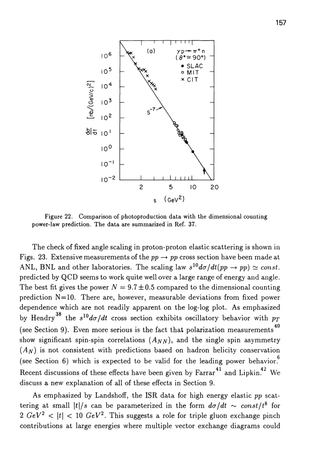
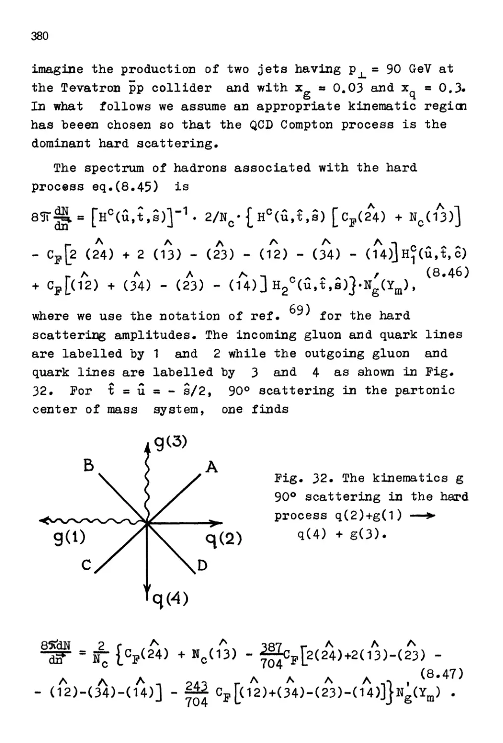
/


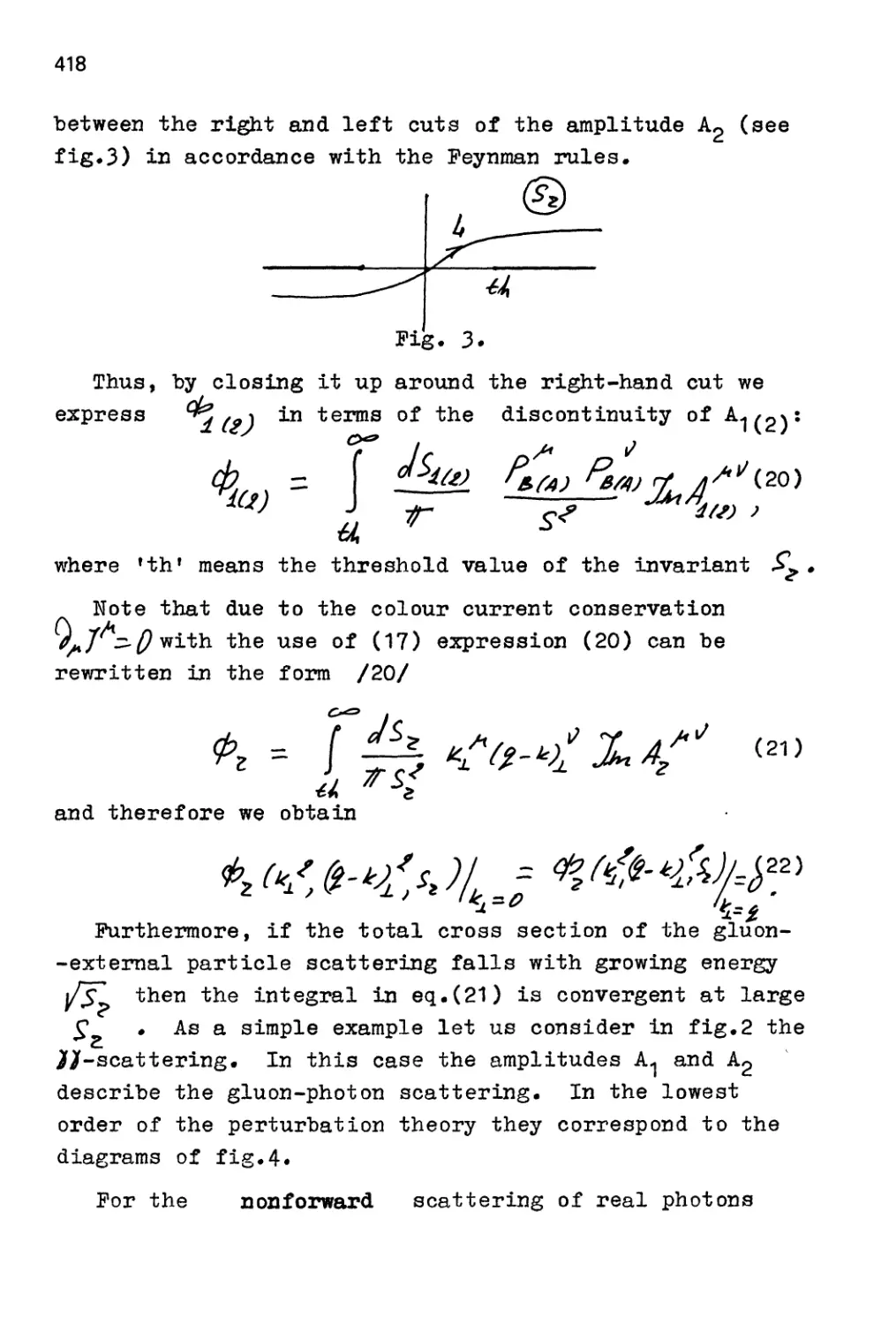


Text
PERTURBATIVE QUANTUM
CHROMODYNAMICS
ADVANCED SERIES ON DIRECTIONS IN HIGH ENERGY PHYSICS
Published
Vol. 1 — High Energy Electron-Positron Physics
(eds. A. AH and P. Soding)
Vol. 2 — Hadronic Multiparticle Production
(ed. P. Carruth^rs)
Vol.3— CP Violation
(ed. C. Jarlskog)
Vol. 4— Proton-Antiproton Collider Physics
(eds. G. A/tare///and L. Di Leila)
Vol. 5— Perturbative QCD
(ed. A. H. Mueller)
Forthcoming
Vol. 6— Quark Gluon Plasma
(ed. R. C. Hwa)
Vol. 7 — Quantunn Electrodynannics
(ed. T. Kinoshita)
Vol. 8 — Interactions Between Elementary Particle Physics and Cosmology
(ed. E. Kolb)
Cover Artwork by courtesy of Los Alamos National Laboratory.
"This work was performed by the University of California,
Los Alamos National Laboratory, under the auspices of the
United States Department of Energy."
Advanced Series on
Directions in High Energy Physics—Vol. 5
PERTURBATIVE QUANTUM
CHROMODYNAMICS
Editor:
A. H. Mueller
World Scientific
Singapore • New Jersey • London • Hong Kong
Published by
World Scientific Publishing Co. Pte. Ltd.,
P O Box 128, Farrer Road, Singapore 9128
USA office: 687 Hartwell Street, Teaneck, NJ 07666
UK office: 73 Lynton Mead, Totteridge, London N20 SDH
Library of Congress Cataloging-in-Publication data is available
PERTURBATIVE QUANTUM CHROMODYNAMICS
Copyright © 1989 by World Scientific Publishing Co Pte Ltd.
All rights reserved. This book, or parts thereof may not be reproduced
in any forms or by any means, electronic or mechanical, including
photocopying, recording or any information storage and retrieval system now
known or to be invented, without written permission from the Publisher.
ISBN 9971-50-564-9
9971-50-565-7 (pbk)
ISSN 0218-0324
Printed in Singapore by Utopia Press.
V
FOREWORD
With the discovery of asymptotic freedom in 1973 Quantum Chromodynamics
(QCD) was born. It was soon realized that the study of nonperturbative effects
would be crucial in order to understand color confinement, chiral symmetry
breaking and, of course, to achieve a quantitative understanding of bound states
and low energy dynamics. It was also realized, right from the start, that the rather
rich structure of QCD perturbation theory could be seen in hadronic processes
involving a high momentum transfer, that is, in hard processes. QCD is widely
viewed to be the correct theory of the strong interactions, mainly because of the
success which has been achieved in predicting and describing such hard processes.
The road has not been easy. It has been necessary to develop an extensive
theoretical apparatus in order to relate properties of the fundamental quarks and
gluon of QCD to the observed properties of hadronic interactions. A lot of work
has been completed in this direction, but much remains to be done both in giving
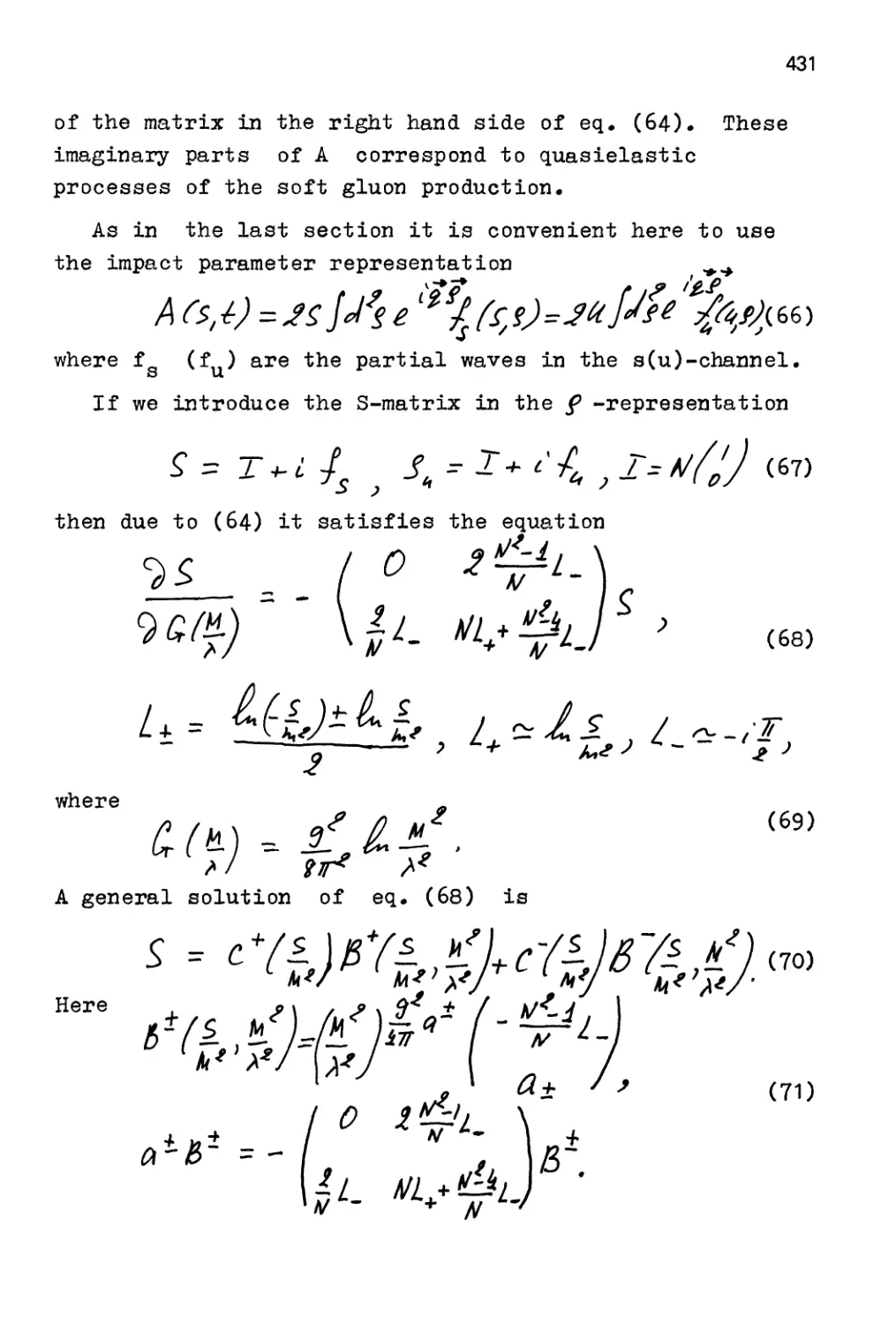
an even more solid foundation to the formalism which has been developed and in
developing new frameworks in which to understand high energy reactions.
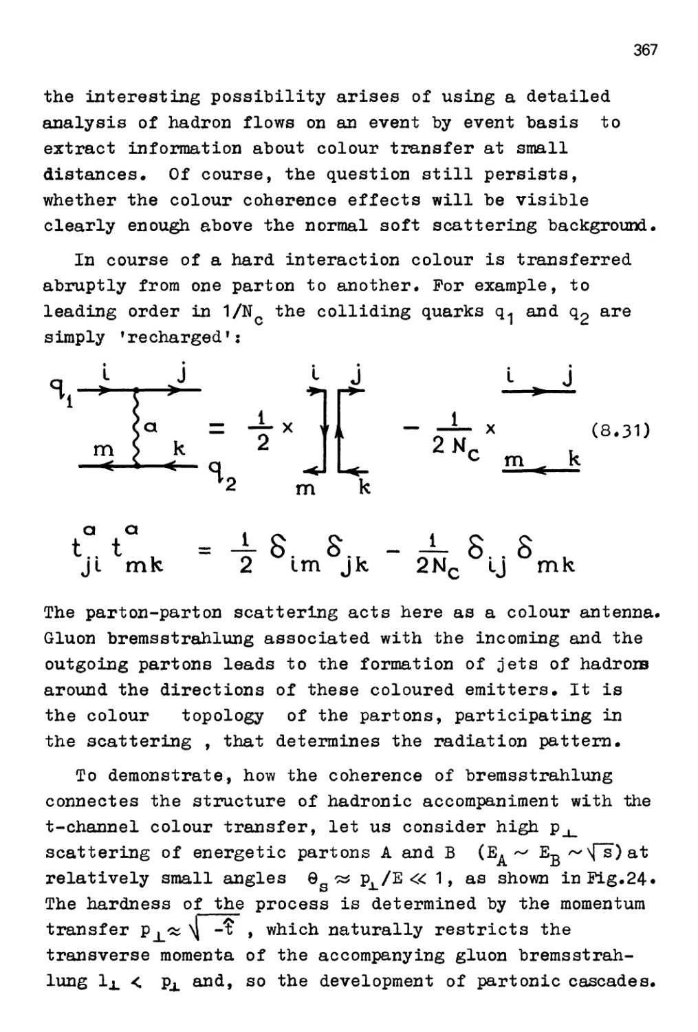
The articles in this volume aim at describing the formahsm which has been
developed in order to relate perturbative QCD to measurable quantities. The
emphasis is placed on understanding perturbative QCD and how it relates to physical
quantities rather than on detailed fits to data. It is hoped that these contributions
will make the rather elaborate formalism of perturbative QCD more accessible to
our theoretical colleagues in neighboring disciplines, to graduate students and to the
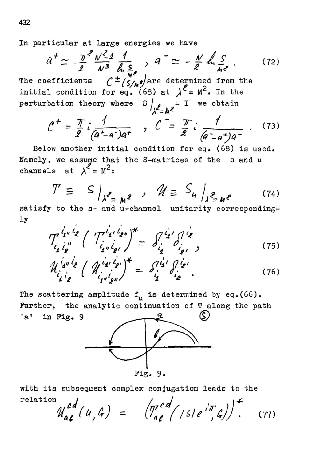
adventurous experimenter who wants to understand exactly where QCD predictions
come from and what they really mean.
At the basis of most high energy applications of QCD is factorization. Without
factorization theorems, the separation of the short distance physics, perturbative
QCD, from the long distance physics of observable hadrons would not be possible.
The standard factorization theorems for hard processes in QCD, and their proofs,
are summarized in the article of Collins, Soper and Sterman.
The article by Brodsky and Lepage deals with exclusive processes in QCD. This
is a very diverse subject encompassing form factors, wide angle elastic scattering
and various reactions involving nuclei. This is also a subject which has important
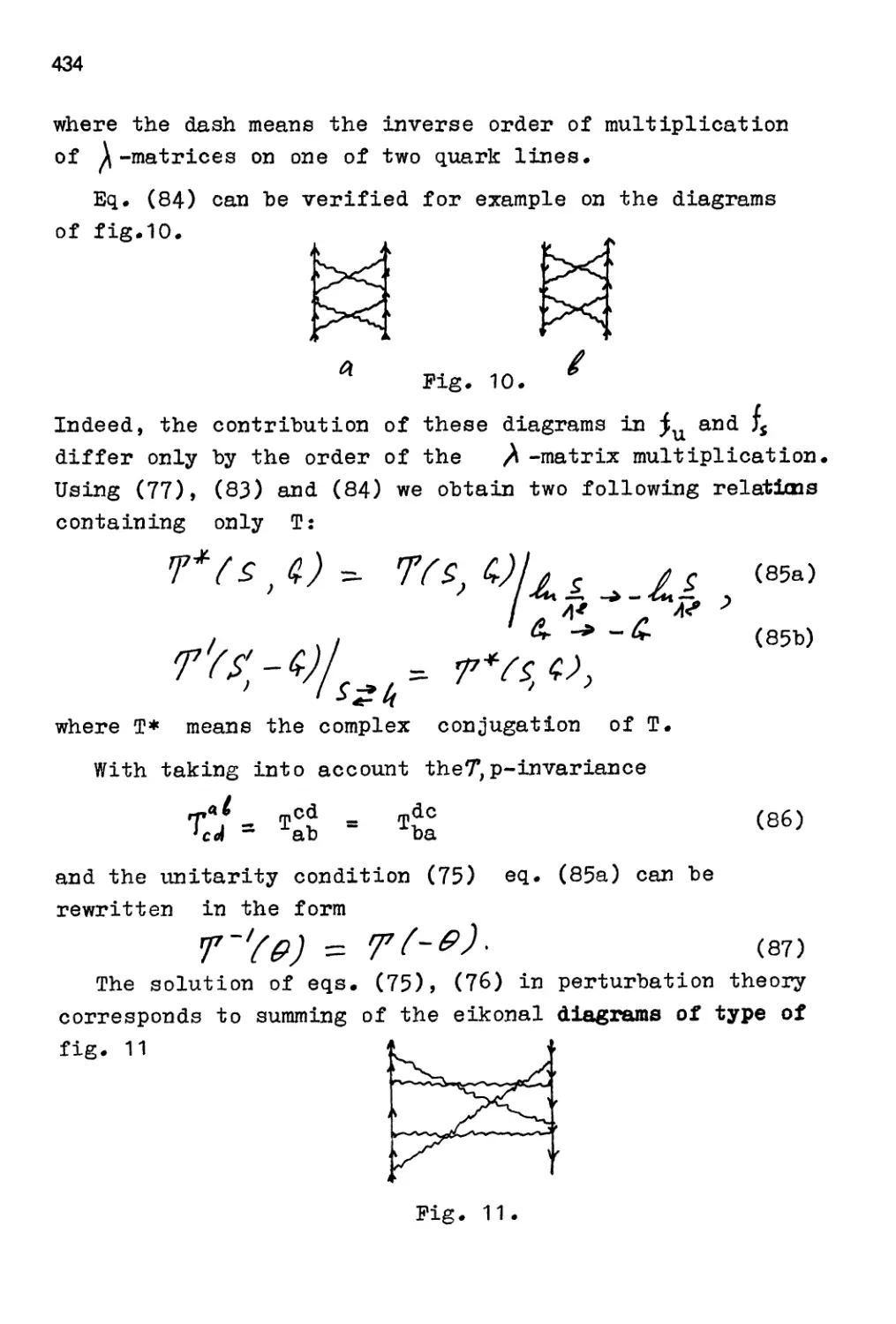
points of contact with nonperturbative QCD and with nuclear physics.
The detailed properties of QCD jets, such as particle distributions within a jet
or between several jets is given in the contribution of Dokshitzer, Khoze and
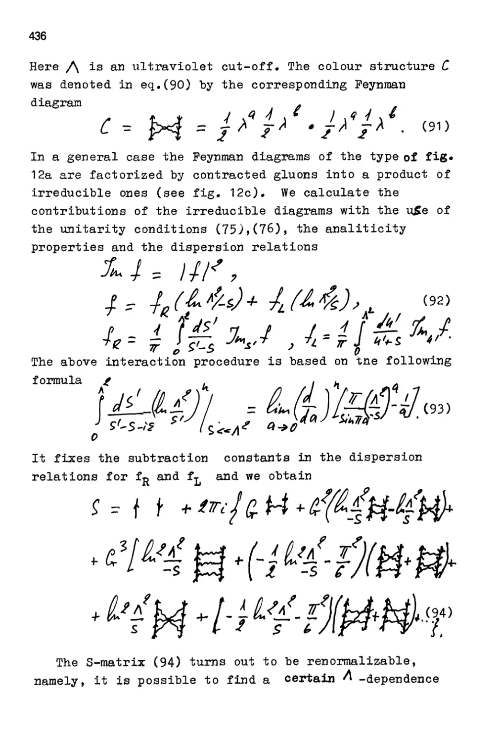
Troyan. This article also describes the QCD basis for Monte Carlo models of single
and multiple jet events.
One of the oldest problems in QCD, that of the behavior of small angle high
energy scattering, is still not completely solved. Exactly how much of this problem
can be solved purely within perturbative QCD is not completely clear at this time.
VI
The Pomeron problem remains one of the most challenging questions in QCD. The
article by Lipatov describes the present understanding on this topic.
Infrared effects and double logarithmic terms in perturbation theory play a
crucial role in many processes. For example, the transverse momentum distribution
of massive /i-pairs or of W and Z production in hadronic collisions can be predicted
only after resuming double-logarithmic terms. Perturbative QCD is applicable to
wide angle elastic scattering only because non-hard regions are suppressed, at
sufficiently high energy, by the doubling logarithmic Sudakov factors. Understanding
particle and multiplicity distributions in QCDjets requires good control over infrared
gluon emission. These topics are discussed in the articles by Ciafaloni and by Collins.
Of course, the articles which follow are not the final word on any of these
subjects. They do, however, furnish soHd and fairly complete discussions as to
what is known at present. We can expect factorization theorems to become more
rigorous and far reaching in the future. The Pomeron and small-x problems in QCD
are perhaps ripe for significant future development, soHdifying our ever growing
qualitative understanding of these questions. Infrared and Sudakov behavior in
QCD present important technical challenges for the future. We can hope that in
10 — 15 years from now, significant advances and improvements will have been
made in all the subjects discussed here. Nevertheless, even at that time, the present
articles should remain a good introduction to the subject of perturbative QCD.
A. H. Mueller
Department of Physics
Columbia University
New York
CONTENTS
Foreword
A. H. Mueller
Factorization of Hard Processes in QCD
/. C Collins, D. E. Soper and G. Sterman
S. J. Brodsky and G. P. Lepage
Coherence and Physics of QCD Jets
Yu L. Dokshitzer, V. A. Khoze and S. I. Troyan
M. Gafaloni
Sudakov Form Factors
/. C Collins
VII
1
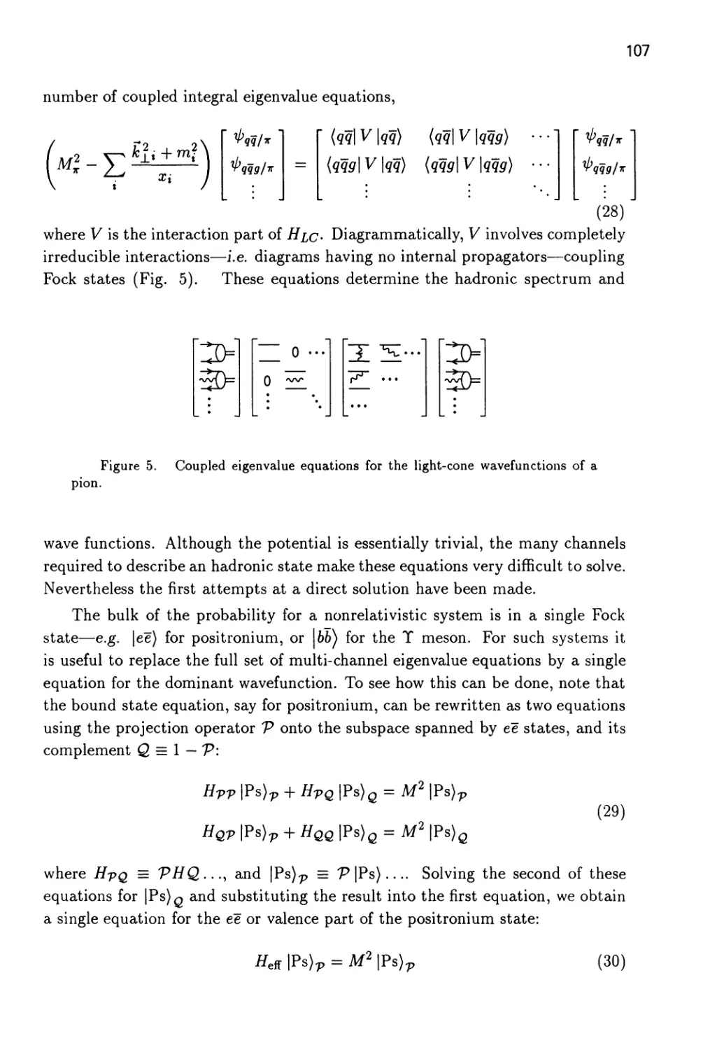
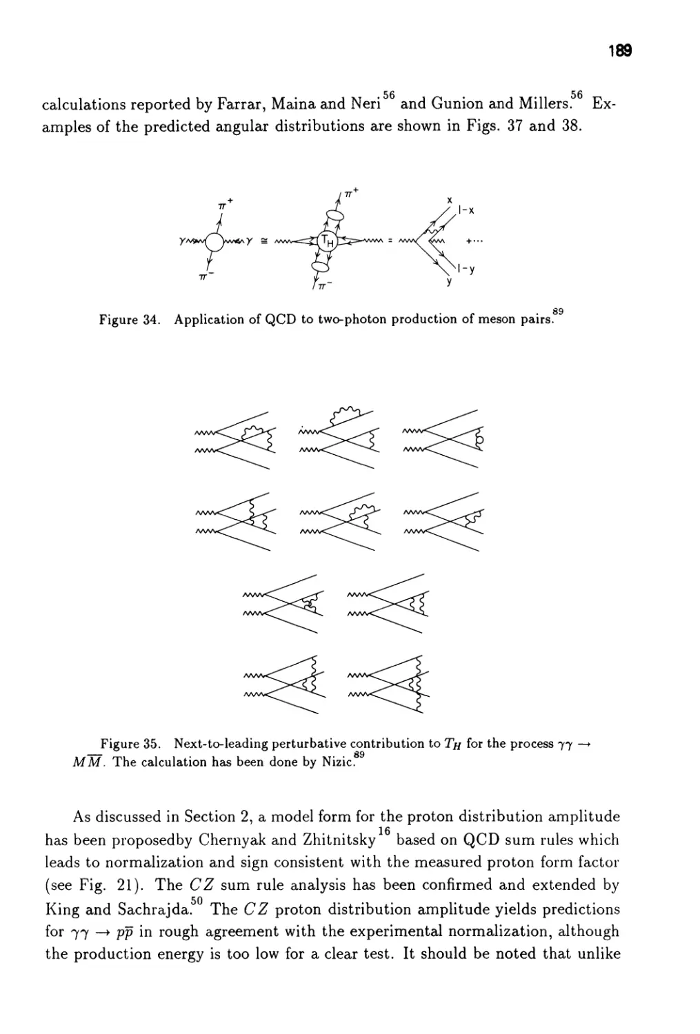
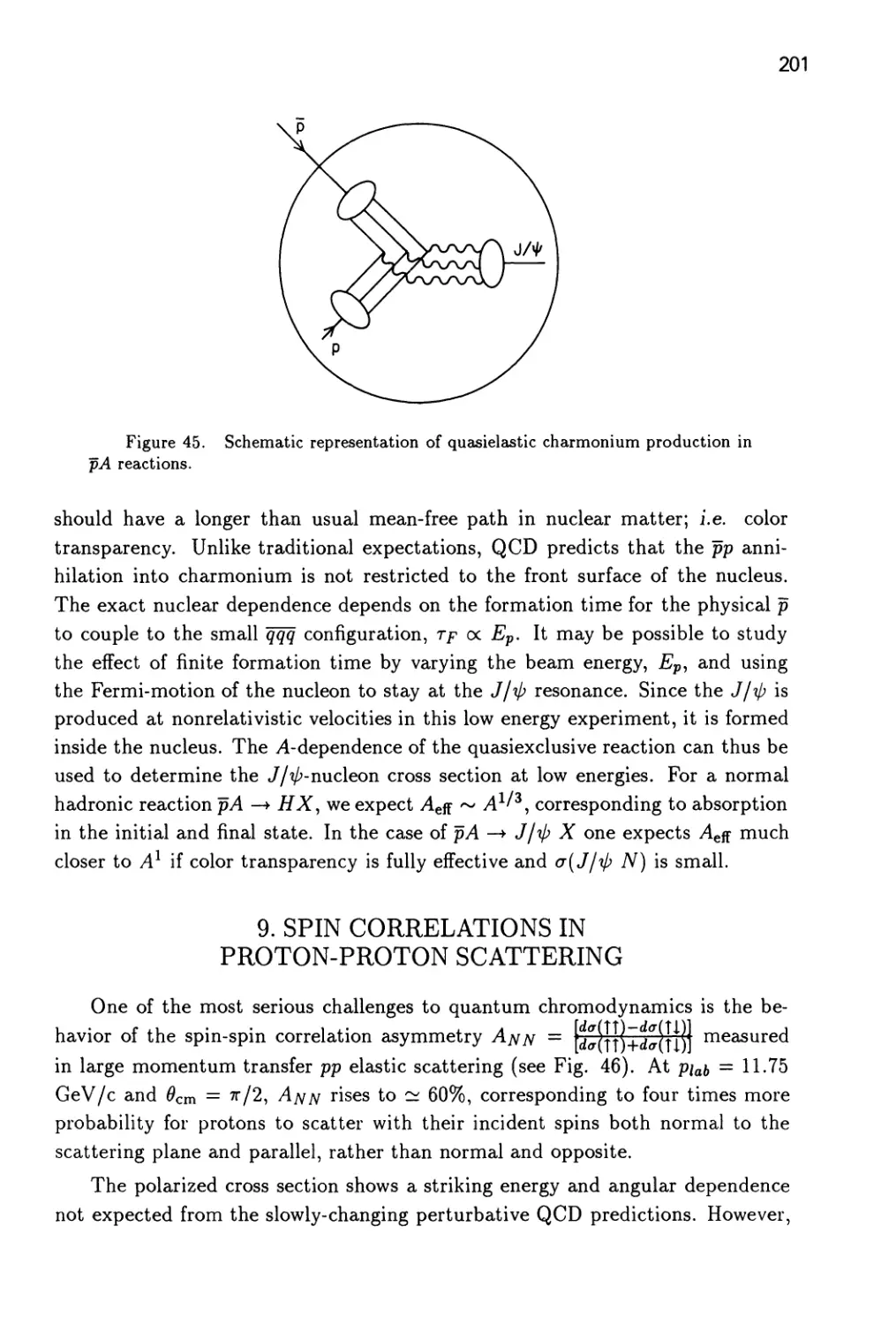
Exclusive Processes in Quantum Chromodynamics 93
241
Pomeron in Quantum Chromodynamics 411
L. N. Lipatov
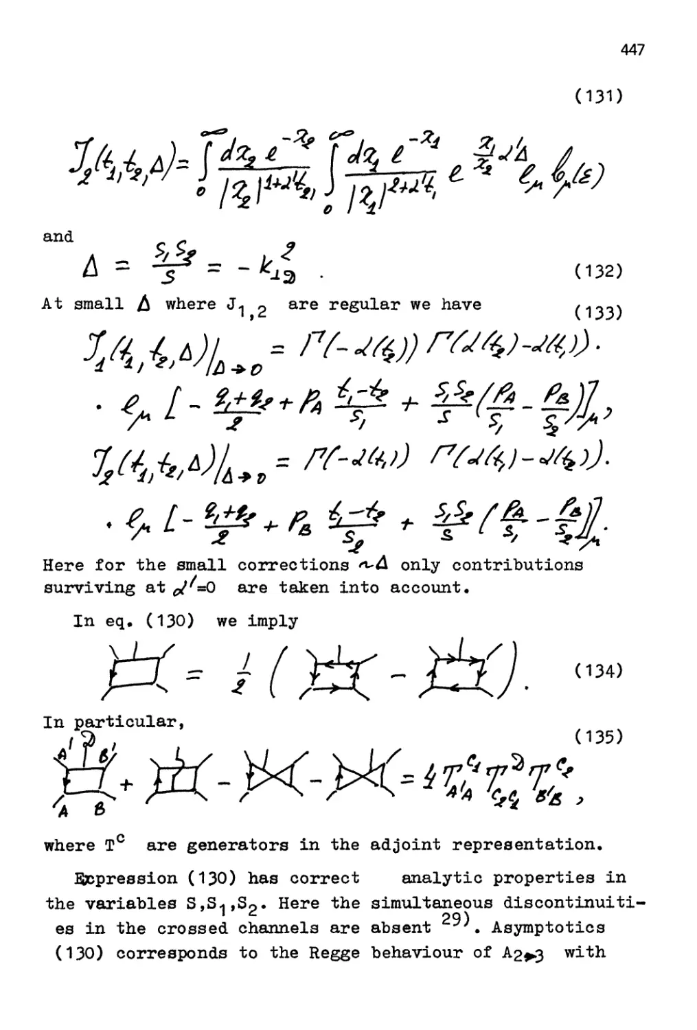
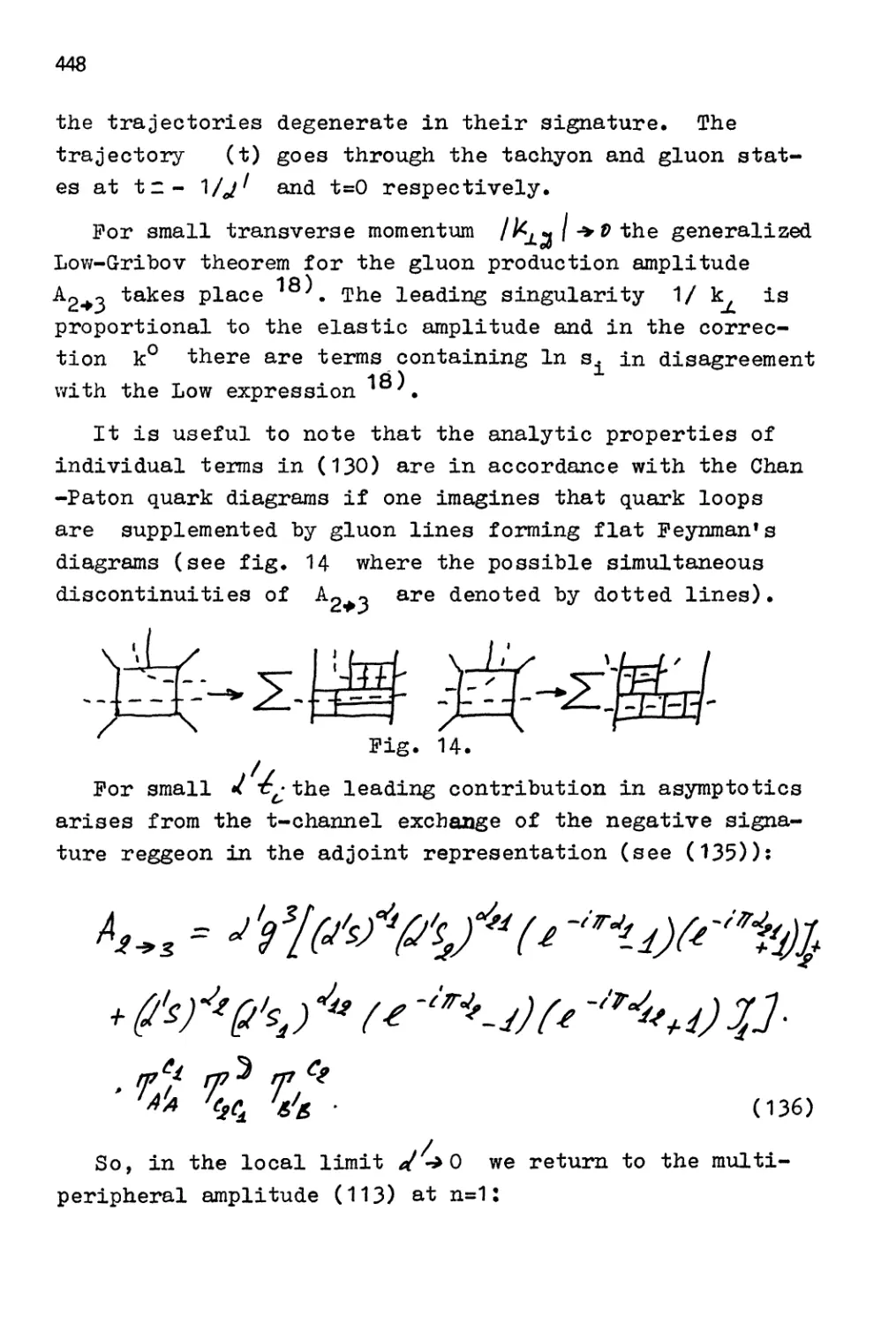
Infrared Singularities and Coherent States in Gauge Theories 491
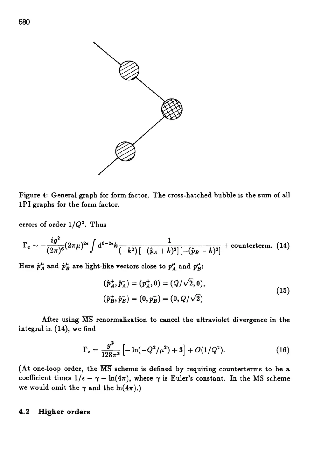
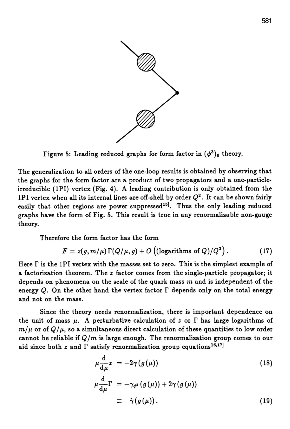
573
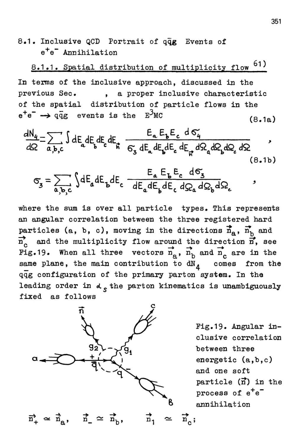
1
FACTORIZATION OF HARD PROCESSES IN QCD
John C. Collins
Physics Department
Illinois Institute of Technology
Chicago, IL 60616, U.S.A.
and
Institute for Theoretical Physics
State University of New York
Stony Brook, NY 11794-3840, U.S.A.
Davison E. Soper
Institute of Theoretical Science
University of Oregon
Eugene, OR 97403, U.S.A.
George Sterman
Institute for Theoretical Physics
State University of New York
Stony Brook, NY 11794-3840, U.S.A.
ABSTRACT
We summarize the standard factorization theorems for hard
processes in QCD, and describe their proofs.
1. INTRODUCTION
In this chapter, we discuss the factorization theorems that enable one to apply
perturbative calculations to many important processes involving hadrons. In this
introductory section we state briefly what the theorems are, and in Sects. 2 to 4, we
indicate how they are applied in calculations. In subsequent sections, we present
an outline of how the theorems are established, both in the simple but instructive
case of scalar field theory and in the more complex and physically interesting case
of quantum chromodynamics (QCD).
The basic problem addressed by factorization theorems is how to calculate
high energy cross sections. Order by order in a renormalizable perturbation series,
any physical quantity is a function of three classes of variables with dimensions of
mass. These axe the kinematic energy scale(s) of the scattering, Q, the masses,
?7i, and a renormalization scale /i. We can make use of the asymptotic freedom of
QCD by choosing the renormalization scale to be large, in which case the effective
2
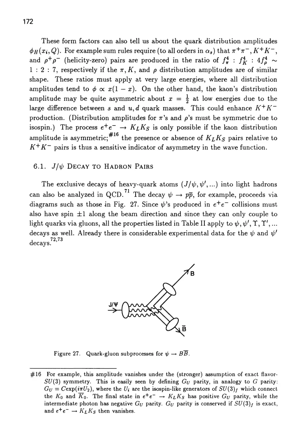
coupling constant g{n) will be correspondingly small, g{n) ^ l/ln(yu/AQCD)- The
renormalization scale, however, will appear in ratios Q/fi and fi/m^ and at high
energy at least one of these ratios is large. If we pick n ^ Q, for instance, then at
n loops the coupling will generally appear in the combination g^^(Q) \n^^(Q/m),
with a = 1 or 2. (See Sect. 7.) As a result, the perturbation series is no longer
an expansion in a small parameter. The presence of logarithms involving the
masses shows the importance of contributions from long distances, where the
precise values of masses (including the vanishing gluon mass!) are relevant. For such
contributions we do not expect asymptotic freedom to help, since it is a property
of the coupling only at short distances. In summary, a general cross section is a
combination of short- and long-distance behavior, and is hence not computable
directly in perturbation theory for QCD.
There are exceptions to this rule. For reasons which will become clear in
Sect. 7, these are inclusive cross sections without hadrons in the initial state, such
as the total cross section for e'^e" annihilation into hadrons, or into jets.
This leaves over, however, the majority of experimentally studied lepton-
hadron and hadron-hadron large momentum transfer cross sections, as well as
inclusive cross sections in e'^e" annihilation with detected hadrons. Factorization
theorems allow us to derive predictions for these cross sections, by separating
(factorizing) long-distance from short-distance behavior in a systematic fashion. Thus
almost all applications of perturbative QCD use factorization properties of some
kind.
In this chapter, we will explicitly treat factorization theorems for inclusive
processes in which (1) all Lorentz invariants defining the process are large and
comparable, except for particle masses, and (2) one counts all final states that
include the specified outgoing particles or jets. The second condition means that
we consider such processes as hadron A + hadron B —^ hadron C -f X, where
the X denotes "anything else" in addition to the specified hadron C. The first
condition means that in this example the specified hadron C should have a
transverse momentum comparable to the center-of-mass energy. For such processes,
the theorems show how to factorize long distance effects, which are not perturba-
tively calculable, into functions describing the distribution of partons in a hadron
— or hadrons in a parton in the case of final-state hadrons. Not only can these
functions be measured experimentally, but also the same parton distribution and
decay functions will be observed in all such processes. The part of the cross section
that remains after the parton distribution and decay functions have been factored
out is the short distance cross section for the hard scattering of partons. This
hard scattering cross section is perturbatively calculable, by a method which we
describe below.
3
Some examples of processes for which one expects a factorization theorem of
this type to hold include (denoting hadrons by A, jB, C ...)
• Deeply inelastic scattering, lepton -f A —> lepton' -f X\
• e+ -f e" -> A + X;
• The Drell-Yan process,
A + jB ->e++e- +J\:,
A + jB->W + X,
A + jB-^Z + X;
• A + jB-^jet + X;
• A 4- jB —> heavy quark -f X.
In the last example, the heavy quark mass, which must be large compared to 1
GeV, plays the role of the large momentum transfer. In the Drell-Yan case, the
kinematic invariants are the particle masses, the square, s, of the center-of-mass
energy, and the invariant mass Q and transverse momentum q± of the lepton pair.
The requirement, for the theorems that we discuss, that the invariants all be large
and comparable means that not only should Q^ be of order 5, but also that either
we integrate over all q± or q± is of order Q.
There are applications of QCD to processes in which there is a large
momentum scale involved but for which the most straightforward sort of factorization
theorem, as discussed in this chapter, must be modified. However, the same style
of analysis as we will describe applies to these more general situations. (The Drell-
Yan process when q± is much less than Q is an example.) We will summarize these
in Sect. 10.
Some of the factorization properties, such as those we describe in this chapter,
have been proved at a reasonable level of rigor within the context of perturbation
theory. But many of the other results have, so far, been proved less completely.
The following three subsections give explicit factorization theorems for three
basic cross sections from the list above, deeply inelastic scattering, single-particle
inclusive annihilation and the Drell-Yan process. These three examples illustrate
most of the issues involved in the application and proof of factorization. We close
the section by relating factorization to the parton model.
1.1 Deeply Inelastic Scattering
Deeply inelastic lepton scattering plays a central role in any discussion of
factorization, both because this was the first process in which pointlike partons were
"seen" inside the hadron, and because much of the data that determines the par-
ton distribution functions comes from measurements in this process. In particular,
let us consider the process e -f A —> e -f X, which proceeds via the exchange of
4
a virtual photon with momentum qf^. Prom the measured cross section, one can
extract the standard hadronic tensor W^'^{q^,p'^),
W" = 1-Jd^e'^y Y^'^A \j 1^{y)\X){X \j"{0)\ A)
Fi{x,Q )[-g'' +—^j+F2(x,Q) — ,
(1)
where Q^ = —QfiQ^, x = Q^/^q-p^ p^ is the momentum of the incoming hadron
A, and j^{x) is the electromagnetic current. (More generally, j'^{y) can be any
electroweak current, and there will be more than two scalar structure functions
Fi.)
We consider the process in the Bjorken limit, i.e., large Q at fixed x. The
factorization theorem is contained in the following expression for W^^^
PF'"'(5^p'') = Y.I T /"MC^'^) ff^(9^ep^M,«s(M)) + remainder.
(2)
Here fa/A(C^/^) is a parton distribution function, whose precise definition is given
in Sect. 4. There, fa/Aiii f^)^C is interpreted as the probability to find a parton of
type a {— gluon, u, u, d, d,...) in a hadron of type A carrying a fraction ^ to ^ -f d^
of the hadron's momentum. In the formula, one sums over all the possible types
of parton, a. We can prove eq. (2) in perturbation theory, with a remainder down
by a power of Q (in this case, the power is Q~^ modulo logarithms, but the precise
value depends on the cross section at hand, and has not always been determined).
We can project eq. (2) onto individual structure functions:
Fi{x,Q^) = ^ / y fa/Aii.tj) Hia (j,—,as{/J,)] + remainder.
'-F2{x,Q^) = Y1 I T •^«m(^'^) "■^2a ( 7, —,as(A^) ) + remainder.
(3)
The extra factors of 1/x and ^jx in the equation for F2 are needed because of the
dependence on target momentum of the tensor multiplying ^2-
Inspired by the terminology of the operator product expansion for the
moments of the structure functions, it is conventional to call the first term on the
right of either of eqs. (2) or (3) the leading twist contribution, and to caJl the
remainder the higher twist contribution. The same terminology of leading and
higher twist is used for the factorization theorems for other processes.
It is not so obvious why proving eq. (2) in perturbation theory is useful,
given that hadrons are not perturbative objects. But suppose we do decide on
5
a way of computing the matrix elements in eq. (1) perturbatively. For any such
formulation for haxiron A, both W^^ and f^/A will depend on phenomena at the
scale of hadronic masses (or some other infrared cutoff), and the exact nature
of these phenomena will depend on our particular choice of A, as well as on the
precise values we pick for both hadronic and partonic masses. The content of the
factorization theorem is that this dependence of W^^ on low mass phenomena is
(mtirely contained in the factor of fa/A-
The remaining function, the hard scattering coefficient H^'^, has two
important properties. First, it depends only on the parton type a, and not directly on
our choice of hadron A. Secondly, it is ultraviolet dominated, that is, it receives
important contributions only from momenta of order Q. The first property
allows us to calculate H^^ from eq. (2) with the simplest choice of external hadron,
A = 6, 6 being a parton. (We will see an example of this in our calculations for the
Drell-Yan process in Sect. 2.) The second property ensures that when we do this
calculation, H^'^ will be a power series in aa(Q), with finite coefficients. We now
assume that nonperturbative long-distance effects in the complete theory factorize
in the same way as do perturbative long-distance effects. Once this assumption
is made, we can interpret our perturbative calculation of H^'^ as a prediction of
the theory. Parton model ideas, summarized in Sect 1.4, give motivation that the
assumption is valid. Note that our definition of the parton distributions, which
we will give in Sect. 4, is an operator definition, which can be applied beyond
perturbation theory.
This ability to calculate the H^^ results in great predictive power for
factorization theorems. For instance, if we measure F2{x,Q'^) for a particular hadron
A, eq. (3) will enable us to determine fa/a- We then derive a prediction Fi(x, Q^)
for the same hadron A, in terms of the observed F2 and the calculated functions
Hia- This is the simplest example of the universality of parton distributions.
The functions Hia may be thought of as hard-scattering structure functions
for parton targets, but this interpretation should not be taken too literally. In
any case, methods for putting this procedure into practice, including definitions
for the parton distributions are the subjects of Sects. 2 to 4.
Originally, eq. (2) was primarily discussed in terms of the moments of the
structure functions, such as
Fi(n,Q^)= / —x"F,(x,Q'),
(4)
n-1
F2(n,Q')= / — x"-*F2(x,g^).
6
With this notation, eq. (3) becomes
Fiin,Q^) = Y^ fa/A{n,m) hJu, 9.,a^ifi)) . (5)
a \ M /
In this form of the factorization theorem, when n is an integer, the fj/y^{n,fi) are
hadron matrix elements of certain local operators, evaluated at a renormalization
scale fi. On the other hand, the structure function moment F2{n,Q ) can be
expressed in terms of the hadron matrix element of a product of two electromagnetic
current operators evaluated at two nearby space-time points. Equation (5) thus
appears as an application of the operator product expansion^'"^'^J. The product of
the two operators is expressed in terms of local operators and some perturbatively
calculable coefficients Hia{n, Q/n, as(fj,)), called Wilson coefficients. It was using
this scheme that the Hia{n,Q/iJ.,as{iJ>)) were first calculated^J.
1.2 Single Particle Inclusive Annihilation
In this subsection, we consider the process 7* —> A -f X, where 7* is an ofF-
shell photon. The relevant tensor for the process, for which structure functions
analogous to those in eq. (1) may be derived, is
D>"'{x,Q) = l-Jd*ye'''yJ2{(^\j>'{y)\AX){AX\r{0)\0), (6)
where q^^ is now a time-like momentum and Q^ = Q^- The sum is over all final-
states that contain a particle A of defined momentum and type. We define a
scaling variable hy z = 2p'q/Q^, where p'* is the momentum of A, and we will
consider the appropriate generalization of the Bjorken limit, that is, Q large with
z fixed.
The factorization theorem here is quite analogous to eq. (2), but incorporates
the slightly different kinematics,
D^'^iz, Q) = Y.fT ^a%^K. Ql\^. «s(/i)) cf^/a(C), (7)
with corrections down by a power of Q, as usual. We have used the same notation
for the hard functions as in deeply inelastic scattering, and as in that case they are
perturbatively calculable functions. Here it is the fragmentation functions dj^jJ^Qj
which are observed from experiment, and which occur in any similar inclusive cross
section with a particular observed hadron in the final state. For example, single-
particle inclusive cross sections in deeply inelastic scattering cross sections require
the factorization both of parton distributions iajA-, with A the initial hadron, and
of distributions c^b/oj with B the observed hadron in the final state. We shall not
go into the details of such cross sections here^^.
7
1,S Drell'Yan
Our final example to illustrate the important issues of factorization is the Drell-Yan
process:
A + jB-./i+-f/i-+X (8)
at lowest order in quantum electrodynamics but, in principle, at any order in
quantum chromodynamics. q^^ is now the momentum of the muon pair. We shall
be concerned with the cross section dcr/dQ^dy^ where Q^ is the square of the muon
pair mass,
Q'=9%, (9)
and y is the rapidity of the muon pair.
We imagine letting Q^ and the center of mass energy y/s become very large, while
Q^/s remains fixed.
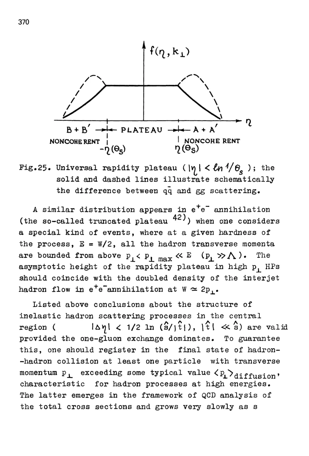
The relevant factorization theorem, accurate up to corrections suppressed by
a power of Q^, is
do-
dQ^dy
rs-*
(11)
Here a and b label paxton types and we denote
XA = G^y—, XB = e ^J—. (12)
The function Hat is the ultraviolet-dominated hard scattering cross section,
computable in perturbation theory. It plays the role of a parton level cross section
and is often written as
when it is not necessary to display the functional dependence of Hah on the kine-
matical variables. The parton distribution functions, /, are the same as in deeply
inelastic scattering. Thus, for instance, one can measure the parton distribution
functions in deeply inelastic scattering experiments and apply them to predict the
Drell-Yan cross section. As before, the parameter /i is a renormalization scale used
in the calculation of Hah-
8
1.4 Factorization in the Parton Model
Having introduced the basic factorization theorems, we will now try to give them
an intuitive basis. Here we shall appeal to Feynman's parton model^K In fact, we
shall see that factorization theorems may be thought of as field theoretic
realizations of the parton model.
In the parton model, we imagine hadrons as extended objects, made up of
constituents (partons) held together by their mutual interactions. Of course, these
partons will be quarks and gluons in the real world, as described by QCD, but
we do not use this fact yet. At the level of the parton model, we assume that
the hadrons can be described in terms of virtual partonic states, but that we are
not in a position to calculate the structure of these states. On the other hand, we
assume that we do know how to compute the scattering of a free parton by, say, an
electron. By "free", we simply mean that we neglect parton-paxton interactions.
This dichotomy of ignorance and knowledge corresponds to our inability to
compute perturbatively at long distances in QCD, while having asymptotic freedom
at short distances.
To be specific, consider inclusive electron-hadron scattering by virtual photon
exchange at high energy and momentum transfer. Consider how this scattering
looks in the center-of-mass frame, where two important things happen to the
hadron. It is Lorentz contracted in the direction of the collision, and its internal
interactions are time dilated. So, as the center-of-mass energy increases the lifetime
of any virtual partonic state is lengthened, while the time it takes the electron to
traverse the hadron is shortened. When the latter is much shorter than the former
the hadron will be in a single virtual state characterized by a definite number of
partons during the entire time the electron takes to cross it. Since the partons do
not interact during this time, each one may be thought of as carrying a definite
fraction x of the hadron's momentum in the center of mass frame. We expect x to
satisfy 0 < a: < 1, since otherwise one or more partons would have to move in the
opposite direction to the hadron, an unlikely configuration. It now makes sense
to talk about the electron interacting with partons of definite momentum, rather
than with the hadron as a whole. In addition, when the momentum transfer is
very high, the virtual photon which mediates electron-parton scattering cannot
travel fax. Then, if the density of partons is not too high, the electron will be able
to interact with only a single parton. Also, interactions which occur in the final
state, after the hard scattering, are assumed to occur on time scales too long to
interfere with it.
With these assumptions, the high energy scattering process becomes
essentially classical and incoherent. That is, the interactions of the partons among
themselves, which occur at time-dilated time scales before or after the hard
scattering, cannot interfere with the interaction of a paxton with the electron. The
9
cross section for hadron scattering may thus be computed by combining
probabilities, rather than amplitudes. We define a parton distribution /a///(0 ^^ ^^^
probability that the electron will encounter a "frozen", noninteracting parton of
species a with fraction ^ of the hadron's momentum. We take the cross section for
the electron to scatter from such a parton with momentum transfer Q^ as the Born
cross section crBiQ^^C)- Straightforward kinematics shows that for free partons
( > X = 2p'q/Q'^, and the total cross section for deeply inelastic scattering of a
hadron by an electron is
CTeHix, Q2) = ^ r de fa/HiO CrB^x/i, Q^). (14)
This is the parton model cross section for deeply inelastic scattering. It is precisely
of the form of eq. (2), and is the model for all the factorization theorems which
we discuss in this chapter.
Essentially the same reasoning may be applied to single-particle-inclusive cross
sections and to the Drell-Yan cross section. For example, in the parton model the
latter process is given by the direct annihilation of a parton and anti-paxton pair,
one from each hadron, in the Born approximation, cr'siQ^^y)- The interactions
which produce the distributions of each such parton occur on a scale which is
again much longer than the time scale of the annihilation and, in addition, final-
state interactions between the remaining partons take place too late to affect the
annihilation. We thus generalize (14) to the parton model Drell-Yan cross section
d(7
dQ'^dy
J2 [ ^^^1 ^^B fa/AiU) h/B{iB) cr's{Q\y\ (15)
where xa,b are defined in (12). Equation (15) is of the same form as the full
factorization formula, (11), except that there is only a single sum over parton species,
since the hard process here consists of a simple quark-antiquark annihilation. In
the parton model, the functions fa/A{(.A) iii Drell Yan must be the same as in
deeply inelastic scattering, eq. (14), since they describe the internal structure of
the hadron, which has been decoupled kinematically from the annihilation and
from the other hadron. It is important to notice that the Lorentz contraction of
the hadrons in the center of mass system is indispensable for this universality of
parton distributions. Without it the partons from different hadrons would overlap
a finite time before the scattering, and initial-state interactions would then modify
the distributions.
We now turn to the technical discussion of factorization theorems in QCD,
but it is important not to loose sight of their intuitive basis in the kinematics of
high energy scattering. In fact, when we return to proofs of factorization theorems
in gauge theories (Sects. 8 and 9) these considerations will play a central role.
10
2. CALCULATION OF THE HARD SCATTERING CROSS SECTION
In this and the following two sections, we discuss the explicit calculation of the
hard scattering functions for the Drell Yan cross section. In doing so, we will
cover most of the technical points which are encountered in applying factorization
in other realistic cases as well.
At order zero in as for the Drell-Yan cross section, the hard process described
by Hab is quark-antiquaxk annihilation, as illustrated in fig. 1. One can simply
compute this paxton level cross section from the Feynman diagram and insert it
into the factorization formula (11). The resulting cross section is not itself a
prediction of QCD, although it is a prediction of the parton model. The factorization
theorem will malce the connection between the two. At the Born level, it is natural
to define fa/a{0 = ^{1 - 0- We then find
^a,b ^a gQ4
(16)
where the factor S^ i indicates that parton a must be the antiparticle to parton b.
Here C(e) is 1 if we work in 4 space-time dimensions. However, when one wants
to calculate higher order contributions, it will turn out to be useful to perform the
entire calculation in 4 — 2€ dimensions. Then
(1 - ef r(l - e) ^^^^
(l-2c/3)(l-2€)r(l-2c)'
The € dependence here arises from three sources. First, the Dirac trace algebra
gives an angular dependence 1 -f cos"^ 0 — 2e. Secondly, one introduces a factor
(/i^/(47r) e'^y so as to keep the cross section at a constant overall dimensionality*
of M~^. Finally, the integration over the lepton angles in 4 — 2e dimensions gives
the remaining e dependence. Actually, it is quite permissible to perform the lepton
trace calculation and the integration over lepton angles in 4 dimensions instead of
4 — 2€ dimensions. This procedure results in multiplying the Born cross section
and the higher order cross section by a common, e-dependent factor. As we will
see below, such a factor will drop out in the physical cross section.
Now let us calculate H at one loop. At first order in ag, the cross section gets
contributions from the graphs shown in fig. 2, along with their mirror diagrams. In
this figure, we show contributions to both the amplitude and its complex conjugate.
* We use {/j,'^/(Att) e'^Y rather than (/i^)^ in anticipation of our use of MS
renormalization.
11
Fig. 1. Born amplitude for the Drell-Yan process.
separated by a vertical line which represents the final state. We will use this
notation frequently below, and refer to diagrams of this sort as "cut diagrams".
The situation now is not so simple, because a straightforward calculation of the
cross section for quark -f antiquark —> fj.'^ -f /i~ -f X according to the diagrams
shown above yields an infinite result when we use massless, on-shell quarks as the
incoming particles.
Fig. 2. Order as contributions to the Drell-Yan cross section.
Following Sect. 1.1, we use the factorization formula (11) applied to incoming
12
partons instead of incoming hadrons. Since the details associated with parton
masses axe going to factorize, we can choose to calculate the cross section for
paxton a -f parton 6—>/i'^-f/i~-f-X' with the partons having zero mass and
transverse momentum. Let us call this cross section Gah'-
5g2d^ = Gath^.XB^Q; ^;a,;e] (18)
In this calculation there are both ultraviolet and infrared divergences. Dimensional
regularization is used to regulate them both. The factorization formula is then
Gab[ XA,XB,Q\ ^5<^s;€
C' • Cat
(19)
Both factors in the formula depend on /i, which is the scale factor introduced
in the dimensional regularization and subsequent MS renormalization^J of Green
functions of ultraviolet divergent operators. One introduces a factor
(20)
for each integration J di^~^^k in order to keep the dimensionality of the result
independent of e. Ultraviolet divergences then appear as poles in the variable
e, which are subtracted away, as explained in Ref. 7. The factor e'^/{Air) that
comes along with the fj. is the difference between MS renormalization and minimal
subtraction (MS) renormalization. Here 7 = 0.5.77... is Euler's constant.
Let us suppose that we have calculated Gab to two orders in perturbation
theory. We denote the perturbative coefficients by
G.6 = Gi:> + ^GlV+C?K^). (21)
(0) :. .-u^ o .:^^ : /i^\ ^(1)
Thus G^j is the Born cross section in eq. (16). G^^ is the first correction.
The first correction G^^ will generally have ultraviolet divergences at e =
0, coming from virtual graphs, and these divergences will appear as 1/e poles.
Following the minimal subtraction prescription, we remove these ultraviolet poles
13
as necessary.* In general 1/e poles of infrared origin will remain in G^j , and we
shall discuss these infrared poles presently.
Let us similarly denote the perturbative coefficients of the hard scattering
cross section Hah by
Ha, = H^:^ + ^ Hil^ + Dial). (22)
It is these coefficients that we would like to calculate.
All we need to know to calculate H from G is the perturbative expansion
of the functions fa/h(^y^)j which, according to the factorization theorem, contain
all of the sensitivity to small momenta, and are interpreted as the distribution of
parton a in paxton b. These functions can be calculated in a simple fashion using
their definitions (Sect. 4) as matrix elements (here in parton states) of certain
operators. When the ultraviolet divergences of the operators are also renormalized
using minimal subtraction, one finds simply
where P^/lix) is the lowest order Altarelli-Parisi^J kernel that gives the evolution
with fi of the parton distribution functions. We will discuss the computations that
lead to eq. (23) in Sect. 4. For now, let us assume the result.
When we insert these perturbative expansions (23) into the factorization
formula, we obtain
G^ahi^A.XB.Q-.-^^ej -h^ G^^^(xA,XB,Q]^\e
2
+ 0{at).
(24)
* In the particular case of the Drell-Yan cross section (or, more generally, a cross
section for which the Born graph represents an electroweak interaction), the first
QCD correction G^j is not in fact ultraviolet divergent, provided that we include
the propagator corrections for the incoming quark lines This follows from (1) the
Ward identity expressing the conservation of the electromagnetic current and (2)
the fact that the photon propagator does not get strong interaction corrections,
at lowest order in QED. It can also be verified easily by explicit computation.
14
We can now solve for Hah- At the Born level, we find
H^ai ixA,XB,Q;^;e]= G^^^ f x^, xa, Q; |; e ] . (25)
Then at the one loop level we obtain
hH^ (xa, xb, Q; ^; e j = gIV ixA,XB, Q; ;^;
(26)
^E/d|.PSl(WGirfex.,Q;|;
+ 2e
c
+ ^E/<i^B^i»^«)^i"i(--if.Q;
: 6
Thus the prescription is quite simple. One should calculate the cross section at
the parton level, G^j , and subtract from it certain terms consisting of a divergent
factor 1/e, the Altarelli-Parisi kernel, and the Born cross section (with e ^ 0). The
result is guaranteed to be finite as e —> 0.
Recall that the Born cross section G^^^ consists of an e dependent factor C(e)
times the Born cross section in 4 dimensions, where C(e) arises from such sources as
the integration over the lepton angles in the Drell-Yan process. A convenient way
to manage the calculation is to factor C(e) out of the first order cross section
also. Then the prescription is to remove the 1/e pole in G^^^(e)/C(e), set e = 0,
and multiply by C(0) = 1. Thus we see that a function of e that is a common
factor to G^j and G\^ cancels in the physical hard scattering cross section, as
was claimed after eq. (17).
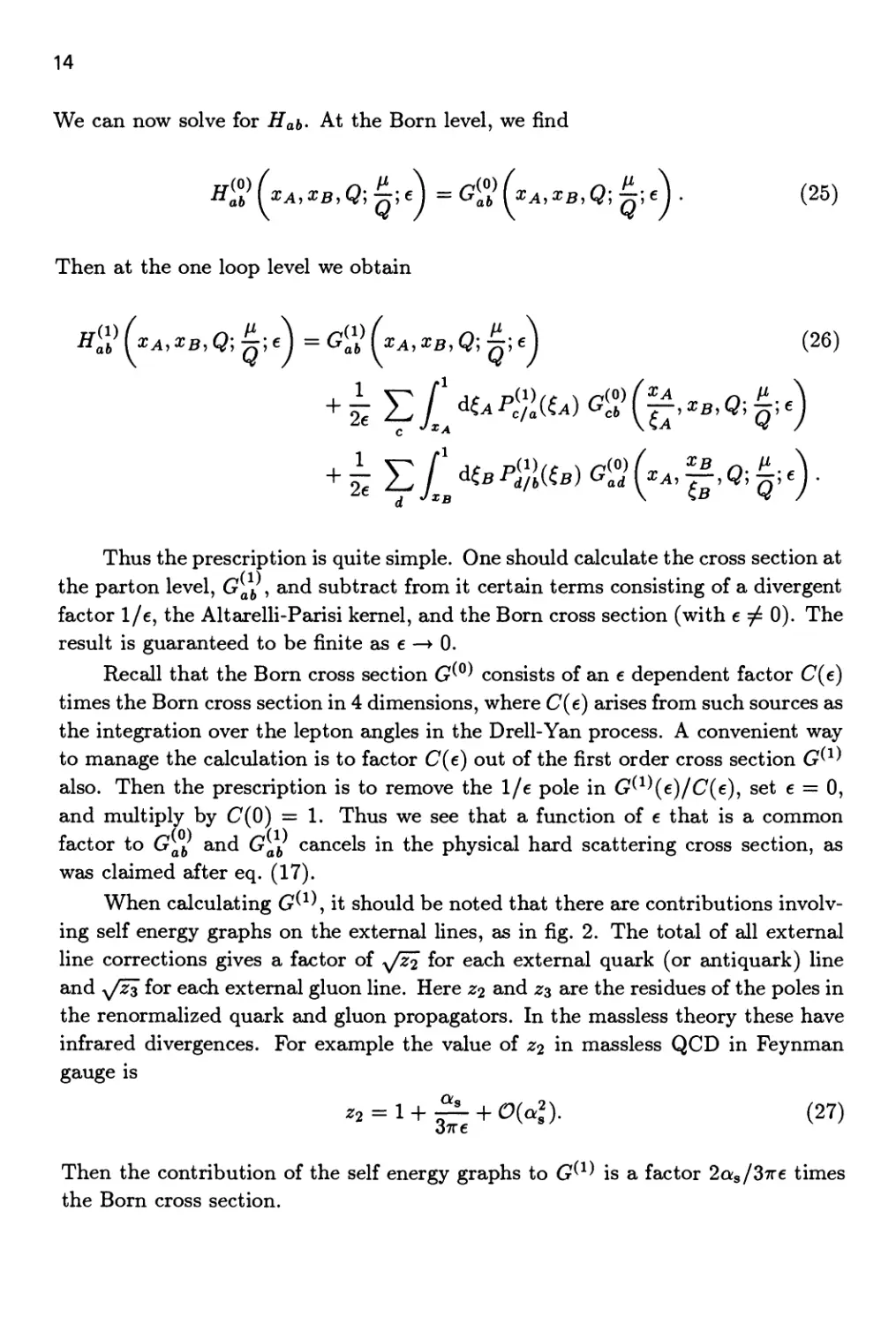
When calculating G^^\ it should be noted that there are contributions
involving self energy graphs on the external lines, as in fig. 2. The total of all external
line corrections gives a factor of y/z2 for each external quark (or antiquark) line
and y/zs for each external gluon line. Here Z2 and z^ are the residues of the poles in
the renormalized quark and gluon propagators. In the massless theory these have
infrared divergences. For example the value of Z2 in massless QCD in Feynman
gauge is
z, = l+^^+Oial). (27)
Then the contribution of the self energy graphs to G^^^ is a factor 2as/37re times
the Born cross section.
15
3. RELATION TO THE RENORMALIZATION GROUP
The prescription (26) for removing infrared poles is intimately related to the ^
dependence of H\i^ — that is, to the behavior of H)^^ under the renormalization
group. In this section, we display this connection and show how it leads to the
approximate invariance of the computed cross section under changes of /x. (Of
course, the complete cross section, to all orders of perturbation theory, is exactly
invariant under changes of /x. What we are now concerned with is the behavior of
a finite-order approximation.)
We recall that the Born cross section G\^ = H^^ contains some /i dependence
from the factor C(fi/Qy e), as specified in eq. (16). The one loop cross section G^^
contains this same factor, and we can simply factor it out of eq. (26) and set it to
1 when we set e = 0 at the end. In addition, G^j contains a factor fi^^ from the
loop integration.
4-2€
k. (28)
The (e'^/J,'^ /AttY factor multiplies the 1/e poles in G^j . Writing
-//2' = -+2^ ln(M) + 0(€), (29)
and reading off the value of A from eq. (26), we find the /x dependence of G^^ -
and thus of ^^j :
Hil^(xA,XB,Q; ^) = Hil\xA,XB,Q; 1) (30)
Q
Ef^UPSliU)HiT(^,xs,Q
Here we have set e = 0 and have suppressed the notation indicating e dependence;
we have also noted that H^^^ does not depend on /x when e = 0, so we have
suppressed the notation indicating /x dependence in H^^\
We see that H^^^ contains logarithms of /x/Q. If ^ is fixed while Q becomes
very large, then these logarithms spoil the usefulness of perturbation theory, since
the large logarithms can cancel the small coupling a;s(/x) that multiplies H^^\ For
this reason, one chooses /x such that ln(/x/Q) is not large. For example, one chooses
fx = Q OT perhaps /x = 2Q or /x = Q/2.
16
The freedom to choose /x results from the renormalization group equations
obeyed by H and fa/AiO- '^^^ renormalization group equation for Hah is
/x— Hah(xA,XB,Q]^,as(fi)] (31)
-X^ / ^CsPd/hiCB^Oisil^)) Had(xA,-^,Q;Q,as(fJ')] •
Here Pc/a(^5<^s(A*)) is the all orders Altaxelli-Parisi kernel. It has a perturbative
expansion
Pc/aii,asifi)) = ^ Pl}liO + ... (32)
where P^/l(0 is the function that appears in eq. (23). Thus at lowest order
the renormalization group equation (31) is a simple consequence of differentiating
eq. (23).
Parton distribution functions also have a fi dependence, which arises from the
renormalization of the ultraviolet divergences in the products of quark and gluon
operators in the definitions of these functions, given in eqs. (43) and (44) below.
The renormalization group equation for the distribution functions is
The physical cross section does not, of course, depend on /x, since p, is not one
of the parameters of the Lagrangian, but is rather an artifact of the calculation.
Nevertheless, the cross section calculated at a finite order of perturbation theory
will acquire some jj, dependence arising from the approximation of throwing away
higher order contributions. To see how this comes about, we differentiate eq. (11)
with respect to // and use eqs. (31) and (33). This gives
d dcr
dfj, dQMy
E f ^^^ f '-t f ^^-
a,6,c *^^^ -^^^ ^^ *^^fi
L A \ f ^ A ^ Xi IJ
xPa/c{U,0'M) fc/A[-T-,fJ-jHah{y-,J-,Q;Q,as{fJ.)\ fb/B{(B,ti)
a,h,c ^^^ J^a/Ia Jxb
17
^A XB ^ 1^
X fa/A{U,l^)Pc/a(CA,Oisifi)) //"eft ( T-y, J", 0; ^ , Q^s(/^) ) fb/B^^B^fJ')
4- B terms.
(34)
Here the two terms shown relate to the evolution of the partons in hadron A.
As indicated, two similar terms relate to the evolution of the partons in hadron
B. We now change the order of integration in the second term to put the (a
integration inside the (a integration, then change the integration variable from ^a
to (a = CaCaj and finally reverse the order of integrations again. This gives
d dcr
d/x dQ2dy
a,b,c -^^^
X Pa/c{CA,Ois{fi)) /c/aI ^,iW l^aftl 7^,7^,Q;^,Q^s(iw) 1 fb/BUB,IJ')
X fa/A\
■T^.fJ'jPc/aiCAyOisilJ')) f^cftf 7^,7^,0; Q,Q^s(/^)l fb/B{^B,IJ')
-h B terms.
(35)
We see that the two terms cancel exactly as long as Pa/b si-nd Hab obey the renor-
malization group equations exactly. Now, when Hab is calculated only to order
a^, it only obeys the renormalization group equation (31) to the same order. In
this case, we will have
when the parton distribution functions obey the renormalization group equation
with the Altarelli-Parisi kernel calculated to order a^ or better. One thus finds
that the result of a Born level calculation can be strongly /x dependent, but by
including the next order the jj, dependence is reduced.
We have argued that one should choose fi to be on the order of the large
momentum scale in the problem, which is Q in the case of the Drell-Yan cross
section. We have the right to choose fi as we wish because the result would be
independent of fi if the calculation were done exactly. The choice ^i ^ Q eliminates
the potentially large logarithms in eq. (30). Another choice is often used. One
substitutes for /x in eq. (11) the value y/s = y/^A^B^- We now have a value of fi
that depends on the integration variables in the factorization.
18
Let us examine whether this is valid, assuming that Pa/h and Hah are
calculated exactly. We replace /x by
t^iKU.ia) = ^l\-^ (yUi^y, 0<A<1. (37)
At A = 0 we have a valid starting point. When we get to A = 1 we have the
desired ending point. The question is whether the derivative of the cross section
with respect to A is zero. Applying the same calculation as before, we obtain
instead of eq. (34) the result
d da ^ [' [' AU [\, 1 , (UiBS
a,6,c "^^^ ^^a/^a ^xb ^ \ H'O
X fa/A {Uy K^y U, (b)) Pc/a (Ca, Ois(fi(X, U,(b)))
VqaU ^b Q )
-\- B terms.
Now making the same change of variables as before, we obtain
d
darn
dA dg2dy
(a(bs
^ f '^^ f 77 f '^' I \ .3
X
''"(li'if'**^^^'^^'"*')''"'*^'''''*'^-"*""
-E/'«^/T/'^.i
\ (Af-tl
In
X fa/A f ^,MA,a/CA,^B)j ■Pc/a(a,as(MA,a/G,<jB)))
"" ^'' lil' if' ^' ^^^'%^^'^^\ <f^)) f^/BUB.^(A,a/a, ^b))
4- jB terms.
(39)
19
We see that the cancellation between the two terms has been spoiled, first by the
differences in the values of /x(A,...) in the two terms, but more importantly by
the differences in the arguments of the logarithm in the two terms. We conclude
that the substitution of s for /x^ results in an error of order ag no matter how
accurately the hard scattering cross section is calculated. This is not a problem
If the hard scattering cross section is calculated only at the Bom level, which is,
in fact, commonly the case. However, it is wrong to substitute s for ^^ when a
calculation beyond the Born level is used.
4. THE PARTON DISTRIBUTION FUNCTIONS
The parton distribution functions are indispensable ingredients in the factorization
formula (11). We need to know the distribution of paxtons in a hadron, based on
experimental data, in order to obtain predictions from the formula. In addition,
we need to know the distribution of paxtons in a parton in order to calculate the
hard scattering cross section Hah- The hard scattering cross section is obtained
by factoring the parton distribution functions out of the physical cross section.
Evidently, the result depends on exactly what it is that one factors out.
4.1 Operator Definitions
In this section, we describe the definition for the parton distribution functions
that we use elsewhere in this chapter. A more complete discussion can be found
in Ref. 9. In this definition, the distribution functions are matrix elements in a
hadron state of certain operators that act to count the number of quarks or gluons
carrying a fraction ( of the hadron's momentum. We state the definition in a
reference frame in which the hadron carries momentum P^ with a plus component
P'^', a minus component P~ = m^ /2P'^, and transverse components equal to zero.
(We use P± = (PO ± P^)/V2).
The definition may be motivated by looking at the theory quantized on the
plane x^" = 0 in the light-cone gauge A'^ = 0, since it is in this picture that
field theory has its closest connection with the parton model^^K In this gauge,
^ = 1, where ^ is a path-ordered exponential of the gluon field that appears
in the definition of the parton distributions. The light-cone gauge tends to be
rather pathological if one goes beyond low order perturbation theory, and covaxi-
ant gauges are preferred for a complete treatment. However quantization on a
null plane in the light-cone gauge provides a useful motivation for the complete
treatment.
In this approach the quark field has two components that represent the
independent degrees of freedom; 'y'^il^(x) contains these components and not the
other two. One can expand the two independent components in tenns of quark
20
destruction operators b(k'^,k±,s) and antiquark creation operators d(k'^jk±,sy
as follows:
j+i;{0,x-,xj,) = (27r)-'Y.J
"^ dk+ .
dk±
2k+
3
X {y+U(k,s)e-'''''bik+,kjL,s) + -y+V{k,s)e+'''''d(k-^,k±,sy}.
(40)
The quark distribution function is just the hadron matrix element of the operator
that counts the number of quarks.
f,/AiO d^ = (2t)-' J2 ifprj / '^^^ (PI KC^+. *x, s)^b{^P+,kjL,s) IP).
(41)
In terms of t/^(x), this is
f,/Aii) = ^j da;-e-«^^^" (P 1^(0, X-, Ox) 7+ ^-(0,0,0±)\P).
We can keep this same definition, while allowing the possibility of computing in
another gauge, by inserting the operator
X
g
P exp I ig J dy-A+(0, y", Ox)te \ , (42)
where P denotes an instruction to order the gluon field operators i4j(0,y~,0x)
along the path. The operator Q is evidently 1 in the A"^ = 0 gauge. With this
operator, the definition is gauge invariant.
We thus arrive at the definition^'^^^
/,m(0 = ^ /clx-e-'«^^-"(P|^(0,a;-,0x)7+aV(0,0,0x)|P) (43)
For gluons, the definition based on the same physical motivation is
/,m(0 = 2;4p+y dx-e-'«^^-" (P |Fa(0, X-,0x)+''a^t ^6(0,0, Ox)/IP),
(44)
where F^^, is the gluon field strength operator and where in Q we now use the
octet representation of the SU(3) generating matrices t^
21
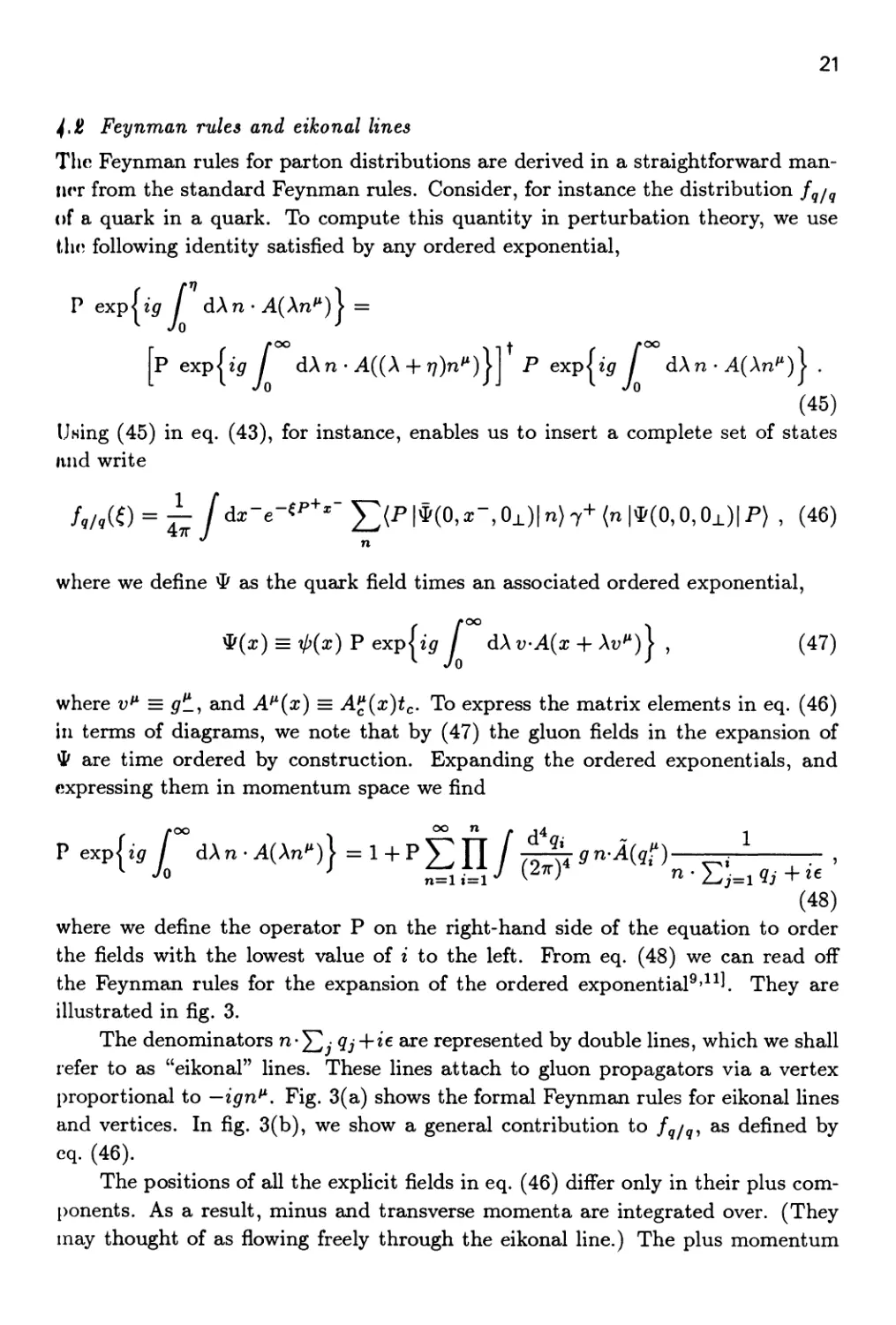
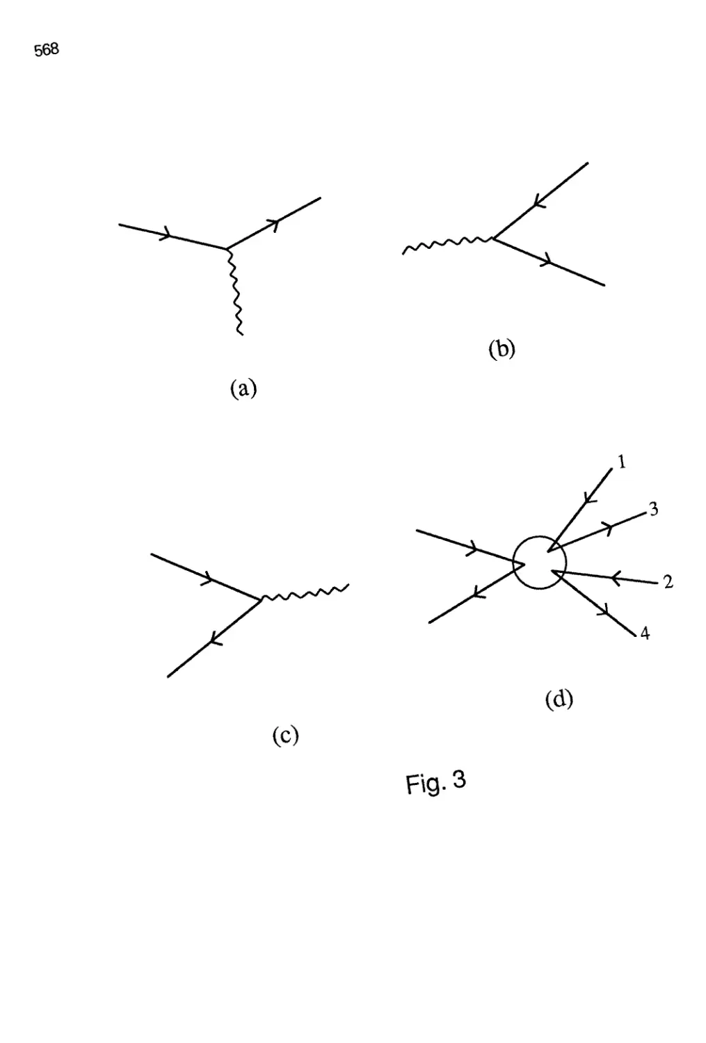
^.jB Feynman rules and eikonal lines
The Feynman rules for parton distributions are derived in a straightforward
manner from the standard Feynman rules. Consider, for instance the distribution fg/g
of a quark in a quark. To compute this quantity in perturbation theory, we use
tlu' following identity satisfied by any ordered exponential,
P expjz^ / dXn'A(Xn^)^
[P exp|z^ / d\n'A((X-\-r])n^)\V P expUg f dAn-A(An^)| .
(45)
Using (45) in eq. (43), for instance, enables us to insert a complete set of states
and write
/,/,(0 = ^ /dx-e-«''*^" V(P|#(0,a;-,0x)|n)7+(n|$(0,0,0x)|P), (46)
47r
" n
where we define ^ as the quark field times an associated ordered exponential,
^(x) = tl^ix) P exp|i^ / dA V'A(x + Xv^)\ , (47)
where v^ = 9-^ and A^(x) = A^(x)tc. To express the matrix elements in eq. (46)
in terms of diagrams, we note that by (47) the gluon fields in the expansion of
^ are time ordered by construction. Expanding the ordered exponentials, and
expressing them in momentum space we find
oo . oo n
P exp{ig J^ dXn- ^(An")} = 1 + P E 11 _/ (2^ Sn-Aiq^
1
" • Ej=i 97 + «'« '
(48)
where we define the operator P on the right-hand side of the equation to order
the fields with the lowest value of i to the left. From eq. (48) we can read off
the Feynman rules for the expansion of the ordered exponential^'^^^. They are
illustrated in fig. 3.
The denominators n-^ • qj + ie axe represented by double lines, which we shall
refer to as "eikonal" lines. These lines attach to gluon propagators via a vertex
proportional to —ign^. Fig. 3(a) shows the formal Feynman rules for eikonal lines
and vertices. In fig. 3(b), we show a general contribution to fg/g, as defined by
eq. (46).
The positions of all the explicit fields in eq. (46) differ only in their plus com-
l)onents. As a result, minus and transverse momenta are integrated over. (They
may thought of as flowing freely through the eikonal line.) The plus momentum
22
(a)
q
>
q-u + ie
igU«tij
q
J
-1
q-u-ie
(b)
P
Fig. 3. (a) Feynman rules for eikonal lines in the amplitude and
its complex conjugate, (b) A general contribution to a parton
distribution.
flowing out of vertex 1 and into vertex 2, however, is fixed to be ^P"*". No plus
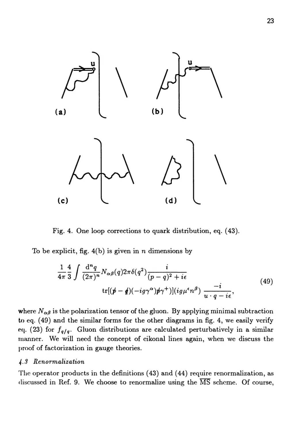
momentum flows across the cut eikonal line in the figure. Fig. 4 shows the one
loop corrections to fq/q{C)-
23
(a)
(c)
(d)
Fig. 4. One loop corrections to quark distribution, eq. (43).
To be explicit, fig. 4(b) is given in n dimensions by
14/ d^o ^^ , .^ ^, os «
qf + it
tr[(j^-rf)(-W"¥7^)](w'n'')
e^^
— I
(49)
u ' q — le
where Na^ is the polarization tensor of the gluon. By applying minimal subtraction
to eq. (49) and the similar forms for the other diagrams in fig. 4, we easily verify
vx{. (23) for fq/q- Gluon distributions are calculated perturbatively in a similar
manner. We will need the concept of eikonal lines again, when we discuss the
proof of factorization in gauge theories.
^.S Renormalization
The operator products in the definitions (43) and (44) require renormalization, as
discussed in Ref. 9. We choose to renormalize using the MS scheme. Of course,
24
renormalization introduces a dependence on the renormalization scale /i. The
renormalization group equation for the iaIA is the AltareUi-Parisi equation (33).
A complete derivation of this result may be found in Ref. 9.
The one-loop result, eq. (23), can actually be understood without looking
at the details of the calculation. At order ag, one has simple one loop diagrams
that contain an ultraviolet divergence that arises from the operator product, but
also contain an infrared divergence that arises because we have massless, on-shell
partons as incoming particles. The transverse momentum integral is zero, due to
a cancellation of infrared and ultraviolet poles, which we may exhibit separately:
J (27r)2-2e k^2 - 4^ j ,^^ ,^^ > • (50)
In this way, we obtain
fa/kii; e) = Sai6il-0+{—-—] — Pi%iO - counterterm + 0(a,^). (51)
The coefficient of l/cuv is the * anomalous dimension' that appears in the
renormalization group equation, that is, the AltareUi-Parisi kernel. Following the
renormalization scheme, we use the counter term to cancel l/cuv term. This leaves
the infrared 1/e, which is not removed by renormalization,
/a/»(^;e) = 6a, 6(1-0-~ Pi)liO + 0{al). (52)
4-4 Reldtion to Structure Functions
Let us now consider the relation of the parton distribution functions to the
structure functions measured in deeply inelastic lepton scattering. If we use the
definition of parton distribution functions given above, then the structure function F2
is given by the factorization equation (2). At the Born level, the hard scattering
function is simply zero for gluons and the quark charge squared, e^, times a delta
function for quarks. Thus the formula for F2 takes the form
^-1
X
'di
-r •/- « "^ VC /'/ (53)
+ Oial).
The sums over j run over all flavors of quarks and antiquarks. Gluons do not
contribute at the Born level, but they do at order Ofg, through virtual quark-aiitiquark
pairs. The hard scattering coeflSicients Cjb can be obtained by calculating (at order
25
G(n) deeply inelastic scattering from on-shell massless partons, then removing the
Infrared divergences according to the scheme discussed in Sect. 2.
The explicit form of the perturbative coefficients Cjt is'*^
Cjk(z,l)
Sjk-
11-j-z
2 1
In
1-^
3 1 3
+
Cj,(z,l) = -l^l{z' + il-zf}l^ln
1-z
+ 1} - 3^(1 - z)
(54)
where the plus subscript to the bracket in the first equation denotes a subtraction
that regulates the z —^ 1 singularity,
dz [C{z)]+ h{z) = / dz [C{z)]+ h(z)e(z > x)
0
/ dz C{z) ^h(z)e(z >x)- /i(l)|.
(55)
4.5 Other Parton Distributions
The definitions (43) and (44) are the most natural for many purposes. They
are not, however, unique. Indeed, any function gb/Aiv)^ which can be related to
fa/A(^) t)y convolution with ultraviolet functions Dab(x/y^Q/lJ') in a form like
9a/A{x) = Y1 (^y/y)^ab{x/y,Q/n,as{fi))fb/A{y) ,
L J X
(56)
is an acceptable parton distribution^"^1. The hard scattering functions calculated
with the distributions Qb/A will differ from those calculated with fa/A^^)-, but this
difference will itself be calculable from the functions Dab as a power series in as(Q)-
The most widely used parton distribution of this type is based on deeply
inelastic scattering, and may be called the DIS definition. The definition is
DIS
/i/i?(^,M)
de
fj,A{x,n) + Y.f ^hlAitt^) ^ Cji (;,!)+ 0{al).
i
i
(57)
for quarks or antiquarks of flavor j. Comparing this definition with eq. (53), we
see that
X
-1
F2{x,Q) = Y.^] ffjiix,Q) + 0{al).
(58)
That is, we adjust the definition so that the order a^ correction to deeply inelastic
scattering vanishes when fi = Q. It is not so clear what one should do with the
gluon distribution in the DIS scheme. One choice^^J is
rDIS
J 9/A
(^, /^) = fg/Aix, /^) - ^ ^ /
r J X
'fh/AiC,f^)^C,Jj,l]+0{al).
(59)
26
This has the virtue that it preserves the momentum sum rule that is obeyed by
the MS parton distributions^!,
a -^0
(60)
If one wishes to use parton distribution functions with the DIS definition, then
one must modify the hard scattering function for the process under consideration.
One should combine eqs. (52) and (59) to get the DIS distributions of a parton in
a parton, then use these distributions in the derivation in Sect. 2.
It should be noted that there is some confusion in the literature concerning
the term +1 that follows the logarithm in Cjg in eq. (54). The form quoted is
the original result of Ref. 4, translated from moment-space to z-space. In the
calculation with incoming gluons, one normally averages over polarizations of the
incoming gluons instead of using a fixed polarization. This means that one sums
over polarizations and divides by the number of spin states of a gluon in 4 — 2e
dimensions, namely 2 — 2e. If, instead, one divides by 2 only, one obtains the
result (54) without the -j-l, which may be found in Ref. 14. This does no harm
if, as in the case of Ref. 14, one wants to express the cross section for a second
hard process in terms of DIS parton distribution functions and if one consistently
divides by 2 instead of 2 — 2e in both processes. However, it is not correct if one
wants to relate the DIS structure functions to MS parton distribution functions,
defined as hadron matrix elements of the appropriate operators, renormalized by
MS subtraction.
5. FACTORIZATION FOR cj)^ THEORY
In this and the next section, we study the factorization theorem in a (j>^ theory for
n < 6 space-time dimensions. First we show how the factorization theorem comes
about for one-loop corrections in deeply inelastic scattering, and compare the field
theory to the parton model. In the next section, we will present a reasonably
complete but compact derivation of the factorization theorem in deeply inelastic
scattering to all orders of perturbation theory.
The scalar theory allows us to study these issues in a simplified but highly
nontrivial context. As emphasized above, the purpose of the factorization theorems
is to separate long-distance behavior in perturbation theory. In the scalar theory,
as we shall see, this behavior is associated with partons that are coUinear to the
observed hadrons. The organization of such "collinear divergences" is central to
factorization in all field theories, but in gauge theories they are joined by "soft"
partons, associated with infrared divergences. Indeed, the basic problem in gauge
theories is to show how that infrared or "soft" divergences cancel (see Sect. 9). In
27
^' theory the infrared problem is absent, so that studying this theory allows us to
liiidy the basic physics of factorization in the simplest possible setting.
The Lagrangian is
£ = i {d(i>f - \rn'^<t>^ - ~5^(A*^e^/47r)'/2<?!>^ + counterterms . (61)
We will use, where necessary, dimensional regularization, with space-time dimen-
nion n = 6 — 2e. It is worth recalling that at n = 6 the theory is renormalizable,
while for n < 6 it is superrenormalizable. We shall not concern ourselves with the
theory for n > Q where it is nonrenormalizable by power-counting, /i is a mass
which enables us to keep g dimensionless as we vary n. We will renormalize the
tlicory with the MS prescription. We use the factor (/i^e'''/47r)^/^ rather than the
more conventional /i% so that we can implement MS renormalization as pure pole
counterterms. (For convenience, we will define the /i<^ counterterm that renormal-
Izes the tadpole graphs by requiring the sum of the tadpoles and their counterterm
to vanish.) We define
/i = /ix/eV^TT. (62)
5.1 Deeply inelastic scattering
Our model for deeply inelastic scattering consists of the exchange of a weakly
interacting boson, A, not included in the Lagrangian (61). This is illustrated
(liagrammatically in the same way as for QCD, in fig. 5. The weak boson couples
to the <l> field through an interaction proportional to hAcfP". There is then a single
structure function which we define by
F{x,Q) = ^ /cl«ye-'"{p|y(y)i(0)|p}, (63)
where j = i(j) . The momentum transfer is g^, and the usual scalar variables are
defined by Q^ = —q^ and x = Q^/2p-g, with p^ the momentum of the target. We
will investigate the structure function in the Bjorken limit of large Q with x fixed,
and our calculations will be for the case that the state |p) is a single (j) particle
(with non-zero mass, as given in eq. (61)).
When Q is large, each graph for the structure function behaves like a
polynomial of \n{Q/m) plus corrections that are nonleading by a power of Q.
Factorization is possible because only a limited set of momentum regions of the space of loop
and final state phase space momenta contribute to the leading power. First we
will explain the power counting arguments that determine these "leading regions",
and how they are related to the physical arguments of the parton model.
The tree graph for the structure function is easy to calculate. It is
Fo = Q^S(2p-q -I- ^2) = S(x - 1). (64)
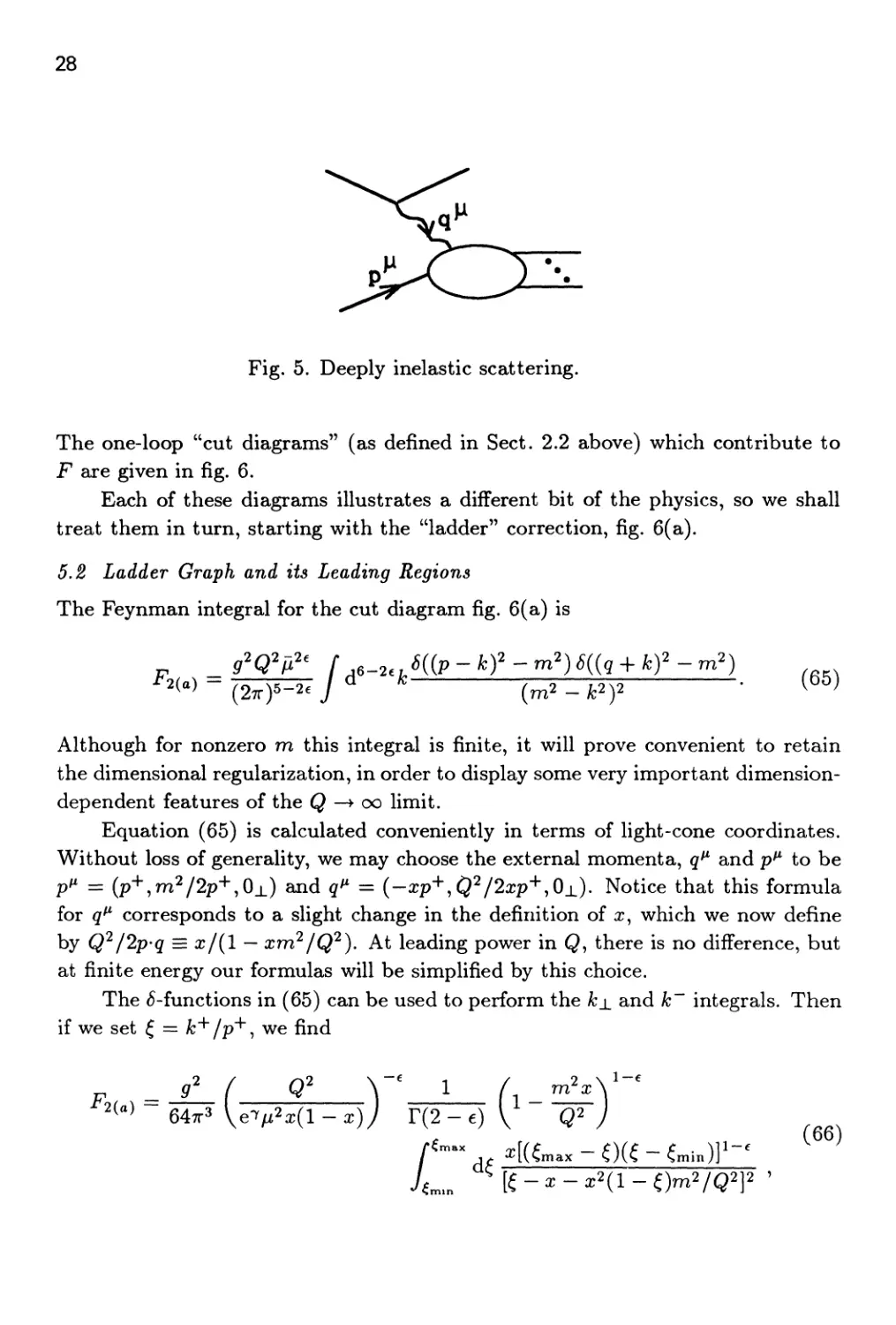
28
Fig. 5. Deeply inelastic scattering.
The one-loop "cut diagrams" (as defined in Sect. 2.2 above) which contribute to
F are given in fig. 6.
Each of these diagrams illustrates a different bit of the physics, so we shall
treat them in turn, starting with the "ladder" correction, fig. 6(a).
5.2 Ladder Graph and Us Leading Regions
The Feynman integral for the cut diagram fig. 6(a) is
(65)
Although for nonzero m this integral is finite, it will prove convenient to retain
the dimensional regularization, in order to display some very important dimension-
dependent features of the Q —> oo limit.
Equation (65) is calculated conveniently in terms of light-cone coordinates.
Without loss of generality, we may choose the external momenta, q^ and p^ to be
pf" = (p+,m2/2p+,0j_) and qf" = (-xp-^,Q^/2xp-^,0±). Notice that this formula
for q^ corresponds to a slight change in the definition of or, which we now define
by Q^/2p-q = x/{l — xm^/Q'^). At leading power in Q, there is no difference, but
at finite energy our formulas will be simplified by this choice.
The (^-functions in (65) can be used to perform the k± and k~ integrals. Then
if we set ^ = k'^ /p^ ^ we find
E
2(a)
9^ f Q' \"' 1 f^_m^x'''-'
QA'K^ ye-^p?x(\ - x)J r(2-€) V Q
L
(66)
29
(a)
(b)
(c)
(d)
(e)
Fig. 6. One-loop corrections to deeply inelastic scattering. For
graphs (b), (d) and (e), we also have the hermitian conjugate
graphs.
where the limits ^^in and ^max are given by
1 -\- X 1 — X
2
2
4771^
X
{1 - x){Q^ i-m^x) '
(67)
In this form, we can look for the leading regions of the ladder corrections. To do
this, it is simplest to set the mass to zero, find the leading regions, and then check
30
back as to whether we must reincorporate the mass in the actual calculation. So,
to lowest order in A = m?' /Q^ ^ {p&) becomes
"^^C) 64x3 VeV^(l-^)y r(2 - e) X(i+^) ^ {^ - x[l + x(l - OA]F '
(68)
To interpret this expression, we must distinguish between the renormalizable (n =
6, e = 0) and superrenormalizable (n < 6, e > 0) cases.
In the super-renormalizable case, (e > 0), the leading-power contribution
(Q/fi)^ comes from near the endpoint ^ = a:(l -j- A). The bulk of the integration
region, where ^ — x = 0(1) is suppressed by a power of Q. The integral is power
divergent when ?7i = 0, and clearly we cannot neglect the mass.
Now consider the renormalizable case, n = 6. When we set e = 0, eq. (68) has
leading power (Q°) contributions from both the region (, — x near zero, where, as
above, the mass may not be neglected, and the region ^ — x = 0(1), where it may.
In the former region, the integral is logarithmically divergent for zero mass, but
since the nonzero mass acts as a cutoff, the two regions ^ ~ x and ^ — a: = 0(1)
should be thought of as giving contributions of essentially equal importance. We
now interpret these dimension-dependent leading regions.
5.3 Collinear and Ultraviolet Leading Regions; the Parton Model
To see the physical content of the leading regions identified above, it is useful to
relate the variable ^ in (66) to the momentum k^^ by the relations
k-= -'
2p+(l - x)
(69)
,^^2 ^ g^(i - oii - x) _ m^[(i-o^ + e(i-x)]
x{l — x) 1 — X
Changing variables to k± , we now rewrite the integral eq. (6S) in a form which
is accurate to leading power in A for n < 6^
^'^^^ - 64^f(2^ X ^ (fcx^-fm2(l-.« + x2))2 • ^^^)
We emphasize that this expression is accurate to leading power in the region
k±^/Q^ = 0(A), which is suflSicient to give the full leading power for ?? < 6,
although not for n = 6, where larger k± also contribute.
Now let us choose a frame in which p'^ is of order Q. When (^ —> a:, the
components of k^ are of order (Q, (^ — x)Q, Q\/(, — x)^ and at its lower limit, (,— x
31
is of order vn?" jQ^. Hence, in the region that gives the sensitivity to ?7i, kx_ is small,
and k^ is ultrarelativistic and represents a particle moving nearly collinear to the
incoming momentum, p'*. In addition, the on-shell line, of momentum p^ — fc^,
is nearly collinear to the incoming line as well. In fact, when m and fcx are both
zero, h^ is also on the mass shell. The energy deficit necessary to put both the
momenta h^ and p^ — h^ on shell is of order hx_ jQ in this frame. Thus, in this
frame, the intermediate state represented by the Feynman diagram lives a time
of order Qlh±^^ which diverges in the collinear limit. The space-time picture for
such a process is illustrated in fig. 7, and we see a close relation to the parton
model, as discussed in Sect. 1.4, which depends on the time dilation of partonic
states. Partonic states whose energy deficit is much greater than m in the chosen
frame correspond to ^ — x of order unity, and do not contribute at leading twist..
Thus here, as in the parton model, there is a clear separation between long-lived,
time-dilated states which contribute to the distribution of partons from which the
scattering occurs, and the hard scattering itself, which occurs on a short time
scale.
t-z-0
Fig. 7. Space-time structure of collinear interaction.
From this discussion, the collinear region, which is the only leading region
when n is less than 6, is naturally described in parton model language.
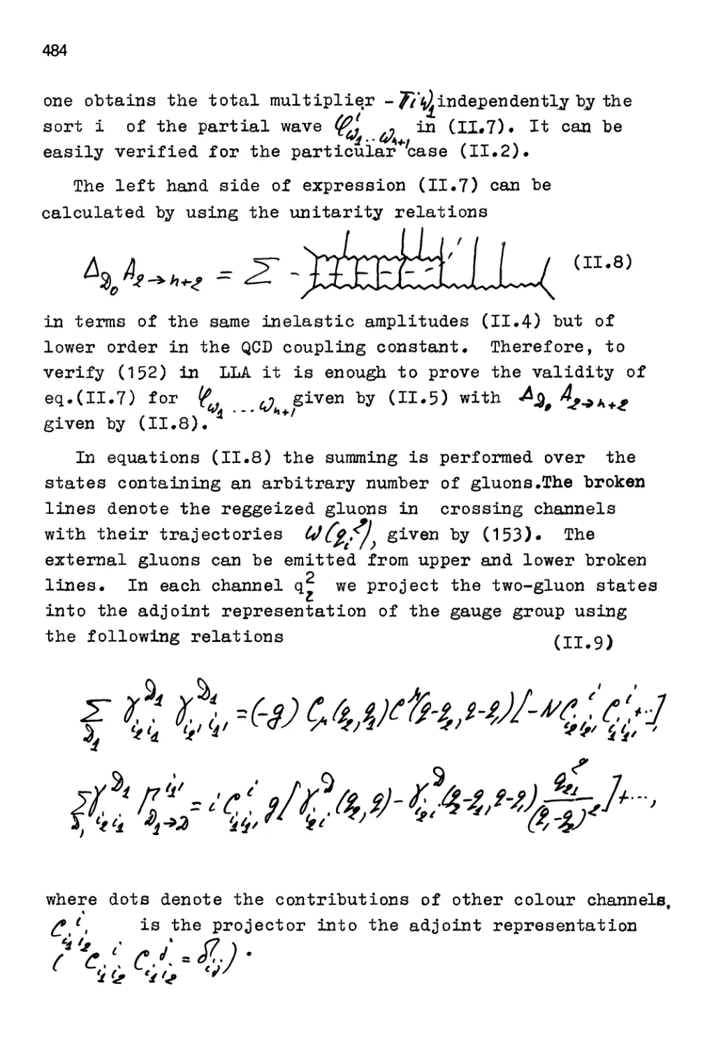
When n = Q^ the collinear region remains leading. In addition, however, all
scales between k_\_ — m and fc^ = Q contribute at leading power, and there is no
natural gap between long- and short-distance interactions. When ^ — x is order
unity, fc^ is separated from p^ by a finite angle, and corresponds to a short-lived
32
intermediate state, where (p — k)^ ^ m^. This leading region, which is best
described as "ultraviolet", is not naturally described by the parton model. But,
in an asymptotically free theory (as {<I>^)q is), such short-lived states may still be
treated perturbatively. We shall see how to do this below.
In summary, the ladder diagram shows two important features: a strong
correspondence with the parton model from leading collinear regions for both su-
perrenormalizable and renormalizable theories and, for the renormalizable theory
only, leading ultraviolet contributions, not present in the parton model.
5.4 Parton distribution functions and parton model
We shall now freely generalize the results for the one loop ladder diagram. Indeed,
as we shall see in Sect. 7, some of the dominant contributions to the structure
function arise from (two-particle-reducible) graphs of the form of fig. 8. A single
parton of momentum k^ comes out of the hadron and undergoes a collision in the
Born approximation. If we temporarily neglect all other contributions, we find
that
Fi^,Q) = / 0^Hk,p)H{k,q) + 0(1/Q<"), (71)
where $ represents the hadronic factor in the diagram and H the hard scattering
(multiplied by the factor of Q^/27r in the definition of the structure function):
Hik, q) = QH((k -f Q)2 - m^). (72)
For (j)^ with n < 6, as in the parton model, the parton momentum k^ is nearly
collinear to the hadron momentum p^. This implies that we can neglect m and
the minus and transverse components of k^ in the hard scattering, so that we can
write
H = Hix/^,Q) = 6a/x-l), (73)
and hence
F{x,Q)= I d^|/p+^^^$(fc,p)
S{ax-1) + 0{1/Q''). (74)
Here we define ^ = k"^ jp'^. The limits on the ^ integral are 0 to 1, since the
final state must have positive energy. We therefore define the parton distribution
function (or number density):
, / Ak'A^kx
---^k, p) s{Cp+/ k+-1).
33
Fig. 8. Dominant graphs for deeply inelastic scattering in parton
model.
With this definition (74) becomes
F{x,Q)
4.^
mHix/(,Q) + 0{\/Q'')
(76)
/(x) + 0(1/Q")
(n < 6).
As we shall see in the next section, the factorization theorem is also true in the
renormalizable theory,
F{x, Q)
1^
f{i)H{xli,Q) + 0{llQ'^)
(n = 6) ,
(77)
where now H is nontrivial. The dominant processes that contribute are illustrated
by fig. 9, which generalizes the parton model only to the extent of having more
than just the Born graph for the hard scattering. These processes first involve
interactions within the hadron that take place over a long time scale before the
interaction with the virtual photon. Then one parton out of the hadron interacts
over a relatively short time scale.
We now note that eq. (75) can be expressed in operator form as
m
ip
+
oo
— — 4 i^ n I *i
27r
dy-e-*«P ''>|<^(0,y-,Ox)^(0)|p).
(78)
OO
34
P
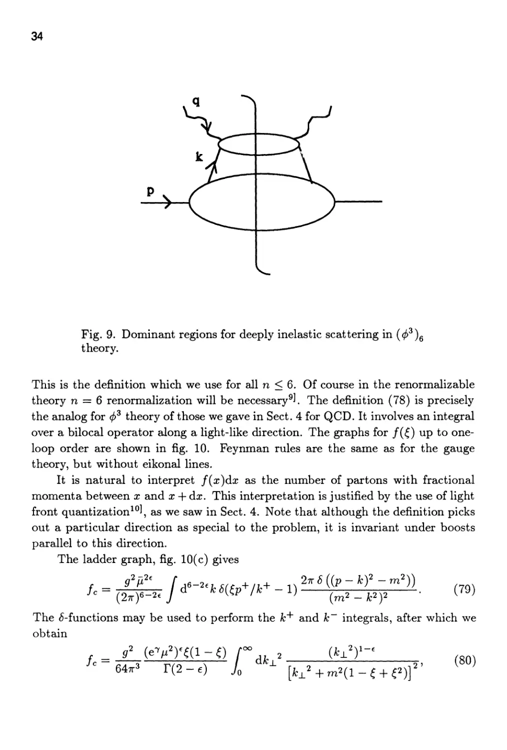
Fig. 9. Dominant regions for deeply inelastic scattering in {(I>^)q
theory.
This is the definition which we use for all n < 6. Of course in the renormalizable
theory n = 6 renormalization will be necessary^J. The definition (78) is precisely
the analog for (f)^ theory of those we gave in Sect. 4 for QCD. It involves an integral
over a bilocal operator along a light-like direction. The graphs for /(^) up to one-
loop order are shown in fig. 10. Feynman rules are the same as for the gauge
theory, but without eikonal lines.
It is natural to interpret f{x)dx as the number of partons with fractional
momenta between x and x -f- dx. This interpretation is justified by the use of light
front quantization^^J, as we saw in Sect. 4. Note that although the definition picks
out a particular direction as special to the problem, it is invariant under boosts
parallel to this direction.
The ladder graph, fig. 10(c) gives
/,
g'P''
(2t)'
-/
a-n.K.V.--i)"'t"-1-r'"^
(79)
The ^-functions may be used to perform the k"^ and k integrals, after which we
obtain
/,
g' (eVmi-0
647r3
r(2 - e)
oo
dk
±
(k^y-^
0
[A:j.'+m2(l-e-he)]
2 '
(80)
35
(a)
(b)
(c)
Fig. 10. Low-order graphs for part on distribution in (j)^ theory.
which matches eq. (70) in the k± —^ 0 limit. That is, we have constructed the par-
ton distribution to look like the structure function at low transverse momentum.
The significance of this fact will become clear below.
For n < 6, eq. (80) is the same as the full leading structure function (70), and
it exemplifies the validity of the parton model in a super-renormalizable theory.
When n = 6^ however, there is a logarithmic ultraviolet divergence from large
k± in (80). So, in the renormalizable theory we must renormalize f{C). (Since
/ is a theoretical construct defined to make treatments of high-energy behavior
simple and convenient, we are entitled to change its definition if that is useful; in
particular, we are allowed to include renormalization in its definition.) If we use
the MS scheme, then the renormalized value of fc for nonzero mass is:
R[fc] = -
g
647r
ai - 0 In
m\i-i+e)
F
(81)
while for zero mass it is (compare eq. (23))
R[fc] = -
^^e(i-oi.
647r
(82)
Now let us see what this means in the calculation of the hard part, as in Sect.
2. To calculate the hard part, we expand eq. (77) in powers of (7^, as in eq. (24),
and solve for H^^\x/^^Q). There is some question about what to do with the
36
higher-twist terms, proportional to powers of m/Q. The simplest method is to
simply define
H^'\x/(, Q) = \f^'\x/(, Q) - M , (83)
m=0
Comparison of eqs. (70) and (80) shows that the low k± region, which is the only
leading region which is sensitive to the mass, cancels between F^^^ and p^\ at the
level of integrands. Thus, for the combination on the right hand side of eq. (83),
it is permissible to set the mass to zero. It is thus practical to set the mass to zero
at the very beginning. It should be kept in mind, however, that this is a matter of
calculational convenience, rather than principle. The factorization theorem allows
us to calculate mass-insensitive quantities whatever the masses we choose, since
all sensitivity to these masses will be factored into the parton distributions.
Now let us return to the remaining diagrams in fig. 6, treating first the "final
state" interactions, fig. 6(b) and (c).
5.5 Final state interactions
The graphs of fig. 6(b) and (c) have a self-energy correction on the outgoing line,
the final state cut either passing through the self energy or not. As we will show,
these graphs have contributions that are sensitive to low virtualities and long
distances. However, they are not of the parton model form, and do not naturally
group themselves into the parton distribution for the incoming hadron. We will
see, however, that there is a cancellation between the two graphs such that they
are either higher twist (n < 6), or may be absorbed into the one-loop hard part
(n = 6).
The self energy graphs give simply the lowest order graph, 6{x — 1), times the
one-loop contribution to the residue of the propagator pole:
i^2(6) = S{X - 1)
r r. r., 2, 2 ^(1-^)
dk_L'k
1287r3yo J^ - - [k_^'^m^l-z + z'^)]^ (84)
-f-counter term].
We may derive this expression in either of two ways. One way is to combine the
denominators of the two propagators in the loop by a Feynman parameter before
performing the k^ and k~ integrals. Then z is the Feynman parameter.
Alternatively, we may first use contour integration to perform the k~ integral. Then we
get (84) by writing k'^ = z (p"'" + ^"'"). The integral is the same by either derivation.
But the second method shows that we may interpret 2 as a fractional momentum
carried by one of the internal lines. Since we will be concerned with the low k±^
region, while the counterterm, if computed with MS renormalization, is governed by
the k± —^ 00 behavior of the integrand, we do not write the counterterm explicitly.
37
There is clearly a significant contribution in (84) from small k±, where the
mass m is not negligible. The cut self-energy graph, in fig. 6(c), will also contribute
in this region. Now the region of low /?_[_ represents the effect of interactions that
happen long after the scattering off the virtual photon, and it is reasonable to
expect that interactions happening at late times cancel, since the scattering off
the virtual photon involves a large momentum transfer Q and therefore should
take place over a short time-scale. However, the uncut self-energy graph only
contributes when x is exactly equal to 1, while the cut self energy graph has no
^-function and thus contributes at all values of x.
This mismatch is resolved when we recognize that we should treat the values
of the graphs as distributions rather than as ordinary functions of x. That is,
we consider them always to be integrated with a smooth test function.
Mathematically, this is necessary to define the ^-function. Physically, the test function
corresponds to an averaging with the resolution of the apparatus that measures
the momentum of the lepton that is implicitly at the other end of the virtual
photon. After this averaging, a measurement of the lepton momentum does not
distinguish the situation where a single quark goes into the final state from the
situation where the quark splits into two.
We therefore consider an average of the structure function F{x) with a smooth
function t{x):
(t,F) = f dxt{x)F{x). (85)
Then the contribution of the self-energy graph is
(t,F2(6)) = t(l)F2(6) . (86)
Next we compute the cut graph, fig. 6(c). Its value is
2/n2
t{x) 6{P - m^) S{{p + q-k)'^~m?) ^ '
[{p + qf - m2]2
To make this correspond with the form of (84), we define z = k"^/{p^ -f- q^)^ and
then use the ^-functions to do the h~ and x integrals. After some algebra, and
after the neglect of terms suppressed by a power of Q, we find
where the Bjorken variable x satisfies
X
2 , _2 - ~^
A;_L + m
Q^z{l-z)\
(89)
38
We now axld the two diagrams to obtain:
9'
1287r
Jo Jo
oo
dkA_'^k±'^[t{x)x^ -t{l)]
z{l-z)
[it±'+m2(l-^ + ^2)]2
4- counter term.
(90)
In the region A;j_ <C Q, a: is close to one, and there is a cancellation in the integrand
of eq. (90). The cancellation fails when z is close to zero or one, but the
contribution of that region is suppressed by a power of Q. We are therefore permitted
to set m = 0 in the calculations of the graphs, after which a calculation (with
dimensional regularization to regulate the infrared divergences that now appear in
each individual graph at k± = 0) is much easier.
5.6 Vertex correction
Finally, we consider the vertex correction fig. 6(d). It has the value
+ counterterm
1
[m2 - Jb2] [m2 - (p + ky] [m2 - (p + it + ^)2]
-S{x - 1)
9
647r
/ dai /
Jo Jo
da2 In
m2(l - ai - a2 - {ai + ^2)^) + Q^Q:2«i
f^'
(91)
where we work in c? = 6 — 2e space-time dimensions to regulate the ultraviolet
divergence. When Q —> 00, we can clearly neglect the mass, so that we have (at
€ = 0)
E
2(d)
8{x - 1)
9
1287r3
ln^-3
+ 0
(92)
F2{d) is higher twist for e > 0.
The graph fig. 6(e) is related to fig. 6(d) by moving the final state cut so that
it cuts the inner lines of the loop. We will not calculate it explicitly. But when
that is done, the quark mass can be neglected, just as for the uncut vertex.
In summary, the only diagram from fig. 6 which corresponds to the parton
distribution is the ladder diagram, fig. 6(a). Non-ladder diagrams are either higher
twist, or contribute only to the hard part (renormalizable case). These results are
consistent with the structure of fig. 8 and fig. 9, which show the structure of
regions which give leading regions for n < Q and n = Q^ respectively. As we shall
show in the next section, it is this structure which enables us to prove that the
39
parton distributions eq. (78) absorb the complete long-distance dependence of the
structure function.
6. SUBTRACTION METHOD
To establish a factorization theorem one must first find the leading regions for
a general graph. We will see how to do this in Sect. 7. The result, for deeply
inelastic scattering in a nongauge theory, has been summarized by the graphical
picture in fig. 9, and it corresponds closely to our detailed examination of the order
g^ graphs. It can be converted to a factorization formula if one takes sufficient
care to see that overlaps between different leading regions of momentum space do
not matter.
An approach that makes this process clear is due to Zimmermann'^J. To treat
the operator product expansion (OPE), he generalized the methods of Bogoli-
ubov, Hepp, Parasiuk, and Zimmermann (BPHZ)'^'^^J that were used to renor-
malize Feynman graphs. (Although the original formulation was for completely
massive theories with zero momentum subtractions, it can be generalized to use
dimensional continuation with minimal subtraction^^J. This allows gauge theories
to be treated simply.) In the case of deeply inelastic scattering a very transparent
reformulation can be made in a kind of Bethe-Salpeter formalism^'^^, although it
is not clear that in the case of a gauge theory the treatments in the literature are
complete. In this section, we will explain these ideas in their simplest form.
There are two parts to a complete discussion: the first to obtain the
factorization, and the second to interface this with the renormalization. We will treat only
the first part completely. In (<^^)6 theory, renormalization is a relatively trivial
affair. Moreover, if we regulate dimensionally, with e just slightly positive, one
can choose to treat as the leading terms not only contributions that are of order
Q^ (times logarithms) as Q —> oo, but also those terms that are of order Q to a
negative power that is of order e. The remainder terms are down by a full power of
Q"^, and can be identified as "higher twist". In this way one has the same structure
for the factorization, without the added complications of renormalization.
Zimmermann's approach is to subtract out from graphs their leading behavior
as Q —> oo. This is a simple generalization of the renormalization procedure that
subtracts out the divergences of graphs. From the structure function -F(x, Q) one
thereby obtains the remainder -FRem(^5 Q)? which forms the higher twist
contributions. The leading twist terms are F — F^^^. It is a simple algebraic proof to show
that F — FRem has the factorized form / * i^, with / being the parton distribution
we have defined earlier, and with '*' denoting the convolution in eq. (77).
40
6.1 Bethe-Salpeter decomposition
In the graphical depiction of a leading region, fig. 9, exactly one line on each side
of the final state cut connects the collinear part and the ultraviolet part. So it
is useful to decompose amplitudes into two-particle-irreducible components. This
will leaxl to a Bethe-Salpeter formalism. Consider, for example, the two-rung
ladder graph, fig. 11, for deeply inelastic scattering off a composite particle. We
can symbolize it as
Fig. 11 = 73 X 7 X 7 X 7/,. (93)
Here 7^ represents the graph that is two-particle-irreducible in the vertical channel
and is attached to the initial state partide, 7 represents a rung, and 7/^ represents
the two-particle-irreducible graph where the virtual photon attaches. It is
necessary to specify where the propagators on the sides of the ladder belong. We
include them in the component just below. Thus 7^ and 7 have two propagators
on their upper external lines. The purpose of having a composite particle for the
initial state is to give an example with a non-trivial 7^, as in QCD with a hadronic
initial state. The vertex joining the initial particle is a bound-state wave function.
Fig. 11. Example of ladder graph with several rungs.
We now decompose the complete structure function as
00
F = 2_^ Gs Gj. Gh
N=0
(94)
41
Here G3 is the sum of all two-particle-irreducible graphs attached to the initial
state particle, Gh is the sum of all two-particle-irreducible graphs coupling to the
virtual photon, and Or is the sum of all graphs for a rung of the ladder. Thus
Gr is the sum of all two-particle-irreducible graphs with two upper lines and two
lower lines, multiplied by full propagators for the upper lines.
The second line of eq. (94) has the inverse of 1 — Gr, and it clearly suggests
a kind of operator or matrix formalism. Indeed, if we make explicit the external
momenta of two ladder graphs, 71 (A;, /) and 72(^5 0? then their product is
(7172)(fc, l) = J ^^7i(fc, k')y2{k', I). (95)
The rung graphs can thus be treated as matrices whose indices have a continuous
instead of a discrete range of values, while G^ and Gh can be treated as row- and
column-vectors.
In the case that the initial hadron is a single parton, as in the low order
examples in Sect. 5, the soft part G^ is trivial: G^ = 1, where '1' represents the
unit matrix.
6.2 Extraction of higher twist remainder
We can now symbolize the operations used to extract the contribution of a graph
to the hard scattering coefficient. Consider the example that lead to eq. (83). We
took the original graph and subtracted the contribution of the graph to f^^^H^^\
where H^^^ is the lowest order hard part. Then we took the large Q asymptote of
the result, by setting all the masses to zero.
Fig. 12. Hard scattering coefficient from fig. 6(a).
We represent this in a graphical form in fig. 12. There, the wavy line represents
the operation of short circuiting the minus and transverse components of the loop
42
momentum coining up from below, and of setting all masses above the line to zero.
Symbolically, we write this as:
Contribution of fig. 6(a) to H^^^ = Pjjh - PjPlh
= Pj{l-P)^h,
where the operator P is defined by
P{kJ) = (27r)^-^6(A;+ - /+)<5(A;-) (5^-^(/j.)
X (Set masses to zero in the part of the graph above P).
(97)
In eq. (96) we have ignored the need for renormalization that occurs if e = 0.
Either we can assume that we are only making the argument when e is slightly
positive, or assume that all necessary renormalization is implicitly performed by
minimal subtraction.
Fig. 13. Contribution of fig. 6(a) to f^^^H^^K
Fig. 6(a) gives two contributions to the factorization: a contribution to the
one-loop hard part H^^^ given in eq. (96) or (83), and a contribution to f^^^H^^\
The second of these we picture in fig. 13 and symbolize as
^Plh. (98)
Thus we can write the remainder for fig. 6(a), after subtracting its leading twist
contribution, as
Rem(fig. 6(a)) = 77,, - 7P7,, - P7(l - P)^f,
= (1-P)7(1-P)7/.. ^ ^
Clearly the operator 1 — P subtracts out the leading behavior.
43
In general, we can write the remainder for the complete structure function as
oo
^=0 (100)
This formula is valid without renormalization, even at € = 0. In the first place,
renormalization of the interactions can be done inside the 7's. This is because
there is nesting but no overlap between, on the one hand, the graphs to which
the operation 1 — P is applied and, on the other hand, the vertex and self-energy
graphs for which counterterms are needed in the Lagrangian of the theory. Further
divergences occur because of the extraction of the asymptotic behavior, and these
give rise to the need to renormalize the parton distribution. But the regions that
give rise to such divergences are of the form where lines in some lower part of a
graph are coUinear relative to lines in the upper part. All such regions are canceled
in eq. (100) since to the operator 1 — P they behave just like the regions that give
the leading twist behavior of the structure function.
6.S Factorization
It is now almost trivial to prove factorization for the leading twist part of the
structure function, which is
F-i^Rem=G,^^Gh-G,(l-P)^—^i^—— Gft. (101)
Simple manipulations give
1-Gr 1-Gr{l-P) (102)
We now have an explicit formula for the hard scattering coefficient:
^ = ^i-G.a-p)^-' (^°^)
while the paxton distribution / satisfies
fxP = G,j-^^P. (104)
One somewhat unconventional feature of our procedure is that not only do we
define P to set to zero the minus and transverse components of the momenta going
44
into the subgraph above it, but we also define it to set masses to zero. Setting
the minus and transverse momenta to zero while preserving the plus component
is exactly the appropriate generalization of BPH(Z) zero-momentum subtractions
to the present situation. Setting the masses to zero as well is a convenient way of
extracting the asymptotic large-Q behavior of a graph, as we saw in our explicit
calculations. Moreover, particularly in QCD, it greatly simplifies calculations if
one works with a purely zero-mass theory. Of course, setting masses to zero gives
infrared divergences in all but purely ultraviolet quantities. The momentum-space
regions that give the divergences associated with the structure function all have
the same form as the leading regions for large Q, fig. 9, so that the 1 — P factors in
eq. (104) kill all these divergences. Note that, just as with Zimmermann's methods,
the P operator can be applied at the level of integrands. In practical calculations,
dimensional continuation serves as both an infrared and an ultraviolet regulator.
In the one-loop example of Sect. 5, the external hadron is a part on, so that in
Gs = S(x — 1) in (104). At one loop, Gr corresponds exactly to /c, eq. (80). This
expression, and the distribution / as a whole in (104) is still unrenormalized, and
contains ultraviolet divergences. These may be removed by minimal subtraction, as
in eq. (81) at one loop, or as discussed more generally in Ref. 9. We should mention,
however, that it would be advantageous to have a subtraction procedure which
combined factorization and renormalization into a single operation. The particular
procedure outlined by Zimmermann'^J does this, but is not immediately applicable
when all particles are massless. Duncan and Furmanski^^l have discussed some of
these issues at length.
6.4 Factorization for Inclusive Annihilation in {(I>^)q
It is easy to generalize the general arguments of this and the previous section to
other processes, such as those listed in the introduction. An important example,
is the cross section in (j>^ theory that is analogous to one-particle inclusive
annihilation in e'^e" annihilation, that was discussed in Sect. 1.2. In the scalar theory,
the structure function for this process is
Dix,Q) = ^ J d'ye"'yJ2{0yiy)\HX){HXy{0)\0), (105)
which is exactly analogous to the QCD version, eq. (6).
It is relatively easy to check that the leading regions for this process have a
form that generalizes fig. 9 for deeply inelastic scattering, that is, they have the
form of fig. 14. This was shown in Ref. 19 (for the case of a non-gauge theory).
An example is given by the ladder graph of fig. 15. We must integrate over
all values of the momentum (k — pY, When [k — pY is coUinear to p'^, the line k
has low virtuality. Then in the overall center-of-mass, the remaining particle q~ k
45
Fig. 14. Example of leading region for inclusive annihilation.
Regions with more than one jet inside the hard subdiagram H
are also leading.
has large energy, approximately Q/2, and is moving in the opposite direction to
the first two particles. We therefore consider the lines p, k — p and k as forming
the jet J A in fig. 14 and q — k together with the vertex where the 'virtual photon'
attaches as forming the hard part H. When (k — p)^ has transverse momentum
of order Q, we put both k and k — p into the hard part.
In a non-gauge theory, these two regions are the only significant ones, together
with a region that interpolates between them. As we shall see in Sect. 7, this
statement generalizes to all orders of perturbation theory. In a gauge theory, like
QCD, all kinds of complication arise because there are also 'leading twist' regions
involving soft gluons.
6.5 Factorization, fragmentation function
Simple generalizations of the arguments for deeply inelastic scattering give the
scalar factorization theorem:
Diz,Q)
1^
C
H(z/C,Q)d{0 + O{l/Q'').
(106)
analogous to eq. (7). Here the fragmentation function is defined in exact analogy to
the parton distribution. We choose axes so that the momentum p^ of the detected
46
Fig. 15. Ladder graph.
particle is in the positive 2:-direction. Then we define:
d{z)
P
+
27rz
dy~e'P'^y /^
53(0 1(^(0, 2/-,0t)| ifX)(ffX 1(^(0)1 0)
X
P
+
(107)
This is interpreted as the number density of hadrons if in a parton. The formulae
are exactly analogous to eqs. (75) and (78) for the parton distribution. Renormal-
ization is needed here also.
7. LEADING REGIONS
As we saw in Sects. 5 and 6, the first step in constructing a complete proof
of a factorization theorem is to derive the leading regions of momentum space
for a graph of arbitrary order. This section begins with a brief description of a
general approach to the long- and short-distance behavior of Feynman diagrams
that results in a derivation of the leading regions. We apply this method to
describe the origin of high-energy logarithms in scalar theories, and go on to discuss
the cancellation of final state interactions, and the infrared finiteness of jet cross
sections.
47
7.1 Mass dependence and leading regions
Consider, then, an arbitrary Feynman integral G{p'^/fi^m/fi)^ corresponding to a
graph G, which is a function of external momenta pj', mass m (possibly zero),
and renormalization scale //. Without loss of generality, we may take G to be
dimensionless. We also assume that the invariants formed from different p^ are all
large, while the pj' themselves have invariant mass of order m. Thus:
Pi'Pj = Q'^Vij^ P] = C»^^ (108)
where Q is a high-energy scale, Q ^ tti, and the r^ij and Ci ^^^ numbers of
order unity. In the following, it will not be necessary to consider the 77,^ and Ct
dependence, and we will write G as G{Q'^I^^^m? j^'^). We will be interested in
the leading term in an expansion in powers of \jQ^. (Always we will allow the
possibility of a polynomial in In Q multiplying the power of Q, in each order of
perturbation theory.)
Suppose G is the result of L loop momentum integrations acting on a product
of / Feynman propagators, times a function iV, which is a polynomial in the
internal and external momenta. For simplicity, we absorb into N the numerator factors
associated with the internal propagators, as well as overall kinematic factors, etc.
G may then be represented schematically as
G(QV/^^mV/^^) = n U^'U N{{k^]Api})f{ \ (109)
The line momenta {A;^}, of course, are functions of the ^f and the pf. Any region
in £^ space which contributes to G at leading power in Q^ will be called a "leading
region". In addition, by a "short-distance" contribution to (109) we will mean that
we have a region of loop momenta in which some subset of the line momenta, {A;^},
are ofF-shell by at least C^(Q^); the short-distance contribution is the factor in (109)
given by these far ofF-shell lines. Short-distance contributions are independent of
masses to the leading power in Q"^, since the integrand can usefully be expanded
in powers of m'^ when propagators axe far ofF-shell. A general leading region has
both short-and long-distance contributions, the latter associated with lines which
are nearer the mass shell. Roughly speaking, factorization is the statement that
the cross section is a product of parton distributions, in which all the long-distance
contributions are found, and a hard-scattering coefficient, which has purely short-
distance contributions. To study factorization, we must characterize all
"longdistance" contributions.
Our analysis depends on two observations. The first concerns the close relation
between the high-energy and zero-mass limits. That is, if the renormalization
48
scale // is chosen to be of 0(Q), then the two limits are equivalent in the function
G(l, m^/Q^). Short-distance contributions to the Q —> oo limit are those involving
lines for which kj is of order Q^. Long-distance contributions are parts of the if
integrations for which kj is much less than Q^. If we scale all momenta down by
a factor proportional to Q, then we axe considering the m —^ 0 limit instead. The
short-distance contributions now have fixed kj and the long-distance contributions
have Feynman denominators kj -f- ie in eq. (109) that vanish in the m —> 0 limit.
Note that if G is such that it only has short distance contributions, then
the Q —* oo limit is G(1,0), i.e., we can just set m = 0. The QCD coupling,
^s(Q), is an implicit argument for G, and we have already chosen to set the
renormalization scale fi equal to Q. Thus in this case the detailed large Q behavior
is renormalization-group controlled in a simpJle way.
When there are long-distance contributions to G, an expansion in powers of
m will often fail. So to find the long-distance contributions to G, one must look
for singularities in the m —^ 0 limit. There are apparent exceptions to this rule,
exemplified by the integral
However, if we factor out the numerator factor m^^ we axe left with an integral
that is singular like 1/m^. This singularity is governed by the denominator. So
what we axe looking for is singularities in the m dependence in the integral over
the denominators of G.
Our second observation is that the integrals in (109) are defined in complex
^f-space. As a result, it is not enough for a set of denominators to vanish in the
integrand of (109) for the integral to produce a singularity at m = 0 in G. We
must have, in addition, a pinch of one or more of the if integrals at the position of
the singularity, between coalescing poles. This fact enables us to apply the simple
but powerful analysis due originally to Landau^^'^^1 on the relation of singularities
in Feynman integranc^^ to the singularities of Feynman integra/^. In the next
subsection we explain the application of this argument.
7.2 Pinch surfaces
We begin by using Feynman parameterization to combine the denominators of
eq.(109) by
G(QV/i',mV/i')= (/-l)!n / da,^(l-5^a,)n d^^, N{{kj},{pi})
x[i2a,{k]{if)~m') + ze] \
j=i
(111)
49
where we have exhibited the loop-momentum dependence of the hne momenta.
There is now a single denominator D{ii^aj)^ which is quadratic in loop momenta
and linear in Feynman parameters. Suppose D{ii^aj) vanishes for some value of
loop momenta and Feynman parameters. We will now derive necessary conditions
for this zero to produce a singularity in G. Then we will apply these conditions
to the case m = 0.
A pole from D = 0 will not give a singularity in G if D can be changed from
zero by a deformation that does not cross a pole in any one oi the momentum or
parameter contours. Consider first the parameter integrals. Because D is linear
in the {«j}, a deformation of the aj integral will change D away from zero, unless
kj = rr? or aj = 0 (112)
for each line. In the first case, D is independent of o^j, while in the second we
note that aj = 0 is an endpoint of the aj integral, away from which it cannot be
deformed.
Now suppose (112) is satisfied, and consider the momentum integrals. D
will be independent of those loop momenta which flow only through lines whose
Feynman parameters are zero. The contours of the remaining loop momenta must
be pinched between singularities associated with the vanishing of D. Since D is
a quadratic function of the remaining momenta, each momentum component sees
only two poles in its complex plane due to the vanishing of D. The condition for
a pinch is thus the same as the condition that the two zeros of the quadratic form
be equal. That is, in addition to D = 0 we must have dDjdi^ = 0 for all i'^ which
flow through one or more on-shell lines. For each such loop momentum, the extra
condition is^^'^^1
where the sum goes over all lines through which the loop momentum if flows.
(Note that any line which is not on shell has aj =0, by eq. (112), so the condition
(113) can be applied to every loop.) Together, (112) and (113) are known as the
"Landau equations". We shall refer to any surface in momentum space on which
the Landau equations are satisfied as a "pinch surface" of the diagram G. With
each pinch surface we associate a "reduced diagram", in which all ofF-shell lines
are shrunk to points. By construction, the reduced diagram contains only those
loop momenta of the original diagram which satisfy (113) with nonzero a's.
7.3 Physical propagation
The Landau equations axe surprisingly restrictive, especially in the zero-mass limit.
To see why, let us rederive the observation of Coleman and Norton^^'^^1 that
50
eqs. (112) and (113) have an appealing physical interpretation. Consider a given
pinch surface. We rewrite (113) on this surface as
T(aj u;j)v^ = 0, (114)
where v^ and ljj axe the four-velocity and energy associated with the momentum
kj^. The units of the Feynman parameters are arbitrary, so suppose we may, if we
wish, interpret aj as the frame-independent ratio of a time to the energy of line j.
Then each of the components of the vector (ajiJj)Vj^ has the units of a distance in
space-time. It is the distance traversed in time (ajUj) by a free particle moving
classically with velocity v^.
Now suppose we associate a definite position a;J* to one of the vertices in the
reduced diagram associated with the pinch surface. Then, if line j attaches to the
vertex at Xj, x^ -\-{aj (j^j)vj^ may be interpreted as the position of the vertex at the
other end of line j. Continuing in this manner, we can associate with the reduced
diagram a position in space-time for every one of its vertices, and a physical process
in which free particles move between these points. Equation (113) ensures that
this program can be carried out consistently, by requiring that in going around
any closed loop we come back to the same position. We can use this construction
as a necessary condition for a pinch surface.
Finally, note that, because eqs. (112) and (113) axe homogeneous in the a's,
a rescaling of the a's leaves the Landau equations satisfied. Hence the vertices
in the physical picture are an indefinite distance apart, and, in particular, this
distance may be arbitrarily large.
7.4 Collinear and infrared pinches; power counting
For a general diagram with arbitrary masses and external momenta the criterion
of physical propagation allows a very rich analytic structure. In the massless limit,
however, this structure actually simplifies since multiparticle thresholds become
degenerate. The physical processes of which an isolated massless (but not
massive) particle is kinematically capable are as follows. First, a massless particle of
momentum p^ may split into two (or more) massless particles of momenta ap^
and (1 — Oi)p^, and vice-versa. This is the source of collinear divergences. Second,
a particle may emit or absorb one (or more) zero energy particles. This is the
source of infrared divergences. We easily check that arbitrary loops involving only
collinear and zero-momentum particles can satisfy the Landau equations.
Generally, we will describe a subdiagram consisting of mutually collinear particles as a
"jet" subdiagram. Lines that have zero momentum in the massless limit we will
call "infrared". A jet subdiagram describes the evolution of a set of collinear lines,
as they absorb and emit other collinear and infrared lines.
51
As an example, let us consider the vertex correction fig. 16a, in dimensionally
regulated (f)^ theory,
VM = / ^
1
[{p' - ky - m2 + ie] [(p + ky - m2 + ie] (F - m2 + ie)'
(115)
where we assume a production process, Q^ = {p' + pY > 0. This example is
used for illustrative purposes only. The term "leading" will refer here only to
this diagram, and not to the behavior of the Born diagram. In fact, fig. 16(a) is
nonleading compared to the Born process for all n < 6.
The Landau equation for fig. 16(a) is
«i(p - J^Y + «2(p + ky + a^k^" = 0. (116)
For on-shell (p^ = p'^ = m^) scattering with m ^^ 0, eq. (116) has no solutions at
all. Note that this is the case even though there is a singular surface illustrated in
fig. 16(b), with
(p + kf = (p' - kf = m^, jfc^ < 0. (117)
This singular surface corresponds to the production of two particles, followed by a
subsequent spacelike scattering. Although such a process is kinematically possible,
it clearly cannot correspond to physical propagation, because the two particles
produced at vertex 1 propagate in different directions, and would therefore not be
able to meet at vertex 2 to scatter again.
Now let us consider the case that tti = 0. By the same reasoning, (117) does
not give a pinch surface, if A; ^ 0. There are nevertheless two sets of solutions.
First, there are infrared solutions where one line has zero momentum,
k^ = 0, «! = ^2 = 0,
(p + A:)'^ = 0, ai =0^3 = 0, (118)
(p - ky = 0, ^2 = «3 = 0.
Second, there are coUinear solutions, where two of the lines are parallel to one of
the outgoing external particles,
2
«i(p - ^Y + ot:ik^ =0, ^2 = 0, k^ = p'k = 0,
2 .. . (119)
«2(p' + ky + a^k^ =0, Oil = 0, k^ = p'-k = 0.
The physical pictures associated with typical infrared and collinear pinch surfaces
are shown in figs. 16(c) and (d), respectively. In each case, there is physically
realizable propagation between vertices.
52
P
P
(b)
p + k-0
k-0
(c)
(d)
P
Fig. 16. (a) Vertex correction, (b) Reduced diagram correspond
ing to eq. (117), (c) Infrared reduced diagram, (d) collinear re
duced diagram.
Now we observe that even though solutions to the Landau equations like
eqs. (118) and (119) give pinch surfaces, they still do not necessarily produce
mass dependence that is relevant to the leading power of Q, and hence are not
necessarily leading regions.
The Born graph for the vertex behaves like Q^. The contribution to the one-
loop graph from the pure short-distance region, from the region, \k^\ = 0(Q), is
Qn-6 'pj-^^s ^}^is region is leading when the theory is renormalizable, at n = 6, but
is non-leading relative to the Born graph when the theory is super-renormalizable,
n < 6.
Next we consider the one-loop graph near its singular surfaces. For example,
consider the integral (115) near the surface defined by the first of eqs. (118). To
be specific, let |A;'^| < Aj^ax? /^ = 0... 3, with A;max being some fixed scale (which
53
must ^ m). In this region the integral behaves as
r Ik. <
Q^Jk.<k^.. k' Q
'"*^-. (120)
rs^
in&x
Compared to the short-distance region, this infrared region is leading only for
n < 4. (The other two infrared regions in (118) require n < 2.) (We remind the
reader that, compared to the Born graph, none of these regions contribute to the
leading power of Q.)
Similarly, near the coUinear pinch surfaces of eq. (118), the integral behaves
as
max
jl2 An-2h. h^-"^
SO that again only for n < 4 do we find collinear contributions from this diagram
that are leading compared with the short-distance contribution.
In summary, for the scalar theory in six dimensions, only short distance
regions are (relatively) leading for fig. 16. This result generalizes to all orders in the
vertex correction for this theory^'*^.
The process of estimating the strength of a singularity is known as "power
counting". We will give more low order examples below, while more general
arguments can be found in Ref. 23. We can, however, summarize the basic result of
these arguments briefly. Let Z) be a reduced diagram with 5 "infrared loops" and
Is infrared lines whose momenta vanish at the corresponding pinch surface, and
with C "collinear loops" and Iq collinear lines whose momenta become
proportional to an external momentum at the pinch surface. Finally, let A^2 denote the
number of two point subdiagrams in R. In (j)^ theory in n space-time dimensions,
let us define^^1 the "degree of divergence" by
u;(R) = nS + (n/2)C - 2Is - Ic + ^^2- (122)
This corresponds to a power law
Q{n-6)V j^^iR) ^^23)
as Q ^ oo. Here V is the number of loops and A is a small parameter that
parameterizes the approach to the singularities in the massless theory. The power
law is measured relative to the power for the Born graph.
In the renormalizable case, n = 6, we get leading behavior only if lj{R) = 0
and there are no graphs that give negative uj{R), The term N^^ which tends to
suppress the behavior of the integral at the singular point, is due to the fact that
the renormalized two-point function must vanish on-shell if the particle is to have
54
zero mass. In this sense, the infrared behavior of the theory is dependent on
renormalization^^^.
In the superrenormalizable case, n < 6, the first factor in (123) gives a negative
power of Q that just corresponds to normal ultraviolet power counting; this is
the power that comes from a purely short-distance contribution to the graph.
A sufficiently strong power law singularity in the massless theory is needed to
overcome this if one is to get a leading contribution.
7.5 Leading regions for deeply inelastic scattering in {<I>^)q
As an application, we now discuss the general leading regions for the basic
inclusive cross sections in {<I>^)q' The criterion of physical propagation shows why the
considerations of Sects. 5 and 6 take into account all relevant leading regions. To
see this, we must generalize our concept of leading regions to include cut diagrams,
of the type discussed in Sects. 5 and 6. There is no problem in doing this, and
power counting may be estimated for collinear and infrared cut lines with the same
degree of divergence eq. (122) as for virtual lines.
It is useful to apply the optical theorem to reexpress the deeply inelastic
scattering structure function eq. (63) as the discontinuity of the forward Compton
scattering amplitude T(^,p),
F(x,Q2)=discr(g,p),
O^ f (124)
Tiq,p) = ^ d«j/e"«'{p|T(i(y)i(0)|p).
This relation holds diagram-by-diagram, once cuts are summed over, so that a
necessary condition for a region L to be leading in F is that it be leading in T.
We thus need to consider the leading regions of the diagrams illustrated by
fig. 17(a), which represents forward Compton scattering. The pinch surfaces are
symbolized in fig. 17(b). The incoming hadron can form a jet of lines, and in
addition, may interact with any number of soft lines, connected to a subdiagram
S consisting of only lines with zero momentum. To see why this is the general
form, consider a singular surface not of this kind, cis in fig. 17(c). Here, one
or more lines of the jet may scattering with the incoming photon to form a set
of on-shell outgoing jets, which then rescatter to emit the outgoing photon and
reform the outgoing jet, which eventually evolves into the outgoing hadron. Such a
process is certainly consistent with momentum conservation. Surfaces of this type
are not pinch surfaces for the amplitude T(^,p), however, because the outgoing
jets can never collide again once they have gone a finite distance from the point
at which they are produced. As a result, in every pinch surface, the incoming
and outgoing photons attach at the same point in space-time, and we derive the
55
(a)
(b)
(c)
Fig. 17. (a) Diagrams for forward Compton scattering, (b)
Reduced diagrams for pinch surfaces, (c) Reduced diagram for
a singular surface which is not pinched.
picture of fig. 17(b). This result shows that all divergences associated with final
state interactions cancel in the sum over final states.
As indicated above, not every pinch surface will correspond to a leading region.
In particular, power counting using eq. (122) shows that there are no infrared
divergences in {(t>^)Qi that is, no zero-momentum lines for any leading region^^l. In
addition, we can show that only the minimum number of jet lines (two) can attach
the jet to the hard part in fig. 17(b). It is a straightforward exercise in counting
56
to prove these results, using (122), the Euler identity (loops = lines - vertices +
1), and the observation that every internal line of a graph begins and ends at a
vertex. In summary, we can show that fig. 9 is indeed the reduced diagram of the
most general leading region for deeply inelastic scattering in the scalar theory.
1.6 Unitarity and jets: the cancellation of final state interactions
The cancellation of final state interactions in deeply inelastic scattering plays an
important role in the analysis for deeply inelastic scattering just described. This
cancellation is a general feature of inclusive hard scattering cross sections, and is
used repeatedly in factorization proofs. The physics behind this cancellation has
already been pointed out in Sect. 5: a hard scattering is well localized in space-
time, and, as a result, it cannot interfere with long-distance effects which describe
the further evolution of the system. Thus, when we sum over final states in an
inclusive cross section, we lose information on the details of evolution in the final
state, and are left with the constraint that, by unitarity, the sum of probabilities
of all final states is unity. As a result, at each order in perturbation theory,
long-distance contributions to final states must cancel.
It is worth noting that it is not always necessary to sum over all final states to
cancel long-distance interactions. There are three kinds of cross sections, among
those mentioned in Sect. 1, for which the cancellation of final state interactions
is important. In deeply inelastic scattering and Drell-Yan, for instance, we sum
over all hadronic final states. In single-paxticle inclusive cross sections, on the
other hand, we shall find in Sect. 9 that cancellation requires the use of Ward
identities. Finally, in jet cross sections, the cancellation comes about in a sum
over all final states which satisfy certain criteria in phase space. Let us hint at
how this happens.
If all non-forward particles in the final state emerge from a single hard
scattering, the criterion of physical propagation requires that the long-distance
contributions will come entirely from soft and coUinear interactions. This is because,
as in the low order example of fig. 16, jets emerging from a single point and
propagating freely cannot meet again to produce a new hard scattering. In this case,
once the energy and direction of a set of jets is specified, the sum over only those
final states consistent with these jets will also give unity, and their collinear and
infrared divergences cancel in the sum. The technical proof of these statements
may be given in a number of ways. The simplest is based on a truncation of
the hamiltonian to describe only collinear and infrared interactions. Then, since
the truncated hamiltonian is hermitian, it generates a unitary evolution operator
whose divergences cancel by the "KLN" theorem^^'^^K It is also useful to see that
this cancellation is manifested on a diagram-by-diagram basis within each leading
region in perturbation theory^^l. Proofs of this type are most easily given in terms
57
of time-ordered or light-cone ordered perturbation theory^^'"^^J.
Technicalities aside, the cancellation of final state interactions at the level of
jets has a number of important consequences. The simplest of these is the finiteness
of jet cross sections in e"^e~-annihilation cross sections"^®J. We have already seen its
importance for the analysis of deeply inelastic scattering in {<t>^)Q- It has a similar
simplifying effect for single-particle inclusive cross sections, as well as for the Drell-
Yan and related cross sections. To illustrate this, we show, in fig. 18 the reduced
diagrams for leading regions in the scalar "Drell-Yan" cross section, defined for
the scalar theory by analogy to eq. (63) in {(t>^)Q, after the sum over final states.
We see that all information about the final state has been absorbed into a single
hard part H. Note that this result holds not only for the fully inclusive Drell-Yan
cross section, but also for semiinclusive cross sections such as hadron-hadron -^
Drell-Yan pair -f jets.
Pa
Pb
Fig. 18. Leading regions for the Drell-Yan cross section in {(J>^)q.
8. FACTORIZATION AND GAUGE INVARIANCE
In this and the following section, we discuss the extension of factorization proofs
to gauge theories. We begin with a discussion of the classical Coulomb field of a
fast moving charge, an example that anticipates what happens in the full quantum
theory.
58
We next summarize the Ward identities we will need. Then we discuss the
leading regions of Feynman graphs in a gauge theory. There are great differences
from the case of the (j)^ theory discussed in the previous section. With the aid
of the example of the vertex graph, we show how, after an appropriate eikonal
approximation. Ward identities are applicable that will combine graphs into a
fac tori zed form.
In the next section, we will show how factorization may be proved for a
variety of experimentally important cross sections, which can be measured in deeply
inelastic scattering, e"^e~ annihilation and hadron-hadron scattering. We should
emphasize at the outset that although we regard existing proofs in all these cases
as reasonably satisfying, there is still room for improvement, especially for hadron-
hadron cross sections. We will point out the shortcomings of existing arguments
in Sect. 10.
8.1 Classical considerations
Before getting into a detailed discussion of Feynman diagrams, it is worth noting
that insight can be gained into the physical content of factorization theorems from
purely classical considerations. This discussion will at once highlight an important
difference between gauge and scalar theories, and at the same time show why this
difference, important though it is, respects factorization.
As we observed in Sect. 1.4, the parton model picture of hadron-hadron
scattering rests in part on the Lorentz contraction of colliding hadrons. Now a
simplified classical analog of a hadron is a collection of point charges, each acting as a
source of a classical scalar field. We would expect that if the parton model, or
factorization, is to make sense, these fields ought to be Lorentz contracted themselves,
and this is just what happens. Let us see how.
Consider first a static classical scalar field </>ci(x), associated with a point
particle of charge q at the origin. If we assume that the field obeys Laplace's
equation, it is given in the rest frame of the particle by
^ci(x) = -^. (125)
Now consider the same field in a frame where the particle is moving at velocity c/S
along the z-axis. Then the field at x'^ in this frame is
<?^cl(^') =
[4 + 7^(^cf-4)2]
1/2 '
(126)
where, as usual, 7 = (1 — ^^)~^/^. For an observer at t' — 0 in the primed system,
the (f) field decreases as 7"^ as (3 approaches unity, except near x'^ = 0. Thus, the (f)
field is indeed Lorentz contracted, and any force proportional to the <j) field is also
59
Lorentz contracted into a small longitudinal distance about x'^ = 0. This means
that in the rest frame of a scalar "hadron", the forces due to another such hadron
approaching at nearly the speed of light are experienced in a Lorentz-contracted
fashion, just as supposed in the paxton model.
Now let us apply this reasoning to a classical gauge theory, in this case classical
electrodynamics. Here, the field in the rest frame of a point particle of charge q is
precisely analogous to eq. (125),
^c^« = #. (127)
Because this is a vector field, however, there is a big difference from the scalar case
in a frame in which the particle moves with velocity 0^X3. In this frame, we find
[x ^^ + jm3ct'- x'.fY'^
A'Jix') = ^^ ^, (128)
For large 7, the field in the zero and three directions are actually independent of
7 at fixed times before the collision. It might therefore seem that a vector field
is not Lorentz contracted, and would not respect the assumptions of the parton
model. If we look, however, at the field strengths rather than the vector potential,
we find a different story. The electric field in the three direction, for instance, is
given in the primed frame by
which shows a 7"-^ falloff. Since the force experienced by a test charge (or parton)
in the primed frame is proportional to the field strength rather than the vector
potential itself, the physical effects of the moving charge are much smaller than
its vector potential at any fixed time before the collision. This in turn may be
understood as the fact that, as 7 —>• 00, the vector potential approaches the total
derivative
qd^\n{l3ct' -x':^). (130)
That is, for any fixed time the vector potential becomes gauge equivalent to a zero
potential.
We can conclude from this excursion into special relativity that factorization
will be a more complicated issue in gauge theories than in scalar theories. Only
60
for gauge invariant quantities will the gauge-dependent, large vector potentials of
moving charges, which naively break factorization, cancel. So, in particular, we
cannot expect factorization to be a property of individual Feynman diagrams, as it
was in scalar theories. On the other hand, we should look for the solution to these
problems in the same techniques which are used to show the gauge independence
of physical quantities.
8.2 Ward identities
The Ward-Takahashi identities of QED and the Taylor-Slavnov identities of non-
abelian gauge theories ensure the perturbative unitarity of these theories. We shall
refer to them collectively as "Ward identities" below.
Ward identities may be expressed in various forms, for instance, as
identities between renormalization constants (the familiar Zi = Z2 of QED). For our
purposes, however, the basic Ward identity is given graphically by the equation
{N\T ^^,A'''{x^)x ■■■ X d^^A'^-ixn) \M) =0, (131)
where A^{x) is an abelian or nonabelian gauge field, and where M and N are
physical states, that is, states involving on-shell fermions and gauge particles, all
with physical polarizations. In particular, physical states do not include ghosts.
Equation (131) will be represented graphically by fig. 19, in which the scalar
operator d^A'^(x) is represented by a dashed line ending in an arrow. In momentum
space, this operator is associated with a standard perturbation theory vertex in
which one gluon field is contracted into its own momentum. Here and below, we
refer to such a gluon as "longitudinally polarized". Note that this is to be taken
as referring to the four-momentum.
0
Fig. 19, Ward identity.
Proofs of eq. (131) are most easily given in a path integral formulation using
BRST invariance, as in, for instance Ref. 29. They can also be proved in a purely
61
graphical form, as in the original proofs of Refs. 30 and 31. Here we need not
concern ourselves with the details of these proofs, although it may be worthwhile to
exhibit the very simplest example of eq. (131). This is the lowest order contribution
to the electron scattering amplitude with a single longitudinally polarized photon.
At this order, we have
qf'uip + qhMP) = ^(P + ^) [(/ + ^ + "^) - (/ + ^)] ^(P) = 0- (132)
The first equality is sometimes referred to as the "Feynman identity", and the
overall result is current conservation at lowest order. This is not surprising, since
classical current conservation is a consequence of gauge invariance. In the quantum
theory, it appears as a matrix element relation, whose validity is ensured by the
Ward identity. A helpful exercise is to construct the analog of eq. (132) for the
scattering of a physically polarized gluon. The graphical proof consists essentially
of repeated applications of identities like eq. (132).
Even without going into the details of the proof of eq. (131), we can elucidate
its interpretation. First, it is true order-by-order in perturbation theory, although
not graph-by-graph in perturbation theory. In addition, we may imagine
constructing a path integral in which only certain momenta are included, for instance
ultraviolet momenta and/or momenta parallel to a given direction. Then at a
given order, the Ward identities hold for both internal and external lines in this
restricted portion of momentum space. This heuristic argument may be verified
by a close look at the graphical proof of Ward identities in Refs. 30 and 31.
So far, we have discussed Ward identities for the S-matrix. As we saw in
Sect. 4, however, we will sometimes be interested in matrix elements involving a
gauge invariant but nonlocal operator which includes the ordered exponential of
the gauge field. Such matrix elements also obey Ward identities, which may be
proved by either of the methods mentioned in connection with eq. (131). The
simplest generalization of (131) to this case is
(N\T {Uid^,A^^{xi) Fexp{ig / dy-^+(0,y-,Ox)}^(0)) | M> = 0, (133)
Jo
where in the ordered exponential A refers to the gauge field in the representation
of field $, which may be a fermion or gauge particle. Equation (133), in various
guises, will be useful in our proofs of factorization.
8.3 Singularities in Gauge Theories
Discussions of factorization start with a catalog of the pinch surfaces of the relevant
Feynman diagrams, as described in Sect. 7. They then proceed, by power counting,
to estimate the strength of singularities encountered in each such surface. The
62
same procedure may be carried out for gauge theories, but, as we will now see,
many of the regions that are nonleading in (f)^ are now leading. Thus the results
are much richer than in (f)^ theory.
The one-loop vertex graph illustrates the origin of the infrared and collinear
singularities. Ignoring overall factors, including group structure, we find that the
graph is given by
t^m(p,p')
d^k v(p')7"(-/ + t + m)fM + ^ + m)j^u{p)
{2ny [{p' - fc)2 - m2 + ie] [{p + fc)2 - m2 + ie] {k'^ + ie)'
(134)
The singularity structure (with one minor exception) is the same as in <f)^ theory;
what changes is the strength of the singularities. To discuss the large Q region,
we will consider, as before, the massless limit. Of the solutions (118) and (119)
to the Landau equations, the first of the infrared solutions (k^ = 0) and both of
the collinear solutions (119) give leading power behavior at large Q, as we will
see. These are singularities in the fully massless theory, and, by our discussion in
Sect. 7, they correspond to long-distance contributions when Q is large.
In addition to these singularities, there is a genuine singularity, at k^ = 0,
even when the fermion mass is nonzero. This is an example of the usual infrared
divergences of QED and is caused by the masslessness of the gluon. This singularity
survives the Q ^ oo limit, of course, and becomes the first of the solutions (118).
The methods that we use to treat both the collinear and especially the infrared
singularities in the fully massless nonabelian theory axe explicitly motivated by the
elegant methods given by Grammer and Yennie^"^J to treat the ordinary infrared
problem in QED. In QED, the infrared divergences correspond directly to the real
physics of the long range of the Coulomb field and the genuinely massless photon.
But in QCD the infrared divergences are cut off by confinement. Since this is a
nonperturbative phenomenon, the resulting cutoff is not easily accessible (if at all)
in perturbation theory. Perturbative calculations must be restricted to sufficiently
short-distance phenomena so that asymptotic freedom is useful. The singularity
structure of the massless theory is just a convenient tool to aid in the factorization
of long-distance phenomena.
8.4 Infrared divergences in gauge theories: the eikonal approximation
We now consider the infrared singularity at k^ = 0. Although our ultimate aim is
to treat the large Q limit, our discussion will not need to assume this limit initially.
Let us see how the integral (134) behaves near this point. As k^ —*■ 0, it is valid
to make the following two approximations in V^(p,p'),
(1) Neglect k^ compared to m and p^ in numerator factors,
) -> . . (135)
(2) Neglect k^ compared to p'-k and p'-k in denominator factors.
63
Together, these two prescriptions define the "eikonal approximation" for the graph.
Simple manipulations show that in the eikonal approximation V^ is given by
/d^ib 1
(2^ i-2p'-k + ie)i2p.k + te)ik^ + tey ^'^^^
In this form it is apparent that the k integral is logarithmically divergent from the
region near k^ = 0. Notice also that, because the numerator in proportional to
//•p, this divergent integral behaves as a constant at as p'-p —> oo, that is, with the
same power as the elementary vertex. This is to be contrasted with the situation
in (f)'^ theory that was explained in Sect. 7. Infrared behavior with the same power
law behavior in Q as the elementary vertex is a characteristic of theories with
vector particles.
The eikonal approximation is, not surprisingly, closely related to the ordered
exponentials of Sect. 4.2, with their eikonal Feynman rules. In fact in making the
(eikonal approximation (135), we are precisely replacing fermion propagators by
(ukonal propagators of the type shown in eq. (48) for the parton distribution
functions. We can anticipate the importance of the eikonal approximation by relating
it to the classical discussion given in Sect. 8.1. Consider a gluon of momentum k^
interacting with an eikonal line in the v^ direction. The only component of the
gluon momentum k^ on which the eikonal propagator depends is v-k, and the only
component of the gluon polarization e^{k) on which the eikonal vertices depends
is v-e. So, as far as the eikonal line is concerned, the gluon acts in the same way as
a fictitious gluon of momentum (v'k)u^ and polarization {v'e)u^^ where u^ is any
vector for which u-v = 1. But this fictitious gluon is longitudinally polarized. That
is, any gluon interacts with an eikonal line in the same way as a longitudinally
polarized, and therefore unphysical, gluon. But we have argued above that such
gluons, although they may be expected to break factorization on a graph-by-graph
basis, should be consistent with it in gauge invariant quantities.
When Q is large, we consider not just the actual infrared singularity at k^ = 0,
but the whole infrared region k^ <C Q- That is, as Q —> oo, we consider the region
k^/Q —> 0. It is possible for the different components of k^/Q to go to zero at
such different rates that the eikonal approximation fails. Since we will rely on this
approximation in proving factorization we will need to evade this failure.
To get an idea of what is involved, let us return to eq. (134), and justify the
eikonal approximation eq. (135) in this simplest of cases. Failure of eq. (135) is
caused by failure of the second of the approximations of which it is comprised:
dropping factors of k^ in the numerator is a safe bet, because, as we have seen,
the factors p^ combine to form large invariants. So, the issue is whether or not we
may neglect k^ compared to p-k and p'-k. This is nontrivial, because it is easy to
find vectors k^ for which p-k and p'-k are small, while k'^ remains relatively large.
64
This will be the case whenever its spatial momentum transverse to the p and p'
directions is large,
k± ~ —k^ ^P'k, p'-k. (137)
This region was called the "Glauber" region in Ref. 33. It is easy to check that
in this region the k^ integral of eq. (134) is logarithmically divergent. If we were
to put in a gluon mass (as is consistent for an abelian theory), the divergence
would disappear, but we would still have a contribution from the region (137) to
the leading-power behavior at large Q, that is, a contribution of order Q^ times
logarithms.
Does this mean that the eikonal approximation is wrong? In fact it does
not. To see this, we appeal to our freedom to deform momentum space contours.
Suppose, for definiteness that p and p' are in the ±z directions, respectively,
and that |p| = |p'|. We then change variables from the set {A;o,ki} to the set
{/c^ = 2~^''^(ko ± (p-k)/a;j,), k±}. (These become light cone variables in the high
energy limit.) Then in the region defined by eq. (137), the A;'^ —^ 0 singularity of
(134) is given by
•^(-ibj.2 + ze) '^ ^ {2^/^LOpK- - A;j.2 + ie) (-23/2a;;,/c+ - ibj.^ + ie)'
(138)
where the variables k^ appear in only one denominator each. In this form we see
explicitly that the k^ integrals are not trapped in the region k^ <C k±^ since they
each encounter only a single pole in this region. As a result, these contours may
be deformed away from the origin into the region \k^\ ~ |^±|- But in this region
the eikonal approximation is valid, provided only that lA;'^! <C Q- So, we may relax
our criteria for the eikonal approximation to include the possibility that, even if
it is not valid everywhere along the undeformed contours, these integrals can be
deformed in such a way that it holds along the deformed contours.
8.5 Collinear divergences and choice of gauge
In addition to infrared divergences, we have to consider collinear divergences in
the massless limit. The nature of the collinear contributions to leading regions
depends on the gauge, els we will now show.
Consider the gluon propagator in a axial gauge n-A = 0. It has the form
DAk) = jf!— (a,. - ''"'''' ^""^-^ + ^^r^) , (139)
P + ^e \ n-k (n-k)
which satisfies
2
KZ),.(.) = M £^ - ^ ) . (140)
65
Such a gauge is "physical" because its propagator has no particle pole when
contracted into any vector proportional to its momentum. Another way of putting
this is that in such a gauge longitudinal degrees of freedom do not propagate.
This is to be contrasted with a covariant gauge like the Feynman gauge, for which
k^D^ty(k) = —ikjy/k'^. As a result, leading regions in which longitudinal degrees of
freedom propagate are present in covariant gauges but absent in physical gauges.
Let us see what this means in practice. To do so, we turn again to the vertex
correction, (134).
We have already stated the locations of the collinear singularities, in eq. (119).
The two possibilities are that A;'^ is proportional to p^ and that it is proportional
to p'^. The corresponding reduced diagrams are shown in fig. 20(a).
(a)
(b)
Fig. 20. Leading collinear reduced diagrams at one loop: (a)
covariant gauge, (b) physical gauge.
By doing the k integral by contour integration, we easily find that in Feyn
man gauge the contribution of momenta close to the singularity where k is pro
66
portional to p is given by
Mp,p') « (2^ y + -pr^ip'hMp) 9-+ (1 + ''^/p^)jj^ (141)
and similarly in the second region. We have exhibited explicitly the numerator
of the gluon propagator. For fixed k"^ = —xp"^, the k± integral diverges, and is
leading power, that is, independent of Q. This is the coUinear divergence. (There
is an additional infrared divergence as k"^ vanishes; this region we have already
discussed. This result for the Q dependence is known as a "Sudakov" double
logarithm; it is associated with the overlap of coUinear and infrared divergences.)
These regions, summarized by the reduced graphs of fig. 20(a) in which two
coUinear lines attach to a hard subdiagram, would not be leading in (<^^)6, because
of the lack of the numerator factor. Note, however, that in the numerator of
the gluon propagator, the term which gives the leading behavior in the coUinear
region is g ^. Since the gluon is moving, by assumption, parallel to p^^ which is
in the plus direction, this corresponds to an unphysical polarization at the vertex
adjacent to the antiquark line. Thus the collinear divergence is associated with a
longitudinally polarized gluon, and we might expect it to be absent in a physical
gauge — at least in this particular diagram.
To verify this, we can compute V^ in an axial gauge. The leading term in
eq. (141) is then replaced by
v,iP,p')« ^ J_^^ ^vip'hMp) (1 + ^^/p"")^
n-k^ + k-n^ k-k^
9—{- ; +
(142)
n-k (n-k)
Using eq. (140) (and remembering that k± = A;^), we easily check that the collinear
divergence in (141) is absent in (142), and that the vertex diagram therefore lacks
the Sudakov double logarithm in axial gauge. Of course, since the theory is gauge
invariant, the corresponding physics, and in particular the double logarithm, has
to show up somewhere, and in axial gauge it occurs in the one loop fermion self
energy. We leave it as a simple but instructive exercise to check that this is indeed
the case. Thus, in axial gauge the reduced diagrams of fig. 20(a) do not correspond
to a collinear divergence, while that of fig. 20(b) does. We emphasize here the fact
that in the Feynman gauge the jets are one-particle irreducible, while in the axial
gauge they are reducible. As we shall see below, this result generalizes to all orders.
In this sense, the gauge theory in a physical gauge behaves, from the point of view
of reduced diagrams for collinear lines, like (<^^)g.
67
This suggests that an axial gauge is the most appropriate one for proving
factorization. However, the singularities at n-A; = 0 cause a lot of trouble. In the
first place they obstruct^^'^^'^^J the contour deformations that we have already seen
are essential to demonstrating factorization; this is equivalent to saying that the
singularities violate relativistic causality on a graph-by-graph basis. Furthermore,
the singularities have to be defined by some kind of principal value prescription,
and it is difficult to ensure that the products of these singularities that occur in
higher order graphs can be defined properly.^'^J
8.6 Power counting for gauge theories
As in the scalar theory, we must use power counting to identify those pinch surfaces
which actually give leading regions. Again, this approach is discussed in detail in
Ref. 23. Here, we once again quote the general result. Assuming the eikonal
approximation, for any leading region with reduced diagram R^ we compute the
infrared degree of divergence, a;(i^), analogous to eq. (122),
Lo{R) = 45 + 2C - 2/5 -Ic-hN2-\- iiVa + F. (143)
We have assumed a space-time dimension 4. As in (122), 5, Is, C*, and Ic are,
respectively the numbers of soft loops and lines, and coUinear loops and lines in
R at the associated pinch surface. N2 is the number of two-point functions in R,
while ATs the number of three-point functions all of whose external lines are in
the same jet. F is derived from the numerator factors where soft lines connect
to collinear lines. It is positive except when all soft lines connecting to coUinear
lines are gluons. The suppression terms, ^N^ and F, axe the only differences from
eq. (122).
We note that the N3 term is present diagram-by-diagram in physical gauges^J,
but that in Feynman gauge the computation holds in general only when gauge
invariant sets of diagrams axe combined for the hard scattering subdiagrams. In
fact, in covariant gauges, individual diagrams may be much more divergent in
the presence of infrared and collinear interactions than is the cross section, and
may even grow with energy'^®^. This is a consequence of the well-known fact that
unitaxity bounds on energy growth are only a property of gauge invariant sets of
diagrams.
8.7 General leading regions
The general leading regions for e'^e"-annihilation processes, for deeply inelastic
scattering and for hard inclusive hadron-hadron scattering are quite analogous to
those for the (<^^)g theory. The basic difference is that lines which paxticipate in
infrared logarithms must be added to the corresponding reduced diagrams.
68
(a)
(b)
Fig. 21. Typical leading regions for annihilation processes, (a)
physical gauge, (b) covariant gauge. The most general leading
region has the possibility of extra jets beyond the two shown
here.
Fig. 21(a) shows a general leading region for a single particle inclusive cross
section in e'^e" annihilation for a physical gauge, and fig. 21(b) for a covariant
gauge
Compared to the leading regions for (<^^)6, summarized in fig. 14, which
include only jets of coUinear lines and hard subdiagrams, to get fig. 21(a) we simply
69
add a "soft" subdiagram, consisting of lines whose momenta vanish at the pinch
singular surface in question. The soft subdiagram contains in general both soft
gluon lines and soft quark loops (as well as ghost loops in covariant gauges); its
external lines, however, are always gluons. These external gluons always attach
to (energetic) lines and not to the hard subdiagrams. The lines attaching jet
subdiagrams to the hard subdiagrams may be either gluons or fermions, but at
leading power only a single line from each jet enters a given hard subdiagram,
just as in ((t>^)Q' The physical picture is also the same as in {(t>^)Q', several hard
particles recede from a hard scattering at the speed of light, forming jets by their
self-interactions. These particles can never interact with each other except by
transfer of soft momenta lA;'^! <C Q- The presence of vector particles in the gauge
theory, however, does give leading power contributions from the exchange of soft
particles. Since k^/Q « 0 for each of these particles, they do not affect those of
the Landau equations, (112) and (113), which involve only the jet subdiagrams.
Of course, it should be kept in mind that the soft lines have zero momentum only
at the exact pinch singular surface. Feynman integrals get contributions from an
entire region near this surface where the soft momenta are much smaller than a
typical energy of a jet, but may approach a nonzero fraction of that energy.
For a covariant gauge, the leading regions are essentially the same, except
that, just as in the one-loop case, arbitrary numbers of longitudinally polarized
gluons may attach the jet to the hard part, as shown in fig. 21(b).
Figures 22(a) and 22(b) show general leading regions for inclusive deeply
inelastic scattering, and the Drell-Yan cross sections in Feynman gauge. As with
((^^)g, the sum over final states eliminates pinch singularities involving final state
jets. The remaining on-shell lines make up the jets associated with the incoming
particles including soft exchanges within and between the jets. In covariant gauges,
longitudinally polarized gluons may connect the jets to the hard part.
9. FACTORIZATION PROOFS IN GAUGE THEORIES
We are now ready to discuss the extension of factorization theorems to gauge
theories, for the basic cross sections discussed above: deeply inelastic scattering,
single particle inclusive annihilation and Drell-Yan production. Each of these will
require new reasoning relative to the scalar case.
Compared to the proof in Sect. 6 for (</>^)g, our treatment of factorization in
gauge theories will be much more modest. Rather than derive closed expressions
for the factorized forms in terms of explicit subtraction operators, we will deal
with the cross sections on a region-by-region basis. We will show that an arbitrary
leading region either contributes to the factorized form of the cross section, or
cancels to leading power when gauge invariant sets of diagrams are combined.
70
(a)
P
P.
(b)
P
B
Fig. 22. Leading regions in Feynman gauge for (a) inclusive
deeply inelastic scattering and (b) Drell-Yan cross sections.
9.1 Deeply inelastic scattering and collinear factorization
We start with the deeply inelastic scattering cross section, h(p) +7*(^) —> X^ with
p^{q^) being the momentum of the incoming hadron h (virtual photon 7*). Here,
as we shall see, the question of factorization reduces to a treatment of collinear
singularities associated with unphysically polarized gluons.
71
Fig. 22(a) illustrates the leading regions in a gauge theory for diagrams that
contribute to the structure function tensor W^^{q^p). There is a single jet J, in the
direction of the incoming particle, and a single hard subdiagram H^^ ^ containing
the hard scattering. Divergences associated with final state interactions cancel
because of unitarity in the sum over different final state cuts of the same Feynman
graph. Thus we have not included regions in which soft gluons from the jet J
interact with the outgoing particles in the hard part if, even though such regions
can give leading contributions to individual cut graphs.
In Feynman gauge, the hard subdiagram is connected to the single jet by
more than one collinear line. This makes the transition to the convolution form of
eq. (2) more complex than in the scalar case.
In physical gauges, the reduced diagram corresponding to an arbitrary leading
region has the same form as for the scalar theory, fig. 9. This simplification is the
reason that most of the original arguments for factorization were given in physical
gauges^J, where essentially the same procedure can be used as in Sect. 6. However,
it is important to show how the proof may be carried out in the covariant gauges,
for two reasons. First, as mentioned above, there are difiiculties associated with
the unphysical singularities encountered in physical gauges, which have not been
fully understood yet^^J. Although these are presumably of a technical nature, and
not associated with the content of factorization, it is surely desirable not to be
completely dependent on this presumption. Second, physical gauges, because of
their noncovariance, are ill-suited to proofs of factorization in the crucial case of
hadron-hadron scattering. So, in the interests of generality, we shall discuss deeply
inelastic scattering in the Feynman gauge. These issues were not treated in Ref. 5.
Let us consider a typical cut Feynman diagram G^^\ where C labels the
cut, in the neighborhood of a leading region L. L is specified completely once we
specify how the graph G is to be decomposed into the subgraphs J and H. We
shall write the contribution from region L to G^^^ as G^^'^\
Referring to fig. 22(a), we see that our problem is to organize the set of
longitudinally polarized lines which attach the jets to the hard parts. Suppose a
set of n gluons of momentum /^* attaches to the hard part H to the left of the
cut, along with a physically polarized parton of momentum A:'* — ^^- /f. Similarly,
suppose a set of n' longitudinally polarized gluons I' -^ attaches to H on the right
of the cut, along with a physically polarized parton of momentum k^ — Yli^'^-
Each momentum l^ is parallel to the external momentum p^ and flows into the
hard part. Each l'^^ is also parallel to p^, but flows out. We sum over all cuts of
the original graph G consistent with this leading region, with fixed n and n'. We
72
can now represent the sum over these allowed cuts C of G^^'^^ as
c
n/(wn/
(144)
X ^ J(^^>(p^ A:^ - E/f, {/r }; A:^ - E/7, {/f 1)^^^^^^^^^
where /x, and Vj are polarization indices for the /j and /'j, respectively, and ry and
ry' are the polarization indices associated with the physical partons attaching to
the hard part on either side of the cut. Of necessity, the sum includes only those
cuts which preserve n and n', and we note that it breaks up into independent sums
over the cuts of the hard part and of the jet.
The integrals in (144) are restricted to the neighborhood of the region L. We
implicitly introduce a variable fi^ to set the scale of L. The integration region in
(144) is set by requiring, for instance, that lines within H have transverse momenta
of order at least //, while those in J have transverse momenta of ji or less, fi will
later be identified with the renormalization scale for the part on distribution.
Because all lines in H are, by construction, far off the mass shell, we replace
the momenta of all its external particles by lightlike momenta in the corresponding
jet direction. Then, if we keep only leading polarization components, the extra
coUinear gluons which attach the hard part to the jet are exactly longitudinally
polarized. Corrections are suppressed by a power of q^. To formalize this
approximation, we introduce the vectors
A* _ ^/^ ,,At _ ^A*
i;''=s!^, t.'*=<?^, (145)
and define
U'l^ = Ai, wk"" = k, u'l"^ = a;. (146)
In terms of these variables, the approximation is
y^H<c„)(^q.. K _ szf, {If'}- k" - E/';, {I'f })iy' (147)
Ch
^(g'';(fc-SA.>^{Ai^,-■■};(fc-EA;.)^,^{AXO),,,'^«"■ IT""''
73
where
H{q''', {k - EAiK, {Ai^"'-}; {k - EA;.)^^ {A^-^^^}),,,. (148)
Ch
i' j'
This replacement is analogous to the operator P introduced for the scalar theory
in Sect. 6.
We will now show that the unphysical polarizations of the extra gluons can
be used to factor them from the hard part. The hard part will become a function
of only the total longitudinal momentum flowing between it and the jet, as is
appropriate for a factorized form, while the longitudinally polarized gluons will
couple to an eikonal line, which we associate with the jets.
Let us show this result first for the diagram on the left-hand side of fig. 23(a),
with a single longitudinally polarized gluon of momentum Z'*, which attaches to
the hard part along with the physically polarized parton of momentum k^ — l^.
(We shall refer to particles by their momentum labels.) If we apply the Ward
identity, eq. (131) to this set of diagrams, we find the result on the right hand
side of fig. 23(a). The left-hand side of fig. 23(a) would vanish, except that the
diagram on the right-hand side, in which the gluon Z'* is attached to the physical
parton, is not included in H by construction. But now consider the identity shown
in fig. 23(b). Here we consider a diagram in which the unphysical line ends in an
eikonal line, while H has a single (physically polarized) external line from J, which
carries the total jet momentum k. The right hand side of figs. 23(a) and 23(b)
are the same, and we derive the identity of fig. 23(c), in which the longitudinally
polarized gluon has been factored onto an eikonal line moving in the opposite
direction from the A-jet.
To be careful, we should note that in each individual cut diagram of fig. 23,
the intermediate states are not physical states, but rather states including on shell
gluons with unphysical polarizations and ghosts. Once graphs for a given cut are
summed over, however, we may replace the unphysical states by physical ones^^J.
So we may, without loss of generality, treat the matrix elements as though they
were between physical states.
The extension of this reasoning to two gluons is straightforward. We use the
identity of fig. 24, analogous to fig. 23. On the right hand side of the first equality
in fig. 24 we have two diagrams in which only the physical parton attaches to the
hard part, and also two diagrams in which one gluon is still attached to the hard
part. (Diagrams in which the two gluon lines are interchanged are not indicated
explicitly in the figure.) In a covariant gauge, Lorentz invariance requires that the
gluon entering the hard part in diagram 4 also be longitudinally polarized (it has
74
(a)
(b)
(c)
Fig. 23. Ward identities for a single gluon. Group sums follow
repeated indices, (a) Identity for hard part; (b) Eikonal identity;
(c) Factorization of the gluon.
no other vectors on which to depend). Thus we can apply the result of fig. 23 for
the single gluon entering the hard part in diagrams 3 and 4. The result is shown
in the second and third equalities in fig. 24. This inductive approach can clearly
be extended to arbitrary order, and we derive fig. 25 for a general leading region.
75
<r
\
\
^)
/=¥%
^\T
^ir
\
;^)
;«)
\
«^ir
/ \
Fig. 24. Application of Ward identities to two collinear gluons
76
Fig. 25. Factorization of collinear gluons.
This gives the overall replacement
Ui
X j^^^Xp"; fc" - ui {ir}; fc" - sr;, {/'f D^;,-;.;^., (^49)
F(g^fc^>''W^(«.{^.■})*'"'^«,{A;})<'''
}
X /(^-^(p'';^ - s;r,{/n;K - s/';, {/f j)^;";.,,.,,
77
where S{u,{Xi})^^'^^ is a lightlike eikonal line in the u^ direction, coupled to n
gluons /,-, and similarly S*{u, {A'})^"^'^ is an eikonal in the same direction coupled
to the n' gluons /'•. It is natural to group the eikonal lines with the jet, and to
define (compare eq. (75))
x5(M,{Ai})<'"'rK{A;.})<'''> (150)
X ^ j(^-')(p''; k" - E/f, {If}; k" - U";, {I'f })l';:„.y
Cj
The function J is linked to the remaining hard part H{q^, kv^) through only
the variable ^ and the physical polarization indices x] and r]'. Using (150) and
(149) in (144), we have
p(t)(^) = y" ^ F(g^$p•«t;'•),,,-i(0■''•'', (151)
where x = —q^l^p-q as in Sect. 1. Thus in each leading region the cross section
factorizes into an ultraviolet contribution times a contribution to the distribution
of the physical parton which remains attached to the hard part. It is clear that we
get every leading region for the parton distribution in this way. Note that when
we sum over all leading regions, the perturbative sums for the hard part H and
the factorized jet J are completely independent.
Equation (151) contains most of the physics of factorization for deeply
inelastic scattering, but a few more steps are required to obtain the result (2). First, one
argues using Lorentz invariance that for unpolarized incoming hadrons the hard
part are both diagonal in the spin indices 'q^x]'. Thus we can sum over the spin of
the partons leaving the jet part and average over the spin of the parton entering
the hard part. This decouples the two factors in spin space. We then sum over all
graphs and over the leading regions L for each graph. The result is
'^""-E/ y^aM(e,M)wr(9^ep•«^'^M)• (152)
a
Here a sum over parton types a is indicated, J^ is the jet part summed over
graphs, leading regions, and spins, and Ti is the hard part summed over graphs
and leading regions and averaged over the incoming spins. Both J^ and H depend
on the parameter ji that sets the scale for the leading regions.
We can relate the functions !F to the MS parton distributions fa/a iii ^he
following manner. We note first that we can carry out exactly the same factorization
78
procedure for parton distributions defined as in eqs. (43) and (44) as for the deeply
inelastic scattering structure functions above. Then, in pla<:e of (152), we find
where gba is some new hard part (a matrix in the space of parton types), while
Ta/A is the same jet function as in (152). Here we define the scale of the leading
regions to be the same as the renormalization scale in the parton distribution, and
we use the same notation for both.
Using eqs. (152) and (153), we find the desired result for the structure
functions.
w••'(9^p'') ~ ^ r ^ h/Aiv,i^) ^^(9^'7P^M,«s(M)). (154)
where the hard part H^^ is defined by the relation
X
V
It should also be possible to demonstrate this factorization in the more careful
manner outlined for the scalar theory in Sect. 6. From (151), the leading region L
may now be represented by fig. 9, the canonical form for deeply inelastic scattering
found in the scalar theory and in physical gauges. Since the same construction may
be carried out for any leading region, one could define a subtraction procedure for
gauge theories analogous to the one for scalar theories. The subtraction operator
for a leading region L then makes the replacement (147) for the hard part for the
region.
9.2 Single-particle inclusive cross sections and the soft approximation
The leading regions for a single-par tide inclusive cross section, e"^4-e~ -^ A(p)H-X,
were shown in fig. 21. There is a jet subdiagram J that describes the jet in which
hadron A is observed. The hard subdiagram H contains two short distance
interactions (one on each side of the final state cut) involving highly virtual particles,
from which one or more jets of interacting coUinear particles emerge. Once again,
there are extra longitudinally polarized gluons connecting the jet J to the hard
subdiagram H. More importantly, in contrast with deeply inelastic scattering,
there is a soft subdiagram S that connects J to H. As a result, the factorization
property fails on a graph-by-graph basis.
We recall that in any given cut Feynman graph for deeply inelastic scattering
there could be soft partons connecting to the hard subdiagram, representing soft
79
interactions between on-shell particles as they enter the final state. However, we
argued that any leading region containing such soft interactions gives a cancelling
contribution when one sums over the possible final state cuts for a given Feynman
graph. Unfortunately, this rather trivial cancellation mechanism does not work
for single particle inclusive pro duct ion^^J. The reason is that we are observing a
particle in the final state rather than summing freely over all final states.
Nevertheless, our aim will be to show that any leading region with a soft subdiagram
connecting J to H cancels. The only remaining leading regions are analogous to
those already encountered in the case of deeply inelastic scattering, in Sect. 9.1,
so that the proof of factorization sketched there carries over.
We consider the contribution from a leading region L to a cut Feynman
diagram. Each such cut diagram is decomposed into subdiagrams J, H, and S. We
now sum over all cut graphs containing the same number of lines connecting the
parts J, if, and S on each side of the cut and call the result G. Our object is to
show that, after summing in addition over where the lines go relative to the final
state cut, ^ G can be rewritten in a factorized form in the high energy limit.
In order to write the kinematic approximations, we pick lightlike vectors v^ =
gH^ in the p^ direction and u^ = gt in the Q^,p^ plane, and define the momentum
fraction ^ of the outgoing hadron A by
U'k = U'p/^. (156)
As in the case of deeply inelastic scattering, we use the longitudinal
polarization of the extra collinear gluon lines which attach the J to the hard part H.
We once again approximate these lines by dominant momentum and polarization
components, so that they appear as longitudinally polarized. Then, we sum over
graphs representing different attachments of the collinear gluons to H and use
Ward identities to remove them from H and attach them instead to eikonal lines
S in the w'* direction. They are then grouped with the jet to form, in this case,
a fragmentation function c?^/a(0- ^^ ^^^^ derive a form analogous to (151), but
with the extra complication of the soft lines.
e
xF(0^(M•p/0t;^{g7})
ll'{rj}
Here J is analogous to the function J in eq. (150). It includes the original jet
subgraph together with eikonal lines attached to the 'extra' longitudinally polarized
gluons that formally attached to the hard part. The indices rj,rj' represent the
80
polarization of the physical parton that enters the hard part carrying momentum
k^ ~ {u'pI£,)v^. The extra complication compared to deeply inelastic scattering
is the soft subgraph 5, which couples to J and H via soft gluons as indicated in
(157).
It is useful to interpret (157) in the language of Sect. 8.1. It describes the jet
A containing the observed hadron A together with the unobserved jets that we
have included in H. All of these jets emerge from a hard scattering and evolve
independently, except for the exchange of soft partons, which are coupled to the
color current of each jet. In the frame of jet A, for instance, all the charges within
the other jets are moving at nearly the speed of light. But then, according to
the discussion of Sect. 8.1, the Lorentz transformed field due to these jets should
be nearly gauge equivalent to zero. Of course, since jet A arises from a quark or
gluon, it is not gauge invariant. We might expect, however, that we can exhibit
the gauge nature of this interaction. To do so, we need a generalization of the
eikonal approximation which we applied in Sect. 8.4 to single parton lines coupled
to soft radiation.
The relevant generalization of the eikonal approximation has been termed the
"soft approximation" ^^'^^'^^'^^J. For the A-jet,it consists of making the
replacement
•qr}' " v>' lai J /T/T/
in which we define
^" = q-v u^, (159)
This approximation replaces each soft gluon entering the A-jet by a fictitious gluon
whose momentum and polarization are both in the w-direction. Before justifying
the soft approximation, let us see what its consequences are.
Once we make the soft approximation, each cut jet diagram is a contribution
to a product of matrix elements precisely of the form to which the Ward identity of
eq. (133) can be applied, with the field ^{x) now representing the field associated
with the physically polarized parton which couples to the hard part. As a result,
we have at out disposal a Ward identity, which can be used to factor soft lines from
the jet subdiagram, by an iterative argument very similar to the one just used to
factor longitudinally polarized collinear gluons from the hard part. The details of
the argument are slightly more complex because of the extra eikonal line, and we
refer the interested reader to Refs. 35 and 36 for details. Here we simply quote
the result, which is illustrated in fig. 26 and may be expressed as
{«/}
Jab{iAil])nn' '^oc^ " "^ocr.'^
<^l . . . yf'n
^ Jrf<i(0„'^K,9!)ir<^'''^•(«^5S)^^^''^'' ^^^°^
81
where ^ac(v'*5^2) stands for the lightHke eikonal line in the v^ direction, to which
have been connected those soft gluons to the left of cut C, with momenta qf^ and
polarization indices cr(L). 5* is defined similarly in terms of soft gluons to the
right of the cut, with momenta q^ and polarization indices <7(R). Finally, we
have made color indices a,6,... explicit, and d(R) is the dimension of the color
representation of the physical parton.
b
Fig. 26. Factorization of soft lines from a jet
82
The complete Green ftinction may now be written in the form
xffa6(Q^e«•9f^{97})
T]T] {tj}
Notice that the jet function has now been factored from the rest of the process.
When we now perform a sum over cuts, we can sum independently over the cuts of
J and over the cuts of the rest of the diagram. In the rest of the diagram, we have a
hard interaction producing the eikonal line S and the jets in H. These are coupled
by final state interactions with the soft gluons in 5. By the general reasoning of
Sect. 7.6, these final state interactions cancel. Thus any leading region with soft
exchanges cancels, and the factorization reasoning reverts to the arguments which
apply in the scalar theory. We shall skip giving these details, and will close this
subsection with a justification of the all-important soft approximation, eq. (158).
The soft approximation consists of an approximation for the polarizations,
and an approximation for soft momenta. The former may be justified by detailed
power counting arguments-^^J, but the underlying motivation is simply that gluon
polarizations proportional to u^ can couple to the A-jet by contracting into
vectors proportional to p^, the momentum of the hadron A. Since w-p = p"^ is a
large invariant, it will dominate by a power over invariants formed from the other
internal momentum components present in J. Note, by the way, that in Feynman
gauge gluon polarizations will have nonvanishing projections onto u^ only if the
soft subdiagram couples to other parts of the diagram as well as J.
The approximation associated with the gluon momentum is more subtle.
Recall that the A-jet is in the plus direction. We claim that one can neglect the
transverse momentum of the gluon compared to its minus momentum. As we
have seen in Sect. 8.4, this is nontrivial. In fact, regions where the transverse
momentum is nonnegligible are leading by power counting.
Recalling the one-loop discussion of Sect. 8.4, a typical denominator from the
i4-jet on the left of the cut is of the form of
U - 9,)' + '■« ~ ^' - 2^^-?." + 2^x-'/x. - kx.f + «« (162)
with t^ a typical line momentum in the A-jet. We would like to set q\_^ to zero in
all denominators like (162), and all we need for that is
^. >
|2^j_-gj_^ - \qu
2
(163)
83
The relevant question is thus whether the q~ momentum contours are trapped at
q7 = 0, at the scale of {2i±'q±i — \q±i\'^)/p'^- Note that poles of this type can only
come from denominators from the A-jet, and not from the hard part or the soft
subdiagram. Now, although every jet line through which q^ flows gives a pole at
a position like (162), close to the origin in the q^ plane, all of these poles are on
the same side of the real axis. To see this, consider how each soft momentum q~
flows from the vertex where it attaches to J to the parton line that attaches J to
H. In general, the q~ pole from any jet line is in the upper half plane ii q~ flows
in the opposite sense relative to the large plus momentum carried by that line.
But q^^ may always be chosen to flow so that q~ is directed in this sense for each
jet line on which it appears. This is evident from fig. 21. Soft gluons to the right
of the cut may be treated analogously. As a result, the q'[ contours may all be
deformed away from jet poles into a region where q±i may be neglected, and the
soft approximation is justified along the deformed contour. By Cauchy's theorem,
it is also justified in the original integral. Thus, the factorization program may be
carried out in e"*"e~ annihilation.
9,3 The Drell-Yan cross section
The thorniest factorization theorems involve two hadrons in the initial state. The
Drell-Yan cross section for the process
a{pa) + b(pb) -^ e+e-iQ") + x (i64)
is the simplest of these, and has therefore received essentially all the attention. Q^
will represent the momentum of the lepton pair t^f. The step from Drell-Yan
to more complex processes, involving observed hadrons or jets in the final state is
relatively straightforward, as indicated in Sect. 7.6.
Factorization for the Drell-Yan cross section has, at times, been the subject
of controversy^^'^^'^^1, although more recent work has, we believe, established its
validity at all orders^^'^^'^^J. Nevertheless, as we shall observe below, there is
plenty of room for improvement in our understanding.
The general leading region for the Drell-Yan process is shown in fig. 22(b).
After the sum over final states, all nonforward hadron jets are absorbed into the
hard subdiagram if, in the same way as in deeply inelastic scattering. In common
with the deeply inelastic scattering and one particle inclusive e"*"e~ annihilation
processes, we can factor collinear gluons from the hard part. Once this is done,
the sum of cut Feynman diagrams for the Drell-Yan cross section is very similar
84
to eq. (157) for e"*"e annihilation,
X fl■(Q^a(«•P^)'^MB(^^•PB)«")'"' ,
where the lightHke vectors v^ = g!l,u^ — g^ have been chosen in the Pj^^Pq
directions, respectively and the parton momentum fractions are defined by ^a =
kA'u/pA'U and ^b = kB'v/pB'V. Here JaUai {Qi}) ^^^ JBi^sAQif}) ^^^ similar
to the parton distribution function J defined for deeply inelastic scattering in
eq. (150), except that soft gluons are still attached to them. Connections between
the parton distribution and a soft sub diagram were absent in the deeply inelastic
scattering cross section, because, after the sum over cuts, there was only one jet,
which cannot by itself produce large invariants in numerator factors. In (165) we
have a soft subdiagram as in e"*"e~ annihilation, but now interacting with the jets
associated with the two incoming hadrons.
Our basic problem is the same as in e"*"e~ annihilation, to show that
contributions from any leading region with a nontrivial soft subdiagram cancel in the sum
over final states and gauge invariant sets of diagrams. Then the remaining leading
regions of eq. (165) are just of a form similar to eq. (144), and the arguments
for factorization may be given as above for deeply inelastic scattering, eqs. (152)
to (155). Naturally, we would like to proceed by analogy to e"*"e~ annihilation.
Thus, we would like to apply the soft approximation to the jets, and factor the
soft gluons from them. The jets would then contribute to parton distributions as
in eq. (153), and, once the remaining soft contributions cancel, we would derive
the desired factorized form, eq. (11).
The main obstacle to this program is shown in fig. 27, which illustrates a
typical low-order example. It shows a single soft gluon, q^, attached to the A-jet.
The soft momentum flows through two lines in the A-jet, an "active" jet line i + q
that carries positive plus-momentum into the hard part, and a "spectator" line
p — i — q that carries positive plus momentum into the final state. We saw in e"^e~
annihilation that the criterion for the applicability of the soft approximation for
qf^ is given by |g~^"^| ^ |^± • (2^j_ -f ^±)|, where i^ is any line in the jet along
which q^ may flow. But this condition may be satisfied along the entire q~ contour
only if the contour is not pinched by poles on opposite sides of the real line. In
e"^e~ annihilation they are not, but in Drell-Yan they are. This is illustrated
by our example, since the poles in the q~ plane due to the jet propagators are
85
P
p-il-q
Fig. 27. Example illustrating obstacles to the soft
approximation.
approximately at
- _ (P - 0' + 2(px - i±)-q± - |gxP + ie
which are on opposite sides of the contour, both at a distance of order 2i±'q±/p'^
from the origin. Thus, in the Feynman integral associated with fig. 27, the q~
contour is forced to go through a region in which the soft approximation fails, and we
are unable to apply immediately the reasoning introduced for e"*"e~ annihilation.
The resolution of this problem is rather technical, and may be found in Ref. 36.
It may be understood most simply as a result of the Lorentz contraction of the
colliding gluon fields, as in Sect. 8.1. In addition, we can give an intuitive
picture here, based on semi-classical considerations in the center of mass frame. We
consider the A-jet to be passing through a soft color field produced by the B-
jet. Consider first the very softest part of the color field, with a spatial extent
~ (1 fm) [p^/(l GeV)]. The self-interactions of the partons in the A-jet are time
dilated, but this field extends so far in space that it interacts with the partons on
the same time scale as that of their self-interactions. However, on this distance
scale, the soft gluons cannot resolve the hadron jet into individual partons. Thus
the jet appears as a color singlet until the time of the hard interaction, at which
time it acquires color because one parton is annihilated. The result is that the
only interactions of the very soft color field occur long after the hard scattering
event, and such interactions cancel because of unitarity. Consider now the part of
the color field of smaller spatial extent, say 1 fm. The point is that the interactions
86
of this color field with the spectator partons in the A-jet don't really matter. The
reason is that the self-interactions of the partons in the A-jet are time dilated, so
that the spectator partons do not interact with the active parton on the 1 fm time
scale in which they interact with the color field. Since the spectator partons are
not observed, unitarity implies that their interactions with the color field will not
affect the cross section. As a technical trick, we could as well replace all of the
spectator partons with an equivalent color charge located at x± = 0, right on top
of the active quark. Then the color field sees a net color singlet in the initial state
and a net colored charge in the final state. Again, the only interactions of the
color field occur long after the hard scattering event, and such interactions cancel
because of unitarity.
Finally, note that the arguments given above are asymmetric between the two
incoming jets. This is natural, because it is only necessary that one of the two
incoming particles move at the speed of light for our arguments to apply. Indeed,
factorization should hold in the (hypothetical) scattering of a truly lightlike particle
with a massive particle at any center of mass energy. We should note that explicit
two-loop calculations which show that infrared divergences cancel at leading power
(although not at higher twist), have been carried out for the most part with one
massive and one massless (eikonal) line^^'^^^J.
10. OUTLOOK AND CONCLUSION
In the foregoing, we have described the systematics of factorization for hard
inclusive cross sections in QCD, and have discussed in some detail the nature of
factorization proofs, first for (<^^)6, and then for gauge theories. Along the way,
we outlined a systematic approach to perturbative processes at high energy, based
on the classification of leading regions.
As we have indicated above, the proof of factorization theorems in gauge
theories is by no means a closed subject. Factorization proofs for inclusive processes
is the first item of a whole list of subjects in which progress has been made, but
for which important work remains to be done. In the following, we briefly
discuss a few other significant topics which relate closely to the methods discussed in
this chapter. Of great importance are extensions of the theorems to more general
situations.
10.1 Factorization Proofs
Factorization proofs in nonabelian gauge theories have reached a certain level of
sophistication in Refs. 34, 35 and 36. Comparison with the discussion for (<^^)6,
however, shows that there is as yet in the literature no complete and systematic
subtraction procedure in QCD of the type explained in Sect. 6, even in the case of
87
deeply inelastic scattering. A subtraction algorithm would eliminate any
lingering uncertainty associated with overlaps between leading regions. Perhaps even
more importantly, such a procedure should make it possible to develop bounds
on corrections to leading power factorization theorems, and to prove factorization
theorems for nonleading power corrections, so-called "higher twist". A model for
this program is presumably to be found in the BPHZ formalism for deeply
inelastic scattering cross sections in scalar and abelian gauge theories developed by
Zimmermann^^, suitably modified to treat the extra infrared problems and gauge
structure of QCD (see Sect. 6).
It should also be noted that the Monte-Carlo event generators^^^ that are
so widespread in analyzing data depend on generalizations of the factorization
theorems; these generalizations have not yet gone significantly beyond the level of
leading logarithms.
In addition, we should mention that additional factorization theorems, of
different but related forms, are central to the analysis of the elastic scattering of
hadrons, which decrease as powers of the energy'^^J.
10.2 Factorization at Higher Twist
It has been proposed'^^j that generalized factorization theorems hold beyond the
leading twist for a wide variety of cross sections. Most work on this possibility
has been carried out for deeply inelastic scattering, where the systematics are
best understood as a generalization of the operator product expansion^^''*^'^^^ In
particular, it has been shown that multiparton distributions may be defined in a
natural way to parameterize soft physics at higher twist^^'^^J.
In hadron-hadron scattering, factorization at higher twist is complicated by
the infrared structure of perturbative QCD. We have seen in Sect. 9 that leading
twist factorization requires the cancellation of infrared divergences. It has been
shown by explicit calculation^^'^^j, however, that infrared divergences do not
cancel beyond a single loop in hadron-hadron scattering for QCD at higher twist.
This is a sharp contrast between the nonabelian and abelian theories. At two
loops, noncancelling divergences occur at the level m^ fs^ in the Drell-Yan
process. Refering to Sect. 8.1, this is precisely the level suggested by the classical
relativistic kinematics of gauge fields. How one should interpret this lack of
cancellation is not quite clear to us. The actual situation, including nonperturbative
effects, may be better or worse than suggested by perturbative calculations^^J. The
fact that perturbation theory respects factorization at m?Is., however, makes it
possible that factorization theorems may hold at this level, even for hadron-hadron
scattering^^j.
10.3 Factorization at the Boundaries of Phase Space
A rich class of perturbative predictions involve the summation of corrections near
88
boundaries of phase space in different processes. Near some of these boundaries,
notably small Q± and small x, cross sections increase greatly.
Along these lines, perhaps the most attention has been given to the Drell
Yan cross section at measured transverse momentum dcr/dQ^d^Qx^^'^^'^^^ with
Q± "C Q and the related two-particle inclusive cross section for e"*" + e~ -^ A -\-
B -\- X at measured transverse momentum^^'^^'^®^ The complete leading-twist
analysis of these cross sections begins with factorized forms of the type of eq. (165),
in which soft partons have been factored from jets, but not yet cancelled. At
the boundary of phase space the cancellation of soft gluons outlined in Sect. 9
still occurs, but is incomplete. All infrared divergences still cancel at leading
power, but finite remainders depend on the small parameter in the problem, for
instance the transverse momentum in the cross sections cited above. By developing
generalizations of the renormalization group equation for each of the functions in
the factorized form eq. (165)'*^^, it is possible to resum systematically higher order
corrections to these quantities.
This general approach can be applied in a number of other physically
important situations. For instance, the r = Q'^/s -^ 1 limit in the inclusive Drell-
Yan cross section is related to the normalization of the Drell-Yan cross section,
the "K-factor"^^'®^'®^'®^l. It is possible to sum corrections which are singular at
r = 1^2,63] ^j^ interesting feature of the result is that it is sensitive to high orders
in perturbation theory^^^ through the running coupling. Because of this, it gives a
measure of the sensitivity to higher-twist effects of perturbative predictions based
on factorization^^j. This sensitivity is found to be nonnegligible in some, but not
all, regions of physical interest.
Another regime, which is of crucial importance for experiments at the Teva-
tron and SSC, is the x —)- 0 limit in hadron-hadron scattering. The cross sections
get into the range of tens of millibarns, which is enormous compared to typical
cross sections at larger x. So far, much work has concentrated on the behavior
of parton distributions at small j;65,66,67,68]^ assuming the validity of the standard
factorization formulas (2), (3) and (11). From a more general point of view,
factorization has been shown to hold explicitly in leading logarithms in x^^K We
would like to suggest, however, that factorization theorems need a more extensive
examination in this region.
In conclusion, we emphasize that essentially every calculation in perturbative
QCD is based on one factorization theorem or another. In view of this, progress
toward developing perturbative QCD as a quantitative system requires further
understanding of the systematics of factorization.
89
ACKNOWLEDGEMENTS
This work was supported in part by the Department of Energy, under contracts
DE-AT06-76ER-7004 and DE-FG02-85ER-40235, and by the National Science
Foundation under contract PHY-85-07627 and under grant No. PHY82- 17853,
supplemented by funds from the National Aeronautics and Space Administration.
REFERENCES
1 K. Wilson, Phys. Rev. 179 (1969) 1699.
2 W. Zimmermann, Comm. Math. Phys. 15 (1969) 208, and Ann. Phys. (N.Y.)
77 (1970) 536, 570.
3 N. Christ, B. Hasslacher and A.H. Mueller, Phys. Rev. D6 (1972) 3543.
4 W.A. Bardeen, A.J. Buras, D.W. Duke and T. Muta, Phys. Rev. D18 (1978)
3998.
5 D. Amati, R. Petronzio, and G. Veneziano, Nucl. Phys. B140 (1978) 54 and
B146 (1978) 29; R.K. ElHs, H. Georgi, M. Machacek, H.D. Politzer, and G.G.
Ross, Nucl. Phys. B152 (1979) 285; A.V. Efremov and A.V. Radyushkin,
Teor. Mat. Fiz. 44 (1980) 17 [Eng. transL: Theor. Math. Phys. 44 (1981)
573], Teor. Mat. Fiz. 44 (1980) 157 [Eng. transL: Theor. Math. Phys. 44
(1981) 664], Teor. Mat. Fiz. 44 (1980) 327 [Eng. transL: Theor. Math. Phys.
44 (1981) 774]; S. Libby and G. Sterman, Phys. Rev. D18 (1978) 3252, 4737;
A.H. Mueller, Phys. Rev. D18 (1978) 3705.
6 R.P. Feynman, "Photon-Hadron Interactions", (Benjamin, Reading, MA,
1972).
7 J.C. Collins, "Renormalization" (Cambridge University Press, Cambridge,
1984).
8 V.N. Gribov and L.N. Lipatov, Yad. Phys. 15 (1972) 781 [Engl, transl: Sov.
J. Nucl. Phys. 46 (1972) 438]; L.N. Lipatov, Yad. Phys. 20 (1974) 181 [Engl,
transl: Sov. J. Nucl. Phys. 20 (1975) 95]; G. AltareUi and G, Parisi, Nucl.
Phys. B126 (1977) 298.
9 J.C. CoUins and D.E. Soper, Nucl. Phys. B194 (1982) 445.
10 J. Kogut and D.E. Soper, Phys. Rev. Dl (1970) 2901; J.D. Bjorken, J. Kogut
and D.E. Soper, Phys. Rev. D3 (1971) 1382.
11 B. Curci, W. Furmanski and R. Petronzio, Nucl. Phys. B175 (1980) 27; L.
Baulieu, E.G. Floratos and C. Kounnas, Nucl Phys. B166 (1980) 321.
12 G. Sterman, Nucl. Phys. B281 (1987) 310.
13 M. Diemoz, F. Ferroni, E. Longo and G. Martinelli, Z. Phys. C39 (1988) 21.
14 G. AltareUi, R.K. Ellis and G. Martinelli, Nucl. Phys. B157 (1979) 461.
15 N.N. Bogoliubov and O. Parasiuk, Acta Math. 97 (1957) 227; K. Hepp, Comm.
Math. Phys. 2 (1966) 301.
90
16 See Ref. 7, for example.
17 G. Curci, W. Furmanski and R. Petronzio, Nucl. Phys. B175 (1980) 27; N.
Isgur and C.H. Llewellyn-Smith, "The Applicability of Perturbative QCD to
Exclusive Processes", CERN preprint CERN-TH.5013/88.
18 A. Duncan and W. Furmanski, Nucl. Phys. B226 (1983) 339.
19 A.H. Mueller, Phys. Rev. D9 (1974) 963; C.G. Callan and M.L. Goldberger,
Phys. Rev. Dll (1975) 1553.
20 L.D. Landau, Nucl. Phys. 13 (1959) 181.
21 R.J. Eden, P.V. LandshofF, D.L Olive and J.C. Polkinghorne, "The Analytic
S-matrix" (Cambridge University Press, Cambridge, 1966).
22 S. Coleman and R.E. Norton, Nuovo Cim. 28 (1965) 438.
23 G. Sterman, Phys. Rev. D17 (1978) 2773, 1789.
24 M. Creutz and L.-L. Wang, Phys. Rev. DIO (1974) 3749; S,-S. Shei, Phys.
Rev. Dll (1975) 164; P. Menotti, Phys. Rev. Dll (1975) 2828.
25 T. Kinoshita, J. Math. Phys. 3 (1956) 65.
26 T.D. Lee and M. Nauenberg, Phys. Rev. 133 (1964) 1549.
27 S.J. Chang and S.K. Ma, Phys. Rev. 180 (1969) 1506.
28 G. Sterman and S. Weinberg, Phys. Rev. Lett. 39 (1977) 1436.
29 G. Itzykson and J.-B. Zuber, "Quantum Field Theory" (McGraw-Hill, New
York, 1980).
30 G. 't Hooft, Nucl. Phys. B33 (1971) 173.
31 G. 't Hooft and M. Veltman, Nucl. Phys. B50 (1972) 318.
32 G. Grammer and D. Yennie, Phys. Rev. D8 (1973) 4332.
33 G.T. Bodwin, S. Brodsky and G.P. LePage, Phys. Rev. Lett. 47 (1981) 1799.
34 G. Bodwin, Phys. Rev. D31 (1985) 2616 and D34 (1986) 3932.
35 J.C. Collins, D.E. Soper and G. Sterman, Nucl. Phys. B261 (1985) 104.
36 J.C. Collins, D.E. Soper and G. Sterman, Nucl. Phys. B308 (1988) 833.
37 P.V. LandshofF, Phys. Lett. 169B (1986) 69, and references therein; P.J. Doust
and J.C. Taylor, Phys. Lett. 197B (1987) 232.
38 J.M.F. Labastida and G. Sterman, Nucl. Phys. B254 (1985) 425.
39 J.C. Collins and G. Sterman, Nucl. Phys. B185 (1981) 172.
40 J.C. Collins and D.E. Soper, Nucl. Phys. B193 (1981) 381.
41 J.C. Collins, D.E. Soper and G. Sterman, Phys. Lett. 109B (1982) 388; J.C.
Collins, D.E. Soper and G. Sterman, Phys. Lett. 134B (1984) 263.
42 W.W. Lindsay, D.A. Ross and C.T. Sachrajda, Nucl. Phys. B214 (1983) 61.
43 R. Doria, J. Frenkel and J.C. Taylor, Nucl. Phys. B168 (1980) 93; J. Frenkel,
J.G.M. Gatheral and J.C. Taylor, Nucl. Phys. B233 (1984) 307. F.T. Brandt,
J. Frenkel and J.C. Taylor, Nucl. Phys. B312 (1989) 589.
44 C. Di'Lieto, S. Gendron, LG. Halliday and C.T. Sachrajda, Nucl. Phys. B183
(1981) 223.
91
45 B. Webber, Ann. Rev. Nucl. Part. Sci. 36 (1986) 253.
46 S.J. Brodsky and G.P. Lepage, this volume.
47 H.D. Politzer, Nucl. Phys. B172 (1980) 349.
48 R.L. JaiFe and M. Soldate, Phys. Lett. 105B (1981) 467.
49 R.K. Ellis, W. Furmanski and R. Petronzio, Nucl. Phys. B212 (1983) 29 and
B207 (1982) 1.
50 J. Qiu, Argonne preprint, ANL-HEP-PR-88-10 (1988).
51 R. JafFe, Nucl. Phys. B229 (1983) 205.
52 O. Nachtmann and A. Reiter, Z. Phys. C24 (1984) 283.
53 K. Kastella, J. Milana and G. Sterman, Phys. Rev. Lett. 62 (1989) 730.
54 Yu.L. Dokshitzer, D.L Dyakonov and S.I. Troyan, Phys. Reports 58 (1980)
269.
55 G. AltareUi, R.K. Ellis, M. Greco and G. MartinelH, Nucl. Phys. B246 (1984)
12; G. Parisi and R. Petronzio, Nucl. Phys. B154 (1979) 427; C.T.H. Davies
and W.J. Stirling, Nucl. Phys. B244 (1984) 337.
56 J.C. Collins, D.E. Soper and G. Sterman, Nucl. Phys. B250 (1985) 199.
57 C.L. Basham, L.S. Brown, S.D. Ellis and S.T. Love, Phys. Rev. D19 (1979)
2018.
58 J. Kodaira and L. Trentadue, Phys. Lett. 112B (1982) 66.
59 E.g., LR. Kenyon, Rept. Math. Phys. 45 (1982) 1261.
60 G. Parisi, Phys. Lett. 90B (1980) 295; G. Curci and M. Greco, Phys. Lett. 92B
(1980) 175.
61 W.L. van Neerven, Phys. Lett. 147B (1984) 175; T. Matsuura, S.C. van der
Marck and W.L. van Neerven Phys. Lett. 211B (1988) 171.
62 S. Catani and L. Trentadue, "Ressumation of the QCD Perturbative Series
for Hard Processes", preprint DFF-93/3/89 (1989).
63 D. Appell, G. Sterman and P. Mackenzie, Nucl. Phys. B309 (1988) 259.
64 G. 't Hooft, in "The whys of subnuclear physics, Erice 1977", ed. A. Zichichi
(Plenum, New York, 1977); A.H. Mueller, Nucl. Phys. B250 (1985) 327.
65 L.N. Lipatov, this volume.
66 L.V. Gribov, E.M. Levin and M.G. Ryskin, Phys. Reports 100 (1983) 1.
67 A.H. Mueller and J.-W. Qiu, Nucl. Phys. B268 (1986) 427.
68 J.C. Collins, "Parton Distributions at Small x", in Proceedings of 7th Topical
Workshop on Proton-Antiproton CoUider Physics, Fermilab 20-24 June 1988
(World Scientific, Singapore, 1989).
69 Joseph Milana, Phys. Rev. D34 (1986) 761.
93
EXCLUSIVE PROCESSES IN QUANTUM CHROMODYNAMICS*
Stanley J. Brodsky
Stanford Linear Accelerator Center
Stanford University, Stanford, California 94S09, USA
G. Peter Lepage
Laboratory of Nuclear Studies
Cornell University, Ithaca, New York 1^853, USA
1. INTRODUCTION
What is a hadron?
In practice, the answer to this question depends upon the energy scale of
interest. At the atomic scale a hadit)n can be treated as an elementary
pointlike particle. The proton's electromagnetic interactions, for example, are well
described by the simple Hamiltonian for a point-like particle:
This Hamiltonian describes a wide range of low-energy phenomena—e.g. proton-
electron elastic scattering (ep —* ep), Compton scattering of protons (7p —>
7p), atomic structure...—and it can be made arbitrarily accurate by adding
interactions involving the magnetic moment, charge radius, etc. of the proton.
The description of the proton becomes much more complicated as the energy
is increased up to the strong interaction scale (~ 1 GeV). In proton-electron
elastic scattering, for example, one must introduce phenomenological form factors
F(Q^) to correct the predictions from the point-like theory: in effect, T(ep) —
F{Q^) ^(epjpoint-like where Q is the momentum transfer and
F{Q') ~ ' ^
Q2 + A2
(2)
One might try to modify the proton-photon interaction in the point-like
Hamiltonian to reproduce the phenomenological form factors, but the resulting interaction
* Work supported in part by the Department of Energy under contract number DE-AC03-
76SF00515 and the National Science Foundation.
94
would be very complicated and nonlocal. Furthermore such a modification would
not suffice to account for the changes in the Compton amplitude of the proton
at high energies. In fact, new terms would have to be added to the Hamiltonian
for every process imaginable, resulting in a horrendously complicated theory with
little predictive power.
The tremendous complexity of the high-energy phenomenology of hadrons
stalled the development of strong interaction theory for a couple of decades. The
breakthrough to a fundamental description came with the realization that the
rich structure evident in the data was a consequence of the fact that hadrons
are themselves composite particles. The constituents, the quarks and gluons, are
again described by a very simple theory. Quantum Chromodynamics (QCD).
The complexity of the strong interactions comes not from the fundamental
interactions, but rather from the structure of the hadrons. The key to the properties
of the form factors and other aspects of the phenomenology of the proton thus
lies in an understanding of the wavefunctions describing the proton in terms of
its quark and gluon constituents.
In this article we shall discuss the relationship between the high-energy
behavior of wide-angle exclusive scattering processes and the underlying structure
of hadrons. Exclusive processes are those in which all of the final state particles
are observed: e.g. ep —^ ep, 7p —>> 7p, pp —>> pp.... As we shall demonstrate, the
highly varied behavior exhibited by such processes at large momentum transfer
be understood in terms of simple perturbative interactions between hadronic
constituents. ' Large momentum transfer exclusive processes are sensitive to
coherent hard scattering quark-gluon amplitudes and the quark and gluon composition
of hadrons themselves. The key result which separates the hard scattering am-
4 2
plitude from the bound state dynamics is a factorization formula: ' To leading
order in 1/Q a hard exclusive scattering amplitude in QCD has the form
1
M = JTH{xj,Q)l[<i>HX^j.Q)[dx] . (3)
0
H.
Here Th is the hard-scattering probability amplitude to scatter quarks with
fractional momenta 0 < x^ < 1 collinear with the incident hadrons to fractional
momenta collinear to the final hadron directions. The distribution amplitude </>//,
is the process-independent probability amplitude to find quarks in the wavefunc-
tion of hadron Hi collinear up to the scale Q, and
n, / n
[dx] = '[[dxj6(l-Y.Xk)- (4)
1=1 ^ k=i
95
Remarkably, this factorization is gauge invariant and only requires that the
momentum transfers in Tfj be large compared to the intrinsic mass scales of QCD.
Since the distribution amplitude and the hard scattering amplitude are defined
without reference to the perturbation theory, the factorization is valid to leading
order in l/Q, independent of the convergence of perturbative expansions.
Factorization at large momentum transfer leads immediately to a number of
5
important phenomenological consequences including dimensional counting rules,
(\ 7
hadron helicity conservation, and a novel phenomenon called "color
transparency", which follows from the predicted absence of initial and final state
interactions at high momentum transfer. In some cases, the perturbation expansion
may be poorly convergent, so that the normalization predicted in lowest order
perturbative QCD may easily be wrong by factors of two or more. Despite the
possible lack of convergence of perturbation theory, the predictions of the spin,
angular, and energy structure of the amplitudes may still be valid predictions of
the complete theory.
This article falls into two large parts. In the first part, we introduce the
general perturbative theory of high-energy wide-angle exclusive processes. Our
discussion begins in Section 2 with a discussion of hadronic form factors for
mesons composed of heavy quarks. This simple analysis, based upon nonrel-
ativistic Schrodinger theory, illustrates many of the key ideas in the relativistic
analysis that follows. In Section 3 we introduce a formalism for describing hadrons
in terms of their constituents, and discuss general properties of the hadronic wave-
functions that arise in this formalism. In Section 4 we give a detailed description
of the perturbative analysis of wide-angle exclusive scattering.
In the second part of the article we present a survey of the extensive
phenomenology of these processes. In Sections 5 and 6 we review the general
predictions of QCD for exclusive reactions and the methods used to calculate the
hard scattering amplitude. Various applications to electromagnetic form factors,
electron-positron annihilation processes and exclusive charmonium decays are also
discussed. One of the most important testing grounds for exclusive reactions in
QCD are the photon-photon annihilation reactions. These reactions and related
Compton processes are discussed in Section 7.
In Section 8, the QCD analysis is extended to nuclear reactions. The reduced
amplitude formalism allows an extension of the QCD predictions to exclusive
reactions involving light nuclei. Quasi-elastic scattering processes inside of nuclei
allow one to filter hard and soft contributions to exclusive processes and to study
color transparency.
The most difficult challenges to the perturbative QCD description of exclusive
96
reactions are the data on spin-spin correlations in proton scattering. We review
this area and a possible explanation for the anomalies in the spin correlations
and color transparency test in Section 9. General conclusions on the status of
exclusive reactions are given in Section 10.
The appendices provide a guide to the main features of baryon form factor and
evolution equations; a review of light-cone quantization and perturbation theory;
8
and a discussion of a possible method to calculate the hadronic wavefunctions
by directly diagonalizing the Hamiltonian in QCD.
-k
Figure 1. Nonrelativistic form factor for a heavy-quark meson
2. NONRELATIVISTIC FORM FACTORS
FOR HEAVY-QUARK MESONS
The simplest hadronic form factor is the electromagnetic form factor of a
heavy-quark meson such as the T. In this section we show how perturbative QCD
can be used to analyze such a form factor for momentum transfers that are large
compared with the momentum internal to the meson, but small compared with
the meson's mass. The analysis for relativistic momentum transfers is presented
in subsequent sections.
Heavy-quark mesons are the simplest hadrons to analyze insofar as they are
well described by a nonrelativistic quark-antiquark wavefunction. The amplitude
that describes the elastic scattering of such a meson off a virtual photon is, by
definition of the form factor, the amplitude for scattering a point-like particle
multiplied by the electromagnetic form factor. The form factor is given by a
standard formula from nonrelativistic quantum mechanics (see Fig. 1):
j^r(k+q/2)Hk). (5)
(Note that the wavefunction's argument is 1/2 of the relative momentum between
the quark and antiquark.) At first sight it seems that we require full knowledge of
97
the meson wavefunction in order to proceed, but in fact we need know very little
about the wavefunction if q is sufficiently large. To see why we must determine
which regions of A:-space dominate the integral in Eq. (5) when q is large.
When f ~ 0 the integral in Eq. (5) is just the normalization integral for
the wavefunction, and F[q ) ~ 1—the meson looks like a point-like particle to
long-wavelength probes. As q becomes large, large momentum flows through
one or the other or both of the wavefunctions in Eq. (5). Since nonrelativistic
wavefunctions are strongly peaked at low momentum, the form factor is then
suppressed. The dominant region of A:-space is that which minimizes the suppression
due to stressed wavefunctions. There are three regions that might dominate:
—♦ —♦ —♦
1) |A: I <C If I, where il)*[k -f q 12) is small but il)[k ) is large;
2) 1^ -I- q I2\ <C If I, where il){k) is small but xl)*{k -\- q/2) is large;
3) \k -f q/2\ ^ \k\ ^ If/4|, where both ^(^) and 'ip*{k -f q/2) are small, but
not as small as the stressed wavefunction in either of the other two regions.
The ^-dependence of the contributions to F(q ) from each of these regions is
readily related to the high-momentum behavior of the wavefunction. In region 1),
k can be neglected relative to q/2 in the first wavefunction and so the form factor
has ^-dependence
2
F{q')^r{q/2). (6)
The contribution from region 2) is essentially identical, as is clear if one makes
the variable change k -^ k ~k -f f/2. In region 3), the phase space contributes
a factor of q^ while each wavefunction goes like tp{q/4) so that
■2
/'(r)~</iV'(974)r- (7)
The dominant region is clearly a function of the high-momentum behavior of the
wavefunction.
In fact wavefunctions for heavy-quark mesons, like those for QED atoms, fall
off as inverse powers of the momentum when it becomes large. As we show below,
the ground state wavefunction falls off like 1/q^ up to factors of log(^^). Then the
form factor is dominated by regions 1) and 2) for large (nonrelativistic) q , and
falls off as ^(f/2) ~ (1/f )^- The contribution from region 3) is suppressed by
an additional factor of l/|f j, and so can be neglected when q is sufficiently large.
Note that this behavior is characteristic of wavefunctions that vanish as powers of
the momentum. With a Gaussian wavefunction, for example, region 3) dominates
and the form factor is exponentially damped for high momentum transfers.
98
Neglecting k relative to q/2^ the contribution to F(q ) coming from region 1)
has the simple form
^
<fk
—^V(A;) = V'(972)0(r=O)
(8)
where ip{f = 0) is the wavefunction evaluated at the origin (in coordinate space).
We can further simplify this equation using the Schrodinger equation for ip{q/2)
(Fig. 2):
4>(q/2) =
e —
(i/2)
2M,
21
-1
{2^)-
V{k -q/2)x{>{k)
(9)
where e is the nonrelativistic binding energy, Mr = Mq/2 is the reduced mass of
the quark and antiquark, and V is the interaction potential between them. The
¥(r = 0)
Figure 2. Momentum-space Schrodinger equation for the meson wavefunction
potential V{q) can be computed using perturbation theory when the momentum
transfer q is large; to leading order it is just the Coulomb interaction modified
by a running coupling constant:
V{q) = -
ATras{q'^)CF
(10)
Here Cf = 4/3 is the value of the Casimir operator for the fundamental repre-
99
sentation of SU3 (i.e. the quark's representation), and
a,{Q') = ^'^
^0 log(QVA^Ci3)
is the running coupling constant of QCD, with scale parameter Aqcd ~ 200 MeV,
and ^0 = 11 — 2ny/3 where Uf is the number of active quark flavors (ny = 4
for the T). Given this behavior for V we can show that the region |.A: | <C If/2|
dominates the integral in Eq. (9) by using arguments similar to those just applied
to the form factor (Eq. (5)). Thus when q is large Eq. (9) becomes
4>(q/2)
rs^
(i/2)
2Mr
21-1
Vi-q/2)^ir=0), (11)
and the form factor takes the form
F(r)« ^'(-0) |v(-,72)3(^r^^ + r(-7^^(-^72)} t(r=o)
« ^^^- --(ff) ^'^^^ l,(.=o)P
(12)
where we have now included the contributions from both regions (1) and (2). So
all we really need to know about the meson is its wavefunction evaluated at the
origin. The high-f form factor is completely determined by perturbation theory
up to an overall multiplicative constant!
Equation (12) has a simple, intuitive interpretation that generalizes easily to
the relativistic case and to other processes. The quantity
2,_-., ^.-, 1 1
(13)
12S7ras(q^/i)MQCF
that appears in the first expression of Eq. (12) is just the nonrelativistic meson
form factor but with each of the initial and final state mesons replaced by an
on-shell quark-antiquark pair. The quark and antiquark share the meson's three-
momentum equally. Our analysis shows that momenta internal to the mesons
100
can be neglected relative to q in this "hard-scattering amplitude"—i.e. that Th
is roughly independent of the relative momenta of the quark and antiquark when
q is large. In coordinate space this means that the separation between the quark
and antiquark in this process (~ l/l9*l) ^^ much smaller than the size of the
mesons. Thus Eq. (12) for the asymptotic form factor can be recast in the highly
suggestive form (Fig, 3)
Fif) = ^(f = 0)rif(9')t/'(r =0) (14)
where tp{r = 0) is the amplitude for finding the quark and antiquark on top of
each other in the initial meson, Tff is the amplitude for scattering the quark-
antiquark pair from the initial direction to the final direction, and il)*{f = 0) is
the amplitude for transforming the resulting quark-antiquark pair into the final
meson.
¥(0)
q/2
+
q/2
¥*(0)
Figure 3. The asymptotic form factor in terms of the hard scattering amplitude
Th and the meson's wavefunction at the origin tl)(f = 0).
Notice that we are justified in using perturbation theory to compute Tjj
only because the hard-scattering subprocess occurs over short distances. This
highlights an important distinction between the perturbative analysis of form
factors and that of other processes like deep inelastic scattering. Perturbative
QCD is reliable only for phenomena that occur over short distances (or near the
light cone). In processes like deep inelastic scattering the short distances arise for
largely kinematical reasons: the cross section for deep inelastic scattering is given
by a matrix element of two currents separated by z^ ~ ^/Q^- By contrast, we
find short distances in our form factor analysis only by looking inside the process.
Short distances arise as a result of the properties of the hard-scattering amplitude
Th—i.e. as a result of the dynamics of the theory. As a consequence the validity
of a perturbative analysis of form factors is perhaps not as well established as it
is for, say, deep inelastic scattering. By the same token the analysis is perhaps
more interesting because of the critical role played by the dynamics and by hadron
structure.
101
Finally we should comment briefly upon the principal limitation of our per-
turbative analysis: it is valid only over a limited range of momentum transfer.
It is clear from our analysis that q (2 must be larger than the root-mean-square
momentum in the wavefunction. This is evident from the form factor for ground-
state positronium, which can be computed analytically:
'''■""'=' ?Tib I <'^'
where 7 = ame/2 is the rms momentum. Here q must be of order 4 times the
rms momentum before the form factor begins to fall off like the asymptotic form
factor. In the QCD case q 12 must also be sufficiently large that the perturbative
part of V(q/2) dominates the nonperturbative part. At the high end, q is limited
by the fact that our analysis is nonrelativistic. Also radiative corrections to the
form factor (Eq. (5)) and to the quark potential (Eq. (10)) contribute corrections
of order q /Mq that become important for relativistic q. These limitations make
it unlikely that our results can be used for the ^ or even for the T; neither meson
is sufficiently nonrelativistic. So we must develop a relativistic analysis if we are
to treat these mesons or, more generally, light-quark hadrons properly.
3. HADRONIC WAVEFUNCTIONS
The relativistic analysis of hadronic form factors and other large-px processes
is conceptually similar to the nonrelativistic analysis. The only significant
difference is in the formalism used to describe hadronic structure in terms of its
constituents. To proceed we require a relativistic formulation of the bound state
problem.
The conventional formalism for relativistic bound states is the Bethe-Salpeter
formalism. In this formalism a meson is described by a covariant wavefunction
BS
ylf^\kuk2) = (0 ITxl;{ki)ij(k2) I M) (16)
that depends upon the four momenta of its quark and antiquark constituents.
Although formally correct, this formalism is of little use in the description of such
simple systems. The problem is that the couplings between different channels—
e.g. between quark-antiquark and quark-antiquark-gluon channels—is usually
large in highly relativistic systems, and the energy available is more than ample
for particle creation. Thus the physics of such systems tends to depend upon the
102
interplay between a large number of channels. A meson for example is a
superposition of states involving a quark-antiquark pair, a quark-antiquark pair plus a
gluon, a quark-antiquark pair plus two gluons, two quark-antiquark pairs, and so
on. In the Bethe-Salpeter formalism this interplay between channels is implicit
since the meson is described entirely by a quark-antiquark wavefunction.
Reference to all other channels is buried inside the potential and irreducible scattering
amplitudes used in analyzing hadronic processes, and as a result these potentials
and scattering amplitudes become largely intractable. Even in situations where a
single channel dominates, the formalism is still quite complicated and very nonin-
tuitive. For example the Bethe-Salpeter wavefunction has no simple probabilistic
interpretation analogous to that for nonrelativistic wavefunctions. Because of
such complexity the Bethe-Salpeter formalism has been largely abandoned, even
in state-of-the-art calculations pertaining to such highly nonrelativistic systems
as positronium or the hydrogen atom.
Intuitively one would like to describe hadrons in terms of a series of wave-
functions, one for each channel, just as one would in nonrelativistic quantum
mechanics: e.g.
Tt) = ^ \qq) 4^qq/n + X^ \qQ9) i^qqg/ir + ' " ' • (17)
Q<1 (1(19
Formally this can be done by quantizing QCD at a particular time, say t — 0, and
using the creation and annihilation operators from the fields to define the basis
states for such a "Fock-state" representation. The problem with this approach is
that the zero-particle state in this basis is not an eigenstate of the Hamiltonian.
An interaction term in the Hamiltonian like gip^f^A^ip contains contributions such
as b^a^d^ that create particles from the zero-particle state. As a result not all of
the bare quanta in an hadronic Fock state need be associated with the hadroii;
some may be disconnected and possibly quite remote elements of the vacuum
(Fig. 4). This greatly compHcates the interpretation of the hadronic
wavefunctions. Also Lorentz transformations are very complicated in this formalism; boost
operators tend to create all sorts of additional quanta. This is because the
quantization surface ^ = 0 is not invariant under boosts, and thus boosting a state
inevitably involves the dynamical evolution (in t) of parts of that state. This is
a serious problem for our analysis of large-p_L processes since the initial and final
state hadrons necessarily have very different momenta.
Fortunately there is a convenient and intuitive formalism, originally due to
9
Dirac, that avoids these problems. This is based upon the "light-cone
quantization" of QCD, where the theory is quantized at a particular value of light-
cone time T = t -\- z rather than at a particular time t. In this formalism the
103
(a) (b)
Figure 4. Perturbative contributions to the pion's qqqqg wavefunction.
Contributions of type b) correspond to creation of a qqg from the vacuum, and have
nothing to do with the hadron. These latter contributions do not arise in light-cone
quantization.
hadronic wavefunctions describe the hadron's composition at a particular r, and
the temporal evolution of the state is generated by the light-cone Hamiltonian:
Hic = P~ = P^ — P^, conjugate to r. Remarkably a simple kinematical
argument shows that the zero-particle state in the light-cone Fock basis is an exact
eigenstate of the full Hamiltonian Hic- Therefore all bare quanta in an hadronic
Fock state are part of the hadron. Furthermore Lorentz boosts are greatly
simplified in this framework since the quantization surface r = 0 is invariant under
longitudinal boosts. It is also convenient to use r-ordered light-cone perturbation
theory (LCPTh), in place of covariant perturbation theory, for much of our
analysis of exclusive processes. LCPTh provides the natural perturbative framework
for computing amplitudes in terms of the light-cone wavefunctions that describe
hadrons, the resulting formalism being conceptually very similar to ordinary time-
dependent perturbation theory in nonrelativistic quantum mechanics. LCPTh is
also very convenient for analyzing other light-cone dominated processes, such as
deep inelastic scattering. Unlike ^-ordered perturbation theory, r-ordered
perturbation theory does not suffer from an explosion in the number of diagrams
relative to covariant perturbation theory.
The advantages of light-cone quantization do not come for free. The
quantization surface r = 0 is not invariant under arbitrary rotations or even under
parity inversions. As a consequence the operators that generate these
transformations are as complicated as the light-cone Hamiltonian, making it difficult, for
example, to specify the spin of a particular hadronic state. However the
simplicity of the vacuum and of boosts is more important for our applications than is
rotation symmetry.
Light-cone quantization and perturbation theory are briefly reviewed for QCD
in Appendix III. In the following sections we describe the Fock state basis and
104
wavefunctions in greater detail, emphasizing those features important to our
analysis of form factors.
3.1. Definitions
It is convenient when quantizing on the light-cone to rewrite four-vectors in
terms of their H-, —, and ± components:
- _ oO
P- = P--P' (18)
_ / ol r)2
P^ = {P\P')
These components transform very simply under boosts along the ^-direction:
P^ —^ exp(±Q;)P^ and Pj_ —^ P ±. In this notation dot-products have the
form
P'P = P^P- - P± P'q = —^ — - P±- q±- (19)
If r = x"^ = t -\- z is to play the role of time in our light-cone formalism then
P~, the momentum conjugate to r, plays the role of the Hamiltonian, and P =
(P"^, P±) is the three-momentum that specifies the state of a particle. The
light-cone energy of a noninteracting particle with mass M is just
p-^zl+^'
p+
9
(20)
and the particle's phase space is given by
(27r)4 ^ ' 2P+(27r)3- ^-^'
Thus a properly normalized momentum eigenstate satisfies
{P\P!) = 2P+(27r)^ 6\E - P!). (22)
Note that the longitudinal momentum P"^ for a particle is always positive.
105
To quantize QCD on the light-cone one defines commutators for the
independent fields at a particular Hght-cone time r. (See Appendix III). Particle creation
and annihilation operators are obtained by Fourier transforming the unrenor-
malized field operators. These create and destroy bare quarks and gluons that
have specific three-momenta and helicities. Using the creation and annihilation
operators we can define a set of basis states for the quantum theory:
|0)
\qq:k>^i)=b^kiXi)d\k2X2) |0)
Iqqg : fciA,} = b\k,Xi)d\k2X2)a\k3\i) |0) *-^'
where 6^, d^ and a^ create bare quarks, antiquarks and gluons having three-
momenta fcj and helicities Aj. Of course these "Fock states" are generally not
eigenstates of the full Hamiltonian Hic- However the zero-particle state is the
only one with zero total P"^, since all quanta must have positive fc"^, and thus this
state cannot mix with the other states in the basis. It is an exact eigenstate of
HiC' Although they do not diagonalize the Hamiltonian, the Fock states form
a very useful basis for studying the physical states of the theory. For example, a
pion with momentum P_ = (P"^, P ±) is described by state
(24)
#1 The restriction k"^ > 0 is a key difference between light-cone quantization and ordinary
equal-time quantization. In equal-time quantization the state of a parton is specified by
its ordinary three-momentum k = (k^^k^^k^). Since each component of k can be either
positive or negative, it is easy to make zero-momentum Fock states that contain particles,
and these will mix with the zero-particle state to build up the ground state. In light-cone
quantization each of the particles forming a zero-momentum state must have vanishingly
small k"^. Such a configuration represents a point of measure zero in the phase space, and
therefore such states can usually be neglected. Actually some care must be taken here
since there are operators in the theory that are singular at k"^ = 0—e.g. the kinetic energy
{kj^-\-M^)/k'^. In certain circumstances states containing fc"*" —+ 0 quanta can significantly
alter the ground state of the theory. One such circumstance is when there is spontaneous
symmetry breaking. However such effects play little role in the sort analysis we deal with
in this article, since we are concerned with high-energy, short-distance phenomena. Note
also that the space of states that play a role in the vacuum structure is much smaller
for light-cone quantization than for equal-time quantization; the state of each parton is
specified by a two-momentum rather than a three-momentum since k"^ — 0. This suggests
that vacuum structure may be far simpler to analyze using the light-cone formulation.
106
where the sum is over all Fock states and helicities, and where
jTc/a;j = TT dxi 6 I 1 — Y^ Xj
(25)
Y[d^kJi^ = Y[d^k^^l67^^ 6
The wavefunction ^^/^(xj, k±i^ Aj) is the amplitude for finding partons with
momenta [xiP'^^Xi P ± -f- k±i) in the pion. It does not depend upon the pion's
momentum. This special feature of light-cone wavefunctions is not too
surprising since Xi is the longitudinal momentum fraction carried by the z^^-parton
(0 < Xi < 1), and k±i its momentum "transverse" to the direction of the meson.
Both of these are frame independent quantities.
Throughout our analysis we employ the light-cone gauge, rj - A = A"^ = 0, for
the gluon field. The use of this gauge results in well known simplifications in the
perturbative analysis of light-cone dominated processes such as high-momentum
hadronic form factors. Furthermore it is indispensable if one desires a simple,
intuitive Fock-state basis, for there are neither negative-norm gauge boson states
nor ghost states in A"^ = 0 gauge. Thus each term in the normalization condition
E/n ^i0^i^"M^"^^-^"^')i'=1 (26)
n,A, I
is positive. This equation follows immediately from the normalization condition
for the full pion-state.
3.2. Light-Cone Bound-State Equations
Any hadron state, such as |7r) for the pion, must be an eigenstate of the light-
cone Hamiltonian. Consequently, when working in the frame where P^ = (1,0)
and P~ = M^, the state |7r) satisfies an equation
(M2 - Hlc) |t> = 0. (27)
Projecting this onto the various Fock states (^^1, {qqg\. •. results in an infinite
107
number of coupled integral eigenvalue equations,
M
E
2.
kli H- mf
Xi
{qqg] v Iqq) {<iq9\ v Im)
• •
• •
^ggg/w
(28)
where V is the interaction part of Hic- Diagrammatically, V involves completely
irreducible interactions—i.e. diagrams having no internal propagators—coupling
Fock states (Fig. 5). These equations determine the hadronic spectrum and
3>
0
• • •
0
'V/V*
• • •
• • •
• • •
Figure 5. Coupled eigenvalue equations for the light-cone wavefunctions of
pion.
a
wave functions. Although the potential is essentially trivial, the many channels
required to describe an hadronic state make these equations very difficult to solve.
Nevertheless the first attempts at a direct solution have been made.
The bulk of the probability for a nonrelativistic system is in a single Fock
state—e.g. |ee) for positronium, or |66) for the T meson. For such systems it
is useful to replace the full set of multi-channel eigenvalue equations by a single
equation for the dominant wavefunction. To see how this can be done, note that
the bound state equation, say for positronium, can be rewritten as two equations
using the projection operator V onto the subspace spanned by ee states, and its
complement 2 = 1—7^:
Hvv |Ps)^ H- HvQ |Ps>g = M^ |Ps)^
(29)
where H-pQ = VHQ...^ and |Ps}^ = ^ |Ps) Solving the second of these
equations for |Ps)q and substituting the result into the first equation, we obtain
a single equation for the ee or valence part of the positronium state:
Heff |Ps)p = M^ IPs)
(30)
108
where the effective ee Hamiltonian is
Hef[ = H-p-p -\r H-pQ
1
M2 - Hqq
Hqv-
(31)
The second term of /fgfF includes all effects from nonvalence Fock states; in light-
cone perturbation theory it is given by the sum of all diagrams for ee —^ ee having
no ee intermediate states (i.e. it is "ee-irreducible"). Thus we have (Fig. 6)
M
k±^ H- ml
x{l — x)
1
i^ee(x,k±) = dy —^ V;fF(a;,fcj.;j/,/j.;M^)V'ee(?/,/j.)-
0
(32)
where \4fF is given by
V,K =
Tirr(ee —)• ee)
[x(l -x)y(l-y)]
1/2
(33)
and Tirr(ee —^ ee) is the ee-irreducible amplitude for elastic ee scattering. The
helicity dependence is implicit in this equation.
(a)
"Cw^
s
• • •
(b)
Figure 6. a) Bound state equation for the ee wavefunction of positronium. b)
The ee-irreducible potential.
One might wonder whether or not this simple equation is also useful for rel-
ativistic states like light-quark hadrons. For positronium the effective potential,
Kff ~ M:^oulomb? is little modified by nonvalence Fock states and so this
reduction to a valence equation is well warranted. However nonvalence states are most
likely quite important for a light-quark hadron, and therefore Veff cannot help
but be very complex in this case. For example, retardation effects must become
significant when non-valence states become important, as is evident from the
109
normalization condition for the valence wavefunction:
?/n
^^^3 '|V^val(a^t,fcj.»,At)|^ = 1 - (V'vajl ^^ l^vaj) (34)
A, " i
—the expectation value of dV^f^/dM^^ a measure of the retardation, equals the
probability carried by nonvalence Fock states. So usually one is forced to use the
full coupled-channel equations when analyzing ordinary hadrons. However, as we
shall see, the valence state plays a special role in high-momentum form factors,
and so the valence-state equation will be useful in our analysis.
3.3. General Properties of Light-Cone Wavefunctions
One major advantage of the Fock-state description of a hadron is that much
intuition exists about the behavior of bound state wavefunctions. So, while the
task of solving Eq. (28) remains formidable, there is nevertheless much we can
say about the hadronic wavefunctions. An important feature that is immediately
evident from Eq. (28) is that all wavefunctions have the general form
M^i, hu A,) = i (V^). (35)
Consequently tpn tends to vanish when
5 = M2-vMi±!!i
Xi
t
oo. (36)
This is intuitively plausible. In the Fock state expansion we think of the bare
quanta as being on mass shell but off (light-cone) energy shell: i.e. each parton
comprising a state with P_ = (P"^, P ±) has
» " ^~P+ ki =m^, (37)
but the sum over all k~ is not equal to P~. In fact the difference is just
Parameter £ is a boost-invariant measure of how far off energy shell a Fock state
is. Thus Eq. (35) impHes that a physical particle has little probability of being
110
in a Fock state far off shell. In general S is large when k\i or Xi is small—i.e. the
wavefunction should vanish as k\i —>• oo or a;^ —> 0. Formally such constraints
appear as boundary conditions on the wavefunctions and are important if the
Hamiltonian is to be well defined (e.g. self-adjoint). These are subtle issues that
we will not discuss here. Suffice it to note that all wavefunctions must satisfy the
conditions
^It V'nl'Si, fcj.i, A,) —► 0 as fc|i —► oo
(39)
V'nla^t, ^it, Aj) —> 0 as Xi —^ 0.
if the free-particle Hamiltonian is to have a finite expectation value.
Perturbation theory is a useful source of intuition concerning wavefunctions
and Fock-state expansions. The electron's Fock-state expansion, for example, can
be computed perturbatively. To lowest and first order there are only electron and
electron-photon components in the physical electron state: e.g. an electron with
momentum P = (1,0) and positive helicity is described by
[physical e|) = |e|) yfz^ +
dfX d k \ (I -♦ \ "♦
7r3(xfl-x)lV2irt^t'^-^-^/ ^er7r/er(^'^-l-)+ (40)
167r3(x(l -x))
e|7| :x,kA il^em/e^i^^^l)-^ "'
where the electron in 67 : x,fcj_) has momentum k^ = {x^k±) and the photon
has momentum k_^ = (1 — x^—k±). The e7-component of this state is readily
computed from the light-cone Hamiltonian using ordinary first-order Rayleigh-
Schrodinger perturbation theory. Schematically this term is given by the
expression
E
ey
mj - Pry
which is identical in form to the LCPTh amplitude for the diagram in Fig. 7.
Thus the 67-wavefunctions follow directly from LCPTh: e.g.
mj — [kj_ H- xmj)/x[l — x) kj_-\- x^m;
Having computed these wavefunctions, the renormalization constant Z2 is fixed
by the normalization condition for the full electron state; obviously Z2 is the
Ill
probability for finding a bare electron in a physical electron. The wavefunctions
for an elementary particle like the electron can be used in much the same way
as the wavefunctions for a composite particle; given the wavefunctions, there is
little distinction between composite and elementary particles in this formalism.
Notice that the 67-wavefunctions do not satisfy the boundary conditions discussed
above, and as a result Z2 is not finite. This is of course just the usual ultraviolet
divergence in QED. As we discuss in the next section, neither of these boundary
conditions is generally satisfied in the absence of ultraviolet {k± —^ 00) and
infrared (a; —^ 0) regulators.
(x.ki)
(1.0)
(1-X,-kj_)
Figure 7. LCPTh amplitude corresponding to the e7-wavefunction for a physical
electron.
More generally perturbation theory can be used to compute the
high-momentum behavior of light-cone wavefunctions. The basic ansatz of perturbative QCD
is that the short distance behavior of the theory is perturbative; only
perturbative interactions are sufficiently singular to contribute at short distances.
Consequently wavefunctions behave in much the same way as perturbative amplitudes
(in LCPTh) when k± —^ 00. This is evident from our analysis of the non-
relativistic wavefunction for heavy-quark mesons: the large-^ dependence of the
wavefunction is obtained by replacing the meson with an on-shell quark-antiquark
pair and computing in perturbation theory. A similar analysis in the relativis-
tic case shows that the pion's qq wavefunction falls off roughly as l/kj_ when
kj_ —► 00, just like the LCPTh amplitude for qq —*■ q*q* that is shown in Fig. 8a.
Similarly one expects the qqg wavefunction to fall like the perturbative amplitude
in Fig. 8b—i.e. tpqqg ^ l/|^j.| as \k±\ —^ 00.
In addition to determining the large-fcj^ behavior of wavefunctions,
perturbation theory also serves as a guide to modelling such things as the helicity
dependence of wavefunctions. Normally one can say little about the angular-momentum
#2 This connection can be made precise using the operator product expansion, as we
illustrate in later sections.
112
(a)
(b)
'^K^
=<^
Figure 8. LCPTh diagrams having behavior similar to that of wavefunctions for
k^ large.
content of a model wavefunction, since the angular momentum operators are very
complicated in light-cone quantization. However perturbation theory can be used
to produce examples of wavefunctions having particular spin quantum numbers,
and these can be used to motivate non-perturbative models. For example, to
see what a pion's qq wavefunction might look like, we can treat the pion as an
elementary particle that couples to the quarks through elementary couplings like
?/j75 TT • Til) or ^^757 • ^TT • f?/). The wavefunction can then be computed pertur-
batively in much the same way we compute ^e^/e above. This wavefunction has
the correct quantum numbers in the limit where the quark-antiquark interactions
are negligible, and so it can serve as the starting point for the design of empirical
wavefunctions to model the pion. Note that such a wavefunction is more
singular at large momenta than the pion's true wavefunction; this is the essential
difference between an elementary particle and a composite particle.
Further intuition about wavefunctions comes from the physics of nonrela-
tivistic bound states. In the rest frame, where P^ = P~ = M and P j. = 0,
time t and light-cone time t = t -\- zjc are almost identical for a nonrelativistic
system since the speed of light c is effectively infinite. Consequently the usual
Schrodinger wavefunction defined at a particular i should be almost the same as
the light-cone wavefunction defined at r « ^. To make the connection notice that
the v^ constituent has longitudinal momentum
A:+ = x,M = k\ H- k\ « m, + 0{m^v^) -f k\ (43)
where the constituent's energy fc|^ is just its mass m, plus small corrections (due to
kinetic and potential energies) of (9(mjt;^) <^k\ ^ rriiv. Thus the quantity XiM —
113
TTii is effectively equal to A:f, and a Schrodinger wavefunction can be converted to
a light-cone wavefunction simply by the replacement: kf —^ XiM — rrii. This is
also evident when we note that all energy denominators have the form
«^2 Sr^kli-\-mj o»>rli:^ y--^ kli -\- {xiM - mi)
(44)
when \xiM — mj <C Tni- This correspondence indicates that nonrelativistic light-
cone wavefunctions are sharply peaked at
^^ = -n ^-Li = 0, (45)
just as Schrodinger wavefunctions are peaked at low ki (<C mi). This is well
illustrated by the wavefunction for ground state positronium (or hydrogen) which
1
is given by
,, . , ,2MY\"^ 87r7
TT ' - ^2
(46)
A:|-f (a:eM-me)2-f 72
w
hen A:^, {xeM — m^)^ <C ml. Here 7 = amr where m,r is the reduced mass.
3.4. Renormalization
As we discuss in earlier sections, perturbation theory indicates that hadronic
wavefunctions do not fall off sufficiently quickly as ^^ —^ 00. This leads to
infinities in the unitarity sum (Eq. (26)), energy expectation values, and in
the wavefunctions themselves. Of course this is not unexpected given that the
wavefunctions and the theory are as yet unrenormalized. To make the theory
finite we must truncate the Fock space by in effect discarding all Fock states with
light-cone energy \S\ > A^. This ultraviolet cutoff can be introduced by using
Pauli-Villars and related regulators or, equivalently, dimensional regularization.
These regulators preserve the Poincare and gauge symmetries of the theory. For
our purposes, however, it is simpler and more intuitive to simply truncate the Fock
space, excluding all states with \S\ or kj_ greater than some A^. This procedure
causes no problems in "leading-log" analyses of the sort we are concerned with
here. The end result is that all loop integrations in LCPTh are finite, and the
wavefunctions all vanish at large k±.
114
Usually one takes A —> oo when computing. However the key physical
characteristic of renormalizable theories is that this cutoff has no effect on the results
for any process provided only that A is much larger than all mass scales, energies,
and so on relevant to the process of interest. So we can compute with finite A.
This is not to say that states with \S\ > A^ are unimportant—the existence of
ultraviolet divergences is dramatic evidence to the contrary. Rather it means
that all low-energy effects due to these very high-energy states can be accounted
for by redefining the coupling constants, masses, etc. appearing in the effective
Lagrangian (or Hamiltonian) for the truncated theory—e.g.
£(^) = i^{id"y-g{A)A"y-m{A))iP -f 1/4^^ -f O ("^^-p^-\-■ - ■] . (47)
These bare parameters vary with A in the usual way, as more or less of the
high-energy Fock space is absorbed:
"^^ ^ ^ ■ (48)
In general nonrenormalizable interactions appear as well, but these are suppressed
by powers of 1/A, as is suggested by simple dimensional arguments. Also the
effective Lagrangian can change radically as A passes thresholds for new heavy
quarks, or say for observing quark substructure (if there is any).
Working with a finite cutoff, the couplings, masses, and wavefunctions of the
theory are both well defined and well behaved. Furthermore they have a simple
interpretation. The bare parameters—5f(A), m(A)...—are the effective couplings
and masses of the theory at energies of order A (i.e. at distances of ^ 1/A). Indeed
as we shall see, a process or quantity in which only a single scale Q is relevant is
most naturally expressed in terms of the couplings, masses, wavefunctions, etc.
of the theory with cutoff A ~ Q. Of course one must compute with A ^ Q, but
the dominant effect of vertex and self-energy corrections is to replace 5f(A), m(A),
ip^^^... by g{Q)y m((5), ip^^^ Thus as Q is increased, ever finer structure is
unveiled in the wavefunctions and in the theory.
The wavefunction V^n (^i,^±i,'^t) has a multipHcative dependence upon A
when xi and k±i are held fixed, and when kj_i <C A^:
2(A) \ '"
115
where Z)- ^ is the usual wavefunction renormalization constant for the j^^ parton.
This formula is easily understood by recalling that ZJ ^ is the probability for
finding a "bare" parton in a "dressed" parton. Also it follows that 0 < Zj < 1.
Furthermore, ZJ ^ generally decreases with increasing A since the effective phase
space, and therefore the probability, for the multi-parton Fock states in a dressed
parton increases with A. Although the probability shifts from Fock state to Fock
state with varying A, the total probability is always conserved:
E/n
^^0^ \i>i''\x.,hi,X,)\' = i+0{j). (50)
One final modification of theory is required. The polarization sum for a gluon
is singular as the gluon's longitudinal momentum k'^ vanishes:
J2',{k,X)el(k,X) = -g,.+ "kh^JhbL. (51)
As a result wavefunctions for states with gluons diverge as A:^ —* 0, again contrary
to the boundary conditions Eq. (39). This singularity is to some extent an
artifact of light-cone gauge. For our purposes it can be regulated by making the
replacement:
1 x'' 1 r 1 1
+ TT^-^T^ • (52)
k+ J 2 {{k"^ -\-i8Y {k+ ~i8)^
Physical amplitudes or cross sections are independent of 6 provided it is
sufficiently small. This implies that gluons decouple when k^ < 8 for some small
6. Thus we can use this regulator with a small but non-zero 6 to obtain wave-
functions that are well behaved when gluons have vanishingly small longitudinal
momenta. Typically the cutoff point must be 6 < {k±)/Q^ where (A:_l) is some
average of the gluon's k±y and Q is the momentum scale of the probe. Therefore
as Q increases, so does the number of "wee" gluons. Notice finally that (A:_l)
can never vanish for physical states since very long wavelength gluons cannot
couple to a color-singlet state. Thus, with finite 6 .and A cutoffs, all Fock-state
wavefunctions are well behaved, both as x^ —> 0 and k±t —^ oo.
116
3.5. Calculating
In principle the hadronic wavefunctions determine all properties of a hadron.
Here we illustrate the relation between the wavefunctions and measurable
quantities by briefly examining a number of processes. These examples also demonstrate
the calculational rule for using wavefunctions: i.e. an amplitude involving wave-
function il^n \ describing Fock state n in a hadron with P_ = (P*^, P ±)^ has the
general form
where Tn is the irreducible scattering amplitude in LCPTh with the hadron
replaced by Fock state n. If only the valence wavefunction is to be used, Tn is
irreducible with respect to the valence Fock state only: e.g. Tn for a pion has
no qq intermediate states. Otherwise contributions from all Fock states must be
summed, and Tn ^ is completely irreducible.
TT —* UU
H
The leptonic width of the tt^ is one of the simplest processes because it
involves only the qq Fock state. The sole contribution to 7r~ decay is from
(0| V„7+(l - 75)V'<( k~) = -y/2P-^f,
(54)
where nc = 3 is the number of colors, /,r ^ 93 MeV, and where only the Lz =
Sz = 0 component of the general qq wavefunction contributes. Thus we have
167r3 'f'^^^^''^>-2Vs'
V'i^'(^.^i) = :r^- (55)
This result must be independent of the cutoff A provided A is large compared
with typical hadronic scales. This equation is an important constraint upon the
normalization of the du wavefunction, indicating among other things that there
is a finite probability for finding a tt" in a pure du Fock state.
117
Hadronic form factor
The electromagnetic form factor of a pion is defined by the relation
(t : £'| JL |t : £) = 2(P + P'r F {-(P' - Pf)
(56)
where Jj^rn is the electromagnetic-current operator for the quarks. The form factor
is easily expressed in terms of the pion's Fock-state wavefunctions by examining
the /i = -f component of this equation in a frame where P_ = (1,0) and P' =
(1,^_l)- Then the spinor algebra is trivial since u (i)7"*-w(/) = 2\/FF, and
the form factor is just a sum of overlap integrals that is quite analogous to the
nonrelativistic result (Fig. 9a):
n,A, a
dxi (Pk±i
(A)
/ n leJ^' V^i^'^'l^*' '^»' ^0 '^n'^(^^^ ^^»' ^0. (57)
Here Ca is the charge of the struck quark, A^ >> qj^^ and
lu =
k±i — Xiq± 4- q± for the struck quark
k±i - Xiq_i
for all other partons
(58)
Notice that the transverse momenta appearing as arguments of the first wave-
function correspond not to the actual momenta carried by the partons but to
the actual momenta minus Xiq±^ to account for the motion of the final hadron.
Notice also that l± and k± become equal as q± —^ 0, and that Ftt —> 1 in this
limit as a consequence of the unitarity condition Eq. (50). The behavior at large
(f^ is discussed at length in subsequent sections.
(a)
(b)
• • •
• • •
Figure 9. Diagrams contributing to the electromagnetic form factor of a hadron:
a) only terms for /i = -f; b) additional terms for /i 5^ +.
118
It is interesting to note that a very different expression is obtained for the
form factor if one examines some other component of the current, for example
the /i = — component. Not only does the momentum dependence of the quark-
photon become more complicated, but the vertex no longer conserves particle
number since there are now terms involving transitions ^ -f 7* —^ Q -\- 9 and
Q -\- 9 -\- y* —> ^, as illustrated in Fig. 9b. These various expressions for the
form factor must all be equal, and yet there is no simple way of demonstrating
this fact. The problem is that rotations must be used to relate one expression
to another, and the rotation operators are complicated in our formalism. The
equality of these expressions implies a nontrivial relationship between different
Fock states, a relationship that ought to be incorporated as much as possible into
empirical models for the pion wavefunctions.
Note finally that our expression for the pion form factor is actually far more
general. The helicity-conserving electromagnetic form factor of any hadron has
precisely the same form.
Deep inelastic scattering
The proton's structure functions are determined to leading order in as{Q^) by
the r-ordered diagrams in Fig. 10. Furthermore the only region to contribute in
this order is kj^ <C Q^ where Q^ = qj^. This is because the hadronic wavefunctions
are peaked at low k±. This has two important consequences: first, we can neglect
k± relative to qj^ to leading order; and second, we can set the ultraviolet cutoff
A equal to Q since only those Fock states with k^ <C Q^ are important. The
structure functions are then
2MFi{x,Q) = ^^^^^^»'£elG,/^(x,Q) (59)
a
where, from Fig. 10,
n,A, i 6=a
is the number density of partons of type a with longitudinal momentum
fraction X in the proton. (The ^^ is over all partons of type a in Fock state n.)
119
This equation leads immediately to a very useful interpretation of the structure
(b)
(c)
Figure 10. LCPTh diagrams contributing to the proton's structure functions for
deep inelastic scattering.
function moments:
1
^+
n+l
dxx^^'G,,j,{x,Q) =
{p\^al+{iD r+Valp)''^'
0
(2Pp^)
+ ^n+2
(61)
where the matrix element is between proton states and is evaluated with
ultraviolet cutoff A = (5, and where the gauge-covariant derivative is m
light-cone gauge. The Q-dependence of the moments is determined simply by the
cutoff dependence of matrix elements of (twist-two) local operators!
4. A PERTURBATIVE ANALYSIS
In this section we develop the techniques needed to understand exclusive
processes with large momentum transfer. This relativistic analysis is very similar to
the nonrelativistic analysis given in Section 2, and, as in the nonrelativistic case,
the result is both simple and intuitive. Generally one finds that the amplitudes for
such processes can be written as a convolution of quark distribution amplitudes
4>{^iiQ)i one for each hadron involved in the amplitude, with a hard-scattering
amplitude Tjj-
4,2
The pion's electromagnetic form factor, for example, can be
120
•,, 3,4,2
written as
1 1
FAQ^) = Jdx Jdy<l>;{y,Q)TH(x,y,Q)M^.Q) (^ "^ ^ (^)) ' ^^^^
0 0
Here Tjj is the scattering amplitude for the form factor but with the pions
replaced by collinear qq pairs—i.e. the pions are replaced by their valence partons.
The process-independent distribution amplitude <t>ir{x, Q) is just the probability
amplitude for finding the qq pair in the pion with Xg = x and x-g = 1 — x:
M-.Q) = j^^,^f,^-rki) (63)
= P.^/^e-^^^-/MO|?(0)^^Wk)(^)
^ .(64)
+ = fi. = 0
The A:_L integration in Eq. (63) is cut off by the ultraviolet cutoff \ = Q implicit
in the wavefunction; only Fock states with energies \S\ < Q^ are important.
The structure of Eq. (62) is very reminiscent of that for the nonrelativistic
form factor (Eq. (14)). The major difference is that here there is a convolution
over the longitudinal momenta of the partons. In a nonrelativistic meson the
longitudinal momentum is sharply peaked about x = 1/2, and thus the x-y
dependence of T// plays no role. One can set a: = y = 1/2 in Tjj, and factor it
out of the integral in Eq. (62). Then one needs only J dx (p, which is just the
wavefunction evaluated at the origin, to compute the form factor. As far as the
nonrelativistic meson is concerned the hard subprocess occurs over very short
distances. The situation is different for a relativistic meson, which is sensitive to
the fact that the hard subprocess is not really a short-distance reaction. Although
the volume within which the subprocess occurs is small in the transverse direction
(|(5£_l| ~ 1/Q), it can extend over large longitudinal distances: 6z~ ~ ^/P^ =
l/m^r in the pion's rest frame. A relativistic meson has structure over such
distances, and therefore the asymptotic form factor is given by a convolution over
#3 The distribution amplitude is gauge invariant. In gauges other than light-cone gauge, a
path-ordered "string operator" Fexp(jQ dsig A{sz) ■ z) must be included between the \p
and tp. The line integral vanishes in light-cone gauge because A • z =^ A^z~(^ — 0 and so
the factor can be omitted in that gauge. This (non-perturbative) definition of 4> uniquely
fixes the definition o( Th which must itself then be gauge invariant.
121
longitudinal momentum. Note that the subprocess is still restricted to a region
very near the light-cone—i.e. bz^ = 6z'^6z~ — 8zJ^ ^ —1/Q^. Such "light-cone
dominated" processes can still be analyzed perturbatively.
The distribution amplitude is only weakly dependent on Q, as is evident from
the evolution equation ' (which we derive below):
1
QqqMx,Q) = J dyV{x,y,a,{Q^))My,Q} (65)
0
,2\\ _
V(x,y, a,{Q')) = a,{Q') Vi{x,y) +ai{Q')V2(x,y) + ■ ■ ■. (66)
The bulk of the Q dependence comes from Th- To leading order in a3((5^), Tjj is
obtained directly from the form factor for 7* -f ^^ —* qq^, where the mesons have
been replaced by collinear qq pairs:
Th{x, y, Q) = ; ^«(^'^'g) (leading order). (67)
[x(l - x)y{l - j,)]'/2
Beyond leading order only the "collinear-irreducible" part of Fgg is retained: all
mass singularities are systematically subtracted out since contributions from low
momenta are already included in the distribution amplitudes. Therefore we can
neglect all quark and meson masses in T//, leaving Q as the only scale. The
amplitude must then have the general form
TH{x,y,Q) = -^f{x,y,a,(Q^)) (68)
where n = 2 from simple dimensional arguments. This means that the pion
form factor falls as 1/(3^, up to logarithms of Q. In general the dimension of
an amplitude is [energy]"" where n is the total number of quarks, gluons, and
leptons in the initial and final states of the process: e.g. n = 6 — 4 for the pion
form factor since the process en —^ eir involves four partons and two leptons.
This "dimensional-counting rule" implies that the nucleon form factor falls off
roughly like l/Q^ with increasing Q, since there is one additional parton in each
of the initial and final states of Tjj relative to the pion case and thus n = 8 — 4.
Generally the more partons that must be scattered from the initial to the final
direction, the more powers of 1/Q there are in the form factor.
122
1 -X, -kjL
1
y.^i+yqj.
-y. \ + (1 -y)qi^
(a)
+ +
XjfvVi
+ •••
Z-5
• • •
(b)
Figure 11. The ^g-irreducible diagrams contributing to the qq form factor
A second consequence of neglecting masses in Tjf is that total quark helicity
is conserved since the vector couplings with gluons cannot flip the helicity of
massless quarks. By its definition (f) carries no helicity, and so the helicity of
the hadron equals the sum of the helicities of its valence quarks in Th- Thus,
for example, hadronic helicity is conserved in high-Q^ form factors—i.e. helicity-
flip form factors such as the nucleon form factor F2 are suppressed by additional
powers of m/Q.
In the following sections we derive these results for the pion's
electromagnetic form factor; the techniques generalize readily to other large-px processes.
We discuss how the distribution amplitudes might be computed nonperturba-
tively. We examine problems that arise in certain processes due to singularities
in Th' Finally, we address the critical question of how large Q must be for these
asymptotic results to hold. We do this by examining competing mechanisms and
by investigating the self-consistency of perturbation theory.
4.1. Factorization—Leading Order Analysis
The pion's form factor can be written in terms of its qq wavefunction alone:
R
iQ') = /
dxcPk
±
167r3
^ ^^'Hy, L) /^^'^^^'^'^"'-^^^"^l i>^'\x, h).
167r3
[x{l - x)y{l - y)f'
(69)
Here T is the sum of all ^^-irreducible LCPTh amplitudes contributing to the qq
form factor for 'y* -\- qq —^ qq (Fig. 11). The ultraviolet cutoff is A >> Q.
#4 The helicity-projection operators for massless quarks are just 1 ± 75. Noting that, for
example, that the vertex t77^(l — 75)1/ equals u^{l — 75)^7^7^^, we see that the vector
coupling of the gluons with the quarks preserves quark helicity. This would not be the
case if the gluon was a scalar where, for example, the coupling might be t7(l — 75)w which
equals u^{l 4-75)^7°^ and flips the quark's helicity. This same sort of argument can also
be used to explain why massless neutrinos are always left-handed.
123
Consider first the disconnected part of T (Fig. 11a). For the moment we
ignore renormalization diagrams, and consider only terms where the photon
attaches to the quark line. The disconnected part then gives a contribution
eg ' ' '
0
jdxjj^ V-'^^*!^, fcx + (1 - x)9-x) ^("Xx, fcx) (70)
to Ftt, where tq is the quark's electric charge. The analysis of this contribution
follows closely that of the nonrelativistic form factor. The integral is dominated
by two regions of phase space when Q^ is large since the wavefunctions are sharply
peaked at low transverse momentum:
1) l^xl <^ (1 — x)Q^ where '4)^^\x^k±) is large;
2) |A;j. + (1 - x)^xl < (1 - x)Q, where i/;(^)*(x, ^x + (1 - a:)^j.) is large.
In region 1), ^x can be neglected in il)^^^*{x^k_[_-\-[\ — x)q±) until |^_lI ^ (\~x)Q'>
at which point tl)^^' begins to cut off the k^ integration. Thus in region 1) we
can approximate Eq. (70) by
1 (i-x)Q
eg
|dx0(^)*(x,(l-x)9-l) j l^V'^^)(x,fcx). (71)
0
The bulk of the integral comes from \k^\ ^ (1 — x)Q. Similarly we obtain the
following contribution from region 2):
1 { (i-x)Q
d?k
e ' ' '
9
0
Jdxl J i^rl,W*{x,h)U^'^\s,-{l-x)qj_). (72)
One can easily show that these approximations are valid to "leading-log" order—
i.e. up to corrections of 0{l/ \og{Q^))—given that tp falls off roughly as l/k]_ in
QCD.
Again as in the nonrelativistic case, we can use the bound-state equation for
the valence wavefunction {c.f. , Eq. (32)) to further simplify these expressions
by isolating the q± dependence of the stressed wavefunctions. The equation for
124
i/;(^)(x,(l-x)^±)is
' SI
(73)
where we have neglected masses in the energy denominator. As above the
dominant contribution here is from |/x| <C (1 — 2/)Q, and so we can approximate this
equation to leading-log order by
1 (i-y)Q
0
It is readily demonstrated that V^ff (a:, (1 —a:)^xj 2/? 0) is free of mass singularities in
light-cone gauge. Consequently all loop momenta are of order Q or larger, and
perturbation theory can be used to compute \4ff. To leading order V^ff involves
the exchange of a single gluon between the quark and antiquark.
Combining Eq. (74) with Eqs. (71) and (72) we arrive at a simple expression
for the contribution to F^ coming from the disconnected part of T (Eq. (70)):
1 1
j dx j dy<t>l{y,[l-y)Q)e,T^^\x,y,Q)<t>ii{x,{l-x)Q). (75)
0 0
Here the unrenormalized quark distribution amplitude <^o is defined by
t dp
M^,Q)=y Yg^V'^^H^,fc±), (76)
#5 Mass singularities do occur in 14ff(^, (1 — ^)9l; 2/, 0) when using covariant gauges. They
arise because the external quarks that carry no transverse momentun:i in this amplitude
are effectively on energy-shell. In most covariant gauges such a quark couples strongly to a
nearly collinear gluon, resulting in an integral over the gluon's transverse momentum that
is logarithmically sensitive to masses and other low-momentum scales: e.g. f dl]_/{lj_ -\-
0(m^)). In light-cone gauge the coupling between a gluon and an on-shell quark vanishes
as the gluon becomes collinear with the quark. This means there is an extra factor l^/Q
in the integral over the gluon's momentum /x, and thus the logarithmic dependence upon
masses is removed. Indeed all contributions from |/x| -C Q are strongly suppressed. The
only diagrams that lead to collinear singularities in light-cone gauge are ones in which
a gluon is exchanged between two nearly on-shell quarks (or gluons) that are collinear
with each other. Such diagrams do not contribute to 1/efT since they are not two particle
irreducible.
125
and the hard-scattering amplitude T^^ is given by
T^H^ = Vei^(x,{l-x)qr^y,0)
1
^1(1 -x)/x
+ (x <-> 2/)
(a)
(77)
Note that Tjj' comes from part of the LCPTh amplitude for 7* + ^^ —> qq (Fig.
12a).
(a)
X. Ox
(a)
H
7
1-x. Oj.
y. yq
z
1-y.1-yq
(b)
(b)
H
Figure 12.
factor.
The unrenormalized hard-scattering amplitude for the pion form
In addition to the disconnected parts, the connected part Tc of T contributes
to Eq. (69) as Q —> 00 (Fig. lib). By the same reasoning used above, we can
neglect /^ and k± relative to q± in Tc to obtain a formula that is identical to Eq.
(75) but with egT^^^ replaced by (Fig. 12b)
g ^(6) ^ Tc(x,0;y,0;gl)
'' "" [x{l~x)y{l-y)f''
(78)
Again Tc is free of mass singularities (in A'^ = 0 gauge) and can be computed
126
perturbatively.
Still ignoring renormalization, the otherwise complete result is therefore
1 1
KiQ') ^ Jdxjdyl 4>l{y. (1 - y)Q) eg Tl[x, 2/, Q) Hx, (1 - x)Q)
0 0
(79)
0
+ <?^o(2/.2/Q)egTjy(l -x,l -y,Q)M^^^Q)
where we have now included contributions for the photon attaching to each of
the quark and the antiquark. The unrenormalized hard-scattering amplitude in
lowest order is given by
rpOf ^x rp{a) .rp{b) 1 GtT CjT Qg (A^)
r^(x,y,Q) = rV + rV = ^3-^^^^-^^ (so)
which is just the Born amplitude for a coUinear qq pair to scatter with the virtual
photon (divided by [x(l — x)y{l — y)] ' ).
Finally we must consider the effects of vertex and propagator corrections in
T^E (Fig. 13). Each of these corrections involves propagators off energy shell
(Q) f (A)
^ 1 \ ^Z
7(A) -.(Q)
^1/^3
Figure 13. Vertex and propagator corrections to the hard-scattering amplitude.
by (P(Q^) and therefore all loop momenta are of order Q or larger (in A^ = 0
gauge). It is then a straightforward consequence of renormalization theory that
the propagators and vertices are modified only by the factors
Z^ IZ\^ for propagators
(81)
Z\ ' IZ\ ' for vertices
up to corrections oi 0{as{Q'^))^ where Z\ ' is the usual renormalization constant
127
w
ith ultraviolet cutoff A. Thus in leading order T% is multiplied by (Fig. 13)
H
where Z^p renormalizes quark-gluon vertices, and Z2 and Z\ ^ renormalize the
quark and gluon propagators. Here we use the fact that a^ is renormalized by
Z^{Z2lZiF?—i.e. that as{h?)zl^\z[^^iz[^^f is independent of A. Also the
photon-quark vertex correction in this amplitude cancels the quark-propagator
correction by the QED Ward identity. So Eq. (79) is corrected to give
1 1
F^[Q'^) ^ JdxJ dy {0*(2/, (1 - y)Q) e, Th{x, y, Q) <t>[x, (1 - x)Q) -V [q ^ q)}
0 0
(83)
where now the leading-order hard-scattering amplitude is
^^^"'^'^^=(l-.)(l-y)Q2 (84)
and the distribution amplitude is given by
7^^) f dp
Since the bulk of the integral in Eq. (85) comes from k\ <C Q^, we can use Eq.
(49) to redefine
^^^^\x,k^) (86)
where now the fc^ cutoff at |/:x| ~ 0 is implicit in the definition of the wavefunc-
tion. Our equations now have the general form proposed in the introduction to
this section.
#6 For example, the full unrenormalized quark propagator has the form d/'(A/Q, Qr,(A^))/(q' •
7) as Q^ = —(^ —*• 00. Since the quark is far off energy shell dp is independent
of masses in this limit. Furthermore the A dependence can be removed by dividing
with the renormalization constant Z\ \ Thus the quantity dF{K/Q,ocs{S?'))lZ2 must
equal di^(l, a,(Q^))/Z^^\ up to corrections of 0(ckj(Q)) due to the fact that A/Q is
not large in the second case. Since d/'(l, a,(Q^)) = 1 + 0(as{Q'^))^ the final result is
dF{A/Q,ot,(A^)) = Z^^V4^\ again up to corrections of 0(c^,(Q'^)).
128
The major effect of the renormalization corrections is to replace as(A^) by
c^s{Q^) in the hard-scattering amplitude, and 0^^^ by ip^^^ in the distribution
amplitude. This is exactly what is expected on the basis of our earlier discussion
of renormalization. The only physical scale in Tjj is Q and so as{Q^) is the natural
expansion parameter. Furthermore Tff only probes structure in the wavefunctions
down to distances of 0{l/Q). Thus the wavefunction 0(^\ defined in a theory
with cutoff Q, incorporates hadronic structure over all distance scales relevant to
the physical process. Structure at distances smaller than \/Q is irrelevant except
insofar as it determines cts{Q^), '^(Q)
The leading order result for Tji is consistent with the dimensional-counting
prediction for the pion form factor: i.e. Tff ~ 1/Q^ up to logarithms of Q. This
rule also shows why it is that only the valence Fock state is relevant for large
Q. For example, the hard-scattering amplitude for scattering a collinear qqqq
state has four additional partons and so must fall as l/Q^] this ampHtude has
many more far off-shell (^ Q^) internal propagators than does the qq amplitude.
The same is true of states with additional gluons provided that one is working in
light-cone gauge.
4.2. The Quark Distribution Amplitude
Everything one needs to know about the pion in order to compute the asymp-
A O
totic form factor is lumped into the quark distribution amplitude <^(x, Q). '
Obviously (j) is intrinsically nonperturbative. However its variation with Q can be
studied in perturbation theory. To see this we differentiate Eq. (85) with respect
to Q to obtain
(Q)
(87)
#7 A hard-scattering amplitude with additional gluons can contribute to leading order in
1/Q when covariant gauges are used. For example, adding a single gluon to the qq hard
scattering amplitude introduces one additional denominator of O(Q^). In addition there
is typically a numerator factor of 0{e ■ q), where e is the gluon's polarization vector. So
such an amplitude is suppressed by e • q/Q"^ ~ l/Q in light-cone gauge where e'^ = 0.
However other gauges can have e • q ^ ^"^9~ ~ Q^, in which case the amplitude with an
additional gluon is not suppressed at all.
129
where 7/- is the anomalous dimension associated with Z2
d
C?^4'^^ = -7.K(Q^))^f'
c.MQ-)y,/ + (i-y)V^(,2)U(Q)
(88)
0
(The singularity at y = 0 in this equation cancels in the final result because the
meson is a color singlet.) The first term in Eq. (87) represents the change in
the probability amplitude cj) due to the addition of more qq states as the cutoff Q
is increcLsed, while the second term represents the loss of probability from those
already present, as Z2 decreases. By using the bound-state equation as in Eq.
(74), we can express 0^^^(x,^x) ^^ terms of (j){x^Q). To leading order we need
only consider one-gluon exchange between the quark and antiquark, and this gives
(Fig. 14)
Zi"^ V '■--/ ^-2 J ''y(l-y)
where again as(A^) is converted to as{Q^) by propagator and vertex corrections.
4
Substituting into Eq. (87) we obtain finally the leading-order evolution equation
7(A)
d? (y. Q)
Figure 14. The qq wavefunction for q]_ = Q"^ large.
for <^:
^^^("' ^) = ^ I / '^^ ^^) ^(^' '^^ - '^(^' '^^ I (^°)
130
where the evolution potential is
V(x,y) = 4Cf |x(l -j,)%-x) (^^_^j-+ -A_^ + (^ il I _ J I = ^(S''^)-
(91)
Operator A in the potential is defined by
2/(1-2/) 2/(1-2/) x(l-x)'
Also h and h are the helicities of the quark and antiquark (<^_/^^ = 1 for pions).
The evolution equation completely specifies the Q dependence of (j){x^Q)\
given <^(x, Qo)? <t>{x^ Q) is determined for any other Q by integrating this equation,
numerically or otherwise. Still it is instructive to exhibit explicitly the most
general Q dependence. Using the symmetry V{x^y) = V{y,x) to diagonalize V^
the general solution of Eq. (90) is easily shown to be
oo
3/2
(t>{x,Q) = x{l-x)Y,<^nCr{2x-\) log-f— (93)
n=0
-7n/2^o
where
,. = .C,|,.4gj-;-^^^}>0^ ,94,
By combining the orthogonality condition for the Gegenbauer polynomials and
the operator definition of (p (Eq. (64)), we obtain an interpretation for the ex-
#8 The evolution potential V(x,y) can be treated as an integral operator. Being symmetric
it has real eigenvalues % and eigensolutions <pn{y) that satisfy J dy V{x, y) w{y) <f>n(y) =
7n<f>n{x) where integration weight w{y) = 1/(2/(1 — y))- The eigensolutions must be
orthogonal with respect to weight w(x), from which it immediately follows that <f)n{x) oa
3/2 3/2
x(l — x)Cn (2x — 1) where Cn is a Gegenbauer polynomial. It is a straightforward
exercise to now extract analytic expressions for the eigenvalues. Given the eigenvalues a
general solution of the evolution equation can be written down as an expansion on the
complete set of eigensolutions, as we do here.
#9 Note that Aqcd is the scale appearing in the running coupling constant; it has nothing
to do with the ultraviolet cutoff A. Recall also that Cr = 4/3 and f3o = 11 — 2n//3 where
Uf is the number of quark flavors.
131
pansion constants in Eq. (93):
2 , -7n/2^o . ,. ^. 1
^ 0 (95)
(2 + n)(l+n) Za/ztxc
—the an's are just matrix elements of local operators.
This analysis shows that the distribution amplitude can be expressed as a
11 12
sum of matrix elements of local (twist-two) operators. ' This sum is just the
operator-product expansion of the operator 0(0)7"^75i/'(z) in Eq. (64). Such an
expansion is warranted since the separation between the fields is very nearly on
the light cone: z^ = z'^z~ — zj_ = 0{l/Q^). The Gegenbauer polynomials also
appear very naturally in this context, as a consequence of the residual conformal
symmetry of QCD at short distances. All of the dimensionful couplings in the
QCD lagrangian can be dropped at very short distances, and so the classical
theory (i.e. tree order in perturbation theory) becomes invariant under conformal
mappings of the space-time coordinates. This conformal symmetry is destroyed
in the quantum field theory by renormalization, which necessarily introduces a
dimensionful parameter such as the cutoff A. However the evolution potential for
(f> is given by tree diagrams in leading order, and so the leading-order potential
ought still to be consistent with the requirements of conformal symmetry. One
such requirement is that local operators that are multiplicatively renormalizable
must transform irreducibly under conformal transformations. In the case of
meson operators conformal symmetry is enough by itself to uniquely specify the
structure of the these local operators. As these are the operators that appear
in the operator-product expansion, conformal symmetry completely specifies the
structure of the expansion for (j). These ideas do not easily generalize beyond
13
leading order.
The operator-product analysis of the distribution amplitude suggests an
important constraint on (f>. The n = 0 Gegenbauer moment of the distribution
amplitude is proportional to the amplitude for pion decay {c.f. Eq. (55)):
1
j dx<j>{x,Q) = -^. (96)
0
Given the shape of (t)[x^Q) this equation normalizes it for any Q. Note that the
132
value of this moment is Q independent. This is because the n = 0 operator is just
the axial-vector current operator. As far as its ultraviolet behavior is concerned,
this operator is conserved and so its anomalous dimension vanishes: 7n=o = 0.
Notice also that 7n > 0 for all other n. Thus only the n = 0 term in the expansion
of (j){x^Q) survives when Q becomes infinite:
<^(x, Q) —» -—^ x(l — x) as Q —> oo. (97)
rir
So (j){x,Q) is completely determined for pions when Q is very, very large.
Notice finally from Eq. (89) that ip^^\x^q±) does in fact fall as l/qj_y up to
logarithms, as q± grows. The high-momentum or short-distance behavior of the
Fock-state wavefunctions is perturbative in nature, and as a general rule is crudely
that of simple Born amplitudes in light-cone perturbation theory. In particular
wavefunctions are not exponentially damped at large fj_, as is frequently assumed
in phenomenological studies.
4.3. Determination of Distribution Amplitudes
Large-px exclusive processes, like most other high-energy processes, involve
physics both at short distances and at long distances. A special feature of the
large-px processes is that we are able to separate short from long distance physics
in a relatively simple fashion. This allows us to analyze each regime separately,
using the tools best suited to that regime. The hard-scattering amplitudes and
the evolution potentials for distribution amplitudes embody the short-distance
physics; they are most effectively analyzed using perturbation theory. However
perturbation theory is largely useless for determining anything about the
distribution amplitudes beyond their Q-dependence. The distribution amplitudes
contain the long-distance physics of a large-px process, and as such require some
sort of nonperturbative treatment.
Given that the distribution amplitude is intrinsically nonperturbative one
might wonder whether it isn't just as well to treat the entire process nonpertur-
batively. This is generally a very bad idea. Any nonperturbative analysis of a
large-px process would have to deal accurately with QCD dynamics over a huge
range of momentum scales—e.g. a vast grid would be required in lattice QCD if
one wanted to accommodate both the relatively small momenta that characterize
hadronic structure and the very large momenta transferred in the process. Such
an analysis would be very inefficient. Instead we can use our renormalization-
group analysis to "divide and conquer" the problem in pieces. First we compute
133
the distribution amplitude (j){x^Qo) for some small Qo, of order a few GeV,
using a nonperturbative technique. The range of relevant momentum scales is quite
modest for this part of the analysis. Then we use the perturbative evolution
equations to evolve <^(x, Q) out to the large values of Q characteristic of the process.
The evolution equations build up the short-distance structure of the hadronic
wavefunction and are trivial to apply. Finally we combine the distribution
amplitudes with the hard-scattering amplitude, which incorporates (perturbatively)
the short-distance structure particular to the process.
We can illustrate the nonperturbative analysis of distribution amplitudes
14 15
with a brief discussion of two such analyses, one using lattice QCD ' and
1 fi
the other QCD sum rules. Both methods are based upon the behavior of matrix
elements of the form (0| T Ti{0) Tj{t) |0>^^°^ where each Ti{t) is the spatial average
of a local operator like those in Eq. (95):
T^{t) = ^ Jd^xT^{x,t).
(98)
V
By inserting a complete set {|^)} of hadronic eigenstates between the two
operators it is easy to see that
(O|ri(0rj(0)|0)^^°) = ^(0|ri(0)|n)(^°^ (n\Tj{0)\0)^^°^ e-*^"* (99)
n
when t > 0. The matrix elements multiplying the exponential in the sum are
precisely those that determine the moments of the distribution amplitude for
state \n).
In the lattice analysis ordinary time is analytically continued to euclidean
time so that it -^ t, and the cutoff Qo is determined by the lattice spacing. The
matrix element in Eq. (99) is computed for large t. The sum is then dominated
by the lowest mass state |no) that couples both to F, and Tj—e.g. the pion for
operators taken from Eq. (95)—and so for sufficiently large t the expectation
value has the form
(0| Ti{t) Tj{0) |0)(^°^ -. (0| Fi(0) |no)^^°^ (no| Fj(0) |0)^^°^ e"^^"* (100)
where Mq is the mass of state |no). The moments of the distribution amplitude
for the lowest-lying state can be read off directly from the large-^ behavior of the
Fj Fj-amplitude.
134
QCD sum rules can be derived for the Fourier transform of the matrix
element,
/.,(<?') = /c/te'"(o|r.(t)r,(o)|o>(«°), (101)
2 ^ n A,^^i:4..,j« T..(J2.
analytically continued deep into the euclidean region q < 0. Amplitude Iij[q )
can be computed in two ways as q^ —> — oo. First, since the two operators are
forced together in this limit, the operator product expansion can be used to
relate the amplitude to vacuum expectation values of such local operators as as F^^
and yVa^uu. These matrix elements are universal and their values are usually
inferred from other processes. On the other hand, the spectral decomposition Eq.
(99) can be used to relate Iij{q^) to the moments of the distribution amplitudes
for hadronic states \n). In practice the sum over hadronic states is replaced by a
sum over a few low lying hadrons together with a continuum contribution
approximated by the formula for free quarks, the threshold being a tunable parameter of
the model. The moments are extracted by fitting the spectral formula for Iij{q^)
to its operator product expansion.
Each of these methods currently suffers from large systematic uncertainties
and so one must be cautious in accepting results derived using them.
Nevertheless such results form a reasonable starting point for phenomenological studies.
Furthermore these methods have played an important role in alerting us to the
potential complexity of hadronic distribution amplitudes. For example, one might
have expected a relatively smooth distribution amplitude for the pion, not too
different perhaps from its asymptotic form x{l — x). However the sum rules, for
example, seem to imply a double-humped distribution x{l — x)(2x — l)'^. The sum
rule predictions for baryons are even more remarkable—e.g. 65% of the proton
momentum is carried by the w-quark with helicity parallel to the proton, while
the remaining quarks split the remainder in this model. It is unclear how
seriously one should take such predictions, but it is clear that unusual x-dependence
is a distinct possibility for hadronic distribution amplitudes. It is also clear that
the reliability of the these nonperturbative techniques, particularly the lattice
analysis, will improve substantially in the not-too-distant future.
Note finally that it was essential for our nonperturbative calculations that the
distribution amplitude have a nonperturbative definition—i.e. in terms of
operator matrix elements in a cut off field theory. Had the distribution amplitude been
#10 In actual practice this procedure is modified to employ a Borel transform so as to de-
emphasize the high-mass region.
135
defined in terms of perturbative constructs, it would have been almost
impossible to carry that definition over into a nonperturbative framework such as that
provided by lattice QCD. In general it is important to provide a nonperturbative
characterization for the contributions omitted from the perturbative analysis of
a process.
4.4. Higher Order Analysis
The leading-order formula for the asymptotic pion form factor results from a
series of approximations. One can systematically undo these approximations to
obtain ' 0{as{Q^)) corrections to F:^(Q^). For example in our leading-order
analysis of the disconnected contribution
eg • ' -
0
/ c/x / ^ ^l,^^>{x, ^x + (1 - x)qi.) rk^''\x, h) (102)
we assumed that large transverse momentum flows through one or the other wave-
function. We ignored the contribution from the region where large momentum
flows through both wavefunctions: k± ~ ^i. 4- (1 — 3:)q± ~ (1 — x)q±. The
contribution from the latter region is easily estimated. We can use the bound
state equation to replace both wavefunctions by a convolution of the perturbative
potential with the distribution amplitude (Eq. (74)) to obtain a contribution
1 1
jdyjdz <i>l{z, (1 - z)Q) T2{y, z, Q) Mv. (1 " y)Q) (103)
0 0
where
1
^^ , d'^ks. Vef[{z,0\x,ks.-\-{l-x)qs.) _ Viff (x, ^_l; ?/,0)
T2{y,Z,Q) = ax I ~—^ rr— ^ ^^-^ 6
16t:^ -(^k_i-\-{l-x)q_i)yx{l-x) -kl/x{l-x)
The k± integration in this expression must be restricted to the region where both
k± and k±-{-{l — x)q± are large, because the contributions from the regions where
one or the other vector is small are already included in the leading-order result.
One way to restrict the range of k^ is to introduce collinear subtractions that
136
remove precisely the contribution included in the leading-order analysis. The
region where k± is small is removed by subtracting
1 (i-^)Q -.
To'\y,z,Q) = Jdx
e
Wt' -{{l-x)q±)yx{l-x) " -k^/x{l-x)
0 -L' V /
(104)
where we neglect k± relative to (1 — x)q± and integrate over \k^\ < (1 — x)Q,
just as in the leading-order analysis (c.f. , Eq. (71)). Similarly the region where
k^ -{■ (1 — z)q^ IS small is removed by
1 (i-^)Q -.
rps2f n\ - f ^ f ^^i- KK{z,0\x,k_i) V^f^{x,-{1 -x)q_i;y,0)
0 -L' V /
(105)
where we have changed variables so that k±-{- {1 — x)q± —^ k±. The subtracted
amplitude (Fig. 15a) contains only large momenta when Q is large, and thus
it can be computed perturbatively and gives an 0{al{Q^)) contribution to the
hard-scattering amplitude Tjj. All masses can be neglected, and no logarithms
of Q can arise from the A:^-integration since Q is the only scale left after the
subtractions.
A similar analysis can be applied to the bound state equation to obtain higher
order corrections to the formula relating the high-f^ wavefunction and the
distribution amplitude (Eq. (74)). These corrections lead to additional 0{al)
contributions to Tff (Fig. 15b), and to 0{al) contributions to the evolution potential
V. In addition to these higher-order corrections, there are corrections coming
from the one-loop (and higher) qq-'iTTedncible diagrams, both for Tjj (Fig. 15c)
and for V. As discussed in earlier sections, these irreducible amplitudes have no
sensitivity to low momenta when they are computed in light-cone gauge, and thus
they are perturbative when Q is large.
This procedure can iterated to produce still higher-order corrections to the
hard-scattering amplitude and to the evolution potential. In this way one
establishes the self-consistency of the factored perturbative result to all orders in
perturbation theory. The only complication arises when endpoint and/or pinch
singularities appear in the hard-scattering amplitude, and these we discuss in the
next section.
A systematic analysis of higher order corrections, based upon Mueller's cut-
vertex formalism, has been given in Ref. 19. Using this method, the validity of
the perturbative expression for the meson form factor has been established to all
137
(a) ki
(1 -x)Q
d^kj.
k
i
(1-x)Q
(b)
(1-x)Q
d2ki
k
i
(c)
+ •••
Figure 15. Diagrams contributing to the second-order hard-scattering amplitude
for the pion form factor.
orders in perturbation theory. The one-loop corrections have also been calculated
17 18
for the meson form factor. '
4.5. Complications
The perturbative analysis of large-px processes relies upon the fact that the
hard subprocess is confined to a small volume near the light-cone. This is a
consequence not of the kinematics of the process but rather of the dynamical
behavior of the hard-scattering amplitude Tjj, all of whose internal propagators
are typically far off shell {\S\ ~ Q^). Unfortuna»tely the x integrations in the
perturbative formula can include points where internal lines in Tjj go on shell.
In form factors these points show up as singularities in Tjj at the endpoints of
the integration—i.e. a; = 0 or a; = 1—and so they are referred to as endpoint
singularities. Singularities can also occur at intermediate values of x in hard-
20
scattering amplitudes for hadronic scattering amplitudes; these are referred to
as pinch singularities. Perturbation theory breaks down in the vicinity of such
#11 In the covariant calculation of a Feynman amplitude every internal propagator has
singular points. Usually these singularities are avoided by deforming the integration contours
into the complex momentum plane. A singularity that occurs at the endpoint of a con-
138
singularities, and so our perturbative results are jeopardized if large contributions
come from such regions.
19 4 . .21
Remarkably it is just in the endpoint ' and pinch regions that Sudakov
form factors appear. In these regions individual quarks (or gluons) tend to scatter
independently of the other partons comprising the hadrons. An isolated, nearly
on-shell quark wants to radiate gluons when it scatters, the amount of radiation
increasing as the change in the quark's state of motion becomes more drastic.
In an exclusive process such hremsstrahlung is prohibited, and as a result the
amplitude is suppressed. This phenomenon is apparent in perturbation theory.
For example, in computing the electromagnetic form factor of a single quark one
obtains double logarithms of Q^ coming from the radiative corrections to the
quark-photon vertex. These exponentiate when summed to all orders to give a
quark form factor that ultimately falls faster than any power of 1/Q. This is the
Sudakov form factor. Such form factors tend to suppress contributions coming
from the endpoint and pinch regions.
Note that double logarithms of Q and Sudakov form factors only appear in
the vicinity of singularities in Th- In other regions all of the constituents of
each hadron are involved in the same hard subprocess. The collinear bunches of
partons representing each hadron in Th carry no color charge, and thus the soft
gluons that normally build up Sudakov form factors decouple.
In this section we examine the contributions coming from the endpoint and
pinch regions. We show where these contributions come from and why Sudakov
suppression is expected.
Endpoint Singularities
Our analysis of the qq contribution to F;,r(Q^) for large Q^ depends upon the
assumption that either k\^ ox k^-\- [\ — x)q± is 0(q±) in the overlap integral
1
cgjdxj^ i^^^'^'ix, ^x 4- (1 - x)q^) V.(^)(x, k^) (106)
0
—i.e. that large momentum flows through one or the other of the wavefunctions.
This is certainly the case except in the infinitesimal region where
1-x-A/Q (107)
if A is the typical transverse momentum in the wavefunction. Within this "end-
tour obviously cannot be avoided in this fashion; this is how endpoint singularities arise
in exclusive amplitudes. In addition it is possible for a contour to be trapped or pinched
between two singularities. This is how pinch singularities arise.
139
point region" both wavefunctions carry small transverse momentum ('^ A). The
meson form factor receives a contribution from this region of order
1
Fep(Q^)
r\^
dx \il;^^\x, \)\
r\^
^ Q
^)
\ 1+26
(108)
when ip^^\x,X) vanishes Uke (1 — x) as a; —> 1. This mechanism, in which
spectator quarks are stopped rather than turned, was actually the first parton
model suggested for hadronic form factors. To assess its importance here we
require information about the qq wavefunction as a; —>- 1. The qq state in the
pion is far off shell in the endpoint region—
1^1
A2
r>^
x{l — x)
r>^
XQ
(109)
—suggesting that perturbation theory might be a reasonable guide to the behavior
of the wavefunction (Fig. 16). Perturbation theory implies 6=1 and thus the
(b)
-1 -X
-1 -X
Figure 16. Born amplitudes whose behavior might be similar to that of the
hadronic wavefunctions as x —^ 1.
endpoint contributions fall as (A/Q)"^, down by a full power of X/Q relative to
the hard-scattering contributions.
#12 We consider only the valence Fock state here since the phase space in the case of n
spectator partons goes like (A/Q)"—small numbers of spectators are favored.
140
The analysis is similar for baryon form factors where
1 ^/« 2+2«
FEPiQn
2)~ / dxi [ dx2\rP^''Kxi,X)\^~(^\
(110)
1-A 0
Perturbation theory again gives 5 = 1, but here the endpoint contribution seems
to be suppressed by only two powers of as(XQ) relative to the hard scattering
prediction:
FEP^^^^^--al{XQ)FHS- (111)
Endpoint singularities are far more severe in the nucleon form factor than they are
in the meson form factor. In general they are equally severe in more complicated
process, such as hadron-hadron scattering.
In fact the suppression of the endpoint region is probably a good deal stronger
than these equations indicate. As far as the photon is concerned the struck quark
is very nearly on shell in the endpoint region since \S\ ~ XQ <C Q^- Furthermore
only the struck quark participates in the hard subprocess in this region; it behaves
as though isolated from the other quarks over time scales of 0(l/\/XQ).
Consequently the endpoint contribution to the amplitude is suppressed by a Sudakov
form factor, and most likely is negligible when Q is sufficiently large.
Pinch Singularities
The pinch singularity ' ' is most serious in hadron-hadron scattering. As
an illustration consider the diagram in Fig. 17a, which contributes to tt-tt
scattering. Three-momentum conservation requires
k±a + k_[.b - ^Ic - ^Ld = (^c - ^a)r\, -f" [Xd - Xa)q±
where k±a • • • ^id are the transverse momenta appearing in the wavefunctions
for each of the pions, Xa - - -x^i are the longitudinal momenta, and where the
relativistic invariants for the process are
3 = r I + ql
t = -ql (113)
u = —f^
with r±'q± = 0. At high energies and wide angles, f^ and qj^ are both large, and
141
so at least one of k±a • • • ^id must be large for most values of Xa ... a:^. Then,
as in our analysis of the meson form factor, the wavefunction with large k± is
replaced by a gluon exchange to give a hard-scattering amplitude, as depicted in
Fig. 17b (where k^a is large). Dimensional counting then implies
Th
a
r>^
f{6cM',Xa...Xi)
(114)
for this contribution. Also the energy denominator in D in Fig. 17a,
D = (a:c-Xa)r|-f (a:d-a:a)^X+2(^i.d~^i.a)-fi.-f-2(^_Lc-^±a)-rL-H- • .+2e, (115)
is of 0{s) indicating that the two quark-quark scatterings occur within a very
short time of each other.
V^(^i+''i)+'^i
a
Xq. Xjjrj_+kj_^
(a)
^•V^i
Xu, k
b''^lb
1.0
/
D=^-^i
"d-^d^i^^d
D
(b)
Figure 17. a) Diagram contributing to tt-tt scatteting. b) Hard scattering
amplitude coming from a).
Notice however that in the pinch region.
A
Xc — Xa\ ^
f^L
^d *^a
A
^\^
Wx\'
(116)
all wavefunction momenta A^ia • • • ^id can be small (~ A). Furthermore the
denominator D is 0{\y/s) or less, and can even vanish. Thus the two quark-quark
142
scatterings can occur more or less independently, at widely separated points. The
scattering process is no longer localized, and factorization does not occur. The s
dependence of the contribution from this region can be readily estimated: a) the
quark-quark scattering amplitudes each give (l/^)^, by dimensional counting;
b) phase space as restricted by in Eq. (116) gives a factor {X/y/s)^\ c) the energy
denominator gives a factor 1/D ^ l/Xy/s. Thus the pinch region contributes
Tps-^-^f(ecM;xa) (117)
which apparently dominates the hard scattering contribution by a factor y/s.
Two things work to suppress this pinch contribution. First the number of
hard scattering amplitudes is much larger than the number of pinch singularity
diagrams. More importantly, perhaps, radiative corrections to the individual
quark-quark amplitudes build up Sudakov form factors that increase the effective
power of 1/5 to something like
! + i|£ log log ( ra ) (118)
which grows infinitely large as |^| ^ 6 —^ 00. These corrections do not cancel here
because the quarks and antiquarks scatter separately here, and not together as
color singlets. So the pinch region is probably completely suppressed by Sudakov
effects when s is sufficiently large. It turns out that a contribution still remains
from a region intermediate between the pinch region and the hard-scattering
21 . .
region. This results in a small correction to the power-law predicted by
dimensional counting. For example, pp elastic scattering at wide angles should fall off
roughly Hke 3~^'^, rather than s~^^ as predicted by dimensional counting.
Considerable progress has been made recently towards a complete analysis of such
effects.
Pinch singularities always show up as singularities in the hard scattering
amplitude TH{xa-,X},..., Q) at points Xa^xi,... away from the endpoints 0 and 1.
The integrals over Xa, x^... are then singular. Not every midpoint singularity in
Tjj actually corresponds to a pinch. For example, singularities that are linear—
e.g. l/{x — c + ie)—do not involve pinches. These cause no problems when
integrating over x: the real part of the amplitude is obtained using a principal
value prescription, while an imaginary part is generated by making the
replacement l/{x — c-{-ie) —> —27riS(x — c). When the singularities are more severe they
must be cut off by explicitly including Sudakov form factors in the pinch region.
The dimensional-counting rule is modified only in these very singular situations.
143
4.6. How Large is Asymptotic Q?
The perturbative formalism we have described is only valid at large
momentum transfers. A critical question then is, How large is large? Here as in any
application of perturbative QCD there are really two issues: 1) the convergence
of perturbation theory; and 2) the relative importance of competing nonpertur-
bative mechanisms. We examine each in term.
The perturbative expansion describing a short-distance process in QCD—e.g.
ao+ai as(Qlf^)/7r-\-...—converges quickly if the characteristic momentum Qeflf for
the process is large compared with the QCD scale parameter Aqcd ^ 200 Mev.
To determine Qeflf for large-pj^exclusive processes we can examine the momentum
flow in the hard-scattering amplitude. The pion's form factor, for example, is
given by
1 1
F.{Q^) ^ Jdxjdy {<t>*{y, (1 - y)Q) e, Th{x, y, Q) <t>{x, (1 - x)Q) + {q ^ q)}
0 0
(119)
where the hard-scattering amplitude is
^^("'^''^)=(l-x)(l-v)Q2- (120)
The running coupling in Tu is associated with gluon-exchange between the quark
and the antiquark as they scatter from the initial to the final direction. Thus it
is natural to set the scale of this coupling equal to the square of the gluon's four
momentum: a^ —> as((l — a:)(l — y)Q ) in Tu. The defining relation for Qgff
then is obviously
1 ' 2 ^ '
0 0 0 0
A small complication is that the usual perturbative formula for as{Q^) has an
unphysical singularity at Q = Aqcd^ and so the integral on the left-hand-side
#13 In earlier sections we set the scale equal to Q^. The changes that result from the
replacement Q^ —»• (1 — x)(l — y)Q^ are higher order in a, and so are irrelevant at very large
Q^. However we are now concerned with how small Q^ can be made before perturbation
theory fails, and for this purpose it is important to use the more physical scale in a,.
144
of this equation is ill-defined. This is easily remedied by redefining the running
coupling so that
where c is a constant (~ 1-3). This is a rather ad hoc remedy, but the ratio
Qef[/Q that results is fairly insensitive to both c and Q unless Q is very small.
The ratio Qef[/Q is clearly quite sensitive to the x-dependence of the
distribution amplitudes, with broader amplitudes giving more emphasis to the region
x,i/ ~ 1 and thus lower Qeflf's. Assuming the asymptotic dependence x(l — x),
one finds that Qef[/Q ~ 0.2. In this case a form factor with momentum
transfer of say 2 Gev actually probes QCD at scales of order only 400 MeV. The
effective momentum transfer is smaller still with the broader distribution
amplitudes suggested by QCD sum rules (Qeff/Q ~ 0.1). The running coupling
constant is of order unity for such small Qeflf's and so perturbation theory is not
likely to converge very well, if at all. Some perturbative properties, such as the
dimensional-counting and helicity-conservation rules, are valid to all orders in
perturbation theory; these might well be applicable even for such Qeflf's- However
it should not be surprising if predictions for things like the magnitude of the form
factor are off by factors of 2 or more. (Note, for example, that replacing as{Q^)
by cts(Qlf^) more than doubles the perturbative prediction for the form factor at
Q = 2 GeV.)
It has proven difficult to measure meson form factors for Q's much above a
couple of GeV. However the proton form factor has been measured out beyond
5 Gev. Unfortunately the hard-scattering amplitudes for baryon form factors
tend to be more singular in the low-momentum region than meson amplitudes
resulting in smaller ratios of Qeff/0* ^S- ^^^ finds that Qeflf/Q ^0.1 for the
asymptotic distribution amplitude X1X2X3, and the ratio is smaller by another
factor of a half to a third for the broader distribution amplitudes predicted by
sum rules. So existing data for the proton form factor, although more accurate,
still probes much the same region in effective momentum as does the data for the
pion form factor.
The ratio Qeff/Q is also relevant to the second important issue—the relative
importance of nonperturbative contributions. We expect the quark-antiquark
interaction in Th to evolve smoothly from nonperturbative to perturbative behavior
as Qeff increases, with the crossover occurring around a few hundred MeV.
Consequently the pion form factor, for example, could be predominantly perturbative
by Q = 2 GeV since QgfF is then of order a few hundred MeV. This is despite the
fact that perturbative interactions bring in factors of a^: the coupling ct3(Q^^)
145
is not particularly small when Qeflf is small, and thus it does not suppress such
#14
interactions much. With protons, perturbative behavior might set in at 3 GeV
or higher, depending upon the distribution amplitude.
For larger Q's one must also worry about nonperturbative contributions
coming from the endpoint region, particularly in the case of baryon form factors and
scattering amplitudes. Perturbative arguments indicate that such contributions
are suppressed by Sudakov form factors, but the extent of this suppression at
accessible Q's is uncertain. The importance of this region also depends sensitively
upon the behavior of the hadronic wavefunctions in the endpoint region: it is
easy to make model wavefunctions in which there is little contribution from the
endpoint region for Q's greater than a few GeV; ' ' it is also easy to make
models in which the region is important even at several GeV (ignoring Sudakov
effects). The situation is further complicated in the case of hadronic scattering
amplitudes by our incomplete understanding of the Sudakov suppression of pinch
singularities.
In the light of these uncertainties the best one can do is to assume the validity
of the perturbative analysis, at least as a qualitative or semi-quantitative guide
to large-p_i^ exclusive processes. This model is quite plausibly correct, and in any
case there is currently no other comprehensive theory of these processes. The
validity of the perturbative model can then be judged by the extent to which it
is capable of accounting for the broad range of available data.
#14 Of course perturbation theory will not converge well if a, is large. When we speak of
"perturbative behavior" here we are again thinking of behavior that is true to all orders—
factorization, dimensional counting, helicity conservation.... It is important to realize
that the validity of the factorized form for a large momentum transfer amplitude is not
necessarily contingent on the applicability of perturbation theory. Indeed there is likely to
be a region of momentum transfer where factorization, dimensional counting... are valid
but where perturbation theory does not converge at all.
146
5. APPLICATIONS OF QCD TO THE
PHENOMENOLOGY OF EXCLUSIVE REACTIONS
In the following sections we will discuss the phenomenology of exclusive
reactions as tests of QCD and the structure of hadrons. The primary processes
of interest are those in which all final particles are measured at large invariant
masses compared to each other: i.e. large momentum transfer exclusive reactions.
This includes form factors of hadrons and nuclei at large momentum transfer Q
and large angle scattering reactions. Specific examples are reactions such as
e~p —* e~p, e'^e" —> pp which determine the proton form factor, two-body
scattering reactions at large angles and energies such as ir'^p —> ir'^p and pp —> pp,
two-photon annihilation processes such as 77 —> K'^K~ or pp —> 77, exclusive
nuclear processes such as deuteron photo-disintegration "yd —> np, and exclusive
decays such as tt"^ —> fi'^i/ or J/^|^ —> 7r"''7r~7r^. In this section we will summarize
the main features of the QCD predictions developed in the previous sections.
QCD has two essential properties which make calculations of processes at
short distance or high-momentum transfer tractable and systematic. The
critical feature is asymptotic freedom: the effective coupling constant as(Q^) which
controls the interactions of quarks and gluons at momentum transfer Q vanishes
logarithmically at large Q^ since it allows perturbative expansions in as(Q^).
Complementary to asymptotic freedom is the existence of factorization theorems
for both exclusive and inclusive processes at large momentum transfer. In the case
of "hard" exclusive processes (in which the kinematics of all the final state hadrons
are fixed at large invariant mass), the hadronic amplitude can be represented as
the product of a process-dependent hard-scattering amplitude ^//(x,, Q) for the
scattering of the constituent quarks convoluted with a process-independent dis-
tribution amplitude </>(x, Q) for each incoming or outgoing hadron. When Q^ is
large, Tjj is computable in perturbation theory as is the Q-dependence of <^(x, Q).
We have discussed the development of factorization for exclusive processes in
detail in Section 4.
Quantum chromodynamics has now been extensively tested in high
momentum transfer inclusive reactions where the factorization theorems, perturbation
theory, and jet evolution algorithms provide semi-quantitative predictions. Tests
of the confining nonperturbative aspects of the theory are, however, either
qualitative or at best indirect. In fact QCD is a theory of relatively low mass scales
(^M5 ^ 200 ± 100 MeV, < k\ >^/2 ^ 300 MeV), and eventually its most
critical test as a viable theory of strong and nuclear interactions will involve
relatively low energies and momentum transfer at the interface of the perturbative
and nonperturbative domain.
147
The understanding of hadronization and the computation of hadron matrix
elements clearly requires knowledge of the hadron wavefunctions. In Table I
we give a summary of the main scaling laws and properties of large momentum
transfer exclusive and inclusive cross sections which are derivable starting from
the light-cone Fock space basis and the perturbative expansion for QCD.
As we have discussed in Section 3, a convenient relativistic description of
hadron wavefunctions is given by the set of n-body momentum space
amplitudes, ^n(3^t5 ^i.,5 A,), i = 1,2, ...n, defined on the free quark and gluon Fock
basis at equal "light-cone time" t = t -\- z/c in the physical "light-cone" gauge
A^ = A^ + i4^ = 0. (Here x,- = kf jp^^ Z)t^« ^ ^-t ^^ ^^^ light-cone momentum
fraction of quark or gluon i in the n — particle Fock state; k^^^ with ^^ k^,^ = 0,
is its transverse momentum relative to the total momentum p'*; and A, is its helic-
ity.) The quark and gluon structure functions Gg^ff(x,Q) and Gg^ff(x^Q) which
control hard inclusive reactions and the hadron distribution amplitudes (I>h(^^ Q)
which control hard exclusive reactions are simply related to these wavefunctions:
Q
Gq/ni^^Q) ^Yl nf/^^i-. / nC?X,- \'(pn{xi,k±^)\'^6{Xq - x) ,
n
and
Q
^.(x.,Q)oc/n.^...^.._(..,.x,) .
In the case of inclusive reactions, such as deep inelastic lepton scattering,
two basic aspects of QCD are relevant: (1) the scale invariance of the
underlying lepton-quark subprocess cross section, and (2) the form and evolution of the
structure functions. A structure function is a sum of squares of the light-cone
wavefunctions. The logarithmic evolution of Gq{x^ Q^) is controlled by the wave-
functions which fall off as \'4^{x^k±)y' ^ as {k\)lk\ at large k\. This for m is a
consequence of the pointlike q —> gq^ g —> gg^ and g —^ qq splittings. By taking the
logarithmic derivative of G with respect to Q one derives the evolution equations
of the structure function. All of the hadron's Fock states generally participate;
the necessity for taking into account the (non-valence) higher-particle Fock states
in the proton is apparent from two facts: (1) the proton's large gluon momentum
28
fraction and (2) the recent results from the EMC collaboration suggesting that,
29
on the average, little of the proton's helicity is carried by the light quarks.
148
Table I Comparison of Exclusive and Inclusive Cross Sections
Exclusive Amplitudes
Inclusive Cross Sections
M^U(f>{xi,Q)^TH(xi,Q)
Q
Measure <^ in 7 —> MM
da ^ UG(xa,Q) (S> da{xa,Q)
Q
n -^
Measure G in ip—^ iX
d<f>(x,Q)
d log g2
= 0^3 [dy] V(x,y)<f){y)
lim (l>{x,Q) = n ^t'Cfi
Q—00 ,
avor
Evolution
dG(x,Q)
d log g2
= a,Jdy P{x/y) G(y)
lim G{x,Q) = 6(x)C
Th : expansion in Qs{Q^)
Power Law Behavior
da
(fpjE
{AB-.CX)^Y.^\n27n!Xf^'^--)
iQ')
flact = Tla ■]- nj, ■]- Tic + rid
da : expansion in as{Q^)
End point singularities
Pinch singularities
High Fock states
Complications
Multiple scales
Phase-space limits on evolution
Heavy quark thresholds
Higher twist multiparticle processes
Initial and final state interactions
149
In the case of exclusive electroproduction reactions such as the baryon form
factor, again two basic aspects of QCD are relevant: (1) the scaling of the
underlying hard scattering amplitude (such as / + qqq —> / + qqq)-, and (2) the form
and evolution of the hadron distribution amplitudes. The distribution amplitude
is defined as an integral over the lowest (valence) light-cone Fock state. The
logarithmic variation of <^(x,(3^) is derived from the integration at large A:^^, i.e.
wavefunctions which behave as ^(x, kx) ^ <^s(^j_)/^i ^^ large k^ This behavior
follows from the simple one-gluon exchange contribution to the tail of the
valence wavefunction. By taking the logarithmic derivative, one then obtains the
evolution equation for the hadron distribution amplitude.
As we showed in Section 3, the form factor of a hadron at any momentum
transfer can be computed exactly in terms of a convolution of initial and final
light-cone Fock state wavefunctions. In general, all of the Fock states contribute.
In contrast, exclusive reactions with high momentum transfer Q, perturbative
QCD predicts that only the lowest particle number (valence) Fock state is required
to compute the contribution to the amplitude to leading order in l/Q.
For example, in the light-cone Fock expansion the proton is represented as
a column vector of states il^qqq, i^ggggi ^ggm • • •• III ^he light-cone gauge,
A^ -\- A^ = 0, only the minimal "valence" three-quark Fock state needs to be
considered at large momentum transfer since any additional quark or gluon forced
to absorb large momentum transfer yields a power-law suppressed contribution
to the hadronic amplitude. Thus at large Q^, the baryon form factor can be
systematically computed by iterating the equation of motion for its valence Fock
state wherever large relative momentum occurs. To leading order the kernel is
effectively one-gluon exchange. The sum of the hard gluon exchange contributions
can be arranged as the gauge invariant amplitude T//, the final form factor having
the form
1 1
Fb{Q^) = J[dy] J[dx] <t>Uyj^Q)TH{xi,yj.Q)<t>B{^t.Q) .
0 0
The essential gauge-invariant input for hard exclusive processes is the
distribution amplitude <I>h{x^Q)' For example (j>Tr(x,Q) is the amplitude for finding
a quark and antiquark in the pion carrying momentum fractions x and I — x
at impact (transverse space) separations less than b± < l/Q. The distribution
amplitude thus plays the role of the "wavefunction at the origin" in analogous
non-relativistic calculations of form factors. In the relativistic theory, its
dependence on log Q is controlled by evolution equations derivable from perturbation
150
theory or the operator product expansion. A detailed discussion of the light-cone
Fock state wavefunctions and their relation to observables is given in Section 3
and in Ref. 30.
The distribution amplitude contains all of the bound-state dynamics and
specifies the momentum distribution of the quarks in the hadron. The hard-
scattering amplitude for a given exclusive process can be calculated perturba-
tively as a function of as{Q^). Similar analyses can be applied to form factors,
exclusive photon-photon reactions, and with increasing degrees of complication,
to photoproduction, fixed-angle scattering, etc. In the case of the simplest
processes, 77 —> MM and the meson form factors, the leading order analysis can be
readily extended to all-orders in perturbation theory.
Figure 18. QCD factorization for two-body amplitudes at large momentum
transfer.
In the case of exclusive processes such as photo-production, Compton
scattering, meson-baryon scattering, etc., the leading hard scattering QCD contribution
at large momentum transfer Q^ = tu/s has the form (helicity labels and
suppressed) (see Fig. 18)
r
Ma+B-^C+d{Q ,^c.m.) = / [dx]<l>c{xc,Q) <l>D{xd,Q) Tnixi^Q ,^c.m.)
X (t>A{Xa,Q) <l>B{xb,Q)
In general the distribution amplitude is evaluated at the characteristic scale Q
set by the effective virtuality of the quark propagators.
151
By definition, the hard scattering amplitude Th for a given exclusive process is
constructed by replacing each external hadron with its mgissless, collinear valence
partons, each carrying a finite fraction x, of the hadron's momentum. Thus Th
is the scattering amplitude for the constituents. The essential behavior of the
amplitude is determined by T//, computed where each hadron is replaced by its
(collinear) quark constituents. We note that Th is "collinear irreducible," i.e. the
transverse momentum integrations of all reducible loop integration are restricted
to k\^ > O(Q^) since the small k± region is already contained in <j>. If the internal
propagators in Th are all far-off-shell 0{Q^), then a perturbative expansion in
as{Q^) can be carried out.
Higher twist corrections to the quark and gluon propagator due to mass terms
and intrinsic transverse momenta of a few hundred MeV give nominal corrections
of higher order in l/Q^. These finite mass corrections combine with the leading
twist results to give a smooth approach to small Q^. It is thus reasonable that
PQCD scaling laws become valid at relatively low momentum transfer of order
of a few GeV.
5.1. General Features of Exclusive Processes in QCD
The factorization theorem for large-momentum-transfer exclusive reactions
separates the dynamics of hard-scattering quark and gluon amplitudes T// from
process-independent distribution amplitudes <^//(x,Q) which isolates all of the
bound state dynamics. However, as seen from Table I, even without complete
information on the hadronic wave functions, it is still possible to make predictions
at large momentum transfer directly from QCD.
Although detailed calculations of the hard-scattering amplitude have not been
carried out in all of the hadron-hadron scattering cases, one can abstract some
general features of QCD common to all exclusive processes at large momentum
transfer:
1. Since the distribution amplitude <J)h is the L^ = 0
orbital-angular-momentum projection of the hadron wave function, the sum of the interacting
constituents' spin along the hadron's momentum equals the hadron spin:
z z
S: = 5
In contrast, there are any number of non-interacting spectator constituents
in inclusive reactions, and the spin of the active quarks or gluons is only
statistically related to the hadron spin (except at the edge of phase space
X —^ 1).
152
2. Since all loop integrations in Tjj are of order Q, the quark and hadron
masses can be neglected at large Q up to corrections of order ^ m/Q.
The vector-gluon coupling conserves quark helicity when all masses are
neglected-i.e. ui^y^u-^ = 0. Thus total quark helicity is conserved in T//. In
addition, because of (2), each hadron's helicity is the sum of the helicities
of its valence quarks in Tjj. We thus have the selection rule
initial final
i.e. total hadronic helicity is conserved up to corrections of order m/Q or
higher. Only (flavor-singlet) mesons in the 0 ^ nonet can have a two-gluon
valence component and thus even for these states the quark helicity equals
the hadronic helicity. Consequently hadronic-helicity conservation applies
31
for all amplitudes involving light meson and baryons. Exclusive reactions
which involve hadrons with quarks or gluons in higher orbital angular states
are suppressed by powers.
3. The nominal power-law behavior of an exclusive amplitude at fixed Oc.m. is
(l/Q)^"^, where n is the number of external elementary particles (quarks,
5
gluons, leptons, photons, ...) in Th- This dimensional-counting rule is
modified by the Q^ dependence of the factors of as{Q^) in Tjj, by the Q^
evolution of the distribution amplitudes, and possibly by a small power
correction associated with the Sudakov suppression of pinch singularities in
hadron-hadron scattering.
The dimensional-counting rules for the power-law falloff appear to be
experimentally well established for a wide variety of processes. ' The helicity-
conservation rule is also one of the most characteristic features of QCD, being a
direct consequence of the gluon's spin. A scalar-or tensor-gluon-quark coupling
flips the quark's helicity. Thus, for such theories, helicity may or may not be
conserved in any given diagram contribution to Tjj depending upon the number
of interactions involved. Only for a vector theory, such as QCD, can one have a
helicity selection rule valid to all orders in perturbation theory.
153
(o)
(b)
+
+
+
+
(c)
+
+
+
Figure 19. (a) Factorization of the nucleon form factor at large Q^ in QCD. (b)
The leading order diagrams for the hard scattering amplitude T//. The dots indicate
insertions which enter the renormalization of the coupling constant, (c) The leading
order diagrams which determine the Q^ dependence of the distribution amplitude
5.2. Electromagnetic Form Factors
Any helicity conserving baryon form factor at large Q^ has the form: [see Fig
19(a)]
1
1
Fb{Q^) = J[dy] j[dx] <t>^s{y,,Q)TH{x,,y,,Q)<^B{x^,Q) ,
0
0
where to leading order in as[Q^), Tjj is computed from 3^ + 7
amplitudes: [Fig. 19(b).]
3^ tree graph
2M
Th =
Q
fi^i.yj)
154
and
M^i,Q) = [[d^k^,] i>v{xi,h,)S{kl, < Q^)
is the valence three-quark wavefunction [Fig. 19(c)] evaluated at quark impact
separation 6j_ ~ 0{Q~^). More detailed formulae for the baryon form factor are
presented in Appendix I. Since (/)£ only depends logarithmically on Q^ in QCD,
the main dynamical dependence of Fb{Q^) is the power behavior (Q^)~^ derived
from scaling of the elementary propagators in Th- More explicitly, the proton's
magnetic form factor has the form:
Gm{Q^) =
■i2
nytn
nm
Q
2\ -7n-7
A2
m
X
l + 0(as{Q)) + 0
The first factor, in agreement with the quark counting rule, is due to the hard
scattering of the three valence quarks from the initial to final nucleon direction.
Higher Fock states lead to form factor contributions of successively higher order
in l/Q^. The logarithmic corrections derive from an evolution equation for the
nucleon distribution amplitude. The 7„ are the computed anomalous dimensions,
reflecting the short distance scaling of three-quark composite operators. The
results hold for any baryon to baryon vector or axial vector transition amplitude
that conserves the baryon helicity. Helicity non-conserving form factors should
fall as an additional power of l/Q^. Measurements of the transition form
factor to the J = 3/2 A'^(1520) nucleon resonance are consistent with Jz = ±1/2
dominance, as predicted by the helicity conservation rule. A review of the data
on spin effects in electron nucleon scattering in the resonance region is given in
Ref. 34. It is important to expHcitly verify that F2{Q^)/Fi{Q^) decreases at large
Q^. The angular distribution decay of the J ftp —*■ pp is consistent with the QCD
prediction Ap + Ap = 0.
Thus, modulo logarithmic factors, one obtains a dimensional counting rule
for any hadronic or nuclear form factor at large Q^ (A = A' = 0 or 1/2)
F{Q')
rs^
F/^~
1
Q4 '
n-1
F.
1
^\^
Q2 '
Fd
1
^\^
0
10
I
c
00
O
0
0
10'
10
-I
10
-2
10
rZ
0
,-3
0
,-4
0
Pion, n = 2
Proton, n = 3
Neutron, n = 3
Deuteron, n=6
Helium 3, n=9
Helium 4, n = l2
xO.
q2 (GeV2)
155
''V>
'V
*%/
35
Figure 20. Comparison of experiment
rule (Q^)"~^F(Q^) ^ const for form factors.
GeV2.
with the QCD dimensional counting
The proton data extends beyond 30
where n is the minimum number of fields in the hadron. Since quark helicity
is conserved in Th and <j>{xi^Q) is the Lz = 0 projection of the wavefunction,
total hadronic helicity is conserved at large momentum transfer for any QCD
exclusive reaction. The dominant nucleon form factor thus corresponds to Fi(Q^)
or Gm{Q^)\ the Pauli form factor F2(Q^) is suppressed by an extra power of Q^.
Similarly, in the case of the deuteron, the dominant form factor has helicity
A = A' = 0, corresponding to yjA{Q'^).
The comparison of experimental form factors with the predicted nominal
power-law behavior is shown in Fig. 20. We will discuss predictions for the
normalization of the leading power terms in Section 5.6. As we have discussed
in Section 4, the general form of the logarithmic corrections to the leading power
contributions form factors can be derived from the operator product expansion
at short distance ' or by solving an evolution equation for the distribution
amplitude computed from gluon exchange [Fig. 19(c)], the only QCD contribution
which falls sufficiently small at large transverse momentum to effect the large Q^
dependence.
The comparison of the proton form factor data with the QCD prediction
arbitrarily normalized is shown in Fig. 21. The fall-off of (Q^)^Gm(Q^) with Q^
156
is consistent with the logarithmic fall-off of the square of QCD running coupling
1 fi
constant. As we shall discuss below, the QCD sum rule model form for the
nucleon distribution amplitude together with the QCD factorization formulae,
predicts the correct sign and magnitude as well as scaling behavior of the proton
and neutron form factors.
0.6
O
0.5
a;
I ^1
Q.
0.4
Previous Data
This Experiment
CZ
BL
6
0
0.2
o
o
8
0
0 20
Q2 [(GeV/c)2]
30
Figure 21. Comparison of the scaling behavior of the proton magnetic form
factor with the theoretical predictions of Refs. 4 and 16. The CZ predictions are
normalized in sign and magnitude. The data are from Ref. 36.
5.3. Comparison of QCD Scaling with Experiment
Phenomenologically the dimensional counting power laws appear consistent
with measurements of form factors, photon-induced amplitudes, and elastic hadron-
33
hadron scattering at large angles and momentum transfer. The successes of the
quark counting rules can be taken as strong evidence for QCD since the
derivation of the counting rules require scale invariant tree graphs, soft corrections from
higher loop corrections to the hard scattering amplitude, and strong suppression
of pinch singularities. QCD is the only field theory of spin ^ fields that has all
of these properties.
As shown in Fig. 22, the data for jp
TT'^n cross section at
7r/2 are consistent with the normalization and scaling da/dt {^p
[lnb/(5/10 GeV)^] f{t/s).
rsy
157
00
o
0^ -
0^ -
0^ -
0^ -
a
\J
5
4
3
2
1
1
0
-1
1
-2
1 ' 1
«< (a)
\X
\ V
\ X
s-'^
1 1 1
1 ' ' ' ' 1
Xp-^7r"'"n
(^♦^90°) -
• SLAC
o MIT
X CIT
-n_
\ —
\^ —
1 1 1 1 1 1 \
0^ -
0' -
0
0
10
10
(Gev2)
20
Figure 22. Comparison of photoproduction data with the dimensional counting
power-law prediction. The data are summarized in Ref. 37.
The check of fixed angle scaling in proton-proton elastic scattering is shown in
Figs. 23. Extensive measurements of the pp —> pp cross section have been made at
ANL, BNL and other laboratories. The scaling law s^^da/dt{pp —> pp) c^ const.
predicted by QCD seems to work quite well over a large range of energy and angle.
The best fit gives the power A^ = 9.7 ±0.5 compared to the dimensional counting
prediction N=10. There are, however, measurable deviations from fixed power
dependence which are not readily apparent on the log-log plot. As emphasized
by Hendry the s^^da/dt cross section exhibits oscillatory behavior with px
(see Section 9). Even more serious is the fact that polarization measurements
show significant spin-spin correlations (A^vA^), and the single spin asymmetry
{A])/) is not consistent with predictions based on hadron helicity conservation
(see Section 6) which is expected to be valid for the leading power behavior.
Recent discussions of these effects have been given by Farrar and Lipkin. We
discuss a new explanation of all of these effects in Section 9.
As emphasized by Landshoff, the ISR data for high energy elastic pp
scattering at small \t\/s can be parameterized in the form da/dt ^ const/t^ for
2 GeV^ < \t\ < 10 GeV^. This suggests a role for triple gluon exchange pinch
contributions at large energies where multiple vector exchange diagrams could
158
10
-30 _
10
-31
10
-32 _
>
10
-33
CVJ
-1-. 10-^0
10
-31
10
-32
10
-33
10
-34
1
I I I I I
i_i_l
1 1 I I I I
J L
J I I I I I
I I I I I
J L
10
-30
10
-31
10
-32
10
-33
10
-34
J I I I ' I
10
-31
10
-32
10
-33
S-^15 20 30 40 60 80 s-^15 20 30 40 60 80 S-^15 20 30 40 60 80
10
-34
Figure 23. Test of fixed 6cm scaling for elastic pp scattering. The data
compilation is from Landshoff and Polkinghorne.
21
dominate. However, from Mueller's analysis one expects stronger fall-off in
t due to the Sudakov form factor suppression. This paradox implies that the
role of the pinch singularity in large momentum transfer exclusive reactions is
43 .
not well understood and deserve further attention. As discussed in Section 4.5,
pinch singularities are also expected to modify the dimensional counting scaling
laws for wide-angle scattering, but the change in the exponent of s is small and
hard to detect experimentally. However, Ralston and Pire have suggested that
the oscillatory behavior in the wide-angle pp scattering amplitude results from
interference between the pinch contributions and the ordinary hard-scattering
contributions to the pp amplitude. Thus pp scattering may provide a
experimental handle on pinch contribution. However it is possible that the oscillations are
specific to particular channels, in which case an alternative explanation is
necessary. We discuss this further in Section 9. Pinch singularities do not arise in
16 4
form factors, or such photon-induced processes as 77 —> MM, 7* -|- 7 —> M,
7
44
M\...Mp/ at fixed angle, 77 —> BB, ^B —> 7^, etc.
45,46
159
5.4. Exclusive Anti-Proton Proton Annihilation Processes
Anti-proton annihilation has a number of important advantages as a probe of
QCD in the low energy domain. Exclusive reaction in which complete annihilation
of the valance quarks occur {pp —> ii^ 77, (^<^, etc.) necessarily involve impact
distances 6_|_ smaller than l/Mp = 5 fm~ since baryon number is exchanged in
the ^-channel. There are a number of exclusive and inclusive p reactions which
can provide useful constraints on hadron wavefunctions or test novel features
of QCD involving both perturbative and nonperturbative dynamics. In several
cases {pp —> ?£, pp —> J/t/^, pp -^ 77), complete leading twist (leading power
law) predictions are available. These reactions not only probe the subprocesses
qqq qqq —> 77, etc., but they also are sensitive to the normalization and shape
of the proton distribution amplitude </)p(xi,X2,X3; Q), the basic measure of the
proton's three-quark valance wavefunction.
The fixed angle scaling laws for the pp channels are:
— {pp -> e+e") 2^ -y— /^ ^ {cosOJnpr)
— {^pp _, ^^) ^ .^-^ f^ {cos 0, inpr)
-^ {pp -> 7M) - -^ p^{cosejnpT)
da . . .-^. 1
d^
{PP-.MM) 2. -J- /^^(cos^,£npT)
KPt)
%{pp^BB)^^^f^\osO,inpT)
The angular dependence reflects the structure of the hard-scattering perturbative
T// amplitude, which in turn follows from the flavor pattern of the contributing
duality diagrams.
It is important to note that the leading power-law behavior originates in the
minimum three-particle Fock state of the p and p, at least in physical gauge,
such as A'^ = 0. Higher Fock states give contributions higher order in 1/s. For
pp —> £l this means that initial-state interaction such as one gluon exchange are
dynamically suppressed (see Fig. 24). Soft-gluon exchange is suppressed since the
incident p or p color neutral wavefunction in the three-parton state with impact
160
operation 6_|_ ^ 0{l/y/s). Hard-gluon exchange is suppressed by powers of cts{s).
The absence of a soft initial-state interaction in these reactions is a remarkable
consequence of gauge theory, and is quite contrary to normal treatments of initial
interactions based on Glauber theory.
Figure 24. Analysis of initial-state interactions in PQCD.
We will discuss in Section 8.1 another class of exclusive reactions in QCD
involving light nuclei, such as pd —> 772 and pd —> n~p which can probe quark
and gluon degrees of freedom of the nucleus at surprisingly low energy. We
will also discuss the "color transparency" of nuclei in quasi-elastic processes like
pA -> U{A - 1).
161
5.5. Additional Tests of Gluon Spin in Exclusive Processes
The spin of the gluon can be tested in a wide variety of exclusive processes:
(a) 77 —^ /9/9, A'*A'*,.... These cross sections can be measured using e"^e~
colliding beams. At large energies (5^2 — iGeV'^) and wide angles, the final-
state helicities must be equal and opposite. These processes can also be used as
1 /?
a sensitive probe of the structure of the quark distribution amplitudes.
(b) Electroweak form factors of baryons. Relations, valid to all order in a^,
can be found among the various electromagnetic and weak-interaction for factors
of the nucleons and other baryons. These relations depend crucially upon quark-
helicity conservation and as such test the vector nature of the gluon. Current data
for the axial-vector and electromagnetic form factors of the nucleons is in excellent
agreement with these QCD predictions, although a definitive test requires higher
energies.
(c) 7rp —^ T^P^PP —* PP^'-" QCD predicts that total hadronic helicity is
conserved from the initial state to the final state in all high-energy, wide-angle,
elastic, and quasi-elastic hadronic amplitudes. One immediate consequence of
this is the suppression of the backward peak relative to the forward peak in
scalar-meson- baryon scattering. This follows because angular momentum cannot
be conserved along the beam axis if only the baryons carry helicity, helicity is
32
conserved, and the baryons scatter through 180^. Data for irp and Kp scattering
is consistent with this observation. However the hard-scattering amplitudes for
these processes must be computed before a detailed interpretation of the data is
possible.
In the case of pp —> pp scattering, there are in general five independent parity-
conserving and time-reversal-invariant amplitudes M{-\--\- -^ ++),A^(H— —>
+-), A^(-+ -^ +-),A^(++ -> +-), and M{ ^ ++). Total-hadron-
helicity conservation implies that M,{-\--\—>• H—) and M,{ >• ++) are power-
law suppressed. The vanishing of the double-flip amplitude implies Af^p^ = Ass-)
and
2Ann -All = 1 {Oc.m. = 90").
Here A^v^v is the spin asymmetry for incident nucleons polarized normal (x) to
the scattering plane. An refers to initial spins polarized along the laboratory
beam direction (I) and Ass refers to initial spin polarized (sideways) along y.
48
Data at piab = 11.75 GeV/c from Argonne appears to be consistent with this
prediction.
(d) Zeros of meson form factors. Asymptotically, the electromagnetic form
factors of charged tt's, iC's, and p{\ = 0)'s have a positive sign in QCD. In a theory
162
of scalar gluons, these form factors become negative for Q^ large, and thus must
vanish at some finite Q^ since F[Q^ = 0) = 1 by definition. Consequently the
absence of zeros in Ft^{Q^^ is further evidence for a vector gluon. We discuss this
in detail in the next section.
5.6. Hadronic Wavefunction Phenomenology
Let us now return to the question of the normalization of exclusive
amplitudes in QCD. It should be emphasized that because of the uncertain magnitude
of corrections of higher order in a5((5^), comparisons with the normalization of
experiment with model predictions could be misleading. Nevertheless, it this
section we shall assume that the leading order normalization is at least approximately
accurate. If the higher order corrections are indeed small, then the
normalization of the proton form factor at large Q^ is a non-trivial test of the distribution
amplitude shape; for example, if the proton wave function has a non-relativistic
shape peaked at Xi ~ 1/3 then one obtains the wrong sign for the nucleon form
factor. Furthermore symmetrical distribution amplitudes predict a very small
magnitude for Q^G^^[Q^) at large Q^.
The phenomenology of hadron wavefunctions in QCD is now just beginning.
Constraints on the baryon and meson distribution amplitudes have been recently
obtained using QCD sum rules and lattice gauge theory. The results are expressed
in terms of gauge-invariant moments < x^ >= J Udxi x^ (j){xi^ fi) of the hadron's
distribution amplitude. A particularly important challenge is the construction
of the baryon distribution amplitude.In the case of the proton form factor, the
constants anm in the QCD prediction for Gm must be computed from moments of
the nucleon's distribution amplitude (^(x,-, Q). There are now extensive theoretical
efforts to compute this nonperturbative input directly from QCD. The QCD
sum rule analysis of Chernyak et al. ' provides constraints on the first 12
moments of (t){x,Q). Using as a basis the polynomials which are eigenstates of
the nucleon evolution equation, one gets a model representation of the nucleon
distribution amplitude, as well as its evolution with the momentum transfer scale.
The moments of the proton distribution amplitude computed by Chernyak et al.^
50
have now been confirmed in an independent analysis by Sachrajda and King.
A three-dimensional "snapshot" of the proton's uud wavefunction at equal
light-cone time as deduced from QCD sum rules at /i ~ 1 GeV by Chernyak
49 . .50
et al. and King and Sachrajda is shown in Fig. 25. The QCD sum rule
analysis predicts a surprising feature: strong flavor asymmetry in the nucleon's
momentum distribution. The computed moments of the distribution amplitude
imply that 65% of the proton's momentum in its 3-quark valence state is carried
by the u-quark which has the same helicity as the parent hadron.
163
A^
Figure 25. The proton distribution amplitude (/>p(a:,-,^) determined at the scale
1 GeV from QCD sum rules.
27
Dziembowski and Mankiewicz have recently shown that the asymmetric
form of the CZ distribution amplitude can result from a rotationally-invariant CM
wave function transformed to the light cone using free quark dynamics. They find
that one can simultaneously fit low energy phenomena (charge radii, magnetic
164
moments, etc.), the measured high momentum transfer hadron form factors, and
the CZ distribution amplitudes with a self-consistent ansatz for the quark wave
functions. Thus for the first time one has a somewhat complete model for the
relativistic three-quark structure of the hadrons. In the model the transverse
size of the valence wave function is not found to be significantly smaller than
the mean radius of the proton-averaged over all Fock states as argued in Ref.
51. Dziembowski et al. also find that the perturbative QCD contribution to the
form factors in their model dominates over the soft contribution (obtained by
convoluting the non-perturbative wave functions) at a scale Q jN ^ 1 GeV, where
A^ is the number of valence constituents. (This criterion was also derived in
Ref. 52.)
53
Gari and Stefanis have developed a model for the nucleon form factors
which incorporates the CZ distribution amplitude predictions at high Q^ together
with VMD constraints at low Q^. Their analysis predicts sizeable values for the
neutron electric form factor at intermediate values of Q^.
A detailed phenomenological analysis of the nucleon form factors for different
shapes of the distribution amplitudes has been given by Ji, Sill, and Lombard-
54 .
Nelsen. Their results show that the CZ wave function is consistent with the
sign and magnitude of the proton form factor at large Q^ as recently measured
by the American University/SLAC collaboration (see Fig. 26).
o
1.6
^ 1.0
or
0.6
o Previous Data
•SLAG E-136
c
?.tVir4^
rWD
I
i
CZ
o
Q
O
KD
a. Inside Integral
mg^=0.3 (GeV/c^)^
0
10
20
30
q2 [(GeV/c)^J
Figure 26. Predictions for the normalization and sign of the proton form factor
at high Q^ using perturbative QCD factorization and QCD sum rule predictions for
the proton distribution amplitude (from Ref. 54.) The predictions use forms given by
Chernyak and Zhitnitsky, King and Sachrajda, and Gari and Stefanis.
165
It should be stressed that the magnitude of the proton forni factor is
sensitive to the X ^ 1 dependence of the proton distribution aniplitude, where non-
55
perturbative effects could be important. The asymmetry of the distribution
amplitude emphasizes contributions from the large x region. Since non-leading
corrections are expected when the quark propagator scale Q^{1 — x) is small, in
principle relatively large momentum transfer is required to clearly test the pertur-
49
bative QCD predictions. Chernyak et al. have studied this effect in some detail
and claim that their QCD sum rule predictions are not significantly changed when
higher moments of the distribution amplitude are included.
The moments of distribution amplitudes can also be computed using lattice
gauge theory. In the case of the pion distribution amplitudes, there is good
agreement of the lattice gauge theory computations of Martinelli and Sachra-
15
jda with the QCD sum rule results. This check has strengthened confidence
in the reliability of the QCD sum rule method, although the shape of the
meson distribution amplitudes are unexpectedly structured: the pion distribution
amplitude is broad and has a dip at x = 1/2. The QCD sum rule meson
distributions, combined with the perturbative QCD factorization predictions, account
well for the scaling, normalization of the pion form factor and 77 —> M'^M~
cross sections.
In the case of the baryon, the asymmetric three-quark distributions are
consistent with the normalization of the baryon form factor at large Q^ and also
the branching ratio for J/tj; —> pp. The data for large angle Compton scattering
IP ""*■ IP ^r^ ^^so well described. However, a very recent lattice calculation of
15
the lowest two moments by Martinelli and Sachrajda does not show skewing
of the average fraction of momentum of the valence quarks in the proton. This
lattice result is in contradiction to the predictions of the QCD sum rules and
does cast some doubt on the validity of the model of the proton distribution
proposed by Chernyak et al. The lattice calculation is performed in the quenched
approximation with Wilson fermions and requires an extrapolation to the chiral
limit.
The contribution of soft momentum exchange to the hadron form factors
is a potentially serious complication when one uses the QCD sum rule model
distribution amplitudes. In the analysis of Ref. 24 it was argued that only
about 1% of the proton form factor comes from regions of integration in which
57
all the propagators are hard. A new analysis by Dziembowski et al. shows
■jo 1 z?
that the QCD sum rule distribution amplitudes of Chernyak et al. together
with the perturbative QCD prediction gives contributions to the form factors
which agree with the measured normalization of the pion form factor at Q^ >
166
4 GeV^ and proton form factor Q^ > 20 GeV^ to within a factor of two. In the
calculation the virtuality of the exchanged gluon is restricted to |/:^| > 0.25 GeV^.
The authors assume as = 0.3 and that the underlying wavefunctions fall off
exponentially at the x c^ 1 endpoints. Another model of the proton distribution
58
amplitude with diquark clustering chosen to satisfy the QCD sum rule moments
come even closer. Considering the uncertainty in the magnitude of the higher
order corrections, one really cannot expect better agreement between the QCD
predictions and experiment.
The relative importance of non-perturbative contributions to form factors is
also an issue. Unfortunately, there is little that can be said until we have a deeper
understanding of the end-point behavior of hadronic wavefunctions, and of the
role played by Sudakov form factors in the end-point region. Models have been
24
constructed in which non-perturbative effects persist to high Q. Other models
have been constructed in which such effects vanish rapidly as Q increases. ' '
If the QCD sum rule results are correct then, the light hadrons are highly
structured oscillating momentum-space valence wavefunctions. In the case of
mesons, the results from both the lattice calculations and QCD sum rules show
that the light quarks are highly relativistic. This gives further indication that
while nonrelativistic potential models are useful for enumerating the spectrum of
hadrons (because they express the relevant degrees of freedom), they may not be
reliable in predicting wave function structure.
5.7. Calculating Th
The calculation of hard-scattering diagrams for exclusive processes in QCD
becomes increasingly arduous as the number of incident and final parton lines
increases. The tree-graph calculations of Tff have been completed for the meson
and baryon form factors, as well as for many exclusive two-photon processes such
as 77 —> pp for both real and virtual photons and various Compton scattering
reactions. Further discussion of the two-photon predictions is given in Section 7.
The most efficient computational methods involve two-component spinor
techniques where the amplitude itself can be converted to a trace. This method was
59 . .
first used by Bjorken and Chen for their calculation of the QED "trident"
amplitudes for fiZ —> fi/i/i. It was further developed by the CALKUL group and
applied to exclusive processes by Farrar and Gunion and their co-workers.
The large number of PQCD tree graph (300,000 for pp scattering) may
help to explain the relatively large normalization of the pp amplitude at large
momentum transfer. For example the nominal one-gluon exchange amplitude
4i7rCf{s/t)as{t)[Ff{t)]^ gives a contribution only about 10~^ of that required by
167
the large angle pp scattering data. It is clearly necessary to develop highly efficient
and autoniatic niethods for evaluating niulti-particle hard scattering amplitudes
Tf{ for reactions such as pp scattering. The light-cone quantization method could
prove highly effective. In this method one expands the S-matrix in the r-ordered
perturbation theory. For numerical computations one can use a discrete basis,
such that in each intermediate state one sums over a complete set of discretized
Fock states, defined using periodic or anti-periodic boundary conditions. The
matrix elements of the light-cone Hamiltonian //"^^e^^ctton ^^^^ simple to compute.
In the expansion all Feynman diagrams and all time-orderings are automatically
summed.
In principle the perturbative QCD predictions can be calculated
systematically in powers oi as{Q^). In practice the calculations are formidable, and thus far
only the next-to-leading correction to the pion form factor and the 77 —>• tttt
amplitude have been systematically studied. The two-photon amplitude analysis is
given by Nizic and is discussed further in Section 7. The complete analysis of the
meson form factor to this order requires evaluating the one-loop corrections to the
hard-scattering amplitude for ^yqq —> qq^ plus a corresponding correction to the
kernel for the meson distribution amplitude. The one-loop corrections to T// for
the meson form factor have been evaluated by several groups. Because of different
conventions the results differ in detail; however Braaten and Tse have resolved
the discrepancies between the three previous calculations. An important feature
is the presence of correction terms of order j^{^-Ca — |)log[(l ~ ^)(1 ~ y)Q^]
which sets the scale of the running coupling constant in the leading order
contribution at Qlff = (1 — x)(l — y)Q^. This is consistent with the expectation that
the running coupling constant scale is set by the virtuality of the exchanged gluon
propagator, just as 'in Abelian QED. This is also consistent with the automatic
scale-fixing scheme of Ref. 63. Thus a significant part of the PQCD higher order
corrections can be absorbed by taking the natural choice for the argument of
the running coupling constant. The next-to-leading correction to the kernel for
the meson distribution amplitude has also been evaluated by several groups. A
surprising feature of this analysis is the fact that conformal symmetry cannot be
used as a guide to predict the form the results even when the /?-function is set to
zero. This is discussed in further detail in Section 4.2.
168
5.8. The Pre-QCD Development of Exclusive Reactions
The study of exclusive processes in terms of underlying quark subprocesses
in fact began before the discovery of QCD. The advent of the parton model and
Bjorken scaling for deep inelastic structure functions in the late 1960's brought
a new focus to the structure of form factors and exclusive processes at large
momentum transfer. The underlying theme of the parton model was the
concept that quarks carried the electromagnetic current within hadrons. The use of
time-ordered perturbation theory in an "infinite momentum frame", or equiva-
lently, quantization on the light cone, provided a natural language for hadrons
64 .
as composites of relativistic partons, i.e. point-like constituents. As discussed
in Section 3, Drell and Yan introduced Eq. (57) for current matrix elements
in terms of a Fock state expansion at infinite momentum. (Later this result was
shown to be an exact result using light-cone quantization.)
Drell and Yan suggested that the form factor is dominated by the end-point
region x ~ 1. Then it is clear from the Drell-Yan formula that the form factor
fall-off at large Q^ is closely related to the x —>• 1 behavior of the hadron structure
function. The relation found by Drell and Yan was
^(<3')~77T^ if F2(x,Q^)~(l-x)
65
Gribov and Lipatov extended this relationship to fragmentation functions
D{z,Q^) at 2: —> 1, taking into account cancellations due to quark spin. Feyn-
man noted that the Drell-Yan relationship was also true in gauge theory models
in which the endpoint behavior of structure functions is suppressed due to the
emission of soft or "wee" partons by charged Hnes. However, as discussed in
Section 4, the endpoint region is suppressed in QCD relative to the leading per-
turbative contributions.
The parton model was extended to exclusive processes such as hadron-hadron
scattering and photoproduction by Blankenbecler, Brodsky, and Gunion and
fifi
by Landshoff and Polkinghorne. It was recognized that independent of specific
dynamics, hadrons could interact and scatter simply by exchanging their common
constituents. These authors showed that the amplitude due to quark interchange
(or rearrangement) could be written in closed form as an overlap of the light-
cone wavefunctions of the incident and final hadrons. In order to make definite
predictions, model wavefunctions were chosen to reproduce the fall-off of the form
factors obtained from the Drell-Yan formula. Two-body exclusive amplitudes in
169
the "constituent interchange niodel" then take the forni of "fixed-angle" scahng
laws
where the power N reflects the power-law fall-off of the elastic form factors of
the scattered hadrons. The form of the angular dependence f(Ocm) reflects the
number of interchanged quarks.
Even though the constituent interchange is model was motivated in part by
the Drell-Yan endpoint analysis of form factors, many of the predictions and
systematics of quark interchange remain applicable in the QCD analysis. A
comprehensive series of measurements of elastic meson nucleon scattering reac-
69
tions has recently been carried out by Bailer et al. at BNL. Empirically, the
quark interchange amplitudes gives a reasonable account of the scaling, angular
dependence, and relative magnitudes of the various channels. For example, the
strong differences between K^p and K~p scattering is accounted for by u quark
interchange in the K^p amplitude. It is inconsistent with gluon exchange as the
dominant amplitude since this produces equal scattering for the two channels.
The dominance of quark interchange over gluon exchange is a surprising result
which eventually needs to be understood in the context of QCD.
The prediction of fixed angle scaling laws laid the groundwork for the
derivation of the "dimensional counting rules." As discussed in Ref. 5, it is natural
to assume that at large momentum transfer, an exclusive amplitude factorize as
a convolution of hadron wavefunctions which couple the hadrons to their quark
constituents with a hard scattering amplitude T// which scatters the quarks from
the initial to final direction. Since the hadron wavefunction is maximal when the
quarks are nearly collinear with each parent hadron, the large momentum
transfer occurs in T}j. The pre-QCD argument went as follows: the dimension of T// is
j^n-4j ^j^ere ^^ — ^^^ _|. ^^^ _|. ^^^ _j. t^^ jg ^^j^^ total number of fields entering T//. In
a renormalizable theory where the coupling constant is dimensionless and masses
can be neglected at large momentum transfer, all connected tree-graphs for T//
then scale as [^l\fs\^~^ at fixed tjs. This immediately gives the dimensional
counting law
dl^ ' ^nA-fns-fnc-fWD —2'
In the case of incident or final photons or leptons n = 1. Specializing to elastic
lepton-hadron scattering, this also implies F{Q^) ~ l/(Q^)^"~^ for the spin
averaged form factor, where Ufj is the number of constituents in hadron H. These
170
5
results were obtained independently by Matveev et al. on the basis of an "auto-
niodality" principle, that the underlying constituent interactions are scale free.
As we have seen, the diniensional counting scaling laws will generally be
niodified by the accuniulation of logarithnis froni higher loop corrections to the
hard scattering aniplitude T//; the phenonienological success of the counting rules
in their simplest form thus implies that the loop corrections be somewhat mild. As
we have seen, it is the asymptotic freedom property of QCD which in fact makes
higher order corrections an exponentiation of a log log Q"^ series, thus preserving
the form of the dimensional counting rules modulo only logarithmic corrections.
6. EXCLUSIVE e+e- ANNIHILATION PROCESSES
The study of time-like hadronic form factors using e'^e" colliding beams can
provide very sensitive tests of the QCD helicity selection rule. This follows
because the virtual photon in e"'"e~ —> 7* —>• Ha^b always has spin ±1 along the
beam axis at high energies. Angular-momentum conservation impHes that the
virtual photon can "decay" with one of only two possible angular distributions
in the center-of-momentum frame: (l-f-cos^^) for | \a ~ ^B |— 1, and sin^^ for
^A ~ ^B |— 0, where \a,b are the helicities of hadron Ha^b- Hadronic-helicity
conservation, Eq. (7), as required by QCD greatly restricts the possibilities. It
implies that \a-{- \b = 2A^ = —2A5, Consequently, angular-momentum
conservation requires | A^ | = | A5 |= ^ for baryons and | A>i | = | A5 |= 0 for mesons;
and the angular distributions are now completely determined:
(e"'"e -^ BB) oc 1 -|- cos^ ^(baryons).
dcosO
d(J 4. _ — . 2
^(e e —► MM) oc sin ^(mesons).
a cos 0
It should be emphasized that these predictions are far from trivial for vector
mesons and for all baryons. For example, one expects distributions like sin 6
for baryon pairs in theories with a scalar or tensor gluon. Simply verifying these
angular distributions would give strong evidence in favor of a vector gluon.
#15 This follows from helicity conservation as well, which is a well-known property of QED
at high energies. The electron and positron must have opposite helicities; i.e. je+lJ = 0,
since it is the total helicity carried by fermions (alone) which is conserved, and there are
no fermions in the intermediate state. In the laboratory frame (—* Pe = *■ Pf), their
spins must be parallel, resulting in a virtual photon with spin ±1 along the beam.
171
The power-law dependence on s of these cross sections is also predicted in
QCD, using the dimensional-counting rule. Such "all-orders" predictions for QCD
allowed processes are summarized in Table II. ' Processes suppressed in QCD
are also listed there; these all violate hadronic-helicity conservation, and are
suppressed by powers of m?/s in QCD. This would not necessarily be the case in
scalar or tensor theories.
Table II
Exclusive channels in e'^e" annihilation. The hj\hBY couplings in allowed processes are -ie{pj\ — pfl)''F(s)
for mesons, -iev{pB)'r'*G{s)u{pA) for baryons, and -ie^tft„pp'j^e^p^FMy{s) for meson-photon final states. Similar
predictions apply to decays of heavy-quark vector states, such as ip,ip\..., produced in e'^e~ collisions.
Allowed
in QCD
Suppressed
in QCD
e+e -^ /i^(A^)/ifl(Afl)
e'^e" —* TT+TT",/{'■'"/<'"
e+e--»^+^-(0),/r+/C-
e'^e" —* 7r^7(±l),;/7,;/'7
e+e" -^p{±^)p{T^),nn,...
c+e" -^ p(±5 JA{t\ ),nA...
e+e--.A(±i)A(T^),yV,---
e+e- -^p+{0)p-{±l),ic+p-,K-^ir-,...
e+e- -^p+{±l)p-{±l),...
e+e- -» p(±i )p(±i),pA, AA,...
e+e- -»p(±i)A(±|),AA,...
e+e--.A(±|)A(±|),...
Angular distribution
sin^^
sin^^
1 + cos^ e
1 + cos^ e
1 + cos^ e
1 + cos^ e
1 + cos^ e
sin^e
sin2e
1 + cos^ 0
sin^e
i|F(5)p^c/52
i |F(.)|2 ~ c/s^
(7ra/2)5 |Fa/^(5)|2 - c/s
\G{s)\'^^c/s*
\Gis)\^^c/s*
|G(s)|2~c/54
< c/s^
< c/s^
<c/s^
< c/s^
< c/s^
All of these perturbative predictions assume that 5 is sufficiently far from
resonance contributions.
Notice the e"^e
7r/9, TTCJ,/<'/<'*,..., are all suppressed in QCD. This oc-
Xp 1= 1 in e"'"e collisions.
curs because the 7 — tt — /? can couple through only a single form factor -
g/ii.r(T^(7)^(^p)^^7r)^(p)^^^^^^ — and this requires
Hadronic-helicity conservation requires A = 0 for mesons, and thus these
amplitudes are suppressed in QCD (although, again, not in scalar or tensor theories).
Notice however that the processes e"'"e~ —*■ 77r,777,77;' are allowed by the helicity
selection rule; helicity conservation applies only to the hadrons. Unfortunately
the form factors governing these last processes are not expected to be large, e.g.
172
These form factors can also tell us about the quark distribution amplitudes
4>H{^iy Q)' For example sum rules require (to all orders in as) that tt'^tt", A'"^A'~,
and p'^p~ (helicity-zero) pairs are produced in the ratio of ft '• ft: '- ^fp ~
1:2:7, respectively if the tt, K, and p distribution amplitudes are of similar
shape. These ratios must apply at very large energies, where all distribution
amplitudes tend to (f) oc x{l — x). On the other hand, the kaon's distribution
amplitude may be quite asymmetric about x = 2 ^^ low energies due to the
large difference between 5 and u,c? quark masses. This could enhance K^K~
production. (Distribution amplitudes for tt's and /9's must be symmetric due to
isospin.) The process e^e~ —> KlI^S is only possible if the kaon distribution
amplitude is asymmetric; the presence or absence of KlKs pairs relative to
K^K~ pairs is thus a sensitive indicator of asymmetry in the wave function.
6.1. J I'll) Decay to Hadron Pairs
The exclusive decays of heavy-quark atoms (J/V', V'', •••) into light hadrons
can also be analyzed in QCD. The decay V' -^ PP-, for example, proceeds via
diagrams such as those in Fig. 27. Since 0's produced in e"^e~ collisions must
also have spin ±1 along the beam direction and since they can only couple to
light quarks via gluons, all the properties listed in Table II apply to 0, ?/>', T, T',...
decays as well. Already there is considerable experimental data for the V' and il)'
, 72,73
decays.
Figure 27. Quark-gluon subprocesses for V* —^ BB.
ij^\% For example, this amplitude vanishes under the (stronger) assumption of exact flavor-
5C/(3) symmetry. This is easily seen by defining Gu parity, in analogy to G parity:
Gu — Cexp(i7rC/2), where the Ui are the isospin-like generators of 5C/(3)/ which connect
the Kq and Kq. The final state in e'^e" —»• KlKs has positive Gu parity, while the
intermediate photon has negative Gu parity. Gu parity is conserved if SU(Z)j is exact,
and e'^e" —»^ K^Ks then vanishes.
173
Perhaps the most significant are the decays t/', i/'' —^ pp-, nn,.... The predicted
angular distribution 1+ cos^ is consistent with published data. This is
important evidence favoring a vector gluon, since scalar- or tensor-gluon theories
would predict a distribution of sin^^H-0(a5). Dimensional-counting rules can be
checked by comparing the V' and tp' rates into pp, normalized by the total rates
into light-quark hadrons so as to remove dependence upon the heavy-quark wave
functions. Theory predicts that the ratio of branching fractions for the pp decays
of the 0 and xj;' is
B{4>' ^ pp) Q (m^ "
B{^ - PP) ~ ^'''" V %
where Qe+e- is the ratio of branching fractions into e'^e~\
Q-'-- = -^nTi ^ = 0.135 ±0.023 .
n(J/xp —> e+e )
Existing data suggest a ratio [M^ijM^Y ^^^^ n = 6 ± 3, in good agreement
with QCD. One can also use the data for xj) —> pp, AA,E!E!,..., to estimate the
relative magnitudes of the quark distribution amplitudes for baryons. Correcting
for phase space, one obtains (/>p ^ 1.04(13) (/>n "^ 0.82(5) (j)'= ^ 1.08(8) (j)^. "^
1.14(5) <Pa by assuming similar functional dependence on the quark momentum
fractions Xi for each case.
As is well known, the decay 0 —> tt'^'tt" must be electromagnetic if G-parity is
conserved by the strong interactions. To leading order in as, the decay is through
a virtual photon (i.e. 0 —> 7* —► tt'^'tt") and the rate is determined by the pion's
electromagnetic form factor:
where s = (3.1GeV)^. Taking FttIs) c^ (1 —s/m^p)~^ gives a rate r(0 —> 7r"^7r~) ^
0.0011 T{ip —> ^"^/z"), which compares well with the measured ratio 0.0015(7).
This indicates that there is indeed little asymmetry in the pion's wave function.
The same analysis applied to ip -^ K^K~ suggests that the kaon's wave
function is nearly symmetric about x — ^. The ratio r(0 —► K'^K~)/r{ip —>
7r"''7r~) is 2 ± 1, which agrees with the ratio [fKlfi^Y ^ ^ expected if tt and K
have similar quark distribution amplitudes. This conclusion is further supported
by measurements of 0 —> Kl^^S which vanishes completely if the K distribution
amplitudes are symmetric; experimentally the limit is r(0 —► KiKs)/^{'^ —^
174
6.2. The -K-p Puzzle
We have emphasized that a central prediction of perturbative QCD for
exclusive processes is hadron helicity conservation: to leading order in l/Q, the total
helicity of hadrons in the initial state must equal the total helicity of hadrons in
the final state. This selection rule is independent of any photon or lepton spin
appearing in the process. The result follows from (a) neglecting quark mass terms,
(b) the vector coupling of gauge particles, and (c) the dominance of valence Fock
states with zero angular momentum projection. The result is true in each order
of perturbation theory in OLg.
Hadron helicity conservation appears relevant to a puzzling anomaly in the
exclusive decays Jj^l) and xj)' —^ pir^ K*K and possibly other Vector-Pseudoscalar
(VP) combinations. One expects the J/xl^ and 0' mesons to decay to hadrons
via three gluons or, occasionally, via a single direct photon. In either case the
decay proceeds via |^(0)|^, where ^(0) is the wave function at the origin in the
nonrelativistic quark model for cc. Thus it is reasonable to expect on the basis of
perturbative QCD that for any final hadronic state h that the branching fractions
scale like the branching fractions into e'^e~:
Usually this is true, as is well documented in Ref. 74 for pp7r^, 27r"''27r tt^,
tt'^'tt'o;, and Stt'^'Stt'tt^, hadronic channels. The startling exceptions occur for pir
— . . . 74
and K*K where the present experimental limits are Qp^ < 0.0063 and Qj^'*j(<
0.0027.
Perturbative QCD quark helicity conservation implies Qp^ = [B(ip' —>
p-K)IB[JI%!) —> p'k)] < Qe+ e-[^j/ii>/^tj;']^ This result includes a form factor
suppression proportional to [Mji^jM^i]^ and an additional two powers of the mass
ratio due to helicity flip. However, this suppression is not nearly large enough to
account for the data.
From the standpoint of perturbative QCD, the observed suppression of ij;' —>
75
V P is to be expected; it is the JIxjp that is anomalous. The xjp' obeys the
perturbative QCD theorem that total hadron helicity is conserved in high-momentum
#17 There is the possibility is the these form factors are dominated by end-point contributions
for which quark masses may be less relevant. Such terms are expected to be strongly
suppressed by quickly falling Sudakov form factors. This could also explain the rapid
falloff of the ^ — tt — /> form factor with increasing Mj.
175
transfer exclusive processes. The general validity of the QCD helicity conservation
theorem at charnrionium energies is of course open to question. An alternative
7fi
model based on nonperturbative exponential vertex functions, has recently been
proposed to account for the anomalous exclusive decays of the J/^. However,
helicity conservation has received important confirmation in J/0 —> pp where the
angular distribution is known experimentally to follow [1 -|- cos^ 0] rather than
sin 0 for helicity flip, so the decays J/'tp —> 7r/9, and KK seem truly exceptional.
The helicity conservation theorem follows from the assumption of short-range
point-like interactions among the constituents in a hard subprocess. One way in
which the theorem might fail for J/xj^ —> gluons —> Trp is if the intermediate gluons
resonate to form a gluonium state O. If such a state exists, has a mass near that
of the J/ipy and is relatively stable, then the subprocess for J/ip —> Trp occurs
over large distances and the helicity conservation theorem need no longer apply.
This would also explain why the J/ip decays into Trp and not the 0'.
75 . .77
Tuan et al. have thus proposed, following Hou and Soni, that the
enhancement of J/ip —> K*K and J/'tp —> pTr decay modes is caused by a
quantum mechanical mixing of the J/ip with a J^^ = 1 vector gluonium state O
which causes the breakdown of the QCD helicity theorem. The decay width for
J/ip —> pTr{K*K) via the sequence J/0 —> O —> pTr{K*K) must be
substantially larger than the decay width for the (non-pole) continuum process J/0 —> 3
gluons —> pTr{K*K). In the other channels (such as pp,pp7r^,27r"''27r~7r^, etc.),
the branching ratios of the O must be so small that the continuum contribution
governed by the QCD theorem dominates over that of the O pole. For the case of
the 0' the contribution of the O pole must always be inappreciable in comparison
with the continuum process where the QCD theorem holds. The experimental
limits on Qpjr and Qj^^j^ are now substantially more stringent than when Hou
and Soni made their estimates of M(p, Tc-^pv and ^c)_j(*~^ in 1982.
78
A gluonium state of this type was first postulated by Freund and Nambu
based on OZI dynamics soon after the discovery of the J/0 and 0' mesons. In
fact, Freund and Nambu predicted that the O would decay copiously precisely
into pTT and K*K with severe suppression of decays into other modes like e'^e~
as required for the solution of the puzzle.
Branching fractions for final states h which can proceed only through the
intermediate gluonium state have the ratio:
^' - ^'''- {Mr - MoY+\n'
It is assumed that the coupling of the J/0 and 0' to the gluonium state scales
176
as the e^e coupling. The value of Q^ is small if the O is close in mass to the
J/0. Thus one requires [Mjj^ — Mc))^-\-\ F^ ;S 2.6 Qh GeV . The experimental
1 In
hmit for Q^-*^ then implies [(Mj/^ - Mq)^ + \ F^] ;S 80 MeV. This implies
Mji^ — Mo \< 80 MeV and To < 160 MeV. Typical allowed values are Mo =
3.0 GeV, To = 140 MeV or Mo = 3.15 GeV, To = 140 MeV. Notice that the
gluonium state could be either lighter or heavier than the J/0. The branching
ratio of the O into a given channel must exceed that of the J/0.
It is not necessarily obvious that a J^^ — 1 gluonium state with these
parameters would necessarily have been found in experiments to date. One must
remember that though O -^ p-K and O —> K*K are important modes of decay, at
a mass of order 3.1 GeV many other modes (albeit less important) are available.
Hence, a total width To — 100 to 150 MeV is quite conceivable. Because of
the proximity of Mo to Mjj^^ the most important signatures for an O search via
exclusive modes J/0 —> K*Kh, J/0 —> p7rh\ h — 7nr,r),r)\ are no longer available
by phase-space considerations. However, the search could still be carried out
using 0' —> K*Kh^ 0' —> /97r/i; with h — tttt, and rj. Another way to search for
O in particular, and the three-gluon bound states in general, is via the inclusive
reaction 0' —> (tttt) -|- X, where the tttt pair is an isosinglet. The three-gluon
bound states such as O should show up as peaks in the missing mass (i.e. mass
of X) distribution.
The most direct way to search for the O is to scan pp or e'^e~ annihilation
at y/s within ~ 100 MeV of the J/0, triggering on vector/pseudoscalar decays
such as TTp or KK*.
The fact that the pTT and K*K channels are strongly suppressed in 0' decays
but not in J/0 decays clearly implies dynamics beyond the standard charmonium
analysis. The hypothesis of a three-gluon state O with mass within = 100 MeV
of the J/0 mass provides a natural, perhaps even compelling, explanation of this
anomaly. If this description is correct, then the ip' and J/0 hadronic decays not
only confirm hadron helicity conservation (at the 0' momentum scale), but they
also provide a signal for bound gluonic matter in QCD.
6.3. Form Factor Zeros in QCD
The exclusive pair production of heavy hadrons |(5i(52)' \Q1Q2Q3) consisting
of higher generation quarks {Qi = t, b,c, and possibly s) can be reliably predicted
within the framework of perturbative QCD, since the required wavefunction input
is essentially determined from nonrelativistic considerations. The results can be
applied to e'^e~ annihilation, 77 annihilation, and W and Z decay into higher
generation pairs. The normalization, angular dependence and helicity structure
177
can be predicted away from threshold, allowing a detailed study of the basic
elements of heavy quark hadronization.
A particularly striking feature of the QCD predictions is the existence of a
zero in the form factor and e'^e~ annihilation cross section for zero-helicity hadron
pair production close to the specific timelike value q^/iMJj — m}i/2m£ where rrih
and m£ are the heavier and lighter quark masses, respectively. This zero reflects
the destructive interference between the spin-dependent and spin-independent
(Coulomb exchange) couplings of the gluon in QCD. In fact, all pseudoscalar
meson form factors are predicted in QCD to reverse sign from spacelike to timelike
asymptotic momentum transfer because of their essentially monopole form. For
ruh > 2mi the form factor zero occurs in the physical region.
To leading order in 1/?^, the production amplitude for hadron pair production
is given by the factorized form
where [dxi] = 6 (X^^=i ^k ~ 0 nib=i ^'^k ^^^ n = 2,3 is the number of quarks
in the valence Fock state. The scale q^ is set from higher order calculations, but
it reflects the minimum momentum transfer in the process. The main dynamical
dependence of the form factor is controlled by the hard scattering amplitude Tjj
which is computed by replacing each hadron by coUinear constituents P-^ — XiPj^.
Since the coUinear divergences are summed in <^/f, T// can be systematically
computed as a perturbation expansion in as{q ).
The distribution amplitude required for heavy hadron production (t>H{^iiQ^)
is computed as an integral of the valence light-cone Fock wavefunction up to
the scale Q^. For the case of heavy quark bound states, one can assume that
the constituents are sufficiently non-relativistic that gluon emission, higher Fock
states, and retardation of the effective potential can be neglected. The analysis
of Section 2 is thus relevant. The quark distributions are then controlled by a
simple nonrelativistic wavefunction, which can be taken in the model form:
tpM{xi,k_ii) =
C
r2r2 A/f2 ^Jl + ^1 ^±2 + ^2
^1^2 ^^^H ~ Xi ~ X2
This form is chosen since it coincides with the usual Schrodinger- Coulomb wave-
function in the nonrelativistic limit for hydrogenic atoms and has the correct
178
large momentum behavior induced from the spin- independent gluon couplings.
The wavefunction is peaked at the mass ratio x, = m,7M//:
mi V C'l)
where (^kl) is evaluated in the rest frame. Normalizing the wavefunction to unit
probability gives
C^ = 1287r {{v^)f^ml(mi + ms)
where (y^ is the mean square relative velocity and rrir — mi7712/(mi -|- m2) is
the reduced mass. The corresponding distribution amplitude is
(i)[xi) =
r^
IGtt^ \x\X2M'^ — X2m\ — xim^
1 7^^^ six - ^^
\/27r mJ/^ V ^ mi -I- m2
ti
It is easy to see from the structure of Th for e^e~ —> MM that the spectator
quark pair is produced with momentum transfer squared q^Xsljs — 4m^. Thus
heavy hadron pair production is dominated by diagrams in which the primary
coupling of the virtual photon is to the heavier quark pair. The perturbative
predictions are thus expected to be accurate even near threshold to leading order
in a5(4m|) where mi is the mass of lighter quark in the meson.
The leading order t^t~ production helicity amplitudes for higher generation
meson (A = 0,±1) and baryon (A = ±1/2, ±3/2) pairs are computed in Ref. 79
as a function of (^ and the quark masses. The analysis is simplified by using the
peaked form of the distribution amplitude, Eq. (6). In the case of meson pairs
the (unpolarized) e"^e~ annihilation cross section has the general form
#18 Fy^{(^) is the form factor for the production of two mesons which have both spin and
helicity (Z-component of spin) as A and A respectively. There are two Lorentz and gauge
invariant form factors of vector pair production. However, one of them turns out to be
the same as the form factor of pseudoscalar plus vector production multiplied by M//.
Therefore the differential cross section for the production of two mesons with spin 0 or 1
can be represented in terms of three independent form factors.
179
d(7 . t _
3
MxMx) = -Ba
4
e+e~
+ «-
/i-r/i
X
1
l^o,o(9')P + -i^r^ \ (3 - 2/?' + 3/?^)|Fi,i(9')P
2m2
-4(l+r)Re(Fi,i(9^)Fo*,i(<7'))+4|Fo,i(9^)|
+
3/?
2m2
2(1 - /?2)
(l+cos^^)|Fo,i(9^)|
2t:2
where ^-^ = 5 = AMf^q^ and the meson velocity is /? = 1 2^. The production
form factors have the general form
F
_ _ {-')
XX
^-2)2 (^XX + f B,j)
where A and B reflect the Coulomb-like and transverse gluon couplings,
respectively. The results to leading order in as are given in Ref. 79. In general A and
B have a slow logarithmic dependence due to the ^^-evolution of the distribution
amplitudes. The form factor zero for the case of pseudoscalar pair production
reflects the numerator structure of the Tjj amplitude.
Numerator "^ ei [ q
m
1
4M?
1
m
XI
H ^22/1
4M?
H ^22/2
For the peaked wavefunction,
Fo%')
1
oc
if)'
ei I q'^
mi
2rn'
-^e2[f
1712
2m
1
771
771
1
If 7771 is much greater than 7712 then the ei is dominant and changes sign at
q^/4:MJj = m,i/2m,2. The contribution of the 62 term and higher order
contributions are small and nearly constant in the region where the ei term changes sign;
such contributions can displace slightly but not remove the form factor zero.
180
These results also hold in quantum electrodynamics; e.g. pair production of
muonium (/x — e) atoms in e_).e_ annihilation. Gauge theory predicts a zero at
^2 — m^/2me.
These explicit results for form factors also show that the onset of the leading
power-law scaling of a form factor is controlled by the ratio of the A and B terms;
i.e. when the transverse contributions exceed the Coulomb mass-dominated
contributions. The Coulomb contribution to the form factor can also be computed
directly from the convolution of the initial and final wavefunctions. Thus,
contrary to the claim of Ref. 24 there are no extra factors of Ois{q^) which suppress
the "hard" versus nonperturbative contributions.
The form factors for the heavy hadrons are normalized by the constraint that
the Coulomb contribution to the form factor equals the total hadronic charge at
q = 0. Further, by the correspondence principle, the form factor should agree
with the standard non-relativistic calculation at small momentum transfer. All
of these constraints are satisfied by the form
M/.2X I67' (Mj^Vf. q^ 2m2
At large q^ the form factor can also be written as
1
0
where /m = (67^/7rM//)^/^ is the meson decay constant. Detailed results for FF
and BcBc production are give in Ref. 79.
At low relative velocity of the hadron pair one also expects resonance
contributions to the form factors. For these heavy systems such resonances could be
related to qqqq bound states. From Watson's theorem, one expects any resonance
structure to introduce a final-state phase factor, but not destroy the zero of the
underlying QCD prediction.
Analogous calculations of the baryon form factor, retaining the constituent
mass structure have also been done. The numerator structure for spin 1/2 baryons
has the form
A -\- Bq^ -I- cq^ .
Thus it is possible to have two form factor zeros; e.g. at spacelike and timelike
values of q^.
181
Although the measurements are difficult and require large luminosity, the
observation of the striking zero structure predicted by QCD would provide a
unique test of the theory and its applicability to exclusive processes. The onset
of leading power behavior is controlled simply by the mass parameters of the
theory.
7. EXCLUSIVE 77 REACTIONS
Two-photon reactions have a number of unique features which are especially
important for testing QCD, especially in exclusive channels:
1. Any even charge conjugation hadronic state can be created in the
annihilation of two photons—an initial state of minimum complexity. Because
77 annihilation is complete, there are no spectator hadrons to confuse
resonance analyses. Thus, one hcis a clean environment for identifying the
exotic color-singlet even C composites of quarks and gluons \qq >, l^'^' >,
\999 >^ \^^9 >? k^^ >,... which are expected to be present in the few
GeV mass range. (Because of mixing, the actual mass eigenstates of QCD
may be complicated admixtures of the various Fock components.)
2. The mass and polarization of each of the incident virtual photons can be
continuously varied, allowing highly detailed tests of theory. Because a
spin-one state cannot couple to two on-shell photons, a J = 1 resonance
can be uniquely identified by the onset of its production with increasing
photon mass.
3. Two-photon physics plays an especially important role in probing
dynamical mechanisms. In the low momentum transfer domain, 77 reactions
such as the total annihilation cross section and exclusive vector meson pair
production can give important insights into the nature of diffractive
reactions in QCD. Photons in QCD couple directly to the quark currents at
any resolution scale (see Fig. 28). Predictions for high momentum
transfer 77 reactions, including the photon structure functions, ^2^(^,(5^) and
F2{x^Q )^ high pT jet production, and exclusive channels are thus much
more specific than corresponding hadron-induced reactions. The pointlike
coupling of the annihilating photons leads to a host of special features which
differ markedly with predictions based on vector meson dominance models.
4. Exclusive 77 processes provide a window for viewing the wavefunctions of
hadrons in terms of their quark and gluon degrees of freedom. In the case of
77 annihilation into hadron pairs, the angular distribution of the
production cross section directly reflects the shape of the distribution amplitude
(valence wavefunction) of each hadron.
182
hadrons
q - y*
Figure 28. Photon-photon annihilation in QCD. The photons couple directly to
one or two quark currents.
Thus far experiment has not been sufficiently precise to measure the
logarithmic modification of dimensional counting rules predicted by QCD. Perturbative
QCD predictions for 77 exclusive processes at high momentum transfer and high
invariant pair mass provide some of the most severe tests of the theory. A simple,
4.0
but still very important example is the Q -dependence of the reaction 7*7 —> M
where M is a pseudoscalar meson such as the rj. The invariant amplitude contains
only one form factor:
It is easy to see from power counting at large Q^ that the dominant amplitude
(in light-cone gauge) gives F-ytjiQ^) ~ ^/Q^ ^-nd arises from diagrams (see Fig.
29) which have the minimum path carrying Q^: i.e. diagrams in which there is
only a single quark propagator between the two photons. The coefficient of l/Q^
involves only the two-particle qq distribution amplitude <t>{x,Q), which evolves
logarithmically on Q. Higher particle number Fock states give higher power-law
falloff contributions to the exclusive amplitude.
83
The TPC/77 data shown in Fig. 30 are in striking agreement with the
predicted QCD power: a fit to the data gives Fjrf(Q^) ^ [XjQ^Y ^^^^ ^ —
1.05 ±0.15. Data for the t]' from Pluto and the TPC/77 experiments give similar
results, consistent with scale-free behavior of the QCD quark propagator and the
point coupling to the quark current for both the real and virtual photons. In the
case of deep inelastic lepton scattering, the observation of Bjorken scaling tests
these properties when both photons are virtual.
The QCD power law prediction, F^^((5^) ~ l/Q^? ^^ consistent with dimen-
5
sional counting and also emerges from current algebra arguments (when both
183
1/Q
11
1/Q
11
Figure 29. Calculation of the 7 - r; transition form factor in QCD from the
valence qq and qqg Fock states.
p Form Factor
(|> Form Factor
PQCD prediction
lO^P
12 3 4
Q2 (GeV2/c2)
5
0
-. CM
1 2
CM
U-
0
12 3 4
Q2 (GeV2/c2)
5
83
Figure 30. Comparison of TPC/77 data"" for the 7 - 77 and y - rj' transition
form factors with the QCD leading twist prediction of Ref. 82. The VMD predictions
are also shown. See S. Yellin, this meeting.
84
photons are very virtual). On the other hand, the 1/Q^ fallofF is also expected in
vector meson dominance models. The QCD and VDM predictions can be readily
discriminated by studying 7*7* -> rj. In VMD one expects a product of form
factors; in QCD the fallofF of the amplitude is still 1/Q^ where Q^ is a linear
combination of Ql and Ql. It is clearly very important to test this essential
feature of QCD.
Exclusive two-body processes 77 —> HH at large s = W^^ = (^1 + ^2)^ and
fixed 62m provide a particularly important laboratory for testing QCD, since the
184
large momentum-transfer behavior, helicity structure, and often even the absolute
normalization can be rigorously predicted. ' The angular dependence of some
of the 77 —> HH cross sections reflects the shape of the hadron distribution
amplitudes <f>H{^ii Q)- The 7a7A' -^ HH amplitude can be written as a factorized
form
1
Mxx'iW^-r.Ocm) = [dyi]<f>*H{xi,Q)^{yi,Q)Txx'{x,y]Wy^,9cm)
0
where Txx' is the hard scattering helicity amplitude. To leading order T oc
a(as/W^^)^ and da/dt ^ W^-/ " /(^cm) where n = 1 for meson and n = 2 for
baryon pairs.
Lowest order predictions for pseudo-scalar and vector-meson pairs for each
helicity amplitude are given in Ref. 82. In each case the helicities of the hadron
pairs are equal and opposite to leading order in 1/W^. The normalization and
angular dependence of the leading order predictions for 77 annihilation into charged
meson pairs are almost model independent; i.e. they are insensitive to the precise
form of the meson distribution amplitude. If the meson distribution amplitudes
is symmetric in x and (1 — x), then the same quantity
1
dx
(l-x)
0
controls the ^-integration for both FTr{Q ) and to high accuracy M(77 —> 7r"*"7r ).
Thus for charged pion pairs one obtains the relation:
Note that in the case of charged kaon pairs, the asymmetry of the distribution
amplitude may give a small correction to this relation.
The scaling behavior, angular behavior, and normalization of the 77
exclusive pair production reactions are nontrivial predictions of QCD. Recent Mark II
85
meson pair data and PEP4/PEP9 data for separated 7r"*"7r~ and K^K~
production in the range 1.6 < VK-y-y < 3.2 GeV near 90° are in satisfactory agreement
with the normalization and energy dependence predicted by QCD (see Fig. 31).
In the case of ttOttO production, the cos ^cm dependence of the cross section can
be inverted to determine the x-dependence of the pion distribution amplitude.
185
The wavefunction of hadrons containing light and heavy quarks such as the K,
D-meson are likely to be asymmetric due to the disparity of the quark masses. In
a gauge theory one expects that the wavefunction is maximum when the quarks
have zero relative velocity; this corresponds to x, oc m^x where m^ = k\^-{- rn?.
An explicit model for the skewing of the meson distribution amplitudes based on
QCD sum rules is given by Benyayoun and Chernyak. These authors also apply
their model to two-photon exclusive processes such as 77 —> K'^K~ and obtain
some modification compared to the strictly symmetric distribution amplitudes.
If the same conventions are used to label the quark lines, the calculations of
Benyayoun and Chernyak are in complete agreement with those of Ref. 82.
The one-loop corrections to the hard scattering amplitude for meson pairs
have been calculated by Nizic. The QCD predictions for mesons containing
56
admixtures of the \gg) Fock state is given by Atkinson, Sucher, and Tsokos.
The perturbative QCD analysis has been extended to baryon-pair production
in comprehensive analyses by Farrar et al. ' and by Gunion et al. '
Predictions are given for the "sideways" Compton process 77 —> pp, AA pair
production, and the entire decuplet set of baryon pair states. The arduous calculation
of 280 77 —> QQQW^ diagrams in T// required for calculating 77 —> BB is greatly
simplified by using two-component spinor techniques. The doubly charged A pair
is predicted to have a fairly small normalization. Experimentally such resonance
pairs may be difficult to identify under the continuum background.
The normalization and angular distribution of the QCD predictions for proton-
antiproton production shown in Fig. 32 depend in detail on the form of the
nucleon distribution amplitude, and thus provide severe tests of the model form
49
derived by Chernyak, Ogloblin, and Zhitnitsky from QCD sum rules.
An important check of the QCD predictions can be obtained by combining
data from 77 —> pp and the annihilation reaction, pp —> 77, with large angle
87
Compton scattering 7p —► 7p. The available data for large angle Compton
scattering (see Fig. 33). for 5 GeV^ < 5 < 10 GeV^ are consistent with the
dimensional counting scaling prediction, s^da/dt = f{Ocm)- In general,
comparisons between channels related by crossing of the Mandelstam variables place a
severe constraint on the angular dependence and analytic form of the underlying
QCD exclusive amplitude. Furthermore in pp collisions one can study timelike
photon production into e"*"e~ and examine the virtual photon mass dependence
of the Compton amplitude. Predictions for the q^ dependence of the pp —► 77*
amplitude can be obtained by crossing the results of Gunion and Millers.
The region of applicability of the leading power-law predictions for 77 —>
186
I
I
t
10
10
10
0
-2
10
10
0
10
-I
T
T
1 r
= tfc TT+TT" data
: 1 |cos0l^O.3
' 1 — Brodsky a Lepage
I0-' y
0^ ^
K^'K" data
cos^l^ 0.6
Brodsky ft Lepage
.5
2.0 2.5
M (GeV/c2)
3.0 3.5
Figure 31. Comparison of 77 —> tt+tt" and 77 —* K^K~ meson pair production
data with the parameter-free perturbative QCD prediction of Ref. 82. The theory
predicts the normalization and scaUng of the cross sections. The data are from the
S5
TPC/77 collaboration.
pp requires that one be beyond resonance or threshold effects. It presumably
is set by the scale where Q^Gm{Q^) is roughly constant, i.e. Q^ > 3 GeV^.
88
Present measurements may thus be too close to threshold for meaningful tests.
It should be noted that unlike the case for charged meson pair production, the
QCD predictions for baryons are sensitive to the form of the running coupling
constant and the endpoint behavior of the wavefunctions.
The QCD predictions for 77 —> HH can be extended to the case of one
or two virtual photons, for measurements in which one or both electrons are
tagged. Because of the direct coupling of the photons to the quarks, the Q\ and
Q2 dependence of the 77 —> HH amplitude for transversely polarized photons is
minimal at W'^ large and fixed ^cm, since the off-shell quark and gluon propagators
187
1.4 -
1.0 -
0.6 -
0.2 =
1.4 -
© 1.0
•g|^ 0.6
V)
0.2 -
1.4 -
1.0
0.6 -
0.2 =
0
0.2
0.4
cose
0.6
0.8
Figure 32. Perturbative QCD predictions by Farrar and Zhang for the cos(^cm)
dependence of the 77 —>■ pp cross section assuming the King-Sachrajda (KS), Chernyak,
Ogloblin, and Zhitnitsky (COZ) , and original Chernyak and Zhitnitsky (CZ) forms
for the proton distribution amplitude, <f)p(xi^Q).
188
10
10
10
to
10^ =
1
0
<
i
^
O 2GeV
■ 3GeV
o 4GeV
V 5GeV
• 6GeV
^ *<^
0
cose
-1
Figure 33. Test of dimensional counting for Compton scattering for 2 < E"/^^ <
6 GeV.^'
in Th already transfer hard momenta; i.e. the 27 coupling is effectively local for
Qh Ql "^ PT' ^^^ ^*^* ~^ ^^ ^^^ ^^ amplitudes for off-shell photons
have been calculated by Millers and Gunion. In each case, the predictions show
strong sensitivity to the form of the respective baryon and meson distribution
amplitudes.
We also note that photon-photon collisions provide a way to measure the
running coupling constant in an exclusive channel, independent of the form of
82
hadronic distribution amplitudes. The photon-meson transition form factors
F^-,m{Q^)^ ^ = '^^•>Vl^', fi ^tc, are measurable in tagged 67 —i
QCD predicts
e'M reactions.
a.(Q2) =
1
i^.(Q')
47r Q2|ir^^(Q2)|2
where to leading order the pion distribution amplitude enters both numerator
and denominator in the same manner.
The complete calculations of the tree-graph structure (see Figs. 34, 35, 36)
of both 77 —)> MM and 77 —► BB amplitudes has now been completed. One
can use crossing to compute Th for pp -^ 77 to leading order in asijpj^) from the
189
calculations reported by Farrar, Maina and Neri and Gunion and Millers.
Examples of the predicted angular distributions are shown in Figs. 37 and 38.
TT
TT
y =
. 89
Figure 34. Application of QCD to two-photon production of meson pairs.
Figure 35. Next-to-leading perturbative contribution to Th for the process 77
— S9
MM. The calculation has been done by Nizic.
As discussed in Section 2, a model form for the proton distribution amplitude
has been proposedby Chernyak and Zhitnitsky based on QCD sum rules which
leads to normalization and sign consistent with the measured proton form factor
(see Fig. 21). The CZ sum rule analysis has been confirmed and extended by
50
King and Sachrajda. The CZ proton distribution ampHtude yields predictions
for 77 —► pp in rough agreement with the experimental normalization, although
the production energy is too low for a clear test. It should be noted that unlike
190
r\^
NAAA/j
r\jy
naaa;
NAAAlj
/\yy,
VAAA*
naaaT I
NAAA
NAAA
ruy
/vn
NAAAl
AA/VWNA)
OuTs
/vry
VVSM
AAA/AAA(|
vaaa;
AAAAtvAA^
NAAAJ-
AAA/'^AA/
NAAAl
AAA/
A/SA
NAA/^'
0^/\
(/\/>
A/W A/NA
WW/'
rsy>
/VW V>A
>^k/N
\/S/\A/
r\/\
/VS/S/" A/VSj
Figure 36. Leading diagrams for 7 + 7 —^ p + p calculated in Ref. 56.
89
meson pair production the QCD predictions for baryons are highly sensitive
to the form of the running coupling constant and the endpoint behavior of the
wavefunctions.
It is possible that data from pp collisions at energies up to 10 GeV could
greatly clarify the question of whether the perturbative QCD predictions are
reliable at moderate momentum transfer. As emphasized in Section 4, an important
check of the QCD predictions can be obtained by combining data from pp —► 77,
77 ~^ PP with large angle Compton scattering 7p —^ 7p. This comparison checks
in detail the angular dependence and crossing behavior expected from the
theory. Furthermore, in pp collisions one can even study time-hke photon production
into e'^'e" and examine the virtual photon mass dependence of the Compton
amplitude. Predictions for the q^ dependence of the pp —^ 77* amplitude can be
obtained by crossing the results of Gunion and Millers. '
191
8
7 -
6 -
0)
1^ 4 -
t
b
3 -
2 -
0
0
0.2
0.4
cos9
0.6
0.8
Figure 37. QCD prediction for the scaling and angular distribution for 7 + 7 —»^
56 «i
p-{-p calculated by Farrar et ai The dashed-dot curve corresponds to Ahr/s = 0.0016
and a maximum running coupling constant a^^'^ = 0.8. The solid curve corresponds
to Ah? 1$ = 0.016 and a maximum running coupling constant aj*"^ = 0.5. The dashed
curve corresponds to a fixed a, = 0.3. The results are very sensitive to the endpoint
behavior of the proton distribution amplitude. The CZ form is assumed.
8. QCD PROCESSES IN NUCLEI
The least-understood process in QCD is hadronization — the mechanism
which converts quark and gluon quanta to color-singlet integrally-charged hadrons.
One way to study hadronization is to perturb the environment by introducing a
nuclear medium surrounding the hard-scattering short distance reaction. This is
obviously impractical in the theoretically simplest processes —
hilation. However, for large momentum transfer reactions occurring in a nuclear
target, such as deep inelastic lepton scattering or massive lepton pair production.
e'^e or 77 anni-
192
I
b
X3
10
t/>
10^ c
0
10
0'
10
-I
T—a
•/ -
• •
= Running a
• — ?
as=0.27
0
0.2
0.4 0.6
COS^cm
0.8
.0
Figure 38. QCD prediction for the scaling and angular distribution for 7 + 7 —>
c z* fi 1
p-{-p calculated by Gunion, Sparks and Millers. ' CZ distribution amplitudes are
assumed. The solid and running curves are for real photon annihilation. The dashed
and dot-dashed curves correspond to one photon space-like, with Ql/s = 0.1.
the nuclear medium provides a nontrivial perturbation to jet evolution through
the influence of initial- and/or final-state interactions. In the case of large
momentum transfer quasiexclusive reactions, one can use a nuclear target to filter and
influence the evolution and structure of the hadron wavefunctions themselves.
The physics of such nuclear reactions is surprisingly interesting and subtle —
involving concepts and novel effects quite orthogonal to usual expectations.
The nucleus thus plays two complimentary roles in quantum chromodynamics:
1. A nuclear target can be used as a control medium or background field to
modify or probe quark and gluon subprocesses. Some novel examples are
color transparency, the predicted transparency of the nucleus to hadrons
participating in high-momentum transfer exclusive reactions, and formation
zone phenomena, the absence of hard, collinear, target-induced radiation by
a quark or gluon interacting in a high-momentum transfer inclusive reaction
if its energy is large compared to a scale proportional to the length of the
target. (Soft radiation and elastic initial-state interactions in the nucleus
still occur.) Coalescence with co-moving spectators has been discussed as
a mechanism which can lead to increased open charm hadroproduction, but
which also suppresses forward charmonium production (relative to lepton
pairs) in heavy ion collisions. There are also interesting special features of
nuclear diffractive amplitudes — high energy hadronic or electromagnetic
193
reactions which leave the entire nucleus intact and give nonadditive
contributions to the nuclear structure function at low xbj- The Q^ dependence of
diffractive 7*p —> p^p is found to have a slope in the ^—dependence exp bt
where b = b{Q^) is of order 1^2 GeV~^, much smaller than expected on
the basis of vector meson dominance and ^—channel factorization.
2. Conversely, the nucleus can be studied as a QCD structure. At short
distances nuclear wavefunctions and nuclear interactions necessarily involve
hidden color, degrees of freedom orthogonal to the channels described by
the usual nucleon or isobar degrees of freedom. At asymptotic momentum
transfer, the deuteron form factor and distribution amplitude are
rigorously calculable. One can also derive new types of testable scaling laws for
exclusive nuclear amplitudes in terms of the reduced amplitude formalism.
8.1. Exclusive Nuclear Reactions — Reduced Amplitudes
An ultimate goal of QCD phenomenology is to describe the nuclear force and
the structure of nuclei in terms of quark and gluon degrees of freedom. Explicit
signals of QCD in nuclei have been elusive, in part because of the fact that an
effective Lagrangian containing meson and nucleon degrees of freedom must be
in some sense equivalent to QCD if one is limited to low-energy probes. On the
other hand, an effective local field theory of nucleon and meson fields cannot
correctly describe the observed off-shell falloff of form factors, vertex amplitudes,
Z-graph diagrams, etc. because hadron compositeness is not taken into account.
We have already mentioned the prediction F^(Q^) ~ l/Q^^ which comes from
simple quark counting rules, as well as perturbative QCD. One cannot expect this
asymptotic prediction to become accurate until very large Q^ is reached since the
momentum transfer has to be shared by at least six constituents. However there is
a simple way to isolate the QCD physics due to the compositeness of the nucleus,
not the nucleons. The deuteron form factor is the probability amplitude for the
deuteron to scatter from p to p -\- q but remain intact. Note that for vanishing
nuclear binding energy Cd —^ 0, the deuteron can be regarded as two nucleons
sharing the deuteron four-momentum (see Fig. 39). The momentum i is limited
by the binding and can thus be neglected. To first approximation the proton and
neutron share the deuteron's momentum equally. Since the deuteron form factor
contains the probability amplitudes for the proton and neutron to scatter from
92 93
p/2 to p/2 -f q/2; it is natural to define the reduced deuteron form factor '
^'^^ ^=Fr. m F.. m •
194
The effect of nucleon compositeness is removed from the reduced form factor.
QCD then predicts the scaling
UQ') ^
rsj
Q
i.e. the same scaHng law as a meson form factor. Diagrammatically, the
extra power of l/Q^ comes from the propagator of the struck quark line, the one
propagator not contained in the nucleon form factors. Because of hadron he-
licity conservation, the prediction is for the leading helicity-conserving deuteron
form factor (A = A' = 0.) As shown in Fig. 40, this scaling is consistent with
94
experiment for Q = pj- ^ 1 GeV.
/%/
p+q=p'
Figure 39. Application of the reduced amplitude formalism to the deuteron form
factor at large momentum transfer.
The distinction between the QCD and other treatments of nuclear amplitudes
is particularly clear in the reaction 7c? —> np; i.e. photodisintegration of the
deuteron at fixed center of mass angle. Using dimensional counting, the leading
power-law prediction from QCD is simply ^(7^? —^ np) ^ gnF{6cm)' Again we
note that the virtual momenta are partitioned among many quarks and gluons,
so that finite mass corrections will be significant at low to medium energies.
Nevertheless, one can test the basic QCD dynamics in these reactions taking into
195
account much of the finite-mass, higher-twist corrections by using the "reduced
amplitude" formalism. ' Thus the photodisintegration amplitude contains the
probability ampHtude (i.e. nucleon form factors) for the proton and neutron to
each remain intact after absorbing momentum transfers pp — l/2pd and pn — l/2pd,
respectively (see Fig. 41). After the form factors are removed, the remaining
"reduced" amplitude should scale as F{Ocm)/PT- The single inverse power of
transverse momentum pr is the slowest conceivable in any theory, but it is the
unique power predicted by PQCD.
6.0
b
4.0
CM
o
2.0 -
0
CO
O
0.2
CO
O
E
0.1 -
0
0
2 3 4
Q2 (Gev2)
Figure 40. Scaling of the deuteron reduced form factor. The data are summarized
in Ref. 92.
Figure 41. Construction of the reduced nuclear amplitude for two-body inelastic
. 92
deuteron reactions.
The prediction that /(^cm) is energy dependent at high-momentum transfer
is compared with experiment in Fig. 42. It is particularly striking to see the QCD
196
prediction verified at incident photon lab energies as low as 1 GeV. A comparison
with a standard nuclear physics model with exchange currents is also shown for
comparison as the solid curve in Fig. 42(a). The fact that this prediction falls
less fast than the data suggests that meson and nucleon compositeness are not
taken to into account correctly. An extension of these data to other angles and
higher energy would clearly be very valuable.
An important question is whether the normalization of the 7c? —► pn ampli-
98
tude is correctly predicted by perturbative QCD. A recent analysis by Fujita
shows that mass corrections to the leading QCD prediction are not significant in
the region in which the data show scaling. However Fujita also finds that in a
model based on simple one-gluon plus quark-interchange mechanism, normalized
to the nucleon-nucleon scattering amplitude, gives a photo-disintegration
amplitude with a normalization an order of magnitude below the data. However this
model only allows for diagrams in which the photon insertion acts only on the
quark lines which couple to the exchanged gluon. It is expected that including
other diagrams in which the photon couples to the current of the other four quarks
will increase the photo-disintegration amplitude by a large factor.
w
CM
E
*
o
CD
1
C\J
0
1 1
n Previous Work
• This Expt.
ec.m=90^
_^^^'
^^j^pcoff^ 1
"¥r-
■V
(a)
a1 -
1
0
500
1000
(MeV)
1500
(/)
C\J
CM
»
0.6
0
1.2
0.6
0
1.8
1.2
0.6
0
1.8
1.2
0.6 t
0 «
F"i~n[
T
ec.mf36.9
r-r-7
1—^1
Z 101.5
113.5
I 126.9
1.2
0.6 b
0
0
143.1*
J U*K
(b) d
.^\ ^
>4H^*v^11
k -
0.6
0
1.8
1.2
0.6
0
1.8
1.2
0.6
0
0.4
0.8
Photon Lab Energy (GeV)
Figure 42. Comparison of deuteron photodisintegration data with the scaling
prediction which requires P(9cm) to be at most logarithmically dependent on energy
at large momentum transfer. The data in (a) are from the recent experiment of Ref. 95.
The nuclear physics prediction shown in (a) is from Ref. 96. The data in (b) are from
Ref. 97.
197
The derivation of the evolution equation for the deuteron and other multi-
quark states is given in Refs. 99 and 93. In the case of the deuteron, the evolution
equation couples five different color singlet states composed of the six quarks.
The leading anomalous dimension for the deuteron distribution amplitude and
the helicity-conserving deuteron form factor at asymptotic Q is given in Ref. 99.
There are a number of related tests of QCD and reduced amplitudes which
require p beams such as pc? —>- ^n and pc? —>- 7r~p in the fixed ^cm region.
These reactions are particularly interesting tests of QCD in nuclei. Dimensional
counting rules predict the asymptotic behavior ^ (pc? —► 7r~p) ~ pryir /(^cm)
since there are 14 initial and final quanta involved. Again one notes that the
^d —► 7r~p amplitude contains a factor representing the probability amplitude (i.e.
form factor) for the proton to remain intact after absorbing momentum transfer
squared f = (p — l/2p^)^ and the NN time-like form factor at s = (p + l/2p(f )^.
Thus A^p(f_^;r-p ~ Fii^{t) Fii^{s) Mri where Mr has the same QCD scaling
properties as quark meson scattering. One thus predicts
fe {pd ^ x-p) fjil)
The reduced amplitude scaling for 7c? —^ pn at large angles and pT ^ 1 GeV
(see Fig. 42). One thus expects similar precocious scaling behavior to hold for
pd —^ 7r~p and other pd exclusive reduced amplitudes. Recent analyses by
Kondratyuk and Sapozhnikov show that standard nuclear physics wavefunc-
tions and interactions cannot explain the magnitude of the data for two-body
anti-proton annihilation reactions such as pd —>- 7r~p.
8.2. Color Transparency
A striking feature of the QCD description of exclusive processes is "color
transparency:"The only part of the hadronic wavefunction that scatters at large
momentum transfer is its valence Fock state where the quarks are at small
relative impact separation. Such a fluctuation has a small color-dipole moment and
thus has negligible interactions with other hadrons. Since such a state stays small
over a distance proportional to its energy, this implies that quasi-elastic hadron-
nucleon scattering at large momentum transfer as illustrated in Fig. 43 can
occur additively on all of the nucleons in a nucleus with minimal attenuation
due to elastic or inelastic final state interactions in the nucleus, i.e. the
nucleus becomes "transparent." By contrast, in conventional Glauber scattering,
198
A-1
Figure 43. Quasi-elastic pp scattering inside a nuclear target. Normally one
expects such processes to be attenuated by elastic and inelastic interactions of the
incident proton and the final state interaction of the scattered proton. Perturbative
QCD predicts minimal attenuation; i.e. "color transparency," at large momentum
transfer.
one predicts strong, nearly energy-independent initial and final state
attenuation. A detailed discussion of the time and energy scales required for the validity
of the PQCD prediction is given in by Farrar et al. and Mueller in Ref. 7.
A recent experiment at BNL measuring quasi-elastic pp —► pp
scattering at ^cm = 90° in various nuclei appears to confirm the color transparency
prediction—at least for piah up to 10 GeV/c (see Fig. 44). Descriptions of elastic
scattering which involve soft hadronic wavefunctions cannot account for the data.
However, at higher energies, piah ^ 12 GeV/c, normal attenuation is observed in
the BNL experiment. This is the same kinematical region Ecm ^ 5 GeV where
the large spin correlation in AjviV are observed. Both features may be signaling
103
new s-channel physics associated with the onset of charmed hadron production
43
or interference with LandshofF pinch singularity diagrams. We will discuss these
possible solutions in Section 9. Clearly, much more testing of the color
transparency phenomena is required, particularly in quasi-elastic lepton-proton
scattering, Compton scattering, antiproton-proton scattering, etc. The cleanest test
of the PQCD prediction is to check for minimal attenuation in large momentum
transfer lepton-proton scattering in nuclei since there are no complications from
pinch singularities or resonance interference effects.
In Section 5.4 we emphasized the fact that soft initial-state interactions pp —►
li are suppressed at high lepton pair mass. This is a remarkable consequence of
gauge theory and is quite contrary to normal treatments of initial interactions
based on Glauber theory. This novel effect can be studied in quasielastic pA —^
l£ {A — 1) reaction, in which there are no extra hadrons produced and the
. o
0.5
- X
u
UJ
cr
<
a
z 0.2
<
q:
I-
0.1
199
T
T
T
T
T
6 GeV/c Aluminum
lOGeV/c
12 GeV/c
1
i
1
i
1
0 5 10 15
INCIDENT MOMENTUM (GeV/c)
Figure 44. Measurements of the transparency ratio
^=¥=>
101
P(A-W^\PA-*PP]
near 90° on Aluminum. Conventional theory predicts that T should be small and
7
roughly constant in energy. Perturbative QCD predicts a monotonic rise to T = 1.
produced leptons are coplanar with the beam. (The nucleus {A — 1) can be left
excited). Since PQCD predicts the absence of initial-state elastic and inelastic
interactions, the number of such events should be strictly additive in the number
Z of protons in the nucleus, every proton in the nucleus is equally available
for short-distance annihilation. In traditional Glauber theory only the surface
protons can participate because of the strong absorption of the p as it traverses
the nucleus.
The above description is the ideal result for large s. QCD predicts that
additivity is approached monotonically with increasing energy, corresponding to
two effects: a) the effective transverse size of the p wavefunction is 6j_ ~ l/\/5,
and b) the formation time for the p is sufficiently long, such that the Fock state
stays small during transit of the nucleus.
The color transparency phenomena is also important to test in purely hadronic
quasiexclusive antiproton-nuclear reactions. For large pr one predicts
200
{pA -^ TT+TT + {A - 1)) C:^ Y^ Gp/Aiv) "^ {PP "^ ^T+TT )
where Gpu{y) is the probability distribution to find the proton in the nucleus
with light-cone momentum fraction j/ = (p^ + p')l{p\ + P>i)' ^^^
~r(pv -^ tt'^tt ) :^
The distribution Gpjj^{y) can also be measured in eA —^ ep{A — 1) quasiexclusive
reactions. A remarkable feature of the above prediction is that there are no
corrections required from initial-state absorption of the p as it traverses the nucleus,
nor final-state interactions of the outgoing pions. Again the basic point is that
the only part of hadron wavefunctions which is involved in the large pT reaction is
iPh{^± ^ ^(1/pt))- J-e. the amplitude where all the valence quarks are at small
relative impact parameter. These configurations correspond to small color singlet
states which, because of color cancellations, have negligible hadronic interactions
in the target. Measurements of these reactions thus test a fundamental feature
of the Fock state description of large pr exclusive reactions.
Another interesting feature which can be probed in such reactions is the
behavior of Gp/j^^{y) for y well away from the Fermi distribution peak at ?/ ~
m^/MA' For y —^ I spectator counting rules predict Gpi^iv) ~ (1—2/)^ —
(1 — J/)^"^"^ where A^^ = 3(^4 — 1) is the number of quark spectators required
to "stop" [yi —► 0) as J/ —► 1. This simple formula has been quite successful
in accounting for distributions measured in the forward fragmentation of nuclei
at the BEVALAC. Color transparency can also be studied by measuring
quasiexclusive J/i/' production by anti-protons in a nuclear target pA —>- J/ip{A —
1) where the nucleus is left in a ground or excited state, but extra hadrons
are not created (see Fig. 45). The cross section involves a convolution of the
PP —^ J/ip subprocess cross section with the distribution Gp^^iv) where y =
{p^ + P^)/{p\ + P>i) is the boost-invariant light-cone fraction for protons in the
nucleus. This distribution can be determined from quasiexclusive lepton-nucleon
scattering iA —> £p{A — 1).
In first approximation pp —>- J/ip involves qqq + ^qq annihilation into three
charmed quarks. The transverse momentum integrations are controlled by the
charm mass scale and thus only the Fock state of the incident antiproton which
contains three antiquarks at small impact separation can annihilate. Again it
follows that this state has a relatively small color dipole moment, and thus it
201
Figure 45. Schematic representation of quasielastic charmonium production in
pA reactions.
should have a longer than usual mean-free path in nuclear matter; i.e. color
transparency. Unlike traditional expectations, QCD predicts that the pp
annihilation into charmonium is not restricted to the front surface of the nucleus.
The exact nuclear dependence depends on the formation time for the physical p
to couple to the small "ggq configuration, Tf oc Ep. It may be possible to study
the effect of finite formation time by varying the beam energy, Ep, and using
the Fermi-motion of the nucleon to stay at the J/ip resonance. Since the J ftp is
produced at nonrelativistic velocities in this low energy experiment, it is formed
inside the nucleus. The A-dependence of the quasiexclusive reaction can thus be
used to determine the J/V'-nucleon cross section at low energies. For a normal
hadronic reaction pA —► HX, we expect Aeff ~ .4^/^, corresponding to absorption
in the initial and final state. In the case of pA —>- J/ip X one expects A^f^ much
closer to A^ if color transparency is fully effective and o-(J/ip N) is small.
9. SPIN CORRELATIONS IN
PROTON-PROTON SCATTERING
One of the most serious challenges to quantum chromodynamics is the
behavior of the spin-spin correlation asymmetry Aj\fjs[ = \dVt\\y+dat\\)\ ^^^sured
in large momentum transfer pp elastic scattering (see Fig. 46). At piab = 11.75
GeV/c and ^cm = 7r/2, Aj\i^ rises to ~ 60%, corresponding to four times more
probability for protons to scatter with their incident spins both normal to the
scattering plane and parallel, rather than normal and opposite.
The polarized cross section shows a striking energy and angular dependence
not expected from the slowly-changing perturbative QCD predictions. However,
202
• ACS BROWN tt 01.
COURT tt ol.
o3G«V/c MICCCR ttol.
o C G«V/c MILCER tt ol
FERNOW ft ol
RATNCR ft ol
CINN ft ol.
OII.79 6fV/c ABEftol.
MCTTlNCN 01 ol
OFALCON tl OL
CRAdB ft ol.
4
MT LIN ot ol
CROSBie ft ol
lob
(6«V/c)
fOi
p/(6«V*/c*)
Figure 46. The spin-spin correlation Ann for elastic pp scattering with beam
1 nfi
and target protons polarized normal to the scattering plane. Ann — 60% implies
that it is four times more probable for the protons to scatter with spins parallel rather
than antiparallel.
the unpolarized data is in first approximation consistent with the fixed angle
scaling law s^^da/dt{pp —*■ pp) = /{Ocm) expected from the perturbative analysis
(see Fig. 23). The onset of new structure at s c^ 23 GeV is a sign of new
degrees of freedom in the two-baryon system. In this section, we will discuss a
possible explanation for (1) the observed spin correlations, (2) the deviations
from fixed-angle scaling laws, and (3) the anomalous energy dependence of
absorptive corrections to quasielastic pp scattering in nuclear targets, in terms of a
simple model based on two J = L = S = 1 broad resonances (or threshold
enhancements) interfering with a perturbative QCD quark-interchange background
amplitude. The structures in the pp —>- pp amplitude may be associated with the
onset of strange and charmed thresholds. If this view is correct, large angle pp
elastic scattering would have been virtually featureless for piab ^ 5 GeV/c, had it
not been for the onset of heavy flavor production. As a further illustration of the
threshold effect, one can see the effect in Aj\fi^ due to a narrow "^^3 pp resonance
at y/s = 2.17 GeV [piab = 1-26 GeV/c) associated with the pA threshold.
.2
The perturbative QCD analysis of exclusive amplitudes assumes that large
momentum transfer exclusive scattering reactions are controlled by short distance
203
quark-gluon subprocesses, and that corrections from quark masses and intrinsic
transverse momenta can be ignored. The main predictions are fixed-angle scaling
5 .
laws (with small corrections due to evolution of the distribution amplitudes, the
running coupling constant, and pinch singularities), hadron helicity conservation,
and the novel phenomenon, "color transparency."
As discussed in Section 8.2, a test of color transparency in large momentum
transfer quasielastic pp scattering at ^cm — 7r/2 has recently been carried out at
BNL using several nuclear targets (C, Al, Pb). The attenuation at piab = 10
GeV/c in the various nuclear targets w£ls observed to be in fact much less than
that predicted by traditional Glauber theory (see Fig. 44). This appears to
support the color transparency prediction.
The expectation from perturbative QCD is that the transparency effect should
become even more apparent as the momentum transfer rises. Nevertheless, at
Plab = 12 GeV/c, normal attenuation was observed. One can explain this
surprising result if the scattering at piab = 12 GeV/c {y/s = 4.93 GeV), is
dominated by an s-channel B=2 resonance (or resonance-like structure) with mass
near 5 GeV, since unlike a hard-scattering reaction, a resonance couples to the
fully-interacting large-scale structure of the proton. If the resonance has spin
5 = 1, this can also explain the large spin correlation Af^f^ measured nearly at
the same momentum, piab = 11-75 GeV/c. Conversely, in the momentum range
Plab = 5 to 10 GeV/c one predicts that the perturbative hard-scattering
amplitude is dominant at large angles. The experimental observation of diminished
attenuation at piab = 10 GeV/c thus provides support for the QCD description
of exclusive reactions and color transparency.
What could cause a resonance aX y/s = b GeV, more than 3 GeV beyond the
pp threshold? There are a number of possibilities: (a) a multigluonic excitation
108
such as \qqqqqqggg)^ (b) a "hidden color" color singlet \qqqqqq) excitation,
or (c) a "hidden flavor" qqqqqqQ^ excitation, which is the most interesting
possibility, since it is so predictive. As in QED, where final state interactions give
large enhancement factors for attractive channels in which Za/v^ei is large, one
expects resonances or threshold enhancements in QCD in color-singlet channels
at heavy quark production thresholds since all the produced quarks have similar
velocities. One thus can expect resonant behavior at M* = 2.55 GeV and
M* = 5.08 GeV, corresponding to the threshold values for open strangeness:
pp —> AK'^p^ and open charm: pp —> AcD^p^ respectively. In any case, the
structure at 5 GeV is highly inelastic: its branching ratio to the proton-proton
channel is B^p ~ 1.5%.
A model for this phenomenon is given in Ref. 103 In order not to over com-
204
plicate the phenomenology; the simplest Breit-Wigner parameterization of the
resonances was used. There has not been an attempt to optimize the parameters
of the model to obtain a best fit. It is possible that what is identified a single
resonance is actually a cluster of resonances.
The background component of the model is the perturbative QCD
amplitude. Although complete calculations are not yet available, many features of
the QCD predictions are understood, including the approximate s~^ scaling
of the pp —> pp amplitude at fixed ^cm ^i^id the dominance of those ampli-
tudes that conserve hadron helicity. Furthermore, recent data comparing dif-
33
ferent exclusive two-body scattering channels from BKL show that quark in«
terchange amplitudes dominate quark annihilation or gluon exchange
contributions. Assuming the usual symmetries, there are ^vq independent pp helicity
amplitudes: 0i = M(++,+-f), 02 = M( —,++), h = M( + -,+-), (f>A =
M( —-|-,-f —), <j>s = M(-f-|-,H—). The helicity amplitudes for quark interchange
have a definite relationship:
(^,(PQCD) = 2(^3(PQCD) - -2(^4(PQCD)
u — mj
The hadron helicity nonconserving amplitudes, (^2(PQCD) and <^5(PQCD) are
zero. This form is consistent with the nominal power-law dependence predicted by
perturbative QCD and also gives a good representation of the angular distribution
over a broad range of energies. Here F{t) is the helicity conserving proton
form factor, taken as the standard dipole form: F{i) = (1 — t/fn^)~^^ with
mj = 0.71 GeV . As shown in Ref. 40, the PQCD-quaxk-interchangc structure
alone predicts Ajvjv — 1-/3, nearly independent of energy and angle.
Because of the rapid fixed-angle s""^ fallofF of the perturbative QCD arnpH-
tude, even a very weakly-coupled resonance can have a sizeable effect at large
momentum transfer. The large empirical values for Aj^j^ suggest a resonant
pp —> pp amplitude with J = L = 5 = 1 since this gives A^pj = 1 (in absence of
background) and a smooth angular distribution. Because of the Pauli principle,
an 5 = 1 di-proton resonances must have odd parity and thus odd orbital
angular momentum. The the two non-zero helicity amplitudes for a J = L — 5 = 1
resonance can be parameterized in Breit-Wigner form:
<^3(resonance) = 127r-^^<i} i(^cra) ^
Pcm '•'' ^'"'M* - Ecrn ~ hT
2
205
(^4 (resonance) = — 127r ^-i,i(^cm)
Pcm "*•■' ^""M'-£cm-jr
cm 2
(The ^Fz resonance amplitudes have the same form with cf^j j replacing d\.-^ j.)
As in the case of a narrow resonance like the Z^, the partial width into nu-
cleon pairs is proportional to the square of the time-like proton form factor:
rPP(5)/r = 5PP|F(s)|Vl^(^^*^)l^ corresponding to the formation of two
protons at this invariant energy. The resonant amplitudes then die away by one
inverse power of (^cm — M*) relative to the dominant PQCD amplitudes. (In
this sense, they are higher twist contributions relative to the leading twist per-
turbative QCD amplitudes.) The model is thus very simple: each pp helic-
ity amplitude (f>i is the coherent sum of PQCD plus resonance components:
(j) = <^(PQCD) + E<^(resonance). Because of pinch singularities and higher-order
43
corrections, the hard QCD amplitudes are expected to have a nontrivial phase;
the model allows for a constant phase 8 in (^(PQCD). Because of the absence
of the 4>s hehcity-flip amplitude, the model predicts zero single spin asymmetry
112
Ai^. This is consistent with the large angle data at p/^ft = 11.75 GeW/c.
At low transverse momentum, pr < 1.5 GeV, the power-law fall-off of (?>(PQCD)
in s disagrees with the more slowly falling large-angle data, and one has little
guidance from basic theory. The main interest in this low-energy region is to illustrate
the effects of resonances and threshold effects on /Ia^//. In order to keep the model
tractable, one can extend the background quark interchange and the resonance
amplitudes at low energies using the same forms as above but replacing the dipole
form factor by a phenomcnological form F{t) oc e~*'^^vl'l. A kinematic factor of
\/sf2pcm is included in the background ampHtude. The value /? = 0.85 GeV
113
then gives a good (it to da/dt at ^cm = ^/2 for pi^b S 5.5 GeV/c. The
normalizations are chosen to maintain continuity of the amplitudes.
The predictions of the model and comparison with experiment are shown in
Figs. 47-52. The following parameters are chosen: C = 2.9 x 10"^, ^ = -1 for
the normalization and phase of <^(PQCD). The mass, width and pp branching
ratio for the three resonances are M^ = 2.17 GeV\ V^ — 0,04 GeV, B^ = I;
M; =. 2.55 GeV, P^ = 1.6 GeV, ^f = 0.65; and M,* = 5.08 GeV, Fc =
1,0 GeV, B^^ = 0.0155, respectively. As shown in Figs. 47 and 48, the deviations
from the simple scaling predicted by the PQCD amplitudes are readily accounted
for by the resonance structures. The cusp which appears in Fig. 48 marks the
change in regime below p^^fc = ^-^ GeV/c where PQCD becomes inapplicable. It
is interesting to note that in this energy region normal attenuation of quasiclastic
pp scattering is observed. The angular distribution (normalized to the data
-1
206
at ^cm = ^/2) is predicted to broaden relative to the steeper perturbative QCD
form, when the resonance dominates. As shown in Fig. 49 this is consistent with
experiment, comparing data at pi^b = 7.1 and 12,1 GeV/c.
CM
CD
E
o
o
■D
10
10
10
10
-2
-3
-4
-5
^
r-
-
1
1
1
Si-
^T)t*>
1
1 1 :
^=
^5^^.
1 1 ■•->
6
P
8
lab
10
(GeV/c)
12
14
Figure 47. Prediction (solid curve) for d(T/dt(pp -* pp) at 0cm = ''■/2 compared
113
with the data of Akerlof ei al. The dotted line is the background PQCD prediction.
o
CL
o
<
Q 2
T5
c:)
T3
1
■o
5
10
P
lab
15
(GeV/c)
20
Figure 48. Ratio of dc/dt{pp -* pp) at ^cm = ?r/2 to the PQCD prediction. The
113
data are from Akerlof et ai (open triangles), Allaby ei ai (solid dots) and Cocconi
ei al. (open square). The cusp at piab = 5.5 GeV/c indicates the change of regime
from PQCD.
The most striking test of the model is its prediction for the spin correlation
Af^j^ shown in Fig. 50. The rise of A^pj to ~ 60% at piah = 11.75 GeV/c is
correctly reproduced by the high energy J=l resonance interfering with <;^(PQCD).
The narrow peak which appears in the data of Fig. 50 corresponds to the onset
20
15
10
5
0
0
0.4
z=cos 6
207
0.8
cm.
Figure 49. The pp — pp angular distribution normalized at ^cm = ^/2 The data
are from the compilation given in Si vers ei a/., Ref. 32. The solid and dotted lines are
predictions for ptab = 12.1 and 7.1 GeV/c, respectively, showing the broadening near
resonance.
of the pp —> pA(1232) channel which can be interpreted as a uuuuddqq resonant
state. Because of spin-color statistics one expects in this case a higher orbital
momentum state^ such as a pp '^F-^ resonance. The model is ailso consistent with the
recent high-energy data point for Ai^n at piah = 18,5 GeV/c and pj^ = 4.7 GeV
(see Fig. 51). The data show a dramatic decrease of /4^jV to zero or negative
values. This is explained in the model by the destructive interference effects above
the resonance region. The same effect accounts for the depression of A^^v for
Plab ^ 6 GeV/c shown in Fig. 50. The comparison of the angular dependence
of Ai^i^ with data at p/afe = 11.75 GeV/c is shown in Fig. 52. The agreement
with the data for the longitudinal spin correlation An at the same p^^fc ^^
somewhat worse.
The simple model discussed here shows that many features can be naturally
explained with only a few ingredients: a perturbative QCD background plus
resonant amplitudes associated with rapid changes of the inelastic pp cross section.
The model provides a good description of the s and t dependence of the
differential cross section, including its "oscillatory'' dependence in 5 at fixed ^cmi
and the broadening of the angular distribution near the resonances. Most
important, it gives a consistent explanation for the striking behavior of both the
spin-spin correlations and the anomalous energy dependence of the attenuation
of quasielastic pp scattering in nuclei. It is predicted that color transparency
should reappear at higher energies [piah > 16 GeV/c), and also at smaller angles
(^cm ^ 60°) at plab = 12 GeV/c where the perturbative QCD amplitude
dominates. If the J = l resonance structures in Aj\fj^ are indeed associated with heavy
208
0.8
0.6 -
0.4
A
NN
0.2
0
-0.2
0
5
10
P,ab (^^V^^)
113
Figure 50. /I/va' as a function of piab at Ocm = ^/2. The dala^*'' are from
Crosbie ei ai (solid dots), Lin ei ai (open squares) and Bhatia ei ai (open triangles).
The peak at piab = 1-26 GeV/c corresponds to the pA threshold. The data are
well reproduced by the interference of the broad resonant structures at the strange
[piab = 2.35 GeV/c) and charm {piab = 12.8 GeV/c) thresholds, interfering with a
PQCD background. The value of Aj^^ from PQCD alone is 1/3.
0.8
0.6
0.4
A
NN
T
(b)
p^=4.7(GeV/c)^
0.2
0
-0.2
12
P
iab
14 16
(GeV/c)
18
Figure 51. A{s/!\i at fixed p^- = (4.7 GeV/c)^. The data point''"' at piab = 18.5
GeV/c is from Court et ai
quark degrees of freedom, then the model predicts inelastic pp cross sections of
the order of 1 mb and 1/ib for the production of strange and charmed hadrons
lift
near their respective thresholds. Thus a crucial test of the heavy quark
hypothesis for explaining Apj^, rather than hidden color or gluonic excitations, is
the observation of significant charm hadron production at piab > 12 GeV/c.
Recently Halston and Pire have proposed that the oscillations of the pp
elastic cross section and the apparent breakdown of color transparency are associated
209
0.8
0.6
0.4
A
NN
0.2
0
-0.2
3
4
p| [(GeV/c)2]
5
106
Figure 52. A^vyv as a function of transverse momentum. The data are from
Crabb ei ai (open circles) and O'Fallon ei ai (open squares). Diffractive contributions
should be included for p|. < 3 GeV^.
with the dominance of the LandshofF pinch contributions ai y/s ^ 5 GeV. The
oscillating behavior of dcr/dt is due to the energy dependence of the relative phase
between the pinch and hard-scattering contributions. Color transparency will
disappear whenever the pinch contributions are dominant since such contributions
could couple to wavefunctions of large transverse size. The large spin correlation
in AjVTV is not readily explained in the Ralston-Pire model. Clearly more data
and analysis are needed to discriminate between the pinch and resonance models.
10. CONCLUSIONS
The understanding of exclusive processes is a crucial challenge to QCD. The
analysis of these reactions is more complex than that of inclusive reactions since
the detailed predictions necessarily depend on the form of the hadronic
wavefunctions, the behavior of the running coupling constant, and analytically complex
contributions from pinch and endpoint singularities. Unlike inclusive reactions,
where the leading power contributions can be computed from an incoherent
probabilistic form, exclusive reactions require the understanding of the phase and spin
structure of hadronic amplitudes. These complications are also a virtue of
exclusive reactions, since they allow a window on basic features of the theory which are
extremely difficult to obtain in any other way. The perturbative QCD analysis
is based on a factorization theorem so that only one distribution amplitude is
required to describe the interaction of a given hadron in any large momentum
transfer exclusive reaction. In some cases the prcdlctlony for exclusive processes
in PQCD are completely rigorous in the sense that the results can be derived ro
210
all orders in perturbation theory. In particular the PQCD results for the pion
form factor, the transition form factor FyTr{Q^)^ and the 77 —> tttt amplitudes are
theorems of QCD and are as rigorous £ls the predictions for R^-¥e-{s), the
evolution equations for the structure functions, etc. Although the perturbative QCD
analysis is complex, it is hard to imagine that any other viable description would
be simpler. At this point there is no other theoretical approach which provides
as comprehensive a description of exclusive phenomena.
The application of perturbative QCD to exclusive processes has in fact been
quite successful. The power laws predicted for form factors and fixed angle
scattering amplitudes have been confirmed by experiment, ranging from the
theoretically simplest reactions 7*7 —> 77 to the most complicated reactions such as
pp —> pp. The application to nuclear exclusive amplitudes such as the deuteron
form factor and 7c/ —♦ np have also been surprisingly successful. Taken together
with input from distribution amphtudes predicted by QCD sum rules, the sign
and magnitude of the meson form factors, the 77 —>- 7r"^7r~, K'^K'^ ^ the Compton
amplitude 7p —> jp and the proton form factor are all apparent, though model
dependent, successes of the theory.
The fact that PQCD scaling laws appear to hold even at momentum transfer
as low as 1 GcV/c suggests that the QCD running coupling constant is rather
slowly changing even at momentum transfers of order 200 MeV. Barring a
conspiracy between non-perturbative and perturbative contributions, the evidence
from exclusive reactions is that A^^ is of order 100 MeV or even smaller,
MS
Alternatively the running coupling constant may "freeze" at the low effective
momenta characteristic of exclusive processes. Thus the analysis of exclusive
reactions provides important information on the basic parameters of QCD.
As we discussed in Section 8.2, recent BNL data for pp quasi-clastic
scattering in nuclei at 0cm = f shows that the number of effective protons in the
nucleus rises with the momentum transfer as predicted by color transparency
at least up to piab = 10 GeV/c. This remarkable empirical result clearly rules
out any description of exclusive reactions based on soft wavefunctions. The
observation of the onset of color transparency in quasi-elastic pp —^ pp scattering
appears to be an outstanding validation of a fundamental feature of perturbative
QCD phenomenology. The tests of color transparency address directly the
central dynamical assumption of the perturbative analysis, that exclusive reactions
at high momentum transfer are controlled by Fock components of the hadron
wavefunction with small transverse size.
However, in direct contradiction to PQCD expectations, the BNL data at
higher momentum, piab ~ 12 GcVjc, indicates normal Glauber attenuation. He-
211
cause of the importance of this and other anomalies and the challenges they pose
to the theory, we have devoted several sections of this article to these topics and
their possible resolution.
The successes of fixed-angle scaling laws could of course be illusory, perhaps
due to soft hadronic mechanisms which temporarily simulate the dimensional
counting rules at a range of intermediate momentum transfer. If such a
description is correct, then the perturbative contributions become dominant only at
very large momentum transfer. Quantities such as Q^Fir(Q^) would drop from
the present plateau to the PQCD prediction, but at a high value of (J^, much
higher than the natural scales of the theory. An important question is whether a
soft hadronic model can also account for the normalization of the cross sections
for other exclusive processes besides form factor measurements. For example,
consider hadronic Compton amplitudes such as 7J3 —> 7p or 77 —♦ 7r"*';r~, As wc
have shown in Section 7, the data appeax to scale in momentum transfer
according to the perturbative QCD predictions. One can consider a simple model where
the hadronic Compton amplitude is given by the product of a point-like
Compton amplitude multiplied by the corresponding hadronic form factor. This mode]
predicts d(T/dt('yp -► 7p) :^ 5 pb/GeV^ at 5 = 8 CeK^, 0 cm = ^/2 compared to
the experimental value of 300 pb/GeV'^ (see Fig. 33). The same simple model
predicts (7(77 —*■ tt'^'tt") :x O.i 726 at 5 = 5 GcV^ compared to the experimental
value of 2 nb (see Fig. 31).
The above estimates are also characteristic of the soft-scattering models in
which the end-point large x regime dominates so that the Compton amplitude is
given by the sum of coherent point-like quark Compton amplitudes with a:^ c^ 1
multiplied by the electromagnetic form factor. Again one has the problem that
the normalization of data for large angle Compton scattering is one to two orders
of magnitude larger than predicted. In contrast, in the perturbative QCD
description there are many more contributing coherent hard scattering amplitudes
for Compton scattering than lepton-proton scattering, so the large relative
magnitude of the proton Compton cross section can be accounted for. In the case
of large angle pp scattering, the large normalization of the data relative to that
obtained by simply multiplying form factors can be understood as a consequence
of the many coherent contributions to T// for this process. We also emphasize
that the observation of color transparency in the BNL experiment implies
minimal attenuation of the incident and outgoing protons and thus appears to exclude
any model in which the full size of the hadron participates in the hard scattering
reaction.
Questions have been raised recently on a number of questions concerning
the application of perturbative QCD to exclusive reactions in the momentum
212
transfer range presently accessible to experiment. The issues involved are very
important for understanding the basis of virtually all perturbative QCD
predictions. The debate is not on the validity of the predictions but on the appropriate
range of their applicability because of possible complications such as nonperturba-
tive effects. The questions raised highlight the importance of further experimental
tests of exclusive processes.
As we have discussed in this article, there are, in addition to the
numerous successes of the theory, a number of major conflicts between perturbative
QCD predictions for exclusive processes and experiment which can not be readily
blamed on higher contributions in as(Q'^). For example, the helicity selection rule
appears to be broken in irp —>• p^p scattering at large angles, the J/'tp —> Trp and
J/^ —> KK* decays. The strong spin correlations seen in large angle pp
scattering at >/5 = 5 GeV are not explained by PQCD mechanisms. Color transparency
appears to fail at the same energy. Small but systematic deviations or oscillations
are observed relative to the PQCD power-law behavior. In each case, the data
seems to indicate the intrusion of soft non-perturbative QCD mechanisms such as
resonances perhaps due to gluonic or color excitations or heavy quark threshold
effects. The presence of contributions from Landshoff pinch singularities may also
be indicated.
Thus exclusive reactions still remain a challenge to theory. A crucial
requirement for future progress is the computation of hadron light-cone wavefunctions
directly from QCD. Unfortunately it appears very difficult to obtain much more
than the leading moments of the distribution amplitude from either lattice gauge
theory or QCD sum rules. The discretized light-cone quantization method
reviewed in Appendix III shows promise, but so far solutions have been limited
to QCD in one space and one time dimension. The computation of hadronic
structure functions, magnetic moments, and electroweak decay amplitudes also
require this non-perturbative input. The detailed understanding of the relative
role of perturbative and non-perturbative contributions to exclusive amplitudes
will unquestionably require a fuller understanding of the hadronic wavefunctions.
Much more theoretical work is also required to compute the hard scattering
amplitudes for experimentally accessible exclusive processes, and to understand
in detail how to integrate over the pinch and endpoint singularities, taking into
account Sudakov suppression in the non-Abelian theory. The computerized
algebraic methods now available can be used to compute the hard-scattering quark-
gluon amplitude Tjj for processes as complicated as pp —> pp and the deuteron
form factor. Each Feynman diagram which contributes to T// represents a
particular overlap of the participating hadron wavefunctions. Considering the
uncertainties in the wavefunctions and the myriad number of diagrams contributing
213
to pp scattering, even getting the correct order of magnitude of the large angle
cross section would be a triumph of the theory. Computations of the higher order
corrections to high momentum transfer exclusive reactions will eventually also be
needed.
More precise predictions for color transparency is needed, particularly ep
quasi-clastic scattering in nuclei. The analysis requires computing the detailed
parameters which control the color transparency effect due to smallness of the
participating Fock state amplitude, and by uncertainties involving the role of
formation zone physics, which controls the length of time the hadron can stay
small as it traverses the nucleus.
The experimental study of exclusive reactions is also in its infancy. Much
more experimental input is required paxticulajly from ep, 7p, pp, and 77 initial
states. Ratios of processes such as 77 —^ pp and A'^'^A can isolate important
features of the baryon wavefunctions. The ratio of the square transition form
factor for 7*7 —^ tt^ to the pion form factor provides a wave-function
independent determination of Qs{Q^)- ^t is important to confirm the color transparency
phenomena, particularly in the simplest channels such as ep quasi-elastic
scattering. It is important to verify that both elastic and inelastic initial and final state
interactions are suppressed in the nucleus. Once this phenomena is validated it
can be used as a "color filter" to separate soft and hard contributions to a large
range of exclusive reactions.
We have emphasized in this article that the correctness of the PQCD
description of exclusive processes is by no means settled. There is now a strong challenge
to design decisive experimental and theoretical tests of the theory. If the theory
survives, the reward is high: through exclusive reactions we can explore both the
behavior of QCD and the structure of hadrons.
APPENDIX I
BARYON FORM FACTORS AND EVOLUTION EQUATIONS
The meson form factor analysis given in Section 3 is the prototype for the
calculation of the QCD hard scattering contribution for the whole range of exclusive
processes at large momentum transfer. Away from possible special points in the
X, integrations a general hadronic amplitude can be written to leading order in
l/Q^ as a convolution of a connected hard-scattering amplitude Tjj convoluted
with the meson and baryon distribution amplitudes:
<!>m{^.Q)= / :^^'^(a:,^x)
214
and
m<Q''
M^iy Q)= / ld^f^±\i^qgq{^t, ^±t) •
The hard scattering amplitude Tjj is computed by replacing each external
hadron line by massless valence quarks each collinear with the hadron's iriomen-
A fi
turn pj* = 3^%?^' For example the baryon form factor at large Q^ has the form
where T/f is the 3^ + 7 —► Zq' amplitude. For the proton and neutron we have to
leading order [Cb = 2/3]
where
X3(l -a:i)2 7/3(1 - J/i)^
a^2(l - X\)^ 2/2(1 -2/1)^
«5(aJ2j/2Q^) Of5(x3y3(5^)
0:2X3(1 - X3) 2/2^/3(1 -l/i)
and
xiX3(l -xi) 1/12/3(1 - j/3)
7'] corresponds to the amplitude where the photon interacts with the quarks (1)
and (2) which have helicity parallel to the nucleon helicity, and T2 corresponds
to the amplitude where the quark with opposite hehcity is struck. The running
coupling constants have arguments Q corresponding to the gluon momentum
transfer of each diagram. Only the large Q^ behavior is predicted by the theory;
we utilize the parameter Mq to represent the effect of power-law suppressed terms
from mass insertions, higher Fock states, etc.
215
The Q^-evolution of the baryon distribution amplitude can be derived from
the operator product expansion of three quark fields or from the gluon exchange
kernel, in parallel with derivation of Eq. (90). The baryon evolution equation to
leading order in a^ is
1
{U ~ 3 Cy F " 1 C B f
0
Here (j> = xiT2a;3<^,C = log(log(3VA^), Cf = (n? - l)/2nc = 4/3, Cb = [ric +
\)/2nc — 2/3, /9 = 11 — (2/3)n/, and V(xi,yi) is computed to leading order in
as from the single-gluon-exchange kernel [see Fig, 19(b)]:
Vj I ^f^^hj A
V{^t.yi) = 2xtX2X^y^ $(yt - Xi)6(xk -yk)— ~- +
Xj \ Xt T X7 yx •*'»
= V'(y.,^«) •
The infrared singularity at Xj = yi is cancelled because the baryon is a color
singlet.
The evolution eqiiation automatically sums to leading order in aj(Q^) all of
the contributions from multiple gluon exchange which determine the tail of the
valence wavefunction and thus the (J^-dependence of the distribution amplitude.
The general solution of this equation is
<^(a:i,Q) = 0:10:2x3 ^ a„ Un-J ) <^„(xi) ,
n=0 ^
where the anomalous dimensions 7n and the eigenfunctions ^n(xt) satisfy the
characteristic equation:
1
0
A useful technique for obtaining the solution to the evolution equations is to
construct completely antisymmetric representations as a polynomial orthonormal
216
basis for the distribution amplitude of multiquark bound states. In this way one
obtain a distinctive classification of nucleon (N) and delta (A) wave functions
and the corresponding Q^ dependence which discriminates N and A form factors.
This technique is developed in detail in Ref, 117.
Taking into account the evolution of the baryon distribution amplitude, the
nucleon magnetic form factors at large Q^, has the form
«?(0')V-. A QW''" [, , ^/ ,^2^ m
2
Gm{Q') - ^ E ^""^ ( >°g72 ) 1 + ^ ( -'(«')'
Q
where the 7„ are computable anomalous dimensions of the baryon three-quark
wave function at short distance and the bmn are determined from the value of the
distribution amplitude <^b(^i Qq) a.t a given point Qq and the normalization of T//.
Asymptotically^ the dominant term has the minimum anomalous dimension. The
dominant part of the form factor comes from the region of the x, integration where
each quark has a finite fraction of the light cone momentum. The integrations
over Xi and y, have potential endpoint singularities. However, it is easily seen
that any anomalous contribution [e.g. from the region X2,X3 ^ 0(m/Q).x\ ~
1 — 0{Tn/Q)] is asymptotically suppressed at large Q^ by a Sudakov form factor
arising from the virtual correction to the q'yq vertex when the quark legs are
fi 1 0
near-on- shell [p2 - 0{mQ)]:' This Sudakov suppression of the endpoint region
requires an all orders resummation of perturbative contributions, and thus the
derivation of the baryon form factors is not as rigorous as for the meson form
19
factor, which ha^ no such endpoint singularity.
One can also use PQCD to predict ratios of various baryon and isobar form
factors assuming isospin or 56^(3)-flavor symmetry for the basic wave function
structure. Results for the neutral weak and charged weak form factors assuming
standard SU(2) x ^(1) symmetry are given in Ref. 47.
APPENDIX II
LIGHT CONE QUANTIZATION AND PERTURBATION THEORY
In this Appendix, we outline the canonical quantization of QCD in A'^ = 0
gauge. The discussion follows that given in Refs. 4 and 51. This proceeds in
several steps. First we identify the independent dynamical degrees of freedom in
the Lagrangian. The theory is quantized by defining commutation relations for
these dynamical fields at a given light-cone time t — t -\- z (we choose r — 0).
These commutation relations lead immediately to the definition of the Fock state
ba^is. Expressing dependent fields in terms of the independent fields, we then
217
derive a light-cone Hamiltonian, which determines the evolution of the state space
with changing r. Finally we derive the rules for r-ordered perturbation theory.
The major purpose of this exercise is to illustrate the origins and nature of
the Fock state expansion, and of light-cone perturbation theory. We will ignore
subtleties due to the large scale structure of non-Abelian gauge fields {e.g. *instan-
tons'), chiral symmetry breaking, and the like. Although these have a profound
effect on the structure of the vacuum, the theory can still be described with a
Fock state basis and some sort of effective Hamiltonian. Furthermore, the short
distance interactions of the theory are unaffected by this structure, or at least
this is the central ansatz of perturbative QCD,
Quantization
The Lagrangian (density) for QCD can be written
C =
1
--Tr(F'^^F^,) + 0(^^-m)T/;
where F*""" = d^'A'' - d'^A^ + iglA^", A""] and iD*' = id^ ~ gA^. Here the gauge
field A^ is a traceless 3x3 color matrix {A*" = J2a ^"^y'^ Tr(r'^T'') = l/2(5'^^
jy-a j>6j _ ^^abcrpc^ ^^ ^^^j ^^^ Quark field 0 is a color triplet spinor (for
simplicity, we include only one flavor). At a given light-cone time, say r = 0, the
t
independent dynamical fields are ?/>± = A-i-0 and ^4^^ with conjugate fields 2^|
and d'^A*j_, where A± = 7^7^/2 are projection operators (A+.\_ = 0, Aj. =
A±i A+ + A_ — 1) and ^* = C^^ i: d"^. Using the equations of motion, the
remaining fields in C can be expressed in terms of ^-|., A^j_:
tl}- = A_^ = T
1
id+
—#
iD± • a_L + /?m
^+
= p--
1
id+
/l+ = 0 ,
A- =
2
2<9+
2.9
idi • ii + T-^ {[id^A^^. A\] ^ 24 r ^'^ T
/.t T« „. T^
= A- +
2g
(t5+)
2
Uid-^A\,A\]^2'^\T''xp+T
with P = ^^ and qx — 7^7-
218
To quantize, we expand the fields at r = 0 in terms of creation and
annihilation operators,
^^(^)= / %Te^J:{'(!^''^-^(^''^''''-
ifc+>0
+ d^{LX) v+ik,X) e'^''\ , T = x-^ = 0
dk-^dH
^'^^'^^ / ^^E{«(^'^)^iW^"'''' + ^'^} ' ^ = ^^-0,
Ar+>0 ^
with commutation relations {h= (^"'",^_l))'
{b{k,x), b^p,x)]^[d{k,x), </t(p,Y)}
= [a(LX), a\p,X^)
3 L-\- a
= ieiT^k^6%k-p)Sxx' ,
{6,^} = {d,d} = ... = 0 ,
where A is the quark or gluon helicity. These definitions imply canonical coni-
mutation relations for the fields with their conjugates (r = j;"*" — i/"^ = 0, x_ =
(x-,xj_),...):
The creation and annihilation operators define the Fock state basis for tlic
theory at r = 0, with a vacuum |0} defined such that 6|0} — d\Q) — a |0) = 0.
The evolution of these states with r is governed by the light-cone Hainiltonian.
Hic = P~-, conjugate to r. The Hamiltonian can be readily expressed in terms
*
of ip^ and .4j_:
219
where
//n = / d^x
Tr {d]^A{diA'^) + 4 (id± ' a± + /?m) j^ {id^ • a^ + 0m) 0+1
JA:+c/2jt
_ V f
1
h^.
^k+
a^k, A) a(^, A)-^ + 6^ (i, A) b{k, A)
/b+
colors
X
k^. +
1
m
/b+
+ ^t(^,A)6(&,A)^ii^
+ constant
is the free Hamiltonian and V the interaction:
1
V= I d^x [2glY{id*'A''\At,,AS\-
^grp /A^l;-^9^'i\[ id^A\A^
2
1
Tr
A^,A
{id^)
^a+A^A
A
9- 7+ ~ o^ , / 1
2id+
(^a+)
^aM^^^
■>
+ Y ^7+ T> -^ ,/.7+ TV !■ ,
^j^i^l j
0
with 0 = V- + 0+ (—* 0 as ^r —► 0) and A'* = (0, A~, /1*l) (—^ .4'' as ^
Fock states are obviously eigenstates of IIq with
Hq \n : k;^,k_i^) = ^ f
ibU
1
m
A:+
/I • K^ ) /Cj^ ^ ) «
t
0). The
It is equally obvious that they are not eigenstates of V, though any matrix
element of V between Fock states is trivially evaluated. The first three terms in
V correspond to the familiar three and four gluon vertices, and the gluon-quark
vertex [Fig. 53(a)]. The remaining terms represent new four-quanta interactions
containing instantaneous fcririion and gluon propagators [Fig. 53(b)]. All terms
conserve total three-momentum ^ = {k^,k±), because of the integral over x in
V. iMirthermore, all Fock states other than the vacuum have total /j"*" > 0, since
each individual bare quantum has k'^ > 0. Consequently the Fock state vacuum
220
(o)
(b)
'Vrx/y-^
•^yv^
3-83
4507A26
Figure 53. Diagrams which appear in the interaction Hamiltonian for QCD on
the light cone. The propagators with horizontal bars represent "instantaneous" gluon
and quark exchange which arise from reduction of the dependent fields in A"^ = 0
gauge, (a) Basic interaction vertices in QCD. (b) "Instantaneous" contributions
must be an eigenstate of V and therefore an eigcnstate of the full light-cone
Hamiltonicui.
Light-Cone Perturbation Theory
We define light-cone Green's functions to be the probability amplitudes that
a state starting in Fock state \i} ends up in Fock state |/} a (light-cone) time r
later
(f\i)G{f,i;r) = {f\e-'^'^'^'\i)
__ f dt ,^
= t / -— e
J 27r
-i€r/2
G(f.z;e){f\i),
where Fourier transform G(/,r, e) can be written
{mG{f,i;t)=(f
1
f - Mlc + iO+
= f
1
+
1
V
1
e - ^LC + iO+ c - //o -f ^0+ c - Hq-{- iO+
+
1
V
1
V
1
t - i/o + tO+ €~Ho-\-iO+ e- Jh + ^0+
+
I
The rules for r-ordered perturbation theory follow immediately when (e — Ho)
is replaced by its spectral decomposition.
-1
' = y
dkfd^k
J Al 167r3Jb+ e~
n : ^, A,) {n : 4,-, A,
S(A;2 + m2)./A;+ + iO+
221
The sum becomes a sum over all states n intermediate between two interactions.
To calculate G[f,i\t) perturbatively then, all r-ordered diagrcims must be
considered, the contribution from each graph computed according to the following
rules:
1. Assign a momentum k^ to each line such that the total A:"^, ^x ^^^ conserved
at each vertex, and such that A:^ = m^, i.e. k' =^ {k^ -\- Tn^)/k'^. With
fermions associate an on-shell spinor.
x(T) A-T
Vk+ V" ' -"" ' ^^ •^-/ 1 x(i) A =i
u(i, A) = -j== (^k-^ 4- /5m + ax
or
^(i> ^) - ~/= (k^- i3m i- d±'k^
A=T
A=i
where x(T) = l/\/2(l,0,1,0) and x{l) = l/vf (0, LO,-1)^. For gluon
lines, assign a polarization vector t*^ = (0, 2e± • k±/k'^^ e±) where ex(T) —
-l/x/2(l,0 and eKi) - l/\/2(l, -i).
2. include a factor 0(k'^)/k^ for each internal line.
3. For each vertex include factors as illustrated in Fig. 54. To convert
incoming into outgoing lines or vice versa replace
u <r-^ V , w <-♦ —v , f <-+ f*
in any of these vertices.
4. For each intermediate state there is a factor
1
interin
where c is the incident P , and the sum is over all particles in the
intermediate state.
5. Integrate J dk'^cfik^/I^tt'^ over each independent k, and sum over internal
helicities and colors.
6. Include a factor -1 for each closed fermion loop, for each fermion line that
both begins and ends in the initial state {i.e. v., .u), and for each diagram
in which fermion lines arc interchanged in either of the initial or final states.
222
a—>
:p^
Vertex Factor
<ju{c) jl^ u{n)
Color Factor
r
+ cyclic permutations}
iC
^abc
^^abe ^(^cde
a
2 ,-,
d r ^(a) ;^6
7
+
2[p7 - Pj)
^r W(c)
(Pc^ + p;~) '''''
^Wvt^d "' "'"' ^^"<^'
,+ _r.+
(p?-pI) ..
Cj • e,
{P?+Pj)^ '■
b
c
2:
d" {Pr. - pi r^
fj^h rpd
zC°^^ iC"^^
^QcAe jc
C T'C
rpej
rKr\/\
/\/\,^K/\/xr
/\/\A^\/vr
-f
<
Figure 54, Graphical rules for QCD in light-cone perturbation theory.
As an illustration, the second diagram in Fig. 54 contributes
1
Oik: -
K)
i—b,d
+
X
.9' E ^W ^\ka-kb. A) u{a) u(d) Aka - h. A) ti(c)
A
1
t=a,c
(times a color factor) to the qq —> qq Green's function. (The vertices for quarks
and gluons of definite helicity have very simple expressions in terms of the mo-
iiicritaof the particles.) The same rules apply for scattering amplitudes, but with
223
propagators omitted for external lines, and with e = P of the initial (and final)
states.
Finally, notice that this quantization procedure and perturbation theory
(graph by graph) are manifestly invariant under a large class of Lorentz
transformations:
1. boosts along the 3-direction - - i.e. p^ —^ ^^P^j P" —* K~^p~, p± -+ p±
for each momentum;
2. transverse boosts — i.e. p"*" ^ p"*", p~ —► p~ + 2p± ♦ Q± + p'^Q\y Pi —^
p_l_ + p'^Q± for each momentum {Q± like A' is dimensionlcss);
3. rotations about the 3-direction.
It is these invariances which lead to the frame independence of the Fock state
wave functions.
APPENDIX III
A NONPERTURBATIVE ANALYSIS OF EXCLUSIVE REACTIONS-
DISCRETIZED LIGHT-CONE QUANTIZATION
Only a small fraction of exclusive processes can be addressed by pcrturba-
tive QCD analyses. Despite the simplicity of the c'*'e~ and 77 initial state,
the full complexity of hadron dynamics is involved in understanding resonance
production, exclusive channels near threshold, jet hadronization, the hadronic
contribution to the photon structure function, and the total e"^e~ or 77
annihilation cross section. A primary question is whether we can ever hope to confront
QCD directly in its nonperturbative domain. Lattice gauge theory and effective
Lagrangian methods such as the Skyrme model offer some hope in understanding
the low-lying hadron spectrum but dynamical computations relevant to 77 an-
1 fi
nihilation appear intractable. Considerable information on the spectrum and
the moments of hadron valence wavefunctions has been obtained using the ITFP
QCD sum rule method, but the region of applicability of this method to
dynamical problems appears limited.
Recently a new method for analysing QCD in the nonperturbative domain
118
has been developed: discretized light-cone quantization (DLCQ). The method
has the potential for providing detailed information on all the hadron's Fock
light-cone components. DLCQ has been used to obtain the complete spectrum
of neutral states in QED and QCD in one space and one time for any mass
and coupling constant. The QED results agree with the Schwinger solution at
infinite coupling. We will review the QCDjl-fl] results bolow. Studies of QED in
120
3-1-1 dimensions are now underway. Thus one can envision a nonperturbative
224
Table III. Comparison Between Tinne-Ordered and r-Ordered Perturbation Theory
Equal t
Equal T = t -{- z
k^ = V f^ + m- (particle ma^s shell)
j^_ ^ ^j + m2
Y+— (particle mass shell)
^ k conserved
Y^ kxy k"^ conserved
Mab = Kl6 + E Kc y l^0_j. j^O _|_ ^^ Vac
A^«6 = Vab-^Z Vac
1
Ea^ -Z.^'-^i^
^Vcb
n\ time-ordered contributions
A:+ > 0 only
Fock states T/-'n(^i)
Fock states 07i(^*it*^i)
n
y: k^ = p^o
(0< xi < 1)
n
f = P" - E ^r
n
1=1 V
225
method which in principle could allow a quantitative confrontation of QCD with
the data even at low energies and momentum transfer.
The basic idea of DLCQ is as follows: QCD dynamics takes a rather simple
form when quantized at equal light-cone "time" r = t -\- z/c. In light-cone gauge
A-^ = A^ + A' ~ 0, the QCD light-cone Hamiltonian
//qcd =Ho+9lh-\-g'^H2
contains the usual 3-point and 4-point interactions plus induced terms from
instantaneous gluon exchange and instantaneous quark exchange diagrams. The
perturbative vacuum is an eigenstate of //qcd ^ind serves as the lowest state in
constructing a complete basis set of color singlet Fock states of //q in momentum
space. Solving QCD is then equivalent to solving the eigenvalue problem:
as a matrix equation on the free Fock basis. The set of eigenvalues {M }
represents the spectrum of the color-singlet states in QCD. The Fock projections
of the eigenfunction corresponding to each hadron eigenvalue gives the quark
and gluon Fock state wavefunctions tpni^i-, ^±t5 ^%) required to compute structure
functions, distribution amplitudes, decay amplitudes, etc. For example, as shown
by Drell and Yan, the form-factor of a hadron can be computed at any
momentum transfer Q from an overlap integral of the ?/>« summed over particle number
n. The e'^e" annihilation cross section into a given J ~ \ hadronic channel can
be computed directly from its ^g^ Fock state wavefunction.
The hght'Cone momentum space Fock basis becomes discrete and amenable
to computer representation if one chooses {anti-)periodic boundary conditions for
the quark and gluon fields along the z~ = z — ct and zj_ directions. In the case of
renormalizable theories, a covariant ultraviolet cutoff A is introduced which limits
the maximum invariant mass of the particles in any Fock state. One thus obtains
a finite matrix representation of //qcj) which has a straightforward continuum
limit. The entire analysis is frame independent, and fermions present no special
difficulties.
Since HiCy ^^> ^l-> ^^id the conserved charges all commute, Hic iy block
diagonal. By choosing periodic (or antiperiodic) boundary conditions for the basis
states along the negative light-cone ip(z~ — -\-L) — ±il}{z~ = —L), the Fock basis
becomes restricted to finite dimensional representations. The eigenvalue problem
thus reduces to the diagonalization of a finite Hcrmitian matrix. To see this,
226
note ihat periodicity in z~ requires P*^ = ^7^ , kf = ^ ni , Yll^i ^^» — ^^•
The dimension of the representation corresponds to the number of partitions of
the integer K as a sum of positive integers n. For a finite resolution K, the
wavefunction is sampled at the discrete points
kf n, { \ 2 K -I
•^t ~ r^^ — T^ ~ ^ T^ y r^t
P+ K \K' X ' *" K
The continuum limit is clearly K -+ cx>.
One can easily show that P~ scales as L. One thus defines P~ ~ ^H .
The eigenstates with P^ :^ ^2 ^^ f^^^j p4- ^^d Pj. = 0 thus satisfy i/ic l^> ^
KH 1^) — M^ 1^), independent of L (which corresponds to a Lorentz boost
factor).
The basis of the DLCQ method is thus conceptually simple: one quantizes the
independent fields at equal light-cone time r and requires them to be periodic
or antiperiodic in light-cone space with period 2/y. The commuting operators,
the light-cone momentum P^ = ^/\ and the light cone energy P~ ~ -^H are
constructed explicitly in a Fock space representation and diagonalized
simultaneously. The eigenvalues give the physical spectrum: the invariant mass squared
M^ — P^Pj,. The eigenfunctions give the wavefunctions at equal r and allow one
to compute the current matrix elements, structure functions, and distribution
amplitudes required for physical processes. All of these quantities are manifestly
independent of L, since M^ = P'^P~ = HK. Lorentz-invariance is violated by
periodicity, but re-established at the end of the calculation by going to the
continuum limit: L -^ oo, K —^ oo with F"*" finite. In the case of gauge theory,
the use of the light-cone gauge A'^ = 0 eliminates negative metric stales in both
Abelian and non-Abelian theories.
Since continuum as well as single hadron color singlet hadronic wavefunctions
are obtained by the diagonalization of Hic^ ^^^ can also calculate scattering
amplitudes as well as decay rates from overlap matrix elements of the interaction
Hamiltonian for the weak or electromagnetic interactions. An important point is
that all higher Fock amplitudes including spectator gluons are kept in the light-
cone quantization approach; such contributions cannot generally be neglected in
decay amplitudes involving light quarks.
The simplest application of DLCQ to local gauge theory is QED in one-space
and one-time dimensions. Since A'^ = 0 is a physical gauge there are no photon
degrees of freedom. Explicit forms for the matrix representation of Hqed are
given in Ref. 8.
227
The basic interactions which occur in Hic{QCT)) are illustrated in Fig. 53.
119
Recently Hornbostel has used DLCQ to obtain the complete color-singlet
spectrum of QCD in one space and one time dimension for Nq = 2,3,4. The hadronic
spectra are obtained as a function of quark mass and QCD coupling constant (see
Fig. 55). Where they are available, the spectra agree with results obtained earlier;
8
CT>
0
a>
SU(2)
SU(3)
SU(4)
Homer:
SU(a) Lattice
T
T
(q)
Baryon Mass
(b)
Meson Mass
0
0.5
.0
L5
m/g
Figure 55. The baryon and meson spectrum in QCD [l + l] computed in DLCQ
119
for Nc = 2,3,4 6is a function of quark mass and coupling constant.
in particular, the lowest meson mass in SU(2) agrees within errors with lattice
121
Plamiltonian results. The meson mass at Nc = 4 is close to the value obtained
in the large Nc limit. The method also provides the first results for the baryon
spectrum in a non-Abelian gauge theory. The lowest baryon mass is shown in
228
Fig. 55 as a function of coupling constant. The ratio of meson to baryon mass as
a function of Nc also agrees at strong coupling with results obtained by Frishman
122
and Sonnenschein.*'^* Precise values for the mass eigenvalue can be obtained by
extrapolation to large K since the functional dependence in IjK is understood.
' ' T
' I
T—'—I—r
1—•—r
51 in I
K - 13/2
0
0.2 0.4 0.6 0.8
|/(l.7rmVq2)'/2
.0
Figure 56. Representative baryon spectrum for QCD in one-space and one-time
,. 119
dimension.
As emphasized above, when the light-cone Hamiltonian is diagonalized for a
finite resolution A', one gets a complete set of eigenvalues corresponding to the
total dimension of the Fock state basis. A representative example of the spectrum
is shown in Fig. 56 for baryon states (B = 1) as a function of the dimensionlcss
variable A = 1/(1 + 7rm^/g^). Antiperiodic boundary conditions are used. Note
that spectrum automatically includes continuum states with B = 1 .
0.5
0.4 I-
•f""T 1 '
0.3 -
-O
0.2
0.
o
-©-.-•
i
0
*—i-Mi^i- 1—
1 T—I—I I '—I—r"'^ I—till
$U<3) MESON
o m/B« 1
w r -0' — • — * —O — ♦ — • — O— + —
« . -
• *• •
J i-
0
0.?
0.4 0.6
. 1 ,
0.8
•I
-I
.0
Figure 57. The meson quark momentum distribution in QCD[l-f I] computed
using DLCQ.
229
1.5
1.0
0,5
0.
—r
" *
1—L
O-
Jfl
'
-
- I_
' 1 '
1
- ♦
. 1 .
"T 1 1 1 ' * '
X
J 1 1 I 1 1 *
' 1
t»
1
-r—
X
r 1 I ■ r ■' r ■
SU(3) BARYON
X m/g = I 6
<> iii/g= 1
*<>
i ly 1 L^ I
■1
-I
—
—
c
0.2 0.4 0.5 0.8
X -- k/K
0
Figure 58. The baryon quark momentum distribution in QCD[1 + 1] computed
using DLCQ.
r—r [—!■ r--t ' 1 * 1—| i i
■ I
T—\—'—T—I—I—^—v-'v -I—1—r
SU(3) BAHYON
"=• m/g= I (-10*)
1
■ J
-I
.*H
«- ^
• .X
Q li I J 1 J I . 1
0
0.2
J L _L J- i— 1 -3C 1
0.4 0.6
^ 1
0.8 i.O
Figure 59. Contribution to the baryon quark momentum distribution from qqqqq
states for QCD[1+1].^^^
The structure functions for the lowest meson and baryon states in SU(3) at
two different coupling strengths mjg = 1.6 and mjg = 0.1 arc shown in Figs.
57 and 58. Higher Fock states have a very small probability; representative
contributions to the baryon structure functions are shown in Figs. 59 and 60.
For comparison, the valence wavefunction of a higher mass state which can be
identified as a composite of meson pairs (analogous to a nucleus) is shown in Fig.
61. The interactions of the quarks in the pair state produce Fermi motion beyond
X = 0.5. Although these results are for one time one space theory they do suggest
that the sea quark distributions in physical hadrons may be highly structured.
4
In the case of gauge theory in 3+1 dimensions, one also takes the k^^ —
230
1.5
I I
.0 •-
0.5
0
i..
0
1111
r—T"
O-
<^
1—r
S{]{'\) RAHYON
>* ni/g=l 6 (HO')
0 m/g- 1 (xlO"*)
___| 1 |_j^J 1 L-i- i L L0 I
0.2 0.^ 0.6 0.8
1.0
Figure 60. Contribution to the baryon quark momentum distribution from
qqqqqqq states for QCD[H-1].
.5 c
I
1.0
«
1—I—I—I—r—r—^-——I—•—I—I—I I r—i—1~
SOU) MSbON
y- vuj^Nrr wrrs or ucsok p«ir
« S'MGlf We50N 4-QK HIGFrR TOOK WFN («13')
H
•t
hr
I
I-
0.5 -r
C
^ ■
\ *
61 . «(
>?
0
\ - _!. J I I J. I A .
0.2 0/f
0.6 0.8
.0
X = k/K
Figure 61. Comparison of the meson quark di.stributions in the qqqq Fock sate
with that of a continuum meson pair state. The structure in the former may be due
119
to the fact that these four-particle wavefunctions are orthogonal.
(27r///_L)nj^ as discrete variables on a finite cartesian basis. The theory is covari
ariLly regulated if one restricts states by the condition
E
^i, + mj
< A
Xi
where A is the ultraviolet cutoff. In effect, states with total light-cone kinetic
energy beyond A^ arc cut off. In a renormalizable theory physical quantities are
independent of physics beyond the ultraviolet regulator; the only dependence on
A appears in the coupling constant and mass parameters of the llamiltonian,
231
123
consistent with the renormalization group. The resolution parameters need to
be taken sufficiently large such that the theory is controlled by the continuuni
regulator A, rather than the discrete scales of the rnomcntuiii space basis.
There are a number of important advantages of the DLCQ method which have
emerged from this study of two-dimensional field theories. They are as follows:
1. The Fock space is denumerable and finite in particle number for any fixed
resolution K. In the case of gauge theory in 3+1 dimensions, one expects
that photon or gluon quanta with zero four-momentum decouple from
neutral or color-singlet bound states, and thus need not be included in the Fock
basis.
2. Because one is using a discrete momentum space representation, rather
than a space-time lattice, there arc no special difficulties with fermions:
e.g. no fermion doubling, fermion determinants, or necessity for a quenched
approximation. Furthermore, the discretized theory has basically the same
ultraviolet structure as the continuum theory. It should be emphasized that
unlike lattice calculations, there is no constraint or relationship between the
physical size of the bound state and the length scale L,
3. The DLCQ method has the remarkable feature of generating the complete
spectrum of the theory; bound states and continuum states alike. These can
be separated by tracing their minimum Fock state content down to small
coupling constant since the continuum states have higher particle number
content. In lattice gauge theory it appears intractable to obtain
information on excited or scattering states or their correlations. The wavefunctions
generated at equal light cone time have the immediate form required for rel-
ativistic scattering problems. In particular one can calculate the rclativistic
form fcictor from the matrix element of currents.
4. DLCQ is basically a relativistic many-body theory, including particle
number creation and destruction, eind is thus a basis for relativistic nuclear and
atomic problems. In the nonrelativistic limit'the theory is equivalent to the
many-body Schrodinger theory.
Whether QCD can be solved using DLCQ — considering its large number of
degrees of freedom is unclear. The studies for Abelian and non-Abelian gauge
theory carried out so far in 1-f-l dimensions give grounds for optimism.
ACKNOWLEDGEMENTS
We wish to thank the following: G. de Teramond, J, F. Gunion, J. R. lliller,
K. Hornbostel, C. R. Ji, A. H. Mueller, H. C. Pauli, D. E. Soper, A. Tang and
S. F. Tuan.
232
REFERENCES
L For general reviews of QCD see J. C. Collins and D. E. Super, Ann. Rev.
Nucl. Part. Sci., 21, 383 (1987); E. Reya, Phys. Kept, fig, 195 (1981); and
A. H. Mueller, Lectures on Perturbative QCD given at the Theoretical
Advanced Study Institute, New Haven, 1985.
2. General QCD analyses of exclusive processes are given in Ref. 4, S. J. Brod-
sky and G, P. Lepage, SLAC-PUB-2294, presented at the Workshop on
Current Topics in High Energy Physics, Cal Tech (Feb. 1979), S. J. Brod-
sky, in the Proc. of the La Jolla Inst. Summer Workshop on QCD, La Jolla
(1978), A. V, Efremov and A. V. Radyushkin, Phys. Lett. B94, 245 (1980),
V. L. Chernyak, V. G. Serbo, and A. R. Zhitnitskii, Yad. Fiz. 31_, 1069
(1980), S. J. Brodsky, Y. Frishman, G. P. Lepage, and C. Sachrajda, Phys.
Lett. 9ifi, 239 (1980), and A. Duncan and A. H. Mueller, Phys. Rev. mi,
1636 (1980).
3. QCD predictions for the pion form factor at asymptotic Q^ were first
obtained by V. L. Chernyak, A, R. Zhitnitskii, and V, G. Serbo, JETP
Lett. 26, 594 (1977), D. R. Jackson, Ph.D. Thesis, Cal Tech (1977), and
G. Farrar and D. Jackson, Phys. Rev. Lett. 4^, 246 (1979). See also
A.M. Polyakov, Proc. of the Int. Symp. on Lepton and Photon
Interactions at High Energies, Stanford (1975), and G. Parisi, Phys. Lett. 84B.
225 (1979). See also S. J. Brodsky and G. P. Lepage, in High Energy
Pkysics-1980, proceedings of the XXth International Conference, Madison,
Wisconsin, edited by L, Durand and L. G, Pondrom (AIP, New York, 1981);
p. 568. A. V. Efremov and A, V. Radyushkin, Rev. Nuovo Cimento 3, 1
(1980); Phys. Lett. MB, 245 (1980). V. L. Chernyak and A. R, Zhitnitsky,
JETP Lett. 2^, 11 (1977); G. Parisi, Phys. Lett. M, 246 (1979); M. K.
Chase, Nucl. Phys. B167. 125 (1980),
4. G. P. Lepage and S. J. Brodsky, Phys. Rev. D22, 2157 (1980); Phys. Lett.
87B. 359 (1979); Phys. Rev. Lett. 43, 545, 1625(E) (1979).
5. S. J. Brodsky and G. R. Farrar, Phys. Rev. Lett. H, 1153 (1973), and
Phys. Rev. Dll. 1309 (1975); See also V. A. Matveev, R. M. Muradyan
and A. V. Tavkheldize, Lett. Nuovo Cimento I, 719 (1973).
6. S. J. Brodsky and G. P. Lepage, Phys. Rev. DM, 2848 (1981),
7. A. H. Mueller, Proc. XVH Recontre de Moriond (1982): S. J. Brodsky,
Proc. XIII Int. Symp. on Multiparticie Dynamics, Volendarn (1982). See
aJso G. Bertsch, A. S. Goldhaber, and J, F. Gunion, Phys. Rev. Lett. 47,
297 (1981); G. R. Farrar, H. Liu, L. L. Frankfurt, M. J. Strikmann,
Phys. Rev. Lett. 6i, 686 (1988); A. H. Mueller, CU-TP-415, talk given at
233
the DPF meeting, Stoors, Conn (1988), and CU-TP-412 talk given at the
Workshop on Nuclear and Particle Physics on the Light-Cone, Los Alamos,
(1988).
8. T. Eller, H, C. Pauli and S. J. Brodsky, Phys. Rev. DM, 1493 (1987).
9. P. A. M. Dirac, Rev. Mod. Phys. 2i, 392 (1949). Further references to
light-cone quantization axe given in Ref. 8.
10. S. D. Drell and T. M. Yan, Phys. Rev. Lett. 24> 181 (1970).
11. S. J. Brodsky, Y. Frishman, G. P. Lepage and C. Sachrajda, Phys. Lett.
91B. 239 (1980).
12. M. Peskin, Phys. Lett. SSfi, 128 (1979); A. Duncan and A. H. Mueller,
Phys. Lett. 9QB, 159 (1980); Phys. Rev, D 2i, 1636 (1980).
13. S. J. Brodsky, Y. Frishman, G. Peter Lepage Phys. Lett. 167B, 347, (1986):
S. J. Brodsky, P. Damgaard, Y. Frishman, G. Peter Lepage Phys. Rev.
D33, 1881, (1986).
14. S. Gottlieb and A. S. Kronfeld, Phys. Rev. DM, 227-233 (1986); CLNS
85/646, June 1985.
15. G. Martinelli and C. T. Sachrajda, Phys. Lett. 19QB. 151, 196B. 184,
(1987); Phys. Lett. B217, 319, (1989).
16. V. L. Chernyak and L R. Zhitnitskii, Phys. Rept. 112, 1783 (1984). Xiao-
Duang Xiang, Wang Xin-Nian and Huang Tao, BIHEP-TH-84, 23 and 29,
1984.
17. F. del Aguila and M. K. Chase, Nucl. Phys. B193, 517 (1982). E. Braatcn,
Phys. Rev, D2i, 524 (1982). R. D. Field, R. Gupta, S. Ottos, and L.
Chang, Nucl. Phys. B186, 429 (1981). F.-M. Dittes and A. V, Radyushkin,
Sov. J. Phys. 21, 293 (1981), Phys. Lett. 134B. 359 (1984). M. H. Sarmadi,
University of Pittsburgh Ph. D. thesis (1982), Phys. Lett. 143B. 471 (1984).
G. R. Katz, Phys. Rev D^i, 652 (1985).
18. E. Braaten and S.-M. Tse, Phys. Rev. D25, 2255 (1987).
19. A. Duncan and A. Mueller, Phys, Rev. D2i, 636 (1980); Phys. Lett. 98fi,
159 (1980); A. Mueller, Ref. 1.
20. P. V. LandshofF, Phys. Rev. niH, 1024 (1974). See also P. Cvitanovic, ihid.
in, 338 (1974); S. J. Brodsky and G. Farrar, ibid. U, 1309 (1975).
21. A.H. Mueller, Phys. Rept. 13, 237 (1981). See also S. S. Kanwal, Phys.
Lett. 224, 1984),
22. P. V. Landshoff and D. J. Pritchard, Z. Phys. Cfi, 9 (1980)
23. J. Botts and G. Sterman, Stony Brook preprint ITP-SB-89-7.
234
24. N. Isgur and C.H. Llewellyn Smith, Phys. Rev. Lett. 52, 1080 (1984).
G. P. Korchemskii, A. V. Radyushkin, Sov. J. Nucl. Phys. 4^, 910 (1987)
and refs. therein.
25. C. Carlson and F. Gross, Phys. Rev. Lett. M, 127 (1984); Phys. Rev. DM
2060 (1987).
26. O. C. Jacob and L, S. Kisslinger, Phys. Rev. Lett. M, 225 (1986).
27. Z. Dziembowski and L. Mankiewicz, Phys. Rev. Lett. ^, 2175 (1987);
Z. Dziembowski, Phys. Rev. D2I, 768, 778, 2030 (1988)
28. J. Ashman et a/,, Phys. Lett. 206B. 384 (1988).
29. See e.g. S. J. Brodsky, J. Ellis and M. Karliner, Phys. Lett. 2Q6B, 309
(1988).
30. S. J. Brodsky, SLAC-PUB-4342 and in the Proceedings of the Vlllth
Nuclear and Particle Physics Summer School, Launceston, Australia, 1987.
31. Arguments for the conservation of baryon chirality in large-momentum
transfer processes have been given by B. L. loffe, Phys. Lett. 63B, 425
(1976). For some processes this rule leads to predictions which differ from
the QCD results given here. The QCD helicity conservation rule also differs
from the electroproduction helicity rules given in 0. Nachtmann, Nucl.
Phys. B115. 61 (1976).
32. D. Sivers, S. J. Brodsky, and R. Blankenbecler, Phys. Rep. 23C, 1, (1976).
33. G. C. Blazey et ai, Phys. Rev. Lett. SS, 1820 (1985); G. C. Blazey,
Ph.D. Thesis, University of Minnesota (1987); B. R. Bailer, Ph.D. Thesis,
University of Minnesota (1987); D. S. Barton, et a/., J. de Phys. 4£,
C2, Supp. 2 (1985). For a review, see D. Sivers, Ref. 32.
34. V. D. Burkert, CEBAF-PR-87-006.
35. M. D. Mestayer, SLAC-Report 214 (1978) F. Martin, et al, Phys. Rev.
Lett. 38, 1320 (1977); W. P. Schultz, et a/., Phys. Rev. Lett. 38, 259 (1977);
R. G. Arnold, et a/., Phys. Rev. Lett. 40, 1429 (1978); SLAC-PUB-2373
(1979); B. T. Chertok, Phys. Lett. 4i, 1155 (1978); D. Day, tt a/., Phys.
Rev. Lett. 42, 1143 (1979). Summaries of the data for nucleon and nuclear
form factors at large Q^ are given in B. T. Chertok, in Progress in Particle
and Nuclear Physics, Proceeding of the International School of Nuclear
Physics, 5th Course, Erice (1978), and Proceedings of the XVI Rencontre
de Moriond, Les Arcs, Savoie, France, 1981.
36. R. G. Arnold tt a/., Phys. Rev. Lett. ^, 174 (1986).
37. R. L. Anderson et a/., Phys. Rev. Lett. ^Q, 627 (1973).
38. A. W. Hendry, Phys. Rev. mO, 2300 (1974).
235
39. G. R. Court tt a/., UM-HE-86-03, April 1986, 14 pp.
40. S. J. Brodsky, C. E. Carlson and H. J. Lipkin, Phys. Rev. D2Q, 2278 (1979);
G. R. Farrar, S. Gottlieb, D. Sivers and G. Thomas, Phys. Rev. D2Q. 202
(1979).
41. G. R, Farrar, RU-85-46, 1986.
42. S. J. Brodsky, C. E. Carlson and H. J. Lipkin, Ref. 40; H. J. Lipkin, (private
com municat ion).
43. J. P. Ralston and B. Pire, Phys, Rev. Lett. 57, 2330 (1986); Phys. Lett. 117B.
233 (1982).
44. S. Gupta, Phys. Rev. D24, 1169 (1981).
45. P. H. Damgaard, Nucl. Phys. B211, 435,(1983).
46. G. R. Farrar, G. Sterman, and H. Zhang, Rutgers Preprint 89-07 (1989).
47. S. J. Brodsky, G. P. Lepage, and S. A. A. Zaidi, Phys. Rev. D23, 1152
(1981).
48. A, Yokosawa, contributed to the 1980 International Symposium on High
Energy Physics with Polarized Targets, Lausanne, Switzerland, 1980
(unpublished). For the review of the model calculations for the pp spin
asymmetries, see S. J. Brodsky and G. P. Lepage in High Energy Physics with
Polarized Beams and Polarized Targets; J. Szwed, Jagellonian University
Report No. TPJU-13/80, 1980 (unpublished) and references therein. A
review of the nucleon-nucleon scattering experiments is given by A. Yokosawa,
Phys. Rep. M, 47 (1980).
49. V. L. Chernyak, A. A. Ogloblin and L R. Zhitnitsky, Novosibirsk preprints
INP 87-135,136, and references therein. See also Xiao-Duang Xiang,
Wang Xin-Nian, and Huang Tao, BIHEP-TH-84, 23 and 29, 1984, and
M. J. Lavelle, ICTP-84-85-12; Nucl. Phys. B260. 323 (1985).
50. L D. King and C. T. Sachrajda, Nucl. Phys. B279, 785 (1987).
51. G. P. Lepage, S. J. Brodsky, Tao Huang and P. B, Mackenzie, published in
the Proceedings of the Banff Summer Institute, 1981.
52. S.J. Brodsky and B.T. Chertok, Phys. Rev. Lett. 31, 269 (1976); Phys.
Rev. Dili, 3003 (1976).
53. M. Gari and N. Stefanis, Phys. Lett. B175. 462 (1986), M. Gari and N.
Stefanis, Phys, Lett. 187B. 401 (1987).
54. C-R Ji, A. F. Sill and R. M. Lombard-Nelsen, Phys. Rev. D36, 165 (1987).
55. See also G. R. Farrar, presented to the Workshop on Quantum Chromody-
namics at Santa Barbara, 1988.
236
56. G. W. Atkinson, J. Sucher, and K. Tsokos, Phys. Lett. 137B. 407 (1984);
G. R. Farrar, E. Maina, and F, Neri, Nucl, Phys. B259, 702 (1985) Err.-ibid.
B263, 746 (1986).; E. Maina, Rutgers Ph.D. Thesis (1985); J. F. Gunion,
D. Millers, and K. Sparks, Phys. Rev. D33. 689 (1986); P. H. Damgaard,
Nucl. Phys. B21i, 435 (1983); B. Nezic, Ph.D. Thesis, Cornell University
(1985); D. Millers and J. F. Gunion, Phys. Rev. DM, 2657 (1986).
57. Z. Dzicmbowski, G. R. Farrar, H. Zhang, and L. Mankiewicz, contribution
to the 12th Int. Conf. on Few Body Problems in Physics, Vancouver, 1989.
58. Z. Dzicmbowski and J. Franklin contribution to the 12th Int. Conf. on Few
Body Problems in Physics, Vancouver, 1989.
59. J. D. Bjorken and M. C. Chen Phys. Rev. JM, 1335 (1966).
60- G. R. Farrar RU-88-47, Invited talk given at Workshop on Particle and
Nuclear Physics on the Light Cone, Los Alamos, New Mexico, 1988;
G. R. Farrar, H. Zhang, A. A. Globlin and I. R. Zhitnitsky, Nucl. Phys.
B311. 585 (1989); G. R. Farrar, E. Maina, and F. Neri, Phys. Rev. Lett.
53, 28 and, 742 (1984).
61. J. F. Gunion, D. Millers, and K. Sparks, Phys. Rev, D22, 689 (1986);
D. Millers and J. F. Gunion, Phys. Rev. D34, 2657 (1986).
62. B. Nizic Phys. Rev. m^, 80 (1987)
63. S. J. Brodsky, G. P. Lepage, P. B. Mackenzie, Phys. Rev, D2£, 228 (1983.)
64. The connection of the parton model to QCD is discussed in G. Altarelli,
Phys. Rep. §1, No. 1, 1982.
65. V. N. Gribov and L. V. Lipatov, Sov. Jour. Nucl Phys. 15, 438, 675 (1972).
66. R. P, Feynman, Photon-Hadron Interactions, (W. A. Benjamin, Reading.
Mass. 1972).
67. J. F. Gunion, S. J. Brodsky and R. Blankenbecler, Phys. Rev. DS, 287
(1973); Phys. Lett, 22B, 649 (1972); see also Ref. 32. References to fixed
angle scattering are given in this review.
68. P. V. Landshoff, J. C. Polkinghorne Phys. Rev. Dlfl, 891 (1974).
69. B. R. Bailer, et al,, Phys. Rev. Lett, fiQ, 1118 (1988).
70. See also A. 1. Vainshtein and V. I. Zakharov, Phys. Lett. 72B, 368 (1978);
G. R. Farrar and D. R. Jackson, Phys. Rev. Lett. 3^, 1416 (1975); B. lofFe,
Ref. 31).
71. For other applications, sec A. Duncan and A. H. Mueller, Phys, Lett. 93B.
119 (1980); see also S. Gupta, Ref. 44.
72. Unless otherwise noted, the data used here is from the compilation of the
Particle Data Group, Rev. Mod. Phys. 52, SI (1980).
237
73. I. Peruzzi et a/., Phys. Rev. QH, 2901 (1978).
74. M. E. B. Franklin, Ph.D Thesis (1982), SLAC-254, UC-34d; M. E. B,
Franklin et al.j Phys. Rev. Lett. ^, 963 (1983); G. Trilling, in Proceedings of
the Twenty-First International Conference on High Energy Physics, Paris,
July 26-31, 1982; E. Bloom, ibid.
75. S. J. Brodsky, G. P. Lepage and San Fu Tuan. Phys. Rev. Lett. 52, 621
(1987).
76. M, Chaichian, N. A. Tornqvist HU-TFT-88-11 (1988).
77. Wei-Shou Hou and A, Soni, Phys. Rev. Lett. M, 569 (1983).
78. P. G. O. Freund and Y. Nambu, Phys. Rev. Lett, M, 1645 (1975).
79. S. J. Brodsky and C R. Ji, Phys. Rev. Lett. M, 2257 (1985).
80. For general discussions of 77 annihilation in e"^e" —► e'^e~X reactions,
see S. J. Brodsky, T. Kinoshita, and H. Terazawa, Phys, Rev. Lett. 2^,
972 (1970), Phys. Rev. D4, 1532 (1971), V. E. Balakin, V. M. Budnev,
and I. F. Ginzburg, JETP Lett. H., 388 (1970), N. Arteaga-Romero,
A. Jaccarini, and P. Kessler, Phys. Rev. D3, 1569 (1971), R. W. Brown
and L J. Muzinich, Phys. Rev. D4, 1496 (1971), and C. E. Carlson and W.-
K. Tung, Phys. Rev. D4. 2873 (1971). Reviews and further references are
given in H. Kolanoski and P. M. Zerwas, DESY 87-175 (1987), H. Kolanoski,
Two-Photon Physics in e"^e~ Storage Rings, Springer-Verlag (1984), and
Ch. Berger and W. Wagner, Phys. Rep. 136 (1987); J. H. Field, University
of Paris Preprint LPNIIE 84-04 (1984).
81. G. Kopp, T. F. Walsh, and P. Zerwas, Nucl. Phys. BZQ, 461 (1974).
F. M. Renard, Proc. of the Vth International Workshop on 77 Interactions,
and Nuovo Cim. 80, 1 (1984). Backgrounds to the C — -}-, J = i signal
can occur from tagged e'^e~ —► e'^e~X events which produce (7 = —
resonances.
82. S. J, Brodsky and G. P. Lepage, Phys, Rev. 224, 1808 (1981),
83. H. Aihara et ai, Phys, Rev. Lett. ^, 51, 404 (1986). Mark II data for
combined charged meson pair production are also in good agreement with
the PQCD predictions. See J. Boyer et aL, Phys. Rev, Lett. 5^, 207 (1986).
84. H. Suura, T. F. Walsh, and B. L. Young, Lett. Nuovo Cimenlo4^505 (1972).
See also M. K, Chase, Nucl. Phys. B167, 125 (1980).
85. J. Boyer et ai, Ref. 83; TPC/Two Gamma Collaboration (11. Aihara ct
a/.), Phys. Rev. Lett. 57, 404 (1986).
86. M. Benyayoun and V. L. Chernyak, College de France preprint LPC 89 10
(1989).
238
87. M, A. Shupe, et al., Phys. Rev. D19, 1921 (1979).
88. A simple method for estimating haxlron pair production cross sections
near threshold in 77 collisions is given in S. J. Brodsky, G. Kopp, and
P. M. Zerwas, Phys. Rev. Lett. M, 443 (1987).
89. See Ref. 82. The next-to-leading order evaluation of Tjj for these processes
is given by B. Nezic, Ph.D. Thesis, Cornell University (1985).
90. S. J. Brodsky, J. F. Gunion and D. E. Soper, Phys. Rev. D36, 2710 (1987).
91. S,J. Brodsky and A. H. Mueller
92. See Ref. 52 and S. J. Brodsky and J. R. Hiller, Phys. Rev. £2a, 475 (1983).
93. C. R. Ji and S. J. Brodsky, Phys. Rev. D34, 1460 (1986); D33, 1951, 1406,
2653, (1986). For a review of multi-quark evolution, see S. J. Brodsky,
C.-R. Ji, SLAC-PUB-3747, (1985).
94. The data are compiled in Brodsky and Hiller, Ref. 92.
95. J. Napolitano et ai, ANL preprint PHY-5265-ME-88 (1988).
96. T. S.-H, Lee, ANL preprint (1988).
97. H. Myers et ai, Phys. Rev. 121, 630 (1961); R. Ching and C. Schaerf, Phys.
Rev. 141, 1320 (1966); P. Dougan et g/., Z. Phys, A 21£, 55 (1976).
98. T, Fujita, MPI-Heidelberg preprint, 1989.
99. S, J, Brodsky, C.-R. Ji, G. P. Lepage, Phys. Rev. Lett. 51, 83 (1983).
100. L.A. Kondratyuk and M. G. Sapozhnikov, Dubna preprint E4-88-808.
101. A. S. Carroll, et ai, Phys. Rev. Lett. 61, 1698 (1988).
102. G. R. Court et ai, Phys. Rev. Lett. 57, 507 (1986).
103. S. J. Brodsky and G. de Teramond, Phys. Rev. Lett. gQ, 1924 (1988).
104. R. Blankenbecler and S. J. Brodsky, Phys, Rev. DlO, 2973 (1974).
105. L A. Schmidt and R. Blankenbecler, Phys. Rev. Hli, 3321 (1977).
106. See Ref. 102; T. S. Bhatia et al, Phys. Rev. Lett. 42, 1135 (1982);
K. A. Crosbie et ai, Phys. Rev. D23. 600 (1981); A. Lin et a/., Phys. Lett.
74B, 273 (1978); D. G. Crabb et ai, Phys. Rev. Lett. 41, 1257 (1978);
J. R. O'Fallon et ai, Phys. Rev. Lett. 39, 733 (1977); For a review, see A.
D. Krisch, UM-HE-86-39 (1987),
107. For other attempts to explain the spin correlation data, sec C. Avllcz,
G. Cocho and M. Moreno, Phys. Rev. D24, 634 (1981); G. R. Farrai,
Phys. Rev. Lett. 5£, 1643 (1986), Err-ibid. 5^, 2771 (1986): H. J. Lipkin,
Nature 324, 14 (1986); S. M. Troshin and N. E. Tyurin, JETP Lett. 44,
149 (1986) [PismaZh. Rksp. Teor. Fiz. 44, 117 (1986)]; G. Preparata and
J. Soffer, Phys. Lett. 180B. 281 (1986); S, V. Goloskokov, S. P. Kulcshov
239
and 0. V. Seljugin, Proceedings of the VII International Symposium on
High Energy Spin Physics, Protvino (1986); C. Bourrely and J. SofTer,
Phys. Rev. D35, 145 (1987).
108. There are five different combinations of six quarks which yield a color
singlet B=2 state. It is expected that these QCD degrees of freedom should
be expressed as B=2 resonances. See, e.g. S.J. Brodsky and C. R. Ji, Ref.
93.
109. For other examples of threshold enhancements in QCD, see S. J. Brodsky,
J. F. Gunion and D. E. Soper, Ref. 90 and also Ref. 88. Resonances
are often associated with the onset of a new threshold. For a discussion,
see D. Bugg, Presented at the IV LEAR Workshop, Villars-Sur-Ollon,
Switzerland, September 6 13, 1987.
110. J. F. Gunion, R. Blankenbecler and S. J. Brodsky, Phys. Rev. r}6, 2652
(1972).
111. With the above normalization, the unpolarized pp clastic cross section is
112. At low momentum transfers one expects the presence of both helicity-
conserving and helicity nonconserving pomeron amplitudes. It is possible
that the data for Af^ at pi^t = 11.75 GeV/c can be understood over the full
angular range in these terms. The large value of A^ = 24ih 8% at pi^b = 28
GeV/c and p^j^ — 6.5 GeV remains an open problem. See P. R. Cameron
ei a/., Phys. Rev. D^, 3070 (1985).
113. K. Abe et al.^ Phys, Rev. D12, 1 (1975), and references therein. The
high energy data for da/dt at ^cm = ^/2 are from C, W^ Akerlof et ai,
Phys. Rev. JM, 1138 (1967); G, Cocconi et a/., Phys. Rev. Lett, ii, 499
(1963); J. V. Allaby et aL, Phys. Lett. 2^, 389 (1966).
114. I. P. Auer et ai^ Phys. Rev. Lett. 52, 808 (1984). Comparison with the low
energy data for An at ^cm = "^72 suggests that the resonant amplitude
below piaff = 5.5 GeV/c has more structure than the single resonance form
adopted here. See L P. Auer et ai, Phys. Rev. Lett. 4S, 1150 (1982).
115. See Ref. 38 and N. Jahren and J. Hiller, University of Minnesota preprint,
1987.
116. The neutral strange inclusive pp cross section measured at piab — 5.5 GeV/c
is 0.45 ± 0.04 mb; see G. Alexander et a/., Phys. Rev. IM, 1284 (1967).
117. Phys. Rev. DSa, 1951 (1986).
118. H. C. PauH and S. J. Brodsky, Phys. Rev. 0^2, 1993, 2001 (1985) and Ref.
8.
240
119. K. Hornbostel, SLAC-0333, Dec 1988; K. Hornbostel, S. J. Brodsky, and
H. C. Pauli, SLAC-PUB-4678, Talk presented to Workshop on Relativistic
Many Body Physics, Columbus, Ohio, June, 1988.
120. S. J. Brodsky, H. C. Pauli, and A. Tang, in preparation.
121. C. J. Burden and C. J. Hamer, Phys. Rev. D37, 479 (1988), and references
therein.
122. Y. Frishman and J. Sonnenschein, Nucl. Phys. B294, 801 (1987), and Nucl.
Phys. B3Q1. 346 (1988).
123. For a discussion of renormalization in light-cone perturbation theory, see
S. J. Brodsky, R. Roskies and R. Suaya, Phys. Rev. D8, 4574 (1974), and
also Ref. 4.
COHERENCE AND PHYSICS OP QCD JETS
Yu.L.Dokshitzer, V.A.IQioze, S.I^Troyan
Leningrad Nuclear Physics Institute
Gatchina, Leningrad 188350, USSR
241
This paper presents a review of euaalytical
perturbative approach to QCD jet physics. The role
of coherent phenomena reflecting the collective
character of multiple hadroproduction is emphasized
242
TABLE OP CONTENTS
1• INTRODUCTION
1.1. Perturbative Approach to Hard Processes and Jets
1.2. Perturbation Theory and Shower Picture
1.3« Leading Logs, Coherence and Hadronization
Schemes
2. SPACE-TIME PICTURE OP QCD BREMSSTRAHLUNG AND
LOCAL PARTON-HADRON DUALITY
2.1. Radiation of Partons
2.2. Porraation and Hadronization Times
2.3« Gluons and 'Gluers': Soft Confinement Scenario
2.4# Angular Ordering and 'Partonic Gas*
2.5* LPHD Concept
3. ESSENCE OP QCD COHERENCE
3*1• Angular Ordering of Successive Parton
Branching
3«2. Hump-Backed QCD Plateau in Particle Spectra
3«3» Soft Gluon Emission from Colourless 'Quark-
-Ant iquark An t enna *
3*4. Physical Origin of Drag Effect
4. DOUBLE LOG APPROXIMATION
4.1. Tree Multigluon Amplitudes for e'*"e"" —»► qq + Ng
4«1.1# Two gluon emission off a quark p_
4.1.2. Angular ordering (N = 2)
4#2. Proof of Angular Ordering
4»3# Virtual Corrections
A*A* Cross Section. Method of Generating
Punctionals
4.5« Multiplicity Distributions in DLA
4*6. Inclusive Particle Spectra in DLA
243
4.7* J$ -Scaling
5. MODIFIED LEADING LOG APPROXIMATION
5.I. Exact Angular Ordering
5•2* MLLA Master Equation
5«3« V-Scheme for Gluon Cascades
5.3.1• Conditional probability V and'interference
remainder'
5.3.2. Test of V-scheme in higher orders
5.4. Jet Polarizability and Colour Monsters
5.5. Magnitude of Dipole Corrections to Jet
Characteristics
6. MLLA RESULTS FOR JET CHARACTERISTICS
6.1. Correlators of Jet Multiplicity
6.2. Inclusive Energy Spectrum of Partons in MLLA
6.3. Developed Cascade and LPHD Concept
6.4. On Infrared Stability of Limiting Parton
Spectrum
7. CHROMODYNAMICS OP HADRONIC JETS
7.1. On Experimental Selection Procedures
7.2. On Structure of Particle Plows in Multiset
Events
7.3. QCD Portrait of Individual Jet
7.3.1. Colliraation of energy in jet
7.3.2. Energy spectrum of particles within
given cone
7.3.3. Collimation of multiplicity inside jet
7.3.4. Angular distribution of multiplicity inside
jet
8. RADIOPHYSICS OP PARTICLE PLOWS
8.1. Inclusive QCD Portrait of qqg Events of
e"*'e"" Annihilation
8.1.1. Spatial distribution of multiplicity flow
244
8.1.2# On total particle multiplicity In
qqg events
8•^•3. Drag effect in three-jet events
8•2. Drag Phenomena in High p^ Hadronic
Reactions
8.3• Prompt J Production at Large p
8#4« Two Jet Production at Large p^^
8#5« Correlations of Internet Particle Plows
8.6« Azimuthal Asymmetry of QCD Jets
9. COHBHMCB AND PINAL PINAL STATES IN DEEPLY
INELASTIC SCATTERING
^.^• The structure of Soft Radiation Associated
with DIS
9•2. Angular Ordering for Space-Like Cascades
9*3» The Structure of Inclusive Specti^im in Target
Pragmen tat i on
9.4. On the QCD Solution of Peynman-Gribov
Puzzle
10. CONCLUSIONS
REPERENCES
245
1• INTRODUCTION
The aim of this paper is to review the perturbative
approach to multiple hadroproductioQ which we consider to
be an important tool for gaining information about the
colour confinement. By the word * confinement' we meam
here not the formal proof of the desired property of
gauge theory with unbroken non-Abelian symmetry, but the
meeining of concrete knowledge about how the 'device*
transforming colour fields into white hadrons operates in
real processes*
1.1. Perturbative Approach to Hard Processes and Jets
Clearly it is the Hard Process (HP) to serve as the
base for scrutinizing this know-how. Here one can
unambiguously use the language of quarks and gluons to give
a detailed description of the small-distance stage of the
1 —8^
evolution by means of the Perturbation Theory (PT) ''.
9-1S^
Recent experiments ^ ^' have presented the solid
evidence for the jet structure of final states in HPs.
These jets are now being intensively studied both at
e"^e" and hadronic machines. Hadronic jet physics will be
one of the central problems of investigation for the
e"*'e", pp fiind ep colliders of the future.
Detailed studies of jets is of importance for better
understanding and testing both PT and non-PT QCD, for
designing experiments of the present and of the future,
and for finding manifestations of new physics.
It would be impossible to be complete in covering the
field, announced in the title, so we must apologize in
advance for being selective in topics discussed and
references cited.
One of the main objects of this paper was to give an
introduction to the analytical PT approach which has not
246
been presented so far in English systematically ''6-20)
^.2^ Petrurbation Theory and Shower Picture
In cxirrent high energy accelerators a collision between
two particles may typically lead to the production of ten
to hundred offsprings* Exact calculations of QCD matrix
elements for multipartonic systems are difficult to use
even in the cases where they can be obtained* Therefore,
one meets the problem of developing an appropriate PT
technique to describe, at least approximately, the
properties of such systems*
The desired PT approximation has to be:
1* complete in accounting for main physical ingredients
(colour dynamics of parton multiplication processes,
asymptotic freedom, energy-momentum conservation etc*),
2* asymptotically exact,
3* powerful in giving testable quantitative predictions
with controllable accuracy,
4* physically transparent and
5* systematic in improving the accuracy.
The key idea is to invoke the parton shower picture
4,u,21-2d; ^iiepe qjjq yiews the evolution, say, of a
jet as a sequence of parton branchings* Generally
speaking, using a shower picture does not necessarily
lead to a loss of accuracy in describing multiparton
phenomena. The main idea of the shower picture is to
reorganize the perturbative expansion in such a way that
its zero order approximation is systematic and involves
an arbitrary number of produced particles* This zero order
approximation can be achieved through an iteration of
basic, A —^ B+C, parton branchings. In principle, it
should be possible to include higher correction to
247
the basic braschlng along with higher point branching
Tertioes A -^ B^-C-fD*** in order to systematically
improTe the accuracy of a calculation. This procedure
'^ is closely related to a renormalization group
27)
approach '^ where the branchings are not so visible and
where higher order corrections can be systematically
calculated*
1«3« Leading Logs, Coherence and Hadronization Schemes
The above mentioned zero order approximation is the
Modified Leading Logarithmic Approximation (MLLA)
taking care of both double logarithmic (DL) and single
logarithmic
which proves to be
necessary to predict quantitatively properties of multi-
particle systems with reasonable accuracy*
Constructing the MLLA we shall pay special attention
to maintaining the probabilistic interpretation of jet
evolution* An existence of such interpretation is far
from trivial in the problems connected with description
of soft pai*ticle distributions (x «1)* Here interference
contributions play an important role and prove to be
unavoidable, unlike the case of the fcuniliar PT problems
dealt with x ^ 1 particle spectra (deep inelastic
scattering and e'^e" annihilation structure functions, Brell-
-Yan and related semiinclusive processes, etc*, see
1,5)
and refs* therein) where it was the matter of skillful
choice of a gauge to approve the straightforward
probabilistic picture*
Nevertheless it appears to be possible, by choosing an
appropriate evolution parameter (jet opening angle) and
accounting for specific angular dependence of soft
emission probabilities to maintain probabilistic
interpretation of the dynamics of soft partonic cascades 24,25»17;^
248
This not only helps 02ie>s physical intuition but provides
the base for Monte Carlo simulations of jet physics*
The most elaborated MC schemes ^^"•^S)^ basing on the
concept of well-developed QCD cascade, becoming better
and better at building in realistic freigmentation and
proper QCD evolution, successfully describe the wealth of
experimental data* It is important to notice, however,
that the use of MC generators for describing the
development of multipartonic systems in terms of classical
Markov chains proves to be of limited value, in principal*
For example, the collective QCD phenomena in multiset
ensembles could be reproduced by MC simulations only in
the large-N^ limit*
We shall focus specially on manifestations of coherent
phenomena* The rediscovez^ of coherence in QCD context in
early eighties •^^»-^'' has led to dreunatic revision of
theoretical expectations about the structure of soft
particle distributions *"°^.
Thus the coherent effects in the intrajet partonic
cascades, resulting, on average, in the angular ordering
of sequential branching, gave rise to the hump-backed
plateau - one of the most striking PT QCD predictions
38-42,28)
#
Due to the internet coherence, responsible for the
dxag effects In nmltldet eTents *3.7.85, ^^^ ^^^ ^^^^.
ant physical phenomenon can be said to be experimentally
Terified, namely the fact that it is the dynamics of the
colour which governs the particle production in
accordance with the QCD radiophysics of hadron flows*
Surely, the main lesson of the observations is not
the proof of coherence: it would be inexcusable to check
quantum mechanics at modem accelerators* Of real
importance is that the PT-coherence has revealed itself in
249
hadron spectra, i.e* confinemexit has not disturbed the PT
-picture of particle generation. The fact that non-PT
effects do not radically rearrange a parton system at the
confinement stage provides evidence in favour of locality
of parton blanching and hadronization processes in
configuration space 4*>^^', thus, supporting the hypothesis
f Local Parton-Hadron Duality (LPHD) ^^7,41)^
The phenomenological fragmentation schemes reflections
way or another, the coherent phenomena* Thus the cluster
Webber-Marches in i model ^^""-^^ ^ naturally incorporates
the angular ordering; the Lund string picture ^^^, on
the other hand, appears to be suitable for a qualitative
reproducing the drag phenomena. Moreover, in the modem
versions of MC algorithms both types of QCD coherence
might be built in ""^ ^« Such schemes seem to be well
subtle for reproducing the bulk of interference phenomena,
excluding some suitable effects.
This paper is organized as follows.
In Sec. 2 we shall sketch the space-time picture of
the partonic system evolution, the role of PT bremsstrah-
lung in the soft confinement scenario for foundation the
concept of the Local Parton-Hadron Duality (LPHD).
In Sec. 3 the physical origin of QCD coherence
phenomena are discussed. One can find here the
qualitative guide to the Angular Ordering (AO) in both time-like
and 9pace-like partonic cascades, of the qq//qqg drag
effect.
In Sec. 4 we briefly discuss the main steps of the
formal proof of AO in the Double Logarithmic
Approximation (DLA) and present the most important DLA results.
In Sec. 5
Logarithmic
Approximation (MLLA) - asymptotically exact zero order approxima
tion of PT, which corectly keeps leading eind next to
250
leading logarithms, is constructed* Specially emphasized
is the possibility to provide the probabilistic
interpretation of the partonic system evolution in MLLA and
the failure of a naive classical branching picture
beyond the BOiLA due to soft 'colour monster* contributions.
In Sec* 6 the MLLA evolution equations for generating
fianctionals are used to predict the shape of inclusive
energy spectra of particles and to calculate the
corrections to asymptotic KNO multiplicity distributions.
In Sec* 7 we consider the gross features of the QCD
event portrait, describe the angular collimn.tion of energr
and multiplicity flows with the increase of jet energy*
The problem of experimental selection rules is also
discussed here* It is pointed out that forcing each hard
scattering event to correspond to a definite number of
jets is seemingly not a good procedure* We emphasize the
use of infrared stable criteria for jets and suggest that
the purely inclusive determinations of jet characteristics
are probably the best way to make sharp connections
between theory and experiment*
In Sec* 8 the interference drag phenomena in the
interjet soft particle distributions in e'^'e"" —^hadrons,
higb-p^ /(E^WjH,***) and other jet production processes
are studied* The azimuthal jet asymmetries prove to be
of interest for checking subtle QCD effects*
In Sec* 9 we consider the manifestations of QCD
coherence in the structure of final states in Deep
Inelastic Scattering (DIS) processes in the small-x region
The QCD solution of the old-famous Feynman-Gribov
paradox is discussed*
251
2. SPACB-TIMB PICTURE OP QCD BREMSSTRAHLUNG AND LOCAL
PARfDON-HADRON DQALITY ^ ^ ^
2*1 • Radiation of Partons
The wealmess of colour isiteractlozi at small space-time
distances does not imply a poverty of dynamics* Indeed,
each HP is followed by cascades of parton (gluons and qq
pairs) production* For example, at, say, W s 20+20 GeV
e'^'e" annihilation energy parton population runs to a
dozen of bremsstrahlung gluons accompanying the parent
qq system*
Radiation of a secondary parton does not lead normally
to appearance of an additional resolvable jet since this
quantum is quasi-collinear to the direction of original q
and prefer to have relatively small energy* This is the
characteristic propeorty of the bremsstrahlung gluon
spectrum
^ ^s^ ^i^ ^^1 ^'<
dy3' ^c -tr" —t ~r (2-^^
which is referred to as Double Logarithmic (DL)*The broad
distribution over transverse momentum Ki ('collinear' or
transverse' logs) occurs
logarlthmi
spectrum
'infrared' or 'longitudinal' logs)*
The DL spectrum (2*1) corresponds to the wide region of
gluon momenta
% «> kj^« k « Q ,
(2.2)
which results in the large total emission probability
increasing logarithmically with the 'hardness' of the
process Q*
252
[otlce that eq« (2*1} describes gluon radiation in the
roved Bom approximation: the account of high order
>cts makes the effective coupling o^^ run with kj_^
(2.3)
%(^\) - ^ ,^^^,^ f ^ « 11/3-N^ - 2/3-n^
b In
This can explain, formally, the appearance of the
collinear cut-off Q^^ in (2.2): splitting of a parton
into two with the small relative transverse momenttun
k. ;^ R~^ -^ few hundred MeV
proves to be beyond the scope of PT (large oC )•
2.2. formation and Hadronization Times
To approach the problem of coexisting PT and non-PT
physics we have to look at the space-time picture of the
qq system evolution in e'*"e~ annihilation.
Prom QED experience two phenomena are well known to be
closely connected with each other, namely, the bremsstrah-
l\xn& of real quanta and the regeneration of the classic
field attached to a free charged particle. Just after the
hard interaction one meets an accelerated charge as a
bare particle which will be accompanied by the normal
Lorentz contracted disk of Coulomb field only at large
distance from the interaction point. The time needed to
regenerate the field component with fixed longitudinal
and transverse momentum projections can be estimated as
*regen. ^ ^^^l ' (2.4)
same
formati
bremsstrahlung , Applying the uncertainty relation to the
virtual state p in the Peynman amplitude for photon
radiation (Pig. 1) one has
f - -^ = PQ ~ -^ =: ^ (2.5)
253
P
P
Pig«1« BremsstraJiluiig from a charged particle.
The fact that in relativistic situation formation
(regeneration) time may become macroscopic leads to a number
of well-knomi peculiar QED phenomena*
These considerations in the QCD context clear up the
fortune of quarks created in e'^e" —^ qq« In the rest
frame of a hadron the gluon field confining quarks has
typical momenta
Per the case of relativistic quarks with p ^W/2 such
confining field has the momentum components
k^ -ky^R-S k^ ~ R"^-(pR) = p
€U3d due to eq« (2*4) needs some time
*regen ^ P»^ (2.6)
to be regenerated.
Thus, starting from the annihilation time t^^ />J^/p^
10"""^ fm up to hadronization time "^hadr'^^ ^ ^^ ^^*
the 200 GeV-quark behaves as a true colour particle
radiating gluons pex*turbatively« An instructive lesson
comes from the case of ultraheayy quark Q with mass mQ>
100 GeV '*^^K Due to the semiweak decay (Q -^ W + q)its
lifetime "^q^ becomes shorter than the hadronization time
C^-1 fin-(—) . p^/mq < t^^^1 fm • p^/mq (2,7)
254
and all the bremsstrahlxmg processes prove to be tmder liie
jurisdiction of PT QCD. One cem say that such quark in
all aspects behaves as if it were a free coloured object«
Applying the same arguments to a secondary part on k
one concludes that its lifetime as a coloured object is
restricted by
t < thadr.'^^^* ^2*^^
Clearly one can say that an additional gluon is emitted
really only if its formation time (2#5} is smaller than
the hadronization time (2«8)
k/k^ < t < kR^. (2.9)
We come to the conclusion that the requirement
kj^R > 1 (2.10)
not only approves the applicability of PT, keeping o^^
formally small, but justifies the very opportunity to
use the quark-gluon language for describing the process.
The parameter (k^R) regulates, so to say, the lifetime
of a secondary part on. The gluons with momenta
satisfying the strong inequality
kj^R » 1, (2.11)
which are the main personages of the DL kinematics (2.2),
will live for long, radiating, in their turn, new
offsprings thus leading to the cascade multiplication of
partons.
2.3* Gluons and 'Gluers': Soft Confinement Scenario
What will be the final hadronic state for such a
complex partonic system ? In attemping to answer this
question let us turn before to the role of more dangerous
- from the PT point of view - kinematic region, netmely,
radiation at the lower edge of PT phase space - with
finite transverse momenta.
255
It should be 'Something' which is radiated strongly
( c*^^ '^ 1) and even could be hardly treated as a gluon
since due to (2«9) this 'Something' is forced to 'hadro-
nize' just immediately after being formed. For a sake of
definiteness let us call such an object
Gluer : k^R ~ 1, (2.12)
stressing the point that it is the prerogative of Gluers
and not of Gluons to glue.
Appearance of gluers is a signal of switching on the
real strong interactions in a coloured system. According
to (2.5) first gluers (with k ~k^~R ) are formed at
t ^R after annihilation. It is the moment when the
distance between q and q starts to exceed 1 fm.
What a non-PT phenomenon has to happen at this moment ?
The answer should be the separation of two jets as
globally blanched subsystems. Such a blanching is neecbd
(pragmatically) to dump the unstability which meuiifests
itself in the PT framework as the catastrophic increase
of interaction strength and, thus, restrains the gluer
radiation probability.
Though up to now we have no qiiantitative description
of blanching process, the plausible picture of what is
going on can be extracted from the Gribov's confinement
scenario f where the cixicial restructuring of the
Dirac sea of light quarks is forced by the strong
external colour field created by outgoing quarks and
leads to phenomenon qualitatively similar to the Q£D
physics of supercharged ions with Z > 137*
With time increasing gluers with larger and larger
energies are formed. Their resulting energy spectrum,
according to (2.1), , .
256
can be said to represent the famous imiform hadronlc
plateau of the old partonlc picture* Thus, the plateau
of relatively soft hadrons k « p appears due to
sequential blancing of spreading colour fields in the qq system
How will additional PT gluons (2.11) contribute to the
hadronic yield ? We have met already with two
characteristic time scales in the evolution of a secondary
gluon: t^^^^ (2.5) and t^^^ (2.8).
Let us introduce one more scale, namely, the moment
when the bremsstrahlung pairticle and its parent will be
separated by the critical 'confinement' dlataxioe R in
the transverse plane
Notice that the three time scales characterizing the
gluon's being are parametrically ordered due to (2.11)
^hadr./'^separ. ^ ^separ.^'^form. ^ ^ »1- (2.15)
At "^separ. ®^®® ^^^ specific non-PT interaction must
take place to blcmch the total colour charge of the
outgoing gluon (e.g., with the help of light qq pair in the
octet state). Our qualitative estimates do support this
need: at this moment appropriate gluers \<^ are formed
which follow the gluon
6 »S , k --^ 1/R© , k. ^R""'*
(2.16)
*form ^ "^hadr. ^ ^^^l " ^© =" ^separ.
Starting from t « t„^_^^ the gluon becomes an in-
dependent source of hadrons with energies
1/R© < ^hadr ^ ^ • ^^'^^^
This additional plateau, from the PT point of view, seems
to be C^/Cp a 9/4 ^^2 times higher than that of original
quark ( qf. eq.(2.1)). It looks like a jet produced in
257
some HP with the effective hardness Q ~k^ but boosted
with the Lorentz-factor Jf « ^/Q -^ 1.
At first glance it might seem strange that the new
subjet did not contribute to the yield of softest
hadrons with
^"^ - ^hadr. "^ ^""^/^ ^^^ ^"^^- ^2.18)
This is, in fact, oxi interesting phenomenon which stems
from the very nature of QCD as gauge theory• The reason
for this is the conservation of colour current plus
coherence: soft hadrons in the energy interval (2«18)
are formed early (t < t_^_^^ ), when the quark and the
gluon k appear to be close to each other in the
transverse plane. Therefore, they act with respect to
gluers ( i^ €N/ R) as a single emitter with total colour
charge equal to that of the original q (for more details
see Subsec* 3*2}«
The same arguments work when one considers the first
blanching (and hadronization) acts at t ^^ R« In the
previous discussion we spoke about the colour field in
the qq system. In fact, the quarks here are not in solo
flight, being accompcuiied by narrow bunches of secondary
M partons (gluons) with t^^^ < R. Indeed, the
probability to meet two original quarks without any
accompaniment can be evaluated as
Po ^ exp (- 2W ) , (2.19)
where
(2.20)
is the total qtiark radiation probability (2.1) restricted
258
by ^fQjpm^ < "t. Here £, stands for the energy resolution,
Q^j^a . i^Z) A o^ (2.21)
A*
Substituting t'^.R'^A"" one obtains
which leads to the power form factor dumping the bare
qq state 8 C
HviZ
P ^(W) b . (2.22)
This means that normally the multipartonic * coats* haye
already appeared nearly q and q at t < R* However, it
is the coherence that makes the long-wave field
insensitive to the internal structure of fraying parton jets and,
thus, maJces the yield of hadrons with finite energies
^^hadr. ^^ ^ ) independent of W.
The latter conclusion is among the brightest
predictions of the PT approach and will be discussed in details
later in Sec. 6« It was based on qualitative
considerations with use of semiclassical space-time description of
radiative processes. The coherent phenomena which can be
emalysed in the PT framework strongly affect the evolution
of pure partonic systems as well.
2.4. Angular Ordering and 'Partonic Gas'
Later on we shall sketch the formal proof and give the
qualitative explanation of the Angular Ordering (AO)
discovered by Fadin, Ermolayev and Mueller -^ *"^''. AO
states that the stmcture of partonic system representing
the jet development can be treated (in the leading DL
approximation) as a tree of independent soft gluon
emissions Into sequentially shrinking angular cones.
Now let us use this fact to justify an important
259
property of the AO partonic sceletons, namely, that the
partons produced in QCD cascades have to hadronlze
independently* To do this consider a pair of partons with
the aaiae hadronization time
t. = eR
2,
k
(see Fig. 2).
^0
z
e,R
Z
(2.23)
E
Pig.2 Partonic
branching in QCD
cascade.
2
Spatial separation between partons at this moment can
be estimated as
^?
t^i0,-.6,)
n
(2.24)
C^l
viv-<
A
k I »©.
Z
»i\
(2.25)
where we have substituted t^^ instead of the total
evolution time of two partonic branches as the largest
contributor due to strong time ordering (2.15)# The
relative angle 6 can be expressed through the time scale
of the decay of their common 'grandpa*
2
k
2
J-
(2.26)
mix)
For the longitudinal distance (2.25) one easily derives
U0 1= ■E^'I ^ " ^1 rr , (2.27)
E
i
E
where Zi(2)
O -^1 ~I. •—Vy\iv\
B-|(2)/Bo " energy (longitudinal
momenttim)
260
fractions in the decay.
Comijiiilug eqs. (2.24)-(2.27). we have
-i i, 1
Jx h ^ Spill. >*»*>' ^ Hulii.'
^2„
i^.^/i!viJ>^j_R(7:^
(2.28)
t<J,4, Evniw ^ ^^ '^i^ii!.
where
z-=i„ = -4l:'t:}
(2.29)
^
characterizes the 'softeness' of the partons £:^ ^ £.
relatively to their parents (B^tE2)« Now
*h > *fS. ^ ^/e©^^ , (2.30)
where &^ stands for the emission angle of the part on
with respect to its subjet ;
2 Vi 7- *^-^^ - ^0^ . (2.31)
Therefore, it is the AO restriction S^ « 6
that forces the (Z* \/'^Q^m^ parameter in (2.28) to be
large and thus providing the partons to be involved in
strong interactions (non-PT hadronization) at relative
distances larger than the typical size of a relativistic
hadron:
Ap^»R , AZ,^ »y; -R . (2.32)
We conclude that in spite of intensive multiplication
of partons in the main DL kinematical region their
density in the configuration space appears to remain
small: PT cascading produces 'the partonic gas'.
Noteworthy to mention, in the deep inelastic scattering very
261
different sltixatloxi takes place. There one faces with the
partonic systems which become dense with decreasing
Bjorken x and look like liquid rather than gas -''.
In this Section we tried to advocate the view that
the PT radiative processes (including gluon emissions and
g —> qq splittings) are likely to prepare comfortable
conditions for the so-called soft confinement. Some non-
-PT physics must surely be there but to our feeling it
reduces to nothing but soft independent hadronization of
partons already prepared (in a controllable way ) at the
PT stage.
2.5. LPHD Concept ^^7,41)
First evidence in favour of the role of PT bremsstrah-
lung in hadroproduction, based on the QCD form factor
dumping the colour correlations between partons, has
become the cornerstone for the *preconfinement' idea ^^.
If colour confinement acts, indeed, locally in the
phase space, providing the global blanching of separating
pieces of a partonic system, then there remains no place
for long-range uncontrollable strong interaction effects
which might be pictured as long strings or colour tubes,
lightening bolts etc. Therefore confinement would have
nothing to do with multiplicities, energy and angular
distributions of particles produced in HPs. Obviously,
^/K or, say, Meson/Baryon ratio lies beyond the scope of
PT. It is the challenge to future qualitative theory of
hadrofo3rmation to describe the mass and the quantum
number dependencies of hadron yield. However, in the soft
confinement pict\ire distributions of different hadrons
must be similar and proportional to the calculable
spectrum of PT partons (at least asymptotically, outside
the domain of influence of phase space boundaries and
kinematical mass effects). Moreover, these similarity
262
coefficients have to be universal constants independent
of the kind of the process, of particle energies and the
total hardness Q*
This is the essence of the Local Part on Hadron Duality
(LIHD) concept. The LPHD approach attempts to describe
the general features of the hadronic systems produced in
HPs, such as the mean multiplicities and multiplicity
distributions, angular patterns of energy and
multiplicity flow, inclusive energy spectra and correlations of
particles etc* without invoking any hadronization scheme
at all. This makes predictions very restrictive and,
therefore, simply testable since there are few parameters
to vary in connecting PT QCD results to experiment. One
of the main purposes of the LPHD approach is to look for
phenomena where PT disagrees with experiment, in order to
deduce some actual knowledge about the physics of
confinement•
3. ESSENCE OP QCD COHERENCE '^6,18,8)
This Section is intended to an elementary introduction
to the basic ideas of coherence phenomena. The purpose
is to provide the reader with the essential qualitative
background helpful for better understanding the material
covered below.
Roughly speaking, there are two types of coherence
effects which occur. The first manifestation of coheraice
is the angular ordering (AO) of the sequential parton
decays. Coherence of the second type deals with the
angular structure of particle flows when three or more
partons are involved in a hard process. Here theparticle
angular distributions depend on the geometry and colour
topology of the whole jet ensemble (radiophysics of
particle flows, see Sec. 8).
263
3.1 • Angular Ordering of Successive Petrton Branching
To elucidate the physical origin of AO let us
consider a simple model of the jet cascade, namely, the
radiation pattern of soft photons produced hy a relati-
vistic e"^e"" pair in a QED shower. (See Pig#3). The
question is to what extent the e"^ and e" independently
emit Y^s* To answer this question one has to estimate
the formation time, the time interval needed for the y -
-quantum to be radiated from, say, e"" leg. According to
eq.(2«3) one has
form
^ . (3-1)
where Gy^ is the 6tngle between the emitted photon and
the electron. Now ^^-61^* ^x " ^x with Xj^ the
transverse wavelength of the radiated photon# Thus,
*form * ^l/^ye
/
fc
Pig. 3. Emission of soft photon, k, after e"^e"" pair
production.
During this period of time the e'*"e"" pair separate, trans
versely, a distance
9
e'e
e -t ^ \. -W^ . (3.2)
264
One concludes that for large angle photon emissions,
the separation of the two emitters, e*^ and e", is
smaller than Xj^ • In this case the emitted photon cannot
resolve the internal structure of the e'^'e" pair and
probes only its total electric charge, which is zero.
Thus for 0wg^» ®e*e" ^® expect
48)
strongly suppressed. This is the Chudakov effect ^ ',well
known in the physics of the Q£D shower ^, The e and e
can he said to emit photons independently only when
ff^' » X^ , that is when 0^^^. , &^^ < ^eT ^ '
The same discussion can be given for QCD cascades whexe
soft gluon radiation is governed by the conserved
(colour) currents. The only difference is that the
coherent radiation of soft gluons by an unresolved pair of
gluons, or quarks, is no longer zero but the radiation
^^■^s g^s i^ i't were emitted from the parent gluon imagined
to be on shell, as is illustrated in Pig.4a. The remarkable
fact is that one gets all double log and single
logarithmic effects correctly, for angular averaged observables, by
emitting the gluon, independently, off line 1 when 9»^^^.^9
off line 2 when 6).<0 and off the parent, line g, when
In the general case of large emgle soft gluon emission
off the raultiparton jet (see Fig.4b) the intrajet partons
p^ can be considered as collimated. As the result this
gluon can be treated as the classical probe testing the
total colour charge of the jet, i.e. of the original
parton p.
' In the middle of fifties in cosmic ray physics it
was observed that in high energy Jf-pair conversion the
ionization is diminished as long as the e'^e^ spatial
separation is below the diameter of an atom.
265
k
(a)
It
II
k
2
1
Fig, 4« An illustration of coherence were wide angle
emission of soft gluon, k» acts as if the emission came
off the parent parton: a) gluon conversion into the
quark-antiqtrnrk pair; b) parton jet emission off a hard
part on p •
The AO occurs not only for the time-like jet evoluti
hut also for the space-like partonic cascades.
Consider» firstly, the soft gluon radiation in the case
of high-p scattering of an energetic parton, when in the
t-chcuanel colour is not transferred (e«g«, electroweak
quark scattering}* As well known one should observe here
two bremsstrahlung cones with opening angles uG c^
centered in the directions of incoming ejid scattered
<e
a
< ©c • a
, &r -scattering euagle, see
partons (©,^ - .^ , ^^.^ - _^ , .^
Pigs. 5 a, b)# Soft emission at larger angles 6.'^Q > ©c
is absent since during the time t^^j^ the ti^ansverse
displacement of the charge proves to be small: ^Pi ^ A
and the situation looks like there were no current change
266
at all
1 2
Fig* 3* Soft gluon radiation in the process of parton
our transfer
However^ in the case of scattering with colour treinsfer
(that is of importance, e«g#, for deeply inelastic
scattering, see Sec* 9) the additional bremsstrahlxuig
contribution appears, which corresponds effectively to the
emission off the t-channel gluon g, when ©. ^0 ^ > ©c >
see Fig* 5c}.
3•2. Hump-Backed QCD Plateau in Particle Spectra *^
The depletion of emission of soft particles inside a
jet (htunp-backed plateau) in the inclusive energy
spectrum, remains one of the most striking predictions of
perturbative QCD# The suppression of soft radiation
follows from the angular ordering of partonic cascade in
going from greater to lesser virtuality and is a direct
manifestation of coherence in QCD. This can be inader-
stood on kinematical ground as the result of two
conflicting tendencies: on one hand due to the restriction k^Vf^
a slow particle is *forced out* at large emission angle
6 > ''/j<f^ , and on the other hand the allowed decaying
single, after a few successive branching, is shrunk to
small values*
Let us illustrate the influence of the colour coherance
267
on particle spectra with the help of the toy model for
part on branching, based on the first order QCD. We start
with an old-fashioned plateau of particles with limited
transverse momenta k0= k^^ R"" for a qiiark jet with
energy £• Here the structure of energy (In k) and
angular (In 1/0 ) spectra appeared roughly the same
dia , , dh dy\ (3.3)
^^^'=-dl^ ' ?<^'
-1 ., ,. .. -n. /«T,N-1
for R"'« k <:<B, (ER) '« e « 1 (see shaded a
Pig.6 a-c). I33 eq. (3.3), Vi. is t^ie rapidity
p is the component of momentum of an outgoing
particle, measured along the parent quark direction*
Accounting for a gluon with energy £ and emission
angle 0^ , let us use a double-log expression for the
radiation probability
The step function iT restricts here the treinsverse
momentum p^£8^> R"" to ensure the gluon's existence
How does the gluon contribute to the particle yield ?
From the standpoint of the orthodox parton model one
might expect the gluon to give rise to a sub jet of
^ —1
hadrons with k© ^ R (e» being the angle between
the registered hadron axxd the gluon) sind an energy
plateau as wide as
R""^ < k < £ . (3-5)
The reduction of this additional plateau to
(R-Go)"'^ < k < e (3.6)
268
8nkR
PnG
-1
Enkj^R
Pig« 6. The effect of coherence on energy, angular and k^
distributions. Dotted areas correspond to the
contribution which is removed when turning from the incoherent
model (dashed) to the coherent one (solid curve). Shaded
areas show the old-fashioned plateau (without taking
accoimt of bremsstrahlung).
proves to be the major consequence of the coherence.
To verify that the restriction (3«6) is intimately
connected with QCD coherence, let us represent the plateau
269
distribution of particles from a gluon jet symbolically
as follows: ^
dn = -^ ^S(Ke'-R-') . (3.7)
This expression can be thought of as a DL spectrum of
bremsstrahlung (k,60 from the gluon (t^©^ ),'projected'
onto the domain of the most intensive radiation
(ol^(k©)/or ^i ) . As it follows from the AO in cascade,
the off-spring particles are independently emitted by the
gluon only inside the cone with the opening angle
Applying this inequality to eq. (3«7)»one obtains
restriction (3«6) at once*
The condition (3.6) reflects the fact that the
particle yield from bremsstrahlung depends rather on Pi^
g,- © of a parent gluon than on its energy. Finally,the
particle multiplicity can be written schematically as
follows: E , ^1
(3.8)
VI
o
Here the first term stands for the background quark
plateau, the second one is constructed from the gluon
emission (3*4) and fragmentation (3#7). The difference
between the coherent euad incoherent approaches has been
encoded in eq#(3«8) with the help of 6
®i?S^ = 1 for the incoherent case
max (3^gj
Qmf-^ "= ^r^ ^or the coherent one.
max o
Now we are ready to deduce various differential
270
distributions p , inserting appropriate 6^ function to
fix K , ©=-© -4-©^ or K. -»c© of the registered
particle. Por the density of the energy »plateau» p(K) our
naive model gives:
^'^-'^(K) = ^ + ^*(^^ER -^^R) (3.10a)
The additional multiplicity Jd In k (j)(k)-1) appears
to be twice as large for the incoherent case (this factor
36
•2' exponentiates with account of multiple branching "^ *
•^'^0» Expressions (3«10) illustrate qvialitatively the
well-known fact that the coherence substantially depletes
the soft part of the energy spectrum giving rise to a
CO
hump (see Pig.6a). For the rapidity (angular)
distribution one obtains
j)^*''''^-(6)) = ^ + u.^lyi^(E9R) (3.11a)
Thus the rapidity spect3?a happen to be qualitatively
similar, both demonstrating maxima at y ^ 0 (see Fig.
6b).
Higher order analysis maintains this conclusion.
Therefore for a purpose of finding the clear manifestations
of QCD coherence y^ is not a good variable.
The essential difference in the structure of particle
distributions over In k and the rapidity y^^ turns out
to be an important lesson. The understanding of this
fact will help to overcome prejudices originated from
the old theory of strong interactions with limited
transverse momenta.
271
3.3*
Soft Gluon Emission from Colourless
' Qimrk-Ant iquark Ant enna' ^-^ > ^^ ^
Let us examine soft emission associated with qq pair
produced in a colour-singlet state in some hard subproceas,
see Pig# ?• This radiation pattern is interesting in its
own right, e.g., in connection with two-jet physics in
the process e'*"e'" —^ qq. Furthermore, neglecting the terms
of order 1/N^ , one can represent the radiation pattern in
the case of complex hard partonic system as a sum of terms
in which each external quark line is uniquely connected
to 6U3 external antiquark line of the same colour
(colourless 'qq-antennae').
e[,^i
I
H
J
Pig.7# Soft gluon emission from a hard colourless qqpair.
In the lowest order the soft gluon distribution takes
the familiar form, cf
eq. (2.1)2
(Zrr z,K
oi,-8r-C
otc-2C
4 5r^
Here
A
ID
CP^Pj)
(p.xHPjk)
£ .
(4)
5s a^ •/a^ a •; a
id
(3.12)
(1 - »i^j); a^ = (1 - nn^), (3.13)
272
]J^,Ei. denote the directions of q,q momenta respectively,
? - direction of the emitted gluon.
A
Let us call the distribution ij , describing the
3?adiation pattern of the colourless qq pair, 'qq-euitenna'*
Antenna ij may be represented in the foiro
A
id = P^j + Pji,
where
^±i * V2-[l/ai ♦ -fli-1^1 . (3*14)
^±^i
The point about splitting the radiation pattern into
two terms P^^ and P.j» is that only the former (latter)
has the pole at 0. s 0 ( 8. = 0), so this term can be
treated as 'belonging to' qtiark i (j). Notice that
after averaging with respect to the azimuthal angle <f •
around the direction n^ we get
<p > H Ci^^ p.. =-i-l/(a,-6>.)
'■i J 23r ^} CLi ^ tj t^ • (3.15)
In other words, <^^i-j/^ is just the incoherent
3?adiation from quark i, confined to the cone 8^ < ^^y
Similarly P^^ azirauthally averaged around n^ describes
the radiation from j into the cone 8^. < 8^^«
This result allows one to incorporate some of the soft
gluon interference effects into the MC programs in a
probabilistic fashion. 3^ restricting the phase space
for soft emission using the angular ordering criterion
interference effects are included - on the average - as
a sum probabilities*
3.4. Physical Origin of Drag Effect ^^
The drag (or string) effect in the qqg events of e'^e"*
annihilation is the best example of QCD coherence of the
second kind. In Sec. 8 we shall have much more to say
273
about this coherence, however, our purpose here Is simply
to explain the basic idea. So far, the most striking
experimental test (see Refs. ^>'*"»'-^'and references there<
in) of this idea is the comparison of associated hadron
production in qqg three jet events with that of q5^
events with the g and Y having similar kinematics ^-^ .
In the plane of the three jets, counting the photon as a
Jet, one finds a suppression of associated hadrons in the
region between the q and q in qqg events as compared
to qqV events.
To illustrate the physical origin of the destructive
interference one can use the simple QED model with the
q and q replaced by e"«s and the gluon by a collinear
e+e*
pair, 'recharging' electrons, see Fig. da.
3
Ca)
3
(b)
"g"=:(e-^e^)
JJy"=(e-^e-)
1
2
Fig.8. QED model for illustrating drag effect. The *glu-
on
t
having double electric charge
compared to the electron. The 'photon' is replaced by a
collinear e'^e" pair.
The q5/ event is illustrated in this model by Fig.8b.
The corresponding radiation pattern is
dQ^ T-. (^2.) .
Hw
k
Zli
2
(3.16a)
274
The soft radiation spectrum in the qq'g' case is
determined by the standard classical currents and may be
written as ^
"'^qq'g') " f ''^K-Tl^ "^^ ^ 23 - U2'^^). (3.16b)
Let us pay attention to the negative contribution of
the antenna 12 , connected with the'repulsion ' of e 's.
It is easy to see that there is no radiation emitted
directly opposite the e'*'e* pair in the symmetric
configuration^ The depletion of radiation originates from
the compensation of electromagnetic fields caused by two
Analogously in QCD the opposite colour charges of
q and q in the qqjf event are replaced by the
effectively eqixal ones in the qqg case, that leads to
the destructive interference• Thus, one meets here the
colour 'recharging' of the quark pair by a gluon.
4. DOUBLE LOG APPROXIMATION ^4-26)
In this Section we shall construct the multigluon
amplitudes Mjj corresponding to the most probable brems-
strahlung patterns, reformulate the answer for [Mjjl in
terms of the classical shower picture (Markov chain) and
discuss briefly the main DLA predictions.
Being too crude to describe quantitatively the
2
evolution of particle spectra with Q , DLA predicts
correctly the asymptotical shape of the KNO distribution,
the position of the hump in energy spectra etc. This
asymptotics, however, proves to be 'too academic',since
the DLA, accounting for gluon cascading and QCD coherence
ignores the energy conservation (recoil effects).
' Notice that this pattern mimics the qqg sample at
Nq « '^, cf. eq. (8.24).
275
We shall consider the DLA as the base for formulating
the true zero order approximation - the MLLA. - in Sec. 5»
The DLA analysis splits into three problems:
construction of tree amplitudes, proof of the Angular Ordering
(AO) and account of virtual corrections.
4.1 • Tree Multigluon Amplitudes for e'^'e"" -^ qq + Ng
Consider gluon radiation accompanying production of
the quark and antiquark with 4-momenta P..fP^« Let k^^
be the 4-moment\im, e^ - the polarization vector and a^^ -
the colour index of the gluon i. Energies of the final
gluons are to be strongly ordered
^+(») » ^i ^> ^2, »-.»60^ (4.1)
to give the dominant contribution to the cross section:
To pick up the angular logs it is useful to choose a
physical gauge, where the gluon emission vertex, either
q —^ qg or g —^ sSf vanishes at collinear momenta
Following Ref. ^^ we use the planar gauge where the
gluon propagator reads
(4.3)
Av^ T^V (KG)
It is convenient to take the gauge vector c proportional
to the total momentum,
c « (1, "o) ; "c = 0 in the e'**e'" cms.
In this gauge q and q emit soft gluons independently
since the interference between them vanishes due to
276
V V^ ^^^ ^-v "^ ^
(4.4)
The resulting amplitude will be explicitly gauge
invariant and it is natural to use only two physical
polarizations ej,'»^' for the final ('realO gluons:
(e,(^^2)^.j
0, (e^. c) = 0
(4.5)
The planar gauge has the advantage of diminishing the
contributions from two nonphysical polarizations in
virtual gluon propagators:
0<M9 ( '<^
3
(4.6)
(0.5)
e '
A
K^ ± V^- C.
(aco(co
+
fi^))
va
2
where CO« (kc) is the gluon energy (c « 1).
4.1.1. Two gluon emission off a quark P-
Q
k
2
1
(a)
(fe)
1
2
Q
Pig. 9. Peynman amplitudes for e e-
2
k
1
Cc)
qqg-i S2
Peynman amplitude corresponding to graphs of Pig. 9
can be written as
e.P_
x.P-
(VXt^P-
t^2 t^i
(4.7a)
277
%
t^'* t^^ . {4.7b)
(4.7c)
where k as k^ + kg*
(4.8)
Singular dependence on the directions of gluon momenta
contains no angular dependence in denominator), and thus
the kinematical regions where both dn^ and dnp
integrations are logarithmic caji be easily shown to be
the following:
«0, « ^ ^ '^ 1
Diagrams of Fig.9 a,b are of the QED type, so let us
concentrate on the third eimplitude Fig.9 c:
Here 0. (OJ - the angle between ^ and k- (ko); d -
the angle between k^» kp* Making use of Eq«(4«9c} one
has
^) v/ / .. ..X J<>^)
278
e-
^'::''(^)-?^ - ^^""A^^z^i^»
<r - "^
i
(0.5) ^s-
These inequalities show that nonphysical polarizations
Q}^*^hK) prove to be negligible indeed. Therefore,
the d^5.(k) factor in eq. (4«7c) can be replaced by the
tremsversal tensor
domiHEuit term
S^y*(2ki+lt2)v =
(4.13)
« C P ^ ^' ^ r'<) dj..(K) p'^o^ 2 (e^K^) ef ^^^(K) f
Finally, one can replace g _ in eq.(4.13) by the unit
tensor g„ ^ : _» ^ ^ _»
2, ^ /--*x (e..'<)CKp-) (4.14)
where we have used eq. (4»9c) to estimate
*
e, p_ -- E.0^ » ^ ^^- To; % •
The resulting DL expression for the gluonic amplitude
(4.7c) of Pig.9 c looks very much alike eqs.(4.7a) and
(4.7b):
^ e^k., e-p a-iarjC ^
% - go }. V • ^-?^ • i f ^ ^ t^ . (4.15)
2^1 (k^+k2)p.
4.1.2. Angular ordering (N«2). Further simplification of
DL amplitudes (4.7a), (4.7b) and (4.15) is connected with
formulation of a shower picture.
279
From the kinematical restrictions (4«9) one concludes
that the DL regions a) and c) overlap, and, thus, the
corresponding amplitudes interfere. It proves to he
possible, however, to avoid the examination of an
interference. To do this let us consider the three non-
-overlapping angular regions
I. ©, » e
II. 6^ » e^ (4.16)
III. 0,. « 0^ ;^©^
and show that the matrix element in each of these regions
takes the form of a product of trivial independent
radiat ion fact ors.
Indeed, in region I the only contribution comes from
the amplitude of Pig. 9a which takes the form (k-jP2>k2P«)
2 ^2^- ®lP- ^2 ®'1
Mj « Sg ' FT" * FT" * "^ * • (4.17)
Kinematical inequality II splits into two subregions:
and
-^ 6) ^» e^^ » e;
60« 1 c ^
In the first case (cf. eq. (4.9b) only graph of fig.SB
contributes as (k2P_» k^P_)
2 ®1^-
%I * Sg •
(4.18)
In the second subregion one has to account for both Figs.
9a and 9c. Here, however, Q,^^&^ , ^^-^ ^ 1^- and
summing (4.7a) and (4.15), with accoxmt of commutation
relation [t^^ "fcU^ifa^c*^ ^^ inequality (4.9a)
one simply arrives at eq.(4.18), which, thus, proves to
be correct all over the region II (4.16).
280
Finally, the diagram of Fig. 9c dominates in the
region III of a quasi-collinear g-jg2 pair# Here k^p_ >>
kpP^ and the amplitude reads
^ e^k- e-p a-iarjC .
Mill « Ss •-tV-•-rV^-i ^ * • (^•'^9)
The tree amplitudes (4#19) in the angular regions (4#lS)
represent the final result of the Na2 sample •
To make the degeneralization transparent let us
formulate the answer in terms of a classical chain of
sequential branching processes.
Pig. 9a (b): quark with momentum p_ emits first the
gluon k^ (kp) and then kp (k^); we attribute the
angular region I (II) to this diagram.
Pig. 9c: quark emits the gluon k- which, in turn,
emits the kg; the region III. Elementary radiation
contributes to the matrix element by the classical
bremsstraJilung factor; emission angles strongly decrease
along each chain; the colour factor corresponds
directly to the classical graph describing genealogy of
the process.
4»2. Proof of Angular Ordering
Now we are ready to foiroulate the rules of constinict-
ing the tree multigluon amplitudes in the DLA.
(i) Draw a Peynman diagram D without 4-gluon vertices.
Strong energy ordering (4«1) makes it possible to group
gluon propagators into N 'gluon lines' - sets of virtual
g states with (approximately) the same energies
(straight lines in Pig. 10). A vertex i —> ±i (j > i)
we shall treat as an emission of j by the gluon line i
(parent particle).
(ii) Now define the region f^ in the space of emission
angles, corresponding to D: angles decrease along each
281
path in the tree, starting from Jf* -—> qq vertex. Along
the quark (antiquark) line emitting sequentially t, L,..«
l^ gluons
1 ^ k. p ^ » ..•>> ^4 ? ; (4.20a)
along the gluon line j
kjj y>j » k^ k^ »..»kj kj , (4.20b)
where j.., d2»***^m <1®^^"^® ^^^ momenta of its offsj^rings,
- momentum of its parent (p. or k^ of a harder
gluon i < j). Inequalities (4.20) defdLne the strong AO
( r )• Notice, that the sequential offsprings here are
not ordered in their energies.
(iii) The dieigram D in the angular region VL is
described by the matrix element
where m is the number of gluons emitted by q, 5^-4-
-momentum of the parent. Noteworthy to mention, ^ is
the momentum of one of the final ('real') partons and not
that of any virtual state.
The colour factor G is built up according to the
usual Peynman rules for D: t^ « \^/2 for any q(q)
q(q)g vertex, i fo^j^ for a 3g-vertex, where a(b)
marks the gluon with the lowest (highest) energy.
Eq.(4.21) represents the so-called QCD 'soft insertLon'
rules (see, e.g., Ref. O.
The proof follows, in fact, the logic line we have met
with in the N=2 case. Let us enumerate eind briefly
discuss the main steps of the proof (for details see
Ref. 24)),
1. Simplify the denominators of the virtual propagators:
282
"^UH
V
g
Fig.10.
The scheme of
a gluon cascade.
^i
Slim nm
t
i' ^—k ^t >
(4*22)
virtual
over all the final decay products k^ of
article q^, k^ being the most energetic
among
Eq* (4.22) follows from the
K,( K, -f- K ) ~ a>, (a).e^ + to^efg) » cJ.a) (ef ^-e!;) ^
J 'J
J e' ^j
^j'^e^A
K-kg
(co.»cOj ^co^; .
(4.23)
2. For each vertex (V) in the tree impose the following
angular restrictions (to pick up all the necessaary G-logs)
s St
(4.24a)
(4.24b)
where s marks the eldest 'son' of f ('father'), u - its
the eldest uncle (among the young brothers of f); see
Pig. 10.
3. Show that due to eq.(4.24) virtual propagators
between V and the qq creation point prove to be
independent of kg. k^.
4. Prove that the DL contribution may come only from
the singular region where the inequalities (4.24) are
fulfilled for each vertex (by showing that the violation of
283
this restriction somewhere in the tree will lead to a loss
of at least one angular logarithm)*
5# Simplify the ntimerators using the plemar gauge and
physical polarizations for the final gluons and proving
the dominance of physical polarizations X^b 1, 2 for
c
each virtual vertex V (Fig#10)
(Xj CX^) (Xj) /tVj>
zi^jli%)-^p-{^\>^\)),
^ (4.25)
where q-Q c^Qpo'^^a* ^30^ ^f Considering then the
chain of vertices along the line f and estimating
(similarly to the N«2 case)
one finally arrives at eq» (4*21)•
6» The last statement to be proved is the possibility
to replace the DL angular regions (4*24)t which might
coincide partially for different diagrams, by the non-
overlapping AO regions P (4*20). One can do this by
induction*
4«3» Virtual Corrections
In refs. ^^^^^^ it was supposed that the account of
virtual corrections results in the multiplication of the
matrix element (4»21) by the factor (4.27)
F
exp[- i[A?^,i) -^ i^fp,^) ^ E^(\ ,^t))}
where 9^^ is the angle between gluon i and its parent:
284
(4.28)
p e
is the Bom probability for a gluon to decay g(p) —3*^ s(p)+
+ g(k <<:p ) inside a cone of half-angle 9 .
' (4.29)
In eq«(4«27) ixf denotes the quark emission probability:
with the DL accuracy.
2
P , thus, is the product of two quark and N gluonic DL
SO)
formfactors "^ 0
The ansatz (4«27) was based on the low order PT
calculations and the physical intuition. The formal proof
S1)
was given in the recent paper -^ ' where Gribov brems-
strahlung theorem based on the dispersional considerations
-'^ ' and the Kirshner-Lipatov method of constructing the
53)
Bethe-Salpeter-type equations for PT amplitudes "^•^' had
been exploited.
4«4« Cross Section. Method of Generating Junctionals
22, 24-26)
The cross section of N-gluon production according to
eqs. (4.21),(4*27) reads
^ i\ Ut? ^ 2(0, K.9)
^rn Jt^ r ^ -^ ^ (4.31)
(where d6]^ denotes the Bom annihilation cross section).
It can be written as a product of the generating function-
als (GP) describing the evolution of two quark jets as
follows:
285
de-im}
•«.xcl.
(4-32)
(4-33)
U-0
Generating fiAnctional Z^(p,0) for a Rluon
the total momentum p and the opening angle
= z
(p.e)
jet with
e
(4.34)
satisfies the Master equation
I (p,e)
exp
3
(4.35)
d\
el
P
00
n(p,©)
Differentiating Z
a
[u(K)Z(K,0j-l] .
over the probing fxinction u(kj^)
near the ^point' u=0 one can obtain multi-particle
exclusive probabilities for the production of any
number of soft gluons with momenta k^^ from the g-jet.
Using eqs. (4#35), (4«34) one can check directly the
correspondence between the exclusive cross section (4«31)
and the functional derivative (4«33).
When studying inclusive N-particle cross sections
one has to apply to d6^fu| the operator
(4.36)
d6:
(N)
owcL
n
1-1
^
SruCKp
V»\ro
s-
S-U(lc)
)m4
u.^o
(n dv.
— )«p{Ja'K ^ '
BuiKA
Su(k)
j • c/e-fzx]
Uro
s-
SuiK.)
ae'{u)
Xk^l
>
which proves to be equivalent to the expansion of
286
the functional d6'[u] near the 'point* u=s1 • As an example,
(no logs in the total cross section); this follows
from eq# (4.35) which gives
Z (p0) =1 . (4.38)
Note, that the GF similar to eq.(4.32) can be
constructed for any other initial state ig) consisting of
number of qxiarks and hard gluons with energies of the
same order and relative angles 0^* '^ 1# (4*39)
where N , N are the numbers of primary q(q) and g -
prajets (e**"e"" —> qq, j> « 8/9; e'^'e" -» qqg, ^ = 17/9;
T-^ 3g, 5^ = 3, etc.).
DLA 26)
In this Subsection we apply the GP technique to deri"v^
the asymptotic behaviour of the KNO-multiplicity
distributions '^^^ in HPs, starting with a single g-jet.
Calculating the multiplicity distribution R=^ ^^ t
one has to integrate over the whole phase volume of each
gluon emitted, applying to the functional Z^(v) the
following operator
This procedure however proves equivalent to the simple
differentiation of function Z^ (u(k)^ u = const):
^ v^r \3u) ^u ,_; ^ ^ ^
a<-»o wtio
= ^ (4.41)
'U.-l
that
Replacing a probing function u in the Master
(4.35) by a constant, one can simply check up
solution appears to depend only on the product of jet
variables, i.e. Oh the 'transverse momentum* of a jet:
287
Z^(P,0 ) = Z (m p6/Q^ u)s Z(y,u). (4.42)
Here Q^ stands for an infrared regulator (gluon 'mass') to
fix the starting point for the perturhative development
of a parton system:
Z(y = 0; u) « 1. (4*43)
Equation (4«35) then takes finally the form
lnZ(y;u) = ^ay'(y-y') a^(y»)Cu Z(y';u) - l] , (4*44)
«■ - Sr 'TiT^XJ ' ^"^A -(4.45)
Running coupling ot (which we suppose to depend on the
transverse momentum of the offspring parton) should be
sufficiently small all over the region tinder consideration^
even at k^,'^ ^o Thus, the condition X ::^ 1 has to
he imposed to justify formally the perturbative approach.
As it is well known an asymptotic KNO distribution
exists with the limit ^^^
lim rn(y) P„(y)] « f(x), x = n/n(y) = fixed.
In terras of GF this is equivalent to the existence of the
limit
lim Z (y;u) = exp(-S/n(y)) = Z( S ). (4.46)
Indeed, replacing a sum over n by an integral in the
Tailor expeinsion for Z (dominant n /N^n(y) —^oo with
y —> oo ) one obtains
v\^o
-JS
S dx[y^^cv)]e
and applying 'llua' operation,
(4.47)
288
Z(^ ) = ^ dz f(x) e'?^ . (4.48)
O
This equation shows that the asymptotic KNO distrihution
function f(x) can be obtained using an inverse Mellin
kx) = J
transformation
-^. llf) e (4.49)
(here Re Jf > Re &^ , where R^ - the position of the
rightest singularity of Z(a) in the jj -plane; as we shall
see later, ^^ < 0)«
Another way of studying the KNO function f(x) is
connected with the multiplicity correlator
njj.(y)~ <n(n-1)...(n-k+1)> « XH n(n-1 )...(n-k:+1 )Pjj
Vt::K
= (d/du)l^[i: uXlL-1 = (d/du)^ Z(y;u)L., ^4.50)
no«1 ; n^ = n(y).
Writing down an alternative Tailor expansion of GF near
^^^ ^ xk
z(y;u) « ^ ^^'V "k^y^^ ^«o ^ '^^^ (4-51^
KnO
and constructing Z(j^), one obtains
Z{B)^llml(^;u-e^ )-amZ-trie -i) =
21 -zr ^"-^ I F—tk J . ^"^-^^^
K-=0
Comparing eqa. (4»52), (4»48) one concludes that the
normalized multiplicity correlators
n^(y)
fv = lim ii-—r (4.53)
^ (H(y))^
are nothing hut the moments of the KNO function
fk = ^ dz x^ f(x). (4.54)
289
Let us differentiate eq. (4»44) over y to obtain
Z'(y;u) = Z(y;u) ^dy' a^(yO [uZ(y';u) - 1^ . (4.55)
o
Then substituting expansion (4«51) for Z and making the
ansatz nj^(y) ^^ (n) • fj^, collect terras proportional to
(u-1)^# The result will be for k=1: (4.56a)
(d/dy)n(y) = ^ dy' a^(y)(5(y') -^ 1)^ J dy •a^(y')5(y • ) ,
o o
for k > 1:
k ^ -(k-1)/ X d -/ N v-^ ^k-m ^m -, ^"^
~ f^ n^"^ ''(y) —• n(y) = >^ ^ -— n(y) x
^- ^ ^y ;^ (k-m)! ml
• \ dy' a^(y') n"^(y)[l + 0(1/5)] .
(4.56b)
Eq» (4*56a) describes the energy behaviour of the total
multiplicity. For large y one has
V , , [765 '(4.57)
n(y) ^ exp( \ dy^a^(y') ) ^exp U ^ (y +\).
0 I 0
The rate of multiplicity growth certainly depends on the
coupling or.
This, however, is not the case for the KNO distributicn,
Indeed, estimating the integral terra in eq.(4.56b) as
vn
i^Y\
and using eq. (4.56a) we come to the reccurency relations
or
(4.58)
K ^ k[ L^.^ ^j<!l ^ iiLMj^
^K K^-1 fe< Wil(i^.m)! vn ^(k^.^) ^^ vnl(K-irn)! yy^(K-w^)
(f^ « f^ » 1).
Following the same lines for a general case o ^^ one
obtains
290
< *<«- ^K ;^4 (K-w.)!v*»l w, VV^, , (4.59)
f cy) , f (p) ^ 1.
0 1
These relations contain no memory about the coupling at
all* This means that the QCD KNO function f (x) appears
to he insensitive to ol^ being moving or fixed, a being
smaller or larger. This amusing phenomenon had been
noted by Bassetto et al. in ref. -^'#
Account for the abovementioned coherent effects which
modifies multiplicity behaviour from refs. ^'^•'^-^^ through
2 2
^^ ^true "^ (1/2 . a )^i|;jio^t coherence
consequently does not affect f(x) (moments fj^ satisfy eq
(4.59) which coincides with those obtained by Konishi in
22)
ref. ^ In the framework of the old approach).
p
We caji now simplify the problem keeping a fixed
(^^(y') « ot^s const). This allows one to find the first
integral of the differential equation
(In Z)" « a^(uZ-1); Z(0) = 1, Z'(0) « 0;
following from eq. (4«55); namely,
Z
t2
= 2a^Z^[u(Z-1) - Inz] • (4.60)
Writing down the solution
. —,. . II = ay (4.61)
2 XNJ 2 fud-l) - In x]
one has to substitute u = exp(-&/n(y)) and consider the
limit y -^oo . This leads to the connection ( a>0)
^4
- '2 ^
Then, making use of the asymptotic relation n(y)a.'^e^,
we finally obtain the following representation for Z(6);
291
8Xld
Here we denoted by R > 0 and ^^ < 0 *^® numbers
Vz,
^a(a:-<--4,x)
dx. I 1
The Tightest singularity of Z(p>) in the complex p -plane
lies at p - p>o - -2.552 (^=0 where Z(p) « 1 - p +
+ 0(p ) is an analyticity point). Expanding Z(^) near
the singularity one obtains using eq*(4#63b)
'2(p)-^a/(W + ^^./(^-^o)- 1^^
2 '^'^ /M
+ (nonsingular terms).
Substituting this expansion into the Mellin integral
(4«49), we derive an asymptotic formulae for f(x) at x»1
(the tail of the KNO distribution) which has the form
^{x:)=e'^a(j,(p,x+1 -^ ^^ 4.^) (4.64)
In the opposite limit x-> 0 (n« n) large f> dominate
where due to eq. (4.63a)
Z(P \ , ^ exp (- 1/2 In^B/c).
Evaluating Mellin integral (4.49) one has roughly
^(2c)^_ "^ 1/x.exp (- 1/2 In^x), (4.65)
which reflects the form factor damping of the low
multiplicity events.
There exists another way of dealing with the KNO
distribution which does not appeal to the Mellin
292
representation and might appear to be useful for the
future more delicate analysis of the KNO phenomenon with
account of nonleading corrections• The idea is to ac-
ciunulate an information ahout discrete moments f^ (i«e«
normalized multiplicity correlators) into the compact
nonlinear equation for the distribution fix) itself. This
equation reads ^^
X f(x) = J dy f(x-y) S dt f(t) In t/y. (4.66a)
Different methods can be used to derive it. We shall
restrict ourselves here by noticing that one can simply
S dx X J operation,which
results in the known recurrency relations (4«58).
Let us remind the reader that f(x) corresponds to the
KNO distribution in a single gluon jet. For a general
case (5^/1) the function f^^'(x) can be found from
the subsequent equation analogous to (4»66a)
X f^?\x) = S dy f^^^(x-y/p) S dt f (t)-ln t/y.
^ (4.66b)
Concluding the discussion of the QCD KNO phenomena let
us emphasize once more that one should not be 'too
optimistic' to apply the DL formulae to the direct
comparison with experimental data. The point here is that
except the standard long-lived problem with non-PT hadro-
nization dynamics the purely PT Single Logarithmic(SL)
corrections appear to be of crucial importance for the
quantitative QCD predictions.
As we shall see in the next Sec, the SL contributions
coming mainly from an account of the recoil effects give
sizable preasymptotic corrections to the KNO distributims
f°^(x) = lim f^^ (xJ=6„(q2)' ). (4.67)
. s
The Q -dependence appears to be too weak to lead to any
testable violation of the KNO scaling, however the shai)
293
of real multiplicity distributions in HPs, due to the SL
effects, will remain to be far from its true
asymptotical DL limit 'forever*.
Concluding this Subsec. let us draw the reader
attention to the point that the Fadin eqtxation (4«66)
(nonlinear integral selfcontained equation for f(x)) seems to
be too nice to have no direct clear physical explanation
basing on the theory of Markov processes.
4*6. Inclusive Particle Spectra in DLA ^'
Applying the operator (4.36) to the product of the jet
functionals (4»39) one can obtain and solve the integral
equations for inclusive spectra (N«1) and correlations
(N :^ 2) of the bremsstrahlung particles, following from
the Master eqxiation (4#35)«
formulae
spectrum of gluons with rapidity
y = Inco/Q^, 0 $ y ^ y = In E^et/^o
from the q-jet (for g-jet Cp/C^ v-^ 1), keeping ol^ fixed
which makes it possible to derive simple analytical
expressions (a « 2Z^^ /<s(^ const , I^ stands for the
modified Bessel functions).
1) Energy distribution (hump-backed plateau)
^S-^iali « Cp/C^-a^(—2—)^/^-I^ (2a>j(y-y)y ). (4-68)
2) Double-differential distribution can be presented as
dn . , ^ ^y©»^e^
—2£ = d/dlne ( ^^ ^
dyd In e ^
= d/dlne ( ^~-2-) , (4-69)
where y^ = y - In 1/0 > 0, Y^ = Y - In 1/0 : (4.70)
dn
dy d m 0
= Cp/C^ • a^-I^ (2a ^|(y-y)yQ )• (4-71)
3) Angular distribution one derives integrating eq.(4.71)
294
over y:
dn/dlne = Cp/C^ • a sh (a Y^). (4*72)
The total multiplicity of bremsstrahlung gluoias, as it
follows trivially from eq.^(4«72), reads
This expression solves the differential equation
( d^/dY^ ) n(Y) « a^ (1 + n (Y)) (4.74)
with the boundary conditions n(0) - n^(0) = 0 (cf•(4*56q))*
4.7* ^ -Scaling ^^^
It is interesting to notice that certain characteristics
of final states exhibit a kind of new scaling behaviour
when one arrives at the well-developed partonic cascades
with increase of the hardness of HP. Let us illustrate
this statement by two examples starting with the study of
the shape of the inclusive energy specti^im.
The DLA energy distribution of gluons, with account of
the running coupling oL(k ) » 2S7blnk^//\ , can be shown
to have the following Mellin representation: (4.75)
where A^ « iGC^b (= 16/3 for n^= 3), \ = In Q^A •
Evaluating the integrals by the steepest descent method
and neglecting for the sake of simplicity a preexponential
factor one obtains
D(y,Y)^exp f(y,Y) = exp 4?(o^^(y,Y), |5^(y,Y), y,Y), (4-76)
where 2.
4^(«^,^Vy)-o((Y-y)-^py-^4^/i^f^ -As, ^ (4.7fe)
^o-f (^aVx ^u-p)^ - (^t^) )
295
Functions et^(y,Y), ^oi7,'!i) must be fovmd from
^f _ £SP
= O . (4.77)
3-i »P
Introducing new convenient variables m ^^ through
A ^ . •< a' -A
,V (4.78)
-I A •> •'A
one can resolve eqs. (4.77) to obtain /- r,n\
In D(y,Y) wf(y,Y) = A {\ Y+X - nTX ) ."^ ~ . ,
where iU.,V obey the following equations
r-T , (4.79a)
^ nyTx
It can be easily seen that the maximura of D corresponds
to y » 1/2-Y ( >> "^ v^x f^ "" °^* Expanding (4.79)
near this point one can reproduce the known formula for
the shape of the hump
D(y,Y) ^ exp(-4 A -tt! n-rs-), (4.80)
A = 4 i^^.
It is interesting to note that the general expression
(4.79) exhibits a kind of a new asymptotical 'scaling
laW' -^ , namely
in D(y,Y) ^ In D (y.Y? ^ p^y/y^^ (4^81)
In D,^ In n (Y) Y»X
Indeed, keeping 5= y/Y fixed we have ■v>«M for Y »X
so that P( "^ ) reduces to
As we have already mentioned above, the restriction
296
X a In Qq/A^ ^ ^^ ^^ ^^ imposed for the formal
applicability of the PT considerations• Por this reason
the inequality Y >>X might seem to be too'academic'•
However the shape of the inclusive spectrum according to
the approximate relation (4*79) turns out to be *infrarel
stable* iia a sense, i#e# it has a final limit withX—*> 0
(•^^CQq) -»<» formally] )•
Later we shall discuss this property in detail in
the context of the MLIjA. Here let us notice that the
insensitivity of the spectrum to the Q value at large
y makes it reasonable to compare spectra of different
hadrons in the t -scaler Por such €in attempt see
ref. ^'K
The second example illustrating ^-scaling concerns the
two-particle energy correlator:
2/
(4.83)
IC^ 4 + ZcU(/,-/<i)
where JU* = tc (y^,Y) are determined by eq. (4.79a)# The
dispersion of the correlator should exhibit therefore ^ -
-dependence
d2 =
Cw 1
in high energy limit Y »X
(4.84)
3. MODIPIED LEADING LOG APPROXIMATION ^'^^
This Section is devoted to the description of the PT
approach which has been designed to describe
quantitatively soft particle spectra (x« 1), following the logic of
the famous Gribov-Lipatov-Altarelli-Parisi(GLAP) approach
297
to BIS and e"^e"" structure functions in hard momenta
region (x'^ 1) "^^ The standard LLA being equivalent
in fact to the renorm-group (RG) approach, is known to
maintain a clear probabilistic picture of the Jet
development via the chain of elementary part on branchings A
B(2) + C(1-Z)
Within the IjLA accuracy the evolution parameter which
separates sequential partonic decays could be chosen in
different wegrs. So, at x '^ 1 (Z. '^ 1) the strong order-
p
ing of parton virtiialities k^ or of transverse momenta
of products kj^j^ or of decay angles ©. worked equally
well. As we know now from the DM experience, the angular
ordering proves to be correct for soft gluon cascades.
Constructing the probabilistic scheme with account of
both the DL €Uid the essential SL effects one has to pay
for better acc\xracy of the approximation by the
tremendous growth of the nxiraber of interference contributions
which must be analysed and interpreted. The interference
graphs contain soft gluon lines connecting harder partons
of quite different generations. Meanwhile, the very
idea of a classical shower picture implies that the
structure of elementary parton decays, i.e. the blocks for
building up the partonic cascade, should depend on just
the nearest 'forefathers' of a considered parton. Thus
the possibility to absorb all essential interference
terms into the local probabilistic scheme is far from
being obvious.
Even much more striking, therefore, looks the fact that
such a scheme not only exists but proves to be (a
posteriori !) a simple generalization of the standard LLA
scheme. That is the reason to refer to this 'zero order'
approximation (at x« 1) as the Modified IjLA (MLLA).
298
To obtain the soft particle content of a jet within the
MLLA one has to use the GLAP chains of two particle
decays eq« (5*1) with
1) the LLA splitting ftinctions H^ ii) describing
1)
g —^ gg, q —> qg and g —> qq subprocesses *',
2) oL(k^ ) prescription for a decay vertex, and
^i+i«®-
exact AO 0. -. ^ 0* (instead of the strong AO
we have leaamed from the DLA).
Now let us concentrate on the last point.
5.1• Exact Angular Ordering
The basic idea of the shower approach is to
'exponentiate* sequential partonic decays separated by an
appropriately chosen evolution parameter t
Z = C (o6g(t)) • exp[ 5 ^ (o<.s(t')) dt»] (5*2)
and to study PT expansions for the 'coefficient function'
C(ol^) and for the 'anomalous dimension' ^i^^) in terms
of probabilities of elementary partonic processes.
Starting from the DLA probabilistic picture, where an account
of QCD coherence has led to the strong AO, it seems
paramet
opening angle:
de
dt tz '
e
(5-3)
This means that all the contributions, which are singular
in the relative angle between partons, should be
attributed to the evolution of a jet and must be absorbed in the
exponential factor of eq.(5«2), whereas the regular
residue factor C, being free of collinear ('mass')
singularities, could be said to describe wide-angle
partonic configurations ('multijet' contributions).
Successive terms of PT series for V(o^s)
correspond to the increasing accuracy in description of
299
elementary partonic decays (6j««1) and thus of the jet
evolution; iterating the coefficient function
C « 1 + ^ + U
^ + .•• (5.5)
one would account for ensembles of increasing number of
such jets with 8j^. ^ 1 (some of which could be soft g-
-jets).
Structure of symbolical series (5»4)i (5«5) might seem
strange ( ^fZ^ as an expansion parameter]), but it is
inherent in soft particle spectra and, as we shall see
below, has clear mathematical basis*
The leading term in eq.(5«4) corresponds to the DLA
for Jf and originates from g —> gg^ decay as
where 1 denotes the 'longitudinal' log coming from the
soft gluon emission• Eq« (5«6) shows, thus, that the
soft log compensates one power of ^[^^ smallness in the
expression for )(C^^) , effectively. Bearing in mind
this rule we are ready now to estimate how do different
partonic decays contribute to ifi'L^) , in order to extract
MLLA effects and analyse higher corrections*
a) Hard two-parton decays A -> BC (Z '^(l-Z) ^ 1)
^Y ^ 5S^^ = ^s » (5.7a)
{5-7b)
b) Z-dependence of coupling in a soft radiation
c) Three-^parton soft decays A -^Ag'g"
The three contributions (5*7) define the MLLA correction
'° ^('^^ '- /mlla = ^^^s + oCc (5.8)
300
erm
and can be taken into account by the specification of the
z-dependence of splitting functions:
4C^ dz/z -^q^^^^ (z) dz. (5.9)
Similarly, the MLLA correjction (5.7c) describes a loss
of one 8tngle-log and needs the angular pattern of
multiple soft gluon production to be analysed in detail:
This problem will be studied in the Subsec^ 5.3 where we
shall construct the exact 'angular kernel' V(3^) (an gmalcg
of the exact energy kernels ^ Ct) :
A
BC «^e(K^) Be clQ
(5.11)
Vf(g)(^ = -S^ f , a^j,^ 1 - (n^nj^),
^sf ^-sg
where subscripts are referred to the gluon - 'son' (s),
its'father' (f) and'grandpa' (g).
Noticing that the integral over S-direction at
®sf^ ®fg? "^^^^= 2/agf is
and at large emission angles 6g£:j5> ©^ , V(fl)<^1/eg^
(; — Y(^) ^ \^l^ = Cohst (5.12b)
one concludes that the kernel (5.11) reproduces the AO
restriction within the DLA accuracy and gives a definite
prescription for account of the Q^^ ^ 0^„ ^ 0 region
(cf. eq. (5.7c)),To see that this prescription is nothing
but the exact AO, the reader is advised to check the
following nice property of the V-kemel:
301
zr
^^^^ azimuth ; 2^ <(j) ^sf ^» ^t'
average
(5.13)
where tJ denotes the step fimction^ This means that th
decay probability (5.11) integrated over the azimuth of
's' (aroiand 'f*) results in the logarithmic ©-distrib
tion (5«12a) inside the parent cone 6^^ ^ ^i^ ^^^
vanishes outside*
empha
»V-scheme' (5.11) proves to eliminate not only A -^Ag'g"
( aY = 0^3 ) but also A -^ Ag'g'^ g'^' i^){^oL^^
elementary splitting process, factorizing them into the chains of
two-i>arton decays completely. The first specific soft
contribution, arising only in the 4 loop, corresponds
to subtle interferences between a parent and its four
offsprings ordered in energy (with all emission angles of the
same small value), contributes to A.V'^ol^ , happens to
2
have an anomalous (1/N^ suppressed) colour factor
('colour monster') and can be interpreted physically in
terms of the 'colour polarizability' of a jet (Subsec.5.4)»
First soft corrections to C( tsl^ ) eq.(5.5) correspond
to '4 jet' e'^e'" -»► qq + g'g'^ (/XC = o(^ ), '5-jet' e'^e"' -
s
0.5 + g^g'''' &^^^ (AC - oi.|^^ ) events etc. They might be
interpreted as multipole interactions between jets:
'colour charge-dipole', 'dipole-dipole' and so on (see
Subsec. 5*3)•
5.2. MLLA lyiaster Equation
The exact AO makes it possible to construct simple
evolution equation for GF. The system of two coupled
equations for the quark (Zj,) and gluon (Zq) functionals
reads (A.B,C = P.G) ^^ ^^^^ ^^^^^^
302
The first term in r#h«s« corresponds to the (form
factor damped) situation when the A-jet (with energy E
and opening angle 6 ) consists of the parent parton onlj
The integral term describes the first splitting A —^ BC
with eingle S between the products. The exponential
factor provides this decay being the first one indeed:
it is the probability to emit nothing in the angular
interval between Q and 6 {^ 0) • The two last factors
account for the further evolution of produced subjets
having smaller energies and 6 as the opening angle • The
MLLA form factors W. are the following (cf.eqs. (4«28) -
(4-30)): Q
"^f^^l
W
ifs^^^[it%)-.^j^j
(5.15)
&~^ 6' I " lie Li'^v^/ v-<f
The transverse momentum of partons in eqs* (5#14),(5»15)
is bounded from below as usual:
k^^^E-z^d-z)©"" > Q^. (5.16)
Differentiating the product expW.(E0) • 2»^( 0 ) over 0
and using eqs»(5«15) one can derive the Master equation
which is free from the DL form factors (cf# eq.(4.35)):
t Z (zE,e) 2^((^z)£,e) - Z^(E,e)]
(5.17)
The Initial condition for this 'regularized' equation
reads
303
ZjE,e;l.(K)) ^_^^^ =^(K-=E) . (5.18)
Readers are welcomed to derive the DLA eq» (4«35) from
MLTiA. eq.(5»17) bearing in mind slightly different
normalization: Z^^-"^ -»u Z^^^.
Notice, that the GPs (5»H) have correct normalization
of eq*(4.38).
All the properties of the parton system produced in
e'*"e" annihilation with total energy W = 2E are described
in the MLLA by the GP
Z + . {u} « (Zp (E, 8; u(k)))
2
(5.19)
When expanding beyond the MLLA range some additional
correction terms oo z^ ^ Z^ etc# should appear in r#h#s.
of the evolution equation (5*15) as well as in eq«(5.19)»
5.3. V-Scheme for Gluon Cascades
Our intention now is to analyse the angular pattern of
multiple soft gluon production
in order to formulate the probabilistic scheme of
cascading (V-scheme, see Subsec. 5.1)•
Studying the system of gluons with strongly ordered
energies (eq.(4*0) one can apply successively the
factorization property (soft insertion rules) to build up
the tree amplitude /c on)
where T^ is an appropriate colour generator. This
amplitude gives rise to the N-particle exclusive cross
section
304
with the maximum power of energy logs. Looking for the
same power of Q -logs in the DLA context (Sec. 4) we
have proved that the angular factor ©^(l'^^}) corresponded
to prohahilistic cascade with strong AO. Now we have to
etnalyse ^{{^Vn^] ) more carefully to show that the V-
-scheme (eq.(5«11)) keeps trace of subleading 0-logs as
well*
The amplitude (5«20) is gauge invariant. However it
proves to be convenient to make use of the planar gauge
connected with the cms of the process (eq.(4*3)) which
kills the interference between '+' (q) and '-* (q) and
reduces the number of diagrams contributing to 6"({y\.]) •
The number of topologically nonequivalent Feynman graphs
for 6" (lV\;\) could be estimated as
= 1, 5, 45, ^700... for N=:1,. ..y)....
The gluon 'i* connecting two harder lines 'l* and 'm' of
A and A"^ introduces the factor /c pp)
T ={K.h) ^ —; =
for 1 / m (Interference terms), and
for 1 = m ('self-energy' graph).
5*3*1* Conditional probability V and 'interference
remainder'
K = 1. <y-^''^ = Cp(H^^ +H_'') (5.24)
305
can be treated laaturally as a sum of probabilities of
independent a^ radiation by q and q.
N g 2> Let us list all the contributions related to q-^
radiation by q :
(5*25)
a
b
d
CpC^
«>H=v''l^^H)*S'T'"l(-^tK'«l"-* =F«!"+
The other part (g- off q) cajai be obtained vxa symmetriza-
2
tion J * + » <—» '""' 3 • ^^° colour structures C^ and C^C,
have appeared. The Cp terms (5#25 d, e) describe
independent radiation of two gluons by q and "q.
p^V
The contributions with CpC^
factor are the material
for constructing the kernel VCnp) determining the
cascade
1
2
Graphs of eq,(5«25) have essentially different angular
behaviour. The item (a) is singular both at a
21
0
and at a^^ —-^
^2+^ ^21» ^1 +
cancel, leading
then
If Bo
I 2 _
is emitted at large angle
H^ and items (a) and (b)
to the AO. Contrary to (a) exxd (b), the
item (c) has no singularity at all. Strictly speaking,
2 ._..a._ .„^.^ _ _ _ . ^ -.2
the pole in I^_ exists when, e.g., a
21
0:
^T. ^
sin ^21^^12
1/0
12*
But it is reasonable to think of
this behaviour as nonsin^ilar because such a pole gives
no angle log contribution to the cross section.
2 2
factor) could be made obvious by rewriting -I^_=3} r+iv
where
Cancellation of the singularity at a-|^
D
l|m,n]
I
Im
- I
In
(5.26)
could be called naturally the 'angular dipole'.
306
Such *n033singular' dependence on the angles between
any pair of particles (i,d) we call in what follows the
'friability' of a contribution.
Less evident is another jproperty of the item (5•25c) -
namely the global integrability over directions of all
the gluons involved. We shall call this property the
'ideality' of contribution. It means that the term
contains no one eingle log and corresponds, therefore, to
configuration with all the angles being large: 9. ^ ^ 1.
With help of the formula
4 ST tvn a^^
one obtains for the item (c)
(5.27)
•^ dx e .... tr
Z
G ' (5.28)
The ideality of (5.25c) is a reason to consider this
term as the 'remainder' (R), excluding it from the
definition of V(n) (i.e. V e (5.25a) + (5.25b)):
Finally, C has the following representation:
^a)=p(2) ^r(2)^ (5.30J
(2)
The contribution p^*^' corresponds to the probabilistic
scheme
P<2) = C/(H^U hJ)(H^2^h2) + {Cjfljc^v2^^j}gy^(i)
(5.31)
The remainder reads:
(5.32)
l F V + -D-i3JsYm(i)
This is the soft correction to coefficient function C we
have discussed above in Subsec. 5.1. As we shall show
below In Subsec."5.5. this dioole term contributes to
307
characteristics as OCoi^) and happen
ond the MLLA scope*
2
Vw N is the 'conditional probability* of the emission
of a »son* ('2») by a 'father' ('1') up to 'grandpa' (' + ')
This saying gets clearness after the azimuthal integration
of n'p aroxmd n-:
^) ^
21
£3r
a
a+
1
a, - a I
(5.33)
Zor 1 (+)
a
4-
(X..-^
i±
a
11
la -
1+
which leads to the exact AO, see eq* (5*13)
Test
scheme
er orders
P
(3
Let us write down the main probabilistic part
accounting for the processes of independent and
cascade radiation:
p
IS)
p
(5)
1 Z
(5.34)
P
O
(3)
3
Z
Z
c:(h>h:)(h;-hh:)(h; + h:)
R
(5)
cx <H^"-)Xw ^ ( hV . Hixi,)
2.(+)
i{-)
^
5
-x; ( h;
+
Hi)]
SV^Yi (+-)
R
(5)
2.
c c^
2.
3
Each of P^
emissions:
(3)
S'yvn(+.-)
Pi^^^ c^ C/-^ C/
P
(3)
ent radiation of '1', '2
I
I
3' by q
nvunber of gluon
is clearly independ
P (3)
q.
1
describes the contribution of the three similar
= H ^
processes (H^
H ^):
308
SYfTn(i)
p
(3) .
2
includes the independent radiation of '2' and '3' by
M', which is restricted by direction of their common
• gran dpa'
+'• as well as the ordered cascade '+*
1
I
t
2
3
I
The remainder R
of contributions:
(3)
contains the two different types
R
(3) «
= R
(3)
R
(3)
(5*35)
(oi)- the 'winding* g-j
(3)
previous order (R^''^'' =
interference structures•
round the remainder R
(R^^>/).
(2)
of the
(b) - the new irreducible
The contributions of Pig.11 contain the collinear
divergencies eind start the evolution of each of the four
(2)
jets forming the dipole R^ '• The interferences
Pig.11. Radiation of go by
the 'dipole leg* gg* Black
circles show other possible
singular insertions.
I
3
ik
between partons of the dipole might be absorbed into
as well. These interferences do not spoil the
'friability* and 'ideality' of the remainder and lead to
309
•next-to-next order' correction to coefficient function C«
The evolution picture of the dipole can be finished by
extraction from the remainder a few other singular terms
which are topologically identical to those of Pig.11, but
correspond to different order of gluon energies. Indeed,
a gluon, dressing '+
»-• and M' partons in the final
state, could be not only the softest one among the three
(as marked by black points in Fig.11), but might have
intermediate or even the largest energy (for the emission
off ' + » and '-')• E*g*, recorabining two interference
diag3?ams, not matched by p^-^-' (eq. (5«34)), one obtains
such a contribution:
I
2x
+
(^P H. C^
c
Z
2
^+^1^-Ci23
(5.36)
The first term here is singular at a^2
0 and corresponds
to the dressing of the dipole rung (M») by the gluon
(*2'), harder than the 'dipole leg* ('S')* The second
term in eq.(5«36) has no a-2 singularity and has to be
combined with a similar one, arising from
(5.37)
CpH;
C
z
^ . .2, ^5
-^-zKK J?r..,
310
to form a new friable structure:
l/2-CpC/H| (H^2 jj^3^^^
H+ ^-[+2]^
(5.38)
To prove the ideality of this remainder it is convenient
to convert eq, (5*38) into the sum of three contributions
which might be thought of as dipole interaction of the
part on '-' with the AO group ' + ','1* and '2':
Z ^fSt^+Xw-^-C^z]
(5.39)
(5.40)
Here we used the identity
1t2
^+'^+1
= «A(2)
(5.41)
that is easy to check. Notice, the symmetry of eq.(5.40)
allows one to remove the energy order between gluons '1'
and '2'.
The first term of eq.(5.37) together with
(5.42)
2C.
_.= C.-^^H'hV. =C„H
I
F Z "+ + -&-0
P +
contributes to the evolution of the dipole (Fig. 11).
Dealing analogously with interference diagrams contain-
1
ing the factors H H_
2 and H %_,
2
one singles out
311
the missing contributions necessary for the total•dreealng'
of R^ '. The corresponding remainder (RV ) looks like
dipole-dipole interaction between jets
(5*43)
C
Z
Z
C--^ H.'H^d)
3
p a
+ -
iC.O ^cP + {^
2)
and proves to be 'ideal' as well.
An additional series of R
(3)
comes from the dipole
interaction inside jet. It originates after removing the
interference terms, necessary for P
(3)
, from the diagrams
of the type of fig.12. This procedure being executed,
S^v"A"i
-2C
F
V %
W^^l -^^,Wf«'
I,.2.3
12
Pig.^2* Ext3?action of dipole interaction inside quark jet
one obtains
2rTl /t.2t.3
2n3
^R = 1/2-Cj.C/H;(h;D-^^2J^ «1 ^;[12]
- 2*1
2
3
(5.44)
+1^+t12l^*
2
The expression in brackets vanishes at a-i .-^ 0 (I-j^
H-j^), so the 'friability' is evident. To prove the
•ideality' of eq.(5«44) let us rewrite it in terms of
H
2
cascade:
(5.45)
aR =
i
z
z
z
2c,c:h:(v;i)!--^vm)-- +
F V
+(1) l[+Z]
Z
-C C
z
'^+ % (+) +[1Z1
2 -tnS
I'4 l)
On the last step we used the identity (5.41).
312
|C,dH'V^X>^ (5.46)
A a 1 i 5 ^5.47)
- 2, F V ■*- Hi) iC+a]
symmetry
of eq.(5«47) allows one to remove the energy order
between M* and *2* (compare with eq. (5*40))#
Let us siimmarize the result for
6^^^(l5^i]) = P^^^+(R^^^/ ^"BSp . (5.48)
The set of Feynman graphs splits into
1. the probabilistic part P^*^' describing independent
and cascade radiation of z^^*^-^ (V-scheme),
2. the first expansion terra of the product of evolution
2
exponents Zp Zq/ Zq// describing the dipole (5.32)
3. the new irreducible interference remainder (5.49)
^3) = (Eq.(5.39) + Eq.(5.40) + Eq.(5.46) + Eq.(5.47)) . ,
^ . Eq. (5.43). ''''^^
The full angle integrals of the items of eq.(5.49) are,
the following:
R
t~<
S7>»»(t)
1 r^ d^ ^ a.
X
M3)=i f^^
The ideality (total integrability) of the remainder shows
313
that the V-scheme kept trace of all suhleading (as well
as leading) angular logs.
When constnictlng P^ ', we dealt with consequtive
emissions of gluons by the seune 'father' as independent
probabilities• For example: Cp%jH^%^^, CpC^H|v^^^jV^^^j
etc. Keeping in mind further integration over azimuths,
one could proceed to replace the energy ordering with the
strict angular ordering of sequential emissions. For
example,
hJh/ = H^V^^) +h/v^J2) (5.51)
is a clear identity. Along this way the V-scheme gets
natural generalization to incorporate hard partonic
decays (a). ~ Cx).) described with use of 9^ (z) splitting
functions. The resultant picture gets symbolical
expression
EXP (o^^Ck^ • 4>' V) -(1 + b!^1^ + R^2^ + R^3) ^ _^)
(5.52)
where EXP denotes the evolution operator 'propagating'
both the major qq configuration (first item in brackets)
and the multiset ensembles qqg, qqg'g'' , qqg g g^^^ etc.
Let us remark that the prescription <3^s(^x^ which
affects essentially soft g emission (see Subsec. 5«1)
had been tested by the direct calculation of renormaliza-*
tion functions in t:
is of 2-loop anomal
e.g., ref. ^^).
^6)
"^ ' and by the analys
The first nonasymptotic exponentiating correction is
mected with 3-particle hard decays A —» BCD that r±
a single 0-log for the whole group (cO "^ cO^ '^ ^3> )»^"*'
could be extracted from the 2-loop analysis of Y (see,e.
g., ref. ""^ '). The same order correction originates from
soft 'colour monsters' mentioned above in Subsec. 5«1f
which we are going to describe now.
314
5»4« Jet Polarizability and Colour Monsters
The V-scheme had been checked in the Ns4 case as well.
In few words, the procedure of the analysis would be the
following. First, the necessary probabilistic part P^^-'is
constimcted. Then the remainder is separated
r(4) ^ r(4) ^ r(4) ^ „i,^^e r(4) =(r(2)/' ^ (r(3)/
accounts for evolution of previous remainder terms.
Finally, the irreducible RV" is 'dipolized' and acquires
the 'friability'.
However R a happens to be 'nonideal' owing to specific
interferences which have topology of a 'gluonic square'
(see Pig. 13).
1 ^ /^3
qC^(c^^2C^)
I
Fig*13» The diagram with nontrivial colour factor (the
'colour monster'). C^=Cp= 4/3 for A=q, C^=CYa3 for A=g.
It is only the contributions proportional to C^'Cy
which spoil the ideality.
The total 'monster' contribution to the cross section
is clearly gauge-invariant since it has the unique
colour structure. Therefore, the axial gauge n^^ = (^«)a^
can be chosen, where there are only 15 'monster' diagrams
(lesser than in pleuiar gauge). Three of them are shown
in Pig.14. After the 'dipolization' is fulfilled the
remainder is reduced to the AO cascade and the trick of
eq.(5»41) is used to convert the interference I^^ to the
1
conditional probability V^(2)t one arrives at the clear
result
315
CX hV^D^ D'* -^ (i<^l) (5.53)
3
H
'f^A'^m^iafim
(5.54)
that could be interpreted as the 'double-dipole'
interaction inside a jet. Notice, the notations here are to be
corresponded to the gauge n = k_, e.g.,
^1^ b'A
1-
a
•f-
a
1 +
O 1 Omm
^2+^-2-
^21^*2+
(5-55)
V
i(H-rf
2
1
-} =
a
1-f
1-
a
+-
^21^2+
^•21 ^2-
^2+^-2
(5.56)
Let us recall that in this gauge there is no soft emission
off q_, and so the graphs of eqs.(5.53),(5.54) contain
both the q -jet eaid the q^-jet contributions.
(a)
+ 4SS
(fc)
— c c
(C)
Pig.l4. Some of 'monster' graphs. Colour factor of the
graph (c) depends on the position of '3* in interference
between '1* and '2'.
316
Integrating the 'monster' (5»53) over angles one
obtains the collinear divergency: (5 £7)
e^i fi^ u^v^ iv,^-^ =
^H \-.^Vx + \ -T^^^h
a^. L J -l-JC ""-^ ^a -l-x 3<^
11-
^ c|a,+ ... Z
5C3)i -or: + 6^(^)
have
since in the main contributing region a-i j.'^Q'pi^ ^31'^^41
« 1 Eqs. (5.55) and (5«56) could be reduced to the
planar gauge expressions.
In the case of single D-interaction (5«46),(5*47) one
would get the first power of log in the square brackets
and hence the finite result (5•50). Singular 'monster'
contributions of eqs.(5»53)j(5»54) to the evolution
exponent could be treated physically as an effect of
'polarizability': a parton interacts with the induced
♦colour dipole moment' of some parton pair*
5*5» Magnitude of Dipole Corrections to Jet
Characteristics
Let us evaluate the 'dipole contribution'of eq»(5«32)
to the mean multiplicity of particles in e"^e""annihilaticin,
This contribution arises when the registered particle
comes from the softest of 'dipole' jets (the 'dipole leg'
gp); other cuts are cancelled by corresponding virtual
corrections. Hence one gets /c cq)
z.
where NQ(k2) denotes the multiplicity originated from ^2*
Here the integral over the directions of g^ and gp (see
eq. (5*28)) and the large opening angle of g2-3et (©2 '^ 1)
were taken into account.
317
Differentiating the DLA eqtiation for multipli
city25.26)
one gets for the inner integral of eq,(5«58)
that leads to
^ (5.60)
'^"ev'^l ^" 6-2-Cpl^NiE)(< -0M = - I^T■'^eV
The result displays the relative smallness '^ oi of a'dipole'
contribution to average characteristics of a process.
6. MLLA RESULTS POR JET CHARACTERISTICS
6,1• Correlators of Jet Multiplicity
17)
Let us calculate the multiplicity correlators as the
first example of exploiting the MLLA GP-technique#
Here we use the correlators normalized to the mean
multiplicity of particles in a gluon jet ? = <n>^ ... :
g-jeu
gjj. =<n(n-1)...(n-k-f1)>g/n^ , g^ = g^ = 1, (6,1a)
f^ =<n(n-1)...(n-.k+1)>q/n^, f^^ = 1, (6.1b)
where gj^ denotes the correlators of a gluon jet, and fj^ -
of a quark jet. For simplicity, all the particle
produced are considered to be identical. These quantities
define the coefficients in the series expansion of the
functionals Z [u] and Z^ [u] on a class of constant probing
o HI
functions (u » const). For example,
oo ,_ ^ xk
K-z o
qL-J =2^ ^kV ^ * ° * ^k»
(6.2)
S" \>«
^
f =^(Tu) Zqt^^ U-, ' '^ = ^V^^
u^^
It is convenient to use also the correlators ^^ and4^^
that are given by the expansion of the functionals
318
ffu] s m Zq[u] , 4^[ul = m Zq|u] , (6.3)
similar to eq, (6.2)• They describe the true k-particle
correlations irreducible to the correlations of smaller
groups of particles. The correlators f^iM^^^ ^^^ related
to Sv(^k) ^ 9' following way;
where the coefficients Qrm-ji ^^ "^^^ polynomial (6,4) are
to be extracted from the expression
For instance: /^ c\
Notice, the quantity V^ s= f^ = <n> /<n> means the multi^
plicity ratio; nJ % /k = d^ and vfTp" = d^ are the
fit A P ^2* (f*
normalized multiplicity dispersions for q- and g-jets#
Let us write down the system of MLLA equations for the
GPs, which follows from eq. (5»17):
r" ^ i 'r
y ' " v ' ^
^ o y
where '^^d/dy, y = In EC/A (E - jet energy, 0 - angle
of a first decay in a jet). Using the symmetry z ^-^(l-z)
in (6.6a) one could change ^4^(71)-> ('f-Z)^CZ) to remove the
singularity of the kernel at Z=1 :
other kernels are regular at Z=1 also:
'^(Z) = Z^ + (1-Z)2, (6.8)
319
9p(7.)
-i +
2.
}
(6.9)
Thus, eqs. (6.7) - (6.9) imply the mean value of ln(1-Z)
1 « y, and so one may use the approximation
2 (y + In (1-Z)) ^Z(y)
(6.10)
in eqs, (6.6).
In the DLA case the account of the singular parts of
the kernels (6.7),(6.9) was quite sufficient. The non-
singular parts as well as the entire kernel (6.8) are
therefore the source of MLLA corrections. Neglecting the
dependence of Z(n/ + ^7; )
integrands, analogously to eq.(6.tO)
system (6.6) substantially:
and ol*^ on Z in nonsingular
, one simplifies the
Zm
Zp)-]d/4Y)[ip)-i
H
z
,,K„cv)£/v)(Z(v)-i
4-
a
h
oL
3 f 2sr
lAV]
(6.11a)
ZI1)-2I1)K^^^^ - fto)[Zci)H]
.(6.11b)
Here ^ {\j\ = "^i^i^ oL (VjAgr' ^® ^^® anomalous dimension that
determines the rate of the multiplicity growth in DLA
(see Sec. 4).
Now let us rewrite the system (6.11) in terms of the
GPs ^ and ^ defined by eq. (6.3). Subtracting eq.
(6.11b) from eq.(6.11a) one obtains the relation between
multiplicity correlators for q- and g-jets:
C
H^-M')
((^H-3fJ
Z, (J^ I \ 3 c
Z-1
h
h
^«=->i
N. ^
-1]).
(6.12)
Here we used the DLA relation
2
q
= z
Cp/N
s
(6.13)
in the correlation term of eq.(6.1la)
320
Dividing eq. (6.11a) by Z- and taking the derivative
of the result one comes with the account of eq«(6.13) to
the following equation /g -^x
It is useful to introduce the 'anomalous dimension' ^ -
__ V
n = exp ^ dy'/ (y) (6.15)
and reduce eq. (6.14) with the help of eqs.(6.2)-(6.4)
to the series of recurrent relations for <^. :
2...2, ./^
<^,W^■■■■"^t^ ^I^-l''<^ ^"»(f -^) ^ .
(6.16)
where a « 11/3-N^ + 2/3-nf-(1 - 20^7^^).
The r.h.s. of eq.(6.l6) equals zero identically at
k ss 1. Hence, ^
Solving this equation by substitution
^'=^ ^o'=-f^ ^0(1^') , (b^rf^,-!*^,) (6.18)
with account of smallness of li (X^^ol.) > one gets the
** 28 17)
MLIiA-corrected rate of the multiplicity growth * '':
^^^o- ^•i(<^-|) + ou!) . (6.19)
Por k > 1 let us insert eqs.(6.18),(6.19) in eq.(6.l6)
to obtain ^ (6^20)
/^^^
where the symbol Q denotes the series
PC \^"^2»
Q^-O, $2 = 1, Q3= 2Cp/N^ = |, 0^4= 1/3 +(2Cp/lIc)^=9V81,...
^^^ #-*^ ^r\^
321
The recurrence (6,16) allows one to calculate "f^ consequtl-
vely. The limit i^^> 0 corresponds to DLA: 4^= 1/3, ^
= 1/4, etc.
For the dispersion of the g-jet one gets the MLLA
correction
'A J. _£ \ K 4- Lo J_ I.
5
(6.22)
C C
Similar to eq.(6.14), the relation (6.12) can be
reduced to (6 23)
that expresses the q-jet correlators through the g-jet
ones. For instance, eq,(6.23) gives the ratio of q-jet to
g-jet multiplicities 58,59).
For the normalized quantity V^/% °^® gets, therefore,
The dispersion of q-jet, e*g#, reads (6#26)
Notice that MLLA corrections to the dispersion of q- and
g-jets appear to be approximately equal, as the dominating
terms in the square brackets of eqs,(6.22),(6.26) are the
sajne
matter of
fact, it follows from eq.(6.25) that the SL correction to
the DL relation
^^Kf_\ (^ ^^) (6.27)
vanishes at n^=0 and is proportional to the small factor
1 - 2Cp/N^ = ^/^c^ = 1/9. Notice, that the smallness of
the colour factor (1 - 2Cp/Nc) allows one to omit in eqs.
322
(6.20) ,(6.23) the terms with 'Q-^ as being proportional to
N^""^ and, thus, to simplify considerably the calculations
Therefore, the account of the SL effects results in the
substantial corrections to 4^^^ and ^^ while the
relation (6.27) between them is violated rather weakly
(see also ref. ^^^)m
Using the numerical values 11^= 3, n^s 3 one obtains
approximately
dq^ ^ 3/4-(l - n5 >o) ^3/4-(1 - 2.1 \| o^^(E) ).
So far we considered the multiplicity correlations for
a single jet. The real events contain seveiul jets. For
example, in the case of e'**e'" —^ q^^+ + q
2 -f « = 2 ^
e e ^
jet " ^jet
which implies that
Combining these equations one gets the numerically
large correction to the DLA-value of <n>/D, which improves
the agreement with experiment. It is of interest to note
that last equation was checked experimentally. This
gave a clear evidence in favour of the independent
evolution and hadronization of the two back-to-back quark
jets.
Attention would be paid also to the fact that the true
parameter of expansion in the recurrent relations (6.20),
(6.23) is the quantity ( K-'^ ). It means that MLLA
corrections to the higher correlators Cat K :>, c^^ » 1)
can not be estimated according to eqs.(6.23), (6.25). But
this non-uniformity in k is connected just with the
crudeness of the chain of transformations leading to eqs.
(6.12),(6.14) and does not come from the initial
functional eqs. (6.6). As a matter of fact, the dependence of
323
Z (y + Ind-z)) on z in eqs. (6«6) for high value of k
could be considered as weak. That is why the reconstruc-
KNO fimct
large z. » 1 (highe
formulae
gjj. and fjj. (or 4^^ ,4^^ ) , which are uniform in (K-^^)
MC simulation of events corresponding to the evolution
eqs. (6#6) is likely to "be the straight way to predict
29)
the shape of KNO distribution at the realistic energies ^;
6.2« Inclusive Energy Spectrum of Partons in MLLA
The inclusive gluon spectrum of A-jet (A=q,g) with the
given 'opening angle' 6 ,
^/^ ^A ~ rr-^ 2a (E, 8; tu(k)]) I , (6.28)
^ 6u(k) ^ Iuh1
is determined by the system of two equations following
from the eqs* (5.15), (5.17):
sli^.v) - Sit) s! * Ww^'^a-t'my) ''•^"
0 0 ^
Here ^^ stands for the regularized AP kernels ; 1 = In r-
= In 1/x, y = In kS/Q^ (1^ = In z/x, y^ = In keJ^Q^)* The
running coupling o(. ^ depends on the transverse momentum
of soft gluon
+ _-
The energy spectoTum for e e annihilation is the sum of
two q-jet contributions:
e e
^^ - e m>^)
(5:* - d X %
e-i (^=-ek.|)
(6.31)
Notice, the region 0 ~ 1 in the angular integral of eq
(6.29) leads to the negligible correction of order/v^ol to
eq. (6.31).
324
Eqs. (6.29) can be solved directly with use of double
Mellin transformation similar to eq.(4.75)» The resulting
integrand proves to have an additional SL factor('^-y
as compared to that of eq. (4#75)»
We shall follow the way that manifests the relation
of eqs. (6.29) to the RG approach. First of all, let us
introduce the variable
Y s In -M. = y + 1 (v>0) (6.32)
that is connected with the largest k available for
partons in a jet. Then turn to the moment representation
d'(u), y) = [ dl e""^ D(l, Y). (6.33)
O
Owing to the fact that the evolution parameter 6 appears
due to strict AO, exclusively in the upper limit of the
integral (6.29), one can write down eqs.(6.29) in a
symbolic matrix form as
^ §(a),Y) =Tde e^^Wi^^—©KY-t) . (6.34)
o
Eq. (6.34) generalizes the RG equation for the LLA
(60^1) over the region of parametrically small moments
u) ~ 1/Ty" <jC 1. Indeed, neglecting 1 «Y in the
arguments of o^w^ and D one could transform eq.(6.34) to
/\
Diagonalization of the kernel matrix 4^(a>) results in
the two * trajectories'
tlriat determine the anomalous dimensions of the two
operators arising from mixing of g and q states in a
cascade:
325
At X « 1 the trajectory v^(u)) ^ singular at a) =0,
^^M = ^'-a.OM, a=f^/^^|-^ , (6.38)
— c
gives the main contribution do D(l,y)#
The 'nonlocal' in Y eq«(6«34) encloses in a compact
form the information about the anomalous dimension, which
is not easy to reveal by meeois of the standard RG approach.
Indeed, let us trace the chain of ti^insformations of
•q. (6.34)= " r <! .
± S(a),Y) =( I'll e ^""^4-v'cp,z,)^Y'»,^y,
The diagonalization leads formally to the known LLA
trajectories with the differential operator as an argument
(see eq* (6.37)}:
Using eq. (6*39) one obtains
d . d ^+ ,.., ^^ ^+ ./ . d X ot
Introducing V as follows : y
i)iuyy) - S(tOX) e.xp 5dv ir(a),cl^tV)) ^ (6.42)
one gets the equation for ^(od^^^) which clearly possesses
the necessary property of locality
where
PK)=^'^.(Y}cx-J^4(Y)
326
The r.h.s. of eq# (6#43) proves to be the correction
'ol^^^ to the l*h*s* C'^^)* In the DLA case
s
5
where ^ = 4a/^ -^ . This result certainly needs neither
diagonalizing nor accurate handling with d/dY and
follows immediately from eq# (6*39):
^£KY,=f(<o.i)|js=^i2=ir£ . (6.45)
Meanwhile, to derive /txt a in the framework of conventional
RG approach one has to sujn up the series ZZ ^icv^s'^ /
representing in fact the square root with c-^ to he found
from the PT expansion of eqs. (6.29)*
Thus, the nonlocal eq# (6«34) reduces the RG series,
defining /pjA, to the shift of the argument of D, which
is inherent to the evolution equation:
^^^'''s) ^(^X; -^^ (^zT^ = (6.46)
The SL correction to Jt^ta corresponds in terms of the
ordinary RG technique to series
^Ws)-^?C,(^f -H <., . (6.47)
This results from the account of the regions ^j'^^^v^ an<i
the renormalization of dL^ ; the last term ^<^s ^^ eq#
(6«47) is connected with the hard decays k^r^^ ^i+l (^®®
eqs#(5*7)). But here eq.(6,34) proves to be very
effective once more: it has already accounted for both the
angular regions 6^^6/^j, (exact AO) and the renormaliza-
tion effect via the shift of the arguments:
327
ici/{>iH.cL,'t''+ ...)] ot^cY)S(y; -y[«i,^Jo(,(Y3S(Y-€}
ots(Y-€) ^CY-e) .
Therefore, combining eqs. (6,43),(6.44) one gets
immediately the SL contribution to V(tO,«iL,) •
^z (6.48)
» o ^
The omitted corrections here are small uniformly in cO .
Eq.(6.48) coincides with the result of RG calculations ''
One can solve the differential eq#(6«41) exactly,
reducing it to confluent hypergeometric equation for the
function <^^(Y)*'D{Y)• Accounting for the initial
conditions fixed by the integral eqs#(6.29) one obtains
the result:
where V-(V*X)cO =(^^,-^ ' V^^" ^^A ''^ =^'♦ ^ = T *
For the Mellin representation of the spectrum in a
physical region (I = In 1/x < Y) the second term in eq.(6.49)
could be omitted:
p/.v B (6.50)
Since it decreases exponentially at R^^D-^-foo and so gives
zero contribution to the contour integral. Its role
consists in the cancellation of the first term near the
poles of rf-T^ + ^ ) and at the left cut (Reo) < 0).
328
ingularit
The asymptotic behaviour e"" provides zero value of the
spectrum D(3c) in a non-physical region xE < Qq(1 > Y)#
The integral eqs* (6.29) determine also the relation
of q and g-jet momentum functions D q(<*^,Y,^):
21F
^ + ^ itLiL_^(£) oi ^ + o(j) , (6.51)
3- 9+(i)-v)_(3)
where j s a)+y(<o,<(Y;) ^<1 (for derivation of the LLA
1 ^
residues C see ref. '). Thus, the asymptotic spectra of
q- and g-jets prove to be similar. In the DLA they have
the known constant ratio Cp/Cy = 4/9. This similarity
appears to be slightly violated by V d^ terras which, as
it follows from Subsec. 6.1, are under the MLLA control.
For the jet multiplicity, taking 60=0 in eq.(6.49),one
gets:
where I and K are the standard modified Bessel finictions.
The second term in eq.(6.52) decreases with Y increasing
and provides the normalization D(a>= 0, E ^ Qq) -^ 1. The
asymptotical energy behaviour of the multiplicity reads
N -(^^P"^expi^-^'^>^ (6.53)
The ratio of parton multiplicities in q- and g-jets
follows from eqs. (6.51) (cf. eq. (6.29)):
329
o
where 60 = 0 was taken• It is seemingly the simplest way
of derivation of the q/g ratio -^^>-^"^, which needs in fact
no more than the LLA coefficient functions and /t)ta«
6.3« Developed Cascade and LPHD Concept
A
rum
quantity Q^ which regularizes collinear divergencies.This
quantity represents the minimal value of the relative Kj^
of decay products in jet evolution. Q also bounds parton
energies E- = x E >,k^/©Q >, Qq^^o' "thus playing the role
of effective mass of a parton•
The choice of the Q^ value sets a formal boundary
between two stages of jet evolution: the one of the parton
branching process, which is controlled by PT, and then the
stage of non-PT transition into hadrons. In essence,
partons and hadrons are the complementary languages. So,
if the theory of hadronization would exist, the result
would be independent of the formal quantity Q^ separating
the two stages. As a matter of fact, for large enough Q
(for example, at Qq^3 GeV) the number of partons produced
at recent energies is certainly small. So, one is forced
to apply for some 'ad hoc' hadronization model describing
the multihadron production as the evolution 'below Q ' of
a partonic system with large invariant masses of parton
pairs. Unfortunately, an experimental verification of
such results looks rather like a touning of parameters,
which are inevitably present in any phenomenological
model,than a test of QCD predictions.
But with the intent look at eq.(6.50) an opportunity
330
to make a model independent prediction may be found. If
PT partons hadronize independently of each other, then
the distribution of a hadron h over the energy fraction
Xv^ is given by convolution of the parton x-spectrum with
the gluon hadronization function C (x^^/x, Q , %)• Hence,
because of the factorized dependence of the integrand in
eq. (6*50) on the jet energy B and Q^, the hadron
spectrum has the same form of eq.(6.50) but with KCtOjQ^)
replaced by the product
K^(a), M^) = K(a),QQ)C^(^,Q^,Mj^). (6.55)
Here
Cg^(^,Qo,Mj^) = S dz z Cg^(z,QotMj,)
is a moment of the hadronization fxinction.
What can be said about the 60 -dependence of the K
factor which influences a shape of the hadronic spectrum ?
We are interested in the kinematical region of relatively
soft (though relativistic) particles. In such a case
essential values of cO under the integral (6.50) are small:
cO « 1 (near the maximum of the spectrum they are
parametrically small: oO'>^'{oC^ ). Therefore, to umderstand
how hadronization affects the spectrum shape one needs to
know behaviour of K at cO —> 0.
Let us consider the two qualitatively different
variants:
K^(oO,Mt^) i^ 1/60-C(Mt^) + const + 0(co), (6.56a)
K^(a),Mj^) ^ const +0(co). (6.56b)
The first (singular) case corresponds to the physical
picture where each coloured parton produced hadrons v/ith
h
a plateau-like energy distribution: C (^) 00 1/z. One
o
can see that in such a case the dip at small x which is
characteristic for partonic spectra never will manifest
itself in experimental hadron spectra.
The regular behaviour (6.56b) corresponds to local in
331
the phase space blanching and hadronization of partons
(see Sec. 2)# It is perhaps surprizing to see the x-
-dependence of xD_ being given completely in teiros of
the PT evolution• Non-PT effects can smear the hadron
distribution over a finite interval in In 1/x# However,
such a smearing is, formally, a higher order effect in
the framework of MLLA.
Thus, the overall normalization factor K is the only
phenomenological parameter which remains arbitrary,
concerning the PT-LPHD approach. It may be found, e#g«,
by fitting the average multiplicity.
The parton spectrum (6.50) has another Interesting
property: for large energy E, when Y > X^ (recall
that y = In E/A , X = In ^
q/A ) $ "tiie sha
rum
as far as Q^, determin
^ ^ ^^^^ ^^ ^Q -.^^ ^Q
stant factor:
K(u),Q^)c:. __i-_. (zy2)S Kg (Z^) (6.57)
at coX « 1, where T^o^ ^^6'^ XA>' (recall, that essential
values of 60
small
<60> ^ I/nTy" « !)• So, this situation resembles
the hadronization function (6.56b). At asymptotically
high jet energy B, when only small cO -region is important,
the spectrum (6.50) for any X '^ 1 has the same shape as
in the case X =0, differing just in the numerical
factor (6.57).
Thus, when the bremsstrahlung cascade is developed
enough, the shape of resulting energy distribution of
particles gets insensitive to the processes occurring at
the last steps of evolution (at kj^/^ ^o^* This
observation may serve to justify the attempts to provide
the developed cascade not with the expensive increase of
total energy E, but with the decrease of Q , thus enhancing
the responsibility of PT for jet evolution at recent
332
energies•
6.4« On Infrared Stability of Limiting Parton Spectrum
The PT formula (6.50) was based on the smallness of
z
^si^D , that
of strong
inequality X = Id Qq//V » 1 even at the last steps of
part on cascade. Decreasing X (and so extending the
responsibility of PT) one comes to the finite 'limiting'
parton spectrum at Qq = A. •
Moreover, at X = 0 eq. (6#50) simplifies noticeably
since in this case K(u) ,Q ) = 1 at all a) . The fact, that
PT formula (6.50) leads to finite result in a somewhat
senseless limit, may be explained formally by integrabili-
ty of the anomalous dimension over the region of 'infrared
pole': ^ j^z
^^^
(6.58)
But so fas one is still unaware, in a rigorous sense, of
14 . , r..Z. ^4.
runn
Furthermore
small
.e ol^
should disappear from the theory, since new physics turns
on and the language of the coloured qxxarks and gluons
ceases to be appropriate. Nevertheless, one might dare to
consider the perturbative approach, PT formulae, to be
plausible, if the predicted results turn to be independent
of the concrete function <^c(^<x^ ^ "^^® dangerous region.
A characteristic feature of the limiting spectrum is
the presence of the maximum. One may find analytically the
asymptotic shape of distribution not too far from its
peak by saddle-point evolution of the integral (6.50):
x»(xy, ^^ exp[-|f (*ii|Pf
Y = In E/A .
Y
(6.59)
It has a broad Gaussian shape with a peak at Ep=Eo=zoE,
333
(6,60)
that grows rather slowly with the jet energy E
E d E^ I T >
o - /^ ^1 b
K^ = '^' - ^6^
(6.61)
The subtracted term here represents a SL correction to
DLA, which is asymptotically small. For example, eq#
(6.61) gives dlnE^dlnE « 0.4 at E = 30 GeV (A. = 150 MeV).
Thus, inclusion of SL terms shifts the maximvim to
lower X. This result is quite obvious because these SL
terms accoxint for the more complete description of harder
parton emissions than the pure DLA does. Therefore, a
share of the total jet energy, which is supplied for
creation of the soft plateau, somewhat lowers due to the
recoil effect, and the spectrum softens.
It is noteworthy to emphasize, that the recent data on
inclusive energy distribution of hadrons in e"*"e""ajinihila-
10 12)
tion (see refs. ^»*^'' and references therein) demonstrate
the existence of the hvimp-backed plateau, supporting the
concept of LPHD. So far, probably the most convincing
evidence for the hump-backed distribution is the
growth of the energy, ^^mp' ^^ which the spectrum
reaches its maximum as one increases the jet
energy. In refs. ^'j^^-' one may find the discussion
of the unexpectedly close correspondence between
the limiting spectrum and the observed hadron
distributions.
To sharpen the influence of AO on the parton
multiplication process, and in attempt to find the
dip in jets produced in hadronic collisions, it
proves to be importeoit to look at the spectra
of particle restricted to lie within a particular
334
opening angle with respect to the jet (see for
detail ref. ^). Here the hump should be observed
for the energetic particles and the influence of
the kineraatical phase space effects will be
reduced.
?• CHROMODYNAMICS OP HADRONIC JETS ''9,61)
In this Section we shall discuss the QCD portrait of
a ;jet ensemble and the properties of an individual jet in
HPs, The emphasis is on the collective QCD phenomena in
the jet dynamics.
7.1. On Experimental Selection Procedures
Traditionally, the final state structure in a hard
collision is interpreted in terms of jets of hadrons with
kinematics corresponding to those of the energetic quarks
and gluons participating in HP. The standard exclusive
procediires for jet finding as well as the reconstruction
of the jet parameters (energy, angular direction, mass and
so on) differ in some details, but all of them are based
on the idea of assigning each hadron in an event to a
certain jet. This has been a very fruitful approach
especially as regards three jet events in e^e""collisions,
where the gluon was found, and two high Pj^ jet events in
hadronic collisions, where the point-like nature of quark
and gluon interactions has been best measured. However,
335
number
is inherently ambiguous, especially as one goes to higher
energies• The ambiguity comes from several sources•
(i) In a particular part of an even it may be equally
correct to identify a set of particles as belonging to
one jet, two jets or even more jets# After all a jet often
has an identifiable substructure consisting of further
jets.
ii) Such a procedure completely ignores the collective
QCD nature of pa3?ticle production in HPs. In particular,
due to colour coherence soft hadrons do not belong to any
particular jet, but have emission properties dependent on
a jet ensemble. The spectrum of particles associated with
3~jet events in e"^e"" annihilation, especially in the wide
etfigle regions, is of this character (see the next Sec).
In particular, this collective phenomenon is not the
least of the factors explaining the measured in the three
-fold-nsymmetric 3-jet events ^ ratio for hadron
multiplicities in g- gind q-jets, that turns out to be lower
than the famous asymptotic value 9/4, see for details
refs. '»'*'^. We emphasize, in addition, that the coherent
influence of the colour topology of the overall jet
ensemble affects not only the flows of interjet particles,
but also the particle distributions inside each jet
(azimuthal asymmetry of jets, see Subsec. 8.6).
Attempting to force particles to belong to some jet in
an event may cause difficulties. This leads, e.g., to the
sizable uncertainties in the finding of a 'jet axis',
resulting in the bias-effects for the particle
distribution relative to such an axis.
It is instructive to recall here the appearance of the
artificial two-humped distribution in the rapidity
spectmra dN/dy observed in experiments (e.g., O. As it
has been demonstrated above in the language of the toy
336
model (see Sec. 3 ) the coherence of QCD does not
produce a dip in dN/dy at y| = 0. Analysis, accounting
for the QCD cascades, maintain this conclusion. So, in
the BL expression
dM _ ^ . isHc
^J
(cf# eq» (4«72) there is no hint of a dip as ^ decreases*
An important point is, that one produces a dip at n/ =
ss 0 simply from a bias ag&inst choosing the jet axis so
that 7^^ = 0 (see for details ref. *^0.
The serious shortcoming of some exclusive procedures
(e.g., dealing with the sphericity tensor) is the lack of
infrared stability of the event characteristics. If the
jet algorithms do not use infrared safe quantities,
comparison with QCD cannot be carried to higher orders axid
the whole procedure, though adequate when only crude data
and crude calculations are available, may have limited
quantitative significance. Even if the jet finding
algorithms are infrared stable, the procedure for assigning
particles to jets remains, in principle, unjustified.
Especially as higher energies are attained a purely
inclusive procedure for quantitatively dealing with hard
collisions is preferable to organizing the event according
to a certain number of jets. There is in general a rather
direct correspondence between jets ajid energy correlations
so that any observable which can be described in terms of
jets can also be described in terms of energy correlations
fiJ,^-)^ As the simplest example consider the angular
distribution of the multiplicity flow in two-jet events
of e"^e~ annihilation. Its study is accessible through
Z 2
axi (energy) multiplicity correlation (E MC) (7.1a)
—^ n T [ AE A£ dE ^gE^ c{g"3
337
E, E^ 46:
(7.1b)
a y
where the sura is over all particle types. The energy
weighted integrals over E^^ and E^^, at fixed angular
directions n and n^^ '^--n^, specify the 'jet' directions
about which one has an associated multiplicity
distribution at variable angular direction n(£?).
The cross section (7«1b), describing the correlation
between two back-to-back energy fluxes (EEC), contains
the known double logarithmic form factor ^* K This
reflects the natural disbalance of the jet directions,
caused by the gluon brerasstrahlung.
The same angular distribution may be discussed in
terms of a more simple double-inclusive correlation
between the energy flux and the multiplicity flow (EMC)
a^r ^ ^ ^^a^^pT 6;dE,dE^ d^^dQ^ ^ ^^-^-^
£. de:
s;
? i ^^o- dlTja: ■ "•^'"
The point is that here the main contribution also comes
from the two-jet sample whose kinematics is practically
fixed by the choice of the direction n • The difference
between the distributions (7.1a) and (7#1b) occurs only
when the angular direction n is parametrically close to
the backward »jet axis*, n ^ -n^# In this case the shape
of the distribution (7.2a) near n = -n^ becomes somewhat
wider due to the natural for QCD 'shaking* of the non-
-registered jet ^5) (0^^^-- (A/W)^, Jf '=^ b/(b+4Cp)
(-^0.64 at n^ = 3) ).
The drag effect physics becomes accessible through
338
a more complicated correlation, E%C, see the next Section
In the general case multiple correlations between the
energy eoid multiplicity flows could be referred to as
In the discussions that follow we shall refer to
measurements involving determinations of jets and jet axes.
To see, qualitatively, the effects we shall be considering
even crude determinations of jet axes are probably
sufficient. However, in making precise quantitative
relation to theory the purely inclusive approach (a use
of E M'^C ) seems to be the best way*
7»2. On Structure of Particle Plows in Multijet Events
As it is discussed in detail in the next Subsec*, the
collimation of the QCD cascade around the parent parton
becomes stronger as the parton energy increases.
Moreover, the collimation of an energy fliix grows much more
rapidly as compared to a multiplicity flow. Therefore, at
asymptotically high energies each event should possess
the clear geometry, that reflects the topology of the
partons participating in the hard interaction. Therefore,
the best characteristic of the final hadronic system is
probably the spatial distribution of the energy flxixes.
After some smearing this takes the shape of the closed
energy surface with a few comparatively sharp bumps,
corresponding to the primary partons. The widths of these
bumps determine the angular apertures of each one of the
main colour currents (see the next Subsec). Fixing a jet
axis with the accuracy higher than the natural angular
width of the corresponding energy flux is unreasonable.
Therefore, the space-energy portrait of events
represents a natural partonometer for registration the
kinematics of the energetic partons participating in HP.
While the hard component of a hadron system (a few
339
hadrons with the energy fraction % '^^) determines the
partonic skeleton of an event, the soft component (the
other hadrons with 7» « 1) forms the bulk of multiplicity.
Closely following the radiation pattern, associated
with the partonic skeleton, the soft component is
concentrated inside the bremsstrahlung cones of QCD jets.
Theoretically, the opening angle of each cone is bounded
by the nearest other jet, since at larger angles
particles are emitted coherently by the overall colour
charge of both jets. Even though the bremsstrahlung
cones of the neighbouring jets strongly overlap, the
resulting total multiplicity can be presented as the
additive sum of the contributions of the individual jets,
see for detail Subsec. 8.1.
If one keeps the angle between the two jets fixed, then
with increase of the total energy these jets become
experimentally distinguishable. This fact stems from the
asymptotical collimation of the energy and multiplicity
flows within each jet. Shrinkage of the characteristic
opening angle permits one to introduce the notions of
the 'intrajet' and the 'interjet' hadron flows.
7.3. QCD Portrait of Individual Jet ^^^
Let us consider the general inclusive characteristics
which may be called, in some sense, the characteristics
of an isolated jet (neglecting the mutual influence of
jets in their ensemble). One can study the properties of
£01 individual q\iark jet when measuring the different
inclusive distributions in the process e'^'e" —> hadrons.
The decay into two gluons of the C-even heavy quarkonium
states, JCq= QQ> might define, by analogy, the individu
al gluon jets. In spite of the high importance of the
coherence phenomena the notion of the isolated jet makes
sense, if one does not deal with the azimuthal effects.
340
but considers only multiplicities, energy spectra and
correlations, etc. In this case all the influence of the
jet ensemble on a given jet may be encoded in a single
parameter 6^ , the jet 'opening angle', this, in essence,
being the angle between the considered jet and the nearest
other one.
Multiplicity, energy spectra of particles and the
other jet characteristics prove to depend not on the jet
energy E but on the hardness, Q, of the process producing
jet, i.e. on the product of jet energy and its opening
angle 0
, , Q = E e^
olliraation o
at
e << 1.
jet. Consider a jet with
the energy E and the opening angle ©^ . Let us try to
answer the question, what is the angular size 6 (Qq/E ^
0 <. 8 ) of the cone, where the definite fraction Ti ^ 1
of the jet energy is deposited (see Pig. 15)» The smaller
Pig.15. Production of a subjet B being registered by the
calorimeter with the angular aperture 9 .
is the angle, where the bulk of the energy is concentrated
(aperture of the energy flux), the higher is the jet
collimation. Experimentally this task would correspond to
the calorimetric measurement of the energy flux being
deposited within the given cone.
Prom the point of view of PT the sequential parton
decays in a cascade are ordered in angles (the 'hard'
decays due to the LLA kinematics and the 'soft' ones due
to the QCD coherence^ Therefore a calorimeter measures
341
an energy of a subjet, initiated by a parton B,produced
at that stage of the cascade evolution where the
characteristic transverse momenta in the decays, kj^ , are of order
zBG, In other words, a calorimeter with an aperture 9
registers the energy spectrum of the intermediate partons
at the certain phase of the development of the partonic
system. Hence, the probability that the energy fraction z
is deposited in a cone with an opening angle 0, should be
related to the inclusive spectrum of partons
5,(2,^ ,\)^Y1 ^l{z,\ ^ ) ^'^•^^
where A denotes the incoming parent parton (A = q, g)and
^^= 1/l> Inln (Ee/A) at 0 < 0^ « 1. We assume here that
the type of the registered parton B is not identified.
To quantify the energy collimation in jet let us suppose
that the deposited share of energy is large, z —> 1. Then
A 1 )
the 'valence' contribution , D. ', dominates in eq.
'A
(7.3)
(7.4)
»:<^.i.,u=^(^-r*'''-^#^^^^
A
t
where ^'5~le'"'5© corresponds to the evolution from the
incoming parton A to the parton B=A, decaying inside a
given cone with opening angle 0 (/jg<^0.5772, C s Cp =
= 4/3, Cg= N^ = 3).
At fixed value of z this formula describes the
distribution in 0 . that has a characteristic maximum at
some angle 6= &^ • Indeed, when 0 •—> 0^ , practically
the whole energy should be deposited in the cone. The
fact, that only a certain energy fraction Z has been
registered, means that the fraction (1-z) is carried away
by the additional hard partons produced at larger angles
(smallness ^d (E0J ; D^^(^ ,^1^ ) -» (1-z) at^^->0).
342
Therefore, the probability D for z ^ 1 should rapidly
decrease when &—> 6^ . On the contrary, with 0
decreasing (down to 6>^A/E ) the share of emission outside
the cone grow5 . The quantity /i^ increases, and so the
probability D, that the energy fraction z is deposited
in the cone, decrease^again (the effect similar to the
Sudakov form factor). To illustrate the energy dependence
of the quantity ^z > v
we present the approximate values of V(2L) Q-'t Z=0.9 and
Z=0.5 (see Fig. 16)
/q(0.9) ^ 0.55, iq(0.5) ^ 0.83;
;g(0.9) ~ 0.30, Jfg(0.5) ^ 0.54.
It follows from eq.(7.5) and Pig. 16 that the energy
collimation in a quark jet is stronger than in gluon one,
and the collimation grows as energy increases.
Energy spectrum of particles within given cone.
Even more subtle proves to be a spectral characteristic
of the energy flux registered by a calorimeter with the
angular aperture 6 . Such a quantity represents a
correlation between the energy flux and a particle within
this flux. This implies, in essence, the double inclusive
cross section: a parton B is registered as well as one of
its offstrings, a particle h, as shown in Pig.15. The
distribution in x, the energy fraction, of hadrons of
type h within the registered energy flux may be presented
as the convolution
In the above D.^ determines the probability to find the
parton B, initiating the subjet with the energy E and the
opening ooigle S » within a jet A^ and J>q describes
343
eoCdecj^
=50%
= 50%
= 90%
= 25%
= 25%
£g=50%
Pig.16. Shrinkage of the cones, in which the fixed shares
of multiplicity (S\ ) or energy (^a ) of a jet A(A=q,g)
are concentrated.
the distribution in the energy fraction x/^z* of hadrons of
type h in a subjet B.
Notice, that one can obtain eq. (7#6) by integrating
the standard expression for the double-inclusive correla-
1)
tion between particles .
An integration over z in eq.(7#6) corresponds to the
simplest case when it is known, that an energy flux is
deposited within a given solid angle, but the corresponding
344
energy share is not measured. If one fixes the value of z,
the integration in eq.(7#6) should be omitted. To estimate
the integral in eq.(7.6) one can neglect z in the
arguments of all logs since only the values of z '^ 1 are
essential. This stems from the behaviour of the function
B-^ at X « 1
B^^U,E%,q^) = 1/x^j)(1/x, InEB^/A , In Q^/A), (7-7)
where P is a slowly changing logarithmic function that
describes the hump-backed plateau (see Sec. 6).
For better understanding the correlative nature of eq.
(7.6) one may consider the two limiting cases.
(i) e-*0„ ,»^Z) -^S'd-Z)^*, gr^'^^^^>^a;,E6l„,Q,). (7.8)
In this case the whole energy flux of a jet A is deposited
in a calorimeter, and the particle spectrum coincides with
that in the overall jet.
Here a'subjet' reduces only to one hadron h, the energy
flux is predetermined by the value of x. Then the
correlation disappear, and the expression (7.6) factorizes
into X, the energy flux, and D^ , the probability for
finding a hadron h with an energy fraction x inside a
jet A.
The correlation, that in a general case (at x < 1) is
described by eq.(7#6), disappears, in fact, also for soft
hadrons h, where x « 1. Emission of such particles
proves to be less sensitive to the energy balance, and it
should be determined by the average 'colour current* of
hard partons. Substituting eq.(7.7) to eq.(7»6) at x « 1
one has
¥^ (x,e ; E,e^ ) ^ <CVNc • Dg^(x,E0,Q^), (7.10)
where D_ is the known spectrum of particles h in a gluon
345
jet having the energy E and the openting angle 6^ , and
the quantity <C>. is (7.11)
In the above
represents the aveiTage 'colour current' of part on B
registered by a calorimeter.
Integrating eq. (7#6) over x one immediately obtains
the multiplicity of hadrons of type h in a registered
flow
n/ ( e; E, e^) - <CVN^-Ng^ (E0). (7.12)
Thus, as it is easily seen from eqs.(7.10), (7.12),for
a registered part of a jet the energy spectrum of
particles as well as their multiplicity are proportional
to those in eoi isolated g-jet with the different hardness
Q = E0. The hardness of a primary A-jet, £0^, determines
only a proportionality coefficient, that is the average
colour current of the parent parton initiating the
registered part of a jet (as measured in the units of a
gluon charge, Cy = N^).
The value of the mean colour current, originated by a
parton A depends on the momentum balance between the
quarks and the gluons in evolution of a jet A* The
momenta carried away by the quarks (^Z^>a) and the gluons
15 "
(< 2 > A) are calculable in the LLA ^» Substituting them
to eq#(7.11) one obtains
<o>^= <^^c -^pG
F
where
346
Eqs.(7»13) describe, in some sense, the process of
losing by a registered parton B the memory of the colour
charge of a parent parton A, as the aperture 6
decreases. In asyraptotics, when E
and &
( e > Qq/E), one has <C^>
n^= 3 and 2.12 for n^ = 6
= <C>^ = 2.4 for
This mean colour current of
00
a parton in a cascade proves to be, naturally, somewhere
in-between the gluon and the quark charges. Therefore,
for a gluon jet the 'colour-grasp" of an emitter decreases
with 6 decreasing, and for a quark jet this quantity
increases, as shown in Pig. 17.
<c>
Pig. 17* The mean colour current of parton <G> in the q-
or g-jet with hardness Q=E0o (E is the jet energy,
e
0
is its opening angle)as registered by the
calorimeter with an angular aperture 0, *$ =
= Inln ^d^/A - lnlnE0/A. .
It is of interest that, while the ratio of the total
multiplicities in g- and q-jets asymptotically equals to
C /C = 9/4, for the case of a narrow cone of observation
this ratio tends asymptotically to 1.
347
xF
g
9
15
10
5
0
e..
(1)
0.05-(2)
O0O5-(3)
io~enx
Pig.18. Energy spectrum of partons (versus In 1/x) in a
gluon Jet with an opening angle 9^, registered
by the calorimeter with an angular aperture 0:
(1) for the whole aperture B/B^ =1, (2)- 6/©^ =
= 0.05, and (3) - &/Br. = 0.05.
Fig. 18 illustrates the dependence of an energy
distribution on the aperture of the registered particle
flow, as given by eq. (7#6). The narrower is the
registration cone, the harder are the particles within
this cone, x > "s-^^ = Q^/E6. On the other hand, eq.(7#6)
describes the average energy flux deposited within a cone
0 around the registered hadron h carrying an energy
fraction x. As seen in Fig.18, a soft hadron with x« 1
is 'accompanied' by the energy flux only starting from
the sufficiently large values of the calorimeter aperture,
e >
e
min
= Qq/xE.
(7.14)
348
Collimatiop of multiplicity inside .iet> By
analogy with the discussion above, one can ask, what is
the angular size © of the cone, where the main part of
jet multiplicity is concentrated, and what is the energy
behaviour of this aperture.
To answer this question quantitatively one should
solve the equation
N/(©^;E,e, )= S'-H/(Ee^) (7-15)
and find the value of the angle ©g. . where the share S'
of the total multiplicity is concentrated. Then accounting
for the DL relation 1T^(E ©^^ ) = C^/N^*N (E©^), from
eqs. (7#12),(7»15) one can obtain
Using eqs. (7#13) we can rewrite eq.(7.l6) in the form
5^0 (7.17)
E©
A A\ p^^ ^Oo -^ r ^' 3-
-Cvi
A
where
a cr1.8, b <^0.8 and a <=« 0.8, b ^ 0.2.
Shown in Fig.l6, for both q- and g~jets, is the
dynamics of shrinkage of the cones ©^ , where the shares
S= 0.25 and S= 0.5 of the jet multiplicity are
concentrated. As it is easily seen, the multiplicity flow
in a q-jet is collimated around the direction of the
energy flux much stronger than in a g-jet. With the jet
energy increasing the collimation of the multiplicity
flow grows much slower than that of the energy flux.
One can obtain a qualitative estimate for the growth
of the multiplicity collimation roughly simplifying eq.
(7.17),
N (E©5-) = S'-N(E) at ©o -- 1,
349
exp
16_M..Ee
b
A
= S' • exp
This leads to
e
8-
LN (E)J V8Wc-ln 1/6-
(7.18)
Thus, the solid angle, where a half of jet multiplicity
is concentrated, decreases with the increase of jet hard-
—1 /A
ness (E ©^ '^ E) approximately as W '^ (E), i#e#
parametrically much slower than in the case of the
energy collimation (see eq# (7#5)).
lar distribution of multiplicity inside .iet<
Finally, let us consider the angular distribution of a
multiplicity flow around the direction of a jet energy
flux. This can be obtained by differentiating eq.(7.12)
over the variable In ©•
u
' - £ <i^^«) - oi^s<>." •"'
M
mam
exponent describing the asymptotical growth of the
particle multiplicity in a jet, as given by eqs.(6.52),
(6.53)
k
dM.t4(Ee))
d^9
■>
(7.20)
350
8. RADIOPHYSICS OP PARTICLE PLOWS 7,8,19)
In the framework of LPHD the source of multiple hadro-
production in HPs is gluon brerasstrahlung, so one should
expect that all of the produced hadrons are the
consequences of the colour dynamics. Therefore, the properties
of the partonic skeleton, such as the flow of colour
quantum numbers, should influence the distribution of
colour singlet hadrons in the final state.
The phenomenon of such a kind has been first observed
in the experiments (see refs. •^»"-»'-^' and references
therein), studying the angular flows of hadrons in three-
-jet (qqg) events from e'^e"' annihilation, the so-called
string '' (or drag ^•^^) effect. The data have strongly
supported the predicted drag of the internet particles in
the direction of the gluon jet (net destructive
interference in the region between the q and q), for details see
Subsec. 8.2.
Detailed studies of the string-like phenomena are of
importeince for the high energy HPs. These effects are
interesting not only in their own right as tests of QCD.
They should be valuable in helping to distinguish new
physics signals from the conventional QCD backgrounds.
In this Section we examine the distributions of
multiplicity flow accompanying reactions with the complex
topology, where three or more hard partons are involved
in a HP. Our emphasis is on the QCD coherent drag
phenomena and their manifestations in different types of
hard interactions. Let us begin v/ith the particle
distributions in the gold-plated three-Jet events.
351
8«1. Inclusive QCD Portrait of qqg Events of
e'^e" Annihilation
8.1.I. Spatial distribution of multiplicity flow
61)
In terms of the inclusive approach, discussed in the
previous Sec.
a proper inclusive characteristic
of the spatial distribution of particle flows in the
e'^e"
qqg events is the E-^MC
(8.1a)
dH
dS2
^=:ZlJaEdEdEdE
E.E^E, ds;
a,b,c
1, c
^x dE, dE^dE^ dE^ ^^n^A d5^
(8.1b)
<3; = ZZ ^l^E dE^dE
3 ^—' 0 A 1> c
a\> c
> 3
EaEt^, '^«'3
dE^dEdE.dQ^dQ.clQ,
where the sum is over all particle types. This represents
an angular correlation between the three registered hard
particles (a, b, c), moving in the directions Hq^, n^ and
n^ and the multiplicity flow around the direction n, see
C V w ft.
0*^1Q^ When all tViT»ftP vftr-hn-nn r\ ^
n, and n^ are in the
D C
Pig.19• When all three vectors n
same plane, the main contribution to dN^ comes from the
qqg configuration of the primary parton system. In the
leading order in ol ^ the parton kinematics is unambiguously
fixed as follows
a
6
Fig#19# Angular
inclusive correlation
between three
energetic (a,b,c)
and one soft
particle (if) in the
process of e'^e""
annihilation
°+ ^ °a'
n
n
b
n
1
n
c'
352
(8.2)
highe
6J UJ i'J
(x^ + x_ + x^ = 2),
where x^^ = 2Ej^/W are the normalized part on energies,
Q^^ are the angles between partons i and j ( + ,- s qp^;
Emphasize here, that owing to coherence, the radiation
of a secondary soft gluon S2 ^^9 ^ ^±^ ^^ angles
than the characteristic angular size of each parton jet
proves to be insensitive to its internal structure: ^2
is emitted by the colour current which is conserved when
the jet splits. That is the reason v/hy one may replace
each jet by its parent parton with P^"^— 0, as, e.g.,
in eq. (8.2).
Let us turn firstly to the simpler case of two-jet
events. Here the particle flow distribution corresponding
to the discussed above correlation (7.2a) can be written
as
where N^(Y^,Y) =(d/dY^)N^(Y^,Y) ; N^(Yi, Y) stands for
the multiplicity in a jet A(A = q,g) of particles,
concentrated in the cone with an angular aperture B^
around the jet direction n^. In the above a^^s 1 - nn^i^
(i = +, -), n^^ H^, ?r,^n^ = -F^,
Y^= In (E/A- >fIT72), Y = In E/A.
and E = W/2 is the jet energy.
To understand the meaning of the quantity N^(Yj^,Y) it
is helpful to represent it as
353
A?=i^^ , Y,-Y,.&z=4(f|f)
Yi
(see for details Subsec. 7»3)«
In the above N-g is the multiplicity initiated by a parton
B within the cone 0? , and D** denotes the structure
function for parton fragmentation A —^ B (see ref# •')•
Eq« (8#4) accounts for the fact that due to coherence the
radiation at small angles 6^ «* 1 is governed not by
the overall colour current of a jet A, but by that of a
sub jet B, developing inside a much narrower cone ©. •
This formula has a correct limit at 6/—► ST,
Y^ —^ Y, A^ -^ 0, d/ ^g'd-Z) ^/, N^(Yi,Y) ^N^(y).
Eq« (8»2) looks, formally, as the sum of two
contributions, accounting for the independent evolution of the
q and q-jets. However, one can see, that this reflects
also the collective character of the soft radiation at
large angles• Indeed, in this case neglecting relative
corrections of order 0(<^ ) one obtains
Nq'(Y^,Y) =>^Nq (Y_,Y) «Nq'(Y)co>{A^-Nq(Y), (8.5)
and eq.(8.2) can be transformed to
Ei!!M= i£t(;-)/(^I-) , (8.6,
where the notations of eqs«(7«20) and (3.13) are used
(a -f a_ = ^^J^^)* Eq« (8,6) represents, in fact the
radiation pattern for the internet gluon emission by ein
antenna (+ -), of eq«(3«12), the factor N_ takes into
o
account that the final gluon is a part of a cascade
For the ao-called radiative two-jet events (e e~—♦ qq/)
the emission pattern is given by a qq sample Lorentz
354
boosted from the quark cms to the lab.system (i#e# the
cms of qq/), and the corresponding particle multiplicity
4- - — 2
should surely be equal to that in e e —v qq at W^ =
2 '
* (Rv + Px) • It is useful also to introduce here the
Lorentz-invariant generalization of the rapidity ^^^ of an
emitted gluon K and its momentum component transverse to
the + and - directions, kj^, (8 7)
By analogy with eq.(8#2) the formula for angular
distribution of particle flow in qq/ events can be
written as (8.8)
where
and
^q(q) == '" ^' V = l^(V^-K^).^q-=^^A^^^^
Y = In E/A. , E = W/2,
I^^ =(+«)- 1/a^ - 1/a^. (8.10)
Por the emission at large angles (a^^'^a^'^ 1) when
according to eq.(8.5) all the factors N* are approximately
the sajne, eq. (8.8) coincides with eq. (8.6).
We are ready now to deal with the three-jet event sample
when a hard radiative photon is replaced by a gluon g-j.
For a given qqg^ configuration the particle flow can be
presented, analogously to eqs. (8.8)-(8.10), as (a ii)
355
with Y^ = In E^/A, Y^^ = In(E^/A-\|^i72 ), Y = In E/A
This formula accounts for both types of coherence: the
angular ordering inside each of jets and the collective
nature of the internet flows. The first three terms in
eq. (8.11) are collinear singular as 0. ~>0 and contain
the factors N
describing the evolution of each of the
, The
QCD Jet initiated by the hard emitters q^q" and g^ •
last term in eq.(8#11) accounts for the interference
between these Jets. It has no collinear singularities
and contains the common factor N (Y, Y) independent of
the direction n#
1000 T
2i^dM
100-
10^
I i I I t I I I ■ ' ■ 1 ■ ' ' ■ I I
-120
-60'
O'
60
120
9
Pig.20. Particle angular flows in the three-fold symmetric
qqg events on the event plane with respect to the
q-jet axis at different values of the parameter
E/A = 60 (1), 1000 (2). Arrows indicate the mean
cone apertures, where the 50% of the energy flow
of each Jet is concentrated.
356
Pig* 20 illustrates the predicted distribution of
particle flows projected onto the event plsuae for the
three-fold symmetric qqg events#
As it follows from eqs. (8«8),(8.11) when replacing a
radiative photon by a gluon g^, with otherwise identical
kinematics, an additional particle flow arises
( SgrdH ) Q^^qqg QSTdN^q^ (8.12)
= a/a^.Ng' (Yg^ . Yg) + [I^^ + Ii_ - I^.] Ng (Y).
Note that for the case of large radiation angles both
cascading factors N become approximately equal and
one has
^"-^T^h = ( (1"+) + (l""-) - (+'^-))^n' (Y). (8.13)
dS^ S 6
An interesting point is that this expression which seems
to look as a 'time' gluon contribution is not positively
definite. One can see clearly, e.g., the net destructive
interference in the region between the q- eind q-jets.
The soft radiation including the gluon jet proves to be
less than that in the absence of the gluon jet ^-^ . This
drag phenomenon is clearly seen in the recent experiments
9 12 13)
(see refs. ^^ >*-^^) thus strongly supporting the LPHD
concept. The physics of drag effect shall be discussed
in more detail in Subsec. 8.1.3*
Finally,let us emphasize that for detailed study of qqg
events it would be important to identify quark and gluon
jets. This could be made in heavy quark events QQg (Q =
= c, b) ^^ . For example, one may utilize the high rates
at the Z°-factories. If we take the integrated luminosity
JX dt /experiment to be ^ 2»10'^ cm" , we expect ^^0^
ccg, bbg events produced. Possible taggings of the
heavy quark jets include, e.g., secondary vertex tag,
triggering on high p^leptons or the specific decay modes
357
of the heavy particles, etc.
8>1»2« Od total particle multiplicity in ggg; events.
Let us discuss the connection of the particle
multiplicities in two-jet etnd three-jet samples of e'*'e"'annihilation.
The particle multiplicity in an individual quark (gluon)
jet can be defined through that in e'^e" —> qq —> hadrons
( jCg^—^ gg —^ hadrons) as follows
N . (W) = 2 N (E).(1 + 0(oL (E))), E = W/2, (8.14a)
^ (M^) = 2 Ng (E)-(1 + 0(o^3(E))), E = M^/2. (8.14b)
When three or more part on s are involved in a HP, say,
e"^e" —> qqg-i the multiplicity can not be interpreted
in a similar simple way. The point is that multiplicity
becomes depending on the geometry of the whole jet
ensemble.
So, the problem arises of describing the multiplicity
in three-jet events, N - , in terras of the discussed
above characteristics of q- and g-jets. The quantity
N -- should depend on the qq^g geometry in a Lorentz-
qqg
-invariant way and should have a correct limit when the
event is transformed to two-jet configuration by
decreasing an energy of a gluon g^ or by decreasing its
emission angle.
Note that when deriving the formula for N^^ accounting
for the interjet contribution, one needs to control
systematically the relatively small ^'{oU terms. Formally,
s
the MLLA analysis does not provide such an accuracy, since
the change of scale of parameter A, say, A.-^C A. leads
to the relative change of N
AN/N ^ >joCg(E) • In C.
The subleading to the MLLA, d^^ corrections to the
ajiomalous dimension l((<^^) (see Sec. 6), that generate ^p!^
terms in the multiplicity, can be calculated if the second
358
loop contribution to the jg function is included. This is
interesting, theoretically, in its own right, but for our
purposes here it is enough to note, that *o^ corrections
to jf can be formally absorbed into the definition of
parameter A. , the value of which is determined phenomeno-
logically from connection of the MLLA partonic spectra
with the measured ones ^ >^ ^,
In the following we shall use the MLLA eqs.(6.52),
(6.53)~formulae for particle multiplicities with just that
very value of TV • This permits one to fix the energy
dependence of the hadron multiplicities including the
terms ^ ^ot^- N.
One can easily check that integration of eq. (8.2) over
the total solid angle reproduces eq.(8.14a). Similarly,
with an account of eq.(5»27) the angular integral of eq.
(8.8) can be written as /g ^c\
aN.j
«^- Ki ;
Now we can transform this formula to the Lorentz-invariant
form. For this let us rewrite ^ (-n as
^q(q) = ^ + 1" ^+(-) ' ^+(-) ^ Sq(-/E (8.I6)
and use the expansion
Nq(Yq) = N^(Y) + Inx^-N^ (Y) + O(oi^.Nq). (8.17)
Then
where
(8.18)
359
aaid E* is the quark energy in the cms of qq, i.e. the
Lorentz-invarifiuit generalization of a true parameter of
hardness of q (q)-det. The multiplicity N_-_ is, by
H4S
analogy
(8.20)
. [ft, ^-^ . ^^ ^ if - ]. ^; (Y) ,
where Y (-j « Y + In 3j:^(.)» Y = Y + In x^ , Y = In B/A .
Using the expansion analogous to eq. (8.17) for the multi
plicity of each of jets one comes to the final Lorentz-
-invariant result
^qqg = C2Nq(Y;.) + Ng(y|) ] • (1+0 i^^) ) (8.21)
with y/. = in (^(EgjA). Y* = lxi(lIWlS^) = 4l^
^%?J
where P^_l stands for the transverse momentum of g^ in the
cms of qq, cf. eq. (8.7).
As is easily seen from eqs.(8.l8),(8.21), the
replacement of a photon by a gluon g-j leads to an additional
multiplicity
which depends not on the gluon energy but on its
transverse momentum, i.e. on the hardness of the primary
process. Eq. (8.2t) reflects the coherent nature of soft
emission and has a correct limit when the event is
transformed to two-jet configuration.
Another form of representing N - . /o 03)
where Y^^ = In if^/A. ) = In E^ ./A , deals with the
multiplicities of two-jet events at the appropriate
invariant pair energies E^^. This formula has also
360
proper limit , 2N_, when qqg configuration is transformed
to a quasi-two-jet one, g + qq with the small etngle
between q eind q«
8.U
Drag effect in three-.iet events
43)
Consider
now the particle flows at large angles to the jets in
+^- ^ «r^ j^g^ ^2,1 the angles between jets^0j^- and the
e^e
qqg
B^ "^ E.
E
jet energies E-. , be large: ©^ ^&, ^^ /^.^ ^
~E ^ W/3» As it was discussed above, the angular
distribution of soft internet hadrons carries information
about the coherent gluon radiation off the colour antenna
being formed when three emitters (q, q and g) separate
from one another. The angular distribution of a secondary
I
Pig. 21• Kinematics of internet radiation in three-jet
events.
soft gluon gp (see Pig. 21) can be written in the
notations of eq. (3«13) as
sgrdN ~
qqg
dQ^
= 1/IVWj:^ («2^*\ ^^m^ =
(r^- )
1/N.^.(A ))-Ng (Y^),
(8.24)
m
cf. eqs. (8.11)-(8.13) and (3.l6b). In the above y„ =
s: In Ee^/A ,0^,= min[0^, e_., 0^} with cos
m
^i ~ ^p^i*
The radiation pattern, corresponding to the case when
a photon )( is emitted instead of a gluon g-j is, cf.(8.6).
361
(8.25)
83rd N ^v _^ A
^ = 1/N^.W^.(5*2) ♦ N' (Y„) = 2VN.(+ -)N*(Y„)
The dashed line in Pig. 22 displays the corresponding
'directivity diagram', projected onto the qq^ plane:
H.(^,)
zc
cjcosa . A
z
(+-) =2Cpa^_V(=t,^) , (8.26)
where
V(o(.P) =
z
5r-oc
or-p
COSoC - cos ^ \ Stv\ol
s
^
Here oC = ^,
, ^ = 0^.-4^
^
(see Fig. 22).
(8.27)
Pig.22. Directivity diagram of soft gluon radiatioia,
projected onto the qqjf (dashed line) and qqg
(solid line) event plane. The curves corresponding
to expressions (8.26) and (8.28) are drawn in
polar coordinates: &-% ^ "^ - In 2W(^2,)* I^otted
circles show the constant levels of density flow
W(H^^) = 1, 2, 4 •
362
Distribution W (Hp) is simply related to the particle
distribution in the two-jet events e'*'e"' —^ q(p^) + q(p_)>
Lorentz boosted from the quark cms to the lab system (i«
e* the cms of qqjf).
V
Replacing i by g^ chaxiges the directivity diagram
essentially because the antenna element g-j now
participates in the emission as well. However, contrary to
intuition , this change does not only lead to the
appearance of an additional particle flow in the g-| direction.
Integrating eq.(8.24) over 9^ one obtains (*»^-^2 ^
W±i (^,) = Nc[^^r^^^.^^ ^ a.^-V(^,)f) - i-ja^^jC^p^
N<5
Pig. 22 illustrates that the particle flow in the
direction opposite to n-j appears to be considerably lower than
in the photon case. So the destructive interference
cancels radiation in the region between the quark jets.
For example, suppose n^?_ = ^4?1 " ^-^i ®^^ °2 Points
in a direction exactly opposite to ^^, that is, midway
between the directions n and n_. Then neglecting the
weak dependence N^. on 9 one arrives at
dM-JdS^ N„^ - 2
^^S' 2 ^ c ^ j/^^^ ^3^29)
2
Due to the constructive interference effects, there is
a surplus of radiation in the q-g and g-q regions.
Thus, the analysis of soft bremsstrahlung radiation
pattern demonstrates particle 'drag' by the g-j jet. This
phenomenon is easy to understand qualitatively. If a term
p
proportional to 1/N^ is dropped, the two remaining
terms in eq.(8.24) may be interpreted as the sum of two
independent (1^^+) and(1^-) antenna pattei^is, boosted
from their respective rest freimes into the ovei^all qqg
cms. The depletion of the q-q region is a direct
363
consequence of these boosts. This scenario literally
67)
repeats the explanation given in the Lund string model. ^
So it appears that the latter provides an excellent
picture for mimicking the collective QCD effects.
Experiment -^* ^t^^^ j^^g presented evidence of the drag
effect in three-jet events. The depletion of particles
was observed in the q-q valley relative to the q-g and g-q
valleys. The strong support of this effect comes from the
comparison of qqg eind qqjf events, that provides the test
4-3)
of coherence effects in a model independent way •^'. Pig.
12)
23 shows the measured ratio 'of particle density in the
q-q region for qqg eind qq/ events. This ratio should be 1
if no coherence effects would be present, since kinematic-
al configurations of both event types were similar.
Emphasize that eqs. (8.11) and (8.24) provide not only
the planar picture, but also the total three-dimensional
pattern of the particle flows in three-jet sample. It is
worth noting that the destructive interference proves to
be so strong, that the particle flow in the region
opposite the gluon jet is smaller than that in the most
kinematically 'unfavourable' direction, which is a normal
to the event plame. In the asymptotics the ratio of
these flows in the case of three-fold symmetric qqg events
is
^^ ^ ^ . = 17/U. (8.30)
N<qq> 2(4Cj.-N^)
As we shall see below, in other types of HPs coherence
should lead to a rich diversity of the collective drag
phenomena. So, let us enumerate the main lessons from
studying this phenomenon.
1. The effects of gluon interference do not permit one
to formulate, a priori, a probabilistic scheme for the
development of partonic cascades. However for each specific
364
icr
cr
icr
PC
0.0
0.0 0.2 0.4 0.6 0.8 1.0
X
Fig.23* Ratio of the
particle density in qqg
and qq/ events as a
function of the scaled
angle X=04./0+ > where
e^. is the angle be-
tween jets q and q.
Shown are data from
JADE, MARK II
and
inclusive characteristic it is possible to divide the
essential coherent effects into two types: (i) accounts
for the coherence effects in the intrajet cascades. These
are reduced on average to the Markov process of particle
multiplication into the sequentially shrinking angular
G
(ii) gives an account of the inter-
cones 9 ^ -u ,
ference effects in the total amplitude for production of
the minimal number of Jets (partons), whose configuration
corresponds to the given experiment
Just this amplitude
reflects the specificity of HP. Each of the produced
jets evolves in an universal manner inside a fixed
opening angle 0^ , which size depends on the mutual
location of jets from the ensemble.
The aforementioned division permits, in any concrete
case, a classical probabilistic picture of parton branchiqg
to be retained, thus allowing event modeling .
2. The experimental evidence of such bright phenomena
as the hump-backed plateau (coherence of the first kind)
and the drag effect (coherence of the second kind) has
shown quite convincingly that these interference effects
365
survive the hadronization stage• Therefore, one can say,
that in spite of confinement the hadronic system reflects
very delicate features of the colour field dynamics,which
in turn stem from the nature of QCD as a gauge theory•
3. The observation of the colour interference between
soft hadrons from, say, q- and g-jets reveals the QCD
wave properties of hadronic flows. Thus, it can be
considered as an experimental proof of the common brems-
strahlung nature of the hadroproduction mechanisms for
both jets. The properties of drag interference phenomena
are deeply rooted in the basic structure of non-Abelian
gauge theory.
4« The relative smallness of the interference effects
does not diminish their fundamental importance. This
consequence of QCD radiophysics is a serious warning
against continuing ideas about independently evolving jets.
5. Drag effects lead to a noticeable azimuthal
asymmetry of particle flow relative to the 'jet axis'.
The character of this asymmetry depends on the geometry
of the whole event, see for details Subsec. 8.6.
8.2. Drag Phenomena in High p^ Hadronic Reactions'* °^^-^'
Jets or individual particles at high p^ in hadron-
-hadron collisions originate from hard parton interaction
at small distances. It is the colour dynamics of these
quarks and/or gluons that determines the topology of
the final state.
Because of the presence of coloured constituents in
both the initial and final states, the study of high Pj_
HPs has proved more complicated than in the case of e'^e"
annihilation. However, the nature of jets, basing on the
dominant role of the QCD bremsstrahlung processes, is the
seime for both reactions. Therefore, the main physical
phenomena and characteristics of final states are very
366
much alike. This puts jet physics on essentially the
same footing as e'*'e*" annihilation.
Let us enumerate the virtue of high p^ processes.
1. A diversity of hard interactions at small distances;
by varying the experimental conditions (triggers) one may
extract the dominant subprocess and turn from one
subprocess to another.
2. Dependence of length and height of the 'plateau* in
the hadron spectra on the different parameters: the
length is determined by the total energy of the collision,
and the height and the plateau structure - by the process
hardness (trigger Ej_ )• Thus^information becomes
available that is inaccessible in e"*'e" annihilation, where
both the energy and the hardness are given by the same
quantity W.
+^-
3. Unlike e e annihilation, where about half of the jets
are generated by heavy quark pairs, subprocesses with
heavy quarks Q are suppressed in hadronic collisions in
a standard way.
4. Pinally, there is the purely practical argument that
just in high Pj_ hadronic collisions the largest possible
energies (hardness) will be reached in the near future.
These reactions are also the best source of high energy
gluon jets. Detailed studies of such processes are
necessary for designing the future experiments and the
analysis of their data, for finding new heavy objects. In
particular, drag effects could provide a valuable
additional tool, helping to extract and to study new
physics.
The variety and complexity of colour antennae typical
for high p , processes, complicate the picture of final
hadronic distributions. However at very high energies,
when particle multiplicities become large enough.
367
the interesting possibility arises of using a detailed
analysis of hadron flows on an event by event basis to
extract information about colour transfer at small
distances. Of course, the question still persists,
whether the colour coherence effects will be visible
clearly enough above the normal soft scattering background
In course of a hard interaction colour is transferred
abruptly from one parton to another. For example, to
leading order in 1/N the colliding quarks q- and q^ are
simply *recharged':
^2
(8.31)
ji mk 2 im jk 2N^ ij mk
The parton-parton scattering acts here as a colour antenna
Gluon bremsstrahlung associated with the incoming and the
outgoing partons leads to the formation of jets of hadrons
around the directions of these coloured emitters. It is
the colour topology of the partons, participating in
the scattering , that determines the radiation pattern.
To demonstrate, how the coherence of bremsstrahlung
connectes the structure of hadronic accompaniment with the
t-channel colour transfer, let us consider high p_j__
scattering of energetic partons A and B (% "^ E-g^\rs)at
relatively small angles 0„ '^ P» /E « 1, as shown in Pig.24•
The hardness of the process is determined by the momentum
transfer Pj_<^ NJ -^ , which naturally restricts the
transverse momenta of the accompanying gluon
bremsstrahlung Ix < Px and, so the development of partonic cascades.
368
\
e
s
Pig«24» Soft gluon bremsstrahlxing accompanying small angle
scattering of partons A+B
the scattering angle)*
A'+B' (
®s «
1 is
In the structure of the final hadronic system three
regions may be separated. Two of them adjoin the
fragmentation regions of the colliding hadrons and occupy
the intervals
av^ = In Pj^/A
(8*32)
where
I
is the pseudorapidity
4 a 1 ■¥ CjOS 6
\
a ^' 1 - cos 0
The hadronic spectrum in each of these intervals
('extended fragmentation regions^ is saturated with the
particles from the hremsstrahlung cones of the incoming
and the scattered partons, and so results from an
sum
B
height of the distribution is determined, roughly
sum
and
f
Cg+C-g
respectively*
In the central region
(8.33)
(final particle angles larger than the scattering angle
V,) the incoming and the scattered partons radiate
369
coherently, and, as a result, the hadron density is
determined by the colour charge C+ of the t-channel
, A A .
exchange• Since in the given kinematics (-t « s) gluon
exchange dominates, we conclude that in the central
region (8.33) hadronic spectrum is determined by the
♦colour strength' of the gluon current C^., and what is of
importance, it becomes universal, independent of the
nature of scattered partons (A, B = q or g).
As one can see from a not complicated analysis, the
resulting spectrum, accounting for the parton branching
effects, is independent of the energy (pseudorapidity) of
the particle registered at angle 6 > 6^ at fixed
transverse momentum k j^ :
R
Jv>^.. -^'^c] .Z OCT ^S^W. '^ A
(8.34)
In this expression x-D^ (x,ln Q/A) is the standard
distribution of particles with energy fraction x in a
gluon jet, for which the product of energy and opening
angle equals Q, see Sec. 6.
Integrating over kj^ of hadrons at fixed vj , we obtain
1
E
Thus, the hadron yield in the interval lh(e)l<4(6^)5;-tM-p-
does not depend on the rapidity, so a flat distribution
emerges ('true plateau', see Pig. 25), whose height is
determined by the hardness of the scattering process.
This is given by the formula, familiar already from the
discussion in the previous Subsec,
f (In Pj^) <:«n' (In Pi/A). (8.36)
370
i
Hri.kO
B + B
I
PLATEAU
NOMCOHEREhfT |
-7(®s^
Ah. A
I MONCOHE RENT
1
Pig.25*
Universal rapidity plateau ( Iv^ I < -^ V^c ^' ^^®
solid and dashed lines illustrate schematically
the difference between qq £ind gg scattering.
+_-
A similar distribution appears in e'e annihilation
4-2 )
(the so-called truncated plateau ^ ^) when one considers
a special kind of events, where at a given hardness of
the process, E = W/2, all the hadron transverse momenta
are bounded from above p. < p, ^^^^ « E
(Pj^»A)*
au in high
The
'X
HPs
should coincide with the doubled density of the internet
hadron flow in e'*'e'"annihilation at W -^
2p
X*
Listed above conclusions about the structure of
inelastic hadron scattering processes in the central
region ( lAV^l < 1/2 In (s/jtl), It I « s) are valid
provided the one-gluon exchange dominates. To guarantee
this, one should register in the final state of hadron-
-hadron collision at least one particle with transverse
momentum Pj^ exceeding some typical value <^PL'>(iiff|^gion'
characteristic for hadron processes at high energies.
The latter emerges in the framework of QCD analysis of
the total cross sections etnd grows very slowly as s
371
increases (see, e.g.^Ref,^'^).
Colour interference between jets seems to become a
phenomenon of large potential value as a new additional
tool for discriminating between HPs
For example,
reconstruction of antenna pattern by the effects of
particle drag may help to visualize the production of
new colourless heavy objects - the Higgs boson H, new
quarks and leptons, supersymmetric particles, and so on.
Most of these objects produce hadronic jets, and the
configurations of interjet particles should differ from
familiar QCD processes like parton scattering.
An instructive example comes from the study of the
radiation pattern associated with the hadronic production
7)
of a heavy Higgs . If H boson is produced via the g-g
fusion of Pig.26a, then the similar plateau f(io,ln %/A )
emerges in hadronic spectrum. However in the case of the
W-W mechanism of Pig.26b the central region (8.33)
should be
(a)
(fe)
P
P
P
P
Pig.26. Hadronic Higgs boson production via a) gg fusion
and b) WW fusion.
empty and the process looks as the quasi-diffractive one
(the gluon emission by initial and final partons at large
372
angles cancel each other coherently because in t-channel
colour is not transferred (see the discussion in Subsec.
3.1).
Another example is the comparison of the production of
a colourless object via gg or qq collisions. Here, if
the hard kinematics is the same, the heights of the
accompanying plateau should differ approximately by a
factor of two (N^/Cp = 9/4).
High Pj_ processes are rich in the drag effects. Let
us consider, for example, the topology of events, result
ing from the quark scattering '
In this case the two crossing processes shown in Pig.
27a and Pig.27b have approximately equal probabilities.
However each of them has its own colour topology, and
therefore specific particle flows, as seen in Pig.27c
and Pig. 27d.
Por the subprocess of Pig.27a, the soft particle
radiation pattern is
4Srdl^'^^'^2 r A A ^ A A
= [(14 + 23) + —'— • (2 (12 + 34) -
d Q ^ 2N^Cp
A A A A «. ^ ^ , (8.37)
- (14 + 23) - (13 + 24)) JCp/N^ • Ng (In E//V),
see for notations eqs. (3*13) and (7.20).
In full analogy with the discussion of string effect
in the previous Subsec, one may say that the leading
contribution (the first term in (8.37)) has the structure
- A A
of the sum of tv/o independent qq~antennae 14 and 23.
This fact also can be mimicked by means of the topological
picture of the Lund model.
' One can find a comprehensive study of the radiation
associated with the different types of parton-parton
scattering in ref. 69).
373
P
(a)
p
u
(e>)
3
f
(c)
1
3
I
A
(d)
1
Fig.27. Colour antennae for two crossing high Pj_
qq scattering processes and the corresponding
particle flows.
It is important to emphasize, however, that here,-unlike
the Lund approach, to each contribution (single string)
there corresponds not a phenoraenological particle
spectrum, connected with the standard plateau of the
parton model, but a dynamical distribution which takes
into account the effects of cascade multiplication.
374
The height of this distribution is determined "by the
hardness of the process. Furthermore, PT approach permits
one to control not only the leading colour contributions,
but also the 0(1/N^) corrections. The interference
between the subprocesses of Pigs.27a and 27b also leads to
the colour-suppressed effects.
Basing on the perturbative prediction for the
distributions of the final particles, it may be possible to
distinguish- on an event by event basis - the definite
fluctuations in the angular structure of particle flows,
corresponding to one of the two topologies of Pig. 27c
or Pig. 27d.
As the first step, one can study the correlations of
the multiplicity flov/s, e.g., their angular asymmetry.
pii
cf. ref. ^
(8.38)
^ = (%R ^ \l - NuL - %r) / (%R -^ \l -" % ^ %R^-
Here N. . is the number of the final particles? in the
angular region ±i on the scattering plane (i denotes
the upper or the lower quadrant, j denotes the right ot
the left quadrant).
As a more complicated example we shall discuss in Sec.
8.4 the characteristic features of the antenna pattern,
associated with a subprocess gq(q) —^ gq(c[)«
Finally, let us briefly consider hard gluon-gluon
scattering g^ + gg —> go + g^ at small angle 63 « 1,
when one-gluon exchemge dominates in t-channel. Here to
leading order in 1/N_ the associated soft radiation is
^^ OI OQ A. A. A. A A A
85rdN ~ [13 + 24 + 1/2-(12 + 34 + 14 + 23)]lJ .(8.39)
dSS
»
This formula shows that two colour configurations of the
participating partons, as shown in Figs. 28a and 28b,
contribute to the radiation pattern.
375
t t
Pig.28. Colour antennae for hard scattering g-j+gp "^E-^-^Sa
in the case when t-channel gluon exchange
dominates
(©g « D-
8.3« Prompt ^Production at Large p
8)
X
Drag effects, very similar to 3-jet events, can be
studied in high p^^ processes, such as Y /tj^ pair,
W, Z, ••• production, where a colourless object is used
7 71)
as a trigger ' •
Consider the three jet production
'^)
P + P
H (Pj^) + jet^ + jetg + j
et
3*
(8.40)
The basic graphs describing the process are shown in Fig.
29• We shall argue in a moment that gq
yq dominates
qq—»Yg« Keeping only the hard Compton scattering process,
the cross section for producing a hard photon of
transverse momentum p = E, corresponding to 90^ scattering in
the centtr of mass system of the parton-parton
72)
scattering, is '
The effects of colour coherence in the prompt W,Z
production at high p. were studying in detail in refs.7,8,31)-
376
—
dp~ d cos 0
= 11-
2
q
q
Jdy
^qD^(Xq,p^)XgD^(Xg.p^)
dS-
+ (P
P).
dPj_
(8.41)
g
CL
Pig.29• Hard scattering graphs leading to 2+ jet
production.
In the above x •x^-s = 4p
2
g „^ _ .^^ and y = y^+y2 with y^ and
yp the rapidities of the outgoing jC and gluon jet
respectively. As usual e is the electric charge of the
quark having flavour q. Then
dG/Cdp^dy d cos 6) =
P
(8.42)
P)
The corresponding formula for the hard process qq -^Vs
IS
dSyCdp^dy d cos 8) =
= Z
q
2
JToC • oL
9P
^ x^Dp<l(x^,p^2) x-Dp^(x.,p/) ^ (P
(8.43)
P).
When x-(x-.) is less than about 0.1 the Compton process
4 o
dominates over annihilation and so we shall neglect the
contribution given by eq.(8.43)»
Now to the main point of this Subsec. In addition to
377
the jet produced in the hard collision there are also soft
gluon emissions associated with the incoming qiiark etnd
gluon lines and with the final state qiiark which lead to
an interference pattern (drag effect) almost exactly as
in the process e'^'e"
qqg# The picture of the soft
gluon emission is schematically illustrated in Pig. 30.
+
g(2) q
Pig•30. Soft gluon emission from the hard scattering
graphs of Pig. 29.
The formula for radiation in direction n, associated
with the hard scattering has the same form as eq.(8.24),
8Sr
dN
dn
= ( (2^3) + (2^1) - -^ C^^^^n' (Ym),
(8.44)
where n^^ is the direction of the part on i
Pig. 31• The variable Y
m
= In Ee^jj/A
, as shown in
govemes the
evolution of a jet with energy E and opening angle 0j^.
In the above
0j^ = min{0^ ^^z>^x} ^^"^^ ^^® ®* "^ ^^±*
As discussed in detail in refs. ^'>^^^ (see also Sec
sr^
6) a reasonable phenomenology can be done for
production^taking the MLLA formulae for multiplicity of
pions in a gluon jet,
N^ (see eqs. (6.52),(6.53)).
To quantify the drag phenomena we shall evaluate
378
!/
I
Fig«31. The kinematics of
90° scattering in the hard
process for Z+jet
production.
the radiation pattern for final state pions projected onto
the plane of the hard scattering axid at angles midway the
between the parton^ involved in the HP, directions
labelled by ABC and D in Fig.31. Thus, dN^/d^
corresponds to the number density of pions in the plane
of the hard scattering and midway between the directions
determined by the incoming gluon and the outgoing photon
(note in Fig.31 that q- and gp are incoming while V and g^
are outgoing lines). Por purposes of illustration we
present in Table
the values of pion multiplicities in
the 30° sectors around the direction A, B, C and D
73)
respectively for different values of B_^/A •
Table
The energy rise of pion multiplicities in the internet
30° sectors
VA
A
B
C
D
60
0.62
0.52
0.51
1.47
200
1.04
0.88
0.87
2.44
10^
1.94
1.57
1.61
4.47
io4
4.3
3.4
3.5
9.6
As is easily seen, the particle production is the largest
379
between the directions of the incoming gluon and the
outgoing quark, but '^•2.3 times smaller between the
directions of the incoming quark and the outgoing quark. So,
just as in the reaction e'^'e" —> qqg, the drag of hadrons
is predicted in the direction of the gluon jet. This
drag effect leads to an azimuthal asymmetry of particles,
which can be seen by looking end on at the struck q-jet,
see for details Subsec. 8.6. The observation of such an
asymmetry may indicate which of the incoming particles in
a given event has shaken off the gluon.
Finally, notice that one can find in refs. ^^t^J ^-j^q
discussion of the observability of the drag effects in
prompt Jf. W production at collider energies above the
soft scattering background.
8)
8.4« Two Jet Production at Large p^ ^
As it ]:ias been mentioned above coherence effects are
more difficult to observe in the spectrum of hadrons
associated with two jet production than in Y or W
production. Nevertheless, there are some specific effects
which should be observable. The only hard scattering
process which has a large asymmetry in the spectrum of
associated hadrons is gq(q) ->gq(q) for which subprocess
the two jet cross section is /o .c>
dy-jdygdpj^^ ^ -^ ^ ^-^dpf
with dc/d p2 referring to the fundamental hard process.
In general, the process gq —^ gq does not dominate the
competing hard processes such as gg —^gg, qq --> qq, etc.
However, if one chooses x„ very small, say x_. < 0.1, and
Xq not too small, then two jet cross sections will be
dominated by eq. (8.45)• As an example of a region where
Sq "^ gq should be the dominant subprocess we might
380
imagine the production of two jets having p = 90 GeV at
the Tevatron pp collider and with x » 0.03 and x = 0.3«
o H
In what follows we assume an appropriate kinematic region
has beeen chosen so that the QCD Compton process is the
dominant hard scattering.
The spectrum of hadrons associated with the hard
process eq.(8.45) is
dN
-xl-1
8gr^=[H^(a,t,S)]
P A A
- Cj,[2 (24) + 2 (13)
2/N^-{H^({i,?,S) [Cj,(2'4) + N^(1^)]
A
(23)
(1^2) - (34) - (U)]H^(u,t,£)
Cp[(l'2)
(3^4)
A
(23)
A
- (U)jH2^(u,t,S)3-Ng(Y^),
(8,46)
where we use the notation of ref •
69)
for the hard
scattering amplitudes. The incoming gluon and quark lines
are labelled by 1 and 2 while the outgoing gluon and
quark lines are labelled by 3 and 4 as shown in Pig#
32. Por t = u =s - s/2, 90° scattering in the partonic
center of mass system, one finds
Pig. 32. The kinematics g
90*^ scattering in the hard
process q(2)+g(1)
q(4) + g(3).
85v(iN
2
dS
A
(12)
W
[Cj,(24) -h N^(13) - ^p[2(2^)+2(1^)-(23) -
A A -
(34)-(14)]
(8.47)
704 ^
[(12)+(34)-(2'3)-(14)]}Ng(Yjjj) .
381
Evaluating eq. (8.47) in the plane of the scattering and
midway between the direction of the parton momenta, in
the partonic center of mass frame, one finds
^^^ » 2.1 N^' (Y_), (8.48b)
dn S ro
^^T- ^ 0.5 Nl (Y ) . (8.48c)
dif g m
or
Por pion production d/dy N can be estimated to be
. or S
d/dy N!. » 9 at p, = E = 90 GeV. Thus, the asymmetry
indicated in eqs. (8.48) may be observable above the
normal soft hadronic background. However, the situation
is quite different than in the case of hard )( or W
production. There one had only a single outgoing jet.
In the present situation there are two outgoing jets axid
it is not apparent which one is the gluon and which one
is the quark jet. In fact, one must use the asymmetry
indicated in eqs. (8.48) to decide which jet is the
gluon and which is the quark. This, in principle, would
give the possibility of comparing high p. quark and
gluon jets in the same event.
8.5« Correlations of Interjet Particle Plows
A new interesting majiifestation of the QCD wave nature
of hadronic flows arises from studying the double-
-inclusive correlations of the interjet flows in e"^e~ —
qqg events, as shown in Fig. 33• The point is that
here, unlike the case of a single-inclusive distributions
examined so far, one faces such tiny effects as the mutual
influence of different qq antennae. These effects can not
be mimicked by the orthodox Lund string model , which
deals with the independently fragmenting string segments
(antennae). To our understanding, only much more
382
sophisticated algorithm for the Lund Monte Carlo the
so-called 'dipole f onnulation * -^^^^-^^ may reproduce them.
The double-inclusive correlation of Pig.33 bear the
information on the colour shielding of qqg- antenna by
a field of gluon ^2* which has been produced in a cascade
on the stage, preceding the emission of a soft gluon go*
Just the latter initiates the registered flow of particle^
so the energies are ordered
E-j « E2 « E^ -- E^ <s^ E^ ^ E = Y//3. (8.49)
It is v/orth noting that' for the single-inclusive
multiplicity flows dN(Vi )/dQ examined so far, these
shielding effects are asymptotically inessential since
^ dQj / J dSS^dSPj ^ J Ej^ 2Tr J Ej 2r (8.50)
/ iwter jet \
^
A^ ' ^^ 3- ^ dQ
The double-inclusive correlation of the internet flows,
d% / d^^d^^ , is of the order of ( fZI )^ N„^. Just
as in the case of drag effect, one can neglect the weak
dependence of the cascading factors N* on angles and the
ratio of the correlation functions will be determined "by
the total lowest order amplitude for e'^e" —» qqg^g2g3*
The angular distribution of particle flows in the
directions of the secondary jets gp and g^, whose
energies are ordered according to eq.(8.49), is given by
the sum of three terms having different structure:
where
383
3 .2 ^ , 3,2
+ lI^(2Cp-N^)[A^^A^ _+ A fA^ _] ,
(8.52)
BlI=NcW>1++^1^1- + N^(2Cj.-N^)[A3_Af^+A3^\f+A^3A2_ ^
Bill = (2Cj. - N^)(2Cp-2N^)Aj_A^2_ ^
In the above A^^ = ^^^/i^^^^^^. a^^. = 1 - ni^j (n^
is the direction of a parton i; i = +,-,1,2,3)»
The genetic link between the gluons g^ and gg,
initiating the flow correlations, is encoded in the tenn
Bj« The remaining terms Bjy and Bjjj correspond to the
independent emission of these gluons. In the large-N^-
limit expressions for By and Bjj simplify and might be
reproduced by the mentioned above ''dipole formulation' of
the Lund MC.
To quantify the correlation effects we shall compare
the ratio of the single-inclusive particle flows between
jets,
dl^ / dN
^■^^^H)/ ^S^^^-) ^ ^^-""^
with the ratio of the double-inclusive ones,
r
^ clQ(,^^dQ(,^/ A^^,^^AQ,^,^y
(8.53b)
Here (ij) denotes the direction midway between the
partons i and j.
In the picture of the independently emitting antennae
(string segments) the additional registration of a
particle flow in the region (1-) does not affect the
fatio ^ , so one would expect *^5~'^4 • ^^^ mutual
influence of antennae leads to the numerically small
difference between the ratios Xj and ^^ • For example,
the ratios of flows, projected onto the event plane, in
384
the case of three-fold symmetric events are (see eqs
(8.24) and (8.51)-(8,53))
t^^ 2.42,
^^<^ 2*06.
The relative smallness of the colour shielding effects
does not diminish their fundamental importance. This
consequence of QCD radiophysics is a serious warning
against ideas about independently fragmenting string
segments.
a
JPig03* Double
inclusive correlation
of two multiplicity
flows in qqg events.
6)
8#6. Azimuthal Asymmetry of QCD Jets
7,73)
As we have already discussed, the treatment of the
structure of final states given by the string picture
qualitatively reproduces the QCD radiation pattern only
up to 0(1/N^ ) corrections (the large-N_-limit). However,
the 1/N_-expansion appears to be, as mathematician would
say, nonuniform. Namely, under specific conditions 1/N
terms become sizable or even dominating.
The simplest example is given by the study of the
azimuthal asymmetry of a quark jet in qqg events. The
radiation pattern is given here by eq.(8.24)» When all
the angles are large the third term in eq.(8.24)(negative
colour-suppressed antenna (+ -) leads to a small (^^0%)
385
correction to the Lund interpretation ^'^ of the drag
effect.
The azimuthal distribution of particles produced inside
a cone of the given opening half-angle 6^, may be
characterized by an asymmetry parameter (see Fig» 34)*
A(ej
M^Je<©) - M^a(©<eo)
1
(^M)
as
^totf®<eo)
^l
•tot
, (8.54)
qqg
3
(a)
2
(&)
3
Fig.34• The azimuthal asymmetry of the quark jet in e'^e
(a) Geometry in the event plane, dashed lines
show the topology of colour strings, (b) Scheme of
azimuthal separation of particles from quark jet, see
eqs. (8.54) and (8.55) .
The azimuthal integration for
(^N)
as
IT
■^ <iiQ)
f
(8.55)
can be done explicitly (see ref. '^^). For parametrically
small ©^ values the contribution of the (+ i)-antenna
(i = -, 1)
to (iiJJ)
a
as
IS
de+/2^
I
e
4-
or
t
Z
)\{^^%) -^
(8.56)
386
while the nonsingular antenna (-1) produces negligible
correction to (aN^„) ^ 6^ • The resulting asymmetry
cLS O
parameter reads
(8.57)
+-
2C ^ 2. 2N,Cp ^ 2,
where we have substituted following eq» (7»20)
^ depends on the geometry of the jet ensemble*
The first colour-favoured term in (8»57) describes the
Lund-motivated asymmetry due to the 'boosted string*
connecting q- and g-directions* The corresponding
asymme
erm
enters the game^ forcing the asymmetry to increase anew
as shown in Pig.35a. This behaviour might be interpreted
as an additional repulsion between particles from two
neighbouring q- and q-jets.
For symmetric configuration
the colour-suppressed term in eq.(8.57) prevails when
^4.. 4 2 arctg (1/N^) » 37°. (8.59)
To realize this effect one has to select qqg-events
with unnatural kinematics, when the hard gluon moves in
opposite direction to the quasi-collinear qq pair.
Fig. 35b displays the predicted asymptotical asymmetry
of the quark jet at finite values of 6© as a fvmction of
387
Fig.35. QCD (solid) versus 'string' (dashed) predictions
for a) G-factor (see eq.(8*57)) and b)asyraraetiy
parameter A in the symmetric qqg events.
the relative angle between the q-, q-jets. The increase
of A with decreasing 0 - discussed above can be seen on3y
for very small values of 8^. The reason is that for
©Q >^ 5® the effect of repulsion is masked by the
fragments of the neighbouring q-jet which fill partially
the e^-cone, leading to drastically increasing negative
contribution to A.
It would be important to observe the aforementioned
phenomenon with the heavy quark (Q=:c,b) jets identified.
The azimuthal asymmetry of produced jets is certainly
not specific to 3-de"t events. An analogous picture
should be observed, e.g., in high p processes. To
elucidate the essence of the phenomenon, let us compare
the angular pattern of the radiation accompanying high i
qq' and qq' scattering (where q and q» have differer
388
flavours) in the quark cms, as shown in Fig. 27a and
Fig* 36 respectively.
1
Fig•36. Colour antennae
for high p^ qq'
qq'
scattering process.
The corresponding particle distributions are given by
eq.(8.37) and by the analogous formula
45rdli^^'
dS^
A A
(12+34)
1
A A.
2N,Cp
A A A A A A^ -,
(2.(14-h23)-(12+34)-(13+24))]
Cp/N^-N^ (In E/A)
(8.60)
Similarly to the discussed above qqg example, first
colour-favoured terms in eqs.(8.37),(8.6O) correspond
topologically to Lund strings, as illustrated in Figs.27a
A A
and 36. 'Boosted' 14 and 23 antennae for the quark
scattering lead to the certain drag phenomena and, in
particular, to the azimuthal asymmetry of the jets .
Unlike this case, for qq' scattering, following the Lund
scenario, one should not expect such asymmetry since both
A A
12 and 34 antennae appear to be straight (each strings
is in its cms).
In the case of qq' scattering the colour-suppressed
term in eq.(8.37) leads to some deviation from the Lund-
-motivated asymmetry. But for the qq' scattering such a
term in eq.(8.60) determines the whole effect.
389
For illustration let us consider the azimuthal
distribution of particles inside the jet-'3* • I^e"tennining
the asymmetry parameter A(0 ) analogously to eq# (8.54)
(see Fig. 37)
A(e^) .
N
2 (e < e^^) - N^^ (e < e^)
N (e < 0^)
(8.61)
one obtains for small opening half-angle 8 around the
det-
'3 * axis
/
H'^
(8.62)
z. ^eMCp
h[^h
%
I
-4lJM^.
w
Aiej-^r ^
a
a
^ t,,, (at,f ^ 4?)l^«/-r
(8.63)
<^ F
where 9« denotes the scattering angle
s
E stands for a jet energy in the cms.
6>^5= ©,^ = or -
a
+
2
(a)
1
2
(6)
1
Pig.37. Definition of the azimuthal asymmetry A(0 ) of
the scattered jet-'3'.
Pig.38 demonstrates the comparison of event shape
factors G (factors in square brackets in eqs.(8.62)^8.63)
with their large-N^j-limits. Od/N^^) term in eq.(8.62)
dominates for angles
e. <
nI
33.6°.
(8.64)
390
0
Fig.38. G-factor for qq»
and qq* scattering.
Solid - QCD, dashed -
large-N_ ('string*)limit
for qq* case ('string'
prediction for qq' case
is G=0).
S
The predicted magnitude of the QCD asymmetry in qq*
scattering appears to be comparable with that of qq'^case.
For example, ^"^^ ^ A^^' at small 0^ and A^^ = 3/8*A^^
at Gg = 90^.
The absolute values of the asymmetry can be estimated
using eqs. (8.37),(8.60). Then,
A^^^ (0
A^^' (0
0
10^, 0
s
90^)
5%,
(
ol
10^, 0
0.12).
s
90^)
2%,
(8.65)
For small opening half-angles the effect grows linearly
with e
0
To increase the magnitude of the asymmetry one
can take 0 larger and use the original eqs.(8.37),(8.60),
accounting for the all contributions including terms, non-
singular in the direction of the jet-'3'« Notice, that
to study the azirauthal properties of jet-'3' the natural
restriction 0 > 20 has to be imposed.
For the interaction of identical quarks new effects
arise leading to the complication of the antenna patterns.
391
(i) Modification of the qq scattering amplitude,
(ii) Opening of the annihilation channel for the qq case.
The associated soft gluon distribution is now given by
for process q(1) + q(2) —^q(3) + q(4)
= [(14+23)R^ + (13+24)R^ + (12+34)(1-Rt-R^) +
1 AA AA AAt 1 fa C.C\
■ (2(12+34) - (14+23) - (13+24))]-Cp/N-'N ^^'^^^
2N Cj,
P'"c g'
and for process q(1) + q(2) —> q(3) + q(4)
^^ =[(12+34)R^. + (13+24)Rg + (14+23)(1-R^;-Rg) +
i AA AA AA-, , (8.67)
j^ (2(14+23) - (12+34) - (13+24))] Cp/N^*Ng.
c F
Here ff ->' S' d^
A = r^--— . A. = -
s A/Z-tu. ' «* N5 St
Keeping in mind that the asymmetry of the jet-»3» comes
A A
mainly from 13 and 23 antennae, one can simply observe
the following peculiarities. The inclusive asymmetry givaa
by eq.(8.66) vanishes at 0 = 90^ (^t~ ^^ ^^® "^° compensa-
tion between the antennae 23 (positive drag) and 13
(negative one). The eq.(8.67) leads to the asymmetry
which, unlike the case of distinguishable quarks (see eq.
(8.6o)) contains also the colour-favoured term 13*Rs
caused by the einnihilation contribution.
Noteworthy to mention, this Lund motivated term
392
produces the negative asymmetry (Fig.39), opposite to the
positive one due to remaining terms. Note, that the
colour-favoured negative asymmetry occurs also for the
cases of qq —> q'q* and qq —> 2g subprocesses.
P
2
1
Fig.39» String topology for
the qq annihilation sub-
process.
Let us emphasize that just the colour-suppressed
0(1/N_ ) term proves to govern the overall asymmetry owing
to the numerical smallness of the annihilation cross
section ( 61/(51- £ 1/10 for 6^ ^ 90^). One concludes,
thus, that QCD differs here qualitatively from the Lund
picture• In this point we at first time meet the situation
when QCD and Lund model give opposite predictions.
To our understanding, this qualitative divergence
should hold on for aoiy string based hadronization scheme,
even with QCD cascades built in.
The quark-quark scattering can be studied in pp
collisions at high p, • Here both qq and qq» scatterings
occur with the relative weights 5/9'(2u«2u + d»d) and
4/9*(2u«d + 2d«u) respectively* The resulting QCD
asymmetry of the jet-'3' (at 0^ ^ 90^), as depicted in
Pig#40, differs noticeably from its large-N^ limit.
In the case of pp scattering the azimuthal distribution
of particles inside the jet-'3* without identification its
393
A(%)
5
0
-5
Pig.40.
e
o
o
1 - 10
2-20
3-
3
0
S
Asymmetry parameter A(0 ) of the scattered
tagged) q-jet in pp collision as a function of
the cms scattering angle Q„. Solid: QCD
prediction. Dashedj large-H„ ('string') limit.
species (q or q jet) may "be characterized by an
asymmetry pattern shown in Pig#41« The asymmetry
(un-
km
2
1 -
0
-1
G^ = 20
^^^^^^^^^^>^
50^
"string"
Pig.41. Different sign
^ asymmetries A(e =20°) of
^ the scattered untagged (q
90 or q) jet-'3* in pp
collisions as predicted by
QCD (solid) and its large
-Nq limit ('string' -
dashed)•
394
proves to "be considerably smaller than in pp case, but
reveals the same sign of effect in contrast to the string
picture.
Curves in Fig.41 correspond to n^= 3# Account of the
process qq
works in the same direction as a rise of
n
f
enhancing the colour-favouring negative asymmetry.
To make the qualitative difference between the
predictions of QCD and its large-N^ limit (string) more
spectacular it is necessary to identify scattered quark jet.
The asymmetry, predicted for the case of tagged quark jet,
is shown in Pig.42. As is easily seen, in the region of
cms scattering angles
QCD predicts A = +(4t7)% jet asymmetry at the half-angle
6 = 30° unlike the opposite sign effect
A = -(2.5 T 1.5)%,
originated from the large-N^ treatment of QCD formulae,
here referred to as the »string-motivated* approach.
70° < e„ < 110°
3
A(%) -
5
0
0=30
O
'/////////////////////M
-5
30
"string"
I
/
/
/
/
/
/
/
Pig.42. Asymmetry parameter A(©q=30°) of the scattered
tagged q-jet in pp-collisions.
395
9. COHERENCE MD FINAL STATES IN DEEPLY INELASTIC
SCATTERING ^^•'^5)
The parton model had its first great successes in
explaining the scaling observed in deeply inelastic lepton
-hadron scattering (DIS). Later, scaling violations were
explained by the approach to asymptotic freedom dictated
by QCD and became the first quantitative testing area of
that theory. The spectrum of particles associated with a
deeply inelastic scattering event has only recently begun
* * '-^ >f^-My ^Q receive serious theoretical treatment.
In this Section we shall briefly summarize the present
situation.
^^^• The Structure of Soft Radiation Associated with DIS
2 2
Hard lepton-hadron interaction with high -q = Q
2 / rN
and fixed x = Q /2Pq knocks the quark with longitudinal
2 2
momentum k = xP at virtuality level k^ ^ Q out of the
initial partonic fluctuation which was prepared long
before scattering.
The probability to find the appropriately prepared
quark-parton inside target nucleon determines the DIS
cross section (structure functions).
The structure of final state is governed by two main
phenomena: dissociation of the initial parton system
whose coherence was destroyed by removing the quark
(target fragmentation) and evolution of the struck quark
(current fragmentat ion).
These fragmentation regions are best separated
kinematically in the Breit frame (q^ = 0, 2xP = -q)• Here,
similar to e'^e"'-annihilation, the process looks like
abrupt spatial spreading of two colour states 3 (the
struck q) and 3 (the disturbed proton) moving in the
opposite directions.
396
The current jet (time-like cascades) should be
identical to that produced in e e annihilation at W =Q*^.
One again finds a hump in the energy distribution with
the dip occurring for particles with finite energies in
the Breit frame.
In the target fragmentation region situation proves to
be much more complicated, especially for x« 1# The DIS
occurs in this case on a 'sea' quark coming from brems-
strahlung of soft (qq)^. pairs in colour octet state
O
(gluon exchange in t-channel)# The dominant structure of
the appropriate fluctuation can be characterized in terms
of the multirung ladders of Pig# 43 determining the small
-X behaviour of D^(x,Q^)# However, in order to calculate
the single particle spectrum in the target jet it is not
enough to consider those graphs shown in Pig#43 even
Pig»43« Ladder graphs, with transverse momentum ordering,
dominating in structure functions at small x.
397
allowing that the horizontal parton lines may fragment.
Sets of graphs which cancel in the structure fiinction no
longer cancel in the inclusive spectrum.
In addition to the offsprings of decaying subjects -
remnants of the ordered 'ladders* (structural
contribution), the collective coherent accompaniment arises,
v^hich is determined by the overall colour topology of
partonic system (soft t-cheinnel contribution).
9#2# Angular Ordering for Space-Like Cascades
Similar to the time-like case, the PT-analysis has
proved the AO of the radiation of soft gluons * I »
associated with the space-like fluctuations shown in
Fig. 43 ^^^ (see also ref. ^^h»
The character of 'soft* radiation associated in the
hard scattering can be understood, to a large extent, by
considering radiation from the elementary vertex p —^ k
+ k
i
appearing in Pig.43
7)
1
Suppose an addition gluon,
^ is radiated from this vertex as shown in Pig.44• Call
^^^ h^-^ ^ Pi-^FpF^ . ^i^^^P/^ ' ^"^^^ ^^ suppose
the usual strong^ ordering appropriate to small
-X processes.
Then there are two cases to consider.
(i)B
t
<
?,
and (ii) p^> p^^
Ca)
Cb)
(c)
Pig»44» Additional soft gluon,-d , radiated from lower
vertex of the graph shown in Pig. 43•
398
(i) When p^ < ^^
p(k^ ) when ©
there is
Pi
( '^[t) '
is 1
of course radiation off
/ _
in the
usual manner. The interesting
» ©^ . Now when Zi^:t) < K^^
s than 6 = 6p^'
region is ^
X
that is
when
e < ©^ <
P
p
^
0
(9.1)
€
the ^ - line can be emitted off the p and k.
lines
coherently. When 2(K^*^) > }fC^^ only the graph of Pig.44c
is effective and here one covers the angular region
p
e ■
p
^l \h
< e
I
(9.2)
However, the coherent emission of Pigs.44a and 44b give
the same answer in the region (9.1) as does the emission
corresponding to Pig.44c in region (9.2).
(ii) When
h > P^,
it does not make sense to route
the momenta as shown in Pig#44# Rather, we should write
the momenta for graphs (a) and (b) as shown in Pig*45#
Then so long as -^^« K^j^^* K^.
these two graphs add
coherently
that is in the region
6
t
<
JI
e
(9.3)
(a)
(6,)
Pig»45« Graphs which add coherently in region -6 :3S> k
1
399
The graph analogous to Pig#44c is already included in
Pig»43 since here k^ is the soft emission off t •
9.3« The Structure of Inclusive Spectrum in Target
Fragmentation
As a result in the target region there also arises the
hump-backed energy particle distribution with predictable
2
shape, evolving with In Q sind In 1/x.
The resulting inclusive spectrum of hadron h in the
target fragmentation can be represented conveniently as a
sum of three terms•
The contribution I related to the upper quark cell in
Fig.43 comes from the soft emission -^ < OC P off the line
k^ , when 9^ , < ©p # , and off the line k^^ when
-^) = s'f^ »'(-P• f^x)] . ''■''
where y = lniO//\.\'^ being the energy of hadron h.
The contribution II also accovmts for t <xP coming
from effective emissions off the vertical gluon lines of
Pig.43 up to angles 6^p < 0p^'
V^dy/{f
(9.5)
«iTP>^^)]
xP °^^VxP' A
where D^ is the sea quark distribution.
The contribution III combines relatively soft gluons
(xP < I < P) off the lower part of the ladder with
fragments of ladder rungs:
400
/ <i^\
S'dv
.
1
p
^^
lil
p
^p
z
SW) '^? ^""l^p' P '"'' H'
^I(f'«^^-')
2
"^Je.^(«I)f-£,V^,e„«x
-e
A
i
ZT
J
U
A
(9.6)
where
%
k
i*«tn^
Pig.46 demonstrates contributions I, II and III
Contributions II and III, being negligible at x ^
with X decreasing.
1 , rise
5-
y = en
CO
A
Pig.46« Contributions to the energy particle spectrum in
DIS target fragmentation region at InQ/A =5,
In 1/x =s 5« I - quark box contribution (dotted
line), II - coherent *t-channel' colour radiation
(dashed), III - fragmentation of ladder rungs
(dash-dotted); solid line - total sum.
The relative magnitude of II versus I depends on the
characteristic value of the *sea* quark k! emission angle
which becomes larger with increase of number of cells in
401
the ladder, i.e# with In 1/x increasing.
Angular structure of the basic ladder is responsible
for the shape of the curve III as well. The most energetic
particles with cO ;C P can originate only from the very
bottom of the ladder where emission angles of partons, and
thus the opening angles of fragmenting subjets, are
comparatively small. This damps the parton cascades,
leading to a smooth increase of the particle yield with
decreasing cO .
2
Evolution of resulting hadron energy spectra with q
and X is shown in Pig.47. The left wings correspond to
the current fragmentation, the right ones - to the hadrons
from target fragmentation.
Similarly to the e'^e" annihilation case, coherence in
DIS stiffens energy spectra. The yield of 'slow* particles
(IncO/m <, 1) should be independent of Q .
9.4# On the QCD Solution of Peynman-Gribov Puzzle
It is important to note that the fragmentation of the
ladder rungs (the contribution III, see eq.(9«6) and Pig.
46) does not populate the energy interval cO < xP. This
coherent phenomenon has been predicted long ago in the
framework of the parton picture suggested by Peynman.
Prom the general physical arguments based on quantum-
78 )
-mechanical coherence V.N.Gribov has shown '' that the
DIS on a quark with the momentum xP ci -Q/2 (in the
Breit system) did not affect the development of the soft
part of the partonic fluctuation. The undisturbed upper
part of the partonic fluctuation in Pig.48 results just
in a single final hadron, thus, leading to the lack of
particles within the rapidity y = lnu)/A interval 0 < y
<ln Q/A. (the so-called Gribov gap).
Later on the experimental observation of the continuous
402
(a)
(&)
Fig.47. Evolution of DIS energy hadron distribution in
the Breit system with a) Q^ : In Q/A = 3, 5, 10
at In 1/x = 5, and b) x: In 1/x = 2, 5, 10 at
In Q/A = 5.
plateau (without the gap) was interpreted as an evidence
in favour of the Peynman conjecture about the identity of
partons with fractionally charged quarks. This fact did
not remove the puzzle however. Moreover, establishing QCD
has only sharpened it, since QCD maintains both the
partonic concept and the physics of coherence which
provided the base for Gribov conclusion about the rapidity
gap.
403
Q
P
Pig.48. Development of partonic fluctuation in DIS and
rapidity distribution of final particles*
As is clear now it is the coherent soft bremsstrahlung
caused by the t-channel colour transfer that fills
partially this gap, being insensitive to the details of the
target wave function•
10• CONCLUSIONS
The perturbative approach represents a model
independent scheme for the quantitative predictions of hadronic
properties of hard processes. So far no experimental fact
exists which endangers this endeavour• This means that
the QCD part on bremsstrsthliing can be thought as the main
source of multiple hadropreduction in hard processes•
Looking for manifestations of the nonperturbative
404
ma^ conclude that
a coloured parton was substituted promptly by a hadron at
the large-distance stage of the evolution.
Finally, we list the main lessons from the above
discussions*
1. It is time to critically revise the experimental
approach to the analysis of the Jet structure of hard
processes. One should abandon any attempt to attribute
each particle in the event to a certain jet. That is, the
notion of isolated Jet should be rejected. Purely
inclusive studies of jet characteristics (calorimetric and many-
-particle E Mr correlation measurements) are probably the
best way to make sharp connection between theory and
experiment.
2. A theoretically substantiated scheme exists (MLLA +
+ LPHD) for making quantitative predictions for jet
characteristics without invoking any phenomenological
hadronization model. Such a scheme maintains the
probabilistic picture of parton branching and could be
simulated by Monte Carlo technique.
3« The hump in the energy spectra - one of the
brightest consequences of the intrajet coherence - evolves with
the hardness of the process in a predictable way. Valuable
information on the confinement mechanism may be obtained
from a comparison of spectra of different hadron species
and from the studies of the fine structure of
distributions varying independently the pairs of parameters: s
2
and t in large p processes, and x and q in DIS.
4« The drag effects, reflecting the interjet coherence
strongly support the LPHD concept. The collective nature
of multiple hadropreduction reveals itself here via QCD
wave properties of multiplicity flows. The drag phenomena
should be valuable in helping to distinguish New Physics
405
signals from the conventional QCD background.
5« Hadroproduction studies within the perturbative
approach are far from being exhausted. The MLLA - LPHD
approach accomodates the attractive features of the
current fragmentation models being free however from
their shortcomings. Moreover the evolution of the
phenomenological models seems to lead to some convergence
between them» In particular the most successful schemes
incorporate nowadays the concept of the well developed
coherent parton cascade as the basic ingredient
necessary to withstand the pressure of the experiment.
ACKNOWLEDGMENTS
We wish to thank Ya. Azimov, V.Fadin and Al.Mueller
for a nice collaboration and sharing with us the belief
in power of the perturbative approach to hadron Jet
physics. We are indebted to S.Bethke, M.Derrick,
W.Hofmann, B.Ioffe, E.Levin, L.Lipatov and T.Sjostrand
for fruitful discussions. We would like to express our
heartfelt gratitude to V.Gribov for the constructive
criticism and stimulating discussions.
406
REFERENCES
1. Dokshitzer Yu.L,, Dyakonov D.I. and Troyan S.I., Phys.
Rep., 58, 270 (1980).
2. Mueller A.H., Hiys.Rep., T^, 237 (1981).
3. Altarelli G., Phys.Rep., §1, 1 (1982).
4« Bassetto A., Ciafaloni M. and Marchesini G., Phys.
Rep., 100, 201 (1983).
5. Gribov L.V., Levin E.M. and Ryskin M.G., Phys.Rep.,
100, 1 (1983).
6. Mueller A.H., in: Proceedings of the 1985 Int.
Symposium on Lepton and Photon Interactions at High
Energies, eds. M.Koniima, K.Takahashi, Kyoto, 162
(1986).
7. Dokshitzer Yu.L., Khoze V.A. and Troyan S.I., in:
Proceedings of the 6th Int.Conference on Physics in
Collisions, ed. M.Derrick (World Scientific,
Singapore) 365 (1987).
8. Dokshitzer Yu.L., Khoze V.A., Mueller A.H. and Troyan
S.I., Colvimbia Preprint CU-TP-374 (1987), to be
published in Rev.Mod.Phys.
9. Yamamoto H., in: Proceedings of the 1985 Int.Symposiun
on Lepton and Photon Interactions at High Energies,
eds. M.Konuraa, K.Takahashi, Kyoto, 50 (1986).
10. Mattig P., Preprint DESY 86-161 (1986); Preprint
CERW-EP/88-59 (1988).
11. Dorfan J., Preprint SLAC-PUB-4287 (1987).
12. Hofmann W., Preprint IiBL-23922 (Talk at the 1987 Int.
Symposium on Lepton and Photon Interactions at High
Energies, Hamburg, July 1987);
Hofmann W., Preprint LBL-24897, to be published in
Ann.Rev.Nucl.Part.Sc i.
13. Sugano K., in: Proceedings of the 6th Int.Conference
on Physics in Collisions, ed. M.Derrick (World
Scientific, Singapore) 365 (1987).
407
14« Bethke S., in: Proceedings of the XXIII Int.Conference
on High Energy Physics, ed, S.C.Loken (World
Scientific, Singapore) 1079 (1987).
15* Saxon D.H., Rutherford Preprint RAL-86-057 (1986).
16, Azimov Ya.I., Dokshitzer Yu.L, and Khoze V.A., in:
Proceedings of the XVII Winter School of the LNPI,
V.I, 162 (1982).
17* Dokshitzer Yu.L. and Troyan S.I., in: Proceedings of
the XIX Winter School of the LNPI, v.I, 144 (1984);
18
Preprint LNPI-922 (1984).
Khoze
S.I., in: Proceedings of the XX Winter School of the
LNPI, V.I, 82 (1985); Preprint LNPI-1051 (1985).
19. Dokshitzer Yu.L., Khoze V.A. and Troyan S.I., in:
Proceedings of the XXII Winter School of the LNPI,
v.II, 3 (1987).
20. Gribov L.V., Dokshitzer Yu.L., Khoze V.A. and Troyan
S.I., in: Proceedings of the XXII Winter School of the
LNPI, v.II, 61 (1987).
21. Lipatov L.N., Yad.Piz., 20, 181 (1974).
22. Konishi K., Ukawa A. and Veneziano G., Nucl.Phys.,
, 45 (1979).
23. Purrnanski W., Petronzio R. and Pokorski S., Nucl.Phys.
, 253 (1979);
Bassetto A., Ciafaloni M. and Marchesini G., Nucl.
Phys., B163. 477 (1980).
24* Padin V.S., Yad.Piz., 37> ^08 (1983).
25* Dokshitzer Yu.L., Padin V.S. and Khoze V.A., Z.Phys.,
325 (1982).
26. Dokshitzer Yu.L., Padin V.S. and Khoze V.A., Z.Phys.,
£18, 37 (1983).
27. Mueller A.H., Nucl.Phys., B228, 351 (1983).
28. Mueller A.H., Nucl.Phys., B213. 85 (1983) and
Errattim quoted in Nucl.Phys., B241 . 141 (1984).
29. Marchesini G.and Webber B.R.,Nucl.Phys.,B238, 1 (1984);
408
Webber B.R., Nucl.Phys., B238, 492 (1984).
30. Webber B.R., Ann.Rev.Nucl.Part.Sci. ,26, 253 (1986);
Cavendish Preprint HEP-87/4 (1987).
31. Marchesini G., Webber B.R., Cavendish Preprint HEP-
-87/ 8 (1987), to be published in Nucl.Phys.
• ♦
32. Sjostrand T., in: Proceedings of the XXIII Int.Conf.
on High Energy Physics, ed. S.C.Loken (World
Scientific, Singapore) v.II, 1157 (1987);
Sjostrand T., Lund Preprint LU TP 87-18, to be
published in Int.J.Mod.Phys.A,
33. Gottschalk T.D., Preprint Calt-68-1075 (1987).
34. Gustafson G., Phys.Lett., 178B, 453 (1985).
35. Gustafson G, and Pettersson U., Lund Preprints LU TP
87-9 and 87-19 (1987).
36. Ermolayev B.I. and Fadin V.S., JETP Lett., 22» 285
(1981).
37. Mueller A.H., Phys.Lett., 104B, 161 (1981).
38. Azimov Ya.I., Dokshitzer Yu.L. and Khoze V.A., JETP
Lett., 25i 390 (1982).
39. Bassetto A., Ciafaloni M., Marchesini G. and Mueller
A.H., Nucl.Phys., B207, 189 (1982).
40. Dokshitzer Yu.L., Fadin V.S. and Khoze V.A., Phys.
Lett., 115B, 242 (1982).
41. Azimov Ya.I., Dokshitzer Yu.L., Khoze V.A. and Troyan
S.I., Z.Phys. C27, 65 (1985).
42. Azimov Ya.I., Dokshitzer Yu.L., Khoze V.A. and Troyan
S.I., Z.Phys. £21» 213 (1986).
43. Azimov Ya.I., Dokshitzer Yu.L., Khoze V.A. and Troyan
42
(1986)
44. Amati D. and Veneziano G., Phys.Lett. ,83B, 87 (1979)
45. Andersson B., Gustafson G., Ingelman G. and Sjostrand
T., Phys.Rep., 22^ 31 (1983).
46. Bigi I., Dokshitzer Yu., Khoze V., Kuhn J. and Zerwas
P., Phys.Lett., 181B, 157 (1986).
409
47. Gribov V.N., Budapest Preprint (1986).
48. Chudakov A.E., Izv.Akad.Nauk SSSR, Ser.Piz., 22,
650 (1955)-
49• Webber B.R. In; Proceedings of the XVI Int.Symposium
on Multiparticle Dynamics, Kiryat Anavim, p.41 (1985).
50. Prenkel J. and Taylor J.C., Nucl.Phys.,B1l6,185(1976)i
Cornwall J.M. and Tiktopoulos G., Phys.Rev., D13,3370
(1976).
51• Ermolayev B.I., Fadin V.S. and Lipatov L.N., Yad.Piz.,
4S» 817 (1987).
52. Gribov V.N., Sov.J.Nucl.Phys., ^, 280 (1967).
53« Kirschner R. and Lipatov L.N., Sov.Phys.JETP, ^
266 (1982).
54* Koba Z., Nielsen H.B. and Olesen P., Nucl.Phys.,
B40, 317 (1972).
55. Azimov Ya.I., Dokshitzer Yu.L. and Khoze V.A., Yad.
Piz., il, 703 (1983).
56. Yung A.V., Yad.Fiz., 21^ 1660 (1981).
57. Kalinowski J. et al., Nucl.Phys., B181, 253 (1981);
Furmanski W. and Petronzio R. Z.Phys., C11, 293
(1982).
58. Mueller A.H., Nucl.Phys., B241, 141 (1984).
59. Malaza E.D. and Webber B.R., Phys.Lett.,149B> 501
(1984).
60. Derrick M. et al. (HRS Collab.), Phys.Lett., 165B,
449 (1985).
61. Dokshitzer Yu.L., Khoze V.A. and Troyan S.I., Yad.
Piz., £[, 1384 (1988).
62. Aichara H. et al. (TPC Collab.), Phys.Rev.Lett.,
52, 577 (1984).
63. Dokshitzer Yu.L., I)yakonov D.I. and Troyan S.I.,Phys.
Lett., 28B, 290 (1978).
64. Basham C, Brown L., Ellis S. and Love S., Phys.Rev.
Lett., £!_, 1585 (1978).
65. Webber B.R. and Rakow P., Nucl.Phys.,B187, 254 (1981).
410
66. Dokshitzer Yu.L«, Khoze V.A. and Troyan S.I., Yad.
Piz., 41, 238 (1988).
67. Andersson B.^Gustafson G., and Sjostrand T., Phys.
Lett., 24;B, 211 (1980).
68. Dokshitzer Yu.L., Khoze V.A. and Troyan S.I., 46,
Yad.Fiz., ^, 1220 (1987).
69. Ellis R.K., Marchesini G. and Webber B.R., Nucl.Phys.
B286, 643 (1987)^ Erratum - ibid, B294, 1180 (1987).
70. Andersson B., Bengtsson H.-U., Gustafson G. and
Nilsson-Almqvist B., Lvind Preprint LU TP 84-11 (1984)
71* Andersson B., Bengtsson M. ajid Gustafson G., Lund
Preprint LU TP-82-10 (1982).
72. Eichten E., Hinchliffe I., Lane K. and Quigg C,
Rev.Mod.Phys., ^ 579 (1984).
73* Dokshitzer Yu.L., Khoze V.A. and Troyan S.I., Preprin
IiNPI-1372 (1988).
74* Ellis R.K., PERMILAB-Conf.-87/108-T (1987).
75. Gribov L.V., Dokshitzer Yu.L., Khoze V.A. and Troyan
S.I., JETPLett., ^, 405 (1987); Phys.Lett., 202B
276 (1988); JETP, £4, 12 (1988).
76. Ciafaloni M., Preprint CERW-TH 4672/87 (1987); Nucl.
Phys., B296, 249 (1987).
77. Ciafaloni M., Report at the XXIII Int.Conference on
High Energy Physics, Berkeley (1986).
78. Gribov V.N., in: Proceedings of the VIII Winter
School of the LNPI, v. II, 5 (1973).
411
POMERON IN QUANTUM CHROMODYNAMICS
L#N«Lipatov
Leningrad Nuclear Physics Institute
Gatchina, Leningrad 188350, USSR
Various approaches to the investigation of the high
energy asymptotics of scattering amplitudes in QCD are
reviewed♦ We begin with the approximation of the two
gluon exchange• Then quark scattering amplitudes v/ith
the elastic and quasielastic unitarity are constructed.
The inelastic amplitude for production of gluons in the
multi-Regge kinematics is obtained in the leading
logarithmic approximation. The bare pomeron trajectory
is calculated at large momentum transfers. In conclusion
the problem of unitarization of the scattering amplitudes
is discussed.
1. INTRODUCTION
Hadron-hadron collisions AB -^ A'B* (see fig. 1)
^' V .—^ yP^'
A
R ^ _.-* , '^
at high energies ya and fixed momentum transfers q =
412
are of interest for elementary particle physicists as a
way to get an important information of hadronic
interactions. Many methods were worked out for theoretical
interpretation of the scattering processes in the Regge
kinematics (1) (see, e.g., ref./1/).
The most consistent approach seems to be the complex
angular momentiim method. In this method the invariant
scattering amplitude A(s,t) is written in region (1) as
an integral over the variable j which is the ana
continued total angular momentum in the t-channel
i\(i,i)=^ ii,s^ i' fa).
lly
(2)
^_i /-T/ / J
Here tA^) is proportional to the t-channel partial wave
amplitude with the signature j^ ^-^i (-1) corresponding
to the even(odd) physical values of the angular momentum.
The integration in eq. (2) goes along a straight line
parallel to the imaginary axis to the right of all
singularities of f.^. The signature factor ^ equals
e
(3)
^
SihTj
Usually it is assumed that f P(t) has only moving
poles in the j-plane-reggeons. The Regge pole trajectory
depends in the linear approximation on two parameters o/
and 0/ which are its intercept and slope. The reggeon
contribution to A(s,t) (2) is
^o^a) ^ 0C^>^. (5)
where /(t) = PaaiC'^) ^OTt("t) is a factorized residue of
413
J?, /f) in the Regge pole#
Besides the signature p the Regge poles have other
quantum numbers (electric and baryonic charge , isospin
and so on)# Masses m_ and spins s of the resonances
8
belonging to a Regge family are related by the equation
c^K^) = s , (6)
where s are even (odd) for the positive (negative)
signature•
The reggeon having vacutom quantum numbers (the Pomeran-
chuck pole or the pomeron) determines the high energy
behaviour of elastic scattering amplitudes and total
cross sections . .
' ' ^ (7)
The pomeron intercept is assumed to be close to
unity
\t)^^ d
(8)
in accordance with experimental data on a slow growth of
hadronic cross sections with energy*
For /^>0 the power-like increase of o^^fvvlth energy
contradicts to the Proissart theorem /2/:
6^ J ^ const (In s)^. (9)
This contradiction is resolved by the fact that besides
Regge poles the partial waves f-(t) must have the Mandel-
J
stam branch points /3/» The reggeon field theory which
allows to calculate their contributions was constructed
by V.N.Gribov /4/« It is known /5/ that in the quantum
field theory one must distinguish the bare and renormaliz-
ed fields# Hence, the bare pomeron parameters -
trajectoriesfl/(t)^residues /(t) and coupling constants ^
414
are renorraalized due to reggeon interactions /4/# But
there is such critical value of A ^ £i^ ^ Z^ , that
for A > A^ the Regge behaviour (7) of ^^f is
transformed into the Proissart-like one /6/:
^ I ^ c (In s)^ . (10)
The experimental data on the hadronic interactions at hd^
energies can be described by the logarithmic dependence
(10) with a small constant c# So, the real pomeron is
assumed to be supercritical one ( A >^c) with rather
small parameters A 9 ^c ^^^ <^^ /7/# These facts
agree qualitatively with QCD predictions if one assumes
that transverse momenta of virtual gluons forming the
pomeron are sufficiently large
M » /^<?^5 ' ^''^
where A qqt)^ 100 MeV is the QCD constant* The arguments
supporting the idea of the anomalously large mass scale
in the pure gluonic systems were given in the framework
of the QCD sum rules /8/#
In the region (11) the pomeron slope is expected to
be small «__—
^' ^ //crj"^ ^^ A'f^r^ (12)
Furthermore, inequality (11) justifies the use of the
QCD perturbation theory when taking into accovint the
asymptotic freedom for the QCD coupling constant g /9/
where n^ is the number of light quarks•
The Pomeranchuck singularity of f^(t) was investigated
in the non-Abelian gauge theory with the Higgs mechanism
415
(14)
in refs# /10/# In a general case of SU(N) gauge group the
leading singularity turns out to be an immovable square
-root branch point at
This result was obtained by summing asymptotic contribu-
2 n
tions (a In s) of the Peynman diagrams, that is in
the leading logarithmic approximation (LLA)#
Por colourless particle collisions in QCD (where N=3)
%IZZ
infrared divergences cancel in the scattering amplitud
calculated in LLA /11/# Due to the asymptotic freedom
(13) the above discussed cut in the j-plane turns into a
set of reggeons, accumulated to the right of the point
0=1 /10,11/» Using conformal invariance of gluon-gluon
scattering amplitudes in the space of impact parameters
the trajectories of these Regge poles are calculated at
large moment\im trajisfers and the lower boiinds on their
intercepts are given /12/, Another approach to the
pomeron problem in QCD was advocated by A»White /13/#
One additional argument for using the perturbation
theory is a certain success of the model in which the
hadron scattering at high energies is described by the
two gluon exchange diagram /14/# For large transverse
momenta (11) of these gluons some results of the known
additive quark model /I5/ are reproduced in spite of the
fact that in this approximation the total cross secticxns
turn out to be proportional not to the number of quarks
in colliding hadrons but to their squared sizes /16/*
In the next section we consider the two gluon
approximation in the version close to ideas of the QCD
sum rules /l6/#
In the third section a more complicated model for
high energy hadron interactions is investigated* In this
model the quark-quark scattering amplitude satisfies
416
quasielastic unitarity requirements with taking into
account an arbitrary number of soft gluons in the
intermediate states of the s- and u-channels /17/.
In the fourth section we build inelastic amplitudes
for gluon-gluon collisions with produced gluons in a
multi-Regge kinematics /10/# For construction of the
amplitudes in the tree approximation the t-channel
unitarity is used. The multiparticle s-channel unitarity is
applied to find radiative corrections in LLA# The
relation of the obtained expressions with analogous
results /18/ in quantum gravity and string theory is also
analysed, Gluon production amplitudes calculated in this
section are used by other people for estimating the
magnitude of the minijet cross sections /19/«
In the fifth section an integral equation for t-channel
colourless partial waves is builtin LLA /10/. It has the
diagrammatic form of an evolution equation /21/.
In the sixth section this equation is solved with
using its two-dimensional conformal invariance and the
parameters of the bare pomeron in QCD are calculated /12/,
In the conclusion unsolved problems are discussed, in
particular - the odderon in QCD /22/ and the iHiitariza-
tion program.
2. HADRON SCATTERING AMPLITUDES IN THE BORN APPROXIMATION
In the lowest order of the QCD perturbation theory
invariant amplitudes A(s,t) of the colourless particle
scattering are determined by the diagram of fig#2 with
the two gluon exchange
Ca
417
/\ (^,^) = //,
/ U^k /^-^'/^'-'^^^
,<'
where A^ and Ap are scattering amplitudes of the virtual
gluon Compton-effect for corresponding external partidLes
In eq# (15) the factor 2 arises as a result of summing
over colour indices fS/^1^},^^^)^- -^''^ -?
for N = 3y and the factor 1/2 is due to the identity of
virtual gluons.
The leading asymptotic contribution r^B in eq,(15) is
supplied by longitudinal components of the gluonic
polarization tensors , l .
s
Introdvicing Sudakov's parameters
A=: V^.AAAr/ y &-^yo.(^.k)f
Eq«(15) can be represented in a factorized form (compare
/20/)
where to q for 3 -^ ^>-=* do not depend on -^ , are
real and equal j ^ P ^ P Al^
The integration contour L in the plane •^z is situated
418
between the right and left cuts of the amplitude Ag (see
fig.3) in accordance with the Peynman rules.
Thus
express
Pig. 3.
by closing it up around the right-hand cut we
'^j (a) in terms of the discontinuity of Awgx:
^ia)
U
r
•^4,,.
dW }
where 'th* means the threshold value of the invariant ^,
Note that due to the colour current conservation
A/^/? with the use of (17) expression (20) can be
rewritten in the form /20/
<Pz
Js
\?
and therefore we
obtain
h ^x'^^z-'^-i X4
/»
1/
(21)
Furthermore, if the total cross section of the gluon-
-extemal particle scattering falls with growing energy
j/^I then the integral in eq.(21) is convergent at large
s
As a simple example let us consider in fig,2 the
Jfjf-scattering. In this case the amplitudes A- and A2
describe the gluon-photon scattering. In the lowest
order of the perturbation theory they correspond to the
diagrams of fig.4#
Por the
nonforward scattering of real photons
419
'^ Pig. 4.
through the virtual heavy quark pair production we
obtain /20,11/
=- ^f^jL^i)' i^.fo^i)^ ^^i.?;- ^^/,M
^
, /- ^ 'x(i-^)if{d--{f)I^J)(eJ)4f/J^-¥i)^^^^^^^
^^'^/y- ;?-^ ^ >*^'^
r^D'
An analogous expression can be obtained for the virtual
photon scattering. We write down it only for q = 0 and
for transverse polarized photons
■ t- Ha-^>^u-,) (A ^J rC?J
* V ^4 f,i) (i- izli-3)-f}a-yJtgM..
P^- p: - - >'■
(24)
In eqs. (23), (24) ^^ is the quark, electric charge
measured in units of the electron charge. The strong
420
coupling ^ -. .f^*. is given above (see (13)), and the
use of the perturbation theory can be Justified if the
quark mass m or the photon virtuality /) are large.
Using the optical theorem (see (7)) the total cross
section for inclusive production of hadrons built from
heavy quarks in the fragmentation regions of each
colliding photon can be calculated /20,11/ :
^w ^ ^ 4 -^ -^^
(25)
air V ^ ^' ^=/ '^^
Let us consider now the production of two pairs of
massless quarks in the high-energy collisions of virtual
photons interacting only with the isovector part of the
electromagnetic current
In this case we use eq# (24) with the substitution
By averaging it over the transverse polarizations of
photons the corresponding total cross section of the //
scattering is
^ 5^ ^ I / i
(28)
where —/<,■ are the isovector photon virtualities. On the
other hand, in the vector dominance model the total cross
section corresponding to the diagram of fig.4 is given
421
by the following expression
^ Fig, 4/
(29)
where m is the $ meson mass, the constant g determin
4-^ —
es the probability of the decay S -> -^"^ because it
parametrizes the pole contribution in the photon mass
operator
/7^/?^ =///.-l^^jM'^- ""'
For/q /—> O^^ rj is given in QCD by the quark loop
diagram
nj^)i, -(i%-sL^.)i-fA€>''''
where the factor 3/2 appears due to summing over colour
and isospin (27) indices.
In the method of the QCD sum i*ules /8/ after the Borel
transformation
(32)
422
expressions (30) and (31) are shovm to coincide
^, ^ ^"fr^ ^-■■■ = ^-h-- (33)
2 2
at the value M = mr of the Borel parameter M^where
nonresonance and nonperturbative corrections (denoted in
eq. (33) hy dots) approximately cancel • This gives
/
$;^^^^
(34)
We assume the analogous cancellation of corrections
2 2
to expressions (28) and (29) at M« = m^ after
9 2 «^
transformation (32) in each photon virtuality q_. = -A-
and obtain /16/
Before doing an estimation of O^^ let us examine in
(35) the contribution of large and small values of '^ .
For m^ the essential region of ^ lies near the
boundaiy points ^ =0, 1, which results in
where ^^^^ is the qq scattering total cross section
in the Bom approximation
The factor 2 in eq.(37) has the same origin as
423
the analogous factor in (15)s the fraction (1/3)^ arises
as a result of averaging over three possible colour
states of quarks, the rest expression coincides with the
Rutherford formula for the ^^scattering cross section
in quantum chromodynamics.
Eq» (36) corresponds to the impulse approximation. In
the general case of scattering of two composite objects
built up of n-j and np quarks we would have
as in the well known additive quark model /15/«
(38)
In the region of small transverse momenta the leading
contribution in (35) is given by the region close to the
boundary points V =0.1 :
= Jtr
r
icy^i^i
(39)
< 4 Mf
where C^ ^ 0.577 is the Euler constant.
It is obvious from the comparison of eqs. (37) and (39)
that the region of small /k ) is emphasized due to
additional factorA/tp/^ > which is justified in
computation where for J = const the half of the integral
contribution appears from the region of small k <0.2;rm^..
Putting in eq. (13) £^ equal to 0.2rm^ for A^^^.^^00 M^
and nx.=3 we obtain the following value for /O ^^ /16/:
^ ^ ^ ^0/m ^ cz ^^ mb. (40)
^^ - S ^^s
This should be compares with ^4.^^^^'^ "^^ found from
the factorization relation ^^^ ^ X ^^^for ff ^^30 mb
which corresponds to the laboratory epergy C^ 70 GeV.
For such rough model the above estimate (40) may be
424
considered as rather satisfactory one because the cross
section SI has a nonzero dimensionality/^1/m and
^ A
therefore depends drastically on the choice of A ^nj) and
on the value of the Borel parameter M for which the
nonresonant and nonperturbative corrections cancel. To
find the stability region of ^^ in the QCD sum rules
for n. , these corrections must be calculated. The
^H- 2 n
power corrections (1/M ) are also important for
finding the mass scale in the vacuum channel.
Before passing to more complicated models for high
energy scattering in QCD we dwell upon the interpretation
of eq. (18) from the point of view of the Wilson operator
expansion. Let us transform (18) to the impact-parameter
representation: -
• '*>i('i,%) "^Mn^^) ^^-^.^.--^^.W, (41)
where
)II C i^
^
(44)
Here the fictitious gluon mass is introduced for
removing the infrared divergence. Note that due to (22)
we have
\A^'\h)=U%*'\i,)^o,
(45)
which means that A(s,t) does not depend on A
425
Furthermore, eq,(45) allows us to use for Cils. f-;&/.f«/J
another expression (of. (43)):
a^X;W.)'-^^^¥^iM^\
Here the complex notations
.(46)
are used.
h= ^^^^^2 , I^J= f^/T^
(47)
It is important that expression (46) is invariant
vmder the Mobious transformations
(48)
where a,b,c,d are complex parameters.
It is possible to consider expression (43) as a four-
-polnt Green function
A ,u. ..r , //5>e
where ^-^^ (f) ^^^ some free fields.
In general an arbitrary field 0 (/*) is transformed
under (48) as follows . 7~ _
^ ''^ -* (wrJ (91
The representation weights h and h determine the
conforraal spin n of the operator and its dimension d:
n = h - "h, d = h + h. (51)
In the free theory for the local operators built
bilinear ly from the fields , , f / ^T
426
the weights h, "E are integer numbers. Due to the
equation of motion ^p ^=5 0 the complete set of the
operators (52)_is the following one . _, _
and the Wilson operator product expajision can be written
in the form , p . "t
ViVi
where non-vanishing structure constants c in the free
theory are eqxial to
>/» lip ^ <?/ /
ViVi
The operators 0 /j^jin eq. (54) are normalized in such
way that due to the conformal invariance the three-point
Green function is (cf. /23/) .
^Ol fpf9, ) f(0 0 /3P„ )lo>
if fO
The two-point correlator of operators (52) equals^
Ai
T ffj - {fc.i
(57)
By using eqs. (49), (54) and (57) we can represent (46)
in the following separable form
J - (5_8)
427
Thus, the scattering amplitude A(s,t) (41) can be
rewritten in such way
^^aU r 1/ /^4.///
4r./;=.w^^/VVyt.'*^^'l;/.s,
ViVi
where constants Cwp) ^"^^ proportional to the coefficient
functions for the Wilson expansion of the blobs in fig. 2
over the operators (cf. (52)):
analytically continued to the unphysical point j=1.
Operators (60) enter in/ the momentum (q) representation.
Because q has small longitudinal components the
correlator of the operators is integrated over its
longitudinal coordinates and after that converts into
two dimensional one {51)• Eq.(59) seems to be helpful
for finding nonperturbative radiative corrections. The
conformal invariance and the Wilson operator product
expansion are used below when calculating the bare
pomeron parameters in QCD.
3. QUARK SCATTERING AMPLITUDES WITH QUASI-ELASTIC
UNITARITY
Por elastic scattering of composite objects in the
region of large momentum transfers
q/ ^>/1
QCD
(61)
the most probable process is such simultaneous interaction
of all partons after which the relative momenta of the
final partons are small enough to produce again their
bound states (see fig. 5)«
In particular, the hadron-hadron scattering in region
(61) can be described in terms of quark-quark collisions.
However, the scattering amplitudes of colour objects in
428
the perturbation theory contain infrared divergences. On
the other hand, from the physical point of view it is
obvious that the transverse components of the virtual
A
8
^/ Pig. 5. "^^
gluon momenta must be larger than mean values of
transverse momenta of quarks inside the hadron because soft
gluons would interact with the colourless hadron as a
whole object. When calculating the quark-quark scattering
amplitudes within the logarithmic accuracy this infrared
cut-off can be achieved by introducing the fictious
small gluon mass X in the gluon propagator. /A is
supposed to be of the order of transverse quark momenta.
In region (61) we have for t2?ansverse gluon momenta k^
in the logarithmic approximation
} ^^ li^j,]<r<r^ . (62)
In this section we calculate the massless quark
scattering in the(extended) double logarithmic
approximation (DLA) where the effective parameters of the
perturbation theo3?y are
T^'/-^^^-§^> (63)
Here S =: ( /^'■^^) > U =. f P-P'")^^^ ^^® squared
energies in the s-cnannel (qq scattiring)and in the u
channel (qq scattering) (see fig. 6) .
429
t
a relatively small term
'X-
i Fig. 6.
In the "R^z^Q kinematics (1) we have ^ Cr-S and
therefore two parameters (59) differ from each other only in
rs^^^i^^.i'TT . Taking this
difference into account we are going to conserve the
analytic properties of the scattering amplitude and the
^-matrix unitarity at high energies.
To sum DL terms Tet us use the bremsstrahlung theorem
/24,25,18/ which states that the gluon with the minimal
value of its transverse momentum is emitted from external
particles which are supposed to lie on their mass shell.
For the elastic amplitude this theorem allows us to write
down the equation which is drawn diagrammatically in fig.7
i
-X
Pig. 7.
Here blobs correspond to the mass shell quark
scattering amplitude with the infrared cut-off shown inside
them. After its differentiation the equation takes the
form
;
9/
(64)
?
where in the right-hand side we neglected the terms of
2 2 ^
the order of g In Q /i^ appearing in particular from
430
the last diagram in fig.7. Eq,(64) is written in a
general case of the SU(N) gauge group (N=3 for QCD),
A =
^ ^ ^ * ' ^ "
Y^ J unifies two xnvariant amplitudes corresponding
to the singlet A^ and ajoint A representations of
the group:
Here i^ , i-, {±09 ip'^ ^-^^ ^^® colour indices of quarks
(antiquarks) and ^^ are the Gell-Mann matrices
normalized as follows Jp^ ^^)^ ^~ j^ ^^
It is possible also to write down analogous to (64)
equations for inelastic amplitudes of producing the gluons
with a small transverse momentum (see, e.g#, fig. 8)(cf.
/25/)
crsC-)s^
V-
+
(66)
-h
Pig. 8.
The total set of such equations describes the S-matrix
evolution with decreasing the infrared cut-off \ (compare
similar equations for parton distributions in the
ultraviolet region /21/)# The unitarity property of the S-
-matrix is conserved during this evolution. So, below we
consider a model in which the S-matrix satisfies the
requirements of the elastic unitarity in the s- and u-
-channels at some fixed value ^ = M. In principle M may
depend on energy. For ^ <' M scattering amplitudes have
additional imaginary contributions due to the iTp-terms
431
of the matrix in the right hand side of eq. (64). These
imaginary parts of A correspond to quasielastic
processes of the soft gluon production.
As in the last section it is convenient here to use
the impact parameter representation ^^
where f^ (f ) are the partial waves in the s(u)-channel.
s u
If we introduce the S-matrix in the ^ -representation
£^T.i4, ^ S,^ I- c-f^^ , I=^fl) (67)
then due to (64) it satisfies the equation
^5 / 0 i^^i.
^am
(68)
where
e n u^ (69)
iir^ /
^
A general solution of eq. (68) is
^ ' Ci± ^ y (71)
432
In particular at large energies we have
a
+
1
s.
^i^U /
^^ Li
^
(72)
The coefficients
c
±
/v^y
Jh<^
are determined from the
initial condition for eq« (68) at ^ = M • In the
perturbation theory where S / ^
= I we obtain
+ _ T
y
2 Y^^.^->^
/
(73)
(^^'-ci'^JCi
Below another initial condition for eq. (68) is used.
Namely, we assume that the S-matrices of the s and u
<? 2
channels at ^ = M :
r
^\'-.,' ' ^-^^ IA .^
(74)
satisfy to the s- and u-channel unitarity
correspondingly
(75)
1-41 'j,/ ^*"
(76)
The scattering amplitude f^ is determined by eq.(66).
Further, the analytic continuation of T along the path
'a' in Pig* 9 ^--t—^ (D
Pig. 9.
with its subsequent complex conjugation leads to the
relation
i
CC'A) -
df/^i^'U.
■/(■
ill)
433
Another possibility to get in the u-channel consists
in moving along the path 'b' in fig«9» At high energies
(1) the left and right cuts in fig»9 effectively coincide
Therefore the continuation along the path *b' looks
dubious. However, it will be shown below that in this
model the S-matrix depends on the only variable
Here ^{G) is an odd function of the effective
coupling constant of a two-dimensional field theory (see
(69))
G = G ( 1/^A/J) (79)
and / is a mass parameter (the ultraviolet cut-off)•
In the framework of the perturbation theory the
variable (7 coincides with the rapidity
& - £k ^ '^^^-^^'^'
(80)
fs - )/T^^iZ>
where m is a dynamical quark mass arising as a result of
the dimensional transmutation
^ ^ h^ J^'^ (i^t.Cr^--),
(81)
Thus, one can use the continuation along the path 'b' in
fig.9, which correspond to the transformation (see (80))
0 _> cr-f>.
(82)
In terras of the variables S and G we obtain for this
continuation
y. . , ^cJ
On the other hand, U and T are related according to
the quark charge symmetry
tt^J (U, G) = (T (U, -G))'^J . (84)
434
where the dash means the inverse order of multiplication
of ^-matrices on one of two quark lines.
Eq. (84) can "be verified for example on the diagrams
of fig.10.
a
Pig. 10.
/
Indeed, the contribution of these diagrams in j^ and Jj
differ only by the order of the ^ -matrix multiplication
Using (77), (83) and
containing only T:
relaticns
#
f^rs
7r9, Q
I
(85a)
>
rrs'
^^li
T^V^ ^),
(85b)
where T* means the complex conjugation of T*
With taking into account theT,p-invariance
T
cd
ab
T
dc
ba
(86)
and the itnitarity condition (75) ©Q* (85a) can be
rewritten in the form
f~Y9)
r^~^)-
(87)
The solution of eqs. (75), (76) in perturbation theory
corresponds to summing of the eikonal diagrams of type of
fig. 11
Pig. 11.
435
They contain a chain of the blobs in the s-chs^nnel each of
which consists of the analogous blobs in the u-channel and
so on (see fig. 12 a,b).
/
Pig. 12.
C
We remind that the integration in transverse components
of gluon momenta is factorized in the powers of the
effective coupling constant (see (69) and (79))♦
Therefore one needs to calculate only the integrals over the
longitudinal momenta k , k^
of virtual quarks in
diagrams of the type of fig.12c (compare fig. 12a).
The Peynman rules for the S-matrix (67) are simple
The propagators of the two colliding quarks are
. k^
is
-/
;
-y
^^<^.^vj , ^--^o:^^5
(88)
The common factor for the diagram of the ti-th order is
^JTi ^ (^ Cr)^'^ C- (89)
where the colour structure C consists of a product of the
gauge group generators. Por example, for the s-channel
box diagram we have
S^'K ^Tc (f ^ J
A
XWlC,^N)^
k
H
(-^"V
jH';^-^-^..
(90)
436
Here /\ is an ultraviolet cut-off. The colour structure C
was denoted in eq,(90) by the corresponding Peynraan
diagram ^
In a general case the Peynman diagrams of the type of fig.
12a are factorized by contracted gluons into a product of
irreducible ones (see fig. 12c). We calculate the
contributions of the irreducible diagrams with the ufie of
the unitarity conditions (75),(76), the analiticity
properties and the dispersion relations
The above interaction procedure is based on tne following
formula
S^'-Swf
(93)
It fixes the subtraction constants in the dispersion
relations for fj^ and f-^ and we obtain
^^'mm-'M-
+ <^ — tb^^ 4-
The S-matrix (94) turns out to be renormalizable,
namely, it is possible to find a certain ^ -dependence
437
of G in accordance with the Gell-Mann - Low equation
JU^ " ^^"^^ (95)
for S (94) to be independent of /I :
Tin? 9Aa^ ^ ^^^^'
For the quark-quark scattering in the SU(N) model we
(96)
have /17/
^fG)^-4Gf-^ ^A/^^-^o^^V. w)
-^ /^
Analogously for the gluon-gluon scattering in the
0(3) model the Gell-Mann - Low function equals
r((^)^ -cf^r-^^^ ^^^^V^
(98)
As it is obvious from eqs. (97) and (98) in both cases
the theory is asymptotically free*
Due to eq. (96) S-matrix (94) depends only on one
variable which can be called the rapidity
Furthermore, S satisfies the Yang-Baxter equation /26/,
which allows one to find it in a closed form for the case
of the quark-quark scattering in the SU(N) model /27/:
'i'ji' 'J. '^' '^ 'ef ^ ' (100)
where
?
438
rcu^.)ra^>.
i.C&l^'XC&) "-^^^'Tc/' 'A
■£.
> (100b)
i^r^) ^ ror-^) A =4,
^ A/
Here XCO) is a possible CDD-factor ^^:
Parameters ^g. s^® purely imaginary. To coordinate (100)
with the perturbation theory (94) we must include in T a
nontrivial ODD factor. The simplest choice is
rW--- ■gV^' - 'r- '-p) (102)
S■4.iC&-'^^•-^•f^)
For this choice S-matrix (100) has poles at the points
<^ = c'r C^ -^) ? (103)
which corresponds to compound states of the quark and anti-
quark. Note that because ^(99) depends on G which is a
fimction of P (see (79)) eq.(103) describes the compound
states with different impact parameters - the Regge
trajectory in the s-channel;
Let us consider now the case of the gluon scattering
in the 0(3) gauge model where S-matrix is given by the
26)
simple algebraic formula
Here
(104)
'i'i. *^'3
439
0M-. £fl :-: ,
1
^ a - '-^')a* W
& ^^ ^/ (105)
&,(&)
'I
y
dM
S
>
al cross section V^f»_ (^)
^
M-
as
It is not difficult to write down the equation of the
type (68) for the 0(3) model and to find that in the case
of the quasi-elastic unitarity Up[j[f) falls at large
energies only as 1/ln s if eq.(104) is used as an initial
condition at ^ 5=M. So, it is reasonable to assume that
taking into account the intermediate states with
relatively hard gluons in the multi-Regge kinematics leads to a
constant \/j^$) ^^ accordance with the Proissart bound.
Concluding the section we stress again that the
scattering amplitude with the elastic unitaxity corresponds to an
asymptotically free field theory.Other choice of
subtraction terms in the dispersion relations seems to modify
only the Gell-Mann-Low function (97) leaving the fi -
dependence of the S-matrix unchanged. Further, the
ambiguity in multiplying S on the ODD factor (101) can
not be completely removed in the perturbation theory.
440
4. LEADING LOGARITMIC APPROXIMATION ?0R INELASTIC
AMPLITUDES
In a non-Abelian gauge theory the contribution of an
individual Peynman diagram is physically senseless because
it depends on the used gauge of the gluon field. The
dispersion method of calculating the scattering amplitudes in
the perturbation theory is very useful for it deals only
with gauge invariant sets of diagrams. This method was
10)
worked out in refs. ' for finding the Regge asymptotics
of scattering amplitudes in LLA where
g^ In s /^ 1, g^<^<:r1. (106)
In these papers the non-Abelian gauge theory with the
Higgs mechanism of the gauge boson mass generation was
considered. In the massless limit there are infrared
divergencies but for the colourless particle scattering
11)
they cancel ' * Therefore, below we shall neglect the
possible divergencies in the transverse momentum integrals
supposing that
iKj^ /^l^ (107)
The gluon-gluon scattering amplitude in region (1) in
the lowest order of the perturbation theory can be written
in the form
A^'^'^ 9fjf ^^ arp" 9 £'(108)
where ^^'s -1 are gluon helicities in the cm.system of
the S-channel. The conservation of helicity of each
colliding particle is explained by the fact that the virtual
gluon in the t-channel interacts with the consrved colour
current which has the diagonal matrix elements between
initial and final states. The generators T^ in eq.(108)
are taken in the adjoint representation:
(T%.A = -"aA'A;M. ^y = i fabc T^" « (109)
441
where fo^c ^^® *^® structure constants of the SU(N) gauge
group•
To calculate the logarithmic corrections from the
higher orders of the perturbation theory we use the S- and U-
channel unitarity. However, in comparison with the quasi
-elastic case considered in the previous section here the
leading logarithmic contribution arises also from
intermediate states with an arbitrary nxomber of gluons in the
multi-Regge kinematics
5'J^
V
Pig. 13.
For this kinematics the corresponding Lorentz invariants
lie in the region (cf. (1))
^1
2
qg
2
^2
^n+1
q
2
s =
= 2p^Pb,
^ i- ^,w
**i-/
(110)
in.
^"^/^r-^f-
J
c=i tclf
If we introduce the Sudakov decomposition
±
^//g'^///^^C-^'^-^-->^f
-e
;
(111)
then relations (110) are equivalent to the followi3ag in-
equalitiej in <• ^, .•
s
+1
i^y.
K^l
d
«d >> • -
• •--^<'/|--'C(112)
It turns out^^^ that the inelastic amplitude A
^^/
S^
^
2-^2+n
region (110) in the Bom approximation has
m
442
a multiperipheral form
V 4 ^ rT7%,
^/...:^v^v.v#^?/^|r^//
Here c^.and C(^ij.i>^i^ ®'*^® respectively the
polarization vector of the gluon D^ and Its production vertex(ii4.)
To prove expression (113) it is enough to verify that the
amplitude decreases at large q^^^ in accordance with the
renormalizability of the Yang-Mills model and its residue
in the pole 1/t^ can be presented as a product of two
amplitudes Ag^.^ and A2^2+n-i*
2
The vanishing of ^2^2+11 ^'''^3) at large (\^ follows
from the relation (115)
and from the transversality condition for
(S, • ^B,
» *
CP. (116)
In the residue of the pole 1/t^ one can substitute Vp^^
X
(Pg -^ -q^) in all vertices C(q ,q ) for Z^'t {"^^t^f)
with a sufficient accuracy. Therefore, it is enough to
examine only the vertices nearest to the line i
443
^(^.■.M. =-^/-^-^ 1^-^.
^
where the last items can be omitted due to eq.(1l6).
On the other hand, to calculate the pole contribution
of the Peynman diagrams at t^=0 we use eq.(113) for the
amplitudes ^2^± ^^^ ^2^2+n-i ^^^ rewrite the correspond
ing Kroneker symbols in the form
(118)
^.fkP '
^ ^ ^
/
In the Regge limit we have for the polarization
structure of the virtual gluon propagator the follov/ing
simplification (cf. (16))
444
^.^
J
^
i;
^
(119)
/^^
Using (119) it is possible to calculate the product of
two symbols (118) (cf. (20),(21)):
?/^..V.A-^^^...L-
(120)
^A^^
/<
/
'^W ^P4
y
/^ /£.-". /.^
^-^Z ^c
e.
^.^
/./ >^
By comparing eqs, (117) and (120) one can conclude that
the above stated factorization of '^2-^2+n ^""^ ^^^ pole l/t^
does take place and therefore expression (113) for the
inelastic amplitude in the Bom approximation is correct.
The validity of (113) can be verified also by
calculating the limit >/-:> 0 of the dual resonance model .
We consider here only the amplitude Aq ^ ^ for the gluon
"""^ 28)
production in the tachyon-tachyon scattering '
3
'^/% '^'
■c/s ,
/
-^i
'e
V'^.
4
Ct^ ^<
^U'^
e
^,. ^, J
3
?y-^-?y^Mi
y
3i' - (121)
where J(t) is the gluon trajectory and the following
445
invariants are introduced (122)
^r-Cf.-f.'/, ^,-(fB-f.'/, f/'P/^p/^^.f'-'/^'■
The vector 4 ^/5?>^ equals
Pa Fs f^^ ^^^
•^i -Vi '^^ ^St
It is not difficult to verify that Ag^o (121) is
invariant under the gauge transformation
^M -^ £^ -i-^ (Vy^ . ^^24)
Pvirthermore, the Integrand in (121) is not changed under
the M'oMus transfoimations
a'Z,-^ 4
^' -^ ■ > '
(125)
where a,b,c,d are real peirameters. The invariant volume
V of their space is infinite. Using (125) we choose the
following 'gauge' for !?,■
In the multi-Regge kinematics (110) the leading asymptotic
contribution arises from the region
^ii ^ir ^ ^ -^<§ " (127)
where expression (121) can be rewritten in the form (ips)
3 J / c ,-f^^'4 ; ^ ,^^^/^ /• /<
/f i""'' /4/
/ ' -?
,^-S-=^'^.^-?^^5^^ /rf/.:^^^;=-£_^^^,^^
446
Integration in (128) is performed over all real values of
£, • One can pick out four subregions corresponding to
the different signs of <> • • Each contribution must be
multiplied by the Chan-Paton factor (129)
ki.i.^.i:T^ --/■^A.^i-^^, 6^.i-4,
V
where X }i^ are generators of the U(N) gauge group in
the fundamental representation. In a subregion the signs
of invariants (122) must be chosen in such manner as to
make the integrals convergent at large I^^l• The amplitude
for other signs of invariants is obtained by analytic
29)
continuation -^'t ^ riooN
<4 &\
J. r= J. -jj
<i
?
where the functions J^ _ are
d:^. e'""' ( h. e~\ AfA
W^.^H^At^,^^'li^^.
ki""'i /«.(
O Ki i ^
447
(131)
^4.i/> / '-
2: A
m'^'^" \ \zf''''' ^^^
and
^ - S = ~ *J3 • 032)
At small /^ where J^ g ^^s regular we have (i'\-^)
U,i
Cf '^ Vy '-^z '^M •* V
Here for the small corrections ^4 only contributions
sui*viving at ^'=0 are taken into account.
In eq, (130) we imply
In particular,
/
-?
(134)
where T^ are generators in the adjoint representation.
BjDpression (130) has correct analytic properties in
the variables S,Si,Sr>. Here the simultaneous discontinuiti
29)
es in the crossed channels are absent -^^ • Asymptotics
(130) corresponds to the Regge behaviour of A2^3 with
448
the trajectories degenerate in their signature. The
trajectory (t) goes through the tachyon and gluon
states at tn- 1/^/ and t=0 respectively.
For small transverse momentum //<^^/-»^the generalized
Lov/-Gribov theorem for the gluon production amplitude
Ag^o takes place ^\ The leading singularity 1/ k is
proportional to the elastic amplitude and in the
correction k^ there are terms containing In s. in disagreement
1ft)
with the Low expression ^ .
It is useful to note that the analytic properties of
individual terms in (130) are in accordance with the Chan
-Paton quark diagrams if one imagines that quark loops
are supplemented by gluon lines forming flat Peynman's
diagrams (see fig. H where the possible simultaneous
discontinuities of A^.o are denoted by dotted lines).
Fig. 14.
For small k tr^-the leading contribution in asymptotics
arises from the t-channel exchange of the negative
signature reggeon in the adjoint representation (see (135)):
, f^f rv^ f^^
'A'a 'e^e^ V^ • (136)
So, in the local limit el -»Q we return to the multi-
peripheral amplitude (113) at n=1:
449
3 / «,^.
^^^i,:f'^^^V'^''^'''Ki^''^
-^
'&
making use of the relations
(137)
(138)
1
The following expression for the graviton production
amplitude in quantum gravity can be obtained from the
dual amplitude of closed string interactions at^^O ^^^
where the effective graviton vertex is given below
(140)
Here C coincides with the gluon vertex (114) and N is
the following vector
yK^ l/77' /^ - A ' ^'^'^
It is important that in C^^ the term l/S^Sg ,containing
the wrong simultaneous poles in S^ and S2,cancels ^^{
Let us now pass to the problem of calculating the
logarithmic corrections to amplitude (113) in LLA. where
g^ln Si^-,^,- - 1, g^ ^<< 1. (151)
450
As it has been said above the dispersion method of
calculation is convenient in the gauge theory * . To
determine the imaginaiy parts of amplitudes in the Sj, and
Uj^ channels the unitarity condition is used. In LLA. the
intermediate particles have their momenta in the multi-
-Regge region (110). In principle, starting from eq.
(113) and calculating in succession the imaginary and
real parts of amplitudes one may find pertxirbatively the
scattering amplitude in the iT-approximation. But up to
now this program is not performed. So, in region (151) on
each step of the iterative procedure we shall neglect
2
imaginary parts of the amplitude ^giF in comparison
2
with its real parts A-g In s, which corresponds just to
LLA. In this approximation the production amplitude is
shown ' to have the multi-Regge form (cf. (70) and(113))
^^3(4^)
h^^^/M/^...
(152)
The gluon trajectory c/ f4^) :z d-^ ^^^J ^
goes through the physical point J5=1, t=0, which means
that the gluon is automatically reggeized when the
relative corrections are taken into account.
Expression (154) contains the infrared divergencies.
By introducing in the propagator the gluon mass ^ we
obtain (cf. (70),(71)):
0U) - - g.vl--^^ ■ (,55)
451
Amplitude (152) corresponds to taking into accoimt
only negative signature exchanges in each crossing
channel t.. Contributions of the partial waves with the
positive signature contain small factors g iTT and are
negligible in LLA. We prove the validity of eq.(152) in
Appendix II (see ^)* Note only that in region (151)
the analytic properties of inelastic amplitudes are
simplified.which gives us a possibility to use the dis-
30)
persion method of calculation (see ).
5. THE INTEGRAL EQUATION FOR VACUUM CHANNEL
PARTIAL Y;AVBS
In the last section inelastic amplitudes -^.p-o .^ i^i the
region (110) giving the leading contribution to the S and
U channel imaginary parts of the elastic amplitude were
calculated (see (152)):
'--/(«r;2^ ^ >'=/ '"' (156)
where the siamming is performed over all possible colours
of scattered and produced gluons.
To factorize the colour structure and to calculate the
integrals in S^ ^^i it is convenient to introduce the t-
-channel invariant amplitudes in the ij -plane:
452
Here P(T) and Pv^ (T) are the signature and the colour
prooector onto the t-channel state T; they are given
below for the adjoint (Ts8) and singlet (T=0) representations
There are eiseful expansions of the colour structure
products in (156):
Lit rpU XT- ^fi^t',
%,;,. u = i" ^r c n
.. Q ^ ^. •' 059)
'i(i ^jf'-i' i^ ^^ 'i'^ ^'
v/here
% == -^o = ^» ^8 = ""^8 " ^^/2. (160)
For summing in (156) over the spin states of the
produced gluons the following relation is used (see(114)):
The Mellin transformation of (157)
with eqs. (152),(157)-(160) allows us to write down
'^Ji^) ill the form
where F ^(k,q-k) are the gluon-gluon off-mass shell
scattering amplitudes satisfying the Bethe-Salpeter
equation
453
cO{-k^)- ^ A ^-i/y/r ■^^; = r^A
I
^... -__^^ ^^^^^
^ 0^ 1,14:1^. ;^A..;;/i?^^^ .<-./>..
The kernel has the form (cf. (161))
:?>A i/;= -f^^ ti:^2^t (i;i^^ (165)
<A^«, V- /^ ^-^/K "^ (k-ic'J^
and a^ is calculated in (160).
With the use of expression (153) for 4//5/it is easy
to verify that at T=s8 the solution of eq.(l64) is a Regge
pole jp
because and cancel exactly the
contribution of two last terms in (165).
The result (166) confirms in the particular case of
the elastic scattering the self-consistency of expression
(152) from the point of view of the S-channel unitarity
(see Appendix II for more general calculations).
Equation (I64) for T=0 describes the vacuum exchange
and corresponds to summing the contributions of the Mandel
stam branch points ' appearing in the j-plane as a result
of the exchange of two reggeized gluons. Its iteration
leads to the infrared divergences. It is shown, however,
11)
that for the colourless particle scattering they cancel .'
Expression (18) for the scattering amplitude of
colourless objects takes the form
454
where the Bethe-Salpeter amplitude y (k,k',q) satisfies
the equation tA^r.\
/n^ A^ (168)
In comparison with (164) here the gluon trajectories
QC"^^) f^(--(i'^f) are written in the right-hand side of
the equation and the following simple transformation of
their integrals is performed
kffic.tf ' -^ (''i-''^iK-'*^''-K)'J
to demonstrate the absence of the divergency at k. = k.
Furthermore, the integral term in eq.(l68) vanishes at
2 2
k =0 or (k-q) =0, which shows with taking into accoimt
(22) that the infrared divergences in eq«(l67) cancel.
Let us consider (168) in the case of the forward
scattering q=0. It is convenieiit to introduce a new
function ^ •
(ffk^k^J = ^^ i-^^,^',^Jl^,^ ■ (170)
For this function eq. (168) is simplified in the
radial variables k = ( |kj , (^):
455
id (fCk k.') = Z ^^/A<- ^>V ^^"f- ^'^-^ (171
(171)
The complete and orthogonal set of eigenfunctions of the
analogous homogeneous equation is
Their eigenvalues are
^
where rV*^? ^ Tyy) ' ^c ^^ "^^^ Euler constant.
Using the closure condition for the set of functions
(172):
(174)
we obtain the following solution of eq#(171)
Ct-^^^^ ^/l^ ^ _t ^-4^^^ a;
(175)
The rightest singularity of f (q ) is situated at
^ = ^- =^ d/^^-^
(176)
456
v/here the tv/o complex conjugated poles which are solutions
of the equation Cj -zl ^^i/ffj^±noh the integration
contour at I^=0, (9^(0,0) = 2 In 2). This singularity is
square root branch point f r^ (lO^ 4?^^ '^• The branch
points corresponding to other pole collisions are situated
B.t U ^ 0.
There exists a simple physical explanation of the
nature of the singularity at 4^^ ^A • Let us expand
f n(q ) in the perturbation theory series
^ £r/^<^i^
(177)
Then the position and the character of the branch point at
^=4 is determined by the asymptotic behaviour of f^(t)
at it -^ c>o which is related with the analogous behaviour
of the on-shell gluon scattering amplitude!
where ni i^ is a characteristic mass parameter for blobs
9^ ^Q • On the other hand, from eq#(l64) a recursion
equation allows one to express F„Vi;/through an integral
of F^/k') and at large In k /m turns into the dif-
10)
fusion equation '
^>-' = iS; ^''S Jy*. (,79)
I ^A, f; = c ^^ w^, xj
J
(180)
where
Here
At q=0 where the diffusion goes in both directions
^ ^ ± o^^ the solution of eq. (180) is
457
(182)
It results in the following singularity of fjCO) (177):
-i^
W^U^-^(f^J'"'-^^-^J'
(183)
For the case q >5 0 there is a suppressxon of the small
values of k <r<q and therefore
ff.. . k
So, we have here another singularity of f . at Cj =:^^x
^*') - ^f^^^-'" -(^-^^)
'4
(185)
and in LLA a slow contraction of the diffraction cone
takes place. Note also that with taking into consideration
*^ 2
the relation n n^ g Ins for the mean number of the
diffusion steps we obtain
(fi 0
^^ (186)
which demonstrates that transverse momenta of produced
particles grow in QCD at high energies.
Expression (75) can be used for calculation of the
total cross section of the polarized scattering with
the production of two jets each containing the hadrons
built of heavy (c and c) quarks (see (23)) :
^ ' S IP^ ^ TTTe 1
(187)
where
458
and was given in (173) • At f' -^O the term/v-A^^
in (187) tends to expression (25) and at ^-^ci^^we have
A/f^L
9 T ^ £
4 ^^y
^^'^ 5-3-?/•;?//?;,?' /?
Thus, in this section we have shown that the pomeron in
LLA is a compound state of two reggeized gluons. As it is
demonstrated in the next section, the unmoving "branch
point at Cf)zz 4^ turns into a set of moving Regge poles
when the asymptotic freedom is taken into account.
6* CONPORMAL INVARIANCE AUD PARAMETERS OP BARE REGGEONS
As in section 2 the solution of eq«(l68) for the
partial waves of the gluon-gluon scattering is convenient
to search in the impact parameter representation (cf«(41))
where f^^') is expressed in terms of t fi:k. 9/{ct,{A^))i
459
/
^ .^ ^
r&^yjl A,.>;-^^^-7>4 ^A
' ''-■^ (191)
• ^ 4.-^;4'/^/y-^//^^j? ^///-v^-/^^,-/^-^-^;
Bq«(l68) can be written in the ^.representation in the
form y ^
^, IP ^ (192)
MAS.A
Here the first terms in the sqiiared brackets are produced
by the last terms in eq«(l68) after the transformation
(see (169))
(193)
LAA,-'''-u)l^rL-^f^,)
where C is a constant depending on the infrared regulariza-
tion scheme• The second terras in these brackets arise
from the last terms in the kernel (165) after the use of
the relation
460
) r \e.
[Sir;
-e
/--
A/^-^ <^7/ rv^,^''*''^^
(194)
where c is another constants More accurate calculation
using the dimensional regularization shows that c and c
effectively can be put equal to zero eind therefore eq.
(192) is correct ^^^. Note that in eq.(192) the
ultraviolet divergences at f =0 and Sp^^O cancel.
Now let us show that eq«(192) is invariant under conform
al transformations (48) considering^ as a complex
coordinate of the two component vector ^=- 2r^/o (47)» In
the Bom approximation
/
(4^
the ftAnction ^(f-J ceoa he chosen in a conforraally invariant
form (46)• Therefore, it is enough only to verify that
this invariance remains after the iteration of eq,(192) in
^y^ • The arbitrary transformat
z\%
be obtained as a combination of rotations f-^^'j^t dilata
tions S-^^S » tremslations 9 -^ fi-^ and inversions:
^.— ^'%w<^.
%i!
(196)
Only invariance of eq.(192) under transformation (196)
needs to be verified. Let us consider for example the last
term in eq.(192)
(197)
where we introduced the S -regularization of infrared
divergent integrals. Performing successively in (197)
461
transformation (196) and putting ^ equal to zero we obtain
(198)
^Mi>,)Nf/^i|^ r//4,ij. lilf
because the first term in the brackets cancels with the
result of differentiating ^ i^/'^and the remaining
contribution of the second tea*m' cancels with an analogous
remainder of the last item in (192)«
Thus, eq«(192) is conformally invariant. The set of eig-
enfunctions of the corresponding homogeneous equation
realizes a representation of the conformal group. The
Kazimir operators L^= i>^i? /^ and L*^= f^^^^ of the
group have the following eigenvalues
where h and h are the conformal weights (see (50)). They
determine the conformal spin A and the dimension of the
corresponding composite operator (see (51))» The complete
set of the eigen functions E ^ of the homogeneous
equation (192) (cf.(55)) / .
(199)
f.^ £, / If*-?*)
(200)
462
>nsists of those with integer^and real ^. Eigen values
(a) i^^^ for £ ' were calculated above (see (173)). We
sum
cOC^^ w) =. ^ (q{U ^. fij-h ^ff^-^^o))^
(201)
To verify (201) it is enough to use the following relation
for 0C(^)^) (173):
^^'' "^=^ £ ^7j7f:j:.' -7^:^}
- -^ T-^ - ■ -^
Eq.(192) due to (201) can be written in the following
simple form (cf.(199))
y
f(i) -^ui m\ 0),
where \ljfj Is a meromorphic function and ^^^>^^/ ^/^ji^O
is given by eq.(46)«
So, the kernel of the integral equation (192) is re~
presented in (202) as a sura of two terms acting on the
coordinates 9c aJ3d /• correspondingly. This property is
especially important for calculating contributions of the
diagrams with many gluon exchanges because it reduces this
463
complicated problem to solving a pair of one dimensional
integral equations (see the discussion in the end of this
section).
Note, that functions (200) are not linear independent.
Indeed, the following relation between E ' and ff ' is
valid ^^^
E
.(203)
^ ^
Nevertheless, the completness and orthogonality conditions
which gives us a possibility to solve explicity the inhomo-
geneous equation (192) ^ (205)
/.to4.> r >!\J^„
.-. /y^.[i.,)fj,'^/j
464
Thus, using conformal invariance (48) we succeeded in
constructing the scattering amplitude for colourless
particle interactions in LLA (see (190),(205))•
Let us discuss now some important properties of f^(205)'
Note that expression (205) contains the divergency at
for /i, sil • However its divergent contribution does not
depend on f^^ -^^ ^'» or-^^, and therefore, may be omitted
(see (45))• This fact allows us to modify the integral in
y in the following way (206)
-a^
At g =0 in (205) the integration over Kand the summation
over ^ can be performed with the result
IIS,', IIUI
ZM,
'XM^ ] f^ ^i\%i.. fmMI,.,^ <-7)
/J - -^P/ ^ih^^^ff
A-//
Expression (207) after calculating the integral in
^coincides with eq.(46) (see Appendix I). This fact proves
indirectly the completneas condition (204)•
Later on it is convenient to use^ a mixed representation
( ^S ) ^0^ "fc^e eigenfunctions E^' :
*,!/ _ iJrf rj^^lt^^.^
h'^^^rJur' ^v-e*//-/A'-«
where q is the momentum transfer and $^%m is the relative
transverse coordinate of two gluons. For small ^the integ-
12)
ral in R can be calculated and we obtain '
465
^0^il))-I
r^£/o^ ikiH) r^-^^i- ^^)j^^,Vi-t/)
In the mixed representation scattering amplitude (205) is
simplified
(210)
7f t-^ -^ C^^-C±')V/^^^L^Oyf^-^^'^>''U
Due to relation (209) t^ is not an analytic function in
vicinity of the point q=0 but nevertheless has a well
defined limit at q-M):
/4/ 'iz p^ii,rh' '^
^ M=~^ ^ (-S p^t^
-it .j> „ .,^^/-i/., .,,, ^-T\2^^)
. ^c (^^fjl ^'^ ti-fj /^- ^4^-/
After substituting this expression in eq#(190)the result
coincides with that obtained above (see (175)).
Further, it is easily to verify that the leading
singularity of f^ (210) is (cf. (185))
On the other hand
In the intermediate region the following asymptotics of f^ ,
takes place
466
f
^^^^yJLo
^'^^-'^S.^c^^-i
i
i ; ^^f; 7 «^"-"•^ '5 ^ =^^^^.
(214)
Let us return to expression (205)• Again we interpret
it as an four-point Green function (cf. (49)): (215)
/^ /«,,?.; ?,;%■)'^oi ? V gV "^UJ^h)/^-
Now {^,r are not free fields and therefore in expemsicn
(52) there is a larger set of composite operators than in
the free theory (53) •. In the limit of small ^^/^only
operators with their weights close to integers survive.The
expression of the type of eq.(58) can be obtained in LM
if one uses relation (202) to express/fe ^'''/'in terms of
E ' and calculates the integral over V by residues of
the propagator /^-^^^J^iV/ ^ ^^® upper half-plane. The
position of its poles can be determined from eq.(173) by
using an iteration procedure in • It is obvious that
at \) -^ C ( ^—^^ — /H^ for m=0,1,..* the integral
in (173) diverges in the lower botnadary ;2f=0 leading to
a singular contribution (cf. (201a))
"■ > (^^Uj^/ :. /Or/Jl (216)
^7/v
Therefore, dimensions (199) of the composite operators
take the form
^W,A, = ^ ^^^/■^^^■^'^A/..^ ,
(217)
where 2f, are the corresponding anomalous dimensions
Por n=m=0 X^^ turns out to be
467
/\i
^.= ^ \ f^ i ^^'^ ^
•» *
This anomalous dimension describes the evolution of the
twist 2 operator c ^-j/-//
S^/M ^/^ ^4^ ^// -• ^^:.^ ^^.5>, (220)
which appears in the Wilson approach to the ep deep inelast-
9 21)
ic scattering /• It is known, that the radiative
correction to^^^n/^ does not contain the singularity ^/it^'^
in agreement with (219)- Other g^^^ ^ (218) give the
anomalous dimensions for higher twist operators.
Using expression (215) one can apply the operator
product expansion to the fields ^ /r / • ^^ corresponds
to calculating f^ (205) in the region of small -^^/jP//^/)
by taking the integral in 1/ by residues of the poles in the
upper(lower) half-plane. The poles in the upper (lower)
half-plane, corresponds to the ultraviolet (infrared)
asymptotics of f^as a function of P^^ . In the region
where the collision of two poles
with opposite imaginary parts of K occurs the ultraviolet
and infrared regimes coincide. The anomalous dimension u^y^
(219) contains the square-root singularity at the point
g^ ss ^ ^/^^ and for the further increasing of g^it is
a senseless question which of two branches of ^^ presorts
the ultraviolet anomalous dimension.
Now we pass to the problem of taking into account the
asymptotic freedom (13)• From experimental data one knows
that the pomeron trajectory is close to unity:
£j U) <-^ ^
(221)
Because in LLA ^^^"^ inequality (221) seems to justify the
use of the perturbation theory in calculating the bare
pomeron parameters. We began with the region of small
momentum transfers.
468
^ ^ ^^f^^S) • (222)
Further on it is convenient to use the mixed
/^/Representation. The eigenfunction E^' (^) (208) for sufficiently
small _f and/t=0 has a power-like behaviour (see (209)):
where V is the function of ^'^ which is determined by the
homogeneous equation for S^S') H ^ ^^^ij
(224)
J[ (Vjixi the case of QCD equals (see (173)) (225)
One possibility to take into account the asymptotic
freedom is to substitute the parameter t^^ in eq#(224) by the
running coupling constant (see (13))
Another possibility is to find from eqs.(173) and (225) the
exponent \? « \P/"-^ kct. (219))
and in the following equation
(227)
C
-4
equivalent to (224) to substitute ^^ by expression (226).
The last approach corresponds to the renormalization group
procedure. It is interesting to know how eqs.(224) and
(225) are related after the substitution. To answer the
question, let us write down eq.(228) in the form
^ -y /I ^ jl
469
Then by inspecting (224) and (229) we conclude that eq«
••
(224) is an analog of the Schrodinger eqimtion for a
mechanical system given by the Hamilton-Jacobi equation
(229)• Thus, taking into account the fact of running the
QCD coupling constant in the Bethe-Salpeter equation (224)
we effectively quantize the renormalization group equation
(228). Of course, due to the uncoramutativity ^^^^^^jrgTf
for finding the correct order of their multiplication one
needs to calculate nonleading corrections ^ a/^^^ this
eqxiation. But further on a semiclassical approach is used.
In this approximation this order is not essential because
of rapid oscillations of eigenfunctions of eq.(224)« Por
small ? ^< Mo^J^^^ needed solution of eqs.(224) and (228)
where we have chosen the branch of possible solutions for
which
is
-^ru) )/ ^ ^
j?t
. -ht^f'^J (231)
With increasing ^ (^ that corresponds to growing ?^we
reach the point Z = 2^ where
tj? Zo ja Af (232)
Then the ftmction 'X "becomes complex. Near F= ?^ we
linearize eq.(224) and find its solution in terms of the
Eiry function
For 2 - ^ >P>/ we obtain
470
By passing to a new integration variable V , where
P^?; r X'^(^%C,)) (235)
expression (234) can be rewritten in the fojpm
^(i) (236)
?-z,»i 4^ *
If we asaume tlmt the eigenvalue!}is so small (see (221))
that y , ,
for sufficiently small aO/i'/then we can put in (236)
f236)
(237)
(238)
In region (236) we may neglect the left-hand side of eq.in
comparison with its right hand side. Let us assume that
the obtained independence of eq.(224) from CJ is conserved
in the confinement region ^<xx ^A where this equation is
not valid. In this case the asymptotics of in the
region of small "^ (see (230)) should be of the form
f CZ) r^Cc^C^^o^-^ T^^f^j) , (239)
where If^ j^Cff) is the phase determined by the QCD interaction
in the confinement region. By sewing together eqs.(235) and
(239) we obtain the following spectrum of the Regge poles
(see (238))
■( 240 )
For a general case £' can be assiuned to lie in the region
^ - c - ^ (241)
The minimally possible value for the position of the
rightest pomeron in the ^-plane is reached at the
boundary ^ =3/4, which means that there is an lower bound for
this pomeron intercept
>5?
(242a)
471
A more cautious estimate for the lower bound can be
obtained if one gives up the assumption (237) and
postulates that eq#(224) becomes wrong for large impact parameters
corresponding to ? > ?^ ; ( ?^ is a value which can be de-
teimined by calculating radiative and nonperturbative
corrections to eq.(224))# For example, if we assume that 4^/^
=s0.2 the lower bound turns out to be slightly slower than
(242)
6^- 1 > 0.3. (242b)
To calculate the poraeron trajectories for large 5 we
sew expression (236) with the function E^' CP) (208) in
which )) is given by (235) and ot^(^) determined by the
scales 2. A. vJST* This leads to the equations
(243)
where the phase dt^i ^j ^^^ calculated above (see (209))•
In ref. ^ the Regge tralectories 4^ (q ) (243) were
computed. Note, that for JUk X»idue to the asymptotic
freedom (13) the right hand side of eq.(243) tends to zero
for all fixed K , which means that its solution is trivial:
!{,-»► 0. Furthermore, we obtain that in this limit the Regge
poles condensate in the region (cf. (185)):
CO < o/^Cf^) ^ le. (244)
Taking into account quantization (243) of and y due to
the asymptotic freedom in QCD one may modify f ,(i^fO (210)
in the following way:
-f Vf, t')
ju
/^ ..—
/r:^7>^x/^^r/^-^/w;""
472
where (J are corresponding generalizations of the Regge
trajectories (243) for the case of a nonvanishing conforra-
al spin n.
The last problem which we want to discuss here concerns
j-plane singularities of partial v/aves with non-vacuum t-
channel quantum numbers possible in a pure gluon system.
The simplest quantum state of the such kind is the odder
on which has the negative charge parity and signatur6^# By
analogy with the poraeron we can consider the odderon field
as a composite operator of the type a^^^^ (J (9|^''~^ ^jf c^
(cf#(220)) which is analytically continued in the complex
j-plane (d ]^q are d-coupling Klebsch-Gordan coefficients).
The corresponding operator O^.^fjin the impact parameter
space has conformal spin n and dimension d= £^£c^{of.
(51)). The product of three gluon fields ^^f.) contains
0* in the Wilson expansion (cf. (54)):
to m,}nh UiUoiijLLLn
(246)
where dots mean contributions of other possible composite
operators (with other charge parity or signature).
The structure coefficients f^ ^ are eigenfunctions of
the following integral equation obtained in the momentum
representation by J. Kwicinski
+ teat,) i- vcLfJf^, ,
where the factor % arises due to the colour projection
of two gluon systems into adjoint representation. In eq.
(247) we used formula (201) for its kernel with ^^(l?;^given
by (202) and L. ^ « P««^*i^* • Separability of the kernel
allows us to search the solution of eq.(247) in the
factorized form
473
I, n, c /J- i < '"■ '-^ 4 ^^'«-' <^.
(248)
where f^ and fr- satisfy to more simple one dimensional
equations
and conformal weights h and h are determined by the
following equations
l^ /^ :z h^ l^-l^l ^ d^ l-Jii)) , (249b)
The eigen value of e4«(247) is a sura of these of eqs«(249a)
cO =: E + F. (250)
Eigen functions of eqs.(249a) are orthogonal for different
weights
(249c)
- »I£ * < - - 1. - •»
Due to tlie conformal invariance £. (fj-) can be expressed
in terms of a function Pj (P^) of one variable Xt'^J .-
/ /f f / ) s /'/>>' Ifiojiojje Y (251)
ji '/^;^/^;-'w / ^ {J:r^
^r^^7./..;V- Fj:(-)[tio V. ^.
'"''' iU-O
9:= tills? , ^= ^'o^t
In a general case of the /t-gluon interaction in the t-
channel we have instead of (249a) the equations
474
where T^^ is the generator of the gauge group SU(N) in the
adjoint representation acting on the colour indices of the
i-th gluon. Again eqs.(249'b) and (250) are valid.
To find approximate eigenvalues of eqs.(252) we expand
kernels ^[L ) ^lL ) ^ the series near a point l^l^C
and leave only two first terms of this expansion. In this
approximation eqs.(252) for colourless states can be
written in the form
^ (253)
where (A^)2 = ■^U°)'^-^ fA^A'+JTAV, l^^f,''^: J-'^ff^;,l?^/.
In the odderon case (where T.T./N =-1/2) eqs.(253) are
simplified (253a)
Usixig relatioi^s [Zlff^i ^Ifl-OA } (^W^= Z^^""-^-
valid independently of arbitrary functions JV(yr) and 5LCf\)
in (251) we obtain that the maximal value of E- and K. for
negative ^fe^is
B^e"- } {(({c)-t(/cc))i-f rtcj (254)
By varying the parameter ^ one can find that the
position of the odderon singularity in the 4/^plane
approximately eqxials
475
p^*^
where iJ ^^a/M^ • Thus, if the approximation of the
integral kernel used in (253a) is good enough, we obtain
rather unexpected result that the bare odderon in the
plane is situated to the right of the bare pomeron. The
analogous calculation of the ^-singularity arising as a
result of the At-gluon exchange gives approximately ^ :=
Cj C::h^fj^^^^ therefore to obtain the asymptotic;^ of scatter
ing amplitudes at high energies one must sum contributions
with an arbitrary number of exchanged gluons. Furthermore,
to take into account the corrections f^^^^tlF besides the
leading logarithmic terms a^ WCJ (see sec. 3) we need
to include in our equations the transitions between states
with a different number of gluons. It correspond to the
mixing of the composite operators built from a different
number of gluon fields in the process of their evolution
with energy.
7. CONCLUSION
In this paper a short review of various approaches to
the pomeron in QCD was presented. The main problem remains
to construct an approximate scheme in the framework of
which the analyticity and multiparticle unitarity
requirements were satisfied. Of course, one may to perform the
unitarization by 'rough force' using the perturbative
results for calculating the phase in the eikonal formula
20)
for elastic scattering amplitude . But in this approach
there is no guarantee that all general properties of the
theory take place.
A more consistent method consists of constructing the
Reggeon calculus ^^ in which all parameters were
calculated from QCD. If one disregards the running of the QCD
coupling constant the cotiformal invariance in the impact
476
parameter space fixes up to a numerical factor the three-
-pomeron vertex. Therefore, the Dyson equation and the
equation for the triple coupling in the modified Reggeon
field theory would "be some algebraic relations for anomalous
dimensions of the composite operators.
But there is a difficulty in performing this program.
Namely, it is incomprehensible to find from QCD the bare
three-pomeron vertex. If we consider the three-reggeon
limit for the colourless particle scattering in the lowest
order of the perturbation theory then comparative
contributions have the diagrams in fig. 15a and 15b.
/
Pig. 15
b
It is important that the expressions for left blobs in
•rmu
although for k
0 they supplement each other to cancel
the infrared divergency. An analogous situation takes
place in LLA where comparative contributions to the
inclusive cross section come from the diagrams of the
type
of fig. 16
A
A
/
Pig. 16.
B
in which there occur transitions between the states with
2, 3 or 4 gluons. It is not clear how to pick out from the
matrix element for fig.16 the contribution responsible for
interaction of three pomerons built from two reggeized
gluons.
477
The possibility to construct scattering amplitudes with
raulti-Regge unitarity looks more realistic» Here there are
two different approaches. The first one consists in
deriving the s-channel equations analogous to eq.(64) which are
obtained by application of factorization theorems for low
transverse momentum gluons. The second one is based on
building confoxroally invariant evolution equations with a
variable number of the t-channel gluons (see the preceding
section)• These approaches seem to supplement each other.
The author is grateful to V.S.Fadin, E.A.Kuraev,
A.P.Bukhvostov, L.L.Enkovski, B.Z.Kopeliovich, E.M.Levin,
N.N.Nikolaev, D.Amati, J.Bartels, J.Kwecinski, E.Leader,
L.Lukashiik, A.Mueller, J.Paton, G.Veneziano, A.White for
helpful discussions.
Appendix I
number of formulae
with conformally invariant expressions. Let us begin with
the check-up of equivalence of eqs.(46) and (207). Due to
conformal invariance it is enough to prove the following
equality for f ,^ ^ , ^, - ^ . ^ ^
r^ljjL-lAifj --
^ ' \f,J'If.!"Ii-f.r„.
(1.1)
. jlfA-^)^ 9./ij !M^j. fi,jUl%/M^
The integral over jc in (1.1) can be presented as a sum of
the simpler divergent integrals of the type
ir
^A,0'4-Him
a-Vif^-f;!) 'i'"^''-" 9^., f'^Vf-fM'-tl)
478
Here an ultraviolet cut-off r^^ was introduced.
Integration over ^ in eq. (1.2) is performed explicitly
by using Peynmari parametrization, which gives
/
Equality (1.1) is verified easily with the help of eqs.
(I.2),(I.2a). Further, eq.(^05) can be rewritten in the
form (for g^«0)
£
■^XII ^'^ ti'/J (%.o)
where we used the linear dependence of E ' and E
(see (1.5))• By performing the integral in V one obtains
formula (58) from which Wilson5 expansion (54) can be
derived.
Now we want to verify asymptotics (209) of E ^ for
small q. In this limit the leading contribution comes from
two integration regions R /v- ^ and R^1/q, which gives
479
where "b^, ^ and a^ ^= l\J^ are given in (209). ^ (i)
can be calculated by using another integration variable Z =
= 2R/j> with subsequent Wick's rotation of the integration
contour i» j/ ( -? =- ^-^'^ ^ C^-r^^o/ ^^-^ 2:'h^^/^)'•
k d-^i^ 4
y^ lS) is calculated by using the radial integration
variables:
i/^f) =^M^ jl/^Jlf^l ^ ■ (i-^b)
^'1/J= f^ /4.^a.4c;/u~'/l^
By substituting (1.4a) and (1.4b) in (1.4) we obtain (209).
To prove the linear dependence of E ' /^^ f /and E ^ jgi
the Fourier transformation in the coordinate K = iLJi'^
from both sides of eq. (1.5) is done
where we used (I.4b), Eq. (I.5a) can be verified for small q
with help of expressions (209), which is enough for its
validity for arbitrary q due to conformal invariance.
Now we are able to prove the orthonormalization
condition
480
44^''^^-/-;^^^^4.w
/^/j
'<v , / I i-A^''*^
(1.6)
The functional dependence of the right hand side of eq.
(1.6) on 5^. In A follows from considerations of con-
formal invariance. It is sufficient for our purposes to
verify only the constant factors a ^ i , b ^ ^/ . We begin
with' the check-up of the second term in (1.6) putting 5^^ =
^ i ^/?/~ ^ ^^^ introducing the new integration variables
^ and ^ , defined by
f S
!i>^ ^ (1-7)
10)
'-'^ - ^'wn I im:i
d-f^
>
"1 J.».'M.,^s^,.^d-i</'
B''\.,U'firi^rwii
reforming in succession integrals over ^ and f we have
481
= £r
^ f.,.^ ^t^^A) C-4)" £
h . i/lJ
^ fi-^^\'^'l / /^"^'^
■ ^'Hi^y lu ^ ij,.pv).
(I*6a)
To check the constant factor in the first terra we integrate
both sides of eq.(1.6) with respect to ^>>/ • 5*rom the
left hand side we obtain (see (I#4a)) /^ ^. ^
which coincides with the integrated first term in the right
hand side*
The completeness condition for the functions E ''^ /> )
/(f^<^0 ^Li' ' I, J
^ ' (!>.., ^J ^ '4^ . ^')
]>,.flf,>J ''^'^''"^'^ '"'"' (i.s)
agrees with eqs. (1.5) and (1.6).
482
Appendix II
Here we derive the LLA result (152) for gluon production
31 i
amplitudes in the raulti-Regge kinematics -^ '• For the
purpose it is helpful to use their analytic properties in
the invariants S' • In the multi-Regge region the
inelastic amplitude can be presented as a sura of several
dispersive contributions corresponding to the simultaneous
cuttings of Peynman's diagrams in Sy. channels compatible
with the reality conditions for intermediate particles ^'
30)
"^ . For example, for the amplitude Ap.^ we have
(II.1)
^£^^c
^rrrr-j- -h . .
where dots denote the contributions of the crossing
diagrams v/ith the singularities in the U.. ^ channels. For
our case of the negative signature in each q.-channel the
taking into account of the crossing diagrams lead to the
antisymmetrized form of the scattering amplitudes. For
example, the first diagram in (II.1) with its crossing
30)
partners gives -^ '
I
e -'^^ I
7 ^s / '^
(II.2)
The absorptive parts in S > ^/, S^^ Q'"^ "t^® thresholds of
^2^L Q-^^s® Q-s Q- result of calculating imaginary parts of
signature factors ^ in (II.2).
Let us verify expression (152) using unitarity conditions
in the direct channels ^y . It is convenient to include
Sct!)''^' at small 4^ ^ ^ ^^ definition of t^^-channel
partial waves, for example,
483
—, —; , :, ^V>^, 44 o,u,c^^ ' (II.3)
Then the real part of the inelastic amplitude Ap j-.2 ^^^
he wl'itten in the form
(II.4)
where i enumerates the different dispersive contributions
(II.1). In our case (152) of the gluon-gluon scattering
(f 0 takes the form
- ni'c, %z^>))^^' ^4^rHp
^t = -'■ ii'. 9 ^''*'^-^
^ >
So, the real part of Ap^p+n "^^ determined by the total
partial wave r.^ ,i Vife show below that the sum of
the discontinuities of A2 p .^^ at all thresholds containing
the particle Po
^ ^t> f^h-h^ ^e>f -^^ ^i (II.o)
is also expressed in terras of ^, o
Indeed, when calculating discontinuity in %j^ v^e
substitute the corresponding signature factor by (--/f'), which
gives the additional multiplier -^/'/i^ -4/^ ) in the
integrand for ^^ 4 in comparison with that for the real
part of A. By summing over 7 the discontinuities A< A
484
one obtains the total multiplier - ^*42independently by the
sort i of the partial wave (P.. ^, in Cll*7)# It can be
easily verified for the particular case (II«2)«
The left hand side of expression (II«7) can be
calculated by using the unitarity relations
in terms of the same inelastic amplitudes (II.4) but of
lower order in the QCD coupling constant. Therefore, to
verify (152) in LLA it is enough to prove the validity of
eq.(II.7) for ^^ _^^^ given by (II.5) with ^^, ^f-^A^.^
given by (II.8).
In equations (II.8) the summing is performed over the
states containing an arbitrary number of gluons.The broken
lines denote the reggeized gluons in crossing channels
with their trajectories (^C^rj given by (153)« The
external gluons can be emitted from upper and lower broken
2
lines. In each channel q^ we project the two-gluon states
into the adjoint representation of the gauge group using
the following relations (II.9)
\
f€'C/'''^;;^/i'''^'^^-^'-^-^'^-'^^^-i
^
U-,
where dots denote the contributions of other colour channels
^ ^, is the projector into the adjoint representation
n .■: c/■ ■ ^.j ■
485
^.
Let us go now to the representation in eq#(II.8)(cf.
(II.7))
'^1 1.1 tr^ ^ (J^
h, As^.,. - ^'- p^ J^^ f]^ Cr „'"-'
?-i urc 2=d ^^-^ <4-■'^-.*/'
, is given by the siom of the diagrams
r, , .. y v44« „. iUi... iUj^ ,
(11.11)
^—•'^... - ' > . .
2
in which the two-reggeon intermediate state in the q.
-channel is described by the factor
I / /
and the one-reggeon inteiroediate state is given by
/ /
(II,12^
(II.12]g;
The explicit expressions for blobs can be built from(II.9)
and (161)# The integration in q. entering in (II#12a) is
implied in (II«11)« To begin with we consider the sum of
the diagrams
\ )
X -H ydx ^yx:p^p<^'- (^^-^3)
a ^ ^ ^ I /"
for which the following equation is valid (see (165))^ti i/«^
^(£7rr ^/r^-f// ^--^^^/j-M-fj)
The solution of this equation is
fij^hi^'// - u~:r^J7^ ■ (ii.i4b)
486
Using (II^HW we can sum all diagrams in eq« (II.8)
which, have the s-channel discontinuities:
■M^, .(11.15)
Puirfclier, due to (II.9) the following graphical equality
takes place
(^^^u^^ia- ■*■ p- =''^ >— • (11.16)
After that we can apply' (11.15) to sum the diagrams in
(II.8) v/ith the discontinuities in the ^^-channels.
Repeating this procedure many times we obtain
^ . j^ (11.17)
which proves the relation (II.7) and therefore eq«(152)
in LLA.
487
References
1. P.D*B«Collins, An introduction to Regge theory and
high energy physics (Cambridge, 1977).
2. M.Froissart, Phys.Rev*, .1^ (1961) 1053.
3. S.Mandelstam, Nuovo Ciraento, .30 (1963) 1148.
4. V.N.Grihov, Sov.Phys* JETP, .26 (1968) 414;
V^N.Gribov, A.A.Migdal, Sov.J.Nucl.Phys...8 (1968)583;
A.A.Migdal, A.M.Polyakov, K.A.Ter-Martirosyan, Phys.
Lett* 48B (1974) 239;
H.D.Abarbanel and J.B.Bronzan, Phys.Rev.D^ (1974)2397.
5. N.N.Bogolyubov, D.V.Shirkov, Introduction to quantum
field theory, M., Nauka, 1973, in Russian;
A.I.Akhiezer, V.B.Berestetski, Quantum electrodynamics
M., Nauka, 1969, in Russian.
6. D.Amati, M.Giafalloni, M.Le Bellac, G.Marchesini,
Nucl.Phys. B112 (1976);
A.R.White, in Hadron Physics in High Energies,
Marseilles, Prance, ed. by C.Bourrely, J.W.Dash and J.Soffer
(1978).
7. A.Kaidalov, K.A.Ter-Martirosyan, Phys.Lett.117B (1982)
247^
A.Capella and J.Tran Thanh Van, Z.Phys.C23 (1984) 165.
8. M.A.Shifman, A.I.Vainshtein, V.I.Zakharov, Nucl.Phys.
BU7 (1979) 385, 448, 519.
9. D.J.Gross, F.W.Wilczek, Phys.Rev.Lett.,^ (1973) 13434
H.D.Politzer, Phys.Lett., 30 (1973) 1346.
10. L.N.Lipatov, Preprint LNPI-157 (1975)^Yad.Piz.,2^
(1976) 642;
E.A.Kuraev, L.N.Lipatov, V.S.Padin, Phys.Lett.,60B
(1975) 50; Zh.Eksp.Teor.Piz. 71 (1976) 840 (Sov.Phys.
JETP ^ (1976) 443); 72 (1977) 337 (Sov.Phys.JETP ^
(1977) 199);
B.M.Mc Coy, T.T.Wu, Phys.Rev.Lett.,2^ (1975) 604;
C.Y.Lo, H.Cheng, Phys.Rev. Dl^ (1977) 2959;
J.Bartels, Phys.Lett., 68B (1977) 258.
488
L.N.Lipatov, L.Szymanowsky, Preprint INR (1980)
"P" IBJ, 11/VII, Warszawa.
11. Ya.Ya.Balitski, L.N.Lipatov, Yad*Fiz.,28 (1978) 1597;
Sov.. J.Nucl.Phys., 28 (1978) 822 i
Jaroszewicz T. Preprint Raport INP~1117/PH, Krakow,
1980.
12. L.N.Lipatov, Zh.Eksp.Teor.Fiz.,^0 (1986) 1536 (Sov.
Phys.JETP §2 (1986) 904).
13. A.White. Pomeron in QCD, Preprint CERN Rev.Th.2976/80.
U. P.E.Low. Phys.Rev. D12 (1975) 163;
S.Nussinov. Phys.Rev. D14 (1976) 246;
J.P.Gunion, D.E.Soper. Phys.Rev. D1^ (1977) 2617.
15. E.M.Levin, L.L.Frankfurt. Sov.Phys.Pis'ma JETP 2 (1965)
652.
16. Ya.Ya.Balitski, L.N.Lipatov, Pis»ma JETP 22 (1979)383;
E.M.Levin, M.G.Ryskin, Yad.Fiz. ^A (1981) 1114.
17. L.N.Lipatov, Preprint CERN Th.4948/88.
18. L.N.Lipatov, Zh.Bksp.Teor.Fiz. 82 (1982) 991; Phys.Lett,
116B (1982) 411; Preprint LNPI~1356 (1987); Preprint
CBRN-TH. 4947/88.
19. A.Mueller and H.Navelet, Service de Physique Theorique
Report NO.SPHT/86-.094, 1986;
L.V.GrilDov, E.M.Levin, M.G.Ryskin, Phys.Rep.100 (1983)1;
J.Kwiecinski, Z.Phys. C22 (1985) 569.
20. H.Cheng, T.T.Wu, Phys.Rev., Jj82 (1969) 1852;
L.N.Lipatov, G.V.Frolov, Yad.Fiz., 22 (1971) 588.
21. L.N.Lipatov, Yad.Fiz.20 (1974) 94 (Sov.Nucl.Phys.20
(1975) 94);
G.Altarelli, G.Parisi, Nucl.Phys. B26 (1977) 298.
22. Donnachie A., Landshoff P.V. Nucl.Phys.B267(1986)690;
Bernard D., Gauron P., Nicolescu B. Phys.Lett. 199
(1987) 125;
B.Z.Kopeliovich, N.N.Nikolaev, I.K.Potahsnikova,
preprint E2~87-918, Dubna, JINR.
23. A.M.Polyakov, Pis»ma JETP 12 (1970) 538.
489
24. V*N*GriTDOV, Yad.Fiz. ^ (1967) 399.
25. E.Kirschner, L^N.Lipatov, Zh.Eksp.Teor.Fiz.S^ (1982)
488;
B.I.Ermolaev, L.N.Lipatov, Preprint CBRN-TH.4959/88.
26. A.B.Zamolodchikov, Al.B.Zamolodchikov, Nucl.Phys.
(1978) 522.
27. B.Berg, M.Karowski, V.Kurak and P.Weisz, Nucl.Phys.
(1977) 125.
28. J.H.Schwarz, Phys.Reports, 82 (1982) 233.
29. R.C.Brower, C.E.Al Tar and J.H.Weis, Phys.Reports,
li (1974) 257.
30. J.Bartels, Phys.Rev. D12 (1975) 2977; 2989.
31. Ya.Ya.Balitski, L.N.Lipatov, V.S.Fadin, Proceedings
of XIV Winter School of LNPI, 1979# in Russian.
32* Yu«L.Dokshitzer, D«I#QyakDnov and S.I.ITroyan. Phys.Rep
58 (1980) 270;
L.V^Gri'boy, £«M#Levin and M#G«Ryskin, Phys.Rep*,
100 (1983) 1.
491
INFRARED SINGULARITIES AND COHERENT STATES IN GAUGE THEORIES
Marce.llo Ciafaloni
Dipartimento di Fisica dell'Universita, Firenze
and INFN, Sezione di Firenze
Contents
1. Introduction and General Features
1.1 Motivation
1.2 The Method of Asymptotic Dynamics
1.3 Infrared and Collinear Singularities. The KLN Theorem
1.4 Coherent States
1.5 Outline
2. Quantum Electrodynamics
2.1 Asymptotic Hamiltonian
2.2 Energy Transfer Evolution Equations
2.3 Coherent States and Soft Radiation Properties
2.4 Angular Dependence and Coherence Patterns
3. Quantum Chromodynamics
3.1 Asymptotic Hamiltonian and Eikonal Vertices
3.2 Leading Singularities in Perturbation Theory
3.3 Leading Coherent State Operator
3.4 The Non-abe]ian Coulomb Phase
3.5 Subleading Bloch-Nordsieck Violating Terms and Confinement
4. The Physics of Soft Gluon Emission
4.1 QCD Form factors
4.2 Coherence Effects and Angular Ordering
4.3 Gluon and Hadron Multiplicity Distributions
5. Outlook
492
1. INTRODUCTION AND GENERAL FEATURES
1.1. Motivation
In recent years, the interest in the infrared (IR) and
mass singularities of gauge theories has widened together with our
understanding of the standard model of fundamental interactions.
The "infrared catastrophe" of Quantum Electrodynamics
(1-5)
(QED) and its solution led to a more correct definition of
asymptotic charged particle states and of measurable quantities. It is
now well known that physical states and observables are characterized
by measures inclusive over soft photons, depending on a finite energy
resolution ^E and, in the massless case, on a finite angular
resolution ^ Q .
Perturbative singularities in Quantum Chromodynamics
,(6-9) (10)
(QCD) are much more severe and their implications on physical
quantities are less direct, because the latter deal with observed
hadrons in which quarks and gluons, treated in the former, are
confined. The confinement scale A determines the coupling strength to
o(,(<S^)= (l>m-')' ^ k= (^^/^c-3f^f)/l2it ^ (1.1)
and perturbation theory, with partonic degrees of freedom, is supposed
to apply to hard processes, such that the typical momentum transfer is
Q»A.
We are thus led to introduce an intermediate scale Q ^ A>
such that OC (Q ) ^ 1, which has the meaning of lowest momentum
s 0 ^
transfer - or inverse distance - at which colour is not screened and
493
(11,12)
quarks and gluons make sense . We can then devise experiments
which are fully inclusive over transverse momenta below Q , and can be
described in terms of partons at this scale. We can finally perform an
analysis of partonic IR singularities similar to QED, though harder,
with Q replacing AE, or Q A6 .
The outcome of such analysis is important for two classes
of questions which parallel somewhat the ones in QED.
On the fundamental side, the occurrence of IR singulari-
(13,14) (15,16)
ties for Q -» 0 might spoil the factorization of the
Q-dependence from the Q -dependence which is basic for the
(17,18,
applicability of perturbative QCD. It has been shown ) that the
2
non factorized terms are suppressed by powers of Q in hadron
initiated processes. However, their very existence in many-parton
initiated processes indicates that, already at perturbative level,
isolated partonic states loose meaning at large times and that instead
low mass colour singlets - directly related to hadronic structures -
(19,20)
arise as 'good' asymptotic states
On the more phenomelogical side, the quantitative IR
analysis is needed in order to compute the Q-dependence (i.e., the
anomalous dimensions) in some inclusive, but infrared sensitive
(21,22)
processes . Among them we find ' seminclusive' cross sections at
the kinematical boundary and quantities involving parton (or hadron)
counting, like multiplicity distributions.
One should finally mention that quantum gravity also shows
(23)
IR singularities. Their analysis, performed long ago for graviton
bremsstrahlung, is basically similar to the QED case, and
correspondingly simple. However the contribution of soft off-shell
gravitons is also important for particle scattering at Planckian
(24)
energies. At such enormous energies, a treatment based on string
theory - which is a finite theory of quantum gravity - exhibits the
494
importance of soft graviton interactions, which become large at
intermediate distances. A deeper analysis of soft graviton exchanges
might help understanding this phenomenon.
While the physical motivations for the IR analysis given
above are rather different in the various cases, it is basically
agreed that the IR structure is always related to the large-time
behaviour of the theory. We shall take this feature as the key to a
unified analysis of IR singularities, and we shall review in the
(5)
following ideas and results of the method of asymptotic dynamics
We shall therefore mostly leave out diagrammatic approaches
which are quite practical, but do not have an obvious space-time
picture.
1.2 The Method of Asymptotic Dynamics
(19,20,27-29)
This approach stems from the Faddeev-
(5)
Kulish treatment of the IR problem in QED. The basic idea is to
obtain an asymptotic Hamiltonian describing the large time evolution
which may be simplified by using the infrared - or eikonal -
approximation for the interaction vertices.
In order to measure the softness of the (on shell)
perturbative vertices, let us define the energy transfer
v =
Z s'i'.'C^O 1 , i l^i'ii 'o) > (1.2)
where q denote the vertex momenta and ^ =+(-) the energy signs for
1 i
outgoing (incoming) partons. As will be discussed at length below, the
smallness of V indicates the degeneracy of the perturbative states
which is at the origin of mass and IR singularities.
495
The starting point of the approach is to separate the
relevant Hamiltonian in a hard and in a soft part. The soft part
contains vertex frequencies V < A > where A is some relevant upper
scale of the process, while the hard part is the remaining one, i.e..
Hi (t) =
h; (k) -^ H,J(t) , (1.3)
where a 1ower cut off A«A is al so understood, so that X < >' < A in
H . We shall set A = Q i-n the QCD case.
In parallel with the decomposition (1.3), also the Hilbert
space of the free parton states is decomposed in the one )\ of hard
h
states-with energy larger than A -and in the soft one, Vf . A
s
scattering problem in )x ®)^ is then treated as a two-potential
h s
problem, where H generates the IR singularities and H screens them.
s h
Thus, the S-matrix can be written as (Fig.l)
s = Ji-^ s,^ ji;
(1.4)
where the Mbller operators
are IR si ngular for A -^ 0, whil e S "Containing at 1 east one H
(29.30) '^ "^
interaction - can be shown to be IR finite.
Eq.(1.4) is the main tool of this apprach. It represents
the IR behaviour as due to initial and final state interactions,
consistently with the idea that IR singularities are a large-time
effect. It is also useful to the extent that the soft evolution
operators (1.5) can be made explicit by using some IR approximation in
496
the form of H . As we shal ] see, this is always the case for the
s
leading IR singularities but not necessarily for the subleading ones,
which are present in the QCD case.
1.3 Infrared and Collinear Singularities. The KLN Theorem
In order to understand the meaning of H , 1 et us discuss
s
the conditions for V to be small. In all gauge theories at hand, the
most important vertices are trilinear in the partonic fields. Two
cases then arise in Eq.(1.2):
(a) All partons are incoming (outcoming). Then y may be small only if
all partons are soft, i.e. (a) ^ A • This is a case of practical
i
importance only for QCD gluons.
(b) There is one incoming and two outgoing partons, or viceversa. Then
the energy transfer can be small, due to a cancellation, even if the
momenta are not smal1.
In fact, due to the mass shell condition, one has that
is small provided only one (massless) momentum is soft, i.e.
I q I if ^ « ^ and u> « A .
Furthermore, if all partons are massless, (1.6) is small
also when q and q are nearly parallel, so that they may be both hard
(|q l>A)' This is the case of collinear singularities, of utmost
/^i
importance in QCD due to their relation to nonvanishing anomalous
(15,16)
dimensions . Despite the fact that this is also a large-time
case consistent with (1.4), we shall not treat it in detail here. The
reason is that the explicit construction of the operators (1.5) has
497
not yet been attempted, to our knowledge, because the col linear part
of H cannot be approximated in a simple way.
s
Therefore, in our explicit calculations, we shall assume that at least
one quantum in H is soft ( CO«A), leaving the col linear case as an
s
interesting problem which deserves further investigation.
In both cases (a) and (b) the smallness of V indicates a
degeneracy of states with different partonic number, and generates
-1
singularities in (1.5) because of V factors due to the large time
(31) (32)
integrations. Long ago, Kinoshita and Lee and Nauenberg
noticed that all singularities of this type cancel if transition
probabilities are summed over all initial and final states which are
nearly degenerate. In formulas, the singularity free quantities are
defined by
Wf! = .2. 2 Is,, r (1.7)
where the sum is extended to all states i, f, which correspond to
small energy trasnfers V. , V ^ A •
In the present approach, the finiteness of (1.7) is seen
to be a simple consequence of the unitarity of the singular
operators. In fact, since they connect mostly states with small
energy transfer, one can state that
Z Sl\ ISX^IJZ^ ^ 1 . (1.8)
Therefore, by inserting (1.4) into (1.7) and by using
(1.8) one can check that initial- and final-state interactions cancel.
yielding
.21 1 \S,;\ - l<(o|S^C.>l , (1-9)
UA f«A
t'
498
where i , f is a choice of states in the deeenerate set
0 0 ^
This proves the KLN theorem, because S is finite.
The above use of the unitarity relation (1.8) is the
prototype of IR cancellation arguments based on their appearance in
(1.4) as initial- and final-state interactions. Note that it is not
sufficient, in general, to sum over final soft quanta only, as done in
the Bloch-Nordsieck theorem. This restricted sum would yield, Instead
of (1.9), the expression
(1.10)
f
where 0 is the IR finite final-state overlap matrix.
Therefore only if J^. and 0 commute (as they do in QED) does the
h
initial state interaction cance], by (1.8). In conclusion the
Bloch-Nordsieck theorem is not generally valid in non-Abelian theories
like QCD, and one must investigate whether this fact may invalidate
factorization theorems.
(*)
For IR singularities the sum in the degenerate set A is equivalent
to summing over '^ . In the collinear case, a different
decomposition of the Hilbert space is needed, which singles out
cones around the initial or final momentum directions, and the sum
is then over the directions inside the cones.
499
1.4 Coherent States
The finite transition probabilities W,^. <^f "the KLN
theorem are defined in (1.7) as incoherent sums over initial and final
states. On the other hand, the IR singularities occur In (1.4) only in
the soft evolution operators^LJ- . This suggests that, rather, initial
and final states should be changed, by incorporating IR effects
coherently. In fact, if we define "dressed" hard states by
W,±> = i^i |K> ^ (1.11)
we obtain that the S-matrix elements
<\r\ s \^i,-> = <^i\sl |ii.> (1-12)
are themselves IR finite.
The new states (1.11) consist of the initial collection
\ p ,...p "I of hard partons, together with an indefinite number of
1^1 A#n 3
soft quanta which are created or annihilated by the soft evolution
n A t
operators -Jt-+ • Since the latter involve the soft Hamiltonian
only, they can change the hard momenta p only by amounts of order
*. i
A , and are thus essentially diagonal in ^ . In order to Isolate
h
the soft field fluctuations we shall define the coherent state
operators lX+ on J{ by
v.)'" ^ [<0{Slt\0\)\^\Sll\W), , (1.13)
where also the hard vacuum fluctuations have been subtracted out.
The operators (1.13), applied to the soft vacuum, yield
states which directly correspond to the notion of coherent states as
500
describing the cloud of soft quanta surronding a given set of hard
partons. They will be explicitly given in the following sections as
functionals of free photon, gluons, or graviton fields.
On the other hand, it is not yet clear from (1.13) to what
extent these are states of maximal coherence - as originally proposed
(3)
in the Glauber approach or whether they correspond to the
(33)
mathematical notion of coherent operators on a given algebra
The explicit construction shows that only in QED do the coherent
states show all expected features. In QCD, on the other hand, only the
IR leading terms exhibit a connection with classical radiation fields
and thus with coherent properties of the IR emission. The infinite
chain of subleading corrections do not.
This is in turn related to the occurrence, in this case, of an
infinite operator algebra and with the lack of non trivial classical
. . (34)
limit of non-abelian gauge theories.
1.5 Outline
We shall describe in the following the IR structure
resulting from the asymptotic dynamics of various gauge theories, by
explicitly constructing the coherent states defined above.
In Sect. II we recall the well known case of QED from this
point of view, both for reference purpose and for introducing the
energy transfer evolution equations proposed by Catani, Marchesini and
(19)
the author (Sec.2.2) .The latter are the main tool for
investigating non-Abelian theories, because they define in a precise way a
hierarchy of subleading singularities absent in QED.
The QCD case is treated in Sec.3, in which we emphasize
the similarities with QED of the leading singularities (Sec.3.2) and
501
the differences for the infinite chain of subleading ones
(Sees. 3.3-3.5). We analyze here the physical implications of the
Bloch-Nordsieck violating terms, and some consequences for the
definition of asymptotic states (Sec.3.5).
In parallel with the more formal structure of the coherent
states we also describe the physical properties of the IR radiation.
After recalling the QED case (Sees. 2.3, 2.4) we discuss QCD in Sec.4,
by emphasizing its characteristic features: coherence patterns and
angular ordering, more than logarithmic multiplicities, infinite chain
of correlations and relation to a branching process.
In the final section 5 we give an overall view of the
matter that we have been able to cover, by pointing out the directions
that should be further investigated and a few outstanding problems.
502
2. QUANTUM ELECTRODYNAMICS
2.1 Asymptotic Hamiltonian
(5)
Let us recall the set up of asymptotic dynamics in QED
in order to understand the basic approximations which allow to make
the IR structure explicit.
As already mentioned, this is a standard on shell
Hamiltonian approach. In the interaction picture the QED Hamiltonian
is (Fig.2)
U (fc) = \<^'^ ^i-.,k)i^ii-^.,^)A Cx,b) ^ (2.1)
and can be expressed in terms of electron and photon creation and
annihilation operators by the customary expansions
where d. ,B are polarization indices and the <r' s are energy signs. In
order to emphasize the energy transfer we can rewrite (2.1) in the
(2.2)
form
Oo
-iVyt
U (fc) 3 Z j dv; kV) e' (2.3)
where the Fourier component h (V) is defined as
503
ff. 6L- &■ '^i *^» \ ^ " e.
(T; CCi f;
(2.4)
and
(2.5)
is the energy transfer.
We wish now to introduce the basic eikonal approximation
in the soft Hamil tonian, obtained from (2.3) by restricting the
frequency range to X <. "^ ^ L . Note first that the small V case
relevant to QED is case (b) of the Introduction, with one incoming and
one outgoing fermion and a soft photon. This is obvious in the massive
case with Ac 0(m) , but is also true in the massless one (A>^ ^)
provided we exclude the col.linear case, as already mentioned.
In fact the photon emission current is easily evaluated
between on shell electron states and vanishes in the soft fermion
limit, while it takes, in the soft photon case, the well-known eikonal
(3,4)
form
%ll'%] f4\i) = K<^, ^^> ^ oi^] ''■''
The use of the approximate vertex (2.6) is the main
advantage of the present on-shel1 approach compared to the (off shell)
diagrammatic one. Its validity here only depends on the assumption
d; ^^ E , which is obviously justified in QED, while in the off shell
case it requires contour distortions for virtual photons, for instance
in the Coulomb interaction.
504
The reason why the vertex (2.6) is called elkonal is that it couples
the charged particles to photons only through their energy momentum
independently of their spin (whose effects are included in the 0(q)
terms). Therefore the charged particles act as external pointlike
(35)
sources in given motion, much as in eikonal scattering
By replacing (2.6) into (2.4), the small frequency form of
r
h ( V) becomes
kV) ='«|Jrf.] Jmf(t) P'^'^Yh) Hf-i-")
?(t)^j(i..\-k*t.) ,i^,^, V'-f'^^' ■
(2.7)
VJe can thus write the simplified form of the soft Hamiltonian
Hi(0= Hu(t)+ Hf((-) ,
(2.8)
H,iik^l\m^it)}'^^'il ^■M^)^
As is known, the simplifying feature of (2.8) is its
linear dependence on creation and annihilation operators, so that it
is diagonal in "Jv , and it has c-number commutators in ){. . Then the
•^ s
soft evolution equation
^
^■|-U,(t,-)= Hjb) Ujt,-) ,2.9,
(1)
admits the standard solution
505
u
i^J'w
t A
}
(a)
t t' .. . .
(2.10)
4)(t) = H*^^' l'^^" [^^-^^^ »^5(^"^]
^OO ^*>a
(b)
which leads to the final expression for the soft Mdller operators
Sit -~z^'^^^M^b'\\^i'^\s[i) M^!!!:^^ ],(--)
where
(2.12)
is the logarithmically divergent Coulomb phase. The IR structure is
thus made completely explicit.
2.2 Energy Transfer Evolution Equations
Before investigating the physical significance of
Eqs. (2.11,12) , let us rederive them from a different point of view,
(19,27-29)
which can be generalized to non-Abelian theories . If the
soft Hamiltonian has the general representation
Hi (t) = I jJi'' li (>'') e , (2.13)
the soft evolution operators have the perturbative expression
506
U
14)
0
which in general does not show a factorized structure.
If however the H operators commute (as they essentially
do in QED) one can symmetrize (2.14) under permutations of V . . . y;
1 n
(35)
and use the eikonal identity
2; ! ...J_ j_ = ff A-- (2.15)
in order to factorize (2.14) and to exponentiate the perturbative
series.
S
If, on the other hand, the h 's have non trivial
commutators, one can still obtain the 1eading IR singularity of (2.14) from
the strong ordering region
l « v;, ... V« « ^ (2.16)
in which one has, approximately.
I =-1
whe
ire the M refers to V-ordering. Therefore, the IR leading soft
Moller operators are given by
^t ' Pv -^ J, J ^, ^ ("M <
(2.17)
507
where r\; denotes the V -ordered product (smaller frequencies operate
(*)
first)
Subleading singularities come from integration regions in
which two or more frequencies are of the same order. As we shall see,
in QED such terms mostly cancel, except for the Coulomb phase.
However, the result (2.17) suggests using the J^-ordered approach in a
sistematic way. This is done by writing the evolution equation in the
V-variab] e
^ U,'(t,?»o) = A^W ^I(t,7H
d V ^ ^ ' t
; (2.18)
where the V^ -evolution Hamiltonian so defined is found, from the
z,,^ (19)
perturbative expansion of Ix , to be
s
t (2.19)
It is straightforward to check from (2.19) that A ( V^)
o
reduces, in the vanishing commutator case, to the exponent in (2.17).
In general, it admits an expansion in multiple h -commutators, which
is found from (2.19) to be
A*(.) - A.C^') = 1. ^^\^)
W- \
y (a)
■«•
Note that the final state operators occurring in the S-matrix
expression (1.4) is by definition ji , which is antiordered in V .
508
Ar(v)=-c^tH;(n-2i^
) (b)
0
ArVx-O'/Jt^-dt, (H)(t,-t,J fH>hV-fw/ftj, H>,)]]
+ ♦>»
(2.20)
r Z i^^r-
dV
[U''^"K.) •'[l^^'f^O^^fi]
r\-(c)
A
Once A. ( ^) is found, the soft Moller operators are given by
j^^'' = p^^ j^^' A±c^'; , (2.21)
A
thus generalizing (2.17) to subleading singularities.
From this point of view, it is obvious that for QED the
expansion (2.20 ) has only two terms, namely
(2.22)
/(v) = -.ire^ (dW ^Wdfl) ?,?. Hi ^ ((f.-K)l) ^ (^-fr'»),
from which the expressions (2.11,12) follow after using the integral
^
( 1 )
Note that the V^-ordering has disappeared in (2.11) because /\ and
. (2)
A are functionals of commuting operators, namely the hard charge
densities and the combination
509
ff (^) = -t f/\^(l) - A^i^)) (2.24)
of soft photon operators.
To summarize, it appears that IR singularities arise in
QED because of its vector nature, leading to the eikonal vertices
(2.6) in the perturbative expansion (2.14), and are so simple because
it is an Abelian theory, for which the commutator algebra occurring in
(2.20) has only two nonvanishing terms.
2.3 Coherent states and soft radiation properties
The coherent state operators are obtained from the
definition (1.13) by evaluating the diagonal matrix elements of _-)t-,
'^'^ /» on a given set of hard states
h
|k> - I K ; "• / t^y . (2.25)
This task is particularly simple on the expressions (2.11,12) which
contain charge densities, diagonal on the states (2.25). We thus
obtain
k A
(2.26)
^ t<J 'U^,•|• ^ ^
where we have subtracted out an unobservable (infinite) phase of
self-interaction type.
510
The S-matrix of a scattering process of a state h into
i
one h has the form (1.4) and is given accordingly in terms of the
IX. ' s in (2.26) as an operator in If :
s
Note that here the finite hard scattering matrix acts on hard states
independently of the soft coherent state operators and is thus ful.ly
factorized as a c-number.
The coherent state operators themselves have a number of
simple properties. First, they are unitary. This fact, together with
the factorization of the hard part noticed before, implies the
Bloch-Nordsieck theorem, as mentioned in the Introduction.
Secondly, they are operatorially factorized in the various
hard charges because they are functionals of the commuting operators
11 (q) in (2.24). This implies that the radiative field is additive in
the hard partons, so that there are no infrared singular correlations
of two different charges.
Finally, they have simple gauge covariance properties. In
fact, a gauge transformation hfi.^=Aqu, changes the exponent in
(2.26) by the quantity
Ltl JJW (Ul) ->*fl)) (2.28)
which vanishes if ^C=0. Thus, the coherent states (2.26) are in
1
I
general changed by a phase factor, and are gauge invariant only if the
total charge is zero.
According to the S-matrix expression (2.27) the soft
radiation properties are determined by the operator and thus by
the current
511
•* (2.29)
which includes both initial and final state emission. In configuration
space, the current density is therefore
0 ^
.i>o
so that the coherent state can be viewed as a product of line
integrals
U
l^^^-- = He^f^p^y j^V^'^'^^^^J,
J
(2.31)
S
where the paths C are defined according to (2.30) and connected by
1
charge conservation. Some of the simp!est paths are shown in Fig.3.
Matrix el ements of (2.27) in Vf are easi 1 y found by the
normal ordering identities
£, - e -€ e ,
^ (a)
(2.32)
• (b)
It is then straight forward to check the following features of the IR
512
• •
emission
(1) The no radiation probability in the process h -+h
i f
exponentiates and is given by
c^Jl
(2.33)
.C, -(^,(-3'(,0 ,
where C is an angular integral depending only on the kinematical
f i
configuration of hard momenta.
We thus see that w^, vanishes for ^-> 0: the IR
singularities make soft photon emission unavoidable.
(2) The emission probabilities are independent Poissonians for each
+
momentum q, due to the linear A (q) dependence of (2.32b).
The average photon multiplicity is, by(2.33)
Kl^; = -£?« Wj' =r 21 Cj- loa ^ , (2.34)
and the emission probabilities are
(2.35)
(3) Energy momentum conservation of the soft photons can be
incorporated by the customary identity
(2(r)'' H^^-«) = J^^I'b ^y»(iB-(«-X«^c))
to yield the generating functional for fixed total soft momentum Q :
r
513
V{^, e?) = Z
H N
dw^M(<l,)..-u(^„) ^{l<\r^)
e^\f>
A
(2.36)
From this functional one can evaluate physical quantities
- which are inclusive over soft photons within the given experimental
resolution. For instance, if the 3-momentum is not observed, and the
measure is inclusive over any number of photons with energy less than
AE^/\, while those with io > ^E are observed, one should set
tl(c|) =
iA (tu)
d
(2.37)
and integrate over the total soft energy up to ^E.
The physical no-emission probability within the energy
resolution AE is obtained by setting H =0 and is given by
(•■
p;'(^AE) =
dS^ S.'i4(BoAE)
TV
A
&
AE \ if ^f'
A
^
\ Ml)
e (m)(ae
• u>).^
b(?^.).
(2.38)
where the real function
kx) =
TT
U
iZ^TC^
(?
^(V / .'u^b*.
u;
■-<■)
- d - - TT X^ t
* %
(2.39)
514
is now IR finite.
Similarly, the complete generating functiona.1 of physical
photons ( A E <" CO. < A ) having total momentum Q^. takes the form
Y-
d
-I'BQ ^ , .c^S
t i •—ID ^V ^ T M
Ae
which essentially corresponds to replacing ^ with A E in (2.36).
Let us finally remark that the coherent states
A
1^ IO^ are indeed states of maximal coherence, because they are, by
(2.32b) eigenstates of the photon annihilation operators. In fact, it
is straightforward to check that
<A^w> -<o|u^^ ^^[^)^^^\oy
JJW (J,t^)
-;<^x (2.41)
^ -f C.C.
while the correlations saturate the uncertainty relation, i.e..
<(A^C*)A;,(1) - <A^<-'>< A;,('))> ) = ^f.>A+('^-3) . (2.42)
In this sense the IR radiation field (2.41) is esentially classical.
2.4 Angular Dependence and Coherence Patterns
The strength and the angular dependence of the IR
radiation is determined, according to Eq.(2.35) by the squared current
515
J
dJi
4K (2.43)
where w1 .= 1(-1) for incoming (outgoing) charges.
The angular integral of (2.43) is elementary and yields
the explicit form of the coefficent
J," VjV " >-''jw
/
v/..= [i- f'Pj C^t'j) J /
(2.44)
where v are the relative velocities and e =¥) e /e are the charge
signs, with an additional minus sign for outgoing ones. In particular,
for two hard charges (either incoming or outgoing) one has
which diverges logarithmically in the ultrarelativistic case.
This shows the expected col 1inear singularity, which
appears both in the form factor and in the multiplicity. In fact, from
(2.33,34) one has
/^ h ^ 2,
^o - ^K^ I M T -^^
0 \-^sx ' ^
2 ^ Z (2.46)
516
In physical high energy electron processes, /\ itself can
2
be taken to be of the order of the momentum transfer q ^ (2p. p- ),
provided one uses the massless kinematics. Thus (2.46) shows that both
form factor and photon multiplicity become of double-log type.
The angular dependence (2.43) in the case of two high
energy electrons is similarly given by
^^ 5»^ 3zc,
(2.47)
which shows collinear singularities when q becomes nearly parallel to
p or p . The two singularities can be separated in a quantitative way
by the identity
B,. (1) ^ -Iv = K * 8"
(2.48)
where the two terms 1(2) are singular only in that direction.
By performing an azimuthal average of each term around its
singularity direction, the decomosition (2.48) simply becomes
<V^^>- T ®(^,r^,i) + - ®{^n-^n) . (2.49)
This allows writing the averaged distribution as
<Jwj,)) -.^'^-
'ib(5)(vT,J+^i^(S)(r,«-i,,)
, 5,<j r^^
; (2.50)
which has a simple additive form.
These manipulations have been mostly used for describing
(36,37)
QCD coherence . In QED, they are useful for more complicated
517
charge patterns, like that in Fig.3d, where one additional pair is
created in the final state. The angular factor is, in this case.
^
M M ^1 ^^"^
and, according to (2.49), the coefficient of each singular term 5 is
iq
an algebraic sum of Qy -functions whose sign is the one of the various
charges e: "seen" by the emitted photon within a cone of aperture
R . In other words, the singular term is always
iq
2" J^.«l Q(e.'^) I'^lc^ (2.51)
where Q( 0 ) is the total charge inside the cone.
iq
Such simple behaviour is not fortuitous, but is a
consequence of the Ward identity
\Y^h - Y'
(2.52)
When the directions of the various momenta p can be considered as
J
parallel with respect to the (large angle) q-direction, only the total
charge counts.
518
3. QUANTUM CHROMODYNAMICS
Non abe]ian gauge theories are characterized by the fact
that the massless vector fields-gluons for QCD-carry a non trivial
charge and therefore interact with one another for arbitrarily small
energies. As a consequence, the asymptotic Hamiltonian is no longer
solvable, being nonlinear in the soft fields.
Nevertheless, some simplification can still be achieved by
a proper use of the eikonal form of trilinear vertices. In fact, the
property (2.6) that soft quanta are coupled to the energy-momentum
vector is still true for gluons, provided the emitted one is much
softer than the emitting partons (quarks or gluons). This applies to
two important cases: first, the one of incoming (outgoing) hard
partons, which can still be treated as external sources, and secondly
the phase space region where emitted gluon energies are strongly
ordered, which turns out to yield the leading IR singularities.
In order to disentangle the simple cases from the general
approach it will be essential to use the energy transfer evolution
equations of Sec. 2.2.
3.1. Asymptotic Hamiltonian and Eikonal Vertices
It is covenient to set up the canonical Hamiltonian forma-
(38,39)
lism for QCD in a covariant gauge in order to better understand
Lorentz invariance. In the interaction representation there are
trilinear quark-gluon, three-gluon and ghost-gluon vertices, and
quadrilinear four-gluon ones (Fig.4).
The three-gluon vertex has a linear momentum dependence
given by
519
y"''%,a.%) -h.-^r*) ^'■'"H%-':^')'i''^iC-C) /'^ (3.1
)
and, in the limit of one soft gluon q , becomes
r
(3.2)
"^ ^Pu ^ u u + non eikonal terms
(b)
The soft Hamiltonian is defined by the customary
restriction ^ < V < ^ on the energy transfer and has the following form
WU^] = H'(t) f Hj^t) + H^t^^) , H^^O , (3.3)
where
A
/i
A
•T-r I. (3.4)
.^ih AfrHi A*>f'» r f ^« ^ -•f"';'"^^ ,
y
and the explicit form of H and H can be found in Ref.(39).
ghost 4
In Eq.(3.4) we have already introduced the eikonal form
(2.6) of the fermionic vertex, because it vanishes in the soft fermion
f P
case m ^^ E '•^ p| -^ 0, and we have omitted H . Both approximations are
4
520
allowed up to the first subleading singularities treated here.
Furthermore, we have omitted H , which plays the role of
ghost
cancelling the longitudinal and scalar degrees of freedom, as
discussed in Ref.(39).
On the other hand, we have kept the full dependence
of r on gluon momenta, as in Eq.(3.1) because the tree-gluon
interaction is still singular if all gluon energies are small, as one can
check on Eq.(3.4) by a simple power counting, with the dimensional
-1
rule A{^) ^ CJ . Therefore, both cases (a) and (b) of small energy
transfer, mentioned in the Introduction, are relevant in QCD.
Case (b), in which one emitted gluon is softer that the
parent (CUEU) ^<6i> =ll'l), allows the use of the form (3.2) of the
2 1 '-^
vertex. Note that in covariant gauges Eq.(3.2a) shows non eikonal
terms which couple the soft gluon field A (q) to fast scalar gluons
. X (39)
p.A(p). It can be shown that scalar and ghost contributions cancel
on physical states which annihilate the BRS charge. Therefore, it is
still correct to keep only the eikona] term (3.2b) whenever a
hierarchy of softness at the vertex arises.
Consider now, in analogy with QED, a set of hard incoming
or outgoing partons (quarks and gluons)
^^> = l^'^l/ K'>f»; •••/ Vk> (3.5)
and a hard process involving a transition h.—#h , where the hard
states are defined by both momenta p. and colours oC. , belonging to
the representation t. of the SU(3) generators. When acting on the
states (3.5) the soft Hamiltonian can be written as
A,. X _ c- \ i M . r<^
Hs(t) = %l, Kr, ^ (t.V,t)+H,(t) + - , (3.6)
lek
521
where the eikonal vertex has been used on the hard states (which
include all quarks) and H^ only contains three-gluon vertices whose
energies are al] soft (CO , a; ,CO <A)- Extra terms, like ghost,
X ^ O
scalar, and four-gluon contributions which are basically irrelevant,
have been omitted.
By treating the soft evolution induced by (3.6) as a
two-potentia] problem, it is a simple matter to find the expressions
Sl^ = tl (O, T«) U^ {a) , (3.7)
where
^ ■ A-
(3.8)
are the coherent state operators,
are the Moller operators for purely soft gluons induced by H^ ,
/\\i.^)= U\[^) AV) U^tO (3.10)
is the soft gluon field, dressed by the residual soft interaction H^ ,
and T (T ) denotes time ordering (antiordering).
+ -
Note that the definition (3.8) is consistent with the one in (1.13),
in which the purely soft evolution has been factored out.
The expression (3.8), containing the dressed gluon fields
evaluated along the hard particle trajectories can be rewritten in the
form
522
(3.11)
which is the analogue of the line integral representation (2.31) in
QED. The difference is that the operators A (x) are no longer free
fields and do not have, therefore, c-number commutators. As a
consequence, the expression (3.11) does not factorize in independent
line integrals for each parton, except for the trivial case in which
there is only one incoming and one outgoing parton, as in the case of
deep inelastic scattering (DIS, cf. Sec.4).
In general, the S-matrix (1.4) in a given h -♦h
1 f
transition takes the form
which is analogous to Eq.(2.27) in QED, except for the colour
structure. In fact, S is now a matrix in the colour indices
h
oC H 1*'^ . r ^"d ft r •[ fi I of the hard incoming and outgoing
states, so that the IR singularities factorize only in this extended
matrix form. This is due to the non abelian nature of the colour
sources, which here is kept even in the limit of large soft gluon
number.
3.2 Leading Singularities in Perturbation Theory
It seems at first sight that a viable approximation to
Eq.(3.8) could be obtained by neglecting the evolution (3.10)
completely, thus replacing the gluon operators by free fields. The
(28)
resulting coherent state operator would read
523
A
, (3.13)
where the U)-ordering is needed because of the colour matrices, but
the operators are otherwise factorized, being functionals of the
commuting gluon field combinations
J[ ^:^ -I [AyM- Ay.o^i'])) . (3.14)
Although interesting, the expression (3.13) is inconsistent with gauge
invariance, because the free field gauge transformation J A =q /L(q)
cannot be commuted through, due to the non abelian path ordering. This
conclusion is confirmed by the perturbative analysis of (3.13). At
2
order g , the expression (3.13) contains only the 2-gluon emission
diagram off the b-leg (Fig.5a), while it should contain the 3-gluon
vertex diagram also (Fig.5b).
A better insight into the problem is gained by the direct
computation of the amplitude for q and q' emission in diagrams (a) and
(b). In the strongly ordered energy region
> < u; « cj ' < A (3.15)
(21)
one can use the eikonal form of the 3-gluon vertex to define a
q-emission current off p and q'
■/;^ (0 = it u + i X. y (^•^^'
h n«i
where t (T ) denote the colour matrices in the fundamental (adjoint)
a a
representation. Similarly, the q'-emission current off p is
524
jl-(f) = ^ t^' (3.17)
and the 2-gluon emission amplitude in the of -♦ B transition of the
quark state involves both currents in the form
where in the last line we have used the matrix element
(3.18)
"^^K'ic, " ^ h'^^ •
(3.19)
The commutator term in (3.18), which arises from the
3-gluon contribution T in (3.16), is essential in order to get the
a
correct gauge transformation properties of M. In fact, the
polarization change ^£^=Xqj., o t ^^ = y ci' yields in (3.18)
r r r r
^H = h'^^v^'m,^. = ^l n'iU'K}^
(3.20)
i.e., is equivalent to a colour rotation of ^ , followed by one of
7^'. Note that the "X rotation can be seen as due to the total colour
charge t'+T of emitted quark and gluon q' or, by colour conservation,
to the initial quark charge t.
An important physical feature of (3.18), related to the
Ward identity (3.20), is the so-called large angle coherence property.
When the softest gluon q,. is emitted at some angle 0 >> 0 , the
r qp q'p
q' and p directions can be identified, so that the amplitude (3.18)
becomes
525
M
tA., tW
(f-iV)
s
t^-^' p-
(3.21)
where the reverse order of t and t is due to the colour
a a'
conservation identity t'+T=t mentioned before. As in QED, the emitted
gluon "sees" the total colour charge within its emission cone.
In general, we can compute from (3.18) the 2-gluon
emission probability, averaged over the colour of the emitting quark
Wi = Cp
2. r-
C€''''
q'111'1
(3.22)
;
where N =3 and C =(N -1)/2N =4/3 for QCD. the angular dependence thus
C F C
found shows non trivial correlations with colour factor C N which,
F C
after a polarization sum, becomes
'\
(Cfl^c) h'a-W.(l)W,(V) = "r
A I
2 I
h'
C^B^^'h)
h
H
, (^•■i ^ fi'i)
(3.23)
This is just the (pq') bremsstrahlung function having the q' col linear
singularity that has been defined in the subdivision (2.48) and
becomes
5 0(5 - ? ) upon azimuthal averaging,
qq' pq' qq'
When integrating Eq.(3.22) over momenta, the first term in
W behaves like (C OC 1 og zi 1 og ^ ) , with two col 1 inear and two IR
2 F s Yi^ X
singularities and exponentiates the single emission term. The
correlation term instead has to be considered together with virtual
526
corrections and behaves like (C bC log— ]og — )N 6( log ^ , with
F s 1^ ^ C s A
two IR and one collinear singularity, the one along q' being cancelled
by virtual terms. Therefore, it provides a non trivial, IR leading,
contribution to the exponent of the quark form factor (Cfr.Sec.4).
In conclusion, this second order calculation shows that
the 3-gluon vertex part in (3.18) is essential for both the gauge
transformation and coherence properties in (3.20,21), and for a
correct calculation of the gluon correlations, which contribute an IR
leading term to the exponent of the quark form factor.
3.3 Leading coherent state operator
The perturbative analysis performed above can be extended
(21)
to any order by the method of soft insertion currents , but also
admits a simple treatment with the asymptotic Hamiltonian (3.6).
The reason is that in the strong ordering regions
^<cc),«a;- ... «^v,< A (3.24)
2
there is a softest gluon at each 3-gluon vertex, so that the eikonal
form (3.2) applies and the interaction term in (3.6) becomes
6
H/(t)^l jdrVJ'^W^^^f,') \'^ Altije" ^■<g)(u,'-.o)^(3.25)
where the constraint (^^ > to defines q^. as the softest gluon at the
r
vertex.
Furthermore, the same region (3.24) is the one providing
the leading IR singularities, according to the discussion of
Sec.(2.2). By inserting the eikonal form (3.25) into (3.6) and (2.17),
the soft Mdller operators take the form
527
- Jl. <^
3
jj W (f
f
= U^ Ueilc
;
i^b'\%w^
CO
V
(3.26)
'U
&
>>•
fl
/^,Jl)
^/.al'*^, ;
where the eikonal coherent state operator is
A
k
(i^\c
- Q/^ tfl
^ 14 , I
L
>
tcl
(a)
(3.27)
'ii;;'.(i)h
-t (Aufl^" A
t
h
(b)
Eqs.(3.26) and (3.27) are somewhat similar to Eqs.(3.8)
and (3.10), with the difference that the evolution is now in the OJ
variable, and that the IR singularities are now explicit in the p-q
denominators. Furthermore, the dressed field \\, ^ is itself obtained
' f* iK.
by a coherent superposition of free fields in the form
C(i)^< y-'i^r = C(^) V^^
(3.28)
where Ta ^ now denotes the same expression as (3.27a), but in the
ab
adjoint representation and for a single gluon of momentum q, i.e.
Ji
lX"^^(tr)=(e^Us I-J^l
>
QTrpC
<J'^^
ab
(3.29)
Eq.(3.28) can be proved by showing that both sides satisfy
528
the correct evolution equation in the ^-variable. We have in fact in
the 1.h.s.
i
Tt>i= "f K(«),i(^:t«-^;(''))]«^
= .5ski].$(s-«i)(T,U 4'"'"'''' kV
(3.30)
7
6? • <\
which is the same equation obtained in the r.h.s., by the explicit
form (3.29) of [l
ab
The final result for the coherent state operators in
Eqs.(3.27-29) modifies therefore the naive expectation of Eq.(3.13),
still keeping a few simplifying features.
First of all, the coherent state (3.27 ) is still a functional of the
momentum like combinations ||-.in (3.14) and is then still factorized
in the colour space of the hard partons, i.e.
A.k . . h ^>i
(3.31)
Secondly it exponentiates the gluon fields (f (q) in (3.28) which
dressed with softer gluons up to energy U^ . Since the exponential
form is related to independent emission, one may say that the coherent
state gives rise to independent emission of gluon coherent states at
lower energies.
More precisely, the coupled equations (3.27a) and (3.28)
can be used iteratively to derive the explicit form of the coherent
state operator in terms of free gluon fields. For a single parton of
momentum p one has
A/
529
u '■:: (Tr)
/i
= P,M^^'^J4^^^ J.,'^f-to
X
-0'^S)'!%]^W [J.,-^., J/2-^2]
A>t.^,>C02'>>
C'^)' j'^M'^NK'^^'] (fctr,,J,vTr,-j^j,-ir^]^
A >U>,>Wj>lA>j>>
f
[J..%,[j„TT,^j„Trj]]
+
• • •
(3.32)
where
h
Ik2
(3.33)
are the eikonal currents, including the ones due to emitted gluons, as
in Eq.(3.16) .
Note that the correlation terms exponentiated in (3.32)
are in one to one correspondence with gluon tree diagrams, the first
non trivial one corresponding to the commutator term in (3.18) and to
the probability correlation (3.23). This is a non trivial feature of
the operator formalism, because virtual corrections are automatically
embodied in the expression (3.32) through the hermitian operator || ^.
They can be made explicit by the normal ordering procedure developed
in Ref.(40).
Finally, another special feature of (3.27) is that the
operators
U
f>
commute at different colours, i.e..
A/f
M*
L
^:;{ro,'u4.['w)
0
(3.34)
because, again, they are functionals of n only. This property implies
530
the Bloch-Nordsieck theorem in colour averaged cross sections. In
fact, according to Eq.(l.lO) the final state interaction cancels by
summing over final gluons, namely
<^>~L£l^-i^=H'<'-/^"%"<1',3.
Cx>lcuv$ fe A
35)
where the trace refers to colour indices. Then, by the commutativity
property (3.34), the trace shows a cyclic invariance and, by
unitarity, the initial state interaction cancels too:
<ey ^ Tz ul sl;s, u^ = r^ K% ^^i- = Ti- ^^^^ •
(3.36)
In other words, by using (3.34), one can exploit the colour sum as if
it were a completeness relation, in order to prove the Bloch-Nordsieck
theorem.
To summarize, the leading IR singularities in QCD
including virtual corrections can be made completely explicit by a
proper use of the eikonal form of the vertices.
The coherent state expressions (3.27,29,32) contain in
compact form the whole branching structure of QCD radiation, whose
physical aspects will be discussed in some detail in Sec.4. On the
formal side, leading singularities are still consistent with the
Bloch-Nordsieck theorem and are in some sense (Eq.3.31) still single
parton properties. These features will no longer hold for subleading
terms.
531
3.4 The non-abelian Coulomb phase
In order to proceed with the analysis of subleading
singularities, it is essential to use the energy transfer evolution
equations of Sec.(2.2). Let us recall that the soft Mbller operators
have the general form
A
37)
J y
where h (V^) was defined in Eq.(2.13). In the eikonal approximation
r
(3.25) h (v>) takes, by (3.6) the simple form
!.>)- \AH a>[2 \lm-yHy^\k%\-^
(3.38)
where the second term in square brackets is the soft gluon
contribution to the emission current.
The first term in the exponent of (3.37) yields the
expression (3.26) for the leading coherent state operator discussed in
the previous section. The second term contains subleading
singularities coming from the 'wrongly' ordered region V,^<(V , but
also gives rise to leading terms in the region >?^ V . In fact, the
contribution to the h commutator of the soft operators A (q) in
(3.38) yields a ^-function term J(V^-V) leading to the effective
y-hamiltonian
/ A
?■
WfJtoLt Htf.-K)1)H'-M)
(3.39)
532
where P.^(p) denotes the total colour density of hard and soft partons
of Eq.(3.38), corresponding to the total charge (above energy 6J )
A
tell GJ ^'
(3.40)
By including the second order evolution (3.39), the
coherent state operators become
'^^ fel &"
u;
i
-- l«^
M
n,:(^)^ v"^
rd
Wfhl
u>
»z
p.p.
(3.41)
where 9 has no tO -evolution because it on.ly involves frequencies
larger than CO , as in Eq.(3.40). The actual evaluation of (3.41) is
simplified by the fact that the relative speed v may differ from 1
for the incident quarks only. In the v =1 limit, the Coulomb phase
only depends on the total colour charge 0(*^) and can therefore be
commuted through the eikonal term. By subtracting the v =1 value in
the exponent, we can rewrite (3.41) in the form
«,'■ . ,/ :..tju,..\ ,\i.At: '
% ^ I"H' '4* {"-B s'iV vr: v,(t-■ to '•'
X
c
r
A
2 I U)
;
(b)
(3.42)
533
U) ^
t:-K.((r)t.
(c)
This result has several interesting features. First of
all, the first factor depending on Q(«*>) commutes with the hard
scattering matrix and factorizes in the final state. Therefore, it
cancels out from cross sections inclusive over final soft gluons and
(19)
becomes irrelevant for any initial state
C
Secondly, the factorU. couples all hard parton pairs as
for the QED phase, but - being non abelian - is instead a matrix
operator depending also on the jt field, due to the OJ -evolution of t
(14)
in Eq. (3.42c). This was a first hint that QCD contains infrared
singular correlations which might spoil the factorization of collinear
singularities in many parton processes. Fortunately it can be shown
that, for initial low mass colour singlets, this factor is a higher
2 2 2
twist effect, being proportional to 1-v, ,ai (m /Q ) , where m is the
(17,19) ^^
quark mass
It should be remarked that, when pair correlations are
present, having initial colour singlets with spectators is not the
same as taking the colour trace over initial partons. Therefore, the
cancellation of the Coulomb interaction in the v =1 limit is more
general that the Bloch-Nordsieck theorem in colour averaged cross
sections. The latter holds for any v and is a trivial consequence of
ij
the colour commutativity equation (3.34) because 1/. in Eq.(3.42) is
still a functional of [|(q) only.
A final point is that the Coulomb interaction is the first
one to distinguish between incoming and outgoing coherent state
operators |J|. . Since the latter occur in the definition of the
aymptotic states (1.11) which yield IR finite S matrix elements, we
must check that incoming and outgoing states are unitarily equivalent.
534
(5)
This is trivially true in QED because the Coulomb interaction
yields only a phase factor, but not in QCD where it yields a
^ (41,20)
\\ -dependent operator. Indeed it has been shown that incoming
and outgoing parton states are unitarily equivalent only if they
cluster in colour singlets of low mass.
This is a perturbative indication for quark confinement.
3.5 Subleading Bloch-Nordsieck Violating Terms
The commutator algebra of the V -hamiltonians occurring in
Eqs.(2.20) and (3.37) is infinite in QCD.
This is due to the fact that the commutator of two cubic soft
hamiltonians (3.6) generates an effective hamiltonian of higher order
(quartic and so on). Furthermore, any number of gluons can be
sequentially emitted by the hard partons. Therefore, IR singular
correlations among any number of incoming partons will be generated by
the series (2.20) of multiple commutators. Since one IR logarithm is
lost when two or more frequencies are degenerate, each correlation
generates a new class of subleading IR singularities, whose number is
infinite too.
The existence of an infinite chain of subleading IR
singularities is a peculiar and important feature of non abelian gauge
theories. It may well be that this is the reason why a consistent
non-abelian theory is either broken (thus generating massive quanta),
or confined. We shall see that already the first subleading
singularities (the only ones considered here) are extremely interesting. In
fact, they generate non trivial two-parton correlations which, on one
hand violate the Bloch-Nordsieck theorem and, on the other hand
severely restrict the possible IR finite asymptotic states.
Technically, the analysis of subleading terms in (3.37) is
535
complicated by two facts. First, the expansion (3.37) yields the gluon
emission amplitudes. If we define the subleading singularities of k-th
^ k+n A n
order as those contributing terms ^. (log tl) to the gluon
emission probabilities, they will come from the expansion (3.37) up to
order 2k. Secondly, subleading terms come not only from higher orders,
but also from the difference between h and its eikonal form (3.38),
which must be subtracted out.
The evaluation of the first subleading singularities,
which involve cubic commutators in an essential way, was carried out
in Ref.(19). The resulting coherent state operator takes the form
K
where we have dropped the trivial part of the Coulomb phase (which
disappears from the cross section) and the new term V is given by
n ,. ,. .+
V(t.-jpO^i+vI 'J, f,,j;ij mG..(i)(VCij.A>)(3.44,
Kj w ►J
-f-
» • •
with
■)'^' t^-'i A^„ m'
(3.45)
+ terms orthogonal to j .
ij
Note that V is qualitatively similar to radiative
corrections to the Coulomb term coming from the 6<)-evolution in
(3.42c), except that it involves the symmetric combination A +A ,
which does not commute with ][ \J\\ • Therefore, the colour commuta-
536
tivity (3.34) no longer holds for the coherent state (3.43), and the
Bloch-Nordsieck theorem will be violated by terms of order
I . , A s^ (13,42)
<X ( fl( log JzL ) , as found by J.C. Taylor and collaborators
In order to derive a few important consequences, let us
2
consider the detailed application at order ^^ of the coherent state
operator (3.43) to a Drel.l-Yan process.
We shall assume that the 'active' partons 1,2 involved in
the hard scattering are eventually arranged in colour singlets with
the 'spectator' partons 3,4 (Fig.6). The hard scattering matrix,
acting on 1,2 only, gives rise to the final state overlap matrix
(1.10) in the space of the active partons' colour
^ ^ '''^- ^ - (3.46)
(0u)^>= {\ IfKflsJy^,
after cancellation of the final state soft gluon interaction.
Therefore, the Drell Yan cross section for a process
inclusive over final soft gluons, having initial colour wave function
kM^ = U'^^'^i) ui'^^'^") (3-^6)
and hard overlap matrix 0' , takes the form
12
^Dr ^
XU-J) XA^^ «'''^ 0\, UTI^^ , '3.47,
where the brackets denote the soft vacuum expectation va]ue•
2
In order to perform a complete calculatlon at order 0(^ ,
3
one must expand the Coulomb interaction term up to order g
537
Ul ^ ^ T^kc [\ ^ iA, ^••- ) /
icy. ^qi I A... t.-t
t^ ^
iik
ik
w t
>^k
;
X'w3 v/,-i],
(3.48)
Ac =
^ 4
A
13//K >
> U.I M
ITJi)
;
and insert Eqs.(3.43,44,48) into Eq.(3.47).
Note first that the factorized eikonal term cancels out
for spectators and yields a modified overlap matrix
On =
(3.49)
for active partons. Then, in the col our singlet case, the matrix
element occurring in (3.47) becomes
t,"-
i
3.
Cr t
[On,^c]^c
+
+ A [0,f ,(A,t^Ac)] |«^, = '<i;'^z-"'^^>,
( 3.50)
where we have noticed the cancellation of the single q> commutator,
for which the colour sums reduce to a trace. The action of Z\ and Zi^
can be evaluated, to first non trivial order, by the replacement
12
; >4^<^(S)]
^5 K, v^^^^
;
A
(3.51)
I'
U=i
^^<\
+
+
We then find that the A and A contributions cancel in fT =-i(A-A') and
add in
U, , so that the A contribution vanishes also.
R C
"f
538
Finally, by performing the colour algebra of the remaining
, 2
terms, we obtain at order ^5 the result
-2 ^ _ .-(
<o,{y ^ Nil n d)a ^ Vl Tr [On t/JU } ^5 ( ^c + ^^ )
y (a)
(b)
(3.52)
(c)
where, by the definitions (3.44,45), we have introduced the
interference integrals
J
F(v) being the bremsstrahlung function in Eq.(2.45), i.e.,
(3.53)
We thus conclude that neither the Coulomb interaction, nor
the new radiative correlation terms in (3.44) cancel in general in a
Drell-Yan process with initial colour singlets. For the Coulomb term
this is due to spectator interactions with colour exchange in the
double commutator which make colour averaging inapplicable. For the
radiative u> terms, it is a genuine violation of the Bloch-Nordsieck
R ^
theorem because the spectators still give rise to colour averaging in
single commutators.
The magnitude of the uncancelled terms c and ^ is
C R
first of all proportional to the higher twist quantities
A / 2 , 2 ?
A ^ {m /Q ) with 1=1,3 and j=2,4. However the IR divergence may
only vanish when the 3 (4) and 1(2) velocities become parallel, so
539
that I =1 , I =1 , and the last factors in (3.52b,c) cancel in
12 32 14 34
pairs, due to the colour singlet condition.
Nearly parallel velocities mean 13 and 24 colour singlets of smal.l
2
mass compared to Q . Therefore we have here an important perturbative
indication of "preconfinement"
(11)
type: only small mass colour
singlet clusters are acceptable as initial states in inclusive
Drell-Yan processes.
It can be shown
(20)
that, indeed, in a simple bound state
model of the finite mass singlets, o and 3 yield finite non
C R
factorized contributions of higher twist type. We shall assume that
the initial state wave functions in (3.47) have an impact parameter
dependence, by taking b =b =0 for active partons and
/(fc) = (^»,^t),^,V)-(u„>/.i) , <w:>-A'>=«
(3.55)
for spectator ones. Correspondingly, the spectator eikonal currents
acquire b-dependent factors
J.
fi
/ ^/^U
/
(3.56)
and all velocities become degenerate, v ^v (i=l,3; j=2,4).
ij 12
By repeating the calculation with the assumptions
(3.55,56) the regulated expressions for the uncancelled terms become
K--i
u^
^''^ h,2{\kri^n]€^'i[6,,-^:jt
tr<\
(3.57)
z
;qtj
-1
^5^^
/
-I
= ^n -OU)
540
b.--^i. {'1 /r/^'*_.u/'3-^^^
(t " "^'i 1;^^ \ (<- -il U -I
/v
-^Aijf^jAI?) FK) ,
(3.58)
where the brackets denote averaging over the impact parameter
dependence of the initial state wave functions.
We thus see that the small mass colour singlet condition
yields a cancellation of spectator and active interactions for
-1 -1
La) ^ Yi , while for tO > R only the active interaction remains in the
radiative case (3.58). In the Coulomb case (3.57) this one is washed
out too because of the [\ (q)-dependence, yielding a constant, non
factorized contribution. It remains an interesting question whether
the logaritmic term (3.58) may be distinguished from the host of
higher twist contributions, thus yielding some evidence for the
Bloch-Nordsieck violating terms (3.44).
541
4. THE PHYSICS OF SOFT GLUON EMISSION
It seems at first sight surprising that the study of soft
gluon radiation and coherence performed above may have physical
applications at all, because of colour confinement, which makes free
gluons unobservable. The key step towards the interpretation of the
above results is offered by the "preconfinement" property, proposed by
(11)
Amati and Veneziano and applied to the jet evolution by Bassetto,
(12)
Marchesini and the author
According to this hypothesis, partly proved in the Refs.
above, the non-perturbative forces responsible for confinement screen
the partons colours up to some scale Q , related to the confinement
scale A by C^ (Q )i^l, but independent of the hard scale of the
process Q. Therefore, the process beginning at virtuality Q can be
perturbatively computed by using a parton language up to virtuality Q
and the latter can be identified with the IR cut-off % used above.
Of course, since Q is an intermediate scale between A
and Q which has been somewhat artificially introduced, it should
disappear from the final results either by factorizing it with
renormalization group arguments, or by computing it with some
understanding of the confinement mechanism. Therefore, there are two.
classes of applications of the IR analysis performed above. One is on
the usual line of partonic interpretation of inclusive processes, with
the difference that the anomalous dimension is singular in some limit,
and therefore IR sensitive. In such case the Q dependence still
0
factorizes, but the IR structure is needed in order to calculate the
singular Q dependence for O^ (Q)-» 0, which is more complicated than
the customary power O^ (Q) ^ . Examples of this kind are the form
factors (Sec.4.1) and the multiplicities (Sec.4.3).
A more extreme point of view is to apply the IR analysis
542
to the exclusive processes themselves, i.e., to the hadronic states
(43,44)
in jets coming out of the hard scattering process . In such
cases one should supplement the perturbative evolution up to Q with a
confinement model for the conversion of the clusters of mass Q into
0
hadrons. A somewhat intermediate attitude is to compute inclusive
hadron distributions both in Q-dependence and normalization, based on
the hypothesis of the "local parton-hadron duality", proposed and
(37,45)
analysed by the Leningrad group
In the following I will try to elucidate the qualitative
features of QCD radiation which give rise to interesting predictions
in the framework explained above and follow from the general treatment
of sec.3. For the details and the quantitative features, I refer to
(21,22,37)
the existing literature
4.1 - QCD Form Factors
There are inclusive measurements in which one identifies
some hard partons (usually quarks) by inhibiting the amount of
(unobserved) soft gluon radiation. Such are x-distributions in DIS and
DY processes at the kinematical boundary, back to back correlations in
e e annihilation, Sterman-Weinberg jet cross sections when the energy
+ -
and angular resolution shrink to zero, and so on.
In such "seminclusive" cross sections the momenta of the
incoming and outgoing hard partons are well defined, within some
energy resolution ^E= tQ and transverse momentum resolution /|q = J Q,
where £ and J are due to the soft gluons and are dependent on the
details of the process. However in all processes considered above
there is normally a preferred longitudinal direction along which hard
partons collide or are emitted. It is then convenient to use for all
soft momenta the Sudakov parametrization
543
C| = 2 l"^ t 2 f^ + -lip / (4.1)
where
r
= i®0^£.^) . fK"i^^'^2.-i) ^ if^ = Q'^
and to introduce the conjugated impact parameter variables
V C . V
^,^= ^S^lfr ^^^z^ ■*- \ '
M-
z V f z V
- ^ik
(4.2)
which will be eventually related to the resolution parameters fc and
By introducing energy momentum conservation as in QED
(Eq.2.36) and by denoting with U-^ ( (| ) the overall coherent state
operator, possibly including final partons as in Eq.(3.12), the
inclusive cross section in B-space takes the form
1r-V
H
rr<o|l(t(Tr']SpU^(TI^jU^(lTJS^.1X^(lT)
(4.3)
where
B
.■BP.. -ifeP
^;(,).e-fr^.^ =-.(yiH^^^^'":t.u..
is the translated [[-operator.
It is clear from (4.3) and (4.4) that V( V) play the role
544
of moment indices for right moving (left-moving) momentum fractions
and b is the usual impact parameter. The seminclusive limit is then
^ ^ -I
given by £'^--♦O ( i'^ --* 0) or o ^ \}^^) ~^0. In the simplest case of
quark scattering or annihilation, the coherent state operator
\X corresponds to the integration contours in Fig.( 3 ) and Eq.(4.3)
H
implies a contour displacement by the quantity B^^ in Eq.(4.2).
The general evaluation of Eq.(4.3) can be performed by the
normal ordering procedure developed in Ref.(40). This one greatly
simplifies for leading singularities and leads to a form factor which
essentially exponentiates the lowest order result, as in QED.
This may seem surprising at first and is due to the fact
that since one is basically looking at the hard partons, the gluon
correlations cancel out, apart from running coupling constant effects.
In order to prove the exponentiation, let us write an
evolution equation in Q= /\ for the form factor in Eq.(4.3), by first
considering the simple case of a fast qq pair in the initial state
(corresponding to a Drell-Yan qq annihilation). We obtain
(4.5)
■u»is-)f, -?A-vX
)
^ Actually, the Identification is N=iV , N=i V in the large N limit
which is appropriate for soft gluons.
545
where P here denotes the colour singlet projection on the qq pair
(Fig.7).
We then eva]uate ji (Q) by commuting annihilation (creation) operators
to the right (left) with the basic identities
(a)
(4.6)
(b)
and we obtain
(4.7)
Finally, by using the colour sing]et condition t +t =0 and
z
t =C =t we can replace the current insertion factors by C-numbers,
^1 F -2
i.e.,
f>,c2 y,Ca ^ "^ ^ /ale ^
where in the ]ast relation we have also neglected the B-dependence of
\X^ . Thus Eq.(4.7) becomes an ordinary differential equation with the
exponential solution
which is similar to the QED result (2.38), with ^ E rougly replaced
546
by Q/()> + V).
We thus see how the unitarity relation (4.6b) is
responsible, by (4.6c), of the cancellation of gluonic correlations in the
dressed field |{ , thus yielding the same result as the free field
case. The same observation applies to the calculation of the
"classical" average field, which, by (4.6), is
<\<. ^rM
thus yielding a result similar to (2.41).
However, correlations due to the gluon charge will instead
be present in quadratic field expectation values, thus showing that
the naive classical interpretation is no longer valid in QCD.
The result (4.8) can be improved and generalized in
(47)
various ways. First of all, renormalization group arguments show
1 2
that g should be replaced by a running value 0^ (q • ) inside the
s s ^•*'
2 2
integral, with q =(p q)(p_q)/p^p ^Q . Such replacement exponentia-
'^* 12 12 0 , ,
c,k+l (25,47)
tes contributions { OC logV) to the anomalous dimension
s
which are due to a partial compensation of real and virtual terms in
the gluon self energy contributions. These effects are qualitatively
present also in Eq.(4.7) because actually
is not exactly unitary due to the B-dependence. However, Eq.(4.9) only
takes into account the eikonal part of the B-function, due to the
intrinsic IR leading approximation we are discussing.
Secondly, the result (4.7) can be generalized to the case
547
of fina] state interactions in a simple way, by rewriting the general
coherent state as
-(-
J-H /
where the fina] colour matrices now act in the initial state through
the replacement t =-t , and P (S) is the colour singlet projection
due to the hard S-matrix. With the notation above , Eq.(4.7) is now
valid in general. We can then use the approximate unitarity (4.9) to
exponentiate (4.7) in matrix form
'' =^u.^ fJB]iL-z/'''J(r-A'''";i'--
^'^
h -^r
where J (J ) act on the indices A^ ( ^ ' ) and the true form factor is
At
obtained by the colour singlet projection
Apart from the well-known two-parton case (4.8) and the
qqg case studied in Ref.(40) the matrix form factor (4.10) cannot be
reduced in general to a single c-number, its eigenvalues depending on
the possible colour flows inside P , which in turn depend on the
dynamics of the hard S-matrix 5|-' • It is anyway interesting how the
present formalism is able to disentangle the colour dependence for any
parton state in terms of the insertion current J ^ and of the hard
^ r
scattering matrix S
fi
548
We shall see next that a systematic use of the coherence
properties will reduce the importance of correlations to the collinear
cones around the emitted partons. For this reason, the collinear
leading part of (4.10) will actually be factorized, the colour
structure affecting only the subleading terms.
4.2 - Coherence Effects and Angular Ordering
We have remarked in the previous section that colour
correlations in QCD virtual corrections do not allow the explicit
evaluation of the form factor (4.10) except in the case when only 2 or
3 partons are present. This is due to interference terms, which
however are dependent on the various collinear singularities in such a
way that the important weight is the total colour charge "seen" by the
emitted gluons (cf.Sec.3.2). It was noticed by Ermolaev and Fadin
(49)
and by Mueller that the evaluation of interference terms greatly
simplifies in the phase space region where gluons are emitted at
relative angles which are strongly ordered, yielding a factorized
(40)
amplitude. Later on, the same was shown to be true for the
coherent state operator, in which the energy ordering can be replaced
by angular ordering among the branches of the emission tree, to double
log accuracy.
In order to understand this point, note first that the
gauge invariance of the coherent state operator, and the conservation
of the total emission current
(4.12)
allow to write the A . fields in a physical gauge.
(48)
The simplest polarization basis at each emission vertex is that
549
with unit vectors perpendicular and parallel to the emission plane.
Only the latter contributes to the eikonal emission vertex of gluon q
i
from parton q whose amplitude becomes
^"^ ^" = ^. T—T- - .-^ .2 ^U. U ; (4.13)
LOl >!- C0odu,i (jj- 01^1
where we have used a small-angle approximation to emphasize the
collinear singularity in t? . .
Consider now the second order coherent state operator for
emission (absorption) of gluons within a cone of semiaperture t/
around the fast parton p . According to Eq.(3.32), it is simply
expressed in terms of the two-gluon emission amplitude (3.18) as
A,^ ^»/
(A>^,B
(4.14)
where q s p and j is defined in Eq.(4.13). In this expression there
0 ki
is no angular ordering, and in particular the softest gluon q is
integrated over the large angle region
e>^ e,, y On»&o, , (4.15)
in addition to the "ordered" ones
dot«Bo\ ^6„ie , e,^ 4^ &02 ^&oi^o . (4-16)
However, the large angle emission in (4.15) is coherent,
in the sense that i 2^ i anf thus the emission amplitude in (3.18)
12 02
and (4.14) factorizes as in (3.21) with the colour matrices t t in
^ ^2
550
reverse order. Therefore, in this region Eq.(4.14) can be seen as
sequential emission off the p-leg of the hard and of the soft gluon,
the latter being at larger angle (Fig.8). In other words Eq.(4.14) can
be rewritten in the form
which covers both regions (4.16) and (4.15) thanks to the
factorization property (3.21). In (4.17) energy and angular ordering
have been exchanged, with respect to Eq.(4.l4), except for the
correlation term, which remains ordered both in eenergy and in angle.
Note that, due to the strong ordering kinematics in
(4.15), the form (4.17) is valid to double log accuracy, i.e., for the
collinear leading singularities, besides the IR .leading ones. However,
(50)
the angular ordering approximation can be extendend , after
suitably defined azimuthal averages, to first subleading collinear and
IR singularities, although a really systematic approach to mixed terms
appears still lacking. It must also be said that some very interesting
physics comes precisely from coherent effects in the azimuthal
(36) (51)
dependence which have been confirmed experimentally
The result (4.17) has been generalized to all orders in
Ref.(40), to yield the expression
\> - Pe n h' PW^M MK,>^J'■] •
(4.18)
where now the gluon field emitted at angle ^ is dressed by
pq
secondary gluons up to energy tO and angle C/ • thus, the angular
q pq
ordering that was apparent in Eq.(4.17) along the fast parton is
generalized by Eq.(4.18) to the full branching structure, as in
Fig.(9). Note that the ordering is between the secondary vertices and
551
the primary one, and not among the secondary vertices themselves.
However, due to the fact that emitted "jets" are more collimated than
the emitting ones, they do not overlap (to leading collinear order)
and cannot interfere.
The lack of interference terms in the formulation (4.18)
greatly simplifies the evaluation of form factors and emission
probabilities. By defining the generating functional
^^ ^ ^ n = o . ' ' ^'■
k
6^M = z fjr,..^,„] "i!±-;ifl=; <,,..,.! i^;i„>
A»
one can prove the form of G proposed by Dokshitzer, Fadin and
(52) , ,
Khoze , by inserting the coherence effects of Refs.(48,49) into a
(12)
previous formulation of Bassetto, Marchesini and the author . The
generating functional factorizes, to double log accuracy, into "single
(*)
jet" quantities
(4.19)
;
and, for each 'jet' p, has a relatively simple exponential form
(4.20)
(*)
This factorization should be not confused with the factorization
(3.31) of the IR leading coherent state which still contains
collinear subleading correlations among the various jets.
552
We thus see that a QCD jet can be interpreted, according
to Eq.(4.20) as an independent emission of clusters, which are
themselves jets at lower energies and aperture angles. In particular,
the QCD form factor, to double log accuracy, takes the factorized form
^\a,^} ry Tto^p (^- Cl i, J Jfll ji^ ) ^ (4.21)
where C is the quadratic Casimir operator of the p. parton
4.3 - Gluon and Hadron Multiplicity Distributions
The final results obtained above in Eqs.(4.19) and (4.20),
(21)
with some generalizations ,summarize the QCD predictions for parton
spectra in hadronic jets. The basic extension of Eq.(4.20) is to
include IR finite collinear singularities and several parton species,
which can be done by replacing the j distribution with the
(53) P''
Altarelli-Parisi distribution matrix , a step which is perhaps not
fully justified, but very useful. Hadronic predictions can thus be
obtained either by using the branching process interpretation of
Eq.(4.20) in Montecarlo simulations, or by the parton-hadron duality
in inclusive distributions. Here we want to elucidate the basic
physical aspects of QCD radiation , and for this reason we shall limit
ourselves to a single jet and to a single species (gluons).
The generating functional (4.20), although written in
compact form, contains a number of non linear effects that we would
like to understand. Compared to the analogous QED result, Eq.(2.40),
the basic difference is that the particle counting parameter u(q) is
replaced by the generating functional G (u) itself. In this sense, the
q
emitted clusters are themselves QCD jets, at a lower energy and momen-
553
turn, thus giving rise to sizeable correlations in the final state.
This branching picture of the QCD emission exhibits the "fractal"
structure of the renormalization group in processes with any number of
gluons in the initial or final state.
The first quantity to be understood is the gluon
multiplicity. Note first that a gluon jet with total energy E and
small aperture angle y does not have a fixed total invariant mass,
but a mass spectrum, whose maximum is at about E 0 = Q, a value which
0 0"
is invariant for Lorentz boosts in the jet direction. The total
multiplicity is obtained by summing those of the gluon sub-jets, which
are emitted according to a double-logarithmic spectrum (as QED
photons). Therefore
f* 9
(4.22)
where the value Q corresponds to the minimal gluon virtuality, acting
as IR cut-off.
Eq.(4.22) is equivalent to the 2nd order differential
equation
(4.23)
with the solution
(4.24)
We thus see the multiplicative effect of the gluon
cascade. While in QED the multiplicity factor in the r.h.s. of (4.22)
would be unity (single photons), thus leading to the double-log
behaviour (2.46), in Yang-Mills theories it gives rise to a positive
554
feedback, leading to the power behaviour (4.24 ).
We have neglected so far running coupling constant
effects. In this context, Eq.(4.24) can be interpreted as giving rise
to the anomalous dimension
^TC ' ''-''^
which therefore is not power behaved, but has a square-root
singularity for 0^-♦ 0. This feature originates from the perturbative
singularity Y /v (V /(N-1) for the first moment of X-distributions,
indicating that this quantity is IR sensitive. The value (4.25) comes
from a resummation of such singularities to all orders, which is
2
roughly equivalent to setting the expansion parameter Ct /(N-1) ^ 1^
i.e., (N-1) /sj )f(y in the first order value. This was first pointed out
(12,54)
by Bassetto, Marchesini and author and by Furmanski, Petronzio
(55)
and Pokorski . The precise coefficient in (4.25) is dependent on
the coherence effects of Sec.(4.2) and was obtained in Refs.(48) and
(49).
By inserting the anomalous dimension (4.25) and the
running coupling constant (1.1) into the renormalization group
equations one obtains the behaviour
(4.26)
which in faster than logarithmic, but not quite power-like. On the
other hand, the Q -dependence still factorizes, because the anomalous
0
dimension (4.25) is still finite. The result (4.26) can be further
improved by calculating the 0(0^ ) correction in the expansion (4.25),
^ (56)
which can be obtained by inserting the angular ordering in the
(12)
ladder type equations for N (a,b=q,q,g). Furthermore, the final
a
555
multiplicity is obtained from the conversion of the (qqg) clusters
into hadrons, which only involves the scale Q , by preconfinement.
Therefore, the Q-dependence of the hadronic jet multiplicity can be
predicted in the form
)JM) /•&a«>M%..,/5« '— ■-^> '"•"'
'"'k (««')
^tr:N^-^rJ,
(44)
in qualitative agreement with experimental data
The generating functional equation (4.20) is much more
general than the multiplicity equation (4.22) derived from it. It
admits the interpretation of a branching process in the parton
energies and aperture angles that has been described in Ref.(21) and
(44)
applied to Montecarlo simulations of the jet evolution . In
inclusive distributions, this is equivalent to the jet calculus rules
(57)
of Konishi, Ukawa and Veneziano (which relate multiple
distributions to the single parton ones) with inclusion of the angular
ordering constraint.
Here we want to understand the physics of gluon
correlations, and we limit ourselves to multiplicity distributions of
a single species (gluon jet). The multiplicity moments are obtained by
setting u(q)=u, a q-independent value, in Eq.(4.20). The corresponding
generating function is again only dependent on the combination Q=E 0 ,
which is the only available Lorentz-boost invariant if transverse
momenta are not observed. By introducing the variable t' ^^ Eq.(4.24 )
into Eq.(4.20), we can rewrite i t as a second order differential
equati on
556
(a)
(4.28)
(b)
The various multiplicity moments F and correlations f
k k
are obtained by inserting into Eq.(4.28) the defining expansions
For istance, for the second correlation moment, we obtain
(4.29)
0 •
with the large Q solution f a/ C N(t') , with
(I^ = -i.. j::' ^ -::—^ - ^ • (4.30)
<^y^ <:a/>^
Thus we find qui te 1arge correlations, wi th a dispersion
over multiplicity ratio of 1/ VT.
Experimentally, the width of the multiplicity distributions is not as
large, but one has to take into account the sizeable, negative,
subleading terms of order yO^ which occur precisely because the f
S , , k
(56)
are IR sensitive. A more realistic calculation , based again on
ladder equations with angular ordering gives the values
•s
J f IT I I^C ^ Hcj]
in good agreement with experimental data at present energies.
In general, the solution of Eq. (4.28) exhibits quite wide
557
(12)
multiplicity distribution and KNO scaling , features that have been
(52)
discussed at length in the literature . However, due to the
sizeable )f^^ corrections - partly due to the logarithmic opening of
phase space - the resulting scaling predictions are not realistic at
present jet energies, ranging in the 10-50 Gev range. For this reason,
phenomenological applications of (4.28) rely for the moment on
Montecarlo simulations, although one would like to incorporate phase
(58)
space effects analytacally. It has been noticed that experimental
data are well described by energy dependent negative binomial
(59)
distributions, thus suggesting a relation to (4.28) in some energy
(60)
range. Indeed, some results in this direction are already
available, and deserve a further analysis.
Our final comment is about the general structure of
Eq.(4.28) and of Eq.(4.20), which for the generating function can also
be expressed in terms of the variable ^ in (4.24 ):
M. . . r> .^
G^\r,u] ^ j^[Si \dx'jdT"(aTy).^)] =
= [(,tr,u)]
(4.32)
Thus we see that the Q and N dependence are entangled together in the
variable '^T', which parametrizes quantum correlations. Therefore, the
U
only limit in which gluon radiation appears as 'classical' is C )^N ,
which requires a large colour source. In this case, X can be
considered as a small parameter, and gluon correlations neglected
compared to the radiation off the large charge (G(ti )£;!' u).
On the other hand, whenever colour charges are comparable
(C f:iN ), any radiation increase means larger ^'s and therefore
higher order correlations. In particular, for the gluon jet in (4.28),
one has the iterative solution
558
(;(r,u) ^ ^^■i^hL^-^)V^(^* '--C ^■■■)^ (4 33)
which is strictly related with the correlation expansion (4.29). In
other words, Yang-Mills coherent states are never classical in the QED
sense.
5. OUTLOOK
We have investigated in this survey the structure of IR
singularities in gauge theories from the point of view of large time
dynamics. This approach is characterized by on shell gauge quanta, for
which the small frequency (eikonal) approximation can be incorporated
in a simple way, and by the explicit unitarity properties of the
coherent state operators describing the IR singularities of the
initial and final states. Such simplifying features are paid by the
lack of explicit Lorentz covariance, which is partly intrinsic to the
IR phenomena as large time effects and is recovered only at the end,
provided measurable quantities are properly defined.
We have also emphasized the unifying features of our point
of view for both abelian and non abelian theories. In both cases the
IR singularities arise as initial and final state interactions, and
the KLN theorem allows the definition of singularity free transition
probabilities. In both cases one can factorize initial and final
coherent state operators as functionals of the soft quanta, with the
difference that in the non abel ian case they also are nontrivial
matrices in the colour space of hard partons.
We remark that this lack of complete factorization of hard
and soft operators in non-abelian theories is due to the fact that
559
soft quanta are charged, so that their emission changes the colour
states of the hard partons. Therefore, the basic difference is the
appearance of colour fluctuations which add a quantum noise to the
classical colour source due to the motion of the hard partons. This
also induces IR singular correlations of any order among initial and
final partons, which are eventually responsible for the violation of
the Bloch-Nordsieck theorem.
We have analyzed several consequences of colour
fluctuations in QCD. First of all, unlike QED, the infrared gluon
emission is not a purely classical phenomenon. Only the leading IR
singularities, connected with tree diagrams, admit a sort of classical
description in terms of nonlinear equations for a dressed gluon field
(Sec.3.3). But even the leading case is characterized by important
gluon correlations of any order, due to the branching structure of
gluon emission (Sec.4.3), which only cancel if soft gluons are not
observed.
Furthermore, an Infinite chain of subleading IR
singularities are present in QCD and show a more fundamental type of
correlations among hard partons, which do not cancel even after a sum
over final soft gluons (Sec.3.5). At the same time, inelastic
contributions to the Coulomb interaction appear, which make initial
and final state operators inequivalent under unitarity transformations
(Sec.3.4). These results mean that isolated partonic states, however
dressed with soft quanta, cannot be constructed in perturbative QCD.
The corresponding IR singularities are dependent on all intervening
hard partons in a non-factorizable way, and only disappear if they
cluster in colour singlets of small mass.
Needless to say, the analysis performed here in Sees. 3
and 4 is far from being complete, and has been extended only to the
first subleading singularities, with some improvements due to the
560
(25,26,47)
renormalization group and to diagrammatic approaches
Furthermore, we have not treated here a few interesting
problems that one would like to understand from the point of view of
asymptotic dynamics. Collinear singularities for massless partons are
still due to small energy transfer and therefore involve large times.
The difficulty is there that all helicity states of gauge quanta are
connected by Al tarelH-Parisi transition vertices, unlike the infrared
case which only involves one type of polarization vector and field
operator. The corresponding time evolution would need a matrix
operator formalism which is still to be investigated in detail.
A somewhat related question is the possible use of
improved IR approximations, of the type involved in the Low
(61)
theorem , which are needed in the analysis of mixed IR-collinear
(62)
singularities . From a diagrammatic point of view this question is
(63)
being understood also in QCD and quantum gravity, and involves the
addition of internal line insertions, still with eikonal vertices. A
similar understanding in the Hamiltonian approach to subleading terms
is still lacking.
Finally, we have not attempted here a parallel treatment
of Quantum Gravity, for which the absence of subleading IR
singularities Is usually taKen for granted'^^'. So.e recent wor. on
(24,64)
string theory has shown the existence of IR singular inelastic
contributions to the Newtonian interaction somewhat similar to the
ones in QCD (Sec.3.4). In the gravitational case, such terms may
appear because energy-momentum exchange provides a sort of non abelian
effect and thus a residual, singularity. A more complete analysis of
such subleading IR singularities is thus needed.
561
Anknowledgements
I wish to thank Stefano Catani and Giuseppe Marnhesini for
a number of conversations on the topics presented here. This work was
performed in part during the workshop "QCD and its Applications" at
the Institute for Theoretical Physics in Santa Barbara, which is
supported by the NSF under Grant No. PHY82-17853, supplemented by
funds from NASA and DOE. I wish to thank Steve Ellis, Al Mueller and
all other participants for the stimulating atmosphere provided at the
workshop.
562
REFERENCES
(1
(2
(3
(4
(5
(6
(7
(8
(9
(10
(11
(12
(13
(14
(15
(16
(17
See, e.g. J.M. Jauch and F. Rohrlich, The Theory of Photons and
Electrons, Addison-Welsey (1955).
F. Bloch and A. Nordsieck, Phys.Rev. 52 (1937) 54; D. Yennie, S.
Frautschi and H. Suura, Ann.Phys. (N.Y.) 13 (1961) 379.
R.J. Glauber, Phys.Rev. 130 (1963) 2529; 131 (1963) 2766.
G. Grammer and D. Yennie, Phys.Rev. D8 (1973) 4332.
L.D. Faddeev and P.P. Kulish, Theor.Math.Phys. 4 (1970) 745.
For a general introduction, see, e.g., W. Marciano and H. Pagels,
Phys.Rep. 36C (1978) 138 and references therein.
Yu L. Dokshitzer, D.I. Dyakonov and S.I. Troyan, Phys.Rep.58
(1980) 270.
A.H. Mueller, Phys.Rep. 73 (1981) 237.
G. A]tarelU, Phys.Rep. 81 (1982) 1.
J.M. CornwaU and G. Tiktopoulos, Phys.Rev. D13 (1976) 3370, D15
(1977) 2837.
D. Amati and G. Veneziano, Phys.Lett., 83B (1979) 87.
A. Bassetto, M. Ciafaloni and G. Marchesini, Nucl.Phys. B163
(1980) 477.
R. Doria, J. Frenkel and J.C. Taylor, Nucl.Phys. B168 (1980) 93.
G.T. Bodwin, S.J. Brodsky and G.P. Lepage, Phys.Rev.Lett. 47
(1981) 1799.
D. Amati, R. Petronzio and G. Veneziano, Nucl.Phys. B140 (1978)
54, B146 (1978) 29.
R.K. Ellis, H. Georgi, M. Machacek, H.D. Politzer and G.C. Ross,
Nucl.Phys. B152 (1979) 285.
W.W. Lindsay, D.A. Ross and G.T. Sachrajda, Nucl.Phys. B214
(1983) 61; B222 (1983) 189.
563
(18) P.H. Sorensen and J.C. Tay]or, NucKPhys. B238 (1984) 284; J.
Frenke], P.H. Sorensen and J.C. Taylor, Z.Phys C35 (1987) 361.
(19) M. Ciafa]oni, Phys.Lett. 150B (1985) 379; S. Catani, M. Ciafaloni
and G. Marchesini, Nucl.Phys. B264 (1986) 588.
(20) S. Catani, M. Ciafaloni and G. Marchesini, Phys.Lett. 168B (1986)
284.
(21) A. Bassetto, M. Ciafaloni and G. Marchesini, Phys.Rep. 100 (1983)
201.
(22) L.V. Gribov, E.M. Levin and M.G. Ryskin, Phys.Rep. 100 (1983) 1.
(23) S. Weinberg, Phys.Rev. 140B (1965) 516.
(24) D. Amati, M, Ciafaloni and G. Veneziano, Phys.Lett. 197B (1987)
81, Int.J.Mod.Phys. 3A (1988) 1615.
(25) I.e. Collins and D.E. Soper, Nucl.Phys. B193 (1981) 381; B194
(1982) 445; B 197 (1982) 446.
(26) I.e. Collins, D.E. Soper and G. Sterman, Nucl. Phys. B 261 (1985)
104; G. Bodwin, Phys.Rev. D31 (1985) 2616.
(27) D.R. Butler and C.A. Nelson,Phys.Rev. D18 (1978) 1196; C.A.
Nelson, Nucl.Phys. B181 (1981) 141.
(28) H.D. Dahmen and F. Steiner, Z.Phys. Cll (1981) 247; H.D. Dahmen,
B. Scholz and F. Steiner, Z. Phys. C12 (1982) 229.
(29) J. Frenkel, J.G.M. Gatheral and J.C. Taylor, Nucl.Phys. B194
(1982) 172; J.G.M. Gatheral, Phys.Lett. 133B (1983) 90.
(30) G. Marchesini and G. Giavarini, Nucl.Phys. B296 (1988) 546.
(31) T. Kinoshita, J.Math.Phys. 3 (1962) 650.
(32) T.D. Lee and M. Nauenberg, Phys.Rev. 133 (1964) 1549.
(33) See, e.g. A.M. Perelomov, Sov. Phys. Usp. 20 (1977) 703.
(34) See, e.g., S. Adler, Phys.Rev. D19 (1978) 1168.
(35) M.Levy and J. Sucher, Phys.Rev. 186 (1969) 1656.
564
(36) Ya.I. Azimov, Yu. L. Dokshitzer, S.I. Troyan and V.A. Khoze,
Phys.Lett. 165B (1985) 47, Sov.J.Nucl.Phys.,43 (1986) 95.
(37) Yu.L. Dokshitzer, V.A. Khoze, S.I. Troyan and A.H. Mueller,
Columbia preprint CU-TP-374 (1988).
(38) T. Kugo and J. Ojima, Progr.Theor.Phys.Suppl. 66 (1979) 1.
(39) S. Catani and M. Ciafaloni, Nucl.Phys. B289 (1987) 535.
(40) S. Catani and M. Ciafaloni Nucl.Phys. B249 (1985) 301
(41) A. Yu. Kamenschik and N.A. Svesknikov, Phys.Lett. 123B (1983)
255.
(42) C.E. Carneiro, M. Day, J. Frenke.l , J.C. Taylor and M.T. Thomasz,
Nucl.Phys. B183 (1981) 445.
(43) For a review, see, e.g., B.R. Webber, Ann.Rev.Nucl.Sci., 36
(1986) 253.
(44) G. Marchesini and B.R. Webber,Nucl .Phys. B238 (1984) 1 and
preprint UPRP-87-212.
(45) Ya.I. Azimov, Yu.L. Dokshitzer, V.A. Khoze and S.I. Troyan,
Z.Phys. C27 (1985) 65.
(46) M. Greco, F. Palumbo, G. Pancheri-Srivastava and Y. Srivastava,
Phys.Lett. 77B (1978) 282.
(47) D. Amati, A. Bassetto, M. Ciafaloni, G. Marchesini and G.
Veneziano, Nucl.Phys. B 173 (1980) 429; M. Ciafaloni and G.
Curci, Phys.Lett. 102B (1981) 352.
(48) B.I. Ermolaev and S. Fadin, JETP Lett. 23 (1981) 269; V.S. Fadin,
Yad.Fiz. 36, N.8 (1982).
(49) A.H. Mueller, Phys.Lett. 104B (1981) 161.
(50) A.H. Mueller, Nucl.Phys. B 213 (1983) 85; B228 (1983) 251; Yu.L.
Dokshitzer and S.I. Troyan, Pror. XlXth Winter School, LNPI,
1984.
(51) W. Bartel et al ., Phys.Lett. 157B (1985) 340; W. Hofmann, Pror.
XXIII Int.Conf. H.E.P., Berkeley (1986) 1093.
565
(52) Yu.L. Dokshitzer, V.S. Fadin and V.A. Khoze, Z. Phys. C15 (1983)
325; C18 (1983) 37.
(53) G. Altarelli and G. Parisi, Nucl.Phys. B126 (1977) 298.
(54) A. Bassetto, M. Ciafaloni and G. Marchesini, Phys.Lett. 83B
(1979) 207.
(55) W. Furmanski, R. Petronzio and S. Pokorski, Nucl.Phys. B155
(1979) 253.
(56) E.D. Malaza and B.R. Webber, Phys.Lett. 149B (1984) 501 Nucl.
Phys. B267 (1986) 702.
(57) K. Konishi, A. Ukawa and G. Veneziano, Nucl.Phys. B157 (1979) 45.
(58) A. Giovannini and L. Van Hove, Z.Phys. C30 (1986) 391.
(59) A. Giovannini , Nuovo Cimento 15A (1973) 543.
(60) A. Bassetto, Padova preprint DFPD 9/1987.
(61) F. Low, Phys.Rev. 110 (1958) 974.
(62) M. Ciafaloni, Nucl.Phys. B296 (1988) 49.
(63) L.N. Lipatov, Nucl. Phys. B307 (1988) 705.
(64) M. Ademo]]o, A. Bellini and M. Ciafaloni (unpublished).
566
FIGURE CAPTIONS
Fig. 1 Picture of the IR singular initial and final state interactions
in a hard scattering process.
Fig. 2 The well known QED vertex and its eikonal form.
Fig. 3 Hard particle contours for (a) Scattering (b) Creation (c)
Annihilation and (d) A more complicated hard process of
Drell-Yan type.
Fig. 4 (a) Quark-gluon (b) Three-g]uon (c) Four-gluon and (d)
Ghost-gluon vertices in QCD.
Fig. 5 Two gluon emission diagrams off a single quark. For cJ << U)'<5^A,
a) and b) contribute in the eikonal form.
Fig. 6 Picture of the overlap matrix with initial-state interaction in
a Drell-Yan process with spectator partons.
Fig. 7 Index saturation scheme for a general form factor corresponding
to the set h h of hard states used in Eq.(4.10).
i f
Fig. 8 Ward identity reduction of the large angle emission diagrams of
the soft gluon q into an effective branching diagram in which
it is emitted first.
Fig. 9 Branching picture of jet evolution with E +E =E and
0 ' 0 ^ 9 ' "^^^ branching probability is the Altarelli-Parisi
distribution matrix.
m -^
F\g-^
568
(b)
(a)
2
(d)
(0
F\g. 3
569
^aiazasIVj^jHs
(a)
(b)
^^il
--=r
(c)
(d)
Fig. 4
570
ta'
t
a
(a)
+ (q<-> q') +
X
Fig. 5
q'
ta-
(b)
3
1
2
4
3'
r
4'
Fig. 6
2
1
>^->
Fig. 7
1
+ X
0
2
X
0
2
571
1
0
Fig. 8
572
Fig. 9
573
SUDAKOV FORM FACTORS
John C. Collins
Physics Department
Illinois Institute of Technology
Chicago, IL 60616, U.S.A.
and
Institute for Theoretical Physics
State University of New York
Stony Brook, NY 11794-3840, U.S.A
ABSTRACT
The theory of the on-shell Sudakov form factor to all order of
logarithms is explained.
1 INTRODUCTION
The key to understanding and using perturbative QCD is the idea of factorization.
Factorization is the property that some cross-section or amplitude is a product
of two (or more) factors and that each factor depends only on physics happening
on one momentum (or distance) scale. The process is supposed to involve some
large momentum transfer, on a scale Q, and corrections to the factorized form are
suppressed by a power of Q. (In general the product is in the sense of a matrix
product or of a convolution.)
The standard factorization theorems are typified by the one for the moments
of the deep inelastic structure functions:
i^n((3) = Cn(a,(Q))*exp
fQ
* Mn(Qo). (1)
Here Fn is the nth moment of one of the structure functions, Cn is a Wilson
coefficient, Mn is a hadronic matrix element of an operator of spin n and twist 2, 7n is
an anomalous dimension, and Qq is a fixed scale. The symbol **' denotes a matrix
product (to allow the possibility of contributions from more than one operator).
The renormalization group has been used to absorb all logarithms of large mass
ratios into the integral over the anomalous dimension. These theorems are described
elsewhere in this volume.
574
In this article, I will treat the Sudakov form factor, which provides the
simplest example of factorization theorems of a more complicated kind. The difference
between this case and deep inelastic scattering results from a difference in the regions
of loop-momentum space that give the leading-twist contributions to the process.
In the case of simple factorization theorems like (1), these regions involve lines with
momenta that are either collinear to the detected particles or are far off-shell. In
individual graphs there are leading twist contributions from regions with soft gluons;
but after an intricate cancellation^'^^, the effects of soft gluons cancel. However, in
the Sudakov form factor the effects of the soft gluons do not cancel. Even so, a more
general factorization theorem holds for this case.
This form factor is the elastic form factor of an elementary particle in an
abelian gauge theory at large momentum transfer Q. Sudakov^J treated the off-shell
form factor in the leading logarithmic approximation. I will treat the on-shell case
and derive the full factorization formula, which is valid to all orders of perturbation
theory and includes all nonleading logarithms.
This relatively simple case is a prototype for such processes as the Drell-Yan
cross section when the transverse momentum is much less than the invariant mass
of the Drell-Yan pair. A treatment to all orders of logarithms is given in ^'^\ and
applications to phenomenology can be found in ®'^^. Work at the leading logarithm
level can be found in ®'®^ and references therein. In ^°^ Sen showed how to treat the
on-shell Sudakov form factor in a non-abelian theory to all orders of logarithms.
The first step in proving any factorization theorem is to understand the
regions of the space of loop momenta that give the "leading-twist" contributions, i.e.
contributions not suppressed by a power of Q. After appropriate approximations it is
possible to use Ward identities to convert the leading-twist contributions into a form
that corresponds to the factorization theorem. A complication here is to eliminate
double counting. Finally a differential equation for the evolution of the form factor
is derived. It is only after this step that it is possible to perform systematic pertur-
bative calculations, without having the validity of a finite-order calculation being
brought into doubt by the possibility of large logarithmic corrections in higher order.
The solution to the equation is in terms of quantities with perturbation expansions
that have no large logarithmic terms in their coefficients.
One topic I will emphasize is the extent to which the fact that we are dealing
with a renormalizable gauge theory of physics comes into the form of the
factorization. To do this I will start by examining what sort of result holds in a super-
renormalizable theory without gauge fields, specifically (f)^ theory in four space-time
dimensions. The {(t>^)^ theory is of course completely unphysical. However, it is a
simple model which exhibits the features common to any superrenormalizable
theory without gauge fields but which has no irrelevant complications. We will see that
a very simple factorization holds true.
575
Next, I will step up the space-time dimension to d = 6. This will render the
model merely renormalizable instead of superrenormalizable. The short-distance
part of the factorization will then become non-trivial, but it will still be of the same
form as for deep inelastic scattering, (1).
Finally, I will return to four dimensions, but now with a gauge theory. To
provide a simple demonstration of how and why all the logarithms are under control,
I must avoid complications that are irrelevant for this purpose. So I will take the
theory to be abelian, with a massive gluon, and treat the annihilation of a qq pair
into a virtual photon. The complications thereby avoided include: a non-abelian
gauge group, the infra-red divergences caused by a massless gluon (which would
mean we would have to discuss a kinematically more complicated process), and
color confinement (which would force us to treat, say, a form factor of a composite
particle). Although these complications are important for real strong interactions,
they are inessential if we are trying to understand "Sudakov" effects by themselves.
2 REDUCED GRAPHS
Consider a form factor
F = {0\m\pAPB)- (2)
Here j is a composite field, for example the electromagnetic current of quarks in
QCD, and \paPb) represents an incoming two-particle state with energy Q:
Q^ = (pa + PbY , (3)
which we assume to be very large.
First we m.ust find the regions of momentum space that are important in
Feynman graphs for this amplitude. We use the method given by Libby and
Sterman^^J. Suppose we scale all momenta by a factor Q:
771 = mQ.
(4)
The reduced mass rh goes to zero as Q goes to infinity, so that we are effectively going
to a massless theory. If all scaled momenta in a graph are off-shell by order unity,
then we get a contribution of order unity (given that we are in a renormalizable
theory, so that the coupling is dimensionless). Then simple perturbation theory is
applicable provided only that the effective coupling a,(Q) is small. Other leading
contributions can come from regions where some of the scaled momenta become
on-shell in the massless theory (m = 0). In this case we obtain a contribution only
when the contour of integration is trapped at the on-shell point, for otherwise we may
576
Figure 1: Typical reduced graph for annihilation form factor. Jet lines are solid,
and soft lines are dashed.
deform the contours into the off-shell region. Such points were called pinch-singular
points in ^^^.
The analysis of Coleman and Norton^^^ can be used to locate the pinch
singular points. Each pinch-singular point can be represented by a reduced graph. The
lines whose scaled momenta are off-shell by order unity are all contracted to points;
they form the vertices of the reduced graph for a pinch singular point. The lines
that have on-shell scaled momenta form the lines of the reduced graph. In order
that the contours of integration be pinched, the reduced graph must represent a
classical scattering process. In the case of an annihilation form factor, the reduced
graphs have the form exemplified by Fig. 1. The on-shell lines either have non-zero
fractions of the scaled momentum of one or other of the incoming lines or they
have zero scaled momentum. These lines are represented by solid and dashed lines
(respectively), and are called jet and soft lines. An arbitrary number of jet lines
parallel to p'^ interact and enter the reduced vertex where the annihilation occurs.
A similar situation occurs for pb' An arbitrary number of soft lines join the two jet
subgraphs.
This can all be said without knowing the field theory. We next need to know
which of the pinch singular points give important contributions as Q —^ oo. For
this purpose we consider only leading twist contributions, i.e., those that are not
suppressed by a power of Q. Which regions give leading-twist contributions will
depend on the theory within which we work, especially on its renormalizability or
superrenormalizability and on the presence or absence of gauge particles.
577
P
B
(a)
P
B
(b)
Figure 2: One loop graphs for form factor in <j)^ theory.
3 SUPERRENORMALIZABLE SCALAR THEORY: {(j)'^)^
(C)
The Lagrangian of <j)^ theory is
l^=\ id4>f - \rn%4>' - l9<l>'-
(5)
In d = 4: space-time dimensions the coupling, g, has positive mass dimension. This
signals that no infinite coupling or wave function renormalization is needed, i.e., that
the theory is superrenormalizable. We define the form factor in eq. (2) by choosing
the composite field j to be ^(f)^.
First consider the one-loop graphs, which are listed in Fig. 2. The graphs with
self-energy corrections. Fig. 2(a) and (b), have reduced graphs equal to themselves.
If these and higher-order self-energy graphs were all that we have, then the form
factor would be equal to
where z is the residue of the renormalized propagator:
(6)
5F(p^T7^^p)
IZ
p^ — m?
as p
m'
(7)
In fact these graphs are all that we have, for vertex graphs like Fig. 2(c)
vanish as Q —^ oo, by a power Q, as we will now show. Fig. 2(c) has the value
r
k
1
(m2 - k^) [m? - (p^ + ky] [m2 - (p^ - ky]
1
(8)
(27r)4Q2 J ^^2 _ j^2) [^2 _ (^^ ^ j^)2J |y^2 _ (^^ _ j^)2J
(9)
578
The possible reduced graphs for Fig. 2(c) are listed in Fig. 3:
(a) Fig. 3(a) corresponds to the region that 1^**! ^ 1, i.e. where all internal lines
are far off-shell. Manifestly the resulting contribution is 0(1/Q^). This is
essentially a result of dimensional analysis coupled with the positive dimension
oig.
(b) Fig. 3(b) corresponds to the region where k^ is collinear to p^. This graph is
also 0{1/Q^), To see this, we use light cone coordinates
PB=Pt = ^, Pt=PA=Q^- (10)
Then in the region symbolized by Fig. 3(b), we have
ib+ = 0(Q), k- = 0{\''Q), kr = 0(AQ), (11)
where A is small. It is now easy to check that the contribution to the form
factor is O (l/Q^). The point is that one quark line is far off-shell and that
there are no compensating numerator factors.
(c) Fig. 3(c) is just Fig. 3(b) with A <-► J5.
(d) For Fig. 3(d), which corresponds to the region where all components of k^ are
much less than Q, we let
for all components. Again we get a contribution of order 1/Q^.
It is fairly easy to show that this analysis holds true to all orders, by the
methods of ^^\ The reduced graphs for the leading twist contributions all have the
form of self energy graphs attached to the lowest order vertex, so that the form
factor is z plus higher-twist contributions. (See eq. (7) for the definition of z.)
4 RENORMALIZABLE SCALAR THEORY: (<^3)6
4.1 One-loop
The sole significant difference in going to six space-time dimensions is caused by the
coupling's becoming dimensionless and the consequent need for coupling and wave
function renormalization. We write the Lagrangian in the form:
(12)
+ ^sz(d4>y - ^Sm^4>' - lti'Sg4>^ + h<j>.
579
(a)
(b)
(c)
(d)
Figure 3: Reduced graphs for Fig. 2(c)
Here m and g are the renormalized mass and coupling, and the last four terms
are the renormalization counterterms. We will use dimensional regularization (i.e.,
space-time dimension d = % — 2c) to cut off the ultra-violet divergences. To
keep the coupling g dimensionless we introduce the unit of mass^^J /i. The
linear term h(j) is adjusted to cancel tadpole graphs; for the other terms we will use
MS renormalization^*^.
The structure of the reduced graphs is the same, as always. What changes is
the size of the contributions. Consider the one-loop vertex graph Fig. 2(c), whose
reduced graphs are in Fig. 3. By following the same method as we used in Sec. 3,
we find that the contributions of the reduced graphs (at <i = 6) are
Fig. 3(a)
Fig. 3(b) or (c)
Fig. 3(d)
Q°,
2/-kO
VQ",
(13)
2/^0
yQ\
Clearly we get a leading contributions solely from the region where all internal lines
are far off-shell. The existence of this contribution is tied to the dimensionlessness
of the coupling.
The contribution of Fig. 2(c) is therefore given by neglecting all masses, with
580
Figure 4: General graph for form factor. The cross-hatched bubble is the sum of all
IP I graphs for the form factor.
errors of order l/Q^. Thus
Here p*^ and pg are light-like vectors close to p^ and p^:
(15)
(pJ,Pi) = (0,pi) = (0,Q/v/2)
After using MS renormalization to cancel the ultraviolet divergence in the
integral in (14), we find
9'
To = ^ [- M-QVm') + 3] + 0{im. (16)
(At one-loop order, the MS scheme is defined by requiring counterterms to be a
coefficient times 1/e — 7 + ln(47r), where 7 is Euler's constant. In the MS scheme
we would omit the 7 and the ln(47r).)
4.2 Higher orders
581
Figure 5: Leading reduced graphs for form factor in (<^^)6 theory.
The generalization to all orders of the one-loop results is obtained by observing that
the graphs for the form factor are a product of two propagators and a one-particle-
irreducible (IPI) vertex (Fig. 4). A leading contribution is only obtained from the
IPI vertex when all its internal lines are off-shell by order Q^, It can be shown fairly
easily that other regions are power suppressed^^^. Thus the only leading reduced
graphs have the form of Fig. 5. This result is true in any renormalizable non-gauge
theory.
Therefore the form factor has the form
F = z{g, m/fi) T{Q/fi, g)-\-O ((logarithms of Q)/Q^) . (17)
Here F is the IPI vertex with the masses set to zero. This is the simplest example of
a factorization theorem. The z factor comes from the single-particle propagator; it
depends on phenomena on the scale of the quark mass m and is independent of the
energy Q. On the other hand the vertex factor F depends only on the total energy
and not on the mass.
Since the theory needs renormalization, there is important dependence on
the unit of mass fi. A perturbative calculation of z or F has large logarithms of
m/fi or of Q//i, so a simultaneous direct calculation of these quantities to low order
cannot be reliable if Q/m is large enough. The renormalization group comes to our
aid since both z and F satisfy renormalization group equations^®'^^^
M^^ =-27{g{fi)) (18)
d
MT-r =-7<^(p(m)) + 27(p(m))
d/i
-7(</(m)). (19)
582
Here 7(5') and 7^2(5') are the anomalous dimensions of the operators <l> and (f)^
respectively, and the renormalization-group operator is
d
d .. . d 2 a
dfi
+ I3ig)- + ^^m^—.
Note that 7 is half its value as defined by many authors.
Evidently we can solve Eqs. (18) and (19) and write
F{Q,m,g,n) = z{g{m),l) exp [2 /"* -A^(<,(/))
expf/ %^{g{^'))T{l,9iQ)).
(20)
(21)
Here g{fi) is the running (or effective) coupling at scale fi. Evidently each factor
may be reliably calculated without large logarithms in higher-order corrections.
4.3 '^Optimization^' of perturbation calculations
In (21) the endpoints of the integrals over fi' are fi' = m and /a' = Q. This is not
necessary; all that is needed is that the endpoints be of order m and Q. This is
important in "optimizing" perturbative calculations. We can write
F{Q, m, 9,fi) = z (gicim), 1/ci) exp
2
m
%i{9{f^'))
M
exp
(22)
r(l/c„<?(c,Q))
Here Ci and C2 are arbitrary constants to be chosen at will. In a calculation to all
orders of perturbation theory the result for F is independent of our choice of ci and
C2. But in a finite order calculation the result has dependence on ci and C2 of the
order of the first uncalculated term. We should choose Ci and C2 not too far from
unity to keep higher order corrections small. The change in F given by varying ci
and C2 by a factor of 2 can be regarded as an estimate of the error in the calculation
induced by uncalculated higher order terms.
There has been much discussion^^J of appropriate ways to choose Ci and C2.
583
5 GAUGE THEORIES
We now consider a form factor in the massive abelian gauge theory whose Lagrangian
IS
+ UV counterterms.
(23)
Here the notation is standard. The renormalized masses and coupling are ?n, M
and g. We regulate ultra-violet divergences by continuing to space-time dimension
(i = 4 — 2e, and we will call A^^ the gluon field and q the quark field. We will treat
the electromagnetic form factor of the quark^
F = (0 I [ri^qm I q{pA), -q{pB)} , (24)
when the center-of-mass energy Q f = y/(pA -^ PbY) gets large compared to all
masses.
Sudakov^^ was the first to discuss such a form factor to all orders of
perturbation theory. His result was for the sum of all the leading logarithms, but with
the quarks off-shell. He found that F ~ exp I—(5f^/87r^)ln^(Q^)j. The on-shell case,
with a massive photon, was first treated (still in leading logarithm approximation)
by Jackiw^^l, with the result that F ~ exp [-(g^/16ir^)\n^{Q^)],
From Sudakov's work (1956) until 1980, there was no progress in going
systematically beyond leading logarithms, despite many attempts. Mueller^°^ and
CoUins"] then gave an aU-orders and aU-logarithms treatment. The treatment below
is an improved version of ^^^. A first version of the present treatment appeared^^^ as
notes on lectures given in 1984.
Notice that in these gauge theory form factors there are two logarithms of Q
per loop rather than the one logarithm per loop that we have in (<^^)6 theory. This
is a symptom of the new physics present in a gauge theory. The effects that we will
investigate reappear in many processes in QCD.
5.1 One loop
Self-energy graphs contribute just as they do in (f)^ theory, and give an overall factor
Z2{g,m,M, fi), the residue of the pole of the quark propagator. So the only non-
^To be precise, note that the operator [97^*9] in (24) is the lenoimalized operator qy'^q +
UV counterterms.
584
Figure 6: One loop vertex in QED.
trivial one-loop graph is the vertex graph, Fig. 6. Its value is
IGtt
4_,., t)(pB)7-(-)>B + ^ + M)Y{iA + |S + M)i'u{pA)NUk)
d*-"k
[-(Pfl - ky + M^- ie] (m^ - fc2 - ie) [-(px + kV + M« - ie]'
(25)
where the numerator of the gluon propagator is
Nxuik) = gx. - kxk^il - 0/ («=' - ^rn' + ie) . (26)
The possible reduced graphs are exactly the same as in (j)^ theory and are listed in
Fig. 3.
Since our theory has a dimensionless coupling, the ultraviolet region, of large
fc, contributes to the leading power of Q, just as in (j)^ theory in six dimensions.
However, unlike (f)^ theory in either dimension, the other three regions also give
leading contributions. This happens because the numerator factor in (25) is O(Q^)
in all three regions; we know from our analysis of (f>^ theory that the graph would
otherwise be of order 1/Q^. We must first understand exactly how this factor of Q^
arises, since a systematic treatment of such enhancements by numerators is the key
to a complete treatment of the form factor to aU orders of perturbation theory. The
mere fact that the reduced graphs Fig. 3(b), (c) and (d) are leading twist means
that a simple factorization like (17) or (21) cannot hold.
^Our 7-matrices are those of Bjorken €md DrelP^J, except that our wave functions satisfy the
noimalization conditions uu = 2m, vv = —2m.
585
5.2 Method of Grammer and Yennie
Consider the region corresponding to the reduced graph of Fig. 3(b). This is where
k^ is collinear to p^ — see eq. (11). In this region the gluon is moving slowly relative
to the quark, p^, and we may regard the gluon and the virtual quark p^ + /j as being
given a large boost from the center-of-mass frame. Thus the term in
with A = + is by far the largest.
It foUows that the sum over u in (25) is dominated by the term with i/ = —.
(Remember that in light-cone coordinates the metric is non-diagonal: g^- = g-^ =
1, g+^ = 5f__ = 0.)
Note that we cannot say that the sum over A is dominated by A = +, because
of the kxku terms in the gluon propagator. (Even if we set ^ = 1, so that we used
Feynman gauge, such terms would arise when we consider graphs with vacuum
polarization corrections for the gluon).
A more general argument giving the same answer can be made by treating
all the 7-matrices as order 1. We wish to see how the numerator terms with large
components, viz. p^, fc"*", pj^ contribute. To do this, we anticommute all 7~'s to the
left and all 7"'"'s to the right and use 7"'" =7" = 0. Then we use the mass-shell
conditions
()^^ - M)u(p^) = 0,
(27)
HPB){h + M) = 0.
Since fc"*" and p^ always multiply a 7" in the numerator and since p^ always
multiplies a 7"*", we find that the large terms only arise from anticommuting a 7" with
the 7^ or a 7"*" with the 7^.
Let us write the numerator as
Yi-h + ^ + M)rih + ^ + mh^Nxu = 5 V>1., (28)
with B" = 7''(—l^B + ^ + M). To simplify this, we use a beautiful trick formalized by
Grammer and Yennie**'. It starts by making the following string of approximations
B''A^ ~ B-A+
1 (29)
B^k.,A+
k+
= k.Bp^
k • ub
586
Here we rely on the facts that + components of Ay and h^ are their largest and that
the — component of B^ is not much smaller than its other components. To put the
result in covariant form, we have defined ti^ to be a light-like vector with xxj = 1,
We now have a factor h^, times the lower vertex. This is a standard situation
where Ward identities can be used. In the present case the result is easy to derive:
=« \{-i>B + ^ - M) + (jig + M)\ {-i,^ + JS + M) (30)
where we used the on-shell condition (27) for the wave function. The factor {pB —
ky — M^ cancels the antiquark propagator and we find that if k^ is restricted to be
collinear to p^, then
^9_ f
with errors being smaller by a power of 1/Q (or A, where A is the small scale factor
in eq. (11)).
The coupling of the gluon to the antiquark has become featureless; it is in
fact insensitive to the spin and energy of the antiquark. AU the gluon sees is the
direction and charge of the antiquark. We do not need an ie prescription for the
pole of 1/k ' ub at fc"*" = 0, for fc"*" is always large in the collinear region.
An exactly similar result holds for the opposite coUinear region (Fig. 3(c))
16^4 Jk colto«r ° * [M* - {pB - kY\{m^ - fe2 - i€){uA ■ k) ^"^ '' ^ '
Furthermore a slightly different result holds if k^ is in the soft region,
symbolized by the reduced graph Fig. 3(d):
P ^ _^ / ^4;^ ^(pB)^iB7^^1^(P^)^A.(fe) .^^.
TT^ J soft
IGtt^ Jsofi (ub ' k — ie) (m? — k^ — ie) (ua - k -\- ie)
The only subtlety in the derivation of this equation is that we must assume that
all components of k are comparable (or at least that \k'^/k~\, \k~/k'^\ <C Q^/M^,
fc'*"fc~ I ^ fcy). However, there is a leading contribution when fc"*" and k~ are of order
X^Q and kx is of order AQ, with A a small quantity. This is the Glauber region^^^,
and there none of the approximations (31) to (33) is valid. Now, in the Glauber
region m^ — k^ ^ m^ -f fcy, independently of fc"*" and k~. So we can get out of this
587
region by deforming the contours of integration over fc"*" and k~ away from the poles
in the quark and antiquark propagators to where at least one of (31) to (33) is valid.
To indicate the direction of deformation, we introduced the ie's with the ua • k and
ub • k denominators.
Note that there are overlap regions for k where two or more of the
approximations (31) to (33) are simultaneously valid. We will see shortly how to avoid the
double counting that this could give in the factorization theorem.
The physics of the general case is visible from the one-loop case. The
simplification in going from eq. (25) to any of (31) to (33) is to replace one or both quark
lines by an eikonal approximation. That is, the quark is replaced by a source of the
appropriate charge that exists along a light-like line in either the -|- or — direction,
and recoil of the approximated quark is neglected. What is happening is that there
is a large relative rapidity between the gluon and the approximated quark. The
gluon only sees a Lorentz-contracted object of a certain charge moving at the speed
of light in a certain direction. On the other hand the quark only sees the gluon for
only a short time in the quark's rest frame immediately before the annihilation.
5.3 Leading regions for general graph
The manipulations in the preceding sections have succeeded in simplifying the
integrand of (25) in the regions where k^ remains close to mass-shell as Q goes to
infinity. We will use these results, and their generalization to higher order to
construct a useful factorized form for the complete form factor.
The first step (in the general case) is to see that, for a general graph F, aU the
regions that give leading-twist contributions have^^^ the form of Fig. 7. Each region
is specified by dividing the graph into four subgraphs, designated "jet-A", "jet-B",
"soft", and "hard". In the subgraphs jet-A and jet-B, the momenta of the internal
lines satisfy \k'^\ >► |fc~| and |fc~| >► \k'^\ respectively. A quark line from jet-A and
an antiquark from jet-B enter the hard subgraph, together with arbitrarily many
gluons. The hard subgraph also includes the vertex for the current. The momenta
of the internal lines of the hard subgraph satisfy |fc^| >► M^. The soft subgraph
consists of lines all of whose momentum components are much less than Q. The
external lines of the soft subgraph are all gluons and attach to one or other of the
jet subgraphs. Some regions have no soft subgraph.
Each of the jet subgraphs and the hard subgraph is connected. The soft
subgraph, if present, may consist of more than one connected component; but each
of its components must be joined to both jet-A and jet-B.
Note that within the jet and soft subgraphs there may be loops with large
ultra-violet momenta. These make up vertices of the reduced graphs (as in Fig. 1).
588
Figure 7: Leading regions for quark form factor.
These reduced vertices are of the same form as the ordinary vertices of the theory if
the corresponding regions of momentum space are to give leading twist contributions.
We must be more precise about the regions represented by Fig. 7. The
momenta satisfy the following requirements. The value of \k^/k~ \ for the momentum
of a soft line must be much less than the value of this ratio for the lines in the }ei-A
subgraph and must be much greater than the ratio for the lines in the jet-J5 subgraph.
This ensures that the Grammer-Yennie approximation is applicable to the coupling
of the soft lines to the collinear lines. The momenta in the hard subgraph must have
virtualities that are much greater than for the momenta in the soft and collinear
subgraphs. This ensures that the Grammer-Yennie approximation applies to the
coupling of collinear gluons to the hard part.
The next step in the proof is to use the same approximations of the Grammer-
Yennie type that we used for the one-loop graph. After use of Ward identities, this
will give a factorization. Then we will write the factors in terms of matrix elements
of certain operators. In general, a given part of the space of loop momenta may be
in the intersection of several different regions of the form of Fig. 7. We will have
to make an arbitrary choice of which region to use. The resulting factorization will
involve graphs with momenta restricted to certain regions of momentum space. We
will convert this intermediate factorization to a more useful factorization by showing
that operator formulae representing the second factorization can be converted to the
same intermediate factorization.
The resulting factorization will still not be in a form that allows perturbative
calculations without large logarithms. But it will enable us to derive a differential
589
Jl
;+k
J^+ k
Jf
Figure 8: Grammer-Yennie approximation and elementary Ward identity.
equation for the Q-dependence of the form factor. The solution of this equation will
be our ultimate result, and will have all the logarithms separated out.
5.4 Factorization
When a gluon collinear to A attaches to the hard subgraph, we use approximation
(29) where now B^ denotes the elem.entary vertex where the collinear gluon attaches
to the hard subgraph. We then use a Ward identity of the sort illustrated in Fig. 8.
We let the vertex he B"" = ig^ and the momenta of the quarks be / and / + fc. Then
It p AC I/*
k • ub
.(fc + /)2-M2
'^gi
iU + M)
iguB
i{^-{-f-{-M)
k'UB [{k-\-iy-M\
[^-^f-M-{f-M)]
i{f + M)
P-M^
Ub
i{l + M)
t( j^ + / + M)
k'UB [{k^iy-M\
(34)
On the right of Fig. 8 we use the double line to denote the eikonal propagator i/k-UB.
When we sum over all ways of attaching the jet gluons to the hard subgraph, there
is a whole set of cancellations and the effect is to take the gluons to the A side of
the hard subgraph, as depicted in Fig. 9. In obtaining this we have used eq. (34)
repeatedly. Each gluon has a factor i/k-UB- Then, we use identities like
• ki ' Ub.
M • Ub.
(fci -h ^2) • Ub.
.ki • Ub.
+
.(^1 + ^2) 'Ub_
M • Ub.
(35)
to write the gluon attachments as if they are to a single line with an eikonal
propagator. Physically, Fig. 9 is telling us that the gluons collinear to A only see the
charge and direction of the antiquark.
Similar arguments applied to the attachments of the gluons collinear to B
to the hard part and to the attachments of the soft gluons to the jets give Fig. 10.
590
Figure 9: Result of applying Ward identities to attachments of gluons from jet A to
the ultraviolet subgraph in Fig. 7.
591
Figure 10: Basic factorization of form factor.
Diagrammatically, Fig. 10 represents a factorization, but with the momenta in the
subgraphs restricted to particular regions. Notice that since the momenta in the soft
part are much less than the momenta in the hard part, we ignore the dependence of
the hard part on the loop momenta that couple the soft to the hard part.
Our aim now is to construct a formula that exhibits the factorization of
Fig. 10, that has explicit operator definitions of the factors, and that has no
restrictions on the momenta of the lines in the Feynman graphs. First let us observe that,
for example, the Feynman rules for both the jet-A subgraph and the eikonal line
attached to it can be derived from the following matrix element of the quark field
with a path-ordered exponential of the gluon field:
0
Texp
tgfi
dz UB ' A{—ubz) q{0)
Pa
(36)
Now consider the following quantity:
J A I :;—; m, Af, g, fi
n
{0\Texp [{g/t' Jo°° dz n ■ Ajnz)] g(0)|p^)
(0|T exp [ig^l' /~ dz n ■ A{nz)] |0)
X UV renormalization factor.
(37)
592
Figure 11: Typical graphs with eikonal self interactions
(a)
(b)
Figure 12: One loop graphs for Ja-
The numerator is the same as (36), except that we have replaced u^ by a space-like
vector n^ = u^ — u^. This has the effect of suppressing the contribution of momenta
for which |fc~| >► l^"*"!? i-c, momenta collinear to B. The need for the vector n^
to be a space-like rather than time-like will appear later. The denominator in
(37) is necessary to cancel graphs, like Fig. 11, with eikonal self-interactions; these
do not appear in Fig. 10. Finally, since we have removed all restrictions on loop
momenta, there are ultra-violet divergences in graphs like Fig. 12; these we define
to be cancelled by renormalization counterterms.
The one-loop contributions to J a are given in Fig. 12, so that
-\- UV counterterm + 0{ol\),
(m2 - fe2) [M2 - {pA + kf] (n • fe + ie)
(38)
This reproduces the contribution to Fig. 6 of the region where k^ is collinear to A.
In (38), Z2 is the residue of the pole of the quark propagator.
593
A jet-B factor may be defined similarly:
, ,PB-n' „ \ _ (0| r g(0) exp [tg/x' f^ dz n • A(-nz)] \pb}
Jb\ ^, ,M,m,g,^^- (0|Texp[w'rd^n-^(-"^)]|0> (39)
X UV renormalization factor.
We now apply the same argument to J a and Jb as the one we applied to
obtain Fig. 10 from Fig. 7. The result has the form
J A = (Jet-i4) X soft factor X hard factor,
(40)
Jj3 = (Jet-B) X soft factor x hard factor,
where "Jet-A" and "Jet-B" are the same quantities as in Fig. 10, but the soft and
hard factors are different. Hence the form factor can be written
F{Q) = J A (^^) X Jb (^^^) X soft X hard + 0(1/Q^). (41)
We next recognize that the soft factor in Fig. 10 has the Feynman rules for
0
Texp
AzuA'A{—zvyj^ exp —igfi' I dzuB' A{—zu'^) OK (42)
with the momenta restricted to the soft region. Suppose we were to define a soft
factor as exactly (42) without any restrictions on loop momenta. Then there would
be divergences from regions where gluons become collinear to u^ or Ub- These
divergences are caused by the fact that u'^ and Ub are light-like and effectively
represent an incoming quark and antiquark of infinitely high energy. An example is
given by the one loop graph. Fig. 13:
ig^ /•_,„ JV+_(fc)
bh-
k
(27r)4 J (k- + i€)(m2 - k^){k+ - ie)'
(43)
The collinear divergences come from the regions where k^/k~ —> 0 or oo with k^k~
fixed. They are evidently artificial divergences. The actual collinear regions of the
original form factor have already been taken into account by the factors J^ and Jb in
eq. (41), so we would also be guilty of double-counting if we were to keep exactly (42)
as our definition of the soft factor. (There is also an ordinary ultraviolet divergence
from the region where \k^\ —» oo; we will deal with this separately.)
What we must do is to observe that the argument that led to the factorization
of Fig. 10 for the form factor can also be applied to (42). The result is that the
collinear parts factorize. This is shown in Fig. 14, where the soft factor is identical
to the soft factor in eq. (41). Therefore we can write the original form factor as
F = Ja{pa • n''ln'')JB{vB ' n^/n^)S{M,m,g, fi) x hard + 0(1/^'), (44)
594
k
Figure 13: One loop graph for eq. (42)
Figure 14: Factorization for eq. (42).
595
s
2
Figure 15: Definition of soft factor,
where S is the quantity (42) divided by its collinear divergences:
S
0
Texp
igfi' I dzuji' A(—zu*t)
Jo
exp
~^9i^^ I dzus ' A(—zu'^)
Jo
0
X 0
X 0
Texp U^f/x' / dzuA'A(—zuA) expligfi^ I dzn'A{zn)
Texpligfi' dzn'A{—zn) exp —igfi' dzuB - A{—zub)\\0
-1
X (0
Texp igfi^ I dzn - A(zn)
L ^0
0 0
Texpligfi^ I dzn'A{—zn)
0 .
(45)
This is represented by Fig. 15, and the last line in the equation has as its sole purpose
the canceling of eikonal self-energies. In (45) we implicitly define UV divergences to
be cancelled by renormalization counterterms.
We finally observe that when the form factor F is divided by JaJb^j a-U its
collinear and soft regions have been cancelled. Hence we can define the hard factor
by
H{Q,g,(i)= Uin F/{J^JbS). (46)
M—♦0
m-*0
Therefore we obtain the factorization
F{Q,m,M,g,fi) =
JA{-QV^;M,m,g,fi)JB{-Q^/^\M,m,g,fi)S{m,M,g,fi)H{Q',g,fi)
-\-0{l/Q').
Here J^, Jb, S and H are defined by Eqs. (37), (39), (45) and (46).
(47)
596
We cannot directly use this equation to control the Q-dependence of F.
However, the dependence of J a and Jb on Q is through the vector n^, since
Q^ = —ApA ' n^/n^ = —Aps • n^/n^- What we will do in the next section is to
compute the Q-dependence of Ja and Jg by differentiating each with respect to n^^
holding the physical momenta p^ and p^ fixed. The Q-dependence of H will be
renormalization-group controlled just as for the Q-dependent factor in <f>^ theory.
The reason for using a spacelike vector n^ can now be explained. On the
various occasions that we factor out a soft region we needed to deform integrals
over gluon momenta away from the Glauber region |Aj"*"Aj~| <C Aj^, just as in deriving
eq. (33). For consistency all these deformations must be in the same direction. In
the case of a soft region for the jet factors Ja and Jb this means that the n • k
denominator must be {k~ — A;"*" + ie) to give the same direction of deformation as in
(33).
6 EVOLUTION EQUATION
In this section we wiU derive equations for the Q-dependence of the form factors,
first in (<^^)6 theory and then in a gauge theory.
6.1 (^')6
The Q-dependence of the form factor (17) for <t>^ theory is under renormalization-
group control — see eq. (21) or (22). That is, after the factorization is obtained,
we may change fi to different values in the two factors to eliminate all the large
logarithms in their perturbation expansions. So we need not bother to derive an
explicit equation for its Q-dependence. However, for the sake of the comparison
with the case of a gauge theory, we will nevertheless do so.
From eq. (22) we have
1^ = 1 {9{C2Q)) + 0{9{c,Q)) ^InT (1 /c„g{c,Q)) + 0(1/Q')
= J(9ic2Q),Ci) + Oil/Q').
The right-hand side of this equatibn can be expanded in powers of g. The expansion
contains no logarithms of Q or of the masses, so it is valid to approximate it by the
first term or two, provided only that g{Q) is small. Since <f>^ theory is asymptotically
free, such an approximation is valid for all large enough values of Q. Indeed, given
that26]
597
we find that
dlnF -4/3
^InQ In(gVA')
+ •... (50)
Here we have used the value of 7 that can be extracted from the one-loop form
factor (16):
9Q (51)
= -<7V(64t') + 0(g*).
Note that the calculation of 7 from the vertex graphs may be done entirely in the
massless theory. This results in a saving of calculational effort.
Since the right-hand-side of (48) is of order g^{Q) with no extra logarithms
of Q, the variation of the form factor for, say, a doubling of Q is small, of order
1/ ln(Q/A). This is comparable to the scaling violations in deep-inelastic scattering.
If we integrate over a wide range of Q, say from a value Qo to a value of order Qq/^j
effects of order unity arise. If both Q/A and Qo/A are large, then
F(Q) = F(Qo)
In(QVA')
Lln(QS/A')J
-2/3
[l + C»(lnln(Qo)/ln(Qo))]. (52)
These results will be used as a standard of comparison when we have derived the
corresponding results for a gauge theory.
The accuracy of the results may be systematically improved by calculating
higher orders in perturbation theory.
6.2 Gauge theory jet factors
In a gauge theory, the form factor satisfies the factorization equation (47). The hard
(or ultra-violet) factor H has Q-dependence that is renormalization group controlled,
just as in (<^^)6 theory. But there is further Q-dependence in the jet factors. This
comes essentially from the possibility of emission of gluons of moderate transverse
momentum in a range of rapidity bounded by the two incoming particles. These
gluons are divided into what we may term left-movers and right-movers by the vector
n^. The remaining contributions are put into the soft factor S and the hard factor
H. The details of the cut-off on rapidity given by the vector n^ are incorrect in the
central region of finite center-of-mass rapidity. The errors are compensated by the
Q-independent factor S if they correspond to quanta of low transverse momentum.
Quanta of large transverse momentum are also included in aU of the factors J^, Jb
and 5, but they are incorrectly approximated; the hard factor H was defined to
cancel these errors.
598
If we were to directly investigate the Q-dependence of the form factor, we
would have to find its dependence on p^ and p^. We would have to trace the flow
of these external momenta inside Feynman graphs, and this would be a hard task.
(See Sen's work^°'^^^ for details on how to do this.) But if, instead, we examine
the factors J^ and Jp, we see that their Q-dependence comes from dependence on
Pa • n^ I'n? and pB • v? jv? respectively. So it is sufficient to find their dependence
on n^, This is very much easier because it involves the result of differentiating in
their definitions the path-ordered exponentials of the gluon field, with respect to
direction. This gives a very simple result, as we will now see.
We have for J a.
^InQ dvy' ^ ^
where Sn^ is a backward-pointing time-like vector, normalized so that ^v? — —v?
and n ' 8n = 0. With our previous representation, where n^ = u*^ — u%^ we have
Sn^ = —u^ — u^. The light-like vectors u'^ and u'^ are defined hy u\ = u'^ = 1,
The Q-dependence of Jb is obtained by the opposite variation of n^:
= -^^ ^-T- (54)
^ In Q dn^
Since this will result .n an equation identical to that for the Q-dependence of J^,
we will restrict our attention to J^.
The result of differentiating the path-ordered exponential with respect to its
direction is
Sn^—— exp \igu^ I dzn ' A(nz)
/•oo r roo
i^f/x' / Az [8n • A + z8n • dA • n] x exp igfi' I dzn • A
Jo I Jo .
(55)
where we used the canonical equal-time commutation relations of the gluon field
to commute A° with A^ and dA^/dt with A^. The resulting Feynman rules for
dJA/dlnQ are exhibited in Fig. 16 and Fig. 17. The version shown in the second
line of Fig. 16 comes from the second derivation which we now give.
Suppose in a given Feynman graph (Fig. 18(a)) for Ja there are N gluons
attaching to the eikonal line. We have a factor
gn^^ -gn^^ -gn^^
' ■ ■ III ■■ ■■I.I——^^.^ I ■■■ ■■^^—■■■■limiW • • • l«ll»IIM»MII »MMW^1M.I ■■■ ■■■■■■ ■»MIH M ..I ^^^M^» ■■■ W ■ II
(Aji • n + ie) {kx - n -\- k2 ' n -\- ie) (kx ' n -\- k2 - n -\- ,. .k^ - n -\- ie)
(56)
Now let us sum over all graphs which are the same as the first one except for having
the N gluons permuted. The result is to replace (56) by
pn^i -gn^"" -gn^""
{k\ ' n-\- ie) (k2 • n -\- ie) (k^ • n + ie)'
(57)
599
aj
A
d\nQ
I GLUON
0 OR MORE GLUONS
Figure 16: Equation for J^.
600
• •
g {8n • kn^ — n ' k Sn^)
(k • n -\- iey
k = (ign^' ) ... fign^'^
Figure 17: Feynman rules for Fig. 16
N = ^ I ' • • y N
Figure 18: Sum over attachments to eikonal line gives eq. (57).
and is illustrated in Fig. 18(b). Finally, we take the derivative given on the right
of eq. (53). This results in a derivative for each of the N gluons, as symbolized in
Fig. 16, each of the derivatives having the form
n 'k -\- ie
"^ (^^) = ,, \.,,{Sn -kn^-n-k Sn"), (58)
dn'' \n'k-\-te/ (A; • n + tey
as stated in the Feynman rules. Fig. 17.
To derive an evolution equation we now use the same style of argument that
we used to derive our first factorization (47). We can again divide momenta into
collinear, soft and hard. (The collinear momenta here are only those collinear to A.)
The simplification that now occurs is that % collinear momentum cannot enter the
differentiated vertex. This is easy to see, since from (58) we find a factor
^ ^ 2k^A--2k-A+ , g.
which is suppressed by a large factor compared with
A'n = A- -A^ (60)
from a regular eikonal vertex. Here k^ and A^ are vectors collinear to p^.
601
d
dlnQ2
Figure 19: Leading regions for J^
(a)
(b)
Figure 20: Factor obtained from Fig. 19 when k is (a) soft, or (b) hard
Therefore, to leading twist, only soft and hard momenta attach to the
differentiated vertex. The result is Fig. 19, which is analogous to Fig. 7 for the form
factor.
Whenever k^ is soft we can use the Grammer-Yennie method to obtain the
factor shown in Fig. 20(a). Whenever k^ is hard its line disappears into a hard
subgraph; then we apply the derivation of Fig. 9 to Fig. 20(b). This gives
dj
dhiQ
J A X [soft + hard] + higher twist.
(61)
j8.3 Operator form of jet evolution
It will be convenient to rewrite the soft factor in (61) so that it has an explicit
definition in terms of a matrix element of an operator, just as we rewrote the jet
and soft factors in Fig. 10 to give eq. (47). The same method of argument as for
602
K = 2
Fig. 10 gives
Figure 21: Definition of K.
~Ql^ = 2^ ^^'^'^'^^^^^ ^ ^^^^
(62)
We have defined the soft term K to have a factor 1/2, since it wiU be multiplied by
2 when we write the evolution equation for the form factor F. Furthermore, this
equation will have an extra hard term coming from the factor H in eq. (47), so we
do not bother to name the hard term in (62).
The definition of the quantity K is given in Fig. 21. It can be written as
iir = 2(0
Texp U^f/x' / dizuj^ ' A[—zuj^
exp
igfi^ I dzn ' A{zn)
Jo
too
igfi^ / dz [Sn ' A-\- z 6n- d{n • A)]
Jo
0
0 Texp \igfi^ I dzu^' A{—zua)
exp
igfi^ I dzn ' A{zn) 0
^0 J 1
-1
with renormalization.
' (63)
No restriction is placed on the internal momenta of K^ so we must add UV coun-
terterms. Sub divergences in K all correspond to the usual renormalizations of the
interaction, and the remaining divergence is an overall divergence, so we must define
it to be cancelled by an additive counterterm:
K(m^ M^g, fi) = Ky^axc + counterterm
= ii^buxc + SK{g, €).
(64)
603
All soft contributions to 51n J^/51nQ are contained in K together with some hard
contributions.
6.4 Gauge theory form factor
We can now write an equation for the form factor
dlnF d\nJA . d\nJB . ^In^T ... . ^
•TT.—:r = -TT^—TT + -TT^—7^" + -TTk—TT + higher twist
dlnQ dlnQ dlnQ dlnQ *^
Q 1 TT
= iir(m, M,g,fi)-\-2 x hard + + higher twist
= K{7n, M, p, ft) -\- G{Q/fi; g) -\- higher twist. (65)
Since the dependence on masses has been separated from the dependence on Q on
the right-hand side of this equation, we will have an effective calculation of the large-
Q behavior of the form factor once we know the renormalization-group equation for
K.
This equation is easy to derive, since iifbare is renormalization group invariant:
[yLdKy^ta^ldyi — 0). So from eq. (64) we find that
dK d
fi— = fi—SK
dfi dfi
The anomalous dimension ^k is finite at c = 0, and if we use minimal subtraction,
't Hooft's methods^^^ show that it is independent of c. The anomalous dimension of
the form factor is zero, since the renormalized operator [^7^^^] has zero anomalous
dimension:
^■^ = 0. (67)
Thus eq. (65) gives the anomalous dimension of G:
We can now write the evolution equation in a form with no large logarithms:
dliiF
dhiQ
Q dfi'
r -^7k{9M) - G {1 /cr, g{c2Q)) - K {m,M,g{fi),fi)
f M
• (69)
604
Here we displayed an overall factor —1, because the dominant term is the integral
over the positive one-loop value of 7^.
7 INTERPRETATION
The physical interpretation of eq. (69) and its derivation is as follows:
When the total energy Q is increased, the phase space available increases
for virtual quanta inside the form factor. Let us consider the size of the phase
space split up into different ranges of transverse momentum. At low transverse
momentum the range of phase-space is governed by the rapidity between the quark
and antiquark — this gives the K term. At large transverse momentum, of order
Q, the quanta can only have finite rapidity, but the range of transverse momentum
increases with Q — this gives the 6r-term. Finally, the intermediate range is filled
in by the anomalous-dimension term.
The precise form — e.g., the Q-independence oi K — and the detailed
derivation rely on the fact that a particle (virtual or real) can only probe details of another
particle (e.g. the initial quark or antiquark) if the relative rapidity is low. At large
relative rapidity there is not sufficient proper time to get a detailed picture. Indeed
the only elementary particle that can even interact at aU across a large rapidity gap
is the spin-1 gluon. Then it just measures the total charge and the direction of the
probed particle. A coherent sum over the detailed structure is needed to give this
result in perturbation theory, the result being formalized in the Ward identities. It
is the need to sum over a set of Feynman graphs to get the physical answer that
results in the technical complication of our derivation.
The key to understanding the derivation is to ask what happens to quanta
inside the form factor when Q is increased by boosting the quark and antiquark in
opposite directions. We first examine quanta with transverse momenta much less
than Q. The argument in the previous paragraph indicates that the interactions of
these quanta with other quanta of very different rapidity, do not depend on the size
of the rapidity gap. Thus the part of the change in F that comes from quanta of
low transverse momenta can be found by measuring the quanta that come into fiU
the interior of the increased rapidity range.
To make this measurement we first measure the contents of the incoming
quark down to some finite rapidity, using the operator
exp igfi^ I dzn'A{nz) .
L ^0
Then we differentiate with respect to n^, to find the change caused by increasing
the range of rapidity.
605
The remaining part of the variation of the form factor with Q comes from the
short-distance regime of large transverse momentum. This region is well understood.
8 SOLUTIONS AND CALCULATIONS
It is easy to solve eq. (69), with the result
F{Q) = F(m,M,p,/x)exp
C2
In
C2Q
jK{9{fi'))-G{l/c,;g{fi'))
+ K (m, M, p(/x), ft) \n{c2Q/n)
+ 0(1/0^),
(70)
A
where F represents the effect of the initial condition for eq. (69), and is determined
by the form factor at low Q. If /x is chosen to be of order the masses then this
is a form in which no large logarithms appear in the coefficients of perturbation
expansions; the logarithms in the unimproved perturbation series for F are either
explicitly in the exponent in (70) or are generated by the integration over ft'.
The leading logarithmic approximation to F{Q) is obtained by using the
result (see later) that jk = P^/(27r^) + ^(p*) ^^^ ^Y writing p(/x') in terms of the
running coupling, g{fi), at a fixed scale. Then the highest power of a logarithm of
Q is obtained from the lowest order term in the exponent. The result is
F = exp
167r
In^ Q^ -h non-leading logs
(71)
In QCD, formulae like (70) can be derived for a number of important cases,
such as the transverse-momentum distribution of the Drell-Yan process^'^^. Since
QCD is asymptotically free, we can do an effective calculation from low orders of
perturbation theory if Q is large. Non-leading logarithmic corrections are thereby
tamed.
8.1 Calculations
We now consider how to calculate the quantities K, G and, particularly, jk that
appear in the exponent in (70) and on the right-hand side of the evolution equation
(69). One method is to start from the Feynman graphs for the form factor. Then
the results of these calculations are compared with the general form eq. (70). This
determines K and G (and hence jk) except for an ambiguity of adding some function
606
oi g to K and subtracting the same function from G. This ambiguity is the same as
the renormalization-scheme ambiguity for K and G, and as such does not directly
pertain to physics: the physics resides in the dependence of the functions K and
G on their other arguments. Especially at higher-order this procedure is rather
lengthy.
Now the terms in the exponent with the largest powers of logarithms are
the most important — in particular the jk term. So a short-cut can be made by
calculating K. At two-loop order there is only one easy graph for K — a vacuum
polarization correction — but for the form factor there are five harder graphs. The
anomalous dimension jk is obtained from K and in particular from its ultra-violet
divergence.
In addition, the form (70) implies many relations between the logarithms of
Q in different orders. These are not manifest in a direct calculation. However their
validity provides nontrivial tests of calculations. Nevertheless aU the coefficients can
be obtained by a direct calculation. For example, from an evaluation of the one-loop
vertex, eq. (25), one can show that
This is evidently of the form of the evolution equation, eq. (65). It implies that
K=^ [in(m^) + C]+ 0{al),
" (73)
G = -^ [H-Q') + c]+ Oia]),
where C is a constant. The value of C is not a priori fixed, and a change of the
constant corresponds to a change of renormalization scheme for K. We choose to
resolve the ambiguity by using MS renormalization applied to a direct calculation
of K from its Feynman rules. Given that to 1-loop
(74)
it is fairly easy to perform the integrals. The result, with MS renormalization, is
that
K=^ln(m'/,i') + 0(al), (75)
from which foUows
yK = 2- + 0(al). (76)
TT
607
It is left as an exercise for the reader to show that the sole 2-loop graph gives
the 0{al) term in jk'
There is a lot of information in these results, even without the two-loop result
(77). For example, let us expand InF in powers of ^ = ln(—Q^//x^)
In F = ^ ((7i2^2 + Cn^ + Cio)
+
( I ( C^24^ "I" C^23^ "I" C^22^ "I" ^21^ "I" ^20 )
(78)
+ 0{1/Q'),
where the coefficients may depend on m, M and /x, but not on Q. The leading
logarithm results imply that C24 = 0. Our formula (65) implies considerably more.
Now, from (78) we have
^^=^(4C7„* + 2Cn)
I • • • •
In order that G in eq. (65) be independent of the masses m and M, (7i2, C23 and
(722 must be independent of m and M (and hence of/x). Furthermore, once one puts
in the one-loop values, the requirement that G satisfies its renormalization group
equation implies that
(?« = -^. (80)
Hence the new information for the form factor F at 2 loops is 2 logarithms
down from the leading logarithm, i.e. it is in C^i and the less leading coefficients,
(721 and (720- The double logarithm coefficient C^i is related to the two-loop term
in 7/^, given in eq. (77); this was the result of a relatively easy calculation. Hence
^" = ^- (81)
The remaining information, for which a full two-loop calculation of the form factor
is needed, is in the terms with one and no logarithms of Q. These are three and
four logarithms down from the leading In^ Q term.
608
8.2 Comparison with other work
One can verify (77) and (80) from the calculation of Barbieri et al^^K Note that in
this calculation one muSt change renormaUzation prescription first.
Korthals-Altes and de RafaeP^^ made a conjecture about an evolution
equation for the form factor we are discussing. Their conjecture is that {Qd/dQ —
l3d/das) InF is linear in InQ. It can be checked that their conjecture is implied by
our eq. (69). However the converse is not true: Their conjectured result does not
imply our eq. (65) with its specific dependences on masses.
A number of calculations of comparable quantities in QCD have been made.
As will be discussed below, generalizations of our formulae apply not only to a simple
quark form factor but notably also to the transverse momentum distribution in
the DreU-Yan process and to two-hadron-inclusive production in e"'"e~ annihilation.
(This last includes the energy-energy correlation as a special case.) The anomalous
dimension ^yx is common to all these processes.
The electromagnetic form factor of a quark in massless QCD also satisfies
our equation (65) or (69), as shown by Sen^°^ The coefficients are now
K= —Cf
TT
i _ ^ + ln(47r)] + O [a]) ,
3
G = -^Cr [In [Q'/^') - |J + O (aj) , (82)
Here Tiy is the number of quark flavors, while Tp, Cp and Ca are the usual group
theory coefficients. {Tp = J» ^^F = | and C^ = 3 for QCD, while Tp = 1, C^ = 1
and Ca = 0 for QED.) Since there are no masses, iiTbare is zero, and the renormalized
K equals its MS counterterm. The resulting pole, as displayed in eq. (82), represents
the infra-red divergence in K, Those terms that appear in the abelian case are given
by our earlier calculations. The only purely nonabelian term in the order to which
we work in eq. (82) is the two-loop CfCa term. We have deduced its value from
30,31,32]^ as I wiU explain later.
The calculation in QCD that can most directly be compared with eq. (82)
is by Gonsalves^^J who has calculated precisely the quark form factor in QCD, at
two-loop order. (The purpose of doing this is that one can use the deduced value
of 7x in other processes.) Gonsalves' results do not obey the correct evolution
equation, which should hold in QCD as well in QED. Note that his renormalization
prescription differs in detail from both MS and MS. The agreement between the
other calculations indicates that there must be an error in Gonsalves' calculation.
609
8.3 Infrared divergences in QCD
Korchemskii and Radyushkin^"'^^^ have studied the infrared divergences of the
electromagnetic form factor of a quark in QCD at large Q. (Their ultimate aim^^J is to
study the full Sudakov problem in QCD.) Consequently their methods have much in
common with the work described in this paper. Indeed their results are written in
terms of path-ordered exponentials that are similar to the ones used in this article.
Moreover they have derived the necessary generalization of the Grammer-Yennie
method to the nonabelian case.
In an abelian theory, the infrared divergences (as the gluon mass goes to
zero) are rather simple: they form a factor which is the exponential of the one loop
infrared divergence. In eq. (69), for the Q-dependence of the form factor, all the
infrared divergences are in the term K. Gluon self couplings in an abelian theory
are induced solely by quark loops, and these loops are suppressed when the gluon
momenta go to zero and the quark mass is nonzero. Hence only the one loop part
of 7x is needed for the calculation of the infrared divergences in the abelian theory.
In QCD the infrared divergences are much more complicated, since the
gluon self couplings are not so suppressed at zero momentum. Korchemskii and
Radyushkin show that the infrared divergences form a factor:
Msofi = (0\TPexp[-ig f dsp^^A^{pAs)]P exp[ig f dsp%A^{pBs)]\0)m. (83)
Jo Jo
The subscript 'IR' means that integrations are restricted to the infra-red region.
When Q^ = (p^ — psY gets large, the infra-red behavior is governed by the
anomalous dimension of the cusp, Fcusp* The ability to do systematic perturbative
calculations at large Q relies on the property, proved by Korchemskii and Radyushkin,
that Fcusp is linear in ln(Q) for large Q:
Tcusp = A{a.) HQ/M) + B(a.) + 0{1/Q^). (84)
This linearity is implied by our results (if it is assumed that they extend to QCD).
610
Indeed >l(a,) in eq. (84) is the same as our 7^.^ The proof is simple;
d _ ^ d
d d
- In M,oft
dliifidlnQ^
d ^- -. ^ (85)
dln/x
(K + Gkr).
' K
dln/x
= 1k{ol»)'
Here we have employed the factorization theorem for In A^goft that is analogous to
the one for the quark form factor. The soft term K is the same as for the form
factor. But the hard term Ctkr is different. Indeed, since it is a pure ultraviolet
quantity, with no scale dependence, it is zero.
This result enables us to obtain the non-abelian part of 7^ at two loop order;
this is the term in eq. (82) that is proportional to CfCa- Since Korchemskii and
Radyushkin investigate the infrared divergences of the form factor with massive
quarks, they cannot calculate the CpTp term.
8.4 Other QCD calculations
Kodaira and Trentadue^^^ considered the energy-energy correlation in e"^e~
annihilation. They worked with a different formalism for the Sudakov foriA factor. Their
calculation was the first from which the nonabelian part of the two-loop value for
7/f can be deduced. They also agree with the abelian part, as calculated directly
from K.
Davies and Stirling^^^ have calculated the DreU-Yan cross section at order
a]. They deduce 7^ and the equivalent of K and G. They confirm the value for 7^
given in eq. (82).
9 APPLICATIONS TO QCD
As has already been noted, there are many cases in QCD where something like a
Sudakov form factor enters. The most straightforward extension of the results in
^Note that in going to the regime of infrared divergences, it is necessary to compute the
anomalous dimensions in the effective low-energy theory that exhibits the decoupling of massive quarks.
611
this article is to transverse momentum distributions. The trans verse-momentum qT
is a third important scale for the cross-section, in addition to the total energy Q and
the hadron mass-scale. Two logarithms of Qlqr per loop are present in Feynman
graphs.
In the case of two-particle inclusive cross-sections in e"^e~ annihilation, Collins
and Soper^^ derived an equation generalizing Eqs. (65) and (69). The same
anomalous dimension 7^ makes its appearance. Technically the main difference between
^^ and the treatment in the present article, aside from having a non-abelian gauge
group, was that there we used an axial gauge n • A = 0 instead of Feynman gauge.
This resulted in a nice simplification. For example, in eq. (37), the line integral of
the gluon field is zero, so that in ^^ the definition of J^ would have been
J A [Pa ■ n'/n') = (0|g(0)|Px)^^ ^„,., (86)
with the dependence on n^ now being a dependence on the choice of gauge.
My treatment of the Sudakov form factor in ^^^ used Coulomb gauge, which
behaves for this purpose rather like the axial gauge. In either gauge, explicit
Feynman graph calculations are made more difficult than in covariant gauge by the
complicated form of the numerator of the gluon propagator. In axial gauge we have
where 'PV denotes the principal-value prescription for the singularities at n-k — 0.
In Coulomb gauge, we have
i^^u g^^u _^2^^2 ^_ i^Sn. kf ^ -kHv? -\-6n'k^' ^ ^
where 8n^ is the vector defined just below eq. (53).
However, there are more fundamental disadvantages than calculational
complexity to use of these physical gauges. It is very hard to define higher order graphs
in the axial gauge because of the need to multiply principal values. To overcome
this, considerable complication in the Feynman rules is necessary^^J, and the
simplicity of the Ward identities is no longer clear. There are also complications in the
Feynman rules in Coulomb gauge beyond 2-loop order^^^. In both cases, it is not
clear that a complete and correct all-orders derivation can be given easily.
We expect corresponding results to the ones for the energy-energy correlation
to hold for the Drell-Yan process; they have been formulated by Collins, Soper and
Sterman^J. This work, because it entails a complete treatment of a factorization
theorem for a process at low transverse momentum, includes treatment of intrinsic
transverse momentum within QCD. In other work of that period, based on leading
612
logarithmic formulations, intrinsic transverse momentum tends to appear as an ad
hoc phenomenological modification to the basic formula for the cross section.
Da vies and Stirling®'^^^ have applied this formalism phenomenologically.
Altarelli et alJ^ have also performed phenomenological calculations, but without
the full treatment of the intrinsic transverse momentum effects.
A further disadvantage to using the physical gauges appears^^ when we try
to derive results for the Drell-Yan cross-section. The problem is that singularities
in the numerators of the gluon propagators (87) or (88) wreck the derivation of the
form of the leading regions. Specifically, we need contour-deformation arguments
generalizing those which we summarized at the end of Sec. 5, and these are invalid in
an axial or Coulomb gauge. So Collins, Soper and Sterman^J were forced to the use
of a covariant gauge, at the price of some extra technicalities in the proofs. At the
same time, the proofs come out to be cleaner. It is a generalization of the method
of ^J that is used in the present article.
Another line of development comes from realizing that similar physical
phenomena to those in the Sudakov form factor occur inside of amplitudes for scattering
in the Regge region. Sen^^^ has produced very important results in this area. He
used Coulomb gauge.
ACKNOWLEDGEMENTS
This work was supported in part by the U.S. Department of Energy, Division
of High Energy Physics, contracts W-31-109-ENG-38 and DE-FG02-85ER-40235,
and also by the National Science Foundation, grants Phy-82-17853 and Phy-85-
07627, supplemented by funds from the National Aeronautics and Spac^
Administration. I wish to thank the Institutes for Theoretical Physics at Santa Barbara and
Stony Brook for their hospitality during part of the preparation of this article.
REFERENCES
1. J.C. Collins, D.E. Soper and G. Sterman, Nucl. Phys. B261, 104 (1985) and
B308, 833 (1988); G. Bodwin, Phys. Rev. D31, 2616 (1985) and D34, 3932
(1986). These papers give the fullest proofs of factorization in the case of the
Drell-Yan and other processes in hadron-hadron scattering. See also Ref. 2 for
inclusive e"^e~ cross sections, and Ref. 38 for the original papers. A summary
is given in the article by CoUins, Soper and Sterman in this volume.
2. J.C. Collins and G. Sterman, Nucl. Phys. B185, 172 (1981).
613
3. V. Sudakov, Zh. Eksp. Teor. Fiz. 30, 87 (1956); (Eng. trans) Sov. Phys. JETP
3, 65 (1956).
4. J.C. Collins and D.E. Soper, Nucl. Phys. B193, 381 (1981), and Nucl.
Phys. B197, 446 (1982).
5. J.C. Collins, D.E. Soper and G. Sterman, Nucl. Phys. B250, 199 (1985);
J.C. Collins and D.E. Soper, "Parton transverse momentum", in "Lepton Pair
Production" ed. J. Tran Thanh Van (Editions Frontieres, Dreux, 1981).
6. C.T.H. Davies, B.R. Webber and W.J. StirUng, Nucl. Phys. B256, 413 (1985).
7. G. AltareUi, R.K. ElUs, M. Greco and G. MartineUi, Nucl. Phys. B246, 12
(1984).
8. Yu.L. Dokshitzer, D.I. Dyakonov and S.I. Troyan, Phys. Reports 58, 269
(1980).
9. G. Parisi and R. Petronzio, Nucl. Phys. B154, 427 (1979).
10. A. Sen, Phys. Rev. D24, 3281 (1981).
11. S. Libby and G. Sterman, Phys. Rev. D18, 3252, 4737 (1978).
12. S. Coleman and R.E. Norton, Nuovo Cim. 28, 438 (1965).
13. G. 't Hooft, Nucl. Phys. B61, 455 (1973).
14. W.A. Bardeen, A.J. Buras, D.W. Duke and T. Muta, Phys. Rev. D18, 3998
(1978).
15. M. Creutz and L.-L. Wang, Phys. Rev. DIO, 3749 (1974); S.-S. Shei, Phys.
Rev. Dll, 164 (1975); P. Menotti, Phys. Rev. Dll, 2828 (1975).
16. See any good modern textbook on field theory, e.g., G. Itzykson and J.-B.
Zuber, "Quantum Field Theory" (McGraw-Hill, New York, 1980), or see J.C.
Collins, "Renormalization" (Cambridge University Press, Cambridge, 1984).
17. E.g. D. Gross in "Methods in Field Theory" (eds. R. Balian and J. Zinn-
Justin) (North-Holland, Amsterdam, 1976), or Collins, Ref. 16.
18. G. Grunberg, Phys. Lett. 05B, 70 (1980) and Phys. Rev. D29, 2315 (1984);
P.M. Stevenson, Phys. Rev. D23, 2916 (1981) and Nucl. Phys. B203, 472
(1982); D.W. Duke and R.G. Roberts, Phys. Reports 120, 275 (1985).
19. R. Jackiw, Ann. Phys. (N.Y.) 48, 292 (1968).
20. A.H. Mueller, Phys. Rev. D20, 2037 (1979).
614
21. J.C. ColUns Phys. Rev. D22, 1478 (1980).
22. J.C. Collins, Argonne preprint ANL-HEP-PR-84-36.
23. J.D. Bjorken and S.D. Drell, "Relativistic Quantum Fields" (McGraw-Hill,
New York, 1966).
24. G. Grammer and D. Yennie, Phys. Rev. D8, 4332 (1973).
25. G. Bodwin, S.J. Brodsky and G.P. Lepage, Phys. Rev. Lett. 47, 1799 (1981).
26. A.J. Macfarlane and G. Woo, Nud. Phys. B77, 91 (1974).
27. A. Sen, Phys. Rev. D27, 2997 (1983) and D28, 860 (1983).
28. R. Barbieri, J.A. Mignaco and E. Remiddi, Nuovo Cim. IIA, 824 (1972).
29. C.P. Korthals-Altes and E. de Rafael, Nucl. Phys. B106, 237 (1976).
30. G.P. Korchemskii and A.V. Radyushkin, Yad. Fiz. 45, 1466 (1987) [Eng.
transL: Sov. J. Nucl. Phys. 45, 910 (1987)].
31. C.T.H. Davies and W.J. Stirling, Nucl. Phys. B244, 337 (1984).
32. J. Kodaira and L. Trentadue, Phys. Lett. 112B, 66 (1982).
33. R.J. Gonsalves, Phys. Rev. D28, 1542 (1983).
34. S.V. Ivanov, G.P. Korchemskii and A.V. Radyushkin, Yad. Fiz. 44, 230 (1986)
[Eng. transl: Sov. J. Nucl. Phys. 44, 145 (1986)].
35. G.P. Korchemskii, "Double Logarithmic Asymptotics in QCD", Dubna
preprint E2-88-600, and "Sudakov Form Factor in QCD", Dubna preprint
E2-88-628.
36. P.V. LandshofF, Phys. Lett. 169B, 69 (1986), and references therein.
37. P.J. Doust and J.C. Taylor, Phys. Lett. 197B, 232 (1987).
38. D. Amati, R. Petronzio, and G. Veneziano, Nucl. Phys. B140, 54 (1978) and
B146, 29 (1978); R.K. ElUs, H. Georgi, M. Machacek, H.D. Politzer, and G.G.
Ross, Nucl. Phys. B152, 285 (1979); A.V. Efremov and A.V. Radyushkin,
Teor. Mat. Fiz. 44, 17 (1980) [Eng. transL: Theor. Math. Phys. 44, 573
(1981)], Teor. Mat. Fiz. 44, 157 (1980) [Eng. transl.: Theor. Math. Phys.
44, 664 (1981)], Teor. Mat. Fiz. 44, 327 (1980) [Eng. transl.: Theor. Math.
Phys. 44, 774 (1981)]; Libby and Sterman, Ref. 11.