© Heldermann Verlag
ISSN 0940-5151

Economic Quality Control
Vol 24 (2009), No. 1, 101 – 116

A Novel Markov System Dynamics Framework
for Reliability Analysis of Systems
Meesala Srinivasa Rao and V.N. Achuta Naikan

Abstract: System reliability is considered as an important performance index. Performance of
engineering systems can be assessed by various techniques. The traditional analytical approach
consists of developing a mathematical model that represents the system and to evaluate its
reliability indices. There have been attempts in the literature to derive more realistic approaches
for the reliability analysis of systems, for example, based on simulations. This paper proposes a
hybrid approach called Markov System Dynamics (MSD) approach which combines the Markov
approach with system dynamics simulation approach for performing a reliability analysis and for
studying the dynamic behavior of systems. This approach will have the advantages of both the
methodologies that of Markov processes as well as system dynamics. The proposed framework
is illustrated by a numerical example for a single component system with increasing failure rates.
The results of the simulation when compared with those obtained by the traditional Markov
analysis clearly validate the Markov System Dynamics (MSD) approach as an alternative for
reliability analysis.
Keywords: Simulation approach, dynamic implications of systems, Markov analysis, Markov
system dynamics.

1

Introduction

Many reliability analysis procedures are based on a large number of unrealistic assumptions leading to over simplification of the systems and resulting in errors of evaluation.
Traditional analytical techniques represent the system by a mathematical model and evaluate the reliability indices from this model using analytic mathematical solutions. These
techniques become very complicated and are often rather unrealistic especially for modern complex systems. The disadvantage with the analytical approach is that the model
used in the analysis is usually a over-simplification of the system; sometimes to an extent it becomes totally unrealistic. In addition, the output of the analytical methods is
usually limited to the values of first moments (expectations) only. The complexity of the
modern engineering systems besides the need for realistic considerations when modeling
their availability/reliability renders analytical methods very difficult to be used. Many
researchers have been searching for alternative methodologies for a more practical and
realistic reliability analysis. Simulation has been used as a powerful tool for modeling and
analysis of system reliability. It fact, it can be used to represent more realistically the
dynamic behavior of systems.

102

Meesala Srinivasa Rao and V.N. Achuta Naikan

A system dynamics representation of Markov models opens up the possibility of a numerical solution and does not make an attempt of finding an analytical solution. Another advantage of system dynamics modeling is that a large number of experiments with varying
values of the input parameters can be done. Hence, sensitivity analysis can be performed
easily during reliability estimation and prediction. Finally, the steady state solutions for
these problems can be obtained by visual inspection of the flow diagrams and by making
use of the fact that in the steady state the net flow into a level is zero.
This paper is divided in to five sections. Section 2 presents the modeling aims and the
approach. Section 3 gives the proposed methodology followed by a system description and
the made assumptions for a single component manufacturing system. Section 4 describes
the model experimentation; Section 5 gives the validation of the proposed model and,
finally, Section 6 contains some conclusions.

2

Modelling Aims and Approach

Traditional Markov methods have several limitations when applied for reliability modeling and analysis of systems. Many researchers (Andrea Bobbio et al. [1], Dimitris
Logothetis et al. [9], Gerard Collas [3], Sandra V. Howell [7], Zoran Pavlovic [11] and
Pratap K.J. Mohapatra and Rahul Kumar Roy [10]) have pinpointed the limitations of
this approach. In addition, several authors have criticized that the assumption of exponential distribution used for Markov processes is unrealistic for modelling the failure process
of many systems. Further, there is much difficulty in solving the Kolmogorov system of
differential equations in Markov models used for reliability and availability analysis (Aldo
Cumani [4] M.H.J. Bollen [2], Endrenyi [5], Islamov [13], and Johnson [8]). The present
work proposes a hybrid approach called Markov System Dynamics (MSD) approach that
combines the Markov approach with the system dynamics simulation approach to overcome some of the limitations of a Markov process. The aim is to arrive at a simple and
efficient way to perform a reliability analysis and to study the dynamic behavior of systems. Following Mohapatra and Roy [10], it is shown that stationary, continuous time
Markov models are algebraically equivalent to linear system dynamics models.
2.1

The Continuous Time Markov Process

A continuous time Markov process is completely described by its transition probability
function pi,j (t) which is the probability that the system is in state j at time t if it started
in state i at time t = 0. Hence, setting i = x(0), we obtain:
px(0),j (t + ∆t) = PX(t+∆t)|{x(0)} ({j})
s
X
=
P(X(t),X(t+∆t))|{x(0)} ({(x(t), j)})
x(t)=1

where s is the total number of states that the system can occupy at any time.

(1)

A Novel Markov System Dynamics Framework for Reliability Analysis of Systems

103

By the law of total probability (1) can be expressed as follows:
s
X
px(0),j (t + ∆t) =
PX(t+∆t))|{(x(0),x(t))} ({j})PX(t)|{x(0)} ({x(t)})

(2)

x(t)=1

The Markov property of forgetfulness yields:
s
X
px(0),j (t + ∆t) =
PX(t+∆t))|{x(t)} ({j})PX(t)|{x(0)=i} ({x(t)})

(3)

x(t)=1

Defining:
PX(t+∆t)|{x(t)} ({j})
∆t→0
∆t

λx(t),j (t) = lim

(4)

and noting that:
PX(t)|{x(0)} ({x(t)}) = px(0),x(t) (t)

(5)

we obtain:
px(0),j (t) =

s
X

px(0),x(t) (t)λx(t),j (t)

(6)

x(t)=1

This equation is known as the “Chapman Kolmogorov equation”. The quantity λk,j (t) is
called transfer or transition rate from state k to state j at time t.
Theoretically, the transfer rates can be time varying or even state dependent, but in
general, they are assumed to be constant. This is the stationarity assumption. Most of
the literature on Markov process makes this stationarity assumption and such models are
termed as homogeneous (or stationary) Markov models.
According to (6), a stationary, continuous time Markov model is then given by: (
s
X
pi,j (t + ∆t) =
pi,k (t)λk,j (t)

(7)

k=1

The transition probabilities pi,j (t) are continuous functions of the time t with the following
properties for all i, j and t:
0 ≤ pi,j (t) ≤ 1
s
X
pi,j (t) = 1

(8)
(9)

j=1

The transfer rates λk,j have the following properties:
λk,j ≥ 0
for k 6= j
λk,j ≤ 0
for k = j
s
X
λk,j (t) = 0 for k = 1, . . . , s
j=1

(10)
(11)
(12)

104

Meesala Srinivasa Rao and V.N. Achuta Naikan

• Let P(t) be the square matrix of the transition probabilities pi,j (t), then rate of
change of P(t) the can be written in the form of the following differential equation:
d
P(t) = P(t)R
dt

(13)

where, R is the square matrix of the transfer rates.
• It can be shown that for such a Markov process, the time spent in state i before
making a transition to state j is exponentially distributed with λ1i,j being the value
of the first moment.
• It may be noted that the exponential distribution has the same forgetfulness as the
Markov process.
• A system with s possible states will have s2 differential equations which is too large
a number to solve easily. One therefore works with state probabilities.
• A state probability Pj (t) is defined as the probability that the system is in state j
at time t (no matter in what state it started at time t = 0). Thus it is the sum of
the probabilities of transition from state i to j:
Pj (t) =

s
X

pi,j (t)

(14)

i=1

The instantaneous rate of change of state probabilities can be derived as:
s
X
d
Pj (t) =
Pi (t)λi,j
dt
i=1

(15)

Defining P (t) as the row vector of state probabilities Pj (t), j = 1, . . . , s, the state equations can be expressed in the following vector matrix form:
d
P (t) = P (t)R
(16)
dt
Taking the transpose of both sides of equation (16), defining Z(t) = P T (t) and noting
that R = RT , we obtain:
Ż = RZ(t)

(17)

This is a vector matrix state differential equation of an autonomous linear system. Thus,
it can be concluded that the stationary, continuous time Markov processes are special
cases of autonomous linear systems.

A Novel Markov System Dynamics Framework for Reliability Analysis of Systems

2.2

105

Development of an Equivalent System Dynamics Model

In this section, a system dynamics model is developed that is equivalent to a continuous
time Markov process. From (15) we see that the instantaneous rate of change of the j th
state probability is:
s
X
d
Pj (t) =
Pi (t)λi,j
(18)
dt
i=1
which can be written as:
s
X
d
Pj (t) = Pj (t)λj,j +
Pi (t)λi,j
dt
i=1

(19)

i6=j

Making use of (12), the relation (19) can be written as follows:


s
s
d
 X
 X
Pi (t)λi,j
λj,k  +
Pj (t) = Pj (t) −
dt
i=1
k=1
i6=j

k6=j

=

s
X
i=1
i6=j

Pi (t)λi,j −

(20)

s
X

Pj (t)λj,k

(21)

k=1
k6=j

The relation (21) constitutes a a level equation with Pj being the level variable, while
s
X

Pi (t)λi,j

(22)

i=1
i6=j

represents the total inflow into the level during the time t and
s
X
Pj (t)λj,k

(23)

k=1
k6=j

is the total flow out of the level. The inflow increases the probability Pj (t) due to transitions to state j, while the outflow reduces Pj (t) due to transitions out of the state j.
Thus, the transfer rates λi,j and λj,k are the constants associated with the input and
output rates.
It can be observed that the rates are linearly dependent on the level variables from which
they emerge. Thus stationary, continuous time Markov models are algebraically equivalent
to linear system dynamics models as already noted in Mohapatra and Roy [10].
In the above sense the stationary Markov models are equivalent to a class of system dynamics models. The state probabilities of the Markov model are equivalent to the state
variables in the system dynamics model, and the single step transition probabilities constitute the parameters of the system. Both methodologies view the system as a collection

106

Meesala Srinivasa Rao and V.N. Achuta Naikan

of states, and are based on the forgetfulness property. The methodologies take resource
to disaggregating in an attempt to capture past data analysis. Application of the system
dynamics framework on Markov processes and their variants has various advantages. The
system dynamics model for a Markov process facilitates incorporation of additional realistic features. In the system dynamics framework, the transient analysis and the steady
state analysis of the Markov process becomes easier.
It should be stressed that there is a great gap in the relevant literature as only a few
attempts have been made in the direction of developing appropriate frameworks and
models for system reliability analysis. Furthermore, the vast majority of the already
published works are dedicated to traditional research models and conclude by pointing out
the need to propose more sophisticated and efficient system reliability analysis frameworks.
Acknowledging the contribution of system reliability modelling and analysis, our work,
proposes a modelling framework that is a combination of the Markov process and the
systems dynamics approaches. The proposed model aims at contributeing to a more
realistic system reliability analysis.

3

The Proposed Methodology

The approach of system dynamics was initiated and developed in the late 1950s by a
group of researchers led by Forrester at the Massachusetts Institute of Technology (MIT),
Cambridge, MA (Forrester [6]). It is a methodology for modeling and redesigning manufacturing, business, and similar systems that are involve man and machine (Towill [14],
Richardson, [12]). It is base on the information feedback theory that provides symbols for
mapping systems in terms of diagrams and equations, and a programming language for
conducting computer simulations. Hence, in this paper, system dynamics (SD) is selected
as the simulation analysis method for a single component system in a manufacturing company. For the development of the model and the simulations, a C-language based iThink
software was used. iThink is a software tool for use in SD and in the methodology for
modeling, simulating, and redesigning manufacturing businesses. It is a continuous flow
oriented simulation software with the capability to visualize the interrelationships that
constitute a process, strategy, or issue. It facilitates quantitative simulation modeling
and analysis for the design of system structures and control, and provides a multi level,
hierarchical environment for constituting and interacting with models. The environment
consists of two major layers: the high level mapping layer and the model construction
layer. Moreover, within the model construction layer, it is possible to create another level
of details containing sub models. An equation view is provided to view the entities on the
model construction layer in a list format, and the exporting of equations from the model.
It also provides a graphical user interface for the model design that supports both expert
and less skilled practitioners of the modeling process.
In this paper, an SD model is derived for a single component system and its reliability
analysis aiming at studying its dynamic behavior. The resulting system is subsequently

A Novel Markov System Dynamics Framework for Reliability Analysis of Systems

107

compared with conventional results. The SD modeling is carried out at an aggregate level,
which is more appropriate for supporting management decision making than conventional
quantitative simulation.
The following sections describe the problem, elaborate the SD model, and evaluate the
simulation analysis. It is known that Markov analysis looks at a system as being in one
of several states. One possible state, for example, is that in which all the components
composing the system are operating. Another possible state is that in which one component has failed, but the other components continue to operate. In this work, initially
the Markov analysis procedure is presented through the use of the example of a single
component system to derive and calculate system reliability. Thereafter, the same system
is modeled by the here proposed approach.
3.1

System Analysis and Assumptions

The Markov analysis include the assumption that each of n components of a system are
in one of two states, i.e., operating or failed. The system state is then defined to be one
of the 2n possible combinations of operating and failed components. According to this
assumption, for a single component system the following two system states are possible.
State Component 1
1
operating
2
Failed
1

λ

2

Figure 1: Transfer rate diagram of a single component system.
Moreover, if the system has a constant failure rate λ, then in the Markov analysis, it is
possible to represent system by the transfer rate diagram as shown in Figure 1. The nodes
in Figure 1 represent the two system states and the branch show the transfer rate λ from
one node to the other of the single component system.
In the Markov analysis, the system reliability is established from system state probabilities
that are evaluated using a rigorous mathematical treatment. However in the proposed
model, the system state probabilities are established by observing the dynamic behavior of
the system over its entire simulated mission period using the system dynamics approach.
This approach is discussed in the following section.
3.2

Markov System Dynamics (MSD) Approach

The proposed MSD methodology starts after identification of the system states as mentioned in the previous section. The remaining stages of traditional Markov analysis are
highly mathematically intensive, whereas the MSD approach is very simple. Moreover,

108

Meesala Srinivasa Rao and V.N. Achuta Naikan

the MSD approach is capable of modeling those systems whose failure rates are decreasing, increasing, or constant in time. It is worth remembering that Markov analysis is
possible only if the failure rate remains constant. The proposed MSD approach has the
following stages.
3.2.1

Construction of the Causal Loop Diagram

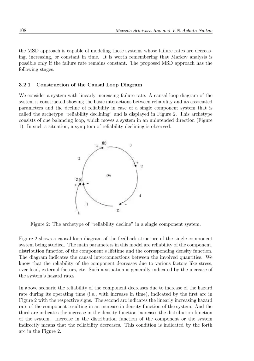
We consider a system with linearly increasing failure rate. A causal loop diagram of the
system is constructed showing the basic interactions between reliability and its associated
parameters and the decline of reliability in case of a single component system that is
called the archetype “reliability declining” and is displayed in Figure 2. This archetype
consists of one balancing loop, which moves a system in an unintended direction (Figure
1). In such a situation, a symptom of reliability declining is observed.

Figure 2: The archetype of “reliability decline” in a single component system.
Figure 2 shows a causal loop diagram of the feedback structure of the single component
system being studied. The main parameters in this model are reliability of the component,
distribution function of the component’s lifetime and the corresponding density function.
The diagram indicates the causal interconnections between the involved quantities. We
know that the reliability of the component decreases due to various factors like stress,
over load, external factors, etc. Such a situation is generally indicated by the increase of
the system’s hazard rates.
In above scenario the reliability of the component decreases due to increase of the hazard
rate during its operating time (i.e., with increase in time), indicated by the first arc in
Figure 2 with the respective signs. The second arc indicates the linearly increasing hazard
rate of the component resulting in an increase in density function of the system. And the
third arc indicates the increase in the density function increases the distribution function
of the system. Increase in the distribution function of the component or the system
indirectly means that the reliability decreases. This condition is indicated by the forth
arc in the Figure 2.

A Novel Markov System Dynamics Framework for Reliability Analysis of Systems

109

The loop displayed in Figure 2 is called a causal loop diagram with positive polarity. In
this way, Figure 2 depicts the archetype “reliability decline” in the context of reliability.
This is the typical behavior of a single component system during its operating time due
to various internal as well as external factors that affect the system directly and indirectly
resulting in a decrease of the reliability. This situation can be analyzed using a Markov
system dynamics (MSD) model.
3.2.2

Development of the Rate and Level Diagrams

The next step in the modeling process is to convert the casual loop diagram to the rate
and level diagram. The transfer rate diagram (Figure 1) of the single component system
is now converted into a comprehensive system dynamic model by utilizing the information
available in the casual loop diagram. This is presented in Figure 3.
For labelling purposes in the model the six echelons, i.e. reliability, distribution function,
mean time to failures, mean time between inspections, hazard rates, and density function of the single component system are abbreviated to R, C, MTTF, MTBI, Z, and f,
respectively.
In the model displayed in Figure 3, the two states of the single component system are
indicated with level variables R and C and the state transition is indicated with the rate
variable f. The initial value of the reliability (indicated by R in Figure 3) of the system
is assumed as unity.

Figure 3: A comprehensive system dynamics model.
The level of reliability decreases by the rate of failures that is measured in terms of the
density function (pdf) of the component or the system. The rate variable pdf of the
system is influenced by the auxiliary variable, the hazard rate (indicated by Z in Figure
3) of the system during the entire operating time (indicated with T in Figure 3).

110

Meesala Srinivasa Rao and V.N. Achuta Naikan

Additionally, the level of the distribution function (CDF) (indicated by C in Figure 3)
increases with the rate variable pdf of the system, leading to the declining reliability of
the system as described in Figure 2. The auxiliary variable hazard rate, main measurement variable of the model, is increased by the rate of failures and with the operating
times. Figure 3 displays the basic structure of the single component non repairable system
reliability model with the corresponding stock/flow diagram.

4

The Model Experimentation

The next stage of the proposed approach is to run the comprehensive MSD model of the
single component system for the reliability analysis and to study its dynamic behavior.
The above mentioned software is used to perform the required simulation runs. The
simulation of the proposed model confirms that the results of the archetype reliability
decline as shown in Figure 4, reliability of the single component system decreases with
the increase of the hazard rate. The simulation result in various values of the density
function and the distribution function for the failure times. From these results it is
possible to identify minimum and maximum values of the distribution function and the
reliability. The simulation analysis shows that the particular approaches to reliability
have a different impact on the behavior of the single component system. Based on the
simulation of this model, critical aspects can be identified. Considering that reliability is
one of the most decisive factors affecting the system’s performance, the simulation study
was based on the following scenarios.
• Scenario 1: Test simulation run.
The system was first simulated by a test simulation run, i.e., the system is run
assuming that it has maximum reliability, i.e., unity at the start of operation with
the operating state at level variable R. The reliability of the system decreases with
increasing operating time.
• Scenario 2: Second simulation run.
In a second simulation run, the system is run assuming a linearly increasing hazard
rate. The reliability approaches its minimum level with increase in time as shown
in Figure 4.
• Scenario 3: Third simulation run.
In a third run, the distribution function is added. In a system with an increase
in the distribution function, the reliability will approach its minimum level with
increasing hazard rate. In this model, the distribution function is represented by
the level variable C which indicates the failed state of the single component system
as shown in Figure 4.

A Novel Markov System Dynamics Framework for Reliability Analysis of Systems

111

Figure 4: The reliability decline.
• Scenario 4: Forth simulations run.
In this run, the mean time to failure is considered. This simulation run shows that
even though the mean time to failure is maximum at the initial stage due to the
changing condition of the system, it decreases after some time. This is shown in
Figure 5.

Figure 5: Decline of the mean time to failures.
• Scenario 5: Fifth simulation run.
In this run, the density function (f) is considered. The simulation run indicates that
the density function varies with increasing time. It is shown in Figure 6.

Figure 6: Varying density function.

112

Meesala Srinivasa Rao and V.N. Achuta Naikan

• Scenario 6: Sixth simulation run.
In this run, the hazard rate (Z) is considered. The simulation run indicates that
the hazard rate approaches its maximum level with increasing time as shown in
Figure 7.

Figure 7: Increasing hazard rate.

Finally, to analyze the reliability of the system, the model has been simulated till its
reliability reaches zero (31 weeks). Figure 8 depicts the dynamic behavior of the single
component system for the different scenarios. The simulated values of various parameters
are also listed in Table 1 for illustrating the dynamic behavior of the system in more
detail.

Figure 8: Dynamic behavior of the single component system.

A Novel Markov System Dynamics Framework for Reliability Analysis of Systems

113

Table 1: Simulated results describing the dynamic behavior of the single component
system.
Weeks Reliability CDF
0
1.00
0.00
1
1.00
0.00
2
0.99
0.01
3
0.97
0.03
4
0.95
0.05
5
0.91
0.09
6
0.87
0.13
7
0.82
0.18
8
0.77
0.23
9
0.71
0.29
10
0.65
0.35
11
0.59
0.41
12
0.52
0.48
13
0.46
0.54
14
0.40
0.60
15
0.34
0.66
16
0.29
0.71
17
0.24
0.76
18
0.20
0.80
19
0.16
0.84
20
0.13
0.87
21
0.10
0.90
22
0.08
0.92
23
0.06
0.94
24
0.05
0.95
25
0.04
0.96
26
0.03
0.97
27
0.02
0.98
28
0.01
0.99
29
0.01
0.99
30
0.01
0.99
31
0.00
1.00

5

Pdf MTTF
0.00 99.50
0.01 98.14
0.02 96.77
0.03 95.42
0.03 94.09
0.04 92.80
0.05 91.55
0.05 90.37
0.06 89.24
0.06 88.19
0.06 87.13
0.06 86.34
0.06 85.47
0.06 84.66
0.06 83.94
0.05 83.31
0.05 82.77
0.04 82.32
0.04 81.94
0.03 81.62
0.03 81.37
0.02 81.17
0.02 81.00
0.01 80.88
0.01 80.78
0.01 80.71
0.01 80.65
0.01 80.61
0.00 80.58
0.00 80.56
0.00 80.55
0.00 80.54

Hazard rate(Z)
0.00
0.01
0.02
0.03
0.04
0.05
0.06
0.07
0.08
0.09
0.10
0.11
0.12
0.13
0.14
0.15
0.16
0.18
0.19
0.20
0.21
0.22
0.23
0.24
0.25
0.26
0.27
0.28
0.30
0.31
0.32
0.33

Validation of the Proposed Model

To validate the proposed model the results of the simulation model are compared with
those obtained through the traditional approach. It is known that the case of linearly
increasing hazard rate (as considered in the proposed model) can be represented as follows:

114

Meesala Srinivasa Rao and V.N. Achuta Naikan

Z(t) = a · t

(24)

The reliability and the density function of the considered simple system are readily available by (24):
t2

R(t) = e−a 2

(25)

2
−a t2

f (t) = ate

(26)

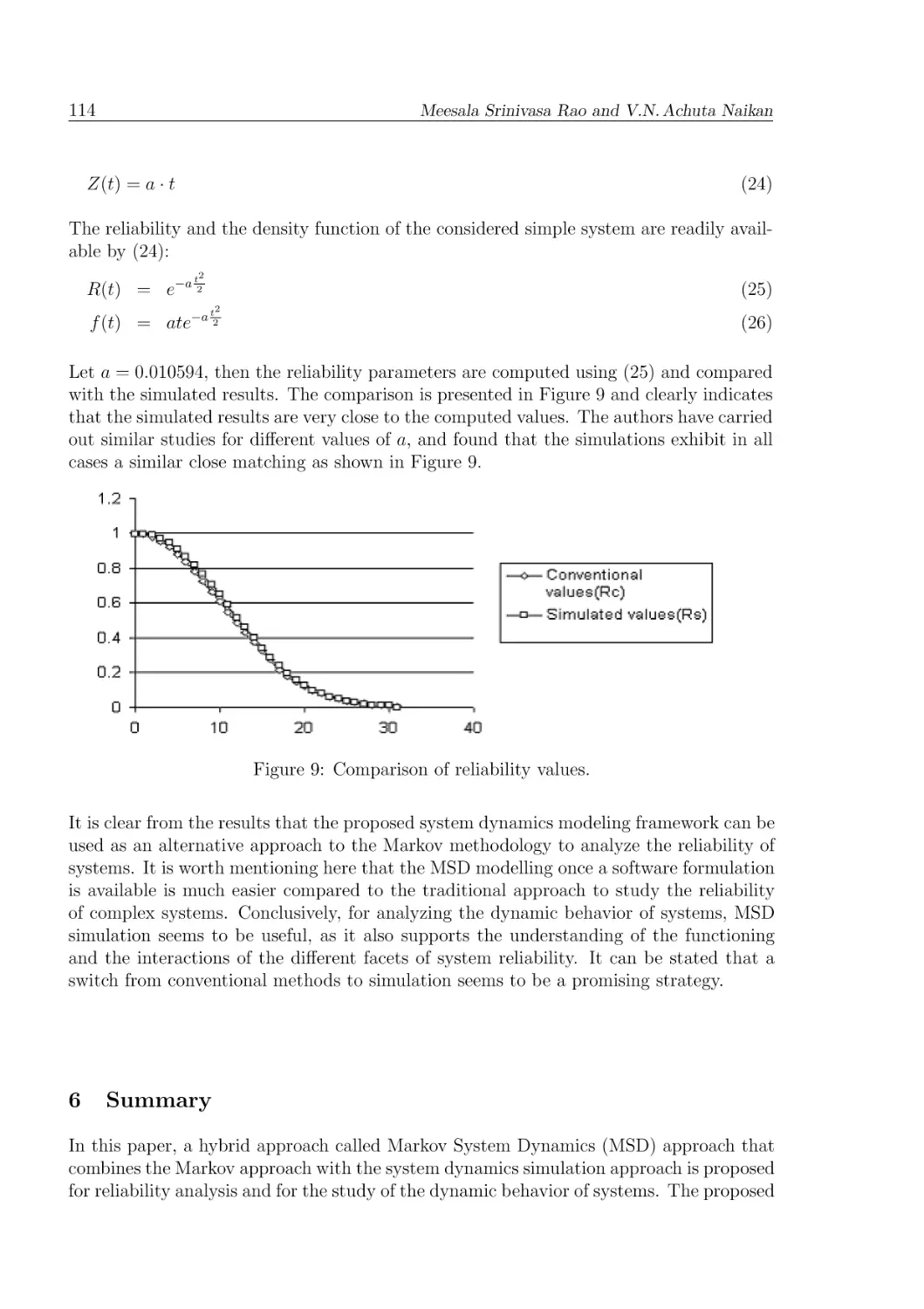
Let a = 0.010594, then the reliability parameters are computed using (25) and compared
with the simulated results. The comparison is presented in Figure 9 and clearly indicates
that the simulated results are very close to the computed values. The authors have carried
out similar studies for different values of a, and found that the simulations exhibit in all
cases a similar close matching as shown in Figure 9.

Figure 9: Comparison of reliability values.
It is clear from the results that the proposed system dynamics modeling framework can be
used as an alternative approach to the Markov methodology to analyze the reliability of
systems. It is worth mentioning here that the MSD modelling once a software formulation
is available is much easier compared to the traditional approach to study the reliability
of complex systems. Conclusively, for analyzing the dynamic behavior of systems, MSD
simulation seems to be useful, as it also supports the understanding of the functioning
and the interactions of the different facets of system reliability. It can be stated that a
switch from conventional methods to simulation seems to be a promising strategy.

6

Summary

In this paper, a hybrid approach called Markov System Dynamics (MSD) approach that
combines the Markov approach with the system dynamics simulation approach is proposed
for reliability analysis and for the study of the dynamic behavior of systems. The proposed

A Novel Markov System Dynamics Framework for Reliability Analysis of Systems

115

framework is illustrated by a single component system and the comparison of the simulated
results with those obtained by the conventional approach show a good match. This
indicates that the Markov System Dynamics (MSD) approach can be looked at as an
alternative approach for reliability analysis. The procedure for the development of the
MSD approach for this system is explained and the simulation model is run to observe all
of its states. The proposed methodology is applicable for all types of failure rates and it
is mathematically much simpler compared to traditional approaches.
Further, this methodology can be used for studying various scenarios having managerial
implications of system reliability. It is important to note that the reliability decline of a
component or a system has to be observed carefully in order to achieve a desired results.
Managers must be aware of the existing interdependencies within the components or
system. Accordingly, the model can be used as a simulation tool. Based on simulation
analyses, managers can learn how to deal with such a comprehensive approach. Moreover,
the different involved parties, i.e., managers, engineers, machine operators, can jointly
work with the model in order to understand the dynamic behavior of systems.

References
[1] Bobbio, A. et al. (1980): Multi state homogeneous markov models in reliability
analysis. Micro electronics Reliability 20, 875-880.
[2] Bollen, M.H.J. (1999): Understanding Power Quality Problems Voltage Sags and
Interruptions. IEEE Press: New York.
[3] Collas, G., et al (1994): Reliability & Availability estimation for complex systems:
a simple concept and tool. Proceedings Annual Reliability and Maintainability Symposium.
[4] Cumani, A. (1982): On the canonical representation of homogeneous markov processes modeling failure time distributions. Micro electronics Reliability 22, 583-602.
[5] Endrenyi (1978): Reliability Modeling in Electric Power Systems. Wiley, New York.
[6] Forrester, J.W. (1961): Industrial Dynamics. MIT Press: Cambridge, MA.
[7] Howell, S.V., Bavuso, S.J., Haley. P.J. (1990): A graphical language for reliability
model generation. Proceedings Annual Reliability and Maintainability Symposium,
IEEE.
[8] Johnson L. (1986): Ensign Eigenvalue eigenvector solutions for two general markov
models in reliability. Micro electronics Reliability 26, 917-933.
[9] Logothetis, D., et al (1995): Markov Regenerative Models. IEEE, 134-142.

116

Meesala Srinivasa Rao and V.N. Achuta Naikan

[10] Mohapatra, P.K.J., Roy, R.K. (1991): System Dynamics Models for Markov Processes. Proceedings of the 9th International Conference of the System Dynamics
Society, Bangkok, Thailand.
[11] Pavlovic, Z., Rakic, P. (1989): An approach to fault tolerant system reliability
modeling. Micro electronics Reliability 29, 343-348.
[12] Richardson, G.P. (1999): Reflections of the of system dynamics. J. Oper. Res. Soc.
50, 440-449.
[13] Rustam, I.T. (1994): Using Markov reliability modeling for multiple repairable
systems. Reliability Engineering and System Safety 44, 113-118.
[14] Towill, D.R. (1993): System dynamics – background, methodology, and applications. IEE Computing & Control Engineering Journal 4, Part 1: 201-208, Part II:
261-268.
[15] Usano, R., Torres, J.M.F., Marquez, A.C. and Castro, R.Z.D. (1996): System dynamics and discrete simulation in a constant work in process system: a comparative
study. Paper presented at International System Dynamics Conference. Cambridge,
MA.
[16] Wolstenholme E.F. (1982): Modeling discrete events in system dynamics models.
Dynamica 6, Part 1.

Meesala Srinivasa Rao (msrsrinivasa@gmail.com)
Dr.V.N.Achuta Naikan (naikan@hijli.iitkgp.ernet.in)
Reliability Engineering Centre
Indian Institute of Technology Kharagpur
721302 West Bengal
India