ML2R Coding Nuggets
Linear Programming for Robust Regression
Pascal Welke∗

Christian Bauckhage†

Machine Learning Rhine-Ruhr
University of Bonn
Bonn, Germany

Machine Learning Rhine-Ruhr
Fraunhofer IAIS
St. Augustin, Germany

ABSTRACT

y

Having previously discussed how SciPy allows us to solve linear
programs, we can study further applications of linear programming.
Here, we consider least absolute deviation regression and solve a
simple parameter estimation problem deliberately chosen to expose
potential pitfalls in using SciPy’s optimization functions.

1

INTRODUCTION

In this note, we revisit linear programming [13] and consider it
as a tool for robust regression analysis. An example of a uni-variate
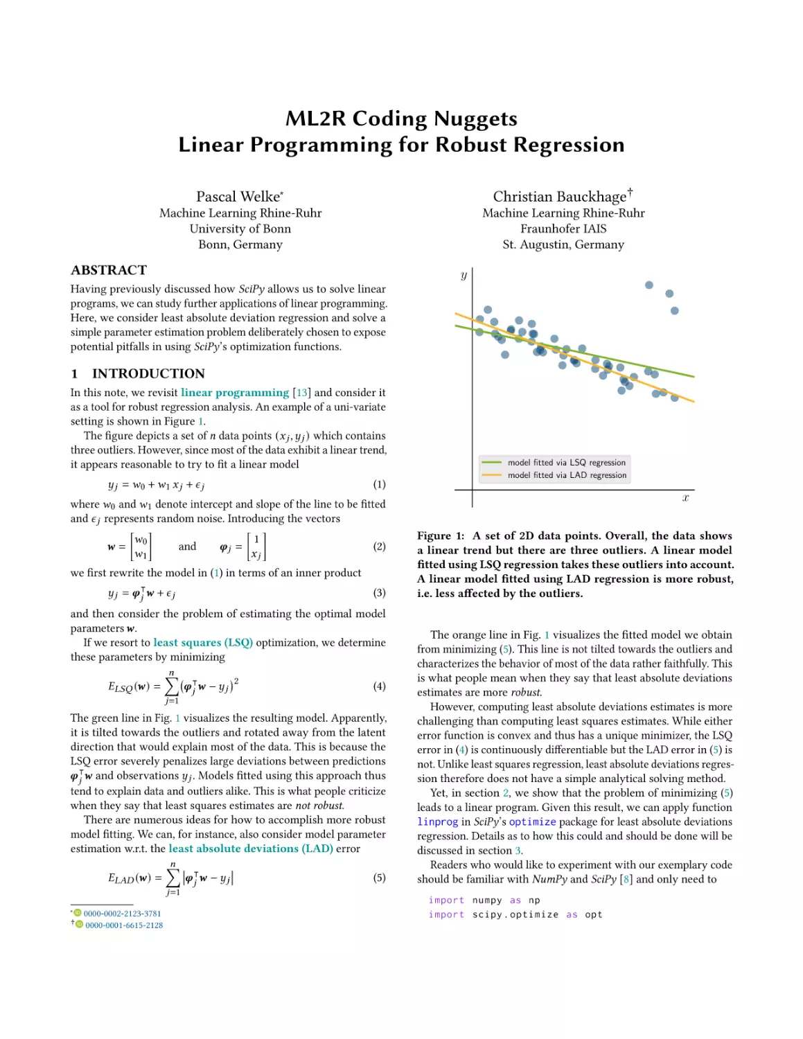
setting is shown in Figure 1.
The figure depicts a set of 𝑛 data points (𝑥 𝑗 , 𝑦 𝑗 ) which contains
three outliers. However, since most of the data exhibit a linear trend,
it appears reasonable to try to fit a linear model
𝑦 𝑗 = 𝑤0 + 𝑤1 𝑥 𝑗 + 𝜖 𝑗

(1)

where 𝑤 0 and 𝑤 1 denote intercept and slope of the line to be fitted
and 𝜖 𝑗 represents random noise. Introducing the vectors
 
 
𝑤
1
𝒘= 0
and
𝝋𝑗 =
(2)
𝑤1
𝑥𝑗
we first rewrite the model in (1) in terms of an inner product
⊺

𝑦𝑗 = 𝝋𝑗 𝒘 + 𝜖𝑗
(3)
and then consider the problem of estimating the optimal model
parameters 𝒘.
If we resort to least squares (LSQ) optimization, we determine
these parameters by minimizing
𝑛
∑︁

2
⊺
𝐸𝐿𝑆𝑄 (𝒘) =
𝝋𝑗 𝒘 − 𝑦𝑗
(4)
𝑗=1

The green line in Fig. 1 visualizes the resulting model. Apparently,
it is tilted towards the outliers and rotated away from the latent
direction that would explain most of the data. This is because the
LSQ error severely penalizes large deviations between predictions
⊺
𝝋 𝑗 𝒘 and observations 𝑦 𝑗 . Models fitted using this approach thus
tend to explain data and outliers alike. This is what people criticize
when they say that least squares estimates are not robust.
There are numerous ideas for how to accomplish more robust
model fitting. We can, for instance, also consider model parameter
estimation w.r.t. the least absolute deviations (LAD) error
𝑛
∑︁
⊺
𝐸𝐿𝐴𝐷 (𝒘) =
𝝋𝑗 𝒘 − 𝑦𝑗
(5)
𝑗=1
∗
†

0000-0002-2123-3781
0000-0001-6615-2128

model fitted via LSQ regression
model fitted via LAD regression

x
Figure 1: A set of 2D data points. Overall, the data shows
a linear trend but there are three outliers. A linear model
fitted using LSQ regression takes these outliers into account.
A linear model fitted using LAD regression is more robust,
i.e. less affected by the outliers.

The orange line in Fig. 1 visualizes the fitted model we obtain
from minimizing (5). This line is not tilted towards the outliers and
characterizes the behavior of most of the data rather faithfully. This
is what people mean when they say that least absolute deviations
estimates are more robust.
However, computing least absolute deviations estimates is more
challenging than computing least squares estimates. While either
error function is convex and thus has a unique minimizer, the LSQ
error in (4) is continuously differentiable but the LAD error in (5) is
not. Unlike least squares regression, least absolute deviations regression therefore does not have a simple analytical solving method.
Yet, in section 2, we show that the problem of minimizing (5)
leads to a linear program. Given this result, we can apply function
linprog in SciPy’s optimize package for least absolute deviations
regression. Details as to how this could and should be done will be
discussed in section 3.
Readers who would like to experiment with our exemplary code
should be familiar with NumPy and SciPy [8] and only need to
import numpy as np
import scipy . optimize as opt

P. Welke and C. Bauckhage

2

THEORY

and 𝑛 inequalities of the form

Generalizing our introductory example, we henceforth assume that
the vectors 𝒘 and 𝝋 𝑗 in (2) are vectors in R𝑚 where 𝑚 ≥ 2. We do
this to emphasize that our following considerations do not only
apply to uni-variate linear regression as in our example (where
𝑚 = 2 ) but also to the multi-variate case (where 𝑚 > 2).
Whenever we decide to perform robust linear regression based
on the LAD criterion, our goal is to find the optimal parameters 𝒘 ∗
of a linear model such that
𝒘 ∗ = argmin
𝒘

𝑛
∑︁

⊺

𝝋𝑗 𝒘 − 𝑦𝑗

(6)

𝑗=1

In order to see that this optimization problem can be cast as a
linear programming problem
𝒛 ∗ = argmin 𝒄 ⊺ 𝒛
𝒛

s.t.

(7)

𝑨𝒛 ⪯ 𝒃
𝑪𝒛 =𝒅

we first of all introduce a set of 𝑛 new variables 𝑟 𝑗 ∈ R. For these
auxiliary variables, we require
⊺

𝝋𝑗 𝒘 − 𝑦𝑗 ≤ 𝑟 𝑗

(8)

which then allows us to express the problem in (6) as
𝒘 ∗ = argmin
𝒘

s.t.

𝑛
∑︁

𝑟𝑗

𝑗=1
⊺
𝝋𝑗 𝒘

(9)
− 𝑦𝑗 ≤ 𝑟 𝑗

𝑗 = 1, . . . , 𝑛

This, in turn, can be written slightly more succinctly, namely as
𝒘 ∗ = argmin 1⊺ 𝒓
𝒘

s.t.

⊺

𝝋𝑗 𝒘 − 𝑦𝑗 ≤ 𝑟 𝑗

(10)
𝑗 = 1, . . . , 𝑛

where 1 ∈ R𝑛 denotes the vector of all ones and the vector 𝒓 ∈ R𝑛
is given by
𝑟 1 
 
𝑟 2 
 
𝒓=.
 .. 
 
𝑟 
 𝑛

(11)

While (10) is beginning to resemble the general form of a linear
programming problem in (7), it involves inequality constraints that
are not of the canonical form.
⊺
We therefore observe that each inequality 𝝋 𝑗 𝒘 − 𝑦 𝑗 ≤ 𝑟 𝑗 can
just as well be written in terms of two inequalities, namely
⊺

−𝑟 𝑗 ≤ 𝝋 𝑗 𝒘 − 𝑦 𝑗 ≤ 𝑟 𝑗

(12)

But this is to say that the 𝑛 inequality constraints in (10) can also
be expressed in terms of 2 · 𝑛 inequalities. Namely, 𝑛 inequalities of
the form
⊺

⇔

𝝋𝑗 𝒘 − 𝑦𝑗 ≤ 𝑟 𝑗

(13)

⊺
𝝋𝑗 𝒘

(14)

− 𝑟 𝑗 ≤ 𝑦𝑗

⊺

⇔

−𝑟𝑖 ≤ 𝝋 𝑗 𝒘 − 𝑦 𝑗
⊺
−𝝋 𝑗 𝒘 − 𝑟 𝑗 ≤ −𝑦 𝑗

(15)
(16)

Next, we write these inequalities more compactly. To this end,
we introduce a matrix 𝚽 ∈ R𝑚×𝑛 and a vector 𝒚 ∈ R𝑛 where
 |
|
| 

𝚽 = 𝝋 1 𝝋 2 · · · 𝝋𝑛 
(17)
 |

|
|


𝑦1 
 
𝑦2 
 
𝒚=.
(18)
 .. 
 
𝑦 
 𝑛
Letting 𝑰 denote the 𝑛 × 𝑛 identity matrix, we can then write our
two sets of inequalities in terms of only two vector inequalities
+𝚽⊺𝒘 − 𝑰 𝒓 ⪯ +𝒚

(19)

−𝚽⊺𝒘 − 𝑰 𝒓 ⪯ −𝒚

(20)

where we deliberately emphasized the sign patterns.
If we then introduce a vector 𝒛 ∈ R𝑚+𝑛 which contains our
model parameters 𝒘 and the auxiliary variables 𝒓 as follows
 
𝒘
𝒛=
(21)
𝒓
we can further rewrite our inequalities such that their left hand
sides only involve a single matrix and a single vector. In particular,
by using matrices [+𝚽⊺ − 𝑰 ] and [−𝚽⊺ − 𝑰 ] of size 𝑛 × (𝑚 + 𝑛),
we can write (19) and (20) as
 
 ⊺
 𝒘
+𝚽
−𝑰
⪯ +𝒚
(22)
𝒓
 
 ⊺
 𝒘
−𝚽
−𝑰
⪯ −𝒚
(23)
𝒓
Next, we go even further and combine both inequalities into
a single inequality. To this end, we introduce yet another matrix
𝑨 ∈ R2𝑛×(𝑚+𝑛) and yet another vector 𝒃 ∈ R2𝑛 which are given by
 ⊺

+𝚽
−𝑰
𝑨=
(24)
−𝚽⊺ −𝑰
 
+𝒚
𝒃=
(25)
−𝒚
These allow us to write (22) and (23) in terms of just a single matrixvector expression, namely
𝑨𝒛 ⪯ 𝒃

(26)

If we finally introduce the following vector 𝒄 ∈
 
0
𝒄=
1

R𝑚+𝑛
(27)

where 0 ∈ R𝑚 is a vector of all zeros and 1 ∈ R𝑛 is the vector of all
ones we already encountered in (10), we realize that we can write
the parameter estimation problem in (10) as follows
𝒛 ∗ = argmin 𝒄 ⊺ 𝒛
𝒛

s.t.

(28)
𝑨𝒛 ⪯ 𝒃

Linear Programming for Robust Regression
This, however, is now easily recognizable as a special case of the
general linear program in (7), namely as a linear program without
equality constraints. Hence, when solving (28) for
 ∗
𝒘
𝒛∗ = ∗
(29)
𝒓

Listing 1: data (𝑥 𝑗 , 𝑦 𝑗 ) used in Fig. 1
data = [[ 4.13617728 ,
[ 8.73491217 ,
[ 2.93003532 ,
[ 2.72854006 ,
[11.54130191 ,
[10.74702164 ,
[ 8.85495879 ,
[ 7.19564619 ,
[ 4.89259177 ,
[ 8.935679 ,
[ 1.28632285 ,
[ 6.4336993 ,
[ 2.2698845 ,
[ 1.51889303 ,
[10.2945996 ,
[ 2.25463225 ,
[ 1.72099191 ,
[10.35250838 ,
[ 9.1996738 ,
[ 9.4554096 ,
[ 3.78639002 ,
[ 3.97164201 ,
[ 4.02737008 ,
[ 1.92092101 ,
[ 5.97314732 ,
[ 0.45048191 ,
[11.84585512 ,
[ 0.91329339 ,
[ 7.99636755 ,
[ 2.73621934 ,
[ 7.88147877 ,
[11.84419908 ,
[ 7.65570306 ,
[ 8.66490933 ,
[ 5.95716291 ,
[ 3.61850327 ,
[ 3.53521089 ,
[ 0.42129088 ,
[ 7.21057937 ,
[ 6.10604803 ,
[ 4.80862845 ,
[10.67573743 ,
[ 5.50938443 ,
[ 1.33516772 ,
[ 3.47074062 ,
[ 7.92451916 ,
[ 5.27691966 ,
[11.18641517 ,
[ 3.48442286 ,
[ 5.33950137 ,

we obtain he sought after optimal model parameters 𝒘 ∗ as the first
𝑚 components of 𝒛 ∗ .

3

PRACTICAL COMPUTATION

Next, we look at how to solve a least absolute deviation regression
problem using SciPy. Without loss of generality, we consider the
uni-variate setting in our introductory example where we are given
given data points (𝑥 𝑗 , 𝑦 𝑗 ) and want to regress the 𝑥 𝑗 onto the 𝑦 𝑗 .
Hence, we first of all assume the given 𝑥 𝑗 and 𝑦 𝑗 have been
gathered in two vectors 𝒙, 𝒚 ∈ R𝑛 which we represent in in terms
of one-dimensional NumPy arrays
vecX = np . array ([ ... ])
vecY = np . array ([ ... ])

(For those who would like to work with a specific example, we
provide the data from Fig. 1 in Listing 1.)
Given vector 𝒙, we can compute the matrix 𝚽 in (17) as shown
in Listing 2.

3.1

The LSQ Solution

As a quick sanity check, we may compute and print the solution to
the least squares problem in (4). Recalling our discussion in [1], we
may use
vecWLSQ = np . linalg . lstsq ( matF .T , vecY )[0]
print ( 'w0 = ', vecWLSQ [0])
print ( 'w1 = ', vecWLSQ [1])

which yields

vecX = data [: ,0]
vecY = data [: ,1]

w0 = 9.412312601314262
w1 = -0.2143803602914957

These are indeed the parameters of the green line plotted in Fig. 1
and we note that the LSQ method convincingly reveals that a line
which models our data reasonably well should have a negative
slope parameter 𝑤 1 .

3.2

8.0605513 ]
5.82386425]
9.25802999]
8.86152583]
11.5
]
5.6387994 ]
6.48474208]
7.09560981]
8.22178878]
6.32814357]
9.84268842]
8.28708713]
9.40753056]
8.97582469]
6.95084626]
9.31717318]
8.78682311]
12.
]
6.09591636]
6.61972217]
8.08030845]
8.20302354]
8.40897327]
7.9211727 ]
7.61088767]
9.99611448]
10.5
]
10.55841044]
7.24451303]
9.93068399]
7.39222799]
5.40747863]
6.69719204]
7.17469259]
7.58802588]
9.13252335]
9.15345905]
9.24856203]
7.61186026]
7.42363516]
8.85805627]
6.77145283]
8.24870815]
9.15036081]
8.68993837]
7.03932189]
7.30516638]
5.72091709]
9.72853925]
7.87556676]]

Listing 2: computing matrix 𝚽 in (17)
matF = np . vstack (( np . ones_like ( vecX ), vecX ))
m , n = matF . shape

The LAD Solution

Next, we set up the ingredients of the linear program in (28) which
allows us to solve the LAD problem in (5). To this end, we proceed
as summarized in Listing 3.
Given vecY and matF, we can compute two arrays matA and vecB
which represent matrix 𝑨 in (24) and vector 𝒃 in (25), respectively.
This is done in lines 1–9. Admittedly, the manner in which we set up
these arrays is a bit clumsy and we could have chosen more compact
ways (e.g. using stacking operators). However, our implementation
emphasizes the sizes of the required arrays and therefore hints at
potential problems with the overall approach.
Finally, in line 11, we compute an array vecC which represents
vector 𝒄 in (27).
At this point, we are good to go and can finally invoke function
linprog in SciPy’s optimize module.

Listing 3: setting up the linear programming problem in (28)
1
2
3
4
5
6
7
8
9
10
11

matA = np . zeros ((2* n , m+n ))
matA [:n ,: m] = + matF .T
matA [n : ,: m] = - matF .T
matA [:n ,m :] = -np . eye (n)
matA [n:,m :] = -np . eye (n)
vecB = np . zeros (2* n)
vecB [: n] = + vecY
vecB [n :] = - vecY
vecC = np . hstack (( np . zeros (m), np . ones (n )))

NOTE: To begin with, we proceed exactly as we did in [13]. Yet, as
we shall see, this will lead to an unreasonable solution to our current
problem. Our goal here is to point out potential pitfalls when working

P. Welke and C. Bauckhage
with linprog. A better, generally more considerate way of invoking
the method will be discussed immediately afterwards.
Given arrays vecC, matA, and vecB, it seems reasonable to call
result = opt . linprog ( vecC , A_ub = matA , b_ub = vecB )

This causes result to be an instance of OptimizeResult which
is a SciPy class that summarizes optimization outcomes. To have a
look at our result, we may therefore
print ( result )

In other words, the default behavior of linprog is to assume
that all the elements of the solution 𝒛 ∗ of a linear program are nonnegative. Whether or not this implemented default behavior is
reasonable is debatable. In our case, it clearly constitutes a trap
for novice users and emphasizes the need for carefully reading
available documentations.
A more considerate use of linprog for our current setting therefore
is to set the parameter bounds. In particular, we could (and should)
proceeds as follows:
result = opt . linprog ( vecC , A_ub = matA , b_ub = vecB ,
bounds =( None , None ))

which yields
con :
fun :
message :
nit :
slack :

array ([] , dtype = float64 )
60.303210125647425
' Optimization terminated successfully . '
9
array ([ 1.06312648 e -09 , -3.47641027 e -10 ,
... ])
status : 0
success : True
x : array ([ 8.12040958 e +00 , 3.74189410 e -11 ,
...])

Note that the arrays in fields slack and x are actually larger
than shown here. We just focus on the 𝑚 = 2 first elements of both
arrays, because x contains the solution 𝒛 ∗ to our problem and the
𝑚 = 2 first elements of 𝒛 ∗ represent the optimal parameters 𝒘 ∗ of
our linear model.
Also note that field success indicates that the optimization
process was successful. (Recall our discussion in [13] where we
emphasized that it is prudent to check for success before using
linprog results in downstream processing.) Hence, if we extract
and inspect our sought after solution using
vecWLAD = result . x [: m ]
print ( 'w0 = ', vecWLAD [0])
print ( 'w1 = ', vecWLAD [1])

we obtain
w0 = 8.120409582750103
w1 = 3.741894096367617 e -11

But how can this be? This solution states that 𝑤 1 ≈ 3.7·10−11 ≈ 0
which does not make sense for our running example.
What went wrong? Doesn’t linear programming work for LAD
optimization after all? Or did we make a mistake in setting up the
linear program? No! It does work and we didn’t make a mistake.
What happened is that we used linprog too naïvely. In addition
to the parameters we discussed in [13], the method has another
crucial parameter bounds which the reference guide describes as
follows
bounds : sequence, optional
A sequence of (min, max) pairs for each element in x,
defining the minimum and maximum values of that
decision variable. Use None to indicate that there is no
bound. By default, bounds are (0, None) (all decision
variables are non-negative). If a single tuple (min,
max) is provided, then min and max will serve as
bounds for all decision variables.

When printed for inspection this yields
con :
fun :
message :
nit :
slack :

array ([] , dtype = float64 )
35.82758700339906
' Optimization terminated successfully . '
7
array ([ 3.27802816 e -08 , 2.50269636 e -08 ,
... ])
status : 0
success : True
x : array ([ 9.97623076 e +00 , -3.70610358 e -01 ,
...])

and thus looks much more reasonable than our previous result.
Indeed, using
vecWLAD = result . x [: m ]
print ( ' w0 = ', vecWLAD [0])
print ( ' w1 = ', vecWLAD [1])

we now find
w0 = 9.976230757187192
w1 = -0.37061035803160336

which are the parameters of the orange line plotted in Fig. 1.

4

SUMMARY AND OUTLOOK

In this short note, we considered a practical application of linear
programming and used it as a tool for robust regression based on
minimizing least absolute deviations. We discussed how to set up a
corresponding linear program which we then solved using function
linprog in SciPy’s optimize module.
Crucially, we emphasized a potential pitfall in using linprog,
namely its (questionable) default behavior of assuming that the
solution to a given problem should be non-negative. As this clearly
does not hold in general, we overrode this default behavior by manually setting the parameter bounds and thus obtained a reasonable
solution to our exemplary problem.
Robust regression is of considerable practical importance and
is frequently applied in data mining, machine learning, computer
vision, and signal processing (see, for example [2–7, 9–12]). Specific
use cases will be discussed in later notes. For now, we conclude
with a remark that must not be missing in any text on least absolute
deviations regression: The idea can be traced back to work by
Boscovich (1757) and Laplace (1793) which means that it predates
the more commonly known method of least squares regression
used by Gauss in 1801 and published by Legendre in 1805.

Linear Programming for Robust Regression

ACKNOWLEDGMENTS
This material was produced within the Competence Center for
Machine Learning Rhine-Ruhr (ML2R) which is funded by the
Federal Ministry of Education and Research of Germany (grant no.
01|S18038C). The authors gratefully acknowledge this support.

REFERENCES
[1] C. Bauckhage. 2015. NumPy / SciPy Recipes for Data Science: Ordinary Least
Squares Optimization. researchgate.net. https://dx.doi.org/10.13140/2.1.3370.
3209/1.
[2] P. Bloomfield and W.L. Steiger. 1983. Least Absolute Deviations: Theory, Applications, and Algorithms. Birkhäuser.
[3] G.D. Evangelidis and C. Bauckhage. 2013. Efficient Subframe Video Alignment
Using Short Descriptors. IEEE Trans. Pattern Analysis and Machine Intelligence
35, 10 (2013).
[4] A. Sovic Krzic and D. Sersic. 2018. L1 Minimization Using Recursive Reduction
of Dimensionality. Signal Processing 151, Oct. (2018).

[5] K.D. Lawrence and J.L. Arthur (Eds.). 1990. Robust Regression: Analysis and
Applications. Marcel Dekker.
[6] Y. Li and G.R. Arce. 2004. A Maximum Likelihood Approach to Least Absolute
Deviation Regression. EURASIP J. on Advances in Signal Processing 2004, 948982
(2004).
[7] P. Meer, D. Mintz, A. Rosenfeld, and D.Y. Kim. 1991. Robust Regression Methods
for Computer Vision: A Review. Int. J. of Computer Vision 6, 1 (1991).
[8] T.E. Oliphant. 2007. Python for Scientific Computing. Computing in Science &
Engineering 9, 3 (2007).
[9] P.J. Rousseeuw and A.M. Leroy. 1987. Robust Regression and Outlier Detection.
John Wiley & Sons.
[10] K. Sabo and R. Scitovski. 2008. The Best Least Absolute Deviations Line - Properties and Two Efficient Methods for Its Derivation. The ANZIAM Journal 50, 2
(2008).
[11] J. Wang, P. Wonka, and J. Ye. 2014. Scaling SVM and Least Absolute Deviations
via Exact Data Reduction. In Proc. ICML.
[12] L. Wang, M.D. Gordon, and J. Zhu. 2006. Regularized Least Absolute Deviations
Regression and an Efficient Algorithm for Parameter Tuning. In Proc. ICDM.
[13] P. Welke and C. Bauckhage. 2020. ML2R Coding Nuggets: Solving Linear Programming Problems. Technical Report. MLAI, University of Bonn.