/


Author: Donoso Y.
Tags: programming languages programming networks wireless networks wireless mesh networks
Year: 2009

Text
Network Design
for IP Convergence
OTHER TELECOMMUNICATIONS BOOKS FROM AUERBACH
Active and Programmable Networks
for Adaptive Architectures and Services
Syed Asad Hussain
ISBN: 0-8493-8214-9
Ad Hoc Mobile Wireless Networks:
Principles, Protocols and Applications
Subir Kumar Sarkar, T.G. Basavaraju,
and C. Puttamadappa
ISBN: 1-4200-6221-2
Introduction to Mobile Communications:
Technology, Services, Markets
Tony Wakefield, Dave McNally, David Bowler,
and Alan Mayne
ISBN: 1-4200-4653-5
Millimeter Wave Technology in Wireless
PAN, LAN, and MAN
Shao-Qiu Xiao, Ming-Tuo Zhou, and Yan Zhang
ISBN: 0-8493-8227-0
Comprehensive Glossary of Telecom
Abbreviations and Acronyms
Ali Akbar Arabi
ISBN: 1-4200-5866-5
Mobile WiMAX: Toward Broadband
Wireless Metropolitan Area Networks
Yan Zhang and Hsiao-Hwa Chen
ISBN: 0-8493-2624-9
Contemporary Coding Techniques and
Applications for Mobile Communications
Onur Osman and Osman Nuri Ucan
ISBN: 1-4200-5461-9
Optical Wireless Communications:
IR for Wireless Connectivity
Roberto Ramirez-Iniguez, Sevia M. Idrus,
and Ziran Sun
ISBN: 0-8493-7209-7
Context-Aware Pervasive Systems:
Architectures for a New Breed of
Applications
Seng Loke
ISBN: 0-8493-7255-0
Performance Optimization of Digital
Communications Systems
Vladimir Mitlin
ISBN: 0-8493-6896-0
Data-driven Block Ciphers for Fast
Telecommunication Systems
Nikolai Moldovyan and Alexander A. Moldovyan
ISBN: 1-4200-5411-2
Physical Principles of Wireless
Communications
Victor L. Granatstein
ISBN: 0-8493-3259-1
Distributed Antenna Systems:
Open Architecture for Future Wireless
Communications
Honglin Hu, Yan Zhang, and Jijun Luo
ISBN: 1-4200-4288-2
Principles of Mobile Computing
and Communications
Mazliza Othman
ISBN: 1-4200-6158-5
Encyclopedia of Wireless and Mobile
Communications
Borko Furht
ISBN: 1-4200-4326-9
Resource, Mobility, and Security
Management in Wireless Networks
and Mobile Communications
Yan Zhang, Honglin Hu, and Masayuki Fujise
ISBN: 0-8493-8036-7
Handbook of Mobile Broadcasting:
DVB-H, DMB, ISDB-T, AND MEDIAFLO
Borko Furht and Syed A. Ahson
ISBN: 1-4200-5386-8
Security in Wireless Mesh Networks
Yan Zhang, Jun Zheng, and Honglin Hu
ISBN: 0-8493-8250-5
The Handbook of Mobile Middleware
Paolo Bellavista and Antonio Corradi
ISBN: 0-8493-3833-6
Wireless Ad Hoc Networking:
Personal-Area, Local-Area,
and the Sensory-Area Networks
Shih-Lin Wu and Yu-Chee Tseng
ISBN: 0-8493-9254-3
The Internet of Things: From RFID
to the Next-Generation Pervasive
Networked Systems
Lu Yan, Yan Zhang, Laurence T. Yang,
and Huansheng Ning
ISBN: 1-4200-5281-0
Wireless Mesh Networking:
Architectures, Protocols
and Standards
Yan Zhang, Jijun Luo, and Honglin Hu
ISBN: 0-8493-7399-9
AUERBACH PUBLICATIONS
www.auerbach-publications.com
To Order Call: 1-800-272-7737 • Fax: 1-800-374-3401
E-mail: orders@crcpress.com
Network Design
for IP Convergence
Yezid Donoso
Auerbach Publications
Taylor & Francis Group
6000 Broken Sound Parkway NW, Suite 300
Boca Raton, FL 33487‑2742
© 2009 by Taylor & Francis Group, LLC
Auerbach is an imprint of Taylor & Francis Group, an Informa business
No claim to original U.S. Government works
Printed in the United States of America on acid‑free paper
10 9 8 7 6 5 4 3 2 1
International Standard Book Number‑13: 978‑1‑4200‑6750‑7 (Hardcover)
This book contains information obtained from authentic and highly regarded sources. Reasonable
efforts have been made to publish reliable data and information, but the author and publisher can‑
not assume responsibility for the validity of all materials or the consequences of their use. The
authors and publishers have attempted to trace the copyright holders of all material reproduced
in this publication and apologize to copyright holders if permission to publish in this form has not
been obtained. If any copyright material has not been acknowledged please write and let us know so
we may rectify in any future reprint.
Except as permitted under U.S. Copyright Law, no part of this book may be reprinted, reproduced,
transmitted, or utilized in any form by any electronic, mechanical, or other means, now known or
hereafter invented, including photocopying, microfilming, and recording, or in any information
storage or retrieval system, without written permission from the publishers.
For permission to photocopy or use material electronically from this work, please access www.copy‑
right.com (http://www.copyright.com/) or contact the Copyright Clearance Center, Inc. (CCC), 222
Rosewood Drive, Danvers, MA 01923, 978‑750‑8400. CCC is a not‑for‑profit organization that pro‑
vides licenses and registration for a variety of users. For organizations that have been granted a
photocopy license by the CCC, a separate system of payment has been arranged.
Trademark Notice: Product or corporate names may be trademarks or registered trademarks, and
are used only for identification and explanation without intent to infringe.
Library of Congress Cataloging‑in‑Publication Data
Donoso, Yezid.
Network design for IP convergence / Yezid Donoso.
p. cm.
Includes bibliographical references and index.
ISBN 978‑1‑4200‑6750‑7 (alk. paper)
1. Computer network architectures. 2. Convergence (Telecommunication) 3.
TCP/IP (Computer network protocol) I. Donoso, Yezid. II. Title.
TK5105.52.D66 2009
004.6’5‑‑dc22
Visit the Taylor & Francis Web site at
http://www.taylorandfrancis.com
and the Auerbach Web site at
http://www.auerbach‑publications.com
2008043273
To my wife, Adriana—
for her love and for our future together.
To my children, Andres Felipe, Daniella, and Marianna—
a gift of God to my life.
Contents
Preface.............................................................................................................xi
About the Author......................................................................................... xiii
List of Translations........................................................................................ xv
1
Computer Network Concepts..................................................................1
1.1 Digital versus Analog Transmission....................................................1
1.2 Computer Networks According to Size..............................................7
1.2.1 Personal Area Networks (PANs)............................................7
1.2.2 Local Area Networks (LANs)................................................7
1.2.3 Metropolitan Area Networks (MANs)...................................8
1.2.4 Wide Area Networks (WANs).............................................10
1.3 Network Architectures and Technologies.........................................11
1.3.1 OSI......................................................................................11
1.3.2 PAN....................................................................................13
1.3.2.1 Bluetooth.............................................................13
1.3.3 LAN....................................................................................15
1.3.3.1 Ethernet...............................................................15
1.3.3.2 WiFi....................................................................15
1.3.4 MAN/WAN........................................................................16
1.3.4.1 TDM (T1, T3, E1, E3, SONET, SDH)...............16
1.3.4.2 xDSL...................................................................18
1.3.4.3 WDM (DWDM)................................................19
1.3.4.4 PPP/HDLC.........................................................20
1.3.4.5 Frame Relay.........................................................20
1.3.4.6 ATM...................................................................21
1.3.4.7 WiMAX..............................................................22
1.3.4.8 GMPLS...............................................................23
1.3.5 TCP/IP................................................................................24
1.4 Network Functions...........................................................................25
1.4.1 Encapsulation......................................................................25
vii
viii
1.5
Contents
1.4.2 Switching.............................................................................26
1.4.3 Routing...............................................................................35
1.4.4 Multiplexing........................................................................41
Network Equipments.......................................................................43
1.5.1 Hub.....................................................................................43
1.5.2 Access Point.........................................................................45
1.5.3 Switch..................................................................................47
1.5.4 Bridge..................................................................................61
1.5.5 Router.................................................................................63
1.5.6 Multiplexer......................................................................... 64
2
LAN Network Design............................................................................67
2.1 Ethernet Solution.............................................................................67
2.1.1 Edge Connectivity.............................................................. 77
2.1.2 Core Connectivity...............................................................83
2.2 WiFi Solution...................................................................................85
2.3 LAN Solution with IP......................................................................88
2.4 VLAN Design and LAN Routing with IP.......................................94
2.5 LAN-MAN Connection................................................................113
3
MAN/WAN Network Design..............................................................125
3.1 Last-Mile Solution..........................................................................125
3.1.1 LAN Extended..................................................................126
3.1.2 Clear Channel...................................................................128
3.1.3 ADSL................................................................................134
3.1.4 Frame Relay.......................................................................142
3.1.5 WiMAX............................................................................148
3.1.6 Ethernet Access................................................................. 153
3.2 MAN/WAN Core Solution............................................................154
3.2.1 ATM (SONET/SDH).......................................................156
3.2.1.1 Digital Signal Synchronization..........................156
3.2.1.2 Basic SONET Signal......................................... 157
3.2.1.3 SONET Characteristics..................................... 157
3.2.1.4 SONET Layers.................................................. 158
3.2.1.5 Signals Hierarchy.............................................. 159
3.2.1.6 Physical Elements of SONET............................ 159
3.2.1.7 Network Topologies..........................................160
3.2.1.8 SONET Benefits...............................................160
3.2.1.9 SONET Standards............................................ 161
3.2.1.10 Synchronous Digital Hierarchy (SDH).............. 161
3.2.1.11 Elements of Synchronous Transmission.............165
3.2.1.12 Types of Connections........................................166
3.2.1.13 Types of Network Elements...............................166
Contents
3.3
3.4
ix
3.2.1.14 Configuration of an SDH Network...................167
3.2.2 Metro Ethernet..................................................................171
3.2.3 DWDM............................................................................171
GMPLS..........................................................................................175
3.3.1 MPLS Packet Fields...........................................................177
3.3.1.1 Characteristics...................................................177
3.3.1.2 Components......................................................177
3.3.1.3 Operation..........................................................179
MAN/WAN Solution with IP........................................................180
4
Quality of Service................................................................................185
4.1 LAN Solution.................................................................................189
4.1.1 VLAN Priority..................................................................190
4.1.2 IEEE 802.1p......................................................................195
4.2 MAN/WAN Solution.....................................................................195
4.2.1 QoS in Frame Relay..........................................................196
4.2.2 QoS in ATM.....................................................................201
4.2.3 QoS in ADSL....................................................................205
4.2.4 QoS in MPLS................................................................... 206
4.2.4.1 CR-LDP........................................................... 208
4.2.4.2 RSVP-TE........................................................... 214
4.3 QoS in IP (DiffServ)...................................................................... 218
4.3.1 PHB..................................................................................221
4.3.2 Classifiers...........................................................................221
4.3.3 Traffic Conditioners..........................................................221
4.3.4 Bandwidth Brokers (BBs)................................................. 222
4.4 QoS in Layer 4 (TCP/UDP Port).................................................. 222
4.5 QoS in Layer 7 (Application)..........................................................227
4.6 Network Design with Bandwidth Manager....................................229
5
Computer Network Applications........................................................235
5.1 Not Real-Time Applications...........................................................235
5.1.1 HTTP...............................................................................236
5.1.2 FTP...................................................................................238
5.1.3 SMTP and (POP3/IMAP)................................................239
5.2 Real-Time Applications..................................................................241
5.2.1 VoIP..................................................................................241
5.2.1.1 IP-PBX..............................................................242
5.2.1.2 Cellular IP.........................................................250
5.2.2 IPTV................................................................................ 264
5.2.3 Videoconference............................................................... 266
5.2.4 Video Streaming............................................................... 268
5.3 Introduction to NGN and IMS Networks..................................... 268
x
Contents
References....................................................................................................273
Index............................................................................................................277
Preface
The need to integrate services under a single network infrastructure in the Internet
is increasingly evident. The foregoing is what has been defined as convergence of
services, which has been widely explained for many years. However, in practice,
implementation of convergence has not been easy due to multiple factors, among
them the integration of different layer 1 and layer 2 platforms and the integration
of different ways of implementing the concepts of quality of service (QoS) under
these technological platforms.
It is precisely for the abovementioned reasons that this book was written; it
aims to provide readers with a comprehensive, global vision of service convergence
and especially of IP networks. We say this vision is “global” because it addresses
different layers of the reference models and different technological platforms in
order to integrate them as occurs in the real world of carrier networks. This book
is comprehensive because it explains designs, equipment, addressing, QoS policies,
and integration of services, among other subjects, to understand why a specific layer
or a technology may cause a critical service to not operate correctly.
This book addresses the appropriate designs for traditional and critical services
in LAN networks and in carrier networks, whether MAN or WAN. Once the
appropriate design for these networks under the existing different technological
platforms has been explained in detail, we also explain under the multilayer scheme
the concepts and applicability of the QoS parameters. Finally, once infrastructure
has been covered, we explain integration of the services, in “not real time” and “real
time,” to show that they can coexist under the same IP network.
The book’s structure is as follows:
Chapter 1—In Chapter 1 we explain some basic concepts of networks, the layer
in which some of the most representative technologies are operating, and operation
of some basic network equipment.
Chapter 2—This chapter concentrates on the specification of a design that’s
appropriate for a LAN network in which converged services are desired.
Chapter 3—Chapter 3 specifies a design that is appropriate both in the backbone and in the last mile in MAN and WAN carrier networks, in order to appropriately support service convergence.
xi
xii
Preface
Chapter 4—Chapter 4 introduces the different QoS schemes under different
platforms and explains how to specify them for critical services in order to successfully execute service convergence.
Chapter 5—Finally, Chapter 5 discusses service convergence for not real-time
and real-time applications, and how these services integrate to the carrier LAN and
MAN or WAN network designs.
About the Author
Yezid Donoso, PhD, is currently a professor of computer networks in the
Computing and System Engineering Department at the Universidad de los Andes
in Bogotá, Colombia. He is a consultant in computer network and optimization for
Colombian industries. He has a degree in system and computer engineering from
the Universidad del Norte (Barranquilla, Colombia, 1996), an MSc degree in system
and computer engineering from the Universidad de los Andes (Bogotá, Colombia,
1998), a DEA in information technology from Girona University (Girona, Spain,
2002), and a PhD (cum laude) in information technology from Girona University
(Girona, Spain, 2005). He is a senior member of IEEE and a distinguished visiting professor. His biography is published in the following books: Who’s Who in
the World, 2006 edition; Who’s Who in Science and Engineering by Marquis Who’s
Who in the World; and 2000 Outstanding Intellectuals of the 21st Century by the
International Biographical Centre, Cambridge, England, 2006. He received the title
Distinguished Professor from the Universidad del Norte (Colombia, October 2004)
and a National Award of Operations from the Colombian Society of Operations
Research (2004). He is the co-author of the book Multi-Objective Optimization in
Computer Networks Using Metaheuristics (2007). He can be reached via e-mail at
ydonoso@uniandes.edu.co.
xiii
List of Translations
Spanish
English
Número de canales de enlaces de
VoIP
Number of VoIP channels
Número de canales de abonados de
VoIP
Number of VoIP trunking
Calidad de servicio IP
IP quality of service
Extensión
Extension
Plan numeración Pal
Main numeration plan
Plan de numeración público
Public numeration plan
Plan de numeración privado
Private numeration plan
Plan de numeración público
restringido
Restricted public numeration plan
Añadir
Add
Borrar
Delete
Modificar
Update
Cancelar
Cancel
Placa IP
IP values
Placas
Values
Direcciones IP para PPP
IP address for PPP
CPU principal
Main CPU
Acceso internet
Internet access
VoIP (esclavo)
VoIP (slave)
xv
xvi
List of Translations
Spanish
English
Dirección de router por defecto
Default gateway address
Máscara subred IP
IP subset mask
Ayuda
Help
Direccion IP
IP address
Nombre gateway VoIP
VoIP gateway name
Configuración IP de Windows 2000
Windows 2000 IP configuration
Nombre del host
Host name
Sufijo DNS principal
Main DNS suffix
Tipo de nodo
Node type
Enrutamiento de IP habilitado
IP routing active
Proxy de wins habilitado
Wins proxy active
Ethernet adaptador conexión de área
local
Ethernet adapter local area connection
Descripción
Description
Dirección física
Hardware address
Mascara de subred
Subnet mask
Puerta de enlace predeterminada
Default gateway
Servidores DNS
DNS servers
Fichero de datos
Date file
Cliente
Client
Tabla ARS
ARS table
Inicio
Start
Herramientas
Tools
Proveedor
Provider
Instalación típica
Typical installation
Modificación tipica
Typical update
Numeración
Numeration
List of Translations
Spanish
English
Números de instalación
Installation numbers
Configuración por defecto
Default configuration
Plan de numeración
Numeration plan
Códigos de servicio
Service codes
Tabla modif. números DDI
Update table DDI numbers
Tabla prefijos fraccionamiento
Fraction prefix table
Fin de marcación
Dial end
Selección automática de rutas
Automatic route selection
Tabla ARS
ARS table
Lista de grupos
Group list
Tabla de horas
Hour table
Grupos del día
Day groups
Operadores/destinos
Operators/destination
Códigos de autorización
Authorization codes
Tono/pausa
Tone/pause
Varios ARS
ARS various
Conversion PTN
PTN conversion
xvii
Chapter 1
Computer Network
Concepts
This book addresses network design and convergence of IP services. In this first
chapter, we present a basic analysis of computer network fundamentals. For more
in-depth information on these topics, we recommend reading [KUR07], among
others.
In this first chapter we present fundamentals on the main difference between
digital transmission and analog transmission, network classification according to
size, some network architectures and technologies, and basic functions that take
place in computer networks; last, we explain the operation of the different devices
with which network design will subsequently take place.
1.1 Digital versus Analog Transmission
When transmitting over a computer network one can identify two concepts. The
first concept is the nature of the data, and the second is the nature of the signal over
which such data will be transmitted.
The nature of data can be analog or digital.
An example of digital data is a text file forwarded through a PC. The characters
of this file are coded, for example, through the ASCII code, and converted to binary
values (1s and 0s) called bits, which illustrate said ASCII character (Figure 1.1). The
same would happen for a binary file (.doc, .xls, .jpg, etc.), in which binary value
illustrates part of the information found in the file, whether through a text processor, spreadsheet, or images.
1
2
Network Design for IP Convergence
Character
A
ASCII HEX 41
ASCII BIN 01000001
Figure 1.1
Digital data.
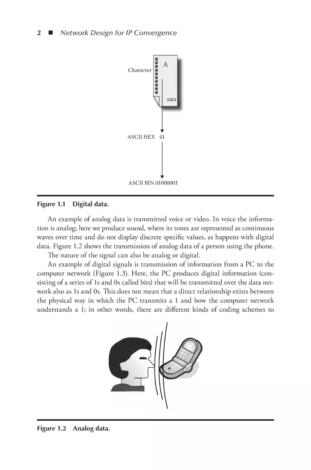
An example of analog data is transmitted voice or video. In voice the information is analog; here we produce sound, where its tones are represented as continuous
waves over time and do not display discrete specific values, as happens with digital
data. Figure 1.2 shows the transmission of analog data of a person using the phone.
The nature of the signal can also be analog or digital.
An example of digital signals is transmission of information from a PC to the
computer network (Figure 1.3). Here, the PC produces digital information (consisting of a series of 1s and 0s called bits) that will be transmitted over the data network also as 1s and 0s. This does not mean that a direct relationship exists between
the physical way in which the PC transmits a 1 and how the computer network
understands a 1; in other words, there are different kinds of coding schemes to
Figure 1.2
Analog data.
Computer Network Concepts
3
*
1 0 1 0 1 0 1
*
1 0 1 0 1 0 1
Figure 1.3
Digital signals.
represent bits and these can vary from PC to network and even between different
network technologies. For example, in transmissions over copper wires there are
network technologies that understand a 1 as a high-voltage (+5 V) level and other
technologies may understand the 1 as –5 V. It is important, therefore, to correctly
interconnect the physical transmission of these technologies so that when a transmitting device forwards a bit as 1 and +5 V, the receiver understands that +5 V
means a 1 at the bit level.
An analog signal is data or information transmitted as a continuous signal
regardless of the nature of the data. Figure 1.4 shows that a PC is transmitting
digital data over analog signals.
We have seen that to transmit information one can use digital or analog signals. The question now is how to represent an analog signal and how to represent
a digital signal.
1
0.8
0.6
0.4
0.2
0
*
*
–0.2
–0.4
–0.6
–0.8
–1
1
0
Figure 1.4
1
0
1
0
1
Analog signals.
0
0.5
1
1.5
2
2.5
3
3.5
4
4
Network Design for IP Convergence
1.5
1
s(t)
0.5
0
–0.5
–1
–1.5
Figure 1.5
0
0.2
0.4
0.6
0.8
1
t
1.2
1.4
1.6
1.8
2
Sin function.
The main characteristic of analog signals is their continuous form with small
changes in the value of the function. Analog signals can be represented through
Fourier series, and in this case every analog transmission could be represented by a
combination of sinusoidal or cosinusoidal functions. In this case we could say that
we have a function that can be described in the following way:
s(t ) = sin(2πft )
Here we can say that the value of the signal in the time (t) domain depends on the
frequency (f ) being used; we would thus be illustrating an analog signal, which is
continuous in time. To show an example, we could say that T = 1 where T = 1 / f
and realizing t from 0 to 2 with 0.01 increments; this 0.01 value has been randomly
selected for this example and any real value could be used to better represent the
curve of the function. Figure 1.5 shows the signal’s behavior for these example
values. We can see in this figure that the behavior is that of a continuous signal
through which we could represent some kind of data.
We could combine a set of sinusoidal functions in such a way that the frequencies used are in the range from 1 to ∞ and using odd values. The odd values of
the sin function are used so that they don’t counteract the values of the function.
We could also make every signal generated by a frequency ( f ) let a multiple of
Computer Network Concepts
5
1.5
1
s(t)
0.5
0
–0.5
–1
–1.5
Figure 1.6
0
0.2
0.4
0.6
0.8
1
t
1.2
1.4
1.6
1.8
2
s(t) function with n = 1.
the fundamental, that is, of (1f ); and also that the value of s(t), the signal as we
increase the frequency, (kf ), be smaller every time due to the factor K inside the
Sin function.
The following equation could describe this.
n
s(t ) =
∑
sin(2 πkft )
4
π k =1,k odd
k
One can see that every new signal generated by a frequency (kf ) multiple of the
fundamental (1f ) generates an oscillation within the fundamental frequency. Since
the value of the oscillation within the total is also being divided by k, this means
that as the number of frequencies (k) increases, its incidence over the value of the
resulting signal [s(t)] is increasingly smaller.
The following scenarios result from the foregoing equation by changing the
value of k, that is, the number of frequencies used.
For all cases T = 1. We will begin by showing the effect when n = 1 (Figure 1.6),
that is, when we only have frequency 1f. In this case the signal is similar to
Figure 1.5.
6
Network Design for IP Convergence
1.5
1
s(t)
0.5
0
–0.5
–1
–1.5
Figure 1.7
0
0.2
0.4
0.6
0.8
1
t
1.2
1.4
1.6
1.8
2
s(t) function with n = 3.
In this new case we show the effect when n = 3 (Figure 1.7). In other words,
we have frequencies 1f and 3f. The resulting effect is that the signal generated by
3f superimposes the signal generated by 1f, with the additional behavior that the
most influential signal over the value of s(t) is 1f, since the oscillation of 3f is much
smaller (one-third) than that of 1f.
The next example shows the resulting signal behavior [s(t)] when n = 5
(Figure 1.8). It is evident in this figure that there are more oscillations (3f and 5f )
in terms of the fundamental frequency (1f ).
We could successively continue trying with different values of n and every
time we will find more oscillations in terms of the fundamental frequency (1f ).
For example, if we have n = 19 (Figure 1.9), the signal will increasingly look more
like a digital style signal. The important thing is that the electronic device can
understand during the time of a bit if the value is, for example, in this case, +1 or
–1. We can conclude from the foregoing that more or fewer frequencies are used to
represent a digital signal.
Finally, if we use n = 299 (Figure 1.10) in this example we see a good representation of a digital signal, which in this case has only two values, +1 or –1. The example
that we have used does not intend to tell us that electronic devices must necessarily
use this range of frequencies; it has been used for educational purposes.
Computer Network Concepts
7
1.5
1
s(t)
0.5
0
–0.5
–1
–1.5
Figure 1.8
0
0.2
0.4
0.6
0.8
1
t
1.2
1.4
1.6
1.8
2
s(t) function with n = 5.
1.2 Computer Networks According to Size
Computer networks may be classified in several ways according to the context of
the study being conducted. The following is a classification by size. Later on we will
specify to which of the networks we will apply the concepts of this book.
1.2.1 Personal Area Networks (PANs)
Personal Area Networks are small home computer networks. They generally connect home computers to share other devices such as printers, stereo equipment, etc.
Technologies such as Bluetooth are included in PAN networks.
A typical example of a PAN network is a connection to the Internet through the
cellular network. Here, the PC is connected via Bluetooth to the cell phone, and
through this cell phone we connect to the Internet, as illustrated in Figure 1.11.
1.2.2 Local Area Networks (LANs)
Local Area Networks are the networks that generally connect businesses, public
institutions, libraries, universities, etc., to share services and resources such as the
8
Network Design for IP Convergence
1.5
1
s(t)
0.5
0
–0.5
–1
–1.5
Figure 1.9
0
0.2
0.4
0.6
0.8
1
t
1.2
1.4
1.6
1.8
2
s(t) function with n = 19.
Internet, databases, printers, etc. They include technologies such as Ethernet (in any
of its speeds, today reaching up to 10 Gbps), Token Ring, 100VG-AnyLAN, etc.
The main structure of a LAN network traditionally consists of a switch to which
the switches of office PCs are connected. Corporate servers and other main equipment are also connected to the main switch. Traditionally, this main switch, which
can be a third layer switch or through a router connected to the main switch, is
the one that connects the LAN network to the Internet. This connection from the
LAN network to the carrier or ISP is called the last mile.
Figure 1.12 shows a traditional LAN network design.
1.2.3 Metropolitan Area Networks (MANs)
Metropolitan Area Networks are networks that cover the geographical area of a city,
interconnecting, for instance, different offices of an organization that are within
the perimeter of the same city. Within these networks one finds technologies such
as ATM, Frame Relay, and xDSL, cable modem, RDSI, and even Ethernet.
A MAN network can be used to connect different LAN networks, whether
with each other or with a WAN such as Internet. LAN networks connect to MAN
networks with what is called the last mile through technologies such as ATM/
SDH, ATM/SONET, Frame Relay/xDSL, ATM/T1, ATM/E1, Frame Relay/T1,
Computer Network Concepts
9
1
0.8
0.6
0.4
s(t)
0.2
0
–0.2
–0.4
–0.6
–0.8
–1
0
Figure 1.10
0.2
0.4
0.6
0.8
1
t
1.2
1.4
1.6
1.8
2
s(t) function with n = 299.
Frame Relay/E1, ATM/ADSL, Ethernet, etc. Traditionally, the metropolitan core
is made up of high-velocity switches, such as ATM switchboards over an SDH
ring or SONET or Metro Ethernet. The new technological platforms establish that
MAN or WAN rings can work over DWDM and can go from the current 10 Gbps
to transmission velocities of 1.3 Tbps or higher. These high-velocity switches can
also be layer 3 equipments and, therefore, may perform routing.
Figure 1.13 shows a traditional MAN network design.
Bluetooth
Cellular Network
Internet
Cellular
PC
Figure 1.11
PAN design.
10
Network Design for IP Convergence
Core Switch
(Chassis)
Ethernet
Last Mile/
Man Connection
Edge Switch
PCs
Servers
PCs
Figure 1.12
LAN design.
1.2.4 Wide Area Networks (WANs)
Wide Area Networks are networks that span a wide geographical area. They typically connect several local or metropolitan area networks, providing connectivity
to devices located in different cities or countries. Technologies applied to these
networks are the same as those applied to MAN networks, but in this case a larger
geographical area is spanned, and, therefore, a larger number of devices and greater
complexity in the analysis that must be done to develop the optimization process
are needed.
Metropolitan Backbone
Switch
ATM/SONET
ATM/SDH
Metro Ethernet
Last Mile/
MAN Connection
(ATM, Frame Relay,
Ethernet, PPP, etc)
ADM
Figure 1.13
MAN design.
SONET or SDH
Metro Ethernet
WAN Connection
Computer Network Concepts
11
WAN Backbone
Switch/Router
MAN Connections
Figure 1.14
WAN design.
The most familiar case of WAN networks is the Internet as it connects many
networks worldwide. A WAN network design may consist of a combination of layer
2 (switches) or layer 3 (routers) equipment, and the analysis depends exclusively on
the layer under consideration. Traditionally, in the case of this type of network,
what’s normal is that it be analyzed under a layer 3 perspective.
Figure 1.14 shows a traditional WAN network design.
In this book we will work with several kinds of networks. Chapter 3 discusses
MAN and WAN network designs.
1.3 Network Architectures and Technologies
This section presents basic concepts of some architectures such as OSI and TCP/
IP, and some models of real technologies. The purpose is to identify the functions
performed by each of the technologies as compared to the OSI reference model.
1.3.1 OSI
This model was developed by the International Organization for Standardization,
ISO, for international standardization of protocols used at various layers. The
model uses well-defined descriptive layers that specify what happens at each stage
of data processing during transmission. It is important to note that this model is
not a network architecture since it does not specify the exact services and protocols
that will be used in each layer.
The OSI model is a seven-layer model:
Physical layer—The physical layer is responsible for transmitting bits over a physical medium. It provides services at the data link layer, receiving the blocks
the latter generates when emitting messages or providing the bits chains when
receiving information. At this layer it is important to define the type of physical medium to be used, the type of interfaces between the medium and the
device, and the signaling scheme.
12
Network Design for IP Convergence
Data Link layer—The data link layer is responsible for transferring data between
the ends of a physical link. It must also detect errors, create blocks made up of
bits, called frames, and control data flow to reduce congestion. The data link
layer must also correct problems resulting from damaged, lost, or duplicate
frames. The main function of this layer is switching.
Network layer—The network layer provides the means for connecting and delivering data from one end to another. It also controls interoperability problems
between intermediate networks. The main function performed at this layer
is routing.
Transport layer—The transport layer receives data from the upper layers, divides
it into smaller units if necessary, transfers it to the network layer, and ensures
that all the information arrives correctly at the other end. Connection between
two applications located in different machines takes place at this layer, for
example, customer-server connections through application logical ports.
Session layer—This layer provides services when two users establish connections. Such services include dialog control, token management (prevents two
sessions from trying to perform the same operation simultaneously), and
synchronization.
Presentation layer—The presentation layer takes care of syntaxes and semantics
of transmitted data. It encodes and compresses messages for electronic transmission. For example, one can differentiate a device that works with ASCII
coding and one that works with BCD, even though in each case the information being transmitted is identical.
Application layer—Protocols of applications commonly used in computer networks are defined in the application layer. Applications found in this layer
include Internet surfing applications (HTTP), file transfer (FTP), voice over
networks (VoIP), videoconferences, etc.
These seven layers are depicted in Figure 1.15.
APPLICATION
PRESENTATION
SESSION
TRANSPORT
NETWORK
DATA LINK
PHYSICAL
Figure 1.15
OSI architecture.
Computer Network Concepts
Figure 1.16
13
PDA.
1.3.2 PAN
PAN technologies include Bluetooth, which is described next.
1.3.2.1 Bluetooth
Bluetooth is the name of the technology specified by standard IEEE 802.15.1, whose
goal traditionally focuses on allowing short-distance communication between fixed
and mobile devices. Devices that most normally use this technology are PDAs (personal digital assistants) (Figure 1.16), printers, laptops, cellular phones, and keyboards, among others.
It is somewhat complicated to write with a pencil, for instance, on a PDA. For
this reason, external keyboards that connect via Bluetooth to the PDA have been
created, thus avoiding the use of connecting cables. In other words, it is very practical for a PDA to have Bluetooth technology so that it can interconnect to different
external devices. The use of Bluetooth is no longer as frequent in laptops, since
laptops now feature built-in WiFi technology that enables their connection to the
14
Network Design for IP Convergence
Internet, among PCs, to a computer network, etc., faster and with a wider range
than with Bluetooth. The market is also seeing devices with built-in WiMAX; this
means that they connect to the Internet not only at a hot spot but anywhere in the
city, even on the go, with standard IEEE 802.16e. Bluetooth, therefore, is an excellent technology for devices that require little transmission Mbps and short range.
In Bluetooth version 1.0 one can transmit up to 1 Mbps gross transmission rate
and an effective transmission rate of around 720 Kbps. It can reach a distance of
approximately 10 m, although it could reach a greater range with more battery use
due to the power needed to reach such distances with a good transfer rate. It uses
a frequency range of 2.4 GHz to 2.48 GHz. Version 1.2 improved the overlapping
between Bluetooth and WiFi in the 2.4 GHz frequencies, allowing them to work
continuously without interference; safety, as well as quality of transmission, was
also improved. Last, version 2.0 improves the transmission rate, achieving 3 Mbps,
and has certain improvements over version 1.2 that correct some failures.
When compared to OSI architecture, Bluetooth is specified in layer 1 and part
of layer 2, as shown in Figure 1.17.
The power range of antennae, from 0 dBm to 20 dBm, is defined in the RF
(radio frequency) sublayer, associated to the physical layer. The frequency is found
in the 2.4 GHz range.
The physical link between network devices connected in an ad hoc scheme,
in other words, among all without an access point, is established in the baseband
sublayer, also associated to the physical layer.
Bluetooth layer 2 is formed by the link manager and the Logical Link Control
and Adaptation Protocol (L2CAP), which provide the mechanisms to establish
connection-oriented or nonoriented services in the link and perform part of the
functions defined in layer 2 of the OSI model.
APPLICATION
PRESENTATION
SESSION
TRANSPORT
NETWORK
DATA LINK
Figure 1.17
L2CAP / Link Manager
PHYSICAL
Base Band
OSI
BLUETOOTH
Bluetooth architecture.
RF
Computer Network Concepts
15
1.3.3 LAN
There are many different types of LAN technologies: some are no longer used and
others are used more than others. In this section we discuss only two of these technologies. Ethernet is the most common wired LAN solution and WiFi is the most
widespread as wireless LAN.
1.3.3.1 Ethernet
Ethernet technology was defined by a group of networking companies and later
standardized by IEEE. Layer 1 of Ethernet defines the electrical or optical characteristics for transmission, as well as the transmission rate. Layer 2 Ethernet consists
of two IEEE standards. The first, standard 802.3, traditionally works with the
CSMA/CD (Carrier Sense Medium Access with Collision Detection) protocol to
access the medium and transmit. The second, 802.2, defines the characteristics of
transmission at the link in case it is connection oriented or nonoriented. Figure 1.18
shows the layers of Ethernet technology.
1.3.3.2 WiFi
WiFi (Wireless Fidelity) technology is a set of IEEE 802.11 standards for wireless
networks. Standard 802.11 defines the functions of both layer 1 and layer 2 in
comparison with the OSI reference model. At the physical layer, the frequency and
the transmission rate depend on the standard being used. For example, standard
802.11a uses the 5 GHz range and can transmit at a range of 54 Mbps; standard
802.11b uses the 2.4 GHz range and can transmit at a rate of 11 Mbps; and standard 802.11g uses the same range as 802.11b and can transmit up to 54 Mbps. A
new standard currently being developed, 802.11n, is aimed at transmitting around
300 Mbps in the 2.4 GHz frequencies. This technology will reach distances of 30 m
to 100 m depending on the obstacles, the power of antennae, and the access points.
APPLICATION
PRESENTATION
SESSION
TRANSPORT
NETWORK
Figure 1.18
Data Link IEEE 802.2
DATA LINK
Media Access Control 802.3
PHYSICAL
10/100/1000/10GBaseX
OSI
Ethernet
Ethernet architecture.
16
Network Design for IP Convergence
APPLICATION
PRESENTATION
SESSION
TRANSPORT
NETWORK
DATA LINK
Data Link
CSMA/CA
PHYSICAL
802.11a,b,g,n
OSI
Figure 1.19
WiFi
WiFi architecture.
As to layer 2 of the OSI model, WiFi defines a standard to access the CSMA/CA
(Carrier Sense Medium Access with Collision Avoid) medium. Figure 1.19 shows
the layers of WiFi technology.
As we have seen, when we talk about the name of LAN technologies we refer to
those that perform the layer 1 and layer 2 functions as compared to the OSI model.
It will therefore be necessary to go over other technologies to see how they complement with regard to network interconnection and other layers of the OSI model.
1.3.4 MAN/WAN
This section analyzes the architectures of LAN network accesses to MAN or WAN
networks, commercially known as last mile or last kilometer, and the architectures
that are part of operator backbones. We will find here that some technologies define
only layer 1 functions and others only layer 2 functions.
1.3.4.1 TDM (T1, T3, E1, E3, SONET, SDH)
Time Division Multiplexing (TDM) technology divides the transmission line into
different channels and assigns a time slot for data transfer to every channel associated with each transmitter (Figure 1.20). This resource division scheme is called
multiplexing and is associated with layer 1.
T1 lines, specifically, consist of 24 channels and their maximum transmission
rate and signaling can be calculated as follows:
Each T1 frame consists of 24 channels of 8 bits each plus 1 bit signaling per
frame, and each frame leaves every 125 µs; thus, 8000 frames are generated in 1 s.
The calculation is as follows:
(24 channels × 8 bits/channel) = 192 bits/frame + 1 bit/signaling frame = 193 bits/
frame * 8000 frames/s = 1,544,000 bps = 1.5 Mbps
Computer Network Concepts
17
APPLICATION
PRESENTATION
SESSION
TRANSPORT
NETWORK
DATA LINK
Figure 1.20
PHYSICAL
T1, E1, SONET, SDH
OSI
TDM
TDM (T1, T3, E1, E3, SONET, SDH) architecture.
Such T1 lines are used in North America while in Europe the lines used are E1. In
the latter case each frame consists of 32 channels of 8 bits each and every frame is
generated every 125 µs.
For an E1 line the transmission rate with data and signaling is given by the following equation:
(32 channels × 8 bits/channel) = 256 bits/frame * 8000 frames/s = 2,048,000 bps
= 2.048 Mbps
In both T and E carriers there are other fairly commercial standards such as T3,
with a maximum data and signaling rate of 44.736 Mbps, and E3, with a rate of
34.368 Mbps. There are other T and E specifications that are used in some countries and are complementary to the ones discussed in this book.
There are other technologies based on TDM that can achieve faster speeds,
such as Synchronous Optical Networking (SONET) used in North America and
Synchronous Digital Hierarchy (SDH) used in the rest of the world. Both technologies, as their name says, perform synchronous transmission between transmitter and receiver.
In SONET, the first carrier layer, OC-1, corresponds to a total transmission rate
of 51.84 Mbps, and in SDH STM-1 corresponds to a total transmission rate of 155
Mbps; the same transmission rate in SONET is given by carrier OC-3. The next
value in SONET is associated to OC-12, and in SDH STM-4, whose total transfer rate is 622 Mbps. In the case of last-mile, high-speed accesses, rates OC-3 and
OC-12 would be used in SONET and STM-1 and STM-4 would be used in SDH.
The next transfer rates, OC-48/STM-16, with a rate of 2.4 Gbps, and OC-192/
STM-64, with a rate of 9.9 Gbps, belong to the backbone of MAN or WAN carrier networks. Still, there are other standards for SONET and SDH that are not
as popular as the ones just mentioned. It is also possible to transmit both SONET
18
Network Design for IP Convergence
APPLICATION
PRESENTATION
SESSION
TRANSPORT
NETWORK
DATA LINK
Figure 1.21
PHYSICAL
HDSL, VDSL, ADSL
OSI
xDSL
xDSL architecture.
and SDH over Wavelength Division Multiplexing (WDM), thus increasing the
transmission rate. WDM is discussed in a later section.
Summarizing, the lines T1, T3, E1, E3, SONET, and SDH correspond to layer
1 of the OSI model.
1.3.4.2 xDSL
Digital Subscriber Line (DSL) technologies provide data transmission at rates
higher than 1 Mbps, and their main characteristic is that they use the wires of
local telephone networks. Examples of DSL technologies include HDSL High bitrate Digital Subscriber Line (HDSL), Very high bit-rate Digital Subscriber Line
(VDSL), Very high bit-rate Digital Subscriber Line 2 (VDSL2), Single-pair Highspeed Digital Subscriber Line (SHDSL), and Asymmetric Digital Subscriber Line
(ADSL) with the newer versions ADSL2 and ADSL2+ (Figure 1.21).
Table 1.1 is a comparison table of the different DSL technologies.
Table 1.1 Comparison of DSL Technologies
Characteristic
HDSL
VDSL
VDSL2
SHDSL
ADSL
ADSL2
ADSL2+
Speed
(Mbps)
2
52 Dn
12 Up
250
100
50
1–4
2.3 SP
4.6 DP
8 Dn
1 Up
12 Dn
1 Up
24 Dn
2 Up
Distance
(Km)
4
0.5–1
Out
0.5
1
4–5
3–4
2
2.5
2.5
Note: SP = Single Pair, DP = Double Pair, Dn = Down.
Computer Network Concepts
19
1010101010
Port P
Optical Port
= 10Gbps
Transmission Rate = 10Gbps
Port P
λ1
λ2
10101010
λ3
10101010
λ4
10101010
10101010
Optical Port
Number of λ
Transmission Rate
Figure 1.22
DWDM.
= 10Gbps
=4
= 40Gbps
(Top) Transmission without DWDM; (Bottom) transmission with
As a consequence of the foregoing speeds, DSL technologies are also used as
high-speed, last-mile access solutions, but with the convenience of using the same
copper lines as telephone lines. We can also say that VDSL and ADSL2+ technologies are appropriate to receive services such as IPTV (Television over IP).
1.3.4.3 WDM (DWDM)
Just like in technologies with TDM, Dense Wavelength Division Multiplexing
(DWDM) technology multiplexes the transmission of different wavelengths over a
single optic fiber. In other words, with this multiplexing not only are 1s and 0s carried at the fiber level, but the 1s and 0s are transmitted over every wavelength.
Figure 1.22a illustrates optic fiber transmission without DWDM, and
Figure 1.22b illustrates the same optic fiber transmission (provided it is compatible) with DWDM.
In this case, devices are currently being developed to support up to 320 λ and
could undoubtedly continue increasing; this means that if the transmission speed of
the optical port is 10 Gbps, with DWDM it would be possible to transmit approximately 3.2 Tbps. Typical devices found today are 128 or 160 λ.
SONET, SDH, and Ethernet are currently being transmitted over DWDM; for
this reason, DWDM is part of layer 1. Figure 1.23 shows DWDM architecture.
20
Network Design for IP Convergence
APPLICATION
PRESENTATION
SESSION
TRANSPORT
NETWORK
DATA LINK
Figure 1.23
PHYSICAL
SONET, SDH, Ethernet
OSI
WDM
DWDM (λs)
DWDM architecture.
1.3.4.4 PPP/HDLC
Point to Point Protocol (PPP) and High Layer Data Link Control (HDLC) are two
technologies related to layer 2 of the OSI model that perform the following functions, among others: establishing the communication in a point-to-point network,
meaning that such technologies do not perform the switching function; retransmitting packages when there is a loss; recovering in case of package order synchronization failure; performing encapsulation (this function will be explained in detail
in a later section); and verifying errors of transmitted bits. The foregoing means
that such technologies do not define any layer 1 characteristics and must obviously coexist with some layer 1 technologies. There are many technologies similar
to PPP and HDLC that despite having common characteristics are incompatible
in function; in other words, if you have a link and connect two routers to this
link, one with HDLC configuration and the other with PPP, such routers will not
understand each other and, no matter how active the interface is in layer 2, it will
not perform its function properly. Similar technologies include LLC and DLC (for
LAN networks), LAP-B (2nd layer of the X.25 networks), LAP-F (for Frame Relay
networks), and LAP-D (for ISDN networks), among others.
Figure 1.24 shows the architecture of HDLC and PPP. One could, for example,
transmit HDLC over HDSL lines or T1 or E1 lines. The same is true for PPP, but
in this latter case one has the POS (Packet over SONET) technology that forwards
PPP over SONET.
1.3.4.5 Frame Relay
Frame Relay is a technology that operates at layer 2 of the OSI reference model
and its main function includes switching, which means that to establish transmission between two edge points in Frame Relay one needs intermediate devices
(called switches) that decide where the packages are to be resent. This function is
called switching. Like PPP it also performs encapsulation and error control through
Computer Network Concepts
21
APPLICATION
PRESENTATION
SESSION
TRANSPORT
NETWORK
Figure 1.24
DATA LINK
HDLC/PPP
PHYSICAL
HDSL, T1, E1, SONET (POS)
OSI
HDLC/PPP
PPP/HDLC architecture.
Cyclic Redundancy Code (CRC). Frame Relay does not define layer 1 although at
a certain point Integrated Services Digital Network (ISDN) lines had been specified as this layer’s solution, but later platforms such as HDSL, line T1, and line E1,
among others, were specified.
Figure 1.25 shows the architecture of Frame Relay, which could, for instance,
be transmitted over HDSL lines or T1 or E1 lines.
1.3.4.6 ATM
Asynchronous Transfer Mode (ATM) is a network technology that uses the concepts of cell relay and circuit switching and that specifies layer 2 functions of the
OSI reference model. What cell relay accomplishes is that the new volume of data
to be transferred, called cell, has a fixed size, contrary to packages, in which size
is variable. ATM cells are 53 bits, of which 48 are data and five are ATM headers. In addition, cell relay technology performs connection-oriented communications and its work scheme is unreliable because the cells are not retransmitted. This
APPLICATION
PRESENTATION
SESSION
TRANSPORT
NETWORK
Figure 1.25
DATA LINK
Frame Relay
PHYSICAL
HDSL, T1, E1, ISDN
OSI
Frame Relay
Frame Relay architecture.
22
Network Design for IP Convergence
APPLICATION
PRESENTATION
SESSION
TRANSPORT
NETWORK
Figure 1.26
DATA LINK
AAL
ATM
PHYSICAL
HDSL, SONET, SDH, ADSL
OSI
ATM
ATM architecture.
technology assumes that if the information is lost and needs to be retransmitted, a
higher layer will take care of it.
Now all higher layer technologies are specified to work with packages. For this
reason it was necessary to specify a sublayer in ATM that will take a package and
will fragment it into smaller units in order to construct cells. Similarly, it is necessary to perform the inverse function; that is, when the receiver receives a number of
cells, this sublayer must be capable of reconstructing the source package relative to
various ATM cells. Another function that must be performed is convergence of services: data, voice, and video convergence was specified in ATM networks, hence it
was necessary to establish a function that would identify the different services and
integrate them into a single transmission network. All of the functions discussed in
this paragraph are performed by a sublayer called ATM Adaptation Layer (AAL).
Figure 1.26 shows the architecture for ATM and AAL and, for example, could
transmit over HDSL, SONET, SDH, and ADSL, among others.
1.3.4.7 WiMAX
WiMAX technology, whose specification is given by standard IEEE 802.16 and
whose solutions span a MAN network, is currently penetrating the markets and
there are still uncertainties about its being able to meet the expectations that have
risen around it.
Standard IEEE 802.16 in general defines both layer 1 and layer 2 according
to the specifications of the OSI reference model. In layer 1 it specifies the type of
coding to be used, and here we can mention QPSK, QAM-16, and QAM-64, and
defines the time slots through TDM. In layer 2 it specifies three different sublayers:
security sublayer, access to the medium sublayer, and convergence of specific services to layer 2 sublayer. In the latter case one can define different types of services
and, last, at this layer it defines the frame structure (Figure 1.27).
Computer Network Concepts
23
APPLICATION
PRESENTATION
SESSION
TRANSPORT
NETWORK
Figure 1.27
DATA LINK
Service Convergence
Security and Access
PHYSICAL
OFDMA/FDMA (802.16)
OSI
WiMax
WiMAX architecture.
1.3.4.8 GMPLS
Multiprotocol Label Switching (MPLS) is a data-carrying technology located
between layer 2 (link) and layer 3 (network), according to the OSI reference model,
that was designed to integrate traffic of the different types of services such as voice,
video, and data (Figure 1.28). It was also designed to integrate different types of
transportation networks such as circuits and packages and, consequently, to homogenize layer 3 (IP) with layer 2 (Ethernet, WiFi, ATM, Frame Relay, WiMAX, PPP,
and HDLC, among others). Through this technology it seems as if IP were connection oriented by means of the creation of the Label Switched Paths (LSPs).
What Generalized Multiprotocol Label Switching (GMPLS) does is expand the
control plane concept of MPLS to cover what is defined in MPLS such as SONET/
SDH, ATM, Frame Relay, and Ethernet and, in addition to supporting the package commutation technologies, also support time-based multiplexing (TDM) or
commutation based on wavelength (λ) or ports or fibers. In this sense, the GMPLS
control plane would encompass platforms of both layer 2 and layer 1 (Figure 1.29).
APPLICATION
PRESENTATION
SESSION
TRANSPORT
NETWORK
Figure 1.28
IP
DATA LINK
MPLS
ATM/ETH/FR/PPP/…
PHYSICAL
SDH/SONET/ETH/DWDM/…
OSI
MPLS
MPLS architecture.
24
Network Design for IP Convergence
APPLICATION
PRESENTATION
SESSION
TRANSPORT
NETWORK
PHYSICAL
OSI
Figure 1.29
GMPLS
DATA LINK
IP
GMPLS
ATM/ETH/FR/PPP/…
SDH/SONET/ETH/DWDM/…
GMPLS
GMPLS architecture.
Hence, we can locate GMPLS vertically covering part of layer 2 and part of layer 1,
depending upon which platform to which it would be applied.
1.3.5 TCP/IP
The set of TCP/IP protocols allows communication between different machines
that execute completely different operating systems. It was developed mainly to
solve interoperatibility problems between heterogeneous networks, allowing that
hosts need not know the characteristics of intermediate networks.
The following is a description of the four layers of the TCP/IP model.
Network Interface Layer—The network interface layer connects equipment to
the local network hardware, connects with the physical medium, and uses a
specific protocol to access the medium. This layer performs all the functions
of the first two layers in the OSI model.
Internet Layer—This is a service of datagrams without connection. Based on a metrics the Internet layer establishes the routes that the data will take. This layer
uses IP addresses to locate equipment on the network. It depends on the routers,
which resend the packets over a specific interface depending on the IP address of
the destination equipment. It is equivalent to layer 3 of the OSI model.
Transportation Layer—The transportation layer is based on two protocols. User
Datagram Protocol (UDP) is a protocol that is not connection oriented: it
provides nonreliable datagram services (there is no end-to-end detection or
correction of errors), does not retransmit any data that has not been received,
and requires little overcharge. For example, this protocol is used for real-time
audio and video transmission, where it is not possible to perform retransmissions due to the strict delay requirements of these cases. Transmission Control
Protocol (TCP) is a connection-oriented protocol that provides reliable data
transmission, guarantees exact and orderly data transfer, retransmits data that
Computer Network Concepts
25
APPLICATION
PRESENTATION
APPLICATION
SESSION
Figure 1.30
TRANSPORT
TCP/UDP
NETWORK
IP
DATA LINK
Network Interface
PHYSICAL
Physical
OSI
(TCP/UDP)/IP
TCP/IP architecture.
has not been received, and provides guarantees against data duplication. TCP
does the task of layer 4 in the OSI model. All applications working under
this protocol require a value called port, which identifies an application in an
entity, and through which value the connection is made with another application in another entity. TCP supports many of the most popular Internet
applications including HTTP, SMTP, FTP, and SSH.
Application Layer—The application layer is similar to the OSI application layer,
serving as a communication interface and providing specific application
services. There are many protocols on this layer, among them FTP, HTTP,
IMAP, IRC, NFS, NNTP, NTP, POP3, SMTP, SNMP, SSH, Telnet, etc.
Figure 1.30 illustrates the TCP/IP model and its layers.
1.4 Network Functions
This section provides an introduction to fundamentals of some of the main functions performed during data network transmission. Among these functions we
mention encapsulation, switching, and routing.
1.4.1 Encapsulation
This function consists of introducing data from a higher layer (according to the
OSI model) in a lower layer, for example, if an IP package is going to be transferred
through a PPP link. Figures 1.24 and 1.30 show that PPP is in layer 2 and IP is
in layer 3; therefore, PPP would encapsulate the IP package. Figure 1.31 shows an
example of encapsulation.
Figure 1.32 demonstrates the encapsulations from the application layer through
to the link layer if we analyze the complete encapsulation process for transmission
of a voice package via VoIP in such a PPP channel.
26
Network Design for IP Convergence
IP Header
PPP Header
Figure 1.31
IP Data
PPP Data
PPP Footer
Encapsulation.
1.4.2 Switching
The switching function is performed by certain devices when making the decision—given an entry frame with a switching value that can be a label in MPLS,
a Data Link Control Identifier (DLCI) in Frame Relay, a Virtual Path Identifier
(VPI)/Virtual Channel Identifier (VCI) in ATM, a Medium Access Control (MAC)
address in Ethernet, or a λ in Optical Lambda Switching (OLS)/Optical Circuit
Switching (OCS)—of which switching value to use, in case the specific technology
allows it, and through which physical outlet port such a frame should exit.
To perform switching, technologies such as Frame Relay and ATM, among
others, a virtual circuit must first be established that communicates two external
switches through a complete network of switches. Such virtual circuits may be created in two ways: Permanent Virtual Circuit (PVC) or Switched Virtual Circuit
(SVC). One characteristic of PVCs is that such virtual circuits are always established, whether or not there is data transmission. SVCs, on the other hand, are
established while data transmission is taking place. Figure 1.33 shows the concept
of virtual circuit, which follows an established path through several switches in the
network. In this case it is possible to use several routes, but only one of them has
been selected as the transmission route through the virtual circuit.
H.323
G.723
Voice
UDP UDP Data
Header
Header
IP Header
PPP Header
Figure 1.32
IP Data
PPP Data
Complete encapsulation via VoIP.
PPP Footer
Computer Network Concepts
Virtual
Circuit
Source
Switch
Figure 1.33
27
WAN Backbone
Switches
Destination
Switch
Virtual circuit.
In Frame Relay, switching takes place through the DLCI value, which is configured along a virtual circuit. A switching scheme in a Frame Relay network is
shown in Figure 1.34. In this example it is possible to transmit information from
PC1 to PC2 or from PC2 to PC1 in their respective LAN networks, which are
connected through a MAN or WAN network in Frame Relay. To exemplify this
case, assume that right now PC1 wants to transmit a package (which can be IP in
layer 3) to PC2. PC1 will forward an Ethernet frame placing its own address (PC1)
as source MAC address and the MAC address of router R1 as destination MAC
address. Based on the destination IP address (this will be explained in more detail
in Chapter 3) associated to the PC2 device, router R1 will perform its routing function and decide to forward the package through the last-mile connection. Since the
last-mile connection is in Frame Relay, R1 will perform the encapsulation in Frame
Relay placing 20 as the DLCI value. Such DLCI values are assigned by the carrier.
This frame will follow the logical path marked by the virtual circuit. Next, the
frame with DLCI 20 will arrive at the Frame Relay switch of carrier SW1 through
the last mile via port P1. Then, SW1 through its switching table will perform the
switching function, changing value DLCI 20 for value DLCI 21 (as indicated in
SW1’s switching table), and forward out the frame via port P2. Following the logical path of the virtual circuit, the frame will come in at SW2 via port P1, where
switching will take place again from DLCI 21 to 22, and will be resent out via
port P2. Subsequently, SW3 will receive the frame with a value of DLCI 22 and
reforward it via port P2 with value DLCI 23 until it finally reaches its destination
network through the last mile with router R2. Router R2 will perform its routing
function, which will be explained later, to remove the layer 2 Frame Relay header
and will replace it with an Ethernet header with the Ethernet destination MAC
address of PC2 for delivery thereto.
In ATM, switching takes place through values VPI and VCI, which are configured along a virtual circuit. Figure 1.35 shows switching in an ATM network.
In this case it is possible to transmit data from PC1 toward PC2 or from PC2
toward PC1 in their respective LAN networks, which are connected through a
MAN or WAN network in ATM. To exemplify this case, assume that right now
P1
SW4
P2
22
SW3
Switching Table
P2 (22)
SW 2
P1 (21)
P1
Switch MAN/WAN
Frame Relay
SW1
Virtual Circuit
Path
P2
Switching in Frame Relay.
Frame
DLCI = 20
20
Router
R1 Last Mile
P2 (21)
21
Figure 1.34
PC1
MAC PC1
Switch LAN
Ethernet
P1 (20)
Switching Table
P1
P2
23
P1 (22)
Router
R2
P2 (23)
Switching Table
MAC PC2
PC2
Switch LAN
Ethernet
28
Network Design for IP Convergence
Figure 1.35
Switching in ATM.
P2
SW4
SW2
P2 (4/5)
P2
4/5
SW3
Switching Table
P1 (1/3)
P1
Switch MAN/WAN
ATM
SW1
Virtual Circuit
Path
P1
Cell (VPI/VCI)
VPI = 1/VCI = 2
1/2
Router
R1 Last Mile
1/3
PC1
MAC PC1
Switch LAN
Ethernet
P2 (1/3)
Switching Table
P1 (1/2)
P1
P2
2/1
Router
R2
P2 (2/1)
Switching Table
P1 (4/5)
MAC PC2
PC2
Switch LAN
Ethernet
Computer Network Concepts
29
30
Network Design for IP Convergence
PC1 wants to transmit a package (which can be IP in layer 3) to PC2. PC1 will
forward a frame placing its own address (PC1) as Source MAC address and the
MAC address of router R1 as destination MAC address. Based on the destination
IP address (this will be explained in more detail in Chapter 3) associated to device
PC2, router R1 will perform its routing function and decide to forward the package through the last-mile connection. Since the last-mile connection is in ATM,
R1 will perform the encapsulation in ATM and construct cells assigning VPI/VCI
1/2. Such VPI/VCI values are assigned by the carrier. Said cell will follow the logical path marked by the virtual circuit. Next, the cell with VPI/VCI 1/2 will arrive
at the ATM switch of carrier SW1 through the last mile via port P1. Then, SW1
through its switching table will switch the values VPI/VCI 1/2 for values VPI/VCI
1/3 (as indicated in SW1’s switching table), and forward out the frame via port P2.
Following the logical path of the virtual circuit, the frame will come in at SW2 via
port P1, where switching will take place again from VPI/VCI 1/3 for 4/5, and will
be resent out via port P2. Subsequently, SW3 will receive the cells with values VPI/
VCI 4/5 and reforward via port P2 with values VPI/VCI 2/1 until finally arriving
at the destination network through the last mile with router R2. Router R2 will
perform its routing function, which will be explained later, to remove the layer 2
ATM header and will replace the Ethernet header cells with the Ethernet destination MAC address of PC2 for delivery thereto.
In MPLS or in GMPLS, as in ATM and Frame Relay, it is first necessary to
establish a logical path to transfer data and then perform the switching function.
Such logical paths in MPLS/GMPLS are called LSPs (Label Switched Paths). Edge
switches that receive an IP package and then retransmit it as an MPLS frame are
called LER (Label Edge Router), and switches that are part of the device’s network
core, that is, those that perform the switching function, are called LSR (Label
Switch Router).
In MPLS, switching takes place through the value of LABELs, which are configured along an LSP. Figure 1.36 shows a switching scheme in an MPLS network.
In this case, it is possible to transmit data from PC1 to PC2 or from PC2 to PC1 in
their respective LAN networks, which are connected through a MAN or WAN network in MPLS. To exemplify this case, assume that right now PC1 wants to transmit a package (which can be IP in layer 3) to PC2. PC1 will forward an Ethernet
frame placing its own address (PC1) as source MAC address and the LER1 MAC
address as the destination MAC address. Based on the destination IP address (this
will be explained in more detail in Chapter 3) associated to device PC2, LER1 will
perform its routing function and decide to forward the package through the lastmile connection. Since the last-mile connection is in MPLS, LER1 will perform
the encapsulation in MPLS assigning 100 as the LABEL value. Such LABEL values
are assigned by the carrier. This frame will follow the logical path marked by the
LSP. Next, the frame with LABEL 100 will arrive at the MPLS switch of carrier
LSR1 through last mile via port P1. Then, LSR1 through its switching table will
perform the switching function, switching LABEL 100 value for a LABEL 200
100
Last Mile
Switching in MPLS.
Frame (Label)
Label = 100
LER1
P1
LSR4
LSR2
P2 (300)
P2
300
LSR3
Switching Table
P1 (200)
P1
Switch MAN/WAN
MPLS
LSR1
Label Switched
Path (LSP)
P2
200
Figure 1.36
PC1
MAC PC1
Switch LAN
Ethernet
P2 (200)
Switching Table
P1 (100)
P1
P2
400
LER2
P2 (400)
Switching Table
P1 (300)
MAC PC2
PC2
Switch LAN
Ethernet
Computer Network Concepts
31
32
Network Design for IP Convergence
value (as indicated in LSR1’s switching table) and forward out the frame via port
P2. Following the path of the LSP, the frame will come in at LSR2 via port P1,
where switching will take place again from LABEL 200 to 300, and will be resent
out via port P2. Subsequently, LSR3 will receive the frame with LABEL 300 and
reforward it via port P2 with LABEL 400 value until it finally reaches its destination network through the last mile with LER2. The LER2 will perform its routing
function, which will be explained later, to remove the layer 2 MPLS header and will
replace the Ethernet header with the Ethernet destination MAC address of PC2 for
delivery thereto.
When the switching function takes place in a network with optical switching,
such function takes place at layer 1 of the OSI reference model. In GMPLS the
switching takes place through the value of the wavelengths (λ), which are configured along an LSP. Figure 1.37 shows a switching scheme in a GMPLS network
with OLS. At this point, it is important to clarify that there are different types of
optical switching, among them OLS/OCS, Optical Packet Switching (OPS), and
Optical Bursa Switching (OBS), but for introductory purposes of the switching
concept, only one example of OLS will be provided. A later chapter shows the
operation of OPS and OBS. Picking up on the MPLS example, in this case one
can transmit data from PC1 to PC2 or from PC2 to PC1 in their respective LAN
networks, which are connected through a MAN or WAN network in GMPLS. To
exemplify this case, assume that right now PC1 wants to transmit a package (which
can be IP in layer 3) to PC2. PC1 will forward an Ethernet frame placing its own
address (PC1) as source MAC address and the MAC address of LER1 as destination MAC address. Based on the destination IP address (this will be explained in
more detail in the Chapter 3) associated to device PC2, LER1 will perform its routing function and decide to forward the package through the last-mile connection.
Since the last-mile connection is in GMPLS, LER1 will transmit the bits through
the LAMBDA (λ) λ1 value. Such λ values are assigned by the carrier. These bits will
follow the logical path marked by the LSP. Next, the bits being transmitted, λ λ1,
will arrive at switch GMPLS of the LSR1 through the last mile via port P1. Then
LSR1 through its switching table will perform the switching function, switching
the value λ λ1 for value λ λ 2 (as indicated in LSR1’s switching table) and forward
out the bits via port P2. Following the LSP path, the bits come in at LSR2 via
port P1, where switching will again take place from λ λ 2 to λ 3, and will be resent
out via port P2. Subsequently, LSR3 will receive the bits with value λ λ 3 and will
reforward them via port P2 with value λ λ1 until finally they reach the destination
network through the last mile with LER2. LER2 will perform routing, which will
be explained later, to reassemble the bits as a frame and add an Ethernet header
with the Ethernet destination MAC address of PC2 for delivery thereto. In this
example we have omitted the GMPLS control plane part because we want to show
only the switching scheme in this section.
Lastly, in technologies such as Ethernet, the switching technology currently
takes place without creating a virtual circuit or LSP. The switching function is
Figure 1.37
PC1
LER1
λ1
1010...10
Last Mile
Switching in OLS.
MAC PC1
Switch LAN
Ethernet
λ2
P2
LSR4
LSR2
P2 (λ3)
P2
LSR3
Switching Table
P1 (λ2)
P1
Switch MAN/WAN
GMPLS
LSR1
Label Switched
Path (LSP)
P1
Switching Table
P1 (λ1) P2 (λ2)
λ3
P1
P2
λ1
LER2
Switching Table
P1 (λ3) P2 (λ1)
MAC PC2
PC2
Switch LAN
Ethernet
Computer Network Concepts
33
34
Network Design for IP Convergence
Switching Table
P1 (MAC PC1)
P2 (MAC PC2)
R1
PC2
Last Mile
P2
P1 Switch LAN
Ethernet
MAC SOUR | MAC DESTI
MAC PC1 | MAC PC2
MAC DESTI | MAC SOUR
MAC PC2 | MAC PC1
PC1
Figure 1.38
Switching in Ethernet.
based on the MAC address of the destination device’s network card; in other words,
the switching tables of the switches record through which physical port each of the
device’s MAC addresses is.
Figure 1.38 shows a switching scheme in an Ethernet network. As in all the previous cases, PC1 will transmit a frame to PC2, but in this case PC1 and PC2 are in
the same LAN network and even in the same broadcast domain; that is, in the same
VLAN (Virtual LAN), in case there are VLANs implemented in the LAN network. In this case, PC1 will include two fields in the frame to be transmitted within
the Ethernet header, where it will place MAC PC2 (whose value corresponds to the
MAC address of the network card found physically in PC2) as destination MAC
address and will place MAC PC1 (whose value corresponds to the MAC address
of the network card found physically in PC1) as source MAC address. Next, this
frame will arrive at the Ethernet switch via physical port P1 and will seek in the
corresponding switching table the PC2 MAC address (MAC PC2). Once found, it
will identify the physical port for such MAC address, which in this case would be
PC2. Lastly, the switch will reforward the frame with destination PC2 via port P2.
This is how switching currently takes place in Ethernet, and we can conclude that
to perform this switching there is no need to construct a virtual circuit or LSP.
The foregoing switching scheme is inconvenient for the new challenges and uses
being given to this technology such as those for aggregation networks and core by
Computer Network Concepts
35
data operators. Standard 802.3ah (from the Institute of Electrical and Electronic
Engineering) standardizes client network access to MAN or WAN networks of
data operators. Even so, many data operators have implemented Ethernet as an
aggregation or core solution for their networks. The problem with this is that the
switching function is well defined for the LAN environment, but is not as appropriate for the MAN environment and so much less is for WAN. For this reason,
research is taking place worldwide for the construction of LSPs in Ethernet or at
least for a switching mechanism similar in technology to MPLS/GMPLS.
1.4.3 Routing
This function takes place when we must transmit data end-to-end through different
networks. This means that in this case it is possible to pass through different layer
2 network technologies. Here, it is also necessary to establish a path between the
end-to-end networks so that the device in the source network can forward the data
to the device in the destination network. Consequently, the routing function takes
place in layer 3 of the OSI reference model. IP, the protocol used in the Internet, is
a transmission protocol that operates at this layer.
In routing, data can be transmitted to different locations. The first type of
transmission is called unicast, where the data to be transmitted goes to a single destination device; in multicast we want to send the same data to a group of destination
devices; in anycast we want to send data to any of the destination devices; and, last,
in broadcast we wish to send the data to all the other devices.
Figure 1.39 illustrates a routing scheme based on IP that shows how it is possible to pass through different layer 2 technologies. In this case, we want to transmit data from a PC1 that is located in a LAN network through router R1 to PC2
that is located on another LAN network through R2 as the destination router. In
order to forward such data from router R1 to router R2, it is necessary to establish
an established path using a routing protocol such as RIP, OSPF, EIGRP, IS-IS, or
BGP, among others. The thick line shows the selected path.
Figure 1.40 shows the same scheme as in Figure 1.39 but with the corresponding routing tables. In this case, we want to transmit a package from PC1, which is
located on a source network, to PC2, which is on a different destination network.
For the transmission to take place, it is necessary to follow these steps: First, PC1
sees that it is on a different network from the destination device (address IP PC2
30.0.0.1; for more information about IP routing see [COM05]); therefore, through
switching, in case there is a switch at the connection between PC1 and router R1,
or through physical broadcast, should there be a Hub, the data is forwarded from
PC1 to its R1 link port via Ethernet, as shown in Figure 1.38. R1 sees that the IP
address of the destination network (30.0.0.0) does not belong to its direct connection and consults its routing table. The R1 routing table shows that to reach
network 30.0.0.0 the package must be resent to R3, and R1 it out through physical
port P1. Then, R3 also sees that it does not have a direct connection to network
Figure 1.39
PC1
Routing with IP.
IP PC2
Switch L AN
Ethernet
R7
R3
R6
R8
R4
R9
R10
R5
Router
R2
IP PC2
PC2
Switch L AN
Ethernet
Router
R1
36
Network Design for IP Convergence
Figure 1.40
PC1
IP:20.0.0.1
Router
R1
P1
R3
IP
2
PC
Routing table.
IP PC2
Switch L AN
Ethernet
30.0.0.0
Routing Table
P1
R7
R3
30.0.0.0
P2
R4
Routing Table
R6
IP PC2
P1
R8
R4
30.0.0.0
P2
R5
Routing Table
IP PC2
R9
P1
R10
R5
30.0.0.0
P2
R2
Routing Table
IP
2
PC
P1
Router
R2
30.0.0.0
PC2
IP: 30.0.0.1
IP PC2
Switch L AN
Ethernet
Direct
Routing Table
Computer Network Concepts
37
38
Network Design for IP Convergence
30.0.0.0 and therefore consults its routing table to find that it must resend the package to R4 via physical port P2. R4 follows the exact same procedure, and consulting
its routing table resends the package to R5 via physical port P2. Next, R5 resends
it to R2. Finally, R2 consults its routing table and sees that it has direct connection
to network 30.0.0.0; hence, the package will be delivered to PC2 through Ethernet
at layer 2, whether through switching, should there be connection switches to the
LAN network, or broadcast, if there are hubs in the LAN network.
Figure 1.41 shows an encapsulation, layer 2 switching, and routing integration scheme. With this figure we can begin to see what type of layer 2 technology
exists between each pair of routers, that is, the type of link layer. For example,
what exists between R1 and R3 is an end-to-end technology that only performs
encapsulation and does not perform switching; in this case, PPP is being used with
a link protocol. Between R3 and R4 we see a technology that performs switching.
Therefore, the thick line means that at layer 2, in this case ATM, it is necessary to
establish a virtual circuit through the ATM network for IP packages to travel from
R3 to R4. A similar situation occurs between R4 and R5, but here it is necessary to
establish an LPS since it is on an MPLS network, and, finally, between R5 and R2
once again we find end-to-end technology, which performs encapsulation but not
switching and for this case is HDLC. One must remember that in both LAN networks where the PC1 and the PC2 are located, the layer 2 technology is Ethernet,
which performs switching but does not establish a virtual circuit or LSP.
Figure 1.42 illustrates a transmission performing routing and switching jointly
at those routers that require it. In this example we can see that there are different
layer 2 technologies between every pair of routers. At this point, it is necessary to
mention that this type of example does not necessarily represent a real case, but
there could be a network shaped like this. First, on the LAN (source and destination) networks we have Ethernet as layer 1 and 2 technologies. Between routers R1
and R3 we have PPP as layer 2 and HDSL could be used as layer 1 technology, for
example. Between R3 and R4 we have a complete ATM switching network as layer
2 and SONET/SDH could be layer 1. Between R4 and R5 we also have a complete
MPLS switching network as layer 2 and SONET/SDH or Ethernet, for example,
could be layer 1. Finally, between R5 and R2 we have an end-to-end HDLC as layer
2 and HDSL could be layer 1.
What follows is a description of the complete transmission procedure between
PC1 and PC2 performing the necessary switching and routing functions.
Step 1: PC1 with address IP 20.0.0.1 wants to transmit an IP data package
to device PC2, whose destination IP address is 30.0.0.1. PC1 notices that
the network address for PC2 (30.0.0.0) is different from its network address
(20.0.0.0) and, therefore, through switching on Ethernet (in the case of hubs
this would be by means of broadcast) would forward it to its default gateway,
which in this case would be R1.
Figure 1.41
PC 1
IP:20.0.0.1
Router
R1
P1
R3
IP
PPP
2
PC
P1
R7
R3
P2
R4
R6
Virtual Circuit
ATM Network
IP PC2
P1
R8
R4
30.0.0.0
P2
R5
IP PC2
P1
R9
R10
R5
30.0.0.0
IP
HDLC
P2
R2
Routing Table
LSP
MPLS Network
Routing Table
Integration of encapsulation, switching, and routing.
IP PC2
Switch LAN
Ethernet
30.0.0.0
Routing Table
30.0.0.0
Routing Table
PC
2
P1
Router
R2
30.0.0.0
PC2
IP: 30.0.0.1
IP PC2
Switch LAN
Ethernet
Direct
Routing Table
Computer Network Concepts
39
Figure 1.42
PC1
IP:20.0.0.1
IP
PC
2
PP
P
Router
R1
P1
R3
PPP
IP
2
PC
Routing and switching.
Eth
e
Switch LAN
Ethernet
30.0.0.0
Routing Table
1/2
1/2
R7
1/ 4
1/4
1/5
1/5
R6
R8
R4
IP
PC2
30.0.0.0
1
I
P
2
R5(1)
Routing Table
Switching Table
1/4
ATM Network
1/3
1/3
Switching Table
R3
IP
PC2
1/3
R4 (1/2) Switching Table
Routing Table
I
P
MPLS
R9
3
4
I
P
I
P
R10
R5
IP
PC2
30.0.0.0
H
D
C L
HDLC
P2
R2
Routing Table
P1
P IP
2C
Router
R2
IP
PC2
30.0.0.0
Eth
e
PC2
IP: 30.0.0.1
IP
PC
2
Switch LAN
Ethernet
Direct
Routing Table
30.0.0.0
40
Network Design for IP Convergence
Computer Network Concepts
41
Step 2: R1 receives the frame, removes the Ethernet header, and consults the
IP address of the destination network (30.0.0.0); R1 consults its routing table
and resends the IP package toward router R4 through the ATM network.
Step 3: R1 fragments the IP package to build 53-byte ATM cells and transmits them through the virtual circuit with a value of VPI/VCI 1/2 as can be
observed in R1’s routing table.
Step 4: The switches of the ATM network will perform switching just as in the
example shown in the ATM network in Figure 1.35. In this case, the switches
will switch the cells with values VPI/VCI 1/2 to 1/3; next, from 1/3 to 1/4 and,
finally, from 1/4 to 1/5, as shown in the switching tables in the ATM network.
Step 5: Router R4 receives the ATM cells corresponding to one IP package
and reassembles them.
Step 6: Router R4 consults the routing table for the destination network
address (30.0.0.0) and decides it must forward the package to R5 through an
MPLS network and that the switching value in this case is 1.
Step 7: As in the ATM network, the switches in the MPLS network will switch
just like the example shown in the MPLS network in Figure 1.36. In this
case, the switches will switch the packages with a LABEL value of 1 to 2, then
from 2 to 3 and, finally, from 3 to 4.
Step 8: Router R5 consults the routing table for the destination network
address (30.0.0.0) and decides it must forward the package to R6 via an endto-end connection through an HDLC encapsulation.
Step 9: Router R6 receives the MPLS package, removes the MPLS header,
checks the destination address (30.0.0.0), and notices that it is connected
directly; for this reason, it will add the Ethernet headers to send the package
by means of the switching function explained in Figure 1.38 for it to finally
arrive at PC2, the destination PC.
1.4.4 Multiplexing
Multiplexing is the process whereby a device called a multiplexer receives multiple
inputs (whether physical channels or signals) and combines them into one to send
them out through a single outlet. The reverse process, when combined channels or
signals are received through a single input and are output in their original form,
is called demultiplexing. The device that performs this process is called a demultiplexer. In practice these devices carry out their functions simultaneously.
There are many forms of multiplexing, among which we will mention Time
Division Multiplexing (TDM), Frequency Division Multiplexing (FDM), and
Code Division Multiplexing (CDM), and in optical communications there is
Wavelength Division Multiplexing (WDM). Access methods based on multiplexing have been created for cases where the medium is shared, for example, in wireless
networks (radio), and different devices want to transmit using the same frequency.
Such access methods include Time Division Multiple Access (TDMA), Carrier
42
Network Design for IP Convergence
1
E1 Channel
E1 Channel
1
SDH
STM-1 Channel
2
3
2
2
1
E1 Channel
E1 Channel
3
3
Multiplexer
ADM
Add Drop Multiplexer
E1 Channel
Figure 1.43
Demultiplexer
E1 Channel
TDM.
Sense Multiple Access (CSMA), Frequency Division Multiple Access (FDMA),
Orthogonal Frequency Division Multiple Access (OFDMA), and Code Division
Multiple Access (CDMA), among others, as there is a wide variety. An example of
multiplexing technology applications includes the following: SDH or SONET use
TDM, ADSL uses FDM, GSM cellular networks use FDMA and TDMA, 802.11g
uses CSMA/CA, and 802.3 uses CSMA/CD.
Figure 1.43 illustrates a multiplexing scheme through TDM. In this case, one
can see how the multiplexer receives an input of three E1 channels and multiplexes
them through a single channel, STM-1, in SDH. However, the demultiplexer
receives channel STM-1 and demultiplexes it through the three E1 channels. The
foregoing shows how for each E1 input in the multiplexer it is awarded a time slot
for the transmission of its information.
Figure 1.44 shows a multiplexing scheme through FDM. In this case one sees
how the multiplexer receives one voice channel, one upstream data channel, and
two downstream channels as input. But in this case the information is sent simultaneously, only through different frequencies. For this reason, total transmission
capacity is divided among the number of transmitters. The figure shows that voice
is transmitted through the F1 frequency range, the upstream data through the F2
range, and the downstream data through the F3 range.
Finally, Figure 1.45 shows a multiplexing scheme through WDM. In this case
the OADM receives three physical channels where each one is associated to a λ value
and it multiplexes, sending the three λ values through a single physical connection.
There are basically two types in WDM: Coarse Wavelength Division Multiplexing
(CWDM) and Dense Wavelength Division Multiplexing (DWDM).
UpStream
2
3
DownStream
Figure 1.44
ADSL Line
1
Voz
Multiplexer
FDM.
F1
1
F2
2
F3
3
1
2
Voz
UpStream
3
Demultiplexer
DownStream
Computer Network Concepts
43
λ1
DWDM Line
λ1
λ1
λ2
λ3
λ2
λ2
λ3
Multiplexer
OADM
Optical Add Drop
Multiplexer
Figure 1.45
λ3
Demultiplexer
WDM.
1.5 Network Equipments
This section explains the most important aspects of the main computer network
connection devices.
1.5.1 Hub
This is the most basic connection device in LAN Ethernet networks with which
we can connect multiple devices (PCs, servers, printers, etc.) through a shared
medium. The hub is a layer 1 device in the OSI reference model. In other words,
its basic function is to receive a series of bits (frame) via a port and retransmit it
through all other ports. For this reason, said device transmits information in a
broadcast form at a physical level. The hub is a device that joins multiple devices
together. Therefore, when a device transmits, another device could also be transmitting and the signals would overlap. The effect this produces is called collision.
For this reason, devices in Ethernet technology support the function known as
Carrier Sense Medium Access with Collision Detection (CSMA/CD). When hubs are
used for network connections this is called shared Ethernet, since all have to share
the same physical medium to transmit. The fact that hubs are layer 1 implies other
consequences such as that the device cannot manage quality of service (QoS) and
is therefore unsuitable for transmission of voice, video, or critical data applications.
Performance can also be strongly affected when using a shared medium due to the
high rates of transmission. In addition, many retransmissions have to take place
due to collisions. Another drawback is failure to configure access control lists to
establish basic safety levels.
PCs, servers, printers, and other devices are connected to the hub using UTP
copper cable with RJ-45 connectors. Several hubs can be connected among them
also using a UTP cable or optic fiber.
Figure 1.46 shows an Ethernet hub.
Figure 1.47 shows a transmission scheme through a hub. Figure 1.47a shows
when PC1 transmits a package to server S. Because the hub is a layer 1 device, it
44
Network Design for IP Convergence
Figure 1.46
Hub.
will be unable to know to which specific device the package is addressed and will
resend the package through all the other ports, as shown in Figure 1.47b. This
operation could result in safety issues in addition to the drawbacks we already
mentioned, because if a user on PC1 is transmitting an unencrypted administrator
password and another user at a PC other than PC1 and server S installs a Sniffer
(software to perform network analysis and to capture packages), he could obtain
this password because the hub would also retransmit it to this PC.
PC1
S
Figure 1.47a
Hub transmission (from PC to Hub).
Computer Network Concepts
45
PC1
S
Figure 1.47b
Hub transmission (from Hub to PCs or Server).
1.5.2 Access Point
Access point is the device used to interconnect devices (PCs) wirelessly (see
Figure 1.48). In this book we will exclusively discuss the LAN connection access
points. As in a hub, the physical medium associated to air is a shared medium and
similar problems as those already mentioned could be experienced as well. A protocol called Carrier Sense Multiple Access with Collision Avoidance (CSMA/CA) was
Figure 1.48
Access point.
46
Network Design for IP Convergence
LAN Connection
(Ethernet)
Internet Connection
PDA
Access Point
Laptop
PC
Figure 1.49
Access point connectivity.
created to manage possible collisions when two or more devices want to transmit
information. The main purpose of this protocol is not detecting collisions, but preventing them. This type of technology is widely used in the so-called Hot Spots
where services such as connection to the Internet are provided. It is normal for an
access point to traditionally connect devices in a wireless fashion to the Ethernet
wired network. This device is traditionally layer 2. Safety is another issue with
shared mediums and in this case, access controls have been implemented at the
access points, for example, at the MAC address or the user authentication. Other
encryption mechanisms implemented include Wired Equivalent Privacy (WEP),
WiFi Protected Access (WPA), and IEEE 802.11i (WPA2). IEEE 802.11 is the standard that specifies operation, with its variety of standards, which include 802.11a
(54 Mbps at 5 GHz), 802.11b (11 Mbps at 2.4 GHz), 802.11g (54 Mbps at 2.4
GHz), and the new standard 802.11n (where the idea is to transmit up to 540 Mbps
at 2.4 GHz).
Figure 1.49 shows an access point connectivity scheme. In this case, every
device, whether a laptop, PC, or PDA, will feature a wireless network card and via
WiFi technology will have network access via the access point. One can also see
that through the access point one can establish connections to a LAN (Ethernet)
network and even to the Internet.
Computer Network Concepts
Figure 1.50
47
Switch.
1.5.3 Switch
In the case of LANs a switch is the most advanced connectivity device in Ethernet
by means of which we can connect multiple devices (PCs, servers, printers, etc.) over
a medium that operates as dedicated or switched. A switch operates at layer 2 of the
OSI model; hence, its basic function is to receive a frame via a port and retransmit
it via a specific port where the destination device is located (Figure 1.50).
Switches consist of a switching matrix commonly called backplane (Figure 1.51)
with a dedicated connection from all input ports to all output ports; that is why all
devices connected to the switch are connected in a dedicated fashion. The figure
shows a dedicated connection from port IN 1 to port OUT 2; concurrently, there
is a dedicated transmission from port IN 3 to port OUT 4. So, if the switch has
1 Gbps input and output ports, it may perform switching of both transmissions
simultaneously, contrary to the hub, which is a shared medium and cannot perform
such transmissions simultaneously.
When the backplane of a switch has the capacity to switch everything that
the input ports send toward the destination ports, it is called a nonblocking switch;
that is, the switch can resend all packages that arrive through the input ports.
Calculating the switching capacity of a switch is simple and is explained next.
Suppose we have a 24-port, 10/100 Mbps switch. This means that the switch
can transmit at either 10 Mbps or 100 Mbps. In this case we will analyze the worst
case, or 100 Mbps. The worst case for a switching function is when all the IN ports
48
Network Design for IP Convergence
OUT
NI
Figure 1.51
Switching matrix.
want to transmit at their maximum rate, which in this example is 100 Mbps. The
calculation is as follows: 2 (if transmissions are full duplex) × 24 (ports) × 100
(Mbps) = 4.8 Gbps. If the backplane value that appears on the device’s brochure is
greater than or equal to 4.8 Gbps, the switch is a nonblocking switch.
Overall, we can say a device’s switching capacity is given by
∑
2 * Port Quantity * Port Velocity
Port Types
Switches can eliminate transmission collisions; still, they will not be eliminated
from the network if there is a network where switches and hubs coexist. One of
the problems with network design is congestion and the only way to be aware of
this problem is by having a clear design. Congestion can happen in a switch when
several IN ports want to send information to the same OUT port, as shown in
Figure 1.52. Here, IN ports (1, 3, and 4) want to send out their transmission via
OUT 2 port. Assuming every port is 1 Gbps, then 3 Gbps would be trying to go
out via a 1 Gbps OUT port. To prevent loss of all packages, queues or buffers are
implemented. The time packages remain in queue, produce delays in the transmission, and severe congestion results in the loss of packages due to saturation of
queues. For this reason a good design and dimensioning of a network is extremely
important. This will be shown in other chapters.
Switches may be of different layers depending on the functions they perform in
addition to their basic layer 2 switching.
A switch will be layer 2, the lowest layer for a switch, if it performs switching in
the LAN case based on the MAC address, which was explained in Section 1.4.2 and
is shown in Figure 1.53. In this case the switch will make the decision of resending an
Computer Network Concepts
49
OUT
NI
Figure 1.52
Congestion in switches.
Ethernet frame based on its destination MAC address by consulting in the switching
table to which OUT port such destination MAC address is associated.
Figure 1.54 shows the switching table of a device, where one can see a record of
several MAC addresses.
Switching Table
P1 (MAC PC1)
P2 (MAC PC2)
R1
P2
PC2
P1 Switch LAN
Ethernet
MAC SOUR | MAC DESTI
MAC PC1 | MAC PC2
MAC DESTI | MAC SOUR
MAC PC2 | MAC PC1
PC1
Figure 1.53
Switching layer 2 in Ethernet.
Last Mile
50
Network Design for IP Convergence
Switching Table
With MAC Address
Figure 1.54
Switching layer 2 in Ethernet with equipment.
Figure 1.55 shows by means of the command ipconfig /all the values of the IP
address and the MAC address (physical address) of a PC.
Figure 1.56 shows how the MAC address of a PC is recorded in the switch’s
switching table, showing the physical port through which it is found, which in this
case is Slot 6 Port 1.
Due to the already mentioned operation, switches will resend the frame through
the port only where the destination MAC address is, as shown in Figure 1.57.
Figure 1.55
Switching layer 2 in Ethernet with equipment.
Computer Network Concepts
Figure 1.56
51
Comparison between switching table and MAC address.
A switch that performs a routing function will be classified as layer 3; however,
switches perform other layer 3 functions, among them switching layer 3.
First, let us discuss the layer 3 switching function. This function means that the
switch has the capacity of switching through the IP address instead of switching
through the MAC address, whose value is layer 2. As seen in Figure 1.58, the switch
could perform switching based on the MAC address or the IP address and the
PC1
S
Figure 1.57a
Switch transmission.
52
Network Design for IP Convergence
PC1
S
Figure 1.57b
(Continued)
forward time would be exactly the same. The question is, when is layer 3 switching
useful? To show this, we will discuss operation of the Address Resolution Protocol
(ARP), which consists of finding the MAC address of a device once the destination
Switching Table
P1 (MAC PC1) 10.0.0.1
MAC DESTI | MAC SOUR
MAC PC2 | MAC PC1
IP DESTI | IP SOURC
10.0.0.2 | 10.0.0.1
R1 Last Mile
P2
P1 Switch LAN
Ethernet
MAC DESTI | MAC SOUR
MAC PC2 | MAC PC1
IP DESTI | IP SOURC
10.0.0.2 | 10.0.0.1
PC2
10.0.0.2
P2 (MAC PC2) 10.0.0.2
PC1
10.0.0. 1
Figure 1.58
Switching layer 3 in Ethernet.
Computer Network Concepts
53
Switching Table
P1 (MAC PC1) 10.0.0.1
PC2
10.0.0.2
R1
Last Mile
P2
P1 Switch LAN
Ethernet
MAC DESTI | MAC SOUR
FFF...FFF | MAC PC1
IP DESTI | IP SOURC
10.0.0.2 | 10.0.0.1
MAC DESTI | MAC SOUR
FFF…FFF | MAC PC1
IP DESTI | IP SOURC
10.0.0.2 | 10.0.0.1
P2 (MAC PC2) 10.0.0.2
PC1
10.0.0. 1
Figure 1.59
Switching layer 3 example.
IP address of such device in the LAN network is given. When the ARP request message is sent, it is sent in such a way that the destination MAC address is broadcast,
but the IP address is known; therefore, it is a layer 2 broadcast but a layer 3 unicast
transmission. Consequently, if the switch is a layer 2 device, it will send the package through all ports as a broadcast, but if the device is layer 3, it may switch based
on the destination IP address. Hence, it will resend the package through a single
port that corresponds to where the destination device is. Figure 1.59 shows this
ARP case. P1 will transmit a message with a destination MAC address in broadcast
(FFF…FFF), but with an IP address (10.0.0.2); therefore, if the switch is layer 3, the
switch will resend the package only through where the PC2 (P2) is found.
Figure 1.60 shows a practical case of a switch with the information of the IP
address, MAC address, and the physical port through which this device is found
recorded in the ARP table.
Now we will explain a second function of layer 3 switches, which is routing.
Devices that perform a routing function are normally called routers and, although
this is entirely true, it does not mean that a switch cannot be a router as well. The
question then would be, where would a switch perform a routing function? In the
case of a LAN network it would be within what is called a Virtual LAN (VLAN)
and, in the case of WAN switches, each switch that simultaneously manages
54
Network Design for IP Convergence
Figure 1.60
ARP table.
technologies such as ATM or MPLS but also manages IP would be considered a
router.
In this first part we will continue discussing LAN switches. This book does not
intend to provide detailed explanations of the VLAN concept; there are good books
that explain it clearly. However, we will provide some fundamentals in order to be
able to design LAN networks with VLAN management. The most basic concept
that a VLAN can manage, and could be the fundamental reason for its configuration and use in LAN networks, is the division in the broadcast domains. Until now,
we have explained that switches separate domains from collision through dedicated
communications, but if a switch is sent a message on broadcast, it will resend such
message through all the other ports. This means that if only one broadcast domain
is available in a LAN network, every time a device sends this type of message it will
invade the network completely. If many broadcast messages are generated, this could
result in poor network performance due to congestion. It is impossible to eliminate
broadcasts from a network because there are many general network applications or
functionalities that must be communicated through these message types; for this
reason, the only mechanism left to improve performance is isolation or division of
such broadcasts through the domains. When VLANs initially came out, they were
used for other purposes, which today could be the reason for their implementation in a network. One of these reasons, for example, is for applying safety policies
through VLAN; in other words, creating policies that allow or deny transmission
of certain applications among VLANs and this way, for example, protect servers.
Computer Network Concepts
55
Switch LAN
Layer 3
Ethernet
SW1
PC2
VLAN 1
PC1
VLAN 3
VLAN 2
PC3
Figure 1.61
Logical scheme of VLANs.
Another reason is for the application of QoS; this way, for example, one can create a
VLAN for Voice over IP (VoIP) services or videoconferences and establish a higher
priority than the other VLANs, therefore making these services prioritary.
Because different VLAN domains are created through VLANs, this means that
two devices that belong to different VLANs cannot see each other during switching; for these devices to see each other there must be routing, for which each VLAN
could be specified as an IP network or subnetwork. It is not necessary to have layer
3 switches to create VLANs; they can be configured in layer 2 switches. But, for
two devices of two different VLANs to be able to see each other and transmit
information, they must be routed, which is precisely the reason for having layer
3 switches in a LAN network, because they perform routing functions that occur
through VLANs.
Figure 1.61 shows the logical scheme of VLANs, which demonstrates the concept of different broadcast domains, that is, different IP networks or subnetworks. In
Figure 1.61 we see that if PC1 wants to communicate with PC2, only the switching
function would take place because both PCs are in the same VLAN. But if PC3
wants to communicate with PC1 or with PC2, since PC3 is on a different VLAN,
the routing function must take place. In this example the router would be layer 3
switch (SW1), which would be the default gateway for those VLAN devices.
If we analyze what the physical scheme of devices belonging to VLANs would
look like, we would have something similar to what is shown in Figure 1.62. Each
device that belongs to a VLAN is differentiated by the texture just as in Figure 1.61.
We can see that one PC of each of the three VLANs is connected to the main switch,
which is layer 3 (the only one that performs routing). The other devices of different
56
Network Design for IP Convergence
PC3
Switch
L2
PC1
Switch
L3
Switch
L2
PC2
Figure 1.62
Physical scheme of VLANs.
VLANs are connected through layer 2 switches. As this figure shows, the physical location of the device does not matter, provided that connectivity is through
Ethernet. Every device will belong to a specific VLAN, and to communicate with
another device in the same VLAN, the process can take place only through switching (PC1 with PC2). Also, notwithstanding where two devices are of different
VLANs, even if it’s in the same switch, as seen in switch L3 (Figure 1.62), for these
PCs to communicate a routing function must take place (PC1 with PC3).
A switch will be layer 4 (according to the OSI model) if it understands the
information found in the TCP or UDP headers. One of the functions of TCP or
UDP is to associate a logical port number to a transmission between client and
server applications. That is, a layer 4 switch must understand the value of source
port TCP or UDP and the value of destination port TCP or UDP, and this way
one can identify what type of application the current package is associated to. Port
numbers range from 0 to 65535. Ports 0 through 1023 are reserved by the Internet
Assigned Numbers Authority (IANA) for certain services with administrative privileges or TCP or UDP fundamental applications. Lastly, 49152 through 65535 are
not established for any application. Table 1.2 shows examples of ports assigned or
used in a standard way for applications.
The foregoing means that with layers 1, 2, and 3 of the OSI reference model we
can arrive at the destination network and the destination device, but it is with layer
4 that we connect with the specific application at such destination device. A switch
with these characteristics will be a device to which one can apply Access Control
Lists (ACLs) or QoS characteristics.
Computer Network Concepts
Table 1.2 Examples of Ports
Port
Protocol
Application
7
TCP,UDP
ECHO (Ping)
20
TCP
FTP—Data Port (File Transfer Protocol)
21
TCP
FTP—Control Port
22
TCP,UDP
SSH (Secure Shell)
23
TCP,UDP
TELNET
25
TCP,UDP
SMTP (Simple Mail Transfer Protocol)
42
TCP,UDP
WINS (Windows Internet Name Server)
49
TCP,UDP
TACACS (Authentication)
53
TCP,UDP
DNS (Domain Name System)
80
TCP
HTTP (Hyper Text Transfer Protocol)
88
TCP
Kerberos (Authentication)
110
TCP
POP3 (Post Office Protocol version 3)—e-mail
143
TCP,UDP
IMAP4 (Internet Message Access Protocol 4)—e-mail
161
TCP,UDP
SNMP (Simple Network Management Protocol)
179
TCP
BGP (Border Gateway Protocol)
220
TCP,UDP
IMAP (Interactive Mail Access Protocol version 3)
264
TCP,UDP
BGMP (Border Gateway Multicast Protocol)
520
UDP
Routing RIP
646
TCP
LDP (Label Distribution Protocol)
1099
UDP
RMI Registry
1433
TCP,UDP
Microsoft SQL database system
1434
TCP,UDP
Microsoft SQL Monitor
1521
TCP,UDP
Oracle
1812
UDP
RADIUS Authentication Protocol
1863
TCP
Windows Life Messenger
57
58
Network Design for IP Convergence
ACLs Table
FTP 10.0.0.1
FTP 10.0.0.2
10.0.0.3
10.0.0.3
FTP 10.0.0.3
From 10.0.0.1
FTP 10.0.0.3
From 10.0.0.2
FTP 10.0.0.3
From 10.0.0.1
R1
Last Mile
P2
PC1
10.0.0.1
Figure 1.63
Switch LAN
Ethernet
Layer 4
.0.3
0.0 .2
P 1 .0.0
FT m 10
Fro
FTP Server
10 .0 .0 .3
F
Fr TP
om 10
10 .0.0
.0 .3
.0
.1
P1
PC2
10.0.0.2
Switch layer 4 applying ACLs.
In the case of ACLs, in Figure 1.63 one sees that the ACLs table allows passage
of the FTP application from PC1 (10.0.0.1) to the FTP server (10.0.0.3) but denies
it for PC2 (10.0.0.2) and, since it is denied for PC2, the package will be rejected by
the switch. In this example it is possible to allow, for example, passage of the HTTP
application to PC2, for which the switch must understand the information that is
in the layer 4 header, that is, TCP or UDP.
In the case of QoS in Figure 1.64, one sees that the QoS table establishes some
priority criteria for every type of application. For example, VoIP has priority 6,
being the highest in this example; next comes HTTP with priority 3, FTP with priority 1, and the rest of the priority 0 applications (default). In this example there are
three PCs that want to transmit information to the Internet through the last mile.
PC1 will transmit HTTP, PC2 FTP, and PC3 VoIP. The switch receives the packages and will resend them according to the priority associated to each application as
per this example; for this reason, it will first resend the VoIP package, second, the
HTTP package, and last, the FTP package. Once again, for the switch to manage
the priorities it must understand the value of ports TCP or UDP.
Figure 1.65 shows a configuration associated to layer 4 through ports TCP or
UDP to establish conditions, in other words, the way of identifying the flow of
information to which QoS or security level access control lists will be applied.
We also find switches that understand beyond layer 4 (TCP or UDP); that is,
they understand the application layer. These devices may understand information
Computer Network Concepts
59
QoS Table
Priority
Application
VoIP
HTTP
FTP
Default
R1
VoIP
FTP
P2
Last Mile
P1
Switch LAN
Ethernet
Layer 4
PC 1
10. 0 .0.1
Figure 1.64
Switch layer 4 applying QoS.
Figure 1.65
Switch layer 4.
P
FT
H
TT
P
PC3
1 0 . 0. 0.3
HTTP
PC2
1 0 . 0. 0. 2
VoIP
60
Network Design for IP Convergence
Switching Table
P1 (100)
P1 (101)
P2 (102)
P2 (103)
P3 (200)
P3 (201)
P3 (202)
P4 (203)
Physical Link
(STM-n/OC-n/GigabitEthernet)
P1
100
101
P3
102
103
203
P2
LSP
Figure 1.66
200
201
202
P4
LSR
Switch layer 2 in MPLS.
associated to headers of applications such as Real-Time-Protocol-Transport (RTP)
and HTTP parameters, among others. The reason for a switch being in this layer is
also associated to ACLs or to QoS.
Finally, regarding LAN switching, we find different types of services for the
networks such as ARP proxy, DHCP server, and authentication proxy; one can
even find services such as DNS. Such services are added as aggregate services to
the basic and advanced operation of switches to somewhat facilitate the number of
devices that organizations must take into account for their networking solution.
Most of the functions that we have already mentioned also apply, or some
of them with certain differences, for the MAN or WAN switches; an example is
establishing the virtual circuit of the LSP to do the switching in WAN switches.
Figure 1.66 shows a switching in MPLS scheme where there are four LSPs. For
example, when a package with a Label 100 arrives at the LSR via physical port P1
(which can be an SDH port, SONET, or GigabitEthernet, for example), the LST
will consult its switching table and will resend the package via physical port P3 and
will change the Label value to 200. The same case would apply to the other LSPs.
As we can see, for these types of switches to perform their switching function they
must first establish logical paths called LSPs in MPLS. If the LSR is layer 3, then
it will also perform routing functions, but in this case such functions would not
be associated to VLANs like in Ethernet but to WAN routing. Such switches may
perform additional functions that are specified in the manufacturers’ brochures for
each reference.
Figure 1.67 shows a switching scheme in ATM in which there are four virtual
circuits. For example, when a cell with a value of VPI/VCI 3/100 arrives at the
switch via physical port P1 (which can be an SDH or SONET port), it will consult
Computer Network Concepts
61
Switching Table
P1 (3/100)
P1 (3/101)
P2 (4/200)
P2 (5/200)
P3 (6/300)
P3 (6/301)
P3 (6/302)
P4 (7/100)
Physical Link
(STM-n/OC-n)
3/100
3/101
P1
P3
4/200
5/200
7/100
P2
Virtual Circuit
Figure 1.67
6/300
6/301
6/302
P4
ATM Switch
Switch layer 2 in ATM.
the switching table and will resend the cells via physical port P3 and the VPI/VCI
value will be changed to 6/300. The same would be true for the other virtual circuits. As we can see, for these types of switches to perform their switching function
they must first establish logical paths that in ATM are called virtual circuits. If the
switch is layer 3 it will perform routing functions like in MPLS.
The same would happen in Frame Relay technology, but instead of switching
with Label or with VPI/VCI, it would switch with DLCI values. Figure 1.68
shows a scheme similar to the ones shown in MPLS and ATM.
1.5.4 Bridge
Bridges are devices that connect to different layer 2 networks. There are also bridges
that connect networks with the same layer 2 technology but where segmentation of
the network is wanted. In the past, there were bridges that connected an Ethernet
network with a Token Ring network, but today switches have all the functions of
bridges. Hence, if one wants to purchase a device that performs bridge functions,
one will ordinarily find that the device being sold is a switch. It is also important to
mention that some functions of bridges are found in routers.
Figure 1.69 shows a typical connectivity associated to a bridge, but which is
embedded in a switch.
Figure 1.70 shows a bridge (switch) with Ethernet ports and an ATM/SDH or
ATM/SONET port.
62
Network Design for IP Convergence
Switching Table
P1 (100)
P1 (101)
P2 (102)
P2 (103)
P3 (200)
P3 (201)
P3 (202)
P4 (203)
Physical Link
(HDSL, T1, E1, ISDN)
P1
100
101
P3
102
103
203
P2
Virtual Circuit
Figure 1.68
200
201
202
P4
Frame Relay Switch
Switch layer 2 in Frame Relay.
Token
Ring
Ethernet
Bridge
Figure 1.69
Bridge.
ATM Uplink
Ethernet Ports
Figure 1.70
Bridge Ethernet—ATM.
Computer Network Concepts
63
Modem
Router
LAN Port — Ethernet
WAN Interface — V.35
Figure 1.71
Router.
1.5.5 Router
In generic terms a router is a device that connects multiple networks by means
of the routing function, which was explained in a previous section. Figure 1.71
illustrates a typical router. A layer 3 switch is a router by definition, independent of
the layer 2 technology (Ethernet, ATM, Frame Relay, HDLC, PPP, etc.), the layer
1 technology (Ethernet, SONET, SDH, HDSL, etc.), or the interfaces or ports
(RJ-45, V.35, etc.) it may exhibit in a specific connectivity case. In the case of the
Internet, routers will understand and make their routing decisions based on the
destination network’s IP address.
One of the consequences of routers connecting to different networks is that for
every network they generate a different broadcast domain. In other words, devices
in the same network will share broadcasts, but such broadcasts will not be retransmitted to a different network; therefore, for two devices in different networks to see
each other, a routing function must be performed.
Figure 1.72 shows the logical scheme of the broadcast domains generated by
routers. According to this example, if PC1 generates a broadcast message, such
message will reach all PCs located in Broadcast 1 Domain (for example, to PC1
and router R1 via port P1), but it will not reach PC3. The foregoing operation
means that PC1 and PC2 can transmit information to each other via switching
because they are in the same broadcast domain, but if PC1 or PC2 wants to transmit information to PC3, it must do it through routing in R1.
In addition to the regular functions of a layer 3 device, many manufacturers
have added to routers other functions such as firewall, VPN, QoS management,
and DHCP servers, among many others.
64
Network Design for IP Convergence
PC2
R1
Domain
Broadcast
1
P1
P2
P3
PC1
Domain
Broadcast
3
Domain
Broadcast
2
PC3
Figure 1.72
Broadcast domain.
1.5.6 Multiplexer
Multiplexers are devices that receive multiple input ports and combine them using
a mechanism explained in Section 1.4.4 to output them through a single output
port.
In SDH and SONET technology multiplexers are called Add Drop Multiplexers
(ADMs), in ADSL they are called Digital Subscriber Line Access Multiplexers (DSLAMs),
and in DWDM they are called Optical Add Drop Multiplexers (OADMs).
Figure 1.73 shows an OADM.
Computer Network Concepts
Ethernet Switch
With DWDM Ports
OADM
DWDM Fiber
OADM
Figure 1.73
OADM.
65
Chapter 2
LAN Networks Design
This chapter introduces designs and configurations of LAN networks, which are
traditionally associated with business networks, college campus networks, and hot
spots, among others. Ethernet and WiFi technologies are used to provide LAN
solutions. This chapter also discusses VLAN design and the connection scheme of
LAN networks to MAN or WAN networks.
2.1 Ethernet Solution
In this section we introduce PC connectivity to edge equipment, connectivity of
the different edge equipment to provide solutions due to the number of points
needed at that edge, and connectivity toward the network core.
We would like to provide some information about the evolution of Ethernet
through time. Standard 802.3 takes off from the Ethernet network standard. In
1980, Digital Equipment Corp. (DEC), Intel, and Xerox (the group that gave rise
to the term DIX) created the standard for a 10 Mbps network over coaxial cable
using the technique to access medium CSMA/CD and called it Ethernet version
1.0. This technique was later improved in 1985 with Ethernet version 2.0. Project
802 of the IEEE adopted Ethernet version 2.0 as the starting point for its standard 802.3 CSMA/CD. Subsequently, new requirements were needed for the new
applications such as multimedia. It is for this reason that standard 802.3u was created and approved in June 1995. The goal of this committee was to maintain the
traditional Ethernet transmission protocol, CSMA/CD; support popular cabling
schemes (10BaseT); and ensure that fast Ethernet technology would not require
changes in protocols of upper layers or in the software that runs in the LAN workstations (i.e., SNMP, MIBs), and would operate at 100 Mbps; use the same type of
67
68
Network Design for IP Convergence
frames, size, and format; maintain the CSMA/CD; support Ethernet and Token
Ring applications; have very simple and cheap design and configuration and strong
support for multimedia; and require a new hub and switch adapting card. Fast
Ethernet may run through the same variety of media as 10BaseT (UTP, STP, and
fiber), but it does not support coaxial cable. It defines three types of medium: 100
Base-TX; category 5, 2 pair UTP and STP cable; and 100 Base-T4. It allows category 3, 4, and 5; 100Base-FX; and optical fiber cable. Subsequently, in 1998, the
IEEE published standard 802.3z, in which 1 Gbps is transmitted in optical fiber
and, in 1999, standard 802.3ab was approved for transmission of 1 Gbps in copper.
This new set of 1 Gbps standards has the following advantages: increased bandwidth and elimination of bottlenecks; wide display capacities using Gigabit over
CAT-5 copper and 6, 6e, and 7 cable; full duplex capacity; quality of service (QoS)
(audio and video); and low cost of acquisition and ownership. Gigabit Ethernet
technology maintains the same specifications as its predecessors: same Ethernet
package format, full duplex and half duplex, CSMA/CD protocol, flow control, and
management objects as they are defined in standard IEEE 802.3. Gigabit Ethernet
can run through optical fiber, but it was established for twisted pairs. It defines
six types of media: 1000BaseSX, short-wave optical fiber; 1000BaseLX, long-wave
optical fiber; 1000BaseCX, 2 pair STP; 1000BaseT, 4 pair UTP; 1000BaseLH and
1000BaseZX, reaching a distance of up to 100 Km, and IEEE through standard
802.3ae specified transmission at 10 Gbps. These are the specifications of this technology: 10GBase-S, 10GBase-L, 10GBase-E, and 10GBase-LX4, reaching up to
approximately 50 Km.
All of these implementations in LAN networks required structured cabling to
establish orderly connectivity between the stations and the edge switches and the
edge switches and the core. Although the purpose of this book is not to design
and specify structured cabling, we will next explain some of the fundamentals of
structured cabling.
A structured cabling system (SCS) is basically an information network within
a building or group of buildings whose transmission medium is a combination of
unshielded twisted pair, UTP, and traditional optical fiber. It is also known by
other names, among them intelligent cabling and signal distribution system. This
cabling system integrates connection of voice, data, and image equipments, that is,
any device whose function is to provide information services through an electrical
or luminic signals conductor. In a structured cabling system it is possible to connect switchboards, telephone extensions, computer terminals, video devices, closed
television circuits, computer networks, faxes, and so on.
The fundamental purpose of a structured cabling system is to provide users
an efficient, inexpensive way of organizing and integrating their information networks, independently of the equipment brands composing such networks, providing as well the possibility of modifying and updating the information network
without having to alter the cabling.
Equipment or devices that compose structured cabling include the following:
LAN Networks Design
69
Patch panel—the central collector of structured cabling
Rack—the device in which hubs, patch panels, switches, etc., are grouped
or located
Patch cord—the cable that goes from the terminal to the work area or from the
patch panel to the hub or switch
Cross connect—a group of connection points installed on a wall or rack used as
mechanical terminations to manage cabling in a building
Transition point—the point in horizontal cabling where a flat cable connects to
a round cable
A structured cabling system consists of the following subsystems: building inlet,
equipment room, vertical cabling (backbone), telecommunications closet, horizontal cabling, telecommunications outlets, work area, and campus.
Building Entrance. The building entrance provides a point where the external
cabling joins the building internal backbone. Standard EIA/TIA 569 defines
the physical requirements for this interface. The building inlet consists of a telecommunications services entrance to the building, which includes the entry
point through the building wall and continuing through to the entrance room
or area. The building entrance should contain the backbone path that interconnects with other campus buildings. In case of communication by means of
an antenna, the antenna would also belong in the building entrance.
Equipment Room. The equipment room is a central location for the telecommunications equipment (e.g., PBX, computers, switch) that serve the building’s
inhabitants. Only equipment that are directly related to the telecommunications system and its support system should be kept in this room. The standard that regulates this subsystem is standard EIA/TIA 569. When selecting
the room, avoid locations that are restricted by building components such
as elevators, stairs, etc., and it should have accessibility for large equipment.
Access to this room should be restricted to authorized personnel only. The
floor resistance should be able to sustain the distributed load and the concentrated load of the installed devices. Distributed load should exceed 12.0 kps
(250 lbf/ft²) and concentrated load should exceed 4.4 kN (1000 lbf) over the
area of greater concentration of devices. The equipment room should not be
located below water level unless measures have been taken to prevent infiltration. The room should have a drain in the event water becomes a problem.
The room should also have direct access to the heating, ventilating, and airconditioning (HVAC) system and should be located away from electromagnetic interference sources, at a distance that reduces interference to 3.0 V/m
through the frequency spectrum. Be very careful of electrical transformers,
motors, generators, X-ray equipment, and transmission radios or radars. It is
desirable to locate the room close to the main backbone. The size of the room
70
Network Design for IP Convergence
Table 2.1
Number of Workstations
Area in m2
Up to 100
14
From 101 to 400
37
From 401 to 800
74
From 801 to 1,200
111
should be enough to accommodate equipment requirements. To determine
the size of the room, take into account current requirements as well as future
projects. When size specifications of equipment are not known, the following
considerations must be taken into account:
Voice and Data Guide. Practice consists of providing 0.07 m2 space in the
room for every 10 m2 of work area. The equipment room must be designed
for a minimum 14 m2. Based on the number of workstations, room size
should be according to Table 2.1.
Guide for Other Equipment. Environmental control equipment such as
energy distributors, air conditioners, and UPA (unit power amplifier)
up to 100 kVA must be installed in the equipment room. UPS (uninterruptible power supply) larger than 100 kVA must be located in separate
rooms. Minimum height of an equipment room should be 2.44 m (8 feet)
without obstructions. The room should be protected from contamination
and pollution that could affect operation and the material of the installed
equipment. When existing contamination exceeds the level established in
Table 2.2, vapor barriers or filters must be installed in the room.
The equipment room must be connected to the backbone route. In case smoke
detectors are required, they must be within the original box to prevent
Table 2.2
Contaminant
Concentration
Chlorine
0.01 ppm
Hydrogen Sulfate
0.05 ppm
Nitrogen Oxide
0.01 ppm
Sulphur Dioxide
0.3 ppm
Dust
100 ug/m3/24 h
Hydrocarbon
4 ug/m3/24 h
LAN Networks Design
71
accidental activation. A drain must be installed under fire detectors to
prevent flooding of the room. HVAC equipment must be provided to
work 24 hours per day and 365 days a year. If the building system does
not guarantee continuous operation, a standalone unit must be installed
for the equipment room. Temperature must be regulated in a range
between 18oC to 24oC with humidity from 30% to 55%. Humidifiers
and dehumidifiers may be required depending on the location’s environmental conditions. Room temperature and humidity must be measured
at a distance of 1.5 m above ground level and after the equipment is in
operation. If backup batteries are used, appropriate ventilation equipment
must be installed.
Interior Finishes. The floor, walls, and ceiling must be sealed to reduce dust.
Finishes must be in bright colors to increase room lighting.
Flooring material must have antistatic properties.
Lighting. Lighting must have a minimum 540 lx, measured 1 m above ground
in a place free of equipment. Lighting must be controlled by one or more
switches located near the room’s entrance.
Power. A separate circuit must be installed to supply power to the equipment
room and this circuit must end at its own electric board. Electric power
entering the room is not specified as it depends on the number of pieces
of equipment installed.
Door. The door must have a lock and must measure, at a minimum, 910 mm
wide and 2.00 mm high. If very large equipment is estimated, then double
doors measuring 1.820 mm wide and 2.280 mm high, must be installed.
Grounding. A 1½ conduit must be installed from the equipment room to the
building’s grounding electrode.
Fire Extinguishers. Portable fire extinguishers must be provided and maintained periodically. They must be installed as close as possible to the door.
Backbone. The backbone provides connection between the telecommunications
cabinet, the equipment room, and the building inlet. The backbone consists
of the backbone cable, the intermediate and principal cross-connect, the
mechanical terminals, and the patch cords.
The Rack. The equipment room and assigned points may be located in different buildings; the backbone includes the transportation medium between
different buildings.
The backbone must support all the equipment found in the rack and frequently
all the printers, terminals, and file servers for one floor of a building. If
more clients or servers are added to a floor, they compete for the available
bandwidth in the vertical cabling. However, there is an advantage, which
is the small number of vertical channels in a building, which allows the
use of more expensive equipment to provide greater bandwidth. This is
the area where optical fiber has become the most appropriate medium.
72
Network Design for IP Convergence
Selecting the Transmission Medium. A backbone for vertical cabling can be
built with any of the previously mentioned standards, but the following
factors must be taken into account: flexibility regarding the services supported, required backbone shelf life, location size, and user population.
Other Design Considerations. No more than two hierarchical layers of
cross-connects can be installed; bridges cannot be used; the length of
the patchcord of the intermediate and principal cross-connect cannot be
longer than 20 m; grounding must comply with the requirements defined
in standard EIA/TIA 607.
Telecommunications Closet. The telecommunications closet is the area inside
the building where telecommunications equipment of the cabling system is
kept. This includes mechanical terminals and cross-connects for the vertical
and horizontal cabling. The norm that standardized this subsystem is EIA/
TIA 569. The telecommunications closet on each floor is a transition point
between the vertical and horizontal cabling route and must be located as close
as possible to the center of the area that it is going to serve.
The telecommunications closet cannot be shared with electrical installations
other than those used for telecommunications. There must be, at a minimum, one closet per floor. Additional closets must be installed when floor
area is greater than 1000 m2 and the horizontal distribution distance is
larger than 90 m.
Multiple closets on one floor must be interconnected at a minimum by
one conduit.
Based on one workstation every 10 m2, the size of the telecommunications
closet must be according to Table 2.3.
The telecommunications closet must be located on floors designed with a
load capacity of 2.4 kPa (50 lbf/ft2). Lighting must be at least 540 lx,
measured 1 m above ground. No suspended ceilings should be installed.
Door dimensions must be at a minimum 910 millimeters wide and 2000
millimeters high, with a lock. Walls, ceiling, and floor must be treated to
eliminate dust. Finishes must be bright to increase room lighting. A minimum of two 15 A and 110 V AC dedicated duplex electrical outlets, each
in separate circuits, must be installed to provide power to the equipment.
Table 2.3
Area in m2
Size of Closet
1000
3000 × 3400 mm
800
3000 × 2800 mm
500
3000 × 2200 mm
LAN Networks Design
73
It must have access to building grounding. The telecommunications closet
must be located in an accessible area in every floor, such as, for example,
a common hallway, and access must be restricted to authorized personnel
only. The closet must have fire protection and smoke detectors must be
installed in their protective cases to prevent accidental activation.
Horizontal Cabling. Horizontal cabling is the portion of the telecommunications cabling system that extends from the telecommunications closet (or
rack, which contains the hubs, patch panels, etc.) to the final users’ workstations. It consists of (1) horizontal cabling, (2) telecommunications outlet, (3)
cable terminators, and (4) cross-connections.
The term horizontal is used because, typically, the cabling system is installed
horizontally through the building floor or ceiling. The services that can
be transmitted through structured cabling include (1) voice transmission
service, (2) data transfer, (3) flexibility relocating devices, and (4) connection to Local Area Network (LAN).
In addition, to satisfy current telecommunications requirements, structured
cabling must enable daily maintenance, relocation, and support for the
installation of new equipment and services.
Telecommunication Outlets. Every work area must have at least two outlet
ports: one for voice and one for data. Different kinds of configuration exist in
accordance with certain standards, as follows:
Universal Services Ordering Codes (USOC). USOC are a series of standards for RJ
connectors developed by Bell Systems, for connection to public networks.
Configurations of TIA/EIA 568-A. Configuration for LAN networks. Local
area network standards designed to operate over UTP designated assignment of pin/par in modular connectors for signal transmission. While
TIA/EIA (T568A and T568B) support all these designations, there are
certain cases where the user decides to cable only the number or pairs
required to support the application.
Work Area. The work area extends from the telecommunications outlet to the
workstation. The work area cable is designed for relatively easy interconnection, so that moving, changing, and adding it can be simple. Components in
the work area include (1) station devices (computers, phones, data terminals,
etc.); (2) patch cables (modular cables, PC adapting cables, fiber jumpers,
etc.); and (3) adapters (balloons), which must be external to the telecommunications outlet.
The work area cable may vary depending on the application. A cable with
identical connectors at both ends is commonly used. When adaptations
are necessary in the work area, they must be external to the outlet. Some of
the most common adaptations are as follows: (1) a special cable or adapter
74
Network Design for IP Convergence
is required when the equipment connector is different from the outlet
connector; (2) a “Y” adapter is required when two services run in the
same multipar cable; (3) a passive adapter may be used when the type of
cable in the horizontal cabling is different from the type of cable required
by the equipment; and (4) an active adapter may be required when pieces
of equipment that use different signal schemes are connected.
In certain cases, pairs may have to be transposed to achieve compatibility.
Certain telecommunications equipment requires resistances in the work area.
This can be accomplished by placing the resistance outside the outlet.
The recommendation is to install one outlet every 10m2.
Finally, for more information on structured cabling specifications, please
refer to the following standards. These are standards that were developed
to standardize structured cabling:
TIA/EIA 568—Standards for cabling in commercial buildings
TIA/EIA 569—Commercial building standard for telecommunications
pathways and spaces
TIA/EIA TSB-36—Specifications for UTP cable
TIA/EIA TSB-40—Specifications for the connection hardware to UTP
cables
TIA/EIA TSB-53—Specifications for STP cable
TIA/EIA 607—Standards for grounding in telecommunications
equipment
TIA/EIA 570—Residential telecommunications cabling standards
TIA/EIA 606—Administration standard for the telecommunications
infrastructure of commercial buildings
IEEE 802.3 and Ethernet/Fast Ethernet LAN standard
IEEE 802.5 and standard Token Ring
ANSI X3T9.5 and FDDI-TP PMD standard
IEEE 802.12 and 100VG-AnyLAN
ATM and ATM forum
A complementary design in new buildings is intelligent buildings, of which
LAN networks are part. The following section talks about the purpose of intelligent buildings.
The first concept about intelligent buildings was born in the 1970s, when the
first buildings with electronic systems, called HVAC systems, were developed. This
consisted of a computer with connected sensors that detected changing environmental conditions. The intelligent concepts were first heard in the United States
around 1981. In the 1980s, security systems, lighting systems, etc., began to
become automated. The first generation of intelligent buildings in London was the
Lloyds building, which was designed by Richard Roger Partnership and consisted
of individual systems. In the second generation, control was performed by a central computer. For example, a fire alarm system linked with the security system
LAN Networks Design
75
could automatically unlock the doors to provide expedited and easy evacuation. An
intelligent building is one that provides a productive and efficient environment by
means of an appropriate combination and optimization of its four basic elements:
structure, systems, services, and administration.
The intention is to increase technical performance, investment savings, and savings in operation costs, in addition to offering occupants maximum well-being,
security, and flexibility. Structure refers to the building’s physical and structural
variables. For example, the distance of the concrete suspended ceiling must be such
that access to the cable trays passing through it is fast and simple, in order to avoid
future complications in cases of maintenance.
Services refers to the facilities that building occupants have for their comfort:
parking, cafeteria, security, etc.
Finally, systems are the devices and controls necessary for the services and
administration to function correctly. The systems allow the administration to keep
appropriate control over power consumption by air conditioning and lighting. The
administration can maintain better stock of spares by programming preventative
maintenance routines, thanks to the automated control of devices. The building
provides enhanced service for personal security and security of goods with subsystems such as access control, closed-circuit TV, and fire detection and control.
Although all subsystems in a building normally operate autonomously—it should
be this way—centralized control dramatically increases efficiency of these systems.
For example, access control together with lighting or air-conditioning control represents the perfect energy savings combination; similarly, the security system linked
with the elevators increases security of goods.
The following is a list of an intelligent building’s systems and considerations
about their function:
Security System. A security system must provide the following services: protection of interior and exterior doors, objects, and specific areas; manual or programmed restricted access; remote supervision and control of security points;
remote opening and closing of doors; programming and recording vault, safe,
etc., opening and closing; and detection systems due to changes in environmental patterns.
Fire Detection and Alarm. A fire detection and alarm system must provide the
following services: continuous supervision and monitoring of all detection
devices, alarms, and/or circuit damages; correct management of the main
and auxiliary water supply system during emergencies; control of elevator
operation; prerecorded messages with instructions; correct management of
air conditioners to prevent circulation of toxic gases and asphyxiating fumes;
generation of audiovisual alarms; automatic communication with firefighters
and other authorities; control of door and stairway pressurization systems;
audio communication with building operators; monitoring of water flow
76
Network Design for IP Convergence
in the networks; monitoring of tank water levels; and automatic control of
valves and gates.
Control of Access to Restricted Areas. A control of access to restricted areas
system must provide the following services: control via magnetic cards, control via proximity cards, recording of all authorized and unauthorized transactions, entry options by hours or days, visitor cards, re-entry control, and
additional keyboard for high security points.
Energy Control. An energy control system must provide the following services:
control air-conditioning equipment and the interior and exterior lighting system; monitor the power substation, power generator, and consumption.
Communications. At a communications platform level, buildings today must
incorporate structured cabling systems that combine copper and optical fiber
according to their needs. Development of recent forms of communication
such as videoconference, high-speed telefax, multimedia service, interconnection of computers with different characteristics, and local area networks
require the use of an advanced structured cabling system capable of supporting all the needs of present day and future communications.
A structured cabling system enables modification of the use of different outlets,
in other words, changing the application of a telephone outlet for a data or television outlet, without incurring in physical works. Overall, the structured cabling
system allows the building complete interconnection flexibility, which permits
multiple uses of space without modifying piping.
A structured cabling system constitutes the distribution network in an intelligent building, integrating into one cabling system a wide range of services and
systems such as voice services (analog–digital), data and LAN services, security
systems, fire alarm control, air-conditioning control, energy control systems, lighting control systems, expert systems, office automation, maintenance systems, and
cabling management and control.
The main purpose when designing an intelligent building is to attain integration of three aspects: automation, communications, and security. Integration of
the three systems provides the following advantages: centralized control, resource
optimization, process automation, increased productivity, high reliability, and
improved living and working conditions.
If each of the systems operates autonomously and integration is accomplished,
the following characteristics will be attained: access control, alarm management
(electronic surveillance), fire control, telesurveillance (video), and technical management—control (lights, energy, air-conditioning, heating, etc.) of machine flows,
metal detection and luggage control, structured cabling system, PABX, tariffication,
videoconference, electronic mail, and, overall, voice, data, and video services.
Having explained certain characteristics and considerations about structured
cabling and intelligent buildings, we will now explain the connectivity scheme and
edge design in a LAN network via Ethernet.
LAN Networks Design
UTP
Cable
77
Hub/Switch
RJ-45
Port
Departmental
Server
Printer
IP
Phone
Figure 2.1
Web Cam
PC1
PC2
Edge connectivity.
2.1.1 Edge Connectivity
Connectivity of devices through Ethernet, in other words, without using a wireless
medium, takes place as follows. PCs, IP telephones, Web cameras, network printers, and other devices whose connectivity is through the data network connect
via copper pairs (traditionally UTP). Figure 2.1 shows connectivity of equipment
toward a hub or edge switch.
Most network connections are actually PC connections more than any other
equipment; for this reason, the size of the network is normally calculated through
this equipment. Other devices such as IP telephones provide the dimensions for
quality of service (QoS) characteristics that we will discuss later.
To provide a solution to an edge, it will probably be necessary to use more than
one hub or switch due to the large number of devices that will be connected. In
order to be able to supply the number of devices to be connected, perhaps it will
be necessary to connect to several hubs or switches or a combination of hubs with
switches between them. This connection can be done through ports with larger
transmission capacity than are usually used as uplink connection toward the core,
or another way, through special ports called stacks. Figure 2.2 shows a switch connection scheme via hubs or switches through an uplink port. This uplink port may
be via copper pairs or optical fiber, and this factor depends on distance and possible
external factors that could affect the physical environment. As you can see, the two
edge switches would be covering the number of ports necessary to connect all the
devices located in that area of that edge.
In the case of connectivity via a stack port, a special port traditionally located in
the back side of hubs or switches is used, and in a logical way gives the appearance
of a single device with a greater number of ports. However, the foregoing function
can also be performed by new devices when they are connected through the uplink
via a management system. Figure 2.3 shows a connectivity scheme through stack
78
Network Design for IP Convergence
C
C
Optical
Fiber
2 Fibers
C
C
Figure 2.2
Hub/Switch
Hub/Switch
Switch connections by uplink.
ports. Most commonly, hubs or switches are manufactured with 24 or 48 ports,
although certain brands handle larger or smaller port numbers. That is, if we have
an edge that requires 60 ports, one would have to buy three 24-port switches or one
48-port switch and one 24-port switch. Lately, manufacturers have opted more for
the connectivity between switches through the uplink port scheme, but this does
C
C
C
C
Figure 2.3
Switch connections by stack ports.
Hub/Switch
Hub/Switch
LAN Networks Design
79
Uplink
C
C
C
C
Figure 2.4
Switch 1
Switch 2
Edge-core connection.
not rule out that there are still a large number of switches that connect through
stack ports.
Connectivity specifications between computing devices such as PCs and hubs
or switches are shown through the concepts of structured cabling, which specify
cabling type (in this case horizontal), patch cords, patch panels, and racks, among
others—topics that are outside the scope of this book.
To conclude, we can say that the purpose of edge is to meet the needs of the
number of pieces of equipment that will be connecting to the computer network,
to establish the number of hubs or switches required to meet such demand, and to
establish how they will connect among each other at that edge.
The other point to specify is the way connectivity occurs at the core and how
many links will be used for such connection. As to the how, this depends, again,
on the distance and possibly other factors such as the influence of external factors
that could affect transmission over copper. It is very common to use connections in
optical fiber from the edge to the core.
Figure 2.4 illustrates an edge-to-core connectivity scheme. In this case, one of
the optical fiber ports on switch 1 is used to connect to switch 2 and the other optical fiber port is used to connect to the core. If we use a stack port scheme to connect
the switches (switch 1 and switch 2), connection to the core would be exactly the
same, that is, through the optical fiber of the uplink port.
Figure 2.5 shows a picture of a real connection case: from a layer 3 edge switch
to a core switch.
80
Network Design for IP Convergence
Edge Switch Layer 2
Switch Layer 3
Uplink Port (Optical Fiber)
1000BaseSX
10/100BaseT Ports
Figure 2.5
Edge-core connection with real equipment.
When talking about properly designing a LAN network, one must take into
account certain factors such as the type of quality of service desired, the security level overall, and the SLAs (Service Level Agreements). When you want to
eliminate the effects caused by collisions in a network, you design a network with
switches, but these devices do not eliminate congestion. To solve or at least be aware
of the congestion level that could be managed in a controlled way, it is necessary
to make a design according to the existing relation from edge to core. What this
relation indicates in the worst case would be the maximum that the edge devices
could send to the core (as servers, Internet outlets, or WAN outlets; that is, the most
critical LAN network devices are located at the core) compared to the total outlet
capacity from this edge to the core.
Let us look at an example. Figure 2.6 shows a 10/100BaseT 24-port switch; let
us assume that we have an uplink port with 100 Mbps (100BaseF) capacity. The
ratio would be given by
Total Capacity to Core (Uplinks): Maximum Transfer to Core
In the worst case, the 24 devices connected to the switch would transmit information to the core, for which the ratio would be
Uplink
C
C
Figure 2.6
Edge-core relation.
Switch 1
LAN Networks Design
81
100 Mbps (Uplink Capacity):24 Ports × 100 Mbps (Maximum Transfer Rate)
100 Mbps:2400 Mbps
100 Mbps:2.4 Gbps
That is,
1:24
As we can see, in this case it has been assumed that equipment connected to the
switch would be transmitting at maximum capacity, in other words, 100 Mbps,
which in practice is not so true; but it is exactly for this reason that a controlled and
known congestion ratio is managed so as not to have to buy an over-dimensioned
network or to have a congested network.
The ideal ratio, as its name states, would never happen; it would be 1:1. This means
that for every device at 100 Mbps there would be a 100 Mbps uplink connection or
that for every 10 ports at 100 Mbps there would be one uplink at 1 Gbps or, lastly,
that for every 10 connections at 1 Gbps, there would be an uplink at 10 Gbps.
The ratio 1:24 is fairly bad, which in a network with a certain degree of transmission would unchain a severe congestion and consequently a degrading of the
services that are being transmitted through such a network.
Manufacturers traditionally recommend a 1:3 ratio or a maximum of 1:5. This
means that for every 30 or 50 ports at 100 Mbps in an edge switch, an uplink connection at 1 Gbps would be necessary. In this case, the ratio would be as follows:
For one 10/100BaseT 48-port switch or two 10/10BaseT 24-port switches,
stacked or connected via uplink among them and with a 1 Gbps uplink to the
core, the ratio would be given by
1 Gbps:48 Ports × 100 Mbps
1 Gbps:4.8 Gbps
1:4.8
The foregoing would mean that for every 10/100BaseT 48-port switch or for every
two 10/100BaseT 24-port switches, 1 Gbps uplink would have to be connected. This
means that if there are two switches with 48 ports or four switches with 24 ports, in
other words, a total of 96 ports at 10/100BaseT, two uplinks of 1 Gbps would have
to be connected, performing a trunking function as illustrated in Figure 2.7. The
trunking function requires that if we connect two uplinks, the spanning tree (SPT)
will have to be activated to prevent formation of a loop between the core and that
edge. When the SPT is activated to one of those two uplinks, it will begin working
82
Network Design for IP Convergence
Trunking
1G
1G
bp
s
bps
C
C
C
C
Switch
Switch
Figure 2.7 Ethernet trunking.
as backup and will be deactivated for data transmission, but when one wants to get
the two uplinks to transmit simultaneously, the two must be active. It is because
of this that when those two uplinks are configured as trunking, they seem like one
only in logical form but with the transmission capacity of the two since the two are
physically active. Since the SPT sees only one uplink in logical form, it will not be
able to deactivate any of them; consequently, in logical form there would be one
uplink with a transmission capacity of 2 Gbps, as shown in Figure 2.7.
The same scheme would occur if instead of having 10/100BaseT ports in the
edge, we had 10/100/1000BaseT ports in the edge, because the uplink speeds would
be 10 Gbps and the ratio would be exactly the same.
When network analyses have been performed in practice, certain networks have
been noted to have good performance and a ratio above 1:5. The only comment I
want to make regarding this is that every network has its own transmission rate and
ability to transmit simultaneously; therefore, if there is a ratio greater than 1:5, it
should be monitored closely in order to detect any increase in conjestion and reduce
the ratio when detecting a small degrading of the network, which would begin to
affect normal behavior of the services.
To conclude this section, I would like to comment that hubs are good connection devices that have been used for a long time and are inexpensive. But, when
designing LAN solutions for services convergence, that is, when in addition to data
we are going to transmit voice and video, hubs do not meet the technical characteristics to manage the QoS and we will have to use switches in those connections,
and perhaps switches above layer 2.
LAN Networks Design
83
2.1.2 Core Connectivity
A core consists of one or several switches that essentially receive connections from
the edge switches and corporate servers, routers, firewalls, and IP-PBX, among
other devices. This means that core devices compose the main part or backbone
of the LAN network. Consequently, this device or set of devices must meet very
specific and robust characteristics to support all the traffic of the LAN network and
the technical demands of the different types of services.
Figure 2.8 shows a typical core connectivity scheme. Here we see that every edge
is connected to the core device via the uplink, which in this case is in optical fiber
but in certain cases could be in UTP cable. The different servers owned by the company, such as Web server, e-mail server, application server, database server, and file
server, could also connect to the core. Since servers are normally located very close
to the core switch, it is common that they connect through UTP. Moreover, these
devices could connect through optical fiber. It is important to mention, though,
that since the servers are used by the majority of people in the organization, these
must be located in a strategic place distance-wise and be connected to a high-performance switch; it is for this reason that they must be connected to the core. Even
based on the characteristics of the server, it could be that this server has more than
one connection to the core switch and more than one way through which the load
balancing function can be performed; that is, all connectivity links would be used
to transmit information. In case the server is for exclusive departmental use (i.e., for
only one department) or the number of simultaneous users is very low, it is possible
that even this server is not connected to the core directly but to an edge switch.
It is normal for firewalls (security devices), routers, videoconference stations
(although they can also connect at the edge), and IP-PBX to be connected to the
core switch. The devices that are performing the function of being the LAN network’s core are in a chassis form; that is, the frame arrives and every company
selects and installs the type of cards (per slot) required according to their connectivity needs. For example, a core switch must have at least one slot with the management card (there are devices that manage two simultaneously so that in case the
main card fails, the second card takes over; these carriers are called carrier class due
to their availability in case of failure); other slots used by cards with two, four, or
eight ports 10GBaseSR (optical fiber multimode to 10 Gbps) for connection of the
edge uplinks; cards with 8 or 16 ports 100BaseSX (optical fiber multimode 1 Gbps)
for connection of edge uplinks; and cards with 16 or 32 ports 1000/100/10BaseT
(UTP cable at 10 Mbps or 100 Mbps or 1 Gbps) for connection of the close edges or
for connection of servers, firewalls, IP-PBX, and videoconference stations, among
other devices. As a result, when a company is going to design and implement the
LAN network, it must select, in addition to the core model (chassis), the type and
number of cards for connection to the edges and the other devices that connect
directly to the core.
Figure 2.8
r
al Fib
er
Optic
C
Core connectivity.
C
C
C
Switch
Core
C
Fibe
File
Server
Database
Server
Application
Server
E-mail
Server
C
ical
Opt
TP
U
Web
Server
C
C
Videoconference
Station
Firewall
Router
IP-PBX
WAN
Internet
84
Network Design for IP Convergence
LAN Networks Design
Figure 2.9
85
Core chassis.
Figure 2.9 illustrates a connectivity with actual devices. This figure shows how
the chassis core switch has two management cards (one is redundant in case the
principal card fails); one card with availability for 12 ports 1000BaseSX to connect the edge switches; one card with 12 ports 1000BaseT to typically connect the
corporate servers, firewall, or edge switches that are found close to the core (≤100
mt) and that the conditions associated to this physical medium allow; and, last, one
card with 24 ports 10/100BaseT to connect, for example, IP-PBX, videoconference
stations, or important PCs.
2.2 WiFi Solution
This type of wireless solution in LAN networks corresponds to connections on the
edge; that is, instead of using some type of guided physical medium, connectivity
is possible through this technology without the need of such a guided physical
medium. Through WiFi one can connect PCs, IP telephones, Web cams, and printers, among other devices. What matters is that they have a wireless network card.
As we saw in Chapter 1, IEEE 802.11 in its different standards specifies operation
86
Network Design for IP Convergence
Access Point
PDA
Laptop
IP Phone
Figure 2.10
IP Camera
Wireless connection.
of this technology; currently on the market is 802.11g with a maximum transmission rate of 54 Mbps and 802.11n is awaited. Figure 2.10 shows a typical wireless
connectivity scheme of devices through an access point. Connectivity is also possible without the use of an access point; this case is called an ad hoc network, which
is shown in Figure 2.11.
A signal study is necessary when designing a wireless LAN network or at least
part of this network, because distances from the access points to the devices and
from the different obstacles deteriorate the signal’s power and, consequently, the
effective transmission rate of the equipment decreases. In the worst cases, there
might be disconnection or even failure to connect at all to the wireless network. As
illustrated in Figure 2.12, every access point has its own coverage in what is called
a cell. As seen here, there will be points that are overlapped by more than one access
PDA
PDA
Laptop
Laptop
Figure 2.11
Ad hoc network.
Laptop
Figure 2.12
Laptop
Laptop
Cells of wireless networks.
Laptop
Access Point 1
Cell 1
PDA
Laptop
Laptop
Access Point 2
Cell 2
Laptop
PDA
LAN Networks Design
87
88
Network Design for IP Convergence
point, as with the PDA in this figure. The device will connect to the access point
with the strongest and most stable signal.
Access points can connect among them in a wireless connection or through
Ethernet to reach the edge switches to attain speeds over 54 Mbps.
Figure 2.13 shows both access points connecting to an edge switch through
a connection via a UTP cable at 1 Gbps, because every computing device that
connects to the access point could transmit up to 54 Mbps for which a 100 Mbps
connection would enter the access point and the switch would generate congestion
in this section of the network.
This is how information can be transmitted between equipment that is connected through a guided physical medium and equipment connected via wireless
and vice versa.
A design that contemplates the cabled part (Ethernet) and the wireless part
(WiFi) is shown in Figure 2.14. In this case, we have several access points covering different areas of the company, and these access points connect to the edge
switches. It is also possible that certain access points will connect directly to the
core switch due to the strategic location of the access points or due to the traffic
requirement characteristics of the PCs connecting to such access points.
2.3 LAN Solution with IP
This section discusses a simple IP addressing design because transmission to this
section can take place only through switching since the equipment has not been
divided into different VLANs (Virtual LANs).
Design with routing will be discussed in the next section.
Before providing a solution with IP addressing, I would like to provide a brief summary of addressing. The intention of this book is not to discuss this theory in detail
but to implement it; very good books on this subject are available on the market.
IP addressing in version 4 (IPv4) consists of four numbers in base 10 whose
values range between 0 and 255. Every number is 1 byte; therefore, if all bits of this
byte are in 00000000 (in base 2), they will correspond to value 0 (in base 10) and if
all bits of this byte are in 11111111 (in base 2), they will correspond to value 255 (in
base 10). Transmissions in IPv4 can be addressed to one single destination device
(unicast), to a group of destination devices (multicast), and to all devices (broadcast). Each of these transmission types, depending on who they are addressed to,
will have its own representation in IP addressing.
Every IP address represents the network where the destination equipment
to which we want to transmit the information is located; it also represents the
specific device in that network that will effectively receive the information. For the
end user using the network service this is clear because he will only write something like http://www.domain1.com or ftp serverFTP.domain2.com. Since names
(DNS—Domain Name System) are not routable, it is necessary to obtain the IP
Figure 2.13
Cell 1
Laptop
Cell wireless integration.
Laptop
Laptop
Access Point 1
C
C
p s)
UTP
(1 G b
Uplink
PDA
Laptop
Cell 2
Laptop
Access Point 2
Switch 1
Laptop
PDA
LAN Networks Design
89
Figure 2.14
al Fib
Optic
er
LAN design with wireless networks.
C
C
r
Fibe
File
Server
Database
Server
C
C
ical
TP
Application
Server
E-mail
Server
C
C
Opt
Switch
Core
U
Web
Server
C
C
Videoconference
Station
Firewall
Router
IP-PBX
WAN
Internet
90
Network Design for IP Convergence
LAN Networks Design
91
address of the equipment with which we want to connect; therefore, the DNS service is required to acquire the IP address. The IP address of device www.domain1.
com could be, for example, 200.20.30.1, where the number 200.20.30 (which in
network terms would be written as 200.20.30.0) means the network where such
Web server is located, and the specific address, .1, that is, 200.20.30.1, is the exact
address of the Web server in network 200.20.30.0. If the company has another
server, for example, ftp.domain1.com (in practice it could be the same physical
device or not; this depends on the configuration made by the network administrator, but let’s assume in this example that it is another device with a different
IP address) whose IP address is 200.20.30.2, this means that the devices are on
the same network (provided no subnets or VLANs are being configured, but this
subject has not yet been discussed in this book). If these two devices want to communicate with each other, such communication will be done through switching
because they are located on the same IP network and no routing is necessary. Now
let’s assume that the address of device serverFTP.domain2.com is 200.20.31.1. In
this case the network address would be 200.20.31.0 and is, therefore, a network
address different from 200.20.30.0. In order for ftp.domain1.com to communicate
with serverFTP.domain2.com, a routing function must to take place in order to go
from network 200.20.30.1 to network 200.20.31.0. Later on we will explain why
addresses 200.20.30.0 and 200.20.31.0 are network identifying addresses.
In IPv4 there are five different ranges, called classes, that group the different
IP addresses.
Class A addresses are addresses between 1.0.0.0 and 126.0.0.0, where the first
number is the network identifier and the next three numbers identify a device
within this network. In this case, we know that device 20.0.0.1 belongs to the same
network as device 20.20.30.85 and both have 20.0.0.0 as network address. For
device 20.0.0.1 to communicate with device 21.0.0.1, it must do routing because
they are in different networks.
Class B addresses are addresses between 128.0.0.0 and 191.0.0.0, where the
first two numbers identify the network and the following two numbers identify the
devices on this network. In this case, we know that device 150.30.0.1 belongs to the
same network as device 150.30.80.220. For device 150.30.0.1 to communicate with
device 150.31.0.1 it must do routing because they are in different networks.
Class C addresses range from 192.0.0.0 to 223.0.0.0. Here, the first three numbers identify the network and the last number identifies a device within the network. In this case we know that device 200.20.30.1 belongs to the same network as
device 200.20.30.220. For device 200.20.30.1 to connect with device 200.20.31.1,
it must do routing because they are in different networks.
The three foregoing classes (A, B, and C) are used for unicast transmissions. Class
D is the only class used for multicast transmission and this range is between 224.0.0.0
and 239.0.0.0. Class E, which is an experimental class and is not used for regular
Internet transmissions, is in the range between 240.0.0.0 and 254.255.255.255.
I will now discuss some special cases.
92
Network Design for IP Convergence
Network Address. When one has the network address (for example, in Class A
10) and the rest of the bits associated to the devices are in 0 (that is, in Class
A 0.0.0 in base 10), it means the network address. In other words, 10.0.0.0
(in bits would be 00001010.00000000.00000000.00000000) is the address
for network 10. These types of addresses are very useful for routers when they
must perform their routing function. For a Class B, for example, 150.30, the
network address would be 150.30.0.0, and for a Class C the network address
would be, for example, 200.20.30.0.
Broadcast Address. When one is on a network (for example, in network 10.0.0.0)
and wants to send information to all devices on this network, instead of placing all bits associated to devices in 0, one now places them in 1; therefore, the
broadcast address for that 10.0.0.0 network will be 10.255.255.255 (in bits it
would be 00001010.11111111.11111111.11111111).
Localhost or Loopback Address. Address 127.0.0.0 is not used for network transmissions but to perform local tests, that is, on the same device. For example,
if we perform a ping 127.0.0.1, no IP package will be transmitted over the
network, but a test will be performed on the IP protocol in the local device.
Now that we have seen some IP concepts, which are enough for this book, we
will review what an IP addressing scheme assignment in a LAN network without
VLANs management would be like. IP addressing is performed notwithstanding
if the LAN connections are being made with Ethernet or WiFi or other LAN solution. For this example I use the IP address of network 10.0.0.0, as mentioned previously, without VLANs management or subnets. Figure 2.15 shows an example of
IP address assignment to different devices in the LAN network. Perhaps in real
life an addressing scheme like the one shown would reflect the physical location
of the device, but according to the scheme shown, it doesn’t matter if a routing
function must be executed. In fact, every communication that will be done will
take place via switching. For example, there are PCs with addresses 10.1.0.2 and
10.2.0.2; laptops with addresses 10.1.0.1, 10.2.0.8, and 10.3.0.1; a PDA with address
10.2.0.1; servers with addresses 10.0.0.4 and 10.0.0.5; a videoconference station
with address 10.10.0.1; an IP-PBX (VoIP) with address 10.10.0.2; firewall (security)
with address 10.0.0.1; and the core switch to be administered, for example, with
address 10.0.0.254. With this connectivity scheme and IP addressing, for example,
the PC 10.1.0.2 via Ethernet or the laptop 10.1.0.1 via WiFi or the PDA 10.2.0.1,
one can communicate with the e-mail server 10.0.0.5 and the function would be
switching.
Figure 2.16 shows the configuration of an IP address of a core switch.
LAN design with IP.
10. 2.0.1
10 .3 .0 .1 10.3.0.2
Optic
al Fib
TP
er
10. 1.0.3
File
Server
Database
Server
C
C
r
Fibe
U
C
C
ical
Switch
Core
10.0.0.254
Application
Server
E-mail
Server 10.0.0.5
C
C
Opt
10 .1 0. 0.1
10 .1 0. 0.2
10.0. 0. 1
Web
Server 10.0.0.4
C
C
10 .2 .0.1
Videoconference
Station
Firewall
Router
10.1.0.1
10.1.0.2
Figure 2.15
10 .2 .0 .2
10.2.0.8
IP-PB X
WAN
Internet
LAN Networks Design
93
94
Network Design for IP Convergence
Figure 2.16
IP address in the core switch.
2.4 VLAN Design and LAN Routing with IP
There are several reasons why organizations have implemented VLANs in their different networks. One reason was to create subnets within the same LAN network
and then distribute the broadcast in each VLAN, that is, to make sure that one
broadcast emitted by a PC will invade only that subnetwork and not the whole organization. Figure 2.17 shows the distribution scheme of a broadcast via VLAN. The
consequence of this is that if two devices in different VLANs want to communicate
with each other, a routing function must take place, because every VLAN is a different subnetwork. In the example in Figure 2.17, for these two devices that belong
to two different VLANs to transfer information, the switch must be layer 3.
Through time manufacturers and users have given the concept of VLANs other
interesting uses such as to establish QoS criteria between VLANs or security policies. For example, through VLANs it is possible to create a subnetwork for critical
services such as VoIP and isolate this service from the broadcasts in the rest of
the LAN network, while providing greater priority to this VLAN service; consequently, VoIP transmission would be assigned greater priority when compared to
other services being transmitted over the network.
Under a logical operating scheme between VLANs, when two devices on the
same VLAN want to connect with each other, they do so through a switching
function, if there are switches connecting them, or through broadcast, if hubs are
connecting them. But, if two devices on different VLANs want to connect, they
LAN Networks Design
95
Switch
VLAN 1
Broadcast Domain 1
Figure 2.17
VLAN 2
Broadcast Domain 2
Broadcast distributed by VLAN.
must do it through a routing function. It is for this reason that Figure 2.18 shows
that broadcast domains belong to each VLAN, but if VLAN 2 wants to communicate with VLAN 3, it must use routing, which is found in a level 3 switch or in
a traditional router.
Under a physical perspective, devices may connect at any point on the network without being distributed according to the VLAN to which they belong.
Figure 2.19 shows a VLAN scheme in which the physical location of the device
is not what matters, but the configuration of the VLAN to which it belongs. For
example, VLAN 1 corresponds to the corporate servers. VLAN 2 corresponds to
the IP-PBX and the videoconference station; in general, it could be the voice and
video services. VLAN 3 corresponds to the PCs connected via Ethernet, and, last,
VLAN 4 corresponds to the devices connected in a wireless way via an access point.
The foregoing means, therefore, that if a PC in VLAN 3 wants to communicate
with a server in VLAN 1, it must route, according to the figure, to the core switch,
which is layer 3. If a PC in VLAN 3 sends a broadcast message, this message will
reach all devices marked as VLAN 3 and not the devices on other VLANs. For
example, it will not reach the servers or the IP-PBX, videoconference station, or
devices connected via access points.
We mentioned earlier that every VLAN generates its own broadcast domain,
which means that a VLAN by nature is a network or, in a more advanced scheme,
could be a subnetwork. If every VLAN is a network, then we could say that
VLAN 1, for example, corresponds to network address 10.0.0.0, VLAN 2 to network address 11.0.0.0, VLAN 3 to network address 12.0.0.0, and, finally, VLAN
4 to network address 13.0.0.0. But, in a LAN network design subnets are more
Figure 2.18
Router
Switch L3
Logical scheme of VLANs.
VLAN 1
Broadcast Domain 1
VLAN 2
Broadcast Domain 2
VLAN 3
Broadcast Domain 3
96
Network Design for IP Convergence
Physical scheme of VLANs.
C
VLAN4
VLAN3
VLAN2
C
Figure 2.19
C
C
VLAN1
er
al Fib
Optic
File
Server
Database
Server
C
r
Fibe
TP
U
Application
Server
E-mail
Server
C
ical
Opt
Switch Core
L3
C
C
Videoconference
Station
IP-PBX
Web
Server
LAN Networks Design
97
98
Network Design for IP Convergence
Network
10 . 0 . 0 . 1
IP Address
IP Address in Bits
00001010 . 00000000 . 00000000 . 00000001
Mask in Bits
11111111 . 00000000 . 00000000 . 00000000
Mask
Figure 2.20
Host
255 . 0 . 0 . 0
Class A addressing.
appropriate and, in fact, are what is implemented. In other words, for example, the
complete network address for the LAN corresponds to address 10.0.0.0 and from
this address one obtains the subnets.
We will now explain very briefly how to create IP subnets. This book will not go
into details of subnetwork management as there are other books that provide this
information in detail.
When one configures the IP address, one must also define another parameter
called mask. The mask tells which bits of the defined IP address correspond to the
network address and which bits correspond to the address of a device in the network. On the mask, when a bit is on 1 it means that same bit on the IP address is
part of the network address, and when the bit on the mask is on 0 that bit is on the
IP address and is part of the equipment address.
For example, in a Class A address the first number identifies the network and
the next three numbers identify the device on that network. Then, on the mask,
the bits of the first number (byte) will be on 1 and the bits of the mask of the next
three numbers (bytes) will be on 0. If all eight bits of the first number of the mask
are on 1, then such number corresponds to 255 on base 10. Figure 2.20 shows the
mask specification for a Class A address such as 10.0.0.0.
In a Class B IP address, the first two numbers (bytes) will now identify the network and the last two numbers will identify a host within that network. Figure 2.21
shows a specification for a Class B address (150.20.0.0). One can see that for the
first two numbers to mean network, a mask 255.255.0.0 must be specified. On the
other hand, in an IP Class C address, the first three numbers identify a network
and only the last number identifies that network’s host. Therefore, the mask for that
Class C addressing will be 255.255.255.0, as seen in Figure 2.22.
Now let’s assume that we have network address 10.0.0.0 and we want to build
subnets within this IP network, for example, to manage VLANs within the LAN
network. In this case we must use some bits, which previously meant host, to now
LAN Networks Design
IP Address
Host
150.20.
0.1
IP Address in Bits
10010110 . 00010100 . 00000000 . 00000001
Mask in Bits
11111111 . 11111111 . 00000000 . 00000000
255.
Mask
Figure 2.21
Network
255.
0.
99
0
Class B addressing.
mean subnetwork. For example, let’s assume that we need to create four subnets
(VLANs) within our LAN network whose IP address is 10.0.0.0. In order to manage four networks it is necessary to use two bits for the subnets, because the number
of subnetworks is obtained from 2n, where n is the number of bits used to represent
the subnets. To solve this case we would use the two most significant bits (first two
bits from left to right) in the second number of the IP (byte) address to represent
the subnetworks. These bits correspond to bit 27 = 128 and to bit 26 = 64. In this
case, by using two bits for subnets one can obtain the following subnetworks associated to the two bits: 00, 01, 10, and 11. Since we are using bits 27 = 128 and 26 =
64, the value of the mask for this subnetwork management will be the sum of the
two amounts (128 + 64), that is, 192. Therefore, the mask would be 255.192.0.0.
Figure 2.23 shows the mask to create the four subnets both in base 2 (bits) as in
base 10 and the four different subnets that result when combining the values of the
two bits of the second byte with the values (00, 01, 10, and 11). Another way of
representing the mask is through /n where n is exactly the number of bits that are in
Network
IP Address in Bits
11001000 . 00011110 . 00010100 . 00000001
Mask in Bits
11111111 . 11111111 . 11111111 . 00000000
Mask
Figure 2.22
Host
200 . 30 . 20 . 1
IP Address
255 . 255 . 255 . 0
Class C addressing.
100
Network Design for IP Convergence
Subnetting Mask
Subnetting Mask in Bits
255.192.0.0
11111111 . 11 000000 . 00000000 . 00000000
ts
g Bi
ttin
e
n
Sub
Subnetting Address
Subnetting Broadcast
Subnet 1 (00)
10.0.0.0 – 10.63.255.255
Subnet 2 (01)
10.64.0.0 – 10.127.255.255
Subnet 3 (10)
10.128.0.0 – 10.191.255.255
Subnet 4 (11)
10.192.0.0 – 10.255.255.255
Figure 2.23
Subnets.
1 in the mask. In the foregoing example then it would be /10 because 10 bits are in
1 in the mask. Under this addressing scheme with mask we could have four subnets
as we have already mentioned and we could have up to 222 – 2 in every VLAN.
The general formula is 2n – 2, where n is the number of bits in the mask that are in
0. Subtract from this value two IP addresses; the first one, for example, in subnetwork 1 (10.0.0.0), which corresponds to the subnetwork address, and the last one
(10.63.255.255), which corresponds to the broadcast address in that subnetwork.
In this example, 222 – 2 would be 4,194,302 available addresses for devices. This
number, evidently, is too large a number for available addresses for devices, since in
reality no VLAN would have this number of devices.
If we apply in logical form the above mentioned subnet scheme to VLANs, such
VLANs would look as illustrated in Figure 2.24. Here we are defining only three
VLANs to which the following subnet addresses are assigned: 10.0.0.0/10 to VLAN
1, 10.64.0.0/10 to VLAN 2 NS, 10.128.0.0/10 to VLAN 3. The L3 switch (core)
would have three IP addresses assigned in this case, one for each VLAN. In VLAN
1 switch L3 has IP address 10.0.0.254, in VLAN 2 it has IP address 10.64.0.0.254,
and in VLAN 3 it has IP address 10.128.0.254. The IP addresses of every VLAN
in switch L3 will be the default gateway addresses of the devices associated to every
VLAN so that they can route toward another VLAN. For example, there is a PC
with address 10.0.0.1 in VLAN 1, whose default gateway is IP address 10.0.0.254,
which is exactly the address of switch L3 in VLAN 1. This way PC 10.0.0.1 will
be able to communicate with the other VLANs by routing through switch L3.
Similarly, there is a PC in VLAN 2 with IP address IP 10.64.0.1, whose default
gateway is IP address 10.64.0.254, which corresponds to the address of switch L3 in
IP: 10.0.0.1
Mask: 255.192.0.0
Default Gateway: 10.0.0.254
VLAN 1
10.0.0.0/10
Figure 2.24 VLANs with IP subnets.
Router
Switch L3
10.0.0.254/10
10.64.0.254/10
10.128.0.254/10
IP: 10.64.0.1
Mask: 255.192.0.0
Default Gateway: 10.64.0.254
VLAN 2
10.64.0.0/10
IP: 10.128.0.1
Mask: 255.192.0.0
Default Gateway: 10.128.0.254
VLAN 3
10.128.0.0/10
LAN Networks Design
101
102
Network Design for IP Convergence
VLAN 2. Last, on VLAN 3 there is another PC with IP address 10.128.0.1, whose
default gateway is address 10.128.0.1, which corresponds to the address of switch
L3 on VLAN 3.
More devices on each of the VLANs could be defined in a similar way configuring IP addresses in the valid range for each VLAN and with their respective mask
and appropriate default gateway.
The following is an example of a VLAN design and implementation with a core
L3 switch and edge switches in both layer 2 and layer 3 to perform routing functions in the network’s edge.
In this example we are using a mask /16, which is 255.255.0.0, to represent the
VLANs or subnets. In this case we are using the second byte (8 bits) completely to
identify the VLANs. This means that we have the possibility of creating up to 28
VLANs, in other words, 256. For every VLAN it would be possible to use the third
and fourth byte to represent devices within such VLAN. That is, it could be possible to have up to 216 – 2 devices, which in this case would be 65,534. To simplify
the designs to be shown in this book and the implementations, we will only show
the design and configuration of two VLANs; for the rest of the VLANs it would be
exactly the same. For this device we have used the first two IP subnets (10.0.0.0/16
and 10.1.0.0/16). The main switch, which is layer 3, has the two VLANs configured.
VLAN 1 has IP address 10.0.0.254/16, and VLAN 2 has IP address10.1.0.254/16.
This core switch has one server connected in VLAN 1 and two servers in VLAN 2.
Edge switch 1, which is also layer 3, has the two VLANs configured. VLAN 1 has
IP address 10.0.0.253/16, and VLAN 2 has IP address 10.1.0.253/16. Two PCs are
connected to each of these VLANs in edge 1 switch. Edge switch 2, which is only
layer 2 and therefore cannot perform routing, has two VLANs configured. VLAN
1 has IP address 10.0.0.252/16 and VLAN 2 has IP address 10.1.0.252/16. As in
edge 1, two PCs are connected to each of these VLANs in edge 2.
As a first step in the analysis of this design, we will look at the core switch. There
is one server connected to VLAN 1 with IP address 10.0.1.1/16, which shows that
it belongs to IP subnet 10.0.0.0/16 associated to VLAN 1. This server has the core
switch in VLAN 1 as default gateway, in other words, to IP address 10.0.0.254. Two
servers and an IP-PBX, whose addresses are 10.1.1.1/16, 10.1.1.2/16 and 10.1.1.3/16,
are connected to VLAN 2, showing that it belongs to subnet 10.1.0.0/16, associated
to VLAN 2. These servers have the switch core on VLAN 2, which is IP address
10.1.0.254, as default gateway.
For our analysis, let’s first look at edge 1, which is a layer 3 switch and therefore
cannot perform the routing function either. Two PCs with IP address 10.0.0.1/16
and 10.0.0.2/16, respectively, are connected in VLAN 1; this shows that they
belong to IP subnet 10.0.0.0/16 associated to VLAN 1. The default gateway of these
PCs is their edge switch or edge 1 in VLAN 1, which corresponds to IP address
10.0.0.253. Two PCs whose IP addresses are 10.1.0.1/16 and 10.1.0.2/16, respectively, are connected to VLAN 2, which demonstrates that they belong to subnet
LAN Networks Design
103
10.1.0.0/16 associated to VLAN 2. The default gateway of these PCs is their edge
switch or edge 1 in VLAN 2, which corresponds to IP address 10.1.0.253.
Edge 2 is a layer 2 switch and therefore will not perform routing. Consequently,
devices connected to this switch will have to rely on the closest layer 3 switch. For
this case, the closest switch is precisely the core switch. Two PCs, whose IP addresses
are 10.0.10.1/16 and 10.0.10.2/16, respectively, are connected in VLAN 1, which
demonstrates that they belong to IP subnet 10.0.0.0/16 associated to VLAN 1.
These PCs have the switch core in VLAN 1 as default gateway, which corresponds
to IP address 10.0.0.254. To VLAN 2 are connected two PCs with IP addresses
10.1.50.1/16 and 10.1.50.2/16, respectively, which demonstrates that they belong to
subnet 10.1.0.0/16 associated to VLAN 2. The default gateway of these servers is
the core switch in VLAN 2, which corresponds to IP address 10.1.0.254.
Figure 2.25 shows the physical implementation design of VLANs. Under the
design shown in Figure 2.25 we must analyze connectivity of the uplink ports
(optical fiber) of edge switches (edge 1 and edge 2) to the core switch. If we review
the figure we can see that uplink ports in the edge switches and the core switch
belong to VLAN 1. If we want to transmit from PC 10.1.0.1 located on edge 1
to server 10.1.1.1 located on the core or to PC 10.1.50.1 located on edge 2, this
transmission must be made through switching. But, a problem arises here: The
ports (uplinks and downlinks) that communicate these switches belong to VLAN
1. Therefore, devices in VLAN 2 located in different switches are incommunicated
and are isolated without communication. To solve this problem, standard 802.1q
was defined; this standard is configured on the ports through which one wants
the packages from other VLANs to be transmitted. Since uplink ports of edge
switches and downlink ports of the core switch belong to VLAN 1, it is necessary
to configure 802.1q in these ports and then the segments generated by devices in
VLAN 2 can be transmitted through these ports. Standard 802.1q is a mark shown
on Figure 2.26.
Figure 2.27 shows the logical design of VLANs and the connected PCs with
their respective default gateway. As we can see, the default gateway in VLAN 1 for
some devices is address 10.0.0.254 and for others it is address 10.0.0.253, depending on which switch they are connected to. If they are connected directly to the
core switch or to edge 2, which is layer 2, the default gateway is 10.0.0.254, as can
be seen in Figure 2.25. For devices connected to edge 1 in VLAN 1, the default
gateway address would be 10.0.0.253, since this switch is layer 3. As a consequence
of this logical design, we can see that no matter the physical location of the device,
all PCs belonging to the same VLAN would transmit information via switching (in
case they are connected through switches. as is the case in this design). The same
situation is observed for VLAN 2.
The following figures show examples of configurations made on certain devices.
Figure 2.28 shows two VLANs configured in the core switch (10.0.0.254).
Figure 2.25
IP: 10.1.0.2
Mask: 255.255.0.0
DG: 10.1.0.253
IP: 10.0.0.2
Mask: 255.255.0.0
DG: 10.0.0.253
t
Op
VLAN 1
10.0.0.254/16
VLAN 2
10.1.0.254/16
IP: 10.0.0.1
Mask: 255.255.0.0
DG: 10.0.0.253
802.1q
VLAN 2
r
ibe
lF
ica
VLANs example (physical design).
IP: 10.1.0.1
Mask: 255.255.0.0
DG: 10.1.0.253
Edge 1
Switch L3
VLAN 2
VLAN 1
10.1.0.253/16 10.0.0.253/16
IP: 10.1.1.3
Mask: 255.255.0.0
DG: 10.1.0.254
IP-PBX
Core
Switch L3
IP: 10.0.10.1
Mask: 255.255.0.0
DG: 10.0.0.254
802.1q
VLAN 2
ber
l Fi
tica
Op
IP: 10.0.10.2
Mask: 255.255.0.0
DG: 10.0.0.254
IP: 10.1.50.2
Mask: 255.255.0.0
DG: 10.1.0.254
IP: 10.1.50.1
Mask: 255.255.0.0
DG: 10.1.0.254
Edge 2
Switch L2
VLAN 2
VLAN 1
10.0.0.252/16 10.1.0.252/16
IP: 10.0.1.1
Mask: 255.255.0.0
DG: 10.0.0.254
IP: 10.1.1.2
Mask: 255.255.0.0
DG: 10.1.0.254
IP: 10.1.1.1
Mask: 255.255.0.0
DG: 10.1.0.254
104
Network Design for IP Convergence
LAN Networks Design
105
VLAN Tag (802.1q)
Figure 2.26
Frame with 802.1q.
In Figure 2.29 we see the IP addresses of the two VLANs. VLAN 1 with IP
address 10.0.0.254, mask 255.255.0.0, and broadcast address 10.0.255.255. VLAN 2
with IP address 10.1.0.254, mask 255.255.0.0, and broadcast address 10.1.255.255.
Figure 2.30 shows the configuration of 802.1q in the core switch. This configuration must also be performed at the edge switches.
Last, Figure 2.31 shows how the Routing Information Protocol (RIP) has been
activated.
It is well known that a new IP protocol has been specified (IPv6). We are currently waiting for carriers and Internet service providers (ISPs) to make it a reality
in Internet operation since all devices manufactured during recent years fully support it. Next, we will discuss certain important aspects of IPv6.
One of the most interesting frontiers in Internet research and development is
the problem posed by new applications, created often, that demand facilities or
characteristics that current protocols cannot provide. For example, multimedia
demands protocols for efficient transportation of images and sounds. Moreover,
real-time audio and video communications have generated a demand for protocols
that can guarantee submittal of information within a maximum delay, and for protocols that can synchronize audio and video chains. Internet has experienced several years of sustained exponential growth, doubling its size every nine months or
less. In early 1994, a new host appeared every 30 seconds and the rate has increased
considerably. Surprisingly, Internet traffic has grown faster than the number of
networks. Traffic increase can be attributed to any of the following reasons: First,
IP: 10.0.1.1
Mask: 255.255.0.0
DG: 10.0.0.254
VLAN 1
10.0.0.0/16
VLANs example (logical design).
IP: 10.0.10.2
Mask: 255.255.0.0
DG: 10.0.0.254
IP: 10.0.0.1
Mask: 255.255.0.0
DG: 10.0.0.253
IP: 10.0.0.2
Mask: 255.255.0.0
DG: 10.0.0.253
10.0.0.254/16
or
10.0.0.253/16
10.1.0.254/16
or
10.1.0.253/16
IP: 10.0.10.1
Mask: 255.255.0.0
DG: 10.0.0.254
IP: 10.1.0.2
Mask: 255.255.0.0
DG: 10.1.0.253
IP: 10.1.0.1
Mask: 255.255.0.0
DG: 10.1.0.253
IP: 10.1.1.2
Mask: 255.255.0.0
DG: 10.1.0.254
VLAN 2
10.1.0.0/16
IP: 10.1.1.1
Mask: 255.255.0.0
DG: 10.1.0.254
IP: 10.1.50.1
Mask: 255.255.0.0
DG: 10.1.0.254
IP: 10.1.50.2
Mask: 255.255.0.0
DG: 10.1.0.254
Figure 2.27
Switch L3 (Core)
Or
Switch L3 (Edge 1)
106
Network Design for IP Convergence
LAN Networks Design
Figure 2.28
107
VLAN configuration.
the Internet population is moving from academicians and scientists to the general
public, thus giving rise to the new use of Internet as a hobby during leisure hours.
Second, new applications that transfer images and videos in real time generate
more traffic than those containing text only. Third, automated search engines generate substantial amounts of traffic while they exhaustively search every place of
the Internet for the information requested. In its expansion to new industries and
countries, the Internet is fundamentally changing, acquiring new administrative
authorities. Changes in authorities cause changes in administrative policies and
new mechanisms are designed to implement such policies. As we have seen, both
the Internet architecture and the protocols that it uses evolve separately from the
Figure 2.29
VLAN IP address.
108
Network Design for IP Convergence
Figure 2.30
VLAN IP address.
idea of a centralized model. Evolution continues as new national centers adhere
to the network, resulting in complex regulation policies. When multiple corporations interconnect private networks using TCP/IP through the Internet, they face
similar problems in their intent to define interaction policies and find mechanisms
to implement such policies. Consequently, much of the research and engineering
efforts around TCP/IP are aimed at searching the means to accommodate new
administrative groups. The purpose of protocol IPv6 maintains many of the characteristics that contributed to the success of IPv4. In fact, designers define IPv6
like IPv4 and certain new modifications. For example, IPv6 still supports sending
without connection (i.e., allows independent routing for each datagram), allows
sender to select the size of the datagram, and demands the maximum number of
hops that a datagram can make before being discarded. As we will see, IPv6 also
Figure 2.31
Routing function.
LAN Networks Design
109
maintains most of the concepts implemented by the options of IPv4, including the
fragmentation facility and source routing.
Despite the many similarities in concept, IPv6 changes most of the protocol
details. For instance, IPv6 uses longer addresses and adds some new characteristics.
More importantly, IPv6 fully reviews the datagram format, replacing the length
option of the IPv4 package for a series of fixed format headers. We will look at the
details after considering the major changes and the reasons for such changes.
The changes introduced by IPv6 can be grouped in the following five categories:
Longer Addresses. The new address length is the most notable change. IPv6 quadruples the size of IPv4 addresses from 32 bits to 128 bits. The available space for
an IPv6 address is so large that it avoids the potential exhaustion of addresses.
Flexible Header Formats. IPv6 uses a new incompatible datagram format. Contrary
to IPv4, which uses a fixed format datagram header where all fields except the
option occupy a fixed octet number, IPv6 uses an optional set of headers.
Improved Options. Like IPv4, IPv6 allows datagrams to include optional control information. IPv6 includes new options that provide additional facilities
not available in IPv4.
Support for Resource Reservations. IPv6 replaces the IPv4 type of resource
specification with a mechanism that allows prior reservation of network
resources. Specifically, the new mechanism supports applications such as realtime video, which requires guaranteed bandwidth and delay.
Provision for Protocol Extensions. Perhaps the most significant change in IPv6 is
the deployment of a protocol where all resources are fully specified to another
and then additional characteristics are allowed. The extension capacity has
the potential to allow the IETF to adapt network hardware changes or new
applications to the protocol.
IPv6 completely changes the datagram format. A datagram has a base header
with a fixed length, followed by zero or more extension headers, followed by the data.
IPv6 has the capacity to address longer lengths than IPv4; therefore, the base header
contains more information in IPv6 than in IPv4. The options and certain fixed
fields that appeared in the IP4 datagram header must be moved to the extensions of
the headers in IPv6. Overall, the changes in datagram headers are as follows:
The alignment has changed from 32-bit multiples to 64-bit multiples.
The header length field has been eliminated, and the datagram length field has
been replaced by a field called PAYLOAD LENGTH.
Length of the origin and destination addresses fields have increased to 16
octets each.
Fragmentation information has been moved outside the fixed fields in the
header base for an extension of the header.
The TIME-TO-LIVE field has been replaced by a field called HOP LIMIT.
The TYPE OF SERVICE field has been replaced by a field called FLOW LABEL.
110
Network Design for IP Convergence
The PROTOCOL field has been replaced by a field that specifies the type of
the following header.
Many fields in an IPv6 base header correspond directly to a field in the IPv4
header. As in IPv4, the first four bits (VERS field) specify the protocol version; the
VERS field in IPv6 always contains a 6 in the IPv6 datagram.
As in IPv4, the ORIGIN ADDRESS and DESTINATION ADDRESS fields
specify the source address and the destination address. In IPv6, however, every
address requires 16 octets.
The field HOP LIMIT corresponds to field TIME-TO-LIVE in IPv4. Unlike
IPv4, when we interpret a time-to-live as a combination of hops (hop-count) and
maximum time (timeout), IPv6 interprets the value as the maximum number of
hops that a datagram can perform before being discarded.
The datagram manager in IPv6 specifies lengths in a new way. First, because
the header size is fixed at 40 octets, the base header does not include a field for the
header’s length. Second, IPv6 replaces the length field in IPv4 for a 16-bit field called
PAYLOAD LENGTH, which specifies the number of octets carried in the datagram,
excluding the datagram header. An IPv6 datagram can have up to 64K data octets.
A new mechanism in IPv6 supports reservation of resources and allows routers to associate every datagram with an assigned resource. This consists of a route
through a lengthwise Internet in which the intermediate router guarantees a specific service quality. For example, two applications that need to send video can
establish a flow in which the delay and bandwidth are guaranteed. Conversely, in a
network a user may need to specify the quality of service desired; then, he can use a
flow to limit traffic in a specific computer or in a specific application sent.
The FLOW LABEL field in the header base contains information that routers
use to associate a datagram with a specific flow and priority. The field is divided
into two subfields.
With FLOW LABEL the first four bits of subfield TCLASS specify the traffic
for the datagram. Values from 0 (zero) to 7 (seven) are used to specify the time-sensitivity of flow-controlled traffic; values from 8 to 15 are used to specify a priority
for nonflow traffic. The remaining 24 bits contain the FLOW IDENTIFIER field.
The origin selects a flow identifier when it establishes the flow. No potential conflict exists between computers because a router uses the combination of the origin
destination of the datagram and the flow identifier when it associates a datagram
with a specific flow.
The paradigm of fixed base header followed by a set of extension headers was
selected as a commitment between generalizing and efficiency. To be completely
general, IPv6 needs to include function-supporting mechanisms such as fragmentation, origin routing, and authentication. However, choosing to allocate fixed fields
in the datagram header for all mechanisms is inefficient because many datagrams
do not use all the mechanisms. For example, when we send a datagram through
a simple local area network, a header containing fields of empty addresses may
occupy a substantial fraction of every frame. Paradigms of extension headers in
LAN Networks Design
111
IPv6 work in a similar way to the options in IPv4—a delivering team can choose
which extension headers to include in a datagram and which to omit, which means
that extension headers provide maximum flexibility.
Consequently, extension headers in IPv6 are similar to the options in IPv4,
with the difference that every datagram includes the extension headers only for
those facilities that the datagram will use. Each of the headers, whether base or
extension, contains a field called NEXT HEADER. The software in an intermediate router and in the final destination where the datagram is to be processed has to
use the value found in the NEXT HEADER field of each header to parse the datagram. To fully extract the information from a datagram header in IPv6 requires a
sequential search through the headers. Note: The NEXT HEADER field in every
header specifies the type of the following header.
It is true that parsing an IPv6 datagram that has only one base header and data
is as efficient as parsing a datagram in IPv4. In addition, we will see that intermediate routers rarely need to process all extension headers.
As in IPv4, reassembly of the datagram in IPv6 takes place at the final destination. However, designers made an unusual decision about fragmentation.
Remember that IPv4 requires an intermediate router to fragment any datagram
that is too large for the MTU (maximum transfer unit) of the network over which
they will be carried. In IPv6, fragmentation is restricted to the source node. Before
sending a message to the network, it is necessary to discover the network MTU, a
technique to find out the minimum MTU along the path toward the message destination. Before the datagram is sent, it is fragmented at its place of origin so that
every datagram is smaller than the MTU of the route. Therefore, no intermediate
fragmentation by a router is necessary.
The base header of IPv6 does not contain analog fields to the fields used for
fragmentation of a header in IPv4. Instead, when fragmentation is required, the
origin point inserts a small extension header after the base header in each fragment.
IPv6 retains a large part of the fragmentation performed in IPv4. Every fragment
must be a multiple of 8 octets; one bit in the MF field marks the last fragment like
bit MORE FRAGMENTS in IPv4; and the identification field of the datagram
carries the only ID that the receiver uses to assemble fragments.
The reason for using end-to-end fragmentation is the possibility of reducing
router overcharges, allowing them to manage a larger number of datagrams per
time unit. Actually, the CPU overcharge required for fragmentation IPv4 could be
significant—in a conventional router CPUs may reach 100% use if they fragment
almost all the datagrams they receive. However, end-to-end fragmentation has an
important consequence: it modifies an essential assumption about Internet.
To understand the consequence of end-to-end fragmentation, remember that
IPv4 was designed to allow changing the routers at any time. For example, if a
network or a router fails, traffic may be routed along a different path. The main
advantage of a system like this is its flexibility—direction of traffic may be modified without having to cut communication and without notifying the data source
112
Network Design for IP Convergence
or destination. In IPv6, however, the pathway cannot be changed as easily because
a change in route implies a change in MTU. If MTU of the new pathway is smaller
than the original pathway, either the datagram must be fragmented in the router
or the source point of the data must be informed. The problem can be summarized
this way: An Internet protocol that uses end-to-end fragmentation needs the source
to discover the MTU of the pathways for each destination, and then it fragments all
datagrams being sent that are larger than the MTU of the respective pathway. Endto-end fragmentation does not accommodate to changes along the way. To solve
the problem of changes along the way that affect the pathway’s MTU, IPv6 allows
intermediate routers to perform IPv6 tunneling through IPv6. When an intermediate router needs to fragment a datagram, the router does not insert an extension
header in the fragment, nor does it make changes in the base header. Instead, the
intermediate router creates a new datagram that encapsulates the original as data.
The router divides the new datagram into fragments, placing the base header in
each one and inserting a fragment extension header in each one. Finally, the router
sends every datagram to its final destination. At the final destination the original
datagram can be formed by assembling the fragments in a datagram, extracting the
data portion from the result.
Headers have a list of addresses that specify intermediate routers through which
the datagram must pass. The NUM_ADDRS field specifies the total number of
addresses in the list and the NEXT_ADDRES field specifies the following address
to which the datagram must be sent.
In IPv6, every address occupies 16 octets, four times the size of the IPv4 address.
The size of the address guarantees that IPv6 can tolerate any reasonable addressing
scheme. In fact, if a designer wants to later change the addressing scheme, the space
of the address is large enough to accommodate the new addressing. The size of the
space for IPv6 addressing is difficult to imagine. One way to look at it is relating it
to the size of the population: the address space is large enough so that every person
on the planet can have enough addresses to set up his own Internet with the same
size as that of the current Internet. Another way to look at it is related to depletion of addresses. For example, consider how much time it would take to assign
all addresses. From a complete 16 octets one can obtain 2128 values. Therefore, the
address space is larger than 3.4*1038. If addresses were assigned at an average of one
million addresses every microsecond, it would take around 20 years to assign all
possible addresses.
Although it solves all capacity problems, the size of the new address implies new
problems: people who maintain Internets must read, input, and manipulate such
addresses. Obviously, the binary notation is unsustainable. However, the dotted
decimal notation used by IPv4 does not make these addresses sufficiently compact
either. To understand why, consider an example of a number of 128 bits in dotted
decimal notation:
104.230.140.100.255.255.255.255.0.0.17.128.150.10.255.255
LAN Networks Design
113
To help build more compact, easier-to-type addresses, IPv6 designers recommended the use of two-point hexadecimal notation (abbreviated as colon hex), in
which the value of every group of 16 bits is represented in its respective hexadecimal
notation and is separated by a colon. For example, the above stated value in dotted
decimal notation transferred to colon hex converts to
68E6:8C64:FFFF:FFFF 0:1180:96A:FFFF
The obvious advantage of colon hex is that it requires fewer digits and less separation
characters than dotted decimal notation. Moreover, colon hex notation includes
two techniques that make it even more useful. First, it allows suppression of zeros;
a chain of contiguous zeros is replaced by a colon. For example, the address
FF05:0:0:0:0:0:0:B3
may be written as
FF05::B3
To make sure that compression of zeros does not result in ambiguous addresses,
the proposal requires that compression be used only once within an address. The
compression of zeros is especially useful when used with the proposed address
assignment scheme since many addresses will contain chains of contiguous zeros.
Second, colon hex notation incorporates decimal suffixes with dots; as we will see,
this property is to be used during the transfer from IPv4 to IPv6. For example, the
following is a valid chain within the colon hex notation:
0:0:0:0:0:0:128.10.2.1
Note that although the numbers separated by colons specify a value of a 16 bits
amount, the numbers within the dotted decimal position represent an octet. With
the foregoing chain, as well, the compression of zeroes can also be applied, resulting
in a chain similar to an IPv4 address:
::128.10.2.1
2.5 LAN-MAN Connection
Last in this chapter I would like to explain the connection to the MAN network
access via last mile. Chapter 3 will explain the design of carrier networks, that is,
last miles and core structure.
114
Network Design for IP Convergence
As can be seen in Figures 2.8 and 2.25, the core switch is part of the network
main structure to which are connected edge switches and also devices such as routers or firewalls. In this case, we will show a connection of the LAN network from
the core switch to the carrier network, for which a router will be needed. Direct
connection from the core switch is also possible.
Due to the diversity of layer 1 and layer 2 technologies by means of which a
MAN or WAN connection can be made, it is necessary to show different scenarios
of possible connection types.
A first group of possible solutions for the last mile would be those where technologies such as xDSL (HDSL, VDSL, ADSL) or line T1, E1, T3, or E3 are used as
layer 1. For these types of layer 1 technologies it is possible to use PPP and HDLC as
layer 2 in the case of end-to-end communications, which are commonly called clear
channels, or technologies that perform switching such as Frame Relay, ATM, or
MPLS, although MPLS currently is a technology associated to the carrier network’s
core. As explained in Chapter 1, a last-mile connection could be made through
PPP/HDSL or HDLC/HDSL or PPP/E1 or HDLC/T1 or Frame Relay/HDSL or
ATM/ADSL. In order to be able to make this type of connection, a device with at
least one port with this type of technology (switch or router) is needed. If the core
switch does not have this option, then a router must be used to supply this type of
MAN or WAN connection in the way shown in Figure 2.32.
Figure 2.32 shows how the connection router to MAN or WAN connects to the
core switch through Ethernet and how the connection router through some of the
technologies shown can connect to the carrier.
With the layer 1 technologies described in this section we can transmit up to
the following rates: ADSL upstream 1 Mbps and downstream 8 Mbps, ADSL2
upstream 1 Mbps and downstream 12 Mbps, ADSL2+ upstream 2 Mbps and
downstream 24 Mbps, HDSL T1 (1.5 Mbps) or E1 (2 Mbps) symmetrically, VDSL
52 Mbps theoretical, and VDSL2 theoretical with 250 Mbps (although at 500 mt
it shows a rate of 100 Mbps and T3 at 44 Mbps).
Figure 2.33 shows an actual device with this type of connection.
Another type of connection that can take place through last mile is through
high-speed wireless schemes such as LAN Extended (802.11) through point-topoint or point-to-multipoint antennae, which can transmit over several kilometers,
or through WiMAX (802.16). In this case connection is direct from bridge 802.11
or 802.16 to the LAN network core. With this technology 10 Mbps or more can
be attained. In fact, WiMAX has been specified until present for approximately
75 Mbps, although in many cases this transmission rate has not been attained.
Figure 2.34 shows the connection scheme through this type of technology.
Figure 2.35 shows an actual device connecting the last mile through LAN
Extended.
When a company requires a last-mile connection with greater speed than those
previously mentioned, it is possible to use another type of layer 1 technology. In
this case we would be referring to SONET, SDH, or Ethernet. As a second case, we
Last Mile
Figure 2.32
ical
Opt
r
Fibe
LAN-MAN connection case 1.
C
C
Videoconference
Station
IP-PBX
Ethernet
Connection
(UTP)
Physical Medium (Optical Fiber, Copper, Microwave, ...)
Layer 1 Technology (HDSL, ADSL, VDSL, T1, E1, ..)
Layer 2 Technology (PPP, HDLC, Frame Relay, ATM, …)
MAN
WAN
Switch
Core
Router
TP
Optic
al Fib
er
U
File
Server
C
C
Database
Server
Application
Server
E-mail
Server
LAN Networks Design
115
116
Network Design for IP Convergence
MAN/WAN Port
LAN Port
Figure 2.33
LAN-MAN connection case 1 with equipment.
describe connection through SONET or SDH. Normally, LAN core switches do
not support SONET or SDH ports, and therefore one must connect to the LAN
core switch a switch with at least one SONET or SDH port to connect it to the
MAN on the last mile. If the core switch supports SONET or SDH ports, connection can be direct. Figure 2.36 shows a switch with SONET or SDH ports, which
is the frontier device with which the last-mile connection is made. With SONET
or SDH it is possible to connect in the last mile, for example, at 155 Mbps through
an OC-3 port in SONET or STM1 in SDH, and at 622 Mbps through an OC-12
port in SONET or STM-4 in SDH. Speeds higher than these are not used traditionally in the last mile but are part of the transmission rates from the core to the
MAN or WAN network.
Figure 2.37 shows an actual device with this type of connection for access to
last mile by means of SONET or SDH.
Finally, another type of high-speed access is through Ethernet. In this case, the
same LAN network core device is used to make the last-mile connection in the last
mile to the carrier. Due to the distance that separates the LAN network from the
carrier, it is normal for the type of optical fiber port and the optical fiber itself used
to be different from the one used to make the LAN connections. Figure 2.38 shows
a last-mile connection scheme through Ethernet.
If VLANs are defined in the LAN network, which happens often, the router
connecting to the last mile would be part of one of such VLANs. Traditionally, it
is associated to the network administration VLAN, but it can also be located in a
different VLAN because security mechanisms can be applied to control access to
the LAN network through the last mile. Therefore, to transfer the information to
the last mile, a routing function must take place. Figure 2.39 shows a design where
the router connecting to the last mile is connected to the LAN network through a
separate VLAN (VLAN 3). This case shows a private IP addressing scheme.
Figure 2.34
Last Mile
r
Fibe
LAN-MAN connection case 2.
C
C
ical
Opt
Videoconference
Station
IP-PBX
Ethernet
Connection
(UTP)
Physical Medium (Wireless)
Layer 1 Technology (802.11 or 802.16)
Layer 2 Technology (802.11 or 802.16)
MAN
WAN
Switch
Core
TP
al Fib
Optic
U
er
Bridge
(802.11/802.16)
LAN Extended/WiMAX
File
Server
C
C
Database
Server
Application
Server
E-mail
Server
LAN Networks Design
117
118
Network Design for IP Convergence
LAN Port
Figure 2.35
LAN-MAN connection case 2 with equipment.
Last, Figure 2.40 shows the connection and routing logical scheme for VLAN
3, through which connectivity to the last mile is attained. As we can see, switch L3
is the main router within the LAN network; therefore, the router as such is used to
perform routing toward MAN or WAN.
Figure 2.36
Last Mile
ical
Opt
r
Fibe
LAN-MAN connection case 3.
C
C
Videoconference
Station
IP-PBX
Ethernet
Connection
(UTP)
Physical Medium (Optical Fiber)
Layer 1 Technology (SONET or SDH)
Layer 2 Technology (ATM)
MAN
WAN
Switch
Core
Switch
L3
TP
r
Optic
al Fib
e
U
File
Server
C
C
Database
Server
Application
Server
E-mail
Server
LAN Networks Design
119
120
Network Design for IP Convergence
SONET or SDH
Port
Ethernet Port
Figure 2.37
LAN-MAN connection case 3 with equipment.
ical
Opt
r
Fibe
LAN-MAN connection case 4.
C
C
Videoconference
Station
IP-PBX
Switch
Core
TP
al Fib
er
Optic
U
File
Server
C
C
Database
Server
Application
Server
E-mail
Server
Figure 2.38
Last Mile
Physical Medium (Optical Fiber)
Layer 1 Technology (Ethernet)
Layer 2 Technology (Ethernet)
Optical
Fiber
MAN
WAN
LAN Networks Design
121
Figure 2.39
IP: 10.1.0.2
Mask: 255.255.0.0
DG: 10.1.0.253
IP: 10.0.0.2
Mask: 255.255.0.0
DG: 10.0.0.253
O
r
e
Fib
802.1q
VLAN 2
al
Core
Switch L3
IP: 10.0.0.1
Mask: 255.255.0.0
DG: 10.0.0.253
ic
pt
VLAN 1
10.0.0.254/16
VLAN 2
10.1.0.254/16
Router connection with VLANs (physical design).
IP: 10.1.0.1
Mask: 255.255.0.0
DG: 10.1.0.253
VLAN 1
10.0.0.253/16
Edge 1
Switch L3
VLAN 2
10.1.0.253/16
IP: 10.1.1.3
Mask: 255.255.0.0
DG: 10.1.0.254
VLAN 3
10.2.0.254/16
IP: 10.0.10.2
IP: 10.1.50.1
Mask: 255.255.0.0
DG: 10.0.0.254 Mask: 255.255.0.0
DG: 10.1.0.254
IP: 10.1.50.2
Mask: 255.255.0.0
DG: 10.1.0.254
VLAN 2
10.1.0.252/16
Edge 2
Switch L2
VLAN 1
10.0.0.252/16
IP: 10.0.1.1
Mask: 255.255.0.0
DG: 10.0.0.254
IP: 10.1.1.2
Mask: 255.255.0.0
DG: 10.1.0.254
IP: 10.1.1.1
Mask: 255.255.0.0
DG: 10.1.0.254
IP: 10.0.10.1
Mask: 255.255.0.0
DG: 10.0.0.254
ber
l Fi
tica
802.1q
VLAN 2
Op
10.2.0.253/16
Router
Last Mile
IP-PBX
MAN
WAN
122
Network Design for IP Convergence
Figure 2.40
IP: 10.0.1.1
Mask: 255.255.0.0
DG: 10.0.0.254
VLAN 1
10.0.0.0/16
IP: 10.1.0.2
Mask: 255.255.0.0
DG: 10.1.0.253
IP: 10.1.0.1
Mask: 255.255.0.0
DG: 10.1.0.253
IP: 10.0.10.1
Mask: 255.255.0.0
DG: 10.0.0.254
Router connection with VLANs (logical design).
IP: 10.0.10.2
Mask: 255.255.0.0
DG: 10.0.0.254
PI: 10.0.0.1
Mask: 255.255.0.0
DG: 10.0.0.253
IP: 10.0.0.2
Mask: 255.255.0.0
DG: 10.0.0.253
10.0.0.254/16
or
10.0.0.253/16
10.1.0.254/16
or
10.1.0.253/16
10.2.0.254/16
Switch L3 (Core)
or
Switch L3 (Edge 1)
VLAN 3
10.2.0.0/16
Last Mile
IP: 10.1.1.2
Mask: 255.255.0.0
DG: 10.1.0.254
VLAN 2
10.1.0.0/16
10.2.0.253/16
Router
MAN
WAN
IP: 10.1.1.1
Mask: 255.255.0.0
DG: 10.1.0.254
IP: 10.1.50.1
Mask: 255.255.0.0
DG: 10.1.0.254
IP: 10.1.50.2
Mask: 255.255.0.0
DG: 10.1.0.254
LAN Networks Design
123
Chapter 3
MAN/WAN
Network Design
This chapter deals with the designs and configurations that cover carrier MAN or
WAN networks depending on whether they cover a city, a region, or a country,
or if international connections are made. The chapter has been divided into two
main sections to tackle this topic. The first part is related to technologies, forms of
connectivity, and access-network-related designs. In other words, this refers to the
networks connecting companies and even individual users to the carrier networks.
This type of connection is also known as last mile, last kilometer, first mile, and first
kilometer. The second section deals with technologies, the connectivity forms, and
the designs related to the core of the carrier networks. In other words, it deals with
the networks in charge of transporting the entire carrier’s flow. The objective of
this book is not to present an exhaustive analysis of every single technology, but
to present the most relevant ones. It is likely that other technologies that are not
being analyzed follow the same model as those analyzed in this book. Two important topics that correspond to GMPLS networks are analyzed at the end of this
chapter, which tackles the MPLS future version and therefore carrier networks and
IP addressing design related to customers’ network interconnection through the
carrier networks.
3.1 Last-Mile Solution
This first section complies with the objective of connecting customers’ LAN networks in the closer connection toward the carrier networks, which was the last
125
126
Network Design for IP Convergence
topic dealt with in the previous chapter. The last chapter analyzed the connection
perspective on the customer’s side and this chapter covers the perspective on the
carrier’s side, so as to have a congruent and supplementary idea between the carrier
and the customer.
Figure 3.1 shows the connectivity part that corresponds to access or last-mile
networks.
3.1.1 LAN Extended
Some operators have suggested, as a first solution, the use of the 802.11 technology
to have access to the carrier. Point-to-point or point-to-multipoint antennae are used
with the multipoint on the carrier’s side. The traditional scheme of these antennae
is that they are connected toward the bridge in an Ethernet port. Figure 3.2 shows
the equipment giving a LAN Extended solution.
Figure 3.3 shows the physical connectivity scheme in the last minute through
LAN Extended. By means of this type of connection, the switch core of the LAN
network is connected to the bridge by means of a port in Ethernet with UTP, except
if the distance is greater than the one supported by this type of cable. The bridge is
connected to the antenna by means of a coaxial cable and this way, having a line of
sight with the antenna located in one of the carrier’s sites, the physical connection
will be made as in the customer’s LAN network. The objective in the carrier’s inlet
consists of being able to connect to the carrier’s backbone. No matter what the connection form, this equipment receiving the bridge in the LAN Extended solution
will need to have available an Ethernet port.
At present there is an inconvenience with this type of suggested connection,
which is the broadcast management. The reason is that the equipment used can
only be layer 2, in which case there would not be a way of dividing into sectors the
broadcast at the LAN network level so as not to pass to the last mile. The problem is that if VLANs are shaped, the packets cannot be routed, and therefore the
transmission toward the other edge through the last mile is not possible. The above
mentioned statement suggests having at least one layer 3 equipment, which could
become the core switch or the LAN Extended bridge; in other words, the important thing is to divide the broadcast into sectors through the different broadcast
domains, that is, VLANs. Figure 3.4 defines two VLANs. The first VLAN is the
internal one, but in reality there could be several internal VLANs, as designed in
Chapter 2. The second VLAN is the external one, where the LAN Extended bridge
and the connection to the carrier are found. The passage of the broadcast from the
LAN network to the last mile would be blocked, and in order to transmit data
toward a connection or an external edge of the LAN network it should be routed in
the switch of core layer 3. Likewise, the layer 3 equipment could be the one usually
working as a connection bridge in the LAN Extended.
Another connection could be that of making a point-to-point communication
between two sites of an organization, in which case the carrier’s network would
Last Mile
Figure 3.1
Access network.
Ethernet
Connection
(UTP)
Physical Medium (Optical Fiber, Copper, Microwave,...)
Layer 1 Technology (HDSL, ADSL, VDSL, T1, E1,..)
Layer 2 Technology (PPP, HDLC, Frame Relay, ATM, ...)
MAN
WAN
Router
Switch Core
LAN
MAN/WAN Network Design
127
128
Figure 3.2
Network Design for IP Convergence
LAN Extended (antenna and bridge).
not be used. This type of solution is broadly used, even though this is not the main
study objective of this book. As in the previous case in which a carrier is used, the
implementation of VLANs is recommended to avoid the broadcast of a LAN network to propagate to the other LAN by means of a LAN Extended. This scheme is
shown in Figure 3.5.
3.1.2 Clear Channel
Another way of connecting in the last mile with the carrier, one that is widely
used, is the one commercially known as clear channel. It is a point-to-point type
of connection between the customer’s LAN network and the carrier’s inlet point.
It is a scheme similar to that of the LAN Extended, only that the type of solution
involves technologies other than 802.11. In this case, technologies such as xDSL are
regularly used (for example, HDSL) and lines T1, T3, E1, and E3, among others.
Technologies and protocols, such as HDLC or PPP, are used at level 2. In this type
of connection there is no other type of level 2 equipment or higher (e.g., switches
and routers) between the two extreme points of the connection (customer’s LAN
and carrier). What can indeed exist are different types of layer 1 equipment such as
repeaters, amplifiers, and multiplexers. Figure 3.6 shows the equipment traditionally used to carry out the clear-channel connection. In this case, the connection of
MAN/WAN Network Design
129
Switch Core or
Distribution
MAN or WAN
Ethernet Connection
(UTP or Optical Fiber)
Bridge 802.11 LAN Extended
Point-to-Point or Multipoint-to-Point
Last Mile
Physical Medium (Wireless)
Layer 1 Technology (802.11)
Layer 2 Technology (802.11)
Coaxial Cable
Ethernet Connection
(UTP)
Bridge 802.11
LAN Extended
Switch Core
LAN
Figure 3.3
LAN extended solution.
the switch to the router can be seen through Ethernet and that of the router to the
model through a V.35 interface.
We will now mention some HDLC and PPP basic characteristics. HDLC is a
data link protocol geared toward bits that is in the second layer of the OSI model. It
has been widely implemented given that it supports half-duplex, full-duplex transmission types in point-to-point and multipoint networks in addition to switching
and nonswitching channels.
Different types of stations have been defined in HDLC as follows:
Figure 3.4
Internal
VLAN
LAN extended with broadcast domains.
Switch L3 (Core)
Switch Core – Bridge (LAN Extended) Connection
MAN
WAN
External
VLAN
Last Mile
130
Network Design for IP Convergence
MAN/WAN Network Design
Bridge 802.11
LAN Extended
131
Bridge 802.11
LAN Extended
Switch Core
LAN 2
Switch Core
LAN 1
Figure 3.5
Point-to-point solution.
Primary. These are responsible for controlling the other stations (secondary)
for the link operation, organizing the data flow control, and detecting errors
and recovering.
Secondary. The secondary stations are under the control of the primary ones, are
not capable of controlling the link, and are activated only when the primary
stations so require.
Combined. This is a combination of primary and secondary stations. Combined stations are capable of sending and receiving commands and responses without the
other stations’ permission; in other words, they have control over themselves.
The channels should be shaped as follows:
Unbalanced Configuration. The unbalanced configuration in HDLC consists
of a primary station and one or more secondary stations. The unbalanced
Modem
Router
Interface V.35
LAN Connection
(Ethernet)
Figure 3.6
Clear-channel equipments.
132
Network Design for IP Convergence
condition is due to the fact that a station controls the rest. This type of configuration can be used in point-to-point or multipoint networks, in the fullduplex or half-duplex modality.
Balanced Configuration. The balanced configuration in HDLC consists of two
or more combined stations, each of which has equal responsibility over the
link control. This type of configuration can be used in point-to-point networks or in the full-duplex or half-duplex modality.
Asymmetric Configuration. The asymmetric configuration in HDLC consists
of two unbalanced point-to-point independent configurations. Each station
has a primary and a secondary state and is considered as two stations.
Finally, the channels can have three operating modes:
Normal Response Mode (NRM). The primary station starts the transmission
toward the second station. The secondary station transmits only if it receives a
specific permission from the primary station. (The unbalanced configuration
is used in this case.)
Asynchronous Balanced Mode (ABM). This uses combined stations. (A balanced configuration is used.)
Asynchronous Response Mode (ARM). This uses a combination of the two
previous modes.
An HDLC frame consists of the following fields:
Delimiting fields—a sequence of flag bits that indicates the start and the end of
the frame (flag octet: 01111110).
Addresses field—used to identify the station that has transmitted or is receiving
the frame (8 bits or more). In PPP this field is 11111111.
Control field—used for sequence numbers and acknowledgement frames,
among others.
Data fields—are of variable length and can include any type of date.
Checksum—a variation of the Cyclic Redundancy Code (CRC-CCITT) that
allows the detection of bytes of lost indication.
There are different types of frames in HDLC in order to conduct the data transmission, as well as the transmission of control data between transmitters and receivers.
Information frames—transport the user’s generated data
Supervision frames—provide acknowledgments, which are used to indicate rejection, receiver that is not ready, receiver that is ready, and selective rejection
Non-numerical frames—provide complementary functions for link control,
such as setting a normal response, asynchronous, disconnected balanced
MAN/WAN Network Design
133
asynchronous, non-numerical confirmation, and disconnected and disconnection request mode.
Figure 3.7 shows the connectivity physical scheme through a clear-channel
connection. The switch core of the LAN network connects through this type of
connection to the router by means of an Ethernet port, traditionally with UTP,
except if the distance is greater than the one supported by this type of cable. The
router is connected to the modem by means of a V.35 interface, and this physical
Switch/Router Core
or Distribution
MAN orWAN
Interface V.35
Modem
Last Mile
Physical Medium (Optical Fiber, Copper)
Layer 1 Technology (HDSL, VDSL, T1, E1, ..)
Layer 2 Technology (PPP, HDLC)
Modem
Interface V.35
Router
Ethernet Connection
(UTP)
Switch Core
LAN
Figure 3.7
Clear-channel solution.
134
Network Design for IP Convergence
communication takes place between the customer’s LAN network and the carrier
inlet through the last mile, whether it is through physical means in copper or optic,
or through microwave or radio. The inlet into the carrier’s site will be done the same
way it’s done in the customer’s LAN network and in a way that is similar to the one
explained in the LAN Extended solution. The objective of the carrier’s inlet is to
connect to the backbone, and usually this connection is made through distribution
equipment that is in charge of connecting many access networks or last miles to the
core equipment, or in several cases the connection is made directly to the equipment that is part of the carrier’s backbone.
If the connection is made through a physical solution such as microwave or
radio link, the modem will need to be changed and the corresponding antenna
installed as shown in Figure 3.8. In this case, layer 2 will continue being the same;
in other words, it could be, for example, HDLC or PPP.
Given that there is a router between the LAN network and the last mile, the
problem mentioned in the LAN Extended solution is not seen here given that the
router carries out the division function of the broadcast domains. Therefore, the
LAN network’s broadcast will remain only in this area and will not exit through the
clear-channel connection (Figure 3.9). It is clear that different broadcast domains
can exist within the LAN network through the VLANs in the switches, but this is
a topic already covered in Chapter 2.
Also in LAN Extended, another connection could be the use of a point-to-point
communication between two organization sites, in which case a carrier network
will not be used. Figure 3.10 shows this scheme.
3.1.3 ADSL
There are many types of carriers that in one way or another carry connectivity and
services to our homes and businesses. This is, for example, the case for telephone or
cable TV carriers. Data transmission technologies were enhanced so the same copper cables could transmit Mbps and not only Kbps. Through ADSL technology it is
possible to transmit different Mbps through the same telephone lines and through
the same coaxial cable through which TV channels are transmitted, and it is possible to transmit different Mbps through cable modem technology.
This section analyzes ADSL technology by means of which we can connect in
the last mile to the carrier. The cable modem case is very similar, but it will not be
covered in this book, even though it is a good last-mile option.
As mentioned in Chapter 1, ADSL is a technology that works using frequency
multiplexing by means of which it is possible to make a phone call and at the same
time have data transmission to (upstream) and from (downstream) the carrier. This
section will explain only the part on data transmission using the ADSL network.
Traditionally, ADSL works with two types of equipment: the switch with ADSL
ports whose name is Digital Subscriber Line Access Multiplexer (DSLAM), which is
MAN/WAN Network Design
135
Switch/Router Core
or Distribution
MAN or WAN
Interface V.35
Modem
Last Mile
Physical Medium (Microwave)
Layer 1 Technology (HDSL)
Layer 2 Technology (PPP, HDLC)
Antenna
Modem
Interface V.35
Router
Ethernet Connection
(UTP)
Switch Core
LAN
Figure 3.8
Clear channel with wireless solution.
located in the carrier, and the modems or bridge or ADSL routers that are located
on the customer’s side.
Prior to explaining the network’s designs through ADSL we will mention some
characteristics of DSL technologies and their evolution.
xDSL is a set of technologies that allows the transmission and receipt of data at
high velocity, using analog, conventional telephone line. Conventional telephone
lines have a bandwidth of 4 KHz, which is sufficient to transmit voice in base band.
Using a conventional modem with this bandwidth and transmission, speeds of 33.6
Kbits/s and, in optimum conditions, even 56 Kbits/s can be achieved.
Figure 3.9
Router
Clear channel with broadcast domains.
Internal
Broadcast
Domain
Last Mile Connection
MAN
WAN
External
Broadcast
Domain
136
Network Design for IP Convergence
Figure 3.10
Switch Core
LAN 1
Modem
Point-to-point solution with clear channel.
Router
Clear Channel
Physical Medium (Optical Fiber, Copper, Microwave, ...)
Layer 1 Technology (HDSL, VDSL, T1, E1, ..)
Layer 2 Technology (PPP, HDLC)
Interface V.35
Switch Core
LAN 2
Ethernet (UTP)
Router
Modem
MAN/WAN Network Design
137
138
Network Design for IP Convergence
In order to increase transmission velocities and to get the maximum potential
out of such a large network, as is the case of the telephone network, several xDSL
technologies were created that convert conventional analog line into high-speed
digital line, using multiplexing and modulation techniques. The telephone network,
made up of copper lines, which are in massive use, is for ideal covering data transportation to large populated areas. Conventional telephone modems provide users
asymmetrical transmission rates, whereas xDSL technologies can be asymmetrical
or not; in other words, they adapt to each user’s requirements. However, this type
of technology has an inconvenience and that is the limited distance between the
subscriber and the company providing the service. This distance cannot be greater
than 6 Km and it may affect the service quality. xDSL systems are known for multiplexing the different signals to be transported; a typical xDSL system is made up of
three channels: a voice channel, an upstream channel, and a downstream channel.
Basically, these three channels are separated by two devices. The voice channel is
isolated by means of a splitter, which is responsible for dividing the high frequencies
from the low ones, while the modem is responsible for modulation and demodulation of the two data channels (upstream and downstream channels). We have different types of DSL technologies, such as the following:
HDSL (High Data Rate Digital Subscriber Line). This was a technique designed
for transmission through copper cables of T1 frames (United States) or E1
(Europe), which is made up of different telephone channels. It withstands
flows of up to 2.048 Mbps. The only inconvenience is that it requires several
copper pairs: two for the transportation of a T1 frame and one for an E1 frame.
Therefore, it cannot be used in the subscriber loop (which has only one pair),
and it is mainly used among switching or mobile telephone base stations.
SDSL (Single Digital Subscriber Line). This is an HDSL version that uses only
a copper pair. Moreover, it allows the simultaneous use of the plain old telephone system (POTS), in other words, the traditional basic telephony service.
Therefore, it can be perfectly used in the subscriber’s loop. It is an asymmetrical
operation; in other words, the assigned bandwidth is the same in the subscribernetwork sense (upstream) as in the network-subscriber sense (downstream).
ADSL (Asymmetrical Digital Subscriber Line). This is similar to SDSL, but in
this case the operation is asymmetrical, giving a greater bandwidth to downstream communication (around 1 MHz) than to upstream (around 110 kHz).
It works like this because it is a technology focused exclusively on its use in
the subscriber’s loop and most of the services required by users need such
asymmetry: Internet access, video-on-demand, telemarketing, etc. For example, a MPEG video transmission requires up to 3 Mbps in the downstream
link and only 64 Kbps in the upstream. The transmission speeds achieved
with ADSL could be up to 1 Mbps in the upstream link and 8 Mbps in the
downstream.
MAN/WAN Network Design
139
ADSL2. This is an ADSL evolution that allows a capacity increase of up to 1
Mbps in the upstream link and 10 Mbps in the downstream. This is achieved
mainly by the use of greater complexity in the signal processing techniques
(with so-called Trellis modulation) and header reduction.
ADSL2+. This keeps the innovations introduced by ADSL2, having as its main
novelty the duplication of the bandwidth used, extending it from 1.104 kHz (of
ADSL and ADSL2) up to 2.208 kHz. This enables duplicating the downstream
link capacity up to 24 Mbps, even though the upstream is kept at 2 Mbps.
VDSL (Very High Data Rate Digital Subscriber Line). While the ADSL technology covers the entire customer’s loop, VDSL technology aims at covering only
the last meters of the mentioned loop (as a maximum 15 km). This enables a
significant increase of binary rate (up to 2 Mbps in the upstream links and
52 Mbps in the downstream). VDSL must go hand-in-hand with the FTTC
(fiber to curb) technology, and most of the customer’s loop is replaced by optic
fiber, which links the telephone station with a device called an optical network
unit (ONU), the English-speaking term, or optical network terminal (ONT),
located very close to the customer’s house. The pair cable remains there from
the ONU to the user, and basically this is where VDSL is used. The ONU
carries out the optic-electric conversion and vice versa.
As far as ADSL, we mentioned that it is a bandwidth technology that enables
the computer to receive data at a high speed, all this through a conventional telephone line by means of the data signal modulation used by the computer. One
of the ADSL characteristics, which contributed to the use of this technology in
Internet, has been that it is an asymmetrical system in which the transmission speed
in both directions is not the same. In an Internet connection, usually the downstream transmission speed (Internet→Host) tends to be greater than the upstream
(Host→Internet). An example of this is access to a Web page. In order to do this we
must make a request to the corresponding server indicating we want to access the
page, which is done with the transmission of a few bytes, while the server sends us
the whole page, which could use from a few Kbytes to many Mbytes. Therefore, it is
necessary to count on a higher download speed. The first specification on the xDSL
technology was defined by Bell Communications Research, a pioneer company in
Integrated Services Digital Network (ISDN), in 1987. At first this technology was
developed for the supply of video-on-demand and interactive television applications. The current ADSL was developed in 1989. The arrival of this new technology
for communications in Spain took place only six to seven years ago, with the implementation of a full rate through the copper pair that is used for telephone purposes.
The government freed the telecommunications market and this led to conflicts
because this allowed other companies to provide Internet services based on the
ADSL technology, but the main part of this technology, which is the subscriber’s
loop, still belonged to Telefonica, which by then had a monopoly over communications in Spain, and the latter rented the subscriber’s loop to different companies so
140
Network Design for IP Convergence
they could exploit it. Given there were few cable operators then and the technology
was not needed by the subscriber’s loop, management forced Telefonica to provide
a telephone infrastructure, which allowed the exploitation of these services at a high
speed. Consequently, with time many companies started offering Internet services
under ADSL, which promotes competition and leads to a price reduction.
ADSL is a signal modulation technology that allows high-speed data transmission through a couple of copper threads (telephone connection). The first difference
between 56K modem modulation and ADSL is that these modulate at a frequency
range greater than the regular ones, 24–1104 kHz for ADSL and 300–3400 Hz for
the regular ones, as well as with voice modulation. This assumes that both types
of modulation can be active simultaneously given that they work at different frequency rates. The ADSL connection is an asymmetric connection and the modems
located in the station and in the user’s house are different. Figure 3.11 shows how an
ADSL connection works. We see that the modems are different and in addition to
this, there is a splitter between them, which is made up of two filters. One is for the
upper passage and the other one is for the lower passage, and its only function is to
separate the two signals that go through the transmission line, that of voice (vocal)
telephony (lower frequencies) and that of data (high frequencies). As seen before,
ADSL needs a pair of modems for each user: the one the user has at home and the
other one at the operator’s station. This duplicity complicated the deployment of
this access technology in the local stations where we had the connection of the
subscriber’s loop. DSLAM was created to solve this problem. The latter consists of
a cabinet that includes various ATU-C modems, and it gathers all the ADSL subscribers’ traffic toward a WAN network. Thanks to this technology, the deployment
of the modems in the stations has been pretty simple, and consequently ADSL has
been widely extended.
We will explain below the ADSL connection scheme. The connection with an
ADSL takes place as follows. The bridge or router with an ADSL WAN port is
connected to the LAN network (core switch) through an Ethernet port. The ADSL
router is connected through the ADSL port (RJ-11) to the telephone line. In the
event that it is necessary to make telephone calls simultaneously, it is necessary to
install a splitter to separate the data connection to the telephone connection in order
to transmit voice. The ADSL line takes you to the carrier in the last mile. ATM is
used as a layer 2 technology in this last mile to establish the virtual circuit. This
ADSL line goes into the distribution or aggregation equipment in the carrier, which
is called DSLAM. The connection to the backbone is done through this DSLAM,
whether it is through a SONET port or SDH, or the connection to the backbone
of the MAN or WAN network to the carrier can be made from an Ethernet port.
Figure 3.11 shows the connection scheme. It can be seen in this figure that through
the DSLAM with the splitter it is possible to receive many connections from the
last mile through different ports and ADSL lines, and through different virtual
circuits with VPI/VCI values in ATM. These configurations of VPI/VCI values
Last Mile
Figure 3.11
ADSL connection.
Switch Core
LAN 2
Ethernet
Connection
(UTP)
Router ADSL
Physical Medium (Copper)
Layer 1 Technology (ADSL)
Layer 2 Technology (ATM)
Data Bus
DSLAM
Telephony
Splitter
Switch Core
LAN 1
Router ADSL
Ethernet
Connection
(UTP)
Last Mile
Physical Medium (Copper)
Layer1 Technology (ADSL)
Layer 2 Technology(ATM)
ATM/(SDH or SONET) or Ethernet
Distribution-Backbone
Connection
Backbone Switch
MAN/WAN
MAN/WAN Network Design
141
142
Network Design for IP Convergence
will be included at the end of this chapter where designs and complete cases of connectivity, even with IP, will be shown.
As previously mentioned, it is necessary to define an ATM virtual circuit with
this ADSL technology. Therefore, it is necessary to shape a VPI/VCI value, and on
the customer’s network side (LAN) it is necessary to define in the ADSL WAN port
the same VPI/VCI value defined in DSLAM. Figure 3.12 shows a virtual circuit
design for the two connections shown through ADSL. As seen in Figure 3.12, two
different virtual circuits have been defined to carry out the two ADSL connections.
The virtual circuit that connects LAN 1 with the carrier has the VPA/VCI 0/100
value and the virtual circuit that connects LAN 2 with the carrier has the value of
VPI/VCI 1/200.
Figure 3.13 shows the back of the DSLAM ADSL, which shows the inlet of the
ADSL lines to the splitter and the data bus connection to the DSLAM. In this case
the splitter has RJ-11 connections.
Figure 3.14 shows the front end of the DSLAM, which shows the management
and uplink ports in order to carry out the connection toward the MAN or WAN
backbone. In this case the uplink is done through Ethernet. (The figure shows that
this could be in optical fiber or in UTP.) This connection could be made, as previously mentioned, by means of an SDH or SONET port.
Figure 3.15 shows an ADSL bridge or router, which would be located in the
customer’s LAN network as an exit (outlet) toward the last mile. In this case the
ADSL equipment has an Ethernet port to connect to the LAN and an ADSL port
with an RJ-11 to connect to the last mile.
3.1.4 Frame Relay
As far as Frame Relay, we will start by mentioning certain characteristics of this
technology and we will explain later how the connectivity scheme and design operate through Frame Relay.
Frame Relay is a low-performance WAN protocol when compared to the old
ATM and the current MPLS. It operates in the Data-Link layer of the OSI reference models. Initially, Frame Relay technology was designed to be used through
the Integrated Services Digital Network (ISDN). Today it is also used through a
wide variety of other network interfaces.
Frame Relay is an example of packet-switching technology. The networks using
this technology have terminal stations that share the network’s transmission means
dynamically, as well as the bandwidth available. The packets of variable length are
used for more efficient and flexible transfers. Further on, these packets are switched
among the different network’s segments until they get to their destination. The
statistical multiplexing techniques control the access to the network in a packageswitching network. The advantage of this technique is a more flexible and efficient
use of the bandwidth. A Frame Relay is often described as an X.25 compact version
with fewer characteristics as far as robustness, such as sliding window management
ADSL with virtual channels.
ATM Cells
Switch Core
LAN 1
Router ADSL
VPI/VCI
0/100
Ethernet
Connection
(UTP)
Last Mile
Physical Medium (Copper)
Layer 1 Technology (ADSL)
Layer 2 Technology (ATM)
ATM/(SDHor SONET) or Ethernet
Figure 3.12
Switch Core
LAN 2
Et hernet
Connection
(UTP )
Router ADSL
00
2
1/
00
2
1/
VPI/VCI
0/100
0/100
VPI/VCI
1/200
Physical Medium (Copper)
Layer 1 Technology (ADSL)
Layer 2 Technology (ATM)
Last Mile
VPI/VCI
1/20 0
DSLAM
Distribution-Backbone
Connection
Backbone Switch
MAN/WAN
MAN/WAN Network Design
143
0/100
144
Network Design for IP Convergence
DSLAM
Splitter–DSLAM
Connection
ADSL Line
Splitter
Figure 3.13
ADSL DSLAM (back).
Uplink Port
Ethernet
Management
Port
Figure 3.14
ADSL DSLAM (front).
Ethernet Port
(LAN Connection)
ADSL Port
(Last Mile Connection)
Figure 3.15
ADSL bridge/router.
MAN/WAN Network Design
145
and the more recent data retransmission. This is due to the fact that Frame Relay
usually operates through WAN installations that offer more reliable connection
services and a higher degree of reliability than those available in the 1980s, which
were used as usual platforms for the WAN X.25. As previously mentioned, Frame
Relay is strictly a layer 2 architecture, whereas X.25 also provides layer 3 services
(the network layer).
Frame Relay is a data packet transmission protocol in which data packets are
transmitted in high-speed bursts through a fragmented digital network in transmission units called frame. Frame Relay requires an exclusive connection during
the transmission period. This is not valid for video and audio transmissions given
that they require a constant transmission flow. Frame Relay is a rapid packet technology given that the error checkup doesn’t happen in any transmission node. The
extremes are the ones responsible for checking errors, but errors in digital networks
are less frequent when compared to analog networks. A rapid packet is transferred
in the Asynchronous Transfer Mode (ATM) with each Frame Relay or with a transmission element. Frame Relay transmits packets at the data forward level of the
open system of interconnection (OSI) before at the network level. No matter if the
packet is of fixed size, a frame is variable in size and can be as long as 1000 bytes
or more.
Almost all Frame Relay users are using it for the same reason: the LAN’s interconnection. It is not surprising that Frame Relay was designed for that same reason.
Prior to Frame Relay, in most cases rented lines or fixed channels in controlled bandwidth networks were used. Some inter-LAN traffic is transported in X.25; however,
this tends to be specific for low-bandwidth applications. Many X.25 networks were
designed some years ago to support low-bandwidth applications and therefore they
are less convenient for large-bandwidth and critical time applications, which are
usually utilized in LANs. This is therefore an alternative for rented lines of a fixed
bandwidth. In spite of this, Frame Relay is not only used for cost savings, but
also for better service quality. A Frame Relay can be highly viable because it offers
the possibility of choosing a new route in case of line failure, and consequently,
because it has a rich interconnection pattern, Frame Relay can reduce the number
of hops between intermediate nodes giving unforeseeable response times. Frame
Relay frames and headers may differ in lengths, given that it offers a wide variety of
available options in the implementation, known as annexes to the definitions of the
basic standard. The information transmitted in a Frame Relay frame may fluctuate
between 1 and 8.250 bytes, but because of a flaw it does it at 1.600 bytes. Frame
Relay networks are geared toward the connection, as are X.25, SNA, and even
ATM. The connection identifier is the union of two fields of two HDLC fields, on
which Frame Relay is based for original specifications of data units (layer 2 protocol). Some control bits (CR and EA) are inserted between the two HDLC fields
that form the data link connection identifier (DLCI). Then other fields with very
special functions in the Frame Relay networks are added. This is due to the fact that
the Frame Relay switch nodes lack a packet structure in layer 3, which is generally
146
Network Design for IP Convergence
used for the implementation of functions, such as flow control and network congestion, and these functions are necessary for the proper operation of any network. The
three most essential ones are Discard Eligibility (DE), Forward Explicit Congestion
Notification (FECN), and Backward Explicit Congestion Notification (BECN).
The DE bit is used to identify frames that could be rejected in the network in case
of congestion. FECN is used with end system protocols that control the data flow
between the transmitter and the receiver, as the windowing mechanism or TEC/
IP; in theory, the receiver may adjust its “window” size in response to the frames
arriving with the activated FECN bit. Obviously, BECN may be used with protocols that control data flow from one extreme to the other in the transmitter itself.
According to this, the network is capable of detecting errors, but not of correcting
them, and in some cases it may even eliminate frames.
For a long time, while the Frame Relay services were receiving the interest of
European users in specific applications, such as the interconnection of local networks, the operators saw that it is necessary to discourage its use to support voice
communications. For technological and regulatory reasons, those were the rules
of the game to which the users have been adhering. Consequently, a new Frame
Relay supply came about that tried to exploit the indubitable appeal that assumes
supporting in the same line the company’s voice, fax, and data transmissions with
the consequent economic (better use of the bandwidth, full rate, etc.) and control
(a single operator and service manager) advantages. And if circumstances advise it,
there is always the possibility for the organizations to install, operate, and manage
by themselves their own Frame Relay networks.
Many users found an inexpensive solution to transport their data with the
migration of point-to-point networks to Frame Relay. Nevertheless, since many of
these dedicated lines were also used to transport voice, it was necessary to look for
a solution to the corporate voice needs.
Voice over Frame Relay (VoFR) allows those responsible for communications
and those in charge of the network to consolidate voice and data, such as fax and
analog modems, with data services in the Frame Relay network. The end result is a
potential cost savings and the simplification of the corporate network management
and operation. VoFR manufacturers and users have stated that in addition to the
savings, VoFR offers a quality comparable to the one obtained in traditional voice
networks (toll quality).
The Implementation Agreement (IA) was ratified by the Frame Relay Forum.
FRF.11 indicates how voice is transported in a Frame Relay network and enables
salespeople to develop services and equipment that can interoperate. This IA allows
for those responsible for a network that are looking to reduce their communication
infrastructure costs and maximize their return on investment of their Frame Relay
network to consider VoFR as an alternative to traditional voice services.
In some cases, the users could discover they have excess bandwidth in their
Frame Relay framework that could efficiently support voice traffic. Other users
could discover that, with a cost increase to acquire additional bandwidth in their
MAN/WAN Network Design
147
Frame Relay connections to include voice traffic, they are actually saving money vis
à vis traditional telephone services offered by local or long-distance vendors.
VoFR may offer an economic solution to the transportation of voice traffic
among the different company’s offices. For example, the person responsible for the
network may integrate some series voice and data channels in the same Frame Relay
connection between the company’s remote offices and the central office. By combining data and voice traffic in an existing Frame Relay connection, the user has
the possibility of making economic phone calls within the company and giving an
efficient use to the network’s bandwidth.
Another example of applications in real time on Frame Relay is video, which
is becoming more popular with time, fostered by the introduction of video coders
with an integrated Frame Relay interface. This is critical because videos require a
constant data flow so they can be delivered without a variation in the delay (jitter),
without shadows and image distortions, in order to obtain a good quality video,
given that the coders manage and store the monitor’s image, and do compression
and make changes to the image from video segments to segments.
The world is seeing a growth in the interest of video applications over Frame
Relay given that users are weighing the economic advantage and the Frame Relay
availability with dedicated lines or ISDN, mainly in those parts of the world where
ISDN is not available. In order to give a solution to video, it was specified in the ATM
networks. The integration of voice, fax, video, and data traffic in a single access line
offers a viable and interesting option for those responsible for corporate networks.
We have made some comments on Frame Relay technology; now we will specify
the connection and design scheme.
This layer 2 technology, which works by means of a virtual circuit configuration, enables making connections to different sites, for example, from a main site
through one physical connection. Likewise, this type of connection can be made
through ADSL with ATM. Once the core is analyzed in this section and a complete
solution that connects different sites through the last miles is shown, we can see the
effect of shaping different virtual circuits. This section covers last-mile connectivity
only as part of this complete scheme.
A Frame Relay connection works as follows: The router with the WAN port,
usually with serial ports, ISDN, and E1, among other layer 1 technologies, is connected to the LAN network (core switch) through an Ethernet port. The router
connects through the serial port (V.35), ISDN, lines E1, etc., to the base band
modem, which connects to the physical means established in the last mile by means
of the carrier. Layer 1 technologies, such as HDSL and lines E1 and T1, are used in
this last mile, as we have previously mentioned. Frame Relay is used in this last mile
as a layer 2 technology for the establishment of the virtual circuit. This virtual circuit goes into the distribution or aggregation equipment (which is at least a switch,
but may also have the routing function) of the carrier, which is usually a multiplatform equipment given it has different level 1 and level 2 connection platforms.
The connection to the backbone of the carrier’s MAN or WAN network is done
148
Network Design for IP Convergence
through this switch, whether by means of a SONET or SDH port or an Ethernet
port. Figure 3.16 shows the connection scheme. As can be seen in this figure, it is
possible to receive many last-mile connections through the switch located in the
carrier, and this is done through different ports and physical lines.
Through each last mile’s physical connection it is possible to make different
logical connections through the virtual circuit. Each virtual circuit is specified
through the DLCI values in Frame Relay. As can be seen in Figure 3.17, the virtual
circuits leave the LAN 1 network toward the carrier, the first one with a DLCI
20 value and the second one with a DLCI 22 value. This shows how, through the
Frame Relay technology, which carries out the switching function, it is possible to
make several logical connections through only one physical connection. These endto-end configurations of DLCI values can be seen in the last part of this chapter,
which covers designs and complete connectivity cases, even with IP.
Figure 3.18 shows the equipment traditionally used to carry out the connection
by means of Frame Relay layer 2 on the customer’s side in its connection to the last
mile. In this case, the switch connection to the router can be seen through Ethernet
and from the router to the modem through a V.35 interface. These modems are
mainly HDSL in layer 1 using copper pairs. As can be seen in this type of connection, this example is the same as the clear-channel connection; the difference at
the equipment lies in the fact that this last-minute connection in the carrier will be
received by an equipment that will switch through Frame Relay.
Figure 3.19 shows some equipment as examples that will be part of the Frame
Relay inlet in the carrier. Here we can see the Frame Relay switch receiving connections through some Winchester connectors and through the splitter making the
connection to the switch.
3.1.5 WiMAX
As with the previous technologies, we will first start with some basic comments
about WiMAX technology and then we will explain the design and connectivity
scheme.
WiMAX (Worldwide Interoperability for Microwave Access) is the name
given to the 802.16 standard that describes the Air Interface for Fixed Systems
of Broadband Wireless Access. The 802.16d standard, already homologated, corresponds to the fixed wireless transmission. The 802.16d standard is a variation of
the fixed standard with the advantage of optimizing the power consumption and
thus reducing the customer premise equipment (CPE) modem size. We then found
the 802.16e, which is responsible for mobile wireless transmission.
WiMAX was designed as a last-mile solution in MANs in order to provide
services at the commercial level. It can provide every level of services necessary for
a carrier, depending on the agreement with the subscriber, different packet services
such as IP and VoIP, and switching services such as TDM, E1s/T1s, traditional
voice, ATM interconnections, and Frame Relay.
Last Mile
Router
Figure 3.16
Frame Relay connection.
Switch Core
LAN 2
Ethernet
Connection
(UTP)
V.35 Interface
Modem
Physical Medium (Copper, Optical Fiber, Microwave)
Layer 1 Technology (HDSL, T1, E1)
Layer 2 Technology (Frame Relay)
Switch
Modem
Modem Rack
Switch Core
LAN 1
Router
Ethernet
Connection
(UTP)
V.35 Interface
Last Mile
Physical Medium (Copper, Optical Fiber, Microwave)
Layer 1 Technology (HDSL, T1, E1)
Layer 2 Technology (Frame Relay)
ATM/(SDH or SONET) or Ethernet
Distribution-Backbone
Connection
Backbone Switch
MAN/WAN
MAN/WAN Network Design
149
Figure 3.17
Switch Core
LAN 2
Ethernet
Connection
(UTP)
20
Frame Relay with virtual channels.
Frame Relay (DLCI 20)
Virtual Circuit
20
Router
22
Modem Rack
Frame Relay (DLCI 21)
Virtual Circuit
Last Mile
Physical Medium (Copper, Optical Fiber,
Microwave)
Layer 1 Technology (HDSL, T1, E1)
Layer 2 Technology (Frame Relay)
ATM/(SDH or SONET) or
Ethernet
Switch Core
LAN 1
Ethernet
Connection
(UTP)
V.35 Interface
Router
Modem
21
V.35 Interface
Modem
Frame Relay (DLCI 22)
Virtual Circuit
22
Switch
Distribution-Backbone
Connection
Backbone Switch
MAN/WAN
150
Network Design for IP Convergence
MAN/WAN Network Design
Figure 3.18
151
Frame Relay equipments (client connection).
Given that the 6–11 GHz frequency range requires a line of sight, its use is
planned for transmission among antennae, but the 2–6 GHz range could be used
for direct distribution to end users. Transmission is more vulnerable to climate conditions at high frequencies, but higher speeds are obtained. The use of low frequencies (less than 700 MHz) is analyzed even if the transmission speed experiences a
reduction because of the use of error correction protocols. At the end of the day, the
actual speed will depend on the number of users simultaneously connected and on
broadband requirements of each of them.
The maximum WiMAX coverage radio (30 to 50 km) will depend on the presence of buildings, mountains, and large obstructions in the middle. However, this
Winchester Connector
(V.35 Interface)
Frame Relay
Switch
Figure 3.19
Frame Relay equipments (carrier).
152
Network Design for IP Convergence
is already progress because that coverage is not achieved with any other wireless
technology.
The bright future of this wireless technology responds to the support it has
received from over 130 organizations: equipment and components manufacturers,
service vendors, software programmers, etc. Intel Corporation manufactures chips
that work as brains in over 80% of the world’s computers; because of this reason
its dissemination has been very significant. Other companies, such as Nokia and
Siemens, are already placing chipsets in their future versions of mobile telephony
and PDAs.
Nowadays, the expected technology to be massively launched is the standard
WiMAX Mobile. The 802.16e standard of the IEEE is a reviewed version of the
802.16-2004 base specification, which is geared toward the mobile market, adding
portability and capacity to mobile customers with IEEE. The 802.16e standard
uses Orthogonal Frequency Division Multiple Access (OFDMA), which is similar
to Orthogonal Frequency Division Multiplexing (OFDM), given that it divides the
multiple subcarriers.
However, OFDMA goes one step beyond gathering multiple subcarriers in subchannels. A single subscriber’s customer station may use all the subchannels within
the transmission period, or multiple customers could transmit simultaneously,
each one using one portion of the total number of subchannels. The 802.16-2004
standard of the IEEE enhances the last mile forward in different crucial aspects:
multipath interference, disseminated delay, and robustness. Multipath interference
and delay enhance the actions in those situations where there is no direct sight line
between the base station and the subscriber’s station.
The emerging media access control of 802.16-2005 is optimized for long-distance links because it has been designed to withstand longer delays and delay variations. The 802.16 specifications adjust media access control management, which
enables the base station to question the subscribers, but there is a certain amount
of delayed time. WiMAX equipment managed in the frequency bands, which are
exempt in the license, uses time division duplication (TDD). The equipment operating within the authorized frequency bands will use TDD or frequency division
duplication (FDD). The 802.16-2005 of IEEE uses an OFDMA for the optimization of data wireless services. For this case the OFDMA signal is divided in 2048.
As previously indicated, the more subcarriers on the same band, the tighter the
subcarriers are.
Table 3.1 shows a summary of the general aspects found in the .16e version of
the IEEE 802.16 standard.
802.16e incorporates new signal’s power adjustment techniques and information coding that enhance yield. This enables mobility and the use of equipment in
interiors. 802.16e is by far the best current alternative for high-capacity Internet
access by the ISPs. It can act as a WiFi supplement or it can fully replace it.
As far as its architecture, it shows a direct correlation with its predecessor 802.162004, where links with lines of sight can be established to interconnect the base
MAN/WAN Network Design
153
Table 3.1
Characteristics
802.16e
Spectrum
< 6 GHz
Functioning
Without direct vision (NLOS)
Bit rate
Up to 5 Mbit/s with 5 MHz channels
Modulation
OFDMA with 2048 QPSK, 16QAM, 64QAM subcarriers
Mobility
Vehicle mobility (up to 120 Km/h)
Bandwidth
Selected between 1.25 and 20 MHz
Typical cell radio
Around 2–5 km
station (BS) of WiMAX Mobile. Moreover, it can provide services included within
the IP applications for mobile workstations (PDAs, portables, vehicle information
systems, among others), and in addition to this an interconnection with existing
WiFi technologies can be achieved. Intel is currently working on marketing the
first phase of the chipset for devices that are compatible with the 802.16e standard,
the PCMCIA cards are an example of this.
Now that we have made some comments on WiMAX technology, we will proceed with comments on connection and design scheme.
As known, WiMAX is a widely used wireless solution for connectivity in fixed
connections and, in the short term, in mobile connections in the metropolitan
scope. From the fixed standpoint, WiMAX is a good solution that may be used in
the last mile. This means and implies that there is a carrier, whose last mile solution is under WiMAX coverage and the connections of base stations are carried
out through high-speed metropolitan rings that, as previously mentioned, could be
ATM/SONET or ATM/SDH or Metro Ethernet, taking into account, however,
that ATM/SONET or ATM/SDH is a solution on the decline.
We have a bridge or router available to make this connection from the customer,
whose exit to the last mile is done through WiMAX. This bridge or router connects to the main switch of the LAN network. On one hand, the WiMAX bridge
or router connects wireless, through the antenna, to its corresponding base station
according to the coverage ratio of each base station. These base stations will be connected further on, which could be done through Ethernet to the core of the carrier’s
network. Figure 3.20 shows a connection scheme through WiMAX.
3.1.6 Ethernet Access
We are presenting in this section the scheme when the last mile is connected
through Ethernet, which is being widely used given it is easier to do so. In this
154
Network Design for IP Convergence
Switch Core or Distribution
MAN or WAN
Ethernet Connection
(UTP or Optical Fiber)
Bridge/Router 802.16
Last Mile
Physical Medium (Wireless)
Layer 1 Technology (802.16)
Layer 2 Technology (802.16)
Bridge/Router 802.16 (WiMAX)
Ethernet Connection
(UTP)
Switch Core
LAN 2
Figure 3.20
Switch Core
LAN 1
WiMAX connection.
case, the connection will be made taking one of the ports of the main switch and
through the optic fiber making the connection to the carrier. Figure 3.21 shows the
scheme for this type of connection.
3.2 MAN/WAN Core Solution
We have already seen several forms of last-mile connection to the carrier; now we
will analyze the carrier’s backbone connection scheme. Traditionally, this backbone has been designed under a transportation technology in SONET or SDH
and the switching is done through ATM. Other alternatives arose with time, such
as POS (Packet over SONET); at the present time many carriers worldwide have
implemented Metro Ethernet as another solution to the backbone of networks and
MAN/WAN Network Design
155
Backbone Switch
MAN/WAN
Distribution-Backbone
Connection
Distribution Switch
ATM/(SDH or SONET) or Ethernet
Last Mile
Physical Medium (Optical Fiber)
Layer 1 Technology (Ethernet)
Layer 2 Technology (Ethernet)
Switch
Core
LAN 2
Figure 3.21
Switch Core
LAN 1
Ethernet connection.
the best thing is that, as time elapses, Metro Ethernet has more followers. Even
if that’s the case, SONET or SDH are not disappearing, but what will indeed
disappear as a switching technology is ATM; actually, what we have seen is that
both technologies SONET or SDH and Ethernet have been adapted to implement
DWDM and through this the carriers’ transmission capacity has increased. As part
of this thematic, it is worth mentioning Multiprotocol Label Switching (MPLS) as
a technology by means of which we can switch, but applying the quality of service
(QoS) concepts in a more straightforward and direct way between IP and level 2,
unlike those cases in which this technology doesn’t exist in the carrier. The optical
switching can be seen as the future in these carriers’ backbone networks through
wavelengths, and in order to carry out the implementation and functionality of
this technology different switching schemes have been proposed: Optical Packet
Switching (OPS), Optical Lambda Switching (OLS), Optical Circuit Switching
156
Network Design for IP Convergence
(OCS), and Optical Burst Switching (OBS), and it is precisely in this subject where
Generalized Multiprotocol Label Switching (GMPLS) plays an important role as a
technology that defines the control plan to achieve this switching.
3.2.1 ATM (SONET/SDH)
We will now analyze ATM working together with Synchronous Optical Network
(SONET) or with Synchronous Digital Hierarchy (SDH) as the first technology
related to the carrier’s backbone in MAN or WAN networks. This is the typical
voice carrier’s network that was converted as a result of the convergence process for
data transmission.
As done with previous technologies, first we will make some basic comments on
SONET or SDH and ATM technologies and then we will explain the design and
connectivity scheme.
SONET is a standard for transportation via optic fiber that was formulated in
1984 by the Exchange Carriers Standards Association (ECSA) for the American
Standards Institute (ANSI), which regulated communication and other industries’
standards. This standard was later included in the SDH of the Consultative
Committee on International Telegraph and Telephone (CCITT), currently called
the International Telecommunication Union (ITU), which regulates international
telecommunication standards.
The first generations of optic fiber systems, before SONET, in the public telephone network used their own architectures, equipment, codes, multiplexing formats, and maintenance procedures (each company had its own standard). This
equipment’s users (Bell regional companies) and companies that interchange carriers (IXCs) in the United States, Canada, Korea, Taiwan, and Hong Kong need a
standard that enables them to mix the equipment from different vendors. This task
of creating such a standard became the responsibility of ECSA so as to establish
a connection standard and connect one optic fiber system with another one. This
standard was called SONET.
3.2.1.1 Digital Signal Synchronization
In order to understand the concept and details of SONET, the meanings of synchronous, asynchronous, and plesynchronous must be well understood. Digital transitions
in the signal take place exactly at the same time in the set of synchronous signals.
However, there is a phase difference between the transition of two signals and this
takes place within established limits. This happens because of propagation time and
jitter delays introduced in the transmission network. In a synchronous network,
all the clocks can be mapped into a primary reference clock (PRC). In the event of
two plesynchronous signals, their signals take place at the same time only with a
small variation. For example, if two networks must work together, their clocks may
come from two different PRCs. Even though these clocks are extremely accurate,
MAN/WAN Network Design
157
Table 3.2
SONET
Bit Rate
SDH
STS-1/OC-1
51.84 Mbps
—
STS-3/OC-3
155.52 Mbps
STM-1
STS-12/OC-12
622.08 Mbps
STM-4
STS-24/OC-24
1244.16 Mbps
—
STS-48/0C-48
2488.32 Mbps
STM-16
STS-192/OC-192
9953.28 Mbps
STM-64
there is a difference between one clock and the other. This difference is known as
plesynchronous difference. If two signals are asynchronous, their transitions do not
take place at the same time.
3.2.1.2 Basic SONET Signal
SONET defines a technology to carry different signals of different capacities
through a flexible synchronous hierarchy. This is possible by means of a multiplexing scheme in bytes (byte-interleaved multiplexing scheme). Such a scheme simplifies multiplexing and offers an end-to-end network. The first step in the SONET
multiplexing process involves the lowest level generation or base signal. In SONET,
this signal is referred to as synchronous transport signal–level 1 or just STS-1, which
works at 51.84 Mbps. Signals at a higher level are whole multiples of STS-1. An
STS-n signal is made up of n byte-interleaved STS-1 signals. Table 3.2 also includes
the optical counterpart of each STS-n signal, which is called Optical Carrier level
n (OC-n), and the SDH.
3.2.1.3 SONET Characteristics
NN Standard for integrated network, based on the optic fiber technology.
NN Compatibility in the equipments built for fiber optic management.
NN Combines, consolidates, and segregates traffic from different sites through a
single installation (preparation or putting a finish).
NN In the synchronous aspect of SONET it refers to more stable operations.
NN Advanced management of operations, administration, maintenance, and provisioning (OAMP).
NN Eliminates the overload of the point-to-point of the ion multiplex (back to back)
using new techniques in the preparation process. These techniques are implemented in a new type of equipment called Add Drop Multiplexer (ADM).
158
Network Design for IP Convergence
NN Standards for rings management.
NN Management of new services transportation such as Asynchronous Transfer
Mode (ATM).
3.2.1.3.1 Frame Format
SONET uses a basic STS-1 transmission frame of 51.84 Mbps. Higher-level signals
are whole multiples of this base frame. The frame may be divided into two parts:
transportation header and synchronous payload envelope (SPE). The latter is then
divided into the route header (POH) and the data to be transmitted.
NN STS-1 Frame Structure. It can be seen as a matrix of 90 columns × 9 rows.
Its first three columns (27 bytes) are for the transportation headers; of these,
9 bytes are for the section header and 18 bytes are for the line header. The
remaining 87 columns make up the SPE.
NN SPE Structure. It is seen as a matrix of 87 columns × 9 rows. The first column
(9 bytes) is used for the POH. Two columns (30 and 59) are not used for
payload and actually have no information. The remaining 84 columns (756
bytes) are used for payload.
3.2.1.3.2 Headers and Control Fields
This is information included in the frame to enable the operation of the network
and the establishment of an OAMP communication between a controller and individual nodes. The information of the STS-1 headers has several layers:
1. Section Headers. These are used for the communication among elements of
adjacent networks (for example, regenerators). They are used for control and
signaling purposes. The purpose of these octets is to identify each STS-1
frame start.
2. Line Header. This is seen in STS-n signals among multiplexers. It enables
locating the SPE in the frame, multiplexing or uniting two fields, switching
automatic protection, and line maintenance.
3. Route Header. This is a header generated in multiplexing points and is managed solely by the initial and final multiplexer. This header manages the state
of the route transmission and SPE monitoring.
3.2.1.4 SONET Layers
SONET is based on layers architecture, corresponding to the physical layer of the
OSI reference model:
MAN/WAN Network Design
159
1. Path—offers transportation services among terminal equipments. Its main
purpose is to map the services required in the format used by the line layer.
2. Line—main function is to transport the information from the upper
layer among ADM. It performs the function of data multiplexing and
demultiplexing.
3. Section—responsible for the SONET frames construction and for its transportation through a single optic fiber link. A line is a sequence of one or more
sections (united by regenerators) through which the structure of the transported signal in the frames is maintained.
4. Photonics—responsible for the transportation of bits through a physical
means and for converting electrical signals into optic signals. Specifies the
type of optic fiber and the characteristics of transmitters and receivers.
3.2.1.5 Signals Hierarchy
SONET defines the Optical Carrier (OC) levels, or optic signals, which are the
equivalent levels of the Synchronous Transport Signals (STS) or electrical signals
for the transportation under optic fiber hierarchies.
SONET supports a concept called virtual tributary (VT). VTs are used to support sub-STS-1 levels, which are low-speed signals.
Eventually all the signals are converted into a base format signal (STS-1—51.84
Mbps). This is done in such a way that lower speed signals are the first ones to be
converted into VT and then they are converted into an STS-1. After converting
them into an STS-1, many of these are multiplexed, in various or in individual
STS-n electrical signals.
No other process is required after the multiplexing for processing the signal; the
only thing needed is a new conversion from the electrical to optical signal.
3.2.1.6 Physical Elements of SONET
A SONET network is made up of the following:
1. Terminal Multiplexer. This is a terminal equipment used to multiplex other
types of digital signals on a SONET network. It is responsible for concentrating any type of lower load signals than the STS-1 on STS-n frames.
2. Repeater. This device is used to regenerate the attenuated signals that travel
long distances through the fiber.
3. Multiplexer. Called ADMs, these are intermediate devices that allow multiplexing/demultiplexing digital signals that travel through the fiber without
the need of disturbing the other signals. Given that SONET is based on a
synchronous technology, it is possible for these devices to know when to enter
or exit the signals of its interest from the STS-n frames that travel through
the SONET. These devices have a large number of uses: as an intermediate
160
Network Design for IP Convergence
device to consolidate signals from two different sites, to implement ring-type
networks, etc.
4. Digital Cross-Connects. These act as ADMs but they allow more complex
connections (with more than two ports). These devices are capable of interconnecting a large number of signals. They work as STS-1 signal switches and
therefore are used for consolidation and segregation within the network. These
devices are widely used for the implementation of hub-type topologies.
3.2.1.7 Network Topologies
1. Point-to-Point. This is the simplest topology of them all and it enables the
easy interconnection of two rapid points, with the disadvantage that it doesn’t
have the growth possibility offered by topologies such as hub. A SONET
point-to-point connection is assembled through the use of the two terminating equipments (Path Terminating Equipment [PTE], such as the terminal
multiplexer) united through a fiber trunk, and if necessary regenerators are
assembled in case the distances are too long, as shown in the previous figure.
2. Point-to-Multipoint. This configuration allows the distribution of signals
that are generated in one point toward consumers located in different sites.
It could be used for television broadcast distributions. This type of topology
is assembled through the use of ADM equipments, which enable taking the
signals needed by the intermediate points without disturbing them so as to
continue with the distribution to the following points.
3. Hub Type. This configuration is made up of a central switch that enables
creating new circuits among different points. This type of configuration is
the more flexible one given that it allows the easy growth of the network.
This type of topology is assembled through the use of a digital cross-connect
switch (DCS), where the different multiplexers arrive from the different
points needed by the network’s circuits.
4. Ring Type. This type of configuration is the most widely used for the interconnection of points enclosed in the same geographic area, such as buildings
inside a college campus. ADM equipments are needed in order to achieve this
type of configuration.
3.2.1.8 SONET Benefits
Among the SONET benefits we can list the following:
1. Network Simplification. One of the best SDH hierarchy benefits is network simplification with respect to networks exclusively based on PDH
(Plesiochronous Digital Hierarchy). An SDH multiplexer may incorporate
basic traffics (2 Mbps in SDH) at any hierarchy level, without the need of
using multiplexers cascade, thus reducing equipment needs.
MAN/WAN Network Design
161
2. Convergence with Its Modular Architecture. No matter the service, SONET
provides broad capacities in terms of flexibility in the service. Many of the
broadband services use ATM. ATM multiplexes the load in cells that can be
routed as needed. SONET is a logical ATM carrier.
3. Reliability. In an SDH network elements are monitored from one extreme to
the other and the maintenance of its integrity is managed.
4. Control Software. The inclusion of control channels within an SDH frame
makes possible a total software control of the network. The network’s management systems include not only typical functionalities such as alarms management, but other more advanced ones such as performance monitoring,
configuration management, resource management, network security, inventory management, network planning, and design.
5. Standardization. SDH standards allow the interconnection of equipments
from different manufacturers in the same link.
6. OAMP. This is one of the main tasks of a network supplier. As a result of
the continuous growth of networks and the wide variety of manufacturers
and types of equipment, there has been a need for centralized management.
OAMP is a set of standards that satisfy this need. SONET improves the network’s management by providing additional functionality for OAMP in its
packet’s transmission overhead to simulate communication channels between
the networks’ controllers or monitors and their nodes and the communication among them. These communication channels are also called OAMP
data channels. SONET enables the dynamic configuration of the network
from remote sites, that is, to habilitate and rehabilitate, from a remote connection, network’s circuits to isolate, block, or redirect traffic due to vendors’
problems, petitions, or service policies.
3.2.1.9 SONET Standards
See Table 3.3.
3.2.1.10 Synchronous Digital Hierarchy (SDH)
SDH and its North American equivalent, SONET, are prevailing technologies in
the physical transportation layer of current broadband optic fiber networks. Its
objective is the transportation and management of many different types of traffic
on the physical infrastructure.
SDH is mainly a transportation protocol (first layer in the OSI model) based
on the presence of a common temporary reference (primary clock) that multiplexes
different signals within a flexible common hierarchy and efficiently manages its
transmission through optic fiber, with internal protection mechanisms.
Using OSI as a reference model, SDH is usually seen as a level 1 protocol, in
other words, a protocol of the transportation physical layer. In this role, it acts as
162
Network Design for IP Convergence
Table 3.3
Standard
Description
ANSI T1.105:SONET
Basic description including multichannel, rates, and
formats structure
ANSI T1.105.01:SONET
Switching automatic protection
ANSI T1.105.02:SONET
Mapping of useful load
ANSI T1.105.03:SONET
In network interfaces
ANSI T1.105.04:SONET
Data communication channel protocols and
infrastructure
ANSI T1.105.05:SONET
Maintenance of connections in cascade
ANSI T1.105.06:SONET
Physical layer specifications
ANSI T1.105.07:SONET
Specification for formats and sub-STS interface rates
ANSI T1.105.09:SONET
Network’s synchronization elements
ANSI T1.119:SONET
Communications—OAMP
a physical carrier of level 2 to 4 applications, in other words, the path used for the
transportation of higher traffic levels, such as IP or ATM. In simple terms, we can
consider SDH transmissions as pipes that carry traffic in the form of data packets.
These packets are of PDH, ATM, or IP applications.
SDH allows the transportation of many types of traffic, such as voice, video,
multimedia, and data packets, like those generated by IP. Its role is mainly the
same for this purpose: to manage the use of the optic fiber infrastructure, that is, to
manage the broadband efficiently while it carries different types of traffic, detects
failures, and recovers the transmission in a transparent manner for higher layers.
The main characteristics found today in any implemented SDH transportation
network system are the following:
NN Digital Multiplexing. This term was introduced 20 years ago and it allowed
for analog communication signals to be carried digitally on the network.
Digital traffic can be carried much more efficiently and it enables monitoring
errors for quality purposes.
NN Optical Fiber. This is the most common physical means deployed in current
transportation networks. It has a greater capacity for carrying traffic than
coaxial or copper pairs, which leads to a decrease in traffic-transportationrelated costs.
MAN/WAN Network Design
163
NN Protection Schemes. These have been standardized to ensure traffic availability.
In the event of a fiber’s failure or fracture, the traffic could be switched to an alternative route, so the end user will not experience any type of service disruption.
NN Ring Topologies. These are being deployed in larger numbers today. The reason is that if a link is lost, there is always an alternative traffic path through
the other side of the ring. The operators may minimize the number of links
and of optic fiber deployed in the network. This is extremely important given
that the cost of installing new optic fiber cables on site is extremely high.
NN Network Management. Managing these networks from a sole remote site is an
important service for operators. Software that enables managing all the traffic
paths and nodes from a single computer has been developed. Nowadays an
operator can manage a wide variety of functions, such as the supply of capacity in response to customers’ demand and monitoring network’s quality.
NN Synchronization. Network operators must provide synchronized temporization to all the network’s elements to make sure that the information going
from one node to the other is not lost. Synchronization is a growing consensus among operators with technological progresses that are more sensitive
to time. Synchronization is becoming a critical point, giving SDH an ideal
network philosophy path.
3.2.1.10.1 Source
Synchronous transmission systems have been developed in such a way that operators
can deploy flexible and resistant networks. Channel insertion and extraction can
be made with a single multiplexer. The standard defines the supply of management
capacity. Actually, an important agreement has been reached in SDH development.
The opportunity for defining this set of standards has been used to address a great
number of problems, for example, the need for defining standard interfaces among
equipment from different manufacturers and the need for facilitating networks
interconnection among transmission hierarchies of North America and Europe.
This standard was completed in 1989 in the ITU-T g.707, g.708, and g.709
recommendations, which define the SDH. In North America, ANSI published its
SONET standard, which is known in the rest of the world as SDH standard.
The UIT-T recommendations define a number of basic transmission rates that
can be used in SDH. The first of these rates is 155.52 Mbps, usually referred to as
STM-1. Higher transmission rates such as STM-4, STM-16, and STM-64 (622.08
Mbps, 2488.32 Mbps, and 9953.28 Mbps, respectively) are also being defined.
These recommendations also define a multiplexing structure in which an STM-1
signal can carry a number of lower rate transmission signals forming part of its useful load. Existing PDH signals can be carried on the SDH network as useful load.
The new synchronous standard offered a wide number of advantages, which made
it an optimum standard with respect to the previous plesynchronous standard:
164
Network Design for IP Convergence
NN Simple and flexible multiplexing and demultiplexing operations, allowing the
extraction and insertion of circuits without disassembling the signal.
NN Easy migration toward higher multiplexing orders, given that they use the
same work philosophy.
NN Headers enable the enhancement of the network’s operation, administration,
and maintenance procedures (OAM).
NN PDH g.702, ATM, etc., signals can be transported.
NN Counts on protection integrated mechanisms.
NN Defines an open optic interface to allow interconnection with other equipments.
3.2.1.10.2 Transmission Rates
The basic SDH unit is the STM-1 structure. Four STM frames are united in two
fields or multiplexed to give an STM-4, which has a higher transmission rate. STM16 and STM-64 offer higher transmission rates and withstand a greater number of
signals in their area of useful load. Thus, STM-4, STM-16, and STM-64 can be
seen as thicker pipes.
3.2.1.10.3 Section Overhead
Data bytes are added to the STM structure, providing a communication channel
between adjacent nodes habilitating the transmission control over the link. This
allows for both nodes to “speak” between each other in the event of section failure,
for example, whenever there is a protection switching.
A path or a route is a term used when referring to a point-to-point circuit for
traffic; in other words, this is the trajectory followed by a virtual container through
the network. A section is defined as the transportation link between two adjacent
nodes. A path is made up of a specific number of sections.
Using the initial pipe analogy, the section can be seen as the length of a pipe
between two network’s nodes and the path as the route taken by the virtual containers on these piping sections.
The end users’ traffic will be transported in virtual containers using a given path
over several sections. (This is a simple and introductory definition. Actually, paths and
sections are different layers of the transportation network, as will be described later.)
An STM is dedicated to a single section; therefore, the section overhead is processed in each node and an STM with new overheads is built for the following
section. However, the virtual container follows a path over different sections, so the
path overhead remains with the container from one end of the path to the other.
The data goes into the network as 2 Mbps digital flows that will be adjusted
in VC-12 virtual containers. An SDH element will multiplex this signal together
with the other three tributary signals in an aggregated signal of higher transmission rate. In the example, this is an STM-1 signal of 155 Mbps and it is in the local
SDH network. This signal can then be multiplexed so as to give an STM-4 signal
MAN/WAN Network Design
165
at 622 Mbps in the following level, reaching STM-64 when carried at 10 Gbps.
Many signals are transported in one fiber in this flow of higher transmission rate,
which is known as a main or backbone network and will transport the data to a
given geographic site.
The 2 Mbps signal may be extracted and delivered to its destination, or if its destination is a terminal equipment, the aggregated signal is demultiplexed descending
to the 2 Mbps signal. The SDH multiplexing structure defines the standard path to
map the signals included in an STM, whose basic unit is an STM-1 structure (155
Mbps). The value of other basic transmission rates is defined by using a multiplication factor of 4. These are the 622 Mbps known as STM-4, 2.5 Gbps known as
STM-16, and the 10 Gbps as STM-64.
But, why do we increase the transmission rate from STM-1 to STM-16 or
STM-4? Transporting data from one point to the other requires an optic fiber
located between one place and the other. This is indeed a costly installation; therefore, the number of installed fibers is limited, with each fiber carrying as much data
as possible, which is feasible by transporting the data at a higher transmission rate,
as is the case in STM-64.
3.2.1.11 Elements of Synchronous Transmission
SDH transmission equipment has three basic functions: multiplexing, line termination, and cross-connecting. In the past, these functions were provided by pieces that
were independent of and different from the equipment, but with the introduction of
SDH, it is possible to combine such functions into a simple network element.
3.2.1.11.1 Functionality of a Network Element
Multiplexing is the combination of various low-speed signals into a single high-speed
signal, which achieves maximum use of the physical infrastructure. Synchronous
transmission systems use Time-Division Multiplexing (TDM).
In line termination/transmission, in one direction, the digital tributary signal
is terminated, multiplexed, and transmitted in a higher speed signal. In the opposite direction, the higher transmission rate signal is terminated, demultiplexed,
and reconstructed as the digital tributary signal. This is the task of line terminals.
Synchronous transmission networks typically use fiber optics as physical transportation links, so this requires termination and transmission of optic signals.
In PDH systems, the termination, multiplexing, and transmission tasks require
different, stand-alone equipment modules, but in SDH these functions may be
combined into a single network element.
The use of cross-connects in a synchronous network implies establishing semipermanent interconnections between different channels in a network element. This
allows traffic to be sent at the virtual container level. If the operator needs to change
the network traffic circuits, forwarding may be achieved by changing connections.
166
Network Design for IP Convergence
This description might suggest that a cross-connect is similar to a circuit
switching, but there are basic differences between them. The main difference is
that switching works as a temporary connection that takes place under control of
an end user, whereas a cross-connect is a transmission technique used to establish
semipermanent connections under the control of the operator through its network
management system. The operator will change this semipermanent connection as
the traffic pattern changes.
Other terms used in the functionalities of SDH network elements are consolidation and aggregation.
Consolidation takes place when traffic in partially used routes is reorganized in
a simple path with a higher load of traffic density.
Grooming takes place when incoming traffic that is aimed at various destinations is reorganized. Traffic for specific destinations is reorganized in paths with
other traffic for such destinations. For example, a specific type traffic like ATM
or data traffic with different destinations may be separated from Public Switching
Telephone Network (PSTN), or Switching Telephone Network, traffic and be carried on a different route.
3.2.1.12 Types of Connections
Different types of connections between elements may be established, namely
the following:
NN Unidirectional—a one-way connection through the SDH network elements;
for example, sending traffic only.
NN Bidirectional—a two-way connection through the network elements, having
information delivery and receipt functions.
NN Drop and continue—a connection where the signal is downloaded to a tributary of the network element, but it also continues via the aggregate signal
toward another network element. These connections may be used for broadcasts and protection mechanisms.
NN Broadcast—a connection where an ingress virtual container is carried to more
than one egress virtual container. In essence, a signal entering the network
element may be transmitted to several places from the virtual container. This
type of connection may be used for video broadcasts, for example.
3.2.1.13 Types of Network Elements
The recommendation of ITU-T-G.782 identifies examples of SDH equipment
through a combination of SDH functions. They are classified as multiplexers (of
which there are seven variances) and cross-connects (where there are three variances). To simplify, only three types of SDH network elements will be considered:
line systems, ADMs, and Digital Cross-Connectors (DXCs).
MAN/WAN Network Design
167
3.2.1.13.1 Line Terminals
Line terminals are the simplest SDH network element. They will implement only
line termination and the multiplexing function, so their use is typical in point-topoint configurations. Certain tributary flows will be combined in the line terminal
to generate a higher speed aggregate flow and this will be transmitted to an optical
link. Network elements are required at the two end points of this link and a fixed
client circuit connection is established between these two terminal points.
3.2.1.13.2 Add-Drop Multiplexers (ADMs)
These devices provide the cross-connection function together with line termination
and multiplexing. In SDH it is possible to drop a virtual container and add another
container to the STM signal in the opposite direction directly without having to
ruffle it as seen previously. This basic advantage of synchronous systems means that
it is possible to flexibly connect signals between network element interfaces (aggregate or tributary). This routing capability allows the cross-connection function to
be distributed by the network, with better results than concentrating it in a large
dedicated cross-connector.
3.2.1.13.3 Dedicated Cross-Connectors (DXCs)
As described earlier, cross-connectivity of ADMs allows for the cross-connection
function to be distributed through the network, but it is also possible to have a
single cross-connect equipment. Digital cross-connectors (DXCs) are the most
complex and expensive SDH equipment.
It is not the inclusion of blocks with cross-connection functions that distinguishes
DXCs from ADMs, but the presence of supervision in higher to lower order connections. This capability of supervising connections is DXCs’ distinctive characteristic.
3.2.1.14 Configuration of an SDH Network
NN Add-Drop Multiplexer—allows insertion and elimination of the SDH signal
NN Terminating unit—similar to Add Drop, but is designed to terminate with
an SDH signal
NN Digital cross-connecter—may provide a link between different level STM
signals
NN Repeater—amplifies the SDH signal
NN ITU-T SDH standards—ITU’s telecommunications sector (ITU-T) is
responsible for coordinating and developing SDH standards for the world.
Table 3.4 lists the most important SDH standards.
168
Network Design for IP Convergence
Table 3.4
Standard
Description
ITU-T G.707
Network node interface for SDH
ITU-T G.781
Recommendations structure for SDH
ITU-T G.782
Equipment types and characteristics for SDH
ITU-T G.783
Characteristics of functional blocks for SDH
ITU-T G.803
Architecture of transportation networks based on SDH
About Asynchronous Transfer Mode (ATM) we can mention the following
characteristics: It is a switching protocol for small packets of data units—with a
fixed size of 53 bytes—called cells. In an ATM network, communications are established through a set of intermediate devices called switches. ATM is the complement
of STM, which means Synchronous Transmission Mode. STM is used in telecommunications networks to transmit data and voice packets over long distances.
The network is based on switching technology, where a connection is established
between two points before data transmission begins. This way, the end points identify and reserve a bandwidth for the complete connection. An ATM cell consists
of small, 53-byte-long (five header and 48 information) packets. The cell header
consists of the routing information, cell priority, and quality of service, and verifies
validity of the header. A bit, which is found in the header control field, is specified. The header control field also contains a bit that specifies whether the packet
is a control packet or a regular packet, and has another bit to indicate whether the
packet can be eliminated or not in case of congestion. The cell size derives from a
commitment between a series of desirable characteristics for each type of traffic.
On the one hand, for transmission efficiency reasons, it is convenient that cells be
reasonably large. On the other hand, from a data transmission point of view, it is
also advisable that cell size be large to prevent excessive segmentation.
The following are some characteristics of ATM networks:
On-Demand Bandwidth. Bandwidth assignment is performed as a function of
the traffic forwarding demand.
Packet Switching Operation. By using fixed-length packets one can use switching nodes at very high speeds.
When two ATM nodes want to transfer, they must first establish a channel or
connection by means of a call or signaling protocol. Once the connection is
established, the ATM cells include information that allows identification of
the connection to which they belong.
Scalability. ATM is designed for a wide range of speeds and different types
of media.
MAN/WAN Network Design
169
Designed for LAN and WAN.
Originally Designed for Use Over Fiber Optic Lines. Availability of copperbased standards.
Designed for High-Reliability Networks. Technologies such as fiber today provide an error rate between 10 and 12 and between 10 and 15. For this reason,
network protocols may be downloaded from error control and flow control
functions. This can be done end-to-end by the higher layer protocols in the
terminal equipment.
Two Defined Levels. The ATM Adaptation Level (AAL) and the ATM level.
The AAL is responsible for carrying out the service convergence (data, voice,
and video) process and the fragmentation and reassembly process, because
application data comes in the form of packets and, as we have mentioned,
ATM operates through cells. The ATM level is responsible for multiplexing
cells and performing switching through the VPI/VCI values established for
the different virtual circuits.
In this section we have presented more characteristics of SONET and SDH
compared to ATM; this is because ATM, as well as MPLS, is increasingly falling
into disuse, while SONET and SDH continue being used.
Having made some comments about SONET, SDH, and ATM technologies,
we will now specify the connectivity and design scheme.
The carrier backbone design is shaped as a loop and takes place through the
ADMs, over which, as its name says, one can multiplex voice and data services.
Traditionally, this connection with ADMs takes place through ports OC-48 in
SONET or STM-16 in SDH, with a transfer rate of 2.4 Gbps, or it can also take
place through ports OC-192 or STM-64, with a transfer rate of 9.6 Gbps, in both
cases without using DWDM, which will be discussed later. The ATM switches
are connected to these ADMs to perform the switching function. In certain cases
both devices may be integrated into a single device. Figure 3.22 shows a connectivity scheme with ATM/SDH or SONET in the carrier backbone, and integration
with different last-mile technologies such as Ethernet (LAN 1), WiMAX (LAN 2),
Frame Relay (LAN 3), and ADSL (LAN 4). Other types of technologies may also
be connected. In this loop we can see three ADMs and three ATM switches connected to the ADMs through SONET or SDH. In this example, three multiplexers
and three switches are specified, but in practice three ADMs and, for instance,
only two ATM switches to perform the switching function could be installed. The
foregoing depends on the network’s switching requirements.
Figure 3.22 also shows that there is distribution equipment to the last mile. This
is the case, for example, of connections with WiMAX, Frame Relay, and ADSL.
In this case, this distribution equipment connects through SONET or SDH to
the ADMs. The last mile via Ethernet connects directly to the ATM switch. What
happens is that this equipment is multi-platform equipment, and just as it supports
ATM backbone.
SONET or SDH
Ring
ADM
Router
Switch Core
LAN 3
Modem
Modem Rack
SONET or SDH
DSLAM
Last Mile
Layer 1 Technology (HDSL, T1, E1)
Layer 2 Technology (Frame Relay)
Frame Relay
Distribution
Switch
ATM Switch
Last Mile
Layer 1 Technology (ADSL)
Layer 2 Technology (ATM)
SONET
or
SDH
SONET or SDH
Switch Core
LAN 1
Switch Core
LAN 2
Last Mile
Layer 1 Technology (Ethernet)
Layer 2 Technology (Ethernet)
ATM Switch
with
Ethernet Ports
Figure 3.22
Switch Core
LAN 4
Router ADSL
170
Network Design for IP Convergence
MAN/WAN Network Design
171
SONET or SDH technology through certain cards, it can also support Ethernet
through others.
Now, in cases where ATM is used as a switching technology, virtual circuits will
be configured through the VPI/VCI and, in cases where there are zones with Frame
Relay, the DLCI will be used. Figure 3.23 shows a scheme in which a virtual circuit
is defined that connects to LANs 3 and 4. A virtual circuit can be defined as follows:
The last mile of base 3 to the carrier takes place through Frame Relay and in this case
a value of DLCI 20 has been defined. Then, the circuit continues in ATM between
the distribution equipment with the ADM, and in this case, the value of VPI/VCI
1/100 has been defined, which reaches the ATM switch through the loop. Next, it
continues in ATM through the SDH loop to the next ATM switch in the direction
of LAN 4 using VPI/VCI 2/200. Subsequently, it switches direction toward DSLAM
via the SDH loop with value VPI/VCI 1/150 and, finally, ends in ATM in the last
mile between the DSLAM and the router located in LAN 4 through an ADSL line
with value VPI/VCI 4/200. In this case, we have been able to analyze an end-to-end
of the virtual circuit connecting the last miles through the SDH loop.
3.2.2 Metro Ethernet
An emerging technology in the carrier network’s core is Ethernet, commonly called
Metro Ethernet in these terms. Ethernet has had a marked evolution since the
1980s, from being a very inexpensive network with low yield in the 1980s and
early 1990s to being a high-speed network and having quality service management
since the mid-1990s, to becoming a technology for access networks and even carrier cores from 2000. Traditional speeds with Metro Ethernet are 1 and 10 Gbps
without DWDM or multiplexing technology, with DWDM in possible higher
speeds. Figure 3.24 shows a connectivity scheme with Metro Ethernet in the carrier backbone and the integration with different technologies in the last mile such
as Ethernet (LAN 1), WiMAX (LAN 2), Frame Relay (LAN 3), and ADSL (LAN
4). Other types of technology may be connected as well. With this last comment
we can conclude that different technological access platforms may still exist as is
done with SDH. In the loop we can see three Metro Ethernet switches connected
among them and forming the metropolitan ring. Integration with different technologies is last mile, as in Ethernet (LAN 1), WiMAX (LAN 2), Frame Relay (LAN
3)—although this one is very little used worldwide—and ADSL (LAN 4). With
these schemes we can show that the last miles, regardless of the type of access technology, can integrate to the core in Metro Ethernet.
3.2.3 DWDM
As we have done with the previous technologies, first we will discuss some basic
information about Dense Wavelength Division Multiplexing (DWDM) technology and then we will explain the connectivity and design scheme.
Virtual circuit.
2/200
2/200
Last Mile
Layer 1 Technology (HDSL, T1, E1)
Layer 2 Technology (Frame Relay)
Frame Relay
Distribution
Switch
ATM Switch
1/150
1/150
4/200
20
2/200
Switch Core
LAN 3
Router
ATM Switch
1/100
SONET or SDH
Ring
ADM
1/100
DSLAM
Last Mile
Layer 1 Technology (ADSL)
Layer 2 Technology (ATM)
SONET
or
SDH
ATM Switch
with
Ethernet Ports
SONET or
SDH
Switch Core
LAN 2
Last Mile
Layer 1 Technology (802.16)
Layer 2 Technology (802.16)
Last Mile
Layer 1 Technology (Ethernet)
Layer 2 Technology (Ethernet)
Switch Core
LAN 1
Figure 3.23
Switch Core
LAN 4
Router ADSL
172
Network Design for IP Convergence
DSLAM
Metro Ethernet backbone.
Last Mile
Layer 1 Technology (HDSL, T1, E1)
Layer 2 Technology (Frame Relay)
Metro Ethernet
Ring
Ethernet
Router
Switch Core
LAN 3
Modem
Modem Rack
Ethernet
Frame Relay
Distribution
Switch
Last Mile
Layer 1 Technology (ADSL)
Layer 2 Technology (ATM)
Ethernet
Ethernet
Switch Core
LAN 1
Switch Core
LAN 2
Last Mile
Layer 1 Technology (802.16)
Layer 2 Technology (802.16)
Last Mile
Layer 1 Technology (Ethernet)
Layer 2 Technology (Ethernet)
Ethernet
Distribution Switch
Figure 3.24
Switch Core
LAN 4
Router ADSL
MAN/WAN Network Design
173
174
Network Design for IP Convergence
As mentioned when explaining the DWDM technology, with DWDM technology
one can increase transmission capacity over fiber optics by using different wavelengths.
DWDM is wavelength multiplexing, also known by its American denomination, Wavelength Division Multiplexing (WDM). The latter consists of sending various signals of differing wavelengths simultaneously over the same line.
Wavelength multiplexing and demultiplexing are performed by means of passive
optical components, similar to the decomposition and recomposition of rainbow
colors through a prism. Wavelength multiplexing also opens up options of optical
addressing in the networks. This way, communications may be directed for good in
one or another direction according to their wavelength.
WDM provides the following advantages:
NN Maximizes capacity of the fiber
−− Increases the capacity of existing optical fiber
−− Reduces the amount of new optical fiber that must be added
−− Allows gradual growth of the capacity as demanded
NN Transmits a large variety of different optical signals
−− Is capable of managing different types of signals, for example, OC-48
and/or OC-192 and/or asynchronous signals, simultaneously
−− Is an independent protocol, which means that it carries only signals. It
can carry FDDI, ESCON, FICON, and/or Ethernet.
WDM and Time Division Multiplexing (TDM) work jointly to optimize
capacity of the fiber. TDM generates the bits flow more rapidly. This bit train,
whether synchronous or asynchronous, is input to a WDM system, together with
other multiplexed flows. Such flows, which originate in a TDM system, are multiplexed at wavelengths assigned for transportation over optical fiber. Every process
increases the total capacity of the link.
DWDM is a technology used at the core of an optical transportation network.
The main components of DWDM can be classified by their position in the
system, as follows:
NN On the transmitter side, lasers with accurate and stable wavelength
NN On the link, optical fiber with low losses and good transmission performance
in the relevant wavelength spectrum, in addition to flat gain optical amplifiers, to amplify the signal in long distances
NN On the receiver side, photodetectors and optical demultiplexers using low
thickness filters or diffractive elements
NN Optical Add Drop multiplexers and optical cross-connect components
These and other components, with their associated technologies, are discussed
next. Although much of this information, especially the pros and cons of several
MAN/WAN Network Design
175
competing technologies, may be more important to the system designer than to end
users or the network designer. It may also interest other readers.
Having introduced DWDM, we will now specify the connectivity and
design scheme.
The number of carriers who are implementing this technology in the backbone of their network is constantly increasing. DWDM can be used, for example, through Metro Ethernet or SONET or SDH; this ensures an increase in the
transmission capacity of carriers in the traditional networks with SONET or SDH
or with Metro Ethernet. In this example, the metropolitan ring consists of the
Optical Add-Drop Multiplexer (OADM), whose functionality is to multiplex by
wavelength. Figure 3.25 shows a network design with DWDM. A client’s LAN
1 network is connected to the carrier through a last mile in Ethernet and subsequently this distribution equipment connects to the OADM 1 using λ 2. The LAN
2 connects through WiMAX in the last mile to the distribution equipment and this
in turn connects through λ1 to the same OADM 1. The metropolitan ring consists
of the OADMs, of which OADM 1 is part, and as can be seen through the optical fiber that communicates the OADMs, multiplexer OADM 1 is transmitting
through λ1 and λ 2 (λ1 + λ 2). LAN 3 network is connecting to the metropolitan ring
through Frame Relay in the last mile and this distribution equipment connects to
OADM 3 through λ 2. Finally, to the OADM 2 connects two distribution devices,
an ATM switch, through λ 2, and a DSLAM, through λ1. The speed of the carrier’s
backbone would be given by the speed of the physical port, multiplied by the number of wavelengths. For example, if the core is Metro Ethernet and the port is at 10
Gbps, one could transmit with two wavelengths, as is the case of Figure 3.25, up
to 20 Gbps. In case it is SONET or SDH and a port at 9.6 Gbps whether OC-192
or STM-64 with two wavelengths, one could also transmit almost 20 Gbps. The
maximum number of wavelengths available in industrial equipment until present
is 192 λ, although equipment with 320 λ is soon expected.
3.3 GMPLS
The last technology associated to carriers’ backbones in MAN or WAN networks we
will discuss is Generalized Multiprotocol Label Switching (GMPLS), although in
practice today carriers have implemented Multiprotocol Label Switching (MPLS);
this means that the switching function takes place through layer 2 labels. The core
in an MPLS network is made up of the Label Switched Routers (LSRs) or MPLS
label switchers.
MPLS was invented in the 1990s and has taken different contributions or properties from IP switching (Ipsilon), Cell Switch Router (Toshiba), tag switching
(Cisco), and IP switching based on aggregate routes, or ARIS (IBM). These companies or technologies used label switching as a method for sending data. The main
idea of MPLS is to add a label to each packet to be sent. These packets are assigned a
DWDM backbone.
OADM 1
λ1 + λ2
Router
λ2
OADM 3
Switch Core
LAN 3
Modem
Modem Rack
λ1
λ1 + λ2
λ1 + λ2
SONET/SDH or Metro Ethernet
with DWDM
OADM 2
SONET or
SDH
λ2
λ1
DSLAM
Last Mile
Layer 1 Technology (HDSL, T1, E1)
Layer 2 Technology (Frame Relay)
Frame Relay
Distribution
Switch
ATM Switch
Last Mile
Layer 1 Technology (ADSL)
Layer 2 Technology (ATM)
λ2
SONET
or
SDH
λ1
Ethernet
Switch Core
LAN 1
Switch Core
LAN 2
Last Mile
Layer 1 Technology (802.16)
Layer 2 Technology (802.16)
Last Mile
Layer 1 Technology (Ethernet)
Layer 2 Technology (Ethernet)
Ethernet Switch
Figure 3.25
Switch Core
LAN 4
Router ADSL
176
Network Design for IP Convergence
MAN/WAN Network Design
177
pair of short length values that synthesize the source and destination of said packet.
MPLS is a versatile solution aimed at addressing current network problems such as
speed, scalability, quality of service, and application of traffic engineering. MPLS
emerges as an intelligent solution for bandwidth management and service requirements, providing effective assignment, delivery, and switching of information or
data through networks [DAV00]. Multiprotocol switching technologies such as
MPLS separate the delivery and control characteristics or functionalities into two
different, clearly identified components. The first component is responsible for the
construction and maintenance of the delivery table. This delivery component is
actually the one that is in charge of sending the packages. The second component
is the signaling scheme to establish labels along the path between the source node
and the destination node [DAV00].
3.3.1 MPLS Packet Fields
NN Label—the field containing the current or real value for the label
NN Exp—bits used for experimentation at the class of service (CoS) level
NN S—a bit that is placed on 1 in the last label entering the stack of labels and on
0 in the rest of elements of labels
NN Time to live (TTL)—field with a length of 8 bits and used to indicate the life
value of the packet
3.3.1.1 Characteristics
MPLS has the following characteristics:
NN Specifying a mechanism to manage traffic between varied machines, hardware, and applications
NN Remaining independent of layers 2 and 3
NN Providing a medium to assign or map IP addresses to labels (second-level
value) used for reforwarding information or data
NN Profiting of existing implementations for routing, such as OSPF (the shortest
route) and RSVP (resource reservation protocol)
NN Supporting in layer 2 technologies such as ATM, Frame Relay, PPP, and
Ethernet, among others
3.3.1.2 Components
The MPLS for transmission or reforwarding of data is supported on a series of
elements:
NN Label Switched Path (LSP). LSPs are the routes through which data or the
path flow from the source to the destination along which a packet is forwarded in a network. The main characteristic of LSPs is that they are formed
178
Network Design for IP Convergence
by means of labels; that is, LSPs are but a path formed by a series of labeled
nodes that allow a packet to be forwarded by label exchanges of one MPLS
node to another MPLS node. An LSP in turn has two elements: the LSP
Ingress (where the route begins) and the LSP Egress (where the route ends).
A more formal definition may be given by the following formula: an LSP m
for a specific packet p is a sequence of routers, <R1 ,..., R n>, with the following
properties:
−− R1 is the LSP Ingress. It is an initial LSR to which is assigned the P label
of the label stack. The stack has a size m.
−− For every i (indicates the number of LSRs), 1 < i < n, p has a label stack
with size m when it is received by LSR R i.
−− During the exchange of the P’s label of R1 toward R n–1 the label stack will
never have a size smaller than m.
−− For every i, 1 < i < n: R i transmits p toward R i+1 by means of MPLS, using
the label found on the top of the label stack.
NN Label Switched Router (LSR). LSRs are devices designed to exchange or
switch labels. In essence, they continue working like traditional routers or
switches with the characteristic that to carry a packet in a network from the
source to the destination they use label switching.
Within a set of LSRs, there are initiation LSRs called Edge or Ingress/Egress
Routers (LERs); these are label switches that do the interface between switches that
do not support MPLS with those that do support this technology.
NN Label Information Base (LIB). LIBs are tables that contain the information
regarding the ingress and egress labels and the port through which the information packet must be sent. Every LSR relies on a LIB to learn the path that
the packet must follow.
NN Label Distribution Protocol (LDP). A Label Distribution Protocol is used in
a network that supports MPLS to establish and maintain label assignment.
For MPLS to operate correctly, the information regarding label distribution
must be transmitted with a high degree of surety or confidence. Moreover,
it is desirable that the control flow has the capability to carry multiple label
messages in a simple packet.
NN Label Switched Path (LSP). Label Switched Path is the path through which
the information transfer will take place. This path is created by a set of devices
called LSRs that represent an MPLS domain. The path or LSP is configured for
a specific packet to travel or be forwarded following the labeled trajectory.
NN Forwarding Equivalence Class (FEC). A representation of a set of packets
that contain or share the same carrying characteristics or requirements. All
packets that are assigned to a specific FEC are treated equally for transmission to their destination.
MAN/WAN Network Design
179
3.3.1.3 Operation
The following steps must be followed in an MPLS supporting network to forward a
package from a source node to a destination node [ROS01; DAV00].
3.3.1.3.1 Creating and Distributing Labels
NN Before starting transmission of traffic, the routers (in this case the LSRs) assign
a label to a specific FEC and then the routers must construct their tables.
NN In addition, with the help of LDP in a downlink way (from destination node
to source node), routers begin distributing the labels and their assignment in
a specific FEC.
NN With the help of LDP, the MPLS traffic characteristics and capabilities
are negotiated.
3.3.1.3.2 Creating the LIB in Every Router
NN When a label is assigned to an LSR, the LSR creates a record in LIB to save
the information regarding said label.
NN The table content will specify the mapping between a label and an FEC.
NN Mapping is establishing the relationship between the port and the ingress
label with the port and the egress label.
NN Table entries are updated regardless of the assignment occurring in the labels.
3.3.1.3.3 Creating the LSP
NN The LSP is created in the opposite direction of the creation of LIB entries. In
other words, the LSP is created from the destination node to the source node,
whereas entries to the LIB are created from the source node to the destination node.
3.3.1.3.4 Inserting and Searching the Label in the Table
NN The first router uses the LIB table to search for the next hop and the request
of a label for a specific FEC.
NN Similarly, the following routers use the labels to find the next hop.
NN Once the packet reaches the egress LSR, the label is eliminated from LIB and
is forwarded to the destination.
3.3.1.3.5 Forwarding Packets
The following example shows how packet forwarding takes place from the LER
(ingress LSR) to the LER (egress LSR).
180
Network Design for IP Convergence
NN Initially, the LER might not have an assigned label for this packet because
this is the first request for delivery or the first packet to be forwarded. As in
an IP network, the route will first be constructed using the IP addresses, and
the LER knows that the next step or hop is the LRS.
NN The request will be spread throughout the network.
NN Every intermediate router (LRSi) will receive a label in its link with a downlink router (LRSi+1).
NN The LER will insert the label in its LIB and will forward the packet to the
next LSR.
NN Every LSR in the route will examine the label that accompanies the incoming
packet and will replace such ingress label in the packet with an egress label.
NN When the packet reaches the final LRS, the LSR will remove the label because
the packet is leaving the MPLS domain toward the destination node.
Figure 3.26 shows a connectivity scheme with MPLS in the carrier backbone
and the integration with different technologies in last mile such as Ethernet (LAN
1), WiMAX (LAN 2), Frame Relay (LAN 3), and ADSL (LAN 4), just like in the
previous cases. The LSPs are defined through this equipment, which defines the
logical paths for data transmission and over which the quality of service parameters
are established.
3.4 MAN/WAN Solution with IP
Finally, in this section we will show a design involving the previous technologies
with IP. In other words, we will show a homogenous scheme in layer 3 and the
routing process between LAN networks through the carrier networks. Once the IP
and layer 2 are integrated, convergence of services for transmission of data, voice,
and video can be performed.
Figure 3.27 shows a connectivity scheme through IP. In this case we have
decided to use the GMPLS technology as layer 2. The case would be similar if
we use any other layer 2 technology shown in previous sections. It could also be
possible that the carrier backbone is in DWDM technology, which would imply a
change in layer 1, for which the scheme currently shown would not change.
For this example, let’s assume that for LAN networks 2, 3, and 4 an LSP has
been created to connect these networks to LAN 1. The last mile technology notwithstanding, LSPs can be created in the carrier backbone. This is the scheme that
is currently being implemented, although it is clear that one can also reach the last
mile with the LSP. In this first case we will use private IP addresses and, later, we
will show the scheme with public IP addresses, that is, we would be connected to
the Internet directly.
For this example we have used IP address 10.0.0.0 as the IP address of the different LAN terminals and the WAN connections. The address 10.1.0.0/16 has been
GMPLS backbone.
Last Mile
Layer 1 Technology (HDSL, T1, E1)
Layer 2 Technology (Frame Relay)
Frame Relay
Distribution
Switch
Last Mile
Layer 1 Technology (ADSL)
Layer 2 Technology (ATM)
Figure 3.26
Switch Core
LAN 4
Router ADSL
Switch Core
LAN 3
Modem
LSR 2
MPLS
Backbone
Router
LSR 3
Modem Rack
DSLAM
LSR 1
Switch Core
LAN 1
Switch Core
LAN 2
Last Mile
Layer 1 Technology (802.16)
Layer 2 Technology (802.16)
Last Mile
Layer 1 Technology (Ethernet)
Layer 2 Technology (Ethernet)
Ethernet
Distribution Switch
MAN/WAN Network Design
181
Figure 3.27
Switch Core
LAN 3
LSR 3
LSP 4
Router
LSR 1
LSP 3
LAN 10.3.0.0/16
LSR 2
MPLS
Backbone
10.255.0.3/29
Virtual Circuit
Frame Relay
DSLAM
Last Mile
Frame Relay
Frame Relay
Distribution
Switch
Virtual Circuit
ATM
Last Mile
ADSL
IP solution.
10.255.0.4/29
Router ADSL
LSP 2
LAN 10.2.0.0/16
Last Mile
802.16
Ethernet
Distribution Switch
Last Mile
Ethernet
10.255.0.1/29
10.255.0.2/29
Switch Core
LAN 2
LAN 10.1.0.0/16
Switch Core
LAN 1
LAN 10.4.0.0/16
Switch Core
LAN 4
182
Network Design for IP Convergence
MAN/WAN Network Design
183
used by LAN 1; this means that any equipment, whether PCs, servers, routers, IP
telephones, or videoconference stations, will use an address in this range. For LAN
2 the address 10.2.0.0/16 has been used; for LAN 3 10.3.0.0.0/16, and, finally, for
LAN 4 the address 10.4.0.0/16 has been used. The IP addressing of the WAN network may be designed in several ways. The first way, which is shown in Figure 3.27,
consists of taking one mask /29; this way we can assign six IP addresses as shown
in the figure. In this case, we have selected IP address 10.255.0.0/29 for the assignment of WAN connections from the different LAN networks. This way, for example,
the WAN outlet of LAN 1 has been assigned address 10.255.0.1/29, LAN 2 network has been assigned 10.255.0.2/29, LAN 3 has been assigned 10.255.0.3/29, and
LAN 4 has been assigned 10.255.0.4/29. Another way to perform WAN connectivity
would be assigning addresses /30 to each of the edges of the LSPs or virtual circuits.
For example, the connection between LAN 1 and LAN 2 can be assigned addresses
10.255.0.1/30 to LAN 1 network and 10.255.0.2/30 to LAN 2. In the connection
from LAN 1 to LAN 3 one can use the following range /30; in other words, LAN
1 would be assigned address 10.255.0.5/30 and LAN 3 would be assigned address
10.255.0.6/30.
Chapter 4
Quality of Service
In this chapter we review some basic concepts about quality of service (QoS) and the
different services and configurations through the different technologies already discussed in the previous chapters. Having explained LAN and WAN network design
in the previous chapters, this chapter explains the QoS configuration scheme for
IP convergent applications to function appropriately. Applications and applications
requirements will be discussed in Chapter 5.
The fast growing pace of network technology has raised concerns and confusion about the QoS concept and how it integrates and benefits networks [WAN01].
Communications networks users are executing critical applications within network
infrastructures that allow them to perform their work efficiently and competitively.
Long response times and out-of-service networks are unacceptable and may have a
negative impact on the competitive business world. The cause for these variations
in network performance is the best-effort type of service provided by current IP
networks.
Despite the problems that arise with the best-effort model, it has been widely
recognized. The real need of improving service architectures appeared in the early
1990s after results of an experimental videoconference on the Internet were analyzed. Real-time applications such as videoconferences are highly sensitive to delays
and because of this do not work well on the Internet, as delays are practically unpredictable. To satisfy the requirements of these applications a new service that can
provide a certain level of resource assurance to the applications is needed.
In its simplest form, quality of service is defined as the mechanism that satisfies
the requirements of network applications, that is, the capability of certain network
element(s) to guarantee satisfaction of network traffic needs to a certain level. All
network layers come into play here. QoS assigns priority according to network traffic needs and thus manages the network bandwidth [WAN01].
185
186
Network Design for IP Convergence
The following parameters have been widely used to describe quality of service requirements [WAN01]:
NN Minimum Bandwidth. The minimum bandwidth requested by an application flow. The time interval to measure bandwidth must be specified because
different intervals may yield different results. Bandwidth assignment is guaranteed by the packet-scheduling algorithms.
NN Delay. A delay request may be specified as average delay or the worst-case
delay. Delay experienced by packets has three components: propagation
delay, transmission delay, and queuing delay. Propagation delay is caused by
the speed of light and is a function of distance, traffic delay is the time it takes
to send a package in a link, and queuing delay is the waiting time that will be
experienced by packets.
NN Delay Jitter. A delay-jitter request is the maximum difference between the
longest and shortest delay experienced by packets. In any case, this should not
be longer than the transmission in the worst case and the queuing delay.
NN Loss Rate. The rate of lost packets and the total transmitted packets. Loss of
packets in the Internet is often caused by congestion, and said losses can be
prevented by assigning sufficient bandwidth and traffic flow.
One of the causes of low performance in networks is congestion. Congestion is
the inability to transmit a volume of information with the capacities established for
a specific equipment of network. Congestion can occur because of the following:
NN Port Congestion. Multiple inlet flows compete for the bandwidth of the same
outlet port.
NN Congestion in Intermediate Nodes. This happens if the backplane (switching
matrix) bandwidth of a node is lower than the total aggregate of its inlets.
NN Network Congestion. This happens if at any point between the source and destination, one or several network equipments or links experience congestion.
There are two options to solve this problem. The first is to increase network bandwidth, which has a cost and the bandwidth is not infinite. The second is to manage
the available bandwidth intelligently. The network can monitor use of its bandwidth, observe the symptoms that signal congestion, and reinforce policies relating
to the provision, use, and distribution of the available bandwidth.
Why is QoS necessary? Congestion is the main cause of failures and of long
response times in networks when one accesses applications sensible to congestion.
QoS solves this problem by providing network resources so that the most important
applications acquire bandwidth at the expense of those with lesser importance.
To solve congestion problems, a network administration scheme that is capable
of detecting and reacting to congestion in order to control it intelligently is necessary. Such a scheme is called traffic control.
Quality of Service
187
Certain applications do not allow delay fluctuations, among them UUCP,
TN3270, video transfer, and VoIP. This delay can be introduced by network equipment, aggregate link, a protocol, or a server.
We will talk about quality of service when the network infrastructure has to
deliver a service level to a specific application, meeting its performance requirements. QoS can distinguish between different types of traffic and assign resources
according to parameters such as bandwidth, jitter (delay variation), and package
losses [WAN01].
Grouping similar types of traffic within one class allows one to use wider QoS
policy schemes. These classes are known as class of service (CoS).
The term soft QoS is used when QoS is applied without end-to-end signaling
and the bandwidth is managed by independently established policies for each interface or in each intermediate node in the network. This option manages congestion
based on priority for each class of service, but does not provide absolute end-to-end
guarantee. To establish a global significance, QoS rules and mapping are distributed by means of network administration platforms. Some examples of this model
include differentiated services (DoS), IP precedence, ToS, and priorities based on
tag 802.1P/Q.
Hard QoS is used when the parameters (bandwidth, delay, etc.) can be negotiated end-to-end. CoS is also used here as a way of grouping sessions with similar
characteristics, but use of the session is monitored at every hop and is forced to comply with the parameters of QoS that have been negotiated. Indeed, the session creates an end-to-end pathway through the network with a single distinction (flowspec)
based on a single session attribute (filterspec). This combination of flowspec and filterspec is called flow and is the basis of RSVP and of integrated services (IntServ).
One of the aspects in networks to comply with Service Label Agreement (SLA)
is control of congestion. To perform congestion control, one of the factors to take
into account is queuing management. In this case, the number of available outlet
port queues has a strong impact on the capability of networks to deliver the desired
QoS for network applications, as it determines how many classes of traffic can be
managed. Each application group is assigned a CoS profile that directly reflects in
an outgoing queue at every port of the node facilitating provision of the end-to-end
service level committed in the SLA. If the number of queues is low, they may not
be enough to manage the varied network applications.
The size of queues is the number of packets that it can store. Generally one
thinks that “the more, the better”; however, voice and video have different requirements. In package-based systems, jitter is directly proportional to the size of the
queue. Buffers that are too long may dramatically increase network jitter (for example, 10 ms for voice and 100 ms for video are acceptable values) when congestions
peaks appear.
When an outlet port is congested, packets must be discarded or stored temporarily until the outlet port can send it. Once packets have fallen into one or more
188
Network Design for IP Convergence
queues an algorithm is used to establish how the packets are transmitted from the
queues to the outlet port [WAN01].
The following are some of these algorithms:
First In First Out (FIFO). This is the simplest queuing and transmission model.
Packets received are placed in a single queue in receiving order and then are
transmitted in the link according to the order in which they were received.
This is a very simple technique, but it does not have the capability to prioritize
packets or to differentiate service classes.
Priority Queuing. This is a more advanced and versatile algorithm that uses the
concept of a task distributor, which is capable of intelligently decongesting
multiples queues. Every outlet queue is assigned a priority level that determines the outgoing sequence. All packets are sent from high to low priority.
Programmable Bandwidth Queuing (PBQ). This is an algorithm that establishes
the bandwidth that will be available for every queue from a specific port in a
flexible and easy to use way, by having 1 Mbps granularity over a 1 Gbps link
(0.1% granularity). This concept is similar to Weighted Fair Queuing (assignment to queues is a fixed percentage of the port’s bandwidth) except that
fixed binary weights and imprecise percentage restrictions are eliminated.
When congestion exceeds the queuing storage factor, packets trying to be
transmitted are discarded. There is an improvement of discarding, known as
selective discarding, which is capable of differentiating traffic into two categories, so that under congestion, network equipment can decide to send some
segments while discarding others. This traffic differentiation is based on the
classification of segments as discard eligible or not. Having a QoS system that
responds to congestion control is only an initial step because these techniques
stop being effective when congestion continues for long periods of time. It is
important to use congestion prevention techniques that feed the generating
sources with information regarding network congestion for them to reduce
the speed of traffic sent and eventually make congestion in the network disappear. These techniques include, among others, IEEE 802.3x, RED, WRED,
and ECN.
Random Early Discard (RED). Its primary use is to provide flow control through
the TCP congestion avoidance window, eliminating low-performance situations caused by the TCP global synchronization effect. This effect is produced
in congestion situations where all new packets in the queue are discarded and
the majority of sessions reduce their flow through the TCP congestion avoidance algorithm. Thus, outlet queues are emptied, even if almost empty, and
congestion is eliminated. However, when flow of sessions starts to increase
(via the TCP window algorithm), congestion occurs once again as well as
large-scale discard of packets. In this case, the network remains between 0%
and oversaturated all the time, which results in low performance of the network. This anomalous situation is eliminated by the network by making level
Quality of Service
189
marks on the queues. Every queue has a maximum (max) and a minimum
(min) within which the RED algorithm is invoked. When traffic is below
the minimum level, no package is discarded, but when packets are above the
maximum level, all packets are discarded. When packets are between maximum and minimum level, RED starts to function and randomly discards
packets at a variable speed (statistically, more packets will be discarded from
sessions that consume more bandwidth). The discarding speed is given by the
level of the queue between the maximum and minimum marks. The higher
the queue level, the faster the discarding speed, and more TCP sessions will
reduce their transmission speed. The resulting effect is that congestion never
lasts a long time to the extent that TCP flow control mechanisms manage
and prevent it.
Weighted RED (WRED). WRED uses the RED algorithm, but instead of discarding any traffic without looking at its content, discarding takes place after
a classification result.
Explicit Congestion Notification (ECN). ECN is an emerging standard in IETF
to mark packets with a congestion status to notify of the congestion forward.
Stations that detect the congestion status will reduce the flow of their transportation sessions (e.g., TCP window), helping to control congestion.
Bandwidth Control. This essentially consists of limiting and shaping the bandwidth. This is a necessary characteristic if a QoS provided bandwidth to its
SLA. Certain switches provide bandwidth control in two ways: a policy based
on flow that is provided over the inlet port and a shaping policy over the outlet
port. Bandwidth policies are mechanisms that limit inlet traffic over a specific
port. Such policies are based on a 0.1% granularity. In excess cases, the discarding process is performed by means of the leaky model, which uses a time
measure to indicate when queue traffic can be transmitted to control speed.
Traffic Shaping. The capability to liberate bandwidth at an outlet port with a
regular and predictive speed. Traffic shaping provides a QoS system with
important characteristics: it removes excess traffic and delivers traffic at constant speed to the next nodes.
4.1 LAN Solution
In this section we analyze quality of service associated to certain LAN technologies.
The most used presently, Ethernet, will be analyzed in this case.
Traditionally, quality of service in Ethernet can be configured in two ways. The
first way is by assigning priority to VLANs, and the second way is by assigning
priority through a field in the Ethernet frame header called IEEE 802.1p standard.
There are other ways of configuring quality of service in LAN networks, such as
through TCP or UDP ports, or at an applications level, but these last schemes will
be discussed later in this chapter.
190
Network Design for IP Convergence
4.1.1 VLAN Priority
As mentioned in previous chapters, one way of dividing a LAN network is through
VLANs. This is primarily done to distribute the broadcast domains, but can also be
defined to assign different priorities among such VLANs. For example, to transmit
critical services such as voice or video, it is necessary that the broadcast receiving
such services does not exceed 5%. It is for this reason that such services must be
assigned within a special VLAN. If these critical services have already been located
in a special VLAN, the following step would be to assign them a specific and higher
priority than any other data exclusive service, and that is not network control.
Figure 4.1 shows a logical scheme of a VLAN configuration with different priorities. As can be observed, the highest priority in this configuration (with a value
of 6) is associated to VoIP and videoconference over IP services. The following
priority, with a value of 4, is associated to the corporate server’s VLAN such as
the application server, database, and file servers. With priority 3 is the equipment
belonging to the VLAN connecting to the WAN network such as e-mail server,
Web server, and the connection router. Finally, associated to priority 0 (the lowest
priority) is the VLAN associated to the organization’s PCs. Equipment in LAN
networks traditionally manage level 8 priority, which are directly associated to the
3 bits of standard IEEE 802.1p. The lowest priority level is 0 and the highest is 7.
Figure 4.2 shows the logical scheme of the logical design illustrated in Figure 4.1.
In this figure we see that the equipment belonging to different VLANs are connected to the core equipment.
The way of configuring VLANs’ priority very much depends on the specific brand
of the equipment. Following, we show a configuration example performed with
Alcatel’s OmniStack and OmniSwitch equipment for the case illustrated in the previous figures. These configurations would be done at the LAN network core switch.
As a first case, we show the example of the VLAN 1 configuration, that is, the
corporate server’s VLAN.
GROUP Number ( 1)
Description (no quotes)
Enable IP (y)
IP Address
IP Subnet Mask (0xff000000)
Disable routing? (n)
Enable NHRP? (n):
IP RIP mode {Deaf(d),
Silent(s),
Active(a),
Inactive(i)} (s)
Default framing type {Ethernet II(e),
fddi(f),
token ring(t),
Ethernet 802.3 SNAP(8),
:
:
:
:
:
:
1
Server Vlan
y
10.0.0.254
255.192.0.0
n
:
a
Database
Server
10.0.0.254/10
Figure 4.1
IP: 10.0.0.1
Mask: 255.192.0.0
Default Gateway: 10.0.0.254
Application
Server
VLAN 1
10.0.0.0/10
Priority = 4
Web
Server
E-mail
Server
Logical scheme of VLANs with QoS.
IP: 10.0.0.2
Mask: 255.192.0.0
Default Gateway: 10.0.0.254
Router
Switch L3
10.192.0.254/10
10.128.0.254/10
10.64.0.254/10
IP: 10.192.0.2
Mask: 255.192.0.0
Default Gateway: 10.192.0.254
IP: 10.192.0.1
Mask: 255.192.0.0
Default Gateway: 10.192.0.254
Videoconference
Station
IP: 10.128.0.1
Mask: 255.192.0.0
Default Gateway: 10.128.0.254
VLAN 3
10.128.0.0/10
Priority = 0
Router
10.192.0.253/10
IP: 10.64.0.1
Mask: 255.192.0.0
Default Gateway: 10.64.0.254
IP: 10.64.0.1
Mask: 255.192.0.0
Default Gateway: 10.64.0.254
IP-PBX
VLAN 2
10.64.0.0/10
Priority = 6
VLAN 4
10.192.0.0/10
Priority = 3
MAN
WAN
Quality of Service
191
Figure 4.2
Opt
ical
Fibe
r
Videoconference
Station
IP-PBX
Physical scheme of VLANs with QoS.
C
C
C
C
IP: 10.64.0.1
Mask: 255.192.0.0
Default Gateway: 10.64.0.254
IP: 10.64.0.1
Mask: 255.192.0.0
Default Gateway: 10.64.0.254
Router
10.192.0.253/10
VLAN4
VLAN3
VLAN2
VLAN1
Switch Core
L3
MAN
WAN
TP
al Fib
er
File
Server
C
C
C
C
Database
Server
IP: 10.0.0.2
Mask: 255.192.0.0
Default Gateway: 10.0.0.254
IP: 10.192.0.1
Mask: 255.192.0.0
Default Gateway: 10.192.0.254
Application
Server
E-mail
Server
IP: 10.128.0.1
Mask: 255.192.0.0
Default Gateway: 10.128.0.254
Optic
U
Web
Server
192
Network Design for IP Convergence
Quality of Service
source route token ring(s)} (e)
Enter a priority level (0...7)(0)
:
:
193
e
4
As a second case we show the example of the VLAN 2 configuration, that is, the
VLAN of VoIP services and videoconference over IP.
GROUP Number ( 2)
:
Description (no quotes)
:
Enable IP (y)
:
IP Address
:
IP Subnet Mask (0xff000000)
:
Disable routing? (n)
:
Enable NHRP? (n) :
IP RIP mode {Deaf(d),
Silent(s),
Active(a),
Inactive(i)} (s)
:
Default framing type {Ethernet II(e),
fddi(f),
token ring(t),
Ethernet 802.3 SNAP(8),
source route token ring(s)} (e) :
Enter a priority level (0...7)(0):
2
Voice and Video Vlan
y
10.64.0.254
255.192.0.0
n
a
e
6
As a third case, we show the example of the VLAN 3 configuration, that is, the
VLAN of the LAN network PCs.
GROUP Number ( 3)
:
Description (no quotes)
:
Enable IP (y)
:
IP Address
:
IP Subnet Mask (0xff000000)
:
Disable routing? (n)
:
Enable NHRP? (n) :
IP RIP mode {Deaf(d),
Silent(s),
Active(a),
Inactive(i)} (s)
:
Default framing type {Ethernet II(e),
fddi(f),
token ring(t),
Ethernet 802.3 SNAP(8),
source route token ring(s)} (e) :
Enter a priority level (0...7)(0):
3
PC Vlan
y
10.128.0.254
255.192.0.0
n
a
e
0
194
Network Design for IP Convergence
802.1p
Figure 4.3
Frame tagged with VLAN priority.
Last, we show the example of the VLAN 4 configuration, that is, the external connection.
GROUP Number ( 4)
Description (no quotes)
Enable IP (y)
IP Address
IP Subnet Mask (0xff000000)
Disable routing? (n)
Enable NHRP? (n) :
IP RIP mode {Deaf(d),
Silent(s),
Active(a),
Inactive(i)} (s)
Default framing type {Ethernet II(e),
fddi(f),
token ring(t),
Ethernet 802.3 SNAP(8),
source route token ring(s)} (e)
Enter a priority level (0...7)(0
:
:
:
:
:
:
4
External Vlan
y
10.192.0.254
255.192.0.0
n
:
a
:
:
e
3
When VLANs are defined with these priorities, switches record the priority through
the IEEE 802.1p in the Ethernet header and also record the value of the VLAN (ID
VLAN) in the frame. Figure 4.3 shows an Ethernet frame with both fields.
Quality of Service
195
802.1p
Figure 4.4
IEEE 802.1p.
4.1.2 IEEE 802.1p
Although through priority configuration in VLANs it is possible to mark the priority in the Ethernet header through standard IEEE 802.1p, this is not the only way
to perform it. For example, it is possible to define the priority level at each physical
port of the switch by identifying a data flow, whether TCP or UDP, or through
an IP address, etc. In conclusion, we can say that field 802.1p is the marking over
Ethernet to subsequently give these packets special treatment, depending on their
priority value. Figure 4.4 illustrates the package with the final marking with the
assigned 802.1p value. The purpose of this book is not to specify quality of service
configurations in different brands, but merely to show some examples. For further
detail on the different brand configuration schemes, you can consult the equipment
manufacturers’ reference manuals. As a sample configuration Table 4.1 shows an
example of QoS in a port of a Cisco device, and from this configuration one can
mark the frames in the 802.1p field.
4.2 MAN/WAN Solution
In this section we discuss management of QoS in MAN and WAN networks both
for last-mile access and in the backbone technologies in the carrier.
196
Network Design for IP Convergence
Table 4.1
Step
Detail
Command
Example
1
Enter into the global
configuration mode
Configure
terminal
Configure
terminal
2
Enter into the interface to
configure
Interface interface
Interface fa0/1
3
Establish priority to the
port
4.2.1 QoS in Frame Relay
This technology provides parameters that are used to manage traffic congestion. It is
possible to eliminate bottlenecks in Frame Relay networks with high-speed connections to the main network and low connections to the edge networks. Bandwidth
values can be configured to limit the rate at which data will be sent from the virtual
circuit (VC) in the main network. Table 4.2 shows the main concepts to be applied
in Frame Relay circuits.
When a virtual circuit for voice is configured, the data can suffer as a result of
the good quality of voice. The following tips should be taken into account when
configuring circuits for voice:
NN Do not exceed the PVC’s Committed Information Rate (CIR). Because voice
cannot tolerate much delay, queuing of voice packets must be minimized.
When the CIR is exceeded (PVC CIR, not the CIR configured in the router),
depending on how congested the rest of the Frame Relay network is, packets
start queuing and, consequently, delaying. With time, queues of the Frame
Relay switch have withstood enough to produce BECNs; as a result, voice
quality is reduced. By maintaining the values at or below the PVC’s CIR
value, transportation of voice works consistently.
NN Do not use Frame Relay adaptive shaping. Frame Relay adaptive shaping is
used when one wants to manage bandwidth according to traffic movement,
that is, whether BECNs are generated or if network congestion is detected. If
the CIR configured within the map class is the same as the true PVC CIR,
there is no need to destroy the traffic produced by the BECNs. If CIR is not
exceeded, no BECNs are generated.
NN If the Bc is small, the Tc is small (Tc = Bc/CIR). The minimum value accepted
for the ideal voice quality is 150 ms. With a small Tc value there is no risk for
long packets. Large Tc values can result in large spaces between the packets
sent, because the router expects a complete Tc period to construct additional
Quality of Service
197
Table 4.2
Term
Definition
Committed Information
Rate (CIR)
The rate (bits per second) that Frame Relay
providers guarantee for data transfer. The value
of CIR is given by the Frame Relay service
provider and configured by users in the router.
Note: This rate is given during a committed time.
Amount/Number of
Committed Information
(Bc)
Maximum number of bits that the Frame Relay
commits to transfer over a committed time
interval. Tc = Bc/CIR
Committed Time (Tc)
The time interval during which users can only
send Bc + Be bits. Tc is calculated as Tc = Bc/CIR.
The value of Tc is not directly configured in
Cisco routers; it is calculated after the Bc and
CIR values are configured. Tc cannot exceed 125
ms.
Explicit Congestion Notice
from the Source Router
(BECN)
A bit in a Frame Relay package header that
indicates network congestion. When a Frame
Relay switch recognizes congestion, it updates
the BECN bit in the packets with destination of
the source router, telling it to reduce the
transmission rate.
values to send the new package. Configure Bc = 1000 bits in the router using
Tc = 150 ms.
NN Make Be = zero. To ensure that the CIR value is not exceeded, Be is set at
zero; therefore, there is no excess burst.
Figure 4.5 shows a configuration of a virtual circuit in Frame Relay that enters
through physical port 5 with a DLCI value of 20 and egress via physical port 6
with a DLCE value of 21. The virtual circuit is defined in both directions; that
is, from physical port 6 to 5, the same DLCI values are retained. The same figure
shows that the virtual circuit is defined as Best Effort in the Service Category field.
This means that this virtual circuit is defined to transmit data. If the virtual circuit
were to transmit voice, it should be configured as Real Time in option F6-SERV_
CAT, thereby reducing delay in the transmission of packets in this circuit because it
would manage a priority higher than the frames being transmitted by a Best Effort
virtual circuit. Figure 4.5 shows a configuration that can be done with a Frame
Relay Mainstreet 3600 switch.
Figure 4.6 shows a virtual circuit configured as Real Time.
198
Figure 4.5
Network Design for IP Convergence
Virtual circuit in Frame Relay best effort.
Figure 4.7 illustrates a possible configuration of a virtual circuit. In this case
CIR = 64 Kbps, Bc = 64 Kb, and Be = 0 Kb. The foregoing suggests that the virtual
circuit ensures transmission of 64,000 bits in 1 second, which is the reason that the
complete transmission is ensured and is a typical voice transmission case. Were the
Figure 4.6
Virtual circuit in Frame Relay Real Time.
Quality of Service
Figure 4.7
199
Parameter configuration in Frame Relay.
virtual circuit to transmit data, one could configure a Be value other than 0, so as
to transmit information by excess. Although it has been said that not every virtual
circuit for data transmission should have a Be value other than 0, for a voice transmission circuit the value of Be has to be 0.
Now, if we have VoIP at the ends to transmit over this virtual circuit, we would
then have a configuration similar to the following example. For this example we
have used a Cisco 2800 router. In the example we are defining in a serial (WAN)
interface, a transmission through a virtual circuit with DLCI 20. In this interface
the map_voice class is defined to define the parameters of the virtual circuit in
the customer border equipment in the last mile. Subsequently, over the router, one
defines telephone extension 100 in port FXS 3/0 through POTS service number
10. Next, in the router, one defines external extension 200 through VoIP service
number 11 and indicates that in case of wanting to establish a phone call to number 200, one will have to route to IP address 200.20.33.5 through the session target
command.
The following is the configuration of the router connected in the virtual circuit
with DLCI 20:
interface Serial0/0
ip address 200.20.30.1 255.255.255.0
encapsulation frame-relay
no fair-queue
frame-relay interface-dlci 20
class map_voice
!
200
Network Design for IP Convergence
dial-peer voice 10 pots
destination-pattern 100
port 3/0
!
dial-peer voice 11 voip
destination-pattern 200
session target ipv4:200.20.33.5
!
map-class frame-relay map_voice
frame-relay cir 64000
frame-relay bc 64000
frame-relay be 0
frame-relay mincir 64000
no frame-relay adaptive-shaping
frame-relay fair-queue
frame-relay voice bandwidth 64000
!
We have shown here how to configure virtual circuits by differentiating whether
they are for data or VoIP transmission.
There is another way of associating priorities to the different services to then
transmit them over different virtual circuits. A configuration scheme is shown
below. In this example, four priority levels are defined. In the highest level, with a
DLCI value of 20, are the Internet Control Message Protocol (ICMP) services; in
the intermediate level, with a DLCI value of 21, is the Telnet service; with regular
priority, with a DLCI value of 22, are the FTP service and the rest of the applications and services with low priority through DLCI 23.
interface Serial0/0
no ip address
encapsulation frame-relay
priority-group 1
!
interface Serial0/0.1 point-to-point
ip address 10.0.0.1 255.255.255.0
frame-relay priority-dlci-group 1 20 21 22 23
frame-relay interface-dlci 20
!
access-list 10 permit icmp any any
priority-list 1 protocol ip high list 10
priority-list 1 protocol ip medium tcp telnet
priority-list 1 protocol ip normal tcp ftp
priority-list 1 protocol ip low
Quality of Service
201
4.2.2 QoS in ATM
As in Frame Relay networks, ATM networks manage certain parameters to establish virtual circuits with QoS. ATM defines different classes of services associated
to the ATM (AAL) level. The service classes are shown in Table 4.3.
As seen in Table 4.3, one can configure virtual circuits through different service
classes (CBR, VBR-RT, VBR-NRT, ABR, and UBR). Until present, the category
Unspecified Bit Rate (UBR) had not been specified and, in this case, no traffic
value is secured and the adaptation level that has been specified is AAL5; this is the
typical Best Effort transmission in Internet.
Table 4.4 shows the parameters secured by each type of service category to comply with the service classes mentioned previously (Class A, B, C, and D).
ATM networks specify certain parameters that subsequently are applied to these
virtual circuits’ services categories. The following are the parameters for bandwidth:
Peak Cell Rate (PCR)—specifies the maximum rate of cells that can be introduced in the network over a virtual connection
Sustainable Cell Rate (SCR)—specifies the average rate over the number of cells
that can be introduced in the network over a virtual circuit
Maximum Burst Size (MBS)—specifies the amount of time that the virtual
connection can accept PCR traffic
Minimum Cell Rate (MCR)—specifies the minimum cell rate that the network
must guarantee for a virtual connection
Table 4.3
Class A
Class B
Class C
Class D
Time Sync
Required
Required
Not required
Not required
Bit Rate
Constant
Variable
Variable
Variable
Connection
Connection
oriented
Connection
oriented
Connection
oriented
Connectionless
AAL
AAL1
AAL2
AAL3
AAL4
Example
Voice/video
circuit
emulation
Voice and
video
compressed
Frame Relay
Data without
connections
(SMDS)
Service
Category
CBR
(Constant
Bit Rate)
VBR-RT
(Variable Bit
Rate–Real
Time)
VBR-NRT
(Variable Bit
Rate–Not
Real Time)
ABR
(Available
Bit Rate)
202
Network Design for IP Convergence
Table 4.4
Max CTD
(Cell
CDV
CLR
Transfer (Cell Delay (Cell Lost
Variation)
Ratio)
Category Bandwidth Delay)
Throughput
CBR
Yes
Yes
Yes
Yes
Yes
Highest
VBR-RT
Yes
Yes
Yes
Yes
Yes
High
VBRNRT
Yes
No
No
Yes
Yes
Medium
ABR
Yes
No
No
No
Yes
Low
UBR
No
No
No
No
No
Lowest
Priority
At the QoS level, ATM specifies the following parameters:
Peak-to-Peak CDV—specifies variation in the delay of the cells to be transmitted
Maximum Cell Transfer Delay (Max CTD)—specifies the delay of the cell from
one end to the next
Cell Lost Ratio (CLR)—ratio of cells transmitted to lost cells
Transmission Rate (bps)
Next we will explain how bandwidth parameters are defined in virtual circuits
through the service categories. Figure 4.8 shows that traffic is constant on CBR
virtual circuits by means of parameter PCR.
PCR
Time
Figure 4.8
CBR virtual circuit.
Transmission Rate (bps)
Quality of Service
203
PCR
MBS
SCR
Time
Figure 4.9
VBR virtual circuit.
Transmission Rate (bps)
In the case of virtual circuits configured as VBR (Figure 4.9), traffic is maintained by means of SCR and the maximum values are controlled through parameters PCR and MBS.
In the case of ABR virtual circuits (Figure 4.10), a minimum value is always
secured by means of parameter MCR and any additional value depends on the
availability of resources in the ATM network.
Finally, no traffic value is secured in a UBR virtual circuit (Figure 4.11)—the only
thing that is done is control that the user does not attempt to transmit more than the
PCR through the circuit—but in this type of circuit none of the values is secured.
In any of the configured virtual circuits that we have discussed, we notice that the
maximum transmission value is always controlled through the PCR parameter. In
PCR
MCR
Time
Figure 4.10
ABR virtual circuit.
Network Design for IP Convergence
Transmission Rate (bps)
204
PCR
Time
Figure 4.11
UBR virtual circuit.
conclusion, if one wants to transmit services or applications, whether with voice or
video, it would be necessary to configure a CBR or VBR-RT virtual circuit.
Having seen how parameters are defined in ATM, we will show some configurations in Alcatel ATM equipment, creating some VBR-RT virtual circuits.
Figure 4.12 shows the creation of a virtual circuit that enters via the SONET or SDH
Figure 4.12
VBR-RT configuration.
Quality of Service
Figure 4.13
205
Traffic parameters.
3/1 port and egresses through port 3/2. In this example the circuit is a Permanent
Virtual Circuit (PVC) with values VPI/VCI 0/200 for port 3/1 and 0/201 for port
3/2. The figure shows that the virtual circuit is configured as VBR-RT.
Figure 4.13 shows the configuration of traffic parameters PCR, SCR, and MBS.
In this example PCR and SCR are in cells per second and MBS in cells. The value
of PCR equal to 740 cells/s corresponds to 3 Mbps and the value of SCR equal to
3710 corresponds to 1.5 Mbps.
Figure 4.14 shows two QoS parameters: first, the value of Priority and second,
the value of Cell Delay Variation (CDV). In conclusion, this shows an example of
how to configure a virtual circuit with QoS to support the transmission characteristics sensitive to the consumed bandwidth and delay.
4.2.3 QoS in ADSL
Although the contribution of ADSL is associated in layer 1 of the OSI model,
it is necessary to configure certain parameters in every ADSL line depending on
whether one is transmitting data or critical services such as voice or video. This
case demonstrates that when QoS is applied, it must be done in all the levels of a
reference model and must also be end-to-end, that is, from the service transmitter
through the final receiver.
206
Network Design for IP Convergence
Figure 4.14
QoS parameters.
Figure 4.15 shows the different parameters that are associated to line ADSL 1/2.
In this example, one is showing configuration of a DSLAM Paradyne BitStorm
4800. This figure shows the parameters associated to the uplink and downlink
transmission rate. In the case of Latency, it shows that it can be configured as
Interleaved or Fast. In case the line is used exclusively for data transmission, it must
be configured as Interleaved. But in the case of voice or video transmission, even,
for example, IPTV, this line must be configured as Fast.
In Figure 4.16 we discuss the Behavior parameter. This parameter can be configured in the DSLAM as Adaptive in case services with variable transmission rates,
such as circuits VBR or ABR in ATM and even UBR, are needed. If services with
constant transmission rates, such as the CBR circuits in ATM, are needed, this
line must be configured as Fixed in the Behavior parameter. The foregoing means
that if one needs to transmit services with voice or video, the ADSL line must be
configured as Fixed.
4.2.4 QoS in MPLS
Two protocols have been defined in MPLS for QoS management. We will first discuss protocol the Constraint Routing–Label Distribution Protocol (CR-LDP) and
then the Resource Reservation Protocol for Traffic Engineering (RSVP-TE), which
specifies the same traditional RSVP protocol but applied in MPLS. For both cases
Quality of Service
Figure 4.15
QoS parameters in ADSL.
Figure 4.16
QoS parameters in ADSL.
207
208
Network Design for IP Convergence
the use of explicit routes (ERs) has been defined; this specifies the path from the
source LSR to the destination LSR.
4.2.4.1 CR-LDP
CR-LDP is a label distribution protocol designed specifically to support quality of
service. This protocol allows the establishment of explicit routes, with quality of
service attributes on each segment of the defined route; it also allows reservation of
resources [ASH02; JAM02].
This protocol is a set of LDP extensions specifically designed to facilitate routing based on LSP restrictions. LDP is the protocol that allows an LSR to inform
another of the different labeling assignments that it has made. CR-LDP is used to
distribute labels and establish and maintain LSPs along the explicit route or the
constrained route. LDP assigns a FEC to every LSP and the LSPs spread through
the network as every LSR assigns an ingress label for an FEC. There are four categories of LDP messages:
DISCOVERY Messages—used to announce and maintain presence of an LSR in
a network and to enable LSP peers to establish label distribution connections
SESSION Messages—used to establish, maintain, and conclude sessions
between LSP peers
ADVERTISEMENT Messages—used to create, change, and erase label mapping messages for FECs
NOTIFICATION Messages—provide administrative and error signaling
The new characteristics are explicit routing, resource and class reservation, LSP
Identifier (LSP ID), Path Preemption, Route Pinning, and Failure Control.
Explicit Routing. As has been previously explained, explicit routing is when an
LSR, generally the LSP ingress node or egress node, determines the complete
route for the LSP. In CR-LDP an explicit route can also be called a constraintbased route or CR-LSP.
Resource and Class Reservation. CR-LDP allows resource reservation by explicit
routes. The characteristics of the pathway can be described in terms of Peak
Data Rate (PDR), Committed Data Rate (CDR), Peak Burst Size (PBS),
Committed Burst Size (CBS), and weight. The PDR and CDR describe the
bandwidth restrictions in the route. The PBS and CBS determine the maximum sizes of the rates and the weight determines priorities relative to every
node. Later on we will explain the main functions of each of these parameters.
There is also an option to indicate whether the resource requirement can be
negotiable. If a parameter is negotiable, an LSR could specify a lower value for
that specific parameter if it cannot be satisfied with the existing resources.
Quality of Service
209
LSP Identifier (LSP ID). Every LSP is identified by an LDP IP, which is unique
in the MPLS network. The identifier consists of the ingress LSR identifier
and by a unique identifier for that LSR of the CR-LSP.
Path Preemption. If an LSP requires a certain reservation of resources and not
enough resources are available, the new LSP may take away resources from
the existing LSPs provided the new LSP has a higher priority than the existing ones. Two parameters are associated with an LSP for this purpose: the
setup priority and the holding priority. The setup and holding priorities show
the preferences to add a new LSP and retain an existing LSP. A new LSP can
preempt an existing LSP if the setup priority of the new LSP is higher than
the holding priority of the existing LSP. These priorities have values in a range
from 0 to 7, where 0 is the priority assigned to the most important routers or
the highest priority routes.
Route Pinning. CR-LDP can reoptimize an LSP. An LSP ID can be used to allow
double reservation during optimization. Under certain circumstances route
changes are not a good option. CR-LDP has a route pinning option. When
this option is used, an LSP cannot change its route once it is established.
Failure Control. CR-LDP has a mechanism to detect signal communication
failures. A recovery procedure must guarantee integrity of the connection at
both ends of the channel. CR-LDP provides varied mechanisms for failure
control, such as rerouting by means of modifications to the LSPs and fast
rerouting by means of backup segments.
The CR-LDP protocol contains the following fields associated to the QoS
parameters. Some of them may also be clearly identified in ATM networks or in
Frame Relay networks.
NN Flags—Identifies which of the following parameters are available for the
negotiation:
−− Peak Data Rate (PDR)
−− Peak Burst Size (PBS)
−− Committed Data Rate (CDR)
−− Committed Burst Size (CBS)
−− Excess Burst Size (EBS)
−− Weight
−− Only the network nodes can change the parameter values. One node may
overwrite the values of the parameters changed before resending the message to the next node and a node can change its reservation level based on
the new parameters. This field is 1 byte long.
NN Frequency—Specifies how frequently the data transmission average date
(CDR) is ensured in the CR-LSP. This field is 1 byte long. Possible values:
−− Very Frequently—Indicates the number of delays required in the service.
If the services do not tolerate long delays, they must be configured with
210
NN
NN
NN
NN
NN
NN
Network Design for IP Convergence
a Very Frequently value. Using a Very Frequently value one ensures the
availability of transmission resources in an LSP for a transmission rate.
This value is used for applications such as video conference.
−− Frequently—Indicates that the applications can tolerate delay variations.
This value is used for applications such as e-mail.
−− Unspecified—Indicates that applications can be guaranteed over a long
period of time. This value is used for applications that require better
effort, such as Internet access.
Weight—Determines the relative priority for multiple LSPs when there is
congestion or little bandwidth available.
Peak Data Rate (PDR)—Determines the maximum value of a transmission
rate with which traffic should be sent via the CR-LSP.
Peak Burst Size (PBS)—Establishes the maximum amount of information to
transmit at PDR.
Committed Data Rate (CDR)—Determines the average information transmission rate that an MPLS domain confirms available for the CR-LSP.
Committed Burst Size (CBS)—Establishes the maximum amount of information to transmit at a CDR rate.
Excess Burst Rate (EBR)—the amount of information to transmit by excess
at a CDR rate.
The following are the different types of LDP messages with an emphasis on
messages used in CR-LDP.
4.2.4.1.1 LABEL REQUEST Message
An LSR will send a LABEL_REQUEST to establish the labels necessary for transmission of an FEC through an LSP.
NN Message ID—32-bit value used to identify this message.
NN FEC TLV—The FEC for which the label is requested.
NN Optional Parameters—This variable length field contains 0 or more parameters, each one codified as a TLV. Optional parameters are
−− Hop Count—specifies the number of LSR hops along the LSP that are
being established by the LABEL REQUEST message.
−− Path Vector—Specifies the LSRs along the LSP that are being established
by the LABEL REQUEST message.
The REQUEST message is used by an upstream LSR to explicitly request that the
downstream LSR assign and publish a label for a FEC. An LSR could transmit a
REQUEST message under any of the following conditions:
Quality of Service
211
NN The LSR recognizes a new FEC by means of the delivery table, and the next
hop is a peer LDP and the LSR does not yet have a mapping from the next
hop for the given FEC.
NN The next hop for the FEC changes and the LSR does not yet have a mapping
from the next hop for the given FEC.
NN The LSR receives a LABEL REQUEST for an FEC from a peer LDP that is on
the higher link, and the LSR does not yet have a mapping of the next hop.
The receiving LSR should respond to a LABEL REQUEST message with a
LABEL MAPPING message with the requested label or with a NOTIFICATION
message indicating that the request cannot be met.
The LABEL REQUEST message identifier serves as an identifier for the LABEL
REQUEST transaction.
When the LSR receiver responds with a LABEL MAPPING message, the
MAPPING message must include a LABEL REQUEST/RETURN message,
which will in turn include the ID of the LABEL REQUEST message.
4.2.4.1.2 LABEL MAPPING Message
An LSR sends a LABEL MAPPING message to a peer LDP to publish the associated FEC. The coding of the message is as follows:
NN Message ID—32-bit value used to identify this message.
NN FEC TLV—The FEC for which the label is requested.
NN Optional Parameters—This variable length field contains 0 or more parameters, each coded as a TLV.
A MAPPING message is used by an LSR to distribute a label mapping for an FEC
to a peer LDP. An LSR is responsible for the consistency of the mapped labels it
has distributed.
4.2.4.1.3 CR-LDP Functioning
NN Ingress node LSR needs to establish a new LSP toward the destination LSR.
The traffic parameters required for the session or the network’s administration policies allow the source LST to determine the route that the new
LSP should follow through the LSRs in the route to the destination LSR.
The source LSR constructs a LABEL_REQUEST message with an explicit
route and with the traffic parameters required for the new route. The source
LSR reserves the resources necessary for the new LSP and then resends the
LABEL_REQUEST to the next LSR.
NN The LSR in the route receives the LABEL_REQUEST message, determines
that it is not the egress node for this LSP, and resends the petition through
212
Network Design for IP Convergence
the route specified in the message. The resources required for the new LSP are
reserved, the explicit route in the LABEL_REQUEST message is modified,
and the message passes to the next LSR. If necessary, the LSR in the route
may reduce the reservation for the new LSP, if the appropriate parameters
were marked as negotiable in the LABEL_REQUEST.
NN The destination LSR determines that it is the egress node for this new LSP.
Any final negotiation of resources takes place and the reservation is made for
the LSP. A label is placed on the new LSP and is distributed to the previous
LSR in the route with a LABEL_MAPPING message, which contains details
of the final traffic parameters reserved for the LSP.
NN The previous LSR on the route receives the LABEL_MAPPING and places it
along the original request using the LSP ID contained both in the LABEL_
REQUEST message and the LABEL_MAPPING. The reservation is finalized, a label is placed on the LSP configuring the inlets of the routing table,
and the new label passes to the source LSR in a LABEL_MAPPING.
NN The process at the source LSR is similar, but there is no need to place a label and
resend it to a previous LSR because this is the ingress LSR for the new LSP.
4.2.4.1.4 Failure Detection and Error Report
CR-LDP uses HELLO LDP messages to detect neighbors and failures. DISCOVERY
or HELLO messages are periodically sent as a package with UDP transportation
protocol to the LDP pot of “all routers in the subnetwork” with group multicast
address. A timer is associated to HELLO messages. There is also a keepalive timer
for every session. If the timer expires, closing the transportation connection, it
closes the LDP session and failure in the peer is assumed [JAM02].
Establishment of a CR-LSP using CR-LDP may fail for several reasons. All
these failures are reported using the message LDP NOTIFICATION. This message generally carries a TLV status for reporting error reasons and codes.
4.2.4.1.5 Modifying LSPs Using CR-LDP
The purpose of this procedure is to change the resources reserved for an established
LSP. It functions by creating a new LSP with the new resource requirements. Once
the new LSP is created, the previous LSP is deleted, hence releasing the resources
used by the previous LSP. Modifications are allowed only when the LSP is established and active. This means that modification is not defined or allowed while the
LSP is being established or in the Release and Withdraw stages [ASH02b].
4.2.4.1.6 Rerouting LSPs
The purpose of rerouting LSPs is to provide a new route for a certain LSP due to
notification failures, changes in topology, or changes in optimization purposes. It
Quality of Service
213
consists of creating a new LSP using at certain points of the path some LSRs different from the previous path. The mechanism supporting this function is known as
make-before-break and consists of establishing a new path [ASH02b] before releasing the previous LSP.
4.2.4.1.7 Managing Priorities
LSPs may be differentiated by assigning them different priorities. When a LABEL_
REQUEST message is sent for an active LSP L1 with the purpose of requesting
changes, the priority used in the LABEL_REQUEST message may be different
from the one used in the previous LABEL_REQUEST message, effectively indicating the priority of this modification requirement.
Network operators can use this characteristic to decide what priority to assign to
the modification requirement, based on its algorithms or policies or other network
traffic situations. For example, the priority of a modification can be determined by
the LSP client. If a client overly exceeds the reserved bandwidth reserved for its LSP
Virtual Private Network (VPN) tunnel, priority of the modification requirement
must be given as a higher value [ASH02b].
4.2.4.1.8 Modification Failures Management
A modification may fail due to insufficient resources or other circumstances. A
NOTIFICATION message is sent back to the ingress LSR to indicate failure of the
LABEL_REQUEST message that is trying to modify the LSP. If the LSP in the
original route fails when a modification attempt is in progress, the attempt must
be aborted using the LABEL_ABORT_REQUEST message. In case of a failure
modification, all modification to the LSP, including the holding priority, must be
restored to the original value [ASH02b].
4.2.4.1.9 Fast Rerouting
Establishment of backup LSPs has been specified in the CR-LDP so that in case of
failures of the active LSP, the information transmission restoring mechanism can
act as quickly as possible. These backups exist throughout the LSP sections, selectively protecting them from failures in the nodes and links. Backup segments have
the provision to be shared among multiple LSPs across the protected set of links
and nodes, so that a scalable solution is provided. We will next discuss exclusive
bandwidth protection, shared bandwidth protection, and bandwidth protection
without guarantees.
To satisfy real-time application needs, such as voice and video, in case of failure,
it is necessary to reroute traffic to alternative routes within a few milliseconds. Since
the local repair mechanism cannot compute and establish alternative routes in a
short time period, the backup tunnels are used to carry traffic in times of failure.
214
Network Design for IP Convergence
When the backup segment is established and failure of a node or link occurs, traffic
is commuted to the backup tunnel from the local repair point. Backup segments
attempt to cover both node and link failures, until the local repair mechanism
computes an alternative route for the primary LSP.
Two additional TLVs, TUNNEL_PROTECT TLV and BACKUP TLV,
are proposed for the CR-LDP. The TUNNEL_PROTECT TLV will be used in
the LABEL_REQUEST message while the BACKUP TLV will be used in the
LABEL_REQUEST message and the LABEL_RELEASE message [ASH02b].
TLV TUNNEL_PROTECT—Tunnel Protect is used by the ingress LSR to
indicate that the tunnel has to be protected while a local repair is in progress. The backup may be selected without bandwidth protection, with
shared bandwidth protection, and with exclusive bandwidth protection.
Using shared bandwidth protection the bandwidth can be shared through
the backup segment routes. Without bandwidth protection indicates that the
backup segments do not need to have bandwidth reservation. Without bandwidth protection and shared bandwidth protection may be selected when no
bandwidth assurances are necessary for the short period of time while the
local repair is taking place.
TLV BACKUP—The TLV backup is used throughout the tunnel backup session to signal that this is a backup session.
4.2.4.2 RSVP-TE
RSVP was initially designed to reserve resources in IP networks. RSVP-TE is an
extension of the original RSVP protocol designed to distribute labels over MPLS;
in addition, it supports the creation of explicit routes, with or without resource
reservations. One of the most important additional characteristics of this protocol
is that it allows rerouting of LSP tunnels, with the purpose of providing a solution
for service outages, congestion, and bottlenecks [AWD01; WAN01]. The new characteristics added to the original RSVP include the following:
NN Label Distribution. Routers and hosts that support RSVP and MPLS may
associate labels to the RSVP flows. MPLS and RSVP combine, making
definition of a flow more flexible. Once the LSP has been specified, traffic
through the route is defined by the label applied to the ingress node. When
the traffic is mapped by means of labels it is possible at this time for a router
to identify the appropriate reservation status of a package, based on the
value of its label. The main difference between routes reserved by the original RSVP and the LSPs established by RSVP-TE is that in the former, the
reserved route is associated with a specific destination and a transportation
Quality of Service
NN
NN
NN
NN
NN
NN
215
level protocol (TCP/UDP); the intermediate nodes will resend packets
based on the IP header. With LSPs (RSVP-TE), the ingress node may determine which packets are sent through the LSP and which packets are sent to
the intermediate nodes.
Node Abstraction Concept. An abstract node is a set of nodes whose internal
topology is transparent to the LSP ingress node. An abstract node is simple
if it contains a single physical node. Using this abstraction concept, an LSP
routed explicitly may be specified as a sequence of IP prefixes or a sequence
of autonomous systems.
Explicit Routing. An explicit route is a sequence of hops from the ingress
node to the egress node. An LSP in MPLS can be configured to follow an
explicit route. For example, a list of IP addresses could be an explicit route.
However, it is not necessary to completely detail the route to be followed;
the route could be specified only in the first hops. An explicit route may be
classified as strict or loose. A strict route may contain only the nodes specified
in the ER and must use them in the designated order, whereas a loose route
must include all the specified hops and maintain order, and may include
additional hops if necessary to reach the specified hops. An explicit route is
useful because it can be used to distribute traffic in networks with high datatransmission levels or to assign backup LSPs in order to protect the network
against failures.
Bandwidth Reservation for LSPs. RSVP-TE has the option of reserving
bandwidth for LSPs by means of the message PATH. The message RESV
will return the label to be used.
Rerouting of LSPs After Failures. It may be desirable to reroute LSPs under
certain circumstances. For example, an LSP tunnel may be rerouted to restore
connectivity after network failure. To implement rerouting RSVP-TE uses
two techniques known as optimized rerouting and fast rerouting.
Location of the Current Route of an LSP. The current route of an LSP must
be periodically updated by the object RECORD_ROUTE.
LSP Priority (Preemption Option). Preemption is when an LSP’s resources
are required for a new, higher priority LSP. The preemption option is implemented by two priorities: The setup priority serves to take resources and the
holding priority is the one used to maintain resources.
4.2.4.2.1 Functional Specification
New objects were added to RSVP-TE in comparison with the RSVP traditional
with the purpose of supporting traffic engineering [AWD01] (see Table 4.5).
All the new objects are OPTIONAL for RSVP; however, the LABEL_
REQUEST and LABEL objects are mandatory for RSVP-TE.
216
Network Design for IP Convergence
Table 4.5
Object Name
Applicability in RSVP Messages
LABEL_REQUEST
PATH
LABEL
RESV
EXPLICIT_ROUTE
PATH
RECORD_ROUTE
PATH, RESV
SESSION_ATTRIBUTE
PATH
4.2.4.2.2 PATH Messages Format
The PATH message is responsible for establishing the status and requesting label
assignments. The following shows the format of PATH messages for RSVP-TE.
4.2.4.2.3 RESV Messages Format
The RESV message is responsible for distributing labels and reservation of resources.
4.2.4.2.4 RSVP-TE Functioning
RSVP-TE is an adaptation of the original RSVP to support LSP tunnels and also
to distribute MPLS labels [AWD01]. Next, we will explain the process to configure
and establish an LSP tunnel.
NN The source LST determines the need to establish a new LSP whose egress node
must be the destination LSR. By means of the administrative policies, the
source LSR determines the route for the new LSP; that is, it decides that the
new LSP should be established through the intermediate nodes. The source
LSR is responsible for constructing the PATH message with an explicit route,
indicating the intermediate LSR on the route toward the destination LSR and
with details of the traffic parameters requested for the new route. The source
LSR sends the PATH message as an IP packet to the next LSR node specified
as the next hop in the explicit route.
NN The intermediate LSR node receives the PATH message. It determines that
it is not the egress node for this LSP. Then, it resends the request along the
specified route by means of the EXPLICIT_ROUTE object, in this case, the
destination LSR node.
Quality of Service
217
NN The destination LSR node determines that it is the egress node for the new LSP.
It assigns the requested resources and selects a label for the new path. This label
is distributed by means of the LABEL object through the RESV message.
NN The intermediate node receives the RESV message of the destination LSR.
With the parameters of this message it determines what resources to reserve,
assigns a label for the LSP, and updates its routing table. Finally, it sends the
RESV message to the node indicated, which, in this case is the ingress node.
NN Processing at the LSR source node is similar; it just is not sent or assigned a
new label because it determines it is the LSP ingress node. The LSP tunnel is
now configured and established.
4.2.4.2.5 Failure Detection and Error Reporting
In RSVP-TE, PATH and RESV message update allows discovery of the active
links. However, this is not considered a robust way of failure detection because
the updating counter will have to be configured with a very small value for it to be
moderately effective. To alleviate the resulting disadvantages and maintain robust
failure detection, the message HELLO is used. This mechanism allows node-tonode failure detection. Another way of rapidly detecting failures is by means of the
objects NOTIFY and NOTIFY REQUEST [AWD01].
4.2.4.2.6 Rerouting
Network topologies are unstable through time. For this reason, if a traffic engineering system wishes to provide good, optimized service, it must have the capability of
responding to change. This is accomplished through rerouting [AWD01]. An LSP
tunnel must be rerouted for the following reasons:
NN Link failure. This rerouting is known as Local Recovery.
NN A better route is available.
NN An LSP’s resources are required for a new LSP, which has a higher priority.
When rerouted for this reason, this is known as Preemption.
There are two types of rerouting:
NN Fast rerouting—used to minimize traffic interruption when the network
is out of service. Fast rerouting is implemented by means of temporary or
backup LSP tunnels, so that local LSP tunnels may be repaired. There are
two basic techniques to configure backup tunnels: one-to-one backup and
facility backup. The one-to-one strategy operates according to a backup LSP
for every protected LSP, while the other strategy focuses on using a single LSP
as backup for a set of protected LSPs.
218
Network Design for IP Convergence
NN Optimized rerouting—used to optimize traffic flows in a changing technology. Whereas fast rerouting is useful because it allows traffic transfer from
one route to another without interruption, optimized rerouting allows construction of an optimum route and transferring traffic without greater interruption problems.
4.3 QoS in IP (DiffServ)
DiffServ is a CoS model that uses Internet better efforts services: differentiate traffic by user, service requirements, and other criteria. Hence, it marks packets so that
the network nodes can provide the different service levels, whether by queuing
priorities or assignment of bandwidth, or by selecting dedicated routes for specific
traffic flows.
Several techniques that attempt to provide predictable Internet services have
been proposed and developed. One technique is integrated services (IntServ) and
its associated protocol, RSVP. The traditional Internet best effort model does not
attempt to differentiate between the traffic flows that are generated by the different hosts. As the traffic flow varies, the network provides its best service, but there
is no control to maintain high service levels for certain flows and not for others.
What DiffServ does is try to provide better service levels in a better effort environment. IntServ is a bandwidth reservation technique that constructs virtual circuits
through the Internet, where the bandwidth requests originate in the applications
being executed at the hosts. Once the bandwidth reservation has been made, it
cannot be reassigned or pretended by another reservation or traffic. IntServ and
RSVP are stateful, based on status; that is, the nodes of the RSVP network must
coordinate with the others to establish an RSVP route and remember the information about the flow status. This may be a very exhaustive task in the Internet where
there may be millions of flows through a router. This proposal is considered very
complex for Internet, but appropriate for smaller corporate networks.
DiffServ is stateless, that is, not based on status, as it minimizes the number of
nodes required in the network to remember the flows. DiffServ is not as good as
IntServ in QoS, but its implementation is much more practical in Internet. DiffServ
edge devices mark packets to describe the level of services they must receive. The
network elements simply respond to such markings without having to negotiate
routes or remember large amounts of information for every flow. Moreover, applications do not need to request a specific service level or provide greater information
about the direction of the traffic. In the IntServ/RSVP environment, applications
negotiate with the network for the service. IntServ is aware of the applications,
thus allowing hosts to communicate useful information to the networks about their
requirements and the status of their flow. In turn, DiffServ is not aware of the
applications (although internally it works to do so). Since DiffServ does not listen to
the applications, it does not benefit from the feedback that such applications could
Quality of Service
219
provide, and, for this reason, DiffServ does not know what the applications really
require. Therefore, there is a possibility of failure to provide the appropriate service
level. Furthermore, DiffServ is not in contact with the other receiving hosts and,
therefore, does not know whether a host can manage the services it will provide.
One could say that Internet needs both technologies: RSVP (or any other complete
QoS model) and DiffServ. The idea is to combine IntServ and DiffServ into an endto-end model, with IntServ as the architecture that allows applications to interact in
the network and DiffServ as the architecture to manage network resources. We have
so far compared DiffServ with IntServ and RSVP, but DiffServ could also be contrasted with MPLS, which implements virtual circuits aimed at ATM, Frame Relay,
or commuted network connectivity. MPLS marks packets indicating reforwarding behavior, but they travel through predefined circuits. MPLS is generally more
sophisticated and complex than DiffServ, but provides better QoS capabilities.
A differentiated services architecture must maintain a simple reforwarding route,
transfer network complexity as closest to the edge as possible, provide a service that
avoids assumptions about the type of traffic using it, use an assignment policy that
is compatible with the short-term and long-term requirements, and maintain the
best effort model for the dominant Internet traffics. Some important aspects about
DiffServ include the following:
NN DiffServ defines a new field, Differentiated Service (DS) in the IP header that
replaces the old Type of Service (ToS) field. The bits sequence in the field indicates the type of service and reforwarding behavior in the network nodes.
NN The 6 bits in the DSCP field may define up to 64 types of network service.
NN Per Hop Behavior (PHB) refers to a specific packet reforwarding treatment
through the DiffServ network. The value in the DSCP field indicates the
PHB to be used.
NN PHBs may satisfy specific bandwidth requirements (i.e., real-time voice support) or provide some priority service. The characteristics of the service may
be designed to improve forwarding or reduce delays and lost packets.
NN Differentiated services may accommodate different types of application requirements and allow service providers to set prices according to their characteristics.
Operations consist of traffic classification. This is done by awarding specific
treatment to every packet based on the mark in the ToS field in the IP header,
which is now called DS CodePoint. All the packets having the same mark are
treated equally.
Segments are marked anywhere in the network (although generally they are
done at an end of a domain), and no extra flow with information on the treatment
to be awarded each segment is needed; rather, the task to be optimized goes in the
ToS field.
220
Network Design for IP Convergence
DiffServ services are based on rules to define the way in which segments will be
initially marked and the manner in which they will be treated by other nodes. In
addition, a bilateral agreement between the points to communicate is necessary.
The three elements that work to provide DiffServ services are as follows:
NN Per Hop Behavior (Behavior between hops mechanisms, PHB)—a set of rules
or policies that define treatment of packets when being marked
NN Traffic Conditioners—alterations added to packets to force compliance of the
service rules
NN Bandwidth Brokers (BBs)—manage communications policies
The ToS field also plays an important role in DiffServ’s operation. In this QoS
scheme it takes the name DiffServ codepoint (DSCP), in which the last two bits
are reserved and six are used for the service code, thus allowing differentiation of
64 services, 48 for global use and 16 for local use.
The architecture of differentiated services is based on the classification and conditioning of incoming traffic at the edge nodes, where they are provided a behavior
aggregate, BA. Every BA is identified by its DSCP. Within the network, packets are
treated according to the PHB associated to their DS codepoint.
DiffServ architecture may be analyzed under different domains.
DiffServ Domain (DS Domain)—A DS domain is a set of nodes that operate
with a set of common services, PHB groups, and policies applied to all nodes.
A domain consists of boundary nodes and interior nodes. Interior nodes
manage only traffic within the networks depending on the PHBs, and the
boundary nodes ensure classification of the traffic according to this DSCP
and the interconnection with other DS or non-DS domains. Nodes or equipment on a DS domain must have DiffServ accessibility or capability, such as
the inclusion of points without DiffServ application capability; that is, not
being able to apply necessary packet behaviors might produce unexpected
effects on the traffic.
Differentiated Service Region (DSR)—A DSR is a set of one or more contiguous DS domains. DS regions are capable of supporting differentiated services
along the paths that span the domains within the region. The regions may
support different PHB groups, that is, different correspondences of DSCP ↔
PHB. To control communication across the different domains in the region,
a TCA and an SLA must be established; or, better yet, one of the same PHB
groups should be adopted, that is, the same DSCP ↔ PHB correspondence.
The most important parts for operation of the DiffServ architecture are PHB,
classifiers, conditioners, and bandwidth brokers.
Quality of Service
221
4.3.1 PHB
PHB is the definition of the treatment given to packets based on the marking policies; that is, it is the one carrying the DS to the packet.
IETF currently defines three PHB classes: expedited forwarding (EF), assured
forwarding (AF), and default (DE).
EF defines a sort of dedicated virtual line between the two nodes communicating,
and it is required that the sending node have a larger rate of egresses than ingresses.
In addition, a small buffer is necessary, as well as priority management, to manage
queues. This PHB must be used only by a small traffic fragment in the network.
AF establishes four levels of traffic priority, which determine the bandwidth to
assign to each type of packet, namely, gold, silver, bronze, and better effort. In this
service scheme, packets with the lowest priority are most likely to be eliminated or not
reach their destination. A regulating mechanism is required for each priority level and
another one is needed to regulate bandwidth management and control congestion.
DS leaves the ToS byte open, restructuring it to the DSCP form for future
incorporation of a PHB.
If packets with the DS byte span several DiffServ domains, they must each
support the same PHB.
4.3.2 Classifiers
Traffic is classified taking into account DSCP according to the PHB it contains.
DiffServ supports a maximum of 64 services. However, these services depend on
the configuration made by the network administrator or the vendor of a product
with built-in DiffServ, as different codes may be found for the same PHB. For
example, the code “011010” may belong to the same PHB as “011000.”
Classification is performed by a router that orders packets within the queues
according to the information in their DS field. Every queue may have a different
treatment according to priority, assigned bandwidth, or discarding policies.
4.3.3 Traffic Conditioners
The purpose of traffic conditioning is to ensure that traffic entering the domain conforms to the rules in accordance with the domain’s service provisioning policies.
Every router is enabled to provide traffic conditioning services by metering,
controlling, guiding, and marking packages to ensure that traffic managed in the
network with service differentiation is managed according to the traffic conditioning agreements, TCAs. This process is described in the following paragraph.
All traffic-related agreements are found within an agreement level called Service
Level Agreement (SLA).
The following are the functions performed by the conditioning components:
222
Network Design for IP Convergence
NN Monitoring. Monitoring traffic patterns according to their traffic profile. For
traffic without profiles, a joint decision is made with other parties to re-mark
or discard the packets.
NN Marking. Every service requires a value in DSCP according to the level of service required by each package to define the PHB that is stored in the packet.
This is done so that edge routers can classify the packets according to their
PHB and their DSCP.
NN Guide/Control. When a packet enters a router, the router classifies it according to the packet’s PCB, but if it does not have a service profile, it is discarded
or re-marked. Also, it regulates the traffic established for every type or profile
of service, thus ensuring justice for the different classes of services, and controls overall traffic to prevent congestion.
4.3.4 Bandwidth Brokers (BBs)
BB was designed according to network organization policies to manage location of
marked traffic. Its function is to guarantee a bandwidth through all the network
elements in an end-to-end connection, according to the required service.
Multilateral agreements for DiffServ domains are infrequent because of the
communication needs of a bilateral agreement between the two points to communicate: the BB needs only to establish relations with a certain level of trust between
the communicating nodes.
DiffServ architecture offers a range of services for each network that are monitored with justice and with agreements between consumers and service providers.
Figure 4.17 shows how QoS can be configured in DiffServ in an IP-PBX for
transmission of IP telephone calls with a DSCP value of EF, that is, the better quality that can be specified. Figure 4.18 shows how to configure DiffServ (DSCP field)
in a LAN switch, and Figure 4.19 shows how one can configure a VoIP flow in a
DiffServ bandwidth manager.
4.4 QoS in Layer 4 (TCP/UDP Port)
An alternative way to apply QoS, but in this case associated to the application, would
be through layer 4, that is, through the TCP or UDP port being used by the application. For this case, the equipment that must understand the value of port TCP or
UDP must be layer 4. This function may be found in most LAN switches or routers.
The objective in this case is for the equipment that is going to apply QoS to review
and understand the value of the port, whether TCP or UDP, and to subsequently
apply the QoS parameters specified for this specific specified flow or application.
Figure 4.20 shows an HTTP packet through a sniffer, where one can see that
the destination port field of header TCP in this case indicates a value of 8080,
which represents the standard port of Proxy HTTP. In conclusion, if the equipment
Quality of Service
Figure 4.17
223
DiffServ configuration in an IP-PBX.
is capable of understanding the TCP port, it will apply the QoS parameters according to the procedure previously explained.
Figure 4.18
DiffServ configuration in a switch LAN.
224
Network Design for IP Convergence
Figure 4.19
DiffServ configuration in a bandwidth manager.
Figure 4.21 shows a File Transfer Protocol (FTP) packet. Here, one sees that
the destination port value is 21, by which this application can be identified and
subsequently apply the QoS parameters.
Figure 4.20
TCP port in an HTTP application.
Quality of Service
Figure 4.21
225
TCP port in an FTP application.
In the case of voice or video transmission, these will be transmitted via UDP
packets. Figure 4.22 shows a VoIP packet in which a UDP with a value of 49604
is used.
From the examples shown, we can realize that when QoS is applied in layer 4
it is possible to understand up to ports TCP or UDP, but it will not be possible to
understand what application is exactly being transmitted when, for example, the
TCP or UDP ports are variable and this situation occurs in VoIP, Videoconference
over IP, and IPTV transmissions.
Figure 4.23 shows how a layer 4 device can understand the TCP or UDP port
and hence identify a specific flow or application.
Once the flow or application through port TCP or UDP is identified, one must
define the QoS parameters to be applied. Figure 4.24 shows some QoS configuration parameters in an OmniSwitch Alcatel 7700. As seen in the figure, it is possible
to configure minimum and maximum bandwidth; priority, which is directly associated with delay; jitter, if the queue is shared or dedicated; and the buffer space,
and jointly it can be marked with the field 802.1p in Ethernet or with the DiffServ
field DSCP in IP.
Hence, once the application has been identified, such defined QoS parameters
would be applied.
226
Network Design for IP Convergence
Figure 4.22
UDP port in a VoIP application.
Figure 4.23
TCP or UDP port in a switch.
Quality of Service
Figure 4.24
227
QoS parameters.
4.5 QoS in Layer 7 (Application)
Another way of identifying the flow to be transmitted with QoS is analyzing the
specific application being transmitted notwithstanding the TCP or UDP ports
being used. The typical case, or the one generating the most inconveniences to be
analyzed through layer 4, is voice or video transmission, because the ports used in
service transmission are variable and normally depend on the manufacturer of the
equipment over which the service is taking place. Exceptions to this are the control
and signaling messages, which are indeed standard and are associated to either an
H.323 or an SIP. A signaling message, for example, is the one used by port TCP
1720.
In order to analyze which application is being transmitted, one needs equipment traditionally denominated layer 7, because this is the application level in the
OSI model. There may be layer 7 switches on the market, but the most common
layer 7 equipment are the bandwidth managers such as Packeteer or Netenforcer.
228
Network Design for IP Convergence
Figure 4.25
VoIP application.
Figure 4.25 shows how a Netenforcer understands a specific application such as
VoIP notwithstanding the codec being used or if port TCP 1720 is used to signal
between two other types of packets and ports. A group called Group-VoIP has
been defined in this case, wherein are defined the set of H.323 standards, different
codecs, and also the signaling messages.
With layer 7 equipment one can define the different services over which one
wishes to apply QoS. Figure 4.26 shows a sample configuration performed with the
Figure 4.26
QoS applications.
Quality of Service
Figure 4.27
229
VoIP parameters.
same bandwidth manager, Allot Netenforcer. Here, one can see that four different
services have been defined: Ping, FTP, HTTP, VoIP, and Fallback for the rest of
the applications to which the best effort would be applied. For every type of service
a different management for QoS parameters would be specified.
Figure 4.27 shows an example of certain QoS parameters that have been defined
for the VoIP service. This example shows a constant value of 24 Kbps reserved
for the VoIP service through the minimum bandwidth and maximum bandwidth
parameters; in addition, it has been assigned the highest priority with the value 10.
4.6 Network Design with Bandwidth Manager
Through the different sections of this chapter we have seen that QoS characteristics
can be configured in different types of equipment such as switches and routers, and
QoS policies can be configured through different schemes such as physical ports,
VLANs, IP routing, TCP or UDP ports, and applications. The foregoing suggests
that the QoS concept may even be applied on extreme equipment in transmission
of the service.
Even though QoS may be configured through different equipment, there
are some called bandwidth managers that have been designed and manufactured
specifically for defining and applying QoS. This section will describe where to place
the bandwidth manager in a network design.
230
Network Design for IP Convergence
Figures 4.28 and 4.29 show that the traditional location of the bandwidth manager is between the main core switch of the LAN network and the connecting
router toward the MAN or WAN in the last mile to the carrier. This shows that
when a QoS application in critical services is required, the bandwidth manager will
be responsible for performing this function in the edge toward the connection with
the carrier where the lowest transmission rates (in Mbps) compared with a LAN
network where transfer rates are higher (in Gbps).
Figure 4.30 shows an example of a bandwidth manager device. In this case we
show an Allot Netenforcer. The bandwidth manager connects to the main switch
of the LAN network through the internal Ethernet port and connects to the router
connecting to the MAN or WAN through the external Ethernet port.
Once the QoS services and parameters have been configured in the bandwidth
manager as shown in the previous QoS section in the application level, the services could be analyzed to verify that they are in compliance with the QoS policies applied. Figure 4.31 shows an example analyzing the bandwidth parameter for
VoIP and FTP services. In this case, 24 Kbps have been reserved for VoIP service
and 15 Kbps for FTP.
Database
Server
Figure 4.28
Application
Server
VLAN 1
10.0.0.0/10
Priority = 4
Web
Server
Videoconference
Station
Router
10.192.0.253/10
MAN
WAN
IP: 10.128.0.1
Mask: 255.192.0.0
Default Gateway: 10.128.0.254
VLAN 3
10.128.0.0/10
Priority = 0
Bandwidth Manager
IP: 10.64.0.1
Mask: 255.192.0.0
IP: 10.64.0.1 Default Gateway: 10.64.0.254
Mask: 255.192.0.0
Default Gateway: 10.64.0.254
IP-PBX
VLAN 2
10.64.0.0/10
Priority = 6
VLAN 4
10.192.0.0/10
Priority = 3
Logical scheme of the bandwidth manager.
IP: 10.0.0.1
Mask: 255.192.0.0
Default Gateway: 10.0.0.254
IP: 10.0.0.2
Mask: 255.192.0.0
Default Gateway: 10.0.0.254
Router
Switch L3
10.192.0.254/10
10.128.0.254/10
10.64.0.254/10
10.0.0.254/10
IP: 10.192.0.2
Mask: 255.192.0.0
Default Gateway:10.192.0.254
IP: 10.192.0.1
Mask: 255.192.0.0
Default Gateway:10.192.0.254
E-mail
Server
Quality of Service
231
Figure 4.29
Opt
ical
Fibe
r
Videoconference
Station
VLAN4
VLAN3
VLAN2
VLAN1
Switch Core
L3
Physical scheme of the bandwidth manager.
C
C
C
C
IP: 10.64.0.1
Mask: 255.192.0.0
Default Gateway: 10.64.0.254
IP-PBX
Bandwidth Manager
r
l Fibe
File
Server
Database
Server
C
C
C
C
IP: 10.0.0.2
Mask: 255.192.0.0
Default Gateway: 10.0.0.254
IP: 10.192.0.1
Mask: 255.192.0.0
Default Gateway: 10.192.0.254
Application
Server
E-mail
Server
IP: 10.128.0.1
Mask: 255.192.0.0
Default Gateway: 10.128.0.254
Optic
a
TP
U
Web
Server
Router
10.192.0.253/10
IP: 10.64.0.1
Mask: 255.192.0.0
Default Gateway: 10.64.0.254
MAN
WAN
232
Network Design for IP Convergence
Quality of Service
233
Ethernet External Port
Ethernet Internal Port
Figure 4.30
port.
Figure 4.31
Bandwidth manager: Ethernet external port; Ethernet internal
Bandwidth manager monitoring.
Chapter 5
Computer Network
Applications
The purpose of this chapter is to integrate certain applications with the infrastructures of convergent networks that we have discussed thus far in previous chapters.
In this chapter we will see that the type of service notwithstanding, voice and video
can be transmitted over the same IP network. Due to the nature of the different
types of applications it is necessary to specify certain QoS parameters, which were
precisely discussed in the previous chapter.
We have divided this applications chapter in two parts. The first part covers
not real-time applications; this means that the QoS requirements are not so critical. Typically, these applications correspond to data transmissions exclusively. The
second part discusses applications commonly grouped as real time; this means that
the QoS requirements are critical. Typically, these applications correspond to transmission of critical data or voice or video transmission. The purpose of this chapter is
not to detail how these applications function, because there are other texts focused
on that subject, but to show and integrate applications to the network infrastructures that we specified in the previous chapters.
5.1 Not Real-Time Applications
Because the service convergence concept involves data, voice, and video transmission, we must also discuss, in a general scheme, the traditional transmission of
data applications. Although we might think that the most worrisome applications
are those that transmit voice or video, it is also true that there are certain data
235
236
Network Design for IP Convergence
applications that might become worrisome due to the expected values such as, for
example, in response time that users have.
In this not real-time section, we will show some characteristics of certain traditional applications. It is not the intention of this book to be exhaustive with respect
to the different applications that might be in operation, but to show how such
applications integrate with the designs shown in previous chapters and to certain
quality of service requirements that may be established.
5.1.1 HTTP
The first application that we are going to discuss is Hypertext Transfer Protocol
(HTTP), which is one of the most common in Internet.
In order to transmit information one must have a server that contains, among
different aspects, the site’s Web pages. We say different aspects because the Web site
might be connected to databases for the acquisition or registration of information,
or it might be connected to security systems or authentication systems, among
others. Therefore, the Web site becomes a robust applications scheme that works
collaboratively. For this case, we will discuss it only from the perspective of data
transmission via HTTP between a server and a client surfing the Web.
Figure 5.1 shows a connectivity scheme between a client application and a server
in HTTP. The figure shows that a client requests a connection toward the HTTP
server, and once the server receives this request, it will respond sending the content
of the Web site. For this example we are assuming the existence of an IP network
such as described in previous chapters. In fact, when applications work over TCP
or UDP, this is the perspective they see of the transmission, regardless of how many
routing or switching functions, among others, must take place for the information
to travel between the server and the client.
Figure 5.2 shows a scheme contemplating different transmission levels and technologies to effectively perform transmission of such application. In this example we
have IP over GMPLS. As to layer 3 in this example, transmission would take place
between the client, whose IP address is 10.1.0.100, and the server, whose IP address
HTTP request message
IP
Network
HTTP Server
Figure 5.1
HTTP connection.
HTTP response message
HTTP Client
10.255.0.4/29
Router ADSL
Figure 5.2
Switch Core
LAN 3
Last Mile
Frame Relay
Frame Relay
Distribution
Switch
Virtual Circuit
ATM
Last Mile
ADSL
DSLAM
Router
10.255.0.3/29
LSR 1
LSP 3
LAN 10.3.0.0/16
LSR 2
MPLS
Backbone
Virtual Circuit
Frame Relay
LSR 3
LSP 4
HTTP application over IP/GMPLS network.
HTTP Server
10.4.0.100
LAN 10.4.0.0/16
Switch Core
LAN 4
LSP 2
LAN 10.2.0.0/16
Last Mile
802.16
Ethernet
Distribution Switch
Last Mile
Ethernet
10.255.0.1/29
Switch Core
LAN 2
HTTP Client
10.1.0.100
LAN 10.1.0.0/16
10.255.0.2/29
Switch Core
LAN 1
Computer Network Applications
237
238
Figure 5.3
Network Design for IP Convergence
HTTP application.
is 10.4.0.100. Regarding layers 1 and 2, we have Ethernet in the LAN networks,
with Ethernet in the client last mile, ATM/ADSL in the server last mile, and MPLS
in the network operator backbone. We can appreciate the integration of the different technological platforms to provide solutions to the convergence of services in
IP networks.
In Figure 5.3 we can see through the Wireshark sniffer an HTTP packet in
which one sees the different levels. In this case we can see the HTTP application
being transmitted over a TCP connection, and this connection, in turn, over IP.
5.1.2 FTP
Similarly, File Transfer Protocol (FTP) requires a server with which the client wishes
to communicate, whether to forward the file toward the server or download it from
it. The communication between the client and the server will take place through
port TCP 21 and transmission of data through port TCP 20 (Figure 5.4).
Figure 5.5, as shown in HTTP transmission, shows for FTP the same network scheme contemplating different transmission levels and technologies. In this
example we have IP over GMPLS. As to layer 3 in this example, transmission will
take place between a client, whose IP address is 10.1.0.100, and the server, whose
IP address is 10.4.0.100. As to layers 1 and 2, we have Ethernet with the LAN
networks, Ethernet in the client last mile, ATM/ADSL in the server last mile, and
MPLS in the network operator backbone. We can appreciate the integration of the
different technological platforms to provide solutions to the convergence of services
in IP networks.
Computer Network Applications
239
FTP control connection port 21
IP
Network
FTP
Server
Figure 5.4
FTP data connection port 20
FTP Client
FTP connection.
In Figure 5.6 we can see through the shown Wireshark sniffer an FTP packet
in which one sees the different levels. In this case we can see the FTP application
being transmitted over a TCP connection, and this connection, in turn, over IP.
5.1.3 SMTP and (POP3/IMAP)
Another service associated to data transmission that we can mention is electronic
mail. As is well known, through this service we can send information, files, images,
etc., to different persons. The protocols used for mail transmission include Simple
Mail Transfer Protocol (SMTP), Post Office Protocol–Version 3 (POP3), and
Internet Mail Access Protocol (IMAP). The last two protocols, that is, POP3 and
IMAP, are used to access mail accounts and retrieve the information.
In order to be able to send this information between users, one must follow
certain steps that are shown in Figure 5.7. User 1 wants to send mail to User 2 ().
Once User 1 has finished writing the mail, the mail is sent to the server in User 1’s
mail account using the SMTP protocol (). Once User 1’s server has received the
message, using SMTP protocol, it will forward the message through the IP network
to User 2’s mail server (). Once this mail has reached User 2’s mail server through
the IP data network through protocol SMPT, User 2 may consult or download
the message received. Therefore, step () is that User 2 may consult or download
through protocols POP3 or IMAP and even via HTTP the mail that has arrived at
his server. Finally, User 2 may read the mail through any of the e-mail clients ().
There are many differences between POP3 and IMAP, but the most common
one is that through POP3 mail is downloaded in the local user machine, while in
IMAP, the idea is to keep mail and the mail administration structure in the server.
Figure 5.8 shows a POP3 packet.
Finally, the connectivity scheme of both e-mail servers and clients is the same
as those previously shown for HTTP and FTP.
Figure 5.5
Last Mile
ADSL
DSLAM
LSR 1
Router
LSP 3
LAN 10.3.0.0/16
LSR 2
MPLS
Backbone
10.255.0.3/29
Virtual Circuit
Frame Relay
LSR 3
LSP 4
FTP application over IP/GMPLS network.
Switch Core
LAN 3
Last Mile
Frame Relay
Frame Relay
Distribution
Switch
Virtual Circuit
ATM
10.255.0.4/29
Router ADSL
FTP Server
10.4.0.100
LAN 10.4.0.0/16
Switch Core
LAN 4
LSP 2
LAN 10.2.0.0/16
Last Mile
802.16
Switch Core
LAN 2
FTP Client
10.1.0.100
LAN 10.1.0.0/16
10.255.0.2/29
Ethernet Distribution
Switch
Last Mile
Ethernet
10.255.0.1/29
Switch Core
LAN 1
240
Network Design for IP Convergence
Computer Network Applications
Figure 5.6
241
FTP application.
5.2 Real-Time Applications
Having explained the basic service scheme and connectivity to the IP network, we
will continue with convergence of critical applications. In other words, transmission
of voice and video over IP networks. Today, new networks have to be designed to
support transmission of voice and even video services. These new networks, which
are called Next Generation Networks (NGNs), have an architecture that integrates
voice and video. Another term has been created, IP Multimedia Subsystem (IMS),
for the architecture that delivers multimedia IP, including mobile networks.
In this section we will first discuss the services and next, each of the architectures that are integrated under a single IP platform.
5.2.1 VoIP
Voice over IP (VoIP) consists of transmitting voice signals through the IP data network
instead of sending them as a digital or analog signal by means of a traditional Public
1
User 1
Figure 5.7
3
2
SMTP
SMTP
User 1’s
Mail Server
E-mail application.
5
4
User 2’s
Mail Server
POP3/IMAP/
HTTP
User 2
242
Figure 5.8
Network Design for IP Convergence
POP3 application.
Switching Telephone Network (PSTN). Voice signals are encapsulated in IP packets
that can be carried as IP native or IP by Ethernet, Frame Relay, ATM, or SONET.
In practice there are two different ways of implementing voice over IP networks. In this section we will analyze two of them: through IP-PBX and under the
IP cellular telephony scheme.
Figure 5.9 shows a VoIP transmission packet. As can be seen, codec G.723 is
being used to digitalize the voice. This information is encapsulated within RealTime Protocol (RTP). RTP, in turn, is within UDP and UDP is within IP. This
is the protocol scheme that works voice or video, whether through H.323, Session
IP Protocol (SIP), or other specified. This book does not discuss SIP or any other
protocol designed for service convergence.
5.2.1.1 IP-PBX
Organizations may need to transmit different telephone calls over IP networks.
This is most commonly case implemented through IP-PBXs. In this case, the
IP-PBX handles many telephone extensions that can be analog or digital and even
IP telephones, which may be connected to the LAN network, whether by Ethernet
or through WiFi. In turn, IP-PBX is one of the pieces of equipment responsible for
redirecting the telephone call through the IP network.
Figure 5.10 shows a generic connectivity and voice transmission using IP-PBX
as gatekeeper (H.323) or as media gateway controller or softswitch in SIP. In this
Computer Network Applications
Figure 5.9
VoIP packet.
IP Cellular Phone
IP-PBX
Softswitch
IP
Network
Extension
Soft Phone
IP-PBX
Softswitch
IP Phone
Figure 5.10
VoIP communication.
243
244
Network Design for IP Convergence
IP Cellular Phone
IP-PBX
Softswitch
IP
Network
Extension
Soft Phone
IP-PBX
Softswitch
IP Phone
Figure 5.11
VoIP communication.
example, every voice device must establish connection toward the destination voice
equipment through the softswitch, as can be seen in Figure 5.10. In this case, when
the voice terminal equipment wants to establish a call, it connects to the softswitch.
Subsequently, the softswitches will establish connectivity between them in order
to connect with the destination voice equipment. Figure 5.11 shows that there are
messages between the softswitches to establish connectivity.
Next, the softswitch sends the connectivity message to the voice destination
equipment to establish the telephone call. Figure 5.12 illustrates this scheme.
Once connectivity is established, the voice transmission will take place between
the two end points, which in this case could be, for example, from a telephone
extension through IP-PBX or an IP telephone to a SoftPhone. Figure 5.13 shows
that the voice packet transfer takes place directly between the end equipment.
In addition to these voice packets, other control packets will be sent between
the end equipment and the softswitches or among softswitches.
As we have seen in the previous figures, at this level of the application we now
see an IP cloud as the network that will serve as connectivity platform for the applications, whether real time or not real time. But this IP cloud will be determined the
same way as explained in previous chapters. For this reason it is necessary to define
a good networking infrastructure with appropriate QoS parameters to ensure coexistence of data services as well as voice and video. The scope of this book does not
Computer Network Applications
245
IP Cellular Phone
IP-PBX
Softswitch
IP
Network
Extension
Soft Phone
IP-PBX
Softswitch
IP Phone
Figure 5.12
VoIP communication.
cover specification of protocols H.323 or SIP or any other messages, because there
are many good books or documents whose purpose is to exactly specify them.
Figure 5.14 shows a picture of an IP-PBX whose functionality consists of connecting both to the IP network and to the PSTN network, in addition to having
lines for internal telephone extensions.
Figure 5.15 shows connectivity of the IP-PBX to the IP network and to the
PSTN network. This means that we can make calls between telephone devices that
are directly connected to the IP network or make calls between IP network equipment and the PSTN network or among equipment in the PSTN network. As we
can see once again, once the quality parameters for voice, video, and data transfer
over IP have been correctly designed and implemented, it is necessary to appropriately configure the equipment to establish the service.
We will now see an example of configuration of an IP-PBX OmniPCX Alcatel.
The purpose is merely to show what a configuration scheme looks like. Figure 5.16
shows the IP configuration of both the management card and the VoIP card.
Figure 5.17 shows configuration of local extensions administered by the IP-PBX.
Figure 5.18 shows configuration of DiffServ with the EF value for quality of
service management.
Figure 5.19 shows IP configuration of the IP-PBX with which the corresponding telephone calls will be made in this example.
246
Network Design for IP Convergence
IP Cellular Phone
IP-PBX
Softswitch
IP
Network
Extension
Soft Phone
IP-PBX
Softswitch
IP Phone
Figure 5.13
VoIP communication.
Now that we have explained integration of the IP-PBXs to the IP networks, we
will discuss how cellular telephone has also become integrated with the IP network
and how it is expected that cellular telephony devices will eventually feature IP
addressing in order to make calls directly through this network.
Management Port
IP Port (VoIP)
PSTN Ports
Internal Lines
Figure 5.14
IP-PBX.
Last Mile
ADSL
DSLAM
LSR 3
LSP 4
Router
10.255.0.3/29
LSR 1
LSP 3
LAN 10.3.0.0/16
LSR 2
MPLS
Backbone
Virtual Circuit
Frame Relay
Network design for VoIP.
Switch Core
LAN 3
Last Mile
Frame Relay
Frame Relay
Distribution
Switch
Virtual Circuit
ATM
10.255.0.4/29
Router ADSL
PSTN
Network
Figure 5.15
IP-PBX
LAN 10.4.0.0/16
Switch Core
LAN 4
LSP 2
LAN 10.2.0.0/16
Last Mile
802.16
Switch Core
LAN 2
PSTN
Network
IP-PBX
LAN 10.1.0.0/16
10.255.0.2/29
Ethernet
Distribution Switch
Last Mile
Ethernet
10.255.0.1/29
Switch Core
LAN 1
Computer Network Applications
247
248
Network Design for IP Convergence
Figure 5.16
IP configuration.
Figure 5.17
Local extensions.
Computer Network Applications
Figure 5.18
DiffServ configuration.
Figure 5.19
IP configuration of the remote IP-PBX.
249
250
Network Design for IP Convergence
5.2.1.2 Cellular IP
As cellular networks have evolved, we have witnessed that part of the concern is
to increase capacity of data transmission over this network. On this matter we can
say as an example that a platform called General Packet Radio Service (GPRS), also
called 2.5G, was created with 2G networks. This platform allowed and increased
transmission capacity over data networks and even the capability of transmitting
data to and from the Internet.
Below is a brief summary of the evolution of cellular networks.
1G (or 1-G) is the abbreviation for the wireless technology for the first generation of cellular phones. The standards for analog cell phones were introduced in
the 1980s and lasted until they were replaced by the second generation (2G) digital
cell phones. The main difference between these two successful mobile telephony
generations, 1G and 2G, is that the radio signals used by 1G are analog while the
2G networks are digital.
But, it is worth explaining here that both systems use digital signaling to connect the radio towers (which hear the mobile stations) to the rest of the system.
But the call itself is coded in digital format in 2G while 1G is modulated only at
a higher frequency (typically 150 MHz and higher). Systems considered first generation use modulated frequency (FM) for voice transmission and frequency shift
keying (FSK) for signaling. The access option to the radio channel was Frequency
Division Multiple Access.
First generation mobile telephony first appeared in 1979 and flourished during
the 1980s. It introduced cellular phones based on cellular networks with multiple
base stations, located relatively closely to each other, and protocols for “transfer” among cells when the telephone moved from one cell to another. Analog
transfers and strictly for voice are the characteristics that identify this generation. With very reduced link quality, connectivity speed was not higher than
2400 bauds. Transfer among cells was imprecise and capacity was low due to the
FDMA technique, which notably constrained the number of users that could
simultaneously access the system, as protocols for stationary channels assignment
suffer this constraint.
September 1981 saw the appearance of the first cellular telephony network with
automatic roaming in Saudi Arabia, a system of the Nordic Mobile Telephone (NMT)
Company. One month later, the Scandinavian countries began NMT networks
with automatic roaming between countries. NMT is a standard used in countries
such as Switzerland, the Netherlands, Eastern Europe, and Nordic Russia, while
TACS was implemented in the United Kingdom; C-450 in the German Federal
Republic, Portugal, and South Africa; RAdiocom-2000 in France; and RTMI in
Italy. Japan had multiple systems. Three standards, TZ-801, TZ-802, and TZ-803,
were developed by NTT, while a complete system component driven by DDI used
the Japanese Total Access Communication System (JTACS) standard.
Computer Network Applications
251
Of the technologies developed in the first generation of mobile telephones, it is
worth discussing the Advanced Mobile Phone System (AMPS) more in depth, because
it was the most transcendental. The architecture, components, and other parameters
of the European networks are similar to those used by AMPS, only with some small
differences in the frequency spectrum used and in the channels implemented.
5.2.1.2.1 Advanced Mobile Phone System (AMPS)
AMPS is a first-generation mobile telephony system developed by Bell Laboratories
in the United States. It was first implemented in 1982.
5.2.1.2.1.1 General Operation — AMPS and same-type mobile telephony systems divide the geographical space into a network of cells or simple cells (hence, the
name cellular telephony) in a way that adjacent cells never use the same frequencies
to prevent interference. Each cell’s base station emits with relatively little power,
compared to the hundreds of watts of previous systems such as IMTS. The power
emitted is less because the cells are smaller. A small cell size also favors reuse of frequencies and largely increases system capacity. However, a larger number of bases
is also required and, consequently, a larger investment.
To establish communication between users occupying different cells, all base
stations are interconnected to a mobile telephony switching office (MTSO), also
called a mobile switching center (MSC). A hierarchy, like the one in regular telephony systems, is established. The use of cellular systems has certain problems,
such as when users switch cells while talking. AMPSs foresee this and are able to
always maintain active communication, provided there are available channels in
the cell entered. This cell handoff is based on analyzing the power of the signal
emitted by the mobile phone and received at the different base stations, and is
coordinated by MTSO. Depending on the mode in which done, communication
may be disconnected for approximately 300 milliseconds and restored immediately
after or is imperceptible to users. These were subsequently called hard-handoff and
soft-handoff, respectively.
5.2.1.2.1.2 Frequency Assignment — In 1980, the FCC allowed two common carriers per cellular service area. The idea was to eliminate the possibility of
a monopoly and provide the advantages usually provided by a competitive environment. Next came two frequency assignment systems, A and B, each with its
own group of channels that shared the assigned frequency spectrum. System A was
defined for companies without telephone cables and system B for companies with
cables.
The FCC originally assigned a 40 MHz frequency band to the AMPS system, formed by 666 duplex channels per service area, with a distance of 30 KHz
between adjacent channels. Channels in system A range from 1 to 333 and system
B channels range from 334 to 666. For mobile units, channel 1 has a transmission
252
Network Design for IP Convergence
frequency of 825.03 MHz and channel 666 has 844.98 MHz. In cellular telephony
systems, transmissions from base to mobile unit or from mobile unit to base station,
simultaneously, are frequently necessary or preferable and are achieved with the
full-duplex transmission mode. Duplex operation is achieved thanks to frequency
of time domain methods. Frequency Division Duplication (FDD) provides two
different band frequencies to every user. In FDD, every duplex channel actually
consists of two simple channels (in one sense). A special device called a duplexer is
used in every mobile unit and is also used in the base station to allow simultaneous
transmission and reception of a duplex channel.
AMPS channel spectrums are divided into two sets or basic groups. One set of
channels is dedicated to the exchange of control information between the mobile
units and the cell site, and are called control channels. The second group, called voice
or user channels, consists of the remaining channels and is used in real conversations and the exchange of data among users. Added frequencies are called expanded
spectrum and include channels 667 to 799 and 991 to 1023.
Even though AMPS was replaced by digital systems such as GSM and D-AMPS,
it was a system of vital historical importance for the development of mobile communications because of its success and for the novel ideas it contributed. Many
operators currently still use it as a backup technology, as it covers more territory
than the future digital technologies (TDMA, GSM, and CDMA). However, by
being purely analog, AMPS is not compatible with short text messaging, SMS, or
with any type of data.
5.2.1.2.2 Second Generation (2G)
Given the inefficiencies in the multiple access method, FDMA, used in first-generation (1G) cellular telephony, new alternatives were suggested to increase the number of simultaneous users in one cell. The second generation (2G) arrived in the
1990s, and, contrary to the former generation, was characterized by being digital.
Digitalization brought with it a reduction in size, cost, and power consumption of
the mobile devices, hence allowing cellular phone batteries to last longer. Other
benefits of digitalization in cellular telephony were the services provided, such as
caller identification, short message texting, SMS, voice messages, and multiparty
conversations, just to name a few. These services depend on the service providers
and the functions supported by the phone device. In addition, the new services
extended their coverage to special environments such as highway tunnels, underground parking, inside buildings, etc. Characterization of the broadband channel
also became increasingly important for operation optimization.
The four standards of second generation—GSM, TDMA, CDMA, and PDC—
dominate wireless networks today, with hundreds of millions of users around the
world, in contrast to the increasingly reduced number of users who are still connected to first-generation analog systems.
Computer Network Applications
253
The 2G systems use more sophisticated coding protocols that are still used in
present-day cellular telephony systems. The predominant technologies are Global
System for Mobile Communications (GSM), standard IS-136 (TIA/EIA136 or
ANSI-136, based on Time Division Multiple Access), CDMA (based on Code
Division Multiple Access), and Personal Digital Communications (PDC), used in
Japan. Protocols used in 2G systems support higher information speeds by voice,
but are limited in data communication. Auxiliary services such as data, fax, and text
messaging can be offered. Most 2G protocols provide different levels of encryption.
A new frequency band was opened to allow new services and new competitors. Band 1.9 GHz (1850–1990 MHz), known as PCS (Personal Communications
Service), created new expectations for users and many telephone companies used the
term PCS for their advertising campaigns.
PCSs are basically categorized in three technologies: GSM, TDMA IS-136,
and CDMA IS-95. These three technologies are the predominant technologies in
second generation.
GSM was the first commercial digital cellular system to be operated. It was
developed in the 1980s from an initiative of the European Commission with equipment manufacturers for regional harmonizing of cellular networks. GSM uses
TDMA access mode in the bands 900/1800/1900 MHz. This standard has also
been adopted by all European countries; it is also very popular on other continents,
with over 45% of the world’s mobile subscribers (in April 1999).
TDMA IS-136, also known as Digital AMPS System (D-AMPS) is the evolution of AMPS used in the band from 800 to 1900 MHz. TDMA was introduced
to protect the investments that service providers had made in AMPS technology, so
that the transition from one generation to the next among its users could be accomplished using their existing networks, without bringing about inconveniences to
subscribers. D-AMPS, like GSM, also expanded globally. TDMA IS-136 divides
the 30 KHz bandwidth in three time slots, increasing capacity threefold with
respect to the AMPS analog version. TDMA IS-136 allows speeds of up to 9.6
Kbps to incorporate its wide variety of digital services.
The TDMA Interim Standard 54 System (IS-54) was released by the
Telecommunications Industry Association (TIA) in early 1991. In 1994, the FCC
in the United States announced that it would assign spectrum for the PCSs in the
1900 MHz band and a series of auctions for that band began.
The personal digital cellular network (PDC) is the world’s second digital standard for mobile systems, although it is used exclusively in Japan, where it was introduced in 1994. PDC is based on TDMA in the bands from 800 to 1500 MHz
and operates at speeds of up to 9.6 Kbps. This system was introduced by Japanese
operator NTT-DoCoMo as a substitute for the older analog systems.
CDMA is a specific form of technology known as spread spectrum and dates
back to the 1940s, when it was used for military communications due to its immunity to interference and high security. In the late 1980s and early 1990s, the company Qualcomm developed a cellular system based on CDMA. In 1993 it was
254
Network Design for IP Convergence
modified and adopted by TIA as Interim Standard 95 (IS-95), also known as cdmaOne. Many operators adopted this standard in the bands from 800 to 1900 MHz.
CDMA IS-95 (cdmaOne) supports data services on switched circuits at speeds of
9.6 to 14.4 Kbps. Protocol IS-95A supports speeds of up to 14.4 Kbps. Protocol
IS-95B (based on packet switching), which was a transition step toward the next
generation, provides data speeds of up to 64 Kbps, maintaining compatibility backwards with existing IS-95A systems. With CDMA, capacity of the system increases
10 to 15 times, compared to AMPS, and more than three times compared to the
systems based on TDMA.
CDMA networks provide a high-speed wireless transmission of data capacity
that provides clients information and image services no matter their location. This
generic technology appears as the technological base of excellence for the next generation of mobile communications, 3G, being a 2G technology. In fact, the global
trend in the industry is the adoption of CDMA.
Another digital system used in Japan is the Personal Handphone System (PHS).
This standard, launched in 1995, is not a cellular technology per se. This technology was designed for densely populated areas where cellular systems may experience coverage problems, with lower costs than cellular telephony. By March 1999,
there were approximately 5.77 million PHS users.
Implementation of second-generation systems began around 1991 when the
first GSM networks became commercially available in Finland.
Some of the migrating pathways toward third generation suggested a gradual
adoption of the technology. Thus appeared 2.5G systems, which exhibit better
characteristics than 2G systems but do not strictly meet the requirements of 3G
systems defined by the International Telecommunications Union (ITU).
Second-generation signaling adapts to protocol SS7 more efficiently and with
greater capacity than do first-generation systems, and facilitates interconnection
with the Integrated Services Digital Network (ISDN). In the case of GSM, there
has been an evolution from a first basic network, which consisted of merely providing telephony service, to more complex networks, to which progressively have been
added value services, provisions of intelligent network, and improved data transfer.
Next, we discuss the structure of the GSM network.
5.2.1.2.3 Global System for Mobile Communications (GSM)
5.2.1.2.3.1 Novelties Introduced by the GSM System — The GSM system allows
connection to the switched telephony network and the Integrated Services Digital
Network, and allows offering telephony users data transmission (up to 9.600 bauds),
group III facsimile, connection to electronic mail systems (X-400), and short message delivery (alphanumeric) that allows delivery and receipt from a mobile terminal, reading them in this latter case, in the corresponding visor. In addition, it
supports other services such as call forwarding, incoming or outgoing call barring,
Computer Network Applications
255
three-party line, call waiting, and more. The security issue in this service provides
important novelties, thanks to the use of the user card, which authenticates validity of the call; encryption facilitates with complete confidentiality (voice, data,
and subscriber identity); and makes it impossible to use stolen equipment by prior
assignment of a serial number to each mobile station.
Its radio component uses frequency bands from 900 MHz with the TDMA
method, which provides eight telephone channels in one carrier and voice coding
at 13 Kbps, assigning an eighth of time to every channel.
5.2.1.2.3.2 GSM Structure — In its basic structure, GSM is organized as a network of continuous radio electrical cells that provide complete coverage of the service area. Every cell belongs to a base station (BS or BTS) that operates a set of
radio channels different from those used in adjacent cells and which are distributed according to a cellular plan. One group of BSs is connected to a base station’s controller (BSC), which is responsible for things such as handover (transfer
of the mobile from one cell to another) or control of BS power and the mobiles.
Consequently, BSC is responsible for managing the complete radio networks and
represents a true novelty with respect to the previous cellular systems. One or several BSCs connect to a mobile switching center (MSC). This is the heart of GSM,
responsible for initiating, routing, controlling, and finalizing calls, as well as for the
tariff information. It is also the interface among varied GSM networks or between
one of them and the public telephony or data networks.
Information regarding subscribers is stored in two databases known as the home
location register (HLR) and the visitors location register (VLR). The first database
analyzes the levels of subscription, supplementary services, and current or most
recent location of mobiles in the local network. The authentication center (AUC)
works in association with HLR; it contains the information by means of which
authenticity of calls is verified to avoid possible fraud, the use of stolen SIM cards,
or enjoying unpaid service. The VLR contains information regarding subscription
level, supplementary services, and location area of subscribers who are or at least
were in another visited zone. This database also contains information regarding
whether subscribers are active or not, thus preventing unproductive use of the network (sending signals to a disconnected location).
5.2.1.2.3.3 Equipment Identification Register — The equipment identity register (EIR) stores information about the type of mobile station being used and can
prevent calls when it identifies that the call has been stolen, belongs to a nonrecognized model, or experiences failure that might negatively affect the network. As for
network communications, a new digital signaling scheme has been developed. For
communication between MSCs and location registers, one uses the mobile application part of signaling system number 7 of the CCITT, an indispensible formula for
international operation of GSM networks.
256
Network Design for IP Convergence
5.2.1.2.3.4 The GSM Radio Interface — GSM uses two multiplexing techniques:
FDMA and TDMA. FDMA consists of dividing the assigned bandwidth to the
cell into radio channels. One radio channel is a pair of frequencies: one for the
uplink between the mobile and the BTS, called Fu, and the other for the downlink
between the mobile and the BTS, called Fd.
Total bandwidth for the GSM system is from 890 to 915 MHz (25 MHz) for the
uplink and from 935 to 960 MHz (25 MHz) for the downlink. Every radio channel
fills a bandwidth of 200 KHz in every sense and, therefore, there will be a total 125
uplink carriers and 125 downlink carriers; one pair is used for control. Every cell
shall have a subset of such carriers. A subdivision of smaller channels takes place
within every radio channel using TDMA. In other words, time is divided into time
intervals or slots, so that they can have eight subchannels that will form a segment
with a duration of 4.62 milliseconds (ms).
Some of these subchannels are used to transfer user information and others
for signaling and control tasks. Transmission of the information is done by bursts,
every 4.62 ms. Hence, for example, the mobile transmits a burst of information
every 4.62 ms that must be introduced into an assigned time slot for communication in the uplink. Similarly, it will receive information every 4.62 ms in the time
slot it has been assigned in the downlink.
5.2.1.2.4 CDMA Technology
CDMA is a generic term that defines a wireless air interface based on spread spectrum technology. For cellular technology, CDMA is a multiple access technique
specified by the TIA as IS-95. In March 1992, TIA established subcommittee TR
4.5 with the purpose of developing a digital cellular telephony standard with spread
spectrum. In July 1993, TIA approved standard CDMA IS-95.
One of the unique traits of CDMA is that despite the existence of a limited
number of phone calls that can be manipulated by a carrier, it is not a fixed number.
Capacity of the systems depends on many factors. Every device that uses CDMA is
programmed with a pseudocode, which is used to expand a low-power signal over
a broad frequency spectrum. The base station uses the same code but inversely to
filter and reconstruct the original signal. The other codes remain expanded, distinguishable from the background noise.
There are many variations today, but the original CDMA is known as cdmaOne
under a Qualcomm registered trademark. The CDMA is characterized by its high
capacity and small radius cells, which use spread spectrum and a special coding
scheme, and for its efficient use of power.
5.2.1.2.4.1 Standard CDMA (IS-95) — Standard IS-95 has been defined by
the U.S. TIA and is compatible with the existing frequencies plan in the United
States for analog cellular telephony. The bands specified are 824–849 MHz for
Computer Network Applications
257
reverse‑link and 869–894 MHz for forward-link. The channels are separated by
45 MHz. Maximum user speed is 9.6 Kbps and a 1.2288 Mbps channel expands.
The expansion process is different for every link. In the forward-link data are coded
with a convolution code (1/2), interleaved, and expanded at a sequence of 64 bits
(Walsh functions). Every mobile is assigned a different sequence. In addition, a
pilot channel (code) is provided for each mobile to determine how to act with
respect to the base. This channel has higher power than the rest and provides a
coherent base that is used by mobiles to demodulate traffic. It also provides time
reference for code correlation. A different scheme is used in the reverse-link because
the data can reach the base by very different routes. Data are coded with a convolution code (1/3). After being interleaved, every six-bit block is used as an index to
identify a Walsh code. Finally, the signal is expanded using the user-specific and
base-specific codes. The power control takes place in the steps from 1 dB and can
be done in two ways: one is to take as reference the power received from the base
station; the other is to receive instructions of base on the adjustment that must take
place. Lastly, it must be noted that the signal being transmitted is modulated using
the QPSK technique filtered from the base to the mobile and QPSK filtered with a
displacement from mobile to base.
5.2.1.2.5 D-AMPS
Digital–Advanced Mobile Telephony Service (D-AMPS) was the product of the
technological evolution of its predecessor, the system AMPS, so that first-generation and second-generation mobile telephones could operate simultaneously using
the same physical infrastructure as AMPS cells. It uses the same 30 KHz channels
as AMPS and the same frequencies. Depending on the combination of telephones
in the cells, the MTSO of the cell determines which channels are analog and which
are digital, and can change the types of channels dynamically, as the combination
of channels changes in a cell.
Uplink channels are in the 1.850 to 1.919 MHz range and downlink channels
are in the 1.930 to 1.990 MHz range, again, in pairs.
5.2.1.2.6 2.5G Generation
There is no technological standard that can be called 2.5G or 2.75G, but certain
mobile networks called 2G incorporate some of the improvements and technologies
of the 3G standard in 2G networks and with data transfer rates higher than those
of regular 2G systems but lower than 3G.
Once second generation was established, the constraints of certain systems
regarding delivery of information became evident. Many applications for information transfer were seen as the use of laptops and the Internet became increasingly popular. Whereas third-generation was on the horizon, some services became
necessary before its arrival. General Packet Radio Service (GPRS), developed for
258
Network Design for IP Convergence
the GSM system, was one of the first to be seen. Until that time, all circuits were
dedicated exclusively to every user in the switched circuit scheme. This was inefficient when a channel transferred only a small percentage of information. The
system allowed users to share the same channel, directing information packets from
the source to the destination, to allow more efficient use of the communications
channels.
Subsequently, improvements were made to the information transfer rates with
the introduction of the Enhanced Data Rates for Global Evolution (EDGE) system. This system is basically the GPRS system with a new frequency modulation
frequency scheme. While GPRS and EDGE were applied to GSM, other improvements were aimed at CDMA, the first step being from CDMA to CDMA2000 1x.
2.5G provides some of the benefits of 3G (for example, data switching in packets) and can use some of the infrastructure used by 2G in the GSM and CDMA
networks. Whereas the terms 2G and 3G are officially defined, 2.5G is not. It was
invented for advertising purposes only. Many of telecommunications service providers will move to the 2.5G networks before massively entering 3G. 2.5G technology has been the fastest and most inexpensive way to update to 3G.
5.2.1.2.6.1 GPRS Technology — Existing data services in 2G cellular networks
were not meeting user and provider needs. From the user point of view, data rates
were too slow and connectivity configuration was too long and complicated. The
service was also too expensive for most users. From a technical point of view, the
disadvantage was the fact that 2G wireless data services are based on switched circuits in the radio transmission. In the air interface, a full traffic channel is assigned
to a single user for a complete call period. In the case of burst traffic (i.e., Internet
traffic), this results in a highly ineffective use of resources. It is evident that for burst
traffic, services that support switched packets provide better use of traffic channels.
This is true because a single channel will be assigned only when necessary and will
be released immediately after the packet transmission. With this principle, multiple
users may share a single physical channel.
In order to correct such deficiencies, two cellular data packet technologies have
been developed: Cellular Digital Packet Data (CDPD), for AMPS, IS-95, and
IS-136, and General Packet Radio Services (GPRS). GPRS was originally developed for GSM, but will also be integrated with IS-136. The next section discusses
GPRS from a GSM point of view.
GPRS is a new GSM-supportable service that largely improves and simplifies
wireless access to data packet networks, i.e., Internet. It applies the radio packet
principle of transferring user data efficiently between the GSM mobile stations
and external data packet networks. Packets may be routed directly from the GPRS
mobile stations to the switched packet networks. Networks based on the Internet
Protocol (IP), for example, global Internet, or on corporate intranet networks
are supported on the current version of GPRS. GPRS users benefit from shorter
access times and higher transfer rates. In conventional GSM, configuration of the
Computer Network Applications
259
connection takes several seconds and transmission rates are restricted to 9.6 Kbps.
In practice, GPRS provides session establishing times under one second and ISDNtype transfer rates of several tens of Kbps.
5.2.1.2.6.2 EDGE — Enhanced Data Rates for Global Evolution (EDGE), is
an update of GPRS that uses the most of the investments made in packet infrastructure and circuit switching by reutilization. Most of the changes in EDGE
deployment focus on radio infrastructure, where software and hardware are added
in every cell.
5.2.1.2.7 Third Generation (3G)
Progress made in third-generation systems by the ITU in the late 1980s were
in the beginning called the Future Public Land Mobile Telecommunications
System (FPLMTS). The name was finally changed to International Mobile
Telecommunications System (IMT-2000), and was created with the purpose of assessing and specifying the requirements of 3G cellular standards to provide high-speed
data and multimedia services.
5.2.1.2.7.1 Requirements of a 3G System — The following requirements are contained in ITU and other standardization bodies’ recommendations, without which a
system should not be considered third generation:
NN High-speed data transmission of up to 144 Kbps for data from mobile users
(vehicle), up to 384 Kbps for portable data (pedestrian), and up to 2 Mbps for
fixed users (stationary terminal)
NN Symmetric and asymmetric transmission
NN Packet switching services, such as Internet traffic (IP) and real-time video,
with connectivity with switched circuits
NN Voice quality comparable to the quality provided by wireless systems
NN Greater capacity and better efficiency of the spectrum compared with the
previous systems (1G and 2G)
NN Compatibility with second-generation systems and possibility of coexisting
and interconnecting with satellite mobile services
NN International roaming between different operators
Third-generation systems must provide support for applications such as voice
in narrow band to real-time multimedia services and bandwidth; capacity to manage data at high speed for network surfing; delivery of information such as news,
traffic, and finances by means of pushing techniques; and remote wireless access
to Internet and intranets, unified message services such as e-mail, applications of
mobile e-commerce, which include banking transactions and mobile purchases,
real-time audio/video applications such as video telephone, active videoconference,
260
Network Design for IP Convergence
audio, and music, specialized multimedia applications such as telemedicine, and
remote security supervision.
5.2.1.2.8 Institutions Involved in the Development of 3G Systems
In Europe, the European Telecommunications Standards Institute (ETSI) proposed the Universal Mobile Telecommunications System (UMTS) third-generation paneuropean standard. UMTS is a member of the global IMT-2000 family
of the third-generation mobile communications system of the UIT. In the United
States, the American National Standards Institute (ANSI) worked on the evolution of the AMPS/IS-136 and CDMA/IS-95 systems. In Japan the Association of
Radio Industries and Businesses (ARIB) also worked on CDMA to prepare thirdgeneration standards.
The regional standardization entities ETSI (Europe), ANSI (United States),
ARIB (Japan), and TTA (Korea) worked on separate proposals for the W-CDMA
standard. These regional entities joined efforts in the 3G Partnership Project (3GPP),
and today there is a joint standard, W-CDMA. ITU received three proposal families for FDD (WCDMA, CDMA 2000, and UWC-136) and three proposals for
TDD (UTRA/TDD, TDD-SCDMA, and DECT). Efforts have subsequently
been coordinated to harmonize IMT-2000 candidates and finally have availability
to the 3G compressed standards.
5.2.1.2.9 Fourth Generation (4G)
The main proposal of fourth generation (4G) is the implementation of Voice over
IP protocol from the cellular phones themselves. The communications protocol
that will enable this new convergence is Unlicensed Mobile Access (UMA). This
technology allows users to connect wirelessly to the Internet and to make calls
through it.
At present, one can make calls over the Internet only using a computer; the
device turns into the link of calls over the Internet. With UMA it will be possible to do the same with a mobile phone instead of a computer. This will enable
users to connect to a broadband wireless network and make their calls over
the Internet. Not only will they be able to talk on the phone, but they will be
able to access all of the GSM/GPRS services of their cellular network: surf
the Web, access e-mail, MMS, SMS, data download, and other possibilities.
With UMA technology, an operator may provide connection in places without
coverage, as it may be able to use a Wireless Local Area Network (WLAN) to allow
its users to connect to the Internet and make calls; the purpose is to get thirdgeneration interaction with short-range technologies, as is the case in a WLAN.
The cellular phone that will operate both in the cellular network and the wireless
WLAN will be, according to experts, a four-band telephone. This means that it
will work with bands of the cellular network and of the WLAN infrastructure.
Computer Network Applications
261
This technology—already available in several parts of the world—will drive current
users to replace fixed telephones with cellular telephones and leave fixed telephony.
When 4G is officially implemented will depend on regulation management.
5.2.1.2.9.1 Introduction of IP in Cellular Mobile Networks — With the help
of Internet, IP protocol is becoming the common language of current communications networks. However, adopting this protocol for certain applications is not free
of problems, many of which are still pending resolution.
Evolution of current second-generation (2G) networks toward third-generation
(3G) seeks to provide increasingly elevated speeds and access via switching packets,
as is the case with GPRS, in order to prepare for a horizon where data traffic shall
surpass voice traffic, with access to IP networks in general and to Internet, specifically, being the main cause of this situation. If one adds to all this that the work
being performed to support Voice over IP carrying is fairly mature, with available
commercial solutions, one can understand why the option of a cellular communications access network fully based on IP has gained strength.
The next logical step would be for this network to naturally assume all the
functions necessary to support mobility. Two groups that develop 3G are moving
in this direction: the Third-Generation Partnership Project (3GPP) and the ThirdGeneration Partnership Project 2 (3GPP2). They have each individually studied
how to convert their access networks into IP networks totally based on routers and
how to adopt the work being performed by the Internet Engineering Task Force
(IETF) to provide mobility via IP. The IETF has been working on a universal
solution to achieve IP mobility known as Mobile IP. This is a general solution that
has not been optimized for any type of access network and, therefore, has serious
inconveniences. One of the key requirements that 3G networks, and overall cellular networks, demand is support of micromobility (the possibility of changing
access points frequently and rapidly within the network). Mobile IP has serious
constraints to comply with this requirement.
There currently exists important synergy between 3G groups and IETF: on
one hand, one is attempting to improve the Mobile IP protocol to comply with
3G requirements, without losing sight of its universal solution character, and, on
the other hand, one has created a new micromobility specialty group. Leaving
IETF and the 3G groups aside, it is also important to mention the Mobile Wireless
Internet Forum (MWIF). Created in February 2000, this forum consists of companies of great significance in mobile communications, data networks, software, and
electronics. Its purpose is to develop key specifications that enable the use of IP in
any type of wireless network, seeking to group in a single approach the efforts of
other groups such as IETF, 3GPP, and 3GPP2. A general description of two of the
most important technologies based on IP—Mobile IP and Cellular IP—is provided
below.
262
Network Design for IP Convergence
5.2.1.2.9.2 Mobile Protocol IP — Mobile IP defines two new entities generically known as agents: the home agent (HA) and the foreign agent (FA), which are
nothing more than two routers, one in the source network of the mobile node and
another in the one it visits, and which perform data management functions similar
to those of the HLR and VLR of the GSM cellular network. When a mobile node
moves to another network, it receives a signal to register from the FA of the visited
network. This way, it detects the change of location, whether with respect to the
HA or to a previous FA. It then acquires the address of the FA, which remains
recorded in its HA. From this point, any datagram sent to the mobile node passes
through its HA, which forwards it to the FA via a tunnel that is responsible for
getting it to the mobile node. Conversely, the mobile node sends the datagrams
directly to their destination node.
The simplicity of the Mobile IP protocol has a price: supporting micromobility.
In high-mobility environments such as cell phones, where the mobile node is frequently changing access points, performance of the protocol may not be as appropriate for the type of service one wants to support. Every change, whether within
the same network, requires a signal exchange with the HA, which slows down the
update process with the subsequent loss of packets this implies.
5.2.1.2.9.3 Cellular IP Protocol — Cellular IP is one of the protocols exclusively
designed to support micromobility, and combined with Mobile IP it allows complete mobility within an IP network.
By being a cellular system, Cellular IP provides a series of advantages that,
when applied correctly, may improve the provisions of future IP networks without
losing any of the properties that characterize IP networks, such as flexibility, scalability, and robustness. It inherits from cellular systems the principles of mobility
management, transfer control, and location of inactive nodes. Cellular IP is based
on simple and inexpensive nodes that may be interconnected to form arbitrary
topologies and operate without a previous complicated configuration.
The universal component of a Cellular IP network is the base station, which
serves as radio access point to the network while concurrently forwarding IP packets and integrating control functions of cellular systems traditionally implemented
in MSCs and BSCs. The IP forwarding is substituted by the Cellular IP’s own
forwarding, where location and support are integrated to the transfer without altering the IP protocol stack. Moreover, a base station may be configured to perform
gateway functions. A gateway is the node responsible for connecting the Cellular
IP access network to the Internet. When a mobile node originating in an external
network is put into service, the gateway acts as a mobility agent (FA) of the Mobile
IP protocol.
Base stations periodically emit signals called beacon signals. These signals incorporate information about the base station and the network. The mobile nodes use
them to detect which is the closest base. A mobile node transmits it packets through
Computer Network Applications
263
the base station from which it receives the best quality signal. For the mobile node,
this base station acts as its router by default. All IP packets sent by the mobile node
are forwarded directly from the base station to the gateway, regardless of the destination address. To do this, a forwarding algorithm of the type hop-by-hop shortest
path is used; that is, the packet follows the shortest path to the gateway.
All CIP nodes have a table called route cache. Packets sent by a mobile node
update the data of these tables in all the nodes they pass. An entry in this cache
saves the IP address of the mobile node that generated the packet, the network
interface through which it passed, and the physical address of the last downlink
neighbor through which it passed. The linking of all the information on these
tables, referred to as a mobile node, serves to reconstruct the path required for packets addressed to such node to reach their destination. Even if a mobile node changes
its access point to the network, the route cache tables point to the new node location, as mobile node is responsible for generating new entries before sending route
update packets. These packets are also used to prevent mobile node entries from
expiring, as they have a limited life period within the route caches. Thus, if a node
wants to stay active and traceable on the network, but does not have packets to send
that maintain its cache entries, it must periodically submit route-update packets.
Cellular IP also incorporates a paging mechanism that allows an inactive mobile
node to maintain is traceability within the network. Other tables known as paging
caches are used for this purpose. By consulting these tables, a node can forward packets toward inactive nodes whose information is not available in the routing caches.
Finally for this section, Figure 5.20 illustrates integration of a cellular network,
whether third-generation EDGE (EGPRS) or UMTS, with the IP network. It also
shows IP Cellular equipment. In this case, one could make telephone calls among
equipment in the same network, whether cellular or IP or between an equipment in
the UMTS network with another that is located in the IP network.
Cellular
Network
EDGE/UMTS
Figure 5.20
IP
Network
Gateway
Cellular network with IP.
264
Network Design for IP Convergence
5.2.2 IPTV
Despite the fact that device manufacturing technologies have progressed, reducing
prices, the use of cellular phones with technology for network, multimedia, etc.,
functions is not yet common. But there is a mass-use device in all homes: the television set. Until today, television has been a unidirectional medium, where one can
only perform basic functions such as switching channels and increasing or lowering
the volume. Data networks have also made great progress, providing an increasingly faster service. Today, not only is data transmitted over the Internet, but so
are voice and video. This has resulted in the emergence of Television over Internet
Protocol (IPTV).
IPTV does not imply going to Web sites to watch television programming.
Transmission of TV over IP implies the method by which the information is sent, in
other words, how video and voice are sent as IP packets until they reach the users.
IP television allows personalized programming for every user; in other words,
they will receive only the programs they want, at the time and with the commercials they wish, contrary to conventional television, where programming is received
by diffusion; that is, all users receive the same channels and programs.
Present-day television sets receive analog signals. For this reason, they require
a device for IP conversion into analog video. This is the set-top box, which also
performs an interactive function of the television over IP. TV signals are coded
and converted into IP packets that will then be forwarded to the Internet. Next,
they are distributed through the network to the final user who with a set-top box
acquires the analog signals to submit to the television set. One important step in
transmission of any type of digital television is video compression. Among the most
common formats used are H.261, H.263, MPEG-2, and MPEG-4, the latter two
being the most commonly used in IPTV.
IPTV is currently one of the most demanding IP services in terms of QoS. A goodquality IPTV transmission may demand between approximately 2 Mbps and 4 Mbps
depending on the codec used, and may even demand higher transmission rates.
Figure 5.21 shows the connectivity scheme of IPTV service in an IP network.
For this case, connecting a traditional TV set, one must use a device called a setup
box. The setup box is a device that features an IP port and a coaxial port to connect it
to the TV and hence project the signal in the TV set. Figure 5.21 shows the general
scheme of an IP service transmission network. In this case, one can receive the original signal from a satellite television network (it could also be any other type of television network), a content server in which we could have pay-per-view or on-demand
video, or a digital camera transmitting news or something similar. These signals are
subsequently converted into IP packets and are traditionally transmitted via multicast addressing, although the service is also adapted for unicast. One also has the
client who is receiving the IPTV service at home or the office. In this case the setup
box will be the device responsible for receiving the IP packets to then send the signal
Content Server
Figure 5.21 IPTV over IP network.
TV
Satellite
Network
Encoder
IPTV Server
Virtual Circuit
ATM
LSR 3
LSP 4
LSR 2
MPLS
Backbone
Virtual Circuit
Frame Relay
DSLAM
Last Mile
JDH/Ethernet
Digital
Camera
10.255.0.4/29
Router ADSL
IPTV Transmission
Network
LAN 10.4.0.0/16
Switch Core
LAN 4
LSR 1
LSP 3
Setup Box
LSP 2
LAN 10.2.0.0/16
Last Mile
802.16
Ethernet
Distribution Switch
Last Mile
Ethernet
10.255.0.1/29
Triple
Play
Switch Core
LAN 2
Setup Box
LAN 10.1.0.0/16
10.255.0.2/29
Switch Core
LAN 1
Computer Network Applications
265
266
Network Design for IP Convergence
Ethernet Port for
IP Connectivity
Coaxial Port for TV
Connectivity
Figure 5.22 Setup box: Ethernet port for IP connectivity; coaxial port for TV
connectivity.
to the TV set via coaxial cable or voice and video cables. Another option would be
to receive the IP packets directly in the equipment, called triple play.
Figure 5.22 shows a setup box. The Ethernet port, with which it will be connected to the IP network, and the coaxial ports for connection to the TV set can
be seen in this device.
5.2.3 Videoconference
Just as in the services previously mentioned, once the IP infrastructure and the
QoS requirements for the different services have been implemented, any other new
service may be set up in the network.
Another service that can be set up in the IP network is videoconference. This
can be done just as for IPTV, as point-to-point communication or as multiple
point–to–multiple point communication. This type of application is real-time and
also requires certain QoS parameters, but videoconference is not as demanding on
bandwith level as IPTV. A good videoconference may be done from 256 Kbps.
Figure 5.23 shows the connectivity scheme of the videoconference service in
an IP network. As can be seen, what is needed for this operation is to know the IP
address of each of the videoconference stations so that the calls to each respective
IP address can be made to transmit voice and video. IP multicast addresses can also
be used for this service.
Figure 5.24 shows a videoconference station. In this equipment one can see the
Ethernet port to connect it to the IP network and the voice and video ports for connection to a video beam or a TV set.
Last Mile
ADSL
Switch Core
LAN 3
LSR 3
LSP 4
LSR 1
Router
LSP 2
Videoconference
Station 3
LSP 3
LAN 10.3.0.0/16
LSR 2
MPLS
Backbone
10.255.0.3/29
Virtual Circuit
Frame Relay
DSLAM
Last Mile
Frame Relay
Frame Relay
Distribution
Switch
Videoconference
Station 1
Virtual Circuit
ATM
10.255.0.4/29
Router ADSL
Figure 5.23 Videoconference over IP network.
LAN 10.4.0.0/16
Switch Core
LAN 4
LAN 10.2.0.0/16
Last Mile
802.16
Ethernet
Distribution Switch
Last Mile
Ethernet
10.255.0.1/29
LAN 10.1.0.0/16
10.255.0.2/29
Switch Core
LAN 2
Videoconference
Station 2
Switch Core
LAN 1
Computer Network Applications
267
268
Network Design for IP Convergence
IP Connection
Video Beam or
TV Connection
Figure 5.24
connection.
Videoconference station: IP connection; video beam or TV
5.2.4 Video Streaming
The final service to be discussed in this book is video streaming. There are other
important services, such as the ones already mentioned, but they are not the
intended purpose of this book.
The difference between a videoconference and video streaming is that the videoconference takes place online whereas video streaming transmissions take place
offline or are at least processed through a server. In this case, video streams do not
have as many QoS parameter requirements compared to other services such as
IPTV, VoIP, and videoconference. In this case, the receivers or clients use a buffer
to store the received IP packets and subsequently project them to the user, conveying the idea of online transmission.
Figure 5.25 shows the connectivity scheme of the video-streaming service in an IP
network. As can be seen, for this service to operate, one needs to know the IP address
of every receiver. It is also possible to use multicast IP addresses for this service.
With this last service discussed in this book, we show that many services may
be integrated by IP convergence. The important thing is to define the appropriate
IP structure and layer 1 and layer 2 platforms in the carrier backbones as in the last
miles, and to establish adequate QoS parameters for each type of service. Once all
of the foregoing has been done appropriately, one can simultaneously transmit different services, satisfying the needs and expectations of clients.
5.3 Introduction to NGN and IMS Networks
Having designed the network infrastructure to support convergence of services
with quality, in this section we will present some fundamentals of Next Generation
Networks (NGNs) and IP Multimedia Subsystems (IMSs). This section will
10.255.0.4/29
Router ADSL
Figure 5.25
Switch Core
LAN 3
LSR 3
LSP 4
Router
LSR 1
LSP 3
LAN 10.3.0.0/16
LSR 2
MPLS
Backbone
10.255.0.3/29
Virtual Circuit
Frame Relay
DSLAM
Last Mile
Frame Relay
Frame Relay
Distribution
Switch
Virtual Circuit
ATM
Last Mile
ADSL
Video streaming over IP network.
Video Streaming Server
10.4.0.100
LAN 10.4.0.0/16
Switch Core
LAN 4
Client
10.2.0.100
LSP 2
LAN 10.2.0.0/16
Last Mile
802.16
Ethernet
Distribution Switch
Last Mile
Ethernet
10.255.0.1/29
LAN 10.1.0.0/16
10.255.0.2/29
Switch Core
LAN 2
Client
10.1.0.100
Switch Core
LAN 1
Computer Network Applications
269
270
Network Design for IP Convergence
summarize the behavior and objectives of these new networks, but will not discuss
their architecture as there are other good books we recommend to understand the
design and architecture of these networks, which are, obviously, based on everything we have discussed in this book,
NGN refers to the evolution of the current telecommunications and telephone
access networks infrastructure, with the purpose of achieving convergence of the new
multimedia services (voice, data, video, etc.) over the same network infrastructure.
The main idea behind these types of networks is the carrying of encapsulated information packets through the Internet. These new networks are constructed from the
Internet Protocol (IP); the term all-IP is commonly used to describe this evolution.
According to the ITU-T, a Next Generation Network is a network based on the
transmission of packets with the capability of providing integrated services, including traditional telephone services, and of exploiting to the maximum the channel’s bandwidth using the quality of service technologies so that transportation is
completely independent from the infrastructure of the network used. In addition,
it provides free access to users of different telephone companies and supports mobility, allowing multipoint access to users. From a more practical point of view, Next
Generation Networks imply two essential changes in the traditional network architecture that have to be evaluated independently.
Regarding network backbone, NGN implies consolidation of several carrying networks (dedicated or overlay) constructed from different individual services
(normally based on IP and Ethernet protocols). It also implies, among many other
things, migration of the voice service from the traditional switched architecture
(PSTN) to the new VoIP in addition to the substitution on the traditional networks
(legacy-service) such as X.25 or Frame Relay. This even implies a migration of the
traditional user to a new service such as IP VPN or transformation of traditional
networks’ infrastructure.
Regarding access networks, NGN implies migrating from the traditional dual
voice and data channel associated with xDSL networks to convergent installations
in which DSLAMS integrate voice or VoIP ports, thus leaving behind the current
switched networks that multiplex voice and data through different channels.
Separation is well-defined in the NGNs between what corresponds to the carrying networks (connectivity) and the services running over such network. This
means that every time that a telephone provider wants to enable a new service,
he can easily do it by defining it from the service layer directly without taking
into account the carrying layer. As has already been said, prorated services shall be
independent of the network infrastructure. The current trend is for these services,
including voice, to lean toward network independence and normally reside in the
users’ devices.
NGNs are based on Internet technologies, including IP protocol and MPLS.
In the application layer, SIP protocols seem to have incorporated from standard
ITU-T H.323. Initially, H.323 was the most popular protocol, although its popularity has decreased with time. For this reason, while traditional VoIP services are
Computer Network Applications
271
being developed, the new SIP services are being received better. However, while in
voice networks full control is under the telephone operator, most of the large-scale
carriers use H.323 as the best choice. Nevertheless, most carriers are conducting
an intensive survey and lend support toward IMS, which gives the SIP protocol a
better opportunity for becoming the new most widely used protocol. One of the
most important devices in NGN for voice applications is softswitch, a programmable device that controls Voice over IP (VoIP) calls. This device enables correct
application of the different protocols in the NGN. Its most important function is to
create the interface for the current PSTN telephone network through the signaling
gateways and the media gateway. However, softswitch may be defined differently
by component manufacturers and may even have more and different functionalities. IP Multimedia Subsystem (IMS) is a standardization of NGN architecture for
Internet multimedia services defined by ETSI and 3GPP.
An IMS network is an architecture per layers developed primarily by 3GPP to
allow provision of the multimedia services currently provided by the Internet, both
to mobile as well as fixed users that are part of a convergent IP network. In other
words, it has multiple access types and provides multiple services, all over Internet
Protocol (IP).
It is considered a multimedia subsystem because it provides real-time multimedia services (video, voice, videoconference, online games) and not real-time
services (data, messages [SMS, MMS], mobile TV, Web, images, shared boards,
push-to-talk)—in general, a set of tools that allow users to use any of these anytime/anywhere features, as is the case with mobile cellular telephony—but with a
3G hand-held device, using the carrier’s IP backbone, and using packet switching,
which is more efficient than circuit switching.
From an infrastructure point of view, IMS defines a clear separation between
the carrying layers, session control, and application. Thus far, vertical architectures
force the use of many exclusive elements and capabilities that complicate the creation and deployment of new services. Instead, IMS adopts the concept of layer
architecture and expands it within a horizontal architecture in which the services
and capabilities may be reused by different applications. The layers are from the
bottom up: access, transportation, control, service, or application.
The access layer may represent all high-speed access such as UMTS Terrestrial
Radio Access Network (UTRAN), CDMA2000 (broadband access technology
used in the mobile networks in the United States), xDSL, cable networks, Wireless
IP, WiFi, etc. The transportation layer represents an IP network. This IP network
may integrate service quality mechanisms with MPLS, DiffServ, RSVP, etc. The
transportation layer consists of the routers (edge routers for access and core routers
for transit) connected by a transmission network. Different transmission stacks may
be contemplated for the IP network: IP/ATM/SDH, IP/Ethernet, IP/SDH, etc. The
control layer consists of session controllers responsible for routing signaling among
users and for invoking new services. Nodes called Call State Control Functions
(CSCFs) are responsible for this. IMS, therefore, introduces session control over
272
Network Design for IP Convergence
the packet field. The application or service layer introduces the applications (added
value services) proposed to users. Operators may position themselves thanks to the
control layer, as integrator of the services they provide or that are provided by third
parties. The application layer consists of application servers (ASs) and Multimedia
Resource Functions (MRFs), which provides all IP Media Substations (IMSs).
Finally, NGN and IMS networks require the network infrastructure and
designs that we have discussed in this book and the quality of service configurations in order for convergence of such services to take place appropriately for each of
the applications’ requirements. It is with the adaptation of protocols SIP or H.323
operating over these network infrastructures that one can implement these NGN
and IMS networks.
References
[ALW04] Alwayn, V., Optical Network Design and Implementation, Cisco Press, 2004.
[AND07] Andrews, J., Ghosh, A., and Muhamed, R., Fundamentals of WiMax: Understanding
Broadband Wireless Networking, Prentice Hall, 2007.
[ASH02a] Ash, J., Girish, M., Gray, E., Jamoussi, B., and Wright, G., Applicability statement for CR-LDP, RFC 3213, January, 2002.
[ASH02b] Ash, J., Lee, Y., Ashwood-Smith, P., Jamoussi, B., Fedyk, D., Skalecki, D., and Li,
L., LSP modification using CR-LDP, RFC 3214, January, 2002.
[AWD01] Awduche, D., Berger, L., Gan, D., Li, T., Srinivasan, V., and Swallow, G. RSVP-TE:
Extensions to RSVP for LSP tunnels, RFC 3209, December 2001.
[BUC00] Buckwalter, J., Frame Relay: Technology and Practice, Addison-Wesley, 1999.
[CAM06] Camarillo, G., and Garcia-Martin, M-A., The 3G IP Multimedia Subsystem (IMS):
Merging the Internet and the Cellular Worlds, 2nd Edition, Wiley, 2006.
[COM05] Comer, D., Internetworking with TCP/IP, Vol. 1, 5th Edition, Prentice Hall, 2005.
[DAV00] Davie, B., and Rekhter, Y., MPLS Technology and Applications, Morgan Kaufmann
Publishers, 2001.
[DAV08] Davie, B., and Farrel, A., MPLS: Next Steps, Vol. 1, The Morgan Kaufmann Series
in Networking, 2008.
[DE06] De Ghein, L., MPLS Fundamentals, CRC Press, 2006.
[DUA02] Duato, J., Yalamanchili, S., and Ni, L., Interconnection Networks, The Morgan
Kaufmann Series in Computer Architecture and Design, 2002.
[ELB06] El-Bawab, T., Optical Switching, Springer, 2006.
[ELL03] Ellis, J., Pursell, C., and Rahman, J., Voice, Video and Data Network Convergence:
Architecture and Design, From VoIP to Wireless, Elsevier, 2003.
[EVA04] Evans, S., Telecommunications Network Modelling, Planning and Design, IEE The
Institution of Electrical Engineers, 2004.
[EVA07] Evans, J. W., and Filsfils, C., Deploying IP and MPLS QoS for Multiservice Networks:
Theory & Practice, The Morgan Kaufmann Series in Networking, 2007.
[GHA03] Ghanbari, M., Standard Codecs: Image Compression to Advanced Video Coding, The
Institution of Electrical Engineers (IEE) Telecommunication Series, 2003.
[GOL07] Goleniewski, L., and Jarrett, K., Telecommunications Essentials: The Complete Global
Source, 2nd Edition, Addison-Wesley, 2007.
[GUI05] Guichard, J., Le Faucheur, F., and Vasseus, J-P., Definitive MPLS Network Designs,
Cisco Press, 2005.
[HAR07] Harte, L., IPTV Basics, Technology, Operation and Services, Althos Publishing, 2007.
273
274
References
[HEL03] Held, G., Ethernet Networks: Design, Implementation, Operation, Management,
Wiley, 2003.
[HEL06] Held, G., Understanding IPTV, Auerbach Publications, 2006.
[HEL08] Held, G., Carrier Ethernet: Providing the Need for Speed, CRC Press, 2008.
[IBE97] Ibe, O., Essentials of ATM Networks and Services, Addison-Wesley, 1997.
[IBE01] Ibe, O., Converged Network Architectures: Delivering Voice and Data Over IP, ATM,
and Frame Relay, Wiley, 2001.
[JAM02] Jamoussi, B., Andersson, L., Callon, R., Dantu, R., Wu, L., Doolan, P., Worster,
T., Feldman, N., Fredette, A., Girish, M., Gray, E., Heinanen, J., Kilty, T., and Malis,
A., Constraint-based LSP setup using LDP, RFC 3212, January, 2002.
[KRA02] Krauss, O., DWDM and Optical Networks, An Introduction to Terabit Technology,
Siemens, 2002.
[KUR07] Kurose, J., and Ross, K., Computer Networking, A Top-Down Approach, 4th Edition,
Addison-Wesley, 2008.
[LAU02] Laude, J-P., DWDM Fundamentals, Components and Applications, Artech House, 2002.
[LIT02] Littman, M. K., Building Broadband Networks, CRC Press, 2002.
[MCC07] McCabe, J., Network Analysis, Architecture and Design, 3rd Edition, The Morgan
Kaufmann Series in Networking, 2007.
[MOR04] Morais, D., Fixed Broadband Wireless Communications: Principles and Practical
Applications, Prentice Hall, 2004.
[MUK06] Mukherjee, B., Optical DWDM Networks, Springer, 2006.
[ODR08] O’Driscoll, G., Next Generation IPTV Services and Technologies, Wiley, 2008.
[OLI06] Olifer, N., Computer Networks: Principles, Technologies and Protocols for Network
Design, John Wiley & Sons, 2006.
[OPP04] Oppenheimer, P., Top-Down Network Design, 2nd Edition, CRC Press, 2004.
[OSB03] Osborne, E., and Simha, A., Traffic Engineering with MPLS, Cisco Press, 2003.
[PAP07] Papadimitriou, G., Papazoglou, C., and Pomportsis, A., Optical Switching, John
Wiley & Sons, 2007.
[PER99] Perlman, R., Interconnections: Bridges, Routers, Switches, and Internetworking
Protocols, 2nd Edition, Addison-Wesley Professional Computing Series, 1999.
[PIO04] Pioro, M., and Medhi, D., Routing, Flow and Capacity Design in Communication
and Computer Networks, The Morgan Kaufmann Series in Networking, 2004.
[POI06] Poikselka, M., Niemi, A., Khartabil, H., and Mayer, G., The IMS: IP Multimedia
Concepts and Services, Wiley, 2006.
[RIC02] Richardson, I., Video Codec Design, Wiley, 2002.
[ROS01] Rosen, E., Viswanathan, A., and Callon, R., Multiprotocol label switching architecture, RFC 3031, January, 2001.
[SCH06] Schmidt, K., High Availability and Disaster Recovery: Concepts, Design and
Implementation, Springer, 2006.
[SHO01] Shooman, M., Reliability of Computer Systems and Networks: Fault Tolerance,
Analysis and Design, Wiley, 2001.
[SIM06] Simpson, W., Video Over IP, A Practical Guide to Technology and Applications,
Elsevier Focal Press, 2006.
[SPO02] Spohn, D., Data Network Design, Mc-Graw Hill, 2002.
[STE94] Stevens, W. R., TCP/IP Illustrated, Vol. 1: The Protocols, Addison-Wesley Professional
Computing Series, 1994.
[STE00] Stern, T., and Bala, K., Multiwavelength Optical Networks, A Layered Approach,
Addison-Wesley, 2000.
References
275
[SUM99] Summers, C., ADSL Standards, Implementation and Architecture, CRC Press, 1999.
[SZI04] Szigeti, T., and Hattingh, C., End-to-End QoS Network Design: Quality of Service in
LANs, WANs and VPNs, Cisco Press, 2004.
[TAN04] Tan, N-K., MPLS for Metropolitan Area Networks, Auerbach Publications, 2004.
[THO99] Thomas, T., and Khan, A., Network Design and Case Studies, 2nd Edition, Cisco
Press, 1999.
[WAN01] Wang, Z., Internet QoS. Architecture and Mechanism for Quality of Service, Morgan
Kaufmann Publishers, 2001.
[YAM05] Yamanaka, N., Shimoto, K., and Oki, E., GMPLS Technologies: Broadband
Backbone Networks and Systems, CRC Press, 2005.
[ZHA07] Zhang, Y., and Chen, H-H., Mobile WiMax: Toward Broadband Wireless
Metropolitan Area Networks, Auerbach Publications, 2007.
[ZHU02] Zhu, Q., High-Speed Clock Network Design, Kluwer Academic Publishers, 2006.
Index
A
ABR virtual circuit, 203
Access Control Lists (ACLs), 56
hub failure to configure, 43
layer 4 switch applying, 58
Access network, 127
Access points, 45–46
connectivity diagram, 46
in wireless LAN design, 88
Ad hoc networks, 86
Add Drop Multiplexers (ADMs), 64, 157, 167
Address Resolution Protocol (ARP), 52
ADSL, 18, 138
bridge/router, 142, 144
connection scheme, 140, 141
defining ATM virtual circuit with, 142
DSLAM front and back views, 142, 144
last-mile MAN/WAN network design
using, 134–142
QoS in, 205–206
QoS parameters, 206, 207
signal modulation, 140
with virtual channels, 143
ADSL2, 18, 139
ADSL2+, 18, 139
Advanced Mobile Phone System (AMPS), 251
frequency assignment in, 251–252
general operation, 251
hard-handoff and soft-handoff in, 251
Aggregation, with SDH, 166
AMPS, 251
Analog data, 2
Analog signals, 3
Analog transmission, 1–6
ANSI-136, 253
Anycast transmission, 35
Application layer
layer 4 switches and, 58
in OSI model, 12
QoS in, 227–229
in TCP/IP, 25
Applications. See Computer network
applications
ARP table, 54
Association of Radio Industries and Businesses
(ARIB), 260
Asymmetric Digital Subscriber Line (ADSL),
18, 138. See also ADSL
Asymmetrical transmission speeds, 139
Asynchronous Transfer Mode (ATM)
technology
bandwidth parameters, 201–202
basic SONET signal and, 157
cell lost ratio, 202
and digital signal synchronization, 156–157
layer 2 switch in, 61
MAN/WAN core network design using,
156–171
in MAN/WAN networks, 21–22
maximum burst size, 201
minimum cell rate, 201
network element functionality, 165–166
network element types, 166–167
parameters by service category, 202
peak cell rate, 201
peak-to-peak CDV, 202
QoS in, 201–205
in SDH networks, 168
and SDH technology, 161–165
and SONET characteristics, 157–158
sustainable cell rate, 201
switching in, 27, 29, 60, 61
277
278
Index
synchronous transmission elements,
165–166
traffic parameters, 205
types of connections, 166
VPI/VCI in, 26
ATM Adaptation Layer (AAL), 22, 169
ATM backbone, 170
Broadcast management, with LAN Extended,
126
Broadcast transmission, 35
and poor network performance, 54
Buffers, 48
Building inlet subsystems, in SCS, 69
Business networks, 67
B
C
Backbone requirements
cross-connects, 72
MAN/WAN core solution, 154–156
in SCS, 71–72
transmission medium, 72
Backplane, 47
Bandwidth, increasing vs. managing, 186
Bandwidth Brokers (BBs), 222
Bandwidth control queuing, 189
Bandwidth manager
DiffServ configuration in, 224
Ethernet external and internal ports, 233
logical scheme, 231
monitoring, 233
network design with, 229–230
physical scheme, 232
Bandwidth reservation, with RSVP-TE, 215
Base stations
in cellular IP protocol, 262
in GSM, 255
Beacon signals, 262
Best-effort QoS model, 185
virtual circuits and, 197
Bidirectional connections, SDH, 166
Binary files, 1
Bit rates, SONET vs. SDH, 157
Bluetooth, 13–14
architecture, 14
Bridges, 61–62, 62
ADSL, 142, 144
Ethernet to ATM, 62
with LAN Extended, 128
WiMAX, 153
Broadcast address, 92
Broadcast connections, with SDH, 166
Broadcast distribution, by VLAN, 95
Broadcast domain, 64
with LAN Extended, 130
logical scheme generated by routers, 63, 64
Cable modem technology, and ADSL, 134
Carrier class, 83
Carrier networks, and last-mile solution, 125
Carrier Sense Medium Access with Collision
Detection (CSMA/CD), 43
Carrier Sense Multiple Access (CSMA), 41–42
Carrier Sense Multiple Access with Collision
Avoidance (CSMA/CA), 45
CBR virtual circuit, 202
Cells, 86
wireless integration, 89
in wireless networks, 87
Cellular Digital Packet Data (CDPD), 258
Cellular IP, 250–251
2.5 G generation, 257–259
Advanced Mobile Phone System (AMPS),
251–252
CDMA technology, 256–257
D-AMPS, 257
Fourth Generation (4G), 260–263
Global System for Mobile Communications
(GSM), 254–256
Second Generation (2G), 252–254
Third Generation (3G), 259–260
Cellular IP protocol, 262–263
Cellular networks
evolution of, 250
with IP, 263
Cisco device, QoS in, 195, 196
Class A/B/C addresses, 91, 98, 99
with IP subnets, 98–100
Class of service (CoS), 187
Classifiers, in DiffServ, 221
Clear Channel, 128–134
with broadcast domains, 136
connectivity physical scheme, 133
equipment, 131
point-to-point solution, 137
wireless solution, 135
Index
Code Division Multiple Access (CDMA), 42,
253–254
Code Division Multiplexing (CDM), 41
College campus networks, 67
Collision, 43
elimination by switches, 48
prevention by switches, 54
Colon hex notation, 113
Committed Information Rate (CIR), 196
Communications control, in intelligent
buildings, 76
Computer network applications, 235
IPTV, 264–266
NGN and IMS networks, 268–272
not-real-time applications, 235–240
real-time applications, 241–268
streaming video, 268
videoconferencing, 266
VoIP, 241–263
Computer network concepts, xi, 1
digital vs. analog transmission, 1–6
network architectures and technologies,
11–25
network classification by size, 7–11
network equipment, 43–65
network functions, 25–42
Congestion, 81
with broadcast messages, 54
and edge connectivity design, 80
and low performance, 186
in switches, 49
Congestion control, 187
Consolidation, with SDH, 166
Constraint Routing-Label Distribution Protocol
(CR_LDP), 206. See also CR-LDP
Control of access, in intelligent buildings, 76
Conventional telephone lines, 135
ADSL technology via, 139
Convergent networks, xi, 268
integrating applications with, 235
Core chassis, 85
Core connectivity, 84
in Ethernet LAN design, 83–85
Core switches
firewall connections to, 83
IP addressing, 92, 94
layer 3 edge switch connection to, 79
in VLAN design, 102
VLANs configured n, 103, 107
CR-LDP
failure detection and error reporting, 212
fast rerouting with, 213–214
279
functionality, 211–212
LABEL_MAPPING message, 211
LABEL_REQUEST message, 210–211
managing LSP priorities with, 213
modification failures management, 213
modifying LSPs using, 212
QoS with, 208–210
rerouting LSPs with, 212–213
Cross connects
backbone requirements, 72
with SDH, 165
in structured cabling, 69
Cyclic Redundancy Code (CRC), 21
D
D-AMPS, 257
Data link connection identifier (DLCI), 145
Data Link Control Identifier (DLCI), in Frame
Relay, 26
Data Link Layer, in OSI model, 12
Dedicated cross-connectors (DXCs), 167
Delay jitter, 186
and size of queue, 187
Delays
QoS requirements, 186
real-time application sensitivity to, 185
Demultiplexing, 41
Dense Wavelength Division Multiplexing
(DWDM), 19, 155, 171–175
architecture, 20
DiffServ architecture, 218–220, 245
bandwidth brokers (BBs), 222
classifiers in, 221
configuration for IP-PBX, 249
configuration in bandwidth manager, 224
configuration in IP-PBX, 223
configuration in switch LAN, 223
differentiated service region (DSR), 220
Per Hop behavior, 220
PHB, 221
traffic conditioners in, 220, 221–222
Digital cross-connects, in SONET networks,
160
Digital data, 1, 2
Digital multiplexing, with SDH, 162
Digital signal synchronization, 156–157
Digital signals, 2, 3
Digital Subscriber Line Access Multiplexer
(DSLAM), 134
280
Index
Digital Subscriber Line (DSL) technologies,
18–19, 64
comparison table, 18
for MAN/WAN networks, 18–19
Digital transmission, 1–6
Donoso, Yezid, xiii
Drop and continue connections, with SDH,
166
DSLAM Paradyne BitStorm 4800, 206
E
E1 lines, 17
E-mail application, 241
Edge connectivity, in Ethernet LAN design,
77–82
Edge switches, 83
Edge-to-core connection scheme, 78
ratio calculation, 80
with real equipment, 80
Edge-to-core ratio, 80, 81
Electronic mail, 239
Encapsulation, 25–26
integration with switching and routing, 39
via VoIP, 26
End-to-end fragmentation, with IPv6, 111
End-to-end QoS, 205
Energy control, in intelligent buildings, 76
Enhanced Data Rates for Global Evolution
(EDGE), 258, 259
Equipment Identification Register (EIR), 255
Equipment room requirements
contamination considerations, 70
door requirements, 71
fire extinguishers, 71
flooring material, 71
grounding, 71
guide for miscellaneous equipment, 70
interior finishes, 71
lighting requirements, 71
number of workstations and room size, 70
power, 71
in SCS, 69–71
voice and data guide, 70
Ethernet evolution, 67–68
Ethernet hubs, 43, 44
Ethernet LAN network design, xi, 67–76
core connectivity, 83–85
edge connectivity, 77–82
structured cabling in, 68–74
subsystems in, 69
Ethernet QoS, by VLAN priority, 190, 193–194
Ethernet technology
in LANs, 15
last-mile MAN/WAN network design
using, 153–154
layer 2 switches in, 49
MAC addresses in, 26
MAN/WAN connection scheme, 155
switching in, 32, 34
Ethernet trunking, 82
European Telecommunications Standards
Institute (ETSI), 260
Explicit congestion notification (ECN)
queuing, 189
Explicit routing
in CR-LDP, 208
with RSVP-TE, 215
Extension headers, in IPv4 vs. IPv6, 110–111
F
Failure control, with CR-LDP, 209
Fast Ethernet, 68
Fast rerouting, 217
with CR-LDP, 213–214
File Transfer Protocol (FTP), 238–239
Filterspec, 187
Fire detection/alarm, in intelligent buildings,
75–76
Firewalls, connections to core switch, 83
First-generation mobile telephony, 250
First In First Out (FIFO) queuing, 188
First kilometer, 125
First mile, 125
Flow, 187
Flowspec, 187
Forwarding Equivalence Class (FEC), 178
Fourth Generation (4G), 260–261
Cellular IP protocol, 262–263
IP in cellular mobile networks, 261
Mobile Protocol IP, 262
Frame Relay technology
adaptive shaping, 196
Backward Explicit Congestion Notification
function, 146
connection scheme, 147–148, 149
Discard Eligibility function, 146
DLCI in, 26
equipment, 151
Index
Forward Explicit Congestion Notification
function, 146
last-mile MAN/WAN network design
using, 142–148
layer 2 switch in, 62
in MAN/WAN networks, 20–21
parameter configuration, 199
QoS in, 196–200
switching in, 27, 28
with virtual channels, 150
Frequency Division Multiple Access (FDMA),
42
Frequency Division Multiplexing (FDM), 41,
42
multiplexing scheme, 42
Frequency multiplexing, in ADSL, 134
FTP, 238–239
over IP/GMPLS network, 240
packet transmission, 241
FTP connection, 239
G
2.5G, 254, 257–258
GPRS technology in, 258–259
3G Partnership Project (3GPP), 260
General Packet Radio Service (GPRS), 250,
257, 258–259
Generalized Multiprotocol Label Switching
(GMPLS), 23, 156, 175–177
architecture, 24
backbone example, 181
characteristics, 177
components, 177–178
inserting and searching labels within tables,
179
IP solution, 182
label creation and distribution, 179
LIB creation, 179
LSP creation, 179
MPLS packet fields with, 177–180
operation, 179–180
packet forwarding, 179–180
switching in, 30
Global System for Mobile Communications
(GSM), 253, 254–256
equipment identity register (EIR), 255
radio interface, 256
structure, 255
GPRS technology, 258–259
281
GSM, 254–256
GSM radio interface, 256
H
Hard QoS, 187
HDLC
asymmetric configuration, 132
Asynchronous Balanced Mode (ABM), 132
Asynchronous Response Mode (ARM), 132
balanced configuration, 132
channel configurations, 131–132
channel operating modes, 132
with Clear Channel, 128
combined stations, 131
connectivity physical scheme, 133
frame fields, 132
frame types, 132–133
Normal Response Mode (NRM), 132
primary stations, 131
secondary stations, 131
station definitions, 129, 131
unbalanced configuration, 131–132
HDSL, 18, 138
High bit-rate Digital Subscriber Line (HDSL),
18
High Data Rate Digital Subscriber Line
(HDSL), 138. See also HDSL
High Layer Data Link Control (HDLC)
technology, 20. See also HDLC
High-performance switches, 83
High-velocity switches, 9
Home location register (HLR), in GSM, 255
Hot spots, 46, 67
HTTP, 236–238
HTTP application, 238
HTTP connection, 236
Hub transmission, 44, 45
Hub typology, in SONET networks, 160
Hubs, 43–44
design for edge connectivity, 77
limitations with QoS management, 82
security issues, 44
Hypertext Transfer Protocol (HTTP), 236–238
application over IP/GMPLS network, 237
282
Index
I
IEEE 802.16, 22
IEEE 802.16e, 14, 152, 153
IEEE 802.11i, 46
IEEE 802.15.l, 13
IEEE 802.1p, QoS determination and, 195
IMAP, 239
Ingress/Egress routers, 178
Integrated services, xi
Intelligent buildings, 74–76
communications in, 76
control of access in, 76
energy control in, 76
fire detection and alarm in, 75–76
integration of automation, communications,
and security in, 76
security systems in, 75
structure, services, and systems in, 75
Intelligent cabling, 68
Intermediate node congestion, 186
International Organization for Standardization
(ISO), 11
Internet, changes and IPv6 development, 107
Internet Assigned Numbers Authority (IANA),
56
Internet Layer, in TCP/IP, 24
Internet Mail Access Protocol (IMAP), 239
IP addressing
address classes, 91
for core switches, 92, 94
in IPv4, 91–92
in IPv6, 109
in VLANs, 107
IP Multimedia Subsystems (IMSs), 241, 268,
271–272
IP-PBX, 242–249
DiffServ configuration, 249
equipment, 246
IP configuration, 248
local extensions administered by, 245, 248
remote IP configuration, 249
IP routing, 36
IP solution, 182
IP subnets, 98–100
IPTV, 264–266
over IP network, 265
setup box, 266
IPv4, IP addressing in, 91–92
IPv6, 105, 108
16-octet addresses in, 112
changes in, 109–111
and colon hex notation, 113
end-to-end fragmentation in, 111
L
Label Distribution, with RSVP-TE, 214
Label Distribution Protocol (LDP), 178, 179
Label Information Base (LIB), 178
creating in each router, 179
Label Switched Paths (LSPs), 23, 60, 177, 178
creation of, 179
modifying with CR-LDP, 212
priority management with CR-LDP, 213
rerouting, 212–213
Label Switched Routers (LSRs), 178
LABEL_MAPPING message, 211
LABEL_REQUEST message, 210–211
LAN Extended, 126–128
antenna and bridge, 128
with broadcast domains, 130
example solution, 129
LAN interconnection, with Frame Relay, 145
LAN-MAN connections, 113–118
LAN networks design, 67
Ethernet solution, 67–85
with IP, 99
LAN-MAN connection, 113–118
LAN solution with IP, 88–93
VLAN design and LAN routing with IP,
94–113
WiFi solution, 85–88
with wireless networks, 90
LAN QoS, 189
and IEEE 802.1p, 195
by VLAN priority, 190, 193–194
LAN switches, 54
LAN with IP network design, 88–93
LANs, 7–8
Last kilometer, 16, 125
Last mile, xi, 16, 113, 114, 125
ADSL solution, 140, 141
routing functions in LAN-MAN
connections, 116
Last-mile MAN/WAN network design,
125–126, 127
with ADSL technology, 134–142
Clear Channel connection, 128–134
with Frame Relay, 142–148
LAN Extended, 126–128
using Ethernet access, 153–154
Index
with WiMAX, 148–153
Layer 4, QoS in, 222–226
Layer 7, QoS in, 227–229
Layer 2 switches, 49
in ATM, 61
with equipment, 50
in Frame Relay, 62
in MPLS, 60
Layer 3 switches, 52, 53
connection to core switch, 79
as routers, 63
Layer 4 switches, 58, 59
applying QoS, 59
Line headers, with SONET, 158
Line termination, with SDH, 165, 167
Local area networks (LANs), 7–8. See also
LANs
architectures and technologies, 15
Ethernet technology in, 15
network design, 10
WiFi technology in, 15–16
Localhost address, 92
Logical ports, examples, 57
Loopback address, 92
Loss rate, and QoS, 186
LSP Identifier, 209
M
MAC address
comparison with switching table, 51
in Ethernet, 26
switching table with, 50
MAN/WAN core network design, 154–156
with ATM (SONET/SDH), 156–171
with DWDM, 171–175
with Metro Ethernet, 171
MAN/WAN network design, 125
GMPLS solution, 175–180
last-mile solution, 125–154
MAN/WAN core solution, 154–175
MAN/WAN QoS, 195
in ADSL, 205–206
in ATM, 201–205
in Frame Relay, 196–200
in MPLS, 206–218
MAN/WAN solution with IP, 180–183
Management cards, 85
MANs, 8–9
Masking, in IP subnets, 99
283
Medium Access Control (MAC) address, 26
Metro Ethernet, 171
backbone example, 173
Metropolitan area networks (MANs), 8–9. See
also MANs
architectures and technologies, 16
ATM technology in, 21–22
Frame Relay technology in, 20–21
GMPLS technology in, 23
network design, 10
PPP/HDLC technologies in, 20
TCP/IP technology in, 24–25
TDM technology in, 16–18
WDM and DWDM technologies in, 19
WiMAX technology in, 22
xDSL technologies in, 18–19
Mobile Protocol IP, 262
MPLS
and CR-LDP QoS, 208–214
QoS in, 206–218
and RSVP-TE QoS, 214–218
Multicast transmission, 35
Multiplexers, 64
in SONET networks, 159–160
Multiplexing, 41–42
with SDH transmission equipment, 165
Multiprotocol Label Switching (MPLS),
23, 175. See also Generalized
Multiprotocol Label Switching
(GMPLS); MPLS
layer 2 switch in, 60
switching in, 30, 31
N
Netenforcer, 227, 228, 229
Network address, 92
Network architectures and technologies, 11
LAN, 15–16
MAN/WAN, 16–24
OSI, 11–12
PAN technologies, 13–14
TCP/IP, 24–25
Network classifications, 7
local area networks (LANs), 7–8
metropolitan area networks (MANs), 8–9
personal area networks (PANs), 7
wide area networks (WNs), 10–11
Network congestion, 186
Network equipment, 43
284
Index
access points, 45–46
bridges, 61–62
hubs, 43–44
multiplexers, 64–65
routers, 63
switches, 47–61
Network functions, 25
encapsulation, 25
multiplexing, 41–42
routing, 35–41
switching, 26–35
Network Interface Layer, in TCP/IP, 24
Network layer, in OSI model, 12
Network management, with SDH, 163
Network simplification, with SONET, 160–161
Next Generation Networks (NGNs), 241,
268–281
Node abstraction concept, with RSVP-TE, 215
Nonblocking switches, 47
O
OAMP, 161
OLS switching, 32, 33
On-demand bandwidth, 168
Optic fiber transmission, 19
Optical Add Drop Multiplexers (OADMs),
64, 65
Optical Burst Switching (OBS), 32, 136
Optical Carrier (OC) levels, SONET
definitions, 159
Optical Circuit Switching (OCS), 26, 155
Optical fiber, with SDH, 162
Optical Lambda Switching (OLS), 26, 155. See
also OLS switching
Optical Packet Switching (OPS), 32, 155
Optical switching, 32, 155
Optimized rerouting, 218
Orthogonal Frequency Division Multiple
Access (OFDMA), 42, 152
OSI model, 11–12
P
Packet forwarding, in MPLS, 179–180
Packet over SONET (POS), 154
Packet switching, in ATM networks, 168
Packet-switching, with Frame Relay, 142
Packeteer, 227
PANs, 7
Patch cords, in structured cabling, 69
Patch panels, in structured cabling, 69
Path layers, with SONET, 159
Path preemption, 209
PDAs, 13
Permanent Virtual Circuit (PVC), 26
Personal area networks (PANs), 7. See also PANs
architecture and technologies, 13
Bluetooth and, 13–14
network design, 9
Personal Digital Communications (PDC), 253
Personal Handphone System (PHS), 254
Photonics layer, with SONET, 159
Physical layer, in OSI model, 11
Plesynchronous difference, 157
Point-to-Multipoint topologies, in SONET
networks, 160
Point to Point Protocol (PPP) technology, 20,
131
with Clear Channel, 128
Clear Channel solution, 137
with Frame Relay, 146
with LAN Extended, 126
in SONET networks, 160
POP3, 239
application, 242
Port congestion, 186
Post Office Protocol-Version 3 (POP3), 239
Presentation layer, in OSI model, 12
Primary reference clock (PRC), 156
Priority queuing, 188
Programmable Bandwidth Queuing (PBQ),
188
Protection schemes, with SDH, 163
Q
QoS table, 58
Quality of service (QoS), xi, xii, 185–189
in ADSL, 205–206
in ATM, 201–205
and Bc/Tc values, 196
in Cisco device port, 195, 196
with CR-LDP, 208–214
delay jitter, 186
delay requirements, 186
in Frame Relay, 196–200, 197
hub limitations in, 82
Index
increasing vs. managing bandwidth for, 186
for IP convergent applications, 185
in IP (DiffServ), 218–222
LAN solution, 189–195
in Layer 7 (Application), 227–229
layer 4 switch applying, 59
in Layer 4 (TCP/UDP port), 222–226
limitations of best-effort model, 185
loss rate and, 186
MAN/WAN solution, 195–218
minimum bandwidth requirements, 186
in MPLS, 206–218
and network design with bandwidth
managers, 229–230
parameters, 227
for real-time vs. not-real-time applications,
235
requirements, 186
sample applications, 228
VLAN uses in, 94
Queues, 48
Queuing management, 187
algorithms for, 188–189
FIFO algorithm, 188
PBQ algorithm, 188
priority queuing, 188
RED algorithm, 188–189
R
Racks, in structured cabling, 69, 71
Random Early Discard (RED) queuing,
188–189
Real-time applications, xi
IPTV, 264–266
service convergence for, xii
streaming video, 268
videoconferencing, 266
VoIP, 241–263
Real-time audio/video
demand for protocols accommodating, 105
sensitivity to delays, 185
Reliability, with SONET, 161
Repeaters
in SDH networks, 167
with SONET networks, 159
Resource and class reservation, with CR-LDP,
208
285
Resource Reservation Protocol for Traffic
Engineering (RSVP-TE), 206. See
also RSVP-TE
Ring typology
with SDH, 163
in SONET networks, 160
Route headers, with SONET, 158
Route pinning, with CR-LDP, 209
Routers, 53, 63
Routing, 35–41
integration with switching and
encapsulation, 39
with IP, 36
by layer 3 switches, 53
with simultaneous switching, 38, 40
Routing table, 37
RSVP-TE
failure detection and error reporting, 217
functional specification, 215
functionality, 216–217
PATH messages format, 216
QoS with, 214–215
rerouting with, 217–218
S
Scalability, in ATM networks, 168
SDSL, 138
Search engines, 107
Second Generation (2G), 252–254
Section headers, with SONET, 158
Section layers, with SONET, 159
Security systems, in intelligent buildings, 75
Service Level Agreements (SLAs), 80
Session layer, in OSI model, 12
Setup box, 264, 266
Shared Ethernet, 43
Shared mediums, safety issues, 46
SHDSL, 18
Signal distribution system, 68
Signal representation, 3–7
Signal study, for wireless LAN network design,
86
Simple Mail Transfer Protocol (SMTP), 239
Sin function, 4
with 19 oscillations, 8
with 299 oscillations, 9
with five oscillations, 7
with single oscillation, 5
with three oscillations, 6
286
Index
Single Digital Subscriber Line (SDSL), 138. See
also SDSL
Single-pair High-speed Digital Subscriber Line
(SHDSL), 18
SMTP, 239
Sniffers, 44, 238, 239
Soft QoS, 187
Softswitches, 244
using IP-PBX, 242
SONET, 114
bit rates vs. SDH, 157
frame format, 158
headers and control fields, 158
in LAN-MAN connections, 116
layers, 158–159
network benefits, 160–161
network topologies, 160
over DWDM, 19
physical elements, 159–160
signaling technology, 157
signals hierarchy, 159
standards, 161, 162
technology characteristics, 157–158
SPE structure, 158
Stacks, 77
switch connections by, 78
Standard CDMA, 256
STM-1 structure, in SDH, 164
Streaming video, 268
over IP network, 269
Structured cabling systems (SCS), 68–74
backbone requirements, 71–72
building inlet subsystem, 69
cross connects in, 69
equipment room requirements, 69–71
horizontal cabling, 73
patch cords in, 69
patch panels in, 69
racks in, 69
role in intelligent buildings, 76
specifications, 74
telecommunications closet requirements, 72
telecommunications outlets requirements,
73
TIA/EIA 568-A configurations, 73
transition points in, 69
work area requirements, 73–74
STS-1 frame structure, 158
Subnetworks, 94, 100
IP, 98
Switch connections
QoS management via, 82
by stack ports, 78
by uplink, 78
between VLANs, 94
Switch transmission, 51–52
Switched Virtual Circuit (SVC), 26
Switches, 47–61
congestion in, 49
design for edge connectivity, 77
layer 2, 49, 62
layer 3, 52
layer 4, 58, 59
TCP or UDP port in, 226
Switching, 26–35
in ATM, 29
in Ethernet, 34
in Frame Relay, 28
integration with encapsulation and routing,
39
in MPLS, 31
in OLS, 33
with simultaneous routing, 40
Switching capacity, 47, 48
Switching matrix, 48
Switching table, 49
comparison with MAC address, 51
with MAC address, 50
Synchronous Digital Hierarchy (SDH), 17,
161–163
ADMs and, 167
bit rates vs. SONET, 157
dedicated cross-connectors, 167
line terminals, 167
network configuration, 167–171
section overhead, 164–165
source, 163–164
standards, 168
transmission rates, 164
Synchronous Optical Networking (SONET),
17
T
T1 lines, 16
TCP/IP, 24–25
architecture, 25
model layers, 24–25
TCP port
in FTP application, 225
in HTTP application, 224
TCP/UDP Port, QoS in, 222–226
Index
TDMA IS-136, 253
Telecommunications closet
lighting requirements, 72
load capacity, 72
SCS requirements, 72–73
sizing design, 72
Television over Internet Protocol (IPTV),
264–266
Terminal multiplexer, with SONET, 159
Third Generation (3G), 259–260
institutional development, 260
requirements, 259–260
TIA/EIA136, 253
TIA/EIA 568, 73, 74
Time Division Multiple Access (TDMA), 41
Time Division Multiplexing (TDM)
technology, 16–18, 41, 42, 165
for MAN/WAN networks, 16–18
with WDM, 174
Traffic classification, with DiffServ, 219
Traffic conditioners, in DiffServ, 221–222
Traffic control, 186
Traffic shaping, 189
Transition points, in structured cabling, 69
Translations, xv–xvii
Transmission procedure, 38, 41
Transport layer, in OSI model, 12
Transportation Layer, in TCP/IP, 24
Transportation protocols, SDH, 161
U
UBR virtual circuit, 204
UDP port, in VoIP application, 226
Unicast transmission, 35, 53
Unidirectional connections, SDH, 166
Universal Mobile Telecommunications System
(UMTS), 260
Universal Services Ordering Codes (USOC), 73
Unlicensed Mobile Access (UMA), 260
Uplink ports, 77, 80, 81
switch connections by, 78
in VLAN design, 103
V
VBR-RT configuration, 204
VBR virtual circuit, 203
287
VDSL, 18, 139
VDSL2, 18
Very High Data Rate Digital Subscriber Line 2
(VDSL2), 18
Very High Data Rate Digital Subscriber Line
(VDSL), 139. See also VDSL
Video applications
delay fluctuations and, 187
with Frame Relay, 147
VLAN priority, 190
Video streaming, 268
Videoconferencing, 266
over IP network, 267
videoconference station, 268
Virtual channels, with Frame Relay, 150
Virtual circuit, 26, 172
ABR, 203
Best Effort configuration, 197, 198
CBR, 202
configuring for voice, 196–197
differentiating for data or VoIP, 200
priority levels, 200
Real Time configuration, 197, 198
router configuration with DLCI 20,
199–200
UBR, 194
VBR, 203
VBR-RT configuration, 204
Virtual LANs (VLANs), 53. See also VLANs
logical scheme, 55
physical scheme, 56
Virtual Path Identifier (VPI), in ATM, 26
Visitors location register (VLR), in GSM, 255
VLAN configuration, 107
logical scheme with QoS, 191
physical scheme for QoS, 192
routing schemes, 118, 123
VLAN design and LAN routing with IP,
94–113
with core L3 switch, 102
default gateways, 103
edge switches, 102–103
frame with 802.l1 tag, 105
logical design, 103, 106
physical design, 104
routing function, 108
VLAN priority
corporate server VLAN, 190, 193
external connection, 194
frame tagged with, 194
for LAN network PCs, 193
QoS determination by, 190, 193–194
288
Index
for VoIP and videoconferencing, 193
VLANs
broadcast distribution by, 95
with IP subnets, 101
logical scheme, 96
physical scheme, 97
QoS uses, 94
router connection
logical design, 123
physical design, 122
Voice over Frame Relay (VoFR), 146, 147
Voice over Internet Protocol (VoIP), 241–242
cellular IP, 250–263
delay fluctuations and, 187
encapsulation via, 26
IP-PBX, 242–249
network design for, 247
QoS parameters, 229
sample application, 228
transmission via UDP, 225
UDP port in, 226
VLAN priority, 190, 193
VoIP communication process, 243, 244,
245, 246
VoIP packet, 243
VoIP. See Voice over Internet Protocol (VoIP)
W
WANs, 10–11
Wavelength Division Multiplexing (WDM),
19, 41, 174
multiplexing scheme, 42
SONET and SDH over, 17–18
Weighted RED queuing, 189
Wide area networks (WANs), 10–11. See also
WANs
architectures and technologies, 16
ATM technology in, 21–22
Frame Relay technology in, 20–21
GMPLS technology in, 23
network design, 11
PPP/HDLC technologies in, 20
TCP/IP technology in, 24–25
TDM technology in, 16–18
WDM and DWDM technologies in, 19
WiMAX technology in, 22
xDSL technologies in, 18–19
WiFi Protected Access (WPA), 46
WiFi technology
built into laptops, 13
in LANs, 15–16
WiMAX Mobile, 152
characteristics and standards, 153
WiMAX technology
architecture, 23
built-in, 14
connection scheme, 154
last-mile MAN/WAN network design
using, 148–153
in MAN/WAN networks, 22
Wired Equivalent Privacy (WEP), 46
Wireless connections, 86
Wireless network cards, 85
Wireshark sniffer, 238, 239
Worldwide Interoperability for Microwave
Access (WIMAX), 148. See also
WiMAX technology
X
xDSL technologies, 18–19, 135, 138–139