/


Author: Lawrence C. Evans
Tags: mathematics differential calculus
ISBN: 978-0-8218-4974-3
Year: 2010

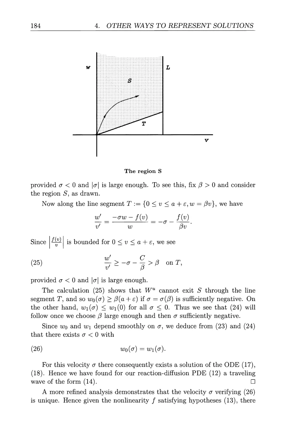
Text
Partial Differential
Equations
SECOND EDITION
Lawrence C. Evans
Department of Mathematics
University of California, Berkeley
Graduate Studies
in Mathematics
Volume 19
American Mathematical Society
*-^~v Providence, Rhode Island
This is the second edition of the now definitive text on partial differential
equations (PDE). It offers a comprehensive survey of modern techniques in the
theoretical study of PDE with particular emphasis on nonlinear equations. Its
wide scope and clear exposition make it a great text for a graduate course in
PDE. For this edition, the author has made numerous changes, including
• a new chapter on nonlinear wave equations,
• more than 80 new exercises,
• several new sections,
• a significantly expanded bibliography.
About the First Edition:
/ have used this book for both regular PDE and topics courses. It has a wonderful
combination of insight and technical detail.... Evans'book is evidence of his mastering
of the field and the clarity of presentation.
—Luis Caffarelli, University of Texas
It is fun to teach from Evans' book. It explains many of the essential ideas and
techniques of partial differential equations ... Every graduate student in analysis should
read it
—David Jerison, MIT
I use Partial Differential Equations to prepare my students for their Topic exam,
which is a requirement before starting working on their dissertation. The book provides
an excellent account ofPDE's ... I am very happy with the preparation it provides my
students.
—Carlos Kenig, University of Chicago
Evans'book has already attained the status of a classic. It is a clear choice for students
just learning the subject, as well as for experts who wish to broaden their knowledge
...An outstanding reference for many aspects of the field.
—Rafe Mazzeo, Stanford University
Editorial Board
James E. Humphreys (Chair)
David J. Saltman
David Sattinger
Julius L. Shaneson
2010 Mathematics Subject Classification. Primary 35-XX; Secondary 49-XX, 47Hxx.
For additional information and updates on this book, visit
www.ams.org/bookpages/gsm-19
Library of Congress Cataloging-in-Publication Data
Evans, Lawrence C, 1949-
Partial differential equations / Lawrence C. Evans. — 2nd ed.
p. cm. - (Graduate studies in mathematics ; v. 19)
Includes bibliographical references and index.
ISBN 978-0-8218-4974-3 (alk. paper)
1. Differential equations, Partial. I. Title.
QA377.E95 2010
515/.353-dc22 2009044716
Copying and reprinting. Individual readers of this publication, and nonprofit libraries
acting for them, are permitted to make fair use of the material, such as to copy a chapter for use
in teaching or research. Permission is granted to quote brief passages from this publication in
reviews, provided the customary acknowledgment of the source is given.
Republication, systematic copying, or multiple reproduction of any material in this publication
is permitted only under license from the American Mathematical Society. Requests for such
permission should be addressed to the Acquisitions Department, American Mathematical Society,
201 Charles Street, Providence, Rhode Island 02904-2294 USA. Requests can also be made by
e-mail to reprint-permission@ams.org.
First Edition © 1998 by the American Mathematical Society All rights reserved.
Reprinted with corrections 1999, 2002
Second Edition © 2010 by the American Mathematical Society All rights reserved.
The American Mathematical Society retains all rights
except those granted to the United States Government.
Printed in the United States of America.
@ The paper used in this book is acid-free and falls within the guidelines
established to ensure permanence and durability.
Visit the AMS home page at http://www.ams.org/
10 9 8 7 6 5 4 3 2 1 15 14 13 12 11 10
I dedicate this book to the memory of my parents,
LAWRENCE S. EVANS and LOUISE J. EVANS.
CONTENTS
Preface to second edition xvii
Preface to first edition xix
1. Introduction 1
1.1. Partial differential equations 1
1.2. Examples 3
1.2.1. Single partial differential equations 3
1.2.2. Systems of partial differential equations 6
1.3. Strategies for studying PDE 6
1.3.1. Well-posed problems, classical solutions 7
1.3.2. Weak solutions and regularity 7
1.3.3. Typical difficulties 9
1.4. Overview 9
1.5. Problems 12
1.6. References 13
PART I: REPRESENTATION FORMULAS
FOR SOLUTIONS
2. Four Important Linear PDE 17
2.1. Transport equation 18
2.1.1. Initial-value problem 18
2.1.2. Nonhomogeneous problem 19
2.2. Laplace's equation 20
2.2.1. Fundamental solution 21
2.2.2. Mean-value formulas 25
2.2.3. Properties of harmonic functions 26
2.2.4. Green's function 33
2.2.5. Energy methods 41
2.3. Heat equation 44
2.3.1. Fundamental solution 45
2.3.2. Mean-value formula 51
2.3.3. Properties of solutions 55
2.3.4. Energy methods 62
2.4. Wave equation 65
2.4.1. Solution by spherical means 67
2.4.2. Nonhomogeneous problem 80
2.4.3. Energy methods 82
2.5. Problems 84
2.6. References 90
3. Nonlinear First-Order PDE 91
3.1. Complete integrals, envelopes 92
3.1.1. Complete integrals 92
3.1.2. New solutions from envelopes 94
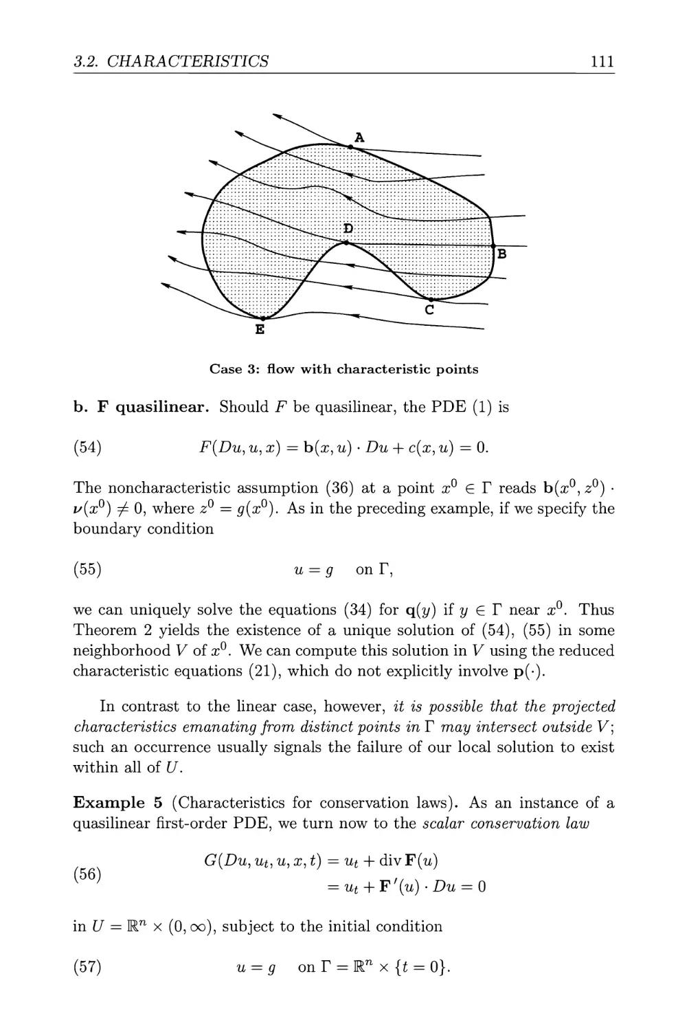
3.2. Characteristics 96
3.2.1. Derivation of characteristic ODE 96
3.2.2. Examples 99
3.2.3. Boundary conditions 102
3.2.4. Local solution 105
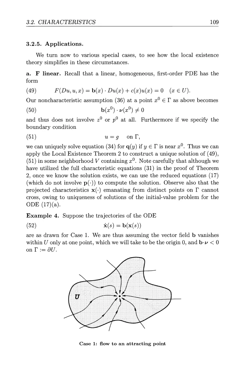
3.2.5. Applications 109
3.3. Introduction to Hamilton-Jacobi equations 114
3.3.1. Calculus of variations, Hamilton's ODE 115
3.3.2. Legendre transform, Hopf-Lax formula 120
3.3.3. Weak solutions, uniqueness 128
3.4. Introduction to conservation laws 135
3.4.1. Shocks, entropy condition 136
3.4.2. Lax-Oleinik formula 143
3.4.3. Weak solutions, uniqueness 148
CONTENTS ix
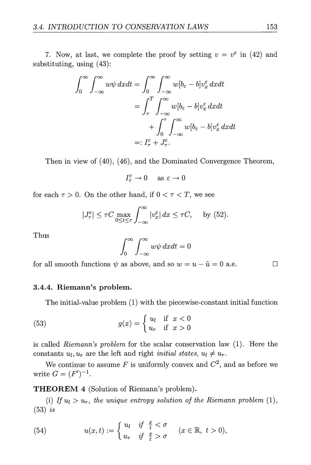
3.4.4. Riemann's problem 153
3.4.5. Long time behavior 156
3.5. Problems 161
3.6. References 165
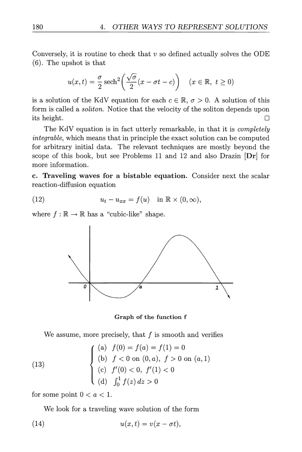
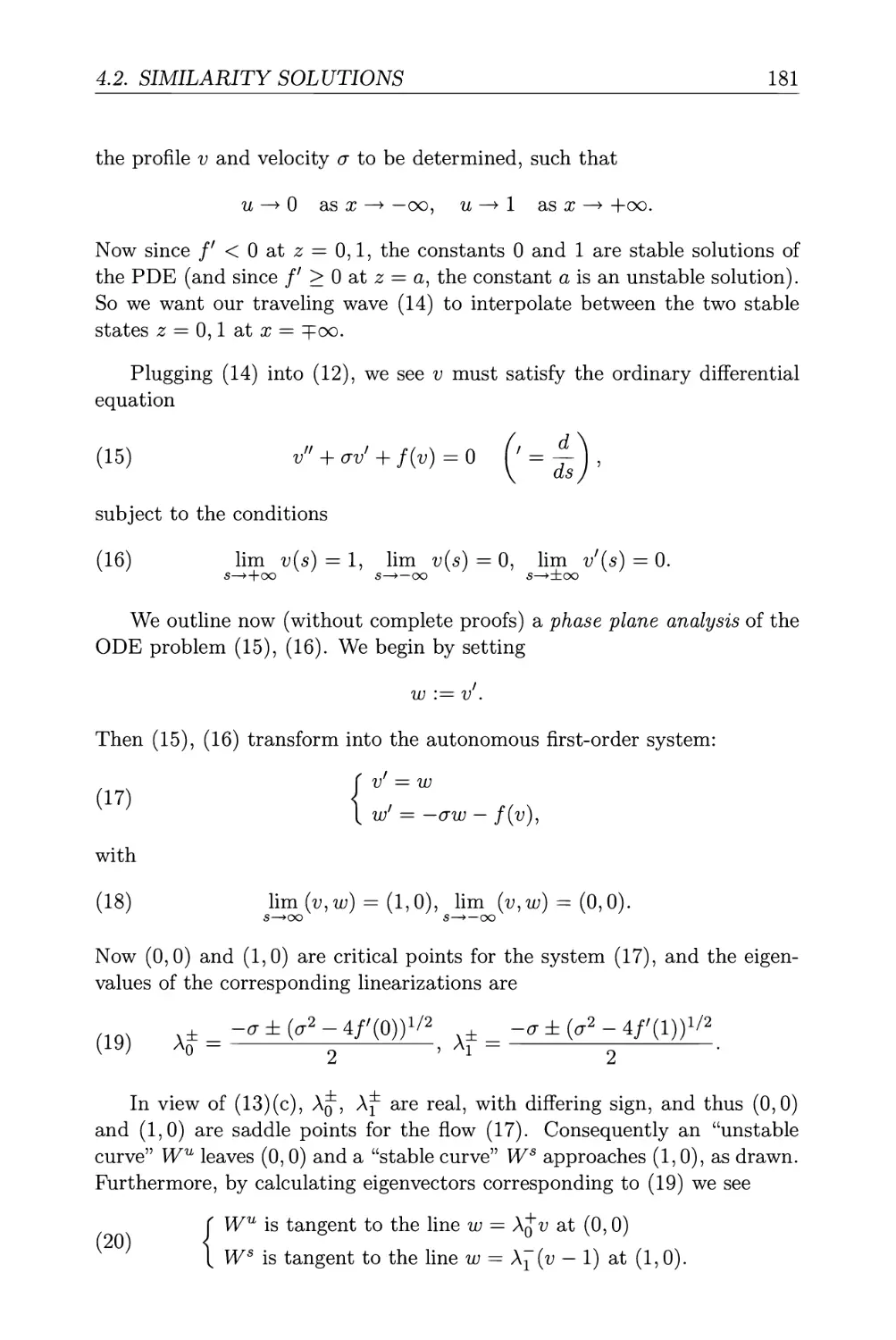
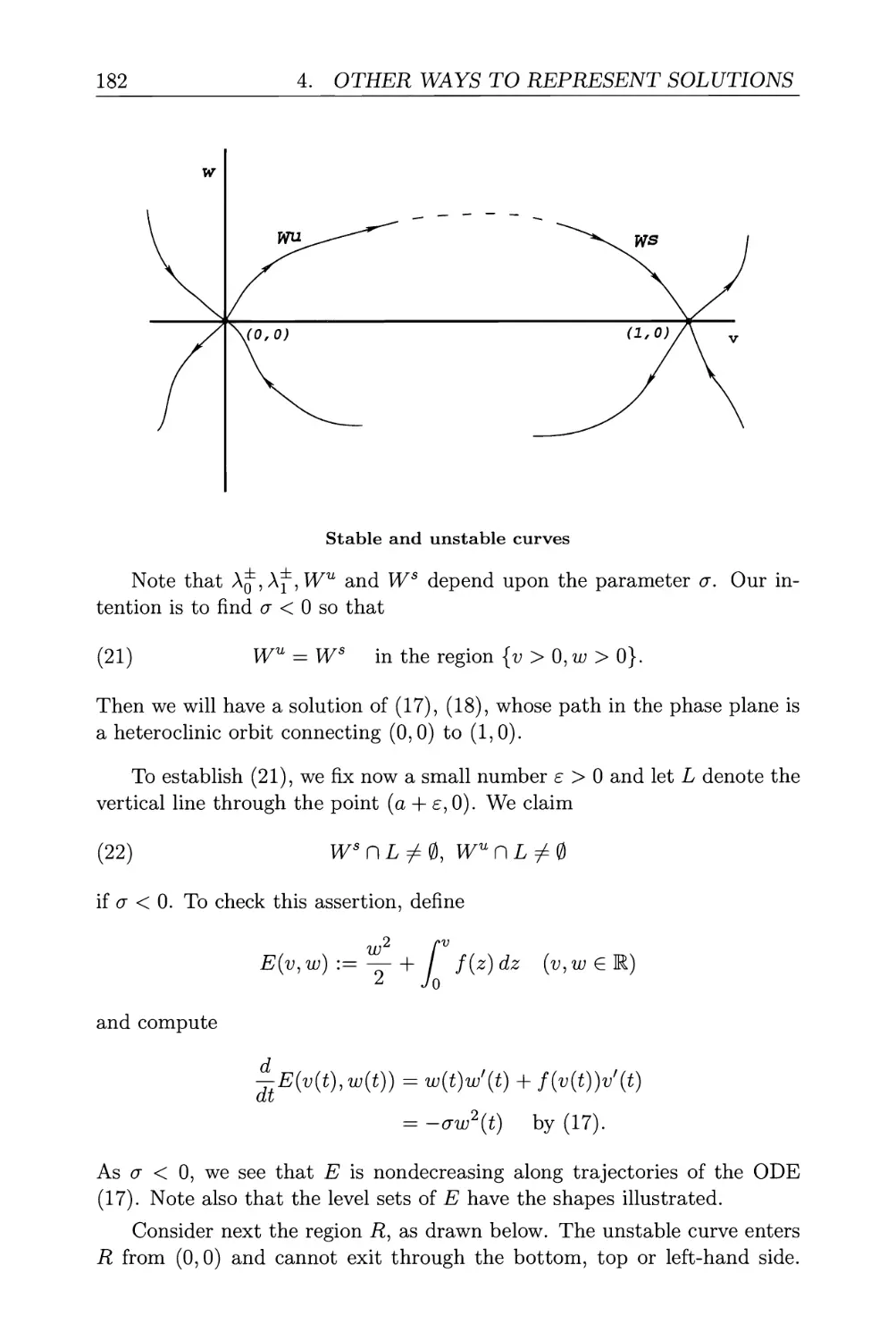
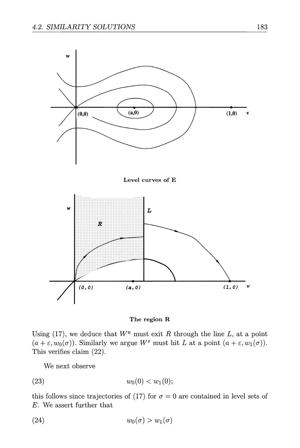
4. Other Ways to Represent Solutions 167
4.1. Separation of variables 167
4.1.1. Examples 168
4.1.2. Application: Turing instability 172
4.2. Similarity solutions 176
4.2.1. Plane and traveling waves, solitons 176
4.2.2. Similarity under scaling 185
4.3. Transform methods 187
4.3.1. Fourier transform 187
4.3.2. Radon transform 196
4.3.3. Laplace transform 203
4.4. Converting nonlinear into linear PDE 206
4.4.1. Cole-Hopf transformation 206
4.4.2. Potential functions 208
4.4.3. Hodograph and Legendre transforms 209
4.5. Asymptotics 211
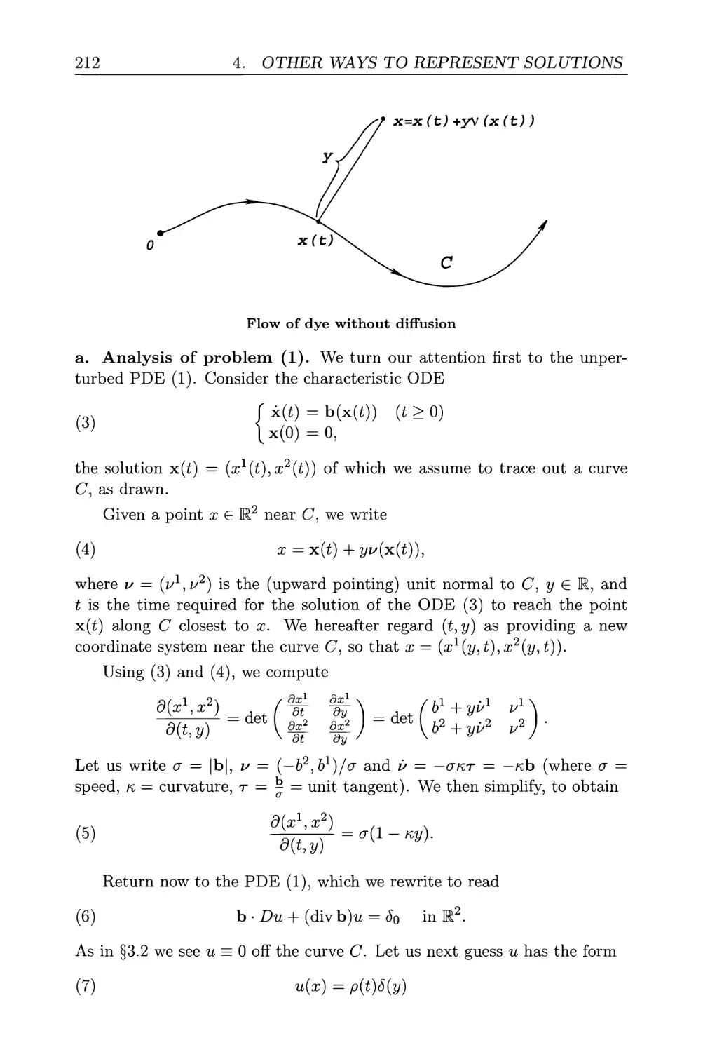
4.5.1. Singular perturbations 211
4.5.2. Laplace's method 216
4.5.3. Geometric optics, stationary phase 218
4.5.4. Homogenization 229
4.6. Power series 232
4.6.1. Noncharacteristic surfaces 232
4.6.2. Real analytic functions 237
4.6.3. Cauchy-Kovalevskaya Theorem 239
4.7. Problems 244
4.8. References 249
PART II: THEORY FOR LINEAR PARTIAL
DIFFERENTIAL EQUATIONS
5. Sobolev Spaces 253
5.1. Holder spaces 254
5.2. Sobolev spaces 255
5.2.1. Weak derivatives 255
5.2.2. Definition of Sobolev spaces 258
5.2.3. Elementary properties 261
5.3. Approximation 264
5.3.1. Interior approximation by smooth functions . . . 264
5.3.2. Approximation by smooth functions 265
5.3.3. Global approximation by smooth functions .... 266
5.4. Extensions 268
5.5. Traces 271
5.6. Sobolev inequalities 275
5.6.1. Gagliardo-Nirenberg-Sobolev inequality 276
5.6.2. Morrey's inequality 280
5.6.3. General Sobolev inequalities 284
5.7. Compactness 286
5.8. Additional topics 289
5.8.1. Poincare's inequalities 289
5.8.2. Difference quotients 291
5.8.3. Differentiability a.e 295
5.8.4. Hardy's inequality 296
5.8.5. Fourier transform methods 297
5.9. Other spaces of functions 299
5.9.1. The space Я"1 299
5.9.2. Spaces involving time 301
5.10. Problems 305
5.11. References 309
6. Second-Order Elliptic Equations 311
6.1. Definitions 311
6.1.1. Elliptic equations 311
6.1.2. Weak solutions 313
6.2. Existence of weak solutions 315
6.2.1. Lax-Milgram Theorem 315
6.2.2. Energy estimates 317
6.2.3. Fredholm alternative 320
CONTENTS
6.3. Regularity 326
6.3.1. Interior regularity 327
6.3.2. Boundary regularity 334
6.4. Maximum principles 344
6.4.1. Weak maximum principle 344
6.4.2. Strong maximum principle 347
6.4.3. Harnack's inequality 351
6.5. Eigenvalues and eigenfunctions 354
6.5.1. Eigenvalues of symmetric elliptic operators .... 354
6.5.2. Eigenvalues of nonsymmetric elliptic operators . 360
6.6. Problems 365
6.7. References 370
7. Linear Evolution Equations 371
7.1. Second-order parabolic equations 371
7.1.1. Definitions 372
7.1.2. Existence of weak solutions 375
7.1.3. Regularity 380
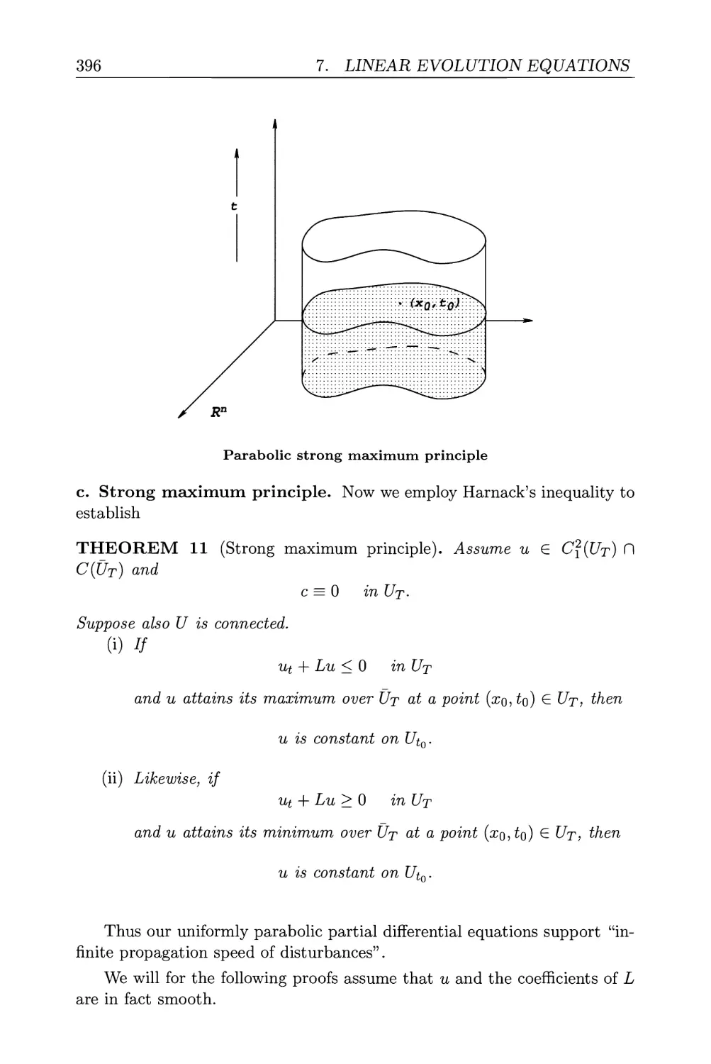
7.1.4. Maximum principles 389
7.2. Second-order hyperbolic equations 398
7.2.1. Definitions 398
7.2.2. Existence of weak solutions 401
7.2.3. Regularity 408
7.2.4. Propagation of disturbances 414
7.2.5. Equations in two variables 418
7.3. Hyperbolic systems of first-order equations 421
7.3.1. Definitions 421
7.3.2. Symmetric hyperbolic systems 423
7.3.3. Systems with constant coefficients 429
7.4. Semigroup theory 433
7.4.1. Definitions, elementary properties 434
7.4.2. Generating contraction semigroups 439
7.4.3. Applications 441
7.5. Problems 446
7.6. References 449
PART III: THEORY FOR NONLINEAR PARTIAL
DIFFERENTIAL EQUATIONS
8. The Calculus of Variations 453
8.1. Introduction 453
8.1.1. Basic ideas 453
8.1.2. First variation, Euler-Lagrange equation 454
8.1.3. Second variation 458
8.1.4. Systems 459
8.2. Existence of minimizers 465
8.2.1. Coercivity, lower semicontinuity 465
8.2.2. Convexity 467
8.2.3. Weak solutions of Euler-Lagrange equation . . . 472
8.2.4. Systems 475
8.2.5. Local minimizers 480
8.3. Regularity 482
8.3.1. Second derivative estimates 483
8.3.2. Remarks on higher regularity 486
8.4. Constraints 488
8.4.1. Nonlinear eigenvalue problems 488
8.4.2. Unilateral constraints, variational inequalities . 492
8.4.3. Harmonic maps 495
8.4.4. Incompressibility 497
8.5. Critical points 501
8.5.1. Mountain Pass Theorem 501
8.5.2. Application to semilinear elliptic PDE 507
8.6. Invariance, Noether's Theorem 511
8.6.1. Invariant variational problems 512
8.6.2. Noether's Theorem 513
8.7. Problems 520
8.8. References 525
9. Nonvariational Techniques 527
9.1. Monotonicity methods 527
9.2. Fixed point methods 533
9.2.1. Banach's Fixed Point Theorem 534
CONTENTS xiii
9.2.2. Schauder's, Schaefer's Fixed Point Theorems . . 538
9.3. Method of subsolutions and supersolutions 543
9.4. Nonexistence of solutions 547
9.4.1. Blow-up 547
9.4.2. Derrick-Pohozaev identity 551
9.5. Geometric properties of solutions 554
9.5.1. Star-shaped level sets 554
9.5.2. Radial symmetry 555
9.6. Gradient flows 560
9.6.1. Convex functions on Hilbert spaces 560
9.6.2. Subdifferentials and nonlinear semigroups .... 565
9.6.3. Applications 571
9.7. Problems 573
9.8. References 577
10. Hamilton—Jacobi Equations 579
10.1. Introduction, viscosity solutions 579
10.1.1. Definitions 581
10.1.2. Consistency 583
10.2. Uniqueness 586
10.3. Control theory, dynamic programming 590
10.3.1. Introduction to optimal control theory 591
10.3.2. Dynamic programming 592
10.3.3. Hamilton-Jacobi-Bellman equation 594
10.3.4. Hopf-Lax formula revisited 600
10.4. Problems 603
10.5. References 606
11. Systems of Conservation Laws 609
11.1. Introduction 609
11.1.1. Integral solutions 612
11.1.2. Traveling waves, hyperbolic systems 615
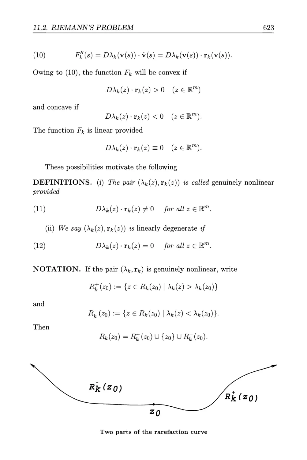
11.2. Riemann's problem 621
11.2.1. Simple waves 621
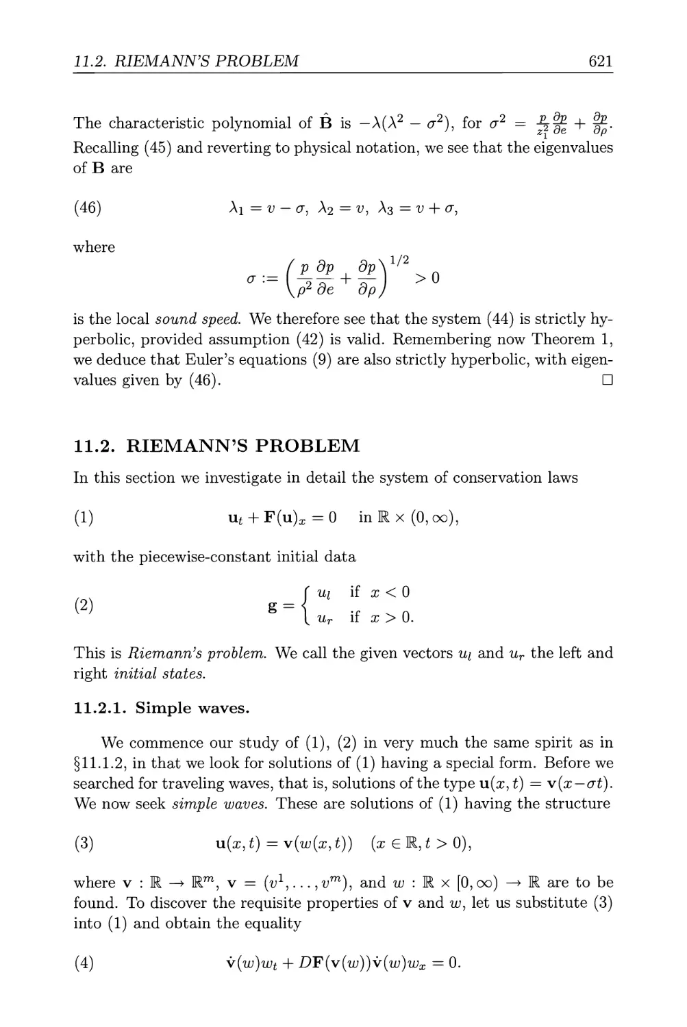
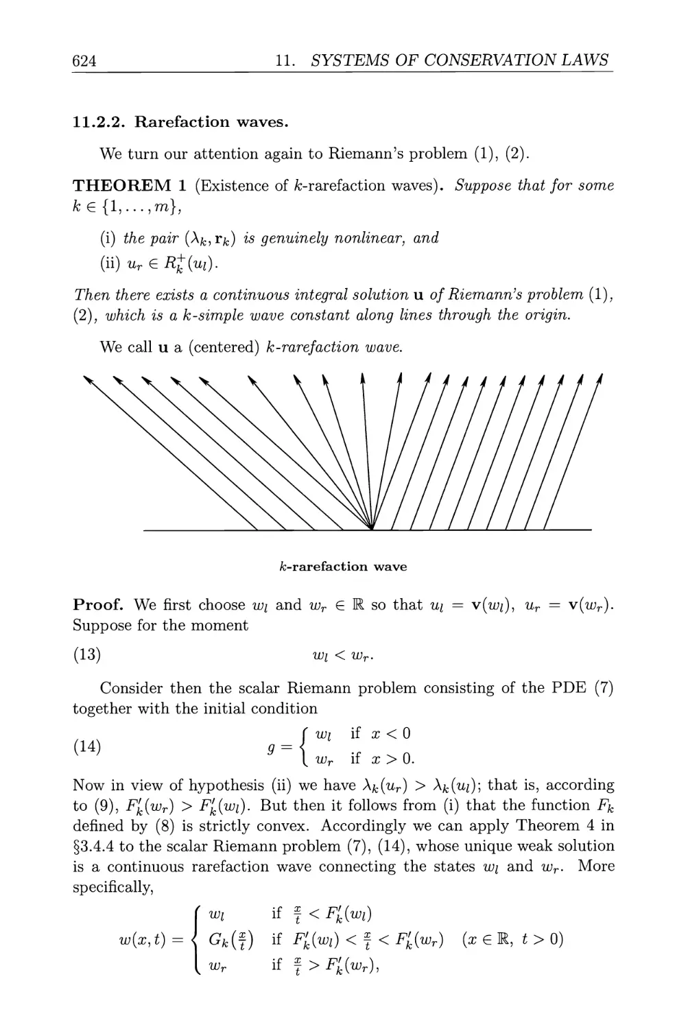
11.2.2. Rarefaction waves 624
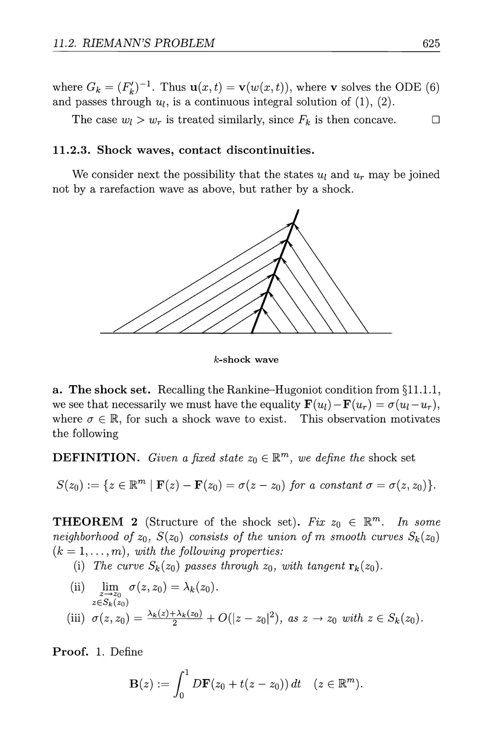
11.2.3. Shock waves, contact discontinuities 625
xiv CONTENTS
11.2.4. Local solution of Riemann's problem 632
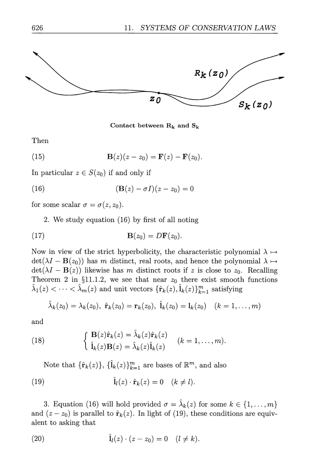
11.3. Systems of two conservation laws 635
11.3.1. Riemann invariants 635
11.3.2. Nonexistence of smooth solutions 639
11.4. Entropy criteria 641
11.4.1. Vanishing viscosity, traveling waves 642
11.4.2. Entropy/entropy-flux pairs 646
11.4.3. Uniqueness for scalar conservation laws 649
11.5. Problems 654
11.6. References 657
12. Nonlinear Wave Equations 659
12.1. Introduction 659
12.1.1. Conservation of energy 660
12.1.2. Finite propagation speed 660
12.2. Existence of solutions 663
12.2.1. Lipschitz nonlinearities 663
12.2.2. Short time existence 666
12.3. Semilinear wave equations 670
12.3.1. Sign conditions 670
12.3.2. Three space dimensions 674
12.3.3. Subcritical power nonlinearities 676
12.4. Critical power nonlinearity 679
12.5. Nonexistence of solutions 686
12.5.1. Nonexistence for negative energy 687
12.5.2. Nonexistence for small initial data 689
12.6. Problems 691
12.7. References 696
APPENDICES
Appendix A: Notation 697
A.l. Notation for matrices 697
A.2. Geometric notation 698
A.3. Notation for functions 699
A.4. Vector-valued functions 703
A.5. Notation for estimates 703
CONTENTS xv
A.6. Some comments about notation 704
Appendix B: Inequalities 705
B.l. Convex functions 705
B.2. Useful inequalities 706
Appendix C: Calculus 710
C.l. Boundaries 710
C.2. Gauss-Green Theorem 711
C.3. Polar coordinates, coarea formula 712
C.4. Moving regions 713
C.5. Convolution and smoothing 713
C.6. Inverse Function Theorem 716
C.7. Implicit Function Theorem 717
C.8. Uniform convergence 718
Appendix D: Functional Analysis 719
D.l. Banach spaces 719
D.2. Hilbert spaces 720
D.3. Bounded linear operators 721
D.4. Weak convergence 723
D.5. Compact operators, Fredholm theory 724
D.6. Symmetric operators 728
Appendix E: Measure Theory 729
E.l. Lebesgue measure 729
E.2. Measurable functions and integration 730
E.3. Convergence theorems for integrals 731
E.4. Differentiation 732
E.5. Banach space-valued functions 733
Bibliography 735
Index 741
Preface to the second
edition
Let me thank everyone who over the past decade has provided me with
suggestions and corrections for improving the first edition of this book. I
am extraordinarily grateful. Although I have not always followed these many
pieces of advice and criticism, I have thought carefully about them all. So
many people have helped me out that it is unfortunately no longer feasible to
list all their names. I have also received extraordinary help from everyone at
the AMS, especially Sergei Gelfand, Stephen Moye and Arlene O'Sean. The
NSF has generously supported my research during the writing of both the
original edition of the book and this revision. I will continue to maintain
lists of errors on my homepage, accessible through the math.berkeley.edu
website.
When you write a big book on a big subject, the temptation is to include
everything. A critic famously once imagined Tolstoy during the writing of
War and Peace: "The book is long, but even if it were twice as long, if
it were three times as long, there would always be scenes that have been
omitted, and these Tolstoy, waking up in the middle of the night, must have
regretted. There must have been a night when it occurred to him that he
had not included a yacht race..."(G. Moore, Avowals).
This image notwithstanding, I have tried to pack into this second edition
as many fascinating new topics in partial differential equations (PDE) as I
could manage, most notably in the new Chapter 12 on nonlinear wave
equations. There are new sections on Noether's Theorem and on local minimizers
in the calculus of variations, on the Radon transform, on Turing
instabilities for reaction-diffusion systems, etc. I have rewritten and expanded the
xvn
XV111
PREFACE TO THE SECOND EDITION
previous discussions on blow-up of solutions, on group and phase velocities,
and on several further subjects. I have also updated and greatly increased
citations to books in the bibliography and have moved references to research
articles to within the text. There are countless further minor modifications
in notation and wording. Most importantly, I have added about 80 new
exercises, most quite interesting and some rather elaborate. There are now
over 200 in total.
And there is a yacht race among the problems for Chapter 10.
LCE
January, 2010
Berkeley
Preface to the first
edition
I present in this book a wide-ranging survey of many important topics in
the theory of partial differential equations (PDE), with particular emphasis
on various modern approaches. I have made a huge number of editorial
decisions about what to keep and what to toss out, and can only claim
that this selection seems to me about right. I of course include the usual
formulas for solutions of the usual linear PDE, but also devote large amounts
of exposition to energy methods within Sobolev spaces, to the calculus of
variations, to conservation laws, etc.
My general working principles in the writing have been these:
a. PDE theory is (mostly) not restricted to two independent
variables. Many texts describe PDE as if functions of the two variables (x, y)
or (x, t) were all that matter. This emphasis seems to me misleading, as
modern discoveries concerning many types of equations, both linear and
nonlinear, have allowed for the rigorous treatment of these in any number
of dimensions. I also find it unsatisfactory to "classify" partial differential
equations: this is possible in two variables, but creates the false impression
that there is some kind of general and useful classification scheme available
in general.
b. Many interesting equations are nonlinear. My view is that overall
we know too much about linear PDE and too little about nonlinear PDE. I
have accordingly introduced nonlinear concepts early in the text and have
tried hard to emphasize everywhere nonlinear analogues of the linear theory.
xix
XX
PREFACE TO THE FIRST EDITION
c. Understanding generalized solutions is fundamental. Many of the
partial differential equations we study, especially nonlinear first-order
equations, do not in general possess smooth solutions. It is therefore essential to
devise some kind of proper notion of generalized or weak solution. This is
an important but subtle undertaking, and much of the hardest material in
this book concerns the uniqueness of appropriately defined weak solutions.
d. PDE theory is not a branch of functional analysis. Whereas
certain classes of equations can profitably be viewed as generating abstract
operators between Banach spaces, the insistence on an overly abstract
viewpoint, and consequent ignoring of deep calculus and measure theoretic
estimates, is ultimately limiting.
e. Notation is a nightmare. I have really tried to introduce consistent
notation, which works for all the important classes of equations studied.
This attempt is sometimes at variance with notational conventions within a
given subarea.
f. Good theory is (almost) as useful as exact formulas. I incorporate
this principle into the overall organization of the text, which is subdivided
into three parts, roughly mimicking the historical development of PDE
theory itself. Part I concerns the search for explicit formulas for solutions, and
Part II the abandoning of this quest in favor of general theory asserting
the existence and other properties of solutions for linear equations. Part III
is the mostly modern endeavor of fashioning general theory for important
classes of nonlinear PDE.
Let me also explicitly comment here that I intend the development
within each section to be rigorous and complete (exceptions being the frankly
heuristic treatment of asymptotics in §4.5 and an occasional reference to a
research paper). This means that even locally within each chapter the topics
do not necessarily progress logically from "easy" to "hard" concepts. There
are many difficult proofs and computations early on, but as compensation
many easier ideas later. The student should certainly omit on first reading
some of the more arcane proofs.
I wish next to emphasize that this is a textbook, and not a reference
book. I have tried everywhere to present the essential ideas in the clearest
possible settings, and therefore have almost never established sharp versions
of any of the theorems. Research articles and advanced monographs, many
of them listed in the Bibliography, provide such precision and generality.
My goal has rather been to explain, as best I can, the many fundamental
ideas of the subject within fairly simple contexts.
PREFACE TO THE FIRST EDITION
xxi
I have greatly profited from the comments and thoughtful suggestions
of many of my colleagues, friends and students, in particular: S. Antman,
J. Bang, X. Chen, A. Chorin, M. Christ, J. Cima, P. Colella, J. Cooper,
M. Crandall, B. Driver, M. Feldman, M. Fitzpatrick, R. Gariepy, J.
Goldstein, D. Gomes, 0. Hald, W. Han, W. Hrusa, T. Ilmanen, I. Ishii, I. Israel,
R. Jerrard, C. Jones, B. Kawohl, S. Koike, J. Lewis, T.-P. Liu, H. Lopes,
J. McLaughlin, K. Miller, J. Morford, J. Neu, M. Portilheiro, J. Ralston,
F. Rezakhanlou, W. Schlag, D. Serre, P. Souganidis, J. Strain, W. Strauss,
M. Struwe, R. Temam, B. Tvedt, J.-L. Vazquez, M. Weinstein, P. Wolfe,
and Y. Zheng.
I especially thank Tai-Ping Liu for many years ago writing out for me
the first draft of what is now Chapter 11.
I am extremely grateful for the suggestions and lists of mistakes from
earlier drafts of this book sent to me by many readers, and I encourage others
to send me their comments, at evans@math.berkeley.edu. I have come to
realize that I must be more than slightly mad to try to write a book of
this length and complexity, but I am not yet crazy enough to think that I
have made no mistakes. I will therefore maintain a listing of errors
which come to light, and will make this accessible through the
math.berkeley.edu homepage.
Faye Yeager at UC Berkeley has done a really magnificent job typing
and updating these notes, and Jaya Nagendra heroically typed an earlier
version at the University of Maryland. My deepest thanks to both.
I have been supported by the NSF during much of the writing, most
recently under grant DMS-9424342.
LCE
August, 1997
Berkeley
Chapter 1
INTRODUCTION
1.1 Partial differential equations
1.2 Examples
1.3 Strategies for studying PDE
1.4 Overview
1.5 Problems
1.6 References
This chapter surveys the principal theoretical issues concerning the
solving of partial differential equations.
To follow the subsequent discussion, the reader should first of all turn
to Appendix A and look over the notation presented there, particularly the
multiindex notation for partial derivatives.
1.1. PARTIAL DIFFERENTIAL EQUATIONS
A partial differential equation (PDE) is an equation involving an unknown
function of two or more variables and certain of its partial derivatives.
Using the notation explained in Appendix A, we can write out
symbolically a typical PDE, as follows. Fix an integer к > 1 and let U denote an
open subset of Шп.
DEFINITION. An expression of the form
(1) F(Dku{x),Dk~1u(x),...,Du(x),u{x),x) = 0 (x e U)
is called a kth-order partial differential equation, where
F : Rn* x Rnk~l x...xfxKx[/^K
1
2
1. INTRODUCTION
is given and
u: U ^R
is the unknown.
We solve the PDE if we find all и verifying (1), possibly only among those
functions satisfying certain auxiliary boundary conditions on some part Г
of dU. By finding the solutions we mean, ideally, obtaining simple, explicit
solutions, or, failing that, deducing the existence and other properties of
solutions.
DEFINITIONS.
(i) The partial differential equation (I) is called linear if it has the form
^ aa{x)D«u = f{x)
\a\<k
for given functions aa (|oj| < £;), /. This linear PDE is homogeneous
(ii) The PDE (I) is semilinear if it has the form
У^ aa(x)Dau + a$(Dk~lu,..., Du, u, x) = 0.
|a|=*
(iii) The PDE (I) is quasilinear if it has the form
У^ aa(Dk~1u,..., Du, u, x)Dau + ао{Ок~хи,..., Du, u, x) = 0.
\a\=k
(iv) The PDE (1) is fully nonlinear if it depends nonlinearly upon the
highest order derivatives.
A system of partial differential equations is, informally speaking, a
collection of several PDE for several unknown functions.
DEFINITION. An expression of the form
(2) F(Dku(x), D^uix),..., Du(x), u(x), x) = 0 (x e U)
is called a kth-order system of partial differential equations, where
F : Rmnk x Rmnk~l x • • • x Rmn xRmx[/^Rm
is given and
is the unknown.
Here we are supposing that the system comprises the same number m
of scalar equations as unknowns (гх1,... ,um). This is the most common
circumstance, although other systems may have fewer or more equations
than unknowns. Systems are classified in the obvious way as being linear,
semilinear, etc.
1.2. EXAMPLES
3
NOTATION. We write "PDE" as an abbreviation for both the singular
"partial differential equation" and the plural "partial differential equations".
1.2. EXAMPLES
There is no general theory known concerning the solvability of all partial
differential equations. Such a theory is extremely unlikely to exist, given
the rich variety of physical, geometric, and probabilistic phenomena which
can be modeled by PDE. Instead, research focuses on various particular
partial differential equations that are important for applications within and
outside of mathematics, with the hope that insight from the origins of these
PDE can give clues as to their solutions.
Following is a list of many specific partial differential equations of
interest in current research. This listing is intended merely to familiarize the
reader with the names and forms of various famous PDE. To display most
clearly the mathematical structure of these equations, we have mostly set
relevant physical constants to unity. We will later discuss the origin and
interpretation of many of these PDE.
Throughout x G ?7, where U is an open subset of Rn, and t > 0. Also
Du = Dxи = (гхХ1,..., гхХп) denotes the gradient of и with respect to the
spatial variable x = (xi,..., xn). The variable t always denotes time.
1.2.1. Single partial differential equations.
a. Linear equations.
1. Laplace's equation
n
Au = ^uXiXi =0.
г=1
2. Helmholtz's (or eigenvalue) equation
—Au = Xu.
3. Linear transport equation
n
Щ + Y^ biu*i = °-
г=1
4. Liouville's equation
n
4
1. INTRODUCTION
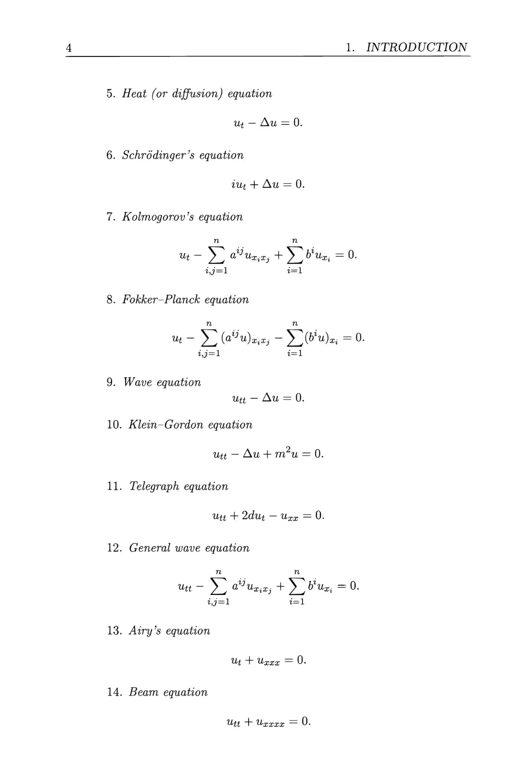
5. Heat (or diffusion) equation
щ — Au = О.
6. Schrodinger's equation
iut + Au = 0.
7. Kolmogorov's equation
n n
щ - ^2 a%JuxiXj + ^2 b%Uxi= °*
i,j=l г=1
8. Fokker-Planck equation
n n
ut~Yl (aiju)^xj - ^2(biu)xi = o.
ij=l г=1
9. Wave equation
uu - Au = 0.
10. Klein-Gordon equation
uu — Au + m2u = 0.
11. Telegraph equation
uu + 2dut - uxx = 0.
12. General wave equation
n n
UU ~ ^2 a%JuXiXj + ^2 b%Uxi = 0*
13. Airy's equation
Щ + uxxx = 0.
14. Beam equation
Utt i Uxxxx = U.
1.2. EXAMPLES
5
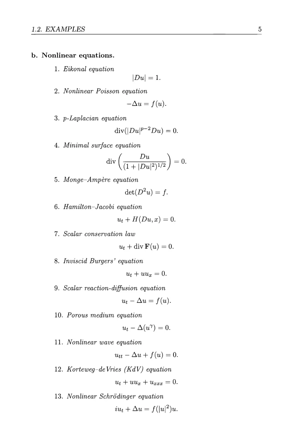
b. Nonlinear equations.
1. Eikonal equation
\Du\ = 1.
2. Nonlinear Poisson equation
-Au = f{u).
3. p-Laplacian equation
div(\Du\p-2Du) = 0.
4. Minimal surface equation
dlV \(l + \Du\*)V2) =
5. Monge-Ampere equation
det(D2u) = /.
6. Hamilton-Jacobi equation
ut + H{Du,x) = 0.
7. Scalar conservation law
ut + divF(u) =0.
8. Inviscid Burgers' equation
щ + uux = 0.
9. Scalar reaction-diffusion equation
щ - Au = f(u).
10. Porous medium equation
ut - A(tx7) = 0.
11. Nonlinear wave equation
utt-Au + f(u) = 0.
12. Korteweg-deVries (KdV) equation
щ + гшя + uxxx = 0.
13. Nonlinear Schrodinger equation
iut + Au = /(|гб|2)гб.
6
1. INTRODUCTION
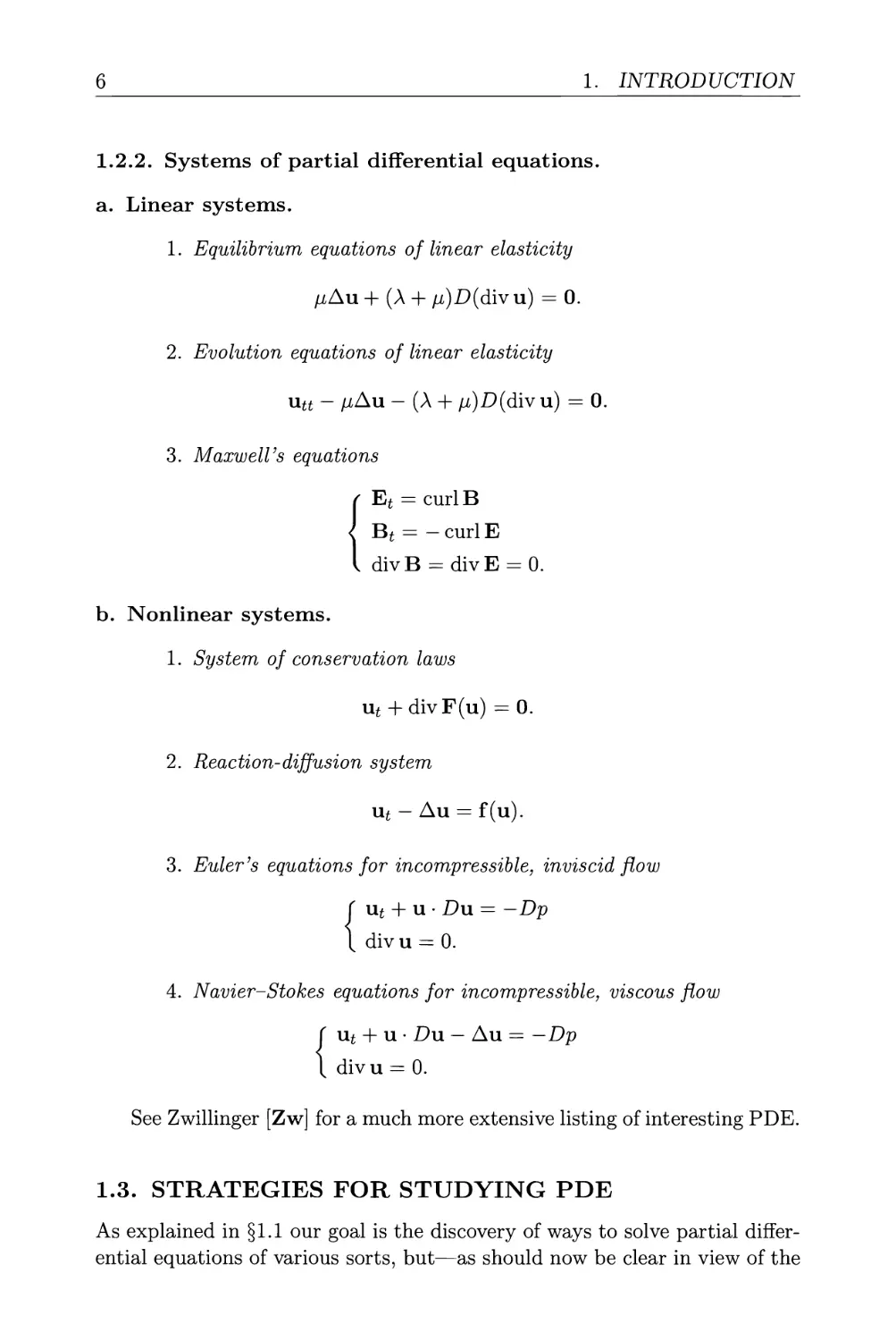
1.2.2. Systems of partial differential equations.
a. Linear systems.
1. Equilibrium equations of linear elasticity
/iAu + (Л + /i)£>(div u) = 0.
2. Evolution equations of linear elasticity
utt - /iAu - (Л + n)D(div u) = 0.
3. Maxwell's equations
Et = curl В
Bt = -curlE
divB = divE = 0.
b. Nonlinear systems.
1. System of conservation laws
ut + divF(u) = 0.
2. Reaction-diffusion system
ut-Au = f(u).
3. Euler's equations for incompressible, inviscid flow
ut + u • Du — —Dp
div u = 0.
4. Navier-Stokes equations for incompressible, viscous flow
ut + u • Du — Au = —Dp
div u = 0.
See Zwillinger [Zw] for a much more extensive listing of interesting PDE.
1.3. STRATEGIES FOR STUDYING PDE
As explained in §1.1 our goal is the discovery of ways to solve partial
differential equations of various sorts, but—as should now be clear in view of the
1.3. STRATEGIES FOR STUDYING PDE
7
many diverse examples set forth in §1.2—this is no easy task. And indeed
the very question of what it means to "solve" a given PDE can be subtle,
depending in large part on the particular structure of the problem at hand.
1.3.1. Well-posed problems, classical solutions.
The informal notion of a well-posed problem captures many of the
desirable features of what it means to solve a PDE. We say that a given problem
for a partial differential equation is well-posed if
(i) the problem in fact has a solution;
(ii) this solution is unique;
and
(iii) the solution depends continuously on the data given in the problem.
The last condition is particularly important for problems arising from
physical applications: we would prefer that our (unique) solution changes
only a little when the conditions specifying the problem change a little. (For
many problems, on the other hand, uniqueness is not to be expected. In
these cases the primary mathematical tasks are to classify and characterize
the solutions.)
Now clearly it would be desirable to "solve" PDE in such a way that
(i)-(iii) hold. But notice that we still have not carefully defined what we
mean by a "solution". Should we ask, for example, that a "solution" и must
be real analytic or at least infinitely differentiable? This might be desirable,
but perhaps we are asking too much. Maybe it would be wiser to require a
solution of a PDE of order к to be at least к times continuously differentiable.
Then at least all the derivatives which appear in the statement of the PDE
will exist and be continuous, although maybe certain higher derivatives will
not exist. Let us informally call a solution with this much smoothness a
classical solution of the PDE: this is certainly the most obvious notion of
solution.
So by solving a partial differential equation in the classical sense we mean
if possible to write down a formula for a classical solution satisfying (i)-(iii)
above, or at least to show such a solution exists, and to deduce various of
its properties.
1.3.2. Weak solutions and regularity.
But can we achieve this? The answer is that certain specific partial
differential equations (e.g. Laplace's equation) can be solved in the classical
sense, but many others, if not most others, cannot. Consider for instance
8
1. INTRODUCTION
the scalar conservation law
щ + F(u)x = 0.
We will see in §3.4 that this PDE governs various one-dimensional
phenomena involving fluid dynamics, and in particular models the formation and
propagation of shock waves. Now a shock wave is a curve of discontinuity
of the solution щ and so if we wish to study conservation laws, and recover
the underlying physics, we must surely allow for solutions и which are not
continuously differentiable or even continuous. In general, as we shall see,
the conservation law has no classical solutions but is well-posed if we allow
for properly defined generalized or weak solutions.
This is all to say that we may be forced by the structure of the
particular equation to abandon the search for smooth, classical solutions. We
must instead, while still hoping to achieve the well-posedness conditions (i)-
(iii), investigate a wider class of candidates for solutions. And in fact, even
for those PDE which turn out to be classically solvable, it is often most
expedient initially to search for some appropriate kind of weak solution.
The point is this: if from the outset we demand that our solutions be very
regular, say fc-times continuously differentiable, then we are usually going
to have a really hard time finding them, as our proofs must then necessarily
include possibly intricate demonstrations that the functions we are building
are in fact smooth enough. A far more reasonable strategy is to consider as
separate the existence and the smoothness (or regularity) problems. The idea
is to define for a given PDE a reasonably wide notion of a weak solution, with
the expectation that since we are not asking too much by way of smoothness
of this weak solution, it may be easier to establish its existence, uniqueness,
and continuous dependence on the given data. Thus, to repeat, it is often
wise to aim at proving well-posedness in some appropriate class of weak or
generalized solutions.
Now, as noted above, for various partial differential equations this is
the best that can be done. For other equations we can hope that our weak
solution may turn out after all to be smooth enough to qualify as a classical
solution. This leads to the question of regularity of weak solutions. As we
will see, it is often the case that the existence of weak solutions depends
upon rather simple estimates plus ideas of functional analysis, whereas the
regularity of the weak solutions, when true, usually rests upon many intricate
calculus estimates.
Let me explicitly note here that once we are past Part I (Chapters 2-4),
our efforts will be largely devoted to proving mathematically the existence
of solutions to various sorts of partial differential equations, and not so much
1.4. OVERVIEW
9
to deriving formulas for these solutions. This may seem wasted or misguided
effort, but in fact mathematicians are like theologians: we regard existence
as the prime attribute of what we study. But unlike theologians, we need
not always rely upon faith alone.
1.3.3. Typical difficulties.
Following are some vague but general principles, which may be useful to
keep in mind:
(i) Nonlinear equations are more difficult than linear equations; and,
indeed, the more the nonlinearity affects the higher derivatives, the
more difficult the PDE is.
(ii) Higher-order PDE are more difficult than lower-order PDE.
(hi) Systems are harder than single equations.
(iv) Partial differential equations entailing many independent variables
are harder than PDE entailing few independent variables.
(v) For most partial differential equations it is not possible to write out
explicit formulas for solutions.
None of these assertions is without important exceptions.
1.4. OVERVIEW
This textbook is divided into three major Parts.
PART I: Representation Formulas for Solutions
Here we identify those important partial differential equations for which
in certain circumstances explicit or more-or-less explicit formulas can be had
for solutions. The general progression of the exposition is from direct
formulas for certain linear equations to far less concrete representation formulas,
of a sort, for various nonlinear PDE.
Chapter 2 is a detailed study of four exactly solvable partial
differential equations: the linear transport equation, Laplace's equation, the heat
equation, and the wave equation. These PDE, which serve as archetypes for
the more complicated equations introduced later, admit directly computable
solutions, at least in the case that there is no domain whose boundary
geometry complicates matters. The explicit formulas are augmented by various
indirect, but easy and attractive, "energy"-type arguments, which serve as
motivation for the developments in Chapters 6, 7 and thereafter.
Chapter 3 continues the theme of searching for explicit formulas, now
for general first-order nonlinear PDE. The key insight is that such PDE
10
1. INTRODUCTION
can, locally at least, be transformed into systems of ordinary differential
equations (ODE), the characteristic equations. We stipulate that once the
problem becomes "only" the question of integrating a system of ODE, it
is in principle solved, sometimes quite explicitly. The derivation of the
characteristic equations given in the text is very simple and does not require
any geometric insights. It is in truth so easy to derive the characteristic
equations that no real purpose is had by dealing with the quasilinear case
first.
We introduce also the Hopf-Lax formula for Hamilton-Jacobi
equations (§3.3) and the Lax-Oleinik formula for scalar conservation laws (§3.4).
(Some knowledge of measure theory is useful here but is not essential.) These
sections provide an early acquaintance with the global theory of these
important nonlinear PDE and so motivate the later Chapters 10 and 11.
Chapter 4 is a grab bag of techniques for explicitly (or kind of explicitly)
solving various linear and nonlinear partial differential equations, and the
reader should study only whatever seems interesting. The section on the
Fourier transform is, however, essential. The Cauchy-Kovalevskaya
Theorem appears at the very end. Although this is basically the only general
existence theorem in the subject, and thus logically should perhaps be regarded
as central, in practice these power series methods are not so prevalent.
PART II: Theory for Linear Partial Differential Equations
Next we abandon the search for explicit formulas and instead rely on
functional analysis and relatively easy "energy" estimates to prove the
existence of weak solutions to various linear PDE. We investigate also the
uniqueness and regularity of such solutions and deduce various other
properties.
Chapter 5 is an introduction to Sobolev spaces, the proper setting for
the study of many linear and nonlinear partial differential equations via
energy methods. This is a hard chapter, the real worth of which is only later
revealed, and requires some basic knowledge of Lebesgue measure theory.
However, the requirements are not really so great, and the review in
Appendix E should suffice. In my opinion there is no particular advantage in
considering only the Sobolev spaces with exponent p = 2, and indeed
insisting upon this obscures the two central inequalities, those of Gagliardo-
Nirenberg-Sobolev (§5.6.1) and of Morrey (§5.6.2).
In Chapter 6 we vastly generalize our knowledge of Laplace's equation to
other second-order elliptic equations. Here we work through a rather
complete treatment of existence, uniqueness and regularity theory for solutions,
including the maximum principle, and also a reasonable introduction to the
1.4. OVERVIEW
11
study of eigenvalues, including a discussion of the principal eigenvalue for
nonselfadjoint operators.
Chapter 7 expands the energy methods to a variety of linear partial
differential equations characterizing evolutions in time. We broaden our
earlier investigation of the heat equation to general second-order parabolic
PDE and of the wave equation to general second-order hyperbolic PDE. We
study as well linear first-order hyperbolic systems, with the aim of
motivating the developments concerning nonlinear systems of conservation laws in
Chapter 11. The concluding section 7.4 presents the alternative functional
analytic method of semigroups for building solutions.
(Missing from this long Part II on linear partial differential equations is
any discussion of distribution theory or potential theory. These are
important topics, but for our purposes seem dispensable, even in a book of such
length. These omissions do not slow us up much and make room for more
nonlinear theory.)
PART III: Theory for Nonlinear Partial Differential Equations
This section parallels for nonlinear PDE the development in Part II but
is far less unified in its approach, as the various types of nonlinearity must
be treated in quite different ways.
Chapter 8 commences the general study of nonlinear partial differential
equations with an extensive discussion of the calculus of variations. Here
we set forth a careful derivation of the direct method for deducing the
existence of minimizers and discuss also a variety of variational systems and
constrained problems, as well as minimax methods. Variational theory is
the most useful and accessible of the methods for nonlinear PDE, and so
this chapter is fundamental.
Chapter 9 is, rather like Chapter 4 earlier, a gathering of assorted other
techniques of use for nonlinear elliptic and parabolic partial differential
equations. We encounter here monotonicity and fixed point methods and a
variety of other devices, mostly involving the maximum principle. We study as
well certain nice aspects of nonlinear semigroup theory, to complement the
linear semigroup theory from Chapter 7.
Chapter 10 is an introduction to the modern theory of Hamilton-Jacobi
PDE and in particular to the notion of "viscosity solutions". We encounter
also the connections with the optimal control of ODE, through dynamic
programming.
12
1. INTRODUCTION
Chapter 11 picks up from Chapter 3 the discussion of conservation laws,
now systems of conservation laws. Unlike the general theoretical
developments in Chapters 5-9, for which Sobolev spaces provide the proper abstract
framework, we are forced to employ here direct linear algebra and calculus
computations. We pay particular attention to the solution of Riemann's
problem and to entropy criteria.
Chapter 12, an introduction to nonlinear wave equations, is new with
this edition. We provide long time and short time existence theorems for
certain quasilinear wave equations and an in-depth examination of semilinear
wave equations, especially for subcritical and critical power nonlinearities in
three space dimensions. To complement these existence theorems, the final
section identifies various criteria ensuring nonexistence of solutions.
Appendices A-E provide for the reader's convenience some background
material, with selected proofs, on inequalities, linear functional analysis,
measure theory, etc.
The Bibliography is an updated and extensive listing of interesting PDE
books to consult for further information. Since this is a textbook and not
a reference monograph, I have mostly not attempted to track down and
document the original sources for the myriads of ideas and methods we will
encounter. The mathematical literature for partial differential equations is
truly vast, but the books cited in the Bibliography should at least provide
a starting point for locating the primary sources. (Citations to selected
research papers appear throughout the text.)
1.5. PROBLEMS
1. Classify each of the partial differential equations in §1.2 as follows:
(a) Is the PDE linear, semilinear, quasilinear or fully nonlinear?
(b) What is the order of the PDE?
2. Let A: be a positive integer. Show that a smooth function defined on
Rn has in general
/n + к - 1\ _ /n + к - 1\
V * )-{ n-1 )
distinct partial derivatives of order k.
(Hint: This is the number of ways of inserting n — 1 dividers | within
a row of к symbols o: for example, oo||ooo|o|ooo||oooo|.
Explain why each such pattern corresponds to precisely one of the
partial derivatives of order A;.)
1.6. REFERENCES
13
The next exercises provide some practice with the multiindex notation
introduced in Appendix A.
3. Prove the Multinomial Theorem:
\a\=k ^ a '
where Д) := ^, a! = ai!a2!. ..an!, anda;a-xf...x^. The sum
is taken over all multiindices a — (ai,..., an) with |a| = k.
4. Prove Leibniz's formula:
Da(uv) = Yl (a))DPuDa-Pv,
(3<a
\(3) '— p\(cL-p)\
where u,v : Rn —> R are smooth, (*) := ./%,, and (3 < a means
Pi <oci (i = l,...,n).
5. Assume that / : Rn —► R is smooth. Prove
\k+1) asx^O
|a|</c
for each A; = 1, 2, This is Taylor's formula in multiindex notation.
(Hint: Fix x G Rn and consider the function of one variable g(i) :=
f(tx).)
1.6. REFERENCES
Klainerman's article [Kl] is a nice modern overview of the field of partial
differential equations.
Good general texts and monographs on PDE include Arnold [Ar2],
Courant-Hilbert [C-H], DiBenedetto [DB1], Folland [Fl], Friedman [Fr2].
Garabedian [G], John [J2], Jost [Jo], McOwen [MO], Mikhailov [M], Petro-
vsky [Py], Rauch [R], Renardy-Rogers [R-R], Smirnov [Sm], Smoller [S],
Strauss [St2], Taylor [Та], Thoe-Zachmanoglou [T-Z], Zauderer [Za], and
many others. The prefaces to Arnold [Ar2] and to Bernstein [Bt] are
interesting reading. Zwillinger's handbook [Zw] on differential equations is a
useful compendium of methods for PDE.
Part I
REPRESENTATION
FORMULAS FOR
SOLUTIONS
Chapter 2
FOUR IMPORTANT
LINEAR PARTIAL
DIFFERENTIAL
EQUATIONS
2.1 Transport equation
2.2 Laplace's equation
2.3 Heat equation
2.4 Wave equation
2.5 Problems
2.6 References
In this chapter we introduce four fundamental linear partial
differential equations for which various explicit formulas for solutions are available.
These are
the transport equation щ + Ь - Du — 0 (§2.1),
Laplace's equation Au — 0 (§2.2),
the heat equation щ — Au — 0 (§2.3),
the wave equation utt — Au = 0 (§2.4).
Before going further, the reader should review the discussions of
inequalities, integration by parts, Green's formulas, convolutions, etc., in
Appendices В and С and later refer back to these as necessary.
17
18
2. FOUR IMPORTANT LINEAR PDE
2.1. TRANSPORT EQUATION
One of the simplest partial differential equations is the transport equation
with constant coefficients. This is the PDE
(1) щ + b • Du = 0 in Rn x (0, oo),
where 6 is a fixed vector in Rn, b = (6i,... , 6n), and и : Rn x [0, oo) —► R
is the unknown, и — u(x,t). Here x — (xi,... , xn) G Rn denotes a typical
point in space, and t > 0 denotes a typical time. We write Du — Dxu =
(?xXl,..., nXn) for the gradient of и with respect to the spatial variables x.
Which functions и solve (1)? To answer, let us suppose for the moment
we are given some smooth solution и and try to compute it. To do so, we
first must recognize that the partial differential equation (1) asserts that a
particular directional derivative of и vanishes. We exploit this insight by
fixing any point (x, t) G Rn x (0, oo) and defining
z(s) := u(x + sb,t + s) 0 G R).
We then calculate
z(s) — Du(x + sb,t + s) • b + щ(х + sb,t + s) — 0
the second equality holding owing to (1). Thus z(-) is a constant function of
5, and consequently for each point (x,t), и is constant on the line through
(x,t) with the direction (6,1) G Rn+1. Hence if we know the value of и at
any point on each such line, we know its value everywhere in Rn x (0, oo).
2.1.1. Initial-value problem.
For definiteness therefore, let us consider the initial-value problem
( . f щ + b • Du = 0 in Rn x (0, oo)
U \ и = g on Rn x {t = 0}.
Here 6 G Rn and p : Rn —> R are known, and the problem is to compute
u. Given (x,t) as above, the line through (x,t) with direction (6,1) is
represented parametrically by (x + sb,t + s) (s G R). This line hits the
plane Г := Rn x {t = 0} when s — —t, at the point (x — tb, 0). Since и is
constant on the line and u(x — t6,0) = g(x — tb), we deduce
(3) u(x, i) = g(x - tb) (x G Rn, t > 0).
So, if (2) has a sufficiently regular solution u, it must certainly be given
by (3). And conversely, it is easy to check directly that if g is C1, then и
defined by (3) is indeed a solution of (2).
d_
ds
2.1. TRANSPORT EQUATION
19
Weak solutions. If g is not C1, then there is obviously no C1 solution of
(2). But even in this case formula (3) certainly provides a strong, and in
fact the only reasonable, candidate for a solution. We may thus informally
declare u(x, i) — g{x — tb) (x E Mn, t > 0) to be a weak solution of (2), even
should g not be C1. This all makes sense even if g and thus и are
discontinuous. Such a notion, that a nonsmooth or even discontinuous function may
sometimes solve a PDE, will come up again later when we study nonlinear
transport phenomena in §3.4.
2.1.2. Nonhomogeneous problem.
Next let us look at the associated nonhomogeneous problem
, v Г щ + b • Du = / in W1 x (0, oo)
W \ u = g onW1 x{t = 0}.
As before fix (x, t) E Mn+1 and, inspired by the calculation above, set z(s) :=
u(x + sb,t + s) for s E R. Then
£(s) = Dtx(x + 56,t + 5) • b + щ(х + sb,t + s) = f(x + 56,t + s).
Consequently
u(x, t) - g(x - tb) = z(0) - z(-t) = / z(s)
f°
— / f(x + sb,t + s)ds
t
/ f(x + (s — t)6, s) ds,
Jo
and so
(5) u(x, t) = g(x -tb)+ I f(x + (s- t)b, s) ds (x E Mn, t > 0)
Jo
solves the initial-value problem (4).
We will later employ this formula to solve the one-dimensional wave
equation, in §2.4.1.
Remark. Observe that we have derived our solutions (3), (5) by in effect
converting the partial differential equations into ordinary differential
equations. This procedure is a special case of the method of characteristics,
developed later in §3.2.
20
2. FOUR IMPORTANT LINEAR PDE
2.2. LAPLACE'S EQUATION
Among the most important of all partial differential equations are
undoubtedly Laplace's equation
(1) Au = 0
and Poisson's equation
(2) -Au = f.'
In both (1) and (2), x G U and the unknown is и : U —► R, и = u(x),
where U С Rn is a given open set. In (2) the function / : U —> R is also
given. Remember from §A.3 that the Laplacian of и is Au = X)ILi ^х*-
DEFINITION. Л C2 function и satisfying (1) is called a harmonic
function.
Physical interpretation. Laplace's equation comes up in a wide variety
of physical contexts. In a typical interpretation и denotes the density of
some quantity (e.g. a chemical concentration) in equilibrium. Then if V is
any smooth subregion within [/, the net flux of и through dV is zero:
/.
F-i/dS = 0,
dv
F denoting the flux density and v the unit outer normal field. In view of
the Gauss-Green Theorem (§C2), we have
/ divFdx= / F-i/dS = 0,
JV JdV
and so
(3) divF = 0 in 17,
since V was arbitrary. In many instances it is physically reasonable to
assume the flux F is proportional to the gradient Du but points in the opposite
direction (since the flow is from regions of higher to lower concentration).
Thus
(4) F = -aDu (a > 0).
*I prefer to write (2) with the minus sign, to be consistent with the notation for general
second-order elliptic operators in Chapter 6.
2.2. LAPLACE'S EQUATION
21
equation (4) is
Substituting into (3), we obtain Laplace's equation
div(Du) = Au = 0.
If и denotes the
chemical concentration
temperature
electrostatic potential,
Fick's law of diffusion
Fourier's law of heat conduction
Ohm's law of electrical conduction.
See Feynman-Leighton-Sands [F-L-S, Chapter 12] for a discussion of the
ubiquity of Laplace's equation in mathematical physics. Laplace's
equation arises as well in the study of analytic functions and the probabilistic
investigation of Brownian motion.
2.2.1. Fundamental solution.
a. Derivation of fundamental solution. One good strategy for
investigating any partial differential equation is first to identify some explicit
solutions and then, provided the PDE is linear, to assemble more
complicated solutions out of the specific ones previously noted. Furthermore, in
looking for explicit solutions, it is often wise to restrict attention to classes
of functions with certain symmetry properties. Since Laplace's equation is
invariant under rotations (Problem 2), it consequently seems advisable to
search first for radial solutions, that is, functions of r = \x\.
Let us therefore attempt to find a solution и of Laplace's equation (1)
in U — Rn, having the form
u(x) — v(r),
where r — \x\ — (x\ + • • • + x2)1/2 and v is to be selected (if possible) so
that Au — 0 holds. First note for г — 1,..., n that
^ = \{х1 + -+х1у1'22х^^ {x*0)-
We thus have
uXt=v\r)X^uXiX%=v>\r)f2+v\r)(±-f)
22
2. FOUR IMPORTANT LINEAR PDE
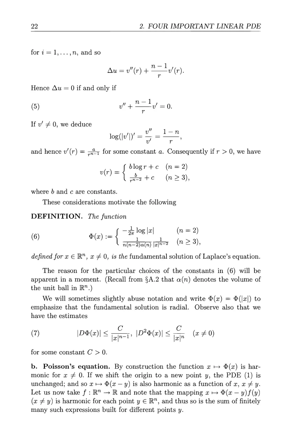
for г — 1,... , n, and so
Д^ = v/7(r) + - v'(r).
Hence Au = 0 if and only if
(5) v" + —-v' = 0.
r
If v' ф 0, we deduce
log(|i; |) = - = -^,
and hence t/(r) = -£ьт for some constant a. Consequently if r > 0, we have
Г Ы.
v(r) = <^ _,
b log r + с (n = 2)
6 +c (n>3),
-2
where 6 and с are constants.
These considerations motivate the following
DEFINITION. The function
-^Flog|x| (n = 2)
n(n-2)a(n) |x|^-2 V77, - °J'
defined for x £ Rn; x 7^ 0, is £/&e fundamental solution of Laplace's equation.
The reason for the particular choices of the constants in (6) will be
apparent in a moment. (Recall from §A.2 that a(ri) denotes the volume of
the unit ball in Rn.)
We will sometimes slightly abuse notation and write Ф(х) = Ф(|х|) to
emphasize that the fundamental solution is radial. Observe also that we
have the estimates
(7) W*)l < ^pi> |Я2Ф(*)| < ^ (x ф 0)
for some constant С > 0.
b. Poisson's equation. By construction the function x и Ф(ж) is
harmonic for x ф 0. If we shift the origin to a new point y, the PDE (1) is
unchanged; and so x 1—> Ф(х — у) is also harmonic as a function of x, x Ф y.
Let us now take / : Rn —► R and note that the mapping x 1—> Ф(х — y)f(y)
(x Ф y) is harmonic for each point у G Rn, and thus so is the sum of finitely
many such expressions built for different points y.
2.2. LAPLACE'S EQUATION
23
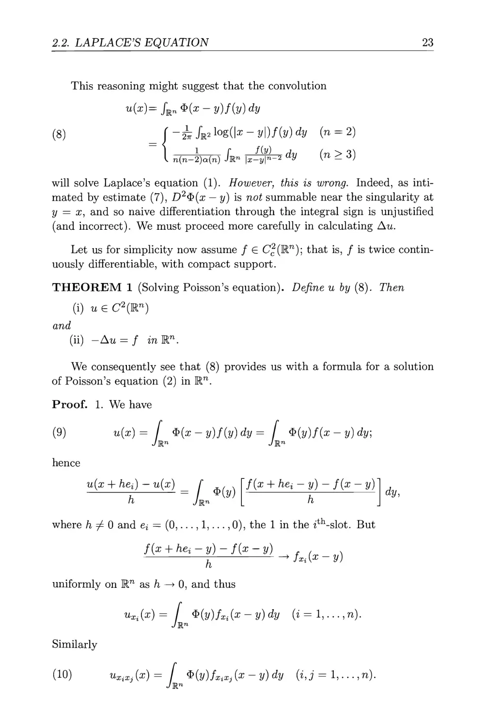
This reasoning might suggest that the convolution
u(x) = fRn<S>(x-y)f(y)dy
(8) _j-±fR2\og(\x-y\)f(y)dy (n = 2)
I n(n-2)a(n) Жп |x-2/|^-2 ^ V77, — 3)
will solve Laplace's equation (1). However, this is wrong. Indeed, as
intimated by estimate (7), D2<$>(x — y) is not summable near the singularity at
у = x, and so naive differentiation through the integral sign is unjustified
(and incorrect). We must proceed more carefully in calculating Au.
Let us for simplicity now assume / G C%(]Rn); that is, / is twice
continuously differentiable, with compact support.
THEOREM 1 (Solving Poisson's equation). Define и by (8). Then
(i) и e C2(Rn)
and
(ii) -Au = f inW1.
We consequently see that (8) provides us with a formula for a solution
of Poisson's equation (2) in Rn.
Proof. 1. We have
(9) u(x)= / ${x-y)f{y)dy= I $(y)f(x-y)dy;
JRn JRn
hence
u(x + hei) — u(x)
I Чу)\
JRn L
f(x + hei -y)~ f(x - y)
h
h
where h ф 0 and e* = (0,..., 1,..., 0), the 1 in the zth-slot. But
f(x + hej -y)~ f(x - y) , , v
^ > Jxi\x - y)
uniformly on W1 as h —> 0, and thus
иХг(х)= / <$>(y)fXz(x-y)dy (i = l,...,n).
JRn
Similarly
(Ю) uXiXj(x)= $(y)fxixj(x-y)dy (ij = l,...,n).
JRn
dy,
24
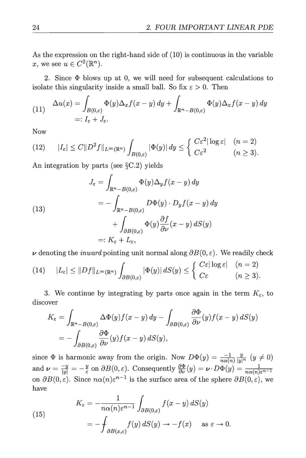
2. FOUR IMPORTANT LINEAR PDE
As the expression on the right-hand side of (10) is continuous in the variable
x, we see и G
2. Since Ф blows up at 0, we will need for subsequent calculations to
isolate this singularity inside a small ball. So fix e > 0. Then
Au(x) = / Ф(у)Ах/(х -y)dy+ Ф(у)Ах/(х - у) dy
(11) JB(0,e) JRn-B(0,e)
=: Ie + Л.
Now
(12) \I£\ < C\\D2/lUco^n) / \*(y)\dy < (
Ce2\loge\ (n = 2)
/б(о,,)'^"'^~ I C^2 (n>3).
An integration by parts (see §C2) yields
Je = / Ф(у) A„/(x - у) dy
JRn-B(0,e)
= -[ D${y)-Dyf{x-y)dy
(13) Jmn-B(Q,e)
+ [ 4>(y)?l(x-y)dS(y)
>dB(0,e)
=: Ke + Le,
v denoting the inward pointing unit normal along 95(0, е). We readily check
Г ( Ce\loge\ (n = 2)
(14) \L£\ < \\Df\\L~{Rn) / №)\dS(y)< '
JdB(o,e) [Се (n> 3).
3. We continue by integrating by parts once again in the term K£, to
discover
Ke= f A<b(y)f(x-y)dy- [ d^{y)f{x-y)dS{y)
JRn-B(0,£) JdB{0,e) av
f^(y)f{X-y)dS(y),
dB(0,e) av
since Ф is harmonic away from the origin. Now ОФ(у) = ~}\ тЧк (у ф 0)
and v = ^ = -\ on 95(0, e). Consequently f*(y) = v-D<S>(y) = ^ф^т
on 95(0, e). Since na(n)£n_1 is the surface area of the sphere 95(0, e), we
have
^ = Л^т / /(* - у) <ВД
/1СЧ na(n)sn 1 JdB(Q,e)
(15)
-/ f(y)dS(y)^-f(x)
J dB(x,e)
as £ —> 0.
2.2. LAPLACE'S EQUATION
25
(Remember from §A.3 that a slash through an integral denotes an average.)
4. Combining now (11)—(15) and letting e —> 0, we find — Au(x) — /(ж),
as asserted. □
Theorem 1 is in fact valid under far less stringent smoothness
requirements for /: see Gilbarg-Trudinger [G-T].
Interpretation of fundamental solution. We sometimes write
-АФ = 50 in Rn,
5q denoting the Dirac measure on Rn giving unit mass to the point 0.
Adopting this notation, we may formally compute
-Au(x) = / -АхФ(х - y)f(y) dy
= I 5xf(y)dy = f{x) (x€Rn),
JRn
in accordance with Theorem 1. This corrects the faulty calculation (9).
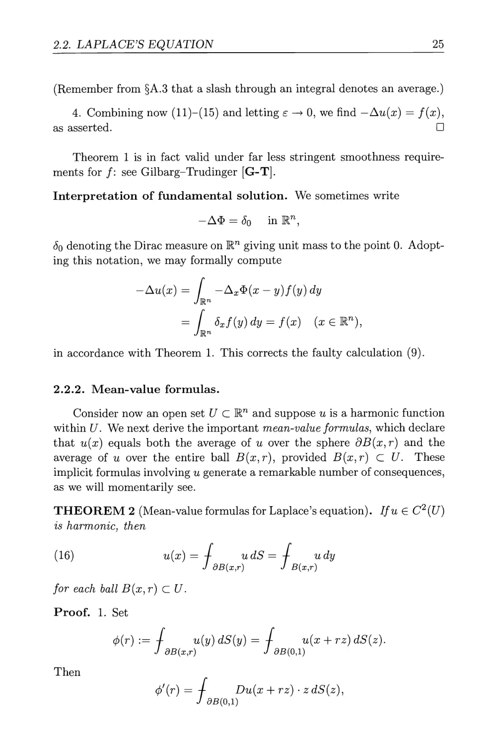
2.2.2. Mean-value formulas.
Consider now an open set U С Шп and suppose и is a harmonic function
within U. We next derive the important mean-value formulas, which declare
that u(x) equals both the average of и over the sphere dB(x,r) and the
average of и over the entire ball Б(ж,r), provided B(x,r) С U. These
implicit formulas involving и generate a remarkable number of consequences,
as we will momentarily see.
THEOREM 2 (Mean-value formulas for Laplace's equation). If и G C2(U)
is harmonic, then
(16) u(x) = + udS = 4- udy
J dB(x,r) J B(x,r)
for each ball B(x,r) С U.
Proof. 1. Set
ф(г) := I u{y) dS{y) = / u(x + rz) dS(z).
J dB(x,r) J dB(0,l)
Then
ф'(г)= + Du(x + rz)-zdS(z),
J 0B(O,1)
26
2. FOUR IMPORTANT LINEAR PDE
and consequently, using Green's formulas from §C2, we compute
ф'(г)=-[ Du(y)-^^dS(y)
J dB(x,r) r
J dB(x,r) OV
= --/ Au(y)dy = 0.
nJ B(x,r)
Hence ф is constant, and so
ф(г) = lim 0(t) = lim f u(y) dS(y) = u(x).
t-+o t^QJ dB{x,t)
2. Observe next that our employing polar coordinates, as in §C.3, gives
udy = / и dS I ds
:,r) JO \JdB(x,s) J
= u(x) / na(n)sn~1ds = a(n)rnu(x). П
THEOREM 3 (Converse to mean-value property). If и G C2(U) satisfies
u(x) —4- udS
J dB(x,r)
for each ball B(x,r) С U, then и is harmonic.
Proof. If Au ф 0, there exists some ball B(x, г) С U such that, say, Au > 0
within B{x,r). But then for ф as above,
O = 0;(r) = -/ Au(y)dy>0,
n^ B(x,r)
?(x,r)
a contradiction. П
2.2.3. Properties of harmonic functions.
We now present a sequence of interesting deductions about harmonic
functions, all based upon the mean-value formulas. Assume for the following
that U С Шп is open and bounded.
2.2. LAPLACE'S EQUATION
27
a. Strong maximum principle, uniqueness. We begin with the
assertion that a harmonic function must attain its maximum on the boundary
and cannot attain its maximum in the interior of a connected region unless
it is constant.
THEOREM 4 (Strong maximum principle). Suppose и G C2(U) П C(U)
is harmonic within U.
(i) Then
max и = max u.
U dU
(ii) Furthermore, if U is connected and there exists a point xq G U such
that
u(xq) = max u,
и
then
и is constant within U.
Assertion (i) is the maximum principle for Laplace's equation and (ii) is
the strong maximum principle. Replacing и by — u, we recover also similar
assertions with "min" replacing "max".
Proof. Suppose there exists a point xq G U with u(xq) — M := тах^гб.
Then for 0 < r < dist(xo,<9L0, the mean-value property asserts
M = u(x0) = f udy < M.
As equality holds only if и = M within Б(жо,г), we see u(y) = M for all
у G B(xo,r). Hence the set {x G U | u(x) = M} is both open and relatively
closed in U and thus equals U if U is connected. This proves assertion (ii),
from which (i) follows. □
Positivity. The strong maximum principle asserts in particular that if U
is connected and и G C2(U) Г\С(й) satisfies
Г Au = 0 in U
\ u — g on dU,
where g > 0, then и is positive everywhere in U if g is positive somewhere
on dU.
An important application of the maximum principle is establishing the
uniqueness of solutions to certain boundary-value problems for Poisson's
equation.
28
2. FOUR IMPORTANT LINEAR PDE
THEOREM 5 (Uniqueness). Letg € C{dU), f € C{U). Then there exists
at most one solution и € C2(U) П C(U) of the boundary-value problem
(17) Г-Д« = / inU
4 у [ и = g on ou.
Proof. If и and и both satisfy (17), apply Theorem 4 to the harmonic
functions w := ±(гх — й). П
b. Regularity. Next we prove that if и G C2 is harmonic, then necessarily
и G C°°. Thus harmonic functions are automatically infinitely differentiable.
This sort of assertion is called a regularity theorem. The interesting point
is that the algebraic structure of Laplace's equation Au = Y^=i uxixt — 0
leads to the analytic deduction that all the partial derivatives of и exist,
even those which do not appear in the PDE.
THEOREM 6 (Smoothness). If и G C(U) satisfies the mean-value
property (16) for each ball B(x,r) С U, then
и G C°°(U).
Note carefully that и may not be smooth, or even continuous, up to dU.
Proof. Let 77 be a standard mollifier, as described in §C4, and recall that
r\ is a radial function. Set ue := rj£ * и in Ue = {x G U \ dist(x, dU) > e}.
As shown in §C4, u£ G C°°(C/e).
We will prove и is smooth by demonstrating that in fact и = u£ on U£.
Indeed if x G U£, then
'(x) = / %(x - y)u(y) dy
Ju
= ^]в(Х,е)Т]
x-y\
u(y) dy
enJo V^ \JdB(x,
= \u(x) [ г) (-) na{n)rn-1dr by (16)
= u(x) / rjedy = u{x).
JB(0,e)
'B(0,e)
Thus u£ = и in J7e, and so гб G C°°([/£) for each e > 0. □
2.2. LAPLACE'S EQUATION
29
с. Local estimates for harmonic functions. Now we employ the mean-
value formulas to derive careful estimates on the various partial derivatives
of a harmonic function. The precise structure of these estimates will be
needed below, when we prove analyticity.
THEOREM 7 (Estimates on derivatives). Assume и is harmonic in U.
Then
(18) \Dau{xv)\ < -±-\\u\\Li{B{x^r))
for each ball B(xo^r) С U and each multiindex a of order \a\ = k.
Here
(19) G0 = -ГТ, Ck = — [k = 1,...).
a(n) a(n)
Proof. 1. We establish (18), (19) by induction on fc, the case к = 0 being
immediate from the mean-value formula (16). For к = 1, we note upon
differentiating Laplace's equation that uXi (i = 1,..., n) is harmonic.
Consequently
|u*i(zo)| = | +
uXi dx |
B{x0,r/2)
on r
(20) = I , N / uUidSl
a{n)rn JdB(xo,r/2)
< у\\Щ\ь°°(дВ(х0^))-
Now if x e дВ{хц,г/2), then B(x,r/2) С B(xo,r) С U, and so
1 (2\n
'^ - ^(й) \r) ^l|Ll(5(x0jr))
by (18), (19) for к — 0. Combining the inequalities above, we deduce
2n+1n 1
|jD%(Xo)l " a(n) rn+i4^ll^(B(xo,r))
if \a\ = 1. This verifies (18), (19) for к = 1.
2. Assume now к > 2 and (18), (19) are valid for all balls in U and each
multiindex of order less than or equal to к — 1. Fix B(xq, г) С U and let a
30
2. FOUR IMPORTANT LINEAR PDE
be a multiindex with |a| = k. Then Dau = (D@u)Xi for some г £ {1,..., n},
| /31 = к — 1. By calculations similar to those in (20), we establish that
\Dau(x0)\ < —||i^«||Lco(eB(x0ir)).
If x G dB(x0,1), then B(x, *j±r) С B{x0,r) С U. Thus (18), (19) for
к — 1 imply
a(n) (V0
Combining the two previous estimates yields the bound
(2n+1nk)k
(21) 1Д°Ц(*о)|<^^
This confirms (18), (19) for |a| = к. D
d. Liouville's Theorem. We assert now that there are no nontrivial
bounded harmonic functions on all of Rn.
THEOREM 8 (Liouville's Theorem). Suppose и : Rn -► R is harmonic
and bounded. Then и is constant.
Proof. Fix xq G Rn, r > 0, and apply Theorem 7 on B(xq, r):
Ш / м ^ \/™Cl|| и
|^Ц^о)| <^prllullb4B(xo,r))
^ VnCia(n) „
as r —> oo. Thus Di*, = 0, and so и is constant. □
THEOREM 9 (Representation formula). Let f G C^(Rn); n > 3. ГЛеп
any bounded solution of
-Au = f inRn
has the form
u{x)= [ ${x-y)f{y)dy + C (xGRn)
for some constant С
2.2. LAPLACE'S EQUATION
31
Proof. Since Ф(х) —► 0 as \x\ —> oo for n > 3, u(x) := JRn Ф(х — y)f(y) dy
is a bounded solution of — Au = / in Rn. If и is another solution, w := u — u
is constant, according to Liouville's Theorem. □
Remark. If n = 2, Ф(х) = —^log|x| is unbounded as |x| —> oo and so
таУ be /r2 Ф(ж - y)/(y) rfy.
e. Analyticity. We refine Theorem 6:
THEOREM 10 (Analyticity). Assume и is harmonic in U. Then и is
analytic in U.
Proof. 1. Fix any point xq G U. We must show и can be represented by a
convergent power series in some neighborhood of xq.
Let r := \dist(x0,dU). Then M := ц^к\\и\\Ь1{в{х^2г)) < oo.
2. Since B(x,r) С B(xo,2r) С U for each x G 5(xo,r), Theorem 7
provides the bound
|Я^|ь~(В(*0,г)) <М(
2n+ln\\«\
|a|H.
Now ^j- < e^ for all positive integers fc, and hence
|а|1а1 <е!а1|а|!
for all multiindices a. Furthermore, the Multinomial Theorem (§1.5) implies
h /- .vi. \-^ \ol\\
nK
|a|=fc
whence
|а|! <п|а|Ы.
Combining the previous inequalities yields the estimate
/2n+1n2e\|a|
(22) \\Dau\\Loo,B,XOfr)) < CM a!.
3. The Taylor series for и at xq is
Dau(x0)
j2^p>(X-XQr,
32
2. FOUR IMPORTANT LINEAR PDE
the sum taken over all multiindices. We assert this power series converges,
provided
(23) 1х-щ1<^кГе-
To verify this, let us compute for each TV the remainder term:
v^ v^ Dau(x0)(x - x0)a
/c=0 \a\=k
EDau(x0 + t(x - xo))(x - xo)a
\a\=N
for some 0 < t < 1, t depending on x. We establish this formula by writing
out the first N terms and the error in the Taylor expansion about 0 for the
function of one variable g(t) := u(xq + t(x — xo)), at t = 1. Employing (22),
(23), we can estimate
|a|=JV Ч 7
- CMnN (2^F = ж -* ° азЛГ^°°- D
See §4.6.2 for more on analytic functions and partial differential
equations.
f. Harnack's inequality. Recall from §A.2 that we write V CC U to
mean V CV С U and V is compact.
THEOREM 11 (Harnack's inequality). For each connected open set V
CC U, there exists a positive constant С, depending only on V, such that
sup и < С inf и
v ~ v
for all nonnegative harmonic functions и in U.
Thus in particular
-jju(y) < u(x) < Cu(y)
for all points x,y G V. These inequalities assert that the values of a non-
negative harmonic function within V are all comparable: и cannot be very
small (or very large) at any point of V unless и is very small (or very large)
everywhere in V. The intuitive idea is that since У is a positive distance
away from dU, there is "room for the averaging effects of Laplace's equation
to occur".
2.2. LAPLACE'S EQUATION
33
Proof. Let r := \ dist(V, dU). Choose x, у G V, \x — y\ < r. Then
u(x) = 4- udz > / udz
J B(x,2r) a(n)2nrn JB{y^r)
= —+ udz = —u(y).
On I, . on 4^y
Z J B(y,r) Z
Thus 2nu(y) > u(x) > ^u(y) if x, у G V, \x — y\ < r.
Since V is connected and V is compact, we can cover У by a chain of
finitely many balls {Bi}^, each of which has radius | and Вг П В{-\ ф 0
for i = 2,... , N. Then
for all x,y G V. D
2.2.4. Green's function.
Assume now [/ С Mn is open, bounded, and dU is C1. We propose
next to obtain a general representation formula for the solution of Poisson's
equation
-Au = f in U,
subject to the prescribed boundary condition
u — g on dU.
a. Derivation of Green's function. Suppose и G C2(U) is an arbitrary
function. Fix x G C/, choose e > 0 so small that 5(x,£) С С/, and apply
Green's formula from §C2 on the region V^ := U — B(x,e) to u(y) and
Ф(у — x). We thereby compute
и(у)АФ(у - x) - Ф(у - i)Aw(j/) dy
= У u(y)~fo(y ~X^~ Ф(у ~ X^^ dS(y^
(24) ^
i/ denoting the outer unit normal vector on dV£. Recall next АФ(х — у) = О
for x ф у. We observe also
\f Ф(у - xAy) dS(y)\ < Cen~l max |Ф| = o(l)
JdB(x,e) VV dB{0,e)
as e —> 0. Furthermore the calculations in the proof of Theorem 1 show
Г дФ f
/ u(y)^-(y - x) dS(v) = t u(y"> dS(y) ~* u№
JdB{x,e) OV J dB{x,e)
34
2. FOUR IMPORTANT LINEAR PDE
as e —> 0. Hence our sending £->0in (24) yields the formula
Г ди дФ
u(x) = Ф(у- х) — (у) - u(y) — (y - x) dS(y)
(25) Jdu dV dV
- \ <S>(y-x)Au(y)dy.
Ju
This identity is valid for any point x G U and any function и G C2{U).
Now formula (25) would permit us to solve for u(x) if we knew the
values of Au within U and the values of щ ди/ди along dU. However, for
our application to Poisson's equation with prescribed boundary values for u,
the normal derivative ди/ди along dU is unknown to us. We must therefore
somehow modify (25) to remove this term.
The idea is now to introduce for fixed x a corrector function фх — фх(у)<>
solving the boundary-value problem
Афх = 0 in U
^ ' | f = Ф(у — x) on dU.
Let us apply Green's formula once more, to compute
- f ф*{у){\и{у)йу= [ u(y)^(y)-<t>*(y)^(y)dS(y)
/27\ Ju Jdu °v dv
= J u{y)9-£{y) - Ф(у - х)^(у) dS(y).
We introduce next this
DEFINITION. Green's function for the region U is
G(x,у) := Ф(у -х)- фх(у) (х,у eU.x^y).
Adopting this terminology and adding (27) to (25), we find
(28) u(x) = - I u(y)^(x,y)dS(y) - f G(x,y)Au(y)dy {x G U),
Jdu и" Ju
where
dG
— (x,y) = DyG(x,y)-v(y)
is the outer normal derivative of G with respect to the variable y. Observe
that the term ди/ди does not appear in equation (28): we introduced the
corrector фх precisely to achieve this.
Suppose now и G C2(U) solves the boundary-value problem
-Au = f in U
(29) 1 ятт
4 7 ' и — g on at/,
for given continuous functions f,g. Plugging into (28), we obtain
2.2. LAPLACE'S EQUATION
35
THEOREM 12 (Representation formula using Green's function). If
и £ C2(U) solves problem (29), then
(30) u(x) = -[ g(y)^(x,y)dS(y)+ [ f(y)G(x,y)dy (xeU).
Jdu ov Ju
Here we have a formula for the solution of the boundary-value problem
(29), provided we can construct Green's function G for the given domain U.
This is in general a difficult matter and can be done only when U has simple
geometry. Subsequent subsections identify some special cases for which an
explicit calculation of G is possible.
Interpreting Green's function. Fix x G U. Then regarding G as a
function of y, we may symbolically write
{ G=0 on a/7,
6X denoting the Dirac measure giving unit mass to the point x.
Before moving on to specific examples, let us record the general assertion
that G is symmetric in the variables x and y:
THEOREM 13 (Symmetry of Green's function). For all x,y eU, хфу,
we have
G(y,x) = G(x,y).
Proof. Fix x,y EC/, x ^ y. Write
v(z) := G(x,z), w(z) := G(y,z) (z G U).
Then Av(z) = 0 (z Ф x), Aw(z) = 0 [z Ф y) and w — v — 0 on
dU. Thus our applying Green's identity on V := U — [B(x, e) U B(y, e)] for
sufficiently small e > 0 yields
(31) / —w-—vdS(z)= —-v--wdS(z),
v denoting the inward pointing unit vector field on dB(x,s)UdB(y,e). Now
w is smooth near x, whence
I / ^-v dS\ < Ce71-1 sup \v\ = o(l) as e -► 0.
JdB(x,e) OV dB(x,e)
36
2. FOUR IMPORTANT LINEAR PDE
On the other hand, v(z) — Ф(г — х) — фх(г), where фх is smooth in U. Thus
lim / —— wdS =\im I -—-(x — z)w(z) dS = w(x),
^*JdB(x,e)dv e-+*JdB(x,e)dv
by calculations as in the proof of Theorem 1. Thus the left-hand side of (31)
converges to w(x) as e —► 0. Likewise the right-hand side converges to v(y).
Consequently
G(y, x) = w(x) = v(y) = G(x, у). D
b. Green's function for a half-space. In this and the next subsection
we will build Green's functions for two regions with simple geometry, namely
the half-space IR+ and the unit ball Б(0,1). Everything depends upon our
explicitly solving the corrector problem (26) in these regions, and this in
turn depends upon some clever geometric reflection tricks.
First let us consider the half-space
Щ = {х = (*i,... ,xn) G Rn | xn > 0}.
Although this region is unbounded, and so the calculations in the previous
section do not directly apply, we will attempt nevertheless to build Green's
function using the ideas developed earlier. Later of course we must check
directly that the corresponding representation formula is valid.
DEFINITION. If x = (xi,..., xn_i, xn) G IR+, its reflection in the plane
dW+ is the point
We will solve problem (26) for the half-space by setting
фх(у) :=Ф(у-х) = Ф(уг -хъ...,уп-1-хп-1,уп + хп) (х,у G R+).
The idea is that the corrector фх is built from Ф by "reflecting the
singularity" from хеШ%Ьох£Щ. We note
фх(у) = Ф(у-х) if ye Ж}:,
and thus
Афх = 0 тЩ
Ф* = Ф(у-Х) ondR%,
as required.
2.2. LAPLACE'S EQUATION
37
DEFINITION. Green's function for the half-space R^ is
в(х,у):=Ф(у-х)-Ф(у-х) (x,yeR+, хфу).
Then
Gyn (x, у) = ФУп (у-х)- ФУп {у - x)
na(n)
Уп %п Уп ~г Xn
\y-x\n \y-x\
Consequently if у G <9R+,
8G
— (£,y) = -Gyn(x,y) = ~ -.
ov not\n) \x — y\n
Au = 0 in Щ
u = g on дЩ.
Suppose now и solves the boundary-value problem
(32)
Then from (30) we expect
(33) U(x) = -*b[ -^dy (*€R£)
na(n) JdRn \x - y\n
to be a representation formula for our solution. The function
2xn 1
K(x,y):=
(xeRl,yedRl)
na(n) \x — y\
is Poisson's kernel for R", and (33) is Poisson's formula.
We must now check directly that formula (33) does indeed provide us
with a solution of the boundary-value problem (32).
THEOREM 14 (Poisson's formula for half-space). Assume g € С(КП_1)П
L^iW1'1), and define и by (33). Then
(i) ueC^iWDnL^iRl),
(ii) Au = 0 in R!f.,
and
(iii) lim u(x) = g(x°) for each point x° € Ж+.
x—>x
хек
38
2. FOUR IMPORTANT LINEAR PDE
Proof. 1. For each fixed x, the mapping у i—> G(x,y) is harmonic, except
for у — x. As G(x,y) = G(y,x), x i—> G(x,y) is harmonic, except for x — y.
Thus x i-> -f^(x, y) = K(x, y) is harmonic for x G M+, у G Ж}..
2. A direct calculation, the details of which we omit, verifies
(34) 1= [ K(x,y)dy
for each x G Elf:. As 5 is bounded, и defined by (33) is likewise bounded.
Since x ь-> if (x, y) is smooth for x 7^ y, we easily verify as well -u G С°°(М+),
with
Дгх(х) = / AxK(x, y)g{y) dy = 0 (x G R»).
JdR^
3. Now fix x° G <9R^, e > 0. Choose 5 > 0 so small that
(35) |5(y) - g(x°)\ <e if |y - x°| < 5, у G 9R».
Then if |x-x°| < f, x G E^,
Kx)-5(x°)| =
(36)
<
/ K(x,y)[g(y)-g(x°)}dy
JdR^
1
™r\B(x0,5)
K(x,y)\g(y)-g(x°)\dy
+
f
JdRi
l-B(x°,6)
K(x,y)\g(y)-g(x°)\dy
=:I + J.
Now (34), (35) imply
I <e K(x,y)dy = e.
JdR^
Furthermore if |x — x°| < | and |y — x°| > 5, we have
\y ~ x°\ < \y - x\ + - < \y - x\ + -\y - x°|;
and so \y — x\ > \\y — x°|. Thus
J < Цд\\ь<*> / K(x,y)dy
JdRi-
<
1^-В(х0,6)
2n+2\\gh~x,
na(n)
0 asxn^ 0+.
/
\y-xXndy
2.2. LAPLACE'S EQUATION
39
Combining this calculation with estimate (36), we deduce \u(x)—g(x°)\ < 2s,
provided \x — x°\ is sufficiently small. □
c. Green's function for a ball. To construct Green's function for the
unit ball 5(0,1), we will again employ a kind of reflection, this time through
the sphere 95(0,1).
DEFINITION. IfxeW1- {0}; the point
x
\x\2
is called the point dual to x with respect to 95(0,1). The mapping x i—> x
is inversion through the unit sphere 95(0,1).
We now employ inversion through the sphere to compute Green's
function for the unit ball U = 5°(0,1). Fix x G 5°(0,1). Remember that we
must find a corrector function фх — фх(у) solving
(Афх = 0 in B°(0,1)
1 ' \ фх = Ф(у-х) on aB(0,l);
then Green's function will be
(38) С(х,у) = Ф(у-х)-фх(у).
The idea now is to "invert the singularity" from x £ 5° (0,1) to x ^
5(0,1). Assume for the moment n > 3. Now the mapping у ь-> Ф(у — x) is
harmonic for у Ф x. Thus у i—> |х|2_пФ(у — x) is harmonic for у фх, and so
(39) ф*(у):=Ф(\х\(у-х))
is harmonic in U. Furthermore, if у G 95(0,1) and x^0,
|x|2|y-x|2 = |x|2f|y|2-2^ + ^
\ \x\z \x\z
= \x\2 — 2y ■ x + 1 = \x — y\2.
Thus (\x\\y - х\)-(п-^ = \x- y|"(n"2). Consequently
(40) фх(у) = Ф(у-х) (у€дВ(0,1)),
as required.
40
2. FOUR IMPORTANT LINEAR PDE
DEFINITION. Green's function for the unit ball is
(41) G(x,y) := Ф(у - x) - Ф(\х\(у - x)) (x,y e 5(0,1), x ф у).
The same formula is valid for n — 2 as well.
Assume now и solves the boundary-value problem
(Au = 0 inB°(0,l)
{Z) \ u = g in 05(0,1).
Then using (30), we see
С r)C
(43) u(x) = - g(y) — (x,y)dS(y).
JdB(0,l) av
According to formula (41),
Gyi(x,y) = ФУ1{у -х)- Ф{\х\{у - x))yi.
But
ФуЛУ — X) = ^v^ :—,
and furthermore
Ф(\Х\(У-Х)) = —^ УгМ -Дг j_?/iM ~Ж»
4 IU/ Ш' na(n)(|x||y-x|)" na(n) \x - y\n
if у € 55(0,1). Accordingly
dG n
— (x,y) = ^2УгСуЛх>У)
г=1
-1 1 n
= —r^]—ыУ2у^(у^ ~x*) - y*\x\2 +x*)
na{n) \x — y\n *-^
-1 \-\x
12
na(n) \x — y\n
Hence formula (43) yields the representation formula
na(n) yaB(0ii) \x - y\n КУ!
Suppose now instead of (42) и solves the boundary-value problem
(Au = 0 in5°(0,r)
{ ' \ u = g on 55(0, r)
2.2. LAPLACE'S EQUATION
41
for r > 0. Then й(х) = u(rx) solves (42), with g(x) = g(rx) replacing g.
We change variables to obtain Poisson's formula
(45) u(x) = rl^K f Sfo) dS{) {x e so(0 r)).
na(n)r JdB{0,r) \x - y\n
The function
K(x,y):=r2~lf l (x£B°(0,r),yedB(0,r))
na[n)r \x — y\n
is Poisson's kernel for the ball 5(0, r).
We have established (45) under the assumption that a smooth solution
of (44) exists. We next assert that this formula in fact gives a solution:
THEOREM 15 (Poisson's formula for ball). Assume g G C(&B(0, r)) and
define и by (45). Then
(i) ^GC°°(S0(0,r));
(ii) Au = 0 inB0(0,r),
and
(in) lim u(x) — g(x°) for each point x° G 95(0,r).
xeB°(o,r)
The proof is similar to that for Theorem 14 and is left as an exercise.
2.2.5. Energy methods.
Most of our analysis of harmonic functions thus far has depended upon
fairly explicit representation formulas entailing the fundamental solution,
Green's functions, etc. In this concluding subsection we illustrate some
"energy" methods, which is to say techniques involving the L2-norms of
various expressions. These ideas foreshadow later theoretical developments
in Parts II and III.
a. Uniqueness. Consider first the boundary-value problem
-Au = f in U
(46) l йтт
7 ' и = д on ои.
We have already employed the maximum principle in §2.2.3 to show
uniqueness, but now we set forth a simple alternative proof. Assume U is
open, bounded, and dU is C1.
42
2. FOUR IMPORTANT LINEAR PDE
THEOREM 16 (Uniqueness). There exists at most one solution и G
C2(U) o/(46).
Proof. Assume и is another solution and set w := и — и. Then Aw — 0 in
[/, and so an integration by parts shows
0 = — wAwdx= / \Dw\2 dx.
Ju Ju
Thus Dw = 0 in £/, and, since w — 0 on <9?7, we deduce w = и — u = 0in
/7. П
b. Dirichlet's principle. Next let us demonstrate that a solution of the
boundary-value problem (46) for Poisson's equation can be characterized as
the minimizer of an appropriate functional. For this, we define the energy
functional
I[w}:= f l\Dw\2-wfdx,
w belonging to the admissible set
Л := {w £ C2(U) \w = gon dU}.
THEOREM 17 (Dirichlet's principle). Assume и G C2(U) solves (46).
Then
(47) I[u] = min I [w].
Conversely, if и 6 A satisfies (47), then и solves the boundary-value problem
(46).
In other words if и £ Л, the PDE — Au — f is equivalent to the statement
that и minimizes the energy /[•].
Proof. 1. Choose w £ Л. Then (46) implies
0 = / (-Au - f)(u - w) dx.
Ju
An integration by parts yields
0= / Du- D(u — w) — f(u — w)dx,
Ju
2.2. LAPLACE'S EQUATION
43
and there is no boundary term since u — w — g — g = 0 on dU. Hence
/ \Du\2 — uf dx — \ Du-Dw — wfdx
Ju Ju
< / -\Du\2dx + / -\Dw\2 -wfdx,
Ju 2 Ju 2
where we employed the estimates
\Du • Dw\ < \Du\\Dw\ < -\Du\2 + -\Dw\2,
following from the Cauchy-Schwarz and Cauchy inequalities (§B.2).
Rearranging, we conclude
(48) I[u] < I[w] (we A).
Since ueA, (47) follows from (48).
2. Now, conversely, suppose (47) holds. Fix any v G C^°(U) and write
i(r) :=I[u + rv] (r GR).
Since и + rv G A for each r, the scalar function i(-) has a minimum at zero,
and thus
'<°>-° ('=!)
drj'
provided this derivative exists. But
i(r) = / -\Du + tDv\2 - (u + rv)fdx
Ju 2
f 1 t2
= / -\Du\2 + tDu-Dv + —\Dv\2- (u + rv)fdx.
Ju 2 2
Consequently
0 = г'(0) = / Du-Dv-vf dx = / (-Au - f)v dx.
Ju Ju
This identity is valid for each function v G C^°(U) and so — Au — f in
ЕЛ П
Dirichlet's principle is an instance of the calculus of variations applied
to Laplace's equation. See Chapter 8 for more.
44
2. FOUR IMPORTANT LINEAR PDE
2.3. HEAT EQUATION
Next we study the heat equation
(1) щ - Au = 0
and the nonhomogeneous heat equation
(2) щ - An = /,
subject to appropriate initial and boundary conditions. Here t > 0 and
xG[/, where U С Rn is open. The unknown is и : U x [0, oo) —► R, -u =
-u(x, £), and the Laplacian A is taken with respect to the spatial variables x —
(xi,..., xn): Au = Axu = Y%=i uxiXi- In (2) the function / : Ux [0, oo) -> R
is given.
A guiding principle is that any assertion about harmonic functions yields
an analogous (but more complicated) statement about solutions of the heat
equation. Accordingly our development will largely parallel the
corresponding theory for Laplace's equation.
Physical interpretation. The heat equation, also known as the diffusion
equation, describes in typical applications the evolution in time of the density
и of some quantity such as heat, chemical concentration, etc. If V С U is
any smooth subregion, the rate of change of the total quantity within V
equals the negative of the net flux through dV:
udx = — F-i/ dS,
Jv Jd\
dt jv jqy
F being the flux density. Thus
(3) ut = -divF,
as V was arbitrary. In many situations F is proportional to the gradient
of и but points in the opposite direction (since the flow is from regions of
higher to lower concentration):
F = -aDu (a>0).
Substituting into (3), we obtain the PDE
щ — adiv(Du) — aAu,
which for a — 1 is the heat equation.
The heat equation appears as well in the study of Brownian motion.
2.3. HEAT EQUATION
45
2.3.1. Fundamental solution.
a. Derivation of the fundamental solution. As noted in §2.2.1 an
important first step in studying any PDE is often to come up with some
specific solutions.
We observe that the heat equation involves one derivative with respect
to the time variable t, but two derivatives with respect to the space
variables Xi (i — 1,... , n). Consequently we see that if и solves (1), then so
does u(\x, X2t) for Л G R. This scaling indicates the ratio ^- (r = |x|) is
important for the heat equation and suggests that we search for a solution
of (1) having the form u(x,t) = v{^) = v(^-) (t > 0, x G Rn), for some
function v as yet undetermined.
Although this approach eventually leads to what we want (see Problem
13), it is quicker to seek a solution и having the special structure
(4) u(M) = 1v(Jl) (xeRn,t>0),
where the constants a, /? and the function v : Rn —► R must be found. We
come to (4) if we look for a solution и of the heat equation invariant under
the dilation scaling
That is, we ask that
u(x,t) = Xau{Xf3x,Xt)
for all Л > 0, x G Rn, t > 0. Setting Л = t"1, we derive (4) for v(y) :=
u(y,l).
Let us insert (4) into (1) and thereafter compute
(5) аГ<а+1Цу) + (3t-(a+Vy • Dv(y) + Г^а+2^Ау(у) = О
for у := t~@x. In order to transform (5) into an expression involving the
variable у alone, we take j3 — \. Then the terms with t are identical, and
so (5) reduces to
(6) av + -y • Dv + Av = 0.
We simplify further by guessing v to be radial; that is, v(y) — w(\y\) for
some w : R —>• R. Thereupon (6) becomes
1 , „ n— 1 .
aw + -rw + w -\ w = 0,
2 r
46
2. FOUR IMPORTANT LINEAR PDE
for r = \y\, ' = J;. Now if we set a = f, this simplifies to read
(rn"V)' + ^(rV)' = 0.
Thus
rn~ V + -rnw = a
2
for some constant a. Assuming lim^ooU^, w' — 0, we conclude a = 0,
whence
But then for some constant 6
(7)
1
w — —-rw.
2
w — be 4 .
Combining (4), (7) and our choices for a,/?, we conclude that 7^72 e ~&~
solves the heat equation (1).
This computation motivates the following
DEFINITION. The function
{0 (x e Rn, t < 0)
is called the fundamental solution of the heat equation.
Notice that Ф is singular at the point (0,0). We will sometimes write
Ф(х,£) = Ф(|х|,£) to emphasize that the fundamental solution is radial in
the variable x. The choice of the normalizing constant (47r)~n/2 is dictated
by the following
LEMMA (Integral of fundamental solution). For each time t > 0,
$(x,t)dx = 1.
Proof. We calculate
/
JM.7
f 1 f и2
/ Ф(хЛ)с1х = - —-пг / e ^ dx
= ~L / еЧг|2 dz
W2 JRn
1 ,n. z*00
= W2II/ '
г? dz,- = 1. П
2.3. HEAT EQUATION
47
A different derivation of the fundamental solution of the heat equation
appears in §4.3.1.
b. Initial-value problem. We now employ Ф to fashion a solution to the
initial-value (or Cauchy) problem
( щ - Au = 0 in Rn x (0, oo)
^ \ и = g on Rn x {t = 0}.
Let us note that the function (x,t) i—> Ф(ж,£) solves the heat equation
away from the singularity at (0,0), and thus so does (x, t) i—> Ф(х — у, t) for
each fixed у G M71. Consequently the convolution
(9)
(x,t) = / $(x-y,t)g(y)dy
= 777W5 / z~^9{y) dy (x GRn,t> 0)
should also be a solution.
THEOREM 1 (Solution of initial-value problem). Assume g G C(Rn) П
L°°(Rn); and define и by (9). Then
(i) ueC°°(Rn x (0,oo)),
(ii) ut(x, t) - Au(x, t) = 0 (x G Rn, t > 0),
and
(iii) lim u(x, t) = #(x°) /or eac/г point x° G Rn.
(x,t)->(a:o,0)
1 lgl2
Proof. 1. Since the function 7^72 e 4* is infinitely differentiable, with
uniformly bounded derivatives of all orders, on Шп x [5, oo) for each 6 > 0, we
see that u G C°°(Rn x (0,oo)). Furthermore
ut(x,£)-Au(x,£) = / [(Ф* - Д*Ф)(х - у, *)]$(у) dy
= 0 (x G Rn, t > 0),
since Ф itself solves the heat equation.
2. Fix x° GKn,0 0. Choose 6 > 0 such that
(11) |p(y) - g(x°)\ <e if |y - x°\ < 6, у G R*.
48
2. FOUR IMPORTANT LINEAR PDE
Then if \x — x°\ < |, we have, according to the lemma,
\u(x, t) - g(x°)\ = \f Ф(х-у,t)[g(y) - g(x0)] dy\
< [ *(x-y,t)\g(y)-g(x°)\dy
JB(x0,S)
+ I *(x-y,t)\g(y)-g(x°)\dy
JRn-B(x°,S)
=:I + J.
Now
I <s / <$>{x-y,t)dy = e,
jRn
owing to (11) and the lemma. Furthermore, if \x — x°\ < | and \y — x°\ > £,
then
\y - x°\ < \y - x\ + - < \y - x\ + -\y - x°\.
Thus \y — x\ > \\y — x°\. Consequently
J<2||p||Loo / ${x-y,t)dy
JRn-B(x°,6)
.|2
-w*L e""dy
\x-vf
g
tn/2 jRrb-B(x°,6)
-&L e"'1"'dy
tnlZ jRrb-B(x°,6)
.ML2
= С / e~^ dz^O as t -► 0+.
jRn-B(x°,6/y/i)
Hence if \x — x°\ < | and t > 0 is small enough, \u(x,t) — g(x°)\ < 2s. D
Interpretation of fundamental solution. In view of Theorem 1 we
sometimes write
Г Ф* - АФ = 0 in Rn x (0, oo)
\ Ф = S0 on Rn x {t = 0},
5o denoting the Dirac measure on Шп giving unit mass to the point 0.
Infinite propagation speed. Notice that if g is bounded, continuous,
g > 0, g ф 0, then
u(x,t) = . " /9 / e~1^L'g(y)dy
1 f \*-y\2
2.3. BEAT EQUATION
49
is in fact positive for all points xGln and times t > 0. We interpret this
observation by saying the heat equation forces infinite propagation speed
for disturbances. If the initial temperature is nonnegative and is positive
somewhere, the temperature at any later time (no matter how small) is
everywhere positive. (We will learn in §2.4.3 that the wave equation in
contrast supports finite propagation speed for disturbances.)
c. Nonhomogeneous problem. Now let us turn our attention to the
nonhomogeneous initial-value problem
П9ч (ut-Au = f inR"x(0,oo)
1 } \ u = 0 on Rn x {t = 0}.
How can we produce a formula for the solution? If we recall the
motivation leading up to (9), we should note further that the mapping (x,£) i—>
Ф(х — у, t — s) is a solution of the heat equation (for given у G Mn, 0 < s < t).
Now for fixed s, the function
(x, t\ s) = / Ф(х -y,t- s)f(y, s) dy
и = и
solves
(ло\ / щ("> 5) ~ Л^'; 5) = ° in Mn x (5, oo)
[ s) I u(.;s) = f(.,s) onR"x{t = s},
which is just an initial-value problem of the form (8), with the starting time
t = 0 replaced by t = s and g replaced by /(•, s). Thus u{-\ s) is certainly
not a solution of (12).
However DuhameVs principle" asserts that we can build a solution of
(12) out of the solutions of (125), by integrating with respect to s. The idea
is to consider
u(x,t)= / u{x,t;s)ds (xeMn, t > 0).
Rewriting, we have
u(x,t)= / ${x-y,t-s)f(y,s)dyds
(13) Jo jRn
fl 1 f \*-y\2
= / 7Z77 Ы2 / e 4t~s)f(y^)dyds,
Jo (47r(i- s))n/z JRn
for x G En, t > 0.
To confirm that formula (13) works, let us for simplicity assume / G
C\(En x [0, oo)) and / has compact support.
*Duhamel's principle has wide applicability to linear ODE and PDE and does not depend
on the specific structure of the heat equation. It yields, for example, the solution of the
nonhomogeneous transport equation, obtained by different means in §2.1.2. We will invoke Duhamel's
principle for the wave equation in §2.4.2.
50
2. FOUR IMPORTANT LINEAR PDE
THEOREM 2 (Solution of nonhomogeneous problem). Define и by (13).
Then
(i) ueCf(Rnx (0,oo)),
(ii) щ(х, t) - Au(x, t) = f(x, t) (x Gin,t> 0),
and
(Hi) lim u(x, t) — 0 for each point x° Gln.
(x,t)^(x°,0)
x£Rn, t>0
Proof. 1. Since Ф has a singularity at (0,0), we cannot directly justify
differentiating under the integral sign. We instead proceed somewhat as in
the proof of Theorem 1 in §2.2.1.
First we change variables, to write
u(x,t)= / <&(y,s)f(x-y,t-s)dyds.
JO JR71
As / G Ci(Rn x [0, oo)) has compact support and Ф = Ф(у, s) is smooth
near s = t > 0, we compute
ut(x,t)= / &{y,s)ft{x-y,t-s)dyds
Jo Jr71
+ I $(y,t)f(x-y,0)dy
Jr™
and
UxiXj
(x,t)= / $(y,s)fXiXj(x-y,t- s)dyds (i,j = l,...,n).
«/o </Rn
Thus ut^D^u^ and likewise u,Dxu, belong to С(Шп х (0, oo)).
2. We then calculate
(14)
ut(x,t) - Au(x,t) = / <%,s)[(— -Ax)/(x-y,i-s)]d2/ds
JO JRn at
+ / *{y,t)f{x-y,Q)dy
JR71
= [[ *(y,s)[(-§--Ay)f(x-y,t-s)]dyds
Je JRn os
+ ff $(y1s)[{-—-by)f{x-y1t-s)}dyds
Jo Лп os
+ [ *{y,t)f{x-y,Q)dy.
Jr™
=: L + X + К
2.3. HEAT EQUATION
51
Now
(15) \J£\ < (||/t||L» + \\D2f\\L°o) Г [ Ф(у, s) dyds < eC,
JO JRn
by the lemma. Integrating by parts, we also find
h = J Jn[(Q-s-Ay)$(y,S)]f(x-y,t-S)dyds
+ / $(y,e)f(x-y,t-e)dy
(16) JJn
- / *(y,t)f(x-y,0)dy
= / $(y,e)f(x-y,t-e)dy-K,
JRn
since Ф solves the heat equation. Combining (14)-(16), we ascertain
щ(х, t) - Au(x, t) = lim / Ф(у, e)f(x -y,t-s)dy
e^° JR™
= f(x,t) (iGRn, t>0),
the limit as e —> 0 being computed as in the proof of Theorem 1. Finally
note K-,t)||Loo <t||/||Loo -►(). □
Solution of homogeneous problem with general initial data. We
can of course combine Theorems 1 and 2 to discover that
(17) u(x, t)= Ф{х - у, t)g(y) dy+ / 9{x-y,t- s)f(y, s) dyds
JR71 JO JRn
is, under the hypotheses on g and / as above, a solution of
ut- Au = f in Rn x (0, со)
(18) l и = g on Rn x {t = 0}.
2.3.2. Mean-value formula.
First we recall some useful notation from §A.2. Assume U С Шп is open
and bounded, and fix a time T > 0.
52
2. FOUR IMPORTANT LINEAR PDF
The region U7
DEFINITIONS.
(i) We define the parabolic cylinder
UT:=U x (0,T].
(ii) Г/ге parabolic boundary о/ С/т is
Г71 1= C/71 — C/71.
We interpret C/71 as being the parabolic interior of U x [0,T]: note
carefully that C/71 includes the top U x {t = T}. The parabolic boundary Г71
comprises the bottom and vertical sides of С/ х [0,T], but not the top.
We want next to derive a kind of analogue to the mean-value property for
harmonic functions, as discussed in §2.2.2. There is no such simple formula.
However let us observe that for fixed x the spheres дВ(х, г) are level sets of
the fundamental solution Ф(х — у) for Laplace's equation. This suggests that
perhaps for fixed (x, t) the level sets of fundamental solution Ф(х — у, t — s)
for the heat equation may be relevant.
DEFINITION. For fixed x G En; t G R, r > 0, we define
E{x,t-r) := ((y, 3) G En+1 I 3 < t, Ф(х - y,t - s) > \X .
2.3. HEAT EQUATION
53
(x, t)
E(x,t;r)
A "heat ball"
This is a region in space-time, the boundary of which is a level set of
Ф(х — y,t — s). Note that the point (x,t) is at the center of the top. E(x,t;r)
is sometimes called a "heat ball".
THEOREM 3 (A mean-value property for the heat equation). Let и G
Ci(Ut) solve the heat equation. Then
(19) «(*,*) = ^ll^^u(y,s)\^dyds
for each E{x,t',r) С Ut-
Formula (19) is a sort of analogue for the heat equation of the mean-value
formulas for Laplace's equation. Observe that the right-hand side involves
only u(y,s) for times s < t. This is reasonable, as the value u(x,t) should
not depend upon future times.
Proof. Shift the space and time coordinates so that x = 0 and t — 0. Upon
mollifying if necessary, we may assume и is smooth. Write E(r) = £7(0,0; r)
and set
(20)
r JJE{r) s
ff \y\2
= u{ry,r2s)-^-dyds.
J J Ed) s
/£7(1)
We compute
|2
Ф\г) = ff J2 uyiVi4~ + 2mei^L dyds
ш JJE(r) E W7 +2u^ dyd
Г--.,.1Е{г) —
=:A + B.
54
2. FOUR IMPORTANT LINEAR PDE
Also, let us introduce the useful function
n It/I
(21) ф := --log(-47rs) + ^-+n\ogr
2 45
and observe ф = 0 on dE{r), since Ф(у, — s) = r_n on dE{r). We utilize
(21) to write
B = —i 4usJ2 УгФуг dVds
1 JJE(r) i=1
= —^ I \ 4nusip + 4 ^2 изУгУгФ dyds;
there is no boundary term since ^ = 0on dE{r). Integrating by parts with
respect to 5, we discover
В
= ~^+T / / -4пи8ф + 4V uyiyi%l>s dyds
=^^ ТХс.г47"^+4 S "^ш ("^" ^)dyds
Л Г Г О ^
= ^+т УУ^ _4пп^ ~ -у 5^ и№Уг dyds ~ А-
Consequently, since и solves the heat equation,
ф'(г) = А + В
Л Г Г О ^
i+T / / -4пАиф -—^2 иУгуг dyds
г—- ././Д(г)
^г^/Л
АпиУ{фУ{ глУ4Уг dyds
Я(г) 5
= 0, according to (21).
Thus 0 is constant, and therefore
ф(г) = Jim 0(f) = u(0,0) (Jim 1 /У М- dyds) = 4«(0,0),
as
I// !£*,.-// hf^.t
tnJJE(t) S2 JJE{1) S2
We omit the details of this last computation. D
2.3. HEAT EQUATION
55
Strong maximum principle for the heat equation
2.3.3. Properties of solutions.
a. Strong maximum principle, uniqueness. First we employ the mean-
value property to give a quick proof of the strong maximum principle.
THEOREM 4 (Strong maximum principle for the heat equation). Assume
и G Ci(Ut) П C{Ut) solves the heat equation in Ut-
(i) Then
max и = max u.
UT гт
(ii) Furthermore, ifU is connected and there exists a point (xo^o) £ Ut
such that
u(xoito) = maxw,
then
и is constant in Ut0.
Assertion (i) is the maximum principle for the heat equation and (ii)
is the strong maximum principle. Similar assertions are valid with "min"
replacing "max".
Interpretation. So if и attains its maximum (or minimum) at an interior
point, then и is constant at all earlier times. This accords with our strong
intuitive understanding of the variable t as denoting time: the solution will
56
2. FOUR IMPORTANT LINEAR PDE
be constant on the time interval [0, to] provided the initial and boundary
conditions are constant. However, the solution may change at times t > to,
provided the boundary conditions alter after to- The solution will however
not respond to changes in boundary conditions until these changes happen.
Take note that whereas all this is obvious on intuitive, physical grounds,
such insights do not constitute a proof. The task is to deduce such behavior
from the PDE.
Proof. 1. Suppose there exists a point (xo, to) G Ut with u(xo, to) = M :=
та,Хцти. Then for all sufficiently small r > 0, E(xo,to;r) С Ut] and we
employ the mean-value property to deduce
M = u(x0,t0) = -^ ft u(y,s)^°~y\2dyds<M,
since
1 = 4^ JJE(X0Mr) (to ~ s)2 dydS-
Equality holds only if и is identically equal to M within E{xQ,t$\r).
Consequently
u(y, s) = M for all (y, s) G £(x0, ^о; r).
Draw any line segment L in Ut connecting (xo, to) with some other point
(yo? 5o) G Ut, with so < to- Consider
ro := min{s > so | u(x, t) = M for all points (x, t) G L, s < t < to}.
Since и is continuous, the minimum is attained. Assume ro > so- Then
^(^o? П)) = M for some point (zq, ro) on LHUt and so и = M on £^(2:0,ro;r)
for all sufficiently small r > 0. Since i£(zo, ro; r) contains L П {ro — cr <t <
ro} for some small a > 0, we have a contradiction. Thus ro = so, and hence
и = M on L.
2. Now fix any point x G C/ and any time 0 < t < to- There exist points
{xo, xi,..., xm = x} such that the line segments in Rn connecting x*-i to Xi
lie in U for i = 1,..., m. (This follows since the set of points in U which can
be so connected to xo by a polygonal path is nonempty, open and relatively
closed in U.) Select times to > t\ > • • • > tm = t. Then the line segments in
Rn_hl connecting (x;-i,t;_i) to (x^,t;) (г = l,...,m) lie in Ut- According
to step 1, и = M on each such segment and so u{x, t) = M. □
2.3. HEAT EQUATION
57
Infinite propagation speed again. The strong maximum principle
implies that if U is connected and и G C{(Ut) П C{Ut) satisfies
щ — Au = 0 in Ut
u = 0 on dU x [0, T]
u = g on C/ x {t = 0}
where g > 0, then и is positive everywhere within Ut if 5 is positive
somewhere on £/. This is another illustration of infinite propagation speed for
disturbances.
An important application of the maximum principle is the following
uniqueness assertion.
THEOREM 5 (Uniqueness on bounded domains). Let g G С(ГТ); / G
C(Ut)- Then there exists at most one solution и G Cf(Ur) П C(Ut) of the
initial/boundary-value problem
/22ч (ut-Au = f inUT
^ \ u — gon Тт-
Proof. If и and и are two solutions of (22), apply Theorem 4 to w :=
±(u-u). □
We next extend our uniqueness assertion to the Cauchy problem, that
is, the initial-value problem for U = Rn. As we are no longer on a bounded
region, we must introduce some control on the behavior of solutions for large
|x|.
THEOREM 6 (Maximum principle for the Cauchy problem). Suppose
и e Cf(Rn x (0,T]) П C(Rn x [0,T]) solves
(9] (щ-Аи = 0 гпМпх(0,Т)
1 ] \ u = g on Rn x {t = 0}
and satisfies the growth estimate
(24) u{x, t) < AeaW2 (x e Mn, 0 < t < T)
for constants Л, а > 0. Then
sup u = supg.
Rnx[0,T] Mn
58
2. FOUR IMPORTANT LINEAR PDE
Proof. 1. First assume
(25) 4aT < 1,
in which case
(26) 4a(T + e)<l
for some e > 0. Fix у G Rn, ц > 0, and define
v(x, t) := u(x, t) - 7 ^ x e4C^-*) (x E Mn, t > 0).
A direct calculation (cf. §2.3.1) shows
vt-Av = 0 inRn x (0,T].
Fix r > 0 and set U := 5°(y,r), C/T = B°(y,r) x (0,T]. Then according to
Theorem 4,
(27) тахг> = maxv.
2. Now if x E Mn,
/i |g-yl2
, ч v(x, 0) = u(x, 0) - ^-v^e4(T+£)
(28) V ; V ; (Т + ф/2
< u(x,0) = #(я);
and if |x — y| = r, 0 < t < T, then
и r2
v(x,t) = u(x,t) - —r—^e^T+e-t)
2
< Aea^2 - M ч /0e^fe=^ by (24)
< Aea(M+r)2 _ ^^ei(^ .
(T + e) V2
Now according to (26), 4/т1, ч = a+7 for some 7 > 0. Thus we may continue
the calculation above to find
(29) v(x,t) < Aea^+r^2 - /i(4(a + 7))n/2e(a+^r2 < sup5,
for r selected sufficiently large. Thus (27)-(29) imply
v(y,t) < sup g
for all у e Rn, 0 < t < T, provided (25) is valid. Let /z -► 0.
3. In the general case that (25) fails, we repeatedly apply the result
above on the time intervals [0,Ti], [Ti,2Ti,], etc., for T\ — ^. □
2.3. HEAT EQUATION
59
THEOREM 7 (Uniqueness for Cauchy problem). Let g e C(Rn), f e
C(Rn x [0, T\). Then there exists at most one solution и E C\ (Rn x (0, T]) П
C(Rn x [0, T]) o/t/ie initial-value problem
(ut-Au = f mRnx(0,T)
1 J \ u = 5 on Rn x {t = 0}
satisfying the growth estimate
(31) \u(x, t)| < Леа|х|2 (x E Rn, 0 < t < T)
for constants A, a > 0.
Proof. If и and и both satisfy (30), (31), we apply Theorem 6 to w :=
±(u-u). □
Nonphysical solutions. There are in fact infinitely many solutions of
щ-Аи = 0 in Rn x (0, T)
(32) \ и = 0 on Rn x {t = 0};
see for instance John [J2, Chapter 7]. Each of these solutions besides и = 0
grows very rapidly as |x| —► oo.
There is an interesting point here: although и = 0 is certainly the
"physically correct" solution of (32), this initial-value problem in fact admits other,
"nonphysical", solutions. Theorem 7 provides a criterion which excludes the
"wrong" solutions. We will encounter somewhat analogous situations in our
study of Hamilton-Jacobi equations and conservation laws, in Chapters 3,
10 and 11.
b. Regularity. We next demonstrate that solutions of the heat equation
are automatically smooth.
THEOREM 8 (Smoothness). Suppose и Е Cf(Ur) solves the heat
equation in Ut- Then
ueC°°(UT).
This regularity assertion is valid even if и attains nonsmooth boundary
values on Г?-
Proof. 1. Recall from §A.2 that we write
C(x, t; r) = {(y, s) | \x — y\ < r, t — r2 < s < t)
60
2. FOUR IMPORTANT LINEAR PDE
to denote the closed circular cylinder of radius r, height r2, and top center
point (x,£).
Fix (xo, to) £ Ut and choose r > 0 so small that С := C(xo, ^o;r) С Ut-
Define also the smaller cylinders С := C(xo,£o;fr), C" := C(xo,to\\r),
which have the same top center point (xo, to)-
Choose a smooth cutoff function £ = £(x, t) such that
Г о < с < i, С = i on c",
\ С = 0 near the parabolic boundary of C.
Extend С = 0 in (Rn x [0, to]) - C.
2. Assume temporarily that и е C°°(Ut) and set
«(ж, t) := С(ж, t)u(x, t) (x€ln,0<t< t0).
Then
vt = (ut + Ctu, Av = CAu + 2Z?C • Du + ttAC-
Consequently
(33) v = 0 on Rn x {i = 0},
and
(34) vt - Av = (tu - 2DQ ■ Du - uA( =: f
inRn x (0,t0). Now set
v(x,t) := / Ф(х-у,Ь-s)~f(y,s)dyds.
JO JRn
According to Theorem 2
(vt-Av=~f inRnx(0,*0)
1 j \ 5 = 0 on Rn x {t = 0}.
2.3. HEAT EQUATION
61
Since |г>|, \v\ < A for some constant A, Theorem 7 implies v = v; that is,
(36) v(x,t)= [ [ $(x-y,t-s)](y,s)dyds.
JO JRn
Now suppose (x,£) G C". As С = 0 off the cylinder C, (34) and (36) imply
u(x,t)= // Q(x-y,t-s)[(ta(y,s)-A(;(y,s))u(y,s)
-2D((y,s)-Du(y,s)]dyds.
Note in this equation that the expression in the square brackets vanishes in
some region near the singularity of Ф. Integrate the last term by parts:
u(x, t) = J J Щх -y,t- s)((s(y, s) + ДС(у, s))
+ 2Dy<$>{x -y,t-s)- D((y, s)]u(y, s) dyds.
We have proved this formula assuming и G C°°. If и satisfies only the
hypotheses of the theorem, we derive (37) with ue = rj£ *u replacing u, rj£
being the standard mollifier in the variables x and t, and let s —> 0.
3. Formula (37) has the form
(38) u(x,t) = ff K(x,t,y,s)u(y,s)dyds ((x,t) G C"),
where
K(x, t, y, s) = 0 for all points (y, 5) G C,
since С = 1 on C'. Note also К is smooth on С - С. In view of expression
(38), we see и is C°° within C" = C(x0, *o; H* □
c. Local estimates for solutions of the heat equation. Let us now
record some estimates on the derivatives of solutions to the heat
equation, paying attention to the differences between derivatives with respect
to Xi (i = 1,..., n) and with respect to t.
THEOREM 9 (Estimates on derivatives). There exists for each pair of
integers fc, / = 0,1,... a constant C^i such that
к I ^kl
C(S??/2) ^^ " rk+2l+n+2\\Uh4C(x,t;r))
for all cylinders C(x, t\ r/2) С C(x, t; г) С Ut and all solutions и of the heat
equation in Ut-
62
2. FOUR IMPORTANT LINEAR PDE
Proof. 1. Fix some point in Ut- Upon shifting the coordinates, we may
as well assume the point is (0,0). Suppose first that the cylinder C(l) :=
C(0,0;1) lies in UT- Let С (\) := C(0,0;±). Then, as in the proof of
Theorem 8,
u(x,t)= II K(x,t,y,s)u{y,s)dyds ({x,t)eC(\))
J Jc(i)
for some smooth function K. Consequently
\DkDltu(x,t)\< [[ \DltDkxK(x,t,y,s)\\u(y,s)\dyds
(39) JJc(i)
< Cr/cz||'^IU1(c(i))
for some constant Cm-
2. Now suppose the cylinder C(r) := C(0,0; r) lies in Ut- Let C{r/2) =
C(0, 0; r/2). We rescale by defining
v(x,t) := u{rx,r t).
Then vt — Av — 0 in the cylinder C(l). According to (39),
\DkxD\v{x,t)\ < Ckl\\v\\L4c{1)) ((*,*) € C(i)).
But DkDltv(x,t) = r2l+kDkDltu(rx,r2t) and ||v||Li(c(1)) = ^||и||^(С(г))-
Therefore
C1
max ID^/Mid < 07,. ,—i-^lbllri/'/^/'^v □
C(r/2) ~ r2l+k+n+2 ^v))
If и solves the heat equation within Ut-> then for each time 0 < t < T,
the mapping ж 1—> u{x,t) is analytic. (See Mikhailov [M].) However the
mapping t н-> ^(x, t) is not in general analytic.
2.3.4. Energy methods.
a. Uniqueness. We investigate again the initial/boundary-value problem
щ — Au — f in Ut
(40) , p
v ' и — g on 1т-
We earlier invoked the maximum principle to show uniqueness and now—
by analogy with §2.2.5—provide an alternative argument based upon
integration by parts. We assume as usual that U С Mn is open and bounded
and that dU is C1. The terminal time T > 0 is given.
2.3. HEAT EQUATION
63
THEOREM 10 (Uniqueness). There exists only one solution и e CI(Ut)
of the initial/boundary-value problem (40).
Proof. 1. If и is another solution, w \—u — и solves
(41)
2. Set
Then
wt — Аги = 0 in Ut
w = 0 on
Frit) := / w2(x, t)dx (0 < t < T).
Ju
•{t) = *fvmdx (•=!
— 2 / wAw dx
Ju
= -2 [ IDwf
Ju
dx<0,
and so
e(t) <e(0) = 0 (0<t<T).
Consequently w = и — и = 0 in Ut- □
Observe that the foregoing is a time-dependent variant of the proof of
Theorem 16 in §2.2.5.
b. Backwards uniqueness. A rather more subtle question asks about
uniqueness backwards in time for the heat equation. For this, suppose и
and и are both smooth solutions of the heat equation in Ut, with the same
boundary conditions on dU:
(ut-Au = 0 in UT
{ ' \ u = g ondC/x [0,T],
( Г щ - Ай = 0 in Ut
[6) { u = g on<9C/x [0,T],
for some function g. Note carefully that we are not supposing и — и at time
t = 0.
64
2. FOUR IMPORTANT LINEAR PDE
THEOREM 11 (Backwards uniqueness). Suppose u,u G C2(Ut) solve
(42), (43). If
u(x,T) = й(х,Т) (же U),
then
u = и within Ut-
In other words, if two temperature distributions on U agree at some time
T > 0 and have had the same boundary values for times 0 < t < T, then
these temperatures must have been identically equal within U at all earlier
times. This is not at all obvious.
Proof. 1. Write w := и — и and, as in the proof of Theorem 10, set
e{t) := / w2(x, t)dx (0 < t < T).
Ju
As before
(44)
Furthermore
e»=-2I|z*"|2"x H)-
'U
Awwt dx
e(t) = -4 / Dw • Dwt dx
Ju
(45) =4/
Ju
= 4 J (Aw)2dx by (41).
Ju
Now since w — 0 on <9C/,
/ |Du>|2<ix = — / wAwdx
Ju Ju
<( f w2dx\ ( f (Aw)2dx)
Thus (44) and (45) imply
(e(£))2 = 4( I \Dw\2dx\
< ( f w2 dx] U f (Aw)2 dx\
= e(t)e(t).
2.4. WAVE EQUATION
65
Hence
(46) e(i)e(t) > (e(t))2 (0 < t < T).
2. Now if e(t) = 0 for all 0 < t < T, we are done. Otherwise there exists
an interval [ti,*г] С [О,Т], with
(47) e(t) > 0 for ti < t < t2, e(t2) = 0.
3. Now write
(48) /(*):= loge(*) (h < t < t2).
Then
fM = W)-W?-° by(46)'
and so / is convex on the interval (ti,^)- Consequently if 0 < r < 1,
t\ < t < £2, we have
яа-т^+т^а-тш^+тд*).
Recalling (48), we deduce
e((l - r)*i + rt) < e(ti)1"re(t)r,
and so
0 < e((l - r)ti + rt2) < e(ti)1-re(t2)r (0 < r < 1).
But in view of (47) this inequality implies e(t) — 0 for all times t\ < t < £2,
a contradiction. □
2.4. WAVE EQUATION
In this section we investigate the wave equation
(1) utt - Au = 0
and the nonhomogeneous wave equation
(2) utt - Au = /,
subject to appropriate initial and boundary conditions. Here t > 0 and
x G [/, where С/ С Rn is open. The unknown is и : [7 x [0, 00) —> R,
n = u(x, £), and the Laplacian A is taken with respect to the spatial variables
66
2. FOUR IMPORTANT LINEAR PDE
x — (xi,..., xn). In (2) the function / : U x [0, oo) —> R is given. A common
abbreviation is to write
Du := uu — An.
We shall discover that solutions of the wave equation behave quite
differently than solutions of Laplace's equation or the heat equation. For example,
these solutions are generally not C°°, exhibit finite speed of propagation, etc.
Physical interpretation. The wave equation is a simplified model for a
vibrating string (n = 1), membrane (n = 2), or elastic solid (n = 3). In
these physical interpretations u(x,t) represents the displacement in some
direction of the point x at time t > 0.
Let V represent any smooth subregion of U. The acceleration within V
is then
f
d
and the net contact force is
d^Svudx=Luttdx
i.
Y-vdS,
dv
where F denotes the force acting on V through dV and the mass density is
taken to be unity. Newton's law asserts that the mass times the acceleration
equals the net force:
uudx — — F • v dS.
V JdV
This identity obtains for each subregion V and so
utt = -divF.
For elastic bodies, F is a function of the displacement gradient Du, whence
utt + divF(Du) = 0.
For small Du, the linearization F(Du) ~ —aDu is often appropriate; and so
uu — a^u = 0.
This is the wave equation if a — 1.
This physical interpretation strongly suggests it will be mathematically
appropriate to specify two initial conditions, on the displacement и and the
velocity щ, at time t — 0.
2Л. WAVE EQUATION
67
2.4.1. Solution by spherical means.
We began §§2.2.1 and 2.3.1 by searching for certain scaling invariant
solutions of Laplace's equation and the heat equation. For the wave equation
however we will instead present the (reasonably) elegant method of solving
(1) first for n = 1 directly and then for n > 2 by the method of spherical
means.
a. Solution for n = 1, d'Alembert's formula. We first focus our
attention on the initial-value problem for the one-dimensional wave equation in
all of R:
/«x Г utt ~uxx = 0 in R x (0, со)
U \ и = д, щ = h on R x {t = 0},
where g, h are given. We desire to derive a formula for и in terms of g and
h.
Let us first note that the PDE in (3) can be "factored", to read
(д д\ ( д д\
(4) U+^JU"^Jtt=Utt",lM=a
Write
(5) *(*,*):=(!-A) u(x,i).
Then (4) says
vt(x, t) + vx(x, t) = 0 (x G R, t > 0).
This is a transport equation with constant coefficients. Applying formula
(3) from §2.1.1 (with n = 1, b = 1), we find
(6) v(x,t) — a(x — t)
for a{x) := г>(х,0). Combining now (4)-(6), we obtain
щ(х, t) — ux(x, t) — a{x — t) in R x (0, oo).
This is a nonhomogeneous transport equation; and so formula (5) from §2.1.2
(with n = 1, b = —1, /(x, t) — a{x — t)) implies for b{x) := u(x, 0) that
u(x, t) — \ a{x + (t — s) — s) ds + b(x + t)
m j° *,
= -/ a(y)dy + b(x + t).
J X — t
68
2. FOUR IMPORTANT LINEAR PDE
We lastly invoke the initial conditions in (3) to compute a and b. The
first initial condition in (3) gives
b(x) = g(x) (x G R),
whereas the second initial condition and (5) imply
a(x) — v{x, 0) = ut(x, 0) — ux(x, 0) = h(x) — g'(x) (x G R).
Our substituting into (7) now yields
2 rx+t
ufa t) = - / h(y) - g'{y) dy + g(x + t).
J x—t
Hence
(8) u(x,t) = hg(x + t)+g(x-t)] + l f h(y)dy (x G R, t > 0).
Z Z Jx-t
This is d'Alembert's formula.
We have derived formula (8) assuming и is a (sufficiently smooth)
solution of (3). We need to check that this really is a solution.
THEOREM 1 (Solution of wave equation, n = 1). Assume g G C2(R);
h G C1(R); and define и by dAlemberVs formula (8). Then
(i) ueC2(Rx [0,oo));
(ii) utt -uxx = 0 in R x (0, oo),
and
(in) lim u(x,t) — g(x°), lim ut(x,t) = h(x°)
(x,t)^(x°,0) (x,t)^(x°,0)
t>0 t>0
for each point x° G R.
The proof is a straightforward calculation.
Remarks, (i) In view of (8), our solution и has the form
u{x, t) = F{x + t) + G(x - t)
for appropriate functions F and G. Conversely any function of this form
solves uu — uXx — 0. Hence the general solution of the one-dimensional wave
equation is a sum of the general solution of щ — ux — 0 and the general
solution of щ + ux — 0. This is a consequence of the factorization (4). See
Problem 19.
2Л. WAVE EQUATION
69
(ii) We see from (8) that if g G Ck and h G Ck~x, then и G Ck but is not
in general smoother. Thus the wave equation does not cause instantaneous
smoothing of the initial data, as does the heat equation.
A reflection method. To illustrate a further application of d'Alembert's
formula, let us next consider this initial/boundary-value problem on the
half-line R+ = {x > 0}:
(9)
utt ~uxx = 0 in R+ x (0, oo)
и — д^щ — h on R+ x {t — 0}
и — 0 on {x — 0} x (0, oo),
where #, h are given, with g(0) — h(0) — 0.
We convert (9) into the form (3) by extending n, #, h to all of R by odd
reflection. That is, we set
u(x,t) (x > 0, t > 0)
U\ X t) ' —
' ' -u(-x,t) (x<0, t>0),
Г g{x) (x > 0)
5(XJ-\-5(-x) (*<0),
~ j h(x) (x>0)
W '" l -Л(-х) (х<0).
Then (9) becomes
uu = uxx in R x (0, oo)
и — д, щ = h on R x {t = 0}.
Hence d'Alembert's formula (8) implies
u(x, t) = \\g{x + t) + g(x ~t)] + \ [ Ну) dy.
J x—t
Recalling the definitions of u, ^, h above, we can transform this expression
to read for x > 0, t > 0:
„„ , , ( h\9(x + t)+g(x-t)] + y^h(y)dy ifx>t>0
(10) u(x,t) = < , .,
\i[5(x + t)-^-x)] + i/!^tMy)^ ifo<x<t.
If h = 0, we can understand formula (10) as saying that an initial
displacement g splits into two parts, one moving to the right with speed one
and the other to the left with speed one. The latter then reflects off the
point x — 0, where the vibrating string is held fixed.
Note that our solution does not belong to C2, unless gff(0) — 0. □
70
2. FOUR IMPORTANT LINEAR PDE
b. Spherical means. Now suppose n > 2, m > 2, and и G Cm(Rn x
[0, oo)) solves the initial-value problem
J utt - &u = 0 in Rn x (0, oo)
^ ) \ и = g, щ = h on Rn x {t = 0}.
We intend to derive an explicit formula for и in terms of g, h. The plan
will be to study first the average of и over certain spheres. These averages,
taken as functions of the time t and the radius r, turn out to solve the
Euler-Poisson-Darboux equation, a PDE which we can for odd n convert
into the ordinary one-dimensional wave equation. Applying d'Alembert's
formula, or more precisely its variant (10), eventually leads us to a formula
for the solution.
NOTATION, (i) Let x G Rn, t > 0, r > 0. Define
(12) U(x;r,t):=-f u{y,t)dS{y),
J dB(x,r)
the average of n(-, t) over the sphere дВ(х, г),
(ii) Similarly,
(13) ' " dBM
G(x;r):=/ g(y)dS(y)
Я(х;г):=/ h(y)dS(y).
J dB(x.r)
For fixed x, we hereafter regard U as a function of r and t and discover
a partial differential equation that U solves:
LEMMA 1 (Euler-Poisson-Darboux equation). Fix x G Шп, and let и
satisfy (11). Then U G Cm(R+ x [0,oo)) and
(Utt-Urr-^Ur = 0 mR+x(0,oo)
^ ' I U = G, Ut = H onR+x{t = 0}.
The partial differential equation in (14) is the Euler-Poisson-Darboux
equation. (Note that the term Urr + IL^Ur is the radial part of the Laplacian
A in polar coordinates.)
Proof. 1. As in the proof of Theorem 2 in §2.2.2 we compute for r > 0
(15) C/r(x;r,t) = -/ Au(y,t)dy.
-I Au(y,t)<
lJ B(x,r)
2.4. WAVE EQUATION
71
From this equality we deduce limr^0+ Ur(x;r,t) = 0. We next differentiate
(15), to discover after some computations that
(16) Urr(x;r,t) = -/ AudS+ (- -l) f Audy.
J dB(x,r) \n J J B(x,r)
Thus limr^0+ Urr(x;r,t) = ^Au(x,t). Using formula (16), we can similarly
compute Urrr, etc., and so verify that U G Cm(R+ x [0, oo)).
2. Continuing the calculation above, we see from (15) that
Ur = -f uttdy by (11)
nJ B(x,r)
= —T^~^i / uttdy.
na[n) rn 1 JB(x,r)
Thus
and so
rn 1Ur = —-- / uttdy,
{rn-lUr)r = -±- f uttdS
r na{n) JdB(x,r)
i
J dB(x,
uttdS = rn-1Utt. П
r)
c. Solution for n = 3, 2, Kirchhoff's and Poisson's formulas. The
plan in the ensuing subsections will be to transform the Euler-Poisson-
Darboux equation (14) into the usual one-dimensional wave equation. As
the full procedure is rather complicated, we pause here to handle the simpler
cases n — 3, 2, in that order.
Solution for n = 3. Let us therefore hereafter take n — 3, and suppose
и G C2(R3 x [0, oo)) solves the initial-value problem (11). We recall the
definitions (12), (13) of {7, G?, H and then set
(17) U := rU,
(18) G := rG, H := rH.
We now assert that U solves
Utt - Urr = 0 in R+ x (0, oo)
(19) { U = G, Ut = H on R+ x {t = 0}
U = 0 on {r = 0} x (0,oo).
72
2. FOUR IMPORTANT LINEAR PDE
Indeed
Utt = rUtt
— r
Г
by (14), withn = 3
rUrr + 2Ur = (U + rUr)r = Urr.
Notice also that Grr(0) = 0. Applying formula (10) to (19), we find for
0<r < t
(20)
U(x; r, t) = \[G{r + t) - G{t -r)] + \ £^ H{y)
dy.
Since (12) implies u{x,t) — limr^0+ U(x;r,t), we conclude from (17), (18),
(20) that
u(x, t) — lim
= lim
G(t + r)-G(t-r) l_ ft+r ъ
2r + 2r
rt+r
/ #Ы
Jt-r
dy
= &(t) + H(t).
Owing then to (13), we deduce
(21)
But
and so
dS.
u(x,t) = %-(t-f gdS]+t-f h
at \ J dB{x,t) ) J dB(x,t)
I g(y)dS(y)=-f g(x + tz)dS(z);
J dB(x,t) J ав(од)
dt
I I gdS) = -f Dg(x + tz)-zdS(z)
\J dB(x,t) J J dB(0,l)
= I Dg(y) ■ (y—^\ dS{y).
J dB(x,t) \ t /
Returning to (21), we therefore conclude
(22) u(x,t)= I th(y)+g(y) + Dg(y)-(y-x)dS(y) (x G R3, t > 0).
J dB(x,t)
This is Kirchhoff's formula for the solution of the initial-value problem (11)
in three dimensions.
2.4. WAVE EQUATION
73
Solution for n = 2. No transformation like (17) works to convert the
Euler-Poisson-Darboux equation into the one-dimensional wave equation
when n = 2. Instead we will take the initial-value problem (11) for n = 2
and simply regard it as a problem for n = 3, in which the third spatial
variable £3 does not appear.
Indeed, assuming и G C2(R2 x [0, 00)) solves (11) for n — 2, let us write
(23) u(xb x2, Ж3, t) := u(xi, £2, t).
Then (11) implies
utt - Дй = О in R3 x (0, 00)
(24^ \ u = g, щ = h on R3 x {t = 0},
for
д(хг,х2,хз) :=д(х1,х2), Цхъх2,х3) :=h(xi,x2).
If we write я = (xi,x2) G R2 and ж = (xi,x2,0) 6 R3, then (24) and
Kirchhoff's formula (in the form (21)) imply
u(x,t) — u(x,i)
(25)
= 7Г|*/ gdS]+t-f hdS,
& \J dB(x,t) J J dB(x,t)
where B{x, t) denotes the ball in R3 with center x, radius t > 0 and where
dS denotes two-dimensional surface measure on dB(x,t). We simplify (25)
by observing
/ gdS=-^[ gdS
J dB(x,t) 47rt JdB{x,t)
2
47rf2
/ 5(y)(l + |D7(y)|2)1/2dy,
JB(x,t)
where 7(2/) = (t2 - |y - ж|2)1/2 for у € В (ж,*). The factor "2" enters
since dB(x,t) consists of two hemispheres. Observe that (1 + ID7I2)1/2 =
t(t2 -\y- ж|2)~1/2. Therefore
/ gdS = ^-f 9{У) dy
J dB(x,t) 2Kt JB(x,t) (t2 -\у- х\гу/2
-11
B(x,t)(t2-\y-x\*)^
dy.
74
2. FOUR IMPORTANT LINEAR PDE
Consequently formula (25) becomes
««.о-*£(«•£ ,., Г^п«у
\d_ I 2 Г 9(У)
(26) 2diytB(Xtt)(t*-\y-x\*)W ;
ff h(y)
+ 2 JB{x,t) (t2 - \y - xP)V2 dy-
But
/*(.,«) (t2 -\У- ^l2)1/2 У J B(o,i) (1 - N2)1'2 '
and so
д_(,2[ 9(У) A
*уТвы)(*-\у-*\2)1/2)
_[ g(x + tz) f Dg(x + tz)-z
J^o.DCl-kl2)1/2 7^(0,1) (1-N2)1/2
_.[ 9(y) , , , f D9{y)-(y-x)
J вы) if -\v- A2)lt2 У J вы) f -\у- *l2)1/2
Hence we can rewrite (26) and obtain the relation
(,7л „(v +Л-1Г tg(y) + t2h(y)+tDg(y)-(y-x)
(27) «^*)-2jB(Xft) & - \y - x|2)i/2
dy
for x E R2, £ > 0. This is Poisson's formula for the solution of the initial-
value problem (11) in two dimensions.
The trick of solving the problem for n = 3 first and then dropping to
n = 2 is the method of descent
d. Solution for odd n. In this subsection we solve the Euler-Poisson-
Darboux PDE for odd n > 3. We first record some technical facts.
LEMMA 2 (Some useful identities). Let ф : R -> R be Ck+1. Then for
fc = l,2,...
w/iere t/ie constants (3j (j = 0,..., к — 1) are independent of ф.
Furthermore,
(iii) /$ = 1.3-5---(2fc-l).
2.4. WAVE EQUATION
75
The proof by induction is left as an exercise.
Now assume
and set
n > 3 is an odd integer
n = 2k + l (k>l).
Henceforth suppose и G Ск+1(Шп х [0, со)) solves the initial-value
problem (11). Then the function U defined by (12) is Ck+1.
NOTATION. We write
( U(r,t) := (Ifa*-1 (^UterS))
(28) i G(r) := (i&)*-1 (r2k~lG(x- r)) (r > 0, t > 0).
[^^(i^^^-^^r))
Then
(29)
U(r,0) = G(r), Ut(r,0) = H{r).
Next we combine Lemma 1 and the identities provided by Lemma 2 to
demonstrate that the transformation (28) of U into U in effect converts the
Euler-Poisson-Darboux equation into the wave equation.
LEMMA 3 (U solves the one-dimensional wave equation). We have
{ Utt - Urr = 0 in R+ x (0, oo)
U = G, Ut = H onl+x{( = 0}
U = 0 on {r = 0} x (0,oo).
Proof. If r > 0
«"wey-^,
dr2) \r dr J
1 д \к
-— j (r2kUr) by Lemma 2(i)
r dr J
--)
r dr I
k-l
Г2к~1 ( Urr +
n-1
Ur
k—1
{r2k-lUtt) = йш
{n = 2k + 1)
76
2. FOUR IMPORTANT LINEAR PDE
the next-to-last equality holding according to (14). Using Lemma 2(ii) we
conclude as well that U = 0 on {r = 0}. D
In view of Lemma 3, (29), and formula (10), we conclude for 0 < r < t
that
(30)
U(r, t) = \ [G(r + t)- G(t -r)] + \ jT" H(y)
dy
for all r G R, t > 0. But recall u{x,t) — Yimr^U(x',r,t). Furthermore
Lemma 2(H) asserts
^(r'i) = (^)fe_1(r2fe"lc/(a;;r'i))
= kf,^ljU(X;r,t),
3=0
and so
Thus (30) implies
lim
r
U(r,t)
о /3kr r'-^o
= lim U{x\ r, t) = u(x, t).
u(x, t) = —r lim
i
**«-*-*+hCm*
= -[G>(t) + H(t)].
Finally then, since n = 2k + 1, (30) and Lemma 2(iii) yield this
representation formula:
(31)
u{x,t) = —
In
n — 3
d\ /1 d\ —
dtj \tdt
tn~2-f gdS
. J dB(x,t) ,
* "-3
n-2-f hdS
J dB(x,t) у
L where n is odd and 7n = 1 • 3 • 5 • • • (n — 2),
for x e Rn, t > 0.
We note that 73 = 1, and so (31) agrees for n = 3 with (21) and thus
with Kirchhoff's formula (22).
It remains to check that formula (31) really provides a solution of (11).
2Л. WAVE EQUATION
77
THEOREM 2 (Solution of wave equation in odd dimensions). Assume n
is an odd integer, n > 3, and suppose also g G Cm+1(Rn); h G Cm(Rn), for
m=n±k. Define и by (31). Then
(i) ueC2(Rnx [0,oo));
(ii) utt - Au = 0 in Rn x (0, oo),
and
(iii) lim u{x,t) = g(x°), lim ut{x,t) = h(x°)
(x,t)^(x°,0) (x,t)^(x°,0)
xew1, t>o xeRn, t>o
for each point x° G M71.
Proof. 1. Suppose first g = 0, so that
n-3
(32) n(M) = _L(I|j 2 (r-*H(x;t)).
Then Lemma 2(i) lets us compute
From the calculation in the proof of Theorem 2 in §2.2.2, we see as well that
Ht = --f Ahdy.
nJ B(x,t)
Consequently
1 /1<9\~
na(n)-fn \t dtJ \JB(x,t) j
1 "«^A. MiS,
na(n)7n V^ #*/ y* JdB(x,t)
On the other hand,
AH(x; t) = Ax-f h(x + y) dS(y) = / ДЛ dS.
J dB(Q,t) J dB(x,t)
Consequently (32) and the calculations above imply uu = Au in W1 x (0, oo).
A similar computation works if h = 0.
2. We leave it as an exercise to confirm, using Lemma 2(ii)-(iii), that и
takes on the correct initial conditions. □
78
2. FOUR IMPORTANT LINEAR PDE
Remarks, (i) Notice that to compute u(x, t) we need only have information
on g, h and their derivatives on the sphere dB(x,t), and not on the entire
ball В (я, i).
(ii) Comparing formula (31) with d'Alembert's formula (8) (n = 1), we
observe that the latter does not involve the derivatives of g. This suggests
that for n > 1, a solution of the wave equation (11) need not for times t > 0
be as smooth as its initial value g: irregularities in g may focus at times
t > 0, thereby causing и to be less regular. (We will see later in §2.4.3 that
the "energy norm" of и does not deteriorate for t > 0.)
(iii) Once again (as in the case n = 1) we see the phenomenon of finite
propagation speed of the initial disturbance.
(iv) A completely different derivation of formula (31) (using the heat
equation!) is in §4.3.3. □
e. Solution for even n. Assume now
n is an even integer.
Suppose и is a Cm solution of (11), m = n^. We want to fashion a
representation formula like (31) for u. The trick, as above for n = 2, is to note
that
(33) u(xb ..., жп+1, t) := u(xi,..., xn, t)
solves the wave equation in Mn+1 x (0, oo), with the initial conditions
й = д, щ = К on Mn+1 x {t = 0},
where
д{хъ ..., xn+i) := д{хъ ..., xn)
\ h(xu • • •, xn+i) := h(xi,..., xn).
As n + 1 is odd, we may employ (31) (with n + 1 replacing n) to secure
a representation formula for й in terms of g, h. But then (33) and (34) yield
at once a formula for и in terms of g, h. This is again the method of descent.
To carry out the details, let us fix x G Mn, t > 0, and write x =
(xi,... , xn, 0) G Mn+1. Then (31), with n + 1 replacing n, gives
(35)
/ ч 1
u{x,t) =
7n+i
n-2
d /1 d\ —
dt\tdtj \ Увв(х,*) >
tat
n-2
+ [~ I 2 |tn_1-f hdS
dB(x,t)
2.4. WAVE EQUATION
79
B(x, t) denoting the ball in Rn+1 with center x and radius t and dS denoting
n-dimensional surface measure on dB(x,t). Now
(36) / 9dS= ) f gdS.
J dB{x,t) in + l)a(« + l)^n JdB{x,t)
Note that dB(x, t) П {yn+i > 0} is the graph of the function j(y) :=
(t2 - \y - x\2f/2 for у € B(x,t) С Rn. Likewise dB(x,t) П {yn+1 < 0}
is the graph of —7. Thus (36) implies
(37) / gdS= (n.u*(n.Uin [ 9Ш + \07(у)\2)1/2(1у,
J dB(x,t) \n + l)a(n + l)tn JB{x^
the factor "2" entering because dB(x,t) comprises two hemispheres. Note
that (1 + \Dj(y)\2)^2 = t(t2 -\y- x|2)-1/2. Our substituting this into (37)
yields
I .,* 2 Г g(y)
JdBfrt)9 (n + l)a(n + l)t-i УВ(Я|0 (t2 -\y- x\2) V2 y
2to(n) /" (y(y)
(n + l)a(n+l)JB(aB|t)(t2-|y-x|2)i/2
dy.
We insert this formula and the similar one with h in place of g into (35)
and find
u{x,t) —
1 2a(n)
7n+i (n + l)a(n + 1)
n-2
et(mj (*7в(яЛ(«2_|у_х|2)1/2^
n-2
+ ('i*y- «»/■ %)
.»/ m dy
JB(x,t)(t2-\y-x\2y/2 yt
tdtj \ J B(x,t)(t2-\y-x\2y/2
nil
Since 7n+i = 1 • 3 • 5 • • • (n — 1) and a{n) — rJn+2\, we таУ compute
7n = 2 • 4 • • • (n - 2) • n.
Hence the resulting representation formula for even n is
Г ri — 2
u(x,t) = —
(38) {
In
dt)\tdt) у JB{Xtt)(t2-\y-x\2y/2Uy
n — 2 / \
+ \m) [tniB{Xtt)(t2-\y-x\2)V2dy
where n is even and jn = 2 • 4 • • • (n — 2) • n,
for ж е Rn, t > 0.
Since 72 = 2, this agrees with Poisson's formula (27) if n = 2.
80
2. FOUR IMPORTANT LINEAR PDE
THEOREM 3 (Solution of wave equation in even dimensions). Assume n
is an even integer, n > 2, and suppose also g G Ст+1(МП); h G Cm(Rn),
form=^. Define и by (38). Then
(i) ueC2(Rnx [0,oo));
(ii) utt - Au = 0 in Rn x (0, oo),
and
(Hi) lim u{x,t) = g(x°), lim ut{x,t) — h(x°)
(x,t)^(x°,0) (x,t)^(x°:0)
xeRn, t>o xew1, t>o
for each point x° G Rn.
This follows from Theorem 2. Observe, in contrast to formula (31), that
to compute u(x, t) for even n we need information on и — g, щ — h on all
of i?(x, t) and not just on dB(x, t).
Huygens' principle. Comparing (31) and (38), we observe that if n is odd
and n > 3, the data g and h at a given point x E Rn affect the solution и only
on the boundary {(y, t) \ t > 0, \x — y\ — i) of the cone С — {(у, t) \ t > 0,
\x — y\ < t}. On the other hand, if n is even, the data g and h affect и within
all of С In other words, a "disturbance" originating at x propagates along
a sharp wavefront in odd dimensions, but in even dimensions it continues
to have effects even after the leading edge of the wavefront passes. This is
Huygens' principle.
2.4.2. Nonhomogeneous problem.
We next investigate the initial-value problem for the nonhomogeneous
wave equation
utt -Au = f in Rn x (0, oo)
(39)
l и = 0, щ = 0 on W1 x {t = 0}.
Motivated by Duhamel's principle (introduced earlier in §2.3.1), we define
и = и{х, t; s) to be the solution of
Г utt(-; s) - Д<; s) = 0 in Rn x (s, oo)
{Ws) \ <; s) = 0, ut(-; s) = /(., s) on Rn x {t = *}.
Now set
(41) u(x,t):= / u(x,t;s)ds (xeRn,t>0).
Jo
Duhamel's principle asserts this is a solution of
utt -Au = f in Rn x (0, oo)
^ ^ u = 0, щ = 0 onInx{t = 0}.
2.4. WAVE EQUATION
81
THEOREM 4 (Solution of nonhomogeneous wave equation). Assume that
n>2andfe C^/^iW1 x [0,oo)). Define и by (41). Then
(i) ueC2(Rnx [0,oo));
(ii) utt -Au = f inW1 x (0, oo),
and
(iii) lim г^(х, t) = 0, lim ш(ж, t) = 0 /or eac/i point x° EKn.
(я,*)->(а;о,0) (я,*)->(а;о,0)
xeRn, t>o xeRn, t>o
Proof. 1. If n is odd, [f ] + 1 = ^2^- According to Theorem 2, we have
u(; •; s) e C2(Mn x [5, 00)) for each s > 0, and so и е C2(Mn x [0, 00)). If n
is even, [f ] +1 = Ц^. Hence u <E C2(Mn x [0, 00)), according to Theorem 3.
2. We then compute
щ(х, t) = u{x, t] t) + / ut(x,t,s) ds = / ut(x,t\s)ds,
Jo Jo
utt(x,t)=ut(x,t;t)+ uu(x,t\s)ds = f(x,t)+ utt(x,t;s) ds.
Jo Jo
Furthermore
A/u(x,£)= / Au(x,t;s) ds = / uu(x,t;s) ds.
Jo Jo
Thus
Utt(x, *) - Aw(a;, t) = /(x, t) (x e Mn, t > 0),
and clearly гг(ж, 0) = щ{х, 0) = 0 for x e Mn. П
The solution of the general nonhomogeneous problem is consequently
the sum of the solution of (11) (given by formulas (8), (31) or (38)) and the
solution of (42) (given by (41)).
Examples, (i) Let us work out explicitly how to solve (42) for n = 1. In
this case d'Alembert's formula (8) gives
-1 px-\-t—s 1 rt rx-\-t—s
u{x, t\s) = - / /(y, s) dy, u(x, t) = - / /(y, s) dyds.
z Jx-t+s Z J0 Jx-t+s
That is,
(43) u{x,t) = - / f{y,t-s)dyds (xeR,t>0).
1 JO Jx-s
82
2. FOUR IMPORTANT LINEAR PDE
(ii) For n — 3, Kirchhoff's formula (22) implies
u{x, t\ s) = (t-s)f f(y, s) dS,
J дВ(хЛ-з)
so that
u(x,t)= I (t-s)l-f f(y,s)dS)ds
JO \J dB(x,t-s) J
4W0 hi
=-lf
dB(x,t-s) (* ~ 5)
f(v,t-r)
dSdr.
r) r
Therefore
(44) u(x, t) = ± [ /(y,f |У, X|) dy (x ER3,t> 0)
** JB(x,t) \y-x\
solves (42) for n — 3. The integrand on the right is called a retarded potential.
□
2.4.3. Energy methods.
The explicit formulas (31) and (38) demonstrate the necessity of making
more and more smoothness assumptions upon the data g and h to ensure
the existence of a C2 solution of the wave equation for larger and larger
n. This suggests that perhaps some other way of measuring the size and
smoothness of functions may be more appropriate. Indeed we will see in this
subsection that the wave equation is nicely behaved (for all n) with respect
to certain integral "energy" norms.
a. Uniqueness. Let U С W1 be a bounded, open set with a smooth
boundary dU, and as usual set Ut = U x (0,T], Тт = Ut — Ut, where
T>0.
We are interested in the initial/boundary-value problem
(45)
( utt- Au = f in Ut
u — g on Тт
щ = h on U x {t = 0}.
THEOREM 5 (Uniqueness for wave equation). There exists at most one
function и Е C2(Ut) solving (45).
2.4. WAVE EQUATION
83
(x0, t0)
t)
Cone of dependence
Proof. If и is another such solution, then w := и — и solves
Wu — Aw = 0 in Ut
w = 0 on Гт
wt = 0 on U x {t = 0}.
Define the "energy"
E(t):=- w?(x,t) + \Dw(x,t)\2dx (0 < t < T).
We compute
Ju
ЩЩг + ^^ • Dwt dx
= / wt(wtt - Aw) dx = 0.
Ju
d_
dt
There is no boundary term since w = 0, and hence wt = 0, on dU x [0,T].
Thus for all 0 < t < T, E(t) = E(0) = 0, and so wuDw = 0 within UT.
Since tt; = 0 on U x {t = 0}, we conclude w = и — и = 0 in Ut- □
b. Domain of dependence. As another illustration of energy methods,
let us examine again the domain of dependence of solutions to the wave
equation in all of space. For this, suppose и G C2 solves
utt - Au = 0 in Rn x (0, oo).
Fix xo E Mn, to > 0 and consider the backwards wave cone with apex (xo, to)
K(xQi to) := {(#, t) | 0 < t < to, \x — xo\ <to~ t}.
84
2. FOUR IMPORTANT LINEAR PDE
THEOREM 6 (Finite propagation speed). If и = щ = 0 on 5(xo,to) x
{t = 0}; then u = 0 within the cone K(xo,to).
In particular, we see that any "disturbance" originating outside B(xo, to)
has no effect on the solution within K(xo,to) and consequently has finite
propagation speed. We already know this from the representation formulas
(31) and (38), at least assuming g — и and h = щ on W1 x {t = 0} are
sufficiently smooth. The point is that energy methods provide a much simpler
proof.
Proof. Define the local energy
e{t) := - / u2t{x,t) + \Du(x,t)\2dx (0 < t < t0).
2 JBixntn-t)
Then
(46)
e(t) = / щии + Du - Dut dx — - ut + \Du\2 dS
JB(xo,t0-t) 2 JdB(xo,t0-t)
= / щ{иы - Au)dx
JB(xnJn-t)
du
J.
+ / ^4 dS-\ [ u2t + \Du\2 dS
ldB(x0,to-t) Oy Z JdB(xo,t0-t)
du l 2 !|n i2
-ut--uzt--\Du\zdS.
dB(xo,t0-t) du 2 2
Now
(47)
du
TvUt
<\ut\\Du\<±u2t+±\Du\2,
by the Cauchy-Schwarz and Cauchy inequalities (§B.2). Inserting (47) into
(46), we find e(t) < 0; and so e(t) < e(0) = 0 for all 0 < t < t0. Thus uu
Du = 0, and consequently и = 0 within the cone K(xo,to). П
A generalization of this proof to more complicated geometry appears
later, in §7.2.4. See also §12.1 for a similar calculation for a nonlinear wave
equation.
2.5. PROBLEMS
In the following exercises, all given functions are assumed smooth, unless
otherwise stated.
2.5. PROBLEMS
85
Write down an explicit formula for a function и solving the initial-
value problem
ut + b-Du + cu = 0 in W1 x (0, oo)
и = g on Rn x {t = 0}.
Here cGK and 6 G Mn are constants.
Prove that Laplace's equation Au = 0 is rotation invariant; that is, if
О is an orthogonal n x n matrix and we define
v(x) :=u(Ox) (xGKn),
then Дг; = О.
Modify the proof of the mean-value formulas to show for n > 3 that
u(0)=-f gdS+—f * Ч / 1мГ9-Л)/^
^ } JdB(o,r) <n - 2)a(n) УВ(0|Г) V \x\n~2 r"~*)
provided
-Au = f in5°(0,r)
u — g on <9B(0, r).
{
4. Give a direct proof that if и G C2(U) П C(C7) is harmonic within a
bounded open set U, then
max и = max гх.
tf dU
(Hint: Define u£ := и + e|x|2 for £ > 0, and show гхе cannot attain its
maximum over U at an interior point.)
5. We say v G C2(U) is subharmonic if
-Дг; < 0 in U.
(a) Prove for subharmonic v that
v(#) < 4- vdy for all B{x,r) С С/.
</ B(s,r)
(b) Prove that therefore max^ v = max^c/ v.
(c) Let ф : Ш —> Ш be smooth and convex. Assume и is harmonic
and v := ф(и). Prove v is subharmonic.
(d) Prove v := \Du\2 is subharmonic, whenever и is harmonic.
2. FOUR IMPORTANT LINEAR PDE
6. Let U be a bounded, open subset of Rn. Prove that there exists a
constant C, depending only on [7, such that
maxM < Cfmaxlal + max If I)
whenever и is a smooth solution of
-Au = f in U
u — g on dU.
(Hint: -ДО + |^Л) < 0, for Л := max^ |/|.)
7. Use Poisson's formula for the ball to prove
rn~\ Г~^} .u(0) < u{x) < Tn'\ Г|^ Х0)
whenever ?/ is positive and harmonic in Б°(0,г). This is an explicit
form of Harnack's inequality.
8. Prove Theorem 15 in §2.2.4. (Hint: Since u = l solves (44) for 5 = 1,
the theory automatically implies
/ K(x,y)dS(y) = l
JdB(0,l)
for each жеБ°(0,1).)
9. Let i£ be the solution of
Au = 0 in M^
и = g on 5R*
given by Poisson's formula for the half-space. Assume g is bounded
and g(x) — \x\ for x e Ж+, |x| < 1. Show D?/ is not bounded near
x = 0. (Hint: Estimate tt(y),)
10. (Reflection principle)
(a) Let U+ denote the open half-ball {x e Rn \ \x\ < 1, xn >
0}. Assume и G C2(t7+) is harmonic in C/+, with г^ = О on
dU+ П {zn = 0}. Set
/ f u(x) iixn>0
t -u(xi,..., zn_b -xn) if жп < 0
for ж e 17 = B°(0,1). Prove v G C2(C7) and thus г? is harmonic
within £/.
2.5. PROBLEMS
87
(b) Now assume only that и e C2(U+) П C(U+). Show that v is
harmonic within U. (Hint: Use Poisson's formula for the ball.)
11. (Kelvin transform for Laplace's equation) The Kelvin transform ICu =
й of a function и : Rn —> R is
u{x) := u(x)\x\n-2 = u(x/\x\)\x\2-n (x ф 0),
where x — x/\x\2. Show that if и is harmonic, then so is й.
(Hint: First show that Dxx{Dxx)T — \x\AI. The mapping x —> x is
conformal, meaning angle preserving.)
12. Suppose и is smooth and solves щ — Au — 0 in W1 x (0, oo).
(a) Show u\(x,t) := u(\x,\2t) also solves the heat equation for
each AgK.
(b) Use (a) to show г>(х, t) := x • Du(x, t) + 2tut(x, t) solves the heat
equation as well.
13. Assume n = 1 and u(x, t) = у(^)-
(a) Show
if and only if
(*) v" + \v* = 0.
Show that the general solution of (*) is
v(z)=c [ e-s2/4ds + d.
Jo
(b) Differentiate u{x,t) — v(-%) with respect to x and select the
constant с properly, to obtain the fundamental solution Ф for
n — 1. Explain why this procedure produces the fundamental
solution. (Hint: What is the initial condition for uT)
14. Write down an explicit formula for a solution of
(ut-Au + cu = f inKnx (0, oo)
\ и = g on Rn x {t = 0},
where cEM.
15. Given g : [0, oo) —> M, with g(0) = 0, derive the formula
u^t) = ^IoV^Wei"t)g{s)ds
88
2. FOUR IMPORTANT LINEAR PDE
for a solution of the initial/boundary-value problem
( щ — uxx = 0 in IR+ x (0, oo)
l и = 0 onM+x{t = 0}
[ и = g on {x = 0} x [0, oo).
(Hint: Let v(x,t) := u(x,t) — g(t) and extend v to {x < 0} by odd
reflection.)
16. Give a direct proof that if U is bounded and и G Ci(Ut) П C(Ut)
solves the heat equation, then
max и = max u.
(Hint: Define u£ := и — et for e > 0, and show u£ cannot attain its
maximum over Ut at a point in Ut-)
17. We say v g C\(Ut) is a subsolution of the heat equation if
vt — Av < 0 in Ut-
(a) Prove for a subsolution v that
1 ff \x — y\2
v(xA) < -— // v(y,s)- гк dyds
V У " 4r- JJE{xMr) ^ \t-sf U
for all E(x,t;r) С С/т-
(b) Prove that therefore max^T v = maxrT v.
(c) Let ф : Ш -^ R be smooth and convex. Assume и solves the heat
equation and v := ф(и). Prove v is a subsolution.
(d) Prove v := \Du\2 + v% is a subsolution, whenever и solves the
heat equation.
18. (Stokes' rule) Assume и solves the initial-value problem
J utt - Au = 0 in Rn x (0, oo)
\ и = 0, щ = h on Rn x {t = 0}.
Show that v := щ solves
J vtt - A^ = 0 in Rn x (0, oo)
\v = h, vt = 0 on Rn x {t = 0}.
This is Stokes' rule.
19. (a) Show the general solution of the PDE uxy = 0 is
u(x,y) = F(x)+G(y)
2.5. PROBLEMS
89
for arbitrary functions F, G.
(b) Using the change of variables £ = x + t, rj = x — t, show
v>tt — uxx = 0 if and only if u^ = 0.
(c) Use (a) and (b) to rederive d'Alembert's formula.
(d) Under what conditions on the initial data #, h is the solution и
a right-moving wave? A left-moving wave?
20. Assume that for some attenuation function a = a(r) and delay
function /3 = (3(r) > 0, there exist for all profiles ф solutions of the wave
equation in (Rn — {0}) x R having the form
u(x,t) =a(r)(/)(t- /?(r)).
Here r = \x\ and we assume /3(0) = 0.
Show that this is possible only if n = 1 or 3, and compute the form of
the functions a, /3.
(T. Morley, SIAM Review 27 (1985), 69-71)
21. (a) Assume E = (S1, E2, Es) and В = (Б1, Б2, В3) solve Maxwell's
equations
~Et = curlB, Bt = - curlE
divB = divE = 0.
Show
Ett-AE = 0, B^-AB = 0.
(b) Assume that u = (/u1,/u2,/u3) solves the evolution equations of
linear elasticity
utt - mAu - (Л + /x)Z>(divu) = 0 inK3x (0, oo).
Show w := divu and w := curlu each solve wave equations,
but with differing speeds of propagation.
22. Let и denote the density of particles moving to the right with speed
one along the real line and let v denote the density of particles moving
to the left with speed one. If at rate d > 0 right-moving particles
randomly become left-moving, and vice versa, we have the system of
PDE
Щ + ux — d(y — u)
vt -vx = d(u-v).
Show that both w := и and w := v solve the telegraph equation
wtt + 2dwt - wxx = 0.
90
2. FOUR IMPORTANT LINEAR PDE
23. Let S denote the square lying in R x (0, oo) with corners at the points
(0,1), (1,2), (0,3), (-1,2). Define
{-1 for (хЛ) е Sn{t >x + 2}
1 for (x,t) eSn{t<x + 2}
0 otherwise.
Assume и solves
Щь -uxx = f in R x (0, oo)
и = 0,щ = 0 onKx{t = 0}.
Describe the shape of и for times t > 3.
(J. G. Kingston, SIAM Review 30 (1988), 645-649)
24. (Equipartition of energy) Let и solve the initial-value problem for the
wave equation in one dimension:
Щь -uXx = 0 in R x (0, oo)
u = g,ut = h on R x {t = 0}.
Suppose g,h have compact support. The kinetic energy is k(t) :=
\ J^oq u<t(xi t) dx and the potential energy is p(t) := \ J^ u^ix, t) dx.
Prove
(a) k(t) +p(t) is constant in t,
(b) k(t) = p(t) for all large enough times t.
2.6. REFERENCES
Section 2.2
Section 2.3
Section 2.4
Section 2.5
A good source for more on Laplace's and Poisson's equations
is Gilbarg-Trudinger [G-T, Chapters 2-4]. The proof of an-
alyticity is from Mikhailov [M]. J. Cooper helped me with
Green's functions.
See John [J2, Chapter 7] or Friedman [Frl] for further
information concerning the heat equation. Theorem 3 is due
to N. Watson (Proc. London Math. Society 26 (1973), 385-
417), as is the proof of Theorem 4. Theorem 6 is taken from
John [J2], and Theorem 8 follows Mikhailov [M]. Theorem 11
is from Payne [Pa, §2.3].
See Antman (Amer. Math. Monthly 87 (1980), 359-370) for
a careful derivation of the one-dimensional wave equation as
a model for a vibrating string. The solution of the wave
equation presented here follows Folland [Fl], Strauss [St2].
J. Goldstein contributed Problem 24.
Chapter 3
NONLINEAR
FIRST-ORDER PDE
3.1 Complete integrals, envelopes
3.2 Characteristics
3.3 Introduction to Hamilton-Jacobi equations
3.4 Introduction to conservation laws
3.5 Problems
3.6 References
In this chapter we investigate general nonlinear first-order partial
differential equations of the form
F{Du,u,x) = 0,
where x G U and U is an open subset of Rn. Here
F :Rn xRxU ^R
is given, and и : U —> R is the unknown, и = u(x).
NOTATION. Let us write
F = F(p, z, x) = F(pb ... ,pn, z, xi,..., xn)
for p G Mn, z G M, x G U. Thus "p" is the name of the variable for which
we substitute the gradient Du{x), and 'У is the variable for which we
substitute u(x). We also assume hereafter that F is smooth and set
F>pr — (rpi,..., rPn)
DZF = Fz
i-Jxr = \гХ1, . . . , Гх-п.)-
п
91
92
3. NONLINEAR FIRST-ORDER PDE
We are concerned with discovering solutions и of the PDE F(Du, u, x) =
0 in [/, usually subject to the boundary condition
u — g on Г,
where Г is some given subset of dU and g : Г —> Ш is prescribed.
Nonlinear first-order partial differential equations arise in a variety of
physical theories, primarily in dynamics (to generate canonical
transformations), continuum mechanics (to record conservation of mass, momentum,
energy, etc.) and optics (to describe wavefronts). Although the strong
nonlinearity generally precludes our deriving any simple formulas for
solutions, we can, remarkably, often employ calculus to glean fairly detailed
information about solutions. Such techniques, discussed in §§3.1 and 3.2,
are typically only local. In §§3.3 and 3.4 we will for the important cases
of Hamilton-Jacobi equations and conservation laws derive certain global
representation formulas for appropriately defined weak solutions.
3.1. COMPLETE INTEGRALS, ENVELOPES
3.1.1. Complete integrals.
We begin our analysis of the nonlinear first-order PDE
(1) F(Du,u,x) = 0
by describing some simple classes of solutions and then learning how to build
from them more complicated solutions.
Suppose first А С Шп is an open set. Assume for each parameter a —
(ai,..., an) GAwe have a C2 solution и = u{x\ a) of the PDE (1).
NOTATION. We write
uan ux\an ••• uxnan / nx(n+l)
DEFINITION. A C2 function и = и(х; a) is called a complete integral in
U x A provided
(i) u(x] a) solves the PDE (1) for each a G A
and
(ii) ra,nk(Dau, D2xau) =n (x G U, a G A).
3.1. COMPLETE INTEGRALS, ENVELOPES
93
Interpretation. Condition (ii) ensures u(x\ a) "depends on all the n
independent parameters ai,...,an". To see this, suppose В С Mn_1 is open,
and for each b G В assume v = v(x; b) (x G U) is a solution of (1). Suppose
also there exists a C1 mapping *ф : А —> В, ф = (г/;1,..., /0n_1), such that
(3) u(x;a) = у{х\*ф{а)) (x G £/, a G A).
That is, we are supposing the function u(x; a) "really depends only on the
n — 1 parameters &i,..., bn-i" • But then
n-l
uXiaj (x; a) = ^ u^ (x; V>(a))^ (a) (г, j = 1,..., n).
k=i
Consequently
n-l l^a\ '•• ^\
det(Dlau) = J2 ^i^i '' * v*nbkn det I ■.. 1=0,
/ci,...,/cn = l Xlb^n ^^ xl)^n /
i Q>\ * * * ' CLri
since for each choice of fci,..., kn G {1,..., n — 1}, at least two rows in the
corresponding matrix are equal. As
n-l
ua.(x;a) = ^УЬк(х;ч1>(а))ф*.(а) (j = 1,... ,n),
k=i
a similar argument shows that the determinant of each n x n submatrix of
(Dau, D^au) equals zero, and thus this matrix has rank strictly less than n.
Example 1. ClairauVs equation from differential geometry is the PDE
(4) x-Du + f(Du) =щ
where / : Rn —> Ш is given. A complete integral is
(5) u(x\a) — a- x + f(a) (x G U)
for a<ERn. П
Example 2. The eikonal* equation from geometric optics is the PDE
(6) \Du\ = 1.
A complete integral is
(7) u(x\ a, b) = a • x + b (x G U)
for x G f/, a G <9B(0,1), 6 G R. П
*zlk,Cov = image (Greek).
94
3. NONLINEAR FIRST-ORDER PDE
Example 3. The Hamilton-Jacobi equation from mechanics is in its
simplest form the partial differential equation
(8) щ + H{Du) = 0,
where H : Rn —► R. Here и depends on x = (xi,..., xn) G W1 and tGR.
As before we have set t = xn+\ and written Du — Dxu = (uXl,..., uXrt). A
complete integral is
(9) u(x, t;a,b) = a-x- iff (a) + b (x G Mn, t > 0)
where aEln,k». □
3.1.2. New solutions from envelopes.
We next demonstrate how to build more complicated solutions of our
nonlinear first-order PDE (1), solutions which depend on an arbitrary
function of n — 1 variables and not just on n parameters. We will construct these
new solutions as envelopes of complete integrals or, more generally, of other
га-parameter families of solutions.
DEFINITION. Let и = u(x;a) be a C1 function of x eU, a e A, where
U cRn and А С Шт are open sets. Consider the vector equation
(10) Dau(x; a) = 0 (x G U, a e A).
Suppose that we can solve (10) for the parameter a as a C1 function of x,
(11) а = ф(х);
thus
(12) Dau(x\ ф(х)) = 0 (xe U).
We then call
(13) v[x) := u[x\ ф(х)) {x E U)
the envelope of the functions {u(-; a)}aeA-
By forming envelopes, we can build new solutions of our nonlinear first-
order partial differential equation:
THEOREM 1 (Construction of new solutions). Suppose for each a G A
as above that и = u(-; a) solves the partial differential equation (1). Assume
further that the envelope v, defined by (12) and (13) above, exists and is a
C1 function. Then v solves (1) as well.
The envelope v defined above is sometimes called a singular integral of
(i).
3.1. COMPLETE INTEGRALS, ENVELOPES
95
Proof. We have v(x) = u(x; ф(х)); and so for i = 1,..., n
m
vXi(x) = иХ1(х;ф(х)) + ^2ич(х,ф(х))ф>х.(х)
3=1
= иХ{(х',ф(х)), according to (12).
Hence for each x G U,
F(Dv(x),v(x), x) = F(Du(x; ф(х)),и(х; ф{х)),х) = 0. П
The geometric meaning is that for each x G U, the graph of v is tangent
to the graph of u(-; a) for a = ф(х). Thus Dv = Dxu(-; a) at x, for a = </>(x).
Example 4. Consider the PDE
(14) u\l + \Du\2) = l.
A complete integral is
u(x, a) = ±(1 - \x - a|2)1/2 (|x - a\ < 1).
We compute
^ =F(x — a)
D«u = j^T—\km = °
(1 — |x — ap)1/^
provided a = ф(х) = x. Thus f = ±1 are singular integrals of (14). □
To generate still more solutions of the PDE (1) from a complete integral,
we vary the above construction. Choose any open set А! С En_1 and any
C1 function h : A! —> E, so that the graph of h lies within A. Let us write
a = (ai,..., an) = (a', an) for a' = (ab ..., an_i) G
pn—1
DEFINITION. Г/ie general integral (depending on h) is the envelope v1 =
v'{x) of the functions
uf(x] a') = u(x] a7, /i(a;)) (x G C/, a7 G Af),
provided this envelope exists and is C1.
In other words, in computing the envelope we are now restricting only
to parameters a of the form a = (a\h(af)), for some explicit choice of the
function h. Thus from a complete integral, which depends upon n arbitrary
constants ai,..., an, we build (whenever the foregoing construction works)
a solution depending on an arbitrary function h of n — 1 variables.
96
3. NONLINEAR FIRST-ORDER PDE
Example 5. Let H(p) = |p|2, h = 0 in Example 3 above. Then
v!(x, t;a) = x - a — t\a\2.
We calculate the envelope by setting Dauf — x — 2ta = 0. Hence a = ^,
and so
x
2t
x
2t
2 \x\2
v'{x,t)=x- — -t\ — \ = i-J- (xGKn, f>0)
At
solves the Hamilton-Jacobi equation v[ + \Dv'\2 = 0. □
Remark. It is tempting to believe that once we can find as above a solution
of (1) depending on an arbitrary function /i, we have found all the solutions
of (1). But this need not be so. Suppose our PDE has the structure
F(Du,u,x) = Fi(Du,u,x)F2(Du,u,x) = 0.
If u\{x, a) is a complete integral of the PDE F\(Du, u, x) = 0 and we succeed
in finding a general integral corresponding to any function /i, we will still
have missed all the solutions of the PDE F2(Du, u, x) = 0.
3.2. CHARACTERISTICS
3.2.1. Derivation of characteristic ODE.
We return to our basic nonlinear first-order PDE
(1) F(Du,u,x) = 0 in U,
subject now to the boundary condition
(2) u = g опГ,
where Г С dU and g : Г —> E are given. We hereafter suppose that F, g are
smooth functions.
We develop next the method of characteristics, which solves (1), (2) by
converting the PDE into an appropriate system of ODE. This is the plan.
Suppose и solves (1), (2) and fix any point x G U. We would like to calculate
u(x) by finding some curve lying within [7, connecting x with a point x° G Г
and along which we can compute u. Since (2) says и = g on Г, we know
the value of и at the one end x°. We hope then to be able to calculate и all
along the curve, and so in particular at x.
3.2. CHARACTERISTICS
97
Finding the characteristic ODE. How can we choose a path in U so all
this will work? Let us suppose the curve is described parametrically by the
function x(s) = (x1(s),..., xn(s)), the parameter s lying in some subinterval
/CR. Assuming и is a C2 solution of (1), we define also
(3) z(s):=u(x(s)).
In addition, set
(4) p(s) := Du(x(s));
that is, p(s) = {p1{s),... ,pn(s)), where
(5) р\з) = иХг(ф)) (г = 1,...,п).
So z(-) gives the values of и along the curve and p(-) records the values of
the gradient Du. We must choose the function x(-) in such a way that we
can compute z(-) and p(-).
For this, first differentiate (5):
n
(6) Р\*) = ^,и***№*№(*)
This expression is not too promising, since it involves the second derivatives
of u. On the other hand, we can also differentiate the PDE (1) with respect
to xf.
n
(7) y^2fFVj{Du,u,x)uXjXi + Fz(Du,u,x)uXi + FXi(Du,u,x) = 0.
3=1
We are able to employ this identity to get rid of the second derivative terms
in (6), provided we first set
(8) xi(s) = FPj(p(s),z(s)Ms)) (j = l,...,n).
Assuming now (8) holds, we evaluate (7) at x = x(s), obtaining thereby
from (3), (4) the identity:
n
J2 FPi (p(s)' z(s)> x(s))n*^ (x(s))
3=1
+ Fz(p(s),z(s),x(s))p4s) + FXi(p(s),z(s), *(*)) = 0.
ds
98
3. NONLINEAR FIRST-ORDER PDE
Substitute this expression and (8) into (6):
(g) p4s) = -FxMs),z(s)Ms))
-■Рг(р(в),ф),х(8)У(в) (i = l,...,n).
Finally we differentiate (3):
n n
(10) z(s) = ^2uXj(x(8))aP(8) = ^jP{s)FPj{p{s),z{s),x{s)),
the second equality holding by (5) and (8).
The characteristic equations. We summarize by rewriting equations
(8)-(10) in vector notation:
f (a) p(s) = -DxF(p(s),z(S),X(s))-DzF(p(S),z(S),X(s))p(s)
(11) J (b)z(s) = DpF(p(s),z(s)Ms))-p(s)
{ (c) i(s) = DpF(p(s),z(s)Ms))-
Furthermore,
(12) F(p(e),z(e),x(e)) = 0.
These identities hold for s E I.
The important system (11) of 2n + 1 first-order ODE comprises the
characteristic equations of the nonlinear first-order PDE (1). The functions
p(0 = (рЧ')? • • • 5Pn(,))5 z('), x(*) = (xl(')i - - • >x?4')) are called the
characteristics. We will sometimes refer to x(-) as the projected characteristic: it
is the projection of the full characteristics (р(-)? z('),x(')) С M2n+1 onto the
physical region U CM71.
We have proved:
THEOREM 1 (Structure of characteristic ODE). Let и G C2(U) solve
the nonlinear, first-order partial differential equation (1) in U. Assume x(-)
solves the ODE (ll)(c), where p(-) = Du(x(-)), z(-) = u(x(-)). Then p(-)
solves the ODE (11)(a) and z(-) solves the ODE (11)(b), for those s such
that x(s) G C/.
We still need to discover appropriate initial conditions for the system
of ODE (11), in order that this theorem be useful. We accomplish this in
§3.2.3 below.
3.2. CHARACTERISTICS
99
Remark. The characteristic ODE are truly remarkable in that they form
an exact system of equations for x(-), z(-) = -u(x(-)), and p(-) = Du(x(')),
whenever и is a smooth solution of the general nonlinear PDE (1). The
key step in the derivation is our setting x = DpF, so that—as explained
above—the terms involving second derivatives drop out. We thereby obtain
closure and in particular are not forced to introduce ODE for the second
and higher derivatives of u.
3.2.2. Examples.
Before continuing our investigation of the characteristic equations (11),
we pause to consider some special cases for which the structure of these
equations is especially simple. We illustrate as well how we can sometimes
actually solve the characteristic ODE and thereby explicitly compute
solutions of certain first-order PDE, subject to appropriate boundary conditions.
a. F linear. Consider first the situation that our PDE (1) is linear and
homogeneous and thus has the form
(13) F(Du,u, x) = h(x) • Du[x) + c{x)u{x) = 0 (xeU).
Then F(p, z, x) = h{x) • p + c(x)z, and so
DPF = b(x).
In this circumstance equation (11) (c) becomes
(14) x(S) = b(x(s)),
an ODE involving only the function x(-). Furthermore equation (11)(b)
becomes
(15) z(S) = b(x(S))-p(S).
Then equation (12) simplifies (15), yielding
(16) z(s) = -c(x(s))z(s).
This ODE is linear in z(-), once we know the function x(-) by solving (14).
In summary,
{m Г(а) x(S)=b(x(S))
1 } 1(b) z(s) = -с(х(5))ф)
comprise the characteristic equations for the linear, first-order PDE (13).
(We will see later that the equation for p(-) is not needed.) □
100
3. NONLINEAR FIRST-ORDER PDE
Example 1. We demonstrate the utility of equations (17) by explicitly
solving the problem
Г xiuX2 - x2uXl =u in U
^ ' \ u = p опГ,
where U is the quadrant {x\ > 0, X2 > 0} and Г = {x\ > 0, x2 = 0} С dU.
The PDE in (18) is of the form (12), for b = (-x2,xi) and с = -1. Thus
the equations (17) read
(!9) \z Z z ~
Accordingly we have
x1(s) = x°coss, x2(s) = x°sins
z(s) = z°es =g(x°)es,
where x° > 0, 0 < s < f. Fix a point (xi,x2) G U. We select s > 0,
x° > 0 so that (xi,X2) = (x1 (s),x2(s)) = (x° cos s,x° sins). That is, x° =
(x2 + xl)1/2, 5 = arctan (f^) • Therefore
u(x) = u(x\s), x2(s)) = z(s) = g(x°) es = <?((x? + xl)1'2) earctan(^).
П
b. F quasilinear. The partial differential equation (1) is quasilinear should
it have the form
(20) F(Du, u, x) = b(x, u{x)) • Du{x) + c(x, u{x)) = 0.
In this circumstance F(p, z, x) = b(x, z) -p + c(x, z), whence
L>pF = b(x,z).
Hence equation (11) (c) reads
x(s) = b(x(s),*(s)),
and (11) (b) becomes
z(s) = b(x(s), z(s)) ■ p(s) = -c(x(s), z(s)), by (12).
Consequently
(a) x(s)=b(x(s),z(s))
(21) '(ь) М*) = -ФФ),Ф))
are the characteristic equations for the quasilinear first-order PDE (20).
(Once again we do not require the equation for p(-).) □
3.2. CHARACTERISTICS
101
Example 2. The characteristic ODE (21) are in general difficult to solve,
and so we work out in this example the simpler case of a boundary-value
problem for a semilinear PDE:
/22ч Г uXl + uX2 = u2 in U
^ ' \ и = g on Г.
Now U is the half-space {x2 > 0} and Г = {x2 = 0} = dU. Here b = (1,1)
and c— —z2. Then (21) becomes
хг=1, x2 =1
i: = z2.
Consequently
X1(s) = X° + 5, £2(s) = 5
Z\b) — l-sz° — l-sg(x°)i
where x° G R, s > 0, provided the denominator is not zero.
Fix a point (#i, #2) £ ^• We select 5 > 0 and x° G R so that (x\, x2) =
(x1 (s), x2(s)) = (x° + 5, 5); that is, x° = x± — x2, s = x2. Then
u(x) = u(x\s),x\s)) = z(S)= 9{X0) - 9{Xl'X2)
1 - sg(x°) 1 - x2g(xi - x2)'
This solution of course makes sense only if 1 — x2g[x\ — x2) ф 0. П
с. F fully nonlinear. In the general case, we must integrate the full
characteristic equations (11), if possible.
Example 3. Consider the fully nonlinear problem
/23x (uXluX2=u in U
^ ' \ и = x\ on Г,
where U = {x\ > 0}, Г = {x\ = 0} = dU. Here F(p, z, x) = p\p2 — z, and
hence the characteristic ODE (11) become
• 1 1*9 9
P =P\P —P
z = 2p1p2
x1 = p2, x2 = p1.
We integrate these equations to find
xi(5) = pV(es - 1), x2(s) = x° +p?(e5 - 1)
z(s) = z° + p0lP°2(e2s - 1)
рх(з) =р?е5, p2(s) =p^e5,
102
3. NONLINEAR FIRST-ORDER PDE
where x° € R, s e R, and z° = (x°f.
We must determine p° = {р\,р%)- Since и — x\ on Г, p\ — uX2(0,x°) =
2x°. Furthermore the PDE иХ1иХ2 = и itself implies p\p\ = z° = (ж0)2, and
so P? = \ ■ Consequently the formulas above become
x1(s) = 2x°(es - l),x2(s) = ^(es + 1)
z(s) = (x°)2e2s
pl(s) = ^es, p2(s) = 2x°es.
Fixapoint (x\,X2) G U. Select s and ж0 so that (x\,X2) = (x1 (s), x2 (s))
= (2x°(es - 1), ^(es + 1)). This equality implies ж0 = ^pi, es = f^ff;
and so
u(x) = u(xHs),x\s)) = z(s) = (*°)V* = (X1+164X2)2.
П
3.2.3. Boundary conditions.
We return now to developing the general theory and intend in the
section following to invoke the characteristic ODE (11) actually to solve the
boundary-value problem (1), (2), at least in a small region near an
appropriate portion Г of dU.
a. Straightening the boundary. To simplify subsequent calculations,
it is convenient first to change variables, so as to "flatten out" part of the
boundary dU. To accomplish this, we first fix any point x° G dU. Then
utilizing the notation from §C.l, we find smooth mappings Ф, Ф : Rn —> Шп
such that Ф = Ф-1 and Ф straightens out dU near x°. (See the illustration
in §C.l.)
Given any function и : U —> R, let us write V := Ф(?7) and set
(24) v{y):=u(*{y)) (yeV).
Then
(25) и(х)=у(Ф(х)) (xeU).
Now suppose that и is a C1 solution of our boundary-value problem (1), (2)
in U. What PDE does v then satisfy in VI
According to (25), we see
n
«**(*) = 2^к(Ф(ж))Ф*.(а;) (i = 1,... ,n);
fc=i
3.2. CHARACTERISTICS
103
that is,
Du(x) = Dv{y)D3>{x).
Thus (1) implies
(26) F{Dv{y)Db{V{y)), v(y), Ф(у)) = F(Du(x), u(x), x) = 0.
This is an expression having the form
G(Dv(y),v(y),y) = 0 in^-
In addition v = h on A, where A := Ф(Г) and h(y) := д(Ф(у)).
In summary, our problem (1), (2) transforms to read
{07, (G(Dv,v,y) = 0 mV
[Z{) \ v = h on A,
for G, h as above. The point is that if we change variables to straighten out
the boundary near x°, the boundary-value problem (1), (2) converts into a
problem having the same form.
b. Compatibility conditions on boundary data. In view of the
foregoing computations, if we are given a point x° E Г, we may as well assume
from the outset that Г is flat near x°, lying in the plane {xn = 0}.
We intend now to utilize the characteristic ODE to construct a solution
(1), (2), at least near x°, and for this we must discover appropriate initial
conditions
(28) P(0)=p°, z(0)=z°, x(0) = x°.
Now clearly if the curve x(-) passes through x°, we should insist that
(29) z° = g(x°).
What should we require concerning p(0) = p°? Since (2) implies
u{x\,... xn_i, 0) = g(xi,..., xn-i) near x°, we may differentiate to find
Uxi(x°) =9хг(х°) {% = l,...,n-l).
As we also want the PDE (1) to hold, we should therefore insist p° =
(Pi? • • • iPn) satisfies these relations:
Г P? = fc(x°) (г = 1,...,п-1)
( ] lF(/,z°,x°) = 0.
These identities provide n equations for the n quantities p° = (pj, • • • ,Pn)-
We call (29) and (30) the compatibility conditions. A triple (p0,z0,x°) E
R2n+1 verifying (29), (30) is admissible. Note z° is uniquely determined
by the boundary condition and our choice of the point x°, but a vector p°
satisfying (30) may not exist or may not be unique.
104
3. NONLINEAR FIRST-ORDER PDE
с Noncharacteristic boundary data. So now assume as above that
x° E Г, that Г near x° lies in the plane {xn = 0}, and that the triple
(p0,£°,x0) is admissible. We are planning to construct a solution и of (1),
(2) in U near x° by integrating the characteristic ODE (11). So far we
have ascertained x(0) = x°, z(0) = z°, p(0) = p° are appropriate boundary
conditions for the characteristic ODE, with x(-) intersecting Г at x°. But
we will need in fact to solve these ODE for nearby initial points as well
and must consequently now ask if we can somehow appropriately perturb
(p°, z°,x°), keeping the compatibility conditions.
In other words, given a point у = (yi,..., yn_i, 0) E Г, with у close to
x°, we intend to solve the characteristic ODE
Г (a) p(s) = -DxF(p(s),z(s),*(s)) -DzF(p(s),z(s),*(s))p(s)
(31) J (b)z(s) = DpF{p{s),z(s),*(*))'P(s)
{ (c) ±(s) = DpF(p(s),z(s),x(s)),
with the initial conditions
(32) P(0)=q(y), z(0)=g(y), x(0) = у.
Our task then is to find a function q(-) = (gfl(-), • • • ? qn(')), so that
(33) Ф°)=Р°
and (<l(y),g(y),y) is admissible; that is, the compatibility conditions
яЧу)=9хЛу) (i = l,...,n-l)
(34)
U(q(y),<?(y),y) = o
hold for all у Е Г close to x°.
LEMMA 1 (Noncharacteristic boundary conditions). There exists a unique
solution q(-) of (33); (34) for all у Е Г sufficiently close to x°, provided
(35) Fp>°,Aa:o)^0.
We say the admissible triple (p°, z°, x°) is noncharacteristic if (35) holds.
We henceforth assume this condition.
Proof. Our problem is to find qn(y) so that
^(q(y)^(y),y) = o,
where ql(y) = gXi (y) for г = 1,..., n — 1. Since F(p°, z°, x°) = 0, the Implicit
Function Theorem (§C7) implies we can indeed locally and uniquely solve
for gn(y), provided that the noncharacteristic condition (35) is valid. □
3.2. CHARACTERISTICS
105
General noncharacteristic condition. If Г is not flat near x°, the
condition that Г be noncharacteristic reads
(36) DpF(p°,z0,x0)-u(x0)^0,
u(x°) denoting the outward unit normal to dU at x°. See Problem 7.
3.2.4. Local solution.
Remember that our aim is to use the characteristic ODE to build a
solution и of (1), (2), at least near Г. So as before we select a point x° E Г
and, as shown in §3.2.3, may as well assume that near x° the surface Г is flat,
lying in the plane {xn = 0}. Suppose further that (p°, z°, x°) is an admissible
triple of boundary data, which is noncharacteristic. According to Lemma 1
there is a function q(-) so that p° = q(x°) and the triple (q(y),#(y),y) is
admissible, for all у sufficiently close to x°.
Given any such point у = (yi,..., yn_i, 0), we solve the characteristic
ODE (31), subject to initial conditions (32).
NOTATION. Let us write
POO = Р(У> s) = p(yb ..., yn_b s)
z(s) = z(y, s) = z(yi,..., yn_b s)
x(s) = x(y, s) = x(yb ..., yn_b s)
to display the dependence of the solution of (31), (32) on s and y. Also, we
will henceforth when convenient regard x° as lying in Rn_1. □
LEMMA 2 (Local invertibility). Assume we have the noncharacteristic
condition FPn(p°, z°,x°) ^ 0. Then there exist an open interval /CI
containing 0; a neighborhood W of x° in Г С En_1; and a neighborhood V
of x° in Rn; such that for each x GV there exist unique s E I, y eW such
that
x = x(y,s).
The mappings x \-> s,y are C2.
Proof. We have x(x°, 0) = x°. Consequently the Inverse Function Theorem
(§C6) gives the result, provided det£)x(x°,0) ф 0. Now
x(y,0) = (y,0) (уеГ);
and so if i = 1,..., n — 1,
w>={\ g:i).-n_1)
106
3. NONLINEAR FIRST-ORDER PDE
Furthermore equation (31) (c) implies
x>a(x°,0) = FPj(p0,z°,x0).
Thus
/1 0Fp>V°,x°)\
£>x(x°,0) =
0 1 :
\0---0Fp><V,x°)/nxn
whence detL)x(x°,0) ф 0 follows from the noncharacteristic condition (35).
П
In view of Lemma 2 for each x E V, we can locally uniquely solve the
equation
(37)
Finally, let us define
(38)
z = x(y,s),
for y = y(x), s = s(x).
u(x) :=z(y(x),s(x))
p(x) :=p(y(x),s(x))
for x E V and 5, у as in (37).
We come finally to our principal assertion, namely, that we can locally
weave together the solutions of the characteristic ODE into a solution of the
PDE.
THEOREM 2 (Local Existence Theorem). The function и defined above
is C2 and solves the PDE
F(Du(x),u(x),x) =0 (xeV),
with the boundary condition
u(x) =g(x) (x e ГПУ).
Proof. 1. First of all, fix у Е Г close to x° and, as above, solve the
characteristic ODE (31), (32) for p(s) = p(y, 5), z(s) — z(y, 5), and x(s) = x(y, 5).
2. We assert that if у Е Г is sufficiently close to x°, then
(39) Ду, s) := F(p(y, 5), z(y, s), x(y, 5)) = 0 (5 E /).
3.2. CHARACTERISTICS
107
To see this, note
(40) f(y, 0) = F(p(y, 0), z(y, 0), x(2/, 0)) = F(4(y), g(y), y) = 0,
by the compatibility condition (34). Furthermore
n n
fs(y, s) = E Fvfi +Fzz + J2 FXjij
n n
= EFv,i-F*, ~ F^) + ^(E FpiPi)
П
+ 2_\^xj(Fpj) according to (31)
= 0.
This calculation and (40) prove (39).
3. In view of Lemma 2 and (37)-(39), we have
F(p(x),u(x),x) = 0 (xe V).
To conclude, we must therefore show
(41) p(x) = Du(x) (xeV).
In order to prove (41), let us first demonstrate for 5 £ /, у Е W that
n
(42) zs(y,s) = ^2jP{y,s)xi{y,s)
and
n
(43) zy.(y, s) = J^'(y, s)x3y.(y, s) (i = 1,..., n - 1).
i=i
These formulas are obviously consistent with the equality (41) and will later
help us prove it. The identity (42) results at once from the characteristic
ODE (31)(b),(c). To establish (43), fix у e Г, i e {1,... ,n - 1}, and set
n
(44) r\s) := zyi(y,s) - ^p*{y, s)x{.{y, s).
108
3. NONLINEAR FIRST-ORDER PDE
We first note гг(0) = gXi(y) — Уг(у) = О according to the compatibility
condition (34). In addition, we can compute
n
(45) r\s) = zyiS - ^2р1х1 +Pi*vis-
3=1
To simplify this expression, let us first differentiate the identity (42) with
respect to yf.
n
(46) zm = E pj/^s + p>x>m.
3=1
Substituting (46) into (45), we discover
n n
(47) r\s) = Y,p\h4 ~ №* = £р$Л, " № " ^K>
3=1 i=i
according to (31)(a). Now differentiate (39) with respect to yf.
n n
We employ this identity in (47), thereby obtaining
n
(48) r\s) = ^(^^4 " %) = -РгЛз).
3=1
Hence гг(-) solves the linear ODE (48), with the initial condition гг(0) = О.
Consequently rl(s) = 0 (s G I, i = 1,... , n — 1), and so identity (43) is
verified.
4. We finally employ (42), (43) in proving (41). Indeed, if j = 1,... , n,
n-l
^ = z8sXj + J] %^- ЬУ (38)
г=1
n n—1 n
= £/**«„ + E ЕрЧ»£, by (42), (43)
fc=l г=1 /c=l
n n—1
= £*>*№*,+ Е4Л-)
k=\ г=1
n n
/c=l fc=l
This assertion at last establishes (41) and so finishes up the proof. □
3.2. CHARACTERISTICS
109
3.2.5. Applications.
We turn now to various special cases, to see how the local existence
theory simplifies in these circumstances.
a. F linear. Recall that a linear, homogeneous, first-order PDE has the
form
(49) F(Du, u, x) = Ъ(х) • Du(x) + c(x)u(x) = 0 (x G U).
Our noncharacteristic assumption (36) at a point x° G Г as above becomes
(50) b(x°) • i/(x°) ^ 0
and thus does not involve z° or p° at all. Furthermore if we specify the
boundary condition
(51) и = g on Г,
we can uniquely solve equation (34) for q(y) if у G Г is near x°. Thus we can
apply the Local Existence Theorem 2 to construct a unique solution of (49),
(51) in some neighborhood V containing x°. Note carefully that although we
have utilized the full characteristic equations (31) in the proof of Theorem
2, once we know the solution exists, we can use the reduced equations (17)
(which do not involve p(-)) to compute the solution. Observe also that the
projected characteristics x(-) emanating from distinct points on Г cannot
cross, owing to uniqueness of solutions of the initial-value problem for the
ODE (17)(a).
Example 4. Suppose the trajectories of the ODE
(52) ±(s) = b(x(s))
are as drawn for Case 1. We are thus assuming the vector field b vanishes
within U only at one point, which we will take to be the origin 0, and Ъ-v < 0
on Г := dU.
Case 1: flow to an attracting point
110 3. NONLINEAR FIRST-ORDER PDE
Can we solve the linear boundary-value problem
b • Du = 0 in U
u — g on Г ?
Invoking Theorem 2, we see that there exists a unique solution и defined
near Г and indeed that xz(x(s)) = xz(x(0)) = g(x°) for each solution of the
ODE (52), with the initial condition x(0) = x° £ Г. However, this solution
cannot be smoothly continued to all of U (unless g is constant): any smooth
solution of (53) is constant on trajectories of (52) and thus takes on different
values near x = 0.
Case 2: flow across a domain
But now suppose the trajectories of the ODE (52) look like the
illustration for Case 2. We are assuming that each trajectory of the ODE (except
those through the characteristic points A, B) enters U precisely once,
somewhere through the set
Г := {x e dU | h(x) • u(x) < 0},
and exits U precisely once. In this circumstance we can find a smooth
solution of (53) by setting и to be constant along each flow line.
Assume finally the flow looks like Case 3. We can now define и to be
constant along trajectories, but then и will be discontinuous (unless g(B) =
g(D)). Note that the point D is characteristic and that the local existence
theory fails near D. □
(53)
3.2. CHARACTERISTICS
111
Case 3: flow with characteristic points
b. F quasilinear. Should F be quasilinear, the PDE (1) is
(54) F(Du, u, x) = b(x, u) • Du + c(x, u) — 0.
The noncharacteristic assumption (36) at a point x° G Г reads h(x°,z°) •
i/(ж0) ^ 0, where z° = g(x°). As in the preceding example, if we specify the
boundary condition
(55) и = g on Г,
we can uniquely solve the equations (34) for q(y) if у G Г near x°. Thus
Theorem 2 yields the existence of a unique solution of (54), (55) in some
neighborhood V of x°. We can compute this solution in V using the reduced
characteristic equations (21), which do not explicitly involve p(-).
In contrast to the linear case, however, it is possible that the projected
characteristics emanating from distinct points in Г may intersect outside V;
such an occurrence usually signals the failure of our local solution to exist
within all of U.
Example 5 (Characteristics for conservation laws). As an instance of a
quasilinear first-order PDE, we turn now to the scalar conservation law
G(Du, щ, u, x, t) = щ + div F(u)
(56) =ut + F'(u)'Du = 0
in U = Rn x (0, oo), subject to the initial condition
(57) и = g onr-Enx{t-0}.
112
3. NONLINEAR FIRST-ORDER PDE
Here F : R -> Mn, F = (F1,... ,Fn), and, as usual, we have set £ =
xn+i. Also, "div" denotes the divergence with respect to the spatial variables
(xb...,xn), and Du = Dxu= (uXl,... ,uXn).
Since the direction £ = xn+\ plays a special role, we appropriately modify
our notation. Writing now q = (p,pn+i) and У — (xit), we have
G(q, z, y) = pn+i + F'^) • p,
and consequently
D9G=(F/(z),l), £>yG = °> DzG = F"(z)-p.
Clearly the noncharacteristic condition (35) is satisfied at each point y° =
(x°,0) E Г. Furthermore equation (21)(a) becomes
Г i<(s) = F*'(z(5)) (i = l,...,n)
(58j \in+1(5) = l.
Hence xn+1(s) — 5, in agreement with our having written xn+i = t above.
In other words, we can identify the parameter 5 with the time t.
Equation (21) (b) reads z(s) — 0. Consequently
(59) z(s) = z° = g(x°);
and (58) implies
(60) x(s)=F'(g(x°))s + x0.
Thus the projected characteristic y(s) = (x(s),s) = (Ff(g(x°))s + x°, 5)
(5 > 0) is a straight line, along which и is constant.
Crossing characteristics. But suppose now we apply the same reasoning
to a different initial point z° E Г, where g(x°) ф g(z°). The projected
characteristics may possibly then intersect at some time t > 0. Since Theorem 1
tells usue g(x°) on the projected characteristic through x° and и = g(z°)
on the projected characteristic through z°, an apparent contradiction arises.
The resolution is that the initial-value problem (56), (57) does not in general
have a smooth solution, existing for all times t > 0. □
We will discuss in §3.4 the interesting possibility of extending the local
solution (guaranteed to exist for short times by Theorem 2) to all times
t > 0, as a kind of "weak" or "generalized" solution.
3.2. CHARACTERISTICS
113
An implicit formula. We can eliminate s from equations (59), (60) to
derive an implicit formula for u. Indeed given x G Шп and t > 0, we see that
since s = t,
u(x(t),t) = z(t) = g(x(t) - tF'(z0)) = g(x(t) - tF'(u(x(t),t))).
Hence
(61) u = g(x-tF'(u)).
This implicit formula for uasa function of x and £ is a nonlinear analogue of
equation (3) in §2.1. It is easy to check that (61) does indeed give a solution,
provided
1 + tDg(x - tF '(u)) • F "(и) ф 0.
In particular if n — 1, we require
l + ^/(x-tF/(7x))F//(7x)/0.
Note that if F" > 0, but g' < 0, then this will definitely be false at some
time t > 0. This failure of the implicit formula (61) reflects also the failure
of the characteristic method. □
c. F fully nonlinear. The form of the full characteristic equations can
be quite complicated for fully nonlinear first-order PDE, but sometimes a
remarkable mathematical structure emerges.
Example 6 (Characteristics for the Hamilton-Jacobi equation). We look
now at the general Hamilton-Jacobi PDE
(62) G(Du, uu u, x, t) = ut + H(Du, x) = 0,
where Du = Dxu = (uXl,. ..,uXn). Then writing q = (p,pn+i), У = (x,t),
we have
G(q, z, y) = pn+i + ff (p, x)\
and so
DqG={DpH{p,x),l), DyG=(DxH(p,x),0), DzG = 0.
Thus equation (11) (c) becomes
( , ( xl(s) = #Pi(p(s),x(s)) (i = l,...,n)
[Ь6) \xn+1(s) = l.
114
3. NONLINEAR FIRST-ORDER PDE
In particular we can identify the parameter s with the time t. Equation
(11) (a) for the case at hand reads
i>\s) = -HXi(p(s),x(s)) (i = 1, ...,n)
pn+1(s) = 0;
the equation (11) (b) is
z(s) = DpH(p(s),x(s)) ■ p(s)+Pn+1(s)
= Z?ptf (p(s), x(s)) ■ P(s) " H(p(s),x(s)).
In summary, the characteristic equations for the Hamilton-Jacobi equation
are
f(a) p(s) = -DxH(p(s)Ms))
(64) i (b) г(з) = £)рЯ(р(в),х(в)).р(в)-Я(р(5),х(в))
1(c) х(з) = СрЯ(р(з),х(з))
for p(.) = (pi(-), • • • ,Pn(0), *(•), and x(-) = (xl(-),..., xn(-)).
The first and third of these equalities,
x = Dp#(p,x)
р = -ДсЯ(р,х),
are called Hamilton's equations. We will discuss these ODE and their
relationship to the Hamilton-Jacobi equation in much more detail, just below
in §3.3. Observe that the equation for z(-) is trivial, once x(-) and p(-) have
been found by solving Hamilton's equations. D
As for conservation laws (Example 5), the initial-value problem for the
Hamilton-Jacobi equation does not in general have a smooth solution и
lasting for all times t > 0.
3.3. INTRODUCTION TO HAMILTON-JACOBI
EQUATIONS
In this section we study in some detail the initial-value problem for the
Hamilton-Jacobi equation:
m (щ + H(Du) = 0 in Rn x (0, oo)
^ { и = g on W1 x {t = 0}.
Here и : IRn x [0, oo) —> Ш is the unknown, и = u(x, £), and Du = Dxu =
(гхЖ1,..., гбЖп). We are given the Hamiltonian H : IRn —> IR and the initial
function g : Mn -> R.
3.3. INTRODUCTION TO HAMILTON-JACOBI EQUATIONS 115
Our goal is to find a formula for an appropriate weak or generalized
solution, existing for all times t > 0, even after the method of characteristics
has failed.
3.3.1. Calculus of variations, Hamilton's ODE.
Remember from §3.2.5 that two of the characteristic equations associated
with the Hamilton-Jacobi PDE
щ + H(Du, x) = 0
are Hamilton's ODE
I P = -M(p,x),
which arise in the classical calculus of variations and in mechanics. (Note
the x-dependence in H here.) In this section we recall the derivation of
these ODE from a variational principle. We will then discover in §3.3.2 that
this discussion contains a clue as to how to build a weak solution of the
initial-value problem (1).
a. The calculus of variations. Assume that L : Rn x Rn —> R is a given
smooth function, hereafter called the Lagrangian.
NOTATION. We write
L = L{v,x) = L{vi,...,vn,xi,...,xn) (y,x G Rn)
and
J DyL — \LVl • • • LVn)
I DxL — \LXl ''' LXn)-
Thus in the formula (2) below 'V is the name of the variable for which
we substitute w(s), and "x" is the variable for which we substitute w(s).
□
Now fix two points x,y G Rn and a time t > 0. We introduce then the
action functional
(2) /[w(-)]:= ftL(w(8)Ms))d8
Jo
defined for functions w(-) = (w1 (-),w2(-),... ,wn(-)) belonging to the
admissible class
A := {w(.) e C2([0,t};Rn) \ w(0) = y, w(t) = x}.
ds
116
3. NONLINEAR FIRST-ORDER PDE
A problem in the calculus of variations
Thus a C2 curve w(-) lies in A if it starts at the point у at time 0 and
reaches the point x at time t.
A basic problem in the calculus of variations is to find a curve x(-) G A
satisfying
(3)
7[x(-)]= min 7[w(-)].
w(-)e.A
That is, we are asking for a function x(-) which minimizes the functional
/[•] among all admissible candidates w(-) G A.
We assume next that there in fact exists a function x(-) G A satisfying
our calculus of variations problem and will deduce some of its properties.
THEOREM 1 (Euler-Lagrange equations). The function x(-) solves the
system of Euler-Lagrange equations
(4) —^ (£)vL(x(5),x(5))) + АХ(х(5),х(5)) = 0 (0 < s < t).
as
This is a vector equation, consisting of n coupled second-order equations.
Proof. 1. Choose a smooth function у : [0,t] -> Rn, y(-) = (j/1^),... ,Уп{')),
satisfying
(5)
and define for r G R
(6)
Then w(-) G A and so
y(0) = y(t) = 0,
w(.):=x(.)+ry(-).
7[x(.)]</[w(.)].
3.3. INTROD UCTION TO HAMILTON-JACOBIEQ UATIONS 117
Thus the real-valued function
i(r):=/[x(-)+ry(.)]
has a minimum at r = 0, and consequently
(7)
,<(„,= 0 (. = |)
Kt) = / L(x(s)+ry(s),x(s) + ry(s))ds,
Jo
provided i;(0) exists.
2. We explicitly compute this derivative. Observe
rt
о
and so
ft n
i\T) = \ ^LVi(± + ry,x + ry)yl+ LXi(-k + ry,x + ry)ylds.
Set r = 0 and remember (7):
0 = i'(0) = / V L^(x, x)y* + LXi(x, хУ <fc.
We recall (5) and then integrate by parts in the first term inside the integral,
to discover
n rt
0
10 p
-—(Lv.(x,x))+LXi(x,x)
ylds.
This identity is valid for all smooth functions y(-) = (y1(-)? • • • >2/n(*))
satisfying the boundary conditions (5), and so for 0 < 5 < t
-^(^(x,x))+Lx.(x,x) = 0 (г = 1,...,п). П
Critical points. We have just demonstrated that any minimizer x(-) G Л
of /[•] solves the Euler-Lagrange system of ODE. It is of course possible
that a curve x(-) G Л may solve the Euler-Lagrange equations without
necessarily being a minimizer: in this case we say x(-) is a critical point of
/[•]. So every minimizer is a critical point, but a critical point need not be
a minimizer.
118
3. NONLINEAR FIRST-ORDER PDE
Example. If L(v,x) = ^rn\v\2 — </>(x), where m > 0, the corresponding
Euler-Lagrange equation is
rax(s) = f (x(s))
for f := — Вф. This is Newton's law for the motion of a particle of mass m
moving in the force field f generated by the potential ф. (See Feynman-
Leighton-Sands [F-L-S, Chapter 19].) D
b. Hamilton's equations. We now transform the Euler-Lagrange
equations, a system of n second-order ODE, into Hamilton's equations, a system
of 2n first-order ODE. We hereafter assume the C2 function x(-) is a critical
point of the action functional and thus solves the Euler-Lagrange equations
(4).
First we set
(8) p(s) := A,L(x(s),x(s)) (0 < s < t);
p(-) is called the generalized momentum corresponding to the position x(-)
and velocity x(-). We next make this important hypothesis:
( Suppose for all x,p G W1 that the equation
I p = DvL(v,x)
I can be uniquely solved for v as a smooth
t function of p and x, v — v(p, x).
We will examine this assumption in more detail later: see §3.3.2.
DEFINITION. The Hamiltonian H associated with the Lagrangian L is
H(p, x) := p • v(p, x) - L(v(p, x), x) (p, x G Rn),
where the function v(-) is defined implicitly by (9).
Example (continued). The Hamiltonian corresponding to the Lagrangian
1/(г>, x) = ^m\v\2 — ф{х) is
Я(р,х) = — \р\2 + ф{х).
The Hamiltonian is thus the total energy, the sum of the kinetic and potential
energies (whereas the Lagrangian is the difference between the kinetic and
potential energies). □
Next we rewrite the Euler-Lagrange equations in terms of p(-),x(-):
3.3. INTRODUCTION TO HAMILTON-JACOBI EQUATIONS 119
THEOREM 2 (Derivation of Hamilton's ODE). The functions x(-) and
p(-) satisfy Hamilton's equations:
x(s) = £>ptf(p(s),x(s))
(10) ' i>(s) =-DxH(p(s),x(s))
for 0 < s <t. Furthermore,
the mapping s i—> if(p(s),x(s)) is constant.
The equations (10) comprise a coupled system of 2n first-order ODE for
x(.) = (x1^ ..., **(•)) and p(.) = (p1^),... ,pn(0) (defined by (8)).
Proof. First note from (8) and (9) that x(s) = v(p(s),x(s)).
Let us hereafter write v(-) = (v1^),... , г>п(-)). We compute for i =
1,... , n that
n
Нхг(р, x) = ^PkVxiiPj X) ~ Lvk(v(p, x), x)v*. (p, x) - Lxi(v(p, x), x)
fc=l
= —LXi(q,x) according to (9)
and
71
HPi(p,x) = vl(p,x) + J2pkv^(p,x) - LVk(v(p,x),x)v$.(p,x)
fc=i
= иг(р,х), again by (9).
Thus
tfPi(p(s),x(s)) = ^(p(s),x(s)) = x\s),
and likewise
#*i(p(s)>x(s)) = -LXi(v(p(5),x(s)),x(s)) = -LIi(X(s),x(s))
= - —(LVf(x(s),x(s))) according to (4)
= -P*W-
Finally, observe
—Я(р, х) = ^ НРг (p, x)p* + Ях. (p, x)x*
г=1
гг
= ^Яр.(р,х)(-Ях.(р,х)) + ЯХг(р,х)ЯРг(р,х) = 0.
г=1
п
See Arnold [Arl, Chapter 9] for more on Hamilton's ODE and Hamilton-
Jacobi PDE in classical mechanics. We are employing here different notation
than is customary in mechanics: our notation is better overall for PDE
theory.
120
3. NONLINEAR FIRST-ORDER PDE
3.3.2. Legendre transform, Hopf—Lax formula.
Now let us try to find a connection between the Hamilton-Jacobi PDE
and the calculus of variations problem (2)-(4). To simplify further, we also
drop the x-dependence in the Hamiltonian, so that afterwards H = H(p).
We start by reexamining the definition of the Hamiltonian in §3.3.1.
a. Legendre transform. We hereafter suppose the Lagrangian L : Rn —>
R satisfies these conditions:
(11) the mapping v i—> L(v) is convex
and
(12) lim -V = +oo.
|u|—>oo \v\
The convexity implies L is continuous.
DEFINITION. The Legendre transform of L is
(13) L*(p) := sup {p-v- L(v)} (p G Rn).
qeRn
This is also referred to as the Fenchel transform.
Motivation for Legendre transform. Why do we make this definition?
For some insight let us note in view of (12) that the "sup" in (13) is really
a "max"; that is, there exists some v* G Rn for which
L*(p)=p-v* -L(v*)
and the mapping v i—> p • v — L{v) has a maximum at v — г>*. But then p =
DL(v*), provided L is differentiable at г>*. Hence the equation p = DL(v)
is solvable (although perhaps not uniquely) for v in terms of p, г>* = v(p).
Therefore
L*(p)=p.v(p)-L(v(p)).
However, this is almost exactly the definition of the Hamiltonian H
associated with L in §3.3.1 (where, recall, we are now assuming the variable x
does not appear). We consequently henceforth write
(14) H = L*.
Thus (13) tells us how to obtain the Hamiltonian H from the Lagrangian L.
Now we ask the converse question: given H, how do we compute L?
3.3. INTRODUCTION TO HAMILTON-JACOBI EQUATIONS 121
THEOREM 3 (Convex duality of Hamiltonian and Lagrangian). Assume
L satisfies (11), (12) and define H by (13), (14).
(i) Then
the mapping p i—> H(p) is convex
and
,. H(p)
km -rr = +°°-
IpHoo |p|
(ii) Furthermore
(15) L = H\
Tkus Д" is tke Legendre transform of L, and vice versa:
L = H\ H = L*.
We say H and L are chm/ convex functions. Tke identity (15) implies tkat
tke tkree statements
( p-v = L(v) + H(p)
(16) < p = DL(v)
( v = DH(p)
are equivalent provided H is differentiable at p and L is differentiable at v:
see Problem 11.
Proof. 1. For eack fixed г;, tke function p >-+ p - v — L(y) is linear; and
consequently tke mapping
p i—> Д"(р) = L*(p) = sup {p • v — L(v)}
veRn
is convex. Indeed, if 0 < т < 1, p,p G Mn, we kave
Я(гр + (1 — т)р) = sup{(rp + (1 — т)р) • v — L(v)}
v
< тsup{p • v — L(v)}
v
+ (1 — r) sup{p • v — L(v)}
V
= тН(р) + (1-т)Н(р).
2. Fix any Л > 0, p ф 0. Tken
H{p) = sup {p • v — L(v)}
veRn
>X\P\-L(X^) (._Ai)
> Alpl — max L.
~ В(0,Л)
122
3. NONLINEAR FIRST-ORDER PDE
Thus liminf|pHoo ^p > Л for all Л > 0.
3. In view of (14)
H(p) + L(v) >p-v
for all p, v G Mn, and consequently
L(v) > sup{p-v- H(p)} = H*(v).
peRn
On the other hand
H*{v) = sup {p • v — sup {p • r — L(r)}}
peRn гешп
= sup inf {p - (v — r) + L(r)\.
Now since v \—> L(v) is convex, according to §B.l there exists seT such
that
L(r) > L(v) +s-(r-v) (re Mn).
(If L is differentiable at g, take 5 = DL(v).) Putting p = s above, we
compute
H*(v) > inf {s-(v-r)+ L(r)} = L(v). □
J ~ reRn
b. Hopf—Lax formula. Let us now return to the initial-value problem (1)
for the Hamilton-J acobi equation and conclude from (64) in §3.2.5 that the
corresponding characteristic equations are
p = 0
z = DH(p).p-H(p)
x = L>#(p).
The first and third of these are Hamilton's ODE, which we in §3.3.1 derived
from a minimization problem for associated Lagrangian L = if*.
Remembering (16), we can therefore understand the second of the characteristic
equations as asserting
z = DH(p)-p-H(p) = L(k).
But at least for such short times that (1) has a smooth solution u, we have
z{t) = u(x(t),t) and consequently
u(x,t)= / L(x(s))ds + 0(x(O)).
3.3. INTRODUCTION TO HAMILTON-JACOBI EQUATIONS 123
Our intention is to modify this expression, to make sense even for large
times t > 0 when (1) does not have a smooth solution. The variational
principle for the action discussed in §3.3.1 provides the clue. Given iGKn
and t > 0, we therefore propose to minimize among curves w(-) satisfying
w(i) = x the expression
/ L(w(s))ds + g(w(0)),
Jo
which is the action augmented with the value of the initial data. We
accordingly now define
(17) u{x, t) := inf J / L(w(s)) ds + #(w(0)) | w(t) = x 1,
the infimum taken over all C1 functions w(-). (Better justification for this
guess will be provided much later, in Chapter 10.)
We must investigate the sense in which the function и given by (17)
actually solves the initial-value problem for the Hamilton-Jacobi PDE:
, v (ut + H(Du) = 0 inRnx(0,oo)
[b) \ u = g onRnx{£ = 0}.
Recall we are assuming H is smooth,
{H is convex and
lim ^M = +00.
We henceforth suppose also
(20) g : Шп —> R is Lipschitz continuous;
this means Lip(ff) := supXjJ/GRn | ^fxZ_9y\ | < oo.
хфу
First we note that formula (17) can be simplified:
THEOREM 4 (Hopf-Lax formula). If x G Rn and t>0, then the solution
и = u(x, i) of the minimization problem (17) is
(21) u(x, t) = min ItL (°^-) + g{y)
DEFINITION. We call the expression on the right-hand side of (21) the
Hopf-Lax formula.
124
3. NONLINEAR FIRST-ORDER PDE
Proof. 1. Fix any у e Rn and define w(s) := у + |(x — y) (0 < s < t).
Then the definition (17) of и implies
u(x,t) < j L(w(s))ds + g(y)=tL (°^A +g(y),
and so
u{x,t) < in£ itL \^-^- ) +g(y)
уешп \ \ t
2. On the other hand, if w(-) is any C1 function satisfying w(t) = x, we
have
L (- f w(s)ds\ < - f L(w(s))ds
by Jensen's inequality (§B.l). Thus if we write у = w(0), we find
tL (^^j + 9(y) < Jo L(w(s)) ds + g(y);
and consequently
^{iL(^)+5(y)}-u(a;'f)-
3. We have so far shown
u(x,t) = in£ itL O^yty +9(y)\ ,
and leave it as an exercise to prove that the infimum above is really a
minimum. □
We now commence a study of various properties of the function и defined
by the Hopf-Lax formula (21). Our ultimate goal is showing this formula
provides a reasonable weak solution of the initial-value problem (18) for the
Hamilton-Jacobi equation.
First, we record some preliminary observations.
LEMMA 1 (A functional identity). For each x G Rn and 0 < s < t, we
have
(22) u(x, t) = min \(t- s)L l^1) + u(y, s)
In other words, to compute u(-, £), we can calculate и at time s and then
use u(-, 5) as the initial condition on the remaining time interval [s,£].
3.3. INTRODUCTION TO HAMILTON-JACOBI EQUATIONS 125
Proof. 1. Fix у € W1, 0 < s < t and choose z € W1 so that
(23) u(y,s) = sL(y^]+g(z).
Now since L is convex and ^-^ = (l — |) |^ + |^^, we have
:И
t ) ~ V t/ \t-s J t
Thus
u(s, t) < tL (") + </(*) < (t - s)L {j^j + sL (^-^j + g(z)
= (t-s)L(j^\+u(y,s),
by (23). This inequality is true for each у G Mn. Therefore, since у i—> u(y, 5)
is continuous (according to the first part of the proof Lemma 2 below), we
have
(24) u(x, t) < min \ (t - s)L ( ^—^ J + u(j/, 5) 1 .
2. Now choose w such that
(x — w \
—j—) +9H,
and set y.= \x+(l- f) ад. Then ^ = *=«; = it«. Consequently
(t-S)L(|^|)+u(y)S)
—-—J + sM = u(x,t),
by (25). Hence
(26) min
D
126
3. NONLINEAR FIRST-ORDER PDE
LEMMA 2 (Lipschitz continuity). The function и is Lipschitz continuous
in Шп x [0,oo); and
u = g on Rn x {t = 0}.
Proof. 1. Fix t>0,x,iG Rn. Choose у еШп such that
(27) tL^^+g(y) = uMu
Then
u(x, i) - u{x, i) = rnin I tL I —^— J + g(z) I - tL I —^— J - g(y)
<g(x-x + y)- g(y) < Lip(g)\x - x\.
Hence
u(x,i) — u(x,t) < Lip(g)\x — x\;
and, interchanging the roles of x and x, we find
(28) \u(x,t) — u(&it)\ < Lip(g)\x — x\.
2. Now select x £ Rn, t > 0. Choosing у = х in (21), we discover
(29) г*0М) <tL(0)+g(x).
Furthermore,
u(x, t) = min <^ tL ( —— J + g(y)
x — v
> g(x) + min I — Lip(p)|x — у| + tL '
= 5(x) - t max{Lip(#)|z| - L(z)} (z = —^—)
= я(ж) — £ max max{u> • z — L(z)}
weB(o,Lip(g)) zemn
= g(x) —t max H.
в(о,ыРЫ)
This inequality and (29) imply
|г*0М) -g(x)\ < Ct
for
(30) C:=max(|L(0)| max |Я|).
B(0,Lip($))
3.3. INTRODUCTION TO HAMILTON-JACOBI EQUATIONS 127
3. Finally select x £Rn,0 <i <t. Then Lip(u(-,t)) < Lip(p) by (28)
above. Consequently Lemma 1 and calculations like those employed in step
2 above imply
\u{x,t) -u(x,i)\ < C\t-i\
for the constant С defined by (30). □
Now Rademacher's Theorem (which we will prove later, in §5.8.3) asserts
that a Lipschitz function is differentiable almost everywhere. Consequently
in view of Lemma 2 our function и defined by the Hopf-Lax formula (21)
is differentiable for a.e. (x,t) £ Rn x (0, oo). The next theorem asserts и in
fact solves the Hamilton-Jacobi PDE wherever и is differentiable.
THEOREM 5 (Solving the Hamilton-Jacobi equation). Suppose x e Rn;
t > 0; and и defined by the Hopf-Lax formula (21) is differentiable at a point
(x,t) ERnx (0,oo). Then
ut(x,t) + H(Du(x,t)) = 0.
Proof. 1. Fix v e Rn, h > 0. Owing to Lemma 1,
г fx ~\~ hv — xi \
u(x + hv. t + h) — min < hL I I + u(y. t)
yeRn { V h J
< hL(v) + u(x,t).
Hence
u(x + hv,t + h) — u(x,t) . N
1 L{v)-
Let h —> 0+, to compute
v • Du(x, t) + щ(х, t) < L(v).
This inequality is valid for all v £ Rn, and so
(31) ut{x, t) + H(Du(x, t)) = щ(х, t) + max{v • Du(x, t) - L(v)} < 0.
The first equality holds since H = L*.
2. Now choose z such that u(x,t) = tL (^j^) + g(z). Fix h > 0 and set
s = t-h,y = p+(l-*)z. Then *=* = *=*, and thus
u(z, t) - u(y, s)>tLi —j— J + g{z)
ч ^ (X — Z
sL\v—?-\+9(z)
128
3. NONLINEAR FIRST-ORDER PDE
That is,
u(x,t)-u((l-§)x + bz,t-h) Tfx-z
h -L\~T
Let h —> 0+, to see that
x — z ( x — z
• Du(x, t) + щ(х, t)> L
Consequently
щ(х, t) + H(Du(x. t)) = uAx. t) + maxjv • Du(x. t) — L(v)\
> щ(х, t) -\ • Du(x, t) — L I
>0.
This inequality and (31) complete the proof. □
We summarize:
THEOREM 6 (Hopf-Lax formula as solution). The function и defined by
the Hopf-Lax formula (21) is Lipschitz continuous, is differentiable a.e. in
Шп x (0,oo); and solves the initial-value problem
. v (ut + H(Du) = 0 a.e. in Rn x (0, oo)
^ } \ u = g onRnx{t = 0}.
3.3.3. Weak solutions, uniqueness.
a. Semiconcavity. In view of Theorem 6 above it may seem reasonable
to define a weak solution of the initial-value problem (18) to be a Lipschitz
function which agrees with g on Шп х {t = 0} and solves the PDE a.e. on
Шп x (0, oo). However this turns out to be an inadequate definition, as such
weak solutions would not in general be unique.
Example. Consider the initial-value problem
{ . (Ut + \ux\2 = 0 inKx(0,oo)
[66) \ u = 0 onRx{t = 0}.
One obvious solution is
u\(x,t) = 0.
However the function
U2(x,t) := <
0 if \x\ > t
x-t if 0 < x < t
-x-t if - t < x < 0
3.3. INTRODUCTION TO HAMILTON-JACOBI EQUATIONS 129
is Lipschitz continuous and also solves the PDE a.e. (everywhere, in fact,
except on the lines x = 0, ±t). It is easy to see that actually there are
infinitely many Lipschitz functions satisfying (33). □
This example shows we must presumably require more of a weak solution
than merely that it satisfy the PDE a.e. We will look to the Hopf-Lax
formula (21) for a further clue as to what is needed to ensure uniqueness.
The following lemma demonstrates that и inherits a kind of "one-sided"
second-derivative estimate from the initial function g.
LEMMA 3 (Semiconcavity). Suppose there exists a constant С such that
(34) g(x + z)- 2g(x) + g(x - z) < C\z\2
for all x, z G Шп. Define и by the Hopf-Lax formula (21). Then
u(x + z,t)- 2u{x,t) + u(x - z,t) < C\z\2
for allx.z eRn,t> 0.
We say g is semiconcave provided (34) holds. It is easy to check that
(34) is valid if g is C2 and supRn \D2g\ < oo. Note that g is semiconcave if
and only if the mapping x *—> g(x) — ^\x\2 is concave for some constant C.
Proof. Choose у е Шп so that u(x,t) = tL (^) + g(y). Then, putting
у + z and у — z in the Hopf-Lax formulas for u(x + z, t) and u(x — z,i), we
find
u(x + z,t) — 2u(x, t) + u(x — z, i)
<
tL[^-^)+g(y + z)
tL[^-^)+g(y)
+
tL[°^-^)+g(y-z)
= д(У + z)- 2g(y) + g{y - z)
< C\z\2, by (34).
□
As a semiconcavity condition for и will turn out to be important, we
pause to identify some other circumstances under which it is valid. We will
no longer assume g to be semiconcave but will suppose the Hamiltonian H
to be uniformly convex.
130
3. NONLINEAR FIRST-ORDER PDE
DEFINITION. A C2 convex function H :
convex (with constant в > 0) if
is called uniformly
(35)
E Hnv, (P)tej > №2 for all p, £ G Rn.
We now prove that even if g is not semiconcave, the uniform convexity
of H forces и to become semiconcave for times t > 0: this is a kind of mild
regularizing effect for the Hopf-Lax solution of the initial-value problem
(18).
LEMMA 4 (Semiconcavity again). Suppose that H is uniformly convex
(with constant 9) and и is defined by the Hopf-Lax formula (21). Then
u(x + z,t) — 2u(x,t) +u(x — z,t) < -jr\z\2
Ot
for all x,zeRn,t> 0.
Proof. 1. We note first using Taylor's formula that (35) implies
(36)
Next we claim that for the Lagrangian L we have the estimate
(37)
for all vi, t>2 € Rn. Verification is left as an exercise.
2. Now choose у so that u(x,t) = tL{^L') + g(y). Then using the
same value of у in the Hopf-Lax formulas for u(x + z, t) and u(x — z,t), we
calculate
u(x + z,t) — 2u(x, t) + u(x — z, t)
' x + z — у
< \tL
+
= 2t
t
+ g(y)
tL\X—^)+g{y)
tL\X-^r^)+g{y)
1 fx + z-y\ lfx-z-y
2L{ t +2 [ t
x-y
t
<2t—
~ 86
2z
T
11 I
< —\z\
the next-to-last inequality following from (37).
□
3.3. INTRODUCTION TO HAMILTON-JACOBI EQUATIONS 131
b. Weak solutions, uniqueness. In this section we show that semi-
concavity conditions of the sorts discovered for the Hopf-Lax solution и in
Lemmas 3 and 4 can be utilized as uniqueness criteria.
DEFINITION. We say that a Lipschitz continuous function и : Rn x
[О, оо) -+Ш is a weak solution of the initial-value problem:
( , (щ + H(Du) = 0 in Rn x (0, oo)
[ j \ u = g onRnx{t = 0}
provided
(a) u(x,0) = g(x) (x e Mn),
(b) щ(х, t) + H(Du(x, t)) = 0 for a.e. (x, f)elnx (0, oo),
and
(c) u(x + z,t) - 2u(x,t) + u(x - z,t) < С (1 + \) \z\2
for some constant С > 0 and all x, z G Mn, t > 0.
Next we prove that a weak solution of (38) is unique, the key point being
that this uniqueness assertion follows from the inequality condition (c).
THEOREM 7 (Uniqueness of weak solutions). Assume H is C2 and
satisfies (19) and g satisfies (20). Then there exists at most one weak solution
of the initial-value problem (38).
Proof*. 1. Suppose that и and и are two weak solutions of (38) and write
w := и — и.
Observe now that at any point (y, s) where both и and и are differen-
tiable and solve our PDE, we have
wt(y, s) = ut(y, s) - ut(y, s)
= -H(Du(y,s)) + H(Du(y,s))
fl d
- / —H(rDu(y, s) + (1 - r)Du(y, s)) dr
Jo ^
= - / DH(rDu(y, s) + (1 - r)Du(y, s)) dr • (Du(y, s) - Du(y, s))
Jo
=: -b(y,s) -Dw(y,s).
Consequently
(39) wt + b-Dw = 0 a.e.
*Omit on first reading.
132
3. NONLINEAR FIRST-ORDER PDE
2. Write v := </)(w) > 0, where ф : Ш —> [0, oo) is a smooth function to
be selected later. We multiply (39) by ф'{ио) to discover
(40) vt + h- Dv = 0 a.e.
3. Now choose e > 0 and define u£ :— rj£ * u, ue := rj£ * u, where r\e is the
standard mollifier in the x and t variables. Then according to §C4
(41) \Due\ < Lip(u), \Due\ < Lip(u),
and
(42) 2)ие -+ Du, Due -► Du a.e., as e -► 0.
Furthermore inequality (c) in the definition of weak solution implies
(43) D2ue,D2ue <c(l + -\l
for an appropriate constant С and all £ > 0, у G Mn, 5 > 2s. Verification is
left as an exercise.
4. Write
(44) be(y, 5) := / DH(rDu£(y, s) + (1 - r)DU£(</, 5)) dr.
Then (40) becomes
vt + he - Dv = (b£ — b) • 2>i> a.e.;
hence
(45) vt + div(vbe) = (div b£)v + (Ъ£ -Ъ) • Dv a.e.
5. Now
divb, = f J2 HPkPi(rDu* + (1 - r)Due)(rueXlXk + (1 - r)u^J dr
(46) < С (l + ^
for some constant C, in view of (41), (43). Here we note that H convex
implies D2H > 0.
3.3. INTRODUCTION TO HAMILTON-JACOBI EQUATIONS 133
6. Fix xo e Mn, t0 > 0, and set
(47) R := max{\DH(p)\ \ \p\ < max(Lip(u),Lip(u))}.
Define also the cone
C:= {(x,t) | 0<t<t0,\x-x0\ <R(t0-t)}.
Next write
e(t) = / v(x,t) dx
JB(x0lR(to-t))
and compute for a.e. t > 0:
e(t) = / vtdx- R vdS
JB(x0lR(t0-t)) JdB(x0lR(to-t))
= - div(vbe) + (div b£)v + (be -b)-Dv dx
JB(x0,R(to-t))
-r[ vdS by (45)
JdB(x0lR(to-t))
= - [ v(h£-v + R)dS
+ I (div he)v + (Ъ£ -b)-Dv dx
JB(xoMto-t))
< f (divb£)^ + (Ъе - b) • Dvdx by (41), (44)
J B(x0,R(to-t))
< С (1 + - ] e(t) + f (be - b) • Dvdx
\ t/ JB(x0lR(to-t))
by (46). The last term on the right-hand side goes to zero as e —> 0, for a.e.
t > 0, according to (41), (42) and the Dominated Convergence Theorem.
Thus
(48) e(t) <cll + -J e(t) for a.e. 0 < * < *0-
7. Fix 0 < e < r <to and choose the function <f>(z) to equal zero if
\z\ < e\Lip(u) + Lip(u)]
and to be positive otherwise. Since и = и on W1 x {t = 0},
г; = 4>(w) = 0(гг — и) — 0 at {t = e}.
134
3. NONLINEAR FIRST-ORDER PDE
Thus e(e) = 0. Consequently Gronwall's inequality (§B.2) and (48) imply
e(r)<e(e)e^cM)da = 0.
Hence
\u — u\ < e\Lip(u) + Lip(u)] on B{x$, R(to — r)).
This inequality is valid for all s > 0, and so и = и in B(xo,R(to — r)).
Therefore, in particular, u(xo,to) — u(xo,to). П
In light of Lemmas 3, 4 and Theorem 7, we have
THEOREM 8 (Hopf-Lax formula as weak solution). Suppose H is C2
and satisfies (19) and g satisfies (20). If either g is semiconcave or H is
uniformly convex, then
is the unique weak solution of the initial-value problem (38) for the Hamilton-
Jacobi equation.
Examples, (i) Consider the initial-value problem:
щ + \\Du\2 = 0 in W1 x (0, oo)
(49) \ u=\x\ on W1 x {t = 0}.
Here H(p) = ^\p\2 and so L(v) = \\v\2. The Hopf-Lax formula for the
unique, weak solution of (49) is
(50) ЦМ) = тт{^ + Ы
Assume \x\ > t. Then
and this expression equals zero if x = у + A-i, ?/ = (|x| — t) A 7^ 0. Thus
u(x,t) = \x\ — I if |x| > t. If |x| < t, the minimum in (50) is attained at
у = 0. Consequently
u(x> *) = 1 И2
x| - t/2 if |x| > t
if Ы < t.
2t
3.4. INTRODUCTION TO CONSERVATION LAWS
135
Observe that the solution becomes semiconcave at times t > 0, even though
the initial function g{x) = \x\ is not semiconcave. This accords with Lemma
4.
(51)
(ii) We next examine the problem with reversed initial conditions:
ut + ±\Du\2 = 0 inMnx(0,oo)
Then
Now
u=-\x\ onl"x{t = 0}.
( *\ ■ f\x~y\2 i i
ulx.t) = mm < — \y\
y ' yeR»\ 2t |y|
°.^-b\) = V~& ^o),
and this equals zero if x = у — At, у = (\x\ + t)]fr. Thus
u(x,t) = -|x| - - (x G Rn, t > 0).
The initial function g(x) — —\x\ is semiconcave, and the solution remains so
for times t > 0. □
In Chapter 10 we will again study Hamilton-Jacobi PDE and discover
another and better notion of weak solution, applicable even if H is not
convex.
3.4. INTRODUCTION TO CONSERVATION LAWS
In this section we investigate the initial-value problem for scalar conservation
laws in one space dimension:
(ut + F(u)x = 0 inMx(0,oo)
^ ) \ u = g onRx{t = 0}.
Here F : К -► К and g : R -► R are given and и : R x [0, oo) -^ R is
the unknown, и = u(x,t). As noted in §3.2, the method of characteristics
demonstrates that there does not in general exist a smooth solution of (1),
existing for all times t > 0. By analogy with the developments in §3.3.3, we
therefore look for some sort of weak or generalized solution.
136
3. NONLINEAR FIRST-ORDER PDE
3.4.1. Shocks, entropy condition.
a. Integral solutions; Rankine—Hugoniot condition. We open our
discussion by noting that since we cannot in general find a smooth solution
of (1), we must devise some way to interpret a less regular function и as
somehow "solving" this initial-value problem. But as it stands, the PDE
does not even make sense unless и is differentiable. However, observe that
if we temporarily assume и is smooth, we can as follows rewrite, so that the
resulting expression does not directly involve the derivatives of u. The idea
is to multiply the PDE in (1) by a smooth function v and then to integrate
by parts, thereby transferring the derivatives onto v.
More precisely, assume
(2) v : R x [0, oo) —> R is smooth, with compact support.
We call v a test function. Now multiply the PDE щ + F(u)x = 0 by v and
integrate by parts:
(3)
roo roo
0 = / / (ut + F(u)x) v dxdt
JO J-oo
roo roo roo roo roo
= — / uvtdxdt— / uvdx\t=o— / / F(u)vxdxdt.
JO J — oo J—oo JO J—oo
In view of the initial condition и = g on R x {t = 0}, we thereby obtain the
identity
roo roo roo
(4) / / uvt + F(u)vx dxdt + / gv dx\t=o = 0.
Jo J—oo J—oo
We derived this equality supposing и to be a smooth solution of (1), but
the resulting formula has meaning even if и is only bounded.
DEFINITION. We say that и e L°°(R x (0,oo)) is an integral solution
of (1); provided equality (4) holds for each test function v satisfying (2).
Suppose then that we have an integral solution of (1). What can we
deduce about this solution from the identities (4)?
We partially answer this question by looking at a situation for which u,
although not continuous, has a particularly simple structure. Let us in fact
suppose in some open region УсКх(0, oo) that и is smooth on either side
of a smooth curve C. Let V\ be that part of V on the left of the curve and
let Vr be that part on the right. We assume that и is an integral solution of
3.4. INTRODUCTION TO CONSERVATION LAWS
137
(1), and that и and its first derivatives are uniformly continuous in Vi and
in Vr.
First of all, choose a test function v with compact support in V\. Then
(4) becomes
/*oo /*oo /*oo /*oo
(5) 0 = / / uvt + F(u)vx dxdt = — / [ut + F(u)x]v dxdt,
JO J-oo JO J-oo
the integration by parts being justified since и is C1 in V\ and v vanishes
near the boundary of V\. The identity (5) holds for all test functions v with
compact support in VJ, and so
(6) ut + F(u)x = 0 inVj.
Likewise,
(7) ut + F(u)x = 0 inK-
Jump conditions along shocks. Now select a test function v with
compact support in У, but which does not necessarily vanish along the curve С
Again employing (4), we deduce
/»oo roo
0 = / / uvt + F(u)vx dxdt
/gx JO J-OO
— uvt + F(u)vxdxdt+ ii uvt + F(u)vxdxdt.
JJvi JJvr
Now since v has compact support within У, we have
/ / uvt + F(u)vx dxdt = — [щ + F(u)x]v dxdt
J Jvt J Jvt
(9) + f {uiv2 + F{ui)iA)vdl
Jc
= I (щи2 + F{ui)ul)vdl
Jc
in view of (6). Here v — (y1, u2) is the unit normal to the curve C,
pointing from Vi into Vr, and the subscript "Г denotes the limit from the left.
Similarly, (7) implies
// uvt + F(u)vxdxdt = — / [uTv2 + F(ur)vl)vdl,
J Jvr J С
138
3. NONLINEAR FIRST-ORDER PDE
Rankine-Hugoniot condition
the subscript V denoting the limit from the right. Adding this identity to
(9) and recalling (8) gives us
/ [(F(ui) - F{ur))vl + (щ - ur)u2]vdl = 0.
Jc
This equality holds for all test functions v as above, and so
(10) (F(ui) - F(ur))vl + (щ - Ur)v2 = 0 along C.
Now suppose С is represented parametrically as {(x, t) \ x = s(t)} for
some smooth function s(-) : [0, oo) —> R. We can then take v — (y1, z/2) =
(1 + 52)-1/2(l,-5). Consequently (10) implies
(И) F{ui) - F{ur) = s{ui - uT)
in У, along the curve C.
NOTATION.
[[u]] — щ — ur = j'^mp in и across the curve С
[[F(u)]\ = F(ui) - F(ur) = jump in F(u)
a = s — speed of the curve C.
3.4. INTRODUCTION TO CONSERVATION LAWS
139
Let us then rewrite (11) as the identity
(12) [[F(u)}} = a[[u}}
along the discontinuity curve. This is the Rankine-Hugoniot condition along
the shock curve C. Observe that the speed a and the values щ, иТ1 F{u{) and
F{ur) will generally vary along the curve С The point is that even though
these quantities may change, the expressions [[i7"^)]] = F{u{) — F(ur) and
cr[[u]] — s{u\ — ur) must always exactly balance.
Example 1 (Shock waves). Let us consider the initial-value problem for
Burgers' equation:
(13) j
with the initial data
(14)
According to the characteristic equations (cf. §3.2.5) any smooth solution
и of (13), (14) takes the constant value z° — g(x°) along the projected
characteristic
y(s) = (g(x°)s + x°,s) (s>0)
for each x° £ R. Thus
u = g
g(x) = ll-x
0
in R x (0, oo)
on R x {t = 0},
if ж<0
if 0 < x < 1
if x > 1.
u(x,t) := <
1 if ж < t, 0 < t < 1
^Ef if t < ж < 1, 0 < t < 1
0 if x > 1, 0 < t < 1.
Observe that for t > 1 this method breaks down, since the projected
characteristics then cross. So how should we define и for t > 1?
Let us set s(t) = ^ and write
Щх,г). |0 if Зф<х
if t > 1. Now along the curve parameterized by s(-), щ = 1, we have nr = 0,
F(uj) = ^(«г)2 = ^, F(tir) = 0. Thus [[F(u)]] = \ = a[[u]], as required by
the Rankine-Hugoniot condition (12). □
140
3. NONLINEAR FIRST-ORDER PDE
Formation of a shock
b. Shocks, entropy condition.
We try now to solve a similar problem by the same techniques.
Example 2 (Rarefaction waves and nonphysical shocks). Again consider
the initial-value problem (13), for which now we take
(15)
9(x) =
0 if x < 0
1 if x > 0.
The method of characteristics this time does not lead to any ambiguity
in defining и but does fail to provide any information within the wedge
{0 < x < t}. To illustrate this lack of knowledge, let us first set
ui(x,t) :=
0 if x < \
1 if x > \.
It is easy to check that the Rankine-Hugoniot condition holds and, indeed,
that и is an integral solution of (13), (15). However, we can create another
such solution by writing
u2(x,t) :=
1 if x > t
f if 0 < x < t
0 if x < 0.
The function u2l called a rarefaction wave, is also a continuous integral
solution of (13), (15). □
3.4. INTRODUCTION TO CONSERVATION LAWS
141
A "nonphysical" shock
Rarefaction wave
Thus we see that integral solutions are not in general unique.
Presumably the class of integral solutions includes various "nonphysical" solutions,
which we want somehow to exclude. Can we find some further criterion
which ensures uniqueness?
Entropy condition. Let us recall from §3.2.5 that for the general scalar
conservation law of the form
Щ + F(u)x = 0,
the solution u, whenever smooth, takes the constant value z° = g(x°) along
the projected characteristic
(i6)
y(s) = (F'(g(x0))s + x°,s) (s>0).
Now we know that typically we will encounter the crossing of characteristics,
and resultant discontinuities in the solution, if we move forward in time.
However, we can hope that if we start at some point in R x (0, oo) and
142
3. NONLINEAR FIRST-ORDER PDE
go backwards in time along a characteristic, we will not cross any others.
In other words, let us consider the class of, say, piecewise-smooth integral
solutions of (1) with the property that if we move backwards in t along any
characteristic, we will not encounter any lines of discontinuity for u.
So now suppose at some point on a curve С of discontinuities that и has
distinct left and right limits, щ and uT, and that a characteristic from the
left and a characteristic from the right hit С at this point. Then in view of
(16) we deduce
(17) F\Ul) >a> F\ur).
These inequalities are called the entropy condition (from a rough analogy
with the thermodynamic principle that physical entropy cannot decrease as
time goes forward). A curve of discontinuity for и is called a shock provided
both the Rankine-Hugoniot identity (12) and the entropy inequalities (17)
hold.
Let us further interpret the entropy condition under the additional
assumption that
(18) F is uniformly convex.
This means F" > 9 > 0 for some constant 9. Thus in particular F' is strictly
increasing. Then (17) is equivalent to our requiring the inequality
(19) щ > ur
along any shock curve. □
Example 3. We again return to Burgers' equation (13), now for the initial
function
0 if x < 0
(20) g(x) = { 1 if 0 < x < 1
0 if x > 1.
For 0 < t < 2, we may combine the analysis in Examples 1 and 2 above
to find
( 0 if x < 0
(21) u(x,t) :=
f if 0 < x < t
1 t (0<t<2).
1 if t < x < 1 +
0 if x > 1 + |
3.4. INTRODUCTION TO CONSERVATION LAWS
143
For times t > 2, we expect the shock wave parameterized by s(-) to continue,
with и = x/t to the left of s(-), и = 0 to the right. This is compatible with
the entropy condition (19). We calculate the behavior of the shock curve by
applying the Rankine-Hugoniot jump condition (12). Now
[[«]] = ^r, [№)]] = £
f(«)
t
a = s(t)
along the shock curve for t > 0. Thus (12) implies
m = ^- (*>2).
Additionally 5(2) = 2, and so we can solve this ODE to find s(t)
(t > 2). Hence we may augment (21) by setting
[0 if x < 0
u(x,t) = \ f if 0 < x < (2t)V2 (t > 2).
I 0 if x > (2t)1'2
See the illustration.
(2t)V2
П
3.4.2. Lax—Oleinik formula.
We now try to obtain a formula for an appropriate weak solution of
the initial-value problem (1), assuming as above that the flux function F is
uniformly convex. With no loss of generality we may as well also take
(22)
F(0) = 0.
144
3. NONLINEAR FIRST-ORDER PDE
As motivation, suppose now g G L°°(R) and define
(23) h(x):= f g{y)dy (igR).
Jo
Recall the Hopf-Lax formula from §3.3 and set
(24) w(x,t) :=min jtL(^—^ J + h(y) i (iGR, t > 0),
where
(25) L = F\
Thus u> is the unique, weak solution of this initial-value problem for the
Hamilton-Jacobi equation:
jwt + F(wx) = 0 in R x (0, oo)
1 Dj \ t^ = /i onRx{t = 0}.
For the moment assume w is smooth. We now differentiate the PDE
and its initial condition with respect to x, to deduce
Г Wxt + F(wx)x = 0 in R x (0, oo)
у ^ = ^ onlx{t = 0}.
Hence if we set и = wx, we discover и solves problem (1).
The foregoing computation is only formal, as we know that w defined
by (24) is not in general smooth. But recall from §3.3 that w is in fact
differentiable a.e. Consequently
(27) u(x,t):= —
minjtL^^-^ ] +h(y)
t
is defined for a.e. (x, i) and is presumably a leading candidate for some sort
of weak solution of the initial-value problem (1). Our intention henceforth
is to justify this expectation.
First, we will need to rewrite the expression (27) into a more useful form.
NOTATION. Since F is uniformly convex, F' is strictly increasing and
onto. Write
(28) G:=(F')_1
for the inverse of F'.
3.4. INTRODUCTION TO CONSERVATION LAWS
145
THEOREM 1 (Lax-Oleinik formula). Assume F : R -► R is smooth and
uniformly convex and g G L°°(R).
(i) For each time t > 0, there exists for all but at most countably many
values of x G R a unique point y(x,t) such that
minjiL fcl) +%)] = tL (Х~У^\ +h(y(x,t)).
(ii) The mapping x i—> y(x, £) zs nondecreasing.
(Hi) For eac/i £ггае £ > О, йе function и defined by (27) is
(29) и(х,г) = о,х~у^г)
for a.e. x. In particular, formula (29) holds for a.e. (x,i) G R x
(0,oo).
DEFINITION. We call equation (29) the Lax-Oleinik formula for the
solution (1), where h is defined by (23) and L by (25).
Proof. 1. First, we note
L{y) = max (vp — F(p)) = vp* — F(p*),
where F'(p*) = г>. But then p* = G(y) according to (28), and so
L(v) = vG(v) - F(G(v)) (v G R)
(cf. §3.3.1). In particular, L is C2. Furthermore
(30) L'{y) = G{y) + vG'{y) - F'(G{v))G\v) = G(v)
by (28), and L"(v) = G'(v) > 0. This and (22) imply L is nonnegative and
strictly convex.
2. Fix t > 0, x\ < #2- As in §3.3 there exists at least one point y\ G R
such that
(31) {tL^^)+h(y1))=minltL(0^y)+h(y)).
We next claim
(32) tL (3^-y±)+h(y1) < tL [X-^pt ) +h(y) if у < У1.
146
3. NONLINEAR FIRST-ORDER PDE
To see this, we calculate X2 — y\ = т{х\ — y\) + (1 — т)(жг — у) and x\—y
(1 - т)(ж1 - yi) + r(x2 - у) for
0<т:= У-^1 <1.
X2-Xi+yi-y
Since L" > 0, we thus have
,(^)<(1_т)£(^)+т£(^)
and hence
(зз) l(^b)+l(^)<l(^^)+l^2-1'
Now notice from (31) that
(i(^) + M^<(i(^)+%).
We multiply (33) by £, add /i(yi) + h(y) to both sides, and add the
resulting expression to the above inequality to obtain (32).
3. In view of (31), in computing the minimum of tL (^-^) + h(y) we
need only consider those у > т/i, where y\ satisfies (31). Now for each iGl
and t > 0, define the point y(x,t) to equal the smallest of those points у
giving the minimum of tL (°^j^) + h(y). Then the mapping x »—> y(x,t) is
nondecreasing and is thus continuous for all but at most count ably many x.
At a point x of continuity of y(-, £), y(x, t) is the unique value of у yielding
the minimum.
4. According to the theory developed in §3.3 for each fixed t > 0, the
mapping
x i—> u>(x, t) := min <{ tL ( ) + h{y)
= tL(X ytix'ty)+h(y(x,t))
is differentiable a.e. Furthermore the mapping x i—> y(x,t) is monotone and
consequently differentiable a.e. as well. Thus given t > 0, for a.e. x the
3.4. INTRODUCTION TO CONSERVATION LAWS
147
mappings x i—> L(x y^ ') and so also x i—> h(y{x,t)) are differentiable as
well.
Consequently formula (27) becomes
tL(g *(М) )+%(*»*))
= L' (* yf(g>t)) (1 - уя(х, t)) + jU(v(*, «))•
But since у i—> £L (^j^) + /i(y) has a minimum at у = т/(х, £), the mapping
z i—> tL ( x~y^' j + h(y(z, t)) has a minimum at z = x. Therefore
_L, /x-y(x,t)\ y^t) + My(M)) = 0>
u(,t) = L'(^M)=G^-j(M)
and hence
according to (30). □
We now investigate the precise sense in which formula (29) provides us
with a solution of the initial-value problem (1).
THEOREM 2 (Lax-Oleinik formula as integral solution). Under the
assumptions of Theorem 1, the function и defined by (29) is an integral solution
of the initial-value problem (1).
Proof. As above, define
w(x,t) = min ItL (:!LJL\ + h(y)\ (x e R, t> 0).
Then Theorem 6 in §3.3.2 tells us w is Lipschitz continuous, is differentiable
for a.e. (x,t), and solves
{ ( wt + F(wx) = 0 a.e. in R x (0, oo)
[ ' \ w = h on R x {t = 0}.
Choose any test function v satisfying (2). Multiply the PDE wt +
F(wx) = 0 by vx and integrate over R x (0, oo):
poo poo
(35) 0= / / [wt + F(wx)]vxdxdt.
JO J-oo
148
3. NONLINEAR FIRST-ORDER PDE
Observe
/»oo /»oo /»oo /»oo /»oo
/ / Wtvxdxdt = — / / wvtxdxdt— / uwx<£r|t=o
*/0 J—oo JO J —oo J—oo
/»oo /»oo /»oo
= / / wxvtdxdt+ / m^<i£|t=o-
*/0 J—oo J—oo
These integrations by parts are valid since the mapping x i—> w(x,t) is
Lipschitz continuous, and thus absolutely continuous, for each time t > 0.
Likewise £ i—> u>(x, £) is absolutely continuous for each igM. Now w(x, 0) =
h(x) = Jq g(y) dy, and so wx{x, 0) = p(x) for a.e. x. Consequently
/•oo /»oo /»oo /»oo /»oo
/ / Wtvxdxdt= / / wxvtdxdt+ / #г;е&г|£=о-
-/О J—oo JO J—oo J—oo
Substitute this identity into (35) and recall и = wx a.e., to derive the integral
identity (4). □
3.4.3. Weak solutions, uniqueness.
a. Entropy condition revisited. We have already seen in §3.4.1 that
integral solutions of (1) are not generally unique. Since we believe the Lax-
Oleinik formula does in fact provide the "correct" solution of this initial-
value problem, we must see if it satisfies some appropriate form of the
entropy condition discussed in §3.4.1. This is not straightforward, however,
since it is not usually the case that the function и defined by the Lax-Oleinik
formula is smooth, or even piecewise smooth.
We identify now a kind of "one-sided" derivative estimate for the
function и defined by the Lax-Oleinik formula (27). This estimate—which is
an analogue for conservation laws of the semiconcavity estimate from
Lemmas 3, 4 in §3.3.3 for Hamilton-Jacobi equations—will turn out to be a
uniqueness criterion.
LEMMA (A one-sided jump estimate). Under the assumptions of
Theorem 1, there exists a constant С such that the function и defined by the
Lax-Oleinik formula (29) satisfies the inequality
С
(36) u(x + z, t) — u(x, t) < —z
for allt > 0 and x, z G R, z > 0.
DEFINITION. We call inequality (36) the entropy condition.
It follows from (36) that for t > 0 the function x i—> u(x,t) — jx is
nonincreasing and consequently has left- and right-hand limits at each point.
Thus also x i—> u(x,t) has left- and right-hand limits at each point, with
ui(x,t) > ur(x,t). In particular, the original form of the entropy condition
(19) holds at any point of discontinuity.
3.4. INTRODUCTION TO CONSERVATION LAWS
149
Proof. We know from §3.3 that in computing the minimum in (29) we need
only consider those у such that | ^p | < С for some constant C; verification
is left to the reader. Consequently we may assume, upon redefining G if
necessary off some bounded interval, that G is Lipschitz continuous.
As G — {F')~x and y(-,t) are nondecreasing, we have
>G(*-^ + M)) forz>0
{'x + z — y{x + z, t) \ Lip(G)z
t ) t
ч Lip(G)z
= u(x + z,t) v J . П
b. Weak solutions, uniqueness. We now establish the important
assertion that an integral solution which satisfies the entropy condition is unique.
DEFINITION. We say that a function ue L°°(Rx (0, oo)) is an entropy
solution of the initial-value problem
щ + F(u)x = 0 in R x (0, oo)
и = g on R x {t = 0}
(37)
provided
/»oo /»oo /»oo
(i) / / uvt + F(u)vx dxdt + gv dx\t=o = 0
JO J—oo J—oo
for all test functions v : R x [0, oo) —> R шй compact support and
(ii) u(z + z,t)- u{x,t) < C(l + -)s
/or «some constant С > 0 and a.e. x, z G R, t > 0; with z > 0.
THEOREM 3 (Uniqueness of entropy solutions). Assume F is convex
and smooth. Then there exists—up to a set of measure zero—at most one
entropy solution of (37).
150
3. NONLINEAR FIRST-ORDER PDE
Proof*. 1. Assume that и and и are two entropy solutions of (37), and
write w := и — и. Observe for any point (x, t) that
f1 d
F(u(x, t)) - F(u{x, t)) = / —F(ru(x, t) + (1 - r)u(x, t)) dr
Jo dr
= / F'(ru(x,t) + (1 -r)u(x,t))dr(u(x,t) -u{x,t))
Jo
=: b(x,t)w(x,t).
Consequently if v is a test function as above,
/>oo />oo
0 = / / (u- u)vt + [F(u) - F(u)]vx dxdt
/oo\ ^0 J-co
У00) />oo />oo
= / / w[vt + bvx]dxdt.
Jo J-oo
2. Now take e > 0 and define ue — rj£ * щ ue — rj£ * u, where rj£ is the
standard mollifier in the x and £ variables. Then according to §C4
(39) II^IIl00 < IMIl°°, II^IIl00 < II^IU00,
(40) u£ ^> u, u£ —> u a.e., as б —> 0.
Furthermore the entropy inequality (ii) implies
Г
(41) <(x,t), u%{x,t)<C\l+ t
for an appropriate constant С and all e > 0, x G R, t > 0.
3. Write
be(x,t):= I F\ru£(x,t) + {l-r)u£(x,t))dr.
Jo
Then (38) becomes
POO /»00 /"ОО ЛОО
(42) 0 = / / w[vt + b£vx] dxdt + / w[b — be]vx dxdt.
Jo J-oo Jo J-oo
4. Now select Г > 0 and any smooth function ^ :Mx(0,T) ^R
with compact support. We choose v£ to be the solution of the following
terminal-value problem for a linear transport equation:
(у£ + Ъ£у£х = ф inRx(0,T)
{ ' \ v£ = 0 on R x {t = T}.
*Omit on first reading.
3.4. INTRODUCTION TO CONSERVATION LAWS
151
Let us solve (43) by the method of characteristics. For this, fix x € K,
0 < t < T, and denote by xe(-) the solution of the ODE
, . Г xe(s) = b£(xe(s), s) (s > t)
1 ' I xe(t) = x,
and set
(45) v£(x, t) := - / %l){xe(s), s)ds (x G R, 0 < t < T).
Then г>£ is smooth and is the unique solution of (43). Since \b£\ is
bounded and ф has compact support, v£ has compact support in R x [0, T).
5. We now claim that for each s > 0, there exists a constant Cs such
that
(46) K\<CS onlx(s,T).
To prove this, first note that if 0 < s < t < T, then
(47) b£|X(x, t) = f F"(rue + (1 - r)ue){ru% + (1 - r)u|) dr < % <
Jo г
by (41), since F is convex.
Next, differentiate the PDE in (43) with respect to x:
(48) vZc + bevexx + beiXvex = iJ>x.
Now set a(x,t) := eAt^(x,t), for
(49) A = - + 1.
s
Then
at + b£ax = Xa + ел*[г>^ + bevxx]
(50) = Aa + ext[-b£,xv£x + фх] by (48)
= [Х-Ь^х]а + ехгфх.
Since г>£ has compact support, a attains a nonnegative maximum over
R x [5, Г] at some finite point (xo, to). If to = T, then vx = 0. If 0 < to < T,
then
С . С
5
152
3. NONLINEAR FIRST-ORDER PDE
Consequently equation (50) gives
(51) [Л - b£,x]a + ext°^x < 0 at (x0, t0).
But since b£^x < j and Л is given by (49), inequality (51) implies
a(zo,*o) < -еХЬофх < eAT||^||L-.
A similar argument shows
a(xbti) > -ехт\\фх\\Ьо*
at any point (xi,£i) where a attains a nonpositive minimum. These two
estimates and the definition of a imply (46).
6. We will need one more inequality, namely
/oo
№(x,t)\dx<D
-oo
for all 0 < t < т and some constant D, provided r is small enough.
To prove this, choose r > 0 so small that ф = 0 on R x (0, r). Then if
0 < t < r, we see from (45) that v£ is constant along the characteristic curve
x£(-) (solving (44)) for t < s < т. Select any partition xq < xi < * * * < xn-
Then т/о < V\ < * * • < UN, where гц := x\(г) (г = 1,..., N) for
(xf(s) = be(xf(s),s) (t<s<r)
I 4(*) = xi-
As ve is constant along each characteristic curve x\(•), we have
N N
Y^\v£(xi^)-v4xi-i^)\ = ^2\^Е{Уг^) -vEhji-i^T)\ <vari;£(.,r),
г=1 г=1
"var" denoting variation with respect to x. Taking the supremum over all
such partitions, we find
/oo roo
\v%(x,t)\dx = vari>£(-,£) < vari;£(-,r) = / \v£x(x,r)\dx < C,
-oo J—oo
since г>£ has compact support and estimate (46) is valid for s = r.
3.4. INTRODUCTION TO CONSERVATION LAWS
153
7. Now, at last, we complete the proof by setting v = v£ in (42) and
substituting, using (43):
/»oo /»oo /»oo /»oo
/ / w^dxdt = J J w[b£ — b]v% dxdt
JO J-oo JO J-oo
rT />oo
= / / w[b£ — b]vx dxdt
J т J—oo
PT /»00
+ / / w[be-b]v£xdxdt
Jo J-oo
=-.rT + jeT.
Then in view of (40), (46), and the Dominated Convergence Theorem,
J* -> 0 as e -> 0
for each r > 0. On the other hand, if 0 < r < T, we see
/oo
|t4|cte<TC, by (52).
•oo
Thus
лоо /*oo
/•OO /•<
u^ dxdt = 0
oo
for all smooth functions ф as above, and so w = и — и = 0 a.e. П
3.4.4. Riemann's problem.
The initial-value problem (1) with the piece wise-constant initial function
(53) 9{х) = {Щ **<°
v } ^V J \ur if x > 0
is called Riemann's problem for the scalar conservation law (1). Here the
constants щ,иг are the left and right initial states, щ фит.
We continue to assume F is uniformly convex and C2, and as before we
write G= {F,)~1.
THEOREM 4 (Solution of Riemann's problem).
(i) If щ > ur, the unique entropy solution of the Riemann problem (1),
(53) is
( щ if f < a
(54) u(x,t):=\ . * (x€R, t > 0),
L ur if j > a
154
3. NONLINEAR FIRST-ORDER PDE
Shock wave solving Riemann's problem for ui>ur
where
F(m) - F{ur)
(55) a :=
щ — ur
(ii) If щ < ur, the unique entropy solution of the Riemann problem (1),
(53) is
( щ if f < F'im)
(56) u(x,t) := < G (f) if F'(ui) < f < F'(ur) (x G R, t > 0).
[ ?xr г/ f > F7(?xr)
Shocks and rarefactions. In the first case the states щ and ur are
separated by a shock wave with constant speed a. In the second case the states
щ and ur are separated by a rarefaction wave.
We know from the theory set forth in §§3.4.2-3.4.3 that the Lax-Oleinik
formula must generate these solutions, and it is an interesting exercise to
verify this directly. We will instead construct the functions (54), (56) from
first principles and verify they are in fact entropy solutions. By uniqueness,
then, they must agree with Lax-Oleinik formulas. This is a nice illustration
of the power of the uniqueness assertion, Theorem 3.
Proof. 1. Assume щ > ur. Clearly и defined by (54), (55) is then an
integral solution of our PDE. In particular since a = [[F(u)]]/[[u]], the Rankine-
Hugoniot condition holds. Furthermore note
F>(Ur) <a= F(*>i)-F(ur) = Г F/(r)dr < F^Ul)
Щ-иг J Ur
in accordance with (17). Since щ > ur, the entropy condition holds as well.
Uniqueness follows from Theorem 3.
ЗА. INTRODUCTION TO CONSERVATION LAWS
155
Rarefaction wave solving Riemann's problem for ui<ur
2. Assume now that щ < ur. We must first check that и defined by (56)
solves the conservation law in the region {F'(ui) < f < F'(ur)}. To verify
this, let us ask the general question as to when a function и of the form
u(x,t) = V[^J
solves (1). We compute
щ + F(u)x = ut + F'(u)ux
Thus, assuming v' never vanishes, we find F' (v(j)) = f • Hence
><*■')=«(f)-G(f)
solves the conservation law. Now v(j) = Щ provided | = F'(ui), and
similarly v(j) = ur if | = F'(ur).
As a consequence we see that the rarefaction wave и defined by (56) is
continuous in R x (0, oo) and is a solution of the PDE щ + F(u)x = 0 in
each of its regions of definition. It is easy to check that и is thus an integral
solution of (1), (53). Furthermore, since as noted in §3.4.3 we may as well
assume G is Lipschitz continuous, we have
«, + ,,,)-,(X.«)-G (21^)-c(f)< Уер
if F'(ui)t < x < x + z < F'(ur)t. This inequality implies that и also satisfies
the entropy condition. Uniqueness is once more a consequence of Theorem 3.
□
156
3. NONLINEAR FIRST-ORDER PDE
3.4.5. Long time behavior.
a. Decay in sup-norm. We now employ the Lax-Oleinik formula (29)
to study the behavior of our entropy solution и of (1) as t —> oo. We assume
below that F is smooth, uniformly convex, F(0) = 0, and g is bounded and
summable.
THEOREM 5 (Asymptotics in L°°-norm). There exists a constant С such
that
(57) \u(x,t)\<^
for allx€R,t> 0.
Proof. 1. Set
(58) a := F'(0);
then
(59) G(a) = 0,
and therefore
(60) L(a) = aG(a) - F(G(a)) = 0, L'(a) = 0.
2. In view of (60) and the uniform convexity of L,
(6i) > (
ад + ь»(^р^)+9(^р^)
\x — у — at\2
for some constant 9 > 0. Since h = Jq gdy is bounded by M := Ц^Ц^Ь we
see from (61) that
tL(^)+h{y)>e^-y;^2-M.
On the other hand,
tL [X (ж at) )+h(x- at) < M.
3.4. INTRODUCTION TO CONSERVATION LAWS
157
Thus at the minimizing point y(x, t) we have
$\x-y(x,t)-<rt\* <
and so
(62)
x-y(x,t)
t
— a
<
С
t1/2
for some constant С
3. But since G(a) = 0, for any xGl, t>0we have
'x-y(x,ty
KM) I =
G
G[^M-, + a)-G(a)
t
< Lip(G)
x-y(x,t)
— a
<
С
according to (62). П
Example 3 in §3.4.1 shows this £-1/2 decay rate to be optimal.
b. Decay to N-wave. Estimate (57) asserts that the L°°-norm of и goes
to zero as £ —> oo. On the other hand we note from Example 3 in §3.4.1
that the L1-norm of и need not go to zero; indeed, the integral of и over R
is conserved (Problem 19). We instead show here that и evolves in L1 into
a simple shape, assuming now that
g has compact support.
Given constants p, g, d, <r, with p, q > 0, d > 0, we define the
corresponding N-wave to be the function
(63) N(x,t) :=
i (f - a) if -(pdt)1/2 <x-at< (qdt)1/2
0 otherwise.
The constant a is the velocity of the TV-wave.
Now define a by (58), set
(64)
d := F"(0) > 0,
158
3. NONLINEAR FIRST-ORDER PDE
(qdt)l/2
TV-wave
and also write
(65)
Note p, q > 0 and
(66)
qdx, g:=2max / qdx.
ve*Jy
G'(a) =
d'
THEOREM 6 (Asymptotics in Z^-norm). Assume thatp.q > 0. Then
there exists a constant С such that
(67)
f°° С
/ \u(;t)-N(;t)\dx<-
c_
72
for all t>0.
Proof. 1. Prom estimate (62) in the proof of Theorem 5 we have
(68)
Now
(x - at) - y(x, t)
<
С
u(x,t) = G
x-y{x,i)
= c\(x-at)-y(x,t) [ ^
= G(a) + G\a)^X-at)-y{x^
+ 0
(x - at) - y(x, i)
3.4. INTRODUCTION TO CONSERVATION LAWS
159
Consequently (59), (66) and (68) imply
1 (x — at) — y(x, t)
(69)
u(x, t)
d
<
С
2. Since g has compact support, we may assume for some constant R > 0
that g = 0 on R П {|x| > R}. Therefore
h(x) =
h- if x < -R
mm h = — - + /i_ = —- + h+.
ж 2 2
e = £W:=^72 (i>0)>
/i+ if x > i?,
for constants h±. A calculation shows
(70)
We next set
(71)
the constant A to be selected later.
3. We now claim that if A is sufficiently large, then
(72) u(x, t) = 0 for x - at < -R - (pd(l + e)t)1/2
and
(73) u(x, t) = 0 for x - at > R + (qd(l + e)t)1/2.
In fact, since (64) implies
we deduce from (60) and (62) that
(74) tL (Х-У(х>*)\ = ^\(x-at)-y(x,t)\2 + Q Л-1/2\
Assume now that
(75) x-at<-R- (pd(l + e)t)l/2.
Then h(x — at) = h- and so
' (x — (x — at))
as t —> oo.
tL
+ h(x - at) = tL(a) + h- = h—
160
3. NONLINEAR FIRST-ORDER PDE
Now if y(x, t) < —R, then
*ь(ж~^(м) )+%(*, £))>/*_,
since L > 0. On the other hand if у(ж, t) > — i?, we employ (74) and (70)
to estimate
tL (^^) + h(v(x, t))>±/X- at)~ y(*'t)? -P- + h. + 0 (t-^)
= |4 + Л_ + 0(г1/2) by (71)
provided A is large enough.
We conclude that (75) forces у (ж, t) = x — at, and so г&(ж, t) = G(a) = 0.
This establishes assertion (72), and the proof of (73) is analogous.
4. Next we assert for A and t large enough that
(76) у(ж, t)>-R if x - at = R - (pd(l - e)t)1/2.
To see this, notice that у (ж, t) < —R implies as above that
tL (Х-У(Х'*А + h(y(x,t)) > h-
Select now a point z such that h(z) = mmh = — | + h- and \z\ < R. Then
we can as before estimate
= -|4 + "- + o(r1/2)</,_,
for A large enough. This proves (76) and a similar argument establishes
that
(77) у(ж, t) <R if ж - at = -R + (qd(l - e)t)l/2.
3.5. PROBLEMS
161
5. Remember from the proof of Theorem 1 in §3.4.2 that the mapping
x i—> y(x,t) is nondecreasing. Hence (69), (76) and (77) imply for large t
that
(78) /K^)-Hf-<0I<7 if
1 ' I R-{pd{l-e)tf/2 <x-at<-R + {qd{l-e)t)1/2.
According to Theorem 5, we have \u\ = 0(t 2) and by definition |iV| =
0(t~^). In addition (71) implies ((l±e)t)% - fr = 0(1). Using these
bounds along with (72), (73) and (78), we estimate
/ \u(x, t) - N(x, t)\dx = 0 (t~1/2) ,
as asserted. □
Example 3 (continued). Observe that we have p = 0, q = 2, a = 0, d = 1
in Example 3 of §3.4.1. In this case
, ч Г f if 0 < x < (2t)1/2
У 0 otherwise,
and so in fact и = N for times t > 2. П
We will study systems of conservation laws in Chapter 11.
3.5. PROBLEMS
In the following exercises, all given functions are assumed smooth, unless
otherwise stated.
1. Prove
u(x, t,a,b) = a-x- tH(a) + b (a G Mn, b G R)
is a complete integral of the Hamilton-Jacobi equation
щ + H(Du) = 0.
2. Compute the envelopes of the family of lines
xi + a2x2 -2a = 0 (a E M)
in R2 and of the family of planes
2a\x\ + 2cl2X2 — xs + a\ + a\ = 0 (ai, a2 G R)
162
3. NONLINEAR FIRST-ORDER PDE
in M3. Draw pictures illustrating the geometric meaning of the
envelopes.
3. Suppose that the formula G(x,z,a) = 0 implicitly defines the function
z = гб(ж, a), where х,а € Mn. Assume further that we can eliminate
the variables a from the identities
f С(ж,г&, а) = О
\ GXi(x,u,a) + Gz(x,u,a)uXi = 0 (i = l,...,n),
to solve for и = гб(х).
(a) Find a PDE that и solves if G = Y%=i ^itf + z3.
(b) What is the PDE characterizing all spheres in Mn+1 with unit
radius and center in Rn x {z = 0}?
4. (a) Write down the characteristic equations for the PDE
(*) ut + b-Du = f in Rn x (0, oo),
where&eM71, / = /(x,t).
(b) Use the characteristic ODE to solve (*) subject to the initial
condition
и = g onlnx{t = 0}.
Make sure your answer agrees with formula (5) in §2.1.2.
5. Solve using characteristics:
(a) xiuXl + x2uX2 = 2u, u(xi, 1) = g{x\).
(b) x\uXl + 2x2uX2 + uX3 = 3u, u(xi, x2,0) = g{x\, x2).
(c) uuXl+uX2 = 1, u(xi,xi) = \x\.
6. Given a smooth vector field b on Mn, let x(s) = x(s,x,£) solve the
ODE
J x = b(x) (s G R)
\ x(t) = x.
(a) Define the Jacobian
J(s, x, t) := det Dxx(s, x, t)
and derive Euler's formula:
Js = divb(x)J.
(b) Demonstrate that
u(x, t) := 5(x(0, x, £)) J(0, x, t)
3.5. PROBLEMS
163
solves
щ + div(ub) = 0 in Ж" x (0, oo)
и = g on Rn x {t = 0}.
(Hint: Show £(u(x,s)J) = 0.)
7. Verify assertion (36) in §3.2.3, that when Г is not flat near x°, the
noncharacteristic condition is
DpF(p°,z0,x0)-u(x0)^0.
8. Confirm that the formula и = g(x — tF'(u)) from §3.2.5 provides an
implicit solution for the conservation law
ut + F(u)x = 0.
9. Consider the problem of minimizing the action f0 L(w(s), w(s)) ds
over the new admissible class
A := {w(.) E C2([0,1}-Жп) I w(t) = x},
where we do not require that w(0) =y.
(a) Show that a minimizer x(-) E Л solves the Euler-Lagrange
equations
-— (ДХ(ВД, x(s))) + DxL(x(s),x(s)) =0 (0 < s < t).
as
(b) Prove that
A,L(x(0),x(0)) = 0.
(c) Suppose now that x(-) E Л minimizes the modified action
Jo
L(w(s),w(s))ds + £(w(0)).
Show that x(-) solves the usual Euler-Lagrange equations and
determine the boundary condition at 5 = 0.
10. If H : Rn -> R is convex, we write L = H*.
(a) Let H(p) = l\p\r, for К r < oo. Show
L(v) = -\v\Sj where - + - = 1.
s r s
(b) Let H(p) = \ Tdj=i aijPiPj + Yh=i biVi, where A = (((Hj)) is a
symmetric, positive definite matrix, b G Mn. Compute L(v).
164
3. NONLINEAR FIRST-ORDER PDE
11. Let H : Шп —> R be convex. We say ^ belongs to the subdifferential of
H at p, written
v G 0ff(p),
if
ff (r) > H(p) + v-(r-p) for all r G Mn.
Prove г; G dH(p) if and only if p G dL(v) if and only if p • г> =
ff(p) + L(v), where L = H*.
12. Assume L\,Li2 : W1 —> R are convex, smooth and superlinear. Show
that
mmJIiW + L2(v)) = max(-#i(p) - ff2(-p)),
where #i = LJ, H2 = L\.
13. Prove that the Hopf-Lax formula reads
u(x, i) = min < tL I —j— J + g(y)
= min \tL\-—-)+g(y)
for R = supRn \DH(Dg)\, H = L*. (This proves finite propagation
speed for a Hamilton-Jacobi PDE with convex Hamiltonian and Lip-
schitz continuous initial function g.)
14. Let E be a closed subset of Rn. Show that if the Hopf-Lax formula
could be applied to the initial-value problem
ut + \Du\2 = 0 inRn x (0,oo)
« = {+oo° Це oiR"x{' = <».
it would give the solution
u(x, t) = — dist(x, E)2.
15. Provide all details for the proof of Lemma 4 in §3.3.3.
16. Assume v},u2 are two solutions of the initial-value problems
u\ + H{Dul) = 0 in Rn x (0,00)
u* = g{ on Rn x {t = 0} (г = 1, 2),
given by the Hopf-Lax formula. Prove the L°°-contraction inequality
sup \и\; t) - u2(; t)\ < sup Ig1 - g2\ (t > 0).
3.6. REFERENCES
165
17. Show that
«(,,«) :=H(t + ^/ST?0
if Ax + t2 > 0
0 if Ax + t2 < 0
is an (unbounded) entropy solution of щ + (-y)x = 0.
18. Assume u(x + z) — u(x) < Ez for all z > 0. Let ue = rje* u, and show
19. Assume -F(O) = 0, и is a continuous integral solution of the
conservation law
ut + F(u)x = 0 inRx (0,oo)
и = g on R x {t = 0},
and гб has compact support in Ш x [0, T] for each time T > 0. Prove
/00 лоо
u(-,t)dx= / 5
-00 «/ — 00
00
for all t > 0.
20. Compute explicitly the unique entropy solution of
(ut+ №) =0 inRx (0,oo)
\ и = g on R x {t = 0},
for
1 if x < -1
^(^) = <
0 if - К x < 0
2 if 0 < x < 1
I 0 if x > 1.
Draw a picture documenting your answer, being sure to illustrate what
happens for all times t > 0.
3.6. REFERENCES
Section 3.1 A nice source for this material is Courant-Hilbert [C-H,
Chapter 2].
Section 3.2 This derivation of the characteristic differential equations is
found in Caratheodory [C]. The proof of Theorem 2
follows Garabedian [G, Chapter 2], John [J2, Chapter 1], etc.
Chester [Ch] and Sneddon [Sn] are also good texts for more
166
3. NONLINEAR FIRST-ORDER PDE
on first-order PDE. Example 3 in §3.2.2 is from Zwillinger
[Zw].
Section 3.3 See Lions [Li], Rund [Ru] and Benton [Be] for more on
Hamilton-Jacobi PDE. The uniqueness proof, which is due
to A. Doughs, is from [Be].
Section 3.4 See Lax [Lxl] and SmoUer [S, Chapters 15,16] (from which
I took the proof of Theorem 3, due to 0. Oleinik).
Theorems 5 and 6 are from DiPerna (Indiana U. Math. J. 24
(1975), 1047-1071) and I am indebted to M. Struwe and to
E. Wiedemann for help with the proofs. A good overall
reference on nonlinear waves is Whitham [Wh].
Section 3.5 Problem 3 is based upon Miller [Mi].
Chapter 4
OTHER WAYS
TO REPRESENT
SOLUTIONS
4.1 Separation of variables
4.2 Similarity solutions
4.3 Transform methods
4.4 Converting nonlinear into linear PDE
4.5 Asymptotics
4.6 Power series
4.7 Problems
4.8 References
This chapter collects together a wide variety of techniques that are
sometimes useful for finding certain more-or-less explicit solutions to various
partial differential equations, or at least representation formulas for solutions.
4.1. SEPARATION OF VARIABLES
The method of separation of variables tries to construct a solution и to a
given partial differential equation as some sort of combination of functions
of fewer variables. In other words, the idea is to guess that и can be written
as, say, a sum or product of as yet undetermined constituent functions, to
plug this guess into the PDE, and finally to choose the simpler functions to
ensure и really is a solution.
167
168
4. OTHER WAYS TO REPRESENT SOLUTIONS
4.1.1. Examples.
The separation of variables technique is best understood in some
examples.
Example 1. Let U С Mn be a bounded, open set with smooth boundary.
We consider the initial/boundary-value problem for the heat equation
{щ — Au = 0 in U x (0, oo)
и = 0 on dU x [0, oo)
и = g on U x {t = 0},
where g : U —> R is given. We conjecture there exists a solution having the
multiplicative form
(2) u(x, t) = v(t)w(x) (xeU, t> 0);
that is, we look for a solution of (1) with the variables x = (xi,..., xn) G U
"separated" from the variable t G [0,T].
Will this work? To find out, we compute
ut(x,t) — v/(t)w(x)1 Au(x,t) = v(t)Aw(x).
Hence
0 = ut(x, t) - Au{x, t) = v'(t)w(x) - v(t)Aw(x)
if and only if
v'(t) Aw(x)
(3)
v(t) w(x)
for all x G U and t > 0 such that w(x),v(t) Ф 0. Now observe that the
left-hand side of (3) depends only on t and the right-hand side depends only
on x. This is impossible unless each is constant, say
v'Ct) Aw(x) ,
v(t) w(x)
Then
(4) v' = fj,v,
(5) Aw = fiw.
We must solve these equations for the unknowns w,v and /x.
4.1. SEPARATION OF VARIABLES
169
Notice first that if /x is known, the solution of (4) is v — de^1 for an
arbitrary constant d. Consequently we need only investigate equation (5).
We say that Л is an eigenvalue of the operator — A on U (subject to zero
boundary conditions) provided there exists a function w, not identically
equal to zero, solving
J —Aw = Xw in U
\ w = 0 on dU.
The function w is a, corresponding eigenfunction. (See Chapter 6 for the
theory of eigenvalues, eigenf unctions.)
If Л is an eigenvalue and w is a related eigenfunction, we set /x = — Л
above, to find
(6) и = de~xtw
solves
, v ( ut- Au = 0 in U x (0, oo)
W \ u = 0 ondUx [0,oo),
with the initial condition u(-,0) = dw. Thus the function и defined by
(6) solves problem (1), provided g = dw. More generally, if Ai,..., Am are
eigenvalues, w\,..., wm are corresponding eigenf unctions, and di,..., dm
are constants, then
m
(8) u = ^2dke-Xktwk
k=i
solves (7), with the initial condition u(-,0) = Y^k=\dkwk- If we can find
ггг, w\,..., etc. such that Ysk=i dkwk — 9-> we are done.
We can hope to generalize further by trying to find a countable sequence
Ai,... of eigenvalues with corresponding eigenfunctions w\,..., so that
oo
(9) ^ dkWk = 5 in U
for appropriate constants di, Then presumably
oo
(10) u = ^dke-XktWk
will be the solution of the initial-value problem (1).
170
4. OTHER WAYS TO REPRESENT SOLUTIONS
This is an attractive representation formula for the solution, but depends
upon (a) our being able to find eigenvalues, eigenfunctions and constants
satisfying (9) and (b) our verifying that the series in (10) converges in some
appropriate sense. We will discuss these matters further in Chapters 6, 7,
within the context of Galerkin approximations. □
Take note that only our solution (6) is determined by separation of
variables; the more complicated forms (8) and (10) depend upon the linearity
of the heat equation.
Example 2. Let us next apply the separation of variables technique to
discover a solution of the porous medium equation
(11) щ - A(u7) =0 in Rn x (0, oo),
where и > 0 and 7 > 1 is a constant. The expression (11) is a nonlinear
diffusion equation, in which the rate of diffusion of some density и depends
upon и itself. This PDE describes flow in porous media, thin-film
lubrication, and a variety of other phenomena.
As in the previous example, we seek a solution of the form
(12) u(x, t) = v(t)w(x) (x Eln, t > 0).
Inserting into (11), we discover that
(13) ^.„-^M
v(ty w(x)
for some constant /x and all x G Mn, t > 0, such that w(x),v(t) Ф 0.
We solve the ODE for v and find
v = ((l-7)/rf + A)*4
for some constant A, which we will take to be positive. To discover w, we
must then solve the PDE
(14) A(w7) = (j,w.
Let us now guess that
w = \x\a,
for some constant a that must be determined. Then
(15) fiw - A(w7) - ц\х\а - c*7(c*7 + n- 2)|x|a7"2.
4.1. SEPARATION OF VARIABLES
171
So in order that (14) hold in Rn, we should first require that a = cey — 2,
and hence
(16) * = 4t-
Returning to (15), we see that we must further set
(17) /x = cr^cry + n - 2) > 0.
In summary then, for each Л > 0 the function
u = ((l-^)fit + X)^\x\a
solves the porous medium equation (11), the parameters a, /x defined by
(16), (17). □
Remark. Observe that since 7 > 1, this solution blows up for x Ф 0 as
£—>£*, for £* := / \\n- Physically, a huge amount of mass "diffuses in from
infinity" in finite time. See §4.2.2 for another, better behaved, solution of
the porous medium equation, and see §9.4.1 for more on blow-up phenomena
for nonlinear diffusion equations.
In the previous example separation of variables worked owing to the
homogeneity of the nonlinearity, which is compatible with functions и having
the multiplicative form (12). In other circumstances it is profitable to look
for a solution in which the variables are separated additively:
Example 3. Let us turn once again to the Hamilton-Jacobi equation
(18) щ + H(Du) = 0 in Rn x (0, 00)
and look for a solution и having the form
u(x, t) = w(x) + v(t) (x GKn, t> 0).
Then
0 = щ(х, t) + H(Du(x, t)) = v'{t) + H(Dw(x))
if and only if
H(Dw(x)) =11 = -v'(t) (x eRn,t> 0)
for some constant /x. Consequently if
H(Dw) = /x
for some /x G R, then
u(x, t) = w(x) — jit + b
will for any constant b solve щ + H(Du) = 0. In particular, if we choose
w(x) = a - x for some a G W1 and set /x = iJ(a), we discover the solution
и = a - x — H(a)t + b
already noted in §3.1. □
172
4. OTHER WAYS TO REPRESENT SOLUTIONS
4.1.2. Application: Turing instability.
Separations of variables and eigenfunction expansions, discussed in
Example 1 above, are very powerful tools in both pure and applied
mathematics. This section discusses an interesting such application.
Assume we are given a smooth vector field f = (Z1, f2) on R2 for which
0 is an equilibrium:
f (0) = 0.
We are interested in comparing the stability of solutions x = (x1, x2) of the
system of ODE
(19) x = f (x) (t > 0)
with solutions u = (г*,1, г*,2) of a corresponding reaction-diffusion system of
PDE
( ut- AAu = f (u) in U x (0, oo)
^ \ u = 0 on dU x (0, oo)
in some bounded, smooth region [/cR2. The matrix
'oi 0
A- x
0 a2
introduces the diffusion constants a\,a<i > 0. (See §9.2.1 for more on
reaction-diffusion equations.)
Linearizations, separation of variables. The linearization of (19) around
the equilibrium solution x = 0 is the linear system of ODE
(21) у = Df(0)y (t > 0)
where у = (у1, у2). The equilibrium x = 0 is asymptotically stable if each
solution у goes to zero as t —> oo. This will be so provided the eigenvalues
of the matrix Df(0) have negative real parts.
Similarly, the linearization of (20) around u = 0 is the linear system of
PDE
(22) vt - AAv = Di(0)v
for v = (г;1, v2). We solve (22) by the separation of variables and subsequent
eigenfunction expansion method introduced in §4.1.1. We therefore write
oo
(23) v(x,t) = £sj(*H(*)
4.1. SEPARATION OF VARIABLES
173
for the eigenfunctions {wj}(^=1 for the Laplacian on U with zero boundary
conditions:
Г —Awj = XjWj in U
\ Wj = 0 on dU.
The theory of such eigenvalues and eigenfunctions appears in §6.5, where we
will learn in particular that
A,->0 (; = 1,...)
and also that we can take {wj}(^1 to be orthonormal in L2(U):
WiWj dx = Sij (г, j = 1,...).
Plugging (23) into (22), we deduce that for j = 1,...
(24) s'j = AjSj
for the matrix
(25) Aj := Di(0) - XjA.
The solution v = 0 is stable if and only if each function Sj decays to 0
as t —> oo. This occurs provided the eigenvalues of the matrices Aj have
negative real parts for j = 1,
We now address the following question: if 0 is an asymptotically stable
equilibrium for the system of ODE (19), does it necessarily follow that 0
is an asymptotically stable equilibrium for the system of PDE (20)? The
perhaps surprising answer is "no". The diffusion terms introduced into the
PDE (20) can in fact transform a stable point for (19) into an unstable point
for (20). This effect is called a Turing instability.
Eigenvalues of Df (0). We investigate this phenomenon by first
introducing explicit conditions on Df (0) that force 0 to be stable for the ODE (19).
Let us hereafter write
Dm-{fl(o) /z22(o)J-U s)-
Then
(26) det(£>f (0) - al) = a2 - a(a + 6) + aS - 7/З.
.
174
4. OTHER WAYS TO REPRESENT SOLUTIONS
We require that 0 be a stable equilibrium of Df(0) and thus that the roots
crb <72 of (26) have negative real parts. This means
, ч (a + S = ai + a2<0
(27) <
I aS — 7/? = <ji<J2 > 0.
Notice that these conditions cover both the cases of real eigenvalues <J2 <
<j\ < 0 and of complex conjugate eigenvalues <j\ — b + ic,<j2 = b — ic with
6<0.
Eigenvalues of Aj. We want to see if by adding in diffusion terms ai, a2 > 0
we can force the eigenvalues of Aj to have positive real parts for some j.
We see from (25) that
(28) det(Aj - ai) = a2 - a (a + 6 - Xj(ai + a2))+p(Xj)
for
(29) p(A) := X2aia2 - X(aiS + a2a) + аб - /3-у.
The roots aij and a2j of the polynomial (28) satisfy
o'ij + &2j = a + S — Xj(ai + a2) < 0,
since a + S < 0 according (27), Aj > 0, ai, a2 > 0. Consequently for the case
of complex conjugate roots aij = bj + icj,a2j — bj — icj, the real part bj
is negative. In this circumstance solutions Sj of the ODE (24) tend to zero
as t —> oo and we have asymptotic stability: this is not what we are looking
for.
Loss of stability. Consequently the only way the PDE system (22) could
lose stability is when we have real roots a2j < <jij. We want to try to select
ai,a2 > 0 in this case so that <jij > 0. Let us imagine starting out with
a\ = a2 = 0 and then increasing these diffusion constants until the system
(22) first begins to lose stability, when aij = 0. This happens provided
(30) p(Aj) = 0.
We seek algebraic conditions implying (30). We may assume without
loss of generality that
(31) S < 0.
Then if a2 = 0, we would have
p(Xj) = -XjdiS + aS - /?7 > 0
4.1. SEPARATION OF VARIABLES
175
according to (27). Thus we must have a2 > 0; that is, we must introduce
some diffusion into the second equation of our PDE system (22) for the
Turing instability to occur.
Now if a < 0, then (27) forces
p(Xj) = X2aia2 - Xj(aiS + a2a) + (aS - pj) > 0,
and so we cannot achieve (30). Consequently we must require
(32) a > 0.
We keep (31) and (32) in mind and rewrite the formula p(Xj) = 0 to
read
aS-iP- SXjdi
xjKa~ xjaV
But then given some Xj > 0, we can easily find a2 > 0 and a\ > 0 solving
(33). Notice that if Xj » 0, we will need to take a\ to be small enough to
ensure that a — Xjd\ > 0.
Interpretation: activators and inhibitors. The sign conditions
Га = 4(0)>0, /? = /i2(0)<0
l7 = /l1(0)>0) S = fl(0)<0
are consistent with our requirements (27), (31) and (32). We may then
interpret u1 as the density of a chemical activator and u2 as the density of
an inhibitor: since a > 0, the activator by itself would increase; but since
P < 0, this growth can be offset by the inhibitor. The signs of 7, S imply
that the inhibitor increases only in response to the presence of the activator.
Condition (27) means that activator/inhibitor balance holds for the ODE
(19), at least near the origin.
We have discovered that diffusion effects can upset this equilibrium,
provided a2 is sufficiently large and a\ sufficiently small. The physical
interpretation is that the inhibitor u2 diffuses away from any given point more
rapidly than the activator u1, and consequently there need not be enough
of the inhibitor present to prevent runaway growth of the activator. Such
react ion-diffusion instabilities are sometimes proposed as simple models for
biological pattern formation: see for example Markowich [Mr].
176
4. OTHER WAYS TO REPRESENT SOLUTIONS
4.2. SIMILARITY SOLUTIONS
When investigating partial differential equations, it is often profitable to
look for specific solutions u, the form of which reflects various symmetries
in the structure of the PDE. We have already seen this idea in our derivation
of the fundamental solutions for Laplace's equation and the heat equation
in §2.2.1 and §2.3.1 and our discovery of rarefaction waves for conservation
laws in §3.4.4. Following are some further applications of this important
method.
4.2.1. Plane and traveling waves, solitons.
Consider first a partial differential equation involving the two variables
x G R, t G R. A solution и of the form
(1) u(x, t) = v(x - at) (x G R, t G R)
is called a traveling wave (with speed a and profile v). More generally, a
solution и of a PDE in the n + 1 variables x = (xi,..., xn) E Rn, t G R
having the form
(2) u{x,t)=v(y-x- at) (x G Rn, te R)
is called a plane wave (with wavefront normal to у G Rn, speed p-, and
profile v).
a. Exponential solutions. In view of the Fourier transform (discussed
later, in §4.3.1), it is particularly enlightening when studying linear partial
differential equations to consider complex-valued plane wave solutions of the
form
(3) u(x,t) = ei(y'x-at\
where a G С and у = (yi,... ,yn) G Rn, a being the time frequency and
{Vi}f=i the wave numbers. We will next substitute trial solutions of the form
(3) into various linear PDE, paying particular attention to the relationship
between у and a — a(y) forced by the structure of the equation.
(i) Heat equation. If и is given by (3), we compute
щ — Au = (—ia + \y\2)u = 0,
provided a = —i\y\2. Hence
_ eW-x-\y\2t
4.2. SIMILARITY SOLUTIONS
177
solves the heat equation for each yGln. Taking real and imaginary parts,
we discover further that e~^ г cos(y-x) and e~\y\ гБт(у-х) are solutions as
well. Notice in this example that since a is purely imaginary, there results
a real, negative exponential term e-^ l in the formulas, which corresponds
to damping or dissipation.
(ii) Wave equation, Klein—Gordon equation. Upon our
substituting (3) into the wave equation, we discover
utt -Au= (-a2 + \y\2)u = 0,
provided a = ±\y\. Consequently
u — ei(yx±\y\t)
solves the wave equation, as do the pair of functions cos(y • x ± \y\t) and
sin(y • x ± \y\t)- Since a is real, there are no dissipation effects in these
solutions; and the absolute value of propagation speed Й = 1 of each such
solution is the same.
Turning next to the Klein-Gordon equation
uu — Au + m2u — 0?
our inserting (3) yields
utt - Au + m2u = {-a2 + \y\2 + m2)u = 0
for a — ±(\y\2+m2) 2. However notice now that the speed -pr of propagation
depends nonlinearly upon the frequency of the initial value егу'х', the slower
oscillating solutions traveling faster. That waves of different frequencies
propagate at different speeds means that the Klein-Gordon equation creates
dispersion.
(iii) Other dispersive equations. Putting и = ег(у'х~а^ into Schro-
dinger's equation
iut + Au = 0,
we compute
1щ + Агх = (a — \y\2)u = 0
when a — \y\2. Therefore
u _ ei{yx-\y\4)
and so this solution displays dispersion.
178
4. OTHER WAYS TO REPRESENT SOLUTIONS
For a final example of a dispersive PDE, let n = 1 and substitute и =
ei(yx-at) jn£0 Airy>§ eqUation
Щ + uxxx = 0.
We calculate
Щ + uxxx = -г(сг + y3)u = 0,
whenever a = —y3.
Phase and group velocities. For a general dispersive linear PDE with
constant coefficients, we can in principle compute as above a = cr(y). We
sometimes refer to ^pp as the phase velocity of the exponential plane-wave
solution (3): this is the speed of propagation in the direction of the unit
vector A.
\y\
However, we will see in §4.3.1 that we can often use the Fourier transform
to write more general solutions of our PDE as a linear superposition of such
exponential plane-wave solutions:
u(x,t)= f е^у'х-а(у^а(у)с1у
for some appropriate function a. To understand the speed of propagation of
u, let us consider the limit t —► oo, while the ratio v := f is held fixed. We
will learn later in §4.5.3 on stationary phase that the main contribution to
the integral
Г ei^x-^y)t)a{y)dy= [ еи^у-а^а(у)
JRn JRn
dy
occurs for wave numbers у for which Da(y) = v. For this reason, we call
Da(y) the group velocity.
b. Solitons. We consider next the Korteweg-de Vries (KdV) equation in
the form
(4) щ + 6uux + uxxx = 0 in R x (0, oo),
this nonlinear dispersive equation being a model for surface waves in water.
We seek a traveling wave solution having the structure
(5) u(x, t) = v(x - at) (x G R, t > 0).
Then и solves the KdV equation (4), provided v satisfies the ODE
(6) -<™' + 6t;t/ + t/" = 0 (/ = |;У
4.2. SIMILARITY SOLUTIONS
179
We integrate (6) by first noting
(7) -av + 3v2 + v" = a,
a denoting some constant. Multiply this equality by v' to obtain
—aw + Sv v + v v = av ,
and so deduce
(8) £9! = _„з + p + at? + ь
where b is another arbitrary constant.
We investigate (8) by looking now only for solutions v which satisfy
v,vf,vn —> 0 as 5 —> ±oo (in which case the function и having the form (5)
is called a solitary wave). Then (7), (8) imply a = b = 0. Equation (8)
thereupon simplifies to read
W)
/\2
=*»(-*+!).
Hence v' = ±v(a - 2V)1/2.
We take the minus sign above for computational convenience and obtain
then this implicit formula for v:
"W dz
fVW Q
(9) 8 = - —-
h z(a -
2z)V2
for some constant c. Now substitute z = f sech2 в. It follows that ^| =
—crsech2 #tanh# and z(<j — 2z)xl2 — q-^- sech2 #tanh#. Hence (9) becomes
(10) s = ^=6 + c,
yJ(J
where в is implicitly given by the relation
(11) | sech2 9 = v(s).
We lastly combine (10) and (11), to compute
^) = |sech2(^(s-c)j (se
180
4. OTHER WAYS TO REPRESENT SOLUTIONS
Conversely, it is routine to check that v so defined actually solves the ODE
(6). The upshot is that
u{x, t) = - seclr l-^-(x-at-c)\ (x G R, t > 0)
is a solution of the KdV equation for each с G R, a > 0. A solution of this
form is called a soliton. Notice that the velocity of the soliton depends upon
its height. □
The KdV equation is in fact utterly remarkable, in that it is completely
integrable, which means that in principle the exact solution can be computed
for arbitrary initial data. The relevant techniques are mostly beyond the
scope of this book, but see Problems 11 and 12 and also Drazin [Dr] for
more information.
c. Traveling waves for a bistable equation. Consider next the scalar
reaction-diffusion equation
(12) щ - uxx = f(u) in R x (0, oo),
where / : R —> R has a "cubic-like" shape.
(13)
Graph of the function f
We assume, more precisely, that / is smooth and verifies
(a) /(0) = /(a) = /(l) = 0
(b) / < 0 on (0, a), / > 0 on (a, 1)
(c) /'(0) < 0, /'(1) < 0
(d) £f(z)dz>0
for some point 0 < a < 1.
We look for a traveling wave solution of the form
(14) u(x, t) = v(x - at),
4.2. SIMILARITY SOLUTIONS
181
the profile v and velocity a to be determined, such that
и —> 0 as x —> —oo, -и —> 1 as x —> +oo.
Now since /; < 0 at z = 0,1, the constants 0 and 1 are stable solutions of
the PDE (and since f > 0 at z = a, the constant a is an unstable solution).
So we want our traveling wave (14) to interpolate between the two stable
states z = 0,1 at x = =Foo.
Plugging (14) into (12), we see v must satisfy the ordinary differential
equation
(15)
v" + av' + f(v) = 0 (' = £),
subject to the conditions
(16) lim v(s) = 1, lim v(s) = 0, lim i/(s) = 0.
s—>+oo s—>—oo s—>±oo
We outline now (without complete proofs) a phase plane analysis of the
ODE problem (15), (16). We begin by setting
w := г/.
Then (15), (16) transform into the autonomous first-order system:
-<rw-f(y),
( v' — W
!7)
t w
with
(18) lim ( v, w) — (1,0), lim {y,w) ~ (0,0).
s^oo s—>—oo
Now (0,0) and (1,0) are critical points for the system (17), and the
eigenvalues of the corresponding linearizations are
± -t7±(a2-4f(0))1/2 ± -a±(a2-4f(l))1/2
liyJ ло — 2 ' ! — 2 '
In view of (13)(c), A^1, Xf are real, with differing sign, and thus (0,0)
and (1,0) are saddle points for the flow (17). Consequently an "unstable
curve" Wu leaves (0,0) and a "stable curve" Ws approaches (1,0), as drawn.
Furthermore, by calculating eigenvectors corresponding to (19) we see
Wu is tangent to the line w — X^v at (0,0)
1 Ws is tangent to the line w — Xx{v — 1) at (1,0).
182
4. OTHER WAYS TO REPRESENT SOLUTIONS
Stable and unstable curves
i± \±
Note that Aq ,Ax ,Wu and Ws depend upon the parameter a. Our
intention is to find a < 0 so that
(21)
Wu = Ws in the region {v > 0, w > 0}.
Then we will have a solution of (17), (18), whose path in the phase plane is
a heteroclinic orbit connecting (0,0) to (1,0).
To establish (21), we fix now a small number e > 0 and let L denote the
vertical line through the point (a + £, 0). We claim
(22) rni/0, WU П L ф 0
if a < 0. To check this assertion, define
w
E(v,w):= — +
rv
/ f(z)dz (v,
Jo
w E
and compute
dt
E(v(t),w(t)) = w(t)w'(t) + f(v(t))vf(t)
= -aw2(t) by (17).
As a < 0, we see that E is nondecreasing along trajectories of the ODE
(17). Note also that the level sets of E have the shapes illustrated.
Consider next the region i?, as drawn below. The unstable curve enters
R from (0,0) and cannot exit through the bottom, top or left-hand side.
4.2. SIMILARITY SOLUTIONS
183
(1,0) v
Level curves of E
The region R
Using (17), we deduce that Wu must exit R through the line L, at a point
(a + £, wo(a)). Similarly we argue Ws must hit Lata point (a + £, wi(a)).
This verifies claim (22).
We next observe
(23)
w0(0) <wi(0);
this follows since trajectories of (17) for a = 0 are contained in level sets of
E. We assert further that
(24)
w0(a) > w^a)
184
4. OTHER WAYS TO REPRESENT SOLUTIONS
The region S
provided a < 0 and \a\ is large enough. To see this, fix /3 > 0 and consider
the region 5, as drawn.
Now along the line segment Г := {0 < v < a + s, w — f3v}, we have
w' = -aw - f(v) = /Q)
Since
(25)
f(v)
is bounded for 0 < v < a + s, we see
—- > —a
/3
> /3 on Г,
provided a < 0 and |a| is large enough.
The calculation (25) shows that Wu cannot exit 5 through the line
segment Г, and so wo(a) > /3(a + s) if a — сг(/3) is sufficiently negative. On
the other hand, wi(a) < wi(0) for all a < 0. Thus we see that (24) will
follow once we choose /3 large enough and then a sufficiently negative.
Since wo and w\ depend smoothly on a, we deduce from (23) and (24)
that there exists a < 0 with
(26)
w0(a) = wi(a).
For this velocity a there consequently exists a solution of the ODE (17),
(18). Hence we have found for our reaction-diffusion PDE (12) a traveling
wave of the form (14). □
A more refined analysis demonstrates that the velocity a verifying (26)
is unique. Hence given the nonlinearity / satisfying hypotheses (13), there
4.2. SIMILARITY SOLUTIONS
185
exists a unique velocity for which there is a corresponding traveling wave.
Compare this assertion with the previous example, where we found soliton
traveling waves of the KdV equation for each given velocity.
4.2.2. Similarity under scaling.
We next illustrate the possibility of finding other types of "similarity"
solutions to PDE.
Example (A scaling invariant solution). Consider again the porous medium
equation
(27) щ - A(u7) = 0 in Rn x (0, oo),
where и > 0 and 7 > 1 is a constant.
As in our earlier derivation of the fundamental solution of the heat
equation in §2.3.1, let us look for a solution и having the form
(28) «(*,*) =-U(^) (xemn,t>0),
where the constants a,/3 and the function v : Rn —> R must be determined.
Remember that we come upon (28) if we seek a solution и of (27) invariant
under the dilation scaling
u(x, t)»\au(\0x,\t);
so that
u(x,t) = Xau(X(Sx,\t)
for all Л > 0, x G Rn, t > 0. Setting Л = i_1, we obtain (28) for v(y) :=
u(y,l).
We insert (28) into (27) and discover
(29) at-(a+Vv(y) + {3t-(a+Vy ■ Dv(y) + t-^+2/3)A(^)(y) = 0
for у — t~^x. In order to convert (29) into an expression involving the
variable у alone, let us require
(30) a + 1 = cry + 2/?.
Then (29) reduces to
(31) av + /3y ■ Dv + A(v7) = 0.
186
4. OTHER WAYS TO REPRESENT SOLUTIONS
At this point we have effected a reduction from n + 1 to n variables. We
simplify further by supposing v is radial; that is, v(y) — u>(|y|) for some
w : R -> R. Then (31) becomes
(32) aw + (3rwf + {vf)" + ^—^ (w7)' = 0,
r
where r = \y\/ = -^. Now if we set
(33) a = n/3,
(32) thereupon simplifies to read
(rn~ V7)0'+/?(rnw)'= 0.
Thus
for some constant a. Assuming limr^oo u>, w' = 0, we conclude a = 0;
whence
(u>7/ = —f3rw.
But then
Consequently
6 a constant; and so
(«л-1)' = -b^V
7
27
(34) u;=^_2_i)gr2yT-1)
where we took the positive part of the right-hand side of (34) to ensure
w > 0. Recalling v(y) = w(r) and (28), we obtain
(35) u(x,t) = ^(b-^/^) T_1 (xe«n-t>o),
where, from (30), (33),
(36) ^=-—^——, 0
n(7-l) + 2' ^ n(7-l) + 2'
The formulas (35), (36) are the Barenblatt-Kompaneetz-Zeldovich solution
of the porous medium equation. □
4.3. TRANSFORM METHODS
187
Finite propagation speed and degenerate diffusions. Observe that
the Barenblatt-Kompaneetz-Zeldovich solution has compact support for
each time t > 0. This is a general feature for (appropriately defined) weak,
nonnegative solutions of the porous medium equation with compactly
supported initial data. The nonlinear parabolic PDE (27) becomes degenerate
wherever и — 0, and the set {u > 0} moves with finite propagation speed.
Consequently the porous medium equation (27) is often regarded as a better
model of diffusive spreading than the linear heat equation, which predicts
infinite propagation speed.
4.3. TRANSFORM METHODS
In this section we develop some of the theory for the Fourier transform T', the
Radon transform TZ and the Laplace transform C. These provide extremely
powerful tools for converting certain linear partial differential equations into
either algebraic equations or else differential equations involving fewer
variables.
4.3.1. Fourier transform.
In this section all functions are complex-valued, and ~ denotes the
complex conjugate.
a. Definitions and properties.
DEFINITION. If и E Ll(Rn), we define its Fourier transform Ти = йЪу
(1) u(y) := --\- f е-™-Уч{х) dx (у E R»)
(27Г)П/2 JRn
and its inverse Fourier transform T~xu = и by
(2) u(y) := -^— / e-M*) dx (у Е R»).
(27T)n/z JRn
Since |е±гжу| = 1 and и Е L1(Rn), these integrals converge for each у Е Mn.
We intend now to extend definitions (1), (2) to functions и Е L2(Rn).
THEOREM 1 (PlancherePs Theorem). Assume и E L^R72) П L2(Rn).
Then й, и Е L2(Rn) and
(3) INlL2(]Rn) = ||й||ь2(Мп) = |MlL2(]Rn)-
188
4. OTHER WAYS TO REPRESENT SOLUTIONS
Proof. 1. First we note that ]£v,we L^R72), then v,w e L°°(Rn). Also
(4) / v{x)w{x) dx = / v(y)w(y) dy,
JRn JRn
since both expressions equal , J.n/2 JRn fRn e~lx'yv(x)w(y) dxdy.
Furthermore, as we will explicitly compute below in Example 1,
/ е-У-^2 dx = nn/l-}£ (t>0).
JRn \t /
2 M2
Consequently if e > 0 and v£{x) := е_£1ж1 , we have v£(y) = f2 W2 • Thus
(4) implies for each e > 0 that
(5) / w(y)e-£lyl2 dy = —|— / W(,
Jr™ (2e)n/z JRn
x)e ^ dx.
2. Now take и G L^R72) П L2(Rn) and set v(x) := u(-x). Let w :=
и * v G L^R72) П C(Rn) and check (cf. Theorem 2 below) that
u = (27r)n/2ui)GL00(Rn).
But
(27T)n/2 JRn
and so w = (27r)n/2|u|2.
Now го is continuous and thus
limy—[— / ^(x)e-^dx = (27r)n/2^(0),
where we employed the lemma from §2.3.1. Since w = (27r)n/2|u|2 > 0, we
deduce upon sending e —> 0+ in (5) that Л is summable, with
w(y)dy=(27r)n/2w(0).
JRn
Hence
/ |u| dy — w(0) — \ u(x)v(—x) dx = / |г&| dx.
JRn JRn JRn
The proof for и is similar. □
4.3. TRANSFORM METHODS
189
Definition of Fourier transform on L2. In view of the equality (3)
we can define the Fourier transforms of a function и G L2(Rn) as follows.
Choose a sequence {uk}f=1 С L^R72) П L2(Rn) with
uk^u inZ/(Rn).
According to (3), \\uk - uj||L2(Rn) = ||зд - 47'IIl2(]R") = \\uk -^||L2(Rn), and
thus {uk}^=1 is a Cauchy sequence in L2(Rn). This sequence consequently
converges to a limit, which we define to be Tu — it:
йк^й inL2(Rn).
The definition of й does not depend upon the choice of approximating
sequence {йк}^=1. We similarly define u.
Next we record some useful formulas.
THEOREM 2 (Properties of Fourier transform). Assume u,v G L2(Rn).
Then
(i) fRnuvdx = fRnuvdy.
(ii) (DocuY= {iy)au for each multiindex a such that Dau G L2(Rn).
(iii) Ifu,v G L^W1) HL2(Rn); tfcen (u* v)" = (2тг)п/2ш).
(iv) Furthermore, и — (й)~
Assertion (iv) is the Fourier inversion formula, which represents a
function и in terms of the exponential plane waves elx'y', provided и G L1(Rn):
(6) n(x) = -±-j-2 [ e^fi(y) dy.
Proof. 1. Let u,v G L2(Rn) and a G C. Then
||u + avll^a^n) = ||u + av\\2L2{Rny
Expanding, we deduce
/ \u\2 + \av\2 + u(av) +u(av) dx = / \u\2 + \av\2 + u(av) + u{av) dy\
and so according to Theorem 1,
/ auv + auv dx = auv + auv dy.
JM.n JRn
190
4. OTHER WAYS TO REPRESENT SOLUTIONS
Take a — 1,г and combine the resulting equalities to deduce
/ uvdx — \ uvdy.
JRn JRn
This proves (i).
2. If г^- is smooth and has compact support, we calculate
{D°uy{y) = jA^ I e-^D^uix) dx
= ; / /0 / D«(e-lx-y)u(x)dx
1 е-^3/(гу)а«(ж)йж = (гу)а«(у).
(2тт)п/2
By approximation the same formula is true if Dau e L2(Rn).
3. We compute for u, v € Lx(Rn) П L2(Rn) and у е Kn that
(u * v)"(y) = , / e-"'2' / и(ф(ж - г) dzdx
J
Jr7
e-iz'yu(z)dz v(y) = (2ir)n'2u(y)v(y).
4. Next we observe that if u, v G L2(Rn), then
uvdx— I uvdx,
since for щи G L^E72) П L2(Rn) both sides equal
егх'уи(у)и(х) dxdy.
n JM™
(2тт)"/2
We also note that
v = (vj.
We may therefore employ assertion (i) to compute
/ {ujvdx — \ uvdx= u(vydx= / uvdx— uvdx.
JRn JRn JRn JRn JRn
This holds for all v G L2(Rn), and so statement (iv) follows. □
b. Applications. The Fourier transform T is an especially powerful
technique for studying linear, constant-coefficient partial differential equations.
4.3. TRANSFORM METHODS
191
Example 1 (Bessel potentials). We investigate first the PDE
-An + u = f in Rn,
where / G L2(Rn). To find an explicit formula for u, we take the Fourier
transform, recalling Theorem 2(ii) to obtain
(7) (1 + \y\2)u(y) = f(y) (У€ШП).
The effect of the Fourier transform has been to convert the PDE into the
algebraic equation (7), the solution of which is trivial:
/
и —
i + Ы2'
Thus
-iff
(8) и = T~
i + \y\2r
and so the only real problem is to rewrite the right-hand side of (8) into a
more explicit form.
Invoking Theorem 2(in), we see
(9) и "В
(2тг)"/2'
where
(10) В
i + M2'
Although В is not necessarily in L1 or L2, we solve formally for В as
follows. Since ^ = /0°° e~tadt for each a > 0, we have 1+| ,2 = /0°° e~^1+lyl ^dt.
Thus
(») в-(гТЕр), = ^Г«-'0((.^'М,*)А
Now if a, b G R, 6 > 0, and we set z = fr1/2^ — r^i, we find
/ егах-6х2 j f / -z2 d
192
4. OTHER WAYS TO REPRESENT SOLUTIONS
Г denoting the contour < Im(z) = —51172 f in the complex plane. Deforming
Г into the real axis, we compute /r e~z dz = J^° e~x dx = it1'2; and hence
(12) |°V*- b*2dx = e-a2^bQ1/2.
Thus
(13) / e^-'lfl2 dy = T\ е*™-** dy3 = ГЛ'е'^
JRn jj[ J-00 ^tJ
by (12). Consequently, we conclude from (11), (13) that
В is called a Bessel potential Employing (9), we derive then the formula
i~ -.|2
УГОО p Л—Ь
. . 0
('«> ^-(srajfj^S^-^** (l€Rn)- D
Example 2 (Fundamental solution of heat equation). Consider again the
initial-value problem for the heat equation
щ-Аи = 0 in Rn x (0, oo)
(16) \ u = g on Rn x {t = 0}.
We establish a new method for solving (16) by computing u, the Fourier
transform of г& in the spatial variables x only. Thus
(щ + \y\2u = 0 for t > 0
(^ u = 5 for t = 0,
whence
Consequently г^ = ( е~г\у\ д) , and therefore
<i7> «-^
where F = e-*^'2. But then
F = jr-i (e-t\y\2) = 1 / eix.j,-t|y|2 d = * e-J#
V ) (2*)»/* W dV (2t)n/*e
by (13). Invoking (17), we compute
(18) u{x, t) = \ / e-^5(y) dy (x Gln,i> 0),
in agreement with §2.3.1. The Fourier transform has provided us with a new
derivation of the fundamental solution of the heat equation. □
4.3. TRANSFORM METHODS
193
Example 3 (Fundamental solution of Schrodinger's equation). Let us next
look at the initial-value problem for Schrodinger's equation
( j iut + Au = 0 in Rn x (0, oo)
^ ' \ u = g onW1 x{t = 0}.
Here и and g are complex-valued.
If we formally replace t by it on the right-hand side of (18), we obtain
the formula
(20) u(x, t) = } f e*^g(y) dy (x G Rn, t > 0),
(4mt)n/2 JRn
where we interpret г 2 as e~* . This expression clearly makes sense for all
times t > 0, provided g G Lx(Rn). Furthermore if \y\2g G Lx(Rn), we can
check by a direct calculation that и solves гщ + Au = 0 in Rn x (0, 00). (We
will not discuss here the sense in which г&(-, t) —> g as t —> 0+, but see §4.5.3
below and Problem 16.)
Let us next rewrite formula (20) as
i\x\2
e 4t /* -гд-у j|y|2
(4тгг£)п/^ JRn
i\x\2 i\y\2 1 / \
Since e 4t 5 e 4* = 1, we can check as in Theorem 1 that if g € I/(Rn) П
L2(En), then
(21) II«M)IIl*(r») = |tollz,2(R») (*>0).
Hence the mapping g \-> u(-,t) preserves the L2-norm. Therefore we can
extend formula (20) to functions g € L2(Rn), in the same way that we
extended the definition of Fourier transform. □
We call
(22) *(*,*):= _^e4ff (ajeR», t#0)
the fundamental solution of Schrodinger's equation. Note that formula (20),
г& = ^ * Ф, makes sense for all times t 7^ 0, even t < 0. Thus we in fact have
solved
, v J ш* + Au = 0 in Rn x (-00, 00)
^ ' j u = 5 onEnx{t = 0}.
In particular, Schrodinger's equation is reversible in time, whereas the heat
equation is not (in spite of Theorem 11 in §2.3.4).
194
4. OTHER WAYS TO REPRESENT SOLUTIONS
Example 4 (Wave equation). We next analyze the initial-value problem
for the wave equation
Г utt-Au = 0 in W1 x (0, oo)
[ ] \u = g, щ = Н onRnx{t = 0},
where for simplicity we suppose the initial velocity to be zero. Take as before
й to be the Fourier transform of и in the variable x G IRn. Then
(йи + \у\2й = 0 fori>0
\ и = g, щ = h for t — 0.
This is an ODE for each fixed у G IRn, the solution of which is
(26) u = 5cos(t|y|) + -7sin(tM).
, V
h
gcos(t\y\) + y-sm(t\y\)\
Inverting, we find
u(x,t) —
In the particular case that h = 0, we have
(27) u(x,t) = -^ / M(ei(*-ir+*|yl) +e^y-%l))dy
{2тг)п/2 JRn 2
for x G Mn, t > 0, a formula we will further analyze in certain asymptotic
limits later, in §4.5.3.
Asymptotic equipartition of energy. Assume that f,g,Dg G L2(Rn).
Recall from §2.4.3 that the energy of the solution и of the wave equation
(24) is
E(t) := \ [ u\ + \Du\2 dx (t > 0)
2 JRn
and that it is constant in time:
E(t) = E(0) = l f h2 + \Dg\2dx.
* JRn
As an application of the representation formula (26) we next show that
(28) lim / \Du\2dx = lim / u^dx = E(0).
This says that asymptotically the total energy splits equally into its potential
and kinetic parts (cf. Problem 24 in Chapter 2).
4.3. TRANSFORM METHODS
195
To establish (28), we compute using (26) that
/ \Du\2dx= f \y\2\u\2dy
JRn JRn
(29) = / |y|2|5|2 cos2(t|y|) + \h\2 sin2(i|y|) dy
JRn
+ / cos(t\y\)sm(t\y\)\y\(hg + gh)dy.
JRn
Now if /eCc°°(Mn), then
/ cos(t\y\)sm(t\y\)fdy = ^ f sm(2t\y\)fdy
= \ f sin(2tr) / fdSdr
2 JO JdB(0,r)
1 f°° d (
= -— — (cos(2tr)) / fdSdr
AtJ0 drK K "JdB(0,r)
= ±- Гcos(2tr)4- if fdS)dr
= or1).
Approximating the integrable function \y\(hg + gh) by a smooth function
with compact support, we see that the last integral in (29) goes to zero as
t —> oo. Using the identity cos2(t\y\) = ^(cos(2t\y\) + 1), we likewise deduce
that
/ \y\2\g\2cos2(t\y\)dy^4 \y\2\g\2dy,
JRn z JRn
and similarly
/ \h\2sm2(t\y\)dy^\ f \h\2dy.
JRn zJRn
It follows then from (29) that
lim / \Du\2dx = \f \y\2\g\2 + \h\2dy = \f \Dg\2 + \h\2 dx = E(0).
D
Example 5 (Telegraph equation). The initial-value problem for the one-
dimensional telegraph equation is
uu + 2dut — uxx = 0 in К x (0, oo)
и — g, щ = h on R x {t = 0},
196
4. OTHER WAYS TO REPRESENT SOLUTIONS
for d > 0, the term u2dut" representing a physical damping of wave
propagation. As before
uu + 2dut + \y\2u = 0 for t > 0
й = д, щ = h for t = 0.
We again seek a solution of the form и = /3e*7 (/3,7 G C). Plugging in
above, we deduce that 72 + 2c?7 + |y|2 = 0; whence 7 = —d ± (d2 — I?/!2)1/2.
Consequently
Г е-<«(/Ше^)4 + /32(у)е-^4) if \y\ < d
ЩУ, t) ~ J g-dt^^gtfd,)* + /?2(y)e-i%)t) if |y| > d
for 7(2,) := (d2 - |2/|2)1/2(|2/| < d), %) := (|y|2 - d2)1^ (|y| > d), where
Pi(y) and /02(y) are selected so that
and
{У) \p1(y)(iS(y)-d) + p2(y)(-i5(y)-d) if \y\>d.
We thereby obtain the representation formula:
-dt
p—dt r
<x^ = Т^Ш / M)eixy^y)t + Р2(уУху-^ЫУ
(27Г) ' J{\y\<d}
p—dt r
(27Г) 7 Л|у1><*}
-dt
9 '{|y|>d}
Notice the terms e~dt, which causes damping as t —> 00. П
4.3.2. Radon transform.
The Fourier inversion formula (6) is significant for PDE theory primarily
since it represents a function in terms of the exponential plane waves егх'у.
We introduce in this subsection the Radon transform 1Z, which provides for
odd dimensions the elegant, alternative decomposition (33), (34) into plane
waves. This is sometimes useful because it is often easier to determine
information concerning the support of a function from its Radon transform,
rather than its Fourier transform.
4.3. TRANSFORM METHODS
197
a. Definitions and properties
NOTATION. We write S12'1 for the unit sphere 95(0,1) in Rn, a typical
point of which we denote uj — (cji, ... , cjn). The plane with unit normal
си G 5П-1 at a distance sGl from the origin is
II(s,cj) :={y eRn \y-uj = s}.
Note that we allow s < 0.
DEFINITION. The Radon transform Пи = и of a function и G C™(Rn)
is
(30) й{х,ш) := [ udS (sGl,wG Sn_1).
JU(S,LJ)
The term on the right is the integral over the plane H(s,uj) with respect to
(n — l)-dimensional surface measure.
THEOREM 3 (Properties of Radon transform). Assume и G C™(Rn).
Then
(i) u{—s, —cj) = u(s,cj).
(ii) (Docu)~= сиа^-^й for each multiindex a.
(iii) (Au)~= -jgiu.
(iv) J/u = 0 in Rn - B(0,R), then u(s,u) = 0 for \s\ > R.
Proof. Assertion (i) is clear, since II(s,cj) = П(—s, — и). То prove (ii),
let {&i,..., 6n_i} be an orthonormal basis of the subspace П(0, со). Then
{6i,..., bn_i, cj} is an orthonormal basis of Rn and so
Consequently
^ =
Z>u =
= / ux.
n—1
JU(S,LJ)
n-1
jd5
) / Du
JU(S,LJ)
Du - и dS.
i)bj
■bo
+ (Du
dS + ш.
■ ш)ш.
Du-
)
codS
198
4. OTHER WAYS TO REPRESENT SOLUTIONS
The integrals of Du ■ bj over H(s, ш) vanish because bj is tangent to U(s, u)
and и has compact support. Since
-/
us = / Du • и dS,
we have proved (ii) for a = в{. The general case follows by induction, and
(Hi) is immediate since |o;| = 1.
Assertion (iv) is obvious, since II(s,cj) П Б(0, R) = 0 if |s| > R. П
Next we discover an interesting connection between the Radon and
Fourier transforms.
THEOREM 4 (Radon and Fourier transforms). Assume that и G C™ (Mn).
Then
n-l>
(31) u(r,cj) := / u(s,cj)e"irsds = (2^)n/2u(rcj) (rGR,wG5'
Jr
where и = J7^ is the Fourier transform.
Proof. As in the previous proof, take {fri,..., frn-i} to be an orthonormal
basis of n(0,cj). Then
'n-1
u(s,cj) = / гЛ y^yjbj + su dy,
■/Rn"1 \i=i /
and so
'n-1
/ u(s,cj)e irs ds = u\ y^Vjbj + suo e irs dyds.
Jr Jr Jr™-1 \ ~[ }
3=1
n-1
We change variables, now writing x := Y^j=i Vj^j + SUJ- Then
/ u(s, u)e~irs ds= [ u(x)e-ir^ dx = (2ir)n'2u(ruj). П
Since we know how to invert the Fourier transform, we can likewise
invert the Radon transform. The surprise is that we discover a nice formula
for odd dimensions.
4.3. TRANSFORM METHODS
199
THEOREM 5 (Inverting the Radon transform),
(i) We have
(32) u(x) = -^— / / n(r, c^r^e™"* dSdr,
2(27r) JrJs"'-1
the function й defined by (31).
(ii) If n = 2k + 1 is odd, then
(33) u{x) = \ r(x • uo,uj)dS
for
(34) r(^):=2pfcpfi(^^
Formulas (33) and (34) provide an elegant and useful decomposition of
и into plane waves.
Proof. 1. According to (31) we have
/ / urn-leiru'xdSdr = {2>K)n'2 [ [ u{ruj)rn-leiru'xdSdr
= 2(2тг)п/2 Г [ u{ru)rn-leiTU)'xdSdr
Jo Jsn~l
= 2(2тг)п/2 / u{y)eiy'xdy
= 2(2тг)пи(х).
For the second equality above, we replaced r by — r and uj by — uj in
computing the integral J_oo JSn-i u(ruj)rn~1elruJ'x dSdr. The last equality is the
Fourier inversion formula (6).
2. The identity (31) also implies that й = (27г)1//2(й)л, the circumflex
now denoting the one-dimensional Fourier transform in the variable r (with
uj held fixed). Consequently
f^LX - u^u~,v- tDH2k
and hence
\ds2kU) W W (27r)l/2 U>
u(s,u) = ^- [ u{r,uj)r2keirsdr.
2тг Jr
Qs2k
200
4. OTHER WAYS TO REPRESENT SOLUTIONS
Put s = x • w:
d2k „ (-l)fc
Now integrate over the unit sphere, to discover
f ^ru{uo • x, cj) dS = ^- / / urn~leir^ drds
JSn-i ds2k 2тг JR JSn-i
(-l)k
= ЬХ2(2тг)^(х)
in light of (32). □
Application (Vanishing of Radon transform). As a quick corollary, we note
that
( if n is odd and и = 0 for |s| < i?,
^ ' \ thenu = 0in£(0,-R).
Compare this statement with assertion (iv) from Theorem 3. To prove it,
observe that for n = 2k + 1, r(s,cj) = 2L x2fc j^2ku(s,uo) — 0 if |s| < Д; and
consequently formula (33) implies (35). □
b. Applications
Example 6 (Another representation formula for the wave equation). If we
fix a unit vector uo G 5П_1, then the plane wave j(x • со — £,cj) solves the
wave equation and therefore so does the superposition of plane waves
(36) u(x,t) := / 7(x • и — £,cj) dS.
JS71-1
We claim now that if n = 2k + 1 is odd and
(—l)k g2k (—l)k
then (36) provides a formula for the solution of the initial-value problem for
the wave equation:
j utt - Au = 0 in Rn x (0, oo)
1 и = д, щ = 0 on M" x {t = 0}.
4.3. TRANSFORM METHODS
201
To confirm this, note first that и = g on Rn x {t = 0} in view of Theorem
5(ii). Consequently we need only check the second initial condition, that
Щ
(x, 0) = — / 7s(x • cj, u) dS = 0.
In view of (37), it will suffice to show that JSn-i As(x • cj,cj) dS = 0 when
Л :—7U for some smooth function I. But
As = / Dl - uo dS]
/n(s,w)
and consequently
/ As(x-cj,cj)d5= / / Dl(y)-ojdS(y)dS(u)=0,
since the integrand is an odd function of со. □
Example 7 (Huygens' principle for hyperbolic systems). A linear system
of first-order PDE
n
ut + ^2BjUXj =0
for the unknown u : Rn x [0, ex)) —> Rm, u = (гб1,..., гбт), is called hyperbolic
if for each у G Rn the m x m matrix
n
B(y):=^yj£,
has m real eigenvalues
Ai(y)<A2(y)<---<Am(y).
We suppose further that B(y) is diagonalizable, meaning there exists a
smooth, invertible matrix A(y) such that
A-\y)B(y)A(y) = B(y) = diagtAifo),..., Xm(y)).
In §7.3 we will employ the Fourier transform to construct solutions of
the initial-value problem
m Г u* + E?=i BjVbj =0 in R" x (0, oo)
' I u = g on Rn x {t = 0}
202
4. OTHER WAYS TO REPRESENT SOLUTIONS
for given data g = (g1,..., gm). Here we provide instead a quick application
of the Radon transform, to conclude information about the support of the
solution when the initial data have compact support.
So let us suppose that u is a smooth solution of (39) and take the Radon
transform in the variables x. We deduce from Theorem 3(ii) that for each
fixed со е S"'1
ut + B(cj)us = 0 in i x (0, 00)
u = g onlx{t = 0}.
Now put v := A_1(cj)u, h := A_1(o;)g. Then v solves the diagonal system
vt + D(cj)vs = 0 in R x (0, 00)
v = h onlx{t = 0}.
That is,
J v{ + \j{u)vJs =0 in R x (0, 00)
\ v? = Ы onlx{t = 0};
and so
v3 {s,uj, i) = hJ(s — \j(u)t,uj)
for j = 1,..., m. It follows that
m
u(s,cj,£) = A(cj)v(s,cj,£) = ^^hP(s — \j(u)t, cj)aj(cj),
aj(cj) denoting the jth column of A(cj). The inversion formulas (33), (34)
then provide for odd n = 2k + 1 the expression
(40) u(s, t)= У^Р(х-ш- Xj(oj)t,Lo)aj(to) dS
for
(-i)fc a2fc ,
2(2n)2kds2k
(41) ',:=ом_;ая^У(«-^И^) (i = l,...,m).
In particular, if
а := min min |A7(cj)| > 0
uesn-1i<j<m
and sptg С i?(0,i?), then
(42) u(x, t) = 0 for \x\ <at-R.
This is a form of Huygens' principle for the hyperbolic system (39) in odd
dimensions n. □
4.3. TRANSFORM METHODS
203
4.3.3. Laplace transform.
Remember that we write i?+ = (0, oo).
DEFINITION. Ifue L1 (!&+); we define its Laplace transform Си = и*
to be
poo
(43) u*{s) := / e~stu(t) dt (s > 0).
Jo
Whereas the Fourier and Radon transforms are most appropriate for
functions defined on all of К (or Rn), the Laplace transform is useful for
functions defined only on K+. In practice this means that for a partial
differential equation involving time, it may be useful to perform a Laplace
transform in t, holding the space variables x fixed. (This is the reverse of
the technique from Examples 2-5 of §4.3.1.)
Example 8 (Resolvents and Laplace transform). Consider again the heat
equation
jvt-Av = 0 in U x (0, oo)
[ V \ v = f on U x {t = 0},
and perform a Laplace transform with respect to time:
v#(x,s)= I e~stv(x,t)dt (s>0).
Jo
What PDE does v* satisfy? We compute
/»oo roo
Av#(x,s)= / e~stAv(x,t)dt= / e~stvt(x,t)dt
Jo Jo
лоо _
= s e~stv(x, t) dt + e~stv\lZ^ = sv#{x, s) - f(x).
Jo
Think now of s > 0 being fixed, and write u(x) := v#(x, s). Then
(45) -Au + su = f in U.
Thus the solution of the resolvent equation (45) with right-hand side f is
the Laplace transform of the solution of the heat equation (44) with initial
data f. (If U = W1 and s = 1, we could now represent v in terms of the
fundamental solution, to rederive formula (15).) □
The connection between the resolvent equation and the Laplace
transform will be made clearer by the discussion in §7.4 of semigroup theory.
204
4. OTHER WAYS TO REPRESENT SOLUTIONS
Example 9 (Wave equation from the heat equation). Next we employ some
Laplace transform ideas to provide a new derivation of the solution for the
wave equation (cf. §2.4.1), based—surprisingly—upon the heat equation.
Suppose и is a bounded, smooth solution of the initial-value problem:
U6) ( utt-Au = 0 in Rn x (0, oo)
^ ' \u = g, ut = 0 onRn x{t = 0},
where n is odd and g is smooth, with compact support. We extend и to
negative times by writing
(47) u(x, t) = u(x, -t) if x G Rn, t < 0.
Then
utt - Au = 0 in Rn x R.
Next define
1 f°°
(48) v(x, t) := /a 41/0 / e~s /uu{x, s) ds (x G Rn, t > 0).
{Ant)1/2 J.oo
Hence
lim v = g uniformly on Rn.
In addition
1 f°°
-oo
poo
= ^py_00e_s2/445(x's)ds
Consequently г; solves this initial-value problem for the heat equation:
(vt-Av = 0 in Rn x (0, oo)
\ v = g on Rn x {t = 0}.
As v is bounded, we deduce from §2.3 that
{^Kt)nll JRn
4.3. TRANSFORM METHODS
205
We equate (48) with (49), recall (47), and set A = ^, thereby obtaining the
identity
x,s)e-^dS=1-(-)2 I е-^-У?
w 7k
T7,—1
-As2 . _ na(n) fX\
9(y) dy.
-J / e-Xr\n-lG{x;r)dr,
poo
/ «(
Jo
Thus
(50) / u{x,s)e~Xs ds
Jo
for all Л > 0, where
(51) G(x;r)=-f g(y)dS(y).
J dB{x,r)
We will solve (50), (51) for u. To do so, we write n = 2k + 1 and note
Jo
\^r J e-Xr2rn-lG(x;r)dr= \ke-Xr\2kG{x-r)dr
(-1)
2k
к />оо
Jo \\rdr
= -f
r dr
(e-^)
J2.k
rz*G(x;r)dr
{rz*-lG(x-r))
e~Xr2 dr,
where we integrated by parts к times for the last equality.
Owing to (50) (with r replacing s in the expression on the left), we
deduce
f°° / ч -Ar2_, na(n) Г
Jo 7T^~2/c+1 7o
r or J
(r^Gfar))
e~Xr2dr.
Upon substituting т — r2 ^ we see that each side above, taken as a function
of Л, is a Laplace transform. As two Laplace transforms agree only if the
original functions were identical, we deduce
(52)
u(x,i)
па(п)*(-Л) V-'cfet».
7rfc2fc+1 V t dt
T"/2
nk+i
-. Since r(|) = тг1/2 and
Now n = 2k + 1 and a(n) = ^^ - j^y.
Г (ж + 1) = хГ(х) for re > 0 (cf. [Rd, Chapter 8]), we can compute
П7Г
1/2
1
1
na(n)
тг^+1 = 2k+lT (§ + 1) ~ (n-2)(n-4)---5-3 ~ 7^'
206
4. OTHER WAYS TO REPRESENT SOLUTIONS
We insert this deduction into (52) and simplify:
This is formula (31) in §2.4.1 (for h = 0). D
4.4. CONVERTING NONLINEAR INTO LINEAR PDE
In this section we describe several techniques which are sometime useful for
converting certain nonlinear equations into linear equations.
4.4.1. Cole—Hopf transformation.
a. A parabolic PDE with quadratic nonlinearity. We consider first
of all an initial-value problem for a quasilinear parabolic equation:
(ut- aAu + b\Du\2 = 0 in Rn x (0, oo)
^ \ u = g onRnx{t = 0},
where a > 0. This sort of nonlinear PDE arises in stochastic optimal control
theory.
Assuming for the moment и is a smooth solution of (1), we set
т:=ф(и),
where ф : R —> K. is a smooth function, as yet unspecified. We will try to
choose ф so that w solves a linear equation. We have
wt = ф\и)ии Aw = ф'(и)Аи + 07/(гб)|^гб|2;
and consequently (1) implies
Wt = ф'(и)щ = ф'(и)[аАи - h\Du\2\
= aAw - [аф"(и) + bfl(u)]\Du\2
= aAw,
provided we choose ф to satisfy аф" + Ъф' = 0. We solve this differential
equation by setting ф = e~^~. Thus we see that if и solves (1), then
/ \ —bu
(2) w = e a
4.4. CONVERTING NONLINEAR INTO LINEAR PDE
207
solves this initial-value problem for the heat equation (with conductivity a):
(wt- aAw = 0 in Kn x (0, oo)
^' \ w = e^2 on Шп x {t = 0}.
Formula (2) is the Cole-Hopf transformation.
Now the unique bounded solution of (3) is
1 f -J,-*
/ e 4
(4тга*)»/2 JRn
and, since (2) implies
w(x, t) = ^—^ / e-^^e^9^ dy (x G Rn, t > 0);
ai
we obtain thereby the explicit formula
1 f -JX — .2
/ e 4
at)n/2 iKn
for a solution of quasilinear initial-value problem (1).
(4) u(x,t) = -£log (j^p / e=J^L-^y)dy) (x €WLn,t> 0)
b. Burgers' equation with viscosity. As a further application, we
examine now for n — 1 the initial-value problem for the viscous Burgers'
equation:
, . J щ — auxx + uux = 0 in 1 x (0, oo)
^' \ u = g onRx{t = 0}.
If we set
(6) w(x,t) := / u{y,t)dy
J —oo
and
(7) h(x):= Г g(y)dy
J —OO
(cf. §3.4), we have
/Rx J wt- awxx + ±гу2 = 0 in К x (0, oo)
w = h onlx{t = 0}.
This is an equation of the form (1) for n = 1, b = |; and so (4) provides the
formula
(1 f -\x-y\2 h(y) \
T^eF>Le 4at ~2ady)-
But then since и = wx, we find upon differentiating (9) that
(10) "(*>*) = J~" '-„-„» «,, (*€R,t>0)
J_ e 4ot 2a dy
is a solution of problem (5), where h is defined by (7). We will scrutinize
this formula further in §4.5.2.
208
4. OTHER WAYS TO REPRESENT SOLUTIONS
4.4.2. Potential functions.
Another technique is to utilize a potential function to convert a nonlinear
system of PDE into a single linear PDE. We consider as an example Euler's
equations for inviscid, incompressible fluid flow:
{(a) ut + u • Dn = -Dp + f in R3 x (0, oo)
(b) divu = 0 inR3x(0,oo)
(c) u = g on R3 x {t = 0}.
Here the unknowns are the velocity field u = (и1, и2, us) and the scalar
pressure p; the external force f = (Z1,/2,/3) and initial velocity g =
(91192\ 9S) are given. Here D as usual denotes the gradient in the spatial
variables x = (#ъЖ2,жз). The vector equation 11(a) means
з
и1 + ^и1. = -рХг+Г (г = 1,2,3).
j=i
We will assume
(12) divg = 0.
If furthermore there exists a scalar function h : R3 x (0, oo) —> R such that
(13) f = Dh,
we say that the external force is derived from the potential h.
We will try to find a solution (u,p) of (11) for which the velocity field
u is also derived from a potential, say
(14) u = Dv.
Our flow will then be irrotational, as curlu = 0. Now equation (11) (b) says
(15) 0 = divu = A?;
and so v must be harmonic as a function of x, for each time t > 0. Thus
if we can find a smooth function v satisfying (15) and Dv(-, 0) = g, we can
then recover u from v by (14).
How do we compute the pressure pi Let us observe that if u = Dv,
then u • Dm = \D(\Dv\2). Consequently (ll)(a) reads D (yt + ^\Dv\2) =
D(—p + /г), in view of (13). Therefore we may take
(16) vt +-\Dv\2 + p = h.
This is Bernoulli's law. But now we can employ (16) to calculate p, up to
an additive constant, since v and h are already known.
4.4. CONVERTING NONLINEAR INTO LINEAR PDE
209
4.4.3. Hodograph and Legendre transforms.
a. Hodograph transform. The hodograph transform is a technique for
converting certain quasilinear systems of PDE into linear systems, by
reversing the roles of the dependent and independent variables. As this method
is most easily understood by an example, we investigate here the equations
of steady, two-dimensional, irrotational fluid flow:
f (a) (^(^-(^^X-uV^+O
(17)
+(a2(u)-(«2)2)<=0
MX2
У (b) ul2-u2xl=0
in R2. The unknown is the velocity field u = (-u1,^2), and the function
cr(-) : R2 —> R, the local sound speed, is given.
The system (17) is quasilinear. Let us now, however, no longer regard
u1 and u2 as functions of x\ and x2:
(18) u1 = t61(xi,X2), и2 = t62(xi,X2),
but rather regard x1 and x2 as functions of ui and u^
(19) x1 = х1(гб1,гб2), x2 = х2(гб1,гб2).
We have exchanged sub- and superscripts in the notation to emphasize the
interchange between independent and dependent variables.
According to the Inverse Function Theorem (§C6) we can, locally at
least, invert equations (18) to yield (19), provided
dju1^2) _ i 2 _ l 2
д{хъх2) UxiUx2 Vxi
(20) }-щ^-«-«*°
in some region of R2. Assuming now (20) holds, we calculate
(21)
UX2 ~ JXUl> UXl ~ ^XU\
UX2 = ~JXU2> UX\ = ^XU2'
We insert (21) into (17), to discover
Г (a) (a2(u) - u2)x2U2 + uiu2(42 +xlj + (<r2(u) - u22)xlUl = 0
(22) <^
[ (b) xi2 - < = 0.
This is a linear system for x = (x1, x2), as a function of и = (xxi, гхг).
Remark. We can utilize the method of potential functions (§4.4.2) to
simplify (22) further. Indeed, equation (22) (b) suggests that we look for a single
function z = z{u) such that
x
°U\
2
X — %U2 '
Then (22) (a) transforms into the linear, second-order PDE
(23) {o-2(u) - u\)zU2U2 + 2uiU2ZUlU2 + (сг2(гб) - u\)zUlUl = 0.
210
4. OTHER WAYS TO REPRESENT SOLUTIONS
b. Legendre transform. A technique closely related to the hodograph
transform is the classical Legendre transform, a version of which we have
already encountered before, in §3.3. The idea is to regard the components
of the gradient of a solution as new independent variables.
Once again an example is instructive. We investigate the minimal
surface equation (cf. Example 4 in §8.1.2)
i. ( Du \ „
di4(i+i^i2)^J=0'
which for n = 2 may be rewritten as
(24) (1 + u2X2)uXlXl - 2uXluX2uXlX2 + (1 + u2Xl)uX2X2 = 0.
Let us now assume that at least in some region of R2 , we can invert the
relations
(25) P1 =uXl(x1,x2), P2 =uX2(x1,x2),
to solve for
(26) x1 = x1(pi,p2), x2 = x2(pi,p2).
The Inverse Function Theorem assures us we can do so in a neighborhood
of any point where
(27) J = detD2u^0.
Now define
(28) t7(p):=x(p)-p-u(x(p)),
where x = (x1,^2) is given by (26), p = (pi,p2). We discover after some
calculations that
(29) I uXlX2 = -Jv,
P1P2
LX2X2 — JVp1p1.
Upon substituting the identities (29) into (24), we derive for v the linear
equation
(30) (1 + p2)vP2P2 + 2p1p2vVlV2 + (1 + Px)vpipi = 0.
Remark. The hodograph and Legendre transform techniques for obtaining
linear out of nonlinear PDE are in practice tricky to use, as it is usually not
possible to transform given boundary conditions very easily.
4.5. ASYMPTOTICS
211
4.5. ASYMPTOTICS
It is often the case that even when explicit representation formulas can be
had for solutions of partial differential equations, these are too complicated
to be of much immediate use. In such circumstances it sometimes becomes
profitable to study the formulas in various asymptotic limits, whereupon
simplifications often appear.
Following are several rather complicated examples, illustrating typical
issues involved in asymptotics for PDE. The results in this section are
explained only heuristically, mostly without formal proofs.
4.5.1. Singular perturbations.
A singular perturbation is a modification of a given PDE by adding a
small multiple e times a higher-order term. In accordance with the informal
principle that the behavior of solutions is governed primarily by the
highest order terms, a solution ue of the perturbed problem will often behave
analytically quite differently from a solution и of the original equation.
Example 1 (Transport and small diffusion). We illustrate this idea by
studying formally the effects of small diffusion upon the transport of dye
within a moving fluid in R2.
Suppose we are given a smooth vector field b : R2 —> R2, b = (V,b2),
representing the steady fluid velocity. Assume dye has been continuously
injected at unit rate into the fluid at the origin, and let u(x) represent the
density of dye at the point x G R2, x = (#i, #2). Then, formally at least as
we shall see,
(1) div(ub) = 60 in R2,
where 5q is the Dirac measure on R2 giving unit mass to the point 0. This
PDE implies that the dye density is transported with the fluid motion at
points x^O.
Consider now for e > 0 the singular perturbation:
(2) -eAu£ + div(ueb) = 60 in R2.
The new term "еД" represents a small, isotropic diffusion of the dye within
the background fluid motion. We are interested in understanding in an
approximate way the structure of the solution ue of (2) and, in particular,
describing if and how ue approximates и for small e > 0.
212
4. OTHER WAYS TO REPRESENT SOLUTIONS
x=x(t)+yv(x(t))
Flow of dye without diffusion
a. Analysis of problem (1). We turn our attention first to the
unperturbed PDE (1). Consider the characteristic ODE
(3)
x(t) = b(x(i)) (i > 0)
x(0) = 0,
the solution x(t) = (x1 (t), x2 (t)) of which we assume to trace out a curve
C, as drawn.
Given a point xGK2 near C, we write
(4)
x = x(t) +yi/(x(t)),
where i/ = (z/1,^2) is the (upward pointing) unit normal to С, у G R, and
t is the time required for the solution of the ODE (3) to reach the point
x(t) along С closest to x. We hereafter regard (£, y) as providing a new
coordinate system near the curve C, so that x — (x1(y,t),x2(y, £)).
Using (3) and (4), we compute
d(x\x2)
d(t,y)
= det
dxl
at
dx2
at
dx1
dy
dx2
dy
det
b1 + yv1 v1
b2 + yv2 v2
Let us write a = |b|, i/ = (—b2,b1)/a and i> = —акт = —кЪ (where a —
speed, к = curvature, r = ^ = unit tangent). We then simplify, to obtain
(5)
d(x\x2)
= сг(1 - ку).
d(t,y)
Return now to the PDE (1), which we rewrite to read
(6) b • Du + (divЪ)и = до in E2.
As in §3.2 we see и = 0 off the curve C. Let us next guess и has the form
(7) u{x) = p{t)5(y)
4.5. ASYMPTOTICS
213
in the (£, y)-coordinates, 6 denoting the Dirac measure on R giving unit mass
to the origin.
What is p{t)l To compute it, take R to be a small, smooth region in
the (#i,£2)-plane, with boundary intersecting the curve С at the points
x(*i) and х(*2), 0 < ti < *2- Let R' denote the corresponding region in the
(£, y)-plane. Then using (5), we calculate
udx= p(t)S(y)a(t)(l-Ky)dydt= / p(t)a(t)dt.
Jr Jr' Jti
Now JR и dx represents the total amount of dye within the region Д, which
is to say, the total amount released between times t\ and £2- This is simply
*2 — *i- Thus
rt2
p(t)a(t)dt = t2-t1.
f
This identity holds for all 0 < t\ < £2, and so p(t) = a(t) 1. Hence (7) says
(8) u(x,t) = 6(y)/a(t)
is a solution of (1), for a(t) :— |b(x(t))|, t > 0. In other words, и represents
the density along the curve С of the dye, whose concentration varies inversely
with the speed of the fluid.
We can further confirm this formula as follows. Let v G C£°(R ). Then
(5) lets us compute that
/ Dvhudx= Dvh-^a(t)(l-K,y)dydt
Dv(x{t)) ■ b(x(t)) dt
/*oo
I
/0
f°° d
= J0 ^«W*))A=-f(0).
Hence we may indeed interpret и defined by (8) as a weak solution of the
unperturbed PDE (1).
b. Analysis of problem (2) for 0 < e « 1. We look now at the
perturbed problem (2). We expect that at time t > 0, the diffusing dye will
fill a ball of radius approximately O^st)1/2) about the point x(t). The dye
will thus be mostly concentrated in a plume as drawn, about the curve C.
214
4. OTHER WAYS TO REPRESENT SOLUTIONS
x(t)
Flow of dye with diffusion
We wish to understand the structure of the solution ue of (2) within this
plume, as e —> 0.
Since the width is presumably of order 0(e1^2) for times 0 < t\ < t < £2
and the total mass of dye corresponding to the same time interval is £2 — *i,
we expect u£ to be of order 0(e~1/2) along C. This suggests that for us to
understand the asymptotics as e —> 0, we should turn our attention to the
rescaled variables
(9) z := £"1/2y, Vе := e1'2^,
the powers of e selected so that z, ve = O(l).
We must therefore rewrite the PDE (2) in terms of the new variables t, z
and Vе. For this, we need first to study the structure of the velocity field b
along the curve С Let us therefore write
(10) b = a(t)r + {a{t)r + (3(t)v}y + 0(y2),
where, as noted before, r
smooth function w:
Ъ/а is a unit tangent vector to C. Now for any
and
Thus
(И)
dx1
Wy = W.
+ wx
dx2
= wXlvx +wX2is2.
X1 ду т шх^ ду
wtv2 — wy<j(l — ку)т2
wXl =
a(l - ку)
-w^1 + wya(l - ку)тг
a(l - ку)
Therefore using (10), (11) (for w = ue), we can calculate
b • Du£ = [ar + (or + @v)y + 0(y2)} ■ Du£
^_ + ^y^ + pyue+o(y2\Du£\).
(1 - ку) (j(l - ку) y
4.5. ASYMPTOTICS
215
Since vs = e1/2^5, z = e 1^2у, we can rewrite the foregoing as
(12) b • Dve = vf + f3zv£z + 0(e1/2).
Similarly, we calculate using (10) and (11) (for w = b1, b2) that
divb = ^r^)^v-^ + [Tl^-r2^
1 -[(ar1)^2 - (ат2)У]
a(l - ivy)
+ [т\ат2 + pv2) - ^(ar1 + pv1)} + 0(y)
= (£+/*)+0(y).
Here we used the identity r = <jkv. It follows that
(13) (divb)vc= (°^+fi\ve + 0{e1'2).
In addition, a similar heuristic argument, the details of which we omit,
suggests that
(14) eAve = vezz + 0(e^2).
Combining now (12)-(14) and recalling (2), we at last deduce v€ satisfies
(15) v\ - v\z + (f3zv% + -vs = 0(sll2).
a
We suppose now that as e —> 0, the functions ve converge in some sense
to a limit:
(16) ve -► v in R2.
Then presumably from (15) we will have
(17) vt - vzz + (pzv)z + -v = 0 in R x (0, oo).
a
We therefore expect
(18) ue = e-V2ve = e-V2(v + o(l)),
with v solving (17). The PDE (17) is consequently a parabolic approximation
(in the variables t, z = e~1/2y) to our elliptic equation (2). The proper initial
condition should be
(19) v = ^r on R x {t = 0}.
216
4. OTHER WAYS TO REPRESENT SOLUTIONS
We will see in Problem 13 that an explicit solution of (17), (19) can be
found, in terms of the solution of an ODE involving /3.
4.5.2. Laplace's method.
Laplace's method concerns the asymptotics as e —> 0 of integrals
involving expressions of the form e-//£, / denoting some given function.
Example 2 (Vanishing viscosity method for Burgers' equation). We next
investigate the limit as £ —> 0 of the solution ue of the initial-value problem
for the viscous Burgers' equation
Г u\ + ueu% - euexx = 0 in R x (0, oo)
1 ] \ ue = g on R x {t = 0}.
Remembering formula (10) from §4.4.1, we note
(21) u€(x,t) = J~°° l
f^4^
tor
(22)
J-oo e 2£ ^
1 |2
K{x,y,t):= |Ж~У| +%) (ж,у 6
«>0),
where /i is an antiderivative of #.
What happens to ?/ as 6 —> 0? Mathematically the term usuxx" in (20)
makes the partial differential equation act somewhat like the heat equation,
in that the solution ue is infinitely differentiable in R x (0, сю), in spite of
the nonlinearity. This follows from the explicit formula (21). On the other
hand, an obvious guess is that the solutions ue should converge as e —> 0 to
a solution и of the conservation law
(23) Ь+(*
Physically, we regard the term ueuxx" as imposing an "artificial viscosity"
effect, which we are now sending to zero. We expect that this vanishing
viscosity technique should allow us to recover the correct entropy solution и
of (23), which may have discontinuities across shock waves, as the limit of
the solutions ue of (20), which are smooth.
We must understand the limiting behavior of the expression on the right-
hand side of (21), as e —> 0.
1 =0
X
u = g
in R x (0, oo)
on R x {t = 0}.
4.5. ASYMPTOTICS
217
LEMMA (Asymptotics). Suppose that k,l : R —> R are continuous
functions, that I grows at most linearly and that к grows at least quadratically.
Assume also there exists a unique point у о G R such that
k(yo) = mm k(y).
Then
{°°^l{y)e~~r~ dy
(24) Hm J-°° КУ) . r , = l(y0).
~° I^e^dy
Proof. Write ко = k(yo). Then the function
fcp-fc(y)
«/— oo
satisfies
He >0, f™oofj,£(y)dy = l,
(25) .
[ /ie(y) —> 0 exponentially fast for у ф yo, as б —> 0.
Consequently
J_ l{y)e~^~ dy f°°
Й r~ -My) = £s / %КЫ ^ = Kvo).
D
Return now to (21), (22). We observe K(x,y,t) = tL (*=*) + %),
2
where L = F* for F(z) = ^-. According to the analysis in §3.4, for each
time t > 0 the mapping у *—> K(x,y,t) attains its minimum at a unique
point у = y(x, t) for all but at most countably many points x. But then the
lemma implies
(26) lim «'(*, t) = X-^^ = G (^1Щ = u{x, t)
e—»0 t \ t J
for G := (F7)"1.
The final equality in (26) is the Lax-Oleinik formula for the unique
entropy solution of the initial-value problem (23). It is a powerful endorsement
of the methods from §3.4 that this formula has reappeared in the context of
vanishing viscosity. (See also Problem 7.) □
We will later discuss the vanishing viscosity method for symmetric
hyperbolic systems in §7.3.2, for Hamilton-Jacobi equations in §10.1, and for
systems of conservation laws in §11.4.
218 4. OTHER WAYS TO REPRESENT SOLUTIONS
4.5.3. Geometric optics, stationary phase.
This section investigates the behavior of certain highly oscillatory
solutions of the wave equation. We begin with some crude, but instructive,
calculations.
a. Geometric optics.
Example 3 (Oscillating solutions). Let us once more turn our attention to
the wave equation
(27) utt -Au = 0 in Rn x (0, oo),
and we now regard the solution и as taking complex values. We fix e > 0
and seek a solution и = и6 of (27) having the form
ip£(z,i)
(28) ue(x,t) = e^^a£(x,t) (x Eln,t> 0),
the real-valued function pe representing the phase and the real-valued
function a€ representing the amplitude. The proposed form (28) for the solution
is called the geometric optics ansatz*. The idea is that highly oscillatory
solutions of the wave equation can be understood by studying a PDE for the
phase function in the limit as e —> 0. Following is a formal demonstration.
Substituting (28) into (27), we find after some computations that
0 = u'tt - Д„« = e*V< №a< - (fY a' + 2^f + A
\ e ez e J
We cancel the term ellp£'e and take the real part of the resulting expression,
to find
(29) asM)2-\Df\2) = e2(ait-Aa£).
Now if as e —► 0
(30) p£ -► p, o£^a/0
in some sense, then presumably from (29) it follows that
(31) pt ± \Dp\ = 0 in Ж" x (0, oo).
* ansatz = formulation (German).
4.5. ASYMPTOTICS
219
We may informally regard the straight line characteristics of these Hamilton-
Jacobi PDE as rays along which the solution (28) concentrates in the high-
frequency limit as e —> 0.
More generally, let us consider the second-order hyperbolic PDE
n
(32) utt - J2 akl(x)u*kxi = ° in Mn x (0, oo)
k,l=l
with akl = alk (fe, I = 1,..., n). We again look for a complex-valued solution
и — ue of the form (28) and calculate
0 = utt ~ Yl a
klue
к,1=1
eiPye f j- akl (^a£ - Щ^а* + ^^ + aeXkXl)).
4,i=i see J
We once again cancel егр''Iе and take real parts to find
(p?)2 - E °ы*м, = ^ U - E *ы*е*
*XkXi
k,l=l I \ k,l=l
Hence if (30) holds in some sense, we may then expect
(n V/2
(33) pt ± \J2 aFpxkPxi = 0 in Rn x (0, oo).
\k,i=i J
See below and also §4.6.1, §7.2.4 for further elaboration of these ideas. □
b. Stationary phase. The foregoing example suggests that the Hamilton-
Jacobi PDE (31) somehow "controls the high-frequency asymptotics for the
wave equation". However the range of validity of the geometric optics ansatz
is highly uncertain in the preceding strictly formal computations. To
understand more clearly the behavior of the solution, we employ next the method
of stationary phase, which is a variant of Laplace's method obtained by
replacing the —1 in the exponent (cf. §4.5.2) with i.
Example 4 (Stationary phase for the wave equation). Look again at the
initial-value problem for the wave equation
Г t4t-Aue = 0 inR"x(0,oo)
[ V \u£ = g£, u\ = 0 onlnx{t = 0},
220
4. OTHER WAYS TO REPRESENT SOLUTIONS
where we hereafter assume ge to have the rapidly oscillating structure
(35) де(х) = а{х)е*р- (хеШп).
Here e > 0, a,p G C^°(Rn), and we suppose
(36) Dp ф 0 on the support of a.
Utilizing formula (27) from §4.3.1, we can write
Ue(x, t) = , \ /9 / ^М(е*(*"У+*|У|) + ei(a:-y-*|y|)) dy (x 6 Rn, t > 0).
(27r)n/^ УМп 2
Invoking (35), we see
(37) ue(x,t) = ^(I£+(x,t) + Ii(x,t)),
where
l^TTj ,/Rn </R"
Changing variables gives
(38) 4(Xjt)= *_/ [ a(z)e^^dydz,
for
(39) 0±(x, y, 2, t) := (ж - z) • у ± t\y\ + p(z).
We want to study the asymptotics of I± as e —> 0. Let us pause in this
example and develop some general machinery, which we will later apply to
(38), (39). □
Example 4 motivates our considering general integral expressions of the
form
(40) Is:= / ег е a(y)dy (x€f),
where а, ф are smooth functions, a has compact support, and e > 0. We
wish to understand the limiting behavior of Ie as e —► 0.
We first examine the special case that ф is linear in y:
4.5. ASYMPTOTICS
221
LEMMA 1 (Asymptotics for linear terms). Let a € СС°°(ЖП) and реШп,
рфО. Then form = 1,2,...
/ е^Уа(у)йу = 0(ет)
J]Rn
as e —► 0.
Proof. Without loss we may assume p = (pi,... ,pn)5 Pi 7^ 0. Then for
m = 1,2,...
/ e1ePya(y)dy=(£-)m f ^(е&У)а(у)<1у
= — / e^y^a(y)dy = 0(e™). D
Next we suppose ф is quadratic in y:
LEMMA 2 (Asymptotics for quadratic terms). Let a e C^°(Rn) and
suppose A is a rea/; nonsingular, symmetric matrix. Then
(41> (d^Lei"'Ayaiy)d^Wr^ioHOi£)) "'^
Here sgn A, the signature of A, denotes the number of positive eigenvalues
of A minus the number of negative eigenvalues.
Proof. 1. First we claim for each ф е C™(Rn) that
lim f f е„-л.-*Ы>-<*щу)ЛхЛу
^0+ J^n J^n
(42) n/2
To confirm this, we start by assuming A is diagonal:
(43) A= diag(Ab...,An) (Afc ф 0, к = 1,... ,n).
Now for fixed у, А б К and <5 > 0, we have
/ eiXx2~Sx2~ixy dx = e4^-*) / e(iA~,5)(x~2(iA-5)j
dx
j!
e4(iA-*) /• _,
222
4. OTHER WAYS TO REPRESENT SOLUTIONS
where Г = {z = (S-iX)1/2(x- щ0щ) \ х е Ш} and we take Re(6-iX)1/2 >
0. Thus Г is a line in the complex plane, which intersects the x-axis at
an angle less than j. We consequently may deform the integral over Г
into the integral along the real axis: see Problem 15. Hence Jr e~z dz —
JR e~x dx = 7Г1/2, and thus
J ei\x2-8x?-ixy dx = __^1__е-щВщ _
JR
{5-iX)1/2'
Since A has the diagonal form (43), we consequently deduce
Js(y) ■■= f
eix-Ax-5\x\2-ix-y ^
iL
П [ eiX^~Sxl-ix^ dxk = W2 П ,/4('"fc"u/2-
2. Now let ф € Cc°°(Mn). Then
JL
f <t>(y)Js(y)dy = irn/2 f ф(у) J] ae4("fc"l2 dV-
Applying the Dominated Convergence Theorem, we deduce
%y\
(44) lim/ <t>{y)Js{y)dy = vn'2 ф(у)Ц /2dy.
Recall that we are supposing Re(-iAfe)1/2 > 0. Thusif A/t > 0, (—iXk)1^2
|Afc|1/2e_T. If instead Afc < 0, then {-i\k)1/2 = \\к\1/2е**. Therefore
OO
JI(-tAife)1/2 = |detA|1/2e-T»8n^
fc=i
and so (44) gives (42), provided A is diagonal.
If A is not diagonal, we rotate to new coordinates to diagonalize A and
again verify (42).
3. Let us now write ae(y) := e^y'Ay. Then if a € C£°(Rn),
/ a(x)ae(x)dx= a(y)a€(-y) dy.
jRn jRn
4.5. ASYMPTOTICS
223
According to (42) (with ^-A replacing A):
вП/2 ef^A(l + 0(s\y\2)),
|detA|V2
a€ interpreted as in (42). Consequently
1 f exssnA f
^- / a(x)ae(x) dx = / a(y)(l + 0(e\y\ )) dy.
But fRn a(y) dy = (27r)^a(0) and JRn a(y)\y\2 dy < oo. Formula (41) follows.
□
For a general phase function 0, we will employ the following result to
change variables and thereby convert locally to one of the earlier cases.
LEMMA 3 (Changing coordinates). Assume ф : Rn —► R is smooth.
(i) Suppose that
D<j>(0) ф 0.
Then there exists a smooth function Ф : Rn —> Rn such that
Ф(0) = 0, Г>Ф(0) = I, and
' ' <£(Ф(ж)) = ф(0) + D<p(0) ■ x for \x\ small.
(ii) (Morse Lemma) Suppose instead that
D(f>{0) = 0, det D2(p{0) ф 0.
Then there exists a smooth function Ф : Rn —> Жп swc/i t/m£
Ф(0) = 0, Г>Ф(0) = I, and
^ ' \ ф(Ф(х)) = ф(0) + ±х-П2ф(0)х for \x\ small.
In other words, we can change variables near 0 to make ф affine in case (i),
quadratic in case (ii).
Proof. 1. Assume rn := Оф{0) ф 0. Then there exist vectors rj,..., rn_i
so that {Yk}t=i is an orthogonal basis of Rn. Define f : Rn x Rn -> Rn by
f (x, y) := (ri -(y-x),..., rn_i -(y-x), ф(у) - ф(0) - D0(O) • ж).
224
4. OTHER WAYS TO REPRESENT SOLUTIONS
Therefore
A,f(o,o)
the {rfc}JJ=1 regarded as row vectors, and so det Dyt(0, 0) ф 0. The Implicit
Function Theorem (§C7) implies we can find Ф : Rn —► Rn such that
Ф(0) = О and
f (ж, Ф(х)) = 0 for \x\ small.
In particular,
ф(Ф(х)) = ф(0) + Иф(0) - x
(47)
V {тк-(Ф(х)-х) = 0 (fc = l,...,n-l).
Differentiating with respect to ж, we deduce as well
(£>Ф(0) - 1)тк = 0 (fc = l,...,n)
and so £>Ф(0) = /. This proves assertion (i).
2. Fix x e Mn. Then *p(t) := 0(te) satisfies
^(1) = ^(0) + <//(0) + / (1 - t)f(t) dt.
Thus if Zty(0) = 0, we have
(48) (/)(х)-(/)(0) + ^ж-А(ж)ж
for the symmetric matrix
А(ж) :=2 / (l-t)D^(tx)dt.
Jo
Observe A(0) = О2ф(0). Let us hereafter suppose Б2ф(0) is nonsingular,
and so the same is true for А(ж), provided \x\ is small. Furthermore, we
may assume upon rotating to new coordinates if necessary that
A(0) = £)20(O) is diagonal.
3. We now claim that there exists for each m G {0,1,..., n} a smooth
mapping Фт : Rn —► Rn, such that
Г Фт(0) = 0, ОФт(0) = J, and
(49) I
{ ф(Фт(х)) = 0(0) + \ Y!U Ф^МА + \ ЕЪ=т+Л(ФгХл
4.5. ASYMPTOTICS
225
for |ж| small, where Am = ((am)) is smooth and symmetric.
Observe in particular that (49) implies
(50) а%(0) = фХ{Х](0) (i,j = m + l,...,n),
and thus dm 'm (x) ^ 0 for \x\ sufficiently small.
4. Assertion (49) for m = 0 is (48) with Ao = A and Фо the identity
mapping. So assume by induction that (49) holds for some m G {0,..., n— 1}
and write
фт(х) := 0(Фт(ж)).
Then
.. m ^ n
(51) фт(х) = ф(0) + -^2фх<х<(0)х% + - ^2 am(x)xiXj for \x\ small.
i=l ij=m+l
Define a mapping IIm+i : Rn —> Rn, IIm+i(y) = x, by writing
nm+i(y) :=
for small \y\. It follows then from (51) that
^ 771+1 1 П
фт(У) = ф(0) + - J2 фх,хМ^ + о S d-lfe)**»*
q / _j т^ъ^ъ \ / Z ' c\
z—\ ij=m-\-2
where
{m-\-Y,i/ \ m-\-l,j / \
ntJ (v) - arn ^arn (y) 7 i - m + 2 r?
и>т\У) т+1,т+1,ч Z,J — Ш "h Z, . . . ,77,
0 otherwise.
Since D2(f)(0) is diagonal, (50) implies
IIm+i(0) = 0, Шт+1(0) = /.
Consequently we can define for small |x| the inverse mapping Sm+i
nm+i' У = am+i(4 Therefore
^ m+l ^ n
^m(STO+i(x)) = ф(0) + 2^2 ФхгхМХ1 +2 5Z am+l(x)xixJi
z—\ i,j=m+2
226
4. OTHER WAYS TO REPRESENT SOLUTIONS
for Am+i := Bm+i о 3m+i. This is statement (49), with m + 1 replacing m
and with Фт+1 := Фт о 2т+ь
The case m = n is assertion (ii) of the lemma. □
The stationary phase method. We can at last combine the information
gleaned in Lemmas 1-3 to explain informally the stationary phase technique
for deriving the asymptotics of
= / e еУ a(y) dy
as s —► 0. We will assume
D(f) vanishes within the support of a
(52)
only at the points yi,..., удг
and furthermore
(53) D2(f)(yk) is nonsingular (k = 1,..., N).
Then for m = 1,...,
/
e ? C(y)a(y)dy
= 0(em),
where £ G C^° vanishes near {yi,..., удг}. This follows since we can employ
Lemma 3(i) to change variables near any point in the support of £ to make
ф affine, with nonvanishing gradient, and apply Lemma 1.
On the other hand if £ is smooth, £ vanishes except near у/-, and С{Ук) =
1, we can employ Lemma 3(ii) to compute
/ ei<Ky)C(y)a(y)dy= f ei(l>Wx»Ca^{x))\detD<f>{x)\dx
jRn JRn
= e^ f е£(*-Ы-^Ы(*-ЫСа(ф(ж))
\<1еЮФ(х)\д,х
according to Lemma 2. Using these estimates and a partition of unity, we
thereby obtain the asymptotic formula as e —> 0:
(54) IC = (2^ g |det^'(№)|1/2e? -<^<-»(a(») + 0(e)).
4.5. ASYMPTOTICS
227
Example 4 (Stationary phase for the wave equation, continued). We can
now apply the foregoing theory to (38), which states
7+^ = ?9^/ / <z)ei*^y^ dydz.
(2-ке)п JRn JRn
This is of the form (40), with (x,t) replacing x and (y,z) replacing y.
Define for fixed x G Kn, t > 0, the set where the mapping (y,z) i->
0+(ж,у, z, £) is stationary:
S+ := {(y, z) | DyjZ<t>+(x,y, z,t) = 0}.
Recall from (39) that ф+(х,у, z,i) = (x — z) ■ у + t\y\ + p(z); and so
Пуф+ = (х-г)+^ (уфО),
D^+ = -y + Dp(z).
Consequently
(55) S+ = ![(y,z)\x = z-t]§j^,y = DP(z)y
and we here and henceforth assume that у = Dp(z) ф 0 if (y, z) € S+.
Now if у Ф 0,
1>1гФл
0}ф+ й}хф+\ = (^(у) -1
D^+ D^+)2nx2n \ -I ВЪ)'
for P(y) := I — т%. We have у = Dp(z) on the stationary set 5+, and so
det(Z^+) = (-l)"det (i- JL_D2pP(Dp)^ .
Now the symmetric matrix E(z) := .^ | D2pP(Dp) has n real
eigenvalues Ai(z),..., An(z). Since £(z)-Dp = 0, we may take Xn(z) = 0. The
other eigenvalues Ai(z),..., An_i(z) turn out to be the principal curvatures
K\(z),..., nn-i(z) of the level surface of p passing through z. Since P2 = P,
the nonzero eigenvalues of r^D2pP(Dp) are the nonzero principal
curvatures. Thus on 5+,
n-l
(56) det(DlJ+) = (-1)" Ш1 - *«<(*))•
г=1
228
4. OTHER WAYS TO REPRESENT SOLUTIONS
We apply the stationary phase estimates for xo e Rn and small to > 0.
If to is small enough, we can invoke the Implicit Function Theorem (§C7)
to solve uniquely the expressions
Dp(z) n , ,
XQ = z-t(>\LMz)Yy= P{z)
for т/о = 2/(#(b*o)5 zo = z(xo,to). Thus the asymptotic formula (54) (with
2n replacing n) implies
4(*о,*о) = —Ц^/ I a(z)ei^>y^ dydz
(27T£jn JRn JRn
ег£ф+[а(г0) + О(е)} as e -► 0,
|det£2^+|V2
0+ and DyZ<fi+ evaluated at (я^Усь^о^о)- Recall further that (56) gives us
an explicit function for det(£^z0+). A similar asymptotic formula holds for
/1(жо,to). Since ue(xo,to) = ^(i+(a;o,£o) + ^-(ж(Ь*о))> we derive detailed
information concerning the limits as £ —► 0, at least for small times to > 0.
П
Remark (Optics and stationary phase). It remains to discuss briefly the
connections between the formal geometric optics and the stationary phase
approaches. Recall that the former brought us to the two Hamilton-Jacobi
equations
(58) pt ± \Dp\ = 0
ipe ip+o(l)
for the phase function oi ue — aee ^ — (a + o(l))e e . Now the
characteristic equations for the PDE pt — \Dp\ = 0 are
(59) { *(S) = _ra
\p(S) = 0,
as previously discussed in §3.2.2. In particular given a point x € Mn, t > 0,
where t is small, the projected characteristic x(-) is a straight line, starting
at the unique point z satisfying
Dp(z)
\Dp(z)
But this relation is precisely what determines the stationary set *S+ above.
Likewise, the characteristics of the partial differential equation pt + \Dp\ = 0
determine the stationary set S~ for ф-.
4.5. ASYMPTOTICS
229
4.5.4. Homogenization.
Homogenization theory studies the effects of high-frequency oscillations
in the coefficients upon solutions of PDE. In the simplest setting we are given
a partial differential equation with two natural length scales, a macroscopic
scale of order 1 and a microscopic scale of order e, the latter measuring the
period of the oscillations. For fixed, but small, e > 0 the solution ue of the
PDE will in general be complicated, having different behaviors on the two
length scales.
Homogenization theory studies the limiting behavior ue —► и as e —► 0.
The idea is that in this limit the high-frequency effects will "average out",
and there will be a simpler, effective limiting PDE that и solves. One of
the difficulties is even to guess the form of the limiting partial differential
equation, and for this, multiscale expansions in e may be useful.
Example 5 (Periodic homogenization of an elliptic equation). This example
assumes some familiarity with the theory of divergence-structure, second-
order elliptic PDE, as developed later in Chapter 6.
Let U denote an open, bounded subset of Rn, with smooth boundary
dU, and consider this boundary-value problem for a divergence structure
PDE:
(60) (-EHf)^xr/ int/
I *,i_1 ue = 0 indU.
Here / : U —► R is given, as are the coefficients au (i,j — 1,..., n). We will
assume the uniform ellipticity condition
X>«M6fc>'iei2
for some constant 9 > 0 and all |/,(Gln. We suppose also
(61) the mapping у i—> alJ(y) is Q-periodic (y G Mn),
Q denoting the unit cube in Rn. Thus the coefficients au'(|) in (60) are
rapidly oscillating in x for small £ > 0, and we inquire as to the effect this
has upon the solution ue. (In applications ue represents, say, the electric
potential within a nonisotropic body having small-scale, periodic structure.)
In the following heuristic discussion let us assume
(62)
ue —► и as e —► 0
230
4. OTHER WAYS TO REPRESENT SOLUTIONS
in some suitable sense and try to determine an equation which и satisfies.
The trick is to suppose u£ admits the following two-scale expansion:
(63)
u£(x) — щ(х, x/e) + eu\{x, x/e) + e2U2(x, x/e) + ...,
where щ : U x Q —> R (г = 0,1,...), щ = щ(х, у). We are thus thinking
of the terms щ as being both functions of the macroscopic variable x and
periodic functions of the microscopic variable у = |. The plan is to plug (63)
into (60) and to determine thereby од, и\, etc. We are primarily interested
in и — щ.
Now if v(x) = w(x^x/s) for some function w — w{x,y\ then ^v —
(ш1 + \w) w> i = Ъ • • • >n- Thus> writins
Lv = - J2{alJ{x/e)vXi)Xj,
L — —~L\ Л—L,2 + Ьз,
we have
(64)
where
( (a) L^:=-E^i(a^'(y)^),,,
(65) I (b) Ь2^:=-Е^1(а^Ы^^,, + (а^'Ы^г)Жя
1(c) Lsw:=-^2lJ=1{a^{y)wXi)Xj.
Next plug the expansion (63) into the PDE Lue — /, and utilize the
decomposition (64), (65) to find
-^Li^oH—(Liui + Ь2щ) + (L\U2 + L2u\ + Ь3од)
+ {terms involving £, £2,... } = /.
Equating like powers of £, we deduce
(66)
r (a) Li^o = 0,
(b) L\u\ + L2^0 = 0,
I (c) L\U2 + L2ui + Lsuq = /, etc.
We examine these PDE to deduce information concerning uq,u\,U2.
Now in view of (65)(a), (66)(a) for each fixed x, щ(х,у) solves Ь\щ = 0
4.5. ASYMPTOTICS
231
and is Q-periodic. It turns out that the only such solutions are constant in
y. Thus in fact
(67) uo = u{x) depends only on x.
Next employ (67), (65) (b), (66) (b) to discover
n
(68) Lim = ^2 alJ(y)yjuxi-
We can as follows separate variables to represent u\ more simply. For г =
l,...,n, let x* = Хг(у) solve
(69) |^ = -e;.i^(4 ьд
l Хг Q-periodic.
As the right-hand side of the PDE in (69) has integral zero over Q, this
problem has a solution \г (unique up to an additive constant). Here we are
applying the Fredholm alternative: see Chapter 6.
Using (69), we obtain
n
(70) ux{x,y) = -^2хЧу)ихЛх) + Щ(х),
г=1
щ denoting an arbitrary function of x alone.
Finally let us recall (66) (c):
(71) Li«2 = / - L2ui - L3u0.
In view of (65) (a) this PDE will have a Q-periodic solution (in the variable
y) only if the integral of the right-hand side over Q is zero. Thus we require
(72) / L2«i + Lsu0 dy= / fdy = f(x).
JQ JQ
Owing to (65) (b) and (70),
/ L2uldy = - Y] ( / a3k(y)uiiykdy)
= E (f aJk(y)xik(y)dy)uXzXj.
u,k=i v<2 J
232
4. OTHER WAYS TO REPRESENT SOLUTIONS
Since и = щ, this calculation and (72) imply
" E ( / <tj(v) - Е^ЫхкЫ dy) иХгф) = /(*).
That is,
(73) / - EIj=i <^^ = / in C/
?x = 0 on <9C/,
where
(74) a«:= / a^{у)-^\у)^Ук{у) dV (i,J = !,•••,n)
are the homogenized coefficients and хг solves the corrector problem (69)
(г = 1,..., n). Thus we expect ue —> и as e —► 0 and гх to solve the limit
problem (73). □
This example clearly illustrates the power of the multiscale expansion
method. It is not at all readily apparent that the high-frequency
oscillations in the coefficients of (60) lead to a constant coefficient PDE of the
precise form (73), (74). We will later introduce some variational principles
characterizing A — ((a2-7)): see Problem 18.
4.6. POWER SERIES
We discuss in this final section solving boundary-value problems for partial
differential equations by looking for solutions expressed as power series.
4.6.1. Noncharacteristic surfaces.
We begin with some fairly general comments concerning the solvability
of the fcth-order quasilinear PDE
(1) ^2 acc{Dk~lu,..., щ x)Dau + an(Dk-lu, ...,u,x) = Q
\a\=k
in some open region U С MJ1. Let us assume that Г is a smooth, (n — 1)-
dimensional hypersurface in U, the unit normal to which at any point x° E Г
is t/(x°) = i/ = {иъ...,ип).
4.6. POWER SERIES
233
NOTATION. The jth normal derivative of и at x° € Г is
P^:=T(J)D«uv«= T (j)- ^L ,-...,-. n
dtf z^ \aj ^ \oi) daixi...da*xn l
\ot\=j x x aiH \-otn=j
Now let go? • • • ? 5fc-i : Г —> M be к given functions. The Cauchy problem
is then to find a function и solving the PDE (1), subject to the boundary
conditions
ди дк~1и
(2) u = g0, —=дъ..., ^к_1=дк_1 on Г.
We say that the equations (2) prescribe the Cauchy data go,..., g^-i on Г.
We now pose a basic question:
{Assuming и is a smooth solution of the PDE (1),
do conditions (2) allow us to compute all the partial
derivatives of и along Г?
This must certainly be so, if we are ever going to be able to calculate the
terms of a power series representation formula for u.
a. Flat boundaries. We examine first the special circumstance that U =
Rn and Г is the plane {xn = 0}. In this situation we can take v = en, and
so the Cauchy conditions (2) read
Ou 3 и
(4) и = go, ^— = Si,..., . k_, = 9k-i on {xn = 0}.
dxn dxn
Which further partial derivatives of и can we compute along the plane
Г = {xn = 0}? First, notice that since и = go on all of Г, we can differentiate
tangentially, that is, with respect to xi (i = 1,..., n — 1), to find
dxi dxi
Since we also know from (4) that
du
■9ъ
dxn
we can determine the full gradient Du along Г = {xn = 0}. Similarly, we
have
I dxndxi dxi
.dh^-dgi (i = l,...,n-l)
dxi - 52,
234
4. OTHER WAYS TO REPRESENT SOLUTIONS
and hence we can compute D2u on Г. Next, we see
d3
U
dxidxjdxTi
= <
d3gp
dxidxjdxn
a2.9i
dxidxj
dg2
dxi
if
if
if
if
i,j,m=l,...,n-l
i,j = l,...,n — l; m = n
i = 1,..., n — 1; j = m = n
г = j = m = n
I 53
along Г, and so we can compute Dsu there. Continuing, it is
straightforward to check that employing the Cauchy conditions (4), we can compute
u, Du,..., Dk~lfu on Г.
Difficulties will arise, however, when we try to calculate Dku. In this
circumstance it is not hard to verify that we can determine each partial
derivative of и of order к along Г = {xn = 0} from the Cauchy data (4),
except for the /cth-order normal derivative
dku
dxkn
Here, at last, we turn to PDE (1) for help. We observe from (1) that if
the coefficient a(o,...,o,/c) is nonzero, we can then solve for
(5)
dku
dxk
a(0,...,0,/c)
2_] aaDau + ao
|a|=fc
a^(0,...,0,fc)
with the coefficients aa (\a\ = k) and ao evaluated at (Dk~1u,..., u, x) along
Г. Now in view of the remarks above, everything on the right-hand side
of equality (5) can be calculated in terms of the Cauchy data along the
plane Г, and thus we have a formula for the missing kth- partial derivative.
Consequently we can in fact compute all of Dku on Г, provided
(6)
a(0,...,0,/c) 7^ °*
We say that the plane Г = {xn = 0} is noncharacteristic for the PDE
(1) if the function a(0,...,/c) is nonzero for all values of its arguments.
Can we calculate still higher partial derivatives? Assuming the
noncharacteristic condition (6), we observe that we can now augment our list (4) of
Cauchy data with the new equality
(7)
dku
dxkn
= gk on Г = {xn = 0},
4.6. POWER SERIES
235
gk denoting the right-hand side of (5). But then we can, as before, compute
all of Dk+lu along Г, except for the term
dk+1u
dxkn+l-
Again we employ the PDE (1). We differentiate (1) with respect to xn,
evaluate the resulting expression on the plane Г, and rearrange to find
0k+1u _ 1
dxk+1 ~ a(0,...)0)fe) " }'
the dots denoting the sum of various expressions, each of which can be
computed along Г in terms of go, • • • ? 9k- Consequently we can ascertain all
of Dk+1u on Г, and an induction verifies that in fact we can compute all the
partial derivatives of и on the plane Г.
b. General surfaces. We now propose to generalize the results obtained
above to the general case that Г is a smooth hypersurface with normal vector
field v.
DEFINITION. We say the surface Г is noncharacteristic for the partial
differential equation (1) provided
(8) Yl a^a ф ° °n r>
\a\=k
for all values of the arguments of the coefficients aa (\a\ = k).
THEOREM 1 (Cauchy data and noncharacteristic surfaces). Assume that
Г is noncharacteristic for the PDE (1). Then if и is a smooth solution of
(1) and и satisfies the Cauchy conditions (2), we can uniquely compute all
the partial derivatives of и along Г in terms ofT, the functions go,..., gk-i,
and the coefficients aa (\a\ = fc),ao.
Proof. 1. We will reduce to the special case considered above.
For this, let us choose any point x° G Г and recall §C.l to find smooth
maps Ф, Ф : Rn -► Mn, so that Ф = Ф-1 and
Ф(ГпБ(х°,г))с{уп = 0}
for some r > 0. Define
v(y):=u(4f(y)),
236
4. OTHER WAYS TO REPRESENT SOLUTIONS
so that
(9) и(х) = у(Ф(х)).
It is relatively easy to check now that v satisfies a quasilinear partial
differential equation having the form
(io) Yl b«Day+b° = °-
|a|=fc
2. We claim
(11) ь(о,...,о,л) ^ 0 on {yn = 0}.
Indeed from (9) we see that for any multiindex a with |a| = k, we have
dkv Г dkv 1
Dau = —-r(D$n)a + < terms not involving —-r > .
dyk { dyi J
Thus from (1) it follows that
0 = 2_, (^aDau + ao
|a|=fc
Edkv ( dkv 1
аа(1)Фп)а-г + < terms not involving —T > ,
|a|=* ^ ^ dVn >
and so
b(0,...,0,*) = Е аа(ЯФТ-
|a|=fc
But DQn is parallel to i/ on Г. Consequently b(o,...,fc) is a nonzero multiple
of the term
E aai/° / 0.
|a|=fc
This verifies the claim (11).
3. Let us now define the functions h$, h\,..., hk-i '- Mn_1 —> M by
ch; dk~^v
(12) г; = /г0, ^— = hi,..., я fc = hk-i on {yn = 0}.
иУп иУп
Thus we can compute ho,..., /i/c-i near у = 0 in terms of Ф and the functions
go, - - - j5fc-i- But then, using (11) and the special case discussed above, we
see that we can calculate all of the partial derivatives of v on {yn = 0} near
y = 0.
And finally, upon recalling (9), we at last observe that we can compute
all the partial derivatives of и on Г near x°. □
4.6. POWER SERIES
237
Remark. It is sometimes convenient to recast the noncharacteristic
condition (8) into a somewhat different form, by representing Г as the zero set of
a function w : Rn —> Ш. So assume that we are given a function w with
Г = {w = 0}
Dw
'\Dw\
and Dw ф 0 on Г. Then v — ±777^7 on Г, and so the noncharacteristic
condition (8) becomes
(13) JZ aa(Dw)a ^ 0 on Г.
|a|=fc
4.6.2. Real analytic functions.
We review in this section the representation of real-valued functions by
power series.
DEFINITION. A function f : Rn -► Ш is called (тез!) analytic near x0 if
there exist r > 0 and constants {fa} such that
f(x)= Ylfa(x ~ x°">a (\x ~ x°i< r)'
a
the sum taken over all multiindices a.
Remarks, (i) Remember that we write x — Хл * * * ^CfJ15
for the multiindex
a = (ai, ...,an).
(ii) If / is analytic near xq, then / is C°° near xq. Furthermore the
constants fa are computed as fa — —^j , where a! = aja^! • • • an\. Thus
/ equals its Taylor expansion about x$:
/(*) = T ^Daf(xQ)(x - xQ)a (\x - xo| < r).
a
To simplify, we hereafter take xq = 0.
Example. If r > 0, set
Then
fix) := -, for \x\ < r/y/n.
f(X) - I - v (х^ + '" + хЛ
\ r ) k=0 V 7
Z^ rk Z^ \ a J Z^ r|a|a|
/c=0 \a\=k V 7 oc
238
4. OTHER WAYS TO REPRESENT SOLUTIONS
We employed the Multinomial Theorem for the third equality above and
recalled that (£') = ^. This power series is absolutely convergent for
\x\ < r/y/n. Indeed,
in °° /1 I i i I I \ к
since \x\\ Л + \xn\ < \x\y/n < r. □
We will see momentarily that the simple power series illustrated in this
example is rather important, since we can use it to majorize, and so confirm
the convergence of, other power series.
DEFINITION. Let
f = ^faXa, 9 = ^2gaXa
a a
be two power series. We say g majorizes /; written
S>>/,
provided
да > I fa I for all multiindices a.
LEMMA (Majorants).
(i) If g » / and g converges for \x\ < r, then f also converges for
\x\ < r.
(ii) If f — ^2a faxa converges for \x\ < r and 0 < s^/n < г, then f has
a majorant for \x\ < s/y/ri.
Proof. 1. To verify assertion (i), we check
^\faXa\ <^0a|Si|ai---|zn|an <00 if \x\ < Г.
a a
2. Let 0 < s^/n < r and set у := s(l,..., 1). Then \y\ = Sy/n < r and
so J2a faVa converges. Thus there exists a constant С such that
\faVa\ < С for each multiindex a.
In particular,
■ f ■< C -С<сЫ
But then
a(x) ■= Cs = сГ |(*|! xa
yw ' s-{xi + --- + xn) ^ s\a\a\
4 ' a
majorizes / for \x\ < s/y/ri. П
4.6. POWER SERIES
239
Remark. We will later need to extend our notation to vector-valued
series. So given power series {fk}™=v {gk}™=v we set f = (J1,...,/771),
g = (g1,..., gm) and write
g»f
to mean
/»/fc (k = l,...,m).
4.6.3. Cauchy—Kovalevskaya Theorem.
We turn now to our primary task of building a power series solution
for the kth-ovdev quasilinear partial differential equation (1), with analytic
Cauchy data (2) specified on an analytic, noncharacteristic hypersurface Г.
a. Reduction to a first-order system. We intend to construct a solution
wasa power series, but must first transform the boundary-value problem
(1), (2) into a more convenient form.
First of all, upon flattening out the boundary by an analytic mapping (as
in §4.6.1), we can reduce to the situation that Г С {хп = 0}. Additionally,
by subtracting off appropriate analytic functions, we may assume the Cauchy
data are identically zero. Consequently we may assume without loss that
our problem reads:
0 for \x\ < r
0 for \x'\ < r, xn = 0,
r > 0 to be found. Here aa (\a\ = k) and ao are analytic, and as usual we
write x' = (#i,..., xn-\).
Finally we transform to a first-order system. To do so, we introduce the
function
„ /. ди ди д2и дк~1и\
u •— У"' дх!'* * *' дхп ' дх\'* * *' Эх*'1h
the components of which are all the partial derivatives of и of order less
than k. Let m hereafter denote the number of components of u, so that
u : W1 —> Mm, u = (г/1,..., иш). Observe from the boundary condition in
(14) that u = 0 for \x'\ < r, xn = 0.
Now for к G {1,...,m — 1}, we can compute ukn in terms of {u^}^1.
Furthermore in view of the noncharacteristic condition a(o,...,o,fc) Ф 0 near
0, we can utilize the PDE in (14) also to solve for u™ in terms of u and
T,\a\=kacx(D 1U,...,U,x)DaU
(14)
+a0(D
u = Ш^
k-\
u,
,u,x)
dk~1u
240
4. OTHER WAYS TO REPRESENT SOLUTIONS
Employing these relations, we can consequently transform (14) into a
boundary-value problem for a first-order system for u, the coefficients of
which are analytic functions. This system is of the general form:
(15) J ~*n ^
uxn = YJj=l Bj(u> x')uXj + c(u, x') for \x\ < r
u = 0 for \xf\ < r, xn = 0,
where we are given the analytic functions Bj : R171 x Rn 1 —> Mmxm (j =
1,... ,n - 1) and с : Rm x IT1"1 -+ Rm. We will write B^ = ((bf)) and
с = (с1,..., cm). Carefully note that we have assumed {Bj}^1 and с do
not depend on xn. We can always reduce to this situation by introducing if
necessary a new component ит+1 of the unknown u, with um+1 = xn.
In particular, the components of the system of partial differential
equations in (15) read
n—1 m
(16) < = ^53b?(u,ar,)^.+cfc(u,a/) (fc = l,...,m).
b. Power series for solutions. Having reduced to the special form (15),
we can now expand u into a power series and, more importantly, verify that
this series converges near 0.
THEOREM 2 (Cauchy-Kovalevskaya Theorem). Assume {B^}^1 and
с are real analytic functions. Then there exist r > 0 and a real analytic
function
(17) u = J2uocXa
a
solving the boundary-value problem (15).
Proof. 1. We must compute the coefficients
Dau(0)
(18) u0
a\
in terms of {Bj}^=l and с and then show that the power series (18) so
obtained in fact converges if \x\ < r and r > 0 is small enough.
2. As the functions {Bj}™~1 and с are analytic, we can write
(19) B^z'H^B^zV (j = l,...,n-l)
4.6. POWER SERIES
241
and
(20) ф,ж') = ^c7)(5zV,
7,<J
these power series convergent if \z\ + \x'\ < s for some small s > 0. Thus
,91x R _ДЗДВ,(0,0) _D?D*c(0,0)
for j = 1,..., n — 1 and all multiindices 7, S.
3. Since u = 0 on {xn = 0}, we have
L>au(0)
(22) ua = ;— = 0 for all multiindices a with an = 0.
a!
Now fix г E {1,... , n — 1} and differentiate (16) with respect to xf.
n—l m / m \ m
uk =SpST^(hklul +bkl ul +^bkl up ul )+ck +\^ckup _
j = l 1=1 ^ p=l ' p=l
In view of (22), we conclude uknX.(0) = c£.(0,0).
If a is a multiindex having the form a — (ai,..., an_i, 1) = (a', 1), we
likewise prove by induction that
Dauk(0) = Dack(0,0).
Next suppose a = (a', 2). Then
/П—1 m
(16)
/П-1 771 \
•n—1 m m m \
= Da(EE(6X*«+E^P«)+E« •
S'=i '=1 p=i p=i
Thus
/71—1 7П
(lb—J. Г U ПЬ
EE6^U+E«
3=1 1=1 p=i
ж=и=0
\7=1 1=1 p=
The expression on the right-hand side can be worked out to be a polynomial
with nonnegative coefficients involving various derivatives of {B^V-^ and с
and the derivatives D^u, where (3n < 1.
242
4. OTHER WAYS TO REPRESENT SOLUTIONS
More generally, for each multiindex a and each к € {l,...,m}, we
compute
Deu*(0)=p£(...,^l?i[Bi>...,^^c>...)Zy»u)...)|x=№=0>
where p£ denotes some polynomial with nonnegative coefficients.
Recalling (18)-(21), we deduce for each а, к that
(23) ua = ga(..., B^j,..., c7^,..., u/3,...),
where
(24) g^ is a polynomial with nonnegative coefficients
and
(25) /3n < an — 1 for each multiindex /? on the right-hand side of (23).
4. Thus far we have merely demonstrated that if there is a smooth
solution of (15), then we can compute all of its derivatives at 0 in terms of
known quantities. This of course we already know from the discussion in
§4.6.1, since the plane {xn = 0} is noncharacteristic.
We now intend to employ (22)-(25) and the method of majorants to show
the power series (17) actually converges if \x\ < r and r is small. For this,
let us first suppose
(26) B*»B, t7 = l,...,n-l)
and
(27) c* » c,
where
Bl:=EBk^v o' = i,...,n-i)
and
c*:=5»V,
7,£
these power series convergent for \z\ + \xf\ < s. Then for all j,7,5,
(28) 0 < |Bi)7>5| < B*7)5, 0 < \съ6\ < с*ъ5.
4.6. POWER SERIES
243
We consider next the new boundary-value problem
(2g) ju^E^B^x^.+c^u*,*') for|x|<r
1 u* = 0 for \x'\ < r, xn = 0,
and, as above, look for a solution having the form
(30) u* = J2">a,
a
where
(3D „s-Z^U.
a!
5. We claim
0 < \v,a\ < u1^ for each multiindex a.
The proof is by induction. The general step follows since
\ua\ = |ga(---5Bi,7,^---'C7,^-"'U/55---)l ЬУ (23)
|,...,|U/3|,...) by(24)
< t£(..., B*7j5,..., c;^,..., u£,...) by (24), (28) and induction
= uk*
Thus
(32) u* » u,
and so it suffices to prove that the power series (30) converges near zero.
6. As demonstrated in the proof of assertion (ii) of the lemma in §4.6.2,
if we choose
Г г r
3 r-(xi-\ + Xn-i) ~(z1-\ + Zm) \ 1 1
for j = 1,..., n — 1, and
Cr
r-(xi-\ \-xn-i) - (zi -\ \-zm)
then (26), (27) will hold if С is large enough, r > 0 is small enough, and
|x;| + \z\ < r.
244
4. OTHER WAYS TO REPRESENT SOLUTIONS
Hence the problem (29) reads
Cr
fev<
.+1
Xn r-(xi + --- + xn-i)-(uu + \-um*) \^<l~*j
for |x| < r
u* = 0 for \x'\ <r, xn = 0.
However, this problem has an explicit solution, namely
(33) u* = V*(l,...,l),
for
(34) ^)-^(--(^ + - + ^-i)
- [(r - On + • • • + xn_i))2 - 2mnCrxn]1/2).
This expression is analytic for \x\ < r, provided r > 0 is sufficiently small.
Thus u* defined by (33) necessarily has the form (30), (31), the power series
(30) converging for \x\ < r. As u* ^> u, the power series (17) converges as
well for \x\ < r.
This defines the analytic function u near 0. Since the Taylor expansions
of the analytic functions uXn and Y^]=i ВДи, x)uXi + c(u, x) agree at 0,
they agree as well throughout the region \x\ < r. □
The Cauchy-Kovalevskaya Theorem is valid also for fully nonlinear,
analytic PDE: see Folland [Fl].
4.7. PROBLEMS
In the following exercises, all given functions are assumed smooth, unless
otherwise stated.
1. Use separation of variables to find a nontrivial solution и of the PDE
UX\UX\X\ ~T ^UX\UX2UX\X2 "T" UX2Ux<2X2 = " Ш K. .
(G. Aronsson, Manuscripta Math. 47 (1984), 133-151)
2. Consider Laplace's equation Au = 0 in M2, taken with the Cauchy
data
u = °' Ш2 = n sin(^i) on ix2 = 0}.
Employ separation of variables to derive the solution
u — \ sin(nxi) sinh(nx2).
4.7. PROBLEMS
245
What happens to и as n —> oo? Is the Cauchy problem for Laplace's
equation well-posed? (This example is due to Hadamard.)
3. Find explicit formulas for v and <r, so that u(x,t) := v(x — at) is a
traveling wave solution of the nonlinear diffusion equation
Щ~ихх = f(u),
where
f(z) = -2z3 + 3z2 - z.
Assume Ит^-юо v = 1, Нт^-оо v = 0, linis-^oo v' — 0.
(Hint: Multiply the equation v" + avf + f(v) = 0 by v' and integrate,
to determine the value of a.)
4. If we look for a radial solution u(x) = v(r) of the nonlinear elliptic
equation
-Au = ^ in Rn,
where r = |x| and p > 1, we are led to the nonautonomous ODE
n — 1
(*) v" + -?—V + ^ = 0.
r
Show that the Emden-Fowler transformation
it .
t := logr, x(t) := ep~lv{e )
converts (*) into an autonomous ODE for the new unknown x = x(t).
5. Find a nonnegative scaling invariant solution having the form
u(x,t) =Гау(хГ0)
for the nonlinear heat equation
щ - A(v?) = 0,
where n^ < 7 < 1. Your solution should go to zero algebraically as
\x\ —> 00.
6. Find a solution of
-Au + u^ =0 in £(0,1)
having the form и = a(l — |x|2)-^ for positive constants a, ft. This
example shows that a solution of a nonlinear PDE can be finite within
a region and yet approach infinity everywhere on its boundary.
246
4. OTHER WAYS TO REPRESENT SOLUTIONS
7. Consider the viscous conservation law
(*) ut +F(u)x-auxx = 0 in R x (0, сю),
where a > 0 and F is uniformly convex.
(a) Show и solves (*) if u(x, i) = v(x — at) and v is defined implicitly
by the formula
rv(s) a
s = / — -dz (seR),
Jc F(z)-az + b v h
where b and с are constants.
(b) Demonstrate that we can find a traveling wave satisfying
lim v(s) = щ, lim v(s) = ur
for щ > ur, if and only if
F(m) - F(ur)
a = .
щ — ur
(c) Let u£ denote the above traveling wave solution of (*) for a = s,
with u£(0,0) = U*+Ur. Compute \im£^QU6 and explain your
answer.
8. Prove that if и is the solution of problem (23) for Schrodinger's
equation in §4.3 given by formula (20), then
N-,<)||L~(Rn) < J^y^\\g\\Li(R")
for each t Ф 0.
9. Assume that и solves the nonlinear heat equation
щ = ^ in R x (0, со)
ul
with ux > 0. Let v denote the inverse function to и in the variable x
for each time t > 0, so that у = u(x, t) if and only if x = v(y, t).
Show that г; solves a linear PDE.
10. Find a function / : R3 —> R, / = /(^,pi,p2), so that if гб is any
solution of the rotated wave equation
uxt = 0,
4.7. PROBLEMS
247
then w := f(u,ux,ut) solves Liouville's equation
(Hint: Show that / must have the form f(z,pi,p2) = a(z) + b(pi) +
Ф2).)
11. (Lax pairs) Assume that {L(t)}t>o is a family of symmetric linear
operators on some real Hilbert space H, satisfying the evolution equation
L = [£, L] = BL- LB,
for some collection of operators {B(t)}t>o. Suppose also that we
have a corresponding family of eigenvalues {A(t)}t>o and eigenvectors
{w(t)}t>o:
L(t)w(i) = X(t)w(t).
Assume that L, Б, Л and w all depend smoothly upon the time
parameter t.
Show that
A = 0.
(Hint: Differentiate the identity Lw = Xw with respect to t. Calculate
12. (Continuation) Given a function и = и(х, £), define the linear
operators L(i)v := — vxx + ^ and B(t)v = — 4г>жжж + 6uvx + Зг£жг>.
Show that
(L - [B, L])v = (щ + г^жжж - 6г^гбж)г; = 0.
Consequently, if и solves this form of the KdV equation:
щ - 6uux + uxxx = 0,
then the eigenvalues of the linear operators L(t) do not change with
time.
13. Show that we can construct an explicit solution of the initial-value
problem (17), (19) from Example 1 in §4.5.1, having the form
•(r',)=^spi<"",w <*e ".«><>>.
the function 7(2) to be found. Substitute into the PDE and determine
an ODE that 7 should satisfy. What is the initial condition for this
ODE?
248 4. OTHER WAYS TO REPRESENT SOLUTIONS
14. Let ue and ve solve the system
Suppose we can write
ue = щ + eu\ + бг^2, ve = vo + tvi + ег>2,
where щ, vq, ui^vi are smooth, щ, vq > 0, and the functions u\, v\ are
bounded, along with their derivatives, uniformly in e.
Show that щ = vo =: w and w solves the nonlinear heat equation
wt- -Qogw)xx = 0.
(T. Kurtz, IVans. AMS 186 (1973), 259-272)
15. Justify in the proof of Lemma 2 in §4.5.3 the transformation of the
2
integral of e~z over the line Г to the integral over the real axis.
16. Utilize Lemma 2 in §4.5.3 to discuss the sense in which и defined by
formula (20) in §4.3.1 converges to the initial data д as t —> 0+.
17. Let n — \ and suppose that ue solves the problem
f-WfK)x = / in (0,1)
I ue(0)= гхе(1) = 0,
where a is a smooth, positive function that is 1-periodic. Assume also
that f eL2(0,1).
(a) Show that u6 —^ и weakly in Hq(0, 1), where и solves
J -auxx = / in (0,1)
I u(0) = u(l) = 0,
for a:= (ft aly)-1 dy)-1.
(b) Check that this answer agrees with the conclusions (73), (74) in
§4.5.4.
(This problem requires knowledge of energy estimates, Sobolev spaces,
etc., from Chapters 5, 6.)
18. (Variational principles in homogenization) Let A(y) = ((au(y))) be
symmetric, positive definite and Q-periodic. Recall from §4.5.4 the
expression (74) for the corresponding homogenized coefficients A =
((a*))-
4.8. REFERENCES
249
(a) Derive for each (Eln the variational formula
£ • At; = min{ / Dw • A(y)Dw dy \ w = у • £ + г>, г> Q-periodic}.
(Hint: The minimum is attained by w = у • £ — Х^Г=1 СгХг? f°r
the correctors хг introduced in §4.5.4.)
(b) Derive also the dual variational formula
T) - A~1rj = min{ / a • A(y)~1cr dy
* Jq
| / cr dy = rj, div a = 0, <r Q-periodic}.
(c) Show that therefore
(| A{yyldy^ <A< J A(y)dy.
(Remember from §A.l that for symmetric matrices R> S means
R — S is nonnegative definite.)
19. Show that the line {t = 0} is characteristic for the heat equation
Щ — uxx- Show there does not exist an analytic solution и of the heat
equation in 1 x R, with и — j-^ on {t = 0}-
(Hint: Assume there is an analytic solution, compute its coefficients,
and show that the resulting power series diverges except at (0, 0). This
example is due to Kovalevskaya.)
4.8. REFERENCES
Section 4.1 See for instance Pinsky [P], Strauss [St2], Thoe-Zachman-
oglou [T-Z] or Weinberger [We] for more on separation of
variables. Grindrod [Gr] and Nishiura [N] discuss Turing
instabilities.
Section 4.2 Theory for nonlinear dispersive PDE may be found in Linares-
Ponce [L-P] and Tao [To]. C. Jones provided the
discussion of traveling waves for the bistable equation, and J.-L.
Vazquez showed me the derivation of Barenblatt's solution.
P. Olver's book [O] explains much more about symmetry
methods for PDE.
Section 4.3 Stein-Weiss [S-W], Stein [Se], Hormander [H], Rauch [R]
and Treves [T] provide much more information concerning
250
4. OTHER WAYS TO REPRESENT SOLUTIONS
Fourier transform techniques. Y. Yu improved the proof of
Theorem 2, and M. Weinstein helped me with Schrodinger's
equation. The asymptotic equipartition of energy formula
(28) is based upon Brodsky (Proc. AMS 18 (1967), 207-208).
Example 5 is from Pinsky [P]. See Helgason [Hg] for a more
careful study of the applicability of the Radon transform:
consult also John [Jl] and Lax [Lx3]. The solution of the
wave equation in §4.3.2 is from Pinsky-Taylor (J. Fourier
Analysis 3 (1997), 647-703.)
Section 4.4 See Courant-Hilbert [C-H] for more on the hodograph and
Legendre transforms.
Section 4.5 J. Neu contributed §4.5.1. Section 4.5.3 is based upon some
classroom lectures of J. Ralston, following Hormander (Acta
Math. 127 (1971), 79-183). The discussion of homogeniza-
tion in §4.5.4 follows Bensoussan-Lions-Papanicolaou [B-L-
P].
Section 4.6 See Folland [Fl, Chapter 1], John [J2, Chapter 3], DiBene-
detto [DB1, Chapter 1].
Section 4.7 Problems 9 and 10 are based upon examples in Zwillinger
[Zw]. R. Kohn contributed Problem 18. Problem 19 is from
Mikhailov [M].
Part II
THEORY FOR
LINEAR PARTIAL
DIFFERENTIAL
EQUATIONS
Chapter 5
SOBOLEV SPACES
5.1 Holder spaces
5.2 Sobolev spaces
5.3 Approximation
5.4 Extensions
5.5 Traces
5.6 Sobolev inequalities
5.7 Compactness
5.8 Additional topics
5.9 Other spaces of functions
5.10 Problems
5.11 References
This chapter mostly develops the theory of Sobolev spaces, which turn
out often to be the proper settings in which to apply ideas of functional
analysis to glean information concerning PDE. The following material is
sometimes subtle and seemingly unmotivated, but ultimately will prove
extremely useful.
Since we have in mind eventual applications to rather wide classes of
partial differential equations, it is worth sketching out here our overall point
of view. Our intention, broadly put, will be to take various specific PDE and
to recast them abstractly as operators acting on appropriate linear spaces.
We can symbolically write
A : X -> У,
253
254
5. SOBOLEV SPACES
where the operator A encodes the structure of the partial differential
equations, including possibly boundary conditions, etc., and X, Y are spaces of
functions. The great advantage is that once our PDE problem has been
suitably interpreted in this form, we can often employ the general and
elegant principles of functional analysis (Appendix D) to study the solvability
of various equations involving A. We will later see that the really hard work
is not so much the invocation of functional analysis, but rather finding the
"right" spaces X, Y and the "right" abstract operators A. Sobolev spaces
are designed precisely to make all this work out properly, and so these are
usually the proper choices for X, Y.
We will utilize Sobolev spaces for studying linear elliptic, parabolic and
hyperbolic PDE in Chapters 6-7 and for studying nonlinear elliptic and
parabolic equations in Chapters 8-9.
The reader may wish to look over some of the terminology for functional
analysis in Appendix D before going further.
5.1. HOLDER SPACES
Before turning to Sobolev spaces, we first discuss the simpler Holder spaces.
Assume U С Rn is open and 0 < 7 < 1. We have previously considered
the class of Lipschitz continuous functions и : U —> R, which by definition
satisfy the estimate
(1) \u(x) - u(y)\ < C\x - y\ (х, yeU)
for some constant С Now (1) of course implies и is continuous and more
importantly provides a uniform modulus of continuity. It turns out to be
useful to consider also functions и satisfying a variant of (1), namely
(2) \и{х)-и{у)\<С\х-у\^ (x,yeU)
for some 0 < 7 < 1 and a constant С Such a function is said to be Holder
continuous with exponent 7.
DEFINITIONS. (i)Ifu:U—>'Ris bounded and continuous, we write
\\u\\c(U) :=sup\u(x)\.
xeu
(ii) The 7th-H61der seminorm of и : U —> R is
г i Г Ы(х) — u(y)\ ]
хфу
and the 7th-Holder norm is
\\u\\cQ^{u) := IMIc(t?) + Mc°.-y(c7)-
5.2. SOBOLEV SPACES
255
DEFINITION. The Holder space
Ck>i(U)
consists of all functions и G Ck(U) for which the norm
(3) \Ы\\с^(0) := Yl \\°аи\\с(и) + Yl [°аи\с^(й)
\a\<k \a\=k
is finite.
So the space Cfc'7(J7) consists of those functions и that are fc-times
continuously differentiable and whose fcth-partial derivatives are bounded and
Holder continuous with exponent 7. Such functions are well-behaved, and
furthermore the space Ck^{U) itself possesses a good mathematical
structure:
THEOREM 1 (Holder spaces as function spaces). The space of functions
Ck,/y(U) is a Banach space.
The proof is left as an exercise (Problem 1), but let us pause here to
make clear what is being asserted. Recall from §D.l that if X denotes a real
linear space, then a mapping || || : X —> [0, 00) is called a norm provided
(i) \\u + v\\ < \\u\\ + ||i>|| for all u. v G X,
(ii) ||Au|| = |A||H| for all и G X, Л G E,
(iii) ||гх|| = 0 if and only if и = 0.
A norm provides us with a notion of convergence: we say a sequence {uk}(j£L1
С X converges to и G X, written Uk —> u, if lim/^oo \\uk~u\\ = 0. A Banach
space is then a normed linear space which is complete, that is, within which
each Cauchy sequence converges.
So in Theorem 1 we are stating that if we take on the linear space
Ck>7(U) the norm || • || = || • \\ск^Ш)-> defined by (3), then || • || verifies
properties (i)-(iii) above, and in addition each Cauchy sequence converges.
5.2. SOBOLEV SPACES
The Holder spaces introduced in §5.1 are unfortunately not often suitable
settings for elementary PDE theory, as we usually cannot make good enough
analytic estimates to demonstrate that the solutions we construct actually
belong to such spaces. What are needed rather are some other kinds of
spaces, containing less smooth functions. In practice we must strike a
balance, by designing spaces comprising functions which have some, but not
too great, smoothness properties.
5.2.1. Weak derivatives.
We start off by substantially weakening the notion of partial derivatives.
256
5. SOBOLEV SPACES
NOTATION. Let C™(U) denote the space of infinitely differentiable
functions ф : U —> R, with compact support in U. We will sometimes call a
function ф belonging to C£°(U) a test function. □
Motivation for definition of weak derivative. Assume we are given a
function и G CX(U). Then if ф G C£°(£/), we see from the integration by
parts formula that
(1) / ифХ1йх = — / иХ1фйх (г = 1,...,п).
There are no boundary terms, since ф has compact support in U and thus
vanishes near dll. More generally now, if A: is a positive integer, и G Ck(U),
and a = (ai,..., an) is a multiindex of order |a| = ai + • • • + an = fc, then
(2)
This
and
equality holds
fuDa<\>dx
Ju
since
Ваф =
we can apply formula (1) \a\
= (-!)'
dai
Щ1"
times.
Q|/ Dau4>dx.
Ju
gan
■дх^Ф
We next examine formula (2), valid for и G Ck(U), and ask whether
some variant of it might still be true even if и is not к times continuously
differentiable. Now the left-hand side of (2) makes sense if и is only locally
summable: the problem is rather that if и is not Cfc, then the expression
uDau" on the right-hand side of (2) has no obvious meaning. We resolve
this difficulty by asking if there exists a locally summable function v for
which formula (2) is valid, with v replacing Dau:
DEFINITION. Suppose u, v G L\oc{U) and a is a multiindex. We say
that v is the ath-weak partial derivative of u, written
Dau = v,
provided
(3) [ иОаф<1х = (-1)\а\[ vфdx
Ju Ju
for all test functions ф G C£°(U).
In other words, if we are given и and if there happens to exist a function
v which verifies (3) for all 0, we say that Dau = v in the weak sense. If there
does not exist such a function г>, then и does not possess a weak ath-partial
derivative.
5.2. SOBOLEV SPACES
257
LEMMA (Uniqueness of weak derivatives). A weak ath-partial derivative
of u, if it exists, is uniquely defined up to a set of measure zero.
Proof. Assume that v,v G L\QC(U) satisfy
/ uDa(j)dx = (-l)|a|/ уфйх = (-l)M[ Ъфдх
Ju Ju Ju
for all ф G C?(U). Then
(4) / (у-у)ф(1х = 0
Ju
for all ф G C™(U), whence v-v = 0 a.e. □
Example 1. Let n = 1, U = (0,2), and
x if 0 < x < 1
гх(ж) = .
w [1 if 1 < z < 2.
Define
f 1 if 0 < ж < 1
г; (ж) = <
w 1 0 if К х < 2.
Let us show г/ = v in the weak sense. To see this, choose any ф G C£°(U).
We must demonstrate
/ иф! dx — — I vфdx.
Jo Jo
But we easily calculate
/ иф' dx = хф> dx + I ф' dx
Jo Jo Ji
= -/ ф(1х + ф(1)-ф(1) = - vфdx,
Jo Jo
as required. □
Example 2. Let n = 1, U = (0,2), and
x if 0 < ж < 1
w '2 if К ж < 2.
258
5. SOBOLEV SPACES
We assert v! does not exist in the weak sense. To check this, we must show
there does not exist any function v G L\oc{U) satisfying
(5) / иф>' dx = — / уфйх
Jo Jo
for all ф G C£°(U). Suppose, to the contrary, (5) were valid for some v and
all ф. Then
— / уф(1х = / иф' dx = / хф' dx + 2 ф'dx
/g\ JO Jo Jo Jl
= - [ фд.х-ф(\).
Jo
Choose a sequence {фт}™=1 of smooth functions satisfying
0 < фт < 1, 0m(l) = 1, Фт(х) -► 0 for all хф\.
Replacing ф by фт in (6) and sending m —> oo, we discover
= 0,
r2 n
1 = lim фт(1) = lim
/ ^0m dx - фт<1х\
a contradiction. П
More sophisticated examples appear in the next subsection.
5.2.2. Definition of Sobolev spaces.
Fix 1 < p < oo and let fc be a nonnegative integer. We define now
certain function spaces, whose members have weak derivatives of various
orders lying in various LP spaces.
DEFINITION. The Sobolev space
Wk*{U)
consists of all locally summable functions и : U —> Ш such that for each
multiindex a with \a\ < k, Dau exists in the weak sense and belongs to
D>{U).
Remarks, (i) If p = 2, we usually write
Hk(U) = Wk>2(U) (fc = 0,l,...).
The letter H is used, since—as we will see—Hk{U) is a Hilbert space. Note
that H°(U) = L2(U).
(ii) We henceforth identify functions in Wk,p(U) which agree a.e.
5.2. SOBOLEV SPACES
259
DEFINITION, //tie Wk'P(U), we define its norm to be
||„,| ._/ (Zla\<kfu\DaU\Pdx)1/P (1<P<00)
I E|a|</c eSS SUPt/ I^N (P = °°)-
DEFINITIONS, (i) Let {um}™=1, и e Wk*(U). We say um converges
to и in Wh,p(U), written
provided
(ii) We write
to mean
чш-+и in Wk>p(U),
lim \\um — u\\Wk,P(U) = 0.
um^u in W^(U)
um^u in Wk'p(V)
for each V С С U.
DEFINITION. We denote by
W*'P{U)
the closure ofC?(U) in Wk*(U).
Thus и € W0 ,p(U) if and only if there exist functions um € C%°(U) such that
um —> и in Wfc*(C7). We interpret W£'P(U) as comprising those functions
и € Wfc'p(t/) such that
"Dau = 0 on at/" for all И < к - 1.
This will all be made clearer with the discussion of traces in §5.5.
NOTATION. It is customary to write
Hk(U) = W**(U).
We will see in the exercises that if n = 1 and U is an open interval in
R1, then и E W1,P(U) if and only if и equals a.e. an absolutely continuous
function whose ordinary derivative (which exists a.e.) belongs to LPiJJ).
Such a simple characterization is however only available for n = 1. In
general a function can belong to a Sobolev space and yet be discontinuous
and/or unbounded.
260
5. SOBOLEV SPACES
Example 3. Take U = B°(0,1), the open unit ball in Rn, and
u(x) = \x\~a (xeU, хф 0).
For which values of a > 0,n,p does и belong to W1,p(U)? To answer, note
first that и is smooth away from 0, with
and so
1Г)иГтЛ1 — —
JcH-1
Let ф € CC°°(C/) and fix e > 0. Then
\Du{x)\ = -^ (x^O).
/ ?i</>Xi dx — — \ uXi(j)dx + / ?i</>z/ d^S,
JU-B(0,e) JU-B(Q,e) JdB(0,e)
v = (z/1,..., i/n) denoting the inward pointing normal on 35(0, б). Now if
a + 1 < n, |£>гб(д:)| G ^(C/). In this case
/ ифиЫБ\< \\ф\\Ьоо [ e~adS <Cen-1_a -* 0.
Thus
/ ucj)Xidx = - uXi(j)dx
Ju Ju
for all ф G C~(C/), provided 0 < a < ra- 1. Furthermore |£ЦЖ)1 = j^tr €
LP(U) if and only if (a + l)p < n. Consequently ?i G W1,P(C7) if and only if
a < —-. In particular гх ^ W1,P(C7) for each p >n. П
Example 4. Let {r^}^-,^ be a countable, dense subset of U = 5°(0,1).
Write
2k
k=i
Then и G W^tf) for а < ^. If 0 < а < ^, we see that и belongs to
W1,P(C/) and yet is unbounded on each open subset of U. □
This last example illustrates a fundamental fact of life, that although
a function и belonging to a Sobolev space possesses certain smoothness
properties, it can still be rather badly behaved in other ways.
5.2. SOBOLEV SPACES
261
5.2.3. Elementary properties.
Next we verify certain properties of weak derivatives. Note very carefully
that whereas these various rules are obviously true for smooth functions,
functions in Sobolev space are not necessarily smooth: we must always rely
solely upon the definition of weak derivatives.
THEOREM 1 (Properties of weak derivatives). Assume u,v G Wk>p(U),
\a\ < k. Then
(i) Dau G Wk~^p(U) and D^(Dau) = Da(D^u) = Da+^u for all
multiindices a,(3 with \a\ + \/3\ < k.
(ii) For each A,/iEK;Aw + ^G Wk*(U) and Da(Xu + fiv) = \Dau +
jiDav, \a\ < k.
(hi) IfV is an open subset ofU, then и G WkiP(V).
(iv) If С e C?(U), then (u G Wk*(U) and
(7) Da((u) = Y^ [n)D^Da~Pu (Leibniz's formula),
where g)=^^LgJI.
Proof. 1. To prove (i), first fix ф G C™(U). Then В$ф G CC°°(C/), and so
/ DauD^dx = (-l)la| [ uDa+^dx
Ju Ju
= (-l)\«\(-l)\«+P\ [ Da+P^dx
Ju
Ju
Thus D^(Dau) = Da+Pu in the weak sense.
2. Assertions (ii) and (iii) are easy, and the proofs are omitted.
3. We prove (7) by induction on |a|. Suppose first |a| = 1. Choose any
ф G C?(U). Then
/ (uDaфdx = [ иОа((ф) - u(Da^dx
Ju Ju
= - f ((Dau + uDa(^dx.
Ju
262
5. SOBOLEV SPACES
Thus Da((u) = (Dau + uDa(, as required.
Next assume I < к and formula (7) is valid for all \a\ < I and all functions
£. Choose a multiindex a with \a\ = 1 +1. Then a = /3 + 7 for some |/?| = /,
I7I = 1. Then for ф as above,
/ C,uDa<\>dx = [ CuDP(Di<t))dx
Ju Ju
= (_i)lfl f J2 (^D^D^uD^dx
U cr<(3 ^a'
(by the induction assumption)
= (_i)l/?l+l7l /" J^ (P\Di(D°tDf>-°4)<l>dx
U cr<(3 ^a'
(by the induction assumption again)
= (-!)|а| / Yl (f) \DPCDa-pu + Da(Da-au](j) dx
(where p = a + 7)
a</3
= (-D|e| Л £ ("Wtf
Ju L<«W
ф dx,
since
a — 7
+
0
□
Not only do many of the usual rules of calculus apply to weak derivatives,
but the Sobolev spaces themselves have a good mathematical structure:
THEOREM 2 (Sobolev spaces as function spaces). For each к = 1,...
and 1 < p < 00, the Sobolev space Wk'P(U) is a Banach space.
Proof. 1. Let us first of all check that |Mlwfc.p(t/) IS a norm. (See the
discussion at the end of §5.1, or refer to §D.l, for definitions.) Clearly
and
ll^llw*.p(t/) — WIMIwfc>p([/)>
Mlwfc>p(t/) = 0 if and only if и = 0 a.e.
5.2. SOBOLEV SPACES
263
Next assume u, v € Wk'p(U). Then if 1 < p < oo, Minkowski's inequality
(§B.2) implies
\u + v\\wk,P{u) = ( J2 \\Dau + Dav\\PLP{u)\
\a\<k '
< Yl (WD^hnu) + \\Dav\\
\a\<k '
< (E \\^\\%(u))1/P + (E H^IIW))
к\а\<к ' \oc\<k
2. It remains to show that Wk,p(U) is complete. So assume {^m}^=1
is a Cauchy sequence in WklP(U). Then for each |a| < fc, {^a^m}m=i *s a
Cauchy sequence in LP(U). Since LP(U) is complete, there exist functions
ua G LP{U) such that
L>aum -+ ua in !/([/)
for each |a| < k. In particular,
Um -+ ^(0,...,0) = : ^ in ЬР(С7).
3. We now claim
(8) и e Wk*{U), Dau = ua (\a\ < k).
To verify this assertion, fix ф e C%°(U). Then
/ иВаф<1х = lim / ишВаф<1х
J и m^°° Ус/
= lim (-l)|a|/ Оаитфйх
m^°° Ус/
= (-1)1*1 / wa0cte.
Ус/
Thus (8) is valid. Since therefore Daum —> Dau in LPiJJ) for all |a| < fc, we
see that um —> и in И^>р(£/), as required. П
264
5. SOBOLEV SPACES
5.3. APPROXIMATION
5.3.1. Interior approximation by smooth functions.
It is awkward to return continually to the definition of weak derivatives.
In order to study the deeper properties of Sobolev spaces, we therefore need
to develop some systematic procedures for approximating a function in a
Sobolev space by smooth functions. The method of molHfiers, set forth in
§C4, provides the tool.
Fix a positive integer к and 1 < p < oo. Remember that U£ = {x G U \
dist(x,dU) > e}.
THEOREM 1 (Local approximation by smooth functions). Assume и G
Wk,p(U) for some 1 < p < oo; and set
ue = rj£ *u in U£.
Then
(i) ue G C°°(U£) for each e > 0,
and
(ii) ue -> и in W*£(U), as s^O.
Proof. 1. Assertion (i) is proved in §C4.
2. We next claim that if |a| < /c, then
(1) Dau£ = r)£*Dau inC/£;
that is, the ordinary ath -partial derivative of the smooth function u£ is the
£-mollification of the ath-weak partial derivative of u. To confirm this, we
compute for x G Ue
Daue(x) = D* f rj£(x-y)u(y)dy
Ju
= / DxVe(x - y)u{y) dy
JU
= (-l)H [ D«rj£(x-y)u(y)dy.
Ju
Now for fixed x G U£ the function ф(у) := r)£(x — у) belongs to C£°(U).
Consequently the definition of the ath-weak partial derivative implies:
/ Dfa(x - y)u(y) dy = (-l)H / V£(x - y)Dau(y) dy.
Ju Ju
5.3. APPROXIMATION
265
Thus
D*ue(x) = (-1)H+H f rj£(x - y)D°u(y) dy
Ju
= [V£*Dau](x).
This establishes (1).
3. Now choose an open set V С С U. In view of (1) and §C4, Dau£
Dau in LPiV) as e —> 0, for each |a| < fc. Consequently
l7/fc—7/11^ — V^ HDa7/£ — Da?/llp —> 0
as e —> 0. This proves assertion (ii). □
5.3.2. Approximation by smooth functions.
Next we show that we can find smooth functions which approximate in
Wk'p(U) and not just in Wlof(U). Notice in the following that we make no
assumptions about the smoothness of dU.
THEOREM 2 (Global approximation by smooth functions). Assume U
is bounded, and suppose as well that и G WkiP(U) for some 1 < p < oo.
Then there exist functions um E C°°(U) П Wk,p(U) such that
um^u inWk*{U).
Note carefully that we do not assert um G C°°(U) (but see Theorem 3
below).
Proof. 1. We have U = U£i Uu where
Ui~{xeU\ dist(z, dU) > 1/i} (i = 1,2,...).
Write Vi := Ui+з - Ui+г.
Choose also any open set Vo С С U so that U = IJ£o ^* Now ^ (СгШо
be a smooth partition of unity subordinate to the open sets {V^}g05 that is,
suppose
() Г о < Ci < i, CieC?(Vi)
Next, choose any function и e Wk'p(U). According to Theorem l(iv) in
§5.2, (iU € Wk*{U) and spt(C»«) С Vt.
266
5. SOBOLEV SPACES
2. Fix 6 > 0. Choose then Si > 0 so small that иг := rj£i * (^гб) satisfies
f К - Ciu||w*.p(tf) ^ 2^тт (г = 0,1,...)
I spt^cWi (г = 1,...),
for Wi := C/i+4 - t/i D V5 (г = 1,...).
3. Write г> := X^o^* This function belongs to C°°(f7), since for each
open set У С С U there are at most finitely many nonzero terms in the sum.
Since и = X}£o Сг^5 we have for each V С С U
oo
II II ^ V^ II г /-и
г=0
oo 1
<*Еда *(з)
2г
г=0
= 5.
Take the supremum over sets У CC f/, to conclude \\v — u\\Wk,Pnj\ < 5. О
5.3.3. Global approximation by smooth functions.
We now ask when it is possible to approximate a function и G Wk,p(U)
by functions belonging to C°°({7), rather than only C°°(U). Such an
approximation requires some condition to exclude dU being wild geometrically.
THEOREM 3 (Global approximation by functions smooth up to the
boundary). Assume U is bounded and dU is C1. Suppose и G Wk,p(U)
for some 1 < p < oo. Then there exist functions um G C°°(U) such that
um^u inWk*(U).
Proof. 1. Fix any point x° G dU. As dU is C1, there exist, according to
§C.l, a radius r > 0 and a C1 function 7 : Rn_1 —> Ш such that—upon
relabeling the coordinate axes if necessary—we have
U П B(x°, r) = {x G B(x°, r) I xn > 7O1,..., xn-i)}.
Set V :=UnB(x°,r/2).
2. Define the shifted point
xe := x + Xeen (x G V, e > 0),
5.3. APPROXIMATION
267
and observe that for some fixed, sufficiently large number Л > 0 the ball
B(x£, s) lies in U П В (ж0, r) for all x E V and all small e > 0.
Now define гбе(ж) := г^(ж£) (х E V); this is the function г^ translated a
distance Xe in the en direction. Next write v£ = r}e*ue. The idea is that we
have moved up enough so that "there is room to mollify within J7". Clearly
ve E C°°(V).
3. We now claim
(4) ve -> и mWk*(V).
To confirm this, take a to be any multiindex with |a| < k. Then
\\Dave - Dau\\LP(v) < \\Dave - Dau£\\LP(v) + \\Daue - Dau\\LP{y).
The second term on the right-hand side goes to zero with e, since translation
is continuous in the L^-norm; and the first term also vanishes in the limit,
by reasoning similar to that in the proof of Theorem 1.
4. Select 6 > 0. Since dU is compact, we can find finitely many points
x® E dU, radii V{ > 0, corresponding sets V{ — [/ПБ0^-1, у) , and functions
Vi E C°°(U) (г = 1, • • •, N) such that dU С U^Ii в° {ХЬ Ч) and
(5) \\Vi -V>\\Wk,p(y:) < 6.
Take an open set Vq CC U such that U С Uz=o ^ and select, using
Theorem 1, a function vq E C°°(Vo) satisfying
(6) \\vo -u\\Wk,P{y^ < д.
5. Now let {d}fLo be a smooth partition of unity on {/, subordinate
to the open sets {У0, 5° (ж?, %) - • - 5°Kr> ТО- Define v := Z)£o CiVu
268
5. SOBOLEV SPACES
Then clearly v G C°°(U). In addition, since и = J2i=o(iU, we see using
Theorem 1 in §5.2.3 that for each |a| < к
N
\\Dav - Dau\\LP{u) < J2 \\Da(dvi) ~ D°(Cm)\\iA>(Vi)
N
< С Y^ H - u\\w*>p(Vi) = C(N + !)*>
according to (5) and (6). □
5.4. EXTENSIONS
Our goal next is to extend functions in the Sobolev space W1,P(U) to become
functions in the Sobolev space W1,p(Wn). This can be subtle. Observe for
instance that our extending и G W1,P(U) to be zero in Rn — U will not in
general work, as we may thereby create such a bad discontinuity along dU
that the extended function no longer has a weak first partial derivative. We
must instead invent a way to extend и which "preserves the weak derivatives
across 9f7".
Suppose 1 < p < oo.
THEOREM 1 (Extension Theorem). Assume U is bounded and dU is C1.
Select a bounded open set V such that U CC V. Then there exists a bounded
linear operator
(1) E : W^P(U) -> W^p(Rn)
such that for each и G W1,P(U):
(i) Ей = и a.e. in U,
(ii) Eu has support within V,
and
(ш)
||^u||vvl.P(Rn) < C||u|Iw1.p(C/')j
the constant С depending only on p, U, and V.
DEFINITION. We call Eu an extension of и to Rn.
Proof. 1. Fix x° G dU and suppose first
(2) dU is flat near x°, lying in the plane {xn — 0}.
5.4. EXTENSIONS
269
*я
U
A half-ball at the boundary
Then we may assume there exists an open ball B, with center x° and radius
r, such that
B+ := ВГ) {xn > 0} С U
В' := В П {хп < 0} С Жп - U.
(3)
2. Temporarily suppose also и Е С1 (С/). We define then
и(х) :=
гб(ж)
if x E £+
-3u(a;i,..., жп_1, -жп) + 4гб(ж1,..., жп_ь -^f) if ж Е В~.
This is called a higher-order reflection of гб from i?+ to B~.
3. We claim
(4) ueC\B).
To check this, let us write u~ := гб|#-, u+ := гб|#+. We demonstrate first
(5) u~n = v+n on {xn = 0}.
Indeed according to (3),
Xnn
uxn \X) ~ ^uXn\xl-> ' ' ' 5 xn—Ъ xn) *UXn{Xi, . . . , Xn—i, )
and so
Uxn\{Xn=o} - uxn\{xn=0} •
This confirms (5). Now since u+ — u on {xn — 0}, we see as well that
(6) uxi\{xn=0} =ихг\{хп=0}
for г = 1,..., n — 1. But then (5) and (6) together imply
D"u-\{Xn=0} = Dau+\{Xn=0}
270
5. SOBOLEV SPACES
х-coordinates
y- coordinates
Straightening out the boundary
for each |a| < 1, and so (4) follows.
4. Using these calculations, we readily check as well
(7) ||u||wi,p(B) < C||u||wi,P(B+)
for some constant С which does not depend on u.
5. Let us next consider the situation that dU is not necessarily flat near
x°. Then utilizing the notation and terminology from §C.l, we can find a
C1 mapping Ф, with inverse Ф, such that Ф "straightens out dU near ж0".
We write у = Ф(ж), x — Ф(у), и'{у) := гб(Ф(у)). Choose a small ball В
as drawn before. Then utilizing steps 1-3 above, we extend v! from B+ to a
function v! defined on all of 5, such that v! is C1 and we have the estimate
11^ ||w1»p(B) ^ C\\u \\w1^p(b+)'
Let W :— Ф(-В). Then converting back to the ж-variables, we obtain an
extension й of и to W, with
(8)
l16llwrl'P(Wr) ^ C||16llwrl'P(C/)-
6. Since dU is compact, there exist finitely many points x® G dU, open
sets Wi, and extensions щ of и to Wi (г = 1,..., iV), as above, such that
dU С (Jill Wi- Take W0 CC U so that С/ С \J?=Q ^ and let {Ct}£o be an
associated partition of unity. Write й :— J2i=o Сг^г, where щ — и. Then
utilizing estimate (8) (with щ in place of и, щ in place of u), we obtain the
bound
(9)
Mln^'PO^) < С|1гб11и^1^(с/)
for some constant C, depending on (7,p, n, etc., but not on г^. Furthermore
we can arrange for the support of й to lie within V DD U.
5.5. TRACES
271
7. We henceforth write Ей := и and observe that the mapping и i—► Eu
is linear.
Recall that the construction so far assumed и G C°°(U). Suppose now
1 < p < oo, и G W1,p((7), and choose г^т G C°°(U) converging to ?z in
И^([7). Estimate (9) and the linearity of E imply
\\Eum — Eui\\wi,P(Rn} < C\\um — ui\\wi,P(yy
Thus {Eum}m=i is a Cauchy sequence and so converges to й =: Ей. This
extension, which does not depend on the particular choice of the
approximating sequence {um}^=1, satisfies the conclusions of the theorem.
The case p = oo is left as an exercise. □
Remarks, (i) Assume now that dU is C2. Then the extension operator
E constructed above is also a bounded linear operator from W2:P(U) to
W2:P(Mn). To see this, note first in steps 3, 4 of the proof that although й
is not in general C2, it does belong to W2,P(B). We also have the bound
l|u||w2>P(£) < C|MIw2>p(£+)5
which follows from the definition (3). As before, we consequently derive the
estimate
(10) ||i£i6||w2,p(]Rn) < С||гб||и/2,Р(£/),
provided dU is C2, the constants С depending only on (7, У, п and p.
We will need these observations later.
(ii) The above construction does not provide us with an extension for
the Sobolev spaces Wk'p(U), if к > 2. This requires a more complicated
higher-order reflection technique.
5.5. TRACES
Next we discuss the possibility of assigning "boundary values" along dU to
a function и G W1,P(U), assuming that dU is C1. Now ii и G C(U). then
clearly и has values on dU in the usual sense. The problem is that a typical
function и G W1:P(U) is not in general continuous and, even worse, is only
defined a.e. in U. Since dU has n-dimensional Lebesgue measure zero, there
is no direct meaning we can give to the expression uu restricted to <9C7".
The notion of a trace operator resolves this problem.
For this section we take 1 < p < oo.
272
5. SOBOLEV SPACES
THEOREM 1 (Trace Theorem). Assume U is bounded and dU is C1.
Then there exists a bounded linear operator
T : Wl'p{U) -» Lp(dU)
such that
(i) Tu = u\du if u€ Wl*{U) П C(U)
and
(H)
\\Ти\\ьр{ди) < Cll^llw1^^)?
for each и G W1,P(U), with the constant С depending only on p and U.
DEFINITION. We call Tu the trace of и on dU.
Proof. 1. Assume first и G C1^). As in the first part of the proof of
Theorem 1 in §5.4 let us also initially suppose x° G dU and dU is flat near
:r°, lying in the plane {xn = 0}. Choose an open ball В as in the previous
proof and let В denote the concentric ball with radius r/2.
Select С e C™(B), with ( > 0 in B, ( = 1 on B. Denote by Г that
portion of dU within B. Set x' = (^i,..., xn-\) G Mn_1 = {xn = 0}.
Then
/ \u\p dxf < f (\u\p dxf = - [ (C\u\p)Xn dx
Jr J{xn=0} JB+
(!) =- / HPCxn +р\и\р~г(sgnu)uXn(dx
JB+
<C [ \u\p + \Du\pdx,
Jb+
where we employed Young's inequality, from §B.2.
2. If x° G dU, but dU is not flat near ж0, we as usual straighten out the
boundary near x° to obtain the setting above. Applying estimate (1) and
changing variables, we obtain the bound
f \u\pdS <C f \u\p + \Du\pdx,
Jt Ju
where Г is some open subset of dU containing x°.
3. Since dU is compact, there exist finitely many points x® G dU and
open subsets Г; С dU (i = 1,..., N) such that dU = (Ji=i ^* an<^
Ц^Иьр(Гг) < C'II^IIwlpcc/) (г' = !> • • • 5 Ю-
5.5. TRACES
273
Consequently, if we write
Tu := u\qu,
then
(2) \\тАьр{ди) < C\\u\\w^p(u)
for some appropriate constant C, which does not depend on u.
4. Inequality (2) holds for и G CX{U). Assume now и G W1^^). Then
there exist functions um G C°°(U) converging to и in W1,P(U). According
to (2) we have
(3) \\Tum - Tui\\LP(dU) < C\\um - ui\\wilP^;
so that {Tum}™=1 is a Cauchy sequence in LP(dU). We define
Tu := lim Tum,
m—>oo
the limit taken in 1^(811). According to (3) this definition does not depend
on the particular choice of smooth functions approximating u.
Finally if и G W^P(U) П C(U), we note that the functions um G C°°(U)
constructed in the proof of Theorem 3 in §5.3.3 converge uniformly to и on
U. Hence Tu = u\qjj- d
We next examine more closely what it means for a function to have zero
trace.
THEOREM 2 (Trace-zero functions in W1^). Assume U is bounded and
dU is C1. Suppose furthermore that и G W1,P(U). Then
(4) ueW^p(U) if and only if Tu = 0ondU.
Proof*. 1. Suppose first и G W0,P(U). Then by definition there exist
functions um G C£°(U) such that
um^u in W^P(U).
As Tum = 0 on dU (m = 1,...) and Г : W^P{U) -> LP(dU) is a bounded
linear operator, we deduce Tu = 0 on dU.
2. The converse statement is more difficult. Let us assume that
(5) Tu = 0 on dU.
*Omit on first reading.
274
5. SOBOLEV SPACES
Using partitions of unity and flattening out dU as usual, we may as well
assume
- . J и € W1'p(M.Tl), и has compact support in Ё™,
*- ' { Tu = 0on dRl = Rn~1.
Then since Tu = 0 on Rn_:L, there exist functions um £ Cl(W+) such that
(7) um -> и in W1'P(R^)
and
(8) Tum = um|Mn-i ^ 0 in U>{Rn-x).
Now if x' € Rn_1, жп > О, we have
fin
|ит(ж',жп)| < \um(x',Q)\ + / \um!Xn(x',t)\dt.
Jo
Thus
/ \um(x',xn)\Pdx' <c( [ \um(x',0)\pdx'
+<~г И [ \Durn(x',t)\pdx'dt) .
Jo Jr™-1 J
Letting m —> oo and recalling (7), (8), we deduce
(9) f \u(xf, xn) \p dx' < Cxi'1 f П f \Du\p dx'c
Jr71-1 Jo Jr71-1
for a.e. xn > 0.
3. Next let ( e C°°(R+) satisfy
С = 1 on [0,1], С = 0 on R+ - [0, 2], 0 < С < 1,
and write
Г Cm(x) := C(mxn) (xeRl)
\ wm :=u(x)(l-(m).
Then
™m,xn = UxnO* ~ Cm) ~ mu(f
'dt
J wm,xn ~ uXn\*- Cr?
\ DxfWm = Dx'u(l -
Cm)-
5.6. SOBOLEV INEQUALITIES
275
Consequently
/ \Dwm - Du\p dx < С f \(m\p\Du\p dx
JR'I JR^
(10) r2/m Г
+ Cmp / \u\pdxfdt
Jo Jr™-1
=:A + B.
Now
(11) A —> 0 as m —> oo,
since Cm Ф 0 only if 0 < xn < 2/m. To estimate the term 5, we utilize
inequality (9):
В <Cmp
(12)
/ fVrn \ ( r2/rn r N
/ t^dt) / / \Du\pdx'dxn
\JQ J \J0 JR"-'1 /
2/m r
' ~ ~ as 771 —> OO.
rZ/m r
<C / |Du|p<te'<ten->0
Employing (10)-(12), we deduce Dwm —> £>?/ in I7(R™). Since clearly
wm -^ и in L^R™), we conclude
wm -> гх in W^R»)
But wm = 0 if 0 < xn < 1/ra. We can therefore mollify the wm to produce
functions um e С™{Ш%) such that um-+u in \¥^Р{Щ). Hence uG \¥^Р{Щ).
D
5.6. SOBOLEV INEQUALITIES
Our goal in this section is to discover embeddings of various Sobolev spaces
into others. The crucial analytic tools here will be certain so-called "Sobolev-
type inequalities", which we will prove below for smooth functions. These
will then establish the estimates for arbitrary functions in the various
relevant Sobolev spaces, since—as we saw in §5.3—smooth functions are dense.
To clarify the presentation we will consider first only the Sobolev space
W1,P(U) and ask the following basic question: if a function и belongs to
W1,P(U), does и automatically belong to certain other spaces? The answer
will be "yes", but which other spaces depends upon whether
(1) l<p<n,
(2) p = n,
(3) n < p < oo.
We study case (1) in §5.6.1, case (3) in §5.6.2, and the borderline case
(2) only later in §5.8.1.
276
5. SOBOLEV SPACES
5.6.1. Gagliardo—Nirenberg—Sobolev inequality.
For this section let us assume
(4) 1 < p < n
and first ask whether we can establish an estimate of the form
(5) IMlL9(Rn) < C\\Du\\LP(Rny
for certain constants С > 0, 1 < g < oo and all functions и G C\
The point is that the constants С and q should not depend on u.
c°°(Rn)
Motivation. Let us first demonstrate that if any inequality of the form (5)
holds, then the number q cannot be arbitrary but must in fact have a very
specific form. For this, choose a function и G C£°(Rn), и ф 0, and define for
Л > 0 the rescaled function
ux(x) :=u(\x) (x GRn).
Applying (5) to г^д, we find
(6) II^a||z,9(]R") < C||^aIIlp(r")-
Now
[ \ux\qdx= f \u(\x)\Ux = -L / \u(y)\qdy,
JRn JRn Л JRn
and
[ \Dux\pdx = X> [ \Du(\x)\pdx = ^ / \Du{y)\*dy.
jRn JRn Л JRn
Inserting these equalities into (6), we discover
and so
(7) IMIz/?(R™) < C\ ~p^\\Du\\LP(Rny
But then if 1 — ^ + ^ ф 0, we can upon sending Л to either 0 or oo in (7)
obtain a contradiction. Thus if in fact the desired inequality (5) holds, we
must necessarily have 1 — ^ + 5 = 0; so that - = - — -, q — -^.
J p q ' q p n' ^ n—p
This observation motivates the following
5.6. SOBOLEV INEQUALITIES
277
DEFINITION. Ifl<p<n, the Sobolev conjugate ofp is
(8) P':- ПР
n — p
Note that
1 1 1
9 — = . P >P-
p* p n
The foregoing scaling analysis shows that the estimate (5) can only
possibly be true for q = p*. Next we prove this inequality is in fact valid.
THEOREM 1 (Gagliardo-Nirenberg-Sobolev inequality). Assume 1 <p
< n. There exists a constant C, depending only on p and n, such that
(10) IMIlp*(r™) < C\\Du\\LP(Rn^
forallueCt(Rn).
Now we really do need и to have compact support for (10) to hold, as the
example и = 1 shows. But remarkably the constant here does not depend
at all upon the size of the support of u.
Proof. 1. First assume p — 1.
Since и has compact support, for each г = 1,..., n and x E Kn we have
/Xi
иХг(хи ...,Xi-i,yi,Zi+i,..., £n) dyi]
-oo
and so
/oo
\Du(xu...,yi,...,xn)\dyi (i = l,...,n).
-oo
Consequently
(11) \u(x)\*-i < ]N / \Du(xi,...,yi,...,xn)\dyi)
Integrate this inequality with respect to x\\
\ \u\^dxi< П(/ \Du\dyi)n dxY
J—oo J —oo ^_y \J—oo /
(12) =( Г \Du\ dVl) "_1 rf[( Г \Du\ dyz) n_1 dxx
\J — oo / J—oo ^_2 \J—oo J
/ roo \^=1 fjL roo roo \ ^=1
<(/ |^|dyi) Щ/ / |^|dxidyi ,
\J—oo / \i=2 °° °° /
278
5. SOBOLEV SPACES
the last inequality resulting from the general Holder inequality (§B.2).
Now integrate (12) with respect to x^
f°° f°° ^_
/ / \u\ n~1 dx\dx2
J — oo J — с
-oo J —oo
/ roo roo \^l [«)_!!_ J_
/ / \Du\dx1dy2) / Y[ir1dx2,
\J — oo J —oo / J —oo ^_-l
for
pOO ЛОО
/OO ЛОО ЛОО
|Z?u| dyi, h := / / |Z?u| cteidj/i (г = 3,..., n).
oo J —oo J —oo
Applying once more the extended Holder inequality, we find
roo roo ^_
/ / lul™-1 dx\dx2
J—oo J —oo
/ roo roo \ ^zj / roo roo \ ^=T
< I / / |£to| (toidy2 / / \Du\ dyidx*
\J — oo J —oo / \J —oo J —oo J
n / roo roo roo \ ^31
И ( / / / \Du\dxidx2dyi\
^_g \J —OO J —OO J —OO /
We continue by integrating with respect to £3,..., rcn, eventually to find
/ \u\ n~1 dx < I I I / • • • / \Du\ dx\.. .dyi... dxn J
JRn fj[ \J-00 J-00 J
(n
f \Du\dxY~1 .
This is estimate (10) for p = 1.
2. Consider now the case that 1 < p < n. We apply estimate (13) to
v := |u|7, where 7 > 1 is to be selected. Then
(n-l
/ l^l™111^) < / \D\u[y\dx = у \u\1~1\Du\ dx
JRn J JRn JRn
liztJ p-1 1
<l{ [ H^-^^dx) P (f \Du\pdx)
We choose 7 so that ^- = (7 — l)zzi * That is, we set
(13)
p
р(п-2)>1;
n — p
5.6. SOBOLEV INEQUALITIES
279
in which case ^rj — (7 — 1)б?т = 7^ = P*- Thus, in view of (5), estimate
(14) becomes
i v i
( / |u|p* dx ) * < С ( f \Du\p dx) . D
\jRn J \JRn J
THEOREM 2 (Estimates for W1*, \<p<n). Let U be a bounded, open
subset ofRn, and suppose dU is C1. Assume 1 < p < n, and и G W1,P(U).
Then и G LP (U), with the estimate
(15) INI LP* (C/) ^ СЦ^Ни^С/)'
the constant С depending only on p, n, and U.
Proof. Since dU is C1, there exists according to Theorem 1 in §5.4 an
extension Ей = й G W^p(Rn), such that
( й = и in С/, й has compact support, and
(16) 1 ll-ll ^rrll II
Because й has compact support, we know from Theorem 1 in §5.3 that there
exist functions um G СС°°(МП) (га = 1, 2,...) such that
(17) иш^й in И^(МП).
Now according to Theorem 1, \\um — ^||LP*тп\ < C\\Dum — Dui\\LP^n^ for
all /,ra > 1. Thus
(18) ит^й mLp*(Rn)
as well. Since Theorem 1 also implies ||^m||LP*(R™) < C||£^m||LP(Rn)>
assertions (17) and (18) yield the bound
INIlp*(R") < C\\Du\\LP(pny
This inequality and (16) complete the proof. D
THEOREM 3 (Estimates for Wq,p, 1 < p < n). Assume U is a bounded,
open subset ofRn. Suppose и G W0,P(U) for some 1 < p < n. Then we
have the estimate
\Ы\ья(и) < C\\Du\\LP{u)
for each q G [l,p*], the constant С depending only on p^q^n and U.
280
5. SOBOLEV SPACES
In particular, for all 1 < p < oo,
\\v>\\lp(U) <C\\Du\\LP{u).
This estimate is sometimes called Poincare's inequality. The difference
with Theorem 2 is that only the gradient of и appears on the right-hand
side of the inequality. (Other Poincare-type inequalities will be established
later, in §5.8.1.)
In view of this estimate, on W0,P(U) the norm Ц^г/Ц^р^) is equivalent
to IMIw1^*/)? ^ U is bounded.
Proof. Since и G W0'P(C7), there exist functions um G C£°(U) (m =
1, 2,...) converging to и in WliP(U). We extend each function um to be
0 on Rn — U and apply Theorem 1 to discover |M|LP*/£A < C\\Du\\LP(jjy As
\U\ < oo, we furthermore have ЦглЦ^^ < СЦг/Ц^*/^ if 1 < q < p*. D
The borderline case p=n. We assume next that
p = n.
Owing to Theorem 2 and the fact that p* = ^- —> +oo as p -^ n, we might
expect и G L°°(C/), provided и G W1,n(U). This is however false if n > 1:
for example, if U = S°(0,1), the function и = log log f 1 + Д-) belongs to
W1,n(U) but not to L°°(U). We will return to this borderline situation in
§5.8.1 below.
5.6.2. Morrey's inequality.
Now let us suppose
(19) n<_p<oo.
We will show that if и G W1,P(U), then и is in fact Holder continuous, after
possibly being redefined on a set of measure zero.
THEOREM 4 (Morrey's inequality). Assume n < p < oo. Then there
exists a constant C, depending only on p and n, such that
(20) ||
for allueC1{Wl), where
7 := 1 — n/p .
5.6. SOBOLEV INEQUALITIES
281
Proof. 1. We claim there exists a constant C, depending only on n, such
that
(21) / \u(y)-u(x)\dy<C f ^fSi dV
J B(x,r) JB(x,r) \y-X\n
for each ball В (ж, г) СКП.
To prove this, fix any point w G <9Б(0,1). Then if 0 < s < r,
\u(x + sw) — u(x)\ =
fs d
/ —ru(x + tw) dt
Jo dt
/ Du(x + tw) - w dt
Jo
< / \Du(x + tw)\dt.
Jo
Hence
(22) / \u(x + sw) - u(x)\dS(w) < \Du(x + tw)\ dS(w).
JdB(0,l) Jo JdB(0,l)
Now
Г / \Du(x + tw)\dS(w)dt= Г / \Du(y)\ dS{y)dt
Jo JdB(o,i) Jo JdB(x,t) tn
Jb(x,s) F - УГ 1
where we put у = x + tw, t — \x — y\. Furthermore
/ \u(x + sw) — u(x)\ dS(w) = ——г / \u(z)— u(x)\dS(z),
JdB(o,i) sn JdB(x,s)
for z = x + su>. Using the preceding two calculations in (22), we obtain the
estimate
/ \u(z) - u(x)\ dS{z) < s"-1 f {Duifn[i dy-
JdB(x,s) JB(x,r) № ~ УГ
Now integrate with respect to s from 0 to r :
f , , ч / м , rn f \Du(y)\ ,
/ u(y) - u{x)\ dy<- ' *Д dy.
JB{x,r) П JB(x,r) № ~ УГ
282
5. SOBOLEV SPACES
This implies (21).
2. Now fix x G Kn. We apply inequality (21) as follows:
\u(x)\ < f \u(x) - u(y)\ dy+ f \u(y)\ dy
J B(x,l) J B(x,l)
£CI\ ,^^r^ + cIHI-(^,i))
Jb(x,i) Iх — У\
p-i
<c( [ \Du\*dy) [ [ —!—^_dy\ P
\Jr" J \JB(x,i)\x-yr p-' J
+ C\\u\\LP(^n}
< C\\u\\Wi,P(Rny
The last estimate holds since p > n implies (n — l)-^i < n, so that
/ I 1 (n-i)^r dV < °°-
Jb(x,i) \Х-УГ )р~'
As x G Mn is arbitrary, it follows that
(23) sup |гх| < C||u||wi,P(En).
Rn
3. Next, choose any two points x,y G Rn and write r := \x — y\. Let
W :=В(х,г)ПВ(у,г). Then
(24) \u(x) - u(y)\ < f \u(x) - u(z)\ dz+ f \u(y) - u(z)\dz.
J w J w
But inequality (21) allows us to estimate
/\u(x) — u(z)\ dz < C-h \u(x) — u(z)\ dz
W J B(x,r)
(25) <C[[ \Du\>dz) If g—^ )
\JB(x,r) J \JB(x,r) \X - Z\( >P-l J
<с{гп-^-1Щ^ \\Du\\LP{Rn)
1 — —
= Cr p\\Du\\LP{Rny
Likewise,
/1 П
\u(y) - u(z)\ dz < Cr p \\Du\\LP{Rn
w
5.6. SOBOLEV INEQUALITIES
283
Our substituting this estimate and (25) into (24) yields
\u(x) - u(y)\ < Cr v ||-Dn||LP(Rn) = C\x - y\ ~p ||Du||LP(Mn).
Thus
Mco,i-n/P(]Rn) = sup <^ ^ < C\\Du\\Lp{Rny
This inequality and (23) complete the proof of (20). D
Remark. A slight variant of the proof above provides the estimate
\u(y)-u(x)\ <Сгг~р I f \Du(z)\pdz )
\JB(x,2r) J
for all и G C1(B(x^ 2r)), у G B(x, r), n < p < oo. By an approximation the
same bound is valid for и G W1,p(B(x,2r)), n < p < oo. We will use this
inequality later in §5.8.2. (This estimate is in fact valid if on the right-hand
side we integrate over B(x1r)1 instead of Б(ж, 2r), but the proof is a bit
trickier.)
DEFINITION. We say u* is a version of a given function и provided
и = и* a.e.
THEOREM 5 (Estimates for W^p, n<p<oo). Let U be a bounded, open
subset ofRn, and suppose dU is C1. Assume n < p < oo and и G W1,P(U).
Then и has a version u* G C°'7([7); for 7 = 1 — ^, with the estimate
\\и*\\с0>-у(и) - ^\\u\\w^p(u)-
The constant С depends only onp^n and U.
In view of Theorem 5, we will henceforth always identify a function
и G W1,P(U) (p > n) with its continuous version.
Proof. Since dU is C1, there exists according to Theorem 1 in §5.4 an
extension Ей = й G W^p(Rn) such that
й = и in С/,
(26) ^ й has compact support, and
Nlnn>P(Rn) < C||tt||wi,P(c/).
284
5. SOBOLEV SPACES
Assume first n < p < oo. Since и has compact support, we obtain from
Theorem 1 in §5.3 the existence of functions um G С£°(МП) such that
(27) ит^й mW^p(Rn).
Now according to Theorem 4, \\um — ui\\co,i-n/P^n\ < C\\um — ^z||w1'P(En)
for all /,ra > 1, whence there exists a function u* G C0,1 n/p(Rn) such
that
(28) иш^ч* in C°^-n/P(Rn).
Owing to (27) and (28), we see that и* = и а.е. on £/, so that u* is a
version of u. Since Theorem 4 also implies ||tfcm||co,i-n/pmn) < C||um||wi,P(]Rn),
assertions (27) and (28) yield
\\u Ц^од-п/р^п) < C'||^||wrl'P(En)-
This inequality and (26) complete the proof if n < p < oo. The case p = oo
is easy to prove directly. D
5.6.3. General Sobolev inequalities.
We can now concatenate the estimates established in §§5.6.1 and 5.6.2
to obtain more complicated (and hard-to-remember) inequalities.
THEOREM 6 (General Sobolev inequalities). Let U be a bounded open
subset ofRn, with a C1 boundary. Assume и G Wk,p(U).
77
(29) к < -,
P
then и G Lq(U), where
1 _ 1 к
q p n
We have in addition the estimate
(30) inline/) < ciMlwfc>p([/)>
the constant С depending only on k,p,n and U.
(H) If
(31) k>-,
p
5.6. SOBOLEV INEQUALITIES
285
then ueCk Ь J ln(U), where
[ any positive number < 1, if ^ is an integer.
We have in addition the estimate
(32) IMIcfc-[?]_i,7([7) < С|М1и^р(с/),
i/ie constant С depending only on k,p,n,^( and U.
Proof. 1. Assume (29). Then since Dau G LP(U) for all |a| < fc, the
Gagliardo-Nirenberg-Sobolev inequality implies
i£\P\<k-l,
and so и G Wfe-1'P*(C/). Similarly, we find u G Wfc-2^**(^7), where ф. =
Лг — ^ = - — Ц. Continuing, we eventually discover after A; steps that и G
W°'9(C/) = L9(C/"), for i = J - £. The stated estimate (30) follows from
multiplying the relevant estimates at each stage of the above argument.
2. Assume now condition (31) holds and - is not an integer. Then as
above we see
(33) wGfHr([/),
for
(34) 1 = 1-1,
r p n
provided Ip < n. We choose the integer / so that
(35) l< - </ + l;
P
that is, we set / —
n
.p.
. Consequently (34) and
Hence (33) and Morrey's inequality imply that Dau G C0,1 " (U) for all
\a\<k-l-l. Observe also that l-S = l-j|+J=|V]+l-p. Thus
k— \—1— 1 [—1+1—— -
и € С LpJ 'LpJ p (C/), and the stated estimate follows easily.
3. Finally, suppose (31) holds, with * an integer. Set I = N-1 = ^-1.
Consequently, we have as above и G Wk~l'r(U) for r = ^b = n. Hence
286
5. SOBOLEV SPACES
the Gagliardo-Nirenberg-Sobolev inequality shows Dau G Lq(U) for all
n < q < oo and all |a| < к — I — 1 = к
. Therefore Morrey's inequality
further implies Dau G C0'1 « ([/) for all n < q < 00 and all |a| < k- N -1.
к—Г—1—1 7/ -
Consequently и е С LpJ ' ([/) for each 0 < 7 < 1. As before, the stated
estimate follows as well. D
Various general Sobolev-type inequalities can also be proved using the
Fourier transform: see Problem 20.
5.7. COMPACTNESS
We have seen in §5.6 that the Gagliardo-Nirenberg-Sobolev inequality
implies the embedding of W^(U) into D>*(U) for 1 < p < щ p* = £^. We
will now demonstrate that W1,P(U) is in fact compactly embedded in Lq(U)
for 1 < q < p*. This compactness will be fundamental for our applications
of linear and nonlinear functional analysis to PDE in Chapters 6-9.
DEFINITION. Let X and Y be Banach spaces, X С Y. We say that X
is compactly embedded in Y, written
ICCF,
provided
(i) \\u\\y < C||^||x (u G X) for some constant С
and
(ii) each bounded sequence in X is precompact in Y.
More precisely, condition (ii) means that if {иь}<£=1 is a sequence in X with
sup/j, ll^llx < 00, then some subsequence {ukj}(jL1 С {uk}(j£L1 converges in
Y to some limit u:
lim \\uki - u\\y = 0.
THEOREM 1 (Rellich-Kondrachov Compactness Theorem). Assume U
is a bounded open subset o/Rn and dU is C1. Suppose 1 < p < n. Then
W^{U) CC Lq{U)
for each I < q < p*.
5.7. COMPACTNESS
287
Proof. 1. Fix 1 < q < p* and note that since U is bounded, Theorem 2 in
§5.6.1 implies
Wl*(U) С Li(U), \\u\\Lq{u) < C\\u\\
It remains therefore to show that if {um}^=1 is a bounded sequence in
W1,P(U), there exists a subsequence {umj}(jL1 which converges in Lq(U).
2. In view of the Extension Theorem from §5.4 we may with no loss of
generality assume that U = Шп and the functions {um}^=1 all have compact
support in some bounded open set V С Шп. We also may assume
(1) SUp ||Mm||wi,P(V) < OO.
3. Let us first study the smoothed functions
u£m :=r)£*um (e > 0, m = 1, 2,...),
rj£ denoting the usual mollifier. We may suppose the functions {иеш}™=1 all
have support in V as well.
4. We first claim
(2) иеш —► иш in Lq(V) as e —> 0, uniformly in m.
To prove this, we first note that if um is smooth, then
ui
,(x) - Um(x) = — rj[ ) (Um(z) ~ Um{x)) dz
£П JB(x,e) \ e )
= / rj(y)(um(x - ey) -um(x))dy
JB(0d)
f1 d
V(y) ~jt (um {x - sty)) dtdy
= -e rj(y) / Dum(x - sty) • у dtdy.
JB(Q,i) JO
'5(0,1)
/
Jb(o,i)
Thus
/ \u£m(x) - um(x)\ dx < e / rj(y) / / \Dum(x - ety)\ dxdtdy
Jv Jb(o,i) Jo Jv
<s \Dum(z)\dz.
Jv
288
5. SOBOLEV SPACES
By approximation this estimate holds if um G W1,P(V). Hence
\\u£m - ит\\ьцу) < e\\Dum\\Li(V) < sC\\Dum\\LPyy
the latter inequality holding since V is bounded. Owing to (1), we thereby
discover
(3) иеш^>иш inL1(F), uniformly in m.
But then since 1 < q < p*, we see using the interpolation inequality for
Z7-norms (§B.2) that
\\um ~ um\\L^(V) < \\um ~ um\\ L1 (V)WUm — um\\£P* (yy
where - = 9 + * , 0 < 9 < 1. Consequently (1) and the Gagliardo-
Nirenberg-Sobolev inequality imply
\\um - ит\\ья(У) < C\\u£m - Um\\Llyy
whence assertion (2) follows from (3).
5. Next we claim
for each fixed e > 0, the sequence {u£n}^=1
(4)
is uniformly bounded and equicontinuous.
Indeed, if x G Rn, then
1*40*01 < / Ve(x - y)\um(y)\ dy
JB(x,e)
С
for m — 1, 2, Similarly
\Du£m(x)\ < f \Drj£(x-y)\\um(y)\dy
JB(x,e)
С
< WDrjeWL^iR^WUmWb^V) < ~^+i < °°>
for rn = 1, Assertion (4) follows from these two estimates.
6. Now fix S > 0. We will show there exists a subsequence {umj}(jL1 С
{um}™=1 such that
(5) limsup \\um3 ~ Щпк\\ья(У) < <*•
5.8. ADDITIONAL TOPICS
289
To see this, let us first employ assertion (2) to select e > 0 so small that
(6) \\u£m-um\\Lq{v) <S/2
for m = 1,2,
We now observe that since the functions {um}^=1^ and thus the
functions {uem}™=1, have support in some fixed bounded set V С En, we may
utilize (4) and the Arzela-Ascoli compactness criterion, §C7, to obtain a
subsequence {ufn.}<^1 С {Um}m=i which converges uniformly on V. In
particular therefore
(?) limsup \\u£mj - uemk\\Lq{y) = 0.
j,k^oo
But then (6) and (7) imply
limsup \\umj - umk\\Lq{y) < 5,
and so (5) is proved.
7. We next employ assertion (5) with S — 1, ^, |,... and use a standard
diagonal argument to extract a subsequence {umi}f^1 С {ит}™=1 satisfying
limsup ||i6m, - umk\\Lq(V) =0. □
Z,/c—юо
Remark. Observe that since p* > p and p* —> oo as p —► n, we have in
particular
Whp(U) CC Lp(U)
for all 1 < p < oo. Observe that if n < p < oo, this follows from Morrey's
inequality and the Arzela-Ascoli compactness criterion (§C8). Note also
that
w^(u) cc i?(u),
even if we do not assume dU to be C1.
5.8. ADDITIONAL TOPICS
5.8.1. Poincare's inequalities.
We now illustrate how the compactness assertion in §5.7 can be used to
generate new inequalities.
290
5. SOBOLEV SPACES
NOTATION. (u)u = iijudy = average of и over U.
THEOREM 1 (Poincare's inequality). Let U be a bounded, connected,
open subset ofM71, with a C1 boundary dU. Assume 1 < p < oo. Then there
exists a constant C, depending only on n,p and U, such that
(!) \Ы - (v>)u\\lp(U) < C\\Du\\LV{u)
for each function и G W1,P(U).
The significance of (1) is that only the gradient of и appears on the
right-hand side.
Proof. We argue by contradiction. Were the stated estimate false, there
would exist for each integer к = 1,... a function Uk G W1,P(U) satisfying
(2) \\ик - Ы)и\\ьр(и) > k\\Duk\\LV(u).
We renormalize by defining
(3) ук'-=7\ / ч и (fc = l,...).
\\Uk - (Uk)u\\LP(U)
Then
(vk)u = 0, \\vk\\bp(u) = !;
and (2) implies
(4) \\Dvk\\Lnu)<{ (k = 1,2,...)-
In particular the functions {г'/с}^=1 are bounded in W1,P(U).
In view of the remark after the proof of the Rellich-Kondrachov Theorem
in §5.7, there exist a subsequence {vk5}JLi c {ук}^1 and a function v G
LP(U) such that
(5) vkj ^v in I^(U).
From (3) it follows that
(6) {v)u = 0, ||v||lp(c/) = 1.
On the other hand, (4) implies for each г — 1,... ,n and ф G C%°(U)
that
/ уфХг dx = lim / Ук,фхг dx = - lim / vkijX^dx = 0.
Consequently v G W1,P(C/), with Dv — 0 a.e. Thus v is constant, since U
is connected (see Problem 11). However this conclusion is at variance with
(6): since v is constant and (y)u — 0, we must have v = 0, in which case
IMIlp(L0 = 0- This contradiction establishes estimate (1). □
A particularly important special case follows.
5.8. ADDITIONAL TOPICS
291
NOTATION. (u)x,r = j-Bfx r\udy = average of и over the ball B(x, r).
THEOREM 2 (Poincare's inequality for a ball). Assume 1 < p < oo.
Then there exists a constant C, depending only on n and p, such that
(7) \\u ~ iu)xAbP(B(x,r)) < CA\Du\\bv{B{x,r))
for each ball B(x,r) С Шп and each function и G W1,p(B°(x,r)).
Proof. The case U = Б°(0,1) follows from Theorem 1. In general, if и G
И^(Б°(х,г)), write
v(y) :=u(x + ry) (y €B(0,1)).
Then v G Wlj,(B°(0,1)), and we have
\\v ~ (^)o,i||lp(B(0,1)) < ^11^^11^(5(0,1))-
Changing variables, we recover estimate (7). □
BMO and W1'11. Assume и G И^'П(ЕП) П1Л(МП), and let B(x,r) be any
ball. Then Theorem 2 with p = 1 implies
,^ — (^Wl dy < Cr-h \Du\ dy
B{x,r)' ' J B(z,r)
1/n / r \ 1ln
<Cr'
\J B(x,r) J \JRn J
Thus и G BMO(En), the space of functions of bounded mean oscillation in
En, with the seminorm
BMO(R") := SUP If \u~ (u)x,r\ dy \ .
B(x,r)cRn [J B(x,r) J
U
See Stein [Se, Chapter IV] for the theory of the space BMO.
5.8.2. Difference quotients.
When we later apply Sobolev space theory to PDE, we will be forced to
study difference quotient approximations to weak derivatives. Following is
the relevant theory, which the reader may wish to postpone studying until
the need arises, in §6.3.
292
5. SOBOLEV SPACES
a. Difference quotients and Wlp.
Assume и : U —► R is a locally summable function and V CC U.
DEFINITIONS.
(i) The ith -difference quotient of size h is
ВЫх) = и{Х + ке?~и{Х) (i = l,.-.,n)
h
for xeV andh eR,0 < \h\ < dist(V, dU).
(ii) Dhu:=(D^...,D^u).
THEOREM 3 (Difference quotients and weak derivatives).
(i) Suppose 1 < p < oo and и G WllP(U). Then for each V С С U
(8) \\Dhu\\lp(v) < C\\Du\\LP{u)
for some constant С and all 0 < \h\ < \ dist(F, dU).
(ii) Assume 1 < p < oo, и G L^V), and t/iere exists a constant С such
that
(9) \\Dhu\\LP{v) < С
for all 0 < \h\ < \ dist(V, <9C/). T/ien
и G Wlj,00, w^ P^IIlp(v) < C.
Assertion (ii) is false for p — 1 (Problem 12).
Proof. 1. Assume 1 < p < oo, and temporarily suppose и is smooth. Then
for each xGF,i = l,...,n, and 0 < \h\ < \ dist(V, dU), we have
u(x + hei) — u(x) — h / uXi(x + thei) dt,
Jo
\u(x + hei) — u(x)\ < \h\ / \Du(x + thei)\ dt.
Jo
so that
Consequently
/ \Dhu\pdx<CJ2 [ [ \Du(x + thei)\pdtdx
Jv ~[ Jv Jo
n ri r
i=1Jo Jv
\Du{x + thei)\p dxdt.
5.8. ADDITIONAL TOPICS
293
Thus
v
\Dhu\pdx<C [ \Du\pdx.
Ju
This estimate holds should и be smooth, and thus is valid by approximation
for arbitrary и G W1,P(U).
2. Now suppose estimate (9) holds for all 0 < \h\ < \ dist(V, dU) and
some constant C. Choose г — l,...,n, ф G C£°(V), and note for small
enough h that
u(x)
iv
that is,
(10)
ф(х + hej) - ф(х)
h
dx =
v
u(x) — u(x — hei)
h
ф(х) dx;
[ u(Dty) dx = - [ {D-hu^dx.
Jv Jv
This is the "integration-by-parts" formula for difference quotients.
Estimate (9) implies
sup \\D^hu\\LP(V} < oo;
h
and therefore, since 1 < p < oo, there exists a function Vi G LP(y) and a
subsequence hk —> 0 such that
(11) DThku -± vi weakly in LP(V).
(See §D.4 for weak convergence.) But then
/ ифх^х— \ ифх^х— lim / uDikфdx
Jv Ju hk^oJu
= - lim / DThkuфdx
hk^oJv г
— — \ Viфdx — — / Viфdx.
Jv Ju
Thus vi = uXi in the weak sense (г = 1,... ,n), and so Du G LPiV). As
и G bP(V), we deduce therefore that и G W^P(V). D
Difference quotients near the boundary. Variants of Theorem 3 can
be valid even if it is not true that V С С U. For example if U is the open
half-ball B°(0,1) П {xn > 0}, V = B°(0,1/2) П {xn > 0}, we have the bound
fv \D^u\p dx < Jjj \uXi \p dx for г — 1,..., n — 1. The proof is similar to that
just given.
We will need this comment in Chapter 6, §6.3.2.
294
5. SOBOLEV SPACES
b. Lipschitz functions and Wlo°.
THEOREM 4 (Characterization of W1'00). Let U be open and bounded,
with dU of class C1. Then и : U —> R is Lipschitz continuous if and only if
ueW^lu).
Proof. 1. First assume U — Rn and и has compact support.
Suppose и G W1,00(Rn). Then u£ := rj£*u, where rj£ is the usual mollifier,
is smooth and satisfies
u£ —> и uniformly as e —> 0,
\\DU£\\ Loo{Rn) < \\Du\\Loo(Rny
Choose any two points x, у G Rn, x ф у. We have
f1 d
u£(x)-u£{y) = J —u£(tx + (l-t)y)dt
= / Du£{tx+{l-t)y)dt-(x-y),
Jo
and so
\u£(x)-u£{y)\ < \\Du£\\Loo(Rn)\x-y\ < \\Du\\Loo(Rn)\x-y\.
We let e —> 0 to discover
\u(x) - u(y)\ < ||^^||Loo(Rn)|x - y\.
Hence и is Lipschitz continuous.
2. On the other hand assume now и is Lipschitz continuous; we must
prove that и has essentially bounded weak first derivatives. Since и is
Lipschitz, we see
\\DihAb^{M^) <Lip(u),
and thus there exists a function vi G L°°(Rn) and a subsequence hk —> 0
such that
(12) Dlhku -± Vi weakly in Lj^R71).
Consequently
/ u(f)Xidx= lim / uDibcfrdx
JRn hk^0 JRn
= — lim / Di ku(j)dx — — \ vi(j)dx
hk^O JRn JRn
by (12). The above equality holds for all ф G C£°(Rn), and so vi = uXi in
the weak sense (г = 1,..., n). Consequently и G W1,00(Rn).
3. In the general case that U is bounded, with dU of class C1, we as
usual extend и to Ей — й and apply the above argument. □
5.8. ADDITIONAL TOPICS
295
Remark. The argument above adapts easily to prove that for any open set
U, и e Wj£°(U) if and only if и is locally Lipschitz continuous in U. There
is no corresponding characterization of the spaces W1,p for 1 < p < oo.
If n < p < oo, then each function и G W1,p belongs to C0,1~n/p] but a
function Holder continuous with exponent less than one need not belong to
any Sobolev space W1,p.
5.8.3. Differentiability a.e.
Next we examine more closely the connections between weak partial
derivatives and partial derivatives in the usual calculus sense.
DEFINITION. A function и : U -► R is differentiable at x G U if there
exists a G Шп such that
(13) u(y) = u(x) + a • (y - x) + o(\y - x\) as у —> x.
In other words,
lim \u(y) -u(x) - a- (y - x)\ = Q
У^х \y — x\
It is easy to check that a, if it exists, is unique. We henceforth write
Du(x)
for a and call Du the gradient of u.
To be sure that this notation is consistent, we need to study the
relationships between the various notions of derivatives:
THEOREM 5 (Differentiability almost everywhere). Assume и G W^(U)
for some n < p < oo. Then и is differentiable a.e. in U, and its gradient
equals its weak gradient a.e.
Recall that we always identify и with its continuous version.
Proof. 1. Assume first n < p < oo. From the remark after the proof of
Theorem 4 in §5.6.2, we recall Morrey's estimate
(14) \v(y)-v(x)\<Cr1~p I [ \Dv(z)\pdz) (yeB(x,r)),
\JB(x,2r) J
valid for any C1 function v and thus, by approximation, for any v G W1,p.
296
5. SOBOLEV SPACES
2. Choose и е WJ£{U). Now for a.e. x £ C/, a version of Lebesgue's
Differentiation Theorem (§E.4) implies
(15) / \Du(x) - Du{z) \pdz^0
J B(x,r)
as r —> 0, Z}?x denoting as usual the weak derivative of u. Fix any such point
x and set
v(y) := u(y) - u(x) - Du(x) • (y - x)
in estimate (14), where
(16) r = \x — y\.
We find
\u(y) — u(x) — Du(x) - (y — x)\
< Cri-n/p | f \Du{x) - Du(z) \p dz )
\JB(x,2r) J
< Cr ( ■/■ |£)и(ж) - Du(z)\pdz I
B(x,2r) J
= o(r) by (15)
= o(|x-y|) by (16).
Thus и is difierentiable at x, and its gradient equals its weak gradient at x.
3. In case p = oo, we note W^C°°(C/) С Wj|£(t/) for all 1 < p < oo and
apply the reasoning above. □
Finally, in view of Theorem 5, we obtain
THEOREM 6 (Rademacher's Theorem). Let и be locally Lipschitz
continuous in U. Then и is differentiable almost everywhere in U.
5.8.4. Hardy's inequality.
In Chapter 12 we will need
THEOREM 7 (Hardy's inequality). Assume n > 3 and r > 0. Suppose
thatueH1{B{Q,r)).
Then Л G L2(B(0,r)), with the estimate
(17) / ^Jodx<C [ \Du\
JB(0,r) \X\ JB(0,r)
2 r U2
2 + ^dx.
Observe that this is not a consequence of the Gagliardo-Nirenberg-
Sobolev inequality.
5.8. ADDITIONAL TOPICS
297
Proof. We may assume и € С°°(Б(0, r)). Note that D f-^j =-щз- Thus
/ ^—dx = - u2D (T—)--?-rdx
JB{Q,t) \Щг JB{Q,r) VN/ \x\
Г rp 111 IT
— I 2uDu - —7x + (n — 1)—T7z dx — / u2is • —-
7бго,г) fI fI Лэжсы fI
/Б(0,г) FI FI JdB(0,r]
Therefore
(2 - n) / ^-Kdx = 2 uDu — &-- / u2 dS,
</£(0,r) FI ^B(0,r) FI r JdB(0,r)
and consequently
(18) / ^dx<C f \Du\2 dx + - f u2 dS.
JB(0,r) \X\ JB(0,r) r JdB(0,r)
Observe next that
2dS.
JdB(0,r) JB(0,r) JB(0,r)
<C f u2 + r2\Du\2dx.
Jb(Ot)
/B(0,r
Dividing by r2, we obtain the trace inequality
,2
- [ u2dS <C [ \Du\2 + %dx.
r JdB(Q,r) JB(0,r) r
Employing this inequality in (18) finishes the proof of (17). D
5.8.5. Fourier transform methods.
Next we employ the Fourier transform (§4.3) to give an alternate
characterization of the spaces Hk(Rn). For this subsection all functions are
complex-valued.
THEOREM 8 (Characterization of Hk by Fourier transform).
Let к be a nonnegative integer.
(i) A function и е L2(Rn) belongs to Hk(Rn) if and only if
(19) (l + \y\k)ueL2(Rn).
(ii) In addition, there exists a positive constant С such that
(20) ^1М1я*(к«) < 11(1 + \у\к)й\\ь*(№) < C\\u\\Hk(Rn)
for eachueHk(Rn).
298
5. SOBOLEV SPACES
Proof. 1. Assume first и G Hk(Rn). Then for each multiindex |a| < fc, we
have Dau G L2(Rn). Now if и G Ck has compact support, we have
(21) D^u = (iy)au
according to Theorem 2 in §4.3.1. Approximating by smooth functions, we
deduce formula (21) provided и G Hk(Rn). Thus (iy)au G L2(Rn) for each
|a| < k. In particular choosing a = (fc, 0,..., 0), (0, fc,..., 0),..., (0,..., fc),
we deduce
[ \y\2k\u\2 dy < С f \Dku\2dx
JR71 JR71
— , , < OO.
Jr™ ' Умп'
Thus
/ (l + Hfc)2|u|2dy<C||^||^(Mn),
</r™ v j
and so (l + |y|fc)UGL2(En).
2. Suppose conversely (1 + \y\k)u G L2(Rn) and |a| < fc. Then
(22) ||(iy)ttU||£2(Rn) < J \y\2^\u\2dy < C||(l + \y\k)U\\2L4Rny
Set
ua := ((iy)°U)v.
Then for each ф G Cc°°(En)
[ (Da(j))udx= f (б«ф)й<1у= [ [гу)аЦ,йу
JR71 JR71 JR71
= (-l)|a| f (f)uadx.
JR71
Thus ua = Dau in the weak sense and, by (22), Dau G L2(Rn). Hence
и G Hk(U), as required. D
It is sometimes useful to define also fractional Sobolev spaces.
DEFINITION. Assume 0 < s < oo and и G L2(En). T/ien u G #s(Rn)
if (1 + |y|s)u G L2(Rn). For noninteger s, we set
IMI#*(R") := IK1 + |y|S)U||L2(R")-
5.9. OTHER SPACES OF FUNCTIONS
299
5.9. OTHER SPACES OF FUNCTIONS
5.9.1. The space H1.
As we will see later in our systematic study in Chapters 6 and 7 of linear
elliptic, parabolic and hyperbolic PDE, it is important to have an explicit
characterization of the dual space of Hq. (See Appendix D for definitions.)
DEFINITION. We denote by H~l{U) the dual space to H&(U).
In other words / belongs to H~l(U) provided / is a bounded linear
functional on Hq{U). Note very carefully that we do not identify the space
Hq with its dual. Instead, as we will see in a moment, we have
H^(U)CL2(U)CH-\U).
NOTATION. We will write ( , ) to denote the pairing between Н~1(и)
andЯ01(C/).
DEFINITION. If f € H~l{U), we define the norm
\\f\\H-4u) := sup {(/,«) | и G H*(U), \\u\\Hi{u) < l} .
THEOREM 1 (Characterization of H~l).
(i) Assume f G H~l{U). Then there exist functions /°,/1,.-.,/n in
L2(U) such that
'u i=i
« П
(1) (f,v)= fv + ^2rvXidx {veHfcU)).
(ii) Furthermore,
'iPfdx)
H~i(U) = inf
\l/2
\ndx
i=0
/ satisfies (1) for f,..., fn € L2(U)\.
(iii) In particular, we have
(2) (v,u)L2(u) = (v,u)
for allue Hl(U), v G L2(U) С Я"1^).
NOTATION. We write "/ = /° - YIi=i ti" whenever (1) holds.
300
5. SOBOLEV SPACES
Proof. 1. Given n, v £ Hq(U), we define the inner product (u, v) := Jv Du-
Dv + uvdx. Let / £ Н~х{и). We apply the Riesz Representation Theorem
(§D.3) to deduce the existence of a unique function и £ H^{U) satisfying
(u,v) = (f,v) for all v £ Hq(U); that is,
(3) / Du • Dv + uv dx = (/, v)
Ju
for each v £ Hq(U). This establishes (1) for
Г /°=гг
I f = ux. (г = l,...,n).
n
2. Assume now / £ H~l(U),
(5) </,*)= / A + $>4
for 5°,51,... , #n £ L2(U). Setting г> = гх in (3) and using (5), we deduce
/ |Du|2 + |u|2 dx< f J" l^l2 dx*
г=0
Thus (4) implies
(6) [J2\f\2dx< [ J2\9rо
Ju i=0 ^ г=0
3. Prom (1) it follows that
if Ц^Ця^с/) — 1- Consequently
и/11я-1([/)<ЦЕ1Г12^
Setting v = и и ц in (3), we deduce that in fact
11иНя1(С7)
1/2
/ n \ 1/2
Assertion (ii) follows now from (4)-(6).
4. The identity (2) follows from assertion (i). □
5.9. OTHER SPACES OF FUNCTIONS
301
5.9.2. Spaces involving time.
We study next some other sorts of Sobolev spaces, these comprising
functions mapping time into Banach spaces. These will prove essential in
our constructions of weak solutions to linear parabolic and hyperbolic PDE
in Chapter 7 and to nonlinear parabolic PDE in Chapter 9.
Let X denote a real Banach space, with norm || ||. The reader should
first of all read §E.5 about measure and integration theory for mappings
taking values in X.
DEFINITION. The space
consists of all strongly measurable functions u : [0,T] —> X with
W l|u||Lp(o,7VO := (/ llu(*)llPrf*J < °°
for 1 < p < oo and
(ii) IH|Loo(o5t;X) := ess sup||u(t)|| < oo.
0<t<T
DEFINITION. The space
C([0,T];X)
comprises all continuous functions u : [0, T] —> X with
llulb([0,T];X) := omwcJ|u(t)|| < oo.
DEFINITION. Let u e Ll{0,T;X). We say v e V-{b,T;X) is the weak
derivative of u, written
u' = v,
provided
f </>'(t)u(t)dt = - [ <j){t)v{t)dt
Jo Jo
for all scalar test functions ф £ C£°(0,T).
302
5. SOBOLEV SPACES
DEFINITIONS, (i) The Sobolev space
W1,p(0, T; X)
consists of all functions u G L?(0, T; X) such that u' exists in the weak sense
and belongs to 1^(0,T;X). Furthermore,
j (£\\u(tW + \\u>(tWdt)1/P (l<p<oo)
Wlw^p^TiX)
ess sup(||u(t)|| + ||u/(t)||) (p = oo).
^ 0<t<T
(ii) We write H\Q,T\X) = И^2(0,Т;Х).
THEOREM 2 (Calculus in an abstract space). Let u e W^p(0,T;X) for
some 1 < p < oo. T/ien
(i) u £ C([0,T];X) (after possibly being redefined on a set of measure
zero).
(ii) u(t) = u(s) + /s* u;(r) dr for allO <s<t< T.
(in) Furthermore, we have the estimate
(7) oma^||u(i)|| < СУи^^одуг),
#ie constant С depending only on T.
Proof. 1. Extend и to be 0 on (—00, 0) and (Г, 00), and then set u£ = %*u,
rj£ denoting the usual mollifier on M1. We check as in the proof of Theorem 1
in §5.3.1 that (u6)' = rj£ * u' on (e, Г - e).
Then as e —> 0,
u£^u ini7(0,T;X)
(8) 1 (ue)'-u' inLfoc(0,T;X).
Fixing 0 < 8 < t < T, we compute
rt
ue(t) = ue{s)+ f u£\r)dr.
J s
Thus
(9) u(t) = u(s)+ I u'(r)dr
J s
for a.e. 0 < s < t < T, according to (8). As the mapping 11—► J*0 u'(r) dr is
continuous, assertions (i), (ii) follow.
2. Estimate (7) follows easily from (9). D
The next two propositions concern what happens when и and u' lie in
different spaces.
5.9. OTHER SPACES OF FUNCTIONS
303
THEOREM 3 (More calculus). Suppose u e L2(0,T;H^(U)), with u' €
L2(0,T;H-\U)).
(i) Then
ueC([0,T];L2(U))
(after possibly being redefined on a set of measure zero).
(ii) The mapping
t^ \\u(t)\\b(U)
is absolutely continuous, with
±\\umi4u) = 2(u\t)Mt))
for a.e. 0<t<T.
(iii) Furthermore, we have the estimate
(Ю) max}\u(t)\\tf(u) < с{\\и\\ьЦо,т;Щ(и)) + №\\ьцо,т;н-чи))),
the constant С depending only on T.
Proof. 1. Extend u to the larger interval [—a, T + a] for cr > 0, and define
the regularizations u£ = r\e * u, as in the earlier proof. Then for £, 5 > 0,
^||u£(t) - us(t)fL4u) = 2(u*'(t) - us'(t),us(t) - u'(t)>.
\u%t)-u\t)\\l4u) = \\u*{s)-u5{s)\\lH
Thus
И„елл „ ^l|22(t/) = „и ys) - u ^V|lL2(!7)
+ 2 Ли£'(т) -u5'(r),u£(r) -us(r))dT
for all 0 < s, t < T. Fix any point 5 G (0, Г) for which
ue(s) -► u(s) in L2(U).
Consequently (11) implies
limsup sup \\ue(t)-u6(t)\\2L4u) < lim / \\ие\т) - us'(r)\\2H.
s,S->0 0<t<T v M^OJo
+ \\u%T)-u\r)\\2HlJU)dT
= 0.
304
5. SOBOLEV SPACES
Thus the smoothed functions {u£}o<£<i converge in C([0,T]; L2(U)) to a
limit v E C([0,T];L2([/)). Since we also know u€(t) —► u(t) for a.e. i, we
deduce u = v a.e.
2. We similarly have
l|ue(t)llb(£0 = N'WIIbdO + 2^V(T)X(r))dT,
and so, identifying u with v above,
(12) ||u(*)||£2(l/) = ||u(5)||22(c/) + 2 f <u'(r),u(r)>dr
for all 0 < s, t < T.
3. To obtain (10), we integrate (12) with respect to s, recall the
inequality Ku^u)! < Ци'Цд—1(с/)11и11я1(с/)' anc^ make some simple estimates. П
For use later in the regularity theory for second-order parabolic and
hyperbolic equations in Chapter 7, we will also need this extension of Theorem
3.
THEOREM 4 (Mappings into better spaces). Assume that U is open,
bounded, and dU is smooth. Take m to be a nonnegative integer.
Suppose и e L2(0,T; tfm+2((7)); with u' e L2(0,T; tfm((7)).
(i) Then
ueC([0,T];tfm+1(^))
(after possibly being redefined on a set of measure zero).
(ii) Furthermore, we have the estimate
(!3) maxT\\u(t)\\Hrn+i(u) < С(||и||Ь2(о5т;Ят+2(с/)) + \\uf\\L2^T.Hm(u))),
the constant С depending only on T, U, and m.
Proof. 1. Suppose first that m = 0, in which case
и E L2(0,T;#2((7)), u' E L2(0,T; L2([/)).
We select a bounded open set V DD U and then construct a
corresponding extension й = Ей, as in §5.4. In view of estimate (10) from that section,
we see
йЕЬ2(0,Г;Я2(У))
5.10. PROBLEMS
305
and
(14) Цй||ь2(0,Т;Я2(У)) < ^IHIl2(0,T;#2(£/))>
for an appropriate constant C. In addition, u' G L2(0,T;L2(y)), with the
estimate
(15) 11й/||ь2(0,Т;Ь2(У)) < С||и/|1ь2(0,Г;Ь2(С/))-
This follows if we consider difference quotients in the t-variable, remember
the methods in §5.8.2, and observe also that E is a bounded linear operator
fromL2((7) intoL2(y).
2. Assume for the moment that u is smooth. We then compute
. d
([ \Du\2dx)\ =2| / Du-Du'dx\ =2\ [ Auu/(
; Jv Jv Jv
<C(\\u\\2H2{v) + \\u'\\l4v)).
There is no boundary term when we integrate by parts, since the extension
u = Eu has compact support within V. Integrating and recalling (14), (15),
it follows that
(!6) mmT\\u(t)\\Hi{u) < C(\\u\\L2{^T.H2{u)) + llu'H^^T^^))).
We obtain the same estimate if u is not smooth, upon approximating by
u£ :— rj£ * u, as before. As in the previous proofs, it also follows that
u€C([0,T];^([/)).
3. In the general case that m > 1, we let a be a multiindex of order
\a\ < m and set v := Dau. Then
v e £2(0,Т;Я2((7)), v' e L2(0,T; L2((7)).
We apply estimate (16), with v replacing u, and sum over all indices \a\ < m,
to derive (13). □
5.10. PROBLEMS
In these exercises U always denotes an open subset of Rn, with a smooth
boundary dU. As usual, all given functions are assumed smooth, unless
otherwise stated.
1. Suppose к e {0,1,... }, 0 < 7 < 1. Prove Ck^(U) is a Banach space.
306
5. SOBOLEV SPACES
2. Assume 0 < /3 < 7 < 1. Prove the interpolation inequality
1-7 7-/3
\\u\\C0n(U) < \\u\\c~W(U) \\UWc~^{uy
3. Denote by U the open square {x G Ш2 \ \xi\ < 1, \x2\ < 1}. Define
i\ — x\ if xi > 0, |хг| < xi
1 + xi ifxi<0, \x*i\<—x\
1 — X2 if X2 > 0, \X\\ < X2
l + x2 ifx2<0, \xi\ < -x2.
For which 1 < p < 00 does n belong to V^1,p([7)?
4. Assume n = 1 and и G V^1,p(0,1) for some 1 < p < 00.
(a) Show that и is equal a.e. to an absolutely continuous function
and v! (which exists a.e.) belongs to 1^(0,1).
(b) Prove that if 1 < p < 00, then
\u(x)-u(y)\<\x-y\1~p ( f \v!\pdt\
i/p
for a.e. x,y £ [0,1].
5. Let [/, У be open sets, with V CC U. Show there exists a smooth
function £ such that ( e 1 on F, ( = 0 near dU. (Hint: Take
V CCW CCU and mollify xw.)
6. Assume U is bounded and U С С (Ji=i ^- Show there exist C°°
functions Сг (i — 15 • • •, ^0 such that
0<Ct<l, sptCtC^i (i = l,...,JV)
The functions {COi^i form a partition of unity.
7. Assume that U is bounded and there exists a smooth vector field oc
such that ex • v > 1 along <9t/, where 1/ as usual denotes the outward
unit normal. Assume 1 < p < 00.
Apply the Gauss-Green Theorem to Jdu \u\poc • vdS, to derive a new
proof of the trace inequality
/ \u\pdS <C [ \Du\p + \u\pdx
JdU JU
for аЛггеС1^).
5.10. PROBLEMS
307
8. Let U be bounded, with a C1 boundary. Show that a "typical"
function и G LP(U) (1 < p < oo) does not have a trace on dU. More
precisely, prove there does not exist a bounded linear operator
Г : Щи) - Щди)
such that Tu = u\qu whenever и G C(U) П LP(U).
9. Integrate by parts to prove the interpolation inequality:
II 7-» II / r<\\ \\ll2\\ Г>2 I 11/2
||£m||x,2 < 6||n||L2 \\D u\\^2
for all и G C%°(U). Assume U is bounded, dU is smooth, and prove
this inequality if и G H2(U) П #o (17).
(Hint: Take sequences {vk}^=1 С C^°(U) converging to и in Hq(U)
and {^/c}^=1 С C°°(U) converging to u in H2{U).)
10. (a) Integrate by parts to prove
||^||ьр<С|НЙ2||/?2гх|Й2
for 2 < p < oo and all и G C™{U).
(Hint: /^ |£>гг|* dx = £?=i /c/ ^^ |£^"2 dx.)
(b) Prove
II r> II / /ом ||l/2|i гл2 111/2
for 1 < p < oo and all и G C™(U).
11. Suppose [/ is connected and и G V^1,p([7) satisfies
Du — 0 a.e. in U.
Prove и is constant a.e. in U.
12. Show by example that if we have ЦГ^Н^у) < С for all 0 < \h\ <
\ dist(V, dU), it does not necessarily follow that и G W1,1^).
13. Give an example of an open set U CMP and a function и G Wl'°°{U),
such that и is not Lipschitz continuous on U. (Hint: Take U to be the
open unit disk in M2, with a slit removed.)
14. Verify that if n > 1, the unbounded function и = loglogfl + щ)
belongs to W^n(U), for U = S°(0,1).
15. Fix a > 0 and let U = i?°(0,1). Show there exists a constant C,
depending only on n and a, such that
[ u2dx<C J \Du\2dx,
Ju Ju
308
5. SOBOLEV SPACES
provided
\{x e U | u(x) = 0}| > a , nG H\U).
16. (Variant of Hardy's inequality) Show that for each n > 3 there exists
a constant С so that
/ ^dx<C f \Du\2dx
JRn \x\ JRn
for alUGF^r).
(Hint: |Dm + A|^2^|2 > 0 for each Л е R.)
17. (Chain rule) Assume F : R —► R is C1, with F' bounded. Suppose U
is bounded and ix £ W1,p(?7) for some 1 < p < oo. Show
v :=
F^G^t/) and ^^F'^K (г = 1,...,п).
18. Assume 1 < p < oo and [/ is bounded.
(a) Prove that if и e W^(U), then \u\ E И^(С7).
(b) Prove и е W^P(U) implies n+,n" e W1'^([7), and
, f Du a.e. on {n > 0}
Du+ = { ) '
I 0 a.e. on {u < 0},
f 0 a.e. on {u > 0}
Du — <
I —Du a.e. on {u < 0}.
(Hint: u+ = lim^o^H^), for
W)'-\0 ifz<0.)
(c) Prove that if и е W^{U), then
Dn = 0 a.e. on the set {u = 0}.
19. Provide details for the following alternative proof that if и £ Hl{U),
then
Du = 0 a.e. on the set {u = 0}.
Let ф be a smooth, bounded and nondecreasing function, such that ф'
is bounded and ф(г) — z if \z\ < 1. Set
ue(x) := еф(и/е).
5.11. REFERENCES
309
Show that ue —^ 0 weakly in Нх(и) and therefore
/ Due-Dudx= / c/)'(u/e)\Du\2dx^0.
Ju Ju
Employ this observation to finish the proof.
20. Use the Fourier transform to prove that if и G Hs(Wn) for s > n/2,
then и е L°°(Rn), with the bound
IMIl°°(R") < С||^|1яв(кп)
for a constant С depending only on s and n.
21. Show that Ищу e Hs(Rn) for s > n/2, then uv E Hs(Rn) and
the constant С depending only on s and n.
5.11. REFERENCES
Sections 5.2-8 See Gilbarg-Trudinger [G-T, Chapter 7], Lieb-Loss [L-L],
Ziemer [Z] and [E-G] for more on Sobolev spaces.
Section 5.5 W. Schlag showed me the proof of Theorem 2.
Section 5.6 J. Ralston suggested an improvement in the proof of
Theorem 4.
Section 5.9 See Temam [Те, pp. 248-273].
Section 5.10 Problem 16: see Tartar [Tr, Chapter 17]. H. Brezis taught
me the trick in Problem 19.
Chapter 6
SECOND-ORDER
ELLIPTIC
EQUATIONS
6.1 Definitions
6.2 Existence of weak solutions
6.3 Regularity
6.4 Maximum principles
6.5 Eigenvalues and eigenfunctions
6.6 Problems
6.7 References
This chapter investigates the solvability of uniformly elliptic, second-
order partial differential equations, subject to prescribed boundary
conditions. We will exploit two essentially distinct techniques, energy methods
within Sobolev spaces (§§6.1-6.3) and maximum principle methods (§6.4).
6.1. DEFINITIONS
6.1.1. Elliptic equations.
We will in this chapter mostly study the boundary-value problem
(Lu = f in U
[) \ u = 0 ondU,
where U is an open, bounded subset of Rn and и : U —> R is the unknown,
и = u{x). Here / : U —> R is given, and L denotes a second-order partial
311
312
6. SECOND-ORDER ELLIPTIC EQUATIONS
differential operator having either the form
n n
(2) Lu = - J2 (aiJ(x)uXl)Xj + Yl Ь*(х)и*г + c{x)u
or else
n n
(3) Lu = - ^2 a%J{x)uXzXj + ^2 b4x)uxi + c(x)u,
for given coefficient functions aZjf, 6г, с (i,j = 1,..., n).
We say that the PDE Lu — f is in divergence form if L is given by (2)
and is in nondivergence form provided L is given by (3). The requirement
that и = 0 on dU in (1) is sometimes called DirichleVs boundary condition.
Remark. If the highest-order coefficients au (г, j — 1,..., n) are C1
functions, then an operator given in divergence form can be rewritten into non-
divergence structure, and vice versa. Indeed the divergence form equation
(2) becomes
n n
(2') Lu = - ^ aiJ{x)uXiXj + 5^ b\x)uXi + c(x)u
for Ъг :— Ъг — ^21=1 a%xj (* = 1? • • • ? n)> and (20 is obviously in nondivergence
form. We will see, however, that there are definite advantages to considering
the two different representations of L separately. The divergence form is
most natural for energy methods, based upon integration by parts (§§6.1—
6.3), and the nondivergence form is most appropriate for maximum principle
techniques (§6.4).
We henceforth assume as well the symmetry condition
aij = aji (i,j = l,...,n).
DEFINITION. We say the partial differential operator L is (uniformly)
elliptic if there exists a constant 9 > 0 such that
(4) £ а*{хШ3 > e\tf
for a.e. x eU and all £ G Mn.
6.1. DEFINITIONS
313
Ellipticity thus means that for each point xGf/, the symmetric n x n
matrix A(x) = {{alJ\x))) is positive definite, with smallest eigenvalue greater
than or equal to в.
An obvious example is aZjf = 5ij, bl = 0, с = 0, in which case the operator
L is —A. Indeed we will see that solutions of the general second-order elliptic
PDE Lu = 0 are similar in many ways to harmonic functions. However,
for these partial differential equations we do not have available the various
explicit formulas developed for harmonic functions in Chapter 2: we must
instead work directly with the PDE. Readers should continually be alert in
the following calculations for uses of the structural condition of ellipticity
(4).
Physical interpretation. As just noted, second-order elliptic PDE
generalize Laplace's and Poisson's equations. As in the derivation of Laplace's
equation set forth in §2.2, и in applications typically represents the density
of some quantity, say a chemical concentration, at equilibrium within a
region U. The second-order term A : D2u = Y^j^i a^uXiXj represents the
diffusion of и within [/, the coefficients ((a*-7)) describing the anisotropic,
heterogeneous nature of the medium. In particular, F := —ADu is the
diffusive flux density, and the ellipticity condition implies
F • Du < 0;
that is, the flow is from regions of higher to lower concentration. The first-
order term b • Du = ^7=1 ^%uxi represents transport within [/, and the
zeroth-order term cu describes the local increase or depletion of the chemical
(owing, say, to reactions). A careful analysis of these interpretations requires
the probabilistic study of diffusion processes.
Nonlinear second-order elliptic PDE also arise naturally in the calculus
of variations (as the Euler-Lagrange equations of convex energy integrands)
and in differential geometry (as expressions involving curvatures). We will
encounter some such nonlinear equations later, in Chapters 8 and 9.
6.1.2. Weak solutions.
Let us consider first the boundary-value problem (1) when L has the
divergence form (2). Our overall plan is first to define and then construct an
appropriate weak solution и of (1) and only later to investigate the
smoothness and other properties of u.
We will assume in the following exposition that
(5)
ali,b\c€L°°(U) (i,j = l,...,n)
314
6. SECOND-ORDER ELLIPTIC EQUATIONS
and
(6) / € L2(U).
Motivation for definition of weak solution. How should we define
a weak or generalized solution? Assuming for the moment и is really a
smooth solution, let us multiply the PDE Lu = f by a smooth test function
v G C£°(U) and integrate over /7, to find
« n n «
(7) / У2 a%Juxi^xj + У^ bluXiv + cuv dx = fv dx,
where we have integrated by parts in the first term on the left-hand side.
There are no boundary terms since v = 0 on dU. By approximation we
find the same identity holds with the smooth function v replaced by any
v G Hq(U), and the resulting identity makes sense if only и G Hq(U). (We
choose the space Hq(U) to incorporate the boundary condition from (1) that
"u = 0ondU".)
DEFINITIONS, (i) The bilinear form B[ , ] associated with the
divergence form elliptic operator L defined by (2) is
„ n n
(8) B[u, v] := / ^2 alJuXiVXj + ^2 b%u*iv + cuv dx
foru,veHl{U).
(ii) We say that и G Hq(U) is a weak solution of the boundary-value
problem (1) if
(9) B[u,v] = (f,v)
for all v G Hq(U), where ( , ) denotes the inner product in L2(U).
The identity (9) is sometimes called the variational formulation of (1). This
terminology will be explained later, in Example 2 of §8.1.2.
More generally, let us consider the boundary-value problem
(w) [Lu = f-Y,UflXi btf
[ ' \ u = 0 on 9/7,
where L is defined by (2) and p G L2(U) (i = 0,... ,n). In view of the
theory set forth in §5.9.1 we see that the right-hand term f = f° — Y^i=\ fXi
belongs to H~l(U), the dual space of Hq(U).
6.2. EXISTENCE OF WEAK SOLUTIONS
315
DEFINITION. We say и € Щ{и) is a weak solution of problem (10)
provided
B[u,v] = (f,v)
for all v € Hq(U), where (/, v) — Ju f°v + Y17=i flyxi dx and ( , ) is the
pairing of H~l(U) and Hq(U).
Other boundary conditions. We will hereafter, as above, focus our
attention exclusively on the case of zero boundary conditions, but in fact a
problem with prescribed, nonzero boundary values can easily be transformed
into this setting. We spell this out by supposing now that dU is C1 and
и £ Hl(U) is a weak solution of
(Lu = f in U
\ и = g on dU.
This means that и = g on dU in the trace sense and furthermore that the
bilinear form identity (9) holds for all v G Hq(U). For this to be possible,
it is necessary for g to be the trace of some H1 function, say w. But then
и := и — w belongs to Hq(U) and is a weak solution of the boundary-value
problem
( Lu = f in U
\ и = 0 on dU,
where f := f - Lw e H~l{U).
See Problems 3-6 to learn how to cast some other sorts of PDE and
boundary conditions into weak formulations.
6.2. EXISTENCE OF WEAK SOLUTIONS
6.2.1. Lax—Milgram Theorem.
We now introduce a fairly simple abstract principle from linear
functional analysis, which will later in §6.2.2 provide in certain circumstances
the existence and uniqueness of a weak solution to our boundary-value
problem.
We assume for this section H is a real Hilbert space, with norm || || and
inner product ( , ). We let ( , ) denote the pairing of H with its dual space.
Readers should review as necessary the basic Hilbert space theory described
in §D.2-D.3.
THEOREM 1 (Lax-Milgram Theorem). Assume that
B:H xH ^R
316
6. SECOND-ORDER ELLIPTIC EQUATIONS
is a bilinear mapping, for which there exist constants a,/3 > 0 such that
(i) |5[гх,v]| < а||гх|| \\v\\ (u,v G H)
and
(ii) (3\\u\\2 <B[u,u] (ueH).
Finally, let f : H —> R be a bounded linear functional on H.
Then there exists a unique element и G H such that
(1) B[u,v] = (f,v)
for all v G H.
Proof. 1. For each fixed element и е Н, the mapping v i—> В [и, v] is a
bounded linear functional on H, whence the Riesz Representation Theorem
(§D.3) asserts the existence of a unique element w G H satisfying
(2) B[u,v] = (w,v) (veH).
Let us write Au = w whenever (2) holds, so that
(3) B[u, v] = (Au, v) (u, v G Я).
2. We first claim A : H —> H is a bounded linear operator. Indeed if
Ai, Л2 G Ш and щ,и2 G H, we see for each v G H that
(A(Xiui + Л2гб2), v) = B[Xiui + X2u2,v] by (3)
= XiB[ui,v] + X2B[u2, v]
— Xi(Aui,v) + X2(Au2,v) by (3) again
= (XiAui + X2Au2, v).
This equality obtains for each v G H, and so A is linear. Furthermore
\\Au\\2 = (Au, Au) = B[u, Au] < a\\u\\ \\Au\\.
Consequently \\Au\\ < ct\\u\\ for all и G H, and so A is bounded.
3. Next we assert
A is one-to-one and
(4)
R(A), the range of A, is closed in H.
6.2. EXISTENCE OF WEAK SOLUTIONS
317
To prove this, let us compute
(3\\u\\2 < B[u,u] = (Au,u) < \\Au\\ \\u\\.
Hence (3\\u\\ < \\Au\\. This inequality easily implies (4).
4. We demonstrate now
(5) R(A) = H.
For if not, then, since R(A) is closed, there would exist a nonzero element
w G H with w G ЩА)^. But this fact in turn implies the contradiction
(3\\w\\2 < B[w,w] = (Aw,w) = 0.
5. Next, we observe once more from the Riesz Representation Theorem
that
(/, v) = (u>, v) for all v G H
for some element w G H. We then utilize (4) and (5) to find и G H satisfying
An — w. Then
В[щ v] = (Au, v) = (w, v) = (/, v) (v G Я),
and this is (1).
6. Finally, we show there is at most one element и G H verifying (1). For
if both B[u, v] = (/, v) and B[u, v] = (/, v), then B[u — u,v] = 0 (v e H).
We set v = и — и to find (3\\u — u\\2 < B[u — й, и — и] = 0. □
Remark. If the bilinear form B[ , ] is symmetric, that is, if
B[u,v] = B[v,u] (u,v G Я),
we can fashion a much simpler proof by noting ((u,v)) := B[u,v] is a new
inner product on Д", to which the Riesz Representation Theorem directly
applies. Consequently, the Lax-Milgram Theorem is primarily significant in
that it does not require symmetry of B[ , ].
6.2.2. Energy estimates.
We return now to the specific bilinear form B[ , ], defined in §6.1.2 by
the formula
« n n
B[u, v]= У2 alJuXiVxi + У2 bluXiv + cuv dx
JuiJ=i i=i
for u,v G Hq(U), and try to verify the hypothesis of the Lax-Milgram
Theorem.
318
6. SECOND-ORDER ELLIPTIC EQUATIONS
THEOREM 2 (Energy estimates). There exist constants a,(3 > 0 and
7 > 0 such that
(i) №,v]| < a\\u\\^{u)\\v\\Hi{u)
and
(ii) P\\u\?Hl(U) - B^ ^ + ^f\\u\\h(U)
for allu.v e Щ(и).
Proof. 1. We readily check
\B[u,v]\ < Y] \\aij\\Loo / \Du\ \Dv\dx
ij=i Ju
+ zZ W\\l°° / \Du\ \v\ dx + ||c||l°° / \u\ \v\dx
i=1 Ju Ju
<а\\и\\щ(и)Ыщ(и)1
for some appropriate constant a.
2. Furthermore, in view of the elHpticity condition (4) from §6.1 we have
в / \Du\2 dx < / У^ aljuXiux. dx
J и Ju^x
(6) = B[u,u] — / У^ bluxu + cu2 dx
<B[u,u] + y \\bl\\Loo / \Du\ \u\dx+\\c\\ roc / и dx.
i=1 Ju Ju
Now from Cauchy's inequality with e (§B.2), we observe
/ \Du\ \u\ dx<e \Du\2 dx + — I u2dx (e > 0).
We insert this estimate into (6) and then choose e > 0 so small that
n Й
Thus
в
2
/ \Du\2 dx < B[u, u} + C u2dx
Ju Ju
6.2. EXISTENCE OF WEAK SOLUTIONS
319
for some appropriate constant C. In addition we recall from Poincare's
inequality in §5.6.1 that
IMIl2(c/) <C\\Du\\L2{u).
It easily follows that
Р\\и\\2Щ(и) ^ B[u,u] +ч\\и\\\2{и)
for appropriate constants /3 > 0, 7 > 0. □
Observe now that if 7 > 0 in these energy estimates, then B[, ] does not
precisely satisfy the hypotheses of the Lax-Milgram Theorem. The following
existence assertion for weak solutions must confront this possibility:
THEOREM 3 (First Existence Theorem for weak solutions). There is a
number 7 > 0 such that for each
(7) ц > 7
and each function
f 6 L\U),
there exists a unique weak solution и G Щ(и) of the boundary-value problem
/йч J Lu + fiu — f in U
d \ u = 0 ondU.
Proof. 1. Take 7 from Theorem 2, let /i > 7, and define then the bilinear
form
B^[u, v] := B[u, v) + il(u, v) (щ v G #£([/)),
which corresponds as in §6.1 to the operator L^u :— Lu-\-fiu. As before ( , )
means the inner product in L2(U). Then B^[ , ] satisfies the hypotheses of
the Lax-Milgram Theorem.
2. Now fix / G L2(U) and set (f,v) := (f,v)L*(u)- This is a bounded
linear functional on L2(U) and thus on Hq(U).
We apply the Lax-Milgram Theorem to find a unique function и G
Hq(U) satisfying
Bp[u,v] = (f,v)
for all v G Hq(U); и is consequently the unique weak solution of (8). □
320
6. SECOND-ORDER ELLIPTIC EQUATIONS
Mapping Hj to H 1. We can similarly show that for all
feL2(U) (i = 0,...,n),
there exists a unique weak solution и of the PDE
{) \ u = 0 on dU.
Indeed, it is enough to note (/, v) — fv f°v + Y17=i f%vxi ^x is a bounded
linear functional on Hq(U), as previously discussed in §5.9.1.
In particular, we deduce that the mapping
L^-^L + iiI-.HlW^H-^U) Gu>7)
is an isomorphism.
Examples. In the case Lu = — Au, so that B[u,v\ = fjjDu • Dv dx, we
easily check using Poincare's inequality that Theorem 2 holds with 7 = 0. A
similar assertion holds for the general operator Lu = — Y17j=i (a^uXi) +
eu, provided с > 0 in U. □
6.2.3. Fredholm alternative.
We next employ the Fredholm theory for compact operators (discussed in
§D.5) to glean more detailed information regarding the solvability of second-
order elliptic PDE.
DEFINITIONS, (i) The operator L*, the formal adjoint of L, is
L*v := - £ WvXj)Xi - J2 ^ + (c " E 6*>>
provided 6* G Cl{U) (i = 1,... ,n).
(ii) The adjoint bilinear form
B* :Hl{U) xH^(U)^R
is defined by
B*[v,u] :=B[u,v]
for allu,v e Hq(U).
(iii) We say that v E Hq(U) is a weak solution of the adjoint problem
L*v = f in U
v = 0 on dU,
provided
B*[v,u] = (f,u)
for ШиеЩ(и).
6.2. EXISTENCE OF WEAK SOLUTIONS
321
THEOREM 4 (Second Existence Theorem for weak solutions),
(i) Precisely one of the following statements holds:
either
(a)
( for each f G L2(U) there exists a unique
weak solution и of the boundary-value problem
, Lu — f in U
(10) '
or else
(P)
и = 0 on dU
[ there exists a weak solution u^Oo/
the homogeneous problem
Lu — 0 in U
(И) '
u = 0
on dU.
(ii) Furthermore, should assertion (/?) hold, the dimension of the sub-
space N С Hq(U) of weak solutions of (11) is finite and equals the
dimension of the subspace N* С Hq(U) of weak solutions of
(12)
L*v = 0
v = 0
in U
on dU.
(iii) Finally, the boundary-value problem (10) has a weak solution if and
only if
(f,v)=0 forallveN*.
The dichotomy (a), (/?) is the Fredholm alternative.
Proof. 1. Choose /x = 7 as in Theorem 3 and define the bilinear form
Bj[u, v] := B[u, v] + 7(u, v),
corresponding to the operator L^u := Lu + ju. Then for each g G L2(U)
there exists a unique function и G Hq(U) solving
(13) Bi[u,v] = (g,v) for all v G Щ(и).
Let us write
(14) и = L~lg
whenever (13) holds.
2. Observe next и G Hq(U) is a weak solution of (10) if and only if
(15) В^щу] = (nu + f,v) for all v G H%(U),
322
6. SECOND-ORDER ELLIPTIC EQUATIONS
that is, if and only if
(16) u = L-\1U + f).
We rewrite this equality to read
(17) u-Ku = h,
for
(18) Ku := -iL~lu
and
(19) h := L;1/.
3. We now claim К : L2(U) —> L2(U) is a bounded, linear, compact
operator. Indeed, from our choice of 7 and the energy estimates from §6.2.2
we note that if (13) holds, then
Р\Ы\2щ{и) < Вч[щи] = (д,и) < \\д\\ьЦи)\Ы\ьЦи) < \\д\\ь*(и)\\и\\щ(и)'
so that (18) implies
\\Кд\\щ{и) < C\\g\\L4u) (g e L2(U))
for some appropriate constant С But since Hq(U) С С L2(U) according to
the Rellich-Kondrachov compactness theorem (§5.7), we deduce that К is
a compact operator.
4. We may consequently apply the Fredholm alternative from §D.5:
either
{for each h G L2(U) the equation
u-Ku = h
has a unique solution и G L2(U)
or else
{the equation
и - Ku = 0
has nonzero solutions in L2(U).
Should assertion (a) hold, then according to (15)—(19) there exists a
unique weak solution of problem (10). On the other hand, should assertion
6.2. EXISTENCE OF WEAK SOLUTIONS
323
(/?) be valid, then necessarily 7^0 and we recall further from §D.5 that
the dimension of the space N of the solutions of (21) is finite and equals the
dimension of the space TV* of solutions of
(22) v-K*v = 0.
We readily check however that (21) holds if and only if и is a weak solution
of (11) and that (22) holds if and only if v is a weak solution of (12).
5. Finally, we recall (20) has a solution if and only if
(23) (M)=0
for all v solving (22). But from (18), (19) and (22) we compute
(M) = -{KM = -if,***) = -(M •
7 7 7
Consequently the boundary-value problem (10) has a solution if and only if
(/, v) = 0 for all weak solutions v of (12). □
THEOREM 5 (Third Existence Theorem for weak solutions).
(i) There exists an at most countable set E С Ш such that the boundary-
value problem
( Lu = Xu + f in U
[ ] \ u = 0 on dU
has a unique weak solution for each f G L2(U) if and only if X £ E.
(ii) If I] is infinite, then S = {\k}(j*L1, the values of a nondecreasing
sequence with
Xk —> +oo.
DEFINITION. We call S the (real) spectrum of the operator L.
Note in particular that the boundary-value problem
Lu = Xu in U
и = 0 on dU
has a nontrivial solution w ф 0 if and only if Л G E, in which case Л is called
an eigenvalue of L, w a corresponding eigenfunction. The partial differential
equation Lu = Xu for L = —A is sometimes called Helmholtz's equation.
324
6. SECOND-ORDER ELLIPTIC EQUATIONS
Proof. 1. Let 7 be the constant from Theorem 2 and assume
(25) Л > -7.
Assume also with no loss of generality that 7 > 0.
2. According to the Predholm alternative, the boundary-value problem
(24) has a unique weak solution for each / G L2(U) if and only if и = 0 is
the only weak solution of the homogeneous problem
Lu — Xu in U
и = 0 on dU.
This is in turn true if and only if и = 0 is the only weak solution of
Lu + "уи — (7 + X)u in U
(26) 1 u = 0 ondU.
Now (26) holds exactly when
(27) и = Lrx(7 + X)u = У^Акщ
7
where, as in the proof of Theorem 4, we have set Ku = ^L~lu. Recall also
from that proof that К : L2(U) -> L2(U) is a bounded, linear, compact
operator.
Now if и = 0 is the only solution of (27), we see
7
(28) is not an eigenvalue of K.
Consequently we see the PDE (24) has a unique weak solution for each
/ G L2(U) if and only if (28) holds.
3. According to Theorem 6 in §D.5 the collection of all eigenvalues of К
comprises either a finite set or else the values of a sequence converging to
zero. In the second case we see, according to (25) and (27), that the PDE
(24) has a unique weak solution for all / G L2(t/), except for a sequence
Xk —> +00. □
Finally, we explicitly note:
THEOREM 6 (Boundedness of the inverse). If X ^ T,, there exists a
constant С such that
(29) Ml*(£0<C||/||l2(£0,
whenever f G L2(U) and и G Hq(U) is the unique weak solution of
( Lu = Xu + f in U
\ и = 0 on dU.
The constant С depends only on X, U and the coefficients of L.
This constant will blow up if Л approaches an eigenvalue.
6.2. EXISTENCE OF WEAK SOLUTIONS
325
Proof. If not, there would exist sequences {fk}^=i С L2(U) and {uk}(j*L1 С
Hl{U) such that
f Luk = At*/, + fk in U
\ ик — 0 on <9C/
in the weak sense, but
IWIl2(c/) > kWfkWunp) {k = i,...).
As we may with no loss suppose ||^fe||L2(C7) = 1> we see Л —» 0 in L2(U).
According to the usual energy estimates the sequence {щ}<^1 is bounded
in Hq(U). Thus there exists a subsequence {u^JLi С {г^}^ such that
Г ^ -" u weakly in #£(17),
\ г^. -►гг in L2(t/).
(See §D.4 for weak convergence.) Then и is a weak solution of
Lu = Xu in U
и = 0 on dU.
Since Л ^ E, n = 0. However (30) implies as well that ЦглЦ^г^ = 1, a
contradiction. □
Complex solutions. The foregoing theory extends easily to include
complex-valued solutions. Given complex-valued u,v G i71([/), write
(u,v)L2(uy.= / uvdx, (u,v)Hi(uy.= / Du • Dv + uv dx,
and set
p, П П
B[u, v]:= У2 aljuXivXj + V" bluXiv + cuv dx,
where " denotes complex conjugate. We check
\B[u,v]\ <a\\u\\Hi{u)\\v\\Hi{u),
P\\u\\2Hi{u) < ReB[uM+l\\u\\2L2{u) (u,v e H%(U))
for appropriate constants a,/? > 0, 7 > 0. Complex variants of the Lax-
Milgram Theorem and Fredholm alternative lead to analogues of
Theorems 3-6 above. □
326
6. SECOND-ORDER ELLIPTIC EQUATIONS
6.3. REGULARITY
We now address the question as to whether a weak solution и of the PDE
(1) Lu = f in U
is in fact smooth: this is the regularity problem for weak solutions.
Motivation: formal derivation of estimates. To see that there is some
hope that a weak solution may be better than a typical function in Hq(U),
let us consider the model problem
(2) -Au = f in Rn.
We assume for heuristic purposes that и is smooth and vanishes sufficiently
rapidly as |x| —> oo to justify the following calculations. We then compute
/ f2dx= (Au)2 dx = Y] / uXiXtuXjX
JRn JRn ■ •_, JRn
n p
(3) =~У2 uXiXlXjuXj dx
= У2 / v-xiXjUxiXj dx= \D2u
idx
Thus we see the L2-norm of the second derivatives of и can be estimated
by (and in fact equals) the L2-norm of /. Similarly, we can differentiate the
PDE (2), to find
-Дй = /,
for и := uXk and / := fXk (k = 1,... ,n). Applying the same method, we
discover that the L2-norm of the third derivatives of и can be estimated by
the first derivatives of /. Continuing, we see the L2-norm of the (m + 2)nd
derivatives of и can be controlled by the L2-norm of the 777th derivatives of
/, for m = 0,1,... □
These computations suggest that for Poisson's equation (2), we can
expect a weak solution и G Hq to belong to Нш+2 whenever the inhomoge-
neous term / belongs to Hm (m = 1,...). Informally we say that и has "two
more derivatives in L2 than / has". This will be particularly interesting for
m = 00, in which case и belongs to Hm for all m = 1,... and thus belongs
to C°°.
Observe, however, the calculations above do not really constitute a proof.
We assumed и was smooth, or at least say C3, in order to carry out the
6.3. REGULARITY
327
calculation (3), whereas if we start with merely a weak solution in H^ we
cannot immediately justify these computations. We will instead have to rely
upon an analysis of certain difference quotients.
The following calculations are often technically difficult but eventually
yield extremely powerful and useful assertions concerning the smoothness of
weak solutions. As always, the heart of each computation is the invocation
of ellipticity: the point is to derive analytic estimates from the structural,
algebraic assumption of ellipticity.
6.3.1. Interior regularity.
We as always assume that U С Шп is a bounded, open set. Suppose also
и G Hq(U) is a weak solution of the PDE (1), where L has the divergence
form
n n
(4) Lu = - Y^ {aiJ(x)uxi)Xj + J2 bi(x)u*i + c(x)u-
i,j=l i=l
We continue to require the uniform ellipticity condition from §6.1.1 and
will as necessary make various additional assumptions about the smoothness
of the coefficients au, Ьг, с.
THEOREM 1 (Interior Я2-^и1агйу). Assume
(5) a« eC\U), b\ceL°°(U) {ij = 1,... ,n)
and
(6) / G L\U).
Suppose furthermore that и G Нх(и) is a weak solution of the elliptic PDE
Lu — f in U.
Then
(7) и е Hlc(U) ;
and for each open subset V С С U we have the estimate
(8) \Ы\\нцу) < С (\\f\\L2(u) + \\и\\щи)),
the constant С depending only on V, U, and the coefficients of L.
328
6. SECOND-ORDER ELLIPTIC EQUATIONS
Remarks, (i) Note carefully that we do not require и G Hq(U); that is,
we are not necessarily assuming the boundary condition и = 0 on dU in the
trace sense.
(ii) Observe additionally that since и G Н^ос(и), we have
Lu = f a.e. in U.
Thus и actually solves the PDE, at least for a.e. point within U. (To
see this, note that for each v G C£°(C/), we have
B[u,v] = {f,v).
Since и G Hioc(U), we can integrate by parts:
B[u,v] = (Lu,v).
Thus (Lu - /, v) = 0 for all v G C~(17), and so Lu = f a.e.)
Proof. 1. Fix any open set V С С £/, and choose an open set W such that
V С С W С С С/. Then select a smooth function £ satisfying
J С = 1 on V, С = 0 on Rn - W,
l о < с < i.
We call С a cutoff function. Its purpose in the subsequent calculations will
be to restrict all expressions to the subset W, which is a positive distance
away from dU. This is necessary as we have no information concerning the
behavior of и near dU. (As an interesting technical point, notice carefully in
the following calculations why we put "£2" and not just "£" in (11) below.)
2. Now since и is a weak solution of (1), we have B[u, v] = (/, v) for all
v G Hq(U). Consequently
(9) У2 / a%JuxiVx3 dx = / fvdx,
where
n
(10) /:=/-$>Чг4-си.
г=1
3. Now let \h\ > 0 be small, choose к G {1,..., n}, and then substitute
(и)
v := -D^h(C2Dhku)
6.3. REGULARITY
329
into (9), where as in §5.8.2 the expression Dku denotes the difference
quotient
,/i t^ _ u{x + hek) - u(x)
Dtu(x) =
h
(heR, h^O).
We write the resulting expression as
(12) A = B,
for
n p
(13) A:=Y aiJuXlvx
dx
idx.
dx
and
(14) B:= f fvt
Ju
4. Estimate of A. We have
A = - E / «"«* \Dkh (с2Ф
= £ / Dhk (а«иХг) U2Dhku) dx
(15) iJ=iJu
= E / *ij'h (Dhkux) U2Dhku)
Here we used the formulas
(i6)
and
(17)
for vh(x) := v(x + hek)-
Returning now to (15), we find
/ vDk hwdx = - / wDkv dx
Ju Ju
D%(vw) = vhD%w + wD%v,
]uxX dx
(18)
= J2 [ ^hDhkuXtDhkz
n r
+ E / [jj>hDhkuXlDhkuKQx3 + (р№)ихМиХ]е
+ (Dhkav)ux%Dhku2ttX3]dx
=: Ai+A2.
330
6. SECOND-ORDER ELLIPTIC EQUATIONS
The uniform ellipticity condition implies
(19) Ax >0 [ (2\D%Du\2dx.
Ju
Furthermore we see from (5) that
\A2\ < С [ (\D%Du\ \D%u\ + (\D%Du\ \Du\ + (\D%u\ \Du\ dx,
Ju
for some appropriate constant C. But then Cauchy's inequality with e (§B.2)
yields the bound
\A2\ <e [ (2\D%Du\2dx + - [ \D%u\2 + \Du\2 dx.
Ju e Jw
We choose e = | and further recall from Theorem 3(i) in §5.8.2 the estimate
/ \D^u\2dx<C [ \Du\2dx,
Jw Ju
thereby obtaining the inequality
\A2\ < в- [ C2\DkDu\2 dx + С [ \Du\2dx.
2 Ju Ju
This estimate, (19) and (18) imply finally
(20) A > °- [ (2\D%Du\2 dx-C [ \Du\2 dx.
2 Ju Ju
5. Estimate of B. Recalling now (10), (11), and (14), we estimate
(21) \B\ < С [ (|/| + \Du\ + \u\)\v\ dx.
Ju
Now Theorem 3(i) in §5.8.2 implies
/ \v\2dx<C [ \D((2D%u)\2dx
Ju Ju
<C [ \D%u\2 + (2\D%Du\2dx
Jw
<C [ \Du\2 + (2\D%Du\2dx.
Ju
Thus (21) and Cauchy's inequality with e imply
\B\<e [ (2\D%Du\2 dx + - f f2+u2dx + - [ \Du\2 dx.
Ju e Ju e Ju
6.3. REGULARITY
331
Select б = |, to obtain
(22) |£|<7 [ C2\D^Du\2dx + C [ f2 + u2 + \Du\2dx.
6. We finally combine (12), (20) and (22), to discover
/ \D%Du\2 dx< [ (2\D%Du\2 dx<C [ f2 + u2 + \Du\2 dx
Jv Ju Ju
for к = 1,..., n and all sufficiently small \h\ Ф 0.
In view of Theorem 3(ii) in §5.8.2, we deduce Du G #£c(*7;Kn), and
thus и G H2oc(U), with the estimate
(23) IMI#2(v) < С (||/||L2(tf) + ||^||Hi(c/)) •
7. We now refine estimate (23) by noting that if V С С W С С С/, then
the same argument shows
(24) IMI#2(vo < С (II/IIl2^) + IMItfHw)) >
for an appropriate constant С depending on V, W, etc. Choose a new cutoff
function С satisfying
Г С = 1 on W, spt С С t/,
l о < с < i.
Now set г; = C2^ i*1 identity (9) and perform elementary calculations, to
discover
/ C2\Du\2dx<C [ f2 + u2dx.
Ju Ju
Thus
1М|Я1(И0 - C (Wf\\L2(U) + \H\l*(U)) •
This inequality and (24) yield (8). D
Our intention next is to iterate the argument above, thereby deducing
our weak solution lies in various higher Sobolev spaces (provided the
coefficients are smooth enough and the right-hand side lies in sufficiently good
spaces).
332
6. SECOND- ORDER ELLIPTIC EQ UATIONS
THEOREM 2 (Higher interior regularity). Let m be a nonnegative
integer, and assume
(25) a^,b\ceCm+\U) (i,j = l,...,n)
and
(26) / € Hm{U).
Suppose и e Hl{U) is a weak solution of the elliptic PDE
Lu — f in U.
Then
(27) и € K+2(U);
and for each V С С U we have the estimate
(28) 1Ы1я™+2(\0 < C(\\f\\Hrn{U) + |M|L2(tf)),
the constant С depending only on m, U, V and the coefficients of L.
Proof. 1. We will establish (27), (28) by induction on ra, the case m = 0
being Theorem 1 above.
2. Assume now assertions (27) and (28) are valid for some nonnegative
integer m and all open sets [/, coefficients агз,Ьг,с, etc., as above. Suppose
then
(29) a^V^m+2([/),
(30) /еЯт+1([/),
and и Е Hl(U) is a weak solution of Lu — f in U. By the induction
hypotheses, we have
(31) и G Я-+2(С/),
with the estimate
(32) IMI#™+2(W) < C(\\f\\Hm{U) + |M|L2(tf)),
for each W С С U and an appropriate constant C, depending only on W,
the coefficients of L, etc. Fix У С С W С С С/.
6.3. REGULARITY
333
3. Now let a be any multiindex with
(33) |a| = 772+ 1,
and choose any test function v E C£°(W). Insert
v := (-l)^Dav
into the identity B[u,v] — (f,v)b2(U)i an(l perform some integrations by
parts, eventually to discover
(34)
for
(35)
and
(36)
B[u,v] = Cf,v)
u:=Dau€H1(W)
/ := D°f - J2 (°) \- £ (D*-W&««)*,
Рфо.
A
*J=1
+ Y^ D^^D^u^ + D^cD^u
i=\
Since the identity (34) holds for each v £ C£°(W), we see that й is a weak
solution of
Lu = f in W.
In view of (29)-(32) and (36), we have / € L2(W), with
(37) ffWmw) < C(\\f\\Hm+4u) + \\u\\L4u)).
4. In light of Theorem 1 then, we see и Е H2(V), with the estimate
||й||Я2(у) < C(||/||L2(1y) + ||U||L2(Ty))
< C(\\f\\Hm+l(U) + lkllL2(t/))-
This inequality holds for each multiindex a with \a\ = m + 1 and и = Dau
as above. Consequently и Е iJm+3(F), and
\u\\h™+3{V) < C(\\f\\Hm+i^j) + |H|l2(£/))-
П
We can now repeatedly apply Theorem 2 for m = 0,1, 2,... to deduce
the infinite differentiability of u.
334
6. SECOND-ORDER ELLIPTIC EQUATIONS
THEOREM 3 (Infinite differentiability in the interior). Assume
а**,Ь*,с€С°°(и) (i,j = l,...,n)
and
f € C°°(U).
Suppose и E Hl(U) is a weak solution of the elliptic PDE
Lu = f in U.
Then
и Е C°°(U).
We are again making no assumptions here about the behavior of и on
dU. Therefore, in particular, we are asserting that any possible singularities
of и on the boundary do not "propagate" into the interior.
Proof. According to Theorem 2, we have и Е H^C(U) for each integer
m — 1,2,.... Hence Theorem 6 in §5.6.3 implies и Е Ck(U) for each
fc = l,2,.... □
6.3.2. Boundary regularity.
Now we extend the estimates from §6.3.1 to study the smoothness of
weak solutions up to the boundary.
THEOREM 4 (Boundary #2-regularity). Assume
(38) aij eCl{U), b^ceL^iU) (г, j = 1,... ,n)
and
(39) / g L2{U).
Suppose that и Е Hq(U) is a weak solution of the elliptic boundary-value
problem
(40) fLu = f in U
и = 0 on dU.
Assume finally
(41) dU is C2.
Then
и g H2(U),
and we have the estimate
(42) Mh*(u) < C(\\f\\b4u) + Ыщи)),
the constant С depending only on U and the coefficients of L.
6.3. REGULARITY
335
Remarks, (i) If и E Hq(U) is the unique weak solution of (40), estimate
(42) simplifies to read
\\U\\H2{U) <C\\f\\L2{U).
This follows from Theorem 6 in §6.2.
(ii) Observe also that in contrast to Theorem 1 in §6.3.1, we are now
assuming и — 0 along dU (in the trace sense).
Proof. 1. We first investigate the special case that U is a half-ball:
(43) U = B°(0,l)nRr\_.
Set V := S°(0, \) П R+. Then select a smooth cutoff function £ satisfying
С = 1 on 5(0, i), С = 0 on Rn - Б(0,1),
о < с < i-
So С = 1 on V and С vanishes near the curved part of <9t/.
2. Since w is a weak solution of (40), we have B[u, v] — (/, v) for all
v E Hq(U); consequently
vdx,
(44) V / aijux.vXjdx= / /
for
n
(45) /:=/-^b\-cu.
3. Now let h > 0 be small, choose fc E {1,..., n — 1}, and write
v := -Dl\Q2Dhku).
Let us note carefully
v(x) = --D-h(C2(x)[u(x + hek) - u(x)})
a
= J^^2^X ~ hek)iu(x) ~ u(x ~ hek)]
- C2(x)[u(x + hek) - u{x)\)
if x E U. Now since и = 0 along {xn — 0} in the trace sense and ( = 0 near
the curved portion of dU, we see v E Hq(U).
336
6. SECOND-ORDER ELLIPTIC EQUATIONS
We may therefore substitute v into the identity (44) and write the
resulting expression as
(46) A = B,
for
n p
(47) А:=У2 aiJu^
Г7-Л JU
dx
and
(48) B:= [ fv
Ju
dx.
4. We can now estimate the terms A and В in almost exactly the same
way that we estimated their counterparts in the proof of Theorem 1. After
some calculations we find
(49) A > в- [ C2\D%Du\2 dx-C [ \Du\2 dx
2 Ju Ju
and
(50) \B\ < - [ (2\D%Du\2 dx + C [ f2 + u2 + \Du\2 dx,
4 Ju Ju
for appropriate constants С We then combine (46), (49), and (50) to
discover
/ \D%Du\2 dx<C [ f2 + u2 + \Du\2 dx
Jv Ju
for к — 1,..., n — 1. Thus recalling the remark after the proof of Theorem
3 in §5.8.2, we deduce
uXk eH\V) (/c = l,...,n-l),
with the estimate
n
(51) ^2 \\ихкХ1\\щУ) < C(\\f\\L2{U) + \\u\\Hi(u))'
k+K2n
5. We must now augment (51) with an estimate of the L2-norm of uXnXn
over V. For this we recall from the Remarks after Theorem 1 that Lu — f
6.3. REGULARITY
337
a.e. in U. Remembering the definition of L, we can rewrite this equality into
nondivergence form, as
n n
(52) - Y^ aiJUxiXj + ^ ^и*г +cu = f,
for Ьг :— Ъг — Y?j=\ axj (i = 1,..., n). So we discover
n n
(53) annuXnXn = - J^ aijux%Xj + ^Ъ1иХг + cu-f.
i+j<2n
Now according to the uniform ellipticity condition, Y^lj=ia^ {x)^j >
6\i\2 for all x £ U, £ G Rn. We set £ = en = (0,..., 0,1), to conclude
(54) ann(x) >в>0
for all xeU. But then (38), (53) and (54) imply
(55) |u
%n%n
<c( J2 \uXlXj\ + \Du\ + \u\ + \f\)
i+j<2n
in U. Utilizing this estimate in inequality (51), we conclude и G H2(V) and
(56) IMI#2(vo < C(\\f\\L2{u) + ||u||L2(c/))
for some appropriate constant C.
6. We now drop the assumption that U is a half-ball and so has the
special form (43). In the general case we choose any point x° G dU and
note that since dU is C2, we may assume—upon relabeling the coordinate
axes if needs be—that
U П B(x°, r) = {x e B(x°, r) | xn > 7(xi,..., xn-i)}
for some r > 0 and some C2 function 7 : Rn_1 —> R. As usual, we change
variables utilizing §C.l and write
(57) У = Ф(я), х = Ф(у).
338
6. SECOND-ORDER ELLIPTIC EQUATIONS
7. Choose s > 0 so small that the half-ball U' := B°(0,s) П {yn > 0}
lies in Ф(С/ П B(x°, r)). Set V := B°(0, s/2) П {yn > 0}. Finally define
(58) u'(y):=u(*(y)) (yeW).
It is straightforward to check
(59) v! Etf1^')
and
(60) v! = 0 on at/' П {yn = 0}
in the trace sense.
8. We now claim v! is a weak solution of the PDE
(61) L'u' = /' in U',
for
(62) f'(y) := /(*(»))
and
(63) LV := - £ («"<)„ + E &Ч. + cV,
к ,1=1 k=l
where
(64) a'fc<(y):= J2 «Г*(Ф(»)Х(Ф(»)Х(Ф(»)) (M = l,...,n),
Г,5=1
(65) Ь'*(у):=£&г(Ф(у))Ф^(*(г/)) (* = l,...,n),
and
(66) C'(y) := с(Ф(у))
for у E £/', fc, Z = 1,... ,n.
If ?/ Е Hq(U') and i?'[ , ] denotes the bilinear form associated with the
operator Z/, we have
(67) By, v'} = / j; л;л + E Ь'ЧУ +cW ^-
^' fc,Z=l fc=l
6.3. REGULARITY
339
Now define
v(x) := у'(Ф(х)).
Then from (67) we calculate
(68)
+
B'[u',v']= E E / aV^*i*
71 71 л p
7^it^iJu' Ju'
Now according to (64), we find for each г, j = 1,..., n that
E «wn**i = Ё E **•<«% =aij>
fc,Z = l Г,5=1 k,l = l
since 1?Ф = (£)Ф)-1. Similarly for i — 1,..., n, we have
Е^к = ЁЕ6Г<фк = ьг-
Substituting these calculations into (68) and changing variables yields, since
|detl^| = 1,
p П П
B'[u, v'] = У2 alJuxivxj + У^ hluXiv + cuv dx
= B[u,v] = (f,v)L2{u) = (f,v')L2{ul).
This establishes (61).
9. We now check that the operator Lf is uniformly elliptic in U'. Indeed
ifyeU' and ^ G Rn, we note that
Ё а'ышкь=itib «p'(*(v))*n<&6
(69) ki=i r's:ik>i=i
= Ё агЧЩу))г]гЪ > e\V\2,
r,s=l
where rj — £Г>Ф; that is, r\r — Y^k=i ®хЛк (r — 1,..., n). But then, since
DQD4! — /, we have £ = rjDty; and so |£| < C\q\ for some constant C.
This inequality and (69) imply
(70) Ё а'к1Ш^1 > e'\tf
k,l=l
340
6. SECOND-ORDER ELLIPTIC EQUATIONS
for some 0' > 0 and all у eU\£e Mn.
Observe also from (64) that the coefficients a kl are C1, since Ф and Ф
are C2.
10. In view of (61) and (70), we may apply the results from steps 1-5
in the proof above to ascertain that v! E H2(V'), with the bound
|H|#2(V") < C(\\f\\L2{Uf) + \\u'\\L2(Uf)).
Consequently
(71) 1Ы1#2(У) < C(\\f\\L2{U) + |H|L2(tf))
for V := Ф(У0.
Since dU is compact, we can as usual cover dU with finitely many sets
Vi,..., Vj\[ as above. We sum the resulting estimates, along with the interior
estimate, to find и Е H2(U), with the inequality (42). □
Now we derive higher regularity for our weak solutions, all the way up
to dU.
THEOREM 5 (Higher boundary regularity). Let m be a nonnegative
integer, and assume
(72) ач,Ъ\сеСт+1(и) (i,j = l,...,n)
and
(73) / E Hm(U).
Suppose that и Е Hq(U) is a weak solution of the boundary-value problem
Lu — f in U
(74) \ u = 0 ondU
Assume finally
(75) 8U isCm+2.
Then
(76) и Е Ят+2([/),
and we have the estimate
(77) INItf™+2(!7) < C {\\/\\нт(и) + IMIl2(J7)) ,
the constant С depending only on ra, U and the coefficients of L.
6.3. REGULARITY
341
Remark. If и is the unique solution of (74), then estimate (77) simplifies
to read
IMItf™+2(£/) < C\\f\\H™(U)-
Proof. 1. We first investigate the special case
(78) U:=B°(0,s)nRl
for some s > 0. Fix 0 < t < s and set V := B°(0, t) П R%.
2. We intend to prove by induction on m that whenever и = 0 along
{xn = 0} in the trace sense, (72) and (73) imply
(79) ueHm+2(V),
with the estimate
(80) \\u\\Hrn+2(V) < С (H/Htfm^) + |H|L2(tf)) ,
for a constant С depending only on [/, V and the coefficients of L. The case
m = 0 follows as in the proof of Theorem 4 above.
Suppose then
(81) а^,Ъ\сеСт+2(й),
(82) /Gffm+1([/),
and i£ is a weak solution of Lu — f in [/, which vanishes in the trace sense
along {xn = 0}. Fix any 0 < t < r < 5, and write W := £°(0, г) П R^. By
the induction assumption we have
(83) и е Hm+2(W),
with the estimate
(84) INI#™+2(W) < С (||/||я^(^) + IMIl2(!7)) •
Furthermore according to the interior regularity Theorem 2, и E H^ (U).
3. Next, let a be any multiindex with
(85) |a|=m + l
and
(86) an = 0.
342
6. SECOND-ORDER ELLIPTIC EQUATIONS
Then
(87) й := Dau
belongs to Hl(U) and vanishes along the plane {xn = 0} in the trace sense.
Furthermore, as in the proof of Theorem 2, й is a weak solution of Lu = f
in U, for
/ := D°f - £ (fy [ £ - (>-V^
/3<a 4^'=1
U:r* , „
i=l
In view of (72), (73), (82) and (84), we see / € L2(W), with
(88) Willow) < С (\\f\\H^(U) + Ыщи)) ■
Consequently the proof of Theorem 4 shows и E H2(V), with the estimate
||й||Я2(у) < С \\\~f\\L2(W) + ||U||l2(W)J
In light of (85)-(88), we thus deduce
(89) \№Ри\\Ь2{У) < С {\\f\\Hm+l{U) + \\U\\L2{U))
for any multiindex /3 with \(3\ — m + 3 and
(90) /?n = 0,l, or 2.
4. We must extend estimate (89) to remove the restriction (90). For
this, let us suppose by induction
(91) II^m||l2(v) < С {\\f\\Hm+4u) + \\u\\L4u))
for any multiindex (5 with |/?| = m + 3 and
(92) /?n = 0,l,...,i,
for some je{2,...,m + 2}. Assume then \/3\ = m + 3,
(93) Pn = j +1.
6.3. REGULARITY
343
Let us write /3 = <y+d, for S = (0,..., 2) and |7| = m+1. Since u € H{£+3(U)
and Lu = / in [/, we have D^Lu = D1f a.e. in [/. Now
sum of terms involving at most j
derivatives of и with respect to xn and
at most 772 + 3 derivatives in all }.
Since ann>9> 0, we thus find by utilizing (91), (92) that
(94) ll^llW) < С {\\f\\Hm+4u) + \\u\\L2{u))
provided \/3\ = m + 3 and /3n — j + 1. By induction on j then, we have
IHItf™+3(!7) < С {\\Днт+Ц17) + \\u\\l2(U)) •
This estimate in turn completes the induction on m, begun in step 2.
5. We have now shown that (72) and (73) imply (79) and (80), provided
U has the form (78). The general case follows once we straighten out the
boundary, using the ideas explained in the proof of Theorem 4. □
We finally iterate the foregoing estimates to obtain
THEOREM 6 (Infinite differentiability up to the boundary). Assume
а1^Ъ\сеС°°(й) (i,j = l,...,n)
and
f € C°°(U).
Suppose и Е Hq(U) is a weak solution of the boundary-value problem
( Lu — f in U
\ u = 0 on dU.
Assume also that dU is C°°. Then
и Е C°°(U).
Proof. According to Theorem 5 we have и Е Hm(U) for each integer m —
1,2,.... Thus Theorem 6 in §5.6.3 implies и E Ck(U) for each к = 1, 2,....
□
The computations in this section have basically been repeated
applications of "energy" methods to higher and higher partial derivatives. The
basic tool of integration by parts has eventually taken us from weak solutions
(belonging merely to Hq(U)) to smooth, classical solutions.
344
6. SECOND-ORDER ELLIPTIC EQUATIONS
6.4. MAXIMUM PRINCIPLES
This section develops the maximum principle for second-order elliptic partial
differential equations.
Maximum principle methods are based upon the observation that if a
C2 function и attains its maximum over an open set U at a point xq E U,
then
(1) Du(x0) = 0, D2u(x0) < 0,
the latter inequality meaning that the symmetric matrix D2u — ((uXiXj))
is nonpositive definite at x$. Deductions based upon (1) are consequently
pointwise in character and are thus utterly different from the integral-based
energy methods set forth in §§6.1-6.3.
Furthermore we will need to require that our solutions и are at least C2,
so that it makes sense to consider the pointwise values of Du, D2u. (In view
of the regularity theory from §6.3 we know however that a weak solution is
this smooth, at least provided the coefficients are sufficiently regular.) As
we will shortly learn, it is also most appropriate now to consider elliptic
operators L having the nondivergence form
n n
(2) Lu = - ^2 a%JuxiXj + ^2 bluXi + cu,
where the coefficients а1*7', 6г, с are continuous and—as always—the uniform
ellipticity condition (4) in §6.1 holds. We continue also to assume, without
loss of generality, the symmetry condition au — о?г (г, j = 1,..., n).
6.4.1. Weak maximum principle.
First, we identify circumstances under which a function must attain its
maximum (or minimum) on the boundary. We always assume U С Mn is
open, bounded.
THEOREM 1 (Weak maximum principle). Assume и E C2(U) П C(U)
and
с = 0 in U.
(i) //
(3) Lu < 0 in U,
then
maxu = max?/.
U dU
6A. MAXIMUM PRINCIPLES
345
(H) H
(4) Lu > 0 in U,
then
min и = min u.
U dU
Remark. A function satisfying (3) is called a subsolution. We are thus
asserting that a subsolution attains its maximum on dU. Similarly, if (4)
holds, и is a super'solution and attains its minimum on dU. □
Proof. 1. Let us first suppose we have the strict inequality
(5) Lu < 0 in U,
and yet there exists a point xo E U with
(6) u(xo) = maxtt.
и
Now at this maximum point xo, we have
(7) Du(x0) = 0
and
(8) D2u(x0) < 0.
2. Since the matrix A — ((a^(xo))) is symmetric and positive definite,
there exists an orthogonal matrix О = ((o^)) so that
(9) OAOT = diag(db..., dn), 00T = I,
with dk > 0 (к — 1,... ,n). Write у = xo + 0(x — xo). Then x — x$ —
0T(y — xq), and so
и
"X%
— / ;Uyk°kii uXiXj — / v иУкУ1°кг°1з \li3 — 1, • • • ,^J-
fe=l fc,Z=l
Hence at the point xo,
n n n
i,j=l k,l=li,j=l
(10) "
= 2-/^^»* by (9)
k=\
<o,
346
6. SECOND-ORDER ELLIPTIC EQUATIONS
since dk > 0 and иУкУк(хо) < 0 (к = 1,..., n), according to (8).
3. Thus at xo
n n
Lu = -^2 aijuxix3 + ^2biu^ - °'
in light of (7) and (10). So (5) and (6) are incompatible, and we have a
contradiction.
4. In the general case that (3) holds, write
u€(x) :=u(x) + eeXxi (x E 17),
where Л > 0 will be selected below and e > 0. Recall (as in the proof of
Theorem 4 in §6.3.2) that the uniform ellipticity condition implies агг(х) > в
(i = 1,..., n, x E U). Therefore
Lue = Lu + eL(eXxi)
<6eA*i[_A2aii + A6i]
<6eAa:i[-A20+||b||LooA]
< 0 in U,
provided we choose Л > 0 sufficiently large. Then according to steps 1 and
2 above maxfju6 — max^[/ u£. Let e —> 0 to find max^tt = max^fyu. This
proves (i).
5. Since — и is a subsolution whenever и is a supersolution, assertion (ii)
follows. □
We next modify the maximum principle to allow for a nonnegative
zeroth-order coefficient c. Remember from §A.3 that и+ — max(w, 0), u~ —
— min(?x, 0).
THEOREM 2 (Weak maximum principle for с > 0). Assume и Е C2(U)n
C{U) and
с > 0 in U.
(i) V
Lu < 0 in U,
then
(11) maxti < maxw+.
и ~ du
6.4. MAXIMUM PRINCIPLES
347
(ii) Likewise, if
Lu > 0 in U,
then
(12) minu> — maxu
U ~ dU
Remark. So in particular, if Lu — 0 in £7, then
(13) тахЫ = тахЫ.
U dU
Proof. 1. Let и be a subsolution and set V := {x G U \ u(x) > 0}. Then
Ku := Lu — cu
< -cu < 0 in V .
The operator К has no zeroth-order term and consequently Theorem 1
implies maxy-u = max^yu = тах^г^. This gives (11) in the case that
V ^ 0. Otherwise и < 0 everywhere in [/, and (11) likewise follows.
2. Assertion (ii) follows from (i) applied to —г&, once we observe that
6.4.2. Strong maximum principle.
We next substantially strengthen the foregoing assertions, by
demonstrating that a subsolution и cannot attain its maximum at an interior point
of a connected region at all, unless и is constant. This statement is the strong
maximum principle, which depends on the following subtle analysis of the
outer normal derivative |^ at a boundary maximum point.
LEMMA (Hopf's Lemma). Assume и G C2(U) П Сг(и) and
с = 0 in U.
Suppose further
Lu < 0 in U
and there exists a point x° G dU such that
(14) u(x°) > u{x) for all x G U.
348
6. SECOND-ORDER ELLIPTIC EQUATIONS
Assume finally that U satisfies the interior ball condition at x°; that is, there
exists an open ball В С U with x° e dB.
(i) Then
du . n.
Ty) > o,
where и is the outer unit normal to В at x°.
(H) //
с > 0 in U,
the same conclusion holds provided
u{x0) > 0.
The importance of (i) is the strict inequality: that §^(#°) > 0 is obvious.
Note that the interior ball condition automatically holds if dU is C2.
Proof. 1. Assume с > 0. We may as well further assume В = Б°(0,г) for
some radius r > 0. Define
v(x) := e"Al*l2 - e~Xr2 (x E 5(0, r))
for Л > 0 as selected below. Then using the uniform ellipticity condition,
we compute
n n
Lv = -^2 alJvxiXj + ^2 b%Vxi+ cv
= e~x^2 ^ aij {-^2XiXj + 2A<%)
n
е-М*\2^Ь{2\хг + с(е-хМ2-е-Хг2)
i=i
< е_А|а:|2(-40А2|ж|2 + 2Atr A + 2A|b||x| + c),
for A = ((aij)), b = (&V..,6n). Consider next the open annular region
R := B°(0,r) - B(0,r/2). We have
(15) Lv < e~A|l|2(-0A2r2 + 2Atr A + 2A|b|r + c) < 0
in R, provided A > 0 is fixed large enough.
2. In view of (14) there exists a constant e > 0 so small that
(16) u(x°) > u(x) + ev(x) (x e дВ(0,г/2)).
6.4. MAXIMUM PRINCIPLES
349
©
xi
du
и
In addition note
(17) u(x°) > u{x) + ev{x) {x G дВ(0,r)),
since v = 0on 95(0, r).
3. From (15) we see
L(u + ev — u(x
°)) < -си(ж0) < О in Д,
and from (16), (17) we observe
u + ev- u(x°) < 0 on dR.
In view of the weak maximum principle, Theorem 2, u+ev — u(x®) < 0 in R.
But u(x°) + ev(x°) - u(x°) = 0, and so
ди, Пч dv , Пч
Consequently
^(Ж0) > -€|?V) = -£^(x°) • x° = 2Лбге-л^2 > О,
ш/ ov r
as required.
П
Hopf 's Lemma is the primary technical tool in the next proof:
THEOREM 3 (Strong maximum principle). Assume и G C2(U) П C(C/)
and
с = 0 in U.
350
6. SECOND-ORDER ELLIPTIC EQUATIONS
Suppose also U is connected, open and bounded.
(i) //
Lu < 0 in U
and и attains its maximum over U at an interior point, then
и is constant within U.
(ii) Similarly, if
Lu > 0 in U
and и attains its minimum over U at an interior point, then
и is constant within U.
Proof. Write M := max^ и and С :={x eU \ u(x) = M}. Then if и ф M,
set
V:={xeU\ u(x) < M}.
Choose a point у G V satisfying dist(y, C) < dist(y,9t/), and let В denote
the largest ball with center у whose interior lies in V. Then there exists
some point x° G C, with x° G SB. Clearly V satisfies the interior ball
condition at ж0, whence Hopf's Lemma, (i), implies §^(#°) > 0. But this is a
contradiction: since и attains its maximum at x° G U, we have Du(x°) = 0.
□
If the zeroth-order term с is nonnegative, we have this version of the
strong maximum principle:
THEOREM 4 (Strong maximum principle with с > 0). Assume и G
C2(U)nC{U) and
с > 0 in U.
Suppose also U is connected.
(i) //
Lu < 0 in U
and и attains a nonnegative maximum over U at an interior point,
then
и is constant within U.
(ii) Similarly, if
Lu>0 in U
and и attains a nonpositive minimum over U at an interior point,
then
и is constant within U.
6.4. MAXIMUM PRINCIPLES
351
The proof is like that above, except that we use statement (ii) in Hopf 's
Lemma.
6.4.3. Harnack's inequality.
Harnack's inequality states that the values of a nonnegative solution are
comparable, at least in any subregion away from the boundary. We assume
as usual that
n n
Lu = -^2 alJuxiXj + ^2 b%Uxi+ cu-
THEOREM 5 (Harnack's inequality). Assume и > 0 is a C2 solution of
Lu = 0 in U,
and suppose V CC U is connected. Then there exists a constant С such that
(18) sup и < Cinf u.
v у
The constant С depends only on V and the coefficients of L.
This assertion is true if the coefficients are merely bounded and
measurable: see Gilbarg-Trudinger [G-T]. We will however provide a proof only
for the special case that Ъг = с = 0 and the a*-7 are smooth (i,j = 1,..., n).
Proof. 1. We may assume и > 0 in [/, for otherwise we could apply the
result to и + e and then let e —> 0+.
Set
(19) v := logu.
Since Lu = 0, we compute
n
(20) 5Z aiiv*i*j + aijyxivxj =0 inU.
Define
n
(21) w := ^2 a%3v*ivxp
so that (20) says
n
(22) - ^ aiJvXiXj = w-
352
6. SECOND-ORDER ELLIPTIC EQUATIONS
2. We calculate for fc, / = 1,..., n that
n
^xjzXi = / v ^Q> VxiXkXiVxj ~r £Q> VxiXkVxjXi ~г -ftj
where the remainder term i?, resulting from derivatives falling upon the
coefficients, satisfies an estimate of the form
(23) \R\ <e\D2v\2 + C(e)\Dv\2
for each e > 0. Thus
n n I n
- ^ aklwXkXl = 2 J] a^- - J] Л*****,
n
-2^2 aiJaklvXixkvXjXl - R.
k,l=i
Differentiating (22), we see that
n
(25) - ^ alhvXiXkXl =wXi + Ri (i = 1,..., n),
k,l=l
where Ri denotes another remainder term satisfying estimate (23).
Furthermore, the uniform ellipticity condition implies
n
(26) Y, aiJaklv^xkVxjXl > 62\D2v\2.
k,l=l
Substituting (25) and (26) into (24) and then choosing e > 0 small
enough, we derive the differential inequality
n n
(27) - Y aklwXkXl+Ybkw** >02\D2v\2-C\Dv\2,
k,i=i k=i
where
n
(28) Ък ~-2Y,aklVxt (fc = l,...,n).
i=i
3. Suppose next V С С U is an open ball of radius r > 0. Choose a
cutoff function С G C°°(U) such that
о < С < i, С = о on at/, с = i on У.
6Л. MAXIMUM PRINCIPLES
353
Let
(29) z := CV
We now assume
(30) z attains its maximum at some point #o £ U.
Then at xo we have
(31) CwXk+4CXkw = 0 (fc = l,...,n).
Furthermore, at this point we have the inequality
/c,Z=l fc=l /c,Z=l /5=1
Hence
(n n \
- J] Ля^ + Y, bkwxk + R,
к ,1=1 k=l J
where the remainder term i?, which comprises terms for which derivatives
fall upon the cutoff function £, satisfies the estimate
\R\ <C((2w + (3\Dw\).
Recalling now (31), we see that in fact
(33) |Д| < C(2w.
Insert this estimate and (27) into (32):
(*\D2v\2<C(4\Dv\2 + C(2w.
But 6\Dv\2 < w, and furthermore w < C\D2v\, according to (22). It follows
that
C4™2 < C(2w,
and therefore
z = (4w < С at the point xo.
Since z attains its maximum at xo and since £ = 1 on V, we consequently
have the estimate
(34) \Dv\<C within the region V.
354
6. SECOND-ORDER ELLIPTIC EQUATIONS
4. Now select xi,#2 £ V. Then
v{x2) — v(x\) < sup \Dv\ r < C,
where we recall that r is the radius of the ball V. We exponentiate to deduce
u{x2) < ^(xi)ec'.
This inequality is valid for all X\,X2 G V, and so the Harnack inequality
(18) is valid if V is a ball. In the general case we cover V С С U with balls
and repeatedly apply the inequality above. □
6.5. EIGENVALUES AND EIGENFUNCTIONS
We consider in this section the boundary-value problem
, v J Lw — Xw in U
W \ w = 0 on dU,
where U is open and bounded, and recall that Л is an eigenvalue of L
provided there exists a nontrivial solution w of (1). From the theory developed
in §6.2 we recall that the set S of eigenvalues of L is at most countable.
The theorems in §6.5.1 below are analogues for elliptic PDE of the
standard linear algebra assertion that a real symmetric matrix possesses real
eigenvalues and an orthonormal basis of eigenvectors. Similarly, the results
in §6.5.2 are PDE versions of the Perron-Frobenius theorem that a matrix
with positive entries has a real, positive eigenvalue and a corresponding
eigenvector with positive entries (cf. Gantmacher [Ga]).
6.5.1. Eigenvalues of symmetric elliptic operators.
For simplicity, we consider now an elliptic operator having the divergence
form
(2) Lu = -J2{a^uXi)xr
where агэ G C°°(U) (i,j = 1,..., n). We suppose the usual uniform elliptic-
ity condition to hold and as usual suppose
(3) ^ = оР' (i,j = l,...,n).
The operator L is thus formally symmetric, and in particular the associated
bilinear form B[ , ] satisfies B[u,v] = B[v,u] (u,v G Hq(U)). Assume also
U is connected.
6.5. EIGENVALUES AND EIGENFUNCTIONS
355
THEOREM 1 (Eigenvalues of symmetric elliptic operators),
(i) Each eigenvalue of L is real.
(ii) Furthermore, if we repeat each eigenvalue according to its (finite)
multiplicity, we have
where
and
S = {\k}kLn
0 < Ai < A2 < A3 <
Afc —► oo as к —► oo.
(Hi) Finally, there exists an orthonormal basis {wk^kLi of L2(U), where
wk £ Hq(U) is an eigenfunction corresponding to Xk:
/4s / Lwk = \kwk in U
{ ' \ wk = 0 on dU,
for к = 1,2,....
Owing to the regularity theory in §6.3, wk e C°°(U), and furthermore
wk g C°°(U) if dU is smooth, for к = 1,2,....
Proof. 1. As in §6.2,
S := L"1
is a bounded, linear, compact operator mapping L2(U) into itself.
2. We claim further that S is symmetric. To see this, select /, g G L2(U).
Then Sf = u means -и G Hq(U) is the weak solution of
Lu = f in U
и = 0 on <9£/,
and likewise Sg = v means v G H^{U) solves
Lv — g in U
v = 0 on <9C/
in the weak sense. Thus
(5/,(/) = (u,(/)=B[i;,u]
and
(/,S<7) = (/,«) = B[«,t;].
356
6. SECOND-ORDER ELLIPTIC EQUATIONS
Since B[u,v] = B[v,u], we see (Sf,g) = (/,Sg) for all f,g e L2(U).
Therefore S is symmetric.
3. Notice also
(Sf,f) = (u,f) = B[u,u}>0 (feL2(U)).
Consequently the theory of compact, symmetric operators from §D.6 implies
that all the eigenvalues of S are real, positive, and there are corresponding
eigenfunctions which make up an orthonormal basis of L2(U). But observe
as well that for rj ф 0, we have Sw — rjw if and only if Lw — Xw for Л = ^
The theorem follows. □
Weyl's Law. The study of the distribution of the eigenvalues of elliptic
operators is extremely important in mathematical physics. A landmark
assertion concerning the asymptotic distribution of eigenvalues is due to
H. Weyl. For the special case of the eigenvalues {A^}^ of the Laplacian in
the smooth, bounded open set U С Rn, taken with zero boundary conditions,
Weyl's Law asserts
r Xj (2тг)"
lim —T~ = \tt\ / \"
k^oo к \u\a\n)
Here \U\ denotes the volume of U.
We next scrutinize more carefully the first eigenvalue of L.
DEFINITION. We call Ai > 0 the principal eigenvalue of L.
THEOREM 2 (Variational principle for the principal eigenvalue),
(i) We have
(5) Ai = тш{В[и,и] | и e Hq(U), \\u\\L2 = 1}.
(ii) Furthermore, the above minimum is attained for a function w\,
positive within U, which solves
( Lw\ — X\W\ in U
\ w\ = 0 on dU.
(Hi) Finally, if и G Hq (U) is any weak solution of
J Lu = X\u in U
\ и = 0 on dU,
then и is a multiple of w\.
6.5. EIGENVALUES AND EIGENFUNCTIONS
357
Remarks, (i) Assertion (iii) says the principal eigenvalue Ai is simple. In
particular
0 < Ai < A2 < A3 < • • • .
(ii) Expression (5) is RayleigWs formula and is equivalent to the
statement
. B[u,u]
Ai = mm —-o .
иеЩ(и) \\u\\zL2{u)
Proof. 1. In view of (4) we see
(6) B[wk,wk] = XkW^kWh^ = A*
and
(7) B[wk,wi] = \k(wk,wi) = 0
for fc,Z = l,2,..., кф1.
2. As {wk}(fc=1 is an orthonormal basis of L2(U), if и G Hq(U) and
IMIl2(c/) = 1? we can write
(8) u = ^ dkwk
for dfc = (u,Wk)L2(u)i the series converging in L2(U): see §D.2. In addition
oo
(9) E^ = HW) = 1-
fc=l
3. Furthermore from (6) and (7) we see that < -7^ > is an orthonor-
l xk J k=i
mal subset of Hq(U), endowed with the new inner product B[ , ].
00
We claim further that < -^ > is in fact an orthonormal basis of
Hq(U), with this new inner product. To see this, it suffices to verify that
B[wk,u] = 0 (fc = l,2,...)
implies и = 0. But this assertion is clearly true, since the identities
B[wk,u] = Xk(wk,u) = 0 (k = 1,...)
358
6. SECOND-ORDER ELLIPTIC EQUATIONS
force и = 0, as {wk}'^L1 is a basis of L2(U). Consequently
oo
/5=1 лк
™к
\\'2
for fJLk= В
11 ~^-
U") ,1/2
, the series converging in Hq(U). But then according to
(8), jik = dkXk ; and so the series (8) in fact converges also in Hq(U).
4. Thus (6) and (8) imply
oo
B[u,u]=4524*k>>4 by (9).
/5=1
As equality holds for и = w\, we obtain formula (5).
5. We next claim that if и G Hq(U) and ЦгбЦ^г^) = 1, then и is a weak
solution of
(10)
if only only if
(и)
( Lu = X±u in U
\ u = Q ondU
B[u, u] = Ai.
Obviously (10) implies (11). On the other hand, suppose (11) is valid.
Then, writing dk = (u,wk) as above, we have
oo oo
(12) £d£Ai = Ai = В[щи] = X^A*.
/5=1 /5=1
Hence
oo
(13) 5>*-Ai)4 = 0.
/c=l
Consequently
dk = (u,Wk) = 0 if Ajfe > Ai.
Since Ai has finite multiplicity, it follows that
m
(14) u = ^2(u,wk)wk
6.5. EIGENVALUES AND EIGENFUNCTIONS
359
for some ra, where Lwk = Ai^. Therefore
771
(15) Lu = }^(u,Wk)Lwk — X\u.
k=i
This proves (10).
6. Next we will show that if и G Hq(U) is a weak solution of (10), и ф О,
then either
(16) и > 0 in U
or else
(17) u < 0 in U.
To see this, let us assume without loss of generality that \\u\\L2 = 1 and note
(18) a+ /3=1
for
a:= [ (u+)2dx, /?:= [ {u~)2 dx.
Ju Ju
Furthermore since u^ G Hq(U), with
( Du a.e. on {u > 0}
[ 0 a.e. on {-и < 0},
f 0 a.e. on {u > 0}
Du = <
[ — Z>u a.e. on {г*, < 0}
(cf. Problem 18 in Chapter 5), we have B[u+,u~] = 0. Accordingly
Ai = B[u,u] = B[u+ ,u+] + B[u~ ,гГ]
> xi\\u+\\h(u) + xi\\u~\\h(u) ЬУ (5)
But then we see that the inequality above must in fact be an equality, and
so
B[u+,u+] = Aillu+H^), B[u~,u~] = Xi\\u~\\2L2{uy
Therefore the claim proved in step 5 asserts
(Lu+=\iu+ in U
1 yj \ u+=0 ondU
360
6. SECOND-ORDER ELLIPTIC EQUATIONS
and
(Lu~=Xiu- in U
[ZU) \ u~=0 ondU
in the weak sense.
7. Next, since the coefficients au are smooth, we deduce from (19) that
u+ e C°°(U) and
Lu+ = Хги+ > О inU.
The function u+ is therefore a supersolution. Thus the strong maximum
principle implies either u+ > 0 in U or else u+ = 0 in U. Similar arguments
apply to u~, and so either (16) or (17) holds.
8. Finally assume that и and и are two nontrivial weak solutions of (10).
In view of steps 6 and 7 above
/ udx ф 0,
Ju
and so there exists a real constant x such that
(21) / u-xudx = 0.
Ju
But since и — хй ls also a weak solution of (10), steps 6 and 7 and the
equality (21) imply u = x^ in U. Hence the eigenvalue Ai is simple. □
6.5.2. Eigenvalues of nonsymmetric elliptic operators.
We will now consider a uniformly elliptic operator L in the nondivergence
form:
n n
Lu = -^2 aiJuxiXj+^2 b%Uxi+cu-
Let us for simplicity assume that au, 6г, с G С°°(С7), that U is open, bounded
and connected, and that dll is smooth. We suppose also au = o?% (i,j =
1,... ,n) and
(22) с > 0 in U.
Notice however that in general the operator L will not equal its formal
adjoint. We therefore cannot invoke as above the abstract theory from §D.6.
And in fact L will in general have complex eigenvalues and eigenfunctions.
Remarkably, however, the principal eigenvalue of L is real, and the
corresponding eigenfunction is of one sign within U.
6.5. EIGENVALUES AND EIGENFUNCTIONS
361
THEOREM 3 (Principal eigenvalue for nonsymmetric elliptic operators),
(i) There exists a real eigenvalue Ai for the operator L, taken with zero
boundary conditions, such that if A G С is any other eigenvalue, we
have
Re(A) > Ai.
(ii) There exists a corresponding eigenfunction w\, which is positive
within U.
(iii) The eigenvalue \\ is simple; that is, if и is any solution of (1), then
и is a multiple of w\.
Proof*. 1. Choose m — [§] + 3 and consider the Banach space X =
Нт(и)пЩ(и). According to Theorem 6 in §5.6.3, X С C2(U). We define
the linear, compact operator A : X —> X by setting Af = u, where и is the
unique solution of
(23) ^ --0 ondU.
\ u —
Next define the cone
С = {и е X | и > 0 in U}.
According to the maximum principle, A : С —> С.
2. Hereafter fix any function w £ C, w ф 0. Employing the strong
maximum principle and Hopf 's Lemma, we deduce
dv
(24) v > 0 in U, — < 0 on dU
ov
for v = A(w).
Remember that w = 0 on dU. So in view of (24) there exists a constant
ц > 0 so that
(25) jiv > w in U.
3. Fix б > 0, rj > 0, and consider then the equation
(26) u = rjA[u + ew]
for the unknown и G C. We claim that
(27) if (26) has a solution u, then rj < fx.
*Omit on first reading.
362
6. SECOND-ORDER ELLIPTIC EQUATIONS
To verify this assertion, suppose in fact и G С solves (26). We compute
и > rjA[ew\ = rjev > — ew,
according to (25). Hence
. rj2€ . rj2€ frj\
и > tjAu > Aw = v > — ew.
Continuing, we deduce
u> (- )ew (k = 1,...)>
a contradiction unless rj < ц. This observation confirms the assertion (27).
4. Define
Se := {u G С | there exists 0 < rj < 2ц such that и = rjA[u + ew]}.
We assert that
(28) Se is unbounded in X.
Indeed, if this were not so, it would follow that the equation
и = 2/jiA[u + ew]
has a solution, in contradiction to (27). To draw this conclusion we have
applied the variant for mappings on convex sets of Schaefer's fixed point
theorem, stated in §9.2.2.
5. Owing to (28), there exist
(29) 0 < % < 2/л
and ve G C, with ||г;б||х > \-> satisfying
(30) ve = r]eA[ve + €w}.
Renormalize by setting
(31) ue := j^j-.
\\ve\\X
6.5. EIGENVALUES AND EIGENFUNCTIONS
363
Using (29)-(31) and the compactness of the operator A, we obtain a
subsequence €k —► 0 so that
rjek —> 7} and ?/6fc —> и in X.
Then (31) implies
(32) \\u\\x = 1,ugC.
Since ?хб = 77бЛ
^б+ 1Ы1х
, we deduce in the limit that и = rjAu. In view
of (32), rj > 0. We may consequently rewrite the above to read
Lw\ — \\W\ in U
w\ = 0 on dU,
for \-l = г], и = w\. Thus Ai is a real eigenvalue for the operator L, taken
with zero boundary conditions, and w\ > 0 is a corresponding eigenfunction.
In view of the strong maximum principle and Hopf 's Lemma, we have
(33) ил > 0 in J7, -^ < о on <9СЛ
Additionally, we know wi is smooth, owing to the regularity theory in §6.3.
6. All expressions occurring in steps 1-5 above are real. Suppose now
A £ С and и is a complex-valued solution of
(ол\ ( Lu = Xu in U
{6} \ u = 0 ondU.
Now choose any smooth function w : U —> K, with w > 0 in £/, and set
v :— ^. We compute
(35)
Writing
Аи = —L(vw) by (34)
2 n
Lv - cv У^ aljwx.vXi H Lit;.
ij=l г=1
for б'г :—Ъг — ^ Y?j=\ a^wxj (г = 1,..., n), we deduce from (35) that
(36) K^+( — - Л J ^ = 0 mU.
364
6. SECOND-ORDER ELLIPTIC EQUATIONS
Take complex conjugates:
(37) Kv+(—-\Jv = 0 inU.
Next we compute
n
(38) K(\v\2) = K(vv) = vKv + vKv - 2 ^ aijvXivXj < vKv + vKv,
since
n n
E aiiZ& = E ai4M& Mtj) + Im(6) Im(O)) > 0
for £ e Cn. Combining (36)-(38), we discover
K(\v\2)<2(Re\-^]\v\2.
Now choose
(39) w := w\~e
for 0 < e < 1. Then
(л \ (л \ n
Lw = —Lwi H zrj— У^ atjwiyXiwiyXi + ecw\~e > (1 - e)\iw.
Consequently
if(M2) < 2(Re A - (1 - 6)Ai)|^|2 in U.
Thus if Re(A) < (l-e)Ab then K(\v\2) < 0 in U. As v = 0 on 91/, according
to (33) and (39), we deduce from the maximum principle that v = ^ = 0
in U. Thus и = 0 in U and so A cannot be an eigenvalue. This conclusion
obtains for each e > 0, and so Re A > Ai if A is any complex eigenvalue.
7. Finally, let и be any (possibly complex-valued) solution of
Lu = X\u in U
(4°) ^ u = 0 ondU.
Since Ke(u) and 1т(гб) also solve (40), we may as well suppose from the
outset и is real-valued. Replacing и by — и if needs be, we may also suppose
и > 0 somewhere in U. Now set
(41) x := sup{// > 0 | w\ - /ми > 0 in U].
6.6. PROBLEMS
365
Then 0 < x < °°- Write v — w\ — хщ so that v > 0 in U and
Г Lv = Хгу > 0 in С/
| ?; = 0 on <9C/.
Now if v is not identically zero, the strong maximum principle and Hopf's
Lemma imply
dv
v>0mU, — < 0 on <9СЛ
ov
Thus
v — eu > 0 in C/ for some б > 0,
and so
^1 — (x + e)?/ > 0 in C/,
a contradiction to (41). Hence v = 0 in C/, and so ?x is a multiple of wi. П
6.6. PROBLEMS
In the following exercises we assume the coefficients of the various PDE are
smooth and satisfy the uniform ellipticity condition. Also U С Rn is always
an open, bounded set, with smooth boundary dll.
1. Consider Laplace's equation with potential function c:
(*) — Au + cu = 0,
and the divergence structure equation:
(**) — div(aDv) = 0,
where the function a is positive.
(a) Show that if и solves (*) and w > 0 also solves (*), then v := u/w
solves (**) for a :— w2.
(b) Conversely, show that iiv solves (**), then и := va1/2 solves (*)
for some potential c.
2. Let
n
Lu = -J2 (aiJuXi)Xj + CU-
Prove that there exists a constant \i > 0 such that the
corresponding bilinear form B[-,-] satisfies the hypotheses of the Lax-Milgram
Theorem, provided
c(x) >-fji (x e U).
366
6. SECOND-ORDER ELLIPTIC EQUATIONS
3. A function и € Hq(U) is a weak solution of this boundary-value
problem for the biharmonic equation
A2u = f in U
ди
dv
provided
^ i и = & = 0 on dU
/ AuAv dx — I fv dx
Ju Ju
for all v E Hq(U). Given / E L2(U), prove that there exists a unique
weak solution of (*).
4. Assume U is connected. A function и Е Нх{и) is a weak solution of
Neumann's problem
-Au = f in U
ди
ди
if
w ^ |^ = o onac/
/ Du - Dv dx = fv dx
Ju Ju
for all v E Нг(и). Suppose / E L2(U). Prove (*) has a weak solution
if and only if
fdx = 0.
I
5. Explain how to define и Е Нг(и) to be a weak solution of Poisson's
equation with Robin boundary conditions:
-Au = f in U
и + |м = о on ас/.
Discuss the existence and uniqueness of a weak solution for a given
/ G L2(C7).
6. Suppose C/ is connected and dU consists of two disjoint, closed sets Ti
and Г2. Define what it means for и to be a weak solution of Poisson's
equation with mixed Dirichlet-Neumann boundary conditions:
(-Au = f in U
и = 0 on Ti
. fe = 0 опГ2.
Discuss the existence and uniqueness of weak solutions.
7. Let и Е Нг(Жп) have compact support and be a weak solution of the
semilinear PDE
-Au + c(u) = f in Mn,
6.6. PROBLEMS
367
where / G L2(Rn) and с : R -> R is smooth, with c(0) = 0 and c' > 0.
Prove u G #2(Rn).
(Hint: Mimic the proof of Theorem 1 in §6.3.1, but without the cutoff
function (.)
8. Let wbea smooth solution of the uniformly elliptic equation Lu =
— Y17j=i a^(x)uxiXj — 0 in U. Assume that the coefficients have
bounded derivatives.
Set v := \Du\2 + Xu2 and show that
Lv < 0 in C/
if Л is large enough. Deduce
\\Du\\Loo{u) < C(\\Du\\Loo{du) + \\u\\Loo{du)).
9. Assume и is a smooth solution of Lu = — J2?j=i a^uxiXj — f m U',
u = 0on <9C/, where / is bounded. Fix x° G <9C/. A barrier at x° is a
C2 function w such that
Lw > 1 in C/, ги(ж°) = 0, w>0on <9СЛ
Show that if w is a barrier at x°, there exists a constant С such that
\Du(x°)\ <C
10. Assume U is connected. Use (a) energy methods and (b) the maximum
principle to show that the only smooth solutions of the Neumann
boundary-value problem
j -Au = 0 in U
\ |M = 0 ondU
are u = C, for some constant C.
11. Assume и G i?1(C7) is a bounded weak solution of
n
" E («*«*«)*, = ° in С/-
Let ф : R —► R be convex and smooth, and set w = ф(и). Show it; is a
weak subsolution; that is, B[w, v] < 0 for all v G Hq(U), v > 0.
368
6. SECOND-ORDER ELLIPTIC EQUATIONS
12. We say that the uniformly elliptic operator
n n
Lu = -^2 а^ихгх^+^2blu^+cu
satisfies the weak maximum principle if for all и G C2(U) П C(U)
( Lu<0 in U
{ u<0 ondU
implies that и < 0 in U.
Suppose that there exists a function v G C2(U) П C(U) such that
Lv > 0 in U and v > 0 on U. Show that L satisfies the weak maximum
principle.
(Hint: Find an elliptic operator M with no zeroth-order term such
that w := u/v satisfies Mw < 0 in the region {u > 0}. To do this,
first compute (v2wXi)Xj.)
13. (Courant minimaxprinciple) Let L = — Y^ij^i^a^uxi)x^ where ((a1-7"))
is symmetric. Assume the operator L, with zero boundary conditions,
has eigenvalues 0 < Ai < Л2 < • • • . Show
\k— max min B[u, u] (fc = 1,2,...).
Se^k-i ues1-
IMIl2=i
Here S/c-i denotes the collection of (k — l)-dimensional subspaces of
Hl{U).
14. Let Ai be the principal eigenvalue of the uniformly elliptic, nonsym-
metric operator
n n
Lu = -^2 alJuxiXj+^2 b%Uxi+cu>
taken with zero boundary conditions. Prove the "max-min"
representation formula:
. Lu{x)
Ai = supinf ,
и x U[X)
the "sup" taken over functions и G C°°(U) with и > 0 in С/, и = 0 on
dU', and the "inf" taken over points x G U.
(Hint: Consider the eigenfunction w\ corresponding to Ai for the
adjoint operator L*.)
6.6. PROBLEMS
369
15. (Eigenvalues and domain variations) Consider a family of smooth,
bounded domains U(r) С Rn that depend smoothly upon the
parameter т G R. As r changes, each point on dll{r) moves with velocity
v.
For each r, we consider eigenvalues Л = А(т) and corresponding eigen-
functions w = w(x, t):
-Aw = Xw in U(r)
w — 0 on <ЭС/(т),
normalized so that ЦгуЦ^^^)) = 1. Suppose that Л and w are smooth
functions of т and x.
Prove Hadamard's variational formula
\dw
JdU{r)
dv
2
v • v dS,
where * = ^ and v • v is the normal velocity of dll(r).
(Hint: Use the calculus formula from §C4.)
16. (Radiation condition) If we separate variables to look for a complex-
valued solution of the wave equation having the form и = e~l<Ttw for
w = w(x) and a G R, а Ф 0, we are led to the eigenvalue problem
(*) -Дгу = Лгу in Rn
where Л := а2.
(a) Show that w = егаш'х solves (*), provided \u\ = 1. Then и =
ег<т(ш-х-ь) js a traveling wave solution of the wave equation.
(b) Show that for n — 3, the function Ф := ^nj solves
-АФ = ЛФ + So in M3.
(c) The Sommerfeld radiation condition requires for a solution of
(*) that
lim r(wr — iaw) = 0,
for wr := Dw • A. Prove that the solution w from (a) does not
satisfy this condition but that Ф from (b) does.
17. (Continuation) Prove that if w is a complex-valued solution of
eigenvalue problem (*) in M3 and if w satisfies the radiation condition, then
w = 0.
370
6. SECOND-ORDER ELLIPTIC EQUATIONS
(Hints: First observe that
Jb(
0 = / wAw — wAw dx — I wwr — wwr dS.
/В(0,Я) JdB(0,R)
hi
Use this and the radiation condition to show
|2 i _2i ,|2
/.
wr\z + <jz\w\z dS — \ \wr — iaw\2 dS —> 0
dB(0,R) JdB(0,R)
as R —> сю. Given now a point жо G R3, select R > \xq\. Then
w(xq) = / Фгс;г — ъиФг dS,
JdB{0,R)
where Ф = Ф(х — xq). Show the integral goes to zero as R —» сю.)
6.7. REFERENCES
Section 6.1
Section 6.3
Section 6.4
Section 6.5
Section 6.6
See Gilbarg-Trudinger [G-T, Chapters 5, 8].
Consult Gilbarg-Trudinger [G-T], Krylov [Krl], [Kr2] and
Ladyzhenskaya-Uraltseva [L-U] for more on regularity
theory for elliptic PDE.
Gilbarg-Trudinger [G-T, Chapter 3]. Protter-Weinberger
[P-W] and Pucci-Serrin [P-S] are good references for further
maximum principle methods.
See Smoller [S, pp. 122-125]. The last part of the proof
of Theorem 3 is modified from Protter-Weinberger [P-W,
§2.8]. O. Hald simplified my proof of Theorem 2.
S. Armstrong contributed Problem 12. Problem 15: see
Garabedian [G, Chapter 15] for more domain variation
formulas. Colton [CI] has more on the Sommerfeld radiation
condition.
Chapter 7
LINEAR
EVOLUTION
EQUATIONS
7.1 Second-order parabolic equations
7.2 Second-order hyperbolic equations
7.3 Hyperbolic systems of first-order equations
7.4 Semigroup theory
7.5 Problems
7.6 References
This long chapter studies various linear partial differential equations
that involve time. We often call such PDE evolution equations, the idea
being that the solution evolves in time from a given initial configuration.
We will study by energy methods general second-order parabolic and
hyperbolic equations and also certain first-order hyperbolic systems. The Fourier
transform, utilized in §7.3.3, and the semigroup technique, discussed in §7.4,
provide alternative approaches.
7.1. SECOND-ORDER PARABOLIC EQUATIONS
Second-order parabolic PDE are natural generalizations of the heat
equation (§2.3). We will study in this section the existence and uniqueness of
appropriately defined weak solutions, their smoothness and other properties.
371
372
7. LINEAR EVOLUTION EQUATIONS
7.1.1. Definitions.
a. Parabolic equations. For this chapter we assume U to be an open,
bounded subset of Rn and as before set Ut = U x (О, Г] for some fixed time
T>0.
We will first study the initial/boundary-value problem
{ut + Lu = / in Ut
u = 0 on dU x [0, Г]
и = g on U x {t = 0},
where / : /7т —> К. and 5 : С/ —> Ш are given and г/ : Ut —> К is the unknown,
г/ = u(x,t). The letter L denotes for each time t a second-order partial
differential operator, having either the divergence form
n n
(2) LU = - ^ (^(Xl 1)ПХг)х3 + ^2 Ь^Ж' *)^ + C^' ^
i,j=l i=l
or else the nondivergence form
n n
(3) Lu = - ^2 at3{x,t)uXiXj +^2ъг(х,Ь)иХг + c(x,t)u,
i,j=l г=1
for given coefficients au, 6г, с (г, j = 1,..., n).
DEFINITION. We say that the partial differential operator §i + L is
(uniformly) parabolic if there exists a constant в > 0 such that
(4) 5>«(*,*)6й>0|£|2
/or a// (x,i) G C7T, £ Gln.
Remark. Note in particular that for each fixed time 0 < t < T the operator
L is a uniformly elliptic operator in the spatial variable x.
An obvious example is au = 5ij,bl = c= f = 0, in which case L = — A
and the PDE ^ + Lu = 0 becomes the heat equation. We will see in fact
that solutions of the general second-order parabolic PDE are similar in many
ways to solutions of the heat equation.
General second-order parabolic equations describe in physical
applications the time-evolution of the density of some quantity u, say a chemical
7.1. SECOND-ORDER PARABOLIC EQUATIONS
373
concentration, within the region U. As noted for the equilibrium setting (i.e.,
second-order elliptic PDE, in §6.1.1), the second-order term Y^j=i a^uxiXj
describes diffusion, the first-order term Y17=i ^%uxi describes transport, and
the zeroth-order term cu describes creation or depletion.
The Fokker-Planck and Kolmogorov equations from the probabilistic
study of diffusion processes are also second-order parabolic equations.
b. Weak solutions. Mimicking the developments in §6.1.2 for elliptic
equations, we consider first the case that L has the divergence form (2) and
try to find an appropriate notion of weak solution for the initial/boundary-
value problem (1). We assume for now that
(5) ^,b\ceU°(UT) (i,j = l,...,n),
(6) / € L2(UT),
(7) 9 € L\U).
We will also always suppose au — о?г (г, j = 1,..., n).
Let us now define, by analogy with the notation introduced in Chapter
6, the time-dependent bilinear form
« n n
(8) B[u,v;t]:= / ^ aij(-,t)uXlvXj + ^^(-,t)ux%v + c(-,t)uvdx
Ju i,j=l г=1
for u, v G НЦр) and a.e. 0 < t < T.
Motivation for definition of weak solution. To make plausible the
following definition of weak solution, let us first temporarily suppose that
и = u(x,t) is in fact a smooth solution of our parabolic problem (1). We
now switch our viewpoint, by associating with и a mapping
defined by
[u(t)](x) := u(x,t) {xeU, 0 < t < T).
In other words, we are going to consider и not as a function of x and t
together, but rather as a mapping u of t into the space Hq(U) of functions
of x. This point of view will greatly clarify the following presentation.
Returning to problem (1), let us similarly define
f : [0,T]^L2(C7)
374
7. LINEAR EVOLUTION EQUATIONS
by
[f(t)](x) := f(x,t) (xeU,0<t<T).
Then if we fix a function v G Hq(U), we can multiply the PDE ^ + Lu = f
by v and integrate by parts, to find
(9)
(u',v) + B[u,v;t] = (f,v) (' = £)
for each 0 < t < T, the pairing ( , ) denoting inner product in L2(U).
Next, observe that
n
(10) щ=д° + ^93х, in UT
J
for g° := f - Y!i=i ь%ихг ~ cu and ^' := YZ=i a%Juxi U = 1, • • •, ™)-
Consequently (10) and the definitions from §5.9.1 imply the right-hand side of
(10) lies in the Sobolev space H~l(U), with
( n V/2 ( \
This estimate suggests it may be reasonable to look for a weak solution with
u' G H~l(U) for a.e. time 0 < t < T, in which case the first term in (9) can
be reexpressed as (u!,v),( , ) being the pairing of H~l(U) and Hq(U). D
All these considerations motivate the following
DEFINITION. We say a function
u G L2{0,T;H^(U)), with u' G L2(0,T;ff-1^)),
гз a weak solution of t/ie parabolic initial/boundary-value problem (1)
provided
(i) (uf,v) + B[u,v-t] = {f,v)
for each v G Hq(U) and a.e. time 0 < t < T and
(ii) u(0) = <?.
Remark. In view of Theorem 3 in §5.9.2, we see u G C([0, T]; L2(C/)), and
thus the equality (ii) makes sense.
7.1. SECOND-ORDER PARABOLIC EQUATIONS
375
7.1.2. Existence of weak solutions.
a. Galerkin approximations. We intend to build a weak solution of the
parabolic problem
{щ -\- Lu = / in Ut
u = 0 ondU x [0,T]
и = g on U x {t = 0}
by first constructing solutions of certain finite-dimensional approximations
to (11) and then passing to limits. This is called Galerkin's method.
More precisely, assume the functions Wk = Wk{x) (k = l,---) are
smooth,
(12) {u>k}kLi is an orthogonal basis of Hq(U),
and
(13) {wkj^i is an orthonormal basis of L2(U).
(For instance, we could take {wk}<£L1 to be the complete set of appropriately
normalized eigenfunctions for L = —A in Hq(U): see §6.5.1.)
Fix now a positive integer m. We will look for a function um : [0, Г] —>
Щ(и) of the form
m
(14) um(t):=^dkm(t)wk,
k=i
where we hope to select the coefficients d^(t) (0 < t < Г, к = 1,..., m) so
that
(15) dh(0) = (g,wk) (fc = l,...,m)
and
(16) (u^,^) + 5[um,^;t] = (f,^) (0<t<T, /c = l,...,m).
(Here, as before, ( , ) denotes the inner product in L2([/).)
Thus we seek a function um of the form (14) that satisfies the
"projection" (16) of problem (11) onto the finite-dimensional subspace spanned by
376
7. LINEAR EVOLUTION EQUATIONS
THEOREM 1 (Construction of approximate solutions). For each integer
m = 1,2,... there exists a unique function um of the form (14) satisfying
(15), (16).
Proof. Assuming um has the structure (14), we first note from (13) that
(17) (u'm(t),wk) = dkm\t).
Furthermore
m
(18) 5[um,^;t] = ^efcZ(t)^(t),
l=i
for ekl(t) := B[wi,Wk',t] (к J — l,...,ra). Let us further write fk(t) :=
(f (£), u>k) (k = 1,..., m). Then (16) becomes the linear system of ODE
m
(19) dkm\t) + J2ekl(t)dlm(t) = fk(t) (k = l,...,m),
1 = 1
subject to the initial conditions (15). According to standard existence theory
for ordinary differential equations, there exists a unique absolutely
continuous function dm(t) = (d^(£),... ,d™(£)) satisfying (15) and (19) for a.e.
0 < t < T. And then um defined by (14) solves (16) for a.e. 0 < t < T. □
b. Energy estimates. We propose now to send m to infinity and to show
a subsequence of our solutions um of the approximate problems (15), (16)
converges to a weak solution of (11). For this we will need some uniform
estimates.
THEOREM 2 (Energy estimates). There exists a constant C, depending
only on U, T and the coefficients of L, such that
**&* \\Um{t)\\L2^ + ||um||L2(0?T;#ol(£/)) + ||uJJ|L2(0jr;if-i(tf))
(20) vstS-L
< C(llf Hl2(0,T;L20/)) + II#IIl20/))
form = 1,2,....
Proof. 1. Multiply equation (16) by d^(t), sum for к — 1,..., m, and then
recall (14) to find
(21) «,um) + B[
Urn? Um ; t] = (f, um)
for a.e. 0 < t < T. We proved in §6.2.2 that there exist constants /3 > 0,
7 > 0 such that
(22) /?||
7.1. SECOND-ORDER PARABOLIC EQUATIONS
377
for all 0 < t < T, m = 1, Furthermore |(f,um)| < ^HfH^m +
^||um|||2(t/), and (u^,um) = жШ\и™<\\Ь(и)) for a*e* 0 < t < Г.
Consequently (21) yields the inequality
(23) ^ (jlumllL2(£/)J + 20\\П™<\\щ(и) - Ci\\U™\\l2(U) + ^2||f\\l2(U)
for a.e. 0 < t < T and appropriate constants C\ and C2.
2. Now write
(Ю
(24)
and
(25)
Then (23) implies
V(t) :=
№ :=
\№)\\Ъ
l|f(*)llb(L
»/(*) < Ci»7(i) + C2£(i)
for a.e. 0 < t < T. Thus the differential form of Gronwall's inequality (§B.2)
yields the estimate
(26)
r,(t) < eClt ^(0) + C2 J £{s) ds\ (0 < t < T).
Since 77(0) = ||um(0)||22(t/) < ||^||^2(t/) by (15), we obtain from (24)-(26)
the estimate
maxT\\um{t)\\l4u) < С (\\g\\2L2(u) + l|f|li2(0,T;L2
(Ю)
3. Returning once more to inequality (23), we integrate from 0 to Г and
employ the inequality above to find
|2
/ llll II2
J0 "и-Ия0Ч
dt
< C (\ЫЪ{и) + Hf \\h(0,T'tL*(U))) '
4. Fix any v G Hq(U), with ||г;||Я1(^) < 1, and write v = v1 + г;2, where
г;1 6 span{^/c}^L1 and (v2,Wk) = 0 (k = l,...,ra). Since the functions
{wk}kLo are orthogonal in H%(U), ЦуЦщ^ < \\у\\щ(и) < !• Utilizing
(16), we deduce for a.e. 0 < t < T that
(и'тУ) + В[итУ;1] = (¥У).
378
7. LINEAR EVOLUTION EQUATIONS
Then (14) implies
(u'm,v) = (u'm,v) = «У) = (f,*;1) -B[umy-t].
Consequently
since H^H^i/m < 1. Thus
14,v)| < C(||f||L2(t/) + ||ит||Я1(с/)),
Thus
U-mWH-^U) < C(llfllL2(£/) + ||ит||Я1(с/)),
and therefore
j llumlltf-i(£/) dt<C I ||f ||L2(£/) + ||ит||Я1(£/)
dt
(U) "•" l^llL^CTjL2^)))*
< CdMll^m + Hf Wl2(0,T:L2(U)))' D
c. Existence and uniqueness. Next we pass to limits as m —> 00, to
build a weak solution of our initial/boundary-value problem (11).
THEOREM 3 (Existence of weak solution). There exists a weak solution
Proof. 1. According to the energy estimates (20), we see that the
sequence {um}~=1 is bounded in L2(0,T;H^(U)) and {u'TO}~=1 is bounded
\nL2{Q,T;H-l(U)).
Consequently there exists a subsequence {ит;}^.г с {um}~=1 and a
function u G L2(0,Г; H&(U)), with u' € L2(0,T; H~l{U)), such that
fumi-u weakly in L2(0,Г;Щ{и))
^ ' lu^-u' weakly in Ь2{0,Т;Н~\и)).
(See §D.4 and Problem 5.)
2. Next fix an integer N and choose a function v € С1([0,Т];Яо([/))
having the form
N
(28) v(t) = J2dk(t)wk,
fc=i
where {c^}^ are given smooth functions. We choose m > N, multiply
(16) by dk(t), sum к — 1,..., N, and then integrate with respect to t to find
(29) / (u'm,v) + B[um,v;t}dt= f (f,v)di.
Jo Jo
7.1. SECOND-ORDER PARABOLIC EQUATIONS
379
We set m = mi and recall (27), to find upon passing to weak limits that
(30) / (u',v) + B[u,v;£]cft = f (f,v)di.
Jo Jo
This equality then holds for all functions v G L2(0,T; Щ(£/))? as functions
of the form (28) are dense in this space. Hence in particular
(31) (u',v) + B[u,v;t] = (f,v)
for each v e Hq{U) and a.e. 0 < t < T. Prom Theorem 3 in §5.9.2 we see
that furthermore u G C([0,T]; L2(U)).
3. In order to prove u(0) = g, we first note from (30) that
(32) / -(v',u) + B[u,v;i]di= / (f,v)di+(u(0),v(0))
jo Jo
for each v G С^^Т]; Я0х(г7)) with v(T) = 0. Similarly, from (29) we
deduce
(33) / -(v/,um)+B[um,v;t]dt= / (f,v)dt + (um(0),v(0)).
JO JO
We set m — mi and once again employ (27) to find
(34) / -(v,,u)+S[u,v;t]dt= / (f,v)dt+(p,v(0)),
JO JO
since итД0) —> g in L2(U). As v(0) is arbitrary, comparing (32) and (34),
we conclude u(0) = g. □
THEOREM 4 (Uniqueness of weak solutions). A weak solution of (11) is
unique.
Proof. It suffices to check that the only weak solution of (11) with f = g = 0
is
(35) u = 0.
To prove this, observe that by setting v = u in identity (31) (for f = 0) we
learn, using Theorem 3 in §5.9.2, that
(36) it G ||u||b(t/)) + Btu>u; *] = <u'> u> + Biu>u' *] = °-
Since
B[u,u;t] > РЫ\2Н1{и) ~ lH\2L2(u) > -7l|u||i2(t/),
Gronwall's inequality and (36) imply (35). □
380
7. LINEAR EVOLUTION EQUATIONS
7.1.3. Regularity.
In this section we discuss the regularity of our weak solutions u to the
initial/boundary-value problem for second-order parabolic equations. Our
eventual goal is to prove that u is smooth, provided the coefficients of the
PDE, the boundary of the domain, etc. are smooth. The following
presentation mirrors that from §6.3.
Motivation: formal derivation of estimates, (i) To gain some insight
as to what regularity assertions could possibly be valid, let us temporarily
suppose и = u(x, t) is a smooth solution of this initial-value problem for the
heat equation:
jut-Au = f inRnx(0,T]
1 } \ u = g onRnx{t = 0},
and assume also и goes to zero as \x\ —> oo sufficiently rapidly to justify the
following computations. We then calculate for 0 < t < T
f f2dx = [ (ut-Au)2dx
(38) = / u2 - 2Auut + (Au)2 dx
JRn
u2 + 2Du • Dut + (ДгО2 dx.
Now 2Du • Dut = ^(\Du\2), and consequently
/ / 2Du-Dutdxds= f \Du\2 dx^-
JO JRn JRn
Furthermore, as demonstrated in §6.3,
f {Au)2dx= f \D2u\2dx.
JRn JRn
We utilize the two equalities above in (38) and integrate in time, to obtain
r
JRr
(39) °^T
sup / \Du\2dx+ / u2 + \D2u\2dxdt
<t<T JRn JO Jr™
<C[[ f f2dxdt+ f \Dg\2dx
\Jo Jru JRn
We therefore see that we can estimate the L2-norms of щ and D2u within
W1 x (0,T), in terms of the L2-norm of /onlnx (0,T) and the L2-norm
of Dg on W1.
7.1. SECOND-ORDER PARABOLIC EQUATIONS
381
(ii) Next differentiate the PDE with respect to t and set й := щ. Then
(ut-Au = f inR"x(0,T]
{ } \ u = g on Rn x {t = 0},
for f := fu g := щ(-,0) = /(-,0) + Ад. Multiplying by u, integrating by
parts and invoking Gronwall's inequality, we deduce
sup / \щ\2 dx + / / \Dut\2 dxdt
<t<T Jr™ Jo Jr™
<C[[ f fidxdt+ [ \D2g\2 + f(-,0)2dx
(41) °^T
But
(42) ^^II/C-jOIIl2^) < C(II/IIl2(R^x(0,T)) + 11Л||ь2(М^х(0,Т)))'
according to Theorem 2(iii) of §5.9.2. Furthermore, writing — Au = / — щ,
we find as in §6.3 that
(43) / \D2u\2dx<C [ f2 + u2dx.
JRn JRn
Combining (41)-(43) leads us to the estimate
rT
sup / \ut\2 + \D2u\2dx+ / / \Dut\2dxdt
<t<r Jr™ Jo JRn
<C[[ [ f2 + f2dxdt+ [ \D2g\2dx),
\Jo Jr71 Jr71 J
(44) ^<~TJ^
for some constant C. □
The foregoing formal computations suggest that we have estimates
corresponding to (39) and (44) for our weak solution to a general second-order
parabolic PDE. These calculations do not constitute a proof, however, since
our weak solution of (11), constructed in §7.1.2, is not smooth enough to
justify the foregoing computations.
We will instead calculate using the Galerkin approximations. To
streamline the presentation, we hereafter assume that {wk}^i is the complete
collection of eigenfunctions for —A on Hq(U) and that U is bounded, open,
with dU smooth. We furthermore suppose that
f the coefficients агК 6г, с (г, j — 1,..., п) are smooth on
(45) \ - V У
[ U and do not depend on t.
382
7. LINEAR EVOLUTION EQUATIONS
THEOREM 5 (Improved regularity).
(i) Assume
geH^U), feL2(0,T;L2([/)).
Suppose alsou G L2(0,T; H$(U)), withu' G L^CTjff-1^)), is the weak
solution of
щ + Ltx = / in Ut
u = 0 ondU x [О, Г]
it = 5 on C/ x {t = 0}.
Г/ien in fact
иеЬ2(0,Г;Я2(С/))ПЬоо(0,Г;Я01(С/)), u' G L2(0,T; L2(C/)),
and we /шг>е t/ie estimate
eSS SUpHu^Htfi^) + ||и||Ь2(0,Г;Я2(^)) + №\\l2(0,T;L2(U))
(46) °^T
< С (J|f ||l2(0,T;L2(^)) + H^lltf^)] >
t/ie constant С depending only on U,T and the coefficients of L.
(ii) /f; in addition,
g€H2(U), f GL2(0,T;L2(C/)),
u G Ь°°(0,Т;Я2([/)), u' G L°°(0,T;L2([/)) nL2(0,T; #<}([/)),
мй t/ie estimate
ess sup(||u(i)||tf2(tf) + Ци^ОЦ^^)) + ||u'||L2(0^;tfi(tf))
0<t<T °
(47) +llu//||L2(0,T;tf-iO/)) < <?(||f|^i(0,T;L20/)) + ||#||я2(£/))-
Assertions (i), (ii) of Theorem 5 are precise versions of the formal
estimates (39), (44) (for the heat equation on U = W1).
Proof. 1. Fixing m > 1, we multiply equation (16) in §7.1.2 by d^ (t) and
sum к = 1,..., га, to discover
(um, um) + £[um, u'J = (f, u'J
7.1. SECOND-ORDER PARABOLIC EQUATIONS
383
for a.e. 0 < t < T. Now
r n
dx
n 10
J U • • i
+ / y2btum,xi^m + CUmU,mdx
A + B.
Since au = а^г (г, j = 1,... ,n) and these coefficients do not depend on £,
we see A = ^(^A[um,um]), for the symmetric bilinear form
P n
A[u,v}:= S"aijuXivXjdx (u,v e H%(U)).
jjj ^л
Furthermore,
С С
\B\ < —||иш||Я1(/7) +бИит11ь2(С/)' Kf'Um)l < ~HfllL2(£/) + б11ит11ь2(С7)
for each e > 0.
2. Combining the above inequalities, we deduce
Wrn\\b{U) + jA 2^[Um,Um]J
< 7(Ни-||вд + llf IliW + 2e||u'jli2a/).
Choosing e = j and integrating, we find
/ \\u'm\\l2(U)dt + SUP A[um(t),Um(t)]
JO 0<t<T
<c(A[um(0),um(0)] + J ||
- С(Ы\щ(и) + HfllL2(0,T;L2(t/)))'
according to Theorem 2 in §7.1.2, where we estimated ||ит(0)||Я1(^) <
1|5,11я1(с/)- As ^-K^] > 6 Ju \Du\2dx for each и £ Hq(U), we find that
(48) sup \\um{t)\\2Hi(u) < C(\\g\\2Hi{u) + ||f|li2(0,T;L2(t/)))-
384
7. LINEAR EVOLUTION EQUATIONS
Passing to limits as m — ггц —► oo, we deduce u G L°°(0,T;.Hq([/)),
u' G L2(0,T;L2(U)), with the stated bounds; cf. Problem 6.
3. In particular, for a.e. t we have the identity
(u» + B[u,v] = (f»
for each v G Hq(U). This equality we rewrite to read
B[u,v] = {h,v)
for h := f - u'. Since h(t) G L2(U) for a.e. 0 < t < T, we deduce from the
elliptic regularity Theorem 4 in §6.3.2 that u(t) G Я2([/) for a.e. 0 < t < T,
with the estimate
Ни11я2([/) - C(l|h|lL2([/) + IIuIIl2(£/))
(49) < C(\\f\\bHu) + W\\h(u) + H\b(u))-
Integrating and utilizing the estimates from step 2, we complete the proof
of (i).
4. The goal next is to establish higher regularity for our weak solution.
So now suppose g G H2(U) П H%(U), f G Я^О^;!2^)). Fix m > 1 and
differentiate equation (16) in §7.1.2 with respect to t. Owing to (45), we
find
(50) (u^, wk) + B[um, wk] = (f, wk) (k = 1,..., m),
where um := u^. Multiply (50) by d^t) and sum к = 1,..., га:
(u'm, um) + B[um, um] = (f, um).
Employing Gronwall's inequality, we deduce
rT
W
SUp ||l4(t)|||2(m+ / ||u'm||#i
0<t<T K J JO °
(51) <С7(1К(0)||Ь(10 + |^|1Ь(о,7^(1;)))
<C(||f 11^1(0,7^(1;))+ 11^(0)11^^)).
We employed (16) in the last inequality.
5. We must estimate the last term in (51). Remember that we have
taken {wh}(j£=1 to be the complete collection of (smooth) eigenfunctions for
—A on Hq(U). In particular, Aum = 0 on dU. Thus
UiMO)!!^ < C||Aum(0)|||2([/) = C(um(0), A2um(0)).
7.1. SECOND-ORDER PARABOLIC EQUATIONS
385
Since Д2ито(0) € span{u;fc}^1 and (um(0),wk) = (g,wk) for к = 1,... ,m,
we have
|um(0)||^2(^ < C(g, A2um(0)) = C(A<?, Aum(0))
<
^l|Um(0)||^2(t/)+C||^||^2(t/).
Hence ||um(0)||^2(c/) < С||#||#2(£/)- Therefore (51) implies
,_ SUP \ЫтШЬ(и)+ \\Um\\m{U)dt
(52) o<t<T Jo oV J
< C(llf lltfi(0,T;L2(^)) + И5|1я2(С/))-
6. Now
B[um,wk] = (f-u^tu*) (fc = l,...,m).
Let Xk denote the kth eigenvalue of —A on Hq(U). Multiplying the above
identity by Xj^d^t) and summing к = 1,..., га, we deduce for 0 < t < T
that
(53) B[um, -Aum] = (f - u'm, -Aum).
Since Aum = 0 on dU, we see B[um,-Aum] = (Lum,—Aum). Next we
invoke the inequality
(54) P\\u\?H4v) ^ (Lu' "Au) + iMbv) (« e #2(£0 П Яо1^))
for constants /3 > 0, 7 > 0. (See Problem 9 and also the remark following
the proof.)
We thereupon conclude from (53) that
llum||#2(£/) < C(||f \\L2(U) + \\u'm\\L2(U) + \\um\\L2(U))•
This inequality, (52), (48) and Theorem 2 in §5.9.2 imply
sup (||i4(t)||£2(m + \\um(t)\\2H2{u)) + / ||uUl#i(m dt
0<t<T JO °K '
< C(llflltfi(0,T;L2(£/)) + ll#ll#2(£/))-
Passing to limits as m = mi —» oo, we deduce the same bound for u.
7. It remains to show u" G L2(0,Г; Я"1 ([/)). To do so, take v e Щ{и),
with ||^||Я1/т < 1, and write v = v1 + v2, as in the proof of Theorem 2 in
§7.1.2. Then for a.e. time 0 < t < T
«,*) = «,!;) = «У) = (fV) - BK,,1]
386
7. LINEAR EVOL UTION EQ UATIONS
according to (50), since u'4 = й'т. Consequently
\(и'^)\<С(\\Г\\Щи) + \\и'т\\нг{и)),
since 11^ Ц #!(£/) — 1- Thus
llUmlltf-1^) - ^(II^IIl2^) + llumlltfi(C/))>
and so u^ is bounded in L2(0,T; Я_1(С/)). Passing to limits, we deduce
that u" G L2(0, Г; Я"1 ([/)), with the stated estimate. □
Remark. If L were symmetric, we could alternatively have taken {wk}^=1
to be a basis of eigenfunctions of L on Hq(U) and so avoided the need for
inequality (54).
Let us now build upon the previous regularity assertion:
THEOREM 6 (Higher regularity). Assume
geH2m+\U), ^GL2(0,T;H2m-2k(U)) (k = 0,...,m).
Suppose also that the following mth-order compatibility conditions hold:
( go := g € H%{U), 9i := f(0) - Lg0 G H%{U),
•••, 9n
._ d"
dt"
%(0) - Lgm-! € Щ(Ц).
Then
dku
€ L2(0, T; H2m+2-2k(U)) (k = 0,..., m + 1);
and we have the estimate
m+l и it.
k=0
(55)
<ftfc
L2(0,T;H2m+2-2k(U))
■m „dfcf|
^ £
Kk=0
dtk
L2(0,T;H2™-2k(U))
+ 115IIЯ2™*1^)
the constant С depending only on m, U, T and the coefficients of L.
Remark. Taking into account Theorem 4 in §5.9.2, we see that
f(o) ея2™"1^), f'(o) ея2т"3([/), ..., ^(ojgF1^),
and consequently
go € H2m+1(U), 91 e H2m~\U), ..., gm € H\U).
The compatibility conditions are consequently the requirements that in
addition each of these functions equals 0 on dU, in the trace sense.
7.1. SECOND-ORDER PARABOLIC EQUATIONS
387
Proof. 1. The proof is an induction on ra, the case m = 0 being
Theorem 5(i) above.
Assume now the theorem is valid for some nonnegative integer m, and
suppose then
(56) g G Я2т+3(С7), ^ G L2(0, Г; Я2т+2"2*:{U)) {k = 0,..., m + 1)
and the (m + l)th-order compatibility conditions hold. Now set u := u'.
Differentiating the PDE with respect to £, we check that u is the unique
weak solution of
(57)
ut + Lu = f in Ut
и = 0 on dU x [0, Г]
u = g on U x {t = 0},
for / := ft, g :— /(•, 0) — Lg. In particular, for m = 0 we rely upon Theorem
5(H) to be sure that u G L2(0,T:H^(U)), u' G L2(0,T; H'^U)).
Since / and # satisfy the (m + l)th-order compatibility conditions, it
follows that / and g satisfy the rath-order compatibility condition. Thus
applying the induction assumption, we deduce
л/с ~
G L2(0, T; H2m+2-2k{U)) {k = 0,..., m + 1)
and
m+l и ,i-~
/c=0 "
dtk
L2(0,T;tf2™+2-2fc(£/))
^E
,fc=0
d4
dtk
+ Щ\н2т+1(и)
L2(0,T;H2m-2k(U))
for f := f. Since u = u', we can rewrite the foregoing:
dku
dtk
€ L2(0, Г; я2т+4-2Л(г7)) (A; = 1,..., m + 2),
m+2
(58) £
(m+l
£
dku
dtk
dH
dtk
L2(0,T;tf2™+4-2fc([/))
+ IIf (°)l I H2m+t{u) + \\Lg\\H2m+l(u)
L2{Q,T;H2m+2-2k(U))
ИЕ
\ife=o
L2(0,T;tf2m+2_2fc(^))
+ \Ын2™+*(и)
388
7. LINEAR EVOLUTION EQUATIONS
Here we used the estimate
(59) ||f(0) ||#2™+i(£/) < C(\\f\\L2^QiT.H2m+2^u^ + \\ff\\L2(0,T;H2™(U)))i
which follows from Theorem 4 in §5.9.2.
2. Now write for a.e. 0 < t < T: Lu = f — u' =: h. According to
Theorem 5 in §6.3.2, we have
llulltf2™+4(£/) < C(l|h||tf2™+2(£/) + IIuIIl2(£/))
< C(l|f \\h2™>+2{U) + IIй l|tf2™+2(£/) + IIuIIl2(£/))-
Integrating with respect to t from 0 to Г and adding the resulting expression
to (58), we deduce
m+2 и ,l.
e""u
k=0
dtk
L2(0,T;H2™+*-2k(U))
(60)
Since
<сГ£||Л
dtk
+ \\g\\H2™<+3(U) + IIuIIl2(0,T;L2(£/))
L2(0,T^2^+2-2fc(t/))
\\u\\l2(0,T',L2(U)) < C(||f||L2(0,T;L2(C/)) + ||^||L2(t/))5
we thereby obtain the assertion of the theorem for m + 1.
□
THEOREM 7 (Infinite differentiability). Assume
geC°°(U), /GC°°(C7T),
and the mth-order compatibility conditions hold for m = 0,1, Then the
parabolic initial/boundary-value problem (11) has a unique solution
ueC°°{UT).
Proof. Apply Theorem 6 for m = 0,1,.
□
As we did for elliptic operators in Chapter 6, we have succeeded in
repeatedly applying fairly straightforward "energy" estimates to produce a
smooth solution of our parabolic initial/boundary-value problem (1). This
assertion requires that the compatibility conditions (53) hold for all m, and
it is easy to see that these conditions are necessary for the existence of a
solution smooth on all of Ut.
Interior estimates, analogous to those developed for elliptic PDE in
§6.3.1, can also be derived, and these in particular do not require the
compatibility conditions.
7.1. SECOND-ORDER PARABOLIC EQUATIONS
389
7.1.4. Maximum principles.
This section develops the maximum principle and Harnack's inequality
for second-order parabolic operators.
a. Weak maximum principle. We will from now on assume that the
operator L has the nondivergence form
n n
(61) Lu = - ^ a%JuXiXj + ^ b%U*i + CU>
i,j=l г=1
where the coefficients alJ ,Ъг,с are continuous. We will always suppose the
uniform parabolicity condition from §7.1.1 and also that a1^ = о?г (i,j =
1,..., n). Recall also that the parabolic boundary of Ut is Г^ — Ut — Ut-
THEOREM 8 (Weak maximum principle). Assume и G C%(UT) П C(UT)
and
(62) с = 0 in UT.
(i) //
(63) щ + Lu < 0 in Ut,
then
maxw = maxw.
(ii) Likewise, if
(64) щ + Ьи>0 in UT,
then
minu = minu.
uT rT
A function и satisfying the inequality (63) is called a subsolution, and
so we are asserting that a subsolution attains its maximum on the parabolic
boundary Гт- Similarly, и is a supersolution provided (64) holds, in which
case и attains its minimum on Гт-
Proof. 1. Let us first suppose we have the strict inequality
(65) ut + Lu<0 in UT,
but there exists a point (xq, to) G Ut with u(xq, to) = max^T u.
390
7. LINEAR EVOLUTION EQUATIONS
2. If 0 < to < T, then (xo,to) belongs to the interior of Ut and
consequently
(66) щ = 0 at (xo,t0),
since и attains its maximum at this point. On the other hand Lu > 0 at
(xo,^o), as explained in the proof of Theorem 1 in §6.4. Thus щ + Lu >
0 at (xo,£o), a contradiction to (65).
3. Now suppose to = T. Then since и attains its maximum over Ut at
(xo,£o), we see
щ>0 at (жо,£о)«
Since we still have the inequality Lu > 0 at (xo,to), we once more deduce
the contradiction
щ + Lu > 0 at (xo, to).
4. In the general case that (63) holds, write ue(x, t) := u(x, t) — et where
б > 0. Then
u\ + Lue = щ + Lu — e < 0 in Ut,
and so max^T ue = maxpT гхе. Let б —► 0 to find max^T и = maxpT u. This
proves assertion (i).
5. As —u is a subsolution whenever и is a supersolution, assertion (ii)
follows at once. □
Next we allow for zeroth-order terms.
THEOREM 9 (Weak maximum principle for с > 0). Assume и e C^(UT)
nC(UT) and
с > 0 in Ut-
(i) If
ut + Lu<0 in Ut,
then
maxw < maxw+.
(И) V
щ + Lu>0 in Ut,
then
minu > -maxw".
UT гт
7.2. SECOND-ORDER PARABOLIC EQUATIONS
391
Remark. In particular, if щ + Lu = 0 within Ut, then
max \u\ = max \u\.
uT rT
Proof. 1. Assume и satisfies
(67) щ + 1м<0 in UT
and attains a positive maximum at a point (xo, to) £ Ut- Since u(xq, to) > 0
and с > 0, we as above derive the contradiction
щ + Lu > 0 at (xo, to).
2. If instead of (67), we have only
щ + Lu < 0 in Ut,
then as before ue(x,t) := u(x,t) — et satisfies
u\ + Lue <0 in C/T.
Furthermore if и attains a positive maximum at some point in Ut, then ue
also attains a positive maximum at some point belonging to Ut, provided
б > 0 is small enough. But then, as in the previous proof, we obtain a
contradiction.
3. Assertion (ii) follows similarly. □
Remark. Unlike the situation for elliptic PDE, various versions of the
maximum principle obtain for parabolic PDE, even if the zeroth-order coefficient
is negative: see Problem 8.
b. Harnack's inequality. Harnack's inequality states that if и is a non-
negative solution of our parabolic PDE, then the maximum of и in some
interior region at a positive time can be estimated by the minimum of и in
the same region at a later time.
THEOREM 10 (Parabolic Harnack inequality). Assume и G C^(UT)
solves
(68)
щ + Lu = 0 in Ut
392
7. LINEAR EVOLUTION EQUATIONS
and
и > 0 in Ut-
Suppose V CC U is connected. Then for each 0 < t\ < £2 < T, there exists
a constant С such that
(69) supu(-,ti) < Cinf u(-,t2).
TTie constant С depends only on V, t\,t2, and the coefficients of L.
This is true if the coefficients are continuous, or even merely bounded
and measurable; see Lieberman [Lb]. We will however provide a proof only
for the special case that Ьг = с = 0 and the aZJ are smooth (г, j = 1,..., n).
The following computations are elementary but tricky.
Proof*. 1. We may assume и > 0 in Ut, for otherwise we could apply the
result tou + 6 and then let e —> 0+.
Set
(70) v := \ogu in Ut-
Using (68), we compute
n
(71) vt = ^2 a%Jvxix3 + a^VxiVxj in UT-
Define
n n
(72) w := ^2 alJvxiXji ™ := ^ a^;^>
so that (71) reads
(73) г^ = w + й.
2. We calculate using (72), (73) for A:, I = 1,..., n that
n
VxkXit — wXkXl + у ^ 2a vXiXkXlvXj + za vXiXkvx^Xl + ii,
where the remainder term Д satisfies an estimate of the form
(74) |Д| < e\D2v\2 + C(e)|Lh;|2 + С
*Omit on first reading.
7.1. SECOND-ORDER PARABOLIC EQUATIONS
393
for each e > 0. Thus
n
EkJ kl
a vXkXlt + at vXkXl
k,l=l
n n
= ^ aHwxkxi +2X^ alJyXjWXi
k,l=l i,j=l
n
+ 2 ^2 aijaklvXiXkvXjXl + R,
i,j,k,l=l
where R now denotes another remainder term satisfying estimate (74).
Therefore choosing e > 0 small enough in (74) and remembering the uniform
parabolicity condition, we discover
n n
(75) wt-^2 aklwXkXl +^bkwXk > e2\D2v\2 - C\Dv\2 - C,
к ,1=1 k=l
where
n
(76) bk:=-2^aklvXl (fc = l,...,n).
l=i
3. Estimate (75) is a differential inequality for w, and our task next is to
obtain a similar inequality for w. Indeed, using (72) and (71), we compute
П П / П
k,l=l i,j=l ^ k,l=l
-2 ^ aijaklvXiXkvXjXl + R,
i,j,k,l=l
R yet another remainder term satisfying (74) for each e > 0. Recalling (71)
and (76), we simplify to discover that
n n
Щ-^2 ahlwXkXl + Y^ bk™Xk
(77) k,i=i k=i
> -C\D2v\2 - C\Dv\2 -C in UT.
4. Next set
(78) w := w + kw,
394
7. LINEAR EVOLUTION EQUATIONS
к > 0 to be selected below. Combining (75) and (77), we deduce
(79) wt-^2 <J*wXkXl + Y,hkwXk > 6-\D2v\2 - C\Dv\2 - С
k,i=i k=i
provided 0 < к < \ is now fixed to be sufficiently small.
5. Suppose next V CC U is an open ball and 0 <ti < t2 <T. Choose
a cutoff function ( С C°°(Ut) such that
fO<c<i, C = 0onrT,
^ ; U = lonyx[ti,t2].
Note that £ vanishes along {t = 0}.
Let /ibea positive constant (to be adjusted below), and assume then
^w + fit attains a negative minimum
(814)
^ at some point (xo,to) С U x (0,T].
Consequently
(82) (wXk+A(Xfcw = 0 at (xo,to) (fc = l,...,n).
In addition
n
0 > (£4w + fit)t - Y^ ^Z(C4^ + fit)XkXl at (ж0, to).
k,l=l
Hence at the point (xo,to),
&t - x; <**Wi) -2 E аЫ(с4)л+д,
k,l=l ' k,l=l
where
(84) |Д| <СС2Н-
Recall now (79) and (82):
0 > /x + C4 ( у l^f - C|^|2 - С - £ 6*&*fc ) + Д,
R another remainder term satisfying estimate (84). Utilizing (82) and (76),
we deduce
(85) 0 > [i + С4 (в— \D2v\2 - C\Dv\2 -c\+R,
7.1. SECOND-ORDER PARABOLIC EQUATIONS
395
where now
(86) \R\<C(2\w\ + C(s\Dv\\w\.
Remember that (85), (86) are valid at the point (xo, to) where C^w + \±t
attains a negative minimum. In particular, at this point w — w + kw < 0.
Recalling the definition (72) of w,w, we deduce
(87) \Dv\2<C\D2v\,
and so
\w\ < C\D2v\ at (xo,£o).
Consequently (86) implies the estimate
(88) |Я| < C(2\D2v\ + C(3\D2v\3/2 < e^\D2v\2 + C(e),
where we employed Young's inequality with e from §B.2. Making use of
(85), (87), (88), we at last discover a contradiction to (81), provided ц is
large enough.
6. Therefore (Aw + jit > 0 in Ut, and so in particular
w + fit> 0 in V x [ti,t2].
Using (73), we deduce then that
(89) vt > a\Dv\2 - (3 in V x [tut2]
for appropriate constants a,/? > 0.
7. The differential inequality (89) for v = logu now leads us to the
Harnack inequality, as follows. Fix xi,X2 £ V, £2 > h. Then
v(x2,t2) - v(xi,ti) = / —г>(з£2 + (1 - s)xi,st2 + (1 - s)ti) ds
Jo ds
= Dv-(x2 — xi) + vt(t2 - *i) ds
Jo
> I -\Dv\\x2 - x±\ + (t2 - t!)[a\Dv\2 - (3}ds by (89)
>-7,
where 7 depends only upon a,/?, |xi — x2\, \t± — t2\. Thus (70) implies
logu(x2,t2) > logu(xi,ti) -7,
and so
u{x2,t2) > e~1u{xi,ti).
This inequality is valid for each x\,x2 G V, and so (69) is valid in the case
V is a ball. In the general case we cover V ddU with balls and repeatedly
apply the estimate above. D
396
7. LINEAR EVOLUTION EQUATIONS
Parabolic strong maximum principle
c. Strong maximum principle. Now we employ Harnack's inequality to
establish
THEOREM 11 (Strong maximum principle). Assume и е СЦРт) П
C{UT) and
с = 0 in Ut-
Suppose also U is connected.
(i) //
щ + Lu < 0 in Ut
and и attains its maximum over Ut at a point (xo?*o) ^ ^т> then
и is constant on Ut0.
(ii) Likewise, if
Ut + Lu>0 in Ut
and и attains its minimum over Ut at a point (xo,£o) ^ ^т, then
и is constant on Ut0.
Thus our uniformly parabolic partial differential equations support
"infinite propagation speed of disturbances".
We will for the following proofs assume that и and the coefficients of L
are in fact smooth.
7.1. SECOND-ORDER PARABOLIC EQUATIONS
397
Proof. 1. Assume щ + Lu < 0 in Ut and и attains its maximum at some
point (xo,to) G Ut-
Select a smooth, open set W С С С/, with xo G W. Let г; solve
Г г;* + 1л; = 0 in Wr
(^ г; = и on Ay,
where At denotes the parabolic boundary of Wt-
Then by the weak maximum principle и < v. Since
и < v < M,
for M := max^T u, we deduce that v = M at (xo, to).
2. Now write v \— M — v. Then, since с = 0, we have
(90) vt + Lv = 0, v > 0 in Wt.
Choose any V CC W with xo G V, V connected. Let 0 < t < to- Then
owing to the Harnack inequality,
(91) max£(-,t) < Cinf £(-,t0).
But infyt;(-,to) < t;(xo,to) =0. As v > 0, (91) therefore implies г; = 0 on
V x {t}, for each 0 < £ < to- This deduction holds for each set V as above,
and so v = 0 in Wt0. But therefore v = M in Wt0- As v = w on A^, we
conclude u = M on cW x [0, to].
This conclusion holds for all sets W as above, and therefore и = M on
^o- □
THEOREM 12 (Strong maximum principle for с > 0). Assume и G
Cf(UT)nC(UT) and
с > 0 m С/т-
Suppose also U is connected.
(i) //
г^ + Z/u < 0 m С/т
and u attains a nonnegative maximum over Ut at a point (xo,to) G
С/т; t/ien
u is constant on Ut0.
(ii) Similarly, if
щ + Lu>0 in Ut
and и attains a nonpositive minimum over Ut at a point (xo,to) G
С/т* t/ien
и is constant on Ut0.
398
7. LINEAR EVOLUTION EQUATIONS
Proof. 1. As above, set M := max^T u. Assume M > О, щ + Lu < 0 in
Ut, and и attains this maximum of M at some point (xo, to) G t/r-
If M = 0, the foregoing proof directly applies, as then
щ + Lv = 0, v > 0 in Wr-
2. Assume instead that M > 0. Select as in the previous proof a smooth,
open set If CC f/, with xo G W. Now let v solve
Г vt + Kv = 0 in Wr
[ т; = u+ on A^,
where
Xt; := Lv — cv.
Note 0 < v < M. Since щ + Ки < —си < 0 on {и > 0}, we deduce from
the weak maximum principle that и < v. As before it follows that v — M
at (x0,t0).
3. Now write v := M—v. Then, since the operator К has no zeroth-order
term, we have
vt + Kv = 0, v > 0 in WT.
Select any У С С W with xq G V, V connected. Let 0 < t < to- Then the
Harnack inequality implies as above that v = u+ = M on 9W x [0, to]. Since
M > 0, we conclude that u = M on dW x [0, t0].
This deduction is valid for all sets W as above, and therefore и = M on
7.2. SECOND-ORDER HYPERBOLIC EQUATIONS
Second-order hyperbolic equations are natural generalizations of the wave
equation (§2.4). We will build in this section appropriately defined weak
solutions and study their uniqueness, smoothness and other properties. It
is interesting, given the utterly different physical character of second-order
parabolic and hyperbolic PDE, that we can provide rather similar functional
analytic constructions of weak solutions.
7.2.1. Definitions.
a. Hyperbolic equations. As in §7.1 we write Ut — U x (0,T], where
Г > 0 and U С W1 is an open, bounded set.
7.2. SECOND-ORDER HYPERBOLIC EQUATIONS
399
We will next study the initial/boundary-value problem
{utt + Lu = f in Ut
u = 0 ondU x [0,T]
и — д^щ — h on U x {t = 0},
where / : [7^ —► M, #, /i: [/ —► R are given, and и : Ut —> К is the unknown,
u = u(x,t). The symbol L denotes for each time £ a second-order partial
differential operator, having either the divergence form
n n
(2) Lu = - Y^ {aij(x,t)uXi)x +^Ь1(х,г)и^ + с(х,г)и
or else the nondivergence form
n n
(3) Lu = - ^2 alJ(x^)uxiXj +^2bl(x,t)uXi + c{x,t)u
for given coefficients alJ\ 6г, с (г, j = 1,..., n).
DEFINITION. We say the partial differential operator J^ + L is
(uniformly) hyperbolic if there exists a constant 9 > 0 such that
n
(4) 5>«(м)&й>*1£12
for all(x,t) e UT, £eMn.
If агэ = 5ij, Ъг = с = / = 0, then L = — A and the partial differential
equation becomes the wave equation, already studied in Chapter 2. General
second-order hyperbolic PDE model wave transmission in heterogeneous,
nonisotropic media.
b. Weak solutions. As before, in §6.1.2 and §7.1.1, we first assume L has
the divergence form (2) and look for an appropriate notion of weak solution
for problem (1). We will suppose initially that
(5) &,Ъ\с€С\ит) (i,j = l,...,n),
(6) / € L2(UT),
(7) geHfcU), heL2(U)
and always assume au = о?г (г, j = 1,..., n).
As in §7.1.1, let us also introduce the time-dependent bilinear form
p. 71 П
(8) B[u,v;t] '=1^2 ^('itf^Vxj +^2bl(-,t)uXiv + c(-,t)uvdx
for щ v e Щ(17) and 0 < t < T.
400
7. LINEAR EVOL UTION EQ UATIONS
Motivation for definition of weak solution. We begin by supposing и =
u(x, t) to be a smooth solution of (1) and denning the associated mapping
u:[0,T\^H№),
by
[u(t)](x) := u(x,t) (z € 17, 0 < t < T).
We similarly introduce the function
f : [0,Г] ^L2(U)
defined by
[f(t)](x):=/(x,t) {xeU, 0<t<T).
Now fix any function v G Щ(и), multiply the PDE uu + Lu = / by v,
and integrate by parts, to obtain the identity
(9) (u",v) + B[u,v;t] = (f,v)
for 0 < t < T, where ( , ) denotes the inner product in L2{U). Almost
exactly as in the parallel discussion for parabolic PDE in §7.1.1, we see from
the PDE utt + Lu = f that
n
for g° := f- Zti Ъ1иХг - си and gi := Z7=i ^uXi (j = 1,..., n). This
suggests that we should look for a weak solution u with u" G if_1(C/) for
a.e. 0 < £ < T and then reinterpret the first term of (9) as (u",v), ( , )
denoting as usual the pairing between if_1(C7) and Hq(U). О
DEFINITION. We say a function
uGL2(0,T;^([/)), withW GL2(0,T;L2([/)), u" G L2(0,T; Я"1^)),
is a weak solution of the hyperbolic initial/boundary-value problem (1)
provided
(i) (u",v) + B[u,v;t] = (f,v)
for each v G Hq(U) and a.e. time 0 <t <T and
(ii) u(0) = g, u'(0) = /i.
7.2. SECOND-ORDER HYPERBOLIC EQUATIONS
401
Remark. In view of Theorem 2 in §5.9.2, we know u e C([0,T];L2([/))
and u' G C([0,T];if~1(C/)). Consequently the equalities (ii) above make
sense.
7.2.2. Existence of weak solutions.
a. Galerkin approximations. By analogy with the approach taken in
§7.1.2 we will construct our weak solution of the hyperbolic initial/boundary-
value problem
{uu + Lu = f in Ut
u = 0 ondU x [0,T]
и = д^щ — h on U x {t = 0}
by first solving a finite-dimensional approximation. We thus once more
employ Galerkin's method by selecting smooth functions wk = Wk(x) (к =
1,...) such that
(11) {wk}^Li is an orthogonal basis of Hq(U)
and
(12) {wk}^Li is an orthonormal basis of L2(U).
Fix a positive integer ra, and write
m
(13) Um(t):=Y,dh(t)wk,
k=l
where we intend to select the coefficients d^(t) (0 < t < T, к = 1,..., m)
to satisfy
(14) dkm(0) = (g,wk) (fc = l,...,m),
(15) dkm'(0) = (h,wk) (k=l,...,m),
and
(16) «, wk) + B[um, wk; t] = (f,wk) (0 < t < Г, к = 1,..., m).
THEOREM 1 (Construction of approximate solutions). For each integer
m — 1,2,..., there exists a unique function um of the form (13) satisfying
(14)-(16).
402
7. LINEAR EVOLUTION EQUATIONS
Proof. Assuming um to be given by (13), we observe using (12)
(17) {u^(t),wk)=dkm"(t).
Furthermore, exactly as in the proof of Theorem 1 in §7.1.2, we have
m
B[um,wk;t] = J2ekl(t)dUt)
l=i
for ekl(t) := B[wuWk\t] (к,I = l,...,m). We also write fk(i) := (f(i),iufc)
(к = 1,..., га). Consequently (16) becomes the linear system of ODE
m
(18) di"(t) + J2ekl(t)dlm(t)=fk(t) (0<t<T, fc = l,...,m),
l=i
subject to the initial conditions (14), (15). According to standard theory
for ordinary differential equations, there exists a unique function dm(t) =
(d^(t),..., d£J(t)), satisfying (14), (15) and solving (18) for 0 < t < T. □
b. Energy estimates. Our plan is hereafter to send ra —► oo, and so we
will need some estimates, uniform in ra.
THEOREM 2 (Energy estimates). There exists a constant C, depending
only on U, T and the coefficients of L, such that
0<*<T (HUm^H^o(^) + \\ПтШ\ьЦи)) + HumllL2(0,T;tf-i(t/))
(19) <c(||f||
L*(0,T;L*(U)) + \\9\\щ(и) + \\h\\b*(U)) >
form = 1,2,....
Proof. 1. Multiply equality (16) by rf^(t), sum к = l,...,m, and recall
(13) to discover
(20) «, iO + Б[ит, <; t] = (f, u'J
for a.e. 0 < t < Г. Observe next (u^,u^) = ^(|||ит11|2(т)- Furthermore,
we can write
« n
B[um, u'm; t] = / "У] о'Чл^ - ^ж
(21)
'^=1
+ / \Ъгит^т + cum\}!mdx
=: Si + B2.
7.2. SECOND-ORDER HYPERBOLIC EQUATIONS
403
Since а%3 = азг (i,j = l,...,n), we see
A /1 \ 1 Г п
(22) Bi = — [ -A[um, um; t])-^ X a^Пт<х*Um<xi dx>
for the symmetric bilinear form
p. П
A[u,v;t] '= У2 a%3u^vx3 dx (u,v e H^(U)).
Ju ■ л
The equality (22) implies
(23) B, > ^QA[um,um;t]J ~ C\\um\\2HlQ{uy
and we note also
(24) \B2\ < С{\\ит\\2Щ{и)
+ llUmlli2(C/))-
Combining estimates (20)-(24), we discover
^ (llUmllL2(C7) +^4[um,Um;t]J < С (J|l4j|L2(c/) + ||ит||Я1(с/) + ||f 1^2(^7)J
(25) < С (||u^|||2(c/) + A[um,um;t] + \\f\\2L2{u)y
where we used the inequality
(26) 9 [ \Du\2dx< A[u,u;t] (ueH%(U)),
Ju
which follows from the uniform hyperbolicity condition.
2. Now write
(27) r,(t) := \\u'm(t)\\l4u)+A[um(t),um(t);t}
and
(28) m ■■= \№)\\Ъ(иу
Then inequality (25) reads
rf(t) < Civ(t) + c2№
404
7. LINEAR EVOL UTION EQ UATIONS
for 0 < t < T and appropriate constants C\, Ci- Thus Gronwall's inequality
(§B.2) yields the estimate
(29)
However,
V(t) < eClt (t](0) + C2 ( ф) ds) (0 < t < T).
77(0) = ||iC(0)||l2(L0 + Л[ит(0),ит(0);0]
<с(\\ЧЬ{и) + \\д\\2Щ{и)),
according to (14) and (15) and the estimate ||ит(0)||Я1/г7) < ||з||я1(с/)- Thus
formulas (27)-(29) provide the bound
\\uUt)\\2L2{u)+A[um(t),um(t);t}
- C \\\д\\щ(и) + II^IIl2(10 + HfHL2(0,T;L2(t/))J '
Since 0 < t < T was arbitrary, we see from this estimate and (26) that
omgCT(||um(t)|||1(c/) + ||u'm(t)|||2a/))
- С{У\\Щ(Ц) + WhWb2(U) + HfllL2(0,T;L2(t/)))'
3. Fix any v £ Hq(U), \\v\\fji(и} < 1, and write v = v1 + v2, where
v1 E span{wk}™=1 and (v2,Wk) = 0 (к = l,...,m). Note Н^Ня^с/) — 1-
Then (13) and (16) imply
«,V> = «,«) = «У) = (f,*1) - В[птУ-1].
Thus
|(u^V)|<C(||f||L2(t/) + ||um||Hol(t/)),
since ll^1!^1^^) — 1* Consequently
/ llumlltf-i(£/)^ ~C J Hf Иь2(С7) + WUrn\\Hi(jj)dt
^ С{\\д\\щ(и) + II^Hl2^) + HfllL2(0,T;L2(t/)))- D
7.2. SECOND-ORDER HYPERBOLIC EQUATIONS
405
с Existence and uniqueness. Now we pass to limits in our Galerkin
approximations.
THEOREM 3 (Existence of weak solution). There exists a weak solution
of (l).
Proof. 1. According to the energy estimates (19), we see that the
sequence {um}^=1 is bounded in L2(0,T;#q([/)), {ufm}™=1 is bounded in
L2(0,T;L2(C/)), and {u£J~=1 is bounded in //(O^ff"1^)).
As a consequence there exists a subsequence {umz}^1 С {um}^=1 and
u G L2(0,T;#<}(E0), with u' G L2(0,T;L2(C/)), u" G Ь2(0,Г; H~l{U)),
such that
(30)
(um|^u weakly in L2(0, Г; #<}(17))
ufmi -± u' weakly in L2(0,T; L2{U))
v u^z - u" weakly in L2(0, T; H'^U)).
2. Next fix an integer N and choose a function v G C1([0, T\;Hq(U)) of
the form
N
(3i) v(t) = j]^(tK
&=1
where {dk}^=1 are smooth functions. We select m > N, multiply (16) by
dk(t), sum к = 1,..., N, and then integrate with respect to t, to discover
(32)
/ (u/4,v) + 5[um,v;t]dt= [ (f,v)dt.
Jo Jo
We set vn — mi and recall (30), to find in the limit that
(33) / (u",v) + £[u,v;£]d£= f (f,v)ett.
Jo Jo
This equality then holds for all functions v G L2(0,T; Hq ([/)), since
functions of the form (31) are dense in this space. From (33) it follows
further that
{u",v) + B[u,v;t] = (f,v)
for all v € Щ(Т7) and a.e. 0 < t < T. Furthermore, u € C{[0,T];L2(U))
and u' € С'([0,Г); H'l{U)).
3. We must now verify
(34) u(0) = <7,
406
7. LINEAR EVOLUTION EQUATIONS
(35) u'(0) = h.
For this, choose any function v e C2([0,T];H^(U)), with v(T) = v'(T) = 0.
Then integrating by parts twice with respect to t in (33), we find
/ (v",u) + B[u,v;t]dt= / (f,v)dt
Jo Jo
(36)
-(u(0),v'(0)) + <u'(0),v(0)>.
Similarly from (32) we deduce
/ (v//,um) + B[um,v;t]dt= / (f,v)dt
Jo Jo
-(um(0),v'(0)) + (u'ro(0),v(0)).
We set m — mi and recall (14), (15) and (30), to deduce
(37) / (v", u) + B[u, v; t] dt = [ (f, v) dt - (g, v'(0)) + (h, v(0)).
Jo Jo
Comparing identities (36) and (37), we conclude (34), (35), since v(0), v'(0)
are arbitrary. Hence u is a weak solution of (1). □
Recalling the energy estimates from Theorem 2, we observe that in fact
u e L°°(0,T;H%(U)), u' e L°°(0,r;L2(C/)), и" е L2(0,T;H-l(U)): see
Theorem 5 below.
THEOREM 4 (Uniqueness of weak solution). A weak solution of (1) is
unique.
The following tricky demonstration would be greatly simplified if we
knew uf(t) itself were smooth enough to insert in place of v in the definition
of weak solution. This is not so, however.
Proof. 1. It suffices to show that the only weak solution of (1) with f =
g = h = 0 is
(38) u = 0.
To verify this, fix 0 < s < T and set
f f/ u(r) dr if 0 < t < s
v(t) := I Jt ~ ~
w 1 0 if s < t < Г.
7.2. SECOND-ORDER HYPERBOLIC EQUATIONS
407
Then v(t) € Щ(и) for each 0 < t < T, and so
/ (u",v) + B[u,v;t]dt = 0.
Jo
Since u'(0) = v(s) = 0, we obtain after integrating by parts in the first term
above:
(39) / -(u',v') + B[u,v;t]dt = 0.
Jo
Now v' = —u (0 < t < s), and so
/ {u',u)-B[v',v;t]dt = 0.
Jo
Thus
^^Ql|u|||2(t/)-^[v,v;^^ = -^SC[u,v;f] + D[v,v;i]dt,
where
and
f n 1
C[u,v\t]:=- / y2b%vXiu + -b%x.uvdx
D[u, v; t] := - / Y^ alJuXivx + Y^^u^f; + ctuvdx,
for гб, f G Hq(U). Hence
^H*)||b(io + ^[v(0),v(0);t] = -J*C[u,v;t] + D[v,v;t]dt,
and consequently
|2 i M„/nMl2
l|u(5)|li2(c/) + ||v(0)||^1(c/)
(40) / /•* \
' CU l|v||w)+ \\u\\h(u)dt+H°)iiW)|
<
2. Now let us write
w
(t) := / u(r)dr (0<t<T),
./o
408
7. LINEAR EVOLUTION EQUATIONS
whereupon (40) becomes
Hs)Hb(l0 + ||w(s)||^i(l0
(41) < cUS\\w(t)-w(s)\\2Hlo{u) + \\n(t)\\l4u)dt+\\w(s)\\l4u)j.
But \\w(t)-w(s)\\2Hi{u) < 2||w(i)||^([/)+2||w(s)||^1([/), and \\w(s)\\L2{u) <
Jq \\u(t)\\L2^dt. Therefore (41) implies
IKs)llL(t/) + (1 - 2eCi)||w(e)||^iw < Ci f \Н\2щ{и) + H\2L4u)dt.
Choose T\ so small that
1 - 2TiCi > \.
Then if 0 < s < Гь we have
l|u(s)||b(c0 + l|w(5)||^lw <сГ ||u||2L2(t/) + ||w||^1(I/)dt.
Consequently the integral form of Gronwall's inequality (§B.2) implies u = 0
on[0,Ti].
3. We apply the same argument on the intervals [Ti,2Ti], [27\,3Ti],
etc., eventually to deduce (38). П
7.2.3. Regularity.
As in our earlier treatments of second-order elliptic and parabolic PDE,
the next task is to study the smoothness of our weak solutions.
Motivation: formal derivation of estimates, (i) Suppose for the
moment и = u(x,t) is a smooth solution of this initial-value problem for the
wave equation:
(utt-Au = f mRnx(0,T]
\u = g,ut = h on Rn x {t = 0}
and assume also и goes to zero as \x\ —> oo sufficiently rapidly to justify the
following calculations. Then as in §2.4.3, we compute
— I / \Du\2 + uj dx ) — 2 \ Du - Dut + щщг dx
tit \jRn J J^rn
— 2 / ut(uu — ДгО dx — 2 щ/ dx
JRn JRn
< u2tdx+ I fdx.
JR71 JRn
7.2. SECOND-ORDER HYPERBOLIC EQUATIONS
409
Applying Gronwall's inequality, we deduce
(42) sup f \Du\2 + u2tdx<c( f f fdxdt+f \Dg\2 + h2 dx ],
with the constant С depending only on T.
(ii) Next differentiate the PDE with respect to t and set u\— щ. Then
Г utt-Au = f inIR"x(0,T]
\й = д, ut = h onRn x{t = 0},
for f := fu g := h, h := utt(', 0) = /(•, 0) + Ag. Applying estimate (42) to
u, we discover
sup / \Dut\2 + u2t dx
JRn
, ч 0<t<T
(44)
<c( f f f2dxdt+ f \D2g\2 + \Dh\2 + f(-,0)2dx).
\JQ JRn JRn J
Now
(45) ™axT\\f(-,t)\\L2(Rn) < C(\\f\\L2(Rnx(0iT)) + ||Л||ь2(м^х(о,т)))'
according to Theorem 2 in §5.9.2. Furthermore, writing — Au — f — щи we
deduce as in §6.3 that
(46) I \D2u\2dx<C f f2 + u2tdx
jRn JRn
for each 0 < t < T. Combining (44)-(46), we conclude
sup / | D2u\2 + \Dut\2 + u2t dx
<t<T JRn
C[ f f f? + f2dxdt+ [ \D2g\2 + \Dh\2dx],
\J0 JRn JRn J
, ч 0<t<T
(47)
<
the constant С depending only on T. □
This estimate suggests that bounds similar to (42) and (47) should be
valid for our weak solution of a general second-order hyperbolic PDE.
We will calculate using the Galerkin approximations. To simplify the
presentation, we hereafter assume that {w^^i is the complete collection
of eigenfunctions for —A on Hq(U) and also that U is bounded, open, with
dU smooth. In addition we suppose
Г the coefficients а%3\ 6\ с (г, j = 1,..., n) are smooth on
(48) \ - V J }
[ U and do not depend on t.
410
7. LINEAR EVOLUTION EQUATIONS
THEOREM 5 (Improved regularity),
(i) Assume
geH^U), heL2(U), f gL2(0,T;L2([/)),
and suppose also u G L2(0,T;H^(U)), with u' G L2(0,T; L2(J7)); u" G
L2(0,T;i7_1(C/)); is t/ie weaA; solution of the problem
{uu + Lu = f in UT
u = 0 ondU x [0, Г]
и — д^щ — h on U x {£ = 0}.
7%еп in /act
ueL^O^tfoHt/)), u'€L°°(0,r;L2(t7)),
and we /mve the estimate
ess sup (||и(г)||Я1(г7) + \\u'(t)\\L2(U})
(50) °^T
< C(llf IIl2(0,T;L2([/)) + 11^11^(17) + \\h\\b*(U))-
(ii) 7/", in addition,
9€H2(U), h€H^(U), f'€L2(0,T;L2(£/)),
t/ien
u e L°°(0,T;tf2([/)), u' € L^O.T;^1 ([/)),
u" € L°°(0,T;L2(U)), u"' € L^Tjtf-1^)),
wi£/i i/ie estimate
ess sup (||и(г)||Я2(с/) + ||u'(i)||„i([/) + \\u"(t)\\L2(u))
(51) °^r
+ И^'И^СО^Я-1^)) - С(ШнЦ0,Т;Ь2(и)) + 1|3||Я2((7) + INItfl(!7))-
Assertions (i), (ii) of this theorem are precise versions of the formal
estimates (42), (47) (for the wave equation in U = M.n).
Proof. 1. In the proof of Theorem 2, we have already derived the bounds
sup (||ит(г)||Я1(г7) + \\u'm(t)\\L2{u))
(52) °^T
< C(llf IIl2(0,T;L2([/)) + |Ы1я01([/) + INIl2((7))-
7.2. SECOND-ORDER HYPERBOLIC EQUATIONS
411
Passing to limits as m = mi —> oo, we deduce (50).
2. Assume now the hypotheses of assertion (ii). Fix a positive integer ra,
and next differentiate the identity (16) with respect to t. Writing um := ufm,
we obtain
(53) . (u/^wk) + B[um,wk} = (f\wk) (fc = l,...,ra).
Multiplying by d1^ (t) and adding for к = 1,..., га, we discover
(54) «, i4) + В[йт, й'т] = (f, i4).
Arguing as in the proof of the energy estimates, we observe
(55) ^(llumlll2([/)+^[um,Um])
< C(\\u'm\\2L2{u) + А[йт,йт] + \\?\\1Чи)),
the bilinear form A[ , ] defined as before.
3. Now
(56) B[um, wk] = (f - u^, w*) (fe = 1,..., ra).
Recall we are taking {u^}^ to be the complete collection of eigenfunctions
for -A on H%(U). Multiplying (56) by Xkd^n(t) and summing к = 1,..., ra,
we deduce
(57) B[um, -Aum] - (f - <, -Aum).
Since Aum = 0 on dU, we have
(58) B[um, -Aum] = (Lum, -Aum).
Next we employ the inequality
(59) • P\\ufH4u) < (Lu, -An) + y\\u\\l4u) (u € H2(U) П ^(tf));
see Problem 9. We deduce from (56)-(59) that
(60) Ииш||я2(С/) < C(llfllL2(C/) + llumllL2(C/) + 11ит|1ь2(С/))-
Using this estimate in (55), recalling \xm = u'm, and applying Gronwall's
inequality, we deduce
sup (\\um(t)\\2H4u) + \\ufm(t)\\2Hl{u) + \\v&(t)\\2L4u))
(61) °^T
< C(\\f\\m(0,T;L2(U)) + IMItf2(*7) + INItfi(t/))*
Here we estimated ||ит(0)||Я2(с/) < С||<7||я2(с/)> as m the proof of Theorem
5 in §7.1.3.
Passing to limits as ra = mi —> oo, we derive the same bound for u.
4. As in the earlier proof of Theorem 5 in §7.1.3, we likewise deduce
u'" G L2(0, Г; Я_1(г7)), with the stated estimate. □
412
7. LINEAR EVOLUTION EQUATIONS
Remark. If L were symmetric, we could alternatively have taken {wk}<^1
to be a basis of eigenfunctions of L on Hq(U) and so avoided the need for
inequality (59).
Now let m be a nonnegative integer.
THEOREM 6 (Higher regularity). Assume
geHm+1(U), heHm(U),
dkf
dtk
Suppose also that the following mth-order compatibility conditions hold:
д0:=деЩ(и), Ь:=11€НЬ(и),...,
921 := <§z£(; 0) - L92l.2 G Щ{11) {if m = 21)
^eL2(0,T;tfm-fe(C/)) (fc = 0,...,m).
(62)
Then
(63)
d2i-!f
W := |я=г(-, 0) - L/i2,_! G Щ(и) (if m = 2l + 1).
~a¥
€ L°°(0, T; ffm+1-fc(Z7)) (A; = 0,..., m + 1),
and we have the estimate
m+lt\dku
fc=0 '
(64)
ess
0<t<T
supJ2
dtk
<
c £
\k=0
Hrn+1~k(U)
dkf\
dtk
L2(0,T;H™<-k(U))
+ ||5||я^+1(с/) + 11л11я™(с/)
Remark. In view of Theorem 2 in §5.9.2, we see that
(65) f(0) G Я™"1^), f'(0) e Hm-2(U),..., f<m-2)(0) e Я1^),
and consequently
50 G #™+1(£/), /»i G Ят(С/), 52 € Я™"1^), /»3 G Hm-\U),
(66)
...,<72,G #*([/) (ifm = 20, h2i+ieH\U) (ifm = 2/ + l).
The compatibility conditions are consequently the requirements that, in
addition, each of these functions equals 0 on dU, in the trace sense.
7.2. SECOND-ORDER HYPERBOLIC EQUATIONS
413
Proof. 1. The proof is by an induction, the case m = 0 following from
Theorem 5(i) above.
2. Assume next the theorem is valid for some nonnegative integer m,
and suppose
Г g e Hm+2{U), h e Ят+1(С/),
(67) l0eL2(O,T;^+1-fc(^)) (fc = 0,...,m+l).
Suppose also the (ra + l)th-order compatibility conditions obtain. Now set
ii := u'. Differentiating the PDE with respect to t, we check that ii is the
unique, weak solution of
{utt + Lu = f in Ut
u = 0 ondU x [0,T]
и = д, щ = h on U x {t = 0},
for
(69) ~f:=ft,g:=h,h:=f(;0)-Lg.
In particular, for ra = 0 we rely upon Theorem 5(H) to be sure that ii G
L2(0,T;Hb(U)), u'€L2(0,T;L2(C/)), u" € L2(0,T; Я"1^)).
Since /, 5 and Л- satisfy the (ra + l)th-order compatibility conditions,
/,<7 and Л- satisfy the rath-order compatibility conditions. Thus applying
the induction assumption, we see
dku
~dtF
with the estimate
m+liid*ui
€ L°°(0, T; Ят+1-*(С^)) (fc = 0,..., m + 1),
sup J^
ess
dtfc
so E
Ят+1~Л(С/)
dkf
,k=0
dtk
L2(0,T;H™-k(U))
Hm(U)
Since u = u', we can rewrite:
dtk
/^\ v~^ \\dru
(70) ess sup >
o<t<T ^
Нт+2-к(Щ
dtk
L2(0,T;Hm+1-k(U))
'm+1"dkf\
+ \\Чн«*-ци) + \\Ы\н™(и) + Ш0)\\н™(и),
\/c=0
dt*
+ ||#l|tf™+2(t/) + ||Л||я^+1(С/)
Ь2(0,Г;Ят+1-'в(С/)) ,
414
7. LINEAR EVOLUTION EQUATIONS
Here we used the inequality
||f \\c([Q,T];Hm(U)) < C(llf 11ь2(0,Т;Я^(С/)) + llf \\b2(0,T;H™(U))),
which follows from Theorem 2 in §5.9.2.
3. Now write for a.e. 0 < t < T that Lu = f - u" =: h. We have
llUHtf™+2(t/) < C(\\h\\Hm^ + ||U||L2(C/))
< C(||f \\h™(u) + llu"ll#™(t/) + ||u||l2(c/)).
Taking the essential supremum with respect to t, adding this inequality to
(70) and making standard estimates, we deduce
771+2 и jL.
Ecru
.... ы
ess
o<t<T ^0
H™+2~k{U)
Лтг+1
^E
,k=0
dH
dtk
+ \\д\\н™<+2(и) + W^W H^^iu)
L2{0,T;Hm+1-k(U)) ,
П
This is the assertion of the theorem for m + 1.
THEOREM 7 (Infinite differentiability). Assume
g,heC™{U), /еС°°(ит),
and the mth-order compatibility conditions hold for m = 0,1,....
Then the hyperbolic initial/boundary-value problem (1) has a unique
solution
ueC°°{UT)-
Proof. Apply Theorem 6 for m = 0,1,
□
7.2.4. Propagation of disturbances.
Our study of second-order hyperbolic equations has thus far pretty much
paralleled our treatment of second-order parabolic PDE, in §7.1. In the
corresponding earlier section §7.1.4, we discussed maximum principles for
second-order parabolic equations and noted in particular that the strong
maximum principle implies an "infinite propagation speed" of initial
disturbances for such PDE. Now strong maximum principles are false for second-
order hyperbolic partial differential equations, and we will instead address
here the opposite phenomenon, namely the "finite propagation speed" of
7.2. SECOND-ORDER HYPERBOLIC EQUATIONS
415
(xq, to)
Domain of dependence
initial disturbances. This study extends some ideas already introduced in
§2.4.3.
For simplicity we will consider in this subsection the case that U = Rn
and L has the simple nondivergence form
n
(71) Lu = - ^2 a^Uxixp
where the coefficients are smooth, independent of time, and there are no
lower-order terms. We as usual require the uniform hyperbolicity condition.
Let us assume now и is a smooth solution of the PDE
(72) utt + Lu = 0 in Rn x (0, oo).
We wish to prove a uniqueness/finite propagation speed assertion analogous
to that obtained for the wave equation in §2.4.3. For this, we fix a point
(a?o, to) £ Rn x (0, oo) and then try to find some sort of a curved "cone-like"
region C, with vertex (xo,to), such that и = 0 within С if и = щ = 0 on
c0 = cn{t = o}.
Motivated by the geometric optics computation in Example 3 of §4.5.3,
let us guess that the boundary of such a region С is given as a level set
{p = 0}> where p solves the Hamilton-Jacobi PDE
/ n v 1/2
(73) Pt - I J2 а%3(х)Р*гРх3 J - 0 in Rn x (0, oo).
We will simplify (73) by separating variables, to write
(74) p(x, t) = q(x) +t-t0 (x G Rn, 0 < t < t0),
416
7. LINEAR EVOLUTION EQUATIONS
where q solves
E?j=i ^Qx^ = 1, 9 > 0 in R» - {x0}
{ q(x0) = 0.
We henceforth assume that q is a smooth solution of (75) on Rn — {xo}.
(In fact q(x) is the distance of x to xo, in the Riemannian metric determined
by ((a*-7)).) We introduce the "curved" backwards wave cone
К := {(s, t) | p(s, t) < 0} = {(ж, t) | g(s) < t0 - t}.
For each t > 0, we further define
(76) i^ := {x | ?(#) < to — i] = cross section of К at time t.
Since (75) implies Dq ф 0 in Rn — {^o}, d-K* is a smooth, (n — 1)-dimensional
surface for 0 < t < to-
THEOREM 8 (Finite propagation speed). Assume и is a smooth solution
of the hyperbolic equation (72). 1/и = щ = 0 on Ко, then и = 0 within K.
We see in particular that if и is a solution of (72) with the initial
conditions
(77) u = g, щ = к on Rn x {t = 0},
then u(xo, to) depends only upon the values of g and h within Ко.
Proof. 1. We modify a proof from §2.4.3 and so define the energy
If n
Ф) •= о / Ut + Y] *%3uXiuXj dx (0 < t < t0).
2. In order to compute e(t), we first note that if / is a continuous
function of x, then
i{L}dx)=-LmiS
dt
according to the coarea formula from §C3. Thus
(78)
2
e(i) = / utuu + У^ аг:>иХгих t dx
Jk* i,j=i
t: lut + Y^ aljux.ux. 1 —— dS
2ЛкЛ* ^ * Vl^9|
=: Л - В.
7.2. SECOND-ORDER HYPERBOLIC EQUATIONS
417
Integrating by parts, we calculate
(79)
A = / ut[ utt - E {axjuXi)Xj ) dx+ Y^ axjuXiujutdS
JKt V t% ) JdKt££x
p П «71
= ~ ut^2 axjuxi dx+ ^2 a%Juxi
MJUtdS,
with z/ = (z/1,..., vn) being as usual the outer unit normal to dKt. But
according to the generalized Cauchy-Schwarz inequality (§B.2)
(80)
n I / П \ 1/2 / П \1/2
E aijuxy < (E «у«х*«х>) (E aiVz/j) •
i,i=l ' H,j=l ' 4.7=1 '
In addition, since q = to — t on d-fQ, we have и = гтД on <9.?Q. Hence
аг°ЧхгЧх,
\Dq\
1
by (75). Consequently inequality (80) reads
(81)
E^J
UTVJ
/A •• \1/2 1
< ( > al^ux.ux. I , _, ,.
Then returning to (79), we estimate using (81) and Cauchy's inequality:
Г f n \1/2 1
\A\ < Ce(t) + J (^ a^uXiuXjj \щ\ — ^
-Ce(i)+^ L (и*+£aiJu^) m\dS
= Ce(t) + B.
3. Therefore inequality (78) gives
e(t) < Ce{t).
Since hypothesis (76) implies e(0) = 0, we deduce using Gronwall's
inequality that
e(t) = 0 for all 0 < t < t0.
Hence щ = Du = 0 in К, and consequently и = 0 in K.
D
418
7. LINEAR EVOLUTION EQUATIONS
7.2.5. Equations in two variables.
In this subsection we briefly consider second-order hyperbolic partial
differential equations involving only two variables and demonstrate that in
this setting rather more precise information can be obtained. The very
rough idea is that since a function of two variables has "only" three second
partial derivatives, algebraic and analytic simplifications in the structure of
the PDE may be possible, which are unavailable for more than two variables.
We begin by considering a general linear second-order PDE in two
variables
2 2
(82) Y^ aiJuXiXj + Yl biuxi +cu = 0,
where the coefficients au, 6г, с (г, j = 1,2), with au = aJZ, and the unknown
и are functions of the two variables x\ and ж 2 in some region U СШ2. Note
that for the moment, and in contrast to the theory developed above, we do
not identify either x\ or X2 with the variable t denoting time.
We now pose the following basic question: is it possible to simplify the
structure of the PDE (82) by introducing new independent variables? In
other words, can we expect to convert the PDE into some "nicer" form by
rewriting in terms of new variables у = Ф(ж)?
More precisely, let us set
У\ = Ъх{х\,хг)
у2 = Ф2(хъх2)
for some appropriate function Ф = (ФХ,Ф2). То investigate this possibility
let us now write
(84) и(х) = у(Ф(х)).
That is, we define v(y) := гл(Ф(у)), where Ф = Ф-1.
From (84), we compute
I UXiXj = Zb=l УукУ1ФкХгФ1Х] + ELl VyAxj
for г, j = 1,2. Substituting into (82), we discover that v solves the PDE
n
(85) EuA4*w + "- = 0,
k,l=l
(83)
7.2. SECOND-ORDER HYPERBOLIC EQUATIONS
419
for
(86)
«И:=Еа',ф',^ (М = 1,2),
where the dots in (85) represent terms of lower order.
We examine the first term in the PDE (85) in the hope we can perhaps
choose the transformation Ф = (Ф-^Ф2) so this expression is particularly
simple. Let us try to achieve
(87)
a11 = a22 = 0.
In view of formula (86) this will be possible provided we can choose both
Ф1 and Ф2 to solve the nonlinear first-order PDE
(88)
an{vXl)2 + 2a12vXlvX2 + a22(vX2)2 = 0 in U.
Observe this is the characteristic equation associated with the partial
differential equation (82), as discussed in §4.6.2.
To proceed further, let us suppose
(89) det A = a11 a22 - (a12)2 < 0 in (7,
in which case we say the PDE (82) is hyperbolic.
Utilizing condition (89), we can then factor equation (88) as follows:
(аЧ+[ви + ((02-Ли)1/2]^)
(9°) • (auvXl + [a12 - ((a12)2 - a11 a22)1/2] vX2)
= an(an(vXl)2 + 2a
12
^xi^a;2
+ a22(vX2)2) = 0.
Now the left-hand side of (90) is the product of two linear first-order
PDE:
(91i)
and
(912)
апг>Х1 +
auvXl +
12\2 11 22\V2
a12 + ((a12)2 _ alla22)
12 /7„12\2 ^11^22\1/2
a — (да ) — a a )
UX2
0 in U
vX2 =0 in U.
420
7. LINEAR EVOLUTION EQUATIONS
We now assume that we can choose Ф1 to be a smooth solution of the
PDE (91i), with БФ1 Ф 0 in U. Then Ф1 is constant along trajectories
x= (хг,х2) of the ODE
(92)
xl = a11
X
.2
a12+((a12)2_alla22)l/2
Similarly, suppose Ф2 is a smooth solution of (9I2), with БФ2 ф 0 in XJ\
then Ф2 is constant along trajectories x = (x1,^2) of the ODE
(93)
x1 = a11
x2 =
a12_((a12)2_alla22)l/2
Curves which are trajectories of either the ODE (92) or (93) are called
characteristics of the original partial differential equation (82). Returning
now to (83), we see that trajectories of solutions of the characteristic ODE
(92) and (93) provide our new coordinate lines.
Additionally we can verify using (89) that
2
(94) a12 = Y^ а^ф1гф13 Ф ° in u-
Combining then (85), (86), (87) and (94), we see that our PDE (82)
becomes in the у coordinates
(95) vyiy2 + • • • = 0,
the dots as before denoting terms of lower order. Let us call equation (95)
the first canonical form for the hyperbolic PDE (82).
If we change variables again by setting z\ — y\ + 2/2, ^2 = V\ — У2, then
(95) becomes
(96) wZlZl - wZ2Z2 -\ = 0.
If we then further rename the variables t = z\, x = £2, then (96) reads
(97) wu - wxx H = 0,
the second-order term of which is the one-dimensional wave operator.
Equation (97) is the second canonical form.
Hence any hyperbolic PDE in two variables of the form (82) can be
converted by a change of variables into the wave equation plus a lower-order
term, assuming we can find the mapping Ф as above.
7.3. HYPERBOLIC SYSTEMS OF FIRST-ORDER EQUATIONS 421
7.3. HYPERBOLIC SYSTEMS OF FIRST-ORDER
EQUATIONS
We next broaden our study of hyperbolic PDE (which we may informally
interpret as equations supporting "wave-like" solutions) to the case of first-
order systems. We continue in the manner of §§7.1 and 7.2 by first employing
energy bounds to construct weak solutions for symmetric hyperbolic
systems. For nonsymmetric, constant coefficient hyperbolic systems, however,
we will instead employ Fourier transform methods.
7.3.1. Definitions.
We investigate in this section systems of linear first-order partial
differential equations having the form
n
(1) ut + J2 в1иъ = f in Mn x (0, oo),
subject to the initial condition
(2) u = g on Rn x {t = 0}.
The unknown is u : Mn x [0, oo) —> Rm, u = (u1,..., um), and the functions
Bj : Rn x [0, oo) -> Mmxm (j = 1,..., n), f : W1 x [0, oo) -»• Rm, g : Rn -»
Rm are given.
NOTATION. For each у е Kn, set
П
B(x,t;y) :=^2yjBj(x,t) (x G Mn, t > 0).
DEFINITION. The system of PDE (1) is called hyperbolic if the mxm
matrix B(x,t;y) is diagonalizable for each x,t/G W1, t > 0.
In other words, (1) is hyperbolic provided for each x,y,t, the matrix
B(x,t,y) has m real eigenvalues
Ai(z,£;y) < X2(x,t;y) < ••• < Am(x,t;y)
and corresponding eigenvectors {rfc(#>£;y)}feLi that form a basis of Rm.
There are two important special cases:
422
7. LINEAR EVOLUTION EQUATIONS
DEFINITIONS, (i) We say (1) is a symmetric hyperbolic system if
Bj(x, t) is a symmetric mxm matrix for each x G Шп, t > 0 (j = 1,..., m).
(ii) The system (1) is strictly hyperbolic if for each x,t/G Rn, у ф О,
and each t > 0; the matrix B(x,£;y) /ms ra distinct real eigenvalues:
Ai(x,£;y) < A2(x,£;y) < ••• < Am(x,t;y).
Motivation for the definition of hyperbolicity. We justify the
hyperbolicity condition as follows. Assume f = 0 and, further, the matrices Bj
are constant (j = 1,..., n). Thus
n
(з) 5>^ = вы
.7=1
depends only on у G Mn.
As in §4.2 let us look for a plane wave solution of (1), (2). That is, we
seek a solution u having the form
(4) u(x, t)=v(y-x- at) (x EKn, t> 0)
for some direction у e Mn, velocity pr (cr G R), and profile v : R —> Rm.
Plugging (4) into (1), we compute
-(71 + 5>,-вЛ ^ = 0.
This equality asserts v' is an eigenvector of the matrix B(y) corresponding
to the eigenvalue a.
The hyperbolicity condition requires that there are m distinct plane wave
solutions of (1) for each direction y. These are
{y-x- \k{y)t)*k{y) (fc = 1,..., m),
where
Ai(y)<A2(y)<---<Am(j/)
are the eigenvalues of B(y) and {гк(у)}™=1 ^е corresponding eigenvectors.
The eigenvalues for \y\ = 1 are the wave speeds.
7.3. HYPERBOLIC SYSTEMS OF FIRST-ORDER EQUATIONS 423
7.3.2. Symmetric hyperbolic systems.
In this section we apply energy methods and the vanishing viscosity
technique to build a solution to the hyperbolic initial-value problem
,5ч fut + £^iB^=f inR"x(0,T]
U \ u = g on Rn x {t = 0},
where T > 0, under the fundamental assumption that
(6) the matrices B^ (x, t) are symmetric (j = 1,..., n),
for x e Mn, 0 < t < T. We will further assume Bj <E C2(Rn x [0, Г]; Mmxm),
with
(7) sup (\Bjl \DXitBjl \DltBjl) < oo (j = l,...,n)
Mnx[0,T]
and
(8) g e tf1^71;^™), f € Я1^ x (0,T);Rm).
Remark. More general systems having the form
n
(9) B0ut + ^BiUx.=f
i=i
are also called symmetric, provided the matrices Bj are symmetric for j =
0,..., n. The theory set forth below easily extends to such systems, provided
Bq is positive definite.
Symmetric hyperbolic systems of the type (9) generalize the second-
order hyperbolic PDE studied in §7.2. For suppose v is a smooth solution
of the scalar equation
n
(io) vu - Ylaijy*^ = °>
where without loss of generality we may take a1^ = o?% (i,j — l,...,n).
Writing
u= (^1,...,^n+1) := (vXl,...,vXnJvt),
424
7. LINEAR EVOLUTION EQUATIONS
we discover u solves a system of the form (9), for m = n + 1, f = 0,
/ 0 ... 0 -al*\
,nj
0 ... 0
\-aV ... -a* 0 /(n+1)x(n+1)
/a11 ... aln 0\
(j = l,...,n),
Bn =
An
V ° ••• ° !/ (n+l)x(n+l)
Observe that the uniform hyperbohcity condition for (10) implies that the
matrix Bo is positive definite.
a. Weak solutions. To ease notation, let us define the bilinear form
f n
B[u,v:tl:=/ VfB,-f.,iku.,).vdx
for 0 < t < T, u,v € Я^Е";]^7").
DEFINITION. We say
ие tffaTi&tR^R™)), with u' € L2(0,r;L2(Rn;Mm)),
is a weak solution of the initial-value problem (5) for the symmetric
hyperbolic system provided
(i) (u',v) + £[u,v;t] = (f,v)
for each v 6 tf^IPjM™) and a.e. 0<t<T and
(ii) u(0) = g.
Here and afterwards ( , ) denotes the inner product in L2(Rn;Km).
Remark. According to Theorem 2 in §5.9.2, u € C([0, Г]; L2(Rn; Rm)) and
so the initial condition (ii) makes sense.
(И)
b. Vanishing viscosity method. We will approximate problem (5) by
the parabolic initial-value problem
uf - eAue + £?=i Bju^ = f in R» x (0, Г]
u6 = g6 on Rn x {t = 0}
for 0 < б < 1, g6 := rje * g. The idea is that for each e > 0, problem (11)
has a unique smooth solution u6, which converges to zero as \x\ —> сю. The
plan is to show that as e —> 0, the u6 converge to a limit function u, which
is a weak solution of (5).
7.3. HYPERBOLIC SYSTEMS OF FIRST-ORDER EQUATIONS 425
THEOREM 1 (Existence of approximate solutions). For each e > 0, there
exists a unique solution ue of (11), with
(12) ue € L2(0,T;H3(Rn;Rm)), ue/ € L2(0,T; tf^ETjM™)).
Proof. 1. Set X = Ьоо((0,Г);Я1(Мп;Мт)). For each vel, consider the
linear system
ut - еДи = f - YTj=i BjvXj in Rn x (О, Г]
и = g£ onE"x{i = 0}.
As the right-hand side is bounded in L2, there exists a unique solution
и е L2(0,T;#2(Rn;Mm)), u' e L2(0,T;L2(Rn;Rm)). Indeed, we can utilize
the fundamental solution Ф of the heat equation (§2.3.1) to represent u£ in
terms of g£ and f - YJj=i Bj/v*j •
Similarly, take v € X and let й solve
щ - еДй = f - E"=i BjVXi in W1 x (0, Г]
й = g£ onKnx{t- 0}.
2. Subtracting, we find й :— и — й satisfies
Г и* - еДй = - £?=i Bjvx> in Шп х (О, Г]
1 j \ и = 0 on Rn x {t = 0},
for v := v — v. From the representation formula of и in terms of the
fundamental solution Ф and Yll=i Bj-vx , we obtain the estimate
П
1(Rn;Rm)-
0<t<T
eSS SUP ||U(t)||#l(Rn;Rm) < ^(б)!! y^BjVgi||L2(0|r.L2(Rn;Rm))
o<t<T j=1
(14) < C(e)\\v\\L2(0^T.Hi^n.Rrn^
< C(e)T1/2ess sup \\v(t)\\H
Thus
(15) ||u|| <C(e)Tl/2\\v\\.
3. If Г is so small that
(16) ОДТ1/2 < 1/2,
then (15) reads ||u — u|| < |||v — v||. According to Banach's Fixed Point
Theorem (§9.2.1) the mapping vnu has a unique fixed point. Then и = и6
solves (11), provided (16) holds.
If (16) fails, we choose 0 < Tx < T so that CT? = 1/2 and repeat the
above argument on the time intervals [0,Ti], [Ti,2Ti], etc.
Assertion (12) follows from parabolic regularity theory (cf. §7.1.3). □
426
7. LINEAR EVOLUTION EQUATIONS
с Energy estimates. We want to send e —> 0 in (11), and for this as
usual need some uniform estimates.
THEOREM 2 (Energy estimates). There exists a constant C, depending
only on n and the coefficients, such that
пт5^(Ии6(011я1(М-;К-) + l|u€,(£)||L2(Rn ;Rm))
(\7\ 0<t<T
< CGMItf^R^R™) + 11^IlL^Tjtf^R^R™)) + 11^ Hl2(0,T;L2(R™;R™)))
for each 0 < e < 1.
Proof. 1. We compute
<-> i(ii
ueHb(R»;R»*)) = « U£') = (^ f - Ё Bi<i + 6AU£) •
Now
(19) |(U ,f)| < ||u ||£,2(Rn.Rm) + ||f|lL2(Rn;Rm)
and
(20) (u6, eAu6) = -cpu€||22(Rn;Mfnxn) < 0.
2. Suppose v e Сс°°(Мп;Мт). Then
v> E вэw*j )= E / (Biv^) •v dx
i=i У j=i J*n
=\ e / ((Biv) •v)^- dx-lib [ (bw v) •v
dx,
the last equality following from the symmetry assumption (6). As v has
compact support, we deduce using (7) that
n I 1 n I /*
(v,^BjVl.) <-£ / (B^.v)-
vcte
<C||v"2
L2(Rn;Rm)'
By approximation therefore
(u£,J>X.)
3=1
< C||u£"2
L2(R";Rm)-
7.3. HYPERBOLIC SYSTEMS OF FIRST-ORDER EQUATIONS 427
Utilizing this bound, (19) and (20) in (18), we obtain the estimate
^(llu€|lL2(R™;R™)) - C(llu€|lL2(R™;Rm) + И*"Hl2(R™;R™)) '
We next apply Gronwall's inequality, to deduce
(21) 0^<у llUwllL2(Rn;Rm) — С (Jlslll,2(Rn;Rm) + 11^ HL2(0,T;L2(Rn;Rm))) '
Since ||g6||L2(R^;R^) < l|g||L2(Rn;R™)-
3. Fix к G {l,...,n} and write vk :— ueXk. Differentiating (11) with
respect to x^, we find
Г v* - eAvk + ZU Bj-v*. = fXk - J2U BJ3Xkv^. in R» x (0, Г]
\ vk = g£Xk on Rn x {t = 0}.
Reasoning as above, we find
~7l(HV llL2(Rn;Rm)) — ^(ll^u€|lL2(Rn;MmXn) + ll^f llL2(R™;M™Xn)J *
Sum the previous inequalities for к = 1,..., n, to deduce
^t(II^U llL2(Rn;MmXn)j — ^(ll^U llL2(Rn;MmXn) + 11^* llL2(R™;M™Xn)j *
Gronwall's inequality now provides the bound
r^^r H^uC(*)llL2(Rn;MmXn)
(23) °-'-T
< ^(ll^g|lL2(Rn;MmXn) + \\*\\ь2(0,Т-,Н1(Шп'Дгп))п
Since ||^Dg€||L2(Rn;MmXn) < ||^g||L2(Rn;MmXn)-
4. Next set v := u6 and differentiate (11) with respect to £, to discover
vt - eAv + E"=i BiVx, = f - E]=i Biltu^ in R» x (0, Г]
(24) ,
v = f-E"=iBig^+eAge onM"x{i = 0}.
Reasoning as before, we compute
0<^<т"и6 (*)Hb2(Rn;Rm) - (^(HjDgllL2(R^;M^x^) +6 II Ag€||L2 (Rn;Rm)
(25) + ||f(0)||L2(Rn;Rm) + ||f|lL2(0,T;H1(Rn;Rm)) + F IL2(0,T;L2(R™;R™)) J *
Now
С
(26) l|Age|l L2(Rn;Rm) — 2 ll^^lll/2(Rn;MmXn)'
since g6 = r)e * g. Furthermore
(27) ||f(0)||L2(Rn;Rm) < C(||f|lL2(0,T;L2(R^;R^)) + H^ Hl2(0,T;L2(R™;R™)))*
This bound, together with (21) and (23), completes the proof. □
428
7. LINEAR EVOLUTION EQUATIONS
d. Existence and uniqueness.
THEOREM 3 (Existence of weak solution). There exists a weak solution
of the initial value problem (5).
Proof. 1. According to the energy estimates (17) there exists a
subsequence ek -> 0 and a function u G L2(0,T',H1(Wl',Wn)), such that u' G
L2(0,T;L2(Rn;Rm)), with
Г u6* -- u weakly in L2(0, Г; tf^R"; Rm))
^ \ u6* -- u' weakly in L2(0, Г; L2(Rn; Rm)).
2. Choose a function v G (^([O^ff^R^R™)). Then from (11) we
deduce
(29) / (ue',v) + eDue :Dv + B[ue,v;t]dt= (f,v)di.
Jo Jo
Let б = 6k —> 0:
(30) / (u',v) + £[u,v;£]6ft = / (f,v)dt.
Jo Jo
This identity is valid for all v G CQOjTjjff^R^R™)), and so
(u',v) + B[u,v;i] = (f,v)
for a.e. t and each v G ff1(Rn;Rm).
3. Assume now v(T) = 0. Then (29) implies
/ -(u€y) + eDu€:Dv + B[u€,v;t]dt= [ (f, v) dt + (g6, v(0)).
Jo Jo
Upon sending e = e^ —> 0, we obtain
/ -(u,v)+B[u,v;t]dt= / (f,v)dt+(g,v(0)).
Jo Jo
Integrating by parts in (30) gives us the identity
/ -(u,v) + B[u,v;t]dt= / (f,v)di+(u(0),v(0)).
Jo Jo
Consequently u(0) = g, as v(0) is arbitrary. П
7.3. HYPERBOLIC SYSTEMS OF FIRST-ORDER EQUATIONS 429
THEOREM 4 (Uniqueness of weak solution). A weak solution of (5) is
unique.
Proof. It suffices to show the only weak solution of (5) with f = g = 0 is
u = 0.
To verify this, note
(31) (u', u) + £[u, u; t] = 0 for a.e. 0 < t < T.
Since \B[u, u]t]\ < С\\и\\^2тп.Штп\, we as usual compute from (31) that
whence Gronwall's inequality forces ||u(0lli2mn.Rm) = 0 (0 < t < T), since
u(0) = 0. ' П
7.3.3. Systems with constant coefficients.
In this subsection we apply the Fourier transform (§4.3) to solve the
constant coefficient system
n
(32) ut + J2 B3uxj = ° in Rn x (0, oo),
with the initial condition
(33) u = g onEnx{t = 0}.
We assume that the {Bj}^=1 are constant m x m matrices and that the
m x m matrix
n
(34) B(y):=J2yjBj
has for each у е En m real eigenvalues
(35) Ai(j/)<A2(y)<---<Am(j/).
There is no hypothesis concerning the eigenvectors, and so we are supposing
only a very weak sort of hyperbolicity here. We also make no assumption
of symmetry for the matrices {В^=1. Consequently the foregoing energy
estimates do not apply. We need a new tool, which we discover in the Fourier
transform.
430
7. LINEAR EVOLUTION EQUATIONS
THEOREM 5 (Existence of solution). Assume
gGF(ln;Rm) (s> | + m).
Г/ien t/iere is a unique solution u G C1([0, oo);Rm) o/t/ie initial-value
problem (32); (33).
See §5.8.4 for the definition of the fractional Sobolev spaces Hs.
Proof. 1. We apply the Fourier transform (§4.3.1), as follows. First,
temporarily assume u = (г^1,..., um) is a smooth solution. Then set
й = (й\...,йт),
where л denotes the Fourier transform in the variable x: we do riot transform
with respect to the time variable t. Equation (32) becomes
n
ut + i^2yjBju = 0]
that is,
(36) ut + iB(y)u = 0 in Rn x (0, oo).
In addition
(37) u-g onKnx{t = 0}.
For each fixed у G W1 we solve (36), (37) by integrating in time, to find
(38) u(y, t) = e-itB^g(y) (у е Шп, t > 0).
Consequently u = (e~itB^g)v, so that
(39) u(M) = 7^72 / eix-ye-itB^g(y) dy (x ER\t> 0).
2. We have derived formula (39) assuming u to be a smooth solution of
(32), (33). We now verify that the function u defined by (39) is in truth a
solution, and so must first check that the integral in (39) converges.
Since g 6 Hs(Rn;Rm), we know according to §5.8.4 that there exists
f £L2(ln;Em) such that
(40) Ш^Са + МТ^Ы! (y€Rn).
7.3. HYPERBOLIC SYSTEMS OF FIRST-ORDER EQUATIONS 431
So in order to investigate the convergence of the integral (39), we must
estimate \\e~itB^\\.
3. For a fixed y, let Г denote the path dB(0,r) in the complex plane,
traversed counterclockwise, the radius r selected so large that the eigenvalues
Ai(y),..., \m{y) lie within Г.
We have the formula
(41) e-itB(y) = J_ /" e~itz(zl - B(y))"1 dz.
2m JT
To verify this, let A(t, y) denote the right-hand side of (41) and fix x E Mm.
Then
B(y)A(t,y)x = ^-J e-UzB(y)(zI - B(y)Tlxdz
= 1Ы e~itz^zI ~ B(y))~lx -x)dz
1 d л/ ч
г at
since /r e~ltz dz = 0. Consequently
(42) (|+«B(y))A(t,») = 0.
In addition
A(0, y)x=^-J (zl - Bfe))"1! dz
(43) = J_ /" x + B(y)(z/ - Bd/))-^
27гг УГ
dz
/г «
2тгг ./г ^
2ттг Jr
Now set
(44) w:={zI-B(y))-lx,
so that ziu — JS(y)w = x. Taking the product with гй, we deduce \w\ < щ
for some constant C. Using this estimate and letting r go to infinity, we
conclude from (43) that A(0,y)x = x. This equality and (42) verify the
representation formula (41).
4. Define a new path A in the complex plane as follows. For fixed y,
draw circles B^ = 5(Л^(у), 1) of radius 1, centered at \k(y) (k = 1,..., m).
Then take A to be the boundary of UfcLi Bk, traversed counterclockwise.
432
7. LINEAR EVOL UTION EQ UATIONS
Deforming the path Г into Д, we deduce from (41) that
(45)
Now
(46)
Furthermore
whence
(47)
Now
e-itB(y) = J_ / e-^(z/_B(y))-1
27гг Уд
\e~itz\ < e* (z6 A).
m
det(zI-B(y)) = Y[(z-\k(y)),
k=l
\det(zI-B(y))\ > 1 ifzeA.
(rT Hy-i_^-B(»))r
(zJ-B(2/)) - det(*7-B(y))'
where "cof" denotes the cofactor matrix (see §8.1.4). We deduce
||(z/-B(y))-1||<||cof(^-B(y))||
(48) <С(1 + \г\т-г + \\ЪШт-х)
<C{l + \y\m-1) ifzeA.
We have utilized in this calculation the elementary inequality
\\k{y)\<C\y\ (ft = l,...,m).
Combining (45)-(48), we derive the estimate
(49) ||e-itB(s/)|| < Ce\\ + \y\m~l) {y 6 Rn).
5. Return now to (37). We deduce using (40), (49) that
J \eix-ye-itB^g(y)\dy<C f Це-^^На + Ы*)-1!^)!^
<ce* / if^ia + iyr-^a + MT1^
sc(I|f|2*)1/2(lrr^^):
< OO,
7.4. SEMIGROUP THEORY
433
since s > t; + m — 1. Hence the integral in (39) converges, and it follows
easily that the function
u(x^ = jA^2 [ e^ye-^^g(y)dy
(27Г)П/^ JRn
is continuous on Rn x [0, oo).
6. To show u is C1, observe for 0 < \h\ < 1 that
u(x,t + h)-u(x,t) = _l Г e,y(e-WW _ е-«в(у)Шу) dy_
h (2тг)п/^п JRn
Since
rt+h
e-»(t+h)B(y) _ e-itB(y) = _i / Щу)е-г*В(у) ^
we can estimate as above that
1(е-*(«+Л)В(у) _ е-«в(у) J < Cet+1(! + |y|m).
Therefore
|u(x, t + h) — u(x,£)
h
<
CeM f |f(y)|(l + |у|те)(1 + 1УГ)"1 dy,
and the integrand is summable since s > ^ + m. Thus щ exists and is
continuous on Rn x [0, oo). A similar argument shows ux. exists and is
continuous (г = 1,..., n). According to the Dominated Convergence Theorem,
we can furthermore differentiate under the integral sign in (39), to confirm
that u solves the system u^ + X^?=i BjUXj = 0. □
In Chapter 11 we will encounter nonlinear first-order systems of
hyperbolic equations.
7.4. SEMIGROUP THEORY
Semigroup theory is the abstract study of first-order ordinary differential
equations with values in Banach spaces, driven by linear, but possibly
unbounded, operators. In this section we outline the basics of the theory and
present as well two applications to linear PDE. This approach provides an
elegant alternative to some of the existence theory for evolution equations
set forth in §§7.1-7.3.
434
7. LINEAR EVOLUTION EQUATIONS
7.4.1. Definitions, elementary properties.
We begin in an abstract setting. Let X denote a real Banach space, and
consider then the ordinary differential equation
(u'(t) = Au(t) (i>0)
U \u(0)=«,
where ' = j-v и G X is given, and A is a linear operator. More precisely,
suppose D(A), the domain of Д is a linear subspace of X and we are given
a possibly unbounded linear operator
(2) A : D(A) -► X.
We investigate the existence and uniqueness of a solution
u : [0, oo) -► X
of the ODE (1). The key problem is to ascertain reasonable conditions on
the operator A so that (a) the ODE has a unique solution u for each initial
point и G X and (b) many interesting PDE can be cast into the abstract
form (1). (We have in mind the situation that X is an LP space of functions
and A is a linear partial differential operator involving variables other than
t. In this case A is necessarily an unbounded operator.)
a. Semigroups. Let us for the moment informally assume u : [0, oo) —► X
is a solution of the differential equation (1) and that (1) in fact has a unique
solution for each initial point и £ X.
NOTATION. We will write
(3) u(t) := S(t)u (t > 0)
to display explicitly the dependence of u(t) on the initial value и е X. For
each time t > 0 we may therefore regard S(t) as a mapping from X into X.
What properties does the family of operators {S(t)}t>o satisfy? Clearly
S(t) : X —> X is linear. Furthermore
(4) S(0)u = u (ueX)
and
(5) S(t + s)u = S(t)S(s)u = S(s)S(t)u (t, s > 0, и G X).
Condition (5) is simply our assumption that the ODE (1) has a unique
solution for each initial point. Finally, it seems reasonable to suppose that
for each и £ X
(6) the mapping 11—> S(i)u is continuous from [0, oo) into X.
7.4. SEMIGROUP THEORY
435
DEFINITIONS, (i) A family {S(t)}t>o of bounded linear operators
mapping X into X is called a semigroup if conditions (4)-(6) are satisfied.
(ii) We say {S(t)}t>o is a contraction semigroup if in addition
(7) И*)||<1 (t>0),
|| || here denoting the operator norm. Thus
\\S(t)u\\ < \\u\\ (i>0, ueX).
The notion of contraction semigroup captures many properties of a nice
flow on X generated by the ODE (1).
b. Elementary properties, generators. The real problem now is to
determine which operators A generate contraction semigroups. We will answer
this in §7.4.2, after recording in this section some further general facts.
Henceforth assume {S(t)}t>o is a contraction semigroup on X.
DEFINITIONS. Write
(8) D(A) := < и e X | lim \)u~u exists in x
and
(9) Au := lim S^u~u (u G D(A)).
We call A : D(A) —> X the (infinitesimal) generator of the semigroup
{S(t)}t>o; D(A) is the domain of A.
THEOREM 1 (Differential properties of semigroups). Assume и € D(A).
Then
(i) S(t)u g D(A) for each t > 0.
(ii) AS{t)u = S{t)Au for each t > 0.
(iii) The mapping 11-> S(t)u is differentiable for each t > 0.
(iv) ftS(t)u = AS(t)u (i>0).
Proof. 1. Let и G D(A). Then
S(s)S(t)u - S(t)u
s^o+ s
v S(t)S(s)u - S(t)u ...
— lim —^—— ^— by the semigroup property (5)
s^0+ S
„, ч ,. S(s)u — и „, s л
= S(t) lim -^ = S(t)Au.
s^0+ S
436
7. LINEAR EVOLUTION EQUATIONS
Thus S(t)u € D(A) and AS(t)u — S(t)Au. Assertions (i) and (ii) are
proved.
2. Let и € D(A), /i > 0. Then if t > 0,
,. (S(t)u-S(t-h)u nMJ
h^o+ { h J
й{х'-»|(^1-ад*
lim ls(t - h) (S(h)u-U -Au)+ (S(t -h)- S(t))Au } = 0,
since SW»-U _> Au and ||5(t - /i)|| < 1. Consequently
S(t)u-S(t-h)u „, ч „
lim -^ -b ^ = 5(t)Au.
л->о+ /i
Similarly
S(t + h)u- S(t)u /4 S{h)u-u
lim — ^- ^^ = 5(t) lim —^- = 5(t)Au.
Thus ^S(t)u exists for each time £ > 0 and equals 5(t)Au = AS(t)u. О
Remark. Since £ i—► А5(£)гб = 5(t)Au is continuous, the mapping t »—►
S(t)u is C1 in (0, oo), if и е D(A).
THEOREM 2 (Properties of generators),
(i) The domain D(A) is dense in X
and
(ii) A is a closed operator.
Remark. To say A is closed means that whenever Uk G D(A) (к = 1,...)
and Uk —► гб, Агб/- —► г; as fe —► oo, then
и e D(A), v = Au.
Proof. 1. Fix any и € X and define then ul := JQ S(s)uds. In view of (6),
Y -> гб in X, as £ —> 0+.
2. We claim
(10)
и* € D(A) (t > 0).
7.4. SEMIGROUP THEORY
437
Indeed if r > 0, we have
5(г)ц{ - ц* _ 1
г г
S{r) U S(s)uds) -( f S(s)uds)]
1 /"*
= -/ S(r + s)u-S(s)uds,
r Jo
where we used the semigroup property (5). Thus
5(г)Ц'-Ц* = 1 ft+rs{s)uds_l frS{s)uds
r r Jt r J0
—> 5(£)u — u, as r —> 0 + .
Hence u4 € D{A), with Ли* = 5(t) и — и. This proves (10) and completes
the proof of assertion (i).
3. To prove A is closed, let щ G D(A) (k = 1,...) and suppose
(11) Uk —> u, Auk -^ v in X.
We must prove и G D(A), v = Агб. According to Theorem 1
S(t)uk — Uk = / 5(s)Ai6fc ds.
Jo
Let fc —>• oo and recall (11):
S(t)u-u = / S(s)vds.
Jo
Hence we have
r S^u ~ u v l [* ж \ л
lim = lim - / blsjvds = v.
t^o+ t t^o+1 J0
But then by definition и G D(A), v — Au. О
с Resolvents. Let A be a closed linear operator on X, with domain D(A).
DEFINITIONS, (i) We say a real number X belongs to p(A), the resolvent
set of A, provided the operator
XI-A:D(A) -*X
is one-to-one and onto.
(ii) If A G p{A), the resolvent operator R\ : X —► X is defined by
Rxu:= (XI- A)"V
According to the Closed Graph Theorem (§D.3), #a : * -> £>(A) С X
is a bounded linear operator. Furthermore,
ARxu = ДдАгб if и е D(A).
438
7. LINEAR EVOLUTION EQUATIONS
THEOREM 3 (Properties of resolvent operators),
(i) If \,р G p(A), we have
(12) R\ — R^ = (fi — \)R\RfJ/ (resolvent identity)
and
(13) R\Rfi = R^Rx-
(ii) lf\>0, then\ep(A),
POO
(14) Дл^ = / e~xtS(t)udt (utX),
Jo
and so \\R\\\ < \.
Thus the resolvent operator is the Laplace transform of the semigroup
(cf. Example 8 in §4.3.3).
Proof. 1. Verification of the identities (12), (13) is left to the reader
(Problem 12).
2. Note first that since Л > 0 and ||5(t)|| < 1, the integral on the right-
hand side of (14) is defined. Let R\u denote this integral. Then for h > 0
and и G X,
*№»-*» = £ {jT e-»[Sit + h)u - S(t)u] dt)
= -\ fe-W-QSWudt
h Jo
+ - / (e-x^-h^-e-xt)S(t)udt
h Jo
= -eXh\ I e-XtS(t)udt
h Jo
-J Гe-xtS(t)udt.
+ '
Hence
h
S(h)R\u-Rxu ~
hm : = — и + \R\u.
л->о+ h
Thus AR\u — —u + \R\u; that is,
(15) (\I-A)Rxu = u (ueX).
7.4. SEMIGROUP THEORY
439
On the other hand if и € D(A),
/•oo /-oo
ARxu = A e-xtS(t)u dt = e-xtAS(t)u dt
(16) i° h
= / e"At5(t)Audt = Дл^.
./о
Our passing A under the integral sign is justified since A is a closed operator:
see Problem 13. Thus
RX(XI -A)u = u (ue D(A)).
In view of (15) and the formula above A/ — A is one-to-one and onto.
Consequently Л g p(A), Дл = (A/ - A)"1 = Rx. □
7.4.2. Generating contraction semigroups.
We now characterize the generators of contraction semigroups:
THEOREM 4 (Hille-Yosida Theorem). Let A be a closed, densely-defined
linear operator on X. Then A is the generator of a contraction semigroup
{S(t)}t>o if and only if
(17) (0,oo)Cp(A) and \\Rx\\ < \ for A > 0.
Л
Proof. 1. If A is a generator, then from Theorem 3(H) we immediately
deduce (17).
2. Conversely, suppose A is closed, densely-defined, and satisfies (17).
We must build a contraction semigroup with A as its generator. For this,
fix Л > 0 and define
(18) Ax := -XI + X2Rx = XARX.
The operator Ax is a kind of regularized approximation to A.
3. We first claim
(19) Axu^Au asA^oo (ueD(A)).
Indeed, since XRxu — и — ARxu = RxAu, \\XRxu — u\\ < \\R\\\ \\Au\\ <
j\\Au\\ -> 0. Thus XRxu ->u&sX^ooifue D(A). But since ||АДЛ|| < 1
and D(A) is dense, we deduce then as well
(20) XRxu —» и as A —» oo, for all и £ X.
440
7. LINEAR EVOLUTION EQUATIONS
Now if и е D(A), then
Axu = XARxu = XRxAu.
In view of (20), our claim (19) is proved.
4. Next, define
oo (\2j.\k
Sx{t) := etA> = e-xtex4R> = e~xt £ ^-Rkx.
fc=o k-
Observe that since ||Дл|| < ^-1>
/c=0 ' /c=0
Consequently {Sx(t)}t>o is a contraction semigroup, and it is easy to check
that its generator is Ад, with D(Ax) = X.
5. Let Л, fi > 0. Since RxR^ = R^Rx, we see AxA^ = АмАд, and so
АМ5Л(<) = 5л(«)Ам for each t > 0.
Thus we can compute
Sx(t)u-S^t)u = J ^[SfA(t-s)Sx(s)u]ds
= / S^(t- s)Sx{s)(Axu- A^u)ds,
Jo
because ^S\(t)u = A\S\(t)u = S\(t)A\u. Consequently (19) implies that
if и e D(A), then \\Sx(t)u - 5M(t)u|| < t\\A\u - AMu|| —> 0 as A,/z —> oo.
Hence
(21) S(£)u := lim 5Л(*)^ exists for each t > 0, гх G -D(A).
A—>oo
As ||5a(£)|| < 1, the limit (21) in fact exists for all uGX, uniformly for t in
compact subsets of [0, oo). It is now straightforward to verify {5(£)}t>o is a
contraction semigroup on X.
6. It remains to show A is the generator of {S(t)}t>o- Write В to denote
this generator. Now
(22) S\(t)u-u= / Sx{s)Axuds.
Jo
7.4. SEMIGROUP THEORY
441
In addition
\\Sx(s)Axu - S(s)Au\\ < \\Sx(s)\\ \\Axu - Au\\ + \\(Sx(s) - S(s))Au\\ -> 0
as Л —► oo, if и G D(A). Passing therefore to limits in (22), we deduce
S(t)u-u= / S(s)Auds
Jo
Hue D(A). Thus D(A) С £>(£) and
_ ,. S(t)u — и A , ^, ,чч
£u = lim -^ = Au (u G D 4 .
Now if Л > О, Л G р(А)Пр(В). Also (А/-В)(2Э(А)) = (XI-A)(D(A)) = X,
according to (17). Hence (XI — B)\D^ is one-to-one and onto, whence
D(A) — D(B). Therefore A = B, and so A is indeed the generator of
{S(t)}t>Q. □
Remark. Let и G R. A semigroup {5(£)}t>o is called u- contractive if
||5(t)|| < eut (t > 0). An easy variant of Theorem 4 asserts that a closed,
densely defined linear operator A generates an u;-contractive semigroup if
and only if
(23) (a;, oo) С р(А) and || Дл|| < т for all А > и.
A — U
This version of the Hille-Yosida Theorem will be required for our first
example below.
7.4.3. Applications.
We demonstrate in this section that certain second-order parabolic and
hyperbolic PDE can be realized within the semigroup framework.
a. Second-order parabolic PDE. We consider the initial/boundary-
value problem
{щ + Lu = 0 in Ut
u = 0 ondUx[0,T]
u = g on U x {t = 0},
a special case (corresponding to / = 0) of (1) in §7.1.1. We assume L has
the divergence structure (2) from §7.1.1, satisfies the usual strong elliptic-
ity condition, and has smooth coefficients, which do not depend on t. We
additionally suppose that the bounded open set U has a smooth boundary.
442
7. LINEAR EVOLUTION EQUATIONS
We propose to reinterpret (24) as the flow determined by a semigroup
on X = L2(U). For this, we set
(25) D(A) :=H^(U)nH2(U)
and define
(26) Au:=-Lu ifueD(A).
Clearly then A is an unbounded linear operator on X. Recall from §6.2.2
the energy estimate
(27) РП\щ(и) < B\UM +7lMlb(tO'
for constants (3 > 0, 7 > 0, where B[ , ] is the bilinear form associated with
L.
THEOREM 5 (Second-order parabolic PDE as semigroups). The operator
A generates a 7-contraction semigroup {S(t)}t>o on L2(U).
Proof. 1. We must verify the hypotheses of the variant of the Hille-Yosida
Theorem mentioned in the concluding Remark in §7.4.2, with 7 replacing ш.
First, D(A) given by (25) is clearly dense in L2(U).
2. We claim now that the operator A is closed. Indeed, let {uk}<j£L1 С
D(A) with
(28) ик^щ Аик-> f in L2(U).
According to the regularity Theorem 4 in §6.3.2,
\Ы - щ\\н*(и) < С{\\Аик - AuiWtf^ + IK ~ ui\\l2(u))
for all к and I. Thus (28) implies {г^}^ is a Cauchy sequence in H2(U)
and so
(29) uk-^u in H2{U).
Therefore и G D(A). Furthermore (29) implies Ащ —> Au in L2(U), and
consequently / = Au.
3. Next we check the resolvent conditions (23), with 7 replacing ш.
According to Theorem 3 in §6.2.2, for each Л > 7 the boundary-value problem
f Lu + \u— f in U
l гб = 0 in au
7Л. SEMIGROUP THEORY
443
has a unique weak solution и G Hq{U) for each / G L2(U). Owing to elliptic
regularity theory in fact и G H2{U) П Щ{и). Thus и е D(A). We may
now rewrite (30), using (26), and find
(31) Xu - Au = /.
Thus (XI — A) : D(A) —► X is one-to-one and onto, provided A > 7. Hence
p(A)D [7,00).
4. Consider the weak form of the boundary-value problem (30):
B[u,v]+4u,v) = (f,v)
for each v G Hq(U), where ( , ) is the inner product in L2(U). Set v = и
and recall (27) to compute for Л > 7
(X-7)\\U\\h(U) < ll/llL2(tf)|M|L2(C,).
Hence, since и = R\f, we have the estimate
||Да/1Ис/) < д^11/1Ь(С/)-
This bound is valid for all / G L2(U) and so
(32) \\Rx\\<^- (A>7),
A-7
as required. □
Semigroup theory provides an elegant method for constructing a solution
to the initial/boundary-value problem (24). It is worth noting however that
this technique requires that the coefficients au, 6г, с (i,j = 1,..., n) of L be
independent of t. The Galerkin method in §7.1 works without this
restriction. On the other hand, semigroup theory constructs at the outset a more
regular solution than the weak solution produced by the Galerkin technique.
But we can also apply the regularity theory in §7.1.3 to demonstrate that
this weak solution is in fact more regular.
b. Second-order hyperbolic PDE. We turn our attention next to the
hyperbolic initial/boundary-value problem
(33)
uu + Lu = 0 in Ut
u = 0 ondU x [0,T]
[ и = g, щ = h on U x {t = 0},
444
7. LINEAR EVOLUTION EQUATIONS
for the operator L and open set U as above. We recast (33) as a first-order
system by setting v := щ. Then the foregoing reads
{щ = v, vt + Lu = 0 in Ut
u = 0 ondU x [0,T]
u = g, v = h onU x {t = 0}.
We will further assume L has the symmetric form
n
Lu = - ^2 {a%3ux%)xj + сщ
where
(34) c>0, aij = aji (ij = 1,... ,n).
Thus for some constant /3 > 0
(35) P\H\2Hi(u) < B[u,u] for all и е H%(U).
Now take
X = H*(U)xL2(U),
with the norm
(36) \\{u,v)\\:={B[uM + \Hb{u))l/2.
Define
and set
(37) A(u,v) := (v, -Lu) for (u, v) G L>(A).
We will show A verifies the hypothesis of the Hille-Yosida Theorem.
THEOREM 6 (Second-order hyperbolic PDE as semigroups). The
operator A generates a contraction semigroup {S(t)}t>o on Hq(U) x L2(U).
Proof. 1. The domain of A is clearly dense in Hq(U) x L2{U).
2. To see A is closed, let {{uk,vk)}^L1 С D(A), with
(ukjVk) -> (u,v), i4(ufc,vjfe) -> (/,#) in Щ{и) x L2(£7).
Since A(v,k,Vk) = (^ь —Lu/~), we conclude f = v and Lu/~ —>• — p in L2(U).
As in the previous proof, it follows that Uk —>• u in H2(U) and p = —Lu.
Thus (u,v) G D(A), A(u,v) = (v,-Lu) = (/,</).
7.4. SEMIGROUP THEORY
445
3. Now let Л > 0, (f,g) € X := #o(C7) x L2(U) and consider the
operator equation
(38) \(u,v)-A(u,v) = (f,g).
This is equivalent to the two scalar equations
\u-v = f {ueH2(U)n H%(U))
(39)
V J 1 Xv + Lu = g (уеЩ(и)).
But (39) implies
(40) \2u + Lu = \f + g {ue H2{U) П Я^(С/)).
Since Л2 > 0, estimate (35) and the regularity theory imply there exists
a unique solution и of (40). Defining then v := \u — f £ Hq(U), we have
shown that (38) has a unique solution (u,v). Consequently p(A) D (0, oo).
4. Whenever (39) holds, we write (u,v) — R\(f,g). Now from the
second equation in (39), we deduce
X\\v\\2L2 +B[u,v] = (g,v)L2.
Substituting v = Xu — /, we obtain
\(\\v\\2L2+B[u,u}) = (g,v)L2+B[uJ]
<(Nli2 + 5[/,/])1/2(lklli2 + 5K^])1/2.
Here we used the generalized Cauchy-Schwarz inequality (§B.2), which holds
owing to the symmetry condition (34). In light of our definition (36),
HK^)|| <^||(/,<7)||;
and so
ЦДа||<^ (а>0),
as required. □
See Friedman [Frl] or Yosida [Y] for the theory of analytic semigroups.
Aspects of nonlinear semigroup theory will be developed later, in §9.6.
446
7. LINEAR EVOLUTION EQUATIONS
7.5. PROBLEMS
In the following exercises we assume U С W1 is an open, bounded set, with
smooth boundary, and T > 0.
1. Prove there is at most one smooth solution of this initial/boundary-
value problem for the heat equation with Neumann boundary
conditions
щ — Au — j in Ut
^ = 0 on dU x [0, Г]
u — g on U x {t = 0}.
2. Assume и is a smooth solution of
щ — Au = 0 in {7 x (0, oo)
и = 0 on <9£/ x [0, oo)
u = g on {7 x {t = 0}.
Prove the exponential decay estimate:
IR,*)lb(t/)<e-Al%||L2a/) (t>0),
where Ai > 0 is the principal eigenvalue of —A (with zero boundary
conditions) on U.
3. (Adjoint dynamics) Suppose that и is a smooth solution of
щ + Lu = 0 in Ut
u = 0 on dU x [О, Г]
гб = <j on £/ x {t = 0},
where L denotes a second-order elliptic operator, and that v is a
smooth solution of the adjoint problem
vt — L*v = 0 in £/t
гб = 0 on dU x [О, Г]
v = Л on J7 x {t = T}.
Show
/ g(x)v(x,Q) dx = / u{x,T)h{x)dx.
Ju Ju
4. (Galerkin's method for Poisson's equation) Suppose / G L2(U) and
assume that um = ^^Lx d^^/c solves
/ Z^i6m • i^^fc dx — I f • Wkdx
Ju Ju
7.5. PROBLEMS
447
for к = 1, ...,m. Show that a subsequence of {^m}m=i converges
weakly in Hq(U) to the weak solution и of
-Агб = / in U
и = 0 on 9C/.
5. Assume
ufc-u in L2(0,T;#!(£/))
uj^v inL^O^tf"1^)).
Prove that v = u'. (Hint: Let ф G С^(0,Г), w G Я<}(17). Then
/ (u'fc, фгп) dt = - (ufe, 0'ги) eft.)
Jo Jo
6. Suppose i7 is a Hilbert space and u& —^ u in L2(0,T;i7). Assume
further we have the uniform bounds
ess sup ||ufc(i)|| < С (к = 1,...)
0<£<Т
for some constant C. Prove
ess sup ||u(t)|| < C.
0<t<T
(Hint: We have f*(v, uk(t)) dt < C\\v\\\b - a\ for 0 < a < b < T and
veH.)
7. Suppose и is a smooth solution of
щ — Au + cu = 0 in U x (0, oo)
и = 0 on dU x [0, oo)
и = g on 17 x {£ = 0}
and the function с satisfies с > 7 > 0.
Prove the exponential decay estimate
\u
(x,t)\<Ce-^ ((x,t)eUT).
8. Assume that и is a smooth solution of the PDE from Problem 7, that
g > 0, and that с is bounded (but not necessarily nonnegative). Show
и > 0. (Hint: What PDE does v := е-Л^ solve?)
9. Prove inequality (54) in §7.1.3, (59) in §7.2.3.
448
7. LINEAR EVOLUTION EQUATIONS
(Hints: Assume и is smooth, и = 0 on dU. Transform the term
(Lu, —Au) by integrating by parts twice, and then estimate the
boundary terms. After changing variables locally and using cutoff functions,
you may assume the boundary is flat. This problem is difficult.)
10. Show there exists at most one smooth solution of this initial/boundary-
value problem for the telegraph equation
[ utt + dut -uxx = f in (0,1) x (0, Г)
u = 0 on ({0} x [0,T])U({1} x [0,T])
и — д,щ~1п on (0,1) x {t = 0}.
Here d is a constant.
11. Prove there exists at most one smooth solution и of this problem for
the beam equation
utt + uxxxx = 0 in (0,1) x (0, T)
u = ux = 0 on({0}x[0,T])U({l}x[0,T])
u = g,ut = h on [0,1] x {t = 0}.
12. Prove the resolvent identities (12) and (13) in §7.4.1.
13. Justify the equality
roo roo
A / e~XtS(t)udt = / e~XtAS{t)udt
Jo Jo
Ю JO
used in (16) of §7.4.1. (Hint: Approximate the integral by a Riemann
sum and recall A is a closed operator.)
14. Define for t > 0
[S(t)g](x)= [ b{x-y,t)g{y)dy (x G Rn),
where g : Rn —> R and Ф is the fundamental solution of the heat
equation. Also set S(0)g = g.
(a) Prove {S(t)}t>o is a contraction semigroup on L2(Rn).
(b) Show {S(t)}t>o is not a contraction semigroup on L°°(Rn).
15. Let {S(t)}t>o be a contraction semigroup on X, with generator A.
Inductively define D(Ak) := {u e D(Ak~l) \ Ak~lu e D(A)} (k =
2,...). Show that if и € D(Ak) for some fc, then S(t)u e D(Ak) for
each t > 0.
16. Use Problem 15 to prove that if и is the semigroup solution in X =
L2(U) of
[ щ — Au = 0 in Ut
u = 0 ondU x [0,T]
и = g on U x {t — 0},
7.6. REFERENCES
449
with g e Cc°°([/), then u(«, t) G C°°(C7) for each 0 < t < T.
7.6. REFERENCES
Section 7.1
Section 7.2
Section 7.3
Section 7.4
Section 7.5
See Ladyzhenskaya [L, Chapter 3], J.-L. Lions [LI], Lions-
Magenes [L-M], Wloka [Wl]. W. Schlag helped me with
the proof of Theorems 5, 6. The proof of the parabolic
Harnack inequality is similar to calculations found in Davies
[Da]. For more on regularity theory, see the books of Krylov
[Krl], [Kr2], Ladyzhenskaya-Solonnikov-Uraltseva [L-S-U]
and Lieberman [Lb].
See Ladyzhenskaya [L, Chapter 4], J.-L. Lions [LI], Lions-
Magenes [L-M] and Wloka [Wl].
The Fourier transform argument is taken from John [J2]; cf.
also Treves [T, §15]. D. Serre has shown me a much more
precise version of Theorem 5, under the further assumption
of strict hyperbolicity.
See Friedman [Frl, Part 2, §1] and Yosida [Y, Chapter IX].
Problem 9: see Brezis-Evans (Arch. Rational Mech. Analysis
71 (1979), 1-13) and also Ladyzhenskaya-Uraltseva [L-U, p.
182].
Part III
THEORY FOR
NONLINEAR
PARTIAL
DIFFERENTIAL
EQUATIONS
Chapter 8
THE CALCULUS OF
VARIATIONS
8.1 Introduction
8.2 Existence of minimizers
8.3 Regularity
8.4 Constraints
8.5 Critical points
8.6 Invariance, Noether's Theorem
8.7 Problems
8.8 References
8.1. INTRODUCTION
8.1.1. Basic ideas.
We introduce some new ideas by supposing that we wish to solve a
particular partial differential equation, which for simplicity we write in the
abstract form
(1) A[u}=0.
In this formula A[ • ] denotes a given, possibly nonlinear partial differential
operator and и is the unknown. There is, of course, no general theory for
solving all such PDE.
The calculus of variations identifies an important class of such nonlinear
problems that can be solved using relatively simple techniques from
nonlinear functional analysis. This is the class of variational problems, that is,
453
454
8. CALCULUS OF VARIATIONS
PDE of the form (1), where the nonlinear operator A[-\ is the "derivative"
of an appropriate "energy" functional /[•]. Symbolically we write
(2) A[.] = I'[.].
Then problem (1) reads
(3) I'[u] = 0.
The advantage of this new formulation is that we now can recognize solutions
of (1) as being critical points of /[ • ]. These in certain circumstances may be
relatively easy to find: if, for instance, the functional /[ • ] has a minimum
at гб, then presumably (3) is valid and thus и is a solution of the original
PDE (1). The point is that whereas it is usually extremely difficult to solve
(1) directly, it may be much easier to discover minimum (or maximum or
other critical) points of the functional I[ • ].
In addition of course, many of the laws of physics and other scientific
disciplines arise directly as variational principles.
8.1.2. First variation, Euler—Lagrange equation.
Suppose now U С Rn is a bounded, open set with smooth boundary dU
and we are given a smooth function
L : Rn x R x U -► R.
We call L the Lagrangian.
NOTATION. We will write
L = L(p, z, x) = L(pi,... ,pn, z, xi,..., xn)
for p G Rn, z G R, and x G U. Thus "p" is the name of the variable for which
we substitute Dw(x) below, and "z" is the variable for which we substitute
w(x). We also set
DPL = (LP1,... ,LPn)
DZL = Lz
DXL = (LXl,..., LXn).
This notation will clarify the theory to follow.
We make the vague ideas in §8.1.1 more precise by now assuming /[•]
to have the explicit form
(4) I[w]:= / L(Dw(x),w(x),x)dx,
Ju
8.2. INTRODUCTION
455
for smooth functions w : U —> R satisfying, say, the boundary condition
(5) w = g on dU.
Let us now additionally suppose some particular smooth function -u,
satisfying the requisite boundary condition и — g on dU, happens to be a
minimizer of /[•] among all functions w satisfying (5). We will
demonstrate that и is then automatically a solution of a certain nonlinear partial
differential equation.
To confirm this, first choose any smooth function v G C£°(U) and
consider the real-valued function
(6)
i(r) := I[u + rv] (r GR).
Since и is a minimizer of /[ • ] and и + rv = и = д on dU, we observe that
г(-) has a minimum at r = 0. Therefore
(7)
г'(0) = О.
We explicitly compute this derivative (called the first variation) by
writing out
(8)
Thus
(r) = / L(Du + tDv, и + tv, x) dx.
Ju
i'{r) — I \^Lp.(Dt6 + tDv,u + rv,x)vXi + Lz(Du + tDv,u + rv,x)vdx.
Jui=i
Let r = 0, to deduce from (7) that
r n
0 = г'(0) = / /]LPi(Du,u,x)vXi + Lz(Du,u,x)vdx.
Finally, since v has compact support, we can integrate by parts and obtain
-I
^2 (LPi(Du, u<> x))Xi + Lz(Du, щ x)
г=1
vdx.
As this equality holds for all test functions u, we conclude и solves the
456
8. CALCULUS OF VARIATIONS
nonlinear PDE
(9) ~ Yl (LP*(Duiщ x^*i + Lz(Du> u,x) = 0 in U.
i=i
This is the Euler-Lagrange equation associated with the energy functional
/[•] defined by (4). Observe that (9) is a quasilinear, second-order PDE in
divergence form.
In summary, any smooth minimizer of /[•] is a solution of the Euler-
Lagrange partial differential equation (9), and thus—conversely—we can try
to find a solution of (9) by searching for minimizers of (4).
Example 1 (Dirichlet's principle). Take
L(p,z,x) = \\p\2.
Then LPl = pi (i — 1,..., n), Lz — 0; and so the Euler-Lagrange equation
associated with the functional
I[w] := \ f
Ju
Dw\2 dx
is
Au = 0 in U.
This fact is Dirichlet's principle, previously introduced in §2.2.5. □
Example 2 (Generalized Dirichlet's principle). Write
n
L(p,z,x) = \ ^2 alJ(x)piPj ~ zf{x\
where alJ — aJl (г, j — 1,..., n). Then LPi = Y^=i alJ(x)Pj (^ — 1? • • • ?n)?
Lz — —f(x). Hence the Euler-Lagrange equation associated with the
functional
r n
I
[го] := / \ У2 aljwXiwXj - wf dx
is the divergence structure linear equation
8.1. INTRODUCTION
457
We will see later (in §8.1.3 and §8.2) that the uniform ellipticity
condition on the au (i,j = 1,..., n) is a natural further assumption, required to
prove the existence of a minimizer. Consequently from the nonlinear
viewpoint of the calculus of variations, the divergence structure form of a linear
second-order elliptic PDE is completely natural. This observation provides
some much belated motivation for the bilinear form techniques utilized in
Chapter 6. □
Example 3 (Nonlinear Poisson equation). Assume we are given a smooth
function / : R —> R, and define its antiderivative F(z) = J^ f(y) dy. Then
the Euler-Lagrange equation associated with the functional
I[w] := / \\Dw\2 -F{w)dx
Ju
is the nonlinear Poisson equation
-Au = f(u) in U. □
Example 4 (Minimal surfaces). Let
L(p,z,x) = (l + \p\2)1/2,
so that
I[w}= f (l + \Dw\2)l'2dx
Ju
is the area of the graph of the function w : U —> R. The associated Euler-
Lagrange equation is
<10) £1(ТТЙЫ,=° ^'
This partial differential equation is the minimal surface equation. The
expression divf /1,1^^1/2 ) on the left side of (10) is n times the mean
curvature of the graph of u. Thus a minimal surface has zero mean curvature.
□
458
8. CALCULUS OF VARIATIONS
Surface area of graph = I[u]
A minimal surface
8.1.3. Second variation.
We continue in the spirit of the calculations from §8.1.2 by computing
now the second variation of /[•] at the function u. This we find by observing
that since и gives a minimum for /[ • ], we must have
i"(0) > 0,
г(-) defined as above by (6). In view of (8) we can calculate
p. П
^"(T) = / У2 LPiPj (DU + TDV> U + TV> X)VXiVXj
Juij=i
n
+ 2 ^^ LPiZ(Du + tDv, и + rv, x)vx.v
г=1
+ Lzz(Du + tDv, и + tv, x)v2 dx.
Setting r = 0, we derive the inequality
p. П
0 < г"(0) = У2 LPiPj(Du,u,x)vXivXj
Juij=i
П
+ 2 ^^ LPiz(Du, u, x)vXiv + Lzz(Du, u, x)v2 dx,
(и)
г=1
holding for all test functions v G C%°(U).
We can extract useful information from inequality (11), as follows. First,
note after a routine approximation argument that estimate (11) is valid for
8.2. INTRODUCTION
459
any Lipschitz continuous function v vanishing on dU. We then fix £ 6 Rn
and define
(12) v{x) := ep(^jiy{x) {xeU)i
where ( G C£°(U) and p : R —> R is the periodic "zig-zag" function defined
by
( x if 0 < ж < -
p(x) = \ - -] p(x + l) = p(x) (x € R).
(1-х if ^ < ж < 1
Thus
(13) \p'\ = 1 a.e.
Observe further that vXi(x) = p'( ^ )£iC + 0(e) as e -> 0, and so our
substituting (12) into (11) yields
0< / Y^L^Du^x^p'f^Cdx + Oie).
JuiJ=i
We recall (13) and send e —> 0, thereby obtaining the inequality
0 < / У2 LPiPj (Du> ui x)&(,j(2 dx.
Juij=l
Since this estimate holds for all ( G C£°(£/), we deduce
n
(14) J2 Lvm(Du, u, x)Zi£j > 0 (£ e Rn, x € U).
We will see later in §8.2 that this necessary condition contains a clue as
to the basic convexity assumption on the Lagrangian L required for the
existence theory.
8.1.4. Systems.
a. Euler—Lagrange equations. The foregoing considerations generalize
quite easily to the case of systems, the only new complications being largely
notational. Recall from §A.l that Mmxn denotes the space of real m x n
matrices, and assume the smooth Lagrangian function
L : Mmxn x Rm x U -► R
is given.
460
8. CALCULUS OF VARIATIONS
NOTATION. We will write
L = L(P, z, x) = L(p\,... ,p™, z1,..., zm, xi,..., x„)
for P € MTOXn, z € Rm, and xeU, where
P =
Pi • • • Pn
vf7! • • • Fn ' mxn
(We are now employing superscripts to denote rows, since this notational
convention simplifies the following formulas.)
As in §8.1.2 we associate with L the functional
(15) I[w] := / L(Dw(x),w(x),x)dx,
defined for smooth functions w : U —> Rm, w = (w1,..., u>m), satisfying the
boundary condition w = g on dU, g : dU —> Шт being given. Here
Dw(x) =
WX!
к шХ1 . . . шХп , mXn
is the gradient matrix of w at x.
Let us now show that any smooth minimizer u = (гб1,..., um) of /[ • ],
taken among functions equal to g on dU, must solve a certain system of
nonlinear partial differential equations. We therefore fix v = (г;1,..., vm) G
C™(U]Rm) and write
г(т) := I[u + rv].
As before,
i'(0) = О.
From this we readily deduce as above the equality
» n m m
о = г;(о) = / Yl J2 Ы (Du'u'x)^+J2 L*k (Du>u' x>k dx -
JU i=l fc=l % k=l
As this identity is valid for all choices of v1,..., г?т, we conclude after
integrating by parts that
n
(16) -J2(Lpk(Du,u,x)) +Lzk(Du,u,x) = 0 in U (k = 1,... ,m).
i=i V г Xi
This coupled, quasilinear system of PDE comprises the Euler-Lagrange
equations for the functional /[•] defined by (15).
8.1. INTRODUCTION
461
b. Null Lagrangians. Surprisingly, it turns out to be interesting to study
certain systems of nonlinear partial differential equations for which every
smooth function is a solution.
DEFINITION. The function L is called a null Lagrangian if the system
of Euler-Lagrange equations
n
(17) -Y2(bpk(Du,u,x)) +Lzk(Du,u,x) = 0 in U (к = 1,... ,ra)
г=1
is automatically solved by all smooth functions u : U —> Rm.
The importance of null Lagrangians is that the corresponding energy
/[w] = /
Ju
L(Dw,w,x) dx
depends only on the boundary conditions:
THEOREM 1 (Null Lagrangians and boundary conditions). Let L be a
null Lagrangian. Assume u, u are two functions in C2(C/, IRm) such that
(18) u = u on dU.
Then
(19) /[u] = /[u].
Proof. Define
г(т) := 1[ти + (1 - r)u] (0 < т < 1) .
Then
•^ i=i fe=i г
m
+ ^2 Lzk (tD\i + (1 - r)Du, ru + (1 - r)u, x)(^ -uk)dx
fc=i
m » r n
E/ -E(LP?(TjDu+(1-T)L>U'TU+(1-r)U':C))a:i
7 1 */ L/ L „* 1
(^ - ufc) dx
k=iJu
l
+ Lzk(tDu + (1 - r)Du, ru + (1 - r)u, x)
0,
462
8. CALCULUS OF VARIATIONS
the last equality holding since the Euler-Lagrange system of PDE is satisfied
by ru + (1 - r)u. The identity (19) follows. □
In the scalar case that m — 1 the only null Lagrangians are the boring
examples where L is linear in the variable p. For the case of systems (ra > 1),
however, there are certain nontrivial examples, which will turn out to be
important for us later.
NOTATION. If A is an n x n matrix, we denote by
cof A
the cofactor matrix, whose (A;,i)th entry is (cof A)* = (—l)l+kd{A)^ where
d(A)!? is the determinant of the (n—1) x (n—1) matrix obtained by deleting
the kth row and ith column from A.
LEMMA (Divergence-free rows). Let u : IRn —> IRn be a smooth function.
Then
n
(20) J>ofZ>u)JXi = 0 (k = l,...,n).
1=1
Proof. 1. From linear algebra we recall the identity
(21) (detP)/ = PT(coiP) (P E Mnxn);
that is,
n
(22) (detP)^ = ^^(cofP)^ (i,j = l,...,n).
fc=i
Thus in particular
я Apt p
(23) £___ = (со£Р)^ (к,т = 1,...,п).
2. Now set P = Du in (22), differentiate with respect to x$, and sum
j = 1,... ,n, to find
n n
53 %(cofDu)^mI. = ^<x.(cof^u)f + <(cof^u)^.
8.1. INTRODUCTION
463
for i = 1,..., n. This identity simplifies to read
(24) E< \ X>ofDu)U ] = ° (< = l • • • > *)•
3. Now if detZ?u(xo) ф 0, we deduce from (24) that
n
E(cofDu)$x.=0 (fc = l,...,n)
at xo- If instead detDu(xo) = 0, we choose a number e > 0 so small that
det(Du(xo) + eI) ф 0, apply steps 1-2 to u := u + £x, and send e —> 0. □
THEOREM 2 (Determinants as null Lagrangians). The determinant
function
L(P) = det P (P eMnxn)
is a null Lagrangian.
Proof. We must show that for any smooth function u : U —> Mn,
n
J2(Ltt(Du)) =° (k = l,...,n).
г=1
According to (23) we have L к = (cof P)^ (г, fc = 1,... , n). But then em-
ploying the notation and conclusion of the lemma, we see
n n
^2(L^(Du)) = J>ofDu)fXi=0 (k = l,...,n). D
г=1 г=1
Some other interesting null Lagrangians are introduced in the exercises.
c. Application. A nice application is a quick analytic proof of a topological
fixed point theorem.
THEOREM 3 (Brouwer's Fixed Point Theorem). Assume
u:B(0,l) ->B(0,1)
is continuous, where B(0,1) denotes the closed unit ball in Шп. Then u has
a fixed point; that is, there exists a point x G B(0,1) with
u(x) = x.
464
8. CALCULUS OF VARIATIONS
Proof. 1. Write В = Б(0,1). We first of all claim that there does not exist
a smooth function
(25) w.B^dB
such that
(26) w(x) = x for all x G dB.
2. Suppose to the contrary that such a function w exists. Let us
temporarily write w for the identity function, so that w(x) = x for all x G B.
In view of (26), w = w on dB. Since the determinant is a null Lagrangian,
Theorem 1 implies
(27) / det£>wdx= / det£>wdx = \B\ ф 0.
Jb Jb
On the other hand, (25) implies |w|2 = 1; and so differentiating, we find
(28) (Dw)Tw = 0.
Since |w| = 1, (28) says 0 is an eigenvalue of DwT for each x G B.
Therefore det Dw = 0 in B. This contradicts (27) and thereby proves no
smooth function w satisfying (25), (26) can exist.
3. Next we show there does not exist any continuous function w verifying
(25), (26). Indeed if w were such a function, we continuously extend w by
setting w(x) =x if x G MP - B. Observe that w(x) ф 0 (x G Rn). Fix e > 0
so small that wi := rje * w satisfies wi(x) Ф 0 (x E Шп). Note also that since
rje is radial, we have wi(x) = x if x G Шп — B(0, 2), for e > 0 sufficiently
small. Then
2wi
w2 := ■: г
|wi|
would be a smooth mapping satisfying (25), (26) (with the ball B(0,2)
replacing В = B(0,1)), in contradiction to step 1.
4. Finally suppose u : В —> В is continuous but has no fixed point.
Define now the mapping w : В —> dB by setting w(x) to be the point
on dB hit by the ray emanating from u(x) and passing through x. This
mapping is well defined since u(x) ф x for all x G B. In addition w is
continuous and satisfies (25), (26).
But this in turn is a contradiction to step 2. □
We will employ Brouwer's Fixed Point Theorem several times in Chapter
9.
8.2. EXISTENCE OF MINIMIZERS
465
8.2. EXISTENCE OF MINIMIZERS
In this section we will identify some conditions on the Lagrangian L which
ensure that the functional /[ • ] does indeed have a minimizer, at least within
an appropriate Sobolev space.
8.2.1. Coercivity, lower semicontinuity.
Let us start with some largely heuristic insights as to when the functional
(1) I[w] := / L(Dw(x),w(x),x)dx,
Ju
defined for appropriate functions w : U —> Ш satisfying
(2) w = g on Щ
should have a minimizer.
a. Coercivity. We first of all note that even a smooth function / mapping
E to E and bounded below need not attain its infimum. Consider, for
instance, / = ex or (1 + x2)~l. These examples suggest that we in general
will need some hypothesis controlling I[w] for "large" functions w. Certainly
the most effective way to ensure this would be to hypothesize that I[w]
"grows rapidly as |гс| —> oo".
More specifically, let us assume
(3) 1 < q < oo
is fixed. We will then suppose
{there exist constants a > 0, (3 > 0 such that
L(p,z,x)>a\p\*-I3
for all peRn, zeR,x eU.
Therefore
(5) I[w]>6\\Dw\\l4u)-<y
for 7 := (3\U\ and some constant 5 > 0. Thus I[w] —> oo as ||.Dw||l<z —> oo.
It is customary to call (5) a coercivity condition on /[•].
Turning once more to our basic task of finding minimizers for the
functional I[ - ], we observe from inequality (5) that it seems reasonable to define
I[w] not only for smooth functions u>, but also for functions w in the Sobolev
466
8. CALCULUS OF VARIATIONS
space W1,q(U) that satisfy the boundary condition (2) in the trace sense.
After all, the wider the class of functions w for which I[w] is defined, the
more candidates we will have for a minimizer.
We will henceforth write
A := {w G W1,q(U) | w = g on dU in the trace sense}
to denote this class of admissible functions w. Note in view of (4) that I[w]
is defined (but may equal +oo) for each w G A.
b. Lower semicontinuity. Next, let us observe that although a
continuous function / : R —> R satisfying a coercivity condition does indeed attain
its infimum, our integral functional /[•] in general will not. To understand
the problem, set
(6) m := inf I[w]
weA
and choose functions uk G А (к — 1,...) so that
(7) I[v>k] —> m as к —> oo.
We call {uk}(fcL1 a minimizing sequence.
We would now like to show that some subsequence of {ик}^=1 converges
to an actual minimizer. For this, however, we need some kind of
compactness, and this is definitely a problem since the space W1,q(U) is infinite
dimensional. Indeed, if we utilize the coercivity inequality (5), it turns out
(cf. §8.2.2) that we can only conclude that the minimizing sequence lies in a
bounded subset of W1,q(U). But this does not imply that there exists any
subsequence which converges in W1,q(U).
We therefore turn our attention to the weak topology (cf. §D.4). Since
we are assuming 1 < q < oo, so that Lq(U) is reflexive, we conclude that
there exists a subsequence {ukj}(jL1 С {uk}(^L1 and a function и G W1^^)
so that
Г ukj -^ и weakly in Lq(U)
[ } \ Dukj -± Du weakly in Lq(U; Rn).
We will hereafter abbreviate (8) by saying
(9) ukj -^ и weakly in W^q(U).
Furthermore, it will be true that и — g on dU in the trace sense, and so
и G A.
8.2. EXISTENCE OF MINIMIZERS
467
Consequently by shifting to the weak topology we have recovered enough
compactness from the coercivity inequality (5) to deduce (9) for an
appropriate subsequence. But now another difficulty arises, for in essentially all
cases of interest the functional /[•] is not continuous with respect to weak
convergence. In other words, we cannot deduce from (7) and (9) that
(10) I[u] = lim I[ukjl
and thus и is a minimizer. The problem is that Du^ —^ Du does not imply
Dukj —> Du a.e.: it is quite possible for instance that the gradients Dukj,
although bounded in Z^, are oscillating more and more wildly as k3; —> oo.
What saves us is the final, key observation that we do not really need
the full strength of (10). It would suffice instead to know only
(11) I[u]<\immil[ukj\.
i-юо
Then from (7) we could deduce I[u] < m. But owing to (6), m < I[u].
Consequently и is indeed a minimizer.
DEFINITION. We say that a function I[-] is (sequentially) weakly lower
semicontinuous on W1,q(U), provided
I[u] < liminf I[uk]
whenever
щ —^ и weakly in W1,q(U).
Our goal therefore is now to identify reasonable conditions on the
nonlinear term L that ensure /[ • ] is weakly lower semicontinuous.
8.2.2. Convexity.
We next look back to our second variation analysis in §8.1.3 and recall
we derived there the inequality
n
Y^ LPiPj(Du(x),u(x),x)№j > 0 (f e Mn,x G U)
holding as a necessary condition, whenever и is a smooth minimizer. This
inequality strongly suggests that it is reasonable to assume that L is convex
in its first argument.
468
8. CALCULUS OF VARIATIONS
THEOREM 1 (Weak lower semicontinuity). Assume that L is smooth,
bounded below and in addition
the mapping p \—> L(p, z, x) is convex,
for each z G M, x G U. Then
I[-] is weakly lower semicontinuous on W1,q(U).
Proof. 1. Choose any sequence {uk}(£L1 with
(12) uk^u weakly in Whq(U),
and set I := liminf^oo 1[щ]- We must show
(13) I[u] < I
2. Note first from (12) and §D.4 that
(14) sup||^||wi,9(t/) < oo.
к
Upon passing to a subsequence if necessary, we may as well also suppose
(15) 1= lim I[uk].
Furthermore we see from the compactness theorem in §5.7 that щ —> и
strongly in Lq{U)\ and thus, passing if necessary to yet another subsequence,
we have
(16) Uk —> и а.е. in U.
3. Fix б > 0. Then (16) and Egoroff's Theorem (§E.2) assert
(17) Uk —> и uniformly on Ee,
where Ee is a measurable set with
(18) \U-Ee\ <e.
We may assume Ee С Ee> for 0 < e' < e. Now write
(19) Fe := Ix G U | \u(x)\ + \Du(x)\ < - j .
8.2. EXISTENCE OF MINIMIZERS
469
Then
(20) \U-Fe\^0 as 6^0.
We finally set
(21) Ge := Ee П Fe
and notice from (18), (20) that \U - Ge\ -► 0 as e -► 0.
4. Now let us observe that since L is bounded below, we may as well
assume
(22) L > 0
(for otherwise we could apply the following arguments to L = L + (3 > 0 for
some appropriate constant (3). Consequently
I[uk] — / L(Duk,Uk,x) dx > / L(Duk,Uk,x) dx
JU JGe
> / L(Du,Uk,x)dx + / DpL(Du,Ukix) - (Dv,k — Du) dx,
JGe JGe
(23)
the last inequality following from the convexity of L in its first argument;
see §B.l. Now in view of (17), (19) and (21)
(24) lim / L{Du,Uk,x)dx = / L(Du,u,x)dx.
*-><» JGe JGe
In addition, since DpL(Du,Uk,x) —> DpL(Du,u,x) uniformly on Ge and
Duk —^ -Dm weakly in Lq(U',Rn), we have
(25) lim / DpL(Du, щ, ж) • (Duk — Du) dx = 0.
*->°° JGe
Owing now to (24), (25), we deduce from (23) that
I = lim I[uk] > / L(Du, u, x) dx.
k^°° JGe
This inequality holds for each e > 0. We now let e tend to zero and recall
(22) and the Monotone Convergence Theorem (§E.3) to conclude
l> / L{Du, u, x) dx = I[u],
Ju
as required. □
470
8. CALCULUS OF VARIATIONS
Remark. It is very important to understand how the foregoing proof deals
with the weak convergence Duk —^ Du. The key is the convexity inequality
(23), on the right-hand side of which Duk appears linearly. Weak
convergence is, by its very definition, compatible with linear expressions; and so
the limit (25) holds. Remember that it is not in general true that Duk —> Du
a.e., even if we pass to a subsequence.
The convergence of u^ to и in Lq is much stronger, and so we do not
need any convexity assumption concerning z i—> L(p,z,x).
We can at last establish that /[ • ] has a minimizer among the functions
in Л.
THEOREM 2 (Existence of minimizer). Assume that L satisfies the co-
ercivity inequality (4) and is convex in the variable p. Suppose also the
admissible set Л is nonempty.
Then there exists at least one function и G Л solving
I[u] = minl[w] .
weA
Proof. 1. Set m := mfwEAI[w]. If m = +oo, we are done, and so we
henceforth assume m is finite. Select a minimizing sequence {uk}^Li- Then
(26) I[uk] -> m.
2. We may as well take j3 = 0 in inequality (4), since we could otherwise
just as well consider L :— L + (3. Thus L > a\p\q, and so
(27) I[w] >a[ \Dw\qdx.
Since m is finite, we conclude from (26) and (27) that
(28) swp\\Duk\\L4(u) < °°-
к
3. Now fix any function w E Л. Since u^ and w both equal g on dU in
the trace sense, we have Uk — w E W0,q(U). Therefore Poincare's inequality
implies
IWlL9(tf) ^ \\uk - w\\b<i(U) + \\w\\l*(U)
<C\\Duk-Dw\\Lq{u) + C<C,
8.2. EXISTENCE OF MINIMIZERS
471
by (28). Hence snpk ЦздЦ^^) < сю. This estimate and (28) imply {uk}(^L1
is bounded in W^q(U).
4. Consequently there exist a subsequence {v>kj}j?=1 С {uk}^L1 and a
function и G Wliq(U) such that
Ukj —^ и weakly in W1,q(U).
We assert next that и G A. To see this, note that for w G A as above,
uk-w G W01,9(17). Now И^([7) is a closed, linear subspace of W^q{U) and
so, by Mazur's Theorem (§D.4), is weakly closed. Hence и — w G W0'q(U).
Consequently the trace of и on dU is 5.
In view of Theorem 1 then, I[u] < liminfj^oo I[uk } — rn. But since
и G Л, it follows that
I[u] — m = min I[w]. П
We turn next to the problem of uniqueness. In general there can be many
minimizers, and so to ensure uniqueness we require further assumptions.
Suppose for instance
(29) L — L(p, x) does not depend on z
and
( there exists в > 0 such that
(30) I E?j=i LVlV] (p, x)tej > m2 (p, £ € K»; x € £/).
Condition (30) says the mapping p \-> L(p, x) is uniformly convex for each
x.
THEOREM 3 (Uniqueness of minimizer). Suppose (29), (30) hold. Then
a minimizer и G A of I[ • ] is unique.
Proof. 1. Assume и,й Е A are both minimizers of /[•] over A. Then
v:=^ EA.We claim
(3D /м < '-ЩМ,
with a strict inequality, unless u — u a.e.
2. To see this, note from the uniform convexity assumption that we have
(32) L(p,x)>L(q,x) + DpL(q,x)-(p-q) + -\p-q\2 (x € U, p,q €Шп).
472
8. CALCULUS OF VARIATIONS
Set q — Du+Du^ p — Du, and integrate over U:
I[v] + JuDpL^ j 'XJ ' { 2 )dX
(33) а г
+ - / \Du - Du\2 dx < I[u].
° Ju
Similarly, set q = Du+Du^ p = Du in (32) and integrate:
f^T(Du + Du \ (Du-Du\ ,
I[v] + / DPL[ ,x ) ■ ( ) dx
(34) Ju
+
■ / \Du - Du\2 dx < Щ.
Ju
Add and divide by 2, to deduce
М + 11\Ои-Вй\Чх<Щ^.
о JU 2
This proves (31).
3. As I[u] — I[u] = minwej[I[w] < I[v], we deduce Du — Du a.e. in U.
Since и — и — g on dU in the trace sense, it follows that u — u a.e. □
8.2.3. Weak solutions of Euler-Lagrange equation.
We wish next to demonstrate that any minimizer и G A of I[ • ] solves the
Euler-Lagrange equation in some suitable sense. This does not follow from
the calculations in §8.1 since we do not know и is smooth, only и G WlA(U).
And in fact we will need some growth conditions on L and its derivatives.
Let us hereafter suppose
(35) |L(p,*,x)|<C(b|* + H* + l)
and also
\DpL(p,z,x)\ < COpI*-1 + И*"1 + 1)
(36) 1 \DxL(p,z,x)\ < C(W + l^-1 + 1)
for some constant С and all p G Mn, z G M, x G U.
Motivation for definition of weak solution. We now turn our attention
to the boundary-value problem for the Euler-Lagrange PDE associated with
our functional L, which for a smooth minimizer и reads
/37x f -Y^=i(LPi(Du^u^x))xi +Lz(Du,u,x) =0 mU
\ и = g on dU.
8.2. EXISTENCE OF MINIMIZERS
473
If we multiply (37) by a test function v € C%°(U) and integrate by parts,
we arrive at the equality
(38)
p П
l 2,ЬР1(Ви,и,х)ух. + Lz(Du,u,x)vdx — 0.
Jui=i
Of course this is the identity we first obtained in our derivation of (37) in
§8.1.2.
Now assume и G Wliq(U). Then using (36) we see
\DvL(Du,u,x)\ < CdDu^-1 + И*"1 + 1) G Lq'(U),
where q' = ^-, ± + ^ = 1. Similarly
(39) \DzL(Du,u,x)\ < C^Dul*-1 + \u\q-x + 1) G Lq'(U).
Consequently we see using a standard approximation argument that the
equality (38) is valid for any v G W0,q(U). This motivates the following
DEFINITION. We say и G Л is a weak solution of the boundary-value
problem (37) for the Euler-Lagrange equation provided
P n
/ 2_] LP (Dv>, u, x)vXi + Lz(Du, u, x)v dx — 0
Jui=i
for allv eW^q(U).
THEOREM 4 (Solution of Euler-Lagrange equation). Assume L verifies
the growth conditions (35), (36) and и G Л satisfies
I[u] — min7[w].
weA
Then и is a weak solution of (37).
Proof. We proceed as in §8.1.2, taking care about differentiating inside the
integrals. Fix any v G W0,q(U) and set
i{r) :=I[u + rv] (т eM).
In view of (35) we see that i(r) is finite for all т.
Let r ^ 0 and write the difference quotient
г(т) — г(0) f L(Du + tDv, и + tv, x) — L(Du, u, x)
(40) * ~Ju
= / Lr(x)dx,
Ju
474
8. CALCULUS OF VARIATIONS
where
LT(x) := —\L{Du{x) + tDv(x),u(x) + tv(x),x) — L(Du(x),u(x),x)}
т
for a.e. x G U. Clearly
n
(41) V(x) —> ^LPz(i>u, w, x)vx. + Lz(Du, u, x)v a.e.
i=i
as r —> 0. Furthermore
1 Г d
LT(x) = - / -—L(Du + sDv,u + sv,x)ds
r Jo ds
Y rr n
= - / У^ ^ (^ + 5^v» ^ + SVi x)vxi
Tj° »=i
+ Lz(Du + sZ>u, гг + su, ж) г; ds.
Next recall from §B.2 Young's inequality: ab < ^ + ^-, where ^ + Л = 1.
Then since u,v E WllQ(U), inequalities (36) and Young's inequality imply
after some elementary calculations that
\LT(x)\ < C(\Du\q + \u\q + \Dv\q + \v\q + 1) G L\U)
for each т ^ 0. Consequently we may invoke the Dominated Convergence
Theorem to conclude from (40), (41) that г'(0) exists and equals
P n
I y^^LPi(Du,u,x)vXi + Lz(Du,u,x)vdx.
Jui=i
But then since г(-) has a minimum for r = 0, we know г'(0) = 0; and thus и
is a weak solution. □
Remark. In general, the Euler-Lagrange equation (37) will have other
solutions which do not correspond to minima of /[-]; see §8.2.5 and §8.5.
However, in the special case that the joint mapping (p, z) \—> L(p, z, х) is
convex for each x, then each weak solution is in fact a minimizer.
To see this, suppose и G Л solves
/42\ \-YA=i(LVi(Duiuix))xi+Lz(Du,u,x) = 0 in U
\ и — g on dU
8.2. EXISTENCE OF MINIMIZERS
475
in the weak sense and select any w G A. Utilizing the convexity of the
mapping (p, z) \—> L(p, z, x), we have
L(p, z, x) + DpL(p, z, x) • (q - p) + DzL(p, z, x) - (w — z) < L(q, w, x).
Let p — Du(x), q = Dw(x), z — u{x\ w = w(x) and integrate over U:
I[u] + / DpL(Du,u,x) - (Dw — Du) + DzL(Du,u,x)(w — u)dx< I[w].
Ju
In view of (42) the second term on the left is zero, and therefore I[u] < I[w]
for each w E A.
8.2.4. Systems.
a. Convexity. We now adopt again the notation for systems set forth in
§8.1.4 and consider the existence question for minimizers of the functional
7[w] := / L(Dw(x),w(x),x)dx,
Ju
defined for appropriate functions w : U —> Mm, where now L : Mmxn x Rm x
U —> R is given.
It turns out the theory developed in §8.2.2 extends with no difficulty to
the case at hand. Let us therefore assume the coercivity inequality
(43) L(P, z, x) > a\P\q -{3 (Pe Mmxn, z e Rm, x G U)
for constants a > 0, (3 > 0 and set also
A := {w G Whq(U;Rm) \ w = g on dU in the trace sense},
where g : dU —> Rm is given.
THEOREM 5 (Existence of minimizer). Assume that L satisfies the
coercivity inequality (43) and is convex in the variable P. Suppose also the
admissible set A is nonempty.
Then there exists u G A solving
I[u] — min/[w].
The proof follows almost exactly the proofs of Theorems 1 and 2 in
§8.2.2. Similarly to Theorem 3 above we have
476
8. CALCULUS OF VARIATIONS
THEOREM 6 (Uniqueness of minimizer). Assume L does not depend on
z and the mapping P •-► L(P, x) is uniformly convex. Then a minimizer
u € Л of I[ ■ ] is unique.
Now suppose additionally
f \L(P,z,x)\ <C(|P|« + |z|« + l)
(44) | \DPL(P,z,x)\< С(\Р\ч-1 + \z\i~l + 1)
I \DzL(P,z,x)\ < C(\P\i-1 + \z\i~1 + 1)
for some constant С and all P € MmXn, z 6 Шт, xeU.
We consider now the system of Euler-Lagrange equations
,.,s (-E?=i(Lpk(Du,u,x))Xi+Lzk(Du,u,x) = 0 in U
{ ' \ ' uk=gk ondU
for к = 1,..., m and define и G Л to be a weak solution provided
m p n
Y^ 1^2 Lpk (Du, u, x)wkx. + Lzk{Dm, u, x)wk dx = 0
for all w G Wq'^C/;Rm), w = (г^;1,..., wm).
THEOREM 7 (Solution of Euler-Lagrange system). Assume L verifies
the growth conditions (44) and u G Л satisfies
I[u] — min/[w].
Then и is a weak solution of (45).
The proof is almost precisely like that of Theorem 4.
b. Polyconvexity. It is rather surprising that there are some
mathematically and physically interesting systems that are not covered by Theorem
5 above but can still be studied using the calculus of variations. These
include certain problems where the Lagrangian L is not convex in P, but I[ • ]
is nonetheless weakly lower semicontinuous.
LEMMA (Weak continuity of determinants). Assume n < q < oo and
uk -^ u weakly in W^q(U; Rn).
Then
det Duk -^ det Du weakly in Lq/n(U).
8.2. EXISTENCE OF MINIMIZERS
477
Proof. 1. First we recall the matrix identity (det P)I — P(cof P)T;
consequently
n
detP = 5>j(cofP)j (i = l,...,n).
3=1
2. Now let w € C°°(U;Rn), w = (w1,.. .,wn). Then
71
(46) detDw = Y/KJ(^{Dwyj (i = l,...,n).
i=i
But the lemma in §8.1.4 asserts E"=i(cof DwYj,x- = °- Thus formula (46)
says
n
3=1
Consequently the determinant of the gradient matrix can be written as a
divergence. Therefore if v G C£°(C/), we have
(47) / vdetDwdx = ~У^ / vx.wl(coi Dw))dx (г = 1,... ,n).
J и j^iJu
3. We have established the identity (47) for a smooth function w, and
so a standard approximation argument yields
(48) / v det Duk dx = - V] / vx ulk(cof Duk)) dx
for к — 1, 2, Now since n < q < oo and щ —^ u in WliQ(U; Mn), we know
from Morrey's inequality that {uk}™=1 is bounded in С0Д"П/9(С/;МП). Thus
using the Arzela-Ascoli compactness criterion, §C7, we deduce uk —> u
uniformly in [7. Returning then to identity (48), we see that we could
conclude
(49) lim / v det Duk dx — — V^ / vxul(coi Du)) dx — \ vdetDudx,
if we knew
(50) lim [ i/>(cofDuk))dx= [ ^(cof Du))dx
k^ooJu J и
for г, j = 1,..., n and each ^ G C£°(U). However (cof Duk)^ is the
determinant of an (n— 1) x (n — 1) matrix, which can be analyzed as above by being
478
8. CALCULUS OF VARIATIONS
written as a sum of determinants of appropriate (n — 2) x (n — 2) submatri-
ces, times uniformly convergent factors. We continue and eventually must
show only the obvious fact that the entries of the matrices Duk converge
weakly to the corresponding entries of Du. In this way we verify (50) and
thus (49).
4. Finally, since {uk}^=1 is bounded in W^q(U;Rn) and \detDuk\ <
C\D\ik\n, we see that {det Duk}<^=1 is bounded in Lq/n{U). Hence any
subsequence has a weakly convergent subsequence in Lq/n(U), which—owing to
(49)—can only converge to det Du. □
We next utilize this lemma to establish a weak lower semicontinuity
assertion analogous to Theorem 1, except that we will not assume that the
Lagrangian L is necessarily convex in P. Instead let us suppose that m — n
and L has the form
(51) L(P, z, x) = P(P, det P, z, x) (P G Mnxn, z G Rn, x G U)
where F:MnxnxMxRnxi7^Ris smooth. We additionally hypothesize
that
Г for each fixed z G Rm, x G Rn, the joint mapping
\ (P, r) i—> F(P, r, z, x) is convex.
A Lagrangian L of the form (51) is called polyconvex provided (52) holds.
THEOREM 8 (Lower semicontinuity of polyconvex functionals). Suppose
n < q < oo. Assume also L is bounded below and is polyconvex. Then
I['} is weakly lower semicontinuous on W1,9(C7;IRn).
Proof. Choose any sequence {u/jjjg^ with
(53) uk -^ u weakly in W^q(U;Rn).
According to the lemma,
(54) det Duk -^ det Du weakly in Lq/n(U).
8.2. EXISTENCE OF MINIMIZERS
479
We can now argue almost exactly as in the proof of Theorem 1. Indeed,
using the notation from that proof, we have
J[iifc] = / L(Duk,uk,x)dx> / L(Duk,uk,x)dx
JU JGe
— I F(Duk,detDuk,uk,x) dx
JGe
> / F(Du, det.Du, uk,x) dx
JGe
+ / Fp(Du, detDu, uk,x) • (Duk — Du)
JGe
+ Fr(Du, det Du, u^, ж) (det Duk — det Du) dx,
in view of (52). Reasoning as in the proof of Theorem 1, we deduce from
(53), (54) that the limit of the last term is zero as к —> oo. □
As before, we immediately deduce
THEOREM 9 (Existence of minimizers, polyconvex functionals). Assume
that n < q < oo and that L satisfies the coercivity inequality (43) and is
polyconvex. Suppose also the admissible set Л is nonempty.
Then there exists и G Л solving
7[u] = min/[w].
Example: elasticity. Much of the interest in polyconvexity comes from
nonlinear elasticity theory, where n — 3. We consider an elastic body, which
initially has the reference configuration U. We then displace each point
x G dU to a new position g(x) and wish to determine the new displacement
u(x) of each internal point xEf/.
If the material is hyperelastic, there exists by definition an associated
energy density L such that the physical displacement u minimizes the internal
energy functional
7[w] := / L(Dw,x)dx
over all admissible displacements w G Л. Now it seems reasonable
physically that L, which represents the internal energy density from stretching
and compression, may explicitly depend on the local change in volume, that
is, on deti^w. In other words, it is physically appropriate to suppose that
L has the form L(P, x) — F(P, detP, x). Then F describes in its first
argument changes in internal energy due to changes in line elements, and in
480
8. CALCULUS OF VARIATIONS
its second argument changes in internal energy due to changes in volume
elements. See Ball (Arch.Rational Mech. Analysis 63 (1977), 337-403) for
more explanation.
8.2.5. Local minimizers.
We pose in this subsection a basic question: under what circumstances
is a critical point of an energy functional I[ • ] in fact a minimizer or a local
minimizer? To be specific, let us assume that и is a smooth solution of the
Euler-Lagrange PDE
-J2i=i(LPi(Duiuix))xi +Lz(Du,u,x) = 0 in U
^ - ятт
и — g on au
and is therefore a critical point of the functional
I[w] — / L(Dw,w,x)dx
Ju
among functions w satisfying the boundary condition w — g on dU. We as
usual assume
p i—> L(p, 2, x) is convex.
We will show that if the graph of x и и(х) lies within a region R
generated by a one-parameter family of graphs x \—> u{x, A) corresponding
to other critical points, then in fact и is a minimizer of /[•] as compared
with admissible variations w taking values within R. More precisely, suppose
that / С R is an open interval containing 0 and {гб(-, Л) | Л G /} is a smooth
one-parameter family of solutions of the Euler-Lagrange PDE
n
(56) -^2(LPi(Du(x,X),u(x,X),x))Xi + Lz(Du(x,\),u(x,\),x) = 0
within [/, such that
(57) u(x)=u(x,0) (xeU).
We as follows construct an admissible function w taking values in the
region i?, the union of the graphs of the functions гб(-, A) for A G /. Take
в : U —> / to be a smooth function satisfying
(58) 9 = 0 on dU.
Define then
(59) w(x) :=u(x,d(x)),
and note that w = и = g on dU.
8.2. EXISTENCE OF MINIMIZERS
481
THEOREM 10 (Local minimizers). The function и is a local minimizer
within the region R, in the sense that
(60) I[u] < I[w]
for any function w constructed as above.
Thus if и is a solution of the Euler-Lagrange PDE and is embedded
within a family of other solutions, then и is a minimizer of /[•] among
functions w having the form (59). If say u\ > 0 for Л small, we can write
any w that is sufficiently close to и pointwise in this form. Notice that Dw
need not be close to Du.
Proof. 1. We first observe that
wXi(x) = uXi{x,d{x)) + u\(x,6(x))6Xi (i = l,...,n).
Hence the convexity of L in its first argument implies
I[w] = / L(Dw,w,x) dx
Ju
(61) = / L(Du + uxDe,w,x)dx
Ju
> / L(Du,w,x) +u\DvL(Du,w,x) • D6 dx,
Ju
where и is evaluated at (x,0(x)) and D — DX.
2. We now introduce the vector field b = (61,..., 6n), defined by
Mx)
(62) bl :— \ u\(x,\)LPi(Du(x,\),u(x,\),x)d\ (г = 1,...,п).
Jo
Then
n
div b = ^2 9xiU\(x, 0(x))LPi(Du(x, 0{x)),u{x, Q{x)),x)
г=1
n гв{х)
+ У2 и\хЛх, X)LPi(Du(x, \),u(x, А), ж)
+ ux(x, X)(LPi(Du(x, \),u(x, \),x))Xid\
= ux(x,6)DpL(Du(x,e{x)),w{x),x) • D9
r9{x) n
+ / Y]uxXi(x, X)LPi(Du(x, X),u(x, X),x)
+ u\(x, X)Lz(Du(x, А), и(х, A), x) dX.
482
8. CALCULUS OF VARIATIONS
We invoked the Euler-Lagrange equations (56) for the last equality in this
calculation. Observe next that
n
(L(Du(x, \),u(x, A), x))x = ^2 LPi(Duiu' x)u*i\ + Lz(Du, щ х)их.
i=l
Hence the foregoing calculation implies
divb = u\(x,9)DvL(Du,w,x) • D6 + / L(Du,u,x)\d\
Jo
— u\(x, 6)DpL(Du, w, x) • D9
+ L(Du(x, 9(x)),w, x) — L(Du, u, x),
in view of (57).
3. We employ this computation in (61), to deduce using the Gauss-
Green Theorem that
I[M > / L(Du, u,x) + divbdx
Ju
= I[u]+ [ Ъ-vdS
Jau
= I[u],
since в — 0 on dU and consequently b = 0 on dU. We have proved (60). □
This calculation provides a glimpse into the deep classical theories as to
when critical points are minimizers or local minimizers: see Morrey [Mo]
and Giaquinta-Hildebrandt [G-H] for more.
8.3. REGULARITY
We discuss in this section the smoothness of minimizers to our energy func-
tionals. This is generally a quite difficult topic, and so we will make a
number of strong simplifying assumptions. Thus we henceforth suppose our
functional /[ • ] to have the form
(1) I[w] := / L(Dw)-wfdx,
Ju
for / G L2(U). We will also take q = 2 and suppose as well the growth
condition
(2)
DpL(p)\<C(\p\ + l) (реГ).
8.3. REGULARITY
483
Then any minimizer и € Л is a weak solution of the Euler-Lagrange PDE
n
(3) -£(L*(Du))*« = / intf;
1=1
that is,
(4) / J~] LPi(Du)vXi dx = / /vcte
for alive Щ(и).
8.3.1. Second derivative estimates.
We now intend to show that if и G Hl(U) is a weak solution of the
nonlinear PDE (3), then in fact и G H^oc{U). But to establish this we will
need to strengthen our growth conditions on L. Let us first of all suppose
(5) \D2L(p)\<C (peRn).
In addition let us assume that L is uniformly convex, and so there exists
a constant в > 0 such that
n
(6) EWp)^^I2 (p.^rb).
Clearly this is some sort of nonlinear analogue of our uniform ellipticity
condition for linear PDE in Chapter 6. The idea will therefore be to try to
utilize, or at least mimic, some of the calculations from that chapter.
THEOREM 1 (Second derivatives for minimizers).
(i) Let и G H1^) be a weak solution of the nonlinear partial differential
equation (3), where L satisfies (5), (6). Then
ueHlc(u).
(ii) If in addition и G Hq{U) and dU is C2, then
и E H2(U),
with the estimate
INI#2([/) < C\\f\\L2{U).
484
8. CALCULUS OF VARIATIONS
Proof. 1. We will largely follow the proof of Theorem 1 in §6.3.1, the
corresponding assertion of local H2 regularity for solutions of linear second-
order elliptic PDE.
Fix any open set V С С U and choose then an open set W so that
V С С W С С U. Select a smooth cutoff function ( satisfying
С = 1 on V, С = 0 in Rn - W, 0 < С < 1.
Let \h\ > 0 be small, choose к G {1,..., n}, and substitute
v := -D;h((2Dhku)
into (4). We are employing here the notation from §5.8.2:
P£u(x) = ti(g + fee*)-tt(g) (XGW).
Using the identity Jv uD^hv dx = — Jv vD^u dx, we deduce
(7) J2 I Dhk(LPi(Du))((2D%4)Xi dx = - f fDkh(C2Dhku) dx.
Now
(8)
DhkLn{Du{x)) = LP,(Du(x + hek))-LPt(Du(x))
1 f1 d
= — I -—Lp.(sDu(x + hek) + (l — s)Du(x))ds
h J0 ds
1 f1 n
= т / y2Lp.Pj(sDu(x + hek) + (l-s)Du(x))
(uXj (x + hek) - uXj (x)) ds
3=1
for
(9) aij>h(x):= I LVzVj{sDu{x + hek) + {l-s)Du{x))ds (г, j = 1,... ,n).
Jo
8.3. REGULARITY
485
We substitute (8) into (7) and perform simple calculations, to arrive at
the identity:
n
(10) +T I aij'hDU^DU2CCXidx
71 «
A1+A2:= У" / ea^hDhkuX]DhkuXidx
■ V / a^hD^uXjD^u2C(x
= - [ fDbh(C2D£u)dx=:B.
Ju
Now the uniform convexity condition (6) implies
(11) A1 >9 [ C2\D^Du\2dx.
Ju
Furthermore we see from (5) that
\A2\<C f C\DhkDu\\Dhku\dx
(12) 7 c r
<e (2\D%Du\2dx + - \D%u\2dx.
Jw e Jw
Furthermore, as in the proof of Theorem 1 in §6.3.1, we have
\B\<e f (2\D%Du\2 dx + - [ f2 + \Du\2 dx.
Ju e Ju
We select e = | , to deduce from the foregoing bounds on Ai,A2lB the
estimate
/ (2\D%Du\2dx<C [ f + \D%u\2dx<C [ f2 + \Du\2dx,
Ju Jw Ju
the last inequality valid according to Theorem 3(i) in §5.8.2.
2. Since ( e 1 on F, we find
/ \D^Du\2 dx<C [ f2 + \Du\2 dx
Jv Ju
for к = 1,..., n and all sufficiently small \h\ > 0. Consequently Theorem 3
(ii) in §5.8.2 implies Du G Я1^), and so и G H2(V). This is true for each
VccU-tlmsueH2oc(U).
486
8. CALCULUS OF VARIATIONS
3. If и G Hq(U) is a weak solution of (3) and dU is C2, we can then
mimic the proof of the boundary regularity Theorem 4 in §6.3.2 to prove
и G if2(C7), with estimate
\\u\\H2{u) < C(\\f\\L2{u) + |Н|Я1(с/));
details are left to the reader. Now from (6) follows the inequality
(DL(p)-DL(0))-p>e\p\2 (pGK").
If we then put v = и in (4), we can employ this estimate to derive the bound
IMI#i(t/) < cII/IIl2^),
and so finish the proof. □
8.3.2. Remarks on higher regularity.
We would next like to show that if L is infinitely differentiable, then so is
u. By analogy with the regularity theory developed for second-order linear
elliptic PDE in §6.3, it may seem natural to try to extend the Н^ос estimate
from the previous section to obtain further estimates in the higher Sobolev
spaces H\oc(U) for к = 3,4,
This method will not work for the nonlinear partial differential
equation (3) however. The reason is this. For linear equations we could, roughly
speaking, differentiate the equation many times and still obtain a linear PDE
of the same general form as that we began with. See for instance the proof
of Theorem 2 in §6.3.1. But if we differentiate a nonlinear differential
equation many times, the resulting increasingly complicated expressions quickly
become impossible to handle. Much deeper ideas are called for, the full
development of which is beyond the scope of this book. We will nevertheless
at least outline the basic plan.
To start with, choose a test function w G C£°(U), select к G {1,..., n},
and set v = — wXk in the identity (4), where for simplicity we now take
/ = 0. Since we now know и G H\oc(U), we can integrate by parts to find
« n
(13) / V LPiP (Du)uXkXwXi dx = 0.
Next write
(14)
и := иХк
8.3. REGULARITY
487
and
(15) azi := LmPj(Du) (г, j = 1,... ,n).
Fix also any V С С C/. Then after an approximation we find from (13)—(15)
that
f n
(16) / S2 alj(x)uXjwXi dx = 0
for all w G Hq(V). This is to say that и G Hl{V) is a weak solution of the
linear, second-order elliptic PDE
n
(I?) -E(fl4L, = ° inK
But we cannot just apply our regularity theory from §6.3 to conclude
from (17) that и is smooth, the reason being that we can deduce from (5)
and (15) only that
a«€L°°(V) (i,j = l,...,n).
However a deep theorem, due independently to DeGiorgi and to Nash,
asserts that any weak solution of (17) must in fact be locally Holder continuous
for some exponent 7 > 0. (See Gilbarg-Trudinger [G-T, Chapter 8].) Thus
if W CC V, we have й G C°^(W), and so
и G CJ£{U).
Return to the definition (15). If L is smooth, we now knowa^Gq0o'c7(C/)
(г, j = 1,..., n). Then (3) and an older theorem of Schauder [G-T, Chapters
4 and 6] assert that in fact
и е C&(U).
But then a1^ G C^(U)^ and so another version of Schauder's estimate
implies
и е C&{U).
We can continue this so-called "bootstrap" argument, eventually to deduce
и is C^(U) for к = 1,..., and so и G C°°(U).
See Giaquinta [Gi] for much more about regularity theory in the calculus
of variations.
488
8. CALCULUS OF VARIATIONS
8.4. CONSTRAINTS
In this section we consider applications of the calculus of variations to
certain constrained minimization problems and in particular discuss the role of
Lagrange multipliers in the corresponding Euler-Lagrange PDE.
8.4.1. Nonlinear eigenvalue problems.
We investigate first problems with integral constraints. To be specific,
let us look at the problem of minimizing the energy functional
(1) I[w] :=2 / \Dw\2dx
Ju
over all functions w with, say, ги = 0оп dU but subject now also to the side
condition that
(2) J[w] := / G(w) dx = 0,
Ju
where G : R —> R is a given, smooth function.
We will henceforth write g = G'. Assume now
(3) |<K*)|<c(|*| + i),
and so
(4) \G(z)\<C(\z\2 + l) (zeR)
for some constant C.
Let us introduce as well the appropriate admissible class
A:={weH%(U) | J[w]=0}.
We suppose also that the open set U is bounded, connected and has a smooth
boundary.
THEOREM 1 (Existence of constrained minimizer). Assume the
admissible set Л is nonempty. Then there exists и G Л satisfying
I[u] = minl[w].
weA
8.4. CONSTRAINTS
489
Proof. Choose, as usual, a minimizing sequence {uk}(^=1 С A with
I[uk] —> m = inf /[ги].
Then as above we can extract a subsequence
(5) ukj -± и weakly in Hq(U),
with I[u] < m. We will be done once we show
(6) J[u] = 0,
so that и G A. Utilizing the compactness theory from §5.7, we deduce from
(5) that
(7) ukj-+u in L2{U).
Consequently
№)| = \J(u) - J{uk)\ < [ \G{u) - G{uk)\dx
Ju
^ <C [ \u-uk\(l + \u\ + \uk\) dx by(3)
Ju
-^ 0 as к —> oo. П
Far more interesting than the mere existence of constrained minimizers
is an examination of the corresponding Euler-Lagrange equation.
THEOREM 2 (Lagrange multiplier). Let и G A satisfy
(9) I[u}= mm I[w].
weA
Then there exists a real number Л such that
(10) Du-Dvdx = \ g(u)v dx
Ju Ju
for alive H£(U).
Remark. Thus и is a weak solution of the nonlinear boundary-value
problem
f-Au = \g(u) in U
{ ' \ u = 0 ondU,
where Л is the Lagrange multiplier corresponding to the integral constraint
(12) J[u] = 0.
A problem of the form (11) for the unknowns (и, Л), with и ф 0, is a
nonlinear eigenvalue problem.
490
8. CALCULUS OF VARIATIONS
Proof. 1. Fix any function v G Hq(U). Assume first
(13) g(u) is not equal to zero a.e. within U.
Choose then any function w G Hq(U) with
(14) / g(u)wdx^0;
Ju
this is possible because of (13). Now write
j(r, a) := J[u + rv + aw]
= G{u + rv + aw) dx (r,aGt).
JU
Clearly
(16) i(0,0)= / G(u)dx = 0.
Ju
In addition, j is C1 and
dj f
(17) — (т, <т)= / g(u + TV + aw)vdx,
ur Ju
dj f
(18) — (r, a) = / g(u +tv + aw)w dx.
uc Ju
Consequently (14) implies
(19) l^0'0^0-
According to the Implicit Function Theorem (§C7), there exists a C1
function ф : R -^ R such that
(20) 0(0) = 0
and
(21) Лт,ф(т)) = 0
for all sufficiently small r, say \т\ < то. Differentiating, we discover
^(т,ф(т)) + ^(т,ф(т))ф'(т) = 0,
8.4. CONSTRAINTS
491
whence (17) and (18) yield
, s ,, , frr q(u)vdx
2. Now set
and write
ги(т) := тг> + ф(т)ъи (|т| < то)
г(т) := I[u + ги(т)].
Since (21) implies J[u + ги(т)] = 0, we see that и + w(r) G A So the C1
function г(-) has a minimum at 0. Thus
(23)
0 = г7(0) = / (Du + rDv + (j){r)Dw) • (Dv + </>'(t)Dw) dx\T=0
Ju
= [ Du-(Dv + </)'(0)Dw)dx.
Ju
iu
Recall now (22) and define
Jjj Du • Dw dx
Jug(u)wdx
to deduce from (23) the desired equality
/ Du-Dvdx — X I g(u)vdx
Ju Ju
for all veH%(U).
3. Suppose now instead of (13) that
g(u) = 0 a.e. in U.
Approximating g by bounded functions, we deduce DG(u) = g(u)Du = 0
a.e. Hence, since U is connected, G(u) is constant a.e. It follows that
G{u) — 0 a.e., because J[u] = Jv G(u) dx = 0. As и = 0 on dU in the trace
sense, it follows that G(0) = 0.
But then и = 0 a.e., as otherwise I[u] > I[0] = 0. Since g(u) = 0 a.e.,
the identity (10) is trivially valid in this case, for any Л. □
492
8. CALCULUS OF VARIATIONS
8.4.2. Unilateral constraints, variational inequalities.
We study now calculus of variation problems with certain pointwise,
one-sided constraints on the values of u(x) for each x G U. For definiteness
let us consider the problem of minimizing, say, the energy functional
(24) I[w] := [ \\Dw\2 - fwdx,
Ju
among all functions w belonging to the set
(25) A:={w e Hl(U) \w>h a.e. in U},
where h : U —> R is a given smooth function, called the obstacle. The convex
admissible set A thus comprises those functions w G Hq(U) satisfying the
one-sided, or unilateral, constraint that w > h. We suppose as well that /
is a given, smooth function.
THEOREM 3 (Existence of minimizer). Assume the admissible set A is
nonempty. Then there exists a unique function и G A satisfying
I[u] = mml[w].
Proof. 1. The existence of a minimizer follows very easily from the general
ideas discussed before. We need only note explicitly that if {u^ }°°_1 С A is
a minimizing sequence with Uk- —^ и weakly in Hq(U), then by compactness
we have u^. —> и strongly in L2(U). Since Uk5 > h a.e., it follows that u> h
a.e. Therefore и G A.
2. We now prove uniqueness. Assume и and и G A are two minimizers,
with и фи. Then w := ^ G Л, and
Ju
= I l(\Du\2 + 2Du ■ Du + |£>u|2) - / (а±й) dx.
Ju
Now 2a ■ b = \a\2 + \b\2 - \a - b\2. Thus
I[w] = f l(2\Du\2 + 2\Du\2 - \Du - Du\2) - f №) dx
Ju
<\\ \\Du\2 - fudx + \ I \\Du\2 - fudx
Ju Ju
= \Щ + i/[u],
the strict inequality holding since и ф и. This is a contradiction, since и
and и are minimizers. П
We next compute the analogue of the Euler-Lagrange equation, which
for the case at hand turns out to be an inequality.
8.4. CONSTRAINTS
493
THEOREM 4 (Variational characterization of minimizer). Let и G A be
the unique solution of
I[u] = mml[w].
Then
(26) / Du- D(w -u)dx> I f(w-u)dx for all w G A.
Ju Ju
We call (26) a variational inequality.
Proof. 1. Fix any element w E A. Then for each 0 < r < 1,
и + t(w — u) = (1 — t)u + rw G Д,
since A is convex. Thus if we set
i(r) := I[u + t(w — u)],
we see that i(0) < i{r) for all 0 < r < 1. Hence
(27) г7(0) > О.
2. Now if 0 < r < 1,
i{r) - г(0) _ 1 f \Du + tD{w - u)\2 - \Du\2
-г(0 1 f \Du + tD{w-u)¥-\DuY
——^ = - ! ! f(u + r[w — u) — u) ax
т т Ju 2
f n n/ ч r\D(w-u)\2
= / DwD(w-u) + -^-^ — - f(w - u) dx.
Ju 2
r\D(w-u)\2
LJU ' UyW — U) -f-
iu
Thus (27) implies
0 < г(0) = Du- D(w -u)- f(w - u) dx. □
Ju
Notice that we obtain the inequality (27), since we can in effect take
only "one-sided" variations, away from the constraint.
Interpretation of the variational inequality. To gain some insight
into the variational inequality (26), let us quote without proof a regularity
assertion (see Kinderlehrer-Stampacchia [K-S]), which states и G W2,oc(U),
provided dU is smooth. Hence the set
О := {x G U | u{x) > h(x)}
494
8. CALCULUS OF VARIATIONS
free boundary
The free boundary for the obstacle problem
is open, and
С := {x G U | u{x) = h(x)}
is (relatively) closed.
We claim that in fact и G C°°(0) and
(28) -Au = / in 0.
To see this, fix any test function v G C£°(0). Then if \r\ is sufficiently small,
w ~ u + tv > h, and so it; G A Thus (26) implies r /0 Du• Dv — fvdx > 0.
This inequality is valid for all sufficiently small r, both positive and negative,
and so in fact
Du - Dv — fvdx = 0
for all v G C^iO). Hence и is a weak solution of (28), whence linear
regularity theory (§6.3) shows и G C°°(0).
Now if v G C%°(U) satisfies v > 0 and if 0 < r < 1, then w := u+rv G Л,
whence J^Du • Dv — fvdx > 0. But since гб G W2'°°(J7), we can integrate
by parts to deduce ^(—Au — f)vdx > 0 for all nonnegative functions
v G C™(U). Thus
(29) -Au > f a.e. in U.
We summarize our conclusions by observing from (28), (29) that
( u> h, —Au > f a.e. in U
(30) < ~
v J \ -Au = f on U n{u>h}.
I
8.4. CONSTRAINTS
495
A harmonic map into a sphere
Free boundaries. The set
F := дО П U
is called the free boundary. Many interesting problems in applied
mathematics involve partial differential equations with free boundaries. Such of these
problems as can be recast as variational inequalities become relatively easy
to study, especially since there is no explicit mention of the free boundary
in the inequalities (30). Applications arise in stopping time optimal
control problems for Brownian motion, in groundwater hydrology, in plasticity
theory, etc. See Kinderlehrer-Stampacchia [K-S].
8.4.3. Harmonic maps.
We consider next the case of pointwise constraints as exemplified by
harmonic maps into spheres. We are interested now in the problem of
minimizing the energy
(31) J[w] :=i / \Dw\2dx
over all functions belonging to the admissible class
(32) A := {w G Н^и-Л171) | w = g on dU, |w| = 1 a.e.}.
The idea is that we are trying to minimize the energy over all appropriate
maps from U cRn into the unit sphere S™'1 = &B(0,1) С Rm. This
problem and its variants arise for instance as simplified models for the behavior
of liquid crystals.
It is straightforward to verify that there exists at least one minimizer in
A, provided А Ф 0.
496
8. CALCULUS OF VARIATIONS
THEOREM 5 (Euler-Lagrange equation for harmonic maps). Let u G Л
satisfy
I[u] = min J[w].
weA
Then
(33) / Du:Dvdx= / \Du\2u-vdx
Ju Ju
for each v G #<}(E/;Rm) П L°°{U;Rm).
We interpret (33) as saying that u = (u1,..., um) is a weak solution of
the boundary-value problem
(34) f-A» = |0u|'„ mu
v f \ u = g on a(7.
The function Л = |£)u|2 is the Lagrange multiplier corresponding to the
pointwise constraint |u| = 1. Note carefully that for a single, integral
constraint (§8.4.1) the Lagrange multiplier is a number, but for a pointwise
constraint it is a function.
Proof. 1. Fix v G H^(U;Rm) П L°°(U;Rm). Then since |u| = 1 a.e., we
have
|u + rv| Ф 0 a.e.
for each sufficiently small r. Consequently
(35) v(r) := U + TV, G Л
|u + rv|
Thus
i(r) := J[v(r)]
has a minimum at r = 0, and so, as usual,
(36) i'(0) = 0.
2. Now
(37) i'(0) = / Du:Dv'(0)dx
Ju
But we compute directly from (35) that
it ч v [(u + tv)-v](u + tv)
v \T) — 1 Г i Fq 5
u + rv u + rvP
8.4. CONSTRAINTS
497
whence v'(0) = v — (u • v)u. Inserting this equality into (36), (37), we find
(38) 0 = [ Du:Dv-Du: D((u • v)u) dx.
Ju
However since |u|2 = 1, we have
(flu)Tu = 0.
Using this fact, we then verify
Du : D((u • v)u) = |L>u|2(u • v) a.e. in U.
This identity employed in (38) gives (33). □
8.4.4. Incompressibility.
a. Stokes' problem. Suppose U С К3 is open, bounded, simply
connected, and set
ВД := / ^\Dw\2-f-wdx,
Ju
for w belonging to
Л := {w G H^{U]R3) | divw = 0 in U}.
Here f G L2(U;R3) is given.
There is no problem in showing by customary methods that there exists
a unique minimizer u G Л. We interpret u as representing the velocity field
of a steady fluid flow within the region J7, subject to the external force f.
The constraint that divu = 0 ensures that the flow is incompressible: see
the Remark at the end of this subsection.
How does the constraint manifest itself in the Euler-Lagrange equation?
THEOREM 6 (Pressure as Lagrange multiplier). There exists a scalar
function p G Lfoc(U) such that
(39) / Du: Dvdx= / pdivv + f -vdx
Ju Ju
for all v G H1^; Ш3) with compact support within U.
We interpret (39) as saying that (u,p) form a weak solution of Stokes'
problem
( - Au = f-Dp in U
(40) < divu = 0 in U
( u = 0 on dU.
The function p is the pressure and arises as a Lagrange multiplier
corresponding to the incompressibility condition divu = 0.
498
8. CALCULUS OF VARIATIONS
Proof. 1. Assume first vgA Then for each r G Ш, u + rv e A. Thus
(41) 0 = t'(0) = /
Jv
Du : Dv — f • w dx.
и
2. Fix now V CC U, V smooth and simply connected, and select w G
H%(V;R3) with divw = 0. Choose 0 < e < dist(V,dU) and set v = v€ :=
rje * w in (41), rje denoting the usual mollifier and w defined to be zero in
U-V. Then
(42) 0 = / Du : Dve - f • ve dx = / Due : Dw - f€ • wdx
for
(43) u€ := rje * u, f€ := ry€ * f.
As u€ is smooth, (42) implies
(44) [ (-Aue-fe)-wdx = 0
for each w e #q (F;М3) with divw = 0.
3. Fix any smooth vector field С € C£°(V;R3) and put w = curl С in
(44). This is legitimate since divw = div(curl£) = 0. Then, temporarily
writing h := Au€ + f€, we find
0= [h.cm\Cdx= f h^d-CD + hHcl3-Cl) + h3(Cl-ClX2)dx,
Jv Jv
for h = (/i1, /i2, /i3), С = (С1? С2^ С3)- An integration by parts reveals
0 = / C\h3X2 - h2X3) + C2(/43 - hlj + C3(/4 - hl2) dx.
Jv
As C\C2,C3 € C£°(V) are arbitrary, we deduce curl h = 0 in К Since V is
simply connected, there consequently exists a smooth function pe in V such
that
(45) Dp6 = h = Au€ + f€ in V.
4. If necessary we can add a constant to pe to ensure Jvpe dx = 0.
In view of this normalization, there exists a smooth vector field v€ : V —►
M3 solving
fdivve=^ mV
[ } 1 v6 = 0 on dV.
8.4. CONSTRAINTS
499
In addition we have the estimate
(47) ||v€||#i(V;R3) < C\\p€\\L2{v),
the constant С depending only on V. (We omit the proof of the
existence of the vector field v€. The construction both is intricate and requires
knowledge of certain estimates for Laplace's equation with Neumann-type
boundary conditions beyond the scope of this book. See Dacorogna-Moser
(Ann. Inst.H Poincare 7 (1990), 1-26) for details.)
Now compute
/ (p6)2 dx= [ pe div v€ dx by (46)
Jv Jv
= - / Dp6 • v€ dx
Jv
= [ (-Au€ - f€) • v€ dx by (45)
Jv
= / Due : Dwe - f€ • v€ dx
Jv
^ lU^H Л1,,еН i ll-P6ll "\
S ||V ||tfi(V;R3)(J|U \\Hi(y) + II1 \\L2(V))
< C\\pe\\L2{v){\\u\\H4u) + \\f\\L2{u)) by (47).
Thus
(48) WpIlHv) < С {\\и\\нЧи) + ||f \\L2{U)) .
5. In view of estimate (48) there exists a subsequence 6j —> 0 so that
(49) p€j -± p weakly in L2(V)
for some p G L2(V). Now (45) implies
/ Due:Dvdx= / p€divv + f€ • wdx
Jv Jv
for all v G Щ(У;Ш3). Sending e = e5 -> 0, we find
(50) / Du: Dvdx — \ pdivv + f-vdx
7y Jv
as well.
6. Finally choose a sequence of sets Vk С С U (к = 1,...) as above,
with Vi С V2 С V3 С • • • and [/ = (J^li V^. Utilizing steps 2-5, we find
pk G L2(Vfc) (к = 1,...) so that
(51) / Du:Dvdx= / p^divv + f-vrfx
•M Jvk
for each v G #о(Т^;М3). Adding constants as necessary to each p^, we
deduce from (51) that if 1 < I < £;, then pk — Pi on Vj. We finally define
p = Pk on Vk (k = 1,...). П
500
8. CALCULUS OF VARIATIONS
b. Incompressible nonlinear elasticity. We return now to the model
of nonlinear elasticity discussed before in §8.2.4. Suppose that u represents
the displacement of an elastic body which has the rest configuration U. Let
us suppose now that the elastic body is incompressible, which now means
det£>u = 1.
We therefore suppose the energy density function L : M3x3 x U —> R is given
and consider the problem of minimizing the elastic energy
J[w] := / L(Dw,x)dx
Ju
over all w in the admissible set
A := {w G Wltq{U\ K3) | w = g on dU, det Dw = 1 a.e.}
for some q > 3.
THEOREM 7 (Minimizers with determinant constraint). Assume the
mapping
P^L{P,x)
is convex and L satisfies the coercivity condition
L{P, x) > a\P\q -/3 {Pe M3x3, x G U)
for some a > 0, f3 > 0. Suppose finally Аф$.
Then there exists u G Л satisfying
I[u] = min/[w].
weA
Proof. We as usual select a minimizing sequence, with
ukj -- u weakly in W^q{U\ M3).
Since
J[u] < liminf J [ufc.l ,
we must only show that и G Л. However, since in view of the lemma in §8.2.4
we have det £>u^ —^ det Du weakly in Lq/n(U), we see that det Du = 1 a.e.,
as required. □
8.5. CRITICAL POINTS
501
Remark on incompressibility. It may seem odd that the incompressibil-
ity condition for Stokes' problem is
(52) divu = 0
and for the nonlinear elasticity problem is
(53) det£>u = 1.
The explanation is that u represents a velocity in (52) and a displacement
in (53). More generally if b is a velocity field, say of a fluid, we compute
the motion of a particle initially at a point x by solving the ODE
x(t) = b(x(t),t) (tGR)
x(0) = x.
Write x(i) = x(i, x) to display the dependence on the initial position x.
Then for each t > 0, the mapping x i-> x(i, x) is volume preserving if
J(x, t) = det Dxx.(t, x) = 1 for all x.
Clearly J(x, 0) = 1, and a calculation verifies Euler's formula:
Jt = (divb)(x,t)J,
the divergence taken with respect to the spatial variables. Hence if div b = 0,
the flow is volume preserving.
8.5. CRITICAL POINTS
Thus far we have studied the problem of locating minimizers of various
energy functionals, subject perhaps to constraints, and of discovering the
appropriate nonlinear Euler-Lagrange equations they satisfy. For this
section we turn our attention to the problem of finding additional solutions of
the Euler-Lagrange PDE, by looking for other critical points. These critical
points will not in general be minimizers, but rather "saddle points" of /[•].
8.5.1. Mountain Pass Theorem.
We develop next some machinery that ensures that an abstract
functional /[•] has a critical point.
502
8. CALCULUS OF VARIATIONS
a. Critical points, deformations. Hereafter H denotes a real Hilbert
space, with norm || || and inner product ( , ). Let / : H —> R be a
nonlinear functional on H.
DEFINITION. We say I is differentiable at и G H if there exists v G H
such that
(1) I[w] = I[u] + (v,w-u) + o(\\w - u\\) (w G H).
The element v, if it exists, is unique. We then write If[u] = v.
DEFINITION. We say I belongs to C^tfjR) if Г [и] exists for each и G
H and the mapping I' : H —> H is continuous.
The theory we will develop below holds if / G С1(Я; R), but the proofs
will be greatly streamlined provided we additionally assume
(2) I' : H —> H is Lipschitz continuous on bounded subsets of H.
NOTATION, (i) We denote by С the collection of functions / G C1^] R)
satisfying (2).
(ii) If с G M, we write
Ac := {u G H | I[u] < c}, Kc:={ueH\ I[u] = c, I'[u] = 0}.
DEFINITIONS, (i) We say и G H is a critical point if Г[и] = О.
(ii) T/ie real number с is a critical value if Ксф§.
We now want to prove that if с is not a critical value, we can nicely
deform the set Ac+€ into Ac-e for some e > 0. The idea will be to solve
an appropriate ODE in H and to follow the resulting flow "downhill". As
H is generally infinite dimensional, we will need some kind of compactness
condition.
DEFINITION. A functional I G ^{Н; R) satisfies the Palais-Smale
compactness condition if each sequence {uk}(j£=1 С Н such that
(i) {^[зд]}^1 is bounded
and
(ii) J'[ufe]->0 in Я
is precompact in H.
8.5. CRITICAL POINTS
503
THEOREM 1 (Deformation Theorem). Assume I G С satisfies the Palais-
Smale condition. Suppose also
(3) Kc = 0.
Then for each sufficiently small e > 0; there exists a constant 0 < S < e and
a function
r/GC([0,l] xH;H)
such that the mappings
т(и) = ф, u) (0<t<l,u6ff)
satisfy
(i) щ{и) = и {ие Я),
(ii) гц(и) = и (гб ^/_1[с-б,с + б]),
(iii) J[ffe(u)] < I[u] (^Я,0<К1),
(iv) 77i(Ac+(J) С Ac_6.
Proof. 1. We first claim that there exist constants 0 < a, e < 1 such that
(4) \\1'Ы\\ > & fc>r each и G Ac+e - Ac-e.
The proof is by contradiction. Were (4) false for all constants a, e > 0, there
would exist sequences dk —» 0, 6k —> 0 and elements
(5) ufe G Ac+6fc - Ac-€k
with
(6) ||J>fc]||<(7fc.
According to the Palais-Smale condition, there is a subsequence {u^jj^i
and an element и G Я with u^. -^ urn H. But then since / G CX{H\ K), (5)
and (6) imply I[u] = с, /'[u] = 0. Consequently ifc ^ 0, a contradiction to
our hypothesis (3).
2. Now fix S to satisfy
2
(7) 0<6<e, 0<5<y.
Write
Л := {гх G Я | I[и] < с - e or I[u] > с + е},
В:={гхеЯ|с-5< J[u] < с + 5}.
504
8. CALCULUS OF VARIATIONS
Since Г is bounded on bounded sets, we verify that the mapping и i—►
dist(t6, A) + dist(t6, B) is bounded below by a positive constant on each
bounded subset of H. Consequently, the function
*(u):=dist(«^) + dist(u,B) (пеЯ)
is Lipschitz continuous on bounded sets and satisfies
(8) 0 < g < 1, g = 0 on A, g = 1 on B.
Set
0<t< 1
(9) fc(t)
_ Г 1, 0<t-_
'~ I l/t, i > 1.
Finally define the mapping V : H —> H by
(10) V(u):=-g(u)h(\\l'[u}\\)l'[u] (u G H).
Observe that V is bounded.
3. Consider now for each и G H the ODE
~%(t)=V(r,(t)) (t>0)
^ 1 r,(0)=u.
As V is bounded and Lipschitz continuous on bounded sets, there is a unique
solution, existing for all times t > 0. We write rj = 77(i, гб) = щ(и) (t>0,u€
H) to display the dependence of the solution on both the time t and the
initial position и G H. Restricting ourselves to times 0 < t < 1, we see that
the mapping 77 G C([0,1] x H;H) so defined satisfies assertions (i) and (ii).
4. We now compute
±i[m(u)]=(r[m(u)],±m(u)
(12) = (I'[m(u)],V(m(u)))
=-д(т(иЖ\\1'[т(и)}\\) \\1'[тЫ)
In particular
jti[m{u)]<o (и€Я,о<«<1),
and so assertion (iii) is valid.
8.5. CRITICAL POINTS
505
5. Now fix any point
(13) и g Ac+6.
We want to prove
(14) m{u) eAc_s
and thereby verify assertion (iv). If rjt(u) ^ В for some 0 < t < 1, we are
done; and so we may as well suppose instead r)t{u) G В (0 < t < 1). Then
g(r]t(u)) = 1 (0 < t < 1). Consequently, calculation (12) yields
(15) JtI[m{u)] = -ЩПтЫШГЫиШ2.
Now if ||/'[Tfe(u)]|| > 1, then (9) and (4) imply
jtI[m(u)} =-\\I'[m(u)}f < -o2.
On the other hand, if ||1'[т74(гх)]|| < 1, (9) and (4) yield
Both these inequalities, and (15), then imply
I[m{u)} < I[u] -a2 <c + S-a2 <c-S by (7).
This estimate establishes (14) and completes the proof. □
b. Mountain Pass Theorem. Next we employ an interesting "min-max"
technique, using the deformation rj built above to deduce the existence of a
critical point.
THEOREM 2 (Mountain Pass Theorem). Assume I G С satisfies the
Palais-Smale condition. Suppose also
(i) /[0] = 0,
(ii) there exist constants r, a > 0 such that
I[u] > a if \\u\\ = r,
and
(iii) there exists an element v G H with
\\v\\ > r, I[v] < 0.
506
8. CALCULUS OF VARIATIONS
Define
Г := {g e C([0,1];H) | g(0) = 0, g(l) = v}.
Then
is a critical value of I.
с = inf max /fg(t)l
ger o<t<i ч /J
Think of the graph of /[ • ] as a landscape with a low spot at 0, surrounded
by a ring of mountains. Beyond these mountains lies another low spot at v.
The idea is to look for a path g connecting 0 to u, which passes through a
mountain pass, that is, a saddle point for /[•]. But note carefully: we are
only asserting the existence of a critical point at the "energy level" c, which
may not necessarily correspond to a true saddle point.
Proof. Clearly
(16) c>a.
Assume that с is not a critical value of J, so that
(17) Kc = 0.
Choose then any sufficiently small number
as) 0<e<i-
According to the Deformation Theorem 1, there exist a constant 0 < 6 < e
and a homeomorphism rj : H —> H with
(19) v(Ac+s) С Ac_s
and
(20) r)(u)=u if и^Гг[с-е,с + е\.
Now select g G Г satisfying
(21) max J[g(t)] <c + 6.
0<t<l
Then g := 77 о g also belongs to Г, since r/(g(0)) = 77(0) = 0 and r/(g(l)) =
r](v) — v, according to (20). But then (21) implies maxo<£<i i[g(t)] < c — J,
whence с — infgGp maxo<£<i Z[g(t)] < с — J, a contradiction. □
8.5. CRITICAL POINTS
507
8.5.2. Application to semilinear elliptic PDE.
To illustrate the utility of the Mountain Pass Theorem, let us investigate
now the semilinear boundary-value problem:
/22ч j -д^ = /M in U
и — 0 on dU.
We assume / is smooth, and for some
n + 2
1 < v <
n-2
we have
(23) \f(z)\<C(l + \z\P), |/'(г)|< Ca + N""1) (zGR),
where С is a constant. We will suppose also
(24) 0 < F(z) < jf(z)z for some constant 7 < ^,
where F(z) := / f(s)ds and zGl. We hypothesize finally for constants
./0
0 < a < A that
(25) a\z\v+l < \F(z)\ < A\z\p+1 (z G R).
Now (25) implies /(0) = 0, and so obviously и = 0 is a trivial solution
of (22). We want to find another.
Observe that the PDE
—Au — HP_ и
falls under the hypotheses above. We will return to this particular nonlin-
earity again in §9.4.2.
THEOREM 3 (Existence). The boundary-value problem (22) has at least
one weak solution u^O.
Proof. 1. Define
(26) I[u] := / \\Du\2 - F(u) dx
for и G Hq(U). We intend to apply the Mountain Pass Theorem to /[•].
508
8. CALCULUS OF VARIATIONS
1 /9
We set H — Hq(U), with the norm ||u|| = (Jv \Du\2 dx) and inner
product (u, v) — Jjj Du • Dv dx. Then
I[u] = \\\u\\2 - f F(u) dx =: h[u] - I2[u].
Ju
2. We first claim
(27) / belongs to the class C.
To see this, note first that for each u,w G H,
h[w] — ^||ги||2 — |||гб + гу — гб||2 = ^|H|2 + (щ w — и) + \\\w — и\\2.
Hence I\ is differentiable at u, with I[[u] — u. Consequently, I\ G С
3. We must next examine the term /2- Recall from the Lax-Milgram
Theorem (§6.2.1) that for each element г>* G Я_1(С/), the problem
-Av = v* in U
v — 0 on dU
has a unique solution v G Hq(U). We will write v — Kv*, so that
(28) К : H~l{U) -> Яд1^) is an isometry.
Note in particular that if w G L2n/n+2(C7), then the linear functional w*
defined by
(w*,u):= / wudx (иеНц(и))
Ju
belongs to H~l(U). (We will misuse notation and say "w G H~l(U)".)
Observe next that p (^) < ^§ • ^ = 2*> and so /M G b2n/n+2(C/)
CH-^U) if и eH^(U).
We now demonstrate that if гб G Hq(U), then
(29) /£[«]=#[/(«)].
To see this, note first that
F(a + b)= F(a) + f(a)b + [ (1 - s)f'(a + sb) ds b2.
Jo
Thus for each w G Щ(и),
h[M = / F(w)dx= / F(u + w — u) dx
Ju Ju
(30) - / F{u) + f(u)(w -u)dx + R
Ju
= I2{u) + [ DK[f{u)\ • D(w -u)dx + Д,
8.5. CRITICAL POINTS
509
where the remainder term R satisfies, according to (23),
|Д| <C [ (l + \u\p-1 + \w-u\p-1)\w-u\2dx
Ju
<c( J \w-u\2 + \w-u\p+l dx)
+ c( f \u\p+1dx)P^ (f \w-u\p+1dx\
Since p + 1 < 2*, the Sobolev inequalities show R = o(\\w — u\\). Thus we
see from (28) that
h[w] = h[u] + (K[f(u)],w -u) + o(\\w - u\\),
as required.
Finally we note that if и,й G Hq(U) with ||гб||, ||й|| < L, then
wi'm - m\\ = \\K[f{u)\ - K[f{u)]\\Hh{u)
= \\m-m\\H-4u)
<||/(«)-/(u)|| 2„ .
But
||/(U)-/(«)|| 2n
< С ( Г ((1 + \u\p~l + |u|p_1)|n - й\)^ dx) 2П
(f i i 2n n+2 \ n
/ (l + |u|p-1 + |u|p-1)^~da:) \\u-u\\L24u)
< C(L)\\u - u\\L2.{u) < C(L)\\u - n||,
where we used (23). Thus I'2 : Hq(U) —> Hq(U) is Lipschitz continuous on
bounded sets. Consequently /2 € C, and we have established assertion (27).
4. Now we verify the Palais-Smale condition. For this suppose {ик}кю=1 С
Щ(и), with
(31) {I[uk]}f=1 bounded
and
(32) />k]-0 mH%(U).
510
8. CALCULUS OF VARIATIONS
According to the foregoing
(33) uk - K(f(uk)) -> 0 intfo1^).
Thus for each e > 0 we have
l№fc],«)l =
/ Duk ■ Dv - f(uk)vdx
Ju
<e\\v\\ (v€Hb(U))
for к large enough. Let v = uk above to find
X
\Duk\2 - f{uk)ukdx
< е\\щ\
for each e > 0 and for all к sufficiently large. For e — 1 in particular, we see
that
(34) / f(uk)ukdx < \\uk\\2 + \\uk\\
Ju
for all к sufficiently large. But since (31) says
/ F(uk) dx) < С < oo
^IKII2
for all к and some constant C, we deduce
\uk\\2 <C + 2 [ F{uk)dx
Ju
<С + 27(Ы|2 + K||) by (34), (24).
Since 27 < 1, we discover that {uk}(^=1 is bounded in Hq(U). Hence there
exists a subsequence {г^}^ and и G Hq(U), with ukj —^ и weakly in
Hq(U) and ukj —> и in LP+1(C7), the latter assertion holding since p+1 < 2*.
But then f(uk) -> f(u) in Н~1(У), whence #[/(ufc)] -> # [/(u)] in H%(U).
Consequently (33) implies
(35)
uk ^u in Hq(U).
5. We finally verify the remaining hypotheses of the Mountain Pass
Theorem. Clearly /[0] = 0. Suppose now that и G Hq(U), with ||гб|| = г, for
r > 0 to be selected below. Then
(36)
I[u]=h[u]-h{u\ = --h[u].
8.6. INVARIANCE, NOETHER'S THEOREM
511
2*
Now hypothesis (25) implies, since p + 1 < 2*, that
\h[u]\<cj \u\p+1 dx <C (J \u\2* dx
< C\\u\\v+l < Crv+l.
In view of (36), then
2 2
*M > т ~ CrP+1 - т = а > °'
provided r > 0 is small enough, since p + 1 > 2. Now fix some element
16 G Я, 16 ф 0. Write г? := to for t > 0 to be selected. Then
I[v] = h[tu] - I2[tu]
= t2h[u] - / F{tu)dx
Ju
< t2h[u] - atv+l [ \u\p+1 dx by (25)
Ju
<0
for t > 0 large enough.
6. We have at last checked all the hypotheses of the Mountain Pass
Theorem. There must consequently exist a function и G Щ(С/), и ф 0, with
I'[u] = u- K[f(u)] = 0.
In particular for each v G Hq(U), we have
/ Du-Dvdx— / f(u)vdx,
Ju Ju
and so и is a weak solution of (22). □
See §9.4.2 for further discussion about nonlinear Poisson equations and
in particular the significance of the critical exponent ^| in hypothesis (23).
8.6. INVARIANCE, NOETHER'S THEOREM
Next we study variational integrands that are invariant under appropriate
domain and function variations and show that solutions of the corresponding
512
8. CALCULUS OF VARIATIONS
Euler-Lagrange equations then automatically solve also certain divergence
structure conservation laws.
8.6.1. Invariant variational problems.
We again turn our attention to the functional
(1) I[w] := / L{Dw,w,x)dx,
Ju
where U сШп and w : U —> R. We as usual write L — L(p, z, x).
NOTATION, (i) Let x : Rn x R -> Rn, x = х(ж,т), be a smooth family
of vector fields satisfying x(x,0) = x for all x G Rn. Then for small |т|,
the mapping x н-> x(x, r) is a smooth diffeomorphism. We call the mapping
x I—> x(x, r) a domain variation. Define also
(2) v(x):=xr(x,0)
and
(3) U(t):=x(U,t).
(ii) Next, given a smooth и : Rn —> R, we consider a smooth family of
function
(4)
Write
(5)
n variations w : Rn x R —> Rn, гу = гу(х,г), such that
ги(ж, 0) = гб(х).
m(x) := гуг(х, 0).
For reasons that will be clear shortly, we call m a multiplier.
Given a functional /[•] of the form (1), we ask if we can find domain
and function variations that are compatible with the Lagrangian L, in the
sense that /[•] is unchanged under these variations.
DEFINITION. We say that the functional /[•] is invariant under the
domain variations x and the function variations w provided
(6) / L(Dw(x,t),w(x,t),x) dx — \ L{Du,u,x)dx
Ju Ju{r)
for all small \r\ and all open sets U С Rn.
Here we write Dw = Dxw. The idea behind this definition is that given a
domain variation x and a function щ we will look for w as some expression
involving гб(х(ж,т)). We will then try to check (6) by changing variables
in the integral term on the left, after which the integration will be over the
region U(t).
8.6. INVARIANCE, NOETHER'S THEOREM
513
8.6.2. Noether's Theorem.
We now show that invariance of the functional implies that the
corresponding Euler-Lagrange equation can be transformed into divergence form:
THEOREM 1 (Noether's Theorem). Suppose that the functional /[•] is
invariant under the domain variation x and the function variation w
corresponding to a smooth function u.
(i) Then
(7) ^
y^(mLPi (Du, u, x)-L(Du, u, x)vl)Xi
( П
= m ^2(LPi(Du,u,x))Xi - Lz(Du,u,:
vi=l
where v = (г?1,... ,г?п) is defined by (2) and the multiplier m by (5).
(ii) In particular, if и a critical point of I[ • ] and so solves the Euler-
Lagrange equation — div(DLp) + Lz — 07 we have the divergence identity
n
(8) y^(mLPi (Du, u, x) - L(Du, u, x)vl)Xi = 0.
г=1
So multiplying by m converts the Euler-Lagrange PDE into divergence
form.
Proof. Differentiating the invariance identity (6) with respect to r and then
setting r = 0 yields the identity
/ DpL • Dm + Lzm dx — I
Ju Jdi
DL • Dm + Lzm dx — \ Lv • v dS.
i и Jdu
The term on the right appears owing to the formula in §C4 for differentiating
integrals over moving regions. Now an integration by parts and the Gauss-
Green Theorem imply
/ (—div DpL + Lz)mdx = / (—mDpL + Lv)'isdS
Ju Jdu
— \ div(—mDpL + Lv) dx.
Ju
This identity is valid for all regions C/, and so the identity (7) follows. D
514
8. CALCULUS OF VARIATIONS
As noted earlier, we can sometimes first guess a domain variation x and
then look for a corresponding function variation w as some formula involving
гб(х(х, т)). Then we will be able to compute the multiplier m in terms of и
and its partial derivatives. The following examples illustrate this procedure,
in increasingly complicated circumstances.
Example 1 (Lagrangians independent of x). If L — L(p, z) does not depend
upon the independent variables x, then the integral (1) is invariant under
translations in space. To be specific, select к G {1,... ,n} and define
x(x,r) := x + те&, u>(x,r) := u(x + те&).
Then
v = efc, m = uXk.
Consequently if и is a critical point, (8) becomes the identity
n
(9) ^2(LPiuXk - LSik)Xi =0 (k = 1,..., n).
г=1
It is a simple exercise to confirm that these formulas follow directly from the
Euler-Lagrange equation. The point is that Noether's Theorem provides a
systematic procedure for searching for such identities. □
Example 2 (Scaling invariance). The functional
I[w]= f \Dw\pdx,
Ju
smooth minimizers и of which solve the p-Laplacian equation
div(\Du\p-2Du) = 0,
is invariant under the scaling transformation
n—p
x i—> Ax, wb>A p u(\x).
To be consistent with previous notation, we put Л = ет and define
x(x,t) := erx, w(x,r) := eT~p~u(erx).
Then
_ n — p
v = x, m — Du - x H u.
P
8.6. INVARIANCE, NOETHER'S THEOREM
515
The corresponding divergence identity (8) for a solution of the p-Laplacian
equation is
(10) J2 ( ( Du ' x + ~~u J P\Du\p~2uXi - |Du\pXi) = 0.
It is again straightforward to check this identity directly.
Application: monotonicity formulas. Assume that и is a smooth
solution of the p-Laplacian PDE within some region U and that the ball B(0, r)
lies within U. If we integrate the divergence identity (10) over B(0,r) and
simplify using the Gauss-Green Theorem, we discover that
(n-p) [ \Du\p dx = r [ \Du\p - p\Du\p~2u2r dS,
where ur := Du • A. Therefore
\x\
T-l— / \Du\*dx)
= ^xr / \Du\p dx + — / \Du\p dS
This is a monotonicity formula, implying
r I—» —— / \Du\p dx is nondecreasing.
г?г р 7в(о,г)
We discuss in Problem 20 an interesting consequence for p — 2. П
In §9.4.2 we will learn the usefulness of the multiplier Du • x, suggested
by Example 2, in studying certain semilinear elliptic equations.
Time dependent problems. If one of the independent variables is
identified with time, then we can interpret (8) as a conservation law resulting
from the invariance of our variational integral.
Example 3 (Conservation of energy for nonlinear wave equations).
Consider the integral expression
(11) I[W] = £ J^l-W2t- Q|ZH2 + iW) dxdt
516
8. CALCULUS OF VARIATIONS
defined for functions w — w(x,t) with, say, compact support. As usual,
we write Dw — Dxw. We can interpret the Lagrangian as representing the
kinetic energy minus the potential energy, by analogy with the ODE example
in §3.3.1. The corresponding Euler-Lagrange equation is the semilinear
wave equation
(12) utt-Au + f(u) = 0
for / := F'.
The integrand of (11) does not depend on the time variable t and is
consequently invariant under shifts in this variable. Noether's Theorem implies
that this invariance forces a conservation law, in this case conservation of
energy. More precisely, we define
x(x, t, t) := (#, t + r), u>(x, t, r) := u(x, t + r),
so that
v = en+i, m = ut.
Then (8) reads
n 1
Y,(~u^t)Xl + (u2t -^(u2t- \Du\2) + F(u))t = 0.
i=i
This can be rewritten as
(13) et - div(utDu) = 0
for the energy density
The divergence operator in (13) acts in the x variables only. If и has compact
support in space at each time, it follows that the total energy is conserved
in time:
|/ l(u2t+\Du\2) + F(u)dx = 0.
at jRn z
In Chapter 12 we will systematically investigate the solvability of semilinear
wave equations of the form (12) and will find this conservation law extremely
useful. □
Example 4 (Scaling invariance for the wave equation). The linear wave
equation
Uu — utt — Au — 0
8.6. INVARIANCE, NOETHER'S THEOREM
517
corresponds to the action functional
(14) I[w] = \ f f w2t- \Dw\2 dxdt.
2 Jo JRn
Similarly to Example 2 above, the functional (14) is invariant under the
scaling transformation
n —1
(x, t) i—> (Ax, At), и i—> А^~гб(Ах, At).
As before, we put A = er and define
n—1
x(x,£,t) := (erx,erx), u>(x,£, т) := eT^r u{eT x^eT x).
Then
v = (x, £), m = ti6t + x • Lm H —u.
The conservation law provided by (8) asserts
Pt — div q = 0
for
t n — 1
P := о ^ + l^^l2) + x * ^wt H jj—uuu
( ъ W-l \ n 1/9 I тл i2\
q := itut + x- Du -\ —и I Du + -\щ — \Du\ )x.
We will present in §12.4 an important application of a similar identity for a
nonlinear wave equation. □
Example 5 (Conformal energy for the wave equation). The following much
more sophisticated example illustrates how Noether's Theorem, even when
not directly applicable, can sometimes help us identify useful multipliers.
The mapping
(15) (x>t)l_>(x,i):=(]^-^,]^-^),
where |x|2 ф t2, is called hyperbolic inversion. Related is the hyperbolic
Kelvin transform Ku — u, defined by
u(x,t) : = гб(хД)||х|2 - 12\Щ2Г
(16) ( x t \ 1
= и
|x|2-£2' |x|2-t2y |M2_t2i=i
II II /X t/ z
, n-i *
518
8. CALCULUS OF VARIATIONS
An exercise for Chapter 12 shows that if Пи — 0, then Пи — 0.
Our intention is to use hyperbolic inversion and the hyperbolic Kelvin
transform to help us design variations in (x, t) and in u. For the first, let us
map (x,t) to (x,t), then add ren+i, and lastly apply hyperbolic inversion
again. A calculation shows that the result is the mapping
(17) X(x,t,r):=-y(x,t + r(\x\2-t2)),
for
(18) 7 :=
\x\2-t2
\x\2-(t + r(\x\2-t2))2'
We next employ a similar procedure to build variations of u: we apply the
Kelvin transform to compute Ku — u, then add ren+i within the argument
of u, and lastly reapply the Kelvin transform. Another calculation reveals
the resulting function variation to be
n-l
(19) w(x, t, t) := 7 2 гб(х(ж, t, r)).
We next compute the multiplier corresponding to (17)-(19) by
differentiating with respect to r and then putting r = 0:
(20) v = (2xt, \x\2 + t2), m = (\x\2 + t2)ut + 2tx -Du + (n- l)tu.
Now we do not assert that the action functional (14) is invariant under
these domain and function variations. Rather, we guess that since the
hyperbolic Kelvin transform preserves solutions of the wave equation, then it
might be useful to multiply the wave equation Пи — 0 by the multiplier m
from (20). This turns out to be so, and after a longish calculation we derive
Morawetz's identity
(21) Q-divr = 0,
where
1 n — 1
(22) с := -(\x\2 + t2){u2t + \Du\2) + 2tx • Duut + (n - l)tuut — u2
is the density of the so-called conformal energy and
(23) r := ((|ж|2 + t2)ut + 2tx -Du+(n- l)tu)Du + t(u2 - \Du\2)x.
8.6. INVARIANCE, NOETHER'S THEOREM
519
Morawetz's identity is important since the conformal energy density с can
be written for n Ф 2 as a sum of nonnegative terms plus a divergence in the
ж-variables:
(i+|x|)2 / n-1 \2 (t-\x\f ( n-1 \2
4 \ 2\x\ ) 4 \ 2|ж| /
i«a\ \Х? + & (\ъ 12 2 (n-3)(n-l) 2\ n-1,. /|ж|2 + £2 \
for гбг := Dt6- |||.
Application: local energy decay. Suppose now that О С Rn denotes
a bounded, smooth open set that is star-shaped with respect to the origin:
see §9.4.2 for the definition and geometric meaning of this condition. Define
the exterior region
U := Rn - O.
Assume in addition that и is a smooth solution of this initial/boundary-value
problem for the wave equation outside of the "obstacle" O:
uu - Au = 0 in U x (0, oo)
и = 0 on dU x {t = 0}
и = д, щ = h on f/ x {£ = 0},
for which the initial data #, /г have compact support.
We assert that if n > 3 and if О С i?(0, i?), there exists a constant С
such that
(25) / u2t + \Du\2dx<^
Jb(o,r)-o г
for times t > 2R. Consequently the energy within any bounded region decays
to zero as t —> oo, although the total energy is conserved.
To prove (25), we first observe from the conservation law (21) that
(26) — cdx — \ divrdx = / r-vdS,
dt J и Ju J so
where v denotes the inward pointing unit normal to dO. Now и = щ = 0
on <90, and hence we can compute from (23) that
r • v = 2t(x • Du)(Du • v) - t\Du\2(x • v)
520
8. CALCULUS OF VARIATIONS
along dO. Since и = 0 on <90, we have Du = (Du • v)v there. Using this in
the formula above, we deduce that
r-v = t\Du\2(x-v) <0,
since О is star-shaped with respect to the origin and v is the inward pointing
normal.
Then (26) and our formula (24) for с imply for each time t > 0 that
(t + \x\)2 ( n-1 ^2
' щ + ur + и
B(0,R)-O 4 V 2\x
(t-\x\)2 ( П-1 \2 \x\2+t2n^ l2 2ч 7
+ - TJJ-[v<t-Ur--zn-u) + ^^ (\Du\2-u2r)dx<C.
4 \ 2\x\ J 2
Taking t > 2R and making some simple estimates, we derive from this the
estimates
(27) / \Du\2-u2rdx<^
Jb{o,r)-o t
and
/^ч f 9 о n-1 (n-1)2 о т С
(28) / г^ + u; + -r-r-wur + v A. J u1 dx<-^.
Jb(o,r)-o W 4|x|2 " t2
Now
и _. / гб2 \ n - 2 гб2
-—гбг = div ——^x —
xl ' V2|x|2 J 2 Ы2
This identity shows that the integral of the last two terms in (28) is non-
negative. The energy decay estimate (25) follows. □
8.7. PROBLEMS
In the exercises U always denotes a bounded, open subset of Rn, with smooth
boundary. All given functions are assumed smooth, unless otherwise stated.
1. This problem illustrates that a weakly convergent sequence can be
rather badly behaved.
(a) Prove Uk(x) = sin(fcx) —^ 0 as к —> oo in L2(0,1).
(b) Fix a, b e R, 0 < Л < 1. Define
Г a if j/k<x< (j + \)/k
"*(*):= |L _., ,^~w,__ J' , 1W, (J = 0,...,fc-1).
b if (j + \)/k <x<(j + l)/k
8.7. PROBLEMS
521
Prove uk -± Xa + (1 - X)b in L2(0,1).
2. Find L = L(p, z, x) so that the PDE
-Au + D(f)-Du = f in U
is the Euler-Lagrange equation corresponding to the functional I[w] :=
JvL(Dw^w^x) dx.
(Hint: Look for a Lagrangian with an exponential term.)
3. The elliptic regularization of the heat equation is the PDE
(*) ut- Au- euu = 0 in f7T,
where e > 0 and UT = U x (0,T]. Show that (*) is the Euler-
Lagrange equation corresponding to an energy functional I£[w] :=
JJv L€(Dw, wt, w, x, t) dxdt.
(Hint: Look for a Lagrangian with an exponential term involving t.)
4. Assume 77 : Rn -> R is C1.
(a) Show L(P,z,x) = rj(z)detP (P G Mnxn,z G Rn) is a null
Lagrangian.
(b) Deduce that if u : Rn -> Rn is C2, then
77(u) detDudx
depends only on и\дц.
5. (Continuation) Fix xq £ u(dU), and choose a function 77 as above so
that JRnr]dz — 1, spt77 С B(xo,r), r taken so small that B(xo,r) П
u(<9f7) = 0. Define
deg(u, xo) — / 77(11) detDutix,
Ju
the degree of u relative to xo- Prove the degree is an integer.
6. Let S С R3 denote the graph of the smooth function и : U —> R,
С/ С R2. Then
(*) /(l + |L>u|2)-idetL>2u dx
represents the integral of the Gauss curvature over S. Prove that
this expression depends only upon Du restricted to dU. (The Gauss-
Bonnet Theorem in differential geometry computes (*) in terms of the
geodesic curvature of <9£.)
522
8. CALCULUS OF VARIATIONS
7. Let m = n. Prove
L(P) = tr(P2) - tr(P)2 (P G Mnxn)
is a null Lagrangian.
8. Explain why the methods in §8.2 will not work to prove the existence
of a minimizer of the functional
I[w] := / (1 + \Dw\2)1'2 dx
Ju
over Л := {w G W1,q(U) \ w — g on dU}, for any 1 < q < oo.
9. (Second variation for systems) Assume и : U —> Rm is a smooth
minimizer of the functional
I[w] := / L(Dw, w, x) dx.
Ju
(a) Show
71 771
d2L
i J=l к ,1=1 i J
for all ж G f/, £ G Rn, 77 G Rm.
(b) Provide an example of a nonconvex function L : Mmxn —> R
satisfying
i,j=l k,l=l c% r J
for all P G Mmxn, £ G Rn, 77 G Rm.
10. Use the methods of §8.4.1 to show the existence of a nontrivial weak
solution и G Hq(U), и ф 0, of
—Au = |гб|9_1гб in U
и = 0 on dU
for 1 < q < *±§, n > 2.
11. Assume /3 : R —> R is smooth, with
0 < a < P'(z) <b (zeR)
for constants a, b. Let / G L2(U). Formulate what it means for
и G Hl{U) to be a weak solution of the nonlinear boundary-value
problem
-Au = f in U
fj* + p(u) = 0 on 8U.
8.7. PROBLEMS
523
Prove there exists a unique weak solution.
12. Assume и is a smooth minimizer of the area integral
I[w]= f {l + \Dw\2)l'2dx,
Ju
subject to given boundary conditions w = g on dU and the constraint
J[w] = f
Ju
wdx = 1.
и
Prove the graph of и is a surface of constant mean curvature.
(Hint: Recall Example 4 in §8.1.2.)
13. Assume / G L2(U). Prove the dual variational principle that
min / -\Dw\2 — fwdx = max —- / |£|2с?х.
weHHU) JU 2 teL2(U;Rn) 2 Ju
div£=/
14. (Multivalued PDE) Show that the variational inequality (26) for the
obstacle problem in §8.4.2 can be rewritten as
-Au + P(u-h)3 f
for the multivalued function
( 0 if z > 0
P(z) := I (-oo,0] if z = 0
I 0 if z < 0.
(See also Problem 3 in Chapter 9.)
15. (Pointwise gradient constraint)
(a) Show there exists a unique minimizer и G Л of
I[w] := / \\Dw\2 - fwdx,
Ju
where / G L2(U) and
Л := {w G Hl{U) | \Dw\ < 1 a.e.}.
(b) Prove
/ Du-D(w — u)dx> / f(w — u)dx
Ju Ju
524
8. CALCULUS OF VARIATIONS
16.
for all w e A.
Assume n > 3 and U is a bounded open set containing 0. Show that
u := щ belongs to if1(f7;Rn) and is a harmonic mapping into the
sphere S^-1. That is, show u is a weak solution of
-Au= |Du|2u
Iu| = l
in U.
17. Let и, и G Hq(U) both be positive minimizers of the Dirichlet energy
I[w] := / \Dw\2.
Ju
Suppose also that и, и > 0 within U. Follow the hints to give a new
proof that
и = и in U.
(Hint: Define w := (^^) ,s := ^2 and 77 := ™^; and show
that
\Dw\ — r\
Du , ч Du
U U
Deduce
|£*H2 ^ V \ s
Du
и
+ a-s)
Du
и
= ±\Du\2 + ±\Du\2
18.
and therefore ^ = ^ almost everywhere.)
(Belloni-Kawohl, Manuscripta Math. 109 (2002), 229-231)
Assume that ai,a2 are smooth, positive functions on U such that
a\ <a2. Let u\,u2 be smooth solutions of
div(aiDui) — 0, div^Dt^) = 0 in U
with Di£2 /0a.e. Suppose finally that
дих ди2 дгг
u\ = u2, -r— = -£—, ai = a2 on du.
ov ov
Prove that
a\ = a2, u\ = U2 within U.
(Hint: Observe that jv a\\Du\\2 dx — Jv a2\Du2\2 dx.)
8.8. REFERENCES
525
19. (Momentum conservation) Given a solution и of the nonlinear wave
equation Du + f(u) — 0, apply Noether's Theorem to the
transformations x(x,t,r) = (x + rek,t), w(x,t,r) = u(x + re^t) to calculate
the momentum density pk and the momentum flux j^ satisfying the
conservation laws
(pk)t - div(jfc) = 0 (к = 1,..., n).
20. Let и be harmonic in some region U CRn and assume 5(0, R) С f/,
u(0) = 0, и ф 0. Define for 0 < r < R the functions
a(r) := z^r / «2 d5, b(r) := -^ / |Duf dx.
4t / «2^, ^(r)^-1
гП JdB(0,r) r" - JB(0,r)
We derived in §8.6.2 the monotonicity formula
0 = « / 16r
(a) Prove that
2 Г 2
—=- / uur dS = -
n_1Лш(о,г) r
(b) Show
(c) Define the frequency function
b2 < T-ab.
~ 2
a
and derive Almgren's monotonicity formula: / > 0.
(d) Demonstrate next that f < f and consequently
a(r) > 77^ (0 < r < R)
for /3 := a>RJ and 7 := ^^. This is an estimate from below
on how fast a nonconstant harmonic function must grow near a
point where it vanishes.
8.8. REFERENCES
Section 8.1 See Giaquinta [Gi] and Giaquinta-Hildebrandt [G-H] for
more about the calculus of variations. Struwe [Str] and Zei-
dler [Zd, Vol. 3] are good references for variational methods.
526
8. CALCULUS OF VARIATIONS
Section 8.2 The proof of Theorem 1 in §8.2.2 is from Ladyzhenskaya-
Uraltseva [L-U]. Section 8.2.5 is based upon Ball-Murat
(Pitman Research Notes Math. Series 254, Longman (1991), 25-
37).
Section 8.3 See Giaquinta [Gi] for additional information about
regularity (and partial regularity) of minimizers.
Section 8.4 The books by Kinderlehrer-Stampacchia [K-S] and
Friedman [Fr3] explain much more about variational inequalities
and free boundary problems. See Helein [HI] and Lin-Wang
[L-W] for further information about harmonic maps.
Section 8.5 The Mountain Pass Theorem is due to Ambrosetti and Rabi-
nowitz (J. Functional Analysis 14 (1973), 349-38). Consult
Rabinowitz [Ra] (the source of §8.5) for further results on
saddle point methods.
Section 8.6 The discussion of Noether's Theorem and its applications is
primarily based upon Reed-Simon [R-S2] and Strauss [Stl].
See also Morawetz's appendix to Lax-Phillips [Lx-P] and
Lax [Lx3]. The identity (24) is from Costa and Strauss
(Quart. Appl. Math. (1981), 351-361).
Section 8.7 Problem 13: see Ekeland-Temam [E-T] for how to formulate
dual variational principles. Problem 18 is due to Alessan-
drini: see Isakov [I, §4.3].
Chapter 9
NONVARIATIONAL
TECHNIQUES
9.1 Monotonicity methods
9.2 Fixed point methods
9.3 Method of subsolutions and supersolutions
9.4 Nonexistence of solutions
9.5 Geometric properties of solutions
9.6 Gradient flows
9.7 Problems
9.8 References
We gather in this chapter various techniques for proving the existence,
nonexistence, uniqueness, and various other properties of solutions for
nonlinear elliptic and parabolic partial differential equations that are not
necessarily of variational form.
9.1. MONOTONICITY METHODS
Let us look first at this boundary-value problem for a divergence structure
quasilinear PDE:
(-diva(Du) = f in U
[) \ u = 0 on dU,
where / G L2(U) is given, as is the smooth vector field a : Rn —> Mn, a =
(a1,..., an). As usual the unknown is и : U —> R, и = гб(х), where U is a
527
528
9. NONVARIATIONAL TECHNIQUES
bounded, open subset of Rn with smooth boundary. Now if there exists a
function F : Rn —» R such that a is the gradient of F,
(2) a(p) = DF(p) (peE"),
then (1) is the Euler-Lagrange equation corresponding to the Lagrangian
L(p, z,x) = F(p) — f(x)z. However if there exists no such potential F, the
variational methods from Chapter 8 simply do not apply to the problem (1).
We inquire instead if there is rather some direct method of constructing
a solution of (1) and in particular ask what are reasonable conditions to
place upon the nonlinearity. For motivation let us note that if (2) were valid
and if F were convex (the natural assumption for the variational theory, as
we have seen in §8.2.2), then for each p,gG Rn
n
(a(p) - a(9)) -(p-q) = £(Fw(p) - ?рМШ " ft)
i=l
/•1 n
= / 5Z FPW (p + f(q ~ p№j - Qj)(Pi - Яг) dt > 0,
the last inequality following from the convexity of F.
This calculation suggests the following
DEFINITION. A vector field a : Rn -► Rn is called monotone provided
(3) (a(p)-a(g))-(p-g)>0
for allp,qeRn.
We will show below that the quasilinear PDE does indeed possess a
weak solution, under the primary structural assumption that the
nonlinearity be monotone. Later we will realize that this condition in effect says that
— div 8l(Du) = / is a nonlinear elliptic partial differential equation. So let
us henceforth assume that the smooth vector field a is monotone and that
(4) |a(p)|<C(l + |p|),
(5) ф)-р>а\р\2-р
for all p G Mn and appropriate constants С, а > 0, (3 > 0. We will see
momentarily that (5) amounts to a coercivity condition on the nonlinearity.
We intend now to build a solution of the boundary-value problem (1) as
9.1. MONOTONICITY METHODS
529
the limit of certain finite-dimensional approximations, thereby extending
Galerkin's method from Chapter 7 to a new class of nonlinear problems.
More precisely, assume that the functions Wk = Wk(x) (к = 1,...) are
smooth and
{wk}fc=i is an orthonormal basis of Hq(U),
taken with the inner product (u, v) = Jv Du • Dv dx. (We could for instance
take {wk}^i to be the set of appropriately normalized eigenfunctions for
-АтЩ(и).)
We will look for a function um G Hq(U) of the form
(6) urn = ^2dkmwk,
fc=i
where we hope to select the coefficients d^ so that
(7) / 8L(Dum) • Dwkdx = / fwkdx (к = 1,... ,ra).
Ju Ju
This amounts to our requiring that um solves the "projection" of the problem
(1) onto the finite-dimensional subspace spanned by {wk}™=1.
We start with a technical assertion.
LEMMA (Zeros of a vector field). Assume the continuous function v :
Rn -> Rn satisfies
(8) v(x) - x >0 if \x\ = r,
for some r > 0. Then there exists a point x G £(0,r) such that
v(x) = 0.
Proof. Suppose the assertion were false; then v(x) ф 0 for all x e I?(0,r).
Define the continuous mapping w : 5(0, r) —> dB(0,r) by setting
w(x) := -j^jv(x) (x€B(0,r)).
According to Brouwer's fixed point theorem (§8.1.4), there exists a point
zeB(0,r) with
(9) w(z) = 2.
But then г G дВ(0, г), and so (8) and (9) imply the contradiction
r
r2 = z ■ z = w(z) • г = —. . ,.v(z) • г < 0. D
530
9. NONVARIATIONAL TECHNIQUES
THEOREM 1 (Construction of approximate solutions). For each integer
m = 1,..., there exists a function um of the form (6) satisfying the identities
(7).
Proof. Define the continuous function v : Rm —> Rm, v = (v1,..., vm), by
setting
vk(d) := / af 2_] djDwj ) • Dwk — fwk dx (к =
for each point d— (di,..., dm) G Mm. Now
r(d)-d= / af J^djD^J • f^dj^J -/f^d^-l dz
7t/ S*=i ' S'=i ' \7=i У
r \ m |2 • m \
— / аУ1^% — /? — /( yZ^jWj ) dx by (5)
= a\d\2 - (3\U\ - S^dj I fwjdx
i=i Ju
>-2\d?-c.
Hence v(d) • d > 0 if \d\ = r, provided we select r > 0 sufficiently large.
We apply the lemma, to conclude that v(d) = 0 for some point d G Km.
Then (10) implies um, defined by (6), satisfies (7). □
We want to take the limit as ra —> oo, and for this will require some
uniform estimates.
THEOREM 2 (Energy estimates). There exists a constant С, depending
only on U and a; such that
(И) \\Um\\H^U)<C(l+\\f\\L2{U))
form = 1,2,....
Proof. Multiply equality (7) by dt^ and sum for к = 1,..., га:
/ 8L(Dum) • DUm dx = fUm dx.
Ju Ju
In view of the coercivity inequality (5), we find
a / \Dum\2 dx < С + / fum dx < С + e / u^ dx + — / /2dx.
У i/ J и J и 4б Ус/
9.1. MONOTONICITY METHODS
531
We recall Poincare's inequality (Theorem 3 in §5.6.1) and then choose e > 0
small enough to deduce (11). D
We wish now to employ the 1? inequalities (11) to pass to limits as
m —> oo, obtaining thereby a weak solution of problem (1), which is to say,
a function и G Hq(U) satisfying the identity
(12) [ a(Du) -Dvdx= [ fv dx for all v G H%(U).
Ju Ju
Employing estimate (11), we can extract a subsequence {umj}<j?=1 that
converges weakly in Hq(U) to a limit u, which we hope to show verifies (12).
However, we encounter a major problem here: we cannot directly conclude
that
3i(Dumj) -> sl(Du)
in any sense whatsoever. Take note: nonlinearities are (usually) not
continuous with respect to weak convergence. (See Problem 2.)
What saves us is the monotonicity assumption on vector field a.
THEOREM 3 (Existence of weak solution). There exists a weak solution
of the nonlinear boundary-value problem (1).
Proof. 1. As noted in the foregoing discussion, we can extract a
subsequence {^J^j С {^m}m=i and a function и G Hq(U) such that
(13) umj -^ и weakly in Hq(U)
and
(14) umj^u mL2(U).
We must show и satisfies (12).
2. In view of the growth condition (4), {a(Dum)}^=1 is bounded in
L2(C/;Rn); and so we may as well suppose—upon passing to a further
subsequence if necessary—that
(15) Si(Dumj) -± £ weakly in L2((7;Rn),
for some £ G L2(C/;Rn). Using identity (7), we deduce
/ £ • Dwk dx — \ fwk dx
Ju Ju
532
9. NONVARIATIONAL TECHNIQUES
L
L
for each к = 1, And so
(16) J £-Dvdx= J fvdx for each v G H%(U).
Ju Ju
3. To proceed further, let us note from the monotonicity condition (3)
that
(17) / (a(D%) - sl(Dw)) • (Dum - Dw) dx>0
Ju
for m = 1,... and all w G Hq(U). But as observed before, equation (7)
yields the identity
/ 8i(DUm) ' Dum dx= fum dx.
Ju Ju
Substitute into (17), to find
fum — 8L(Dum) • Dw — 8l(Dw) • (Dum — Dw) dx > 0.
w
Let m = mj -^ oo and recall (13)—(15), to deduce
fu-£-Dw- a(Dw) • (Du - Dw) dx > 0.
Ш
We simplify using identity (16) with v = и and discover
(18) [ (£- a(Dw)) • D(u -w)dx>0 for all w e H%(U).
Ju
4. Fix any v e Hq(U) and set w := и — Xv (Л > 0) in (18). We obtain
then
/ (| - a(Du - XDv)) -Dvdx> 0.
Ju
Send Л -► 0:
(19) / (f - a(Du)) -Dvdx>0 for all v e H%(U).
Ju
Replacing v by —v, we deduce that in fact equality holds above. Then (16)
and (19) taken together yield
/ 8l(Du) -Dvdx= j fv dx for all v e H%(U).
Ju Ju
Hence и is indeed a weak solution of (1). □
This use of monotonicity is the method of Browder and Minty, a
remarkable technique which employs the inequality condition (3) to justify passing
to weak limits within a nonlinearity.
Let us assume now the vector field a satisfies the condition of strict
monotonicity] that is,
(20) (a(p) - a(g)) -(p-q)> в\р - q\2
for all p, q G Mn and some constant в > 0.
9.2. FIXED POINT METHODS
533
THEOREM 4 (Uniqueness of weak solution). Assume the strict
monotonicity property (20) holds. Then there exists only one weak solution of
(1).
Proof. Assume that и and и are two weak solutions. Consequently
/ sl(Du) • Dv dx = / Si(Du)-Dvdx= / fvdx,
Ju Ju Ju
and so
/ [r(Du) - r(Du)} -Dvdx = 0
Ju
for each v G Hq(U). We set v := и — и and use (20) to deduce
/.
Du-Du\zdx = 0.
и
Thus u — u a.e. in U. О
H2 regularity. Under the strengthened monotonicity assumption (20) our
weak solution и in fact belongs to H2(U) and so satisfies
— div r(Du) = / a.e. in U.
To demonstrate this, we select g,^GKn and set p — q + /i£, кф О, in (20).
We obtain, after dividing by /г2, the inequality
^ [.'(« +*0-.'fa))6 s()|f|a.
1 ^
г=1
Now send /г —> 0:
(21) £<.(<?)^>0|£l2 fe(eKn).
We can thus interpret the nonlinear PDE — diva(Du) = / as being
uniformly elliptic. The proof of H2 regularity of the weak solution now follows
almost precisely as in the proof of Theorem 1 in §6.3.1.
9.2. FIXED POINT METHODS
We study next the applicability of topological fixed point theorems to
nonlinear partial differential equations. There are at least three distinct classes
of such abstract theorems that are useful. These are:
534
9. NONVARIATIONAL TECHNIQUES
(a) fixed point theorems for strict contractions,
(b) fixed point theorems for compact mappings,
and
(c) fixed point theorems for order-preserving operators.
We present below applications of types (a) and (b). The utility of order-
preserving properties for nonlinear PDE will be explained later, in §9.3.
9.2.1. Banach's Fixed Point Theorem.
Hereafter X denotes a Banach space. The simplest fixed point theorem
of all is
THEOREM 1 (Banach's Fixed Point Theorem). Assume
A :X ^X
is a nonlinear mapping, and suppose that
(1) ||А[и]-А[й]|| <7||u-u|| (u,ueX)
for some constant 7 < 1. Then A has a unique fixed point.
DEFINITION. We say that A is a strict contraction if (I) holds.
Proof. Fix any point щ G X and thereafter iteratively define uk+\ = A[uk]
for A; = 0,1,.... Then
||A[ufc+i] - A[uk]\\ < -f\\uk+1 - uk\\ = j\\A[uk] - A[uk-i]\l
and so
\\A[uk+1] - A[uk}\\ <-yk\\A[uo\-uo\\
for к = 1, 2, Consequently if к > /,
k-2
\\ик-щ\\ = \\А[ик-г] - A[uz_i]|| < Y^ \\A[ui+i] - АЫ\\
k-2
< \\А[щ]-щ\\ J2 ^j'
3=1-1
Hence {uk}(^L1 is a Cauchy sequence in X, and so there exists a point и G X
with uk —> и in X. Clearly then A[u] = u. Hence и is & fixed point for A,
and hypothesis (1) ensures uniqueness. □
9.2. FIXED POINT METHODS
535
Applications of Banach's Fixed Point Theorem to nonlinear PDE usually
involve perturbation arguments of various sorts: given a well-behaved linear
elliptic partial differential equation, it is often straightforward to cast a
small nonlinear modification as a contraction mapping. The hallmark of
such proofs is the occurrence of a parameter which must be taken small
enough to ensure the strict contraction property.
Sometimes however we can eliminate such a smallness hypothesis by an
iteration, as now illustrated.
Example 1 (Reaction-diffusion equations). Let us investigate the
solvability of the initial/boundary-value problem for the reaction-diffusion system
{ut — Au = f (u) in Ut
u = 0 on dU x [О, Г]
u = g on U x {t = 0}.
Here u = (ul,...,um), g = (#\...,#m), and as usual UT = U x (0,T],
where U G Mn is open and bounded, with smooth boundary. The time
T > 0 is fixed. We assume that the initial function g belongs to Hq(U; Rm).
Concerning the nonlinearity, let us suppose
(3) f : Rm -> Km is Lipschitz continuous.
This hypothesis in particular implies
(4) |f(*)|<C(l + |z|)
for each z G Rm and some constant C.
Adapting the terminology from §7.1, we say that a function
(5) u G L2(0,T;H^(U;Rm)), with u' G L2 (O.Tjtf-^nr1)),
is a weak solution of (2) provided
(6) (u',v) + B[u,v] = (f(u),v) a.e. 0<t<T
for each v G Щ(и;Шт) and
(7) u(0) = g.
In (6) ( , ) denotes the pairing of fl^C/jR"1) and Щ(и;Шт), В[ , ] is the
bilinear form associated with —A in Яд([/;Мт), and ( , ) denotes the inner
product in L2(U;Rm). The norm in Щ(и;Жт) is taken to be
1Н1я01(слнт) = (/ \Dn\2dXy.
Recall from §5.9.2 that (5) implies u G C([0,T];L2(U;Rm)), after possible
redefinition of u on a set of measure zero.
536
9. NONVARIATIONAL TECHNIQUES
THEOREM 2 (Existence). There exists a unique weak solution of (2).
Proof. 1. We will apply Banach's Theorem in the space
X = C([0,T};L2(U;Rm)),
with the norm
llvll := ^ax^Hv^)!!^^.^).
Let the operator A be defined as follows. Given a function u G X, set
h(t) := f(u(t)) (0 < t < T). In light of the growth estimate (4), we see
h G L2(0,T;L2([/;Rm)). Consequently the theory set forth in §7.1 ensures
that the linear parabolic PDE
(8)
( wt — Aw = h in Ut
w = 0 on dU x [0, Г]
w = g on U x {t = 0}
has a unique weak solution
(9) w e L2(0,T',H^(U',Rm)), with w7 е Ь2(0,Т;ЯЧ([/;Г)).
Thus w G X satisfies
(10) (w7, v) + S[w, v] = (h, v) a.e. 0 < t < T
for each v G H%(U;Rm) and w(0) = g.
Define A : X -^ X by setting A[u] = w.
2. We now claim that
f if T > 0 is small enough, then
(11) <^
[ A is a strict contraction.
To prove this, choose u, u G X, and define w = A[u], w = A[\i] as above.
Consequently w verifies (10) for h = f (u), and w satisfies a similar identity
for h := f (u).
We calculate as in §7.1
и ~н2 oil ~n2
— ||w - w||L2(;7;IRm) + 2||w - w||Hi(t/;Rm)
= 2(w — w, h — h)
(12) 1
< e||w - w|||2(t/;Rm) + -||f(u) - f(u)|||2(t/;Rm)
e
1,
< 6C||w - *\\Н1{и#т) + -||f (u) - f (u)\\L2{u.R
e - v-.-m)'
9.2. FIXED POINT METHODS
537
by Poincare's inequality. Selecting e > 0 sufficiently small, we deduce
— ||w - w|||2(c/;Rm) < C||f (u) - f (u)|||2(c/;Rm) < C||u - u|||2(c/;]Rm),
since f is Lipschitz. Consequently
(13) llwM ~ ^Wl^^m) < С J \\n(t)-n(t)\\l2{U;Rm)dt
<CT\\u-u\\2
for each 0 < s < T. Maximizing the left-hand side with respect to 5, we
discover
||w-w||2 < CT||u-u||2.
Hence
(14) Hul-^MII^CT^IIu-ull,
and thus A is a strict contraction, provided T > 0 is so small that (CT)1/2 =
7 < 1.
3. Given any Г > 0, we select T\ > 0 so small that (CT1)1/2 < 1. We can
then apply Banach's Fixed Point Theorem to find a weak solution u of the
problem (2) existing on the time interval [0,Т\]. Since u(t) e H^(U;Rm)
for a.e. 0 < t < T\, we can upon redefining T\ if necessary assume u(T\) G
Observe that the time T\ > 0 depends only upon the Lipschitz constant
for f. We can therefore repeat the argument above, to extend our solution to
the time interval [T\, 2T\]. Continuing, after finitely many steps we construct
a weak solution existing on the full interval [0, Г].
4. To demonstrate uniqueness, suppose both u and u are two weak
solutions of (2). Then we have w = u, w = u in inequality (13), whence
||u(s) -u(3)|||2(c/;Rm) < С I ||u(t) -u(t)|||2(c/;Rm)dt
for 0 < s < T. According to Gronwall's inequality, u = u. П
Interpretation. In common applications problem (2) records the evolution
of the densities u1,..., um of various chemicals, which both diffuse within a
medium and interact with each other. The diffusion term is Au (or more
generally (aiAu1,..., amAum) where the constants а& > О characterize the
diffusion of the kth chemical). The reaction term f(u) models the chemistry.
In the foregoing example we made the unreasonable assumption that f is
538
9. NONVARIATIONAL TECHNIQUES
globally Lipschitz. In more realistic models f is often a polynomial in u
and there are interesting problems as to the global existence or blow-up of
a solution. (A simple such example is treated in §9.4.1.)
We will later employ Banach's Fixed Point Theorem to prove long and
short time existence for solutions of certain quasilinear wave equations in
§12.2.
9.2.2. Schauder's, Schaefer's Fixed Point Theorems.
Next we extend Brouwer's Fixed Point Theorem (§8.1.4) to Banach
spaces. The key assumption is now compactness. Throughout this
subsection X continues to denote a real Banach space.
THEOREM 3 (Schauder's Fixed Point Theorem). Suppose К С X is
compact and convex, and assume also
A:K^K
is continuous. Then A has a fixed point in К.
Proof. 1. Fix б > 0 and choose finitely many points г/i,... ,un€ G K, so
that the open balls {В°(щ, е)}^ cover K:
Ne
(15) Kc\jB°(uue).
i=l
This is possible since К is compact. Let Ke denote the closed convex hull
of the points {г/i,... ,г^е}:
( Ne Ne Л
Ke '= I J2 Х^ I 0 < A; < 1, ^ A; = 1
к г=1 г=1 )
Then Ке С К, since К is convex. Now define Pe : К —► Ke by writing
Z?=! distju, К - В°{щ,е))щ
Z^dist^K-B^uue))
PcM:=^c Г \7 1,[? ("G10.
The denominator is never zero, because of (15). Now clearly P€ is continuous,
and furthermore for each и G K, we have
Ejlei dist(u, К - В°(щ, е))\\щ - u\\
Z^dist^K-B^u^e))
(i6) или - пи < ^Tv ~Z Z*! ,7 ^e-
9.2. FIXED POINT METHODS
539
2. Consider next the operator A€ : Kt —> Ke defined by
Ae[u] := P€[A[u}\ (ueKe).
Now Ke is homeomorphic to the closed unit ball in ШМе for some Me < Ne.
Brouwer's FixedPoint Theorem (§8.1.4) therefore ensures the existence of a
point ue G Ke with
Ae[ue] =ue.
3. As К is compact, there exist a subsequence €j —► 0 and a point и е К,
such that гхб. —► и in X. We claim г*, is a fixed point of A. Indeed, using
estimate (16), we deduce
K. - A[v4]\\ = \\Aej[u£j] - A[uej]\\ = \\Pej[A[uej}]-A[uej]\\ < €j.
Consequently, since A is continuous, we conclude и = A[u]. D
We next transform Schauder's Fixed Point Theorem into an
alternative form which is often more useful for applications to nonlinear partial
differential equations.
DEFINITION. A nonlinear mapping A : X —► X is called compact
provided for each bounded sequence {щ}<£=1 the sequence {А[щ]}(^1 is pre-
compact; that is, there exists a subsequence {и^}^1 such that {А[и^]}^1
converges in X.
THEOREM 4 (Schaefer's Fixed Point Theorem). Suppose
A:X ^X
is a continuous and compact mapping. Assume further that the set
{u e X | и = XA[u] for some 0 < Л < 1}
is bounded. Then A has a fixed point.
The assertion is that if we have a bound on any possible fixed points of
any of the operators Л A for 0 < Л < 1, then we have the existence of a fixed
point for A. This is in accordance with the remarkable informal principle
that "if we can prove appropriate estimates for solutions of a nonlinear PDE,
under the assumption that such solutions exist, then in fact these solutions
do exist". This is the method of a priori* estimates.
The advantage of Schaefer's Theorem over Schauder's for applications is
that we do not have to identify an explicit convex, compact set.
*a priori = from before (Latin).
540
9. NONVARIATIONAL TECHNIQUES
Proof. 1. Choose a constant M so large that
(17) \\u\\ <M if и = XA[u] for some 0 < A < 1.
Define then
' A[u] if ||A[u] || <M
pS ifPNII>M.
(!8) A[u] := я мл[ц]
Observe Л : 5(0, M) -► £(0,M). Now set К = closed convex hull of
A(B(0, M)). Then since A and thus A are compact mappings, К is a
compact, convex subset of X. Furthermore A : К —> К.
2. Invoking Schauder's Fixed Point Theorem, we infer the existence of
a point и € К with
(19) A[u] = u.
We now claim additionally that и is a fixed point of A. If not, then according
to (18) and (19) we would have
\\ащ\\>м
and
(20) u = xm forA=jj^[jI<l.
But 11it11 = \\A[u]\\ = M, a contradiction to (17) and (20). □
A fixed point theorem for convex sets. For certain applications it is
convenient to have available a variant of the previous theorem, asserting that
if К is a convex subset of a Banach space X, with OGif, and if A : К —► К
is a continuous and compact mapping for which the set
{и е К | и = \A[u] for some 0 < A < 1}
is bounded, then A has a fixed point in K.
The proof is a slight modification of the argument above.
Application. Employing Schauder's and Schaefer's Fixed Point Theorems
for PDE depends upon quite different considerations than applications of
Banach's Theorem. The crucial assumption is now not that some parameter
be small, but rather that we have some sort of compactness. As the inverses
of linear elliptic operators are typically smoothing, compactness is indeed
available for certain nonlinear elliptic equations. Following is a quick, albeit
fairly crude, example:
9.2. FIXED POINT METHODS
541
Example 2 (A quasilinear elliptic PDE). We present now a simple
application of Schaefer's Theorem by solving the semilinear boundary-value
problem
( v f - Дгх + b(Du) + /ли = 0 in U
(' { u = 0 ondU,
where U is bounded and dU is smooth. We assume b : W1 —> R is smooth,
Lipschitz continuous and thus satisfies the growth condition
(22) \b(p)\<C(\p\ + l)
for some constant С and all p G Mn.
THEOREM 5 (Existence). If fi > 0 is sufficiently large, there exists a
function и G H2(U) П Hq(U) solving the boundary-value problem (21).
Proof. 1. Given и G H$(U), set
(23) / := -b{Du).
Owing to estimate (22), we see that / G L2(U). Now let w G Hq(U) be the
unique weak solution of the linear problem
f -Aw + ^w = f in U
[ ] \ w = 0 ondU.
By the regularity theory proved in §6.3, we know additionally that w G
H2(U), with the estimate
(25) \H\h*(u) < C\\f\\L4u)
for some constant С
Let us henceforth write A[u] = w whenever w is derived from и via (23),
(24). In light of (22) and (25), we have the estimate
(26) 1№]||Я2(1/)<С7(|Н|Я1(со + 1).
2. We now assert that A : Hq(U) —► Hq(U) is continuous and compact.
Indeed, if
(27) uk^u in^([/),
then in view of estimate (26) we have
(28) sup\\wk\\H2{u) < oo,
к
542
9. NONVARIATIONAL TECHNIQUES
for Wk = A[uk] {к = 1,...). Thus there is a subsequence {w^j^i and a
function w G Hq(U) with
(29) wkj^w in H%(U).
Now
/ Dwk- • Dv + fiwkvdx = — / b(Duk)vdx
Ju J ° Ju
for each v G Hq(U). Consequently using (22), (27) and (29), we see
/ Dw • Dv + fiwvdx = — / b(Du)vdx
Ju Ju
for each г; G Щ(и). Thus ги = Л[гх].
Hence (27) implies A[uk] —> А[гх] in Hq(U), and so A is continuous. A
similar argument shows that A is compact, since if {uk}^Li is bounded in
Hq(U), estimate (22) asserts that {^[^/c]}£Li is bounded in H2(U) and so
possesses a strongly convergent subsequence in Hq(U).
3. Finally, we must show that if /z is large enough, the set
{u G #o(t/) | гб = ЛАМ for some 0 < A < 1}
is bounded in Hq(U). So assume г/ G Hq(U),
и = А.А[гх] for some 0 < A < 1.
Then ^ = A[u]\ or, in other words, и G #2(C7) П H$(U) and
—Дгх + /ш = Xb(Du) a.e. in /7.
Multiply this identity by и and integrate over £/, to compute
/ \Du\2 + fi\u\2dx = - / Xb(Du)udx< / CflZH + l)|u| dx
Ju Ju Ju
<\ I \Du\2dx + C [ \u\2 + 1 dx.
2 Ju Ju
Thus if ii > 0 is sufficiently large, we have Н^Ня^гу) — ^ f°r some constant
С that does not depend on 0 < A < 1.
4. Applying Schaefer's Fixed Point Theorem in the space X = Hq(U),
we conclude that A has a fixed point и G Hq(U) П H2(U), which in turn
solves our semilinear PDE (21). □
9.3. METHOD OF SUBSOLUTIONS AND SUPERSOLUTIONS 543
Warning. A plausible plan for constructively solving (21) would be to
select some u° and then iteratively solve the linear boundary-value problems
/ -Auk+1 + iiuk+l = -b(Duk) in U
{ uk+1=0 ondU (fc-°'1--0-
However, we cannot assert that {uk}^Q then converges to a solution of
(21). Schauder's and Schaefer's Fixed Point Theorems do not say that any
sequence converges to a fixed point. (But see the proof in §9.3 following.)
See Gilbarg-Trudinger [G-T] for much more sophisticated applications
of fixed point theorems to nonlinear elliptic PDE.
9.3. METHOD OF SUBSOLUTIONS AND
SUPERSOLUTIONS
Our application of Schaefer's Theorem above in §9.2.2 depends upon the
regularity estimates for solutions of elliptic equations. We turn our
attention now to another basic property of elliptic PDE, namely the maximum
principle, and demonstrate how various resulting comparison arguments can
be used to solve certain semilinear problems. The idea is to exploit ordering
properties for solutions. More precisely, we will show that if we can find a
subsolution и and a supersolution й of a particular boundary-value problem
and if furthermore u<u, then there in fact exists a solution satisfying
и < и < й.
We will investigate this boundary-value problem for the nonlinear Pois-
son equation:
j-Au = f(u) in U
[) \ u = 0 ondU,
where / : Ш —► R is smooth, with
(2) \f'\<c (zeR)
for some constant С
DEFINITIONS, (i) We say that й е Hl(U) is a weak supersolution of
problem (1) if
(3) / Du-Dvdx> / f(u)v
Ju Ju
dx
544
9. NONVARIATIONAL TECHNIQUES
for each v G Hq(U), v > 0 a.e.
(ii) Similarly, и G H1^) is a weak subsolution provided
(4) / Du-Dvdx< / /(u)v dx
Ус/ Ju
for each v G Hq(U), v > 0 a.e.
(Hi) We say гх G Hq(U) is a weak solution of (1) г/
/ Du-Dvdx— I f(u)vdx
Ju Ju
for each v G Hq(U).
Remark. If щи G C2(U), then from (3) and (4) it follows that
-Ай > f{u), -Au < f(u) in U.
THEOREM 1 (Existence of a solution between sub- and supersolutions).
Assume there exist a weak supersolution й and a weak subsolution и of (1),
satisfying
(5) и < 0, й > 0 on dU in the trace sense, и<й a.e. in U.
Then there exists a weak solution и of (1); such that
u< и < й a.e. in U.
Proof. 1. Fix a number Л > 0 so large that
(6) the mapping z i—► f(z) + Xz is nondecreasing;
this is possible as a consequence of hypothesis (2).
Now write щ = щ and then given щ (к = 0,1, 2,...), inductively define
щ+i G Hq(U) to be the unique weak solution of the linear boundary-value
problem
/7ч Г -Aixfc+i + A^/c+i = f{uk) + \uk in U
[) { uk+1 = 0 ondU.
2. We claim
(8) и = Щ<и1<--<ик<-'- a.e. in U.
9.3. METHOD OF SUBSOLUTIONS AND SUPERSOLUTIONS 545
To confirm this, first note from (7) for к = 0 that
(9) / Du\ - Dv + Xu\v dx = / {f{uo) + Xuq)v dx
Ju Ju
for each v G Hq(U). Subtract (9) from (4), recall щ — и, and set
v := {u0 - ^i)+ G Hq(U), v>0 a.e.
We find
(10) / D(uq — u\) - D(uq — щ)+ + Х(щ — ui)(uq — ui)+ dx < 0.
Ju
IU
But
D(uq-ui) .
0 a.e. on {uo < u\\.
(See Problem 18 in Chapter 5.) Consequently,
, D(uq — u{) a.e. on {щ > u{\
I \D{uQ
J{UQ>U\}
^i)|2 + А(г/о — ui)2 dx < 0,
so that щ < u\ a.e. in U.
Now assume inductively that
(11) Щ-1 < uk a.e. in U.
Prom (7) we find
(12) / Duk+i • Dv + \uk+iv dx = / (f(uk) + Xuk)v dx
Ju Ju
and
/ Duk • Dv + Xukv dx = / (f(uk-i) + Xuk-i)v dx
Ju Ju
for each v G Hq(U). Subtract and set v := (uk — uk+i)+. We deduce
/ \D(uk - uk+1)\2 + X(uk - uk+1)2 dx
J{uk>uk+1}
= / i(f(uk-i) + Aixfc_i) - {f{uk) + Xuk)](uk - uk+1)+ dx < 0,
Ju
the last inequality holding in view of (11) and (6). Therefore uk < uk+\ a.e.
in [/, as asserted.
546
9. NONVARIATIONAL TECHNIQUES
3. Next we show
(13) Uk < й a.e. in U (k = 0,1,...).
Statement (13) is valid for к = 0 by hypothesis (5). Assume now for
induction that
(14) Uk < й a.e. in U.
Then subtracting (3) from (12) and taking v := (щ+г — u)+, we find
\D(uk+i ~ u) |2 + A(ixfc+i - u)2 dx
I,
{uk+1>u}
<
/ i(f(uk) + Aixfc) - (/(tx) + \u)](uk+i - u)+ dx < 0,
Ju
by (14) and (6). Thus щ+i < й a.e. in U.
4. In light of (8) and (13), we have
(15) и < • • • < Uk < Щ+1 < - - - < й a.e. in U.
Therefore
гх(ж) := lim щ(х)
exists for a.e. x. Furthermore we have
(16) uk-+u inL2(C7),
as guaranteed by the Dominated Convergence Theorem and (15). Finally,
since we have 11/(^)11^2(^7) < ^(ЦздЦ^^) + 1), we deduce from (7) that
supfc НздНд^т) < oo. Hence there is a subsequence {ukj}(^1 which converges
weakly in Щ(и) to и е H%(U).
5. We at last verify that и is a weak solution of problem (1). For this,
fix v e H%(U). Then from (7) we find
Let к —► oo:
/ Duk+i - Dv + \ик+1У dx = / (f(uk) + Xuk)v dx.
Ju Ju
/ Du - Dv + Xuv dx = / (f(u) + Агх)г; dx.
Ju Ju
Canceling the term involving A, we at last confirm that
/ Du-Dvdx— \ f(u)vdx,
Ju Ju
as desired. □
This proof illustrates the use of integration by parts, rather than the
maximum principle, to establish comparisons between sub- and supersolu-
tions.
9.4. NONEXISTENCE OF SOLUTIONS
547
9.4. NONEXISTENCE OF SOLUTIONS
We now complement the theory in §§9.1-9.3 with some nonexistence
assertions for solutions of various nonlinear partial differential equations. The
overall procedure will be to assume there exists a solution and then to obtain
certain inequalities, which in turn force a contradiction.
9.4.1. Blow-up.
Blow-up for large enough initial data. We begin by considering an
initial/boundary-value problem for a parabolic equation with a simple
quadratic nonlinearity:
( щ — Au = u2 in Ut
(1) I u = 0 ond*7x(0,T)
У и = g on U x {t = 0}.
We will show that if T > 0 and g > 0 are large enough in an appropriate
sense, then there does not exist a smooth solution и of (1). We can regard
the nonlinear heat equation in (1) as a simple reaction-diffusion equation (cf.
Example 1 in §9.2.1). The nonlinear term alone corresponds to the ODE
u=n2 ('=!)'
which certainly blows up in finite time, provided u(0) > 0. The purely
diffusive effects on the other hand yield the heat equation, which tends to
smooth out irregularities. The following analysis must therefore untangle
the competing effects of blow-up from the u2 term and smoothing from the
Au term.
We proceed by choosing w\ to be an eigenfunction corresponding to the
principal eigenvalue Ai > 0 of —A in Hq(U). Then owing to the theory in
§6.5.1, w\ is smooth,
J — Aw\ = \\w\ in U
\ w\ = 0 on dU,
and we may furthermore assume
(2) wi > 0 in U, / wi dx = 1.
Ju
Suppose и is a smooth solution of (1), with g > 0,# ф 0, so that и > 0
within Ut by the strong maximum principle.
548
9. NONVARIATIONAL TECHNIQUES
THEOREM 1 (Blow-up for large data). Assume that
(3) / gw\ dx > \\.
Ju
Then there cannot exist a smooth solution и of (1) existing for all times
T>0.
Proof. Define
Then
r)(t) := / u(x,t)wi(x)dx (0 < t < T).
Ju
7] = / utwidx= / (Au + u2)widx
(4) Ju JU
= / uAwi +u w\dx — —\\T) + l и w\ dx.
Ju Ju
Furthermore
rj = uw\ dx = / uwx' wx' dx
Ju Ju
< f / и w\ dx I I / w\ dx I
= ( / u2wxdx j by (2).
Employing this inequality in (4), we find
(5) ^-Airy-fry2.
Writing £(t) := eXltr}{t) gives
£ = eAl*?7 + \ieXltr) > eXltr)2 = e"Al^2.
Thus
and therefore
-1 -1 1 - e~Xlt
Щ~Щ+ Ai '
Rearranging, we deduce
£(0)Ai
£(*)>
Ai-e(0)(l-e->i*)'
9.4. NONEXISTENCE OF SOLUTIONS
549
provided the denominator is not zero. But now suppose (3) holds, so that
77(0) = £(0) > Л. Then £(t) ^ +oo as i ^**, for t* := ^ log (^^) • □
Our proof shows that either the solution is not smooth enough to justify
the calculation above or else
lim / u(x,t)wi(x) dx = oo
*-»** J и
for some time 0 < £* < £*. In this case we say и "blows up" at time £*.
Blow-up for small initial data. We discuss next an interesting variant
of the foregoing proof, now for this initial-value problem in all of space:
( ut-Au = up in Rn x (0, T)
^ ' \ и = g on W1 x {t = 0}.
We assume the nonnegative initial function g ф 0 is smooth, with compact
support.
THEOREM 2 (Blow-up for small data). Assume
(7) К р <
n
Then there cannot exist a nonnegative, integrable and smooth solution и of
(6) existing for all times T > 0.
Proof. Since we are working in all of Mn, we must replace the eigenfunc-
tion used before. Instead, introduce the fundamental solution of the heat
equation evaluated at a time s > 0 (which we will select later):
Ф(х, s) — —7Г- e 4s .
V ' ; (47rs)n/2
Recall that
Ф(х, s)dx = 1.
/
Furthermore, a calculation shows that
n
(8) ЛФ(х,5) + — Ф(х,5) >0.
2s
Define
vit) := / u(x,t)${x,s)dx.
jRn
550
9. NONVARIATIONAL TECHNIQUES
Then (8) implies
7](t) = / ut$dx= / (Аи + ир)Ф(1х
Jr™ Jr™
= / иАФ + ирФ(1х>-^rj(t)+ / ирФ(1х
JR™ 25 J^n
for Ф = Ф(х, s). As in the previous proof,
rf < f ирФс1х.
Jr™
Therefore
(9) fj>-Xrj + rf
for
2s
We integrate (9) by setting £(£) := extr)(t). Then
£ > е-л(Р"1)^Р.
Integrating and rewriting, we discover that
ep_1(o)A
e~\t) >
Л-ер-1(0)(1-е"л(р-1)<)'
This differential inequality shows that £ —► oo in finite time if
77(0)=£(0)>A^.
Recalling the definitions of Л and Ф, we rewrite this condition as saying
where 7 > 0. But our condition (7) on p implies | — -^ < 0, and hence for
any initial function g ф 0 we can select s so large that (10) is valid. □
9.4. NONEXISTENCE OF SOLUTIONS
551
9.4.2. Derrick—Pohozaev identity.
We investigate next a nonlinear elliptic PDE to which different
differential inequality methods apply, namely the nonlinear boundary-value problem
, . (-Au = \u\p-1u in U
^ ' \ u = 0 ondU.
Now the theory in §8.5.2 applies to (11) provided
(12) k,<i±!
and proves the existence of a nontrivial solution и ф 0. Let us now instead
suppose
n + 2
(13) __<p<00.
Our goal is to demonstrate under a certain geometric condition on U that
(13) implies и = 0 is the only smooth solution of (11). We see therefore
that the restriction to condition (12) in §8.5.2 was in some sense natural,
and consequently say p — ^| is a critical exponent.
DEFINITION. An open set U is called star-shaped with respect to 0
provided for each x G U, the line segment
{Ax | 0 < Л < 1}
lies in U.
A star-shaped domain
552
9. NONVARIATIONAL TECHNIQUES
Clearly if U is convex and OG [/, then U is star-shaped with respect to
0. But a general star-shaped region need not be convex.
LEMMA (Normals to a star-shaped region). Assume dU is C1 and U is
star-shaped with respect to 0. Then
x • v(x) > 0 for all x G dU,
where v denotes the unit outward normal.
Proof. Since dU is C1, if x G dU", then for each e > 0 there exists 5 > 0
such that \y — x\ < 6 and у G U imply u(x) • | ~^. < e. In particular
limsup i/(x) • , ~X < 0.
y^x |y - £|
Let ?/ = Ax for 0 < Л < 1. Then у G [7, since C/ is star-shaped. Thus
/ x X ,. /x (^Ж — Ж) ^ ^
!/(x) • — = - hm i/(x) • tt f > 0. П
Ы л->1- Ax — x
We next prove that there can exist no nontrivial solution to problem
(11) for supercritical growth, provided U is star-shaped. The proof is a
remarkable calculation initiated by multiplying the PDE — Дг*, = |г^|р_1г^ by
x • Du and continually integrating by parts. Our selection of the multiplier
x • Du is inspired by Example 2 in §8.6.2.
THEOREM 3 (Nonexistence of nontrivial solution). Assume и G C2(U)
is a solution of problem (11) and the exponent p satisfies inequality (13).
Suppose further U is star-shaped with respect to 0 and dU is C1. Then
и = 0 within U.
Proof. 1. We multiply the PDE by x • Du and integrate over [/, to find
(14) / (-Au)(x • Du) dx= [ Hp" Vx • Du) dx.
Ju Ju
We rewrite this expression as
A = B.
9.4. NONEXISTENCE OF SOLUTIONS
553
2. The term on the left is
(15)
3. Now
(16)
П p
n „ n -
= ^2 uxi(xjUXj)Xidx- ^2 / uxyxjUXjdS
i,j=iJu i,j=iJdu
=:Ai + A2.
П „
ij=iJu
-L^+t^s*
= (л-™\ f \ Du\2 dx + f ^-(u ■ тЛ И.Я.
fu Jdu
On the other hand, since ti = 0on dU', Du{x) is parallel to the normal v(x)
at each point x G dU. Thus Du(x) — ±\Du(x)\v(x). Using this equality, we
calculate
(17) A2 = - [ \Du\2{vx)dS.
Jdu
Combine (15)-(17), to deduce
2-n
A =
2
4. Returning to (14), we compute
n
В := } J \u\p~1uxjUXj dx
[ \Du\2 dx - I [ \Du\2(v • x) dS.
IV л
j^Ju\v + l)Xj 3 P + lJu
5. This calculation and (14) yield
(18) (—-) [ \Du\2dx+- f \Du\2(v -x)dS = -^— [ \u\p+1 dx.
V ' \ 2 J Jv' ' 2 Jdu' ' v > P + lJu
554
9. NONVARIATIONAL TECHNIQUES
In view of the lemma above, we then obtain the inequality
<19) ИХ'^^рТтХ1"'"1*-
But once we multiply the PDE — Au — by и and integrate by parts,
we produce the equality
/ \Duf
Ju
\2dx= / \u\p+1dx.
iu Ju
Substituting into (19), we thus conclude
P + lJ Ju
2 //-г i/ ju
Hence if и ф 0, it follows that ^ - ^ < 0; that is, p < ^±|. П
The equality (18) is sometimes called the Derrick-Pohozaev identity.
9.5. GEOMETRIC PROPERTIES OF SOLUTIONS
9.5.1. Star-shaped level sets.
We explain in this subsection a simple method that is occasionally useful
for studying the geometric properties of the level sets of solutions to various
PDE. The easiest such case occurs when we look at harmonic functions in
an open set U having the form
U = W-V,
where У СС W, for open sets V, W, each of which is star-shaped with
respect to 0. Write
Г0 = dW, Ti = dV.
We consider the problem
{Au = 0 in U
u = l on Ti
и = 0 on Го-
Physically и corresponds to the electrostatic potential generated within the
region [/, once we fix the potential value to be one on Ti and zero on Tq.
According to the strong maximum principle 0 < и < 1 within U.
9.5. GEOMETRIC PROPERTIES OF SOLUTIONS
555
THEOREM 1 (Star-shaped level sets). For each 0 < Л < 1 the level set
Гл := {x G U | u{x) = A}
is a smooth surface and is the boundary of a set star-shaped with respect to
0.
Proof. 1. For each \i > 0, the function x i—> u(fix) is harmonic, and thus
so is
v(x) := — {и(1лх))\^=1 — Du(x) - x [x G [/).
Now since и — 0 on Го, Du(x) points in the direction of —v(x) at each
point x G <9W\ Additionally, we have x • u(x) > 0 on Го, since W is star-
shaped with respect to 0. Consequently v — Du • x < 0 on Го- Similarly
v < 0 on Ti. According then to the strong maximum principle for harmonic
functions, v < 0 in U. In particular, Z}?/ 7^ 0 within U. Consequently the
Implicit Function Theorem (§C7) implies that Гд is a smooth surface for
0< A< 1.
2. Extend и to equal 1 on all of V and write
Ux:={xeW\u> A}.
Then Ux is an open subset of W and dUx — Гд. By the strong maximum
principle, Ux is connected.
Now let x G Гд and let v{x) denote the outer unit normal to Гд at
x. Then Du(x) points in the direction of — i/(x). Since v(x) < 0, we have
x • 1/(ж) > 0. This inequality holds for each x G Гд.
3. It follows that Гд is the boundary of a set star-shaped with respect
to 0. To see this, return to the proof of the lemma in §9.4.2, and notice
that if Гд were not star-shaped with respect to 0, we could then find a point
x G Гд for which у — fix ^ U\ if \i is close to 1, \i < 1. But then we can
derive the contradiction
ulx) • A = - lim t/(x) • , X ~ , < 0. □
\X\ /z->l- |/iX — X\
9.5.2. Radial symmetry.
In this subsection we take U = B°(0,1) to be the open unit ball in IRn
and investigate this boundary-value problem for a semilinear Poisson PDE:
f-Au = f(u) in U
{) 1 u = 0 ondU.
556
9. NONVARIATIONAL TECHNIQUES
We are interested in positive solutions:
(3) и > 0 in U
and will assume / : К —> R is Lipschitz continuous but is otherwise arbitrary.
Our intention is to prove that и is necessarily radial, that is, u(x) depends
only on r = |x|. This is quite an unexpectedly strong conclusion, since we
are making essentially no assumption on the nonlinearity.
a. Maximum principles. Our proofs will depend upon an extension of
the maximum principle for second-order elliptic PDE.
LEMMA 1 (A refinement of Hopf's Lemma). Suppose V С Шп is open,
v G C2(V), and с G L°°(V). Assume
-Av + cv > 0 inV
' ^ \ v > 0 in V.
Suppose also v ф 0.
(i) If x° G dV, v(x°) — 0; and V satisfies the interior ball condition at
x°, then
(5) |(x»)<0.
(ii) Furthermore,
(6) v > 0 in V.
Observe that we are here making no hypothesis concerning the sign of
the zeroth-order coefficient c.
Proof. Let w := e~Xxiv, where Л > 0 will be selected below. Then v —
eXxiw, and so
cv > Av = A(eXxiw) = X2v + 2XeXxiwXl + eXxiAw.
Thus
-Aw - 2XwXl > (A2 - c)w > 0 in V,
•t \ II l|!/2
if Л = ЦсЦ^оо.
Consequently w is a supersolution for the elliptic operator Kw := —Aw—
2XwXl, which has no zeroth-order term. The strong maximum principle
implies w > 0 in V. According to Hopf's Lemma (§6.4.2) therefore, f^(#°) < 0.
But
^(x0) = ^(x0).,(x°) = e-^^(x0)
since v(x°) = 0. Assertion (i) therefore holds, and assertion (ii) follows since
w > 0 in V. О
9.5. GEOMETRIC PROPERTIES OF SOLUTIONS
557
LEMMA 2 (Boundary estimates). Let и € C2(U) satisfy (2), (3). Then
for each point x° € dU П {xn > 0}, either
(7) uXn(x°)<0
or else
(8) uXn{x°) = 0, uXnXn{x°) >0.
in either case, и is strictly decreasing as a function of xn nearx0.
Proof. 1. Fix any point x° e dU П {xn > 0} and let v — i/(x°) =
(z/i,..., i/n) denote the outer unit normal to dU at x°. Note vn > 0.
2. We first claim
provided
(9) /(0) > 0.
Indeed
0 = -Au - f(u) = -Au - f(u) + /(0) - /(0)
< — Au + cu,
for c(x) :— — f0 f'(su{x)) ds. According to Lemma 1, |^(ж°) < 0. Since Du
is parallel to v on dU and vn > 0, we conclude uXri(x°) < 0.
3. Now suppose
(10) /(0) < 0.
If uXri(x°) < 0, we are done. Otherwise, since Du is parallel to i/,
(11) Du(x°) = 0.
As (2) is invariant under a rotation of coordinate axes, we may as well
suppose x° — (0,..., 1), v = (0,..., 1).
4. We assert
(12) uXiXj(x°) = -f(0)viVj for each г, j = 1,... ,n.
Since и — 0 on dU, we have u(x'\/y(x/)) — 0 for all x' G Rn_1, \x'\ < 1,
where y(xf) — (1 — \x'\2)1/2. Differentiating with respect to X{ and Xj (i,j =
1,..., n — 1) and using (11), we conclude
(13) uXiXj{x°) = 0 (i,j = l,...,n-l).
558
9. NONVARIATIONAL TECHNIQUES
Reflection through a plane
Since uXri < 0 on dU П {xn > 0} and uXri(x°) — 0, the mapping x' i—>
uxn(x'il(x')) has a maximum at x' — 0. Thus
(14) uXnXi(x°) = 0 (г = 1,...,п-1).
Finally, (13), (14) and the PDE (2) force uXnXn(x°) = -/(0). This equality
is (12) for v = (0, ...,1). Returning to the original coordinate axes, we
obtain (12).
5. Setting i — j — n in (12), we find using (10) that
b. Moving planes. We introduce next a "moving plane" P\, across which
we will reflect our partial differential equation.
NOTATION, (i) If 0 < A < 1, define the plane
Px := {x g Rn | xn = A}.
(ii) Write x\ := (xi,..., xn_i, 2A — xn) to denote the reflection of x in
(iii) Ex := {x G U \ A < xn < 1}.
THEOREM 2 (Radial symmetry). Let и G C2{U) solve (2), (3). Then и
is radial; that is,
u(x) = v(r) (r = |x|)
for some strictly decreasing function v : [0,1] —> [0, oo).
9.5. GEOMETRIC PROPERTIES OF SOLUTIONS
559
Proof. 1. We consider for each 0 < A < 1 the statement
(15л) uix) < uixx) for each point x G Ex.
2. According to Lemma 2, (15л) is valid for each Л < 1, Л sufficiently
close to 1. Set
(16) A0 := inf{0 < A < 1 | (15M) holds for each A < /i < 1}.
We will prove
(17) Ao = 0.
Assume instead Ao > 0. Write w(x) := u(xx0) — u(x) (x G E\0). Then
-Aw = f(u(x\0)) - f{u{x)) = -cw in EXo,
for c(x) := — J0 ff(su(xx0) + (1 — s)u(x)) ds. As w > 0 in E\0, we deduce
from Lemma 1 (applied to V — Ex0) that w > 0 in Ex0, wXn > 0 on P\0 П U.
Thus
(18) u(x)<u(x\0) in EXo,
and
(19) uXn < 0 on PXo П U.
Using (18), (19) and Lemma 2, we conclude
(20) u(x) < u(xx0s) in Ех0-е for all 0 < e < £o,
if ^o is small enough. Assertion (20) contradicts our choice (16) of Ao, if
A0>0.
3. Since Ao = 0, we see u{x\,..., xn_i, — xn) > u(x±,..., xn) for all x G
Un{xn > 0}. A similar argument in Un{xn < 0} shows u(x\,..., xn_i, — xn)
< u(x\,..., xn) for all x G С/ П {xn > 0}. Thus гх is symmetric in the plane
P0 and uXn = 0 on P0-
This argument applies as well after any rotation of coordinate axes, and
so the theorem follows. □
560
9. NONVARIATIONAL TECHNIQUES
9.6. GRADIENT FLOWS
In this section we augment our discussion of abstract semigroup theory for
linear operators (§7.4) by introducing certain nonlinear semigroups,
generated by convex functions. Applications include various nonlinear second-
order parabolic partial differential equations.
9.6.1. Convex functions on Hilbert spaces.
Convexity has been an essential ingredient in much of our analysis of
nonlinear PDE thus far. We now broaden our view by considering convex
functions defined on (possibly infinite-dimensional) Hilbert spaces.
Hereafter H will denote a real Hilbert space, with inner product ( , )
and norm || ||.
DEFINITION. A function
I : H —► (—oo, oo]
is convex provided
I[tu + (1 - t)v] < rl[u] + (1 - t)I[v]
for all u,v G H and each 0 < r < 1.
Note carefully that we allow / to take on the value +oo (but not —oo).
The function I is called proper if / is not identically equal to +oo. The
domain of / is
D(I) :={ueH\ I[u] < +oo}.
DEFINITION. We say I: H —> (—oo, +oo] is lower semicontinuous if
{Uk —> и in H implies
I[u] < liminf I[uk].
/c—>oo
As in the finite-dimensional case (cf. §B.l), it is important to understand
when the graph of / has a supporting hyperplane.
DEFINITIONS. Let I : H -► (-oo, +oo] be convex and proper.
(i) For each и G H, we write
(1) dl[u] :={veH\ I[w] > I[u] + (v,w- u) for all w G H}.
The mapping dl : H —> 2H is the sub differential of /.
(ii) We say и G D(dl), the domain of dl, provided dl[u] Ф 0.
The geometric interpretation of (1) is that v G dl[u] if and only if v
is the "slope" of an affine functional touching the graph of / from below
at the point u. Since this graph may have a "corner" at u, dl[u] could be
multivalued.
9.6. GRADIENT FLOWS
561
THEOREM 1 (Properties of subdifferentials). Let I: H -► (-oo,+oo] be
convex, proper and lower semicontinuous. Then
(i)D(dI)QD(I).
(ii) If v G dl[u] and v G dl[u], then
(v — v, и — и) > 0 (monotonicity).
(iii) I[и] = mmw^H I[w] if and only г/O G <Э/[гх].
(iv) For eac/i w £ H and A > 0; the problem
и + Ас?/[гх] Э w
has a unique solution и G D(dl).
Assertion (iv) means that there exist и G D(dl) and v G dl[u] such that
гх + Xv — w.
Proof. 1. Let и G D(97), v G 9/[гх]. Then /[гу] > I[и] + (v,w - u) for all
w G if. Since 7 is proper, there exists a point щ with /[uq] < +oo. Thus
I[u] < I[uq] + (г;,и — щ) < oo and so и G D(I). This proves (i).
2. Given г> G dl[u], v G 9/[u], we know
I[u] > I[u] + (г>, и — гх), /[гх] > 7[гх] + (г), гх — гх).
As (i) implies /[гх], /[гх] < +оо, we may add the foregoing inequalities and
rearrange to obtain (ii).
3. If /[гх] = min /, then
(2) I[w] > /[гх] + (0, w - гх) for all w G H.
Hence 0 G dl[u]. If conversely 0 G 9/[гх], then (2) holds, and so /[гх] = min /.
4. Given w G H and Л > 0, define
(3) /[гх] := |||гх||2 + Л/[гх] - (u,w) (гх G Я).
We intend to show that J attains its minimum over i/.
Let us first claim that
{Uk —^ и weakly in H implies
/[гх] <liminf I[uk].
562
9. NONVARIATIONAL TECHNIQUES
In other words, we are asserting for a convex function / that lower semicon-
tinuity with respect to strong convergence of sequences implies lower semi-
continuity with respect to weak convergence. To see this, suppose uk —^ и
in H and
liminf I[uk] = lim I[ukj] = / < oo
/c—>oo j—>oo
for some subsequence [ukj\jL\ С {uk}(j£=v For each e > 0 the set K£ = {w G
H | I[w] < l + s} is closed and convex and is thus weakly closed according to
Mazur's Theorem (§D.4). Since all but finitely many of the points {ukj}j^=i
lie in K£, и lies in K£, and consequently
I[u] < I + e — liminf/[u/c] + e.
/c—>oo
This is true for each e > 0 and thus (4) follows.
5. Next we assert that
(5) I[u] >-C- C\\u\\ {u G H)
for some constant С. То verify this claim, we suppose to the contrary that
for each к = 1, 2,... there exists a point щ G H such that
(6) 1[ик}<-к-к\\ик\\.
If the sequence {uk}<%L1 is bounded in i7, there exists according to §D.4 a
weakly convergent subsequence: uk —^u. But then (4) and (6) imply the
contradiction I[u] — —oo. Thus we may as well assume, passing if necessary
to a subsequence, that \\ик\\ —> oo. Select щ G H so that 1[щ] < oo. Set
\\uk\\ V IKII/
Then convexity implies
I[zk] < 7r\l[Uk] + ( 1 " йЛг ) /N < "fc + |/[iXo]|-
If/cII V \\uk\\J
As {z/c}^i is bounded, we can extract a weakly convergent subsequence:
zkj —^ z and again derive the contradiction I[z] = —oo. We thereby establish
the claim (5).
6. Return now to the function J defined by (3). Choose a minimizing
sequence {uk}(kL1 С Н so that
J[uk] —> inf J[w] — m.
9.6. GRADIENT FLOWS
563
Owing to (3) and (5), m is a finite number. Thus we deduce from (3),
(5) that the sequence {и^}<^=1 is bounded. We may then extract a weakly
convergent subsequence: u^ —^ u. As the mapping и i—► ||u||2 is weakly lower
semicontinuous, J has a minimum at u. Then assertion (iii) says 0 G dJ[u].
A computation verifies that dJ[u] = и — w + Xdl[u], and so
и + Ас?/[гх] Э w.
7. To confirm uniqueness, suppose as well
и + Xdl[u] Э w.
Then и + Xv — w, и + Xv = w for v G cW[u], г; G 9/[u]. Owing to the
monotonicity assertion (ii),
( u й\ 1 ll2
0 < (и — u,v — v) — U-w, —— + — I = —— ||гх — гх|| .
Since Л > 0, и — и. □
We introduce next nonlinear analogues of the operators R\,A\
introduced in §7.4.
DEFINITIONS. (1) For each X > 0 define the nonlinear resolvent JA :
H —> D(dl) by setting
J\[w] :=u,
where и is the unique solution of
и + Xdl[u] Э w.
(2) For each X > 0 define the Yosida approximation A\ : H —> H by
(7) Ах[ш]:=^Ш {weH).
Think of A\ as a sort of regularization or smoothing of the operator
A = 01.
THEOREM 2 (Properties of J\,A\). For each X > 0 and w,w G H, the
following statements hold:
(i) \\Jx[w]-Jx[w]\\<\\w-w\\,
(ii) \\Ax\w] - Ax[w\\\ < f \\w - w\\,
564
9. NONVARIATIONAL TECHNIQUES
(iii) 0 < {w - w, Ax[w] - Ax[w]),
(iv) Ax[w]edI[Jx[w}}.
(v) Ifw€D{dI), then
sup\\Ax[w]\\<\A°[w]
where \A°[w]\ := mmzedI[w] \\z\\.
(vi) For each w G D(dl),
lim Jx[w] = w.
л—►и
Proof. 1. Let и = J\[w\, й = J\[w]. Then и + Xv = w, и + Xv = w for
some г> G 9/[гх], г; G <9/[u]. Therefore
||гу — w\\2 = ||гх — u + Л (г; — v)\\2
= ||гх — й||2 + 2X(u — и, v — v) + А2||г> — v\\2
> \\u — u||2,
according to Theorem 1 (ii). This proves assertion (i), and assertion (ii)
follows at once from the definition (7) of the Yosida approximation A\.
2. We verify (iii) by using (7) to compute
(w-w,A\[w\ -A\[w\) = -(||гу-й||2- (w-w,J\[w] - J\[w]))
> j(\\w - w\\2 - \\w - w\\ \\Jx[w] - Jx[w}\\) > 0,
according to (i).
3. To prove (iv), note that и = J\[w] if and only if и + Xv = w for some
vedl[u] = dI[J\[w\]. But
w-u w-J\[w]
v = —y- = = Ax[w].
4. Assume next w G D(dl), z G dl[w]. Let и = Ja[w], so that и + Xv =
w, where v G dl[u]. By monotonicity
0<(w-u,z-v)=(w- Jx[w],z - w~^w\\ = (\A\[w],z - Ax[w}).
9.6. GRADIENT FLOWS
565
Consequently
АРлМН2 < (ААлИ.г) < X\\Ax[w}\\ \\z\\,
and so
MaMII < INI-
This estimate is valid for all Л > 0, z e dl[w]. Assertion (v) follows.
5. Uw€D(dI), then
||JAM - ^|| = ЛЦЛлИП < А|Л°И1,
and hence J\[w] —> w as Л —> 0. Now let w G D(dl) — D(dl). There exists
for each e->0a point w G D(dl) with ||w — u|| < e. Then
||Ja[H -гу|| < ||JaM -ЛИП + 11ЛИ -w\\ + ||гу-гу||
< 2||гу — w\\ + \\J\[w] — w\\
<2e+\\Jx[w]-w\\.
Since w G D(dl), J\[w] —> w as Л —> 0. Thus
limsup || J\[w] — w\\ <2e
for each e > 0. □
9.6.2. Sub differentials and nonlinear semigroups.
As above, let H be a real Hilbert space, and take / : H —> (—oo, +oo]
to be convex, proper, lower semicontinuous. Let us for simplicity assume as
well
(8) dl is densely defined, that is, D(dl) = H.
By analogy with the theory of linear semigroups set forth in §7.4, we propose
now to study the differential equation
fu'(t)+A[u(t)]B0 (t>0)
W \ u(0)= u,
where и G H is given and A = dl is a nonlinear, discontinuous operator,
which is perhaps multivalued. Assuming for the moment (9) has a unique
solution for each initial point u, we write
(10)
u(t) = S(t)u {t > 0)
566
9. NONVARIATIONAL TECHNIQUES
and regard S(i) so defined as a mapping from H into H for each time
t > 0. We will employ the notation (10) to emphasize similarities with
linear semigroup theory, previously introduced in §7.4. But carefully note
here and afterwards that the mapping и \—> S(t)u is in general nonlinear.
As in §7.4 it is reasonable to expect further that
(11) S(0)u = u (ueH),
(12) S(t + s)u = S(t)S(s)u (t, s > 0, ue Я),
and for each и G H
(13) the mapping t \—> S(i)u is continuous from [0, oo) into H.
DEFINITIONS, (i) A family {S(i)}t>o of nonlinear operators mapping H
into H is called a nonlinear semigroup if conditions (11)-(13) are satisfied.
(ii) We say {S(t)}t>o is a contraction semigroup if in addition
(14) \\S(t)u - S(t)u\\ < \\u - u\\ (t > 0, u,ug H).
Our intention is to show that the operator A — dl generates a nonlinear
semigroup of contractions on H. In particular we will prove that the ODE
u7(t) G -dl[u(t)] (t > 0)
u(0) = щ
for a given initial point и G H, is well-posed. This is a kind of infinite-
dimensional "gradient flow" governed by dl. Later in §9.6.3 we will see that
certain quasilinear parabolic PDE can be cast into the abstract from (15).
THEOREM 3 (Solution of gradient flow). For each и G D(dl) there exists
a unique function
(16) u G C([0, oo); Я), with u' G L°°(0, oo; Я),
such that
(i) u(0) = u,
(ii) u(t) G D{dl) for each t > 0,
and
(in) u7(t) G -dl[u(t)} for a.e. t > 0.
(15)
9.6. GRADIENT FLOWS
567
Proof. 1. We first build approximate solutions by solving for each Л > О
the ODE
Г17ч J4(*) + AA[uA(t)]=0 (t>0)
(17j I uA(0) = u.
According to Theorem 2(ii) the Yosida approximation A\ : H —> H is
an everywhere defined, Lipschitz continuous mapping, and thus (17) has a
unique solution ид G C^QO, oo); H).
Our plan is to show that as Л —> 0+, the functions ид converge to a
solution of (15). This is subtle, however, as the operator A = dl is in
general nonlinear, multivalued, and not everywhere defined.
(18) j vA(t) + A[vA(t)]=0 (t>0)
2. First, let us take another point v G H and consider as well the ODE
vx(t)} = 0
va(0) = v.
Then
2 di"UA_VA"2 = (UA ~ VA'UA " VA)
= {-Ax[ux} + Ax[\\], uA - vA) < 0,
owing to Theorem 2(Hi). Hence
(19) ||uA(t)-vA(t)||<||u-u|| (t>0).
In particular, if h > 0 and v — u\(h), then by uniqueness vA(t) = \i\(t + h).
Consequently (19) implies
||uA(i + fc)-uA(i)||<||u(/i)-u||.
Divide by h and send h —► 0:
(20) К(*)||<||иА(0)|| = ||Ал[и]||<|Л0[и]|,
the last inequality resulting from Theorem 2(v).
3. We next take Л, \± > 0 and compute
(21) ^I|ua-u,||2 = (ua-<,ua-u,)
= (-,4A [ил] + ^[u^], uA - uM).
Now
uA - uM = (uA - JA[uA]) + (JA[uA] - J^u^}) + (JM[uM] - uM)
= АЛА[иА] + JA[uA] - J^} - М/Ди^Ь
568
9. NONVARIATIONAL TECHNIQUES
Consequently
(A\[u\] - ^[uM], uA - iv) = (Ал[ил] - ЛЛимЬ J\[ux] - JM[uM])
(22) + {Ax Ы - A^ [uM], XAX [uA] - МмЫ)•
Since A\[u\] € <9/[Ja[ua]] and Дц[им] 6 dllJ^u^}}, the monotonicity
property implies that the first term on the right-hand side of (22) is nonnegative.
Thus
(Ax[ux] - AJuM], ил - им) > Л||Лл[ил]||2 + /хЦЛЫИ2
-(\ + »)\\АхЫ\\\\А^}\\.
Since
(Л + М)Ил[ил]|| РМЫ|| <\(Ших]\\2 + \\\АМ\\2)
+ /х (ЦЛЫ12 + |||Лл[ил]||2) ,
we deduce
(Ах[их] - АрЫ,их - и„) > - ^||^M|2 - |||Лл[ил]||2.
But ||Лл[ил]|| = ||ил|| < \А°[и}\ according to (20), whence
(Ах[их] - AM, ил - и„) > - *±± \А°[и}\2.
Recalling (21), (22), we obtain the inequality
|||ил-и,||2<^±^|Л°[п]|2 (t>0);
and hence
,2 ^ (Л + МЬ „Or 1|2
(23) ||иА(*)-иД*)Г<^-^ф1>]|' (t>0).
In view of estimate (23) there exists a function и е C([0, oo); i?) such that
ил -► и uniformly in C([0,T], Я)
as Л —> 0, for each time T > 0. Furthermore estimate (20) implies
(24) и'л ->■ и' weakly in L2(0, T; H)
for each T > 0 and
(25) ||u'(t)|| < \A°[u}\ for a.e. t.
9.6. GRADIENT FLOWS
569
4. We must show u(t) e D(dl) for each t > 0 and
u'(i) + <9I[u(i)] Э 0 for a.e. t > 0.
Now
|| JA[uA](t) - uA(t)|| = A||AA[uA](t)|| = A||u'A(t)|| < X\A°[u]\
by (20). Hence
(26) JA[uA] -► u uniformly in C([0, Г]; Н)
for each Г > 0.
For each time t > 0,
-и'л(*) = Лл[ил(0]еа/[Л[ил(*)]].
Thus given w E H, we have
/И > I[Jx[u\(t)]] - (uA(t),w; - Л[ил(*)])-
Consequently if 0 < s < t,
(t - s)I[w] > f I[Jx[ux(r)]] dr- J (u'A(r), w - JA[uA(r)]) dr.
In view of (26), the lower semicontinuity of /, and Fatou's Lemma (§E.3),
we conclude upon sending Л —► 0 that
(t - s)I[w] > / I[u(r)] dr- (u7(r), w - u(r)) dr
J s J s
for each 0 < s < t. Therefore
I[w] > I[u(t)\ + (-u'(t),w- u(t))
if t is a Lebesgue point of u', I[u]. Hence for a.e. t > 0,
/И > I[u(t)] + (-u'(t),w- u(t))
for all weH. Thus u(t) G D{dl), with
-u'(t) € 9/[u(t)]
for a.e. t > 0.
570
9. NONVARIATIONAL TECHNIQUES
5. Finally we prove u(t) G D(dl) for each t > 0. To see this, fix t > 0
and choose tk —> t such that u(tk) G D(dl), —uf(tk) G 9/[и(^)]. In view of
(25) we may assume, upon passing if necessary to a subsequence, that
u'(^fc) ~~^ v weakly in H.
Fix w G H. Then
I[w] > I[u(tk)] + (-u'fa), w - u(tk)).
Let tk —> t and recall that u G C([0, oo]; if) and 7 is lower semicontinuous.
We obtain the inequality
I[w] > J[u(t)] + (-v,tu-u(t)).
Hence u(t) G D(dl) and -v G dl[u(t)].
6. We have shown u satisfies assertions (i)-(iii). To prove uniqueness,
assume ii is another solution and compute
||u — ii||2 = (u7 — ii7, u — ii) < 0 for a.e. t > 0,
2 at
since -u' G dl[u], -u7 G dl[u]. П
Remarks, (i) The operator A = 9/ in fact generates a nonlinear
contraction semigroup on all of H. If u, v G D(97), we write as above
limuA(t) = u(t) = 5'(t)u
л—>и
and
lim v>(t) = v(t) = 5(t)v.
Л—>L)
Owing to (19), we see
\\S(t)u - S(t)v\\ < \\u - v\\ (t > 0)
if u,v G D(dl). Using this inequality, we uniquely extend the semigroup of
nonlinear operators {S(t)}t>o to H — D(dl).
(ii) We have assumed that D(dl) is dense in H solely to streamline the
exposition. In general {S(t)}t>o is a semigroup of contractions on D(dl) С
H.
9.6. GRADIENT FLOWS
571
9.6.3. Applications.
We now illustrate how some of the abstract theory set forth in §9.6.1 and
§9.6.2 applies to certain nonlinear parabolic partial differential equations.
Let us hereafter suppose U is a bounded, open subset of En, with smooth
boundary dU. We choose H = L2(U), and set
jvL(Du)dx itueH^U)
+oo otherwise,
(27) I[u] := |
where L : R" —»• R is smooth, convex and satisfies
(28) \D2L{p)\<C (pERn),
(29) EWp)^>^I2 (Р^емп)
for constants С, в > 0.
THEOREM 4 (Characterization of dl).
(i) / : if —> (—oo, +oo] is convex, proper and lower semicontinuous.
(ii)D(dI) = H2(U)DHS(U).
(iii) IfuE D{dl), then dl is single-valued and
9I[u] = - ^2{LPz(Du))Xi a.e.
i=l
Proof. 1. I is clearly proper and convex. Furthermore, since I is weakly
sequentially lower semicontinuous (cf. Theorem 1 in §8.2.2), I is lower semi-
continuous.
2. Define the nonlinear operator A by setting
D(A):=H2(U)nHUU),
ЛН := - Y,U{LPt{Du))Xi (и е D(A)).
We must prove A = dl.
First let v G D(A), v = A[u], w e L2(U). If w £ H%{U), then I[w] =
+oo and so clearly
(30) I[w]>I[u] + (v,w-u).
572
9. NONVARIATIONAL TECHNIQUES
Assume next w G Hq(U). Thus
r n
(v,w-u) = - / y2(LPi(Du))Xi(w-u)dx
r n
= / y^Lp.(Du)-(Dw-Du)dx.
Since L is convex,
L(Dw) > L(Du) + DpL(Du) • (Dw - Du) a.e. in U.
Integrating over U gives (30).
3. We have thus far shown that А С dl; that is, D(A) С D(dl) and
Au G 9/[гх] for гх G D(A). To conclude, we must prove that A D dl.
Select any function / G L2(U). If we minimize the functional
2
Г w2
J[w]:= / L(Dw) + — -fwdx
Ju 2
over the admissible class Л — Hq(U), we will find и G Hq(U), which is a
weak solution of
n
(31) u-^(LPt(Du))Xr=f in СЛ
г=1
According to calculations similar to those for the proof of Theorem 1 (ii) in
§8.3, we see that in fact и G H2(U), with the estimate
(32) H\H2{U) < C\\f\\L2
(£/)•
Thus и G D(A), and и + A[u] = f. Consequently the range of / + A is all
of H. But this implies A — dl. For if v G D(dl), w G <Э/[г>], then there
exists и G D(A) such that гх + A[u] — v + w. Since A[u] G 9/[гх], гу G 9/[г;],
the uniqueness assertion of Theorem l(iv) implies и = г>, гу = А[гх]. Thus
А = 9/. □
We can now look at the initial/boundary-value problem:
Щ ~ YZ=i{LPi{Du))Xi =0 in U x (0, oo)
(33) { и = 0 on dU x (0, oo)
гх = 5 on [7 x {t = 0},
9.7. PROBLEMS
573
where g € L2(U). In accordance with Theorem 4, we can recast this problem
into the abstract form
fu'(t) = -dl[u(t)] (t>0)
(34) \ u(0) = g.
We apply Theorem 3. If g G H2(U) ПHq(U), there exists a unique function
u G C([0, oo); L2(C/)), with u' G L°°((0; oo); L2(C/)),
that is, a weak solution of (33). In view of the estimate
||u(t)|^2(c/)<C||u,(t)||L2(c/),
we see u G L°°((0, oo), H2(U) П #<}([/)) as well.
9.7. PROBLEMS
In these problems U always denotes a bounded, open subset of Mn, with
smooth boundary.
1. Assume the vector field v is smooth. Give another proof of the lemma
in §9.1 for this case by solving the ODE
x(t) = -v(x(t)) (t>0)
x(0) = y.
Let us write the solution as x(£, y) to display the dependence on the
initial point y. For each fixed time t > 0, the map у i—> x(t,y) is
continuous and so has a fixed point. Conclude that v has a zero in
the closed ball Б(0,г).
Assume a : R —> K. is continuous and a(/n) —^ a(/) weakly in L2(0,1)
whenever fn —^ f weakly in L2(0,1). Show a is an affine function;
that is, a has the form
a(z) = az + P (z G R)
for constants a, /?.
(Penalty method) Let e > 0. Define
0 if z > 0
Pe(z) :-л z if ^ < q^
and suppose ue G Hq(U) is the weak solution of
/v (-Aue + 0e{ue) = f in U
U \ u6 = 0 on9[/,
574
9. NONVARIATIONAL TECHNIQUES
where / G L2(U). Prove that as e —> 0, ue —^ и weakly in Hq(U), и
being the unique nonnegative solution of the variational inequality
/ Du - D(w — u)dx> I f(w — u) dx
Ju Ju
for all w G Щ{и) with w > 0 a.e.
Approximating the variational inequality by (*) is the penalty method.
4. (Solutions periodic in time) Assume
in U x (0, oo)
on dU x (0, oo)
on Ux{t = 0},
where g G L2(U), f G L°°(UT) for each T > 0. Suppose r > 0 and /
is r-periodic in t; that is, f{x,t) — f(x,t + r) (x E U,t > 0). Prove
there exists a unique function g G L2(U) for which the corresponding
solution и is r-periodic.
5. Consider the nonlinear boundary-value problem
-Au + b(Du) =f in U
и — 0 on <9C/.
Use Banach's Fixed Point Theorem to show there exists a unique
weak solution и G H2(U) П H$(U) provided b : Rn —> R is Lipschitz
continuous, with Lip(b) small enough.
6. Assume / : K. —> R is Lipschitz continuous, bounded, with /(0) = 0
and /;(0) > Ai, Ai denoting the principal eigenvalue for —A on Hq(U).
Use the method of sub- and supersolutions to show there exists a weak
solution и of
-Au = f(u) in U
и — 0 on dU
и > 0 in U.
Assume that гх, й are smooth sub- and supersolutions of the boundary-
value problem (1) in §9.3. Use the maximum principle to verify
directly
и — Щ < u\ < - - - < Uk < - - - < й,
where the {щ}^0 are defined as in §9.3.
(Noncompact families of solutions)
(a) Assume n > 3. Find a constant с such that
u(x) := (1 + |x|2)^
9.7. PROBLEMS
575
solves Yamabe's equation
n+2
I n-2
Note the appearance of the critical exponent ^|. (Compare
with Problem 6 in Chapter 4.)
(b) Check that for each A > 0,
(c)
is also a solution.
Show that
u\{x) :=
( л N
\\2 + \x\2;
n-2
I 2
)
II^A|lz,2*(]Rn) = ||^||L2*(Rn), HD^aIIl^r^) = I|£4Il2(M")
for each Л and thus that {^a}a>o is n°t precompact in L2* (W1).
9. Let и solve the semilinear heat equation
щ-Аи = f(u) in Rn x (0, oo).
Assume that и and its derivatives go to zero rapidly as \x\ —> oo.
(a) Show that
d_
~dt
/ -\Du\2 — F(u) dx = — / u2dx.
where F' =/, F(0) = 0.
(b) Now show that
ей
/ |x|2(^|D^|2-F(^))dx
= - / u2t\x\2-2nF{u) + {n-2)\Du\2dx.
jRn
This is a parabolic analogue of the Derrick-Pohozaev identity.
(Bauman, Chen, Phillips, Euro. J. Applied Math. 6 (1995), 115-126)
10. Let К С W1 be a closed, convex, nonempty set. Define
fl_f 0 if x e К
7[XJ:~\oo iix^K.
Explicitly determine A = dl, Jx = (I + ЛА)"1, Ax = ^^ (Л > 0) in
terms of the geometry of K.
576
9. NONVARIATIONAL TECHNIQUES
11. Give a simple example showing that the flow
(*) u' G -dl[u] (t > 0)
may be irreversible. (That is, find a Hilbert space H and a convex,
proper, lower semicontinuous function I : H —> (—oo,+oo] such that
the semigroup solution of (*) satisfies
S(t)u = S(t)u
for some t > 0 and и ф и.)
12. Let и = u(x,t) denote the height at x G R2 of a sandpile that grows
as sand is added at rate / = /(x, t) > 0. We assume the stability
condition
\Du\ < 1,
meaning that nowhere can the sandpile have slope greater than 1. As
usual, Dxu — Du. We propose the dynamics
щ - div(aDu) = f in R2 x (0, oo),
where a = a(x, i) > 0 describes the flow rate of sand rolling downhill,
that is, in the direction — Du. Suppose lastly that
spta С {\Du\ = 1},
so that the sand flows downhill only if the slope is one.
Show that the foregoing implies
f-ще dl[u],
for the convex function
0 if ueL2(R2), \Du\ < 1 a.e.
I[u] := ,
oo otherwise.
13. Assume и is a smooth solution of the gradient flow system (33) in
§9.6.3, where L satisfies the uniform convexity condition (29). Show
there exist constants C, 7 > 0 such that
/ u^(x,t)dx<Ce-^ (t>0).
Ju
14. Let и be a smooth solution of the nonlinear heat equation
щ - Аф(и) = 0 in Rn x (0, 00),
9.8. REFERENCES
577
where ф' > 0. Assuming \Du\ > 0, derive the formula
d f ,„ , , f \D2v\2 \D2vDvi2
dt
for v := ф(и)
/ |Du| dx = -
\Dv\
\Dv\
dx < 0,
9.8. REFERENCES
Section 9.1 See J.-L. Lions [L2] and Zeidler [Zd, Vol. 2]. The booklet
[E] is a survey of methods for confronting weak convergence
problems for nonlinear PDE.
Section 9.2 Zeidler [Zd, Vol. 1] has more on fixed point techniques.
Consult also Gilbarg-Trudinger [G-T, Chapter 11]. S.
Armstrong helped me with Schaefer's Theorem.
Section 9.3 See Smoller [S, Chapter 10].
Section 9.4 Section 9.4.1 is based upon Payne [Pa, §9]. Theorem 2 in
§9.4.1 is due to H. Fujita (J. Fac. Sci. U. Tokyo Sect. I 13
(1966), 109-124).
Section 9.5 Section 9.5.2 is due to Gidas, Ni, and Nirenberg (Comm.
Math. Phys. 68 (1979), 209-243).
Section 9.6 This material is from Brezis [Br2], which contains much more
on nonlinear semigroups on Hilbert spaces. See Barbu [Ba]
or Zeidler [Zd, Vol. 2] for nonlinear semigroup theory in
Banach spaces.
Chapter 10
HAMILTON-JACOBI
EQUATIONS
10.1 Introduction, viscosity solutions
10.2 Uniqueness
10.3 Control theory, dynamic programming
10.4 Problems
10.5 References
10.1. INTRODUCTION, VISCOSITY SOLUTIONS
This chapter investigates the existence, uniqueness and other properties of
appropriately defined weak solutions of the initial-value problem for the
Hamilton-Jacobi equation:
(щ + H(Du, x)=0 in Rn x (0, oo)
W \ и = g on Rn x {t = 0}.
Here the Hamiltonian H : Rn x Шп —> Ж is given, as is the initial function
g : Rn -> R. The unknown is и : Rn x [0, oo) -^ R, и = u(x,t), and
Du = Dxu — (гхХ1,..., uXri). We will write H — H(p, x), so that "p" is the
name of the variable for which we substitute the gradient Du in the PDE.
We recall from our study of characteristics in §3.2 that in general there
can be no smooth solution of (1) lasting for all times t > 0. We recall
further that if H depends only on p and is convex, then the Hopf-Lax
formula (expression (21) in §3.3.2) provides us with a type of generalized
solution.
In this chapter we consider the general case that H depends also on x
and, more importantly, is no longer necessarily convex in the variable p. We
579
580
10. HAMILTON-JACOBI EQUATIONS
will discover in these new circumstances a different way to define a weak
solution of (1).
An approximation. Our approach is to consider first this problem:
Г u\ + H(Due, x) - eAue = 0 in W1 x (0, oo)
^ ' \ ue = g on W1 x {t = 0},
for б > 0. The idea is that whereas (1) involves a fully nonlinear first-order
PDE, (2) is an initial-value problem for a quasilinear parabolic PDE, which
turns out to have a smooth solution. The term бА in (2) in effect regularizes
the Hamilton-Jacobi equation. Then of course we hope that as e —> 0 the
solutions ue of (2) will converge to some sort of weak solution of (1). This
technique is the method of vanishing viscosity.
However, as e —> 0 we can expect to lose control over the various
estimates of the function ue and its derivatives: these estimates depend strongly
on the regularizing effect of eA and blow up as e —> 0. However, it turns
out that we can often in practice at least be sure that the family {ue}e>0
is bounded and equicontinuous on compact subsets of M.n x [0, oo).
Consequently the Arzela-Ascoli compactness criterion, §C7, ensures that
(3) u€j —> и locally uniformly in Rn x [0, oo),
for some subsequence {u6j }°^ and some limit function
(4) ueC(Rn x [0,oo)).
Now we can surely expect that и is some kind of solution of our initial-
value problem (1), but as we only know that и is continuous and have
absolutely no information as to whether Du and щ exist in any sense, such
an interpretation is difficult.
Similar problems have arisen before in Chapters 8 and 9, where we had to
deal with the weak convergence of various would-be approximate solutions to
other nonlinear partial differential equations. Remember in particular that
in §9.1 we solved a divergence structure quasilinear elliptic PDE by passing
to limits using the method of Browder and Minty. Roughly speaking, we
there integrated by parts to throw "hard-to-control" derivatives onto a fixed
test function and only then tried to go to limits to discover a solution. We
will for the Hamilton-Jacobi equation (1) attempt something similar. We
will fix a smooth test function v and will pass from (2) to (1) as e —> 0 by
first "putting the derivatives onto v".
But since (1) is fully nonlinear and in particular is not of divergence
structure, we cannot just integrate by parts to switch to differentiations
ЮЛ. INTRODUCTION, VISCOSITY SOLUTIONS
581
on v, as we did in §9.1. Instead we will exploit the maximum principle to
accomplish this transition, at least at certain points.
We will call the solution we build a viscosity solution, in honor of the
vanishing viscosity technique. Our main goal will then be to discover an
intrinsic characterization of such generalized solutions of (1).
10.1.1. Definitions.
Motivation for definition of viscosity solution. We henceforth assume
that H, g are continuous and will as necessary later add further hypotheses.
The technique alluded to above works as follows. Fix any smooth test
function v e C°°(Rn x (0, oo)) and suppose
( и — v has a strict local maximum at some point
^ l (х0,£о)еМпх(0,оо).
This means
(u - v)(xq, to) > (u - v)(x, t)
for all points (x, £) sufficiently close to (хо,*о)? wu^n (x^) Ф (#(b*o)-
Now recall (3). We claim for each sufficiently small 6j > 0, there exists
a point (x6., t6j) such that
(6) u€j — v has a local maximum at (x€j,t€j)
and
(7) (x€j, t€j) -> Oo, t0) as j -> oo.
To confirm this, note that for each sufficiently small r > 0, (5) implies
max^e^ — v) < (u — v)(xo,*o)> В denoting the closed ball in Mn+1 with
center (xo, to) and radius r. In view of (3), u6j -^ и uniformly on B, and so
тах&в(г^' —v) < (u€j — v)(xo, to) provided 6j is small enough. Consequently
uej — v attains a local maximum at some point in the interior of B. We can
next replace r by a sequence of radii tending to zero to obtain (6), (7).
Now owing to (6), we see that the equations
(8) Duei(xej,te.) = Dv(xej,tej),
(9) utj(xej,tej) =vt(xe.,te.)
and the inequality
(10)
- Au'J (xe., t4 )>-Av {xej, t4)
582
10. HAMILTON-JACOBI EQUATIONS
hold. We consequently can calculate
vt(x€j, U.) + H(Dv(x€j, t€j), x€j)
(n) =utj(xej,tej) + H(Du^(xej,tej),x€j) by (8),(9)
= б,А^(хб,,Ц) by (2)
<€^-ДфбяЦ) by (10).
Now let 6j —> 0 and remember (7). Since v is smooth and H is continuous,
we deduce
(12) vt(x0, t0) + H(Dv(x0, t0), x0) < 0.
We have established this inequality assuming (5). Suppose now instead
that
(13) и — v has a local maximum at (xo, to)
but that this maximum is not necessarily strict. Then u — v has a strict local
maximum at (x(h*o)> for i)(x, t) := v(x, t)+S(\x — xo\2 + (t — to)2) (S > 0). We
thus conclude as above that щ{хо^о) + H(Dv(xo1to)1xo) < 0, whereupon
(12) again follows.
Consequently (13) implies inequality (12). Similarly, we deduce the
reverse inequality
(14) vt(x0, to) + H(Dv(xo, to), xo) > 0,
provided
(15) u — v has a local minimum at (xo, to).
The proof is exactly like that above, except that the inequalities in (10),
and thus in (11), are reversed.
In summary, we have discovered for any smooth function v that
inequality (12) follows from (13), and (14) from (15). We have in effect put the
derivatives onto г>, at the expense of certain inequalities holding. □
Our intention now is to define a weak solution of (1) in terms of (12),
(13) and (14), (15).
DEFINITION. Assume that и is bounded and uniformly continuous on
Rn x [0,T]; for each T > 0. We say that и is a viscosity solution of the
initial-value problem (1) for the Hamilton-Jacobi equation provided
(i) и = g on W1 x {t = 0};
10.1. INTRODUCTION, VISCOSITY SOLUTIONS
583
and
(ii) for each v G C°°(Rn x (0, oo));
{if u — v has a local maximum at a point (xo, to) Glnx (0, oo),
then
vt(xo, to) + H(Dv(xo, to), xo) < 0,
and
{if u — v has a local minimum at a point (xo, to) G Kn x (0, oo),
then
vt(x0, to) + H(Dv(x0, t0), x0) > 0.
Remark. Note carefully that by definition a viscosity solution satisfies (16),
(17), and so all subsequent deductions must be based on these inequalities.
The previous discussion was purely motivational.
For emphasis, we repeat the same point, which has caused some
confusion among students. To verify that a given function и is a viscosity solution
of the Hamilton-Jacobi equation щ + H(Du, x) — 0, we must confirm that
(16), (17) hold for all smooth functions v. Now the argument above shows
that if и is constructed using the vanishing viscosity method, it is indeed a
viscosity solution. But we will also see later in §10.3 that viscosity solutions
can be built in entirely different ways, which have nothing whatsoever to do
with vanishing viscosity.
The point is that the inequalities (16), (17) provide an intrinsic
characterization, and indeed the very definition, of our generalized solutions.
We devote the rest of this chapter to demonstrating that viscosity
solutions provide an appropriate and useful notion of weak solutions for our
Hamilton-Jacobi PDE.
10.1.2. Consistency.
Let us begin by checking that the notion of viscosity solution is consistent
with that of a classical solution. First of all, note that if и G С1(МП х [0, oo))
solves (1) and if ^x is bounded and uniformly continuous, then и is a viscosity
solution. That is, we assert that any classical solution ofut + H(Du,x) = 0
is also a viscosity solution. The proof is easy. If v is smooth and и — v
obtains a local maximum at (xo,£o), then
J Du(xo,to) = Dv(xo,to)
\ ut(xo,to) =^(x0,£0).
584
10. HAMILTON-JACOBI EQUATIONS
Consequently
vt(xo, to) + H(Dv(xo, t0),xo)
= щ(хо, to) + H(Du(xo, to), xq) = 0,
since и solves (1). A similar equality holds at any point (xo, to) where u — v
has a local minimum.
Next we assert that any sufficiently smooth viscosity solution is a
classical solution and, even more, that if a viscosity solution is differentiable at
some point, then it solves the Hamilton-Jacobi PDE there. We will need
the following calculus fact:
LEMMA (Touching by a C1 function). Assume и : Rn —> R is continuous
and is also differentiable at the point xq- Then there exists a function v G
Сг(Жп) such that
(18) u(xo) = v(x0)
and
(19) u — v has a strict local maximum at xq-
Proof. 1. We may as well assume
(20) xo = 0, u(0) = Du(0) = 0,
for otherwise we could consider u(x) := u(x + xo) — u(xo) — Du(xo) • x in
place of u.
2. In view of (20) and our hypothesis, we have
(21) u{x) = \x\pi(x),
where
(22) pi : Rn -> R is continuous, px(0) = 0.
Set
(23) P2(r):= max {|Pl(x)|} (r > 0).
x£B(0,r)
Then
(24) p2 : [0,oo) —> [0,oo) is continuous, рг(0) = 0,
10.1. INTRODUCTION, VISCOSITY SOLUTIONS
585
p2\x\
v(x) := / p2(r) dr + \x\2 (x € Rn).
J\x\
and
(25) P2 is nondecreasing.
3. Now write
Г2|х|
l\x\
Since \v(x)\ < |ж|р2(2|ж|) + \х\2, we observe
(26) «(0) = Dv(0) = 0.
Furthermore if x ф 0, we have
2x x
Dv(x) = щР2(2|ж|) - -гг,Р2(\х\) + 2x,
andsovGC^W1).
4. Finally note that if x ^ 0,
u(x) — v(x) — \x\pi(x) —
/•2|*|
/ p2(r)dr-
J\x\
-\x\2
f2\x\
<\x\p2(\x\)- / P2(r)dr-\X\2
< -\x\2 by (25)
<0 = u(0)-v(0).
Thus и — v has a strict local maximum at 0, as required. □
THEOREM 1 (Consistency of viscosity solutions). Let и be a viscosity
solution of (1); and suppose и is differentiable at some point (#o, *o) £ Rn x
(0,oo). Then
щ(х0, to) + H(Du(xo, to), xo) = 0.
Proof. 1. Applying the lemma above to u, with Rn+1 replacing Rn and
(xo,to) replacing xo, we deduce there exists a C1 function v such that
(27) и — v has a strict maximum at (#o, *o)-
2. Now set ve := rje * v, ?7€ denoting the usual mollifier in the n + 1
variables (x,t). Then
(28) ^ L>f6 —> Dv uniformly near (xo,to)
^€ -> vt;
586
10. HAMILTON-JACOBI EQUATIONS
and so (27) implies
(29) и — ve has a maximum at some point (x6, t6),
with
(30) (x6, te) -► (x0, t0) as б -► 0.
Applying then the definition of viscosity solution, we see
vet(xe,te) + H(Dve(xe,te),xe) <0.
Let б —> 0 and use (28), (30) to deduce
(31) vt(xo, t0) + H(Dv(x0, t0),x0) < 0.
But in view of (27), we see that since и is differentiable at (#o, to),
Du(x0, t0) = £Цхо, t0), ifct(x0, t0) = vt(xo, t0).
Substitute above, to conclude from (31) that
(32) щ(х0, t0) + H(Du(x0, t0), x0) < 0.
3. Now apply the lemma above to — и in Rn+1, to find a C1 function v
such that и — v has a strict minimum at (xo,to). Then, arguing as above,
we likewise deduce
щ(хо, t0) + H(Du(x0, t0), x0) > 0.
This inequality and (32) complete the proof. □
10.2. UNIQUENESS
Our goal now is to establish the uniqueness of a viscosity solution of our
initial-value problem for Hamilton-Jacobi PDE. To be slightly more general,
let us fix a time Г > 0 and consider the problem
, v Г щ + H(Du, x) = 0 in Rn x (0, Г]
^ \ и = g on Rn x {t = 0}.
We say that a bounded, uniformly continuous function и is a viscosity
solution of (1) provided и — g on Rn x {t = 0}, and the inequalities in (16)
(or (17)) from §10.1.1 hold if и — v has a local maximum (or minimum) at
a point (x0,t0) eRn x (0,T).
LEMMA (Extrema at a terminal time). Assume и is a viscosity solution
of (1) and и — v has a local maximum (minimum) at a point (xo,to) G
W1 x (0,T]. Then
(2) vt(x0, t0) + H(Dv(x0, t0),x0) < 0 (> 0).
The point is that we are now allowing for to = T.
10.2. UNIQUENESS
587
Proof. Assume и — v has a local maximum at the point (xo,T); as before
we may assume that this is a strict local maximum. Write
5(x, t) := v(x, t) + —^— (iGf, 0 < t < T).
Then for б > 0 small enough, u — v has a local maximum at a point (x€, £€),
where 0 < te < T and (жб,£б) —> (#o,T). Consequently
5t(a;€, t€) + H(Dv(xe, te),xe) < 0,
and so
^t(^e, *e) + /y _ t x2 + H(Dv(xe, t6), X€) < 0.
Letting б —> 0, we find
vt(x0,T) + H(Dv(x0, Г), x0) < 0.
This proves (2) if tx — ^ has a maximum at (#o, ^)- A similar proof gives the
reverse inequality should u — v have a minimum at (#o, ^)- П
To go further, let us hereafter suppose the Hamiltonian H to satisfy
these conditions of Lipschitz continuity:
() Г \H(p,x)-H(q,x)\<C\p-q\
[ ' I \H(p,x)-H(p,y)\<C\x-y\(l + \p\)
for x, 7/,p, g G Rn and some constant С > 0.
We come next to the central fact concerning viscosity solutions of the
initial-value problem (1), namely uniqueness. This important assertion
justifies our taking the inequalities (16) and (17) from §10.1.1 as the foundation
of our theory.
THEOREM 1 (Uniqueness of viscosity solution). Under assumption (3)
there exists at most one viscosity solution of (1).
The following proof is based upon an unusual idea of "doubling the
number of variables". See the proof of Theorem 3 in §11.4.3 for a related
technique.
Proof*. 1. Assume и and и are both viscosity solutions with the same
initial conditions, but
(4) sup (u — u) =: a > 0.
Rnx[0,T]
*Omit on first reading.
588
10. HAMILTON-JACOBI EQUATIONS
Choose 0 < e, A < 1 and set
Ф(х, у, t, s) :=u(x, t) — й(у, s) - X(t + s)
(5) -±(\x-y\2 + (t-s)2)-e(\x\2 + \y\2),
for x, у e Rn, t, s > 0. Then there exists a point (xo, yo, to, so) G R2n x [0, Г]2
such that
(6) <£(x0,2/0,to,S0) = 0m^X л Ф(х,7/^,5).
M2nx[0,T]2
2. We may fix 0 < б, Л < 1 so small that (4) implies
(7) Ф(х0, уо, t0, s0) > sup Ф(х, x, t, t) > -.
Rn x [0,T] ^
In addition, Ф(хо, yo-> to, so) > Ф(0, О, 0, 0); and therefore
A(t0 + 50) + ^(|x0 - yo\2 + (to - so)2) + б(|х0|2 + Ы2)
< u(xo, to) - u(t/0, so) - u(0,0) + u(0,0).
Since и and и are bounded, we deduce
(9) |x0 -yo|J*o -so| = 0(e) as 6^0.
Furthermore (8) implies e(|xo|2 + \yo\2) — O(l), and consequently
б(|ж0| + Ы) = е1/4е3/4(|ж0| + |yo|)
<61/2 + Сбз/2(|жо|2 + |уо|2)
< Се1/2.
Thus
(Ю) е(|Жо| + Ы) = 0{е1'2).
3. Since Ф(хо,уо,^,5о) > Ф(хо,хо, to, to), we also have
u(xo, to) - u(yo, so) - A(t0 + so) - -2 (|ж0 ~ 2/oI2 + (to - so)2)
- е(|х0|2 + \yo\2) > u(xo, to) - u(x0, t0) - 2At0 - 2e|x0|2.
Hence
"2 (ко - Уо\2 + (to - so)2) < u(x0, t0) - u(t/0, so) + A(t0 - so)
+ б(х0 + уо) • (^o -Уо)-
10.2. UNIQUENESS
589
In view of (9), (10) and the uniform continuity of u, we deduce
(11) \xo-yol\to-s0\ = o(e).
4. Now write ш(-) to denote the modulus of continuity of щ that is,
\u{x,t) -u(y,s)\ < u(\x-y\ + \t-s\)
for all x,y G Rn, 0 < t, s < T, and u(r) -> 0 as r -► 0. Similarly, £(•) will
denote the modulus of continuity of u.
Then (7) implies
- < u(x0, t0) - u(t/0, 50) = ^(x0, t0) - гл(х0, 0) + u(x0, 0) - u(x0, 0)
+ u(x0, 0) - u(x0, t0) + u(x0, t0) - u(yo, so)
<a;(t0)+cj(t0) + ^(o(6)),
by (9), (11) and the initial condition. We can now take e > 0 to be so
small that the foregoing implies j < и (to) + a;(to) 5 and this in turn implies
to > fi > 0 tor some constant \i > 0. Similarly we have so > M > 0.
5. Now observe in light of (6) that the mapping (x, t) \—> Ф(ж,т/о>1, so)
has a maximum at the point (xo, to). In view of (5) then,
и — v has a maximum at (xo, to)
for
ф, t) := u(y0, 50) + A(t + s0) + ^(k - 2/o|2 + (* - s0)2) + e(|x|2 + |т/0|2).
Since ?z is a viscosity solution of (1), we conclude, using the lemma if
necessary, that
^(x0, to) + H(Dxv(x0, t0), xo) < 0.
Therefore
(12) Л + 2{t°~ So) + H (|(x0 - Уо) + 2бхо, xo) <0.
We further observe that since the mapping (y, s) i—>> — Ф(хо,у, to, 5) has
a minimum at the point (7/0, so),
u — v has a minimum at (7/0, so)
590
10. HAMILTON-JACOBI EQUATIONS
for
v(y, s) := u(x0, t0) - Л(t0 + s) - ^(|x0 - y\2 + (t0 - s)2) - e(\x0\2 + \y\2).
As и is a viscosity solution of (1), we know then that
vs(yo, s0) + H(Dyv(y0, s0), Уо) > 0.
Consequently
(13) -\+2{t°~S0) +н(^(х0-у0) - 2буо, Уо) > 0.
6. Next, subtract (13) from (12):
(14) 2Л < H I ~2 (xo - yo) - 2eyo, уо J - H (-^(x0 - уо) + 2еж0, х0
In view of hypothesis (3) therefore,
(15) Л < Ce(\x0\ + Ы) + С|Жо - yol (l + 1х°~Уо1 + е(\х0\ + |у0|)) ■
We employ estimates (10), (11) in (15) and then let e —> 0, to discover
0 < Л < 0. This contradiction completes the proof. □
10.3. CONTROL THEORY, DYNAMIC
PROGRAMMING
It remains for us to establish the existence of a viscosity solution to our
initial-value problem for the Hamilton-Jacobi partial differential equation.
One method would be now to prove the existence of a smooth solution ue of
the regularized equation (2) in §10.1 and then to make good enough uniform
estimates. This technique in fact works but requires knowledge of certain
bounds for the heat equation beyond the scope of this book.
In this section we provide an alternative approach of independent
interest, which is suitable for Hamiltonians which are convex in p.
We will first of all introduce some of the basic issues concerning control
theory for ordinary differential equations and the connection with Hamilton-
Jacobi PDE afforded by the method of dynamic programming. This
discussion will make clearer the connections of the theory developed above in
§§10.1-10.2 with that set forth earlier in §3.3.1. The remarkable fact is
that the defining viscosity solution inequalities (16), (17) in §10.1.1 are a
consequence of the optimality conditions of control theory.
10.3. CONTROL THEORY, DYNAMIC PROGRAMMING 591
(x (T) , T)
(x,t)
x(s)=f(x(s),a(s))
Response of system to the control cx(-)
10.3.1. Introduction to optimal control theory.
We will now study the possibility of optimally controlling the solution
x(-) of the ordinary differential equation
x(s) = f (x(s), ot(s)) (t<s<T)
x(t) = x.
Here ' = ^, T > 0 is a fixed terminal time, and x G Шп is a given initial
point, taken on by our solution x(-) at the starting time t > 0. At later
times t < s < Г, x(-) evolves according to the ODE, where
f:RnxA^Rn
is a given bounded, Lipschitz continuous function and A is some given
compact subset of, say, Rm. The function a(-) appearing in (1) is a control, that
is, some appropriate scheme for adjusting parameters from the set A as time
evolves, thereby affecting the dynamics of the system modeled by (1).
Let us write
(2) A := {ex : [0, Г] -> А \ a(-) is measurable}
to denote the set of admissible controls. Then since
(3) |f (x, a)| < C, |f (x, a) - f (y, a)\ < C\x - y\ (x, у e M7\ a G A)
for some constant C, we see that for each control a(-) G Л, the ODE (1)
has a unique, Lipschitz continuous solution x(-) = xa'''(-), existing on the
time interval [£, Г] and solving the ODE for a.e. time t < s < T. We call
x(-) the response of the system to the control a(-), and x(s) the state of the
system at time s.
592
10. HAMILTON-JACOBI EQUATIONS
Our goal is to find a control «*(•) which optimally steers the system.
However in order to define what "optimal" means, we must first introduce a
cost criterion. Given x G Rn and 0 < t < T, let us define for each admissible
control cx(-) G Л the corresponding cost functional
(4) C*,t[«(0] := J r(x(5), *(s)) ds + g(x(T)),
where x(-) = x^(-) solves the ODE (1) and
r:Knxi^K, g : Rn -> R
are given functions. We call r the running cost per unit time and g the
terminal cost, and will henceforth assume
Г \r(x,a)\, |aO)| <C
L |r(x,a)-r(y,a)|, |#(x) -#(y)| < C|x - y|
for some constant C.
Given now x G Rn and 0 < t < Г, we would like to find if possible
a control «*(•) which minimizes the cost functional (4) among all other
admissible controls. This is a finite horizon optimal control problem. (See
Problems 10 and 11 for infinite horizon problems.)
10.3.2. Dynamic programming.
The method of dynamic programming investigates the above problem by
turning attention to the value function
(6) u(x,t):= inf CXit[«(•)] (xeRn, 0 < t < Г).
The plan is this: having defined u(x,t) as the least cost given that we
start at the position x at time t, we want to study и as a function of x
and t. We are therefore embedding our given control problem (1), (4) into
the larger class of all such problems, as x and t vary. The idea then is
to show that и solves a certain Hamilton-Jacobi type PDE and to show
conversely that a solution of this PDE helps us to synthesize an optimal
feedback control.
Hereafter, we fix x G Rn, 0 < t < T.
THEOREM 1 (Optimality conditions). For each h > 0 so small that
t + h<T, we have
( rt+h
(7) u{x,t)= inf I I r(x(s),cx(s))ds + u(-x(t + h),t + h)
c*(-)eA [Jt
where x(-) = x°^')(-) solves the ODE (1) for the control a(-).
10.3. CONTROL THEORY, DYNAMIC PROGRAMMING 593
Proof. 1. Choose any control ai(-) G Л and solve the ODE
Г xi (5) = f (xi(5), «1(5)) (t<s<t + h)
\ Xi(t) =X.
Fix б > 0 and choose then 0:2(•) G Л so that
(9) u(Xi(i + /i), * + &)+*> [ r(x2(s),a2(5))ds + £(x2(T)),
Jt+h
where
x2(s) = f (x2(s), a2(s)) (t + h<s<T)
1 x2(t + /i)=xi(t + /i).
Now define the control
cxi(s) if t < s <t + h
a2(s) if t + h<s<T,
and let
x3(s)=f(x3(s),a3(s)) (t<5<T)
x3(t) = x.
By uniqueness of solutions to the differential equation (1), we have
f Xl(5) if t<5<t + /l
(13) хз(*) = 4 ( .
у x2(s) if t + h < s <T.
Thus the definition (6) implies
u(x,t)<Cx,t[ctz(-)]
= J r(x3(s),ct3(s))ds + g(x3(T))
= / r(xi(s),ai(s))d5+ / r(x2(s),a2(s))ds + #(x2(T))
< / r(xi(s),ai(5))ds + u(xi(t + /i),t + /i) + 6,
the last inequality resulting from (9). As «i(*) G Л was arbitrary, we
conclude
(14) u(x,t) < inf < r(x(s),a(s))ds + u(x(t + h),t + h)\ + e,
<*(-)eA [Jt J
594
10. HAMILTON-JACOBI EQUATIONS
x(.) =xaH(-) solving (1).
2. Fixing again e > 0, select now c*4(-) G Л so that
(15) u(x,t) + e> r(x4(s),a4(s))ds + #(x4(T)),
where
-X4(s) = f(x4(s),a4(s)) (t<s<T)
X4(t) = X.
Observe then from (6) that
(16) u(x4(t + h),t + h)< J r(x4(s), a4(s)) ds + #(x4(T)).
Jt+h
Therefore
u(x,t) + e> inf i/ r(x(s),a(s))ds + ^(x(t + /i),t + /i) L
«(•)€Л [Jt J
x(-) = xa(')(-) solving (1). This inequality and (14) complete the proof of
(7). D
10.3.3. Hamilton—Jacobi—Bellman equation.
Our eventual goal is writing down as a PDE an "infinitesimal version"
of the optimality conditions (7). But first we must check that the value
function и is bounded and Lipschitz continuous.
LEMMA (Estimates for value function). There exists a constant С such
that
Kx,t) | < C,
\u(x,t) -u(x,i)\ < C(\x-x\ + \t-t\)
for allx.xeW1, 0<t,i<T.
Proof. 1. Clearly hypothesis (5) implies и is bounded on Rn x [0, Г].
2. Fix x, x e Mn, 0 < t < T. Let e > 0 and then choose a(-) e Л so that
(17) u(x,t)+e>[ r(x(s),&(s))ds + g(Z(T)),
where x(-) solves the ODE
i(s) = f(x(s),a(s)) (t<s<T)
1 x(t) = x.
10.3. CONTROL THEORY, DYNAMIC PROGRAMMING 595
Then
fT
u(x,t) — u(x,t) < / r(x(s),a(s))ds + g(x.(T))
(19) Л т
-J r(k(s),ac(s))ds-g(x(T)) + e,
where x(-) solves
x(s) = f(x(s),a(s)) (t<s<T)
\ x(t) = x.
Since f is Lipschitz continuous, (18), (20) and Gronwall's inequality (§B.2)
imply |x(s) — x(s)| < C\x — x\ (t < s < T). Hence we deduce from (5) and
(19) that u(x, t) — u(x, t) < C\x — x\ + e. The same argument with the roles
of x and x reversed implies
\u(x,t)-u(x,t)\<C\x-x\ (x,xGf, 0<t<T).
3. Now let x e Mn, 0 < t < i < T. Take e > 0 and choose a(-) e Л so
that
u(x,t) + e> / r(x(s),a(s))ds + #(x(T)),
x(-) solving the ODE (1). Define
&(s) :=a(s + t-i) for i < s < T
and let x(-) solve
{
x(s) = f (x(s), d(s)) (t<s<T)
x(t) = x.
Then x(s) = x(s + t — i). Hence
rT
f
u(x,t) — u(x,t) < / r(x(s),a(s)) ds + g{k(T))
(21) -J r(x(s),a(s))ds-^(x(r)) + e
= - / r(x(s), a(s)) (is + <Kx(T + i - i)) - 5(x(T)) + ,
JT+t-i
<C\t-t\ + e.
596
10. HAMILTON-JACOBI EQUATIONS
Next pick a(-) so that
rT
where
(x, t) + e > J r(x(s), &(s)) ds + 5(x(T)),
{
x(s) =f(x(s),a(5)) (t<s<T)
x(t) = x.
Define
( &(s + t-t) if t < s < T + t - t
°^ *~ \ &(T) if Г + t - i < s < T,
and let x(-) solve (1). Then cx(s) = cx(s + t — t), x(s) = x(s + t — i) for
£<s<T+£— t. Consequently
(x, t) - u(x, t) < У r(x(s), a(*)) ds + <?(x(T))
-^ r(x(s),*(s))ds-g(x(T)) + e
= f r(x(s), a(s)) ds + ^(x(T)) - ^(x(T + t-t)) + .
<Ут+г-£
/T-ht-t
<C|t-t| + e.
This inequality and (21) prove
\u(x,t)-u(x,i)\ <C|t-t| (0 <t <t <T, x eRn). П
We prove next that the value function solves a Hamilton-Jacobi type
partial differential equation.
THEOREM 2 (A PDE for the value function). The value function и is the
unique viscosity solution of this terminal-value problem for the Hamilton-
Jacobi-Bellman equation;
(22)
{
щ + mm {f (ж, a) • Du + r(x, a)} = 0 in Rn x (0, Г)
и = g on Rn x {t = T}.
aeA
Remarks, (i) The Hamilton-Jacobi-Bellman PDE has the form
ut + H(Du,x) = 0 inRnx(0,T),
for the Hamiltoniari
(23) H(v,x) :=min{f(x,a) -p + r(x,a)} (p,xeRn).
a€A
10.3. CONTROL THEORY, DYNAMIC PROGRAMMING 597
From the inequalities (5), we deduce that H satisfies the estimates (3) in
§10.2.
(ii) Since (22) is a terminal-value problem, we must specify what we mean
by a solution. Let us say that a bounded, uniformly continuous function и
is a viscosity solution of (22) provided
(&)u = g on Rn x {t = T},
and
(b) for each v G C°°(Rn x (0,T))
{if и — v has a local maximum at a point (xo, to) G Rn x (0, Г),
then
vt(x0, to) + H(Dv(xo, to), xo) > 0,
and
{if и — v has a local minimum at a point (xo, to) G Rn x (0, Г),
then
vt(xo, to) + H(Dv(xo, to), xo) < 0.
Observe that for our terminal-value problem (22) we reverse the sense of the
inequalities from those for the initial-value problem.
(iii) The reader should check that if и is the viscosity solution of (22),
then w(x,t) := u(x,T — t) (x G Mn,0 < t < T) is the viscosity solution of
the initial-value problem
(wt- H(Dw, x) = 0 in Rn x (0, Г)
{ w = g on Rn x {t = 0}.
Proof. 1. In view of the lemma, и is bounded and Lipschitz continuous. In
addition, we see directly from (4) and (6) that
u(x,T)= inf CXiT[a(-)] = g(x) {x G Rn).
2. Now let v G C°°(Rn x (0,T)), and assume
и — v has a local maximum at a point (xo, to) G Rn x (0, T).
We must prove
(26) vt(xo, to) + min{f (x0, a) • Dv(xo, to) + r(x0, a)} > 0.
598
10. HAMILTON-JACOBI EQUATIONS
Suppose not. Then there exist a G A and 9 > 0 such that
(27) vt(x, i) + f (x, a) • Dv{x, t) + r(x, a) < -9 < 0
for all points (x, £) sufficiently close to (xo,to)? saY
(28) |x-x0| + |* — *o| < &
Since u — v has a local maximum at (xo, to), we may as well also suppose
(u-v)(x,t) < (u-v)(xo,to)
(29)
[ for all (x,t) satisfying (28).
Consider now the constant control cx(s) = a (to < s < T) and the
corresponding dynamics
jx(e) = f(xW,a) (t0<5<T)
\ x(t0) = x0.
Choose 0 < /i < 5 so small that |x(s) — xo| < 5 ior to < s < to + h. Then
(31) v*(x(s), s)+f (x(s), a)-Dv(x(s), s)+r(x(s), a) <-9 {t0 < s < to+h),
according to (27), (28). But utilizing (29), we find
u(x(to + h),t0 + h) - u(xo, to) < v(x(t0 + h),t0 + h) - v(x0, to)
rto+h j rto+h
= / —V(x(s), 5) ds = / V*(x(s), 5) + I>v(x(s), 5) • x(s) ds
rto+h
= / v*(x(s),s) +f(x(s),a) • Dv(yi(s),s)ds.
J t0
In addition, the optimality condition (7) provides us with the inequality
rto+h
(33) u(xo,to) < / r(x(s),a)ds + u(x(to + h),to + h).
J t0
Combining (32) and (33), we discover
pto+h
0 < / vt(x(5), s) + f (x(s), a) • Z>v(x(s), s) + r(x(s), a) ds < -0/i,
according to (31). This contradiction establishes (26).
3. Now suppose
u — v has a local minimum at a point (xq, to) £ ^n x (0, Г);
ЮЛ CONTROL THEORY, DYNAMIC PROGRAMMING 599
we must prove
(34) vt(xo, to) + min{f (x0, o) * Dv(x0, t0) + r(x0, a)} < 0.
aeA
Suppose not. Then there exists 9 > 0 such that
(35) vt(x, t) + f (x, a) • Dv(x, t) + r(x, a) > 6 > 0
for all a G A and all (x,t) sufficiently close to (xo,to), saY
(36) |x — xo| + |t — to| < 5.
Since iA — v has a local minimum at (xo, to), we may as well also suppose
(u-v)(x,t) > (u-v)(xo,to)
1 for all (x, t) satisfying (36).
Choose 0 < h < S so small that |x(s) — xo| < S for to < s < to + h, where
x(-) solves
|х(в)=ВД,аМ) (t0<s<T)
t x(t0) = x0
for some control a(-) G Д. This is possible owing to hypothesis (3).
Then utilizing (37), we find for any control a(-) that
u(x(to + h), to + h) - u(xo, to)
> v(x(t0 + h), to + h) - v(xo, to)
rto+h i
(39) = / -v(x(s),s)ds
rto+h
= / v*(x(s),s) +f(x(s),a(s)) • Dv(x(s),s)ds,
J t0
by (38). On the other hand, according to the optimality condition (7) we
can select a control a(-) G Л so that
(40) u(x0,t0)> / r(x(s),cx(s))ds + u(x(to + h),to + h)- —.
«/to ^
Combining (39) and (40), we discover
Oh fto+h
^r > / t*(x(s), 5) + f (x(s), a(s)) • Л;(х(в),в)
+ r(x(s),a(s))ds > 0/i,
according to (35). This contradiction proves (34). □
600
10. HAMILTON-JACOBI EQUATIONS
Design of optimal controls. We have now shown that the value function
щ defined by (6), is the unique viscosity solution of the terminal-value
problem (22) for the Hamilton-Jacobi-Bellman equation. How does this PDE
help us solve the problem of synthesizing an optimal control? In informal
terms, the method is this. Given an initial time 0 < t < T and an initial
state x G Mn, we consider the optimal ODE
/x'W = f(x*(s),a'M) (t<s<T)
(41) {x-W-,.
where at each time s, cx*(s) G A is selected so that
f(x*(s), «*(*)) • Du(x*(s), a) + r(x*(S), «*(«))
( j =H(Du(x*(s),s),X*(s)).
In other words, given that the system is at the point x*(s) at time s, we
adjust the optimal control value cx*(s) so as to attain the minimum in the
definition (23) of the Hamiltonian H. We call <**(•) so defined a feedback
control
It is fairly easy to check that this prescription does in fact generate a
minimum cost trajectory, at least in regions where и and «*(•) are smooth
(so that (42) makes sense). There are however problems in interpreting (42)
at points where the gradient Du does not exist.
10.3.4. Hopf—Lax formula revisited.
Remember that earlier in §3.3 we investigated this initial-value problem
for the Hamilton-Jacobi equation:
,4«ч (ut + H(Du)=0 inR"x(0,T]
1 } \ w = ^ onRnx{^0},
under the assumptions that
p н-> H(p) is convex, lim ——— = +oo,
|p|-oo |p|
and
g : Шп —> Ш is Lipschitz continuous.
Notice that we are now taking 0 < t < Г, to be consistent with §10.2. We
introduced as well the Hopf-Lax formula for a solution:
(44) u(x,t) = min \и(°^^-) +g{y)\ (xGKn,t>0),
y£Rn I \ t J J
ЮЛ CONTROL THEORY, DYNAMIC PROGRAMMING 601
where L is the Legendre transform of H:
(45) L(v) = sup {p • v - H[p)} (q e Mn).
p£Rn
In order to tie together the theory set forth here and in §3.3, let us
now check that the Hopf-Lax formula gives the correct viscosity solution,
as defined in §10.1.1. (The proof is really just a special case of that for
Theorem 2.)
THEOREM 3 (Hopf-Lax formula as viscosity solution). Assume in
addition that g is bounded. Then the unique viscosity solution of the initial-value
problem (43) is given by the formula (44).
Proof. 1. As shown in §3.3 the function и defined by (44) is Lipschitz
continuous and takes on the initial function g at time t = 0. It is easy to
verify as well that и is also bounded on Rn x (0, Г], since g is bounded.
2. Now let v G C°°(Rn x (0, oo)) and assume u — v has a local maximum
at (xo, to) Glnx (0, oo). According to Lemma 1 in §3.3.2,
(46) u(x0,to) = min j(£0-t)L(^—^ ] +u(x,t)\
x£Rn { \to — t J J
for each 0 < t < tQ. Thus for each 0 < t < £0, x G Rn
(47) u(x0,*o) < (*o - t)L (^rf J +u(x,t).
But since u — v has a local maximum at (xo, to),
u(xo, t0) - v(xq, to) > u(x, i) - v(x, t)
for (x,t) close to (xo,to). Combining this estimate with (47), we find
(48) v(x0, t0) - v(x, t) < (t0 - t)L (^f)
for t < to, (x, t) close to (xo, to). Now write h = to —t and set x = xo — hv,
where v G W1 is given. Inequality (48) becomes
^(xo,to) — v(xo — hv^to — h) < hL(v).
Divide by h > 0 and send h —► 0:
vt(xo, to) + Dv(xo, t0) -v - L(v) < 0.
602
10. HAMILTON-JACOBI EQUATIONS
This is true for all v£R" and so
(49) vt(x0, t0) + H(Dv(x0, t0)) < 0,
since
(50) H(p)= sup{p-v-L(v)},
veRn
by the convex duality of H and L. We have, as desired, established the
inequality (49) whenever и — v has a local maximum at (xo,to)-
3. Now suppose instead и — v has a local minimum at a point (xo, to) G
Rn x (0,T). We must prove
(51) vt(x0, t0) + H(Dv(x0, t0)) > 0.
Suppose to the contrary that estimate (51) fails, in which case
vt(x, t) + H(Dv(x, t)) < -в < 0
for some 9 > 0 and all points (x, t) close enough to (xo,to). In view of (50)
(52) vt(x, t) + Dv(x, t)-v- L(v) < -в
for all (x,t) near (xo,*o) and aU ^ £ ^n-
Now from (46) we see that if h > 0 is small enough,
(53) u(xo, to) = hL ( —-—- J + u(xi,to - h)
for some point x\ close to xo- We then compute
f1 d
v(xo,to) - v(xi,to — h)= -—v(sxo + (1 - s)xi, to + (s — l)h) ds
Jo ds
= / Dv(sxo + (1 - s)x±, to + (s - l)h) • (xo - x±)
Jo
+ vt(sxo + (1 — s)xi, £o + (5 — l)h)hds
= hj\v{---)-(^p-)+vt{---)ds.
Now if /i > 0 is sufficiently small, we may apply (52), to find
7 J — Oh.
But then (53) forces
v(xo,h) ~ v(xi,to - h) < u(xo,to) - u(xuto - h) - Oh,
a contradiction, since и — v has a local minimum at (xo,to)- Consequently
the desired inequality (51) is indeed valid. □
10Л. PROBLEMS
603
10.4. PROBLEMS
1. Assume и is a viscosity solution of
щ + H(Du, x) = 0 in Rn x (0, oo).
Show that и := — и is a viscosity solution of
щ + H(Du, x) = 0 in Rn x (0, oo),
for H(p,x) := —H(—p,x).
2. Let {г^}^ be viscosity solutions of the Hamilton-Jacobi equations
u\ + H(Duk, x) = 0 in Rn x (0, oo)
(k = 1,...), and suppose uk —> и uniformly. Assume as well that H
is continuous. Show и is a viscosity solution of
щ + H(Du, x)=0 in Rn x (0, oo).
Hence the uniform limits of viscosity solutions are viscosity solutions.
3. Suppose for each e > 0 that ue is a smooth solution of the parabolic
equation
n
u\ + H(Due,x) - eJ2 aiJ<iXj =0
in Rn x (0,oo), where the smooth coefficients d1^ (i,j = l,...,n)
satisfy the uniform eUipticity condition from Chapter 6. Suppose also
that H is continuous and that ue —> и uniformly as e —> 0.
Prove that и is a viscosity solution of щ + H{Du) x) = 0. (This
exercise shows that viscosity solutions do not depend upon the precise
structure of the parabolic smoothing.)
4. Let иг (г = 1,2) be viscosity solutions of
Г u\ + H(Du\ x) =0 in Rn x (0, oo)
\ u* = g* on Rn x {t = 0}.
Assume H satisfies condition (3) in §10.2. Prove the contraction
property
sup |^(-, t) - u2(; t)\ < sup l^1 - g2\ (t > 0).
5. (a) Show that u(x) := 1 — |x| is a viscosity solution of
f H = l in (-1,1)
lJ \u(-l) = u(l) = 0.
604
10. HAMILTON-JACOBI EQUATIONS
This means that for each v G C°°(—1,1), if и — v has a maximum
(minimum) at a point xq G (—1,1), then |г/(хо)| < 1 (> !)•
(b) Show that u(x) := \x\ — 1 is not a viscosity solution of (*).
(c) Show that и is a viscosity solution of
f -\u'\ = -l in (-1,1)
1 J \U(-1)=U(1)=0.
(Hint: What is the meaning of a viscosity solution of (**)?)
(d) Why do problems (*), (**) have different viscosity solutions?
6. Let U С W1 be open, bounded. Set u(x) := dist(x,dU) (x G 17).
Prove that и is Lipschitz continuous and that it is a viscosity solution
of the eikonal equation
\Du\ = 1 in U.
This means that for each v G C°°(U), if и — v has a maximum
(minimum) at a point xo G [7, then |Dv(xo)| < 1 (> 1).
7. Suppose an open set U С Mn is subdivided by a smooth hypersurface
Г into the subregions V^~ and V~. Let i/ denote the unit normal to
Г, pointing into V~*~'. Assume that n is a viscosity solution of
H(Du) = 0 in [7
and that n is smooth in V^~ and У-. Write u^ for the limit of Du • i/
along Г from within У+, and write u~ for the limit from within V~.
Prove that along Г we have the inequalities
H(Xu~ + (1 - \)u+) > 0 if u~ < u+
and
H(Xu- + (1 - Л)0 < 0 if n+ < u^,
for each 0 < A < 1.
8. A surface described by the graph of и : Ш2 —> R is illuminated by
parallel light rays from the vertical ез direction. We assume the
surface has constant albedo and in addition is Lambertian, meaning that
incoming right rays are scattered equally in all directions. Then the
intensity г = i(x) of the reflected light above the point x G K2 is given
by the formula i = ез • z/, where v is the upward pointing unit normal
to the surface.
10.4. PROBLEMS
605
Show that и solves a PDE of the form
\Du\ =n
for a given function n = n(x), computed in terms of the intensity
i. (Finding the surface by solving this PDE for и is the shape from
shading problem.)
9. A yacht starts at the point (xi,0) on the positive xi-axis and sails
to the right at speed b\ > 0. Another yacht is initially at the point
(0,^2) along the positive X2-axis and starts in pursuit, sailing always
towards the first yacht at speed 62 > b\.
Find the PDE solved by
u(x\, X2) := time it takes the second yacht to intercept the first.
(Think of this as a dynamic programming problem, but with no
controls.)
10. (Infinite horizon control problem) Assume f and r satisfy the
conditions given in §10.3. Given a point x G Mn and a control belonging
to Л := {ex : [0, 00) —> A | cx(-) is measurable}, let x(-) be the unique
solution of the ODE
f x(*)=f(x(5),a(5)) (5>0)
\ x(0) = x.
Fix Л > 0 and define the discounted cost
POO
Cx[a(.)]:= / e-Xsr(x(s),cx(s))ds.
Jo
Define the value function
u(x):= inf Cx[a(-)].
(a) Show that и is bounded and that if Л > Lip[f], then и is Lip-
schitz continuous.
(b) Show that if 0 < Л < Lip[f], then и is Holder continuous for
some exponent 0 < a < 1.
11. (Continuation) Prove that the value function и is a viscosity solution
of the PDE
Xu - min {f (x, a) • Du + r(x, a)} = 0 in Rn.
аел
606
10. HAMILTON-JACOBI EQUATIONS
(This means that if v is smooth and и — v has a local maximum at a
point xo, then
Xu — min{f (x, a) • Z>u + r(x, a)} < 0
at xo, and that the opposite inequality holds if и — v has a local
minimum at xq.)
The next sequence of exercises develops some of the theory of viscosity
solutions for fully nonlinear elliptic PDE of second order.
12. Remember from §A.l that if R,S G Sn, we write R > S if R - S
is nonnegative definite. A function F : Sn x Rn x Rn -► R, F =
_F(i?,p, x), is elliptic provided
R>S implies F(R,p,x) < F(S,p,x).
Here §n denotes the space of real, n x n symmetric matrices.
(a) Show that F(R) = - tr R is elliptic.
(b) More generally, show that if A e Sn and A > 0, then F(R) =
-A: R = - tr(ART) is elliptic.
(c) Show that if for each к = 1,... ,ra, F^ is elliptic, then so are
maxFfc and mini^.
к к
13. Let F be continuous and elliptic. We say that a function и G C(U) is
a viscosity solution of the fully nonlinear elliptic PDE
(*) F(D2u,Du,x) =0 inC/,
provided for each v G C°°(?7), (i) if и — v has a local maximum at a
point xo G C/, then F(D2u(xq)^ Du(xo)^xo) < 0 and (ii) if n — v has a
local minimum at a point xo G C/, then F(D2u(xo), Du(xo),xo) > 0.
Show that if и is a C2 solution of (*), then и is a viscosity solution.
14. Assume that uj~ is a viscosity solution of
F(D2uk,Duk,x) = 0 in U
for A; = 1, Suppose ик ^> и uniformly and show wis a viscosity
solution of
F(D2u,Du,x) =0 in СЛ
10.5. REFERENCES
Section 10.1 The definition of viscosity solutions presented here is due to
Crandall, Evans and Lions (Trans. AMS 282 (1984), 487-
502), who recast an earlier definition set forth in the basic
10.5. REFERENCES 607
paper of Crandall and Lions (Trans. AMS 277 (1983), 1-42).
Section 10.2 The uniqueness proof follows the first paper cited above, with
improvements I learned from M. Crandall.
Section 10.3 P.-L. Lions [Li] observed the connection between the
definition of viscosity solution and the optimality conditions
of control theory. The books of Fleming-Soner [F-S] and
Bardi-Capuzzo Dolcetta [B-CD] provide much more
information about viscosity solutions and the connections with
deterministic and stochastic optimal control.
Section 10.4 D. Ostrov contributed Problem 8. Consult Cabre-Caffarelli
[C-C] and Gilbarg-Trudinger[G-T] for more about fully
nonlinear elliptic equations.
Chapter 11
SYSTEMS OF
CONSERVATION
LAWS
11.1 Introduction
11.2 Riemann's problem
11.3 Systems of two conservation laws
11.4 Entropy criteria
11.5 Problems
11.6 References
11.1. INTRODUCTION
In this chapter we study systems of nonlinear, divergence structure first-
order hyperbolic PDE, which arise as models of conservation laws.
Physical interpretation. In the most general circumstance we would like
to investigate a vector function
и = и(ж,«) = (и1(х,«),...,um(x,t)) (xGRn, *>0),
the components of which are the densities of various conserved quantities in
some physical system under investigation. Given then any smooth, bounded
region [/ С Rn, we note that the integral
(1) / u(x,t)dx
Ju
609
610
11. SYSTEMS OF CONSERVATION LAWS
represents the total amount of these quantities within U at time t. Now
conservation laws typically assert that the rate of change within U is
governed by a flux function F : Rm —> Mmxn, which controls the rate of loss or
increase of u through dU. Otherwise stated, it is appropriate to assume for
each time t
(2) ^- f udx = - f F(u)i/dS,
dt JU JdU
v denoting as usual the outward unit normal along U. Rewriting (2), we
deduce
(3) f utdx = - / F(u)i/ dS = - [ div F(u) dx.
JU JdU JU
As the region U С Rn was arbitrary, we derive from (3) this initial-value
problem for a general system of conservation laws:
, v (ut + div F(u) =0 in Rn x (0, oo)
^ \ u = g on Rn x {t = 0},
the given function g = (g1,..., gm) describing the initial distribution of
u= {v},...,um).
At present a good mathematical understanding of problem (4) is largely
unavailable (but see Zheng [Zh]). For this reason we shall henceforth
consider instead the initial-value problem for a system of conservation laws in
one space dimension:
(Г)) (ut + F(u)x = 0 in R x (0, oo)
W \ u = g on R x {t = 0},
where F : Rm -► Rm and g : R -► Rm are given and u : R x [0, oo) -► Rm is
the unknown, u = u(x, i). We call Rm the state space and write
F = F(z) = (F\z),..., Fm(z)) (z e Rm)
for the smooth flux function.
We intend to study the solvability of problem (5), properties of its
solutions, etc.
Example 1. The p-system is this collection of two conservation laws:
ut ~ ux — 0 (compatibility condition)
ut — P(ul)x = 0 (Newton's law)
11.1. INTRODUCTION
611
in R x (0, oo), where p : R —> E is given. Here
(7) F(z) = (-z2,-p(z1))
for z = (2:1,2:2). The p-system arises as a rewritten form of the scalar
quasilinear wave equation
(8) utt ~ (p(ux))x = 0 in R x (0, 00).
Taking и1 := ux, и2 := щ, we obtain the system (6), with the stated
interpretations. □
Example 2. Euler's equations for compressible gas flow in one dimension
are
{Pt + {pv)x = 0 (conservation of mass)
(pv)t + (pv2 + p)x — 0 (conservation of momentum)
(pE)t + (pEv + pv)x = 0 (conservation of energy)
in R x (0, 00). Here p is the mass density, v the velocity, and E the energy
density per unit mass. We assume
2
where e is the internal energy per unit mass and the term ^- corresponds to
the kinetic energy per unit mass. The letter p in (9) denotes the pressure.
We assume p is a known function
(10) P = p(p,e)
of p and e; formula (10) is a constitutive relation. Writing u = (w1,^2,^3) =
(p, pv, pE), we check that (9) is a system of conservation laws of the requisite
form
ut + F(u)x = 0 in R x (0, oo)
forF = (Fx,F2,F3),
( F1(z) = z2
(И) | FHz) = ^+p(z1,fi-^)2)
lF3(z) = ^+p(zba_i(a)2)a)
where z = (z\, Z2,2:3), z\ > 0. □
612
11. SYSTEMS OF CONSERVATION LAWS
Example 3. The one-dimensional shallow water equations are
ht + (vh)x = 0 (conservation of mass)
(vh)t + (v2h + \) = 0 (conservation of momentum)
in E x [0, oo), where v is the horizontal velocity and h > 0 is the height.
Putting q := vh, we can rewrite the equations into standard conservation
law form:
Ы + Qx = 0
Г Ы + qx = 0
U(*+*).-°-
Here
f<*)-(*-i+^)
for Z = {Z\,Z2),Z\ > 0. □
11.1.1. Integral solutions.
The great difficulty in this subject is discovering a proper notion of weak
solution for the initial-value problem (5). We have already encountered
similar issues in §3.4 in our study of the much simpler case of a single or
scalar conservation law (i.e., ra = 1 above).
Following then the development in §3.4.1, let us suppose
J v : E x [0, oo) -► Rm is smooth,
\ with compact support, v = (г;1,..., vm).
We temporarily assume u is a smooth solution of our problem (5), take
the dot product of the PDE u^ + F(u)x = 0 with the test function v, and
integrate by parts, to obtain the equality
/*oo poo roo
(13) / / u • vt + F(u) • v* dxdt + g • vdx\t=o = 0.
JO J—oo J—oo
This identity, which we derived supposing u to be a smooth solution, makes
sense if u is merely bounded.
DEFINITION. We say that u e L°°(R x (0, oo);Mm) is an integral
solution of the initial-value problem (5) provided the equality (13) holds for all
test functions v satisfying (12).
Continuing now to parallel the development in §3.4.1 for a single
conservation law, let us now consider the situation that we have an integral solution
u of (5) which is smooth on either side of a curve C, along which u has
simple jump discontinuities. More precisely, let us assume that FcRx(0, oo)
ILL INTRODUCTION
613
Rankine-Hugoniot condition
is some region cut by a smooth curve С into a left-hand part V\ and a
right-hand part Vr.
Assuming that u is smooth in Vj, we select the test function v with
compact support in V\ and deduce from (13) that
(14)
ut + F(u)x = 0 inV/.
Similarly, we have
(15)
u* + F(u)x = 0 in УГ,
provided u is smooth in Vr. Now choose a test function v with compact
support in V but which does not necessarily vanish along the curve С
Then utilizing the identity (13), we find
(i6)
ЛОО POO
0=/ / u- v* + F(u) • wxdxdt
JO J-oo
= // u-vt + F(u)-vxdxdt+ // u-v* + F(u)-vx
J JVi J Jvr
dxdt.
614
11. SYSTEMS OF CONSERVATION LAWS
As v has compact support within V, we deduce
/ / u • v* + F(u) • vx dxdt — — \\ [ut + F(u)x] • v dxdt
J JVi J JVi
(17) + /(u^2 + F(uO^)-vd/
Jc
= /(u^2 + F(uO^)-vd/,
Jc
owing to (14). Here v — (yl,v2) is the unit normal to the curve С
pointing from Ц into Vr, and the subscript "Г denotes the limit from the left.
Likewise (16) implies
/ / u • v* + F(u) • vx dxdt = - (uru2 + F(ur)z/X) • v dl,
J Jvr J с
"r" denoting the limit from the right. Adding this identity to (17) and
remembering (16), we deduce
/ [(F(m) - F(ur)y + (u, - ur)is2} .vdl = Q.
Jc
This identity obtains for all smooth functions v as above, whence
(18) (F(u,) - ¥{иг)У + (щ - ur)u2 = 0 along C.
Suppose now the curve С is represented parametrically as {(x,i) \ x =
s(i)} for some smooth function s(-) : [0, сю) —► R. Then v — (i/1,!/2) =
(l + s2)_1/2(l,-s). Consequently (18) reads
(19) F(m) - F(ur) = ё(щ - ur)
in V along the curve C.
NOTATION.
[[u]] = u^ — ur = jump in u across the curve С
[[F(u)]] = F(m) - F(ur) = jump in F(u)
(7 = 5 = speed of the curve С
Let us then rewrite (19) as the identity
(20) [[F(u)]] = ,[[u]]
along the discontinuity curve, the Rankine-Hugoniot jump condition. Note
carefully this is a vector equality.
11.1. INTRODUCTION
615
11.1.2. Traveling waves, hyperbolic systems.
We have seen in §3.4 that the notion of an integral solution for
conservation laws is not adequate: such solutions need not be unique. We are
therefore intent upon discovering some additional requirements for a good
definition of a generalized solution. This will presumably entail as in §3.4
an entropy criterion based upon an analysis of shock waves. This
expectation, now as carried over to systems, is largely correct, but first of all we
must study more carefully the nonlinearity F in the hopes of discovering
mathematically appropriate and physically correct structural conditions to
impose.
Let us start by first considering the wider class of semilinear systems
having the nondivergence form:
(21) ut + B(u)ux = 0 inEx(0,oo),
where В : Жш —► MmXm. This system is for smooth functions equivalent to
the conservation law in (5), provided
B = £>F =
F1 ... F1
Z\ Zm
rpm rpm
' Z\ ' Zm '
We consider now the possibility of finding particular solutions which
have the form of a traveling wave:
(22) u(x, t) = v(x - at) (x € E, t > 0),
where the profile v : R —► Em and the velocity a £ K. are to be found. We
substitute expression (22) into the PDE (21) and thereby obtain the equality
(23) -aV(x - at) + B(v(x - at))w\x - at) = 0.
Observe that (23) says a is an eigenvalue of the matrix B(v) corresponding
to the eigenvector v'.
This conclusion suggests (exactly as for the linear theory in §7.3) that
if we wish to find traveling waves or, more generally, wavelike solutions of
our system of PDE, we should make some sort of hyperbolicity hypothesis
concerning the eigenvalues of B.
DEFINITION. If for each z e Km the eigenvalues ofB(z) are real and
distinct, we call the system (21) strictly hyperbolic.
We henceforth assume the system of partial differential equations (21)
(and the special case В = DF of conservation laws ) to be strictly hyperbolic.
616
11. SYSTEMS OF CONSERVATION LAWS
NOTATION, (i) We will write
(24) \x{z) < \2{z) < ■ ■ ■ < \m{z) (zeRm)
to denote the real and distinct eigenvalues of B(z), in increasing order,
(ii) Then for each к = 1,..., m, we let
rk(z)
denote a corresponding nonzero eigenvector, so that
(25) B(z)rk(z) = Xk(z)rk(z) (bl,..,m,zelm).
Since we are always assuming the strict hyperbolicity condition, the vectors
{rk(z)}f=l span Rm for each zeRm.
(iii) Next, since a matrix and its transpose have the same spectrum, we
can introduce for each к = 1,... , m a nonzero eigenvector
for the matrix B(z)T, corresponding to the eigenvalue \k(z). Thus
(26) B(z)T\k(z) = Xk(z)lk(z) (k = 1,..., m, z € Rm)-
This equality is usually written
(27) lk(z)B(z) = X(z)lk(z) (bl,...,m,zGRm).
Thus {l/c(^)}/cLi can be regarded as left eigenvectors of B(z), and {r/c(^)}^Li
are right eigenvectors.
Remark. Additionally, we observe
(28) li(z) • rk(z) = 0 if к ф I (ze Mm).
To confirm this, we compute using (25) and (26) that
\k(z)(k(z) ■ rk(z)) - h(z) ■ (B(z)rk(z)) = (B(z)Tk(z)) ■ rk(z)
= Xl(z)(ll(z)-rk(z)),
whence (28) follows since Xk(z) ^ \i(z) if к ^ I.
Let us first show that the notion of strict hyperbolicity is independent
of coordinates.
ILL INTRODUCTION
617
THEOREM 1 (Invariance of hyperbolicity under change of coordinates).
Let и be a smooth solution of the strictly hyperbolic system (21). Assume
also Ф : Rm —► Em is a smooth diffeomorphism, with inverse Ф. Then
(29) u := Ф(и)
solves the strictly hyperbolic system
(30) щ + В(й)йх = 0 mlx(0,oo),
for
(31) В(5) := ДФ(Ф(5))В(Ф(5))ДФ(5) (z £ Em).
Proof. 1. We compute u^ = £)Ф(и)и^, ux = ДФ(и)их, and so equation
(30) is valid for B(5) = /ЭФ^В^ЛФ-1^), where 5 = Ф(г). Substituting
z = Ф(5), we obtain (31).
2. We must prove that the system (30) is strictly hyperbolic. If Xk(z) is
an eigenvalue of B(z), with corresponding right eigenvector rk(z), we have
B(2)rfc(2:) = Afc^r^z).
Setting
(32) ffc(5) := ЯФ(Ф(5))г*(Ф(5)),
(33) \k{z) := А*(Ф(5)),
we compute
(34) B(z)rk(l) = \k(z)ik(z).
Similarly if lk(z) is a left eigenvector, we write
(35) \k(z) := 1*(Ф(5))£>Ф(5)
and calculate
(36) 1л(5)В(5) = Лл(5)1л(5).
In view of (32)-(36), we conclude that the system (30) is strictly hyperbolic.
□
Next we study how \k(z), rk(z) and lk(z) change as z varies:
618
11. SYSTEMS OF CONSERVATION LAWS
THEOREM 2 (Dependence of eigenvalues and eigenvectors on
parameters). Assume the matrix function В is smooth, strictly hyperbolic.
(i) Then the eigenvalues Xk{z) depend smoothly on z€ Rm (k = 1,..., m).
(ii) Furthermore, we can select the right eigenvectors rk(z) and left
eigenvectors lk(z) to depend smoothly on z £ Em and satisfy the normalization
\rk(z)l \\k(z)\ = 1 (k = l,...,m).
Proof. 1. Since B(z) is strictly hyperbolic, for each zq £ Mm we have
(37) Ai(^o) < МЫ < • • • < Xm(z0).
Fix к £ {1,..., m} and any point zq £ Rm, and let rfc(zo) satisfy
Г 5(2:0)^(2:0)= Xk(z0)rk(z0)
I 1^(2:0)1=1.
Upon rotating coordinates if necessary, we may assume
(38) г*(2*)) = ет = (0,...,1).
We first show that near 2:0, there exist smooth functions Xk(z),rk(z) such
that
Г В(2:^(2:)= A*(2:) 1^(2:)
I \rk(z)\=l.
2. We will apply the Implicit Function Theorem (§C7) to the smooth
function Ф:Гх1хГ-> Rm+1 defined by
ф(г, Л, z) = (B(z)r - Xr, \r\2) (r, zeRm, AG
Now
<ЭФ(г, A, z)
d(r,X)
(
-ri\
B(z) - A/
\2п...2гт 0 /
(m+l)x(m+l)
and so, according to (38), it suffices to check that
(39)
det
/ ° \
B(z0) - Xk(zo)I ':
-1
V 0 2 0 /
^0.
11.1. INTRODUCTION
619
3. Note that for e > 0 sufficiently small, the matrix
(40) Be = B(z0)-(\k(z0) + z)I
is invertible. In light of (38),
Therefore
&c€-m — €€-m-
(
0 \
/
0 \
/
Bf
0 \
0
V0...2 2(-e)-V
-1 I I (-e)-1
V0...2 0 / \0...0 1 /
Consequently, since the determinant of the second matrix before the equals
sign is one, we have
/ 0 \
det
-1
\0...2 0 /
= 2(detB6)(-6)"1
= 2]J(\j(zo)-(\k(zo) + e))(-e)(-e)-1
Зфк
-+ 2 П(Л;Ы " A*(*o)) as б -► 0.
As B(zq) is strictly hyperbolic, the last expression is nonzero. Condition
(39) is verified. We may thus invoke the Implicit Function Theorem (§C7)
to find near zq smooth functions \k(z) and rfc(z), satisfying the conclusion
of the theorem.
4. It remains to show that we can define \k(z) and т^(г) for all z G Mm
and not just near any particular point zq. To do so, let us write
R := sup{r > 0 | A/c(^), Yk(z) as above exist and are smooth on Б(0, г)}.
If R = oo, we are done. Otherwise, we cover dB{0,R) with finitely many
open balls into which we can smoothly extend Afc(-) and г^(-), using steps
1-3 above. This yields a contradiction to the definition of R.
A similar proof works for the left eigenvectors.
□
Observe that we are not only globally and smoothly defining the
eigenvalues and eigenspaces of B, but are also globally providing the eigenspaces
with an orientation.
This proof depends fundamentally upon the one-dimensionality of the
eigenspaces. See Problem 3 for an example of what could go wrong in the
hyperbolic, but not strictly hyperbolic, setting.
620
11. SYSTEMS OF CONSERVATION LAWS
Example 1 (continued). For the p-system (6), we have
ut + B(u)ux = 0,
for
The eigenvalues are Ai = —<т, Л2 = a, for a := pf{zi)1/2. These are real and
distinct provided we hereafter suppose the strict hyperbolicity condition
(41) pf > 0.
For the nonlinear wave equation (8) this is the physical assumption that the
stress p{ux) is a strictly increasing function of the strain ux. D
Example 2 (continued). Euler's equations (9) comprise a strictly
hyperbolic system provided we assume p > 0 and
where p = p(p, e) is the constitutive relation between the mass density, the
internal energy density and the pressure. This assertion is however difficult
to verify directly, as the flux function F defined by (11) is complicated.
Let us rather change variables and regard the density p, velocity v and
internal energy e as the unknowns. We can then rewrite Euler's equations (9)
in terms of these quantities and, in so doing, obtain after some calculations
the system
(43)
( Pt + VPx + PVx = 0
< vt + vvx + ^Рх = 0
{ et + vex + £yx = 0,
provided p > 0. These equations are not in conservation form. Setting now
u = (гх1,^2,^3) = (р, г>, е), we rewrite (43) as
(44) u* + B(u)ux = 0 in Kx (0,oo),
for
(45) B(z) = z2I + B(z),
where
B(z) :=
0
к%(*ъъ)
0
z\
0
JlP(zi,zz)
0
i§i(zb*3
0
11.2. RIEMANN'S PROBLEM
621
The characteristic polynomial of В is — A(A2 - <r2), for a2 = ^|| + |£.
Recalling (45) and reverting to physical notation, we see that the eigenvalues
of В are
(46) \i = v — a, A2 = v, A3 = v + cr,
where
\p2 <9e 9p/
is the local sound speed. We therefore see that the system (44) is strictly
hyperbolic, provided assumption (42) is valid. Remembering now Theorem 1,
we deduce that Euler's equations (9) are also strictly hyperbolic, with
eigenvalues given by (46). □
11.2. RIEMANN'S PROBLEM
In this section we investigate in detail the system of conservation laws
(1) ut + F(u)x = 0 inRx(0,oo),
with the piecewise-constant initial data
щ if x < 0
(2) - - -f ^n
ur if x > 0.
This is Riemann's problem. We call the given vectors щ and ur the left and
right initial states.
11.2.1. Simple waves.
We commence our study of (1), (2) in very much the same spirit as in
§11.1.2, in that we look for solutions of (1) having a special form. Before we
searched for traveling waves, that is, solutions of the type u(x, t) = v(x—at).
We now seek simple waves. These are solutions of (1) having the structure
(3) u(x, t) = v(w(x, t)) (x e E, t > 0),
where v : R -> Em, v = (v\..., vm), and w : R x [0, oo) -> R are to be
found. To discover the requisite properties of v and го, let us substitute (3)
into (1) and obtain the equality
(4) ir(w)wt + DF(v(w))ir(w)wx = 0.
622
11. SYSTEMS OF CONSERVATION LAWS
Now in view of equation (25) from §11.1.2, with В = DF, we see (4)
will be valid if for some к G {1,..., ra}, w solves the PDE
(5) wt + \k{v(w))wx = 0
and v solves the ODE
(6) v(*) = r*(v(e)) (' = £)•
If (5) and (6) hold, we call the function u defined by (3) a к-simple wave. The
point of all this is that we can regard (6) as an ODE for the vector function v,
and then—once v has been found by solving (6)—we can interpret equation
(5) as a scalar conservation law for w.
Let us next identify circumstances under which we can employ the
construction (3)-(6) to build a continuous solution u of (1). We must examine
first the ODE (6).
DEFINITION. Given a fixed state zo G W71, we define the ^-rarefaction
curve
to be the path in W71 of the solution of the ODE (6) which passes through zq.
Rk(zQ)
zo
Rarefaction curve
Given then the solution v of (6), we turn to the PDE (5), which we
rewrite as the scalar conservation law
(7)
for
(8)
wt + Fk(w)x = 0
Fk(s):= [ \k(v(t))dt (se
Jo
The PDE (7) will fall under the general theory developed in §3.4 provided
Fk is strictly convex (or else strictly concave). Let us therefore compute
(9)
F'k(s) = Xk(y(s)),
11.2. RIEMANN'S PROBLEM
623
(10) F^s) = £>Afc(v(s)) • v(e) = DXk(v(s)) • rfc(v(«)).
Owing to (10), the function Fk will be convex if
DXk(z)-rk(z)>0 (zeRm)
and concave if
D\k(z)-rk(z)<0 (zeRm).
The function Fk is linear provided
D\k(z)-rk(z) = 0 {zeRm).
These possibilities motivate the following
DEFINITIONS, (i) The pair (\k(z),rk(z)) is called genuinely nonlinear
provided
(11) DXk(z) • rk(z) ф 0 for all z e Mm.
(ii) We say (\k(z),rk(z)) is linearly degenerate if
(12) DXk(z) • rk{z) = 0 for all z e Km.
NOTATION. If the pair (\k,rk) is genuinely nonlinear, write
R£(Z0) := iZ ^ КкЫ I Ы*) > Ы*0)}
and
Rk(zo) •= {* £ Rk(zo) I Xk(z) < Ы*о)}-
Then
Rk(zo) = Rj;(zo) U {z0} U Л* (z0).
Rk(zQ)
z0
Two parts of the rarefaction curve
624
11. SYSTEMS OF CONSERVATION LAWS
11.2.2. Rarefaction waves.
We turn our attention again to Riemann's problem (1), (2).
THEOREM 1 (Existence of fc-rarefaction waves). Suppose that for some
к е {l,...,ra}7
(i) the pair (A&,r&) is genuinely nonlinear, and
(ii) ur e ЛкЫ)-
Then there exists a continuous integral solution u of Riemann's problem (1);
(2)7 which is a k-simple wave constant along lines through the origin.
We call u a (centered) k-rarefaction wave.
k-rarefaction wave
Proof. We first choose wi and m
Suppose for the moment
(13)
£ E so that щ = v(i^), ur = v(wr).
Wi < Wr.
Consider then the scalar Riemann problem consisting of the PDE (7)
together with the initial condition
, ч ( wi if x < 0
(14> g=\ -f ^n
I wr if x > 0.
Now in view of hypothesis (ii) we have A&(nr) > Хк(щ)] that is, according
to (9), F'k(wr) > F'k(wi). But then it follows from (i) that the function F&
defined by (8) is strictly convex. Accordingly we can apply Theorem 4 in
§3.4.4 to the scalar Riemann problem (7), (14), whose unique weak solution
is a continuous rarefaction wave connecting the states wi and wr. More
specifically,
Wi if f < F'k(wi)
w(x,t) = { Gfe(f) if F'k{Wl) < f < F'k(wr) (x € R, t > 0)
if f > fl(wr),
Wr
11.2. RIEMANN'S PROBLEM
625
where Gk = (F^) l. Thus u(x,t) = v(w(x, £)), where v solves the ODE (6)
and passes through щ, is a continuous integral solution of (1), (2).
The case wi > wr is treated similarly, since Fk is then concave. П
11.2.3. Shock waves, contact discontinuities.
We consider next the possibility that the states щ and ur may be joined
not by a rarefaction wave as above, but rather by a shock.
к-shock wave
a. The shock set. Recalling the Rankine-Hugoniot condition from §11.1.1,
we see that necessarily we must have the equality Т?(щ) — F(ur) = а(щ — иг):
where a £ R, for such a shock wave to exist. This observation motivates
the following
DEFINITION. Given a fixed state z0 G Шт, we define the shock set
S(zq) := {z e Rm | F(z) — F(zq) = a(z — zo) for a constant a = a(z, zq)}.
THEOREM 2 (Structure of the shock set). Fix z0 e Rm. In some
neighborhood of zq, S(zq) consists of the union of m smooth curves Sk(zo)
(к = 1,..., m), with the following properties:
(i) The curve Sk(zo) passes through zq, with tangent t^zq).
(ii) lim a(z,z0) = \k(z0).
zeSk(zo)
(in) <r(z, z0) = Afc(z)+2Afc(zo) + 0(\z - z0\2), asz^zo with z e Sk(z0).
Proof. 1. Define
B(z) := / DF(z0 + t(z - z0)) dt (z e Mm).
626
11. SYSTEMS OF CONSERVATION LAWS
Contact between R^ and Sk
Then
(15) B(z)(z-z0) = F(z)-F(z0).
In particular z G S(zo) if and only if
(16) (B(z)-al)(z-z0)=0
for some scalar a — a(z, zo).
2. We study equation (16) by first of all noting
(17) B(zq) = DF(z0).
Now in view of the strict hyperbolicity, the characteristic polynomial Л i—>
det(A/ — B(zo)) has m distinct, real roots, and hence the polynomial Л н-►
det(A/ — B(z)) likewise has m distinct roots if z is close to z$. Recalling
Theorem 2 in §11.1.2, we see that near z$ there exist smooth functions
\\{z) < - - < \rn(z) and unit vectors {rk(z) ,lk(z)}™=1 satisfying
Afc(^o) = Afc(z0), rk(z0) = rk(z0), lk(zo) = lfc(*o) (fc = 1,..., m)
and
/1сЛ Г &(z)rk(z) = Xk(z)rk(z)
(18) < - - - (fc = 1,... ,ra).
V \ lk(z)B(z) = Xk(z)lk(z) K
Note that {rk(z)}, {lk{z)}™=1 are bases of IRm, and also
(19) \l(z)-rk(z) = 0 {кф1).
3. Equation (16) will hold provided a = Xk(z) for some fc G {1,... , ra}
and [z — zo) is parallel to rk(z). In light of (19), these conditions are
equivalent to asking that
(20)
li(z)-(z-zo) = 0 (1фк).
11.2. RIEMANN'S PROBLEM
627
These equalities amount to m — 1 equations for the m unknown components
of z, which we intend to solve using the Implicit Function Theorem (§C7).
So define Фк : Rm -> W71'1 by setting
Фк(г) := (...,lk-i{z) • (2;-2;0),U+i(2;) • (z - z0),...).
Now &k(zo) = 0 and
/ li(^o) \
ОФкЫ =
U-i(^o)
Wi(zo)
V lm(^o) / (m-l)xm
the entries of this matrix being regarded as row vectors. Since the vectors
{lfc(^o)}fcLi f°rm a basis of IRm, we see
rank D&k{zo) = m — 1.
Accordingly, there exists a smooth curve ф^ : R —> IRm such that
(21) <MO)=*o
and
(22) **(<£*(*)) = 0 for all * close to 0.
The path of the curve фк(') for t near zero defines Sk(zo). We may repara-
meterize as necessary to ensure
(23)
14(01 = i
It
4. Now (20)-(22) imply
(24)
<£fc(*) = zo + /J-(t)rk(<Pk(t))
for all £ near zero, where /x : R —> К is a smooth function satisfying /x(0) =
0, /i(0) = 1. Differentiating (24) with respect to £ and setting t = 0, we thus
find
(25)
4(0) = rk(zo).
628
11. SYSTEMS OF CONSERVATION LAWS
Hence the curve Sk(zo) has tangent rk(zo) at zq. Assertion (i) is proved.
5. In light of the foregoing analysis, there exists a smooth function
a : Rm x Rm -> R such that
(26) F(cj>k(t)) - F(zo) = (r(4>k(t),zo)(4>k(t) - zo)
for all t close to zero. Differentiating with respect to t and setting t = 0, we
deduce from (21) that
DF(zo)fa(0) = a(zo,zo)<j>k(0).
In light of (25), we see that ct(zq,zq) — \k{z§). This establishes assertion
(и).
6. Now write a(t) := &fyk(t),zo), so that (26) reads
F(0fc(i)) - F(zo) = <тШФк№ ~ zq).
Differentiate twice with respect to t:
(D2F(4>k{t))j>k{t))4>k{t) + DF(<]>k(t))ik{t)
= a(t)(4>k(t) - z0) + 2&(t)4>k(t) + <r(t)fa(t).
Evaluate this expression at t = 0 and recall cr(0) = \k(zo), фк(0) = zq,
фк(0) = rk(z0):
(27) (2(7(0)/ - D2F(z0)vk(zo))rk(z0) = (DF(z0) - Xk(z0)I)4>k(0).
7. Let ^k(t) = v(t) be a unit speed parameterization of the rarefaction
curve Rk(zo) near z$ (as in (6) above). Then
(28) <ЫО) = *о, М*) = тк(1>кШ
Thus
DF(tl>k(t))rk(t) = \k(t)rk(t),
for
Ajfe(t) := Xk(r/>k(t)), rk(t) := rk(r/>k(t)).
Next differentiate with respect to t and set t — 0:
(29) (D2F(z0)rfc(z0) - Afc(0)/)rfc(zo) = -(£>F(*b) - Afc(z0)7)rfc(0).
Add (27) and (29), to obtain
(30) (2<7(0) - Afc(0))rfc(z0) = (L>F(z0) - Afc(zo)/)(^fc(0) - rfe(0)).
11.2. RIEMANN'S PROBLEM
629
Take the dot product with lfc(zo) and observe lfc • 14. ^ 0, to conclude
(31) 2a(0) = Afc(0).
We deduce from (31) that
2(j(0 - Ы*о) ~ Afc(*) = Oit2) as t -► 0.
Assertion (iii) follows. □
We see from Theorem 2(iii) that the curves Rk(zo) and Sk(zo) agree at
least to first order at z$. Next is the assertion that in the linearly degenerate
case these curves in fact coincide.
THEOREM 3 (Linear degeneracy). Suppose for some к G {1,..., m} that
the pair (A&, r^) is linearly degenerate. Then for each zq G Rm,
(i) Rk(zo) = Sk(z0)
and
(ii) a(z, z0) = Xk(z) = Xk(zo) for all z G Sk(zo).
Proof. Let v = v(s) solve the ODE
ir(s) = Tk(v(s)) (seR)
v(0) = zo.
Then the mapping s i—> Afc(v(s)) is constant, and so
F(v(e)) - P(zd) = [SDF(v(t))v(t)dt= fSDF(v(t))rk(v(t))dt
Jo Jo
= / Xk{v{t))rk{v{t))dt = Xk(z0) f ir(t)dt
Jo Jo
= Xk{z0)(v(s) - Zq). D
b. Contact discontinuities, shock waves. We next undertake to
analyze in light of Theorems 2 and 3 the possibility of solving Riemann's
problem by joining two given states щ and ur by some kind of shock wave.
Contact discontinuities. Suppose first that (Xk^k) is linearly degenerate
and
(32)
ur e Sk(ui).
630
11. SYSTEMS OF CONSERVATION LAWS
/c-contact discontinuity
We then define an integral solution of our system of conservation laws by
setting
(33)
for
(34)
u(x,t) =
щ if x < at
ur if x > at,
a = а{иг,щ) = Xk(ui) = \k(ur).
Now observe from our analysis in §3.2.1 that since Хк{щ) = Xk(ur) = a,
the projected characteristics to the left and right are parallel to the line
of discontinuity. We interpret this situation physically by saying that fluid
particles do not cross the discontinuity. The line x = at is called а к-contact
discontinuity.
Shock waves. We next turn our attention to the case that (\k,rk) is
genuinely nonlinear and
(35) ur e Sk(ut),
as before. If we consider the integral solution
щ if x < at
ur
if x > at,
(36) u(x,t) =
for
(37) a = а(иг,щ),
we see that there are two essentially different cases according as to whether
(38) XkM < ХкЫ)
11.2. RIEMANN'S PROBLEM
631
or else
(39) \к(щ) < h(ur).
Now in view of assertion (iii) from Theorem 2, we have then either
(40) Afc(i6r) < а{иг,щ) < \к(щ)
or
(41) \к(щ) < <г(иг,щ) < \k(ur),
provided ur is close enough to щ.
This dichotomy is reminiscent of a corresponding situation in §3.4, for a
scalar conservation law. By analogy with the entropy conditions introduced
there, let us hereafter agree to reject the inequalities (41) as allowing for
"nonphysical shocks" from which characteristics emanate as we move
forward in time. We rather take (40) as being physically correct. The informal
viewpoint is that then the characteristics from the left and right run into
the line of discontinuity, whereupon "information is lost" and so "entropy
increases". This interpretation was largely justified mathematically in §3.4
with our uniqueness theorem for weak solutions that satisfied this sort of
entropy condition.
Refocusing our attention again to systems, we therefore agree to regard
(40) as the correct inequalities to be satisfied:
DEFINITION. Assume the pair (A&, r^) is genuinely nonlinear at щ. We
say that the pair (щ,иг) is admissible provided
ur e Sk(ui)
and
(42) Afc(i/r) < а(иг,щ) < Хк(щ).
We refer to (42) as the Lax entropy condition. If (щ,иг) is admissible,
we call our solution u defined by (36), (37) a к-shock wave.
By analogy with our decomposition of Rk(zo) into Rk (zq), let us
introduce this
DEFINITION. If the pair (\k,*k) ^ genuinely nonlinear, we write
Sk(zo) := iz ^ Sk{z0) | Xk{z0) < <r{z,z0) < \k{z)}
632
11. SYSTEMS OF CONSERVATION LAWS
Shock curve
and
Sk(zo) := iz € Sk(z0) | Xk(z) < a(z,z0) < Xk(z0)}.
Then
Sk(zo) = S+(zo)U{zo}US;(z0)
near zq. Note then that the pair (щ,иг) is admissible if and only if
11.2.4. Local solution of Riemann's problem.
Next we glue together the physically relevant parts of the rarefaction
and shock curves.
DEFINITIONS, (i) If the pair (\k,*k) ^s genuinely nonlinear, write
Tk(z0) := R£(z0) U {z0} U Sb(zo).
(ii) If the pair (А^г/с) is linearly degenerate, we set
Tk(z0) := Rk(zo) = Sk(zo).
Owing to Theorem 2(H), the curve Tk(zo) is C1. Employing the notation of
§11.2.3, we see that nearby states щ and ur can be joined by a /c-rarefaction
wave, a shock wave or a contact discontinuity provided
(43) щеТк{иг).
We now at last ask if we can find a solution to Riemann's problem
provided only that ur is close to щ (but (43) may fail for each к = 1,... , га).
The hope is that by moving along various paths Tk for different values of
/c, we may be able to connect щ to ur, utilizing a sequence of rarefaction
waves, shock waves, and/or contact discontinuities.
11.2. RIEMANN'S PROBLEM
633
Sk(ZQ)
R]c(z0)
Structure of the T-curve
THEOREM 4 (Local solution of Riemann's problem). Assume for each
к = l,...,ra that the pair (\k,*k) ^s either genuinely nonlinear or else
linearly degenerate. Suppose further the left state щ is given. Then for each
right state ur sufficiently close to щ there exists an integral solution u of
Riemann's problem, which is constant on lines through the origin.
Proof. 1. We intend to apply the Inverse Function Theorem (§C6) to a
mapping Ф : Rm —► Rm, defined near 0 as follows.
First, for each family of curves T& (к = 1,..., m) choose the nonsingular
parameter r^ to measure arc length; that is, if z,z G Mm with z G Tk(z),
then
T~k(z) — Tk(z) = (signed) distance from z to z along the curve Tk(z).
We take the plus sign for Tk(z) if z G R£(z), the minus sign if z G S^(z).
2. Given then t = (ti,... ,tm) G Rm, with |i| small, we define Ф(£) = z
as follows. First, temporarily write
(44) ut = z0.
Then choose states z\,...,zm to satisfy
(45)
Now write
(46)
and define
(47)
( zi G Ti(*0), n(zi) - ti(zq) = tb
Z2 G T2(zi), T2(Z2) - T2(zi) = t2,
I, Zm G lmyZjYi—x)^ Тш\7!,ш) ^m\Zm—\) = ^71
Z = ^m?
Ф(£) = z.
634
11. SYSTEMS OF CONSERVATION LAWS
Note Ф is C1 and
(48) Ф(0) = z0.
3. We claim
(49) £>Ф(0) is nonsingular.
To see this, observe
Ф(0,..., tk,..., 0) - Ф(0,..., 0) = tkrk(z0) + o{tk) as tk -► 0.
Thus
and so
дФ
— (0) =rk(zo) (k = l,...,m),
ДФ(0) = (г!(2:о),...,гт(2:о))г
the entries regarded as column vectors. This matrix is nonsingular, since
{rfc(*o)}fcLi is a basis.
4. In light of (49), the Inverse Function Theorem applies: for each state
ur sufficiently close to щ there exists a unique parameter t = (ti,... ,tm)
close to zero such that Ф(£) = ur.
Recall next that if Zk-\ and Zk are joined by a /c-rarefaction wave, this
wave is
Zk-i if f < Xk(zk-i)
Gfc(f) if Xk(zk-i) < f < \k(zk), tor Gk = (F'kr1
{ zk if \k{zk) < f •
Moreover if zk-i, Zk are joined by a /c-shock, it has the form
Zk-i if f < <r(zkiZk-i)
Zk if a(zk,Zk-i) < f,
where A/C(z/C) < cr(zk, Zk-\) < A/C(z/C_i). In both cases the waves are constant
outside the regions Xk(zo) — £ < f < Xk(zo) + e, for small e > 0, provided
Zfc, Zk-i are close enough to z$. This is true for к — 1,..., т.
Since Ai(zo) < ••• < Am(zo), we see then that the rarefactions, shock
waves and/or contact discontinuities connecting щ = z$ to z±, z\ to z^ Z2
to 2:3, ..., zm-i to zm = ur do not intersect. П
11.3. SYSTEMS OF TWO CONSERVATION LAWS
635
11.3. SYSTEMS OF TWO CONSERVATION LAWS
In this section we more deeply analyze the initial-value problem for m = 2,
which is to say, for a pair of conservation laws:
( ul + F1(u1,u2)x = 0
9 w>/ i 9ч „ in R x (0, oo)
(1) I u2 + F2{u\u2)x = 0 K
( v} = g1,u2 = g2 onix{t = 0}.
Here F= (F1,F2),g= (g\g2),u= (u\u2).
11.3.1. Riemann invariants.
Our intention is first to demonstrate that we can transform (1) into a
much simpler form by performing an appropriate nonlinear change of
dependent variables. The idea is to find two functions w1^2 : R2 —► R with
nice properties along the rarefaction curves Ri,R2:
DEFINITION. We say
w{ : R2 -> R
is an ith-Riemann invariant provided
(2) Dw\z) is parallel to \j(z) (z E R2, г ф j).
We will see momentarily how useful condition (2) is, but let us first pause
to ask whether Riemann invariants exist. It turns out that since we are now
taking m = 2, this is easy. Indeed, because lj(z) • Yi(z) = 0 (г ф j), we see
(2) is equivalent in R2 to the statement
(20 Dw\z) • Ti{z) = 0 (i = l,2,zG R2),
which is to say
(3) wl is constant along the rarefaction curve Ri (г = 1, 2).
In particular, any smooth function wl satisfying (3) satisfies also (2'), (2)
and so is an ith-Riemann invariant.
In the case that m > 2, Riemann invariants do not in general exist.
Now we can regard w = (w\, W2) = (w1(zi^ Z2),w2(z\, z<ij) as being new
coordinates on the state space R2, replacing z — (zi, 2:2). More precisely, we
define w : R2 -> R2 by setting
(4) w(z) = vr(zi,z2) = {w1(zi,z2),w2(zi,Z2)).
636
11. SYSTEMS OF CONSERVATION LAWS
The inverse mapping is z(w) — z(wi,W2) = (z (1^1,1^2), z2(wi, 1^2)).
Let us now utilize the transformation (4) to simplify our system of two
conservation laws (1). For this, let us suppose henceforth u = (v},u2) is a
smooth solution of (1). We now change dependent variables by setting
(5) v(x, t) := w(u(x, t)) (x e R, t > 0).
What system of PDE does v = (v1, v2) satisfy?
THEOREM 1 (Conservation laws and Riemann invariants). The
functions vl,v2 solve the system
v? + Ai(u)t;2 = 0
(6) r.L^„J-n -Rx(0,oo).
The point is that the system (6), although not in conservation law form,
is in many ways rather simpler than (1). Note in particular that whereas
the PDE for u1 involves the term u2, the PDE for v1 does not entail v2.
Similarly, the PDE for v2 does not involve v\.
Proof. According to (5), we see that for г = 1, 2, i ^ j?
v\ + Aj(u)4 = Dw\u) • ut + Xj^Dw^u) • ux
= Dw\u) • (-F(u)x + Xj(u)ux)
= Dw\m) • (-DF(u) + \j{m)I)mx = 0,
since, by definition, Dwl is parallel to \j. D
Remarks, (i) We can interpret the system of PDE (6) by introducing the
ODE
(7) Хг(з) = Х^(и(Хг(з),з)) (5>0)
for г = 1, 2, j ф i. Then we see from (6) that
(8) vl is constant along the curve (xi(s), s) (s > 0)
for i = 1,2.
(ii) Recall from §11.2 that our condition of genuine nonlinearity reads
(9) D\z(z) • n(z) ^ 0 (z e R2, г = 1,2).
11.3. SYSTEMS OF TWO CONSERVATION LAWS
637
Since we can also regard Aj as a function of w = (w\,W2), we can rewrite
(9) to read
(10) J^O (weR2, гфз).
To see (9) is equivalent to (10), observe that if (10) fails, then
dwj ^ dzk dwj '
But since ^2k=i ж~Шг — $ij — 0 for г Ф j, we see that (11) asserts that D\
к j
is parallel to Dwl. However, Dwl is perpendicular to r^, and so we obtain
a contradiction to (9). Hence (9) implies (10), and the converse implication
is established in the same way. □
Example (Barotropic compressible gas dynamics). We illustrate the
foregoing ideas by examining in detail Euler's equations for compressible gas
dynamics (Example 2 in §11.1) in the special case that the internal energy
e is constant. The relevant PDE are
pt + (pv)x = 0 (conservation of mass)
(pv)t + (pv2 + p)x — 0 (conservation of momentum),
(!2) ! ,_.л , ,„.2
where we now assume
(13) P = p(p)
for some smooth function p : R —> R. Formula (13) is called a barotropic
equation of state. We assume the strict hyperbolicity condition
(14) p' > 0.
Setting u = (v},u2) — (p,pv), we can rewrite (12), (13) to read
ut + F(u)x = 0,
for
F = (F\F2) = (z2,(z2)2/z1+p(z1))
and z — (zi, 2:2), provided z\ > 0. Then
DF = { -(f)2+p'(^) 4
638
11. SYSTEMS OF CONSERVATION LAWS
Consequently
(15) А^-р'Ы172, А2 = ^+р'Ы1/2-
Z\ Z\
In physical notation,
(16) Ai = v — cr, Л2 = v + a,
for the sound speed
(17) <x:=p'(p)1/2-
Remembering (7), we consider next the ODE
(18) ±i(t) = v(xi(t), t) + (j(xi(t), t),
(19) x2(t) = v(x2(t), t) - (j(x2(t), £),
where cr(x,t) := pf(p(xyt))^, t > 0. We know from (8) that the Riemann
invariant v1 = г^1(и) is constant along the trajectories of (18) and v2 =
w2(u) is constant along trajectories of (19).
To compute w1 and w2 directly, let us carry out some computations on
the system (12). First we transform (12) in nondivergence form:
(20) pt + pvx + pxv = 0,
(21) ptv + pvt + pxv2 + 2pvvx +Px = 0-
Multiplying (20) by a2 = p'{p) and recalling (13) gives us
(22) pt + vpx + a2pvx = 0.
In addition (20), (21) combine to yield
(23) pvt + pwx + Px = 0.
We now manipulate (22), (23) so that the directions Ai, A2 = v =F cr
appear explicitly. To accomplish this, we multiply (23) by a and then add
to and subtract from (22):
( . ( Pt + (v + cr)px + pa(vt + (v + ct)vx) = 0
\pt + (v~ cr)px - pa(vt + (v - cr)vx) = 0.
11.3. SYSTEMS OF TWO CONSERVATION LAWS
639
We then deduce from (24) that
, , f i[p(xi(t),t)}+p(x1(t),t)a(x1(t),t)£[v(x1(t),t)}=0
(25) <
[ ^|p(x2(t),t)]-p(x2(t),t)(7(X2(t),t)|[T;(X2(t),t)]=0.
As ft = a2% we see
(26) --£ ± -^ = 0 along the trajectories of (18), (19),
p at at
provided p > 0.
Think now of the Riemann invariants as functions of p and v. Then
since v1 — w1(p^ v) is constant along the curve determined by xi(-), we have
dw1 d r , , N N1 dw1 d v , , N X1
= Жа^(х1(*)'*)]+лГаИх1(*)'*)]'
This is consistent with (26) if
dw1 a(p) dw1
dp p ' <9г>
We similarly deduce
<9ги2 (j(p) <9ги2
9p p ' dv
Integrating, we conclude that the Riemann invariants are, up to additive
constants,
i fp<r(s) , 2 ЛМ5) ,
)l = / -^d5 + ^, w2 = / -±-Lds-v.
Ji s Ji s
We leave it as an exercise to check that wl,w2, taken now as functions of
2 = (zi, 2:2), satisfy the definition of Riemann invariants. □
11.3.2. Nonexistence of smooth solutions.
Illustrating now the usefulness of Riemann invariants, we establish the
following criterion for the nonexistence of a smooth solution:
THEOREM 2 (Riemann invariants and blow-up). Assume g is smooth,
with compact support. Suppose also the genuine nonlinearity condition
(27) d^->0 inR2 (i = 1>2> *±Э)
holds. Then the initial-value problem (1) cannot have a smooth solution u
existing for all times t > 0 if
w
(28) either v\ < 0 or г>2 < 0 somewhere on R x {t = 0}.
640
11. SYSTEMS OF CONSERVATION LAWS
Proof. 1. Assume for the time being that u is a smooth solution of (1).
Write
(29)
a:=vl, b:=vl,
where v = w(u), v = (vl, v2), solves the system of PDE (6). We differentiate
the first equation of (6) with respect to x, to compute
(30)
<9A2 о д\2 7
аг + А2ах + -—a + -—ab = 0.
We employ then the second equation of (6), which we rewrite as
V2t+\2V2x={\2-\l)h.
Substituting this expression into (30) gives
(31) at + A2ax + -—a2 +
i ал
2Л.2
(V{ + \2VZX)
a = 0.
A2 — Ai dw2
2. To integrate (31), fix xo G К and set
(32) £(«) :=exp(^^-^-^K2 + A2^)(x1(S),S)dS) ,
where
rxi(3)=A2(u(xi(3))S)) (s>0)
\ 2>i(0) = Xo.
Next is the key observation from (8) that г;1 is constant along the curve
(x\(s),s). So write
v1(xi(s),s) = vl = v1(xo,0) (s>0).
Thus we see that the expression (^\2—\1 dwz) ' considered ^ ^ function of
v = w(u), depends only on v2. Let us set
^):=l\x^-M){vlv)dv-
Then (32), (33) imply
(34) «W—P^MuV.M..))]*)
= exp(7(42fa(t),())-7(»2(x0,0))).
11.4. ENTROPY CRITERIA
641
3. We now transform (31) to read
where a(t) := a(#i (£),£) and we assume a/0. Consequently
(^(t)a(t))-1 = (а(О)Г1 + jf* ^Г1 W Л.
This equality in turn rearranges to become
(35) a{t) = a(0)C\t) (l + a(0) Г ^ГЧ*) ^
4. Now in view of the system of PDE (6), v is bounded. Thus we
deduce from (34) that 0 < в < £(£) < 9 for all times t > 0, for appropriate
constants 0,9. Therefore it follows from (27) and (35) that a is bounded
for allt > 0 if and only if a(0) > 0, that is, if
4(xo,0)>0.
A similar calculation holds with v2 replacing v1. We conclude that if either
v\ < 0 or else v2 < 0 somewhere on R x {£ = 0}, there cannot then exist a
smooth solution of (1), lasting for all times t > 0. □
11.4. ENTROPY CRITERIA
In our study of Riemann's problem in §11.2 we have taken Lax's entropy
condition
(1) Afc(ur) < сг(иг,щ) < Хк(щ)
for some к G {1,..., m} as the selection criteria for admissible shock waves.
There is great ongoing interest in discovering other mathematically
correct and physically appropriate entropy conditions of various sorts, with the
aim of applying these to more complicated integral solutions of our system
of conservation laws, so as to obtain uniqueness criteria, more information
concerning allowable discontinuities, etc.
One general principle, instances of which we have already seen for scalar
conservation laws in §4.5.1 and for Hamilton-Jacobi equations in §10.1, is
642
11. SYSTEMS OF CONSERVATION LAWS
that physically and mathematically correct solutions should arise as the limit
of solutions to the regularized system
(2) u* + F(u<% - eu£xx = 0 in R x (0, oo)
as e —> 0. The idea is to interpret the term ueuxx" as providing a small
viscosity effect, which will presumably "smear out" sharp shocks. The hope
is to study various aspects of the problem (2) in the limit e —> 0, and thereby
to discover more general entropy criteria, to augment Lax's condition (1).
The next subsections discuss aspects of this general program.
11.4.1. Vanishing viscosity, traveling waves.
We begin our investigation of the parabolic system (2) by first seeking
a traveling wave solution, having the form
(3) ue(x, t) = J^^) (x e R, t > 0),
where as usual the speed a and profile v must be found. Substituting (3)
into (2), we find v : R -> Rm, v = v(s), must solve the ODE
(4) v = -aw + £>F(v)v r= —
\ as
Assume now щ,иг G Rm are given and furthermore
(5) lim v = щ, lim v = гбг, lim v = 0.
s—>—oo s^+oo s—>±oo
Then from (3) we deduce
щ if x < at
ur if x > at.
(6) limu£(x,t) = i
Hence the limit as e —> 0 of our solution to (2) gives us a shock wave
connecting the states щ,иг. The plan now is to study carefully the form of
a and v and thereby glean more detailed information about the structure
of the shock determined by (6).
The first and primary question is whether there in fact exist a and v
solving (4), (5). Integrating (4), we deduce
(7) v = F(v) - crv + с
for some constant с G Rm. We conclude from (5) that
(8) F(i6/) — ащ + с = F(ur) — aur + с
11Л. ENTROPY CRITERIA
643
Hence
(9) F(ui)-F(ur) = a(ui-ur).
In view of (5), (8) and (9), our ODE (7) becomes
(10) v = F(v) - ¥(щ) - <t(v - щ).
Now think of the left state щ as being given, and suppose we are trying
to build a traveling wave connecting щ to a nearby state ur. From (9) we
see that necessarily ur G Sk(ufi for some к G {1,..., m} and
(11) a = а(иг,щ).
We refine this observation as follows:
THEOREM 1 (Existence of traveling waves for genuinely nonlinear
systems). Assume the pair (A^,r^) is genuinely nonlinear for к — l,...,ra.
Let ur be selected sufficiently close to щ. Then there exists a traveling wave
solution of (2) connecting щ to ur if and only if
(12) ureS-(ui)
for some к G {1,..., m}.
Proof. 1. Assume first a and v solve (4), (5). Then, as noted above,
necessarily ur G Sk(ui) for some к G {1,... ,m}, a = а{иГ1щ). Now set
(13) G(z) := F(z) - ¥(щ) - a(z - щ).
Our ODE (10) then reads
(14) v = G(v),
and we have
(15) G(Ul) = GK) = 0,
according to (9). We compute
DG(ut) = DF(ui) - gI\
and so the eigenvalues of DG at щ are {Хк(щ) — ^l/cLp w^h corresponding
right and left eigenvectors {г^Ц}^, гк = гк(щ), 1к = 1к(щ)-
644
11. SYSTEMS OF CONSERVATION LAWS
2. Now since ur G Sk(u{) and \ur — щ\ is small, we know from
Theorem 2(iii) in §11.2.3 that
\к(иг) + \к(щ)
a = h o(\Ur - щ\).
Thus
л , x ^к(щ) -Xk(ur) , n ,.
In order that there be an orbit of the ODE (14) connecting щ at 5 = —oo
to ur G Sk(ur) at 5 = +oo, it must be that Хк(щ) — cr > 0, for otherwise the
trajectory would not converge to щ as 5 —> — oo. Thus if \ur — щ\ is small
enough, \k{ur) < Л^(гб/), which is to say ur G S^(ui).
3. We omit proof of the sufficiency of condition (12): see Majda-Pego
(J. Diff. Eq. 56 (1985), 229-262). □
The preceding result employs the genuine nonlinearity assumption, but
the assertion holds in general, provided we introduce an appropriate variant
of Lax's entropy condition (1). So let us suppose now ur G Sk(u{) for some
к G {1,..., m} and furthermore
Г a(z, щ) > a(ur, ufi for each z lying
\ on the curve Sk(v>i) between ur and щ.
Condition (16) is Liu's entropy criterion. (Observe that this condition is
automatic provided (A^,r^) is genuinely nonlinear, ur G S^(ui), and ur is
sufficiently close to щ.)
We can motivate (16) by again seeking traveling wave solutions of system
(2). So assume щ is given. Then provided \ur — щ\ is small enough, it turns
out that there exists a traveling wave solution u£(x,t) = v(^^), v solving
(4), (5), if and only if the entropy condition (16) is satisfied. See Conlon
(Adv. in Math. 35 (1980), 1-18) for a proof.
To make this all a bit clearer, we next present in detail a specific
application.
Example (Traveling waves for the p-system). Let us consider again the
p-system
(17) K.2_„/..n -
u\ — v% = 0 (compatibility condition)
ut ~~ P(ul)x — 0 (Newton's law),
11.4. ENTROPY CRITERIA
645
under the usual strict hyperbolicity condition
(18) p' > 0.
We investigate the existence of traveling wave solutions to the regularized
system
( £.1 £,2 n
(19) { £2Щ = £2
Notice we have added the viscosity term only to the second equation. This
makes sense physically, as the first line of (17) is only a mathematical
compatibility condition.
Assume now u£ = v(^=^) is a traveling wave solution of (19), with
(20) lim v = щ, lim v = ur, lim v = 0.
Writing v = (г'1, г'2), we compute from (19) that
• 1 -2
-crv1 — vL
(21) <J "" " ° ~~ ds
v } ' — av2 — p(v1)' = v2.
An integration using (20) gives
(22) I ayl + у2 = ™* + ^1 = ^ + V*
\ v2 = a(vf -v2) +p(v}) -piy1) =a(v2 - v2) +p{yl) -piy1),
for щ = (vl^vf), ur = (v^v2). In particular,
{
<jv\ + v2 = av\ + v2
av2 +p(vf) = av2 +p{yl).
Solving these equations for cr, we obtain
(23) <x2 = Р№-*"1\
v} - vf
Suppose hereafter v]. > vj. In view of (18) we can take a > 0. In this
situation the Liu entropy criterion reads
/24) P(zi)-p(vp > p{vlr)-p(v})
zx - vj v} - v\
646
11. SYSTEMS OF CONSERVATION LAWS
for all z on the curve Sk(v>i) between щ and ur, z = (zi, z<i).
We now claim the system of ODE (22), with asymptotic boundary
conditions (20), has a solution if and only if the entropy condition (24) holds.
To confirm this, combine the two equations in (22) to eliminate v2:
Now g(y\) = 0 and g(y}) = 0, according to (23). Thus in order that the ODE
(24) have a solution, with lim^-oo v1 = vf, lim^oo v1 = v^ we require
g(zi) > 0 for v$ <zi<vl.
But this is precisely the entropy criterion (24). A similar calculation works
if г^ < v]. П
11.4.2. Entropy/entropy-flux pairs.
Both Lax's and Liu's entropy criteria provide restrictions on possible
left- and right-hand states joined by a shock wave (or a traveling wave for
the viscous approximation). It is however of considerable interest to widen
still further the entropy criteria, so as to apply to more general integral
solutions of our conservation laws.
One idea is to require that an integral solution satisfy certain "entropy-
type" inequalities.
DEFINITION. Two smooth functions Ф, Ф : Rm -> R comprise an
entropy/entropy-flux pair for the conservation law щ + F(u)x = 0 provided
(25) Ф is convex
and
(26) D$(z)D¥(z) = DV(z) (z e Mm).
To motivate condition (26), suppose for the moment u is a smooth
solution of the system of PDE ut + F(u)x = 0. We then compute
Ф(и)* + Ф(и)х = 1?Ф(и) • ut + M(u) • ux
^ ' = (-M(u)DP(u) + D*(u)) • ux = 0
by (26). This computation says the quantity Ф(и) satisfies a scalar
conservation law, with flux Ф(и).
11.4. ENTROPY CRITERIA
647
Now in general integral solutions of (1) will not be smooth enough, owing
to shocks and other irregularities, to justify the foregoing computation. The
new idea is instead to replace (27) with an inequality:
(28) Ф(и)* + Ф(и)я < 0 in R x (0, oo).
In applications Ф(и) will sometimes be the negative of physical entropy and
Ф(и) the entropy flux. The inequality (28) therefore asserts that entropy
evolves according to its flux but may also undergo sharp increases, for
instance along shocks.
Let us hereafter rigorously understand (28) to mean
/o°° По ф(иЬ + *(uK dxdt > О
(29)
I for each v e CC°°(R x (0, oo)), v > 0.
We consider once more the initial-value problem
Ju, + F(u)x = 0 inRx(0,oo)
^U; 1 u = g onRx{£ = 0}.
DEFINITION. We call u an entropy solution of (30) provided u is an
integral solution and u satisfies the inequalities (29) for each entropy/entropy-
flux pair (Ф, Ф).
Let us now attempt to build for general initial data g an entropy solution.
As in §11.4.1 we expect such a "physically correct" solution u to be a limit
of solutions u£ of approximating viscous problems
Г uf + F(u<% - eu£xx= О in R x (0, oo)
У } \ u£= g on R x {t = 0}.
We assume u£ is a smooth solution of (31), converging to 0 as |x| —> oo
sufficiently rapidly to justify the calculations below. Let us further suppose
{u£}o<£<i is uniformly bounded in L°° and furthermore
(32) u£ —► u a.e. as e —► 0
for some limit function u. (In practice it is extremely difficult to verify this
a.e. convergence.)
THEOREM 2 (Entropy and vanishing viscosity). The function u is an
entropy solution of the conservation law (30).
648
11. SYSTEMS OF CONSERVATION LAWS
Proof. 1. Choose any smooth entropy/entropy-flux pair (Ф,Ф). Left
multiplying (30) by 1)Ф(и£) and recalling (26), we compute
*xx
Ф(ие)< + Ф(и£)х = ££>Ф(и£К
= £Ф(и£)хх-в(^Ф(и£К).и!.
As Ф is convex,
(34) (D4(u£)u£x)-u£x>0.
2. Multiply (33) by v e C£°(R x (0,oo)), v > 0. We integrate by parts
and discover that
roo roo
/ / <f>(ue)vt + y(u£)vxdxdt
JO J-oo
roo roo
= / £(D2<£>(u£)u£x) • u£xv - еФ(и£)ухх dxdt
JO J-oo
/*схз roo
>- / e$(\\£)vxxdxdt,
Jo J-oo
the last inequality holding in view of (34) and the nonnegativity of v.
Now let e —> 0. Recalling (32) and the Dominated Convergence
Theorem, we obtain
roo roo
/ / Ф(и)^ + У(и)ух dxdt > 0.
Jo J-oo
Thus u verifies the entropy/entropy-flux inequalities (29). If Ф and Ф are
not smooth, we obtain the same conclusion after an approximation.
3. Finally fix v G C£°(R x [0,oo);Rm) and take the dot product of the
PDE in (31) with v. After integrating by parts, we obtain
roo roo roo
/ / u£ • wt + F(u£)vx + eu£ • wxx dxdt + I g • vdx\t=v = 0.
Jo J—oo J—oo
We send e —> 0, to deduce u is an integral solution of (30). □
Example 1. In the case of a scalar conservation law (i.e. m — 1), for any
convex Ф we can find a corresponding flux function Ф, namely
Ф(г) := f &(w)F'(w)dw (z e R).
J ZQ
See §11.4.3 following for an application. □
11.4. ENTROPY CRITERIA
649
Example 2. For the p-system we have m = 2. To verify (25), (26) we must
find Ф, Ф, with Ф convex and
A solution is
2
Z2
S>(z) = f + P(Zl), *(z) = -p(Zl)z2 (zeR2),
where P' — p. Note Ф is convex, since p' > 0. D
See the exercises for further examples.
11.4.3. Uniqueness for scalar conservation laws.
As a further illustration of the ideas in §11.4.2, let us now consider again
the initial-value problem for a scalar conservation law
щ + F(u)x = 0 in R x (0, oo)
(35) \ u = g onRx{t = 0}.
Hence the unknown и — u{x,t) is real-valued and F : R —> R is a given
smooth flux function.
In §3.4 we carefully studied the problem (35), making use of the primary
assumption that F be strictly convex, to derive the Lax-Oleinik formula (see
§3.4.2). Let us now drop the assumption that F be convex and devise an
appropriate notion of weak solution. As above, we introduce entropies:
DEFINITION. Two smooth functions Ф, Ф : R —> R comprise an
entropy/entropy-flux pair for the conservation law щ + F(u)x — 0 provided
(36) Ф is convex
and
(37) &(z)F\z) = 4\z) (z e R).
As noted in Example 1 above, for each convex Ф there exists a corresponding
flux Ф.
The entropy condition for и reads
Ф(и)г + *(w)x < 0 on R x (0, oo)
for each entropy/entropy-flux pair Ф, Ф. This means
Jo°° По ф(и)ъ + ф(^К dxdt ^ °
(38)
1 for each v G C~(R x (0, oo)), v > 0.
650
11. SYSTEMS OF CONSERVATION LAWS
DEFINITION. We call и <E C([0,oo),L1(E)) П L°°(R x (0,oo)) an
entropy solution of (35) provided и satisfies the inequalities (38) for each
entropy/entropy-flux pair (Ф, Ф) and u(-, t) —> g in L1 as t —> 0.
Remarks, (i) This definition supersedes our earlier definition of "entropy
solution" in §3.4.3.
(ii) Taking Ф(г) = ±z, Щг) = ±F(z) in (38), we deduce
/*oo no
JO J-c
uvt + F(u)vx dxdt — 0
for all v > 0 and thus for all vgCJ(Rx (0, oo)). It is an exercise to prove
then that
PGO POO POO
/ / uvt + F(u)vx dxdt + I gv dx\t=o = 0
JO J—oo J—oo
for all v G C*(K x [0, oo)), since гх(-, t) —> 5 in L1. Thus an entropy solution
is an integral solution.
We discussed in §11.4.2 the construction of an entropy solution, and we
now prove uniqueness.
THEOREM 3 (Uniqueness of entropy solutions for a single conservation
law). There exists—up to a set of measure zero—at most one entropy
solution of (35).
As in the proof of Theorem 1 in §10.2, the basic idea will be to "double
the variables" in the problem.
Proof*. 1. Let и be an entropy solution of (35). Then
/*oo /*oo
(39) / / Ф(и)уь + 4{u)vx dxdt > 0
Jo J-00
for all v G C£°(R x (0,00)), v > 0, where Ф is smooth, convex and
Ф(*)= f &(w)F'(w)dw
J ZQ
for any zq. Fix a G R and take
(40) Фк(г) :=/3k(z - a) (zeR),
*Omit on first reading.
11.4. ENTROPY CRITERIA
651
where for each к — 1,..., the function /3/~ : R —> R is smooth, convex and
Pk(z) —> \z\ uniformly
Pk(z) ~~^ sen(z) boundedly, a.e.
Thus Ф/с(^) —> |z — a| uniformly for z G R. A flux corresponding to (40) is
Ф*(*)= f p'k(w-a)F'(w)dw.
J a.
Consequently for each z
ф/с(^) -> / sgn(w-a)F'(w)dw = sgn(z-a)(F(2:) - F(a)).
«/a
Putting Ф&, Ф/с into (39) and sending к —> oo, we deduce
roo roo
(41) / / \u-a\vt + sgn(u-a)(F(u)-F(a))vxdxdt>0
J0 J-oo
for each a G R and v as above.
2. Next let и be another entropy solution. Then
roo roo
(42) / / \u-a\vs + sgn(u-a)(F(u)-F(a))vydyds>0
JO J-oo
where a G R and v G C£°(R x (0, oo)), 5 > 0.
Now let w G C£°(R x R x (0,oo) x (0,oo)), w > 0, w = w(x,y,t,s).
Fixing (y, s) G Rx (0, oo), we take a — u(y, s), v(x,t) — w(x,y,t,s) in (41).
Integrating with respect to y, 5, we produce the inequality
roo roo roo roo
roo roo roo roo
/ / / / \u(x,t)-u(y,s)\wt
JO JO J-00 J-00
(43)
+ sgn(u(x,t) — u(y,s))(F(u(x,t)) — F(u{y,s)))wx dxdydtds > 0.
Likewise, for each fixed (x,i) G R x (0, 00) we take a — u{x,t\ v(y,s) -
w(x,y, i, 5) in (42). Integrating with respect to ж,£ gives
/*00 /*QO /*QO /*QO
/ / / / \u(y,s)-u(x,t)\ws
(44) Jo Jo J-00 J-00
+ sgn(u(y, s) — u(x, t)) (F(u(y, s)) — F(u(x, t)))wy dxdydtds > 0.
Add (43), (44):
roo roo roo roo
I I I I \u(x,t)-u{y,s)\{wt + ws)
JO JO J-oo J-oo
(wx + wy) dxdydtds > 0.
(45) + sgn(n(x, t) - й(у, s)) (F(u(x, t)) - F(u(y, s)))
652
11. SYSTEMS OF CONSERVATION LAWS
3. We design as follows a clever choice for w in (45). Select rj to be
a standard mollifier as in §C4 (with n = 1) and, as usual, write %(x) =
it (!) •Take
(x-y\ (t-s\ (x + y t + s
W{x,y,t,s) :=Ve\ -ТГ- )Ve[ -ТГ- Ф
where ф € C£°(R x (0, сю)), ф > 0. We insert this choice of w into (45) and
thereby obtain
/•OO /-OO /-OO /-OO f
/ / / / j|u(l,t)-U(j/,s)|^
2 ' 2
ж + у t + s
(46) +sgn(«(x,t)-u(j/,e))(F(«(x,t))-F(u(i/,e)))0Xl 2
% ( —~— I Ve —^— ) dxdydtds > 0.
Change variables by writing
- _ x+y т _ t+s
j, — 2 5 ° — 2
у — 2 5 d — 2 '
Then (46) implies
/OO ГОО
/ G(y,s)Ve(y)Ve{s)dyds>0,
OO J — OO
-OO «/— OO
where
/*O0 /*00
G(y,s) := / / |tx(x + y,t + 5)-u(x-y,t-5)|0t(^,t)
«/0 «/-00
(48) + sgn(u(x + y,t + s)— u(x -y,t-s))
(F(u(x + y,i+s)) — F(u(x — y,i — Ъ)))фх{х,Ь) dxdi.
Now u(x + y,i + s) —> гх(жД), u(x — y,i — s) —> u{x,t) in L^ as y,s —> 0.
Since the mappings (a, 6) i—> |a — 6|, sgn(a — b)(F(a) — F(b)) are Lipschitz
continuous, we deduce upon letting e —> 0 in (47) that
/*oo /»oo
/ / \и{х,1)-й{х,Т)\фь{х,Т)
JO J-oo
+ sgn(u(x,i) — u{x,i)) (F(u(x,i)) — F{u(x,i))) фх{х,Т) dxdi > 0.
Rewriting x — x, t — i, we have therefore
roo roo
(49) / / a(x,t)<l>t(x,t) + b(x,t)<l)x(x,t)dxdt>0,
JO J-oo
11.4. ENTROPY CRITERIA
653
for
a(x,t) := \u(x,t) — u{x,t)\
b(x, i) := sgn(u(x, t) - u(x, t))(F(u(x, t)) - F(u(x, t))).
4. We now employ the inequality (49) to establish the ^-contraction
inequalities
(50)
J^ \u(x, t) - u(x, t) I dx < /f^ \u(x, s) - u(x, s) | dx
•OO
-oo
for a.e. 0 < s < t.
To prove this assertion, we take 0 < s < t, r > 0 and let 0(ж,£) = a(x)/3(t)
in (49), where
a : R —> R is smooth,
a(x) = 1 if |x| < r, a(x) — 0 if |x| > r + 1,
I a7 (*) I <2
and
f /3 : R -> R is Lipschitz,
/3(r) = 0 if 0<r<s or r>t +6,
/?(r) = 1 if s + 5 < т < £,
l^ /3 is linear on [s, 5 + 5] and [i, t + 5],
for 0 < 5 < £ — s. We deduce
ps+£ roo
t+6 roo
-1 rs-\-o roo 1 /•t-l-0 /*oo
- / / a(x^r)a(x)dxdr > - / / a(x^r)a(x)dxdr
5 Js J-00 О Jt J_oo
t J — oo
/•H-d /•
Let r —> 00:
r<|x|<r+l}
s+£ /*oo
6(x, т)с/(ж)6(т) dxdr.
1 pt+d roo 1 /»s-h() /*oo
- / / a(x^r)dxdr < - / / a{x,r)dxdr.
0 Jt J-00 ° Js J-00
Next let 5 -> 0 to deduce (50) for a.e. 0 < 5 < t.
5. In light of (50) and the fact that u(-, £), u(-, £) —> 5 in L1 as t —> 0, we
at last conclude w = ia.e. □
654
11. SYSTEMS OF CONSERVATION LAWS
11.5. PROBLEMS
1. Show that this generalization of the p-system is a strictly hyperbolic
system if p', q' > 0:
f u\ - q(u2)x = 0
\u2-p(u1)x = 0.
2. (a) Verify that the shallow water equations (Example 3 in §11.1)
form a strictly hyperbolic system, provided h > 0.
(b) Show that for a smooth solution (h,q) = (h,vh), with h > 0,
the shallow water equations can be recast into this alternate
conservation law form:
f Ы + iyh)x = 0
Check that this is a strictly hyperbolic system.
3. Define for z E R, z Ф 0, the matrix function
i /cos(f) sin(f) \
Vsm(f) -cos(f)7
and set B(0) = 0. Show that В is C°° and has real eigenvalues, but
we cannot find unit-length right eigenvectors {r 1(2)^2(2)} depending
continuously on z near 0. What happens to the eigenspaces as z —> 0?
4. (Rarefaction curves) Show that for the shallow water wave equations
in the form (*) from Problem 2 the rarefaction curves i?i,i?2 in the
(/i, t>)-plane are given by the formulas
2Vh±v = c,
where с is a constant.
5. (Shock curves) For the shallow water wave equations in the variables
(/1, g), find a formula describing the shock set S(zq) in the (/1, g)-plane,
where zq — (ho,qo) and ho > 0. For the particular case that qo — 0,
show that the shock set is given by the expression
±(h-ho)h(l 1\*
q V2 U /w
6. (Continuation) Construct an entropy solution u = (/i, q) of the shallow
water equations, corresponding to the Riemann initial data щ — (/i/, 0)
for x < 0 and ur = (/ir, 0) for x > 0, where hi > hr > 0.
11.5. PROBLEMS
655
Your answer should consist of a rarefaction wave connecting щ to an
intermediate state щ — (hi, qi) — (hi, Vihi) and a shock wave
connecting щ to ur. To do this, transfer the formula from Problem 5 to the
(h, v)-plane, and show that there exists a point of intersection (hi,Vi)
of a rarefaction curve through (hi, 0) and a shock curve through (hr, 0).
7. Confirm that the functions w1,w2 computed for the barotropic gas
dynamics in §11.3.1 are indeed Riemann invariants.
8. Suppose that Ф is an entropy for the shallow water equations in the
form (*) from Problem 2. Prove
д2Ф _ъд2Ф
dv2 dh2'
9. Show that Ф = pv2/2 + P(p) is an entropy for the barotropic Euler
equations (from §11.3.1), provided P"(p) — p'(p)/p, p > 0. Confirm
that Ф is convex in the proper variables. What is the corresponding
entropy flux Ф?
10. (Gradient flux function) Suppose that F = Вф, where ф : Rm —> R.
Show that
Ф := -|z|2, Ф := z • D(f)(z) - ф(г)
form an entropy/entropy-flux pair for the system of conservation laws
u* + F(u)x = 0.
11. (Antigradient flux function)
(a) Assume that m = 2 and F has the "antigradient" form F =
(фг2^Фг1) for a convex function ф : R2 —> R. Confirm that
Ф:=ф, Ф :=фХ1фг2
are an entropy/entropy-flux pair for the system u^ + F(u)x = 0.
(b) Find an entropy/entropy-flux pair for the generalization of the
p-system given in Problem 1.
12. Formulate what it means for Ф, Ф to be an entropy/entropy-flux pair
for the general system of conservation laws
ut + divF(u) = 0 in Rn x (0, oo).
13. Maxwell's equations for nonlinear dielectrics read in part
J Dt = curlH
\ Bt = -curlE
656
11. SYSTEMS OF CONSERVATION LAWS
in R3 x (0,oo), where E denotes the electric field; H the magnetic
field; D the electric displacement; and В the magnetic induction.
(We suppose the current J vanishes.) We introduce the constitutive
relations
H = L>B77(B,D), E = L>dtKB,D),
determined by a given convex electromagnetic field energy rj = т/(Б, D).
Show that
Ф := 77, Ф := Ddtj x DbV
are an entropy/entropy-flux pair.
14. (Nonconvex flux function) Assume that и is an entropy solution of
the scalar conservation law щ + F{u)x — 0 and that, as in §3.4.1, и is
smooth on either side of a curve {x = s(t)}.
(a) Prove that along this curve the left- and right-hand limits of и
satisfy
F(Xui + (1 - X)ur) > XF(ui) + (1 - X)F(ur) if Щ < ur
and
F(Xut + (1 - X)ur) < XF(ui) + (1 - X)F(ur) if ur < щ
for each 0 < A < 1. These inequalities are called condition
E. Draw pictures illustrating the geometric meaning of these
inequalities.
(Compare with Problem 7 in Chapter 10.)
(b) What does condition E imply if F is uniformly convex?
15. (Explicit solutions for nonconvex flux) Compute the unique entropy
solution of the Riemann problem
щ + {иъ — u)x = 0 in R x (0, 00)
^ ^ и = g on R x {t = 0},
for
-1 if x<0
if x > 0.
9(x) = J x
(Hint: The solution involves a rarefaction wave with a shock along its
left edge. Make sure your solution verifies condition E, introduced in
the previous problem.)
16. (Continuation) Discuss the structure of the entropy solution of the
conservation law (*) from Problem 15, for
-1 + A if x< -1
g(x) = {-l-Xx if -Kx<0
1 if x > 0,
11.6. REFERENCES
657
when Л > 0 is small. How does this perturbation affect the behavior
of the shock in the solution found in the previous problem?
17. Assume и is a smooth solution with compact support in space of the
scalar conservation law in several variables
(щ + div F(u) = 0 in Rn x (0, oo)
\ и = g on Rn x {t = 0},
where F = (F1,..., Fn). Show that if и is another smooth solution
with initial data g, we have the ^-contraction estimate
\\u(-,t) -u(-,£)||Li(Rn) < \\g - д\\ьцш")
for each time t > 0.
(Hints: Show that w := и — и satisfies wt + div(bw) — 0 for an
appropriate vector field b = Ь(ж, £). Let T > 0 and introduce the
solution v of the adjoint problem vt + b • Dv — 0 in Шп х [О, Г], with
the terminal condition v(-,T) — sgn(w(-,T)).)
11.6. REFERENCES
T.-P. Liu wrote the initial draft of this entire chapter.
Section 11.1 The shallow water equations are discussed in Holden-Risebro
[H-R] and LeVeque [LV]. P. Colella helped me with the
calculations in §11.1.2. The proof of Theorem 2 follows
suggestions of W. Han. See Bresson [Bs], Courant-Friedrichs
[C-F], Dafermos [D], Majda [Mj], Xiao-Zhang [X-Z], and
Zheng [Zh] for more.
Section 11.3 I followed Logan [Lo] for the example. Consult Neu [Ne] for
more on using Riemann invariants.
Section 11.4 See Smoller [S] for more about viscous traveling waves. The
uniqueness theorem in §11.4.3 is due to S. Kruzkov (Mat.
Sbornik 123 (1970), 228-255).
Section 11.5 Problem 3 is taken from Kato [K]. Problems 4-6 are based
upon Holden-Risebro [H-R]. Problems 10 and 11 are from
Smoller [S], and Problem 13 is from Dafermos [D].
Chapter 12
NONLINEAR WAVE
EQUATIONS
12.1 Introduction
12.2 Existence of solutions
12.3 Semilinear wave equations
12.4 Critical power nonlinearity
12.5 Nonexistence of solutions
12.6 Problems
12.7 References
12.1. INTRODUCTION
This final chapter studies the existence (or sometimes nonexistence) of
solutions to the initial-value problem for the semilinear wave equation
(1) utt-Au + f(u) = 0.
The linear case that f(u) = m2u is the Klein-Gordon equation. We will
also discuss certain mildly quasilinear wave equations having the form
(2) utt - Au + f(Du, uu u) = 0,
where as usual we write Du = Dxu for the gradient in the x-variables.
We follow the custom of putting the nonlinearity on the left of the equals
sign in (1) and (2): this simplifies some later formulas a bit. More
complicated quasilinear wave equations, in which the coefficients of the second-
order derivatives depend on Du, ut,u, are beyond the scope of this book.
659
660
12. NONLINEAR WAVE EQUATIONS
12.1.1. Conservation of energy.
Considering first the semilinear PDE (1), we hereafter set
>(z)~ Г f(w)dw (ze
Jo
Then F(0) = 0 and F' = f. We recall from §8.6.2 that the energy of a
solution и of (1) at time t > 0 is
ВД:= / \(u2t + \Du\2) + F(u)dx
and that this energy is conserved:
THEOREM 1 (Conservation of energy). Assume that и is a smooth
solution of the semilinear wave equation (1) and that u(-, t) has compact support
in space for each time t. Then
t\-+E(t) is constant
Proof. We calculate
E(t) = / щиа + Du • Dut + f(u)ut dx= щ(ии - Au + f(u)) dx = 0,
jRn JRn
where * = J^. □
The integration by parts in this proof is valid, since и has compact
support in space for each time. In many subsequent proofs we will similarly
integrate by parts, implicitly relying upon our solution's vanishing for large
\x\ to justify the computation.
12.1.2. Finite propagation speed.
Recalling the domain of dependence calculation for the linear wave
equation in §2.4.3, we reintroduce the backwards wave cone:
DEFINITION. Fix x0 G Rn, to > 0 and define the backwards wave cone
with apex (xo,to):
K(xo,to) := {{x,t) | 0 < t < to, \x — xq\ < to — t}.
The curved part of the boundary of K(xo,to) is
Г(х0, to) := {(x, t) \0 <t<t0,\x- xq\ = to - t}.
12.1. INTRODUCTION
661
THEOREM 2 (Flux estimate for semilinear wave equation). Assume that
и is a smooth solution of the semilinear wave equation (1).
(i) For each point (xo, to) Glnx (0, oo) we have the identity
(3) \ f \ \utv - Du\2 + F(u) dS = e(0),
V2 Jr(xo,t0) z
where v := x~x° and
\x—xo\
e(t):= -{u2t + \Du\2) + F(u)dx (0<t<t0).
JB(xo,t0-t) 2
(H) //
F>0
and
n(-,0),^t(*,0) = 0 within Б(хо,^о),
then и = 0 within the cone K(xo,to).
The expression on the left-hand side of (3) is the energy flux through
the curved surface Г(жо,*о)-
Proof. 1. We compute that
e(t) = / щщг + Du • Dut + f(u)ut dx
JB(x0,t0-t)
- f \{u2 + \Du\2) + F{u)dS
= / ^-ut--(u2 + \Du\2)-F(u)dS
l
1. - ,2
,utu - Du\l + F(u) dS,
dB(x0,t0-t) 2
since
\utv - Du\2 = u2 - Ъщ-^- + \Du\2.
Now integrate in time between 0 and to to derive (3). Notice that the factor
4= appears when we switch to integration over Г(хо,£()), since this surface
is tilted at constant angle \ above Б(жо,£о) x {^ — 0}.
2. If u(-,0),ut(-,0) еОоп B(x0,t0), then e(0) = 0 since F(0) = 0. As
F > 0, it follows from (4) that e = 0. We deduce that щ, Du = 0, and
therefore и = 0, within the cone K(xo,to). П
662
12. NONLINEAR WAVE EQUATIONS
Although the mildly quasilinear wave equation (2) does not in general
have a conserved energy, we can nevertheless adapt the previous proof to
show finite propagation speed.
THEOREM 3 (Domain of dependence). Assume that
/(0,0,0)-0
and that и is a smooth solution of the quasilinear wave equation (2). If
u(-, 0), щ(-, 0) = 0 within B(xo, to),
then и = 0 within the cone K(xo,to).
So any disturbance originating outside B(xo,to) does not affect the
solution within K(xo,to). Consequently the effects of nonzero initial data
propagate with speed at most one.
Proof. Define
_ 1
lB(x0,t0-t)
(t) := - / u2t + \Du\2 + u2dx (0 < t < t0).
2 JB(xnJn-t)
Then
utuu + Du • Dut + ищ dx
-t)
12 ' u2dS
m = [
J B(xo,to~
-4 u? + \Duf
z JdB(x0it0-t)
= / ut(uu - Au + u) dx
JB(xo,t0-t)
+ [ ^щ dS-\ I u2 + \Du\2 + u2 dS
JdB(x0,to-t) Oy 2 JdB(xo,t0-t)
< / ut(—f(Du,ut,u)+u)dx.
JB(xo,t0-t)
Since /(0, 0,0) = 0 and и is smooth,
\f(Du,uuu)\ < C(\Du\ + \ut\ + \u\)
for some constant С depending upon ||Z??x, гл^, 1х||ь°°- We conclude that
e[t) <C u2t + \Du\2 + u2dx = Ce(t).
JB(xo,t0-t)
As e(0) = 0, Gronwall's inequality (§B.2) implies e = 0. Therefore и = 0
within the cone K(xq, to). П
12.2. EXISTENCE OF SOLUTIONS
663
12.2. EXISTENCE OF SOLUTIONS
We devote this section to proving existence theorems for solutions of the
mildly quasilinear initial-value problem
Г utt-Au + f(Du,<ut,u) = 0 inMnx(0,T]
^ ' \ и = g, щ = h on Шп x {t = 0}.
Similarly to §7.2, we say that a function u G Х,2(0,Г;Я£с(Мп)), with
u' G L2(0,T;L2oc(Mn)) and u" G L2(0,T;H^(Rn)), is a weak solution of
the initial-value problem (1) provided u(0) = g, u'(0) = h,
f:=-/(Du,u',u)GL2(0,r;L2oc(R")),
and
(u",v) + B[u,v] = (f,v)
for each v G H1^71) with compact support and a.e. time 0 < t < T. Here
В[щ v] :— JRn Du - Dv dx.
We always assume
/(0,0,0) = 0.
12.2.1. Lipschitz nonlinearities.
We start with a strong assumption on the nonlinearity, namely that
(2) /:K"xtxK^R is Lipschitz continuous.
THEOREM 1 (Existence and uniqueness).
(i) Assume g G Я£С(МП), h G L?oc(Rn). Then for each Г > 0 there
exists a unique weak solution u of the initial-value problem (1).
(ii) If in addition g G Hlc(Rn), h G Я^С(МП), then
uGL~((0,T);tf2c(M")),
и'еЬ~((0,Г);Я11ос(М")),
u"GL°°((0,T);L2oc(M")).
Proof. 1. We will first suppose that T > 0 is sufficiently small, as
determined below. Given R» 1, let us consider first the initial/boundary-value
problem
{utt -Au + f(Du, щ, u) = 0 in B(0, R) x (0, T]
u = 0 ondB(0,R)x[0,T]
u = g,ut = h опВ(0,Л)х{« = 0}.
664
12. NONLINEAR WAVE EQUATIONS
We temporarily also assume g £ Hq(B(0,R)).
Introduce the space of functions
X:={u£L°°(0,T;Hb(B(0,R))) | u' G Ь°°(0,Г;L2(B(0,R)))},
with the norm
||u|| := ess sup (||u(i)||Hi(B(0rB)) + \\u'{t)\\L2{B{o!R))).
Given v G X, we hereafter write и = A[v] to mean that uelis the
unique weak solution of the linear problem
( utt -Au= -f{Dv, vu v) in B(0, R) x (О, Г)
(4) | u = 0 ondB{0,R)x(0,T)
{ и = д, щ = h on B(0, R)x{t = 0}.
This weak solution exists according to Theorems 3-5 in §7.2.
Suppose that we are given also v G X, and likewise write и = A[v]. Put
w := и — и. Then w is the unique weak solution of
wtt -Aw = f(Dv, vu v) - f(Dv, vt, v) in B(0, R) x (0, Г)
w = 0 on dB(0, R) x (0, Г)
w = 0, wt = 0 onB(0,R)x{t = 0}.
Consequently estimate (50) from §7.2 provides us with the bound
||w|| < C||/(£>v,v',v) -/(£>v,v/,v)||L2(o>r;i2(B(o,H))).
In view of the Lipschitz continuity of /, it follows that
Iwll2
<C f f \Dv-Dv\2 + \v'-v'\2 + \v-v\2dxdt<CT\\v-ir\\2.
Jo Jb(o,r)
Since w = и — й = A[v] — A[v], we deduce that
IMv]-A[v]||<i||v-v||
provided T > 0 is small enough, depending only upon the Lipschitz constant
of /. Banach's Theorem (§9.2.1) now implies the existence of a unique fixed
point uGl, which is the unique weak solution of (3).
2. In particular we may assume that T < 1. Let S — R — 1. Then
the finite propagation speed (Theorem 3 in §12.1) implies that the solution
12.2. EXISTENCE OF SOLUTIONS
665
within the cylinder B(0, S) x [О, Т] depends only upon the initial data g, h
restricted to B(0, S + T) С С B(0, R). Consequently our temporary
assumption that g G Hq(B(0,R)) does not matter, since we can multiply g by a
cutoff function vanishing near <9B(0, R) without affecting the solution within
B(0,S)x[0,T].
Suppose now that we repeat the above construction for another large
radius R > R > 1, to build a weak solution u of (3) (with R replacing R).
Then owing to uniqueness and finite propagation speed, we have
u = u опВ(0,Д-Т) x [0,T].
Consequently, we can construct solutions щ for a sequence of radii Rk —> 00,
and these solutions will exist and agree on any compact subset of Rn x [0, T],
for sufficiently large к. The common value of these solutions for large к
determines our unique weak solution u of (1) for times 0 < t < T.
We have therefore built a unique solution of (1) on Rn x [0, T] provided
Г > 0 is sufficiently small. We then extend the solution to the time intervals
[Г, 2Г], [2Г, 3T], etc., to construct a unique weak solution existing for all
time.
3. Select к G {l,...,n} and let u := D%u denote a corresponding
difference quotient of u (§5.8.2). Then u is the weak solution of
J utt - Au + b • Du + ей + dm = 0 in Rn x (0, T)
\ и = д, щ = h on Rn x {t = 0},
where g = D%g, h — D%h and
!ti = /0 fPj(sDu(x + hek,t) + (1 - s)Du(x,t),sut(x + hek,t)
+(1 — s)ut(x, t), su(x + hek, t) + (1 — s)u(x, t)) ds,
с := /q1 /z(- ")ds, d:= $ /Pn+1(- --)ds.
As above, we can estimate for large R > 0 that
||u|| = ess sup (||u(t)||Hi(B((VR)) + ||u'(t)||L2(B(0jH))) < C,
the constant С depending only on \\д\\нЦв(о,2Я)) < С||5||#2(Б(о,зя)) and
INIl2(b(0,2#)) ^ С||'111я1((о,зя))- The above estimates for к — 1,... , n show
that u g'l°°((0,T);^2oc(R^)) and u' e Loo((0,T);^1oc(Rn)). Finally, we
use the PDE иц — Au + f(Du, щ, и) — 0 to estimate fB,0 щ u^t dx and so
conclude that u" e L°°((0, Г); ^(R71)). ' □
666
12. NONLINEAR WAVE EQUATIONS
12.2.2. Short time existence.
Consider again the problem
Г uu-Au + f(Du,uuu) = 0 inRnx(0,T]
^ \ u = g, ut = h onW1 x{t = 0}.
We hereafter drop the restrictive assumption (2) that the nonlinearity /
be Lipschitz continuous and instead just suppose that / is a given smooth
function. Our goal is proving there is a unique solution, existing for at least
some short time interval [0, T]. We will need more smoothness on the initial
data, requiring g e Hk(Rn), h G Я/с_1(Мп) for a possibly large integer к
(depending on n).
We first introduce some new estimates for the Sobolev space Нк(Шп):
THEOREM 2 (Sobolev inequalities for Hk). Suppose that the functions
щ,..., um belong to Hk(Rn), where к > |.
(i) If\Pi\ + --- + \f3m\<k, then
m
(6) \\D^u^-D^um\\L2{Rn) <СП||и,||я*(К»)
i=i
for a constant С = C(n, m, k).
(ii) Let f : Rm —> R be a smooth function satisfying /(0) = 0. Then
f(uu...,um)eHk(Rn) and
(7) \\f(uU • • • 5 ^т)Ця^(М-) < Ф(1к1||я^(М-)5 • • • 5 Н^т||я^(М-))5
where Ф is a continuous function, nondecreasing in each argument and
depending only upon /, £;, n, m.
Proof. 1. We leave the proof of (6) to the reader: see Problem 12.
2. Let 0 < |a| < k. Then Daf(ui,... ,um) can be written as a finite
sum of terms of the form
AD^Ujl-..D^Ujl,
where A depends on the partial derivatives of / of order at most к evaluated
at (ui,...,Um), I < fc, 0 < \/3j\ < |a|, and /3i 4 h Pi = a.
Recall from Theorem 6 in §5.6.3 that к > т- implies the estimate
12.2. EXISTENCE OF SOLUTIONS
667
Therefore ||A||loo is bounded by a term depending only upon / and ||i£j||#fc
(j — 1,..., m). According then to estimate (6),
is bounded by an expression involving only ||^||я^, for j — 1,...,m. Since
/(0) = 0, we can similarly estimate ||/(^i,... ,um)\\L2. This establishes
(7). □
We next demonstrate that if we select the time T > 0 sufficiently small,
depending upon the initial data g, /1, we can find a solution existing on
Rn x (0,T]r
THEOREM 3 (Short time existence). Assume / : Г x R x R ^ R
is smooth, /(0,0,0) = 0. Suppose also g e Hk(Rn), h e ^^(W1) for
k> § + 1.
There exists a time Г > 0 such that the initial-value problem
utt -Au + f(Du, uu u) = 0 inW1 x (0, T]
(8) , r
w } u = g, щ = к onW1 x{t = 0}
has a unique weak solution u; with
u e L°°(0,T;#fc(Rn)), u' G L^Tjtf*-1^)).
The time T of existence provided by the proof depends in a
complicated way upon both / and ||g|^fc(Kn)> Н^11яА:-1(Еп) an<^ can be very short
if ||#||#fc(Rn) an(l Н^Ня^-Чк™) аге 1агёе- We will see in §12.5 that solutions
of even the simpler semilinear wave equation need not exist for all time.
Proof. 1. Let
X:={ue L^&T-H^R")) I u' e L°°(0,T;L2(Rn))}
with the norm
||u|| := ess sup(||u(t)||Hi(R«) + IIu'WIIl^r»))-
0<t<T
We introduce also the stronger norm
|||u||| := ess sup(||u(t)||Hfc(]Rn) + ||u7(t)||Hfc-i(Rn)).
o<t<r
668
12. NONLINEAR WAVE EQUATIONS
For Л > 0 define
Xx:={ueX\ |||u||| < A,u(0) = 5,u'(0) = h}.
If v G X\, we write u = A[v] to mean that u solves the linear initial-value
problem
Г utt -Au = -f(Dv, vu v) in Rn x (0, T]
^ \ u = 5, u* = h on Rn x {t = 0}.
Define
£?A;(*) := Ни(*)11я*(кп) + IIй ФНя*-1^)
and
*Ш := llv(*)llfr*(R«) + 11у/(*)11я*-1(к«)-
2. We claim now that we have the estimate
(10) Ek(t) < Ek(0) + С [ V(Fk(s)) ds (0 < t < T)
Jo
for some continuous and monotone function Ф depending only upon n, к
and /.
To prove (10), let \a\ < к - 1 and apply Da = D* to the PDE (9), to
discover
wtt- Aw = -Da(f(Dv,vuv))
for w := £)a?z. Therefore we can use estimate (7), with к — 1 in place of к
and with m — n + 2, to compute
— / (u^ + |I>w| ) dx = 2 / г^ги^ + Dw • £)гу^ rfx
= 2 / гу^(гу« - Aw)dx
JRn
= -2 / wtDaf(Dv,vuv)dx
< / «;? + |£>«/pt;,t;t,t;)|2dx
JRn
< / w2 dx + СФ2(||'г;Х1||я^-1(Мп),..., |KJ|#fc-i(Rn),
</Rn
/ w?dx + V(Fk(t)),
</Rn
<
12.2. EXISTENCE OF SOLUTIONS
669
for some appropriate function Ф. Apply Gronwall's inequality and then sum
the above over all |a| < к — 1 to deduce (10).
3. We assert next that if Л > 0 is large enough and Г > 0 is small
enough, then
A : Хл -> Xx.
To see this, observe that (10) implies
(ii) |||u|||2 < IMI^r») + IN&fc-i(R») + cr*(|||v|||2)
for some function Ф. Let
^ := ^(\\9\\нк(цп) + 11^11я*-1(кп))
and then fix Г > 0 so small that
A2
СТФ(А2) < —.
Then (11) forces |||A[v]|||2 < A2, and consequently A[v]=ueXX-
4. Next we claim that if A is large enough and Г is small enough, then
(12) ||A[v]-A[v]||<|||v-v||
for all v, v G X\.
To confirm this, let us write u = A[v], u = A[v]. Put w := u — u. Then
if
\Dw\2 + w2 + w2 dx
= 2 / wt(f(Dv, vt, v) - f(Dv, vu v) + w) dx
jRn
< w2 + w2dx + C \Dv - Dv\2 + \vt - vt\2 + \v- v\2 dx,
JR71 JR71
the constant С depending on \\Dv, щ,Ъ, Dv, vt,v\\b°°- This quantity is
bounded since the functions v, v belong to Xx and к > | + 1. Invoking Gronwall's
inequality, we deduce that
max
0<£<T
/ \Dw\2 + \wt\2 + w2dx
<C / \Dv- Dv\2 + \vt - vt\2 + \v- v\2 dxdt
Jo Jr™
<CT\\v-v\\2.
670
12. NONLINEAR WAVE EQUATIONS
We can now select T small enough to ensure (12).
5. Select any uo G X\. According to the proof of Banach's Theorem
from §9.2.1, if we inductively define щ+i := A[uk] for к — 0,..., then
щ —> u in X and
A[u] = u.
Furthermore, since |||щ||| < Л, we have u G X\. Uniqueness follows from
(12). П
Note carefully the strategy of this proof. We showed that for small
Г > 0 the operator A is a strict contraction in the weaker norm 11 • 11 and
also preserves certain estimates in the stronger norm 111 -111. Consequently the
iteration scheme from Banach's Theorem provides a sequence that converges
in X, to a fixed point that actually lies in the better space X\. We did not
have to show that A is a strict contraction in the stronger norm.
12.3. SEMILINEAR WAVE EQUATIONS
This section and the next section discuss the initial-value problem for semi-
linear wave equations:
Г utt -Au + f(u) = 0 in Rn x (0, oo)
1 и = g, щ = h on Rn x {t = 0}.
We will prove much stronger existence theorems than those in §12.2 not
only because the nonlinear term f(u) is simpler than f(u,Du,ut) but also
because we have for (1) the conserved energy functional
E(t)-= I ku2t + \Du\2) + F(u)dx,
unavailable for the general quasilinear wave equations. Our main goal is
discovering when solutions exist for all times t > 0.
12.3.1. Sign conditions.
Our first existence theorem holds for nonlinearities such that f(z) and
z have the same sign.
THEOREM 1 (Sign condition on /). Suppose f is smooth and
(2) zf{z)>0 (zgR).
Assume g e H1^), h e L2(Rn); F(g) e L^W1).
12.3. SEMILINEAR WAVE EQUATIONS
671
Then the initial-value problem (1) has a global weak solution u existing
for all times, with
(ue L?oc((0, oo); L2(R-)) П L°°((0, 00); Я1^))
ju'G L°°((0, oo); L2(Rn)), F(u) e L°°((0, oo); L^R»)).
Furthermore, we have the energy inequality
(3) £?(*) < E(0) for all times t > 0.
Note that we do not assert equality in (3): our solution is not known to
be smooth enough for us to calculate rigorously that E = 0.
Change of notation. Starting with the following proof, we transition
away from boldface notation, indicating a mapping of time t into a space of
functions of x, and will instead hereafter regard our solution as a function
и — u(x, t) of both variables x and t together.
Proof. 1. According to the sign condition (2), F(z) — J*QZ f(w)dw is non-
decreasing for z > 0 and is nonincreasing for z < 0. Select a sequence of
smooth function Fk : R —► R so that
Fk > 0, Fk -> F pointwise, Fk < F, Fk = F on [-fc, k]
and /fc := F'k is Lipschitz continuous, with zfk(z) > 0 for all z G R.
We solve the problems
|4-Д^ + ЛИ = 0 inR"x(0,oo)
^ ' \ ufc = p, uk = h on Mn x {t = 0}.
Since fk is Lipschitz continuous, there exists according to Theorem 1 in
§12.2 a solution uk satisfying
Г uk,Duk,uk € C([0,oo);L2(Mn)),
\ D2xuk,Dxuk,ukt E L~((0,oo);L2(R")).
2. This is enough regularity to allow us to calculate for almost every
time t that
h(t) = i I Wu")2 + \Duk\2)+F^k)dx = °-
at j^n z
Therefore
(5) Ek(t) = Ek(0) = [ hh2 + \Dg\2) + Fk(g) dx.
672
12. NONLINEAR WAVE EQUATIONS
Now Fk(g) —> F(g) pointwise as к —► oo, and 0 < Fk(g) < F(g). Since
F(g) € L1, we can apply the Dominated Convergence Theorem to deduce
Ek(0)^ f l(\Dg\2 + \h\2) + F(g)dx = E(0).
JRri z
Since Fk > 0, we also have the bound
(6) mmT\\v$,Duk\\L2m<C
and consequently for each time Г > 0
(7) max \\ukII/2mn\ < C.
\ / 0<t<T v ; —
We extract a subsequence (which we reindex and still denote uuk") such
that
vr —> и strongly in Ljoc(Rn x (0, 00)) and a.e.,
Duk, u\ -± Du, щ weakly in L2oc(Rn x (0, 00)).
3. Next, multiply the PDE (4) by uk and integrate over Rn x (0,T):
\t=T
\t=o
Since ukfk{uk) > 0, (6) and (7) imply the estimate
/ f \Duk\2-(uk)2 + ukfk(uk)dxdt = [ ukukdx
Jo Jr™ Jr™
(8) / / \ukfk(uk)\dxdt<C.
Jo Jr71
4. We next assert that the functions {gk := fk{uk)}^=1 are uniformly
integrable. This means that for each e > 0, there exists 5 > 0 such that if
E is a measurable subset of Rn x (0, T) and \E\ < 5, then JJE \gk\ dxdt < e
for all k.
To confirm this, we calculate using (8) that
ft \gk\dxdt= ff \fk(uk)\dxdt+ ff \fk(uk)\dxdt
JJE JJEn{\uk\>\} JJЕП{\ик\<\}
<\ ff \ukfk{uk)\dxdt+\E\m^\fk{y)\
aJJe \у\<х
<\с(Т) + \Е\тж\Ш\.
12.3. SEMILINEAR WAVE EQUATIONS
673
Take Л so large that —j-*- < |. Then for all but finitely many к
If \gk\ dxdt <E- + \E\ max |/(y)| < e,
JJe z \у\<х
provided \E\ < 5 for 5 > 0 sufficiently small.
5. We claim now that
(9) fk(uk) -+f(u) in Lloc(Rn).
To see this, again write gk := Д(г*/°), put g := f{u), and fix R > 0, e > 0.
In view of the uniform integrability proved in step 4, we can select 5 > 0 so
that \E\ < 6 implies JE\gk\dx < s for к = 1, According to Egoroff's
Theorem (§E.2), there exists a measurable set E so that \E\ < 5 and gk —> g
uniformly on Б(0, R) — E. Therefore
limsup / \gk — gl\dx < limsup / \gk — gl\dx < 2e.
k,l^>oo JB(0,R) /c,Z—>oo JE
This is true for each e > 0. Consequently {gk}(j£=1 is a Cauchy sequence in
L1(5(0, R)) and so converges to some g G Ь1(Б(0,Я)). Since gk —> g a.e.,
we deduce g — g.
6. Because
г4 - Au* + fk(uk) = 0 in Mn x (0, oo),
we deduce upon multiplying by a smooth test function and passing to limits
that
(10) utt -Au + f(u) =0 in Rn x (0, oo).
Furthermore
/ u\ + \Du\2 dx < liminf / (ukf + |D^|2 dx;
and according to Fatou's Lemma (§E.3),
/ F(u) dx< liminf / Fk{uk)dx.
These last two inequalities together imply E(t) < E(0). □
674
12. NONLINEAR WAVE EQUATIONS
12.3.2. Three space dimensions.
Nonlinear wave equations in three space dimensions are physically the
most important and turn out to admit useful L°° estimates owing to the
special form of the solution to the linear nonhomogenous problem provided
by the retarded potential formula (44) from §2.4.2.
So let us now look at the initial-value problem
J utt - Au + f(u) = 0 in R3 x (0, oo)
^ \ и = g, ut = h on R3 x {t = 0}.
We henceforth always assume that / : R —► R is smooth, with /(0) = 0, and
that g,heC°
THEOREM 2 (Short time existence and blow-up in L°°).
(i) There exists a time T > 0 and a unique smooth solution и of the
initial-value problem (11) on R3 x (0, Г).
(ii) If the maximal time Г* of existence of this smooth solution is finite,
then
(12) \\mJ\u(-,t)\\L~>m = oo.
Assertion (12) is important since (unlike Theorem 3 in §12.2.2) it
provides a simple criterion for the failure of the solution to exist beyond time
T*. We will see in Theorem 3 below and also in §12.4 that we can sometimes
bound the L°° norm of solutions and so ensure existence for all time.
Proof. 1. We will look for a solution и having the form
и = v + w,
where v solves the homogeneous wave equation
vtt - Av = 0 in R3 x (0, oo)
(13)
and w solves
#, vt = h on R3 x {t = 0}
wu - Aw = -f(u) in R3 x (0, oo)
w = Wt = 0 on R3 x {t = 0}.
Formula (44) from §2.4.2 lets us write
■w=-hjs
f(u(y,t-\y-x\))
B(x,t) \У ■
W(x,t)=-— : : dy.
12.3. SEMILINEAR WAVE EQUATIONS
675
Hence our desired solution и must solve the nonlinear integral identity
(14) u(x,t) = v(x,t) - — , \ dy (xeR3,t>0),
47r JB(x,t) F - У]
where for each fixed (ж, t) we write
(15) u*(y):=u(y,t-\y-x\) (yeB(x,t)).
2. Introduce the collection of functions
X :={ue C([0, Г] x R3) | u(«, 0) = 5, \\u - v\\Loo < 1},
where v solves the linear, homogeneous problem (13). Since 5, h are smooth,
so is г'. Thus there exists a constant C± such that
(16) IMIl°°((o,t)xr3) < Ci
for all nGX.
We define the nonlinear mapping A : X —► C([0, Г] xR3) by
A[u](x,t):=t;(x,t)4 / f^\ dy.
4тт Уя(*,*) |ж - y|
Then if г*,, u G X,
||A[u] - A[u]||Loo((0idxR3) < sup (± [ lf{u2 ff)l dy)
xeR*,o<t<T \47r JB(x,t) \x-y\ J
f ki*-u*|
< С sup / — r- dy
x£R3,0<t<T JB(x,t) \X ~ У\
-и f dy
< C\\u - 4|l~((0,t)xR3) sup /
xeR3A<t<TJB\
xem3,o<t<TJB{x,t) \x — У]
<CT ||m —u||Loo((0j:r)x]R3)>
the constant С in the second line depending upon max^^^ \f'(w)\. For
the last inequality in this calculation we noted that fB,Q r) тЗ = Cr2.
Fix T so small that A is a strict contraction. Observing also that A :
X —► X if T is small, we see from Banach's Theorem (§9.2.1) that A has a
unique fixed point щ which consequently solves the integral identities (14).
3. We can apply the same method to estimate the first and even higher
derivatives of u. To see this, write и := D%u for a difference quotient,
k = 1,2,3 (§5.8.2). Then
йи -Ай + сй = 0 in R3 x (0, Г]
u = g,ut = h on R3 x {t = 0}.
676
12. NONLINEAR WAVE EQUATIONS
where g := D%g, h := D^h and с := J0 f'(su{x + Zie^, i) + (1 — s)u(x, t)) ds.
The function с is bounded, since и is bounded.
As above,
(17) u(x,t) = v(x,t)-±- [
lB(x,t) \x - У\
where
dy.
vu - Av = 0 in Ж3 x (0, oo)
v = g,vt = h on R3 x {t = 0}.
In particular, v is smooth, and consequently (17) implies
||u(-,t)||Loo <C + C J \\u(',s)\\Loods (0<t<T).
We invoke Gronwall's inequality (§E.2) next to estimate the L°°-norms of
Du. We can similarly bound щ. Writing и = uXk or щ, we see that и is a
weak solution of
utt - Au + f'[u)u = 0.
We can now apply our difference quotient argument to this PDE to derive
L°° bounds on D2u. By induction we can similarly estimate all the partial
derivatives of и in terms of the L°°-norm of u.
4. Now let Г* denote the maximal time of existence of a smooth solution.
If Г* < oo, but (12) fails, we can as above estimate all the derivatives of и
on M3 x [0, T*) and therefore extend the solution beyond this time. □
12.3.3. Subcritical power nonlinearities.
We now turn our attention to the nonlinear wave equation in three
dimensions with a power-type nonlinearity:
J uu ~ ^u + |гб|р_1гб = 0 in R3 x (0, oo)
\ и - 5, щ = h on R3 x {t = 0},
the energy for which is
ip+i
ВД==/ ^K2 + |^|2) + ^r
Jr3 2 p + 1
dy.
We assume j,/igCc°
Our goal now is building a global solution for 1 < p < 5 .
12.3. SEMILINEAR WAVE EQUATIONS
677
THEOREM 3 (Subcritical existence theorem). If 1 < p < 5, then there
exists a unique global smooth solution of (18).
Section 12.4 will introduce more sophisticated techniques to handle the
critical case p — 5.
Proof. 1. In view of Theorem 2, we may assume we have a smooth solution
и existing on R3 x (0, T) for some T > 0. We need to show that
IMIl°°(R3x(0,T)) < С
for some constant С — C(T).
Let Q
Vtt - Av = 0 in R3 x (0, oo)
v = g, vt = h on R3 x {t = 0},
so that as in the previous proof
|ц*|р-У
lB(x,t) \Х~У
u(x, t) = v(x, t)-— ^f-1 f- dy.
47Г JB{ ~ ~
Recall from (15) our notation that u*(y) := u(y, t — \y — x\) for у G B{x, t).
Since g,h are smooth, v is bounded on R3 x [0,T]. Therefore
(19) \u(x,t)\ <C + I(x,t) (xGl3,0<t<T)
for
f \u*\p
Hx^) := / 1 \dV-
JB(x,t) F - У\
2. Then
/ r I *i2 \1/2 / r \1/2
(2°) И***) ^ / 1^12 dy) / l^*|2(P"1}^ •
\JB(x,t) F - УГ / \JB(x,t) J
Hardy's inequality (Theorem 7 in §5.8.4) implies
(21) / J^fdy<c[ iDu^ + ^dy.
JB(x,t) \У - x\ JB(x,t) *2
Now
Du* = Du — ущ,
for v — T^Efi • Consequently the energy flux identity (3) in §12.1.2 implies
(22)
f \Du*\2dy=^= [ \utv - Du\2 dS < £7(0).
JB(x,t) V 2 Jr(z,t)
678
12. NONLINEAR WAVE EQUATIONS
(u
(24) < С
tS \JK(x,t)
Recalling next Poincare's inequality (7) in §5.8.1, we see that
/ \u* - (u*)Xit\2dy < Ct2 f \Du*\2dy,
JB(x,t) JB(x,t)
for the average (u*)xj := j-^ixt)4* ^У- Hence
(23) i / (u*)2dy<C f \Du*\2dy + Ct\{u*)x,t\2.
1 JB{x,t) JB(x,t)
We now compute that
*)x,t| < Tq / \u\dS < -3 / \ut\dyds+ \ \g\dy
1 Jr(x,t) г \JK(x,t) JB(x,t) j
If \ut\2dyds) \K(x,t)\*+C\\g\\Lo
\JK(x,t) J
<^(0)i+C||^||Loo.
This estimate, combined with (20)-(23), gives
/ \ 1/2
(25) /(*,i)<C[ / K|2(p"1}^ .
\JB(x,t) J
3. Suppose now that 1 < p < 4. Then 2(p — 1) < 6 = 2*, and therefore
the Sobolev inequalities (§5.6.3) imply
11 *p— 111 ^ /^IL.*llP—1 ^ ri
If 11^(б(^)) < c7||u 11Я1(Б(^)) ^ a
Consequently (19) and (25) yield
\u(x,t)\ < C,
and we have derived the required estimate on |Н|х,оотзх(о,т))-
The next case is 4 < p < 5. Then 2(p - 1) = 2(p - 4) + 6 = 2(p - 4) + 2*,
and the foregoing calculations show that
/ \ 1/2
/(*,*) < С I / \u*\2<r-Vdy) < C\\u\\p-J.
\JB(0,t) J
12.4. CRITICAL POWER NONLINEARITY
679
Therefore (19) implies
\u(x,t)\<C + C\\u\\pL-J<C + ^\\u\\Loo,
the last inequality valid since 0 < p — 4 < 1. This again provides a bound
ОП |M|loo(E3x(o5T)). □
We will see in Problem 15 that the proof can be modified to show for the
critical power p = 5 that there exists a global smooth solution provided the
energy E(0) is small enough. The next section introduces more advanced
techniques, to construct a solution even for large energy when p = 5.
12.4. CRITICAL POWER NONLINEARITY
We consider now the initial-value problem
utt - Au + u5 = 0 in R3 x (0, oo)
^ ) { и = g, щ = h on R3 x {t = 0},
with corresponding energy
(2) E(t):= [ hu2t+\Du\2) + ^dy.
We continue to suppose g,h G C£°(R ). Our task is showing that there
is a smooth solution, even for this critical power p = 5 case for which the
methods of the previous section fail.
We will first need more detailed information about the linear wave
equation:
THEOREM 1 (Estimates for wave equation in three dimensions). Let v
solve the linear initial-value problem
Г vu-Av = f mR3x(0,oo)
\ v = 5, vt = h on R3 x {t = 0}.
For each T > 0 we have the estimate
SUP |K-,t)||L6(R3) + |M|L4(0T;L12(R3))
(4) o<t<T
< C(\\D9\\l*(№) + IMIl2(R3) + \\1\\ьЦ0,Т;Ь2(Щ))
for a constant С = C(T).
680
12. NONLINEAR WAVE EQUATIONS
Proof. 1. Approximating f^g^h by smooth functions if necessary, we may
assume v is smooth. We then compute for
a[t) := ( v% + \Dv\2dx)
2d(i)a(i) = 2 / (vu ~ Av)vt dx
= 2 f fvtdx<2a(t)\\f(.,t)\\v-
that
Therefore
sup ||2M-,i)||L2 < C(\\Dg\\L2 + \\h\\L2 + \\f\\LH0,T&)).
0<t<T
Since for n — 3 dimensions, 2* = 6, the Sobolev inequalities (§5.6.3) provide
the stated estimate for sup0<^<T IMIl6-
2. The proof of the L4(0, Г; L12) bound for v is beyond the scope of this
textbook. See Sogge [So] for details and also Shatah-Struwe [S-S]. □
Recalling the energy flux calculation appearing §12.1, we introduce the
following
NOTATION. Given (x0, T) G R3 x (0, oo) and 0 < s < T, write
0(5) - 0(5, ж0, T) := -= / -\utv - Du\2 + — dS
V 2 Jr(x0,to)n{s<t<T} z о
for the energy flux through the curved surface Г(жо, Т) for times between s
and T.
THEOREM 2 (L6-energy flux estimate). If и is a smooth solution of
uu — A^ + иъ = 0 in R3 x [0, T), we have the estimate
(5) / и^х<Сф(з)з
JB{xo,T-s)
for each point xq G R3 and each time 0 < s < T.
Theorem 2 is important since it implies, as we will later see, that the full
energy density \{v% + |£^|2) + \v? cannot "concentrate" near (xo,T). The
proof depends upon a nonlinear variant of the scaling invariance identity
introduced for the linear wave equation in §8.6.
12.4. CRITICAL POWER NONLINEARITY
681
Proof. 1. We may assume xo — 0 and suppose for the time being that
5 = 0. Inspired by Example 4 of §8.6, we multiply the PDE Пи + иъ = 0 by
the multiplier
m := (t — Т)щ + x - Du + u.
After some rewriting, we derive the Morawetz-type identity
u6
(6) pt-divq = -y,
for
(7)
and
, ^(v% + \Du\2 u6\
p:=(t-T) (-*—^ +У ) +x-Duut + uut
^ ^ fu? - \Du\2 u6\
(8) q := ((t - Т)щ + x-Du + u)Du + f -*—^ L - — J x.
Select a time 0 < r < Г. We integrate (6) over the truncated backward
wave cone if (0, Г) П {0 < t < r}, ending up with three terms corresponding
respectively to integrations over the curved side Г(0,Г) П {0 < t < r}, the
bottom Б(0, Г) x {t = 0} and the top 5(0, Г - т) х {t = r}. The latter
term goes to zero as r —> T. Thus we discover
,6
dxdt < 0
lK(0,T)
(9) A-B=-f \<
for
A:=-= p-q-vdS, В := / p(-,0) dx,
v 2 </г(о,т) Jb(o,t)
where z/ := jff.
2. We now claim that
(10) A = 4=/ (*-Г)к-^ + Л dS+l [ u2(.,0)dS
v 2 Уг(о,г) I NI ^ JdB{o,T)
for nr := Dw • -Л. To confirm this, we first observe that Ы = T — t on
Г(0,Г) and then check after a calculation using (7), (8) that
(11) p — q • v — —\x\{ut — ur)2 +и(щ — ur) on Г(0,Г).
We transform the surface integral over the curved surface Г(0,Г) to an
integral over the ball 5(0, Г), by putting
(12) u*(y):=u(y,T-\y\).
682
12. NONLINEAR WAVE EQUATIONS
Then и* = A • Du* = ur - щ, and so (11) implies
(13)
A = - f \y\(u*)2+u*u*dy
Jb(o,t)
2
f ( u*\ f (u*)2
= -/ |j/|U; + n dy+/ ^yj-+u*u*dy.
Jb(o,t) V l2/l/ </в(о,т) \у\
Since div f A j = A in R3, we can compute
Уя(о,г) M 2Jb(o,t) \\y\J
= - [ u*u*rdy + \ [ (u*)2dS.
Plugging this identity into (13) and converting back to the original variables
gives us the formula (10).
3. Next we assert that
(14)
'B(0,T)
To see this, notice first that
,2
B<-T f \dx+\! u2(-,0)dS.
Jb(o,t) 6 2 JdB(o,T)
в
Jb(o,t) \ z b /
Now if |x| < Г, then
(x.Du + и)щ \<^ + ^(Du- — + —
2, 2,1 \ \x\ \x\
Tut T
Consequently
B<-T
Jb(o,t) 6 2 J в
X
Du+ ~r~^u
Du+ -г-т^и
B(0,T)
\Du\2dx
f и6 Т f u2 2
= —T / — dx + — / т—гк + r~luur dx.
Б(0,Т)
Since div (тА) = t"W in ^3> we calculate as in step 2 that the last integral
equals \ fdB,0 тл и2 dS. This proves (14).
12.4. CRITICAL POWER NONLINEARITY
683
и
Ur — Щ + -j—г
\x\
2
dS
2
Г(0,Г) '"'
1/3 / \ 2/3
4. Combining (9), (10) and (14), we deduce that
T f u6dx<C [ (T-t)
(15) < СТф(0) + С [ ^~
Jr(0,T) \x\
< СТф{0) + С I [ u6dS\ If \x\-s/2dS)
\Mo,T) J \JmT) J
Since Jw0 Tx |x|"3/2 dS = CT3/2, we deduce finally that
/ u6dx<C(i)(0)1/s.
JB(0,T)
This is the inequality (5) for 5 = 0, and the general case that 0 < s < T
follows similarly. □
We present next the major assertion that our critical power wave
equation has a smooth solution existing globally in time:
THEOREM 3 (Global existence for u5 nonlinearity). Assume that /, g are
smooth functions with compact support
Then there is a unique smooth solution of the initial-value problem (1)
existing for all time.
Proof. 1. Assume that 0 < T < oo and that и is a smooth, compactly
supported solution existing on M3 x [0, Г). We will show that
(16) ueL°°(R3 x [0,T)),
in which case our results from §12.3 imply that и can be smoothly extended
beyond time T.
2. We first assert that if we knew
(17) ueL4(0,T;L12(R3)),
then (16) would hold. To see this, differentiate the PDE □гб + гб5 = О to find
Dv + 5u4v — 0, for v := uXk (k — 1,2,3). The linear estimate (4) provides
the bound
sup \\Du\\L6<C + C \\u4Du\\L2 dt
0<t<r JO
684
12. NONLINEAR WAVE EQUATIONS
for 0 < r < T.
Now
" 4t^ '|l2 Ь H^i6||L6цгхц^г;
and consequently
I 4 7^4 II ^ II T\ II II Il4
\U Du\\t2 < \\Vu\\t6\\u\\
fT 1
sup \\Du\\L6 < С + С sup ||Z>u||L6 / \\u\\ALl2dt <C + - sup ||i>u||L6,
<t<r 0<t<r JO 2 0<t<r
0<t<r
provided r > 0 is so small that
I ihi£^^:=^-
Since и G 1/(0, Г; L ), we can select т = ^ > 0 such that
/fcr
г(к+1)т
/ IMll12 dt < 5 for /с = 1,..., m — 1.
We can then iteratively apply the foregoing argument on the time intervals
[О, т], [т, 2т],..., [(га — 1)т, T), eventually to deduce
sup ||£4|L6 < a
0<t<T
Since и has compact support, this implies IM|Loo((0,t)x]R3) < С and so (16)
is valid.
3. Next we show for each point xo G R3 that
(18) lim /
Indeed the key estimate (5) provided by Theorem 2 asserts
( v?dx<C(j){s)^
Jb(x0,T-s)
for the energy flux 4>(s). But according to Theorem 2 in §12.2, ф(в) =
e(s) — limr^o e(r) for
u6 dx = 0.
lB(x0,T-s)
JB(xn.T-t) 2 0
6
6
Since t \—» e(i) is nonincreasing, it follows that Hms^T^(s) = 0 and
consequently that (18) holds. (Notice in this argument that we do not need
12.4. CRITICAL POWER NONLINEARITY
685
to know that limr^o e(r) = 0, although the next step shows this is in fact
true.)
4. We assert now that (18) implies
(19) lim / v% + \Du\2dx = 0
S^T JB(x0,T-s)
for each point xo. To confirm this, let us first show that (18) implies
(20) и G L4(0, Г; L12(B(x0, T - *))).
To prove this, we first observe that owing to the linear estimate (4),
(21) Щ\ь±{3,т,Ь12(В(х0,Т-1))) <C + C ||^5||L2(B(rro,T-t)) dt
Js
for each s < т < T. The interpolation inequality ||^||Lio < \\u\\j/6 ||гб||^12
(§B.2) implies
||^5||L2 = \\u\\5Ll0 < \\и\\Ьб\\и\\\12>
Consequently,
/ h5\\L*(B(xo,T-t))dt< SUp \\u\\L6{B{x^T_t)) \\u\\L^(B(x0,T-t))dt'
Js s<t<T Js
It follows then from (18) and (21) that given any e > 0 we can select a time
0 < s < T such that
\\и\\ь*(8,т-Ь^(В(х0,Т-1))) < C + e\\u\\L4(s,T;L^(B(xo,T-t)))
for all s < т < T. This expression has the form
Ф(т) < d + еф(т)4 (s<r<T)
with 4>(s) — 0. It follows that
Ф(т) < 2Ci (s < т < T)
provided that e is sufficiently small. This proves (20).
But then (20) lets us apply the method of step 2 to v := uXk (k — 1, 2, 3)
and v := щ. This reasoning provides the bound
sup \\Du,ut\\Le(B(XoT_t)) < C,
0<t<T
686
12. NONLINEAR WAVE EQUATIONS
which in turn gives us (19).
5. Next we improve slightly on (20): we claim that for each xo G
there exists 5 — S(xo) > 0 such that
(22) и E L4(0, T; L12(£(x0,T-t + 5))).
To prove this, notice first that (18) and (19) together imply that given
any constant e > 0, we can find 0 < s < T for which
(23) / u2t + \Du\2 + v?dx<c.
JB(x0,T-s)
Then
(24) / ut + \Du\2 + u6dx<2e
JB(xo,T-s+6)
for some small 5 > 0. Consequently, a standard energy calculation shows
sup / u6 dx < Ce.
s<t<TJB(xo,T-t+6)
The techniques introduced above in step 4 then establish (22).
6. In summary so far: for each point xo, there exists 5 — 6(xq) > 0 such
that и verifies (22). As и has compact support, we can find finitely many
points {xk}^=1 such that sptu(-,T) С Ufc=i B{xk,5{xk)). It follows that
ueL4(0,T;L12(R3)).
Then step 2 implies и e L°°(M3 x [0,T)). As noted in step 1, proving this
was our goal. □
12.5. NONEXISTENCE OF SOLUTIONS
We next identify some circumstances under which the semiHnear nonlinear
wave equation Uu + f(u) = 0 does not have a solution existing for all time.
Our method will be to introduce appropriate integral quantities depending
on the time variable i, for which we can then derive differential inequalities,
involving convexity, that lead to contradictions.
12.5. NONEXISTENCE OF SOLUTIONS
687
12.5.1. Nonexistence for negative energy.
We study first the initial-value problem
utt - Au + f(u) = 0 in Rn x (0, oo)
^ ] и = д, щ = h onRn x {t = 0}.
We always assume that ^,/iG C£°(Rn) and that /(0) = 0. Hence a smooth
solution, if it exists, will have compact support in space for each time,
according to Theorem 3 in §12.1.2.
THEOREM 1 (Nonexistence for negative energy). Assume that for some
constant A > 2 we have the inequality
(2) zf(z)<XF(z) (zeR).
Suppose also that the energy is negative:
(3) E(0) = [ \{\Dg\2 + h2) + F(g) dx < 0.
Then there cannot exist for all times t > 0 a smooth solution и of (1).
Therefore the solution constructed in the proof of Theorem 2 in §12.3.2
cannot in general continue for all time.
Proof. 1. Define
I(t) :=- u2 dx.
2 Jmn
Then
(4)
I" = \ Ut+uuttdx= / u2 + u(Au — f (u)) dx
= [ u2t-\Du\2 -uf(u)dx.
JRn
The integration by parts is justified, since и has compact support in space
for each time.
According to the conservation of energy, we have
E(t)= [ \{u2 + \Du\2) + F{u)dx = E{Q)
688
12. NONLINEAR WAVE EQUATIONS
for each time t > 0. Add and subtract (2 + 4a)E(0) to (4):
I" = (2 + 2a) / ^t2 dx + 2a / |Zb|2 dx
JRn JRn
+ / (2 + 4a)F(^)-^/(^)dx-(2 + 4a)£(0).
JRn
Select a > 0 so that 2 + 4a = A, where Л is the constant in hypothesis (2).
Then the last integral term is nonnegative, and hence
(5) I" > (2 + 2a) [ u\ dx - XE(0).
JRn
Since I' = J ищ dx, inequality (5) implies
(6) (1 + a) (J7)2 < (1 + ol) ( [ u2dx]( [ u\ dx] < I {I" - /3),
for p := -XE(0) > 0.
2. Put
J := Га.
Then (6) lets us compute
(7) J" = a{a + \)Г(«+2\1')2 -аГ^^1" < -арГ^+Ъ = -a/3J1+1/-.
This shows that J is a concave function of t. Suppose now that J7(to) < 0
for some time to > 0. Then the concavity of J implies
J(t) < J(t0) + (t- t0) J7(t0) (t > 0),
and this inequality provides the contradiction that J(t) < 0 for large times
t. Assume instead that J' > 0 for all t > 0. Then from (7) it follows that
J" < -a/3J1+1/a(0) =: -7.
We have 7 > 0, since our negative energy hypothesis (3) implies g ф 0. Thus
J'(t) < J7(0)-7t<0
for large t, and we again reach a contradiction. □
12.5. NONEXISTENCE OF SOLUTIONS
689
12.5.2. Nonexistence for small initial data.
Satisfying the negative energy hypothesis (3) in the previous subsection
requires that g not be too small. Remarkably, certain semilinear wave
equations do not possess solutions existing for all times t > 0, even for certain
arbitrarily small and smooth initial data g, h.
As an example, consider this initial-value problem in three space
dimensions:
utt -Au- \u\p = 0 in R3 x (0,00)
l и = g, щ = h on R3 x {t = 0}.
Take any smooth initial data with
(9) / gdx>0, / hdx>0
and spt 5, spt h С 5(0, R). We will deduce from these conditions alone that
there is no solution, provided the exponent p > 1 is small enough.
THEOREM 2 (Nonexistence for small data). Assume that
Kp<l + V2.
Then under the above conditions on g and h, the initial-value problem (8)
does not have a smooth solution и existing for all times t > 0.
This statement should be contrasted with the global existence of smooth
solutions of Uu + \u\v~1u — 0 in R3 x (0,oo) shown in §12.3 and §12.4 for
1 <p<5.
Proof. 1. We assume to the contrary that и is in fact a solution and derive
a contradiction. Since the initial data have support within 5(0, ii), Theorem
3 from §12.1.2 implies that u(-, t) is supported within the ball 5(0, R + t).
Put
udx.
m = /
Then
I" = / uudx— \ \u\p dx.
Jr3 JR3
Since u(-, t) vanishes outside the ball 5(0, R + t), we have
i/p
1= [ udx<([ \u\pdx) iBiO.R + t)]1
690
12. NONLINEAR WAVE EQUATIONS
and therefore
(10) /">c/p(l + i)"3(p_1)
for a constant с > 0.
2. We next introduce the solution v of the linear wave equation
Vtt - Av = 0 in R3 x (0, oo)
(11) . ч ,
v ; (i) = j,D( = /i onl3x{t = 0}.
According to the retarded potential formula (44) in §2.4.2, we have
/ 1 f \u\p(y,t— \y — x\) , . .
u(x, t) = v(x, t) + — ^^ l-. ll dy > v(x, t).
47r JB(x,t) \У - x\
Now (11) and (9) imply
/
v dx = c\ + c<it
Rn
for constants ci,C2 > 0. Furthermore, since we are working in n = 3 space
dimensions, Huygens' principle tells us that v has support within the annular
region A := B(0,t + R) - B(0,t - R), which has volume \A\ < C(1 + t)2.
Hence
ci + C2t = / vdx < / i£ dx
<c(/ \u\pdx\ (1 + £)2(1
\ 1/p
4 ~'4-l/p)
It follows that
JR3
/R3
for some constant с > 0. Since /(0),/7(0) > 0, we deduce that
(12) I>c{l + t)4~p.
3. Let e > 0 and as follows combine (10) and (12):
I" > cl1+ep-l-e{l + t)-^v~l)
> d1+£(l + t)(4-p)(p-l-*)(l + t)-3(p-l)
= cl1+£(l + t)-fl
12.6. PROBLEMS
691
for \x := (p — l)2 + e(4 — p). Since 1 < p < 1 + л/2, we can fix e > 0 so small
that
(13) 0 < ц < 2.
Since /' > 0,
/"7'>c/71+e(l+ *)-";
and thus
{{I1)2)' > c(/2+e(l + *)"")' + cfil2+£(l +1)-»+1 > c(/2+e(l + *)-")'.
Consequently
(14) (/')2(0 > (Z')2(0) + c(/2+£(l + t)"" - /2+e(0)).
Now (12) implies I2+£(t)(l + t)_/i > 2/2+£(0) for large enough times,
say, t > to- Therefore we can deduce from (14) that
(/')2>c/2+e(l + t)-"
provided t > to- Then
(j-/2)' = -£-r^-lI' < -f (1 + 0"M/2-
Integrating, we see that
o<r*W<r-/»<*)-f£^.
This is a contradiction, since /i < 2 according to (13) and so the integral on
the right diverges as t —► oo. □
12.6. PROBLEMS
The following problem set includes questions on both linear and nonlinear
wave equations, as well as the related nonlinear Schrodinger equation. All
given functions are assumed smooth, unless otherwise stated.
1. Assume и has compact support in space and solves the quasilinear
wave equation
n
utt - ^2(LPi(Du))Xi =0 in En x (0, oo).
t=i
692
12. NONLINEAR WAVE EQUATIONS
Determine the appropriate energy E(t) and show Ё = 0.
2. Let и solve the Klein-Gordon equation
м Г i6tt - Агб + т2гб = 0 in Rn x (0, oo)
^ \ u = g, ut = h on Rn x {t = 0}.
(a) Show that the energy
E(t) := - / и? + |L>?/|2 + m2u2 dx (t > 0)
is constant in time.
(b) Modify the proof in §4.3.1 showing asymptotic equipartition of
energy for the wave equation to prove that
lim / \Du\2 + m2u2dx = E(0).
3. Suppose и solves the initial value problem (*) from Problem 2 for the
Klein-Gordon equation. Write x = (x,xn+i) for x G Rn and define
u(x,t) := u(x,t) cos(mxn+i).
(a) Show that й solves the wave equation Пй = 0 in Rn+1 x (0, oo).
(b) Derive a formula for the solution of the initial-value problem for
the Klein-Gordon equation when n — 1. (This is a variant of
the method of descent, introduced in §2.4.1.)
4. Assume и solves
utt - Au + dut = 0 in Rn x (0, oo),
which for d > 0 is a damped wave equation. Find a simple exponential
term that, when multiplied by u, gives a solution v of
vu — A^ + cv = 0
for a constant с < 0. (This is the opposite of the sign for the Klein-
Gordon equation.)
5. Check that for each given у G Rn, у ф 0, the function и = е**'*-**)
solves the Klein-Gordon equation
uu — A^ + f^2^ — 0
12.6. PROBLEMS
693
provided a — (\y\2 + m2)*. The phase velocity of this plane wave
solution is -pr > 1. Why does this not contradict the assertions in
§12.1 that the speed of propagation for solutions is less than or equal
to one?
6. Suppose
utt ~ Агб = 0 in R3 x (0, oo)
u = д,щ = h on R3 x {t = 0},
where 5, h have compact support. Show there exists a constant С such
that
t)\ <C/t (xGR3, t>0).
(Hint: Use the representation formula for the solution from §2.4.1.)
7. Let и solve 0
utt - Аг^ = 0 in R2 x (0, 00)
u = g,ut = h on R2 x {t = 0},
where g, h have compact support. Show that
\u(x,t)\ < C/t* (хеШ2, t >0)
for some constant C.
8. Suppose ue solves the linear wave equation in n = 2 space dimensions,
with the initial conditions u\ — h = 0 and
e e(r-D(3-r) if l<r <3
0 otherwise,
where r = \x\. Show that although \g£\ < 1, we have
max \ue\ —> 00 as e —► 0.
R2x[0,4]
(Hint: Use (26) in §2.4.1 to compute ue(Q,t) for t > 3.)
9. (Kelvin transform for wave equation) The hyperbolic Kelvin transform
Ku = й of a function г*, : Rn x R —► R is
u(x,t) :^^(xJ)||x|2-^2|V=^^|2X_^2?^|2_^j 2^,
provided |x|2 7^ t2, where
x - t
\x\2 — £2' \x\2 — t2
694
12. NONLINEAR WAVE EQUATIONS
Show that if Uu = 0, then Пй = 0.
(Compare with Problem 11 in Chapter 2.)
10. Assume that и and v solve the system
(u-v)t = 2asin(*&)
where а ф 0. Show that both w := и and w := v solve the sine-Gordon
equation in the form
Wxt — sinw.
Why is this equivalent to the PDE Dw = sin it;?
11. (Continuation) Alternatively, given a solution v of the sine-Gordon
equation, we can try to solve the system (*) to build a second solution
u. This procedure is called a Backlund transformation.
Start with the trivial solution v = 0, and use the Backlund
transformation to compute for each choice of the parameter a another solution
u. (Hint: First show и must have the form f(at + x/a). Also show
that (tan(u/4))t = atan(u/4).)
12. Prove the Sobolev-type inequality (6) in §12.2.2.
(Hints: If и е Hk and (3 is a multiindex with |/?| < fc, we have
the estimate ||-D^u||lp < C||u||#fc, where p satisfies (a) p = oo if
*"* + ? <0;(b)2<p<ooifi-| + M = 0;and(c)I = i-^
if ^ — ^ + ^ > 0. Assume that the multiindices |/?i|,..., |/?r| satisfy
(a) above, |/?r+i|,..., |/?s| satisfy (b), and |/?s+i|,..., \(3m\ satisfy (c).
Estimate Ц^1^! • • • D^um\\2L2.)
13. A smooth function u : Rn x [0, oo) -► Rm, u = (г^1,..., um), is called a
wave map into the unit sphere S171'1 = dB(0,1) С Rm provided that
everywhere in Rn x [0, oo), |u| = 1 and u# — Au is perpendicular to
5m"1 at u.
Show that therefore u solves the system of PDE
uu- Au= (|£>u|2- |ut|2)u.
14. Prove that if u is a wave map into the unit sphere, with compact
support in space, we have conservation of energy:
— / \ut\2 + \Du\2dx = 0.
at jRn
15. (Small energy for p = 5) Adapt the proof of Theorem 3 in §12.3.3 to
show the existence of a smooth solution of
utt - Au + u5 = 0 in R3 x (0, oo)
u = 5, щ = h on R3 x {t = 0},
12.6. PROBLEMS
695
provided the energy E(0) is sufficiently small.
(Hint: Modify estimate (24) in §12.3.3 by introducing the L6-norm of
Many techniques developed for semilinear wave equations have
counterparts for nonlinear Schrodinger (NLS) equations, to which we devote the
remaining exercises.
16. Let и be a complex-valued solution of the nonlinear Schrodinger
equation
(*) iut + Au = f{\u\2)u in Rn x (0, oo).
Here / : R -► R. Demonstrate that if f G Rn, then
w(x, t) := ei(2e^-iei2t)^(x _ ^ t)
also solves the NLS equation. This shows the Galilean invariance of
solutions.
17. Assume и solves the nonlinear Schrodinger equation (*) from Problem
16 and decays rapidly, along with its derivatives, as \x\ —► oo. Derive
these identities:
/7 Г
/ \u\2 dx = 0 (conservation of mass),
dt
— I \Du\2 + F{\u\2) dx — 0 (conservation of energy),
dt JRn
f uDu — uDu л . . ч
/ ; dx — 0 (conservation of momentum).
jRn 2г
where F' = /, and
d /* й.Огб — uDu
It
Remember that \u\2 = uu.
18. (Continuation)
(a) Under the hypotheses of the previous problem, derive the
identity
d2
.9 / |x|2|^|2dx
dt2 JRn
8[ \Du\2dx + 4n [ f(\u\2)\u\2-F(\u\2)dx.
JRn JRn
(b) Use (a) to show that there does not exist a solution of the cubic-
NLS equation
iut + Au+ \u\2u = 0 in Rn x (0, oo)
696
12. NONLINEAR WAVE EQUATIONS
existing for all times t > 0, if
E(0)= f \Du(-,0)\2-
Н-Ж
dx < 0
and n > 2. (R. Glassey, J. Math. Physics 18 (1977), 1794-1797)
12.7. REFERENCES
D. Tataru provided me with comments and suggestions for this chapter.
Section 12.2 Shatah-Struwe [S-S] was my primary source for this section.
Section 12.3 See Shatah-Struwe [S-S] for more. Theorem 1 follows I.
Segal (Bull. Soc. Math. Prance 91 (1963), 129-135) and
Theorems 2 and 3 follow K. Jorgens (Math. Z. 77 (1961), 295-308).
Section 12.4 M. Grillakis (Ann. of Math. 132 (1990), 485-509) proved the
key estimate in Theorem 2 and the existence Theorem 3. Our
presentation of the latter uses simplifications due to Smith
and Sogge: consult Sogge [So] and Shatah-Struwe [S-S].
Section 12.5 See Strauss [Stl], John [J3].
Section 12.6 Problem 8 is from Protter-Weinberger [P-W]. Problem 15:
J. Rauch observed that small energy implies global existence
for p = 5. J. Holmer helped me with Problems 16-18.
APPENDICES
A. Notation
B. Inequalities
C. Calculus
D. Functional analysis
E. Measure theory
APPENDIX A: NOTATION
A.l. Notation for matrices.
(i) We write A = {{a^)) to mean A is an m x n matrix with (i,j)th
entry a^. (Sometimes, as in §8.1.4, it will be convenient to use
superscripts to denote rows.)
A diagonal matrix is denoted diag(di,..., dn).
(ii) Mmxn = space of real m x n matrices.
Sn = space of real, symmetric n x n matrices,
(iii) tr A = trace of the matrix A.
(iv) det A — determinant of the matrix A.
(v) cof A = cofactor matrix of A (see §8.1.4).
(vi) AT — transpose of the matrix A.
(vii) If A — {{a^)) and В — {{bij)) are m x n matrices, then
771 П
697
698
APPENDICES
and
(m n \ 2
EE4 •
*=i i=i /
(viii) If A G Sn and, as below, x = (xi,... , xn) G Rn, the corresponding
quadratic form is x • Ax — J27j=i aijxixj-
(ix) If А, В G§n, we write
to mean that A — В is nonnegative definite. In particular, we write
A>91
if x-Ax>9\x\2 for allxGRn.
(x) We sometimes will write у A to mean ATy, for A G Mmxn and у G
Rm.
A.2. Geometric notation.
(i) Rn — n-dimensional real Euclidean space, M = R1.
5^-! = dB(Q, 1) = (n - l)-dimensional unit sphere in Rn.
(ii) ei — (0,..., 0,1,..., 0) = ith standard coordinate vector.
(iii) A typical point in Rn is x — (xi,..., xn).
We will also, depending upon the context, regard x as a row or
column vector.
(iv) R™ = {x = (xi,..., xn) G Rn | xn > 0} = open upper half-space.
R+ = {x G R | x > 0}.
(v) A point in Rn+1 will often be denoted as (x, t) = (xi,..., xn, t), and
we usually interpret t — xn+i = time.
A point x G Rn will sometimes be written x = (x;, xn) for xf =
(vi) С/, У, and W usually denote open subsets of Rn. We write
V CCU
if V С V <Z U and У" is compact, and say V is compactly contained
in C7.
(vii) dU — boundary of U, U = U U dU — closure of U.
APPENDIX A: NOTATION
699
(viii) UT = Ux (0,T].
(ix) Тт = Ut — Ut = parabolic boundary of Ut-
(x) B(x,r) = {y G Rn | \x — y\ < r} = closed ball in Rn with center x
and radius r > 0.
(xi) B®(x,r) = open ball with center x, radius r > 0.
(xii) C(x,t;r) = {y G Rn,s G R | \x - y\ < r,t - r2 < s < t} = closed
cylinder with top center (x,£), radius r > 0, height r2.
(xiii) a(n) = volume of unit ball Б(0,1) in Rn = r7^\.
na(ri) = surface area of unit sphere dB(0,1) in Rn.
(xiv) If a = (ai,..., an) and b = (6i,..., bn) belong to Rn,
П / П \ 2
а-Ь = ^2 агЬг-> \a\ = I X! a4 '
i=l \i=l /
(xv) Cn = n-dimensional complex space; С = complex plane.
If z G C, we write Re(^) for the real part of z and Im(z) for the
imaginary part.
A.3. Notation for functions.
(i) If и : U -> R, we write
u(ar) = u(xi,..., xn) (x G C/).
We say и is smooth provided и is infinitely differentiable.
(ii) If u, v are two functions, we write
и = v
to mean that и is identically equal to v; that is, the functions u, v
agree for all values of their arguments. We use the notation
и := v
to define и as equaling v.
The support of a function и is denoted
spti£.
700
APPENDICES
(in) u+ — max(n, 0), и = — min(?x, 0), и = u+ — и , \u\—u^ + u .
The sign function is
( 1 if x > 0
sgn(x) = < 0 if x = 0
I -1 if x < 0.
(iv) If u : U -> Rm, we write
u(x) = (^(s),..., um(x)) (x e U).
The function uk is the kth component of u, A; = 1,..., m.
(v) If S is a smooth (n — l)-dimensional surface in Rn, we write
Lfds
for the integral of / over S, with respect to (n — 1)-dimensional
surface measure. If С is a curve in Rn, we denote by
[ fdl
Jc
the integral of / over С with respect to arclength.
(vi) Averages:
// dy := —^-r— / f dy = average of / over the ball B{x, r)
B(x,r) a(n)rn JB{x,r)
and
i fdS:=—,\ _л I fdS
J dB(x,r) na(n)rn JdB(x,r)
= average of / over the sphere дВ(х, г).
More generally,
// du := —7=z / f d/ji= average of / over set £",
E H\E) Je
provided fj,(E) > 0.
/ ч f l lf X e E
(vii) xe{x) — S , Xe is the indicator function of E.
[0 if x <£ E;
(viii) A function и : U —> R is called Lipschitz continuous if
|u(z) -u(y)| < C|x-?/|
for some constant С and all x, у G £/. We write
-r. г i \u(x) — u(y)\
Lip u] := sup J-V n^1-
x,y6C/ Iх - У\
хфу
(ix) The convolution of the functions /, g is denoted
f*9-
APPENDIX A: NOTATION
701
Notation for derivatives. Assume и : U —> R, x G U.
W ё(х) = lim^o Ц(*+^ЬЦ(*>, provided this limit exists,
(ii) We usually write г^ for J^.
(in) Similarly, ^- = ux%Xj, dxifxujdxk = г^.^, etc.
(iv) Multiindex Notation:
(a) A vector of the form a = (ai,..., an), where each component c^
is a nonnegative integer, is called a multiindex of order
\a\ = a\-\ h an.
(b) Given a multiindex a, define
v J dx*1 • • • дхпп х n
(c) If A; is a nonnegative integer,
Dku(x) := {Dau(x) | H = /c},
the set of all partial derivatives of order k. Assigning some ordering
to the various partial derivatives, we can also regard Dku(x) as a
point inKn\
(d) l^ti| = (Ew=fc|/?ati|2)1/2.
(e) Special Cases: If к — 1, we regard the elements of Du as being
arranged in a vector:
Du := (uXl,..., uXn) = gradient vector.
Therefore Du G Mn. We will sometimes also write
x
ur := -—г • Du
\x\
for the radial derivative of u.
If к — 2, we regard the elements of D2u as being arranged in a
matrix:
(^X\X\ ' ' ' %lln \
= Hessian matrix.
uxnx\ • • • UXnXn / nXn
Therefore D2u G Sn, the space of real symmetric n x n matrices.
(v) Au = Y^i=i uxiXi = tr(D2u) = Laplacian of u.
(vi) We sometimes employ a subscript attached to the symbols D, D2,
etc. to denote the variables being differentiated. For example if
и = u(x,y) (x G Rn, у G Rm), then Dxu = (uXl,... ,uXn), Dyu =
{uyi,... ,иУгп).
702
APPENDICES
Function spaces.
(i) C(U) = {u : U -> R | и continuous}.
C(U) = {uG C(U) | и is uniformly continuous on bounded subsets
off/}.
Ck(U) — {u : U —> R | и is &-times continuously differentiable}.
Ck(U) — {u G Ck(U) | £>аи is uniformly continuous on bounded
subsets of C7, for all |a| < A:}.
Thus if и G Ck(U), then £>аи continuously extends to U for each
multiindex a, |a| < k.
(ii) C°°(C7) = {u : C7 -> R \ и is infinitely differentiable} = (~)™=0 Ck(U)
(iii) CC(U), Ck(U), etc. denote these functions in C(U), Ck(U), etc. with
compact support
(iv) LP(U) = {u : U -^ Ш \ и is Lebesgue measurable, |H|LP(£/) < oo},
where
:=(/в1«Г*)
V
\\u\\lp(u) := [ \u\pdxj (l<p<oo).
L°°(U) = {и : [7 —> R | и is Lebesgue measurable, Цг/Ц^оо^) < oo},
where
IMIl°°(lo :—ess suP(/ M-
Lfoc(C7) = {u : U -> R | u G LP(y) for each V С С C/}.
(See also §D.l.)
(v) ||Du|| LP(U) — II Mil
II^2^IIlp(^/) = III^2^IIIlp(^)-
(vi) Wk*(U), Hk(U), etc. (k = 0,1,2,..., 1 < p < oo) denote Sobolev
spaces: see Chapter 5.
(vii) Ck^(U), Ck^(U) (k = 0,... ,0 < /3 < 1) denote Holder spaces: see
Chapter 5.
(viii) Functions of x and t. It is occasionally useful to introduce spaces
of functions with differing smoothness in the x- and ^-variables,
although there is no standard notation for such spaces. We will for
this book write
Cl(UT) = {u:UT-^R\u, Dxu, D2xu, щ G C{Ut)}.
In particular, if и G CI(Ut), then u, Dxu, etc. are continuous up to
the top U x {t = T}.
APPENDIX A: NOTATION
703
A.4. Vector-valued functions.
(i) If now m > 1 and u : U —> Rm, u = (u1,..., ■um), we define
Dau = (Daux,..., Daum) for each multiindex a.
Then
and
as before.
(ii) In the special
I
Du:=
\
Dku
\Dku\ :
case к =
< •••
■«£ •••
= {Dau | \a\ =
(
= £ 1^1
\|a|=fc
1, we write
«k\
:
um /
"'in mxn
:fc}
\ 1/2
')'
gradi
(Hi) If m = n, we have
n
div u := tr(Du) = Y^ игх. = divergence of u.
2=1
(iv) The spaces C(C7;Mm), Z^(C7;Rm), etc. consist of those functions u :
U -> Mm, u = (u1,...^^, with ^ G C(C7), LP(C^), etc. (г -
l,...,m).
Remark on sub- and superscripts. As illustrated above, we will adhere
to the convention of setting in boldface mappings which take values in Rm
for m > 1 (or else in Banach or Hilbert spaces). The component functions of
such mappings will be given superscripts. On the other hand, a typical point
x G Rn is not boldface and has components with subscripts, x— (xi,..., xn).
Matrix-valued mappings will also be set in boldface, and their
component functions written with either superscripts or a mixture of sub- and
superscripts, depending upon the context.
A.5. Notation for estimates.
Constants. We employ the letter С to denote any constant that can be
explicitly computed in terms of known quantities. The exact value denoted
by С may therefore change from line to line in a given computation. The
big advantage is that our calculations will be simpler looking, since we
continually absorb "extraneous" factors into the term C.
704
APPENDICES
DEFINITIONS, (i) (Big-oh notation.) We write
f = 0(g) as x -> x0,
provided there exists a constant С such that
\f{x)\<C\g{x)\
for all x sufficiently close to xo-
(ii) (Little-oh notation.) We write
f = o(g) as x -> x0,
provided
x^x0 \g(X)\
11тЩ^=0.
Remark. The expression uO(g)" (or uo(g)") is not by itself defined. There
must always be an accompanying limit, for example "as x —> #o" above,
although this limit is often implicit.
A.6. Some comments about notation.
The foregoing notation is largely standard within the PDE literature,
with a few significant exceptions:
(i) We employ the symbol "Du", and not "Vix", to denote the gradient
of the function u. The reason is that "D2u" then naturally denotes the
Hessian matrix of u, whereas u\72u" would be confused with the Laplacian.
The multiindex notation also looks better with the letter D.
(ii) Most books and papers on partial differential equations denote by
"fi" the open subset of Rn within which a given PDE holds.
As indicated above, we will instead mostly use the symbol "[/" for such
a region. The advantages are several. First of all, since a typical solution is
denoted u, it makes sense to denote its domain by U and not to switch to
a Greek letter. Furthermore, once we call a given open set C7, the letters V
and W are then available for subregions.
Lastly, it is important to save fi as the standard symbol for a probability
space. Many important partial differential equations have probabilistic
representation formulas (cf. Freidlin [Fd]), and although such are beyond the
scope of this book, it seems wise to avoid the possibility of future notational
confusion.
APPENDIX B: INEQUALITIES
705
APPENDIX В: INEQUALITIES
B.l. Convex functions.
Definition. A function f : Шп —> Ж is called convex provided
(1) f(rx + (1 - r)y) < rf(x) + (1 - r)f(y)
for all x, у G Rn and each 0 < т < 1.
THEOREM 1 (Supporting hyperplanes). Suppose f : Rn —► R is convex.
Then for each x G Rn йеге exists r G Rn st/c/j, £/m£ £/&e inequality
(2) /(l/)>/(*)+r-(i/-x)
holds for ally G Rn.
The mapping ?/i—> f{x) + r- (y — x) determines the supporting hyperplane
to / at x. Inequality (2) says the graph of / lies above each supporting
hyperplane. If / is differentiable at x, r — Df(x).
If / is C2, then / is convex if and only if D2f > 0. The C2 function /
is uniformly convex if D2f > 91 for some constant 9 > 0: this means
n
THEOREM 2 (Jensen's inequality). Assume f : Rm —► R is convex and
U С Rn is open, bounded. Let u : C7 —> Rm 6e summable. Then
(3) f(jvidx\<j f(u)dx.
Remember from §A.3 the notation -fyiidx = щ Jv udx — average of u
over U.
Proof. Since / is convex, for each p G Rm there exists r G Rm such that
f(q)>f(p) + r-(Q-p) forallgeR™
Let p = j-jj\idy, q = u(x):
/(u(x)) >f(fudy\+r. (u{x) -Judy).
Integrate with respect to x over U. □
We discuss convex functions more fully in §3.3.2 and §9.6.1.
706
APPENDICES
В.2. Useful inequalities.
Following is a collection of elementary, but fundamental, inequalities.
These estimates are continually employed throughout the text and should
be memorized.
a. Cauchy's inequality.
(4) afe<|_ + L (a,6€R).
Proof. 0 < (a - b)2 = a2 - 2ab + b2. □
b. Cauchy's inequality with e.
b2
(5) ab <ea2 + — (a, b > 0, e > 0).
Proof. Write
°"=((2е)1/2о)Ык
and apply Cauchy's inequality. □
с Young's inequality. Let 1 < p,#<oo, i + i = 1. Then
ap bq , f ^4
(6) ab<— + — (a,6>0).
P Q
Proof. The mapping x i—> ex is convex, and consequently
a6 = eloga+logb = e^losaP+ilosb9 < Iebgap + Ieiogb* = ^ + ^
~ p 9 p q'
П
d. Young's inequality with e.
(7) аб < еар + С(б)Ь* (а, 6 > 0, б > 0)
for С(б) = (бр)-^"1.
Proof. Write ab = ((ер)1//ра) f , *>1/р j and apply Young's inequality. □
e. Holder's inequality. Assume 1 < p, g < oo, - + - = 1. Then if
u G I^(C7), v G L9(tf), we have
(8) / \uv\dx < \\и\\ЬРтл\\у\\Ьяту
Ju
APPENDIX B: INEQUALITIES
707
Proof. By homogeneity, we may assume \\u\\lp = \\у\\ья = 1. Then Young's
inequality implies for 1 < p, q < oo that
/ \uv\dx < - I \u\p dx-\— / |d9dx = 1 = IMIlpIM
J и V Ju Q J и
ья-
□
f. Minkowski's inequality. Assume 1 < p < oo and u,v G LP(U). Then
(9) \\u + v\\lp(u) < \\u\\lp(u) + \Mlp(u)-
Proof.
\u + v\\Plp(u) ~ / \u + v\Pdx< / |г£ + г>|р 1(|г^| + |г>|) dx
< (/B,u+„i^)v ((Xm^)1/p+ (Juw*f)
= \W + v\\1^u)(\\u\\lp(U) + \Mlp(U))- П
Remark. Similar proofs establish the discrete versions of Holder's and
Minkowski's inequalities:
(10) | |£JU«*fc| < (ELi №)Чп=х №)*>
I (EJU К + ЫР)" < (ELi klp)" + (EJU Np)",
for a = (ai,..., an), b = (6i,..., bn) G En and 1 < p < oo, ± + ± = 1.
g. General Holder inequality. Let 1 < Pi,... ,pm < °°? with ^- + -£- +
\- — = 1, and assume щ G LPk (U) for A: = 1,..., m. Then
Vm
(11)
/ \ui---um\dx < JJ H^I^Pfc^).
•^ fc=i
Proof. Induction, using Holder's inequality П
h. Interpolation inequality for L^-norms. Assume l<s<r<t<oo
and
r s i '
Suppose also it G LS(C/) П L*(17). Then и G Lr(U), and
(12) INI^to < IHIl«(i/)IIuIIl«(V
708
APPENDICES
вг , ч (l-fl)r
п
Proof. We compute
/ \u\rdx = [ \u\er\u\^~e>dx
Ju Ju
< (f \urtrdx\ s (j \и\^-в)гт^тг dx\
We have invoked Holder's inequality, which applies since ^ + ^ ~ 'r = 1.
i. Cauchy—Schwarz inequality.
(13) |x-y|<|x||y| (x,yeRn).
Proof. Let б > 0 and note
0 < \x ± ey\2 = \x\2 ±2ex-y + e2\y\2.
Consequently
±x-y<-\x\2 + ^\y\2.
Minimize the right-hand side by setting e = -pj, provided у Ф 0. П
Remark. Likewise, if A is a symmetric, nonnegative n x n matrix,
In I In V/21n V/2
(14) ^ агЗХгУГ\ < 5Z aiJXixj ^Z а^УгУо (X> У G ^И'
|M=1 I \*J=1 / yJ=l /
j. Gronwall's inequality (differential form).
(i) Let rj(-) be a nonnegative, absolutely continuous function on [0,T],
which satisfies for a.e. t the differential inequality
(15) r/(t)<<l>(t)r,(t) + №,
where (j>(t) and ip(t) are nonnegative, summable functions on [0,T]. Then
t Г Г1
(16) 77(f) < еЬФМ*8 77(0) + / ^(5)(fe
L Jo
for all 0 < t < T.
(ii) In particular, if
г] <фт\ on[0,T] and 77(0) = 0,
then
77 = 0 on [0,T].
APPENDIX B: INEQUALITIES
709
Proof. From (15) we see
for a.e. 0 < s < T. Consequently for each 0 < t < T, we have
Jo Jo
This implies inequality (16). П
k. Gronwall's inequality (integral form).
(i) Let £(£) be a nonnegative, summable function on [0,T] which satisfies
for a.e. t the integral inequality
(17) №<Ci [ £(s)ds + C2
Jo
for constants С\,Съ > О. Then
(18) £(i) < C2(l + CiteClt)
for a.e. 0 < t < T.
(ii) In particular, if
for a.e. 0 < t < T, then
№ <d [ £(s) ds
Jo
£(t) = 0 a.e.
Proof. Let rj(t) := /J f (s) ds; then rf < CiT? + C2 a.e. in [0, Г]. According
to the differential form of Gronwall's inequality above
V(t) < eClt(rK0) + C2t) = C2tec^.
Then (17) implies
f (t) < Ci77(t) + C2 < C2(l + CiteClt). □
710
APPENDICES
Rn-1
The boundary of U
APPENDIX C: CALCULUS
C.l. Boundaries.
Let U С Rn be open and bounded, к G {1, 2,... }.
DEFINITION. We say the boundary dU is Ck if for each point x° e dU
there exist r > 0 and a Ck function 7 : Rn_1 —> R such that—upon relabeling
and reorienting the coordinates axes if necessary—we have
U П В (ж0, r) = {xe B(x°, r)\xn> 7(xb ..., xn_i)}.
Likewise, dU is C°° if dU is Ck for к = 1, 2,..., and dU is analytic if the
mapping 7 is analytic.
DEFINITIONS, (i) If dU is C1, then along dU is defined the outward
pointing unit normal vector field
The unit normal at any point x° G dU is i/(x°) = v = (v\,..., un).
(ii) LetueC^U). We call
APPENDIX C: CALCULUS
711
х-coordinates
у-coordinates
Straightening out the boundary
the (outward) normal derivative of u.
Straightening the boundary. We will frequently need to change
coordinates near a point of dU so as to "flatten out" the boundary. To be more
specific, fix x° G dU, and choose r, 7, etc. as above. Define then
yi = Xi =: Фг(х) (i = 1,..., n - 1)
Уп = xn-7(xb...,xn_i) =: Фп(ж),
and write
Similarly, we set
У = Ф(ж).
and write
Xi = yi =: Ф%) (г = l,...,n- 1)
Then Ф = Ф -1, and the mapping ж i—> Ф(х) = у "straightens out 9f7" near
x°. Observe also that det D<& = det D* = 1.
C.2. Gauss—Green Theorem.
In this section we assume U is a bounded, open subset of Rn and dU is
c1.
THEOREM 1 (Gauss-Green Theorem).
(i) Suppose и е Cl(U). Then
(1)
/ uXi dx = uvl dS (i — 1,..., n).
Ju Jdu
712
APPENDICES
(ii) We have
(2) divudx= u-vdS
JU JdU
for each vector field u G C1(U;Rn).
Assertion (ii), also called the Divergence Theorem, follows from (i)
applied to each component of u = (u1,..., un).
THEOREM 2 (Integration by parts formula). Let u,v G C1^). Then
(3) / uXivdx — — \ uvXidx+ / uvv1 dS (i — 1,... , n).
7c/ 7c/ Jdu
Proof. Apply Theorem l(i) to uv. П
THEOREM 3 (Green's formulas). Let u,v G C2([7). ГЛеп
(i) ^Atidx = /Wgd5,
(ii) J*^ Dv • Du dx — — Jv uAv dx + Jdu §£u dS,
(iii) h uAv - vAu dx = Jduu§£-vl% dS.
Proof. Using (3), with uXi in place of и and v = 1, we see
/ uXiXidx = / uxy dS.
Ju Jdu
Sum i = 1,..., n to establish (i).
To derive (ii), we employ (3) with vXi replacing v. Write (ii) with и and
v interchanged and then subtract, to obtain (iii). □
C.3. Polar coordinates, coarea formula.
Next we convert n-dimensional integrals into integrals over spheres.
THEOREM 4 (Polar coordinates).
(i) Let f : Rn —> R be continuous and summable. Then
[ fdx= Г I [ fdS)dr
JRn JO \JdB(xo,r) J
for each point xo G En.
(ii) In particular
±([ fdx)=[ fdS
ar \JB(x0,r) J JdB(x0,r)
for each r > 0.
Theorem 4 is a special case of the following theorem.
APPENDIX C: CALCULUS
713
THEOREM 5 (Coarea formula). Let и : Шп —> Ш be Lipschitz continuous
and assume that for a.e. r G R the level set
{x G Rn | u(x) = r}
is a smooth, (n — 1)-dimensional hypersurface in Rn. Suppose also f :Шп —>
R is continuous and summable. Then
[ f\Du\dx= Г If fdS]dr.
JRn J-oo yJ{u=rj J
Theorem 4 follows from Theorem 5 if we take u(x) = \x — xo\. See
[E-G, Chapter 3] for more on the coarea formula. The word "coarea" is
pronounced, and sometimes spelled, "co-area".
C.4. Moving regions.
Consider a family of smooth, bounded regions U(r) С Шп that depend
smoothly upon the parameter r G 1L Write v for the velocity of the moving
boundary dU(r) and v for the outward pointing unit normal.
THEOREM 6 (Differentiation formula for moving regions). Iff = f{x, r)
is a smooth function, then
^[ fdx= f fv-vdS+f /ri
йт JU(t) JdU(r) JU(t)
dx.
C.5. Convolution and smoothing.
We next introduce tools that will allow us to build smooth
approximations to given functions.
NOTATION. If U С Шп is open and e > 0, we write
Ue:={xeU\ dist(x,dU) > e}.
DEFINITIONS, (i) Define 77 G C°°(Rn) by
Ф).= /Сехр(га^) if w<1
1 0 if \x\ > 1,
the constant С > 0 selected so that JRn 77 dx = 1.
(ii) For each e > 0; set
т/Дат) := -v (j) •
We call 77 the standard mollifier. The functions rje are C°° and satisfy
/ rfedx = l, sptfo) cB(0,e).
714
APPENDICES
DEFINITION. If f :U —> R is locally integrahle, define its mollification
fe := Ve * / in Ue.
That is,
fe{x) = / Ve(x-y)f(y)dy= / r)e(y)f(x-y)
JU «/5(0,6)
dy
for x G f7e.
THEOREM 7 (Properties of mollifiers).
(i) f<eC°°(U€).
(ii) fe—>f a.e. as e —> 0.
(iii) If f £ C(U), then f€ —> f uniformly on compact subsets ofU.
(iv) Ifl<p<cx>andfe tfJJJ), then /e - / m Lfoc(C/).
Proof. 1. Fix ж G t/£, г G {1,... ,n}, and /г so small that ж + foe; G Ue
Then
/е(д + /иц)-/е(ж) = 1 Г 1
h enJuh
= -[-
enJvh
for some open set KCC U. As
ж + /ie, - у \ /x-y
v\ -v
x + hei — y
1
л
/
r/l
^x + /ie; -
V €
-*Л
—
/
/
-v\
(x-y\
V e /J
6
x-y
1 /x-y
/Ы dy
f{y)dy
uniformly on V, the partial derivative /J.(x) exists and equals
/ T]e,xi(x-y)f(y)dy.
JU
A similar argument shows that Dafe(x) exists, and
D°f<{x) = / D°rie{x - y)f(y) dy (x e Ue),
Ju
for each multiindex a. This proves (i).
2. According to Lebesgue's Differentiation Theorem (§E.4),
(4) lim/ |/(y)-/(x)|dy = 0
r^°J B{x,r)
APPENDIX C: CALCULUS
715
for a.e. x e U. Fix such a point x. Then
\r{x)-f{x)
dy
f r,e(x-y)[f(y)-№]
JB(x,e)
<4/ v(°^1)\f(y)-f(x)\dy
£nJB(x,6) \ £ )
<cl \f(y)-f(x)\dy^0 ase^O,
J B(x,e)
by (4). Assertion (ii) follows.
3. Assume now / G C(U). Given V CC U, we choose V CC W CC U
and note that / is uniformly continuous on W. Thus the limit (4) holds
uniformly for x G V. Consequently the calculation above implies fe —> f
uniformly on V.
4. Next, assume 1 < p < oo and / G Lfoc(U). Choose an open set
V CC U and, as above, an open set W so that V CC W CC U. We claim
that for sufficiently small e > 0
(5) WflbPiv) < Wfhnwy
To see this, we note that if 1 < p < oo and iGV,
i/ewi
/ Ve(x-y)f(y)
JB(x.e)
dy
< / ^-^(x-y^ix-y^midy
JB(x,e)
<([ rlt{x-y)dy\ ([ r,e(x-y)\f(y)\4y)
\ 1/P
Since fB, x r]e(x — y) dy = 1, this inequality implies
\fe(x)\Pdx< f I [ fle{x-y)\f{y)\*dy)dx
V JV \JB(x,e) J
< [ \f(y)\P\ f Ve(x-y)dx)dy= f \f(y)\Pdy,
JW \JB(y,e) J JW
ЧУ,*)
provided e > 0 is sufficiently small. This is (5).
5. Now fix V CC W CC U, S > 0, and choose g G C(W) so that
\\f - 9\\lp(w) < s.
716
APPENDICES
Then
ll/e - fhp(v) < \\f ~ 9ehp(v) + \\9e - 9\\lv{v) + 11$ - fhp(v)
< 2||/ - g\\bp(w) + \\ge - ghp(v) by (5)
<26 + \\ge-g\\LP{v).
Since g€ —> g uniformly on V, we have limsup6^0 \\fe — f\\bp(v) < 25.
П
C.6. Inverse Function Theorem.
Let U С En be an open set and suppose f : U
(f1,..., /n). Assume x0 € U, z0 = f (ж0).
Remember from 8A.4 that we write
Г is C\ f
i f -
'f1
XI
J Xn
Df
gradient matrix of f.
' J X\ ' ' ' J Xn ' ПХП
DEFINITION.
Jf = Jacobian off—\ det Df\
d(f\...,fn)
d(xi,...,xn)
Rn
•Zr
Rn
THEOREM 8 (Inverse Function Theorem). Assume f € Cl(U;Rn) and
ЛЫ ф 0.
Then there exist an open set V С U, with xq € V, and an open set W С Шп,
with zq 6 W, such that
(i) the mapping
is one-to-one and onto and
APPENDIX C: CALCULUS
717
(ii) the inverse function
f"1 : W -»• V
isC1.
(iii) Iffe Ck, then i~l € Ck (k = 2,...).
C.7. Implicit Function Theorem.
Let n, m be positive integers. We write a typical point in Rn+m as
(x,y) = (xi,...,xn,yi,...,ym)
for x € Rn, у 6 Rm.
Let С С Mn+m be an open set and suppose f : U -> Rm is C1, f
(/\ • • •, /m)- Assume (ж0, J/o) eU, z0 = f (x0, j/o)-
NOTATION.
/ fг f1 f1 .. f1 \
I J XI ■ Jxn Jyi Jym \
Df =
\ fm fm fm fm J
\Jxi •*• Jxn Jyi •*• Jym / mx(n+m)
(Dxf, Dyi) — gradient matrix off.
Rn+m
Rm
Rn
718
APPENDICES
DEFINITION.
Jy{ = I det Dyf |
3(/V..,/m)
0(yi,...,2/m)
THEOREM 9 (Implicit Function Theorem). Assume f G C^t^R™) and
Jyf{x0,yo) ^0.
Г/ien £/iere exists an open se£ V С U. with (xo,yo) € V, an open set W С
Шп, with xo G W, and a C1 mapping g : W —> Rm 5^c/i £/m£
(i) g(^o) = Мъ
(ii) f(x,g(x)) = zo (же W),
and
(Hi) г/ (ж, у) G V and f(x,y) = £0; tfien у = g(x).
(iv) Iff e Ck, then g G Ck (k = 2,...).
The function g is implicitly defined near xq by the equation f (ж, y) — zq.
Rn+m
- f
дт
*0
C.8. Uniform convergence.
We record here the Arzela-Ascoli compactness criterion for uniform
convergence:
Suppose that {fk}kL1 is a sequence of real-valued functions defined on
Rn, such that
|Д(х)|<М (bl,...,xGRn)
for some constant M and that the functions {fk}kLi are uniformly equicon-
tinuous, meaning that for each e > 0, there exists 5 > 0 such that \x — y\ < S
implies \fk(x) - fk(y)\ < e, for ж, у G Rn, fc = 1,....
Then there exists a subsequence {fkj}JL\ Q {fk}^=i and a continuous
function /, such that
fkj —> / uniformly on compact subsets of Rn.
APPENDIX D: FUNCTIONAL ANALYSIS
719
APPENDIX D: FUNCTIONAL ANALYSIS
D.l. Banach spaces.
Let X denote a real linear space.
DEFINITION. A mapping || || : X —> [0, oo) is called a norm if
(i) \\u + v\\ < \\u\\ + ||г>|| for all u, v G X,
(ii) ||Лгх|| = |Л||Н| for allueX, \e R,
(in) ||гх|| =0 if and only ifu = 0.
Inequality (i) is the triangle inequality.
Hereafter we assume X is a normed linear space.
DEFINITION. We say a sequence {uk}^=1 С X converges to и G X,
written
uk -> гх,
if
lim \\uk — u\\ = 0.
DEFINITIONS, (i) A sequence {щ}<£=1 С X is called a Cauchy sequence
provided for each e > 0 there exists N > 0 st^c/i that
H^fc — ^II < € /or a^ k,l > N.
(ii) X is complete г/ eac/i Cauchy sequence in X converges; that is,
whenever {uk}fcL1 is a Cauchy sequence, there exists и G X such that {uk}(j£L1
converges to u.
(in) A Banach space X is a complete, normed linear space.
DEFINITION. We say X is separable if X contains a countable dense
subset.
Examples, (i) LP spaces. Assume U is an open subset of Rn and 1 < p <
oo. If / : U —► R is measurable, we define
_ f {Ju\f\^dxf,p ifl<p<oo
I ess supjy |/1 if p — oo.
We define LP(U) to be the linear space of all measurable functions / :
U —> R for which ||/||lp(c/) < °o. Then LP(U) is a Banach space, provided
we identify two functions which agree a.e.
(ii) Holder spaces. See §5.1.
(iii) Sobolev spaces. See §5.2. □
720
APPENDICES
D.2. Hilbert spaces.
Let H be a real linear space.
DEFINITION. A mapping ( , ) : H x H —> R is called an inner product
if
(i) (гх,г>) = (г;,гх) /or all u,v £ H,
(ii) £/ie mapping и i—► (гх, г») is linear for each v £ H,
(in) (гх, гх) > 0 /or all и е Н,
(iv) (гх, гх) = 0 if and only if и — 0.
DEFINITION. If ( , ) is an inner product, the associated norm is
(1) ||гх|| :=(щи)1/2 (гх G Я).
The Cauchy-Schwarz inequality states
(2) \(u,v)\ < \\u\\\\v\\ (гх,г; G#).
This inequality is proved as in §B.2. Using (2), we easily verify (1) defines
a norm on H.
DEFINITION. A Hilbert space H is a Banach space endowed with an
inner product which generates the norm.
Examples, a. The space L2(U) is a Hilbert space, with
(f,9) = / fgdx.
Ju
b. The Sobolev space Hl(U) is a Hilbert space, with
(/,</) = [ fg + Df-Dgdx.
Ju
DEFINITIONS, (i) Two elements u,v G H are orthogonal if (u,v) = 0.
(ii) A countable basis {гх;^}^ С Н is called orthonormal if
Г (wk, wi) = 0 (fc, I = 1,...; к Ф I)
\ ||tufe|| = l (fc = l,...).
If гх G H and {wk}<^=1 С Н is an orthonormal basis, we can write
oo
k=l
the series converging in H. In addition
\ы\2 = ^2(u>wk)2-
fc=l
APPENDIX D: FUNCTIONAL ANALYSIS
721
DEFINITION. If S is a subspace of H, S± = {u G H \ (u,v) = 0 for all
v G S} is the subspace orthogonal to S.
D.3. Bounded linear operators.
a. Linear operators on Banach spaces.
Let X and Y be real Banach spaces.
DEFINITIONS, (i) A mapping A : X —>Y is a linear operator provided
A[\u + jiv] = Л Аи + jiAv
for all u, v G X, Л, /i GR.
(ii) The range of A is R(A) := {v G Y \ v — Au for some и G X} and
the null space of A is N(A) := {u e X \ Au = 0}.
DEFINITION. A linear operator A: X ^Y is bounded if
\\A\\ := sup{||Au||y | \\u\\x < 1} < oo.
It is easy to check that a bounded linear operator A : X —► Y is
continuous.
DEFINITION. A linear operator A : X —> Y is called closed if whenever
щ —> и in X and Auk -^vinY, then
Au — v.
THEOREM 1 (Closed Graph Theorem). Let A : X -► Y be a closed,
linear operator. Then A is bounded.
DEFINITIONS. Let A : X -► X be a bounded linear operator.
(i) The resolvent set of A is
p(A) — {rj G R | (A — rjl) is one-to-one and onto}.
(ii) The spectrum of A is
a(A)=R-p(A).
If rj G p(A), the Closed Graph Theorem then implies that the inverse
(A — rjl)'1 : X —> X is a bounded linear operator.
722
APPENDICES
DEFINITIONS, (i) We say 77 € <r(A) is an eigenvalue of A provided
N(A-VI)^{0}.
We write crp(A) to denote the collection of eigenvalues of A; cp(A) is the
point spectrum.
(ii) If rj is an eigenvalue and w ф 0 satisfies
Aw — rjw,
we say w is an associated eigenvector.
DEFINITIONS, (i) A bounded linear operator u* : X -> R is called a
bounded linear functional on X.
(ii) We write X* to denote the collection of all bounded linear functionals
on X; X* is the dual space of X.
DEFINITIONS, (i) IfueX,u* e X* we write
to denote the real number u*{u). The symbol ( , ) denotes the pairing of X*
and X.
(ii) We define
\\u*\\ := sup{(?i*,7i) | ||гх|| < 1}.
(in) A Banach space is reflexive if (X*)* = X. More precisely, this
means that for each u** G (X*)*; there exists и G X such that
(7i**,7i*) = (гх*,гх> for all u* G X*.
b. Linear operators on Hilbert spaces.
Now let H be a real Hilbert space, with inner product ( , ).
THEOREM 2 (Riesz Representation Theorem). Я* can be canonically
identified with H; more precisely, for each u* G #* there exists a unique
element и G H such that
(гх*, v) — {u, v) for all v G H.
The mapping и* н-> и is a linear isomorphism of H* onto H.
APPENDIX D: FUNCTIONAL ANALYSIS
723
DEFINITIONS, (i) If A : H -> H is a bounded, linear operator, its
adjoint A* : H —> H satisfies
(Au,v) = (u,A*v)
for all u,v G H.
(ii) A is symmetric if A* — A.
D.4. Weak convergence.
Let X denote a real Banach space.
DEFINITION. We say a sequence {uk}<j£=1 С X converges weakly to
и G X, written
uk —^ гх,
if
(u*,uk) -► (гх*,гх)
for each bounded linear functional u* G X*.
It is easy to check that if uk —> и, then uk —^ гх. It is also true that any
weakly convergent sequence is bounded. In addition, if uk —^ гх, then
||гх|| < liminf Цгх^Ц.
/с—>оо
THEOREM 3 (Weak compactness). Let X be a reflexive Banach space
and suppose the sequence {uk}<^=1 С X is bounded. Then there exists a
subsequence {гхд-}^ С {uk}<kL1 and и G X such that
ukj -± u.
In other words, bounded sequences in a reflexive Banach space are
weakly precompact. In particular, a bounded sequence in a Hilbert space
contains a weakly convergent subsequence.
Mazur's Theorem asserts that a convex, closed subset of X is weakly
closed.
IMPORTANT EXAMPLE. We will most often employ weak
convergence ideas in the following context. Take U С Шп to be open, and assume
1 < p < oo. Then
the dual space of X = LP(U) is X* = Lq(U),
724
APPENDICES
where - + ^ = 1, 1 < g < oo. More precisely, each bounded linear functional
on LPiJJ) can be represented as / i—> J^ gf dx for some g G Lq(U). Therefore
fk^f weakly in Щи)
means
(3) / gfk dx—>gfdx as к —> oo, for all 3 G Lq(U).
Ju Ju
Now the identification of Lq(U) as the dual of LPiU) shows that
LP(U) is reflexive if 1 < p < 00.
In particular Theorem 3 then assures us that from a bounded sequence in
LP(JJ) (1 < p < 00) we can extract a weakly convergent subsequence, that
is, a sequence satisfying (3). This is an important compactness assertion,
but note very carefully: the convergence (3) does not imply that fk —► /
pointwise or almost everywhere. It may very well be, for example, that the
functions {fk}(kL1 oscillate more and more rapidly as к —► oo. (See Problem
1 in Chapter 8 and also Problem 2 in Chapter 9.) □
D.5. Compact operators, Fredholm theory.
Let X and Y be real Banach spaces.
DEFINITION. A bounded linear operator
К :X^Y
is called compact provided for each bounded sequence {uk}(^=1 С X, the
sequence {Kuk}(£L1 is precompact in Y; that is, there exists a subsequence
{ukj}JLl such that {Kukj}JL1 converges in Y.
Now let H denote a real Hilbert space, with inner product ( , ). It is
easy to see that if a linear operator К : H —► H is compact and uk —^ щ
then Kuk —► Ku.
THEOREM 4 (Compactness of adjoints). If К : H —> H is compact, so
is K* :H ^ H.
Proof. Let {uk}(%L1 be a bounded sequence in H and extract a weakly
convergent subsequence ukj —^ и in H. We will prove K*ukj —► K*u.
Indeed,
\\K*uk3 - K*u\\2 = (K*ukj - K*u,K*[ukj - u])
= {KK*ukj-KK*u,ukj-u).
Now since K* is linear, K*ukj —^ K*u, and so KK*ukj —> KK*u. Thus
яг*!**. -> if*u. J J □
APPENDIX D: FUNCTIONAL ANALYSIS
725
THEOREM 5 (Fredholm alternative). Let К : H -► H be a compact
linear operator. Then
(i) N(I — K) is finite dimensional,
(ii) R(I — K) is closed,
(iii) R{!-K)=N{I-K*)±,
(iv) N(I -K) = {0} if and only if R(I -K)=H,
and
(v) dimN(I - K) = dimN(I - K*).
Proof. 1. If dim7V(/ — K) — +oo, we can find an infinite orthonormal set
{uk}£=1^N{I-K). Then
Кик = ик (fc = l,...).
Now \\ик—щ\\2 = \\uk\\2—2(uk,ui) + \\ui\\2 — 2 if к Ф /, and so \\Кщ—Кщ\\ —
y/2 for к ф 1. This however contradicts the compactness of K, as {Kuk}(^L1
would then contain no convergent subsequence. Assertion (i) is proved.
2. We next claim there exists a constant 7 > 0 such that
(4) \\u - Ku\\ > 7|M| for all и е N(I - K)^.
Indeed, if not, there would exist for к — 1,... elements щ G N(I — K)1-
with ||ifcfc|| = 1 and \\uk — Кщ\\ < ^. Consequently
(5) Uk - Kuk -> 0.
But since {uk}(£L1 is bounded, there exists a weakly convergent subsequence
ifcfc. —^ u. By compactness Ku^. —> Ku, and then (5) implies щ5 —» Ku — u.
We therefore have и E N(I — K) and so
(ukj,u) = 0 (j = 1,...).
Let fe7- —> 00 to derive a contradiction.
3. Next let {^}£i С Д(/ - if), vfc -> v. We can find uk e 7V(J - K)1-
solving uk — Kuk = Vk- Using (4), we deduce
Ibfc-^ll >l\Wk ~Щ\\-
Thus Uk —> и and и — К и = v. This proves (ii).
4. Assertion (iii) is now a consequence of (ii) and the general fact that
R(A) = N(A*)± for each bounded linear operator A:H—>H.
726
APPENDICES
5. To verify (iv), let us suppose, to start with, that N(I — if) — {0},
but Hi = (I — K)(H) С Я. According to (ii), Hi is a closed subspace of H.
Furthermore Hi = {I — K){H{) С Hi, since I —K is one-to-one. Similarly if
we write Я& = (I — K)k(H) [k = 1,...), we see that Я& is a closed subspace
oftf, tffc+1Ctffc (fc = l,...).
Choose гх& G Щ with ||гх&|| = 1, щ G H^+1. Then ifi^ — ifixj =
-(uk-Kuk) + (ui-Kui) + (uk-ui). Now if A: > /, Я^+1 С Я^ С Яг+1 С Яг.
Thus ик — Кик, щ — Кщ, uk G Я/+1. Since щ G Я^, ||г^|| = 1, we deduce
\\Kuk — Кщ\\ > 1 (fc, / = 1,...). But this is impossible since К is compact.
6. Now conversely assume R(I — if) — Я. Then owing to (iii), we
see that N(I — if*) = {0}. Since if* is compact, we may utilize step 5 to
conclude R(I - if*) = Я. But then N(I - if) = Д(/ - if*)-1 = {0}. This
conclusion and step 5 complete the proof of assertion (iv).
7. Next we assert
dimN(I - if) > dim R(I - if )^.
To prove this, suppose instead dimN(I — K) < dimR(I — if)-1. Then there
exists a bounded linear mapping A : N(I — if) —► R(I — if)1- which is one-
to-one, but not onto. Extend Л to a linear mapping A : H —> R(I — if)1- by
setting Au — 0 for и G N(I — K)^. Now A has a finite-dimensional range
and so A and thus К + A are compact. Furthermore iV(/ — (if + A)) =
{0}. Indeed, if Ku + Au = u, then и - Ku = Au G i?(/ - if)-1. Hence
?i — if n = Au — 0. Thus ?i G iV(/ — if) and so in fact и — 0, since Л is
one-to-one on N(I — if). Now apply assertion (iv) to К = К + A. We
conclude R(I - (if + A)) = Я. But this is impossible: if v G R(I - if)-1,
but г> ^ i?(^4), the equation
?i — (Ku + An) = v
has no solution.
8. Since R(I - if*)-1 = N(I - if), we deduce from step 7 that
dimiV(/ - if*) > dim R(I - K*)^
= dimN(I-K).
The opposite inequality comes from interchanging the roles of if and if*.
This establishes (v). □
Remark. Theorem 5 asserts in particular either
( for each / G Я, the equation и — К и — f
(a) <
{ has a unique solution
APPENDIX D: FUNCTIONAL ANALYSIS
727
or else
the homogeneous equation и — Ku — 0
(/5)
[ has solutions и ф 0.
This dichotomy is the Fredholm alternative. In addition, should (/3) obtain,
the space of solutions of the homogeneous problem is finite dimensional, and
the nonhomogeneous equation
(7) u-Ku = f
has a solution if and only if / G N(I — if*)-1.
Now we investigate the spectrum of a compact linear operator.
THEOREM 6 (Spectrum of a compact operator). Assume dimH = 00
and К : H —► H is compact Then
(i) 0 G a{K),
(ii) a(K) - {0} = ap(K) - {0},
and
( cr{K) — {0} is finite, or else
(in) <
[ cr(K) — {0} is a sequence tending to 0.
Proof. 1. Assume 0 $. cr(K). Then К : H —► iif is bijective and so
I — К о K~l, being the composition of a compact and a bounded linear
operator, is compact. This is impossible, since dimiif = 00.
2. Assume 77 G (7(if), 77 ^ 0. Then if N(K - rjl) = {0}, the Fredholm
alternative would imply R(K — rjl) = H. But then 77 G p(K), a
contradiction.
3. Suppose now {rjk}(£L1 is a sequence of distinct elements of <j(K) — {0}
and r]k —► 77. We will show 77 — 0.
Indeed, since % G ap{K), there exists ад^О such that Kwk — rjkwk.
Let #£ denote the subspace of H spanned by {wi,... ,wk}. Then Нк С
iffc+i for each fc = 1, 2,..., since the {wk}^L± are linearly independent.
Observe also (K — rjkI)Hk С Щ-i (к — 2,...). Choose now for к =
1,... an element uk G Hk, with гх& G #^Li and Цгх^Ц = 1. Now if к > /,
#г_! С Яг С Я^_! С Нк. Thus
ifrxfc J^-lX/
% Vi
(Кщ - щщ) (Кщ - щщ)
I 1Lk til
Vk m
>i.
since ii'ufc — rjkUk, Кщ — гцщ, щ G Hk-i- If 77^ —» 77 ^ 0, we obtain a
contradiction to the compactness of K. □
728
APPENDICES
D.6. Symmetric operators.
Now let S : H —> H be linear, bounded, symmetric, and write
m := inf (5гх,гх), M := sup (5гх,гх).
uftH иен
IN=i Ы\=1
LEMMA (Bounds on spectrum). We have
(i) cr(S) С [ra,M], and
(ii) m,MG(j(5).
Proof. 1. Let 77 > M. Then
[rju-Su.u) > (r]-M)\\u\\2 (ueH).
Hence the Lax-Milgram Theorem (§6.2.1) asserts rjl — S is one-to-one and
onto, and thus 77 G p(5). Similarly 77 G p(S) if 77 < ra. This proves (i).
2. We will prove M G <r(5). Since the pairing [u,v] := (Мгх — 5гх,г;)
is symmetric, with [гх, гх] > 0 for all и £ H, the Cauchy-Schwarz inequality
implies
I(Мгх - 5гх,г;)| < (Мгх - Su,u)1/2(Mv - Sv,v)1/2
for all гх, г> G H. In particular
(6) ||Мгх - 5гх|| < C(Mu - Su, гх)1/2 (гх G Я)
for some constant С.
Now let {гх/J^ С H satisfy ||гх&|| = 1 (к — 1,...) and (5гх&, гх&) —> М.
Then (6) implies ЦМзд - Suk\\ -► 0. Now if М G /o(S), then
гх* = (М/ - Я)"1 (Мгх* - Suk) - 0,
a contradiction. Thus M G <т(5), and likewise m G cr(S'). □
THEOREM 7 (Eigenvectors of a compact, symmetric operator). Let H
be a separable Hilbert space, and suppose S : H —> H is a compact and
symmetric operator. Then there exists a countable orthonormal basis of H
consisting of eigenvectors of S.
Proof. 1. Let {77*} comprise the sequence of distinct eigenvalues of 5,
excepting 0. Set 770 = 0. Write Щ = N(S), Hk = N(S - rjkI) (k = 1,...).
Then 0 < dimi^o < 00, and 0 < dimHk < 00, according to the Fredholm
alternative.
APPENDIX E: MEASURE THEORY
729
2. Let и G Я/с, v G Щ for /с ф I. Then 54^ = щи, Sv — тци and so
щ(и,у) = {Su,v) = (u,Sv) = rn(u,v).
As Щ ф rji, we deduce (гх,г;) = О. Consequently we see the subspaces H^
and Щ are orthogonal.
3. Now let H be the smallest subspace of Я containing Яо, -Hi, Thus
Я = {X^fclo^^ | га E {0,... },ifcfc E Hj^dk G M}. We next demonstrate
Я is dense in Я. Clearly S(H) С Я. Furthermore ^(Я-1) С Я"1: indeed if
гх G Я-1 and v e H, then (5гх, г;) = (гх, 5г;) = 0.
Now the operator S = S\g± is compact and symmetric. In addition
cr(S) = {0}, since any nonzero eigenvalue of S would be an eigenvalue of S
as well. According to the lemma then, (Su,u) — 0 for all и G Я-1. But if
u,v G Я-1,
2{Su,v) = (S(u + v),u + v) -(Su,u) - (Sv,v) = 0.
Hence 5 = 0. Consequently H1- С N(S) С Я, and so H1- = {0}. Thus H
is dense in Я.
4. Choose an orthonormal basis for each subspace H^ (к — 0,...),
noting that since Я is separable, Яо has a countable orthonormal basis. We
obtain thereby an orthonormal basis of eigenvectors. □
Most of these proofs are from Brezis [BR1]. See also Gilbarg-Trudinger
[G-T, Chapter 5], Lax [Lx2], Reed-Simon [R-Sl] and Yosida [Y].
APPENDIX E: MEASURE THEORY
This appendix provides a quick outline of some fundamentals of measure
theory.
E.l. Lebesgue measure.
Lebesgue measure provides a way of describing the "size" or "volume"
of certain subsets of Rn.
DEFINITION. A collection M of subsets ofW1 is called a a -algebra if
(i) 0,1ПЕД
(ii) AeM implies Rn-AeM,
and
(iii) if {Ак}?=1 С М, then иГ=1 Ак, ПГ=1 АкеМ.
730
APPENDICES
THEOREM 1 (Existence of Lebesgue measure and Lebesgue measurable
sets). There exist a a-algebra M of subsets ofW1 and a mapping
| | :.M^[0,+oo]
with the following properties:
(i) Every open subset ofRn and thus every closed subset o/Rn belong to
M.
(ii) If В is a ball in W1, then \B\ equals the n-dimensional volume of B.
(iii) If {А^}^=1 С М and the sets {A^}^L1 are pairwise disjoint, then
a)
fc=l
y] \Ak\ ("countable additivity").
k=i
(iv) IfAQB, where В e M and \B\ = 0, then A e M and \A\ = 0.
The sets in M are called Lebesgue measurable sets and |-| is n-dimensional
Lebesgue measure.
Remarks, (i) From (ii) and (iii), we see that \A\ equals the volume of any
set A with piecewise smooth boundary.
(ii) We deduce from (1) that
(2) |0|=O
and
(3)
IM
fc=l
oo
< 2Z №k\ ("countable subadditivity")
k=l
for any countable collection of measurable sets {Ak}^Lv
NOTATION. If some property holds everywhere on En, except for a
measurable set with Lebesgue measure zero, we say the property holds almost
everywhere, abbreviated "a.e.".
E.2. Measurable functions and integration.
DEFINITION. Let f : Rn -► R. We say f is a measurable function if
f-\U)eM
for each open subset [/cR.
Note in particular that if / is continuous, then / is measurable. The
sum and product of two measurable functions are measurable. In addition
if {/fc}fc5L0 are measurable functions, then so are limsup Д and liminf Д.
APPENDIX E: MEASURE THEORY
731
THEOREM 2 (Egoroff's Theorem). Let {fk}f=vf be measurable
functions, and assume
fk^ f a.e. on A,
where А С Шп is measurable, \A\ < oo. Then for each e > 0 there exists a
measurable subset E С A such that
(i) \A-E\<e
and
(ii) fk~>f uniformly on E.
Now if / is a nonnegative, measurable function, it is possible, by an
approximation of / with simple functions, to define the Lebesgue integral
/
JRT
fdx.
Cf. §E.5 below. This agrees with the usual integral if / is continuous or
Riemann integrable. If / is measurable, but not necessarily nonnegative, we
define
/ fdx= f+dx- f dx,
JRn JRn JRn
provided at least one of the terms on the right-hand side is finite. In this
case we say / is integrable.
DEFINITION. A measurable function f is summable if
|/| dx < oo.
/
JRr
Note carefully our terminology: a measurable function is integrable if
it has an integral (which may equal +oo or — oo) and is summable if this
integral is finite.
DEFINITION. If the real-valued function / is measurable, we define the
essential supremum of / to be
ess sup/ := inf{/i G R | |{/ > /i}| = 0}.
E.3. Convergence theorems for integrals.
The Lebesgue theory of integration is especially useful since it provides
the following powerful convergence theorems.
732
APPENDICES
THEOREM 3 (Fatou's Lemma). Assume the functions {fk}kLi are non-
negative and measurable. Then
I lim inf Д dx < lim inf / fk^x-
THEOREM 4 (Monotone Convergence Theorem). Assume the functions
{fk}^=i are measurable, with
о < Л < h < • • - < fk < Л+i < • • •.
Then
/ lim fk dx = lim / fk dx.
JRn &—>°° /c—>oo J^n
THEOREM 5 (Dominated Convergence Theorem). Assume the functions
{fk}^=i are integrable and
Л -> / a.e.
Suppose also
|/fc| < 9 a-e.,
for some summable function g. Then
/ fkdx -► / f dx.
JRn JRn
E.4. Differentiation.
An important fact is that a summable function is "approximately
continuous" at almost every point.
THEOREM 6 (Lebesgue's Differentiation Theorem). Let f : Rn -> R be
locally summable.
(i) Then for a.e. point xq G Шп,
f fdx^>f(x0) asr^O.
B(x0,r)
(ii) In fact, for a.e. point xq G Mn,
(4) / \f(x)-f(x0)\dx^0 asr^O.
J B(x0,r)
A point xq at which (4) holds is called a Lebesgue point of /.
APPENDIX E: MEASURE THEORY
733
Remark. More generally, if / G L^0C(Rn) for some 1 < p < oo, then for a.e.
point xq G Mn we have
/ \f(x)-f(x0)\pdx^0 asr^O.
J B{x0,r)
E.5. Banach space-valued functions.
We extend the notions of measurability, integrability, etc. to mappings
f : [0,T] ^X
where Г > 0 and X is a real Banach space, with norm || ||.
DEFINITIONS, (i) A function s : [0,T] -> X is called simple if it has
the form
m
(5) s(t) = J]x^(t)ui (0<t<T),
г=1
where each E{ is a Lebesgue measurable subset of [0,T] and щ G X {% —
l,...,ra).
(ii) A function f : [0,T] —> X zs strongly measurable if there exist simple
functions Sk : [0,T] —> X s?zc/i t/iat
sfc(t) ->f(t) /or a.e. 0<£<T.
(iii) A function f : [0, T] —> X is weakly measurable г//or eac/i -u* G X*;
t/ie mapping t i—> (u*,f(i)) is Lebesgue measurable.
DEFINITION. We say f : [0,T] -> X is almost separably valued if there
exists a subset N С [0,Г]; with \N\ = 0, such that the set {f(i) | £ G
[0,T] -iV} is separable.
THEOREM 7 (Pettis). ГЛе mapping f : [0, Г] —> X is strongly measurable
if and only if f is weakly measurable and almost separably valued.
DEFINITIONS, (i) If s(t) = Y%LiXEi(t)ui is simple, we define
/ s(t)dt:=^\
(6) / s(t)dt:=Y*\Ei\v,
(ii) И^е say i/ie strongly measurable function f : [0, T] —> X is summable
if there exists a sequence {s^}-^ of simple functions such that
(7)
/ ||sfc(t)-f(t)||di->0 a*fc->oo.
Jo
734
APPENDICES
(iii) /// is summable, we define
(8)
/ f(t)dt= Hm / sk(t)dt.
Jo /c_>0° Jo
THEOREM 8 (Bochner). A strongly measurable function f : [0,T] -► X
is summable if and only ift\-+ ||f(*)|| is summable. In this case
and
for each u* G X*.
/ f{t)dt\\< f ||f(t)||dt,
Jo II Jo
u*,^ f{t)dtj = j (u*,f(t)}
dt
Good books for measure theory are Folland [F2] and DiBenedetto [DB2]
See Yosida [Y, Chapter V, Sections 4-5] for proofs of Theorems 7, 8.
BIBLIOGRAPHY
[Am] W. F. Ames, Nonlinear Partial Differential Equations in Engineering (Vol. I—II),
Mathematics in Science and Engineering 18, 18-11, Academic Press, 1965, 1972.
[Arl] V. I. Arnold, Mathematical Methods of Classical Mechanics, Springer, 1986.
[Ar2] V. I. Arnold, Lectures on Partial Differential Equations, Springer, 2004.
[Bk] I. Bakelman, Convex Analysis and Nonlinear Geometric Elliptic Equations^
Springer, 1994.
[Ba] V. Barbu, Nonlinear Semigroups and Differential Equations in Banach Spaces,
Noordhoff, 1976.
[B-CD] M. Bardi and I. Capuzzo Dolcetta, Optimal Control and Viscosity Solutions of
Hamilton-Jacobi-Bellman Equations, Birkhauser, 1997.
[B-L-P] A. Bensoussan, J.-L. Lions and G. Papanicolaou, Asymptotic Analysis for
Periodic Structures, North-Holland, 1978.
[Be] S. Benton, The Hamilton-Jacobi Equation: A Global Approach, Academic Press,
1977.
[Bt] D. L. Bernstein, Existence Theorems in Partial Differential Equations, Annals of
Mathematical Studies, Princeton, 1950.
[B-J-S] L. Bers, F. John and M. Schechter, Partial Differential Equations, American
Math. Society, 1964.
[Bs] A. Bresson, Hyperbolic Systems of Conservation Laws: The One-dimensional
Cauchy Problem, Oxford, 2000.
[Brl] H. Brezis, Analyse Fonctionnelle, Masson, 1983.
[Br2] H. Brezis, Operateurs Maximaux Monotones et Semi-groupes de Contractions
dans les Espaces de Hilbert, North-Holland, 1973.
[C-C] X. Cabre and L. CafFarelli, Fully Nonlinear Elliptic Equations, Colloquium
Publications, Vol. 43, American Math. Society, 1995.
[С] С Caratheodory, The Calculus of Variations and Partial Differential Equations
of First Order, Chelsea, 1982.
735
736
BIBLIOGRAPHY
[Ch] С. Chester, Techniques in Partial Differential Equations, McGraw-Hill, 1971.
[C-M] A. Chorin and J. Marsden, A Mathematical Introduction to Fluid Mechanics (3rd
ed.), Springer, 1993.
[CI] D. Colton, Partial Differential Equations: An Introduction, Dover, 2004.
[C-F] R. Courant and К. О. Friedrichs, Supersonic Flow and Shock Waves, Springer,
1976.
[C-H] R. Courant and D. Hilbert, Methods of Mathematical Physics, Vol. 2, Wiley-
Interscience, 1962.
[D-M] B. Dacorogna and P. Marcellini, Implicit Partial Differential Equations, Progress
in Partial Differential Equations and their Applications 37, Birkhauser, 1999.
[D] C. Dafermos, Hyperbolic Conservation Laws in Continuum Physics, Springer,
2005.
[Da] E. B. Davies, Heat Kernels and Spectral Theory, Cambridge University Press,
1989.
[DB1] E. DiBenedetto, Partial Differential Equations, Birkhauser, 1995.
[DB2] E. DiBenedetto, Real Analysis, Birkhauser, 2002.
[Dr] P. G. Drazin, Solitons, Cambridge University Press, 1983.
[D-Z] P. Duchateau and D. W. Zachman, Partial Differential Equations, Schaum's
Outline Series in Math., McGraw-Hill, 1986.
[E-T] I. Ekeland and R. Teman, Convex Analysis and Variational Problems, North-
Holland Elsevier, 1976.
[E] L. C. Evans, Weak Convergence Methods for Nonlinear Partial Differential
Equations, CBMS Regional Conference Series in Mathematics 74, American Math.
Society, 1990.
[E-G] L. C. Evans and R. F. Gariepy, Measure Theory and Fine Properties of
Functions, CRC Press, 1992 (An errata sheet for this book is available through the
math.berkeley.edu website).
[F-L-S] R. Feynman, R. Leighton and M. Sands, The Feynman Lectures in Physics, Vol.
II, Addison-Wesley, 1966.
[F-S] W. Fleming and M. Soner, Controlled Markov Processes and Viscosity Solutions,
Springer, 1993.
[Fl] G. Folland, Introduction to Partial Differential Equations, Princeton University
Press, 1976.
[F2] G. Folland, Real Analysis: Modern Techniques and their Applications, Wiley-
Interscience, 1984.
[Fd] M. Freidlin, Functional Integration and Partial Differential Equations, Princeton
University Press, 1985.
[Frl] A. Friedman, Partial Differential Equations of Parabolic Type, Prentice—Hall,
1964.
[Fr2] A. Friedman, Partial Differential Equations, Holt, Rinehart, Winston, 1969.
[Fr3] A. Friedman, Variational Principles and Free Boundary Problems, Wiley-Inter-
science, 1982.
[Ga] F. Gantmacher, The Theory of Matrices, Chelsea, 1977.
[G] P. Garabedian, Partial Differential Equations, Wiley, 1964.
BIBLIOGRAPHY
737
[Gi] M. Giaquinta, Multiple Integrals in the Calculus of Variations and Nonlinear
Elliptic Systems, Princeton University Press, 1983.
[G-H] M. Giaquinta and S. Hildebrandt, Calculus of Variations, Vol. I—II, Springer,
1996.
[Gh] N. Ghoussoub, Self-dual Partial Differential Systems and Their Variational
Principles, Springer, 2009.
[G-T] D. Gilbarg and N. Trudinger, Elliptic Partial Differential Equations of Second
Order (2nd ed.), Springer, 1983.
[Gr] P. Grindrod, Patterns and Waves: The Theory and Applications of Reaction-
Diffusion Equations, Oxford, 1991.
[HI] F. Helein, Harmonic Maps, Conservation Laws and Moving Frames (2nd ed.),
Cambridge, 2002.
[Hg] S. Helgason, The Radon Transform, Birkhauser, 1980.
[He] D. Henry, Geometric Theory of Semilinear Parabolic Equations, Lecture Notes
in Mathematics 840, Springer, 1981.
[H-R] H. Holden and N. H. Risebro, Front Tracking for Hyperbolic Conservation Laws,
Springer, 2002.
[H] L. Hormander, The Analysis of Linear Partial Differential Operators, Vol. 1-4,
Springer, 1983-85.
[Ik] M. Ikawa, Hyperbolic Partial Differential Equations and Wave Phenomena,
Translations of Mathematical Monographs 189, American Math. Society, 2000.
[I] V. Isakov, Inverse Problems for Partial Differential Equations, Springer, 1998.
[Jl] F. John, Plane Waves and Spherical Means Applied to Partial Differential
Equations, Wiley-Interscience, 1955.
[J2] F. John, Partial Differential Equations (4th ed.), Springer, 1995.
[J3] F. John, Nonlinear Wave Equations: Formation of Singularities, University
Lecture Series 2, American Math. Society, 1990.
[Jo] J. Jost, Partial Differential Equations (2nd ed.), Springer, 2007.
[К] Т. Kato, Perturbation Theory for Linear Operators (2nd ed.), Springer, 1980.
[K-S] D. Kinderlehrer and G. Stampacchia, An Introduction to Variational Inequalities
and Their Applications, Academic Press, 1980.
[Kl] S. Klainerman, Partial Differential Equations, in The Princeton Companion to
Mathematics (T. Gowers, ed.), Princeton, 2008.
[Krl] N. V. Krylov, Lectures on Elliptic and Parabolic Equations in Holder Spaces,
Graduate Studies in Mathematics 12, American Math. Society, 1996.
[Kr2] N. V. Krylov, Lectures on Elliptic and Parabolic Equations in Sobolev Spaces,
Graduate Studies in Mathematics 96, American Math. Society, 2008.
[L] O. A. Ladyzhenskaya, The Boundary Value Problems of Mathematical Physics,
Springer, 1985.
[L-S-U] O. A. Ladyzhenskaya, V. A. Solonnikov and N. N. Uraltseva, Linear and Quasi-
linear Equations of Parabolic Type, American Math. Society, 1968.
[L-U] O. A. Ladyzhenskaya and N. N. Uraltseva, Linear and Quasilinear Elliptic
Equations, Academic Press, 1968.
[Lxl] P. Lax, Hyperbolic Systems of Conservation Laws and the Mathematical Theory
of Shock Waves, SIAM, 1973.
738
BIBLIOGRAPHY
[Lx2] P. Lax, Functional Analysis, Wiley, 2002.
[Lx3] P. Lax, Hyperbolic Partial Differential Equations, Courant Lecture Notes in
Mathematics 14, American Math. Society, 2006.
[Lx-P] P. Lax and R. Phillips, Scattering Theory, Academic Press, 1967.
[LV] R. LeVeque, Numerical Methods for Conservation Laws, Birkhauser, 1992.
[L-L] E. Lieb and M. Loss, Analysis, Graduate Studies in Mathematics 14, American
Math. Society, 1997.
[Lb] G. M. Lieberman, Second Order Parabolic Partial Differential Equations, World
Scientific, 1996.
[L-W] F. Lin and C. Wang, The Analysis of Harmonic Maps and Their Heat Flows,
World Scientific, 2008.
[L-P] F. Linares and G. Ponce, Introduction to Nonlinear Dispersive Equations, Springer,
2009.
[LI] J.-L. Lions, Equations Differentielles Operationnelles et Problemes aux Limits,
Springer, 1961.
[L2] J.-L. Lions, Quelques Methodes de Resolution des Problemes aux Limites поп
Lineaires, Dunod, 1969.
[L-M] J.-L. Lions and E. Magenes, Nonhomogeneous Boundary Value Problems and
Applications, Vol. I—III, Springer, 1972.
[Li] P.-L. Lions, Generalized Solutions of Hamilton-Jacobi Equations, Research Notes
in Mathematics 69, Pitman, 1982.
[Lo] J. D. Logan, Applied Mathematics (3rd ed.), Wiley-Interscience, 2006.
[Mj] A. Majda, Compressible Fluid Flow and Systems of Conservation Laws in Several
Space Variables, Applied Mathematical Sciences 53, Springer, 1984.
[Mr] P. Markowich, Applied Partial Differential Equations: A Visual Approach, Springer,
2007.
[MO] R. McOwen, Partial Differential Equations: Methods and Applications, Prentice
Hall, 1996.
[M] V. P. Mikhailov, Partial Differential Equations, Mir, 1978.
[Mi] F. H. Miller, Partial Differential Equations, Wiley, 1947.
[Mo] С. В. Morrey, Jr, Multiple Integrals in the Calculus of Variations, Springer, 1966.
[Ne] J. Neu, Training Manual on Transport and Fluids, Graduate Studies in
Mathematics 109, American Math. Society, 2009.
[N] Y. Nishiura, Far from Equilibrium Dynamics, Translations of Mathematical
Monographs 209, American Math. Society, 2002.
[O] P. Olver, Applications of Lie Groups to Differential Equations, Springer, 1986.
[Pa] L. E. Payne, Improperly Posed Problems in Partial Differential Equations, SIAM,
1975.
[Py] I. G. Petrovsky, Lectures on Partial Differential Equations, Wiley-Interscience,
1954.
[P] M. Pinsky, Partial Differential Equations and Boundary-Value Problems, with
Applications (2nd ed.), McGraw-Hill, 1991.
[P-W] M. Protter and H. Weinberger, Maximum Principles in Differential Equations,
Prentice-Hall, 1967.
BIBLIOGRAPHY
739
[P-S] P. Pucci and J. Serrin, The Maximum Principle, Birkhauser, 2007.
[Ra] P. Rabinowitz, Minimax Methods in Critical Point Theory with Applications to
Differential Equations, CBMS Regional Conference Series in Mathematics 65,
American Math. Society, 1986.
[R] J. Rauch, Partial Differential Equations, Springer, 1992.
[R-Sl] M. Reed and B. Simon, Methods of Modern Mathematical Physics I: Functional
Analysis (2nd ed.), Academic Press, 1980.
[R-S2] M. Reed and B. Simon, Methods of Modern Mathematical Physics III: Scattering
Theory, Academic Press, 1979.
[R-R] M. Renardy and R. Rogers, A First Graduate Course in Partial Differential
Equations, Springer, 1993.
[Rd] W. Rudin, Principles of Mathematical Analysis (3rd ed.), McGraw-Hill, 1976.
[Ru] H. Rund, The Hamilton-Jacobi Theory in the Calculus of Variations, Krieger,
1973.
[S-S] J. Shatah and M. Struwe, Geometric Wave Equations, Courant Lecture Notes in
Mathematics 2, American Math. Society, 1998.
[Sm] V. I. Smirnov, Integral Equations and Partial Differential Equations, A Course
of Higher Mathematics Vol. IV, Addison-Wesley, 1964.
[S] J. Smoller, Shock Waves and Reaction-Diffusion Equations, Springer, 1983.
[Sn] I. Sneddon, Elements of Partial Differential Equations, McGraw-Hill, 1957.
[So] C. Sogge, Lectures on Nonlinear Wave Equations (2nd ed.), International Press,
2008.
[Se] E. Stein, Harmonic Analysis, Princeton University Press, 1993.
[S-W] E. Stein and G. Weiss, Fourier Analysis on Euclidean Spaces, Princeton
University Press, 1971.
[Stl] W. Strauss, Nonlinear Wave Equations, CBMS Regional Conference Series in
Mathematics 73, American Math. Society, 1992.
[St2] W. Strauss, Partial Differential Equations: An Introduction (2nd ed.), Wiley,
2008.
[Str] M. Struwe, Variational Methods (4th ed.), Springer, 2008.
[To] T. Tao, Nonlinear Dispersive Equations: Local and Global Analysis, CBMS #106,
American Math. Society, 2006.
[Tr] L. Tartar, An Introduction to Sobolev Spaces and Interpolation Spaces, Springer,
2007.
[Та] M. Taylor, Partial Differential Equations, Vol. I—III, Springer, 1996.
[Те] R. Temam, Navier-Stokes Equations, North-Holland, 1977.
[T-Z] D. W. Thoe and E. C. Zachmanoglou, Introduction to Partial Differential
Equations with Applications, Dover, 1986.
[T] F. Treves, Basic Linear Partial Differential Equations, Academic Press, 1975.
[V] J. L. Vazquez, The Porous Medium Equation: Mathematical Theory, Oxford,
2007.
[Wb] A. G. Webster, Partial Differential Equations of Mathematical Physics, Dover,
1955.
[We] H. Weinberger, A First Course in Partial Differential Equations, Blaisdell, 1965.
740
BIBLIOGRAPHY
[Wh] G. B. Whitham, Linear and Nonlinear Waves, Wiley-Interscience, 1974.
[Wl] J. Wloka, Partial Differential Equations, Cambridge University Press, 1987.
[X-Z] L. Xiao and T. Zhang, The Riemann Problem and Interaction of Waves in Gas
Dynamics, Pitman, 1989.
[Y] K. Yosida, Functional Analysis (6th ed.), Springer, 1980.
[Za] E. Zauderer, Partial Differential Equations of Applied Mathematics,
Wiley-Interscience, 1983.
[Zd] E. Zeidler, Nonlinear Functional Analysis and Its Applications, Vol. 1-4, Springer.
[Zh] Y. Zheng, Systems of Conservation Laws: Two Dimensional Riemann Problems,
Progress in Partial Differential Equations and Their Applications 38, Birkhauser,
2001.
[Z] W. Ziemer, Weakly Differentiable Functions, Springer, 1989.
[Zw] D. Zwillinger, Handbook of Differential Equations (3rd ed.), Academic Press,
1997.
INDEX
a priori estimates, 539
action, 115, 163, 517
activator, 175
adjoint, 446, 723
bilinear form, 320
of elliptic operator, 320
admissible states, 631
Airy's equation, 4, 178
almost everywhere (a.e.), 730
almost separably valued function, 733
amplitude and phase, 218
analyticity, 237-244
of harmonic functions, 31
of solutions to heat equation, 62
power series, 240-244
antigradient flux function, 655
Arzela—Ascoli compactness criterion, 289,
477, 580, 718
asymptotics, 156, 211-232
averages, 700
Backlund transformation, 694
backwards uniqueness
heat equation, 63
Banach space, 255, 262, 719
Barenblatt-Kompaneetz-Zeldovich
solution, 186
barrier, 367
basis
of eigenfunctions, 170, 355, 375, 381, 384,
386, 409, 411, 412, 529
orthonormal, 720
beam equation, 4, 448
Bernoulli's law, 208
Bessel potential, 192
biharmonic equation, 366
bilinear form, 314
estimates for, 317-319
time-dependent, 373, 399, 424
bistable equation, 180
blow-up
conservation law, 639
nonlinear heat equation, 548, 549
nonlinear wave equation, 674, 686-691
porous medium equation, 171
reaction diffusion equation, 538
Bochner's Theorem, 734
bootstrap argument, 487
boundary, 710
analytic, 710
Ck, 710
normal to, 710
straightening, 102, 235, 239, 337, 343,
711
boundary condition
Dirichlet, 312
mixed, 366
Neumann, 366, 446
nonlinear, 523
Robin, 366
boundary data
admissible, 105
compatibility conditions on, 103
noncharacteristic, 104, 105, 163
boundary-value problem
eigenvalue problem, 354
homogenization of, 229
Laplace's equation, 40
nonlinear boundary conditions, 522
nonlinear eigenvalue problem, 489
nonlinear Poisson equation, 543, 555
Poisson's equation, 27, 41
741
742
INDEX
quasilinear elliptic equation, 527, 541
second-order elliptic equation, 311, 314
semilinear elliptic equation, 507, 551
Browder-Minty method, 532, 580
Burgers' equation, 5, 139, 140, 142
vanishing viscosity, 216
viscous, 207
calculus of variations, 11, 43, 116, 123,
453-526
Cauchy data, 233
Cauchy problem
for boundary data, 233
for heat equation, 47
for Laplace's equation, 245
Cauchy sequence, 255, 263, 673, 719
Cauchy-Kovalevskaya Theorem, 10,
239-244
chain rule, 308
characteristic equation, 419
characteristics, 10, 19, 96-114, 151, 162,
212, 228, 420
and boundary conditions, 102-105
and local solution to PDE, 105-108
applications of, 109-114
crossing, 111
derivation, 97
examples of, 99-102
projected, 98
summary of characteristic ODE, 98
Clairaut's equation, 93
Closed Graph Theorem, 437, 721
coarea formula, 416, 713
coercivity, 465, 475
cofactor matrix, 432, 462
Cole-Hopf transformation, 207
compact
embedding, 286
linear operator, 724
mapping, 539
complete
integral, 92, 161
linear space, 255, 719
condition E, 656
conformal
energy, 518
transformation, 87
conservation law, 5, 8, 10, 135-161, 163,
609-657
characteristics for, 111, 142
decay in sup-norm, 156
decay to N-wave, 157
derivation, 609
implicit solution, 113
initial-value problem, 135
integral solution, 136, 147
Lax-Oleinik formula, 145
Rankine-Hugoniot condition, 139
systems, 6, 12, 609-649
uniqueness, 149-153, 650-653
viscous, 246
conservation of
energy, 515, 611, 660, 670, 687, 692, 695
mass, 611, 612, 695
momentum, 525, 611, 612, 695
constitutive relation, 611, 620, 637
constraints
incompressibility, 497
integral, 488
one-sided, 492
pointwise, 495
contraction, 534, 536, 566, 653, 657
semigroup, 435
control theory, 590
controls
admissible, 591
optimal, 11, 600
converting nonlinear into linear equations,
206-210, 246
convex function, 163, 528, 560, 705
domain, 560
subdifferential of, 164, 560
supporting hyperplane, 705
convexity, 469
uniform, 130, 142, 143, 705
corrector problem
for Green's function, 34
for homogenization, 232, 249
cost
functional, 592
running, 592
terminal, 592
Courant minimax principle, 368
Crandall, M.-Lions, P.-L., 607
critical
exponent, 245, 511, 551, 575, 679-686,
694
point, 117, 454, 501-506
value, 502
curvature, 212
mean, 457, 523
principal curvatures, 227
cutoff function, 328
d'Alembert's formula, 68, 69, 78, 81, 89
Deformation Theorem, 503, 506
DeGiorgi-Nash estimates, 487
degree, 521
Derrick-Pohozaev identity, 554, 575
difference quotients, 291-293, 329, 335,
473, 484, 665, 675
and weak derivatives, 292
definition of, 292
differential equations
INDEX
743
in Banach spaces, 434
in Hubert spaces, 504, 565
diffusion, 211, 313
and transport, 211-216
equation, 4, 44
DiPerna, R., 166
Dirac measure, 25, 35, 48, 211, 213
Dirichlet's
boundary condition, 312
energy functional, 42, 523, 524
principle, 42, 456
generalized, 456
dispersion, 177
dissipation, 177
divergence form PDE, 312, 372, 527
domain of dependence
generalized wave equation, 416
nonlinear wave equation, 660-662
wave equation, 83
domain variations, 369, 511-519, 713
Dominated Convergence Theorem, 133,
153, 222, 433, 474, 546, 648, 672, 732
doubling variables, 587, 650
Douglis, A., 166
dual space, 722
of Щ, 299
dual variational principle, 249, 523
duality of Hamiltonian and Lagrangian, 121
Duhamel's principle, 49, 80
dynamic programming, 11, 590, 592, 605,
606
Egoroff's Theorem, 468, 731
eigenfunction, 169, 323
basis, 355
eigenvalue, 11, 169, 323, 354, 616, 618, 722
nonsymmetric elliptic operator, 360-365
principal, 11, 356-365, 446, 547, 574
symmetric elliptic operator, 354-360
eigenvector, 354, 618, 722
left, 616
right, 616
eikonal equation, 5, 93, 604
generalized, 416
elasticity
linear, 6, 89
nonlinear, 479, 500
elliptic operator
fully nonlinear, 606
linear, 312
divergence form, 312, 313, 327, 354,
365
nondivergence form, 312, 344, 360
quasilinear, 483, 541
elliptic regularization, 521
ellipticity, 313
Emden-Fowler transformation, 245
energy decay
wave equation, 519-520
energy estimates
quasilinear elliptic equation, 530
second-order elliptic equation, 317
second-order hyperbolic equation, 402
second-order parabolic equation, 376
symmetric hyperbolic system, 426
energy flux, 661, 677, 680
energy methods
heat equation, 62-65
Laplace's equation, 41-43
wave equation, 82-84
entropy condition, 12, 142, 148, 631, 641
condition E, 656
Lax's, 631
Liu's, 644
entropy solution
single conservation law, 149, 165, 656
system, 647, 650
entropy/entropy-flux pair, 646, 649, 655,
656
envelopes, 94, 162
construction of solutions using, 94
equipartition of energy, 90, 194-195, 692
essential supremum (ess sup), 731
Euler equations, 611, 620
barotropic, 637, 655
incompressible, 6, 208
Euler's formula for Jacobians, 162, 501
Euler-Lagrange equation, 456, 472, 512,
513
harmonic maps, 496
one-dimensional, 116, 163
systems, 460, 476
Euler-Poisson-Darboux equation, 70, 75
exponential solutions, 176
extensions, 268-271
factoring PDE, 67, 419
Fatou's Lemma, 569, 673, 732
feedback control, 592
Fick's law, 21
first-order equation, 9, 91-166
complete integral, 92
notation for, 91
first-order hyperbolic system, 11, 201,
421-433
fixed point methods, 11, 533-543
fixed point theorem
Banach's, 534, 536, 537, 574, 664, 670,
675
Brouwer's, 463, 529
Schaefer's, 539, 542
Schauder's, 538
Fokker-Planck equation, 4
744
INDEX
Fourier transform, 10, 187-196, 297-298,
309, 429
and Radon transform, 198-200
and Sobolev spaces, 297
applications, 190-196
definition of, 187, 189
inversion formula, 189
properties, 187, 189
Fourier's law, 21
Fredholm alternative, 231, 725, 727
free boundary problem, 495
frequency function, 525
Fujita, H., 577
fully nonlinear PDE, 2
elliptic, 606
function spaces
BMO, 291
Ck, 702
Ck^, 255
Cf, 702
Hk, 258
Hs, 298
Я"1, 299
Hk, 259
LP, 702, 719
Wk>P, 258
w£'p, 259
Banach space-valued, 301-305
function variations, 511-519
fundamental solution
heat equation, 46, 87, 185, 192
Laplace's equation, 22, 25
Schrodinger's equation, 193
Galerkin's method, 170, 375, 401, 446, 529
Gauss-Bonnet Theorem, 521
Gauss-Green Theorem, 20, 306, 482, 711
general integral, 95
generator of semigroup, 435-439
genuine nonlinearity, 623, 630, 636
geometric optics, 218-228, 415
Gidas, B.-Ni, W.-Nirenberg, L., 577
gradient flow, 566, 576
Green's
formulas, 33, 34, 712
function, 33-41
derivation of, 33-35
for ball, 40
for half-space, 37
symmetry of, 35
Grillakis, M., 696
group velocity, 178
Hadamard's
example, 245
variational formula, 369
Hamilton's differential equations, 114, 115,
119
Hamilton-Jacobi equation, 5, 10, 11, 94,
96, 114-135, 171, 415, 579
characteristics for, 113, 115, 122
Hopf-Lax formula, 123
semiconcavity condition, 129
solution a.e., 127
uniqueness, 131
weak solution, 131
Hamilton-Jacobi-Bellman equation, 596
and optimal controls, 600
Hamiltonian, 118, 596
duality with Lagrangian, 121
harmonic
function, 20
mapping, 495, 524
heat ball, 53
heat equation, 4, 9, 44-65, 176
backwards uniqueness, 63
derivation, 44
energy methods, 62-65
fundamental solution, 46
infinite propagation speed, 49
initial-value problem, 47
maximum principle, 57
mean-value formula, 53
nonhomogeneous problem, 44, 49
nonlinear, 245, 246, 248, 547, 575, 576
regularity, 59, 61
strong maximum principle, 55
uniqueness, 57, 59
Helmholtz's equation, 3, 323
Hilbert space, 720
Hille-Yosida Theorem, 439, 442, 444
hodograph transform, 209
Holder spaces, 254-255
homogeneous PDE, 2
homogenization, 229-232, 248
Hopf's Lemma, 347, 350, 361, 363, 365, 556
Hopf-Lax formula, 10, 120-135, 164, 579,
600-602
horizon
finite, 592
infinite, 605
Huygens' principle, 80, 202
hyperbolic system
constant coefficients, 201-202, 429-433
nonlinear, 615, 654
symmetric, 423-429
hyperbolicity, 419, 421, 422
for symmetric system, 422
strict, 422, 615, 620, 637
uniform, 424
hyperelastic materials, 479
INDEX
745
Implicit Function Theorem, 104, 224, 228,
490, 555, 618, 619, 627, 718
incompressibility, 497-501
inequality
Cauchy's, 706
with e, 706
Cauchy-Schwarz, 43, 84, 417, 445, 708,
720, 728
Gagliardo-Nirenberg-Sobolev, 10,
276-280
general Sobolev-type, 284
Gronwall's, 377, 379, 381, 384, 404, 408,
409, 411, 417, 427, 429, 537, 595, 662,
669, 676
differential form, 708
integral form, 709
Hardy's, 296-297, 308, 677
Harnack's, 32, 86, 351, 391
Holder's, 706
interpolation, 306, 307, 685
Jensen's, 705
Minkowski's, 263, 707
Money's, 10, 280-284
Poincare's, 280, 289-291, 470, 531
Young's, 706
with e, 706
inhibitor, 175
initial-value problem
Burgers' equation, 139
conservation law, 135, 143, 149, 610, 647,
649
Hamilton-Jacobi equation, 114, 123, 128,
134, 579, 582, 586, 590, 600
heat equation, 47, 192, 203
nonlinear wave equation, 663, 667, 670,
674, 677, 683, 687, 689
quasilinear parabolic equation, 206, 580
Schrodinger's equation, 193
telegraph equation, 195
transport equation, 18, 85
viscous Burgers' equation, 207
wave equation, 67, 194, 200, 204, 219
initial/boundary-value problem
beam equation, 448
heat equation, 57, 88, 168
parabolic equation, 547
quasilinear parabolic equation, 572
reaction-diffusion system, 172, 535
second-order hyperbolic equation, 399
second-order parabolic equation, 372
wave equation, 69, 82, 519
inner product, 720
integral solution, 136, 147, 612, 650
integration by parts formula, 712
interior ball condition, 348, 556
invariance, 511-520
Galilean, 695
in time, 515
scaling, 45, 185, 245, 514, 516, 680
translation, 514, 525
Inverse Function Theorem, 105, 209, 210,
633, 634, 716
inversion
hyperbolic, 517
through sphere, 39
irreversibility, 193, 576
irrotational fluid equations, 209
Jorgens, K., 696
/c-contact discontinuity, 630
/c-rarefaction wave, 624
/c-shock wave, 631
k-simple wave, 622
Kelvin transform
Laplace's equation, 87
wave equation, 517, 518, 693
Kirchhoff 's formula, 72
Klein-Gordon equation, 4, 177, 659, 692
Kolmogorov's equation, 4
Korteweg-deVries (KdV) equation, 5, 178,
247
Kovalevskaya's example, 249
Kruzkov, S., 657
Lagrange multiplier
as eigenvalue, 489
as function, 496
integral constraints, 489
pressure as, 497
Lagrangian, 115, 454, 459
duality with Hamiltonian, 121
null, 461, 463, 521, 522
Lambertian surface, 604
Laplace transform, 203-206, 438
applications, 203-206
definition of, 203
Laplace's equation, 3, 9, 20-43, 313
analyticity, 31
derivation, 20
Green's function, 33-41
Harnack's inequality, 32
Liouville's Theorem, 30
mean-value formulas, 25
regularity, 28, 29
Laplace's method, 216
Lax pairs, 247
Lax-Milgram Theorem, 315, 317, 319, 365,
508, 728
Lax-Oleinik formula, 10, 143-161, 217
Lebesgue
integral, 731
measure, 729
point, 732
746
INDEX
Lebesgue's Differentiation Theorem, 296,
714, 732
Legendre transform, 120, 121, 163, 164, 601
classical, 210
Leibniz's formula, 13, 261
linear degeneracy, 623, 629
linear operator, 721
bounded, 721
closed, 721
symmetric, 355, 723
linear PDE
definition of, 2
Liouville's
equations, 3, 247
Theorem, 30
Lipschitz continuity, 700
and differentiability a.e., 294
and weak partial derivatives, 294
lower semicontinuity, 560
weak, 467, 468, 562
majorants, 238, 242
maximum principle, 10
Cauchy problem for heat equation, 57
heat equation, 55, 88
Laplace's equation, 27, 85
strong, 360, 361
heat equation, 55
Laplace's equation, 27
second-order elliptic equation, 347-351
second-order parabolic equation,
396-398
weak
second-order elliptic equation, 344-347
second-order parabolic equation,
389-391
Maxwell's equations, 6, 89
nonlinear, 655
Mazur's Theorem, 471, 562, 723
mean-value formulas
heat equation, 53
Laplace's equation, 25, 26, 85
measurable
function, 730
strongly, 733
weakly, 733
sets, 730
method of descent, 74, 78, 692
minimal surface equation, 5, 210, 457
minimax methods, 368, 505-511
minimizer, 455, 460
existence of, 465-471, 475, 479
local, 480-482
regularity, 482-487
uniqueness of, 471
mixed boundary conditions, 366
mollifier, 264, 713
momentum, generalized, 118
Monge-Ampere equation, 5
Monotone Convergence Theorem, 469, 732
monotonicity, 11, 527-533, 561
strict, 532
monotonicity formula
Almgren's, 525
Laplace's equation, 525
p-Laplacian, 515
Morawetz identity, 518. 681
Morse Lemma, 223
Mountain Pass Theorem, 505, 510
moving plane method, 558-559
multiindices, 13, 701
Multinomial Theorem, 13, 238
multipliers, 511-519
multivalued equation, 523, 565, 566
iV-wave, 157
Navier-Stokes equations, 6
Neumann boundary conditions, 366
Newton's law, 66, 118, 611
Noether's Theorem, 511-520
noncharacteristic
boundary data, 104, 105, 163
surface, 234, 235, 237
nonconvex flux function, 656-657
nondivergence form PDE, 312, 372
nonexistence of solutions, 547-554,
639-641, 686-691, 695
nonhomogeneous problem
heat equation, 49, 51
transport equation, 19
wave equation, 80
nonlinear eigenvalue problem, 489
nonlinear Schrodinger (NLS) equation, 695
norm, 255, 719, 720
normal
derivative, 711
to surface, 710
notation
for estimates, 703
for functions, 699-703
for matrices, 697-698
geometric, 698-699
null Lagrangian, 461, 463, 521, 522
О, о notation, 704
obstacle problem, 492
Ohm's law, 21
Oleinik, O., 166
optimality conditions, 592
orthogonality, 720
p-Laplacian, 5, 514
monotonicity formula, 515
p-system, 610, 649
INDEX
747
generalization of, 654
traveling waves for, 644
Palais-Smale condition, 502, 503, 505, 509
parabolic
approximation, 215
boundary, 52
cylinder, 52
parabolicity, 372
partial derivatives, 13, 701
count of, 12
partial differential equation
definition of, 1
partition of unity, 265, 267, 270, 274, 306
pattern formation. 175
penalty method, 574
periodic solution, 229-232, 574
Perron-Frobenius Theorem, 354
phase, 218
plane, 181
velocity, 178, 693
Plancherel's Theorem, 187
plane wave, 176, 178, 196, 422
Poisson's
equation, 20, 23, 313, 446
nonlinear, 5, 457
formula
ball, 41, 86, 87
half-space, 37, 86
wave equation, 74, 79
kernel
ball, 41
half-space, 37
polar coordinates, 712
poly convexity, 478
porous medium equation, 5, 170, 185
Barenblatt-Kompaneetz-Zeldovich
solution of, 186
variant of, 245
potentials, 208, 209
projected characteristics, 98
propagation speed, 187, 202
finite, 78, 84, 89, 164, 414-417, 660-662
infinite, 49, 396
proper function, 560
quasilinear PDE, 2
Rademacher's Theorem, 127, 296
radial solution, 21, 22, 245
radiation condition
Sommerfeld, 370
Radon transform, 196-202
and Fourier transform, 198-200
applications, 200-202
definition of, 197
inversion formula, 199
properties, 197-199
vanishing of, 197, 200
Rankine-Hugoniot condition, 139, 140, 143,
614
rarefaction
curve, 622
wave, 140, 624, 654, 655
Rauch, J., 696
Rayleigh's formula, 357
reaction-diffusion equation, 547
bistable, 180
scalar, 5
system, 6, 172, 535
reflection, 69, 86, 269, 558
reflexive space, 722
regularity, 8
heat equation, 59, 61
Laplace's equation, 28, 29
minimizers, 482-487
second-order elliptic equation, 326-343
second-order hyperbolic equation,
408-414
second-order parabolic equation, 380-388
Rellich-Kondrachov Compactness
Theorem, 286, 322
resolvent, 203
identity, 438
nonlinear, 563
set, 437, 721
response of system to controls, 591
retarded potential, 82, 674
Riemann invariants, 635-641, 655
blow-up, 639
Riemann's problem, 12, 153-156, 621-634
local solution of, 633
Riesz Representation Theorem, 300, 316,
317
Robin boundary conditions, 366
sandpiles, 576
scalar conservation law, 135-161, 612,
649-653
several variables, 657
Schauder estimates, 487
Schrodinger's equation, 4, 177, 246
nonlinear, 5, 695-696
second-order elliptic equation, 10, 311-370
bilinear form for, 314
boundedness of inverse, 324
eigenvalues and eigenfunctions, 354-365
existence theorems, 319-324
Harnack's inequality, 351
maximum principles, 344-351
regularity, 326-343
boundary, 334-343
interior, 327-334
second-order hyperbolic equation, 11,
398-420, 423
748
INDEX
as semigroup, 444
finite propagation speed, 414-417
in two variables, 418-420
canonical forms, 420
regularity, 408-414
weak solution of, 401-408
second-order parabolic equation, 11,
371-398
as semigroup, 442
Harnack's inequality, 391-395
maximum principles, 389-398
regularity, 380-388
weak solution of, 373-379
Segal, L, 696
semiconcavity, 129, 130
semigroup, 203
linear, 11, 433-445, 448, 449
nonlinear, 11, 560, 565-573, 575, 576
semilinear PDE, 2
separable space, 719
separation of variables, 167-172, 244
shallow water equations, 612, 654, 655
shape from shading, 605
shock set, 625, 654
shock wave, 8, 139, 142, 615, 625, 631, 642,
647, 654, 655
nonphysical, 140, 631
short time existence, 666-670
signature of matrix, 221
similarity solutions, 45, 176-187
simple
function, 733
waves, 621
sine-Gordon equation, 694
singular
integral, 94
perturbation, 211
Sobolev inequalities, 275-286, 666
Sobolev space, 10, 255
approximation, 264-268
compactness, 286-289
completeness of, 263
convergence in, 259
definition of, 258
differentiability a.e., 295
extensions, 268-271
fractional, 298
norm, 259
traces, 271-275
soliton, 180
solution
classical, 7
entropy, 149, 165, 647, 650, 656
integral, 136, 612
viscosity, 581, 606
weak, 8, 544, 582
Sommerfeld radiation condition, 369
sound speed, 621, 638
spectrum, 323, 721
compact operator, 727
compact, symmetric operator, 728
complex, 361
point, 722
spherical means, 67, 70
star-shaped
level sets, 554
set, 519, 551, 552
state
of system, 591
space, 610
stationary phase, 178, 219-228
Stokes'
problem, 497
rule, 88
strain, stress, 620
strict hyperbolicity, 615, 654
subdifferential, 560
subharmonic function, 85
subscripts, superscripts, 460, 703
subsolution, 345, 367, 544, 574
heat equation, 88
Laplace's equation, 85
summable function, 731
supersolution, 345, 543, 574
system, 2
analytic PDE, 239
conservation laws, 609-649
constant coefficient, hyperbolic, 201-202,
429-433
Euler's equations, 208
Euler-Lagrange, 459-463, 475-480
irrotational flow, 209
ODE, 181
reaction-diffusion, 172, 535
semilinear hyperbolic, 615
Taylor's formula, 13, 31, 32, 237
telegraph equation, 4, 89, 195, 448
terminal-value problem
adjoint equations, 446, 657
Hamilton-Jacobi equation, 597
heat equation, 63
transport equation, 150
test function, 256
traces, 271-275, 307
transport equation, 3, 9, 18-19, 67
traveling wave, 176, 178, 180, 181, 245, 246
conservation law, 615, 642-645
Turing instability, 172-175
uniform integrability, 672
uniqueness
backwards in time, 63
Cauchy problem for heat equation, 59
INDEX
749
conservation law, 149-153, 650-653
Hamilton-Jacobi equation, 131-134
heat equation, 63
in calculus of variations, 471
Poisson's equation, 27
quasilinear elliptic equation, 533
viscosity solution, 587
value function, 592, 605
vanishing viscosity method, 216, 580, 583,
647
variation
first, 454-457, 460
second, 458-459, 522
variational formulation
of elliptic equation, 314
variational inequality, 492-495, 524, 574
velocity
group, 178
phase, 178, 693
version of a function, 283
viscosity solution, 579-607
definition of, 582
existence, 590
of elliptic equations, 606
uniqueness, 586, 587
wave
N-, 157
plane, 176, 422
rarefaction, 140, 624
shock, 142, 615, 625, 631, 642, 647
simple, 621
traveling, 176, 178, 180, 181, 245, 246,
615, 642-645
wave cone, 83, 660
wave equation, 4, 9, 65-84, 177, 200
d'Alembert's formula, 68
derivation, 66
dimension
even, 78-80
odd, 74-78, 200
one, 19, 67-69, 75, 89, 90, 247
three, 71-72, 89, 679, 693
two, 73-74, 693
energy decay, 519
equipartition of energy, 90, 194-195, 692
generalized, 4
Kirchhoff's formula, 72
method of descent, 74, 78
nonhomogeneous, 65
nonlinear, 5, 12, 247, 516, 620, 659-696
Poisson's formula, 74
quasilinear, 611, 659, 663-670, 691
semilinear, 659, 670-686
wave map, 694
wave speeds, 176, 422
weak continuity of determinants, 476
weak convergence, 447, 466, 521, 531, 573,
580, 723
weak partial derivative, 255-268
definition, 256
examples, 257-260
properties, 261-262
uniqueness, 257
weak solution
conservation law, 149-153, 612, 649
Euler-Lagrange equation, 472
first-order hyperbolic system, 424
Hamilton-Jacobi equation, 128-135
second-order elliptic equation, 313-325
second-order hyperbolic equation,
399-408
second-order parabolic equation, 373-379
transport equation, 19
well-posed problem, 7, 245
yacht race, 605
Yamabe's equation, 575
Yosida approximation, 563, 567