/


Text
Infoirmoatnion
Transmiosfs
by Orthogonal Functions
second Edition |
| eos
aS
a
By
W
e
1... * n
|
a
AS
OA
i
M4:
LIAN
TY
_ Berlin. Heidelberg New
..
Digitized by the Internet Archive
in 2022 with funding from
Kahle/Austin Foundation
https://archive.org/details/transmissionofinO000harm
~~
>
Henning F. Harmuth
Transmission of Information
by Orthogonal Functions
Second Edition
Springer-Verlag Berlin Heidelberg New York
1972
Dr. HENNING F. HARMUTH
Consulting Engineer and Adjunct Associate Professor,
Department of Electrical Engineering
The Catholic University of America, Washington, D.C.
Library
f 1.U.P.
Andiana,
Pa.
With 210 Figures
SS
ee
ee
ISBN 3-540-05512-6 2nd edition Springer-Verlag Berlin Heidelberg New York
ISBN 0-387-05512-6 2nd edition Springer-Verlag New York Heidelberg Berlin
ISBN 3-540-04842-1
Ist edition Springer-Verlag Berlin Heidelberg New York
ISBN 0-387-04842-1
1st edition Springer-Verlag New York Heidelberg Berlin
eee
This work is subject to copyright. All rights are reserved, whether
the whole or part of the material
is concerned, specifically those of translation, reprinting, re-use ofillustrations
, broadcasting, reproduction
by photocopying machine or similar means, and storage in data banks.
Under § 54 of the German Copyright Law where copies are made for other than private use, a fee is
payable to the publisher, the amount
of the fee to be determined by agreement with the publisher,
© by Springer-Verlag, Berlin - Heidelberg 1972. Printed in Germany.
Library of Congress Catalog Card Number 73-166 296
The use of general descriptive names, trade names, trade marks,
etc. in this publication even if the
former are not especially identified, is not to be taken as a sign that
such names, as understood by
the Trade Marks, and Merchandise Marks Act, may accordingly
be used freely by anyone.
To my Teacher
EUGEN
SKUDRZYK
PREFACE
The orthogonality of functions has been exploited in communications
since its very beginning. Conscious and extensive use was made of it by
Kotel’nikov in theoretical work in 1947. Ten years later a considerable
number of people were working in this field. However, little experimental
use could be made of the theoretical results before the arrival of solid state
operational amplifiers and integrated circuits.
The advantages of Walsh functions, which are emphasized in this book,
were recognized independently by several scientists in the early sixties.
Among them were E. Gibbs, K. Henderson, F. Ohnsorg, G. Sandy and
E. Vandivere, whose work was not published until many years later.
Somewhat more than half the illustrations in this second edition were
not contained in the first edition and this reflects the changes in contents.
The most striking difference between the two editions is the progress
toward practical applications made in the intervening three years. However,
it may turn out that the most important change is one that appears rather
theoretical on the surface and that concerns shift-invariant features strongly
connected with sine-cosine functions. These functions are projections of
the exponential function which, in turn, is the character group of the real
numbers. The topology of the real numbers is generally accepted to be the
same as that of time or a one-dimensional space, and this is the basis for
a variety of claims that sinusoidal functions are unique and superior to
all others.
Time may well have the same topology as the real numbers, but we
will never know. We can only make a finite number of measurements and
there must be a finite distance between them, either in time or in space.
The topology of time or space which permits experimental verification is
thus that of a finite number of integers. Small as this theoretical point
might appear, it provides enough uncertainty to admit at least denumerably
many systems of functions to applications that were previously believed
to be reserved for sine-cosine functions. Asynchronous filters and mobile
radio communication based on nonsinusoidal functions are carried in this
book all the way to block circuit diagrams, primarily to help demonstrate
this point.
Viil
Preface
A new theory is not generally accepted unless its advantages can be
demonstrated convincingly. In engineering, a convincing demonstration
means working equipment. The long years between the dawn of a theoretical conception and working equipment can only be bridged in a country
that tolerates unsinusoidal activities and with the support of many fellow
scientists. The author wants to express his gratitude to some of those who
helped him most: F. A. Fischer, Darmstadt; M. Scholz, Bonn; H. Schlicke,
Milwaukee; G. Lochs, Innsbruck; F. H. Lange, Rostock; H. Lueg, Aachen;
J.D. Lee, Washington;
J.H. Rosenbloom,
Washington;
L. B. Wetzel,
Washington; C. M. Herzfeld, New York. Furthermore he wants to thank
the International Telephone and Telegraph Company, Electro-Physics
Laboratories, for the financial support of his work. Last but not least,
thanks are due to Ms. A. Navon, Washington, Ms. M. Haggard, San Jose,
and Mr. T. Frank, Washington, for the proofreading.
Washington,
D.C., February 1972
Henning
F. Harmuth
CONTENTS
INTRODUCTION
Historical Background and Motivation for the Use of Nonsinusoidal FuncLOIS Be eee
ener
eee
ne
oe ee
ed eters
aay eres Mean
imine beh, Xe
Orthogonal Functions, Walsh Functions and Other Basic Mathematical
GONCE DESH ere ite MeMe roe yey
che cs heme See hors, wr akfe
Biltenncvolmlumesand sspacer slic Sermeemmenm wren neemreme-y ietnevncenc ir-teten te
Dmecteands Garbich dMransmissiOneOfesl2ialSecus.
e-em
smectite men
INonsinusoldale Electromagnetics WAVES mim cn cnc cneer tcinen etent nue e toms
Statisticalmlhcoryeote Communication mrnrmec acim cilcne wenn ou nasi
1. MATHEMATICAL
FOUNDATIONS
ail (imi Nepernel Tums
6 6 5 0 6 66 6 6 o 6 Bo OO Du oO do
imimieOrnhoronalityeandslaineats Independence wm
irmon cn nne ne
1.1.2 Series Expansion by Orthogonal Functions
........
1.1.3 Invariance of Orthogonality to Fourier Transformation. . .
(IZ AWA ISIN
2 6 6 6 6.6 A nim to wo a 5 6 & Oho o
1.1.5 Hadamard Matrices and General Two-Valued Functions
1.1.6 Haar Functions and General Three-Valued Functions
(ele; SEUNChHONSE With Several
alia DICSiace cm. ina) ucnl emetic
urate
Melis ona
hoe Generalized sROUnici eeAnaly SiSmermmenr ns ween terest.
1.2.1 Transition from Fourier Series to Fourier Transform. . .
120" Generalized. Bourier Lranstorm ss
ae
eee
1.2.3 Invariance of Orthogonality to the Generalized Fourier Transre eaters te
ee
ee ees. eee
a
ee
LOLI
1.2.4 Examples of the Generalized Fourier Transform ..... .
cnn enon
1 Py, Su astavvalsh=BounicislranstOrim) eae ee rete
casei
cee
ee
1 Ds Gubast) Haarrourtcrsliranstormi
2). 2-4 «+ 4s 6 4s) ae
1 fee 7 Generalized Laplace Transform <2
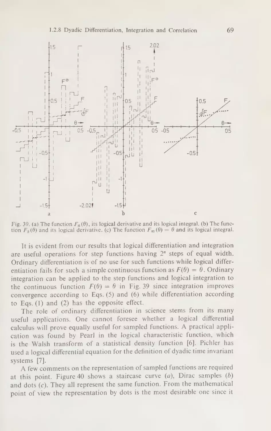
1 .2.8 Dyadic Differentiation, Integration and Correlation... «s+
urent oil oit n IN Ie i -1e/il-lNr Ninn MNO
1.3.1 Physical Interpretation of the Generalized Frequency... .
1.3.2 Power Spectrum, Amplitude Spectrum, Filtering of Signals . .
1.3.3 Examples of Walsh-Fourier Transforms and Power Spectra .
oes Pae-ante sila 7 ohceON e.ca
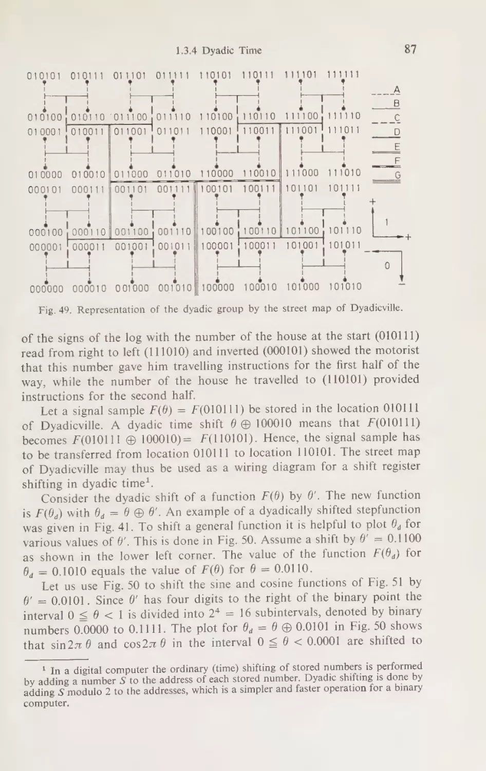
LStaeDyadicn Lime arg = eres outers
(eseGeneralizedsEnequencyamemrein
2. SEQUENCY
FILTERS
FOR
TIME
AND
SPACE
SIGNALS
oe 6
a)i (Cromeallnatorn lenilverts toe Abie Seals 4 6 5 656 ooo
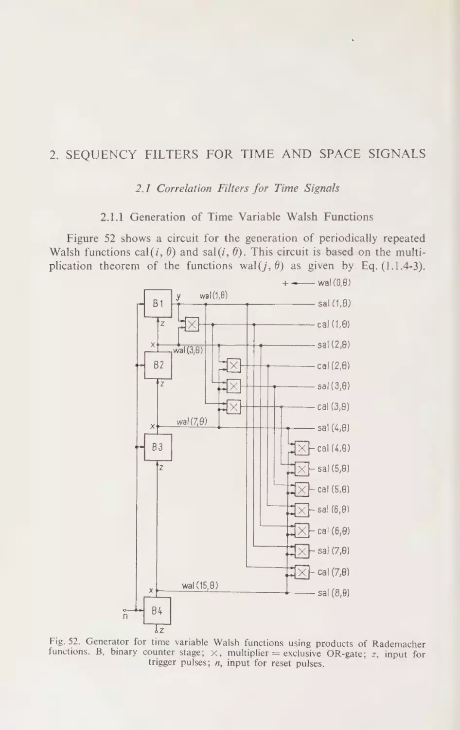
2.1.1 Generation of Time Variable Walsh Functions. ......
es
se eee
7 - Go
6
21.2) Sequency Low-Pass Filters
- - .. 1.2 22 s+ 44+: +
2.1.3 Sequency Band-Pass Filters
.......
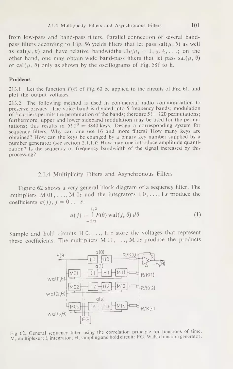
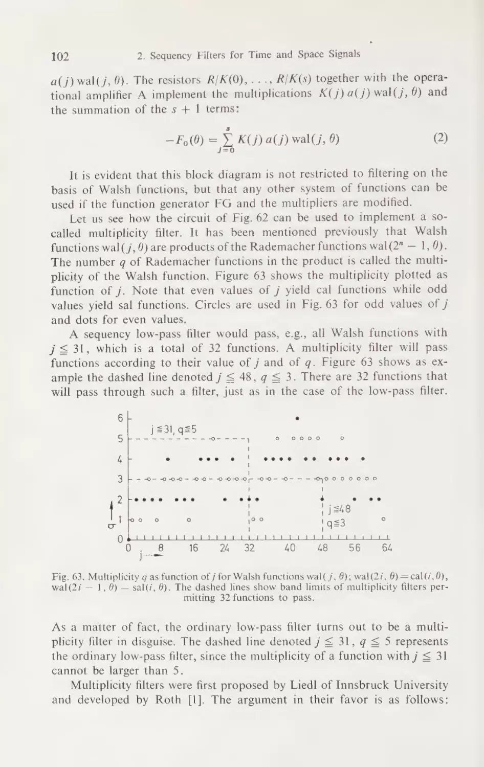
2.1.4 Multiplicity Filters and Asynchronous Filters
Contents
.......+.-.+++-.:-.
2.2 Resonance Filters for Time Signals
.......-.
2.2.1 Series and Parallel LCS Resonance Filters
nee nme
ner
ime
s
m
i
E1ltCiS
Resonances
299) Tow-Pass LCS
9.2.3 Parametric Amplifiers . «3 3) .07s 3) @ es oaine en ese
2.3 Instantaneous Filters for Space Signals. ......-.----2.3.1 Filters for Signals with One Space Variable . .
..... .
2.3.2 Filters for Signals with Two Space Variables
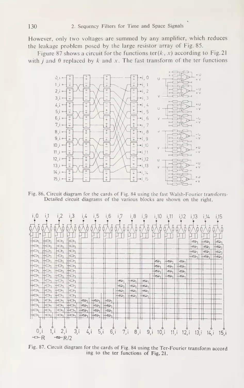
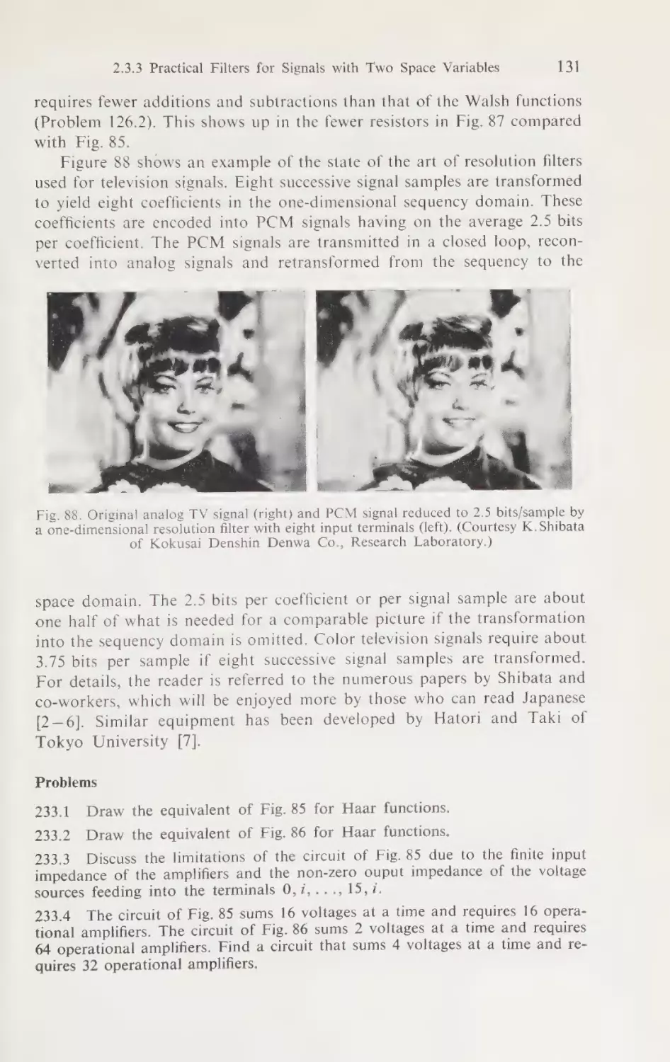
2.3.3 Practical Implementation of Filters for Signals with Two Space
peer
ee
ey
eee
a0 6 ce
Variables.
2.3.4 Filters for Signals with Three Space Variables. ......
ae
--eaee 0
2.4 Sampling Filters for Space Signals = 2 222.4.1 Generators for Space Variable Walsh Functions ......
2.4.2 Sampling in Two or Three Space Dimensions by Block Pulses
Braye, WMG Mies!
6 4 5 o Ho 6 ob AO oe
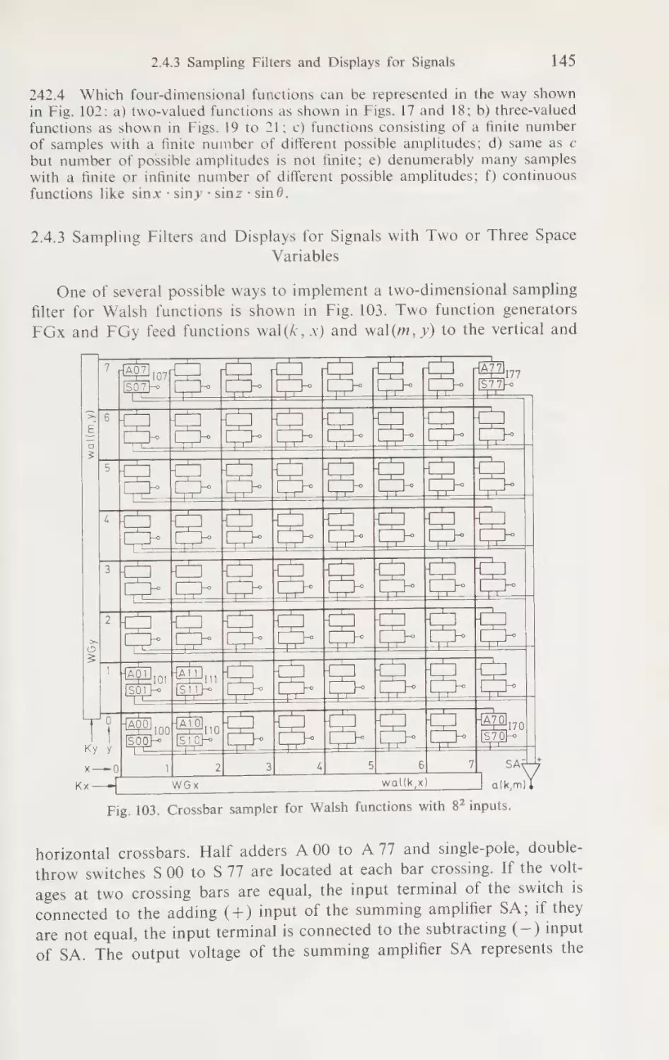
2.4.3 Sampling Filters and Displays for Signals with Two or Three
Space Variables 5—. 2 25) ce cee ge ce gee a
eee
DS, ytaiell Seauemey Wiis
6 6 ooo
tn oH
2.5.1 Filters Based on the Generalized Fourier Transform ...
25.2) Filters) Based on) Difterences Equations mys -ann- ee
. DIRECT
TRANSMISSION
.
OF SIGNALS
3.1 Orthogonal Division as Generalization of Time and Frequency
Division <2 oP ae OS
ae
ee ne
as
ag ees Meera mr,
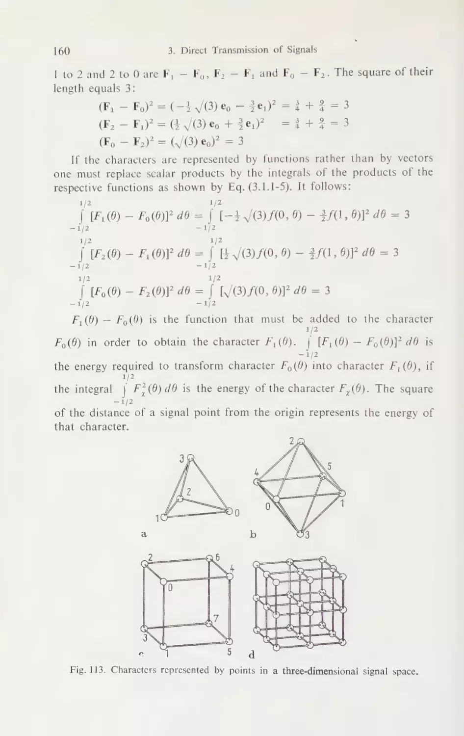
Brielm@Re presentatlOTn@.i91
Si)a lcm mn mle te en
SMe Bxamples#ofeSicnall Saas asm anaes
3.1.3 Amplitude Sampling and Orthogonal Decomposition . .. .
Be Practicalwero blemSe@ lmlnai
Sti) SS] Cie i
mn
a
eee
3 .o leGircuitseot Onthoconale Divisional
mieneenn anon amen
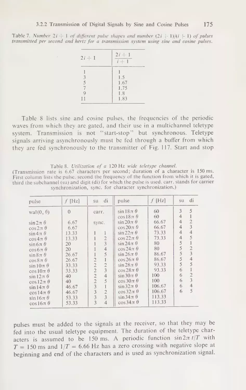
3.2.2 Transmission of Digital Signals by Sine and Cosine Pulses
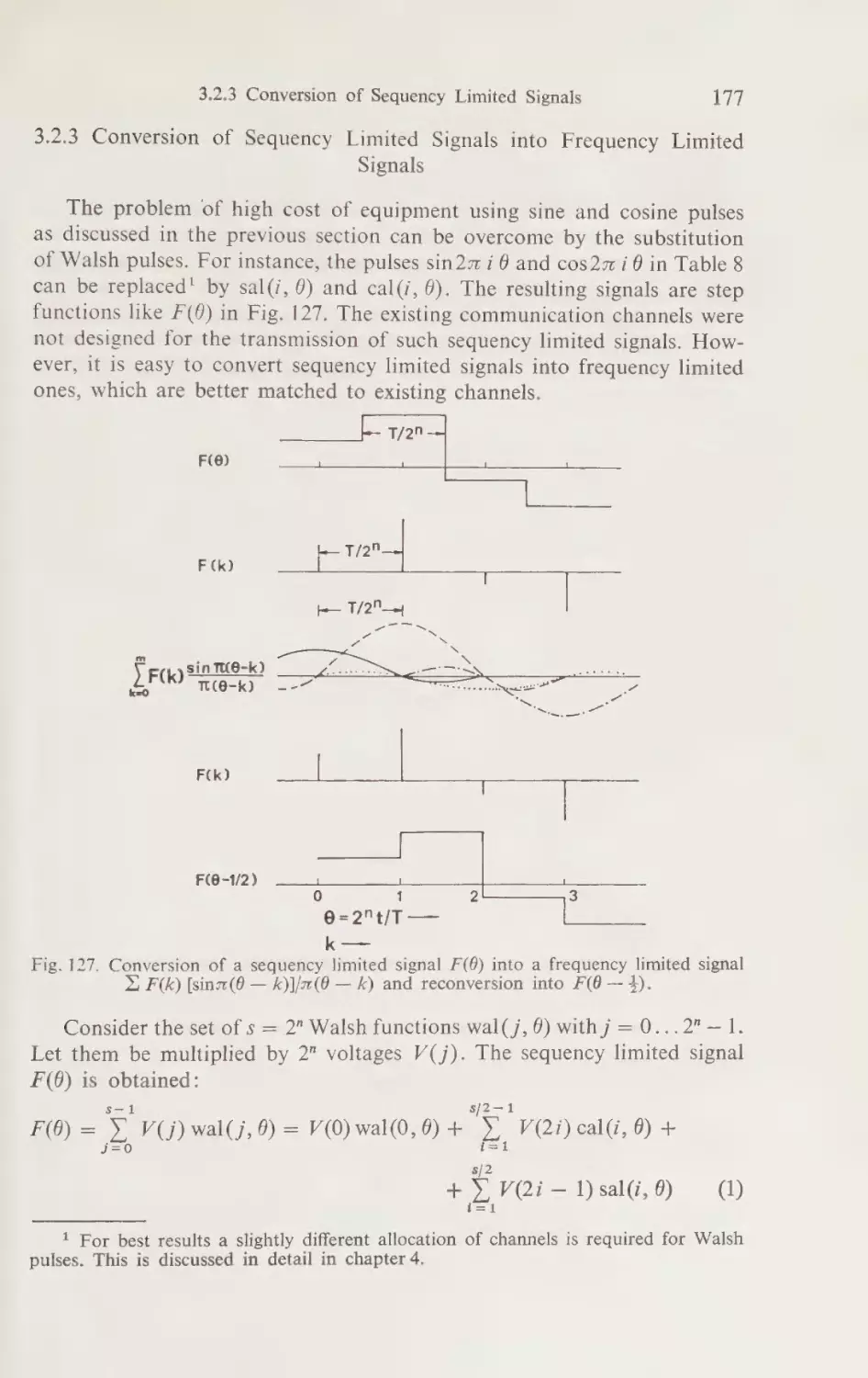
3.2.3 Conversion of Sequency Limited Signals into Frequency Limited \Signalss 7.2
252 o hee
ahces een
ee a
ee
ee
3.5. Characterization
3.3.1 Frequency
Of Communications
Response
@ hantic!se- alan
it ienn anemone
of Attenuation and Phase Shift of a
Commaunicatiomm hai cle meee eer
3.3.2 Characterization of a Communication Channel by Crosstalk
Parameters,
. CARRIER
sc
TRANSMISSION
ee
eed
ee
eee
OF SIGNALS
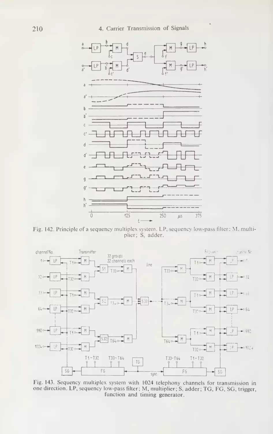
44i) Niele IMicxluiletieim GNIMD) 2 so 6 5 pe oe oe
A
ee
4.1.1 Modulation and Synchronous Demodulation. .......
4.1.2 Correction of Time Differences in Synchronous Demodulation
4.1.3 Methods of Single Sideband Modulation
oF fe.) at) Wiese, 6) tet) is) ke
4.2 Multiplexing of Time Variable Signals
AA IMU. NRG « 5 6 6 5 6 oo 8
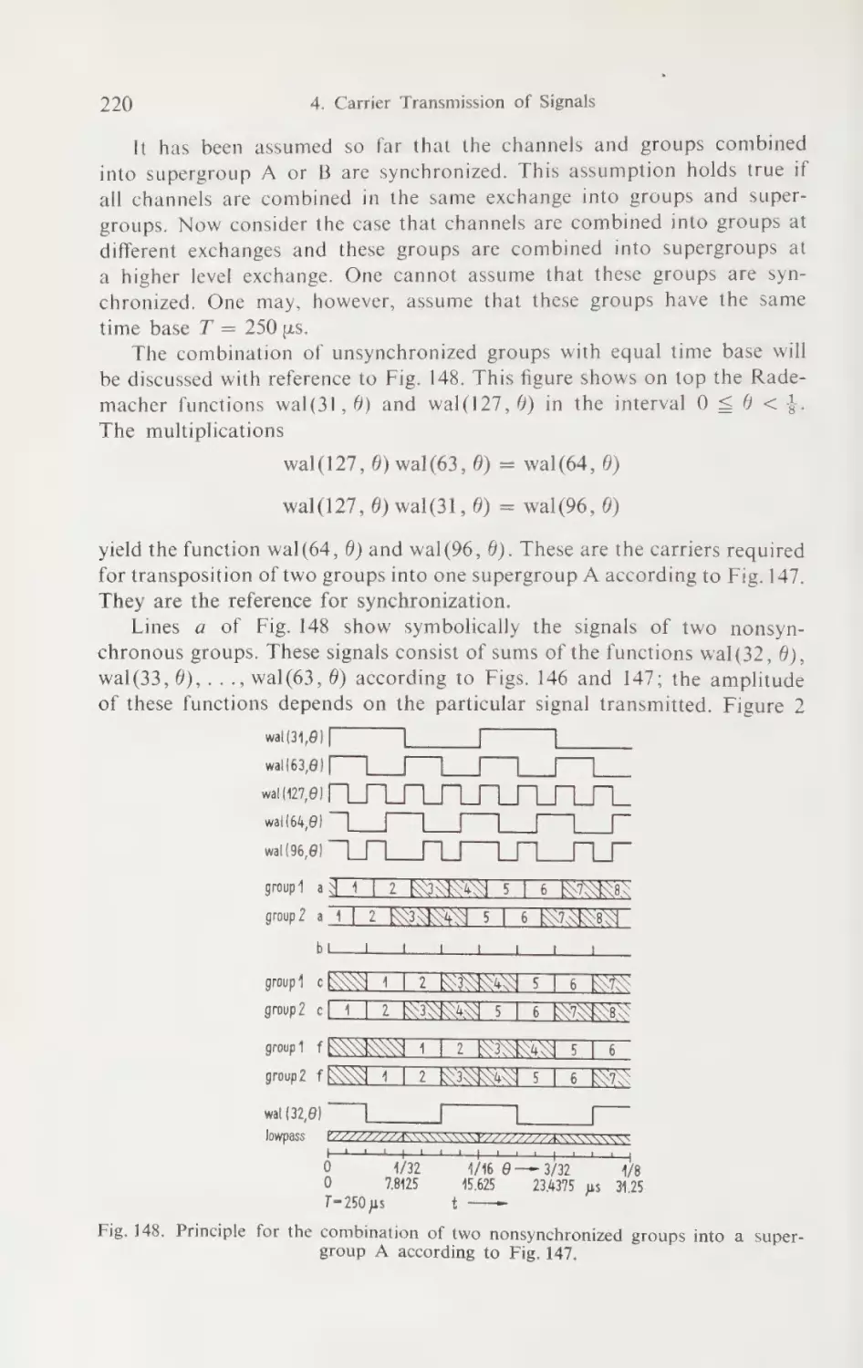
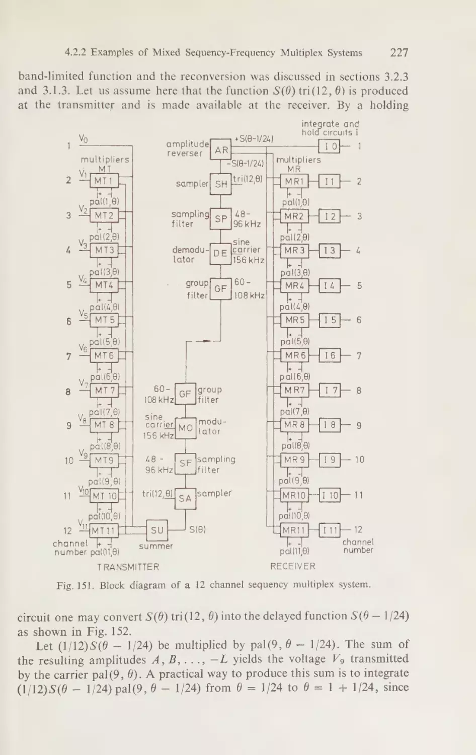
4.2.2 Examples of Mixed args ee ee
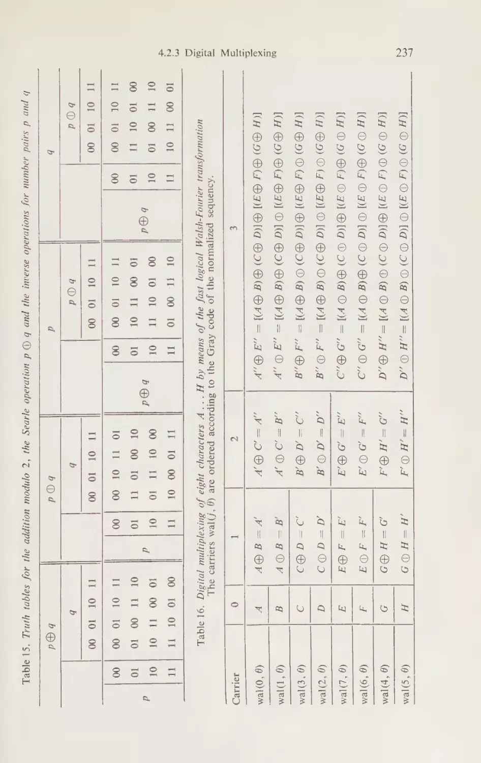
4.2.3 Digital Multiplexing.
ke
ee
oe
Multiplex Systems
ae PPE
234
Contents
4.3 Time Base,
ALS Time
ABV) “Unitas.
CLSV8} (Cloves
Xi
Time Position and Code Modulation
See WMleyehuileniiorny (UIRIMD) o 6 5 6 5 @ 9 6 6 oo OO
Leto ator INiloyelwibyreyrmy (MPI)
=. 6 4 6 56 6 9 6 9 0 OO
IMakovaiultetatoras (CCIMD) 3 5 co 59 a 6 6 on bp Go 8 Oe
. NONSINUSOIDAL
ELECTROMAGNETIC
239
241
243
WAVES
Sail IDypyolls Teaveltriion Gi WWI WERKE og gp co 6 6 a
5.1.1 Hertzian Dipole Solution of Maxwell’s Equations
.... .
Suil2 Neale 7AemmOa—= WANE 74S TENSE 5 og 6 6 9 A
Oe oo
8
Suil.) IMbgaiae IDYpOKe iNav
6 6 6 65 5 59 5 6 ooo
eo
alee implementationeo
hacia tOLs mali iemeetin
wei nomen
244
244
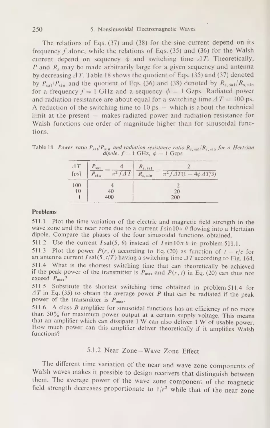
250
252
ES)
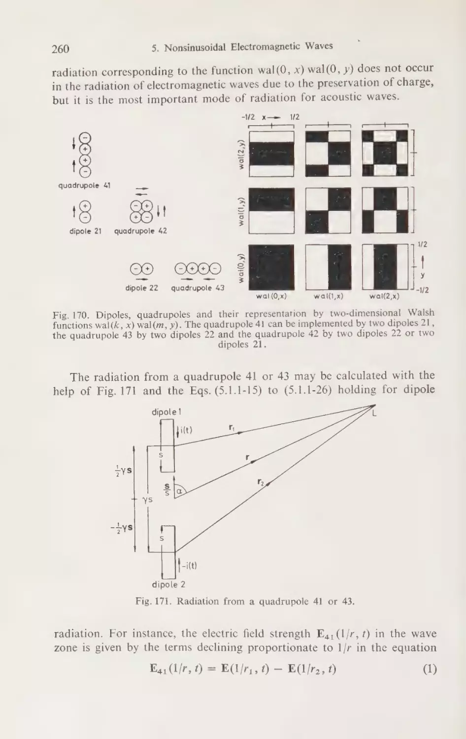
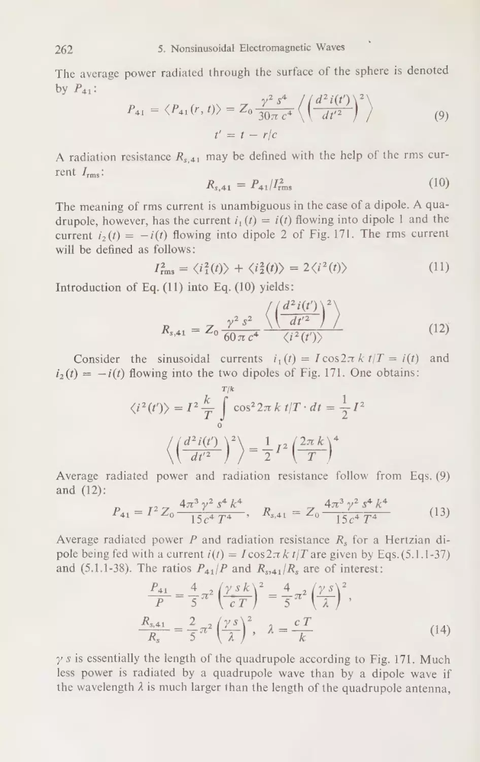
5.2 Multipole Radiation of Walsh) Waves
=<. -: =... ..... .
5.2.1 Radiation of a One-Dimensional Quadrupole
.......
5.2.2 Radiation of a Two-Dimensional Quadrupole
.......
S28) Michio alee.
1 6 5 6 on ope
op
Oo oo
259)
259
264
266
Sse intenerencesEtleclsam
ODP lei il CC Uns meni
alt=jnl-Mra l-iNT
.. .
5.3.1 Radiation Diagram of a Row of Spherical Radiators
PEPE UBTSool lip alile homnln, a A Merect ahh moe Ceo Mom | cece ie Mec meses.
. .
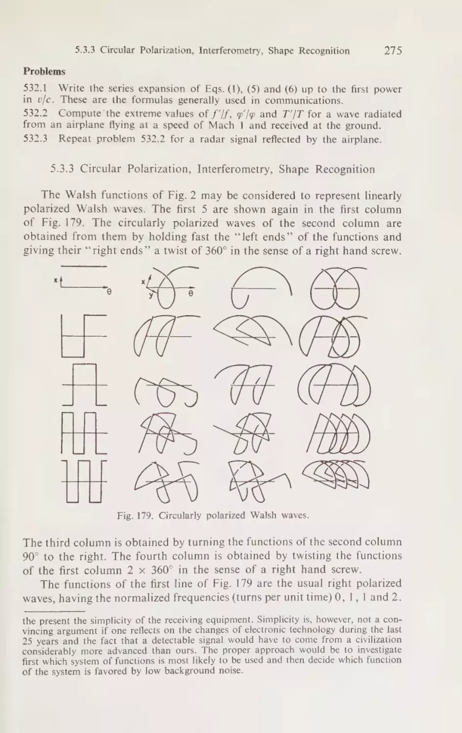
5.3.3 Circular Polarization, Interferometry, Shape Recognition
267
267
274
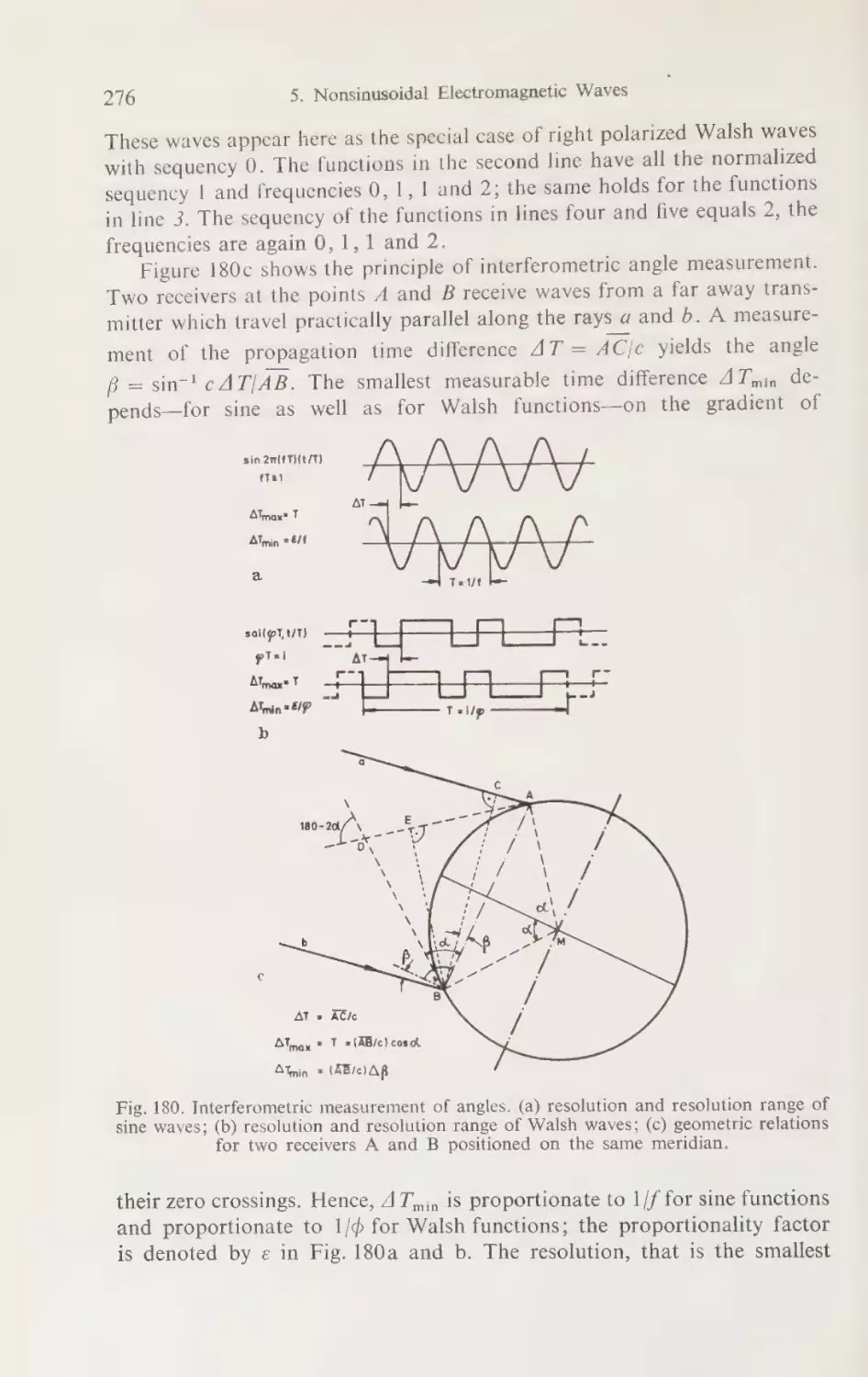
275
282
5.4 Signal Selection and Synchronization. ........-.-++-s-.
282
.
....
Communication.
Mobile
in
Signals
of
5.4.1 Separation
286
.......-.-.
5.4.2 Synchronous Reception of Walsh Waves
. APPLICATION OF ORTHOGONAL
PROBLEMS
FUNCTIONS TO STATISTICAL
6.1 Series Expansion of Stochastic Functions. .......+.+-.+..,
Oo eG
ooh
. 56 56 6 ob GoGo Oh Ooo
Gili “Wissel IMB
6.1.2 Statistical Independence of the Components of an Orthogonal
re ONCE WEN
LED CoP RCO” cosacy Ser ratey iy Slag 4 ie hoi cunt USC
2)
292
bo 8 oO ao ee
5 5 6 6 6 6 6 6 ooo
Go (Maine IDIAMINERINSES,
Sample Funcfrom
Signal
a
of
Deviation
Square
Mean
6.2.1 Least
igs Onis NG woman CLrar
es USER GORE Unt bees ee
oS Se
eliCes
tng) elie eos pet Genre kehrce oe, Gee
622.2 PxamplesrOt CHCUUS
-T unr nr
emt
mean incni nes
Gage Matched sHiltersesmn
......-..-+.-.--.
6.2.4 Compandors for Sequency Signals
297
296
297
299
303
305
308
2 2 3 2 Se
2 2 2
6.3) Multiplicative Disturbances
308
HOO
oOo
eb
oho
5
0
6
5
.
5
Faahine
OSkil lhivertarsnes
6.3.2 Diversity Transmission Using Many Copies ....... .- 314
. SIGNAL
DESIGN
FOR
IMPROVED
RELIABILITY
316
ae
an ee) als oe 2s
Pla Vavistnissionts Capacity syn.
316
ie
ee
a 60 se
Tete Measures) Of (Bandwidth) si.
321
.
.
.
.
Channels
Communication
of
Capacity
Transmission
7.1.2
328
...........
7.1.3 Signal Delay and Signal Distortions
..
of Signals...
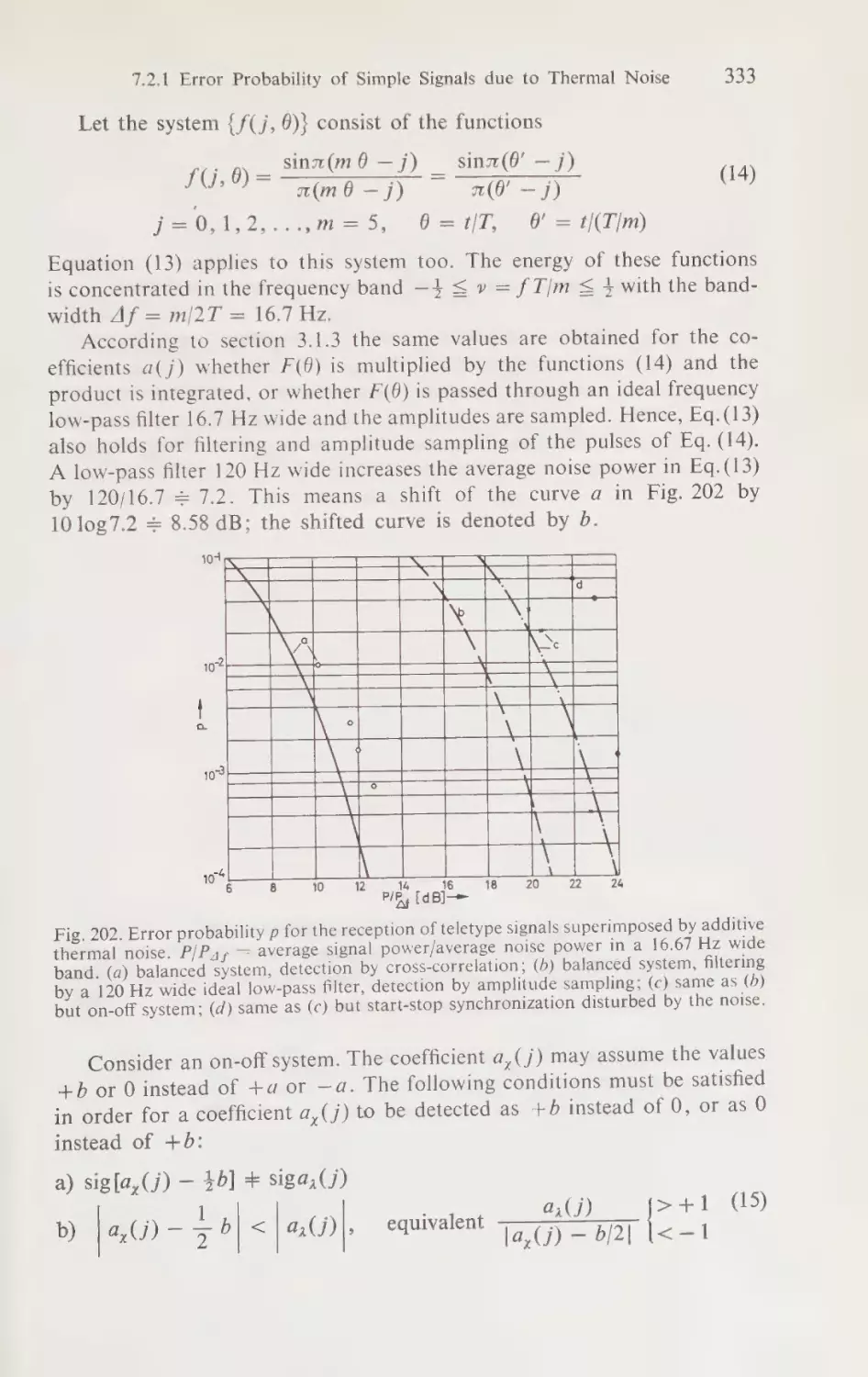
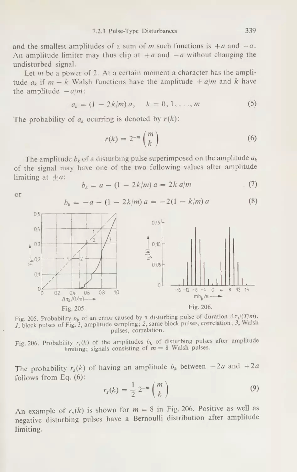
7.2.1 Error Probability of Simple Signals
2
DePeak. Power Limited sienals)
7
7.293 Pulse-lype Disturbances ~ 2 - =
7.2 Error Probability
se
sees
55s
. .
due to Thermal Noise
2 5 5 2: 6 2. = 2 4
= s+ +2 © 4+ >> oo 6
6-2-5
330
330
334
SW
Xii
Contents
7.3 Coding ©< 0s 400 se yaaa
ee Gera eee
340
73,1, Coding with Binary Elements
“ae 9 ae sue eee ee
340
7.3.2 Orthogonal, Transorthogonal and Biorthogonal Alphabets. . 344
7.3.3 Coding for Error-Free Transmission
..... . fe Palas
351
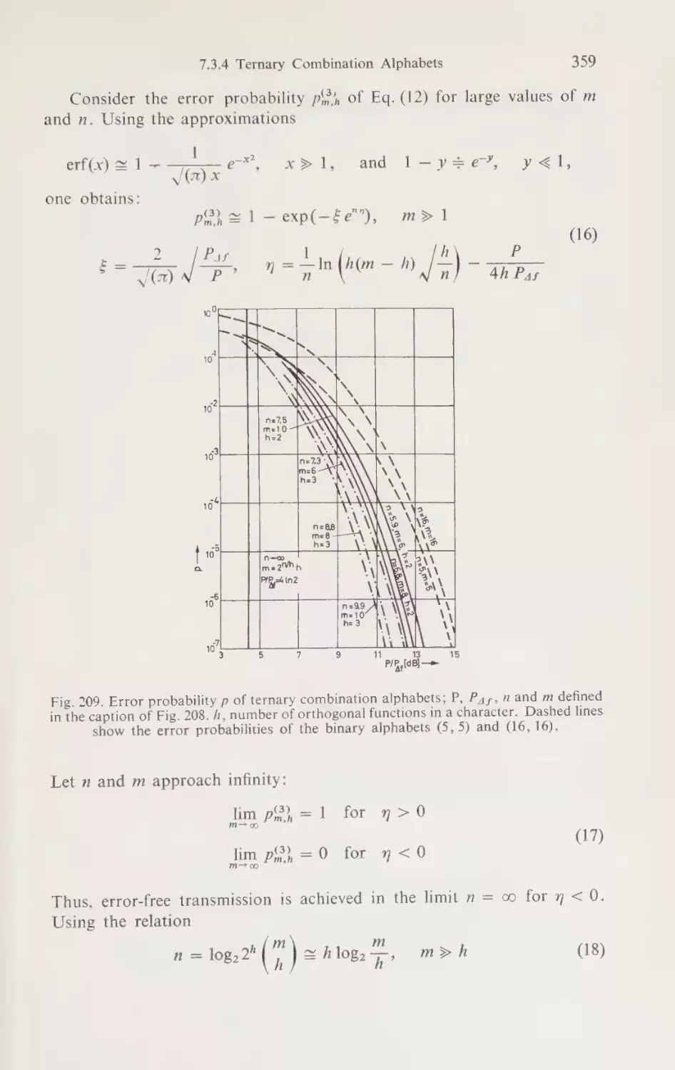
73.4 Ternary Combination Alphabets
7355s
ee
ee 852,
7.3.5 Combination Alphabets of Order 27
+1 .........
361
REFERENCES
ENIDEX ©4&
¥. 5 aoe.
5
wena
ee
Je: giv a sa sevhaladh cet ee eek mn
caelep
367
389
Equations are numbered consecutively within each of the sections 1.1.1
to
7.3.5. Reference to an equation from a different section is made by writing
the
number of the section in front of the number of the equation, e.g.,
(5.2.3-1) for
(1) in section 5.2.3.
INTRODUCTION
Historical Background and Motivation for the Use
of Nonsinusoidal Functions
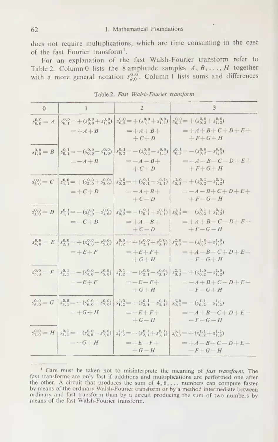
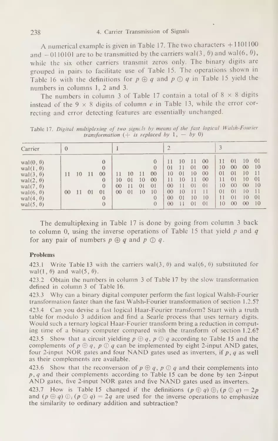
During the nineteenth century, the most important functions for communications were block pulses. Voltage and current pulses could be generated
by mechanical switches, amplified by relays and detected by a variety of
magneto-mechanical devices. Sine-cosine functions and the exponential
function were well known and so was Fourier analysis, although in a somewhat rudimentary form. Almost no practical use could be made of this
knowledge with the technology available at that time. Hertz used the exponential function to obtain his famous solution of Maxwell’s equations
for dipole radiation but he was never able to produce sinusoidal waves?.
His experiments with wave propagation were done with what we would
call colored noise today.
Toward the end of the nineteenth century, more practical means to
implement capacitances than Leyden jars and metallic spheres were found.
The implementation of inductances through the use of coils had been known
long before. Practical resonant circuits for the separation of sinusoidal
electromagnetic waves of different frequencies could thus be built around
the turn of the century. Low-pass and band-pass filters using coils and
capacitors were introduced in 1915 and a large new field for the application
of sinusoidal functions was opened. Speaking more generally, the usefulness of sinusoidal functions in communications is intimately related to the
availability of linear, time invariant circuit components in a practical
form.
A major breakthrough of technology was provided by the introduction
of semiconductors. The switch was added as a linear, time variable component of extreme usefulness. Furthermore, the previous emphasis on
fewer circuit components and, especially, the exclusion of active components such as tubes became obsolete. This change opened the way for the
use of nonsinusoidal functions.
There were two schools of thought from the beginning. The one tried
to find functions that were best suited for a given problem from the mathematical point of view. The parabolic cylinder functions were found to
1 The word ‘“‘sinusoidal’’ seems to have been introduced to communication engineering by A. Graham Bell in 1876. See pages 9 and 10 of [17] and page 192 of [18].
Introduction
y
compress the signal energy into the smallest section of the time-frequency
domain. This result was already known to Wiener in the early thirties.
In the fifties, prolate spheroidal functions were found to be almost as
good and separable by time sampling. Not much came of either system of
functions since the practical difficulties were too great to justify their use.
The second school of thought tried to find functions that led to equipment easily implemented by the available technology. This approach will
yield, from the mathematical point of view, optimal solutions for given
problems by coincidence only. However, simplification of equipment is
in itself a desirable goal for the engineer. In addition, inherent simplicity
makes it possible to develop equipment that would otherwise be too
complicated.
As an example of the last statement, consider television. Black-andwhite TV pictures are signals with two space variables and the time variable.
No filters on the basis of sine-cosine functions ever became known for
such signals, despite the high degree of sophistication of filters for time
signals. The so-called Walsh functions, on the other hand, made it possible
to design such filters, and they have already been implemented in their
simplest form.
The search for useful functions led first to the system of Walsh functions,
which assume the two values +1 and —1 only. The basic discussion of
theory and equipment is usually presented for this system of functions.
When it comes to practical equipment design, other systems of two- or
three-valued functions are often used; however, it would be impractical
to constantly refer to all these other functions. A similar situation exists
in time division multiplexing which is generally discussed in terms of
block pulses while actually a variety of other pulse shapes is used.
There were unforeseen but happy developments when the applications
of Walsh
functions
in communications
were
investigated.
First,
it was
found that Walsh functions were excellently suited for the analysis of
sampled signals and the design of equipment for such signals. Second, the
heavy emphasis on time as the variable in communications was found to
be closely connected to sinusoidal functions but the connection did not
carry over to Walsh functions. As an example, consider a tunable generator
for sinusoidal functions. Probably every reader will think of a generator
for time variable sinusoidal functions. Indeed, it is hard to imagine a
generator that produces space variable sinusoidal functions that can be
tuned, e.g., from 20 cycles per meter to 20,000 cycles per meter. It is one
of the primary tasks of science to recognize and overcome such impediments
to thinking.
Walsh functions are presently the most important example of nonsinusoidal functions in communications. They have been used for the
transposition of conductors in open wire lines for more than 60 years.
Rademacher functions, which are a subset of the Walsh functions, were
Introduction
3}
used for this purpose toward the end of the 19th century [1]. The complete
system of Walsh functions seems to have been found around 1900 by
J. A. Barrett’. The transposition of conductors according to Barrett’s
scheme was standard practice in 1923, when J. L. Walsh introduced them
into mathematics [3, 4, 6]. Communications engineers and mathematicians
were not aware of this common usage until very recently [5]. Individual
Walsh functions have been used for a much longer time. They may be
found on ancient temples*, and the pattern of the checker board used for
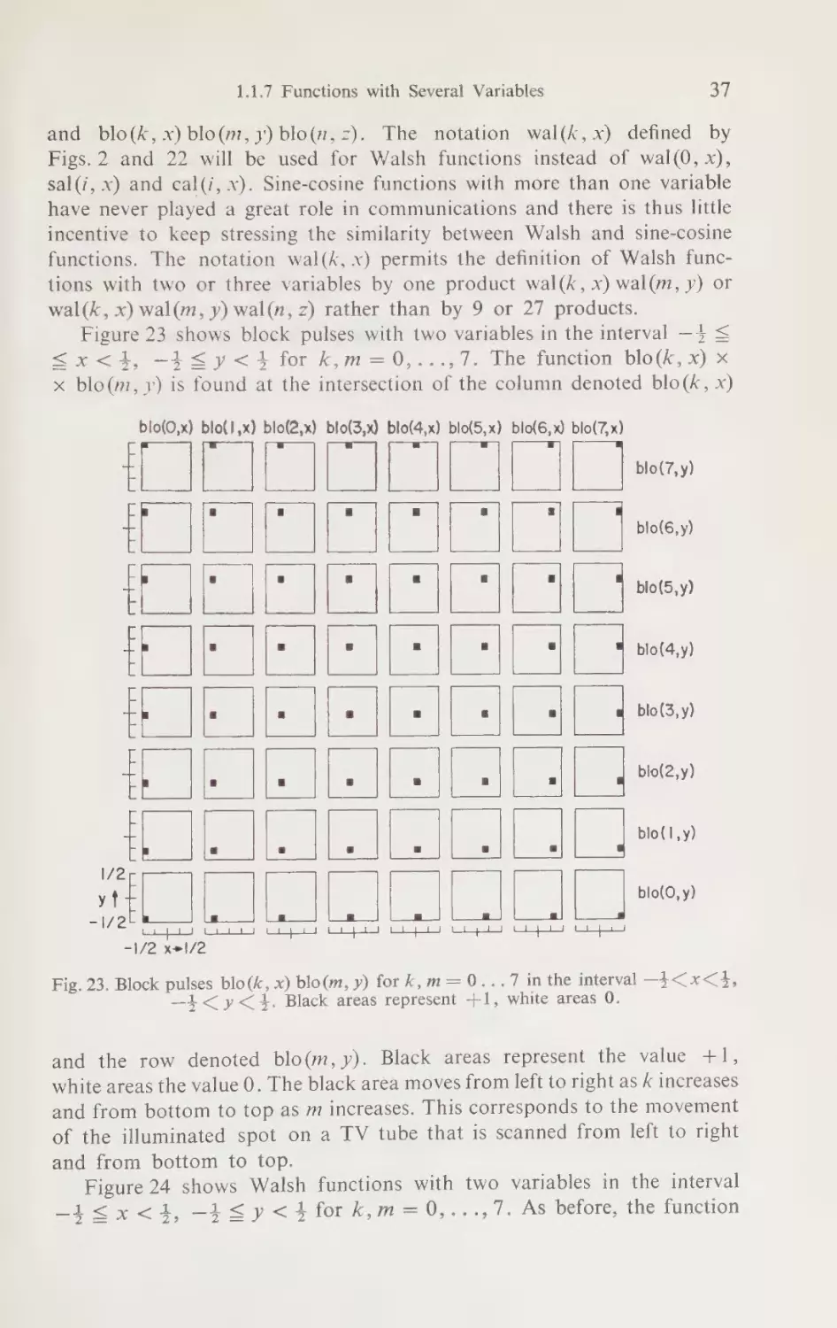
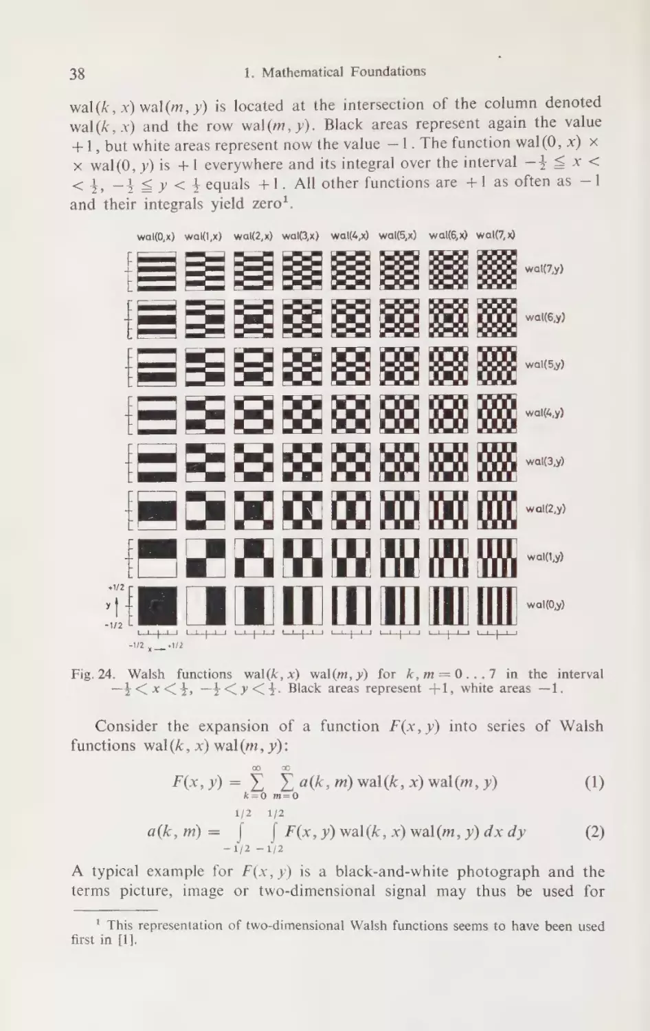
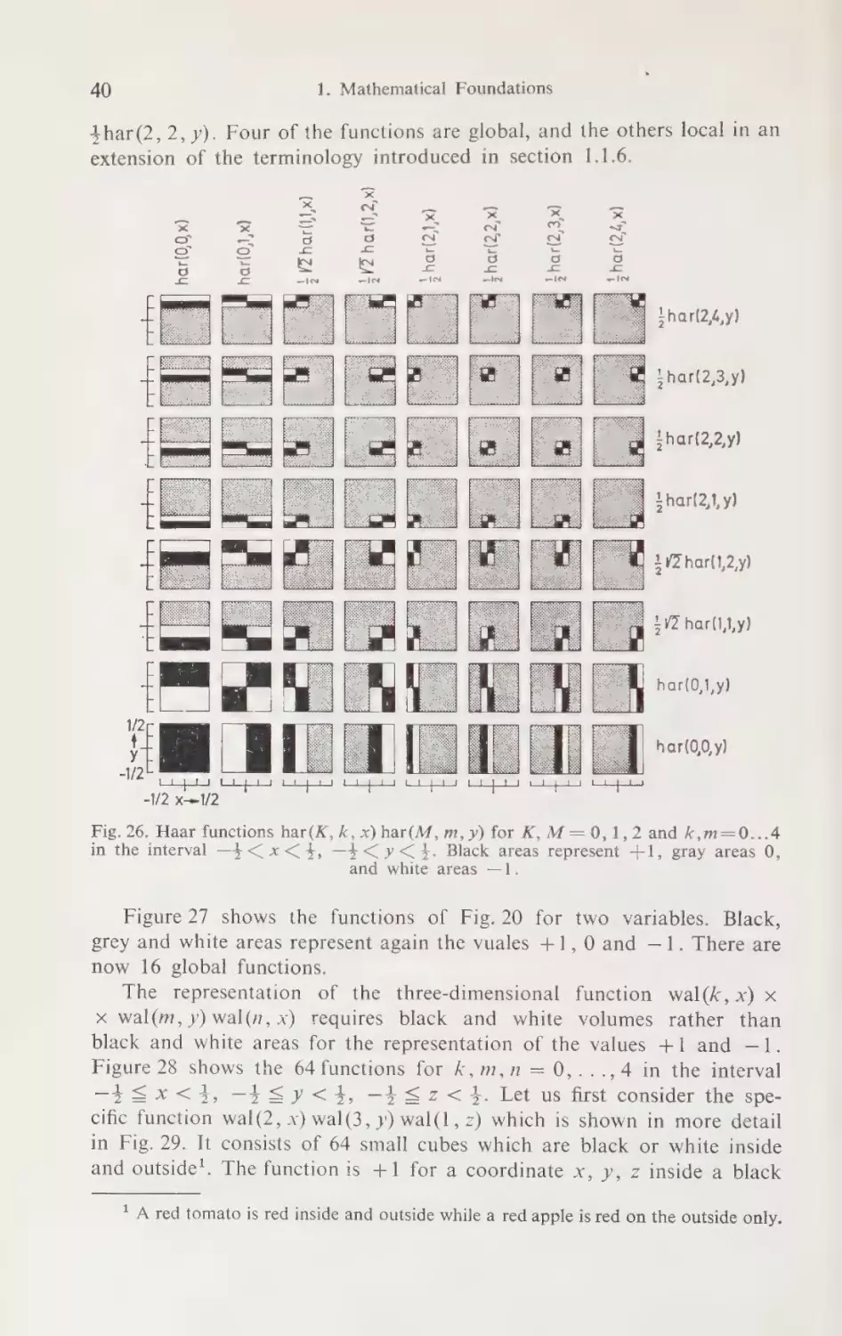
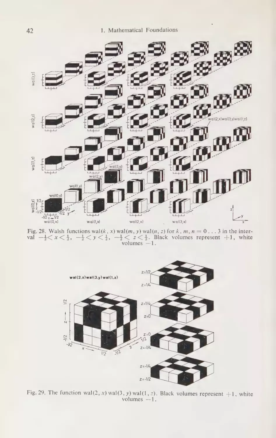
playing checkers or chess turns out to be a two-dimensional Walsh function.
Orthogonal
Functions, Walsh Functions and Other Basic
Mathematical Concepts
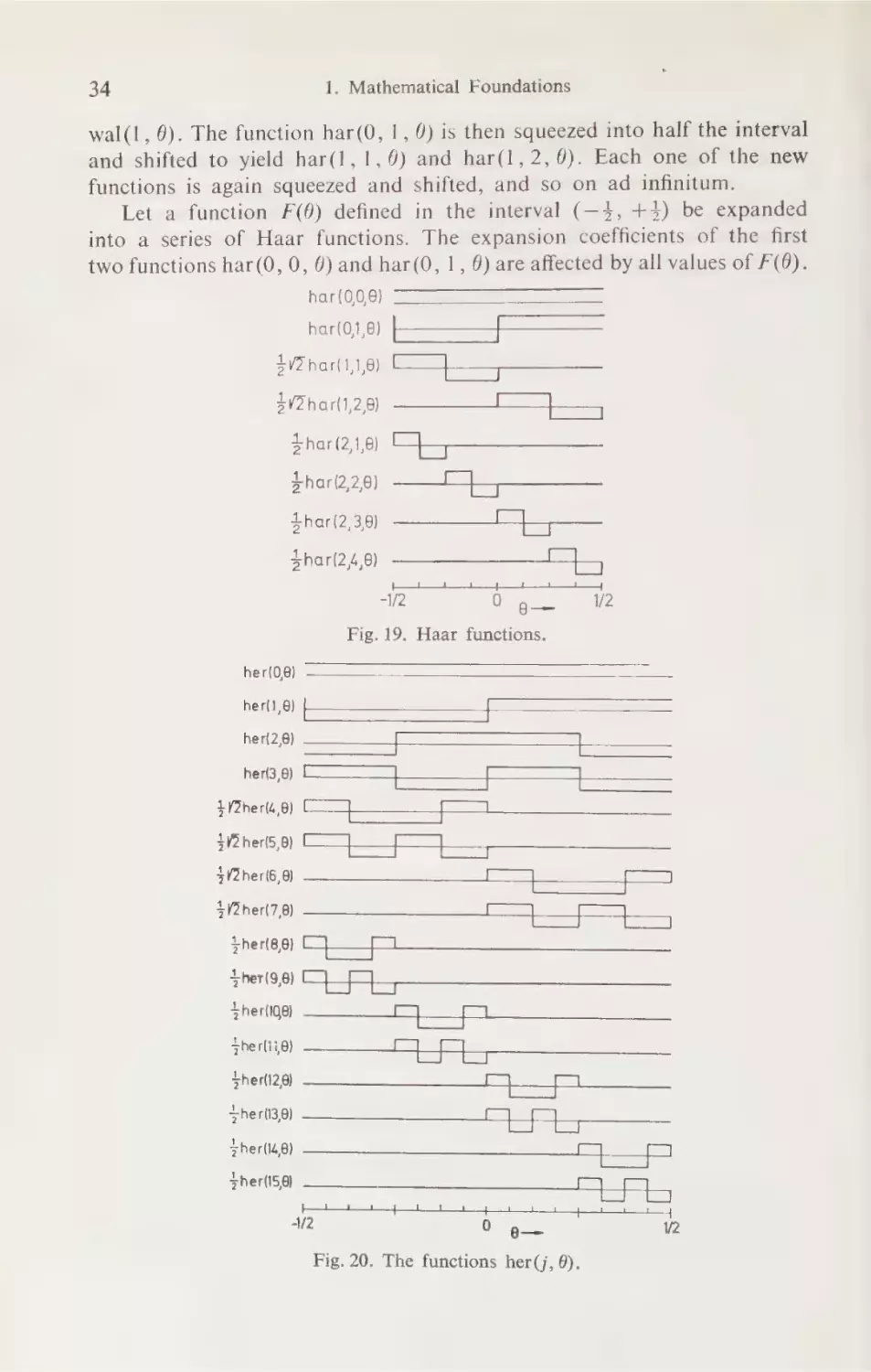
Two functions f(j, 6) and f(k, 9) are called orthogonal in the interval
1/2
—4<06<tH
ifthe integral
| f(j, 0)f(k, 0) dO is zero for j+ k. They are
—1/2
orthogonal and normal or orthonormal if the integral equals 1 for j= k.
The best known system of orthonormal functions is the system of sine and
cosine functions shown in Fig. 1, with the normalized time 6 = ¢/T as
variable. These functions are used in Fourier series expansions and it is
easily verified that the integral of the product of any two functions is zero.
wal(0,8)
>>
2 sin 206
Sa
\2 cos 216
ANN,
V2sin 418
SO
2 cos4n8
PRI
RL SP V2sin 616
ee
aoe
(pgs rORROET
ae Sa?
e—
Fig. 1. Orthonormal
sine and cosine elements.
1 John A. Barrett is mentioned by Fowle in 1905 as inventor of the transposition of
conductors according to Walsh functions; see particularly page 675 of [2].
2 Rademacher functions are conspicuous all around the outside walls of the main
palace at Mitla near Oaxaca, Mexico [7]. A Walsh function cal(3/8,x) appears less
conspicuously above the entrance.
4
Introduction
Walsh functions are another example of orthonormal functions. Fig. 2
shows the first 64 of them. The notation sal(i, 9) and cal(i, @) is used for
these functions. The letters s and c allude to sine and cosine functions,
to which the respective Walsh functions are closely related; the letters al
are derived from the name Walsh. The functions cal(i, 0) are even functions
like ./(2)cos27i6, the functions sal(i, 0) are odd functions like
/(2) sin2a i 0.
In Fig) ithe parameter? = eee errr /(2) sin2z i 6 and J/(2) cos22i6
gives the number of oscillations in the interval —} S @ < 4, which is the
normalized frequency i = f 7. One may interpret i as “one half the number
of zero crossings per unit time,” rather than as “oscillations per unit
time” [8, 9, 10]. The zero crossing at the left side, 6 = —4, but not the
one at the right side, 6 = +4, of the time interval is counted for sine
functions.
The parameter i also equals one half the number of zero crossings in
the interval —4 < 6 < 4 for the Walsh functions in Fig. 2. In contrast
to sine-cosine functions, the sign changes are, in general, not equidistant.
If, unlike in Fig. 2, i is not an integer, then it equals “one half the average
number of zero crossings per unit time.”” The term “‘ normalized sequency”’
has been introduced for i, and ¢ = i/T is called the nonnormalized sequency, which is measured in zps:
sequency in zps = 4 (average number
of zero crossings per second)
The concepts of period of oscillation t = 1/f and wavelength A = v/f
are connected with frequency. Substitution of sequency ¢ for frequency f
leads to the more general concepts of ‘‘average period of oscillation”’
t = 1/¢ and “‘average wavelength” A = v/¢:
average period of oscillation = average separation in time of the
zero crossings multiplied by 2,
average wavelength = average separation in space of the zero
crossings, multiplied by 2; v is the velocity of propagationof a zero
crossing.
One of the most important features of sine and cosine functions is
that almost all time functions used in communications can be represented
by a superposition of sine and cosine functions, for which Fourier analysis
is the mathematical tool. The transition from time to frequency functions
is a result of this analysis. This is often taken so much for granted by the
communications engineer that he instinctively sees a superposition of
sine and cosine functions in the output voltage of a microphone or a teletype transmitter. Actually, the representation of a time function by sine
and cosine functions is only one among many possible ones. Complete
systems of orthogonal functions generally permit series expansions that
Introduction
5
correspond to the Fourier series. For instance, expansions into series of
Bessel functions are much used in communications. There are also transforms corresponding to the Fourier transform for many systems offunctions.
Hence, one may see a superposition of Legendre polynomials, parabolic
cylinder functions, etc., in the output voltage of a microphone.
Zyl
1
3
5
7
9
sal(i,8)= wal(2i-1,8)
00000
f
000011
a=
f
|
000101 KF
lie
f——
00011)
Rt
001001
RRR} — HHT FSO
i
cal(i,8) = wal(2i,9)
2i
0
0 000000
1
fF
}
2 000010
2
i
{
|
f
4 000100
3
f$—|—_f
j——-f—--]
6 000110
46 eR
EF
8 001000
=
EF HE EE 10 001010
i CONON
pe tet
e
r 12 007 100
eC ONO bee ete
el tae
ee
at tele
ie ee 14 -000190
199001111
ee se et eS ee
8 <a eS SE FE FEE
16 010000
a OVOO0 |late
er
ee
Se
ee eet ee 8. 010010
19, 000011 PS
eS re et ee 10
eee
HE
20 0170100
00101 ee
a
ee
EE
22 010010
23010 hha aae
eet ee 12
eee
24701110068
25 011001 eo
ad ee
Ee
13: SESE:
ee
26. 0110010
27 017017 FRESE
EEE: 16 EFF
=F
28° (011100
29 011101 KEEFER
EEE: 115EHF
FEF
30-0110
31077177 FERRELL:
16 (EEE
HE 322:100000
33 100001 FAEFEFLFL ALAA
17 FFE
34 100010
35 100071 FEFLFLELRAFLALAL AEH
18.LAER
HE AE 36. 100100
37 100101 KALA ELH
LAE 19 FALL
HIF: 38 100110
39 100711 FLFLAFEARLEHLA
HAA
A: 20 “HEEL
A
40 101000
41 107001 FARLELAR-ARLALRAE AAR
21 AR ALAA AIR: 42 101010
017 FERALAS:
22 LEAL AA
HAA
44 101100
TOTe
10000
0010
0100
0110
111000
111010
11100
111110
Fig. 2. Orthogonal Walsh elements wal(0, @), sal(i, 0), cal(i, 9). The numbers 27 and
2i— 1 are given in decimal and binary notation; i is the normalized sequency.
The transition from the system of sine-cosine functions to general
systems of orthogonal functions brings simplifications as well as complications to the mathematical theory of communication. One may, e.g.,
avoid the troublesome fact that any signal occupies an infinite section of
the time-frequency-domain by substituting a time-function-domain. Any
time-limited signal composed of a limited number of orthogonal functions
occupies a finite section of this time-function-domain.
Introduction
6
Filtering of Time and Space Signals
The acid test of any theory in engineering is its practical application.
Filters are the area of application in which Walsh and similar functions
have made the biggest progress toward practical use’. Filters for time signals
have been developed that use the correlation principle and are implemented
by multipliers, integrators, adders, and storage circuits. Furthermore,
filters using the resonance principle have been implemented with the usual
coils and capacitors supplemented by switches. It is worth noting that
filters based on nonsinusoidal functions do not necessarily have to be
synchronized in any way to the signal: There are filters that require synchronization but there are others that do not; they are referred to as asynchronous filters.
One of the most interesting new developments are filters for signals
with space variables. There has been a need for such filters ever since
television was introduced and such recent developments as the picturephone and picture transmission from deep space probes have increased
this need. The usual theory of filters for time variable signals cannot be
used for spatial filters. Digital computers have been applied very successfully to this problem by Alexandridis, Andrews, Carl, Kabrisky, Kennedy,
Parkyn, Pratt, Wintz and others. These computer techniques are discussed
in an excellent book by Andrews and are not dealt with here [11]. Analog
circuits based on the computer techniques can be implemented by the usual
means of electrical engineering and experimental equipment for the bandwidth reduction of TV signals has been developed succesfully by Enomoto”,
Hatori*, Miyata*, Shibata’, Taki* and others in Japan.
Not surprisingly, binary functions lead to simple digital filters. Two
varieties are known, one based on the generalized Fourier analysis the
other on difference equations.
Direct and Carrier Transmission
of Signals
The jumps between +1 and —1 of the Walsh functions make them
appear to be poorly suited for the transmission through existing communication channels. However, one should keep in mind that a signal
consisting of 2m independent amplitudes per second requires a frequency
bandwidth of nm hertz according to the sampling theorem, regardless of
how those independent amplitudes were generated. A frequency bandpass or low-pass filter can transform signals consisting of a superposition
1 Certain applications for which Walsh-Fourier analysis is used as mathematical tool
while the implementation is done by computers are comparably or more advanced.
See, for instance, the problems at the end of section 1.2.8.
? Tokyo Institute of Technology. — * Tokyo University. — * Hitachi Ltd., Central
Research Lab., Tokyo. —
ment Lab., Tokyo.
* Kokusai Denshin Denwa Co. Ltd., Research and Develop-
Introduction
oil
of Walsh functions into a frequency band limited signal, while a sampleand-hold circuit will reconvert it into its original shape.
One of the most promising areas of application of Walsh functions is
in multiplexing. Several experimental multiplexing systems have been
developed that make use of the rather different technology’. The emphasis
has been lately on the design of systems that are compatible with existing
frequency or time multiplexing equipment. Several solutions to this problem
have been found: a method for the transmission of digital signals matched
to the requirements of the switched telephone plant; a mixed sequencyfrequency method for the multiplexing of the usual 12 telephone channels
into a group; and a digital multiplexing method that is compatible with
digital cables but avoids the poor use of the amplifier power at low activity
factors that is characteristic for time multiplexing.
Most existing communication channels favor sine-cosine functions. This
is so because of technological advantages and not because of laws of nature.
Cables or open wire lines that could not, nor need not, transmit sinusoidal
functions have always existed. The telegraph lines of the 19th century,
using electromechanical relays as amplifiers, were such lines, and they
have recently made a comback as digital cables. Radio channels are allocated
according to the frequency of sinusoidal functions by human laws. It
will be shown in some detail that they could be allocated just as well according to the sequency of Walsh functions, at least on paper.
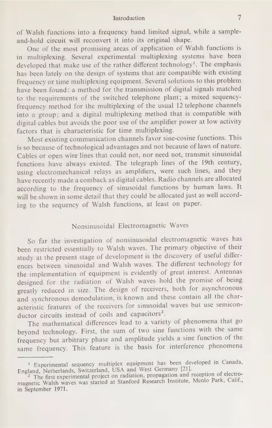
Nonsinusoidal
Electromagnetic
Waves
So far the investigation of nonsinusoidal electromagnetic waves has
been restricted essentially to Walsh waves. The primary objective of their
study at the present stage of development is the discovery of useful differences between sinusoidal and Walsh waves. The different technology for
the implementation of equipment is evidently of great interest. Antennas
designed for the radiation of Walsh waves hold the promise of being
greatly reduced in size. The design of receivers, both for asynchronous
and synchronous demodulation, is known and these contain all the characteristic features of the receivers for sinusoidal waves but use semiconductor circuits instead of coils and capacitors’.
go
The mathematical differences lead to a variety of phenomena that
same
the
beyond technology. First, the sum of two sine functions with
of the
frequency but arbitrary phase and amplitude yields a sine function
na
phenome
nce
same frequency. This feature is the basis for interfere
1 Experimental
sequency
England, Netherlands,
multiplex
Switzerland, USA
equipment
and West
has
been
Germany
developed
[21].
in Canada,
and reception of electro2 The first experimental project on radiation, propagation
Menlo Park, Calif.,
Institute,
Research
Stanford
at
started
was
waves
magnetic Walsh
in September 1971.
8
Introduction
ranging from multipath transmission to radiation diagrams of antennas
to shaping of radar return signals by the target, and so forth. Second, the
derivative of a sinusoidal function is again a sinusoidal function. As a
result, sinusoidal electromagnetic waves have the same shape in the near
zone and the wave zone; furthermore, the waves of multipole radiation
have the same shape as waves of dipole radiation. Walsh waves sum very
differently from sinusoidal waves and their shape is changed by differentiation. Hence, effects depending on summation and differentiation are very
different from what one is used to from sinusoidal waves.
The general form of a sine function V sin(2aft + «) contains the
parameters amplitude V, frequency f and phase angle «. The general form
of a Walsh function V sal(¢ T, t/T + to/T) contains the parameters amplitude V, sequency ¢, delay to and time base 7. The normalized delay,
to/T, corresponds to the phase angle. The time base T is an additional
parameter and it accounts for a major part of the differences in the applications of sine-cosine and Walsh functions. For instance, the Doppler
effect changes the sequency exactly the way it changes the frequency.
However, the time base is changed so that the product ¢ T remains unchanged
and it permits
a correct
identification
of the Walsh
waves
up
to relative velocities of the order of half the velocity of light.
Most problems concerning Walsh waves can presently be answered in
terms of geometric optic only, since wave optic is a sine wave optic. On
the other hand, there is little doubt that nonsinusoidal electromagnetic
waves are a challenging field for basic research. The generation of nonsinusoidal radio waves implies that such waves can be generated in the region
of visible light, and this leads ultimately to the question of why white light
should be decomposed into sinusoidal functions?.
Statistical Theory of Communication
Fourier analysis forces us to assume that a time signal is infinitely
long, or has an infinite bandwidth or is infinite in time and frequency.
This is particularly troublesome in the statistical theory of communication
which requires at least one more infinite quantity. The substitution of
general systems of orthogonal functions for sine-cosine functions and a
time-function-domain for the time-frequency-domain brings a well-needed
simplification.
Beyond mathematical simplification, Walsh functions provide us with
some very practical advantages. A nonlinear compressor will not generate
new Walsh functions if a signal consisting of a superposition of Walsh
functions is passed through it; the compressor will merely redistribute
' Theoretical and experimental work on optical spectroscopy based on Walsh functions or Hadamard matrices was done in England [16] and the United States [14, 15, 19].
A scintillation counter for nuclear spectroscopy was developed in the Soviet Union [20].
Introduction
9
the energy among the functions already present’. Jain pointed out that
crosstalk in a multiplex system due to nonlinearities, e.g., the hard limiter
in a Satellite repeater, can be avoided by using Walsh functions as
carriers [13].
In coding theory, Walsh functions have been known under the name
Reed-Muller codes for about 20 years, and they are among the distinguished
few codes that were actually used. Despite this early use in coding, the
statistical theory of communication using general systems of orthogonal
functions and Walsh functions in particular is in its infancy.
1 The usefulness of Walsh functions for nonlinear processes was recognized by Weiser
in the early sixties but his untimely death delayed the use of his work for several years [12].
1. MATHEMATICAL
FOUNDATIONS
1.1 Orthogonal Functions
1.1.1 Orthogonality and Linear Independence
A system {f(j, x)} of real and almost everywhere nonvanishing functions f(0, x), f(1, x),... is called orthogonal in the interval x» S x S x,
if the following condition holds true:
TAG. ie,
x) dx
=
X; OjK
The functions are called orthogonal and normalized if the constant XY,
is equal 1. The two terms are usually reduced to the single term orthonormal or orthonormalized.
A nonnormalized system of orthogonal functions may always be
normalized. For instance, the system {X;
*/* f(j, x)} is normalized, if XY,
of Eq. (1) is not equal 1. Systems of orthogonal functions are special cases
of systems of linearly independent functions. A system {f(j, x)} ofm functions is called linearly dependent, if the equation
Lesa =0
m-—1
2)
is satisfied for all values of x without all constants c(j) being zero. The
functions f(j, x) are called linearly independent, if Eq. (2) is not satisfied.
Functions of an orthogonal system are always linearly independent, since
multiplication of Eq. (2) by f(k,x) and integration of the products in
the interval x9 S x S x, yields c(k) = 0 for each constant c(j).
A system {g(j, x)} of m linearly independent functions can always be
transformed into a system {f(j, x)} of m orthogonal functions. One may
1.1.1 Orthogonality and Linear Independence
11
write the following equations:
(Os)
= Cog a (Use)
FA, x) = ero 80, x) + C11 (1, *)
|
FQ, x) = C29 2(0, x) + coi B(1, x) + 22 2,
x)
elc:
Substitution
a
|
J
of the f(j,x) into Eq. (1) yields just enough
equations
for determination of the constants C,,:
Vie (0; x) dx = Xo
(4)
{F0. Sligo)
[Pd,x»dx =X,
Xo
Xo*1
(re, x)dx=X,,
(fd, 9/2,»
|fO,x)fQ@,x)dx =0,
dx =0
etc.
The coefficients X), X,,... are arbitrary. They are | for normalized
systems. It follows from Eq. (2) that Eq. (4) actually yields values for the
coefficients c,, as only a system {g(j, x)! of linearly dependent functions
could satisfy Eq. (4) identically.
Figures 1 to 3 show examples of orthogonal functions. The independent
variable is the normalized time @ = t/T. The functions of Fig. | are orthonormal in the interval —4+ < 0 < 4; they will be referred to as sine and
cosine elements. One may divide them into even functions f.(/, 0), odd
functions f,(i, 9) and the constant
4.0) = G0)
1 or wal(O, 0):
= «|Qeos2ni 0
—Pa 0 S45
= f,(i, 0) = ./(2) sin2ai6
(5)
= wal(0, 6) = |
= undefined
625,
0>
+4
The term element is used to emphasize that a function is defined
is
in a finite interval only and is undefined outside. The term gulse
interval.
finite
a
outside
zero
used to emphasize that a function is identical
interval
Continuation of the sine and cosine elements of Fig. 1 outside of the
periodic
pulses;
cosine
and
sine
the
yields
by f(U, 9) =0
—1<6<t
funccontinuation, on the other hand, yields the periodic sine and cosine
tions.
1. Mathematical
le
=
Foundations
It is easy to see, that the condition
for sine and cosine elements:
1/2
1/2
—1/2
—1/2
(1) for orthogonality is satisfied
| 1./(2)cos2x7i6 dd =0
[ 1/(2)sin2xi6d0 =
1/2
6d
| ./(2)sin2xi6-./(2)sin2ak
= 1/2
1/2
=
| ./(2)cos2xiO-./(2)cos2ak0d6 = bi,
= iyo
Wi
| /(2) sin2xi6-./(2) cos2ak 6d0 =0
= iP
1/2
Pi
deee |
=il//2
Figure 2 shows the orthonormal system of Walsh functions or—more
exactly
— Walsh elements, consisting of a constant wal(0, 6), even functions cal(i, 6) and odd functions sal(i, 9). These functions jump back and
forth between +1 and —1. Consider the product of the first two functions.
It is equal —1 in the interval —4+ < 6 < Oand +1 in the interval 0 < 6 <
< +4. The integral of these products has the following value:
1/2
0
[| wal(0, 0) wal(1, 0)d0 =
| (+1)(—1)d6+
-1/2
1/2
—1/2
[ (41) (+1) dé
0)
The product of the second and third element yields +1 in the intervals
450 < —4 and 0S 6 < +4, and —1 in the intervals -1 < 6 <0
and +4 < @ < +4. The integral of these products again yields zero:
1/2
—1/4
0
| wal(1,
6)wal(2,0)d0 = { (—1)(-1)d6+
=
Liz
SZ
[(-D(4+) d6 +
-1/4
1/4
1/2
(0)
1/4
+ [ (+)(4)d6+
{ (+)(-1)d6=0
One may easily verify that the integral of the product of any two functions is equal zero. A function multiplied with itself yields the products
(+1) (+1) or (—1)(—1). Hence, these products have the value 1 in the
whole interval —+ < 6 < +4 and their integral is 1. The Walsh functions
are thus orthonormal.
Figure 3 shows a particularly simple system of orthogonal functions.
Evidently, the product between any two functions vanishes and the integrals
of the products must vanish too. For normalization the amplitudes of the
functions must be ,/(5).
1.1.1 Orthogonality and Linear Independence
13
An example of a linearly independent but not orthogonal
functions are Bernoulli’s polynomials B,(x) [4, 5]:
Boo
iL
B,; (x)
=x-},
Bax)
B3(x) = x9 — 3x7 +4x,
B,(x) is a polynomial
B(x)
=
x?
system of
—x+t
= x4 — 2x3 + x? —
of order j. The condition
Led) Be)
Il 0
can be satisfied for all values of x only if c(m) x” is zero. This implies
c(m) = 0. Now c(m — 1)B,,_ (x) is the highest term in the sum and the
same reasoning can be applied to it. This proves the linear independence
of the Bernoulli polynomials.
One may see from Fig. 4 without calculation that the Bernoulli polynomials are not orthogonal. For orthogonalization in the interval —1 S
<x < +1 one may substitute them for g(j, x) in Eq. (3):
Po(x) = Bo(x) = 1
P, (X) = Cio Bo(X) + C11 Bi(x),
a er
ee
ee
ete.
io
iv)
£(3y)
:
eee
£(3,8) oi
a
ee
+ + —— fin
F) —|_f
$f
-V/2
ie)
a
aaa
a
a
Fig. 3. Orthogonal
pt
block
v2
+
i
O=4/T
v=fT
Fig. 4. Bernoulli
pulses f(j,4) and
polynomials.
FSU>?):
Using the constants ¥, = 2/(2j + 1) one obtains from Eq. (4):
sf
Jldx
=X
=2
=A
1
1
J [ero + (1(x —})P dx =X,
fl
=F,
| [ero + Cy(% — 2ldx = 0
Fal
The coefficients c,9 = 4, C11 = 1, ete. are readily obtained. The orthogonal
polynomials P,;(x) assume the following form:
Pa@) = -Gx? - 1)
Pi@ =x,
Po(x)=1,
P(x) = 4(5x* — 3x), Pax) = $(35x* — 30x? + 3)
1. Mathematical
14
Foundations
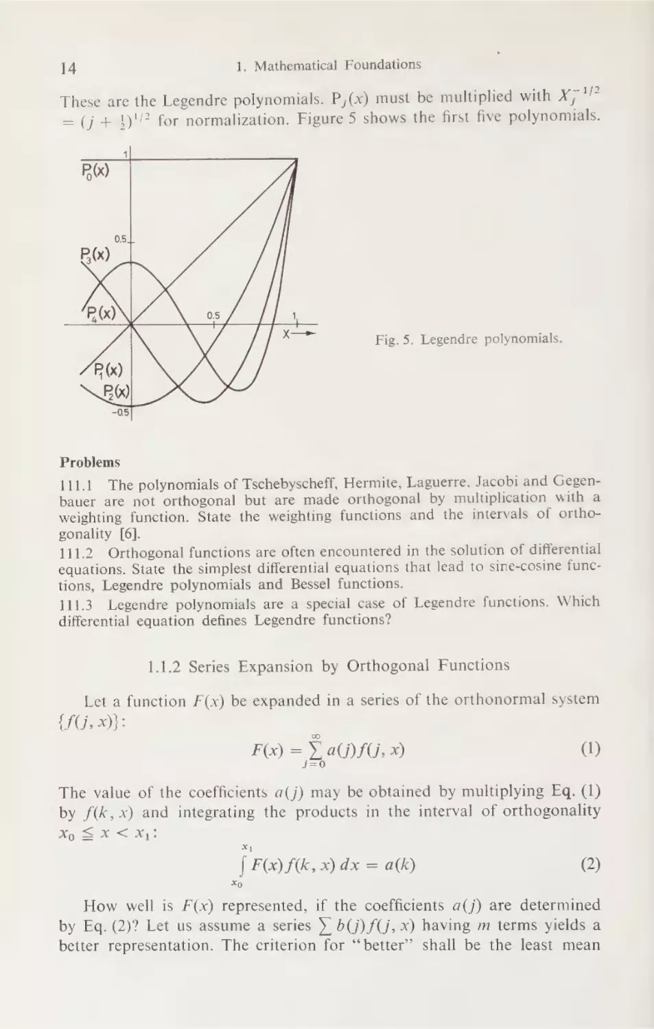
These are the Legendre polynomials. P,(x) must be multiplied with Me Ne
= (j + 4)'/? for normalization.
Figure 5 shows the first five polynomials.
Fig. 5. Legendre
polynomials.
Problems
The polynomials of Tschebyscheff, Hermite, Laguerre, Jacobi and Gegen111.1.
bauer are not orthogonal but are made orthogonal by multiplication with a
weighting function. State the weighting functions and the intervals of orthogonality [6].
Orthogonal functions are often encountered in the solution of differential
111.2
equations. State the simplest differential equations that lead to sine-cosine functions, Legendre polynomials and Bessel functions.
Legendre polynomials are a special case of Legendre functions. Which
111.3
differential equation defines Legendre functions?
1.1.2 Series Expansion by Orthogonal
Functions
Let a function F(x) be expanded in a series of the orthonormal system
WAGE x)} :
00
F(x) = Lap (J, x)
(1)
The value of the coefficients a(j) may be obtained by multiplying Eq. (1)
by f(k, x) and integrating the products in the interval of orthogonality
Oy SS de XS SME
| FO) fk, x) dx = alk)
(2)
How well is F(x) represented, if the coefficients a(j) are determined
by Eq. (2)? Let us assume a series } b(j) f(j, x) having m terms yields a
better representation. The criterion for “better” shall be the least mean
1.1.2 Series Expansion
by Orthogonal
Functions
US)
square deviation Q of F(x) from its representation:
o= | [Fe —Yawsu.9) ax
Xo
J F?(x) dx — 2¥ B) [ FOSU, x) dx + f ews.) ee
Using Eq. (2) and the orthogonality of the functions f(j, x) yields Q in the
following form:
.
Soil
m—1
= | Pads — Ya) +¥ BW) - a?
(3)
The last term vanishes for b(j) = a(j) and the mean square deviation assumes its minimum.
The so-called Bessel inequality follows from Eq. (3):
ya) < ¥a(i) Sn
(Reding
(4)
The upper limit of summation may be © instead of m — 1, since the integral
does not depend on m and must thus hold for any value of m.
The system {f(j,x)}
is called orthogonal, normalized and complete,
if the mean square deviation Q converges to zero with increasing m for
Sx < x,:
any function F(x) that is quadratically integrable in the interval x9
tim f [Fe) —Yasu.0)] ax =0
*1
m—1
Xo
@)
(5)
ES
The equality sign holds in this case in the Bessel inequality (4):
Lew= {|Peas
j=
(6)
xo
Equation (6) is known as completeness theorem or Parseval’s theorem. Its
physical meaning is as follows: Let F(x) represent a voltage as function
of time across a unit resistance. The integral of F?(x) represents then the
energy dissipated in the resistor. This energy equals, according to Eq. (6),
the sum of the energy of the terms in the sum ) a(j)f(j, x). Putting it
differently, the energy is the same whether the voltage is described by the
time function F(x) or its series expansion.
The system {f(j, x)} is said to be closed’, if there is no quadratically
integrable function F(x),
{ F2(x) GN =
(7)
1 A complete orthonormal system is always closed. The inverse of this statement
holds true if the integrals of this section are Lebesgue rather than Riemann integrals.
The Riemann integral suffices for the major part of this book. Hence, integrable will
mean Riemann integrable unless otherwise stated.
1. Mathematical
16
Foundations
for which the equality
(8)
| F@)SG, x) dx = 0
is satisfied for all values of j.
Incomplete systems of orthogonal functions do not permit a convergent
series expansion of all quadratically integrable functions. Nevertheless,
they are of great practical interest. For instance, the output voltage of
an ideal frequency low-pass filter may be represented exactly by an expansion in a series of the incomplete orthogonal system of (sinx)/x functions.
Whether a certain function F(x) can be expanded in a series of a particular orthogonal system {f(j, k)} cannot be told from such simple features
of F(x) as its continuity or boundedness’ [5—7].
Problems
112.1 F(x) represents a time-varying voltage across a resistor and is quadratically
integrable. What is the physical meaning of this statement?
112.2 Can there be a signal in communications represented by a time-varying
voltage that is not quadratically integrable?
<x <1
112.3. A function F(x) is zero for all rational values ofx in the interval0
and 1 for all irrational values. The Lebesgue integral yields 1. Does a Riemann
integral exist? Can you plot this function? Let F(x) be 1 for all real values of x
in the interval O << x <1. Can F(x) now be plotted and Riemann-integrated?
1.1.3 Invariance of Orthogonality to Fourier Transformation
A time function f(j, 8) may be represented under certain conditions
by two functions a(j, v) and b(j, v) by means of the Fourier transform:
fG, 9) = | [aG, ») cos2a»6+ b(j, ») sin2x
»6] dy
(1)
(9.0)
aj, ?) = ae 0) cos2a » 6 dé
Ne)
DG, v) = AG. O)sin2xv6d6
O=t/T,
y=fT
(2)
00)
It is advantageous for certain applications to replace the two functions
a(j,v) and b(j, ) by a single function’:
SC.) =a)
(3)
! Bor instance, the Fourier series of a continuous function does not have to converge
in every point. A theorem due to Banach states that there are arbitrarily many orthogonal systems with the feature, that the orthogonal series of a continuously differentiable
function diverges almost everywhere.
2 Real notation is used for the Fourier transform to facilitate comparison with the
formulas of the generalized Fourier transform derived later on.
1.1.3 Invariance of Orthogonality
to Fourier Transformation
17
It follows from Eq. (2) that a(j, v) is an even and b(j, v) an odd function
of »:
a(j, v) =
a(j, —2)3
b(j, v) —F =D;
=)
(4)
Equations (3) and (4) yield for g(j, —»):
2;
—y)
a(j,¥) and b(j,)
and (5):
= a(j,
may
—v)
+ dj,
—v)
=
a(j, v) —
bj, »)
be regained from g(j,v) by means
AG) = ale -9)
(5)
of Eqs. (3)
se, =7)|
(6)
BG. = 2182 = 893-9)
Using the function g(j,v) one may write Eqs. (1) and (2) in a more
symmetric form:
IG; 0) =
ec. v) (cos2a
v 0 + sin2z
v 0) dy
(7)
ej.) =
Ge 0) (cos2z
vy6 + sin2z
v 0) dé
(8)
The integrals of b(j, v) cos2a v6 and a(j, v) sin2a v6 in Eq. (7) vanish
since a(j, v) 1s an even and b(j,v) is an odd function of y.
Let {f(j, 9)} be a system orthonormal in the interval -40 < 6 < +40
and zero outside. @ may be finite or infinite. The functions f(/, 6) are Fourier
transformable’. Their orthogonality integral,
| SU, Df (k, 6) dO = db;
(9)
may be rewritten? using Eq. (7):
me | ie. y) (cos2a v 6 + sin2z y 6) | d0 = 3;, |
ae
HCO
|ees 0) (cos2av6 + sin2z
v 0) a6)dv=6;,¢
(19)
— 0
ice)
Oj,
| g(j,») glk, v) dv =
B28)
Hence, the Fourier transform of an orthonormal
an orthonormal system {g(j, »)}.
system {f(j, 0)} yields
1 Orthonormality implies the existence of the Fourier transform and the inverse
transform (Plancherel theorem).
;
2 The integrations may be interchanged, since the integrands are absolutely integrable.
1. Mathematical Foundations
18
Substitution
of
gj,» =a,»
+5G,%,
gk, ») = alk, ») + d{k, »)
into Eq. (10) yields it in terms of the notation a(j,v), b(j, »):
[ eG. »)gk, »)dv = | [a(j, ») + bG, »)] alk, ») + b(k, »)] do
= | [a(j, ») ak, ») + bj, ») b(k,
dy = bj
Figure 6 shows as an example the Fourier transforms of sine and cosine
pulses. These pulses are derived from the elements of Fig. 1 by continuing
them identical to zero outside the interval —4 < 6 < +4:
g(0,r) =
1/2
;
| 1(cos2uv6 + sin2av 6) d0 = ———~
—1/2
|
shed
ses
gi, ?) =
| J/(2) cos2x
i 0(cos2a » 6 + sin2z v 6) db
=i
1/2
oy)
=
aah
=5V@
sina(vy — i)
sina(y + >)
(ee
‘a u(y +i) ,
11
ae
| ./(2) sin2z i 6(cos2x v 6 + sin2z v 6) dé
—1/2
=)
1
sinz(y — 1)
CMe
(2) ||
SS
sina(vy + “|
er
ee
Fig. 6. Fourier transforms g(j, 7) of sine and cosine pulses according to Fig. 1. a wal(0,0);
b, V (2) sin2x 6; c, (2) cos2x 6; d, V/(2) sindx 6; e, /(2)cos4n 6.
1.1.3 Invariance
of Orthogonality
19
to Fourier Transformation
Table 1 shows the Fourier transforms of Walsh pulses derived by continuing the elements sal(i, 0) of Fig. 2 identical to zero outside the interval
-$S 054k:
1/2
gs(i, v) =
| sal(i, 6) /(2) sin2x » 6 dé
—1/2
Table 1. Fourier transforms of sal(i, 0), i=1,...,
gsd,v)
I
+2 + (2) —
=
ay
g,(2,”) =
nae
ae1
ee
8 / (2) —,
8
g5(4, v)
—
)
g;(5, v)
=>
g,(6,”)
=+16
)
_
—
1
/
(2) ——
-———
1
16+// (2) ae
=r
g;,9,”)
=
2,
sin?
uv a gy
ede
sin——
cos—5—
sin
v
1
uy
—7— sin*
-——
j
v
UY
5) cos ——
mn
5
v
sin
uY
—
PH i
is
uv
8
sin
2
a)
ae
mn sin 3
sin
Ae
ie
sin uy
7
uv
sin
cos
v
a
VQ
—32
=
al
uy
V (2) —— sin —— cos
1
TE
1
gt?
1
uv
g,(1, 7) = +32 V (2) —— sin——
e
v
—— cos
sin’ 2 =
uy
2 uv
uv
GD)
v
ae
v
sin
OP
=
a ED
—— sm
sin—— cos——
sin]
It
16
ay
—— sin*
—— cos — cos
0
g;(10, v) = +32 V (2) —— cos——
TD
uv
sin —
sin
mv
—
Ty
+32 V (2) —— cos—-— cos — sino— sine
(ea)
35
eas)
cos
uy0.
gU
Be
sin’
—
v
Stra
sin
>> cos
any
MER
sin—-
——
]
V 2) —— cos
1
Gee
g.(7, ») as 16 v (2)
a
ea(on2)
ea ED
sin? —
—4 VQ— cos
gs(3, »)
—
3
>
1
v ( Nee
16.
5.
SEG
ES
uv
ee
ae
aoe
SI
8
2 UY
sin 37
sin’
sin’
9
5
2 UY
35
sin’5
ey fells sin? 2”
32
16
—— Oecos2” sin”A sin"8 cos16 sin? 32=
BOS2 = ee432iN 2)
1
5
HED
g,(15, ») = +32 V (2) —— SS
1
(G5) = = 2 SiC
COS
uv
oy
RBH
pe
re OS
uv
TY
mY
TOME
ar
uv
ge 8
De
——————————
pe
|,
UY
ee
oy Hb
== sin* 35Ge cos
eee
1. Mathematical Foundations
20
Table | gives the Fourier series expansion of the periodic functions sal(i, 6)
if y assumes the values 1, 2,... only!. Figure 7 shows plots of the Fourier
transforms of several Walsh pulses.
Fig. 7. Fourier transforms g(j,v) of Walsh pulses according to Fig. 2.
4); d, —sal(2, 6); e, cal(2, 8).
a, wal(O, 6); b, sal(1, 6); c, —cal(1,
that even time functions
time functions transform
of the frequency have a
of frequency » is a cosine
oscillation with reference to 6 = 0, if the Fourier transform has the same
value for +y and —y; it is a sine oscillation, if the Fourier transform has
the same absolute value but opposite sign for +yv and —y.
Figure 8 shows the Fourier transforms g(j,v) of three block pulses
of Fig. 3. They are no longer either even or odd?.
Figure 9 shows a system of orthogonal sine and cosine pulses. They
are time shifted compared with those of Fig. 1, so that all functions have
jumps of equal magnitude at 0 = —4 and 6 = +4. Their Fourier transforms g(j, v) are shown in Fig. 10:
One may readily see from these examples
transform into even frequency functions and odd
into odd frequency functions. Negative values
perfectly valid physical meaning. The oscillation
:
sina(vy — k)
g(j, ¥) Geet
k=
=
ie
°
for even j
(12)
k=5Cit
1)
for oddj
! Compare this Table 1 with Table 1 of [7] showing the Walsh series expansion of
sine and cosine functions. Plots of some of the functions in Table 1 without the weighting function (sin? x)/x were published by Filipowsky [9]. A closed formula for the Fourier
series of Waish functions is contained in an unpublished report by Simmons [10].
2 The Fourier transforms of the various block pulses are different but their frequency
power spectra are equal. The power spectrum is the Fourier transform of the auto-correlation function of a function, and not the Fourier transform of the function itself
(Wiener-Khintchine theorem). The connection between Fourier transform, power spectrum and amplitude spectrum is discussed in section 1.3.2. See also [4].
1.1.3 Invariance of Orthogonality to Fourier Transformation
PI|
15
10) \ :\(3,8)
\
Fig. 8. Fourier transforms g(j, ») of the block pulses f(A, 9), f(2, 6) and f(3, 9) of Fig. 3.
£(6,8)=-V/2cos (618+1/4)
£(5,8)=\Zsin(618+1/4)
f(4,8)=-V2cos (4116 +1/4)
£(3,8)=V2sin
(4118+sy/4)
f(2,8)=-)2 cos(2708
+11/4)
Fig. 9. Orthonormal system of sine
and cosine pulses having jumps of
equal height at
6 = —4 and 0 = +4.
Pd
f(1,8)=\2sin (2n8+n/4)
f(0,8) = constant
=
2
i
°
ee
pulses of Fig. 9.
Fig. 10. Fourier transforms g(/, v) of the sine and cosine
ra
1. Mathematical Foundations
2)
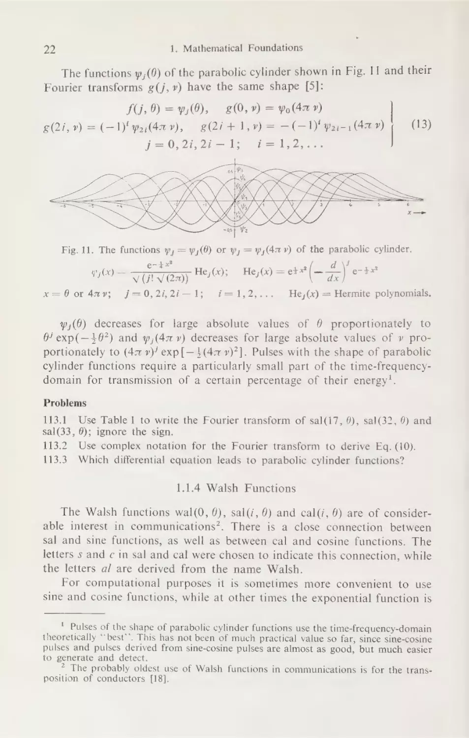
The functions y,(0) of the parabolic cylinder shown in Fig. 11 and their
Fourier transforms g(j, v) have the same shape [5]:
fi, 9) = yj),
8, ») = po(4z »)
g(2i+1,%) = —(-1) pai-1 47») | (13)
g(2i,%) =(—1)'poi(4ar),
j [Og21, 21
a
ee
Fig. 11. The functions y; = y,(9) or y; = y,(47 v) of the parabolic cylinder.
oes,
dV eax=
ip Loommr GTEC
(CTV T mech Fe Fl ch(a) es= et=( Eee
x=Oor4nv;
j=0,2%42i—1;
t=1,2,...
He,(%) = Hermite
polynomials.
wy,(8) decreases for large absolute values of # proportionately to
6/ exp(—467) and w,(4z v) decreases for large absolute values of » proportionately to (4a v)/ exp[—4(4z v)?]. Pulses with the shape of parabolic
cylinder functions require a particularly small part of the time-frequencydomain for transmission of a certain percentage of their energy’.
Problems
113.1
Use Table 1 to write the Fourier transform of sal(i7, 6), sal(32, 0) and
sal(33, 9); ignore the sign.
113.2
113.3.
Use complex notation for the Fourier transform to derive Eq. (10).
Which differential equation leads to parabolic cylinder functions?
1.1.4 Walsh
Functions
The Walsh functions wal(0, 0), sal(i, 0) and cal(i, 9) are of considerable interest in communications”. There is a close connection between
sal and sine functions, as well as between cal and cosine functions. The
letters s and c in sal and cal were chosen to indicate this connection, while
the letters a/ are derived from the name Walsh.
For computational purposes it is sometimes more convenient to use
sine and cosine functions, while at other times the exponential function is
' Pulses of the shape of parabolic cylinder functions use the time-frequency-domain
theoretically “best’’. This has not been of much practical value so far, since sine-cosine
pulses and pulses derived from sine-cosine pulses are almost as good, but much easier
to generate and detect.
? The probably oldest use of Walsh functions in communications is for the transposition of conductors [18].
1.1.4 Walsh Functions
23
more convenient. A similar duality of notation exists for Walsh functions.
A single function wal(j, 0) may be defined instead of the three functions
wal(0, 0), sal(i, 0) and cal(i, 6):
wal(2i, 6) = cal(i, 0),
wal(2i — 1, 8) = sal(i, 0)
aL
1
©)
es
The functions wal(j, 6) may be defined by the following difference equa-
toms
wal(2j
+ p, 6)
= (—1)¥1+? fwal[j, 2(6 + 4] + (—1)'*? walls, 2 — 4)]} |(2)
PO
0f ls
f= Os le 2,55
walt0; 6) =O
= 1» for
wal(0,0)
for
—-4$<6<};
"0 = 1,10 = 4-5
|
For explanation of this difference equation consider the function
wal(j, @). The function wal(j, 20) has the same shape, but is squeezed
into the interval —1 < 6 < +4. wal[j,2(@ + 4)] is obtained by shifting
wal(j, 26) to the left into the interval —4 < 0 < 0, and wall[j, 2(8 — 4)]
is obtained by shifting wal(j, 20) to the right into the interval 0 S 6< +4.
p= Ib.
j=2,
p=1 and
As an example consider the cases j= 0,
obtains:
one
1
=
[2/2]
and
0
=
[0/2]
Using the values
wal(1, 6) = (—1)°+! {wal[0, 2(6 + 4)] + (—1)°*? wal[0, 2(6 — 4)]}
wal(5, 0) = (—1)!+1 {wal[2, 2(6 + 4)] + (-1)**? wal[2, 2(6 + 4}
It may be verified from Fig. 2 that wal(1, 6) = sal(1, @) is obtained from
wal(0, 6) by squeezing it to half its width, multiplying the function that is
shifted to the left by —1, and the function that is shifted to the right by + Ls
wal(5, 6) = sal(3, 4) is obtained by squeezing Wwal(2, 0)1—= cal (110) to
+1
half its width, multiplying the function that is shifted to the left by
—1.
by
and the function that is shifted to the right
The product of two Walsh functions yields another Walsh function:
wal(h, 6) wal(k, 6) = wal(r, 9)
for
This relation may readily be proved by writing the difference equation
turns
It
other.
each
wal(h, 0) and wal(k, #0), and multiplying them with
of
out that the product wal(h, 9) wal(k, 0) satisfies a difference equation
the same form as Eq. (2).
1 Walsh functions are usually defined by
definition has many advantages but does not
number of sign changes as does the difference
generalization of frequency in section 1.3.1.
sal(1, 0), sal(2, 0), sal(4, 6), ... in igs 2s
products of Rademacher functions. This
yield the Walsh functions ordered by the
equation. This order is important for the
Rademacher functions are the functions
2 [j/2] means the largest integer smaller or equal 4j.
24
1. Mathematical Foundations
The determination of the value of r from the difference equation is
somewhat cumbersome. The result is that r equals the modulo 2 sum of
h and k:
wal(h, 0) wal(k, 0) = wal(h @ k, 8)
(3)
The sign @ stands for an addition modulo 2. k and h are written as binary
numbers and added according to the rules
O®1 =1@0=1,
0@0
=
in
of
10
1@1=0
(no carry). Addition modulo 2 is what a half adder does
binary digital computers. As an example, consider the multiplication
wal(6, 0) and wal(12, 0). Using binary numbers for 6 and 12 one obtains
for the sum 6 @ 12.
OHlOF
a6
@® 1100...12
1010...
10
It may be verified from Fig. 2 that the product wal(6, 6) wal(12, 6) equals
wal(10, 6).
The product of a Walsh function with itself yields
only the products (+1)(+1) and (—1)(—1) occur.
wal(0, 6), since
wal(j, 6) wal(j, 6) = wal(0, 6)
(4)
j@j=0
The product of wal(j, @) with wal(0, 6) leaves wal(j, 6) unchanged:
wal(j, 8) wal(0, 6) = wal(j, 9)
pa
(5)
=)
The multiplication of Walsh functions is associative since only products
of +1 and —1 occur:
[wal(h, 0) wal(j, 0)] wal(k, 0) = wal(h, 0) [wal(j, 8) wal(k, 6)]
(6)
Walsh functions form a group with respect to multiplication. Equation (3)
shows that the product of two functions yields again a Walsh function;
the inverse element is defined by Eq. (4) and is equal to the element itself;
the unit element is wal(0, 0) according to Eq. (5); the associative law is
shown to hold by Eq. (6). The group of Walsh functions is an Abelian or
commutative group since the factors in Eqs. (3), (4) and (5) may be commuted. Mathematically speaking, the group of Walsh functions is isomorphic
to the discrete dyadic group.
To determine the number of elements in a group and its subgroups,
consider what numbers can occur if two numbers, k and h, that are both
smaller or equal 2° — 1, are added modulo 2. k and h are written as binary
Ind
jana,
:
Pa.
1.1.4 Walsh Functions
25
numbers:
Wi
pee 2a
preg WO
et
k= qs-1 28-1 4 Gene et
Duk
The modulo
2 sum
h@
k
=
p21 + po 2° = 2°— |
gies
14a2 S2°— 1 +7)
cs Gen = U_or
eee edora
of / and k yields:
(ps-1
© Ge-1)
* 25-1
+ °°
+
Do
@ GW) ° 2°
(8)
The smallest number occurs if all the factors in front of the powers of 2
are zero. This number is obtained for h =k and equals 0. The largest
number is obtained if all these factors are 1; the resulting number,
ie
ee
ee
is obtained for h = (28 — 1)
®k. This means, that in binary notation k
has zeros where h has ones and vice versa. A group thus contains the Walsh
functions wal(0, 6) to wal(2' — 1, 8), a total of 2° functions. Subgroups
contain the functions wal(0, 6) to wal(2” — 1, 0), 0 <r <-s. These are all
subgroups. Since a subgroup contains 2” elements it has 2°/2” = 2°—" cosets.
Evidently, powers of 2 play an important role for Walsh functions.
Using Eg. (1) one may rewrite the multiplication theorem (3) of the
Walsh functions as follows:
cal(i, 0) cal(k, 6) = cal(i @ k, 8)
sal(i, 6) cal(k, 0) = sal{{k ® (i — 1)] + 1, 6}
cal(i, 6) sal(k, 6) = salffi@ (kK — 1)] + 1, 9} $
sal(i, 0) sal(k, 0) = cal[(i — 1) @ (k — 1), 9]
cal(0, 0) = wal(0, 6)
}
(9)
are orthogonal
The sine and cosine functions sin27i0 and cos27i0
in the interval —4 < 9 < +4. This is the system required for a Fourier
series expansion. The Fourier transform requires the system {sin2av 6,
cos2a 6} which is orthogonal in the whole interval —oo < 6 < +00.
Note that i is an integer and thus denumerable, while v is a real number
and thus nondenumerable.
The system of Walsh functions orthogonal and complete in the whole
interval —co < 9 < +00 is denoted by {sal(u, 6), cal(u, 4)}, where mu is
a real number. It will be shown later on that this system may be obtained
by “‘stretching” sal(i, 0) and cal(, #) just as the system {sin2a v 6,cos2v0}
can be obtained by stretching sin27i6 and cos2~i6. Another definition
1. Mathematical
26
Foundations
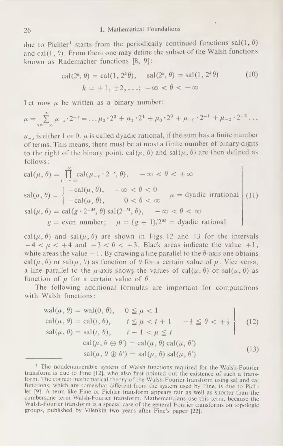
due to Pichler! starts from the periodically continued functions sal(1, 0)
and cal(1, 0). From them one may define the subset of the Walsh functions
known as Rademacher functions [8, 9]:
k =
(10)
sal (2*, 0) = sal(1, 2*6)
cal(2*, 6) = cal(1, 2*6),
+1, +2,...;
-0
<9<
+0
Let now pw be written as a binary number:
-
=
y
agin
=
rineoe
+
p24
+
fg *2°
+
M-1
gy
+
[4-2 ye
ae ee
w_,is either | or 0. wis called dyadic rational, if the sum has a finite number
of terms. This means, there must be at most a finite number of binary digits
to the right of the binary point. cal(u, 6) and sal(u, @) are then defined as
follows:
eal(u, y=
mie
|| callie.
2 =2
—cal(u, 0),
ee
+cal(u, 0),
Fao
-—-o<0<0
Or
g =even
number;
uu = dyadic irrational } (11)
6 =
sal (5.0) = <cal(e* 2-450) sal (2338.0)
}
oe
sae
ae)
pw =(g + 1)/2” = dyadic rational
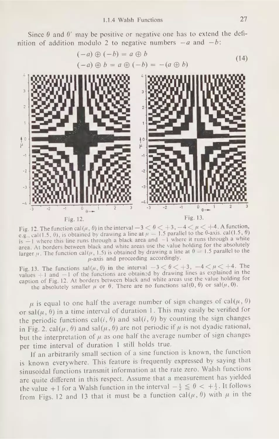
cal(u,9) and sal(u,6) are shown in Figs. 12 and 13 for the intervals
—4<p< +4 and —3 < 6 < +3. Black areas indicate the value +1,
white areas the value —1. By drawing a line parallel to the 6-axis one obtains
cal(u, 0) or sal(u, 6) as function of 6 for a certain value of w. Vice versa,
a line parallel to the “-axis shows the values of cal(u, 6) or sal(u, 0) as
function of w for a certain value of 6.
The following additional
with Walsh functions:
formulas
are
important
wal(u, 0) = wal(0; 0).
0 = p<
Cal (Wag) == cal(iag).
LS [i
bet
Sal
(i 0) = "saline.
NE
eee)
|
—-$<6<
44
(12)
|
cal(u, 0 @ 6’) = cal(u, 6) cal(u, 6’)
sal(u, 0 ® 0’) = sal(u, 8) sal(u, 6’)
' The
transform
form. The
functions,
ler [9]. A
for computations
(13)
nondenumerable system of Walsh functions required for the Walsh-Fourier
is due to Fine [12], who also first pointed out the existence of such a transcorrect mathematical theory of the Walsh-Fourier transform using sal and cal
which are somewhat different from the system used by Fine, is due to Pichterm like Fine or Pichler transform appears fair as well as shorter than the
cumbersone term Walsh-Fourier transform. Mathematicians use this term, because the
Walsh-Fourier transform is a special case of the general Fourier transforms on topologic
groups,
published by Vilenkin two years after Fine’s paper
[22].
1.1.4 Walsh Functions
27
Since @ and 6’ may be positive or negative one has to extend the definition of addition modulo 2 to negative numbers —a and —b:
(-—a) @(—b)=a@b
(-—a) @b=a@(-b) = -@@ 5)
w
N
-4
Fig. 13.
Fig. 12.
Fig. 12. The function cal(, 9) in the interval —3<6<
+3,—4<
nu < +4.A
function,
4)
e.g., cal(1.5, 9), is obtained by drawing a line at u = 1.5 parallel to the 0-axis. cal(1.5,
a white
is --1 where this line runs through a black area and —1 where it runs through
for the absolutely
area. At borders between black and white areas use the value holding
to the
larger «. The function cal(, 1.5) is obtained by drawing a line at 6 = 1.5 parallel
-axis and proceeding accordingly.
+4. The
Fig. 13. The functions sal(u, @) in the interval —3< 06< +3, —4<u<
explained in the
values --1 and —1 of the functions are obtained by drawing lines as
holding for
caption of Fig. 12. At borders between black and white areas use the value
0).
the absolutely smaller « or 0. There are no functions sal(0, 0) or sal(u,
u is equal to one half the average number of sign changes of cal(w, 0)
or sal(u, #) in a time interval of duration 1. This may easily be verified for
the periodic functions cal(i, 9) and sal(7, 6) by counting the sign changes
in Fig. 2. cal(w, 0) and sal(u, 6) are not periodic if w is not dyadic rational,
but the interpretation of w as one half the average number of sign changes
per time interval of duration 1 still holds true.
If an arbitrarily small section of a sine function is known, the function
that
is known everywhere. This feature is frequently expressed by saying
functions
Walsh
zero.
sinusoidal functions transmit information at the rate
are quite different in this respect. Assume that a measurement has yielded
the value +1 for a Walsh function in the interval -} < 6 < +4. It follows
from
Figs. 12 and
13 that it must
be a function
cal(w, 4) with mw in the
1. Mathematical Foundations
28
interval 0 < w < 1. Let an additional measurement in the interval4
<0<1
yield —1; the value of ywis thus restricted to the smaller interval 4 S pw < |
according to Fig. 12. A further measurement yields, e.g., —1 for the interval
1 <6 < 1.5 and +1 for the interval 1.5 S$ 0 < 2; this restricts yz to the
still smaller interval 0.5 < w < 0.75. A doubling of the time interval 46
required for measurement successively halves the interval Ay within which
the sequency pw remains undetermined. The product A 6 A remains constant
and may be interpreted as the uncertainty relation for Walsh functions. The
transmission rate of information is not zero, since more information about
is obtained with increasing observation interval 46.
the exact value of
A few words may be added for the mathematically inclined reader
about the connection between the systems {wal(0, 9), sal(i, 6), cal(i, 9)}
and {1, we) sin2z i 6, a (2) cos27 i6}. Both are orthonormal systems in
Hilbert space L,(0, 1) and one may base on both of them very similar
theories of the Fourier series and the Fourier transform. The reason for
this is that both may be derived from character groups. The system of
circular functions {cosk x, sink x} is derived from the group {e'**}, which
is the character group of the topologic group of real numbers. The system
of Walsh functions may be derived from the character group of the dyadic
group; the dyadic group is the topologic group derived from the set of
binary representations of the real numbers. The most striking difference
between the functions—continuity of circular functions and discontinuity
—is caused by the different topology of the real numbers
of Walsh functions
and the dyadic group [8, 11, 12, 20].
An example showing the close connection between the functions sal (/,@)
and sin27i6 is given in Fig. 14. Short and long distances between the
zero crossings alternate in such a way as to give a strikingly good fit. Note
that for 7 S$ 10 the Walsh function is +1 or —1 whenever the sine function.
is +1 or —1 but this does not always hold true for larger values of 7.
Problems
114.1
A system of functions cannot form a finite group unless the magnitude
of all amplitudes is 1. Why can they not be larger or smaller?
114.2
Which real values can the amplitudes of a system of functions assume if
the system is to form a group?
114.3
Can there be a system of real three-valued functions that forms a group?
1 Care should be taken not to confuse the uncertainty relations of transforms with
that of quantum mechanics. The quantum mechanical uncertainty relation is an axiom
that connects the accuracy of measurement of the location and the momentum of a
particle, which are independent physical quantities. The uncertainty relations of transforms are mathematical deductions that connect the accuracy with which a function is
known in the original domain with the resulting accuracy in the transform domain.
The function and its transform are not independent, they are usually connected by oneto-one mapping. The mathematical formalism is sometimes the same for different fields
of science but a quantum mechanical interpretation of a result requires that a quantum
mechanical axiom is introduced first.
1.1.4 Walsh Functions
29
sal(1,8)
sin 278
sal(2,8)
sin 418
sal(3,6)
sin 618
sal(48)
sin8r8
sal(5,@)
sin 10m8
sal(6,6)
sini276
sal(7,8)
sin 146
sal(8,8)
sin 1678
sal(9,6)
sin 186
sal(i0,8)
sin 2076
sal(11,8)
sin2276
sal(12,8)
sin 24r8
sal(13,8)
sin 2616
Fig. 14. Sine and sal functions
with the same
sequency.
= positive integer,
The exponential functions ei2knim & —0,1,...,m
114.4
unit element. Is the group
form a group under multiplication. State inverse and
a subgroup when mm is even.
commutative? How many elements are there? Find
m is a prime number?
when
or
Can there be a subgroup when m is odd,
expansion of the function
series
Walsh
a
of
Compute the first 8 coefficients
114.5
FO) — 0, —3 =U
4.
ns in the interval —3<90< +3
114.6 Using Fig. 12 plot the following functio
6), cal(.5, 4), RIS), ())cal(1,
equal:
are
and see in which interval they
calle ioaw)s
are called Rademacher functions.
114.7 The functions wal(2” — 1, 9), n> 0,
ts of Rademacher functions. A
produc
as
written
be
All Walsh functions can
obtained by multiplication of s
is
it
Walsh function has the multiplicity s if
, 0) wal(7, 9) wal(3, 0) wal(1, 9)
wal(15
=
6)
,
wal(10
E.g.,
ns.
Rademacher functio
@ 3 @1). Plot the multiplicity s
15@7
=
10
has the multiplicity s = 4 (observe:
Otel:
of wal(j, 6) as function of j fori
1. Mathematical
30
Foundations
114.8 Plot a step function with 8 steps of equal width in the interval —4 SO0<4
and amplitudes +1, +2, +3, +1, —1, +1, +1, —1. Compute all coefficients
of its Walsh series expansion. Let the step function be amplitude clipped at +2.
Compute the coefficients of the Walsh series expansion. Are any new terms
generated? How many terms unequal to zero can exist for a step function having 2" steps of equal width in the interval —} <0 < 4?
114.9 Does the product of 2m Rademacher functions yield a cal or a sal function?
Is the multiplicity of a sal function an even or odd number?
114.10
Plot the derivatives of the functions wal(31, 0), wal(15, 6) and wal(7, 9),
114.11
which consist of positive and negative Dirac functions. Plot the derivative of
wal(k, 0) for k = 31 @15, 31 @®7 and 31 © 15 @7. State the connection between modulo 2 addition and the way the derivative of wal(k, 6) may be obtained
from the derivatives of wal(31, 0), wal(15, 0) and wal(7, 6). Is the sequency
of a Walsh function changed by differentiation?
114.12
Compare the derivatives of the functions wal(1, 9), wal(2, 9), wal(4, 4)
and wal(8, 0) with that of wal(k, 0), k < 16.
1.1.5 Hadamard
Matrices
and
General
Two-Valued
Functions
Let M denote a square matrix with real elements. The inverse matrix
M-! is defined by the product MM~-! = 1, where 1 is a unit matrix
with elements | along the main diagonal and elements 0 everywhere else.
The transposed matrix M* of M is obtained by interchanging the rows
and columns. M is called an orthogonal matrix if the inverse M~' and the
transposed M* are equal except for a factor’. A Hadamard matrix H is
an orthogonal matrix with elements +1 and —1 only. There exists one
Hadamard matrix each of rank | and 2:
+1
+1
Phe .=[+,
aibolilae id H=| -|0)
], |
Two
Ha, =
(1)
non-trivially different matrices exist with rank 4:
+1
+1
41
+41
—1
-1
41
+1
—1
+1
41
-1
+1
-—-1
41
-I1
+1
>
Hy.
=
41
41
-!1
+1
41
-1
+1
+1
—1
+1
+1
—1
+1
+1
+41
(2)
Matrices of higher rank can be obtained by Kronecker products”. It is
usual to write + and — instead of +1 and —1 for the matrix elements.
' Many authors require that this factor must be one, but we shall use the term orthogonal and normalized for this case.
? The Kronecker product S x K of two matrices is obtained by multiplying S with
each element k;; of K and substituting the multiplied matrices k;; S for the elements kiy
of K. The Kronecker product H, x H2 is shown in Eq. (3), other examples are given
in section 5.4.2.
°
1.1.5 Hadamard
Matrices
and General
Two-Valued
Functions
31
Using this notation the Kronecker product of H, with itself yields:
Seale
-|-
-|4-
H, x H, =
Ee
=
H,
a
—H,
(3)
dion
ch
=
-+
This matrix is equal to H4, except for a different ordering of the rows.
The rank of a Hadamard matrix with rank higher than 2 must be an
integer multiple of 4. With one exception at least one Hadamard matrix
is known for all possible ranks up to 200. Certain Hadamard matrices of
rank 2” are related to Walsh functions. This relationship is readily recognized
from Fig. 15 for the rank 4 and 8.
A process that generates complete systems of two-valued functions
from Hadamard matrices will be explained with reference to Fig. 16a. The
++
++
--++
-++-
+-+fio
oS
et
-1/2
ee
Fee
/2
a
---
+ +
+
—==-+4+
+4 --=
Fig. 15. Relationship
Hadamard
between
matrices of rank
Walsh functions.
ee
certain
t++—--t+--
a
Ss
i
teas
2” and
+
—=—
+
+4 —
—' 4
—-++4—-+--¢
-+—-++4+-4+°+--+
-+ -+-
a
——
-/2
me
Si
+
ea Nimes
1
O|
+
+
=
-
-
+
+
+
-
=
+
=
-
|
=
+
+
1
0
+
+
-
+
+
-
b
-
-
+
+
+
-
+
4
+
=|
+
-
106
7
7\+|—-|-|) +14! -|-[ +! +)-|-]+]+4+]/-|-[ +] 8
+
+
ne
+r
3
Z|
1
0
-
a
+
+
=
+
+
=
+
+
=
3
6] 4) -—| -—| +14] -—| —] +] -] #) #]) -] -] #1 #] 7] 9
+] 10
si+|—-|—-| +]/-| +] +] -|-—| +] 4+]-| +] -|-|]
ey Hr tt
4 | +) =| —l 41 =| 4] +] =) + =) =] +] a]
12
cel ee
pe
taal
Bele ea eas ee ede
03
=
|
Fie
el
ih
ate
ae
VC)
ala
Se
|
fey
eythrele Vealent ele
0S
is
ea
| Hl Rt
oO} +) lal — et a
a
/2
==
0
+
0
0
+
+
-
-
-
+
=
-
+
+
+
=
-
T\+|-j-|+]4+]-|]-|+
=
7
+
+
0
1
2
3
-
+
-
4
+
-
+
-
5
+
+
-
+
Es
+
6
7
(SN Ses
ea eS leat
+/4+]/-]+/-|-]+]9
6] +)/—-|-]4]+4)/-|-[+
al eet allVital
LS i oUt i
-|-|+/+/-/]-|]+]10
-|-|+/4/-|-|+]11
4) -|4]4]/-|+)-|-|+
=i +i\—l 4a)
l=) 12
3)-| 4) —-|4)4]/-|4]-|+]/-|}+]—-|+)/-]13
2/4) —-] 4+] —-l-} +) -] +
+/—-j4+}+]—-|+)/-]14
tl4l—}4)—[4+]-|+]-|4+])/-|-|+}/-]+]15
+etreee
Ol+) 4+) 4+)—-]}+/}-| +] - ei
b
l functions from HadaFig. 16. Derivation of complete systems of two-valued orthogona
mard matrices by means of the alternating process.
1. Mathematical
32
Foundations
system of Walsh functions in the interval (0, 1) is obtained from the Hadamard matrix H, = (+) in row 0 by dividing the interval in half, and writing + in the left half and — in the right half; this yields row 1. Rows 2
and 3 are obtained by dividing the intervals of row 1 in half; writing + —
in the intervals where row 1 shows +, and —+ where row 1 shows —
yields row 2. Writing + — where row 0 shows + yields row 3. The process
may be continued ad infinitum. Fig. 16a shows on the right the number
of the row and on the left the number of the row from which it was derived.
Figure 16b shows the same process applied to the Hadamard matrix
H,,. Again the number of the row is shown on the right and the number
of the row from which it was derived on the left. Figure 17 shows the plotted functions.
The Kronecker product also permits the generation of new functions.
However, the two functions represented by H, in Eq. (1) are represented
by rows | and 3 in Eq. (3). Hence, the Kronecker product not only adds
new functions but also changes the ordering of the ones already obtained.
pe
mn
net
1
had(4,211,8
an
esi
ite),
hedeaiie
had(4,4 118
5M ae
ea
A
hadi
ise
= Qa (ae 4,213
8
hades
had(4,41365)
sony
1G)s
=)
=
Se
Se
LSet
fF
oe an
aaa
N)
@o
a@
=©=
2
Pa
ear
headin, se
Le
TLL
oe aie rete 2158
TLS
La
ts 2158
oige
LLP Le ned
LP
LP Eee
ae heist)
PLL Ly a
einer
PILL
La
heaig, 376)
“LIL
LU US LI LI hadl4,4178)
iS
SS
SS SSS
0
Fig. 17. Example
oa
of functions
generated
1
according
to Fig. 16b.
The “alternating” process of Fig. 16 only adds new functions. Crittenden
has generalized this process and proved the completeness of the systems
of functions generated [1].
A Hadamard matrix of rank 12 was reported by Paley [2]. It is of
interest in communications since it is usual to multiplex twelve telephony
channels into a group. Figure 18 shows the orthogonal functions associated
1.1.6 Haar Functions and General Three-Valued Functions
33
with this matrix. The notation pal(j, 0) is used in honor of Paley. It may
readily be verified that the product of two Paley functions does not necessarily yield a function of the system. Hence, these functions do not form
pal(0,8)
ah
pati)
pa)
patt,)
pals)
ee
Se
LF
FF
FF}
ALFALFA
SUNN
a
sees a
pal(7,) >}
ee
pat) ——}——_ >}
pat,6)F——}——F} —F
patio Sf}
pattie) $$}. —
on
0
a
1/2
a
§——
]
Fig. 18. Paley functions pal(j, 4).
a group as the Walsh functions do. However, the product of a function
with itself yields the constant pal(0, 4):
(4)
pal(j, 6) pal(j, 6) = pal(, 9).
Problems
Does a relation like Eq. (4) hold for systems of two-valued functions other
115.1.
than the Walsh and Paley functions?
The alternating process is based on the Hadamard matrix H,. Use the
115.2
matrix H4,. instead of H, to derive functions analogous to Fig. 16.
twenty115.3. Extend the system of Paley functions in Fig. 18 from twelve to
four functions with the help of Figs. 16 and 17.
voltages.
115.4 Assume the Paley functions of Fig. 18 are available as time varying
pal(i2, 6)
What is the time variation of the voltage that produces the functions
voltage
to pal(23, 0) according to problem 115.3? What is the time variation of the
that produces pal(24, 6) to pal(47, 9) from pal(0, @) to pal(23, 0)?
1.1.6 Haar
Functions
and
General
Three-Valued
Functions
Haar functions assume the values +1, 0 and —1 multiplied by powers
of ./(2). The first few functions are shown in Fig. 19. har(0,0, 0) and
har(0, 1, 0) are identical to the first two Walsh functions wal(0, 6) and
1. Mathematical Foundations
34
wal(1, 0). The function har(0, 1, @) is then squeezed into half the interval
and shifted to, yield har(1,1, 6) and har(1, 2,6). Each one of the new
functions is again squeezed and shifted, and so on ad infinitum.
Let a function F(0) defined in the interval (—4, +4) be expanded
into a series of Haar functions. The expansion coefficients of the first
two functions har(0, 0, 0) and har(0, 1, 9) are affected by all values of F(@).
har(0,0,8)
har(0,1,8) |—-
_f—-- ~~
V2 har(1,1,6) C—_ |___,—____—
3V2har(1,2,8) Si
Shar (2,1,8) C4
—________
Fhar(2,2,8) —
|
————_
thar(2,36) ———_—__1_}___—_
Sharl2,,4,8)
——
——
-1/2
4
Oye
at
ete
Fig. 19. Haar functions.
her(0,8)
her(1,8) a
aE
her(2,8) ———
a
her(3,6) >}
dt
__
+¥Zher(4,6) NS
+2 her(5,6) ————
$¥Zher(6, 6)
4
$2her(7,6) 1
—}_ fF
ther(8) ee
ther(9,8) ee
SS
ee
+her(106) Fa
the r(ii,8) oy
f4ya +
ther(12) lo
}—_fra___
he r(I3,@) $$$.
pher(l4,6) Se
ther(156)
bt
4/2
42 tf
tt
nn
Oise
Fig. 20. The functions her(j, 0).
2
1.1.6 Haar
Functions
and General
Three-Valued
Functions
35
The coefficients of the other Haar functions are affected by fractions
4,4,4,... of the values of F(@) only. These functions help represent
certain local sections of F(@) and are therefore referred to as local functions.
har(0, 0, 6) and har(0, 1, 6) are called global functions. The engineering
interest in this difference stems from the fact that a better representation
of certain sections of a function is often desired. For instance, the most
important parts of a TV picture are usually in the center and a better representation of the center sections is thus desirable than of the edge
sections.
The system of Walsh functions consists of global functions only, while
the Haar system contains two global functions only. One may generate
systems with global functions between these extremes. Figure 20 shows a
system using the first four Walsh functions. The Haar process of squeezing to
one half and shifting is then applied to the functions her(2, @) and her(3, 0).
The signs are chosen so that all functions are non-negative for +0.
Another method to generate systems of three-valued functions is shown
in Fig. 21. Again the first four Walsh functions are used. The Haar process
ter(0,8)
ter( 1,8) |
f
ee ee
ter(4,8) (f+
+ter(5,8) C4—_f1—
Ste r(6,8) Cf
}—
Ster(7,8)
ee
Sinai y
=e
lead
a
eset
Ster(8,6)
Lter(g@)
Tter(10,6)
Ster(118)
Se
Ster(12,6)
Lter(138)
pj},
Lter(14,8)
ff
Lter(158)
——}-+ 1,
bter(ig9) CL
zter(17,8) q ft __
iter(18,6) qf} —_—
iE
2
1
1
a
}
oer
1
a
Fig. 21. The functions ter(/, 4).
4
2
36
1. Mathematical Foundations
of squeezing and shifting is applied to the three functions ter(1, 0), ter(2, 9)
and ter(3, 0). The squeezing in Fig. 21 is done by substituting 40 for 0,
while 20 was substituted in Fig. 20.
The processes shown in Figs. 20 and 21 permit one to choose 2” Walsh
functions for a global representation. One then still has a choice ofn generating processes for the local functions. For 2” = 2’ one has only the Haar
functions, for 2” = 2? one has the processes of Figs. 20 and 21, for 2” = 2°
one can squeeze the functions by the substitution of 26, 46 or 86 for 6; etc.
Note that the amplitudes of the functions in Fig.21 areO,
+1,+2,+4,...
Multiplications by powers of 2 require only a shift of the binary point
in digital computers and are fast to perform. Additional multiplications
by ./(2) are required for the functions of Fig. 19 and Fig. 20 if the normalization is to be retained.
Problems
116.1
Can one apply the processes of Figs. 20 and 21 to the first four functions
of Fig. 17?
116.2 Can one apply the processes of Figs. 20 and 21 to the first eight functions
of Fig. 17?
116.3
Apply the process
of Fig. 21 to the Paley functions
of Fig. 18.
116.4 The human eye resolves pictures in the center (yellow spot) better than
further away from the center. Which functions in Fig. 21 could one use to produce
such an effect?
1.1.7 Functions
with Several
Variables
Many signals in communications are functions of several variables.
For instance, TV signals have two space variables and the time variable.
The functions discussed in the previous sections are readily extended to
several variables but some changes of notations are indicated.
Figure 22 defines the notation blo(A, x) for block pulses. Block pulses
with two and three variables may be written as products blo(k, x) blo(m,y)
oO)
TION)
OCs)
—I1
wal(1,x) |
DIO 0(2,x)
(2:x)) ees
eee |
wal(2,x)
blo (3,x)
wal(3,x)
oFrat be
Kees ))LG)
blo (5,x)
=a:
blo (6,x)
wal(6,x)
J-1.
F_1
V2
+4+4_1_ +
14_1_1—_
x—
Sa
+1/2
f
|
=
wal(5,x) | |
T1_
blo (7,x)
—}4
=
| A
————o
wal(7,x) f | ro
F
=|
—L
1
a8
=
ae
14
+
test tat
x—e
+
+1/2
Fig. 22. Definition of the notation used for block pulses and Walsh functions with space
variables.
1.1.7 Functions with Several Variables
ay
and blo(k,x) blo(m,y) blo(m,z). The notation wal(k,x) defined by
Figs. 2 and 22 will be used for Walsh functions instead of wal(0, x),
sal(i, x) and cal(i, x). Sine-cosine functions with more than one variable
have never played a great role in communications and there is thus little
incentive to keep stressing the similarity between Walsh and sine-cosine
functions. The notation wal(k, x) permits the definition of Walsh functions with two or three variables by one product wal(k, x) wal(m, y) or
wal(k, x) wal(m, y) wal(n, z) rather than by 9 or 27 products.
Figure 23 shows block pulses with two variables in the interval —4 S
SN
5,
lo
ee = Oe, 1 Lhe aunction blo(k; x) x
x blo(m,y) is found at the intersection of the column denoted blo(k, x)
OOS00
HO ooooooOoo oHooo
FOOD
oo
FOTO ooo
HOOD
(OSH EIOG0 «
blo(O,x) blo(1,x) blo(2,x) blo(3,x) blo(4,x
ieseo.ol 2S Se fea.D xz Ss od aN =
*CoT0o0
-1/2 x#l/2
Fig. 23. Block pulses blo(k, x) blo(m, y) fork,m=0... fl in the interval -t<x<4,
—1<y<}.
Black areas represent +1, white areas 0.
and the row denoted blo(m,y). Black areas represent the value +1,
white areas the value 0. The black area moves from left to right as k increases
and from bottom to top as m increases. This corresponds to the movement
of the illuminated spot on a TV tube that is scanned from left to right
and from bottom to top.
Figure 24 shows Walsh functions with two variables in the interval
AS before, the tunction
—t<ax<4, -$s5y <4 fork,m= OF,
1. Mathematical
38
Foundations
wal(k, x) wal(m,y) is located at the intersection of the column denoted
y). Black areas represent again the value
wal(k, x) and the row wal(m,
the value —1. The function wal(O, x) x
now
represent
areas
white
but
+1,
x wal(0, y) is +1 everywhere and its integral over the interval —-$<x<
<4, -1< y < $equals +1. All other functions are +1 as often as —1
and their integrals yield zero’.
wal(0,x)
wal(1,x)
wal(2,x)
wal(3,x)
wal(4,x)
wal(5,x)
wal(6,x)
wal(7,x
wal(7,y)
wal(6,y)
< Pa) o—a x Ss
wal(4,y)
wal(3,y)
wal(2,y)
wal(y)
HLL
UY
YD
ee
mm
mm
me
eS
ea
RD
a me
BRSBe
ee
tet
ace
Se
SmSe
EMI
MPL
ee
ee
Bee
Ee
EE
(ES
wal(0,y)
C
i
f
at
C
Fig. 24. Walsh
functions wal(k,x) wal(m,y) for k,m=0O...7
in the interval
—t<x<4t, —4<y<4. Black areas represent +1, white areas —1.
Consider
functions
the expansion
of a function
F(x,y) into series of Walsh
wal(k, x) wal(m, y):
FCesa) =
s) ‘ia(k, m) wal(k, x) wal(m, y)
k=0
We
a(k, m) =
[
(1)
m=0
ye
| F(x, y) wal(k, x) wal(m, y) dx dy
(2)
SSP Sip
A typical example for F(x,y) is a black-and-white photograph and the
terms picture, image or two-dimensional signal may thus be used for
1 This representation of two-dimensional
first in [1].
Walsh functions seems to have been used
1.1.7 Functions
with Several
Variables
39
F(x, y). The term a(0,0) wal(0,x)wal(0,y) in the series expansion
represents the average value of F(x,y) or — in easily understandable
terminology — the average brightness or the dc component of the image
F(x, y). The other terms a(k, m) wal(k, x) wal(m,y) may then be said
to represent
ac components.
Figure 25 shows the functions of Fig. 17 for two variables. Note that
there are 16 functions that would represent the average value of a function
F(x,y) in a series expansion while only the function wal(0, x) wal(0, y)
would do this in the case of Walsh functions.
had(4413,y)
had(4313,y)
had(4,213y)
had(4,113,y)
had(44I1,y)
had(4,3!1,y)
had(42!1,y)
A
eSS
Sasso
me.
Sasa
eee...
SSSeu
ee
(eet
GH
fa
ER
maaE
BS
il SS
had(4,)!1,y)
S
Surat
#4
0522 4 and
for kom
had(4, k |K, x) had(4,m|M,y)
functions
Fig. 25. The
+1, white
represent
areas
Black
y<}.
-4<
4,
<
x
<<
—-$}
interval
K,M=1,3 inthe
areas —1.
Figure 26 shows Haar functions with two variables. Black and white
t
areas again represent the values +1 and —1 while grey areas represen
multis
function
Haar
the
shows
the value 0. Note that this representation
x) x
plied by certain coefficients. For instance, the function thar(2, 2,
at the interx har(2, 2, y) rather than har(2, 2, x) har(2, 2, y) is found
denoted
row
the
and
2,x)
thar(2,
section of the column denoted
40
1. Mathematical
Foundations
thar(2, 2, y). Four of the functions are global, and the others local in an
extension of the terminology introduced in section 1.1.6.
meek
~
N
ca
=
=
ad
Sy
pa
(=)
g
fe
fs
Te
HIN
We)
Ree
=
=
ba
=
>
i
a
oo
=
‘
ha)
c
sv
Ss
ia
=
N=
IN
IN
IN
IN
IN
ee
2
2
tharl2,4,y)
Shar(2,3,y)
Shar(2,2,y)
$har(2,1,y)
¥2 har(1,2,y)
¥2 har(l,1,y)
hart0,1,y1
har(0,0y)
-1/2 x-=1/2
Fig. 26. Haar functions har(K, k, x) har(M, m,y) for K, M=0,1,2 and k,m=0...4
in the interval —t}<x<4, —4+<y<4. Black areas represent +1, gray areas 0,
and white areas —1.
Figure 27 shows the functions of Fig. 20 for two variables. Black,
grey and white areas represent again the vuales +1, 0 and —1. There are
now 16 global functions.
The representation of the three-dimensional function wal(k, x) x
x wal(m,y) wal(n, x) requires black and white volumes rather than
black and white areas for the representation of the values +1 and —1.
Figure 28 shows
the 64 functions
for k,m,n
=0,...,4
in the interval
—35%x%<+t, -4+5y<4, -—$52 <4. Let us first consider the specific function wal(2, x) wal(3,y) wal(1, z) which is shown in more detail
in Fig. 29. It consists of 64 small cubes which are black or white inside
and outside’. The function is +1 for a coordinate x, y, z inside a black
1 A red tomato is red inside and outside while a red apple is red on the outside only.
1.1.7 Functions
with Several Variables
41
cube and —1 for a coordinate inside a white cube. The four layers of cubes
on the right hand side show how the 64 small cubes are arranged inside
the large cube.
her(3,x)
¥2herl4,x)YZ
her(5,x)
IN
ain
her(7,x)
/2her(6,x)/2
—In
-|In
417 her(7,y)
is
+
a +¥2 herl6,y)
1 5VZherl5,y)
lf
+¥Zher(4,y)
C
G
+]
her(3,y)
iF
ia
ii
her(2,y)
t
her(1,y)
V2-
’+
her(0,
~y2t
Lops
ey? ga?
Lrpss
tizid
Litis
crfis
Lifits
y)
ttrfisjttr+ts
Fig. 27. The functions her(k, x) her(m, y) for k,m=0...7in the interval —4}<x<},
—t<y<}4. Black areas represent +1, gray areas 0, and white areas —1.
Let us now return to Fig. 28. Sixty-four large cubes like the one of
Fig. 29 are arranged in a cubic pattern just as the squares in Fig. 24 are
arranged in a square pattern. The dashed lines are intended to make this
three-dimensional arrangement more apparent. Furthermore, scales emx
phasize the 16 large cubes in the front plane. The function wal(k, x)
x wal(m,y) wal(n, z) is found at the intersection of the x-row denoted
wal(k, x), the y-row denoted wal(m, y) and the z-column denoted wal(n, z).
Note that the terms x-row and y-row have to be used since the terms row
and column suffice for the description of square patterns but a third term
for the description of cubic patterns is lacking.
Since a representation of functions with three variables according to
Fig. 28 is not very lucid, only examples of a specific Haar function and
a specific block pulse with three variables are shown in Figs. 30 and 31.
1. Mathematical
42
Foundations
we
:
ol
Hie
; aoeae,
m7
gto! na Bf
Ww O/2
ae
oz
> 1/2 —_V2 x=
gto
V/2
wal(0,x)
wal(1,x)
wal(2,x)
ma
y
x
Fig. 28. Walsh functions wal(k, x) wal(m, y) wal(n, z) fork, m,n =O... 3 in the interval —4< x<4,
-—t<y<4,
—4< z<4. Black volumes represent +1, white
volumes
—1,
wal(2,x)wal(3,y) wal(i,z)
V2
Fig. 29. The function wal(2, x) wal(3, y) wal(1, z). Black volumes represent
volumes —1.
+1, white
1.1.7 Functions with Several Variables
43
yhar(1,2,x) har(11,y) har(,1,z)
Fig. 30. The function }har(1, 2, x) har(1, 1, y) har(O, 1, z). Black volumes represent +1,
gray volumes 0, and white volumes —1.
blo(2,x) blo(1,y) blo(2,z)
z=1/2
function is +1 inside the
Fig. 31. The block pulse blo(2, x) blo(1,y) blo(2, z). The
from that of Fig. 22.)
somewhat
differs
notation
(The
.
black volume and zero elsewhere
Problems
in Fig. 28?
Where is the function wal(3, x) wal(3, y) wal(3, z) located
117.1.
the manner
in
28
Fig.
of
z)
wal(3,
y)
wal(2,
x)
wal(1,
117.2. Draw the function
of Fig. 29.
2, z) in the manner
117.3. Draw the function }har(0, 1, x) har(1, 1, y) har(1,
of Fig. 30.
x) used in Fig. 31
117.4 What is the difference between the block pulse blo(2,
22?
and the block pulse blo(2, x) in Fig.
44
1. Mathematical
Foundations
117.5
The arrangement of the small black and white cubes inside the large cube
in Fig. 29 is uniquely determined by the arrangement of the black and white
squares on the visible surface of the large cube. Is this true for all the Walsh
functions in Fig. 28? Is this true for all Walsh functions? Is there a similar relationship between the values of an analytic function on a closed surface and in
the enclosed volume?
117.6 Isa Haar function with three variables defined by its values on the surface
of a cube? Compare the functions har(2, 2, x) har(2,2,y)har(2,2,z) and
nein, 3, 29) lovin, 3), 3) Ineeiie(2, 3), 2).
117.7
How many different block pulses according to Fig. 31 exist that are zero
on the surface like the block pulse shown?
1.2 Generalized Fourier Analysis
1.2.1
Transition
from
Fourier
Series to Fourier
Transform
The Fourier transform belongs to the basic knowledge of every communications engineer. Its derivation from the Fourier series is shown here
in a special way that will facilitate understanding of the more general
transition from orthogonal series to orthogonal transforms?.
Consider the orthonormal system {f(j, 9)} of sine and cosine elements,
the first few of which are shown in Fig. 1. The elements f(j, 6) are divided
into even elements f,(/, 9), odd elements /,(i, 6) and the constant f(0, 6):
f, 6) = wal(0,0)=1
ogy
| fel Oia iC) cos2a1 8
Piss
f.G, 6) = ./(2) sin2x i6
undefined
-456<
(1)
6<-4,02
Gai)
+4
+4
ele
Sine and cosine elements may be continued periodically outside the interval
—4 < 6 < +4 to obtain the periodic sine and cosine functions:
SOO)
=o
(7,0) ee 6) = ,/(2) cos2z
i0
<7
= +o
(2)
|AG, 8) = JQ) sin2ni6
Periodic continuation of a function defined in a finite interval is one way to
extend the interval of definition. Consider a function F(@) defined in the
interval —} < 6 <4. An example is the triangular function shown on
top of Fig. 32a. If conditions required for convergence are Satisfied, one
may expand F(9) into a series of the orthonormal system {fCU, 9)\ defined
' The transition from the Fourier series to the Fourier transform has mainly tutorial
value. A mathematical correct transition without an additional assumption is not possible
since the Fourier series uses a system of denumerable functions but the Fourier transform
one of non-denumerable functions. A corresponding remark applies to the transition
from orthogonal series to the generalized Fourier transforms in section 1e2228
1.2.1 Transition from Fourier Series to Fourier Transform
FN
ss
=a
pee A Se
a
=<
ee,
ae
|
“——
Ak
San
45
=a
eet)!
wal (0,8)
ee
Vesin2x8
/2cos 218
oN
HERE
eA
or
oe
OO
AR x
ars
TN
¥2 sin 2x0" =<
SS
a
Sy
7
Van
N
hp al
a
V4
4aN
/2sin4n8
\Y
fo
oN
lie
V2 cos 4708
as
mee
Se
Z
Et
7
'
ca
Bl
ah i
Mh
Tee eee
=
wale)
VGN
es
FU)
wal (0,0)
V2sin x8
SS
2 cos 21r6' LS
/2cos8
47x6" ee
2 sin
/2sin2n8
Oe Sh BP
V2 cos 46" o>
s
Loe
——
2 sin 610!
ars
Wosend
2s SS
—
V2 sin 818"
—
an
LOS
SS
ON
“_
ta
~“
2
Se
aa
b
JES
aS
Ne
—A 3
'
V2 cos 818
a
\2cos21.8
+—_——
=)
=}
=|
=4/2
—$—$A > $$$
ee
0
a
,
AF
“™.
2 sin de
a
ae \/2cos48
O6—~
2
ane
————
]
—-wal (0,8') ——
ee
ee
oe
/2 sin2n6' == So
F
(8)
— wal (0,8)
/2sinx 6/2
2 cos 1 8/2
V2 cos 2x8’ — a
2 sin4n0"
|
3x8
\/2sin
£-~ J?005308
Sa
—t
Sm
Sao
V2sinx 8
oe
(2coskn@! <2
feos08
/2 sin6x6' Se
2 sin3106/2
2 cos6x8" = ee
\/2cos 3106/2
/2sin8x8' —
>
—
c
=
-4/2
zii=
—4/u,
Te
0
==
0
+
—
(io ——a
Fa
=H
Ae)
—
+
2
Fig. 32. Expansion of a function F(6) in a series of sine-cosine elements having various
intervals of orthogonality.
@) —4=°0<7,
(6) tse Ook
(i253
0< 2,
{wal(0, 0), v (2) cos2% i 6, V (2) sin2z i 6}
{wal(0, +6), v (2) cos2a (Zi) 6, V (2) sin22(4i) 0}
{wal(0, £6), V (2) cos2(4i) 8, \ (2) sin2a(4i) 0}
1. Mathematical Foundations
46
in the same interval as F(0). The triangular function of Fig. 32a is expanded
into a series of sine and cosine elements. If the triangular function is continued outside its interval of definition, one must continue the sine and
cosine elements in the same way; two of the possible ways are particularly
important: Periodic continuation of the triangular function requires
periodic continuation of the sine and cosine elements. Hence, the periodic
triangular function of Fig. 32a is expanded in a series of the periodic sine
and cosine functions. If, on the other hand, the triangular function is continued by F(9) = 0 outside the interval —4} < 6 < 4, it has to be expanded
in a series of sine and cosine pulses, which are zero outside that interval.
Let F(0) be expanded in a series of sine and cosine elements:
F(6)
a(0),f(0, 0) + (2) ¥ [ac(i) cos2ar i 9 + a,(i) sind i 6]
I
1/2
a(0) =
1/2
| F(0)f(0,0)d0 =
—1/2
| F(6) dd
—1/2
1/2
(3)
a.(i) = ./(2) [ F(0)cos2xi6dé
—1/2
(
1/2
a,(i) = /(2) { F(0)sin2xi
6dé
—1/2
The coefficients a(O) and a,(i) are plotted for the triangular function of
Fig. 32a in Fig. 33a. All coefficients a,(i) are zero, since the triangular
function
is an even
function.
05
O4
0.4
03
03
| o2
= 02
= 04
0.
0
a
0
4
2
3
mn
0
c
0
4
%
{
2
3
4
2
3
4
0.6
|
05
0.5
04
0.4
03
=
S02
=
Spe:
S04
b
0.3
0
0.
0
0
‘
2
3
4
d
WE
yp ——
Fig. 33. Coefficients of the expansion of the triangular function F(@) in a series of sine
and cosine elements according to Fig. 32. a,(v) denotes the limit curve for the elements
stretched by a factor
> oo.
1.2.1 Transition from Fourier Series to Fourier Transform
47
Let the variable 6 on the right hand side of Eq. (3) be replaced by the
new variable 6’:
6’ = O/E,
E> 1
(4)
This substitution “stretches” the elements ,/(2) sin2z i, /(2) cos27i0
and f(0, @) by a factor €. The new interval of orthogonality is —&/2 <
< 6 < &/2. The orthogonal system of the stretched elements J(2) sin27i0',~
/ (2) cos2 i 6’ and f(0, 6’) is not normalized, since these functions have
the same amplitude as the original elements but are &-times as wide. The
integral over the square of the stretched functions yields € rather than 1.
Hence, the stretched functions have to be multiplied by &-'/? to retain
normalization.
F(@) is not stretched, but is continued into the interval —&/2 < 0 <
< —4Landi< 6 < &/2 by F(6) = 0. This continuation of F(@) and the
stretching of f(0, 6), \/(2) cos2~i 6 and ,/(2) sin27 76 is shown for € = 2
and € = 4 in Figs. 32b and c.
The expansion of F(@) in a series of the stretched elements has the
following form:
F(@) =
a(é, 0) (0, &) + /Q)) Y,faclé, i) sepeenuee:
at |
a isin on i6'| |
(5)
The factor £-! contained in 6’ may be combined with the factor i in the
argument 2716’. This is trivial for sine and cosine functions but it may
be used as a point of departure for the generalization of the Fourier transform:
cos22 i 6’ = cos2z i(O/E) = cos2x(i/é) 0
(6)
sin2zi 6’ I= sin2z i(6/£) II= sin2(i/£) 0 |
FO, &) l|= FO, OE)
I
FO/E, 8)
The notation f(0/€, 9) is strictly formal and is of no consequence.
The series expansion of F(#) assumes the following form:
F(@) = <5 (a. oF (E a) JQ), &, faea cosa
ly ee sind
a(é.i)=,]( 2E ).|FiO)costa
&/2
4}
=).|Foa0
0 5, iD y= JG
a,(é, i) -,/(=) { F(6)sin2a 6 dO
—§/2
0Zs
7)
1. Mathematical’ Foundations
48
Introduction
of new constants,
a, (2) = /@a,i),
i
4% |wr| = (© a(é,i),
|
= /® a€,0),
(8)
O
wr|
yields
FO) == {a(z)r(=-9) is
+
co
ae
i
i
g
g
JO, 2, ez
./(2
a. (=)cos2a— 6 + a, (=)sind
i 6]}
g
9
c; they
a(0/é) and a,(i/é) are plotted for § = 2 and € = 4 in Fig. 33b and
elements
cosine
and
sine
hold for the expansion of F(9) in a series of the
of Fig. 32b and c.
to infinity; i/€ shall remain
Let & increase
constant:
(10)
Jim, ae(£) = a0). fim, a. (=) = 40)
is =v= fT
i may be any integer number. i as well as i/ are denumerable.
other hand, must be allowed to be any non-negative real number
be non-denumerable or some of the following integrals would
Hence, the Fourier series contains denumerably many orthogonal
but the Fourier transform contains non-denumerably many.
The limits a,(v) and a,(v) follow readily from Eqs. (6) and
&/2
», on the
and thus
be zero.
functions,
i):
00
a.(v) = Jim JQ) |F(6) cos2a _ 6do = (2) [FQ) cos2z v6 dé
— 0
=e) 2
é/2
a,(v) = JimJ) |F(0) sinda
co)
i
(11)
646 = (2) | F(0) sin2x » 6 dO
ae
—€/2
In order to find an integral representation for F(@), consider a certain
value 0 = 09. Equation (9) yields F(6o) as a sum of denumerably many
terms, which may be plotted along the numbers axis at the points i/§ as
shown in Fig. 34. The distance between the plotted terms is equal to 1/&.
Hence, the sum of the terms multiplied by 1/& as given by Eq. (9) is equal
to the area under the step function of Fig. 34. Using Eq. (9), one may
approximate this area arbitrarily close for sufficiently large values of §
by the following integral:
F(0) = (2) | [a.(v) cos2 v 6 + a,(v) sin2x » 6] dy
(12)
1.2.2 Generalized
The lower
in Eq. (9)
neglected,
variable »
Fourier
Transform
49
limit of the integral is zero, because the lower limit of the sum
approaches zero. The first term of the sum of Eq. (9) may be
since it contributes arbitrarily little for large values of €. The
in Eq. (12) must assume the values of all real positive numbers
O We 2 3 Alf
Fig. 34. Transition from Fourier series to Fourier transform.
X(0)= a(=)s(z M0), x(=) = it, (=) V (2) cos 2a 6 +- a, (=) V (2) sin2a 6
3
&
and not only of denumerably many of them, or the integral could not be
interpreted as a Riemann integral.
Equation (11) shows that a,(v) is an even and a,(v) is an odd function
of ». Hence, Eq. (12) may be rewritten into the following form:
F(@) = ia[A(v) cos2a
A(vy)
ee
=4/Qa.0),
6 + B(r) sin2a » 6] dy
Be) =4/2a4,0)
(13)
a,(v) is identically zero for the triangular function of Fig. 32; a,(%) is
plotted in Fig. 33d according to the following formula:
a=
d0 = = JQ) (smsze8 i
272) f( = 5) cos2a v6
Problem
a,(0) has the same value in Fig. 33a to c but not in Fig. 33d. What is
121.1
the reason and how much larger is a,(0) in Fig. 33d?
1.2.2 Generalized
Fourier
Transform!
Consider a system of functions {f(0, 9), fei, 9), fs@, 6) orthonormalized
in the interval -40 < 6 < 40. The subscript c indicates an even function
and the subscript s an odd function. @ may be finite or infinite. Hence,
1 For other generalizations see [1, 2].
1. Mathematical Foundations
50
interval of
the results will be applicable to functions having an infinite
. Let all
orthogonality, such as the functions of the parabolic cylinder
s f,(i, 9)
functions f,(i, 0) be nonnegative for 6 = 0, and let all function
not have
do
cross from negative to positive values at 0 = 0. The functions
interval
the
in
to be continuous or differentiable. A function F(@) defined
—10 < 0 < 40 is expanded in a series:
|
FO) = a(0)(0, 6) +S [acl fei, 9) + aL,
@/2
a(i)=
@/2
{ FO FG, 6)d0,
-@/2
/
a,@)= | FO LG, 8) 40
a
(1)
—@/2
a(0) = | F(6)f(,6) dé
Be
6 is replaced! by 6’ in the functions f(0, 9), f-(i, 8) and fs, 0):
=
Oy,
y=yE)>1,
JimyG)=o
(2)
The expansion of F(9) in a series of the stretched functions is obtained
in analogy to Eq. (1.2.1-5):
FO) = ey[a D/O, 0) + la DAG 9) + aE DAG oy} @)
The stretched functions are orthonormal in the interval -tyO
< 6 <4y0.
F(8) is continued by F(#) = 0 into the intervals —$y@ < 6 < —30 and
4190 <0<4y9.
The factor i/y is combined with i so that 6 instead of 0’ may be written
on the right hand side of Eq. (3). 22 i(6/&) had been replaced trivially by
2x(i/£)6 in Eq. (1.2.1-6); since i and 6 are not necessarily connected as
product in f,(i, 0) and f,(/, 6) the following substitutions must be considered
purely formal until proved otherwise. In particular, i/§ should be considered
a symbol rather than a fraction:
UAC 6’) = f.(i, 6/y) = TUE;
8)
FG, 9) = FG, Oy) = FG, 9)
(4)
£0, 6) =f, Oly) = FO/E, 8)
1 The method used applies to a large class of systems of functions. Exact mathematical proofs can be obtained without excessive mathematical requirements for individual
systems of functions only. For instance, the results of this section seem to apply for dyadic
rational values of i/E = w only in the case of Walsh functions; in reality they apply to
all real values of i/&.
1.2.2 Generalized Fourier Transform
51
The series expansion of F(@) assumes the following form:
FO) =Toy Es OF (G9) +5, [aED4(B+ |
+ al.ife(3.6)]}
yO/2
MEDS yor!) FOS. (= a)ao,
i
ae
a(é, 0) ==
| F(6)d0
—yo/2
yO/2
BEN ees
New
Tor
coefficients
f ; a)do
FO) fs[:
are introduced:
a.(z) =V0)aE). a (=) =VOaED, 4 (F) =Vor2€.9 ©
In order to make Eqs. (5) and (6) more than a formal notation, one must
demand that the coefficients a,(i/£) or a,(i/£) have either the same value for
all values of i and &, as long as i/E = mw is constant, or that they converge?
toward a limit for large values of i and &:
:
pve
jim 4. (=) = a,(u),
io
oe
,\im_ a. (=) UID Ysa
2
(7)
Again, one has to postulate that
is a nonnegative real number and thus
is non-denumerable, while 7 or i/£ is denumerable.
The limits in Eq. (7) exist, if f.(i/&, 0) and f,(i/&, 9) approach limit
functions f.(u, 6) and f,(u, 6) that are defined as follows?:
yo/2
;
yo/2
lin, | FOSe(z. a)a0 = Jim | F(6) f.(u, 9) dO
es
me
|
(8)
| FO). (=+9) 40 = Jim | F(0) f,(, 0) dO
-yo/2
—y@/2
y = y)
1 The left hand limit shall be taken, if left and right hand limit differ.
2 The integrals shall represent Cauchy’s principal value. They must hold for all
quadratically integrable functions F(0).
1. Mathematical Foundations
a2
the interval -t+y9<
The functions f,.(i/&, 0) and f,(i/&, 9) converge in
9). This type of con< 0 <4y@ to the limit functions /.(y, 6) and f,(“,
vergence is called weak convergence [3].
It follows from Eq. (5) to (8):
yo/2
F(0) ACs 6)d6
a (ay Selon
. 2yo/2
;
a(n) = jim | F(0) f, (=.a)d0
peas
é
(9)
—y@/2
ns (9)
Let F(0) be a function that vanishes outside a finite interval. Equatio
reduce to the following simplified form:
a(u) = | FO)F-(u,0)d6,
as(u) = | FO SAH, 9) 46
(10)
In order to find an integral representation for F(9), consider a certain
value 6 = 0). Equation (5) yields F(6o) as a sum of denumerably many
i/y
terms which may be plotted along the numbers axis at the points
plotted
the
between
distance
The
34.
Fig.
in
as
i/§
of
instead
= i/y(€)
terms is 1/y. Hence, the sum of the terms multiplied by 1/y as given by
Eq. (5) is equal to the area under a step function. This area may be represented by an integral, if € and thus y(é) grow beyond all bounds:
oO
F(0) = | [ac(u) fe(us 0) + ase) fe(H, 9)] a6
(11)
0
a,() and a,(m) are called the generalized Fourier transform of F()
for the functions f,(, 0) and f,(w, 9). Equation (11) is an integral representation of F() or its generalized inverse Fourier transform. Whether these
integrals actually exist cannot be stated without specifying the functions
fe(u. 0) and f,(u, 9) more closely. The variable uw plays the same role as
the variable v in the usual Fourier transform. Hence, wu is called a generalized
—and normalized — frequency.
f.(i, 9) and f,(i, 9) are defined for positive integers i only. Hence,
fe(u, 0) and f,(w, 9) are defined for non-negative real numbers w only.
One may extend the definitions to negative real numbers:
FA p> 0) = SA—}>
0),
LACE 6) =
=a;
6)
(12)
f-(, 9) is an even function of 9 as well as of w, and f,(, 9) is an odd function of 0 as well as of wp.
Equations (9) and (10) show that a,(m) is an even and a,() is an
odd function
of w. Hence,
Eq. (11) may
be brought into the form
of
1.2.3 Invariance
of Orthogonality
to the Generalized
Fourier Transform
53
Eq. (1.2.1-13):
F@) = J [A(w) fe(u, 0) + BOW) f.(u, 9] du
A(u) =4a,(u),
(13)
Bu) = 44;(u)
Problem
The weak convergence in Eq. (8) does not define the functions f.(/, 9)
122.1
and f,(“, 9) completely. In which way may these functions vary and still satisfy
Eq. (8)?
1.2.3 Invariance of Orthogonality to the Generalized Fourier Transform
Consider the function G(u):
G(u) = J/2)[A@ + BWW] = 4JV@la-(u) + a(4)]
(1)
Since A(u) is even and B(m) is odd, one obtains for G(—p):
G(-» = JQ[A(-4 + B(-)] =J@A() — BWI
A(u) and B(m) may be regained from G(y):
A(u) =4/Q(E(w + G-w],
BY) =4/@I(E - G(-w)]
Using G(w) one may rewrite Eqs. (1.2.2-10) and
form of Eqs. (1.1.3-7) and (1.1.3-8):
@)
(1.2.2-13) into the
F(6) =4 JQ) | GH [Cu9) + fH,9] du
(3)
| FO Lu, ) + flu, 9] 46
(4)
Gu) =4 JQ
Use is made in Eq. (3) of the fact that the integrals of A(u) f.(u, 9) and
B(ut) fou, 0) vanish.
Consider
a system
6)} of orthonormal
{f(j,
functions
that vanish
outside a finite interval:
[£G, 9 f(k, 8) 40 = 54x
(5)
Let g(j,) denote the generalized Fourier transform of f(j, 0). It follows
from Eq. (4)
2,4) =4J2 |fG. O 1K, ® + flu, 9] 40
(6)
1. Mathematical
54
Foundations
Equation (5) may be transformed as follows:
Ce
FVQ) J sk. mMLf(u,9)+ fue, au dO = Ojn
(7)
[ sk.) FVQ) JfG,9)Lf(u,9)+ fue, as}du = Ojx
fk
wMsG.wWdu=on
|
An orthogonal system {f(j, 9)} that vanishes outside a finite interval is
transformed by the generalized Fourier transform into an orthogonal
system {g(j, /)}1.2.4 Examples of the Generalized Fourier Transform
Consider the generalized Fourier transform of the triangular function
of Fig. 35 for Legendre polynomials [1]:
Po(x)=1,
Pi
=x,
Po) =x?
The interval of orthogonality is —1 < x < +1.
and the following transformations are made:
— 1), ete.
x = 26 is substituted
fO, 6) = Po(24)
f-(i, 0) = Pe, 6) =
(—1)' Gi + 1)? Pai(28)
SG; 0) =P. 0) == (=)
Gr
ea (28)
eee
ces A
| (1)
|
The system {(0, 6), P.(i, 0), P.(i, 8)} is orthonormal in the interval
—4<6< +4. All functions P,(i,6) are positive for 6 = 0, and all
functions P,(i, 0) have a positive differential quotient. Written explicitly,
the first few polynomials read as follows:
f0,9)=1,
P,(1,6)=2./(3)0, P.(1,6)= —4./(5)(126? — 1)
P,(2, 6) = —./(7)(2063 — 36), P.(2,0) = $/(9) (56064 — 1206? + 3) ©)
The coefficients a,(i) and a,(i) for Fig. 35a may be readily computed:
1/2
ai) =
ie
ai) =
3/8
{ F(0)P.G, 0) d6 = 2{ (1 — £6) P.G, 6) a0
| F(0)P.(,0)d6=0,
3/8
:
a(0)=2/ (1 — $6)d6
—1/2
a,(i) and a(0) are plotted in Fig. 36a.
10)
(3)
4
a
B06) ==
2
ce
ee
wal(0,8)
ee ees ea
|
=
aa
P28)
P, (26") ===}a
|
pe
—P, ag
ee
== — P(2/20)
(
N=
Pi, (28’) me
P
P, (1/2,8)
(26’) ae
(28’) See
P,(2/2.8)
a
See
P, (3/2,8)
—=
a
Ee
Wp oes
P,(3/28)
a
FeWi2.8)
ee
=Py(28!) 29 Ne
, O— 2
<I
p. (261)a _———
V2
+—
to
=
41
ae)
(8)
|
P(1/4,8)
P, (28’) Oe
Po(1/4,8)
a
—P, (26') SS
=.
oe
cr
8)
Pe (26°) Fa
Pa
Ps (20) ho
ee
eee
-Ps (28’) Sp.
4 P,(3/4,8)
a ia
P (4/4,8)
SS
—Py (20') LS
P(4/4,8)
Pg (26') A
P,(5/4,8)
Pg (26') ee
+
—+—
cote
c
-1/2
+-
—4/4
Po(5/4,8)
eee
— Pi (26') SS
i
oe
=
0
Fa
+—
+
eae 12
ie 3’
=
s having various
Fig. 35. Expansion of a function F (0) in a series of Legendre polynomial
intervals of orthogonality.
(a)
—t<
O<as-
(bo) -1S0<1,
@ —259<2,
{wal(0, OO). IEMs
ON) AG,
6)}
(walQ, 6), P.(i/2, 6), P(i/2, )}
{wal, 6), P.(i/4, 6), Ps(i/4, 9)}
1. Mathematical Foundations
56
= 2. P27, @)
Let 0 in Eq. (2) be replaced by 0’ = 6/y, where y = y(€) =
in Fig. 35b.
shown
as
interval
the
double
over
stretched
are
and P,(i, 0)
6) and
P,(i/2,
functions
stretched
the
by
replaced
are
(2)
The functions
PGi. Os
P,(1/2, 6)= P,(1, 6/2) = 2 /@)G9)
P.(1/2, 0) = P.(1, 6/2) = —$ /(5)[12G9)? — 1]
P,(2/2, 6) = P,(2, 6/2) = —/(7)[20(30)? — 349)]
P.(2/2, 0) = PC;
0/2).= + JQ) [560(46)*
—
120(46)?
|
|
+ 3]
The coefficients a,(i/2) have the following value:
+1
3/8
(5)
a,(i[2) = [ F()P.G/2, 8) d0 =2{ (1— $6)P./2,6)d0
=
0
Values of a,(i/2) are plotted in Fig. 36b. They do not have exactly the
same values as the coefficients a,(i) of Fig. 36a since, e.g., P.(2/2, 9) is
not equal P,(1, 8).
04
0.4
0,3
= 0.3
=
zs
_
a
S 0.2
3s 02
= OA
3 0.
o
a
oS
0
4
b
0
0
i
LL
3
4
Pee
04
=. 0,3
S. 02
=
S 04
=
¥.
5
c
OL
Fig. 36. Coefficients of the expansion
of the triangular function F(@) in a
series of Legendre polynomials according to Fig. 35. a.() is the limit curve
for the polynomials stretched by a
|
0
ip Pe
Ny ere
3
4
factor
> oo.
Let the functions (2) be stretched over four times the interval by the
substitution 6’ = 0/y, where y = y(€) = € = 4 as shown in Fig. 35c:
P.(1/4, 6) = P,(1, 6/4) = 2./(3)@8)
P.(1/4, 6) = P.(1, 6/4) = —4$ /(5)[1246)? — 1]
P,(2/4, 6) = P,(2, 6/4) = —./(7)[20(46)* — 346)
|
P.(2/4, 6) = P.(2, 6/4) = 4 ./(9)[56046)* — 12046)? + 3]
|
(6)
- 1.2.4 Examples of the Generalized Fourier Transform
Some
57
coefficients a,(i/4) are plotted in Fig. 36c:
1)
3/8
a.(i/4) = | F(6) P.Gi/4, 8) d0 = 2 { @ — $6) P.(i/4, 6) d0
(7)
‘
In order to compute the limit a,(i/&) for large values of i and &, one
needs P.(i/E&, 6) = P.(i, 6/§) for large values of i and small values of 6/&.
An asymptotic series for Legendre polynomials P,(x) is known that holds
for large values ofj and for small values of x:
mane
/(2)
\( peaccdry :
:
oe
1
Pj (x) = ing Usa]
Xs
1
+ =) cos"?
d digey |
-
a
]
x + 7" +
1
ane =)
cercos (i+ 5)e0s ‘x+q2)}
(8)
Using Eq. (1) one obtains:
Pe Oe)
ond 8
V(x)
é
> oo:
The limit functions P,(w, 9) and a,(u) follow for
JG
P.(4, 0) =
2
cos4u 6
(9)
8
ment {Fo Pit, Odd = =a j( = * a)cos4 aide
ae
)
3
Gy
sin 34/4
ean)
\?
Ge
a,() is the generalized Fourier transform of the triangular function
of Fig. 35 for Legendre polynomials. It is plotted in Fig. 36a to c. One may
readily see how the coefficients a,(i), a-(i/2) and a, (i/4) converge to a.(u).
a,(v) in Fig. 33 and a,(m) in Fig. 36 are equal except for scale factors.
One may see from the differential equation of Legendre polynomials that
this is generally so:
er ype ce 0, f= 0,1,2,.-,
(eee
Cl)
This equation reduces for small values of x and large values ofj to the
differential equation of sine and cosine functions:
z 4
j2z=0
(12)
Hence, the generalization of the Fourier transform is mainly of interest
for systems of orthogonal functions that are not defined by such differential
equations, which are reduced by stretching to the one of sine and cosine
functions. Since Walsh functions are defined by a difference rather than
a differential equation, they may be expected to yield a more rewarding
result than Legendre polynomials. The generalization of the Fourier
58
Fa
Pais
SS Sar
ee
De
a
aia ae we
ee
ae
~WTt--See
ir
L----
tes a
a2
= 4
so
haip =
ie sa|(2,8)
ee cal (2,8)
P25 ec eto ts $al (3,8)
Bh gg
ee
0
|
i
}
F (8)
ee
ee
ay pe
SS
ae ee
af
8)
sal(3,6’) --.1+---=~
oat
et
r
: ) WTI e
sal
-jifjta
Sal(8,0)
tae
f
b
ts
eee
1
id
ea
Fao
-4/2
+—
0
sal (4,8)
—_————++
ee
sali)
{cs
(
sal 2G) xl
a
eee
ee
ee
sal ((3,0), -.@_=———
a
or
sal (4,0') 5 ee
——
a
— F(8)
ind
sal(§Q)) SR
SS
SS SS
sl (3/2,8)
re
I
sal(9,6') ..
POO
a
ot
gel) a
a
a GP)
5
OPWTt
= -—
gO sg egey gy
sal (14,8) BN ggWg
A
gE yo
sal(15,8)
URLS
ee
Le
SALE e
al(16,6) L
e
2
Cc
m2
a
ee0
s|re
8581 (7/4,8)
i
sl (2,8)
arn. sal (9/4,8)
sal(11,6') .SO
sali2,8)
oat
al (3/48)
er)
ca 8
sal(6,) a
ee
ee
sal(7,8) --Se
a
(
5 (38)
aE
et
=
:
sal ZB)
6/2,8)
4 So
tr
8) =20-54 =628eeCFL
sal(5,
ge
Gt), ==
ae
ger eaee
eee rege
Wd ee
ee ee
aa
sal (4,8)
Q
a
s
ee
ea b apee
sal(4,0) 225
wa 0
a= 6a(Cl)
¢al¢1,8)
aghartgeeglan™guageacr
grageee:
PLLUFT Sis ts
ae
re
Tbe
a
ee
ee
sarge
rs
oe
a= ae
eg ee
F (8)
i
ieee ee
sal (11/4,8)
= gal (3,8)
TYAN
- sal (15/4,8)
sal (4,8)
A G2
Fig. 37. Expansion ofa function F(6) in a series of Walsh elements having various intervals
of orthogonality.
(a) -4S50<%4,
{wal(0,
6), cal(i, 6), sal(i, 6)}
(b) —1<0<1,
{wal(0, 6), cal(i/2, 6), sal(i/2, 0)}
(c) —2560<2,
{wal(0, 6), cal(i/4, 6), sal(i/4, 6)}
59
1.2.4 Examples of the Generalized Fourier Transform
transform to the Walsh-Fourier transform is due to Fine. However,
Fine did not distinguish between even and odd functions. This distinction
is important for the applications of Walsh-Fourier analysis to communications. The mathematically rigorous theory for Walsh functions separated
into even and odd functions—that is cal and sal functions—is due to
[2]:
Pichler
Let the functions f(0, 9), f-(i, 9) and f,(i, 8) represent Walsh functions:
f(, 6) = wal(0, 6),
fs, 6) = sal@, 9)
f-(i, 0) = cali, 0),
(13)
The triangular function of Fig. 37a yields the coefficients
1/2
3/8
a(0) = { F(6) wal(0, 6) d6 =2 { a — $6)d6,
—1/2
0
3/8
a,(i) = 0
a.(i)=2f (1 — $6)cal@,6)d0,
Fig. 38a shows some
values of a(0) and a.(i).
04
0.4
|0.3
0.3
02
=
Bie Oy2.
= 0.4
S04
GS
0
a
ir
C
——
04
t 2s
0
0
I
0
0
4
04
tC
= us0.2
ah
EtOy
SN
S04
3
4
3
4
(4i+n)/4 ——
So
b
“
0
i
2
3
ts) /2—<—=
4
d
2
ae
F(@) in a series of
Fig. 38. Coefficients of the expansion of the triangular function
for the elements stretched
Walsh elements according to Fig. 37. a,() is the limit curve
by a factor §— oo.
sal(i/&, 6)
With y(é) =€& one obtains cal(i/é, 0) = cal(i, 6/&) and
6) and
/2,
= sal(i, 0/&). Inspection of Fig. 37a to ¢ shows that cal(2i
over
ally
cal(4i/4, 0) are equal to the function cal(i, 9) continued periodic
may
result
This
double or four times the original interval of definition.
it
Hence,
.
also be inferred readily from the difference equation (1.1.4-2)
60
1. Mathematical Foundations
holds in the interval
—4 < 0 < 4:
cal(i, 0) = cal(é i, 0/€) = cal i/é, 6)
&=2"
r=
1,2,/..5
--$850<4
Inspection of Fig. 37a to c shows further that the following relations hold
in the interval -4 < 0 <1}:
cal(i, 0) =‘cal(2i/2, 0) = cal[Qi
1/270)
= cal(4i/4, 0) = cal[(4i + 1)/4, 6] I
cal [(4i + 2)/4, 6]
(14)
l| cal [(4i + 3)/4, 0]
I
cal[(Ei
+ mE, 0] 1 =0,1,...,€ —1;€ =2
Substituting (€i + n)/é = uw,
iS wu <i+t
1, one obtains:
cal(u,.¢) = cali, 9),
PS hail
cal(u, 0) = wal(0,0),,
OSp<i
ei = ee
|
(15)
ahs
|
Corresponding relations are obtained for sal(y, 0):
salt 45.0) =*sal(ii0)3 9 ota w ities.)
tome Ie 2 ees
(16)
—# Ss 0 <4
The limit functions cal(u, 8) and sal(, 6) have been derived here in an
heuristic manner for the interval —4+<6<4.
Pichler has obtained
cal(u, 0) and sal(w, 6) in a mathematically rigorous way for the whole
interval —co < 6 < o, but his proofs require a very good command of
mathematics. Figures 12 and 13 show a very ingenious representation of
the functions cal(u,@) and sal(w, 6) found by him [2].
Functions that are identical in the interval —4 < 6 < 4 yield the same
expansion coefficients for F(#). Hence, one obtains for a,(w) and a,(u):
1/2
a.(“) = a,(i) = | F(6) cal(i, 0) d6
ESOT Ry hE
—1/2
1/2
as(u) = a,(i)
I
| F(@) sal(i, 6) dO
[ral
Sipe
1/2
a.(u) = a(0) = —1/2{ F()d0
(17)
OSn<l
=F Ode
a lee,
a.[(2i + )/2], a.[(4i + 7)/4] and the limit a,(u) are shown in Fig. 38b
to d for the triangular function of Fig. 37. The computation of the functions
1.2.5 Fast Walsh-Fourier Transform
61
a,() and a,() is very simple for Walsh functions, since one only has to
compute the coefficients a(0), a.(i) and a,(i) and plot these values from 0
to 1, from i to i + 1, or from i to i — | to obtain a,(w) and a,() in the
als,
Os
Li
eed ol Ob
— tl Ser.
miery
Problems
Try to generalize the Fourier transform for the parabolic cylinder functions
124.1
One bicm il Usesyi—i/(e) se
a.(0/£) in Fig. 36 differs from the value of the limit curve. Why is that so
124.2
and how large is the difference?
1.2.5 Fast Walsh-Fourier
Transform
The time required to obtain the Fourier transform may be drastically
reduced by means of a method known as fast Fourier transform. A corresponding fast Walsh-Fourier transform was found by Green [I] and
generalized by Welch [2, 3]. Kane, Andrews and Pratt have used a twodimensional fast Walsh-Fourier transform for the compression of information of pictures [4]. Whelchel and Guinn have used it for signal classification [5]. The form presented here distinguishes between even and odd
functions and lists them according to the number of sign changes as in
Fig. 2.
Consider a function F(9) in some interval. Let this interval be divided
into 2" equally wide subintervals. For illustration, the special case 2* = 8
will be discussed. The average values of F(6) in the 8 intervals of length 1/8
are denoted by 84, 8B,...,8H. F(6) is thus represented by a step function that is a least mean square fit of F(6) for this number of intervals.
may
The Walsh-Fourier transforms a,() and a,() of these step functions
be obtained from the average values Ae Bo o.., with
4A+B4+CH+DHT+E+
7-6
Pepe
=p
ust
FL G+H=a(0)
=4,(y),
Or
Hal)
=2,(py),
Ora
aa
= 0,(1) = 4.4);
1s
2
=4,(u);
Leo
202
= 4,(u),
PASH) ESS)
f+ Ge
ar
Dh
the help of Fig. 2:
+f
— GH
444+ B-C-D+E+F—-G-—H=4,Q)
4A-B-C+D+E—F-G+H=a,(2)
-A+LB+C—-D+E-F-G+H=a4,3) =4,(y),
H=a4,(3) = 4,(p);
-A+B-C+D+E-—F+G-—
et
=a4,(y),
Sn
4A-B+C-D+E-F+G-—H=4,(4
There are 23(23 — 1) = 56 or generally 2"(2"
to obtain the 2” coefficients a,(w) and a,(/). The
form requires 2"n additions only. Note that the
ao)
ENS Nace)
= 4
— 1) additions necessary
fast Walsh-Fourier transWalsh-Fourier transform
1. Mathematical Foundations
62
does not require multiplications, which are time consuming in the case
of the fast Fourier transform’.
For an explanation of the fast Walsh-Fourier transform refer to
Table 2. Column 0 lists the 8 amplitude
samples
A, B,..., H
together
with a more general notation sj). Column 1 lists sums and differences
Table 2. Fast
0
0,0
Walsh-Fourier
1
0,0 __
transform
2
Of0)
20;ON
0; 0s
HO
3
OO» || OO
0,0,
.0,0
Soo
= A | S01 = + Corot
51,0) |S0:2=
+ oli + 514) 50,3 = + (So,2 + $1;2)
=+A+B
=+A+B+
+C+D
=A
B+ C+D LES
+F+G4+H
g00
= B | sit —(se8
— st8) |so'3—=
— Gog —Sty) |S003 — Cora — Sra
=—A+B
=—A4A— Be
+C+D
=—-4—B—C—D+FE+F+G+H
S90
= C |50 Ome 2 8-508) |soa — 4 Gog — Srey) sels =
oa — So)
=+C+D
=—A+B+
=—=—A—p+ CDE
C=)
=i Gy
Seg =D
Seg — Ceo ore) Wora== aalsary 57 a) \oura eatSe)
=—C+D
= 4— 3
Ap
6)
CoD
_ eG
pee
80= E |spi=
+ (8204850) |S2= + (921+
98:9) |S073 = — (ora +5172
=+E4+F
=—+E+F+
+G+H
=-A—B=C
ED TE
=
Ge
S$0
= F |s1=—
(a0 —S50)|812 = — (31 — 88°) |80.3 = + (802-5119)
=—E+F
=
—FE—F+
+G+H
=—A+B+C—D+E
—F—G+H
Seo
= G |9+
Geo 596) |Sato = + yt — 99") |Sars = — Woo Sia
=-+G+H
=—E+F+
+G—H
=—A+
BC per
re GH
S79
= A |$35 =— (erg — S70) |Sita = — Gag bss) |Sogoshea)
=—G+H
=F
Pt
= 4B CD) PE
+G—H
—F4+G—H
' Care must be taken not to misinterprete the meaning of fast transform. The
fast transforms are only fast if additions and multiplications are performed one after
the other. A circuit that produces the sum of 4,8,... numbers can compute faster
by means of the ordinary Walsh-Fourier transform or by a method intermediate between
ordinary and fast transform than by a circuit producing
means of the fast Walsh-Fourier transform.
the sum
of two numbers
by
1.2.5 Fast Walsh-Fourier
Transform
63
of each two of the samples, again together with a more general notation.
Sums and differences of column 1 are shown in column 2, while column 3
shows sums and differences of column 2. The general notation sj?, shows
in each case, which terms of the previous column are added or subtracted.
The third column yields the Walsh-Fourier coefficients a(0), a,(/) and a,(7).
The fast Walsh-Fourier transform can be represented by a recurrence
formula or difference equation that follows from that of the Walsh functions (1.1.4-2):
Sonal ee
nS
tore eal)
Sia |
(1)
[7/2] = largest integer smaller or equal 4/
0
lores
evens
» = f0re7:—0dd
kal) lee
tae ee
at a=! (heen7) ae, =O)
Olid
oof = Onan,
2™~' — 1; 2" = number of amplitude samples
As an example consider the term for j= 3,
it follows with [7/2] = [3/2] = 1 and x = 1:
p=1,
k =0,
m=3.
$373 = (— 1)? [80:3 + (-D sea
This is identical with the term in the lower right corner of Table 2.
The quantities [j/2] and x may be produced in a binary computer as
follows: Let j be represented by a binary number. Division by 2 shifts the
binary point by one place. The number to the left of the binary point is
[j/2], the number to the right is x. Example:
mp
The
follows
can be
Further
(C01,
2) 13110
LOM s
etp7 = 13>
x=)
ses eee eta bgt
computation starts with the 2” terms Sy
ee — all
ae oO
from [j/2] = [0/2] = 0 that the terms Se aa
2.
Table
of
column
computed. These are the terms in the second
would
this
since
computed,
terms with [j/2] = [1/2] = 0 cannot be
require terms s;’3 while only terms with x = 0 are available.
The terms s?’? permit the computation of the 2""' terms sand
the 2"-! terms s,’? since x may be zero or |, and j may thus be 0 or 1,
both values yielding [7/2] = 0.
The fast inverse Walsh-Fourier
transform
is obtained
by computing
the coefficients A, B,..., H from the coefficients a(0),a,(1),..., as(4).
This may be done by inverting the recursion formula for the see One
:
it the following
j,0 and s;’,,
:
:
two
of sj",
obtains from the sum and difference
recursion formulas:
i/2
es
cee ies
Hb?
See
§+Li/21
ca 4(—1)
=. Sl
aa 5
))
(54,0
(Si.
HPA
/
iO
(Siem
ope
ri Shem
cae
Sim
1. Mathematical Foundations
64
Both may be written together in one formula:
0)
spe, = a(— PHU [sho + (— Phe
p =0 or 1; x = 0 for j = even,
x = 1 for j = odd;
[j/2] = largest integer smaller or equal 7/.
Problems
Develop a fast Walsh transform for a function F(x,y) represented by
125.1
4 4 values as shown in Fig. 78. Discuss the saving over the ordinary Walsh
transform for a function represented by 2” x 2” values rather than 4 x 4.
values.
125.2 Do the same for a function F(x, y,z) defined by 4 x4 x4
1.2.6 Fast Haar-Fourier
Let us denote the coefficients
by a(J,j):
Transform
of a Haar-Fourier
expansion
of F(@)
1/2
a(J,j) = | F(6)har(VJ,
j,0)d6
(1)
—1/2
Using the notation of section 1.2.5 and the Haar
one obtains the following values for a(J,/j):
functions
of Fig. 19
+4+B4+C+D+£E4+F+G64
H=a(0,0)
—~A—B—C-D+E+F+G+4+H=a(0,1)
ee
Be Gan)
= $,/(2)a(1,1)
thie
=G He tea
- Arr R
Ged
Teg ed
Sho
=A al282)
ra)
+ G— H = 4a(2,4)
There
are
2(2% — 1) + 2'(2? — 1) + 27(2' — 1) = 24 additions
and
subtractions necessary to obtain the 2° Haar coefficients multiplied by
powers of ,/(2). Using 2" values instead of the 2 values A,..., H one
requires 2(2" — 1) + 2'(2"-* — 1) +--+ +:27°(2""—1)+---4+2"-1(Q2! — 1)
= 2"n additions and subtractions. The number of operations for the
ordinary Haar-Fourier transform is thus the same as for the fast WalshFourier transform if one ignores the multiplications by powers of Ie)
Andrews was first to point out the existence of a fast Haar-Fourier
transform [1]. Its principle is shown for the eight values A,..., H in
Table 3. A comparison of Tables 2 and 3 shows immediately what savings
in computations can be obtained. The fast Walsh-Fourier transform
1.2.6 Fast Haar-Fourier Transform
65
requires 8 + 8 + 8 additions and subtractions while the fast Haar-Fourier
transform requires 8 + 4 + 2 only. In the general case of 2" values instead
of 2° one
tractions.
needs
2" + 21
.
4--+ +42 = 2(2"— 1) additions
Table 3. Fast Haar-Fourier
ie
So
A
| A+B
Bo}
C+D|
2
and
transform
3
(A+ B)+(C+D)
| (44+ B)+ (C+ D+
+ (E+ F)+ (G+ H)]= a0, 0)
D+
-(4+8(C+
(E+ F)+(G+H)|
)4+
r (2+ F)+ (G+ H)] = aQ, 1)
(A+ B)—(C+D)
= 4/(2)a(1,1)
C | E+F|
D
|G+4+4| (E+ F)—(G+4)
Pa
|eA——B
a
oD
= 4a(2,1)
= fa(2,2)
G
H
= 74(2,3)
=74(2,4)
| E=F
|G—H
sub-
= 4/Q)a(1,2)
The multiplications by powers of ,/(2) have so far been ignored. The
even powers require a shift of the binary point only and this takes little
time in a binary computer. About half the coefficients require an additional
multiplication by ,/(2). This multiplication may often be avoided by using
nonnormalized Haar functions. The use of nonnormalized functions is
a drawback when noise is involved but ,/(2) is so close to 1 that this drawback is not too important. The main objection to Haar functions is that
they do not seem to give equally good results in image processing as Walsh
functions’. Pearl has introduced a performance measure for comparing
the effectiveness of various systems of functions for image representation [2].
Problems
126.1
Show that the fast transform for the functions her(/, #) of Fig. 20 requires
more additions and subtractions than the fast Haar transform but fewer than the
fast Walsh transform.
126.2
Derive the fast transform for the functions ter(j, 0) of Fig. 21 and discuss
their advantages and drawbacks (multiplications required, use of 4” instead of
2” functions).
126.3 Develop a fast Haar transform for the functions of two variables shown
in Fig. 26 and compare it with the fast Walsh transform of problem 125.1.
1 A very promising way to reduce computing time and equipment complexity for
transformations is shown by the logical Walsh-Fourier transform discussed in sec-
tion 4.2.3. The idea is to replace addition and subtraction by reversible algebraic operations that require no carry, for instance by the addition modulo 2.
1. Mathematical Foundations
66
1.2.7 Generalized
Laplace Transform
and its inverse
The Laplace transform X(a, ») of a time function F(@)
may be written as follows:
(1)
X(6,7) = | Fy e=*2en- a?
10)
FG) =e
(2)
82 ar
ie",
Xo
ed
It is apparent that the Laplace transform of F(#) may be consider
F(@)
s
function
makes
e-7°
factor
to be a Fourier transform of F(0) e~°°. The
ed
Fourier transformable that are not quadratically integrable. The generaliz
(1)
Eqs.
from
remark
this
from
follows
Laplace transform in real notation
and (2):
%
1
a,(o,») = | F(@)e~
29 f(y, 9) 40
a(o,¥) = [ FO) e-99f(r, 6) db
F(6) =e
(3)
f [a.(c, ») fe(v, 9) + as(0, »)f(r, 9)] ay
The integrals in Eq. (3) do not have the lower limit — 0 as do the integrals of the generalized Fourier transform, since the factor e~°? might
make them divergent. F() must vanish sufficiently fast for large negative
values of 6. The usual assumption F(#) = 0 for 6 < 0 is used here.
1.2.8 Dyadic Differentiation, Integration and Correlation
Signals in communications may be continuous functions such as the
output voltage of a microphone. Other signals are represented by discrete
samples. Digital equipment always uses signals in sampled form. The mathematical tool of calculus is well suited for continuous signals but it does
not fit the requirements of sampled signals very well. For instance, differentiation of a polynomial is extremely easy on paper but rather cumbersome for a computer. Gibbs has undertaken to develop mathematical
methods specifically for sampled signals or sampled data systems. This
effort leads to Walsh functions if one considers 2” equally spaced signal
samples, since all possible signals can be represented exactly by a Walsh
series expansion containing the 2” functions wal(0, x), ..., wal(2" — 1, x),
where x stands for a space or time variable’. The mathematical theory of
u The important point seems to be the assumption of a finite number of samples,
which is closer to reality than the assumption of a denumerable or nondenumerable
number of samples. The calculus of finite differences uses a denumerable number of
1.2.8 Dyadic
Differentiation,
Integration
and Correlation
67
Gibbs is still in its infancy and it may eventually turn out as one of the
most important contributions to sequency theory. A short introduction is
attempted here.
Consider the’ differentiation of the exponential function:
Pe
76 © 2s
Ue
P20
s
€ teat.0.
(1)
This relation may be used to define the process of differentiation. The close
relationship between exponential functions and Walsh functions mentioned
at the end of section 1.1.4 suggests the definition of a new operator which
will be denoted by g/g@ analogous to the differential operator d/d0:
SH WM,
The process defined by
dyadic differentiation or
the notation g/g 6 used
Consider the logical
finite Walsh series:
= J wali, 8
(2)
Eq. (2) is variously called logical differentiation,
Gibbs differentiation’ (the last expression explains
for the operator).
differentiation of a function represented by a
Bey
F() = ¥,aj) wal(j, 8)
3)
The logical derivative? g F(6)/g 6 = F‘(6) follows from Eq. (2):
Mri
FOO) = =pre a(j) wal(j, 9)
(4)
The process of integration may also be defined with the help of the
exponential function and then carried over to Walsh functions? :
aes
fei2nxjé dé
=
1
Tae
Aa
i2njoé
dgwal(j, #)g6 = -wal(j, 8)
(5)
(6)
samples, e.g., when used as in section 2.2.1, or a non-denumerable number, e.g., when
the gamma function is defined by a difference equation. Any mathematical method that
assumes more than a finite number of samples and sample values is a mathematical
overkill if used to analize or predict the results of measurements. Concepts like convergence, completeness, Riemann or Lebesgue integrability, introduced in section 1.1.2,
will no longer be required once the mathematical methods for finite numbers of independent signal samples are sufficiently developed.
1 The definition of the logical derivative is to some extend arbitrary. The definition
used here corresponds to the logical derivative of the second kind in Gibbs’ terminology.
The sign @ is generally used to distinguish addition on the dyadic group from
addition on the real numbers. This notation is extended here to differentiation, integration,
convolution, etc. Parentheses are used instead of a circle for the logical derivative since
a prime with circle was not available to the typesetter.
3 The case 7= 0 must be excluded. The integral of the exponential function is in
this case @ while the logical integral does not exist. Only functions with mean value zero
have a logical integral.
1. Mathematical
68
Foundations
The logical integral of the function F(@) in Eq. (3) becomes!:
roa |
b F(0)g 9 = 7 =a(j) wal(j, 6)
(7)
The exponential functions are eigenfunctions of the differential equation
while the Walsh
equation
functions
yOy=l
yO)=yO),
y —idajy=0,
are eigenfunctions
yo-jy=90,
(8)
of the logical differential
yO)=1
(9)
as may readily be seen from Eqs. (1) and (2).
For example, consider the Rie function F,,(6):
nO) = wal(2! Pea) poe>> 2-"wal(2” — 1, 9)
= Jwal(, 0) re
0) — aewal(7, 0) — sywall(5, 6) —
1
- Sq WalGl, Oye
(10)
The staircase function F in Fig. 39a shows F4(6) which consists of the first
four terms of the sum, while the staircase function F in Fig. 39b shows
F;(0) which consists of the first five terms. The function F in Fig. 39c
shows the infinite sum F,,(0) = 6.
The first logical derivative of F,, a follows from Eq. (2):
m
a
——
a F,,(0)= <wal(1, 0) — sd feat
— 1,6)
(11)
F{? (0) and FY? (0) are shown by the dashed-dotted lines in Figs. 39a and b.
The logical derivative of F,,(0) diverges.
The logical integral of F,,(6) is defined by the series
d
H
F,,(0)
g0 = —q
mi) &
wal(1
wal(
, 9)
ie es
1
aotTees We
2"(2" —
The integral function of F,(6) is shown by
The integral function of F;(@) is practically
convergence of the series. The integral exists
in Fig. 39c by dots. Dots rather than a line
has jumps at dyadically rational? values of
clearly visible.
1)
wal(2"—1,6).
(12)
the dashed line in Fig. 39a.
the same due to the rapid
for F,,(0) = 0 and is shown
are used since the function
6. Some of these jumps are
' According to footnote 3, page 67, functions F(@) are excluded for which a(0) is
NO’ Zero.
? A binary number 0.10111...
number
is called dyadically rational if it’ contains a finite
of ones to the right of the binary point.
1.2.8 Dyadic Differentiation, Integration and Correlation
69
Cc
Fig. 39. (a) The function Fy, (@), its logical derivative and its logical integral. (b) The func-
tion F;(8) and its logical derivative. (c) The function F (9) = 0 and its logical integral.
It is evident from our results that logical differentiation and integration
are useful operations for step functions having 2” steps of equal width.
Ordinary differentiation is of no use for such functions while logical differentiation fails for such a simple continuous function as F(@) = 6. Ordinary
integration can be applied to the step functions and logical integration to
the continuous function F(#) = 6 in Fig. 39 since integration improves
convergence according to Eqs. (5) and (6) while differentiation according
to Eqs. (1) and (2) has the opposite effect.
The role of ordinary differentiation in science stems from its many
useful applications. One cannot foresee whether a logical differential
calculus will prove equally useful for sampled functions. A practical application was found by Pearl in the logical characteristic function, which
is the Walsh transform of a statistical density function [6]. Pichler has
used a logical differential equation for the definition of dyadic time invariant
systems [7].
A few comments on the representation of sampled functions are required
at this point. Figure 40 shows a staircase curve (a), Dirac samples (6)
and dots (c). They all represent the same function. From the mathematical
point of view the representation by dots is the most desirable one since it
1. Mathematical Foundations
70
shows a value of the function for those values of 6 for which it is defined.
The representation by Dirac samples is appealing to engineers since it
reminds one of short pulses which usually represent sampled functions in
analog equipment. The representation by dots as well as that by Dirac
15/32L
15/32;
-1/2
15/32
il
—o
aja
-1/2
o
eee
;
Ss a
F
a
(ee
Hh
Fig. 40. Graphic
pe
bet
«12
oh
Pe ee cy:
b
c
representation of a sampled function F,(6) by a staircase curve (a),
Dirac samples (b) and dots (c).
samples would be confusing in Fig. 39 and the staircase representation was
used for this reason. One may readily see that the staircase curve in Fig.40a
is obtained for 6 > 0 by drawing in Fig. 40c a horizontal line from a dot
to the abscissa of the next dot to the right; for 6 < 0 the horizontal line
is drawn to the left. The arrows in Fig. 40a show these different ways
of plotting for positive and negative values of 6. As a result one must
be careful to distinguish between functional values for 6 = +0 and 6= —0
as will soon become evident when dyadic correlation is investigated.
In Fourier analysis the auto-correlation function of a signal F(0) is
defined by the integral
@/2
Krr(0,) = lim 5 | F(6) F(6 + 6,) a0.
(13)
-0/2
In Walsh-Fourier analysis the following
auto-correlation function
integral defines
the dyadic
| F(0) F(6 @ 9.) d0 = F(@) © F(6,).
(14)
1/2
Drr(9.) =
There is no.
convolution
tions'. The
interval just
—1/2
need to distinguish between dyadic correlation and dyadic
since addition and subtraction modulo 2 are identical operadyadic correlation integral can be defined for the infinite
like the ordinary correlation integral in Eq. (13) [7]. However,
" Consider the two points +1 and —1 on the complex unit circle. Going clockwise
(subtraction) or counterclockwise (addition) half the length of the circle brings one from
—1 to +1 or from +1 to —1.
1.2.8 Dyadic
Differentiation,
Integration and Correlation
71
the dyadic correlation integral can also be defined for a finite interval
which we chose to be —4} < 0 < 4. This is the more useful integral in
communications since any practical signal has a beginning and an end.
If the signal F(@) is zero outside the interval —4 < 6 < 4 the dyadically
shifted signal F(@ @ 0,) is zero outside the interval —$ < 6 © 0, < 5. If
6 @ 6, were replaced in this condition and in Eq. (14) by 6 + 0, the integral
could yield nonzero values for D;-(6,) in the interval —1 <6, < +1,
which is twice the range of 6. The addition modulo 2 assures that Dy -(9,)
is zero outside the interval —4 < 0, < 4. This is readily seen from Fig. 41
which shows the staircase function F,(0) of Fig. 40a and the dyadically
shifted function F,(@ © 6,) for various values of 6,.
For an explanation of Fig. 41 consider the value F4(6) in Fig. 40 at
the point 6 = 6/16 or @ = 0.0110 in binary notation. The value F,4(0.0110)
Gy =-0.0101
@y=-0.0110
re
8)=0.0010
8, =0.0001
ne
8,=0.0100
ae
pee
ea
Se eo 2 ee!
eis
=
2
Oo
i=
eo =
oe
=o
oO
@y=0,0101
ee
pee
ory
@y=0.0110
8y-0,0011
ce
ee
Wel ip
Or 5
@y=0.0111
ee
ee
V2 2
0 4
1/2
Pes BN = yal =
—0.0111 = —7/16,
Fig. 41. The dyadically shifted staircase function F,(6@ 90,) for 6, =
+0.
—0.0110,..., + 0.0111. F,(@) is shown by the curve denoted 0, =
is plotted from this point to the right till the next larger value of 0 is reached
for which F,(0) is defined. Consider now the shift §,, = 0.0100 as shown
6,
in the lower left corner of Fig. 41. The point 6 = 0.0110 becomes 0@
= 0.0110 @ 0.0100 = 0.0010 and F,(0.0110) is plotted from 6 = 0.0010
iP
1. Mathematical
Foundations
to the right until the next larger value of 9 is reached for which F(6 @ 9,)
is defined.
The definitions for addition modulo2 given in section 1.1.4 have to
be used if 0 or 0, are negative. The modulo 2 addition of two numbers
with equal signs yields a positive number, while the addition of numbers
with different signs yields a negative number. Special cases occur when
two numbers ofequal absolute value are added: (+a)®(+a) =(—a)@(—a)
= +0, (+4) @ (—a) = (—a) © (+a) = —0. Note also that two different
curves for 6, = +0 and 0, = —O are shown in Fig. 41 since a @ (+0)
yields a but a @ (—0) yields —a.
Using Fig. 41 and the definition of the dyadic auto-correlation function
(14) one could compute the dyadic auto-correlation function of F,(@).
There is, however, a faster method. In Fourier analysis it is usual to compute
the auto-correlation function via the Fourier transform. The same technique can be used in Walsh-Fourier analysis.
Let the Walsh-Fourier series in Eq. (3) be substituted for F(6) in Eq. (14):
1/2 gn_4
Drr(6.) =
ned
| ¥ a(j)wal(j, 6) Y a(kywal(k,6@6,)d0
—1/2
J=0
(15)
k=0
1/2
a(j)=
| F(6) wal(j, 6) dé
(16)
-1/2
Using the relation wal(k, 0 ® 6,) = wal(k, 0) wal(k, 6,) and the orthonormality of the Walsh functions one obtains:
2n—1
Drr(6,) = jeae, a’ (j) wal(j, 9.)
= a” (0) wal(O. 6.) +
a.(i) = a(2i),
Oni
2th ill
2 a*(i) cal(i, 0,) + Ss a2(i) sal(i,6,)
(17)
a,(i) = a(2i — 1)
The Walsh-Fourier transform (16) of F(@) yields the coefficients ap
Squaring them and applying the inverse transform according to Eq: (12)
yields the dyadic auto-correlation function.
The ordinary auto-correlation function is always symmetric but this
is not necessarily so for the dyadic auto-correlation function since its
series expansion (17) contains the skew-symmetric functions sal(i, 0,).
Consider Dp »(6,) for 6, > 0. The functions cal(i, 6,) and sal(i+ 1, 6,) are
identical for 6, > 0 and one may rewrite the sum (17):
Der(O:) = ¥[eBG) + ali + DJ cal, 8,
t=]
cal(0, 6,) = wal(0, 6,),
(18)
a-(0)=a(0),
6,>0
1.2.8 Dyadic Differentiation, Integration and Correlation
73
az (i) + a?(i + 1) represents the average power of the terms a,(i) cal(i, 0)
and a,(i + 1) sal(i+ 1, 0). De,(0,) for 0, > 0 is thus the Walsh transform
of the sequency power spectrum of F(0). Without the restriction 0, > 0 the
function Dr r(@,) is still a power spectrum, but it is the power spectrum
a*(j) [7]. Its analog in Fourier analysis would be a frequency power spectrum separated into sinusoidal and cosinusoidal components.
The relationship between the dyadic correlation function and the
Sequency power spectrum was first reported by Pichler. Due to its similarity
to the Wiener-Khintchine theorem it is referred to as the Pichler theorem.
Fig. 42. The dyadic auto-correlation function
Drr(6,) of the staircase function F,(6).
Figure 42 shows the dyadic correlation function F,(@) defined by
Eq. (10). Using Eqs. (16) and (17) one may write it without any computations:
Drr(6,) = 4 7 wal(1, 6,)+ 8-7 wal(3, 6,) + 16-* wal(7, 6,) + 32-7 wal(15, 6,)
Let us multiply Eq. (17) by wal(j, 9,) and integrate:
1/2
| Drr(9,)
wal(j,
0.) do,
=
a’ (j)
(19)
—1/2
The meaning of this equation is the following: Let a dyadic auto-correlation function D;;(6,) be specified by 2” equidistant samples. Its Walsh
transform yields 2” coefficients a(j). There are 2*” signals F(6) that yield
the same dyadic auto-correlation function due to the two possible signs
of the square roots of the 2” coefficients a*(j). All signals are defined
by Eq: (3).
The dyadic correlation function (14) requires a finite time interval
while the ordinary correlation function (13) requires an infinite interval.
Since infinite intervals are an abstraction and never occur in engineering,
the dyadic correlation function appears more desirable. However, a signal
often consists of many more independent samples than can be stored in processing equipment. It is of interest to generalize the dyadic correlation func-
1. Mathematical Foundations
74
tion for this case. Gibbs defined such a function in 1967 but its properties
have not been investigated in any detail and the implementation of a
practical correlator is very difficult. We shall use a correlation function
that can be produced by the asynchronous filter to be discussed in
section 2.1.4.
Let F(0) in Eq. (14) be replaced by F(@ + 0’), which is a signal of the
same shape but shifted. The function F(6 © @,) in Eq. (14) remains unchanged. The new correlation function E;,(0’, 9,) is thus defined as follows:
1/2
| F@+ 9) FO Go, av
E050,) =
(20)
—1/2
Let Walsh series be substituted’:
2n-1
F(6 + 6’) = ¥. a(j, 6’) wal(j, 9)
j=0
2n-1
F(0 ® 6.) = ¥ a(j, 0) wal(j, 9) wal(j, 9.)
(21)
j=0
1/2
a(j, 0’) =
| FO + 6’) wal(j, 6) d6
—1/2
One
obtains:
2n—-1
Err(', 6,) = icPIICE 0’) a(j, 0) wal(j, 9.)
(22)
Figure 43 shows five correlation functions (22) for the function F,(@) of
Fig. 40. As one would expect they all have their maximum at 6’ = 0.
The use of the Walsh transform instead of the Fourier transform for the
computation of the correlation function (22) affects of course only the
speed of the computation and the complexity of the equipment but leaves
the correlation function itself unchanged. The functions of Fig. 43 all look
rather similar. The reason is that the coefficient a(1) = a(1,0) of F,4(6)
equals + according to Eq. (10), while the other coefficients a(3, 0), a(7, 0)
and a(15,0) equal —1/8, —1/16 and —1/32. If two or more coefficients
are of approximately equal magnitude the correlation functions for different values of 0, differ strongly and provide information about symmetry
properties of the correlated function.
In many uses of correlation functions, such as the detection of radar
return signals, one prefers very short correlation functions rather than the
! The use of Walsh series avoids multiplications if the coefficients a(j, 0) are chosen
to be
+1 and —1 or +2" and —2", which means simpler equipment and faster computation. A further improvement is obtained by avoiding ordinary addition and subtraction.
Instead of interpreting the values 4-1 and —1 of the Walsh functions by the ‘operators’ + and — one interprets them by the operators © and @ (Searle operation, see
section 4.2.3). These operators require no carries, full adders are replaced by half adders,
etc. The use of these methods requires, however, a more general concept of orthogonal
series expansion.
1.2.8 Dyadic Differentiation, Integration and Correlation
75
wide functions of Fig. 43, some of which have very flat maxima. It will
be discussed in section 5.4.2 how correlation functions can be transformed
into narrow pulses. A different method may be found by solving problem
128.6.
A circuit that can produce the correlation functions Er, (6’, 6,) according to Eq. (22) is shown in Fig. 65. Let the signal F(9) be applied to the
input of the shift register R. The delay in each stage is 1/16. The output
voltages of the stages 0,1,... represent the functions F(# — 15/16),
Fig. 43. The correlation
F(@ — 14/16),...
or
function Err(6’, 9,) of the function F,(0) of Fig. 40 for five
values of 6,.
generally
S0,S1,..-,515
summers
nated UR
AOE DACRE
which
0),
a(1,0),...,a(15,
output
The
s.
tional amplifier
Er-(6’,
represent
SU 15 then
F(6 + 6’). The
output voltages of the
coefficients
represent the Walsh-Fourier
B They may be multiplied by the coefficients
represent F(0), using resistors and operavoltages of the summers SU0,SU.1,...,
0,) for 6, = 9, Wi UGeeaa
Problems
of Eq. (10).
Write the r-th logical derivative g"/g 0” of wal(j, 9) and F,,(6)
128.1.
and
+0.1000
=
6,
shift
dyadic
a
for
41
Fig.
in
Plot the function F,(@)
128.2
6, = —0.1100.
76
1. Mathematical
Foundations
128.3
Expand the function F,(6@ 0.0101) in Fig.41
determine the logical derivative g/g 6 and plot it.
into
a Walsh
series;
128.4 The dyadic auto-correlation function of Fig. 41 has amplitudes specified
at 16 points. One might expect that there are 2'° signals that generate this autocorrelation function but there are only 2+. What is the reason?
128.5
Substitute the Walsh functions wal(2", 6) for wal(2" — 1, 6) in Eq. (10).
Plot the sum of the first four terms, its logical derivative, the dyadically shifted
functions according to Fig. 41 and the dyadic auto-correlation function.
128.6 A standard problem in radar is the elimination of the so-called sidelobes
of structured radar signals (Sidelobes are the sections of the auto-correlation
function that do not vanish outside a small interval around 6’ = 0). Show that
the dyadic correlation function E,,;(6’, 0,) of Eq. (20) can be used to solve this
problem. Show that the computation according to Eq. (22) leads to high speed
digital circuit implementation.
128.7
Multiplication of the kernel of Eq. (13) by exp(—i2z2 v 6) yields Woodward’s two-dimensional auto-correlation function [13]. The square of its magnitude is called the ambiguity function and it is used to process radar signals
with a Doppler shift [14]. Show that a sidelobe-free certainty function in the
range-Doppler domain can be derived by linear, time-invariant processes by
means ofthe four-dimensional dyadic correlation function /F(6 + 6’) F(0 @ 6,) x
x exp {—i2z[»’(0 + 6’) — »4(0 © 8,)]}} dé, where 6 = t/T and »v ale
128.8 Apply the results of problems 128.6 and 128.7 to sidelobe suppression of
one- and two-dimensional antenna arrays with 2” and 2” x 2" dipoles.
1.3 Generalized Frequency
1.3.1 Physical Interpretation of the Generalized
Frequency
is a parameter
Frequency
that distinguishes the individual functions
of the systems {cos2a ft} or {sin2a ft}. Its usual physical interpretation
is “number of cycles per unit of time.’’ The normalized frequency » = fT
is interpreted as “number of cycles in a time interval of duration 1.”
The generalized frequency may be interpreted as “average number of
zero crossings per unit of time divided by 2” or as “average number of
sign changes per unit of time divided by 2.” The normalized generalized
frequency w is interpreted as “average number of zero crossings per time
interval of duration 1 divided by 2.” The generalized frequency has the
;
:
ay
dimension
s~!:
=
OT,
oaqT,
(1)
The definition of the generalized frequency has been chosen so that it
coincides with that of frequency if applied to sine and cosine functions.
For instance, a sine oscillation with frequency 100 Hz has 100 cycles per
second or 200 zero crossings per second. One half the number of zero
crossings per second equals 100, which is the same number and dimension
as that of the frequency'. The zero crossings of sine and cosine functions
* The number of sign changes per unit of time has been used to define an instantaneous frequency of frequency modulated sinusoidal oscillations ly 2x Bile
1.3.1 Physical Interpretation of the Generalized Frequency
77
are equally spaced but the definition of the generalized frequency makes
it applicable to functions whose zero crossings are not equally spaced and
which need not even be periodic.
It is useful to’ introduce the new term “‘sequency”’ for the generalized
frequency ¢. One reason is that the term generalized frequency is already
used in connection with damped oscillations; another is that there are
transversal waves in three-dimensional space which have a frequency as
well as a sequency. The measure of sequency is “‘average number of zero
crossings per second divided by 2,”’ for which one may use the abbreviation
Zps.
Consider the Walsh functions cal(i, 0) and sal(i, 6) in Fig. 2. 7 equals
one half the number of sign changes in the interval —4+ S 6 < 4 and
¢@ = i/T is the sequency of the periodically continued functions. If the
functions are stretched by a factor & they will have 2i sign changes in the
interval —4& < 6 < $€; i/E = w will be one half the average’ number
of sign changes in an interval of duration 1.
Consider as a further example the periodically continued Legendre
polynomials P.(i, 6) and P,(i, 0) of Fig. 35a. They have 27 sign changes
in the interval —4 < 6 < +4. Stretching them by a factor € makes the
duration of this interval equal € and i/£ = w becomes one half the average
number of sign changes per time interval of duration 1.
Let the normalized variables » and 6 in sin2z v0 be replaced by the
non-normalized variables f= »/T and t = OT:
:
t
:
2a ft
sin2a v6 = sin2a( fT) = Si
(2)
The time base T drops out. Sine and cosine functions contain the three
parameters amplitude, frequency and phase angle. This is not so for complete
systems of orthogonal functions which do not have sequency and time base
Walsh functions sal(w, 6) or Legendre polyconnected by multiplication.
between w and 0. Hence, the substitutions
comma
nomials P,(w, 6) have a
@ = p/T and t = OTyield:
sal(u, 0) = sal(PT,t/T),
Ps(u, 8) = PT, t/T)
(3)
These functions contain in their general form the four parameters amplitude V, sequency ¢, delay fo, and time base T:
y sal ($7,
a= it
T
).
(ain )
T
vp, (#7,
changes
1 The sequency of a periodic function equals one half the number of sign
number of sign
per period. The sequency of a non-periodic function equals one half the
changes per unit of time, if this limit exists.
1. Mathematical
718
Foundations
Problems
For a certain sequency there is one sine and one cosine function, or one
131.1.
sal and one cal function. How many different functions with an equal number of
zero crossings exist in the following systems: a) parabolic cylinder functions;
b) had functions of Fig. 17; c) pal functions of Fig. 18; d) (sinx)/x functions.
131.2 What measure frequency meters that ‘‘count cycles” in a certain time interval?
Why give frequency meters that use resonance more information than
131.3
cycle counting frequency meters?
1.3.2 Power
Spectrum,
Amplitude
Filtering of Signals
Spectrum,
One may derive the frequency function aZ(v) + as (v) from the Fourier
transforms a,(v) and a,(v) of Eq. (1.2.1-11) and interpret it as frequency
power spectrum. In analogy, one may interpret the sequency function
a2() + a?(u) derived from the generalized Fourier transforms a.(u) and
a,(u) of Eqs. (1.2.2-9) and (1.2.2-10) as a sequency power spectrum.
Let Eq. (1.2.2-5) be squared and integrated using the notation of
Eq. (1.2.2-6) for the coefficients:
[rows Holeyle9+
Suleaedraleeala
0
The integrals of the cross-products of different functions vanish due to the
orthogonality of the functions. The integrals of f7(0/E, 6), fZ(i/E&, 0) and
f2(i/E, 6) multiplied by y~! yield 1:
jreod=tle(%)+
8 fa(dj+e()]]
The sum has the same form as that of Eq. (1.2.2-5). Hence, it may be
interpreted as the area under a step function and the sum may be replaced
by an integral for large values of € and y = y(€):
foe)
J F* (6) d0 = ! [az(u) + a3(w)ldu=4 | [ai(u) + a@ldu
—
(3)
0
Using non-normalized notation one obtains:
fo)
[ F/T) dt=T | [a(pT) + a(¢ T)] d(T)
00)
Cc
(4)
1.3.2 Power
Spectrum,
Amplitude
Spectrum,
Filtering of Signals
719
T[a2(w) + a2(u)] du is the energy of the components a,(u) fc(u, 0) to
a(u + du) fe(u + du, 0) and a,(u) f.(u, 9) to au + du) f(u + du, 9),
if the integral of F?(t/T) is interpreted as the energy of the signal F().
Hence, a2(u) + a2(u) has the dimension of power and may be interpreted
as sequency power spectrum or sequency power density spectrum.
Using the function G(),
G(v) = A(r) + BO) = 4/2) [a-() + a50)],
the frequency
one may rewrite
following form:
power
spectrum
az(v) + a2(v) into the
(5)
a?(v) + a2(r) = 2[A?(») + B?@)] = GO) + G(-»)
Use has been made of Egg. (1.1.3-3), (1.1.3-6) and (1.2.1-12). The sequency
power spectrum may be rewritten as follows:
(6)
a2(u) + a3(u) = 4[4?(u) + B?(W)] = G?(e) + G*(—H)
The square root [a2(v) + a3(v)]'? may be interpreted as frequency
amplitude spectrum. Such an interpretation is not possible for the square
root [a2(w) + az(w)]'!? of the sequency power spectrum, since a specific
feature of sine and cosine functions is required for it. Using the relation
(7)
A sinx + Bcosx = (A? + B?)'?? cos (x= tan! =|
one may rewrite Eq. (1.2.1-12) as follows:
FG) — Vo
F
dy
| [a2(v) + a2(v)]'/? cos 22y@ — tan“! al
a.(v
(8)
de
The factor [a2(v) + a2(v)]'/? may be interpreted as frequency amplitu
frequency »
spectrum, since it represents the amplitude ofthe oscillation with
functions
of
Systems
.
v)/a,(v)
tan-'a,(
without regard to the phase angle
interthis
permit
not
do
(7)
Eq.
like
that do not have an addition theorem
and a,(/4)
pretation of the square root [a¢(u) + az(p)]'!?. However, a.(u)
even and odd part
are just like a,(v) and a,(v) the amplitude spectra of the
of the function F(@).
signal F(@)
Filters or, more generally, systems that change an input
concept
The
rs.
operato
by
ed
describ
be
may
into an output signal Fo(#)
nce
importa
lar
particu
of
is
systems
linear
ing
of linear operators describ
denote
ns. Let 2
in connection with complete systems of orthogonal functio
an operator and {f(j,9)} a complete
system
of orthogonal
functions.
f(/, 9) generates
Application of Q to a particular function or input signal
an output signal g(j, 9):
QFG, 9) = 8,9)
(9)
80
1. Mathematical
Foundations
The operator 2 is called linear if the proportionality law and the super-
position law hold for all functions of the system {/(/, 6)}:
Pag) (6)
Q i any;
= aye so.)
@) = 5 2 a(j)f(j, 9)
EW
proportionality law
(10)
superposition law
(11)
70)
Q2 may be a function ofj and 0. If2 depends on 6, the operator and
the system it describes are linear and time-variable; otherwise they are
linear and time-invariant. An example of a linear, time-variable system is
the amplitude modulator. Let an input signal F(6) be represented by the
sum )) a(j)f(j, 9) and the carrier by h(k, 6) = 2. h(k, 6) may be, e.g.,
a sine carrier ,/(2)sin2%k6 or a Walsh carrier wal(k, 6). Amplitude
modulation with suppressed carrier yields:
FO) Wk, 0) = 2 FO) =2Y
aNIGH = LaieG.8)
(2)
g(j, 9) = h(k, 6) fi, 8)
It is best to use Walsh functions wal(j, 6) for f(j, 0) if h(k, 6) is a
Walsh carrier wal(k, 6). One obtains for g(/, 6):
g(j, 9) = wal(k, 0) wal(j, 6) = wal(k @ j, 6)
If h(k, #) is a sine carrier \/(2) sin2~k 6 one should use the functions
FO, 6), /(2) sin2xi6 and ,/(2)cos2xi6 for the system {f(j, 6)}. The
functions g(j, 0) are then
2(0, 6)
g(2i, 0)
= ,/(2) sin2xk0
cos22a(k — i) 0 — cos2a(k + i) 6
g(2i — 1, 6) = sin2a(k — i) 6 + sin2x(k + i) 6
OO
ae
The definition of linearity has changed
munication theory. First it was restricted
constant coefficients, then to time invariable
operators. The present definition does not
or time invariable operator. It has been used
Oe A
during development of comto differential operators with
but not necessarily differential
require Q to be a differential
by mathematicians for a long
time.
If a system is described by a linear operator 2 and if one is free to
choose the system of functions {f(j, 6)}, one may choose the system of
eigenfunctions of 2. Equation (9) assumes the following form in this case:
It is convenient to call f(j, 6) an eigenfunction of Q even if f(j, 9) on the
right hand side of Eq. (13) has to be replaced by the time shifted function
S17, = 0@)1.
1.3.2 Power Spectrum, Amplitude Spectrum, Filtering of Signals
81
In the frequency theory of communication the electrical characteristics
of filters are described by the frequency response of attenuation and phase
shift. This description assumes that a voltage V cos2x ft is applied to
the input of a filter. The steady state voltage V,(f) cos[2a ft + «.(f)]
appears
at the output.
The frequency
functions
—2 logV,(f)/V
= —2logV.(»)/V and «,(f) = «,() are called frequency response of attenuation and phase shift. Let an input signal F(0) have the Fourier transforms
a.(v) and a,(v). The output signal Fo(@) follows from Eq. (1.2.1-12):
Fo(8) = \/(2) | {a-() K-(v) cos [2 » 6 + «,(v)] +
10)
+ a,(v) K.(v) sin[2a v 6 + «,(v)]} dv
Ky) =VeM/IV;
v=fT,
(14)
6 =1/T
The description of filters by means of frequency response of attenuation
and phase shift is eminently suited for telephone filters. Matched filters,
on the other hand, are usually described by means of the pulse response.
A voltage pulse of the shape of the Dirac function 6(@) is applied to the
input and the shape of the output voltage D(@) is determined. No reference to sine and cosine functions is required. Which system of functions
is used for the description of a filter is strictly a matter of convenience.
Let the voltages V f.(u, 0) and V f,(u, 6) be applied to the input of
a filter instead of V cos2a ft. The functions f,(u, 0) and f,(u, 8) are the
same that occur in the generalized Fourier transform (1.2.2-10). The steady
state voltages V,(u) f-[u, 9 — 9.(u)] and V,(u) f,[u, 8 — 9,()] shall occur
at the filter output. Let —2logV,(u)/V and —2logV,(u)/V be called
attenuation. 6,(u) and 6,() are called delay, since the term “phase shift”
cannot be applied to functions other than sine and cosine. These simple
relations between input and output voltage exist for filters consisting of
coils and capacitors if f,(u, 0) and f,(w, 8) are sine and cosine functions.
However, one may design filters that contain multipliers, integrators, storages, resistors and switches, which will attenuate and delay Walsh functions but will distort sine and cosine functions. Such filters are better
described by Walsh functions than by sine-cosine functions.
Let a signal F(@) have the generalized Fourier transforms a,(j) and
a,(m). Let the steady state attenuation and delay be —2logV.(u)/V,
—2logV,(w/V and 6,(u),6,(u). The output signal follows from Eq.
(1.2.2-11):
Fo(0) = | {aclu) Kelw)felts 8 — 8.(H)) + a5(H) Kem) fol, 9 — O.(u)]} dy
;
KN
viv. KG
= VQ
(15)
Comparison of Eqs. (14) and (15) shows that only K,(v) and «,(v) occurs
in Eq. (14), but not K,(v) and «,(v). Such terms would occur if frequency
82
1. Mathematical Foundations
filters would distinguish between sine and cosine functions of the same
frequency. The input voltage V sin2aft would then produce the output
voltage V,(f) sin[2aft + a«,(f)] rather than V.(f) sina ft + «.(f)].
Such a distinction between sine and cosine requires some time-variable
circuit element and can thus not occur in frequency filters which are linear
and time-invariant. Filters based on sine and cosine pulses rather than on
the periodic sine and cosine functions distinguish between sine and cosine.
An example of such a filter will be given later on.
Problems
132.1
An operator transforms all sine functions into sal functions and all cosine
functions into cal functions. Can this operator be linear? Must this operator be
linear?
132.2 A more general definition of the superposition law replaces the functions
SG, 9) by their logarithm [1]. What restriction is imposed by this definition?
Are there useful signals that satisfy this restriction?
1.3.3 Examples
of Walsh-Fourier
Transforms
and Power
Spectra
Figure 44 shows time functions F(@), their Walsh-Fourier transforms
G(“), a-(“4), a,() and their sequency power spectra az(w) + a3 (mu):
G(u) =4.VQ) | FCO) [cal(u,6)+ sal(u,6)]dd
|
HUE ANCOR ernyhy CL ew ONAO = ea |i
az() + a?(u) = G?(u) + G?(—p)
F(8)
G(u)
twa 0) Lae
| We
Pei
eeled
2
3 (8)
RN)
Se)
eee
ac(u)
as (Ww)
a? (u)+a3
(11)
CMs.
eee
eee
Ss
tees
Fe
ee
i
evel — —tabtot,
ee
6 sal (2,8)
LF
}—
7 cal(2,8)
}—F 4
qu
1
—
17
eee
__1__}__1
4
_i
leh
=
8sal(39) FLL PAL se Cs ——
a
ae
Ke
+—t—_}—1
10
pp
alt
1_f
eh.
eee
=,
_———
ys So
——
it.
ye
=.
=
Fig. 44. Some time functions F(@), their Walsh-Fourier transforms G(w), a(u), as(K)
and their sequency power spectra a2(u) + a2(u) = G?(u) + G?(—p).
1.3.3 Examples
of Walsh-Fourier
Transforms
and Power
Spectra
83
One may see that compression of the first block pulse by a power of
2 in the time-domain produces a proportionate stretching of the transform
G(). The delta function 6(@) is obtained in the limit. Its transform G(j)
has a constant value in the whole interval —0oo < wu < oO.
One may further see, that the transform G() of the Walsh pulses in
lines 1,4, 5,..., 8 are ‘“‘sequency-limited”’. This is in contrast to the well
known result of Fourier analysis that a time-limited function cannot have
a frequency-limited Fourier transform. The Fourier transforms shown in
Fig. 6 for the sine and cosine pulses according to Fig. 1 go on to infinity.
Walsh-Fourier transform avoids the troublesome infinite time-bandwidth
products of the ordinary Fourier analysis; bandwidth refers of course to
sequency bandwidth in the case of Walsh-Fourier transform.
A class of time functions that are time and sequency-limited may be
inferred from Fig. 44. The Walsh pulses cal(i, 6) and sal(i, #) vanish outside the time interval —4 < 6 < 4. Their Walsh-Fourier transforms vanish
S$wS ++ lhbor-iSuwSs +i.
outside the sequency intervals —(i + 1)
a finite number of Walsh pulses
of
consisting
F(6)
function
time
Hence, any
is time and sequency-limited:
F(6) = a(0) wal(0, 9) 3 [a,(i) cal(i, 0) + a,(i) sal(i, )] (2)
wal(0,60) = cal(i, 0) = sal, 6) =0
for
|0| > 4
Let F(@) have the Walsh-Fourier transform G(). It holds:
F(O)
= 0" for.
|0| = 3
Gi)
= OF aor
ul
(3)
i
The orthogonality of a system of functions is invariant to the generalized Fourier transform and that includes the Walsh-Fourier transform.
Hence, one may write G(y) explicitly, if the coefficients a(0), a.(/) and
a,(i) of the expansion (2) are known. Let g(0, yw), g-(i,mu) and g,(i,/)
denote the Walsh-Fourier transforms of wal(0, 6), cal(i, @) and sal(i, 6).
One obtains the transform G() of F(9):
G(u) = a(0) gO, w) aes [ac(i) Bei,MW)+ s(7) 8s(7,)]
(4)
The functions g(0),g,(1,),&c(1,™),-- +» 8s(3, m) are shown in Fig. 44,
second column, lines 1,4,5,...,8. One may readily infer the shape of
g-(i,4) and g,(i,) for larger values Ole7s
Figure 45 shows the Walsh-Fourier transforms of sine and cosine
pulses that vanish outside the interval —4 < 6 < 4. One may readily see
how the orthogonality of the transformed functions is preserved. Figure 46
shows the coefficients a(0), a.(i) and a,(i) of the expansion of periodic
sine and cosine functions in a series of periodic Walsh functions. The band
84
1. Mathematical
Foundations
v7
WN
|wal (0,8)
|
|
|
wal (0,8)
ey
W2
’
NZ
2 sin 2n0
¥2 sin 218
Tar iS
aie
py
1 ||(2cos 2ne
|
| | V2 cos 218
A
el
KS
vt
if
\2 sin 48
Ne
=15)
a Ee
rn
-10
I
{
+/
\2 cos 416
2 cos 410
fn
IE
I
0
5
10
Gi
el
| 2 sin 418
wel
}
1/2
|
Te
if odae ot ee
|
Pe
15
4
mie
-10
=5
(es
; 0
Oe A
5
10
15
aa
Fig. 45.
Fig. 46.
Fig. 45. Walsh-Fourier transforms G(w) of the sine and cosine pulses derived from the
elements of Fig. 1.
Fig. 46. Coefficients of the expansion of the periodically continued sine and cosine elements of Fig.1 in a series of periodic Walsh functions cal(i, #) and sal(i, 6).
spectra of Fig. 45 are replaced by line spectra. The analogy to Fourier
transform of a pulse and Fourier series of the corresponding periodic
function is evident.
Figure 47 shows the frequency power spectra az(v) + a2?(v) = G?(v) +
+ G?(—») for the first five sine and cosine pulses of Fig. 9 and the block
oe
ae
-
as
—=
G2
(v)+62(-v)
/
pes
0
SS
0
Fig. 47. Frequency
6.6
power
13.3
+
20
fee
—t—
26.6
——+—
33.3
v—
7
—————————
40 f [Hz]-~ 46.6
spectra a2(v) + a2(v) = G?(v) + G?2(—»)
of the sine and
cosine pulses of Fig. 9. (a) f(0, 8); (b) f(1, 9), f(2, 9); (©) f(, 9), £(4, 8). Curve d is the
frequency power spectrum of the block pulses of Fig. 3 if they have five times the energy
of the block pulse of Fig. 9. The frequency scale in hertz holds for T = 150 ms.
1.3.4 Dyadic Time
85
pulses of Fig. 3. The area under the curves multiplied by T represents the
energy of the signals. The curves in the whole interval —co < 6 < @
are obtained by continuing them as even functions into the interval » < 0.
This continuation is of much less interest for power spectra than for the
Fourier transform G(y) or the Walsh-Fourier transform G(j), since they
are always even functions.
Problems
133.1
Plot the Walsh transforms G(), a.(“), a;(4) and the sequency power
spectrum for the staircase function of Fig. 40a.
133.2
Do the same for the functions denoted 6, = 0.0001 and 6, = 0.0010
in Fig. 41.
1.3.4 Dyadic Time
The concept of dyadic time shifts was needed in connection with dyadic
correlation and some of its ramifications will be discussed in this section.
Consider the two binary numbers 00 and 01 located at the points —1 and
+1 of the unit circle in the complex plane. Adding 01 modulo 2 to one
of the two numbers produces the other. This is shown in Fig. 48 by the
arrows pointing counter clockwise. Figure 48 shows further the numbers
10 and 11 located at the points —1 and +1 of a second unit circle. Again
Fig. 48. Addition modulo 2 on the dyadic group with four elements 00, 01, 10 and 11.
the addition modulo 2 of 01 transforms one number into the other. Consider now the addition modulo 2 of 10. This process requires two unit
circles located in a plane perpendicular to the previous ones. One may
readily see that the points 10 and 01 are both one half circle length away
from the point 00, while the distance between the points 00 and I1 is two
half circle lengths. Distance measured in this way is called Hamming
distance. Subtraction in Fig. 48 is done by advancing clockwise around
one of the circles, which produces the same result as addition.
Our usual concept of time requires that the addition of a time interval
to a certain time point yields a later time point. The process is equivalenl
to adding a positive real number to another, which results in a larger reat
86
1. Mathematical Foundations
number. One says that the topology of time is the same as that of real
numbers.
Is it possible to think of time to behave like the points 00 and Ol in
Fig. 48 when 01 is added modulo 2? Let us first reflect that most time
measurements are done by a modulo addition: seconds and minutes are
added modulo 60, hours modulo 12, days modulo 7. Only the years are
added like the real numbers!. Consider now a primitive animal living in
the tropics. It experiences day and night but knows nothing about seasons,
clocks and calendars. All nights are equal and so are all days. Adding or
subtracting a twelve hour period at any given moment will change day to
night or night to day. The concept of time for this animal will be that
of dyadic time. Of course, a new concept of time that distinguishes between
past and future will dawn on it when it gets eaten by a bigger animal’.
From the standpoint of physics the dyadic model of time plays a role
comparable to the early models of non-Euclidean geometry. There may
never be a use for it, but one cannot be sure since there are many animals
in physics that have no need and no means to distinguish between past
and future.
Things are much simpler in communications. If a sampled signal has
been received and stored one can operate on it with any concept of time
that yields useful results. Let us first replace the multi-dimensional model
of the dyadic group in Fig. 48 by a model that requires two dimensions
only. Figure 49 shows a street map of Dyadicville. There are several types
of streets classified A, B,... according to increasing quality. All houses
are located at the ends of class A streets. There
are no street crossings,
only intersections. A motorist travelling from the house 010111 near the
upper left corner to the house 110101 in the upper middle measures the
distance travelled as follows: Going east or north (to the right or to the
top) he adds the distances travelled, but going west or south he subtracts
them. Furthermore, due to the different quality of the streets he considers
all streets A, B,... equally long and denotes their length by 1. His log
reads as follows: —4(A) — 4(B) — 4(C) + 4(D) — 4(£) + 4(F) + 4(F) +
+ $(E) — 4(D) + 4(C) — 4(B) + 4(A) = —1(B) + 1(F). Adding the absolute values of the distances travelled on each class of street yields 2, which
is the Hamming distance of the numbers 010111 and 110101. A comparison
' The Mayans extended the modulo addition in a complicated fashion to years.
This troubled the last adherents of Maya culture on the island of Tayasal in Lake Petén,
Guatemala, when their calendar was about to reach the end of a cycle. Reportedly, a
Jesuit priest delivered them from this evil in 1697 by bringing the Christian calendar and
the Spanish rule that came with it. This example shows that there is more than one concept
of time one can strongly believe in, and that some concepts of time are better than others.
2 This is the simplest manifestation of dyadic time. A more sophisticated one is
presented in section 1.2.8. In wave propagation, ordinary addition creates an unsymmetry between space and time since a wave can propagate in the direction of a positive
or negative space variable while the time variable is always increasing (positive). This
unsymmetry does not occur if modulo 2 addition is used.
1.3.4 Dyadic Time
O10101
!
O1ONI1
’
OVLIO1
’
O1L111
’
110101
’
87
110007
!
é
ordroo!ordi10
ortool orti10 110100! 110110
vrata loner ariognl 011011 110001
H
H
t
’
i
!
|
|
|
|
(
010000
010010
é
é
011000
011010
110000
110010
000101
00011)
001101
001111
100101
POON
4
é
»)
e
oe i
oa
000100 , 000110
sen
000011
I
|
4
000000
|
I
he
!
¢
000010
é
é
TDEION
'
Ttattd
’
é
rN 10h 111410
MAC.
|
A
a
C
Ge op
!
é
2
é
111000
111010
i
228
aa
‘
)
é
é
001100! 001110
100100 , 100110
Peete
ee
I
|
é
001000
Fig. 49. Representation
pO
|
1
1
i
1
ee
|
é
é
001010]/100000
of the dyadic group
|
é
100010
5
101110
101001,
a
101011
Aas ae
\
I
0
!
101000
é
101010
by the street map
=
of Dyadicville.
of the signs of the log with the number of the house at the start (010111)
read from right to left (111010) and inverted (000101) showed the motorist
that this number gave him travelling instructions for the first half of the
way, while the number of the house he travelled to (110101) provided
instructions for the second half.
Let a signal sample F(#) = F(010111) be stored in the location 010111
of Dyadicville. A dyadic time shift 6 © 100010 means that F(O10111)
becomes F(010111 @ 100010)= F(110101). Hence, the signal sample has
to be transferred from location 010111 to location 110101. The street map
of Dyadicville may thus be used as a wiring diagram for a shift register
shifting in dyadic time’.
Consider the dyadic shift of a function F(#) by 6’. The new function
is F(0,) with 6, = 0 @ 6’. An example of a dyadically shifted stepfunction
was given in Fig. 41. To shift a general function it is helpful to plot 6, for
various values of 6’. This is done in Fig. 50. Assume a shift by 0’ = 0.1100
as shown in the lower left corner. The value of the function F(6,) for
4, = 0.1010 equals the value of F(#) for 6 = 0.0110.
Let us use Fig. 50 to shift the sine and cosine functions of Fig. 51 by
6’ = 0.0101. Since 6’ has four digits to the right of the binary point the
interval 0 < 0 < 1 is divided into 2+ = 16 subintervals, denoted by binary
numbers 0.0000 to 0.1111. The plot for 0, = 8 © 0.0101 in Fig. 50 shows
that sin2z 6 and cos2z 6 in the interval 0 < @ < 0.0001
are shifted to
performed
1 Tn a digital computer the ordinary (time) shifting of stored numbers is
is done by
by adding a number S to the address of each stored number. Dyadic shifting
for a binary
adding S modulo 2 to the addresses, which is a simpler and faster operation
computer.
88
1. Mathematical Foundations
By= 8
8y= 80.0001
8q= 8©0.0100
|
|
8g=
§4= 8@Q0101
| A
8@ 0.0010
8g= 8@ 0.0011
8,=4 8@00110
,|
8y= 8@0.0111
0.1100
0.1000
0.0100
0
op 8@0.1000
8y= 8 @ 0.1001
8g= 8@ 0.1010
8g= 8@ 0.1011
Qg= 8@ 0.1100
1.0000}
01100
0.1000F
00100
Qg= 00.1101
Oy: 8@0.1110
Gg: 6@0.1111
L. -S'168e
-eseaee
-Seeaesoea
0
= ew
See
aks &
S Sere
Ssadg.=
SS
3]
See
So eo
ee
eguaes.
GE ee =
=
Fig. 50. Connection between the ordinary time @ and the dyadic time 04 = 0@ 0 for
various time shifts 6’.
the
interval
0 © 0.0101
< 6, < 0 @ 0.0101
+ 0.0001.
The
numbers
on
the bottom of Fig. 51 show from which interval the plotted section of the
function came. For instance, 0.0101 in the first interval of sin22(0 @ 0.0101)
and cos2(@ @ 0.0101) indicate that the sections of the functions sin2z 6
and cos2z @ in the interval 0.0101 are plotted.
Several features of dyadic shifting may readily be recognized from
Fig. 51. Symmetry and skew-symmetry of the functions remain unchanged,
just like in Fig. 41. The definite integral of the functions remains also unchanged. The orthogonality of sin2a 0 and cos2z 6 is preserved, and this
will obviously hold for other orthogonal functions!. The definite integral
of the square of a function will not be changed by a dyadic shift, implying
the preservation of energy.
* The number of intervals must be finite or the concept of Riemann integration cannot
be applied. There is no need to consider infinitely many intervals since this case cannot
occur in communications.
1.3.4. Dyadic Time
(ale So AS)
Sy ST 4
ST gay t=
ley
OF
—-
89
4
Rey co (erie 12
Oe
Se)
Oy
-
-
Oooo
ee
0
eon
SS
OO
Se
--—-
eeaeegaqqQngdeqgogornaananaas
=
sin
26 |
|
'
r
ihe
—
ea
Afi
|
iia
wl
|
=
(a) wis)
oO
Fig. 51. Invariance
5)
011000010000
of area, orthogonality and energy to a dyadic shift.
Problems
Write the motorist’s log for a trip from house 111010 to 101010.
134.1
134.2 Draw the street map of Dyadicville when it contained 16 houses and
number the houses, then enlarge Dyadicville to 32 houses.
Redraw Fig. 48 for a group that has its elements located at the points
134.3
+1, +i, —1, —i of the unit circle. Discuss addition and subtraction.
A binary counter advances according to the time 4 in Fig. 50. How can one
134.4
transform the output of the counter so that it advances according to the time 6,?
134.5 A motorist in Dyadicville can proceed in two directions at each intersection. Ternarytown was laid out to have no intersections but street crossings
only, which give a motorist three directions to proceed. Like in Dyadicville, the
houses are all located at the ends of the lowest class streets. Draw the street map.
134.6 The school of Dyadicville was located at a place where it could be reached
by the pupils from each house by an equal number of steps. Indicate the location.
The physics teacher, interested in equalizing the travelling times of electromagnetic
waves, devised the Dyadicville schoolhouse antenna for magnetic dipole radiation
shown in Fig. 168.
2. SEQUENCY
FILTERS
FOR
TIME
AND
SPACE
SIGNALS
2.1 Correlation Filters for Time Signals
2.1.1
Generation
of Time
Variable
Walsh
Functions
Figure 52 shows a circuit for the generation of periodically repeated
Walsh functions cal(i, 6) and sal(i, 6). This circuit is based on the multiplication theorem of the functions wal(j, 9) as given by Eq. (1.1.4-3).
+ -——
wal (0,8)
sal (1,8)
cal (1,8)
+——_——sal (2,8)
cal (2,8)
sal (3,8)
cal (3,8)
sal (4,8)
cal (4,8)
sal (5,8)
cal (5,8)
sal (6,8)
cal (6,8)
sal (7,8)
cal (7,8)
wal (15,8)
sal (8,8)
$z
Fig. 52. Generator for time variable Walsh functions using products of Rademacher
functions. B, binary counter stage; x, multiplier= exclusive OR-gate; z, input for
trigger pulses; ”, input for reset pulses.
2.1.1 Generation of Time Variable Walsh Functions
91
Binary counters B1 to B4 produce the functions wal(t..0) = sal(, 6);
wal(3, 0) = sal(2, 0), wal(7, 6) = sal(4, 6) and wal(15, 0) = sal(8, 8).
The multipliers shown én Fig. 52 produce from these Rademacher functions the complete system of Walsh functions. wal(0, 0) is a constant positive voltage.
The multipliers are gates having a truth table as shown in Table 4,
since Walsh functions assume the values +1 and —1 only. Comparison
of this truth table with that of the exclusive OR-gate or the half adder
shows that the multipliers in Fig. 52 may be exclusive OR-gates, if an
output 0 stands for a positive voltage + V and an output 1 for a negative
voltage
—V.
and for an exclusive
Table 4. Truth tables for a multiplier for two Walsh functions (a)
OR-gate (6).
Consider a Walsh function generator having 20 binary counters rather
Walsh
than 4 as shown in Fig. 52. A total of 22° = 1048576 different
to
required
are
OR-gates
exclusive
functions can be obtained. Nineteen
their
of
accuracy
The
.
functions
possible
produce any one of the 202°
the binary
sequency will depend on the trigger pulse generator which drives
to comle
worthwhi
is
It
.
problems
aging
er
counters. There are no drift
er
synthesiz
y
frequenc
a
of
that
with
r
generato
a
pare the simplicity of such
represenhand,
other
the
On
.
functions
sine
discrete
delivering a million
between
tative switching times of the fastest digital circuits are presently
s
function
Walsh
of
sequency
highest
the
restricts
This
100 ps and 10 ns.
Sine
time.
from 10° zps = 100 Mzps to 101° zps = 10 Gzps at the present
decades ago.
waves with frequencies of 100 MHz to 10 GHz were produced
ng speeds
switchi
The generator of Fig. 52 is not well suited for high
build-up
The
s.
because of the accumulative delay in the exclusive OR-gate
again
are
There
[1].
of delays is avoided by the circuit shown in Fig. 53
4)
1,
wal(111
ns
functio
four counter stages B that produce the Rademacher
RadeThe
on.
operati
to wal(1, 6). They are parallel triggered for faster
pulses wal’ (1111, 9)
macher functions are differentiated and yield the trigger
The obtained nega54.
Fig.
to wal’ (1, 0) as shown in the pulse diagram of
not pass through
may
or
may
tive trigger pulses! tri(1000, @) to tri(1, 6)
have to be rectified to obtain
1 The differentiated Rademacher functions do not
cally suppress positive
automati
will
es
AND-gat
g
followin
the
since
these trigger pulses,
pulses.
a2
2. Sequency Filters for Time and Space Signals
the AND-gates A 1 to A 4, reach the OR-gate and trigger the flip-flop FF.
Which pulses may pass through the AND-gates A 1 to A4 is determined
by the voltages supplied to the second input terminals of the gates. Fig. 53
tri(10000,6)
loldal
wal(1111,6)
wal(111,8)
w al(11,8)
tri(1000,8)
tri(100,8)
tri(10,9)
Sei} K
(-1)'
Fig. 53. Generator for time variable Walsh functions using derivatives of Rademacher
functions.
B, binary counter stage; T, trigger gate; D, differentiator; A, AND-gate;
OR, OR-gate; FF, flip-flop; C, stage of a shift register or counter.
trilt0000,8) HEI
tit tlt
WalNLhOl fF Cree
WGI Oe si
sre
Pea aoe ee
wal(11,6)
[
ee
fi
eres
SoU NW) ime age stat tek Scae eS a
wat'(11116)
Go
wal'(111,6)
eae
L—
l
al
=" sie
wal'(11,9)
&
|___
wal'(1,6)
L
T
-wal'(1,8) |
1a 21818102)
tri(100,8)
:
ae
Ss
tri (10, 8)
tri (1,8)
|
Wolt0le)
Lr
sumiHOLe
==
Fig. 54. Pulse diagram
healOe
eas Le
eye
(im
Tittle
=
@
4
|
Gimn)
iia
ae
Sl
1/4
for the Walsh
|
2
2
3/4
function
|
J
1
generator
of Fig. 53.
shows that these voltages are supplied by counter or shift register stages
C.
The number stored in these stages represents the parameter j of the
output
function wal(/j, #) in binary form.
Several other principles for the generation of Walsh function
s are
known
[2, 3].
2.1.2 Sequency Low-Pass Filters
93
Problems
211.1
Draw
a pulse diagram for Fig. 52.
211.2 How much time is approximately required to switch the circuit of Fig. 53
from a function wal(j, @) to a different function wal(k, 0)? Compare this with
fast switching frequency synthesizers.
Extend the circuit of Fig. 53 so that four Walsh functions can be produced
211.3
simultaneously.
2.1.2 Sequency Low-Pass
Filters
It has been shown in section 1.3.2 how a filter can be characterized
by a system of functions {f,(u, 9), fo(™, 9)} instead of sine and cosine
functions [1—7]. Equation (1.3.2-15) had been obtained, representing the
signal Fy(@) at the filter output, if the signal F(6) is applied to the input.
Substitution of the system of Walsh functions {cal(u, @), sal(u, 6)} into
Eg. (1.3.2-15) yields:
Fo(8) = | {ae(u) Ke(m) cal[u, 8 — O.(u)] +
(6)
(1)
+ a,(u) Ke(u) sal lu, 0 — 9,(4)]} de
The following relations of section
from Eq. (1):
cal(u, 6) = wal(0, @)
cal(u.0) =
ical, 9)
sal(u, 0) =
sal, 0)
ee
ae
1.2.4 are needed
al
Of
ea
|
(2)
Teles
ee
2
to derive filters
—"T< pst
|
2s a3
Let a signal G(@) be divided into time sections —3 = 6<4,4S560<
Such a
< 3,..., F(@) denotes the section in the interval —4 < 0 <4.
a synbut
G(@),
division does not place any restrictions on the signal
of the
end
and
g
beginnin
chronization signal is required from which the
may
(1)
Eq.
of
a,(m)
and
intervals can be derived. The coefficients a,(u)
Egs.(2):
be computed for F(6) with the help of
1/2
au) =a(0)=
| F(O)wal0,6)d6
—1/2
1/2
a(u) =a(i)=
| F(6)calG, 0) 46
—1/2
1/2
a,(u) = 4,(i)=
| F(6) sal(i, 6) 46
—1/2
—_
OSu<!1
i IIA wi<itds
nee
er
(3)
94
2. Sequency
Filters for Time and Space Signals
;
The specific features of the Walsh functions make it possible to transform the representation of a time limited function F(#) by an integral
into a representation by a sum:
oO
F(0) = | [ac(u) cal(u, 8) + a,(u) sal (us,6)] 0
10)
= a(0) wal(0, 6) + y [a.(i) cal(i, 6) + a,(7) sal(i, 6)]
The attenuation coefficients K,(w)
6,() and 0,() in Eq. (1) determine the
delays may be chosen freely within the
following choice is made in order to be
by a sum rather than an integral:
Ku) = KO,
K.(u) = Keli),
OO eor
(4)
and K,() as well as the delays
filter. Attenuation coefficients and
limits of physical realization. The
able to represent the output signal
0.(0)= 60)
6.(u) = 6.(i)
NIEtO)
OSH<1
|
iS p<itl
(5)
ater ae
|
Equation (1) assumes the following form:
Fy() = a(0) K(0) wal[0, 8 — (0)] + Y.{a-(i) K.(i) calli, 6 — 8,()) +
+ a,(i) K.(i) sal[i, 89— 6,@]}
(6)
Let us consider a filter for which the following holds:
KO)=1,
6@0)=1;
K.@)=K,@) =0
(7)
F,(0) follows from Eqs. (1) to (6):
1
Fo(0) = | a.(u)cal(u, 6 — 1) du = a(0) wal(0, 6 — 1)
(8)
10)
The form of the integral suggests calling this a low-pass filter or, more
precisely, a sequency low-pass filter, in order to distinguish it from the
usual frequency low-pass filter. Its block diagram is shown in Fig. 55a,
and a time diagram in Fig. 55b. An integrator I determines a(0) according
to Eq. (3). a(0) can be sampled at the end of the interval -4 <9 <4
at the integrator output by switch s,. The integrator is then reset by switchs, .
a(O) for the section of G(6) in the interval 4 < 6 < 3 is obtained by integrating G(#) during that time interval, etc. a(0) must be multiplied by
wal(0, 6 — 1) according to Eq. (8). wal(0, 6) is a constant with value 1.
Hence, a(0) wal(0, 4 — 1) is the voltage a(0) obtained in the interval
—4 <6 <4, sampled at 6 = +4 and stored during the interval 4$<0<
< 3. A holding circuit H is shown in Fig. 55a, and a practical version of
this sequency low-pass filter is shown in Fig. 55c.
2.1.2 Sequency Low-Pass Filters
95
For numerical values consider a frequency low-pass filter with 4 kHz
cut-off frequency. A signal at the output of this filter has 8000 independent amplitudes per second. Hence, the steps of Go(@) in Fig. 55b must
AD isda |
|
DS
=Fi(@)
i
a
_F(6)
G(8)
d
ae
a
ered
(c) practical
Fig. 55. Sequency low-pass filter. (a) block diagram, (b) time diagram,
circuit. I, integrator; H, holding circuit; A, operational amplifier.
¢ = 1/2T
be T = 1/8000 = 125 us long; the cut-off sequency equals
Walsh= 4000 zps = 4 kzps. Use is made here of the sampling theorem of
y
sequenc
for
Fourier analysis, which happens to be trivially simple
low-pass filters [8 —10].
Problems
1% of the inteThe resetting time for the integrator in Fig. 55 is about
212.1.
ors alterintegrat
two
using
by
gration time. Show how this error can be avoided
nately.
Fig. 55 is about 100 ohms
212.2 The impedance of the field effect transistor s> in
cut-off sequency? Would
kzps
4
a
for
be
when conducting. How large can C2
e?
desirabl
be
ohms
10
to
ce
impedan
the
of
on
a reducti
What is the purpose of the resistor R2 in Fig. 55?
212.3
96
2. Sequency Filters for Time and Space Signals :
2.1.3 Sequency Band-Pass
Filters
Let us derive simple sequency band-pass filters. The multiplication
theorems of Walsh functions derived in section 1.1.4 are needed:
cal(i, 0) cal(k, 0) = cali @ k, 8)
sal(i, 0) cal(k, 0) = sal{[k ® (i — 1)] + 1, 9}
sal(i, 0) sal(k, 0) = cal[(@i — 1) @ (k — 1), 9]
(1)
[cal(O, 0) = wal(0, 0)]
The multiplication theorems (1) are very similar to those of sine and cosine
functions, except that one term only stands on the right hand side instead
of two terms for the sum and the difference of the frequencies. A consequence is that the modulation of a Walsh carrier by a signal yields a
single (sequency) sideband modulation. This makes it possible to implement sequency band-pass filters by a principle well known but little used
for frequency band-pass filters.
Let the signal F(0) of Eq. (2.1.2-4) be ‘“‘sequency shifted” by multiplication with cal(k, 6). Using Eq. (1) one obtains:
F(6) cal(k, 6) = a(0) cal(k, 6) + ¥ [ac(i) calli @ k, 6) +
+ a,(i) sal{[k © @ — 1] + 1, 63] + a.(k) wal(O, 6) +
+ a,(k) sal{[k ® (k — 1)] + 1, 6}
(2)
Passing this signal through a low-pass filter described by Eq. (2.1.2-7)
yields in analogy to Eq. (2.1.2-8) the output signal Fo, (6):
k+1
Foi (0) = a.(k) wal(0, 6 — 1) = | a-(u) cal(u, 6) cal(k, 6 — 1) du
k
cal(k, 6 — 1) = cal(k, 6)
(3)
Multiplication of Fo,(8) by cal(k, 6 — 1) shifts the filtered signal to
its original position in the sequency domain:
k+1
Fo(0) = Fo: (0) cal(k, 6 — 1) = a,(k) cal(k, 0 — 1) = { a,(u)cal(u, 0) du
k
wal(0, 0 — I)cal(k,0 —1)=cal(K,0—
1),
“cal? (k, 0 — 1) =
14)
The last integral suggests the name sequency band-pass filter. For its
practical implementation, one must put a multiplier in front of the sequency
low-pass filter of Fig. 55 to perform the multiplication (2). A second multi-
2.1.3 Sequency Band-Pass Filters
97
plier after the sequency low-pass filter performs the multiplication (4).
Figure 56 shows such a band-pass filter. The same function cal(k, 0) is
fed to both multipliers, since cal(&, 0) has the period | and is thus identical
F(®)
Fo(®)
Fig. 56. Sequency band-pass filter. M, multiplier for Walsh functions; LP, sequency
low-pass filter.
with cal(k, 6 — 1). Suitable multipliers are shown in section 3.2.1. Note
that multiplication by a Walsh function means multiplication by +1 or
—1 only; multiplication by +1 leaves a signal unchanged, multiplication
by —1 reverses its amplitude.
Figure 57 shows attenuation and delay as functions of sequency for
a sequency low-pass filter with K(0) = 1, and several band-pass filters.
The coefficients K,(i) and K,(i) are zero, except for the values of i for
K(0)=4
K(0)=4
——
0
he
SS
0
4000
T=125 ps
8000 12000s*
0
4000 8000s”
0
Fig. 57. Attenuation
0
4000 8000 12000s*
4000
T=425ps
T=425 ps
2
y
8000s"
OO
Ca
(= =—
Gace
|
wears
ee
T=425 ys
i
and delay of sequency
filters.
which they are shown to be 1. The hatched areas at the band limits w = i
indicate that the function cal(i, #) or sal(i,@) passes through the filter;
cross-hatched areas indicate that they do not pass.
The normalized bandwidth mw. — “,; = i, — i; = 4m equals 1 for all
filters of Fig. 57. Let us denote the quotient bandwidth/(lower band
limit) = Ay/u, as relative bandwidth. The following relations may be
seen to hold for Am/u, from Fig. 57:
Aju, =1
Api,
= 4
Apju, =1/k
for K,d)=1
or
K,() =1
for
-K(2) = lor
K3@).=
for
K(k) =1
K,(k) =1
or
1
98
2. Sequency
Filters for Time
and Space Signals
E
The functions cal(k, 0) or sal(k, 0) fed into the sequency band-pass filter
of Fig. 56 determine the relative bandwidth. Relative bandwidths smaller
or equal | only can be achieved with this circuit.
The normalized sequency w as well as the non-normalized sequency
p = p/T for T = 125 us are plotted in Fig. 57. The values of ¢ show the
channels that one would use in multiplexing telephone signals, if each
signal may assume 8000 independent amplitudes per second.
The sequency response of attenuation and delay shown in Fig.57 1s
idealized. At the present, in practical filters the root mean square deviation
of the filter output voltage lies between 0.01 and 0.001. The mean square
deviation is thus between 10-* and 10-°, which means the attenuation in
the stop-bands of Fig. 57 is between —40 and —60 dB.
The infinitely steep filter edges shown in Fig. 57 also hold for practical
filters. This result is startling to an engineer used to thinking in terms of
frequency filters. However, sequency filters use switches that introduce a
time quantization of the signal. Keeping this in mind, the discontinuous
change of attenuation is not surprising. The discontinuity would disappear,
if the Walsh functions of the whole interval —co < 0 < +00 were used
rather than the sections in the interval —4+ < 6 <4.
Attenuation and delay of sequency filters are constant in the pass-band
according to Fig. 57. Hence, there are inherently no attenuation or delay
distortions. Delay in the stop-bands is not defined for ideal filters, since
no energy is passed. Real filters pass energy in the stop-bands. This delay
is shown by dashed lines in Fig. 57.
Figure 58 shows a sine wave (a) at the input of several sequency filters
and the resulting output signals. (b) is the output of a sequency low-pass
filter with K.(0) = 1. (c), (d) and (e) are the outputs of band-pass filters
with K,(1) = 1, K.(1) =1 and K,@) = 1. @), (@), and (h) are they outputs obtained from several band-pass filters connected in parallel: K,(0)
= K,(1) = 1 (f); Ke(0) = K,(1) = K-(1) = 1 (g); Ke) = K,() = K-(1)
= K.(2) = 1 (bh),
Figure 59 shows sequency amplitude spectra of sinusoidal functions (a)
of equal frequency and amplitude but various phases. The amplitude
spectra a,(u“) = a,(pT) are shown by (b), the amplitude spectra a,(u)
= a,(p T) are shown by (c). The oscillograms (b) and (c) were obtained
by sampling the output voltages of a bank of 16 sequency filters. Squaring
and adding the traces (b) and (c) yields the sequency power spectra.
Band-pass filters according to Fig. 56 permit relative bandwidths
Ap/u, = 1,4,4,... only. Figure 60 shows a band-pass filter for relative
bandwidths Ayu/u, = 1,2,3,.... This circuit uses a low-pass filter LP 1
according to Fig. 55, which integrates the input signals over time intervals
of duration 7. A further low-pass filter LP 2 integrates over time intervals
of duration 7/2, or 7/3, or T/4,... . The output voltages of the two lowpass filters are shown in Fig. 60a and b; the integration period of LP 1
2.1.3 Sequency
Band-Pass
Filters
99
and LP 2 is chosen equal to 7/2. The different delay times of LP 1 and
LP 2 are compensated by the holding circuit SP. The difference of the
t
i
H
HH
tH
i
-
HHH
}
i
!
H
H
}
H
i
t+
}
i
}
|
H
i
H
i
i
i
ttt
tt
H
++
A
!
i
Tp
I
a
j
||
:
+
=
+
te
RE
|
Fig. 58.
+i
||
|
i
Fig. 58. Approximation ofsinusoidal functions by Walsh functions. (a) sinusoidal function,
9);
frequency 250 Hz; (b) a(0)wal(0,9); (c) a,(1)sal(1,9); (d) a-(1)cal(1, 0); (e) a,(2)sal(2,
(f) is the sum of b and c; (g) is the sum of b, c and d; (h) is the sum of b, c, d and e. Time
base
T —
1 ms;
horizontal
scale 0.5 ms/div. (Courtesy
Technische
Hochschule
C. Boesswetter and W. Klein of
Darmstadt.)
Fig. 59. Walsh-Fourier transforms of sinusoidal waves. (a) sinusoidal waves, frequency
1 kHz,
various
phases;
horizontal
scale
0.1 ms/div.
(b) and
(c) show
Walsh-Fourier
transforms a,(¢ T) and a,(¢ T) of a; time base T — 1.6 ms; horizontal scale 625 zps/div.
(Courtesy C. Boesswetter and W. Klein of Technische Hochschule Darmstadt.)
voltages of Fig. 60a and b yields the output signal F)(0) of this wide
band-pass filter.
There is another important difference between the band-pass filters of
Fig. 60 and
56 besides the different relative bandwidth.
The functions
»
100
2. Sequency Filters for Time and Space Signals
sal(w, 0) as well as cal(w, 9) may pass the filter of Fig. 60 in the pass-band,
while only sal(w, 4) or cal(w, 0) may pass a filter according to Fig. 56.
A great variety of filters may be derived from the basic types discussed.
Fig. 61 shows a sequency high-pass and a sequency band-stop filter derived
10
8=t/T—-
Fig. 61. Sequency high-pass filter (a) and
sequency band-stop filter (b). LP, sequency
low-pass
filter; BP, sequency
band-pass filter; D, delay circuit.
2.1.4 Multiplicity Filters and Asynchronous
Filters
101
from low-pass and band-pass filters. Parallel connection of several bandpass filters according to Fig. 56 yields filters that let pass sal(u, 0) as well
as cal(u, 6) and have relative bandwidths Au/u, = 1,4,4$,...; on the
other hand, one may obtain wide band-pass filters that let pass sal(, 6)
or cal(u, 8) only as shown by the oscillograms of Fig. 58f to h.
Problems
213.1
Let the function F(0) of Fig. 60 be applied to the circuits of Fig. 61, and
plot the output voltages.
213.2
The following method is used in commercial radio communication to
preserve privacy: The voice band is divided into 5 frequency bands; modulation
of 5 carriers permits the permutation of the bands; there are 5! = 120 permutations;
furthermore, upper and lower sideband modulation may be used for the permutations; this results in 5! 2° = 3840 keys. Design a corresponding system for
sequency filters. Why can one use 16 and more filters? How many keys are
obtained? How can the keys be changed by a binary key number supplied by a
number generator (see section 2.1.1.)? How may one introduce amplitude quantization? Is the sequency or frequency bandwidth of the signal increased by this
processing?
2.1.4 Multiplicity Filters and Asynchronous
Filters
Figure 62 shows a very general block diagram of a sequency filter. The
10,...,1s produce the
multipliers M01,...,M Os and the integrators
eoctticients a(j)o 7 = 0. . 28:
1/2
a(j) = | F(0) wal(j, 9) dé
(1)
—1/2
Sample
and hold circuits HO,..., Hs
these coefficients.
store the voltages that represent
The multipliers M11,..., M 1s produce the products
a(0)
a
wal
Feo
wal(2,6)
A
[M11
{pel} EH
-FA(8)
R/K(1)
MT
Fig. 62. General sequency filter using the correlation principle for functions of time.
M, multiplexer; I, integrator; H, sampling and hold circuit; FG, Walsh function generator.
Filters for Time and Space Signals
2. Sequency
102
a(j) wal(j, 0). The resistors R/K(0),..., R/K(s) together with the operational amplifier A implement the multiplications X(j) a(j) wal(j, ) and
the summation of the s + | terms:
(2)
~Fy(0) = K(j) a(j) wal(j, 9)
It is evident that this block diagram is not restricted to filtering on the
basis of Walsh functions, but that any other system of functions can be
used if the function generator FG and the multipliers are modified.
Let us see how the circuit of Fig. 62 can be used to implement a socalled multiplicity filter. It has been mentioned previously that Walsh
functions wal(/j, 0) are products of the Rademacher functions wal(2” — 1, 4).
The number g of Rademacher functions in the product is called the multiplicity of the Walsh function. Figure 63 shows the multiplicity plotted as
function of 7. Note that even values ofj yield cal functions while odd
values yield sal functions. Circles are used in Fig. 63 for odd values of j
and dots for even values.
A sequency low-pass filter would pass, e.g., all Walsh functions with
j < 31, which is a total of 32 functions. A multiplicity filter will pass
functions according to their value of j and of g. Figure 63 shows as example the dashed line denoted j < 48, g < 3. There are 32 functions that
will pass through such a filter, just as in the case of the low-pass filter.
6
gisele
SD ace a A
fo eee
ete
(IT
0
°
ns
8
meee eee
Sa
°
re
me
TTT
———
°
FTE
16
Hg
a
ee
0
aN TPS
IL SSE
BY
40
48
56
64
Fig. 63. Multiplicity g as function ofjfor Walsh functions wal(j, 6); wal(27, 0)=cal(i,9),
wal(2i — 1, 0) = sal(i, 0). The dashed lines show band limits of multiplicity filters permitting 32 functions to pass.
As a matter of fact, the ordinary low-pass filter turns out to be a multiplicity filter in disguise. The dashed line denoted j < 31, g < 5 represents
the ordinary low-pass filter, since the multiplicity of a function with j < 31
cannot be larger than 5.
Multiplicity filters were first proposed by Liedl of Innsbruck University
and developed by Roth [1]. The argument in their favor is as follows:
2.1.4 Multiplicity Filters and Asynchronous Filters
103
It is known that a polynomial with m terms approximates a function
usually much better than a Fourier series with m terms. A polynomial of
order q contains in its Walsh series expansion only functions with multiplicity q or less. This makes one suspect that Walsh functions with high
multiplicity but low sequency contribute less to the approximation than
such with low multiplicity but high sequency.
Multiplicity filters are very expensive for time signals but the principle
carries over to filters for space signals and leads to more attractive implementations there.
It is often thought that filters based on functions other than sinecosine require synchronization. This is not so. Asynchronous filters for
Walsh functions have been known as long as synchronous filters [1]. Consider the sampled signal F(@ + 6’) in Fig. 64. It is shown as a step function
with steps of equal width, but there is no difficulty applying the results of
F(8+ 6’)
SV
Rann
nan
A
Ty
F(6+7/16)
F(@)
F(6-7/16)
0
=
1 Se
tos
SS
2 —_ fF
_
3
lf}
—_—Ao
$$
fF
5
—
SF
SS A
@ 6 ———
—
_
o
es) if
4 FAS Ft oO 8B
YEE
39
—AAL_FLHA
SFE
12
—
See
138———————"_
fe aS
— AAA EA
14
18
Se
es
[2
(a
at
0
ea
—
1/2
ee
ree
(Laat
Fig. 64. Asynchronous filtering of a signal F (0+ 6’).
»
104
2. Sequency Filters for Time and Space Signals
this section to a signal represented by Dirac samples. F(@ + 6’) may have
any position in time. Synchronizing pulses syn sample F(@ + 6’) and shift
it by a fraction of the width of a step. The signal is now synchronized with
the filter. Let us point out once more that no synchronization is required
between the original signal and the synchronization pulses.
The synchronized signal F(0 + 7/16) is decomposed by the functions
wal(j, 0) shown in Fig. 64, and 16 coefficients a(0),...,a(15) are obtained:
1/2
a(j,7/16) =
| F(O + 7/16) wal(j, 9) d6
(3)
—1/2
The signal is then shifted by —1/16, and a second set of coefficients is
obtained:
1/2
a(j,6/16) =
| F(O + 6/16) wal(j, 0) dé
(4)
—1/2
Again, the signal is shifted by —1/16 and decomposed. This process continues until the signal has been shifted by — 15/16 and become F(@ — 7/16).
The next and all succeeding shifts will yield zero for all coefficients a(/, 6’).
Figure 65 shows a circuit that performs these decompositions. The
signal is fed to the input of a 16 stage analog shift register R. The synchronization pulses syn of Fig. 64 are the shift pulses for the register. If
F (9)
Fig. 65. Block diagram of an asynchronous filter according to Fig. 64. R, stages of an
analog shift register; S, SU, summers with adding and subtracting input terminals.
F(@ + 6°) is fed to the input, the output voltages of the 16 register stages
will successively represent F(0 + 7/16), F(0 + 6/16),..., F(O — 7/16).
Summers $0 to S15 with adding (+) and subtracting (—) inputs are
connected to the outputs of the register stages. The connections are made
according to the positive and negative values of the Walsh functions in
Fig. 64. The output voltages of the summers represent the coefficients
a(0)'= a(0,0°) to a5) =a(15205)
2.1.4 Multiplicity Filters and Asynchronous Filters
105
Filtering is performed by multiplying the coefficients a(j) by attenuation coefficients K(j) and retransforming from the sequency to the time
domain. Let us assume that all attenuation coefficients K(0),..., K(15)
equal 1. The output voltages a(0),...,a(15) are then fed to the inputs
of summers SU with adding and subtracting inputs. The voltages fed to
SU 0 are added and subtracted according to the positive and negative signs
of the 16 Walsh functions in the interval h = 0, or —1/2 S$0 < —1/2+
+ 1/16, in Fig. 64. Similarly’, adding and subtracting in SU 8 and SU 15
is done according to the signs in the intervals h = 8 and h = 16.
Figures 66a, d and g show the output signals Fo(0), Fs (9) and F,5(9)
for K(0),..., K(15) = 1. Evidently, the filter acts as a delay line in this case.
Consider now the band-pass filter defined by K(0) = 0, K(1),..., KS)
= 1. The output voltage of S 0 in Fig. 65 is not fed to the summers SU,
but everything else remains unchanged. Figures 66b, e and h show the
0’)
Fig. 66. Output signals Fo (9), Fs (9) and F, 5 (0) of the filter of Fig. 65 if the signal F(0 +
KO) = 0,
of Fig. 64 is applied to the input. (a), (d), (g): K(O)... K(15) = 1; (b), ©), (h):
IK)
ee KS)
(CG) GG) se (O)
IK)
OR K(2)
eel)
iene
resulting output signals Fo(#), Fs(9) and F,;(0). The output signals of
pa
another band-pass filter defined by K(0) = K(1) = 9, 1 OP Peers ond OE)
are shown by Figs. 66c, f and 1.
Problems
the binary
Compare the multiplicity of the Walsh functions in Fig. 63 with
214.1
of j
values
some
for
ity
multiplic
the
plot
then
and
representation of / in Fig. 1,
larger than 63.
series expansion
214.2. What is the multiplicity of the Walsh functions in the
of @ in section 1.2.8?
Plot the output signal F,(9) in analogy to Fig. 66.
214.3
on the time to the sequency
1 In terms of matrix notation the transformatifrom
and the inverse transformation
matrix
d
Hadamar
a
with
ation
domain is done by multiplic
by multiplication with the transposed matrix.
106
2. Sequency Filters for Time and Space Signals
2.2 Resonance Filters for Time Signals
2.2.1
Series and
Parallel
LCS
Resonance
Filters
Figure 67a shows a series resonance circuit with an inductor L and
a capacitor C,. A switch S, a capacitor C, and another switch sy have
been added. The initial voltages across the capacitors are v,(0) = V, and
Fig. 67. Serial (a) and
Lo=L
parallel
(b) LCS circuit.
v2(0) = V,. The switch S is closed at the time t = 0. The current i(t) and
the voltages v,(t) and v(t) are defined by the following equations:
it) = S (V, — V2) sino t
v(t) = Vy —$(; — V2) 1 — cos 2)
v2(t) = V2
+4(Vy — V2) 1 — cose ft)
(a0)
VQILC),
(1)
Z=/QL/C)
One obtains the following relations at the time t = z/a:
i(njo)=0,
m4(a/o)=V2,
wv (x/m) =
V,
(2)
The voltages across the capacitors at the times tf = 0 and ft= m/w are
interchanged by this circuit. To this point the circuit is identical with the
resonant transfer switch by Haard and Svala [1 —4].
Consider now the function sal(4, t/T) shown in line J of Fig. 68. It
can be represented by the amplitude samples of line 2. Let the switch So
in Fig. 67a add the charge q = +V, C at the times of positive amplitude
samples and the charge g = —V, C at the times of negative amplitude
samples to the charge in the capacitor C,. The switch S shall always be
closed as shown by line 3 of Fig. 68 (black = closed). Let the capacitors
C, and C, of Fig. 67a be initially free of charge. The first positive charge
g=+V,C applied at the: time f= — 72-7116 according to Fig. 68
produces the voltage V,; = q/C across capacitor C,. Line 4 of Fig. 68
shows v,(t) and v,(t) according to (1) for w = 82/T. The voltage v,(t)
becomes zero and v,(t) becomes V, at the time ¢ = —T/2 + 37/16. At
2.2.1 Series and Parallel LCS Resonance Filters
107
this moment a negative charge gq = —V, C makes v,(¢) jump to —V,.
During the following time interval of duration a/w = T/8 the voltages
across C, and C, are interchanged, yielding v, (tf) = +V,; and v,(t) = —Vy
at the time t = —7/2 + 57/16. At this moment, a positive charge
qg = +V,C makes v,(4) jump from +V, to +2V, and the exchange of
voltages begins again. Line 4 in Fig. 68 shows how v,(t) and v,(f) increase
sal(4,t/T)
|
sal(3,t/T)
ees
ee
----.
t~---4--
v,(t)
Ho
1/2
ES
v(t)
—L
4___1___}—_1
0
—L
4
$—__1—_1-
ets
4,11
12
the function applied to the
Fig. 68. Time diagrams for a LCS resonance filter tuned to
input terminal.
increase of
proportionately with time. This increase is analogous to the
a current
from
fed
circuit
LC
serial
a
of
r
capacito
the voltage across the
Since the
circuit.
LC
the
with
e
resonanc
in
current
source by a sinusoidal
e,
amplitud
its
of
samples
time
the
by
ted
represen
been
Walsh function has
the current source had to be replaced by a charge source.
circuit of Fig. 67a.
Let now the function sal(3, t/T) be applied to the
(= closed) and white
The switch S is operated according to the black
voltages v,(t) and
(= open) sections of line 7 in Fig. 68. The resulting
time. The circuit of
v,(t) in line 8 increase again proportionately with
d Walsh functions.
Fig. 67a is thus a serial resonance circuit for time sample
sal(3, ¢/T) to the
of
Figure 69, lines J to 4, shows the application
and the circuit is
time
circuit of Fig. 67a, if the switch S 1s closed all the
time. Similarly,
with
e
thus tuned to sal(4, ¢/T). The voltages do not increas
to sal(3, ¢/7)
tuned
circuit
lines 5 to 8 show the application of sal(4, ¢/T) toa
proportionv,(t)
and
v,(t)
of
by the switch S. Again, there is no increase
ately with time.
ons wal(0, t/T) to
Figure 70 shows the application of the eight functi
S. For simplificaswitch
the
by
sal(4, t/T) to a circuit tuned to sal(3, t/T)
»
108
2. Sequency Filters for Time and Space Signals
tion, the voltages v,(t) and v(t) between the sampling times ¢ = —7/2 +
+ 7/16, —T/2 + 37/16,... are shown by straight lines rather than the
correct curved lines used in Figs. 68 and 69. One may see that only wal(0, t/T)
and sal(3, ¢/T’) produce voltages that increase proportionately with time.
sal(3,t/T)
t
“1/2
hp
0
Aa
1/2
Fig. 69. Time diagrams for a LCS resonance filter not tuned to the function applied to
its input terminal.
wal(0,t/T)
sal(1,t/T)
ae
ae
ee |
i
Ss
a
7
y et
SS
a
ae
Bes
:
<
a
——
a
—s
1-y
+
=
zs
tt
a
oe
sal(3,t/T)
ee
See
a
a
et
re
ee
0
oe oe a
t ——
teal
ee
-
ee
a
5
/2
v,(t)
v,(t)
ny
tH
a
a
er
sal(2,t/T)
st
ee
7/2
Eeeee
=
;
ae
y(t) pe
eS
se
walt)
ne
'
T/2
Fig. 70. Time diagrams for a LCS resonance filter tuned to sal(3, t/T).
The eight functions
wal(0, t/T) to sal(4, ¢/T) are applied to its input terminal.
2.2.1 Series and Parallel LCS
Resonance
Filters
109
This is in complete analogy to the serial tuned LC circuit for sinusoidal
functions: Feeding a de current or a sinusoidal current of proper frequency
from a current source to such a circuit produces a voltage across the capacitor that increases proportionately with time. Contrary to what one is
used to from resonance circuits for sinusoidal functions, the circuit of
Fig. 67a distinguishes between the functions sal(3, t/T) and cal(3, t/T)
even though both have the same sequency. The reason is, of course, that
the switch S introduces synchronization which is absent in resonance
circuits for sinusoidal functions.
Figure 71 shows when the switch S has to be closed (= black) or open
(= white) to cause the circuit of Fig. 67a to be in resonance with the
respective Walsh function sal(1, #) to sal(4, 6). One may readily see that
sal(t,@) Ke
cal(1,8)
sa
ea
2
(28) a
cal(2§)
pate
ee
ee
sal(3g) ES
ee
lee
a
(See Sie
LT
cal(39) 2
ee
el ee
ee
ee
sal(4,6)
}
1
1
Jj
_t
L
er
=1f2.
1.
{—__1.
J
1
4
6 ———
1/2
Fig. 71. Operating times of the switch S in Fig. 67 for tuning the filter to the functions
sal(1, @) to sal(4, 6). Black areas:
0
S closed; white areas:
S open.
49 = 1/8 or AT = T/8 whenever
S must be closed for intervals of duration
the Walsh function changes sign. For sal(3, 6) and cal(3, 6) some of these
intervals are contiguous, while for sal(4, 6) all these intervals are contiguous.
Figure 67b shows the parallel tuned LCS circuit for Walsh functions.
Switch S, inductor L, and capacitor C are now in parallel rather than in
series as S, L and C, are in Fig. 67a. The voltages v,(t) and v2 (t) are
replaced by the currents i,(¢) and 1, (t), while the current i(¢) is replaced
by the voltage v(t). A positive or negative magnetic flux must be added
instead of a positive or negative charge. In principle, this can be done by
driving the currents i, from a current source through a transformer as
shown. Opening the switch s, makes /, (¢) jump by +i), while opening s_
makes i,(¢t) jump by —ip.
The inductor L in Fig. 67a only serves to exchange the voltages across
enough
C, and C;. The value of L is unimportant as long as it is small
sample
amplitude
next
the
before
voltages
the
to allow the exchange of
exchange
this
as
soon
as
opened
be
may
S
switch
The
is fed into the circuit.
is performed and closed when the next charge q is fed into the capacitor C,.
2. Sequency
110
Filters for Time and Space Signals
Evidently, the inductor in Fig. 67a may be replaced by a variety of circuits
using operational amplifiers, switches and capacitors, but no inductors
that will exchange the voltages across C, and C,. An equivalent statement
holds for the capacitor C in Fig. 67b.
Since the voltages v,(t) and v,(t) are only of interest at certain time
points tf, = (n +4)7/8 =na/wm + 7/16 where n equals 0, +1, +2,...
according to Figs. 68 to 70, one may use difference equations for the
analysis of the circuits of Fig. 67. Let us denote v,(f,) by v,() and v2 (t,)
by v,(n). Let the switch S in Fig. 67a always be closed and let sy) always
be open. According to Eq. (2) the voltages v,(n) and v2(n) are connected by
the following two difference equations of first order:
v(n+
1)=v,(m),
vn
+ 1) = v(m)
(3)
Let the switch sy be momentarily closed at the time ¢,. The applied charge
dn = C v(m) increases the voltage across the capacitor C, from v,(n) to
v,(n) + v(m). The Eqs. (3) assume the following form for this case:
v,(n+1)=v2(n),
v2(n + 1) = 0, (n) + v1 (7)
(4)
Separation of the variables yields two difference equations of second order:
v(m + 2) — 11 (m) = 4 (”)
v2(n + 2) — v2(n) = y(n + 1)
(5)
The solutions of the homogeneous equations are:
vy(n) = Vy, (4+ 1" + VYy2(—1"
v2(n) = V23(4+1)" + Vo2(—1)"
(6)
If the voltages v{ (7) represent the Walsh functions wal(0, t/T) or sal(4, t/T)
by amplitude samples at the times f, one obtains:
vi(n) = V(+1)"
The inhomogeneous terms
homogeneous equations.
The reader is referred
difference equation [6—8].
the switch S is not closed
here.
or
v(m) = V(—1¥
(7)
are thus in resonance with the solutions of the
to the literature for the solution of this type of
The generalization of Eq. (4) to the case where
all the time is straight forward and is omitted
Problems
221.1
oa
ig.
68.
Derive Eqs. (1) from the differential equation of the circuit of Fig. 67a.
Derive Eqs. \3) to (6) if the switch S is operated according to line 7 of
221.3
Write sal(3, t/T) in the form of Eq. (7) and compare it with the solution
of the homogeneous equation derived in problem 221.2.
2.2.2 Low-Pass
2.2.2
Low-Pass
LCS
Resonance
LCS
Resonance
Filters
ili
Filters
Consider the circuit of Fig. 72. Except for the switches S, and S, it is
the basic low-pass filter section known from frequency theory. The initial
i,(t) =k
v,(t)
Fig. 72.
Basic
LCS
filter.
low-pass
Lo=L
i,(t)
st
pee
32 v(t)
Gy =2C
V3 (t)
[ese€
voltages across the capacitors are v,(0) = V,, v2(0) = V2 and v3(0) = V3.
The switches S, and S, are closed at the time ¢ = 0. The currents /,(¢),
i>(t) and the voltages v,(t), v2(t), v3(4) are defined by the following equations:
:
i; (Z) =
eo
OeS (V, —2V2+
1
:
in (t) aie
1
OA
v,(t) = V;
ae
|
:
V3)sin./(2)@t+ a7 (Ms — V3)sinwt
Lay
(V, —2V,+V3)sin./Q)ot tees) ee V3)sinot
—4(V, —2V2 + V3) — cos ./(2) ot) —
~4(V, — V5)(1 — cost)
Og
Ce
2a
7)
(1)
cos, O08)
cos Oa +
+4(V,—V3)(1
De WN),
— cosmt)
ee ae)
The currents 7,(t) and i,(¢) are equal at the time t = a|,/(2) o. No
current flows at that moment through switch S,, and the switch may thus
be opened. The voltage v.(t) and the currents 7, (¢) = 1 (t) have the following values at this time:
V2 (a/,/(2) o) = (V1 + Vs)
ix (alQ) 0) = ay Vs — V5) sinaQ)
(2)
After opening switch S, the circuit of Fig. 72 is the same as that of Fig. 67a
except that L is replaced by 2L. Current and voltages for the time
i m/f (2) w are defined by the following equations:
i,(t) = in(t) = ae
v(t) = V2
v3(t)
=
V2
—
— V>)sinot
|
+4(V1 — V3) cos t
|
L(V;
=
V3) cosa
t
(3)
ne
2. Sequency Filters for Time and Space Signals
The current becomes zero at the time ¢f = /m and the voltages assume the
following values:
v1 (s/w) = V2
— 4(V1— Vs)
v2 (x/@) = V2 (20/,/(2) wo) = 4(V, + V3)
v3 (m/w) =
V2
+ (V1
—
|
(4)
V3)
In the preceding section the difference equations (2.2.1-3) were derived
from Eq. (2.2.1-2) for the time points ¢,. By analogy, one obtains from
Eq. (4) the following difference equations if the switch S, is closed at the
times t, = nz/m and opened at the times na/w + m|,/(2) wo:
vi(n + 1) = v2(n) — F[01() — v3(7)]
|
vo(n + 1) = S[v,(m) + 03(n)]
v3(n
ai 1) =
U2 (n) a8 $[v; (n) PS
(5)
v3(n)]
|
If the charges q1,n = Cv, (n) and q3,n = C v3(n) are applied to the capacitors C, and C, of Fig. 72 at the time #,, one obtains the following equa-
tions instead of Eq. (5):
(1 + 1) = %(”) — $11 @) + 4) — v3) — 3(0)] |
vo(n + 1) = $[01(@) + v1) + v3”) + 03(7)]
v3(n + 1) = v2(n) + 4[01(@) + 21 (2) — v3) — 03(n)] |
(6)
Consider as the simplest case that switch S, of Fig. 72 is always closed.
The separation of variables yields the following three difference equations
of second order:
v(m + 2) — v1,(n) = v4 (”) — S$[oi + 1) — 13(n + 1D] |
v2(n + 2) — vo(m) = 4 [v(m + 1) + 03(n + 1]
(7)
v3(m + 2) — v3(m) = v3(n) + $[0j(m + 1) — 03(n + 1)]
Comparison with Eq. (2.2.1-5) shows that the homogeneous equations are
the same. The voltages v(m) and v5(m + 1) must be suitably chosen to
avoid resonance between inhomogeneous terms and the solutions of the
homogeneous equations. In other words, one must remove as much energy
at the output terminal as is fed into the input terminal. This is accomplished
by matched termination of the filter output in frequency theory. The
general idea for obtaining resonance filters for Walsh functions seems
fairly clear. However, particular solutions of the inhomogeneous equations (7) for specific functions v(m) and v4(n) are of limited value. What
is needed are particular solutions for classes of functions, but little progress has been made in this direction.
The inductors in Fig. 72 may readily be replaced by operational amplifiers, Capacitors and switches since their function is strictly to transform
the initial voltages V,, V, and V3 into the voltages v, (1/w), v2(a/w) and
v3(1/@) according to Eq. (4). However, the difference equations (5) to (7)
2.2.3 Parametric Amplifiers
113
lead to a simple implementation by digital circuits and thus to a simple
digital filter that is equivalent to the analog filter of Fig. 72, and this appears
to be the more promising way to a practical use of LCS filters.
According to the results of the last two sections Walsh functions are
excellently suited for filtering signals that are represented by amplitude
samples at equidistant time points. The reason for this is that a simple
sample-and-hold circuit can transform such amplitude samples into a step
function with steps of equal width. Such step functions can be represented
more easily by a superposition of Walsh functions than, e.g., by a superposition of sine-cosine or (sinx)/x functions. The emphasis on the Walsh
functions is thus due to the fact that the present technology makes sampleand-hold circuits easier to implement than circuits that transform, for
instance, an amplitude sample into a (sinx)/x function.
Problems
222.1
Derive Eqs. (1) from
222.2
Derive Eqs. (7) if the
222.3
Assume v3(n + 1) =
v;(m), €.g., 0(m) = V(—1)",
the differential equation of the circuit of Fig.
switch S; is operated according to line 7 of Fig.
—v;(n) in Eq. (7), substitute a Walsh function
and find a particular set of solutions for Eq.
72.
68.
for
(7).
2.2.3 Parametric Amplifiers
The amplification of sinusoidal oscillations by a periodic variation of
an oscillating system has been investigated since the middle of the 19th
century. The principle of this “parametric amplification”’ has been applied
to sinusoidal electromagnetic oscillations since about 1915 [1]. Considerable interest was aroused when Manley and Rowe showed in 1956 that
parametric amplifiers have very low noise figures [2].
Parametric amplifiers for sampled signals may readily be derived from
the sequency resonance filters discussed in the two preceding sections. Let
the charge Q, be in the capacitor C, of Fig. 73 and let C, have the capacity C.
The voltage across C, is denoted by Vo:
Vo=
Qo/C
(1)
The energy stored in C, equals W,:
Wo = 4CVG =
OG/2C
(2)
Let the capacity of C, be decreased from C to C/p, p > 1. Voltage Vo
and energy W, are transformed into V and W:
V=
Qo =pV
PYo
Clp
lec
W = ~—(pV0.)?=P Wo
2p
(3)
114
2. Sequency Filters for Time and Space Signals :
The energy W, is amplified by a factor p. However, this is a “one shot”
amplification and it has to be shown how the process can be repeated.
The principle is to transfer the energy W from capacitor C, to capacitor C,,
M4
abe
Cy
S1
|
ieSe
Vo
L
|
Ca
a
Fig. 73. Principle of a parametric
V4
“S
==
S14
0
Cy
|
Vo
L
{*
\
L Ss
amplifier for sampled signals. Capa-
city of C, = C or C/p. Capacity
of Cym C.
Cap {s4
b
change the capacity of C, from C/p back to C, and transfer the energy
stored in capacitor C, back into C,. The capacity of C, may then be again
reduced to C/p.
Let switch S, in Fig. 73a be closed when the initial voltage V, has
been pumped to V,; = pV . Current and voltages are defined by the
following equations:
i(t) = S sino t
De
ar = et — (1 = cose 0|
v(t) = V aa
(1 — cosa f)
Z=JS(L/Co),
Plots of
Note that Z
in capacitor
fortunately,
p =1 when
switch S, is
Eq. (4):
wo =1/f(LC),
Co = Cl(p + 1)
v,(¢), v2(t) and Zi(t) are shown for p = 1,
2,3 in Fig. 74.
i(t) is independent of p. The voltage v(f) and thus the energy
C, reach their peak at the time @ 1/22 = + ort=a/o. Unthe voltage v,(t) is not zero at this time, except for the case
no amplification is achieved. To remedy the situation the
closed at the time ¢, when v, (tf) becomes zero. t, follows from
cosw ft, =
i
— ee
G14
PSNI
es
(5)
t, varies from z/w for p = 1 to a/2w for p = o0.
After S, has been closed, a current i(t) will flow in Fig. 73a through
S2, L and C,. This current will become zero at the time to > t,. All the
energy pW, must be in C, at this time since no energy is left in Chor,
2.2.3 Parametric Amplifiers
115
The following equations define i(t) and v,(f) in the interval t; < t S f,:
i(t) = rar
0, (2) =
L/(p — 1) cos@,(t — ty) — sinw,(t — t,)]
v— [/(p — 1)sinw,(t — ¢t,) + cosw,(t — t,)]
Opt
C) = a) ip
)
11)
The time ¢, follows from the condition i(t,) = 0. Fig. 75 shows plots of
current and voltages for p = 1,2,3, and oo. The voltage v,(t2) follows
2Nomatine—s|
S
x
Fig. 74. Voltages and current as
functions of time for the circuit
of Fig. 73a if Sz is always open.
|,
-yl
p=3
from Eq. (6) or, more easily, from the preservation of energy:
V2(t2) = (2p Wo/C)*? = J (Pp) Vo = ViA/(p)
p=l
hate
p=2
i
(7)
3
aS
wt/2T——
1/2
Fig. 75. Voltages and currents as functions of time for the circuit of Fig. 73a if S2 is
closed at the time ¢,.
2. Sequency Filters for Time and Space Signals
116
Let the capacity
interval ¢; < t < tz
in C, will then flow
Voltage, charge and
QO, and W,:
Vy i
of C, be increased from C/p to C during the time
and let switch S, be opened at time f2. The charge
back into C, in analogy to the plot p = 1 in Fig. 74.
energy in C, at the time ft, + m/w are denoted V,,
(D) Von
es (OO
W,=p
(8)
Wo
A new cycle of operation may start. n cycles yield a voltage and charge
amplification of p"*, and an energy amplification of p". Hence, the amplifier yields a digitally controlled exponential amplification even though
no nonlinear circuit elements are used. Note that energy and charge are
amplified, not power. A power amplification is achieved by sampling a
signal & times per second and amplifying the energy of each sample. The
efficiency of the amplifier is theoretically 100% since all the pumping
energy is transformed into signal energy.
Figure 73b shows a parametric amplifier with input and output circuit.
Its time diagram is shown by Fig. 76. Capacitor C, is charged through So
to a voltage V,. Switch S, is open during this time. S, opens and S, closes
BV
ese
sesCer ere
aoe
At
eye ores
to
eS eee
Se
to+Tt/W
torT/W+t,
= 2 to+
TE/w
Fig. 76. Time diagram for a recycling parametric amplifier according to Fig. 73b (black
= switch closed, white = switch open).
at t = 0. The capacitance of C, is changed from C to C/3 at the same
moment, but this change does not have to be instantaneous. Switch S, is
closed during the interval t,; < t < ft, and the capacitance of C, is changed
from C/3 to C. During the time ft, < t < t, + a/w the energy flows back
from C, to C,. This time interval could be used for amplification if C,
were made variable. The second pumping cycle starts at t = tf, + a/w.
The input energy amplified p” times will be in C, at the time nt, +
+ (n — 1)a/m. If S; and S, are open one may extract the amplified energy
by closing S;. Any residual energy can be removed from C, by closing S,.
An experimental amplifier by Walker [3] using voltage variable capacitors in a bridge circuit for C, was not very successful because of the
small capacitance and large leakage of these capacitors. There is, however,
2.3.1 Filters for Signals with One Space Variable
Wily
a very promising application in the mechanical amplification of an electric
charge. Let capacitor C, in Fig. 73 be a mechanically variable capacitor,
e.g., a rotary capacitor. Let the whole circuit be made superconducting.
The amplifier ‘will then be free of thermal noise. Careful construction
should avoid contact potentials and Peltier effect. Since the inductivity L
is fixed there should be little difficulty in suppressing noise caused by external magnetic fields. This is an advantage over the Ries-Satterthwaite amplifier, which amplifies, however, a current rather than a charge and is thus
not directly comparable [4]. Since the capacitor C, and the switches can be
operated mechanically there is no need to have any electromagnetic energy
near the amplifier that could interfere with the signal energy. It appears
that such an amplifier should be capable to amplify charges of the order of
a single electron charge. The ratio p between largest and smallest capacity
of a rotary capacitor can readily be made 10, yielding an energy amplification of 10 dB per pumping cycle. Allowing 10 ms operating time for the
switches calls for a period-of about 100 ms per pumping cycle, which means
the energy can be amplified 100 dB per second. Using an amplifier with
several stages rather than one recycling stage would increase the speed.
Problems
Design a parametric amplifier with three stages instead of one stage that
223.1
is recycled three times.
Design a digitally controlled amplifier that amplifies a voltage p"!? times 223.2.
or attenuates it p~”/? times.
Design a bridge circuit that uses four voltage variable capacitors for C;
223.3
in Fig. 73.
Why is it more desirable to make the capacitor C, than the inductor L
223.4
variable?
2.3 Instantaneous
Filters for Space Signals
2.3.1 Filters for Signals with One
Space Variable
Let F(0, x) be a signal with the time variable 6 and the space varlable x in the interval —4 < 6 < 4, -4. < x < }. Its Walsh-Fourier transform is a(j, k):
1/2
1/2
[ F(O, x) wal(j, 0) wal(k, x) d0 dx
aie) =
(1)
=i 2
The inverse transform is defined by a double sum:
oe)
00
F(6,x) = 9, > a(j, k) wal(j, 9) wal(k,x)
j=0
(2)
k=0
Space functions are usually encountered as sample functions. It is then
ea ae
convenient to replace the notation F(0, x) by F(@, 4) with i ai Ue
= 8
2"
for
shown
is
2" _ 1. The connection between the x and A scales
118
2. Sequency Filters for Time and Space Signals
in Fig. 77. The integral in Eq. (1) assumes the following form for a function F(0, h) that is sampled in space but continuous in time:
;
a(j,kK)=
12| an—4
eS F(6,
h) wal(j,
Ss)
9) wal
(k,
Mitts
WD
[rates
dé
(3)
We
The inverse transform in Eq. (2) remains unchanged except that x is replaced
by (A + 4)/2" — 4 and the upper limit of k becomes 2” — 1.
0
2
3
4
5
6
7
ice aiaiesitiie tin
+1
|
zh
Sh.
LH
rat Ti
LTT
=
! Lilies
CT [+
iia
tt aigiia=
Fig. 77. Sequency
filter using the correlation principle for functions with one
variable h assuming eight values.
space
The transformation in Eq. (3) and the inverse transformation may be
performed in two steps:
a(6|k) = > FO, h) wal(Ke,oo -5)
(4)
1/2
aoe
aL) weal Od
(5)
a(0|k) = Y'aj, &) wal(j, 6)
6)
FO,I)= Yak) wal(k,>Z* — 3)
(7)
Filtering is done by multiplying a(j,k) by an attenuation coefficient
K(j, k). In the simplest cases K(j, k) may be factored:
K(j, k} = G(j) H(k)
(8)
2.3.2 Filters for Signals with Two
Space Variables
119
The time filtering may then be done as discussed in sections 2.1.2 and 2.1.3,
and the transformation in Eqs. (5) and (6) may be ignored here. Space
filtering is performed by multiplying a(0 | k) by H(k) before or after time
filtering, and then retransforming according to Eq. (7). A space shift could
be incorporated by replacing wal(k, x) by wal[k, x — x(k)] during retransformation, but this has so far not been of interest.
Figure 77 shows a circuit for the space filtering. The input signal
F(6,h) is defined at 2” = 8 space points h = 0,...,7. The transforma-
tion in Eq. (4) is accomplished by feeding the eight time signals F(0, 0), ...,
F(6@,7) to the adding and substracting input terminals of eight summers.
Note that the connections to adding and subtracting input terminals are
made according to the functions wal(0, x) to wal(7, x) represented by the
signs + and — written in vertical columns.
The inverse transformation in Eq. (7) of the attenuated coefficients
H(k) a(@| k) is again performed by summers with adding and subtracting
input terminals. Note that now the signs + and — written in horizontal
rows represent the functions wal(0, x) to wal(7, x). This interchange of
rows and columns is equivalent to the use of a matrix for transformation,
but of the transposed matrix for the inverse transformation in matrix
algebra. From Figs. 12, 13 and 22 one may readily infer that the function
wal(j, 9) or wal(k, x) is plotted horizontally if 6 or x are variables and j
or k parameters, but vertically if j or k are variables and 6 or x parameters.
Typical signals with the time variable and one space variable are produced by line reading equipment. For instance, a paper tape with symbols
on it pulled past eight photocells will produce the function F(0,h) of
Fig. 77 as output voltages of the photocells.
Problems
Redraw the circuit diagram of Fig. 77 for filtering by Haar functions.
231.1
231.2 What effect has the possibility or impossibility of factoring K(j, k) on the
circuit of Fig. 77?
231.3. Write the transformation and retransformation of Fig. 77 in matrix
notation.
2.3.2 Filters for Signals with Two
Space Variables
The Walsh-Fourier transform and the inverse transform of a space
Sx < 4, -4< y < } are defined by:
signal F(x,y) in the interval -}
Wiey
a(k,m)=
|
yp
| F(x, y) wal(k, x) wal(m, y) dx dy
(1)
=41/2 —1/2
F(x,y) = YY. atk, m) wal(k, x) wal(m, y)
k=0
m=0
(2)
120
2. Sequency Filters for Time and Space Signals
~
A filtered signal F(x, y) is obtained by multiplying the transform a(k, m)
with attenuation coefficients K(k, m):
wo
Fo(x,y) =
>
k=0
¥& K(k,
m) atk, m) wal(k,x) wal(m,y)
(3)
m=0
No shifts of wal(k, x) and wal(m, y) to wal [k, x — x(k)] and wal[m, y — y(m)]
will be considered.
Figure 78 shows a circuit that generates the Walsh-Fourier transform
a(k, m) of a space signal F(x, y). The signal is represented by 4 x 4 voltages a,b,...,p in the x, y-plane as shown in the lower right corner.
y2
a(2,3)= Tleroivatoneucna:
-1/2 -V2
=
+a-b-c+d
-e+f+g-h
+i-j-kel
-m+n+0-p
|
“2
x——
1/2
wal(2,x)wal(3,y)
1/2
1/2
wal(0, y)
“V2
x——
1/2
Fig. 78. Principle of a sequency filter for functions of two space variables x and y. Lhe
circuit shown transforms F(x, y) into a(k,m). A similar circuit is required for the
inverse transformation.
Four printed circuit boards denoted by wal(0,x) to wal(3,x) are
intersected by 4 x 4 wires; only seven of them are shown by dashed lines
to avoid obscuring the picture. The voltages a,..., p are applied to these
4 x 4 wires. Resistors R feed them to the adding (+) or subtracting (—)
2.3.2 Filters for Signals with Two
inputs of summing
occur
and
amplifiers
Space Variables
A. At the outputs
of the board
121
wal(0,x)
the four voltages a+b+c+d,e+ft+gth,i+j+k4l
m+n-+o0+p; the topmost output of the board wal(1,x) yields
the voltage
—a—
b+
c+d,
etc. Note that the resistors of each board
are connected to the adding or subtracting input of the summing amplifier
according to the positive and negative sign of the respective Walsh function:
++++
represents wal(0,x),
——++
represents wal(l, x),
—++-— represents wal(2, x) and +—+-— represents wal(3, x).
A second set of four printed circuit cards is denoted by wal(0,y) to
wal(3,vy). These cards have the same circuitry as the cards wal(0, x) to
wal(3, x) but are rotated 90°. Again, only seven of the sixteen intersecting
wires are shown by dashed lines. The output voltages of the cards wal(0, x)
to wal(3, x) are fed to these sixteen intersecting wires as shown. One may
readily infer that the output voltage of the summing amplifier denoted by
00 is the sum (€ +b+ct+a)+(e+ft+gtAt+G@t+j+tk
+O
+(m+n+o0+4p)
and thus represents the Walsh-Fourier coefficient
a(0,0) except for an unimportant scaling factor. Generally, a summing
amplifier denoted by km yields the Walsh-Fourier coefficient a(k,m).
For instance, km = 23 yields -(—a
+b+c—d)+(-e+f+g—h)—-
—(-i+j+k—-D+(—m+4+n+0-—p) = a(2, 3). This sum is written
in a square in the upper left corner of Fig. 78. The positive and negative
signs of the voltages a,...,p correspond to the values +1 (= black)
and —1 (= white) of the Walsh function wal(2,x) wal(3,y) shown in
the lower right corner.
The “half filter’ of Fig. 78 produces the Walsh-Fourier transform
a(k,m) of the signal F(x, y). An essentially equal circuit will do the inverse transformation and reproduce F(x,y) from the transform a(k, m).
A filtering effect is obtained by modifying the voltages a(k, m). Before we
can enter into a discussion of this filtering we must develop a suitable and
simple representation of the processes to be studied. When investigating
the filtering of time signals one may plot the signal as a function of time,
its Fourier transform! as a function of frequency, the attenuation and phase
shift of the filter as a function of frequency, the Fourier transform of the
filtered signal as a function of frequency, and finally the filtered signal as
a function of time. All these plots can be done in a two-dimensional cartesian
coordinate system.
The very same plots can be drawn for space signals F(x,y) but one
needs three-dimensional cartesian systems. Some simplification is required
for their representation on two-dimensional paper. The first step is to replace the continuous function F(x, y) by a sampled function F(h, i). While
F(x,y) is defined for any value of x and y in an interval -4$5x <j,
1 Usually one does not plot the Fourier transform but the frequency power spectrum,
is
which does not contain phase information in terms of Fourier analysis. This procedure
information.
phase
to
insensitive
very
is
ear
the
since
signals
telephony
for
permissable
2. Sequency Filters for Time and Space Signals
122,
—4< y <4, the function F(A, i) is defined for non-negative integer values
of h and i only. Such a sample function is shown in Fig. 79. This representation is still too cumbersome. Table 5 shows a better representation: the
value of F(h, i) is printed at the intersection of row f and column 7. For
instance, F(6, 12) has the value +3.
F(6,12)
N
<n Se
SD SOS
SEINE)
i NA]
SNS
SNES
—
Nt
>
“
eS
G39) SNA)
O°
2".
beth
eee:
til.
aes
Fig. 79. Sample
The
Walsh-Fourier
transform
pee
function
a(k,m)
F(h, i).
of F(h,i)
is represented
by
Table 6 and Fig. 80?.
a(6,12)
Fig. 80. Walsh-Fourier transform a(k, m) of the sample function F(h,i) of Fig. 79.
: The computations for Figs. 80 and 83 were done by H.C. Andrews
versity of Southern California.
of the Uni-
2.3.2 Filters for Signals with Two Space Variables
123
Consider now the representation of the attenuation function K(k, m)
of the filter. Figure 81 shows such a function having the value +1 for
k-+ m < 14 and 0 fork
+ m>
14. It is evident that one can plot any
attenuation function in this way or that one can represent K(k, m) by a
K(k,m)=1
=0
k+#m<14
k+m>l14
14
$
pe
J)
Pn
oo
rae
g oe.
Hh
f an
Ei
/
Fig. 81. Attenuation function K(k, m) for a sequency
low-pass filter.
table like Tables 5 and 6. This is shown in a further simplified form in
Fig. 82. Instead of writing the values of K(k, m) we only indicate by black
dots where these values should be written. The line k + m = 14 is then
16
e198)
@.
46.
6.
eeeee
14
eae
Eo
ey
°
10
20
G0
ete
Oy
©
0 “e106
nene
a
10)
«
oe
}8
te
at
6e@0e«
24
4
0.
0
@
@
Bee)
SO
Toh
e ye
e697
6
2
Oe
Or
©
©
@
ee.
6,
6
6.0)
67
6
6
6)
@
6,6
76
%0:
©
©
©
@
o_o
6
8
ate
POR
°
ee
e\e
°
e°
°
oe
°
el e
6a
6)
67
6.570
*e
0
@
(e
“e'
TO °
¢
12
v4te
ee
eo}
\e ee
“OX °
0 00
ct)
1
on e
@ erkied.
10
e°
H
ONO
eee
00
'
ements
tO,
Ss 0.
ee
° ee
ia
s
@
'¢ ‘e
°
°
suloiced
‘eo eee
©
4
\
SO
ee
ee
©
0 b-_»_»_»—_o__«
0
Xe
oat) Ye ee
©
©
s_ k?+m?std?
ey
017-0
Oi. 6)5 (077
Svk+m<i4
=6
6.8
je)
0
ea
Yex.@
@
K(2,3)
@cLe.
ee
@
Ol
et
.¢
©
.©).¢
0
©
ene.
Kee
@
07
&
©
Cn
ee
ole
&
oe
6
©
(0)
ee ve
(On
O'0:7
8
Se
I e110
O60)
©
silemelieteuomeme
PO
E
ef
0.)
©
©
©0@
ks14, ms14
0 0-0
OOS
Teme
aet
CR
6-6.
ee
“40
14
16
limits
Fig. 82. The (k, m)-plane of the two-dimensional sequency domain with three band
for low-pass filters.
drawn. The attenuation function of Fig. 81 may readily be visualized by
imagining the value +1 at all those dots for which k + m is smaller or
equal 14 and the value 0 for all other values of k +m.
124
2. Sequency Filters for Time and Space Signals
Table 5. Representation of a two-dimensional sampled function F(h, i)
15
14
—15 —13
13
11
13
12
—11
9
11
10
9
8
—9
7
11
vy)
—7
5
>
—5
—3
—3
1
1
- |
—1
+1
7
+1
+5
6
5
4
3
2
1
0
+3
+5
+7
+9
+11
+13
+15
4,
0
+3
3
3
45
+7
+7
+9
+9 +11
11
13
13
15
+15 +13
13
11
1
?)
9
i
ih
-5
—5
3
—3
—1
+1
+3
+5
+7
5
3
3
1
+1
1
+1
-3
+3
+5
+5
+7
47
+9
+9
11
47
+9
+9
+11
+11
+13
+13
+15
+15
+13
413
+11
+11
+9
+15
+13
+11
+9
+13 +11
11.
+9
+9
+
+7
+5
+9
47
+5
43
47
+5
+3
+1
+1
—1
~—1
1
+1
+3
43
+5
+5
47
+1
+3
45
+7
43
45
47
+9
+5
47
+9
+11
+7
+9
+11
+13
+9
+11
+13
+15
11 +13
+13 +15
+15 +13
13 +11
+9
+11
13 +15
+13
+11
1
+9 +11 +13 +15 +13 +11
+11 +13
15
13 +11
+9
+13
15
13 +11
9
7
+15 +13 +11
+9
47
5
+13 +11
+9
+7
5)
3
+11
+9
7
5 +3
|
+9
47
+5
+3
+1
i
3
4
Table 6. Walsh-Fourier
5)
6
Tf
transform a(k,m)
716
=4
0
0
0 +8
0
0
0
0
0
0
0
0
0 —4
0
0
0
0
0 +16
0
0. +8
oO
—5
0
0
0 +4
0
0
— 9
0
0
0
0
0
0
Oe
0
0
0
0
QO =-8
0
Oo +4
0
On
0
0
OR
=)
0
OR.
0
0
0
0) ==
0
0
0
OP
2
0
0
0
0 +86
0
0 +32
—2
ae
0
0
Q) = 2
0
—0
0
Oa
0
0
NWANDA~1CO”} oNnoocornrococococeoo
OF
0
O22
0
0
3
A
°
2
3
4
5
6
7
8
+9
47
+5
+3
+1
1
3
9
+9
47
47
+5
3
1
1
3
5
+5
+3
+3
+1
+1
—1
1
5}
3
5
5
fi
if
9
LOS
+5
12-9
+11 +13 +15
(13
15 +13
+3
+1
1
3
1
3 —5
—3
—5
—7
5
7
9
if
9 —l1
9 —11 —13
—11 —13 —15
138)
145
of the function F(h,i) of Table 5
0
0
@
+2
0
0
O
+2
0
+4
0
0
+8
0
0
0
8
0
OQ) se2
0
On
2
0
0
eR
0
0
0
0
0
0) =-6
0
OFZ
0
0 -+-6
0
0
+6
0
0
QO
0
0
0 +2
0
0
0
0
0
0
Q) S58)
0
0 +4
0
0
0
0
0
—8
0
Oa
0
0
0
0
0
Q
0
0
0 =,
=e
0
9)
1
OS
0
0 +6
0 =-2
0
+2
0
0
0
0
0
0
O +2
OF -2
0
+2
0
0
0
0
0
0
0
0
0
0
0
0
oO +8
0
0
0
OMe
0
0
0
0
0
0
0
0
O46
A
A filter defined by the attenuation function K(k, m) = 1 fork +m < 14
and K(k,m) = 0 for k + m> 14 is referred to as a low-pass filter. The
all inclusive name would be “‘two-dimensional spatial attenuation low-pass
filter.” On the basis of Walsh and Haar functions or, generally speaking,
on the basis of two- and three-valued functions one can build filters for
signals with up to three space variables and the time variable, hence the
term “two-dimensional spatial.” The term “attenuation” is justified by
the fact that one not only may have an attenuation function K(k, m), but
also a resolution function R(k,m) which leads to “resolution low-pass
filters.” Indeed, it is the resolution filter which is mainly of interest for TV
picture transmission at the present time.
2.3.2 Filters for Signals with Two Space Variables
125
The dashed line k? + m? = 14? in Fig. 82 defines another low-pass
filter: K(k,m) equals 1 for k* + m? < 14? and 0 for k? + m? > 14’.
A third low-pass filter is defined by the condition K(k, m) = | fork < 14,
m S 14 and K(kK,m) = 0 fork > 14,m>
14.
The low-pass filters discussed so far let certain parts of the WalshFourier transform a(k,m) pass unchanged and suppressed others completely. The representation of Fig. 82 is, however, capable of handling
more complicated cases. Consider, e.g., the attenuation function defined
as follows?:
K(k,m)=1
for
K(k,m) =4
for
14<k+m,
K(k,m)=4
for
147°<k? +m?,
Khem)
stor
i4<k,
=0
k+ms
14
k* +m?
ks
s 14
14,ms
14
14 <m
The part of the transform a(k, m) between the limits k = 0, m = 0 and
k +m = 14 in Fig. 82 will pass this filter unchanged; the part between
the limits k + m = 14 and k? + m? = 14? will be attenuated to half its
amplitude, etc.
Let us now turn from attenuation filters to resolution filters. The output
voltages a(k,m) of the 16 operational amplifiers in Fig. 78 denoted by
00 to 33 shall be fed to 16 analog/digital converters. Let some of the voltages be converted into binary numbers with many digits and the other
voltages into binary numbers with a few digits only. The voltages a(k, m)
are thus represented with different “resolution” and the resolution is a
function of k and m.
Let us define a resolution function R(k, m). The notation R(k, m) = 5
shall mean that the voltage a(k, m) is represented by 5 binary digits. We
can use Fig. 82 to define a resolution filter. For instance, a simple resolution
low-pass filter is defined by:
R(k,m)=5
for
k+msl4
Rk)
a= a0 OTM
kay
24
A more sophisticated resolution low-pass filter is obtained by the following definition:
4
IRGC wi)
eot
es
R(k,m)=4
for
14<k+m,
=o
tor
147
tote
14k
Rim)
Rear
0
1 K(k, m) is ambiguous for
importance here.
k =0, m=
ke
k? + m? < 14
mk
= 147m = 14
14 =
14 and k = 14,
m= 0 but this is of no
126
2. Sequency Filters for Time and Space Signals
:
In order to apply these results to TV pictures let i and A in Table 5
assume the values 0 to 511 rather than 0 to 15. This corresponds to a TV
picture with 512 lines and 512? picture elements. k and m in Fig. 82 must
also assume the values from 0 to 511. The implementation of a filter with
512? inputs would be a formidable task if done according to Fig. 78. There
are two methods to simplify such a filter. First, one can decompose the
Fig. 83. The letter “‘“A” as sample function F(A, 7), its Walsh-Fourier transform a(k,m),
and the retransformed function Fo(h,i) after passing through a low-pass filter defined
by Fig. 81.
2.3.3 Practical Filters for Signals with Two Space Variables
127
square of 512? picture elements into smaller squares. For instance, a good
choice would be 32 squares with 167 picture elements each. A filter with
167 inputs is then needed which transforms sequentially the 32 square
picture sections’. Second, the circuit of Fig. 78 can be brought into a more
practical form.
The distinction between attenuation and resolution filters does not
vanish for binary space signals. Such a signal F(/, i) consisting of a black
letter A on a white background is shown in Fig. 837. Also shown is its
Walsh-Fourier transform a(k, m) and the inverse transform Fo(h, 7) after
14,
k+ms
filtering by a low-pass filter defined by K(k,m)=1 for
K(k, m) = 0 for Kk+ m>
14.
Problems
Write the voltage at point 32 of the card wal(2, y) in Fig. 78 in the way
for point 23.
232.2 How many additions and subtractions are required for the Walsh-Fourier
transformation of F(h,i) in Fig. 79 if the ordinary and the fast transform are
used?
A good low-pass filter for images of man-made objects is defined by
232.3
K(k, m) =1 forkmsSr, K(k,m)=0forkm>r. Plot this curve in Fig. 82
and explain why it yields better results than the three curves shown.
232.1.
shown
2.3.3
Practical
Implementation
of Filters for Signals with
Variables
Space
Two
If the continuous function F(x, y) is replaced by the sampled function
F(h,i) the Walsh-Fourier integral,
WPS
a(k,m)=
{
ay
(1)
| F(x, y) wal(k, x) wal(m, y) dx dy
—i/2 —1/2
is replaced by a double sum:
| i+
has
ngage
———
— —5)wal Pass
6. ——_——
x
a(k,C m) = 2 oe, F(h, i) wal («,
*)
—-—];
(2
(2)
The relative position of the scales for x, y and h,i is shown in Fig. 84.
The summation in Eq. (2) can be performed in two steps:
ria
2n-1
1
*-5
alk \i)i= >, Fi)wal (.“Z
ont
kee
;
ak (2) Wal (1;
Gham) =")
i=
1 This simplification results in a somewhat
2 See footnote 1, p. 122.
ea
ae
51
oD,
D)
reduced
performance.
(3)
2. Sequency Filters for Time and Space Signals
128
;
Consider the case 2” = 16 and let the voltages F(h,i) for a fixed value
of i and for
h = 0,...,15
be fed to the input terminals
0,7,...,15,7
of the circuit in Fig. 85. The voltages —a(0|i),..., —a(15|i) are obtained at the output terminals 7,0,...,7,15. For instance, the voltage
OSArda ,
fos OP
9). 6)
oo
con
orn
154
NaN
M4
30%
Wo)
ie!
3
12
Wh wv
10
‘g!
|
“oe
v3)
i
ar
Se
Ze
aS
ls |
A
A
ov
ee
A
an
vA)
6
=
5
A
ona
A
MD
2ail
30
i
aA
3
SAT
1
0
oe
an
sf!
F(h,i)-~ a(k,m)
Fig. 84. Practical version of a sequency half filter for functions of two space variables x
and y or A and i.
a(0|7) at the output terminal 7,0 is the negative sum
ages:
of all input volt-
15
h - 33)
==,
= FeJ) = — eesFb, e wal (0,75
=|)
A0
The voltage at output terminal i, 1 equals:
ad|j=—)
iif
15
i)
a Fa,)+ +)2 fp)
Fl, i) =—Yv2,Fai
(hi) wall(U(lege3
. The 16 horizontal printed circuit cards in Fig. 84 contain each the
circuit of Fig. 85. If the function F(h, i) is fed to the 16? input terminals
denoted 0,0 to 15,15 one obtains the voltages a(0| 15), a(1|15),...,
2.3.3 Practical Filters for Signals with Two Space Variables
129
a(15| 15) at the output terminals of the topmost card and generally the
voltaresea (Oil 7 wea
oda
t=O, cok
op atrany one‘of the lo cards.
The second summation transforms a(k |i) into a(k,m). This process
is the same as before except that the summation
rather than for h = 0,...,15.
LOMMn Si
2eeroetoetae
Hence,
ot 17
is now fori = 0,..., 15
cards with the circuit of Fig. 85
Le) Loe TIMER
We. is Ife 195
PARAL v/\0 Wt x DAD o/b HAD i ialDAD BAD DAD DAD DAU OAD
Sst
=
nesses
eStats isis
els
ee
eet
forte
te He te |
Scheie He Hoy
pote
He Hes
isisfeite
Seas
foctex feel Hell
Ho [en He: fortes
Loy [real ren Hea
Hea
is
Se
Se
S
ete foie ei
S
fe eee
erie
= rene Heal Heal Hey
fen Tent eal trea! roa re
roy Hen Hen] HoytHtoy| He
SHSSS
oe
en exHenHe
fet
Fes Penl Hex re Heal ro
fe
Hen Her Her eaten He
bie lm 2t ai en Sh 6A 7 8h Si 16 th) 12) cree
z]
Fig. 85. Circuit diagram
for the cards of Fig. 84 using the Walsh-Fourier
All resistors have the same value.
transform,
can again be used, but they must be positioned vertically as shown in
Fig. 84.
The circuit of Fig. 84 is much simpler than the one of Fig. 78 since
all cards are equal and the connection between the horizontal and vertical
cards can be made by means of a socket rather than by wires that have
to be fiddled through the cards. Note that the operation of this filter does
not depend on the use of Walsh functions: The circuit of Fig. 85 can be
implemented, e.g., for the use of Haar functions; it can also be implemented
according to the fast Walsh-Fourier transform rather than the ordinary
Walsh-Fourier transform used in Fig. 85; etc. The arrangement of the
cards in Fig. 84 is not affected by such a change.
A circuit diagram for the fast Walsh-Fourier transform is shown in
Fig. 86. Each block produces the sum and the difference of the two input
voltages either directly or with reversed polarity. The signs in the first
three columns of blocks are the same as those of the coefficients sz’, in
columns 1, 2 and 3 in Table 2. The signs for the fourth column of blocks
follow from Eq. (1.2.5-1). The circuit diagrams of the four types of blocks
are shown on the right side of Fig. 86.
The fast Walsh-Fourier transform requires 64 operational amplifiers
compared with the 16 of the ordinary Walsh-Fourier transform of Fig. 85.
130
2. Sequency
Filters for Time and Space Signals
However, only two voltages are summed by any amplifier, which reduces
the leakage problem posed by the large resistor array of Fig. 85.
Figure 87 shows a circuit for the functions ter(k, x) according to Fig.
21
with j and 0 replaced by &k and x. The fast transform of the ter functions
Diez
at
GE
Divas
ao
3,i°
Lae
i
0) =
nae
8,i-¢
Stee
10i-ft
z
=
g
t
Wied
hes
[)
St,
N)
Ki
Wy AE
ye i “fr
:
a
YELY
(\ ti,
\) a,
.
Pics
Bc.
[} =
5°
Bit
Fi,
~
(\ {= i
%
13, areal
wif
+
15,145
=
=
i,12
A
:
+ bi,13
+ Ki,
Be
Fig. 86. Circuit diagram for the cards of Fig. 84 using the fast Walsh-Fourier transform:
Detailed circuit diagrams of the various blocks are shown on the right.
[2
13
ih U5
16
WE
AI ANY
=
pS
=a
=; =|]
Hey ||
=
=
ae
=
te
LI
iH
4
=siul
Sie
ote
|
-R
Ae
Ral
2sh
a
1}
ial
'
I
The ea Hesal[TT
~
OAD
pss Py
ts
a
HS}
I
[HS
peace
ELS
a ete
=
al
OT
Pil eelett Hh
TSS
3
nnn
to
=) Hen sa restent
ey Hey Hessre tet
hen Her Hes Hey Hes
OF
zusammen
rhs
ee Wt
Tr
Osi
et [Heee
esrHe
|
all
8) Oe
Pareay
Fre
Se
eo
ot
TT
ea
erie
Grier
oT
al
Te
Th
Te
She
S 1 aiOem
ti
ms
arto
1S
eal
6h
15,1
-}R/2
Fig. 87. Circuit diagram for the cards of Fig. 84 using the Ter-Fourier transform accord
ing to the ter functions of Fig. 21.
2.3.3 Practical Filters for Signals with Two Space Variables
131
requires fewer additions and subtractions than that of the Walsh functions
(Problem 126.2). This shows up in the fewer resistors in Fig. 87 compared
with Fig. 85.
Figure 88 shows an example of the state of the art of resolution filters
used for television signals. Eight successive signal samples are transformed
to yield eight coefficients in the one-dimensional sequency domain. These
coefficients are encoded into PCM signals having on the average 2.5 bits
per coefficient. The PCM signals are transmitted in a closed loop, reconverted into analog signals and retransformed from the sequency to the
Fig. 88. Original analog TV signal (right) and PCM signal reduced to 2.5 bits/sample by
a one-dimensiona! resolution filter with eight input terminals (left). (Courtesy K.Shibata
of Kokusai Denshin Denwa Co., Research Laboratory.)
space domain. The 2.5 bits per coefficient or per signal sample are about
one half of what is needed for a comparable picture if the transformation
into the sequency domain is omitted. Color television signals require about
3.75 bits per sample if eight successive signal samples are transformed.
For details, the reader is referred to the numerous papers by Shibata and
co-workers, which will be enjoyed more by those who can read Japanese
[2—6]. Similar equipment has been developed by Hatori and Taki of
University
Tokyo
[7].
Problems
233.1
Draw
the equivalent
of Fig. 85 for Haar
functions.
233.2
Draw
the equivalent
of Fig. 86 for Haar
functions.
233.3.
Discuss
impedance
sources
233.4
the limitations
of the circuit
of the amplifiers and the non-zero
feeding into the terminals
of Fig. 85 due to the finite input
ouput impedance
of the voltage
0,/,..., NS) fe
The circuit of Fig. 85 sums 16 voltages at a time and requires 16 opera-
tional amplifiers. The circuit of Fig. 86 sums 2 voltages at a time and requires
64 operational amplifiers. Find a circuit that sums 4 voltages at a time and requires 32 operational amplifiers.
132
2. Sequency
Fil‘ers for Time
and Space Signals
2.3.4 Filters for Signals with Three
F(x, y,z) is the three-
basis for filtering signals
mathematical
The
dimensional
Space Variables
Walsh-Fourier
transform:
a(k, m,n)
We
Wie
app
| F(x, y, 2) wal(k, x) wal(m, y) wal(n, z)dxdydz
a
—1/2
(I)
—1/2
co
co
k=0
m=0
F@,732) = >,
co
(2)
SY a(k, m,n) wal(k,x) wal(m,y) wal(n,z
n=0
4/2
a(2,3,1) =} ff F (x,y,z) wal(2,x) wol(3,y) wal (1,z dx dy dz =
-1/2
1/4<27<1/2
933 433 —————
3
+03-b3
Garalio)
c3
+ d3
g3
- h3
CaN petit
Kons
—m3+n3
o3 -p3
+ a2- b2
c2 + d2
= ens fie
g2- he
+12
= j2
-m2+
n2
k2 +12
Fio2.—ipe
m=3
- al+ bl
cl
+el-
gi +h1
fi
-dl
-if+ji
kt =f
+mi-
o1
ni
+ pf
- 00+bO
cO
- dO
+ e0-f0
gO
+ hO
- 10+ jo
+m0-n0
kO - lO
00 + pO
ut Pept 324
Om M1 ait ut
Ot ips 20,1304
Fig. 89. Principle of a sequency filter for signals with three space variables or two space
variables and the time variable.
2.3.4 Filters for Signals with Three Space Variables
133)
A filtering effect is obtained by multiplying the transform a(k, m,n) with
attenuation coefficients K(k, m, m) or using a variable resolution R(k, m, n)
before retransformation.
Figure 89 shows the principle of a circuit that produces 4° = 64 coefficients a(k,m,n) from 4° input voltages denoted ar,...,pr, with
r = 0,1,2,3.
These voltages are fed to the input terminals a0,...,p3
of the printed circuit cards on the left side, denoted —}<z< —% to
1 <z <4. The transform a(k, m,n) is obtained at the output terminals
k,m,n of the cards on the right side, denoted m = 0,1, 2,3. The circuit
diagram of the cards —4} < z < —} to } Sz < } is shown by Fig. 90,
while Fig. 91 shows the diagram of the cards m = 0,1, 2, 3.
The terminals 00,0 to 33,3 of the cards on the left are connected to
the terminals of the cards on the right showing the same number. Only
the four wires connecting the terminals 23,0; 23,1; 23,2 and 23, 3 are
shown rather than all 64 wires. The need for such a cable connection is
inherent for filters for three-dimensional signals. The filters for signals
with one variable 9 or x in Figs. 62, 65 and 77 require a two-dimensional
circuit. Signals with two variables x and y lead to the three-dimensional
circuits of Figs. 78 and 84. Signals with three variables require fourdimensional circuits, which can be implemented by means of a cable.
ore
op
elses
ee me ailfeneay
+
+
(gs
eee FSeeFS
ee [>a
oss
ele
Hoye
“tele
=S
|
als
=
UN esas
(dil
eS
H
el
2
a
=]
oS
o_
oJ
|
03r
.
te=
bss FS
S5 FS
S53 [>
FS [>
=
=
ite
Sar
Snir
Oakes
FS
FS
Seefs} —IE)
oaerieriantited
“Ee,
OBS
O_FS5
“ii
Sie
oe
FS
FS
Sie
As
[>
HL
00
eee oft
fess
a
=
Wisi
on
-oa
Es
“nlp
Ole
Hate
Ht
s=2M2S5'
r=Op i) 4, s
=
ru
We
S
Ea) >
*fevtr
W/2+r/h4<z <-Wh+r/h
Fig. 90. Circuit diagram for the cards in Fig. 89 denoted
—1/24+7/4s7z<
—1/4+7/4;
by
r=0,1, 2,3.
The function F(x, y,z) is shown in the lower right corner of Fig. 89
by four squares in the (x, y)-plane stacked in the direction z. The threethe
dimensional Walsh function wal(2, x) wal(3,y)wal(1, z) is shown in
—1.
value
the
same way; black areas indicate the value +1, white areas
This is the same function as shown in Fig. 29 by black and white cubes.
134
2. Sequency Filters for Time and Space Signals
~
The transform a(2, 3,1) is also shown. Note that the signs of a3 to po
correspond to the black (+) and white (—) areas of the function
wal(2, x) wal(3, y) wal(1, z).
as
Im3
2m3
3m3
(ioe
= ad
Om2
Im2
>
Z
3m2
iy
Hya
=
3
z
oO
° S ro)
f=)
r=)
0
S
S =
Se
NO
[s
Imj
_wfl |_1m,2
3:
ni
an
(ler
3m,0
3m,]
=
2m,2
=
°3
ot
oa
Im3
me
as. 5°
3m,2
3m,3
m=O,pM Book)
253
Fig. 91. Circuit diagram
for the cards in Fig. 89 denoted
by m=
0,1, 2,3.
A filter for a space-time function F(x, y, t) is obtained from the circuit
of Fig. 89 by inserting sample-and-hold circuits between the terminals
a0,al1,a2 and a3; etc. The input signal is then fed to the 42 terminals
MUR
eds 10
There is no theoretical difficulty in extending the one-, two- and threedimensional filters of Figs. 77, 78 and 89 to four-dimensional filters for
space-time signals F(x,y, z,t). However, the actual representation of a
circuit with 4* = 256 input and output terminals is a major drafting
project.
Television signals are typical three-dimensional functions F(x,y, 2).
Sequency filters are at the present the only known means for the implementation of attenuation or resolution filters for them, since the optical
methods of Fourier transformation can be applied to two-dimensional
spatial signals F(x,y) only. The present state of technology makes twodimensional sequency filters practical, but three-dimensional filters are
very expensive. To make them useful will probably require that the present
Ya)
s)
lo
wn
uw
Sou
<
ie th
u
ae
LO
<s)
%
%
© 0000000°0%0000
©20000°0000000000
%0000
02000000008
©00200000000000000
00
0209000000990
e©00000000000000
0000
0020090000002
0200000000%°00000
©0020°000000000000
©02000000000°%%0000
©0°00°000000%°00000
00 0
0200000000000
© 00°020°0000%0°00000
00000
0000970000000
°0000°7000°000000000
© 0020020200000000
(15,0115)
a(k,1510) g& xy)
Ser"
SSeS
aS
© 0000000000000
00
0000000009200
000000000000
0
00000000000000
00
0200000000000
000
©0000000°0070
000
0000000009000
©0000000°000000
000000000000
© 0200000000
© 002000000
0020000000
0002000090000
e©20000200000
%0 0
0000000
Q/(f+L>ZS91/((+8-)
©0200°0200000000
©2200000%02000000
©0200000%0000000
%0200000
0200000002
0
©0020000000000000
0°00000°000°000
0
000
©208200007000%9°
000
0000000000900
00002°0000°0000000
% 0 0 Oo
©02002°°0000%%°0
%%020000
0000000200
'6'6)30,'0) (0:-0)10, (65.07 (0510) °0) 0)(0/0
%000000
000000002
0 0
%%000
002000000
©00000000°02%0000
VoQoo~n
(15,010)
L
-~
40 A\e)
»
0)
00 0
000900007000%90
©200200070070000090 0
0090000
©0090 0002020%F70
©022090020000020000
000
©000°009
©0020 002070009702920000
020090 00
0000009007070
2%0 0 0
0002000002220
0 0
©002000000270002920
0909 OO
0020000009000
0
0000
©0200020700002029
0 0208°00000%9°000 0
k=0
00 0
0 0°0000°20%0
©202000°000000009000
°00202000000000000
©000000070707000000
00
0 000°00°0%2000
0000020200000
©0002
©020000000°00%°000
0200000
00000000209
0000
090008000000
0200000
0200090800070
0 O
©020°00000000°%0
00°0000°000
0002000
©20020000°00°%00000
00
o00200000000000°0
0209000
0000000000
0 00200°0000000 0
a(0510)
|
© 00200000000000
©02000000000%°9009000
000
0000000000090
0009000
020000000090
00209000000000000
00000
0°000°000070
000
0200000009000
©000000000000000
0°000000000%09000
°0 0
0000000000090
0000000000%°000°00
020000000°0000000
090000
0020070000000
0©0000000090000000
0©020000009000900000
0000000000000 0
L
—
6
1335
Space Variables
2.3.4 Filters for Signals with Three
two-dimensional
three-dimensional
large scale integrated circuit techniques be advanced to
circuits. Furthermore, the only foreseeable economic
application of three-dimensional filters for TV signals would be live TV
a(k,mlj)-- a(k,m,n)
F(h,i,j) ~ a(k,mlj)
16% input terminals for signals
Fig. 92. Practical version of a sequency half filter with
the blocks
with three space variab les. The blocks on the left are shown in detail in Fig. 84,
on the right in Fig. 93.
136
2. Sequency Filters for Time and Space Signals ~
broadcasting from Mars or a similar futuristic project. The reduction of
digits in television PCM signals by one or two orders of magnitude by
means of a resolution filter would increase the signal-to-noise ratio by 10
to 20 dB.
After these words of caution let us consider methods for simplifying
three-dimensional filters. The decisive simplification is brought by sampling
filters discussed later on, since the instantaneous filters work
100 to 1000
times faster than required for TV signal filtering and are thus poorly utilized
without some time-sharing method. Let us here consider the instantaneous
half filter with 16% inputs shown in Fig. 92. The space function F(x, y, z)
is replaced by the sample function F(h, i, 7). The blocks on the left denoted
by j perform the following transformation (2° = 16 in Fig. 92):
2s—1 25—1
erie >
a(k,m|j)=
ese
1
jiae, Jt
1
a wal(k,oa
F(h, i,j)
_ akx)wal (m.tet: eee>)
(3)
9) o\\
6}
\)
k 15 | 0}
a(k,15
xe)
\
1
\
: NMRA
aSOREN
N shian
oNSW ECS
10
a(k,m|j) — a(k,m,n)
PB
Fig. 93. Half filter for the transformation
Circuit diagrams
645
of the function a(k, m |) into a(k, m,n).
of the 16 cards are shown
in Figs. 85 to 87.
2.4.1 Generators for Space Variable Walsh Functions
137
The blocks on the right denoted by k complete the three-dimensional
transformation:
i
p+ 4
1
a(k,m,n)= > a(k,m|j)
wal (n, 4-5)
(4)
;
=o
OF:
?
The transformation in Eq. (3) is performed by the circuit of Fig. 84, of
which 2° are required, while Eq. (4) represents 27° one-dimensional transformations. Figure 93 shows a suitable circuit; each of the 16 cards has
the same circuit as the cards in Fig. 84. A total of 16° wires is required
to connect the output terminals of the blocks on the left side of Fig. 92
with the input terminals of the blocks on the right side. The cable with
16 wires shown should clarify the pattern of the connections.
The number of printed circuit cards according to Figs. 85, 86 or 87
required for Fig. 92 is 2 x 167 + 16? = 768. This number is frightening
in terms of individual components technology, since it translates into
221184 resistors required for the ordinary Walsh transform. The situation
is more hopeful in terms of thick or thin film technology since all cards
are equal and all resistors have the same value.
Problems
234.1
234.2
shown
Draw the circuits of Figs.90 and 91 for Haar functions.
Write the output voltage at the point 132 of card m = 3 in Fig. 89 as
for the point 231.
Draw the connections of the wires leading to the input terminals a(k,7,0),
234.3
eae toi>) of the block) ki in Fig.92.
2.4 Sampling Filters for Space Signals
2.4.1
Generators
for Space Variable Walsh
Functions
Generators for space variable Walsh functions that automatically
produce a set of such functions are required for the implementation of
sampling filters. It is worthwhile to contemplate the difficulty of designing
a tunable sinusoidal generator, which produces space functions with 20 to
20000 oscillations per meter, with the difficulty of designing one that
produces time functions with 20 to 20000 oscillations per second. The
differing degree of difficulty carries over to other types of sinusoidal equipment and goes a long way to explain why time signals are so much more
important in communications than space signals.
Several generators for space variable Walsh functions will be conover
sidered here to show how concepts familiar in the time domain carry
95
Fig.
in
diagram
pulse
its
and
94
Fig.
of
circuit
to the space domain. The
54.
and
53
Figs.
of
r
generato
function
time
the
of
nt
are the space equivale
, x) to
There is no problem in interpreting the Walsh functions wal(1111
138
2. Sequency
Filters for Time and Space Signals ~
wal(0001,x) shown on top of Fig. 95, their derivatives wal’(1111, x) to
wal’ (0001, x), the trigger functions tri(1000, x) to tri(0001, x) obtained
from the derivatives, the sum function sum(1101,x) of the triggers
tri(1000,
x), tri(0100,x) and tri(O0001, x), and the resulting Walsh function wal(1101, x). There is also no problem converting such a pulse diagram into a circuit that produces time variable Walsh functions wal(k, 6).
gp
44
EN sD
tri(1000,x)
|tri(100,x)
jtri(10,x) — |tri(l,x)
' 2|
|
[a0}}(411)421]43](44)]45][2s][a7][a8][a9]fo |For](ra [a far ag
)
aoe
etn
wal(1101,x) -|
+]
==
—
+]
4
4
Omh——s2
a
4!
4
4
eran
-|
4
+)
FS
-]
et
Sa IES
4
“1h
1
asi [S
+)
-|
4
SSS
6
ee
aie
ert
+)
-|
—
8
0
a
4+
—
|
\aerd
+)
1
-|
a
1
10
—
-|
2
1/h
4
ae
+]
-]
4
12
1
+]
i
4
14
4
4
1/2
J
Fig. 94. Generator for space variable Walsh functions wal(k, x) using the derivatives
of Rademacher functions. A, half adder; C, stage of a shift register or counter.
wal(1111,x)
WUD
I
LP
MOCOES) I
ea
WallCOO ls)
wal(iiiyx)
wal(Olx)
(aa
laa
LL ttt
t
L711
wal(0ol1x)
L—
wal'(0001,x)
-
_
!
-wal'(0001,x) |
UMBCOSS
WIE
tri(0100, x)
T
tri(0010, x)
tri(O001,x) TT
SUC
wal(1101,x)
i
oF ft tr
T
I
—_
]
T
T
Mbt
ISM anh
[ES
i=
Cy
0
L
x—-1/2
Fig. 95. Pulse diagram
CLES
TT WE [ey(Ps
2a
1
M
Cie
a
ah
0
it
|
we
je
for the generator
J
/2
of Fig. 94.
The meaning of trigger pulse in time for a binary circuit is that the polarity
of a voltage with value +1 is reversed at this point in time and remains
unchanged until the next trigger pulse. Translating this into Space means
that the polarity of a voltage of value +1 is reversed at the point in space
where the trigger pulse is applied and remains unchanged until the next
trigger pulse. For instance, the trigger pulse tri (0001, x) in Fig. 95 indicates
that the output voltages in the interval 0 < x < 5 should have the opposite
polarity from that in the interval —+ < x < 0. A closer study of Fig. 94
2.4.1 Generators for Space Variable Walsh Functions
139
shows that the trigger voltage tri(0001, x) is applied at the left end and
in the middle of the interval —4 < x < 4. One may readily verify that
the other trigger voltages in Fig. 94 are also applied at the space points*
required by Fig.'95. Let the number 1101 be stored in the stages C4 to
C 1 of Fig. 94. The output voltages are then tri(1000, x) = —1, tri(100, x)
= —1, tri(10, x) = +1 and tri(1,x) = —1. These voltages are applied
to 16 half adders A. Let the voltage +1 be applied to the second input
AQ. The output voltages of the 16 half adders represent then
terminal of
the Walsh function wal(1101, x) by samples taken in the middle of the
pulses as shown by the scale (h) in Figs. 94 and 95.
Another Walsh function generator is shown by Fig. 96. It contains
four rows of eight half adders that are arranged like the functions
wal(1111, x) to wal(0001, x) in Fig. 95. Some of the half-adders are numbered, others not, but this may be ignored at the moment. Again, let the
a
Yow
oe
a
3
+]
(-1)'|wal(111,x)
LTA
C3
a
EaK
=
+l
ea
es
ail
See
es=
| (a
Vase begs! asc
Se ea
i
—
1
Fe
al
+
+
4
12
ee
L
i
(pes
AW
psi]
-l.
wal(1001,x)
S|
+
ar
a
ea
=-
(-1)°] wal(11,x)
(1)! wal(1, x)
yl
yl
41
41
(-)) wall1111,x)
1
4
|
4
4
1
4
J
1/2
of Rademacher
Fig. 96. Generator for space variable Walsh functions using products
or counter. All other
functions wal(25 — 1, x). C1 to C4 are stages of a shift register
(les)
blocks are half adders. wal(1001, x) = wal(1111, x) wal(i11, aval
number 1101 be stored in the stages C1 to C4. The following voltages
= —1,
are applied to the four rows of half adders: wal(i1l1,x)
may
One
wal(111,x) = —1, wal(1l,x)= +1 and wal(1,x) = —1.
function
the
represent
voltages
output
verify that the
readily
The principle used by
x).
,
wal(1001
=
x)
wal(1,
x)
wal(111,
x)
,
wal(1111
— 1, x)
this generator is the multiplication of Rademacher functions wal(2°
shown
ers
half-add
The
in analogy to the time function generator of Fig. 52.
one
since
omitted,
be
by solid lines but without numbers in Fig. 96 may
the
to
equal
thus
is
input voltage is always +1 and the output voltage
lines
dashed
by
shown
er
second input voltage. Furthermore, the half-add
by dashed
without numbers may be omitted if the four connections shown
of Fig. 52.
one
the
to
equal
ly
lines are made. The resulting circuit is essential
of —1/32.
1 There should be no difficulty explaining the space shift
140
2. Sequency Filters for Time and Space Signals ~
Another generator based on the functions wal (2°, x) is shown in Fig.97.
The half adders A are arranged according to the functions wal(1, x) to
wal(1000, x) in Fig. 98. The output voltages represent the function wal(k, x)
if the number k is stored in binary form in the shift register or counter
stages C1 to C4, which is more convenient than in Fig. 96. If the time
ees
wal(1000,x)
wall(iOix))
<I
el
<1
——
eS
0} ne
2
-1/2
st
4
$4
-W4
X——
les
et
ea
ee Cee eee
6
8
10
gp
0
1)
pee
12
ee
at
ener
14
V4
V2
Fig. 97. Generator for space variable Walsh functions using products of the shifted Rademacher
functions
wal(2’, x). A, half adder; C, stage of a shift register
wal(1101, x) = wal(1000, x) wal(100, x) wal(1, x).
wallOOO dss) [ae =oe nak ee || enn
TALE hole4 acetal
WallO100;x)ige (| ="
wal(1O00-)5 | [rye
wal(1101,x)L_J
LJ
se
0 h—2
“W200
x——
SS
nei
EE
ee
SG
[ieee een
ee fees
|
eee
ee
peslovel ick
4
or counter.
teal
er ca|
Se
ea
ee eee
6
8
10
12
eee
14
0
1/2
Fig. 98. Pulse diagram for the generator
of Fig. 97.
variable function wal(j, #) instead of the voltage +1 is fed to the terminal
shown on top of Fig. 96 one obtains the space-time function wal(k, x) wal(j, 6)
at the output terminals. Note that the circuit of Fig. 94 can also be used
in this fashion, but switching delays accumulate more rapidly.
Problems
241.1
Explain the relationship of the number 1101 stored in the stages Cl
to C4 of Fig. 96 and the function wal(1001, x) generated, using the concept
of
Gray code [1].
241.2
If the voltage +1 rather than wal(/, 6) is fed to the terminal on top
of
Fig. 97 one may eliminate three half-adders.
Which
ones?
2.4.2 Sampling in Two or Three Space Dimensions
141
Redesign the circuit of Fig. 96 so that the functions wal(/, 4) wal(k, x)
241.3
can be generated.
241.4 Design a generator for time functions wal(j, @) according to the principle
of Fig. 97. Which difficulty occurs that is absent in the space function generator?
2.4.2 Sampling in Two or Three Space Dimensions
Walsh Functions
by Block Pulses and
Sampling in two space dimensions is usually based on the system of
block pulses blo(k, x) blo(m, y) shown in Fig. 23. There it is pointed out
that the black square representing the value +1 moves like the illuminated
spot on a TV tube that is scanned from left to right and from bottom to
top. This type of sampling is a decomposition of a space function F(x,y)
into the system of block pulses.
A possible implementation of a Walsh function sampling device will
be explained with reference to Fig. 99. The left part of the illustration
Bo»:
wal(6,y)
FGy
wal(m,y)
wal(5,x)
blo(k,x)
wal(k, x)
wal(5,x)wal(6,y)
b
blo(5,x)blo(6,y)
a
s (b) using the crossbar prinfunction
Walsh
and
(a)
pulses
block
by
g
Fig. 99. Samplin
ciple in two dimensions.
n generator FGx
shows a crossbar sampler using block pulses. The functio
by a voltage 0 at all
produces the function blo(5, x) which is represented
| is applied. Similarly,
vertical bars except at the bar 6 to which the voltage
y) which is represented
the generator FGy produces the function blo(6,
7, to which the voltby a voltage 0 at all horizontal bars except vt the bar
applied is indicated
|
age | is applied. The crossing of the bars with voltage
x) blo(6, y).
blo(5,
n
by a black dot. This dot represents the functio
ns is shown in
functio
Walsh
Sampling by the crossbar principle using
and negative
e
positiv
by
Fig. 99b. The function wal(5, x) represented
n generator
functio
the
by
d
voltages applied to the vertical bars is supplie
to the horiy)
wal(6,
n
functio
the
FGx, while the generator FGy supplies
indicated
are
s
voltage
applied
zontal bars. The crossings of bars with equal
of the
areas
black
the
to
ponds
by the black dots. The dot pattern corres
»
142
2. Sequency
Filters for Time and Space Signals
function wal(5, x) wal(6,y). The white areas correspond to the crossings
where a voltage difference exists.
The crossbar principle is presently the most likely one to be used if
the flat TV screen ever becomes practical. However, Fig. 99 may also
represent information storage in a magnetic core memory. The usual way
is to store one bit in one core or one word in one storage location. This
corresponds to storage according to block pulses. Storage according to
Walsh functions would distribute each bit over all cores or each word
over all storage locations. It is interesting to note that the destruction of
one storage location destroys the information stored in this location completely and leaves all other information unchanged in the case of block
pulse storage. In the case of Walsh function storage, all information would
be degraded — resulting, e.g., in smaller output pulses — but no information would be completely destroyed. In theory, such a storage would remain
operable as long as more than half the storage locations were operating.
Let us extend the crossbar principle to three space dimensions. The
bars have to be replaced by planes and the bar crossings by the intersection points of three perpendicular planes. These planes are represented in
Fig. 100 by four parallel rods. Each one of the four inputs in the x, y and z
Sauna
fee ke
L_|
pole
cae
Fig. 100. Principle of the crossbar sampler in three dimensions using Walsh
functions.
The function shown
is wal(2, x) wal(3, v) wal(1, z) with wal(2, x)=
wal(3,
y) = +1
Woe il
land
wall (iz) =
=1
l=
—-1+1+41
1
the
1.
direction denoted by + or — is connected to four rods located in
a plane.
The inputs in the x direction feed to rods in a plane perpendicular
to the
x axis, the inputs in the y direction to rods in a plane perpendicular
to
the y axis, and the inputs in the z direction to rods in a plane
perpendicular to the z axis. The black spheres in Fig. 100 are located
like the
2.4.2 Sampling in Two or Three Space Dimensions
143
black cubes in Fig. 29. They represent the value +1 of the function
wal(k, x) wal(m, y) wal(n, z). The white spheres represent the value —1.
A small change is required to turn the principle shown by Fig. 100
into a practical circuit. According to Fig. 101 the inputs in the x and y
direction are fed to exclusive OR-gates XOR located at each crossing of
the input rods. The outputs of the gates feed into vertical rods. Let us
/
Fig. 101. Principle of an improved crossbar sampler in three dimensions
functions. XOR, exclusive OR-gate.
using Walsh
assume that the voltage +10 V is fed to each x and y input denoted by +,
and the voltage —10 V to each x and y input denoted by —. The voltages +10 V and —10 V will then be applied to the vertical rods as shown.
Let the voltages +10 V and —10 V also be applied to the inputs denoted
by + and — in the z direction. The black spheres are then located at the
rod crossings with no voltage difference, while the white spheres are located
at the crossings with a voltage difference of 20 V.
The spheres in Fig. 101 are arranged like a stack of printed circuit
to
cards that have connectors at the bottom and rear edge. This is easy
much
be
would
100
Fig.
in
implement. The three intersecting sets of rods
harder to implement.
n of
For the sake of completeness let us briefly consider the extensio
and
variables
space
three
with
t)
Z,
the crossbar principle to signals F(x, y,
sharing
Time
sharing.
space
or
time
by
the time variable. This may be done
x), wal(m, y)
means that the three generators producing the functions wal(k,
wal(m, y) x
x)
wal(k,
s
function
all
that
and wal(n, z) are switched so fast
apprecichanges
¢)
y,Z,
F(x,
signal
the
x wal(n, z) are generated before
of 512°
on
generati
the
requires
this
n,
ably. In terms of TV type resolutio
»
144
2. Sequency
Filters for Time and Space Signals
functions 30 times per second. Space sharing calls for the replacement of
the spheres in Fig. 101 by exclusive OR-gates. There would be 4° gates in
each one ofthe four x z-planes spanned by the rods in Fig. 101. The outputs
of each set of 4? gates would feed into the vertical rods of a cubical rod
structure exactly like the one in Fig. 101. Four such structures would be
required if the time functions wal(0, t/7) to wal(3, t/T) are used. The four
inputs in the z-direction of Fig. 101 would be connected in parallel and
one value + or — of the time function wal(j,t/T) would be fed to
all of them. In this way one could actually construct equipment that represents the intersection of four three-dimensional spaces in one point.
The graphic representation of the principle would require four illustrations
like Fig. 101 plus a fifth with the spheres replaced by exclusive OR-gates.
_ | Few
/2 xX BR ~~ Ze
Z
“A
VW4<t/T<1/2
wal(3,t/T)=-1
OSt/T<14
wal(3t/T)=1
a -Wo<t/T<0
ae
a
7
Fig. 102. The
Kee
Nv
bie
Iz Nt
wal(3,t/T) =-1
Al2<tIT<-14
wal(3,t/T)=1
four-dimensional function wal(2, x) wal(3,»)wal(1, z) wal(3, #). Black
volumes represent -+-1, white volumes —1.
This is too hard to draw. We show instead the four-dimensional function
wal(2, x) wal(3,y) wal(1, z) wal(3, t/T) in Fig. 102, which may help in
understanding this paragraph.
Problems
242.1
Let the 2 x8 bars in Fig. 99 be replaced by 2 x512 bars. How much
time at most is available for the generation of one function wal(k, x) wal(m, y)
if the whole system of functions is to be generated 30 times per second?
242.2
Replace the 3 x 4 “planes” in Figs. 100 and 101 by 3 x 512 planes. How
many different functions can be generated and how much time at most is available
for the generation of one if the whole system of functions is to be generated
30 times per second?
242.3
Draw one of the four cubes in Fig. 102 as a lattice with spheres as shown
in Fig. 101 and indicate the voltages applied by the space function wal(2, x) x
x wal(3, y) wal(1, z).
:;
s In reality the numbers would be much smaller, for a variety of reasons, but still
impressive.
2.4.3 Sampling Filters and Displays for Signals
145
242.4 Which four-dimensional functions can be represented in the way shown
in Fig. 102: a) two-valued functions as shown in Figs. 17 and 18; b) three-valued
functions as shown in Figs. 19 to 21; c) functions consisting of a finite number
of samples with a finite number of different possible amplitudes; d) same as c
but number of possible amplitudes is not finite; e) denumerably many samples
with a finite or infinite number of different possible amplitudes; f) continuous
functions like sinx - siny-sinz-sin@.
2.4.3 Sampling Filters and Displays for Signals with Two or Three Space
Variables
One of several possible ways to implement a two-dimensional sampling
filter for Walsh functions is shown in Fig. 103. Two function generators
FGx and FGy feed functions wal(k, x) and wal(m, y) to the vertical and
a
ap
iifeerealeta lee
ye
eee
in
(BEBEBREE.
Slee
ie
=a
snes
mal
‘=
a
ie
oe)
eS Ea?
Geto
cacy
ee
eet ee
ee
|a
[as [a [eS [|e |e
see
=|
Hn
veda
can)
some
peicese Hee)
lia
eae
ca pn fl Ro
a
cas asc
ie lese cr||
Seley |e
S
sel baie
fos) ea om
| ton
So
|SiK
{C+
eso cai
eo
ee
Sela
| er er a (a. fos. (eS. [GS
zi [sia
|
Ky y {S92
x—-0
Kx
2
1
3
4
WGx
Fig. 103. Crossbar
6
5
wal(k,x)
sampler for Walsh
functions
il
SAT
ay
with 8? inputs.
horizontal crossbars. Half adders A00 to A77 and single-pole, doublevoltthrow switches S00 to $77 are located at each bar crossing. If the
is
switch
the
of
terminal
input
ages at two crossing bars are equal, the
they
if
SA;
amplifier
summing
the
connected to the adding (+) input of
are not equal, the input terminal is connected to the subtracting (—) input
s the
of SA. The output voltage of the summing amplifier SA represent
146
2. Sequency Filters for Time and Space Signals ~
Walsh-Fourier
transform
a(k,m) of the signal applied to the input ter-
minals I 00 to 177 of the sampler.
The filtering process of an attenuation filter requires that each sample
a(k,m) is multiplied by an attenuation coefficient K(k, m) and that the
inverse transformation is performed. In the simplest case K(k, m) is either
1 or 0. The coefficients a(k,m) for which K(k, m) is zero do not need
to be produced at all. Consider as example a low-pass filter according to
Fig. 82 that multiplies all coefficients a(k, m) by 1 for k S$ 6, m S 6 and
by 0 for k > 6,m> 6. The Walsh function generator WGy would then
produce the function wal(0,
y), while the generator WGx would produce
successively the functions wal(0, x), wal(1,x),..., wal(6, x). The coefficients a(0,0), a(0,1),...,a(6,0) are obtained at the output of the
summing amplifier SA. The generator WGy then produces the function
wal(1, y) and the generator WGx produces again wal(0, x), wal(1, x),...,
wal(6, x). The coefficients a(1,0), a(1, 1),..., a(6, 1) are obtained. This
process continues until the function wal(6, y) is produced by generator WGy
and the functions wal(0, x), wal(1, x),..., wal(6, x) by generator WGx.
If the Walsh function generators are advanced from one function to the
next by trigger pulses via binary counters — as, e.g., in Fig. 94, 96 and 97 —
the filtering process is performed by resetting the counters whenever they
reach a predetermined value. This may be a fixed value as just discussed,
but there is no great problem in resetting according to the conditions
k+me<r or k? +m? <r? which yields more complicated low-pass
filters according to Fig. 82.
Let us consider resolution filters. The voltage a(k, m) in Fig. 103 would
be fed to an analog/digital converter. The generators WGx and WGy
would produce the functions wal(k, x) and wal(m, y) as above. The number of bits into which a(k,m) would be encoded would be made a function of k and m.
The input signal in Fig. 103 could be provided by an array of microphones, e.g., for the production of images by sound waves in water, by
photocells in a pattern reader, or by any other transducer that converts
an observable quantity into a voltage. Progress in large-scale integration
may eventually make it possible to produce such a sampler with 512 x 512
input terminals instead of the 8 x 8 shown!. By using phototransistors as
input devices one would then have an image scanner with a filter built in.
Only three external connections beyond the power supply leads would be
required: The terminals Kx and Ky for trigger pulses and the output
terminal of the summing amplifier SA. The Walsh function generators
WGx and WGy for 512 functions would not be much more complex than
the ones for 16 functions discussed in section 2.4.1. A very large number
* The development of silicon diode arrays with 500000 individual diodes on a single
slide of silicon for camera tubes was recently reported [2].
2.4.3 Sampling Filters and Displays for Signals
147
of half-adders A and switches S would be required (5127 = 262144), but
they would all be equal. Not all of them would have to work properly.
It is known from computer simulation that one may expect a reduction
of the number of digits by a resolution filter to about { compared with
sampling by block pulses. This not only decreases the bandwidth of the
transmitted signal but also the necessary switching speed of the sampling
device.
A sampling filter for a function with three space variables is obtained
by replacing the spheres in Fig. 101 by half adders Ahij and single-pole,
double-throw switches Shij according to Fig. 104. The two output terminals of Shij are connected to the adding and subtracting input terminals
of a summing amplifier as in Fig. 103. The input terminal [hij of the switch
may be connected to any transducer that provides a voltage as output.
Three Walsh function generators are required to feed the x, y and z rods
according to Fig. 101. Otherwise, the three-dimensional filter hardly differs
from the two-dimensional one. There is no difficulty continuing on to
four-dimensional filters for signals F(x, y, Z, t), but there is little incentive
to do so at present.
The sampling devices discussed so far correspond to the decomposition of images by two-dimensional block pulses using a Nipkow disc’ or
a more modern TV pick-up tube. There still remains the problem of reconverting the filtered transform a(k, m) or a(k, m, n) to the space signals.
Figure 105 shows the principle of this reconversion. A crossbar device
jez)
i
hi
(xy)
Fig 105.
Fig, 104.
for sampling. Ahi,
Fig. 104. Circuit to be substituted for the spheres in Fig. 101 if used
exclusive OR-gate; Shij, single-pole, double-throw switch.
Fig. 105. Crossbar
display for Walsh
functions.
turn
like that of Fig. 103 drives at each crossing a half-adder Ahi which in
m)
+a(k,
voltages
The
Shi.
operates a single-pole, double-throw switch
and —a(k, m) are fed to all switches. Either +a(k, m) or —a(k, m) passes
the reconthrough the switch to the output terminal Ohi. This completes
constructed for Walsh
1 A sampling device analogous to the Nipkow disc could be
functions as well.
148
2. Sequency Filters for Time and Space Singnals ‘
version for those cases where a positive or negative output voltage is
wanted.
A problem arises in the reconversion of optical images. A positive
voltage is easily transformed into light by means of a glow tube or a similar
device. A negative voltage, however, cannot be used to subtract already
emitted light. The storage device Hhi is used in Fig. 105 to overcome this
problem. A positive or negative charge proportionate to +a(k,m) or
—a(k, m) is fed through Shi into Hhi. At the end of a scanning cycle —that
is, after the voltages
+a(k,m)
and
—a(k,m)
for all values of A and m
have been applied to Shi—the charge in Hhi is converted into light. Only
charges of one polarity can be in the storage devices Hhi at this moment
if all coefficients a(k,m) have been transmitted unchanged. This is not
necessarily so if filtering is used, but the problem is overcome by input
and output transducers with a logarithmic characteristic [1]. The implementation of the circuit of Fig. 105 in semiconductor technology using,
e.g., metastable states for storage and the exponential variation of distribution curves to obtain a logarithmic characteristic, is a challenging task for
scientists working in the semiconductor field. The practical incentive for
such a development is the expected reduction of the bandwidth of TV
signals to about $, but there is also the prospect of a significant increase
of brightness compared with crossbar displays using block pulses.
For a partial explanation of the last statement consider Fig. 106a. The
block pulse blo(5, x) represented by a voltage +10V is applied to the
vertical bars, and a block pulse blo(6, y) represented by a voltage —10 V
is applied to the horizontal bars. A voltage difference of 20 V is produced
OV
ov 2
lov J
ov O91 |
avo
10V
1%
oe
>
OV aa
||
e
+10V
-10V
:
0 lo fo Jo lo 0
SGCOS
G55
.
20V
‘
~10V
eos
ov 8
OV
+10V
~10V
+10V
~10V
ci
&-
|
oye
oy
20V
+10V
Soret
ene ee
1
oa
1
'
+
Fig. 106. Voltage differences in a simplified crossbar display using block pulses (a) and
Walsh functions (b).
where the function blo(5, x) blo(6,y) is +1. The voltage difference at
most other bar crossings is zero, but there are a few with 10 V difference.
Let a voltage-difference-to-light converter be placed at the bar crossings,
2.5.1 Filters Based on the Generalized
Fourier Transform
149
e.g., a glow tube. The largest permissable voltage difference would be
limited to twice the difference that just starts light emission. Furthermore,
light can only be emitted from one bar crossing at a time. These two restrictions limit the brightness of a produced image.
Let us now turn to Fig. 106b that shows the function wal(5, x) applied
to the vertical and the function wal(6,y) applied to the horizontal bars.
Note that the sign of 10 V corresponds to that of the Walsh function at
the vertical bars but is reversed at the horizontal bars, just as it was for
the block pulse. Only voltage differences of 20 V and 0 V occur now.
There is no intermediate voltage difference and hence no restriction on
the permissable largest voltage difference. Furthermore, light is emitted
from half the bar crossing at a time. The latter effect becomes, of course,
even more important in three-dimensional displays. A modulation may
be achieved in Fig. 106a and b by varying the time during which the voltages are applied.
Problems
243.1
Draw a detailed circuit diagram of Fig. 104.
Let a glow tube be connected to Ohi in Fig. 105 and let a capacitor be
243.2
used for the storage Hhi. Draw the circuit diagram.
243.3. A trigger pulse is used in electronic photo flash units to discharge a
capacitor at a certain moment through a glow tube. Draw a corresponding trigger
circuit for problem 243.2.
The flying spot scanner inherently decomposes into the system of block
243.4
pulses. How can it be made to decompose into the system of Walsh functions?
Let electrons be emitted by an array of 512? emitters in a plane and focused
243.5
in another plane as done by an electron microscope. Could this principle be used
to decompose a signal F(x,y) into Walsh functions? How could the Walsh
function pattern be generated in one or both of the two planes?
2.5 Digital Sequency Filters
2.5.1
Filters
Based
on the Generalized
Fourier
Transform
One of the most promising applications of sequency filters based on
Walsh functions are digital filters. One reason is that numerical Walsh-
Fourier transformation of signals requires additions and subtractions only,
while numerical Fourier transformation requires multiplications.
For an explanation of a digital sequency filter consider the block diagram of Fig. 107. A signal F(0) is passed through a sequency low-pass
filter LP. Let the step function F,(9) at its output have steps of duration
T/16. The amplitudes of the steps are converted by the analog/digital converter AD into binary digital characters, which are delivered at the rate
of 16 characters per time unit 7 to the digital storage ST dele dusetror
150
2. Sequency Filters for Time and Space Signals
16 consecutive characters be denoted by A, B,..., H,...,P. The fast
Walsh-Fourier transform of section 1.25 may be used to obtain from these
16 characters the 16 coefficients a(0), a,(1),a.(1),..., a,(8). Additions
and subtractions only have to be performed by the arithmetic unit AU
to obtain one, several or all of these coefficients. Assume the coefficient
a-(5) alone is computed as shown in Fig. 107. The 16 coefficients —a,(5),
F(8)}$—F(6)
A
P
tant)
F(8)
Fig. 107. Block diagram of a digital sequency filter. LP, sequency low-pass filter of Fig. 555
AD, analog/digital converter; ST, digital storage; AU, arithmetic unit performing additions
and subtractions; DA, digital/analog converter,
+a,(5), +a,(5), —a,(5),... with the signs corresponding to the signs of
cal(5, 6) in Fig. 2 are transferred into the digital storage ST 2. Reading
these 16 coefficients out serially through a digital/analog converter DA
yields the analog output signal Fo (0). The connection between input signal
F(@) and output signal Fj(9) follows from Eqs. (2.1.2-3) and (2.1.3-4):
1/2
a.(0) = | FG) cal@, 0) d0= a.(i)
=
6
—1/2
6
Fy (0) = a,(5) cal(5, 6 — 1) = { a,(u) cal(u, 6) dO
(1)
Let Fo(8) be obtained by feeding cal(5, 6) into the sequency filter of
Fig. 56. Let Fo(@) deviate from its nominal value according to a Gaussian
distribution with mean square deviation 10-° referred to a unit voltage.
The crosstalk attenuation of the coefficients a,(i), i + 5, and a,(i) is then
—60 dB. A much higher crosstalk attenuation can be obtained by a digital
filter. Let F, (0) in Fig. 107 have the mean square deviation 10-° referred
to a unit voltage. If 2” samples of F, (6) are used to compute a,(5), and
if the analog/digital conversion introduces a negligible error, one obtains
a mean square deviation of a, (5) of 10-°/2" referred to a unit voltage. The
crosstalk attenuation in dB is thus 10log10-°/2" = —(60 + 10n log2).
For 2" = 16 as used in Fig. 107 one obtains a crosstalk attenuation of
—(60 + 40 log2) = —72 dB.
Problems
251.1
Draw the block diagram of a digital filter corresponding to the analog
filter of Fig. 60.
251.2
Draw the block diagram of a digital multiplicity filter with j< 48,q <3
according to Fig. 63.
251.3
Draw the block
Figs. 64 and 65.
diagram
of a digital asynchronous
filter according
to
2.5.2 Filters Based on Difference Equations
2.5.2 Filters Based on Difference
151
Equations
It has been pointed out earlier that the difference equations describing
LCS resonance filters are instructions for the design of digital filters.
A digital resonance filter for the function sal(4, 9) is shown in Fig. 108.
An analog signal F(@) is fed through a sequency low-pass filter SL and
V(n+2)+v'(n+2)
vin)+v'(n)
v(n+2)
Fig. 108. Recursion filter for the function sal(4, 0). SL, sequency low-pass filter; ADC,
analog/digital converter; AD, adder; ST, storage.
I),
Digital signals mln) od
the analog/digital converter ADC.
v'(n + 2),... are applied at the times n,n +1,n + Dane torone input
of the adder AD, while a signal v(n), v(n + 1), v(m + 2),... is applied to
the other input. The output of the adder represents v’(n + 2) + v(n + 2)
at the time n + 2. The previously added signals v’(m + 1) + v(n + 1)
and v’(n) + v(n) are represented by the outputs! of the storage ST | and
ST 2. The output of ST 2 is fed back to the one input terminal of the
adder AD. The following relation must hold for this feedback loop:
v(n + 2) = v(n) + '(n)
(1)
ECS
This is the difference equation (2.2.1-5) of the voltage v,(m) of an
trivial
t
resonance filter for the function sal(4, 0). The filter is somewha
variable
since the Rademacher functions sal(2°,@) do not require time
ting a
investiga
circuits. Some fresh points of theory are encountered by
68.
and
67
Figs.
to
resonance circuit for the function sal(3, 6) according
ns
equatio
of
sets
ng
In analogy to Eq. (2.2.1-4) one derives the followi
from Fig. 67a and line 8 of Fig. 68:
v,(n + 1) = v2(M)
pi
2) = on + 1)
p(n + 1) = 0,(m) + 14%)
(2)
va(n + 2) = 027 + 1)
(3)
p(n + 3) = 01(n + 2) + 14H + 2)
v,(n + 4) = 0,(n + 3) + v4 (2 + 3)
(4)
+ v,(n + 1)
v,(n + 3) = v2(n + 2)
v,(n + 4) = v2 (n + 3)
ie
GS)
OAs O12, aie, Flax. ot
there is no difficulty
The variables v, and v2 in Eq. (3) are separated, and
Eq. (2) succeeds by
in
ion
separat
The
(5).
separating them in Eqs. (4) and
that they can be read in and out
1 The storages ST shall contain a buffer storage so
at the same time.
LS}?
2. Sequency Filters for Time and Space Signals
~
substituting n — 4 for n in Eq. (5):
v,n+1)
=v,
—1)+0,m7—-—1)
for
n24;
v,(1) = v2(0)
Olen)
(6)
v,(n + 2) = vi (n + 1) + oy (n + 1)
(7)
vy(n + 3) = v4 (n)
(8)
+ v;(n)
v,(n + 4) = vi (n + 2) + 0, (n 4+ 2)
p=
(9)
Ay
A similar set of equations is obtained for v,. The four Eqs. (6) to (9) are
equivalent to one difference equation with variable coefficients. Using the
Kronecker symbol 6;,, one may write it as follows:
04i+1,m[0,(m) — v(m — 2) — v,(m — 2)] +
+ 041+2,m[v1
(mm) — vi(m — 1) — v(m — 1)] +
+ 64¢+3,m[v,(m) — v(m — 3) — v,(m — 3)] +
+ 64i+4,m[0,(m) — v(m — 2) + v,(m — 2)] = 0
MA) 3
(10)
NG Pe Bina&
Figure 109 shows a digital circuit for the difference equations (6) to
(9) or (10) with the signals at various points indicated for eight successive
times. The circuit consists of the adder AD and two storages ST, just like
the circuit of Fig. 108. In addition, two switches S 1 and S 2 are used that
provide time-variable feedback links.
Let us assume the signal v'(n + 1) is fed from
verter to one input of the adder AD and the signal
as shown in Fig. 109a. The signals v’(m) + v(n) and
are stored in ST 1 and ST 2. The relation v(m + 1) =
must hold if the feedback loop is closed from ST 2
This represents the solution
an analog/digital conv(n + 1) to the other,
v'(n — 1) + v(n — 1)
v’(n — 1) + v(n — 1)
to AD via switch S 2.
of Eqs(6):
A shift pulse is then applied that shifts the signal v’(n + 1) + v(m + 1)
into storage ST 1, and v’(n) + v(n) into ST 2 as shown by Fig. 109b. Immediately afterwards the switches S 1 and S 2 are switched from position |
to position 0, and the next signal v’(n + 2) is fed to adder AD (Fig. 109c).
The feedback loop from ST 1 to AD is closed via switch S 1. The relation
v(n + 2) = v'(n + 1) + v(m + 1) must hold. This is the solution of Hoz(7):
Note that the signal v’(n) + v(n) occurs on both input and output terminals
of storage ST 2.
A shift pulse is now applied. The signal v’(n + 2) + v(m + 2) is read
into storage ST 1 while the signal v’(m) + v(n) is recycled and remains in
153
2.5.2 Filters Based on Difference Equations
storage ST 2, as shown in Fig. 109d. The switches ST ] and ST 2 are returned from position 0 to position | and the next signal v'(n + 3) is applied
to the adder AD (Fig. 109e). The feedback loop is closed from sl 2.to
AD via $2, and the relation v(m + 3) = v(m) + v(m) must hold. This is
the solution of Eq. (8).
Another shift brings v’(m + 3) + v(m + 3) and v'(n + 2) + v(n + 2)
4)
into the storages ST 1 and ST 2 (Fig. 109f). Feeding the signal v’(n +
for
2)
+
to the adder yields the condition v(n + 4) =uv'(@ + 2) + v(m
viln)+vin)
v'(n+2)+v(n+2)
v'(n-1)+v(n-I)
v'(n+
vine
a€8 shift
q
switch
v'(n+1)+v(n41)
+
v(n+3)
+
=v'(n)+v(n)
=v’
—-v'(n+2)+v(n+2)
v'(n+3)+v(n+3)
v'(n)+v(n)
i€
b
switch
add
v(n+3)
e
shift
-|
-| + +v(n-1)
'(n-1)
vin4l)=v
( +] =v"
ate
add
v'(n)+v(n)
) v'(n33)+Vv(n+3)
v'(n+3)
1+0
v'(n+1}+vin-1)
v'(n+2) Mi' (n+2)+v(n+2)
au
Vv“(n)+v(n)
gshirt
Cshift
v'(n+2)+v(n+2)
v(n+4)=v'(n+2)+v(n +2)
vi(n+4)+v(n+4)
v'(n)+v(n)
h
start over
d
switch O-1
with
n replaced
v'(n+3)+v(n+3)
by n+4
k loops for the function sal(3, 4),
Fig. 109. Recursion filter with time variable feedbac
AD, adder; ST, storage; S, switch.
cycle.
n
recursio
one
of
states
t
differen
eight
the
showing
n of Eq. (9). A shift
the feedback loop in Fig. 109g. This is the solutio
109h. If now the next
Fig.
by
pulse brings the circuit into the state shown
the state shown by
again
obtains
signal v’(n + 5) is applied to AD one
4.
Fig. 109a with n replaced by n +
108 and 109 could
It is evident that digital filters like those of Figs.
uller coded
Reed-M
or
returns
radar
of
be used to detect binary sequences
signals’.
Problems
if set to resonate with the
Discuss the operation of the circuit of Fig. 109
252.1
71).
Fig.
function cal(3, 9) (use
(peg)
252.2 Repeat problem 252.1 fotmsal
the circuit of Fig. 72.
of
lent
equiva
252.3. Find the digital
1 The
chapter 7.
connection
between
Reed-Muller
codes
and
Walsh
functions
is treated
in
3. DIRECT TRANSMISSION OF SIGNALS
3.1 Orthogonal Division as Generalization of Time and Frequency Division
3.1.1 Representation
of Signals
Consider a telegraphy alphabet containing a finite number of characters. An example is the teletype alphabet having 32 characters. It is usual
to represent them by sets of 5 coefficients with value +1 or —1:
charactersi;
--]
character25) —1
1
ela
eeet
= 1
he
=f
410
ete.
In general, the characters may consist of sets of m coefficients having arbitrary values rather than just the values +1 or —1. The following notation
is appropriate in this case:
character y;
“a,(0),@,/@).2 =
.@-( fa.
a an — 1}
(1)
The representation of characters by time functions is another important
representation. Consider m time functions f(j, 6). Let the functions be
multiplied by the coefficients a,(j) and the products be added. One obtains
the representation of the character v by the time function FO):
F,(0) =
me
aA,
0)
(2)
The coefficients a,(j) may be regained individually from Fe (G), a0 the
system of functions {f(j, @)} is linearly independent. The process is particularly simple if the functions are orthogonal. Let them be orthogonal and
normalized in the interval —4 < 6 <4. The coefficient a,(k) is obtained
by multiplying F,(9) with f(k, 0) and integrating the product; the shorter
expression “correlating F,(9) with f(k, 0)” is generally used for this process:
1/2
ea
1/2
[POM 940 = Fapd) |14, DFE, 6) 40 = afk)
@)
Let m equal 5; let a,(0), a,(2), a,(3) equal +1 and a,(1), a,(4)
equal
—1. F,(@) has then the shape shown in Fig. 3, if the functions FC,
8) are
the block pulses of Fig. 3. F, (9) represents voltage or current of the
usual
teletype signals as function of time.
The values of the coefficients a,(j) transmitted by the signal
EF
@)rot
Fig. 3 may also be obtained by amplitude sampling at proper times.
Hence,
the terms transmission by time multiplex or by time division are used.
3.1.1 Representation of Signals
S55
The block pulses of Fig. 3 may also be interpreted as frequency functions f(j, v). The character x is then represented by the frequency function F,(). If F,(@) 1s applied to 5 suitable frequency band-pass filters,
one may recover the coefficients by sampling the output voltages of these
filters. Frequency multiplex or frequency division are usual terms for this
type of transmission.
Recovery of the transmitted coefficients by sampling in time or frequency domain without further computation is not possible for most
orthogosystems of orthogonal functions'. Recovery by means of their
l
orthogona
terms
The
(3).
Eq.
to
nality is always possible according
advantage
The
case.
this
in
te
appropria
division or orthogonal multiplex are
is
of orthogonal division is that the number of useful systems of functions
more
is
there
Hence,
division.
frequency
or
much larger than for time
n.
freedom of choice for the best system for a particular applicatio
vectors in
by
rs
characte
t
represen
tly
frequen
ations
Theoretical investig
the representaa signal space. How is this vector representation related to
ular cartesian
tion by orthogonal functions? Consider m-dimensional, rectang
vectors equals
coordinates having the unit vectors e;. The length of these
f(/, 9):
the integral of the square of the orthonormal functions
1/2
| #7?(j, 0) do = e;-e, = 1
(4)
—1/2
k, vanishes since they
The scalar product of two vectors e; and e,, j+
n orthogonal funcare perpendicular to each other. The connection betwee
by the orthogonality
tion and vector representation may thus be expressed
1/2
relation:
(5)
[ FG, OSE, 8) dO = ee. = 93x
—1/2
in signal space:
A character y is represented by the vector F,
F,=
2a,(e
m—1
(6)
m linearly independent
Instead of m orthogonal vectors one may also use
ons f(j, 9) are not
functi
the
vectors. This representation is obtained, if
orthogonal but linearly independent.
character F,(#) composed
As a practical example consider a teletype
|:
Fig.
to
of 5 sine and cosine elements according
,/(2) cos4a 8 +
F (0) = a,(0) fO, 6) + a,(1) (2) sin4a 6 + a,(2)
+ a,(3) ./(2) sin6x 6 + a, (4) /(2) cos6x 6
ese leaeae
(7)
Such
then needed to compute the coefficients.
1 More than one amplitude sample is
what
the integral in Eq. (3) and this is not
te
compu
to
d
metho
a
r,
howeve
is,
a process
n.
divisio
ncy
freque
or
time
as
stood
is generally under
156
T equals
3. Direct
Transmission
150 ms if the duration
is a much-used
of Signals
of a teletype character is 150 ms, which
standard. The coefficients a,(j) are
+1
or
—1
for a bal-
anced system, and +1 or 0 for an on-off system. Let F,(@) be applied at
the receiver simultaneously to 5 multipliers which multiply F (9) with the
5 functions f(0, 0) to /(2)
cos6a 0. The
output
voltages
of the 5 multi-
pliers are integrated during the time interval —} < 6 <4. The output
voltages of the five integrators represent the values of the coefficients a,(j)
of (7) at the time 6 = 4. Fig. 110 shows oscillograms of the output voltages of the 5 integrators during the interval —} < 6 < 4. There are 32 different traces for each of the 5 output voltages due to the 32 characters of
Fig. 110.
cients
Detection
+-1 and
—1
of the
coeffi-
by cross-corre-
lation of 32 different teletype signals composed of sine and cosine pulses. Duration of the traces
T= 150ms (Courtesy H. Wagenlehner of Battelle-Institut Frankfurt.)
the teletype alphabet. 16 traces reach a positive value (+1)
for 6 = 4 and
16 a negative value (—1). This indicates a balanced teletype
system. In an
on-off system, 16 traces would assume the value 0 instead
of a negative
value at 6 = 4. The apparent lack of symmetry between
the traces ending
at +1 and those ending at —1 is caused by an additional signal
,/(2) sin2x 0
added to the characters for synchronization. The element
s OQ) sin2a 0
and ,/(2) cos2a 6 do not appear in Eq. (7) for this reason.
3.1.2 Examples of Signals
157
All three discussed representations of signals contain the coefficients
a,(j). The vectors e; permit the representation of m coefficients by one
vector F,, the time functions f(j, 9) the representation by one time function F,(). Some Signals, such as the output voltage of a microphone, are
usually available as time functions. Their representation by coefficients will
be discussed in section 3.1.3.
Problems
—1 +1 by means of vectors and Walsh
—1
Write the character +1 +1
311.1
functions.
What is the difference between orthogonal and linearly independent
311.2
vectors?
311.3. The connection between Hadamard matrices and Walsh functions was
discussed in section 1.1.5. Let the row j of a matrix represent the components of
one vector in Eq. (5) and the row k the components of the other vector. What
does the integral in Eq. (5) mean in terms of matrix algebra?
3.1.2 Examples
of Signals
Figure 1lla shows two characters Fo = eo and F, = —€p in signal
space. The same characters are shown below as time functions for the
block pulse f(0, 6) or the Walsh pulse sal(1, 0):
F,(6) =
+f, 9),
Fo(6) =
+sal(1, 6),
or
F,(6) = —fO,4)
F,(@) = —sal(1, 9)
Figures 111b and c show characters F, and F,(@) constructed from the
vector e, and the values +1, 0, —1 or +1, +4, —14, —1 for the coefficients a,(0).
Figures 111d, e and f show characters constructed from vectors €o
Fig. 111d
and e,, or from two functions. Written in detail, the characters of
have the following form:
Hy
eo:
or
C15,
Ea = eo — ex,
Cy en)
Bo
PoGy=
fl, eo),
0,
ere
f(
F,(0)=
Fy(0) =
wal(0, 8) + sal(1, 6),
F,(0)=
or
F, (6) = —wal(0, @) + sal(, 6),
a eo
Cy
f@, 6) — fd, 9)
wal(0, 6) — sal(1, 0)
F3(0) = —wal(0, 6) — sal(, 0)
are shown below
The functions f(0, 4), fU, 9), wal, 0) and sal(1,6)
functions are
these
of
Fig. 111d; the characters Fo (0) to F3(0) composed
shown above them.
158
3. Direct Transmission
of Signals
The terms binary, ternary and quarternary may be applied to the
characters of Fig. 111, since the individual vectors or functions are multiplied by coefficients that assume 2, 3 or 4 different values. Figure 112 shows
a
b
Cc
0
0
&
0
en
iI
4
2
[=
18°
2
r1f09) TC
SOL
0
Fig. 111. Characters
that
acter
three
read
&
-@
shen
_wal(0,6)
eaten
8)
represented
]
by points in one- and two-dimensional
and by time functions.
signal spaces
terms like “binary character” are generally not applicable, if a charconsists of more than one vector or function. Figure 112a shows the
characters of a so-called transorthogonal alphabet. The characters
in vector representation as follows:
Fo =4 /() @o+4e,,
F, =0e,
—
bere
oe
ao Gyo
+ Fey
€o is multiplied by one of the three coefficients +4 ./G), 0 or —4 Gee;
by one of the two coefficients 4 or —1. If the vectors €o and e, are
rotated
relative to the signal points, representations are obtained that have
three
different coefficients for each vector, or two different coefficients
for eg
and three for e,. Signals composed of the functions S(O, 8) and
f(1, 6) or
3.1.2 Examples of Signals
159
wal(0, 0) and sal(1, #) are shown below the vector model:
F,(6) = —4,./(3) £0, 9) + 4/0, 4)
4./(3) wal(O, 6) + 4sal(1,6),
F,(0) =
F,(0) = —4./(3) wal(0, 6) + 4sal(1, 9)
Figure
alphabet:
112b
the four characters
shows
eo
oe,
pre
F,(6) = —sal(1,
of a so-called
er
i Ee
9)
biorthogonal
eo
These characters look very similar to those of Fig. 111d. The similarity
disappears, if the characters are composed of more than two vectors or
functions.
The dashed lines in Fig. 112 show distances between certain signal
points. All signal points of the transorthogonal alphabet (Fig. 112a) have
the same distance from each other. The vectors from signal points 0 to 1,
Dit0e [1 aioe)
rua]
Gz
oe
FT} saise
vO
1
ensional signal space and by time
Fig. 112. Characters represented by points in a two-dim
functions.
:
3. Direct Transmission of Signals
160
1 to 2 and 2 to O are F, — Fo, F, — F, and Fo — F,. The square of their
length equals 3:
(F, —
F,)* = (-4 /(3) €y —
A
F,)? =
(Fo —
F2)? = (/(3) €o)? = 3
2€4)° I
|
+.
(4 /(3) €o + 3e,)?
BW
flw
a
pho
plo
If the characters are represented by functions rather than by vectors
one must replace scalar products by the integrals of the products of the
respective functions as shown by Eq. (3.1.1-5). It follows:
1/2
1/2
[ :@ — FeO? 46 II= | [-4/@SO, 9 — 2/0, OP a6 = 3
—1/2
— a2
1/2
1/2
[ (2@ -A®OP d= | BYGSO, 6) — Z/0, OP dé = 3
—1/2
—1/2
1/2
1/2
| [Fo@) -—
—1/2
xP 46 = | [/GB)S0, 7 dé = 3
= Tia
F,(0) — Fo(9) is the function
that must
be added
F,(0) in order to obtain the character F,(6).
1/2
to the character
| [F:(6) — Fo(®)]? dO is
—1/2
the energy required to transform character F)(@) into character F, (0), if
1/2
the integral
| ee (0) d@ is the energy of the character F,(0). The square
—1/2
of the distance of a signal point from the origin represents the energy of
that character.
Fig. 113. Characters represented by points in a three-dimensional
signal space.
3.1.2 Examples of Signals
161
Figure 113 shows characters composed of three vectors. The spheres
represent the signal points. The rods between them represent the distances
between adjacent points. No unit vectors eg, e; and e, are shown. Normalization is different from Figs. 111 and 112. It is chosen so that the distances
between adjacent signal points in Figs. 113a, b and c are equal. The values
of the coefficients in vector space depend on the orientation of the unit
vectors e;. For instance, the four characters of the transorthogonal alphabet of Fig. 113a may be written as follows:
Fy = + 156 +71 Qe - = VJ Gex
P= 0e-7V@a-BVOV@e
1
i
jens
—7%
F; =
1
+ZV8e-
Oe, +
VV
e
Oe, + ae) /(3) e2
The energy of all four characters is equal:
R=K}-W-F-3
The distances between the four signal points are also equal:
Fo
—
Fi)? =
(Fo =F)
=:
=(F,
=F)
=
1
Figure 114a shows a representation of these four characters by three
block pulses f(0, 6), f(1, 6) and f(2, 6) as well as by three Walsh pulses
wal(0, 6), sal(1, #) and cal(1, 6).
In the case of the biorthogonal alphabet of Fig. 113b it is reasonable
to orient the coordinate system so that two opposed signal points are located
on each axis. The following simple vector representation results:
Fe
=€9,
Ex =i,
F2—¢,
F,—
H,—
—e),
—e;,
9 €
F53=
These characters composed of three block pulses or three Walsh functions
are shown in Fig. 114b.
The characters of the alphabet of Fig. 113c may be written in a particularly simple form, if the axes of the coordinate system intersect the
surfaces of the cube at their centers:
Fo = €o + €1 + 2
ae
oc ne jac e>
Ky = €5 4 ey — ©
F,; = —€o
+ €; — €2
ty = Oy = Gh ae
Fo
— &1 + &2
Ka = ¢;,—e;
— e>
=
F, =
—€)
—@€p —
Figure 114c shows these characters composed
three Walsh pulses.
1 — &2
of three block pulses and
3. Direct Transmission of Signals
162
The perspicuity of the vector representation is lost, if the characters
consist of more than three vectors. The characters of some alphabets may
readily be specified for four or more vectors or functions. This is true, e.g.,
a
ee
b
ie
Po
aenel =I)
Gem AU
femeereen
1
©
eee
oe
all)
UD
ee 7 rms
me)
PA
0
c
ria
cal.a)
]
Fig. 114. Characters
of Fig. 113 represented
by time functions.
for the characters of the biorthogonal and the binary alphabets of Figs. 113b
and c. Transorthogonal alphabets already require considerable computation. One may compose m + | characters of a transorthogonal alphabet
from m functions. These m + 1 characters are specified by m(m + 1) coefficients a,(j); 7=0,..2m— 1, ¥=0,...,m, The following conditions are available for their computation:
a) The energy of all m + 1 characters is equal. This statement yields m
conditions.
b) The distances between the m + 1 characters are equal. There are
m + (m— 1) + (m — 2) +--+ + 1 =4m(m + 1) distances between m + |
characters.
A total of }m(m + 3) equations are available for the determination of
the m(m + 1) coefficients. A considerable number of coefficients can be
chosen freely or fixed by additional conditions.
Problems
312.1
Compute the energy
between them) --1l =-1 --1y
of the following four signals
—1)—--1,
=)
1
i
and
the
a
distances
312.2 Do
the same
for the signals
+1+1-+1—1,
+141 —1 +1,
el
ae let lee ee ie
312.3 Plot the signals of 3.121 and 312.2 with block pulses and Walsh pulses
as in Fig. 114.
3.1.3 Amplitude Sampling and Orthogonal Decomposition
3.1.3 Amplitude
Sampling and Orthogonal
163
Decomposition
The sampling theorem of Fourier analysis states that a signal consisting of a superposition of periodic sine and cosine functions sin2a ft
and cos22 ft with frequencies in the interval 0 < f < Af is completely
determined by 24f amplitude samples per second if Af is measured in
hertz [1—6]. This sampling theorem has been generalized by Kluvanec
for other complete systems of orthogonal functions [7]. In essence, Kluvanec’s
sampling theorem states that a signal consisting of a superposition of functions f.(¢ T, t/T) and f,(¢ T, t/T.) with sequencies in the intervalO < ¢ S$ Ad
is completely determined by 24¢ amplitude samples per second if 4¢ is
measured in zps. It will be shown in this section that amplitude sampling
of a frequency limited signal is mathematically equivalent to its decomposition into the incomplete orthogonal system [sinz(0 + j)]/x(6 + 7); 7 = 0,
+1,+2,... The corresponding result for sequency limited signals composed of Walsh functions has been discussed in section 2.1.2. It turned
out to be so simple that it is evident without calculation.
A frequency limited signal F(#) with no components having a normalized frequency v = fT > 4 may be expanded in a series of orthogonal
functions that vanish outside the interval —4 < v < 4. Sine-cosine pulses,
Walsh pulses, Legendre polynomials, etc. are suitable functions. The following system of sine-cosine pulses will be used, the phase angle 47 being
introduced to simplify the result:
gj, ¥) =)
g(0, »)
=i
(21, »)
= ,/(2) cosQaiv + 42)
lea — 1,7) =./(@) sinQzi» + 42)
for»
e(j.v) =0
>4 and
Te
021
The Fourier transform
of these pulses:
» < —4
ee 1
|
a
|
}
G(v) of a signal F(@) is expanded in a series
G(v) = «(0) + Ds [«(2i — 1) ./(@2) sinQmiv + $a) +
|
+ «(2i) ./(2) cos(2aiv + 42)]
x(0) =
1/2
[ GO)dr,
= 1/2
1/2
«(2 =| GO) /QcosQniv+4aydvf
—1/2
1/2
a(2i—1)=
[{GO) /Q)sinQziv + 42) dy
1/2
The inverse Fourier transform yields F(@):
F(6) = { [GQ) (cos2x » 6 + sin2x v 6) dy
Si OO)
©
164
3. Direct Transmission of Signals
The sum (2) is substituted me G(v). Keeping in mind that G(y) is zero outside the interval
F(0)
=
—4 < » < 4 one obtains:
eo
x(0) sinerae oe
0 <B}
pee
.
sinz(@ + 7)
+900 Tea |
@)
A frequency limited signal F(0) may thus be represented by a series of the
incomplete orthogonal system of (sinx)/x functions. It follows from section 1.1.3 that these functions are orthogonal. One may prove it directly
by evaluating the integral
r sinz(6 +k) sinx( +/)
|
He 8}
a(6 + k)
Kee iO
(0 + j)
ae
4)
ee ae are
The coefficients «(0), «(27 — 1) and «(2i) of Eq. (3) may be obtained by
sampling the amplitude of the signal F(9) at the times 6 = t/T = 0, +1,
+2,... For instance, all functions [sinz(@ — i)]/7(6 — i) and [sina(6 + 7)]/
(6 + i) are zero for 0 = 0 and (sinz 0)/z 0 is 1. Hence, it holds F(O) = «(0).
It follows from Eq. (4) that the coefficients «(0), «(27) and «(2i — 1)
may also be obtained by orthogonal decomposition of F(#) by (sinx)/x
functions.
;
|
fro ae
do =
a(0) = FO)
a (21) Fe
|ai —1) = FO)
“for
7=0
taiors jae
for
(5)
j= =i
The equivalence of amplitude sampling and orthogonal decomposition
is not restricted to frequency limited signals. Let a finite number of discrete oscillations A, sin27»,6 and B,cos2z», 0 with »,>3 be added
to F(9#). An ideal low-pass filter with cut-off frequency » = 4 would suppress these additional oscillations, and amplitude sampling would again
yield the coefficients «(0), «(27) and «(27 — 1). Orthogonal decomposition of the new signal F(0) + A, sin2z », 6 + B,cos2z , 6 also yields
a(0), «(2i) and a(Qi-— 1), since the functions A,sin2zy,0
and
B, cos2a v0 yield no contribution:
ice)
| TAG) foe
—
+ 7)
Weer arin) a Uenieaee Uh sinz(6
(6 + j)
eM
oo
- froa
sina(@ + 7)
Ve = pL Ss oO eh Ta
©)
3.1.3 Amplitude Sampling and Orthogonal Decomposition
165
It remains to be shown that continuous bands of oscillations do not
yield any contribution either. Let a function D(@) be added to F(@), which
contains no oscillation with frequency || < 4. The Fourier transform of
D(@) must then be zero in the interval —4 < » < 4. On the other hand,
the Fourier transform of the functions [sina(@ + j)]/7(@ + j) is zero outside this interval. The two Fourier transforms are thus orthogonal to each
other and the same must hold for the time functions:
r DO) sint(0
{|
ST +f) a04._= 0
.
(7)
The sampling theorem may readily be extended from the low-pass to
the band-pass case. Consider the delta functions 6(0 —i), i=0, +1,
+2,..., shown in Fig. 115. Their Fourier transform,
[ 6(6 — i) (cos2av 6 + sin2a y 6) dO = ,/(2) sinQaiv + a/4)
is also shown;
use is made
of the relation
sin(—2aiv + 2/4) = cosQaiv
+ 2/4)
wal(0,v)
Se
en
a
sl
on
5(8)
bas Ee en
Oa
/2 sin(2mv+t/4)
wl
ae
Se
ee
Bietasae Bae ae
Ba
roles)
Cine eee lice!
(Zeosl2nver/e
5
=
eee
6(8+1)
——
#2sinlarvette)
oY
: the
ae
=
ee
: 4
fPeostimverlt)__
7 pene
Y
+1
ae
—
\
-1/2
(8)
ae
sal
5(8+2)
N
ie
eee
1
W2
48kHz
4
J.
1
—t——
4
1
96kHz
a1
>
=
4
+
4
40. oh
e—
—_
2
Fig. 115. Delta functions 6(6 — i) and their Fourier transforms (2) sin (22 iv+2/4),
i= 0, +1, +2,... The scale in kHz holds for 12 x 8000 delta functions per second.
If all oscillations outside the band 0 < »v S 4 are suppressed by a low-pass
filter one obtains the inverse transform
|
.
1/2
=
y 6)dy = >
sin2a
+
6
»
x
(cos2
2/4)
+
iv
a
sin(2
| a/(2)
1/2
(9)
3. Direct Transmission of Signals
166
Let us now consider the more general case that all oscillations outside the band vy S vy S v9 + 4 are suppressed:
| ./Q) sinQa iv + 2/4) (cos2a v6 + sin2a v 6) dy +
=yo— 1/2
vo+1/2
+
| J (2) sin(2a
iv + 2/4) (cos2a v6 + sin2a yO) dy = f(r, § — i)
vO
. sina(6 — i)
. sin2z ¥9(8 — 7)
= cos2z
(6v9 (6 Se— i) eee
on (Oa i) ee
Ae
+ cosz(
AOD
sin2z ¥9(6 — 1)
= ———_—_—
a(0 — 7)
10
)
For vg = 0 one obtains again the result of Eq. (9). Other useful results
are obtained for 1». = 4,1,4,... For instance, v9 = 4 yields:
sin2a(6 — 7)
syi
ey) ‘ Ye ee
aa
eer
Ee
f(z
‘
m(O — i)
sinz(@ — 7)
lee
es
a(0 — i)
11
a
This function is shown for 7 = 0 by the solid line in Fig. 116. It has zeros
at the points 0 = +1, +2,..., just like the function (sinz 6)/x 0 which
sin 2m8 _ sinté
718
Tt8
Fig. 116. Delta
function
6(@) after passing
0<y»<4
through
(dashed) and
frequency
4}<»<1
filters with pass-band
(olid).
is shown by the dashed line. Hence, sampling a signal with the amplitudes
A(i) at the times 6 = 7 and passing the samples through a band-pass filter
3.2.1 Circuits for Orthogonal Division
167
with pass-band 4 < v9 <1 yields the functions A(i)f(4, 0 — i), while
sampling these functions at the times 6 = 7 yields in turn the amplitude
samples A(/).
Problems
313.1
Compute the function f(1, 6 — 7) of Eq. (10), plot it and discuss the zero
crossings.
313.2
What is the power density spectrum of Eq. (8)?
313.3
Plot the power density spectrum of the functions f(0, 6 — 7), fG, 8 — 7)
and f(1,
0 —7).
313.4
Combine the first two terms of f(79, 6 — i) in Eq. (10) into one and show
that v) does not have to be 4,1,...
313.5
A class of functions is defined by amplitude samples at equal intervals.
The additional condition that the functions be frequency or sequency bandlimited reduces the class to one function. It is common knowledge in communications that a function is ‘fairly well’ defined by the location of its zero
crossings (clipped speech is understandable; limiting signals to one positive and
one negative amplitude value to simplify the correlator works well in radar signal
processing; etc.). The zero crossings define a large class of functions that seems
to be reduced to a smaller class by the equipment or the human ear. There must
be some additional mathematical condition that reduces the class of functions
defined by the location of the zero crossings just like the additional condition of
bandwidth limitation reduces the class of functions defined by amplitude samples.
3.2 Practical Problems of Transmission
3.2.1 Circuits for Orthogonal Division'
Figure 117 shows a block diagram for the transmission of 5 coefficients
a,(j) by orthogonal division. A function generator FG generates 5 funcfons f(0, 0),...,f(4, 9) at the transmitter, which are orthogonal in the
interval vip t<41T. The five coefficients a,(0),...,a,(4) are represented by voltages, which have a constant value oe the interval
4T <t <4T. The functions f(j, 6) are multiplied by the coefficients
aof) in the multipliers M. The five products a,(j)f(j, 9) are added by
fe resistors R and the operational amplifier TA. The resulting signal is
transmitted and enters the receiver through the amplifier RA. It is then
applied to 5 multipliers M. The signal is multiplied simultaneously with
each one of the 5 functions f(j, 0) used in the transmitter as carriers for
the coefficients. Function generators FG in the transmitter and receiver
must be synchronized. The 5 products of the received signal with the functions f(j, 9) are integrated in the integrators I during the interval —47 S
< t < 4T. The voltages at the integrator outputs represent the coefficients
a,(0) (6 a,(4) at the time t = 4T.
1 See [1—5]
for a more
detailed
discussion
of circuits.
168
3. Direct Transmission of Signals
Another set of five coefficients denoted by a,(0) to a,(4) is transmitted
during the interval 47 < t < 37. The functions f(0, 0) to f(4, 0) of the
function generator FG in the transmitter and receiver are required again.
Transmitter
Receiver
Fig. 117. Block diagram for signal transmission by orthogonal functions f(j, 6). FG,
function generator; M, multiplier; I, integrator; TA, transmitter amplifier; RA, receiver
amplifier.
Hence, these functions are periodic with period T. The voltages representing the coefficients a,(j) during the interval —4+7 < t < 47 in the transmitter are changed suddenly at ¢ = 47 and represent the coefficients a,(j)
during the interval $7 < t < 3T. The integrators in the receiver are reset
at t = 47 and start integrating the voltages delivered from the multipliers
during the interval 47 < t < 3T.
For practical use the block diagram of Fig. 117 has to be augmented
by a synchronization circuit. Furthermore, modems are required to transform the coefficients a,(j) delivered to the transmitter into the proper
form and also to transform the coefficients obtained at the receiver at the
time 47 into the desired form.
Several generators for time-variable Walsh functions have been discussed in section 2.1.1. Figure 118 shows a function generator for generation of phase stable sine and cosine oscillations for the pulses of Fig. 1
and 9. The binary counters B 1 and B2 produce Rademacher functions,
from which the filters extract the fundamental sinusoidal functions. The
first harmonic has three times the frequency of the fundamental oscillation.
In practical applications it is better to leave out the filters and to produce
a better approximation of the sine functions by a superposition of Rademacher functions.
There are three basic types of multipliers. The first multiplies two voltages that can assume two values only, say +1 V and —1V. This type
of multiplier is implemented by logic circuits and usually referred to as
3.2.1 Circuits for Orthogonal Division
169
exclusive OR-gate or half-adder. The second type multiplies a voltage V,
having arbitrary values with a voltage V, that can assume a few values
g
V3=—V4 cal(i,8)
cal (i,8)
\
\,cal (i,8)
- cal (i,8)
sal (1,8)
\,sal (i)
-sal (i,8)
cal (k,8)
~V,cal (k,8)
—cal (k,)
b
Fig. 118.
Teese, IS)
Fig. 118. Generator for phase locked sine and cosine functions. B, binary counter; F, filter;
z, input for trigger pulses. x and y are complementary outputs of the counters.
Fig. 119. Multipliers for the multiplication of an arbitrary function by Walsh functions.
(a) single multiplication, (b) multiple multiplication (e.g., filter bank).
only. Figure 119a shows an example of this type. Voltage V, assumes
the values +1 or —1 only. The output voltage equals either +V, or —V,,
where V, may have any value within the voltage range of the operational
amplifier A. The circuit works as follows: The non-inverting input terminal (+) of the amplifier is grounded, if the field effect transistor FET
is fully conducting. V; must equal —V, to bring the inverting input terminal (—) also to ground potential. Let FET be non-conducting. The noninverting terminal is then at V, and the inverting terminal must also be
at V,. This requires V3 to equal V,. A variation of this multiplier is shown
in Fig. 119b.
The third basic type of multiplier multiplies two arbitrary voltages.
In principle, this type can be implemented by Hall effect multipliers, field
effect transistors and logarithmic elements. These devices are usually unsatisfactory for practical applications due to low impedance, temperature
drift, price, etc. Fairly suitable is the diode quad multiplier. Fig. 120 shows
a representative circuit. It deviates from the usual one by not using trans-
formers.
A major step in overcoming the perennial problem of analog multipliers was the recent introduction of encapsulated multipliers that can be
used like operational amplifiers. One type uses the variable transconduct-
170
3. Direct Transmission of Signals
ance of semiconductor junctions. It yields errors of about 1% for operating frequencies up to about | MHz. Somewhat smaller errors and higher
speeds, but at much higher costs, are obtained by resistor-diode networks
that produce the square of an input voltage. These networks are used in
place of the diodes in a bridge circuit like the one of Fig. 120.
Fig. 120. Multiplier using diode quad.
The voltage V, in Fig. 119 assumes the values +1 or —1 only and
may be considered to be represented by one binary digit. Four binary
digits represent a voltage that can assume 16 values. A corresponding
multiplier requires four field effect transistors rather than the one in Fig. 119a
and a more complicated resistor network. Such a multiplier is due to
P. Schmid. It yields excellent results, but the one voltage must be available
in digital form.
Figure 121 shows an integrator. The capacitive feedback of the operational amplifier yields an output voltage that is proportionate to the integral
S
t
tt)
vplt)=--h fv, (t") dt
A
0
Fig. 121. Integrator.
of the input voltage with great accuracy. The switch s resets the integrator
by discharging the capacitor. The practical implementation of this switch
is usually by a field effect transistor.
Multiplier, integrator and function generator suffice in principle for
the detection of any function. Superior circuits are available for special
functions. Figure 122 shows a detector for sine and cosine pulses accord-
3.2.1 Circuits for Orthogonal
Division
171
ing to Fig. 1. This circuit makes use of the fact that sine and cosine pulses
sin22it/T and cos2zit/T are eigenfunctions of the following differential
equation:
vo
Ag? j2 T
y =
0,
y(—4T)
= yGT),
y'(-4T)
= y' GT)
(1)
The output voltage v3(t) of amplifier 4, of Fig. 122 is
vs(t) = —(R, C,)-1 [ 15) dt — (R. C1)" { v2.@ at
v(t)
ee
in
SS
Ry
a
1C
1
Rp
(2)
Cos
$—0
¥3(t)
Ay
DS
ss
ee
Vo (t) = Me (t)
Fig. 122. Detector
for sine and cosine pulses sin22it/T and cos2zit/T according to
Fig. 1. Ro C, = T/2mi, Rg Cp = T/2ui, Ry = 7i Ro; 51 and sz are closed at
The output voltage v4(t) =
f= +7/2.
—v2(t) of Az equals:
va(t) = —(Re C2)"* | v3) dt
= (Ry Cy Ry Cr)? [f v(t) dt dt’ + (Ro Cy Ra Cay* Jf va (#') dt de’
(3)
= 50U)
Differentiating twice and reordering the terms yields:
vy’ (t) + (Ro Ci Ra Cy)-* v2 (t) =
—(Ri Ci Ra C2)* 114)
(4)
Choosing Rz C, R4 C2 = (7/27 i)? makes the left hand side of Eqs. (1)
and (4) identical. The inhomogeneous term v, (/) is equal to V, cos2a k t/T
or V, sin2ak t/T for —4T = t < 4T. The shape of v,(t) outside of this
interval is of no interest, since the switches s, and s, are closed at ¢ = +4T.
v3(7/2) and v4(Z/2) are zero for i + k and RR; =awiR,z; Vi sin2ait/T
yields v3(7/2) = 0 and v4(7/2) = (—1)'V;. Figure 123 shows oscillograms
of v3(t) and v4(‘) for i = k = 1. Figure 124 shows oscillograms of v3(?)
for i = 128 and input voltages V, cos2ak ¢/T with k equal to 128, 129
and 130; this means that the circuit is tuned for detection of a cosine
172
3. Direct Transmission of Signals
pulse of 128 cycles and that cosine pulses with 128, 129 or 130 cycles are
fed to its input.
The losses of the circuit of Fig. 122 are comparable to those of mechanical resonators. Q-factors of several thousand at a frequency of 100 Hz
are readily obtained without use of regeneration. The frequency range for
its application lies between fractions of 1 Hz and about 100 kHz. The
lower limit is determined by leakage, the upper by the frequency response
of operational amplifiers [6].
Fig.124.
Fig. 123.
Fig. 123. Typical voltages of the circuit of Fig. 122. (a) input voltage v, (t) =
(5) and
(c): resulting voltages
v3(t) and
v4(t); (d): input
voltage
v,(t) =
Vsin2z t/T;
Vcos2z HAE?
(e) and (f): resulting voltages v3(t) and v4(t). Horizontal scale: 15 ms/div. (Courtesy
P. Schmid, R. Durisch and D. Nowak of Allen-Bradley Co.)
Fig. 124. Typical voltages of the circuit of Fig. 122. Circuit is tuned for the detection of
sine and cosine pulses with i = 128 cycles. Output voltages v3(t) shown are caused
by
input voltages v,(¢) with 128 cycles (a), 129 cycles (b) and 130 cycles (c). Duration
of the
traces is T = 78 ms. (Courtesy P. Schmid, R. Durisch and D. Nowak of Allen-Bradley
Co.)
Problems
321.1
|
The amplifier in Fig. 121 saturates at +10
V. The peak input voltage
|
is also +10
V. What value must RC have, if the integration interval has the
duration 7, to avoid saturation and make full use of the peak output voltage?
321.2
A field effect transistor used for the switch s in Fig. 121 will have
a
resistance of about 100 ohms when conducting and 100 megohms when
not
conducting. How does this influence the choice of R in the product
RC?
3.2.2 Transmission
of Digital Signals by Sine and Cosine Pulses
ive
321.3 A multiplier by P. Schmid was mentioned as an advancement of the
circuit of Fig. 119a. Design one for 16 values +1/15, +3/15,... of V2.
321.4
Generalize the circuit of Fig. 118 so that the functions sin6z 0, cos6z 0
and sin8a 0, cos8a @ are generated too.
321.5
Replace amplifiers and resistors in Fig. 120 by transformers. What is the
usual name of the resulting circuit?
321.6
Design a resistor-diode network that yields approximately the output
voltage v? if the input voltage is v 20.
321.7
Repeat problem 321.6 for v
<0 and combine the two circuits.
3.2.2 Transmission
of Digital Signals by Sine and Cosine Pulses?
One block pulse of Fig. 3 can be transmitted per second and hertz
through an idealized frequency low-pass filter. This is the limit for detection of the block pulses by amplitude sampling without correction of intersymbol interference. The same transmission rate holds for the “raised
cosine pulses” in time domain. Some of them are shown in Fig. 125. Those
0
Fig. 125.
Raised
cosine
if
2T
t—
1 + cos2a(t — ny de
pulses in time domain: 1 + cos2z1/T,
and 1 + cos2z(t — 2T)/T.
pulses are not orthogonal but linearly independent. They may be detected
by amplitude sampling. Detection by cross-correlation with sample functions requires circuits to correct the intersymbol interference.
The pulses [sinz(@ + j)]/7(@ + j) permit one to transmit 2 pulses per
second and hertz. However, these pulses cannot be used in practice. Arbitrarily large amplitudes can occur, if a sequence of such pulses is transmitted; any deviation from ideal synchronization may lead to arbitrarily
large crosstalk between the pulses. There does not seem to be any way to
transmit faster than at half the Nyquist rate if amplitude sampling is used,
at least not without paying a power penalty.
Sine and cosine pulses of Figs. 1 or 9 permit transmission rates higher
than one pulse per second and hertz [12, 13]. The Nyquist limit of two
pulses per second and hertz can be approached arbitrarily close by using
more and more complex equipment. This may be seen from Fig. 126 which
shows three systems of functions. The first consists of a block pulse of
duration T only. Its frequency power spectrum is shown on the right. The
functions.
1 See [1—11] for more examples of transmission systems using orthogonal
174
3. Direct Transmission of Signals
frequency band required for transmission shall be defined —somewhat
arbitrary—as 0 < f < fg = 1/T. One block pulse can then be transmitted
per second and hertz.
It is reasonable to identify the block pulse as function wal(0, 6) of
Fig. | and to transmit a block pulse, a sine pulse and a cosine pulse of
duration 37 instead of 3 block pulses of duration T each. The power
a
0
fy=1/T
Fig. 126. Comparison of the frequency bandwidth required by various systems of functions.
spectra of the pulses are shown in Fig. 126. The bandwidth required for
transmission is reduced to 0 S$f < 2f,/3 = 2/37. Hence, 1.5 pulses are
transmitted per second and hertz.
Consider a further step. Instead of transmitting a series of 5 block
pulses of duration T each, one may transmit simultaneously one block
pulse, 2 sine pulses and 2 cosine pulses of duration 57. The required frequency band is reduced to 0 Sf < 3f,/5 = 3/5T according to Fig. 126.
This means that 1.67 pulses are transmitted per second and hertz.
The required frequency band for the simultaneous transmission of one
block pulse, 7 sine and 7 cosine pulses of duration (Qi)
7 equals
Of
(+ 1)(2i+4+ 1)T. The transmission rate equals (27 + 1)/(i + 1)
pulses per second and hertz. This rate approaches 2 for large values of 7.
Table 7 shows values for the number 27 + 1 of different pulse shapes
and for the number (27 + 1)/(i + 1) of pulses transmitted per second and
hertz. One may see that the number of different pulse shapes and
thus
the complexity of the equipment increases rapidly as (2i + 1)/(i +
1) approaches 2.
3.2.2 Transmission
of Digital Signals by Sine and Cosine Pulses
WHS)
Table 7. Number 2i + 1 of different pulse shapes and number (2i + 1)/(i + 1) of pulses
transmitted per second and hertz for a transmission system using sine and cosine pulses.
2i+1
= + 1
i+
I
5
5
i
9
ita!
1
1
LS
1.67
1.75
1.8
|1.83
Table 8 lists sine and cosine pulses, the frequencies of the periodic
waves from which they are gated, and their use in a multichannel teletype
system. Transmission is not “‘start-stop” but synchronous. Teletype
signals arriving asynchronously must be fed through a buffer from which
they are fed synchronously to the transmitter of Fig. 117. Start and stop
Table 8. Utilization of a 120 Hz wide teletype channel.
(Transmission
rate is 6.67 characters
per second;
duration
of a character
is 150 ms.
First column lists the pulse, second the frequency of the function from which it is gated,
third the subchannel (su) and digit (di) for which the pulse is used. carr. stands for carrier
synchronization, sync. for character synchronization.)
pulse
f [Hz]
di
0
sin2z 6
6.67
6.67
13.33
13333
20
20
26.67
26.67
33.33
33233
40
40
46.67
46.67
53.33
55} hs!
ee
pulse
|if \laba
| su.
sin 182 0
60
eS
cos 182 6
60
4
sync.
sin20z 6
66.67
CN
ie
—~
it,
3
if
4
i}
sy
i
yl
D2
IA}
a!
DB
ss
QB
il
3
3)
3
3
Bae
cos20z
sin 222
cos22z
sin 24
cos 24a
sin26z
cos 262
sin28a
cos28z
sin30z
cos 30z
sin 327
cos32z
sin 342
cos 34a
carr.
wal(0, 8)
cos2z 6
sin4a 6
cos4a 6
sin6z 6
cos6z 6
sin8z 6
cos 8a 6
sin 10z 6
cos10z 0
sinl2z 0
cos12z 0
sinl4z 0
cos 142 0
sinl6z 0
cos 16 0
a
| su.
|
6
0
6
0
6
0
6
0
0
0
6
0
0
0
0
Te
66.67
Was
73.33
80
80
86.67
86.67
93.33
93.33
100
100
106.67
106.67
S333
113.33
nnn
di
1
43
4
4
5
4
it
5.
ged
5
3
5S
4
5
55
Gul.
Cue
Gus
one
»
6
EEE
pulses must be added to the signals at the receiver, so that they may be
fed into the usual teletype equipment. The duration of the teletype characters is assumed to be 150 ms. A periodic function sin2z t/T with
T = 150 ms and 1/T = 6.66 Hz has a zero crossing with negative slope at
beginning and end of the characters and is used as synchronization signal.
176
3. Direct Transmission of Signals
A teletype system according to Table 8 can operate some 100 to 200
teletype channels in a telephony channel, depending on the quality of the
telephony channel. With such a large number, the question of power loading becomes important. Tests have shown that error rates of 10-7 and
less can be obtained without exceeding the permissible power loading.
This figure holds for transmission between two subscribers, a much more
severe condition than transmission between two telephone exchanges. No
coding or other error-reducing methods were used. For comparison, the
widely used telex system accommodates 24 teletype channels in one
telephony channel, but exceeds the permissible power loading by about
a factor 3. Exceeding the power loading is quite usual for high speed data
transmission systems. There is at least one system that requires the bandwidth of one telephony channel but the power load of eight channels to
transmit 2400 bits/s. It should be pointed out that synchronous transmission is very sensitive to phase jumps which occur in switched telephone
networks over long distances. Error rates may increase to 10-* and more,
depending on how fast lost synchronization can be reestablished.
One reason why sine and cosine pulses yield very reliable transmission
is that telephony channels are designed for distortion free transmission of
periodic sine and cosine functions. Sine and cosine pulses containing very
many cycles come close to the periodic functions and suffer little delay or
attenuation distortions. Another reason is that errors in telephone channels
are mainly caused by pulse-type interference rather than thermal noise.
It will be shown in chapter 6 that thermal noise affects all orthogonal pulse
shapes equally. Pulse-type interference, however, affects block pulses more
than others, particularly if amplitude sampling is used for detection.
Equipment using sine and cosine pulses has been developed under
names like Kineplex [5], OSC, Rectiplex [11], etc. Except for Kineplex,
none was ever used to any extent due to the high cost. A digital version
of Rectiplex, appropriately named Digiplex', has recently been developed
and is expected to reduce costs to about one third.
Problems
322.1
One five digit character is transmitted every 100 ms. The bandwidth of
the channel is 180 Hz. How many teletype channels can be accommodated
theoretically in this bandwidth if 100 ms long sine and cosine pulses are used
for the digits and if synchronization is ignored?
322.2 Is the number of channels in problem 322.1 changed significantly if
synchronization is not ignored?
322.3. How many different pulse shapes are used in problem 322.1 and how close
does one approach the Nyquist limit of 2 pulses transmitted per second and
hertz?
ie Digiplex as well as Rectiplex were developed by Kokusai Denshin Denwa Gor
which is an operating company for Japan’s overseas communication, in cooperation
with
manufacturing
companies.
3.2.3 Conversion of Sequency Limited Signals
3.2.3 Conversion
of Sequency
Limited Signals into Frequency
Signals
Wai
Limited
The problem of high cost of equipment using sine and cosine pulses
as discussed in the previous section can be overcome by the substitution
of Walsh pulses. For instance, the pulses sin2z i @ and cos2z i in Table 8
can be replaced! by sal(i, 6) and cal(i, 0). The resulting signals are step
functions like F(@) in Fig. 127. The existing communication channels were
not designed for the transmission of such sequency limited signals. However, it is easy to convert sequency limited signals into frequency limited
ones, which are better matched to existing channels.
eu
F(6)
+
sin T00-k)
DFW) T(@-k)
F(k)
F(O=1/2:)
Fig. 127. Conversion
een
of a sequency
een
eer
limited signal F(@) into a frequency limited signal
>» F(x) [sinz(@ — k)]/x(6 — k) and reconversion into F(@ — 4).
Consider the set of s= 2” Walsh functions wal(/, 9) with j= 0... 2” — Me
Let them be multiplied by 2” voltages V(j). The sequency limited signal
F(@) is obtained:
F(6) =
s/2—1
V(j) wal(j, 0) = V(0) wal(0, 6) + ia V(2i) cal(i, 0) +
rs
V(2i — 1)sal(i, 6)
(1)
1 For best results a slightly different allocation of channels is required for Walsh
pulses. This is discussed in detail in chapter 4.
178
3. Direct Transmission of Signals
The sum has only a finite number of terms. There is no need to consider
an infinite sum since this case cannot occur in communications. The highest
normalized sequency of any Walsh function contained in this signal is
4s = 2"-!. Hence, the signal is limited to the nonnormalized sequency
band 0 < ¢ < 2""'/T. F(0) is a step function as shown in Fig. 127. The
steps have the width 7/2" or an integer multiple thereof. Sampling the
amplitudes of these steps every 7/2” seconds yields the sampled function
F(k). Passing F(k) through an idealized frequency low-pass filter with a
sharp cut-off at the frequency s/2T = 2"-'/T produces the sum of (sin x)/x
functions shown. The function F(k) can be regained by sampling this sum
of (sinx)/x functions, and a hold circuit will produce the time-shifted
original signal F(# — 4).
The idealized frequency low-pass filter with sharp cut-off and the
(sinx)/x functions have a number of undesirable properties. For instance,
precise synchronization is required. A low-pass filter with a symmetric
roll-off of the attenuation avoids these properties at the price of a larger
bandwidth used [1, 2]. If the sample function F(A) in Fig. 127 is fed to
an analog/digital converter that produces a stream of block pulses, one
has solved the problem of transmitting sequency-limited signals through
a digital cable.
Problems
323.1
Do the samples F(k) of F(@) in Fig. 127 have to be taken in the middle
of the steps? Is any synchronization between F(6) and the sampling circuit
required if the sampling time and the transient time between the steps are negligibly short compared with 7/2"?
323.2
Let a signal consist of a sum of s parabolic cylinder functions of Fig. 11.
How many samples will in general determine the signal?
323.3. What is the frequency bandwidth required for the transmission of signals
according to Eq. (3.1.1-2), regardless of the functions f(j, 0) chosen?
3.3 Characterization
of Communication
Channels
3.3.1 Frequency Response of Attenuation and Phase Shift
of a Communication Channel
Communication channels are usually specified by the attenuation and
phase shift of harmonic oscillations as function of their frequency. A voltage V cosmt is applied to the input and the steady state voltage at the
output V.(@) cosw[t — t,(w)] is measured. The quantities log V/V.(@)
= a,(m) and w t.(w) = b.(@) are attenuation and phase shift as a function
of the frequency m. The parameter c may be omitted, if attenuation and
phase shift of Vcoswt and Vsinw? are equal. Since it is well known
3.3.1 Frequency Response of Attenuation
179
that periodic sine and cosine functions transmit information at rate zero
only, it is interesting to investigate why those functions are used for characterization of communication channels.
Let the communication channel be divided into the transmission line
and the circuitry at its ends. The line is described by a partial differential
equation or a partial difference-differential equation. The terminal circuitry
is described by ordinary differential or difference-differential equations, if
its dimensions are not too large. In particular, it will be described by a differential equation with constant coefficients, if the circuit components are
such time invariant items as coils, capacitors and resistors. A sinusoidal
voltage applied to the input of such a circuit appears in the steady state
as an attenuated and phase shifted voltage at the output; the sinusoidal
shape and the frequency are preserved. Hence, the circuit may be characterized by the frequency response of attenuation and phase shift. A characterization by other functions—for instance Walsh functions—is per-
fectly possible, but more complicated since the shape of these functions
is changed.
Consider a transmission line described by the telegrapher’s equation
Lise2ys
0? w
07 w
Ow
L, C, R, and A are the inductivity, capacity, resistivity and conductivity
per unit length. The line is distortion-free if LA is equal R C. Its general
solution in this case is as follows:
w(x, 1) = eo“ [f(@ —:ct) + g(x +. €2)]
m= (LAER CLC.
ca (LC).
(2)
LA oR C= 0
f(x — ct) and g(x + ct) are arbitrary functions determined by the
initial and boundary conditions. The only change suffered by these function during transmission is an attenuation and a delay. This feature also
holds for non distortion-free lines, if they are “‘electrically short”. According to K. W. Wagner [1] a line of length x is electrically short, if the following condition holds for x:
ee
2efe..
©
As an example consider an open wire line. The two conductors are
copper wires of 3mm diameter at a distance of 18cm. The following
typical values apply:
L = 2.01 x 10⁻³ H/km, C = 5.9 x 10-° F/km
R=495Q/km, A =0
180
3. Direct Transmission of Signals
One obtains Z = 540 Q and 2Z/R = 225 km. This line is like a distortionfree line for distances smaller than 225 km. Inserting regenerative amplifiers at shorter distances, one may transmit signals distortion-free over
any distance.
As a further example, consider a telephone cable between exchange
and subscriber. The conductors are paper-insulated copper wires of 0.8 mm
diameter. The following typical values apply:
L=7x
R=
10-*H/km,
70Q/km,
Z=_
C=3.3
i450,"
x 10-° F/km
22/R = 4km
This line will be electrically short for some subscribers but not for all.
The usual coaxial cables have a wave impedance Z between 50 and
100 Q. Let the resistivity be 10 Q/km. 2Z/R will then be between 10 and
20km. This is the order of magnitude of the usual distances between
amplifiers. However, one must keep in mind that the telegrapher’s equation
does not allow for the skin effect. An investigation of the skin effect for
functions other than sine and cosine seems to be lacking?.
Despite these results, sine and cosine functions do play a distinguished
role in the theory of transmission lines. One important reason is Bernoulli’s
method for the solution of partial differential equation with time invariant
coefficients. Assume that w(x, 1?) in Eq.(1) may be represented as the
product of a space variable u(x) and a time variable v(t):
w(x, t) = u(x) v(t)
(4)
Substitution of u(x) v(t) into Eq. (1) yields two ordinary differential equa-
tions:
d*u
EEE +(A-
d*v
RA) ua =0
dv
Their eigenfunctions are cos /(A — RA)x,
where y is defined as follows:
“
sin./@— RA)x
_ EALRC
[lla
RO
a
oT
Cm 4
ee
=a]
and
e,
(6)
Bernoulli’s method is of great importance for finding solutions of the
telegrapher’s equation and of other partial differential equations that
satisfy certain initial and boundary conditions. However, it is the method
of solution that favors sine and cosine functions. Time variable lines would
;
' Superconductive cables are
in the nanosecond region [4, 5].
potential, if organic compounds
temperature, as some physicists
almost distortion-free and transmit switching transients
Such superconductive cables could have great practical
can be developed that are superconducting at room
believe to be possible.
3.3.1 Frequency Response of Attenuation
181
in general not permit a separation of the solution into a time and a space
dependent factor.
The propagation of electromagnetic radio waves is described by the
wave equation. It is obtained for one-dimensional propagation as a special
case of the telegrapher’s equation with R = A = 0. Its general solution is:
w(x, t) =f(x —ct+e(xt+cd)
(7)
This solution has the same form as Eq. (2), except that the attenuation
term e~™ is missing. Hence, a radio link behaves like a distortion-free line.
Radio waves do not have to be sine waves or be described by sine functions. Different transmitters do not have to operate in different frequency
bands; they may instead operate in different sequency bands. There are
excellent practical reasons for allocating radio channels according to frequency, but these reasons are mainly the simplicity of implementing receivers and transmitters rather than laws of nature. It will be shown later
on that mobile radio communication is indeed theoretically possible with
Walsh waves.
Let us consider characterization of communication channels from
another angle. It is reasonable to describe the features of a channel by
functions that are distinguished by the transmitted signals. There have
been so many pulse shapes proposed and used for digital transmission
that it would be hard to claim a particular one as the only useful one for
characterizing a channel. This does not hold for telephony signals. It is
general practice to regard telephony signals as a superposition of sine and
cosine functions. Hence, these functions appear preeminent for the characterization of telephony channels. The difficulty is that there is no overwhelming reason why telephony signals should be regarded as superpositions of sine and cosine functions. Consider voice signals represented by
the output voltage of a microphone. A long sustained vowel will produce
a voltage consisting with good approximation of a sum of a few sinusoidal
oscillations. The system producing the vowel is time-invariant and is
activated by the vocal cords with a sine function. Such a system is described
by a partial differential equation with time independent coefficients and
a sinusoidal excitation function. This is not so for voiceless consonants,
particularly sounds like p, t or k. The system producing the sounds is
described by a partial differential equation with time-variable coefficients
and there is no sinusoidal excitation function. There is no particular reason
why one should consider such sounds to consist of a superposition of sine
and cosine functions and not of functions of some other complete system
of orthogonal functions.
Experimental work by Klein, Boesswetter, Tasto, Liike, Maile, Robinson and others has shown that voice signals may indeed be considered to
be a superposition of Walsh functions. Like and Maile have built a telephony multiplex system using filters that permit Walsh functions up to
182
3. Direct Transmission of Signals
a sequency of 4000 zps to pass through rather than sine-cosine functions
up to a frequency of 4000 Hz. There is no discernible difference of performance. Boesswetter [3] has built an analyzer and a synthesizer for a
vocoder using 16 filters that filter according to the sequency of Walsh
functions rather than according to the frequency of sine functions. Klein
has shown for a few examples, that voice decomposed by Walsh functions
contains “‘sequency formants”? just as voice decomposed by sine-cosine
functions contains frequency formants; these investigations are continuing.
A theoretical argument explaining these results is given in section 6.1.1.
Sandy has used Walsh functions in theoretical work on speech analysis
as early as 1962 [6]. Robinson has shown that a digital vocoder can be
implemented efficiently on the basis of Walsh functions, a result that was
also predicted by Wien [7—10].
Problems
331.1
Why is a superconductive cable almost distortion-free?
331.2
The telegrapher’s equation ignores the skin effect which is usually stated
as frequency variation of the resistance. Is it necessary or only convenient to
describe the skin effect in terms of frequency?
331.3
What causes most of the distortions in a modern communication system,
the coaxial cables and microwave links or the filters in the terminals?
331.4 A differential equation with two variables x and y, in the combination
x? +. y? only, is usually not separated by Bernoulli’s product method but the
substitution r? = x? + y? is made. Which functions and which transform take
the place of sine-cosine functions and the Fourier transform? What are the eigenfunctions of the circular diaphragm of a telephone headset or a loudspeaker?
3.3.2 Characterization
of
a Communication
Channel
by Crosstalk Parameters
Having shown that communication channels do not have to be characterized by sine-cosine functions raises the question, how else they may
be characterized. A consistent theory of communication based on orthogonal functions requires a method of characterization that will apply to
all or at least many systems of orthogonal functions. As a side effect this
more general characterization will simplify the discussion of channel capacity in section 7.1.
Consider a complete system of orthogonal functions {fC 9)}. Let
them be divided into even functions f,(i, 0), odd functions f,(i, 6) and the
constant f(0, 0). The voltage V f.(i, 0) instead of V,cosmt is applied to
the input of a channel. For the time being, let the channel be such that
the steady state voltage V.(i) f.[i, 0 — 0.(i)] is obtained at the output.
This will hold for a large class of systems of functions {f(j, 9)} in the
case of a distortion-free transmission line. V,(i)/V = K,(i) or Ig V/V.(i)
=a.(i) is the generalized attenuation of the communication channel.
3.3.2 Characterization of a Communication
Channel
183
0.(i) = b,(i) is the generalized delay, since the term phase shift is applicable
to sine and cosine functions only.
the output voltage V,(/)fs[i, 8 — 9s(@)].
An input voltage V/f,(i, 0) produces
Attenuation and delay are defined by V,(/)/V = K,(i), logV/V.@) = as@
and 6,(i) = b,(i). The constant Vf(0,0) yields V(0)f[0, 6 — 9(0)],
V(0)/V = K(0), logV/V(O) = a(O) and 6(0) = b(0).
Let the functions of the system {f(0, 9), f.(i, 9), f,(i, 9)} be stretched
by the substitution i> i/§ = w. Let i and & increase beyond all bounds.
,9)} is obtained according to SECuON ele
0), f(u,
The system {f.(u
K.(i), K,(i), ac(i), a,(i), b- (i) and b,(i) become K,(u),.- «> b,(u). In particpu8
ular, one obtains for the special functions f.(w,9) = J (2) cos2z
= ,/(2) cosw t and f,(u, 6) = /(2) sin2x ub = ,/(2) sinwt the frequency
functions K.(@),..., 6,(w). The indices c and s may be omitted, if sine
and cosine functions of the same frequency are equally attenuated and
delayed; the functions K(w), a(w) and b(@) are obtained. Hence, the
characterization of communication channels by the frequency response of
attenuation and phase shift is included as a special case.
In general, the functions V f,(i, 9) are not only attenuated and delayed
g,(i, @) is obtained instead of
but distorted. The new output function V
V.(i) foi, 0 — 9-(i)]. Let g-(i, 6) be expanded into a series of the system
Ik, 6 — 0,(i)]}. The values of the delay
{f[0, 6 — 60.@)], f-[k, 8 — 6.@)].fs
6.(i) will be defined later on. The variable is now k, while 7 is a constant
(Wie sige ORE
Sal iia a
geli, 0) = K(ci,0)f10, 0— 9.(0)) +
fk, 4 — 8.)
sk),
+ ¥ (Kei, ck) felk, 6 — 0) + K(ci
K(ci,0) = | g-(i, 9) f[0, 6 — 6,(i)] 48
—%
(1)
K(ci,ck) = | geld, 9) felk, 0 — 9-(i))40
io6)
K(ci, sk) = [ gc(i, 9)folk, 0 — 0-46
6,(i).
Consider the integral K(c i, ck) for i = k. Its value depends on
The
.
maximum
absolute
Let 6.(i) be chosen so that K(c7, ¢ i) assumes its
it
that
so
defined
then
is
generalized delay 9,(i) = b.(i) and 6,(i) = 6,(i)
ns.
distortio
ng
decreasi
with
approaches the value for the distortion-free line
zations
The coefficients K(c i, 0), K(ci, ck) and K(ci,s k) are generali
K,(i)
channel.
cation
communi
of the attenuation K,(i) for a distorting
0);
K(e7,
s
amvector
by
ted
represen
has the one variable i and may be
be
may
and
k,
and
7
s
variable
K(ci,ck) and K(ci,sk) have the two
184
3. Direct Transmission of Signals
represented by a matrix K(ci):
K(el, 0) Kc ly el) Ke tesa kee ceo
K(e2,.0) Kie2, cl) Kie2a dy hie 2.7) Kiel
eee
ee
K(ci) = | K(c 3,0) K(c 3, c1) K(c3,51) K(c ered
We (ae PR 4 As 0
(2)
The output voltages V g,(i, 6) are obtained, if Vf,(i, 0) instead of
Vf-(i, 9) is applied to the input. Coefficients K(si,0), K(si,ck) and
K(si,sk) are obtained in analogy to Eq.(1). The matrix K(si) has the
form of the matrix (2), but ci is replaced by si.
Transmission of V f(0, 6) yields V g(0, 6) and the coefficients K(0, 0),
K(0, ck) and K(0,sk) which may be written as line matrix:
K(0) = K(0, 0) K(O,c 1) K(0, 51) K(0,c2) K(0, 52)...
The three matrices K(c i), K(si) and K(0) may be combined into one:
K=
K(O,0) K(O,sl)
K(O,e1) K(0,s2)
KQ@,c2)
A(sil, 0) ACs ees dl) Rs eh) Kis eu) Rel ee) ee
A(cl,0) Kel sl) Kic loc y Riles 2ktet
oli
K(s 2, 0) K(s2, 51) K(s 2, ¢1) K(s 2, 5 2) K(s2,c2)...
K(e2, 0) K(e2, 91) Kez.) Kie2, 52) Kie2.c2) 0
(3)
The terms outside of the main diagonal of K vanish, if the functions
S(j; 9) are not distorted. The terms in the main diagonal become the onedimensional
set of attenuation
coefficients
K(0) = K(0,0),
K.(i)
= K(c1, ci) and K,(j) = K(si, 87).
The delay times 0,(i) of Eq. (1) and the corresponding delay times 6,(7)
and 6(0) for the transmission of the functions V f;(7, 8) and V (0, 0) may
also be written as matrix:
Ome
0
0...
fs (Nubia
“|
Neate
ai igh
0 6.(2) ... |
(4)
The two matrices K and @ characterize the communication
channel for
the system of functions {f(j, 6)}.
Distortions in a channel cause crosstalk in multiplex transmi
ssion. One
application of the matrix K is for the correction of this
crosstalk. Hence,
cross-talk matrix is an appropriate term for K, while
@ may be called the
delay matrix.
4. CARRIER TRANSMISSION OF SIGNALS
4.1 Amplitude Modulation (AM)
4.1.1 Modulation
and Synchronous
Demodulation
The transmission of constants a,(j) by a system of orthogonal functions {f(j, @)} has been discussed in the previous chapter. The transmission
of time functions F(#) or F,(6) by means of a system of time functions
{D(k, 8)} will be discussed now. These functions P(k, 0) will be called
carriers. F(6) denotes any time function, e.g., the output voltage of a
microphone. The notation F,(@) is used to emphasize time functions that
contain a finite number of coefficients a,(j), such as teletype signals:
F,(0) =
j=0
¥.a,(j)fG, 9)
The carriers &(k, 0) are predominantly sine and cosine functions at
the present. There is, however, neither a mathematical nor a physical
reason why other functions could not be used. This holds for transmission
via wire lines, wave guides, radio links, etc. Periodic trains of block pulses
are used to some extent as carriers in cables.
Functions that form a group with respect to multiplication are particularly well suited as carriers from the mathematical point of view. Amplitude modulation of such functions yields inherently a single sideband
modulation. Multiplex systems using such carriers do not need single sideband filters. The term single sideband modulation is used here with a more
general meaning than usual. The exact meaning of this and other terms
used in a generalized sense is best explained by an example.
Consider amplitude modulation of a cosine function by a signal F(@).
Let F(0) be expanded into a Fourier series in the interval -4 < 0 < }:
F(@) = a(0) + Jay [a.(i) cos2ia 6 + a,(i) sin2iz 6]
(1)
of
Let F(#) pass through a low-pass filter that suppresses all terms
much
very
nted
impleme
be
the sum with index i> k. Such filters can
no imlike the sequency filters in section 2.1.2, but implementation is of
186
4. Carrier Transmission of Signals
portance here. The filtered signal Ft(0) has i = k rather than i = oo as
upper limit of the sum of Eq. (1). Amplitude modulation of the carrier
,/(2) cosQ2o 0 by Ft(6) yields:
k
Ft (9) ./(2) cos Q, 8 ay [a.(i) cos(MQ9 — 271) 0 — a,(i) sin(Qy — 27 i) 6]
+ a(0) ./(2) cosQo 6 + 5; [a.(i) cos(Qy + 271) 6 + a,(i) sin(Q_ + 27 i)6]
a
(2)
The first sum represents the lower sideband. It follows the term with
the frequency {25 of the carrier, which is produced by the de component
of F+(@). The second sum represents the upper sideband.
Let F(@) be expanded into a Walsh series:
F(@) = a(0) 1, [a.(i) cal(i, 0) + a,(i) sal(i, 6)]
= a(0) + Y [a-(i) wal(2i, 8) + a,(i) wal(2i — 1, 6)]
-$S0<4
3)
Let F(8) pass through a sequency low-pass filter that suppresses all
terms with index i> k. The filtered signal Fit(#) has i=k as upper
limit of the sum of Eq. (3). The series expansion of Ft(@) and Ftt(0) have
thus the same number of terms. Amplitude modulation of a Walsh carrier
wal(j, 0) by Fit(6) yields:
k
Fit) wal(j, 0) = a(0) wal(j, 0) + ¥) {a-(i) wal(2i @ j, 6) +
i=1
+ a.(i) wal[(2i — 1) ® j, 8)}}
(4)
Comparison of Eqs. (4) and (2) shows that the de component a(0) is
transmitted in both cases by the unchanged carrier. There is, however, one
sum only in Eq. (4). Depending on the value of j, this sum may describe
an “upper”, “lower’’, or “‘partly upper, partly lower sideband”. Consider,
for example, a number 2k having 7 digits in binary notation. Let j be
larger than 2k and letjhave zeros at the 7 lowest binary places. The following relations hold:
22@jH=j+2,j+4,...j+2k>j
CIN)
OF = Jerk]
Stee ee ae
Peed 2 cen oe ey
|
ey
(5)
|
All indices 2i@ j and (2i — 1) @j of the sum of Eq. (4)
are larger
than the indexj of the carrier wal(j, 0) for this choice of 7. This
corresponds
to an upper sideband modulation.
187
4.1.1 Modulation and Synchronous Demodulation
As a further example, let j have ones at the 7 lowest binary places.
One obtains in this case:
2G 77
2k <J
— 25) —4,...43—
Now the indices 2i @ j and (2i
smaller than the index of the carrier
sideband modulation.
The numbers 27 @ j and (2i —
larger than j and for other values
— 1) ®j in the sum of Eq. (4) are all
wal(j, 4). This corresponds to a lower
1) @j will be for certain values of i
smaller than j, if j has neither zeros
This corresponds to
only nor ones only on the 7 lowest binary places.
tion.
modula
nd
sideba
a partly upper, partly lower
carriers yield two
Why does amplitude modulation of sine and cosine
only one sideband?
sidebands, but amplitude modulation of Walsh carriers
of sine and cosine:
For the answer consider the multiplication theorems
2cosi 0 cosk 6 = +cos(i — k) 6 + cos(i + k) 9
9 sini @cosk 6 = +sin(i — k) 9 + sin(i + k) 8 |
Icosif sink 6 = —sin(i — k) 0 + sin(@i + k) 0
|
9 sini sink @ = +cos(i — k). 6 — cos(i + k) 0
(7)
on the right hand sides
There is a sum of two sine or cosine functions
s and cosi@ or sini@
of these equations. Let cosk 6 or sink 6 be carrier
modulated onto those
Fourier components of a signal that are amplitude
produced. Hence, the
is
carriers. An upper and a lower side-oscillation
s is a consequence
carrier
double sideband modulation of sine and cosine
of the multiplication theorems of Eq. (7).
ms of Walsh funcLet us consider once more the multiplication theore
tions:
cal(i, 9) cal(k, 6) = cal(r, 0)
r=i@k
sal(i, 0) cal(k, 0) = sal(r, )
r=([k@@i-D]+1
cal(i, 0) sal(k, 6) = sal(r, 0)
r=[i@O(kK-D]
sal(i, 0) sal(k, 6) = cal(r, 0)
r=(G-)DO@(k—-}))
(8)
+1
side of Eqs. (8). Let
There is only one Walsh function on the right hand
8) Walsh components
cal(k, 9) or sal(k, 6) be carriers and cal(i, 9) or sal(i,
s. There is not
carrier
the
onto
ated
modul
ude
of a signal that are amplit
one function only. This it
one upper and one lower ““side-function” but
functions yields a single
the reason why amplitude modulation of Walsh
sideband modulation.
188
4. Carrier Transmission
A circuit for amplitude
Fig. 128a.
F(8)
modulation
Ftt(g)
of Signals
of a Walsh
carrier is shown
in
Ftt()cal (j,8)
Ftt(p)
b
cal (,8)
Fig. 128. Amplitude modulator (a) and demodulator (b) for Walsh carriers.
LP, sequency
low-pass filter; M, multiplier for Walsh functions.
The cosine carrier J/(2) cos 2) 6 modulated by Ft(6) in Eq.(2) may be
demodulated by multiplication with /(2) cos Qo 6:
[Ft(8) \/(2) cos Qo 6] ./(2) cos Qy 6 = Ft(9) (1 + cos2 2, 8)
(9)
The first term on the right hand side represents the demodulated
signal.
The second term must be suppressed by a filter. Half the power
is lost on
the average by this filtering. This power loss is unimportant,
if the product
Fi(8),/(2)cos Qy 6 can be amplified before multiplication with n@lcos
Ona
Let a signal Dt(@) be transmitted by a carrier ,/(2) cosQ,
6. Synchronous demodulation by /(2) cos Qy 6 yields:
[Dt
(6),/(2) cos21 6],/(2)
cosQy 6 = D*(6) [cos(Q. — 21) 0+c0s(Qy +2,) 6]
(10)
Let the signals F+(6) and D*(@) contain oscillations
with frequencies
in the intervalO < » < », only and let the demodulate
d signals pass through
a frequency filter with cut-off frequency v,. F+(0)
will be received without
interference from Dt(0), if the frequencies of
the carriers /(2) cosQo 6
and /(2) cos, 0 satisfy the following condit
ions:
1(2
a 2Q,)/2s| =
eg,
OS
S75
(11)
Let the signal Ft(6) J(2) cosQ, 6 be first
multiplied by an auxiliary
carrier J(2) cos, 6 and let the product
then be modulated by multiplication with 2cos(Q, — 2.0:
{LF
t(8) ./(2) cos. Q, 6] \/(2) cos Q, 6} 2cos(Q, —
Q,) 0
= Fi (0) [lL cos2(Q,.
©.) gee cos2.2, 6 + cos2.Q, 6]
The desired term Ft(0) is obtained.
right hand side must be filtered.
The three undesired
terms
(12)
on the
4.1.1 Modulation and Synchronous Demodulation
189
Let a signal Di(6) i (2) cos(Qo — 22,) 6 be received. Direct synchronous demodulation according to Eq. (9) yields:
[Dt (6) ./(2) cos(Qo — 2.2,) 6] ./(2) cos. Qo 4
(13)
= Dt(@) [cos2 2, 6 + cos2(Qo — 2,) 4]
The signal of Eq. (13) may be filtered if the frequency bandwidth of Di(@)
is sufficiently small. Hence, there is no interference between F+(@) and this
image signal. This is not so, if the signal Dt(6) a/(2) cos(Qo — 2.2;)6
is first multiplied by an auxiliary carrier /(2) cos 2, 6 and then demodulated by multiplication with 2cos(Q) — 2,) 0:
{LDt (6) \/(2) cos(Qo — 2.2,) 6] (2) cos 2, 6} 2c0s(2y — Q,) 6
= Di(6) [cos2Q, 6 + cos2(Qy) — 22,)6 + 1+ cos2(259 — 2,) 9] (4)
The term Di(@) appears on the right hand side of Eq. (14). Ft(0) is
affected by the image signal Dt(#). One may see from Eqs. (7) and (14)
that the reception of image signals is a consequence of the multiplication
theorems of sine and cosine. There would be no interference by image
signals, if there were one term rather than two on the right hand side of
Eg. (7).
Let us consider the same processes, if Walsh carriers are used instead
of sine-cosine carriers. Let the signal Ftt(6) wal(j, 6) of Eq. (4) be multiplied by wal(j, 9):
[Fit (8) wal(j, 6)] wal(j, 6) = Fit) wal(0, 0) = Fit(@)
(15)
j@j=9
synchronous
There is no high sequency term to be filtered, contrary to
e usually
differenc
this
,
However
carriers.
demodulation of sine-cosine
systems
nnel
multicha
in
anyway
required
is
filtering
means very little, since
let a
that,
show
To
.
channels
different
from
signals
in order to separate
9):
signal Dtt(@) be transmitted by a second carrier wal(/,
Dit) = 5b) + a [b.(i) cal(i, 0) + b,(i) sal, 9)]
(16)
= ¥ e(r)wal(r, 0)
8) yields:
Synchronous demodulation of Dtt(0) wal(/, 6) by wal(j,
[Dtt(@) wal(/, 8)] wal(j, @) = Dit (0) wal(/ @ j, #)
=Sc()wald@i@r,6)
1)
r=0
wal(0, 9), cal(i,@)
Let Fit(0) and Dtt(6) contain Walsh functions
0) with r S$ 2k
wal(r,
ons
and sal(i, 0) with i < k only, or Walsh functi
sequency lowa
by
filtered
only. Let further the demodulated signals be
on wal(/ ® j © r, 9)
pass filter with cut-off sequency w = k. No Walsh functi
190
4. Carrier Transmission of Signals
of Eq. (17) will pass through this filter, if the following condition is satisfied:
1@)]
Or elk
fia 0 eee
(18)
Only two of the many possible ways to satisfy Eq. (18) will be discussed.
Let the number 2k have 7 binary digits. Let 7and / be larger than 2k and
let them have zeros only at the 7 lowest binary places. One obtains:
LO resell
lal
2
lee oe
l@®j@r=/@j),/@j4+1,...,/@j7
+ 2k
The condition
loner
(19)
(20)
must be satisfied, in order for Eq. (18) to hold. Adding jmodulo 2 on both
sides of Eq. (20) yields:
l>2k
The last transformation
@j=2k4+j
uses the relation
(21)
7 ® j = 0 and the fact that 2k
has 7 binary places only, while j has zeros at its 7 lowest binary places.
Adding / modulo 2 in Eq. (20) yields a second possibility to satisfy
pts):
FON
my
(22)
Conditions like Eqs. (21) and (22) divide the sequency spectrum into
sequency channels just as the frequency spectrum is divided into frequency
channels by the requirement of certain frequency bandwidths for the
channels. A more general method for allocating sequency channels for
Walsh carriers based on group theory will be given later.
It is possible to multiply a signal
Ftt(9) wal(j, 6) first with an auxiliary
carrier wal(h, 6) and then demodulate it by multiplication with a carrier
wal(j @ h, 0):
{LF
tt(6) wal(j, 6)] wal(h, 6)} wal(j @ A, 6)
= [Ftt(@) wal(j @ A, 6)] wal(j @ h, 0) = Fit(6)
(23)
There is no interference by image signals, if Walsh carriers are used.
To show this, let a received signal Dtt(6) wal(/, 0) be multiplied first by
wal(h, 6) and then by wal(j @ h, 6):
{[Dtt (#) wal(/,6)] wal(h, 6)} wal(j @ h, 6)
= Dit(0) wal @ h @j @ A, 0) = Dtt() wal(1 @ j, 0)
2k
= ¥ e(r) wal @ J © r, 6)
(24)
Di+(@) wal(/
© j,8) contains no component that could pass through a
sequency low-pass filter with cut-off sequency 4 = k, as long as
the condition in Eq. (18) is satisfied. The absence of image signals can be
traced
to the occurrence of only one Walsh function on the right hand
side of
the multiplications theorems in Eq. (8).
of Time
4.1.2 Correction
Differences
in Synchronous
Demodulation
19]
Figure 128b shows a block diagram for the synchronous demodulation
of Walsh carriers.
Amplitude modulation of functions of other complete, orthogonal
systems may be discussed in very much the same way. No other systems
have shown practical advantages so far, but this may well be due to an
insufficient effort. Most of the better known functions have multiplication
theorems that produce not one or two terms as in the case of Walsh or
sine-cosine
functions,
but an infinite series of terms.
Carriers of periodic
block pulses form an orthogonal system but not a complete one. Their
amplitude modulation differs strongly from that of sine-cosine or Walsh
functions.
Problems
the Walsh
Substitute the system of Paley functions of section 1.1.5 for
411.1
functions and investigate modulation and demodulation.
ated by
Amplitude modulated sinusoidal carriers are often demodul
411.2
carriers?
Walsh
for
used
be
process
this
rectification. Can
be performed
It is sometimes claimed that amplitude modulation can only
411.3.
is used for
1.3.2
section
of
n
definitio
by a nonlinear system. Is this correct if the
a linear system?
4.1.2 Correction
of Time
Differences in Synchronous
Demodulation
cos {29 0. It shall
Consider a frequency band limited signal F(6) ,/(2)
a local carrier
with
ication
multipl
be synchronously demodulated by
reference to
with
nce
differe
phase
the
a/(2) cos(2 6 + «) which has
[I]:
6
the received carrier ,/(2) cos
Cd)
+ cos(220604+)]
F(0) (2) cos Qo 6, (2) cos(Qo 6 + «) = F(@) [cosa
auxiliary local carrier
Let the signal be frequency-shifted by an
wi 2) cos(Q, 0 + «,) and then be demodulated
carrier 2cos[(Q) — 2,) 0 + as):
synchronously by the local
— 2) 4 + as]
{LF(8) ./(2) cos Qo 4] (2) cos(Q, 0 + o)} 2cos[(Qo
22,9 +o) + cos(2 2,6 +a)}
= F(0) {cosa + cos [2({2o — Q,) 6 — x9] + cos(2
=X,
+ Xs,
Ko
=
&,
—
&s
(2)
signal F(0) multiplied by
Equations (1) and (2) contain the desired
essed by filters. There
suppr
be
can
cos« and high frequency terms which
One may derive, e.g.,
cosx.
of
al
are a number of methods for the remov
local cosine carrier
the
from
«)
a sine oscillation J/(2) sin(Q,) 6 +
signal by this sine
ed
receiv
the
of
a/(2) cos(Qo 8 + a). Multiplication
oscillation yields:
+ sin(22.6 + «)] (3)
F(6) ./(2) cos 20 8 ./Q) sin(Qo 6 + &) = F(6) [sine
192
4. Carrier Transmission of Signals
Let us assume F(0) may be written as sum F(#) = 1 + M Ft(6) where
Fi(6) is a signal that contains practically no energy below a certain frequency and M is the modulation index. The right hand side of Eq. (3)
assumes the form:
sinx« + MFt(0) sinw + [1 + MFt(6)] sin(2Q, 6 + «)
(4)
The second and third term can be suppressed by a frequency low-pass
filter. The term sina remains. It may be used in a feedback loop to shift
the local carrier ./(2) cos(2 0 + «) and thus /(2) sin(2, 8 + «) in such
a way that sinw vanishes. « then equals zero or an integer multiple of z
and cosa equals +1 or —1. Let the feedback loop be stable for « = 0,
+22,
+40,...
and
unstable
for
« =
+2,
cies ie
LCmEValueSs
cos« = —I1 are then unstable. Figure 129 shows a block diagram of a
receiver that corrects the phase difference in this way. « is assumed to
be zero except in the feedback loop, where values holding for « + O are
shown. A very detailed treatment of synchronous demodulation of sinusoidal carriers is given by Viterbi [2].
Consider the correction of a time difference, if Walsh carriers are
used. The signal Ftt(@) wal(j, 0) of Eq. (4.1.1-15) shall be demodulated
[+MF"(@)][sinacssin(2Q,6+00)
sinol
[MF eliZens0,8
2 cos(Q,8+cx)
[2cos\Qq
input
on
Fig. 129. Correction of the phase difference between received and local carrier
V (2)cosQ2o 0
and ¥ (2) cos(2o 8+ «). M, multiplier; LP, frequency low-pass
filter; HFO, high
frequency
oscillator; PS, variable phase shifter; PD, fixed phase shifter
for 90°. x is
put equal 0, except in the feedback loop.
by multiplication with the local carrier wal(j,@ — 6,).
The carriers
wal(j, 8) and wal(j,
— @,) are periodic functions and do not vanish
outside the interval —$ < 9 < 4. The demodulated signal
has the following form:
Fit (0) wal(j, 6) wal(j, 6 — 6,)
(5)
The product of wal(j, 6) and wal(j, 0) is known, but
not that of wal(j, 0)
and
wal(j,9—6,).
The
problem
is similar
to
that
of multiplying
with the multiplication theorems
in Eq. (4.1.1-7)
/(2) cos 2, 4 with wi(2) cos(Qy 6 + «) in Eqs. (1).
This
cannot
be performed
multiplication
4.1.2 Correction of Time Differences in Synchronous Demodulation
193
alone, one needs in addition the shift theorems of sine and cosine functions:
cos(« — B) = cosa cosf + sine sinf
J) cos(Q, 6 + x) must
be decomposed
ete.
by this shift theorem,
(6)
and the
multiplication theorems in Eq. (4.1.1-7) may then be applied. Multiplication and shift theorems are essentially the same for sine and cosine functions, since Eqs. (4.1.1-7) are multiplication theorems if read from left to
right and shift theorems if read from right to left. Walsh functions have
very simple binary shift theorems in Eq. (1.1.4-13),
wal(j, 6 ® 6,) = wal(j, 9) wal(j, 4),
but Eq. (5) contains the ordinary subtraction sign and not a modulo 2 addition or subtraction sign.
Certain special cases of the shift theorem of Walsh functions may be
derived readily. Figure 2 shows that the periodically continued functions
sal(1, 6) and cal(1, @) are transformed into each other by a shift of ++
or +47 in unnormalized notation; the shift equals +4 for sal(2, 0) and
the
cal(2, 0), +4 for sal(3, 0) and cal(3, @), etc. Let i be a power ofs2
following general formula holds:
(7)
k= 07152...
2-7) = sal” 0);
cal(2) @
Consider the more general case holding for any integer value Ort:
(8)
cal(i, 8 + 65) = sal(i, 8)
Table 9 shows values of 6, fori = 1,..., 32. 0p is determined by Eq. (7)
for i = 2*. These values are marked by a star in Table 9. One may see
that 0, = 4 for i = 3 is equal 0) = —4 for i = 1 with the sign reversed.
6, for i = 3 may thus be called the “image” of 6) for i = 1 with reference
to line i = 2 = 21. One may readily see that 6) for i = 5, 6, 7 is the image
of 0) for i = 3,2, 1 with reference to line i = 4 = 27. This law of images
may be written as follows:
cal(2* + j, 0 + 00) = sal(2* +7, 9)
cal(2* = 7,0 — 05) = sal@* —7, 9)
[OE
le
ee Ot a
|
(9)
|
functions.
Equations (7) and (9) are the special shift theorem of the Walsh
cosine
and
It corresponds to the relation sinx = cos (x —42) for sine
functions.
(7) and (9):
The following relations hold for the sal functions instead of
sal" .6 —2-'2) = —cal(2*, 0)
sal(2* + j, 6 + 9) = —cal(2* + j, 9)
7,0 + 05) = —eal(2* — J; 9)
sal(2” —
kel eo aeal
at ee
(10)
(11)
194
4. Carrier Transmission
of Signals
Equations (9) to (11) yield:
cal(i, 9 + 09) =
—cal(i,
sal(i, 9 + 65) =
—sal(i, 86 — 6)
9 — 9)
(12)
or
cal(i, 0 + 6,) =
—cal(@i, 0),
sal(i, 6 + 0,) =
—sal(i, 0)
(13)
6, = —2/64|
Values of 6, are shown in Table 9.
It would be cumbersome to obtain 9) and 6, for large values of i by
an extension of Table 9. One can obtain 6,
binary number. 6, equals —4, if the lowest
tion of Table 9 readily shows that 6, is —4
—1, if the lowest binary digit is a 0 and the
ally holds: 6, equals —2-*~', if the k lowest
much faster by writing 7 as
binary digit is 1. An inspecfor all odd values of i. 0, is
second lowest is a 1. Generbinary digits are zero.
Table 9. Some values of 99 and 6, for the special shift theorem of the periodic Walsh functions
cal(i, 0) and sal(i, 0)
binary
binary
1
2
3
4
5
6
7
8
9
10
11
12
13
14
15
16
000001
000010
000011
000100
000101
000110
000111
001000
001001
001010
001011
001100
001101
001110
001111
010000
17
18
19
20
21
22
23
24
25
26
a7
26
29
30
31
32
010001
010010
010011
010100
010101
010110
010111
011000
011001
011010
011011
0111006
011101
O11110
O11111
100000
1/4
1472
—=1/§- | -=1/4
29/4 © he 2
={1/16 | =1/8
=i/4 (| =1)2
1/8. Gpdi4
14> | 1p
i/32 1 HG
=/4) |) = 1/2
=1/8> | 1/4
ia 1) S12
4/16
P3118
= 1/49 oe 0
1/8 | = 1/4
1/4 - eat
«21/128. == 1/64
The absolute value of 4 is derived in the same way from the binary
representation of i. |@)| equals 2-*~*, if the & lowest binary digits are
Zero. Oy equals — ||, if the digit k + 2 is 0; 0) equals +|6 | if the digit
k + 21s 1. Consider as example the numbers i = 20 and i = 28 in Table 9.
The two lowest binary digits (A = 2) are zero; this yields |0)| = 2-2-2 =1/16.
The fourth binary digit (A + 2 = 4) is 0 for i = 20 and 6) equals —1/16;
for i = 28 the fourth digit is 1 and 6) equals +1/16. A proof of the rules
for determination of 0) and 6, was given by Pichler [3].
A circuit for the correction of a time difference between received carrier
and local carrier may be based on the special shift theorem of Walsh functions (Fig. 130). Let us assume the signal [1 + M Fit(6)] cal(i, 6) is re-
4.1.2 Correction
of Time
Differences
in Synchronous
Demodulation
195
ceived. F''(@) is a signal that has passed through a sequency low-pass filter.
A local carrier cal(i, 6 — 6,) is produced in the function generator FG.
The local carrier passes a variable delay circuit RV. The carrier cal(i, 6)
is obtained at the output of RV once the circuit is locked onto the received
eae
alles
feedback loop | <¢al(i,8)sal(i,6-6,)>
sal(i.8-6,)
av Pe
Fs|
0
cal(i,)
1+MF*t(8)
out
Fig. 130. Correction of a time difference between received and local carrier cal(i, ™)
and cal(i, 6 — 6,); i= power of 2. M, multiplier; FG, function generator; RV, variable
delay circuit; D, fixed delay by 69; I, integrator; AT, amplitude sampler; LP, averager.
6, is put equal to 0, except in the feedback loop.
carrier. A further delay circuit with fixed delay produces the carrier
cal(i, 6 — 6, + 65) = sal(i, 6 — 6,). The received signal is multiplied by
sal(i, 6 — 0,) and the product is integrated during the orthogonality interval -4+6,<6<4+4 96, of sal(i, 6 — 6,). The output voltage of the
integrator I is sampled at the times 4 + 0,,3 + 6,,3 + 6,,... by the
sampler AT, and is fed to an averaging circuit TP. This circuit averages
over many sampled amplitudes. The following average is obtained at the
output of TP due to the fact that the integrator I averages over the intervals —4kK+6,56<4k + 6,:
<[l + MFtt(6)] cal(i, 6) sali, 6 — 0,)>
Let us assume
that the average
of the second term,
<M Fti(6) cal(i, 0) sal(i, 6 — 8,)>,
increases
more
(14)
(15)
slowly with increasing averaging time than the average
<cal(i, 0) sal(i, 9 — 6,)>
of the first term. The term in Eq. (16) dominates then in
of the averager. It may be used to shift the local carrier
thus sal(i, 0 — 6,), so that Eqs. (16) and (15) vanish.
for which Eqs. (16) and (15) vanish are obtained from the
(16)
the output voltage
cal(i, 0 — 9,) and
The values of 0,
following integral:
1/2
<cal(i, 6) sal(i, 0 — 9,)> = | cal(i, 6) sal(i, 0 — 6,) d0 = Fe1si(8,)
—1/2
(17)
4. Carrier Transmission of Signals
196
sane) WWE
ol UG)
$$
2a((7 6
oS
___ __
ey
ANd
\palttnn|
cal (6,8)
sal)(6,6)) —————
eal(5,¢) ————
ante
sal (5,8) ————
Aha
Col
6)
fa
cal(3,8)
———
wrt Awrrede ———
sal (38)
———__ 9X4Aws
Awe
eat (20
S20)
GeO)!
Sea
sal (1,8) —————
ANY
———
afte
pA
——
———_
pat
Aas
———
Sy
rT
ea
Ce
Shae
eC
ERA
wag
OOO
Wall (0,0)
sal (8,8)
———
ae
ee
cal (7,8)
sal(79)
cal(6,8)
ee
sal (6,6)
|
cal (5,8)
sal (5,8)
cal(4,6)
Fig. 131. Correlation
functions
Figure 131 shows some functions F¢;,¢i:(6,) and F'si,si(8,) in the main
diagonal. F,;,5:(0,) is shown just below the main diagonal and F%;,-i(6,)
just above. The interval 0 < 0, < 1 is shown; the functions have to be
continued periodically outside this interval. F.;,5;(9,) is shown enlarged
in Fig. 132. The dashed lines shall give some insight into their structure;
a more detailed discussion of the correlation functions of Walsh functions
would lead too deeply into abstract mathematics. One may see, however,
irom, Fig. 132) that =F.)
.;(0). vanishes tor rine2 ls wee
tte
equals zero or an integer multiple of +20) = +1/2i. This result may
also be obtained from Eqs. (7) and (13). The feedback loop in Fig. 130 may
be: made stable for” 0)
0. 2/27. 4/27,
ands Unstablemton
us
= +1/2i, +3/2i,....
Consider the Walsh functions of Fig. 2 continued periodically to the
left and right. A shift of sal(¢, 0), i = 2", by 0, =0, +2/27, 44/27...
yields again the periodic function sal(i, 9). Things are more complicated
if i is not a power of 2. F.:,s;(0,) vanishes for certain values 0, = 6%,
but sal(i, 9 — 5) is in general not identical with sal(i, 6). Methods to
1 An extensive investigation of the correlation functions
of Wetscher of the Innsbrucker Kreis [4}.
is contained
in the thesis
4.1.2 Correction of Time Differences in Synchronous Demodulation
SC
eC
RARAD
Ante
aaa
Fe1,07(8y)
AA
Artowe®
Diddy
wig,
OO
—.
ale
a
“AA
4
“Ae
OO
Moy
NYA
—_——S——_—SS=VIqI~@«C
ee
fon ae vy
any
Sees
SSS
SS
197
sll
(8,8)
cal (7,8)
———
sal(7,6)
ol)
Seas
ae
sal(6,8)
VOSA
Aortrdey
Siang
atta,
cal (5,8)
————— sal(5,0)
SS
Se
Se
“vy
ow
cal (3,6)
SS
sal(3,0)
iil((4,0)
Lad
Ao
JAR
LAS
Sw
———————
ys
AYN,
—_—
cal (2,6)
——
OF
are
eS
ie
RNs
«Ko
on
SA
NS
cal (1,8)
wes
een
—
wo
SKF
sal (1,8)
wat(0,8)
sal (4,6)
cal(3,6)
sal (3,8)
for periodic Walsh
cal(2,8)
sal(2,8)
functions.
I
Fig. 132.
Cross-correlation
functions F,;,,;(6,) of some
Walsh
functions.
cal(1,6)
sal (1,8)
wal(0,8)
198
4. Carrier Transmission of Signals
cope with this situation will be discussed later on in the section on synchronous reception of Walsh waves in radio transmission.
A Walsh function tracking filter according to Fig. 130 has been developed by Liike and Maile of AEG-Telefunken for a sequency multiplex
system.
There are a number of ways to generalize, improve or simplify the
discussed method for the correction of time differences. For instance, the
signal [cal(r, 0) + M Ftt(0)]cal(i, 6) may be transmitted instead of
[1 + M Ftt(0)] cal(2*, 6) if r ® i equals a power of 2. The three blocks I,
AT and TP in Fig. 130 may be combined into one. The feedback voltage
sinx in Fig.129 and <cal(i, 6) sal(i, 6— 0,)> in Fig. 130 may be fed
into the oscillator or function generator rather than into a phase shifter
PS or delay circuit RV.
Problems
412.1
Determine 9) and 6, for sal(17, 8), sal(19, 6) and sal(29, 6) by extending Table 9 and by means of the rules following Eq. (13).
412.2
Design a variable delay circuit that could be used for R V in Fig. 130.
412.3
Substitute sin27i0 and cos27i@ for sal(i, 0) and cal(i, 6) in Fig. 131
and plot the correlation functions. How many are not identically zero?
4.1.3 Methods
of Single Sideband
Modulation
Amplitude modulation of sine or cosine carriers yields a double sideband modulation due to the multiplication theorems of these functions.
There are a number of methods for the elimination of one sideband that
can be analyzed very well by orthogonal functions.
Consider two transmitters, both radiating sinusoidal functions of frequency 2,, but having a phase difference of $2. The carriers, amplitude
modulated by time functions Ft(#) and Dt(@), shall have the form Ft(@) x
x ,/(2) cos Qo 6 and Dt (0) ,/(2) sin Qo 6. It is assumed that the frequency
QQ, can be reproduced exactly at the receiver, but that there is a phase
difference « between
the received carriers \/(2) cosQo 6, ,/(2)sinQ_9
and the locally produced carriers \/(2) cos(Qp 6 + «), J (2) sin(Qo 0 + «).
Multiplication of a received signal S(O),
S(6) = Ft(0) /(2) cosQo 6 + Dt(G) ,/(2) sinQp 8
(1)
by ,/(2) cos(Qy 6 + «) and ,/(2) sin(Qo 6 + «) yields:
S(8) ,/(2) cos(Qy 6 + x) = Ft(@) cos« + Dt(6) sina +
+ Ft(9) cos(225 6 + «) + Dt(6) sin(Q_ 6 + a)
(2)
S(8) /(2) sin(Qy 6 + «) = —Ft(6) sin« + Dt(0) cosa +
+ Ft(@) sin(2.Q, 6 + «) — Dt(6) cos(2.Q2y 6 + a)
(3)
The terms on the right hand sides of Eqs. (2) and (3) multiplied by
cos(225 9 + x) or sin(22) 6+ «) contain very high frequency com-
4.1.3 Methods of Single Sideband Modulation
199
ponents only; they shall be suppressed by filters. The right hand sides
contain then Ft(@) or Dt(@) only if the phase difference « vanishes. Hence,
two carriers of equal frequency but a phase difference $2 may transmit
two independent signals Ft(@) and Dt(#) without mutual interference.
Putting it differently, each frequency channel can be subdivided into two
phase channels which will be denoted here as sine and cosine channel.
Synchronous demodulation permits utilization of both phase channels.
A certain time function may always be transmitted through the sine
channel, but never through the cosine channel in order to make them
distinguishable. One may, for instance, replace Ft (8) in Eq. (3) by 1 + Ft(@)
and require that F*(9) and Di(@) have practically no energy below a certain frequency. The signal S(6) may then be demodulated by the circuit
of Fig. 129. The signal [1 + M Ft(@)] (1 + cos2Q, 6) is obtained at output 1, and D(#) (1 + cos22, 6) is obtained at output 2.
Single sideband modulation is an excellent practical means for transmitting through sine and cosine channels. To show this, let a signal F(@)
be expanded into a series of sine and cosine pulses according to Fig. 1:
F(8#) = a(0) f(O, 6) + Ve) > [a.(i) cos22 16 + a,(i) sin2z
i 6]
(4)
t=1
-$S0<3
Fourier transforms g(0, ¥), g-(i, v) and g,(i, v) of these
by Eq. (1.1.3-11). The first five transforms are shown in
Let us denote the products f(0, 6) ,/(2) cos 2, 6, f(0,
2cos22i 6 cosQy 0, 2cos2aiO sinQo 4, 2sin2zi6 cosQo 6
pulses are given
Fig. 6.
9) ./(2) sin Qo 0,
and 2sin27i6 x
x sinQ) 6 by do,c(A), do,s(9), dei,c(9), dei,s(9), dsi,s(8) and dsi,s(9). The
Fourier transforms of these products are denoted by ho,c(v),.--, Msi,s(”):
/
hoe)
(2) ae
RA
Os
%) (7) 80, y + ¥o)]
Peis
%o) (2) Sold, es
hei, e(v)
=
4/2)
hsi, (Y)
=
s /(2) KSA
Ua
Yo) Gig Us
]
|
Vo)]
(5)
(2 oe Vo)]
Hq = Lol2m
The signs in parentheses hold for the Fourier transforms /o,,(”), hei,s(v)
and
hy;,5(v).
The Fourier transforms G,(v) and G,(v) of the functions F(9) (2) ox
x cosQ, 6 and F(6) ./(2) sinQo 4 are obtained from Eqs. (4) and (5):
Ge(v) = a(0) ho,(0) + ¥,[ac(i) here) + a5(i) Bsi,c)]
=
G,(v)
=
a(0) ho, s(v) alg a [a.(i) hei,s(”)
(6)
ai a;(i) hs, s(v)]
Consider the case a.(1) = a,(1) = 1 and all other coefficients equal
zero to get an understanding of the shape of G,(v) and G,(v). The result-
200
4. Carrier Transmission of Signals
ing Fourier transforms of the functions
\/(2) cos2.x 6 ./(2) cosQo 9,
/(Q) sin22 6 ./(2) cosQo 6,
—./(2) cos2.m 6 ,/(2) sinQy 6
4/(2) sin2z 6 /(2) sin Qp 6
are shown in the first four lines of Fig. 133. Note that ,/(2) cos2 6 and
,/(2) sin2x 6 are cosine and sine pulses, which are zero outside the interval
Hey SS
The following single sideband signals may be derived from the transforms in the first four lines of Fig. 133:
fcs(0) = cos2z 6 sinQ, 6 + sin2x@6cos2,d
|
fec(9) = cos2 6 cosQ_ 6 — sin2z 6 sinQ, 6
fz-(0) = cos2z 6 sinQ, 6 — sin2a 6 cos2, 0
(7)
f.;(0) = cos2x 0 cos2, 6 + sin2a 0'sin2, 0
The Fourier transforms of these functions are shown in lines 5 to 8 of
Fig. 133. The functions f.,(9) and f..(9@) have almost all of their energy in
the upper sideband » > 2)/2z7. f,.(0) and f,,(8) have most of their energy
in the lower sideband » < 2,/2. Both phase channels are used, since all
four signals in Eq. (7) contain the sine carrier sin 2, 6 and the cosine carrier
cos) 6. The practical implementation of single sideband modulation
according to Eq. (7) is usually called second method or phase shift method
of SSB modulation [2]: A signal F(8) is modulated onto the carrier sin 29 0,
and the same signal with all oscillations 90° phase shifted is modulated
onto the carrier cos 2) 6; sum or difference of the modulated carriers yields
single sideband signals. The first method of SSB modulation obtains the
same result by suppressing one sideband by means of a filter.
pe
AEN
z
hg
ee,
6
era
(3 of
fe
SOS
No
aa alas
ES
Pee
NG) ae
teil
a
a
tage a
ee
3
Sa
=f
2 cos 2mt/T
-cos Wot
2cos2mt/T-sinWot
3 of
4
VAS
as
2sin 2mt/T cos Wot
2sin 27t/T
-sin Wot
COS 2Tt/T Sin Wot +Sin 2Ttt/T -cosWot
cos2mt/T:
cosWot -sin2Tt/T sin Wot
cos2mt/T -sinWot - sin2Tt/T-coswet
COS2TH/T-coswg + Sin 2Tt/Tsin
Wot
eae
%
i
COS 2Mt/T
-cOS Wot + Sin2TLt/T-cos
Wot
Fig. 133. Fourier transforms of sine and cosine carriers amplitude modulated
and cosine pulses.
by sine
4.1.3 Methods
of Single Sideband Modulation
201
Line 9 in Fig. 133 shows why negative frequencies cannot be disregarded. This transform looks like the transforms of lines 5 and 6 for
positive values of y = fT; nevertheless, this is not a single sideband signal.
Single sideband and double sideband modulation permit the same
number of channels in a certain frequency band, if the two phase channels
of each frequency channel are used. The exploitation of double sideband
modulation in this way—usually referred to as quadrature modulation—
is handicapped by high crosstalk in the case of telephony transmission.
Single sideband modulation, on the other hand, causes more distortions
in digital signal transmission if SSB filters are used. A double sideband
transmitter transmits all energy either through the sine or the cosine channel
of a certain frequency band; a single sideband transmitter transmits all
energy through the sine as well as the cosine channel of a frequency band
half as wide. Thermal noise influences both methods equally, provided of
course that phase-sensitive filtering is used for double sideband signals;
otherwise one would receive the signal from one phase channel but the
noise from both phase channels.
The investigation of amplitude modulation by means of sine and cosine
pulses suffers from the fact that these functions are not frequency limited
and are cumbersome to plot. The results are simpler to obtain with Walsh
functions. Consider the Walsh functions of Fig. 2 as frequency functions
wal(0, v), cal(i, v) = wal(2i, v) and sal(i, v) = wal(2i — 1, y) instead of
time functions. The following time functions are obtained by a Fourier
transformation:
(oe)
wk, @) =
[ wal(2k, v) cos2a » 6 dy
oe
w(2k + 1,6)= { wal(2k +1,»)sin2xvOdy,
(8)
k=0,1,2,...
The functions w(j, 0) cosQ, 0 and w(j, 9) sin) 6,j = 2k or 2k + 1,
have the following Fourier transforms:
2 { w(2k, 0) cos Qo A cos2x vd
=
=100
+wal(2k, v + 9)
2 [ w(2k,6) sinQ, 6 sin2xv6d0 =
r
;
| w(2k + 1,0)cosQ) 6 sin2xav6d0=
2
wal(2k,¥ — %) +
wal(2k,» — %) —
—wal(2k,
Dae
Vo)
wal(2k + 1,» — Vo) +
4+wal(2k + 1,» + ¥%)
6 db = —wal(2k +1,» — %) +
2 [ w(2k + 1,6)sinQ 6 cos2a
—
0
+wal(2k + 1,” + ¥)
\
(9)
202
4. Carrier Transmission of Signals
The following signals having all energy in the upper or lower sidebands
only may be derived from the time functions in Eq. (8):
w(0,0) cos 256 — w(1, 6) sin 2, 6, w(0, 8) cos25 6 + w(1,
6) sin2, |
w(0,0) sinQ, 6 + wO,8) cos 256, w(0, 6) sinQ25 6 — wl, 8) cosQo 6
w(2,0) cos 25 6 — w(3, 9) sin2, 9, w(2, 8) cos2, 0 + w(3, 9) sin
Q, 6
(10)
w(2,0) sin25 0 + w(3, 6) cos2, 6, w(2, 6) sinQ, 6 — w(3, 6) cos2, 8
Four Fourier transforms of the functions in Eq. (10) are shown in
Fig. 134. The arrows indicate the direction in which the absolute value of
W (0,8)cos $2,8-w(1,8)sin 22 8
al.
ee ee ee ee
w(0,8)sin 228+ w(1,8)
cos£2,8
Fae
es
w(0,8)cos 2,8 +w(1,8) sin 2,8
(es ils Sa bey na
0
=1
Fig. 134.
Fourier
transforms
of
some
Yo
Vp-W2
frequency
=
limited
single
sideband
signals;
29/22.
the frequency of wal(2k, v) and wal(2k + 1, v) increases. The direction of
the arrows remains unchanged for the upper sidebands and is reversed for
the lower ones.
A block diagram for the second method of single sideband modulation
is shown in Fig. 135a. The frequency limited signal F(0) is fed through
two phase shifting networks. Two signals appear at their outputs, whose
oscillation components have a phase difference of 90° but are otherwise
equal. The carriers cos27 19 0 and sin2z vo 6 are amplitude modulated.
The sum of the products yields an upper sideband signal, the difference
a lower sideband signal.
A very similar method is due to Saraga [3]. The carriers cos2z7v §
and sin2z y @ are added to the phase shifted signals according to Fig. 135b.
The two sums are multiplied together. An upper sideband signal is generated; in addition, signals are produced in the baseband and around
4.1.3 Methods of Single Sideband
Modulation
203
double the carrier frequency 27). A simple band-pass filter suppresses
these undesirable signals.
A further single sideband modulation method is due to Weaver [4].
Figure 136 shows a block diagram for its implementation. A signal F(0)
with no energy outside the band 0 < f< 1/T or -lsSv=/fTS +1 is
g(B)cos 21r(vy+1/2)8+
+h(8)sin 2(vg+1/2)8
Fig. 135:
Fig. 136.
Fig. 135. Outphasing method (a) and Saraga’s fourth method of single sideband modulation (b) of a carrier with frequency 79 by a frequency limited signal F(0). PS, phase
shifting network;
M, multiplier; S, adder; BP, band-pass filter; F’(@) single sideband
signal.
Fig. 136. Weaver’s third method of single sideband modulation of a carrier with frequency
Y9 ++ by a frequency limited signal F(#). OS, oscillator; M, multiplier; LP, low-pass
filter.
modulated onto the carriers sinz 6 and cosa @ with frequency », = f, T
= 1 or f; = 1/2T. The frequency of the carrier is in the middle of the band
used. The modulated carriers pass through low-pass filters with cut-off
frequencies », = f, T = 4. The filtered signals are modulated onto the
high frequency carriers sin22(v) + 4)4 and cos2a(¥%9 + 4) 0. The sum
yields an upper sideband signal, the difference a lower sideband signal.
For an explanation of Weaver’s method let the frequency limited input
signal F(#) be expanded into a series of the functions w(2k,6) and
w(2k + 1, 0) derived by the Fourier transform in Eq. (8) from the Walsh
functions:
F(0) = ¥ [a(2k) wk, 6) + a2k +N wRk + 1,9)
(1)
It suffices to trace one even and one odd function of the series in Eq. (11)
through the circuit of Fig. 136 rather than F(#). The simplest functions,
204
4. Carrier Transmission of Signals
w(0,9) and w(1,0) are used. Their Fourier transforms wal(0, ) and
wal(1, ¥) are shown in Fig. 137, line /. The arrows point in the direction
of increasing absolute values of ». Modulation of cosa 4 shifts the Fourier
w (0,8)
w (1,8)
1
2w(0,8)cos 18
FAAS
G
2
2w(0,8)sin x8
2w (1,8)
sin18
3
299(8)
=Gor(8)+9q2 (8)
29; (8)=91(8) +91(8)
9
2hg (8)=ho1(8)+hgp (6)
2 h,(8)=hy,+(B)
hyp(8)
4 (8)
ie
6
Yoo'8)
Ree]
7
a.
94(8)
a)
1 (8)
:
hy Cl
9
12
2gp (8) cos 2m (vq+1/2) 8
2g, (8)cos 27 (vo+ 1/2) 8
So
Ss.
(8)sin2rr(vq+1/2)8
2h,
ho(8)sin2x(v,+1/2)8
Go(B)cos Zrr(vg+1/Z)B+hg(B)sin2n(y+4/6 _g,(Bcos 2rr(ve+t/2)B-+ h,(B)sin 2re(v,+1/2)8
|
Spokes
4
i
am!
i
u
res
ae
=
+
Se
i
ee
7
Fig. 137. Fourier transforms
i
+
aS
——
1
22
Le
fen
4
1 4
—=-
=
= OSS+
Seal
aS
T
of the third method
22
1
=
>
of single sideband
modulation.
transforms of line / by4 to the right and to the left (line 2). The transform shifted to the left isshown hatched for clarity. The two shifted transforms are shown superimposed where they overlap and have equal signs.
Modulation of sinz @ shifts the transform of w(0, 6) by4 to the right
and the transform multiplied by —1 by 4 to the left, while the signs are
reversed for w(1, @) (line 3). Low-pass filters suppress all components outside the band —} < y» < } (lines 4 and 5). The resulting signals go (6)
and h,(0) have even transforms (lines 4 and 5): Lines 6 to 9 show the
even transforms of go; (9), o2(9) and h,, (6), h,.(0) which may be superimposed to yield go(#) and h,(@); also shown are the odd transforms of
4.1.3 Methods of Single Sideband Modulation
205
ho, (9), Aor (A) and g14(9), g12(0) which yield the transforms of ho(6) and
g,(9) superimposed.
The transforms oflines 6 to 9 have the shape of wal(0, v) and wal(1, 7).
Hence, one obtains the transforms of the following functions with the
help of Eq. (9),
Zo (9) cos2x(v9
+ 4) O =
[g01(9) + Bo2(8)] cos2a(r
+ 4) 4
(12)
h, (8) sin2a(v
+ 4) 6 =
[hy (0) + Ay2(0)] sin2x(7)
+ 4) 90
(13)
to
as shown in lines /0 and JJ. The transforms of lines 4 and 5 are shifted
by v> + 4 to the right and left; the shifted transforms are multiplied by
+1 or —1 according to the four possible products of even or odd transforms with sine or cosine carrier as shown in Eq. (9).
The sum of lines /0 and // yields the Fourier transforms of an upper
sideband signal (line 12). The difference yields the transform of a lower
sideband signal.
The generally used method of single sideband modulation is the suppression of one sideband by a filter. This filter causes distortions which
are particularly objectionable for the transmission of digital signals.
Figure 138a shows the frequency power spectrum of a signal with practically no energy outside the band 0 S v S 279. It is not necessary for the
following investigation that the power spectrum actually be rectangular in
the band 0 < y S 21, as shown. Figures 138b to d show the shift of
three such signals into adjacent bands by means of amplitude modulation of carriers with frequencies »,, vy, + 2%) and », + 4%. Band-pass
filters having transmission functions as shown by the dashed lines, suppress the lower sidebands. Figure 138e shows the sum of the upper sidebands. The oscillations in the hatched frequency areas are partly attenuated
and their phase shift does not vary linearly with frequency. This causes
signal distortions. At the receiver, the signals are separated by band-pass
filters, and additional distortions are introduced (Fig. 138, fto h). The power
spectra of the demodulated signals are shown in Fig. 138, ito k. The hatched
areas indicate where oscillations are improperly attenuated and phase
shifted, and thus cause signal distortions.
There are two ways to keep the distortions small. One may shape the
signals, so that most of their energy is located in frequency bands where
the single sideband filters cause little distortion. Or one may locate the
edges of the single sideband filters far away from the frequency bands
which contain most of the signal energy. The first method is used in vestigial sideband modulation’. This method is particularly useful, if digital
signals are to be transmitted by time division through existing telephony
channels [6]. A detailed account of this method is given by Bennet and
1 Vestigial sideband modulation
goes back to Nyquist
[5].
206
4. Carrier Transmission of Signals
Davey [7]. The second method is used
tion [8]. Its principle will be discussed with
have practically all their energy in the
(Fig. 139). The width of the empty band
in transposed sideband modulareference to Fig. 139. The signals
frequency band 27) Sv S 4%
0 < » < 279 is neither zero nor
aed been
hl
:
ine
:
_ fe.
RT WINGY
ie
pris
iL
v.
SNES
0
%
V- 2, V,
TRARY’
KAS
0 mm
Fig. 138.
5 ae
NWA EE
*
Vetlvy Ver4yy v,+6v
4M by By
Fig. 139.
Fig. 138. Power spectra for the modulation and demodulation of three signals by single
sideband modulation. Bandwidth of the signals is 279; lowest frequency of the signals is 0.
Fig. 139. Power spectra for the modulation and demodulation of three signals by transposed sideband modulation. Bandwidth of the signals is 219; lowest frequency of the
signals is 2%.
small compared to the bandwidth Ay = 2, of the signal. It is not important that 2%) equals Av. It is only necessary that the empty band
0 < y < 2¥9 be wider than the frequency band in which the single sideband filters cause distortions.
Figures 139b to d show the shift of three such signals into adjacent
frequency bands by amplitude modulation of carriers with the frequencies
ve — 2%, ¥, and ¥, + 279. Band-pass filters having the transmission functions shown by the dashed lines suppress the lower sidebands. The sum
of the three upper sidebands is shown in Fig. 139e. The signals are not distorted, since there is no energy in the frequency areas where the band-pass
filters distort. At the receiver, the signals are separated by band-pass filters.
Distortions are introduced in the frequency areas shown hatched (Fig. 139f
4.1.3 Methods
of Single Sideband
Modulation
207
to h). The power spectra of the demodulated signals are shown in Fig. 139i
to k. The non-distorted power spectra of the demodulated signals are again
located in the band 27) < » < 4y9 as in Fig. 139a. The distorted and
folded-over
oscillations are located
in the unused
bands 0 Sy
S 295 and
y>A4yo.
Figure 140a shows a signal v,(f) that can be transmitted by transposed
sideband modulation:
v,(t) =
+Vsin30z t/T —
Fig. 140. Detection ofdigital signals.
(a) signal V(-+-sin 30x 6 — sin 34z 6);
ouput voltages of the function detectors for cos30z @ (b), sin30z 0
(c), cos32x%0
(d), sin32z6 (e),
cos 34a @ (f) and sin34z 0 (g). Duration of the traces:
J = 150 ms.
(Courtesy P. Schmid, D. Nowak
and R.Durisch of Allen-Bradley
Go)
V sin34x t/T
4, Carrier Transmission of Signals
208
The binary character +1 — | is transmitted by this signal. sin30z t/T has
15 oscillations in an interval of duration T and sin34z t/T has 17 oscillations. It follows from Fig. 141 that the energy of 0, (f) is concentrated in
the band (15 — 1) < »¥=fTS (174+ 1). The lower frequency limit is
equal to 2%) = 14; the bandwidth is Ay = 4. The width of the empty
ys]
05
i
aN
TEN
iy AN
|
HA ‘\
e/a
025
“i
\\
WYi
\
\;
fF
iN
\
HON
\
Chgset
Sears
0 ve
1
f [Hz] +8000
2
16000
3
24000
4
32000
5
40000
Fig. 141. Frequency power spectra of the following pulses according to Figs. 1 and 126:
4 4/(2) wal(0, 0) (a), sin22 4 (b), cos27 6 (c), sind @ (d), cos4z 6 (e), sin6z 6 (f),
cos6z 0 (g), sin8x 6 (h), cos8z 0 (i). 0 = t/T, v = fT,
for T= 123 us"
—4 5 6 <4; fis
written in hertz
band 0 < » < 2”, is 144»/4 and is thus much wider than in Fig. 139.
The coefficients +1 — 1 can be regained from this signal according to
Figs. 140b and f by means of a function detector as shown in Fig. 122. It is
quite unimportant what other signals are outside the band 14 <7 S 18.
Figures 140c, d, e, and g show that a wrong signal produces very little output voltage at the sampling time.
Problems
413.1
Repeat the plots of Fig. 133 with cos4a t/T and sin4z ¢/T substituted for
sin2z t/T and cos2 t/T.
413.2
Repeat the plots of Fig. 134 for w(2, @) and w(3, 9).
413.3
Repeat the plots of Fig. 137 for w@, 6) and w(, 8).
413.4
Twelve telephone channels are multiplexed into a group that occupies
the frequency band from 60 kHz to 108 kHz. Repeat the plots of Fig. 139 for this
case.
4.2 Multiplexing of Time
4.2.1
Multiplex
Variable Signals
Systems
One of the most important applications of amplitude modulation is
in multiplexing. Consider a frequency multiplex system for telephony.
m telephony signals are passed through frequency low-pass filters and
amplitude modulated onto m sine or cosine carriers. In principle, the modulated carriers are added and may then be transmitted via a common
link. Single sideband filters are inserted after the modulators to suppress
one sideband.
4.2.1 Multiplex Systems
209
There are several methods to separate frequency multiplex signals at
the receiver. Synchronous demodulation is one such method and it can
be applied to non-sinusoidal carriers as well. The received multiplex signal
is multiplied in m modulators by the same m carriers that were used for
multiplexing at the transmitter. The carriers in the receiver must be synchronized to those in the transmitter. This means the frequency must be
right and the phase difference very small. The demodulated signals pass
through m low-pass filters which suppress the contributions from signals
of wrong channels. A practical frequency multiplex system differs of course
from this principle, since specific features of sine and cosine functions are
utilized in practical systems. Here the emphasis is on those features, which
sine and cosine functions share with other complete systems of orthogonal
functions.
The two methods of quadrature modulation and single sideband modulation are known in frequency multiplexing, and they were discussed in
the previous section. Corresponding modulation methods exist for sequency multiplexing [8]. Lacking better terms, one may denote them by
quadrature and single sideband modulation too. There are two Walsh
functions cal(7, #) and sal(i, 6) for each sequency 7. Quadrature modulation means that cal(i, 6) as well as sal(i, 0) are amplitude modulated by
two independent signals. Single sideband modulation means that either
cal(i, #) or sal(i, 6) only are modulated. One sequency sideband is generated in either case, but the carrier sequencies have to be spaced twice as
wide apart for quadrature modulation as for single sideband modulation.
For explanation of the principle of sequency multiplexing by means of
Walsh carriers refer to Fig. 142. The output voltages of two microphones
are applied to points a and a’. They are passing through two sequency
low-pass filters LP. Step voltages appear at their outputs 6 and b’. These
are fed to the multipliers M and amplitude modulate two periodic Walsh
carriers applied to points c and c’. The modulated carriers d and d’ are
added in S and the output voltage e is obtained. This voltage is multiplied
at the receiver in two multipliers M by the same Walsh functions as used at
the transmitter. The two voltages appearing at the outputs g and g’ of
the multiplier are fed through sequency low-pass filters LP that are equal
to those used in the transmitter. The step voltages at the outputs / and h’
are equal to those at b and b’. They may be fed directly into a telephone
headset. The low-pass filters of the transmitter produce a delay of 125 us
and those of the receiver produce another 125 us delay. The dashed sections
of the time diagram of Fig. 142 indicate these delays.
Let us discuss sequency multiplexing in more detail from the purely
academic point of view in order to elucidate its strong and weak points.
Practical requirements will be considered in the following two sections.
Figure 143 shows a multiplex system with 1024 channels for transmission in one direction. Multiplexing of analog signals will be discussed.
4. Carrier Transmission of Signals
210
Fig. 142. Principle of a sequency multiplex system. LP, sequency low-pass filter; M, multiplier; S, adder.
channel No
Transmitter
LP
32 groups
32 channels each
Tes
T1o>
mere
M
-
ice
T3204
paeras
0
———f-
ols2aool tt Hsa}--——t
}
64o-—
[P
S2c
pees
+,
|
55,0
M
a
ea
T320—>
M
LP
rr
e064
|
Oat
genh
:
$32
M
el
Wl
T 33-164
M32
|t
aM
‘omo{
PL tyel
T320
me
T33-T64
16
eee
fe ees
eee
Sync,
Ce
rs
aE
|
Fig. 143. Sequency multiplex system with 1024 telephony channels for transmission in
one direction. LP, sequency low-pass filter; M, multiplier; S, adder; TG, FG, SG, trigger,
function and timing generator.
4.2.1 Multiplex Systems
Ait
There is no problem in modifying input and output circuits for other types
of signals. For instance, the voltages +V and —V only are applied to
the inputs of the channels for transmission of binary digital signals. Eight
channels are required for the transmission of a usual PCM telephony signal.
Such details are omitted from the further discussion, since they are no more
important for the principle of sequency multiplexing than for that of time
or frequency multiplexing.
The two-wire line coming from a subscriber is split by a hybrid circuit
into a transmitting and a receiving branch. A signal on the transmitting
branch is applied to one of the 1024 inputs of the transmitter. It passes
a sequency low-pass filter LP with cut-off sequency of 4 kzps. The switches
of the low-pass filters are driven by pulses of the timing generator SG.
The input signal F(@) is transformed into a step function Ftt(@); F(6)
and Ftt(@) are shown in Fig. 144 but without the delay of 125 us between
F(@) and Fti(@).
After filtering, the signal is amplitude modulated onto one of 32 Walsh
carriers T 1 to T 32 in one of the multipliers M. The first four carriers
wal(0, 6) to wal(3, 9) are shown in Fig. 144. Duration T and position of
their orthogonality interval coincides with the steps of the signal Fit(@).
8) FLEA PALL PP
wal(0,@)
—f
=I
~sin2@ Se
-cos2O8
a
a
eee i
mrasepecsal
ee
+
la
+
lr eee
+
—
Sth 28 PPP
ASA SA PA
ek
4
0
4
it
1
4
1
425
ee
——
250
1
4
375
it
us
it
4
500
th
Fig. 144. Time
diagram
for the multiplex
system
of Fig. 143.
32 modulated carriers are combined by the adders S 1 to S 32 into one
group. As a result, 32 groups with 32 channels each are obtained as shown
in Fig. 143. The figure 32 is chosen as example only; principles for judiciously
choosing size of groups and supergroups will be discussed later.
The output voltages of the adders are amplitude modulated onto the
Walsh carriers T 33 to T 64 in the multipliers M. Adder S 33 adds the:
De
4. Carrier Transmission
of Signals
resulting 32 voltages. A step voltage is obtained at the output of S 33.
The width of the steps is equal to (32)-? x 125 us Y 122 ns. The amplitude of this output signal assumes 8000 x (32)* = 8192000 independent
0< ¢ S
amplitudes per second. The signal occupies the sequency band
< 4.096 Mzps. This multiplex signal may be transmitted directly to the
receiver or it may be used to modulate a sine or Walsh carrier.
At the receiver the signal is first multiplied in 32 multipliers M with
the carriers T 33 to T 64 and then in 32 multipliers with the carriers T |
to T 32. The demodulated signals pass then through the sequency low-pass
filters LP, which are equal to those in the transmitter.
The block diagram of Fig. 143 holds for quadrature modulation as
well as for single sideband modulation. The two methods differ only in
the carriers used.
Table 10. Generation of carriers T1 to T 32 by the multiplication wal(k, 0) wal(l, 6)
= wal(j,0) and of the carriers T 33 to T 64 by the multiplication wal (k,#) wal(/, #) wal(31, )
= wal(j, 9)
carrier
Ty
lier)
ae 8)
T 4
WS
rr ©
WY
Te 8
WY
T 10
Te ih
ali
Til}
T 14
Wels
T 16
Ty
T 18
1)
T 20
a AM
22
AL DB}
T 24
Te25
ne26
RTT
T 28
Slee,
T 30
sk
les 2
index
SS
|]
0
1
2
3}
t
5
6
7
8
9
0
1
3
3
7
df
7
i
15
15
15
15
15
15
15
15
31
31
31
31
31
31
31
31
31
31
31
31
31
31
31
31
index
carrier
0
0
1
0
3
2
1
0
yj
6
5
4
3
2
1
0
15
14
13
12
11
10
9
8
7
6
5
4
3
2
1
0
138)
T 34
Woe
T 36
is7
T 38
139
T 40
T 41
T 42
T 43
T 44
T 45
T 46
T 47
T 48
T 49
T 50
T 51
52
AN Se}
T 54
ss
56
SY
E58
iS)
T 60
T 6l
T 62
T 63
T 64
0
a2
64
96
128
160
192
224
256
288
320
352
384
416
448
480
Sl
544
576
608
640
672
704
736
768
800
832
864
896
928
960
992
0
63
127
27
255
255
255)
255
S11
Suit!
511
oy it!
S11
511
S11
S11
1023
1023
1023
1023
1023
1023
1023
1023
1023
1023
1023
1023
1023
1023
1023
1023
0
0
32
0
96
64
32
0
224
192
160
128
96
64
32
0
480
448
416
384
Sey
320
288
256
224
192
160
128
96
64
32
0
4.2.1 Multiplex Systems
iS
The Walsh functions wal(0, 6) to wal(31, #) are best used for the carriers T 1 to T 32. Their generation by means of the multiplication theorem
wal(k, 6) wal(/, 0) = wal(k
@/,0) from
the
Rademacher
functions
wal(1, 6), wal(3, 6), wal(7, 6),..., wal(2” — 1, 6),... is shown by Table 10. Rademacher functions can be generated by binary counters as shown
in Figs. 52 and 53.
The carriers T 33 to T 64 must be chosen so that no crosstalk is produced and no sequency bandwidth is wasted. Table 11 shows a possible
choice of these carriers. Walsh functions are shown in this table in the
notation wal(j, 6) as well as cal(i, 0), sal(7, 8). One may see that the last
five digits of the normalized sequency written as a binary number is always
zero. The 32 carriers T 1 to T 32 may be fitted between any two of the
carriers T 33 to T 64. The available sequency band is completely used,
there are no lost sequency bands between adjacent channels.
Concepts of group theory may be used to progress beyond the purely
empirical way of choosing the carriers. The Walsh functions wal(0, @) to
wal(1023, 6) form a group with 2'° elements. The functions wal(0, 9) to
wal(31, 6) are a subgroup with 2° elements. There are 21°/2° = 32 cosets
of this subgroup. This is just the number of carriers T 33 to T 64. The
Walsh functions generated by the modulation of carriers T 33 to T 64 by
the functions wal(0, #),..., wal(31, 6) are the elements of the 32 cosets.
All possible functions wal(j, 9) usable as carriers T 33 to T 64 are obtained
by multiplying each one of the functions wal(0, 4), wal(32,@),...,
wal(992, 6) of Table 11 with any one function wal(0, 6), wal(1, 9),...,
wal(31, 6). Such a multiplication means only a reordering of the elements
of each coset. One can multiply wal(0, 6) with one of the 32 functions
wal(0, 6), wal(1, 9),..., wal(31, 0). One may further multiply wal (32, 4)
with these 32 functions, then wal(64, 0), etc. There are a total of 32°?
= 216° such products, which means
there are 21°° possible choices of
carriers T 33 to T 64, none of which would waste sequency bandwidth or
produce crosstalk.
Figure 144 shows sine and cosine carriers besides the Walsh carriers
wal(0 6) to wal(3, 9). One may use them as carriers T 1 to T 32 in Fig. 143.
The multipliers would have to be of a more complicated type in this case.
The 32 modulated carriers could be added without having to pass a single
sideband filter. This type of quadrature modulation shows the close connection between frequency and sequency multiplexing.
One may readily see from Fig. 144 that any system of functions that
is orthogonal in a finite interval can be used for the carriers T 1 to T 32708
Fig. 143 if the input signals F(@) are filtered by sequency low-pass filters.
This does not hold for the carriers T 33 to T 64. They must have multiplication theorems similar to those of sine-cosine or Walsh functions.
Figure 143 shows an extra synchronization line between transmitter
and receiver. Actually, one or more of the 1024 channels can be used for
>)
)
2}
9
9
9
9
9
=}
}
9
9
9
9
9
)
9
9
)
9)
9)
o)
9
=}
)
9
9
S}
9
9
)
==
v9 L
£9 L
€9 LL
19 L
09L
6Siu
8o L
HAS val
9o L
IS Alb
vs L
(AS IE
(GS dh
UES
OS L
6v L
8p L
(Giz ib
or L
Ci de
by L
Sill
Cis
bial
Or L
(fe, dl,
8€ L
JAS Mb
9€ L
ce L
ve L
Con
ETE
OLITT
IOTTT
OOTTT
TIOLL
OIOLT
LOOT T
OOOTT
IT TOL
OLTOL
1O10L
OOTOL
TLOOL
O00!
TOOOT
OO00T
TITIO
OITLO
1OLTO
OOTTO
T1010
OTOLO
TOOTO
00010
TT T00
OT100
10100
00100
11000
01000
10000.
00000
AIeUIG
ie
O£
6C
87
LZ
97
SC
VC
SG
GG
NE
0C
6l
81
LI
OI
cl
vl
el
(el
Ml!
Or
6
8
Ik,
9
¢
v
€
G
I
0
yewoep
[em ‘f) (9
96P
O8P
COP
Shr
CEV
OIV
OOP
P8t
89E
CSE
OCE
OTE
bOE
887
CLG
9ST
OPT
VCC
807
cél
OLT
091
bri
8cl
Elli
96
08
v9
80
ce
91
0
Aauanbas
S79.
0000T
ITTIO
ITTIO
OTTTO
OTTIO
LOTTO
LOTTO
OOTTO
OOTTO
TTOLO
T1010
O1OLO
01010
10010
10010
00010
00010
TT 100
TT 100
OT 100
OT LOO
10100
10100
00100
00100
11000
T1000
01000
01000
10000
10000
00000
Areulg
OT
cl
cl
vl
tl
eal
€I
Gi!
GI
IT
IT
Ol
Ol
6
6
8
8
Ib,
ib,
9
9
¢
g
Vv
v
6
€
G
G
I
I
0
[euloap
“Tes
(9
OOOOTTTTT
OOOOOT TTT
OOOOTOTTT
OOOOOOT TT
OOOOLTOLT
QOOOOTOTT
OOOO LOOT T
OOOOOODDTT
OOOOTTIOT
OOOOOT TOT
OOOOTOTOT
OOOOOOTOT
OO00T TOOT
OOCOOTOOT
00001 000T
OO0OO000T
OOOOTT TIO
OOO00T 110
OOOOTLOT TO
0000001 10
OOOOT TOTO
OO000T0T0
000010010
000000010
000011100
000001 100
000010100
000000100
00001 1000
000001000
000010000
000000000
yeuisap
“Ted“(@
C66
096
876
968
p98
CEB
008
89L
9EL
vOL
CLO
Or9
809
OLS
brs
TIS
O8?P
SPV
OIP
D8E
CSE
OTE
887
9ST
VCT
C6l
O9l
STI
96
v9
GS
0
AIeUIG
Ss
a}
Ss
)
s
ro}
s
a}
Ss
co)
Ss
9
s
=)
s
o)
Ss
co)
iS
)
Ss
)
Ss
9
Ss
9
s
=}
Ss
=)
s
2a
uonouny
is)
OOOOOTTTTT
OOOOOOT TTT
OOOOOTOT IT
0000000! TT
OOOOOTTOTT
OOODDOOTO! T
OOOOOTOOT I
000000001 I
OOOOOTTIOL
000000! TOT
OOOOOTOLOT
0000000101
QOOOOT TOOT
0000001001
0000010001
000000000 I
OOOCOOT TT TO
OOOOOOTT 10
OOCOOTOTTO
00000001 10
OOOCOT TOTO
0000001010
0000010010
0000000010
QO000T 1 100
0000001 100
0000010100
0000000100
00000T 1000
0000001000
0000010000
0000000000
[eWIISep
p1
(9 “DIRS *(6 “A)Te9
A1eulg
xajdiyjnutwajsds
fo s1q Epl
(9 */)jem
uonouny
ay fo SdatddDd TEXT PUL “TT AQRL
f
of Signals
4. Carrier Transmission
214
(GS th,
tedb,
OGRE
6c L
8c L
JECE Aly
97LL
SGAh
veoL
(EG Aly
GGak
UGaly
OG
6r.L
STL
fi]! Aly
OI L
Sil cll;
VAL Ab
Ell dh
Gl Ab
ie de
OT L
@ ah
de
ji, lly
9 L
S Jt
7 dh
(Sally
G, lb
ih db
4.2.1 Multiplex Systems
INS
transmission of a synchronization signal. A Walsh function wal(2” — 1, 0),
which is a Rademacher function, is transmitted if a constant voltage is
applied to the channel 2”. The orthogonality of the Rademacher functions
is invariant to shifts. Tracking filters that lock onto them can be built with
relative ease. The modulated Walsh functions form a statistical background
and can be suppressed by long averaging times of the tracking filters as
pointed out in section 4.1.2.
Requirements for synchronization and rise times may be inferred from
Fig. 145. Let the signal v.(t) represent the output voltage of a telephony
multiplex system with 1024 channels. The width of the steps is 122 ns.
The information of the signal is completely contained in its amplitudes.
If the signal ve(t) is transmitted, it suffices—in the absence of noise—
to sample the amplitudes of the steps, in order to obtain all the information. The sampling may be done anywhere in the 122 ns long intervals, and this is the tolerance interval for the synchronization.
Consider
Fig. 145. Finite rise time of a step function and filter for the conversion of v,(t) into v,(t).
The filter also reconyerts v,(t) into v,(t).
the rise time. Let the rise time be so slow that it takes 122 ns to change
from ve(T) to ve(2T), from ve(2T) to ve(3T), etc. as shown by Va(t) in
Fig. 145. The original step voltages may be regained by sampling va(t)
The maximum rise time is thus
exactly at the points 0,7,27,37,....
In general, rise time plus synerror.
ion
synchronizat
no
is
there
if
ns,
122
chronization error must be less than 122 ns.
216
4. Carrier Transmission of Signals
Amplitude sampling is a poor detection method in the presence of
noise. However, one may readily see that vg(t) can be reconverted to ve(t)
by integration, since the integral over v,(t) taken from, e.g., T to 2T is
proportionate to v.(2T) — v.(T).
The circuit shown in Fig. 145 will transform v.(t) into vg(t), theoretically without any ringing. It is a classical problem of frequency theory to
approximate a filter which can do this. The simplicity with which this
problem can be solved within the wider framework of sequency theory is
due to the use of a time variable element—the field effect transistor F—
in the filter.
Consider Fig. 146 for a discussion of single sideband modulation of
Walsh functions. The original signal F(6) and the signal Fit(@) filtered
by a sequency low-pass filter are shown on top; the time shift between
ee
wal(0@
f
wal (2) +
+
}
wal (46)
wa
66
+
I
f
|
+
+
1
t
f
f + +
| —}
+
+
+
t f t +
| +
} +
f 1 f +
wal (0,@) 1
:
I
+
r
sin
-sin4av@ IO
L
0
Ss
OO
utSe
SS SS SS
425
250
t
eS
375)
is)
eee
500
—e
Fig. 146. Time diagram of a single sideband sequency multiplex system. Time base for
the low-pass filters is T=
125 us; time
base
for the carriers
is
T = 250 US.
F(9) and Fitt(@) is omitted. The Walsh carriers wal(0, 6), wal(2, 6),
wal(4, 6), wal(6, 0),... are shown. Their time base is 250 us, which is
twice the duration of the steps of Ftt(@). The filtered signal Ftt(@) is represented by the following expression in the interval 0 S ¢ < 250 us:
Ftt(9) = c(O) wal(O, 0) + c(1) wal(1,
C= (byiT
to
125s
=
250s
6)
ee
©)
Amplitude modulation of one of the carriers wal(2j, 0) of Fig. 146 by
Fit(0) yields:
Ft+(6) wal(2j, 0) = c(O) wal(2j, 0) + c(1) wal(2j + 1, 0)
(2)
4.2.1 Multiplex Systems
Di
Modulation produces just those Walsh carriers wal(2j + 1,6) that are
left out in Fig. 146. Hence, the modulated Walsh functions occupy the
whole available sequency band.
Figure 146 also shows sine functions with a time base of 250 us. Their
amplitude modulation by Ftt(#) does not yield a (frequency) single sideband modulation. The correspondence between Walsh and sine functions
in the case of quadrature modulation is based on the fact that wal(0, @)
is the first function of a Walsh as well as a Fourier series. The signal Ftt (0)
of Eq. (1), however, contains the function wal(1, 9), which does not belong
to a Fourier series.
A characteristic feature of frequency multiplex systems compared with
time multiplex systems is the ease with which signals in communication
networks or radio signals can be combined and separated. The reason is
that frequency multiplex signals are inherently marked by their frequency,
which is independent of delay times. Time multiplex signals, on the other
hand, having various unknown delay times need some additional marking
in order to be separable. Since sequency multiplex signals are also inherently marked by their sequency, one will expect them to lead to communication networks that are very similar to those for frequency multiplex signals.
Figure 147 shows a possible sequency allocation for groups and supergroups in a communication network. This allocation is chosen so that
group, supergroup A or supergroup B are cosets of the mathematical subgroup of Walsh functions wal(j, 9) with j smaller than 32, 128 or 256.
uuuuuusiiii
supergroup B, 64 channels
“ od
wal (is.
)
Tijuuus supergroup A, 32 channels
eee
S)
ON
Oe
Se
group, 16 channels, wal(32,6),wal(34,6),...,
wal(62,8)
\
DAs
Q)
baseband
SS
eS
ee
04
64
T=250 us
Fig. 147. Occupation
128
of sequency
ee
192
256
a
=
320
ee
384
448 kzps 512
bands by multiplexing 4 kzps wide base bands.
Single sideband modulation and a time base of 250 us are assumed. The
individual channels occupy basebands from 0 to 4 kzps. Sixteen basebands
make a group that occupies the sequency band from 64 to 128 kzps. The
carriers are wal(32 + 2j, 6); 7=0,1,..., 15.
Amplitude modulation of the carrier wal(96, 6) by a group shifts the
sequency band into the interval from 128 to 192 kzps; the carrier wal (64, @)
shifts a group into the band from 192 to 256 kzps. These 32 channels are
marked supergroup A in Fig. 147.
218
4. Carrier Transmission
of Signals
Modulation of a carrier wal(192, 60) by a supergroup A shifts it into
the band from 256 to 384kzps; the carrier wal(128,0) shifts a supergroup A into the band from 384 to 512 kzps. The resulting 64 channels
are denoted by supergroup B in Fig. 147. Table 12 shows to which position
of the sequency band the channels are shifted. The 16 channels of a group
Table 12. Transposition of the carriers wal(32, 0)... wal(62, 0) of a group to the carriers
wal(64, 0)... wal(126, 0) of a supergroup A and the carriers wal(128, 0)... wal(256, @)
of a supergroup B. The sequency of the carriers is equal to 2j kzps for T = 250 us
Supergroup A: 2 groups
Group:
channel
1
2
3
4
5
6
il
8
9
10
iil
12
13
14
15
16
16 channels
E
carrier wal(96, 6)
96 = 1100000
carrier wal(64, 6)
64 = 1000000
|i binary
ii
j binary
i
100000
100010.
100100
100110
101000
101010
101100
101110
110000
110010
110100
110110
111000
111010
111100
111110
64
66
68
70
72
74
76
78
80
82
84
86
88
90
92
94
1000000
1000010
1000100
1000110
1001000
1001010
1001100
1001110
1010000
1010010
1010100
1010110
1011000
1011010
1011100
1011110
96
98
100
102
104
106
108
110
112
114
116
118
120
122
124
126
3)
34
36
38
40
42
44
46
48
50
52
54
56
58
60
62
E binary
1100000
1100010
1100100
1100110
1101000
1101010
1101100
1101110
1110000
1110010
1110100
1110110
1111000
1111010
1111100
1111110
Supergroup B: 2 supergroups A
Carrier wal(192, 6)
192 = 11000000
ii
128
130
132
134
136
138
140
142
144
146
148
150
152
154
156
158
J binary
10000000
10000010
10000100
10000110
10001000
10001010
100011006
10001110
10010000
10010010
10010100
10010110
10011000
10011010
10011100
10011110
Carrier wal(128, 0)
128 = 10000000
|i
|j binary
10100000
10100010
10100100
10100110
10101000
10101010
10101100
10101110
10110000
10110010
10110100
10110110
10111000
10111010
10111100
10111110
ii
2
J binary
11000000
11000010
11000100
11000110
11001000
11001010
11001100
11001110
11010000
11010010
11010100
11010110
11011000
11011010
11011100
11011110
|y
224
226
228
230
232
234
236
238
240
242
244
246
248
250
252
254
E binary
11100000
11100010
11100100
11100110
11101000
11101010
11101100
11101110
11110000
11110010
11110100
11110110
11111000
11111010
11111100
11111110
4.2.1 Multiplex Systems
219
are shifted by the carriers wal(j,6), j = 32, 34,...,62, from the baseband. For instance, the signal in channel 10 is modulated onto the carrier
wal(50, 6). The. sequency of wal(50,0) is equal to 2 x 50 = 100 kzps
and the signal occupies the band from 100 to 104 kzps. The carrier wal (50, 6)
becomes wal(82, 6) by multiplication with wal(96, 0), or wal(114, 0) by
multiplication with wal(64, 0) in supergroup A. Channel 10 occupies the
band from 2 x 82 = 164 to 168 kzps or the band from 2 x 114 = 228 to
232 kzps. Finally, the carrier wal(50,6) becomes one of the carriers
wal(146,
0), wal(178,
6), wal(210,6) or wal(244,6) in supergroup B.
Channel 10 occupies one of the 4 kzps wide bands with lower limit
Pee 1466292 kpc
lS = 30 kzps;, 26x 210 = 420 kzps on2ex 244
= 488 kzps.
Consider the case of a supergroup B, a supergroup A and a group
being transmitted. The signal occupies the sequency band from 64 to
512 kzps according to Fig. 147. One may extract the group by means of
a sequency low-pass filter with cut-off sequency of 128 kzps. A low-pass
filter with 256 kzps cut-off sequency will extract the group and the supergroup A. This simple kind of filtering is possible only if the cut-off sequency
isscdualetOe ze
4 i— 2) kzps-tr — Os 1
2k oe
Consider as a further example the transmission of a supergroup B.
Either the 32 channels in the band from 256 to 384 kzps or the 32 channels in the band from 384 to 512 kzps shall be extracted. Supergroup B is
multiplied by the carrier wal(128,
6). Table 12 shows that the band
< 384kzps (j = 128,...,190) is transposed into the band
256 <
(1a <3 128 k7os) yj —=10,5.4,/02);
the band)
384 <9 — 512 kzps
(j = 192,...,254) is transposed into the band 128 <¢ < 256 kzps
(j = 64,..., 126). A sequency low-pass filter having a cut-off sequency
of 128 kzps can extract the band 0 < ¢ < 128 kzps. A multiplication by
wal(64, @) can shift it to the band 128 < ¢ < 256 kzps, which is the band
for a supergroup A.
Let supergroup B be multiplied by wal (192, 9) instead of by wal(128, 0).
The band 256 < ¢ < 384 kzps (j = 128,..., 190) is transposed into the
band 128 < @ < 256 kzps(j = 64, ..., 126), the band 384 <0. = -o12 KzZps
(j = 192,...,254) into the band 0<¢ < 128kzps (j =0,..., 62).
A sequency low-pass filter can extract the band 0 < ¢ < 128 kzps, which
now contains the other channels of supergroup B.
Any individual channel in the band 2j < ¢ < 2j+4kzps can be
extracted by multiplication with wal(j, 9), and filtering by a sequency lowpass filter having 4 kzps cut-off sequency. The filtered signal may then
be shifted to any position in the sequency spectrum by multiplying it with
the proper Walsh carrier. The extraction of individual channels or groups
of channels without need to demodulate and remodulate all channels is
very similar to what can be done in time multiplexing. It may be used to
route individual channels through a switched communication network [9].
4. Carrier Transmission
220
of Signals
It has been assumed so far that the channels and groups combined
into supergroup A or B are synchronized. This assumption holds true if
all channels are combined in the same exchange into groups and supergroups. Now consider the case that channels are combined into groups at
different exchanges and these groups are combined into supergroups at
a higher level exchange. One cannot assume that these groups are synchronized.
One
may,
however,
assume
that these groups
have
the same
time base T = 250 us.
The combination of unsynchronized groups with equal time base will
be discussed with reference to Fig. 148. This figure shows on top the Rademacher functions wal(31, 4) and wal(127, 6) in the interval
The multiplications
0 < 6 < }.
wal(127, 0) wal(63, 6) = wal(64, 0)
wal(127, 0) wal(31, 6) = wal(96, 0)
yield the function wal(64, 0) and wal(96, 6). These are the carriers required
for transposition of two groups into one supergroup A according to Fig. 147.
They are the reference for synchronization.
Lines a of Fig. 148 show symbolically the signals of two nonsynchronous groups. These signals consist of sums of the functions wal(32, @),
wal(33,6),..., wal(63, 0) according to Figs. 146 and 147; the amplitude
of these functions depends on the particular signal transmitted. Figure 2
wal (34,8) Pee
Bee
ee
a
att 70a
ae
2
water LPLPLPLPLAP
LP
wail6e01eae
fenaetealeBe
vase O\ce
(hae
ee ea
grupt ay 4 | 2 ROSS 5 Te RASS
group2 a 1 | 2 RGSRSN
5 T 6 NSS
a
ee ee
ee
a
group! cS
4 T 2 NSIS 5 To RSS
grovp2 cL 4 | 2 K3NSN 5 Te RSS
group? f SSS
tT? BIAS ST
group2 FES tT 2 RSS
5 TR
wal (32,6) ay
lowpass
eee
a
ee
2227777
ZASSSSSSSS
ZZ ZZILLES
P+
tt
0
4/32
0
7.8425
T= 250 pis
tt
4/16 @ —= 3/32
15.625
23.4375 os
Fig. 148. Principle for the combination of two nonsynchronized
group
4/8
34.25
5
A according to Fig. 147.
groups into a super-
4.2.1 Multiplex Systems
DON
shows that a signal containing the functions wal(32, 0), wal(33, 6),...,
wal(63, 6) is a step function with steps 1/64 wide. The signals in the lines
a of Fig. 148 are divided into intervals 1/64 wide. Their amplitudes are
constant in these intervals. The individual intervals are denoted by 1, 2,...
One may further see from Fig. 2 that a signal containing the functions
wal(32, #),..., wal(63, 6) and having the amplitude v in the interval
—1/2 < 6 < —1/2 + 1/64 must
have
the amplitude
—v
in the interval
—1/2 + 1/64 < 6 < —1/2 + 2/64. This result holds generally: the amplitudes have the same absolute value and opposite sign in any two intervals
2k
2k
1
Dik
]
OK
2
Lines a of Fig. 148 show such intervals of equal absolute value of the signal
alternatively hatched and not hatched. The amplitudes have equal absolute
value and opposite sign in the intervals | and 2, 3 and 4, 5 and 6, etc.
Sampling the signals of lines a at the time indicated by the trigger pulses
of line 6 and holding the sampled voltages during an interval of duration 1/64 yields the signals of lines c. They are synchronized with the carriers wal(64, 6) and wal(96, 0). This synchronization is not yet sufficient.
Group 2 in line c begins at time 9 = 0 with the intervals 1 and 2 in which
the amplitudes have equal absolute value. Group | begins with two intervals for which this is not so. Shifting the groups by a sampling and holding circuit yields the signals of lines f. Group 1 is now synchronized correctly but group 2 is not. Group | has to be taken from line f and group 2
from line c for modulation of the carriers wal(64, 0) and wal(96, 8). Note
that the problem of synchronization differs from that of time division,
since groups | and 2 may be shifted with reference to each other by any
multiple of 1/32. Such an arbitrary shift would cause an interchange of
channels in time division.
Written symbolically, the signal of supergroup A has the following
form:
(group 1) wal(64, 0) + (group 2) wal(96, 9)
Demodulation of supergroup
following two signals:
A by wal(64,0)
or wal(96, 0) yields the
[(group 1) wal(64, @) + (group 2) wal(96, @)] wal(64, 0) =
= (group 1) + (group 2) wal(32, 9)
[(group 1) wal(64, #) + (group 2) wal(96, 4)] wal(%6, () =
= (group 2) + (group 1) wal(32, 0)
One of the terms of each of the right hand sides must be suppressed
in order to obtain group | or group 2 separately. It is easier to suppress
the terms (group 1) or (group 2) than the others. This is of no practical
9)
consequence, since the terms (group 1) wal(32, 0) and (group 1) wal(32,
of Signals
4. Carrier Transmission
222.
are obtained,
may
which
by wal(32, 6):
be demodulated
[((group 2) wal(32, 0)] wal(32, 6) = (group 2)
[((group 1) wal(32, 6) wal(32, 6)] = (group 1)
The
terms
(group 1) and (group 2) can
be suppressed
by a sequency
low-pass filter that integrates over the intervals 0 < 6 < 1/32, 1/32 <
< @ < 2/32, etc. These integration intervals are shown in the last line of
Fig. 148. Their non-normalized duration is equal to 7.8125 ws for a 1024 channel telephony system. These integration intervals extend over two intervals of group 2 (line c) and over two intervals of group 1 (line f), in which
the amplitudes of the signals have equal absolute value and opposite sign.
Hence, the integration yields zero and the signals are suppressed.
Multiplication of group 2 in line c and group | in linef by wal(32, 4)
makes the signs in the intervals | and 2, 3 and 4, etc., equal. There is no
cancellation by integration and the signals (group 2) wal(32,4) or
(group 1) wal(32, 0) pass through the sequency low-pass filter.
oebew eben
Fig. 149. Oscillograms of sequency
multiplexing of a telephone signal.
(a)
input
signal
F(@);
(b) output
Fi*(@) of a sequency low-pass filter;
(c) carrier wal(S, @); (d) first modu-
is
:
lation Fit(#)wal(5,0); (e) carrier
wal(9,0); (f) second modulation
F*t(0)wal(5,8)wal(9,6)
= Fit (6) wal(12, 6);
horizontal scale 50 us/div. (Courtesy H. Like
and R. Maile of
AEG-Telefunken AG.)
Figure 149 shows some oscillograms of a sequency multiplex system
developed by Liike and Maile. The carrier wal(5, @) is shown for clarity
instead of one of the carriers wal(32, 6),..., wal(62, 0) in Fig. 147. For
the same reason, the carrier wal{9, 6) is shown for the second modulation
4.2.2 Examples
of Mixed
Sequency-Frequency
Multiplex
Systems
PR}
rather than the carrier wal(96, 6) or wal(64, 6) of Fig. 147. The crosstalk
attenuation obtained in this equipment was about —55dB if an extra
synchronization line was used, and dropped to about —53 dB if the synchronization signal was transmitted with the telephony signals and extracted by a Walsh function tracking filter. This attenuation would be high
enough to meet telephony standards if signal compandors are used. However, sequency multiplexing is mainly of interest for peak power limited
digital signals at the present, and —53 dB crosstalk attenuation is more
than enough in this case.
Other sequency multiplex systems have been developed by Hutibner,
Davidson, Bagdasarjanz and Loretan, Roefs and Van Ittersum, Lopez
de Zavalia and Moro, Barrett and Gordon [10—15].
Problems
421.1
Which Walsh carriers are used in Fig. 142? Substitute two others and
repeat the plot.
421.2
Four signals are to be multiplexed by Walsh functions. Each signal has
8000 independent amplitudes per second. Plot the four signals at the output
terminals of the sequency low-pass filters. The four carriers shall have the time
base T = 125 us. The first carrier is wal(0, 0). Choose the other three carriers
so that neither sequency bandwidth is lost nor overlapping of bands occurs.
Plot the modulated carriers. Plot their sum. Plot the sum multiplied with each
one of the four carriers. Plot the four products after having passed a sequency
low-pass filter with a bandwidth of 4 kzps.
421.3
The transmission line in Fig. 143 shall be a frequency band limited channel.
What bandwidth is required? (See section 3.2.3.)
4.2.2 Examples
of Mixed
Sequency-Frequency
Multiplex
Systems
In order to define areas of application for sequency multiplexing, let
us list its characteristic features and compare them with those of time and
frequency multiplexing.
a) Equipment can easily be implemented by the present (binary) semiconductor technology, a feature shared with time multiplexing but not
with frequency multiplexing.
b) The amplitude distribution of sequency multiplex signals is essentially a
Gaussian distribution and very similar to that of frequency multiplex signals;
this statement holds for analog as well as for digital signals. Hence, sequency
multiplex signals have the amplitude distribution for which the existing frequency multiplex channels have been designed. Time multiplex signals do
generally not have a Gaussian amplitude distribution; in particular, the amplitudes of time multiplexed binary digital signals assume two values only.
c) The average power of sequency multiplexed signals is independent
of the activity factor! if automatic volume control is used. The average
power per channel and thus the signal-to-noise ratio increase with a de1 The activity factor gives the fraction of channels actually busy.
4. Carrier Transmission
224
of Signals
creasing activity factor. The same holds true for frequency multiplexing.
In the case of time multiplexing, the average power of an active channel
is independent of the activity factor and the average power of the multiplex
signal declines with the activity factor. In the transmission of peak power
limited binary signals in the presence of thermal noise sequency multiplexing yields definitely lower error ratest than time multiplexing for activity
factors of 50°% or less while time multiplexing yields definitely lower error
rates for activity factors close to 100%. Since the activity factor of a multiplex system rarely exceeds 25%, means have been developed to increase
it for time multiplexing by methods usually referred to as “‘time assignment”. These methods must yield activity factors well above 50%—not
counting the time used for the transmission of additional information required by these methods—to make them worthwhile.
d) Errors in digital signal transmission through the switched telephone
network are mainly caused by burst-type interference. The error rates of
digital time multiplex signals are orders of magnitude above those for
frequency multiplex signals under these conditions*. Sequency multiplexing should yield about the same error rates as frequency multiplexing.
e) Sequency multiplexing yields presently some 40 dB crosstalk attenuation. This is sufficient for digital signals, most analog telemetry or TV
signals, and low grade voice or scrambled voice signals. It is not sufficient
for commerical voice channels that should have about 70 dB crosstalk
attenuation. Although 70 dB apparent crosstalk attenuation can be attained
by compandors, the more prudent approach is to restrict sequency multiplexing for the time being to applications for which 40 dB suffices. The
progress of technology will most probably improve the crosstalk attenuation and 70 dB might be a less formidable figure a few years from now.
f) Time multiplexing favors the time-shared use of one complex piece
of equipment. Frequency and sequency multiplexing favor the simultaneous
use of several but simpler pieces of equipment. Which approach is more
economical depends on the state of technology. Time-sharing communication lines and telegraphy equipment were universal before 1920. The
introduction of frequency filters emphasized simultaneous use; e.g., several
low speed teletypewriters replaced one high speed teleprinter. Time sharing
became again attractive after 1950 due to the introduction of the transistor.
The present trend to integrated circuits with high tooling-up costs and
relatively low costs thereafter may again bring a shift from time sharing
to simultaneous use.
g) Time multiplexing as well as sequency? multiplexing are less suitable
than frequency multiplexing for multiplexing of unsynchronized signals.
1 See section 7.2.2.
2 See section 3.2.2.
3 The succesful solution of problems 128.6 and 128.7 suggests that a general
solution of the synchronization problem exists for sequency multiplexing.
4.2.2 Examples of Mixed Sequency-Frequency
Multiplex Systems
DS;
Typically, such unsynchronized signals occur in networks where signals
are generated at various points and multiplexed at other points.
h) Sequency and time multiplexing require no single sideband filters
and thus avoid the costs as well as the distortions caused by them. The
distortions are of little importance for voice transmission but are the main
reason why the transmission rate of digital signals is generally one third
or less of the Nyquist rate.
i) Individual extraction of a channel is done easily in time multiplexing
but requires considerable expense in frequency multiplexing. Sequency
multiplexing lies between these two extremes.
j) Frequency multiplexing requires individual tuning of filters. Time
and sequency multiplexing do not require any individual tuning but use
an accurate clock pulse generator instead, that is shared by many circuits.
A possible way to combine the strong points of sequency and frequency
multiplexing will be discussed with reference to Fig. 150. It shows frequency multiplexing used above the group level and sequency multiplexing below the group level. The combination of several groups originating
sequency
multiplexing
N subchannels for
s
data, teletype, etc.
(8000/N amplitudes
per second
1
2
frequency
, multiplexing
each)
12 channels
(8000 amplitudes
; Per’ second each)
5 groups
(48 kHz bandwidth each)
1
iz
2
supergroup
4
D
;
|
,60-108kHz
frequency
band
|
Fig. 150. Mixed
sequency-frequency
multiplex
system
interfacing at the group
level.
at different locations into a supergroup will thus not require any synchronization between the groups. Equipment costs are less important above the
group level than below since they are shared by at least twelve channels.
Furthermore, signal distortions caused by frequency filters are less important above the group level since such distortions are caused, at the
present, mainly by the single sideband filters of the channels.
Sequency multiplexing below the group level offers the advantage of
reduced costs and reduced distortions. Furthermore, the size of the equipment is reduced and the need for individual tuning of filters is eliminated.
226
4. Carrier Transmission of Signals
Synchronization is required for all signals to be combined into a group,
but this is no problem since the multiplexing equipment below the group
level will be either on the same rack or at least in the same room. The
amplitude distribution of the group signal must be approximately Gaussian
to be compatible with existing frequency multiplex equipment above the
group level, a requirement that cannot be met by time multiplexing if
binary signals are to be transmitted and that would generally require
compandors if analog signals are to be transmitted.
According to Fig. 150, the subdivision of a group into twelve channels
can be retained even though the number 12 leads to somewhat more complicated circuits than a power of two. The further subdivision of a channel
into N subchannels is done again by sequency multiplexing. Typical values
for N for teletype transmission are 128, 144 or 192.
Figure 151 shows the block diagram of the multiplex system. It is
assumed that 12 voltages V, to V,;,, having a constant value during inter-
vals. 0 < ¢-< 7125 us; 125 us < 1 </250 us, ete: ware: fed) to (the channel
inputs. These voltages may be analog or quantized, in particular they may
be quantized to two values +V and —V. Modems are required to transform the voltage supplied by the signal source into this form. If the signal
source is a microphone, the modem consists of a sequency low-pass filter
as shown in Fig. 55. If the signal source is a teletypewriter, the modem
consists of sequency multiplexing equipment similar to the one discussed
here but working much more slowly.
The twelve Paley functions pal(j, 0) of Fig. 18 are used for multiplexing. Figure 152 shows the voltage V, on top and the carrier pal(Q, 6)
below.
V, is constant in the interval
0< 6<1
or
0<?¢< 125uys for
6 = t/T and T = 125 us. This voltage is multiplied with pal(9, 6) in the
multiplier MT 9 of Fig. 151. The resulting voltage V, pal(9, @) is fed to
the summing amplifier SU. There are two wires connecting each multiplier with the summing amplifier SU since the multipliers are actually
single-pole, double-throw switches as will be explained later on.
The sum of the output voltages of the 11 multipliers and the voltage V’,
is denoted by S(@). A typical voltage S(6) is shown in line 4 of Fig. 152.
The 12 independent amplitudes of S(@) are denoted by 4, B,...,L. How
these amplitudes are derived from the input voltages Vo,..., V,;, is shown
on the right hand side of Fig. 152. The sequency multiplexing process
ends here.
The step function S(@) is not particularly suited for transmission
through a frequency band-limited channel. To make S(0) frequency limited one may sample it by the trigger function tri(12, 6) shown in Fig. 152.
One obtains the very narrow pulses S(@) tri(12, 0). Passing them through
a frequency low-pass or band-pass filter produces a frequency bandlimited signal that contains the same information as S(0). The process
of converting a (sequency band-limited) step function into a frequency
4.2.2 Examples of Mixed Sequency-Frequency
Multiplex Systems
Doi
band-limited function and the reconversion was discussed in sections 3.2.3
and 3.1.3. Let us assume here that the function S(@) tri(12, 0) is produced
at the transmitter and is made available at the receiver. By a holding
integrate and
hold circuitsI
1 Vo
amplitude
multipliers
1
ow
:
multipliers
sampler
FMR |
; pall1,6)
2
pal(t,d)
3
sors
ilter
V pal(2,6)
(Oe
i
3
pal(2,8)
5
demodulator
4
group
5
filter
6
6
7
i
8
group
filter
2
echo] nee
;
8
modu-
10
g
Lae pees
10
filter
12
channel
S(8)
number pal(11,6)
a
tasie:
TRANSMITTER
Fig. 151. Block diagram
1
alee! +
ee
11
MR11
12
ee
channel
pal(11,6)
number
RECEIVER
of a 12 channel sequency
multiplex
system.
circuit one may convert S(6) tri(12, 6) into the delayed function S(6 — 1/24)
as shown in Fig. 152.
Let (1/12).S(6 — 1/24) be multiplied by pal(9, 6 — 1/24). The sum of
the resulting amplitudes 4, B,..., —L yields the voltage V> transmitted
by the carrier pal(9, 0). A practical way to produce this sum is to integrate
(1/12) S(@ — 1/24) pal(9, 6 — 1/24) from 6 = 1/24 to 6 = 1 + 1/24, since
4. Carrier Transmission of Signals
228
the steps have all the same width. The multiplication is done in Fig. 151
by the amplitude reversing amplifier AR, which produces the voltages
S(O — 1/24) and —S(0 — 1/24), and the multipliers MR, which are singlepole, double-throw switches. The output voltages of the multipliers are fed
to integrate-and-hold circuits I that integrate over the time interval 1/24 <
< 6 <1 + 1/24, sample the integrated voltage at the time 9 = 1 + 1/24
and hold it from 6 = 1 + 1/24 to 6 = 2 + 1/24.
The step function S(6) in Fig. 152 has steps of 125/12 x 10° = 10.4167 us
duration. The steps must be sampled 12 x 10°/125 = 96000 times per
Vg
pal(9,8)
Vopal(9, 6)
+--+
+
F
:
trize)
+
|
B
5 sl6)
+
D
=
| |
;
12A =+Vo+Vj+ V+ V3+ Vie Vet Vet Vt Vat Vor Viot Viy
a
E
-
-
:
V7"Vg+Yo-Yo Vi
12B =+Vy-V, -V2+V3-V,-Ve-Vge
"ats
G
Lt
|—
ft ft fp fp ft ft tt
12C =+Vp+V,-V>-V3e V,-Ve5—Ve-V7+
Vee 9+ Vio-V1
+V+ Vio+ yy
12D =+Vo-V)+V2-V3- Vi+V5-Ve-V7-Ve
tf
128 24Vpe¥y-Vor¥3-V,-VerVe-V7-VaVorVane Vay
12F =+Vo+ Vy4Vz-V3+Vi-V5-Ve+V7-Va-Vo-VioeVy
$ S(6)tril12,8)
B
D
:
E
|
#5 S10 -1/24)
x
te
c
Plots
KL
12G
12H
121
12}
12K
I2L_
=+\h+ Vj+Vo+ V3- V+ V5-Ve-V7* Va- Vo-Vio- Vii
=+Vp- Vy +Vz+W3# V,-V5+Ve-V-VeeVo-Vio-Vin
=+\o-V
-Vo V3+V+ V5-Vg+V7Ve- Vor Vag- Vay
=+Vo-Vj -Vo- V3+ V+ V5+VeVz+Va- Vo-Vio+ Vir
=+Vo+V,~ Vz-V3- V+ Vg VetV7- Vas Vo-Vio-Vir
=+\p-Vy+
Vz V3-Vi- VeeVe+ V+ Vg- Vas Vag- Vii
eres
eens py meena fa
B
O
e
3 S16-1/24) pall9,e-1/24) || | | fa
s
CS
=e
-G
=i,
|
A
|
-|
Sk
+A+B¥C+D-E-F-G+H-|
-J+K-L
= Vg
9
75/S(8+1/24) pall9,6-1/24)48"
24
Fig. 152. Time variation of certain voltages in Fig. 151.
second. The frequency band 4 <=» <1
in Fig.115 becomes 48 <f<
< 96 kHz. This is unfortunately not the usual band of the group filter
and the signal has to be shifted by 16 kHz to pass through the group filter.
Two possible ways to shift the sequency multiplexed signal S(0) of
Fig. 152 into the group band 60 kHz < f < 108 kHz will be discussed
with reference to Fig. 153. Line a shows the frequency power spectrum
of a delta pulse used for sampling. Passing the sampled pulses through a
low-pass filter with cut-off frequency fo = 48 kHz produces the power
spectrum b. Double sideband modulation of a carrier with frequency
fc = 60 kHz produces the power spectrum c. One may suppress the signal
in the band
12 kHz
< f S 60 kHz as shown
in line d. This method
quires a low-pass filter with carefully controlled
Nyquist
re-
[1] roll-off at
4.2.2 Examples of Mixed Sequency-Frequency
Multiplex Systems
229
fo = 48 kHz and a high-pass or band-pass filter with carefully controlled
roll-off at f. = 60 kHz.
Using a band-pass filter with pass-band 48 kHz < f < 96 kHz one
obtains the power spectrum e from the spectrum a. The roll-off of this
filter at fo = 48 kHz and 2/9 = 96 kHz must be carefully controlled.
je
0
32
1.
64
96
||
Fig. 153. Frequency
128
160
204
=
shifting by sampling and by amplitude modulation of a sinusoidal
carrier.
Shifting the signal into the band 60 kHz < f S 108 kHz seems to be done
best by modulating a carrier with frequency f, = 156 kHz and using the
lower sideband as shown by the power spectrum f. The upper sideband
starting at 204 kHz is so far away that it will be suppressed by the group
filter.
The second method requires one high quality filter per group. If several
groups are generated in one exchange it will be more economical not to
use the easy to produce sampling functions tri(12, 6) of Fig. 152 and
several expensive sampling filters SF according to Fig. 151, but the hard
to produce function (sin2a 6)/a 6 — (sinz §)/x 6 of Fig. 116 and inexpensive filters SF. The cost of producing the more complicated functions is
then shared by several groups. The details of this process will not be discussed here since they have to be dealt with in the following example of a
multiplex system, which is compatible at the telephone channel level rather
than the group level but still avoids high quality frequency filters for each
channel or group.
4. Carrier Transmission of Signals
230
Substituting v9 = 4 into Eq. (3.1.3-10) yields the function
sin8a(6—i)
sin9x(06 —i)
MOO D=T@=)
(1)
aO =F)
which has a constant power density spectrum in the band 4<%<45
and no power outside. This band becomes 32 kHz < f < 36 kHz for
sin9n8_ sin 8n9
ne
no
=|
Fig. 154. The function f(4, 6) according to Eq. (3.1.3-10).
T = 125ys.
maya
The
function /(4,6) is shown
in Fig. 154 in the interval
ety,
The use of the function f(4, 6 — 7) for multiplexing will be discussed
with reference to Figs. 155 and 156. The input signal at the point a1 is
72 kHz
channel 12
104-108 k Hz
(36-40kHz)
60-108 kHz
oO =r Q =) = oO
60-64 kHz
(4-8 kHz)
32-36 kHz
Fig. 155. Block diagram for frequency multiplexing using the function f(4, 9). I, integrator; SH, sample-and-hold circuit; M, multiplier; SU, summing amplifier; BP, bandpass filter; MO, modulator; GF, group filter.
averaged over periods of duration T = 125 us by the integrator I 1. The
output voltage of the integrator at the end of an averaging period is sampled
and stored in one of the four sample-and-hold circuits SH 11,..., SH 14.
Since four holding circuits are used the voltages can be stored 4 x 125 us
= 500 us. The four functions f(4,9), f(4,6—1), f(4,6—2) and
4.2.2 Examples of Mixed Sequency-Frequency
Multiplex Systems
231
(4, 6 — 3) are multiplied in the multipliers
M11,...,M 14 with the
stored voltages and the products are added in the summing amplifier
SU 11. The output signal of SU 11 has most of its energy in the frequency
vil
li
ee es ee
aa
Pe
+A
ee
ope eee
eee See
oy Be
% “ifs tit
aoa
tii
h3
——————
a
“UHMMN na “i
NA
“mn
ae a
ab
i i|jt
ite~<ara
di4
3
Fig. 156. Time
7
geoee
diagram
:
for Fig. 155.
band 32 kHz < f < 36 kHz. It is not exactly band limited since the func-
tions f(4, 0 — i) in Fig. 156 are time limited in the interval -2 5 6 —-—i 82
and the circuits have practical limitations. A simple band-pass filter BP 1
with about 30 dB attenuation outside the pass-band 32 kHz < f S 36 kHz
will increase the total attenuation to about 70 dB. A modulator MO 1
fed with a 28 kHz carrier shifts the signal to the upper sideband 60 kHz S
4kHz Sf s 8 kHz.
< f < 64kHz and to the lower sideband
712 kHz are
The eleven carriers with frequencies 32 kHz, 36 kHz,
yields
ancnae
used for the other eleven channels. Summation of all oe
the
while
kHz
the upper sideband signal in the band 60 kHz <f s 108
252,
4. Carrier Transmission of Signals
lower sideband signal is located in the band 0 < f S 44kHz. A group
filter GF suppresses the lower sideband.
The circuit of Fig. 155 looks rather complex but it is well suited for
integrated circuit techniques. There is no need to discuss the integrator I 1
and the sample-and-hold circuit. The multipliers M 11,..., M 14 should
be of the Schmid type mentioned in section 3.2.1. The functions /(4, 0), ...,
(4, 0 — 3) are fed as streams of binary numbers to the multipliers. The
generation of these numbers by a read-only storage is costly, but the number generator can be shared by many telephone channels. The circuit in
Fig. 155 from I1 to SU 11 contains no coils and needs no tuning. The
band-pass filter BP 1 is simple and only one kind of band-pass filter with
pass band from 32 kHz to 36 kHz is required for all twelve channels.
For the demultiplexing process consider Figs. 157 and 158. The group
signal is fed to twelve modulators MO 1,..., MO 12 and multiplied by
carriers with frequency 28 kHz, 32 kHz,..., 72 kHz. The resulting signals
are fed through band-pass filters BP 1 like the ones in Fig. 155, with an
attenuation of about 30 dB outside the pass-band. The output of the filter
is fed to the four multipliers M 11,..., M 14, which are equal to those in
72 kHz
channel 12
60-108kHz,,
1
channel 1
Fig. 157. Demultiplexing using the function f(4, 0). GF, group filter; MO, modulator;
BP, band-pass filter; M, multiplier; I, integrator; SA, sampling switch; HO, holding
circuit.
Fig. 155, and multiplied with the functions f(4, 0),...,/(4, 8 — 3). The
products are integrated over periods of 500 us duration, the integration
intervals being staggered by 125 us as shown by the lines d11 to d14 in
Fig. 158. The output voltages of the integrators are sampled just before
resetting by the sampling pulses hl to h4. The sampled voltages gl are
stored in the holding circuit HO till the next sample is taken. Note that
the samples gl represent the voltages in line d1 of Fig. 156 at the end
of the integration intervals. The holding circuit HO in Fig. 157 transforms
the Dirac samples gl intoa step function 01 which can be fed directly
to a headset.
4.2.2 Examples of Mixed Sequency-Frequency Multiplex Systems
Fig. 158. Time
exe}
diagram for Fig. 157.
Problems
Three PCM voice channels are operated at a transmission rate of 192 kilo422.1
bits per second via a satellite link. Design a sequency multiplex system that will
pass them through the group band 60—108 kHz of the telephone network.
Compare the amplitude distribution with that of a time multiplex system using
8 amplitude levels.
Substitute the function f(7/2, 9 — i) for f(4, 6 — i) in Eq. (1) and discuss
422.2
the resulting changes.
Design a read-only storage that produces the functions f(4, 0)... f(4,0 — 3)
422.3
in digital form and repeats them periodically.
Compute the fraction of power outside the band 4 = » = 4.5 if the func422.4
tion f(4, 9) is time limited in the interval —2 < 6 = +2. What fraction of the
S» <4 and 4.5 < y | 5? Express this power in dB
power is in the bands 3.5
4 = v = 4.5. How much additional attenuation
band
the
in
power
the
to
referred
by a filter is required to obtain 70 dB crosstalk attenuation to adjacent bands?
Usethe formula sin9x = sin8x cosx + cos8x sinx to show that f(4, 0 —i)
422.5
in Eq. (1) represents the single sideband modulated signal [sina(@ — i)|/x(0 — i).
Use the result of problem 313.4 to show that the sampling filters SF
422.6
and SP as well as modulator MO and demodulator DE in Fig. 151 are not needed.
234
4. Carrier Transmission of Signals
A much used multiplexing scheme shifts three telephone channels into
422.7
the bands 12 to 16, 16 to 20 and 20 to 24 kHz. Four such “‘pregroups” are then
shifted into the group band by lower sideband modulation of carriers with frequency 120, 108, 96 and 84 kHz. Investigate the use of the functions fG, 9 =i) h
f(2, 9 —i) and f(4, 6 — i) instead of the function of Eq. (1) for multiplexing
into the pregroup.
4.2.3 Digital Multiplexing
It has been pointed out before that sequency filters based on Walsh
functions can be implemented easily as digital filters. Since band-pass
filters require sequency shifting of signals just as. multiplex systems do,
one will expect that sequency multiplex systems can be implemented easily
by digital equipment. Consider the multiplexing of two telephony signals
according to Fig. 142 for illustration.
Two signals F,(0) and F;(0) are to be multiplexed. These signals are
represented by the curves a and a’ in Fig. 142. The amplitudes in a particular interval, say the interval 125 us < t < 250 us, are transformed into
digital form by an analog/digital converter. Table 13 lists the digital representation +1101100 for Fit(@) and —0110101 for F{*(6). Multiplexing
of these two values will be discussed with reference to Table 13. It is assumed that F,(6) and F;(8) are signals of an 8-channel multiplex system.
The 8 Walsh functions wal(0, 6) to wal(7, 0) are used as carriers. Only
two of the channels carry signals. This corresponds to an activity factor
of 0.25, which is representative for telephony multiplex channels during
peak traffic.
The two carriers wal(1, 8) and wal(5,) can be represented by 8 digits
+1 and —1 as shown in the columns c and c’ of Table 13. The carriers
wal(1, #) and wal(S, 6) amplitude modulated by F{'(6) and FI(@) yield
the numbers +1101100 and —0110101
in the columns d and d’. The multiplex
by adding the two numbers of the same
plex signal is represented by numbers
multiplied by +1 or —1 as shown
signal F(6) of column e is obtained
line in column d and d’. The multihaving one more digit than F‘*(6)
or Fit(@).
The 9 x 8 digits — including the sign — of the signal F(#) may be
transmitted in many ways. For instance, one could use 72 block pulses
with amplitudes +1 or —1. In this case, sequency division would be used
for multiplexing and time division for transmission. The 72 pulses would
be the same number as for time multiplexing of8channels, if one parity check
digit were added to the 8 digits of each channel. Such a check digit would
permit single error detection but no error correction.
Demodulation of F(@) is done by multiplying F(0) with wal(1, 6) and
wal(5, 6). The resulting binary numbers are shown in columns g and g’.
Integration of F(9) wal(1, 0) and F(@) wal(5, 6) means adding the 8 numbers in columns g and g’, which yields +1101100000 and —0110101000.
4.2.3 Digital Multiplexing
235
Table 13. et sequency multiplexing of two signals F{*(0) and Fi*(6) according to
VTE HOD CoE
,g refer to the respective lines in Fig. a 140) F(0) stands for the sum
F}t (0) wal(1, 0) + Fit(@) wal(5, 6)
c
Fit(@) x
d’
e
g
ge
Fit
(6) x
F(@)
F(@) wal(1, 0) | F(0) wal(5, 0)
x wal(i,6) | xX wal(5,6)
+1
+1
+1
+1
1
—1
—1
1
+1
—1
—1
+1
|
|
|
|
+1101100
+1101100
+1101100
+1101100
1
1101100
+1 | —1101100
+1 | —1101100
1
1101100
| —0110101
| +0110101
| +0110101
| —0110101
| +0110101
| —0110101
| —0110101
| +0110101
+00110111 | +00110111
+10100001 | +10100001
+10100001 | +10100001
+00110111 | +00110111
—00110111 | +00110111
| —10100001 | +10100001
—10100001 | +10100001
—00110111 | +00110111
-+-00110111
—10100001
—10100001
+00110111
+00110111
—10100001
—10100001
+00110111
+1101100000
| —0110101000
-+-1101100
—0110101
Division by 8 yields the original values of Fi'(6) and Fit(6). The practical
way to obtain these numbers would of course be to apply the fast WalshFourier transformation of section 1.2.5 to the multiplex signal F(6). Inclusion of this less time-consuming method would obscure the explanation
of the principle.
The signal F(@) contains only numbers with absolute value 00110111
and 10100001; two of each have negative signs and two of each positive
signs. This is typical for two active channels. Hence, if one number is
changed due to interference it can be corrected by comparison with the
three unchanged numbers. In most cases, it is also possible to correct two
errors, and in many cases more than two errors can be corrected. There
is thus a definite advantage over time division. The underlying reason is
that no useful information is transmitted three fourths of the time if the
activity factor is 0.25 and time division is used.
Searle pointed out that the multiplex signal F(6) in Table 13 does not
need to have more digits than the signals F,(9) and F,(@) from which it
is obtained [1]. In order to accomplish this one must replace addition and
subtraction by operations that leave the number of digits unchanged. The
obvious replacement for addition is modulo 2 addition. In order to find
a replacement for subtraction consider Table 14. It shows the truth table
for the modulo 2 addition ofp and qg. Since 0 @ 0 and 1 @ 1 yield the
same result one needs a second operation that yields two different results
when two zeros or two ones are combined. The Searle operation p © q
yields
0 @ 0 = 1 and 1 © 1 = 0; hence it may be used. A second
Searle
operation q © p, also defined by Table 14, could be used too, but the
difference between p © g and g © p 1s trivial.
Consider now the multiplexing of the two voltages represented by the
numbers P = 11101100 and QO = 00110101 (the signs + and — are replaced
4. Carrier Transmission of Signals
236
by 1 and 0). One obtains with the help of Table 14:
P ® Q = 11101100 @ 00110101 = 11011001
(1)
= 11101100
(2)
P © Q = 11101100© 00110101
Using the inverse operations defined in Table 14 one may regain P and Q
from
P@®Q and
PQOQ.
Table 14. Truth tables for the addition modulo 2, p@® q, the Searle operations p © qg
and q@ p, and the inverse operations yielding again p and q
0
1 t1ae0
ihe|Vallee)
Mii
Pp
wl
11080
OF}
pP®gq
1A Ot
0
OF iO
PO
iui
0
It is evident from Eq. (2) that the operation P © Q yields the number P
regardless of the value of Q. This is not satisfactory since it means the numbers P and Q are mixed or multiplexed in P ® Q only, but not in P © Q.
One way to overcome this difficulty is by operating on pairs of binary
digits rather than on single digits. Table 15 shows the truth table for the
addition modulo 2 of number pairs p and g, which may of course be infered from Table 14. New in Table 15 is the Searle operation p © g on
number pairs p and qg. The entries in this truth table depend on p and q,
while the entries for p © q and q © p in Table 14 depended on either g orp
only?.
Table 16 shows in column 0 eight binary characters 4,..., H that are
to be multiplexed. Column | shows eight numbers 4’,..., H’ obtained
by modulo 2 addition and Searle operation from the characters A,..., H.
The same processes yield columns 2 and 3. A comparison with Table 2 in
section 1.2.5 shows that Table 16 defines a fast logical Walsh-Fourier transform’. The slow way for obtaining it is defined by the operations on the
characters A....., H, rather than A’.9-
ein:
colummnes:
' Using ordinary addition and subtraction one has the relations (p + q) + (p — q)
= 2p and (p+ gq) — (p — q) = 2q. Using modulo 2 addition and Searle operation
one obtains in analogy (p ® gq) @; (p © g) =p and (p @ gq) O; (p © gq) = G. Table 15
defines the operations ©, © and the inverse operations @;, Qj.
? The logical Walsh transform is introduced here for a very specialized use. It is,
however, evident that it could be used instead of the ordinary Walsh transform in applications like radar signal processing (1.2.8), digital filtering (2.5) and generally whenever the Walsh transformation is performed by digital computers or digital rather than
analog circuits. The resulting reduction in processing time and equipment complexity
is of great interest but little is known about the usefulness of the logical transforms.
From the theoretical point of view the logical transform discards the topology of the
real numbers for the amplitude y of a function »(@) just like this topology was discarded
for the variable 0 in section 1.2.8.
prei|
4.2.3 Digital Multiplexing
10
OP
00
Eis
00
IT
10
Ole
(7 O59) OU ODI OlGOD) O@ OP) =,
WO =H Od
wH =H Od
f
5
H
(9 “9) [eM
(9 “p)TeM
(9 ‘S)TeA
Od
(7 OD) OW OF) Ola OO) Of OY) =,H Oa
wt = DOL
(9 “z)TeM
OMrN=,9 0,9
a
(9 ‘¢)TeM
(7H Od) @4 ODI Old OD) O@
d= dO ,€
a
(9 “Lem
dC O.€
q
O(4 @DI Old OD) Of OP) = ,4 OE
Me
(9 ‘Drew
wd = 9) Od
(Ha @d)
OU OF! Old ©D) OF OP) = A OLA
qd
OMI =.) O,9
(a @9)
1 =) OV
(“ote
(aH © 9) OU Og) Ola OD) OF
(aH ®d) OU OD! Ol Od) Of OM = 4 Ov
y
| w=
00K
(1 @)) OU ODI Ola O) OU OM=,7O¥W
z
TOLD)
€
b@d
00
OF
IT
10
10
IT
OF | TO
00 | 00
Ol
10
Or 00 10 It | 10
10 Ir OF 00 | 00
If
10
00
OF
Ol
00
10
II
000
Olam
b
d
MerLea EEL
EO}
Ole
10 | 10
00 | 00
10 00
OOMIOMOl
JO 00ND
O- Tf 00
Ir OF 10
II OF
b
“S{ 2QeL
b@d
uoiippo ayl Aof sajqni yindy
It Of 10 00
b@d
bOd
sof suoijnsado assaauy ays puv b ) d uojnsado ajavag ays *Z ojnpou
d
0
| I
||, OF
| 10
11)00
‘Aouenbas pozi[ewsou oy} JO apOd ABIH 9} 0} SUIPIODOB PatopJO oie (g “/)[PA Sole. OY L
UOYDUAOLSUDA] Aaldno.-YS]DAA JvI180] Spf ays fo sunau dq F]*** PY Sdajavapyo JYysla fo suixajdiyjnwu JvJ{1sIG “9 WIGQeL
Ir of
00°10
OF II
t0n 00"
Tie OF ey0" 00
bOd
b
b pun d said saqunu
4. Carrier Transmission of Signals
238
A numerical example is given in Table 17. The two characters + 1101100
and —0110101 are to be transmitted by the carriers wal(3, 0) and wal(6, 9),
while the six other carriers transmit zeros only. The binary digits are
grouped in pairs to facilitate use of Table 15. The operations shown in
Table 16 with the definitions for p ® g and p@ q in Table 15 yield the
numbers in columns 1, 2 and 3.
The numbers in column 3 of Table 17 contain a total of 8 x 8 digits
instead of the 9 x 8 digits of column e in Table 13, while the error correcting and error detecting features are essentially unchanged.
Walsh-Fourier
Table 17. Digital multiplexing of two signals by means of the fast logical
transformation (+- is replaced by 1, — by 0)
Carrier
wal (0,
wal(1,
wal(3,
wal(2,
wal(7,
wal(6,
wal(4,
0
0)
4)
0)
@)
8)
8)
6)
TOR
OOS
1
0
0
OO
0
0
OlOL
2
1 oe LO eeie
01 11 O1
OT
TORO
Oe chee
Elie
3
OO
OO
OOS
OO)
OR
LOL
10 00 OO
501i Oe
Tee
TO
Ou
10
Ona
OmOn
wal(5, 8)
The demultiplexing in Table 17 is done by going from column 3 back
to column 0, using the inverse operations of Table 15 that yield p and g
for any pair of numbers p ® g and p © q.
Problems
423.1
Write Table 13 with the carriers wal(3, 0) and wal(6, 6) substituted for
wal(1, 6) and wal(5, 0).
423.2
Obtain the numbers in column 3 of Table 17 by the slow transformation
defined in column 3 of Table 16.
423.3. Why can a binary digital computer perform the fast logical Walsh-Fourier
transformation faster than the fast Walsh-Fourier transformation of section 1.2.5?
423.4
Can you devise a fast logical Haar-Fourier transform? Start with a truth
table for modulo 3 addition and find a Searle process that uses ternary digits.
Would such a ternary logical Haar-Fourier transform bring a reduction in computing time of a binary computer compared with the transform of section 1.2.6?
423.5
Show that a circuit yielding p ® g, p © q according to Table 15 and the
complements of p© q, p © q can be implemented by eight 2-input AND gates,
four 2-input NOR gates and four NAND gates used as inverters, if p, g as well
as their complements are available.
423.6
Show that the reconversion of p © gq, p © q and their complements into
p,q and their complements according to Table 15 can be done by ten 2-input
AND gates, five 2-input NOR gates and five NAND gates used as inverters.
423.7 How is Table 15 changed if the definitions (p © q) @;(p © q) = 2p
and (p © q) ©; (p © gq) = 2g are used for the inverse operations to emphasize
the similarity to ordinary addition and subtraction?
4.3.1 Time Base Modulation
(TBM)
239
423.8
The extension of modulo 2 addition to negative numbers is given by
Eq. (1.1.4-14). Explain why the following definitions of the Searle operation for
negative numbers are useful: (—a) © (—b) = —(a © b), (—a)
0b = —(aQ
D),
a® (—b) =aQOb.
423.9
Derive the rules for the inverse operations @; and ©, applied to negative
numbers, e.g. (—a) ©; b =a @; b, (—a) ©; (—b) =a O;b.
423.10
Show
that
an
Exclusive-OR
pP ©; q while no gate is required
gate
produces
the sign of p@®gq
and
to produce the sign of p © g and p @; g, where
p and q are positive or negative numbers, if + is represented by 0 and — by 1.
4.3 Time Base, Time
Position
and Code
4.3.1 Time Base Modulation
Modulation
(TBM)
Any carrier can be amplitude modulated if it can be written as time
function V ®(k, 6 + 6.) = V O(k, t/T + to/T). One will expect that three
more individual modulation methods can be defined, since this carrier
contains the normalized sequency k, the time base T and the delay f
besides the amplitude V. Modulation of 7 is called a time base modulation.
The basic idea is to replace 6 by a function g(@). There are several
ways to do this. Let F(@#) be the modulating signal and M a modulation
index. One may use the definition:
D(k,0) = Olk, 2(9)]
(1)
Adip= |[l + MF(6)] d0 = zfu + MF(t/T)|dt
(2)
This is the approach taken in frequency modulation of sinusoidal carriers. However, the advantages of this approach are strongly connected
to the fact that frequency and time are combined as product,
D(k, 0) = sink 0
(3)
for sinusoidal functions. The comma between k and @ in the general case
makes the following definition of g(#) more advantageous:
2(0) = 6[1 + MF(6)] =¢
|MF(0)| <1
1+ MF(6)
;
(4)
The modulated parameter is now clearly the time base 7. Figure 159 shows
how a sine function and a Walsh function are changed if the time base 7
is changed into 37/4 and 7/2.
The modulation index M may be positive or negative. Larger values
of F(@) reduce the time base for M > 0 and increase the time base for
M <0. This is in close analogy to frequency modulation, where an increased voltage of the modulating signal may increase or decrease the
frequency of the carrier.
4, Carrier Transmission of Signals
240
modFigure 159 shows that the required bandwidth increases with the
longest.
the
as
wide
as
half
is
shown
base
time
shortest
The
ulation index M.
s
The frequency or sequency bandwidth occupied by the short function
funclong
the
by
occupied
that
as
large
as
twice
is
0”)
sal(3,
or
sin2z 6”
tions sin22@ or sal(3, 0). A detailed analysis of energy distribution as
function of sequency for various values of M and signals F(6) is still lacking.
A possible circuit for time base modulation of Walsh functions is shown
in Fig. 160. Let the signal have the shape shown by the first line of the
pulse diagram. It is sampled at time 06 = 0 by the amplitude sampler AT (a);
the sampled voltage is stored in the holding circuit SP(b). An integrator I
aye
sin278
Tp)
sin 218"
ap
0
Q=t/T—
0
eati-= 12
carrier
‘oral
op
in
T= $1
0 e’=t/T+—1/2
sal (3,8)
ts
FF
0
a: |
|
|
b LT
ee?
pee
es
eesiel
Didcgree
,
“ap 521.8
me
mod.
|
ee
In
T=3
sin 218”
asp
1/2
c
www
rT
wo
V/V
c
Ok Sepeeaes pre
sta
pe 4
et LAE
Lt 12
Fig. 159.
Fig. 159. Time base modulation
(iene
52
38
ve
Fig. 160.
of a sine and a Walsh
function.
Fig. 160. Block and time diagram for time base modulation of Walsh carriers. AT, amplitude sampler; I, integrator; SV, voltage comparator; SP, storage; Z, counter; FG, function generator.
produces a ramp voltage. A voltage comparator SV compares this ramp
voltage with the one held in SP and resets integrator I when both voltages
become equal. A sawtooth voltage (c) results. The amplitude and duration
of the sawteeth are proportionate to the voltage stored in SP.
The pulses (d) from the comparator SV which reset integrator I are
also fed into the counter Z. A pulse (e) is generated by Z if a certain number of pulses has been received from SV; this number is 8 in Fig. 160.
The pulse (e) clears SP and stores a new amplitude sample of the signal
via sampler AT. Note that the distance between sampling points depends
on the sampled amplitude. Counter Z is reset, when the pulse (e) is generated. This resetting happens at the times 0, 0, 30, and 40. The ampli-
4.3.2 Time Position Modulation (TPM)
241
tude of the signal at time @ is twice as large as at time 0. Hence, the sawteeth are twice as long as before. The 8 pulses (d) generated by the voltage comparator SV in the time interval 0 < 6 < @ have twice the distance as
in the interval 0 < 0 < O. Feeding these pulses into a function generator
for Walsh functions generates time base modulated Walsh functions at its
output; Fig. 160 shows the modulated carrier sal(3, 0).
4.3.2 Time Position Modulation
(TPM)
The variable 0 of the carrier V ®(k, 6 + 09) was replaced by a function g(@) in the case of time base modulation. The parameter 0 is replaced
by a function /(@) in the case of time position modulation. Let F(6) again
denote the modulating signal and M a modulation index. The following
definitions are introduced:
D(k, 0 + Oo) = O[k, 6 + h(O)]
h(6) = 05 + MF(0)
;
(1)
The modulation index M may be positive or negative. ®[k, 0 + 0) +
+ M F(6)] will be shifted toward larger values of 0 for larger values of
F(0) if M is negative; the opposite holds if M is positive. This corresponds
to phase modulation, where the phase of the carrier may be advanced or
retarded by a larger amplitude of the signal. Figure 161 shows a sinus-
oidal carrier ®(1, 0) = sin2z 0 for the three shifts MF(6) = 0, —4 and
—1. Below is shown the Walsh carrier ®(3, 0) = sal(3, 6) for the same
sin 238
Iga
™~
sin 2n(0-1/4)=cos2n8
sin 2n(8-1/2)=-sin 218
=!
-1/2
=
0
g=t/T—~
1/2
sal (3,8 -1/4) = cal (3,8)
sal (3,8 -1/2) =—sal (3,8)
i
—
1
t
——_t_1_.
0
=t/T——
Y2
Fig. 161. Time position modulation of a sine and a Walsh function.
242
4. Carrier Transmission of Signals
three shifts. Note that the section of a function which projects beyond
the limits +4 or —4 due to a shift is added at the other end of the function.
Figure 162 shows a block diagram and a pulse diagram for time position modulation of Walsh carriers. The amplitude sampler AT samples
periodically the amplitude of the input signal at the times 0, OVO
and the resulting voltages are held for a certain time (4) in a holding circuit
4
0
1
A®
86—-
ee
6 BAB
+
8—=
AB«8
Fig. 162. Block and time diagram for the time position modulation of Walsh carriers.
AT, amplitude sampler; I, integrator; SP, storage; SV, voltage comparator; TG, trigger
generator; GA, gate; U, divider; FG, function generator.
SP. An integrator I produces a ramp voltage (c). A voltage comparator SV
generates a pulse (d) as soon as the ramp voltage reaches the value of the
voltage stored in SP. This pulse clears SP and resets integrator I. Positive
pulses (5) are obtained at the output of SP, whose duration is proportionate
to the amplitude of the sampled voltage. Trigger pulses (e) may pass from
the trigger generator TG through gate GA 1 as long as the pulse (d) is
present (f/f).
A divider U1 produces trigger pulses (g) from the trigger pulses (e),
that have a much larger period. They pass through gate GA 2 to the function generator FG, which produces periodic Walsh functions, e.g., sal(3, 0).
The trigger pulses (f) are added through gate GA 2 to the trigger pulses (g)
immediately after the times 0,9,20,...
The output of the function gen-
erator FG is a time position modulated Walsh function, if the period of
the pulses (e) is small compared with that of the pulses (g). The divider
U2 produces pulses (h) from the pulses (g) that turn on the sampling
circuit AT at the times 0,0,20,...
4.3.3 Code Modulation
(CM)
243
Demodulation circuits for time base and time position modulated
Walsh carriers have been devised. They are based on the same principles
used for the modulating circuits, but depend strongly on the transmission
link envisaged.
4.3.3 Code
Modulation
(CM)
Modulation of the normalized sequency k of a carrier V O(k, 0+ 6,)
is called code modulation for the following reason: k distinguishes the
functions of a system, which is evident if a particular system of functions
is substituted for O(k, 0), e.g., wal(k, 6) with k = 0,1,2,... The 128 signals that may be constructed from 7 binary block pulses form such a system
with k = 0,1,..., 127. These signals are used for transmission of telephony signals by means of pulse code modulation. This suggests a consideration of modulation of the normalized sequency as a generalization
of pulse code modulation.
Code modulation of functions such as sal(i, 6) and cal(i, 0) means a
discontinuous change of the functions, since i can assume integer values
only. This is in contrast to amplitude, time base and time position modulation, which permit continuous changes. However, the functions sal(, 6)
and cal(u,6) are defined for all real values of w with the exception of
sal(0, 6). Hence, code modulation may be continuous, at least in theory?.
There is no essential difference between code modulation and time base
modulation for sinusoidal functions, since i and 0 are connected as product
and not separated by a comma as for Walsh and other functions. It holds:
ake
aL
sini @ = sin 7 t
(J)
A modulation of i may be interpreted as a modulation of 1/T and vice
versa.
There are many possible modulators and demodulators for code modulation. Using integer values of the normalized sequency i only, one may
produce all functions ®(i, 6) and connect the proper one through a switch
to a common line. The demodulator may be based on cross-correlation of
the received functions with all possible ones. A more ingenious demodulator
for Walsh functions may use the fast Walsh-Fourier transform of section 1.2.5 as was done by Green and collaborators. An even simpler demodulator can be based on the fast logical Walsh-Fourier transform of
section 4.2.3.
1 In reality the situation is reversed since an infinitesimal change of amplitude, time
base or time position can neither be produced nor detected.
5. NONSINUSOIDAL ELECTROMAGNETIC
5.1 Dipole Radiation of Walsh
Waves
5.1.1 Hertzian Dipole Solution of Maxwell’s
Maxwell’s equations written in the MKSA
following form:
oD
curLH = Tar + g,
curlE =
divD =e,
WAVES
Equations
system of Giorgi have the
OB
— an
(1)
divB = 0
(2)
In empty space the electric and magnetic field strengths E and H are connected with the electric displacement D and the magnetic induction B by
two additional equations:
D
=e,
E,
B=yu,H
(3)
€) 1s the dielectric constant and fw, the magnetic permeability of empty
space. For engineering purposes they are mainly of interest in the following two combinations:
Zo=
:
f
|(#2) = 3779,
1
c = ——~
= 3:10?
Eo
\/(€o Ho)
Current density g and charge density @ are connected
equation:
divg
6g
ae an
m/s
za
—n()
4
oe
by the continuity
(5)
The computation of electromagnetic field strengths in empty space is simplified by the introduction of a vector potential A and a scalar potential ¢:
1
H =—curlA,
i cur
E=
OA
——~ay
grad¢
(6)
5.1.1 Hertzian Dipole Solution of Maxwell’s Equations
245
The vector potential is not completely specified and an additional condition may be introduced, which is called Lorentz convention:
divA
+
Eo —
==1()
(7)
Introduction of Eq. (6) into Eq. (1) yields with the help of Eq. (7) equations for the potentials:
V’ A — £0 Mo
07A
@2
Ga =
—Ho8,
haan
ee
(8)
The following integrals taken over the whole space are particular solutions
of these partial differential equations:
A(x, y, 2,0)
l|
Ho {ff Et Ct 10)aeaq at
#(e,y,2,) = ga [[ [See
y
=
an
1
o(5 756,
6 —7/¢)
dean dt
r is the distance between the points with coordinates x,y,z
Tete
et (Yar)? paz 90 )2)2
(9)
0)
and &,7,¢:
(11)
Let two time variable charges +q(t) and —q(t) be located at the ends
of a (very short) Hertzian dipole represented by the dipole vector s. A dipole moment and its derivative are defined:
p=a()s,
p=
=ils
(12)
i(t) is the current flowing in the dipole. It is assumed that s is so short
that q(f) and i(f) do not vary over the length of the dipole.
It can be shown! that the dipole moment yields the following vector
potential:
pe
lho
4nr
The Lorentz convention in Eq. (7) yields the scalar potential from Eq. (13):
(14)
(cae _ mee
1
?
4m Eo
Gre
r?
1 The derivation of the electric and magnetic field strengths in Eqs. (15) and (16) from
Maxwell’s equations is extremely tedious. Most textbooks use the Gaussian cgs system
of
rather than the MKSA system which the engineer wants. Furthermore, a separation
solutions
to
leads
which
performed,
usually
is
method
product
Bernoulli’s
by
variables
favoring sine-cosine functions as pointed out in section 3.3.1. The presentation used here
follows closely the one in the 18th edition of the renowned book by Abraham, Becker
and Sauter [5]. The development of the theory will be much more understandable from
Eqs. (15) and (16) on.
5. Nonsinusoidal Electromagnetic Waves
246
To simplify writing the argument t — r/c of the dipole moment will not
be written from here on.
Introduction of Eqs. (13) and (14) into Eq. (6) yields the field strengths
produced by the Hertzian dipole:
CsZoolt
be
IDL
ores.
.
(20
c
H=
DE
ee
P ae) eal erecl
(SP
Ate
C
(3(pr)r
eee
Ve)
She
(16)
(aes
eae
his
The first terms in Eqs. (15) and (16) decline proportionate to 1/r. They
are called wave zone components and denoted by E(1/r, t) and H(1/r, 2):
Bs
Z,
re
(pryr..
( os
ZS
¥ rae
di —Tle) rx (tx s)
dt
cre
FxXir x s)=(Sr)r—
_
ET
Dpaxer
4Ancr
r
ees
oe
s(rr)
di(t— r/c)
sxr
dt
sr
4er
(18)
The wave zone components transport energy to infinity. The power P(r, fr)
flowing at a certain time ¢ through the surface of a large sphere with radius r
is given by the surface integral of Poynting’s vector:
P = E(/r,t) x H(l/r,1) = Zo( S
4ncr
a
;e52)se<
dt
‘ssina
\* /dif
— rie)
a Z.(5-—~)
sr
P@t=
fpPao = “A rer
(
iGaecar|
— = cosa,
sr
Sr
ay?
2/(di(t —
aS
ST
\7 r
dt
ie
Ord,
:
= Sink
(“Se
2
mam
2x
;
| |sin2a-r2 sinodoedp
a=0p8=0
8?
° 62 c?
fats ~ r/c) )
a
dt
Introduction of the rms current,
Lease 17 (0)
eee
(21)
5.1.1 Hertzian Dipole Solution of Maxwell’s Equations
yields the radiation
resistance
247
R, from the average radiated power
P= <Per.p>= Pty = 25
((SP))
(aA
dt’
P:
aa
di(t’)\?
Ry = Pins = 2 (Gr)
(23)
The terms in Eqs. (15) and (16) declining proportionate
denoted E(1/r?, t) and H(1/r?, t):
Te
Cir)
vs
A(pir)
ee
ae
4a r? ( r
2
4
EAU
The term H(1/r?,
field strength since
In the case of the
portionate to 1/r?
to 1/r? are
res
Zo si(t — ric)
(3(sr)r
| ee
es |ee
P|
4x r?
( S42
Le
peor
A 7?
—
s
4
Sit
— re)
S xr
ast
4a r?
sr
Co
ce)
t) is called the near zone component of the magnetic
it is the dominating term in Eq. (16) for small values of r.
electric field strength the term in Eq. (15) declining prois usually called the near zone component:
EU?)
= An225
(=2P*
- p)
r?
ie
at
Ie
(lca
4
Let the sinusoidal current i(t) = Icos2z k t/T be fed into the Hertzian
dipole. Its derivative and its integral will be sinusoidal too. Hence, the
three components of the electric field strength in Eqs. (17), (24) and (26)
will vary with time like —sin2akt/T, cos2akt/T and +sin2zk t/T.
In other words, they will vary like the antenna current except for phase
shifts.
Consider now a Walsh current i(t) = Ical(k, t/T) fed into the Hertzian
dipole. Its derivative consists of Dirac pulses and its integral of sections
of ramp functions. The time variation of the three components of the
electric field strength and the two components of the magnetic field strength
SS
ilt-tealliatm
Sowseoew>=>=—»,
—FALF EE
Fig. 163. Walsh shaped antenna current i(f) and the
|
|
strengths
produced
by a
Eli’t)
E(1/r.t)
:
resulting time variations of
the elctric and magnetic field
E(1/n3t)
ARF
fe
H(1/r2,t)
Hertzian electric dipole.
tit.
H(1/r,t)
248
5. Nonsinusoidal Electromagnetic Waves
is shown in Fig. 163. Note that the spatial variation of the field strength
does not depend on the antenna current.
The wave zone of the magnetic field strength is defined as the zone
where H(1/r, ¢) is much larger than H(1/r?, t). One obtains from Eqs. (18)
and (25) the condition:
i> C
i(t)
di(t)/dt
| wave
zone
for H
(27)
For the electric field strength the wave zone is defined by the requirement that E(1/r, 7) is much larger than E(1/r?, t) and E(1/r?, t), which
leads to two conditions:
Tee.
ay
i(t)
SHOE
|3(sr)r—r’s|
aC
a
wave zone for E
(28)
2| 1#O 4 |136nr—7?5|
i
ai(Oidin
GO| res(srer)|
a
The condition of Eq. (27) defining the wave zone of the magnetic field
strength contains no angular term in contrast to the conditions of Eqs. (28)
and (29) for the electric field strength. However, the angular term in
Eqs. (28) and (29) can be neglected unless the angle between s and r is close
to 0 or 180° as may be seen by rewriting the angular term as follows:
iGo
wes
Tre G<1
a,
Whores
ie?
(30)
sin(rs)
Let the sinusoidal current i(f) = Fcos2%k t/T = Icos2ac
t/A be fed
into the Hertzian dipole. The condition in Eq. (29) assumes the following
form if the angular term is disregarded:
eee
Y ea sin2z c t/A
r2 >
C2
ee
ee
27
-1=* sin2ac t/A
= (1/22)?
(31)
This is the familiar condition for the wave zone of sinusoidal waves. The
conditions in Eqs. (27) and (28) yield:
ae
Icos2z c t/a
2m Go:
—I
7 sin2z ct/A
-. A
2z|
cos 27 ctlA
sin2ac t/a
(32)
At the times t = n//2c the right hand side of Eq. (32) is infinite and
there is no wave zone. The reason for this is that the wave zone component
vanishes at these times and the components declining proportionate to
1/r? are all that is available.
5.1.1 Hertzian Dipole Solution of Maxwell’s Equations
249
Let us turn to the Walsh functions. At the times when the antenna
current i(t) in Fig. 163 is switched from +J/ to —/J or vice versa the wave
zone components consist of infinitely large Dirac pulses and the wave zone
ranges from zero to infinity. At all other times the wave zone component
vanishes and only the components declining proportionate to 1/r? and 1/r3
are left.
The highly idealized antenna current of Fig. 163 is replaced in Fig. 164
by a more realistic one with finite switching times A T. Its derivative consists
SAREE
aa.
“Paha
i(t)=1 cal(3,t/T, AT/T)
fal
Fig. 164.
Antenna
current
AT
Al
di(t)
ECL) ——wlical (Gert tpeAle aa)
te
and its derivative.
21
my
TW2
0
V2
of block pulses of duration A T and magnitude 21/4 T. Consider the general
case of a Walsh current J cal(k, t/T) or I'sal(k, t/T); the same approximation as for i(t) shall be used. One obtains the following averages <(di/dt)*>
and <i (i):
ACAD Sis) ram at ck rca
it
(8) aay (1 2) ey
Pee ele
Radiated
power and radiation resistance follow from Eqs. (22) and (23):
Tee
MESS
a
AW © ers tee
ye
mse
ea Adin os Zane
i
R= 455(1
Ore
Ae
AT.
ZigSo
37,
39
cr)
ep ( Sela Zee
3nc?T?
3T
e
3
AT
ae
t/T yields the followThe sinusoidal current Icos2a k t/T or Isin2ak
resistance:
radiation
ing values for radiated power and
2
Pal? Se
a
ye
eae
2
iF
g2
tf? oo
PE
ee ARG
ease
5 ee
EG
ee
aces 370 c?
T? 37 c?
(37)
38
Cy
250
5. Nonsinusoidal Electromagnetic Waves
The relations of Eqs. (37) and (38) for the sine current depend on its
frequency
f alone, while the relations of Eqs. (35) and (36) for the Walsh
current depend on sequency ¢ and switching time AZ. Theoretically,
P and R, may be made arbitrarily large for a given sequency and antenna
by decreasing AT. Table 18 shows the quotient of Eqs. (35) and (37) denoted
by P.a1/Psin and the quotient of Eqs. (36) and (38) denoted by Ry a1/Rs,sin
for a frequency f = | GHz and a sequency ¢ = | Gzps. Radiated power
and radiation resistance are about equal for a switching time J T = 100 ps.
A reduction of the switching time to 10 ps — which is about the technical
limit at the present — makes radiated power and radiation resistance for
Walsh functions one order of magnitude higher than for sinusoidal func-
tions.
Table 18. Power ratio P,a)/Psin and radiation resistance ratio Rg sa1/Rs,
sinfor a Hertzian
dipole. f = 1 GHz, ¢ = 1 Gzps
AT.
[ps]
les)
Po
=
4
ae fat
eee
Z
Rssin.
227 fAT(1 — 46 AT/3)
4
40
400
2
20
200
Problems
511.1
Plot the time variation of the electric and magnetic field strength in the
wave zone and the near zone due to a current Jsin10z @ flowing into a Hertzian
dipole. Compare the phases of the four sinusoidal functions obtained.
511.2
Use the current Jsal(5, 6) instead of Jsin102 6 in problem 511.1.
511.3
Plot the power P(r, t) according to Eq. (20) as function of t — r/c for
an antenna current J sal(5, t/T) having a switching time AT according to Fig. 164.
511.4 What is the shortest switching time that can theoretically be achieved
if the peak power of the transmitter is Pax and P(r, t) in Eq. (20) can thus not
exceedpanny
511.5
Substitute the shortest switching time obtained in problem 511.4 for
AT in Eq. (35) to obtain the average power P that can be radiated if the peak
power of the transmitter is Pmax.
511.6 A class B amplifier for sinusoidal functions has an efficiency of no more
than 50% for maximum power output at a certain supply voltage. This means
that an amplifier which can dissipate 1 W can also deliver 1 W of usable power.
How much power can this amplifier deliver theoretically if it amplifies Walsh
functions?
5.1.2 Near
Zone—Wave
Zone
Effect
The different time variation of the near and wave zone components of
Walsh waves makes it possible to design receivers that distinguish between
them. The average power of the wave zone component of the magnetic
field strength decreases proportionate to 1/r? while that of the near zone
5.1.2 Near Zone—Wave
Zone Effect
251
component decreases proportionate to 1/r+. A comparison of the two
powers enables one to determine the distance of the transmitter by measurements at the receiver. A similar remark holds for the electric field strength,
Eq. (5.1.1-15), but it contains three terms, the average powers of which
decline proportionate to 1/r?, 1/r*+ and 1/r®, and the discussion is thus
somewhat more complicated.
Consider an antenna current i(t) = J cal(k, t/T, AT/T) with the transient time AT according to Fig. 164. Let
47 be so short that the received
energy during the transient time is practically due to the wave zone component only, while during the rest of the time the energy is due to the near
zone component only. The average output power of the receiver caused
by the magnetic wave zone component is denoted by Pyw, while Pyn denotes the average output power caused by the near zone component:
2:
Paw = Cs
Ss
di(t—r/c)\?\
(Garr;
dt.
sxr _
sr
=
is
2 Nie
ee)
SsCr
ie
(1)
es
SE ENC) NCES OCT Ce
TSN
Pax = Ca(( 4a r?
)) £7; = ¢s (57)
2ZKAT eS <¥
ie
we
(2)
The coefficients C, and C, depend on the gain of the receiving antenna
and the receiver. The ratio Pyw/Pyx is obtained from Eqs. (1) and (2):
Paw
Doig
2 kA iE
2kA
T
pe = 20s (ae) p(t- =F)
ae
o
The angular component (s x r)/sr does not occur in this equation
any more. The coefficient C3 equals 1 if antenna and receiver gain is the
same for wave and near zone component. For C3; = 1 and kAT/T <1
one obtains from Eq. (3) a formula for the distance r between transmitter
and
receiver:
a
cAT
Be jects
IF
pe
Lot
J (ar)
Pun
=
(2)
4
©
The distance re where Py and Pyw are equal is of interest:
re = $e \(TATI2k) = 3¢ (47/24)
(5)
The values AT = 0.047 and k = 3 hold for the function of Fig. 164. One
obtains in this case re = 120007 (r- in kilometers, T in seconds). For
T =1ms one obtains re = 12km. The sequency ¢ = k/T of this wave
is 3000 zps and its average wavelength is 2 = c/¢ = 100 km. This wavelength would be unacceptable for sinusoidal waves in an application like
aircraft collision warning, due to the size of the antenna. However, a long
average wavelength does not imply a long antenna in the case of Walsh
functions.
DS)
5. Nonsinusoidal Electromagnetic Waves
Let us consider a sinusoidal antenna current. A separation of the wave
zone component in Eq. (5.1.1-18) from the near zone component in
Eq. (5.1.1-25) is only possible if a synchronization signal is available. Such
a synchronization signal can be derived in theory from the electric field
strength. The first term in Eq. (5.1.1-16) is essentially the time derivative of
the second term. In Eq. (5.1.1-15), on the other hand, the second term is
the derivative of the third term, but the first is not exactly the derivative
of the second. This results in a phase shift between electric and magnetic
field strength which depends on the distance from the transmitter. Hence,
the near zone—wave zone effect exists for sinusoidal waves too, but it is
not as pronounced as for Walsh waves’.
Problems
512.1
Distance measurements by electromagnetic waves are usually based on
the radar principle. How does power and energy of the reflected radar signal
decrease with the distance of the target?
512.2 Compare the possible accuracy of distance measurement by the radar
principle and by the near zone — wave zone effect.
512.3
The usefulness of the near zone — wave zone effect could be greatly
increased if a component could be found whose power declines proportionate
to 1/r? rather than proportionate to 1/r*. Is such a component contained in
Eggs. (5.1.1-15) and (5.1.1-16)? Multiply these two equations according to
Eq. (5.1.1-19). Why is it difficult to use this component? Is there a way to overcome
the difficulty with a time variable receiving antenna?
512.4 It is often assumed that the energy carried by components of the electric
and magnetic field strength decreasing faster than proportionate to 1/r returns
to the transmitter. Consider such energy at a certain time in the space between
two spheres of radius R and R + AR. Let the transmitter be disassembled in a
time interval shorter than 2 R/c. Where is the energy going to return to? Where
is this energy stored and what will happen to it if there is no perfect vacuum?
Do these considerations apply generally to radiators of electromagnetic and
other waves?
5.1.3 Magnetic Dipole Radiation
ra Jfe ae- Jae
a
_ Let the substitutions,
be made in Eqs. (5.1.1-1) and (5.1.1-2). The charge and current densities
shall be zero. The substitutions in Eq. (1) then yield the original set of
Maxwell’s equations and they represent a new solution for those sections
* It is interesting to observe that in this case synchronization is required for sine
waves but not for Walsh waves. This result together with the results on sidelobe suppression
in the range-Doppler
domain
(1.2.8)
and
filters
for space
variable
signals
(2.3, 2.4) supports the contention that sine functions appear to be so good for practical
applications because only those applications for which they are good have been developed
during the last 70 years while the other applications have been neglected. See also the
comment on Walsh wave radar on page 281.
5.1.3 Magnetic Dipole Radiation
253
of space where charge and current density are zero. Poynting’s vector in
Eq. (5.1.1-19) remains unchanged and the same power is radiated at any
moment through the surface of a large sphere. Equations (5.1.1-15) and
(5.1.1-16) assume the following form:
Bee
alr lee]
po-B(Laxetixy
cr
r
ve!
r
It has to be shown what currents and charges produce the magnetic
and electric field strengths in Eqs. (2) and (3). p may be rewritten as follows:
:
Moi()SS
Moi(t)a
m(f)
p(t) = i(s ; = AS
Uo $
Ho J@
4
Ho /(@)
oe
m(t) = Mo i(t)a
s
(5)
a= a—
S
m is the magnetic dipole moment produced by a current i(¢) that flows
in the sense of a right hand screw around a loop of area a in a plane. The
orientation of the plane is defined by the vector a which is perpendicular
to the plane and points in the same direction as s. Equations (2) and (3)
may be rewritten with the magnetic dipole moment:
1
1
oe
c
(mr)r
(= >*- ni)“
3(mr)r
oe
Beer
E=
3({mdtr)r
)
rare
1
1
Mt eT
= =aeGar
c
r
6
mxr
at
(7)
m = m(t — r/c)
The components of the field strengths declining proportionate to 1/r become
in analogy to Eqs. (5.1.1-17) and (5.1.1-18):
ee
42 Zo J/(@r
iehag
- sit)2
L
1
eve
Fr
Zo J(@
4ncr
J(a) di(t —rlc)r x @ Xx a)
4ncr
dt
ditt — rie) axr
dt
ar
ar
;
8)
(9)
Waves
Electromagnetic
5. Nonsinusoidal
254
Power P(r, t), average power P and radiation resistance R, have the same
form as in Eqs. (5.1.1-20), (5.1.1-22) and (5.1.1-23) except that s? is replaced
by a:
P(r, 1) = Zo goa (ite y
Lag
Git
is ae
( dt’
)
(42)
)
Zig
Rs= eae?
(10)
ye
oe
dt’
G2)
ne
The components of the field strengths declining proportionate to 1/r? and
1/r> may be rewritten as follows:
Pes
LS
ol
Cc
3(mr)r
m|
_ V@i(t—r/c)
a
(3(ar)r
=
Aes
Cc
_
he 4x Zo ./(a) r? ( ie
m Xv
ae
te
6464) Hea
Ee) aaai@)
iware a) Se
ek
1
His)
= 4nZ
Jar
4 Ae
Se
at
en
o (ingore
ger
ar a = | m dt
aos
Al
(15)
Equation (15) represents the static magnetic field of a magnetic dipole or
of an equivalent current flowing in a loop, while Eq. (14) represents the
SSSSe itera)
Se
eS
Er
iene
———
AH
Es
E(1/r,t)
Fig. 165. Walsh shaped an-
H(1/r3 t)
:
tenna current i(t) and the
resulting time variations of
the electric and magnetic
Ht? t)
field strengths produced by
a Hertzian magnetic dipole.
H(1/r,t)
static electric field of this current. Figure 165 shows the time variation of
the various components of the electric and magnetic field strengths.
5.1.4 Implementation of Radiators
DS)
Problems
513.1 The magnetic dipole moment in Eq. (4) is produced by a current flowing
in a loop. What other means exists to produce a magnetic dipole moment that
is the more obvious equivalent of the electric dipole?
513.2 Why is there no equivalent to the generation of amagnetic dipole moment
by a current flowing in a loop for the electric dipole?
5.1.4 Implementation
of Radiators
Antennas in use at the present are designed for the radiation of sinusoidal waves. There are so-called frequency independent antennas that
radiate sinusoidal waves of a wide frequency range [1]. Typical representatives are the biconical antenna and the antennas with logarithmic periodicity. These antennas are quite capable of radiating Walsh waves. However,
here it is of more interest to find antennas that are specifically designed
for the radiation of Walsh waves.
The Hertzian electric and magnetic dipoles can radiate any wave but
the power is vanishingly small. Many such dipoles may be used simultaneously to radiate more power. Figure 166a shows several Hertzian dipoles, each fed by one generator. Using several generators would be very
expensive for sinusoidal waves. The resonance dipole of Fig. 166b may be
DQQAQLN
a
Fig. 166. Row of Hertzian electric dipoles (a), resonance dipole for sinusoidal waves (b)
and principle of a Hertzian electric dipole array for Walsh
waves
(c).
thought of as an ingenious way of feeding many Hertzian dipoles by one
generator. A wave fed into the dipole is reflected at its ends. A standing
waye is produced if the length of the dipole is an integer multiple of one
half of the wave length. Each point of the resonance dipole then acts like
a Hertzian dipole, but the amplitude of oscillation of charge and current
depends on the location of the point.
5. Nonsinusoidal
256
Electromagnetic Waves
Generators for Walsh shaped currents are very inexpensive since they
consist of switches that feed positive or negative currents into the dipole.
Figure 166c shows an array of four dipoles fed by field effect transistors.
Note that semiconductor switches automatically provide a current feed
even though the sources for the voltages + V and — V are voltage sources.
The wires feeding the driving voltages wal(j, 9) and —wal(j, 6) to the
transistors are arranged so that the delay times are theoretically equal for
all transistors.
The Hertzian dipole DI in Fig. 166c consists of circular areas of conducting material. They do not have to be arranged along a line as shown
but they can be arranged in two dimensions. Such a two-dimensional
arrangement cannot be used for a resonance dipole.
The Hertzian magnetic dipole appears at the present more promising
than the electric dipole. Figure 167 shows a linear array of four such dipoles, each one consisting of two circular loops, one shown by a solid line
b yV
C)
-wal().8)
|
wal(j,6)
Ac
ot
op)
Fig. 167. Hertzian magnetic
dipole array for Walsh
waves.
ay
SY
the other by a dashed line. A current from the bus +V
flows clockwise
through the dashed loop and the transistor to ground if wal(j, @) is positive. A negative value of wal(/j, 6) makes a current flow counter clockwise
through the solid loop. This illustration makes it more apparent why one
cannot feed the currents wal(j, 0) and —wal(/j, 6) directly to the loops
in Fig. 167 or to the dipoles in Fig. 166c. The wires leading to the bases
of the transistors radiate in a way that is hard to predict. Hence, the power
flowing through them must be kept small. The high power is only flowing
through the loops and the transistors to ground. If the transistors are
small compared with the area of the loops one can approximate the theoretical assumptions fairly well. The current flowing in the bus +V is
constant for transistors with ideally matched switching characteristic. The
5.1.4 Implementation of Radiators
257
capacitors along the bus are only required because such an ideal matching
is practically impossible.
Figure 168 shows a further step toward a practical radiator. A twodimensional array of 16 magnetic dipoles, consisting of two circular loops
each, can be obtained by etching from a card (1), copper-clad on both
sides as used for printed circuits. The loops shown dashed are on the far
side of the card, the loops shown solid on the near side. Transistor chips
can be soldered to the points e, b and c (emitter, base, collector).
capacity and power feed
equal delay distributor
Fig. 168. Two-dimensional
array of Hertzian
magnetic dipoles.
Conductors from the points e, b and +V — shown for one magnetic
dipole only — lead to two cards (2), each copper-clad on one side and
separated by a thin dielectric foil. The conductor from e is connected to
one copper foil (solid dot) but insulated from the other, to which the
conductor from +V is connected. This implements the capacitors of
Fig. 167. The conductor from 4 is insulated from both copper foils. The
copper foils must have slots radiating from the point where the conductors
from +V
and e are connected in order to prevent eddy currents.
A third printed circuit card (3) etched from a sheet copper-clad on
both sides provides the connections between the 2 x 16 conductors from
the bases b of the transistors to the two input wires carrying the voltages
wal(j, 0) and —wal(j, 0). The conducting strips on this card are arranged
like the streets of Dyadicville in Fig. 49. The delay times are thus equalized.
But there are other compensations too: For any charge moving to the
258
5. Nonsinusoidal Electromagnetic Waves
any
right or up there is an equal charge moving to the left or down. For
counter
a
in
flowing
current
a
is
there
loop
e
current flowing in a clockwis
clockwise loop. As a result, these charges and currents cannot produce
dipole radiation but only high order multipole radiation.
n magnetic dipoles arranged as in Fig. 168 produce n times the electric
and magnetic field strengths in (5.1.3-8) and (5.1.3-9). Poynting’s vector
and the average power (5.1.3-11) are thus increased by a factor n?, which
means that the average power radiated per dipole and the radiation resistance of each dipole increase by a factor n. This is a well known effect.
It is used, e.g., in acoustics when several loudspeakers are located close
together and driven in parallel. The higher radiation resistance of the resonance dipole in Fig. 166b compared with that of the Hertzian dipole
may also be explained by this superposition of the field strengths rather
than the powers.
Since the resonance antenna is so important for sinusoidal waves one
may well ask for its equivalent for Walsh waves. It was shown in section 2.2.1
that resonance filters for Walsh functions are obtained from resonance
filters for sine-cosine functions by the introduction of a time variable
element. Hence, one may expect that the time invariant rod resonating
for sine waves can be made to resonate for Walsh waves if it is made time
variable. Figure 169 shows the principle. A conductor of length L is short
as
a
7
(2
Ree
(33
ye
an
es
ae
alt
ee
of
ie
yf
al
“
“pS
oun
ee
K—
ed
aa
|
Ee
a)
Latino
sa Sal =
a
ee ae eee
t—
Fig. 169. Principle of a resonance
QLie
L
antenna
ALIc
for Walsh
waves.
circuited at its end and may in addition be short circuited at x = 0 and
x = L/2 by the switches s, and s3. A short current pulse is applied to the
conductor by switch s,, as shown by Fig. 169a. This pulse travels along
5.2.1 Radiation of an One-Dimensional
the conductor
it is reflected
grams on the
travels to the
Quadrupole
to the right (b and c). At the end, x = L,
and travels toward x = L/2 as shown in
right hand side show the value +1 when
fight and —1 when it travels to the left.
closed when the pulse arrives at the time
259
of the conductor
d. The time diathe current pulse
The switch s3 is
¢ = 3L/2c, as shown in d and e.
The pulse is thus reflected and travels to the right again. At x = L it is
reflected at the time t = 2L/c. Switch s3 is now open so that the pulse
can travel to x = 0, as shown by f and g, where it arrives at the time
t = 3L/c. The closed switch s, causes a reflection, the pulse travels to
the right (A), and is reflected by the closed switch s3 at the time 7L/2c,
as shown by 7. A comparison of the time diagram of Fig. 169 with the
Walsh functions of Fig. 2 shows that the function cal(3, ¢c t/4L + 3/8) has
been generated.
Problems
514.1
Investigate the radiation from a biconical antenna due to a Walsh shaped
input current.
514.2 What is the order of magnitude of the diameter of the loops in Figs. 167
and 168 for a switching time of 1 ns?
514.3. In which direction radiates the antenna of Fig. 168 the maximum power
and in which direction is no power radiated?
Try to design an antenna like the one of Fig. 168 with the magnetic di514.4
poles arranged in a three-dimensional pattern. Would such a radiator be useful
in connection with a parabolic mirror?
5.2 Multipole Radiation
of Walsh
5.2.1 Radiation of an One-Dimensional
Waves
Quadrupole
Let us turn from dipole radiation to more general modes. Figure 170
shows that there are two orthogonal modes of dipole radiation: The vertically polarized radiation denoted “dipole 21” and the horizontally polarized
radiation denoted “dipole 22.” In principle, both modes permit the transmission of independent signals, but crosstalk caused by a rotation of the
polarization vector usually prevents the practical use of both dipole modes.
Two dipoles may be combined according to Fig. 170 to produce three
orthogonal modes of quadrupole radiation denoted “‘quadrupole 41, 42,
43.” It is also shown in Fig. 170 how these and the higher modes of
multipole radiation may be investigated conveniently by means of twodimensional Walsh functions wal(k,x) wal(m,y). The dipole 21 is represented by the function wal(0, x) wal(1, y), the quadrupole 42 by the
function wal(1, x) wal(1, y), etc., if the signs + and — of the poles are
identified with the values +1 and —1 of the Walsh functions. The unipole
5. Nonsinusoidal Electromagnetic Waves
260
radiation corresponding to the function wal(0, x) wal(O, y) does not occur
in the radiation of electromagnetic waves due to the preservation of charge,
but it is the most important mode of radiation for acoustic waves.
V2 x—— 112
—+—
@)
wal(2,y)
—_
quadrupole
dipole 21.
41
wal(1,y)
quadrupole 42
——
—_—_-
dipole 22
>
wal(0,y)
quadrupole 43
wal (0,x)
ah
ii
wal(1,x)
Wane aml
dee
Fig. 170. Dipoles, quadrupoles and their representation by two- dimensional Walsh
functions wal(k, x) wal(m, y). The quadrupole 41 can be implemented by two dipoles PA|p
the quadrupole 43 by two dipoles 22 and the quadrupole 42 by two dipoles 22 or two
dipoles 21.
The radiation from a quadrupole 41 or 43 may be calculated with the
help of Fig. 171 and the Eqs. (5.1.1-15) to (5.1.1-26) holding for dipole
dipole |
tit)
dipole 2
Fig. 171. Radiation
from
a quadrupole
41 or 43.
radiation. For instance, the electric field strength E,,(1/r, t) in the wave
zone is given by the terms declining proportionate to 1/r in the equation
E,,(1/r, t) = E(1/r,, t) — E(1/ra, t)
(1)
5.2.1 Radiation of an One-Dimensional Quadrupole
261
where E(1/r,, 4) and E(l/r2, ¢) are obtained by the substitution of r, or rz
into Eq. (5.1.1-17). These two vectors are defined in Fig. 171:
tetas Ss, kp
3) s
(2)
For r > ys the following relations are obtained:
fe—
1,000 =F (:- 7
|
il
ipa veil sb 7
=cosa)
§
= cosa)
(3)
a
ae s di(t— r|c)
i(t — r,/c) = i(@¢t — r/c) +=ZY ieee.
=
1
i(t — ra/e) = it — r/c)— OR
s di(t — r/c)
es
oP
COS&
Furthermore, using the relation
mi
XS=F,2XS=FrFxs
(4)
one obtains:
Zoyszcosa d7i(t—r/c)
rx (rxs
E,, (l/r, _ Zoy s cose d?i(t = r/c) x (FX 8)
4a c? r
dt?
ee
(5)
The magnetic field strength in the wave zone is obtained in a corresponding way:
Ha
(1/r, t)
0)= ws?
= H(1/r,,t) — H(/r.,
2
2°
d-1(t — T/C)
Six F
dt?
ST
nf
Cosa,
4nc?r
(6)
The essential difference between Eas. (5.1.1-17), (5.1.1-18) and (5), (6) is
the replacement of the first derivative of the antenna current i(t) by the
second derivative.
Poynting’s vector is derived from Eqs. (5) and (6):
Py
= Bir
Dx Hy, (1/r, t)
(2s? sin cosa) eo" - o's
a
4nc*r
(7)
dt?
P4,(r, t) denotes the power radiated through the surface of a large sphere
of radius r:
Peet
adO
oO
Dye
2
(a)
at?
= Zo (a-)
4nc*r
nm
dx dB
| [r sin? cos*a
a=0
m
ae
a eascme|
tC)
dat
302 c* (
dt?
:
2
B=0
g
(8)
5. Nonsinusoidal Electromagnetic Waves
262
The average power radiated through the surface of the sphere is denoted
by Paq:
EZ
Pay
=
Pals)
“2 s*
=
Zo
d7i(t')
ig
(( aie
)
(9)
{=f—T/e
A radiation resistance R,,4, may be defined with the help of the rms curenim rere
Reva
=
Pasllens
(10)
The meaning of rms current is unambiguous in the case ofa dipole. A quadrupole, however, has the current i, (t) = i(t) flowing into dipole 1 and the
current i,(f) = —i(t) flowing into dipole 2 of Fig. 171. The rms current
will be defined as follows:
Tims = “ti (@)> + 22> = 247°)
(11)
Introduction of Eq. (11) into Eq. (10) yields:
Rep
602c*
(Ge)
)
eee
<i2(t"’)>
(12)
Consider the sinusoidal currents i,(t) = Icos2akt/T = i(t)
i,(t) = —i(t) flowing into the two dipoles of Fig. 171. One obtains:
and
T/k
:
k
1
EY =Pa | cos? k1/T-dt = =I?
0
a7)
\e
1p
ate
Average radiated
and (12):
Pay =
power
and
radiation
4x3 y? 54 k4
ie Zo
2
2
Tsetse
k\*
2B
resistance
follow
from
4x3 y? s+ k4
Path
20 sareesee
Egs. (9)
ee
Average radiated power P and radiation resistance R, for a Hertzian dipole being fed with a current i(t) = [cos27kt/T are given by Eqs.(5.1.1-37)
and (5.1.1-38). The ratios P,,/P and R,,4,/R, are of interest:
Pais
Pewee
Rs 41
(LE)
Ae
ES Va
=} Thien (=I.
Ds
2
=3~(4).
ga
ft
(14)
y s is essentially the length of the quadrupole according to Fig. 171. Much
less power is radiated by a quadrupole wave than by a dipole wave if
the wavelength A is much larger than the length of the quadrupole antenna,
5.2.1 Radiation
of an One-Dimensional
Quadrupole
263
which is a basic assumption for the Hertzian dipole. It is well known that
this is the reason why light emitted from an atom is predominantly dipole
radiation.
Consider now Walsh shaped currents +J cal(k, t/T) and —I cal(k, t/T)
fed into the dipoles of Fig. 171. Since the second derivative of the current
is required it is not sufficient to use the approximation J cal(k, t/T, AT/T)
to the ideal Walsh shaped current as shown in line 2 of Fig. 164. The more
i,(¢) = ia (ty=tl cal(k; til ATT, 2) as
approximation
sophisticated
AT denotes the time needed for
required.
is
172
Fig.
of
2
shown in line
—
1 Ical(3,t/T)
FE
2 Icall3t/T, AI/T,e)
=I
d
\]
\]
3 gy Lcall3,t/T, A/T, €)
-21/AT
e AT
\
a
+21/e(AT)
AT:
2
4 Sul call3,t/ 7, AT/T.e)
(ee
2
ee
-21/elAT"
Se
a
0
V2
at a point in the wave
Fig. 172. Time variation of the electric and magnetic field strength
1/3. The retardation r/c
zone due to radiation from a quadrupole. A T = (3/10) (7/8), € =
between
antenna
current
and field strengths is disregarded.
derivative
the current i(t) to change from —J to +/ or vice versa. The
negative
or
positive
its
to
0
from
change
to
AT
e
time
di(t)/dt requires the
versa.
vice
or
peak value +2J/AT
ng values
For small values of AT one obtains from Fig. 172 the followi
for <i2(t)) and <d?i(d/dt*>:
+ <2ks%
i(t) = Ical(k,t/T,AT/T, 2); ¢S4, AT <T/2,
WORT?
ae) \?\
me peas
cone.
) rr
eara
(Se)=
(15)
264
5. Nonsinusoidal Electromagnetic Waves
Radiated
power and radiation resistance follow from Eqs. (9) and (12):
a
ae
8y7
s* k
15x
Tacter(ary”
Ss
Sy
4y? 5* k
poten
ee
on
Zo 15a ct+e T(AT)?
ES
ue)
Average radiated power P and radiation resistance R, for a Hertzian
dipole fed with a current Jcal(k, t/T, AT/T) according to Fig. 164 are
given by Eqs. (5.1.1-35) and (5.1.1-36). One obtains the following ratios
P4i/P and
Ry41/Rs:
Eig
ea
es |eee
Pe 37(Gr)
Rae
i.
Tt
Te
be a eat GN
pone (7)
NAF
(2*) :
AES a
- 35> (cz) (25)
Ce
A =cT/k = average wavelength.
The comparison of Eqs. (17) and (14) shows that the ratio P,,/P can
be increased by a reduction of AT and « in the case of Walsh functions
while this possibility does not exist in the case of sinusoidal functions.
For a given ratio y s/A < 1 the power radiated by a quadrupole Walsh
wave may thus exceed the power radiated by a dipole Walsh wave.
One may infer from Fig. 172 that the dipole wave and the quadrupole
wave generated by equal antenna currents are orthogonal at a certain
Space point in the wave zone. The dipole wave generated by the current
i= Ical(3, t/T, AT/T, e) is proportionate to di/dt, the quadrupole wave is
proportionate to d*i/dt?. The integral of the product (di/dt) (d?i/dt?) is
zero; the integration interval may be —7/2 < t < +7/2 or an interval of
duration A T located symmetrically around the jumps of Jcal(3, t/T,AT/T, e).
Problems
521.1
Compute the electric and magnetic field strengths of quadrupole 41 radiation that decrease proportionate to 1/r?.
521.2 How must the Hertzian dipoles of Figs. 166 to 168 be fed to yield quadrupole 41 radiation?
521.3
What is the minimum switching time for a certain value of ¢ and a fixed
peak power of the transmitter?
5.2.2 Radiation
of a Two-Dimensional
Quadrupole
Figure 173 shows a quadrupole 42 and defines certain quantities used
below. The relations
m=r—-—tyu,
m=r+4yu
(1)
5.2.2 Radiation of a Two-Dimensional
Quadrupole
265
yield the electric and magnetic field strengths in the wave zone analogous
to Eqs. (5.2.1-5) and (5.2.1-6) for r > yu:
E,2 (l/r, t) =
K(1/r,, t) —
ee
Heir)
E(1/r2, 2)
yuscosp
er Pare
= BG)
—
_ yuscosp
4x c? r
d7i(t—r/c)
dt*
HC
r x (r xs)
Sr
C2)
r7, 0)
d*i(t—r/c)
dt?
sxr
7
(3)
Equations (5.2.1-7) to (5.2.1-9) holding for a quadrupole 41 are replaced
by the following equations:
nN
y us sine cosB\?
(d?i(t — ric)\?
Poel Seer |bearer
ie
y? uw? s?
Par (r, t) az Zo
m
30-2
ct
vy? uz g2
r
(d7i(t — r/c) \?
|
dt2
d*i(t’)
(5)
z
Fae | OO ai ot(( ai
a)
Ry,42 =
e
(6)
;
Zo
The equations for quadrupole radiation hold for distances r between
transmitter and receiver that satisfy the conditions of Eqs. (5.1.1-27) to
L
dipole
1
u2=s?
S
us
=
St = Cosi
a
= cosB
dipole 2
Fig. 173. Radiation from a quadrupole 42.
5. Nonsinusoidal
266
Electromagnetic
Waves
»
(5.1.1-29). In addition the relations
he
OF
Aiea tb
(8)
must be satisfied for the quadrupole radiation. For smaller values of r,
one will receive the sum of dipole and quadrupole radiation. The field
strengths of a dipole radiation vary with time proportionate to di/dt while
the field strengths of a quadrupole radiation vary proportionate to ad?ijdi.
According to Fig. 172 these field strengths will be orthogonal to each other
at any point in space for a Walsh shaped antenna current. They may thus
be received independently and their average power may be compared. This
is a second effect that indicates the distance from the transmitter. A sinusoidal current will produce this effect too, but the sum of the first and second
derivative of a sine function is a phase shifted sine function and its two
components cannot be separated without synchronization.
Problems
522.1
How must the antenna of Fig. 168 be fed to yield quadrupole 42 radiation?
522.2
In which direction is no power radiated?
5.2.3 Multipole Radiation
Figure
172 shows
that Ical(k, t/T, AT/T, «) = i(t) is orthogonal
to
di/dt, and di/dt is orthogonal to d*i/dt*. However, i(¢) is not orthogonal
to d?i/dt?. Consider now the next higher approximation i(t) = Jcal x
x (k, t/T, T/T, , e’) as shown in Fig. 174. The second derivative d?i/dt?
consists of pairs of positive and negative pulses of trapezoidal shape rather
than rectangular shape as in Fig. 172. The first derivative di/dt has rounded
corners in contrast to Fig. 172. The third derivative d?i/dt? consists of
four rectangular pulses at the jumps of i(t), which would degenerate into
Dirac pulses in Fig. 172.
One may infer from Fig. 174 the following orthogonal sets of functions:
{i(t), difdt, d*i/dt*}, {dildt, d?i/dt?}, {d?i/dt?, d>i/dt?}. The third and
higher derivatives of the dipole current occur when one advances from
quadrupole radiation to higher order multipole radiation. The field strengths
of dipole and quadrupole, or dipole and octupole, or quadrupole and
octupole radiation will be orthogonal to each other in the wave zone for
a current according to Fig. 174. A sinusoidal current produces orthogonal
field strengths
for dipole
and
quadrupole
(dsinw t/dt = coswt,
d* sinw
= —w’
function
to each
t/dt? = —q@ sinw t), but not for octupole radiation (d? sinw t/dt?
cosm t). If the current i(t) has the shape of a parabolic cylinder
as shown in Fig. 11 all its derivatives are orthogonal to i(t) and
other.
5.3.1 Radiation Diagram of a Row of Spherical Radiators
267
Problems
Derive the electric and magnetic field strength in the wave zone for an
523.1
octupol.
523.2
Derive the power radiated.
+]
|
a0
1 Ical(3,t/T)
2 i(t)=call3t/T,AVTe,e)
ATH
+21/AT
4A.
_| leat
-21/AT
3 dilt)/dt
la
+2I/e( AT)
4 di(t)/dt?
eAT
5 @ilt)/dt?
-2/ee'(AT!
et
ee
- 31/8
-/4
———
cal(3, t/T) by the function
Fig. 174. Third order approximation of the transients of
quadrupole and octupole
cal(3, t/T, AT/T, €, &) and resulting time variation of dipole,
radiation.
5.3 Interference Effects, Doppler Effect
5.3.1 Radiation Diagram of a Row
of Spherical Radiators
2
Consider a row of radiators located on the line Dears
by
denoted
is
s
radiator
all
to
as shown in Fig. 175. The total current fed
current
the
by
fed
is
+D/2
<
x
S
i,(t). A section Ax of the row —D/2
of the total curi,(t) Ax/D, if all the radiators receive an equal fraction
radiators within
the
to
fed
is
Ax/D
t)
rent i,(t); otherwise the current i,(x,
Hertzian dipole
one
be
there
Let
x.
an interval +4x/2 around the point
7) the electric
(5.1.1-1
Eq.
from
obtains
per interval of length Ax. One
0:
=
x
at
located
dipole
field strength generated by the
E(I/r, 2) = EQ+TAX
E(t) = Zo 5
~ 47¢D
dig(x,t = Ie) 4,
dt
(1)
(2)
268
5. Nonsinusoidal Electromagnetic Waves
The current i,(x, 1) 4x/D fed to the dipole located at point x produces
the voltage E(t — x c~' sin) in the direction r as shown by Fig. 175:
bea
tgs
di,(x,t— re“!
deer
— xc"
poe
sing) ,
Die
r+ 5 sin»)
Dr
=
Dr
=cos(90+)
Stee=cosa@
or
a
(D/2)siny
4D/2
(D/2)sing
\
We
Fig. 175. Radiation from a row D of dipoles. s, dipole vector (all dipoles parallel);
D, antenna vector; r, vector from center of antenna to receiver at infinity.
Let the line —D/2
The field strength
Hertzian dipoles is
x c-' sinfp), where
< x < +D/2 be divided into 2m + 1 intervals Ax.
Ep(1/r,t,¢) produced in the direction r by 2m + 1
the sum of 2m +4 1 field strengths E(1/r, t' —nAx x
m runs from —m to +m:
+m
E, (jr; t,o) = »
EG]
= E,(¢, D)
Fr
ED, t)=
nA
Tr
ee i
ors)
ae
(4)
+m
oe
» aes
Ate CID) pS Gls
t=
t' —nAxc™'
sing)
(5)
t — re
The sum in Eq. (5) gives the area of 2m + 1 strips of width 4x and height
righ i,(x, t’ — nAxc~' sind). For simplified computation one may replace
5.3.1 Radiation Diagram of a Row of Spherical Radiators
it by an integral:
269
D/2
_
Est)
LoS
dia
= 12D
,
ae
ae
yr la t' —xec-'
e
sind) dx
(6)
—D/2
A comparison of Eqs. (5.1.1-17) and (5.1.1-18) shows that the magnetic
field strength produced by the dipole row may be obtained from Eq. (4) by
multiplication with 1/Z, and substitution of [s x r]/srfor[r x (r x s)]/s7r?:
Hy(I/r, 4,4) = Eo.) —=~"
(7)
10)
Poynting’s vector for the dipole row becomes:
Py = Ep(I/r, t, 4) x Hp(/r, t, 6) = Zo* EB,
sinta—
8)
where « is the angle between r and s.
The time average,
<EB(p, t)>/XEBO, 1)> = Ea($)/EdO)
(9)
gives the relative average power radiated in direction r by a row of spherical radiators. Multiplication of E3()/E5(0) by sin?a yields the relative
average power radiated by a row of Hertzian dipoles in direction r.
The extension of these results to quadrupole radiation offers no major
problem. The second derivative of i,(x, t' — nAxc-' sind) rather than
the first is used and Poynting’s vector contains an additional factor y s cosa
in Eq. (5.2.1-7) or yucosB in Eq. (5.2.2-4) that does not occur in
Eq. (5.1.1-19).
as
As an example consider the current i,(x,t) = Ical(k, RAT
of
consists
current
the
of
shown for k = 3 in Fig. 164. The derivative
such
2k/7
there-are
2I/AT:
block pulses of width AT and amplitude
pulses per second. For ¢ = 0 one obtains from Eq. (6) during the duration
AT of a block pulse the following value:
D/2
ZGS
pa |
Ze ls
=
——
= ———__
1
£0.)=qien
| ar®* ~ IncAT
= 15)
Zils \A 2k
£3(0) = (680.0) =(S25) Far
oy
(11)
Fig. 176.
A typical block pulse Ep(0, ¢) and its integral are shown in line / of
t < 0,
Let ¢ be larger than zero. The derivative of i,(x, t) is zero for
obtains
it is 21/AT for 0 < t S$ AT and it is again zero for t > AT. One
(6):
for the derivative of the current i,(x,t—r/¢ — xc! sind) in Eq.
dia _
dt
=2IAT
= 0
for
(ct — nising < x
{
for (ct—r—cAT)/sing <x<(ct—r)/sin¢
x <(ct—r—cAT)/sin¢
for
(12)
5. Nonsinusoidal Electromagnetic Waves
270
The integral in Eq. (6) may now be rewritten:
U
(13)
=5S f dx = Fol, =
Eo(b,8)
L
The upper and lower limits U and L are defined as follows:
L=
< —D/2 <
—r—cAT)/sind
(ct
for
—D)/2
< (ct — r)/sind
—D/2 < (ct —r—cAT)sing
for
L=(ct—r-—cAT)sind
<
< +D/2
|(14)
U = (ct — r)/sin¢
for
—D/2 < (ct —n)/sin¢d < +D/2
U = +D/2
for
(ct —r—cAT)/sind
< +D/2 <
< (ct —r)/sin¢
One obtains two solutions of Eq. (13) which may be conveniently distinguished by the conditions sind < c AT/D in Eq. (15) and sind 2 cAT/D
in Eq. (16):
En(¢,t)
=0
=
Il
for,
—
<
f=Ties
D sing
ae
ct—r
1
£00.) (SF
+ 5)
for
D sind
ee
ee
oe
ee
<<
Sires
D sing
x
= E,(0,t)
for
D sind
ee
1
= Jy liegu eae
of
oles
for
—
D
=
riles
DSe
+ AT
ect—r—cAT
.
Dsingd
si
sng
DIG
+UT
Spee
=i)
for
D sing
a
+AT<t—rlc
i
eT
2¢
(15)
5.3.1 Radiation Diagram of a Row of Spherical Radiators
HD, t=
0} tor
Pep (apg aaah
2G
meal,1
Se
Oy ge
la
ak
271
0.0( Sang iy =|
for
_ Dsind Per
a
ee
2¢
ze
epi h
mai AUER pret
for
ie
ine
ip
EG
ef
(16)
ee
ZG
ct—r—cAT
|
Oa
ig
= 0 f
s
D2e
Se
r2¢e
AT
24 ir
BEAT
Figure 176 shows Ep(¢?,7?) and its integral for various values of
and 4. In the direction ¢ = 0 one obtains a block pulse of
D/c AT =o
Enly.t)/Epl0,t) a/Eoly,t)/E,(0,t)dt
:
é
psinp=0
0 dB
=
p sinp=1/2
-0.8 dB
;
pe
-176dB
2
Pe
i psinp=3/2
-2.85 dB
tis
5 psinp=2
-3.80dB
=100
O=
10
'
=
0° 4’
p=
5°44
1
u
ee. a0 agsti(0)
—p=100 p= 0°34’
hee
Ol ips. C708
pistol teas"
p= 100
p=
Pigeettes2
218
Be Boo
p
p=100
p=
063
0.675
0252:
1° 9
as
a] 14
0.5
jar
0.58
vane
-Bsng
eo
-Psing
oid (haces
and its integral in the wave zone as
Fig. 176. Time variation of the electric field strength
from —IJ to +J
by a transient
function of the angle ¢ and the ratio D/c AT = @ caused
of an antenna current J cal(k, t/T, AT/T).
5. Nonsinusoidal Electromagnetic Waves
YY!
duration AT, since the delay time is the same for any wave E(I/r, ¢),
and the wave E,(1/r, t, @) of Eq. (4) differs from E(1/r, ¢) by a factor only.
For increasing values of > the block pulse of line / in Fig. 176 changes
to a trapezoidal shape (line 2) and to a triangular shape (line 3). For still
larger values of ¢ one obtains again trapezoidal pulses but they do not
reach the peak value Ep(¢, t)/Ep(0, t) = 1 any more (lines 4 and 5). The
pulses for @ sind <1 are defined by Eq. (15), the ones for @ sind 2 1
by Eq. (16).
The integrated functions Ep(?, t) on the right side of Fig. 176 show
the distortions of a transmitted Walsh function for ¢ + 0. The linear
transistion from 0 to 1 during the time AT in line / corresponds to the
linear transistion of the antenna current from —J to +/ during the time
AT in the second line of Fig. 164. This linear transition becomes rounded
and the transition time increases as o@ sinf grows. The largest transition
time occurs for ¢ = 90° and it equals dT + D/c = AT(1 +).
The time average Ej5(¢) follows from Eqs. (9), (11), (14), (15) and (16):
EB) =~ [ ERO, at
(17)
L
E3($)/E3(O) is plotted for various values of o in Fig. 177. Note that this
antenna radiation diagram applies when the positive and negative pulses
O
2
4
6
potj]—
8
10
Fig. 177. Radiated average power E2($) normalized by E? (0) as function of the angle ¢.
of E(!/r,t) and H(l/r, t) represented by di(t)/dt in Fig. 164 are so far
apart that there is no interference between two adjacent pulses. This condition may be expressed mathematically for a wave generated by a current Ical(k, t/T, AT/T) as follows: The time interval between adjacent
pulses equals 7/2" * —AT
or Tj2"—AT for 2" = 2h = 0"
wave
travels c(7/2" — AT) during the shorter time. There can be no interference
between adjacent pulses if the length D of the dipole row in Fig. 175 is
shorter than c(7/2" — AT). More precisely, the diagrams of Pig, 177
5.3.1 Radiation Diagram of a Row of Spherical Radiators
ys)
hold for angles ¢ for which the condition
Dsingd S c(T/2" — AT)
(18)
is satisfied.
The results obtained for dipoles may be extended qualitatively to
quadrupole and higher order multipole radiation as follows: The pulse
duration AT of the dipole radiation has to be replaced by the pulse duration e AT or e AT for quadrupole and octupole radiation according to
Figs. 172 and 174. Since «AT is smaller than AT, and ¢’ AT is smaller
than e AT one obtains higher values for 0 in Fig. 177 for a fixed length D
of a row of quadrupoles or octupoles. Hence, the radiation diagram becomes narrower. Furthermore, since quadrupole radiation consists of
pairs of pulses with opposite sign and octupole radiation consists of quadruplets of pulses with opposite signs, there will be interference between
these pulses that make the radiation diagram narrower.
Pearlman has computed radiation diagrams according to Fig. 177 for
cases for which the condition of Eq. (18) is not satisfied [1]. Figure 178
0
2
4
6
p []——
1
0
=|
‘C20 ees Oe Ce
Ol
:
eee
Cee
Fig. 178. Radiated average power Ep () normalized by Ep (0) as function of the angle a)
k=1...8. The curve denoted ‘“‘single
for antenna currents cal(k, ¢/T, 47/T) with
pulse” is the same as the one for @ = 100 in Fig. 177.
gives some of his results for an antenna current J cal(k, t/T, AT/T) with
k =1,...,8. The curve denoted “single pulse” is the same as the curve
for 0 = 100 in Fig. 177. The deviations from this curve for smaller values
of @ are insignificant.
Problems
Derive plots equivalent to those of Fig. 176 for quadrupole radiation;
531.1
the antenna current is defined by Fig. 172.
531.2 Using the results of problem 531.1 plot the diagram corresponding to
Fig. 177 and compare the plots for dipole and quadrupole radiation for small
angles of 9.
5. Nonsinusoidal Electromagnetic Waves
274
5.3.2 Doppler Effect
f(t — x/c) 1s transformed
A sinusoidal electromagnetic wave E sin2a
' — x'/c). The shifted
Esin2af'(t
wave
the
into
by the Doppler effect
frequency has the value
1 — v/e
ns
1
(1)
eae
fmt
where v is the relative velocity of transmitter and receiver.
5, 4) = Esal($T, t/T — x/cT)
A Walsh wave
is transformed
equations of relativistic mechanics
by the transformation
t' + vx' |e?
ae?
Bee
ae a
~~ Jee)
wy
eee
(4)
SS
=
(2)
3
into the following form:
BC are
(x )
sa
) a
cl
5)
AG
=
v?/c?)
yplsBs aie EE Do
1 — vie
In order to bring Eq. (4) into the form of Eq. (2) one must define the
transformed sequency ¢’ and time base T’ as follows:
d
—)
eeee
It follows:
Ef)
¢
——
aw
1 — v/c
=
5
ure*)
( )
Gs)
aeUSSsee
=Esal(@
Tif
(6)
+ xjer)
(7)
Equations (5) and (1) show that sequency ¢ and frequency
f are changed
equally by the Doppler effect. The additional change of the time base T
according to Eq. (6) generates an invariant of the Doppler effect or of
the Lorentz transformation:
T'¢' =T¢
(8)
A sine wave with frequency f radiated by a transmitter with relative
velocity v cannot be distinguished from one with frequency f’ radiated
by a transmitter with relative velocity 0. This is generaily not so for Walsh
functions’. One may readily see from Fig. 2 that a reduction of the sequency
d = 8/T of sal(8, 0) to ’ = #¢ yields ¢’ = 6/T, but the resulting Walsh
wave would differ from sal(6, 0).
1 There have been attempts to detect intelligent signals transmitted from other
planets. These attempts were based on the assumption that such signals would be sine
waves with a frequency in a location of the spectrum where the background noise is
particularly low, e.g., at 1.42 GHz. The Lorentz invariance of y TJ raises the question
of whether Walsh waves are not more suitable. For high power transmitters Walsh
waves have a considerable advantage over sine waves from the standpoint of transmitter
dissipation and efficiency of power conversion. The main advantage of sine waves is at
5.3.3 Circular Polarization, Interferometry, Shape Recognition
DiS
Problems
532.1
Write the series expansion of Eqs. (1), (5) and (6) up to the first power
are the formulas generally used in communications.
532.2 Compute’the extreme values of f’/f, 9’/m and T’/T for a wave radiated
from an airplane flying at a speed of Mach 1 and received at the ground.
532.3
Repeat problem 532.2 for a radar signal reflected by the airplane.
in v/c. These
5.3.3 Circular Polarization, Interferometry,
Shape Recognition
The Walsh functions of Fig. 2 may be considered to represent linearly
polarized Walsh waves. The first 5 are shown again in the first column
of Fig. 179. The circularly polarized waves of the second column are
obtained from them by holding fast the “left ends” of the functions and
giving their “right ends” a twist of 360° in the sense of a right hand screw.
Fig. 179. Circularly
polarized
Walsh
waves.
The third column is obtained by turning the functions of the second column
90° to the right. The fourth column is obtained by twisting the functions
of the first column 2 x 360° in the sense of a right hand screw.
The functions of the first line of Fig. 179 are the usual right polarized
waves, having the normalized frequencies (turns per unit time) 0,1, 1 and 2.
the present the simplicity of the receiving equipment. Simplicity is, however, not a con-
vincing argument if one reflects on the changes of electronic technology during the last
25 years and the fact that a detectable signal would have to come from a civilization
considerably more advanced than ours. The proper approach would be to investigate
first which system of functions is most likely to be used and then decide which function
of the system is favored by low background noise.
5. Nonsinusoidal
276
Electromagnetic Waves
waves
These waves appear here as the special case of right polarized Walsh
zed
normali
the
all
have
with sequency 0. The functions in the second line
s
function
the
for
holds
sequency | and frequencies 0, 1, | and 2; the same
the
2,
equals
five
and
four
in line 3. The sequency of the functions in lines
frequencies are again 0,1, 1 and 2.
Figure 180c shows the principle of interferometric angle measurement.
Two receivers at the points 4 and B receive waves from a far away transmitter which travel practically parallel along the rays a and b. A measurement of the propagation time difference AT = AC/e yields the angle
p= sine. cAT/AB. The smallest measurable time difference AT min de-
pends—for
sine as well as for Walsh
functions—on
the gradient
of
sin 2n(fT)(t/T)
fTa1
AT
[Soon
Amin = €/f
a
Tz=iV/f
——
pti
|
Lae
AT
ATmax® T
od
Mrin = €/P
AT
=
Tsi/p oe
ad
AC/c
ATmax = 1 = (AB/c) cosh
OTmin = (AB/CIAR
Fig. 180. Interferometric measurement of angles. (a) resolution and resolution range of
sine waves; (b) resolution and resolution range of Walsh waves; (c) geometric relations
for two receivers A and B positioned on the same meridian.
their zero crossings. Hence, AT nin iS proportionate to 1/f for sine functions
and proportionate to 1/f for Walsh functions; the proportionality factor
is denoted by « in Fig. 180a and b. The resolution, that is the smallest
5.3.3 Circular Polarization, Interferometry,
Shape Recognition
DET
measurable time A T,,;, or the smallest measurable angle AB & cA TAB:
is approximately equal for sine and Walsh functions. However, the resolution range is completely different. The largest permissible value of TANS
must lie between —7/2 and +7/2, if T is the period of the wave, since
a wave delayed by a multiple of T is equal to the undelayed wave. Hence,
AT max equals T. Since T equals 1/f in the case of sine functions, AN Wes
equals AT yj,/e. Certain Walsh functions sal(i, #) have a shortest period
T = i/b and AT max equals then iA Tij,/¢. Such a Walsh function is shown
for i = 3 in Fig. 180b. Other usable values are i = 2° —41 according to
Table 9 in section 4.1.2. A large value of i increases the resolution range
AT max Without increasing the smallest measurable time difference Adee
The following representative values may be computed from Fig. 180c.
Let A and B be two points at « = 52° northern and southern latitude
and assume AT.,;, to be 10-9 s. The distance AB is about 10000 km and
the usable observation angle 180° — 2a« = 76°. The resolution equals
AB = 3 x 10⁻⁸ or AB = 0.05”. The value of i is obtained from the following relation:
i> CAT nA Ton = 6 COSK/AB = 2.5- 108s = 10°
(1)
An angle of 0.05” corresponds to a distance of about 11m on the
surface of the moon and of about 3 km on the surface of Mars when Mars
is close to Earth. For comparison, the smallest resolvable angle of 0.05”
is about one order of magnitude smaller than the best that can be done
with astronomical telescopes.
This method of angle measurement appears attractive for space probe
tracking. An accurate knowledge of the distance AB would frequently not
be required. Such a case is guidance of a space probe to the vicinity of
another or to a beacon transmitter. A considerable amount of data processing equipment is required. The previously assumed value i = 10° means
that two Walsh functions consisting of a periodic sequence of 10° block
pulses have to be compared. A minimum storage capacity of 2 x 10° bits
would be required for the comparison. Additional storage capacity would
be needed to improve the signal-to-noise ratio by averaging over many
multiples of 10° pulses. Averaging over, ¢.g., 1000 multiples would require
a total of some 12 x 10° bits storage capacity.
B2
Figure 181 shows a radar R and two point-like targets B1 and
B 1
from
reflected
waves
sine
show
b
and
a
that are close together. Lines
received
is
which
waves
sine
two
these
of
and B2. Line c shows the sum
by the radar. A periodic sine wave would look the same whether reflected
sine wave
by two targets or by a single, more reflecting target. The pulsed
lines a
with
d
compare
end
and
g
beginnin
at
of line c shows deviations
pulse
the
if
,
distorted
them
of
two
only
and
cycles
and b. There are 1000
energy
the
Hence,
GHz.
1
is
y
frequenc
carrier
the
duration is 1 ws and
5. Nonsinusoidal
278
Electromagnetic Waves
»
indicating two targets is in the order of 0.1% of the total energy of the
pulse and is insignificant.
Let us consider the reflection of Walsh waves. Lines d and e show the
waves reflected from B | and B 2, and line
f shows their sum. The difference
between waves reflected from one or two targets is no longer restricted
to beginning and end of a pulse. A periodic Walsh wave would still tell
how many targets there are and what the differences of their distances are,
although the absolute distance could not be inferred from the shape of
the reflected signal.
Since lines d to fin Fig. 181 show that the sum of several Walsh waves
of equal shape but various time shifts may be a differently shaped wave,
one must investigate the reflection on the radar dish. The proper approach
would be to solve the wave equation for the particular boundary and initial
conditions. This has not been done yet. Wave optics has been dominated
by sine and cosine functions as much as communications. There is no
theory for Walsh waves or complete systems of orthogonal waves. It would
be wrong to treat Walsh waves as a superposition of sine and cosine waves
and apply the known results of wave optics to these sine and cosine waves.
Sequency filters, sequency multiplexing and the results for Walsh wave
Pal
By
do
1+ cosa
By
d=r,
::
dq,
Fig. 181.
Fi
Fig. 181. Reflection of sine and Walsh
coSa,-r, cosa,
h=n+d
Fig. 182.
waves by two point-like targets.
g. 182. Reflection of waves according to geometric optics by a parabolic mirror (a)
and two perpendicular mirrors (b).
5.3.3 Circular Polarization, Interferometry, Shape Recognition
279
antennas would never have been found,
if the Walsh functions had been
treated as a superposition of sine and cosine functions.
Lacking a wave theory, one may use geometrical optics as a first ap-
proximation. Figure 182a shows a cut of a parabolic dish. The distances
r, and r, +d are equal. Hence, a Walsh wave radiated from the focal
point D will be delayed equally whether reflected at B or C and will add
without time shift. Vice versa, a signal reflected by a parabolic dish to
the focal point D will not be distorted even though it is not sinusoidal.
Another example of a distortion-free reflector is the perpendicular
mirror shown in Fig. 182b. It follows from the geometric relations shown
in that figure that the two propagation paths a and b are equally long.
Hence,
there will be no time shift between
Walsh
waves
reflected from
various points of the reflector, and the Walsh wave will be reflected without change of shape. It can be shown that this result also holds for a threedimensional perpendicular reflector.
In general, a Walsh wave reflected by a target of finite dimension will
no longer be a Walsh wave. The shape of the reflected wave will yield
information about the geometric size and shape of the target. Consider
the reflection of a step, like the one of sal(1, 6) at 6 = 0 in Fig. 2, from
a sphere as shown in Fig. 183a. A correct treatment would again require
a solution of the wave equation. A first approximation may, however, be
obtained by assuming that a spherical wave is radiated from each point
on the surface of the sphere that is illuminated by the incident wave. The
reflected step computed under this assumption is shown on the right of
Fig. 182a. Initially the wave is reflected by the points on the surface of
the sphere close to the plane S only. After the time t = 2R(1 — sinf)/c
has elapsed, the wave will be reflected by all points on the sphere having
a distance smaller than 4c ¢ from plane S and much more power will be
reflected. At the time t = 2R/c all points on the illuminated half of the
sphere reflect, and there will be no increase of reflected power for larger
values of t. Since all Walsh functions may be considered to be superposicontions of step functions with positive or negative amplitude, one may
183a.
Fig.
from
functions
Walsh
struct the shape of reflected
The computation of the shape of the reflected step wave is as follows:
distance
The amplitude due to the reflection from an annular area with
R dp,
RcosP
27
area
its
to
onate
proporti
is
183a
Fig.
4¢t from plane S in
of
direction
the
into
back
reflects
area
this
of
sinf
but only the fraction
the
of
incidence. The voltage u displayed on an oscilloscope as a function
by
given
angle f is thus
n[2—B
u(B) = 20 R? K | cos" sinp’ dB’ = Ka R*(1 — sin? f)
O0<BS4n
Q2)
280
5. Nonsinusoidal Electromagnetic Waves
»
Ste (R-x)sina
c
0
ct
Fig. 183. Shapes of step waves reflected by perfect scatterers of various shapes. (a) sphere;
(b) rod of length L and diameter d< L; (c) cylinder; (d) circular disc of diameter QRS
(e) radar reflector (3 perpendicular mirrors).
5.3.3 Circular Polarization, Interferometry, Shape Recognition
281
where K is a factor that corrects the dimension and allows for attenuation,
amplification, reflectivity, etc.
Since uw is displayed on an oscilloscope as a function of time and not
of 6 one may substitute
ct =2R(1
— sinf)
from Fig. 183 into Eq. (2):
i
Wel) =o
Z
J)~ (1- 5) |. CLSZR?
ulenr= KAR.
Cro2k
u(c t) is the curve plotted in Fig. 183a.
Figure 183b shows the shape of a step wave reflected by a rod of
length L and diameter d < L for various angles « of incidence. Figure 183c
shows the reflection by a cylinder, if the incidence is perpendicular to the
axis. Figure 183d shows the reflection by a circular disc of diameter 2R
for various angles « of incidence, and Fig. 183e that of a radar reflector
consisting of three perpendicular mirrors. The obvious implication of
Fig. 183 is that a Walsh wave radar can distinguish small and lightweight radar reflectors directly from the real thing while a sine wave radar
requires secondary effects, e.g., different velocity caused by air drag.
The question arises of which Walsh functions would be best for shape
recognition. Consider sal(8, 6) in Fig. 2. This function is easy to filter and
process. However, it has a shortest period of 6 = 4 or t = 4T and this
causes ambiguities, if a target has a larger dimension than 4c T, or if
there are several targets with distances larger than 4c T. The function
sal(7, 9) is harder to filter and process than sal(8, 6), but its shortest
period is 9 = 1 or t = T and ambiguities will occur for targets with dimension larger than c T.
The function sal(1, #) is equally simple to filter and process as sal(8, 0)
and also has the shortest period T. However, sal(1, 6) has 2 steps only,
while sal(7, 0) has 14 steps, and it is the steps that provide information
about the shape of the target, not the constant sections of the functions.
Hence, the more complicated Walsh functions are better from the theoretical point of view.
Interferometric tracking of space probes and radar target analysis can
be and are done by sinusoidal waves too. The point here is, that Walsh
waves behave inherently very different from sine waves and thus offer a
promising alternative for a more detailed study of resolution and useful
signal-to-noise ratios that might be obtained.
The discussion has been restricted to Walsh functions even though the
electromagnetic waves in the wave zone are differentiated Walsh functions
for dipole radiation and higher derivatives for multipole radiation. A discussion of shape recognition by these waves would require the introduction
of the parameters AT, ¢ AT, ¢’AT, etc., and it appears premature to carry
5. Nonsinusoidal
282
Electromagnetic
Waves
™
the theoretical development any further before much more
work on electromagnetic Walsh waves has been done.
experimental
Problems
Plot the projection of the curves in Fig. 179 onto the x and y planes.
533.1
Using the results of problem 533.1 suggest a way to generate circularly
533.2
polarized Walsh waves.
Using problem 533.2 and the results of section 5.1.1 plot the time variation
533.3
of the electric and magnetic field strength in the wave zone projected onto the x
and y plane as well as in axonometric representation as in Fig. 179.
How can one increase the resolution range of the sine wave in Fig. 180?
533.4
For a switching time of 1 nanosecond for the antenna current how large
533.5
must d> — d; be in Fig. 181 to avoid overlapping of the pulses of lines e and f?
5.4 Signal Selection and Synchronization
5.4.1 Separation
of Signals in Mobile
Communication
One of the most important advantages of sinusoidal waves is the invariance of their orthogonality to time shifts. For explanation consider a
sine carrier ,/(2) sin2n6 amplitude modulated by a signal F,(6). The
signal F,(0) is practically constant during any period of n cycles of the
carrier a2) sin22n6@. Synchronous demodulation of the modulated carrier may be represented by the following integral:
6’ +1/2
| F.(@) JQ) sin2a n 6 ./(2) sin2z m 6 dé =
6’— 1/2
6’ + 1/2
= F,(6’)
[ ./(2)sin2an6./(2)sin2xm 0d = F,(6) bam
(1)
6’—1/2
In the case of mobile radio communication a sum of many modulated
carriers with various time shifts is received. Hence, F,(@) ,/(2) sin2an 6
is replaced by
> F,,(0) ,/(2) sin2x n(6 — 6n)
and Eq. (1) assumes the following form:
Gary 2
|
6’— 1/2
j
ps F,(9) \/(2) sin2an(6 — 0| ,/(2) sin2m6d6 =
='F,(@") COS 2a 20-07,
(2)
The time shifts 6, introduce attenuation but not crosstalk. The
orthogonality of sine and cosine functions of the same frequency is destroyed by the time shifts but the orthogonality to functions of different
5.4.1 Separation of Signals in Mobile Communication
283
frequency is preserved. The subsets of functions A 2) sink(6 — 6,)} or
{,/(2) cosk(@ — 6,)} are orthogonal for any values of 0,. The underlying
reasons for this are the shift theorems of sine and cosine functions:
sink(0 + 6,) = sink 0 cosk 0, + cosk @ sink 0,
cosk(@ + 6,) = cosk 6 cosk 6, — sink 6 sink 6,
G3)
Consider now the one-dimensional wave equation,
Ol
ms 2 é7u
4
ee
Se
a
and its general solution
u(x, t) = g(t — x/c) + A(t + x/Cc)
(5)
The ordinary addition and subtraction signs occur in the arguments t + x/c
and t — x/c, just as in the shift theorems (3) of sine and cosine functions.
It is often believed that sine-cosine functions are therefore uniquely advantaged over all other functions in wave propagation. For purposes of
communications it is stated that from the complete system of sine-cosine
functions one half—either all the sine or all the cosine functions—can
be used as carriers in mobile communication,
but less than one half of
the functions of other complete systems can be used.
A simple example will show that Walsh functions can do exactly as
well as sine-cosine functions: From the complete system of Walsh functions one half—either all the sal or all the cal functions—can be used
as carriers. The example will also show that there are infinitely many other
systems of functions that are just as good for mobile communication, at
least on paper.
The electric or magnetic field strength in the wave zone produced by
the antenna current cal(j, t/T) consists of Dirac pulses at the jumps of
cal(j, t/T — r/c T). Trains of such Dirac pulses produced by the antenna
currents cal(5, t/T) and cal(3, t/7) are shown in lines / and 2 of Fig. 184.
It is evident that these pulse trains are orthogonal regardless of time shifts
since the one function is zero whenever the other has a Dirac pulse. An
exception could only occur if the pulses of lines 7 and 2 would coincide.
However, the probability of this happening accidentally is zero since the
Dirac pulses are infinitely short while the time intervals between them are
finite. The assumption of infinitely short Dirac pulses plays for Walsh
functions a similar role as the assumption of infinitely long sinusoidal
waves for sine-cosine functions.
Line 3 in Fig. 184 shows the sum of lines / and 2. This is the time
variation of the electric and magnetic field strength at the receiver input.
Let a switch be operated according to the gating function g(t) of line 4.
This function is synchronized to one of the pulses with period T of F(t);
this pulse is denoted by a. The switch is closed periodically 16 times during
»
5. Nonsinusoidal Electromagnetic Waves
284
a time interval of duration 7 and the gated function F(t) is fed to an integrator. The output voltage of the integrator is the function cal (S, t/T)
with a time shift as shown in line 5. A de voltage is superimposed on
cal(5, t/D), representing the undetermined constant of the indefinite
integral which is of no interest. Regardless of the time shift of cal(5, t/T)
10 zero crossings if the superimposed de volt-
there will be 10 jumps—or
age is eliminated—per time interval of duration 7. A counter may thus
|
be used to recognize cal(5, ¢/T) by its sequency.
1s
¢/T)
cal(5,
than
rather
¢/T)
cal(3,
function
the
Let us assume that
to be received. The gating function synchronized to the pulse a of F(t)
yielded cal(5, ¢/T). As soon as the counter has identified this carrier as
having the wrong sequency, the gating function g(t) is shifted relative to
1 Ceal(5,t/T))
ah | ae
2 (cal(3,t/T)]
=:
—
|aAse ad
ee
ay
al!
3 F(t)
--
4 g(t)
ra ea Pa CM Sy at
6 g(t-1/16)
Se ee
EE
Pe
7 callS(ttiT4)
J
8 g(t-1/40)
(a
Pp |
5 callS(t-toT+1/4)
<c
!
Jadieeede
b
he
b!
Po
Re aa EI,
I I
fy oe
ere
hott
9 cal(3(t-to/T+23/80)
eee
j
:
ee
1
|
eae
1
4
“Tye
=i
4
4
ei
owe
4
i
Fig. 184. Selection of the carrier cal(3, t/T) from the input signal F(¢).
F(t) and synchronized to the first pulse following pulse a, which is pulse b.
The shifted gating function g(t — 7/16) is shown in line 6 while line 7
shows the integral of the Dirac pulses passed through the switch operated
according to g(t — 7/16). This is again the function cal(5, t/T). The
counter will identify it as having the wrong sequency and the gating function g(t) is shifted again. The first pulse following pulse 6 is pulse c. The
gating function synchronized to pulse c is shown in line 8 and the integral
of the passed Dirac pulses in line 9. This function has 6 jumps per time
interval of duration T and the counter will identify it as having the desired
sequency. The gating function remains synchronized to pulse c. The circuit
can separate Walsh carriers with different sequency but it cannot distinguish between a sal and a cal carrier with the same sequency since they
differ by a time shift only. The analogy to sine and cosine carriers is perfect.
Assume the current cal(3, t/T) had been amplitude modulated before
it was fed to the transmission antenna. The received function cal(3, t/T)
is then amplitude modulated too. Demodulation can be accomplished by
rectification, just as in the case of an amplitude modulated sinusoidal
5.4.1 Separation of Signals in Mobile Communication
285
carrier. This process is called asynchronous demodulation. A process which
is more complicated but superior in the presence of noise is synchronous
demodulation. In the case of a sinusoidal carrier it requires multiplication
of the received’carrier by a sinusoidal function of equal frequency and phase
generated in the receiver. In the case of Walsh carriers multiplication by
a Walsh function with equal sequency and “time position” is required.
the
In other words, the carrier of line 9 in Fig. 184 must be multiplied by
receiver.
the
in
synchronized function cal[3, (¢ — to)/T + 23/80] generated
A method to obtain this synchronization will be discussed in the followone of the
ing section; the synchronization of the gating function g(t) to
time.
same
the
at
with
dealt
be
pulses a, b or c of line 3 of Fig. 184 will
with
together
0)
cal(5,
and
0)
cal(3,
Figure 185 shows the functions
second
the
of
ality
orthogon
the
that
their first two derivatives. It is evident
derivatives.
derivatives is independent of time shifts just like that of the first
Lae
2 calle)
———
EF EE
SLR
3 d cal(3,8)
=
d6
ad
, deall5,8132) _ _|_1—____1_d8
1
Pe
5 déeal (3/6),
48
deal(59-132) _}.
2
1
=
—
=
Care
4
t
4
1
2
asi
onality of higher derivatives of the Walsh
Fig. 185. Invariance to time shifts of the orthog
functions.
of the first derivative of cal(3, 9)
The same holds true for the orthogonality
number of systems of funcand the second derivative of cal(5, 8). A great
may thus be constructed.
ion
tions suitable in theory for mobile communicat
the same as discussed
ially
The selection process at the receiver is essent
required rather than
are
ations
above. The only difference is that n integr
function.
Walsh
al
origin
the
one to convert the m-th derivative into
Problems
switching time JT = 1 nanosecond,
For T = 100 microseconds and a
541.1
1% for
be provided with a probability of
how many sequency channels can
interference between two channels?
ased by assigning additional channels
Can the number of channels be incre
541.2
radiation?
to transmitters using quadrupole
provide
still higher multipole radiation to
and
ole
octup
Can one use
541.3
transmitters
duced
intro
ously
previ
the
ing
still more channels without chang
and receivers for dipole radiation?
286
5. Nonsinusoidal Electromagnetic Waves
5.4.2 Synchronous
Reception of Walsh
Waves
The function cal(3, ¢/T — t,/T) of line 9 in Fig. 184 is shown again
in Fig. 186 in the line denoted t, = 57/8 together with the same function
having time shifts from t, = 0 to t, = 77/8. Figure 186 also shows the
function cal(3, t/T — t,/T) which is the local carrier produced in the recal(3t/T-ty/T)
epee
a
og 1 LE
" ~=a—c
sw
Or
en)
OSS
(GR
=
=
9°
LS
cal(3t/T-ty/ Tat
ie (ulelae [elaleeet heee (3,t/T-ty/T) Vee
cal(3t/T-ty/T)
td WSL
i
2
LL. Gt
a
0
ese
We
WES
WSS
:
I
Fig. 186. Synchronization of the selected carrier by means of a cross-correlation function.
ceiver. This carrier is plotted for t, = 0 to t, = 77/8. The cross-correlation
functions of the received and locally produced carrier are shown on the right
for 4, = 0, 7/8,..., 17/8 and 7, =0,7/8,.-., 718. these cross-correla=
tion functions assume the values +1, +4, 0, —4 and —1. The value +1
indicates that 7, equals ¢, which means that the two carriers are synchronized. There are two ways to generate the cross-correlation functions: a) one
may multiply the received carrier cal (3, t/T — t,/T) with the eight local carriers
having time shifts t, = 0 to 4, = 77/8; b) one may multiply the locally produced carrier cal(3, ¢/T — t,/T) with the eight received carriers having time
shifts ¢, =0 to ¢, = 77/8. Both methods yield the same result since an interchange of ¢, and ¢, yields the same cross-correlation functions in Fig. 186.
In the presence of noise it is inconvenient to have to distinguish the
value +1 from the values +4 of the cross-correlation function and this
problem becomes even more severe for carriers with higher sequency.
It is, however, evident that the cross-correlation functions in Fig. 186 show
a certain pattern that makes them recognizable even if the peak value +1
5.4.2 Synchronous
Reception
of Walsh
287
Waves
is blanked out. This suggests using methods of pattern recognition to
derive a more useful representation of the cross-correlation function. Let
us write the 8 x 8 values of the 8 cross-correlation functions of Fig. 186
as a matrix:
o) lI
nie
—1
—|l
0
ml
—2
ar
0
—1
2
=]
—2
1
—l
+2
—1
0
Sell
—2
ae
0
+1
(1)
+2.
If there existed an inverse matrix C-! one could multiply C by C7’
and obtain the unit matrix with ones along the main diagonal and zeros
everywhere else. Let C be factored into a Kronecker product of two matrices
of lower rank:
G
+2
—|
0
+1
—1
+2
—1
0
Oe
Sie
+2
-1
—1l
+2
afk
eal ery
A
i
re
@)
The matrix K has no inverse, but the matrix S has one:
+2
+1
0
aol
2
el
(|
—1
O +1
SS" =4
It follows:
S=2.x, K-=4
-!l
0
2
+2
0
-!1
42
+1
+1
+2
(Pe)
+1
+2
+1
—1
+24
Oo
4-1
+1
0
0
+1
+2
-1
0
+1
-2
-!1
-2
—-!
Oa
0
—|
—2
—-1
+1
0
-1
-2
+2
+1
O
-l
+1
42
+1
O>
0
+1
42
+1
-l
0
+1
+2
0
0
+1
Q
0
0
—!l
0
0
0
-!1
0
0
0
-1
0
0
0
Oils
lh
eee
eos Oe
Oper
0
0
—1
0
ae
8H OSs
AO
OueO
Ome Ome
0
Ome
0
ert
One)
0
=!
1
ee
4
NR
0
fell
0
On!
0
O°
0
0
0
0
-1
Om
0
0
0
0
0
FI
OR
Oe
(5)
288
5. Nonsinusoidal Electromagnetic Waves
The matrix Q is the closest to an inverse matrix of C. It is evident
from Eq. (5) why an inverse does not exist: The entries —1 indicate that
the function cal(3, ¢/7 — 4) is identical to —cal(3, ¢/T), and such a relation holds true for all Walsh functions according to Table 9 in section 4.1.2.
This is, of course, hardly a drawback since +1 is easier to distinguish
from —1 than from 0.
Figure 187 shows on the left the cross-correlation functions from
Fig. 186 denoted by Vp to V; and on the right the diagonalized crosscorrelation functions according to the matrix (5) denoted Uy to U;. Figure 188 shows a circuit that transforms eight voltages
V) to V7 that are
Vs Lj
Uo |_____...
Vi t—1,-,
Ur —_|_____...
CO
he
ee
eS
a
eee
Fig. 187. Diagonalization
Save
eee
i
Cte
t
A
ty
4
4
mS
of the cross-correlation
te
4
4
aU
=
function
1
5
of Fig. 186.
proportionate to the rows or columns of Eq. (1) into eight voltages U, to
U, that are proportionate to the rows or columns of Eq. (5). The values
of the resistors and their connection to the adding and subtracting input
terminals of the operational amplifiers represent the matrix (4).
Let us now turn to the block diagram of a synchronous receiver for
electromagnetic Walsh waves shown in Fig. 189. The input voltage from
the antenna is fed to the antenna switch A 1, which is operated according
to the gating function g(t) of Fig. 184, and to an integrator I 1. The integrated Dirac pulses are fed to the analog shift register ASR with 16 stages.
The shift register is recycled via a feedback loop, an attenuator C1 and
the adder AD 1. This recycling causes the periodic signal to be added
coherently while noise is added incoherently. The attenuator prevents an
infinite increase of the recycled voltage. One may readily recognize the
similarity between a frequency band-filter and the recycled shift register;
the attenuator C1 replaces the losses of the filter.
The feedback loop of the shift register ASR is connected to a counter
COU. The wanted carrier is also fed to this counter. If the sequency of
5.4.2 Synchronous Reception of Walsh Waves
289
cal(3, t/T) is not the same as that of the received signal, an inhibit pulse
is sent to the gate IG which causes the gating function fed through PS
Up=2Vo+V;+0V2-V3
-2V,-Vs+0Ve+V
U;= Vo +2\; Vy * OV;
V, oflV5-V5 +0Vy
U2=O\pV;+2V2+ V3
+0V,-Ve-2 V5- V7
U3 = V+ OV; * \b+2V3
+V\+ OV,-Ve-2V,
Uy =-2\p-\; a OV2+ \3
+2\,4Ve+ OV, = Vy
V
=71/8 ©
Fig. 188. Diagonalizing
circuit for the transformation
of the voltages
V; into
Uj.
to Al to slip and to lock onto the next Dirac pulse. If the sequency of
the received signal is correct nothing happens and the gating function
stays locked.
Al,A2 antenna switches, 11,12 integrators
AD1,A02 adders, C1,C2 exponential attenuators
antenna
analog
shift
register
comparator
ASR
pulse shifter
MU NaN ele
integrators
Walsh function
IN
generator
diagonalizer
a
switche S
and synchronized
'selected
carrier out
Fig. 189. Block diagram of a synchronous
largest voltage
detector
receiver for electromagnetic Walsh waves.
5. Nonsinusoidal Electromagnetic Waves
290
The function cal(3, ¢/7) is fed from the generator WFG to the multipliers MU. The 8 time shifted functions cal(3, t/T) to cal(3, t/T — 7/8) are
also fed to these multipliers from ASR. The voltages Vo to V7 at the output terminals of the integrators IN represent the cross-correlation function at one of the times t, = 0, 7/8,..., 77/8 according to Fig. 187, but
the value of ¢, is not yet known. The voltages are fed to the diagonalizer
DIA, the circuit of which is shown by Fig. 188. The largest one of the
output voltages U, to Ug determines the multiplier MU to which the
received signal synchronized with cal(3, ¢/7) has been fed. The circuit LVD
detects which voltage is the largest and applies the voltage +1 to the
respective output terminal, while all others are at voltage 0. Circuits that
detect the largest of several voltages will be discussed in section 6.2.2. The
output voltage +1 of LVD closes the respective switch SW and applies
the received and properly synchronized signal to the output terminal.
It can be demodulated by multiplication with the function cal(3, ¢/T)
delivered by the Walsh function generator WFG.
It remains to be explained how the receiver of Fig. 189 can lock to
a train of Dirac pulses with period T. According to Fig. 190 the gating
function g(t) is replaced by two functions g,(t) and g(t) that are time
ela
ees eee
y g(t)
3 galt) —_JL——___
Fig. 190.
Principle
of tracking
a
train of Dirac pulses with period T.
shifted relative to each other but overlap. g,(t) operates the gate A 1 in
Fig. 189 while g,(f) operates the gate A 2. If the signal F(t) is lined up
with g,(t) and g2(t) as shown in Fig. 190 the output voltages of the two
analog shift registers ASR and ASH will be equal and the comparator
COM will do nothing. If the pulse F(t) is delayed or advanced so much
that it passes the gate Al but not the gate A 2 or vice versa, the output
voltages of ASR and ASH will not be equal and the comparator COM
will shift the gating functions g,(t) and g2(t) so that the output voltages
become equal.
There are evidently a large number of technological problems that have
not been discussed and a closer study of Fig. 189 shows many improvements that could be made. The important point here is, however, that all
theoretical requirements for asynchronous and synchronous reception of
Walsh waves are met by the circuit, and that no part of the circuit is utopian
for the present state of semiconductor technology.
Problems
542.1
zation
The generation of the cross-correlation function and its quasi diagonaliare done in two steps in Fig. 189. Combine them into one.
5.4.2 Synchronous Reception of Walsh Waves
291
542.2 The average received power of the carrier cal(3,7/T) is 1mW, T is
100 microseconds and the switching time (the duration of the Dirac pulses) is
1 nanosecond. How large is the power flowing through the antenna switches A 1
and A 2 when they are closed?
542.3. What must be changed in Fig. 189 if the carrier cal(2, t/T) is to be received?
542.4 Repeat 542.3 for asynchronous reception.
542.5
Compare the matrix (1) with the auto-correlation function of cal(3, 6)
in Fig. 131. Write then the corresponding matrices for cal(2, 0), cal(5, 0), cal(6, 0)
and cal(7, @) [2].
542.6 Determine the matrices corresponding to Eq. (4) for the four functions
of 542.5, write the matrices corresponding to Eq. (5) and check the position of
the entries —1 with the values of 0, in Table9 in section 4.1.2.
6. APPLICATION OF ORTHOGONAL FUNCTIONS TO
STATISTICAL PROBLEMS
6.1 Series Expansion of Stochastic Functions
6.1.1 Thermal
Noise
Consider a set of time functions g,(0), A = 1,2,..., which do not
have to be orthogonal. Each function shall be expanded into a series of
the complete orthonormal system {f(/, 9)} in the interval -40
<6 < 30:
ie)
£10) = j=0
» aA) SU; 9)
@/2
(1)
a,(j)= f{ g,(@)S(j, 8) a6
- 0/2
The coefficients a,(j) have certain values for a fixed value of j = jp and
variable values of A. « functions g,(0) yield ¢ coefficients a,(j). Let q, of
them be in the interval 0 < A < AA, q in the interval 4A < A < 244,
etc. The fractions ¢,/t, q2/t,... shall be plotted over the intervals 0 to
AA, AA to 2AA, etc. The result is a step function. Assume that it can be
approximated for small values of 4A by a continuous density function.
This density function can be different for each value of 7. One calls a,(/)
equally distributed with reference to j, if the density functions are identical
for all values of 7. Furthermore, let the coefficients a,(j) and a,(k) be statistically independent for 7 + k. The set of time functions g,(6) is called
a sample of white noise with reference to the orthogonal system {f(j, 0)}.
a, (jo) 1s called Gaussian distributed, if its density function is the derivative of the error function. The set of functions g, (0) is called white Gaussian
noise or thermal noise’, if the a,(j) are equally distributed with reference
to j, statistically independent and Gaussian distributed for a certain j = jo.
For the practical measurement of the coefficients a,(j) consider a generator for the functions f(j, 8). The index j cannot run from zero to infi* Use of these terms is not uniform in the literature. Thermal noise is frequently
called Johnson noise [10] or resistor noise. The noise generated by thermai agitation of
electrons in an ohmic resistor is thermal noise, if the electrons are described by Boltzmann Statistics rather than Fermi statistics.
6.1.1 Thermal Noise
293
nity as in Eq. (1); jcan only assume a finite number m of values0,...,m— 1.
Time is divided into non-overlapping intervals of duration @. The function g,(6) in the first time interval is denoted by g,(@), the function in
the time interval 2 by g,(@). A finite number ¢ of intervals is possible only;
A runs from | to e. Let the m functions f(j, 0) be available simultaneously
and let there be m multipliers and integrators. The m coefficients a,(/),
j =0,...,m — 1, can be measured in the first interval. These coefficients
are represented by the integrator output voltages at the end of the first
time interval of duration 0. Repetition of these measurements for all z
time intervals yields the mz coefficients a,(j); j=0,...,m—1,
Aion lean
obi
Assume the set of functions g,(0) is thermal noise. Let us plot the
fraction q,/e of measurements yielding a value of a,(j) in the interval
(r —1) 44 < A < rAA. The resulting m step functions may be approximated by continuous density functions w,(j, A) as shown in Fig. 191, if
\
<Wal, Ao)
Fig. 191. Density functions w,(j, A) of thermal noise. j = 0...m — 1; A denotes the
normalized output voltages of the m integrators.
AA is sufficiently small and ¢ sufficiently large. The equal distribution with
reference to j causes the following relation to hold for a certain A = Ao:
wa(O,
Ao)
=
w(1,
Ao)
=
w(2,
Ao)
a
ae
(2)
The distribution of the coefficients a,(j) generally depends not only on
the set of functions g,(9), but also on the system {/(/, 6). However, it
is independent of the system {f(/, 6)} under very general assumptions for
thermal noise.
294
6. Application of Orthogonal Functions to Statistical Problems
For a proof of this statement let us replace the complete orthonormal
system {f(j, 0)} by another system {h(j, 9)} that is also complete and
orthonormal in the interval —4}0 < 0 < 40. The functions f(j, 9) and
Let the functions
h(j, 0) shall be bounded.
series
00
eK) fk, 9),
h(j,0) =)
k=0
elk) =
hA(j, 6) be expanded
@/2
J h(7,9) fk, 49
- 6/2
into a
QB)
The sum 5° c,(k) shall converge absolutely. The series (3) then converges
uniformly.
g,(0) is expanded into a series of the system {h(j, 9)}:
BS
6/2
g,(0) = Yb, (AAG, 9), bi) = J 8,(6) h(i, 6)dO
Ry
(4)
-—@/2
Using Eqs. (1) and (3) one obtains:
6/2
b=
ee
| 8,0) ¥ esl) Sk, 8)
- 0/2
k=0
Eo
@/2
=>
ck)
k=0
-
o
{ g,(0)f(k,
9)d0 = k=0
© ej(k) a,(k)
6/2
(5)
The last sum converges absolutely, if all a,(A) are bounded.
The sum of statistically independent, Gaussian distributed variables is
a Gaussian distributed variable. Hence, the b,(j) have a Gaussian distribution, if the a,(k) are statistically independent. The mean of the a,(k) and
of the 5,(j) is zero.
The density function w,(k, A) of the a,(k) reads for thermal noise as
follows:
1
wk, A) = J/(2%) mou exp(—A?/202)
(6)
Integration over A yields 1/m,
walk)= [walk,A)dA = —
—o
and the sum of m terms w,(k) yields 1:
Seo ea
k=0
The variance o2 in Eq. (6) is defined by:
eee
o2 = lim — JY az(k)
USE
th Hest
(7)
6.1.1 Thermal Noise
295
The density function of c;(k) a,(k) equals:
1
ees
=
wel a]
Jz) m
—cj7(k) A?
ong
202,
Oka=lim— Y>c}(k) ab(k)= of(lim — Ya (k)= e}(K)08
we
ale
Sect
=
ee
b> 00
(8)
Hel
The density function ofthe variable b,(j) follows from Eqs. (5), (7) and (8):
42
)
—)
Wo(J;
)
—
/ (22) MO»
exp
m-1
aes
20
(9)
m—1
(10)
of= Conc
lim— mA¥ BE) = k=0¥ ofe= 08k=0D cF(k)
R
]
t
The last step in Eq. (10) makes use of the initial assumption that the distribution of a,(k) and thus of does not depend on k.
If Parseval’s theorem (1.1.2-6) is satisfied or, putting it differently, if
the functions A(j, 6) may be represented with arbitrary accuracy in the
sense of a vanishing mean square deviation by the system {f(j, 6)}, one
obtains from Eq. (3):
[||S eWsi.9] 40= 3.4 aD
[9U,.0d0=1=
6/2
@/2
oc
— 6/2
—@/2
k=0
2
a
k=0
It follows from Eqs. (10) and (11), that the condition
of = o2(1 + &)
(12)
is satisfied and that « approaches zero for sufficiently large values of m.
The variables 5,(j) and a,(j) then have the same variance. The density
functions of Fig. 191 remain unchanged, if the samples g,(@) of thermal
noise are expanded in a series of the system {h(j, 6)} instead of {f(/, 6)}.
Thermal noise is usually defined in the literature by a Fourier series
rather than by the general orthogonal series (1). One may substitute in
Eq. (1) the sine and cosine pulses that vanish outside the interval —40 <
< § < 40 for the system {f(j, #)}. According to the results of this section,
there is no difference whether thermal noise is defined by a Fourier series
or by a series of functions {h(j, 9)} that can be expanded in a Fourier
series as shown by Eq. (3).
It has been stated in section 3.3.1 that audio signals were found to
have sequency formants, if decomposed by Walsh functions, just as they
have frequency formants, if decomposed by sine-cosine functions. Furthermore, audio signals filtered by sequency filters could hardly be distinguished
from signals filtered by frequency filters, if the information flow was the
same. If audio signals had the distribution of thermal noise, and if the ear
could decompose these signals into an infinite number of components
296
6. Application of Orthogonal Functions to Statistical Problems
according to Eqs. (1) or (4) one should expect such results. The experimental results show that audio signals are sufficiently similar to thermal
noise and that the ear decomposes them into sufficiently many components
to make the results of this section applicable.
Problems
611.1
What does uniform convergence of a series mean?
611.2 What is the difference between Boltzmann, Bose and Fermi statistics?
611.3
What is the difference between thermal noise of an ohmic resistor caused
by electrons described by Fermi and by Boltzmann statistics?
6.1.2 Statistical Independence of the Components
Orthogonal Expansion
of an
It has been assumed in the preceding section that the coefficients
a,(h) and a,(k) are statistically independent for h + k. It remains to be
shown that this independence also holds for the coefficients b,(j) and
b,() when j + /. These coefficients have a Gaussian distribution. They
are statistically independent, if the correlation coefficient 0 or the covariance oj, vanish. Using the absolute convergence of the series in (6.1.1-5)
one obtains:
oh = b,j) b,(Dy = lim —¥>b,j) bx(D
.
1
= lim—e
= lim
t
ice)
ice)
bx (A) a; (A) Ye (k) a, (|
ee
[3 Seu) alk) ax(t) 2,06)
=, ye (h) cx(k) lim > a,(h) a,(k)
l
t
Denote by « the largest sum — ), a,(h) a,(k) for any pair h, k and a finite
value of 4; it follows:
Purs
~ ¥ax(h) ax(k) $ «
Q)
Hee ey Ayeee)
(3)
The double sum converges absolutely, since the sums of ¢;(h) and c¢;,(k)
converge absolutely:
Y, Yeutt) alk) = K
(9)
e
6.2.1 Least Mean
Square Deviation of a Signal from Sample Functions
297
Equations (3) and (4) yield:
OFr =< eK
(5)
€ approaches zero for large values of « by definition and the covariance 07;
vanishes.
6.2 Additive
6.2.1 Least Mean
Square Deviation
Disturbances
of a Signal from Sample Functions
Let a time function F,(@) be composed of the first m functions of the
orthogonal system {f(/, )}:
ita,
F,(8) = La DIGs Oo
=40 50 = 50
(1)
F,(9) is called a character of an alphabet. There is only a finite number of
such characters, if the coefficients a,(j) are not arbitrary but can assume
a finite number of values only. The teletype alphabet, e.g., contains 32 characters; m equals 5 and the coefficients a,(j) may assume two values.
Let F,(@) be transmitted. A disturbance g,(9) is added during transmission and the signal
F(6) = F,(9) + g,(9)
(2)
is received. Let us assume that F(6) can be expanded in a series:
FO) = ali) 4.9) = ¥ lay) + aa DIIG, 9
2
a(jy= | FO)AG,9)d9; a,(j)=0 for j2m
@)
— 6/2
j runs from 0 to infinity and not from 0 to m — 1. a,(j) is defined by
Eq. (6.1.1-1).
It must be decided at the receiver which character F,(0),y=1...%.-.is the one which most probably caused the signal F(9). The probability
of a transformation of F,,(9) into F(@) depends on the probability that
F,,(0) was transmitted. Let us assume all characters are transmitted with
equal probability. The decision depends then only on the disturbances
g,(9). No decision is possible for a single character, if nothing is known
about the set g, (0). However, it is known in many cases that a disturbance
g,(9) with large energy is received less often than one with little energy.
Putting it differently, the probability of receiving a disturbance g,() with
energy between W and W + AW decreases monotonically with increasing W. The signal F(@) is most likely produced by a character F,,(9) that
Functions to Statistical Problems
6. Application of Orthogonal
298
may be transformed additively with the least energy into F(0). The energy’
AW,, required for this transformation is given by the integral
J
@/2
AW, =
6/2
| [F@)- F,()P d6= { [F?(6)—2F@) FG) + Fy G)] 40(4)
—@/2
—@/2
The integral of F?(0) yields the energy of the received signal, the integral of F7 (0) the energy of the character F,,(0) with which the signal is
compared. The integral of F(6) F,,(0) is the correlation integral or the
correlation of the signal F(@) and the character F,,(@).
The contribution to AW,, by F?(8) is the same for all characters F,,(9)
and may be ignored. If, furthermore, the energy of all characters is the
same,
@/2
Wee
| fea
=
(5)
- 6/2
one may ignore F7(0) too. The smallest value
correlation integral alone in this case:
AW, is determined by the
@/2
AW, = minimum
for
| F(6) F,,(@) d@ = maximum
(6)
— 6/2
The transmitted character F,(0) will be detected correctly if AW, has its
minimum for p = x.
Signal detection by means of Eqs. (4) and (6) is called detection by
the criterion of least mean square deviation. Samples g,(@) of thermal
noise satisfy the conditions for which such a detection is proper. There are
many types of additive disturbances for which the conditions are not satisfied, such as pulse-type disturbances or so-called intelligent interference.
Using adders, multipliers and integrators, one may determine in principle the most probably transmitted character from Eq. (4) or Eq. (6). The
effort required, however, is usually too great. Let an alphabet have n
characters. n energies
AW,, or n correlation integrals have to be computed
according to Eq. (4) or Eq. (6). These computations should be done simultaneously. Hence, ” or n/2 adders, multipliers and integrators are required.
Less expensive methods can be obtained by substituting Eqs. (1) and (3)
into Eq. (4):
AW, = ¥a°(j)~ 23 aljays) + ¥,20)
= Yla) — ay(AP + Y47Cd)
)
m4
AW,, = minimum for ¥° [a(j) — a,(j)? = minimum
i=0
auThe term energy is used for the definite integral of the square of a function. Its
meaning is the same as the one generally used in electrical engineering, if the function
represents the voltage across or the current through a unit resistor.
6.2.2 Examples of Circuits
or
m-1
299
m—1
AW,, = minimum for 25) a(j)a,(j) — ¥ a2(j) = maximum
j=0
foe)
ioe)
j=m
j=0
J=0
The sums ) aj (j) or ¥ a?(j) may be ignored, since they yield the same
value for each y. One
energy:
obtains
from Eq. (7) for characters
m-1
with equal
AW,, = minimum for )) a(j) a,(j) = maximum
(8)
=O
Equations (3), (7) and (8) show that only the coefficients a,(j), j < m,
of the noise sample g,(0) affect the decision which character F,,(0) was
the most likely to produce the received signal F(@).
m multipliers and integrators rather than n or n/2 are required for the
practical implementation of Eqs. (7) and (8). This means a reduction from
32 or 16 to 5 in the case of the teletype alphabet.
Let us substitute the sum a,(j) + a,(j) from Eq. (3) for a(j) in Eq. (7):
m—
AW.,, = minimum
for LISI
mal
GD eee DNA
Gh \\ a2(j) = maximum
J=0
j=0
The effect of the disturbances g,(@) on the signal decision is due to
m—1
the sum
2 ¥ a,(j)a,(j). The probability of a wrong
j=0
decision
@/2
depends
solely on the statistical properties of the coefficients a,(j) = | g,(9) x
- 06/2
x f(j;, 6) dé.
Let g,(0) be a sample of thermal noise. The statistical properties of the
coefficients a,(j) are then—under very general conditions—independent
of the orthogonal system {f(j, 6)} used. The transmitted signal F,(@) 1s
composed of these functions according to Eq. (1). Hence, it is quite unimportant for the probability of a wrong decision which functions f(/, 9)
are used to compose the signal, if the disturbances are additive thermal
noise.
Problems
cause
621.1. In which communication links is thermal noise the most important
of errors?
transmitted
621.2 What are the most important causes of errors of digital signals
through the switched telephone plant?
whether the char621.3. Give examples of practically used alphabets and state
energy.
same
the
acters have all
6.2.2 Examples
of Circuits
for
Let us discuss some circuits that use Eqs. (6.2.1-7) and (6.2.1-8)
obtained
are
a(j)
nts
coefficie
the
how
shows
192
signal detection. Figure
f(j, 6). This
from the received signal F(0) by means of sample functions
300
6. Application of Orthogonal Functions to Statistical Problems
circuit is basically the same as the one of Fig. 117, except that the disturbed
coefficients a(j) instead of the undisturbed coefficients a,(j) are obtained.
signal in
tee eeea
f(0,8)
i
a(1)
Fig. 192. Extraction of the coefficients a(j) from the received signal
F(@). M, multiplier; I, integrator.
(1,8)
The sums
of the products a(j)a@,(j)
according to Eq. (6.2.1-8) are
produced by the circuit of Fig. 193. The characters are composed of three
functions, m = 3. Hence, three coefficients a,,(0), a,(1) and a@,(2) occur
¥a(0) Va(1) Va(2)
Rag(0)
"Rlaatt)
R/ag (2)
==
Fig. 193. Signal detection
by the largest sum.
Vo.
All characters have equal energy.
Vo = V[a(0) a9 (0) — a(1) ao (1) — a(2) ao (2)];
V, = V[a(0)
a, 0) + a(1) a, (1) — a(2) a, (2));
V2 = V[a(O) a2(0) + a(1) a2 (1) — a(2) ap (2)].
6.2.2 Examples of Circuits
301
that are represented by voltages. The coefficients a,(0), a,(1) and a,(2),
y = 1,2,... are represented by resistors. The operational amplifiers A
have differential inputs. The inverting input terminals are denoted by (—),
the noninverting ones by (+).
For the implementation of Eq. (6.2.1-7) let us note that the sum of
a?(j) is the same for all AW,,. This sum may be disregarded, if the smallest
AW.,, shall be determined without any need to know the value of AW,.
The sum of a(j) a,(j) is produced as before, except that the sign must be
reversed. Hence, one may use the circuit of Fig. 193, but the inverting and
noninverting input terminals of the operational amplifiers must be interchanged as in Fig. 194. The sum of a;(j) is produced by an additional
line with constant voltage +V
and resistors of proper value.
Va(0) Va(1) Va(2)
+V
R/az (1)
ft
RVA (2)
R
===
not have to have equal
Fig. 194. Signal detection by the smallest sum. The characters do
energy.
Vo ="V[ab(0) + aa (1) + 46(2) — a(0) ao 0) + a(1) do) + a(2) ao (2)];
V, = Viai(0)+ ai) + a3(2) — a) a,0)— a) a1 0) + a) 1 QI;
V> = Va(0)+ a3(1) + a3(2) — a(0) a2 (0) — a(1) aa (1) + 42) a22)];
R, = RigO +40 +a4Q); s=0,1,2.
302
6. Application
of Orthogonal
Functions
to Statistical
Prdblems
Circuits are required to determine which output voltage Vo, V1, V2, in Fig. 193 is largest and which output voltage Vo, V;,... in Fig. 194 is
smallest. One type of circuit that determines the largest or smallest of n
voltages uses a ramp voltage that is compared via n comparators with
the n voltages. The first comparator to fire determines the smallest voltage
in case of an increasing ramp voltage; the largest voltage is determined
by the first comparator to fire in case of a decreasing ramp voltage. An
advantage of this type of circuit is that the ramp voltage does not have
to vary linearly with time and that voltage fluctuations are fairly unimportant. The drawback is the non-instantaneous operation.
An instantaneous comparator is shown in Fig. 195. The voltage at the
common point of each group of 4 diodes equals the largest applied positive voltage. Let V3 be the largest voltage. The voltage at the noninverting
+|-1-1
-1+1-1
14141
-{-1-1
=|=1-+1
OM eMGW
Fig. 195. Detection of the largest positive voltage Vo to V7. The largest voltage is determined by the values of B,, B, and B3 shown.
Vy
B,
B,
Bs
1
1
ll
oP
se
1
i
1
il
ye
ee
LSet
El
SEL
+1
SH
seih
|
ee
ee
eet
Seal
input terminal (—) of amplifier A, is larger than at the noninverting
input terminal (+). Assuming sufficient amplification the output voltage B,
will be at negative saturation, which shall be indicated by B, = —1. The
amplifiers A, and A; receive a larger voltage at the noninverting input
terminal (+) than at the reversing one (—). Both are driven to positive
6.2.3 Matched
Filters
303
saturation, denoted by B, = B; = +1. The output voltages B,, B, and
B; indicate the largest voltage V;, 7= 0,..., 7, by representingj as binary
number. The diode characteristics must be very similar for good results.
r amplifiers are required for comparison of 2” voltages. Variations of the
circuit can detect which of several voltages has the largest or the smallest
magnitude.
Figure 196 shows another circuit for determination of the largest voltage. The three amplifiers A,, A, and A; are driven to positive or negative
saturation by the differences between the three voltages Vo, V; and V2.
The 3! = 6 possible permutations of the output voltages are shown in
the table of the figure caption. They denote not only the largest but also
the second and third largest—that is the smallest—voltage. The voltages
s>-By
Fig. 196. Detection
of the relative values of voltages.
largest voltage
second largest voltage
third largest voltage
ee
eee
Vo
Vi
V2
V;
Vo
V2
V2
Vo
Vi
V;
V2
Vo
Vo
V2
V;,
V2
Vi
Vo
0 Bo
©
en See ee ee
Vo, V, and V, may be positive or negative. This circuit is much more
sensitive than the one of Fig. 195, since the voltages are fed directly to
the amplifiers rather than through diodes. Its drawback is the large number
of amplifiers required. A comparison of n voltages requires measurement
m-—-D+@—2)4+°°°+1= tn@—- 1) voltage differences. Hence,
of
195,
a total of n(n — 1) differential amplifiers are needed. The circuit of Fig.
amplifiers
l
differentia
n
on the other hand, requires for n = 2” voltages log.
only.
Problems
of the circuit
622.1. Devise a logic circuit that transforms the output voltages
other seven
the
at
0
and
i,
terminal
output
the
of Fig. 195 into a voltage +1 at
terminals if the input voltage V; is the largest.
with the
Modify the circuit of Fig. 195 for the detection of the voltage
622.2
largest magnitude.
of Fig. 196?
Howcan the circuit of Fig. 195 be made as sensitive as the one
622.3
6.2.3 Matched
Filters
obtained by
It has been assumed so far that the coefficients a( j) are
product.
the
of
tion
integra
and
0)
f(j,
with
multiplication of the signal F (0)
uses
method
t
differen
very
ally
technic
but
A mathematically equivalent
6. Application of Orthogonal
304
Functions to Statistical Problems
matched filters. It is customary to use the pulse response rather than the
frequency response of attenuation and phase shift to characterize matched
filters. Consider a narrow block pulse D(@) having the amplitude 1/e inside
the interval —4e < 6 < 4e and the amplitude 0 outside. This pulse approaches the delta function 6(9) for vanishing values of e. Consider further
a bank of filters. Let the pulse 6(6 + 4) be applied at time 6 = —4 to
the input of the filter 7. The output function /(j, 9), -+ 8S 6< +4, of
Eqs. (6.2.1-1) and (6.2.1-3) shall be produced. f(/, 0) is the pulse response
of filter 7.
The time function F,(8) of Eq. (6.2.1-1) can be produced by applying
the pulses a,(j) 6(@ + 4) to m filters with pulse response SC, 9) and summing the outputs. These filters are denoted as transmitter filters.
The receiver filters invert the process. The functions F,(0) or F(@) are
applied to their inputs during the time interval —} S$ 6 <4, and the
coefficients a,(j) or a(j) in Eq. (6.2.1-3) are obtained at the output of
filter jat the time 6 = +4. Let the functions f(j, 9) be represented by the
orthonormal system of pulses D(@ — ke); k =0, +1, +2,...:
a(j) fj, 9) = ai)Ed(k) DO — ke)
1/2
Ket+e/2
d,(k) = | fj,0)D@ —ke)d6=
—1/2
ee
Sel
hy tron te NP ZS
The
functions f(j, 6) are
(1)
| f(j,0)dd=fli, kee
Ke—e/2
generally
not
represented
exactly
by the
system {D(6 — k«)}, since the sum in Eq. (1) represents a step function.
However, if ¢ becomes sufficiently small the mean square deviation between
f(j, 9) and the step function becomes arbitrarily small for those functions
that can be generated.
Let the receiver filter 7 produce the output h(j, 6), -+ 5643,
if
the input 6(@ + 4) is applied. The input function D(@ — ke) = D(6' + 4)
produces the output A(j, 6’) = h(j, 86— 4 — ke) if e is sufficiently small.
Hence, the function a(j)f(j, 9) applied to the input produces the following output signal:
a(j) D,di(k) AG, 8 —4+=—ke),
kS0;4t1.
,eli2e
— CC)
This signal has the value
af) 2,4s(k) RG, —ké)
(3)
at time 6 = +4. Let us substitute f(j,k «)e from Eq. (1) for d,(k) in
Eq. (3). The sum yields the area of stripes of width « and height f(j, k ¢) x
x h(j, —k«). This sum may be replaced by an integral, if ¢ is sufficiently
6.2.4 Compandors
for Sequency Signals
305
small:
1/2
a(j)
| S47, DAG,
-—1/2
—9) 28,
6 = lim ke
;
d@ = lime
0.
(4)
ne
This integral equals | for
AZ, 8) =f, —9)
(5)
The coefficient a(j) is obtained at the output of the receiver filter at
the time 6 = 4. On the other hand, the output 0 is obtained, if the function a(/) f(/, 0), 1 +7, is applied to the input of receiver filter j:
iyfee
1/2
a(l) | fl, ) Aj, -0)d0 =a)
—1/2
[fU,)fG,9)d0=0
—1/2
fH.
(6)
The pulse response of the receiver filter 7 must be f(j, —0) if the pulse
response of the transmitter filter 7 is f(j, 6). Transmitter and receiver
filters are identical for even functions f(/j, 6) = f(j, —9®), and for odd
functions f(j, 6) = —f(j, —9).
Matched filters do not need multipliers to determine the coefficient
a(j) in Eq. (6.2.1-3). This is frequently an advantage over correlator circuits. In general, one cannot say whether correlators or matched filters
are superior. Multipliers for Walsh functions, e.g., are very accurate.
Matched
filters, on the other hand, do not have to be constructed from
coils and capacitors, but may be circuits like the one shown in Fig. 122.
Problems
623.1
Compare advantages and drawbacks of matched filters and correlators
for Walsh functions. In which sections of this book were they discussed?
623.2
Devise a circuit using coils, capacitors and switches that can detect sine
and cosine pulses like the circuit of Fig. 122.
623.3 Characterize a matched filter for the return signal of a chirp radar. Try
to apply the principle to Walsh waves with varying sequency.
6.2.4 Compandors
for Sequency Signals
It is well known that instantaneous compression of a frequency limited
signal produces a signal that is not frequency limited anymore. The reason
for this is that compression of sine functions always generates harmonics.
This is not so for sequency limited functions composed of Walsh functions. Figure 197a shows as an example two characters F,(0) and F,(0):
F,(6) = wal(0, 0) ms (—1)' sal(i, 6) ~ dcal@, 6) + Leal, 0)
F,(6) = —wal(0, 6) 5) (—1)! sal(i, 6) + ¥ cali, 6)
6. Application
306
of Orthogonal
Functions to Statistical Problems
Sending these characters through a compressor having the characteristic
shown by Fig. 197b produces the signals F',(0) and Fi (6) of Fig. 197c.
These signals contain exactly the same Walsh functions as the characters
F,(0) and F,(0); they are only multiplied by different coefficients.
Consider a compressor characteristic 7 = E erf [¢/,/(2) GO], Letwv@)
= W,(—« << x) be the amplitude distribution function of a signal
before compression. The function W2(y) = W2(-#% <7 Sy) is ob-
tained’:
= JQ)o ert
2 < /(2)oerf-! S
4 = W, (V2) «ert Z|
Wa) = Nia (-< cis wil2) cen
o ee 4
wo(y) = /(22) ae OP (ext 2) w, (Var
Consider further a signal composed of the 16 Walsh functions wal(0, 4)
to wal(15, 6) of Fig. 2. All 16 functions equal +1 in the interval 0 < 0 <
< 1/16. Among the 2!° binary characters that can be produced from the
16
16 functions there is 1 = (0 )character with amplitude 16(+1) = 16 in
this interval; 16 = (i
= 14; 120=
characters have the amplitude 15(+1) + 1(—1)
(5 )characters have the amplitude 14(4+1) + 2(—1) = 12;
etc. The same result holds for any other time interval. Hence, binary
characters composed of Walsh functions have a Bernoullian amplitude
distribution. Let a character be composed of m Walsh functions with
amplitude +a or --a. The probability ps[(@m — 2h) a] of sampling an
amplitude (m — 2h) a equals:
1
pal(m — 2h)
a] = (5)"(7
3 ji
The distribution
0% Peon
function is W(x),
= (5) 2h)
W.
Raed
=
1577
(—
where [x] denotes the largest integer smaller or equal to x.
W(x) can be approximated for large values of m by the error function:
W(x) = . (1+ Bree
The derivative
w,(x) is shown
=
WW(x)s
in Fig. 198b.
B=
Compressor
ta"
characteristics
n = Eerf[¢/,/(2)o] are shown for o = 0.5E£, E and 2E in Fig. 198a. The
1 Equation (11) in chapter 4 of [3].
6.2.4 Compandors for Sequency Signals
307
corresponding density functions w (y) are shown in Fig. 198c:
w2(y) = exp
Wr(y)
ja— 07) (ct)
2
= at+ erf (ext ll
J
n= E ert (C25 )
l
Fig. 197.
Fig. 198.
Fig. 197. Compression of sequency multiplex signals. (a) original signal; (b) compressor
characteristic; (c) compressed signal.
Fig. 198.
Compression
of sequency
multiplex
signals.
(a) compressor
characteristics ;
(b) density function of the statistical variable €; (c) density functions after compression.
6. Application of Orthogonal
308
Functions to Statistical Problems
rmed into an
Note that the Gaussian distribution of Fig. 198b is transfo
equal distribution for o = E.
hold for
Figures 198a and c also show lines denoted by “13%”. They
S$1.5£
|¢|
for
a non-reversible compressor with the characteristic 7 = ¢
des
amplitu
all
and n = +1.5E for |€| 2 1.5£. This compressor clips
case
the
in
des
absolutely larger than 1.5£, which are 13% of the amplitu
detail
of a Gaussian distribution. This clipper will be discussed in more
in ‘séction® 7.2.1.
Problems
that
Can you devise a compander for a modulated sinusoidal function
624.1
modula144
Fig.
of
carriers
sinusoidal
the
Try
?
harmonics
new
any
create
does not
ted by the step function.
624.2 What practical applications have companders?
that
624.3. Replace the curves denoted “13%” in Fig. 198a and c by curves
Gaussian
hold for a clipper that clips the 32% absolutely largest amplitudes of a
distribution.
6.3 Multiplicative Disturbances
6.3.1 Interference
Fading
Let a radio signal be transmitted via several paths. The samples of the
same signal interfere with one another at the receiver. Consider as example
a sine wave transmitted via two paths. The samples A, cos2z ¥% 6 and
A, cos2x ¥9(0 — 6,) with a delay difference 6, are received. The sum of
the two samples may be written in two forms:
A, COS2% V9 6 + Az COS2% 79 (6 — 4,)
= (A, + A, cos2m V9 6,) CcoS2% V9 6 + Az SiN27 Yq A sin2z V9 6,
= [A? + 2A, A, cos2z V9 0, + AZ]'/? cos(2% 9 8 — «)
(1)
A phase sensitive receiver receives one of the two terms of the second
line. The amplitude of the signal received varies between A, + A> and
A, — A, or between A, and — A>. A phase insensitive receiver determines
the amplitude of the oscillation in the third line of Eq. (1). It varies
between A, + A, and 0.
The mathematical reason for this variation of the amplitudes is evidently
that a time shift 6, = 2 of an oscillation cos2z v9 0 has the same
effect
as an amplitude reversal, cos27 ¥9(0 — a) = —cos2m 7) 0. It appears
reasonable to use other functions for which the equivalence between time
shift and amplitude reversal does not hold or does hold for large values
of 6, only. A general theoretical investigation of useful functions is mathematically very complicated. It is, however, obvious that a superposition
6.3.1 Interference Fading
309
of time shifted, differentiated Walsh functions according to Fig. 163 would
not cancel by interference.
A simpler application of orthogonal functions for the transmission
through an interference-fading medium follows from the narrow bandwidth of the system discussed in section 3.2.2 for teletype transmission.
The concept is as follows: Frequency diversity is a well known method
for improving transmission reliability under the influence of interference
fading. Signals are modulated onto several carriers rather than one. More
than 2 or 3 carriers can generally not be used due to bandwidth limitations.
The narrow bandwidth required by the system discussed in section 3.2.2
makes it possible to use 10 or more carriers instead of 2 or 3 without
excessive requirements for bandwidth. The question is, whether it is worthwhile to spread a fixed transmitter power over so many carriers. A short
digression into known results of diversity transmission is necessary before
an answer can be given.
Let a harmonic oscillation with frequency 7) be radiated. Using the
Rayleigh fading model, one obtains at the receiver input a voltage e(0):
e(0) = v(8) cos[2z v 6 + «(9)]
(2)
v(0) is a slowly fluctuating envelope, which is practically constant during
an interval 6, — 46, < 6 < 0) + 46,, and which has a Rayleigh distribution with the following density function:
yp)
w(v)
=
2v
D7
——
7
2 exp (
) =
Vie
—_—
a)
0
@)
v <0
62 equals the expectation E(¢):
(4)
5 = 0?) = (v?®))
The phase angle x(0) also fluctuates slowly. It shall have a constant
density function:
1
—%7SK=
A
=0
a<
—t%,
“>
+47
(5)
+7
An improvement in transmission reliability requires that two or more
statistically independent “copies” of the signal are received. Hence, the
prodensity function of the joint distribution of the amplitudes shall be a
(3).
Eq.
by
defined
as
duct of density functions
inA number of methods are known for the reception of statistically
spaced
antennas
several
uses
diversity
Space
signal.
a
of
dependent copies
al
sufficiently far apart. Angle diversity obtains copies by means of direction
nating
antennas with narrow beams. Two polarized antennas discrimi
ent
independ
fairly
provide
waves
d
polarize
y
circularl
left
and
between right
310
6. Application of Orthogonal Functions to Statistical Problems
copies in the short wave region. Frequency diversity uses several sinusoidal
carriers and time diversity transmits the signal repeatedly.
Having obtained several independent copies of a signal the problem
of making best use of them arises. There are basically three methods
available. a) The copy is used which has the largest average power during
a time interval 0, (optimal selection). b) All copies are added (equal gain
summation). c) All copies are multiplied before summation by factors that
depend on their average power during an interval 6, (maximal ratio summation).
For a comparison of the three methods let q statistically independent
copies of the signal F(0) be available. Let fading transform copy / from
F(6) into G,(0). A sample g,(0) of thermal noise is added to G,(6). Hence,
the following is received as copy /:
Hi(6) = Gi(6) + g,(9)
G,(9) is represented during a short time
according to Eq. (2):
(6)
6, by the following
G,(@) = v;,(89) cos[27 v9 4 + «)(99)],
9% —4%5950,
equation
+46,
(7)
v,; and o, are assumed to be constant in the interval 6, —-46,<6<
< 6) + $6.
The probability p(v; < vg) of v; being smaller than a threshold v, or,
putting it differently, the fraction of time which v; is smaller than v, follows
from Eq. (3):
nD
2
P(t, < v9) = Wes) = |ao exp [==| dv =1- exp(— #)
(8)
1)
Let g statistically independent copies be received, all having the same
distribution. pq(v; < v,) is the probability that the amplitudes 1, of all g
copies are smaller than vj:
Pq(t1 < Us) = W,(v,) = [1 — exp(—v3/67)]}?
(9)
The average power of the copy G,(6) in a time interval of duration
that is an integer multiple of 1/9, follows from Eq. (7):
4,,
00 + O,/2
a | FO) dd ==1 FO) = Pi(6.) =
1
I
2 v} =
P;
(10)
80 — 04/2
Let P, denote the average noise power received with copy /. The signalto-noise power ratio,
P,[Py = v?/2Py
(11)
6.3.1 Interference Fading
Syl
is a quantity that fluctuates due to the fading only. The probability of P,
being below a threshold P, follows from Eqs. (8) and (11):
_
P/P, = v7 /2P, < P,/P, = v5/2P,
|
W(P,) = p(Pi/Pr < PolPr) = p(vi < Ve) = W(v,) ¢ (12)
W(P,) = 1 — exp(—v2/6?) = 1 — exp(—2P,/6) |
Let the copy with the largest value P,/P, be selected from the q available copies. The probability that P,/P, is smaller than P,/P, for all copies
follows from Eq. (9), if all copies are statistically independent:
W,(P,) = [1 — exp(—2P,/67)}?
(13)
The mean of this distribution was calculated by Brennan:
fart-eorerara§
(22: fawry
2P
- OP
10)
~
10)
=
a
ais
2P,
~|-
(14)
™o
Let us denote the average signal-to-noise power ratio of each copy by
Pee
Teale =
CPi
Pe) a
Caner
The average signal-to-noise power ratio P;,4/P, of the best copy is obtained
with the help of the relation <P,> = 467 = Ps:
Pie
Vee
Pie (=) >» ais
)
The ratio (P;q/P,)/(Ps/P,) is shown in Fig. 199 by the points denoted
by a. One may readily see that the average signal-to-noise power ratio
increases insignificantly if more than three or four copies are used for
optimal selection.
Replacing optimal selection by equal gain summation of g copies
yields, according to Brennan, the following relation:
PyqlP, = (Ps/Pr) (1 + 4%(q — 1)]
(16)
P,,/P;, stands now for the average signal-to-noise power ratio of the sum
of all g copies of the signal.
The ratio (P;,4/P,)/(Ps/Pr) is shown in Fig. 199 by the points denoted
by b. Optimal selection and equal gain summation differ only slightly if
2 copies are used (¢ = 2). However, equal gain summation yields an
improvement of 4.5 dB over optimal selection if g = 10 copies are used.
For maximal ratio summation the amplitudes of copy / in a time interval of duration 6, is multiplied by a weighting factor which is proportionate
to the rms-value of copy / and inversely proportionate to the rms-value of
the noise of that copy. Brennan derived the following expression replacing
312
6. Application of Orthogonal Functions to Statistical Problems
Eqs. (15) and (16):
PyqlPr
=
(P,/P,) q
(17)
P,q/P, now denotes the average signal-to-noise power ratio of the weighted
sum of q copies of the signal.
The ratio (Ps,4/P,)/(Ps/P,r) is shown in Fig. 199 by the points denoted
by c. Maximal ratio summation is somewhat better than equal gain summation. The difference is less than | dB for the range of values of g shown
and approaches 1.05 dB for infinite values of q.
ES
COMCO
OE
ail
WwW
=[dB)
ARTE)
/R
(2
==
IND)
|
Pe)
sy
GS a
Sy T@)
gq—~
Fig. 199. Increase of the average signal-to-noise power ratio by diversity reception according to Brennan. g, number of received copies of the signal; (P,,/P,)/(P;/P,) = (average
signal-to-noise power ratio of g copies)/(average signal-to-noise power ratio for 1 copy).
a, optimal selection; 4, equal gain summation; c, maximal ratio summation.
The increase of the average signal-to-noise power ratio provides a good
means for comparing the various methods for utilization of copies of the
signal. The fraction of time during which transmission is possible is, however, a better measure for the reliability of a link. Equations (8) and (12)
yield such a measure. The first gives the fraction of time during which a
voltage v, is below a threshold v,, the second the fraction of time during
which the average signal-to-noise power ratio P,/P, is below a threshold
P,/P,. Let us now rewrite Eq. (12) by introducing the median P, = Py
for which W(P,) equals 4:
It follows:
W(Pu) = 4 = 1 — exp(—2 Py,/67)
2Pi,10° = In2 = 0.693
2 P,|62 = (Po/Pm) In2 = 0.693 Po/Pa
(18)
1
Oo
Equation (12) may be rewritten:
W(P.) = 1 — exp(—0.693 P,/Pxy)
(20)
6.3.1 Interference Fading
313
The probability of P,/P, being larger than P,/P, becomes:
p(PilP. > P./P.) = 1 — WC) = exp(—0.693 P,/Px)
Q1)
p(Pi/P, > PglPr) is shown in Fig. 200 by the curve g = 1. The ordinate
of that figure shows the percentage of the time during which P, is larger
than a threshold P,. Here P, and P, are divided by the median Py, for
normalization.
If g copies are received one obtains from Eq. (13) the probability that
P,/P, is larger than P,/P, for at least one copy:
pe(PilP, > Po[P.) = 1 — [1 — exp(—2P,/6*)}*
One may rewrite this equation using Eq. (19):
Pu)I?
693
p(PilP, > PolPr) = 1 — [1 — exp(—0.Po/
(22)
Pa(PilP, > PolP,) is shown in Fig. 200 by the solid lines for q = 2, 4
and 8. These curves give the percentage of the time during which diversity
76
7
=o
=4
Onn
R/Ry 8]
8
12
16
trans40 during which the normalized signal power of a diversity
Fig. 200. Relative time
figures due to Brennan). qg, number
from
(derived
P,/Py
d
threshol
a
exceeds
mission
dashed lines: equal gain summation;
of received copies; solid lines: optimal selection;
without diversity.
n
receptio
line:
dotted
dashed-
2, 4 or 8 copies
transmission is possible if optimal selection is used with
and if a ratio P,/P, larger than P,/Py is required.
of the time during
The dashed lines in Fig. 200 show the percentage
the threshold P,. Hence,
which P, of a sum of 2, 4 or 8 copies is larger than
ty transmission iS PpoOsthey give the fraction of time during which diversi
314
6. Application of Orthogonal Functions to Statistical Problems
sible if equal gain summation is used with 2, 4 or 8 copies and if a ratio
P,/P, larger than P,/Py is required’.
Problems
631.1
Verify the relation in Eq. (4) of
631.2 Discuss qualitatively the effect of
waves.
631.3
A time shift is equivalent to an
as well as for sinusoidal functions. What
tions to make the necessary time shift
the Rayleigh distribution.
multipath transmission on Walsh dipole
amplitude reversal for Walsh functions
can one do in the case of Walsh funcvery large?
6.3.2 Diversity Transmission
Using Many
Copies
The methods discussed in the previous section for obtaining statistically
independent copies of a signal usually provide only a few copies. Polarization diversity cannot yield more than two copies. Space and angle diversity
could theoretically yield many copies. However, consideration of cost and
the space required limit this number in practice. For instance, antennas
have to be spaced several hundred meters apart for space diversity in the
short wave region. Frequency and time diversity are the only practical
methods that can provide many copies of the signal.
In order to apply the curves of Fig. 200 to frequency and time diversity,
one must keep in mind that q “‘equal” signals are radiated while only one
signal is radiated for space and angle diversity. Given a certain average
transmitter power, the average power radiated per signal is smaller by a
factor |/q for frequency and time diversity than for space and angle diversity. This drawback of frequency and time diversity may, of course, be
compensated. Instead of using g antennas for reception as in space and
angle diversity, one may use one antenna with g-times the gain; this would
just compensate the reduced signal power of each copy.
Let the transmitter power and the receiver antenna be fixed. Replacing
ordinary transmission (q = 1) by q-fold frequency diversity will bring an
improvement only if the average signal-to-noise power ratio at the receiver
input is increased, despite the decrease of the signal-to-noise power ratio
of each copy by 1/g. Reduction of the average signal power per copy by
1/q reduces the median Py, in Fig. 200 to Py/q. Given a certain threshold
P, the ratio P,/Py becomes ¢ P,/Py. Using g-fold frequency diversity,
the fraction of time during which the average signal power exceeds
q P,/Py must be larger than the fraction of time during which the average
signal power exceeds P,/Py for ordinary transmission. Consider an example: The curve g = | in Fig. 200 yields 40 = 957,100 10ilog Bales,
= —11 dB, while the curves for g = 2 yield for 10 log2P,/Py = —8 dB
1 These curves cannot be represented by tabulated functions
for g > 2 but have to
be computed numerically [2].
6.3.2 Diversity Transmission
Using Many
Copies
SUIS)
the values 40 = 99% and 99.3%. Hence, twofold diversity increases the
fraction of time during which the average signal power is larger than P,
from 95% to 99% or 99.3%. One may readily see that such an improvement is possible if the curves q = | and q = 2 are separated horizontally
by at least 10 logg = 10log2 = 3 dB. The points denoted by “3 dB”
show where this separation is just 3 dB. Evidently twofold diversity with
equal gain summation is worthwhile if satisfactory operation occurs for
more than 40% of the time, while optimal selection will be worthwhile
only if satisfactory operation is possible for more than 55% of the time.
Based on the same considerations the separation between the curves
gq = 1 and q =4 must be at least 10log4 = 6dB and between q = |
and q = 8 at least 10 log8 = 9 dB in order to make fourfold or eightfold
diversity worthwhile. The points in Fig. 200 denoted by “6dB” and
“9 dB” indicate where these separations are just 6 and 9dB. Optimal
selection is worthwhile only if satisfactory operation is possible at least
70% or 80% of the time. For equal gain summation all three points “3 dB,
“6 dB” and “9 dB” are located on the line 40 = 40%. Frequency diversity using equal gain summation is worthwhile if satisfactory operation
is possible at least 40% of the time and is then best with the largest number
of copies.
It has been discussed in section 3.2.2 that a certain frequency bandwidth may be well utilized by sine and cosine pulses. Six teletype circuits
require about 120 Hz bandwidth according to Table 8, twelve circuits
about 240 Hz. A total of 2400 Hz bandwidth are required for tenfold frequency diversity transmission of these twelve circuits. The spacing of the
ten copies by multiples of 240 Hz is sufficient in the short wave region.
Problems
What are suitable frequencies for the ten carriers required for tenfold
632.1
band
frequency diversity transmission of six teletype channels in the telephony
from about 300 to 3600 Hz?
addi632.2. How can the unused bandwidth in problem 632.1 be exploited for
and
band
frequency
used
the
t
throughou
spaced
signals
ation
tional synchroniz
used for monitoring the time variation of the channel?
if teletype
632.3. How are the results of problems 632.1 and 632.2 changed
used?
are
duration
ms
150
than
rather
ms
100
of
signals
7. SIGNAL DESIGN FOR IMPROVED
7.1 Transmission
7.1.1
Measures
RELIABILITY
Capacity
of Bandwidth
It was recognized very early during the development of communications that the possible transmission rate of symbols of a communication
channel depended on its frequency response of attenuation and phase
shift. For instance, the famous theorem by Nyquist [1] states that one
independent symbol may be transmitted per time interval of duration t
through an idealized frequency low-pass filter of bandwidth Af, where
t= 1/24f
(1)
The transmission rate of symbols is defined in this case by the number
1/t of independent symbols transmitted per unit time [2, 3]. Shannon took
into account that the possible transmission rate of information depends
On statistical disturbances as well as on the frequency response of attenuation and phase shift [4, 5]. He obtained the celebrated formula for the
possible transmission rate of information through an idealized frequency
low-pass filter under the influence of additive thermal noise,
C=Aflog( + PiPas)
(2)
where C is the transmission capacity stated, e.g., in bits per second. Af is
the frequency bandwidth of the idealized low-pass filter and P/Paz is the
quotient (average signal power)/(average noise power in the band 0 Sis
4/).
It is important for the present purpose that Eq. (1) as well as Eq. (2)
contain the frequency bandwidth Af. A consistent theory of communication based on complete systems of orthogonal functions requires a definition of transmission capacity that does not need the concept of frequency.
First, frequency is eliminated from the average noise power Py, in the
frequency band 0 < f < Af. To do so let the noise, represented by a voltage, be applied through an input resistance R, to an integrator that integrates this voltage over a time interval AT. A total of 1 integrations is
performed. The integrator output voltage at the end of the Z-th integration will be denoted by V,. For thermal noise the mean voltage <V,» is
equal to zero. The mean square deviation from zero, multiplied by 1/R,,
Sie
7.1.1 Measures of Bandwidth
is an average power and may characterize the noise just like Py, does:
Vi
Sg
OR
A
SS iin
Cz )
’
ae
=
l
2,
(3)
Re
Using section 6.1.1 this result may be generalized. Let g, (0) of Eq. (6.1.1-1)
The
be a voltage across a resistor R, which is caused by thermal noise.
in
9)
f(j,
functions
the
and
notation V,(¢) will be used instead of g,(0)
OI/V,
[V(j,
voltages
ed
normaliz
the same equation are replaced by the
where
V is defined as follows:
T’/2
6/2
;
@)
E=13 ==9
=7p | VUDVDd
[£0.9166,940
= Ti/2
1
é
— 6/2
voltages
The coefficients of (6.1.1-1) are represented by normalized
followthe
assumes
then
(6.1.1-1)
using the notation V-'V,(j). Equation
ing form:
g,(6) = V1 Vil) = YaaDFG.) = VAY VA) V9
1
a= VI VAD= | 2OFU.940= apr | HOVE
102
6/2
(5)
52
— 6/2
integrator and inteLet the voltages V-'V,(t) V(j, t) be applied to an
time 47’ equals
the
at
voltage
grated from —47” to +47’. The output
to the unit
equal
chosen
is
tor
integra
—V,(j) if the time constant of the
be derived
may
power,
of
ion
dimens
with
of time T. The quantity Vj (j)/R.,
by TR;
divided
d,
square
be
(5)
Eq.
in
V(t)
from the output voltage. Let
4T':
to
—47’
and then integrated from
T’/2
= | V2(t) Ret dt =¥ V2(/)R
(6)
ae
—T’/2
the noise sample g,(9), the
Since the left side is the average power of
n term Vi (j)/R, in the
certai
A
ng.
right side must have the same meani
onentj,or f(j, 9), of the noise
sum represents the average power of the comp
over « samples of noise g,(9),
sample g,(0). Averaging the term V2?(j)/R
;
e
P, = <V3(/) Ra!) = lim
ae
eee
VAC) Ra”
oh
nent j of the noise samples or
yields the average power P, of the compo
is the same for anyj in the case
of “the noise”. The distribution of V,(j)
which component is averaged.
of thermal noise. Hence it makes no difference
over A by the average over j.
In this case one may replace* the average
esis is
average requires that the ergodic hypoth
1 This exchange of time and ensemble
satisfied.
318
7. Signal Design for Improved Reliability
Furthermore, the average
of one component:
of m components
equals m times the average
CE,VAG) Rat) = mdVEU) Re) = mP,
(s)
The value of P; is quite independent of the orthogonal system WAGES
Multiplication of the noise samples g,() by the functions of an orthogonal
system {h(j, 9)}, which have the same orthogonality interval as the functions f(j,#) and can be expanded into a series according to (6.1.1-3),
yields voltages V;(j) instead of V,(j). It follows, however, from Eqs. (6.1.1-4)
tOr(Gr ele 12)
VAN RE
Y= VirGy Ba >
(9)
This finishes the investigation about the replacement of Py; in Eq. (2).
Let us now turn to the replacement of A/ in that equation by a parameter
that is independent of sine and cosine functions.
Assume the m = 2/ + 1 orthogonal functions {0,07 7-G30G7- Gor
-- Sc, 9), f(/, 8) may be transmitted through a communication channel
during the orthogonality interval —4 < 6 < 4. Consider as a special case
the functions of the Fourier series:
JO70) = 1)
(0,0) = 2) cost0,
she
(sw
tel
0. 0) = J(2) sin2x
i6,
ae
O=
1T
These sine and cosine e/ements are orthonormal in the interval a
(10)
SS
ES
and undefined outside. Let them be stretched by the substitution
0’ = 6/é
as in section 1.2.1:
S(O, 6’) = f(O/E,8)
(11)
Fei, 8) = /(2) cos2x i(6/é) = ./(2) cos2a(ilé) 6 = f.(i/é, 8)
fold, 6') = /(2) sin2x 1(6/8) = J(2) sin2x(i/8) 6 = F.lE, 8)
-$S50S4, 16505348
The duration of the orthogonality interval has been increase
d from 1
to €. The number of functions transmitted per unit of
time shall remain
constant. €(2/ + 1) functions must be transmitted in
the interval &-times
as large. The index 7 runs from 1 to k, where k is defined
by the equation
Qi+1é=2k+1,
k=E04+4 41/28)
(12)
Let € approach infinity. The time limited sine
and cosine elements
become the periodic sine and cosine functions with
the frequencies i/é
=v =fT. The frequency » runs from vy, = I/F
to », = kK/E since i runs
from
| to k. The difference %% — ¥,, denoted as the
frequency bandwidth
7.1.1 Measures of Bandwidth
319
Av = AfT = lim(% — »1) = Jimk/é = 421 + 1)
(13)
Av, is given by
21+
Se
1
1 m
ee
ai OTT
m|T is the number of orthogonal functions transmitted per unit time T.
The bandwidth Ay or Af is a measure of the number k of orthogonal
sine or cosine elements transmitted during the interval of orthogonality,
if the number of elements and their orthogonality interval —$ © 9S 46
approaches infinity. According to Eq. (14) one may use mI|T, instead of Af,
which is the number of sine and cosine elements transmitted per unit
time T.
The frequency bandwidth Af is only a measure of the number of sine
and cosine functions that can be transmitted. On the other hand, m/T may
be interpreted as a measure of the number of orthogonal functions that
can be transmitted per unit of time, without reference to sine and cosine
functions. Hence, m/T is a generalization of the concept of frequency band-
width.
Jf and m/T goes beyond the greater generality
The difference between
every
of m/T. It is often cumbersome for theoretical investigations that
The
omain.
quency-d
time-fre
the
of
function occupies an infinite section
hatched
domain
section in Fig. 201a shows the section of the time-frequencyoccupied by a function that differs from zero in the interval
\|Y
0
WG...
f
ty t{—
t;
a
eh
t{—
0
b
0
ty
tp t—.
c
main. (a) section of the timeFig. 201. Time-frequency-domain and time-function-do
(b) section, of the time-frequencyfrequency-domain occupied by a time limited signal,
of the time-function-domain
domain occupied by a frequency limited signal; (c) section
Lim.
4/3 hp—H =T3i2-i
=
—ft
fp
signal.
limited
function
and
time
a
by
occupied
ed by a frequencyt, =< t Sf, only. Figure 201b shows the section occupi
< f2. The hatched
f
<
f,
l
interva
the
in
o
limited function that is non-zer
rily at some value
areas can be made finite only by truncating them arbitra
functions.
of f or ¢ since there are no time- and frequency-limited
of time and
class
a
is
there
that
1.3.3
section
in
It has been shown
ng to replace the timesequency limited functions. This makes it tempti
this would unnecesfrequency-domain by a time-sequency-domain. But
It is better to introduce
sarily distinguish the system of Walsh functions.
of functions {f(j, 9)},
a ‘“‘time-function-domain.”’ Consider a system
320
7. Signal Design for Improved Reliability
which are orthogonal in the finite interval tf; < ¢ S ¢, and zero outside;
j=0,1,...,j1,---)J2,-.. Let signals be composed of functions with
the index jrunning from j, to j,. According to Fig. 201c, the time is plotted along the abscissa and the indices j or j/T = j/(t, — t,) along the
ordinate of a cartesian coordinate system. The signals considered occupy
the hatched section of this time-function-domain. These signals are exactly
time and “‘function”’ limited.
Let us investigate the connection between sequency bandwidth A¢
and m/T. The system of functions
shall be orthogonal and 2i shall equal the number of zero crossings in
the orthogonality interval. The same considerations apply as for the sine
and cosine elements. Equations (13) and (14) are obtained again, but the
normalized sequency yu has to be substituted for the normalized frequency v.
Furthermore, A» is replaced by Au:
Aj = fim(ue— 4s) = JimkiE= $01 + 1)
Au
2 ie
er
Mins Gy es ONL.
(16)
oD
Comparison of Eqs. (13) and (14) with Eqs. (16) and (17) shows:
a) The normalized frequency bandwidth Ay is a measure of the number
of functions of the system {,/(2) cos2z
y6, ./(2) sin2a
» 6} that can be
transmitted in a normalized time interval of duration 1.
b) The normalized sequency bandwidth 4 is a measure of the number
of functions of the more general system {f.(u, 0), f,(u, 9)} that can be
transmitted in a normalized time interval of duration 1.
c) The frequency bandwidth Af= A»/T is a special case of the sequency bandwidth 4d = Ay/T, but m/2Tis an even more general measure
of bandwidth since it applies to all complete systems of orthogonal functions including those to which the concept of sequency in its present definition is not applicable. m/2T equals “‘one half the average number of
functions transmitted per unit time 7”’.
Problems
711.1
What does the ergodic hypothesis state? Its experimental verification
requires that many sources of statistical (time) variables are available simultaneously. Can you give an example occurring in communications?
7 11. 2 How can one check by measurements whether a noise generator delivers
noise with Gaussian amplitude distribution in a certain frequency band?
711.3
What section of the time-frequency-domain is occupied by the parabolic
cylinder functions of Fig. 11?
7.1.2 Transmission
7.1.2 Transmission
Capacity
of Communication
Channels
Capacity of Communication
Consider signals F,(@) that are composed
321
Channels
of the system of functions
{f(0, 9), f-G, 9), KT, 9)} orthogonal in the interval -4 < 0 <}.
F,(0) = 4,0) 0, 9)+ ¥.fae) felG,9)+ as ACG,9)
Pm
AS Do exec
Let F,(@) be transmitted through a communication channel. Then assume
for the time being that the functions f(0, 9), f.(i, 6) and f,(7, 0) are only
attenuated and delayed by the time 6(0) during transmission. Using the
attenuation coefficients K(0), K.(i) and K,(i) of section 1.3.2 one obtains
for the signal at the receiver:
Fe (0)= b,(0)f10,
6—6(0)]+
+ Ye Selis9 — 00)] + be Lili, 0 — OOD
b,(0) = K(0) 4,0),
bey) = Ke) acy),
Q)
Bs,(4) = Ks) as,
The receiver shall determine which one of the possible characters F,,(@)
was transmitted. The least-mean-square-deviation criterion shall be used
for the decision. Sample signals F,, (6) must be produced at the receiver
which are as similar as possible to the received signals F,z(0). It is then
necessary to decide which integral J(y, 7) is smallest:
ly. p=
09+1/2
| jx
— Fu OP 40
69—1/2
ian
(3)
Ws pa Seay Oh SARS Aree EP
Ang Oke
Let us assume the sample functions
equal to the received signals:
Fyy(0) = F,2()
The integral J(y, y) is
from zero by at least
small since it is only
from Eggs. (2) and (3)
F,.(8) could be made
for
exactly
p= %
then zero. The integral J(y, y) for y + x must differ
17. The minimum difference AJ cannot be arbitrarily
possible to determine a finite difference. It follows
due to the orthonormality of the system {f(O, 9),
Sei, 9), FG, D}:
I(y,~)= [b,) — 5,O)P +
+
y
(4)
YVilbev@) =
Deh
} > AI
le oh [bs (i) x5. b,,(i)]?
5
( )
Consider those signals F,.(@) that differ from F,,2() in only one of
the coefficients a,(0), a-,(i) or as,(i); one of the following conditions
322
must
7. Signal Design for Improved Reliability
hold:
[b,, (9) 7
b,(0)]? yes AT
[bopG) ~b,0P
24l,
[b,0)— 6,0)" 241
(6)
The minimal values 4a(0), Aa.(i) and Aa,(i) by which the coefficients of
two signals must differ at the transmitter follow from Eqs. (2) and (6):
|a,(0) — a,(0)| 2 4a(0) = (AD)"?/K(0)
l@cy(i) — 4¢y(i)| 2 4a,(i) = (AD*?/K.@)
|as(@) — 4s,@)| 2 Aa,@) = (AD? /K,(@)
Let a,(0), a-,(i) and a,,(i) be restricted to values between
The number
(7)
+ A and
ro S$ 2A K(O)(AD*/2 + 1
rey
—A.
of possible coefficients is then given by ro, rei and rsi:
Wns 2A ROA!
SOAK AOMAD'? 41s
ee:
The “ones”? on the right sides take into account the possibility that the
coefficients may have the value zero. The largest integers that satisfy the
inequalities (8) must be taken for r,, r-; and rs;. The permissible values
of the coefficient: a,(O) aré 0; PAGO), +2Aa(0),. 25 if 7, isvodd; tor
even r, they are +44a(0), +3Aa(0),.
Let K,(i), fori > /,, and K,(i), for i > /,, be so small that the following relations hold:
pase
loxtor)
ith
ree)
Gloria
(9)
No information can be transmitted with a single function f.(i, 6), for
i>I,, or f,(@, 6), for i > 1,. For simplification let us put
Lom
los
(10)
where / is called the band limit. Information can be transmitted beyond
the band limit but the process is different. The coefficients of at least two
functions f.(i, 0) and/or f,(i, 9), i > /, must be changed to obtain a different signal. This type of transmission is impossible if the attenuation
increases so rapidly beyond the band limit that the condition
S.(epi) = bg OE + Bool) — b OP} <4)
is satisfied for any pair y and yp.
The number of distinguishable signals that can be transmitted during
a time interval of duration 7 is then given by the product
l
ro
I Toilsi
=1
7.1.2 Transmission Capacity of Communication
Channels
S13}
The information transmitted per unit of time, or the transmission capacity
of the channel, is the logarithm of this product divided by 7:
1
C=
T
l
joer, ae by (logrei
i=1
9
logs)
(12)
Let us consider a special case of Eq. (12). It follows from Eq. (8) for
To
=
Fei
=
Ps;
=!P:
KO) =k)
= 4G),
teal
ts /
All functions f(0, 6), f-(i, 0) and f,(i, 0), i
It follows from Eq. (12):
</, are attenuated equally.
Ge = einer
(13)
If the system of functions used are the periodic sine and cosine functions, one may substitute 4f from Eq. (7.1.1-14) and obtain:
(14)
C = 2Aflogr = Aflogr?
This formula has the structure of Shannon’s formula (7.1.1-2) although
it was derived under different assumptions. It will be shown in the remainder of this section that r in Eqs. (13) and (14) is replaced by
(1 + P/P4,)'!? if the same assumptions are made as in the derivation of
Eq: (/-1.1-2).
Consider signals F,(6) composed of r functions f(j, 6). The orthogonality interval is =
Y=
Of 5!
Sis
F,(0) = Ya D£G9)
f-0, 9), £0, O};
{f, )} = {f0, 9),
4T.
r=2k +1.
(15)
r of the signal:
e
The integral of F2(6) yieldsaethe averag powe
1/2
i FaUi(T) dt = P,
| F2(0) d0 = = “1
i
—1/2
/T) dt =F a)
_ +=i]2 Yaar,
one may
Instead of representing a signal by a time function F,(0),
accordspace,
signal
n
represent it by a point in a r-dimensional cartesia
in
point
1,
..,r—
j=0,.
ing to section 3.1.1. Let the unit vectors e,,
these
of
length
the
of
the direction of the r coordinate axes. The square
2).
unit vectors equals the integral of the square On fj,
1/2
{ 7G, 2) 46 = ej = 1,
—1/2
T/2
(7G.aD
-—T/2
dt= T= Te;
(17)
324
7. Signal Design for Improved Reliability
A signal is represented by the following sum:
f= 1
F, = j=0
2 4,(/e
(18)
F, rather than F,(@) is written in vector representation, and F, represents
a certain point in the r-dimensional space. Its distance from the origin
is Dy:
3
p,=|ryanes| =|roao| =cP?
1/2
as)
A sample of thermal noise,
£10) = > ai DMG)
(20)
may also be represented by a vector:
oA HeLay
<F
(21)
According to Eqs. (6.2.1-7) and (6.2.1-8) only the r components f(j, 9)
or e,; that occur in the signal are important in Eqs. (20) and (21). Hence,
g,(0) is divided into two parts gi(@) and g4’(0); the part g;’(@) may be
ignored:
r=
2) = j=0
Yai)
s=YVaGd)e
j=0
cf
&
gi)
= a DSGO) eh = ¥ aCe,
(22)
The distance of the point g from the origin equals D}:
p= [PY
i= a,(3)|
r—1
(23)
iL?
The average power of many noise samples g; is denoted by P,,7; the indices r and T indicate the number of orthogonal components of the noise
sample and the duration of the orthogonality interval:
;
Pir
=
]
lim 7
B
2
Test
:
dak (j)
(24)
J=
It has been shown in sections 6.1.1 and 6.1.2 under very general assumptions, that the distribution of the coefficients a,(j) is the same for
all j, if the g,(9) are samples of thermal noise. Equation (24) may thus
be rewritten as follows:
t
P,.r = ECO
lim—CralY. a3(j) =r Py
(25)
7.1.2 Transmission Capacity of Communication
Channels
B25
The average over / for fixed j may be replaced by the average over j for
fixed A:
pan = Sa? (J)
t> 00
(26)
y=
The substitution « = r yields:
lime = inv. 7.9)
r?o
ESS) |
(27)
1
Comparison of Eqs. (23) and (27) shows that the distance Dj of all points
g’ from the origin approaches (7P,,7)'/* for large values of r. The points
representing thermal noise are located in signal space arbitrarily close to
the surface of a r-dimensional sphere with radius (TP,,r)"’?.
The average power of ¢ signals F, follows from Eq. (16):
ya)
(28)
r—
yay
This equation may be rewritten, if the coefficients a,(j) have the same
distribution for all j and if they are statistically independent:
(29)
P =lim— Y¥; a3(j) =lim — ¥) a3(d)
eth
peal
a0)
(Hl
The substitution « = r yields:
(30)
lim P = lim Dae)
at
Comparison
close to the
large values
A signal
by the point
WnvS
Geran:
with Eq. (19) shows that all points F, are located arbitrarily
surface of a r-dimensional sphere with radius (TP) exer
of r.
with an additive noise sample g; superimposed is represented
F, +e = Dla) + ales.
We
ae
1,2,...
are
surface of a sphere with radius NCC?
tim (7S fa,(f) + rh
r—-1
W/Z
located
arbitrarily
close
to the
Fe P,7)'!* for large values of r:
=fim [FYloz) + BDI
= lim, J(T)(P + Pex)?
Ro
1/2
G1)
One may decide unambiguously which signal F, caused the disturbed
signal F, + g; if the distance between any two signal points is at least
2(TP,,r)'/2. The possible number of points having this minimum distance
from one another is equal to the possible number of signals. To determine
326
7. Signal Design for Improved Reliability
V of a r-dimensional sphere having the
this number consider the volume
radius R [3, 4]:
V
r/2
=
~ Lar+1) :
r
2:
Bed
The volume V, between two concentric spheres with radius R and R — ¢€
approaches for large numbers r the volume V:
r/2
V i GreD).
4
[R’ —(R—)'] Din
Meh
2h,
Hence,
most
of the volume
[ = (= =)
R |=
of the r-dimensional
surface. A good estimate of the possible number
sphere
is close
33)
to its
of signal points is ob-
tained by dividing the volume of the sphere with radius ,/(7) (P + P,,7r)'/?
by that of a sphere with radius (7P,,r)'/?:
Te(P
itPl!
[Pe
CLE
ae
(34)
Each signal F,(0) has the duration 7. The limit of the error-free transmission rate thus becomes:
C =lim 7 log (1+z]
Pa
r/2
hime
lim +7
IP
log ( + z|
(35)
One may see that r, which is the number of orthogonal functions in a
signal F,(8), must approach infinity. The interval of orthogonality
—4T
St S4T may be finite or infinite. The ratio P/P,,7 of the average
signal to the average noise power may also be finite or infinite. Equation (27) shows that the average noise power P,,r is infinite for finite T;
according to Eq. (30) the same holds true for the average signal power P.
The transmission capacity grows beyond all bounds if T is finite and P/P,.7
is not zero.
Consider two special cases of Eq. (35) for which the orthogonality
interval approaches infinity. For the first example let us use a system of m
orthogonal functions {f(j, 6)} that vanish outside the interval —4k T’ <
Sts -—4kT’'+T’, where kK=T/T' is an integer. Consider, furthermore, a system of m orthogonal functions {f(j,
— 1)} that are shifted
by —1 and which may have the same shape as the functions f(j, 0). These
functions vanish outside the interval —4kT’'+ T’<t< -4kT'+2T’.
Continue this way until the system {f(j, 0 — k + 1)! is reached which
vanishes outside the interval $k T’— T’ < t <4kT’. The total number
of orthogonal functions produced is then:
mk=r;
m,k,r = integers
(36)
The factor r/2T in Eq. (35) becomes mk/2k T’ = m/2T’. The average
noise power P,,r becomes P,,,7, because m functions only are non-zero in
7.1.2 Transmission Capacity of Communication
Channels
327
any one of the k time intervals and because 7’ is the duration of the orthogonality interval. One obtains from Eq. (35):
:
mk
B
m
The derivation of this formula shows that one does not have to wait infinitely long to obtain the information in the signal F,(0). Part of the information is available at the ends of the & time intervals.
As a second example consider m = 2/ + 1 sine and cosine elements
in the interval —47 < t < 47. These elements are stretched by a factor
£ > 1. According to Eq. (7.1.1-12) one has to substitute k= €(/ + 44 1/26)
for / in order to keep the number of functions transmitted per unit of time
constant. The number of orthogonal functions in the interval —3¢T S
<t<4HéT is given by:
=2k+1=(Q1+l)é=meéE
(38)
It follows from Eq. (7.1.1-14) that the factor r/2T in Eq. (35) is replaced
by mé/2ET = m/2T = Af. The average noise power P,,r is replaced by
Peet. It follows that Pmeer = Pas since the signals occupy the frequency
band 0 < f < Af and all sine and cosine components of the noise samples
obwith frequencies in this band are received. Shannon’s formula is thus
tained from Eq. (35):
je
iB
mé
:
| = Af log (1+ |
G = jim 7 F 108 (1+ =~
(39)
1
Af= 7
m
Pmeet
= Pas
s (13), (14),
Some care must be exercised in interpreting the formula
nal funcorthogo
of
ssion
transmi
the
(35), (37) and (39). They hold for
to the
onds
corresp
This
time.
variable
tions with the one independent
electroAn
.
currents
or
voltages
by
nted
transmission of signals represe
also has the inmagnetic wave travelling in free space in the z-direction
s for the poposition
nal
orthogo
two
has
but
dependent variable ¢ only,
, in a
However
them.
of
each
to
apply
s
formula
larization vector, and the
variables x and y may
wave travelling in a wave guide in direction z, the
additional degrees
appear in addition to 7 as independent variables. These
to each of them.
of freedom show up as modes and the formulas apply
as the limit of what
Hence, Shannon’s formula should not only be viewed
but as a guide to better
existing communication channels can transmit,
number of transmittable
channels. Equations (13) and (35) show that the
determining transmission
orthogonal functions is the principal factor
is to use channels that
capacity. A possible way to increase this number
space coordinates. Optical
transmit signals which are variables of time and
telescopes are used in this way.
328
7. Signal Design for Improved Reliability
~
Problems
712.1
A communication receiver for time signals connected to a parabolic
antenna receives all the noise collected by the antenna from a solid (spatial)
angle. A photographic film in the image plane of a parabolic mirror receives a
spatial signal. Does a particular point in the image plane receive all the noise
collected by the parabolic mirror?
712.2 Why is it theoretically possible but practically difficult to use the parabolic
antenna as efficiently as the parabolic mirror?
712.3
Can you find a theoretical way to overcome the difficulty of 712.2 by
using Walsh waves with short switching time instead of sinusoidal waves?
7.1.3 Signal Delay and Signal Distortions
Several simplifying assumptions have been made for the derivation of
the transmission capacity in Eq. (7.1.2-12). The elimination of these assumptions will be investigated in this section.
Let the functions f.(7,0) and f,(i, 9) in Eq. (7.1.2-2) be delayed by
6,(i) and 6,(i) rather than by a common delay time 6(0). The functions
in Eq. (7.1.2-2) are then no longer orthogonal and 6(0) is no longer the
delay time of the signal. For a more general definition of a signal delay
time let f(0, 0), f.(i, 6) and f,(i, 6) be transmitted individually. The functions K(0) f[0, 6 — 6(0)], K.@)
fcli,6 — 9,(i)] and K,(i) f,[i, 6 — 0,(i)] are
then received. Let them be cross-correlated with sample functions f(0, 6),
S-(i, 8) and f,(i, 0). The time difference between 6 = 0 and the absolute
maxima of the cross-correlation functions yield the delays 6(0), 6.(i) and
6,(i). The values of the maxima yield the attenuation coefficients K(0),
K.(i) and K,(i). Using these coefficients one may derive a sample function Fy (9) from F,(9) in Eq. (18):
F,u(9) = K(0)a,(0)
(0,f8)+ YK Ode, Ofeld 0) + Ks(i)
as (i)FG, 9] (1)
The received signal F,,(9) has the same shape, but @ must be replaced
by 6 — 0(0), 6 — 0.(i) or 6 — 6,(i) on the right side. Let the cross-correlation function of F/(0) and F,x(6),
[ Fy) Fiu(O — 61) dd = f(6)
(2)
yield an absolute maximum for a certain value of 6’ = §,. This value is
defined as the delay time or the propagation time of the signal F,(6).
Since it is not known at the receiver which signal is going to arrive, it is
advantageous to define a propagation time independent of y. One may,
for instance, average the values 6,, if there are R different signals FG) 5
to define a propagation time 0,:
re
R
(3)
7.1.3 Signal Delay and Signal Distortions
329
The propagation time of a signal carrying information is a statistical
variable which can be identified in first approximation only with the concepts of group delay or signal delay originally defined in optics [2].
The received signal F,,(6) has the shape of Eq. (1) if @ is replaced by
6 — 6(0), 6 — 6.(i) or 6 — 0,(i) on the right side. The sample function
F,,(9) has this shape too, but # must be replaced by 6 — 6, on the right
side. Let the functions f[0, 6 — 0(0)], f.[i, 9 — 0.(i)] and f,[i, 9 — 9,(@)]
be expanded in a series of the system {f(0,6 — 6z), f-(i, 4 — 4x),
f(i, 9 — 6,)}. One obtains in analogy to Eq. (3.3.2-1) the following equations, an which) @=s¢'—.0;,07, = 710300 0)|,. fe =felin9 — 9.0)|
and f, = f.[i, 8 — 9,(i)] is written for abbreviation:
fo = K(0, 0) FO, 0) + Y{KO, eWfelk, 0) + KO, 51) flk,0
fa Ket, 07
0.2) +> [K(ci, ck) f.(k,v) + K(ci,sk)f; (kK, 0)]
(4)
sk)flke, 0)
fe = K(si, 0)fO, 0) + [K(s feb) folk0) + K(si,
Let these series be substituted into the formula for F,£(6). The first
term of F,-(6) has the following form:
|KO) a, (0) K(0, 0) +
[Ke(i) ae,(i) K(ci, 0) + Ki) a @) K(si, 0))}x
x f(0, 0— 4)
(5)
There is mutual interference or crosstalk between the coefficients. It is
possible in principle to devise distortion correcting circuits that compensate
the crosstalk within the accuracy of measurement, so that K(0)a,(0) x
x f(0, 6 — 4) is obtained in place of (5). F,2(0) and F, (8) are then
identical.
Let us further assume that f(0, 0), f-(é, 9) and f,(i, 0) are not only
time
attenuated and delayed during transmission but also suffer a linear,
into
ed
transform
are
f,(i,9)
and
f-(i,9)
f(0,9),
.
invariant distortion
functions
the
Let
3.3.2.
section
to
according
8)
g,(i,
and
2(0, 6), g-(i, 0)
n
FO. 0), f.@,O) and 7,(i, 9) be transmitted individually. The correlatio
sample
functions of the received functions g(0, 9), g-(i, 9) and g,(/, 0) with
between
shift
time
The
produced.
are
6)
fs(7,
and
9)
fc(i,
9),
f(0,
functions
and 6,(7).
their absolute maxima and @ = 0 yields the delays 0(0), 9.(/)
KO, 0),
=
The values of the maxima yield the attenuation coefficients KO)
(6) of
Fy
K.(@) = K(ci, ci) and K,(@i) = K(si,si). Sample functions
0,
yields
(2)
Eq. (1) may be constructed with these coefficients. Equation
funcdistorted
the
and Eq. (3) defines a propagation time 6,. Now let
of the system
tions g(0, 9), g-(i, 9) and g,(/, 9) be expanded in a series
330
7. Signal Design for Improved Reliability
»
{f(0, 0 — 61), fe(i, 9 — 91), f,(i, 9 — O1)}. The resulting expressions are
formally
the
same
as those in Eq. (4) and the same conclusions apply.
Problems
731.1
How are phase velocity and group velocity defined?
713.2
Under which conditions can phase velocity or group velocity become infinite?
713.3
Using the results of problem 713.2 and considering the restrictions on
the velocity of energy transport imposed by the special theory of relativity, specify
when concepts like group velocity and group delay can be used in communication
to characterize the velocity with which signals are transmitted.
7.2 Error Probability of Signals
7.2.1 Error Probability of Simple Signals due to Thermal
Noise
Consider the transmission of teletype characters in the presence of
thermal noise. The probability of error will be computed for several
methods of transmission and detection. The general form of such characters
represented by time functions is:
F,(6) =
as
Os Oe
ayes)
es, 32
ee
(1)
The functions f(j, 9) are orthonormal in the interval —4 < 6 < }. T is
the duration of a teletype character which is usually 100, 150 or 167 ms.
The coefficients a,(j) have the values +1 and —1, or +a and —a, for
a balanced system; they are +1 and 0 for an on-off system. A sample
g,(9) of additive thermal noise transforms the character F,(@) into the
signal F(6):
F(@) = F,(8) + g,(8)
1/2
£1) =YaDsG9,
a= | g@f(.0) a0
ali) = 4,64) + aC)
—1/2
J=0
FO) = a)fG9,
6
The energy of all characters is the same in a balanced system. Using the
least-mean-square-deviation criterion from sample functions FEO)
FLO) = ¥ a DSG9)
4
(3)
one may decide, according to Eq. (6.2.1-8), which value of yp will give
PhD a,(j)
(4)
7.2.1 Error Probability of Simple Signals due to Thermal Noise
Baill
its maximum value. All coefficients a(j) must have the same sign as the
coefficients a,(j) if the maximum is to occur for y = x. The sum (4) then
has the following value:
4
OE OE ee GOSS GeeXM
ay la(s)I.
Eels
J=
If, for example, a(0) had the opposite sign of a,(0), the sum (4) would
—a,(0),
be larger for the character F,(#) with the coefficients a,(0) =
F,(9):
for
than
,4
K=1,...
a, (k) = a,(k),
1
a
$ fa(0)] + 1a) + 1a) + 1a@)+1a@1, y=
Sy
Y aNa=| ~ aera fal + lal +la@l + lal, v=x
j=0
to Eq. (2), in
The following two conditions must be satisfied, according
a,(j):
and
a(j)
for
signs
order to have different
a) siga,(j) + siga,(/)
b) |a,(/)| < |a,(j)|,
:
equivalent
a
|
ar
I
a
a
|
aa <-l
(>)
siga,(j) means “sign ol a,(})=
positive is +
In the case of thermal noise the probability of a,(j) being
of
probability
the
Hence,
and the probability of being negative is also 4.
ay):
of
sign
the
of
condition (a) being satisfied equals 7, independent
computation of
The distribution of x = a,(j)/|a,(j)| is needed for the
can be +a or
j)
a,(
Since
satisfied.
the probability of condition (b) being
as
distribution
same
the
has
x
—a only, |a,(j)| is a constant. Therefore,
by
(6.1.1-6)
Eq.
from
obtained
is
x)
a,(j). The density function w,(k,
density funcsubstituting x for A. From w,(k, x) follows the conditional
one of
equals
k
that
probability
The
j.
=
k
tion w(x) for the condition
a,(j) have the same
the m = 5 values of j is 1/m, since the coefficients
Thus the density function
distribution for all j in case of thermal noise.
(6.1.1-6):
w(x) follows from Eq.
oe
(k
Sa
Te
eee
7 (Qn) 6 exp(—x?/20;)
ee
ee
aa oe
|
oer7g,
x = a,(jlla,(i)| = ada
(9)
|
with equal energy. Hence,
Each coefficient a,(j) in Eq. (1) is transmitted
the average signal power P equals:
T/2
:
a
]
jose | F2(6) dt = j=0¥.a2(j) = 5a?
fk
Et 2
B52
7. Signal Design for Improved Reliability
This result may be generalized and solved for a?:
Bee Pn
Equation (7.1.2-25) yields for
(7)
r= & = 1:
ea
Egy
e
:
lim— )) af(j) = <az(j)> = Pir
Ce
The mean
(8)
Cae ant
square deviation becomes
0g =
MP, 7/P = Py t/P,
Pn,t
=
MP
7
(9)
where P,,,r is the average power of m orthogonal components of thermal
noise in an orthogonality interval of duration T.
Using Eq. (7.1.2-39) one may rewrite o?:
oP= Pal,
-Af= mor
(10)
P4y is the average power of thermal noise in a frequency band of width Jf.
The probability p(x > 1) + p(x < —1) that x is larger than +1 or
smaller than —1 follows from Eq. (6) by integration:
P(x
PS
>
ty14+ p(xCe
en ~
JGn) 6,
|exp
SF) ax.
(S27
1
=1-exf(-—)
The
=1-ent(/-)
probability p, that conditions
(11)
(a) as well as (b) of Eq. (5) are
satisfied becomes:
IZ
Pi eee4 1 Tee ert (/7-)|
(12)
The probability that the conditions of Eq. (5) are not satisfied is 1 — Pi;
the probability that they are not satisfied for any of the m = 5 coefficients
a,(j) is (1 — p,)"; the probability that they are satisfied for at least one
of the m coefficients equals p,,:
Pam
|
OS p=
(=) 1 + erf (/se-)]
(13)
The probability of error p,, does not depend on the system of functions
{f(j, 9)} used, provided these functions satisfy the conditions of sections
6.1.1
andsO.2
a
5
The numerical values m = 5 and Af = car ok
16.7 Hz apply to
the much used teletype standard of 150 ms per character. Curve
a of Fig. 202
shows p» = ps of Eq. (13) as function of P/P4, for these values
of m and
Af. The measured points a were obtained with an early version
of the
equipment shown in Fig. 117, with the system {f(j, 9} consisti
ng of sine
and cosine pulses according to Fig. 1.
7.2.1 Error Probability of Simple Signals due to Thermal
Noise
333
Let the system {f(/, 6)} consist of the functions
;
a
sinz(m 0 — 7)
, 0) =
qx
=
“xm 0— 7)
sina (6’ — j)
=
(14)
—
m(O’ — j)
j= OSlnoek
ae at a5.) (Cl tT)
0) = .1)(7)/m)
Equation (13) applies to this system too. The energy of these functions
is concentrated in the frequency band —4 < vy = fT/m S 4 with the bandwidth Af = m/2T = 16.7 Hz.
According to section 3.1.3 the same values are obtained for the coefficients a(j) whether F(0) is multiplied by the functions (14) and the
product is integrated, or whether F(6) is passed through an ideal frequency
low-pass filter 16.7 Hz wide and the amplitudes are sampled. Hence, Eq. (13)
also holds for filtering and amplitude sampling of the pulses of Eq. (14).
A low-pass filter 120 Hz wide increases the average noise power in Eq. (13)
by 120/16.7 = 7.2. This means a shift of the curve a in Fig. 202 by
10 log7.2 = 8.58 dB; the shifted curve is denoted by 5.
6
8
10
12
14
16
18
22
20
24
superimposed by additive
Fig. 202. Error probability p for the reception of teletype signals
power in a 16.67 Hz wide
thermal noise. P/P4, = average signal power/average noise
(b) balanced system, filtering
band. (a) balanced system, detection by cross-correlation;
sampling; (c) same as (b)
amplitude
by
detection
filter,
low-pass
ideal
wide
by a 120 Hz
disturbed by the noise.
zation
synchroni
start-stop
but
(c)
as
but on-off system; (d) same
the values
Consider an on-off system. The coefficient a,(j) may assume
satisfied
be
must
ons
conditi
ng
followi
The
—a.
+b or 0 instead of +a or
or as 0
0,
of
instead
+b
as
detected
be
to
a,(j)
in order for a coefficient
instead of +5:
a) sigla,(j) — $6] + siga,(/)
b)
aj) ~ 5 |<
a,(J) ;
equivalent
al)
Ta)
— 2)
|e* 1
Soy
(15)
334
7. Signal Design for Improved Reliability
»
a,(j) — 4b may be +45 or —4), since a,(j) may be +b or 0. The conditions in Eqs. (5) and (15) are thus the same, but +a and —a have to be
replaced by +45 and —4b. The average power of the m coefficients with
values +h or 0 equals P = 4m}? and it follows:
(4b)? = P/2m
(16)
Comparison of Eqs. (7) and (16) shows that P has to be replaced by
+P in the equations holding for a balanced system to get the equations
for an on-off system. This means a shift of curves a and b in Fig. 202 by
10 log2 = 3 dB. The shifted curve 6 is denoted by c. The measured points c
were obtained by adding thermal noise to the block pulses of teletype
characters, after which the disturbed signals were filtered by a 120 Hz wide
low-pass filter and then fed to the receiving magnet of a teletype receiver.
The measured points agree fairly well with curve c, although the block
pulses did not have the shape of the pulses in Eq. (14), the low-pass filter
was not ideal, and the magnet ofa teletype receiver works only very roughly
as an amplitude sampler. The measured points d hold for the same teletype transmission, but start-stop pulses were transmitted through the noisy
channel for synchronization. The points c and d depend strongly on the
care taken in adjusting the teletype receiver.
Problems
721.1
Determine the first two terms of a series expansion of Eq. (13) for small
values of p,; and specify when the first term can be used to represent p,,.
721.2 The concept of conditional probability was used in the derivation of
Eq. (6). How is it defined?
721.3
How are the received digits sampled in a mechanical teletype receiver?
Discuss what quantity is actually sampled.
7.2.2 Peak Power
Limited
Signals
It has been assumed so far that the average signal power is the determining factor in the error probability. However, power amplifiers generally
limit the peak power rather than the average power. Consider an amplifier
that clips amplitudes at + E and delivers a peak power Pe. Average power
P and peak power Pz of a signal consisting of binary block pulses, having
positive or negative amplitudes, are the same. The error probability p,
of Eq. (7.2.1-12) for one digit is plotted in Fig. 203 as a function of P/P ay
= P,/P4, and denoted ‘Theoretical limit”’.
Let these pulses be amplitude modulated onto a carrier. The curve
“Theoretical limit”? would still apply if the carrier is a Walsh carrier. The
peak power of a sinusoidal carrier would have to be 3 dB larger to yield
the same average power; the curve denoted by m/n = 1 in Fig. 203 holds
for a sinusoidal carrier, amplitude modulated by binary block pulses.
335
7.2.2 Peak Power Limited Signals
Only about one quarter of the channels in a telephony multiplex system
are busy during peak traffic. Using block pulses for PCM transmission,
the amplifiers are used 4 of the time only, while no signals, or at least not
very useful signals, are transmitted } of the time. The peak power must
be increased by 10 log4 = 6 dB to obtain the same average signal power
that the amplifier would deliver if useful signals would be amplified all the
time. The resulting curve is denoted by m/n = 0.25 in Fig. 203. The ratio
\iss
Ww?>
9,
ae
\ 308
10°
045
ea
Li
!1
Theoretical
oS
limit =
10
a:
wt
=
a
{
iar
:
Vere
(Omezee
io
dg
20
R/ Fas 6B] —
Fig. 203.
cee
22
Ze
2528
0,05
0
30
1
2
3
4
F(¢)—=
5
6
i
Fig. 204.
;
peak signal power/average noise
Fig. 203. Error probability p as function of P,/P4s =
division, sine carrier, activity
time
lines:
Solid
m/2T.
=
Af
width
of
band
a
power in
pulses, percentage of clipped
cosine
4
and
sine
4
lines:
dashed
factors 1, 0.25 and 0.05;
amplitudes shown.
512 signals F,,(6) being in intervals
Fig. 204. Probability p[F(9)] of the amplitudes of the
mean and mean square deviation
of width 0.1. Gaussian density function with equal
shown for comparison.
4
+ b,(i) sin27i6).
a,(0), a,(i), bi) = £1; F,6) = 4,0) + VQ) 2[ay(i) cos27i0
channels and n the
m/|n is the activity factor, m being the number of busy
in the ground
occur
number of available channels. Very low activity factors
the activity
of
sum
stations of multiple access satellite systems, since the
satellite
the
of
factor
factors of the ground stations is equal to the activity
203.
Fig.
in
shown
is
0.05
transponder. A representative curve for m/n =
Walsh
or
osine
sine-c
by
Consider now the transmission of binary digits
peaks although most
pulses. The resulting signals F(#) have very large
204 shows the probFigure
amplitudes are much smaller than the peaks.
336
7. Signal Design for Improved Reliability
ability p[F(0)] of such a signal having an amplitude within an interval
0.1 wide. Superimposed is a Gaussian density function having the same
mean and mean square deviation. According to the results of section 6.2.4
this density function approximates very accurately the probability function of the amplitudes of signals consisting of a sum of Walsh pulses. The
plots of Fig. 204 are symmetrical for negative values of F(0).
The average power of the signals would be very small if the large but
rare peaks would be transmitted. The large peaks must be limited to increase the average signal power. The dashed lines in Fig. 203 show the
results of amplitude clipping for sine-cosine pulses in the presence of additive thermal noise. The parameters 0.64%, 4.6%, 13°% and 32% indicate
the percentage of amplitudes clipped. The curves hold for de transmission
or for transmission by a Walsh carrier. They also hold approximately for
single sideband modulation of sine carriers. Walsh pulses yield very similar
curves [I]. Little energy is transferred to adjacent frequency bands by
clipping of sums of sine and cosine pulses [2], while no energy is transferred to adjacent sequency bands by clipping of sums of Walsh pulses.
The following conclusions may be drawn from Fig. 203. Serial transmission of binary block pulses produces the lowest error rates, if the
activity factor is close to 1. Parallel transmission by sine-cosine or Walsh
pulses yields lower error rates, if the activity factor is 0.5 or less. The exact
percentage of clipped amplitudes is not critical. The clipper characteristic
and the density function of a clipped Gaussian amplitude distribution is
shown in Fig. 198 for 13% of the amplitudes clipped. Note that a decrease
of the activity factor keeps the energy of a pulse unchanged in the case of
serial transmission, while in the case of parallel transmission the average
power will be kept constant, and the energy of a pulse will be increased
if an automatic gain control amplifier is used.
An increase of the required peak power is needed for equal error rates
if the block pulses are replaced by other pulse shapes used in serial transmission. Table 19 shows the increase A P; required for some typical pulse
shapes. The solid curves in Fig. 203 have to be shifted to the right by AP;
Table 19. Increase A Px of peak signal power over the peak power of a block pulse for equal
error probability
Pulse shape
I
2
de block pulse, E for 0 < t< T/n, 0 otherwise
raised cosine pulse in frequency domain; roll-off
factional
0
3
4
same,
same,
5
6
raised cosine pulse in time domain, Fig. 125
triangular pulse, E(1 + n¢/T), —T]n<t<0
JHU HTP), OK PK ihe
Qe
4.1
r= 0.75
r = 0.5
1.8
Te
7.2.3 Pulse-Type Disturbances
ceil
to apply to these pulses. The “raised cosine pulse in frequency domain”
is defined by the equation
(OE Year
Sincnil
wat
= cosurnt)
I
Arnis)
r is the so-called roll-off factor of the low-pass filter used for pulse shaping [3], 2 is the number of channels, and 7/n is the duration of a block
pulse if m of them have to be transmitted during the time T.
Problems
722.1
What causes the conspicuous peaks around F(@) = 1, 2,4 in Fig. 204?
722.2
The so-called TASI system (Time Assignement Speech Interpolation) is
used to improve the activity factor in submarine cables. What prevents its use in
multiple access satellite communication? On which link is the activity factor
most important and what makes its use there difficult?
Substitute Walsh pulses for sine-cosine pulses and compute curves like
722.3
those in Fig. 203.
7.2.3 Pulse-Type Disturbances
The error probability of digital signals is independent of the particular
system of orthogonal functions used for their transmission if the disturbances
are caused by additive thermal noise. This is not so for pulse-type disturbances which are more important than thermal noise on telephone lines.
Let us assume that the amplitude of a disturbing pulse is much larger
than the largest amplitude of the undisturbed signal. Then let these pulses
pass through an amplitude limiter. If the rise and fall times of the pulses
are sufficiently short, block pulses of various length but equal amplitude
will be obtained at its output. Let these pulses be observed during R time
intervals of duration 7; there shall be one pulse in r intervals. r/R is the
probability for the occurrence of a pulse during an interval of duration T,
if r and R are very large. W,(T) is written for r/R as r and R approach
infinity; W,(T) is the distribution function for the occurrence of a pulse.
Let the duration At, of the pulses be observed and let g out of Q have
a duration At, < T,. The limit q/Q for infinite values of g and Q is denoted
by W,(t,), the distribution function for the length of the pulses.
Let the occurrence and the length of the pulses be statistically independent. The distribution function W(T, t,) of the joint distribution is then
defined by the product
W(T, ts) = W,(T) W2(ts)
(1)
and
W(T,t,) cannot be determined by separate measurement of W,(T)
rather
RQ
of
total
A
W,(t,) if statistical independence does not hold.
than R + Q measurements would then be required.
The distribution function W(T, t,) applies when only one pulse occurs
get very
‘n an interval of duration 7. If more pulses occur, computations
338
7. Signal Design for Improved Reliability
involved. Hence, it is assumed that more than one pulse occurs very infrequently.
Denote by p the probability that a signal of duration T is changed
beyond recognition by a pulse of duration At, < t,. The conditional
probability of an error equals p,, under the condition that a pulse of duration At, S T, is received:
Li
CEE
IAEA
PC SAGs
Ty
WT, t,)
(2)
The conditional probability p, may be calculated for various pulse
shapes and detection methods. p can be computed if W(T,7,) is known
from measurements. The knowledge of p, suffices for a comparison of
the susceptibility of various pulse shapes and detection methods to disturbances.
Let the transmitted character consist of m block pulses as shown in
Fig. 3 for m = 5. Each pulse has the duration T/m. A positive or negative
amplitude shall be detected by amplitude sampling. A disturbing pulse
with duration At, 2 T/m causes an error with probability p, = 4 since
half of the disturbing pulses change the sign of at least one of the m sampled
amplitudes. The probability p, increases linearly with 47, in the interval
0 < At, S T/m, as shown by curve J in Fig. 205.
Let the sign of the amplitudes of the block pulses be determined by
cross-correlation. This means that the integral of the pulses is sampled.
The amplitudes of the received signal can be limited at +a and —a if the
undisturbed signal has the amplitude +a or —a. A disturbing pulse with
positive amplitude superimposed on a signal pulse with amplitude +a
will be suppressed completely. On the other hand, the amplitude of a
negative disturbing pulse would be limited to —2a since +a — 2a is —a,
the smallest amplitude the limiter would allow. On the average, one half
of the disturbing pulses have an amplitude +2a or —2a, the others have
an amplitude zero. No error will occur if the duration At, of the disturbing pulses is so short that the following relation holds:
2aAt,<aT|m
Aviron
@)
The conditional probability p, depends for
aTim
S$ 2adt,S2aT/m
or
T/2ms
At, < T/m
(4)
on the position in time of the disturbing pulse. p, jumps from 0 to £ at
At, = T/2m and increases for larger values of Ar, linearly to 4 as shown
by curve 2 in Fig. 205. There is a strong threshold effect at At, = T/2m.
Consider the transmission of characters composed of m Walsh functions. Let each function have the amplitude +a/m or —alm. The largest
7.2.3 Pulse-Type Disturbances
339
and the smallest amplitudes of a sum of m such functions is +a and —a.
An amplitude limiter may thus clip at +a and —a without changing the
undisturbed signal.
Let m be a power of 2. At a certain moment a character has the amplitude a, if m — k Walsh functions have the amplitude + a/m and k have
the amplitude —a/m:
Gea= (i—Qkim)jah
MeO
sll oan
(5)
The probability of a, ocurring is denoted by r(k):
BOL.
Le
(
k
(6)
The amplitude 5, of a disturbing pulse superimposed on the amplitude a,
of the signal may have one of the two following values after amplitude
limiting at +a:
, = a—(l —2k/m)a=2kalm
(7)
or
(8)
b, = —a—(1 — 2k/m)a = —2(1 — k/m)a
0.15
0.10
0,05
0
0
Oreos
Os,
THe,
08740
At. /(1/m)—>
a
eaB eee OWE
mby ‘a—=
S8 VIZ 46
Fig. 206.
Fig. 205.
Fig. 205. Probability p, of an error caused by a disturbing pulse of duration At,/(T/m).
3, Walsh
J, block pulses of Fig. 3, amplitude sampling; 2, same block pulses, correlation;
pulses, correlation.
after amplitude
Fig. 206. Probability r,(k) of the amplitudes b, of disturbing pulses
limiting; signals consisting of m= 8 Walsh pulses.
The probability r,(k) of having an amplitude b, between
follows from Eq. (6):
r= s2"(%)
—2a and
+2a
)
as
An example of r,(k) is shown for m = 8 in Fig. 206. Positive as well
e
amplitud
after
negative disturbing pulses have a Bernoulli distribution
limiting.
7. Signal Design for Improved
340
The
cross-correlation
Reliability
of a binary signal F,(6) composed
of Walsh
pulses wal(/, 9),
FO) = — Yia,(j)wal(j,8),
m—1
4,4) = £1
j=
yields:
T/2
aT
| F@ watta) dr =<,
Gamt
1=0,4.,m— 1 | 10)
=T/2
According to Eqs. (7) and (8), the absolute value of the amplitude of the
disturbing pulse cannot be larger than 2a and no error can occur if its
duration At, is so small that the relation 2a 41, < aT/m holds. Hence,
Pp is Zero for
Ate
Dizm
(11)
This is the same value as for block pulses.
The calculation of the conditional error probability p, is very tedious
for longer disturbing pulses [5]. The result of the calculation is shown by
curve 3 of Fig. 205. The error probability is somewhat lower than for
block pulses and has several thresholds.
Better results are obtained if the signal composed of Walsh or sinecosine pulses is amplitude limited at the transmitter as discussed in section 7.2.2, since the amplitude limiter at the receiver may then be set to
lower levels.
Problem
723.1
Investigate errors caused by impulse disturbances on signals consisting
of amplitude clipped superpositions of Walsh pulses according to problem 722.3.
7.3 Coding
7.3.1 Coding with Binary Elements
It has been discussed in section 3.1.1 that a signal may be represented
by a time function F,(9), a vector F, or a set of coefficients a,(j). A set
of R different signals is called an alphabet. A certain function F,(@) is a
character of the alphabet. Some problems of designing the characters will
be discussed here for which orthogonality may be used to advantage.
A disturbance of a character may cause it to be mistaken for a different
character at the receiver. A suitable choice of the R characters of an alphabet may reduce the probability of this happening for certain types of disturbances. Some methods for making a suitable choice will be investigated.
Let the R characters be represented by m coefficients:
GO),
a, (1)
ot i
Le
een
eee
(1)
7.3.1 Coding with Binary Elements
341
9)},
Such alphabets are called block codes. Using a system of functions {/(j,
tation by
orthogonal in the interval —4 S @ S 4, one obtains the represen
time functions:
F,0) = Yad DLG9)
Q)
nt
Generally, the signal at the input of a receiver may be a time depende
nt
depende
time
a
s
electric or magnetic field strength, in other instance
time
by
tation
represen
the
voltage or current. It appears reasonable to use
ity. However,
functions when looking for alphabets with low error probabil
unimportant
are
0)
f(j,
functions
it has been shown in section 6.2.1 that the
in case of
error
of
ity
probabil
the
and the coefficients a,(j) alone decide
noise. Different systems of functions {f(j, §)} require
additive thermal
practical difficulties
different frequency bandwidths for transmission and the
do not influence
they
but
,
different
are
n
for their generation and detectio
nts a,(j)
coefficie
the
by
rs
characte
the
t
the error rate. One may represen
in this special case.
\
the coefficients a,(j)
A further simplification is achieved by restricting
—], or by | and 0.
to two values which are usually denoted by +1 and
a disturbance leaves a
One often makes the additional assumption that
permitted value’. This
coefficient unchanged or changes it to the other
and a,(1) = +1, written
means a character with coefficients a,(0) = +1
be changed by a disturin short notation as the character +1 + 1, can
al
lb eet eel sork—
bancento onecof the four iorms—- Lt
that
6.2.1
section
in
only and not, e.g., into +4 + 4. It has been shown
into a(j) which may have
the coefficient a,(j) ischanged bya disturbance
—1. There are a number
or
+1
any value even though a,(j) can be only
permitted for a(j).
often
are
—1
of reasons why only the values +1 and
usually assumed
was
it
theory
At the beginning of development of coding
d by amplidecode
were
and
pulses
that the functions f(j, 9) were block
a negative
and
+1
as
eted
interpr
was
tude sampling. A positive amplitude
sums in Eqs. (6.2.1-7) and
one as —1. This quantization changes the
rate.
error
the
(6.2.1-8) and generally increases
ve thermal noise require,
Disturbances from sources other than additi
on the time functions F,(9)
in principle, an investigation of their effects
It has been shown
CG) SG; §) rather than on the coefficients a,(j).
ofa,
effect of pulse-type disturbances
in the previous section 7.2.3 that the
9) and on the clipping amplidepends on the shape of the functions f(j,
to consider only the coefficients
tude. Despite these results, it is customary
on
the Fourier transform of the density functi
1 The characteristic function, which is
of statistical
sums
of
n
igatio
invest
the
in
age
advant
of a statistical variable, can be used to
is the Walshdyadic characteristic function, which
n
variables. Pear] has shown that a
very similar properties in the investigatio
has
on,
functi
y
densit
the
of
orm
Fourier transf
here may be considered to be caused
sed
discus
error
of
type
The
[12].
of modulo 2 sums
signal
signal! with values 0 or 1 to the transmitted
by the modulo 2 addition of a disturbing
with values 0 or
1.
342
7. Signal Design for Improved Reliability
~»
of code alphabets that are designed for resistance to pulse-type disturbances,
and to distinguish only between positive and negative values of the coefficients. The reasons for this are the requirement of simple implementation
and the compatibility with existing equipment.
The theory of coding by binary elements is based on the assumption
that the undisturbed coefficients a,(j) as well as the disturbed coefficients
a(j) can be +1 and —1, or | and 0, only. The coefficients a,(j) and a(j)
are usually called elements in this case. Alphabets consisting of characters
with equal number of elements are called binary block-alphabets or binary
block-codes. Since the undisturbed as well as the disturbed characters
contain only the elements +1 and —1, one may consider them to be
binary numbers. Number theory applied to binary numbers may then be
used in the investigation of coding problems. Binary coding has been
treated in a large number of publications starting with Hamming [I —5].
An excellent summary was given in a book by Peterson [6, 7]. Non-binary
alphabets have also been investigated using number theory [8, 9].
The value of a code alphabet for communications depends on the error
rate that can be achieved. Computation of this error rate is often very
difficult. Hence, it is common to use the ‘‘Hamming distance” for judging
the quality of an alphabet in the theory of coding by binary elements.
It denotes the number of binary elements in which two characters differ.
For instance, the characters
+1+1+1+141
and
+1 S144
+ 1—1 or 11111 and 11110 have the Hamming distance 1. The probability of decoding a disturbed character y into the wrong character » often
decreases with increasing Hamming distance between the two characters.
Consider, for instance, characters consisting of a sequence of block pulses.
The larger the number of pulses in which the characters differ, the larger
may be the number of disturbed pulses without an error occurring. The
Hamming distance is particularly useful if the peak power rather than the
energy of the transmitted signal is limited.
The following example shows that a large Hamming distance does not
necessarily mean a low probability of error. 2” characters can be constructed from m elements +1 or —1. The smallest Hamming distance d
between two characters is 1. One may increase d by constructing the 2”
characters from m’ > m elements. The energy of each transmitted character
is increased by the factor m'/m if the energy per element is kept constant.
The decrease of the error probability is partly derived from the construction of the characters and partly by their larger energy. It is often reasonable to base the comparison of two alphabets on equal energy of the characters or on equal average energy. A character with m’ > m elements must
then contain m/m’ times the energy per element. Hence, the Hamming
distance is increased, but the probability of error for one element is also
increased, e.g., if the errors are caused
by additive thermal noise. It can-
not be decided without calculation which effect dominates.
7.3.1 Coding with Binary Elements
343
Alphabets with one parity check digit are an example of a reduction
of the error rate under the influence of additive thermal noise by increasing the smallest Hamming distance. Consider the 2” = 32 characters of
the teletype alphabet:
iF
ee
2
ate |
ee ol
Se
4.
etme
i
==
=—S
—
=
et
—
|
|
(3)
11
etc.
The smallest Hamming distance equals 1. Let a parity check digit +1 be
added to all characters having an odd number of elements | and a check
digit —1 to all characters with an even number of elements 1:
1
iveeleriie
SL tC Log
De
ee
ete
ep
pai
4
Ops
(4
ip
ES
dies
|
Pt
Ree
(4)
al 5 wl
The
The smallest Hamming distance has thus been increased to 2.
1).
+
m/(m
to
generally
or
energy per element must be reduced to 5/6
the
while
m,
of
values
large
The factor m/(m + 1) approaches 1 for
Hamming distance is still doubled.
an alphaThe smallest Hamming distance between the characters of
many
ntly
sufficie
adding
by
d,
y
bet may be made 3,4,... or generall
Making
s.
alphabet
tic
systema
called
are
check digits. These alphabets
more than /eled = 21 + 1 one may decode all characters correctly, if no
correction of
the
permits
21
=
d
nces.
disturba
by
ments have been reversed
s. Hence,
reversal
/
of
on
correcti
without
n
] — 1 reversals and the detectio
ng alpha-detecti
/-errors
and
ting
-correc
Lerrors
one distinguishes between
coefficients a(j) are
bets. This distinction is necessary only if the disturbed
(6.2.1-7) and (6.2.1-8)
limited to the values +1 or —1. According to Eqs.
deAW, = AW,, would have to hold in order to make an error
the relation
AW,
and
that AW,
tection without correction possible. The probability
noise. There are,
thermal
to
due
are
ances
disturb
the
if
are equal is zero
zero.
not
is
however, disturbances for which this probability
ts 1 and 0 form
The 2” characters constructed from m binary elemen
ns have the
functio
Walsh
a group under addition modulo 2. Note that the
et or a
alphab
group
same feature [11]. An alphabet is called a binary
of this group. A systebinary group code if its characters are a subgroup
ers form a group.
matic group code is a systematic code whose charact
344
7. Signal Design for Improved Reliability
A special class of binary group codes are the Reed-Muller codes [5, 10].
Their characters contain m elements, m being a power of 2. The number
of check elements is m — k and the number of characters is 2“; k has the
value
ca Fay
r<m
(5)
The smallest Hamming distance is d = 2”~’.
Consider an example where m = 2+ = 16 and r = 1 (Reed-Muller
alphabet of first order). It follows @=27—=—% and k= 14 4=05.
This alphabet contains 2° = 32 characters constructed
from
16 elements,
16 — 5S= 11 of which are check elements. This alphabet is denoted as
(16, 5)-alphabet or generally as a (m,k)-alphabet. Table 20 shows the
characters of this (16, 5)-alphabet with the elements represented by +1
and —1. Compare the signs of the elements of the first 16 characters with
the Walsh functions of Fig. 2. The signs correspond to the positive and
negative amplitudes of the Walsh functions. The signs of the elements of
characters 17 through 32 are obtained by reversing the signs of the characters 16 through 1. One may thus construct a Reed-Muller alphabet with
m characters as follows: The $m Walsh functions wal(j, #),7=0...4m—1,
represented by 4m plus and minus signs yield one half of the characters;
the other half of the characters are represented by the functions — wal(j, 8).
Thus the Reed-Muller alphabets belong to the class of orthogonal alphabets.
Problems
731.1
Indicate which houses of Diadicville in Fig. 49 have to be eliminated to
obtain the smallest Hamming distance 2.
731.2
How
many
different answers
to problem 731.1
exist?
731.3
What is changed if the check digits in Eq. (4) are not added at the end
of the character but inserted between two columns?
7.3.2 Orthogonal, Transorthogonal
and Biorthogonal Alphabets
To save space let us consider a (4, 3)-alphabet instead of a (16, 5)alphabet. It contains 2* = 8 characters. The first four are the first four
Walsh functions of Fig. 2:
Le
+1
+1
+1
+1
2;
-1l
—- 1
+1
+1
ah
=)
ee
el
a |
4,
1
= 1 A
(1)
7.3.2 Orthogonal,
and Biorthogonal
Transorthogonal
345
Alphabets
The elements of Eq. (1) form a Hadamard matrix X. Interchanging
rows and columns yields the transposed matrix X*:
—1
eae
iewi!
—]
+1
-l
sit
+1
+1
-1
+1
-l
the
(2)
The product X X* yields the unit matrix 1 multiplied by 4:
+1
—1
oe
+1
—1
+1
sell
+1
ee
va
15)
les sh
=
+10 41)
=]
fe i
aco
0
al
OP
iP
Se
ye or Pe ea
|
aca
1
ea
abl
=|
+1
—1
(3)
sed matrix
A matrix is called orthogonal if its product with its transpo
orthocalled
is
t
alphabe
An
.
constant
a
by
ed
yields the unit matrix multipli
matrix.
nal
orthogo
an
of
s
element
the
as
written
be
gonal if its elements can
[6ror
The alphabet (1) iS an orthogonal alphabet; the characters Lito
32.
ers 1getor
Table 20 form an orthogonal alphabet, as do the charact
(1). An alphabet
Eq.
in
ers
charact
all
of
element
third
the
Let us omit
with three elements and four characters is obtained:
+1
+1
—1
—1
—]
+1
+1
—1
|
+1
(4)
|
1
matrix Y*
The product of the matrix Y and the transposed
+1
—]
—|
+1
ihe e)
Ly face's
Shel
sy 2
]
Y*=
|
yields
—]
—1
+1
+1
—|
+1
=
aI
|
|
+
4
Vv 4| 2
|
—|
ll|sp
|
WR
WR
Re
OR
WR
RS
\
hh
a)
WR
me
oh WR
(5)
346
7. Signal Design for Improved Reliability
»
Table 20. The coefficients a,(j) of the characters of a (16,5)-alphabet according to ReedWIR,
x
I
2
3
4
5)
6
Ul
8
9
10
11
12
13
14
i)
16
17
18
19
20
21
DD;
23
24
25
26
27
28
29
30
31
52
Ue
a
a
Ge
NO
6 BP
Ee
f= Og
eS)
AID
ID) lh
Al pl +L Sel el al sel ced eel ee el Sel)
BSS)
ee
—1
+1 +1 +1 +1 +1 +1 +441
—1
—1
—1
—1
—1 +1
—1
1
+1 +1
al
—1
+1 +1 +1 +1 +1
—1
+1
—1
—1
+1 +1
—1
—1
+1 +1
—1
—1
—1
—1
—1
+1
+1 +1 +1
—1
+1 +1 —1 —1 —1 —1 +1 +1 +1 +1 —1 —1 —1 —1 --1 +1
—1 —1 +1 +1 +1 +1 —1 —1 41 +1 —1 —1 —1 —1 41 1
—1 —1 +1 +1 —1 —1 +1 +1 +1 +1 —1 —1 +1 +1 —1 —1
+1 +1 —1 —1 +1 +1 —1 —1 +1 +1 —1 —1 +1 +1 —1 —1
—1 +1 +1 —1 —1 +1 +1 —1 —1 +1
—1
+1 +1
—1
—1
+1
1 +1
—-1
—1
—1
+l -Fl
—1 +1
—f
—1 41 1 —1 = 1 1
1
+1
+1
—1 +1
—1
—1
+1 +1
—1
—1 +1
—1 +1 «+1 —1
—1 +1 —1 —1 +1 —1 +1 +1 ~—1
+1 +1
—I
—1 +1
+1 —1
1
=i --)
—=1 —1
+l —1
i 4
=f te
et
{
=Fl
=1 --l -et 1 el =f et = et
ene
=) spl
1 al
1
1
et eS
ee
eae
le
titi
Il
ell
a St al
1
o-P
1 li
1 el
1
el =
ei
a
le
a
ie
a ih aa) Sei aif S47
1 =f
+1
=1
=1
YF
=f
+41
=1
41
—f 22 41 =p
1-1
Lael
+L
Hl
bl
—1
=1 11
Eh
—1
Peel
lel
ih
=f
1 St
ber
ee
Pol=Perl
=1 isaek
=)
et
iat
i
et
ae
Lol
=f
sel
abl
—)
1
el
tt
tel
sel
=)
1-1
bt
=f
=P ei ey
2171 Sep eS
Lol
el
el
Sl
Se
el
St
Se
eae
rl
aed
ol =
lel le
lt
fe
a
ee
Del
SS)
aa
SS
ea
See
eet
ee
Teel
spl
Sei
seh
Al
i)
al Sa Sl Ee
Pea
Pa
ail
at
Seal Si SE)
Ei
i)
1
—1 +1 +1 +1 +41
Poel
pl
al
ST
1
ae
ee
et eg
Spl
Pl
sel SPS
el Sere
at
Seat
te
Ida)
SP ea
tea
ee
St
aa
et
1
1
The difference between the elements on the principal diagonal and the
others is larger for the matrix (5) than for the unit matrix (3). For this
reason the alphabet (4) is called transorthogonal. The practical meaning
of transorthogonality is evident from the alphabets (1) and (4).
Both
contain four characters, and the Hamming distance between any two
characters equals 2, However, the alphabet (1) requires four elements
and
the alphabet (4) only three.
Let the characters of the alphabet (4) be represented by vectors:
I.
Fo = +e
+e,
+e
Ds
F, =
—e@)
—e,
+e,
Sh
F,=—-e)
+e,
—e,
4.
Fy =
Cte
+€
and Biorthogonal Alphabets
7.3.2 Orthogonal, Transorthogonal
347
The end points of these four vectors are the corners of a tetrahedron, as
shown in Fig. 113a, if the origin of the coordinate system is placed at the
a
center of the tetrahedron and the coordinate system is rotated into
proper position.
to
The terms off the principal diagonal of the matrix Y Y* are close
s.
character
four
than
more
zero for transorthogonal alphabets with
rs
Let the orthogonal alphabet (1) be supplemented by the characte
:
elements
the
obtained by changing the signs of
-1
St
—1
+1
6.
1
se.)
a
+1
+1
8.
=
(lee
-1
+l
a
-1
(©)
Le)
called
The (4, 3)-alphabet consisting of the characters in Eqs. (1) and (6) is
Any
nal.
biorthogo
also
is
biorthogonal. The (16, 5)-alphabet of Table 20
from
d
distance
Hamming
the
character of a biorthogonal alphabet has
of a biany other except for one which has the distance 2d. An example
shown
one
the
is
alphabet
ler
orthogonal alphabet that is not a Reed-Mul
by the octahedron in Fig. 113b.
ents be
Let the representation of characters by elements or coeffici
of
system
a
r
Conside
s.
function
time
by
replaced by the representation
of
one
by
ed
multipli
is
n
functio
Each
@).
f(j,
16 orthogonal functions
added.
are
s
product
the
and
20
Table
in
er
charact
a
the 16 coefficients of
characters are repreIf the functions f(j, 9) are block pulses, the first 16
characters by the
sented by the Walsh functions of Fig. 2, the second 16
same Walsh functions multiplied by —1.
—1 and adding
Instead of multiplying the 16 block pulses by +1 or
n by +1
functio
the products, one could just as well multiply one Walsh
ers
charact
The
s.
or —1 and the other fifteen by 0 and add the product
21
Table
in
shown
as
0
are then represented by the coefficients + 1, —1 and
lists
column
first
the
and
#)
where the first row lists the index j of wal(j,
6) are multiplied by
the number x of the character. The functions wal(/,
products is trivial
the
of
ion
the coefficients +1, —1 or 0. The summat
er.
charact
each
since one product only is unequal zero for
et of Table 21 and
One has the curious result that the ternary alphab
. Both alphabets
signals
same
the
the binary alphabet of Table 20 yield
kind of disturany
of
nce
influe
the
must have the same error rate under
bance.
y alphabet of Table 21
Instead of representing the characters of the ternar
f(0, 0), 8 sine and 7 cosine
by 16 Walsh pulses, one may use the constant
spectra of the first 5 pulses
power
ncy
freque
pulses according to Fig. 9. The
and c. The sixteenth character
are shown in Fig. 47 by the curves a, 5
power spectrum would be
would be F,.6(9) = Ni) sin(16a 6 + 4). Its
348
7. Signal Design for Improved Reliability
.
Table 21. The coefficients a,(j) of the characters
of a ternary biorthogonal alphabet.
ey ees
ae Oe LS
Oo
S&S
N
_
awe
w
Nn
SSO)
lo)
~
ANE
AA
HIB
eal)
+
a
a
a
+
=
ao
OmMANANDNAKLWYNH—
a
-}—-
+
of
+-
+
=~
|
late
aseOorooooo
SOO
OOM
ooo
ooo
oa
oe
oo
|
|
|
|
Oo
ooo
o-oo
oc
cc
Sooo
os
oococooooroaocooococs
Soc
S“oCCcoococoocooaaoomoceoo
|
|
|
ioe)Nm
|
mococoecoocoecococecoooocoooooooocor
SSCSCOSOSCOCOOCOOCOC
OS
SK
OCC
OC
CC
OCC
OH ooroececeocooocooooooocooooooocooooo#co
COC
OoFPooocooooeacocoooooocoooooSeoroesce
ocooorececooooooooocooocooooooooroc
ooooorooococooocooocococoooocooooo
ceoocooecoroocooocoocooocooococoooococOoOKC
a
ooooeocorocococooocooooococoocoooc
SVS
SYevSVoeii=)
ooooooocoo
'S
Ors
OSS
SSS
eooeocecooorococoocoococ
oooocoocococoeo
eeoescooooocoooor
ooocoococo
eeocoeoo
centered at vy= 8 in Fig. 47. Choosing T = 150 ms, which is a much used
standard for teletype signals, one obtains the unnormalized frequencies
shown there. The signal F,.(9) would have its energy centered at about
53.33 Hz and there would be practically no energy above 60 Hz. One should
not conclude from this narrow bandwidth that the alphabet of Table 21
is better than that of Table 20. One may multiply pulses according to
Fig. 9 by the coefficients +1 and —1 of Table 20 and add the products.
The resulting 32 signals have almost no energy above 60 Hz.
One may construct 2'° characters from 16 binary coefficients. The
(16, 5)-alphabet of Table 20 uses 2° of them. It is usual to say that this
alphabet contains 5 information digits and 11 check digits or — better —
that each character contains 5 bits of information and 11 bits of redundancy.
A total of 3'° characters may be constructed from 16 ternary coefficients.
The alphabet of Table 21 uses 2° of them; one may assign the information
5 bits to each character. One will, however, be reluctant to assign the
7.3.2 Orthogonal, Transorthogonal
and Biorthogonal Alphabets
349
redundancy log, (3'® — 2°) to them. The concept of redundancy is useful,
if alphabets of a certain order are considered. Without this restriction
there is no reason why the characters of the (16, 5)-alphabet should not
be considered to be derived from the r'® characters of an alphabet of
order r rather than from the 2!° characters of an alphabet of order 2.
The concept of distance has also proven useful in the general theory
of coding, no longer restricted to binary elements. For a generalization of
the Hamming distance consider two characters represented by time functions F,(0) and F,,(6) in the interval —4 < 0 < 4. The energy required
to transform F,() into F,,(8) is W,,:
1/2
(7)
Wy» = | [F,(0) — Fo(O)P 46
=1/2
The energy of the character F,(9) is W,:
2)
W, =
(8)
| F? (6) dé
—1/2
is W,
The average energy of all R characters of an alphabet
R
oe
(9)
4LPx W,
er x.
where p, is the probability of transmission of charact
and F, (8) is defined
F,(0)
ers
charact
the
of
d,,,
The energy distance’
by normalization of the energy Wras
d.xv = W. Xv |W
(10)
onal functions f(j, 9):
Let F,(6) and F, (6) be constructed from m orthog
FO) =FaDLG 9). FD = LADD
One obtains for W,,, and W,:
We = Sat
Wee = Silog(d)~ oP
Let all characters have the same energy
W =
— OD
(12)
W,,. It follows:
fi al
Le
y)
epee
2W
ye
Y 4,J) CF)
1/2
Ty
—
1
=
F,(6)d0
{ F,(6)
Uae
1 The term “normalized nonsimilarity”
integration interval is infinite [7].
(13)
oD
the
has been used for energy distance if
350
7. Signal Design for Improved Reliability
It holds for the characters of Table 21:
m—1
mn;az(j)=DO =]
4
j=
re
Poot (4,0) = ya (j) ay(j)=
distances
d,,=4
xv
y= 32 —y-+ 1
for 4=¥y
| o
The following energy
dabley2t:
for
for
~+y,
are thus obtained
for
32—yp+1
for the characters
¥=32—yp+1
|
= 0) fore =a
2
10f.
of
(14)
Yue vy 32 —
|
The characters of Table 20 yield:
Yaa) =Yan)=16
ae
(15)
a
ie
» 4,(/) ay (7) = ¥ 4,(/) ay (J) =) +16
ee
i.
for
for x= y
| 0 for
d,,=4
y¥=32-—y+1
y+y, 32—yp+1
for
¥=32-—ywHl
=0
for
y=y
=2
for
x+y,
(16)
32-—ypt+1
The distances d,,, of the characters of Table 20 would have the values 16,
0 or 8, if W,,, in Eq. (10) were divided by W/log,m = W/4 rather than
by W. This is just the number of elements in which the characters differ,
1.e., their Hamming distance.
The energy distance d,,, of two characters is equal to the square of the
vector connecting their signal points in signal space. These vectors are
represented by the rods between the signal points in Fig. 113. The term
distance has an evident meaning in the vector representation. Due to the
normalization of d,,, one must require, for the vector representation, that
the signal points have the average distance 1 from their common center
of gravity.
Let the R characters of a biorthogonal alphabet be listed in such a
sequence that the relation
is satisfied. It follows:
1/2
F,(9) =
|
op | F(0) F(0) a0 = &
—1/2
—
Fp,
1, for
(8)
Gy =p
fOr t= tRieee
0
for
(17)
y¥+y, R-yptl
(18)
7.3.3 Coding for Error-Free Transmission
35]
It follows from Eq. (13) that the character x of a biorthogonal alphabet
has an energy distance 4 from the character R — xy + | and an energy
distance 2 from all other characters; y =1,..., R.
Problems
Find a transorthogonal alphabet with 8 characters based on a Hadamard
732.1.
matrix.
Using the result of problem 732.1, for which number of characters can
732.2
you readily find transorthogonal alphabets?
Find a biorthogonal alphabet with 8 characters based on a Hadamard
732.3
matrix but different from Eqs. (1) and (6).
Give three examples of orthogonal alphabets with 16 characters based
732.4
on
Hadamard
matrices.
7.3.3 Coding for Error-Free Transmission
Shannon’s formula for the transmission capacity of a communication
channel proves that an error-free transmission is possible as a limiting case.
From the derivation of that formula in section 7.1.2 it is evident how
alphabets may be obtained which approach the transmission capacity of
the channel and which have vanishing error rates in the presence of additive thermal noise.
Consider a system of Fourier expandable orthogonal functions f(j, 9)
in the interval —4} < 9 < 4. Random numbers do(j) with a Gaussian
ed
distribution are taken from a table and the character Fo (8) is construct
[1—3]:
Fo(0) = aolALC. ®)
(1)
is then
One may assume that the numbers a,(j) represent voltages. F(0)
of
sample
a
from
ished
distingu
be
cannot
Fy(9)
a time variable voltage.
bounds.
all
beyond
grows
m
if
thermal noise
construct a
Using another set of m random numbers a,(j), one may
be constructed
second character F,(0). The general character F,(0) can
The unnormalby means of m Gaussian distributed random numbers a,(j).
capacity of
ized duration of these characters equals 7. The transmission
signal-toaverage
the channel of Eq. (7.1.2-37) follows from m, T and the
noise power ratio P/Pm,r:
IP
m
heii ssot
))
c=
oe, (:rs 7)
Ft
(2)
ers F,(0)
Let n be the largest integer smaller than 2°T and let n charact
be constructed :
raes(it se Se
(3)
BZ
7. Signal Design for Improved Reliability
These n characters form the first alphabet. Now let Z alphabets with n
characters each be constructed in this way and pick one alphabet at random.
If n and L approach infinity, the probability is arbitrarily close to 1 that
this alphabet yields an error rate approaching zero.
These ‘‘random alphabets” are very satisfying from the theoretical point
of view. There are, however, practical drawbacks. It is not only interesting
to see how good the alphabet is in the limit, but what the probability of
error is for a finite amount of information per character. Elias found the
first non-random alphabet approaching the error probability zero for finite
energy per bit of information [4, 5]. The transmission rate of information
was, however, much smaller than Shannon’s limit. The so-called combination alphabets also yield vanishing error probabilities and come very close
to Shannon’s limit.
Problem
733.1
Random numbers are usually generated with equal distribution, e.g., by
drawing numbers in a lottery or by computing irrational numbers. How are
random numbers with Gaussian distribution obtained from them?
7.3.4 Ternary Combination
Alphabets
m orthogonal functions f(j, 6) can transmit m coefficients a,(j). A total
of R = 3” characters can be constructed if a,(j) may assume the three
values +1, 0 and —1. Writing (1 + 2)” instead of 3” yields the following expansion:
ai(l #2) = 2° (7 +2 (7) x saat) Lone +
(M YO
This decomposition divides the set of R characters into subsets of char-
acters containing equally many functions f(j, 9). There is | = ay
char-
acter containing no function, because all coefficients a,(j) are zero. Furthermore, there are are = 2m characters, consisting of one function each,
because
only one coefficient
a,(j) equals
+1
or
—1. These
characters
form the biorthogonal alphabets. In general, there are 2" (‘ characters,
each containing / functions a,(j)f(j, 9), where a,(j) equals +1 or —1.
Since
ie is the number
of combinations of h out of m functions, these
alphabets are called ternary combination alphabets for h + 0, 1 or m.
m
Table 22 shows the number 2(i of characters in such alphabets.
7.3.4 Ternary Combination Alphabets
353
Table 22. Number of characters in ternary combination alphabets. According to Kasack [2],
the numbers above the line drawn through the table belong to “good” alphabets
6
8
10
12
14
16
18
20
2
24
40
60
84
112
144
180
32
80
160
| 280
448
672
960
16
80
240
560
1,120}
2,016
3,360
32
192
672
1,792
4,032
8,064
64
448
1,792
5,376
13,440
128
1,024
4,608
15,360
250me2,
504
Lil520
512
5,120
8
Goh)
ee
Onn)
SY!
60
LO
— So
Equation (1) yields, for h = m, the aa
= 2™ characters that contain
all m functions a,(j)f(j, 9) with a,(j) equal +1 or —1. These are the
characters of the binary alphabets.
Consider an alphabet with characters containing h functions f(j, 9).
Each character contains h coefficients a,(j) equal to +d, or —d) andm — h
coefficients equal to zero. Let these characters be transmitted. Cross-correlation of the received signal with the functions f(j, 6) yields the coefficients a,(j). Let additive thermal noise be superimposed on the signal.
The qpenicicnts a(j) are obtained, which have a Gaussian distribution
with a mean either +a), 0 or —do, denoted by a¢(j), a(j) and
a-(j):
oS
)= ey
+1,
(<i) )eg)
ao
GU)
—
Ao
The variance
(7.2.1-10):
SiO
<a
o2 of these
a
pe
ow
e= 0
tee (“ep)
distributions
- Py,
Pi
follows
Par
from
Eqs. (7.2.1-7)
h Pas
rt = Or
h number of coefficients a,(j) with value +d
n = log,2"
a
ao
to
(3)
or —do;
4 information per character in bits, if all characters are
transmitted with equal probability ;
in an
Pn,,r average power of n orthogonal components of thermal noise
Le
orthogonality interval of duration
354
7. Signal Design for Improved Reliability
P = has average signal power; Af = n/2T;
P4, average power of thermal noise in a frequency band of width Air
The average noise power P,,7 rather than P,,r or Pm,r is used as a
reference in order to facilitate comparison between binary and ternary
i
alphabets.
The alA sums
m= 1.
Se =
s a(j) a, (J)
j=0
(4)
must be produced from the m coefficients a(j) received, and the largest
one must be determined for decoding according to Eq. (6.2.1-8). m —h of
the coefficients a,,(j) are 0 for any y. Consider those sums for which certain coefficients a,,(j) are 0, for instance those for j= 0,...,m—h— 1.
The remaining / coefficients a,,(j) equal +a or —dp and yield 2" different
sums S,,. The largest of these 2" sums will contain / positive terms
a(j)a,(j), while the remaining m — h terms are 0. The largest of all 2(is
sums S,, will be the sum whose non-vanishing terms contain the h coefficients a(j) with the largest magnitude. The sum will be largest for the
transmitted character F,(@) when the absolute value of the / coefficients
at (7) and a~!(j/) is larger than that of the m — A coefficients a®(j),
and if in addition a“!(7) is larger and a~*(j) is smaller than zero. Hence,
the following two conditions must be satisfied for error-free decoding (see
Big 7207):
1; All coefficients e¢? = a“? ({)/ag and
non-negative:
O
<
qn
Si)
<=
—a-*
= —a—""(G)
jag. are
166
(5)
2. None of the / coefficients +a%¢' and —a‘! is smaller than the
absolute value of one of the m — A coefficients a = a(j)/ag. This
condition needs to be satisfied only if condition | is satisfied:
Par
Be
ao
ayy
=O
for)
The density functions w,(x) of a”
1
Onia
P
YAO!
SSaigeaye a el
Wa(y) = 0
a eal) < ©
(6)
and w2(y) of |a| are given by:
Sf
ANE
«5 (S3>)
w(x)
5)
OjS1a52 Co
=68
< <<
a
05
y <0
03
7.3.4 Ternary Combination Alphabets
350
The probability of p(a*” < 0) = W,(0) of the condition (5) not being
satisfied equals:
0
ee
pac?
2
=0)=
=
l
W,(0) = Ole
—(x — 1)
| exp (4)
l
a
1
= SE [ — erf (saya)
The probability p(—a~"
dx
;
o
< 0) has the same value:
p(-—a~? < 0) = $[1 — erf(1/./(@2) 0]
(8)
a(+!)
alt). jal)
-1
0
Fig. 207. Density functions of at”, a~?, a,
combination
4
|a| and at!) — |qg©)| for a ternary
alphabet. The hatched areas indicate errors.
p>) denotes the probability that the condition (5) is not satisfied for at
least one of the h coefficients a+’? and aT:
p® =1- [1 — WF = 1 — 2°" + erf JQ) oF
(9)
7. Signal Design for Improved Reliability
356
)exp (2a jay
PX
| mae (-
a Co
me
(Zyl).
‘
ort
vt
oe
< oo. Its density
— |a™|, 0 < a+
Consider the distribution of a?
function is given by’:
4
“J
~ 2 J
ia;
l
yi
4G?
Co exp (
=
1
—z—
ent ( 20
)|
zZ=x-ysd
C =4[l + erf(1/V(2)0)]
The probability that the condition (6) is not satisfied for a certain one
of the h(m — h) differences at?” — [a | and —a~”
— ja| is
0
p(at® — |a®| <0)
p(at® > 0)
= W(0) = i w@) dz
0
= ryercs |exp fcie
[ —erf (=|
dz
_ 1 + 2erf(I//2) 0) — 2erf (1/20) — erf?(1/20)
%
2fl + erf(1/./Q) 0)
p\>),-» denotes
the probability
that the condition (6) is not satisfied
for all h(m — h) differences at? — |a®| and
Pence
7"
ec)
q
—aWcP — |a™|:
ea Ol
(11)
Equations (9) and (11) yield the error probability p9), of ternary combination alphabets, biorthogonal alphabets and binary (mm, m)-alphabets:
(3)
Pim,h
b=
— py)
Panen)
1-2-4 [ + erf (a5=)) [ tomtosal
(12)
@* =h PisinP.
Equation (12) yields for h = m the error probability of a binary alphabet
with m coefficients a, (j) and 2” characters, which is the same as Eq. (7.2.1-13):
|
SU
es
(
A
C=
MORE
ip IP
=
i
Pm)
Vee
IP
Privo)
;
Nee Mi
m
el
m
]
[i+ et (a5)
n = 1og.2" ("") =m
1 See pages 198 and 199 of [3].
m
aces
i)
7.3.4 Ternary Combination Alphabets
Bo
The error probability of biorthogonal alphabets follows for h = 1:
he
eS
yO
ES tea
1 [1 + erf(1/20)}?
1
Oo
|(>
Peri ert (=)
2 1+ erf(1/,/@)o)
J(Q)o
1
2
o
Pir
P
PAs
AP?
n = 10952
\"~'
(14)
log,2m
(7)
Figure 208 shows the error probability for some biorthogonal alphabets. The error probability of the binary (5, 5)-alphabet (curve n = 35
m = 5) and the (16, 16)-alphabet (curve n = 16, m= 16) are shown for
comparison. The curve n = 5, m = 5 is the same as curve a in Fig. 202.
tos
x
yalAY
41n2
n+,
m=
13
average signal power; P4;,
Fig. 208. Error probability p of biorthogonal alphabets. P,
Af= n/2T; n, information
width
of
band
y
frequenc
a
in
noise
thermal
of
power
average
of orthogonal functions
number
m,
s;
character
the
of
duration
7,
bit;
in
of the characters
binary alphabets (5, 5)
lines:
dashed
;
alphabets
onal
biorthog
in the alphabet. Solid lines:
and
(16, 16).
along
The choice of the average signal-to-noise power ratio plotted
signal
average
the
of
meaning
The
tion.
the abscissa requires explana
orthogonal compower P is evident. The average noise power P,r of one
n T is used
duratio
of
interval
nality
orthogo
an
in
ponent of thermal noise
since the
ion,
impress
false
a
give
would
P/Pi,r
as reference. Plotting
amounts of informacharacters of the various alphabets transmit different
per bit of information. It is better to use P/n, the average signal power
358
7. Signal Design for Improved Reliability
tion, rather than P. This gives P/P4,, which is used in Fig. 208:
(P/niPi, =] Pin Pig = LP,
p= Pika
Af
Hel
(15)
Consider the transmission of characters with n = 5 bits of information
with an error probability of 10-°. According to Fig. 208, the binary alphabet (n = 5, m = 5) requires a ratio P/P,, of 11 dB and the biorthogonal
alphabet (n = 5, m = 16) one of 8 dB. Hence, the biorthogonal alphabet
requires 11 — 8 = 3 dB less signal power. The price paid for this gain is
an increase in the number of orthogonal functions required from m = 5
to m = 16; a 16/5-times larger section of the time-function-domain or,
somewhat less precise, a 16/5-times wider frequency band is required.
Consider further the transmission of characters with n = 16 bits of information with an error probability of 10-%. The binary alphabet (n = 16,
m = 16) requires a ratio P/Py, of 11.7dB; the biorthogonal alphabet
(n = 16, m = 32768) one of 5.8 dB. Thus the biorthogonal alphabet requires only about one quarter of the signal power of the binary alphabet
(11.7 — 5.8 = 5.9 dB). The number of functions required increases, however, from
16 to 32768.
The smaller the required error probability the more justified is the use
of a biorthogonal alphabet. For example, it requires a ratio P/P4, of
11.2 dB for an error probability of 10-7 (curve n = 5, m = 16 in Fig. 208),
while the binary alphabet (n = 5, m = 5) requires a ratio of 14.8 dB,
a possible reduction of the signal power by 14.8 — 11.2 = 3.6 dB. This
same difference amounts to somewhat more than 7 dB for the alphabets
n = 16, m = 32768 and n = 16, m = 16 at an error probability of 10-7.
Figure 209 shows the error probability of ternary combination alphabets
according to Eq.(12). A comparison with Fig. 208 shows that these particular
ones need a larger ratio P/P4, than the biorthogonal alphabet but a smaller
one than the binary (m,m)-alphabets. For instance, the biorthogonal
alphabet n = 10, m = 512 yields an error probability of 10-5 for a ratio
P/P4s of
8dB; the comparable combination alphabet n = 9.9, m = 8,
h = 3 requires a ratio of about 10.5 dB.
Figure 209 shows that there are alphabets which transmit more information n with the same number m of functions than the binary (7m, m)alphabet and nevertheless yield a lower error probability. These alphabets
do more than exchange ‘“‘more functions” for “less signal power’. Consider the curve n = 8.8, m = 8, h = 3. A character of a binary (8, 8)alphabet transmits with m = 8 functions the information n = 8 bits, which
is less than the n = 8.8 bits of the ternary combination alphabet that
requires also m = 8 functions. The error probability of the binary (8, 8)alphabet is represented by a curve that lies between the curves n = 3)
m= 5 and n = 16, m = 16 in Fig. 209. This curve is about 3 dB to the
right of the curve n = 8.8, m = 8, h = 3 for error probabilities between
LOn and lO<@
7.3.4 Ternary Combination Alphabets
359
Consider the error probability p@), of Eq. (12) for large values of m
and n. Using the approximations
]
erf(x)
=
1 —
J)
A/
one
v
>
and
Il.
x>
x Caer
1 —
y =
m>
Il
e’,
y
<
lis
?
obtains:
pS = 1 —exp(—fe""),
(16)
foo
ee
(ar)
n=Lin(aen -
Ee
In
PS
) |) -
n
ap
4h Pas
\
NN
273
hz3
an]
13
P/F (dB) ——
15
Fig. 209. Error probability p of ternary combination alphabets; P, P4,, 2 and m defined
in the caption of Fig. 208. A, number of orthogonal functions in a character. Dashed lines
show the error probabilities of the binary alphabets (5, 5) and (16, 16).
Let n and m approach infinity:
limp), =e
for”
4
0
m~> oo
lim p= I On for,
4 = 0
(17)
Thus, error-free transmission is achieved in the limit
Using the relation
n = oo for 4 < 0.
m>h
(18)
n = logs2*( 7")= hogs
+
360
7. Signal Design for Improved Reliability
one may transform the condition 7 < 0 into the following condition, holding for a constant value of h:
P/Pay > 41n2
(19)
A ratio P/P4, larger than 41n2 yields error-free transmission for infinitely large m and n, and finite h; the error probability is 1 if P/Py, is
smaller than 41n2.
The limit “annicitiarn limp), for m —> oo, n— oo is
shown in Figs. 208 and 209. This limit is the same for the biorthogonal
alphabets (i = 1) and the combination alphabets (h > 1). Hence, the
combination alphabets are the superior ones from the standpoint of functions or bandwidth required, since the number m of functions required
increases proportionate to 2” for biorthogonal alphabets but only propor-
tionate to 2"/"h for combination alphabets.
Let h not remain constant as m and n approach infinity, but let it increase proportionate to m*, 0 <a <1. The condition m> h of Eq. (18)
is still satisfied for large m. The condition 7 < 0 then yields the following condition in place of Eq. (19):
5 n2s
ream
wOrsia
<
(20)
Error-free transmission is possible if « is smaller than 1.
Let us investigate how Shannon’s limit of the transmission capacity in
the form of Eq. (7.1.2-37) is approached by ternary combination alphabets. The average noise power P,, must be replaced by Pm,r in Eq. (16).
It follows:
Pas
=
Par
=
0 Pip
= — Pur
(21)
The condition 7 < 0 becomes:
Sin jim h) Jz
al< ase
~
ne
m
The approximation n = log:2( h
(22)
= hlog, > ,m>h,
is substituted on
the left side and the terms are reordered:
m
Sp
In ie
h
i
ae
Inma h ~ >In (102:=|
IP
[UES
m,
(23)
The term in the brackets becomes 1 when m becomes infinite and / remains
finite; it becomes (1 — «)/(1 + «) for h= m*, 0 < « < 1. The informa-
7.3.5 Combination Alphabets of Order 2r + 1
361
tion transmitted error-free per unit time is equal to n/T since n is the information of each character transmitted during an orthogonality interval
of duration T:
D ogaind
n
Co
ao
SS
ee
70
I
(24)
h = constant
oho
Je
ee
ie eay ICTS
OP NON 9:
Be
o%
=
<n
Ss
ne)
The logarithm to the base 2 must be used in Eq. (7.1.2-37) if the transmission capacity is to be obtained in bits per unit time:
m
m
IP
PAE
ae
| .
al
;
2
1
In2
le
Per
FP.
é
Pn,
:
ie)
The right side of Eq. (26) is larger by a factor 2 or 2(1 + «)/(1 — «) than
the right hand sides of Eqs. (24) and (25). Hence, a ternary combination
alphabet with / = constant transmits half as much information error-free
as permitted by Shannon’s limit, provided the signal-to-noise power ratio
P/P,,.7 is small. The physical meaning of the condition P/P,,7 <1 is
evident; the coefficients of a ternary alphabet have only the three values
+1, 0 and —1. An increase of the average signal-to-noise power ratio
P/Pm,7 is worthless once the error probability has reached zero. Use could
be made of an increased ratio P/P,,,7 only if the coefficients could assume
more than the three values +1, 0 and —1. The ternary combination alphabets must be replaced by alphabets of higher order.
A more detailed investigation of ternary combination alphabets was
published by Kasack [2].
Problems
Compute some curves with m = 16 and various values of h according
734.1
of m?
to Fig. 209. What computational difficulty arises for large values
and 209 to
208
Figs.
in
curves
the
of
approach
of
rate
the
e
Investigat
734.2
h.
of
the theoretical limit for various values
increasingly
734.3. The curves of Figs. 208 and 209 show that coding becomes
ation links exist
worthwhile with decreasing error probability. Which communic
and errors mainly
with a requirement for error probability in the order of 10-°
caused by thermal noise? Which links may be anticipated?
7.3.5 Combination Alphabets of Order 2r + 1
ge)
Let characters F,(@) be composed of m orthogonal functions
asmay
nts
coefficie
—1 <6 <4}, multiplied by coefficients a,(j). These
of
total
A
s.
alphabet
sume 2r + 1 values rather than 3 as for ternary
d
expande
be
2r)™
+
(1
(1 + 2r)™ characters F,(@) can be produced. Let
S60)
7. Signal Design for Improved Reliability
in a binomial
(1 + 2r)p\
hs
series:
leih
+20),({™m
(AE
ened
Ws
ve
m
+ (2r)m (2)
(1)1
ent("| is the number of characters in the alphabet containing h of
the m functions f(/, 6). This means that h of the coefficients a,(j) are non-
zero; x runs from | to ent). These characters form a combination
alphabet of order 2r + 1. Let all these characters be transmitted
equal probability. The information per character in bits equals:
n = logs(2r' (7))= hlog, 5,
m>h
with
(2)
Each of the h coefficients a,(j) + 0 may assume 2r values. They are
denoted by a4,, 9 = +1,..., +r. The probability of a coefficient a,(j)
assuming the value a, is denoted by p(o). Let p(o) be independent of j.
The average power of the functions f(j, 0) is P
1/2
“2207 [ @r7U.0ar= Sowa
se
ie
» P(e) =1
Pay
)
The average power of the characters composed of h functions f(j, ) is P:
(4)
P=hP,
The following assumptions are made:
a) The probability of a coefficient a y(j) having the value a, is independent of @: p(e)= 1/27
b) The difference ie—ae 1| 1s independent of @. |a, — a,_,| = ao.
This condition is satisfied if a, is a multiple of ao: 4,= 0 9,0
= 21,
C8)
SEYPe
The average power P, of a function f(j, 0) follows from Eqs. (3) and (4):
r= Fo @. (8) $e CeVeren gg ?
me
ee
GE
Ge
eae
DOr
se Il
P
(5)
10> TGP) Ore)
Let a character F,(6) be transmitted. Cross-correlation with the functions f(j, 9) yields the coefficients a,(j) at the receiver. Superimposed ad-
7.3.5 Combination
Alphabets of Order 2r -+- 1
363
ditive thermal noise changes these coefficients into a(j). They have a
Gaussian distribution with mean |0] 4d), —l|e| a or 0; Jo] =1,...,6r.
These coefficients are denoted by aj), a? (j) and a (j):
(2D «carey ae,
ao
(SPD = carey = =e
ao
(=)
—
<a»
=
(6)
0
Ao
The variance of these distributions follows in analogy to Eq. (7.3.4-3):
o2 = (a? (jf)/ao> = hA(r + 1) 2r + 1) Pir/6P
=h(r + 1) Cr +1) P, 7/6n
h number
of non-zero
n = log, ent)
2r
P,.7
P
P,,
P= hr + 1) Gr + 1) Pasion P
(7)
coefficients a,(/j);
information per character in bits, if all characters
are transmitted with equal probability;
number of non-zero values which the coefficients a,(j) may assume;
average power of n orthogonal components of thermal noise in an
orthogonality interval of duration 7;
= had(r + 1) (2r + 1)/6 average signal power; Af = n/2T;
average power of thermal noise in a frequency band of width Af.
The characters of combination alphabets of higher than third order
are not transmitted with equal energy. One must determine the smallest
energy AW,, according to Eq. (6.2.1-7) for the detection of the signal. This
means that the ent" |sums
S, = ¥lai) — (DF
(8)
must be computed and the one with the smallest value determined. An
error occurs if S,, is not smallest for y = %, where x denotes the transmitted character F,(6).
The smallest value of S,, is obtained if the / smallest terms [a(j) — 4, (j))’
are added. The / terms, for which a(j) is equal to a,(j) + 0 in the noisefree case, will be the # smallest terms in the presence of additive thermal
noise if the following conditions are satisfied (see Fig. 210):
1. None ofthe h coefficients a+? = a+®(j)/ay and —a~? = —a~(j)/do
is farther from its correct mean
a) eR
eerie
ae
|a,/do| = |@| than from the other means
2 None of the / coefficients a+? and —a‘™ is farther from one of
h coefthe means 1,...,r than the absolute value of one of the m —
satisfied.
is
|
condition
if
only
satisfied
be
ficients a. This condition must
364
7. Signal Design for Improved Reliability
a
These two conditions are essentially equal to the conditions (7.3.4-5)
and (7.3.4-6) for ternary combination alphabets. The calculation of the
WEN.
e
o,
-Ipl-1=ipl
ipl
ipi-1
Iplet
jsS
ac)
Ses
-f+1
‘1
G
r+)
Fig. 210. Density functions of a, a~?, a¢), a@2, ate), a—” and aG”), The hatched
areas
indicate errors.
error probability is much more complicated. Only the results will be stated
here.
Let p{?',*» denote the error probability due to thermal noise of a combination alphabet of order 2r + 1, using h out of m functions. For large
values m, h, r and small values of 07,
man 1,
tle
=
n = log,(2r)
tote hr
rea
i
Pan
Sloe,
Pee
(9)
rm
(h
one obtains the following formula:
Pm’ > = 1 — exp(—e"") exp(—e"”2)
mal
Na
A
3P
NG jg pase
Tae
I
lO
a) Tia
(10)
3P
4h r? Pur
7.3.5 Combination Alphabets of Order 2r + 1
365
Let the information n per character grow beyond all bounds:
lim’ Pi
0,
|
afore
Hy
=i).
TOL
yo <0,
jim moe
ay eatbittary
cy
0
The case 7. < 0, 7, > 0 is not possible because it holds:
]
a2
ees
[ Bue
The term in
that 7. must
0 and 7, > 0
the following
ef
=1
Sie
g
eee eee
8h r? ar |2 E sate
aP
(he
Shr? zr |
?
the second bracket is equal to 7,. It follows from 7; > 0
be larger than 0. Hence, 7, < 0 yields the error probability
yields the error probability | for n > oo. Rewriting 7 yields
condition for error-free transmission:
P.
4h
Py > cre In(m — hyh
(13)
Substitution of n from Eq. (9) yields:
E
oan
Pap
3)
2In(m
— hyh
dn mh)
(la)
)
Let us investigate how Shannon’s limit in the form of Eq. (7.1.2-37
averThe
1.
+
2r
order
of
s
can be approached by combination alphabet
for 72:
age noise power Pj, must be replaced by Pp, in Eq. (10)
n
Pir
a —
n Pr
Pas = P=
m
One obtains from Eq. (11):
P.
4h
;
(re
(15)
ae > 3 r? 2 In(m =— hyh
0 for
lim Pri,
Using the relation
h
~ 20h
=
m
s from Eq. (15):
which follows from Eq. (9) for r > 1, one obtain
P
3m?
h
eraee
pee
aD) toe: {|a7 In(m — nF |oa
16
ue
17
OP
side of this inequality
One must choose /h = h(m) so that the right
m and a fixed ratio
of
value
n
becomes as large as possible for a certai
um by differenmaxim
a
find
to
P/Pm,r- The expression is too complicated
the logarithm
of
front
in
A
factor
the
tiation. One may see, however, that
term in the
the
large,
too
es
becom
h
should be as large as possible. If
arbitrarily
e
becom
then
would
term
This
brackets becomes smaller than 1.
366
7. Signal Design for Improved Reliability
»
small with increasing m. Hence, 4 is chosen so that the equation
3m?
ee
4h? In(m —h)h
et
pee
RS
tant
yore
18
ce)
is satisfied. This suggests the choice:
h = m/2/(Inm)
(19)
It follows from Eq. (17):
m
]
KP
"<> Tame (5)
~— ——
esZ
The information n/T transmitted per unit time becomes:
C=
7 < oF
This formula differs
values of P/P,,,7 only
probably accounted for
rather than a Gaussian
wt
iow: bel ar log |
(21)
from Shannon’s limit in Eq. (7.1.2-37) for large
by the factor (Inm)-!/3. This small difference is
by having chosen an equal distribution for P(e)
distribution. The physical meaning of the condi-
tion P/P,,,7 > K is readily understandable. r > 1 had been assumed in
Eq. (9); many different values for the coefficients a z(J) will permit an
error-free transmission only if the average signal-to-noise power ratio is
large.
REFERENCES
ordered by sections’
Introduction
ile Rademacher, H.: Einige Satze von allgemeinen Orthogonalfunktionen. Math.
Ann. 87 (1922) 122—138.
5
. Fowle, F. F.: The transposition of conductors. Trans. AIEE 23 (1905) 659
to 687.
_ Osborne, H.S.: The design of transpositions for parallel power and telephone line circuits. Trans. AIEE 37 (1918) 897—936.
. Pinkert, H. S.: Induktionsschutz fiir Fernsprechleitungen. Telegraphen- und
Fernsprechtechnik, 3. Sonderheft (1919) 108—119.
. Klein, W.: Die Theorie
Heidelberg: Springer,
. Walsh, J. L.: A closed
3 2h
. Bernal, I., Groth, I.:
1968, p. 127.
. Mann,
P. A.:
Der
des Nebensprechens
auf Leitungen. Berlin/Gottingen/
1955.
set of orthogonal functions. Amer. J. Math. 45 (1923)
Ancient
Mexico
Zeitablauf von
in color.
New
Rauschspannungen.
York:
Elektr.
McGraw-Hill,
Nachrichten-
Technik 20 (1943) 183—189.
_ Stumpers, F. L.: Theory of frequency modulation noise. Proc. IRE 36 (1948)
1081 —1092.
_ Voelcker, H. B.: Toward a unified theory of modulation. Proc. IEEE 54
(1966) 340—353, 735—755.
H.C.: Computer techniques in image processing. New York:
Press, 1970.
E.: Walsh function analysis of instantaneous nonlinear stochastic
Thesis, Department of Electrical Engineering, Polytechnic Insti-
. Andrews,
Academic
. Weiser, F.
problems.
tute of Brooklyn (1964).
and their
. Jain, P. C.: Problems of synchronization and nonlinear distortion,
effect on the detection of Walsh functions. Proc. 1971 Walsh Functions
Symposium,
192—198.
1 References
showing
ter. Appl.
. Decker, J. A.: Hadamard-transform exhaust-analysis spectrome
Opt. 10 (1971) 24—27.
15. Nelson, E. D., Fredman, M. L.: Hadamard spectroscopy. J. Opt. Soc. Amer.
60 (1970) 1664—1669.
a number
of the form AD 000-000 may
be ordered
by this
, Virginia 22151.
number from Clearinghouse, National Bureau of Standards, Springfield
Symposium is
Functions
Walsh
1970
the
of
s
Proceeding
the
for
number
The order
Symposium is
Functions
Walsh
1971
the
of
s
Proceeding
the
AD 707-431, the one for
published as special
AD 727-000. The Proceedings of the 1971 Symposium where also
(August 1971).
issue of the IEEE Transactions on Electromagnetic Compatibility EMC-13
rs, 345 East
It can be ordered under number 71 C 14-EMC from IEEE Headquarte
47 Street, New
York, New
York
10017.
References
368
»
. Gibbs, J. E., Gebbie, H. A.: Application of Walsh functions to transform
spectroscopy. Nature 224 (1969) 1012 —1013.
. Bell, A. G.: Researches in telephony. Proc. American Academy of Arts and
Sciences 12 (1876) 1—10.
. Marland, E.A.: Early electrical communication. New York: AbelardSchuman, 1964.
. Decker, J. A.: Experimental realization of the multiplex advantage with a
Hadamard transform spectrometer. Appl. Opt. 10 (1971) 510—514.
. Soroko, L. M.: The Hadamard transform scintillation counter. 16 pages;
Pseudo noise sequences applicable to multiplex systems of particle detection.
15 pages; Multiplex targets. 7 pages (all three papers in Russian); Communications of the Joint Institutes for Nuclear Research R 13-5696, R 13-5722,
R 13-5699 (1971). Available from Joint Institutes of Nuclear Research (Dubna),
Head Post Office Box 79, Moscow, USSR.
. Canada: see reference [11], section 4.2.1; England: see reference 4, section
4.2.2: Netherlands: see reference [14], section 4.2.1; Switzerland: see reference [12], section 4.2.1; U.S.A.: D. I. Durst, Grumman Aerospace Corp., Bethpage, N. Y. (personal communication); H.E. Jones, Westinghouse Electric
Corporation, Baltimore, Md. (personal communication); West Germany: see
references [10] and [13], section 4.2.1.
. Hiibner, H.: Symposium tiber Anwendungen yon Walshfunktionen Washington 1971. Internationale Elektronische Rundschau 25 (August 1971)
208 —212.
. Bath, M., Burman, S.: Walsh spectroscopy of Rayleigh waves. Geophysics
(J. Soc. Explor. Geophys., Tulsa, Oklahoma), (in press).
. BoBwetter, C.: Stand und Entwicklung der Anwendung von Walsh-Funktionen in der Nachrichtentechnik und verwandten Gebieten. N7TZ 24 (1971)
478
— 480.
. Lackey, R. B.: So what’s a Walsh function. Proc. LEEE Fall Electronics Conf.,
Chicago,
18 —20 Oct.,, 1971, 368—371-
. Gubbins, D., Scollar, I., Wisskirchen, P.: Two dimensional digital filtering
with Haar and Walsh transforms. Ann. Géophys. vol. 27/2 (1971) 85—104.
1.11
ile Tricomi, F'.: Vorlesungen iiber Orthogonalreihen. 2nd ed. Berlin/Heidelberg/
New York: Springer, 1970.
. Sansone, G.: Orthogonal functions. New York: Interscience, 1959.
. Lense, J.: Reihenentwicklungen in der mathematischen Physik. Berlin: de
Gruyter, 1953.
. Milne-Thomson, J. M.: The calculus of finite differences. London: Macmillan,
1951.
: Norlund, N. E.: Vorlesungen iiber Differenzenrechnung. Berlin: Springer, 1924.
NN
. Gradshtein, I. S., Ryzhik, I. M.: Tables of integrals, series and products.
New York: Academic Press, 1966.
ttle
I Courant,
R., Hilbert, D.: Methoden der mathematischen Physik. Berlin:
Springer, 1931.
Ps Morse, P. M., Feshbach, H.: Methods of theoretical physics. New York:
McGraw-Hill, 1953.
a3 Whittaker, E.T., Watson, G.N.: A course of modern analysis. London:
Cambridge University Press, 1952, Chapter 9.
References
369
. Titchmarsh, E. C.: Theory of the Fourier-integral. London: Oxford University
Press, 1937.
. Alexits, G.: Konvergenzprobleme der Orthogonalreihen. Berlin: Deutscher
Verlag der Wissenschaften, 1960.
. Davis, H. F.: Fourier series and orthogonal functions. Boston: Allyn & Bacon,
1963.
1) (s)
. Smirnow, W. I.: Lehrgang der hoheren Mathematik. Teil 2, Berlin: Deutscher
Verlag der Wissenschaften, 1961.
. Titchmarsh, E. C.: Theory of the Fourier-integral. London: Oxford University
Press,
1937.
. Bracewell, R.: The Fourier-transform and its applications. New York: McGrawHill, 1965.
. Bennet, W. R., Davey, J. R.: Data transmission. New York: McGraw-Hill,
£959;
. Wiener, N.: The Fourier-integral and certain
Cambridge University Press, 1933.
of its applications.
London:
. Hartley, R. V. L.: A more symmetrical Fourier analysis. Proc. IRE 30 (1942)
144—150.
. Boesswetter, C.: Analog sequency analysis and synthesis of voice signals.
Proc. 1970 Walsh Functions Symposium, 220—229.
_ —: The mutual spectral representation of trigonometric functions and Walsh
functions. Proc. 1971 Walsh Functions Symposium, 43—46.
. Filipowsky, R.F.: On the correlation matrices of trigonometric product
functions. IBM J. Research and Development 14 (1970) 680—685.
10. Simmons, R. E.: A short review of Walsh functions and the Walsh-Hadamard
transform. Naval Electronics Laboratory Center Technical Note 1850,
6-11-01 N/ZR011-01-01/NELC Z155. San Diego, Calif. 92152.
11. BéBwetter, C.: Die Eigenschaften der Sequenz-Analyse und -Synthese von
Signalen. NTZ 24 (1971) 193—201.
1.1.4
cs
1. Walsh, J. L.: A closed set of orthogonal functions. Amer. J. of Mathemati
45 (1923) 5—24.
H.: Einige Satze von allgemeinen Orthogonalfunktionen.
2. Rademacher,
Math. Annalen 87 (1922) 122—138.
Trans. Elec3. Henderson, K. W.: Some notes on the Walsh functions. JEEE
50—52.
(1964)
tronic Computers EC-13
orthogonalen
4, Liedl, R.: Uber eine spezielle Klasse von stark multiplikativ
130—137.
(1964)
68
ik
Mathemat
fiir
te
Monatshef
en.
Funktionensystem
fte
_ —: Walsh-Funktionen und endlichdimensionale Hilbertraume. Monatshe
—348.
342
(1966)
70
atik
fiir Mathem
oefFourier-K
_ —: Uber gewisse Funktionale im Raum C® [0, 1] und Walshfizienten. Monatshefte fiir Mathematik
72 (1968) 38—44.
. Weiss, P.: Zusammenhang von Walsh-Fourier-Reihen mit
Monatshefte fiir Mathematik 71 (1967) 165—179.
mit
. Pichler, F.: Synthese linearer periodisch zeitvariabler Filter
benem Sequenzverhalten. Arch. elektr. Ubertragung 22 (1968)
rung
. —: Das System der sal- und cal-Funktionen als Erweite
Polynomen.
vorgeschrie150—161.
des Systems
cal-Fouriertransforder Walsh-Funktionen und die Theorie der sal- und
Austria 1967.
mation. Thesis, Dept. of Mathematics, Innsbruck Univ.,
370
»
References
. Vilenkin, N. W.: On a class of complete orthogonal systems (in Russian).
zv. Akad. Nauk SSSR, Ser. Math. 11 (1947) 363—400.
. Fine, N.J.: On the Walsh-functions. Trans. Amer. Math. Soc. 65 (1949)
372—414,
. —! The generalized Walsh functions. Trans. Amer. Math. Soc. 69 (1950)
66—77.
. Paley,
R. E.:
A remarkable
series
of orthogonal
functions.
Proc.
London
Math. Soc. (2) 34 (1932) 241—279.
. Selfridge, R. G.: Generalized Walsh transforms. Pacific J. of Math. 5 (1955)
451 —480.
. Toni, S.: Su un notevole sistema
orthogonale
di funzioni.
Atti Accad.
Sci.
Ist. Bologna, Cl. Sci. fis., Ann. 246 Rend. XI, Ser. 5, No. 1 (1958) 225 —230.
. Morgenthaler, G. W.: On Walsh-Fourier series. Trans. Amer. Math. Soc.
84 (1957) 472—S07.
. Wiener, N.: Nonlinear problems in random theory. New York: MIT Press
and Wiley, 1958, p. 21.
. Fowle, F. F.: The transposition of conductors. Trans. AIEE 23 (1905) 659
to 687.
. Peterson, W. W.: Error-correcting codes. New
York:
MIT
Press and Wiley,
1961.
. Loomis,
L. H.: An introduction to abstract harmonic analysis. New York:
Van Nostrand, 1953.
. Hammond, J.L., Johnson, R.S.: A review of orthogonal square wave
functions and their application to linear networks. J. Franklin Inst. 273 (1962)
211—225.
. Vilenkin, N. W.: On the theory of Fourier integrals on topologic groups
(in Russian). Mat. Sbornik (N.S.) 30 (72) (1952) 233—244.
. Fine, N.J.: The Walsh functions, in Encyclopaedic Dictionary of Physics.
Oxford: Pergamon Press (in press).
24. Polyak, B., Shreider, Yu. A.: The application of Walsh functions in approximate calculations. Voprosy Teorii Matematicheskikh Mashin 2, Bazilevskii
(Editor), Moscow: Fizmatgiz 1962.
. Boulton, P.I.: Smearing techniques for pattern recognition (HadamardWalsh transformation). Thesis, Univ. of Toronto, Canada (1968).
. Kokilashvili, V. M.: Approximation of functions by means of Walsh-Fourierseries (in Russian). Soobshcheniya Akademii Nauk Gruzunskoy SSR 55
(1967) 305—310.
. Shneyder, A. A.: The uniqueness of expansions in Walsh functions (in Russian). Mat. Sbornik 24 (66) (1949) 279—300.
- —: Series of Walsh functions with monotonic coefficients (in Russian).
Izv. Akad. Nauk SSSR, Ser. Mat. 12 (1948) 179—192.
. Koenig, M., Zolesio, J.: Problems numeriques relatifs aus fonctions de Walsh.
Comp. Ren. Acad. Sc. Paris 271 (23 Nov. 1970) 1074—1077.
. Franks, L.E.: Signal theory. Englewood Cliffs, N.J.: Prentice Hall 1969,
Deo:
. Maxwell, J. C.: A treatise on electricity and magnetism, reprint of the third
edition of 1891. New York: Dover 1954, Vol. 1, p. 470.
32; Adams, R.N.: Properties and applications of Walsh functions. Thesis,
University of Pennsylvania, Moore School of Electrical Engineering,
Philadelphia (1962).
335 Ohnsorg, F.: Properties of complex Walsh functions. Proc. IEEE Fall Electronics Conf., Chicago, 18—20 Oct. 1971, 383—385.
References
BiAl
1.1. 5
I Crittenden, R. B.: On Hadamard matrices and complete orthonormal systems.
IEEE Trans. Computers, submitted.
2: Paley, R. E.,A.: On orthogonal matrices. J. Math. Phys. 12 (1933) 311 —320.
3k Hadamard, M.J.: Resolution d’une question relative aux determinants.
Bull. Sci. Math. A 17 (1893) 240—246.
. Golomb, S. W., Baumert, L. D.: The search for Hadamard
Math. Monthly 70 (1) (1963) 12—17.
matrices. Amer.
. Sylvester, J.J.: Thoughts on inverse orthogonal matrices, simultaneous
sign-successions, and tessalated pavements in two or more colors, with
applications to Newton’s rule, ornamental tile-work, and the theory of numbers. Phil. Mag. 34 (1867) 461 —475.
. Welch, L. R.: Walsh functions and Hadamard matrices. Proc. 1970 Walsh
Functions Symposium, 163—165.
. Henderson, K.W.: Previous investigation of realization of an arbitrary
switching function with a network of threshold and parity elements. IEEE
Trans. Computers C-20 (1971) 941 —942.
Uotls 6
it Haar, A.: Zur Theorie der orthogonalen Funktionensysteme.
69 (1910) 331—371;
Math.
Ann.
71 (1912) 38—53.
1.1. A
Di: Meltzer, B., Searle, N. H., Brown, R.: Numerical specification of biological
form. Nature 216 (7 Oct. 1967) 32—36.
1.2. 1
ils Fourier, J.: Théorie analytique de la chaleur (1822). English edition:
The
analytical theory of heat (1878), reprinted New York: Dover 1955.
iz: 2
1. New
il Morse, P. M., Feshbach, H.: Methods of theoretical physics, Vol.
York: McGraw-Hill, 1953, pp. 942—945.
McGraw_ Bracewell, R.: The Fourier-transform and its applications. New York:
Hill, 1965.
in normierten
. Kantorowitsch, L. W., Akilow, G.P.: Funktionalanalysis
1.
section
8,
Chapter
1964,
-Verlag,
Akademie
Raumen. Berlin:
interpretation
. Ahmed, N., Bates, R. M.: A power spectrum and related physical
Walsh Functions
for the multidimensional BIFORE Transform. Proc. 1971
Symposium, 47—50.
1971 Walsh Functions
5. Ahmed, N., Rao, K. R.: Generalized transform. Proc.
.
Symposium, 60—67.
ourier
Walsh-F
using
s
sequence
6. Kak, S. C.: Classification of random binary
analysis. Proc. 1971 Walsh Functions Symposium, 74—77.
1.2.4
es und des Begriffes
1. Harmuth, H.: Verallgemeinerung des Fourier-Integral
1.
439—45
(1964)
18
gung
Ubertra
Frequenz. Arch. elektr.
als Erweiterung des
a Pichler, F.: Das System der sal- und cal-Funktionen
und cal-Fouriersalder
Theorie
die
und
onen
Funkti
WalshSystems der
Univ., Austria
ck
Innsbru
tics,
Mathema
transformation. Thesis, Dept. of
1967.
372
References
. Bowyer,
.
.
.
.
.
.
D.: Walsh functions, Hadamard matrices and data compression,
Proc.
1971 Walsh Functions Symposium, 33—37.
Andrews, H. C.: Walsh functions in image processing, feature extraction
and pattern recognition. Proc.
1971 Walsh Functions Symposium, 26—32.
Alexandridis, N., Klinger, A.: Walsh orthogonal functions in geometrical
feature extraction. Proc.
1971 Walsh Functions Symposium, 18—25.
Moharir, P.S., Sama, K.R., Prasada, B.: Amplitude bounds and quantization schemes in the Walsh-Fourier domain. Proc.
1971 Walsh Functions
Symposium, 142—150.
Sandy, G. F.: Some Walsh functions analysis techniques. Proc. 1971 Walsh
Functions Symposium, 151—157.
Carl, J. W., Kabrisky, M.: Playing the identification game with Walsh functions. Proc. 1971 Walsh Functions Symposium, 203 —209.
Ahmed, N., Rao, K.R.: Transform properties of Walsh functions. Proc.
IEEE Fall Electronics Conf., Chicago, 18—20 Oct. 1971, 378—382.
1.2.5
Ue Green, R.R.: A serial orthogonal decoder. Space Programs Summary, Jet
Propulsion Laboratory, Pasadena, Calif., No. 37—39, vol. 4 (1966) 247—251.
. Posner, E. C.: Combinatorial structures in planetary reconnaissance. Symposium on error-correcting codes. Math. Research Center of the US Army,
Univ. of Wisconsin, 1968.
. Welch, L. R.: Computation of finite Fourier series. Space Programs Summary, Jet Propulsion Laboratory, Pasadena, Calif., No. 37—39, Vol. 4 (1966)
295 —297.
. Pratt, W. K., Kane, J., Andrews, H. C.: Hadamard transform image coding.
Proc. IEEE 57 (1969) 58—68.
. Whelchel, J. E., Guinn, D. F.: Fast Fourier-Hadamard transform and its
use in signal representation and classification. EASCON’ 68 Record (1968)
561 —573.
. Shanks, J.L.: Computation of the fast Walsh-Fourier transform. JEEE
Trans. Computers C-18 (1969) 457—459.
. Agarwal, V. K.: A new approach to the fast Hadamard transform algorithm.
Proc. 1971 Hawaii Int. Conf. System Sciences, 408—410.
. Kabrisky, M., Carl, J. W.: Sequency filtered densely connected transforms
for pattern recognition. Proc. 1971 Hawaii Int. Conf. System Sciences,
223 —228.
. Parkyn, W.A.: Sequency and periodicity concepts in imagery analysis.
Proc. 1971 Hawaii Int. Conf. System Sciences, 229—232.
. Kennedy, J.D.: Experimental Walsh-transform image processing. Proc.
1971 Hawaii Int. Conf. System Sciences, 233—235.
. Schmidt, R. O.: A collection of Walsh function programs. Proc. 1971 Walsh
Functions Symposium, 88—94.
. Pratt, W. K.: An algorithm for a fast Hadamard matrix transform of order
twelve. IEEE Trans. Computers C-18 (1969) 1131—1132.
. Carl, J. W.: Comment on ‘An algorithm for a fast Hadamard matrix transform of order twelve’. IEEE Trans. Computers C-20 (1971) 587—588.
. Webb, S.R.: Some comments on the fast Hadamard transform of order
twelve. IEEE Trans. Computers C-20 (1971) 588—589.
1S; Henderson, K. W.: Comments on ‘Computation of the fast Walsh-Fourier
transform’. IEEE Trans. Computers C-19 (1970) 850—851.
16. Lechner, R. J.: Comment on ‘Computation of the fast Walsh-Fourier transform’ IEEE Trans. Computers C-19 (1970) 174.
References
We Pearl, J.: Basis-restricted
spectral representations.
751—752.
transformations and performance
JEEE Trans. Information Theory
S18
measures for
YY-17 (1971)
1.2.6
H.C., Pratt, W. K.: Digital image transform processing. Proc.
1970 Walsh Functions Symposium, 183 —194.
2 Pearl, J.: Basis-restricted transformations and performance measures for
spectral representations. Proc. 1971 Hawaii Int. Conf. System Sciences,
321 —323.
is Andrews,
1.2.8
. Gibbs, E.: Walsh spectroscopy, a form of spectral analysis well suited to
binary digital computation (1967). This paper is now accepted as fundamental
but Gibbs never succeeded in publishing it.
of a logical differential
i). Gibbs, E., Millard, M. J.: Walsh functions as solutions
equation. DES Report 1 (1969); Some methods of solution of linear ordinary
logical differential equations. DES Report 2 (1969). National Physical Laboratory, Teddington, Middlesex, England.
. Gibbs, E.: Some properties of functions on the nonnegative integers less
than 2". DES Report 3 (1969); Functions that are solutions of a logical
differential equation. DES Report 4 (1970). National Physical Laboratory,
Teddington, Middlesex, England.
. Gibbs, E.: Discrete complex Walsh functions; Sine and Walsh waves in
physics. Proc. 1970 Walsh Functions Symposium, 106—122, 260—274.
. Pichler, F.: Some aspects of a theory of correlation with respect to Walsh
harmonic analysis (1970), AD 714—596.
1971
. Pearl, J.: Application of Walsh transform to statistical analysis. Proc.
Hawaii Int. Conf. System Sciences, 406—407.
Uber. Pichler, F.: Walsh-Fourier-Synthese optimaler Filter. Arch. elektr.
tragung 24 (1970) 350—360.
functions and
. Pichler, F.: Walsh functions and optimal linear systems; Walsh
.
.
.
.
.
.
1970 Walsh Functions Symposium, 17—22 and
linear system theory. Proc.
175—182.
G.J.: Correlation properties of pseudo Rademacher-Walsh
Simmons,
codes. Proc. 1971 Walsh Functions Symposium, 84—87.
Walsh
Pitassi, D. A.: Fast convolution using Walsh transforms. Proc. 1971
130—133.
Functions Symposium,
on. Proc.
Gethoefer, H.: Sequency analysis using correlation and convoluti
—123.
118
um,
Symposi
s
Function
1971 Walsh
1971 Walsh
Frank, T.H.: Implementation of dyadic correlation. Proc.
.
111—117
um,
Symposi
s
Function
applications to
Woodward, P. M.: Probability and information theory with
radar. New York: McGraw-Hill, 1953.
York: McGrawRihaczek, A. W.: Principles of high-resolution radar. New
Hill, 1969.
by binary
iS. Erickson, C. W.: Clutter cancelling in auto-correlation functions
sequency pairing (1961) AD 446-146.
Theory \T-7 (1961)
16. Golay, M. J.: Complementary series. IRE Trans. Inform.
82 —S/..
374
References
»
ies: 1
(te Stumpers, F. L.: Theory of frequency modulation noise. Proc. IRE 36 (1948)
1081 —1092.
2. Mann, P. A.: Der Zeitablauf von Rauschspannungen. Elektr. Nachr.-Technik
20 (1943) 183—189.
3. Panter, P. F.: Modulation, noise and spectral analysis. New York: McGrawHill, 1965.
4. Harmuth, H.: A generalized concept of frequency and some applications.
IEEE Trans. Inform. Theory IT-14 (1968) 375 —382.
5. Alexandridis, N. A.: Relations among sequency, axis symmetry, and period
of Walsh functions, [EEE Trans. Inform. Theory \T-17 (1971) 495 —497.
eae2
1. Oppenheim, A. V., Schafer, R. W., Stockham, T. G.: Nonlinear filtering of
multiplied and convolved signals. Proc. IEEE 56 (1968) 1264—1291.
2. Pichler, F., Gibbs, J. E.: Comments on transformation of Fourier power
spectra into Walsh power spectra. Proc.
1971 Walsh Functions Symposium,
51—54.
3. Ohnsorg, F. R.: Spectral modes of the Walsh-Hadamard transform. Proc.
1971 Walsh Functions Symposium, 55—S59.
4. Yuen, C. K.: Upper bounds on Walsh transforms, Report No. 66 (1971),
Basser Computing Department, University of Sidney, Australia.
1.3.3
1. Claire, E. J., Farber, S. M., Green, R. R.: Practical techniques for transform
data compression/image coding. Proc. 1971 Walsh Functions Symposium,
2—6.
2. Yuen, C. K.: Walsh functions and Gray code. Proc. 1971 Walsh Functions
Symposium, 68—73.
3. Claire, E. J., Farber, S. M., Green, R. R.: Acoustic signature detection and
classification techniques. Proc.
1971 Walsh Functions Symposium, 124—129.
1.3.4
1. Rosenbloom, J. H.: Physical representation of the dyadic group. Proc. 1971
Walsh Functions Symposium, 158—165.
2. Pichler, F.: On space state description of linear dyadic invariant systems.
Proc. 1971 Walsh Functions Symposium, 166—170.
Pastel
1. Lebert, F.J.: Walsh function generator for a million different functions.
Proc. 1970 Walsh Functions Symposium, 52—54.
2. Peterson, H. L.: Generation of Walsh functions. Proc. 1970 Walsh Functions
Symposium, 55—57.
3. Lee, J.S.: Generation of Walsh functions as binary group codes. Proc.
1970 Walsh Functions Symposium, 58—61.
4. Manoli, S. H.: Walsh function generator. Proc. IEEE 59 (1971) 93—94.
5. Elliott, A. R.: A programmable Walsh function generator. 197/ Int. Electrical, Electronics Conference and Exposition, Toronto, Digest 144—145.
6. Yuen, C. K.: A new Walsh function generator. Electronics Letters (in press).
7. Redinbo, G. R.: An implementation technique for Walsh functions. [EEE
Trans. Computers C-20 (1971) 706—707.
References
35
2.1. 2Z
Ue Wagner,
K. W.: Spulen- und Kondensatorleitungen. Arch. Elektrotechn.
8 (1919) 61—92, received by the publisher on 7 January 1915.
De Campbell, G. A.: Physical theory of the electric wave filter. Bell System
Tech. J. 1 (1922) 1—32; US-patent applied for on 15 July 1915.
S. Zobel, O. J.: Theory and design of uniform and composite electric wave
filters. Bell System Tech. J. 2 (1923) 1—46.
. Bartlett, A. C.: The theory of electrical artificial lines and filters. New York:
Wiley, 1930.
. Guillemin, E. A.: Communication Networks. Vol. 1: The classical theory of
lumped constant networks. Vol. 2: The classical theory of long lines, filters,
and related networks. New York: Wiley, 1931.
. Cauer, W.: Theorie der linearen Wechselstromschaltungen. Leipzig: Akademische Verlagsgesellschaft, 1941. English edition: Synthesis of linear communication networks. New York: McGraw-Hill, 1958.
. Pichler, F.: Synthese linearer periodisch zeitvariabler Filter mit vorgeschriebenem Sequenzverhalten. Arch. elektr. Ubertragung 22 (1968) 150—161.
. Harmuth, H.: Sequency filters based on Walsh functions. ZEEE Trans.
Electromagnetic Compatibility EMC-10 (1968) 293—295.
. —: Sequency filters. Proc. of the Summer School on Circuit Theory 1968,
Czechoslovak Academy of Science, Prague.
2.1. R)
le Vandivere, E. F.: A flexible Walsh filter design for signals for moderately
low sequency.
Proc.
1970
Walsh Functions Symposium,
3—6.
Ds Lee, T.: Hardware approach to Walsh function sequency filters. Proc. 1970
Walsh Functions
Symposium,
7—1\.
2 Harmuth, H.: Survey of analog sequency filters based on Walsh functions.
Proc. 1970 Walsh Functions Symposium, 208 —219.
Pratt, W. K.: Linear and nonlinear filtering in the Walsh domain. Proc.
1971 Walsh Functions Symposium, 38—42.
a: Walsh, D. M.: Walsh domain filter techniques. Thesis, Dept. Electrical
Engineering, University of South Florida (1970).
4.
esi 4
t Roth, D.: Special filters based on Walsh functions. Proc. 1970 Walsh Functions Symposium, 12—16.
. Harmuth, H.: Grundziige einer Filtertheorie fiir die Maanderfunktionen
A, (0). Arch. elektr. Ubertragung 18 (1964) 544—554. Meander functions
and Walsh functions are identical: A,(@) = wal(n, 8).
. Clark, B. R.: Convergence of the Walsh expansion of x?, x* and Ze" NOK
—L<x <4. Proc. 1971 Walsh Functions Symposium, 155—157.
1
. Haard, H.B., Svala, C.G.: US Patent No. 2718621.
. Harmuth, H.: Resonance filters based on Walsh functions. Proc. 1970
Kyoto Int. Conf. Circuit and System Theory, 195—198; Sequenzfilter fiir
Signale mit zwei Raumvariablen und LCS-Filter. N7Z 23 (1970) 377—383.
. Milne-Thomson, L. M.: The calculus of finite differences. London: Macmillan,
1951.
_ Norlund, N.E.: Vorlesungen iiber Differenzenrechnung. Berlin: Springer,
1924.
References
376
5. Gelfond,
A. O.:
Differenzenrechnung.
Berlin:
VEB
Deutscher
Verlag
der
Wissenschaften, 1958.
of Walsh function resonant
6. Golden, J. P., James, S. N.: Implementation
106—110.
ium,
Sympos
ns
Functio
Walsh
1971
Proc.
filters.
for Walsh functions. Proc.
filters
t
resonan
LCS
N.:
7. Golden, J. P., James, S.
1971, 386—390.
IEEE Fall Electronics Conf., Chicago, 18—20 Oct.
2.2.3
ers. London: Mac1. Tucker, D. G.: Circuits with periodically varying paramet
millan, 1964.
of nonlinear elements,
2. Manley, J. M., Rowe, H. E.: Some general properties
.
part 1. General energy relations. Proc. IRE 44 (1956) 904—913
Proc. 1970
s.
function
Walsh
on
based
r
amplifie
ic
Parametr
E.:
3. Walker, J.
Walsh Functions Symposium, 62—64.
ic amplifier for
4. Ries, R. P., Satterthwaite, C. B.: Superconducting parametr
nts 38 (1967)
Instrume
c
Scientifi
Rev.
voltages.
the measurement of small
1203 —1209.
Desek
1. Harmuth, H.: Survey of analog sequency filters based
Proc. 1970 Walsh Functions Symposium, 208 —219.
on Walsh functions.
2.3.2
Proc.
1. Andrews, H.C., Pratt, W.K.: Digital image transform processing.
1970 Walsh Functions Symposium, 183—194.
coding.
2. Pratt, W. K., Kane, J., Andrews, H. C.: Hadamard transform image
Proc. IEEE 57 (1969) 58—68.
3. Parkyn, W. A.: Digital image processing aspects of the Walsh transform.
Proc. 1970 Walsh Functions Symposium, 152—156.
4. Harmuth, H.: Sequency filters based on Walsh functions for signals with
two space variables. Proc. 1971 Hawaii Int. Conf. System Sciences, 414—416.
5. Habibi, A., Wintz, P. A.: Image coding by linear transformations and block
(1971)
Technology COM-19
quantization. TEEE Trans. Communication
50—62.
6. Andrews, H.C.:
Trans. Computers
Multidimensional rotations
C-20 (1971) 1045 —1050.
in feature
selection.
[EEE
2.363
1. Boesswetter, C.: Analog sequency analysis and synthesis of voice signals.
Proc. 1970 Walsh Functions Symposium, 220—229 (particulary p. 224).
2. Enomoto, H., Shibata, K.: Features of a Hadamard transformed television
signal. Proc. 1965 National Conf. of the Institute of Electrical and Communications Engineers of Japan, paper 881, 1 page. Television signal coding
method by orthogonal transformations. Proc. 1966 Joint Convention of
Electrical and Electronics Engineers of Japan, paper 1436, 2 pages. Television
signal coding method by orthogonal transformation. Papers of the 6th Research Group on Television Transmission, Institute of Television Engineers of
Japan (1968), 24 pages. Experiment on television signal PCM system by
orthogonal transformation. Proc. 1969 Joint Convention of Electrical and
Electronics Engineers of Japan, paper 2219, 2 pages. Orthogonal transform
coding system for television signals. Television (Journal of the Institute of
Television Engineers of Japan) 24 (1970), No.2, 99—108. All papers in
Japanese.
References
BVA
. Shibata, K., Ohira, T.: PCM CODEC for orthogonal transformed television
signals (in Japanese). Proc. 1969 Joint Convention of Electrical and Electronics
Engineers, paper 2619, 1 page.
. Shibata, K.,, Ohira, T., Terauchi, S.: Color television signal orthogonal
transformation PCM terminal equipment (in Japanese). Papers of the Technical Group on Communication Systems (1970), Institute of Electrical and
Communications Engineers of Japan; order No. CS 70-47 (1970-07), 25 pages.
. Shibata, K.: On PCM of color television signals using an orthogonal transformation (in Japanese). Proc.
1970 National Conference of the Institute of
Electrical and Communications Engineers of Japan, paper S.9—11, 2 pages.
. Shibata, K.: Television signal PCM by orthogonal transformation (internal
report in English) (1968). Available from KDD Research Laboratory, 1—23,
2-chome, Nekameguro, Meguro-ku, Tokyo.
. Taki, Y., Hatori, M. et a/.: On the band compression of television signals
by the E-sequence transformation technique (in Japanese). Papers of the
Technical Group on Information Theory (1970), Institute of Electrical and
Communications Engineers of Japan; order No. IT 70-13 (1970-05).
8. Enomoto, H., Shibata, K.: Orthogonal transform coding system for television
signals. Proc. 1971 Walsh Functions Symposium, 11—17.
oO Skolnik, M. I.: Radar handbook. New York: McGraw-Hill, 1970, p. 11--66.
2.4.1
1. Lackey,
R.B., Meltzer, D.: A simplified
IEEE Trans. Computers (in press).
definition
of Walsh
functions.
2.4.3
12 Oppenheim, A. V., Schafer, R. W., Stockham, T. G.: Nonlinear filtering of
multiplied and convolved
signals. Proc. JEEE 56 (1968) 1264—1291.
Ds Boyle, W.S., Smith, G. E.: Charge coupled devices — A new approach to
MIS device structure. JEEE Spectrum 8, No.7 (July 1971) 18—27.
2.5.1
LG Nowak, D.J., Schmid, P. E.: Introduction to digital filters. ZEEE Trans.
Electromagnetic Compatibility EMC-10 (1968) 210—220.
Ze Robinson, G.S., Granger, R.L.: A design procedure for nonrecursive
digital filters based on Walsh functions. Proc. 1971 Walsh Functions Symposium, 95—100.
3. Murray, G. G.: Digital Walsh filter design. Proc. 1971 Walsh Functions
Symposium, 101—105.
4. Walsh, D. M.: Design considerations for digital Walsh filters. Proc. IEEE
Fall Electronics Conf., Chicago, 18—20 Oct. 1971, 372—3717.
3.1.1
1. Lerner, R. M.: Representation of signals; design of signals. Lectures on
Communication System Theory. New York: McGraw-Hill, 1961.
Ds Akiyama, M.: Orthogonal PCM transmission with weighted bit length.
J. Inst. Electr. Comm. Engrs. Japan 49 (1966) 1153—1159.
3: Schmid, P. E., Dudley, H. S., Skinner, S. E.: Partial response signal formats
for parallel data transmission.
Record, 811—816.
1968 IEEE Int. Conf. on Communications,
378
References
. Chang, R. W., Gibby, R. A.: A theoretical study of performance of an orthogonal multiplexing data transmission scheme, 1968 IEEE Int. Conf. on Communications, Record, 833 —837.
5. Lange, F. H.: Signale und Systeme. Vol. 1. Braunschweig: Vieweg, 1966.
6. Blachman, N. M., Spectral analysis with sinusoids and Walsh functions. JEEE
Trans. Aerospace and Electronic Systems AES-7 (1971) 900—905.
3e1k3
1. Whittaker, J. M.: Interpolatory function theory. Cambridge Tracts in Mathematics and Mathematical Physics 33. London: Cambridge University Press,
1935.
2. Levinson, N.: Gap and density theorems. Amer. Math. Soc. Coll. Publ. 26
(1940).
3. Shannon, C. E.: Communication in the presence of noise. Proc. IRE 37
(1949) 10—21.
4. Goldmann, S.: Information theory. Englewood Cliffs, N.J.: Prentice Hall,
1953.
5. Linden, D. A.: A discussion of sampling theorems. Proc. IRE 47 (1959)
1219—1226.
6. Kohlenberg, A.: Exact interpolation of band-limited functions. J. Appl.
Phys. 24 (1953), 1432—1436.
7. Kluvanec, I.: Sampling theorem in abstract harmonic analysis. Matematickofyzikalny Casopis Sloven. Akad. Vied 15 (1965) 43—48.
3.2.1
1. Lange, F. H.: Korrelationselektronik. Berlin: Verlag Technik, 1959.
2. BURR-BROWN Research Corp.: Handbook of operational amplifier applications. Tucson, Ariz., 1963.
3. PHILBRICK
RESEARCHES,
Inc.: Applications manual for computing
amplifiers. Dedham, Mass., 1966.
4. Johnson, C.K.: Analog computer techniques. New York: McGraw-Hill,
1963.
5. Korn, G. A., Korn, T. M.: Electronic analog and hybrid computers. New
York: McGraw-Hill, 1964.
6. Schmid, P., Nowak, D., Harmuth, H.: Detection of orthogonal sine and cosine
pulses by linear active RC networks. Proc. 1967 Int. Telemetering Conf.,
Washington, D.C., 210—220.
7. Swick, D. A.: Walsh-function generation. IEEE Trans. Inform. Theory 1T-15
(1969) 167.
Br2e2
1. Kawai, K., Michishita, H., Yamauchi, K., Sasaki, H.: A new carrier multiplex telegraph system using phase modulation. J. Inst. Electr. Comm. Engrs.
Japan 48, 8 (1965) 1369—1377.
2. Sanders, R. W.: The digilock orthogonal modulation system. Advances in
Communication Systems 1 (1965) 57—75.
3h. Kuhn, B. G., Morey, K. H., Smith, W. B.: The orthomatch data transmission system, IEEE Trans. Space Electronics and Telemetry SET-9 (1963)
63
— 66.
4. Viterbi, A. J.: On coded phase-coherent communications. IRE Trans. Space
Electronics
and Telemetry,
SET-7
(1961) 3—14.
References
379
5. Mosier, R.R., Clabaugh, R.G.: Kineplex, a bandwidth-efficient binary
transmission system. Trans, ALEE,
Communication and Electronics 76 (1957)
723 —727.
6. Jaffe, R. M.: Digilock telemetry system for the Air Force special weapons
center’s Blue Scout Jr. IRE Trans. Space Electronics and Telemetry, SET-8
(1962) 44—50.
7. Sanders, R. W.: Communication efficiency comparison of several communication systems. Proc. IRE 48 (1960) 575—588.
8. Doelz, M. L., Heald, E. T., Martin, D. L.: Binary data transmission techniques
for linear systems. Proc. IRE 45 (1957) 656—661.
9. Wier, J. M.: Digital data communication techniques. Proc. IRE 49 (1961)
169 —209.
10. Filipowsky, R. F., Muehldorf, E.1.: Space communications systems; Space
communications techniques. Englewood Cliffs, N.J.: Prentice Hall, 1965.
11. Katsumaru, K., Hayashi, T., Takada, Y., Ogawa, K.: Super multichannel
carrier telegraph system by phase modulation (Rectiplex system). Fujitsu
Sci. Techn. J. 1 (1965) 261 —279.
12. Harmuth, H.: On the transmission of information by orthogonal time functions. Trans. AIEE Communication and Electronics 79 (1960) 248 —255S.
13. —: Radio communication with orthogonal time functions. Trans. AIEE
Communication and Electronics 79 (1960) 221—228.
14. Osatake, T., Kirisawa, K.: An orthogonal pulse code modulation system.
Electronics and Communications in Japan 50 (1967) 35—43. Translated by
Scripta Electronica Inc.
15. Michishita, H., Kawai, K.: Rectiplex. J. Inst. Electr. Comm. Engrs. Japan
53, 1 (1970) 22—32.
S43}
1. Sunde, E. D.: Ideal binary pulse transmission by AM and FM. Bell System
Tech. J. 38 (1959) 1357—1426.
2. Nyquist, H.: Certain topics in telegraph transmission theory. Trans. ALEE
47 (1928) 617—644.
3. Schreiber, H. H.: Bandwidth requirements for Walsh functions. JEEE Trans.
Information Theory IT-16 (1970) 491—493.
4. Kak, S. C.: Sampling theorem in Walsh-Fourier analysis. Electronics Letters
6 (1970) 447—448.
5. DeBuda, R., Harmuth, H. F.: Conversion of sequency limited signals into
frequency limited signals and vice versa. IEEE Trans. Information Theory
IT-17 (1971) 343—344.
SeahiI
1. Wagner, K. W.: Elektromagnetische Wellen. Basel: Birkhauser, 1953.
2. Smirnow, W. I.: Lehrgang der héheren Mathematik, Part 2. Berlin: Deutscher
Verlag der Wissenschaften, 1961.
. Boesswetter, C.: Analog sequency analysis and synthesis of voice signals.
Proc.
1970 Walsh Functions Symposium, 220—229.
. Rathbun, D. K., Jensen, H. J.: Nuclear test instrumentation with miniature
superconductive cables. IEEE Spectrum 5 (1968) 91—99.
. Allen, R. J., Nahmann, N. S.: Analysis and performance of superconductive
coaxial transmission lines. Proc. [EEE 52 (1964) 1147—1154.
. Sandy, G. F.: Square wave (Rademacher-Walsh functions) analysis. Mitre
Corp., Working Paper WP-1585 (1968).
References
380
transform speech compression. Proc. 1971
411—413.
Sciences,
System
Hawaii Int. Conf.
8. Robinson, G., Campanella, S. J.: Digital sequency decomposition of voice
signals. Proc. 1970 Walsh Functions Symposium, 230—237.
9. Campanella, S.J., Robinson, G.S.: A comparison of Walsh and Fourier
transformations for application to speech. Proc. 1971 Walsh Functions
7. Robinson,
G.: Walsh-Hadamard
Symposium, 199—202.
10. Wien, R. A.: Walsh functions. USAECOM-CADPL
24 pages.
Report No. 132 (1970),
3.3.2
1. Siebert, W. M.: Signals in linear time invariant systems. Lectures
munication system theory. New York: McGraw-Hill, 1961.
on com-
4.1.1
1. Costas, J. P.: Synchronous communication. Proc. IRE 44 (1956) 1713—1718.
2. Black, H.S.: Modulation theory. New York: Van Nostrand, 1953.
3. Schwartz, M.: Information transmission, modulation and noise. New York:
McGraw-Hill, 1959.
4. Panter, P. F.: Modulation, noise and spectral analysis. New York: McGrawHill, 1965.
5. Viterbi, A. J.: Principles of coherent communication. New York: McGrawHill, 1966.
4.1.2
1. Baghdady, E.J.: Analog modulation systems. Lectures
system theory. New York: McGraw-Hill, 1961.
on communication
2. Viterbi, A. J.: Principles of coherent communication. New York: McGrawHill, 1966.
3. Pichler, F.: Das System der sal- und cal-Funktionen als Erweiterung des
Systems der Walsh-Funktionen und die Theorie der sal- und cal-Fouriertransformation. Thesis, Dept. of Mathematics, Innsbruck University, Austria
1967, p. 47.
4. Wetscher, J.: Korrelationsfunktionen der urspriinglichen Walshfunktionen.
Thesis, Dept. of Mathematics, Innsbruck University, Austria 1970.
4.1.3
1. Honey, J. F., Weaver, D. K.: An introduction to single sideband communication. Proc. IRE 44 (1956) 1667—167S.
2. Norgaard, D. E.: The phase-shift method of single-sideband signal genera-
3s
4.
5.
6.
tion; The phase-shift method of single-sideband signal reception. Proc. IRE 44
(1956) 1718 —1743.
ppt A
Single-sideband generation. Electronic Technology 39 (1962)
168—171.
Weaver, D. K.: A third method of generation and detection of single-sideband
signals. Proc. IRE 44 (1956) 1703—1705.
Nyquist, H.: Certain topics in telegraph transmission theory. Trans. ALEE
47 (1928) 617—644.
Becker, F.K., Davey, J.R., Saltsberg, B.R.: An AM vestigial sideband
data transmission set using synchronous detection for serial transmission up
to 3000 bits per second. Trans. AIEE, Communication and Electronics 81
(1962) 97—101.
References
381
if Bennett, W. R., Davey, J. R.: Data transmission. New York: McGraw-Hill,
1965.
8. Harmuth, H., Schmid, P. E., Nowak, D. L.: Transposed sideband modulation
for data transmission. IEEE Trans.
868 —870.
Communication Technology COM-15 (1967)
4.2.1
il, (Crome, Tie lel, Isles, Go Ge, Mlle, S18, Mees,
IR. Iii, di, Iss
Modern communications. New York: Columbia University Press, 1962.
2 . Flood, J. E.: Time division multiplex systems. Electronic Engr. 25 (1953)
2
6, 03,8101—— 106 16
— 150)
. Roberts,
.
.
.
.
.
.
.
.
.
.
14.
15
F.F.,
Simmonds,
J.C.:
Multichannel
communication
systems.
Wireless Engr. 22 (1945) 538—549, 576—589.
Bennett, W. R.: Time division multiplex systems. Bell System Tech. J. 20
(1941) 199—221:
Technical Staff Bell Telephone Laboratories: Transmission systems for communications. Winston-Salem, N.C.: Western Electric Co. Technical Publications, 1965.
Schwartz, M., Bennett, W. R., Stein, S.: Communication systems and techniques.
New York: McGraw-Hill, 1966.
Landon, V. D.: Theoretical analysis of various systems of multiplex transmission. RCA Review 9 (1948) 287—351, 438—482.
Harmuth, H.: Sequenz-Multiplexsysteme fiir Telephonie- und Dateniibertragung. 1. Quadraturmodulation, 2. Einseitenband-Modulation. Arch. elektr.
Ubertragung 22 (1968) 27—35, 102—108.
Pichler, F.: Das Sequenzvielfach, ein neues Sprechwegenetz fiir vollelektronische Fernsprechvermittlungsamter. X//. Int. Wiss. Kolloquium der Technischen Hochschule Ilmenau 7 (1967) 15—20.
Hiibner, H.: On the transmission of Walsh multiplexed signals; Analog and
digital multiplexing by means of Walsh functions. Proc.
1970 Walsh Functions Symposium, 41—45, 238—247.
Davidson, I. A.: The use of Walsh functions for multiplexing signals. Proc.
1970 Walsh Functions Symposium, 23—25.
Bagdasarjanz, F., Loretan, R.: Theoretical and experimental studies of a
sequency multiplex system. Proc.
1970 Walsh Functions Symposium, 36—40.
Liike, H.D., Maile, R.: Telephonie-Multiplexsystem mit orthogonalen
Walshfunktionen — Aufbau und Mefergebnisse. Report FE/FI Nr. 2/69,
AEG-Telefunken, Research Institute, Ulm, West Germany.
Roefs, H. F. A.: Een code division multiplex system met behulp van orthogonale Hadamard codes (1971); Van Ittersum, F.: Orthogonale code detektie
door middel van de ‘“‘fast Walsh-Fourier”’ transformatie (1971). Theses, Dept.
Electrical Engineering, Technological University Delft, Netherlands.
Lopez de Zavalia, J., Moro, S. M. (Universidad Nacional de Tucuman,
Instituto de Ingeniera Eléctrica, San Miguel de Tucuman, Argentina): Trabajos sobre funciones de Walsh. Supplemento de Revista Telegrafica Electronica
(August 1971), p.S10 (Summary of three papers presented at the XXII
Semana de la Ingeniera Eléctrica y Electronica, 13 to 17 September 1971,
Buenos Aires).
4.2.2
13 Sunde, E. D.: Ideal binary pulse transmission by AM and FM. Bell System
Tech. J. 38 (1959) 1357—1426.
382
References
2. Bayless, J. W., Jones, R. A., Gupta, S.C.: A comparison of time division
and Walsh multiplexing for a multiuser communication satellite link. Proc.
1971 Hawaii Int. Conf. System Sciences, 318 —320.
3. Hiibner, H.: Multiplex systems using sums of Walsh functions as carriers.
Proc. 1971 Walsh Functions Symposium, 180—191.
4, Gordon, J. A., Barrett, R. A.: Majority multiplexing using Walsh functions.
Proc. 1971 Walsh Functions Symposium, 171—176.
5. Barrett, R., Karran, J.: Correlation-multiplex data-transmission system.
Electronics Letters 4 (29 Nov. 1968), 538—539.
4.2.3
1. Searle, N.H.: A ‘logical’ Walsh-Fourier transform. Proc. 1970 Walsh
Functions Symposium, 95—98.
2. Helm, H.A.: An application of coding algebra to the design of a digital
multiplexing system using linear sequential circuits. Proc. IEEE Seventh
Annual Symposium on Switching and Automata Theory (1966), 14 pages.
4.3.1
1.
2.
3.
.
4.
Van der Pol, B.: Frequency modulation. Proc. IRE 18 (1930) 1194—1205.
Hund, A.: Frequency modulation. New York: McGraw-Hill, 1942.
Cuccia, C. L.: Harmonics, sidebands and transients in communication engineering. New York: McGraw-Hill, 1952.
Black, H.S.: Modulation theory. Princeton, N.J.: Van Nostrand, 1953.
4.3.2
1. Crosby, M. G.: Communication by phase modulation. Proc. IRE 27 (1939)
126—136.
2. Black, H.S.: Modulation theory. Princeton, N.J.: Van Nostrand, 1953.
3. Panter, P. F.: Modulation, noise and spectral analysis. New York: McGrawHill, 1965.
4.3.3
1. Oliver, B. M., Pierce, J. R., Shannon, C. E.: The philosophy of PCM. Proc.
IRE 36 (1948) 1324—1331.
2. Mayer, H.F.: Principles of pulse code modulation. Advan. Electron. New
York: Academic Press, 1951.
3. Flood, J. E.: Time division multiplex systems, part 4. Electronic Engr. 25
(1953) 146—150.
4. Goodall, W. M.: Telephony by pulse-code-modulation. Bell System Tech. J.
26 (1947) 395 —409.
5. de Jager, F.: Delta modulation: A method of PCM transmission using the
l-unit-code. Philips Research Report 7 (1952) 442—466.
6. eens R.: Spectra of quantized signals. Bell System Tech. J. 27 (1948)
446 —472.
5.1.1
1. Hertz, H.: Die Krafte elektrischer Schwingungen behandelt nach der Maxwell-
schen Theorie. Ann. Phys., Neue Folge 36 (1889) 1—22.
2. Hertz, H.: Electric waves. New York: Dover, 1962 (originally published by
Macmillan in 1893).
3. Slater, J. C., Frank, H.: Electromagnetism. New York: Mc-Graw-Hill, 1947.
References
383
. Ware, L. A.: Elements of electromagnetic waves. New York: Pitman, 1949.
. Becker, R., Sauter, F.: Theorie der Elektrizitdét, vol. 1, 18th ed. Stuttgart:
Teubner, 1964.
. Landau, L, D., Lifschitz, E. M.: Lehrbuch der theoretischen Physik, vol. 2,
nH
NF
Klassische Feldtheorie. Berlin: Akademie-Verlag, 1964.
. Kraus, J.: Antennas. New York: McGraw-Hill, 1950.
. Schelkunoff, S. A.: Electromagnetic waves. New York: Van Nostrand, 1943.
. —: Advanced antenna theory. New York: Wiley, 1952.
oon
5.1.4
1. Rumsey, V.H.:
Press, 1966.
Frequency
independent
antennas.
New
York:
Academic
ShSbil
1. Perlman, J.: Radiation patterns for antennas with Walsh current inputs.
Proc. 1970 Walsh Functions Symposium, 65—69.
2. Harmuth, H.: Electromagnetic Walsh waves in communication. Proc. 1970
Walsh Functions Symposium, 248—259.
ees
1. Harmuth, H.: Grundlagen und mégliche Anwendungen der Sequenztechnik.
Bull. schweizer. elektrotechn. Ver. 59 (1968) 1196—1203.
2. Rihaczek, A. W.: Principles of high-resolution radar. New York: McGraw-
Hill 1969.
5.4.1
1. Harmuth,
H.F.:
Asynchronous
filters
and
mobile
radio
communication
based on Walsh functions. Proc. 1971 Walsh Functions Symposium, 210 —218.
iw).
Harmuth,
modulation
T. H.: Theoretical study of the synchronous
problem for a Walsh wave receiver (1971) AD 725—755.
H. F.,° Frank,
de-
6.1.1
1. Doob, J. L.: Stochastic processes. New York: Wiley, 1953.
der Ziel, A.: Noise. Englewood Cliffs, N.J.: Prentice Hall, 1954.
3. Rice, S.O.: Mathematical analysis of random noise. Bell System Tech. J.
23 (1944) 282—332, 24 (1945) 46—156.
4. Smullin, D., Haus, H. A.: Noise in electron devices. New York: Wiley, 1959.
5. Bennett, W.R.: Electrical noise. New York: McGraw-Hill, 1960.
6. Davenport, W. B., Jr., Root, W. L.: An introduction to the theory of random
signals and noise. New York: McGraw-Hill, 1958.
7. Schwartz, M.: Information transmission, modulation and noise. New York:
McGraw-Hill, 1959.
8. Root, W.L., Pitcher, T.S.: On the Fourier series expansion of random
functions. Ann. Math. Statistics 26 (1955) 313—318.
9, Haus, H. A., et al.: IRE standards of methods of measuring noise in linear
twoports. Proc. IRE 48 (1960) 60—68.
10. Johnson, J. B.: Thermal agitation of electricity in conductors. Phys. Rev.
32 (1928) 97—109.
11. Johnson, J. B.: Electronic noise: The first two decades. JEEE Spectrum 8,
2. van
No. 2 (1971) 42—46.
384
References
6.2. 1
IK Kotel’nikov, V. A.: The theory of optimum noise immunity (translation of the
.
.
.
.
.
.
.
.
Russian original, published in 1947, by R. A. Silverman). New York: McGrawHill, 1959.
Siebert, W. M., Root, W. L.: Statistical decision theory and communications,
in Lectures on communication system theory. New York: McGraw-Hill, 1961.
Middleton, D.: An introduction to statistical communication theory. New York:
McGraw-Hill, 1960.
Wainstain, L. A., Zubakov, V. D.: Extraction of signals from noise. Englewood Cliffs, N.J.: Prentice Hall, 1962.
Harman, W. A.: Principles of the statistical theory of communication. New
York: McGraw-Hill, 1963.
Wiener, N.: Extrapolation, interpolation and smoothing of stationary time
series. New York: MIT Press and Wiley, 1949.
Hancock, J. C.: Signal detection theory. New York: McGraw-Hill, 1966.
Levinson, N.: The Wiener RMS error criterion in filter design and prediction.
J. Math. Phys. 25 (1947) 261 —278.
Kolmogoroff, A.: Interpolation and extrapolation of stationary random
sequencies. Bulletin de l’'academie des sciences de USSR, Ser. Math. 5 (1941)
3—14,
. Sherman, S.: Non-mean
square error criteria. LRE Trans. Information Theory
IT-4 (1959) 125—126.
11. Bode, H. W.: A simplified derivation
of linaer least-square smoothing and
prediction theory. Proc. IRE 38 (1950) 417—426.
12. Arthurs, E., Dym, H.: On the optimum detection of digital signals in the
presence of white Gaussian noise. JRE Trans. Communication Systems CS-10
(1962) 336—372.
6.2.2
1. North, D. O.: An analysis of the factors which determine signal/noise discrimination in pulsed-carrier systems. Reprinted in Proc. JEEE 51 (1963) 1016
to 1027.
2. Turin, G. L.: An introduction to matched filters. JRE Trans. Information
Theory \T-6 (1960) 311—329.
3. Zadeh, L. A., Ragazzini, I. R.: Optimum filters for the detection of signals
in noise. Proc. JRE 40 (1952) 1123—1131.
4. Peterson, E. L.: Statistical analysis and optimization of systems. New York:
Wiley, 1961.
6.2.4
il Corrington, M.S., Adams, R. N.: Advanced analytical and signal processing techniques. Applications of Walsh functions to nonlinear analysis (1962)
AD 277—942.
2. Weiser, F. E.: Walsh function analysis of instantaneous nonlinear stochastic
problems. Thesis, Polytechnic Institute of Brooklyn, 1964.
3. Harmuth, H.: Transmission of information by orthogonal functions. 1st ed.
New York/Heidelberg/Berlin: Springer, 1969.
4. Ahmed, N., Rao, K.R., Abdussattar, A.L.: BIFORE or Hadamard trans-
form. IEEE Trans. Audio and Electroacoustics AU-19 (1971) 225 —234.
6.3.1
1, Baghdady, E. J.: Diversity techniques. Lectures
theory. New York: McGraw-Hill, 1961.
on
communication ‘system
References
385
. Brennan, D. G.: Linear diversity combining techniques. Proc. IRE 47 (1959)
LOTS = 1102.
. Pierce, J. N., Stein, S.: Multiple diversity with non-independent fading.
Proc. IRE 48 (1960) 89—104.
. Price, R.: Optimum detection of random signals in noise with application to
scatter multipath communications. JRE Trans. Information Theory IT-2 (1956)
125—135.
. Price, R.. Green, P. E.: A Communication technique for multipath channels,
Proc. IRE 46 (1958) 555 —570.
. Glen, A. B.: Comparison of PSK vs FSK and PSK-AM vs FSK-AM binary
coded transmission systems. JEEE Trans. Communication Systems CS-8 (1960)
bho
87—100.
. Ridout,
.
.
.
.
.
.
.
iS:
P. N., Wheeler, L. K.: Choice of multi-channel telegraph systems
for use on HF radio links. Proc. JEE 110 (1963) 1402—1410.
Turin, G.L.: On optimal diversity reception I. JRE Trans. Information
Theory IT-7 (1961) 154—166.
—: On optimal diversity reception I]. IRE Trans. Communication Systems
CS-10 (1962) 22—31.
Law, H.B.: The detectability of fading radiotelegraph signals in noise.
Proc. IEE 104B (1957) 130—140.
Voelcker, H. B.: Phase shift keying in fading channels. Proc. IRE 107B
(1960) 31—38.
Pierce, J. N.: Theoretical diversity improvement in frequency-shift keying.
Proc. IRE 46 (1958) 903—910.
Alnatt, J. W., Jones, E. D., Law, H. B.: Frequency diversity in the reception
of selective fading binary frequency-modulated signals. Proc. IEE 104B
(1957) 98—110.
Bello, P. A., Nelin, B. D.: The effect of frequency selective fading on the binary
error probabilities of incoherent and differentially coherent matched filter
receivers. IEEE Trans. Communication Systems CS-11 (1963) 170—186.
Schwartz, M., Bennett, W.R., Stein, S.: Communication systems and techniques. New York: McGraw-Hill, 1966.
Hele il
i Nyquist, H.: Certain topics in telegraph transmission theory. Trans. AILEE
47 (1928) 617—644.
R. V.L.: Transmission of information. Bell System UG, de
(1928) 535—563.
. Kiipfmiiller, K.: Die Systemtheorie der elektrischen Nachrichteniibertragung.
Stuttgart: Hirzel, 1952.
. Shannon, C.E.: A mathematical theory of communication. Bell System
Zs Hartley,
Tech. J. 27 (1948) 379—423, 623 —656.
_ —: Communication in the presence of noise. Proc. IRE 37 (1949) 10—21.
a
. Fano, R. M.: Transmission of information. New York: MIT Press and Wiley,
1961.
. Fey, P.: Informationstheorie. Berlin: Akademie-Verlag, 1963.
. Sommerville, D. M. Y.: An introduction to the geometry of N dimensions.
New York: Dutton, 1929.
. Madelung, E.: Die mathematischen Hilfsmittel des Physikers. Berlin/Gottingen/
Heidelberg: Springer, 1957.
386
References
Hells)
1. Harmuth, H.: Die Ubertragungskapazitat von Nachrichtenkandlen nach der
Verallgemeinerung des Begriffes Frequenz. Arch. elektr. Ubertragung 19
(1965) 125—133.
2. Sommerfeld, A.: Uber die Fortpflanzung des Lichtes in dispergierenden
Medien. Ann. Phys. 44 (1914) 177—202.
iezell
1. Davenport, W. B., Jr., Root, W. L.: An introduction to the theory of random
signals and noise. New York: McGraw-Hill, 1958.
2. Harman, W. W.: Principles of the statistical theory of communication. New
York: McGraw-Hill, 1963.
3. Wainstein, L. A., Zubakov, V. D.: Extraction of signals from noise. Englewood
Cliffs, N.J.: Prentice Hall, 1962.
7.2.2
1. Harmuth, H., Schmid, P. E., Dudley, H. S.: Multiple access communication
with binary orthogonal sine and cosine pulses using heavy amplitude clipping. 1968 LEEE Int. Conf. on Communication, Record, pp. 794—799.
2. van Vleck, J. H., Middleton, D.: The spectrum of clipped noise. Proc. LEEE
54 (1966) 2—19.
3. Sunde, E. D.: Ideal binary pulse transmission by AM and FM. Bell System
Tech. J. 38 (1959) 1357—1426.
4. Harmuth, H., Schmid, P. E., Dudley, H. S.: Multiple access communication
with binary orthogonal sine and cosine pulses using heavy amplitude clipping.
IEEE Trans. Communication Technology COM-19 (1971) 1247—1252.
e2eS
1. Aikens,
A. J., Lewinski,
D. A.: Evaluation
of message
circuit
noise.
Bel/
System Tech. J. 39 (1960) 879—909.
2. Smith, D. B., Bradley, W. E.: The theory of impulse noise in ideal frequencymodulation receivers. Proc. IRE 34 (1946) 743—751.
3. Bennett,
W.R.:
Electrical noise.
New
York:
McGraw-Hill,
1960.
4. Stumpers, F. L.: On the calculation of impulse-noise transients in frequencymodulation receivers. Philips Research Reports 2 (1947) 468 —474.
5. Harmuth, H.: Kodieren mit orthogonalen Funktionen. Arch. elektr. Ubertragung 17 (1963) 429—437, 508—518.
Hosoi
1. Hamming, R. W.: Error detecting and error correcting codes. Bell System
Tech. J. 29 (1950) 147—160.
2. Slepian, D.: A class of binary signaling alphabets. Bell System Tech. J. 35
(1956) 203 —234.
3. Wozencraft, J. M., Reiffen, B.: Sequential decoding. New York: MIT Press
and Wiley, 1961.
4. Gallager, R. G.: Low-density parity-check codes. Cambridge, Mass.: MIT
Press, 1963.
5. Muller, D. E.: Application of Boolean algebra to switching circuit design
and to error detection. JRE Trans. Electronic Computers EC-3 (1954) 6—12.
6. prea W. W.: Error correcting codes. New York: MIT Press and Wiley,
References
387
7. —: Progress of information theory 1960—63. ZEEE Trans. Information Theory
IT-10 (1963) 221 —264.
8. Lee, C. Y.: Some properties of non-binary error correcting codes. [RE Trans.
Information Theory IT-4 (1958) 72—82.
9. Ulrich, W.: Non-binary error correcting codes. Bell System Tech. J. 36
(1957) 1341 —1388.
10. Reed, I.S.: A class of multiple-error-correcting codes and the decoding
scheme. JRE Trans. Information Theory IT-4 (1954) 38—49.
11. Weiss, P.: Uber die Verwendung von Walshfunktionen in der Codierungstheorie. Arch. elektr. Ubertragung 21 (1967) 255—258.
12. Pearl, J.: Walsh processing of random signals. Proc. 1971 Walsh Functions
Symposium, 137—141.
13. Helm, H. A.: Group codes and Walsh functions. Proc. 1971 Walsh Functions
Symposium, 78—83.
14. Pearl, J.: Application of Walsh transform to statistical analysis. IEEE Trans.
Systems, Man and Cybernetics SMC-1 (1971) 111—119.
eSs2
1. Golomb, S. W., Baumert, L. D., Easterling, M. F., Stiffler, J. J., Viterbi, A. J.:
Digital communications. Englewood Cliffs, N.J.: Prentice Hall, 1964.
2. Harmuth, H.: Orthogonal codes. Proc. IEE 107 C (1960) 242—248.
3. Aronstein, R. H.: Comparison of orthogonal and block codes. Proc. IEE
110 (1963) 1965 —1967.
4. Hsieh, P., Hsiao, M. Y.: Several classes of codes generated from orthogonal
functions. IEEE Trans. Information Theory IT-10 (1964) 88—91.
5. Fano, R.: Communication in the presence of additive Gaussian noise.
Communication Theory. New York: Academic Press, 1953.
6. Lachs, G.: Optimization of signal waveforms. IEEE Trans. Information
Theory IT-9 (1963) 95—97.
7. Neidhardt, P.: Informationstheorie und automatische Informationsverarbeitung.
Berlin: Verlag Technik, 1964.
Tees:
1. Wood, H.: Random normal deviates. Tracts for Computers 25. London:
Cambridge University Press, 1948.
2. US Department of Commerce: Handbook of mathematical functions. National
Bureau of Standards, Applied Mathematical Series 55. Washington, D.C.:
US Government Printing Office, 1964.
3. The Rand Corporation: A Million random digits with 100000 normal deviates.
Glencoe, Ill.: The Free Press, 1955.
4. Peterson, W. W.: Error correcting codes. New York: MIT Press and Wiley, 1961.
5. Elias, P.: Error-free coding. [RE Trans. Information Theory \T-4 (1954)
29 —37.
7.3.4
1. Harmuth, H.: Kodieren mit orthogonalen Funktionen, II. KombinationsAlphabete und Minimum-Energie-Alphabete. Arch. elektr. Ubertragung 17
(1963) 508—518.
2. Kasack, U.: Korrelationsempfang von Buchstaben in bindrer bzw. ternarer
Darstellung bei Bandbegrenzungen und gaufischem Rauschen. Arch. elektr.
Ubertragung 22 (1968) 487—493.
ed.
3. Harmuth, H.: Transmission of information by orthogonal functions. 1st
New York/Heidelberg/Berlin: Springer, 1969.
388
References
Additional references may be found in the first edition, second printing of
this book and particularly in: Lee, J. D.: Review of recent work on applications
of Walsh functions in communications. Proc. 1970 Walsh Functions Symposium,
26—35. The following papers were published in the Proceedings of the Symposium
on Theory and Applications of Walsh Functions, 29 and 30 June 1971, at the Hatfield Polytechnic, Dept. of Electrical Engineering and Physics, P.O. Box 109,
Hatfield, Hertfordshire, England:
1. Barrett, R., Gordon, J. A.: Walsh functions — an introduction. 2. Davies,
A.C.: Some basic ideas about binary discrete signals. 3. Kennett, B. L. N.:
Introduction to the finite Walsh transform and the theory of the fast Walsh
transform. 4. Searle, N. H.: Walsh functions and information theory. 5. Kremer,
H.: Algorithms for the Haar functions and the fast Haar transform. 6. Harmuth,
H. F., Frank, T.: Multiplexing of digital signals for time division channels by
means of Walsh functions. 7. Gordon, J. A., Barrett, B.: On coordinate transformations and digital majority multiplexing. 8. Hiibner, H.: Methods for multiplexing and transmitting signals by means of Walsh functions. 9. Moss, G. C.:
The use of Walsh functions in identification of systems with output nonlinearities.
10. Durrani, T.S., Stafford, E.M.: Control applications of Walsh functions.
11. Morgan, D. G.: The use of Walsh functions in the analysis of physiological
signals. 12. Pichler, F.: On discrete dyadic systems. 13. Gethdffer, H.: Convolution and deconvolution with Walsh functions. 14. Hook, R.C.: Time variable
recursive sequency filters. 15. Frank, T. H.: Circuitry for the reception of Walsh
waves. 16. Georgi, K. H.: An analog Walsh vocoder using a matrix transformation. 17. Liedl, R., Pichler, F.: On harmonic analysis of switching functions.
18. Koenig, M., Zolésio, J.: Problémes numériques relatifs aux fonctions de
Walsh.
INDEX
Activity factor, 223, 335
Circular polarization of Walsh waves,
Addition modulo two, 24
Additive disturbances, 297
Alphabets
biorthogonal, 159, 344-51
orthogonal, 344-51
transorthogonal, 195, 344-51
Alternating process, 31
Amplitude clipping, 336
Amplitude distribution, of sine-cosine
pulses, 335
Amplitude sampling, 163
Amplitude spectrum, 78
Analytic functions, 44
Angle diversity, 309
Antenna diagram, 267
Antenna, resonant, 258
Associative law, Walsh functions, 24
Asynchronous demodulation, 285
Asynchronous filters, 6, 101
Attenuation function, two-dimensional,
123
Auto-correlation function, 70-75
Average period of oscillation, 4
Average wavelength, 4
275
Clipped speech, 167
Code modulation, 243
Coding, 340-66
Combination alphabet
ternary, 352-61
of order 2r + 1, 361
Commercial radio communication,
privacy of, 101
Compandor, 305
Bandwidth, measures of, 316
Bernoulli polynomials, 13
Bernoulli’s product method, 180
Bessel functions, 5
Bessel inequality, 15
Bessel transform, 182
Biconical antenna, 259
Biorthogonal alphabets, 159, 344-51
error probability of, 357
Block code, 341
Block pulses
in two dimensions, 37
in three dimensions, 43
Burst errors, 337-40
Calculus of finite differences, 66
Characteristic function, dyadic, 341
Compression, instantaneous, 305
Correlation circuits, 299-303
Correlation detection, 156
Correlation function, diagonalization,
287
Correlation of Walsh functions, 196
crossbar sampler
four-dimensional, 143
three-dimensional, 142
two-dimensional, 141
voltage differences in, 148
Cross-correlation function, diagonalization, 287
Crosstalk matrix, 184
Crosstalk parameters, 182
Detection, least mean square, 297
Digiplex, 176
Digital filters, improved attenuation of,
150
Diode quad multiplier, 170
Dipole array, 255
one-dimensional, 268
three-dimensional, 259
two-dimensional, 257
Dipole moment, 245, 253
Dipole row
average power radiated, 272
time variation of field strength,
271
Distance of signal points, 159
Distortion-free line, 179
390
Index
Dirac samples, 70
Diversity methods, comparison of, 312
Diversity reception, 309
Doppler effect, 274
Dyadic convolution, 70
Dyadic correlation function,
four-dimensional, 76
two-dimensional, 74
Dyadic Walsh transform, 72
Dyadic differentiation and integration,
66
Dyadic group, 24, 85
Dyadic rational, 26, 68
Dyadic shift, 71, 87
Dyadic shifting, invariance properties,
89
Dyadic time, 85
Dyadic wave propagation, 86
Electric dipole, 245
Energy distance, 349
Equal gain summation, 310
Ergodic hypothesis, 320
Error correction, 343
Error detection, 343
Error-free coding, 351, 360
Error probability, 330
of biorthogonal alphabets, 357
examples for teletype, 333
of ternary combination alphabets,
359
Error rates, teletype, 176
Fading, 308
Fast logical Walsh-Fourier transform,
236
Fast Haar-Fourier transform, 64-65
Fast Walsh-Fourier transform, 61-64
circuit for, 130
Feedback, time variable, 153
Filters, description of, 81
Formants of speech, 182
sequency, 295
Frequency, bandwidth interpretation,
319
Frequency diversity, 310
Frequency division, 153
Frequency filters, 81
Frequency modulation, 239, 243
Frequency synthesizer, 91
fast switching, 92
Function bandwidth, 320
Function detectors, 170
Function generators, 169
Function limited signals, 320
Gibbs
Global
Group
Group
Group
Group
differentiation, 67
functions, 35
code, 343
delay, 329
filter, 229
velocity, 330
Haar functions, 33-36, 39-43
three-dimensional, 43
two-dimensional, 40
Haar process, 35
Hadamard matrices, 30-33, 345
relation to Walsh functions of, 31
Had functions, 32
Half adder, 91
Hamming distance, 86, 342
Her functions, 34
Hertzian dipoles, 245-59
two-dimensional array of, 257
Information storage, distributed, 142
Interference fading, 308
Interferometry, 275
Invariance of orthogonality, 53
Inverse modulo 2 addition, 236
Inverse Searle operation, 236
Johnson noise, 292
Kineplex, 176
Kronecker product, 30
Laplace transform, 66
Largest voltage detector, 302
LCS filters, 106
Least mean square detection, 297
Legendre functions, 14
Legendre polynomials, 5, 14, 54
Legendre differential equation, 57
Linear dependence of functions, 10
Linear operator, 79, 82
Local functions, 35
Logical characteristic function, 69
Logical differential equation, 68
Logical differentiation, 67
Logical fast Walsh-Fourier transform,
236
Logical Haar transform, 238
Logical operations, circuits for, 238
Logical operations, with negative
numbers, 239
Index
Logical transform, 65
Lorentz convention, 245
Lorentz invariance, 274
Magnetic dipoles, 253
array of, 256
Matched filters, 303
Maximal ratio summation, 310
Maxwell’s equations, 244
Mobile communication, 282
synchronous reception in, 286
Multipath transmission, 314
Multiplexing, 208
Multiplicative disturbances, 308
Multiplicity of Walsh functions, 29
Multipliers, basic types of, 168
Multipole radiation, 266
Near zone component of field, 247
Near zone energy storage, 252
Near zone ~ wave zone effect, 251
Non-Euclidean geometry, 86
Nonsinusoidal waves, experimental
work on, 7
Number theory, 342
Nyquist limit, 173, 316
Octupole radiation, 267
Optical images, reconversion of, 148
Optimal selection, 310
Orthogonal alphabets, 344
Orthogonal decomposition, 163
Orthogonal division, 153
Orthogonal expansion, statistical
independence, 296
Orthogonal matrix, 30
Orthogonal polynomials, 14
Orthogonal vectors, 155
Orthogonality, invariance to shifts, 282
orthonormal functions, 10, 12
OSC, 176
Paley functions, 33
Parabolic cylinder functions, 22, 61
for multipole radiation, 266
Parametric amplifiers, 113-17
with logarithmic amplification and
attenuation, 117
nonrecycling, 117
power amplification in, 116
pumping capacitors, 116
recycling, 114, 116
Parity check, 343
Parseval’s theorem, 15, 295
39]
PCM television, 131, 136
Peak power limitation, 334
Phase channel, 199
Phase modulation, 241
Phase shift method of SSB, 200
Phase velocity, 330
Power loading, 176
Power spectrum, 78
Polarization, 259
circular, 275
Polarization diversity, 309
Poynting’s vector, 246
Propagation time, 328
Proportionality law, 80
Pulse compression, 75
Quadratically integrable functions, 15
Quadrature modulation, 209
Quadrupoles, 259-66
Quadrupole row, 273
Rademacher functions, 3, 23
Radiated power, 247
of quadrupoles, 262, 265
Radiation resistance, 247
of quadrupoles, 262, 265
Radiators, two-dimensional, 257
Radar
decoys in empty space, 281
sidelobes in, 76
Walsh wave, 278, 281
Raised consine pulse, 173
Random alphabet, 352
Rayleigh distribution, 309
Redundancy, 348
Rectiplex, 176
Reed-Muller alphabets, 344
Resolution filters, 125-31
definition of, 125
for color TV, 131
sampling type, 146
state of the art, 131
Resolution function, 125
Resonance antenna, 258
Resonant transfer switch, 106
Roll-off factor, 337
Sampled functions, two-dimensional,
124
Sampled signals, parametric amplification of, 114
Samples, finite number of, 66
392
Sampling
in multiple dimensions, 141
Kluvanec’s theorem, 163
Searle operation, 74, 235
Sequency
definition of, 4
discussion, 77
Sequency bandwidth, 320
Sequency channels, 190
Sequency filters
asynchronous, 101
band-stop,
100
band-pass, 95
bank of, 98
delay in, 98
delay line, 105
difference equation of, 110
digital, 149
digital asynchronous, 150
distortions in, 98
high-pass, 100
instantaneous, 117
low-pass, 92
matched termination of, 112
multiplicity of, 101
practical attenuation of, 98
practical two-dimensional, 128
recursion type, 153
resolution type, 125
resonance low-pass, 111
resonant type, 106
sampling type, 137
space-time, 118
spatial, man-made objects, 127
terminology of, 124
three-dimensional, 132
two-dimensional, 119
wide band-pass, 100
Sequency formants, 295
Sequency limited signals, 82
Sequency, Lorentz invariance, 274
Sequency multiplexing
amplitude distribution, 223
burst errors, 224
carrier generation, 212
channel allocation, 217
choosing carriers, 213
comparison with time and frequency
multiplexing, 223
crosstalk, 224
digital, 235
digital signals, 211
extraction of channels, 225
Index
individual tuning, 225
network synchronization, 220
Paley carriers, 226
principle, 210
series-parallel equipment, 224
telephone channels, 230
telephone group, 226
transient time, 215
synchronization, 215
Sequency power spectrum, examples,
82
Sequency selective reception, 284
Sequency synthesizer, 90, 92
Shannon formula, 316
Shannon’s limit, 361, 366
Shape recognition, 279
Shift invariance
class of functions, 285
orthogonality, 282
Shift theorem, 193
Sidebands: single, double, 186-91
Sidelobes, of radar signal, 76
Signal delay, 328
Signal detection, least mean square,
297
Signal distortions, 328
Signal spaces, 158
Sine-cosine detector, 171
Sine-cosine pulses, amplitude distribution of, 335
Sine elements, 11
Sine pulses, 11
Sine pulses, Fourier transform of,
18, 20
Space diversity, 309
Special shift theorem, 194
Single sideband modulation (SSB),
198-208
ip
comparison with double sideband modulation, 201
outphasing method, 200
Saraga’s method, 203
transposed, 206
vestigial, 205
Weaver’s method, 203
Statistical independence of orthogonal
expansions, 296
Stretching of functions, 47
Subgroup of dyadic group, 25
Superconductive cables, 180
Superposition law, 80
generalization of, 82
Index
Synchronous demodulation, time
differences, 191
Synchronous receiver, 288
Synchronous reception, 286
Systematic alphabets, 343
EAS 3317
Telegrapher’s equation, 179
Teletype transmission, 175
snelexemie
Ter-Fourier transform, circuit, 130
Ter functions, 35
Ternary combination alphabets,
CErorsa 359
Thermal noise, 292, 324
orthogonal expansion of, 293
Time base, 8, 77
Time base modulation (TBM), 239-41
Time diversity, 310
Time division, 153
Time-frequency-domain, 319
Time-function-domain, 319
Time position modulation (TPM),
241-43
Time-sequency-domain, 319
Tracking filter, 198
Transmission capacity, 316-30
Transorthogonal alphabets, 344-51
Transposition of conductors, 3
393
Uncertainty relations, 28
Unit element of dyadic group, 24
Vector representation of signals, 155
Wave equation, 181, 283
Wave zone
components of, 246
definition of, 248
Walsh waves, 249
Walsh-Fourier transform
fast logical, 236
two-dimensional, 122, 126
Walsh functions, 4, 22-30
surface relation of
three-dimensional, 42
two-dimensional, 38
Walsh generator
time, 90
space, 137
Walsh pulses, Fourier transform of, 19
Walsh wave radar, 278, 281
Walsh waves
asynchronous demodulation of, 284
distortion of, 278
synchronous demodulation of, 285
zps, defined, 4
“71/14/72. — TH/18/203
_QA
Harmuth,
Henning
F.
“404.5
h .H3G
Puore
Transmission
of
information
by
orthogonal
functions
001.539 H228T2
RHODES
R. STABLEY
LIBRARY
INDIANA UNIVERSITY OF PA.
INDIANA, PENNSYLVANIA
wu
0
agoooooaearidd