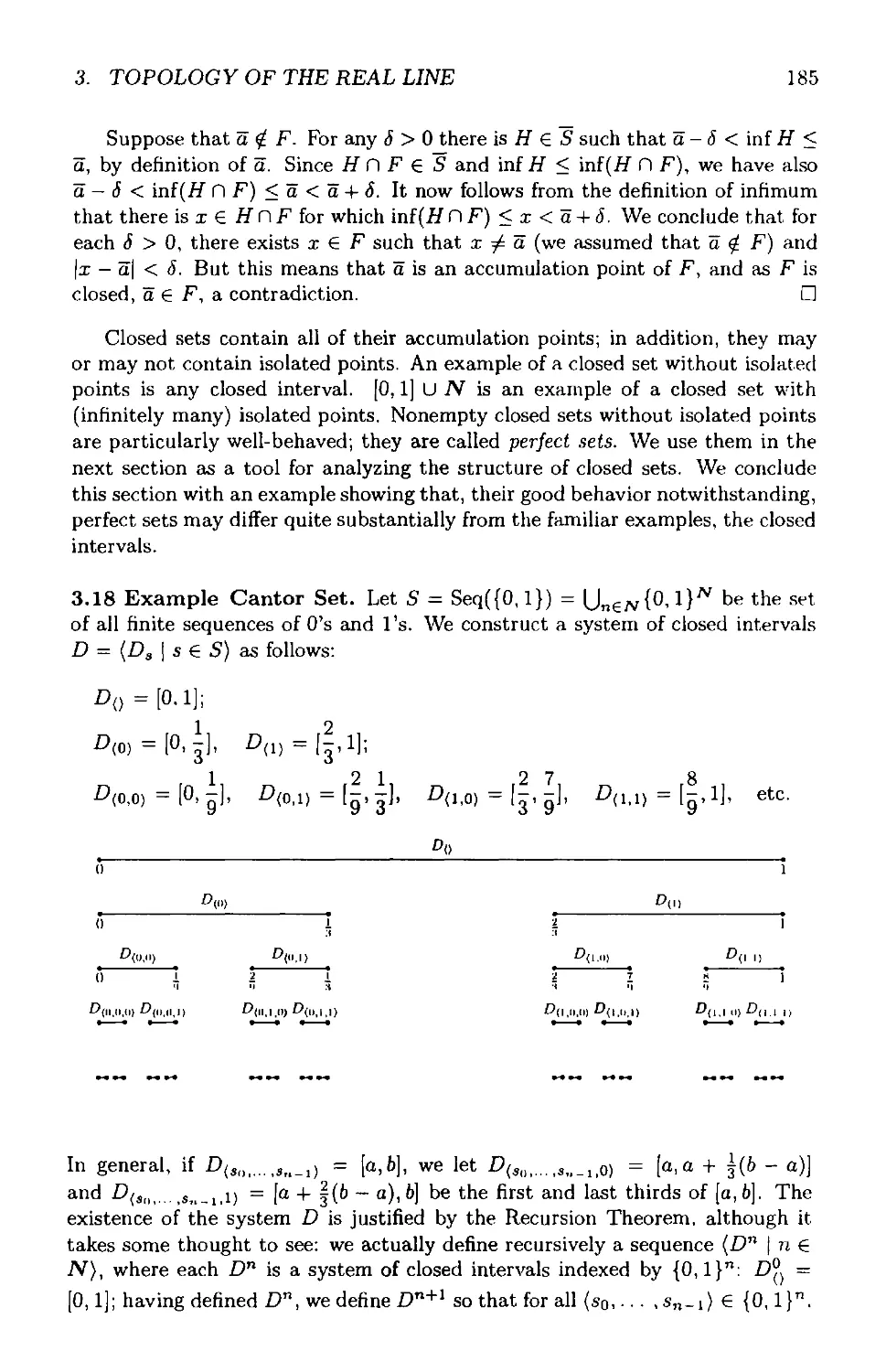
/


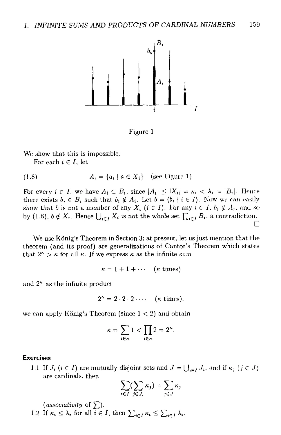


Text
INTRODUCTION TO
SET THEORY
Third Edition, Revised and Expanded
Karel Hrbacek
Thomas Jech
INTRODUCTION TO
SET THEORY
PURE AND APPLIED MATHEMATICS
A Program of Monographs, Textbooks, and Lecture Notes
EXECUTIVE EDITORS
Earl J. Taft
Rutgers University
New Brunswick, New Jersey
Zuhair Nashed
University of Delaware
Newark, Delaware
EDITORIAL BOARD
M. S, Baouendi
University of California,
San Diego
Jane Cronin
Rutgers University
JackK. Hale
Georgia Institute of Technology
S. Kobayashi
University of California,
Berkeley
Marvin Marcus
University of California,
Santa Barbara
Ж 5 Massey
Yale University
Anil Nerode
Cornell University
Donald Passman
University of Wisconsin,
Madison
Fred S. Roberts
Rutgers University
Gian-Carlo Rota
Massachusetts Institute of
Technology
David L. Russell
Virginia Polytechnic Institute
and State University
Walter Schempp
Universitat Siegen
Mark Teply
University of Wisconsin,
Milwaukee
MONOGRAPHS AND TEXTBOOKS IN
PURE AND APPLIED MATHEMATICS
1. K. Yano, Integral Formulas in Riemannian Geometry (1970)
2. S. Kobayashi, Hyperbolic Manifolds and Holomorphic Mappings (1970)
3. V. S. Vladimirov, Equations of Mathematical Physics (A. Jeffrey, ed.; A. Littlewood,
trans.) (1970)
4. B. N. Pshenichny!, Necessary Conditions for an Extremum (L. Neustadt, translation
ed.; K. Makowski, trans.) (1971)
5. L. Narici et al., Functional Analysis and Valuation Theory (1971)
6. S. S. Passman, Infinite Group Rings (1971)
7. L Domhoff, Group Representation Theory. Part A: Ordinary Representation Theory.
Part B; Modular Representation Theory (1971,1972)
8. W. Boothbyand G. L. Weiss, eds., Symmetric Spaces (1972)
9. Y. Matsushima, Differentiable Manifolds (E. T. Kobayashi, trans.) (1972)
10. L. E. Ward, Jr, Topology (1972)
11. A. Babakhanian, Cohomological Methods in Group Theory (1972)
12. R. Gilmer, Multiplicative Ideal Theory (1972)
13. J. Yeh, Stochastic Processes and the Wiener Integral (1973)
14. J. Barros-Neto, Introduction to the Theory of Distributions (1973)
15. R. Larsen, Functional Analysis (1973)
16. К Yano and S. Ishihara, Tangent and Cotangent Bundles (1973)
17. C. Procesi, Rings with Polynomial Identities (1973)
18. R. Hermann, Geometry, Physics, and Systems (1973)
19. N. R. Wallach, Harmonic Analysis on Homogeneous Spaces (1973)
20. J. Dieudonne, Introduction to the Theory of Formal Groups (1973)
21. I. Vaisman, Cohomology and Differential Forms (1973)
22. B.-Y. Chen, Geometry of Submanifolds (1973)
23. M. Marcus, Finite Dimensional Multilinear Algebra (in two parts) (1973, 1975)
24. R Larsen, Banach Algebras (1973)
25. R O. Kujala and A. L. Vftter, eds., Value Distribution Theory: Part A; Part B: Deficit
and Bezout Estimates by Wilhelm Stoll (1973)
26. К. B. Stolarsky, Algebraic Numbers and Diophantine Approximation (1974)
27. A. R. Magid, The Separable Galois Theory of Commutative Rings (1974)
28. R R McDonald, Finite Rings with Identity (1974)
29. J. Satake, Linear Algebra (S. Koh et al., trans.) (1975)
30. J. S. Golan, Localization of Noncommutative Rings (1975)
31. G. Klambauer, Mathematical Analysis (1975)
32. M. K. Agoston, Algebraic Topology (1976)
33. K. R. Goodeart, Ring Theory (1976)
34. L E. Mansfield, Linear Algebra with Geometric Applications (1976)
35. N. J. Pullman, Matrix Theory and Its Applications (1976)
36. B. R. McDonald, Geometric Algebra Over Local Rings (1976)
37. C W. Groetsch, Generalized Inverses of Linear Operators (1977)
38. J. E. Kuczkowski and J. L Gersting, Abstract Algebra (1977)
39. С O. Christenson and W, L. Voxman, Aspects of Topology (1977)
40. M. Nagata, Field Theory (1977)
41. R L Long, Algebraic Number Theory (1977)
42. W, F. Pfeffer, Integrals and Measures (1977)
43. R. L Wheeden and A. Zygmund, Measure and Integral (1977)
44. J. H. Curtiss, Introduction to Functions of a Complex Variable (1978)
45. K. Hrbacek and T. Jech, Introduction to Set Theory (1978)
46. W. S. Massey, Homology and Cohomology Theory (1978)
47. M. Marcus, Introduction to Modem Algebra (1978)
48. E. C Young, Vector and Tensor Analysis (1978)
49. S. B. Nadler, Jr, Hyperspaces of Sets (1978)
50. S. K. Segal, Topics in Group Kings (1978)
51. A. C M. van Rooij, Non-Archimedean Functional Analysis (1978)
52. L. Corwin and R. Szczarba, Calculus in Vector Spaces (1979)
53. C Sadosky, Interpolation of Operators and Singular Integrals (1979)
54. J. Cronin, Differential Equations (1980)
55. C. W. Groetsch, Elements of Applicable Functional Analysis (1980)
56. I. Vaisman, Foundations of Three-Dimensional Euclidean Geometry (1980)
57. H. I. Freedan, Deterministic Mathematical Models in Population Ecology (1980)
58. S. B. Chae, Lebesgue Integration (1980)
59. C. S. Rees ef ah, Theory and Applications of Fourier Analysis (1981)
60. L Nachbin, Introduction to Functional Analysis (R. M. Aron, trans.) (1981)
61. G. Orzech and M. Orzech, Plane Algebraic Curves (1981)
62. R. Johnsonbaugh and W. E. Pfaffenberger, Foundations of Mathematical Analysis
(1981)
63. W. L. Voxman and R. H. Goetschel, Advanced Calculus (1981)
64. L. J. Corwin and R. H. Szczarba, Multivariable Calculus (1982)
65. V. /. Istr^tescu, Introduction to Linear Operator Theory (1981)
66. R. D. J8rvinen, Finite and Infinite Dimensional Linear Spaces (1981)
67. J. К. Веет and P. E. Ehrlich, Global Lorentzian Geometry (1981)
68. D. L. Armacost, The Structure of Locally Compact Abelian Groups (1981)
69. J. W. Brewer and M. K. Smith, eds., Emmy Noether A Tribute (1981)
70. К. H. Kim, Boolean Matrix Theory and Applications (1982)
71. T. W. Wieting, The Mathematical Theory of Chromatic Plane Ornaments (1982)
72. D. B.Gauld, Differential Topology (1982)
73. R. L. Faber, Foundations of Euclidean and Non-Eudidean Geometry (1983)
74. M. Carmeli, Statistical Theory and Random Matrices (1983)
75. J. H. Carruth etah, The Theory of Topological Semigroups (1983)
76. R. L. Faber, Differential Geometry and Relativity Theory (1983)
77. S. Barnett, Polynomials and Linear Control Systems (1983)
78. G. Karpilovsky, Commutative Group Algebras (1983)
79. F. Van Oystaeyen and A. Verschoren, Relative Invariants of Rings (1983)
80. /. Vaisman, A First Course in Differential Geometry (1984)
81. G. W. Swan, Applications of Optimal Control Theory in Biomedicine (1984)
82. T. Petrie and J. D. Randall, Transformation Groups on Manifolds (1984)
83. K. Goebel and S. Reich, Uniform Convexity, Hyperbolic Geometry, and Nonexpansive
Mappings (1984)
84. T. Albu and C. N3st£sescu, Relative Finiteness in Module Theory (1984)
85. K. Hrbacek and T. Jech, Introduction to Set Theory: Second Edition (1984)
86. F. Van Oystaeyen and A. Verschoren, Relative Invariants of Rings (1984)
87. 8. R. McDonald, Linear Algebra Over Commutative Rings (1984)
88. M. Namba, Geometry of Projective Algebraic Curves (1984)
89. G. F. Webb, Theory of Nonlinear Age-Dependent Population Dynamics (1985)
90. M. R. Bremneret al., Tables of Dominant Weight Multiplicities for Representations of
Simple Lie Algebras (1985)
91. A. E. Fekete, Real Linear Algebra (1985)
92. S. 8. Chae, Holomorphy and Calculus in Normed Spaces (1985)
93. A. J. Jerri, Introduction to Integral Equations with Applications (1985)
94. G. Karpilovsky, Projective Representations of Finite Groups (1985)
95. L Narici and E. Beckenstein, Topological Vector Spaces (1985)
96. J. Weeks, The Shape of Space (1985)
97. P. R. Gribik and К. O. Kortanek, Extremal Methods of Operations Research (1985)
98. J.-A Chao and W. A. Woyczynski, eds., Probability Theory and Harmonic Analysis
(1986)
99. G. D. Crown et al., Abstract Algebra (1986)
00. J. H. Carruth et al., The Theory of Topological Semigroups, Volume 2 (1986)
01. R. S. Doran and V. A. Beffi, Characterizations of C*-Algebras (1986)
02. M. W. Jeter, Mathematical Programming (1986)
03. M. Altman, A Unified Theory of Nonlinear Operator and Evolution Equations with
Applications (1986)
04. A. Verschoren, Relative Invariants of Sheaves (1987)
05. R. A. Usmani, Applied Linear Algebra (1987)
06. P. Blass and J. Lang, Zariski Surfaces and Differential Equations in Characteristic p >
0 (1987)
07. J. A. Reneke et al., Structured Hereditary Systems (1987)
08. H. Busemann and B. 8. Phadke, Spaces with Distinguished Geodesics (1987)
09. R. Harte, Invertibility and Singularity for Bounded Linear Operators (1988)
10. G. S. Ladde et al.. Oscillation Theory of Differential Equations with Deviating Argu-
ments (1987)
11. L Dudkinetal., Iterative Aggregation Theory (1987)
12. T. Okubo, Differential Geometry (1987)
13. D. L. Stand and M. L. Stand, Real Analysis with Point-Set Topology (1987)
114. Т. С. Gard, Introduction to Stochastic Differential Equations (1988)
115. S. S. Abhyankar, Enumerative Combinatorics of Young Tableaux (1988)
116. H. Strade and R. Famsteiner, Modular Lie Algebras and Their Representations (1988)
117. J. A. Huck aba, Commutative Rings with Zero Divisors (1988)
118. W. D. Wallis, Combinatorial Designs (1988)
119. W. Wipslaw, Topological Fields (1988)
120. G. Karpilovsky, Field Theory (1988)
121. S. Caenepeel and F. Van Oystaeyen, Brauer Groups and the Cohomology of Graded
Rings (1989)
122. W. Kozlowski, Modular Function Spaces (1988)
123. E. Lowen-Colebunders, Function Classes of Cauchy Continuous Maps (1989)
124. M. Pavel, Fundamentals of Pattern Recognition (1989)
125. V. Lakshmikantham et al., Stability Analysis of Nonlinear Systems (1989)
126. R. Sivaramakrishnan, The Classical Theory of Arithmetic Functions (1989)
127. N. A. Watson, Parabolic Equations on an Infinite Strip (1989)
128. К J. Hastings, Introduction to the Mathematics of Operations Research (1989)
129. 8. Fine, Algebraic Theory of the Bianchi Groups (1989)
130. D. N. Dikranjan et al., Topological Groups (1989)
131. J. C. Morgan II, Point Set Theory (1990)
132. P. Bilerand A. Witkowski, Problems in Mathematical Analysis (1990)
133. H. J. Sussmann, Nonlinear Controllability and Optimal Control (1990)
134. J.-P. Florens et al., Elements of Bayesian Statistics (1990)
135. N. Shell, Topological Fields and Near Valuations (1990)
136. 8. F. Doolin and C. F. Martin, Introduction to Differential Geometry for Engineers
(1990)
137. S. S. Holland, Jr., Applied Analysis by the Hilbert Space Method (1990)
138. J. Okninski, Semigroup Algebras (1990)
139. К Zhu, Operator Theory in Function Spaces (1990)
140. G. 8. Price, An Introduction to Multicomplex Spaces and Functions (1991)
141. R. 8. Darst, Introduction to Linear Programming (1991)
142. P. L. Sachdev, Nonlinear Ordinary Differential Equations and Their Applications (1991)
143. T. Husain, Orthogonal Schauder Bases (1991)
144. J. Foran, Fundamentals of Real Analysis (1991)
145. W. C. Brown, Matrices and Vector Spaces (1991)
146. M. M. Rao and Z. D. Ren, Theory of Oriicz Spaces (1991)
147. J. S. Golan and T. Head, Modules and the Structures of Rings (1991)
148. C. Small, Arithmetic of Finite Fields (1991)
149. K. Yang, Complex Algebraic Geometry (1991)
150. D. G. Hoffman eta!.. Coding Theory (1991)
151. M. O. Gonz&ez, Classical Complex Analysis (1992)
152. M. O. Gonzalez, Complex Analysis (1992)
153. L W. Baggett, Functional Analysis (1992)
154. M. Sniedovich, Dynamic Programming (1992)
155. R. P. Agarwal, Difference Equations and Inequalities (1992)
156. C. Brezinski, Biorthogonality and Its Applications to Numerical Analysis (1992)
157. C. Swartz, An Introduction to Functional Analysis (1992)
158. S. 8. Nadler, Jr., Continuum Theory (1992)
159. M. A. Al-Gwaiz, Theory of Distributions (1992)
160. E. Perry, Geometry: Axiomatic Developments with Problem Solving (1992)
161. E. Castillo and M. R. Ruiz-Cobo, Functional Equations and Modelling in Science and
Engineering (1992)
162. A. J. Jerri, Integral and Discrete Transforms with Applications and Error Analysis
(1992)
163. A. Chartieret al., Tensors and the Clifford Algebra (1992)
164. P. Bilerand T. Nadzieja, Problems and Examples in Differential Equations (1992)
165. E. Hansen, Global Optimization Using Interval Analysis (1992)
166. S. Gueme-DelabriPre, Classical Sequences in Banach Spaces (1992)
167. Y. C. Wong, Introductory Theory of Topological Vector Spaces (1992)
168. S. H Kulkami and 8. V. Limaye, Real Function Algebras (1992)
169. W. C. Brown, Matrices Over Commutative Rings (1993)
170. J. Loustau and M. Dillon, Linear Geometry with Computer Graphics (1993)
171. W. V. Petryshyn, Approximation-Solvability of Nonlinear Functional and Differential
Equations (1993)
172. E. C. Young, Vector and Tensor Analysis; Second Edition (1993)
173. T. A. Bick, Elementary Boundary Value Problems (1993)
174. M. Pavel, Fundamentals of Pattern Recognition; Second Edition (1993)
175. S. A. Albeverio et al., Noncommutative Distributions (1993)
176. W. Fulks, Complex Variables (1993)
177. M. M. Rao, Conditional Measures and Applications (1993)
178. A. Janicki and A. Weron, Simulation and Chaotic Behavior of a-Stable Stochastic
Processes (1994)
179. P. Neittaanntiki and D. Tiba, Optimal Control of Nonlinear Parabolic Systems (1994)
180. J. Cronin, Differential Equations: Introduction and Qualitative Theory, Second Edition
(1994)
181. S. Heikkiia and V. Lakshmikantham, Monotone Iterative Techniques for Discontinuous
Nonlinear Differential Equations (1994)
182. X Mao, Exponential Stability of Stochastic Differential Equations (1994)
183. B. S. Thomson, Symmetric Properties of Real Functions (1994)
184. J. E. Rubio, Optimization and Nonstandard Analysis (1994)
185. J. L. Bueso et al., Compatibility, Stability, and Sheaves (1995)
186. A. N. Michel and K. Wang, Qualitative Theory of Dynamical Systems (1995)
187. M. R. Darnel, Theory of Lattice-Ordered Groups (1995)
188. Z. Naniewicz and P. D. Panaglotopoulos, Mathematical Theory of Hemivariational
Inequalities and Applications (1995)
189. L. J. Corwin and R. H. Szczarba, Calculus in Vector Spaces: Second Edition (1995)
190. L. H. Erbe et al., Oscillation Theory for Functional Differential Equations (1995)
191. S. Agaian et al., Binary Polynomial Transforms and Nonlinear Digital Filters (1995)
192. M. I. Gil’, Norm Estimations for Operation-Valued Functions and Applications (1995)
193. P. A. Grillet, Semigroups: An Introduction to the Structure Theory (1995)
194. S. Kichenassamy, Nonlinear Wave Equations (1996)
195. V. F. Krotov, Global Methods in Optimal Control Theory (1996)
196. К. I. Beidaret al., Rings with Generalized Identities (1996)
197. V. /. Arnautov et al., Introduction to the Theory of Topological Rings and Modules
(1996)
198. G. Sierksma, Linear and Integer Programming (1996)
199. R. Lassar, Introduction to Fourier Series (1996)
200. V. Sima, Algorithms for Linear-Quadratic Optimization (1996)
201. D. Redmond, Number Theory (1996)
202. J. К. Веет et al., Global Locentzian Geometry: Second Edition (1996)
203. M. Fontana et al., Prufer Domains (1997)
204. H. Tanabe, Functional Analytic Methods for Partial Differential Equations (1997)
205. C. Q. Zhang, Integer Flows and Cycle Covers of Graphs (1997)
206. E. Spiegel and C. J. O’Donnell, Incidence Algebras (1997)
207. B. Jakubczyk and W. Respondek, Geometry of Feedback and Optimal Control (1998)
208. T. W. Haynes et al., Fundamentals of Domination in Graphs (1998)
209. T. W. Haynes etal., Domination in Graphs: Advanced Topics (1998)
210. L A. D’Alotto et al., A Unified Signal Algebra Approach to Two-Dimensional Parallel
Digital Signal Processing (1998)
211. F. Halter-Koch, Ideal Systems (1998)
212. N. K. Govil et al.. Approximation Theory (1998)
213. R. Cross, Multivalued Linear Operators (1998)
214. A. A. Martynyuk, Stability by Liapunov’s Matrix Function Method with Applications
(1998)
215. A. FaviniandA. Yagi, Degenerate Differential Equations in Banach Spaces (1999)
216. A. Illanes and S. Nadler, Jr., Hyperspaces: Fundamentals and Recent Advances
(1999)
217. G. Kato and D. Struppa, Fundamentals of Algebraic Microlocal Analysis (1999)
218. G. X.-Z. Yuan, KKM Theory and Applications in Nonlinear Analysis (1999)
219. D. Motreanu and N. H. Pavel, Tangency, Flow Invariance for Differential Equations,
and Optimization Problems (1999)
220. K. Hrbacek and T. Jech, Introduction to Set Theory, Third Edition (1999)
221. G. E. Kolosov, Optimal Design of Control Systems (1999)
222. A. I. Prilepko etal.. Methods for Solving Inverse Problems in Mathematical Physics
(1999)
Additional Volumes in Preparation
INTRODUCTION TO
SET THEORY
Third Edition, Revised and Expanded
Karel Hrbacek
The City College of the
City University of New York
New York, New York
Thomas Jech
The Pennsylvania State University
University Park, Pennsylvania
MARCEL
Marcel Dekker, Inc.
DEKKER
New York • Basel
Library of Congress Cataloging-in-Publication
Hrbacek, Karel.
Introduction to set theory / Karel Hrbacek, Thomas Jech. — 3rd ed., rev. and
expanded.
p. cm. — (Monographs and textbooks in pure and applied mathematics;
220).
Includes index.
ISBN 0-8247-7915-0 (alk. paper)
1. Set theory. I. Jech, Thomas J. II. Title. III. Series.
QA248.H68 1999
511.3’22—dc21 99-15458
CIP
This book is printed on acid-free paper.
Headquarters
Marcel Dekker, Inc.
270 Madison Avenue, New York, NY 10016
tel: 212-696-9000; fax: 212-685-4540
Eastern Hemisphere Distribution
Marcel Dekker AG
Hutgasse 4, Postfach 812, CH-4001 Basel, Switzerland
tel: 41 -61 -261 -8482; fax: 41-61 -261 -8896
World Wide Web
http://www.dekker.com
The publisher offers discounts on this book when ordered in bulk quantities. For more infor-
mation, write to Special Sales/Professional Marketing at the headquarters address above.
Copyright © 1999 by Marcel Dekker, Inc. All Rights Reserved.
Neither this book nor any part may be reproduced or transmitted in any form or by any
means, electronic or mechanical, including photocopying, microfilming, and recording, or
by any information storage and retrieval system, without permission in writing from the
publisher.
Current printing (last digit)
10 987654321
PRINTED IN THE UNITED STATES OF AMERICA
Preface to the 3rd Edition
Modern set theory has grown tremendously since the first edition of this book
was published in 1978, and even since the second edition appeared in 1984.
Moreover, many ideas that were then at the forefront of research have become,
by now, important tools in other branches of mathematics. Thus, for example,
combinatorial principles, such as Principle Diamond and Martin’s Axiom, are
indispensable tools in general topology and abstract algebra. Non-well-founded
sets turned out to be a convenient setting for semantics of artificial as well
as natural languages. Nonstandard Analysis, which is grounded on structures
constructed with the help of ultrafilters, has developed into an independent
methodology with many exciting applications. It seems appropriate to incor-
porate some of the underlying set-theoretic ideas into a textbook intended as a
general introduction to the subject. We do that in the form of four new chapters
(Chapters 11-14), expanding on the topics of Chapter 11 in the second edition,
and containing largely new material. Chapter 11 presents filters and ultrafilters,
develops the basic properties of closed unbounded and stationary sets, and cul-
minates with the proof of Silver’s Theorem. The first two sections of Chapter 12
provide an introduction to the partition calculus. The next two sections study
trees and develop their relationship to Suslin’s Problem. Section 5 of Chapter
12 is an introduction to combinatorial principles. Chapter 13 is devoted to the
measure problem and measurable cardinals. The topic of Chapter 14 is a fairly
detailed study of well-founded and non-well-founded sets.
Chapters 1-10 of the second edition have been thoroughly revised and reor-
ganized. The material on rational and real numbers has been consolidated in
Chapter 10, so that it does not interrupt the development of set theory proper.
To preserve continuity, a section on Dedekind cuts has been added to Chapter 4.
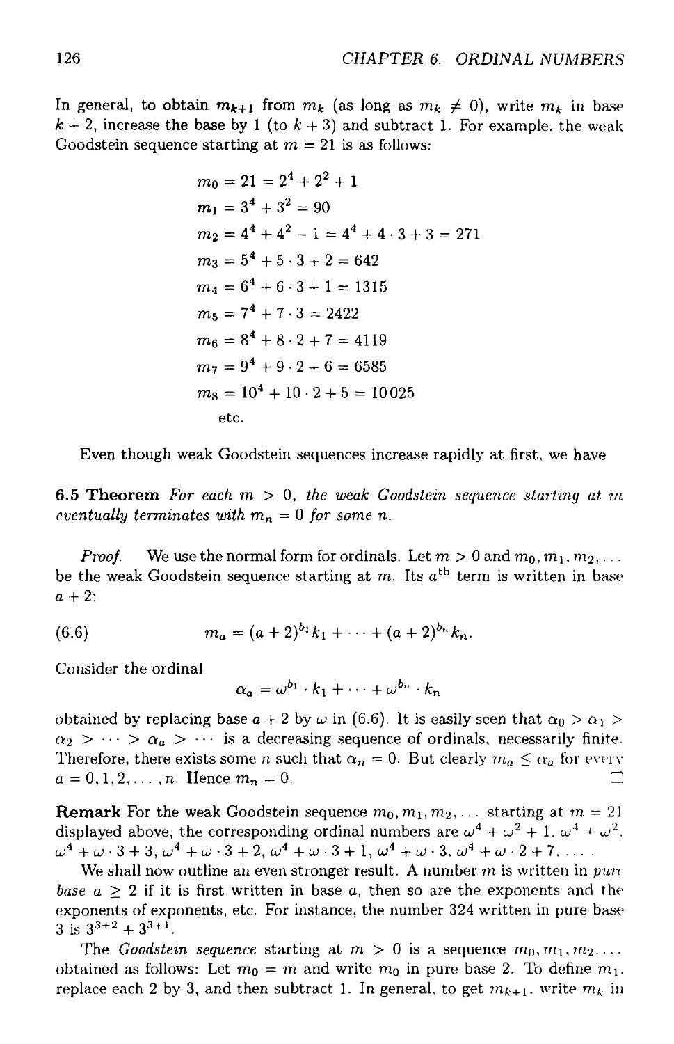
New material (on normal forms and Goodstein sequences) has also been added
to Chapter 6.
A solid basic course in set theory should cover most of Chapters 1-9. This
can be supplemented by additional material from Chapters 10-14, which are
almost completely independent of each other (except that Section 5 in Chapter
12, and Chapter 13, refer to some concepts introduced in earlier chapters).
Karel Hrbacek
Thomas Jech
iii
This page intentionally left blank
Preface to the 2nd Edition
The first version of this textbook was written in Czech in spring 1968 and
accepted for publication by Academia, Prague under the title Uvod do teorie
mnoiin. However, we both left Czechoslovakia later that year, and the book
never appeared. In the following years we taught introductory courses in set
theory at various universities in the United States, and found it difficult to se-
lect a textbook for use in these courses. Some existing books are based on the
“naive” approach to set theory rather than the axiomatic one. We consider
some understanding of set-theoretic “paradoxes” and of undecidable proposi-
tions (such as the Continuum Hypothesis) one of the important goals of such
a course, but neither topic can be treated honestly with a “naive” approach.
Moreover, set theory is a natural choice of a field where students can first be-
come acquainted with an axiomatic development of a mathematical discipline.
On the other hand, all currently available texts presenting set theory from an
axiomatic point of view heavily stress logic and logical formalism. Most of them
begin with a virtual minicourse in logic. We found that students often take a
course in set theory before taking one in logic. More importantly, the emphasis
on formalization obscures the essence of the axiomatic method. We felt that
there was a need for a book which would present axiomatic set theory more
mathematically, at the level of rigor customary in other undergraduate courses
for math majors. This led us to the decision to rewrite our Czech text. We
kept the original general plan, but the requirements for a textbook suitable for
American colleges resulted in the production of a completely new work.
We wish to stress the following features of the book:
1. Set theory is developed axiomatically. The reasons for adopting each
axiom, as arising both from intuition and mathematical practice, are carefully
pointed out. A detailed discussion is provided in “controversial” cases, such as
the Axiom of Choice.
2. The treatment is not formal. Logical apparatus is kept to a minimum
and logical formalism is completely avoided.
3. We show that axiomatic set theory is powerful enough to serve as an un-
derlying framework for mathematics by developing the beginnings of the theory
of natural, rational, and real numbers in it. However, we carry the development
only as far as it is useful to illustrate the general idea and to motivate set-
theoretic generalizations of some of these concepts (such as the ordinal numbers
and operations on them). Dreary, repetitive details, such as the proofs of all
VI
PREFACE TO THE SECOND EDITION
the usual arithmetic laws, are relegated into exercises.
4. A substantial part of the book is devoted to the study of ordinal and
cardinal numbers.
5. Each section is accompanied by many exercises of varying difficulty.
6. The final chapter is an informal outline of some recent developments in
set theory and their significance for other areas of mathematics: the Axiom of
Constructibility, questions of consistency and independence, and large cardi-
nals. No proofs are given, but the exposition is sufficiently detailed to give a
nonspecialist some idea of the problems arising in the foundations of set theory,
methods used for their solution, and their effects on mathematics in general.
The first edition of the book has been extensively used as a textbook in un-
dergraduate and first-year graduate courses in set theory. Our own experience,
that of our many colleagues, and suggestions and criticism by the reviewers led
us to consider some changes and improvements for the present second edition.
Those turned out to be much more extensive than we originally intended. As
a result, the book has been substantially rewritten and expanded. We list the
main new features below.
1. The development of natural numbers in Chapter 3 has been greatly
simplified. It is now based on the definition of the set of all natural numbers
as the least inductive set, and the Principle of Induction. The introduction of
transitive sets and a characterization of natural numbers as those transitive sets
that are well-ordered and inversely well-ordered by € is postponed until the
chapter on ordinal numbers (Chapter 7).
2. The material on integers and rational numbers (a separate chapter in
the first edition) has been condensed into a single section (Section 1 of Chapter
5). We feel that most students learn this subject in another course (Abstract
Algebra), where it properly belongs.
3. A series of new sections (Section 3 in Chapter 5, 6, and 9) deals with
the set-theoretic properties of sets of real numbers (open, closed, and perfect
sets, etc.), and provides interesting applications of abstract set theory to real
analysis.
4. A new chapter called “Uncountable Sets” (Chapter 11) has been added.
It introduces some of the concepts that are fundamental to modem set theory:
ultrafilters, closed unbounded sets, trees and partitions, and large cardinals.
These topics can be used to enrich the usual one-semester course (which would
ordinarily cover most of the material in Chapters 1-10).
5. The study of linear orderings has been expanded and concentrated in one
place (Section 4 of Chapter 4).
6. Numerous other small additions, changes, and corrections have been made
throughout.
7. Finally, the discussion of the present state of set theory in Section 3 of
Chapter 12 has been updated.
Karel Hrbacek
Thomas Jech
Contents
Preface to the Third Edition iii
Preface to the Second Edition v
1 Sets 1
1 Introduction to Sets......................................... 1
2 Properties................................................... 3
3 The Axioms................................................... 7
4 Elementary Operations on Sets............................... 12
2 Relations, Functions, and Orderings 17
1 Ordered Pairs............................................... 17
2 Relations .................................................. 18
3 Functions................................................... 23
4 Equivalences and Partitions................................. 29
5 Orderings................................................... 33
3 Natural Numbers 39
1 Introduction to Natural Numbers........................... 39
2 Properties of Natural Numbers............................... 42
3 The Recursion Theorem....................................... 46
4 Arithmetic of Natural Numbers............................... 52
5 Operations and Structures................................... 55
4 Finite, Countable, and Uncountable Sets 65
1 Cardinality of Sets......................................... 65
2 Finite Sets................................................. 69
3 Countable Sets.............................................. 74
4 Linear Orderings............................................ 79
5 Complete Linear Orderings................................... 86
6 Uncountable Sets............................................ 90
5 Cardinal Numbers 93
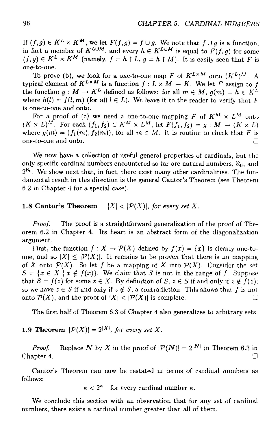
1 Cardinal Arithmetic....................................... 93
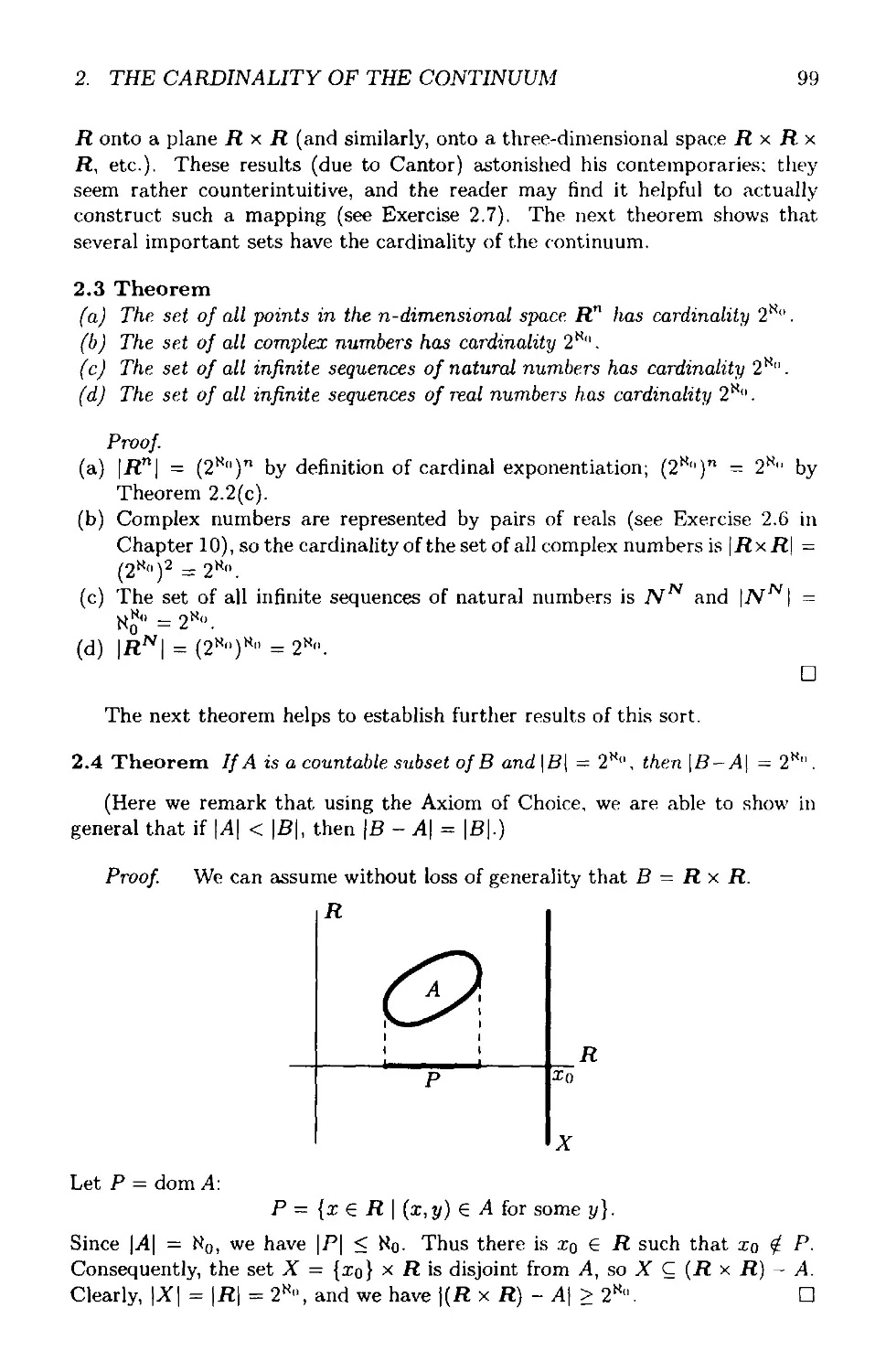
2 The Cardinality of the Continuum............................ 98
vii
viii
CONTENTS
в Ordinal Numbers 103
1 Well-Ordered Sets...........................................103
2 Ordinal Numbers.............................................107
3 The Axiom of Replacement....................................Ill
4 Transfinite Induction and Recursion.........................114
5 Ordinal Arithmetic..........................................119
6 The Normal Form.............................................124
7 Alephs 129
1 Initial Ordinals............................................129
2 Addition and Multiplication of Alephs.......................133
8 The Axiom of Choice 137
1 The Axiom of Choice and its Equivalents.....................137
2 The Use of the Axiom of Choice in Mathematics...............144
9 Arithmetic of Cardinal Numbers 155
1 Infinite Sums and Products of Cardinal
Numbers.........................................................155
2 Regular and Singular Cardinals..............................160
3 Exponentiation of Cardinals.................................164
10 Sets of Real Numbers 171
1 Integers and Rational Numbers...............................171
2 Real Numbers................................................175
3 Topology of the Real Line...................................179
4 Sets of Real Numbers .......................................188
5 Borel Sets..................................................194
11 Filters and Ultrafilters 201
1 Filters and Ideals........................................ 201
2 Ultrafilters ...............................................205
3 Closed Unbounded and Stationary Sets .......................208
4 Silver’s Theorem............................................212
12 Combinatorial Set Theory 217
1 Ramsey’s Theorems...........................................217
2 Partition Calculus for Uncountable Cardinals................221
3 Trees.......................................................225
4 Suslin’s Problem............................................230
5 Combinatorial Principles....................................233
13 Large Cardinals 241
1 The Measure Problem.........................................241
2 Large Cardinals.............................................246
CONTENTS ix
14 The Axiom of Foundation 251
1 Well-Founded Relations..................................251
2 Well-Founded Sets.......................................256
3 Non-Well-Founded Sets...................................260
15 The Axiomatic Set Theory 267
1 The Zermelo-Fraenkel Set Theory
With Choice.................................................267
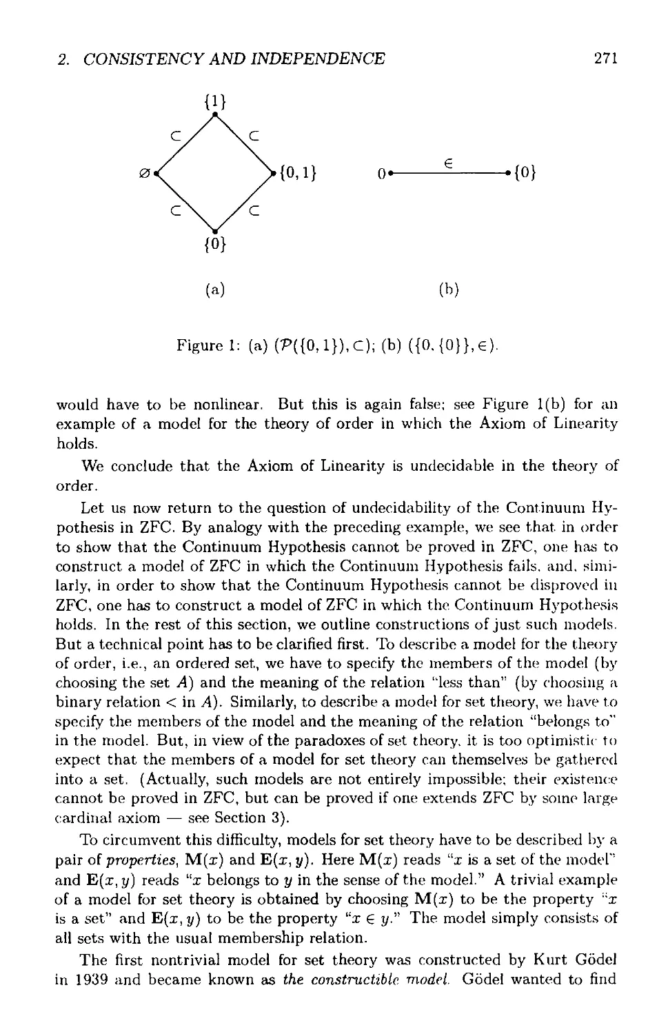
2 Consistency and Independence............................270
3 The Universe of Set Theory..............................277
Bibliography 285
Index 286
This page intentionally left blank
Chapter 1
Sets
1. Introduction to Sets
The central concept of this book, that of a set, is, at least on the surface,
extremely simple. A set is any collection, group, or conglomerate. So we have
the set of all students registered at the City University of New York in February
1998, the set of all even natural numbers, the set of all points in the plane тг
exactly 2 inches distant from a given point P, the set of all pink elephants.
Sets are not objects of the real world, like tables or stars; they are created
by our mind, not by our hands. A heap of potatoes is not a set of potatoes, the
set of all molecules in a drop of water is not the same object as that drop of
water. The human mind possesses the ability to abstract, to think of a variety of
different objects as being bound together by some common property, and thus
to form a set of objects having that property. The property in question may
be nothing more than the ability to think of these objects (as being) together.
Thus there is a set consisting of exactly the numbers 2, 7, 12, 13, 29, 34, and
11,000, although it is hard to see what binds exactly those numbers together,
besides the fact that we collected them together in our mind. Georg Cantor, a
German mathematician who founded set theory in a series of papers published
over the last three decades of the nineteenth century, expressed it as follows:
“Unter einer Menge verstehen wir jede Zusammenfassung M von bestimmten
wohlunterschiedenen Objekten in unserer Anschauung oder unseres Denkens
(welche die Elemente von M genannt werden) zu einem ganzen." [A set is
a collection into a whole of definite, distinct objects of our intuition or our
thought. The objects are called elements (members) of the set.]
Objects from which a given set is composed are called elements or members
of that set. We also say that they belong to that set.
In this book, we want to develop the theory of sets as a foundation for other
mathematical disciplines. Therefore, we are not concerned with sets of people or
molecules, but only with sets of mathematical objects, such as numbers, points
of space, functions, or sets. Actually, the first three concepts can be defined in
1
2
CHAPTER 1. SETS
set theory as sets with particular properties, and we do that in the following
chapters. So the only objects with which we are concerned from now on arc1
sets. For purposes of illustration, we talk about sets of numbers or points even
before these notions are exactly defined. We do that, however, only in examples,
exercises and problems, not in the main body of theory. Sets of mathematical
objects are, for example:
1.1 Example
(a) The set of all prime divisors of 324.
(b) The set of all numbers divisible by 0.
(c) The set of all continuous real-valued functions on the interval [0.1].
(d) The set of all ellipses with major axis 5 and eccentricity 3.
(e) The set of all sets whose elements are natural numbers less than 20.
Examination of these and many other similar examples reveals that sets
with which mathematicians work are relatively simple. They include the set of
natural numbers and its various subsets (such as the set of all prime numbers), as
well as sets of pairs, triples, and in general n-tuples of natural numbers. Integers
and rational numbers can be defined using only such sets. Real numbers can
then be defined as sets or sequences of rational numbers. Mathematical analysis
deals with sets of real numbers and functions on real numbers (sets of ordered
pairs of real numbers), and in some investigations, sets of functions or even
sets of sets of functions are considered. But a working mathematician rarely
encounters objects more complicated than that. Perhaps it is not surprising
that uncritical usage of “sets1' remote from “everyday experience” may lead to
contradictions.
Consider for example the “set” R of all those sets which are not elements
of themselves. In other words, R is a set of all sets x such that x ;r (e reads
“belongs to,” £ reads “does not belong to”). Let us now ask whether Re R.
If R e Ry then R is not an element of itself (because no element of R belongs
to itself), so R R\ a contradiction. Therefore, necessarily R $ R. But then
R is a set which is not an element of itself, and all such sets belong to 7?. We
conclude that R e /?; again, a contradiction.
The argument can be briefly summarized as follows: Define R by: .r € 7? if
and only if x x. Now consider x = R; by definition of R, R 6 R if and only if
R R; a contradiction.
A few comments on this argument (due to Bertrand Russell) might be help-
ful. First, there is nothing wrong with R being a set of sets. Many sets whose
elements are again sets are legitimately employed in mathematics — see Exam-
ple 1.1 — and do not lead to contradictions. Second, it is easy to give examples
of elements of Я; e.g., if x is the set of all natural numbers, then x x (the set
of all natural numbers is not a natural number) and so x 6 R. Third, it is not
so easy to give examples of sets which do not belong to Я, but this is irrelevant.
The foregoing argument would result in a contradiction even if there were no
sets which are elements of themselves. (A plausible candidate for a set which is
an element of itself would be the “set of all sets” V; clearly V € У. However.
2. PROPERTIES
3
the “set of all sets” leads to contradictions of its own in a more subtle wav —
see Exercises 3.3 and 3.6.)
How can this contradiction be resolved? We assumed that we have a set R
defined as the set of all sets which are not elements of themselves, and derived
a contradiction as an immediate consequence of the definition of R. This can
only mean that there is no set satisfying the definition of R. In other words,
this argument proves that there exists no set whose members would be precisely
the sets which are not elements of themselves. The lesson contained in Russell's
Paradox and other similar examples is that by merely defining a set we do not
prove its existence (similarly as by defining a unicorn we do not prove that
unicorns exist). There are properties which do not define sets; that is, it is not
possible to collect all objects with those properties into one set. This observation
leaves set-theorists with a task of determining the properties which do define
sets. Unfortunately, no way how to do this is known, and some results in logic
(especially the so-called Incompleteness Theorems discovered by Kurt Godel)
seem to indicate that a complete answer is not even possible.
Therefore, we attempt a less lofty goal. We formulate some of the relatively
simple properties of sets used by mathematicians as axiorns, and then take care
to check that all theorems follow logically from the axioms. Since the axioms
are obviously true and the theorems logically follow from them, the theorems
are also true (not necessarily obviously). We end up with a body of truths
about sets which includes, among other things, the basic properties of natural,
rational, and real numbers, functions, orderings, etc., but as far as is known,
no contradictions. Experience has shown that practically all notions used in
contemporary mathematics can be defined, and their mathematical properties
derived, in this axiomatic system. In this sense, the axiomatic set theory serves
as a satisfactory foundation for the other branches of mathematics.
On the other hand, we do not claim that every true fact about sets can be
derived from the axioms we present. The axiomatic system is not complete in
this sense, and we return to the discussion of the question of completeness in
the last chapter.
2. Properties
In the preceding section we introduced sets as collections of objects having
some property in common. The notion of property merits some analysis. Some
properties commonly considered in everyday life are so vague that they can
hardly be admitted in a mathematical theory. Consider, for example, the “set of
all the great twentieth century American novels.” Different persons1 judgments
as to what constitutes a great literary work differ so much that there is no
generally accepted way how to decide whether a given book is or is not an
element of the “set.”
For an even more startling example, consider the “set of those natural num-
bers which could be written down in decimal notation” (by “could” we mean
that someone could actually do it with paper and pencil). Clearly. 0 can be so
4
CHAPTER 1. SETS
written down. If number n can be written down, then surely number n + 1 can
also be written down (imagine another, somewhat faster writer, or the person
capable of writing n working a little faster). Therefore, by the familiar principle
of induction, every natural number n can be written down. But that is plainly
absurd; to write down say IO10 in decimal notation would require to follow 1
by IO10 zeros, which would take over 300 years of continuous work at a rate of
a zero per second.
The problem is caused by the vague meaning of “could.” To avoid similar
difficulties, we now describe explicitly what we mean by a property. Only clear,
mathematical properties are allowed; fortunately, these properties are sufficient
for expression of all mathematical facts.
Our exposition in this section is informal. Readers who would like to see
how this topic can be studied from a more rigorous point of view can consult
some book on mathematical logic.
The basic set-theoretic property is the membership property: “ ... is an
element of ... which we denote by 6. So “X e У” reads “X is an element of
У” or “X is a member of У” or liX belongs to У.”
The letters X and У in these expressions are variables; they stand for (de-
note) unspecified, arbitrary sets. The proposition “X G У” holds or does not
hold depending on sets (denoted by) X and У. We sometimes say “X 6 У” is
a property of X and Y. The reader is surely familiar with this informal way of
speech from other branches of mathematics. For example, “m is less than n” is
a property of m and n. The letters m and n are variables denoting unspecified
numbers. Some m and n have this property (for example, “2 is less than 4” is
true) but others do not (for example, “3 is less than 2” is false).
All other set-theoretic properties can be stated in terms of membership with
the help of logical means: identity, logical connectives, and quantifiers.
We often speak of one and the same set in different contexts and find it
convenient to denote it by different variables. We use the identity sign “=” to
express that two variables denote the same set. So we write X = Y if X is the
same set as Y [X is identical with Y or X is equal to У).
In the next example, we list some obvious facts about identity:
2.1 Example
(a) X = X.
(b) If X - У, then У = X.
(c) If X = У and У = Z, then X = Z.
(d) If X = У and X G Z, then У G Z.
(e) If X = Y and Z G X, then Z G У.
(X is identical with X.)
(If X and У are identical, then Y
and X are identical.)
(If X is identical with У and У is
identical with Z, then X is identical
with Z.)
(If X and У are identical and X
belongs to Z, then Y belongs to Z.)
(If X and У are identical and Z
belongs to X, then Z belongs to У.)
2. PROPERTIES
5
Logical connectives can be used to construct more complicated properties
from simpler ones. They are expressions like “not ... “ ... and ... “if .. . ,
then ... and “ ... if and only if ...
2.2 Example
(a) “X G Y or Y 6 X” is a property of X and Y.
(b) “Not X 6 Y and not Y 6 X” or, in more idiomatic English, “X is not an
element of У and Y is not an element of X” is also a property of X and У.
(c) “If X = У, then X G Z if and only if У G Z” is a property of X, У and Z.
(d) “X is not an element of X” (or: “not X G X”) is a property of X.
We write X У instead of “not X G У” and X / У instead of “not X = У.”
Quantifiers “for all” (“for every”) and “there is” (“there exists”) provide
additional logical means. Mathematical practice shows that all mathematical
facts can be expressed in the very restricted language we just described, but that
this language does not allow vague expressions like the ones at the beginning of
the section.
Let us look at some examples of properties which involve quantifiers.
2.3 Example
(a) “There exists У € X.”
(b) “For every У G X, there is Z such that Z G X and Z 6 У.”
(c) “There exists Z such that Z G X and Z У.”
Truth or falsity of (a) obviously depends on the set (denoted by the variable)
X. For example, if X is the set of all American presidents after 1789, then (a)
is true; if X is the set of all American presidents before 1789, (a) becomes false.
[Generally, (a) is true if X has some element and false if X is empty.] We say
that (a) is a property of X or that (a) depends on the parameter X. Similarly,
(b) is a property of X, and (c) is a property of X and У. Notice also that
У is not a parameter in (a) since it does not make sense to inquire whether
(a) is true for some particular set У; we use the letter У in the quantifier only
for convenience and could as well say, “There exists IV G Xor “There exists
some element of X.” Similarly, (b) is not a property of У, or Z, and (c) is not
a property of Z.
Although precise rules for determining parameters of a given property can
easily be formulated, we rely on the reader’s common sense, and limit ourselves
to one last example.
2.4 Example
(а) “УеХ.”
(b) “There is У G X.”
(c) “For every X, there is У G X.”
Here (a) is a property of X and У; it is true for some pairs of sets X, У
and false for others, (b) is a property of X (but not of У), while (c) has no
parameters, (c) is, therefore, either true or false (it is, in fact, false). Properties
6
CHAPTER!, SETS
which have no parameters (and are, therefore, either true or false) are called
statements; all mathematical theorems are (true) statements.
We sometimes wish to refer to an arbitrary, unspecified property. We use
boldface capital letters to denote statements and properties and. if convenient,
list some or all of their parameters in parentheses. So A(X) stands for any
property of the parameter X, e.g.. (a), (b), or (c) in Example 2.3. Е(А'.У) is
a property of parameters X and У, e.g., (c) in Example 2.3 or (a) in Example
2.4 or
(d) ЛХ € У or X = У or У € X."
In general, P(X, У,... ,Z) is a property whose truth or falsity depends on
parameters X, У,..., Z (and possibly others).
We said repeatedly that all set-theoretic properties can be expressed in our
restricted language, consisting of membership property and logical means. How-
ever, as the development proceeds and more and more complicated theorems an*
proved, it is practical to give names to various particular properties, i.e.. to de-
fine new properties. A new symbol is then introduced (defined) to denote the
property in question; we can view it as a shorthand for the explicit formulation.
For example, the property of being a subset is defined by
2,5 X C Y if and only if every element of X is an element of У.
“X is a subset of У” (X С У) is a property of X and У. We can use it in
more complicated formulations and, whenever desirable, replace X С У by its
definition. For example, the explicit definition of
uIf АСУ and У C Z, then X C Z.”
would be
‘‘If every element of X is an element of У and every element of Y is an
element of Z, then every element of X is an element of Z.”
It is clear that mathematics without definitions would be possible, but ex-
ceedingly clumsy.
For another type of definition, consider the property P(A):
“There exists no У £ X.”
We prove in Section 3 that
(a) There exists a set X such that P(X) (there exists a set X with no elements),
(b) There exists at most one set X such that P(A), i.e., if P(A) and P(X')-
then X = X’ (if X has no elements and Xf has no elements, then X and
Xf are identical).
(a) and (b) together express the fact that there is a unique set X with the
property P(X). We can then give this set a name, say 0 (the empty set), and
use it in more complicated expressions.
3. THE AXIOMS
7
The full meaning of “0 C Z” is then “the set X which has no elements is a
subset of Z У We occasionally refer to 0 as the constant defined by the property
P.
For our last example of a definition, consider the property Q(X, У, Z) of X,
У, and Z:
“For every U, U G Z if and only if U € X and U € У /’
We see in the next section that
(a) For every X and У there is Z such that Q(X, У Z).
(b) For every X and У, if Q(X,y, Z) and Q(X, У, Z'), then Z = Z'. [For every
X and У, there exists at most one Z such that Q(X, У, Z).]
Conditions (a) and (b) (which have to be proved whenever this type of definition
is used) guarantee that for every X and У there is a unique set Z such that
Q(X, У, Z). We can then introduce a name, say X А У, for this unique set Z.
and call X П У the intersection of X and У. So Q(X, У, X П У) holds. We refer
to П as the operation defined by the property Q.
3. The Axioms
We now begin to set up our axiomatic system and try to make clear the intuitive
meaning of each axiom.
The first principle we adopt postulates that our “universe of discourse" is
not void, i.e., that some sets exist. To be concrete1, we postulate the existence
of a specific set, namely the empty set.
The Axiom of Existence There exists a set which has no elements.
A set with no elements can be variously described intuitively, e.g.. as the
set of all U.S. Presidents before 1789, the set of all real numbers ,r for which
x2 — -1, etc. All examples of this kind describe one and the same set, namely
the empty, vacuous set. So, intuitively, there is only one empty set. But we
cannot yet prove this assertion. We need another postulate to express the fact
that each set is determined by its elements. Let us see another example:
X is the set consisting exactly of numbers 2, 3, and 5.
У is the set of all prime numbers greater than 1 and less than 7.
Z is the set of all solutions of the equation x3 - 10x2 + 31x — 30 = 0.
Here X — У, X = Z, and У = Z, and we have three different descriptions
of one and the same set. This leads to the Axiom of Extcnsionality.
The Axiom of Extcnsionality If every element of X is an element of Y and
every element of Y is an element of X, then X = У.
Briefly, if two sets have the same elements, then they are identical. We can
now prove Lemma 3.1.
8
CHAPTER 1. SETS
3.1 Lemma There exists only one set with no elements.
Proof. Assume that A and В are sets with no elements. Then every
element of A is an element of В (since A has no elements, the statement “a € A
implies a G B” is an implication with a false antecedent, and thus automatically
true). Similarly, every element of В is an element of A (since В has no elements).
Therefore, A = B, by the Axiom of Extensionality. □
3.2 Definition The (unique) set with no elements is called the empty set and
is denoted 0.
Notice that the definition of the constant 0 is justified by the Axiom of
Existence and Lemma 3.1.
Intuitively, sets are collections of objects sharing some common property, so
we expect to have axioms expressing this fact. But, as demonstrated by the
paradoxes in Section 1, not every property describes a set; properties ilX X"
or “X = A” are typical examples.
In both cases, the problem seems to be that in order to collect all objects
having such a property into a set, we already have to be able to perceive all sets.
The difficulty is avoided if we postulate the existence of a set of all objects with
a given property only if there already exists some set to which they all belong.
The Axiom Schema of Comprehension Let P(rr) be a property of x. For
any set A, there is a set В such that x G В if and only if rr G A and P(a:).
This is a schema of axioms, i.e., for each property P, we have one axiom.
For example, if P(x) is “x = rr,1’ the axiom says:
For any set A, there is a set В such that x € В if and only if x e A
and x — X, (In this case, В = A.)
If Р(я?) is “x x”, the axiom postulates:
For any set A, there is a set В such that x € В if and only if x G A
and x x.
Although the supply of axioms is unlimited, this causes no problems, since
it is easy to recognize whether a particular statement is or is not an axiom and
since every proof uses only finitely many axioms.
The property P(rr) can depend on other parameters p,... .q; the correspond-
ing axiom then postulates that for any sets p....q and any A. there is a set
В (depending on p,,.. ,q and, of course, on A) consisting exactly of all those
x G A for which Р(я:,р,... , g).
3.3 Example If P and Q are sets, then there is a set R such that x e R if and
only if x € P and x e Q.
3. THE AXIOMS
9
Proof, Consider the property P(rr, Q) of x and Q: “x e Q.” Then, by the
Comprehension Schema, for every Q and for every P there is a set R such that
x € R if and only if x e P and P(rr, Q), i.e., if and only if x € P and x € Q. (P
plays the role of A, Q is a parameter.) □
3.4 Lemma For every A, there is only one set В such that x G В if and only
if x e A and P(a:).
Proof If B' is another set such that x € Bf if and only if x 6 A and P(.r),
then x G В if and only if x G B', so В = Bf, by the Axiom of Extensionality.
□
We are now justified to introduce a name for the uniquely determined set B.
3.5 Definition {r 6 Л | P(r)} is the set of all x G A with the property P(x).
3.6 Example The set from Example 3.3 could be denoted {xG P |xg Q}.
Our axiomatic system is not yet very powerful; the only set we proved to
exist is the empty set, and applications of the Comprehension Schema to the
empty set produce again the empty set: {rr 6 0 | P(rr)J = 0 no matter what
property P we take. (Prove it.) The next three principles postulate that some
of the constructions frequently used in mathematics yield sets.
The Axiom of Pair For any A and B, there is a set C such that x 6 C if and
only if x — A or x = B.
So A € C and В 6 C, and there are no other elements of C. The set C is
unique (prove it); therefore, we define the unordered pair of A and В as the set
having exactly A and В as its elements and introduce notation {A,B} for the
unordered pair of A and B. In particular, if A = B, we write {A} instead of
{A, A}-
3.7 Example
(a) Set A = 0 and В = 0; then {0} = {0,0} is a set for which 0 € {0}, and if
x G {0}, then x = 0. So {0} has a unique element 0. Notice that {0} 0,
since 0 G {0}, but 0^0.
(b) Let A = 0 and В = {0}; then 0 € {0, {0}} and {0} € {0, {0}}, and 0 and
{0} are the only elements of {0, {0}}.
Note that 0 # {0, {0}}, {0} # {0, {0}}.
The Axiom of Union For any set 5, there exists a set U such that x 6 U if
and only if rr G A for some A G 5.
Again, the set U is unique (prove it); it is called the union of S and denoted
by (J S. We say that 5 is a system of sets or a collection of sets when we want
to stress that elements of S are sets (of course, this is always true — all our
10
CHAPTER 1. SETS
objects are sets — and thus the expressions “set” and “system of sets” have the
same meaning). The union of a system of sets S is then a set of precisely those1
j? which belong to some set from the system S.
3.8 Example
(a) Let S = {0, {0}}; x 6 and only if 6 A for some A 6 5, i.e.. if
and only if x 6 0 or x € {0}. Therefore, x e IJS if and only if x ~ 0;
U 5 = {0}
(b) U0 = 0-
(c) Let M and N be sets; x 6 |J{N} if and only if x 6 M or x 6 TV.
The set (J{Л/, TV} is called the union of M and TV and is denoted M U TV.
So we finally introduced one of the simple set-theoretic operations with which
the reader is surely familiar. The Axiom of Pair and the Axiom of Union are
necessary to define union of two sets (and the Axiom of Extensionality is needed
to guarantee that it is unique). The union of two sets has the usual meaning:
x € M U TV if and only if x 6 Л/ or x € N.
3.9 Example {{0}} U {0, {0}} = {0, {0}}.
The Axiom of Union is, of course, much more powerful; it enables us to form
unions of not just two, but of any, possibly infinite, collection of sets.
If A, B, and C are sets, we can now prove the existence and uniqueness of the
set P whose elements are exactly A, B, and C (see Exercise 3.5). P is denoted
{A,B,C} and is called an unordered triple of A, B, and C. Analogously, we
could define an unordered quadruple or 17-tuple.
Before introducing the last axiom of this section, we define another simple
concept.
3.10 Definition A is a subset of В if and only if every element of A belongs
to B. In other words, A is a subset of В if, for every x, x € A implies x e B.
We write А С В to denote that A is a subset of B.
3.11 Example
(a) {0} C {0, {0}} and {{0}} C {0, {0}}.
(b) 0 C A and A C A for every set A.
(c) {a: € A | P(rr)} C A.
(d) If A 6 S, then A C (JS.
The next axiom postulates that all subsets of a given set can be collected
into one set.
The Axiom of Power Set For any set S, there exists a set P such that X e P
if and only if X C S.
Since the set P is again uniquely determined, we call the set of all subsets
of S the power set of S and denote it by V(S).
3. THE AXIOMS
11
3.12 Example
(a) P(0) = {0}.
(b) P({a}) = {0,{a}}.
(c) The elements of P({a, b}) are 0, {a}, {6}, and {a, b}.
We conclude this section with another notational convention. Let P(z) be
a property of x (and, possibly, of other parameters).
If there is a set A such that, for all x, P(z) implies x 6 A, then {.r c A |
P(z)} exists, and, moreover, does not depend on A. That means that if A' is
another set such that for all x, P(z) implies z e A\ then {z € Af | P(z)} =
{z € A | P(z)}. (Prove it.)
We can now define {z | P(z)} to be the set {z 6 A | P(z)}, where A is any
set for which P(z) implies x G A (since it does not matter which such set A
we use), {z | P(z)} is the set of all x with the property P(z). We stress once
again that this notation can be used only after it has been proved that some A
contains all z with the property P.
3.13 Example
(a) {z | x € P and x e Q} exists.
Proof P(z, P, Q) is the property “x G P and x e Q”: let A — P. Then
P(z, F, Q) implies x e A. Therefore, {.z | x € P and x G Q} — {z G P |
z t P and x € Q} = {z € P | x G Q} is the set R from Example 3.3. □
(b) {z | z = a or x = b} exists; for a proof put A = {a. b}; also show that
{z | x = a or x = b] = {a, b}.
(c) {z | x £ z} does not exist (because of Russell's Paradox): thus in this
instance the notation {z | P(z)} is inadmissible.
Although our list of axioms is not complete, we postpone the introduction
of the remaining postulates until the need for them arises. Quite a few concepts
can be introduced and some theorems proved from the postulates we now have
available. The reader may have noticed that we did not guarantee existence of
any infinite sets. This deficiency is removed in Chapter 3. Other axioms are
introduced in Chapters 6 and 8. The complete list of axioms can be found in
Section 1 of Chapter 15. This axiomatic system was essentially formulated by
Ernst Zermelo in 1908 and is often referred to as the Zermelo-Fraenkel axiomatic
system for set theory.
Exercises
3.1 Show that the set of all z such that z G A and z В exists.
3.2 Replace the Axiom of Existence by the following weaker postulate:
Weak Axiom of Existence Some set exists.
Prove the Axiom of Existence using the Weak Axiom of Existence and the
Comprehension Schema. [Hint: Let A be a set known to exist; consider
{z 6 A | z / z}.]
12
CHAPTER 1. SETS
3.3 (a) Prove that a “set of all sets” does not exist. [Hint: if V is a set of
all sets, consider {x G V | x x}.]
(b) Prove that for any set A there is some x A.
3.4 Let A and В be sets. Show that there exists a unique set C such that
x G C if and only if either x € A and x В or x € В and x A.
3.5 (a) Given A, By and C, there is a set P such that x € P if and only if
x = A or x = В or x = C.
(b) Generalize to four elements.
3.6 Show that P(X) С X is false for any X. In particular, P(X) ф X for
any X, This proves again that a “set of all sets” does not exist. [Hint:
Let Y = {u G X | и £ u}; Y e P(X) but Y £ X.j
3.7 The Axiom of Pair, the Axiom of Union, and the Axiom of Power Set
can be replaced by the following weaker versions.
Weak Axiom of Pair For any A and B, there is a set C such that A G C
and В G C.
Weak Axiom of Union For any S, there exists U such that if X G A and
A G S, then X G U.
Weak Axiom of Power Set For any set 5, there exists P such that X C S
implies X G P.
Prove the Axiom of Pair, the Axiom of Union, and the Axiom of Power
Set using these weaker versions. [Hint: Use also the Comprehension
Schema.]
4. Elementary Operations on Sets
The purpose of this section is to elaborate somewhat on the notions introduced
in the preceding section. In particular, we introduce simple set-theoretic op-
erations (union, intersection, difference, etc.) and prove some of their basic
properties. The reader is certainly familiar with them to some extent and we
leave out most of the details.
Definition 3.10 tells us what it means that A is a subset of В (included in
В), A Q B. The property C is called inclusion. It is easy to prove that, for any
sets A, B, and C,
(а) АСА.
(b) If А С В and В C A, then A = B.
(c) If А С В and В С C, then ACC.
For example, to verify (c) we have to prove: If x G A, then x G C. ButifxG A,
then x G B, since A С B. Now, x G В implies x G C, since В С C. So x G A
implies x G C.
If А С В and A / B, we say that A is a proper subset of В (A is properly
contained in B) and write A С B. We also write В D A instead of А С В and
В Э A instead of A С B.
Most of the forthcoming set-theoretic operations have been mentioned be-
fore. The reader probably knows how they can be visualized using Venn dia-
grams (see Figure 1).
4. ELEMENTARY OPERATIONS ON SETS
13
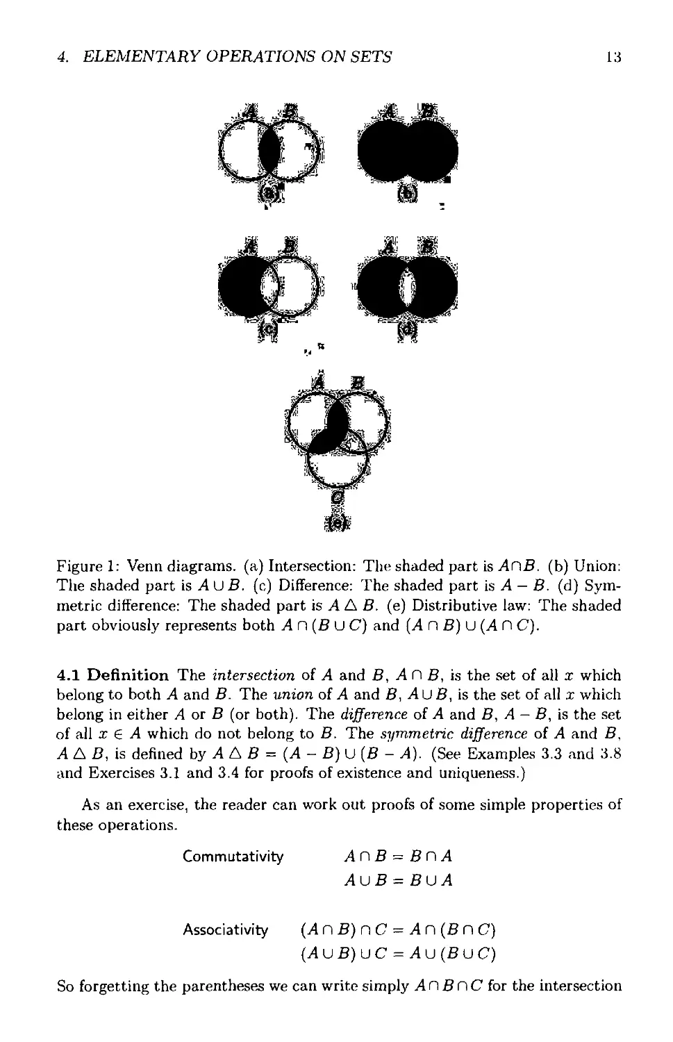
Figure 1: Venn diagrams, (a) Intersection: The shaded part is AnB. (b) Union:
The shaded part is A U B. (c) Difference: The shaded part is A — B. (d) Sym-
metric difference: The shaded part is A A B. (e) Distributive law: The shaded
part obviously represents both А П (B U C) and (Л пВ)и(ЯпС).
4.1 Definition The intersection of A and В, Л A B, is the set of all x which
belong to both A and B. The union of A and В, A U B, is the set of all x which
belong in either A or В (or both). The difference of A and В, A - B, is the set
of all x e A which do not belong to B. The symmetric difference of A and B,
А Л B, is defined by А А В = (A - В) U (В - A). (See Examples 3.3 and 3.8
and Exercises 3.1 and 3.4 for proofs of existence and uniqueness.)
As an exercise, the reader can work out proofs of some simple properties of
these operations.
Commutativity
AnB=BnA
AuB-BuA
Associativity (A n В) n С ~ A n (В П C)
(AuB)UC = Au(BuC)
So forgetting the parentheses we can write simply А П В П C for the intersection
14
CHAPTER 1. SETS
of sets A, B, and C. Similarly, we do not need parentheses for the union and
for more than three sets.
Distributivity A n (В U С) = (А П В) U (А О C)
А и (В о С) = (А и В) о (А и С)
DeMorganlaws С ~ (А п В) = (С - А) и (С - В)
С - (А и В) - (С - А) о (С - В)
Some of the properties of the difference and the symmetric difference are
Ап(В-С)-(ЛпВ)-С
A - В — 0 if and only if А С В
A A A = 0
А А В - В A A
(A AB) AC- А А (ВАС)
Drawing Venn diagrams often helps one discover and prove these and similar
relationships. For example, Figure 1(e) illustrates the distributive law Ал (B U
C) = (AnB) U (An C). The rigorous proof proceeds as follows: We have1 to
prove that the sets An (BuC) and (AnB) U (An C) have the same elements.
That requires us to show two facts:
(a) Every element of An (BuC) belongs to (AnB) U(AnC).
(b) Every element of (AnB)U(An C) belongs to An(BU C).
To prove (a), let a € An(BuC). Then a € A and also a 6 BUC. Therefore,
either a € В or a € C. So a € A and a € В or a € A and a € C. This means
that a 6 АП В or a € А П C; hence, finally, a € (A nB) U (AnC).
To prove (b), let a 6 (AnB)U (An C). Then a € А О В or a € А О C. In
the first case, a € A and a € B, so a € A and a € BuC. and a € А П (В U C).
In the second case, a € A and a € C, so again a € A and a € BuC, and finally.
a e А О (В U С). П
The exercises should provide sufficient material for practicing similar (de-
ment ar у arguments about sets.
The union of a system of sets S was defined in the preceding section. Wr
now define the intersection p| S of a nonempty system of sets S: x € П S if and
only if x € A for all A € S. Then intersection of two sets is again a special
case of the more general operation: А О В = f){ A, &}• Notice that we do not
define Q0; the reason is that every :r belongs to all A e 0 (since there is no
such A), so П0 would have to be a set of all sets. We postpone more detailed
investigation of general unions and intersections until Chapter 2, where a more
wield у notation becomes available.
Finally, we say that sets A and В are disjoint if An В — 0. More generally.
S is a system of mutually disjoint sets if А П В — 0 for all A, В € S such that
A B.
4. ELEMENTARY OPERATIONS ON SETS
15
Exercises
4.1 Prove all the displayed formulas in this section and visualize them using
Venn diagrams.
4.2 Prove:
(a) A G В if and only if А О В = A if and only if A U В = В if and only
if A - В = 0.
(b) A G В П C if and only if A G В and A G C.
(с) В U С C A if and only if В C A and CCA.
(d) A - В = (A U В) - В = A - (A П B).
(e) AnB = A-(A-B).
(f) A- (B-C) = (A-B)U(AnC).
(g) A = В if and only if А А В = 0.
4.3 For each of the following (false) statements draw a Venn diagram in which
it fails:
(а) A - В = В - A.
(b) An Be A.
(с) А С В U C implies A G В or A С C.
(d) В П C G A implies В G A or С C A.
4.4 Let A be a set; show that a “complement” of A does not exist. (The
“complement” of A is the set of all x £ A.)
4.5 Let S 0 and A be sets.
(a) Set T\ = {Y € P(A) | Y = А П X for some X € S}, and prove
А П (J S = (jTi (generalized distributive law).
(b) Set ?2 = {Y G P(A) | Y = A - X for some X € S}, and prove
Л-и^ = ПТ2
x-ns=l>
(generalized De Morgan laws).
4.6 Prove that f] S' exists for all S 0. Where is the assumption S 0 used
in the proof?
This page intentionally left blank
Chapter 2
Relations, Functions, and
Orderings
1. Ordered Pairs
In this chapter we begin our program of developing set theory as a foundation
for mathematics by showing how various general mathematical concepts, such
as relations, functions, and orderings can be represented by sets.
We begin by introducing the notion of the ordered pair. If a and b are sets,
then the unordered pair {a, b} is a set whose elements are exactly a and b. The
“order’’ in which a and b are put together plays no role; {a,b} = {b, a}. For
many applications, we need to pair a and b in a way making possible to “read
off” which set comes “first” and which comes “second.” We denote this ordered
pair of a and b by (a, b); a is the first coordinate of the pair (a, b), b is the second
coordinate.
As any object of our study, the ordered pair has to be a set. It should be
defined in such a way that two ordered pairs are equal if and only if their first
coordinates are equal and their second coordinates are equal. This guarantees
in particular that (a, b) (b,a) if a b. (See Exercise 1.3.)
There are many ways how to define (a, b) so that the foregoing condition is
satisfied. We give one such definition and refer the reader to Exercise 1.6 for an
alternative approach.
1.1 Definition (a, b) = {{a}, {a,6}}.
If a / b, (a,b) has two elements, a singleton {a} and an unordered pair
{a,b}. We find the first coordinate by looking at the element of {a}. The
second coordinate is then the other element of {a, 6}. If a = b, then (a. a) =
{{a}, {a,a}} = {{a}} has only one element. In any case, it seems obvious that
both coordinates can be uniquely “read off” from the set (a, b). We make this
statement precise in the following theorem.
17
18
CHAPTER 2. RELATIONS, FUNCTIONS, AND ORDERINGS
1.2 Theorem (a, b) = (a', 6') if and only if a — a! and b ~ bf.
Proof If a = a1 and b - bf, then, of course, (a,b) = {{a},{a,6}} =
{{a'}, {a', b'}} = (a?The other implication is more intricate. Let us assume
that {{a}, {a, 6}} = {{a'}, {a',6'}}. If a £ b, {a} - {a7} and {a, b} = {a',b'}.
So, first, a = a1 and then {a, 6} = {a, У} implies b = b'. If a = 6, {{a}, {a. a}} =
{{a}}. So {a} = {a'}, {a} = {a', dz}, and we get a = a* — b', so a = a' and
b = bl holds in this case, too. □
With ordered pairs at our disposal, we can define ordered triples
(a,b,c) = ((а,Ь),с),
ordered quadruples
(a, b, c, d) = ((a, b, c), d),
and so on. Also, we define ordered “ one-tuples”
(a) = a.
However, the general definition of ordered n-tuples has to be postponed until
Chapter 3, where natural numbers are defined.
Exercises
1.1 Prove that (a,b) € P(P({a,b})) and a,b e |J(a,6). More generally, if
a € A and b G A, then (a, b) € P(P(A)).
1.2 Prove that (a, 6), (a, b, c), and (a,b,c, d) exist for all a, 6, c, and d,
1.3 Prove: If (a, 6) ~ (b,a), then a = b.
1.4 Prove that (a, 6, c) = (a,,b/,c/) implies a - a1, b = b', and c = d. State
and prove an analogous property of quadruples.
1.5 Find a, 6, and c such that ((a,b),c) / (a, (6,c)). Of course, we could use
the second set to define ordered triples, with equal success.
1.6 To give an alternative definition of ordered pairs, choose two different
sets □ and A (for example, □ = 0, A = {0}) and define
(a,b) = {{<*-□},{«>,£}}•
State and prove an analogue of Theorem 1.2 for this notion of ordered
pairs. Define ordered triples and quadruples.
2. Relations
Mathematicians often study relations between mathematical objects. Relations
between objects of two sorts occur most frequently; we call them binary rela-
tions. For example, let us say that a line I is in relation Ri with a point P if I
passes through P. Then Rj is a binary relation between objects called lines and
objects called points. Similarly, we define a binary relation R2 between positive
2. RELATIONS
19
integers and positive integers by saying that a positive integer m is in relation
Rz with a positive integer n if m divides n (without remainder).
Let us now consider the relation R{ between lines and points such that a
line I is in relation R\ with a point P if P lies on I. Obviously, a line I is in
relation Ri to a point P exactly when I is in relation R'x to P. Although different
properties were used to describe R\ and Rj, we would ordinarily consider R\
and Rx to be one and the same relation, i.e., R\ = Rx. Similarly, let a positive
integer m be in relation R2 with a positive integer n if n is a multiple of m.
Again, the same ordered pairs (m, n) are related in Rz as in R2, and we consider
Rz and R2 to be the same relation.
A binary relation is, therefore, determined by specifying all ordered pairs of
objects in that relation; it does not matter by what property the set of these
ordered pairs is described. We are led to the following definition.
2.1 Definition A set Я is a binary relation if all elements of R are ordered
pairs, i.e., if for any z G R there exist x and у such that z = (z, y).
2.2 Example The relation Rz is simply the set {z | there exist positive integers
Tn and n such that z = (тп,п) and m divides n}. Elements of Rz are ordered
pairs
(1,1),(1,2),(1,3),...
(2,2), (2,4), (2,6),...
(3,3),(3,6),(3,9),...
It is customary to write xRy instead of (x,y) € R. We say that x is in
relation R with у if xRy holds.
We now introduce some terminology associated with relations.
2.3 Definition Let R be a binary relation.
(a) The set of all x which are in relation R with some у is called the domain of
R and denoted by domR. So domR = {x | there exists у such that xRy}.
dom R is the set of all first coordinates of ordered pairs in R.
(b) The set of all у such that, for some x, x is in relation R with у is called the
range of R, denoted by ran R. So ran R = {3/ | there exists x such that xRy}.
ran R is the set of all second coordinates of ordered pairs in R. Both dom R
and ranR exist for any relation R. (Prove it. See Exercise 2.1).
(c) The set dom R U ran R is called the field of R and is denoted by field R.
(d) If field R С X, we say that R is a relation in X or that R is a relation
between elements of X.
2.4 Example Let Rz be the relation from Example 2.2.
dom Rz = {m | there exists n such that m divides n}
= the set of all positive integers
20
CHAPTER 2. RELATIONS, FUNCTIONS. AND ORDERINGS
because each positive integer m divides some n, e.g., n = m;
ranB2 = {n I there exists m such that m divides n}
= the set of all positive integers
because each positive integer n is divided by some m. e.g., by m — n\
field B2 — dom R? U ran R^ = the set of all positive integers;
B2 is a relation between positive integers.
We next generalize Definition 2.3.
2.5 Definition
(a) The image of A under R is the set of all у from the range of R related in
R to some element of A; it is denoted by B[A]. So
B[A] = {г/ € ran R | there exists x 6 A for which xRy}.
(b) The inverse image of В under R is the set of all x from the domain of R
related in R to some element of B; it is denoted R~1 [В]. So
B“J[B] = {z € dom R I there exists у € В for which xRy}.
2,6 Example R^ 1[{3, 8,9,12}] = {1,2,3,4,6,8,9,12}; B2[{2}] = the set of all
even positive integers.
2.7 Definition Let В be a binary relation. The inverse of R is the set
B”1 - {z I z = (x,y) for some x and у such that (?j.z) e B}.
2.8 Example Again let
B2 = {z I z — m and n are positive integers, and th divides n}: then
R~* = {w I w = and (m,n) € B2}
= {w I w = m and n are positive integers, and m divides n}.
In our description of B21 we use variable m for the first coordinate and
variable n for the second coordinate; we also state the property describing B2 so
that the variable m is mentioned first. It is a customary (though not necessary)
practice to describe R2 1 in the same way. All we have to do is use letter m
instead of n, letter n instead of m. and change the wording:
B.J1 = {w I w = (m,n), n , m are positive integers, and n divides m}
= {w I w — m , n are positive integers, and m is a multiple of n}.
Now B2 and R2 1 are described in a parallel way. In this sense, the inverse of
the relation “divides” is the relation “is a multiple.”
The reader may notice that the symbol B“*[B] in Definition 2.5(b) for the
inverse image of В under В now also denotes the image of В under B-1. For-
tunately, these two sets are equal.
2. RELATIONS
21
2.9 Lemma The inverse image of В under R is equal to the image of В under
Z?-1.
Proof Notice first that domЯ = ran/?"1 (see Exercise 2,4). Now, x G
dom R belongs to the inverse image of В under R if and only if for some у 6 В,
(x,y) G R. But (z,y) G R if and only if (t/,z) G Z?-1. Therefore, x belongs to
the inverse image of В under R if and only if for some у G B, (t/, x) G Z?"1. i.e..
if and only if x belongs to the image of В under Z?’1. □
In the rest of the book we often define various relations, i.e., sets of ordered
pairs having some particular property. To simplify our notation, we introduce
the following conventions. Instead of
{w | w = (z,y) for some x and у such that P(z, ?/)},
we simply write
{(z,y) I P(x,y)}.
For example, the inverse of R could be described in this notation as {(z,y) |
(j/,z) G /?}. [As in the general case, use of this notation is admissible only if
we prove that there exists a set A such that, for all x and y. P(z.t/) implies
(x,y) e A.]
2.10 Definition Let 7? and S be binary relations. The composition of 7? and
S' is the relation
So R = {(z, z) | there exists у for which (z,y) G R and (t/, z) G S}.
So (z, z) G So/? means that for some y, xfly and ySz. To find objects related
to z in S о Z?, we first find objects у related to z in /?, and then objects related
to those у in S. Notice that R is performed first and S second, but notation
S о R is customary (at least in the case of functions; see Section 3).
Several types of relations are of special interest. We introduce some of them
in this section and others in the rest of the chapter.
2.11 Definition The membership relation on A is defined by
€д = {(a,6) | a G A, b G A, and a G b}.
The identity relation on A is defined by
Idx = {(a, b) | a G A, b G A, and a - 6}.
2.12 Definition Let A and В be sets. The set of all ordered pairs whose
first coordinate is from A and whose second coordinate is from В is called the
cartesian product of A and В and denoted A x B. In other words,
A x В = {(a,6) | a G A and b G B}.
Thus Ax В is a relation in which every element of A is related to every element
of B.
22
CHAPTER 2. RELATIONS, FUNCTIONS, AND ORDERINGS
It is not completely trivial to show that the set A x В exists. However, one
gets from Exercise 1.1 that if a e A and b 6 B, then (a. b) G P(P(A U B)).
Therefore,
A x В = {(a,6) € P(P(AO B)) | a e A and b G B}.
Since P(P(AU B)) was proved to exist, the existence of A x В follows from the
Axiom Schema of Comprehension. [To be completely explicit, we can write,
A x В = {w G P(P(A U B)) | w = (a,6) for some a G A and b G B}.]
We denote A x A by A2. The cartesian product of three sets can be introduced
readily:
A x В x C = (A x B) x C.
Notice that
A x В x C — {(a, b, c) | a G A, b G B, and cG 0}
(using an obvious extension of our notational convention). A x A x A is usually
denoted A3.
We can also define ternary relations.
2.13 Definition A ternary relation is a set of unordered triples. More explic-
itly, S is a ternary relation if for every и G S, there exist x, y, and z such that
и = (z, y, z). If SC A3, we say that S is a ternary relation in A. (Note that a
binary relation В is in A if and only if R C A2.)
We could extend the concepts of this section to ternary relations and also
define 4-ary or 17-ary relations. We postpone these matters until Section 5 in
Chapter 3, where natural numbers become available, and we are able to define
n-ary relations in general. At this stage we only define, for technical reasons,
unary relations by specifying that a unary relation is any set. A unary relation
in A is any subset of A. This agrees with the general conception that a unary
relation in A should be a set of 1-tuples of elements of A and with the definition
of (z) = x in Section 1.
Exercises
2.1 Let R be a binary relation; let A = IJ(U^)- Prove that (x,y) G R
implies x G A and у G A. Conclude from this that domB and ran В
exist.
2.2 (a) Show that B-i and So R exist. [Hint: В-1 C (ranB) x (domB),
S' о В C (dom В) x (ran S).]
(b) Show that A x В x C exists.
2.3 Let В be a binary relation and A and В sets. Prove:
(a) B[AuB] = B[A]UB[B].
(b) B[AnB] С В А]ПВ[В].
(c) B[A-B] D R[A] - B[B].
3. FUNCTIONS
23
(d) Show by an example that C and 3 in parts (b) and (c) cannot be
replaced by
(e) Prove parts (a)-(d) with R"1 instead of R.
(f) R~1 [Z?[A]] 2 A H dom R and /?[/?“1 [Z?]] 2 Bn ran R; give examples
where equality does not hold.
2.4 Let RC X x Y. Prove:
(a) Z?[X] — ran/? and R~1 [У] = dom/?.
(b) If a $ dom/?, R[{a}] - 0; if 6 £ ran/?, /?-1[{6}] = 0.
(c) dom/? = ran/?'1; ran/? - domZ?-1.
(d) (R'1)-1 = J?.
(e) R 1 о Z?2lddom/?; R° R ^Idran/?-
2.5 Let X = {0, {0}}, Y = P(X). Describe
(a)
(b) Idy.
Determine the domain, range, and field of both relations.
2.6 Prove that for any three binary relations /?, S', and T
T о (S' о R) = (T о S) о R.
(The operation о is associative.)
2.7 Give examples of sets X, У, and Z such that
(a) X x Y / Y x X.
(b) X x (У x Z) / (X x У) x Z.
(с) X3 / X x X2 [i.e, (X x X) x X / X x (X x X)].
[Hint for part (с): X = {a}.]
2.8 Prove:
(a) A x В = 0 if and only if A = 0 or В = 0.
(b) (Ai U A2) x В = (Ai x B) U (A2 x B);
Ax(BiU B2) = (Ax Br) U (A x B2).
(c) Same as part (b), with U replaced by П, and A.
3. Functions
Function, as understood in mathematics, is a procedure, a rule, assigning to
any object a from the domain of the function a unique object 6, the value of
the function at a. A function, therefore, represents a special type of relation, a
relation where every object a from the domain is related to precisely one object
in the range, namely, to the value of the function at a.
3.1 Definition A binary relation F is called a function (or mapping, corre-
spondence) if aFbi and aF62 imply by — b2 for any a, 6i, and 62. In other
words, a binary relation F is a function if and only if for every a from dom F
there is exactly one b such that aFb. This unique b is called the value of F
at a and is denoted F(a) or Fo. (F(a) is not defined if a domF.] If F is a
function with domF ~ A and ranF G Z?, it is customary to use the notations
24
CHAPTER 2. RELATIONS, FUNCTIONS, AND ORDERINGS
F : A B, (F(a) | a € A), (Fu | a € A), (Fo)oex for the function F. The
range of the function F can then be denoted {F(a) | a € A} or {Fa}(i^A.
The Axiom of Extensionality can be applied to functions as follows.
3.2 Lemma Let F and G be functions. F = G if and only if dom F = domG
and F(x) = G(z) for all x 6 domF.
We leave the proof to the reader. □
Since functions are binary relations, concepts of domain, range, image, in-
verse image, inverse, and composition can be applied to them. We introduce
several additional definitions.
3.3 Definition Let F be a function and A and В sets.
(a) F is a function on A if domF = A.
(b) F is a function into В if ranF С B.
(c) F is a function onto В if ranF = B.
(d) The restriction of the function F to A is the function
F f A = {(a,b) e F (a € A}.
If G is a restriction of F to some A, we say that F is an extension of G.
3.4 Example Let F = {(z, 1/z'2) | x / 0, x is a real number}. F is a function:
If aFbi and aF^, by = 1/u2 and = 1/a2, so bi — &2-
Slightly stretching our notational conventions, we can also write F = (l/.r2
z is a real number, x 0). The value of F at z, F(z), equals 1/z2. It is a
function on A, where A = {x | x is a real number and x 0} = domF. F is a
function into the set of all real numbers, but not onto the set of all real numbers.
If В — {z | x is a real number and z > 0}. then F is onto B. If C = {z I 0 <
x < 1}, then f[C] = {x | z > 1} and — {z | z < -1 or x > I}.
Let us find the composition f о /:
/о / = {(r,z) | there is у for which (z,y) € f and 6 f]
= {(z,z) | there is у for which z / 0, у = 1/z2, and у 0, z — l/?/2}
- {(z, z} | x 0 and z — z4}
= (t4 | т / 0).
Notice that f о f is a function. This is not an accident.
3.5 Theorem Let f and g be functions. Then g о f is a function, g о f is
defined at x if and only if f is defined at x and g is defined at /(z). i.e.,
dorn(p о f) = dom f Г) / ~ l|domp].
Also, [g о /)(z) — p(/(z)) for all x € dom(p о f).
3. FUNCTIONS
25
Proof. We prove first that g о f is a function. If x(g о f)z\ and x{g о f)z2<
there exist yi and y? such that xfyi, y\gz\, and xfy<2, y?gz2- Since f is a
function, yi = yz> So we get г/ip^i, yigz2, and zi — 22, because g is also a
function.
Now we investigate the domain of g о f. x 6 dom(y о /) if and only if
there is some z such that x{g о /)z, i.e., if and only if there is some z and
some у such that xfy and ygz. But this happens if and only if x € dom f
and у = f(x) € domy. The last statement can be equivalently expressed as
x 6 dom f and x 6 /-1[domy]. □
This theorem is used in calculus to find domains of compositions of functions.
Let us give one typical example.
3.6 Example Let f = (x2-l | x real), g = (y/x | x > 0). Find the composition
W-
We determine the domain of g о f first, dom f is the set of all real numbers
and domy = {z | x > 0}. We find /-1[domy] - {z | f(x) e domy} = {x |
z2 - 1 > 0} = {z I x > 1 or x < -1}. Therefore, dom(y о /) = (dom /) О
/“^domp] = {z I x > 1 or x < -1} and g о f — {(z, z) | x > 1 or x <
-1 and, for some y, z2 — 1 = у and ^/y = z} = {Vx2 - 1 | x > 1 or z < -1).
If f is a function, its inverse is a relation, but it may not be a function.
We say that a function f is invertible if f~l is a function.
It is important to find necessary and sufficient conditions for a function to
be invertible.
3.7 Definition A function f is called one-to-one or injective if ai € dom /,
02 6 dom /, and ay a2 implies /(ai) /(аг). In other words if a! € dom /,
0,2 € dom f, and /(ui) = /(<12), then ai = 02- Thus a one-to-one function
attains different values for different elements from its domain.
3.8 Theorem A function is invertible if and only if it is one-to-one. If f is
invertible, then f~l is also invertible and (У-1)”1 = f.
Proof
(a) Let f be invertible; then /-1 is a function. It follows that f~l(f(a)) — a for
all a € dom f. If ai,a2 € dom f and /(ai) ~ ffa), we get y-1(/(ai)) =
У-1 (/(аг)) and ai = (12. So f is one-to-one.
(b) Let f be one-to-one. Ifa/"1^ and we have bifa and 62/a. There-
fore, 61 = 62, and we have proved that f~l is a function.
(c) We know that (У-1)-1 = f by Exercise 2.4(d), so f~} is also invertible
(consequently, f~} is also one-to-one).
26
CHAPTER 2. RELATIONS, FUNCTIONS, AND ORDERINGS
3.9 Example
(a) Let f = (1/x2 | x / 0); find f~l. As f = {(x, 1/x2) | x 0}, we get
/-1 = {(1 /x2,x) | x / 0}. /-1 is not a function since (1,-1) 6 f~\
(1,1) € Z”1- Therefore, f is not one-to-one; (1,1) e f. ( — 1,1) € f.
(b) Let g = (2x - 1 | x real); find g~}. g is one-to-one: If 2x} - 1 = 2x2 - 1.
then 2xi = 2x2 and Xi = x%. g = {(x,y) | у = 2x - 1, x real}, therefore,
= {(У^) I У = 2x - 1, x real}.
As customary when describing functions, we express the second coordinate
(value) in terms of the first:
9 1
r \ У+1 ।
(У,х) x = ——, у real
Finally, it is usual to denote the first (“independent”) variable x and the second
(“dependent”) variable y. So we change notation:
9 1 =
x 4- 1
У = —’ x real
x real ).
3.10 Definition
(a) Functions f and g are called compatible if /(x) = p(x) for all x € dom f П
domp.
(b) A set of functions F is called a compatible system of functions if any two
functions f and g from F are compatible.
3.11 Lemma
(a) Functions f and g are compatible if and only if f U g is a function.
(b) Functions f and g are compatible if and only if f Г (dom f О domp) =
g [ (dom f О doing).
We leave the easy proof to the reader, but we prove the following.
3.12 Theorem If F is a compatible system of functions. then |J F is a function
with dom(IJF) = |J{dom f | f € F}. The function (JF extends all f 6 F.
Functions from a compatible system can be pieced together to form a single
function which extends them ail.
Proof Clearly, |JF is a relation; we now prove that it is a function. If
(a, 61) € (J F and (a, 62) € (J F, there are functions /1, /2 F such that (a, 61) €
/1 and (ct,62) € /2- But /1 and /2 are compatible, and a € dom/1 Odom f%\ so
61 = f(ai) = f(a2) = 62.
It is trivial to show that x e dom(|J F) if and only if x € dom f for some
fe F. □
3.13 Definition Let A and В be sets. The set of all functions on A into В is
denoted BA. Of course, we have to show that BA exists; this is done in Exercise
3.9.
3. FUNCTIONS
27
It is useful to define a more genera! notion of product of sets in terms of
functions.
Let S = (St | i € I) be a function with domain I. The reader is probably
familiar mainly with functions possessing numerical values; but for us, the values
Si are arbitrary sets. We call the function (S, | г € I) an indexed system of sets,
whenever we wish to stress that the values of S are sets.
Now let S = (Si | i e I) be an indexed system of sets. We define the product
of the indexed system S as the set
S = {f | f is a function on I and 6 St for all i e 1}.
Other notations we occasionally use are
П<адиб/), П5*
iEl те/
The existence of the product of any indexed system is proved in Exercise
3.9.
The reader is probably curious to know how this product is related to the
previously defined notions A x В and A x В x C. We return to this technical
problem in Section 5 of Chapter 3. At this time, we notice only that if the
indexed system S is such that Si = В for all i G A then
П«. = в'
те/
The “exponentiation” of sets is related to “multiplication” of sets in the same
way as similar operations on numbers are related.
We conclude this section with two remarks concerning notation.
(J A and P A were defined for any system of sets A (A / 0 in case of
intersection). Often the system A is given as a range of some function, i.e., of
some indexed system. (See Exercise 3.8 for proof that any system A can be so
presented, if desired.)
We say that A is indexed by S if
A = {5, | i € 7} = ran 5,
where S is a function on I, It is then customary to write
|Jx = |J{s, це/} = и^
tEl
and similarly for intersections. In the future, we use this more descriptive no-
tation.
Let f be a function on a subset of the product A x B. It is customary to
denote the value of f at (x,y) € A x В by rather than /((ir.y)) and
regard f as a function of two variables x and y.
28
CHAPTER 2. RELATIONS, FUNCTIONS, AND ORDERINGS
Exercises
3.1 Prove: If ran f C domp, then dom(p о /) = dom /.
3.2 The functions /t : г = 1,2,3 are defined as follows:
/1 = (2z - 1 | x real),
/2 = I x > 0),
/3 = (1/z I x real, x 0).
Describe each of the following functions, and determine their domains
and ranges: /2 0 /ь /1 0 /2, fa ° fi, /1 о fa.
3.3 Prove that the functions /1, /2, /3 from Exercise 3.2 are one-to-one, and
find the inverse functions. In each case, verify that dom f, — ran(/7~1).
ran/, = dom(/“1).
3.4 Prove:
(a) If / is invertible, f~1 о f = Iddom/, f ° f~l = Idran
(b) Let f be a function. If there exists a function g such that g о f ~
Lldom/ then f is invertible and f~l = g f ran f. If there exists a
function h such that f о h — Idran / then f may fail to be invertible.
3.5 Prove: If f and g are one-to-one functions, g о f is also a one-to-one
function, and (g о У)"1 — f~1 о g~ L
3.6 The images and inverse images of sets by functions have the properties
exhibited in Exercise 2.3, but some of the inequalities can now be replaced
by equalities. Prove:
(a) If f is a function, f~1 [A OB] = f~1 [A] n l[B].
(b) If f is a function, /-1[А - B] = У“*[А] - /
3.7 Give an example of a function f and a set A such that / П A2 f f A.
3.8 Show that every system of sets A can be indexed by a function. [Hint:
Take I = A and set = г for all i e A.]
3.9 (a) Show that the set BA exists. [Hint: BA С P(A x B),]
(b) Let | г € I) be an indexed system of sets; show that Пге/
exists. [Hint: x
3.10 Show that unions and intersections satisfy the following general form of
the associative law:
U F«= U(UF°)’
aeUS aGC
A k= AdV-)'
fte|JS CeS (ieC
if S is a nonempty system of nonempty sets.
3.11 Other properties of unions and intersections can be generalized similarly.
De Morgan Laws:
B - U F- = П (s -
a£A a£A
B - П F“ = U - F“)-
пбД afzA
4. EQUIVALENCES AND PARTITIONS
29
Distributive Laws:
(UF^n(UG'>)= U
a£A b&B (a,b)c4x В
(П ^)U(PGb)= П (FaUGb).
at A b€B (а,Ь)ЕАхВ
3.12 Let f be a function. Then
/[UF-1= U/tri,
а£Л a£A
r1[Un = Ur та
afEA a£ A
/IHfJc p|/|FJ,
a£A at A
г1\Пп= Агта
а(ЕЛ aCA
If f is one-to-one, then G in the third formula can be replaced by =.
3.13 Prove the following form of the distributive law:
A(UF».b)= U (Ar./(«)>’
fteA beB f£BA aXzA
assuming that Fa^ A Fa,b2 = 0 for al! a e A and 61,62 € B, 61
6'2- [Hint: Let L be the set on the left and R the set on the right.
Fa>f(a) Q UbGB ^a»b> hence Faj(aj С ПаеА^ЬеВ ^a-b) = so
finally, R. C L. To prove that L G H, take any x e L. Put (a, 6) € f
if and only if x € Fa^ and prove that f is a function on A into В for
which x e ПпеЛ so x 6 H.]
4. Equivalences and Partitions
Binary relations of several special types enter our considerations more frequently.
4.1 Definition Let R. be a binary relation in A.
(a) R is called reflexive in A if for all a € A, aRa.
(b) R is called symmetric in A if for all a,b 6 A, aRb implies bRa.
(c) R is called transitive in A if for al! a, 6, c € A. aRb and bRc imply a Re.
(d) R is called an equivalence on A if it is reflexive, symmetric, and transitive
in A.
30
CHAPTER 2. RELATIONS, FUNCTIONS, AND ORDERINGS
4.2 Example
(a) Let P be the set of all people living on Earth. We say that a person p is
equivalent to a person q (p = q) if p and q both live in the same country.
Trivially, = is reflexive, symmetric, and transitive in P. Notice that the
set P can be broken into classes of mutually equivalent elements; all people
living in the United States form one class, all people living in France are
another class, etc. All members of the same class are mutually equivalent;
members of different classes are never equivalent. The equivalence classes
correspond exactly to different countries.
(b) Define an equivalence E on the set Z of all integers as follows: xEy if
and only if x — у is divisible by 2. (Two numbers are equivalent if their
difference is even.) The reader should verify 4.1(a)-(c). Again, the set. Z
can be divided into equivalence classes under (or, as is customary to say,
modulo) the equivalence E. In this case, there are two equivalence classes,
the set of even integers and the set of odd integers. Any two even integers
are equivalent; so are any two odd integers. But an even integer cannot be
equivalent to an odd one.
The situation encountered in the previous examples is quite general. Any
equivalence on A partitions A into equivalence classes; conversely, given a suit-
able partition of A, there is an equivalence on A determined by it. The following
definitions and theorems establish this correspondence.
4.3 Definition Let E be an equivalence on A and let a € A. The equivalence
class of a modulo E is the set
[а] я = € A | xEa}.
4.4 Lemma Let a, b € A.
(a) a is equivalent to b modulo E if and only if [a] £ = [d]#.
(b) a is not equivalent to b modulo E if and only if [а]^ Ci [Ь]е = 0.
Proof
(a) (1) Assume that aEb. Let x € a]#, i.e., xEa. By transitivity, xEa and
aEb imply xEb, i.e., x e [b e- Similarly, x € implies x e [a]^
(bEa is true because E is symmetric). So [o]e = [6]e
(2) Assume that [ujf: = [Ь]е. Since E is reflexive, aEa, so a e [ajs. But
then a € [fcjs, that is, aEb.
(b) (1) Assume aEb is not true; we have to prove [a]s Cl [6]e = 0. If not, there
is x € [u|e Ci [6]e; so xEa and xEb. But then, using first symmetry
and then transitivity, aEx and xEb, so aEb, a contradiction.
(2) Assume finally that [a]e Ci [6]e = 0. If a and b were equivalent modulo
E, aEb would hold, so a 6 [b]#. But also a € [a]s, implying [a] e Ci
[fc] 2 0, a contradiction.
□
4. EQUIVALENCES AND PARTITIONS
31
4.5 Definition A system S of nonempty sets is called a partition of A if
(a) 5 is a system of mutually disjoint sets, i.e., if C € S, D € S, and C D,
then C Ci D = 0,
(b) the union of S is the whole set A, i.e., IJ5 — A.
4.6 Definition Let E be an equivalence on A. The system of all equivalence
classes modulo E is denoted by A/E\ so A/E = {[a] e|a€ A}.
4.7 Theorem Let E be an equivalence on A; then A/E is a partition of A.
Proof. Property (a) follows from Lemma 4.4: If [a]# E, then a and b
are not E-equivalent, so [a|E П [&]e = 0. To prove (b), notice that (J A/E — A
because a e [g]e. Notice also that no equivalence class is empty; surely at least
a e [а]я. □
We now show that, conversely, for each partition there is a corresponding
equivalence relation. For example, the partition of people by their country of
residence yields the equivalence from (a) of Example 4.2.
4.8 Definition Let S be a partition of A. The relation Es in A is defined by
Es = {(a, b) € A x A | there is C € S such that a € C and b e C}.
Objects a and b are related by Es if and only if they belong to the same set
from the partition 5.
4.9 Theorem Let S be a partition of A; then Es is an equivalence on A.
Proof.
(a) Reflexivity. Let a € A; since A = (J 5, there is C € S for which a E C, so
(a, a) € Es>
(b) Symmetry. Assume aEsb; then there is C € S for which a € C and beC.
Then, of course, b € C and a € C, so bEsa.
(c) Transitivity. Assume aEsb and bEsc; then there аге C e S and D e S
such that a € C and b e C and b e D and c e D. We see that b € С П D.
so CnD / 0. But S is a system of mutually disjoint sets, so C = D. Now
we have a € С, c € C, and so aEsc.
□
The next theorem should further clarify the relationship between equiva-
lences and partitions. We leave its proof to the reader.
4.10 Theorem
(a) If E is an equivalence on A and S = A/E, then Es = E.
(b) If S is a partition of A and Es is the corresponding equivalence, then
A/Es = S.
32
CHAPTER 2. RELATIONS, FUNCTIONS, AND ORDERINGS
So equivalence relations and partitions are two different descriptions of the
same “mathematical reality.” Every equivalence E determines a partition S =
A/E. The equivalence Es determined by this partition S is identical with the
original E. Conversely, each partition S determines an equivalence Es\ when
we form equivalence classes modulo Es, we recover the original partition S.
When working with equivalences or partitions, it is often very convenient to
have a set which contains exactly one “representative” from each equivalence
class.
4.11 Definition A set X C A is called a set of representatives for the equiva-
lence Es (or for the partition S of A) if for every C e S, X C\C = {a} for some
a e C.
Returning to Example 4.2 we see that in (a) the set X of all Heads of State
is a set of representatives for the partition by country of residence. The set
X = {0,1} could serve as a set of representatives for the partition of integers
into even and odd ones.
Does every partition have some set of representatives? Intuitively, the an-
swer may seem to be yes, but it is not possible to prove existence of some such
set for every partition on the basis of our axioms. We return to this prob-
lem when we discuss the Axiom of Choice. For the moment we just say that
for many mathematically interesting equivalences a choice of a natural set of
representatives is both possible and useful.
Exercises
4.1 For each of the following relations, determine whether they are reflexive,
symmetric, or transitive:
(a) Integer x is greater than integer y.
(b) Integer n divides integer m.
(c) x у in the set of all natural numbers.
(d) C and C in P(A).
(e) 0 in 0.
(f) 0 in a nonempty set A.
4.2 Let f be a function on A onto B. Define a relation E in A by. aEb if
and only if /(a) = /(b).
(a) Show that E is an equivalence relation on A.
(b) Define a function on A/E onto В by ^([<i]e) - (verify that
^(Ые) = e) if |«]e =
(c) Let j be the function on A onto A/E given by j(a) — [a]#. Show
that о j — f.
4.3 Let P = {(r, 7) € 7? x 7? | r > 0}, where R is the set of all real numbers.
View elements of P as polar coordinates of points in the plane, and define
a relation on P by: (r, 7) if and only if r = rf and 7 - 7' is
an integer multiple of 2?r. Show that ~ is an equivalence relation on
P. Show that each equivalence class contains a unique pair (r. 7) with
0 < 7 < 2?r. The set of all such pairs is therefore a set of representatives
for ~.
5. ORDERINGS
33
5. Orderings
Orderings are another frequently encountered type of relation.
5.1 Definition A binary relation R in A is antisymmetric if for all u.6 € A.
aRb and bRa imply a — b.
5.2 Definition A binary relation R in A which is reflexive, antisymmetric, and
transitive is called a (partial) ordering of A. The pair (A, R) is called an ordered
set.
aRb can be read as “a is less than or equal to b” or ilb is greater than or
equal to a” (in the ordering R). So, every element of A is less than or equal to
itself. If a is less than or equal to b, and, at the same time, b is less than or
equal to a, then a = b. Finally, if a is less than or equal to b and b is less than
or equal to c, a has to be less than or equal to c.
5.3 Example
(a) < is an ordering on the set of all (natural, rational, real) numbers.
(b) Define the relation Сд in A as follows: x Сд у if and only if x С у and
x,y e A. Then Сд is an ordering of the set A.
(c) Define the relation Эд in A as follows: x Эд у if and only if x Э у and
x,y e A. Then Эд is also an ordering of the set A.
(d) The relation | defined by: n | m if and only if n divides m is an ordering of
the set of all positive integers.
(e) The relation Мд is an ordering of A.
The symbols < or < are often used to denote orderings.
A different description of orderings is sometimes convenient. For example,
instead of the relation < between numbers, we might prefer to use the relation <
(strictly less). Similarly, we might use Сд (proper subset) instead of Сд. Any
ordering can be described in either one of these two mutually interchangeable
ways.
5.4 Definition A relation 5 in A is asymmetric if aSb implies that bSa does
not hold (for any a, b € A). That is, aSb and bSa can never both be true.
5.5 Definition A relation S in A is a strict ordering if it is asymmetric and
transitive.
We now establish relationships between orderings and strict orderings.
5.6 Theorem
(a) Let R be an ordering of A; then the relation S defined in A by
aSb if and only if aRb and a b
is a strict ordering of A.
34
CHAPTER 2. RELATIONS, FUNCTIONS, AND ORDERINGS
(b) Let S be a strict ordering of A; then the relation R defined in A by
aRb if and only if aSb or a = b
is an ordering of A.
We say that the strict ordering S corresponds to the ordering R and vice
versa.
Proof.
(a) Let us show that S is asymmetric: Assume that both aSb and bSa hold for
some a, b € A. Then also aRb and bRa, so a = b (because R is antisym-
metric). That contradicts the definition of aSb. We leave the verification
of transitivity of S to the reader.
(b) Let us show that R is antisymmetric: Assume that aRb and bRa. Because
aSb and bSa cannot hold simultaneously (S is asymmetric), we conclude
that a = b. Reflexivity and transitivity of R are verified similarly.
□
5.7 Definition Let a, b 6 A, and let < be an ordering of A. We say that a and
b are comparable in the ordering <ifa<6or6<a. We say that a and b are
incomparable if they are not comparable (i.e., if neither a < b nor b < a holds).
Both definitions can be stated equivalently in terms of the corresponding strict
ordering <; for example, a and b are incomparable in < if a 0 b and neither
a < b nor b < a holds.
5.8 Example
(a) Any two real numbers are comparable in the ordering <.
(b) 2 and 3 are incomparable in the ordering |.
(c) Any two distinct a,b € A are incomparable in Id^.
(d) If the set A has at least two elements, then there are incomparable elements
in the ordered set (P(A), Cp^j).
5.9 Definition An ordering < (or <) of A is called linear or total if any two
elements of A are comparable. The pair (A, <) is then called a linearly ordered
set.
So the ordering < of positive integers is total, while | is not.
5.10 Definition Let В C A, where A is ordered by <. В is a chain in A if
any two elements of В are comparable.
For example, the set of all powers of 2 (i.e., {2°, 21,22,23,. .. }) is a chain in
the set of all positive integers ordered by |.
A problem that arises quite often is to find a least or greatest element among
certain elements of an ordered set. Closer scrutiny reveals that there are several
different notions of “least” and “greatest.”
5. ORDERINGS
35
5.11 Definition Let < be an ordering of A, and let В C A.
(a) b G В is the least element of В in the ordering < if b < x for every x G B.
(b) & € В is a minimal element of В in the ordering < if there exists no x G В
such that x < b and x 0 b.
(a') Similarly, b G В is the greatest element of В in the ordering < if, for every
x 6 B, x < b.
(b') b € В is a maximal element of В in the ordering < if there exists no x G В
such that b < x and x 0 b.
5.12 Example Let N be the set of positive integers ordered by divisibility
relation |. Then 1 is the least element of N, but N has no greatest element.
Let В be the set of all positive integers greater (in magnitude) than 1. В =
{2,3,4,...}. Then В does not have a least element in | (e.g., 2 is not the
least element because 2 | 3 fails), but it has (infinitely) many minimal elements:
numbers 2, 3, 5, etc. (exactly all prime numbers) are minimal. В has neither
greatest nor maximal elements.
We list some of the properties of least and minimal elements in Theorem
5.13. The proof is left as an exercise.
5.13 Theorem Let A be ordered by <, and let В C A.
(a) В has at most one least element.
(b) The least element of В (if it exists) is also minimal.
(c) If В is a chain, then every minimal element of В is also least.
The theorem remains true if the words “least” and “minimal” are replaced
by “greatest” and “maximal”, respectively
5.14 Definition Let < be an ordering of A, and let В C A.
(a) a € A is a lower bound of В in the ordered set (A, <) if a < x for all x g B.
(b) a G A is called an infimum of В in (A, <) [or the greatest lower bound of
В in (A, <)] if it is the greatest element of the set of all lower bounds of В
in (Л,<).
Similarly,
(a') a G A is an upper bound of В in the ordered set (A, <) if x < a for all
x G B.
(b') a G A is called a supremum of В in (A, <) [or the least upper bound of В
in (A, <)] if it is the least element of the set of all upper bounds of В in
(Л<)-
Note that the difference between the least element of В and a lower bound of
В is that the second notion does not require b G B. A set can have many lower
bounds. But the set of all lower bounds of В can have at most one greatest
element, so В can have at most one infimum.
We now summarize some properties of suprema and infima.
36
CHAPTER 2. RELATIONS, FUNCTIONS, AND ORDERINGS
5.15 Theorem Let (A, <) be an ordered set and let В G A.
(a) В has at most one infimum.
(b) If b is the least element of В, then b is the infimum of B.
(c) If b is the infimum of В and beB, then b is the least element of B.
(d) b G A is an infimum of В in (A, <) if and only if
(i) b < x for all x G B.
(ii) If bf < x for all x G B, then b( < b.
The theorem remains true if the words “least” and “infimum” are replaced
by the words “greatest” and “supremum” and “<” is replaced by “>” in (i) and
(ii)-
Proof.
(a) We proved this in the remark preceding the theorem.
(b) The least element & of В is certainly a lower bound of B. If b' is any lower
bound of B, b* < b because b G B. So b is the greatest element of the set
of all lower bounds of B.
(c) This is obvious.
(d) This is only a reformulation of the definition of infimum.
□
We use notations inf(B) and sup(B) for the infimum of В and the supremum
of B, if they exist. If В is linearly ordered, we also use min(B) and max(B) to
denote the minimal (least) and the maximal (greatest) elements of B, if they
exist.
5.16 Example Let < be the usual ordering of the set of real numbers; let
Bj = {z | 0 < x < 1}, B2 = {z I 0 < x < 1}, B3 = {z I x > 0}. and
B4 — {z | z < 0}. Then Bi has no least element and no greatest element, but
any b < 0 is a lower bound of B], so 0 is the greatest lower bound of Bi; i.e..
0 = inf(B). Similarly, any b > 1 is an upper bound of Bj, so 1 — sup(Bi).
The set B2 has a least element; so 0 = min(Bs) = inf(B-j); it does not have a
greatest element. Nevertheless, зир(Вг) — 1- The set B3 has neither a greatest
element nor a supremum (actually B3 has no upper bound in <): of course1.
пИ(Вз) = 0. Similarly, B4 has no lower bounds, hence no infimum.
5.17 Definition An isomorphism between two ordered sets (P. <) and (Q.
is a one-to-one function h with domain P and range Q such that for all pi. p2 G P
Pi < P2 if and only if h(pi ) h(p2).
If an isomorphism exists between (F, <) and (Q, -<), then (F <) and (Q, -<) are
isomorphic.
We study isomorphisms in a more general setting in Chapter 3. At this
point, let us make the following observation.
5. ORDERINGS
37
5.18 Lemma Let (P, <) and (Q, -<) be linearly ordered sets, and let h be a one-
to-one function with domain P and range Q such that h{pi) -< /1(^2) whenever
pi < p2‘ Then h is an isomorphism between (P, <) and (Q, 4).
Proof. We have to verify that if pi,P2 € P are such that A(pi) -< h(p2\
then p\ < p2- But if pi is not less than p2? then, because < is a linear ordering
of P, either pi = p2 or p2 < pi- If pi = P2, then h(pi) - h(p2). and if p2 < pi.
then h(p2) -< h{pi), by the assumption. Either case contradicts h{pi) 4 ^(£2)
□
Exercises
5.1 (a) Let R be an ordering of A, 5 be the corresponding strict ordering of
A, and P* be the ordering corresponding to 5. Show that P* = P.
(b) Let S be a strict ordering of A, P be the corresponding ordering,
and 5* be the strict ordering corresponding to R. Then S* = S.
5.2 State the definitions of incomparable elements, maximal, minimal, great-
est, and least elements and suprema and infima in terms of strict order-
ings.
5.3 Let P be an ordering of A. Prove that P-1 is also an ordering of A, and
for В Q A,
(a) a is the least element of В in P-1 if and only if a is the greatest
element of В in P;
(b) similarly for (minimal and maximal) and (supremum and infimum).
5.4 Let P be an ordering of A and let В Q A. Show that P О В2 is an
ordering of B.
5.5 Give examples of a finite ordered set (A. <) and a subset В of A so that
(a) В has no greatest element.
(b) В has no least element.
(с) В has no greatest element, but В has a supremum.
(d) В has no supremum.
5.6 (a) Let (A, <) be a strictly ordered set and b £ A. Define a relation -<
in В = A U {6} as follows:
x ч у if and only if (x, у G A and x < y) or (z G A and у = b).
Show that 4 is a strict ordering of В and ч C1A2 =<. (Intuitively,
-< keeps A ordered in the same way as < and makes b greater than
every element of A.)
(b) Generalize part (a): Let (Ai,<i) and (Аг^<г) be strict orderings,
Ai П A 2 = 0. Define a relation 4 on В = Ai U A 2 as follows:
x -< у if and only if x, у G Ai and x <1 у
or x,y e A2 and x <2 у
or x G A] and у G A2.
38
CHAPTER 2. RELATIONS, FUNCTIONS. AND ORDERINGS
Show that -< is a strict ordering of В and -< OAf =<ь DA’2 =<2
(Intuitively, -< puts every element of At before every element of A2
and coincides with the original orderings of Ai and A2.)
5.7 Let R be a reflexive and transitive relation in A (R is called a preordenng
of A). Define E in A by
aEb if and only if aRb and bRa.
Show that E is an equivalence relation on A. Define the relation R/E in
A/E by
[a]£• R/E [6]e if and only if aRb.
Show that the definition does not depend on the choice of representatives
for [a]s and [6]e. Prove that R/E is an ordering of A/E.
5.8 Let A = P(X), X ± 0. Prove:
(a) Any S C A has a supremum in the ordering C4; sup 5 = 1J5.
(b) Any S C A has an infimum in Сд; inf S — p|5 if S 0 0; inf 0 = X.
5.9 Let Fn(X, Y) be the set of all functions mapping a subset of X into Y
[i.e., Fn(X, У) = (Jzcx Yz]. Define a relation < in Fn(X, Y) by
f < g if and only if / C g.
(a) Prove that < is an ordering of Fn(X, У).
(b) Let F C Fn(X, У). Show that supF exists if and only if F is a
compatible system of functions; then sup F = (J F.
5.10 Let A 0; let Pt (A) be the set of all partitions of A. Define a relation
< in Pt(A) by
51 =<: 5з if and only if for every C € 5i there is D € S2 such that С C D.
(We say that the partition 5j is a refinement of the partition S2 if 5i S2
holds.)
(a) Show that =<: is an ordering.
(b) Let 51,52 € Pt(A). Show that {51,5г} has an infimum. [Hint:
Define 5 = {С О D I С E 5] and D 6 5г}.] How is the equivalence
relation Es related to the equivalences Est and Es2?
(c) Let T C Pt(A). Show that infT exists.
(d) Let T C Pt(A). Show that supT exists. [Hint: Let Tf be the set of
all partitions 5 with the property that every partition from T is a
refinement of 5. Show that supT' = inf T.]
5.11 Show that if (P, <) and (Q, -x) are isomorphic strictly ordered sets and
< is a linear ordering, then -< is a linear ordering.
5.12 The identity function on P is an isomorphism between (P. <) and (P. <).
5.13 If h is isomorphism between (P, <) and (Q, 4), then h~[ is an isomor-
phism between (Q, ч) and (P, <).
5.14 If f is an isomorphism between (Pi,<i) and (P2, <2), and if g is an
isomorphism between (P2, <2) and (P3, <3), then go f is an isomorphism
between (Pi, <1) and (P3, <3).
Chapter 3
Natural Numbers
1. Introduction to Natural Numbers
In order to develop mathematics within the framework of the axiomatic set
theory, it is necessary to define natural numbers. We all know natural numbers
intuitively: 0, 1, 2, 3, ... , 17, ... , 324, etc., and we can easily give examples of
sets having zero, one, two, or three elements:
0 has 0 elements.
{0} or, in general, {a} for any a, has one element.
{0, {0}}, °r {{WL{{W}}}i or> in general, {a,b} where a / b, has two
elements, etc.
The purpose of the investigations in this section is to supplement this intuitive
understanding by a rigorous definition.
To define number 0, we choose a representative of all sets having no elements.
But this is easy, since there is only one such set. We define 0 = 0. Let us proceed
to sets having one element (singletons): {0}, {{0}}, {{0,{0}}};in general, {z}.
How should we choose a representative? Since we already defined one particular
object, namely 0, a natural choice is {0}. So we define
1 = {0} = {0}.
Next we consider sets with two elements: {0, {0}}, {{0}, {0, {0}}}, {{0}< {{0}}},
etc. By now, we have defined 0 and 1, and 0 / L We single out a particular
two-element set, the set whose elements are the previously defined numbers 0
and 1:
2 = {0,1} = {0, {0}}.
It should begin to be obvious how the process continues:
3 = {0,1,2} ={0,{0},{0,{0}}}
4 = {0,1,2,3} = {0, {0}, {0, {0}}, {0, {0}, {0, {0}}}}
5 = {0,1,2,3,4} etc.
39
40
CHAPTER 3. NATURAL NUMBERS
The idea is simply to define a natural number n as the set of all smaller
natural numbers: {0,1,.. ., n - 1}. In this way, n is a particular set of n
elements.
This idea still has a fundamental deficiency We have defined 0, 1, 2, 3, 4,
and 5 and could easily define 17 and—not so easily—324. But no list of such
definitions tells us what a natural number is in general. We need a statement
of the form: A set n is a natural number if ... . We cannot just say that a set n
is a natural number if its elements are all the smaller natural numbers, because
such a “definition” would involve the very concept being defined.
Let us observe the construction of the first few numbers again. We defined
2 = {0,1}. To get 3, we had to adjoin a third element to 2, namely 2 itself:
3 = 2U {2} = {0,1} (J {2}.
Similarly
4 = 3u{3} = {0,1, 2} U {3},
5 = 4 U {4}, etc.
Given a natural number n, we get the “next” number by adjoining one more
element to n, namely n itself. The procedure works even for 1 and 2: 1 = 0u{0}.
2 = 1 U {1}, but, of course, not for 0, the least natural number.
These considerations suggest the following.
1.1 Definition The successor of a set x is the set 5(z) =:rU{r}.
Intuitively the successor S(n) of a natural number n is the “one bigger"
number n+1. We use the more suggestive notation n + 1 for 5(n) in what follows.
We later define addition of natural numbers (using the notion of successor) in
such a way that n + 1 indeed equals the sum of n and 1. Until then, it is just a
notation, and no properties of addition are assumed or implied by it.
We can now summarize the intuitive understanding of natural numbers as
follows:
(a) 0 is a natural number.
(b) If n is a natural number, then its successor n + 1 is also a natural number,
(c) All natural numbers are obtained by application of (a) and (b), i.e.. by
starting with 0 and repeatedly applying the successor operation: 0. 0 + 1 =
1, 1 + 1=2, 2 + 1 = 3, 3+1=4, 4+1 = 5, ... etc.
1.2 Definition A set I is called inductive if
(a) o e I.
(b) If n e /, then (n + 1) e I.
An inductive set contains 0 and, with each element, also its successor. Ac-
cording to (c), an inductive set should contain all natural numbers. The precise
meaning of (c) is that the set of natural numbers is an inductive set which con-
tains no other elements but natural numbers, i.e.. it is the smallest, inductive
set. This leads to the following definition.
1. INTRODUCTION TO NATURAL NUMBERS
41
1.3 Definition The set of all natural numbers is the set
TV = {z | z G 7 for every inductive set 7}.
The elements of N are called natural numbers. Thus a set z is a natural number
if and only if it belongs to every inductive set.
We have to justify the existence of N on the basis of the Axiom of Com-
prehension (see the remarks following Example 3.12 in Chapter 1), but that is
easy. Let A be any particular inductive set; then clearly
TV = {zGA|zGlfor every inductive set /}.
The only remaining question is whether there are any inductive sets at all. The
intuitive answer is, of course, yes: the set of natural numbers is a prime example.
But a careful look at the axioms we have adopted so far indicates that existence
of infinite sets (such as TV) cannot be proved from them. Roughly, the reason
is that these axioms have a general form:
“For every set X, there exists a set Y such that ...
where, if the set X is finite, the set Y is also finite. Since the only set whose
existence we postulated outright is 0, which is finite, all the other sets whose
existence is required by the axioms are also finite. (See Section 2 of Chapter 4
for a more rigorous elaboration of these remarks.) The point is that we need
another axiom.
The Axiom of Infinity. An inductive set exists.
Some mathematicians object to the Axiom of Infinity on the grounds that a
collection of objects produced by an infinite process (such as TV) should not be
treated as a completed entity However, most people with some mathematical
training have no difficulty visualizing the collection of natural numbers in that
way. Infinite sets are basic tools of modern mathematics and the essence of set
theory. No contradiction resulting from their use has ever been discovered in
spite of the enormous body of research founded on them. Therefore, we treat
the Axiom of Infinity on a par with our other axioms.
We now have the set of natural numbers TV at our disposal. Before proceed-
ing further, let us check that the set TV is indeed inductive.
1.4 Lemma TV is inductive. If I is any inductive set, then NCI.
Proof. 0 G N because 0 € 7 for any inductive I.
If n G N, then n G I for any inductive 7, so (n + 1) G I for any inductive
7, and consequently (n + 1) G TV. This shows that TV is inductive. The second
part of the Lemma follows immediately from the definition of TV. □
The next step is to define the ordering of natural numbers by size. As it
is our guiding idea to define each natural number as a set of smaller natural
numbers, we are led to the following.
42
CHAPTER 3. NATURAL NUMBERS
1.5 Definition The relation < on N is defined by: m < n if and only if m G n.
It is of course necessary to prove that < is indeed a linear ordering and
that the ordered set (N, <) actually has the properties that we expect natural
numbers to have. The needed theory is developed in the rest of this chapter.
Exercises
1.1 x C S(x) and there is no z such that x C z C S(x).
2. Properties of Natural Numbers
In the preceding section we defined the set TV of natural numbers to be the
least set such that (a) 0 € TV and (b) if n G TV, then (n + 1) € TV. We also
defined m < n to mean m € n. It is the goal of this section to show that the
above-mentioned concepts really behave in the familiar ways.
We begin with a fundamental tool for study of natural numbers, the well-
known principle of proof by mathematical induction.
The Induction Principle. Let P(z) be a property (possibly with parameters).
Assume that
(a) P(0) holds.
(b) For all n G TV, P(n) implies P(n + 1).
Then P holds for all natural numbers n.
Proof. This is an immediate consequence of our definition of TV. The
assumptions (a) and (b) simply say that the set A = {n G N | P(n)} is
inductive. TV C A follows. □
The following lemma establishes two simple properties of natural numbers
and gives an example of a simple proof by induction.
2.1 Lemma
(i) 0 < n for all n G TV.
(ii) For all kyn G TV, к < n + 1 if and only if к < n or к — n.
Proof (i) We let P(z) to be the property “0 < z” and proceed to establish
the assumptions of the Induction Principle.
(a) P(0) holds. P(0) is the statement “0 < 0,” which is certainly true (0 = 0).
(b) P(n) implies P(n + 1). Let us assume that P(n) holds, i.e., 0 < n. This
means, by definition of <, that 0 = n or 0 G n. In either case, 0 G nu{n} =
n + 1, so 0 < (n + 1) and P(n + 1) holds.
Having proved (a) and (b) we use the Induction Principle to conclude that
P(n) holds for all n G TV, i.e., 0 < n for all n G TV.
(ii) This part does not require induction. It suffices to observe that k G
n U {n} if and only if к G n or к — n. □
2. PROPERTIES OF NATURAL NUMBERS
43
The proof of the next theorem provides several other, somewhat more com-
plicated examples of inductive proofs.
2.2 Theorem (TV,<) is a linearly ordered set.
Proof.
(i) The relation < is transitive on N.
We have to prove that for all кут^п G TV, к < m and m < n imply
к < n. We proceed by induction on n; i.e., we use as P(z) the property “for all
ky m € TV, if к < m and m < z, then к < z.”
(a) P(0) holds. P(0) asserts: for all k,m G TV, if к < m and m < 0, then
к < 0. By Lemma 2.1(i), there is no m G TV such that m < 0, so P(0) is
trivially true.
(b) Assume P(n), i.e., assume that for all k, m € N, if к < m and m < n, then
к < n. We have to prove P(n 4- 1), i.e., we have to show that к < m and
m < (n + 1) imply к < (n 4 1). But if к < m and m < (n + 1), then by
Lemma 2.1(h) m < n or m = n. If m < n, we get к < n by the inductive
assumption P(n). If m = n, we have к < n from к < m. In either case,
к < n 4-1 by Lemma 2.1(h). This establishes P(n + 1).
The Induction Principle now asserts the validity of P(n) for all n G TV; this is
precisely the statement of transitivity of (TV, <).
(ii) The relation < is asymmetric on TV.
Assume that n < к and к < n. By transitivity, this implies n < n. So
we only have to show that the latter is impossible. We proceed by induction.
Clearly, 0 < 0 is impossible (it would mean that 0 G 0). Let us assume that
n < n is false and prove that (n + 1) < (n + 1) is false. If (n 4 1) < (n 4 1)
were true, we would have either n 4 1 < n or n 4 1 = n [Lemma 2.1(h)].
Since n < n 4 1 holds by Lemma 2.1(h) and we have proved transitivity of <
previously, we conclude that n < n, thus contradicting our inductive assumption
(to wit, that n < n is false). We have now established both (a) and (b) in the
Induction Principle [with P(z) being “z < x is false”]. We can conclude that
n < n is impossible for any n G TV. We now know that < is a (strict) ordering
of TV.
It remains to prove
(hi) < is a linear ordering of N.
We have to prove that for all m, n G TV either m < n or m = n or n < m.
We proceed by induction on n.
(a) For all m G N, either m < 0 or m = 0 or 0 < m. This follows immediately
from Lemma 2.1(i).
(b) Assume that for all m G TV, either m < n or m = n or n < m. We have
to prove an analogous statement with (n + 1) in place of n. If m < n, then
m < (n 4 1) by Lemma 2.1(H) and transitivity. Similarly, if m = n then
m < (n+ 1). Finally, if n < m, we would like to conclude that n 4 1 < m.
This would show that, for all m G TV, either m < (n 4 1) or m = {n 4 1) or
(n + 1) < m, establishing (b), and completing the proof. So we prove that
if n < m, then (n 4 1) < m holds for all m G TV by induction on m [n is
44
CHAPTER 3. NATURAL NUMBERS
a parameter; that is, we are going to apply the Induction Principle to the
property P(x): “If n < x, then n -F 1 < x”]. If m = 0, the statement “if
n < 0, then n+ 1 < 0” is true (since its assumption must be false). Assume
P(m), i.e., if n < m, then (n+ 1) < m. To prove P(m +1), assume that.
n < m 4- 1; then n < m or n ~ m. If n < m, n 4- 1 < m by the inductive
assumption, and son + 1 <m + l. If n = m then of course n + 1 = m 4- 1.
In either case P(m 4- 1) is proved. We conclude that P(m) holds for all
m E TV, as needed.
Finally, we finish the proof of (iii) by observing that the assumptions (a)
and (b) of the Induction Principle have now been established. □
The reader should study the preceding proof carefully for its varied appli-
cations of the Induction Principle. In particular, the proof of part (iii) is an
example of “double induction”: In order to prove a statement depending on
two variables, m and n, we proceed by induction on one of them (n); the proof
of the induction assumption (b) then in itself requires induction on the other
variable m (for fixed n). See Exercise 2.13.
Before proceeding further, we state and prove another version of the Induc-
tion Principle that is often more convenient.
The Induction Principle, Second Version. Let P(x) be a property (possibly
with parameters). Assume that, for all n E TV,
(*) If P(fc) holds for all к < n, then P(n).
Then P holds for all natural numbers n.
In other words, in order to prove P(n) for all n E TV, it suffices to prove
P(n) (for all n E TV) under the assumption that it holds for all smaller natural
numbers.
Proof. Assume that (*) is true. Consider the property Q(n): P(/c) holds
for all к < n. Clearly Q(0) is true (there are no к < 0). If Q(n) holds, then
Q(n -F 1) holds: If Q(n) holds, then P(/c) holds for all к < n, and consequently
also for к = n [by (*)]. Lemma 2.l(ii) enables us to conclude that P(/c) holds
for all к < n -F 1, and therefore Q(n 4- 1) holds. By the Induction Principle.
Q(n) is true for all n E TV; since for к E TV there is some n > к (o.g., n = A? 4-1).
we have P(/c) true for all к E TV, as desired. □
The ordering of natural numbers by size has an additional important prop-
erty that distinguishes it from, say, ordering of integers or rational numbers by
size.
2.3 Definition A linear ordering of a set A is a well-ordering if every
nonempty subset of A has a least element. The ordered set (A, -<) is then
called a well-ordered set.
2. PROPERTIES OF NATURAL NUMBERS
45
Well-ordered sets form a backbone of set theory and we study them exten-
sively in Chapter 6. At this point, we prove only:
2.4 Theorem (TV, <) is a well-ordered set.
Proof. Let X be a nonempty subset of TV; we have to show that X has
a least element. So let us assume that X does not have a least element and let
us consider TV - X. The crucial step is to observe that if к E N - X for all
к < n, then n E N - X: otherwise, n would be the least element of X. By the
second version of the Induction Principle we conclude that n € TV - X holds for
all natural numbers n [P(x) is the property “z E TV - A?”] and therefore that
X — 0, contradicting our initial assumption. □
We conclude this section with another property of the ordering <.
2.5 Theorem If a nonempty set of natural numbers has an upper bound in the
ordering <, then it has a greatest element.
Proof Let A C TV, A 0 be given; let В ~ {к E TV|fc is an upper bound
of A}; we assume that В 0.
By Theorem 2.4, В has a least element n, so n = sup(A). The proof is
completed by showing that n E A. [See Theorem 5.15(c) in Chapter 2, with
“supremum” in place of “infimum,” etc.] Trivial induction proves that either
n = 0 or n = к 4- 1 for some к E TV (see Exercise 2.4), Assume that n A; we
then have n > m for all m E A. Since A / 0, it means that n / 0. Therefore,
n = к 4- 1 for some к E TV, which gives к > m for all m E A [Lemma 2.1 (ii)
again!]. Thus к is an upper bound of A and к < n, a contradiction. □
Exercises
2.1 Let n E TV. Prove that there is no к E TV such that n < к < n 4- 1.
2.2 Use Exercise 2.1 to prove for all m,n E TV: if m < n, then m 4- 1 < n.
Conclude that m < n implies m 4 1 < n + 1 and that therefore the
successor S(n) = n 4-1 defines a one-to-one function on TV.
2.3 Prove that there is a one-to-one mapping of TV onto a proper subset of
TV. [Hint: Use Exercise 2.2.]
2.4 For every n E TV, n 0, there is a unique fc E N such that n — к + 1.
2.5 For every n E TV, n / 0,1, there is a unique к E TV such that n =
(/c 4 1) 4“ 1.
2.6 Prove that each natural number is the set of all smaller natural numbers,
i.e.,
n = {m E TV | m < n}.
[Hint: Use induction to prove that all elements of a natural number are
natural numbers.)
2.7 For all m, n E TV
m < n if and only if m C n.
46
CHAPTER 3. NATURAL NUMBERS
2.8 Prove that there is no function f : N —> N such that for all n € TV,
f(n) > f (n + 1). (There is no infinite decreasing sequence of natural
numbers.)
2.9 If X C TV, then {X, < ПХ2) is well-ordered.
2.10 In Exercise 5.6 of Chapter 2, let A = TV, b = N. Prove that as defined
there is a well-ordering of В = TV и {TV}. Notice that x ч у if and only
if x e у holds for all xt у € В.
2.11 Let P(x) be a property. Assume that к G TV and
(а) P(k) holds.
(b) For all n > k, if P(n) then P(n 4- 1).
Then P(n) holds for all n > k.
2.12 (Finite Induction Principle) Let P(x) be a property. Assume that к e N
and
(a) P(0).
(b) For all n < k, P(n) implies P(n 4-1).
Then P(n) holds for all n < k.
2.13 (Double Induction) Let P(j:.7/) be a property. Assume
(**) If P(kJ) holds for all kJ € TV such that к < m or (k = m and
I < n), then P(m,n) holds.
Conclude that P(m,n) holds for all m,n € TV.
3. The Recursion Theorem
Our next task is to show how to define addition, multiplication, and other
familiar operations of arithmetic. To facilitate this, we develop an important
general method for defining functions on TV.
We begin with some new terminology. A sequence is a function whose domain
is either a natural number or TV. A sequence whose domain is some natural
number n € TV is called a finite sequence of length n and is denoted
(аг | i < n} or (at | i = 0,1,... , n — 1} or (no, , cin-i)-
In particular, (}( = 0) is the unique sequence of length 0, the empty sequence,
Seq(A) = UneTV denotes the set of all finite sequences of elements of A.
(Prove that it exists!) If the domain of a sequence is TV, we call it an infinite
sequence and denote it
(ai | i 6 TV) or (at | i = 0,1,2 ...} or (ai)~0.
So infinite sequences of elements of A are just members of . The notation
simply specifies a function with an appropriate domain, whose value at i is аг.
We also use the notation {a, | i G TV}, {at}£E0, etc., for the range of the
sequence (аг | i € TV). Similarly. {az | г < n} or {ао,аь- • ,an-i} denotes the
range of {at | i < n).
Let us now consider two examples of infinite sequences.
3. THE RECURSION THEOREM
47
(a) The sequence s : TV —> TV is defined by
«о = 1;
Sn+i = n2 for all n G TV.
(b) The sequence f : TV —► TV is defined by
/о = 1;
fn+i =/n x (n + 1) for all n G TV.
The two definitions, in spite of superficial similarity, exhibit a crucial differ-
ence. The definition of s gives explicit instructions how to compute for any
z G TV. More precisely, it enables us to formulate a property P such that
sx = у if and only if P(x, y)\
namely, let P be “either x = 0 and у = 1 or, for some n e TV, x = n + 1
and у = n2.” The existence and uniqueness of a sequence s satisfying (a) then
immediately follows from our axioms:
s = {(x,y) G TV x TV I P(x, j/)}.
In contrast, the instructions supplied by the definition of / tell us only how
to compute fx provided that the value of f for some smaller number (namely,
x - 1) was already computed. It is not immediately obvious how to formulate
a property P, not involving the function / being defined, such that
fx-У if and only if P(z,y).
We might view the definition (b) as giving conditions the sequence / ought
to satisfy: “/ is a function on TV to TV which satisfies the ‘initial condition’:
/о = 1, and the ‘recursive condition’: for all n G TV, /n+1 = fn x (n + 1).”
Such definitions are widely used in mathematics; the reader might wish
to draw a parallel, e.g., with the implicit definitions of functions in calculus.
However, a definition of this kind is justified only if it is possible to show that
there exists some function satisfying the required conditions, and that there do
not exist two or more such functions. In calculus, this is provided for by the
Implicit Function Theorem. We now state and prove an analogous result for
our situation.
The Recursion Theorem For any set Л, any a € A, and any function g :
A x TV —► Л, there exists a unique infinite sequence f : TV —> A such that
(а) /о u,
(b) /n+1 = g(fn,n) for all n e TV.
In Example (b), we had A = TV, a = 1, and = и x (u +1). The set a
is the “initial value” of /. The role of g is to provide instructions for computing
/n+I assuming fn has been already computed.
48
CHAPTER 3. NATURAL NUMBERS
The proof of the Recursion Theorem consists of devising an explicit definition
of f. Consider again Example (b); then fn is the zi-factorial; and an explicit
definition of f can be readily written down:
/о ~ 1 and fTn = 1 x 2 x • x (m - 1) x m if m 0 and m e TV.
The problem is in making “ • ” precise. It can be resolved by stating that fm
is the result of a computation
1
1 x 1
[1 x 1] x 2
[1 x 1 x 2] x 3
[1 x 1 x 2 x x (m - 1)] x m.
A computation is a finite sequence starting with the “initial value’’ of f and
repeatedly applying g. In the example above, the m~step computation t is a finite
sequence that is of length m 4-1 where tg = 1 and tk+\ — k- x (fc 4-1) = M
for all к < m, к > 0. The rigorous explicit definition of f then is:
fm = tm where t is an тп-step computation (based on a = 1 and g).
The problem of the existence and uniqueness of f is reduced to the problem of
showing that there is precisely one m-step computation for each m e TV.
We now proceed with the formal proof of the Recursion Theorem. As this
theorem and its generalizations are among the most important methods of set
theory, the reader should study the preceding intuitive example and the proof
itself carefully.
Proof The existence of f. A function t : (m + 1) —♦ A is called an m-step
computation based on a and g if tg — a, and, for all к such that 0 < к < m,
tk+i = к). Notice that t C TV x A. Let
F = {f e P(N x A) | t is an m-step computation for some natural number m}.
Let / = (J F.
3.1 Claim f is a function.
It suffices to show that the system of functions F is compatible—see Theorem
3.12 in Chapter 2. So let t,u 6 F, domf = n E TV, domu = m e N. Assume,
e.g., n < m\ then n C rn, and it suffices to show that U- — Uk for all к < и.
This can be done by induction (in the form stated in Exercise 2.12). Surely,
to = a = uq- Next let к be such that к 4 1 < n, and assume tk = Uk- Then
tjH-i = Р(^Д) = 9(иь,к) = Thus tk = uk for all к < n.
3. THE RECURSION THEOREM
49
3.2 Claim dom f = TV; ran f С A.
We know immediately that domf C TV and ran/ C A. To show that
dom / = TV, it suffices to prove that for each n E TV there is an n-step com-
putation t. We use the Induction Principle. Clearly, t — {(0,a)} is a 0-step
computation.
Assume that t is an n-step computation. Then the following function t+ on
(n. 4- 1) -I- 1 is an (n + l)-step computation:
= tk if к < n:
tf+l “ n)-
We conclude that each n € N is in the domain of some computation t E F,
so TV C (J(eFdomi = dom/.
3.3 Claim / satisfies conditions (a) and (b).
Clearly, fo — a since to = a for all t € F. To show that /n+1 = g(fn, n) for
any n E TV, let t be an (n + l)-step computation; then ijt — Д for all к E domt.
so /n+i = tn+i = g(tn,n) = g(fn,n).
The existence of a function / with properties required by the Recursion
Theorem follows from Claims 3.1, 3.2, and 3.3.
The uniqueness of /. Let h : TV —+ A be such that
(a’) ho = a;
(b’) /in+i = g(hn,n) for all n E TV.
We show that /n = hn for all n E TV, again using induction. Certainly /0 =
a = /i0- If fn = hn, then /n+i = g(fn,n) = g{hn,n) = Лп+1; therefore, f = h,
as claimed. □
As a typical example of the use of the Recursion Theorem, we prove that the
properties of the ordering of natural numbers by size established in the previous
section uniquely characterize the ordered set (TV, <).
3.4 Theorem Let (А, ч) be a nonempty linearly ordered set with the properties:
(a) For every p E A, there is q E A such that q >- p.
(b) Every nonempty subset of A has a 4 -least element.
(c) Every nonempty subset of A that has an upper bound has a 4-greatest
element.
Then (А, ч) is isomorphic to (TV, <).
Proof We construct the isomorphism / using the Recursion Theorem.
Let a be the least element of A and let g(x, ri) be the least element of A greater
than x (for any n). Then a E A and g is a function on A x TV into A: notice
that gix.n) is defined for any x E A because of assumptions (a) and (b) in
Theorem 3.4, and does not depend on n. The Recursion Theorem guarantees
the existence of a function f : TV —> A such that
50
CHAPTER 3. NATURAL NUMBERS
(i) fo = a = the least element of A.
(ii) /n+i = = the least element of A greater than fn.
It is obvious that fn 4 fn+i for each n € TV. By induction, we get fn -< f17l
whenever n < m (see Exercise 3.1). Consequently, f is a one-to-one function.
It remains to show that the range of f is A.
If not, A - ran f 0; let p be the least element of A - ran f. The set
В = {q € A | q 4 p} has an upper bound p, and is nonempty (otherwise.
p would be the least element of A, but then p = /□). Let q be the greatest
element of В [it exists by assumption (c) in Theorem 3.4]. Since q -< p. we have
q = for some m 6 TV. However, it is now easily seen that p is the least
element of A greater than q. Therefore, p = fm+\ by the recursive condition
(ii). Consequently, p € ran/, a contradiction. □
In some recursive definitions, the value of fn±[ depends not only on fn, but
also on fk for other к < n. A typical example is the Fibonacci sequence:
1, 1, 2, 3, 5, 8, 13, 21..
Here /о = 1, /1 = 1, and fn+y — fn + /n-i for n > 0. The following theorem
formalizes this apparently more general recursive construction.
3.5 Theorem For any set S and any function g : Seq(S) —► S there exists a
unique sequence f : N —* S such that
fn = g(f 1 n) = g({fo,. .. ,/n-i)) for all n e N.
Notice that, in particular, /и = g(f f 0) = </(()) = </(0). To obtain the
Fibonacci sequence, we let
11 if t is a finite sequence of length 0 or 1;
P(0 = S
1 in_j + tn_2 if t is a finite sequence of length n > 1.
Proof The idea is to use the Recursion Theorem to define the sequence
(Fn\ne N} = {f \n\ne N).
So let us define
Co = 0;
Fn+i = Fn и {(Ti,p(Fn))} for all n € N.
The existence of the sequence (Fn | n € TV) follows from the Recursion Theorem
with A — Seq(S), a = (), and G : A x TV —* A defined by
11 U {(n, g(t)}} if Z is a sequence of length n;
G(t, n) = <
I () otherwise.
It is easy to prove by induction that each Fn belongs to Sn and that Fn C
for all n e TV. Therefore (see Exercise 3.1), {Fn | n € TV} is a compatible
3. THE RECURSION THEOREM
51
system of functions. Let f = Une7V t then clearly f : N —> S and f Г n = Fn
for all n € TV; we conclude that fn = Fn±i(n) = g(Fn) = g(f f n), as needed.
□
Further examples on the use of this version of the Recursion Theorem can
be found in Chapter 4. At present, we state yet another, “parametric,1’ version
that allows us to use recursion to define functions of two variables.
3.6 Theorem Let a : P —♦ A and g : P x Ax N A be functions. There
exists a unique function f : P x TV —> A such that
(a) f(p,ty = a(p) for all p e P;
(b) f(p, n 4- 1) = g(p,f(p, n), n) for all n E TV and p € P.
The reader may prefer the notation /Pio in place of f(p, 0), etc.
Proof This is just a “parametric” version of the proof of the Recursion
Theorem. Define an m-step computation to be a function t : Px (m+l) -> A
such that, for all p E P,
i(p, 0) = a(p) and t(p, к + 1) = g(p, t(p, k), k)
for all к such that 0 < к < m. Then follow the steps in the proof of the
Recursion Theorem, always carrying p along. Alternatively, one can deduce the
parametric version directly from the Recursion Theorem (see Exercise 3.4).
□
We now have all the machinery needed to define addition of natural numbers,
as well as other arithmetic operations. We do so in the next Section.
Exercises
3.1 Let f be an infinite sequence of elements of A, where A is ordered by
-< Assume that fn -< fn+\ f°r n € TV. Prove that n < m implies
fn fm for all n,m € TV. [Hint: Use induction on m in the form of
Exercise 2.11, with к = n+ 1.]
3.2 Let (A, -<) be a linearly ordered set and p,q € A. We say that q is a
successor of p if p 4 q and there is no r € A such that p 4 r < q. Note
that each p E A can have at most one successor. Assume that (A, -<) is
nonempty and has the following properties:
(a) Every p e A has a successor.
(b) Every nonempty subset of A has a ч-least element.
(c) If p € A is not the ч-least element of A, then p is a successor of
some q E A.
Prove that (А,ч) is isomorphic to (TV,<). Show that the conclusion
need not hold if one of the conditions (a)-(c) is omitted.
3.3 Give a direct proof of Theorem 3.5 in a way analogous to the proof of
the Recursion Theorem.
52
CHAPTER T NATURAL NUMBERS
3.4 Derive the “parametric” version of the Recursion Theorem (Theorem 3.6)
from the Recursion Theorem.
[Hint: Define F : TV - Ap by recursion:
Fy = a e Ap;
Fn+i = G(Fn,n)
where G : Ap x N —> Ap is defined by G(x, n)(p) — g(p.x(p).n) for
x € Ap, n G N. Then set f(p,n) = Fn(p).]
3.5 Prove the following version of the Recursion Theorem:
Let g be a function on a subset of A x TV into A, a € A. Then there is a
unique sequence f of elements of A such that
(а) /о = a;
(b) /n + 1 — g(fn,ri) for all 7i € TV such that (n + 1) 6 dom/:
(c) f is either an infinite sequence or f is a finite sequence of length
k + 1 and g(fk, к) is undefined.
[Hint: Let A = A U {a} where a $ A. Define g : A x TV ► A as follows:
i v I 9(x>if defined;
^(jgn) = S _
la otherwise.
Use the Recursion Theorem to get the corresponding infinite sequence f.
If fi = a for some I € TV. consider f ГI for the least such l.\
3.6 Prove: If X C TV, then there is a one-to-one (finite or infinite) sequence
f such that ran/ — X. [Hint: Use Exercise 3.5.]
4. Arithmetic of Natural Numbers
As an application of the Recursion Theorem we now show how to define addition
of natural numbers, and we use Induction to prove basic properties of addition.
In similar fashion, one can introduce other arithmetic operations (see Exercises).
4.1 Theorem There is a unique function + : TV x N —> TV such that
(a) +(m,0) - m for all m e TV;
(b) +(m<n + 1) = + (m, zi) T 1 for all zn,n 6 TV.
Proof In the parametric version of the Recursion Theorem let A = P -
TV. a(p) = p for all p € TV and </(p. .r, zz) = ;r + 1 for all p, zi € TV. L
Notice that letting n — 0 in (b) leads to +(m,0 + 1) = +(zn.O) 4- 1: but
+ (m,0) — m by (a) and 0 + 1 = S(0) = 1 by the definition of the number 1
Thus we have +(m, 1) = m + 1 — S(m) and, as we claimed earlier, the successor
of m € TV is really the sum of m and 1, justifying our notation for it. Of course,
we write tzi 4 n instead of +(zzi, n) in the sequel.
The defining properties of addition can now be restated as
4. ARITHMETIC OF NATURAL NUMBERS
53
4.2 m 4 0 — rn.
4.3 m 4 (n 4 1) = (m 4 n) 4 1.
Properties of recursively defined functions are typically established by in-
duction. As an example, we prove the commutative law of addition.
4.4 Theorem Addition is commutative; i.e., for all m,n E N,
(4.5)
m 4- n — n 4 m.
Proof. Let us say that n commutes if (4.5) holds for all m E N. We prove
that every n E TV commutes, by induction on n.
To show that 0 commutes, it suffices to show that 0 4 m = m for all m
[because then 0 + m = m40by 4.2]. Clearly, 0 4 0 — 0, and if 0 4 m — m. then
0 4 (m 4 1) = (0 4 m) 4 1 = m 4- 1, so the claim follows by induction (on m).
Let us now assume that n commutes, and let us show that n 4 1 commutes.
We prove, by induction on m, that
(4.6) m 4 (n 4 1) = (n 4 1) 4 m for all rn E TV.
If m ~ 0, then (4.6) holds, as we have already shown. Thus let us assume that
(4.6) holds for m, and let us prove that
(4.7) (m41)4(n41) = (n4 1)4(m4 1).
We derive (4.7) as follows:
(m 4 1)4 (ti 4 1) - ((m 4- 1) 4- ti) 4- 1
= (n 4 (m 4 1)) 4 1
- ((n 4- m) 4- 1) 4- 1
— ((m 4- 7i) 4- 1) + 1
= (m 4- (n 4- 1)) 4 1
= ((n 4 1) 4 m) 4 1
= (n 4 1) 4 (m 4 1)
(by 4.3]
[since n commutes]
[by 4.3]
(since 7i commutes]
[by 4.3]
[since (4.6) holds for 77?]
[by 4.3].
□
Detailed development of the arithmetic of natural numbers is beyond the
scope of this book. Readers who are so inclined may continue in it by work-
ing the exercises at the end of this section, and thus convince themselves that
axiomatic set theory has the power to establish rigorously all of the usual laws
of arithmetic. From there one can proceed to define such notions as divisibility
and prime numbers and prove fundamental results of elementary number theory,
such as the existence and uniqueness of a decomposition of each natural number
into a product of prime numbers.
54
CHAPTER 3. NATURAL NUMBERS
Having established the natural numbers and their arithmetic, one can pro-
ceed to define rigorously, first, the set Z of integers, then the set Q of rational
numbers, and derive their corresponding arithmetic laws. These constructions
are well known from algebra, and most readers probably encountered them
there. For completeness, we describe them in some detail in Section 1 of Chap-
ter 10, which can be studied at this point. In any case, we view the arithmetic
of integers and rationals as rigorously established from now on.
We conclude this section with a remark about axiomatic arithmetic of nat-
ural numbers. The theory of arithmetic of natural numbers can be developed
axiomaticafiy. The accepted system of axioms is due to Giuseppe Peano. The
undefined notions of Peano arithmetic are the constant 0, the unary operation
S, and the binary operations 4- and •. The axioms of Peano arithmetic are the
following:
(Pl) If S(ri) = S(m), then n - m.
(P2) S(n) / 0.
(P3) n 4- 0 = n.
(P4) n 4- S(m) - S(n 4- m).
(P5) n • 0 = 0.
(P6) n S(m) = (n • m) 4- n.
(P7) If n 0, then n = S(k) for some k.
(P8) The Induction Schema. Let A be an arithmetical property (i.e., a property
expressible in terms of + , •. S, 0). If 0 has the property A and if A(^)
implies A(S(fc)) for every k, then every number has the property A.
It is not difficult to verify that natural numbers and arithmetic operations,
as we defined them, satisfy all of the Peano axioms (Exercise 4.8). Most of the
needed facts have been proved already.
Exercises
4.1 Prove the associative law of addition:
(k 4- m) 4- n = к 4- (m 4- n) for all fc.m.n € TV.
4.2 If m, n, к e JV, then m < n if and only if m 4- к < n 4- k.
4.3 If m,n e N then m < n if and only if there exists к G TV such that
n = m 4- k. This к is unique, so we can denote it n — m. the difference
of n and m. This is how subtraction of natural numbers is defined.
4.4 There is a unique function (multiplication) from N x N to N such that
m 0 = 0 for all m G TV;
m • (n 4- I) = m n 4- m for all m, n e TV.
4.5 Prove that multiplication is commutative, associative, and distributive
over addition.
4.6 If m, n, к G TV and к > 0, then m < n if and only if m к < n k.
4.7 Define exponentiation of natural numbers as follows:
m° = 1 for all m G TV (in particular, 0° = 1);
mn+1 = mn m for all т.п G TV (in particular, 0n = 0 for n > 0).
5. OPERATIONS AND STRUCTURES
55
Prove the usual laws of exponents.
4.8 Verify the axioms of Peano arithmetic. The needed results can be found
in the text and exercises.
4.9 For each finite sequence (ki | 0 < i < n} of natural numbers define
I 0 < ^ < ^) (more usually denoted 52o<«n or 52 Xo* M so that
E0=0;
= k0;
• • • ,kn) = , fcn-i) + kn for n > 1.
5. Operations and Structures
The functions +, •, etc., are usually referred to as operations. The aim of this
section is to define the general concept of operation and to study its properties.
Each of the aforementioned operations assigns to a pair of objects (numbers,
sets) a third object of the same kind (their sum, difference, union, etc.). The
order may make a difference, e.g., 7 — 2 and 2-7 are two different objects. We
therefore submit the following definition.
5.1 Definition A binary operation on S is a function mapping a subset of S2
into S.
Nonletter symbols such as -h, x, *, A, etc., are often used to denote opera-
tions. The value (result) of the operation * at (s, y) is then denoted x * у rather
than *(t, y).
There are also operations, such as square root or derivative, which are applied
to one object rather than to a pair of objects. We introduce the following
definitions.
5.2 Definition A unary operation on S is a function mapping a subset of S
into S. A ternary operation on S is a function on a subset of S3 into S.
5.3 Definition Let f be a binary operation on S and ACS. A is closed under
the operation f if for every x,y € A such that /(t, y) is defined, f(x, y) e A.
One can give similar definitions in the case of unary or ternary operations,
5.4 Example
(a) Let + be the operation of addition on the set of all real numbers. Then
+ is defined for all real numbers a and b. The set of all real numbers, as
well as the set of all rational numbers and the set of all integers, are closed
under -K The set of even natural numbers is closed under 4-, but the set
of odd natural numbers is not.
56
CHAPTER 3. NATURAL NUMBERS
(b) Let 4- be the operation of division on the set of all real numbers. 4- is not
defined for (a, 6) where 6 = 0. The set of all rational numbers is closed
under -r, but the set of all integers is not.
(c) Let S be a set; define binary operations Us and As on S as follows;
(i) If x, у e S and x U у G S, then x Us у = x U y.
(ii) If x, у G S and x П у в S, then xftsy = zR У-
If we take S — P(A) for some A, Us and As are defined for every pair
(x,y) e S2.
When developing a particular branch of mathematics, we are usually inter-
ested in sets of objects together with some relations between them and opera-
tions on them. For example, in number theory or analysis, we study the set of
all (natural or real) numbers together with operations of addition and multipli-
cation, relation of less than, etc, In geometry, we study the set of all points and
lines with relations of incidence and between and operation of intersection, etc.
We introduce the notion of structure to describe this situation abstractly.
In general, a structure consists of a set A and of several relations and oper-
ations on A. For example, we consider structures with two binary relations and
two operations, say a unary operation and a binary operation. Let A be a set,
let Hi and H-2 be binary relations in A, and let f be a unary operation and g a
binary operation on A. We make use of the five-tuple (A, Hi, R-г. /. g) to denote
the structure thus defined.
5.5 Example
(a) Every ordered set is a structure with one binary relation.
(b) (А, ид, Ад, Сд) is a structure with two binary operations and one binary
relation.
(c) Let R be the set of all real numbers. (Л, +, x, 4-) is a structure with
four binary operations.
We now proceed to give a general definition of a structure. In Chapter 2.
we introduced unary (1-ary), binary (2-ary), and ternary (3-ary) relations. The
reason we did not talk about n-ary relations for arbitrary 7? is simply that we
could not then handle arbitrary natural numbers. This obstacle is now removed,
and the present section gives precise definitions of n-tuples, n-ary relations and
operations, and n-fold cartesian products, for all natural numbers n.
We start with the definition of an ordered n-tuple. Recall that ordered
pair (a01^i) has been defined in Section 1 of Chapter 2 as a set that uniquely
determines its two coordinates, «о and ar, i.e.,
(a0,ai) = (60,6i) if and only if ag = ba and «1 = 6b
We called ag the first coordinate of (ao,ai), and ai its second coordinate. In
analogy, an n-tuple (09,^1, • ,an-i) should be a set that uniquely determines
its n coordinates, а0; ... , an_i; that is, we want (*)
(*)
(ag.... r йл-i) = (bo,... ,6n-i) if and only if аг = Ьг for all t = 0.. . . , n -- 1.
5. OPERATIONS AND STRUCTURES
57
But we already introduced a notion that satisfies (*): it is the sequence of
length n, (ao, ai, ..., an-i). The statement that
(ao, • - , an_ i) = (&o, • • • , bn-\) if and only if a, = bt for all i = 0,... , n - 1
is just a reformulation of equality of functions, as in Lemma 3.2 in Chapter 2.
We therefore define n-tuples as sequences of length n. For each г, 0 < i < n,
аг is called the (г 4- l)s£ coordinate of (a0,ab... ,an_i). So ao is the first
coordinate, ai is the second coordinate, ... , an_ i is the n-th coordinate. [Really,
a more consistent terminology would be zeroth, first, ... , (n — l)st coordinate,
but the custom is to talk about the first and second coordinates of points in the
plane, etc.]
We notice that the only 0-tuple is the empty sequence () ~ 0, having no coor-
dinates. 1-tuples are sequences of the form (ao) [i.e., sets of the form {(O,ao)}];
it usually causes no confusion if one does not distinguish between a 1-tuple (a0)
and an element ao-
If (At | 0 < i < n) is a finite sequence of sets, then the n-fold cartesian
product По<«п 015 defined in Section 3 of Chapter 2, is just the set of all
n-tuples a = (ao, ai,... , an-i) such that ao E Aq, ai E A], ... , an_] E An_ i.
If At = A for all г, 0 < i < n, then По<г<п A* = ^1е set ^-tuples
with all coordinates from A.
We note that A° = {()} and A1 can be identified with A. An ?i-an/
relation R in A is a subset of An. We then write /?(ag,ai,... . an_i) in-
stead of (ao,ai,... ,an-i) E R. Similarly, an n-ary operation F on A is a
function on a subset of An into A; we write F(a$,a\,... ,an-i) instead of
F((ao,ai,... ,an-i)). Finally, we generalize the notation already introduced in
the case of pairs and triples. If P(xo,xi,... , rn-i) is a property with parame-
ters ro, ri, ... , rn-i, we write
{(ao, • | Яо e Ло, • • • ,Яп-1 e Ai-1 and P(a0,... , an_ i)}
to denote the set
{a E JI At | for some aOt. •. ,an_b a = (a0, •.. ,an_!)and P(a0,... , an_ j)}.
0< t< n
We note that 1-ary relations need not be distinguished from subsets of A,
and 1-ary operations can be identified with functions on a subset of A into A. Cl-
ary relations (0 and {()} do not have much use, but nonempty 0-ary operations
are quite useful. They are objects of the form {((),a)} where a E A. We call
them constants and in the sequel identify them with elements of A [i.e.. we do
not distinguish between {((),a)} and a].
The exercises at the end of this section contain further information about
these and related concepts.
The problem with this approach is that the ordered pair from Chapter 2,
(ao,ai) = {{ao}, {ao,ai}}, is generally a different set from the just-defined
2-tuple (ag,ai) = {(0, ao), (1, ai)}. Consequently, we have two definitions of
58
CHAPTER 3. NATURAL NUMBERS
cartesian product, Ло x Ai and По<к2 A, two definitions of binary relations
and operations, etc. However, there is a canonical one-to-one correspondence
between ordered pairs and 2-tuples that preserves first and second coordinates.
Define <5((ao,ai)) = (ao,^i); then 6 is a one-to-one mapping on Ло x A\ onto
По<»<2 A and z is a first (second, respectively) coordinate of (аот<м) if and
only if x is a first (second, respectively) coordinate of (ao,ai). For almost all
practical purposes, it makes no difference which definition one uses. Therefore,
we do not distinguish between ordered pairs and 2-tuples from now on. Similar
remarks hold about the relationships between triples and 3-tuples, etc. In fact,
it is possible to define n-tuples for any natural number n along the lines of
Chapter 2. The idea is to proceed recursively and let
(no) == йо;
(ao,ai,. ♦. , an) = ((«о»fli, • • • , an_]),an) for all n e TV, n > 1.
However, making this precise involves certain technical problems. We do not yet
have a Recursion Theorem sufficiently general to cover this type of definition
(but see Exercise 4.2 in Chapter 6). As we have no need for an alternative
definition of n-tuples, we refer the interested reader to Exercise 5.17. We use
notations (ao, • • • -йп-i) and (no, ,an-i) interchangeably from now on.
We continue this section by generalizing the notion of a structure. First, a
type т is an ordered pair ((ro,... (/o, • • * >/n-i)) of finite sequences of
natural numbers, where r, > 0 for all i < m - 1, i > 0. A structure of type r is
a triple
21 = (Л, ,/Sz-l))
where Ri is an r<-ary relation on A for each i < m - 1 and Fj is an /j-ary
operation on A for each j < n — 1; in addition, we require F3 0 if f3 = 0
Note that if f3 = 0, F3 is a 0-ary operation on Л. Following our earlier remarks,
F3 is a constant, i.e., just a distinguished element of Л. For example, 91 = (TV.
(<), (0, T, •)) is a structure of type ((2), (0,2,2)); it carries one binary relation,
one constant, and two binary operations. 9Я = (Л, (), (0,1.-h, —. x , 4-)) is a
structure of type ((), (0,0,2, 2,2,2)), etc. We often present the structure as
a (1 4- m 4- n)-tuple, for example (TV, <, 0, 4-, •), when it is understood which
symbols represent relations and which operations. We call A the universe of
the structure 21.
We now introduce a notion that is of crucial importance in the theory of
structures. (In the special case of ordered sets, compare with Definition 5.17 in
Chapter 2.)
5.6 Definition An isomorphism between structures 21 and 21' ~ (A', (R'o, ....
R'm-i), (Fq, ... , F^-i)) of the same type т is a one-to-one mapping h on A
onto Л' such that
(a) Ri(ao,..< , ar,-i) if and only if R'Jhfav),... ,/i(ari_i)) holds for all ao.
ar,_i € A and i < m - 1.
(b) h(F3(aOi... ,a/,-i)) = F^h(a0),... , Л(ад_1)) holds for all a0.....aZ/_i €
A and all j < n - 1 provided that either side is defined.
5. OPERATIONS AND STRUCTURES
59
For example, let (А, Rz, f,g) and (A\ R2, f', gf) be structures with
two binary relations and one unary and one binary operation. Then h is an
isomorphism of (A, R\, f,g) and (A', R\, R2, f\g') if all of the following
requirements hold:
(a) h is a one-to-one function on A onto A!.
(b) For all A, aR^b if and only if h(a)R\h(b).
(c) For all a, b G A, aR2b if and only if h(a)/?2^(^)-
(d) For all a G A, f(a) is defined if and only if ff(h{a)) is defined and /i(/(a)) =
Л^))-
(e) For all a, b G A, g(a, b) is defined if and only if g'(h(a), h(b)) is defined and
/i(p(M)) = gWa),h(b)}.
The structures are called isomorphic if there is an isomorphism between
them.
5.7 Example Let A be the set of all real numbers, <л be the usual ordering of
real numbers, and + be the operation of addition on A. Let A7 be the set of all
positive real numbers, <д> be the usual ordering of positive real numbers, and x
be the operation of multiplication on A'. We show that the structures (А, <л, +)
and (A', <Af, x) are isomorphic. To that purpose, let h be the function
/1(37) — ex for x G A,
We prove that h is an isomorphism of (А, <д, T) and (A', <xs x)* We have to
prove:
(a) h is a one-to-one function on A onto A'. But clearly h is a function, dom h —
A, and ran/i = A'. If 371 X2, then eX1 so h is one-to-one. (In this
example, we assume knowledge of some facts from elementary calculus.)
(b) Let Ti,X2 G A; then x^ <д x% if and only if h(xi) <a> /1(372). But the
function ex is increasing, so Xi < if and only if eT1 < eX2 is indeed true.
(c) Let 37i, T2 6 A; then zi 4-x% is defined if and only if /1(371) x /1(372) is defined
and h(xi 4- Х2) = /1(371) x /1(2:2). First, notice that both 4- on A and x on
A! are defined for all ordered pairs. Now, /1(371 4-372) = eI1+X2 = eTl x e12 —
/1(371) x /1(372). О
The significance of establishing an isomorphism between two structures lies
in the fact that the isomorphic structures have exactly the same properties as
far as the relations and operations on the structures are concerned. Therefore,
if the properties of these relations and operations are our only interest, it does
not make any difference which of the isomorphic structures we study.
5.8 Example Let (A,/?) and (B,S) be isomorphic (/? and S are binary rela-
tions). R is an ordering of A if and only if S is an ordering of B. A has a least
element in R if and only if В has a least element in S.
Proof. Let h be an isomorphism of (A, /?) and (B, S). Assume that R is an
ordering of A. We prove that S is an ordering of B. Hence, let />1,62, Ьз G В and
61S&2) Ь2$Ьз. Since h is onto B, there exist a 1,02, аз G A such that 61 = /i(ai),
60
CHAPTER 3. NATURAL NUMBERS
62 = ^(^2), and 62 = /1(аз). Because aiRa? holds if and only if /i(ai)Sh(a2)
holds, i.e., if and only if b^Sb? holds, we conclude that a\Rai and similarly
a>2Ra%. But R is transitive in A, so а^Ваз. But then h(ai)Sh(a3), i.e., &1S63.
We leave the proof of reflexivity and antisymmetry to the reader. Similarly, one
proves that if S is an ordering of B, then R is an ordering of A. Now let A
have a least element. We claim that В has a least element. Let a be the least
element of A, i.e, aRx holds for all x G A. Then h(a) is the least element of B.
as the following consideration shows. If у € В. then у = Л(х) for some т G A
(h is onto B). But, for this x, aRx holds. Correspondingly, h(a)Sh(x) holds;
and we see that h(a)Sy holds for all у 6 В. Thus h(a) is the least element of
B. □
An isomorphism between a structure 21 and itself is called an automorphism
of 21. The identity mapping on the universe of 21 is trivially an automorphism
of 21. The reader can easily verify that the structure (TV. <) has no other auto-
morphisms. On the other hand, the structure (Z, <), where Z is the set of all
integers, has nontrivial automorphisms. In fact, they are precisely the functions
Д, he Z, where Д(х) = x 4- h. Sonic further properties of automorphisms are
listed in Exercise 5.12.
Consider a fixed structure 21 = (A, (Ro,... , Rm~ 1). (Eq.En_1))- A set.
В C A is called closed if the result of applying any operation to elements of В is
again in B, i.e., if for all j < n -1 and all ao,... , aft _ j e B, F} (a0,.. . . _ 1) e
В provided that it is defined. In particular, all constants of 21 belong to B. Let
С C A; the closure of C, to be denoted C, is the least closed set containing all
elements of C:
C = Q{B С A I С С в and В is closed}.
Notice that A is a closed set containing C, so the system whose intersection
defines C is nonempty. It is trivial to check that C is closed; by definition, then.
C is indeed the least closed set containing C.
5.9 Example
(a) Every set В C A is closed if 21 has no operations.
(b) Let R be the set of all real numbers and let C = {0}. The set of all
natural numbers N is the closure of C in the structure (R, f) where f is
the successor function defined by
f(x) — x + 1 for all real numbers x.
(c) Let C — {0,1}; the set of all integers Z is the closure of C in the structure
(R, +, -) or in (R, + , x).
(d) The set of all rationals Q is the closure of 0 in (R, 0,1, +, x, 4-).
The notion of closure is important in algebra, logic, and other areas of math-
ematics. The next theorem shows how to construct the closure of a set “from
below.”
5. OPERATIONS AND STRUCTURES
61
5.10 Theorem Let 21 = (A, {Ro,... , Rm-i}, {Fo, • • , Fn-i)) be a structure
and let C Q A. If the sequence {Ci \ i e N) is defined recursively by
C0 = C;
Ci+1 = Ct и Foie/0] и • • и F„_1[C’/"-,]>
then С = (J“o С.-
Of course, the notation AqU* - UAn-i is a shorthand for (J0<l<n Observe
that Сг C C\+i for all i, so the sequence {C, | i G N) is nondecreasing (see
Exercise 3.1).
Proof. Let C — U^oC. We have to prove that С С C. This in turn
follows if we show that C is closed, because С Э Cq — C. So let j < 7i
and ao,,.. ,af.~i € C. FYom the definition of union we get that each ar [for
0 < r < f} - 1] belongs to some Ci\ let ir be the least i e TV such that ar e C1.
The range of the finite sequence {ir | 0 < 7' < f} - 1) of natural numbers
contains a greatest element г (this is a fact easily proved by induction; see
Exercise 5,13). Since {Сг | i 6 TV) is nondecreasing, we have ar 6 C for
all r < f} - 1, r > 0. We conclude that if Fj{ao,... is defined, then it
belongs to Fj [c/;] C Cj+i С C, so C is closed.
It remains to prove the opposite inclusion С С C. Clearly, Cq = С С C. If
Ci С C, then Fj [(?/'] С C for each j < n - 1 because C is closed, and therefore
also Ct+i С C. We conclude using the Induction Principle that C? С C for all
i G TV and, finally, C = IJ^o Cj C (7, as required. □
We close this section with a theorem that is often used to prove that all
elements of a closure have some property P. It can be viewed as a generalization
of the Induction Principle, which is its special case for the structure (TV,S)
(S is the successor operation) and C = {0},
5.11 Theorem Let P(t) be a property. Assume that
(a) P(a) holds for all a € C.
(b) For each j < n - 1, if P(ao), ... , Р(а/;_1) hold and F7(a0l is
defined, then P(Fj(ao, - • • ,аЛ-1)) holds.
Then P(t) holds for all x 6 C.
Proof. The assumptions (a) and (b) postulate that the set В — {;r € A |
P(t)} is closed and С С B. □
Exercises
5.1 Which of the following sets are closed under operations of addition, sub-
traction, multiplication, and division of real numbers?
(a) The set of all positive integers.
(b) The set of all integers.
62
CHAPTER 3. NATURAL NUMBERS
(c) The set of ail rational numbers.
(d) The set of all negative rational numbers.
(e) The empty set.
5.2 Let * be a binary operation on A.
(a) * is called commutative if, for all a,b € Л, whenever a * b is defined,
then b * a is also defined and a * b — b * a.
(b) * is called associative if, for all a, b, с E A, (a*b)*c = a* (b*c) holds
whenever the expression on one side of the equality sign is defined
(the other expression then must also be defined).
Which of the operations mentioned in this section are commutative or
associative?
5.3 Let * and A be operations in A. We say that * is distributive over A if
a * (b A c) — (a * b) A (a * c) for all a, b, с E A for which the expression on
one (and then also on the other) side is defined. For example, multipli-
cation of real numbers is distributive over addition, but addition is not
distributive over multiplication.
5.4 Let A 0, В = Р(Л). Show that (B,Ub,Pb) and (В,Пв,ив) are
isomorphic structures. [Hint: Set h(x) = В — z; notice that Us in the
first structure corresponds to Пд in the second structure and vice versa.]
5.5 Refer to Example 5.7 for notation.
(a) There is a real number a E Л such that a 4- a — a (namely, a ~ 0).
Prove from this that there is a' E A' such that af x o! — af. Find
this a'.
(b) For every a E A there is b E A such that a 4- b =- 0. Show that for
every ar E A! there is br E Л' such that a! x bf ~ 1. Find this bf.
5.6 Let Z+ and Z~ be, respectively, the sets of all positive and negative
integers. Show that (Z+, <, +) is isomorphic to {Z~. >, 4-) (where < is
the usual ordering of integers).
5.7 Let R be a set all elements of which are n-tuples. Prove that R is an
n-ary relation in A for some Л.
5.8 For every n-ary operation F on A there is a unique (n 4- l)-ary relation
R in Л such that F(ao, • • . , &n-i) = an if and only if R(ao, • . • «un . b un)
holds.
5.9 Let В = По<кп Лг; ^he projection of В onto its (i 4-1 )-st coordinate set
is the function яг : В —> Ai defined by я,(a) = Prove that ttz is onto
At and that a = (яо(а),... ,7rn_i(a)). More generally,
(a) For any f : C —* B, let /г ~ о /, 0 < i < n. Then Л : C —► At
and /(c) = (/o(c),... ,/n_i(c)).
(b) Given fi : C —> Лг. 0 < i < n, define f : C —► В by /(r) -
</o(c),... ,/n-i(c)>- Then fi = тгго/.
5.10 По<кп Л* / 0 if and only if At 0 for all i > 0, i < n. [Hint: Induction.]
5.11 Let В = Seq^); the function length : В —* TV, and operations head,
tail, * (concatenation), and conv (converse) are defined on В as follows:
length((ao,... ,am-i)) = иг;
head((aOi • ,aTn-i)) = a0 (if m > 1);
tail((a0,. •. = («!»••• ^m-i) (if m > 1);
5. OPERATIONS AND STRUCTURES
63
(&o, • • • i ) * (b0, •»• , bn—i) — (й), - • i £m+n— i) where ct at for
0 < i < m and сг — Ь,_т for m < i < m 4- n - 1;
conv((ao,... , am-i)) = (b0,... , bm-i) where bt = aTn-t-i for 0 <
i < m — 1.
Prove that for those a, b, с E В where the appropriate operations are
defined
length (a * b) = length(a) 4- length (b);
length(tail(a)) = length(a) - 1;
a = head(a) * tail(a);
head(a * b) ~ head(a);
tail(a * b) = tail(a) * b;
a * (b * c) — (a * b) * c;
conv(conv(a)) = a;
conv(a) = conv(tail(a)) * head(a).
5.12 Let 21, 23, and 6 be structures of type r. Prove that
(a) 21 is isomorphic to 21.
(b) If 21 is isomorphic to 23 then 23 is isomorphic to 21.
(c) If 21 is isomorphic to 23 and 23 is isomorphic to €, then 21 is isomor-
phic to €.
Prove further that
(d) The identity function on the universe of 21 is an automorphism of 21.
(e) If f and g are automorphisms of 21, then fog is also an automorphism
of 21.
(f) If f is an automorphism of 21, then /-1 is also an automorphism of
21.
5.13 Let (&o,... , be a finite sequence of natural numbers of length n >
1. Then its range {^o, • • • , ^n-i} has a greatest element (in the standard
ordering of natural numbers by size). [Hint: Use induction on the length
of the sequence-]
5.14 Construct the sets Co, Ci, C2, and C3 in Theorem 5.10 for
(a) 21 = (Я, S) and C = {0}.
(b) 21 = (Я, 4-, -) and C = {0,1}.
5.15 Let R C A2 be a binary relation. Define a binary operation Fr on Л2 by
F/?((ai, <22), (bi, 62)) = (01,62) if аг = bi (and is undefined otherwise).
Show that the closure of R in (Л2, Fr) is a transitive relation. Show that
if R is reflexive and symmetric, then its closure is an equivalence relation.
5.16 Let В = Seq(X) where A = {a,b,c,... is the set of all letters
in the English alphabet. Refer to Exercise 5.11. Identify sequences of
length 1 with elements of Л, so that A Q B. Now let F be a binary
operation defined as follows:
if z, у e В and у 6 A (i.e., it has length 1), then F(x} y) = y*x*y
(F is undefined otherwise).
Let C be the closure of A in the structure (B, F). Prove that c = conv(c)
64
CHAPTER 3. NATURAL NUMBERS
for all c € C. (The elements of C are called palindromes.) [Hint: Use
Theorem 5.11.]
5.17 Define n-tuples so that
(a) (a0) = ao-
(b) (ao,ab... ,an) = ((a0,... ,an_i),an) for all n > 1.
[Hint: Say that a is an n-tuple if there exist finite sequences f and
(ao,... , an_ i) of length n such that
(i) fo = do-
(ii) /t+1 = (/tlal+i) for all i < n - 1, i > 0.
(iii) a = /n-ь
Show that for each n-tuple a there is a unique pair of finite sequences f.
(ao,.. . , an-1) of length n such that (i), (ii), and (iii) hold; we then write
a — (ao,... ,an-i). Show that for every finite sequence (ao,... . an- i)
of length n there is a unique n-tuple a = (ao,... ,aT1_i). Then prove (a)
and (b).]
Chapter 4
Finite, Countable, and
Uncountable Sets
1. Cardinality of Sets
From the point of view of pure set theory, the most basic question about a set
is: How many elements does it have? It is a fundamental observation that we
can define the statement “sets A and В have the same number of elements”
without knowing anything about numbers.
To see how that is done, consider the problem of determining whether the
set of all patrons of some theater performance has the same number of elements
as the set of all seats. To find the answer, the ushers need not count the patrons
or the seats. It is enough if they check that each patron sits in one, and only
one, seat, and each seat is occupied by one, and only one, theatergoer.
1.1 Definition Sets A and В are equipotent (have the same cardinality) if
there is a one-to-one function f with domain A and range B. We denote this
by |Л| = |Z?|-
1.2 Example
(a) {0, {0}} and {{{0}}, {{{0}}}} are equipotent; let /(0) = {{0}}. /({0}) =
{{{0}}}
(b) {0} and {0, {0}} are not equipotent.
(c) The set of all positive real numbers is equipotent with the set of all negative
real numbers; set f(x) = — x for all positive real numbers x.
1.3 Theorem
(a) A is equipotent to A.
(b) If A is equipotent to B, then В is equipotent to A.
(c) If A is equipotent to В and В is equipotent to C, then A is equipotent to
C.
65
66
CHAPTER 4. FINITE, COUNTABLE, AND UNCOUNTABLE SETS
Proof.
(а) 1с1д is a one-to-one mapping of A onto A.
(b) If f is a one-to-one mapping of A onto B, is a one-to-one mapping of
В onto A.
(c) If f is a one-to-one mapping of A onto В and g is a one-to-one mapping of
В onto C, then g о f is a one-to-one mapping of A onto C.
□
Similarly, the following definition is very intuitive.
1.4 Definition The cardinality of A is less than or equal to the cardinality of
В (notation: |A| < |B|) if there is a one-to-one mapping of A into B.
Notice that |A| < |B| means that |A| = |C| for some subset C of B. We
also write |A| < \B\ to mean that |A| < \B\ and not |A| = \B\, i.e., that there
is a one-to-one mapping of A onto a subset of B, but there is no one-to-one
mapping of A onto B. Notice that this is not the same thing as saying that
there exists a one-to-one mapping of A onto a proper subset of B; for example,
there exists a one-to-one mapping of the set N onto its proper subset (Exercise
2.3 in Chapter 3), while of course |7V| = |7V|.
Theorem 1.3 shows that the property |A| = |B| behaves like an equivalence
relation: it is reflexive, symmetric, and transitive. We show next that the
property |A| < \B\ behaves like an ordering on the “equivalence classes” under
equipotence.
1.5 Lemma
(a) If\A\ < \B\ and |A| - |C|, then |C*| < \B\.
(b) If\A\ < \B\ and |B| = |C|, then |A| < |C|.
(c) |A| < |A|.
(d) If\A\ < |B| and |B| < |C|, then |A| < |C|.
Proof Exercise 1.1.
□
We see that < is reflexive and transitive. It remains to establish antisym-
metry. Unlike the other properties, this is a major theorem.
1.6 Cantor-Bernstein Theorem 1/1X1 < |Y| and |Y| < |X|, then |X| =
in
Proof If |X| < |Y|, then there is a one-to-one function / that maps X
into Y; if |Y| < |X|, then there is a one-to-one function g that maps Y into X.
To show that |X| = |Y| we have to exhibit a one-to-one function which maps
X onto Y.
Let us apply first / and then g\ the function g о f maps X into X and is
one-to-one. Clearly, g /[X]] С p[Y] С X; moreover, since / and g are one-to-
one, we have |X| = |^[/[X]]| and |Y| = |p[Y]|. Thus the theorem follows from
the next Lemma 1.7. (Let A = X, В = p[Y], AL = p[/[X]].)
a
1. CARDINALITY OF SETS
67
1.7 Lemma If A\ С В C A and (AJ = |A|, then |B| = |A|.
The proof can be followed with the help of this diagram:
Proof Let f be a one-to-one mapping of A onto A\. By recursion, we
define two sequences of sets:
^>0 i 1, • • • , An j • • •
and
B0 i В 1 ) • • • 5 Bn i • • •
(In the diagram, then An’s are the squares and the Bn’s are the disks.)
Let
Aq = A, Bq = B,
and for each n,
(*) An+1-/[An), Bn+i=f[Bn].
Since Ao 5 Bq Э Ab it follows from (*).by induction, that for each n, An 2
An+i. We let, for each n,
On = An — Bn,
and
C = Q Cn, D = A — C.
71 = 0
(C is the shaded part of the diagram.) By (*), we have /[Cn] = Cn+i, so
DO
f[C] = U cn.
Tl=l
Now we are ready to define a one-to-one mapping g of A onto B:
5(x) = <
/(x)
X
if x e C;
if x € B.
68
CHAPTER 4. FINITE, COUNTABLE, AND UNCOUNTABLE SETS
Both g [ C and g [ JD are one-to-one functions, and their ranges are disjoint.
Thus g is a one-to-one function and maps A onto f[C] U D — B. □
We now see that < has all the attributes of an ordering. A natural question
to ask is whether it is linear, i.e., whether
(e) |A| < \B\ or \B\ < |A| holds for all A and B.
It is known that the proof of (e) requires the Axiom of Choice. We return to
this subject in Chapter 8; in the meantime, we refrain from using (e) in any
proofs.
By now, we have established the basic properties of cardinalities, without
actually defining what cardinalities are. In principle, it is possible to continue
the study of the properties | A| — |B| and | A] < |B| in this vein, without ever
defining |A|; one can view |A| — |B| simply as shorthand for the property "A is
equipotent to ВЛ etc. However, it is both conceptually and notationally useful
to define | A |, “the number of elements of the set A.” as an actual object of set
theory, i.e., a set. We therefore make the following assumption.
1.8 Assumption There are sets called cardinal numbers (or cardinals) with
the property that for every set X there is a unique cardinal |X| (the cardinal
number of X, the cardinality of X) and sets X and Y are equipotent if and only
if |X| is equal to |Y|.
In effect, we are assuming existence of a unique “representative" for each
class of mutually equipotent sets. The Assumption is harmless in the sense that
we only use it for convenience, and could formulate and prove all our theorems
without it. The Assumption can actually be proved with the help of the Axiom
of Choice, and we do that in Chapter 8. Moreover, for certain classes of sets,
cardinal numbers can be defined, and the Assumption proved, even without the
Axiom of Choice. The most important case is that of finite sets.
We study finite sets and their cardinal numbers in detail in the next section.
Exercises
1.1 Prove Lemma 1.5.
1.2 Prove:
(a) If |A\ < \B\ and |B| < |C|, then | A| < |C|.
(b) If |A| < |B| and |B( < |C|, then | A| < |C|.
1.3 If A С B, then |A| < |B|.
1.4 Prove:
(a) |A x B\ = \B x A|.
(b) |(A x B) x C| - (A x (B x C)|.
(c) |A| < |A x B| if В # 0.
1.5 Show that |S| < |T(S)|. [Hint: |S| = ){{a} | a € 5}|.]
1.6 Show that |A| < |AS| for any A and any S 0. [Hint: Consider constant
functions.]
1.7 If S С T, then |As| < |AT|; in particular, |An| < |Am| if n < m. [Hint:
Consider functions that have a fixed constant value on T - 5.]
2. FINITE SETS
69
1.8 |T| < |ST| if |S| > 2. [Hint: Pick u,v e S, и £ v, and, for each t e T,
consider ft :T —* S such that ft(t) = u, ft(x) — u otherwise.]
1.9 If |A| < |B| and if A is nonempty then there exists a mapping f of В
onto A.
It is somewhat peculiar that the proof of a fundamental, general result, like
the Cantor-Bernstein Theorem, should require the use of such specific sets as
natural numbers. In fact, it does not. The following sequence of exercises
leads to an alternative proof, and in the process, acquaints the reader with the
fixed-point property of monotone functions, an important result in itself.
Let F be a function on F(A) into P(A). A set X C A is called a fixed point
of F if F(X) — X. The function F is called monotone if X C Y C A implies
F(X) Q E(Y).
1.10 Let F : F(A) —> P(A) be monotone. Then F has a fixed point. [Hint:
Let T = {X_Q A 1 F(X) С X}. Notice that T / 0. Let X = QT and
prove that X e T, F{X) € T. Therefore, F(X) С X is impossible.]
1.11 Use Exercise 1.10 to give an alternative proof of the Cantor-Bernstein
Theorem. [Hint: Prove Lemma 1.7 as follows: let F : P(A) —> P(A) be
defined by F(X) = (A - B) U /[X]. Show that F is monotone. Let C be
a fixed point of F, i.e., C = (A - B) U /[C], and let D = A -- C. Define
g as in the original proof and show that it is one-to-one and onto B.]
1.12 Prove that X in Exercise 1.10 is the least fixed point of F, i.e., if F(X) =
X for some X C A, then X С X.
The remaining exercises show that the two proofs are not that different, after
all.
A function F : P(A) —* P(A) is continuous if ^(Ц€ЛГХг) — |Jie7V
holds for any nondecreasing sequence of subsets of A. ((X, | i € N) is nonde-
creasing if Хг C X} holds whenever i < j.)
1.13 Prove that F used in Exercise 1.11 is continuous. [Hint: See Exercise
3.12 in Chapter 2.]
1.14 Prove that if X is the least fixed point of a monotone continuous function
F : P(A) —* F(A), then X = where we define recursively
Xo - 0, Хг+1 = F(X.).
The reader should compare the proof of Lemma 1.7 with the construction of
the least fixed point for F(X) — (A - B) U/[X] in Exercise 1.14.
2. Finite Sets
Finite sets can be defined as those sets whose size is a natural number.
2.1 Definition A set S' is finite if it is equipotent to some natural number
n € TV. We then define |S| = n and say that S has n elements. A set is infinite
if it is not finite.
70
CHAPTER 4. FINITE, COUNTABLE, AND UNCOUNTABLE SETS
By our definition, cardinal numbers of finite sets are the natural numbers.
Obviously, natural numbers are themselves finite sets, and |n| = n for all n e N.
However, we have to verify that the cardinal number of a finite set is unique.
This follows from Lemma 2.2
2.2 Lemma If n £ N, then there is no one-to-one mapping of n onto a proper-
subset X Cn.
Proof. By induction on n. For n — 0, the assertion is trivially true.
Assuming that it is true for n, let us prove it for n 4- 1. If the assertion is false
for n + 1, then there is a one-to-one mapping f of n + 1 onto some X C n + 1.
There are two possible cases: Either n € X or n £ X. If n £ X, then X C ?i.
and f f n maps n onto a proper subset X ~ {f(n)} of n, a contradiction. If
n € X, then n — f(k) for some к < n. We consider the function g on n defined
as follows:
3(.>=и
|/(n)
for all i 0 fc, i < n;
if i = к < n.
The function g is one-to-one and maps n onto X - {n}, a proper subset of n, a
contradiction. □
2.3 Corollary
(a) If n 0 m, then there is no one-to-one mapping of n onto m.
(b) If |S| = n and |S| = m, then n = m.
(c) N is infinite.
Proof
(a) If n m, then either n C m or m C n, by Exercise 2.7 in Chapter 3. so
there is no one-to-one mapping of n onto m.
(b) Immediate from (a).
(c) By Exercise 2.3 in Chapter 3, the successor function is a one-to-one mapping
of N onto its proper subset N - {0}.
□
Another noteworthy observation is that if m,n e IV and m < n (in the
usual ordering of natural numbers by size defined in Chapter 3), then m C n.
so m = |m| < |n| = n, where < is the ordering of cardinal numbers defined in
the preceding section. Hence there is no need to distinguish between the two
orderings, and we denote both by <.
The rest of the section studies properties of finite sets and their cardinals in
more detail.
2.4 Theorem If X is a finite set and Y С X, then Y is finite. Moreover,
|Г| <|X|.
2. FINITE SETS
71
Proof. We may assume that X = {xo, • • • where (x0,... ,xn«i) is
a one-to-one sequence, and that Y is not empty. To show that Y is finite, we
construct a one-to-one finite sequence whose range is Y. We use the Recursion
Theorem in the version from Exercise 3.5 in Chapter 3. Let
ко = the least к such that xjt 6 У;
= the least к such that к > kx, к < n, and x^ € Y (if such к exists).
We leave it to the reader to verify that this definition fits the pattern of
Exercise 3.5 in Chapter 3. [Hint: A = n ~ {0,1,... , n - 1}; a — min{/c € n |
Xk € У}; g(t,i) = min{/c € n | к > t and Xk € У} if such к exists; undefined
otherwise.] This defines a sequence (ко,... ,km-i). When we let уг = for
all i < m, then Y = {j/» | i < m}. The reader should verify that m < n (by
induction, кг > i whenever defined, so especially m - 1 < km^\ < n - 1). □
2.5 Theorem If X is a finite set and f is a function, then /[X] is finite.
Moreover, |/[X]| < |X|.
Proof Let X = {xq, .., ,xn-i}. Again, we use recursion to construct
a finite one-to-one sequence whose range is /[X]. Actually, here we use the
version with f(n + 1) — g(f f n). We ask the reader to supply the details; the
construction goes as follows:
ко - 0,
k{+i = the least к > ki such that к < n and /(x^) /(x^.) for all j < i
(if it exists), and j/t = /(x^.). Then /[X] = {y0, • • for some m < n.
□
As a consequence, if (a, | i < n) is any finite sequence (with or without
repetition), then the set {a, | i < n} is finite.
All the constructions made possible by the Axioms of Comprehension when
applied to finite sets yield finite sets. We now show that if X is finite, then
T(X) is finite, and if X is a finite collection of finite sets, then 1JX is finite.
Hence addition of the Axiom of Infinity is necessary in order to obtain infinite
sets.
2.6 Lemma If X and Y are finite, then X U У is finite. Moreover, |X U У| <
|X| 4- |У|, and if X and Y are disjoint, then |X U У| - |X| 4- |У|.
Proof IfX = {xq, •.. ,xn-i} and if У = {j/o, - where (x0......
xn_i) and (j/o, • • ,!/m-i) are one-to-one finite sequences, consider the finite
sequence z — (xo,... , xn-i, yo>... , ym-i) of length n + m. (Precisely, define
z = (zz | 0 < i < n 4- m) by
zt = хг for 0 < i < n, Zi = yi-n for n < i < n + m.)
72
CHAPTER 4. FINITE, COUNTABLE, AND UNCOUNTABLE SETS
Clearly, z maps n + m onto X U Y. so X U Y is finite and |X U Y| < n + m by
Theorem 2.5. If X and Y are disjoint, z is one-to-one and |X U Y| = n + m.
□
2.7 Theorem If S is finite and if every X e S is finite, then |JS is finite.
Proof We proceed by induction on the number of elements of S. The
statement is true if |S| = 0. Thus assume that it is true for all 5 with |S| = n,
and let S = {Aq, ... , An-i,Xn} be a set with n+1 elements, each Хг € S
being a finite set. By the induction hypothesis, a^d we have
(n— 1 \
U UX„,
J=O /
which is, therefore, finite by Lemma 2.6. □
2.8 Theorem If X is finite, thenP(X) is finite.
Proof By induction on |X|. If |A| = 0, i.e., X = 0, then P(X) = {0}
is finite. Assume that T(X) is finite whenever |X| = n, and let Y be a set
with n+1 elements: Y — { • Уп}- Let X - {j/o, • - - ,Уп-1 }• We note
that T(Y) = T(X) U U, where U — {u | и C Y and yn € u}. We further
note that |L7| = |T(X)| because there is a one-to-one mapping of U onto P(X):
f(u) = и — {?/n} for all и E U. Hence P(Y) is a union of two finite sets and.
consequently, finite. □
The final theorem of the section shows that infinite sets really have more
elements than finite sets.
2.9 Theorem If X is infinite, then |X| > n for all n € N.
Proof It suffices to show that |X| > n for all n e TV. This can be done by
induction. Certainly 0 < |A|. Assume that |X| > n: then there is a one-to-one
function f : n —► X. Since X is infinite, there exists x € (A - ran/). Define
g — f U {(n, x)}; g is a one-to-one function on n + 1 into A. We conclude that
|A|>n+l. □
To conclude this section, we briefly discuss another approach to finiteness.
The following definition of finite sets does not use natural numbers: A set A is
finite if and only if there exists a relation ч such that
(а) ч is a linear ordering of X.
(b) Every nonempty subset of X has a least and a greatest element in -<
Note that this notion of finiteness agrees with the one we defined using finite
sequences: If X = {.to- - - , xn~i}, then xq -< •• ч xn~i describes a linear
ordering of X with the foregoing properties. On the other hand, if (X, -<)
satisfies (a) and (b), we construct, by recursion, a sequence (/о-/ь • -)• as
2. FINITE SETS
73
in Theorem 3.4 in Chapter 3. As in that theorem, the sequence exhausts all
elements of X, but the construction must come to a halt after a finite number
of steps. Otherwise, the infinite set {/со/ь/г, • } has no greatest element in
We mention another definition of finiteness that does not involve natural
numbers. We say that X is finite if every nonempty family of subsets of X
has a C-maximal element; i.e., if 0 U C T(X), then there exists z € U such
that for no у € U, z C y. Exercise 2.6 shows equivalence of this definition with
Definition 2.1.
Finally, let us consider yet another possible approach to finiteness. It follows
from Lemma 2.2 that if X is a finite set, then there is no one-to-one mapping
of X onto its proper subset. On the other hand, infinite sets, such as the set
of all natural numbers TV, have one-to-one mappings onto a proper subset [e.g.,
/(n) = n + 1]. One might attempt to define finite sets as those sets which
are not equipotent to any of their proper subsets. However, it is impossible to
prove equivalence of this definition with Definition 2.1 without using the Axiom
of Choice (see Exercise 1.9 in Chapter 8).
Exercises
2.1 If S = {Xo, • • , Xn-i} and the elements of S are mutually disjoint, then
lU5| = S?=‘o1|^l-
2.2 If X and Y are finite, then X x Y is finite, and |X x Y| = |X| • |Y|.
2.3 If X is finite, then |7>(X)| = 2'XL
2.4 If X and Y are finite, then XY has |X||y| elements.
2.5 If |X| = n > к = [Y|, then the number of one-to-one functions f : Y —> X
is n (n - 1)........(n — к -I-1).
2.6 X is finite if and only if every nonempty system of subsets of X has
a C-maximal element, [Hint; If X is finite, |X| = n for some n. If
U C P(X), let m be the greatest number in {|Y| | Y e (/}. If Y e U
and |Y| = m, then Y is maximal. On the other hand, if X is infinite, let
U = {Y С X | Y is finite}.]
2.7 Use Lemma 2.6 and Exercises 2.2 and 2.4 to give easy proofs of com-
mutativity and associativity for addition and multiplication of natural
numbers, distributivity of multiplication over addition, and the usual
arithmetic properties of exponentiation. [Hint: To prove, e.g., the com-
mutativity of multiplication, pick X and Y such that |X| = m, |Y| = n.
By Exercise 2.2, m *n = |X x Y|, n m — |Y x X|. But X x Y and Y x X
are equipotent.]
2.8 If A, В are finite and X С A x B, then |X| ~ where kn =
|ХП({а} xB)|.
74
CHAPTER 4. FINITE, COUNTABLE, AND UNCOUNTABLE SETS
3. Countable Sets
The Axiom of Infinity provides us with an example of an infinite set — the set
N of all natural numbers. In this section, we investigate the cardinality of N;
that is, we are interested in sets that are equipotent to the set TV.
3.1 Definition A set S is countable if |S| = |7V|. A set S is at most countable
Thus a set S is countable if there is a one-to-one mapping of N onto S, that
is, if S is the range of an infinite one-to-one sequence.
3.2 Theorem An infinite subset of a countable set is countable.
Proof. Let A be a countable set, and let В C A be infinite. There is an
infinite one-to-one sequence {an}^L0, whose range is A. We let bo = a*n, where
ko is the least к such that a^ € B. Having constructed bn, we let 5n+i = .
where is the least к such that e В and / Ъг for every i < n.
Such к exists since В is infinite. The existence of the sequence (5n)£T0 follows
easily from the Recursion Theorem stated as Theorem 3.5 in Chapter 3. It is
easily seen that В = {bn | n € N} and that (bn)£Lo is one-to-one. Thus В is
countable. □
If a set S is at most countable then it is equipotent to a subset of a countable
set; by Theorem 3.2, this is either finite or countable. Thus we have Corollary
3.3.
3.3 Corollary A set is at most countable if and only if it is either finite or
countable.
The range of an infinite one-to-one sequence is countable. If (an)£L0 is an
infinite sequence which is not one-to-one, then the set {an}£L0 may be finite
(e.g., this happens if it is a constant sequence). However, if the range is infinite,
then it is countable.
3.4 Theorem The range of an infinite sequence {an}^LQ most countable,
i.e., either finite or countable. (In other words, the image of a countable set
under any mapping is at most countable.)
Proof. By recursion, we construct a sequence (5n) (with either finite or
infinite domain) which is one-to-one and has the same range as {an)^L0. We
let bo = ao> and, having constructed bn, we let = ajtn+1, where A:n+i is the
least к such that аь bt for all i < n. (If no such к exists, then we consider the
finite sequence (bi | i < n).) The sequence (b|) thus constructed is one-to-one
and its range is {an}£To- О
One should realize that not all properties of size carry over from finite sets
to the infinite case. For instance, a countable set S can be decomposed into two
3. COUNTABLE SETS
75
disjoint parts, A and B, such that |A| = |Z?| = |5|; that is inconceivable if S is
finite (unless S = 0).
Namely, consider the set E = {2/c | k € N} of all even numbers, and the set
О = {2k 4- 1 | k € TV} of all odd numbers. Both E and О are infinite, hence
countable; thus we have 1TV | = |7?| = |O| while TV = E U О and E П О = 0.
We can do even better. Let pn denote the nth prime number (i.e., p$ = 2,
Pi — 3, etc.). Let
So = {2* \k G TV}, Si = {3fc | к G TV}, ... , Sn = | к G ЛГ}, ... .
The sets Sn (n € TV) are mutually disjoint countable subsets of N. Thus we
have TV D 5n> where |5n| = |TV| and the 5n’s are mutually disjoint.
The following two theorems show that simple operations applied to countable
sets yield countable sets.
3.5 Theorem The union of two countable sets is a countable set.
Proof. Let A = {an I п € TV} and В = {bn | n e TV} be countable. We
construct a sequence (cn)£L0 as follows:
c2fc = Ufc and C2fc+i = bk for all k e TV.
Then A U В = {c„ | n € TV} and since it is infinite, it is countable. □
3.6 Corollary The union of a finite system of countable sets is countable.
Proof. Corollary 3.6 can be proved by induction (on the size of the system).
□
One might be tempted to conclude that the union of a countable system of
countable sets in countable. However, this can be proved only if one uses the
Axiom of Choice (see Theorem 1.7 in Chapter 8). Without the Axiom of Choice,
one cannot even prove the following “evident” theorem: If S = {An | n e TV}
and |An| = 2 for each n, then (J^L0 An is countable!
The difficulty is in choosing for each n € TV a unique sequence enumerating
An. If such a choice can be made, the result holds, as is shown by Theorem 3.9.
But first we need another important result.
3.7 Theorem If A and В are countable, then A x В is countable.
Proof It suffices to show that |TV x TV| = |TV|, i.e., to construct either
a one-to-one mapping of TV x TV onto N or a one-to-one sequence with range
TV x TV. [See Exercise 3.1(b).]
(a) Consider the function
f(k,n) = 2fc • (2n+ 1) - 1.
We leave it to the reader to verify that f is one-to-one and that the range
of / is TV. □
76
CHAPTER 4. FINITE, COUNTABLE, AND UNCOUNTABLE SETS
(b) Here is another proof: Construct a sequence of elements of N x N in the
manner prescribed by the diagram.
(3,0)
We have yet another proof:
□
3.8 Corollary The cartesian product of a finite number of countable sets is
countable. Consequently, Nm is countable, for every m > 0.
Proof Corollary 3.8 can be proved by induction. □
3.9 Theorem Let (An I n e TV) be a countable system of at most countable
sets, and let (an | n € TV) be a system of enumerations of An; i.e., for each n G
N, an = {an(k) | к G TV) is an infinite sequence, and An = {an{k) | к e TV}.
Then о An is at most countable.
Proof. Define / : TV x TV —> by f(n, k) = an(k). f maps N x N
onto |X=O so latter is at most countable by Theorems 3.4 and 3.7. □
As a corollary of this result we can now prove
3. COUNTABLE SETS
77
3.10 Theorem If A is countable, then the set Seq(A) of all finite sequences of
elements of A is countable.
Proof It is enough to prove the theorem for A = TV. As Seq(TV) =
U~ о the theorem follows from Theorem 3.9, if we can produce a sequence
(fin | n > 1) of enumerations of Nn. We do that by recursion.
Let g be a one-to-one mapping of TV onto N x TV. Define recursively
ai(i) = (г) for all г € TV;
йп+1(г) = (6o, • • ,^n-i32) where р(г) = (гьг2) and
(50, • • - ,bn-i) = йп(й), for all i e TV.
The idea is to let an-j-i(i) be the (n + l)-tuple resulting from the concatenation
of the (ij)th n-tuple (in the previously constructed enumeration of n-tuples,
an) with i2. An easy proof by induction shows that an is onto TVn, for all
n > 1, and therefore IJJXi TVn countable. Since TV0 = {()}, U^=o a^so
countable. □
3.11 Corollary The set of all finite subsets of a countable set is countable.
Proof. The function F defined by F((ao............«п-i)) — {^o.......«n-i}
maps the countable set Seq(A) onto the set of all finite subsets of A. The
conclusion follows from Theorem 3.4. □
Other useful results about countable sets are the following.
3.12 Theorem The set of all integers Z and the set of all rational numbers Q
are countable.
Proof. Z is countable because it is the union of two countable sets:
Z = {0,1,2,3,... } U {-1, -2, -3,...}.
Q is countable because the function f : Z x (Z - {0}) —► Q defined by f{p. q) =
p/q maps a countable set onto Q. □
3.13 Theorem An equivalence relation on a countable set has at most count-
ably many equivalence classes.
Proof. Let E be an equivalence relation on a countable set A. The function
F defined by F(a) = [a]# maps the countable set A onto the set A/E. By
Theorem 3.4, AfE is at most countable. □
3.14 Theorem Let 21 be a structure with the. universe A, and let С G A be at
most countable. Then C. the closure of C, is also at most countable.
78
CHAPTER 4. FINITE, COUNTABLE, AND UNCOUNTABLE SETS
ao(k) =
al+i(A:) =
where g(k) =
Proof. Theorem 5.10 in Chapter 3 shows that C = Q> where Co = C
and Ct+i = Ct U Fo[C/°] U • • • U Fn_i[<7^"-1 j. It therefore suffices to produce a
system of enumerations of (C< | i e N).
Let (c(k) | k € TV) be an enumeration of C, and let g be a mapping of TV
onto the countable set (n + 1) x TV x x • x . We define a system
of enumerations (at | i E N} recursively as follows:
c(A?) for all к E TV;
< Fp(at(r°),... ,а,(г£'-1)) if0<p<n-l;
if p — n,
The definition of ах+1 is designed so as to make it transparent that if ai enu-
merates Cx, a1+i enumerates Cx+i (with many repetitions). By induction, a,
enumerates Cx for each г € TV, as required. □
We conclude this section with the definition of the cardinal number of count-
able sets.
3.15 Definition |A| = N for all countable sets A.
We use the symbol Ko (aleph-naught) to denote the cardinal number of
countable sets (i.e., the set of natural numbers, when it is used as a cardinal
number).
Here is a reformulation of some of the results of this section in terms of the
new notation.
3.16 (a) Ko > n for all n E TV;
if Ko > к for some cardinal number к, then к = Kq or к = n for some
n E TV (this is Corollary 3.3).
(b) If |A| = No, |B| = Ko, then |AU B| = Ko, |A x B| = Ko (Theorems
3.5 and 3.7).
(c) If |A| = Ko, then |Seq(A)| = Ko (Theorem 3.10).
Exercises
3.1 Let |Ai| = IA2I, |Bi| = |B2|. Prove:
(a) If Ai О A2 — 0, Bi П B2 = 0, then |A 1 U A2| = |Bi U B2I.
(b) |Ai x ^1 = |Si x B2|.
(c) |Seq(A1)| = |Seq(A2)|-
3.2 The union of a finite set and a countable set is countable.
3.3 If A 0 is finite and В is countable, then A x В is countable.
3.4 If A 0 is finite, then Seq(A) is countable.
3.5 Let A be countable. The set [A]n = {5CA||5| = n}is countable for
all n E TV, n 0.
4. LINEAR ORDERINGS
79
3.6 A sequence (sn)^=o °f natural numbers is eventually constant if there is
no G IV, s € N such that sn = s for all n > n0. Show that the set of
eventually constant sequences of natural numbers is countable.
3.7 A sequence (sn)£L0 of natural numbers is (eventually) periodic if there
are no,p € IV, p > 1, such that for all n > no, sn+p = sn. Show that the
set of all periodic sequences of natural numbers is countable.
3.8 A sequence (sn)£5_0 °f natural numbers is called an arithmetic progression
if there is d € IV such that sn+i = sn + d for all n E N. Prove that the
set of all arithmetic progressions is countable.
3.9 For every s = (s0, • • A-i) € Seq(IV - {0}), let f(s) = psG" • -p®1?/
where pt is the sth prime number. Show that f is one-to-one and use this
fact to give another proof of | Seq(IV)| = Ko-
3.10 Let (5, <) be a linearly ordered set and let (An | n € N) be an infinite
sequence of finite subsets of S. Then IJ^Lo most countable.
[Hint: For every n € IV consider the unique enumeration (an(k) I k <
|An|) of An in the increasing order.]
3.11 Any partition of an at most countable set has a set of representatives.
4. Linear Orderings
In the preceding section we proved countability of various familiar sets, such as
the set of all integers Z and the set of all rational numbers Q. The important
point we want to make is that we cannot distinguish among the sets IV, Z, and
Q solely on the basis of their cardinality; nevertheless, the three sets “look"
quite different (visualize them as subsets of the real line!). In order to capture
this difference, we have to consider the way they are ordered. Then it becomes
apparent that the ordering of N by size is quite different from the usual ordering
of Z (for example, N has a least element and Z does not), and both are quite
different from the usual ordering of Q (for example, between any two distinct
rational numbers lie infinitely many rationals, while between any two distinct
integers lie only finitely many integers). Linear orderings are an important tool
for deeper study of properties of sets; therefore, we devote this section to the
theory of linearly ordered sets, using countable sets for illustration.
4.1 Definition Linearly ordered sets (A, <) and (E,-<) are similar (have the
same order type) if they are isomorphic, i.e., if there is a one-to-one mapping/ on
A onto В such that for all <xb € A, aj < holds if and only if f(a\ ) -< /(«2)
holds. (See Definition 5.17 in Chapter 2 and the subsequent Lemma.)
Similar ordered sets “look alike”; their orderings have the same properties
[see Example 5.8 in Chapter 3]. It follows that (IV, <) and (Z, <) are not
similar; likewise, (Z, <) and (Q, <) are not similar, and neither are (IV, <) and
(Q, <) (Here, < is the usual ordering of numbers.)
It is trivial to show that the property of similarity behaves like an equivalence
relation:
80
CHAPTER 4. FINITE, COUNTABLE, AND UNCOUNTABLE SETS
(a) (A, <) is similar to (A, <).
(b) If (A, <) is similar to (B, -<), then (B, -<) is similar to (A, <).
(c) If (Ai, <i) is similar to (A2, <2)7 and (A2, <2) is similar to (A3, <3), then
(Аь <1) is similar to (A3, <3/
Just as in the case of cardinal numbers, it is possible to assume that with
each linearly ordered set there is associated an object called its order type so
that similar ordered sets have the same order type. To avoid technical problems
connected with a formal definition of order types, we use them only as a figure
of speech, which can be avoided by talking about similar sets instead. We define
order types of well-ordered sets (the most important special case) rigorously in
Chapter 6.
We begin our study of linear orderings by establishing that a finite set can
be linearly ordered in only one way. up to isomorphism.
4.2 Lemma Every linear' ordering on a finite set is a well-ordering.
Proof. We prove that every nonempty finite subset В of a linearly ordered
set (A, <) has a least element by induction on the number of elements of B. If В
has 1 element, the claim is clearly true. Assume that it is true for all n-element
sets and let В have n + 1 elements. Then В = {6}uB' where B' has n elements
and b B'. By the inductive assumption, Br has a least element b'. If b' < b.
then bf is the least element of B; otherwise, b is the least element of B. In either
case, В has a least element. □
4.3 Theorem Z/(Ai, <1) and (A2. <2) wre linearly ordered sets and |Ai| = |A2 =
is finite, then (Ai,<i) and (A2,<2) are similar.
Proof. We proceed by induction on n - |Ai ( = |A2|. If n = 0, then
Ai — A2 = 0 and (Ai,<i), (A2,<2) are clearly isomorphic. Assume that the
claim is true for all linear orderings of n-element sets. Let |Ai| = |A2| = n + 1.
We proved that <1 and <2 are well-orderings, so let ai (a2, respectively) be
the least element of (Ai, <1) [(A2, <2), respectively]. Now |Ai - {ajl = |A2 -
{a-2}I — n, so by the inductive assumption, there is an isomorphism g between
(Ai - {ai},<i n(Ai - {«i})2) and (A2 - {a2}, <2 H(A2 - {a2})2). Define
f Ai — A2 by
/(ai) = a2;
/(a) = g(a) for a e Ai - {aL}.
It is easy to check that f is an isomorphism between (Ai, <1) and (A2, <2).
□
We conclude that for finite sets, order types correspond to cardinal numbers.
As the examples at the beginning of this section show, linear orderings of infinite
sets are much more interesting. We next look at some ways of producing linear
orderings that will be useful later.
4. LINEAR ORDERINGS
81
4.4 Lemma If (X, <) is a linear ordering, then (X. < !) is also a linear or-
dering.
Proof. Left to the reader (see Exercise 5.3 in Chapter 2). □
For example, the inverse of the ordering (7V.<) is the ordering (7V,<-1):
•••4 C’1 3 <-1 2 <“1 1 C”1 0; notice that it is similar to the ordering of
negative integers by size:
----4 < -3 < -2 < -1
and that it is not a well-ordering.
4.5 Lemma Let (Xi, <i) and (X2, <2) be linearly ordered sets and Х1ПХ2 = 0.
The relation < on A = Ay U A2 defined by
a < b if and only if a, b G Ay and a <y b
or a,b 6 A2 and a <2 b
or a € Ay, be A 2
is a linear ordering.
Proof. This is Exercise 5.6 in Chapter 2, so again we leave it to the reader.
□
The set A is ordered by putting all elements of Ay before all elements of A%.
We say that the linearly ordered set (X, <) is the sum of the linearly ordered
sets (Xi, <1) and (X2, <2).
Notice that the order type of the sum does not depend on the particular
orderings (Xb <1) and (X2, <2), only on their types (see Exercise 4.1). As an
example, the linearly ordered set (Z, <) of all integers is similar to the sum of
the linearly ordered sets (TV, <-1) and (N, <) (< denotes the usual ordering of
numbers by size).
Next, let us consider ways to order cartesian product.
4.6 Lemma Let (Xi, <1) and (X2, <2) be linearly ordered sets. The relation <
on A = Xi x X2 defined by
(ai,a2) < (bi,b2) if and only if ay <y by or (ay — by and 02 <2 ^2)
is a linear ordering.
Proof. Transitivity: If (ai,a2) < (by, b2) and (bi,b2) < (ci, c2), we have
either ay <1 bj or (ay ~ bi and 02 <2 Ьг)-
In the first case ay <y by and by <1 cy gives ay <1 cL. In the second case,
either bi <1 and ay <1 cy again, or bi = cj and b2 <2 c2, so that ai = ci and
n2 <2 c2. In either case we conclude that (ai.u2) < (c’i,c2).
Asymmetry: This follows immediately from asymmetry of <1 and <2.
Linearity: Given (ai, a2) and (bi, b2), one of the following cases has to occur:
82
CHAPTER 4. FINITE, COUNTABLE, AND UNCOUNTABLE SETS
(a) щ <1 [so (aba2) < (6i,62) .
(b) b\ <i ax [so (6Ь62) < (ад) .
(c) ai = b\ and a2 <2 62 [so (ai,a2) < (6i,62)].
(d) a\ = b\ and 62 <2 a2 [so (6i,62) < (ai,a2)].
(e) ai = b\ and a2 = 62 [so (ai,a2) = (6i,62)].
In each case (ai,a2) and (6i, 62) are comparable in <.
□
We call < the lexicographic ordering {lexicographic product) of Ai x A2; the
terminology comes from the observation that if Ai = A2 = {a, b,... , z} is the
set of all letters and <i=<2 is the alphabetic ordering a<16<1c<1-<1z,
then < orders elements of Ai x A2 (“two-letter words”) as they would be in a
dictionary.
One can easily generalize the notion of lexicographic ordering to a product
of any finite or infinite sequence of linearly ordered sets.
4.7 Theorem Let ((At,<t) | i e I) be an indexed system of linearly ordered
sets, where I C TV. The relation ч on defined by
f -<g if and. only if diff(/,p) = {г e 11 /, / pj / 0 and filt <„,
where io is the least element of diff(Ap)
(in the usual ordering < of natural numbers)
is a linear ordering of Пге/ ™ ca^e(^ lexicographic ordering/
Proof Transitivity: Assume that f 4 g and g ч h and let io [jo, respec-
tively] be the least element of diff(Ag) [diff(^, h), respectively]. If io < we
have fitt < gin and p1(l = h^, so fUt < hV) and io is the least element of diff (A h).
We conclude that f h. The cases io = Jo and io > jo are similar.
Asymmetry: f ч g and g 4 f is impossible because it would mean that
Ao < Pio and gin < fin for io = the least element of diff (/, g) = diff (p, /).
Linearity: If diff(Ap) = 0, we have f = g. Otherwise, if i0 is the least
element of diff(/, g), either /tn < pTn or Ao > Piu holds and, consequently, either
f ч g or f s g. □
In particular, if (Аг, <г) = (A, <) for all г € I ~ TV, 4 is the lexicographic
ordering of the set AN of all infinite sequences of elements of A.
One can also choose to compare second coordinates before comparing the
first coordinates and so define the antilexicographic ordermg ч of Ai x A2:
(ai,a2) ч (6i,62) if and only if a2 <2 62 or (a2 = 62 and ai <1 6j).
The proof that ч is a linear ordering is entirely analogous to the lexicographic
case. The two orderings are generally quite different; compare, for example,
the lexicographic and antilexicographic products of Ai = TV — {0,1,2,...} and
A2 = {0,1} (both ordered by size):
4. LINEAR ORDERINGS
83
ordered lexicographically:
(0,1) (1,1) (2,1) (3,1)
(0,0) (1,0) (2,0) (3,0)
ordered antilexicographically:
(0,1) —(1,1) —(2,1) —(3,1)
t__________________________________
(0,0)—(1,0) —(2,0) —(3,0)
The first ordering is similar to (TV, <) and the second is not [it is the sum of
two copies of (TV, <)].
The previous results show that there is a rich variety of types of linear
orderings on countable sets. It is thus rather surprising to learn that there
is a universal linear ordering of countable sets, i.e., such that every countable
linearly ordered set is similar to one of its subsets. The rest of this section is
devoted to the proof of this important result.
4.8 Definition An ordered set (X, <) is dense if it has at least two elements
and if for all a, b e X, a < b implies that there exists x G X such that a < x < b.
Let us call the least and the greatest elements of a linearly ordered set (if
they exist) the endpoints of the set.
The most important example of a countable dense linearly ordered set is the
set Q of all rational numbers, ordered by size. The ordering is dense because,
if r, s are rational numbers and r < s, then x = (r + s)/2 is also a rational
number, and r < x < s. Moreover, (Q, <) has no endpoints (if r € Q then
r + l,r - 1 € Q and r — 1 < r < r + 1). Other examples of countable dense
linearly ordered sets are in Exercises 4.6 and 4.7. However, we prove that all
countable linearly ordered sets without endpoints have the same order type.
4.9 Theorem Let (P, ч) and (Q,<) be countable dense linearly ordered sets
without endpoints. Then (P, -<) and (Q,<) are similar.
Proof. Let (pn I n £ N) be a one-to-one sequence such that P = {pn | n g
TV}, and let (qn | n G TV) be a one-to-one sequence such that Q = {#n I n G TV}.
A function h on a subset of P into Q is called a partial isomorphism from P to
Q if p pf if and only if h(p) < h(pf) holds for all p, pl G dom h.
We need the following claim: If h is a partial isomorphism from P to Q such
that dom h is finite, and if p G P and q G Q, then there is a partial isomorphism
hp,q 2 b such that p G domhPiq, and q G ran/ip>q.
84
CHAPTER 4. FINITE, COUNTABLE, AND UNCOUNTABLE SETS
Proof of the claim. Let h = {(pit, qi2),... ,(pik,qtk)} where ptl -< pt2 -<
• -< Pik, and thus also qix < qZ2 < < qik. If p $ domh, we have either
p -< pit or pb -< p -< pti,+l for some 1 < e < k, or ptk -< p. Take the least
natural number n such that qn is in the same relationship to qti T... , qtk as p is
to ptl,... , ргк; more precisely, qn is such that:
if P -< Pm then qn <
if pZt < p -< рг1 + 1, then qtf < qn <qit + J; and
if Рг* P> then qik < qn.
The possibility of doing this is guaranteed by the fact that (Q, <) is a dense
linear ordering without endpoints. It is clear that hf = hu {(p,<?n)} is a partial
isomorphism. If q € ranh', then we are done. If q ranh', then by the same
argument as before (with the roles of P and Q reversed), there is pm E P such
that h' U {(pm,g)} is a partial isomorphism, and we take the least such m, and
let hp'q = hr U {(pm,q)}- The claim is now proved. П
We next construct a sequence of compatible partial isomorphisms by recur-
sion:
ho =0,
hn+ 1 ~ (hri)p„ .q,,
where (hn)PriiQn is the extension of hri (as provided by the claim) such that.
pn € dom(/in)pfl,qM, qn € ran(/zti)p<iiQ)t. Let h = (Jnejv hn. It is trivial to verify
that h : P —> Q is an isomorphism between (P, -<) and (Q, <). □
4Л0 Theorem Every countable linearly ordered set can be mapped isomorphi-
cally into any countable dense linearly ordered set without endpoints.
Proof Theorem 4.10 requires a one-sided version of the previous proof.
Let (P,-<) be a countable linearly ordered set and let (Q,<) be a countable
dense linearly ordered set without endpoints. For every partial isomorphism h
from the ordered set (P, -<) into Q and for every p € P, we define a partial
isomorphism hp D h such that p € domhp. Then we use recursion again. □
Exercises
4.1 Assume that (Ai,<i) is similar to (Bb-q) and (A2,<2) is similar to
(B2, -<2)-
(a) The sum of (Ai, <1) and (Аг, <2) is similar to the sum of (Pi. -4)
and (P2, -<2), assuming that At П A2 = 0 - Pi О B2.
(b) The lexicographic product of (Ab <J and (A2, <2) is similar to the
lexicographic product of (Pi, -q) and (P2, -<2).
4.2 Give an example of linear orderings (Ai, <1) and (A2, <2) such that
the sum of (Aj, <1) and (А2,<г) does not have the same order type
as the sum of (A21 <2) and (Ai,<i) (“addition of order types is not
commutative’1). Do the same thing for lexicographic product.
4.3 Prove that the sum and the lexicographic product of two well-orderings
are well-orderings.
4. LINEAR ORDERINGS
85
4.4 If (Ai | i € TV) is an infinite sequence of linearly ordered sets of natural
numbers and |A,| >2 for all i € TV, then the lexicographic ordering of
IlfeJV *s no^ a well-ordering.
4.5 Let ((Ai, <i) | i € I) be an indexed system of mutually disjoint linearly
ordered sets, I C TV. The relation -< on (Jtez defined by: a ~< b if and
only if either a, b € A, and a <i b for some i € I or a € At, b e Aj and
i < j (in the usual ordering of natural numbers) is a linear ordering. If
all <i are well-orderings, so is -<.
4.6 Let (Z, <) be the set of all integers with the usual linear ordering. Let -<
be the lexicographic ordering of ZN as defined in Theorem 4.7. Finally,
let FS C ZN be the set of all eventually constant elements of ZN \
i.e., (a, | i e TV) € FS if and only if there exist n0 € AZ. a 6 Z sue]]
that аг = a for all i > no (compare with Exercise 3.6). Prove that FS
is countable and (FS, -< DFS2) is a dense linearly ordered set without
endpoints.
4.7 Let -< be the lexicographic ordering of TV7'7 (where TV is assumed to be
ordered in the usual way) and let P C TV7'7 be the set of all eventually
periodic, but not eventually constant, sequences of natural numbers (see
Exercises 3.6 and 3.7 for definitions of these concepts). Show that (P, -<
ПР2) is a countable dense linearly ordered set without endpoints.
4.8 Let (A, <) be linearly ordered. Define -< on Seq(A) by: (ao......пж-1) ~<
(bo,.. . , 6n_i) if and only if there is к < n such that аг = br for alH < к
and either a* < b^ or a* is undefined (i.e., к — m < n). Prove that
is a linear ordering. If (A, <) is well-ordered, (Seq(A), -<) is also well-
ordered. (In this ordering, if a finite sequence extends a shorter sequence,
the shorter one comes before the longer one.)
4.9 Let (A, <) be linearly ordered. Define -< on Seq(A) by: (ao,. - . am-1) -<
(bo,... , bn-i) if and only if there is к < m such that аг = Ьг for all г < к
and either < b^ or bk is undefined (i.e., к — n < m). Prove that ~< is a
linear ordering. If |A| > 2, it is not a well-ordering. (In this ordering, if
a finite sequence extends a shorter one, the longer one comes before the
shorter one.) If A = TV and < is the usual ordering of natural numbers.
-< is called the Brouwer-Kleene ordering of Seq(TV); it is a dense linear
ordering with no least element and a greatest element ().
4.10 Let (A, <) be a linearly ordered set without endpoints, A 0. A closed
interval [a, 6] is defined for a,b G A by [a,6] = {z € A | a < :r < b}.
Assume that each closed interval [a,5], a,b € A, has a finite number of
elements. Then (A, <) is similar to the set Z of all integers in the usual
ordering.
4.11 Let (A, <) be a dense linearly ordered set. Show that for all a,b G A.
a < b, the closed interval [a, b], as defined in Exercise 4.10, has infinitely
many elements.
4.12 Show that all countable dense linearly ordered sets with both endpoints
are similar.
4.13 Let (Q, <) be the set of all rational numbers in the usual ordering. Find
subsets of Q similar to
86
CHAPTER 4, FINITE, COUNTABLE, AND UNCOUNTABLE SETS
(a) the sum of two copies of (TV, <);
(b) the sum of (TV, <) and (AZ. <~l);
(c) the lexicographic product of (TV, <) with (TV, <).
5. Complete Linear Orderings
We have seen in the preceding section that the usual ordering < of the set Q
of all rational numbers is universal among countable linear orderings (Theorem
4.10). However, when arithmetic operations on Q are considered, it becomes
apparent that something is missing. For example, there is no rational number x
such that x2 — 2 (Exercise 5.1). Another example of this phenomenon appears
when one considers decimal representations of rational numbers. Every rational
number has a decimal expansion that is either finite (e.g., 1/4 = 0.25) or infinite
but periodic from some place on (e.g,, 1/6 — 0.1666 ••) (see Section 10.1).
Although it is possible to write down decimal expansions О.а^газ--- where
is an arbitrary sequence of integers between 0 and 9, unless the sequence
is finite or eventually periodic, there is no rational number x such that x =
О.ахазйз --. (As a specific example, consider 0.1010010001 • .) It is clear
from these considerations that the ordered set (Q, <) has gaps.
The notion of a gap can be formulated in terms involving only the linear
ordering.
5.1 Definition Let (P, <) be a linearly ordered set. A gap is a pair (A, B) of
sets such that
(a) A and В are nonempty disjoint subsets of P and A U В = P.
(b) If a € A and b 6 B, then a < b.
(c) A does not have a greatest element and В does not have a least element.
For example, let В = {x € Q | x > 0 and x2 > 2} and A = Q - В — {x c
Q | x < 0 or (x > 0 and x2 < 2)}. It is not difficult to check that (A, B) is a
gap in Q (Exercise 5.2). Similarly, an infinite decimal expansion which is not
eventually periodic gives rise to a gap (Exercise 5.3).
At this point, we ask the reader to recall the notions of upper and lower
bound, and supremum and infimum, that were introduced in Chapter 2. We
call a nonempty subset of a linearly ordered set P bounded if it has both lower
and upper bounds. A set is bounded from above (from below) if it has an upper
(lower) bound.
Let (A,B) be a gap in a linearly ordered set. The set A is bounded from
above because any b € В is its upper bound. We claim that A does not have a
supremum. For if c were a supremum of A then either c would be the greatest
element of A or the least element of B, as one can easily verify.
On the other hand, let S be a nonempty set, bounded from above. Let
A = {x | x < s for some s € S},
В ~ {x | x > s for every s € S}.
COMPLETE LINEAR ORDERINGS
87
The reader is asked to verify that the-pair (A, B) satisfies the first two properties
(a) and (b) in the definition of a gap. Now assume that S does not have a
supremum. Then (A,B) is a gap, because the greatest element of A, or the
least element of B, would be the supremum of S.
We notice that the existence of gaps is closely related to the existence, or
rather nonexistence, of suprema of bounded sets. Thus we are led to the defini-
tion of a complete ordered set.
5.2 Definition Let (P, <) be a dense linearly ordered set. P is complete if
every nonempty S С P bounded from above has a supremum. Note that (P, <)
is complete if and only if it does not have any gaps.
As we have seen, dense linearly ordered sets are not necessarily complete.
However, every dense linearly ordered set can be completed by “filling the gaps,”
and the result is essentially uniquely determined. This is the content of the
following important theorem.
5.3 Theorem Let (P, <) be a dense linearly ordered set without endpoints.
Then there exists a complete linearly ordered set (C, -<) such that
(a) PQC.
(b) If p,q G P, then p < q if and only if p -< q (-< coincides with < on, P).
(с) P is dense in C, i.e., for any p,q 6 P such that p < q, there is c G C with
p -< c q.
(d) C does not have endpoints.
Moreover, this complete linearly ordered set (C, is unique up to isomorphism
over P. In, other words, if (C*, --<*) is a complete linearly ordered set which
satisfies (a)-(d), then there is an isomorphism h between (C, -<) and (Cfy-P)
such that h(x) — x for each x G P. The linearly ordered set (<7, -<) is called the
completion of (P, <).
As is usual in theorems of this type, the uniqueness part of the theorem is
easier to prove. For that reason, we do it first.
Proof of Uniqueness of Completion. Let (C, -<) and (CT W) be two complete
linearly ordered sets satisfying (a)-(d). We show that there is an isomorphism
h of C onto C* such that h(x) — x for each x G P.
If c G C, let Sc — {p G P \p =< c}. Similarly, let Sc* - {p G P | p c*} for
c* G C*. If S is a nonempty subset of P bounded from above, let sup В be the
supremum of S in (C(, -<) and sup* В be the supremum of S in (<7*, -<*). Note
that sup Sc = c, sup* Sc* = c*.
We define the mapping h as follows: h(c) — sup* Sc.
Clearly, h is a mapping of C into C*; we have to show that the mapping is
onto and that
(a) If c -< d, then /г(с) -<* h(d).
(b) h(x) = x for each x G P.
To show that h is onto, let c* G C* be arbitrary. Then c* = sup* Sc*, and
if we let c — sup Sc* then Sc — Sc* and c* — h(c). If c d, then (since P
88
CHAPTER 4. FINITE, COUNTABLE, AND UNCOUNTABLE SETS
is dense in C) there is p G P such that c p -< d. It is readily seen that
sup* Sc -<* p -<* sup* Sa and hence h(c) -<* h(d). From this we conclude that
h is an isomorphism using Lemma 5.18 from Chapter 2. Finally, if т G P, then
x = sup Sx = sup* Sx and so h,(x) = x. □
To prove the existence of a completion, we introduce the notion of a Dedekind
cut.
5.4 Definition A cut is a pair (А, B) of sets such that
(a) A and В are disjoint nonempty subsets of P and А и В = P.
(b) If a G A and b G B, then a < b.
We recall that a cut is a gap if, in addition, A does not have a greatest
element and В does not have a least element. Notice that since P is dense, it
is not possible that both A has a greatest element and В has a least element.
Thus the remaining possibilities are that either В has a least element and A
does not have a greatest element, or A has a greatest element and В does not
have a least element. In either case, the supremum of A exists: In the first case,
the supremum is the least element of B, and in the other case, the supremum is
the greatest element of A. Hence, we consider only the first case and disregard
the cuts where A has the greatest element.
5.5 Definition A cut (A, B) is a Dedekind cut if A does not have a greatest
element.
We have two types of Dedekind cuts (A, B):
(a) Those where В = {x G P | x > p} for some p G P\ we denote (A, B) = [p].
(b) Gaps,
Now we consider the set C of all Dedekind cuts (A, B) in (P, <) and order C '<\s
follows:
(A, B) (A', B') if and only if A C A(.
We leave it to the reader to verify that (C, =^) is a linearly ordered set.
If p, q G P are such that p < q, then we have [p] -< [g]. Thus the linearly
ordered set (P\-<), where P' = {[p | p G P}, is isomorphic to (P, <). We
intend to show that (C, -<) is a comp etion of (P', -<). Since (P, <) and (P\ -<)
are isomorphic, it follows that (P, <) has a completion.
It suffices to prove
(c') Pf is dense in (C, -<),
(d') C does not have endpoints,
and, of course,
(e) (C, -<) is complete.
To show that P' is dense in C, let c, d G C be such that c -< d; i.e., с = (A, B),
d — (A\ B'), and A C A'. Let p G P be such that p G Af and p A. Moreover,
we can assume that p is not the least element of B. Then (А, В) -< [p] -< (A', B')
and hence Pf is dense in C. [This also shows that (C, -<) is a densely ordered
set.]
5. COMPLETE LINEAR ORDERINGS
89
Similarly, if (А, В) G C, then there is p € В that is not the least element of
B, and we have (А, В) -< [p]. Hence C does not have a greatest element. For
analogous reasons, it does not have a least element.
To show that C is complete, let S be a nonempty subset of C, bounded from
above. Therefore, there is (Ao, Bo) G C such that A C Ao whenever (А, B) G S.
To find the supremum of S, let
As=(J{A|(A,B)eS'} and Bs = P — As = Q{B | (A,B) G S).
It is easy to verify that (As, Bs) is a cut. (Note that Bs is nonempty because
Bo C Bs.) In fact, (AsyBs) is a Dedekind cut: As does not have a greatest
element since none of the A’s does.
Since As 2 A for each (A,B) G S, (As, Bs) is an upper bound of S; let us
show that (As, Bs) is the least upper bound of S. If (А, B) is any upper bound
of S, then A C A for all (A,B) G S, and, so, As = (J{A I € S} C A;
hence (As, Bs) =$ (А, B). Thus (As, Bs) is the supremum of S. □
Theorem 5.3 is now proved. In particular, the ordered set (Q, <) of rationals
has a unique completion (up to isomorphism); this is the ordered set of real
numbers. As the ordering of real numbers coincides with < on Q, it is customary
to use the symbol < (rather than -<) for it as well.
5.6 Definition The completion of (Q, <) is denoted (H, <); the elements of R
are the veal numbers.
We get immediately the following characterization of (H, <).
5.7 Theorem (H, <) is the unique (up to isomorphism) complete linearly or-
dered set without endpoints that has a countable subset dense in it.
Proof. Let (C, -<) be a complete linearly ordered set without endpoints,
and let P be a countable subset of C dense in C. Then (P, -<) is isomorphic to
(Q, <) and by the uniqueness of completion (Theorem 5.3), (C, -<) is isomorphic
to the completion of (Q, <), i.e., to (K, <). □
It remains to define algebraic operations on R and show that they satisfy
the usual laws of algebra and that on rational numbers they agree with their
previous definitions. As this topic is of more interest to algebra and real analysis
than set theory, we do not pursue it here. The reader interested in learning how
the arithmetic of real numbers can be rigorously established can at this point
read Section 10.2.
Exercises
5.1 Prove that there is no x G Q for which x2 = 2. [Hint: Write x = p/q
where p, q G Z are relatively prime, and use p2 = 2q2 to show that 2 has
to divide both p and g.]
90
CHAPTER 4. FINITE, COUNTABLE, AND UNCOUNTABLE SETS
5.2 Show that (A,B), where A = {z € Q | x < 0 or (x > 0 and x2 < 2)}.
В = {xeQ\x>0 and x2 > 2}, is a gap in (Q, <). [Hint: To prove
that A does not have a greatest element, given x > 0. x2 < 2. find a
rational e > 0 such that (x 4- e)2 < 2. It suffices to take f < x such that
x2 4- 3xe < 2.]
5.3 Let 0.0102^3 • • • be an infinite, but not periodic, decimal expansion. Let
A = {z 6 Q | x < 0.<2i a-2 • Uk for some к 6 TV - {0}}, В = {.re Q '
x > 0,0,1(12 аь for all к € N - {0}}- Show that (A.B) is a gap in
(Q, <)•
5.4 Show that a dense linearly ordered set (P, <) is complete if and only if
every nonempty S С P bounded from below has an infimum.
5.5 Let D be dense in (P, <), and let E be dense in (D, <). Show that E is
dense in (P, <).
5.6 Let F be the set of all rational numbers that have a decimal expansion
with only a finite number of nonzero digits. Show that F is dense in Q.
5.7 Let D (the dyadic nationals') be the set of all numbers mjlP- where m is
an integer and n is a natural number. Show that D is dense in Q.
5.8 Prove that the set R - Q of all irrational numbers is dense in R. [Hint:
Given a < 6, let x — (a 4- 6)/2 if it is irrational, г = (a 4- b)/\/2 otherwise.
Use Exercise 5.1.]
6. Uncountable Sets
All infinite sets whose cardinalities we have determined up to this point turned
out to be countable. Naturally, a question arises whether perhaps all infinite sets
are countable. If it were so, this book might end with the preceding section. It
was a great discovery of Georg Cantor that uncountable sets, in fact, exist. This
discovery provided an impetus for the development of set theory and became a
source of its depth and richness.
6.1 Theorem The set R of all real numbers is uncountable.
Proof. (Rt <) is a dense linear ordering without endpoints. If R were
countable, (R, <) would be isomorphic to (Q, <) by Theorem 4.9. But this is
not possible because (R. <) is complete and (Q, <) is not. П
The proof above relies on the theory of linear orderings developed in Section
4. Cantor’s original proof used his famous “diagonalization argument.’' We give
it below.
Cantor’s Proof of Theorem 6.1. Assume that R is countable, i.e.. R is the
range of some infinite sequence Let a^.a^a^a^ • • be the decimal
expansion of rn. (We assume that a decimal expansion does not contain only the
digit 9 from some place on, so each real number has a unique decimal expansion.
See Section 10.1.) Let bn — 1 if — 0, bn — 0 otherwise; and let r be tho
6. UNCOUNTABLE SETS
91
real number whose decimal expansion is 0.616263 . We have bn hence
r rn, for all n = 1, 2,3,a contradiction. □
The combinatorial heart of the diagonal argument (quite similar to Russell’s
Paradox, which is of later origin) becomes even clearer in the next theorem.
6.2 Theorem The set of all sets of natural numbers is uncountable; гп fact,
\P(N)\>\N\.
Proof The function / : TV —* P(N) defined by /(n) = {n} is one-to-one,
so |TV| < |P(TV)|. We prove that for every sequence {Sn | n € AT) of subsets of
TV there is some S C TV such that S / Sn for all n e TV. This shows that there
is no mapping of TV onto P(TV), and hence |TV| < |P(TV)I.
We define the set S C TV as follows: S = {n g TV | n 5n}. The number
n is used to distinguish S from Sn: If n € Sn, then n $ 5, and if n $ Sn, then
n € S. In either case, S / Sn, as required. □
Detailed study of uncountable sets is the subject of Chapter 5 (and subse-
quent chapters). Here we only prove that the set 27x7 = {0,1}7'7 of all infinite
sequences of 0’s and Ts is also uncountable, and, in fact, has the same cardi-
nality as P(N) and R.
6.3 Theorem \P(TV)| = |2N| = |Я|.
Proof. For each S C TV define the characteristic function of S, у 5 : AT —>
{0,1}, as follows:
, . fo if n G S;
Xs(n) = C
11 if n £ S.
It is easy to check that the correspondence between sets and their characteristic
functions is a one-to-one mapping of P(N) onto {0,1}7'7.
To complete the proof, we show that |A| < |P(TV)| and also I277! < |Д| and
use the Cantor-Bernstein Theorem.
(a) We have constructed real numbers as cuts in the set Q of all rational
numbers. The function that assigns to each real number r = (А, B)
the set A C Q is a one-to-one mapping of R into P(Q). Therefore
|Л| < |P(Q)|. As |Q| = |TV|, we have |P(Q)| = |7>(7V)| (Exercise 6.3).
Hence |Я| < |7>(2V)|.
(b) To prove 127V| < |A| we use the decimal representation of real numbers. The
function that assigns to each infinite sequence (an}^=Q of 0’s and I’s the
unique real number whose decimal expansion is 0.аоа^а-з - is a one-to-one
mapping of 2N into R. Therefore we have I277! < |«R|.
□
We introduced Kq as a notation for the cardinal of TV. Due to Theorem
6.3, the cardinal number of R is usually denoted 2Ktl. The set R of all real
92 CHAPTER 4. FINITE, COUNTABLE, AND UNCOUNTABLE SETS
numbers is also referred to as “the continuum”; for this reason, 2Kn is called the
cardinality of the continuum. In this notation, Theorem 6.2 says that Ko < 2Ku.
Exercises
6.1 Use the diagonal argument to show that TVN is uncountable. [Hint:
Consider (an n € TV) where an = (ank I к 6 TV). Define d € TV7'7 by
dn — ann 4- 1.
6.2 Show that |TV*| = 2K". [Hint: 2* G TVN G p[N x TV).]
6.3 Show that |4| = |B| implies |P(A)| = |P(B)|.
Chapter 5
Cardinal Numbers
1. Cardinal Arithmetic
Cardinal numbers have been introduced in Chapter 4. The present chapter is
devoted to the study of their general properties, with the particular emphasis
on the cardinality of the continuum, 2K°. In this section we set out to define
arithmetic operations (addition, multiplication, and exponentiation) on cardinal
numbers and investigate the properties of these operations.
To define the sum к 4- A of two cardinals, we use the analogy with finite sets:
If a set A has a elements, a set В has b elements, and if A and В are disjoint,
then A U В has a -I- b elements.
1.1 Definition к 4- A = |A U B| where |A| = к, |B| = A, and A n В = 0.
In order to make this definition legitimate, we have to show that к + A does
not depend on the choice of the sets A and B. This is the content of the following
lemma.
1.2 Lemma If A, B, A', Bf are such that |A| = |A'|, |B| ~ |B'|, and An В =
0 = А' П B’t then |A U B\ = |A' U B'\.
Proof. Let f and g be, respectively, a one-to-one mapping of A onto A1
and of В onto Bf. Then f U g is a one-to-one mapping of A U В onto Af U B'.
□
Not only does addition of cardinals coincide with the ordinary addition of
numbers in case of finite cardinals, but many of the usual laws of addition
remain valid. For example, addition of cardinal numbers is commutative and
associative:
(а) к 4- A = A 4 к.
(b) к 4- (A + g) = (к 4- A) 4- g.
These laws follow directly from the definition. Similarly, the following inequal-
ities are easily established:
93
94
CHAPTER 5. CARDINAL NUMBERS
(с) к < к + A.
(d) If Ki < «2 and Ai < A2, then «1 + Ai < «2 + A2.
However, not all laws of addition of numbers hold also for addition of cardinals.
In particular, strict inequalities in formulas are rare in case of infinite cardinals
and, as is discussed later (Konig's Theorem), those that hold are quite difficult
to establish. As an example, take the simple fact that if n / 0, then n + 71 > n.
If к is infinite, then this is no longer true: We have seen that (see
3.16(b) in Chapter 4], and the Axiom of Choice implies that к + к = к for every
infinite к.
The multiplication of cardinals is again motivated by properties of multipli-
cation of numbers. If A and В are sets of a and b elements, respectively, then
the product A x В has a b elements.
1.3 Definition к • A = |A x B\, where |A| - к and |B| = A.
The legitimacy of this definition follows from Lemma 1.4.
1.4 Lemma If А, В, A*, B’ are such that |A| = | A'|, | B\ = \Bf\, then |Ax B| =
\A' x B'\.
Proof. Let f : A —► A', g : В —* В1 be mappings. We define h : A x В —♦
A’ x Bf as follows:
Л(а,6) = (/(а),р(6)).
Clearly, if f and g are one-to-one and onto, so is h. □
Again, multiplication has some expected properties; in particular, it is com-
mutative and associative. Moreover, the distributive law holds.
(e) к A = A • к.
(f) к • (A • /х) = (к - A) • /x.
(g) к • (A + /х) = к • A + к • /x.
The last property is a consequence of the equality
A x (B U C) - (A x B) U (A x C),
that holds for any sets A, B, and C. We also have:
(h) к < к • A if A > 0.
(i) If «j < «2 and Ai < A2, then м • Ai < «2 • A2.
To make the analogy between multiplication of cardinals and multiplication of
numbers even more complete, let us prove
(j) к + к = 2 • к.
Proof If IA| = к, then 2 к is the cardinal of {0,1} x A. We note that
{0,1} x A = ({0} x A) U ({1} x A), that |{0} x A| = |{ 1} x A| = к. and that
the two summands are disjoint. Hence 2 к = к + x. П
As a consequence of (j), we have
(k) к + к < к к, whenever к > 2.
1. CARDINAL ARITHMETIC
95
As in the case of addition, multiplication of infinite cardinals has some properties
different from those valid for finite numbers. For example, Kq • Ro — No [see
3.16(b) in Chapter 4]. (And the Axiom of Choice implies that к к = к for all
infinite cardinals.)
To define exponentiation of cardinal numbers, we note that if A and В are
finite sets, with a and b elements respectively, then ab is the number of all
functions from В to A.
1.5 Definition № = |AB|, where | A| — к and |B| = Л.
The definition of № does not depend on the choice of A and B.
1.6 Lemma If | A] = |A'| and |B| = |B'|, then | AB| = \A’B' |.
Proof. Let f : A —* A1 and g : В —* B/ be one-to-one and onto. Let
F : AB —► AfB be defined as follows: If к 6 AB, let F(k) = h, where h € A/B
is such that h(g(b)) — /(fc(6)) for all b € B, i.e., h = f о к о g^1.
В ----------- В'
fc h = F(k)
A------у----- A'
Then F is one-to-one and maps AB onto A,B . □
It is easily seen from the definition of exponentiation that
(1) к < ka if A > 0.
(m) A < № if к > 1.
(n) If ki < k>2 and Ai < Аг, then /cA1 <
We also have
(о) к к = №.
To prove (o), it suffices to have a one-to-one correspondence between A x A, the
set of all pairs (a, b) with a, b 6 A, and the set of all functions from {0,1} into
A. This correspondence has been established in Section 5 of Chapter 3.
The next theorem gives further properties of exponentiation.
1.7 Theorem
(a) ka+m = № • kP.
(b) (№)M = kA;x.
(с) (к- ХУ = A<
Proof. Let к = |K|, A = |L|, /1 = \M|. To show (a), assume that L and M
are disjoint. We construct a one-to-one mapping F of Kb x onto
96
CHAPTERS. CARDINAL NUMBERS
If (/>p) € KL x > we let F(f,g) — f U g. We note that f U g is a function,
in fact a member of and every h e KLijM is equal to F(f,g) for some
(Лр) 6 KL x KM (namely, f = h f L, g = h Г M). It is easily seen that F is
one-to-one.
To prove (b), we look for a one-to-one map F of KL*M onto (FL)A/. A
typical element of KL*M is a function f : L x M —> K. We let F assign to f
the function g : M —> KL defined as follows: for all m 6 M, g(m) = ii e KL
where h(l) ~ (for all I 6 L). We leave it to the reader to verify that F
is one-to-one and onto.
For a proof of (c) we need a one-to-one mapping F of KM x LM onto
(K x L)M. For each (/b/2) € KM x LM, let F(/i,/2) - g : M (F x L)
where g{m) — (/i (m),/2(m)), for all m 6 M. It is routine to check that F is
one-to-one and onto. □
We now have a collection of useful general properties of cardinals, but the
only specific cardinal numbers encountered so far are natural numbers, No, and
2H°. We show next that, in fact, there exist many other cardinalities. The fun-
damental result in this direction is the general Cantor’s Theorem (see Theorem
6.2 in Chapter 4 for a special case).
1.8 Cantor’s Theorem |JV| < |F(JV)|, for every set X.
Proof. The proof is a straightforward generalization of the proof of The-
orem 6.2 in Chapter 4. Its heart is an abstract form of the diagonalization
argument.
First, the function f : X —> P(X) defined by f(x) = {z} is clearly one-to-
one, and so |X| < |P(X)|. It remains to be proven that there is no mapping
of X onto P(X). So let f be a mapping of X into 'P(X). Consider the set
S — {x G X | x f(x)}- We claim that S is not in the range of f. Suppose
that S = f(z) for some z 6 X. By definition of S, z 6 S if and only if z f(z):
so we have z 6 S if and only if z S, a contradiction. This shows that f is not
onto Р(Л'), and the proof of |X| < ('P(X)| is complete. C
The first half of Theorem 6.3 of Chapter 4 also generalizes to arbitrary sets.
1.9 Theorem |P(X)| = 2Iх*, for every set X.
Proof Replace N by X in the proof of ^(TV)! = 2|/v' in Theorem 6.3 in
Chapter 4. □
Cantor’s Theorem can now be restated in terms of cardinal numbers as
follows:
к < 2* for every cardinal number к.
We conclude this section with an observation that for any set of cardinal
numbers, there exists a cardinal number greater than all of them.
1. CARDINAL ARITHMETIC
97
1.10 Corollary For any system of sets S there is a set Y such that |У| > |X|
holds for all X e S.
Proof. Let Y = By Cantor’s Theorem, |У| > | (JS|, and clearly
| US| > |X| for all X € S (because X C |JS if X e S). □
Exercises
1.1 Prove properties (a)-(n) of cardinal arithmetic stated in the text of this
section,
1.2 Show that /c° = 1 and к1 = к for all к.
1.3 Show that 1* = 1 for all к and 0* = 0 for all к > 0.
1.4 Prove that < 2* \
1.5 If | A| < |B| and if A 0, then there is a mapping of В onto A. We
later show, with the help of the Axiom of Choice, that the converse is
also true: If there is a mapping of В onto A, then |A| < B|.
1.6 If there is a mapping of В onto A, then < 2's'. Hint: Given g
mapping В onto A, let f(X) = p'^X], for all X C A.]
1.7 Use Cantor’s Theorem to show that the “set of all sets” does not exist.
1.8 Let X be a set and let f be a one-to-one mapping of X into itself such
that /[X] С X. Then X is infinite.
Call a set X Dedekind infinite if there is a one-to-one mapping of X onto
its proper subset. A Dedekind finite set is a set that is not Dedekind infinite.
The remaining exercises investigate properties of Dedekind finite and Dedekind
infinite sets.
1.9 Every countable set is Dedekind infinite.
1.10 if X contains a countable subset, then X is Dedekind infinite.
1.11 If X is Dedekind infinite, then it contains a countable subset. [Hint: Let
x € X - /[X]; define x0 = x, Xi = /(x0), . • , xn+i = /(xn), .... The
set {xn | n 6 TV} is countable.]
Thus Dedekind infinite sets are exactly those that have a countable subset.
Later, using the Axiom of Choice, we show that every infinite set has a countable
subset; thus Dedekind infinite = infinite.
1.12 If A and В are Dedekind finite, then A U H is Dedekind finite. [Hint:
Use Exercise 1.П.]
1.13 If A and В are Dedekind finite, then A x В is Dedekind finite. [Hint:
Use Exercise 1.11.]
1.14 If A is infinite, then P(P(A)) is Dedekind infinite. [Hint: For each n 6 TV,
let Sn — {X C A | |X| = n}. The set {Sn | n € TV} is a countable subset
ofPGP(A)).]
98
CHAPTER 5. CARDINAL NUMBERS
2. The Cardinality of the Continuum
We are by now well acquainted with the properties of the cardinal number N(i.
the cardinality of countable sets. We summarize them here for reference, using
the concepts of cardinal arithmetic introduced in the preceding sec tion.
(а) к < No if and only if к € TV.
(b) 7i + No = No 4- No = No (n € TV).
(c) n • Nq = No - No = No (n € TV. n > 0).
(d) NJ = No (n € TV, n > 0).
In the present section we study the second most important infinite cardinal
number, the cardinality of the continuum, 2K|>. To begin with, we recall that
2K° is indeed the cardinality of tin' set R of all real numbers.
2.1 Theorem |/t| = 2H°.
Proof. This is the second half of Theorem 6.3 in Chapter 4. □
The next theorem summarizes arithmetic properties of the cardinality of the
continuum.
2.2 Theorem
(a) n + 2Kn = No + 2N" = 2M(1 + 2N” = 2K<‘ (n e N).
(b) n 2K° = No • 2K(‘ = 2K" 2K,t - 2K<’ (n e TV, n > 0/
(c) (2nT = (2K“)Kf) = = n£° = 2N" (n € TV, n > 0/
Proof
(a) This follows from the obvious sequence of inequalities
2Kn < n + 2K,J < No + 2N“ < 2K° + 2Kn = 2 2K° = 21 + K(’ = 2Kn
by the Cantor-Bernstein Theorem.
(b) Similarly, we have
2n" < n 2Kn < No 2Kn < 2Ku 2No = 2K,,+K[1 = 2Kn.
(c) We have both
2^° < (2Nn)Ti < (2Ho)H° — 2K” =
and
2n° < < No" < (2N")Nn = 2n" = 2n".
□
It is interesting to notice that Theorem 2.2, although an easy corollary of
laws of cardinal arithmetic and the Cantor-Bernstein Theorem, has some rather
unexpected consequences. For example, 2K° • 2N" = 2Nt) means that |R x R\ ~
|Я|; however, the set R x R of all pairs of real numbers is in a one-to-one
correspondence with the set of all points in the plane (via a cartesian coordinate
system). Thus we see that there exists a one-to-one mapping of a straight line
2. THE CARDINALITY OF THE CONTINUUM
99
R onto a plane R x R (and similarly, onto a three-dimensional space R x R x
R. etc.). These results (due to Cantor) astonished his contemporaries; they
seem rather counterintuitive, and the reader may find it helpful to actually
construct such a mapping (see Exercise 2.7). The next theorem shows that
several important sets have the cardinality of the continuum.
2.3 Theorem
(a) The set of all points in the n-dimensional space. Rn has cardinality 2K°.
(b) The set of all complex numbers has cardinality 2K".
(c) The set of all infinite sequences of natural numbers has cardinality 2Kn.
(d) The set of all infinite sequences of real numbers has cardinality 2N°.
Proof
(a) |Rn| = (2Nn)n by definition of cardinal exponentiation; (2N(’)n = 2K<1 by
Theorem 2.2(c).
(b) Complex numbers are represented by pairs of reals (see Exercise 2.6 in
Chapter 10), so the cardinality of the set of all complex numbers is | R x R\ =
(2Nn)2 = 2Kh.
(c) The set of all infinite sequences of natural numbers is and IJV^I =
KoG = 2No.
(d) |Rn| = (2N“)Kn = 2Nn.
□
The next theorem helps to establish further results of this sort,
2.4 Theorem If A is a countable subset of В and |£?| = 2K°, then \B- A| — 2K".
(Here we remark that using the Axiom of Choice, we are able to show in
general that if |A| < |B|, then - A| = |B|.)
Proof We can assume without loss of generality that В = R x R.
Let P = dom A:
P = {z 6 R | (z, y) 6 A for some y}.
Since |j4| = No, we have |P| < Ho. Thus there is zq e R such that xo P.
Consequently, the set X = {zo} x R is disjoint from A, so X C (R x R) - A.
Clearly, |X| = |R| = 2K“, and we have |(R x R) - A| > 2Ntl. □
100
CHAPTERS. CARDINAL NUMBERS
2.5 Theorem
(a) The set of all irrational numbers has cardinality 2H°.
(b) The set of all infinite sets of natural numbers has cardinality 2Kn.
(c) The set of all one-to-one mappings of N onto N has cardinality 2Nn.
Proof.
(a) The set of all rationals Q is countable, hence the set — Q of all irrational
numbers has cardinality 2N° by Theorem 2.4.
(b) The set of all subsets of TV, P(TV), has cardinality 2K(I, and the set of all
finite subsets of TV is countable (see Corollary 3.11 in Chapter 4), hence
the set of all infinite subsets of N has the cardinality of the continuum.
(c) Let P be the set of all one-to-one mappings of TV onto TV; as P C TVN.
clearly |P| < 2K°. Let E and O, respectively, be the sets of all even and
odd natural numbers. If X С E is infinite, define a mapping /x TV - > TV
as follows:
/x(2fc) = the kth element of X (/c€ TV);
/x(2A: + 1) = the Arth element of TV - X (ke IV).
Notice that TV - X 2 О is infinite, so fx is a one-to-one mapping of N
onto N. Moreover, it is easy to show that Xi X^ implies fxt / fx2
thus have a one-to-one correspondence between infinite subsets of E and
certain elements of P. Since there are 2K(1 infinite subsets of E by Theorem
2.5(b), we get |P\ > 2K° as needed.
□
Yet other similar results are provided by the next theorem. The definitions
and basic properties of open sets and continuous functions can be found in
Section 3, Chapter 10.
2.6 Theorem
(a) The set of all continuous functions on R to R has cardinality 2K".
(b) The set of all open sets of reals has cardinality 2Kn.
Proof.
(a) We use the fact (proved in Theorem 3.11, Chapter 10) that every continuous
function on R is determined by its values on a dense set, in particular by
its values at rational arguments: If f and g are two continuous functions
on R, and if f(q) = g(q) for every rational number g, then f = g. Thus
let C be the set of all continuous real-valued functions on R. Let F be a
mapping of C into R® defined by F(f) ~ f \ Q. By the fact, above, F
is one-to-one, so |C| < |= (2Ktl )K° = 2Ktl. On the other hand, clearly
|C| > 2K“ (consider the constant functions).
(b) Every open set is a union of a system of open intervals with rational end-
points (see Lemma 3.14 in Chapter 10). There are open intervals with
rational endpoints (each such interval is determined by an ordered pair of
2. THE CARDINALITY OF THE CONTINUUM
101
rationale), and hence 2Ko such systems. This shows that there are at most
2Nn open sets. On the other hand, if a, b € /?, a -=f b, then (a, oo) (b, oo),
so there are at least 2Kn open sets.
□
The results of this section demonstrate the importance of the cardinal num-
ber It should not be surprising that the problem of determining the mag-
nitude of 2n° is of fundamental significance. We know that 2^° is greater than
No, but how much greater? Cantor conjectured that 2Kn is the next cardinal
number after No- This is the famous Continuum Hypothesis.
The Continuum Hypothesis There is no uncountable cardinal number к such
that к < 2Nn.
In words, the Continuum Hypothesis asserts that every set of real numbers is
either finite or countable, or else it is equipotent to the set of all real numbers.
There are no cardinalities in between. In 1900, David Hilbert included the
Continuum Problem in his famous list of open problems in mathematics (as
Problem 1). It is still not fully resolved today. In 1939, Kurt Godel showed that
the Continuum Hypothesis is consistent with the axioms of set theory. That
is, using the axioms of Zermelo-Fraenkel set theory (including the Axiom of
Choice), one cannot refute the Continuum Hypothesis. In 1963, Paul Cohen
proved that the Continuum Hypothesis is independent of the axioms. This
means that one cannot prove the Continuum Hypothesis from the axioms. We
discuss these questions in more detail in Chapter 15.
We conclude this section with an example of a set that has cardinality greater
than the continuum.
2.7 Lemma The set of all real-valued functions on real numbers has cardinality
22k« > 2N„
Proof. The cardinal number of Rr is (2n")2N" = 2N(r2,<<1 = 22><". □
Exercises
2.1 Prove that the set of all finite sets of reals has cardinality 2N“. We remark
here that the set of all countable sets of reals also has cardinality 2N”,
but the proof of this requires the Axiom of Choice.
2.2 A real number x is algebraic if it is a solution of some equation
(*) anxn 4- rin-ix”"1 4- - * • 4- a{x 4- a0 = 0,
where ao» • — , an are integers. If x is not algebraic, it is called transcen-
dental. Show that the set of all algebraic numbers is countable and hence
the set of all transcendental numbers has cardinality 2Ho.
2.3 If a linearly ordered set P has a countable dense subset, then |P\ < 2N“.
2.4 The set of all closed subsets of reals has cardinality 2K°.
102
CHAPTER 5. CARDINAL NUMBERS
2.5
2.6
2.7
Show that, for n > 0, n • 22H° = No • 22K° - 2K“ • 2^“ = 22*0 • 22*0 =
(22К°)П _ (22H°)Ko — (22k°)2n" — 22K(I
The cardinality of the set of all discontinuous functions is 22N<i. [Hint:
Using Exercise 2.5, show that |/?я - C| = 22K(’ whenever |C| < 2K(,.|
Construct a one-to-one mapping of R x R onto R. [Hint: Ifa,be [0.
have decimal expansions О.а^аз • • and 0.6162Ьз - . map the ordered
pair (a, b) onto О.а^агЬгазЬз ‘ * E [0,1]. Make adjustments to avoid
sequences where the digit 9 appears from some place onward ]
Chapter 6
Ordinal Numbers
1. Well-Ordered Sets
When we introduced natural numbers, we were motivated by the need to for-
malize the process of “counting”: the natural numbers start with 0 and are
generated by successively increasing the number by one unit: 0, 1, 2, 3, ... ,
and so on. We defined the operation of successor by 5(.r) ~ x U {x} and intro-
duced natural numbers as elements of the smallest set containing 0 and closed
under S.
It is desirable to be able to continue the process of counting beyond natural
numbers. The idea is that we can imagine an infinite number и that comes
“after” all natural numbers and then continue the counting process into the
transfinite: и, и 4-1, (co 4 1) + 1, and so on.
In the present chapter we formalize the process of transfinite counting, and
introduce ordinal numbers as a generalization of natural numbers. As is usual
in any meaningful generalization, the resulting concept shares many features of
natural numbers. Most important, the theorems on induction and recursion are
generalized to theorems on transfinite induction and transfinite recursion.
As a starting point, we use the fact that each natural number is identified
with the set of all smaller natural numbers: n = {m 6 N | m < ?i}. (See
Exercise 2.6 in Chapter 3.) By analogy, we let w, the least transfinite number,
to be the set N of all natural numbers: и = N = {0,1,2,... }.
It is easy to continue the process after this “limit” step is made: The oper-
ation of successor can be used to produce numbers following и in the same way
we used it to produce numbers following 0:
S(u) = cj U {u} = {0,1,2,.. . , cj},
S(S(cu)) - 5(a>) U {5(a/)} = {0,1,2,... etc.
We use the suggestive notation
S(u) ~ и 4- 1, S(S(u>)) = (io 4- 1) 4 I — и 4 2, etc.
103
104
CHAPTER 6. ORDINAL NUMBERS
In this fashion, we can generate greater and greater “numbers”: 4- 1,
4- 2, ... , a) 4- n, ... , for all n € N. A number following all + n can again
be conceived of as a set of all smaller numbers:
• 2 — u? 4- u? — {0,1,2,... ,u;,a; + l,a> + 2,...}.
The reader may wish to introduce still greater numbers; e.g.,
• 2 4- 1 = u> 4- u) 4- 1 — {0,1,2,... ,u?,u?4-l,u,4_2,... , 4- },
uj • 3 = u/ 4~ 4"
~ {0,1,2,... , uj, uj 4~ 1, uj 4~ 2,... ,u?4_u>,u,4_a>4_l1--.},
tv • ш = {0,1,2,... , 4- 1,... ,a>-2lu>-24-l,... , 3,... , • 4.... }.
The sets we generate behave very much like natural numbers, in this respect:
they are linearly ordered by €, and every nonempty subset has a least element.
We called linear orderings with this property well-orderings (see Definition 2.3
in Chapter 3). As the concept of well-ordering is, along with cardinality, one of
the most important ideas in abstract set theory, let us recall the definition:
1.1 Definition A set W is well-ordered by the relation < if
(a) (W, <) is a linearly ordered set.
(b) Every nonempty subset of W has a least element.
The sets generated above are all examples of sets well-ordered by the relation
€. Later in this chapter we show that all well-orderings can be represented by
such sets and we introduce ordinal numbers to serve as order types of well-
ordered sets. More examples of well-ordered sets can be found in the exercises
at the end of this section.
The fundamental property of well-orderings is that they can be compared
by their “lengths.” The precise meaning of this is given in Theorem 1.3.
Let (L, <) be a linearly ordered set. A set S C L is called an initial segment
of L if S is a proper subset of L (i.e., S # L) and if for every a € S, all x < a
are also elements of S. (For instance, both the set of all negative reals and the
set of all nonpositive reals are initial segments of the set of all real numbers.)
1.2 Lemma If (W, <) is a well-ordered set and if S is an initial segment of
(W, <), then there exists a € W such that S = {x € W ) x < a}.
Proof Let X = W - S be the complement of S. As S is a proper subset
of W, X is nonempty, and so it has a least element in the well-ordering <. Let a
be the least element of X. If x < a, then x cannot belong to X, as a is its least
member, so x belongs to S. If x > a, then x cannot be in S because otherwise a
would also be in S as S is an initial segment. Thus S = {z € W | x < a}. □
If a is an element of a well-ordered set (W, <), we call the set
Иф] = {z € W | x < a}
1. WELL-ORDERED SETS
105
the initial segment ofW given by a. (Note that if a is the least element of IV,
then W[a] is empty.) By Lemma 1.2, each initial segment of a well-ordered set
is of the form Wfa] for some a € W. Of course, W[a] is also well-ordered by
< (more precisely, by < QW[a]2); we usually do not mention the well-ordering
relation explicitly when it is understood from the context.
1.3 Theorem If (IVi, <i) and (W2, <2) are well-ordered sets, then exactly one
of the following holds:
(a) either Wi and W2 are isomorphic, or
(b) Wi is isomorphic to an initial segment ofW2, or
(c) W2 is isomorphic to an initial segment ofWi.
In each case, the isomorphism is unique.
This theorem provides the method of comparison for well-orderings men-
tioned above: we say that has smaller order type than W2 if Wj is isomorphic
to W2[a] for some a € W2.
Before we prove Theorem 1.3, we prove the following lemma and state some
of its corollaries. A function f on a linearly ordered set (L, <) into L is increasing
if Xi < x2 implies f(xi) < f(x2^ Note that an increasing function is one-to-one,
and is an isomorphism of (L, <) and (ran/, <).
1.4 Lemma If (W, <) is a well-ordered set and if f : W —* W is an increasing
function, then f(x) > x for all x € W.
Proof. If the set X = {x € W | /(x) < x} is nonempty, it has a least
element a. But then f(a) < a, and f(f (a)) < f(a) because f is increasing. This
means that f(a) € X, which is a contradiction because a is least in X. □
1.5 Corollary
(a) No well-ordered set is isomorphic to an initial segment of itself.
(b) Each well-ordered set has only one automorphism, the identity.
(c) IfW\ and W2 are isomorphic well-ordered sets, then the isomorphism be-
tween Wi and W2 is unique.
Proof
(a) Assume that f is an isomorphism between W and VH[a] for some a e W.
Then f(a) 6 W[a] and therefore /(a) < a, contrary to the lemma, as f is
an increasing function.
(b) Let f be an automorphism of W. Both f and /-1 are increasing functions
and so for all x 6 W, f(x) > x and /-1(x) > x, therefore x > /(x). It
follows that f(x) = x for all x e W.
(c) Let f and g be isomorphisms between and W2. Then f о g~l is an
automorphism of W2 and hence is the identity map. It follows that f = g.
□
1.6 Proof of Theorem 1.3 Let Wy and W2 be well-ordered sets. It is a
consequence of Lemma 1.4 that the three cases (a), (b), and (c) are mutually
106
CHAPTER 6. ORDINAL NUMBERS
exclusive: For example, if Wi were isomorphic to W2[a2] for some a2 € W2 and
at the same time W2 were isomorphic to Wi[aj] for some ai € Wi, then the
composition of the two isomorphisms would be an isomorphism of a well-ordered
set onto its own initial segment.
Also, the uniqueness of the isomorphism in each case follows from Corollary
1.5; thus, we only have to show that one of the three cases (a), (b). and (c)
always holds. We define a set of pairs f C IV1 x W2 and show that either f or
/-1 is an isomorphism attesting to (a), (b), or (c). Let
f = {(x, y) 6 Wi x IV2 I IVi[x] is isomorphic to W2 [2/]}.
First, it follows from Corollary 1.5 (a) that f is a one-to-one function: If Wi x
is isomorphic both to W2 [?/] and to then y — 1/ because otherwise
would be an initial segment of W2[y'] (or vice versa) while they are isomorphic,
and that is impossible. Hence (x,y) G f and (x,yf) € f imply у ~ y'. A similar
argument shows that (z, y) e f and (2/, y) 6 f imply x — x'.
Second, x < xf implies f(x) < f(x'): If h, is the isomorphism between Wi [.r'
and ^[/(x')], then the restriction h f IVijx] is an isomorphism between
and W2[h(r)], so = h(z) and f(x) < /(x')-
Hence f is an isomorphism between its domain, a subset of Wi, and its
range, a subset of W2. If the domain of f is IV1 and the range of f is W2, then
Wi is isomorphic to W2. We show now that if the domain of f is not all of Иj
then it is its initial segment, and the range of f is all of IV2. (This is enough to
complete the proof as the remaining case is obtained by interchanging the role
of Wh and TV2 )
So assume that dom/ IV]. We note that the set S - dom/ is an initial
segment of W\: If x € S and z < x, let h be the isomorphism between [t]
and W2[/(x)]; then h f W\ [z] is an isomorphism between [z] and H/2|^(^)],
so z € S. To show that the set T = ran / = IV2, we assume otherwise and,
by a similar argument as above, show that T is an initial segment of W2. But
then dom / = W][a] for some a £ W\, and ran/ = И/2[6] for some b € W2. In
other words, / is an isomorphism between WJaj and И^б]. This means, by
the definition of /, that (a, b) ё /, so a 6 dom/ = [a], that is, a < a, a
contradiction. □
Exercises
1.1 Give an example of a linearly ordered set (L, <) and an initial segment
S of L which is not of the form {x | x < a}, for any a € L.
1.2 a; + 1 is not isomorphic to tv (in the well-ordering by €).
1.3 There exist 2M() well-orderings of the set of all natural numbers.
1.4 For every infinite subset A of TV, (A, <) is isomorphic to (TV, <).
1.5 Let (Wi, <1) and (W2l <2) be disjoint well-ordered sets, each isomorphic
to (TV, <). Show that the sum of the two linearly ordered sets (as defined
in Lemma 4.5 in Chapter 4) is a well-ordering, and is isomorphic to the
ordinal number tv -I- tv = {0,1,2,... , + l,u> + 2,. .. }.
1.6 Show that the lexicographic product (TV x TV, <) (see Lemma 4.6 in
Chapter 4) is isomorphic to
2. ORDINAL NUMBERS
107
1.7 Let (IV. <) be a well-ordered set, and let a W. Extend < to W' =
W U {a} by making a greater than all x € W. Then TV has smaller order
type than W'.
1.8 The sets W = JVx {0,1} and W = {0,1} x TV, ordered lexicographically,
are nonisomorphic well-ordered sets. (See the remark following Theorem
4.7 in Chapter 4.)
2. Ordinal Numbers
In Chapter 3 we introduced the natural numbers to represent both the cardi-
nality and the order type of finite sets and used them to prove theorems on
induction and recursion. We now generalize this definition by introducing ordi-
nal numbers.
Ordinal numbers continue the procedure of generating larger numbers into
transfinite. As was the case with natural numbers, ordinal numbers are de-
fined in such a way that each is well-ordered by the € relation. Moreover, the
collection of all ordinal numbers (which as we shall see is not a set) is itself well-
ordered by 6, and contains the natural numbers as an initial segment. And most
significantly, ordinal numbers are representatives for all well-ordered sets: every
well-ordered set is isomorphic to an ordinal number. Thus ordinal numbers can
be viewed as order types of well-ordered sets.
2.1 Definition A set T is transitive if every element of T is a subset of T.
In other words, a transitive set has the property that и 6 v € T implies
и € T. For more on transitive sets we refer the reader to the exercises in this
section, and to Chapter 14.
2.2 Definition A set a is an ordinal number if
(a) о is transitive.
(b) a is well-ordered by Ga.
It is a standard practice to use lowercase Greek letters to denote ordinal num-
bers. Also, the term ordinal is often used for ordinal number.
For every natural number m, if к e I 6 m (i.e., к < I < m), then к e rn.
Hence every natural number is a transitive set. Also, every natural number is
well-ordered by the ё relation (because every n € TV is a subset of N and N is
well-ordered by €). Thus
2.3 Theorem Every natural number is an ordinal.
The set N of all natural numbers is easily seen to be transitive, and is also
well-ordered by €- Thus N is an ordinal number.
2.4 Definition co = TV.
We have just given the set N a new name uj.
108
CHAPTER 6. ORDINAL NUMBERS
2.5 Lemma If a is an ordinal number, then S(a) is also an ordinal number.
Proof S(ot) = aU{a} is a transitive set. Moreover, ftU(ft} is well-ordered
by G, a being its greatest element, and o C oU {a} being the initial segment
given by a. So 5(a) is an ordinal number. □
We denote the successor of a by a + 1:
a + 1 = 5(a) = a U {a}.
An ordinal number a is called a successor ordinal if a = (3 + 1 for some
0. Otherwise, it is called a limit ordinal. For all ordinals a and 0, we define
a < /3 if and only if a G /3, thus extending the definition of ordering of natural
numbers from Chapter 3. The next theorem shows that < does indeed have all
the properties of a linear ordering, in fact, of a well-ordering.
2.6 Theorem Let a, 0, and 7 be ordinal numbers.
(a) If ot < 0 and 0 < 7, then a < 7.
(b) a < 0 and 0 < a cannot both hold.
(c) Either a < 0 or a = 0 or 0 < a holds.
(d) Every nonempty set of ordinal numbers has a <-least element. Conse-
quently, every set of ordinal numbers is well-ordered by <.
(e) For every set of ordinal numbers X, there is an ordinal number а X. (In
other words, “the set of all ordinal numbers" does not exist.)
The proof uses the following lemmas.
2.7 Lemma If a is an ordinal number, then a ct.
None of the axioms of set theory we have considered excludes the existence
of sets X such that X G X. However, the sets which arise in mathematical
practice do not have this peculiar property.
Proof. If a G a then the linearly ordered set (a, GQ) has an element x = a
such that xGr, contrary to asymmetry of Ga. □
2.8 Lemma Every element of an ordinal number is an ordinal number.
Proof Let a be an ordinal and let x G a. First we prove that x is
transitive. Let и and v be such that и € v G x; we wish to show that и G x.
Since a is transitive and r G ft, we have v G a and therefore, also и G a. Thus
u, v, and x are all elements of a and и € v G x. Since GQ linearly orders ft, we
conclude that и G x.
Second, we prove that Gz is a well-ordering of x. But by transitivity of a
we have x C a and therefore, the relation GT is a restriction of the relation Ga-
Since Ga is a well-ordering, so is Gz. □
2. ORDINAL NUMBERS
109
2.9 Lemma If a and /3 are ordinal numbers such that a C 0, then a € /3.
Proof Let a C 0. Then 0 — a is a nonempty subset of 0, and hence
has a least element 7 in the ordering G$. Notice that 7 C a: If not, then any
6 G 7 — a would be an element of 0 — a smaller than 7 (by transitivity of 0).
The proof is complete if we show that a C 7 (and so a = 7 G 0).
Let 8 G a; we show that 6 G 7. If not, then either 7 G 6 or 7 = 6 (both 8
and 7 belong to 0, which is linearly ordered by g). But this implies that 7 G a.
since a is transitive. That contradicts the choice of 7 G 0 - a. □
Proof of Theorem 2.6
(a) If a G 0 and 0 G 7, then a G 7 because 7 is transitive.
(b) Assume that a G 0 and 0 € a. By transitivity, o G a, contradicting
Lemma 2.7.
(c) If a and 0 are ordinals, а П 0 is also an ordinal (check properties (a) and
(b) from the definition) and a Q 0 C a, a Q 0 C 0. If a П 0 = a, then
a C 0 and so a G 0 or a = 0 by Lemma 2.9. Similarly, а П 0 = 0 implies
0 G a or 0 = a. The only remaining case, aC\0 G a and аГ\0 G cannot
occur, because then ct П 0 G a and а П 0 G 0, leading to ctQ0 G 0 and
a contradiction with Lemma 2.7.
(d) Let A be a nonempty set of ordinals. Take a G A, and consider the set
а П A. If a О A = 0, a is the least element of A. If qA A 0, a A A C q
has a least element 0 in the ordering GQ. Then 0 is the least element of A
in the ordering <.
(e) Let X be a set of ordinal numbers. Since all elements of X are transitive
sets, (J X is also a transitive set (see Exercise 2.5). It immediately follows
from part (d) of this theorem that G well-orders (J X; consequently, (JX
is an ordinal number. Now let a = 5(|JX); a is an ordinal number and
a X. Otherwise, we get a Q |JX and, by Lemma 2.9, either a = |J X
ora GjX. In both cases, a G 5(|JX) = a, contradicting Lemma 2.7.]
□
The ordinal number (J X used in the proof of (e) is called the supremum of
X and is denoted supX. This is justified by observing that (JX is the least
ordinal greater than or equal to all elements of X:
(a) If a G X, then a C |JX, so a < (JX.
(b) If a < 7 for all a g X, then a C 7 for all a G X and so |JX C 7. i.e.,
U*<7-
If the set X has a greatest element 0 in the ordering <, then supX = 0.
Otherwise, supX > 7 for all 7 G X (and it is the least such ordinal). We see
that every set of ordinals has a supremum (in the ordering <).
The last theorem of this section restates the fact that ordinals are a gener-
alization of the natural numbers:
по
CHAPTER 6. ORDINAL NUMBERS
2.10 Theorem The natural numbers are exactly the finite ordinal numbers.
Proof. We already know (from Theorem 2.3) that every natural number
is an ordinal, and of course, every natural number is a finite set. So we only
have to prove that all ordinals that are not natural numbers are infinite sets. If
о is an ordinal and a N, then by Theorem 2.6(b) it must be the case that
a > (because a / u>), so о D because cy is transitive. So c> has an infinite*
subset and hence is infinite. □
Every ordinal is a well-ordered set, under the well-ordering 6- If о and 3
are distinct ordinals, then they are not isomorphic as well-ordered sets because
one is an initial segment of the other. We also prove that any well-ordered set
is isomorphic to an ordinal number. This, however, requires an introduction of
another axiom, and is done in the next section.
One final comment. Lemma 2.8 establishes that each ordinal number n has
the property that
a = {/? | /? is an ordinal and (3 < a}.
If we view a as a set of ordinals, then if a is a successor, say /? + 1, then it
has a greatest element, namely 0. If a is a limit ordinal, then it does not have
a greatest element, and c* = sup{$ | 0 < o}.
Note also that by definition, 0 is a limit ordinal, and sup® = 0.
Exercises
2.1 A set X is transitive if and only if X Q?(X).
2.2 A set X is transitive if and only if |JX С X.
2.3 Are the following sets transitive?
(a) {0, {0},{{0}}},
(b) {0, {0},{{0}},{0,{0}}},
(c) {0-{{0}}}-
2.4 Which of the following statements are true?
(a) If X and Y are transitive, then X U Y is transitive.
(b) If X and Y are transitive, then X П Y is transitive.
(c) If X € Y and Y is transitive, then X is transitive.
(d) If X C Y and Y is transitive, then X is transitive.
(e) If Y is transitive and S С Р(У), then У U S is transitive.
2.5 If every X € S is transitive, then (J S is transitive.
2.6 An ordinal a is a natural number if and only if every nonempty subset
of о has a greatest element.
2.7 If a set of ordinals X does not have a greatest element, then supX is a
limit ordinal,
2.8 If X is a nonempty set of ordinals, then QX is an ordinal. Moreover.
p| X is the least element of X.
3. THE AXIOM OF REPLACEMENT
111
3. The Axiom of Replacement
As we indicated at the end of Section 2, well-ordered sets can be represented
by ordinal numbers. The following theorem states precisely what we mean by
“representation.”
3.1 Theorem Every well-ordered set is isomorphic to a unique ordinal number.
We give a proof of this theorem below. Although the reader may find the
proof entirely acceptable, it nevertheless has a deficiency: it uses an assump-
tion which, however plausible, does not follow from the axioms that we have
introduced so far. For that reason it is necessary to introduce an additional
axiom.
Proof. Let (W, <) be a well-ordered set. Let A be the set of all those
a G W for which IV [a] is isomorphic to some ordinal number. As no two
distinct ordinals can be isomorphic (one is an initial segment of the other), this
ordinal number is uniquely determined, and we denote it by aQ.
Now suppose that there exists a set S such that S = {ort | a G A}. The set
S is well-ordered by G as it is a set of ordinals. It is also transitive, because if
7 G aa let ip be the isomorphism between W[a] and aa and let c — 1 (7);
it is easy to see that 92 f c is an isomorphism between IV [c] and 7 and so 7 G S.
Therefore, S is an ordinal number, S = o.
A similar argument shows that a € A, b < a imply b € A: let y? be the
isomorphism of W[a] and aa. Then 92 Г IV[b] is an isomorphism of IV[6] and
an initial segment I of aa. By Lemma 1.2, there exists 0 < aa such that
I = I 7 < 0} = 0; i.e., 0 = Qb. This shows that b G A and с*ь < c*o.
We conclude that either A = W or A = W[c] for some с G IV (Lemma 1.2
again).
We now define a function f : A —> S = a by /(a) = aa. From the definition
of S and the fact that b < a implies аь < it is obvious that f is an isomor-
phism of (A, <) and o. If A — W[c], we would thus have c G A, a contradiction.
Therefore A = IV, and f is an isomorphism of (IV, <) and the ordinal a.
This would complete the proof of Theorem 3.1, if we were justified to make
the assumption that the set S exists. The elements of S are certainly well
specified, but there is no reason why the existence of such a set should formally
follow from the axioms that were considered so far.
To further illustrate the problem involved, consider two other examples:
To construct a sequence
(0, W.{{0}}-{{{0}}}. •••>•
we might define
a0 = 0,
an+i = {an} for all n G N,
112
CHAPTER 6. ORDINAL NUMBERS
following the general pattern of recursive definitions. The difficulty here is that
to apply the Recursion Theorem we need a set A, given in advance, such that
g : N x A —* A defined by g(n,x) = {x} can be used to compute the (n + l)st
term of the sequence from its nth term. But it is not obvious how to prove from
our axioms that any set A such that
0 € A, {0} G A, {{0}} G A, {{{0}}}e A,...
exists. It seems as if the definition of A itself required recursion.
Let us consider another example. In Chapter 3, we have postulated existence
of u>; from it, the sets a; +1 = gjU {w}, u> + 2 = (u> + 1)U {a; + 1}, etc., can easily
be obtained by repeated use of operations union and unordered pair. In the
introductory remarks in Section 1, we “defined” tv + tv as the union of tv and the
set of all GJ + n for all n G and passed over the question of existence of this
set. Although intuitively it is hardly any more questionable than the existence
of tv, the existence of w + tv cannot be proved from the axioms we accepted so
far. We know that, to each n G there corresponds a unique set tv + n; as yet.
we do not have any axiom that would allow us to collect all these w + n into
one set. The next axiom schema removes this shortcoming.
The Axiom Schema of Replacement Let P(x, y) be a property such that for
every x there is a unique у for which P(x, y) holds.
For every set A, there is a set В such that, for every x G A, there is у G В
for which P(r, y) holds.
We hope that the following comments provide additional motivation for the
schema.
3.2 Let F be the operation defined by the property P; that is, let F(x) denote
the unique у for which P(x, y). (See Section 2 of Chapter 1.) The corresponding
Axiom of Replacement can then be stated as follows:
For every set A there is a set В such that for all x G A, F(x) G B.
Of course, В may also contain elements not of the form F(x) for any x G A:
however, an application of the Axiom Schema of Comprehension shows that
{y G В | у = F(x) for some x G A} = {y G В | P(x,y) holds for some x G A}
= {y | P(x,2/) holds for some x G A}
exists. We call this set the image of A by F and denote it {F(x) | z G A} or
simply F[A].
3.3 Further intuitive justification for the Axiom Schema of Replacement can
be given by comparing it with the Axiom Schema of Comprehension. The latter
allows us to go through elements of a given set A, check for each x G A whether
or not it has the property P(x), and collect those x which do into a set. In
3. THE AXIOM OF REPLACEMENT
113
an entirely analogous way, the Axiom Schema of Replacement allows us to go
through elements of A, take for each x € A the corresponding unique у having
the property P(z, $/), and collect all such у into a set. It is intuitively obvious
that the set F[A] is “no larger than” the set A. In contrast, all known examples
of “paradoxical sets” are “large,” on the order of the “set of all sets.”
3.4 Let F be again the operation defined by P, as in (3.2). The Axiom of
Replacement then implies that the operation F on elements of a given set A can
be represented, “replaced,” by a function, i.e., a set of ordered pairs. Precisely:
For every set A, there is a function f such that dom f - A and
f(x) = F(x) for all x € A.
We simply let f = {(z, y) € A x В | P(x, 2/)}, where В is the set provided by
the Axiom of Replacement. We use notation F Г A for this uniquely determined
function f. Notice that ran(F f A) = F[A].
We can now complete the proof of Theorem 3.1:
We have concluded earlier that in order to prove the theorem, we only have
to guarantee the existence of the set S = {oa | a € W], where for each a € W,
ota is the unique ordinal number isomorphic to W[aj.
Let P(x,y) be the property:
Either x € W and у is the unique ordinal isomorphic to W[rr],
or x W and у = 0.
Applying the Axiom of Replacement [with P(x, y) as above] we conclude that
(for A = W) there exists a set В such that for all a € W there is о € В for
which P(a, a) holds. Then we let
S = {a e В | P(a,a) holds for some a € W] = F[W]
where F is the operation defined by P. □
Using Theorem 3.1, we have:
3.5 Definition If W is a well-ordered set, then the order type of W is the
unique ordinal number isomorphic to W.
And what about the examples mentioned above? It turns out that we need
a more general Recursion Theorem. Compare the following theorem with the
Recursion Theorem proved in Chapter 3:
3.6 The Recursion Theorem Let G be an operation. For any set a there
is a unique infinite sequence (an | n e ЛГ) such that
(a) ao = a-
(b) an+i = Gia^n) for all n e N.
114
CHAPTER 6. ORDINAL NUMBERS
With this theorem, the existence of the sequence (0, {0}, {{0}}....) and of
w + w follows (see Exercise 3.2). We prove this Recursion Theorem, as well as
the more general Transfinite Recursion Theorem, in the next section.
Exercises
3.1 Let P(z, y) be a property such that for every x there is at most one у for
which P(x, y) holds. Then for every set A there is a set В such that, for
all x € A, if P(x, y) holds for some y, then P(z. y) holds for some у e В.
3.2 Use Theorem 3.6 to prove the existence of
(a) The set {0.
(b) Theset {ЛГ.Т^ЛТХР^ЛГ)),...}.
(c) The set w + w = ш U {w, w + l,(w + 1) + 1,...}.
3.3 Use Theorem 3.6 to define
Vo = 0;
Vn+l=P(Vn) (new);
VC = U Vn.
3.4 (a) Every x e is finite.
(b) is transitive.
(c) VL is an inductive set.
The elements of are called hereditarily finite sets.
3.5 (a) If x e K, and у e then {x, y} e
(b) If X e K, then UN € and P(X) e Vw.
(c) If A e and f is a function on A such that f(x) € VL for each
x e A, then /[X] e VL.
(d) If X is a finite subset of then X 6 Vw.
4. Transfinite Induction and Recursion
The Induction Principle and the Recursion Theorem are the main tools for
proving theorems about natural numbers and for constructing functions with
domain TV. We used them both extensively in the previous chapters. In this
section, we show how these results generalize to ordinal numbers.
4.1 The Transfinite Induction Principle Let P(x) be a property (possibly
with parameters). Assume that, for all ordinal numbers a:
(4. 2) IfP(0) holds for all 0 < a, then P(a).
Then P(o) holds for all ordinals at.
Proof. Suppose that some ordinal number 7 fails to have property P, and
let S be the set of all ordinal numbers 0 < 7 that do not have property P. The
4. TRANSFINITE INDUCTION AND RECURSION
115
set S has a least element o. Since every 0 < has property P, it follows by
(4.2) that P(o) holds, a contradiction. □
It is sometimes convenient to use the Transfinite Induction Principle in a
form which resembles more closely the usual formulation of the Induction Prin-
ciple for TV. We do it by treating successor and limit ordinals separately.
4.3 The Second Version of the Transfinite Induction Principle Let
P(t) be a property. Assume that
(a) P(0) holds.
(b) P(o) implies P(o + 1) for all ordinals a.
(c) For all limit ordinals a Ф 07 i/P(/?) holds for all 0 <a, then P(a) holds.
Then P (a) holds for all ordinals a.
Proof It suffices to show that the assumptions (a), (b), and (c) imply
(4.2). So let a be an ordinal such that P(/3) for all Z? < a. If a - 0, then P(a)
holds by (a). If a is a successor, i.e., if there is 0 < a such that a — 0 + 1. we
know that P(/?) holds, so P(o) holds by (b). If a 0 is limit, we have P(a) by
(c). □
We proceed to generalize the Recursion Theorem. Functions whose domain
is an ordinal ot are called transfinite sequences of length a.
4.4 Theorem Let Q be an ordinal number, A a set, and S = Ua<o se^
of all transfinite sequences of elements of A of length less than Q. Let g : S —* A
be a function. Then there exists a unique function f : Q —* A such that
/(o) = g(J Г a) for all a < Q.
The reader might try to prove this theorem in a way entirely analogous
to the proof of the Recursion Theorem in Chapter 3. We do not go into the
details since this theorem follows from the subsequent more general Transfinite
Recursion Theorem.
If 13 is an ordinal and f is a transfinite sequence of length we use the
notation
f = (aa | a < tf).
Theorem 4.4 states that if g is a function on the set of all transfinite sequences
of elements of A of length less than Q with values in A, then there is a transfinite
sequence {aa | a < Q) such that for all a < Q, aa = р((а^ | £ < a)).
4.5 The Transfinite Recursion Theorem Let G be an operation; then the
property P stated in (4-6) defines an operation F such that E(n) = G(F f a)
for all ordinals a.
Proof We cal И a computation of length a based on G if t is a function,
dom£ = o + l and for all 0 < a, t(0) = G(t \ 0).
116
CHAPTER 6. ORDINAL NUMBERS
Let P(rr, y) be the property
(4.6)
{x is an ordinal number and у = t(x) for some computation t of length x
based on G,
or x is not an ordinal number and у = 0.
We prove first that P defines an operation.
We have to show that for each x there is a unique у such that P(t, y). This
is obvious if x is not an ordinal. To prove it for ordinals, it suffices to show,
by transfinite induction: For every ordinal a there is a unique computation of
length a.
We make the inductive assumption that for all /? < a there is a unique
computation of length 0, and endeavor to prove the existence and uniqueness
of a computation of length a.
Existence: According to the Axiom Schema of Replacement applied to the prop-
erty “y is a computation of length x” and the set a, there is a set
T — {t 11 is a computation of length /3 for some /3 < a}.
Moreover, the inductive assumption implies that for every 3 < a there is a
unique t € T such that the length of t is 0.
T is a system of functions; let t = |JT. Finally, let r = 7 U {(a, G(7))}. We
prove that r is a computation of length a.
4.7 Claim r is a function and domr = at + 1.
We see immediately that dom t = [JteTdom£ = ЦзеДЗ + 1) — conse-
quently, domr = domIU {at} = a +-1.
Next, since a £ dom 7, it is enough to prove that t is a function. This follows
from the fact that T is a compatible system of functions.
Indeed, let 2] and ta € T be arbitrary, and let domti = Зь domt2 = 32-
Assume that, e.g., 31 < З2; then 31 C fa, and it suffices to show that ^(7) =
£2(7) for all 7 < (3\. We do that by transfinite induction. So assume that
7 < 3i and = t2(3) for all 5 < 7. Then Zj [ 7 = t2 Г 7, and we have
^(7) = Г 7) = G(t2 [ 7) -= <2(7)- We conclude that ^(7) = ^2(7) for all
7 < 3i This completes the proof of Claim 4.7.
4.8 Claim r(3) = G(r f 3) for all 0 < a.
This is clear if 3 = <*, as r(a) = G(t) — G(r Г a). If 3 < <>> pick teT such
that 3 € domt. We have r(3) = t(3) = G(t Г 3) = G(r Г 3) because t is a
computation, and t C r.
Claims 4.7 and 4.8 together prove that r is a computation of length at.
Uniqueness: Let a be another computation of length a; we prove r = cr. As
r and a are functions and dom r = a + 1 = dom a, it suffices to prove by
transfinite induction that 7(7) = (7(7) for all 7 < at.
4. TRANSFINITE INDUCTION AND RECURSION
117
Assume that r(tS) = tr(tS) for all 6 < 7. Then 7(7) = G(r f 7) = G (а Г 7) =
<7(7). The assertion follows.
This concludes the proof that the property P defines an operation F. Notice
that for any computation t, F f domt = t. This is because for any fi 6 dom 2.
t0 = t Г (0 + 1) is obviously a computation of length /3, and so, by the definition
of F, F(0) = t0(0) = t(0).
To prove that F(a) = G(F Г a) for all a, let t be the unique computation
of length a; we have F(o) = t(a) = G(t f a) = G(F f a). П
We need again a parametric version of the Transfinite Recursion Theorem.
If F(z,x) is an operation in two variables, we write F2(t) in place of F(z, t).
Notice that, for any fixed z, Fz is an operation in one variable. If F is
defined by Q(z,x, 3/), the notations F2[A] and Fz Г A thus have meaning:
FZ[A] = {у I Q(z,x,y) for some x e A};
Fz Г A = {(rr, у) I Q(z, x, y) for some x 6 A}.
We can now state a parametric version of Theorem 4.5.
4.9 The Transfinite Recursion Theorem, Parametric Version Let G
be an operation. The property Q stated in (4.10) defines an operation F such
that F(z,a) = G(z,Fz f a) for all ordinals a and all sets z.
Proof. Call t a computation of length a based on G and z if t is a function,
domt = о + 1, and, for all 0 < a, t(0) = G(z,t Г 0).
Let Q(z,rr,y) be the property
(4.10)
x is an ordinal number and у — t(x) for some computation t of length x
< based on G and z, or
x is not an ordinal number and у = 0.
Then carry z as a parameter through the rest of the proof in an obvious way.
□
It is sometimes necessary to distinguish between successor ordinals and limit
ordinals in our constructions. It is convenient to reformulate the Transfinite
Recursion Theorem with this distinction in mind.
4.11 Theorem Let G\f G2, and G3 be operations, and let G be the operation
defined in (4-1%) below. Then the property P stated in (4-0) (based onG) defines
an operation F such that
F(0) = Gi(0),
F(a + 1) = G2(F(a)) for all a,
F(a) = Ga(F t a) for all limit a £ 0.
118
CHAPTER 6. ORDINAL NUMBERS
Proof. Define an operation G by
(4-12)
G(x) = у if and only if either
(a) x = 0 and у — G4(0), or
< (b) x is a function, domrr = a + 1 for an ordinal a and у = G-2(^(n)), or
(c) x is a function, domr = a for a limit ordinal a 0 and у = Сз(х), or
(d) x is none of the above and у — 0.
Let P be the property stated in (4.6) in the proof of the Transfinite Recursion
Theorem (based on G\ The operation F defined by P then satisfies F(a) =
G(F f a) for all a. Using our definition of G, it is easy to verify that F has
the required properties. □
A parametric version of Theorem 4.11 is straightforward and we leave it to
the reader.
We conclude this section with the proofs of Theorems 3.6 and 4.4.
Proof of Theorem 3.6. Let G be an operation. We want to find, for every
set a, a sequence (an | n 6 w) such that qq — a and an+i = G(an.n) for all
n e N.
By the parametric version of the Transfinite Recursion Theorem 4.11, there
is an operation F such that F(0) = a and F(n+ 1) = G(F(n), n) for all n e TV.
Now we apply the Axiom of Replacement: There exists a sequence (an | n E
that is equal to F f w. and the Theorem follows. C
Proof of Theorem 4-4- Define an operation G by
G(t) =
5(t) if t e 5;
0 otherwise.
The Transfinite Recursion Theorem provides an operation F such that F(a) =
G(F Г a) holds for all ordinals nt. Let f = F [ Q. Lj
Exercises
4.1 Prove a more general Transfinite Recursion Theorem (Double Recursion
Theorem): Let G be an operation in two variables. Then there is an
operation F such that F(/3,a) = G(F Г (0 x a)) for all ordinals S and
a. [Hint: Computations are functions on (0 + 1) x (a + 1).]
4.2 Using the Recursion Theorem 4.9 show that there is a binary operation
F such that
(a) F(t, 1) = 0 for all x.
(b) F(x, n + 1) — 0 if and only if there exist у and z such that x — (у. г)
and F(y, n) = 0.
We say that x is an n-tuple (where n e w, n > 0) if F(x, n) = 0. Prove
that this definition of n-tuples coincides with the one given in Exercise
5.17 in Chapter 3.
5. ORDINAL ARITHMETIC
119
5. Ordinal Arithmetic
We now use the Transfinite Recursion Theorem of the preceding section to
define addition, multiplication, and exponentiation of ordinal numbers. These
definitions are straightforward generalizations of the corresponding definitions
for natural numbers.
5.1 Definition — Addition of Ordinal Numbers For all ordinals /3,
(a) p + 0 = Д
(b) p -I- (q + 1) = (p 4- q) 4- 1 for all a.
(c) p 4- a = sup{j3 4- 7 | 7 < o} for all limit a 0.
If we let a = 0 in (b), we have the equality p + 1 = p 4- 1; the left-hand
side denotes the sum of ordinal numbers p and 1 while the right-hand side is
the successor of p.
To see how Definition 5.1 conforms with the formal version of the Trans-
finite Recursion Theorem, let us consider operations Gi, G2, and G3 where
G](z,z) = z, = я; -h 1, and G3(z,rr) = sup(ranrr) if x is a function
(and <7з(г,я) = 0 otherwise).
The parametric form of Theorem 4.11 then provides an operation F such
that for all z
(5-2)
{F(z,0) = Gi(z,0) = z.
F(z,ot 4- 1) = Ga(2,Fz(a)) = F(z,ot) 4- 1 for all a.
F(z,a) = G3(z,F2 f at) = sup(ran(Fz [ at)) = sup({F(z,7) | 7 < a})
for limit a 0.
If p and a are ordinals, then we write p + a instead of F(/3, a) and see that the
conditions (5.2) are exactly the clauses (a), (b), and (c) from Definition 5.1.
In the subsequent applications of the Transfinite Recursion Theorem, we
use the abbreviated form as in Definition 5.1, without explicitly formulating the
defining operations Gi, G2, and G3 to conform with Theorem 4.11.
One consequence of (5.1) is that for all P,
(P + 1) + 1 = P + 2,
(P + 2) + 1 = p + 3,
etc. Also, we have (if a ~ p = w):
cu 4- = sup{w 4- n I n < w},
and similarly,
(w + w) + w = sup{(w 4- w) 4- n I n < w}.
In contrast to these examples, let us consider the sum m 4- for m < ил We
have m -4* co — sup(m + n | n < u?} = w, because, if m is a natural number.
120
CHAPTER 6. ORDINAL NUMBERS
m + n is also a natural number. We see that m + to / cu + m; the addition of
ordinals is not commutative. One should also notice that, while 1 2, we have
1 4-cu = 2 4-w. Thus cancellations on the right in equations and inequalities are
not allowed. However, addition of ordinal numbers is associative and allows left
cancellations. (Lemma 5.4.)
In Chapter 4 we defined the sum of linearly ordered sets. We now prove that
the ordinal sum defined in 5.1 agrees with the earlier more general definition.
5.3 Theorem Let (Wj, and (W2,<2) be well-ordered sets, isomorphic to
ordinals et) and a2f respectively, and let (W, <) be the sum of (Wi, <i) and
(W2, <2). Then (W, <) is isomorphic to the ordinal Qi + o2-
Proof. We assume that W\ and W2 are disjoint, that W = W\ U W2, and
that each element in Wi precedes in < each element of W2, while < agrees with
<1 and with <2 on both W[ and W2. We prove the theorem by induction on
02-
If a2 ~ 0 then W2 = Wi, and 01+02 = 01.
If q2 = ft + 1 then W2 has a greatest element a, and W\a is isomorphic to
oi + 0; the isomorphism extends to an isomorphism between W and 01 + o2 =
(01 + 0) + 1.
Let 02 be a limit ordinal. For each 0 < o2 there is an isomorphism fp
of 01 + 0 onto W[a^] where a0 e W2\ moreover, f@ is unique, a0 is the 0th
element of W2, and if 0 < 7 then fyC fr Let f = U^<a2 As 01 + o2 =
U/3<a2(Qi + 0), follows that f is an isomorphism of 01 + o2 onto W. □
5.4 Lemma
(a) If oi, a2t and 0 are ordinals, then 01 < q2 if and only if 0 + Oy < 0 + o2.
(b) For all ordinals Oi, o2, and 0, 0 + 01 = 0 + o2 if and only if ot\ = o2.
(c) (o + 0) + 7 = о + (0 + 7) for all ordinals o, 0, and y.
Proof.
(a) We first use transfinite induction on o2 to show that Q] < a2 implies
0 + Qi < 0 + a2- Let us then assume that a2 is an ordinal greater than +
and that 07 < 6 implies 0 + Qi < 0 + 5 for all 6 < a2. If a2 is a successor
ordinal, then a2 = 5 +1 where 5 > сц. By the inductive assumption in case
8 > Q], and trivially in case 8 = we obtain 0+ai < 0 + 5 < (0 + 5) + l =
0 + (5 + 1) = 0 + a2. If a2 is a limit ordinal, then oti + 1 < a2 and we have
0 + «i < (0 + ai) + 1 = 0 + (ai + 1) < sup{0 + 8 I 8 < a2} = 0 + q-2
To prove the converse we assume that 0 + O] < 0 + a2- If n2 < the
implication already proved would show 0 + ot2 < 0 + сц. Since a2 ~ сц is
also impossible (it implies 0 + a2 = 0 + qJ, we conclude from linearity of
< that Qi < a2.
(b) This follows immediately from (a): If Qi / a2, then either Qi < a2 or
a2 < щ and, consequently, either 0 + < 0 + a2 or 0 + a2 < 0 + ui. If
ai = a2, then 0 + oti = 0 + a2 holds trivially.
5. ORDINAL ARITHMETIC
121
(c) We proceed by transfinite induction on 7. If 7 = 0, then (a 4- 0) 4- 0 —
o4-0 = o4-(0 4-O). Let us assume that the equality holds for 7, and let
us prove it for 7 + 1:
(a + 0) + (7 + 1) = [(a + 0) + 7] + 1 = + (/? + 7)] + 1
= a + [(/? + 7) + 1] = a + [/3 + (7 + 1)]
(we have used the inductive assumption in the second step, and the second
clause from the definition of addition in the other steps).
Finally, let 7 be a limit ordinal, 7 0. Then (a + 0) 4- 7 = sup{ (a 4- 0) 4- 6 |
5 < 7} = sup{o 4- (/? 4- 5) I 6 < 7}. We observe that sup{0 4- 6 | 6 < 7} =
(3 4- 7 (the third clause in the definition of addition) and that 0 4- 7 is
a limit ordinal (if £ < /3 4- 7 then £ < (3 4- S for some 6 < 7 and so
£ + 1 < (/? 4- J) 4- 1 = 0 4- (<£ 4- 1) < (3 4- 7 because 7 is limit). It remains
to notice that sup{o 4- (/? 4- J) | 6 < 7} = sup{o + £ | £ < 0 4- 7} (because
(3 + 7 = sup{/3 4- <£ I < 7})» and so we have (a + 0) 4- 7 = sup{o 4- £ I £ <
^7} = a 4- (3 4- 7), again by the third clause in Definition 5.1.
□
The following lemma shows that it is possible to define subtraction of ordinal
numbers:
5.5 Lemma If a < 0 then there is a unique ordinal number £ such that o4-£ =
Proof As a is an initial segment of the well-ordered set 0 (or a = 0),
Theorem 5.3 implies that 0 = a 4- £ where £ is the order type of the set 0 - a =
{p I a < v < 0}. By Lemma 5.4(b), the ordinal £ is unique. □
Next, we give a definition of ordinal multiplication:
5.6 Definition — Multiplication of Ordinal Numbers For all ordinals
0,
(a) 0 0 = 0.
(b) 0 -(a 3-I) = 0- a3-0 for all a.
(c) 0 о = sup{/3 7 I 7 < 0} for all limit a Ф 0.
5.7 Examples
(a) 0-1= 0 • (0 4- 1) = 0-03-0 = 0 + 0 = 0.
(b) 0 • 2 = 0 • (1 4- 1) = 0 • 1 4- 0 = 0 4- 0\ in particular, и • 2 = cu 4- cu.
(c) 0-3 = 0'(2 + l) = 0.2 + 0 = 0 + 0 + 0, etc.
(d) 0 cu = sup{0 • n I n € cu} = sup{/3,0 + 0, 0 + 0 + 0,-
(e) 1 • о = о for all o, but this requires an inductive proof:
1-0 = 0; l-(o 4-1) = 1- o4-1=o4-1;
1 • о = sup{l - 7 I 7 < 0} = sup{7 I 7 < 0} = о if о is limit, о / 0.
(f) 2 • cu = sup{2 • n I n € u>} = ал Since cj-2=u’-Fu’^uj, we conclude that
multiplication of ordinals is generally not commutative.
122
CHAPTER 6. ORDINAL NUMBERS
For more properties of ordinal products, see Exercises 5.1, 5.2 and 5.7.
Ordinal multiplication as defined in 5.6 also agrees with the general definition
of products of linearly ordered sets as defined in Chapter 4:
5.8 Theorem Let a and /3 be ordinal numbers. Both the lexicographic and the
antilexicographic orderings of the product a x 0 are well-orderings. The order
type of the antilexicographic ordering of a x 0 is a 0. while the lexicographic
ordering of о x 0 has order type 0 * ot.
Proof. Let 4 denote the antilexicographic ordering of a x 0. We define an
isomorphism between (a x 0,^0 and о 0 as follows: for £ < a and 77 < 0. let.
/(£, 77) - Q - ?/ + C The range of f is the set {a 77 4- £ | r] < 0 and £ < а} = о • 3
and f is an isomorphism (we leave the details — proved by induction — to the
reader; see also Exercises 5.1, 5.2, 5.7, and 5.8). □
5.9 Definition — Exponentiation of Ordinal Numbers For all 0.
(a) 0Q = 1.
(b) 0a+l = 0a -0 for alia.
(c) 0a = sup{/P I 7 < a} for all limit a £ 0.
5.10 Example
(a) 01 = 0, 02 = 0 • 0, 03 = 02 • 0 = 0 • 0 • A etc.
(b) 0^ = sup{/3n | n e ш}; in particular,
lw = 1,
2^ — cu, 3^ = iu, ... , = cu for any n € cu,
= sup{cun | n e cu} > co.
It should be pointed out that ordinal arithmetic differs substantially from
arithmetic of cardinals. Thus, for instance, 2W = co and co*1 are countable
ordinals, while 2K° = is uncountable.
One can use arithmetic operations to generate larger and larger ordinals:
0, 1, 2, 3, ... . co, lu 4" 1, cu 4* 2, ... , lu • 2, cu • 2 4" 1, ... , co 3, ... . co 4. ... .
co co — co2, co2 + 1, ... , co2 • 2, .. . . u3, ... , co4, . .. , co*1, co*1 4- 1.л" 2.
... , co"’ co = aTj+1, ... , co"2, ... , co" , ... , co" , ... , co" ....
The process can easily be continued. We define e - sup{cu. co". л" .
One can then form г 4- 1, £ 4- co, etc.
Exercises
5.1 Prove the associative law (a • 0) • 7 = a • (0 7).
5.2 Prove the distributive law a - (0 4- 7) = о • 0 4- a • 7.
5.3 Simplify:
(a) (lu 4- 1) 4- co.
(b) co 4- co2.
(c) (co 4- 1) • iu2.
5. ORDINAL ARITHMETIC
123
5.4 For every ordinal a, there is a unique limit ordinal and a unique natural
number n such that a = /3 + n. [Hint: p ~ sup{7 < a | 7 is limit}.]
5.5 Let a < (3. The equation C 4- a = (3 may have 0, 1, or infinitely many
solutions.
5.6 Find the least a > such that C 4- a = a for all C < a.
5.7 (a) If щ, az, and /3 are ordinals and /3^0, then O] < 02 if and only if
P Ql < (3 0'2.
(b) For all ordinals сц, q2, and P £ 0, (3 • aj = p • a2 if and only if
ai = a2-
5.8 Let p, and 7 be ordinals, and let a < p. Then
(a) a + 7 < P 4- 7,
(b) a • 7 < p 7
and < cannot be replaced by < in either inequality.
5.9 Show that the following rules do not hold for all ordinals a, P, and 7:
(a) If a 4- 7 = P 4- 7, then a = p.
(b) If 7 > 0 and a • 7 = p • 7, then a = p.
(c) (0 4- 7) • nt = 0 • Q 4- 7 • a.
5.10 An ordinal a is a limit ordinal if and only if a = cu - p for some p.
5.11 Find a set A of rational numbers such that (A,<q) is isomorphic to
(7 <) where
(a) a = cu 4- 1,
(b) a = cu • 2,
(c) a = us 3,
(d) a =
(e) a — e.
[Hint: {n - 1/m I m,n 6 A - {0}} is isomorphic to w2, etc.]
5.12 Show that (w 2)2 u>2 22.
5.13 (a) a0+y = a0 a7.
(b) (a^)7 - a0 \
5.14 (a) If a < p then a7 < pT
(b) If a > 1 and if p < 7, then a0 < a7.
5.15 Find the least £ such that
(а) ш 4- £ = C
(b) С = С, C 7^ 0-
(c) о/ = C-
[Hint for part (&): Let Co = 0, Cn+i = ш 4- Cn, C = sup{Cn | n 6 cu}.]
5.16 (Characterization of Ordinal Exponentiation) Let a and P be ordinals.
For /:/?—> nt, let $(/) = {C < p | /(C) / 0}. Let S(p,a) = {/ | / : P -
a and $(/) is finite}. Define 4 on S(/?,a) as follows: / g if and only
if there is Co < P such that /(Co) < </(Co) and /(C) = </(C) for all C > Co-
Show that (S(p,ot), -<) is isomorphic to (a0, <).
5.3 Simplify:
(a) (^4 1) 4' u).
(b) us 4- us2.
(c) (w + 1) • us2.
124
CHAPTER 6. ORDINAL NUMBERS
6. The Normal Form
Using exponentiation, one can represent ordinal numbers in a way similar to
decimal expansion of integers. Ordinal numbers can be expressed uniquely in
normal form, to be made precise in the theorem below. We apply the nor-
mal form to prove an interesting result about so-called Goodstein sequences of
integers.
First we observe that the ordinal functions q + /3, cr/3, and oft are continuous
in the second variable: If 7 is a limit ordinal and fi = supp<7 /3P, then
(6.1) a + /3 ~ sup(a + /3^), a /3 = sup(a •/ЗД = supa^.
P<7 p<7 ^<7
This follows directly from Definitions 5.1, 5.6, and 5.9. As a consequence, we
have:
6.2 Lemma
(a) IfQ<a<y then there is a greatest ordinal fi such that a • fi < 7.
(b) If 1 < a < 7 then there is a greatest ordinal fi such that oft < 7.
Proof. Since a • (7 + 1) > 7 4- 1 > 7, there exists a 6 such that a • 6 > 7.
Similarly, because > 7 + 1 > 7, there is a J with a6 > 7. The least 6 such
that a • 5 > 7 (or that a# > 7) must be a successor ordinal because of (6.1), say
6 = (3 + 1. Then fi is greatest such that a - fi < 7 (respectively, c\$ < 7). □
The following lemma is the analogue of division of integers:
6.3 Lemma If 7 is an arbitrary ordinal and if a 0, then there exists a unique
ordinal fi and a unique p < a such that 7 = a 0 4- p.
Proof. Let fi be the greatest ordinal such that a fi < 7 (if a > 7 then
/3 = 0), and let p be the unique p (by Lemma 5.5) such that a - fi 4~ p = 7. The
ordinal p is less than a, because otherwise we would have a- (/34-1) = a /34- a <
a . fi 4- p = 7, contrary to the maximality of /3.
To prove uniqueness, let 7 = a • /31 + pi = a /З2 + P2 with px, p2 < a. Assume
that /3i < /З2. Then /31 4-1 < /З2 and we have а-ft 4-(a 4-£2) = ct-(/?i +1) + P2 <
q• /З2 +P2 = • /31 4- pi, and by Lemma 5.4(a), pi > a + P2 > ct, a contradiction.
Thus /31 = /З2, and pi = P2 follows by Lemma 5.5. □
The normal form is analogous to decimal expansion of integers, with the
base for exponentiation being the ordinal cu:
6.4 Theorem Every ordinal a > 0 can be expressed uniquely as
a ~ of31 &i 4* • £2 + + kn,
where fi\ > /З2 > • • • > fin> and > 0, k-2 > 0, ... , kn > 0 are finite.
6. THE NORMAL FORM
125
We remark that it is possible to have a ~ A, see Exercise 6.1.
Proof. We first prove the existence of the normal form, by induction on
a. The ordinal a = 1 can be expressed as 1 = w° 1.
Now let q > 0 be arbitrary. By Lemma 6.2(b) there exists a greatest 0 such
that ajP < a (if a < cu then (3 = 0). Then by Lemma 6.3 there exist unique 6
and p such that p < and a = uA J + p. As < a, we have <5 > 0 and p < a.
We claim that 6 is finite. If 6 were infinite, then a > • J > • cu =
contradicting the maximality of 0. Thus let — 0 and = J.
If p = 0 then ot ~ uA • ki is in normal form. If p > 0 then by the induction
hypothesis,
p = U^2 • + • • • + oA • kn
for some 02 > • • > 0n and finite £2,... , kn > 0. As p < , we have
< p < and so /31 > /?2- It follows that a = ki Ч-си^2 ------------1-oA -fcn
is expressed in normal form.
To prove uniqueness, we first observe that if 0 < 7, then • к < A for
every finite к: this is because • к < • cu = cu/3+1 < uA From this it easily
follows that if a = uA • &i 4- • • • 4- kn is in normal form and 7 > Z?i. then
a < up.
We prove the uniqueness of normal form by induction on a. For a = 1,
the expansion 1 — cu° • 1 is clearly unique. So let a ~ • ki + • • • oA • kn —
A • £1 4- • * • 4- uAr* • £m. The preceding observation implies that 0i =71. If we
let 8 = uZ1 = uA, p = uA • H---------F • kn and a ~ uA • £2 4--------F ,
we have a — 6-ki +p — J 4-cr, and since p < J and a < 5, Lemma 6.3 implies
that кi = £1 and p — a. By the induction hypothesis, the normal form for p is
unique, and so m = nt 02 = 72, • • • , 0n = 7n> = ^2, • • > kn = £n. If follows
that the normal form expansion for a is unique. □
We use the normal form to prove an interesting result on Goodstein se-
quences. Let us first recall that for every natural number a > 2, every natural
number m can be written in base a, i.e., as a sum of powers of a:
m = abl • k\ 4- • • • 4- ab“ • kn,
with bi >> bn and 0 < ki < a, i = 1,... , n. For instance, the number 324
can be written as 44 4- 43 4- 4 in base 4 and 72 • 6 + 7 4 + 2 in base 7. A weak
Goodstein sequence starting at m > 0 is a sequence mo, mj, m2,... of natural
numbers defined as follows:
First, let mo = m, and write mo in base 2:
m0 =2bl +•••+2''".
To obtain mi, increase the base by 1 (from 2 to 3) and then subtract 1:
mi =3bl + • • • + 3b" -1.
126
CHAPTER 6. ORDINAL NUMBERS
In general, to obtain mjt+i from mk (as long as m* 0), write mk in base
к + 2, increase the base by 1 (to к + 3) and subtract 1. For example, the weak
Goodstein sequence starting at m = 21 is as follows:
m0 = 21 = 24 + 22 + 1
mi = 34 + 32 = 90
m2 = 44 + 42 - 1 = 44 + 4 • 3 + 3 = 271
m3 = 54 + 5 • 3 + 2 = 642
m4 = 64 + 6 3 + 1 = 1315
m5 = 74 + 7 3 = 2422
m6 = 84+ 8-2 + 7 = 4119
m7 = 94 + 9 2 + 6 = 6585
ma = 104 + 10-2 + 5 = 10025
etc.
Even though weak Goodstein sequences increase rapidly at first, we have
6.5 Theorem For each m > 0, the weak Goodstein sequence starting at m
eventually terminates with mn = 0 for some n.
Proof. We use the normal form for ordinals. Let m > 0 and mo, mj, m2.. ..
be the weak Goodstein sequence starting at m. Its ath term is written in base
a 4- 2:
(6. 6) ma = (a + 2)b‘fc1 + + (a + 2)b,‘kn.
Consider the ordinal
aa = a?1 •&! + ••+ a?" • kn
obtained by replacing base a 4~ 2 by и in (6.6). It is easily seen that a0 > >
ot‘2 > " ' > > " ' is a decreasing sequence of ordinals, necessarily finite.
Therefore, there exists some n such that — 0. But clearly ma < (\a for every
a — 0,1,2,. .. , n. Hence mn = 0. □
Remark For the weak Goodstein sequence mo, mi, m2, - . - starting at m = 21
displayed above, the corresponding ordinal numbers are <j4 4- u;2 4- 1. u? u/2,
и? 4~ tv • 3 T 3, u? 4- uJ * 3 4- 2, u? 4- • 3 4- 1, cu4 4~ co • 3, cu4 4~ cu 2 4~ 7.
We shall now outline an even stronger result. A number m is written in purt
base a > 2 if it is first written in base u, then so are the exponents and the
exponents of exponents, etc. For instance, the number 324 written ill pure base
3 is 33+2 + 33A
The Goodstein sequence starting at m > 0 is a sequence m0, mi, m-2....
obtained as follows: Let mo = m and write m0 in pure base 2. To define mp
replace each 2 by 3, and then subtract 1. In general, to get write m^. in
6. THE NORMAL FORM
127
pure base к + 2, replace each к + 2 by к + 3, and subtract 1. For example, the
Goodstein sequence starting at m = 21 is as follows:
m0 = 21 = 22’ + 22 + 1
mi = З33 + 33 ~ 7.6 x 10¹²
m2 = 44< + 44 - 1 = 44< + 43 • 3 + 42 • 3 4- 4 • 3 + 3 ~ 1.3 x 10154
m3 = 5s5 + 53 - 3 + 52 3 + 5 • 3 4- 2 ~ 1.9 x 102184
m4 = 66° 4- 63 • 3 4- 62 3 4- 6 • 3 4-1 ~ 2.6 x IO36305
etc.
Goodstein sequences initially grow even more rapidly than weak Goodstein
sequences. But still:
6.7 Theorem For each m > 0, the Goodstein sequence starting at m eventually
terminates with mn — 0 for some n.
Proof Again, we define a (finite) sequence of ordinals c*o > <*1 > • * >
aa > • as follows: When ma is written in pure base a + 2, we get c*a by
replacing each a + 2 by ал For instance, in the example above, the ordinals are
IVй* 4* 1, 4_a/w, Lif** 4-о>3-34-а>2-3+алЗ + 3, 4* a/3-3 4-w2• 3 4- a? • 3 4~ 2,
оЛ + cu3 • 3 4- w2 • 3 + cu • 3 4* 1, etc. The ordinals aa are in normal form, and
again, it can be shown that they form a (finite) decreasing sequence. Therefore
an = 0 for some n, and since ma < aa for all a, we have mn = 0. □
Exercises
6.1 Show that u/ = e.
6.2 Find the first few terms of the Goodstein sequence starting at m = 28.
This page intentionally left blank
Chapter 7
Alephs
1. Initial Ordinals
In Chapter 5 we started the investigation of cardinalities of infinite sets. Al-
though we proved several results involving the concept of |X|, the cardinality
of a set X, we have not defined |X| itself, except in the case when X is finite or
countable.
In the present chapter we consider the question of finding “representatives”
of cardinalities. Natural numbers play this role satisfactorily for finite sets.
We generalized the concept of natural number and showed that the resulting
ordinal numbers have many properties of natural numbers, in particular, induc-
tive proofs and recursive constructions on them are possible. However, ordinal
numbers do not represent cardinalities, instead, they represent types of well-
orderings. Since any infinite set can be well-ordered in many different ways (if
at all) (see Exercise 1.1), there are many ordinal numbers of the same cardi-
nality; w, w + 1, cu + 2, ... ,cu + cu, ... , cu • w, cu • w 4- 1, ... are all countable
ordinal numbers; that is, |cu| = |u> + 1| = + w| = • • - = No. An explanation of
the good behavior of ordinal numbers of finite cardinalities — that is, natural
numbers — is provided by Theorem 4.3 in Chapter 4: All linear orderings of a
finite set are isomorphic, and they are well-orderings. So for any finite set X,
there is precisely one ordinal number n such that |n| = |X|. We have called this
n the cardinal number of X.
In spite of these difficulties, it is now rather easy to get representatives for
cardinalities of infinite (well-orderable) sets; we simply take the least ordinal
number of any given cardinality as the representative of that cardinality.
1.1 Definition An ordinal number a is called an initial ordinal if it is not
equipotent to any /? < a.
1.2 Example Every natural number is an initial ordinal, w is an initial ordinal,
because w is not equipotent to any natural number, cu + 1 is not initial, because
|cu| = |u> + 1|. Similarly, none of cu + 2, a) + 3, cu + w, cu • w, cu1*', ... , is initial.
129
130
CHAPTER 7. ALEPHS
1.3 Theorem Each well-orderable set X is equipotent to a unique initial ordi-
nal number.
Proof. By Theorem 3.1 in Chapter 6, X is equipotent to some ordinal
a, Let ao be the least ordinal equipotent to X. Then ao is an initial ordinal,
because |qo| = \0\ for some 0 < cxq would imply |X| = |0|, a contradiction.
If oo / c*i are initial ordinals, they cannot be equipotent, because |a01 = I
and, say, ao < would violate the fact that ai is initial. This proves the
uniqueness. □
1.4 Definition If X is a well-orderable set, then the cardinal number of X.
denoted |X|, is the unique initial ordinal equipotent to X. In particular. |X| =
for any countable set X and |X| = n for any finite set of n elements, in agreement
with our previous definitions.
According to Theorem 1.3, the cardinal numbers of well-orderable sets are
precisely the initial ordinal numbers. A natural question is whether there are
any other initial ordinals besides the natural numbers and w. The next theo-
rem shows that there are arbitrarily large initial ordinals. Actually, we prove
something more general. Let A be any set; A may not be well-orderable itself,
but it certainly has some well-orderable subsets; for example, all finite subsets
of A are well-orderable.
1.5 Definition For any A, let h(A) be the least ordinal number which is not
equipotent to any subset of A. h(A) is called the Hartogs number of A.
By definition, h(A) is the least ordinal a such that |a| £ |A|.
1.6 Lemma For any A, h(A) is an initial ordinal number.
Proof. Assume that = |h(A)| for some (3 < h(A). Then /3 is equipotent
to a subset of A, and /3 is equipotent to h(A). We conclude that h(A) is
equipotent to a subset of A, i.e., h(A) < h(A), a contradiction. □
So far, we have evaded the main difficulty: How do we know that the Hartogs
number of A exists? If all infinite ordinals were countable, h(u;) would consist
of all ordinals!
1.7 Lemma The Hartogs number of A exists for all A.
Proof. By Theorem 3.1 in Chapter 6, for every well-ordered set (VF. /?)
where W C A, there is a unique ordinal a such that (a,<) is isomorphic to
(W, R). The Axiom Schema of Replacement implies that there exists a set H
such that, for every well-ordering R e P(A x A), the ordinal a isomorphic to
it is in H. We claim that H contains all ordinals equipotent to a subset of A.
Indeed, if f is a one-to-one function mapping a into A, we set W = ran f and
R = {(M/M) I/3 < 7 < a}. R C A x A is then a well-ordering isomorphic
L INITIAL ORDINALS
131
to a (by the isomorphism /). These considerations show that h(A) — {q € H |
a is an ordinal equipotent to a subset of A}, and justify the existence of h(A)
by the Axiom Schema of Comprehension. □
The preceding developments allow us to define a “scale” of larger and larger
initial ordinal numbers by transfinite recursion.
1.8 Definition
wa+i = h(oja) for all a;
cua = sup{cuj3 | 0 < q} if a is a limit ordinal, q / 0.
The remark following Definition 1.5 shows that pa+i | > |cua |, for each a, and
so |cua | < |w/?| whenever a < /3.
1.9 Theorem
(a) is an infinite initial ordinal number for each a.
(b) I/O, is an infinite initial ordinal number, then Q = toa for some a.
Proof
(a) The proof is by induction on a. The only nontrivial case is when a is a
limit ordinal. Suppose that |wa| — |7| for some 7 < then there is
0 < a such that 7 < (by the definition of supremum). But this implies
|cuaI = [7I < Icu^l < |wa| and yields a contradiction.
(b) First, an easy induction show that a < iva for all a. Therefore, for every
infinite initial ordinal Q, there is an ordinal q such that Q < (for
example, a = Q + 1). Thus it suffices to prove the following claim: For
every infinite initial ordinal Q < cua, there is some 7 < a such that f? =
The proof proceeds by induction on a. The claim is trivially true for a = 0.
If a = 0 + 1, Q < iva — hiujp) implies that |Q| < so either Q = and
we can let 7 = /?, or Q < and existence of 7 < /3 < a follows from the
inductive assumption. If a is a limit ordinal, 11 < — sup{u\g | /3 < a}
implies that Q < for some 0 < a, The inductive assumption again
guarantees the existence of some 7 < 0 such that Q = toy.
□
The conclusion of this section is that every well-orderable set is equipotent to
a unique initial ordinal number and that infinite initial ordinal numbers form a
transfinite sequence cua with a ranging over all ordinal numbers. Infinite initial
ordinals are, by definition, the cardinalities of infinite well-orderable sets. It is
customary to call these cardinal numbers alephs; thus we define
Kq = LOci
for each a.
132
CHAPTER 7. ALEPHS
The cardinal number of a well-orderable set is thus either a natural number
or an aleph. In particular, (7V( = Nq in agreement with our previous usage. The
reader should also note that the ordering of cardinal numbers by size defined in
Chapter 4 agrees with the ordering of natural numbers and alephs as ordinals
by < (i.e., G): If |X| = Na and |У| = N/з, then |X| < |У| holds if and only if
Na < N/j (i.e., cua € w/j) and a similar equivalence holds if one or both of |X|
and |У| are natural numbers.
In Chapter 5 we defined addition, multiplication, and exponentiation of car-
dinal numbers; these operations agree with the corresponding ordinal addition,
multiplication, and exponentiation, as defined in Chapter 6, as long as the
ordinals involved are natural numbers but they may differ for infinite ordi-
nals. For example, cuo + Wo / wo if + stands for the ordinal addition, but
wo + wo = wo if + stands for the cardinal addition. The addition of cardi-
nal numbers is commutative, but the addition of ordinal numbers is not. To
avoid confusion, we employ the convention of using the cu-symbolism when the
ordinal operations are involved, and the a/ep/i-symbolism for the cardinal op-
erations. Thus wo + wq and 2U'° indicate ordinal addition and exponentiation
(cuo -4- wo = sup{u> + n | n < cuo} > wo, 2Wn = sup{2n | n < wo} = wo), while
No 4- No and 2Kn are cardinal operations (No + No — No, 2N° is uncountable).
Exercises
1.1 If X is an infinite well-orderable set, then X has nonisomorphic well-
orderings.
1.2 If a and /3 are at most countable ordinals then a 4- 0, a * (L and are
at most countable. [Hint: Use the representation of ordinal operations
from Theorems 5.3 and 5.8 and Exercise 5.16 in Chapter 6. Another
possibility is a proof by transfinite induction.]
1.3 For any set A, there is a mapping of P(A x A) onto Zz(A). [Hint: Define
f(R) = the ordinal isomorphic to R, if R C A x A is a well-ordering of
its field; /(R) = 0 otherwise.]
1.4 |A| < |A| + h(A) for all A.
1.5 |h(A)| < [P(P(A x A))| for all A. [Hint: Prove that |P(/z(A))| <
|P(P(A x A))| by assigning to each X G P(/i(A)) the set of all well-
orderings R C A x A for which the ordinal isomorphic to R belongs to
X.]
1.6 Let h*(A) be the least ordinal a such that there exists no function with
domain A and range a. Prove:
(a) If a > /t*(A), then there is no function with domain A and range a.
(b) h*(A) is an initial ordinal.
(C) h(A) < h’(X).
(d) If A is well-orderable, then h(A) = /i*(A).
(e) /t*(A) exists for all A.
[Hint for part (e): Show that a G h*(A) if and only if a ~ 0 or a = the
ordinal isomorphic to R, where R is a well-ordering of some partition of
A into equivalence classes.]
2. ADDITION AND MULTIPLICATION OF ALEPHS
133
2. Addition and Multiplication of Alephs
Let us recall the definitions of cardinal addition and multiplication: Let к and A
be cardinal numbers. We have defined к + A as the cardinality of the set X U Y,
where |X| = к, |У| = A, and X and Y are disjoint:
|Х| + |У| = |ХиУ| ifX ПУ = 0.
As we have shown, this definition does not depend on the choice of X and У.
The product к A has been defined as the cardinality of the cartesian product
X x У, where X and У are any two sets of respective cardinalities к and A:
|X| • |K| = |X x У|;
and again, this definition is independent of the choice of X and У. We verified
that addition and multiplication of cardinal numbers satisfy various arithmetic
laws such as commutativity, associativity, and distributivity:
к + A = A + к,
к • A = A • к,
к + (A -I- /х) = (к + A) + /x,
к • (A • /x) = (« • A) • /x,
к • (A + /х) = к • A + к • /x.
Also, if к and A are finite cardinals (i.e., natural numbers), then the operations
к + A and к • A coincide with the ordinary arithmetic operations.
The arithmetic of infinite numbers differs substantially from the arithmetic
of finite numbers and in fact, the rules for addition and multiplication of alephs
are very simple. For instance:
Ko + n — Ko
for every natural number n. (If we add n elements to a countable set, the result
is a countable set.) We even have
Ko + Ko = Ko,
since, for example, we can view the set of all natural numbers as the union of
two disjoint countable sets: the set of even numbers and the set of odd numbers.
We also recall that
Ko • Ko = Ko.
(The set of all pairs of natural numbers is countable.) We now prove a general
theorem that determines completely the result of addition and multiplication of
alephs.
134
CHAPTER 7. ALEPHS
2.1 Theorem Ka for every a.
Before proving the theorem, let us look at its consequences for addition and
multiplication of cardinal numbers.
2.2 Corollary For every a and 0 such that a < 0, we have
Also,
n • = KQ,
for every positive natural number n.
Proof. If a < (3y then on the one hand, we have N/j = 1
and on the other hand, Theorem 2.1 gives = Np. Thus by the
Cantor-Bernstein Theorem • ft/? =
The equality n * is proved similarly. □
2.3 Corollary For every a and [3 such that a < 0, we have
Na H-N/3 = Ntf.
Also,
n 4- = Kq
for all natural numbers n.
Proof If a < 0. then N# < Na + Np < N# 4- = 2 • N# = Кд. and the
assertion follows. The second part is proved similarly. П
Proof of Theorem 2.L We prove the theorem by transfinite induction. For
every a, we construct a certain well-ordering -X of the set x and show,
using the induction hypothesis for all 0 < a. that the order-
type of the well-ordered set (uja x x) is at most coa. Then it follows that
< Kri, and since we have
We construct the well-ordering X of x cja uniformly for all cjft; that is.
we define a property X of pairs of ordinals and show that -< well-orders u?n x
for every wa.
We let (cti,a2) x (/?i,/З2) if and only if:
either max{ai,a2} < max{/3i,02}, or max{ai,a2} = max{/3i,/32} and aj <
or max{ai,cr2} = max{/3i,/32}, Oi = 0\ and a2 < 02-
We now show that -x is a well-ordering (of any set of pairs of ordinals).
First, we show that -X is transitive. Let 07, o2, 0\, 02, 71, 72 be such
that (ai,a2) -< (01,02) and (0i,02) (71,72)- It follows from the definition
of -X that max{ai,a2} < max{/3i,/32} < max{7i,72}; hence max{ai,a2} <
max{7i,72}. If max{ai,a2} < max{7i,72} then (а1?а2) (71,72)- Thus
assume that max{ai,a2} = max{/3i,/32} = max{71,72}- Then we have oi <
2. ADDITION AND MULTIPLICATION OF ALEPHS
135
0i <71, and so 6*i < 7i. If 6*i < 71, then (6*1, 6*2) -< (71,72); otherwise, we have
6*1 = 01 =71- In this last case, max{6*i,6*2} = max{0j,02} = max{7i,72},
and 6*1 =0i =71, so, necessarily, 6*2 < 02 < 72, and it follows again that
(<*1,6*2) -< (71,72)-
Next we verify that for any 6*1,6*2,01,02, either (01,0^2) -< (01,0г) or
(01,0г) -< (6*1,6*2) or (6*1,6*2) = (01,0г) (and that these three cases are mu-
tually exclusive). This follows directly from the definition: Given (<*1,6*2) and
(01,0г), we first compare the ordinals max{6*i,6*2} and тах{01,02), then the
ordinals 6*1 and 0i, and last the ordinals 6*2 and 02.
We now show that -< is a well-ordering. Let X be a nonempty set of pairs of
ordinals; we find the -<-least element of X. Let S be the least maximum of the
pairs in X; i.e., let d be the least element of the set {тах{б*,0} | (o,0) € %}.
Further, let
Y - {(a,0) 6 X I тах{б*,0} = 5}.
The set У is a nonempty subset of X, and for every (б*, 0) € Y we have
тах{б*, 0} = moreover, d < тах{б*',0'} for any (a\0f) e X - У, and
hence (o\0) -< (а\0’) whenever (<*,0) 6 У and (a(y0f) e X - Y. Therefore,
the least element of У, if it exists, is also the least element of X. Now let o() be
the least ordinal in the set {б* | (б*,0) € У for some 0}, and let
Z = {(a,0) 6 У I <* = 6*0}-
The set Z is a nonempty subset of У, and we have (o,0) -< (az,0') whenever
(б*,0) e Z and (б*',0') e У - Z.
Finally, let 0O be the least ordinal in the set {0 | (ao,0) 6 Z}. Clearly,
(<*o, 0o) is the least element of Z, and it follows that (б*о, 0o) is the least element
of X.
Having shown that -< is a well-ordering of x for every o, we use this
well-ordering to prove, by transfinite induction on a, that хц,| < Кл, that
is,
We have already proved that No • No ~ No, and so our assertion is true for
a — 0. So let a > 0, and let us assume that N#- N/j < N^ for all 0 < a . We prove
that x iv'Q I < NQ. If suffices to show that the order-type of the well-ordered
set (cjri x utk, -<) is at most If the order-type of x were greater than
then there would exist (6*1,6*2) € u?a x such that the cardinality of the
set
X — {(£1,^2) 6 x | (C11C2) -< (<*l,<*2)}
is at least Na. Thus it suffices to prove that for any (6*i, 6*2) 6 uia x we have
|X| <NQ.
Let 0 - max{6*i,6*2} + 1. Then 0 E u(i> and, for every «1,<2) € X, we
have max{fi,£2} < max{6*i,6*2} < 0, so £1 e 0 and $2 € 0. In other words.
X C 0 x 0.
Let 7 < 6* be such that |0| < N7. Then |X| < |0 x 0| — |0| -10| < N7 -N7, and
by the induction hypothesis, N7 • N7 < N7. Hence, |X| < N7, and so |X| < Nrt
as claimed.
136
CHAPTER 7. ALEPHS
Now it follows that |o>a x o>Q| < KQ. Thus we have proved, by transfinite
induction on a, that HQ • for all a. Since Na < • Na, we have
KQ • = KQJ and the proof of Theorem 2.1 is complete. □
Exercises
2.1 Give a direct proof of KQ 4- by expressing cja as a disjoint union
of two sets of cardinality KQ.
2.2 Give a direct proof of n • = KQ by constructing a one-to-one mapping
of wa onto n x (where n is a positive natural number).
2.3 Show that
(a) K” = KQ, for all positive natural numbers n.
(b) |[Ka]n| — where [Krt]n is the set of all n-element subsets of
for all n > 0.
(c) |[Ka]<cu| = where [KQ]<W is the set of all finite subsets of Kri.
[Hint: Use Theorem 2.1 and induction; for (c), proceed as in the proof
of Theorem 3.10 in Chapter 4, and use Ko • KQ = HQ.j
2.4 If a and 0 are ordinals and |a| < and |0| < then |a 4- fl\ <
Z?| < la^l < (where a + /3, and a0 are ordinal operations).
2.5 If X is the image of by some function /, then |X| < [Hint:
Construct a one-to-one mapping g of X into wa by letting g(x) = the
least element of the inverse image of {z} by /.]
2.6 If X is a subset of such that |X| < then |o>a - X( —
Chapter 8
The Axiom of Choice
1. The Axiom of Choice and its Equivalents
In the preceding chapter, we left unanswered a fundamental question: Which
sets can be well-ordered? Interestingly, the question was posed in this form only
at a later stage in the development of set theory. Cantor considered it quite
obvious that every set can be well-ordered. Here is a fairly intuitive “proof” of
this “fact.” In order to well-order a set A, it suffices to construct a one-to-one
mapping of some ordinal A onto A. We proceed by transfinite recursion. Let a
be any set not in A. Define
some element of A if A 0,
a otherwise,
some element of A — {/(0)}
a
etc. Generally,
/(*) =
some element of A - гап(/ Г a)
a
if A-{/(O)}^0,
otherwise,
if A - ran(/ f a) 0,
otherwise.
Intuitively, / lists the elements of A, one by one, as long as they are available;
when A is exhausted, f has value a.
We first notice that A does get exhausted at some stage A < Л(А), the
Hartogs number of A. The reason is that, for a < /3, if f(j3) a, then /(/3) e
A - гап(/ f 0), f(a) e ran(/ f /?), and thus f(a) f(0). If /(a) / a
were to hold for all a < Л(А), f would be a one-to-one mapping of h(A) into
A, contradicting the definition of Л(А) as the least ordinal which cannot be
mapped into A by a one-to-one function.
Let A be the least a < h(A) such that f(ot) — a. The considerations of the
previous paragraph immediately show that f f A is one-to-one. The “proof”
137
138
CHAPTER 8. THE AXIOM OF CHOICE
is complete if we show that гап(/ Г A) — A. Clearly гап(/ Г A) C A; if
ran(/ f A) C A, A - ran(/ Г A) 0 and /(A) a, contradicting our definition
of A.
Our use of quotation marks indicates that something is wrong with this
argument, but it may not be obvious precisely what it is. However, if one tries
to justify this transfinite recursion by the Recursion Theorem, say in the form
stated in Theorem 4.5 in Chapter 6, one discovers a need for a function G such
that f can be defined by = G(f [ a). Such a function G should have the
following properties:
G(f Г et) 6 A - гап(/ Га) if A - гап(/ Г а) 0,
G(J f a) = a otherwise.
If A were well-orderable, some such G could easily be defined; e.g.:
. | the -<-least element of A - ranz if x is a function and A - ranz 0.
G(z) = <
la otherwise,
where -< is some well-ordering of A. But in the absence of well-orderings on A.
no property which could be used to define such a function G is obvious.
More specifically, let S be a system of sets. A function g defined on S is
called a choice function for 5 if g(X) e X for all nonempty X e S.
If we now assume that there is a choice function g for P(A), we are able to
fill the gap in the previous proof by defining
~ ranz) if z is a function and A - ranz 0,
1 a otherwise.
We proved the difficult half of the following theorem, essentially due to Ernst
Zermelo:
1.1 Theorem A set A can be well-ordered if and only if the set P(A) of all
subsets of A has a choice function.
Proof The proof of the second half is easy. If -< well-orders A, we define
a choice function g on P(A) by
. . I the least element of z in the well-ordering -< if z 0,
sw = l« =
□
The problem of well-ordering the set A is now reduced to an equivalent
question, that of finding a choice function for P(Af We first notice Theorem
1.2.
L THE AXIOM OF CHOICE AND ITS EQUIVALENTS
139
1.2 Theorem Every finite system of sets has a choice function.
Proof. Proceed by induction. Let us assume that every system with n
elements has a choice function, and let |5| = n 4- 1. Fix X e S; the set
5 - {Л"} has n elements, and, consequently a choice function gx- If X = 0,
g — g% и {(X, 0)} is a choice function for S. If X 0, gx ~ gx U {(X, z)} is a
choice function for S (for any x € X). □
The reader might be well advised to analyze the reasons why this proof
cannot be generalized to show that every countable system of sets has a choice
function. Also, while it is easy to find a choice function for P(7V) or P(Q)
(why?), no such function for P(R) suggests itself.
Although choice functions for infinite systems of sets of real numbers have
been tacitly used by analysts at least since the end of the nineteenth century, it
took some time to realize that the assumption of their existence is not entirely
trivial. The following axiom was formulated by Zermelo in 1904.
Axiom of Choice There exists a choice function for every system of sets.
Sixty years later, in 1963, Paul Cohen showed that the Axiom of Choice
cannot be proved from the axioms of Zermelo-Fraenkel set theory (more on this
in Chapter 15). The Axiom of Choice is thus a new principle of set formation;
it differs from the other set forming principles in that it is not effective. That is,
the Axiom of Choice asserts that certain sets (the choice functions) exist with-
out describing those sets as collections of objects having a particular property.
Because of this, and because of some of its counterintuitive consequences (see
Section 2), some mathematicians raised objections to its use.
We next examine several equivalent formulations of the Axiom of Choice and
some of the consequences it has in set theory and in mathematics. Following
that, at the end of Section 2, we resume discussion of its justification. To
keep track of the use of the Axiom of Choice in this chapter, we denote the
theorems whose proofs depend on it, and exercises in which it has to be used,
by an asterisk. In later chapters, we use the Axiom of Choice without explicitly
pointing it out each time.
1.3 Theorem The following statements are equivalent:
(a) (The Axiom of Choice) There exists a choice function for every system of
sets.
(b) Every partition has a set of representatives.
(c) If (Хг | i 6 I) is an indexed system of nonempty sets, then there is a
function f such that f(i) 6 Xt for all i € I.
We remind the reader that a partition of a set A is a system of mutually
disjoint nonempty sets whose union equals A. We call X C A a set of represen-
tatives for a partition S of A if, for every C 6 5, X П C has a unique element.
(See Section 4 of Chapter 2 for these definitions.)
140
CHAPTER 8. THE AXIOM OF CHOICE
The statement (c) in Theorem 1.3 can be equivalently formulated as follows
(compare with Exercise 5.10 in Chapter 3):
(d) If / 0 for all i 6 I, then X' ± 0-
Proof. (a) implies (b). Let f be a choice function for the partition 5:
then X = ran f is a set of representatives for S. Notice that for any C e 5,
/(C) 6 ХПС, but f(D) £ ХПС for D fC [because /(D) 6 D and DnC = 0].
So X П C = {/(C)} for any C e 5.
(b) implies (c). Let С, = {г} x X<. Since i if implies Сг П Сг, = 0,
S — {Ct | г 6 7} is a partition. If / is a set of representatives for S, / is a set of
ordered pairs, and for each i €/, there is a unique x such that (г,х) e / П C,.
But this means that / is a function on I and /(:) 6 Xt for all i 6 I.
(c) implies (a). Let S be a system of sets; set I = S — {0}, Xc — C for
all C 6 I. Then (Xc | C 6 1} is an indexed system of nonempty sets. If
f Псе/ Xc> / is a choice function for S if 0 $ S. If 0 6 S, then / U {(0,0)}
is a choice function for S. □
Theorem 1.3 gives several equivalent formulations of the Axiom of Choice.
Many other statements are known to be equivalent to the Axiom, and we use
some in the applications. The most frequently used equivalent is the Well-
Ordering Theorem, which states that every set can be well-ordered (its equiv-
alence with the Axiom follows from Theorem 1.1). Another frequently used
version (Zorn’s Lemma) is given in Theorem 1.13.
But first we present some consequences of the Axiom of Choice.
1.4 Theorem* Every infinite set has a countable subset.
Proof. Let A be an infinite set. A can be well-ordered, or equivalently,
arranged in a transfinite one-to-one sequence (aQ | a < fi) whose length fi is an
infinite ordinal. The range C = {aft | a < a;} of the initial segment {aa | a < u)
of this sequence is a countable subset of А. П
1.5 Theorem* For every infinite set S there exists a unique aleph such
that |S| = KQ.
Proof As S can be well-ordered, it is equipotent to some infinite ordinal,
and hence to a unique initial ordinal number u>Q. □
Thus in the set theory with the Axiom of Choice, we can define for any set X
its cardinal number |X| as the initial ordinal equipotent to X. Sets X and Y are
equipotent if and only if |X| is the same ordinal as |Y| (i.e., |X| = |Y|). Also,
the ordering < of cardinal numbers by size agrees with the ordering of ordinals
by e: |X| < |Y| if and only if |X| € |Y|. These considerations rigorously justify
Assumption 1.7 in Chapter 4:
There are sets called cardinals with the property that for every set X there
is a unique cardinal |X|, and sets X and Y are equipotent if and only if |X| is
equal to |Y|.
L THE AXIOM OF CHOICE AND ITS EQUIVALENTS
141
As € is a linear ordering (actually a well-ordering) on any set of ordinal
numbers, we have the following theorem.
1.6 Theorem* For any sets A and В either |A| < |B| or |B| < |A|.
1.7 Theorem* The union of a countable collection of countable sets is count-
able.
Proof. (Compare with Theorem 3.9 in Chapter 4.) Let S be a countable
set whose every element is countable, and let A = |JS. We show that A is
countable.
As S is countable, there is a one-to-one sequence (An | n 6 TV) such that
S = {An|n€TV}. For each n 6 TV, the set An is countable, so there exists a
sequence whose range is An.
By the Axiom of Choice, we can choose one such sequence for each n. [That
is: For each n, let Sn be the set of all sequences whose range is An. Let F be a
choice function on {5n | n 6 TV}, and let sn = F(5n) for each n.]
Having chosen one sn = (an(^) I k € TV) for each n, we obtain a mapping f
of N x TV onto A by letting /(n, k) — an{k). Since N x A is countable and A
is its image under /, A is also countable. □
1.8 Corollary* The set of all real numbers is not the union of countably many
countable sets.
Proof. The set R is uncountable. □
1.9 Corollary* The ordinal is not the supremum of a countable set of count-
able ordinals.
Proof. If {| n € TV} is a set of countable ordinals, then its supremum
a = sup{an | n € TV} = (J
neTV
is a countable set, and hence a < ац. □
1.10 Theorem* 2N(I > Hi.
Proof. This follows from Theorem 1.5 and the fact that 2Nn > Ko. □
As a result, the Continuum Hypothesis can be reformulated as a conjecture
that
2K° = Hi,
the least uncountable cardinal number.
142
CHAPTER 8. THE AXIOM OF CHOICE
1.11 Theorem* If f is a function and A is a set, then |/[Aj| < |A|.
Proof For each 6 e /[A], let Хъ = /-1({6}). Note that Хъ ф 0 and
X\^ П Хъ* = 0 if f>i b2- Take g e Пбе/[Д) then 9 : /И1 “> and
implies p(6i) 6 X^, p(6i) 6 Хь2, so g(bi) p{62)- We conclude that g is a
one-to-one mapping of /(A) into A, and consequently |/[A]| < |A|. □
1.12 Theorem* If |5| < and, for all AeS, | A| < Na. then | |J5| < Nf>.
Proof This is a generalization of Theorem 1.7. We assume that S # 0 and
all Ae S are nonempty, write S = {A„ | p < Ka} and for each у < choose
a transfinite sequence A„ = (ам(к) | к < Na) such that Au — {ар(к) | к < Nf>}.
(Cf. Exercise 1.9 in Chapter 4.) We define a mapping f on x onto |J5
by ftp'K) — ар(к). By Theorem 1.11,
(Js| < |R„ x No| =
(the last step is Theorem 2.1 in Chapter 7). П
We next derive Zorn’s Lemma, another important version of the Axiom of
Choice.
1.13 Theorem The following statements are equivalent:
(a) (The Axiom of Choice) There exists a choice function for every system of
sets.
(b) (The Well-Ordering Principle) Every set can be well-ordered.
(c) (Zorn's Lemma) If every chain in a partially ordered set has an upper bound,
then the partially ordered set has a maximal element.
We remind the reader that a chain is a linearly ordered subset of a partially
ordered set (see Section 5 of Chapter 2 for this definition, as well as the defini-
tions of ‘‘ordered set,” "upper bound,” "maximal (dement,'’ and other concepts
related to orderings).
Proof Equivalence of (a) and (b) follows immediately from Theorem 1.1:
therefore, it is enough to show that (a) implies (c) and (c) implies (a).
(a) implies (c). Let (A, =<:) be a (partially) ordered set in which every chain
has an upper bound. Our strategy is to search for a maximal element of (A, )
by constructing a ^-increasing transfinite sequence of elements of A.
We fix some b A and a choice function g for P(Af and define (art | n <
h(A)) by transfinite recursion. Given (a^ | £ < a), we consider two cast's. If
b A a^ for all f < ct and AQ = {a € A | -< a holds for all С < а} ± 0. we let
= c;(Aa); otherwise we let = b.
We leave to the reader the easy task of justifying this definition by Theorem
4.4 in Chapter 7. We note that afk = b for some a < h(A); otherwise, du | £ <
h(A)) would be a one-to-one mapping of h(A) into A. Let A be the least n for
1. THE AXIOM OF CHOICE AND ITS EQUIVALENTS
143
which aa — b. Then the set C ~ {a^ | £ < A} is a chain in (A, =$) and so it
has an upper bound c e A. If с 4 a for some a e A, we have a E Ад / 0 and
ax = р(Ад) b, a contradiction. So c is a maximal element of A. (It is easy to
see that, in fact, A = /3 + 1 and c = a@.)
(c) implies (a). It suffices if we show that every system of nonempty sets
S has some choice function. Let F be the system of all functions f for which
dom f C S and /(X) € X holds for any X e S. The set F is ordered by
inclusion C. Moreover, if Fq is a linearly ordered subset of (F, C) (i.e., either
f C 9 or g G f holds for any f,g€ Fo), /о = U is a function. (See Theorem
3.12 in Chapter 2.) It is easy to check that fo^F and /0 is an upper bound
on Fo in (F, C).
The assumptions of Zorn’s Lemma being satisfied, we conclude that (F, G)
has a maximal element f. The proof is complete if we show that dom f — S. If
not, select some X e S - dom / and x 6 X. Clearly, f = f U {(X, z)} € F and
/ D /, contradicting the maximally of f. □
We conclude this section with a theorem needed in Chapter 11.
1.14 Theorem* If (A, is a linear ordering such that e A | у 2?} | < ЬЦ
for all x e A, then |A| < N7.
Proof Exactly as in the proof of Zorn’s Lemma, we construct an increasing
sequence (a^ | £ < A) of elements of A for which Ад — 0, i.e., there is no a e A
such that -< a holds for all £ e A. As (A, ^:) is linearly ordered, this means
that, for every a e A, a for some £ e A. (We say that the sequence
(a$ I C < A) is cofinal in (A,
We have A = (Jf<д{у € A | у |{?/ e A | у a^ }| < by assumption,
and A < (otherwise, < A and (a^ | £ < is a one-to-one mapping of
into {у e A I у contradicting the assumption). By Theorem 1.12.
|A| < N7. □
Exercises
1.1 Prove: If a set A can be linearly ordered, then every system of finite
subsets of A has a choice function. (It does not follow from the Zermelo-
Fraenkel axioms that every set can be linearly ordered.)
1.2 If A can be well-ordered, then P(A) can be linearly ordered. [Hint: Let
< be a well-ordering of A; for X, У C A define X Y if and only if the
<-least element of X A Y belongs to X.]
1.3* Let (A, <) be an ordered set in which every chain has an upper bound.
Then for every a € A, there is a <-maximal element x of A such that
a < x.
1.4 Prove that Zorn’s Lemma is equivalent to the statement: For all (A, <),
the set of all chains of (A, <) has an С-maximal element.
1.5 Prove that Zorn’s Lemma is equivalent to the statement: If A is a system
of sets such that, for each В C A which is linearly ordered by C ? (J В e A,
then A has an C-maximal element.
144
CHAPTER 8. THE AXIOM OF CHOICE
1.6 A system of sets A has finite character if X 6 A if and only if every finite
subset of X belongs to A. Prove that Zorn’s Lemma is equivalent to the
following (Tukey’s Lemma): Every system of sets of finite character has
an C-maximal element. [Hint: Use Exercise 1.5.]
1.7* Let E be a binary relation on a set A. Show that there exists a function
f : A —► A such that for all x 6 A, (x,/(x)) 6 E if and only if there is
some у G A such that (z, у) G E.
1.8* Prove that every uncountable set has a subset of cardinality Ni.
1.9* Every infinite set is equipotent to some of its proper subsets. Equiva-
lently, Dedekind finite sets are precisely the finite sets.
1.10 * Let (A, <) be a linearly ordered set. A sequence (an | n€ w)of elements
of A is decreasing if an+i < for all n G w. Prove that (A, <) is a well-
ordering if and only if there exists no infinite decreasing sequence in A.
1.11 * Prove the following distributive laws (see Exercise 3.13 in Chapter 2).
ter ses fesT ter
U(CVm)= ndj^/w)-
ter ses fesT t€T
1.12 * Prove that for every ordering on A, there is a linear ordering < on A
such that a b implies a < b for all a, b 6 A (i.e., every partial ordering
can be extended to a linear ordering).
1.13 * (Principle of Dependent Choices) If R is a binary relation on M / 0
such that for each x G M there is у 6 M for which xRy. then there is a
sequence (zn | n G w) such that xnRxn^\ holds for all n 6 cu.
1.14 Assuming only the Principle of Dependent Choices, prove that every
countable system of sets has a choice function (the Axiom of Countable
Choice).
1.15 If every set is equipotent to an ordinal number, then the Axiom of Choice
holds.
1.16 If for any sets A and В either |A| < |B| or |B| < |A|, then the Axiom of
Choice holds. [Hint: Compare A and В = h(A).j
1.17 * If В is an infinite set and A is a subset of В such that |A| < |B|. then
\B~A\ = \B\.
2. The Use of the Axiom of Choice in Mathe-
matics
In this section we present several examples of the use of the Axiom of Choice
in mathematics. We have chosen examples which illustrate the variety of roles
the Axiom of Choice plays in mathematics, but which do not require extensive
background outside of set theory. Other applications of the Axiom of Choice can
be found in the exercises and in most textbooks of general topology, abstract
2. THE USE OF THE AXIOM OF CHOICE IN MATHEMATICS
145
algebra, and functional analysis. The examples are followed by some discussion
of importance and soundness of the Axiom of Choice.
2.1 Example. Closure Points. According to the usual definition, a sequence
of real numbers (xn | n 6 N} converges to a 6 R if for every positive real
number e there exists 6 TV such that |zn - a| < c holds for all natural
numbers n > ne. (In this example, |x| denotes the absolute value of x, and not
the cardinality of x.)
Let A be a set of real numbers. Advanced calculus textbooks commonly
characterize closure points of A in either (or both) of the following ways:
(a) a 6 R is a closure point of A if and only if there exists a sequence {xn |
n 6 TV) with values in A, which converges to a.
(b) a 6 R is a closure point of A if and only if for every positive real number
c there exists x 6 A such that |x - a| <e.
It is then necessary to prove that (a) and (b) are equivalent.
(a) implies (b). Given e > 0, there is ne 6 TV such that |xn - a| < e for all
n > ne. In particular, - a| < c and хПе 6 A.
(b) implies (a). The usual proof proceeds as follows: Let Xn = {z € A |
|z — a| < l/n}. By (b), Xn Ф 0 for all n 6 TV. Let (zn | n 6 TV) be a sequence
such that xn 6 Xn for all n 6 TV. Then each xn 6 A and (xn | n 6 TV) converges
to a. □
The question usually passed over is, What reasons do we have to assume
that any such sequence (xn | n 6 TV) exists? Notice that we do not give any
property P(z,y) such that P(n,y) holds if and only if у = zn (for all n 6 TV).
Such a property can be exhibited in special cases (e.g., if A is open — see
Exercise 2.1); however, it has been shown that the equivalence of (a) and (b)
for all A G R cannot be proved from the axioms of Zermelo-Ftaenkel set theory
alone. Of course, if we do assume the Axiom of Choice, the fact that Xn 0
for all n G TV immediately implies that Ппе/v
2.2 Example. Continuity of a Function. The standard definition of conti-
nuity of a real-valued function of a real variable is as follows:
(a) /:/?—>/? is continuous at a € R if and only if for every e > 0 there is
6 > 0 such that |/(z) — /(a)| < € for all x such that |z — a| < 6.
Continuity is also characterized by the following property:
(b) f : R R is continuous at a G R if and only if for every sequence
{xn | n G TV) which converges to a, the sequence (f(xn) | n G TV) converges
to /(a).
It is easy to see that (a) implies (b): If {xn | n G TV) converges to a and
if e > 0 is given, then first we find 5 > 0 as in (a), and because (zn | n € TV)
converges, there exists ns such that |zn — a| < 6 whenever n > ns- Clearly,
|/(zn) — f(a)| < c for all such n.
If we assume the Axiom of Choice, then (b) also implies (a), and hence (a)
and (b) are two equivalent definitions of continuity Suppose that (a) fails, then
there exists z > 0 such that for each 6 > 0 there exists an x such that |z - a| < 6
146
CHAPTER 8. THE AXIOM OF CHOICE
but |/(x) - f(a)| > e. In particular, for each k = 1,2,3,..., we can choose some
Xk such that — a| < l//c and — /(a)| 5 £• The sequence {xk | к € Af)
converges to u, but the sequence | к G N) does not converge to f(a). so
(b) fails as well. □
As in Example 2.1, it can be shown that the equivalence of (a) and (b)
cannot be proved from the axioms of Zermelo-Fraenkel set theory alone.
2.3 Example. Basis of a Vector Space. We assume that the reader is fa-
miliar with the notion of a vector space over a field (e.g., over the held of real
numbers). Definitions and basic algebraic properties of vector spaces can be
found in any text on linear algebra.
A set A of vectors is linearly independent if no finite linear combination
ai iq + •+an^n of elements ui,... , vn of A with nonzero coefficients оц.on
from the field is equal to the zero vector. A basis of a vector space V is a maximal
(in the ordering by inclusion) linearly independent subset of V.
One of the fundamental facts about vector spaces is
2.4 Theorem* Every vector space has a basis.
Proof. The theorem is a straightforward application of Zorn’s Lemma:
If C is a C-chain of independent subsets of the given vector space, then the
union of C is also an independent set. Consequently, a maximal independent
set exists. [For more details, see the special case in the next example.] □
This theorem cannot be proved in Zermelo-Fraenkel set theory alone, without
using the Axiom of Choice.
2.5 Example. Hamel Basis. Consider the set of all real numbers as a vector
space over the field of rational numbers. By Theorem 2.4 this vector space has
a basis, called a Hamel basis for R.
In other words, a set X C R is a Hamel basis for R if every x G R can be
expressed in a unique way as
x = ri - 4- - - - 4- rn - xn
for some mutually distinct Xi,... ,xn G X and some nonzero rational num-
bers ri,... ,rn. Below we give a detailed argument that a set X with the last
mentioned property exists.
A set of real numbers X is called dependent if there are mutually distinct
Ji,... ,xn G X and ri,... ,rn G Q such that
П • Xi 4- • • + rn • xn = 0
and at least one of the coefficients и,... ,rn is not zero. A set which is not
dependent is called independent. Let A be the system of all independent sets
of real numbers. We use Zorn’s Lemma to show that A has a maximal element
2. THE USE OF THE AXIOM OF CHOICE IN MATHEMATICS
147
in the ordering by C; the argument is then completed by showing that any
C-maximal independent set is a Hamel basis.
To verify the assumptions of Zorn's Lemma, consider Ao C A linearly or-
dered by C. Let Xq — U^o; Xo is an upper bound of Ao in (A, C) if Xo e A.
i.e., if Xq is independent. But this is true: Suppose there were Xi,... ,xn € Xo
and ri,... , rn e Q, not all zero, such that n • Xj 4- • • • 4- rn - xn = 0. Then
there would be Xi,... , Xn 6 Ao such that Xi € Xj,... . xn € Xn. Since Ao
is linearly ordered by C, the finite subset {Xi,... , Xn} of Ao would have a
C-greatest element, say Xt. But then xi,... ,xn € XZ, so X, would not be
independent.
By Zorn’s Lemma, we conclude that (A,C) has a maximal element X. It
remains to be shown that X is a Hamel basis.
Suppose that x e R cannot be expressed as п * xi + • • • + rn xn for any
ri,..., rn € Q and xi,... , xn 6 X. Then x X (otherwise x — 1 * x), so
X U {x} D X, and X U {x} is dependent (remember that X is a maximal
independent set). Thus there are Xi,... ,xn € X U {x} and si,....sn € Q,
not all zero, such that • Xi 4- • • • 4- sn • xn — 0- Since X is independent,
x € {xi.....xn}; say, x = xz, and the corresponding coefficient 0. But
then
X — хг
where Xi,.. . , xt_i, Xt+i,... ,xn € X, and the coefficients are rational numbers.
This contradicts the assumption on x.
Suppose now that some x 6 R can be expressed in two ways: x = rj •
Xi 4- • + rn xn = si • yi 4- • • • 4- sfc • j/fc, where Xi,.. . ,xn. У\.Ук € X.
ri,... ,rn, Si,... , st G Q - {0}. Then
(2.6) и • xi 4- • - • 4- rn • xn - si yi --Sfc • yk = 0.
If {xi,... ,xn} / {in,... ,3/fc} (say, Xi £ {yi,... .X/fc}), (2.6) can be written as
a combination of distinct elements from X with at least one nonzero coefficient
(namely, п), contradicting independence of X. We can conclude that n — k and
— Vti j • • • , xn = yt„ for some one-to-one mapping (fy,... , in) between indices
1,2,... , n. We can thus write (2.6) in the form (ri-su )-Xi 4----l-(rn-s1rf )-x„ =
0. Since Xi,... ,xn are mutually distinct elements of X. we conclude that
П — $1! = 0,... . rn — StTt — 0, i.e., that ri = sZl,... , rn = slri.
These arguments show that each x 6 R has a unique expression in the
desired form and so X is a Hamel basis.
The existence of a Hamel basis cannot be proved in Zermelo-Fraenkel set
theory alone; it is necessary to use the Axiom of Choice.
2.7 Example. Additive Functions. A function f : R —► R is called additive
if /(x 4- у) = /(x) 4- f(y) for all x, у 6 R An example of an additive function
if provided by fa where /й(х) = a • x for all x G R, and a G R is fixed.
148
CHAPTER 8. THE AXIOM OF CHOICE
Easy computations indicate that any additive function looks much like fa
for some a 6 R. More precisely, let f be additive, and let us set /(1) = a. We
then have
/(2) = /(1) + /(1) = a 2, /(3) = /(2) + /(1) = a • 3,
and, by induction, /(b) = a • b for all b e N - {0}. Since /(0) + /(0) = /(0 + 0) =
/(0), we get /(0) = 0. Next, f(-b) + /(b) = /(0) = 0, so /(-b) = -/(b) =
a (—b) for b G TV. To compute /(1/n), notice that
a = /(1) = /(1/n) + у + /(1/n) = n • /(1/n);
n times
consequently, /(1/n) = a - 1/n. Continuing along these lines, we can easily prove
that f(x) = a-x for all rational numbers x. It is now natural to conjecture that
f(x) = a x holds for all real numbers x\ in other words, that every additive
function is of the form fa for some a G R. It turns out that this conjecture
cannot be disproved in Zermelo-bYaenkel set theory, but that it is false if we
assume the Axiom of Choice. We prove the following theorem.
2.8 Theorem* There exists an additive function f : R R such that f fa
for all a 6 R.
Proof Let X be a Hamel basis for R. Choose a fixed x E X. Define
if x = ri • xi 4- * + rt • хг + • • + rn • xn and хг — x,
0 otherwise.
It is easy to check that / is additive. Notice also that 0 X and X is
infinite (actually, |X| = 2Kn). We have f(x) ~ 1 (because x = 1 • x is the basis
representation of x), while /(£) = 0 for any i G X, z / ж (because x does not
occur in the basis representation of x = 1 x of x). If f = fa were to hold for
some a 6 Я, we would have f(x) = 1 = a • x, showing a 0, and, on the other
hand, f(x) = 0 = a • 5, showing a = 0. □
2.9 Example. Hahn-Banach Theorem. A function f defined on a vector
space V over the field R of real numbers and with values in R is called a linear
functional on V if
/(a • и 4- 0 • ?;) = a • f(u) 4- 0 /(u)
holds for all u, v € V and a, 0 6 R.
A function p defined on V and with values in R is called a sublinear functional
on V if
p(u 4- v) < p(u) 4- p(v) for all u, v 6 V
and
p(a . u) = a • p(u) for all и 6 V and a > 0.
2. THE USE OF THE AXIOM OF CHOICE IN MATHEMATICS
149
The following theorem, due to Hans Hahn and Stefan Banach, is one of the
cornerstones of functional analysis.
2.10 Theorem* Let p be a sublinear functional on the vector space V. and let
fo be a linear functional defined on a subspace Vb of V such that fo(v) < p(y)
for all v 6 Vq. Then there is a linear functional f defined on V such that f Э /t)
and f(v) < p(y) for all v G V.
Proof. Let F be the set of all linear functionals g defined on some subspace
W of V and such that
foQg and g(v) < p(v) for all v G W.
We obtain the desired linear functional f as a maximal element of (F, G). To
verify the assumptions of Zorn’s Lemma, consider a nonempty Fq C F linearly
ordered by G. If go = IJFq, go is an G-upper bound on Fo provided go G F.
Clearly, go is a function with values in R and go D fQ. Since the union of a set of
subspaces of V linearly ordered by G is a subspace of V, dom gQ = Usgf(> dom g is
a subspace of V. To show that go is linear consider u, v G dom go and o, € R.
Then there are gygf 6 Fo such that и 6 dom# and v G dom#'. Since Fq
is linearly ordered by G, we have either g Q gf or gf C g. In the first case.
u, v,a-u+fL v G dom#' and до(а-и+/3'п) = g'(a-u-t-/Fv) — ct• g'(u) + • g'(v) -
a • #o(u) + ft 1 9o(y)\ the second case is analogous. Finally, #o(u) = g(u) < p(u)
for any и G dom#o and g G Fo such that и G dom#. This completes the check
of go G F.
By Zorn’s Lemma, (F, G) has a maximal element f. It remains to be shown
that dom / = V. We prove that dom f С V implies that / is not maximal. Fix
и G V — dom/; let W be the subspace of V spanned by dom/ and u. Since
every w G W can be uniquely expressed as w = x + a и for some x G dom /
and a G R, the function fc defined by
A(w) = f(x) + a • c
is a linear functional on W and fc D /. The proof is complete if we show that
c G R can be chosen so that
(2.11) fc(x 4- a • u) = /(x) + a • c < p(x + a - u)
for all x G dom / and a G R.
The properties of f immediately guarantee (2.11) for a = 0, So we have to
choose c so as to satisfy two requirements:
(a) For all a > 0 and x G dom/, f(x) + a c < p(x + a • u).
(b) For all a > 0 and у G dom/, f(y) 4- (-a) c < p(y + (-a) • u).
Equivalently,
/(#) — p(y - a • u) < a • c < p(x + a • u) — f(x)
150
CHAPTER 8. THE AXIOM OF CHOICE
and then
should hold for all x,y 6 dom / and a > 0. But, for all v,t € dom/,
/(«) + f(t) = f(v + 0 < p(v + t) < p(y - u) + p(t + u)
and thus
/(v) - p(v - u) < p(t + u) - /(£).
If A — sup{/(u) -p(v-u) | v € dom/} and В = inf{p(t + u) - /(/) | t € dom /}.
we have A < B. By choosing c such that A < с < B, we can make the identity
(2.12) hold. Z
2.13 Example, The Measure Problem. An important problem in analysis
is to extend the notion of length of an interval to more complicated sets of real
numbers. Ideally, one would like to have a function p defined on P(R). with
values in [0, oo) U {oo}, and having the following properties:
0) /z([a, 6]) — b — a for any a. b € R,a<b.
i) /1(0) - 0, p(R) - oo.
ii) If {An}^°_0 is a collection of mutually disjoint subsets of R. then
(CXJ \ oc
[J j = p(A71).
ri —() / n=O
(This property is called countable additivity or a-additivity of p.)
iii) НАНЯЛСЯ, and A + a = {r + a | x € A}, then p(A + a) — p(A)
(translation invariance of /z).
Several additional properties of p follow immediately from 0)—iii) (Exercise
2.3):
iv) If А П В — 0 then p(A U B) ~ p{A) 4- p(B) (finite, additivity).
v) If A С В then p(A) < p(B) (monotonicity).
However, the Axiom of Choice implies that no function p with the above-
mentioned properties exists:
2. THE USE OF THE AXIOM OF CHOICE IN MATHEMATICS
151
2.14 Theorem* There is no function /i : V(R) [0,oo) U {oo} with the
properties 0) - v).
Proof. We define an equivalence relation ~ on R by:
x у if and only if x — у is a rational number,
and use the Axiom of Choice to obtain a set of representatives X for It is
easy to see that
(2.15) R = [J {A 4- r | r is rational};
moreover, if q and r are two distinct rationals, then X + q and X + r are disjoint.
We note that p(X) > 0: if p(X) — 0, then p(X 4- q) - 0 for every q € Q, and
/ля) = 52 vtx+?) = °,
q€Q
a contradiction. By countable additivity, there is a closed interval [a, b] such
that p(X П [n. bj) > 0. Let Y = X Ci [ft, bj. Then
(2.16) □ (У + ?) C M + l]
qeQn[0,l]
and the left-hand side is the union of infinitely many mutually disjoint sets
Y 4- q, each of measure p{Y + q) = p(Y) > 0. Thus the left-hand side1 of (2.16)
has measure oo, contrary to the fact that /i([a, b 4- 1]) = b 4- 1 - a. □
The theorem we just established demonstrates that some of the requirements
on p have to be relaxed. For the purposes of mathematical analysis it is most
fruitful to give up the condition that p is defined for all subsets of R. and require
only that the domain of p is closed under suitable set operations.
2.17 Definition Let 5 be a nonempty set. A collection 6 C P(S) is a a-
algebra of subsets of S if
(a) 0 6 G and S G 6.
(b) If X G G then 5- X e 6.
(c) If Xn 6 (5 for all n, then IJ^Lo %n € & and Xn C 6.
2.18 Definition A a-additive measure on a cr-algebra G of subsets of S is a
function p : 6 —► [0, oo) U {oo} such that
i) mW = о, mW > 0-
ii) If {An}£T0 is a collection of mutually disjoint, sets from G. then
/ oo \ oo
м Ux" = £>(%«).
\n—0 / n=0
152
CHAPTER 8. THE AXIOM OF CHOICE
The elements of 6 are called ц-measurable sets.
The reader can find some simple examples of cr-algebras and cr-additive mea-
sures in the exercises. In particular, P(5) is the largest сг-algebra of subsets of
5; we refer to a measure defined on P(S) as a measure on S.
The theorem we proved in this example can now be reformulated as follows.
2.19 Corollary Let ц be any a-additive measure on a a-algebra G of subsets
of R such that
(0) [a, b] C & and ц([а, 6]) = b - a, for all a,b 6 R, a < b.
(Hi) If A € & then A + a e & and ц(А + a) = ц(А), for all a e R.
Then there exist sets of real numbers which are not ц-measurable. □
In real analysis, one constructs a particular a-algebra of Lebesgue mea-
surable sets, and a сг-additive measure ц on 971, the Lebesgue measure, satisfying
properties (0) and (iii) of the Corollary. So existence of Lebesgue nonmeasur-
able sets is a consequence of the Axiom of Choice. Robert Solovay showed that
the Axiom of Choice is necessary to prove this result.
Other ways of weakening the properties 0)-iv) of ц have been considered,
and led to very interesting questions in set theory. For example, it is possible
to give up the requirement iii) (translation-invariance) and ask simply whether
there exist any a-additive measures ц on R such that /i([a,6j) = b — a for all
a, b 6 R, a < b. This question has deep connections with the theory of large
cardinals, and we return to it in Chapter 13. Another interesting possibility
is to give up ii) (countable additivity) and require only iv) (finite additivity).
Nontrivial finitely additive measures do exist (assuming the Axiom of Choice)
and we study them further in Chapter 11.
Let us now resume our discussion of various aspects of the Axiom of Choice.
First of all, there are many fundamental and intuitively very acceptable results
concerning countable sets and topological and measure-theoretic properties of
the real line, whose proofs depend on the Axiom of Choice. We have seen two
such results in Examples 2.1 and 2.2. It is hard to image how one could study
even advanced calculus without being able to prove them, yet it is known that
they cannot be proved in Zermelo-Fraenkel set theory. This surely constitutes
some justification for the Axiom of Choice. However, closer investigation of the
proofs in Examples 2.1 and 2.2 reveals that only a very limited form of the
Axiom is needed; indeed, all of the results can still be proved if one assumes
only the Axiom of Countable Choice.
Axiom of Countable Choice There exists a choice function for every countable
system of sets.
It might well be that the Axiom of Countable Choice is intuitively justified,
but the full Axiom of Choice is not. Such a feeling might be strengthened by
realizing that the full Axiom of Choice has some counterintuitive consequences.
2. THE USE OF THE AXIOM OF CHOICE IN MATHEMATICS
153
such as the existence of nonlinear additive functions from Example 2.7, or the
existence of Lebesgue nonmeasurable sets from Example 2.13. Incidentally, none
of these consequences follows from the Axiom of Countable Choice.
In our opinion, it is applications such as Example 2.9 which mostly account
for the universal acceptance of the Axiom of Choice. The Hahn-Banach The-
orem, Tichonov’s Theorem (A topological product of any system of compact
topological spaces is compact.) and Maximal Ideal Theorem (Every ideal in a
ring can be extended to a maximal ideal.) are just a few examples of theorems
of sweeping generality whose proofs require the Axiom of Choice in almost full
strength; some of them are even equivalent to it. Even though it is true that we
do not need such general results for applications to objects of more immediate
mathematical concern, such as real and complex numbers and functions, the
irreplaceable role of the Axiom of Choice is to simplify general topological and
algebraic considerations which otherwise would be bogged down in irrelevant
set-theoretic detail. For this pragmatic reason, we expect that the Axiom of
Choice will always keep its place in set theory.
Exercises
2.1 Without using the Axiom of Choice, prove that the two definitions of
closure points are equivalent if A is an open set. [Hint: Xn is open, so
Xn П Q ф 0, and Q can be well-ordered.]
2.2 Prove that every continuous additive function f is equal to fa for some
a 6 R.
2.3 Assume that /z has properties 0)—ii). Prove properties iv) and v). Also
prove:
vi) /ДА U В) = /ДА) + /z(B) - /z(A П В).
vii) д(и“оАО<£“=од(А.)-
2.4 * Let S = {X C S | |X| < No or |S - X| < No}. Prove that S is a
a-algebra.
2.5 Let € be any collection of subsets of S. Let (5 = p|{T|(£CT and S’ is a
a-algebra of subsets of S}. Prove that G is a a-algebra (it is called the
a-algebra generated by €).
2.6 Fix a 6 5 and define /z on P(S) by: /ДА) = 1 if a 6 А, /ДА) = 0 if
a A. Show that д is a a-additive measure on 5.
2.7 For A C S let /z(A) = 0 if A = 0, /z(A) = oo otherwise. Show that /z is a
cr-additive measure on S.
2.8 For A C S let /ДА) = |A| if A is finite, /ДА) = oo if A is infinite, /z is a
cr-additive measure on S; it is called the counting measure on S.
This page intentionally left blank
Chapter 9
Arithmetic of Cardinal
Numbers
1. Infinite Sums and Products of Cardinal
Numbers
In Chapter 5 we introduced arithmetic operations on cardinal numbers. It
is reasonable to generalize these operations and define sums and products of
infinitely many cardinal numbers. For instance, it is natural to expect that
1 + 1 + ‘ ‘ ; = Ho
No times
or, more generally,
к + к 4- • • • = к X.
A times
The sum of two cardinal numbers Ki and «2 was defined as the cardinality of
Ai U A2, where Ai and Л2 are disjoint sets such that |Л1| = /ti and l^lal = M-
Thus we generalize the notion of sum as follows.
1.1 Definition Let (Ai | i € I) be a system of mutually disjoint sets, and let
|Д| = кг for all i € I. We define the sum of (кг | г € 7) by
= IJa
iG/
The definition of uses particular sets At (2 € 7). In the finite case,
when 7 = {1,2} and ki + «2 = |Л1 u we have shown that the choice of Ai
and A2 is irrelevant. We have proved that if A{, A2 is another pair of disjoint
sets such that |j4i | = /ti, IA2[ = k2j then 1А{ U A'2I = |Л1 U Л2|.
155
156
CHAPTER 9. ARITHMETIC OF CARDINAL NUMBERS
In general, one needs the Axiom of Choice in order to prove the corresponding
lemma for infinite sums. Without the Axiom of Choice, we cannot exclude the
following possibility; There may exist two systems (An | n 6 TV), (А'п | n € TV)
of mutually disjoint sets such that each An and each Aln has two elements, but
U“ 0 An is not equipotent to U^Lo A'n-
For this reason, and because many subsequent considerations depend heavily
on the Axiom of Choice, we use the Axiom of Choice from now on without
explicitly saying so each time.
1.2 Lemma If (At | i € I) and | i e I) are systems of mutually disjoint
sets such that |At| = |A(| for all i e I, then | (Ji6{ AJ — | |JiG/
Proof. For each i 6 Ц choose a one-to-one mapping /t of Аг onto A'.
Then f = [Jte/ fx is a one-to-one mapping of (Ji6/ Ax onto |Jie/ A't. □
This lemma makes the definition of kx legitimate. Since infinite unions
of sets satisfy the associative law (Exercise 3.10 in Chapter 2), it follows that the
infinite sums of cardinals are also associative (see Exercise 1.1). The operation
has other reasonable properties, like: If кх < Аг for all i 6 7, then кг <
A, (Exercise 1.2). However, if кг < A{ for all i 6 7, it does not necessarily
follow that Ai (Exercise 1.3).
If the summands are all equal, then the following holds, as in the finite case:
If = к for all i € A, then
У^ Kt = к -Ь к + • = к A.
A times
(Verify! See Exercise 1.4.)
It is not very difficult to evaluate infinite sums. For example, consider
n = 1 + 2 1 3+ n + • (n 6 TV).
It is easy to see that this sum is equal to Ho- In fact, this follows from a general
theorem.
1.3 Theorem Let A be an infinite cardinal, let ка (a < A) be nonzero cardinal
numbers, and let к = sup{«Q | a < A}. Then
ка = A • к = A sup{/ta | a < A}.
Q< A
Proof On the one hand, кп < к for each a < A, and so <
Eo<a к = к - A. On the other hand, we notice that A = Е2л<а 1 — Eo<a k&-
We also have к < Е2л<л ^he sum E2q<a Ka *s an uPPer bound of the /ta’s and
к is the least upper bound. Now since both к and A are < J2o<a follows
that к • A, which is the greater of the two, is also < J2q<a The conclusion
of Theorem 1.3 is now a consequence of the Cantor-Bernstein Theorem. □
1. INFINITE SUMS AND PRODUCTS OF CARDINAL NUMBERS
157
1.4 Corollary If (i € I) are cardinal numbers, and if |7| < sup{/tt I i 6 I},
then
2_\ Ki — SUp Kx.
(In particular, the assumption is satisfied if all the Kj’s are mutually distinct.)
□
The product of two cardinals and k% has been defined as the cardinality
of the cartesian product Ai x A21 where Ai and A4 are arbitrary sets such that
|Ai| = к\ and |Лг| = «2- This is generalized as follows.
1.5 Definition Let {A< | i 6 I) be a family of sets such that |AJ = кг for all
i € I. We define the product of {kx | i € 1} by
ПKi = П Ai
iei te/
We use the same symbol for the product of cardinals (the left-hand side) as for
the cartesian product of the indexed family («i | г € 7). It is always clear from
the context which meaning the symbol fj has.
Again, the definition of fjte / «t does not actually depend on the particular
sets Ai.
1.6 Lemma If (Aj | i € 7) and (A' | i € I) are such that |AJ = |A'| for all
ie I, then 1 П»е/ л<1 = । П<6/Л1-
Proof. For each i € 7, choose a one-to-one mapping fi of At onto A't. Let
f be the function on Пгс/ defined as follows: If x = (xi | i € I) 6 A.
let f(x) = (A(zi) I i 6 7). Then f is a one-to-one mapping of onto
The infinite products have many properties of finite products of natural
numbers. For instance, if at least one is 0, then f]ie, кг = 0. The products
also satisfy the associative law (Exercise 1.7); another simple property is that if
Ki < At for all i € 7, then Пге/ (Exercise 1.8). If all the factors кг
are equal to к, then we have, as in the finite case,
Ki = к к - • • = кх.
Д times
(Verify! See Exercise 1.10.) The following rules, involving exponentiation, also
generalize from the finite to the infinite case (see Exercises 1,11 and 1.12):
Th)A = П(«,А),
iei «е/
Ц(кА’) = A’.
»e/
158
CHAPTER 9. ARITHMETIC OF CARDINAL NUMBERS
Infinite products are more difficult to evaluate than infinite sums. In some
special cases, for instance when evaluating the product Па< a au increasing
sequence | a < A) of cardinals, some simple rules can be proved. We consider
only the following very special case:
77 — 1 • 2 3...n • • • (n C TV).
n= i
First, we note that
oo oc
[Jn< [] Ho = = 2K".
H=1 n=l
Conversely, we have
сад сад oo
2K П2 П' П"
7=1 71 = 2 П = 1
and so we conclude that
1-2-3.......n - • •• = 2Kh.
We now prove an important theorem, which can be used to derive various
inequalities in cardinal arithmetic.
1.7 Konig’s Theorem If and A? (i 6 I) are cardinal numbers, and. /f
k? < At for all i G /, then
it!
Proof First, let us show that < П,е/ Let {A, | ? 6 7) and
{Bt | i € I) be such that |Лг| = к7 and \Вг | = Аг for all i e I and the Д/s are
mutually disjoint. We may further assume that At С Вг for all i e I. \\re find
a one-to-one mapping f of Ute / into ГЪе/
We choose dt € Bi - Aj for each i € 7, and define a function f as follows:
For each x G [J1€/ Аг, let гх be the unique i С I such that x € A,. Let
f(x) = (аг | i e I), where
I x if i — iT,
a, — <
I dj if i y- 1 j-.
If x / y, let f(x) = a and f(y) = b and let us show that a b. If г;1 — iy = /.
then a, = x while 6t = y. If ix / iy = i, then аг — dt A while Ьг = у C A. In
either case, f(x) f(y) and hence f is one-to-one.
Now let us show that кг < П, At. Let Вг (i € Z) be such that \Bj\ = A,,
for all i € I. If the product Пг were equal to the sum could
find mutually disjoint subsets of the cartesian product, Пгв/-^ SUC;L that
|X(| = for all 1 and
ихг = Пв„
7б/
1. INFINITE SUMS AND PRODUCTS OF CARDINAL NUMBERS
159
Figure 1
We show that this is impossible.
For each i € I, let
(1.8) A) = {a, | a € (see Figure 1).
For every i € /, we have Ai G Вг, since |/1J < |X,( = к7 < Аг = |BJ. Hence
there exists bt € Bt such that Ьг $ Д. Let b = (6, | г G I). Now we can easily
show that b is not a member of any Хг (i G I)'. For any i G 7, A £ At. and so
by (1.8), b £ Хг, Hence (Jie/ Xi is not the whole set П:е/ a contradiction.
□
We use Konig’s Theorem in Section 3; at present, let us just mention that the
theorem (and its proof) are generalizations of Cantor’s Theorem which states
that 2K > к for all к. If we express к as the infinite sum
к = 1 + 1 + • • • (к times)
and 2Л as the infinite product
= 2 • 2 • 2 • - - • (к times),
we can apply Konig’s Theorem (since 1 < 2) and obtain
к = Е1<П2 = 2"
Exercises
1.1 If Л (i G I) are mutually disjoint sets and J = СЛе/ and if (j G J)
are cardinals, then
12(52 = E
jQJ,
(associativity of £).
1.2 If < Хг for all i € 7, then £i6/ Kt < ]C1G/ At.
160
CHAPTER 9. ARITHMETIC OF CARDINAL NUMBERS
1.3 Find some cardinals кп,Ап (n € TV) such that кп < An for all n, but
- 2^п=0Лп-
1.4 Prove that л + л 4-(A times) = A к.
1.5 Prove the distributive law:
A' (£«.) = ^(A - «,).
«с/ te/
1-6 I Uic/ A| < zLxc/ И»1*
1.7 If Jt (г € I) are mutually disjoint sets and J - |JiG/ Jx, and if (j € J)
are cardinals, then
IJ( П = П
i€l jQJi jQJ
(associativity of fj).
1.8 If кг < Ai for all i € 7, then
Пк' - ПА*
>е/ .е/
1.9 Find some cardinals кп, An (n € TV) such that кп < An for all n, but
П~о«п=П“оА„.
1.10 Prove that к - к - • - - (A times) = kx.
1.11 Prove the formula ~ Generalize the proof
of the special case (ям)А = (кА)м, given in Theorem 1.7 of Chapter 5.]
1.12 Prove the formula
PJ(ka’) = A’.
t€/
[Hint: Generalize the proof of the special case ka • = л:А+м given in
Theorem 1.7(a) of Chapter 5.]
1.13 Prove that if 1 < < Ax for all г e /, then £te/ кг < П»е/
1.14 Evaluate the cardinality of По<а<ил Q- [Answer: 2N1.]
1.15 Justify existence of the function f in the proof of Lemma 1.2 in detail by
the axioms of set theory.
2. Regular and Singular Cardinals
Let | у < tf) be a transfinite sequence of ordinal numbers of length We
say that the sequence is increasing if whenever v < у, < тТ If is a
limit ordinal number and if {au | v < tf) is an increasing sequence of ordinals,
we define
a — lim = sup{az/ | у < }
v —
and call a the limit of the increasing sequence.
2.1 Definition An infinite cardinal к is called singular if there exists an in-
creasing transfinite sequence < &) of ordinals « whose length $ is
2. REGULAR AND SINGULAR CARDINALS
161
a limit ordinal less than к, and к = lim^tf a». An infinite cardinal that is not
singular is called regular.
A subset X С к is bounded if sup X < к, and unbounded if sup X = к.
2.2 Theorem Let к be a regular cardinal.
(a) If X С к is such that |X| < к then X is bounded. Hence every unbounded
subset of к has cardinality к.
(b) If A < к and / : A —* я, then /[A] is bounded.
Proof.
(a) This is clear if X has a greatest element. Thus assume that the order type
of X is a limit ordinal, and let | и < $} be an increasing enumeration
of X. As |tf| = |X| < /t, we have -0 < к, and because к is a regular cardinal,
it follows that supX = lim^^ < к.
(b) As |/[A]| < A < к, this follows from (a).
□
An example of a singular cardinal is the cardinal we have
Nu, = lim Hn,
n—
where tv < and Hn < Hw for each n.
Similarly, the cardinals Nw.w, are singular:
— hm
n—
~ lim 1
П—
= lim Нл.
a—»ivi
On the other hand, Ho is a regular cardinal.
The following lemma gives a different characterization of singular cardinals.
2.3 Lemma An infinite cardinal к is singular if and only if it is the sum of
less than к smaller cardinals: к = where |Z| < к and кг < к for all
i € Z.
Proof If к is singular, then there exists an increasing transfinite sequence
such that к = lim^^ where i? < к and < к for all и < I). Since every
ordinal is the set of all smaller ordinals, we can reformulate this as follows:
«= |Jau = Uae)-
If we let A„ = au - then (Au | и < ft) is a sequence of fewer than
к sets of cardinality kv — |AJ - |au - - lQ^l < and since the
162
CHAPTER 9. ARITHMETIC OF CARDINAL NUMBERS
Ay’s are mutually disjoint, this shows that к = as required. Thus the
condition in Lemma 2.3 is necessary.
To show that the condition is sufficient, let us assume that к — No-
where A is a cardinal less than к, and for all a < A, ка are cardinals smaller
than к. By Theorem 1.3, к — A • supQ<A«Q, and since A < к, we necessarily
have к = supa<A ка. Thus the range of the transfinite sequence (кг> | a < A)
has supremum к, and since ка < к for all a < A, we can find (by transfinite
recursion) a subsequence which is increasing and has limit к. Clearly, the length
of the subsequence is a limit ordinal 0 < A, and it follows that к is singular.
□
An infinite cardinal Rrt is called a successor cardinal if its index a is a
successor ordinal, i.e., if Ra = Rtf+i for some /3. If к = Rtf then we call + ]
the successor of к and denote it k+ . If a is a limit ordinal, then Rrt is called a
limit cardinal. If a > 0 is a limit ordinal, then RQ is the limit of the sequence
2.4 Theorem Every successor cardinal Rq+ t is a regular cardinal.
Proof. Otherwise, Rrt+i would be the sum of a smaller number of smaller
cardinals:
Ra+ l ~ '
itl
where |7| < Rrt+i, and < Rq+i for all i G I. Then |7| < R<y and к, < Rn for
all i G I, and we have
N(l+1 = 52 - 52 ' |7| < Nrl
tG/ ге/
This is a contradiction, and hence Rq+i is regular. □
By Theorem 2.4, every singular cardinal is a limit cardinal. Let us look now
at limit cardinals.
2.5 Lemma There are arbitrarily large singular cardinals.
Proof. Let Ra be an arbitrary cardinal. Consider the sequence
Rq » Ra+Ь Ra + 21 • • i Ra+n, * (tl G IV).
Then
Rcv+uj " lim Ra-f-n,
n—
and hence Rq+w is a singular cardinal greater than Rtt. □
All uncountable limit cardinals we have seen so far were singular. A ques-
tion naturally arises whether there are any uncountable regular limit cardinals.
Suppose that Rrt is such a cardinal. Since a is a limit ordinal, we have
RQ = lim Rtf,
J—-a
2. REGULAR AND SINGULAR CARDINALS
163
i.e., is the limit of an increasing sequence of length a. Since RQ is regular,
we necessarily have a- > which together with a < gives
(*) a =
Already this property suggests that has to be very large.
Although the condition (*) seems to be strong, it is not as strong as it looks.
2.6 Lemma There are arbitrarily large singular cardinals such that Rrt = a.
Proof. Let be an arbitrary cardinal. Let us consider the following
sequence:
Q0 =
Ql —
1 — ^Ck„
for all n € TV, and let a — lim^^^ an. It is clear that the sequence (ROfi | n 6
N) has limit RQ. But then we have
= lim = lim an+1 = a.
Tl—*07 П—*07
Since is the limit of a sequence of smaller cardinals of length w, it is singular.
□
An uncountable cardinal number that is both a limit cardinal and regular
is called inaccessible (it is often called weakly inaccessible to distinguish this kind
from cardinals that are defined by a stronger property — see Section 3). It is
impossible to prove that inaccessible cardinals exist using only the axioms of
Zermelo-Fraenkel set theory with Choice.
2.7 Definition If a is a limit ordinal, then the cofinality of a, cf(a), is the least
ordinal number d such that a is the limit of an increasing sequence of ordinals
of length
(Note that cf(ar) is a limit ordinal and cf(o) < a.) Thus is singular if
cf(u;Q) < and is regular if cf(uQ) =
Let a be a limit ordinal which is not a cardinal number. If we let к = |n|.
there exists a one-to-one mapping of к onto a, or, in other words, a one-to-one
sequence (qu | p < к} of length к such that {o-,7 | p < к} = a. Now we can
find (by transfinite recursion) a subsequence which is increasing and has limit
a. Since the length of the subsequence is at most к, and since к = |cv| is less
than о (because a is not a cardinal), we conclude that cf(ct) < q.
Thus we have proved the following:
164
CHAPTER 9. ARITHMETIC OF CARDINAL NUMBERS
2.8 Lemma If a limit ordinal a is not a cardinal, then cf(a) < a.
As a corollary, we have, for all limit ordinals a,
cf(a) = a if and only if a is a regular cardinal.
2.9 Lemma For every limit ordinal a, cf(cf(a)) = cf(a).
Proof Let 1У = cf(a). Clearly, iV is a limit ordinal, and cf(^) < We
have to show that cf(t?) is not smaller than t?. If 7 = cf(tf) < t?, then there
exists an increasing sequence of ordinals (^ | £ < 7) such that p^ = i9.
Since $ = cf(a), there exists an increasing sequence of ordinals (au | p < d)
such that limp—t? = a. Then the sequence (a^ | £ < 7) has length 7 and
lim^—7 = a. But 7 < and we reached a contradiction, since d is supposed
to be the least length of an increasing sequence with limit a, □
2.10 Corollary For every limit ordinal a, cf(a) is a regular cardinal. □
Exercises
2.1 cf(^) = cf(^+tJ) = cv.
2.2 cf(Nwl) = wi, сЦНщз) = (V2-
2.3 Let a be the cardinal number defined in the proof of Lemma 2.6. Show
that cf(a) = iv.
2.4 Show that cf(a) is the least 7 such that a is the union of 7 sets of
cardinality less than |q|.
2.5 Let be a limit cardinal, a > 0. Show that there is an increasing
sequence of alephs of length cf(NQ) with limit NQ.
2.6 Let к be a limit cardinal, and let A < к be a regular infinite cardinal.
Show that there is an increasing sequence (ap | p < cf(«)) of cardinals
such that limp^Cf(^) = к and cf(ap) = A for all p.
3. Exponentiation of Cardinals
While addition and multiplication of cardinals are simple (due to the fact that
= Nq = the greater of the two), the evaluation of cardinal expo-
nentiation is rather complicated. Here, we do not give a complete set of rules
(in fact, in a sense, the general problem of evaluation of kx is still open), but
prove only the basic properties of the operation kx. It turns out that there is a
difference between regular and singular cardinals.
First, we investigate the operation 2N". By Cantor’s Theorem, 2N,> > in
other words,
(3.1)
2K" > Ne+1.
3. EXPONENTIATION OF CARDINALS
165
Let us recall that Cantor’s Continuum Hypothesis is the conjecture that
2Nn — Ki. A generalization of this conjecture is the Generalized Continuum
Hypothesis-.
2n” ~ Nq-i-i for all a.
As we show, the Generalized Continuum Hypothesis greatly simplifies the
cardinal exponentiation; in fact, the operation can then be evaluated by very
simple rules.
The Generalized Continuum Hypothesis can be neither proved nor refuted
from the axioms of set theory. (See the discussion of this subject in Chapter
15.)
Without assuming the Generalized Continuum Hypothesis, there is not much
one can prove about 2K<r except (3.1) and the trivial property:
(3.2) 2K,r < 2N/< whenever a < 0.
The following fact is a consequence of Ko nig’s Theorem.
3.3 Lemma For every a,
(3.4) cf(2K") > Ka.
Thus 2n,> cannot be since cf(2Kiv) = Wo, but the lemma does not prevent
2Ng from being . Similarly, 2N1 cannot be either NWl or or etc.
Proof. Let 1У = cf(2N'*); is a cardinal. Thus 2N” is the limit of an
increasing sequence of length t?, and it follows (see the proof of Lemma 2.3 for
details) that
2N" =
where each is a cardinal smaller than 2K,r. By Konig’s Theorem (where we
let Ay = 2K- for all p < $), we have
«I, < П 2n-
i/<i9
and hence 2N,> < (2 м")19. Now if 1? were less than or equal to we would get
2N~ <
a contradiction. □
The inequalities (3.1), (3.2), and (3.4) are the only properties that can be
proved for the operation 2N" if the cardinal is regular. If is singular, then
various additional rules restraining the behavior of 2N° are known. We prove
one such theorem here (Theorem 3.5); in Chapter 11 we prove Silver’s Theorem
(Theorem 4.1): If is a singular cardinal of cofinality cf(KQ) > and if
2n« = for all £ < a, then 2Ntt = Na+i-
166
CHAPTER 9. ARITHMETIC OF CARDINAL NUMBERS
3.5 Theorem Let be. a singular cardinal. Let us assume that the value oj
2n* is the same for all £ < a, say 2K* = N#. Then 2N” = R#.
Note that it is implicit in the theorem that R# is greater than Ra. For
instance, if we know that 2Ku = Rw+5 for all n < then 2H-' = R^+s-
Proof Since Rn is singular, there exists, by Lemma 2.3, a collection (k? |
i € I) of cardinals such that < RQ for all i € 7, and |Z| = R7 is a cardinal
less than Rn, and Ra = XZigz кг- By the assumption, we have 2K’ = R# for all
i e 7, and also 2H‘> = R#. so
2*.. = ’ *• = [] 2“’ = [] = (2N^ )N-- = 2N- = N;j.
itl itl
We now approach the problem of evaluating Rn’. whore Rn and Rj are
arbitrary infinite cardinals. First, we make the following observation.
3.6 Lemma If a < (3, then RnJ = 2H".
Proof. Clearly, 2K/* < R^. Since RQ < 2N", we also have
R*d < = 2K1’ K-' =3 2Кз
because R# = max{RftlRfl}. □
When trying to evaluate Rn* for о > (3. we find the following useful.
3.7 Lemma Let a > (3 and let S be the set of all subsets X C such that
|A”| = Then |S’| = N*‘.
Proof. We first show that < |5|. Let S' be the set of all subsets
XC^jx such that |X| = R#. Since R# • RQ = Rft, we have |S'| = |S|. Now
every function f : is a member of the set S' anti hence Q S'.
Therefore. Rn* < |S|.
Conversely, if X € S, then there exists a function f on tv# such that X is the
range of f. We pick one f for each X G S and let f = F(X). Clearly, if X Y
and f = F(X) and g = F(T). we have X = ran f and Y = ran</. and so f x #
Thus F is a one-to-one mapping of S into tVn''. and therefore |5i < Rn'•
We are now in a position to evaluate Nnd for regular cardinals Rn - under tin1
assumption of the Generalized Continuum Hypothesis.
3.8 Theorem Let us assume the Generalized Continuum Hypothesis. If Nn is
a regular cardinal, then
f^n if[3<a,
1 H/a+i if s > a-
3. EXPONENTIATION OF CARDINALS
167
Proof. If 0 > q, then = 2n'* = by Lemma 3.6. So let 0 < a
and let S = {X C a!Q | |X| = H^}. By Lemma 3.7. |S| = N«". By Theorem
2.2(a), every X e S is a bounded subset of tvn. Thus, let В - be
the collection of all bounded subsets of We will show that |B| < as
Sc B, it then follows that = HQ.
Since В = U<5<cu(, Ж we bave
|B| < £ 216'-
5<u/,,
However, for every cardinal < HQ, we have 2N^ = H7+i < and so 2^ <
for every 6 < tvQ, and we get
ibi < ^22161 < 12 N“ =
5<^(I <5<u>,v
□
We prove a similar (but a little more complicated) formula for singular Na.
but first we need a generalization of Lemma 3.3.
3.9 Lemma For every cardinal к > 1 and every a. cf(«K") >
Proof. Exactly like the proof of Lemma 3.3, except that 2K'’ is replaced
by kk”. □
3.10 Theorem Let us assume the Generalized Continuum Hypothesis. If
is a singular cardinal, then
i/N0<cf(Nft),
Na'1 = <N„+1 »/cf(Na) < Ng < N„.
btf+i i/N0>No.
Proof. If (3 > a, then Na'' = 2N" = If Ng < cf(N„), then every
subset X C such that |X| = N/? is a bounded subset, and we get
by exactly the same argument as in the case of regular .
Thus let us assume that cf(Ka) < On the one hand, we have
Na <N^' <N«- = 2n" =N„+1.
On the other hand, cf(Na'*) > N/j by Lemma 3.9, and since Нд > cf(Hft). we
have cf(Na3) cf(Ha), and therefore Thus necessarily Hq* = Kn + i.
□
If we do not assume the Generalized Continuum Hypothesis, the situation
becomes much more complicated. We only prove the following theorem.
168
CHAPTER 9. ARITHMETIC OF CARDINAL NUMBERS
3.11 Hausdorff’s Formula For every a and every [I,
Proof. If 0 > a + 1, then = 2N'\ - 2N", and Na+1 < < 2K-<;
hence the formula holds. Thus let us assume that 0 < o. Since
and Nq+i < it suffices to show that j < * HQ + j.
Each function f : cu# —► cvrt+i is bounded; i.e., there is 7 < tvQ+i such that
/(C) < 7 for all C < (this is because o/a+i is regular and < cua + i). Hence.
U
7<^-.+ 1
Now every 7 < tvQ+i has cardinality |^| < and we have (by Exercise 1.6)
I U7<w„ + 1 7U'"I < £7<^,.+1 Ык'’- Thus
7<^> + l 7<w.,+ )
□
This theorem enables us to evaluate some simple cases of (see Exercise
3.5).
An infinite cardinal is a strong limit cardinal if 2N" < for all 0 < o.
Clearly, a strong limit cardinal is a limit cardinal, since if = H7+1, then
2N^ > Not every limit cardinal is necessarily a strong limit cardinal: If 2Nn
is greater than then is a counterexample. However, if we assume the1
Generalized Continuum Hypothesis, then every limit cardinal is a strong limit
cardinal.
3.12 Theorem If is a strong limit cardinal and if к and A are infinite
cardinals such that к < and A < then kx <
Proof кх < (к А)* л = 2K A <
An uncountable cardinal number к is strongly inaccessible if it is regular
and a strong limit cardinal. (Thus every strongly inaccessible cardinal is weakly
inaccessible, and, if we assume the Generalized Continuum Hypothesis, every
weakly inaccessible cardinal is strongly inaccessible.) The reason why such
cardinal numbers are called inaccessible is that they cannot be obtained by the
usual set-theoretic operations from smaller cardinals:
3. EXPONENTIATION OF CARDINALS
169
3.13 Theorem Let к be a strongly inaccessible cardinal.
(a) If X has cardinality < к, then P(X) has cardinality < к.
(b) If each X € S has cardinality < к and |S| < к, then |JS has cardinality
< к.
(c) If \X\ < к and f : X —► л, then sup/[X] < к.
Proof
(а) к is a strong limit cardinal.
(b) Let A = |S| and /i = sup{|X| | X € S}. Then (by Theorem 2.2(a)) p < к
because к is regular, and | (J < A p < к.
(c) By Theorem 2.2(b).
□
Exercises
3.1 If 2n" > Nq, then Na" = 2*4
3.2 Verify this generalization of Exercise 3.1; If there is 7 < a such that
N*" > say N*" = then
3.3 Let a be a limit ordinal and let N/j < cf(Na). Show that if N*'1 < К for
all £ < q, then Na'' — [Hint: If X C cvQ is such that |X| ~ then
X C for some £ < a.]
3.4 If is strongly inaccessible and /3 < a, then Hq" = Na. [Hint: Use
Exercise 3.3.]
3.5 If n < cv, then = Nn-2N'*. [Hint: Apply Hausdorff’s formulan times.]
3.6 Prove that Пп<^ [Hint: Let A, (i < cv) be mutually disjoint
infinite subsets of ил Then
П «п > П( ПN") ИТ E > EK = e-
n<ш Kw п(ЕЛж i<ui n€.4, Kw
The other direction is easy.]
3.7 Prove that
=N«" -2N1.
[Hint: = (En<w«n)N1 < (Пп<.М*‘ = Пп<Лп' = n„<JNn '
2К,) = (Пп<ш«п)’(2К1)Ко =Н«»-2«>.]
This page intentionally left blank
Chapter 10
Sets of Real Numbers
1. Integers and Rational Numbers
In Chapter 3 we defined natural numbers and their ordering and indicated how
arithmetic operations on natural numbers can be defined. The next logical step
in the development of foundations for mathematics is to define integers and
rational numbers. The guiding idea in both cases is to make an arithmetic
operation that is only partially defined on natural numbers (subtraction in the
case of integers, division in the case of rationals) into a total operation, and
belongs more properly in the realm of algebra than set theory. We thus limit
ourselves to outlining the main ideas, and leave out almost all proofs. Those
can be found in most textbooks on abstract algebra. Better still, the reader
may work out some or all of them as exercises.
In Exercise 4.3 of Chapter 3 we defined subtraction for those pairs (n, m) of
natural numbers where n > m. In this case, n - m is the unique natural number
к for which 7i = m 4- k. If n < m, no such natural number к exists, and n - rn
is undefined. If n - m is to be defined, it has to be a ilnew’’ object; for the time
being, we represent it simply by the ordered pair (n,m). However, intuitively
familiar properties of integer arithmetic suggest that different ordered pairs ma}'
have to represent the same integer: for example, (2.5) and (6,9) both represent
-3 [2 -5=6-9=- 3]. In general, (ni,mi) and (712^2) represent the same
integer if and only if nj - mi — П2 — m2. At this point, this makes sense only
intuitively, but it can be rewritten in the form
Til + m2 = П2 -F mi,
which involves only addition of natural numbers (which has been previously
defined). These remarks motivate the following definitions and results.
Let Z1 = TV x TV. Define a relation ~ on Zf by (u, 6) « (c, d) if and only if
a 4- d = b 4- c. The relation « is an equivalence relation on Zf. (This has to be
checked, of course.) Let Z = Z* j » be the set of all equivalence classes of Z'
modulo We call Z the set of all integers; its elements are integers.
171
172
CHAPTER 10. SETS OF REAL NUMBERS
One immediate consequence of the definition is of set-theoretic interest.
1.1 Theorem The set of all integers Z is countable.
Proof. Theorem 3.13 in Chapter 4. Theorem 3.12 in Chapter 4 gives
another proof. □
Next, define a relation < on Z as follows: [(a, 6)] < [(c, d)] if and only if
a + d < b + c. [Recall that intuitively (a, b) represents a — b and (c, d) represents
c — d, so a - b < c — d should mean a + d < b + c.]
One can prove that < is well defined (i.e., truth or falsity of [(a, 6)] < [(c, d)\
does not depend on the choice of representatives (a, b) and (c, d) but only on
their respective equivalence classes) and that it is a linear ordering.
Finally, we observe that for each integer [(a, b)] either a > b, in which case
(a, b) w {a - b, 0) (here - stands for subtraction of natural numbers, which
is defined in this case), or a < b, in which case (a.b) ~ (0,b - a). It follows
that each integer contains a unique pair of the form (n,0), тг e TV or (0.?i).
n e TV - {0}. So [(n,0)] are the positive integers and [(0,n)] are the negative
ones. The mapping F : N —► Z defined by F(n) = [(n,0)j is one-to-one
and order-preserving [i.e., m < n implies that F(rn) < F(n)]. We identify each
integer of the form [(n, 0)] with the corresponding natural number n, and denote
each integer of the form [(0,n)| by -n. So, e.g., -3 = [(0,3)] ~ [(2,5)] = [(6.9)].
as expected.
The rest of the theory is now straightforward. One can prove that (Z. <)
has no endpoints and that {x € Z | a < x < b}, a, b G Z, a < b, has a finite
number of elements. Also, every nonempty set of integers bounded from above
has a greatest element, and every nonempty set of integers bounded from below
has a least element. One can define addition and multiplication of integers by
[(a, 6)] 4- [(c, d)] = [(a + c, b + d)],
[(a, 6)] • [(c, d)] = [(ac + bd, ad + be)]
and prove that these operations satisfy the usual laws of algebra (commutativity,
associativity, and distributivity of multiplication over addition), and that for
those integers that are natural numbers, addition and multiplication of integers
agree with addition and multiplication of natural numbers.
We define subtraction by
[(a,b)]-[(c,d)] = [(a,b)]+(-[(c,d)]),
where — [(c, d)] = [(d, c)] is the opposite of [(c, d)]. Notice that ~[(n,0)] =
[(0,7i)] = — n and — [(0,n)] — [(71,0)] = тг, in agreement with our previous
notation.
Absolute value of an integer a, |a|, is defined by
. . fa if a > 0;
a = <
I -a if a < 0.
1. INTEGERS AND RATIONAL NUMBERS
173
Additional properties of these concepts can be proved as needed. Addition, sub-
traction, and multiplication are defined for all pairs of integers. There remains
the inconvenience that division cannot always be performed.
We say that an integer a is divisible by an integer b if there is a unique
integer x such that a — b • x\ this unique x is then called the quotient of a and
b. We would like to extend the system of integers so that any a is divisible by
any b and all useful arithmetic laws remain valid in the extended system. Now.
if 0 • x = 0 is to be valid in the extended system for all x, we see immediately
that no number a can be divisible by 0; the equation a — 0 • x has either none
or many solutions, depending on whether a / Oor a = 0. The best we can hope
for is an extension in which for all a and all b 0 there is a unique x such that
a = b • x.
Let Ql = Z x (Z - {0}) = {(a,b) e Z2 | b # 0}. We call Q' the set of
fractions over Z and write a/b in place of (a,b) for (a, b) 6 Q' We define an
equivalence ~ on the set Qf by
v ~ if and only if a d — b • c.
b d J
Let Q = Ql/ w be the set of equivalence classes of Q modulo Elements of
Q are called rational numbers; the rational number represented by a/b is denoted
d/b\. [Later, the brackets are habitually dropped and we do not distinguish
between a rational number and the (many) fractions that represent it.]
There is an obvious one-to-one mapping i of the set Z of integers into the
rationals: r ,
Z(fl) = [?] .
(Later, we identify integers with the corresponding rationals.) We now define
addition and multiplication of rationals:
га] гс] Га • d + b c
Ш + LrfJ = ITd . ’
In order to lay the foundations satisfactorily, one should prove the following:
(a) Addition and multiplication of the rationals are well defined (i.e.. indepen-
dent of the choice of representatives).
(b) For integers, the new definitions agree with the old ones: i.e., i(a + b) -
i(a) + i(b) and i(a b) = i(a) • i(b) for all a, b 6 Z.
(c) Addition and multiplication of rationals satisfy the usual laws of algebra.
(d) If A G Q, В € Q, and В [0/1], then the equation A = В • X has a unique
solution X € Q. Thus division of rational numbers is defined, as long as
the divisor is not zero; we denote this operation 4-: X — A 4- B.
Finally, we extend the ordering of integers to the rationals.
First, notice that each rational can be represented by a fraction a/b where
the denominator b is greater than 0:
ft] —a
= ~^b
and either b > 0 or - b > 0.
174
CHAPTER 10. SETS OF REAL NUMBERS
We now define the natural ordering of rationals:
' a I г c'
Ш< Ы
If b > 0 and d > 0, let
if and only if a • d < b • c.
We again leave to the reader the proof that the definition does not depend
on the choice of representatives as long as b > 0 and d > 0, that < is really a
linear ordering, that for a, b € Z, a < b if and only if [cz/1] < [b/1]. and that the
usual algebraic laws (such as: if a < b then a 4 c < b 4- c, etc.) hold. Wo have
again
1.2 Theorem The set of rationals Q is countable.
Proof. Theorem 3.13 in Chapter 4. Theorem 3.12 in Chapter 4 gives
another proof. [ .
The next result has been referred to in Chapter 4.
1.3 Theorem (Q,<) is a dense linearly ordered set and has no endpoints. In
fact, for every r £ Q there exists ?i 6 TV such that r < n.
Proof. Q is infinite; since a/b - 1 < a/b < a/b 4 1, Q has no endpoints.
If r < 0 we can take n ~ 1. If r > 0, we write r — a/b where a > 0. b > 0.
a. b e TV. and take n — a + 1.
It remains to show that (Q, <) is dense. Let r, s be rationals such that r < s;
assume that r = a/b and s = c/d. where b > 0 and d > 0. Now we let
a • d 4- b c
2 b-d
[i.e., x = (r 4 s)/2]. Then r < x < s.
We conclude this section with a few remarks on decimal (or, in general, bast'
p) expansions of rationals. Every integer p > 1 can serve as a base of a number
system. The one generally used has p ~ 10. Another useful case is p — 2.
1.4 Lemma Given a rational number r, there is a unique integer e such that
e < r < e 4 1. We call e the integer part of r, e — [г].
Proof. Let ?’ — a/b. b > 0. Assume that a > 0. 1 < b, so a < a - b and
г = a/b < a E Z. It now follows that S — (x € Z | x < r} C Z has an upper
bound a in Z. If a < 0. then 0 is an upper bound on S. Therefore. S has a
greatest element e. Then e < r < c 4 1. and clearly e is the unique integer with
this property. □
The expansions of integers in base p are sufficiently well known. By Lemma
1.4, r = [г] 4 q where [r] is an integer and q € Q. 0 < q < 1. We concentrate
on the expansion of q.
Construct a sequence of digits 0, 1, .... p - 1 by recursion, as follows:
2. REAL NUMBERS
175
Find aj G {0,... ,p — 1} such that a\/p < q < (ai 4- l)/p (let ai = [q pj).
Then find a2 6 {0,... ,p-1} such that ai/p+a2/p2 < q < ai/p + (a2 + l)/p2
(let a2 = I(<7 ~ai/p) -p2]).
In general, find ajt E {0,... ,p - 1} such that
т • . . + Г"
p p*
Qfe + I
pk
take ajt =
Qfc-i
pk-l
We call the sequence (аг | i E TV) the expansion of q in base p. When p — 10,
it is customary to write q = O.aja2a3 ....
One can show
(a) There is no i such that a7 = p — 1 for all j > i.
(b) There exist n E TV and I > 0 such that an+t = an for all n > ?zq (the
expansion is eventually periodic, with period I).
Moreover, if q = a/b, then we can find a period I such that I < |6|. Conversely,
each sequence (c^ | i E TV) with the properties (a) and (b) is an expansion of
some rational number q (0 < q < 1).
Exercises
1.1 Prove some of the claims made in the text of this section.
1.2 If r E Q, r > 0, then there exists n E TV - {0} such that 1/n < r. [Hint:
Use the fact mentioned in Theorem 1.З.]
2. Real Numbers
The set R of all real numbers and its natural linear ordering < have been
defined in Chapter 4, Section 5, as the completion of the rationals. In particular,
every nonempty set of real numbers bounded from above has a supremum, and
every nonempty set of real numbers bounded from below has an infimum. Here
we consider the algebraic operations on real numbers. We first prove a useful
lemma.
2.1 Lemma For every x E R and n E TV — {0} there exist r,stQ such that
r < x < s and s — r < 1/n.
Proof Fix some tq, so E Q such that rQ < x < so, and some к E TV - {0}
such that к > n(sQ - Consider the increasing finite sequence of rational
numbers (7\){Lo where гг = fq + i/n. Let j be the greatest i for which r, < .r;
notice that j < k. Now we have rj < x < fj+1 and r7+] - f7 = 1/n. It suffices
to take r = f?. s = fj + i- □
We now define the operation of addition on real numbers.
176
CHAPTER 10. SETS OF REAL NUMBERS
2.2 Definition Let x,y e R. We let z + у = inf{r + s \ r, s e Q, x < г. у < л*}-
(The symbol T on the right-hand side refers to the addition of rational numbers.)
We note that the infimum exists, because the nonempty set in question is
bounded below (by p T Q, for any p, q E Q, p < x, q < y). It is also clear that
if both x and у are rational numbers, then x 4- y, under the new definition, is
equal to x 4- p, where 4- is the previously defined addition of rationals.
2.3 Lemma Let x,y,z € R.
(i) x 4- у = у + x.
(ii) (x + у) + z = x + (у + z).
(iii) x 4“ 0 = x.
(iv) There exists a unique w € R such that x 4- w — 0. We denote w = -x,
the opposite of x.
(v) If x < у then x + z < у + z.
Proof. We use some simple properties of suprema and infima (see Exercise
2,1). (i), (ii), and (iii) follow immediately from the corresponding properties of
rational numbers.
(iv) We recall that x = inf{s E Q | x < s} = sup{r € Q | r < a:}. This
suggests letting w = inf{-r | r E Q, r < x}. We have x 4- w = inf {5 - r |
r, s E Q, x < s, r < 2;}. As r < x, x < s imply s — r > 0, it follows
x 4- w > 0. Assume x 4- w > 0; by density of Q in R and Exercise 1.2, there
exists n E TV — {0} such that 1/n < x 4“ w. But, Lemma 2.1 guarantees
existence of some r, s € Q, r < x < s, such that s - r < 1/n. Therefore
x 4- w < 1/n, a contradiction. This shows the existence of a w with the
property x 4- w — 0. If also x 4- v — 0, we have (using (i), (ii), and (iii))
w = w 4- 0 — 0 4- w = (v 4- x) 4- w = v 4- (x 4- w) = v 4- 0 = u, so w is
uniquely determined.
(v) If x < у then x4-z<y4-£is immediate from the definition of addition
(and Exercise 2.1). If x 4- z ~ y + zy we have x = x 4- 0 = z4-(z + ('2)) -
(x + z) + (-z) = (y + z) + (-z) = у 4-(z4-(-2)) = t/4-0 = y, a contradiction.
□
The operation of multiplication on positive real numbers can be defined in
an analogous way. We let R+ = {x € R | x > 0}.
2.4 Definition Let x, у € R+. We let x • у = inf{r • s | r, s E Q, x < г, у < .s}.
2. REAL NUMBERS
177
2.5 Lemma Let xby,z €
(vi! ) x - (y 4- z) = x • у 4- x • z.
(vii') x у = у * x.
(viii1) (x * у) • z = x • (у z).
(id) x • 1 = x.
(d) There exists a unique w € such that x • w = 1. We denote w ~ 1/z,
the reciprocal of x.
(xi!) If x < у then x - z < у • z.
Proof. Entirely analogous to the proof of Lemma 2.3. For (xz) we let
w = inf{l/r |rG Q, 0 < r < z}. □
It is now a straightforward matter to extend multiplication to all real num-
bers. We first define the absolute value of x E R
x if x > 0;
—x if x < 0
and notice that for x 0, |z| 6 R+ (if x < 0 then 0 = x 4- (—x) <0 4- (— z) =
2.6 Definition For z, у G R we let
f |z J - |y| if x > 0, у > 0 or x < 0, у < 0;
x - у = -(|z| |jJ) if x > 0, у < 0 or x < 0, у > 0;
0 if x = 0 or у = 0.
We leave to the reader the straightforward but tedious exercise of showing
that this definition agrees with the definition of multiplication of rationals from
Section 1, and proving the following lemma.
2.7 Lemma Let x,y,z € R.
(vi) x • (y 4- z) = x у 4- x zt
(vii) x у = у • x.
(viii) (x • y) • z = x • [y • z).
(гх) x 1 — x.
(x) For each x € R, if x 0, then there exists a unique w E R such that
x w = 1.
178
CHAPTER 10. SETS OF REAL NUMBERS
(xi) If x < у and z > 0 then x z < у • z.
As before, we denote the unique w in (x) by 1/x. We also define division bv
a nonzero real number x: у 4- x — у • (1/т).
A structure 21 ~ (A, <, 4-, •, 0,1) where < is a linear ordering, 4- and are
binary operations, and 0, 1 are constants, such that all the properties (i) (v)
and (vi)-(xi) are satisfied is called an ordered field in algebra. The contents ot
Lemmas 2.3 and 2.5 can thus be summarized by saying that the real numbers
(with the usual ordering and arithmetic operations as defined above) are an
ordered field. As the ordering of the real numbers is complete, they are a
complete ordered field.
2.8 Theorem The structure 9Я — (R, <, +, -,0,1) is a complete ordered field.
It is possible to prove that the complete ordered field is unique, i.e.. if 21 -
(A, <, +, -,0,1) is also a complete ordered field, then 21 and are isomorphic.
As the proof requires a fairly heavy dose of algebra, we do not present it here
(but see Exercise 2.5).
We conclude this section by mentioning a well-known fact about real numbers
that we use in Section 6 of Chapter 4. We leave the proof as an exercise.
2.9 Theorem (Expansion of real numbers in base p) Let p > 2 be a nat-
ural number. For every real number 0 < a < 1 there is a unique sequence of real
numbers {an}^=:1 such that
(a) 0 < an < p, for each n = 1,2,...
(b) There is no no such that an ~ p - 1 for all n > n0.
/с/ a\/p 4- • • T an/pn < a < ai/p 4- • • * 4- (an + l)/pn, for each n > 1.
The real number a is rational if and only if is eventually periodic.
Exercises
2.1 Let AC В С Я, A/0. If В is bounded from below then inf В < inf A.
If В is bounded from above then sup A < sup B. If, in addition, for every
b e В there exists a E A such that a < b, then inf В = inf A. Similarly
for sup.
2.2 For every x E R+ and n E TV — {0} there exist r,s E Q such that
0 < r < x < s and 1 < s/r <14 1/n. [Hint: Fix ro e Q such that
0 < ro < x, and /с G N-{0} such that kr$ > n. Use Lemma 2.1 to find
r,s G Q, < r < r < s, so that s — r < 1/k, and estimate s/r.\
2.3 Prove that if a, 6 E R, b / 0, then the equation a = b x has a unique
solution.
2.4 Prove that for every a E R+ there exists a unique x E R+ such that
x * x — a.
2.5 Prove that every complete ordered field is isomorphic to R.
[Hints:
5. TOPOLOGY OF THE REAL LINE
179
1. Given a complete ordered field 21 = (A, <, 4-,-,0,1) consider the
closure C of {0,1} under 4- and •. Let £ be the structure obtained
by restricting the ordering and the operations of 21 to C. Show
that C is (uniquely) isomorphic to Q = (Q, <, 4-, •, 0,1). This is the
“algebraic” part of the proof
2. Show that for every a G A there is c 6 C such that a < c. (If not,
then S = {a 6 A | a > c for all с 6 C} is nonempty and bounded
below, but does not have an infimum, because a G S implies a - 1 6
S.)
3. Use 2. to show that C is dense in (A, <).
4. Use 3. to show that the isomorphism between Д and C extends
uniquely to an isomorphism between and 2L]
2.6 (Complex Numbers) Let C = R x R, and let us define addition and
multiplication on C as follows:
(cti, аз) 4- (bi, b2) = (ai + &i, a2 + b2);
(ai,аг) • (bi,b2) = • bj - a2 • b2,щ ♦ b2 4- a2 • bj).
Show that 4- and • satisfy (i)-(iv) of Lemma 2.3 and (vi)-(x) of Lemma
2.7.
3. Topology of the Real Line
The main result of the preceding section is a characterization of the real number
system as a complete ordered field. This is the usual departure point for the
study of topological properties of the real line. We give some basic definitions
and theorems of the subject in this section. Our objectives are to justify the
claim that set theory, as we developed it so far, provides a satisfactory founda-
tion for analysis, to show some consequences of the previously proved results,
and to provide a convenient reference for some concepts and theorems used else-
where. Readers who studied advanced calculus should be familiar with most of
this material. In any case, one can skip this section and refer to it only as
needed.
We begin with a definition of a familiar concept.
3.1 Definition Let (P, <) be a linear ordering, a, b 6 P, a < b. A (bounded)
open interval with endpoints a and b is the set (a,b) = {j? € P | a < x < b}.
A (bounded) closed interval with endpoints a and b is the set [a, b] = {.т E
P j a < :r < b}. We also define unbounded open and closed intervals (a,oc).
(- гС'.а), [а, сю), ( — ex?,a], and (—00,00) = P in the usual way: for example,
(a, 00) = {z t P I a < A We employ the standard notation (a, b) for open
intervals, even though it clashes with our notation for ordered pairs; the meaning
should always be clear from the context.
180
CHAPTER 10. SETS OF REAL NUMBERS
The next theorem is a consequence of the existence of a countable dense
subset in R.
3.2 Theorem Every system of mutually disjoint open intervals in R is at most
countable.
Proof. Let P = Q П J 5 where S is a system of mutually disjoint open
intervals in R and Q is the set of all rational numbers. As Q is dense in R,
each open interval in S contains at least one element of P. As elements of S
are mutually disjoint, each element of P is contained in a unique open interval
from S. The function assigning to each element of P the unique open interval
from S to which it belongs is a mapping of an at most countable set P onto S.
Hence S is at most countable, by Theorem 3.4 in Chapter 4. □
This is a convenient place to mention a famous problem in set theory dating
from the beginning of the century: Let (F, <) be a complete linearly ordered
set without endpoints where every system of mutually disjoint open intervals is
at most countable. Is (P, <) isomorphic to the real line? This is the Suslin's
Problem. Like the Continuum Hypothesis, it remained unsolved for decades.
With the help of models of set theory, it has been established that it, like the
Continuum Hypothesis, can be neither proved nor refuted from the axioms of
Zermelo-Fraenkel set theory. The reader can find out more about these matters
in Chapter 15.
3.3 Definition A system of sets S has the finite intersection property if every
nonempty finite subsystem of S has a nonempty intersection.
An example of a system of sets with the finite intersection property is the
range of a nonincreasing sequence of nonempty sets, i.e., S = {An I n e N}
where An 0, Э An> for all n, nf e N. n < nf.
The next theorem is a consequence of the completeness of the real line.
3.4 Theorem Any nonempty system of closed and bounded intervals in R with
the finite intersection property has nonempty intersection.
Proof. Let S be such a system. Let A = {z G R | [z,y] € S for some у e
be the set of all left endpoints of intervals in S. We show that A is bounded
from above. Fix [a, b] 6 «S', then certainly x < b, because in the opposite case
we would have a < b < x < у and the intervals [z,y], [a, 6] would be disjoint,
violating the finite intersection property for the 2-element subset {[z, y], [a, b]}
of S. So b is an upper bound on A. By the completeness property, A has a
supremum a. If [a, b] is an interval in S, we have a < a because a e A, and
a < b because b is an upper bound on A. So a G [a, b] for any [a, b] E S and Q S
is not empty. □
Completeness of the real line is also the reason why the notion of limit works
as well as it does. We recall some very familiar definitions from calculus.
3. TOPOLOGY OF THE REAL LINE
181
3.5 Definition Let (an | n E N) be an infinite sequence of real numbers,
(a) (an) is nondecreasing if an < an' holds for all n,n' E TV such that n < nl.
It is increasing if an < an' holds whenever n < n’.
(b) (an) is bounded from above if its range {an | n E TV} is bounded from
above. Similarly for bounded from below. (an) is bounded if it is bounded
from above and below.
(c) (an) has a limit a [converges to a] if for every € > 0, £ E R, there is no E TV
such that, for all n > no, |an - a| < £.
(d) (an) is a Cauchy sequence if for every e > 0, € € R, there is no € TV such
that, for all m,n> no, l^m ~ an| < £
Here are a few fundamental theorems about convergence. Note the crucial
role the completeness of R plays in the proofs.
3.6 Theorem Every nondecreasing sequence of real numbers bounded from above
has a limit.
Proof. If {an | n € TV} is bounded from above, then it has a supremum
a. We prove that (an | n € TV) converges to a. Let £ > 0 be given. Since
a - £ < a, and a is the least upper bound on {an | n E TV}, there is n0 such
that a — £ < аП(). We now have, for all n > no, a - £ < ant) < an < a < a T e,
i.e., |an — a| < £. This shows that (an) converges to а. П
3.7 Definition Let (kn | n € TV) be an increasing sequence of natural numbers.
The sequence (n^ri | n E TV) is called a subsequence of {an | n € TV). (Note that
it is just the composition of (an) о {кп}.)
3.8 Theorem Every bounded sequence of real numbers has a convergent sub-
sequence.
Proof. Assume that (an | n E TV) is bounded. Let bn = inf{tzjt | k > n}
and observe that the sequence {bn | n e TV) is nondecreasing and bounded from
above (every upper bound on (an) is an upper bound on (bn)). By Theorem
3.6, (6n) has a limit a. We construct a subsequence of (an) with limit a by
recursion:
/cq — 0, i.e., — n-o,
given kni let kn+i be the least к E TV such that к > ко and
We have to show that such fc’s exist. But a = sup{6n | n E TV} (see the proof
of Theorem 3.6) and so there is i > kn such that
1
a--------< o, < a.
n + 1
182
CHAPTER 10. SETS OF REAL NUMBERS
Also, Ьг = inf{ajt | к > i} and so there is k > i such that
. 1
Ьг < ak. < a 4--------.
n + 1
We now have k > kn with
as required.
The subsequence (ajtt( | ?i E N) of (an) is such that for every n > 1.
la/,.-,. - a| < 1/n. From this it follows easily that (a*,,) converges to a (see
Exercise 3.4). T
3.9 Theorem Every Cauchy sequence of real numbers converges.
Proof. Every Cauchy sequence is bounded: If (an) is a Cauchy sequence,
let £ = 1 in Definition 3.5(d); the result is no E TV such that for all n > ii(}.
|ano _ an| < 1 (we also let m — n0). So an„ - 1 < an < unn + 1 for all n > n^.
and letting
Mi = max{aQ,... ,aniJ_i,an(, + 1}
M2 = min{a0,... ,an(1_ban() - 1}
produces the desired upper and lower bounds on {an | n E TV}.
By Theorem 3.8, (an) has a subsequence (a^,) converging to a E R; we prove
that {an) itself converges to a. So let £ > 0 be given; since converges to
u, there is no € TV such that for all n > no, |сц-п — u| < e/2. Since (an) is a
Cauchy sequence, there is E TV such that for all ni.n > ?ц. |aHi - nN| < £/2.
Let П2 — max{n0, ni}. If n > 712- then |an - a| < |an - 1 4- |«a- -- a\ <
e/2 + £/2 — £ and we have established that (an) has a limit а. П
We now turn our attention to continuous functions and open and closed sets.
3.10 Definition A function f . R —* R is continuous at a E R if for every
£ > 0 there is 6 > 0 such that for all x E R, if |z -a| < 6, then |/(.r) - /(a)| < £.
f is continuous if it is continuous at every a E R. A set A C R is open if for
every a E A there is 6 > 0 such that |.r - < 8 implies that. :r E A. [Or. in
other words, the open interval (a-d,cz + £)CA.j A set В is closed if its relative
complement R - В is open.
Continuous functions are particularly simple and are a main objec t of study
in mathematical analysis. For our purposes, we need only a result showing that
a continuous function is uniquely determined by its values on a dense subset of
R (such as the rationals).
3.11 Theorem Let D C R be dense in R. If f\D~g\D where f and g arc
continuous, then f = g.
3. TOPOLOGY OF THE REAL LINE
183
Proof. Suppose that / g\ then f(a) / t?(cz) for some a E R. Let
e — |/(tz) - p(a)|/2. As both f and g are assumed continuous at a, there exist
AbA2 > 0 such that if |z - a| < Ai, then |/(z) - /(a)| < e. and if |.r - a| < A2.
then |<?(.т) — <?(a)| < £• The density of D guarantees existence of ,r £ D such
that |x - a| < min{Ai,But now |/(a) ~ p(a)| < |/(a) - f(x)\ + |/(.r) --
t?(x)| 4- |<?(x) - p(a)| < £ 4- 0 4- £ = |/(a) - p(a)|. a contradiction. [We have used
the fact that f(x) = g(x) for x E D in replacing the middle term by 0.] □
Similarly, open and closed sets are relatively simple and well-behaved. It
is obvious from the definition that a set is open if and only if it is a union
of a system of open intervals. Consequently, the union of any system of open
sets is open and the intersection of any system of closed sets is closed. Open
intervals are the simplest examples of open sets; closed intervals, finite sets, and
{1/n | n E TV - {0}}U{0} are typical examples of closed sets. Other examples
can be obtained by using the next lemma.
3.12 Lemma The intersection of a finite system of open sets is open. The
union of a finite system of closed sets is closed.
Proof. Let A} and A? be open sets. If a E Ai А A2. there are A], 62 > 0
such that - a| < Ai implies x 6 Aj and |z - u| < 62 implies x E A2. Put
6 — min{5], 5*2}; then A > 0 and |x — a| < 6 implies x E Aj AA2. This argument
proves that the intersection of two open sets is open. The claim for any finite*
system of open sets is proved by induction, and the claim for closed sets by
taking relative complements in R and using the De Morgan Laws (Section 4 in
Chapter 1). □
3.13 Theorem The following statements about f : R —* R are equivalent:
(a) f is continuous.
(b) f~} A] is open whenever AQRis open.
(c) f~x\B is closed whenever В C R is closed.
Proof. (a) implies (b). Assume that f is continuous. If a E f~1 [A],
/(a) E A and so there is £ > 0 such that |y - f(a)\ < £ implies у E A (because
A is open). By definition of continuity there is 6 > 0 such that |.t - a| < A
implies |/(x) - /(a)| < £. So we found A > 0 such that |x - a| < 6 implies
f(x) E A, i.e., x E f~1 [A], showing f~1 [A] open.
(b) implies (a). Let a E R and £ > 0. The assumption (b) implies that
f~1[(f(a) - s, f (a) 4- £)] is open (and contains a). Thus there is 5 > 0 such that
|x - a| < 6 implies x E /-1[(/(a) - £, /(a) 4- £)], i.e., f(x) E (/(a) - £. f(a) 4- £),
establishing the continuity of f at a.
The equivalence of (b) and (c) follows immediately from Exercise 3.G(b) in
Chapter 2. C
In the rest of this section we prove some results about open and closed sets.
The following lemma is used in Chapter 5 to determine the cardinality of the
system of all open sets.
184
CHAPTER 10. SETS OF REAL NUMBERS
3.14 Lemma Every open set is a union of a system of open intervals with
rational endpoints.
Proof Let A be open and let S be the system of all open intervals with
rational end points included in A. Clearly, (J S C A\ if a € A, then (a -5, a+ 5) C
A for some 3 > 0 and we use the density of Q in R to find rj, Г2 6 Q such that
a - 3 < ri < a < Г2 < a + 3. Now a € (t’i, r?) C A, so a € (J S, showing that
US = A □
We have defined closed sets as complements of open sets. It is useful to have
a characterization of them in terms of the behavior of their points.
3.15 Definition a € 7? is an accumulation point of A C Jt if for every 3 > 0
there is x e A, x a, such that |x - a| < 3. a e R is an isolated point of A C 7?
if a e A and there is 5 > 0 such that |x - a| < 3, x a, implies x A.
It is easy to see that every element of A is either an isolated point or an
accumulation point, and that there may be accumulation points of A that do
not belong to A.
3.16 Lemma A Q R is closed if and only if all accumulation points of A belong
to A.
Proof Assume that A is closed, i.e., R - A is open. If a € R - A. then
there is 3 > 0 such that |x-a| < 3 implies x € R~A, so a is not an accumulation
point of A. Thus all accumulation points of A belong to A.
Conversely, assume that all accumulation points of A belong to A. If a 6
7? — A, then it is not an accumulation point of A, so there is 3 > 0 such that
there is no x € A, x a, with |x - a| < 3. But then |x - a| <5 implies
x € R - A, so R — A is open and A is closed. □
As an application, we generalize Theorem 3.4.
3.17 Theorem Any nonempty system of closed and bounded sets with the finite
intersection property has a nonempty intersection.
Proof. Let S be such a system. We note that the intersection of any
nonempty finite subsystem T of S is a nonempty closed and bounded set. So
S = {p|T|Tisa nonempty finite subsystem of S} is again a nonempty system of
closed and bounded sets with the finite intersection property, and the additional
property that the intersection of any nonempty finite subsystem of S actually
belongs to S. Since obviously QS = QS, it suffices to prove that Q S 0.
The proof closely follows that of Theorem 3.4. Let A — {inf F | F € $}. We
show that A is bounded from above. Fix G € S; then for any F € S we have
F О G e S and inf F < \nf(F П G) < sup(F П G) < supG, so A is bounded
by supG. By the completeness property, A has a supremum a. The proof is
concluded by showing a € F for any F e S.
3. TOPOLOGY OF THE REAL LINE
185
Suppose that a £ F. For any 3 > 0 there is H € S such that a - 5 < inf H <
a, by definition of a. Since H О F € S and inf H < inf (H OF), we have also
a — 3 < inf(/f П F) < a < a + J. It now follows from the definition of infimum
that there is x € H П F for which inf(2/ О F) < x <a + 3. We conclude that for
each 3 > 0, there exists x € F such that x a (we assumed that a F) and
|x - a| < But this means that a is an accumulation point of F, and as F is
closed, a e F, a contradiction. П
Closed sets contain all of their accumulation points; in addition, they may
or may not contain isolated points. An example of a closed set without isolated
points is any closed interval. [0,1] U N is an example of a closed set with
(infinitely many) isolated points. Nonempty closed sets without isolated points
are particularly well-behaved; they are called perfect sets. We use them in the
next section as a tool for analyzing the structure of closed sets. We conclude
this section with an example showing that, their good behavior notwithstanding,
perfect sets may differ quite substantially from the familiar examples, the closed
intervals.
3.18 Example Cantor Set. Let S = Seq({0,1}) = be the set
of all finite sequences of 0’s and l’s. We construct a system of closed intervals
D = (D3 | s € S) as follows:
= [0.1];
1 2
= [°. d> D(1) = [-, 1];
о о
1 2 1 2 7 8
D(o,o) = [0, „], D(0,i) = [-, -], D(!,0) = [-,-], D(lil) = [-, 1], etc.
У У <j о У У
In general, if D(s, = [a,b], we let ,s„_li0) = [a,a + |(6 - a)]
and S7i ltl) = [a + |(6 — a), 6] be the first and last thirds of [a, 6]. The
existence of the system D is justified by the Recursion Theorem, although it
takes some thought to see: we actually define recursively a sequence (Dn | n €
TV), where each Dn is a system of closed intervals indexed by {0, l}n: =
[0,1]; having defined Dn, we define Dn+1 so that for all (sq, •. • > sn-i) € {0,1 }n.
186
CHAPTER 10. SETS OF REAL NUMBERS
,s„. !,0) = + № - “)! and D?st‘ . >.1> = Iе + № ' "M whp,p
[a, ft] = D”..... r and then let D = UneN Dn.
Now let Fn = U{-^ | s G {0, l}n}, so that Fo = [0,1], Fj = [0. g] U [g. 1].
etc. Notice that each Fn is a union of a finite system of closed intervals, and
hence closed (see Lemma 3.12). The set F = Fn is thus also closed; it is
called the Cantor set.
For any f e {0.1}" we let Df - Qne;v Df\n. We note that Df C F and
Dj 0 (Theorem 3.4). Moreover, the length of the interval T?/fn is l/3n. so
the infimum of the lengths of the intervals in the system (P/fn I n 6 TV) is
zero. It follows that Df contains a unique element: Df = {dy}. Conversely,
for any a e F there is a unique f E {0,1}" such that a = df. let f =
(J{s € Seq({0,1}) | a € D3}. (Compare these arguments with Exercise 3.13 in
Chapter 2.) d = {df | f 6 {0,1}") is thus a one-to-one mapping of {0. 1}" onto
F, and we conclude that the Cantor set has the cardinality of the continuum
We prove two out of many other interesting properties of the set F.
(1) The Cantor set is a perfect set.
Proof. We know that F is closed and nonempty already, so it remains to
prove that it has no isolated points. Let a € F and 5 > 0; we have to find
x G F, x a, such that — a| < 6. Take n € TV for which l/3n < 6. As we
know, a = df for some f € {0,1}"; let x = dg where g is any sequence of 0's
and 1’s such that g f n = f f n and f / g. Then a t, but a.x G Dfn — T?7i,(
which has length l/3n < 6, so |x - a| < <5, as required. □
(2) The relative complement of the Cantor set in [0,1] is dense in [0. 1].
Proof. Let 0 < a < b < l;we show that (a, b) contains elements not in F.
Take n G TV such that 7^7 < ~{b - a). Let к be the least natural number for
which jr > u; we then have a < Д < < b. The open interval
ЗА 4- 1 ЗА + 2
З^1 ' 3n+1
the middle third of
к к + 1
3*’ 3n
is certainly disjoint from F. and we see that (a, b) contains elements not in F.
Exercises
3.1 Every system of mutually disjoint open sets is at most countable. The
statement is false for closed sets.
3.2 Let S be a nonempty system of closed and bounded intervals in R If
inf{6 - a I [a, bj G S} =0. then Q5 contains at most one element.
3. TOPOLOGY OF THE REAL LINE
187
3.3 Let (P, <) be a dense linearly ordered set where every nonempty system
of closed and bounded intervals with the finite intersection property has
a nonempty intersection. Then P is complete. (This is a converse to
Theorem 3.4.)
3.4 {an)^LQ converges to a if and only if for every к € TV, к > 0, there is
n0 6 TV such that, for all n > n0, |an — a| < \/k.
3.5 If converges to a and to b, then a = b (the limit is unique). This
justifies the usual notation limn„,oQ an for the limit, if it exists.
3.6 Every convergent sequence of reals is a Cauchy sequence.
3.7 The number a = sup{inf{afc | к > n} | n e TV} used in the proof of The-
orem 3.8 is called the lower limit of (an) and is denoted lim inf,^^ an.
Similarly, b — inf{sup{aj; | к > n} | n € TV} is called the upper limit of
(an) and denoted limsup^^ an. Prove that
(a) b exists for every bounded sequence and a < b.
(b) If c is a limit of some subsequence of (an}, then a < e < b.
(c) {an} converges if and only if a = b (and if it does, a is its limit).
3.8 There is a sequence (an) with the property that for any a e R, {(in) has
a subsequence converging to a. [Hint: Consider an enumeration of all
rational numbers.]
3.9 Show that f : R —* R is continuous at a e R if and only if for every
n e TV there is fc € TV such that for all x € R, |x — < 1/fc implies
|/(x) - Да)| < 1/n.
3.10 Let f:R-iR be continuous, a, 6, у € R, a < b and /(u) < у < f(b).
Prove that there exists x € H, a < x < 6, such that /(.т) = у (the
Intermediate Value Theorem). [Hint: Consider x = sup{z 6 [a, 6] |
/(г) < у}-]
3.11 Let f : R —> R be continuous, a, b € R, a < b. Prove that the image of
[a, 6] under f is closed.
3.12 Let f : R -t R be continuous, a, b € H, a < b. Prove that there is
x e [a, 6] such that f(x) > f(z) for all z e [a, 61. Therefore, the image of
a, 6] under f is bounded.
3.13 If A is open and {xn) converges to a € A, then there is rto € TV such that
for all n > n0, an € A.
3.14 a e R is a closure point of A C R if for every J > 0 there is x € A such
that — a] < J. a € R is a closure point if and only if it is either an
isolated point of A or an accumulation point of A. Let A be the set of
all closure points of A. A is closed if and only if A = A.
3.15 Every open set is a union of a system of mutually disjoint open intervals.
[Hint: If A is open and a € A, |J{(t,У) I a £ (x,?/) G A} is an open
interval.]
3.16 Give an example of a decreasing sequence of closed sets with empty in-
tersection.
3.17 Show that Exercises 3.11 and 3.12 remain true for any closed and bounded
set C in place of the closed interval [a, 6].
3.18 We describe an alternative construction of the completion of (Q. <). A
sequence (an)^L0 °? rational numbers is a Cauchy sequence if for each
188
CHAPTER 10. SETS OF REAL NUMBERS
rational p > 0 there is no such that |an - anJ < p whenever n > n(i.
Let C be the set of all Cauchy sequences of rational numbers. We define
an equivalence relation on C by (an)£L0 « (^n)^Lo И and only if for
each p > 0 there is no such that |an - 6n| < P whenever n > ng, and a
preordering of C by (an)^L0 (bn)J£Lo and ОП^У for each p > 0 there
is no such that an — bn < p whenever n > ng. Prove that
(a) ~ is an equivalence relation on C.
(b) =$ defines a linear ordering of C/~.
(c) The ordered set С/ is isomorphic to R.
4. Sets of Real Numbers
The Continuum Hypothesis postulates that every set of real numbers is either at
most countable or has the cardinality of the continuum. Although the Contin-
uum Hypothesis cannot be proved in Zermelo-Fraenkel set theory, the situation
is different when one restricts attention to sets that are simple in some sense,
for example, topologically. In the present section we look at several results of
this type.
4.1 Theorem Every nonempty open set of reals has cardinality 2K°.
Proof. The function tanx, familiar from calculus, is a one-to-one mapping
of the open interval (—тг/2,7г/2) onto the real line R; therefore, the interval
(-7t/2,7t/2) has cardinality 2W(>. If (a, b) and (c, d) are two open intervals, the
function
4 d - c. .
/(x) = c + ----(x - a)
b — a
is a one-to-one mapping of (a, 6) onto (c,d); this shows that all open inter-
vals have cardinality 2Wn. Finally, every nonempty open set is the union of a
nonempty system of open intervals, and thus has cardinality at least 2N<I. As a
subset of R, it has cardinality at most 2Ntl as well. □
4.2 Theorem Every perfect set has cardinality 2Kn.
We first prove a lemma showing that every perfect set contains two disjoint
perfect subsets (the “splitting51 lemma). Let P denote the system of all perfect
subsets of R
4.3 Lemma There are functions Gq and G\ from P into P such that, for each
F eP, G0(F) C F, G^F) C F and G0(F)nGi(F) = 0.
Proof. We show that for every perfect set F there are rational numbers r,
s, r < s, such that F П (--oo,rj and F О [s, -Foo) are both perfect.
Let a = inf F if F is bounded from below (notice that in this case a e F)
and a = — oo otherwise. Similarly, let /3 = supF if F is bounded from above
(/3 € F) and [3 = -Foo otherwise. There are two cases to consider:
4. SETS OF REAL NUMBERS
189
(a) (a, /3) C F. In this case, any r, s € Q such that a < r < s < /3 have
the desired property: for example, if cr € /?, then ГП (-oo,r] = [a,rj;
otherwise, F И (-оо,г] = (—oo, r] (and we noted that all closed intervals
are perfect sets).
(b) (a, /3) 2 E. Then there exists a € (a, 0), a F. The set F is closed (i.e., its
complement is open), and thus there is J > 0 such that (a-5,a + <5)nF = 0.
We note that a < a - 6 (because о = inf F, there exists x € F, о < x < a)
and similarly a + 8 < /3- Any r, s € Q such that a-8<r<a<s<a+8
have the desired property: for example, F П (-oo,r] is clearly closed and
nonempty (F П ( — oo, r] = F П (-oo,a]). If it had an isolated point 6,
we could find 8f < 8 such that x € (b — 8f, b + J'), x b, implies x F о
(-oo, г] = Fri(-oo, a-f-(5). But for such x, x < b+8' < r + 8f < a+8' < a 4-6,
so x G (-oo, a 4- (5). We conclude x </ F, showing that b is an isolated point
of F. This contradicts the assumption that F is perfect.
To complete the proof of the lemma, we fix an enumeration ((rn,sn) | n e N)
of the countable set of all ordered pairs of rationals, and define Gq(F) = F A
(—oo,rn], (51(F) = FA [sn,oo), where (rn,sn) is the first (in our enumeration)
pair of rationals for which rn < sn and both FA(-oo,rn] and F П [sn, oo) are
perfect. □
One more result is needed to prove Theorem 4.2. For any bounded nonempty
set A C R, we define the diameter of Af diam(A), as sup A — inf A. The next
lemma shows that each perfect set has a perfect subset of an arbitrarily small
diameter.
4.4 Lemma There is a function H : P x (TV - {0}) —* P such that, for each
F e P and each n € TV, n / 0, T7(F, n) C F and diam(7/(F, n)) < 1/n.
Proof Let F e P, n e TV, n > 0. There exists m e Z such that
FA (m/n, (m + l)/n) 0. (Otherwise, F C {m/n | m G Z}, so all points
of F would be isolated.) Take the least m > 0 with this property, or. if none
exists, the greatest m < 0 with this property. Let a — inf FA (m/n, (m 4- l)/n)
and b — sup F П (m/n, (m 4- l)/n). Clearly, m/n < a < b < (m 4- l)/n. so
b — a < 1/n. We define H(F, n) = FA [a, 6]. Clearly, F is closed, F 0. The
definition of infimum implies that a is not an isolated point of H(F, n). and
neither is b. An argument similar to the one used in case (b) in the proof of
the previous lemma shows that no x € (a, 6) C (m/n, (m 4- l)/n) is an isolated
point of H(F, n) either, so H(F,n) is perfect. □
Proof of Theorem ^.2, This proof is now easy. It closely resembles the
argument used in Section 3 to show that the Cantor set has the cardinality 2N,).
Let F be a perfect set; we construct a system of its perfect subsets (Fs | s G S),
where S — Seq({0,1}), as follows:
= F-,
,sM_j,o) “ ^(^o(F(5l)r j)), n);
.. 1,i) -^(f5i(F^S()t j). n).
190
CHAPTER 10. SETS OF REAL NUMBERS
For any f € {0,1}" we let Ff ~ Fftn- Ff 0 by Theorem 3.17
Moreover, Ff contains a unique element: If x.y € F/, |x - y\ < diam(Fy) •
diam(Fpn) < 1/n for all n € TV, n 0, so x = y. Let df be the unique element
of Ff. The function (df | f € {0, 1}"} is a one-to-one mapping of {0.1}" into
(although not necessarily onto) F. showing that the cardinality of F is at least
2H°. Since F C /?, it is also at most 2N°. Theorem 4.2 now follows from the
Cantor-Bernstein theorem. □
Our next goal is to show that closed sets also behave in accordance with the
Continuum Hypothesis: They are either at most countable or have cardinality
2H°. This is an immediate consequence of Theorem 4.2 and the following:
4.5 Theorem Every uncountable, closed set. contains a perfect subset.
4.6 Corollary Every closed set of reals is either at most countable or has the
cardinality 2H°.
We give two proofs of Theorem 4.5. The first proof is quite simple; however,
it uses the fact that the union of any countable system of at most countable
sets is at most countable. The proof of this requires the Axiom of Choice (see
Chapter 8). Our second proof does not depend on the Axiom of Choice at all;
it also provides a deeper analysis of the structure of closed sets, which is of
independent interest. It uses transfinite recursion (see Chapter 6).
Proof of Theorem 3.5. Let A be a set of real numbers. We call a € R
a condensation point of A if for every 6 > 0 the set of all x 6 A such that
|j: - < 5 is uncountable (i.e., neither finite nor countable). It is obvious from
the definition that any condensation point of A is an accumulation point of A.
We denote the set of all condensation points of A by Af:.
(1) Ac is a closed set.
Proof By Lemma 3.16 it suffices to show that every accumulation point
of Ac belongs to Ac. If a is an accumulation point of Ac and 5 > 0, then
there is x € Ac such that |x — a| < 5. Let e — 6 — |x — n| >0. There are
uncountably many у € A such that |?/ — x| < e\ but our choice of e guarantees
that if I?/ - x| < Ef then \y - a) < \y - x| 4- |x - - a| < e 4- |r - a| = J, so there are
uncountably many у € A such that \y - n| < <5, and a € Ac. □
Now let F be a closed set; then Fc C F (see Lemma 3.16). Our next
observation is
(2) C = F - Fc is at most countable.
Proof. If a € C, then a is not a condensation point of F, so there is
6 > 0 such that F П (a - a 4- is at most countable. The density of the
rationale in the real line guarantees the existence of rational numbers r, s suc h
that a - 6 < r < a < s < a 4 6. This shows that for each a G C there is
4. SETS OF REAL NUMBERS
191
an open interval (r, s) with rational endpoints such that a e F П (?\ s) and
F П (r, s) is at most countable; in other words, С C |J{F П (r, s) | r. s e Q. r <
s, and FA(r, s) is at most countable}. But the set on the right side of the last
inclusion is a union of an at most countable system of at most countable sets,
so it, and consequently C, too, is at most countable. (Here we use the fact
dependent on the Axiom of Choice.) □
(3) If F is an uncountable set, then Fr is perfect.
Proof. We know Fc is closed [observation (1)] and nonempty [observation
(2)]. It. remains to show that Fc has no isolated points. So assume that, a 6 Fe
is an isolated point of Fc. Then there is 5 > 0 such that |x - a| < d, .r n,
implies x Fc. But then, for this J, |s - a) < J and x 6 F imply .r = a or
x € F — Fc, which is an at most countable set by observation (2). Thus there
are at most countably many x € F for which |z - a| < contradicting the
assumption a e Fc. □
Observation (3) completes the proof of Theorem 4.5. □
For an alternative proof of Theorem 4.5, and for its own sake, we begin a
somewhat deeper analysis of the structure of closed sets. In general, closed sets
differ from perfect sets in that they may have isolated points. We first prove1
4.7 Theorem Even/ cloned set has at most countably many isolated points.
Proof If a is an isolated point of a closed set F, then there is J > 0 such
that the only element of F in the open interval (a - J, a 4- 6) is a. Using the
density of the rationals in the reals, we can find r. s € Q such that a - 6 < г <
a < s < a 4- so that a is the only element of F in the open interval (r,s)
with rational endpoints. The function that assigns to each open interval with
rational endpoints containing a unique element of F that element as a value, is
a mapping of an at most countable set onto the set of all isolated points of F.
The conclusion follows from Theorem 3.4 in Chapter 4. □
4.8 Definition Let A C /?; the derived set of A, denoted by A'. is the set of
all accumulation points of A.
It is easy to see that a set A is closed if and only if A' C A and perfect if
and only if A 0 and A* — A. Also, the derived set is itself a closed set. (See
Exercise 4.4 for these results.) Theorem 4.7 says that for any closed F. the set
F - Ff of its isolated points is at most countable. These considerations suggest
a strategy for an investigation of the cardinality of closed sets.
Let F 0 be a closed set. If F — Ff, F is perfect and |F| = 2N(I. Otherwise.
F = (F - F') U Ff and |F - F'| < No, so it remains to determine the cardinality
of the smaller closed set FL If F' = 0 then F = F - Ff has only isolated points
and |F| < No.
192
CHAPTER 10. SETS OF REAL NUMBERS
If Ff is perfect, then |F'| = 2Wn, so |F| = 2K(). It is possible, however, that
F' again has isolated points; for an example, consider F = TV U {m - | m. n €
TV, m > 1, n > 1}. In that case we can repeat the procedure and examine
F" = (F')'. If F" = 0 or F" is perfect, we get |F| < No or |F| = 2*4 But F'f
may again have isolated points, and the analysis must continue. We can define
an infinite sequence (Fn | n € TV) by recursion:
Fo = F;
Fn+i =(Fn)'.
All Fn are closed sets; if for some n e TV Fn = 0 or Fn is perfect, we get
|F| < Kq or |F| = 2Ko. Unfortunately, it may happen that all of the Fn’s have
isolated points. We could then define Fw = p|ne;v Fn; this is again a closed set,
smaller than all Fn. If Fw is perfect, we get |F| > |FJ = 2K“, and if F^ = 0.
F = Unc/vC-Fi - Fn+j) is a countable union of countable sets, which can be
proved to be countable (without use of the Axiom of Choice). The problem
is that even F^ may have isolated points! (Construction of a set F for which
this happens is somewhat complicated, but see Exercises 4.5 and 4.6.) So we
have to consider further F^+i = F^, F^+z = F^+1, ..., and, if necessary, even
F^^u, = Fuj^-n and so on. As the sets are getting smaller, there is good
hope that the process will stop eventually, by reaching either a perfect set or 0.
This was the original motivation that led Georg Cantor to the development of
his theory of transfinite or ordinal numbers.
4.9 Definition Let A be a set of reals. For every ordinal ct we define, by
recursion on a,
A<°> = A;
_ (Atfd)' _ derived set of Atah
_ p'j (Q a iimit ordinal),
£<a
4.10 Theorem Let F be a closed set of reals. There exists an at most countable
ordinal 0 such that
(a) For every ct < 0, the set - F^a+1} is nonempty and at most countable,
(b) F<e+1> = F<e>.
(с) P — F^el is either empty or perfect.
(d) C = F — P is at most countable.
In particular, the theorem gives a decomposition of each uncountable closed
set F into a perfect set P and an at most countable set C.
Proof. For each o, the set F^rt) is closed. This is easily seen by induction,
because the derived set of a closed set is closed, and the intersection of closed
sets is a closed set. For each a, the set F^ - F^k+1^ is the set of all isolated
points of F<a\ and so is at most countable by Theorem 4.7.
4. SETS OF REAL NUMBERS
193
As long as the transfinite sequence (F<al) is decreasing
(i.e., F^ D F^ when a < /3). By the Axiom Schema of Replacement there
exists an ordinal number © such that F<e+1> = F<e\ [To see this, assume
that F(“> — F(a+1) / 0 for all a and let 7 be the Hartogs number of P(F).
The function g(a) — — F<a+1\ a < 7, is a one-to-one mapping of 7 into
P(F), a contradiction.] Let © be the least such ordinal. [As a matter of fact, a
consequence of the argument given below is that © is an ordinal less than u>i.j
Let P — F<e\ We have (F^)' = F<e\ so the set P is either empty or
perfect. Let C ~ F - P.
Let (Jo, Ji, • , Jn, • • •) be a sequence of all open intervals with rational
endpoints. For each a € C, let aa be the unique a < © such that a € F^ -
F<a+1\ and let
/(a) = the least n such that Jn О F<a ’) = {a}.
Since a is an isolated point of F^a‘i\ there is an interval Jn that has only
the point a in common with F^a,1\ so / is well defined.
The function f maps C into w. We complete the proof by showing that f
is one-to-one. Thus let a,b e C, and assume that /(a) = f(b) = n. Let us say
that aa < ab. Then F(a/’> C F<Q"\ and b € Jn П F<a'-> C Jn n F^“\ so b = a.
Hence f is one-to-one and so C is at most countable. □
Every uncountable closed set has a perfect subset. This suggests that there
may not be a simple example of an uncountable set of reals that does not have
a perfect subset. And indeed, it is necessary to use the Axiom of Choice to find
such an example.
4.11 Example An uncountable set without a perfect subset.
Using the Axiom of Choice, we construct two disjoint sets X and Y, both of
cardinality 2Nu, such that neither X nor Y have a perfect subset. We construct
X and У as the ranges of two one-to-one sequences (xa | cr < 2K°), (ya | q <
2Wo) to be defined below.
As proved in Chapter 5, the number of all closed sets of reals is 2Nn. Thus
there are only 2W° perfect sets of reals, and we let (Fa | a < 2H<)} be some
one-to-one mapping of 2Kn onto the set of all perfect reals. To construct (xa)
and {ya}, we proceed by transfinite recursion (for a < 2NtJ)-
We choose To and yo to be two distinct elements of Fq- Having constructed
(#£ I £ < cr) and (y^ | £ < a) (where a < 2K”), we observe that the set
Pa - ({*« I < < a} и {y€ I C < a})
has cardinality 2K" (because |/3>£*| = 2Nl1 and |a| < 2N") and we choose distinct
xa, уa € Pa such that both xa and ya differ from all 2^, (£ < a).
The sequences (x^ | £ < 2Mo) and (y$ | f < 2K(I) are one-to-one and their
ranges X and Y are disjoint sets of cardinality 2Wo. Neither X nor Y have a
perfect subset: if P is perfect, then P = Pa for some a < 2No, and F П X ф
0 ф P П У because xa € P П X and ya € P П У. □
194
CHAPTER 10. SETS OF REAL NUMBERS
Exercises
4.1 Every perfect set is either an interval of the form [a, b], (-oo,aj, [b. +oc),
or R = (-oo, +oo), or it is the union of two disjoint perfect sets.
4.2 Assume that the union of any countable system of countable sets is count-
able. Prove that every uncountable closed set contains two disjoint un-
countable closed sets (a “splitting” lemma for closed sets).
4.3 Use Exercise 4.2 to give yet another proof of the fact that every uncount-
able closed set has cardinality 2N(I.
4,4 Let A* be the derived set of AC R. The set A' is closed. A is closed it
and only if A'C A. A is perfect if and only if A' = A and A 0.
4.5 The set F = {1} U {1 - l/2ni | > 1} U {1 - l/2n‘ - 1/2тг‘+П2 | >
1, n2 > 1} is closed, F' = {1} U {1 - l/2n’ | щ > 1}, F" = {1}, and
F"' = 0.
4.6 The set F = {1} U {1 - l/2ni - l/2ni+n2----------^2^1+^+ ] k <
ni and nt > 1 for all i < k} has Fw — Fn = {1}.
4.7 The decomposition of a closed set F into P U C where P П C — 0, P is
perfect, and C is at most countable, is unique; i.e.. if F — Pi U Gj where
Pi is perfect and Pi and Ci are disjoint and |Gi | < Ho, then Pi — P and
Ci = C. [Hint: Show that P is the set of all condensation points of F.]
5. Borel Sets
Theorem 4.1 and Corollary 4.6 show that open and closed sets are either at
most countable or have cardinality 2Ntl. It is tempting to try to prove similar
results for more complicated, but still relatively simple, sets. How do we ob-
tain such sets? One idea is to use set-theoretic operations, such as unions and
intersections. Now, a union or an intersection of a finite system of open sets
is again open, so no new sets can be obtained in this way, and the same holds
true for closed sets. The next logical step is to consider unions and intersections
of countable systems. We define Borel sets cis those sets of reals that can bf1
obtained from open and closed sets by means of repeatedly taking countable
unions and intersections.
5.1 Definition A set В C R is Borel if it belongs to every system of sets
5 C P(R) with the following properties.
(a) All open sets and all closed sets belong to 5.
(b) If Bn C S for each n e TV, then ^nd belong to 5.
В denotes the system of all Borel sets.
In other words, В = Q{5 C P(R) | 5 has properties (a) and (b)} is the
smallest collection of sets of reals that contains all open and closed sets and
is “closed” under countable unions and intersections. [Note that P(R) has
properties (a) and (b), so the intersection is defined.] It is possible to prove
some properties of Borel sets using this definition. We give one example (see
also Exercises 5.1, 5.2).
5. BOREL SETS
195
The notion of a tz-algebra of subsets of S is defined in 2.17, Chapter 8.
5.2 Theorem The collection В of all Borel sets is a a-algebra of subsets of R.
Proof Let С = {X C R | R - X 6 B}. We show that C has properties
(a) and (b) from Definition 5.1.
If X is open, then R - X is closed, so R - X e В and X e C. Similarly, X
closed implies X G C. This shows C has property (a).
If Bn G C for each n G N, then R - Bn G В for each n G N. hence
R ~ UXo Bn = А~=о(Л " Bn) e B, and о Bn e C. This, and a similar
argument for intersections, shows that C has property (b).
We conclude that В С C. Hence X G В implies X G C, which implies
R-XeB. □
Theorem 5.2 shows that the collection В of all Borel sets is the cr-algebra
generated by all open sets (or, by all closed sets); see Exercise 2.5 in Chapter
8. However, for a deeper study of Borel sets it is desirable to have some more
explicit characterization of them. Let us consider which sets are Borel once
more.
First, all open sets and all closed sets are Borel by clause (a). We define
E“ = {В C R I В is open};
П° = {В C R | В is closed}.
Thus E, С В, П, С B. Next, countable unions and intersections of open sets
must be Borel by clause (b). Countable unions of open sets are open (see the
remark following Theorem 3.11) and do not produce new sets; so we define
= {В c R I В = p] Bn where each Bn 6 E,}.
n—0
Clearly Е, С and it is possible to prove that the inclusion is proper (see
Exercise 5.3), so we obtain some new Borel sets in this way. Similarly, one
defines
E° = {В с Д I В - Q Bn where each Bn 6 П“}
n=0
and proves that II| C S2 — B.
It is also true that П? C 11° and E] C S2 (see Exercise 5.3). The process
can be continued recursively. We define
E3 = {В c R I в = (j Bn where each Bn e П^}
n=0
and similarly
П3 = {В С Д I В = Q B„ where each Bn e ^}.
n=0
196
CHAPTER 10. SETS OF REAL NUMBERS
In general, for any к > 0,
E^+1 = {B G R I В = (j Bn where each Bn e Il£}
n=0
and
П?+1 = {В C R | В = p] Bn where each Bn G E£}.
n=0
By induction, 52° С В and П° С B, for all k e N, k > 0. It can also be shown
(with the help of the Axiom of Choice; we omit the proof) that
^un»C£“+i and E° U П{* С П°+1,
so the hierarchy produces new Borel sets at each level. One might hope that all
Borel sets are obtained in this fashion, that is, that В = (Jb=i = П°,
but it is not so. There are sequences (Bn | n G N) such that Bn G S° + 1 С В
for each n e N, but (J^L0 Bn or П^-о Bn does not belong to any S° or П°
(although it is of course Borel). We see again the need for a continuation of the
construction of the hierarchy into “transfinite.”
5.3 Definition For all ordinals a < cjj we define collections of sets of reals
and П° as follows:
(a) S? = {В C R | В is open},
П? = {В C 7? | В is closed}.
(b) E°+1 = {В C R I В = U“= 0 Bn Where each Bn e П° },
П° + 1 = {В C R | В = о Bn where each Bn e E° }.
(c) E° = {В C R | В = U“=o Bn where each Bn e for some (3 < a},
П° = {B C R | В = HZo Bn where each Bn 6 E^ for some 0 < n} (o a
limit ordinal).
[In view of the next lemma, one could use clause (c) for successor ordinals as
well, instead of (b).]
5.4 Lemma
(i) For every ot < tvi,
cn° + 1 and П” CE»O+1.
(ii) For every a <
S°CE°+i and П°СП°+1.
(iii) If Be E°, then R- В еП°; if В € П°, then R- В e E°.
(iv) If Bn e E° for each n e N, then U^L0Bn e E°; if Bn e for each
n e N, then о Bn € П°.
(v) If a < 0 then E° C E° G П°, and П° G П°, П“ C E§.
5. BOREL SETS
197
Proof.
(i) TYivial: in Definition 5.3(b), let Bn = В for all n.
(v) Every open set is in Eg (see Exercise 5.3), and similarly, every closed set
is in Ilg. Hence E? C Eg and П? C ng. Also, П? C E° and S? C ng.
by (i). Then we proceed to prove that the assertion holds for every a < (3,
by induction on /3.
(ii) Follows from (v).
(iii) By induction on a.
(iv) This innocuous statement requires the Countable Axiom of Choice: For
each n, if Bn G E°, then Bn = Um=o for some countable collection
{Bmn | m 6 TV} of sets Bmn 6 U7<a For each n, we choose one such
collection (along with its enumeration (Bmn I m 6 TV)), and then
oo oo ОС
U = U U
n=0 n=0 m=0
is the union of the countable collection {Bmn | (n. m) € N x N} and thus
in E°.
The proof for П° is similar.
□
It is clear (by induction on a) that each S° and each П° consists of Borel
sets. What is important, however, is that this hierarchy exhausts all Borel sets.
5.5 Theorem A set of reals is a Borel set if and only if it belongs to S° for
some a < cji (if and only if it belongs to П° for some a < cji/
Proof It suffices to show that the set
5 = U s° = U n°
o<ui
is closed under countable unions and intersections. Thus let {Bn | n G TV} be a
countable collection of sets in <S. We show that, e.g., H^_o Bn is in 5.
For each n let otn be the least a such that Bn 6 . The set {an | n G TV}
is an at most countable set of ordinals less than and thus (by the Countable
Axiom of Choice) its supremum a = sup{an | n G TV} — (J{on f n e TV} is an
ordinal less than By Lemma 5.4 we have Bn € П° for each n. Consequently,
U~ о belongs to E° + 1 and hence to 5. □
We note, without proof, that Theorem 4.5 can be extended to all Borel sets:
Every uncountable Borel set contains a perfect subset. In particular, every
uncountable Borel set has cardinality 2H°. In Chapter 8 we mentioned the a-
algebra of Lebesgue measurable sets of reals; of course, В С ПН, but there
198
CHAPTER 10. SETS OF REAL NUMBERS
exist also Lebesgue measurable sets which are not Borel. In fact, one cannot
prove in Zermelo-FYaenkel set theory that all uncountable Lebesgue measurable
sets have cardinality 2N°.
The construction of the Borel hierarchy is just a special case of a very general
procedure. We observe that the infinitary unions and intersections used in it
are, in some sense, generalizations of the usual operations (J and П. We define:
F is a (countably) infinitary operation on A if F is a function on a subset of
AN (the set of all infinite sequences of elements of A) into A, and introduce
structures with infinitary operations. This can be done formally by extending
the definition of type (see Section 5 in Chapter 3) by allowing fj E 7Vu(/V} and
postulating that Fj is an infinitary operation whenever fj — N. The definition
of a set В C A being closed remains essentially unchanged; if fj--N we require
Fj((<z? | г G TV)) G В for all {аг | i G TV) such that аг E В for alli€ N and Ff
is defined. The closure C of a set C C A is still the least closed set containing
all elements of C.
In this terminology, the system of Borel sets is just the closure of the system
of all open and closed sets under the infinitary union and intersection. Mort'
precisely, we Jet 21 = (A^i, F^} where A = P(R), Fi((B: | t E TV)) =
and F2((Bt | i e N)) = Cl^o a^d С = {B Q R \ В is open or В is closed}.
Then B = C.
Exercise 5.9 provides another example of a structure with infinitary opera-
tions and a closed subset of some mathematical interest.
One important general question about the closure is that of its cardinality.
We proved the simplest result providing an answer in Theorem 3.14 of Chapter
4. There it was assumed that C is at most countable, and all operations arc
finitary. We now generalize this, first, to arbitrary C, and then to structures
with infinitary operations.
5.6 Theorem Let 21 = (A, (Rq, .... RTTl_|), (Fq,... . F„_i)) be a structure and
let С C A, Let C be the closure of C. If C is finite, then C is at most countable;
if C is infinite, then |C| — |C|.
Proof. We proved in Theorem 5.10 in Chapter 3 that C — Ut^o where
Co = C and G+1 - GuFolC^Ju- • -UFn_,[Cy •]. If C is finite, then each C,
is finite, and |C| < R0- И C Is infinite and |C| = then we prove by induction
that |Cjt| = Rn for all k: Assume that it is true for Сг; then \C{'\ < - Na.
IF,[C/']| < and |C,+11 = Hence |C| = No = Kt>.
When 21 is a structure with infinitary operations, Theorem 5.6 can be gen-
eralized but the cardinality estimate is different. Let 21 be a structure, and
for simplicity let us assume that 21 has just one operation F and that F is an
infinitary operation (the result can of course be generalized to structures with
more than one operation). 21 has universe A, and F is a function on a subset of
A^ into A, where A“ is the set of all sequences (an | n E TV) with values in A.
5. BOREL SETS
199
5.7 Theorem Let 21 = (A, F) be a structure where F is a function on a subset
of into A, and let С C A. Let C be the closure of C in 21, i.e.,
С = p|{X С A I F[XU] С X and С С X}.
If C has at least two elements, then |C| < |C|X".
Proof. We construct an cj]-sequence
Co С С, C ... С Ca C ... (a<aq)
of subsets of A as follows:
C0 = C;
Co+i = CaUFK];
Ca = [J Q if a is a limit ordinal.
Let C be the closure of C in 21 and let D = |JQ<Wi By induction on a we
have Ca С C, so D С C. On the other hand, if (an | n e N) is a sequence in
D, then (an | n e N) € Ca for some a < cui: for each n let be the least £
such that an GQ, and let a = sup{fn n G JV}. And if (an | n G 2V) G domF
then F((an | n G N)) G CQ+i; hence F'D"] C D, so D D C.
Thus C = Ua<wi T° estimate the size of C, we first prove, by induction
on q, that |CQ| < |С|Н<’ • 2Kn. This is certainly true for a = 0. If the estimate
is true for a, then
|CQ+11 < |CQ| + |CQ|X° < (|C|X° • 2X")X" = |C|X" • 2х".
If a is a limit ordinal, and if the estimate is true for all £ < q, then
|CQ| < |a| • |C|X" 2х" = |C|X" 2х"
(because |q| < Ko). Finally, we have
|C| < Ki • |C|X" • 2х" = |C|X" 2х",
because Kj • 2х" = 2х". And if |C| > 2, then |C|X" > 2х", and we have |C| <
|C|X". □
Exercises
5.1 If X is Borel and a G R then X + a = {z + a | x G X} is Borel. [Hint:
Imitate the proof of Theorem 5.2.]
5.2 If X is Borel and f : R — R is a continuous function, then f ![X] is
Borel.
200
CHAPTER 10. SETS OF REAL NUMBERS
СЛ СП
5.3 Prove that every open interval is a union of a countable system of closed
intervals and conclude from this fact that S° С Since 11° G
conclude that S° G S° anc* П° C This yields immediately that
П° G П° and G П°.
5.4 Prove by induction that S° U П° G Gi П° + 1 for all n € N.
5.5 Prove that for each ct, both S° and П° are closed under finite unions
and intersections, i.e., if B[ and B2 € then B\ U B2 € and
Bi П B2 € , and similarly for П°.
5.6 Let f : R —* 1? be a continuous function. If В € then /“^B] e
Similarly for П°.
.7 Show that the cardinality of the set В of all Borel sets is 2Nh.
.8 Prove that the Borel sets are the closure of the set of all open intervals
with rational endpoints under infinitary unions and intersections. This
shows that in a structure with infinitary operations, the closure of a
countable set may be uncountable.
5.9 Let Fn be the set of all functions from a subset of R into R The
infinitary operation lim (limit) is defined on Fn as follows: lim((/t | i (E
TV)) — f where f(x) = liniy-^o whenever the limit on the right side
exists, and is undefined otherwise. The elements of the closure of the set
of all continuous functions under lim are called Haire functions. Show
that Baire functions need not be continuous. In particular, show that
the characteristic functions of integers and rationals are Baire functions.
5.10 For a < lui, we define functions (on a subset of R into R) of class a as
follows: the functions of class 0 are all the continuous functions; f is of
class a if f = limn_oc fn where each fn is of some class < ct. Show that
Baire functions are exactly the functions of class a for some a < cjj.
5.11 Show that the cardinality of the set of all Baire functions is 2Kn.
Chapter 11
Filters and Ultrafilters
1. Filters and Ideals
This chapter studies deeper properties of sets in general. Unlike earlier chapters,
we do not restrict ourselves to sets of natural or real numbers, and neither do we
concern ourselves only with cardinals and ordinals. Here we deal with abstract
collections of sets and investigate their properties. We introduce several concepts
that have become of fundamental importance in applications of set theory. It
is interesting that a deeper investigation of such concepts leads to the theory of
large cardinals. Large cardinals are studied in Chapter 13.
We start by introducing a filter of sets. Filters play an important role in
many mathematical disciplines.
1.1 Definition Let S be a nonempty set. A filter on S is a collection F of
subsets of S that satisfies the following conditions;
(a) S e F and 0 F.
(b) If X e F and Y € F, then X П Y 6 F.
(c) If X e F and X C Y C S, then Y G F.
A trivial example of a filter on S is the collection F = {S} that consists
only of the set S itself. This trivial filter on S is the smallest filter on S; it is
included in every filter on S.
Let A be a nonempty subset of S, and let us consider the collection
F = {AC X D A}.
The collection F so defined satisfies Definition 1.1 and so is a filter on S. It is
called the principal filter on S generated by A.
If in this example, the set A has just one element a, i.e., A = {a} where
a e S, then the principal filter
F = {X C S | a e X}
201
202
CHAPTER 11. FILTERS AND ULTRAFILTERS
is maximal: There is no filter F' on S such that Fl D F (because if X G Ff - F
then a X, but {а} G Ff as well, and so 0 = X П {a} G Ff, a contradiction).
We shall prove shortly that there are maximal filters that are not principal.
To give an example of a nonprincipal filter, let S be an infinite set, and let
(1.2) F = {X C S | S - X is finite}.
F is the filter of all cofinite subsets of S. (X is a cofinite subset of S if S — X
is finite.) F is a filter because the intersection of two cofinite subsets of S is a
cofinite subset of S. F is not a principal filter because whenever A G F then
there is a proper subset X of A such that X 6 F (let X be any cofinite subset
of 4, X / A).
1.3 Definition Let S be a nonempty set. An ideal on S is a collection 1 of
subsets of S that satisfies the following conditions:
(a) 0 G I and S I.
(b) If X G I and Y G Z, then X U Y G I.
(c) If Y G I and X C Y, then X G I.
The trivial ideal on S is the ideal {0}. A principal ideal is an ideal of the
form
(1.4) I = {X | X C A}
where ACS.
To see how filters and ideals are related, note that if F is a filter on S then
(1.5) Z={S-X|XgF}
is an ideal, and vice versa, if I is an ideal, then
(1.6) F={S-X|XgZ}
is a filter. The two objects related by (1.5) and (1.6) are called dual to each
other.
The filter of cofinite subsets of S is the dual of the ideal of finite subsets of
S. In Exercises 1.2 and 1.3 the reader can find other examples of nonprincipal
ideals.
We recall (Definition 3.3 in Chapter 10) that a nonempty collection G has the
finite intersection property if every nonempty finite subcollection {Xi.XTt}
of G has nonempty intersection Xj П • • • П Xn / 0.
It follows from (a) and (b) of Definition 1.1 that every filter has the finite
intersection property. In fact, if G is any subcollection of a filter F. then G has
the finite intersection property.
Conversely, every set that has the finite intersection property is a subcollec-
tion of some filter.
1.7 Lemma Let G / 0 be a collection of subsets of S and let G have the finite,
intersection property. Then there is a filter F on S such that G C F.
1. FILTERS AND IDEALS
203
Proof. Let F be the collection of all subsets X of S with the property that
there is a finite subset {Xi,... , Xn} of G such that
Xj П • - • П Xn C X.
Clearly, S itself is in F, and 0 is not in F because G has the finite intersection
property. The condition (c) of Definition 1.1 is certainly satisfied by F. As for
the condition (b), if X Э Xj П • • П Xn for some Xi,... , Xn G G, and if Y D
Yi П - • -nYm for some Yi,... , Ym € G, then X DY D Xi П - • • AXnnYi П- • -Ci Y,n.
so X П Y G F. Thus F is a filter. □
The filter F constructed in Lemma 1.7 is the smallest filter on S that extends
the collection G. We say that G generates the filter F. See Exercise 1.6.
1.8 Example Let S be a Euclidean space and let a be a point in S. Consider
the collection G of all open sets U in S such that a 6 U. Then G has the
finite intersection property and hence it generates a filter F on S. F is the
neighborhood filter of a.
1.9 Example. Density. Let A be a set of natural numbers. For each n G A,
let A(n) = |A П {0, ...,n - 1}| denote the number of elements of A that are
smaller than n. The limit
d(4) = lim
n—.oo n
if it exists, is called the density of A. For example, the set of all even numbers
has density 1/2 (Exercise 1.7). Every finite set has density 0, and there exist
infinite sets that have density 0. (For example, the set {2n | n 6 TV} of all
powers of 2 — Exercise 1.8.)
Let A and В be sets of natural numbers. If А С В then A(n) < B(n) for
all n, and so if both A and В have density then d(A) < d(B). In particular, if
d(B) = 0 then d(A) = 0.
Also, for every n, (A U B)(n) < A(n) + B(n), and if A and В are disjoint
then (AuB)(n) = A(n) + B(n). Hence d(AuB) < d(A) + d(B) (provided that
the densities exist), and d(A U B) = d(A) + d(B) if A and В are disjoint. If
both d(A) and d(B) are zero, then d(A U B) = 0.
This gives us an example of an ideal on TV, the ideal of sets of density 0:
Id = {A | d(A) = 0}.
We have 0 G Ц and N Id (because d(IV) = 1)- If А С В and В G Id then
A G Id, and if both A G Id and В e Id then A U В G Id. Thus Id is an ideal.
As noted above, Id contains all finite sets, but also some infinite sets.
As a final remark, not every set A C N has density. It is not difficult to
construct a set A such that the limit Iimn_.cc A(n)/n does not exist (Exercise
1.9).
204
CHAPTER И. FILTERS AND ULTRAFILTERS
We conclude this section with the introduction of an important concept that
has many applications in analysis;
1.10 Definition A measure on a set S is a real-valued function m defined on
P(S) that satisfies the following conditions:
(a) m(0) = 0, m(S) > 0.
(b) If А С В then m(A) < m(B).
(c) If A and В are disjoint then m(A U B) = m(A) + m(B).
(Notice that the density function on P(N) satisfies the conditions, except that
it is not defined for a// subsets of TV.)
It follows that m(A) > 0 for every A, and that m(S - A) = m(S) - m(A).
Property (c) is called finite additivity, and clearly
m(Ai U U An) = rn(Ai) + • + m(An)
for any disjoint finite collection {Ai,.. . , An}.
At this point, we can only give two trivial examples of measures:
1.11 Example Let S be a finite set, and let ?n(A) = |A( for A C S. This is
the counting measure on S.
1.12 Example Let S be a nonempty set and let a G S. Let m(A) — 1 if a 6 A.
and m(A) = 0 if a A. (A trivial measure.)
In the next section, we construct nontrivial measures on N.
Exercises
1.1 If S is a finite nonempty set, then every filter on S is a principal filter.
1.2 Let S be an uncountable set, and let I be the collection of all X C S
such that |X| < No- / is a nonprincipal ideal on S.
1.3 Let S be an infinite set and let Z C S be such that both Z and S - Z an»
infinite. The collection / =(XC$|X-Zis finite} is a nonprincipal
ideal.
1.4 If a set A C S has more than one element, then the principal filter
generated by A is not maximal.
1.5 If X is a nonempty set of filters on S, then p|{F | F G X} is a filter on
S.
1.6 The filter constructed in the proof of Lemma 1.7 is the smallest filter on
S that includes the collection G.
1.7 Let A be the set of all natural numbers that are divisible by a given
number p > 0. Show that d(A) = 1/p.
1.8 Prove that the set {2n | n G TV} has density 0.
1.9 Construct a set A of natural numbers such that
limsupA(ri)/n - 1 and liminf A(n)/n — 0.
n —-co n—*oo
2. ULTRAFILTERS
205
2. Ultrafilters
2.1 Definition A filter U on S is an ultrafilter if for every X C S, either X € U
or S - X eU.
The dual notion is a prime ideal:
2.2 Definition An ideal I on S is a prime ideal if for every X C 5. either
X G I or S - X € /.
2.3 Lemma A filter F on S is an ultrafilter if and only if it is a maximal filter
on S.
Proof If F is an ultrafilter, then it is a maximal filter, because if Ff D F is
a filter on S, then there is X C S in Ff — F. But because F is an ultrafilter, S-X
is in F, and hence in F', and we have 0 = X П (S - X) G F\ a contradiction.
Conversely, let F be a filter but not an ultrafilter. There is some X C S
such that neither X nor S - X is in F. Let G = Fu{X). We claim that G has
the finite intersection property.
If Xi,..., Xn are in F, then Y — Xi П • • И Xn g F, and Y ПX ф 0 because
otherwise (S - X) DY and so S — X G F, contrary to the assumption. Hence
Xi П • -ПХППХ Ф 0, which means that G — Fu {X} has the finite intersection
property.
Thus there is a filter F' on S such that F' D Fu {X}. But that means that
F is not a maximal filter. □
We have seen earlier that there are principal filters that are maximal. In
other words, there exist principal ultrafilters. Do there exist nonprincipal ultra-
filters?
Let S be an infinite set, and let F be the filter of cofinite subsets of S. If U
is an ultrafilter and U extends F, then U cannot be principal. Thus, to find a
nonprincipal ultrafilter it is enough to find an ultrafilter that extends the filter
of cofinite sets.
Conversely, if U is a nonprincipal ultrafilter, then it extends the filter of
cofinite sets because every X G U is infinite (Exercise 2.2).
The next theorem states that any filter can be extended to an ultrafilter.
However, the proof uses the Axiom of Choice, and in fact it is known that the
theorem cannot be proved in Zermelo-Fraenkel set theory alone.
2.4 Theorem Every filter on a set S can be extended to an ultrafilter on S.
The proof uses Zorn’s Lemma. In order to apply it we need the following
fact:
2.5 Lemma If C is a set of filters on S and if for every F^F? g C. either
Fi C Fz or Fz Q Fy, then the union of C is also a filter on S.
206
CHAPTER 11. FILTERS AND ULTRAFILTERS
Proof. This is a matter of simple verification of (a), (b), and (c) in Defi-
nition LI, □
Proof of Theorem 2.j. Let Fo be a filter on S; we find a filter F Э Fo that
is maximal.
Let P be the set of all filters F on S such that F D Fo, and let us consider
the partially ordered set (P, c). By Lemma 2.5, every chain C in P has an
upper bound, namely |JC. Thus Zorn’s Lemma is applicable, and (P, C) has
a maximal element U. Clearly, U is a maximal filter on S and U D Fo. By
Lemma 2.3, U is an ultrafilter. □
There is a natural relation between ultrafilters and measures. Let us call a
measure m on S two-valued if it only takes values 0 and 1: for every A C S.
either m(A) = 0 or m(A) — 1.
2.6 Theorem (a) If m is a two-valued measure on S then U = {AC S
m(A) = 1} is an ultrafilter.
(b) IfU is an ultrafilter on S, then the functionm onP(S) defined by m(A) = 1
if A € U and m(A) ~ 0 if A U is a two-valued measure on S.
Proof. Compare the definitions of ultrafilter and measure. Note that if A
and В are disjoint, then at most one of them is in an ultrafilter (or has measure
1). c
We now present one of many applications of ultrafilters. This particular ap-
plication is a generalization of the concept of limits of sequences of real numbers.
2.7 Definition Let U be an ultrafilter on N, and let (an)^_0 be a bounded
sequence of real numbers. We say that a real number a is the U-limit of the
sequence,
a = liman,
if for every £ > 0, {n | |a„ - a| < £} € U.
First we observe that if a U-limit exists then it is unique. For. assume that
a < b and both a and b are U-limits of (an)£L0. Let £ = (6 - a)/2. Then the
sets {n | |an — a| < and {n | |an - < e} are disjoint and so cannot both be
in U,
If U is a principal ultrafilter, U — {A | no G A} for some no- then lim^ aT1 ~
ann, for any sequence (an)JTLo- This is because for every e > 0, {n | |un - an,j <
2 {no} € U.
If (an)^L0 is convergent and limn—oo = u, then for every nonprincipal
ultrafilter U, lim^ an = a. This is because for every e > 0, there exists some к
such that {n | |aTl - a| < f} D {n | n > k}, and {n | n > € U.
The important property of ultrafilter limits is that the U-limit exists for
every bounded sequence:
2. ULTRAFILTERS
207
2.8 Theorem Let U be an ultrafilter on N and let {an)^L0 be a bounded se-
quence of real numbers. Then limy an exists.
Proof. As is bounded, there exist numbers a and b sucli that
a < an < b for all n. For every x G [a, 6], let
Ax = {n | an < z}.
Clearly, Aa = 0, Аь = TV, and Ax C Ay whenever x < y. Therefore Aa ф U,
Аь G U. and if Ax € U and x < y, then Ay € U. Now let
c = sup{z | A* U}-,
we claim that c = limy an. As for every £ > 0, Ac_e £ U while Ac+e € U. and
because Ac+e — Ac-। U {n | c - e < an < c 4- e}, it follows that {n | |an - c| <
E}eU. □
As an application of ultrafilter limits, we construct a nontrivial measure on
TV.
2.9 Theorem There exists a measure m on N such that m(A) = d(A) for
every set A that has density.
Proof. Let U be a nonprincipal ultrafilter on TV. For every set A C TV,
let
m(A) = lim
u n
where A(n) = |A П n|. Clearly, if A has density then m(A) = d(A). Also,
it is easy to verify that m(0) = 0 and m(N) — 1, and that А С В implies
m(A) < m(B). If A and В are disjoint then (A U B)(n) = A(n) + B(n), and
the additivity of m follows from this property of ultrafilter limits:
lhn(an 4- bn) = liman + lim6n.
We leave the proof, which is analogous to that for ordinary limits, as an exercise
(Exercise 2.5). □
Exercises
2.1 If U is an ultrafilter on S, then P(S) — £7 is a prime ideal.
2.2 If U is a nonprincipal ultrafilter, then every X € U is infinite.
2.3 Let U be an ultrafilter on S. Show that the collection V of sets X C S x S
defined by X e V if and only if {a G S | {6 € S | (a,b) G X} G £7} € U
is an ultrafilter on S x S.
2.4 Let £7 be an ultrafilter on S and let f : S —> T. Show that the collection
V of sets X С T defined by X € V if and only if G £7 is an
ultrafilter on T.
2.5 Prove that limy(an 4- bn) = limy an 4- limy bn.
208
CHAPTER 11. FILTERS AND ULTRAFILTERS
3. Closed Unbounded and Stationary Sets
In this section we introduce an important filter on a regular uncountable cardinal
— the filter generated by the closed unbounded sets. Although the1 results of this
section can be formulated and proved for any regular uncountable cardinal, we
restrict our investigations to the least uncountable cardinal (See Exercises
3.5-3.9.)
3.1 Definition A set С С о?! is closed unbounded if
(a) C is unbounded in tvi, i.e.. supC = tvi.
(b) C is closed, i.e., every increasing sequence
oo < eti < • < otn < • • (n € tv)
of ordinals in C has its supremum sup{on | n € tv} € C.
An important, albeit simple, fact about closed unbounded sets is that they
have the finite intersection property; this is a consequence of the following:
3.2 Lemma If Ci and C2 are closed unbounded subsets of tvi, then Cj nC2 is
closed unbounded.
Proof It is easy to see that Ci П C2 is closed; if eq < a2 < • • • is a
sequence in both Ci and C2, then о = sup{on | n € tv} € Ci П C2.
To see that C\ Г1С2 is unbounded, let 7 < tvi be arbitrary and let us find n
in Ci П C‘2 such that a > 7. Let us construct an increasing sequence
CHQ < во < О] < в1 < • • ' < C*n < вп <
of countable ordinals as follows: Let ot0 be the least ordinal in Cj above 7. Then
let во be the least в > in C2. Then Q) € Cj, and so on.
Let a be the supremum of it is also the supremum of {/3n}n(=^.
The ordinal a is in both C] and C2 and therefore a € C\ П C2. □
The set tvj of all countable ordinals is closed and unbounded. (However,
here we use a consequence of the Axiom of Choice, namely the regularity of 07:
the supremum of every countable sequence of countable ordinals is a countable
ordinal.) Another example of a closed unbounded set is the set of all limit
countable ordinals (Exercise 3.2). For other, less obvious examples see Exercises
3.3 and 3.4.
As the collection of all closed unbounded subsets of tvi has the finite inter-
section property, it generates a filter on ivu
(3. 3) F - {X C ivi I X D C for some closed unbounded C}.
The filter (3.3) is called the closed unbounded filter on 07.
3. CLOSED UNBOUNDED AND STATIONARY SETS
209
3.4 Lemma If {Cn}n^ a countable collection of closed unbounded sets, then
ls dose(I an(l unbounded. Consequently, if {Xn}n(z^ is a countable
collection of sets in the closed unbounded filter F, then Xn € F.
Proof. It is easy to verify that the intersection C — Q^L0 Cn is closed. To
prove that C is unbounded, let 7 < 07; we find ct € C greater than 7.
We note that C = QXo where for each n, Dn = Co A - • nCn; the sets Dn
are closed unbounded and form a decreasing sequence: Dq D D\ Э D^ 2 • .
Let (an I n € us) be the following sequence of countable ordinals: 7 < oto <
< , and for each n, Qn+i is the least ordinal in Dn above an. Let n be
the supremum of {on}neuJ. To show that a e C, we prove that a G Dn for each
n. But for any n, a is the supremum of {otjt | к > n + 1}, and all the at for
к > n 4- 1 are in Dn because Dn D Dn+i D • • • D (k > n). □
Closely related to closed unbounded sets are stationary sets. Stationary
sets are those sets S C 07 which do not belong to the ideal dual to the closed
unbounded filter. A reformulation of this leads us to the following definition.
3.5 Definition A set S С 07 is stationary if for every closed unbounded set
C, S П C is nonempty.
Clearly, every closed unbounded set is stationary, and if S is stationary and
S С T C 07, then T is also stationary. Later in this section we present an
example of a stationary set that does not have a closed unbounded subset. But
first we prove the following theorem.
A function f with domain S C 07 is regressive if /(о) < a for all a / 0.
3.6 Theorem A set S C 07 is stationary if and only if every regressive function
f : S —► 07 is constant on an unbounded set. In fact, f has a constant value on
a stationary set.
This theorem is a good example of how an uncountable aleph such as Ni
differs substantially from Nq. On uncountable cardinals there is no analogue of
the function f : u; —* u; defined by /(n) = n - 1 for n > 0, /(0) - 0, which
has each value only finitely many times. A consequence of Theorem 3.6 is that
on 07. a function that satisfies /(a) < a repeats some value uncountably often,
unless the domain of f is “small,” that is, not stationary.
One direction of the theorem states that if S C 07 is not stationary, then
there is a function on S such that /(a) < a for all a 0, and f takes each value
at most countably many times. Such a function is constructed in the following
example.
3.7 Example Let A C be a nonstationary set; hence there is a closed
unbounded C such that А И C = 0. Let / : A —► 07 be defined as follows:
/(a) = sup(CПa) (a € A).
210
CHAPTER 11. FILTERS AND ULTRAFILTERS
Because /(a) € C (see Exercise 3.1) and Cn A = 0, we have f(a) < a. And for
each 7 < u/ь when a € A is greater than the least element of C above 7. then
/(a) > 7 and so f does not have the same value for uncountably many a’s.
To prove the other direction of the theorem we need a lemma.
3.8 Lemma Let {C$ | £ < <^1} be a collection of closed unbounded sets. The
set С C cui defined by
(3. 9) a e C if and only if a e for all £ < a (a 6 cui)
called the diagonal intersection of the is closed unbounded.
Proof. First we prove that C is closed. So let ao < Щ < •• < an < •
be an increasing sequence of elements of C and let a be its supremum. To prove
that a is in C we show that a € for all £ < a.
Let £ < a. Then there is some к such that £ < and hence £ < ciTi for all
n > к. Since each an is in C, it satisfies (3.9), and so for each n > к we have
an € But is closed and so ci, the supremum of {an}n>fc, is in C^.
Next we prove that C is unbounded. Let 7 < uq and let us find a g C
greater than 7. We construct an increasing sequence ao < «1 < «2 < • • • as
follows:
Let «о — 7- The set П^<СЪ| C^ is closed unbounded (by Lemma 3.4) and so
we let cq be its least element above «о- Then we let a2 be the least element of
Cl^<ai Q above ai, and in general,
(3.1 0) an < f*n+i € P) Q.
£ < u
The let a be the supremum of and let us prove that a G C.
We are to show that a € for all £ < a. So let £ < a. There is к such that
£ < ctfc, and for all n > к we have on+i € Q, by (3.10). But a is the supremum
of {an}n>fc and hence is in Q. □
Proof of Theorem 3.6. Let S be a stationary set and let f : S —> aq be a
regressive function. For each 7 < wi, let Ay = f~l [{7}]; we show that for some
7 the set Ay is stationary.
Assuming otherwise, no Ay is stationary and so for each 7 < oq there is
a closed unbounded set C7 such that Ay И Cy = 0. Let C be the diagonal
intersection of the Cy, that is,
(3.1 1) a e C if and only if a € Cy for all 7 < a.
If a € C7, then a Ay and so /(a) y. Thus (3.11) means that if a G C. then
/(o) / 7 for all 7 < a; in other words, /(a) is not less than a. But C is closed
unbounded and hence it intersects the stationary set S. But for all a € S, f{(\)
is less than a. A contradiction. П
3, CLOSED UNBOUNDED AND STATIONARY SETS
211
As an application of Theorem 3.6 we construct a stationary set S С uq,
whose complement is also stationary. Note however that the construction uses
the Axiom of Choice. (It is known that the Axiom of Choice is indispensable in
this case.)
3.12 Example A stationary set whose complement is stationary.
Let C be the set of all countable limit ordinals. For each а e C there exists
an increasing sequence xa = {xan | n € a?) with limit a. For each ?i, we let
f„ : C —* uq be the function fn(a) = хлп-
For each n, because < a on C. there exists yn such that the set
Sn = {а € C | fn(a) = 7n} is stationary.
We claim that at least one of the sets Sn has a stationary complement. If
not, then each Sn contains a closed unbounded set, so their intersection does
too. Hence p|^L0 Sn contains an ordinal a that is greater than the supremum of
the set {7n}new But in that case the sequence xa ~ {xan | I
n € of) = (7n | n € u>) does not converge to ot, a contradiction. □
As another application of Theorem 3.6 we prove a combinatorial theorem
known as the Д-lemma. Although it is possible to prove the Д-lemma directly,
the present proof illustrates the power of Theorem 3.6.
3.13 Theorem Let {At | i € /} be an uncountable collection of finite sets.
Then there exists an uncountable J С I and a set A such that for all distinct
i,j e J, Ai и Aj — A.
Proof. We may assume that I = uq, and since the union of Ki finite sets
has size Ki, we may also assume that all the Аг are subsets of uq. Clearly,
uncountably many Аг have the same size and so we assume that we have a
collection {Aa | а < cui} of subsets of oq, each of size n, for some fixed number
n.
Let C be the set of all a < cui such that maxA^ < a whenever £ < a. The
set C is closed unbounded (compare with Exercise 3.4). For each k < n. let
Sjt = {а € C | | Aa П ot| — к}-, there is at least one к for which is stationary.
For each m = 1,... , к, let /m(o) = the mth element of Aa; we have /ш(а) < а
on Sfc. By A; applications of Theorem 3.6, we obtain a stationary set T C S\-
and a set A (of size к) such that Ал П a = A for all a € T.
Now when a <3 are in T, then Aa C 0 (because 0 € C) and Art П о =
АрГ)0 — A, and it follows that AanA^ — A [because (Aa -a)nA/j = 0]. Thus
{Aa | а € T} is an uncountable subcollection of {Aa | a < oq} which satisfies
the theorem. □
Exercises
3.1 An unbounded set С C uq is closed if and only if for every X С C, if
sup X < uq, then supX € C.
3.2 The set of all countable limit ordinals is closed unbounded.
212
CHAPTER 11. FILTERS AND ULTRAFILTERS
If X is a set of ordinals, then ct is a limit point of X if for every 7 < a there
is /3 € X such that 7 < (3 < a. A countable a is a limit point of X if and only
if there exists a sequence ocq < оц < • in X such that sup{ct„ | 11 € lj} — o.
Every closed unbounded С C contains all its countable limit points.
3.3 If X is an unbounded subset of oq, then the set of all countable* limit
points of X is a closed unbounded set.
If f : u>i —* oq is an increasing function, then a < aq is a closure point of f
if /(<?)< о whenever £ < a.
3.4 The set of all closure points of every increasing function f : oq —► cjj is
closed unbounded.
Let к be a regular uncountable cardinal. A set С С к is closed unbounded if
supC - n and sup(C Q ot) € C for all a <
3.5 If Ci and C‘2 are closed unbounded, then С] П C2 is closed unbounded.
The closed unbounded filter on к is the filter generated by the closed un-
bounded sets.
3.6 If Л < к and each CQ, a < Л, is closed unbounded, then Пл<дСп is
closed unbounded,
A set S С к is stationary if SFC / 0 for every closed unbounded set С С к
3.7 The set {ot <« | a is a limit ordinal and cf(ot) — ш} is stationary. If
к > Nj, then the set {a < к | cf(ot) = 07} is stationary.
3.8 If each CU} a < к, is closed unbounded, then the diagonal intersection
{a < « | a € Cf for all £ < ct} is closed unbounded.
A function with dom f С к is regressive if /(a) < rv for all a e dom /, a 0.
3.9 A set S С к is stationary if and only if every regressive function on S is
constant on an unbounded set.
4. Silver’s Theorem
Using the techniques introduced in Sections 2 and 3 we now prove the following
result on the Generalized Continuum Hypothesis for singular cardinals.
4.1 Silver’s Theorem Let Кд be a singular cardinal such that cf Л > ал If
for every a < Л, 2Hf> = then 2Ka = Кд+1.
We prove Silver’s Theorem for the special case Кд = using the theory
of stationary subsets of Nj. The full result can be proved in a similar way. using
4, SILVER'S THEOREM
213
the general theory of stationary subsets of к = cf Л (see Exercise 4.1). Thus
assume that 2K“ = for all a < an- One consequence of this assumption,
to be used repeatedly in this section, is that < NWI for all a < an (see
Theorem 3.12 in Chapter 9).
Let f and g be two functions on an. The functions f and g are almost
disjoint if there is some a < on such that /(/?) / g(j3) for all (j > a.
4.2 Lemma Let | a < a>i} be a family of sets such that |Ла| < for
every a < uji, and let F be a family of almost disjoint functions,
FC П1*
at<cv i
Then |F| < .
Proof Without loss of generality we may assume that Aa С wn, for each
a < oq. Let So be the set of all limit ordinals 0 < a < u/д. For f € F and
a € So, let /*(ot) denote the least /3 such that /(a) < As f*(a) < a for
every a € So, there exists, by Theorem 3.6, a stationary set S C So such that
/* is constant on S. Therefore f f S is a function from S into a;#. for some
/3 < on- Let us denote this function f Г S by <p(/).
If f and g are two different functions in F, then <p(f) and <^(^) are also
different: even if their domains are the same, say S, then f \ S g \ S because
f and g are almost disjoint. Thus is a one-to-one mapping with domain F.
The values of <p range over functions defined on a subset S of on into some
wp < Thus we have
|F|<2n‘- £
□
A slight modification of Lemma 4.2 gives the following:
4.3 Lemma Let F С Па<ш1 a fam^y °f almost disjoint functions, such
that the set T = {a < oq | |Aa| < Na} is stationary. Then |F| < .
Proof In the proof of Lemma 4.2, let So be the stationary set So — {<a €
T | a is a limit ordinal}. The rest of the proof is the same. П
Using Lemma 4.3, we easily get the following:
4.4 Lemma Let f be a function on oq such that /(a) < for all a < lji .
Let F be a family of almost disjoint functions on a/д. and let
Ff = {g € F | for some stationary set T C aq, g(a) < f (a) for all a G T}.
Then |F/| < NWI.
214
CHAPTER 11. FILTERS AND ULTRAFILTERS
Proof. For a fixed stationary set T, the set {g e F | g(a) < for all a €
T} has cardinality at most , by Lemma 4.3. Thus |F| < 2Kt • .
□
We now prove the crucial lemma for Silver’s Theorem:
4*5 Lemma Let {AQ | a < wi} be a family of sets such that |Aa| < for
every a < a)i, and let F be a family of almost disjoint functions,
Fc [J
a<a>i
Then |F| < +
Proof Let U be an ultrafilter on that extends the closed unbounded
filter. Thus every set S 6 U is stationary.
Without loss of generality we may assume that Aa C , for each a < luj .
Let us define a relation < on the set F as follows:
f < g if and only if {o < | /(a) < </(a)} 6 U.
We claim that < is a linear ordering of F. If f < g and g < h then f < Ir
because
{a | /(a) < h(a)} D {a | /(a) < 5(a)} n {a | fl(a) < h(a)} 6 U.
If f,g E F and f g, then {a | /(a) = <?(»)} most countable and therefore
not in U, and so one of the sets {a | /(a) < p(a)}, {a | p(aj < /(o)} belongs
to U. Thus either f < g or g < f. It follows that < is a linear ordering on F.
Now, if f,g € F and g < f, then g € Ff where
Ff = {p E F | for some stationary T. g(a) < f(ot) for all « € T}.
and by Lemma 4.4, |F/| < NW|. Thus for every f € F. \{g e F \ g < f}\ < .
As < is a linear ordering of the set F, it follows from Theorem 1.14 in
Chapter 8 that |F[ < N^-ц. □
Silver’s Theorem (for A = u?i) is now an easy consequence of Lemma 4.5:
Proof of Silver’s Theorem. For each a < wi, let = Р(и;п); as 2N“ =
we have |AO| = N«+i- For every set X C let fx 6 Па<У1 be
function defined by
fx(&) — X Clu)a.
If X Y then fx fy> and moreover, fx and fy are almost disjoint. This is
because there is some a < such that X П ujq Y n ivq for all /3 > a. Thus
F — {fx I X E is a family of almost disjoint functions, and by Lemma
4.5, |F| < + Therefore, 2N-i = Kwi + 1. ’ □
4. SILVER'S THEOREM
215
Exercises
4.1 Prove Silver’s Theorem for arbitrary Л of uncountable cofinality.
[Throughout Section 4, replace uq by к — cf A, and replace the sequence
| a < uq) by a continuous increasing sequence of cardinals (Ao | a <
к). Use Exercise 3.9.]
This page intentionally left blank
Chapter 12
Combinatorial Set Theory
1. Ramsey’s Theorems
The classic example of the type of question we want to consider in this section
is the well-known puzzle: Show that in any group of 6 people there are 3 w'ho
either all know each other or are strangers to each other. We are implicitly
assuming that the relation “t knows y1’ is symmetric.
The argument goes as follows. Consider one of these people, say Joe. Of the
remaining 5 people, either there are at least 3 who know Joe. or there an1 at
least 3 who do not know Joe. Let us assume that Peter, Paul, and Mary know
Joe. If two of them, say Peter and Paul, know each other, then we have 3 people
who know each other (Joe, Peter, and Paul). Otherwise, Peter, Paul, and Mary
are 3 people who are strangers to each other. If Peter, Paul, and Mary are 3
people who do not know Joe, the argument is similar.
We now restate this problem in a more abstract form that allows for ready
generalizations.
Let S' be a set. For r 6 TV, r 0, [S']r = {XCS'||X| = r}is the collection
of all r-element subsets of S. (See Exercise 3.5 in Chapter 4.) Let {A}*-^
be a partition of [S’]r into s classes (s 6 TV - {0}); i.e., [S]r = and
Ai n Aj = 0 for i j. We say that a set H C S is homogeneous for the partition
if [Я]г C Ai for some г; i,e., if all r-element subsets of H belong to the same
class Ai of the partition.
It may help to think of the elements of the different classes as being colored
by distinct colors. We thus have s colors (numbered 0, 1,... ,s - 1) and each
r-element subset of S' is colored by one of them. Homogeneous set are monochro-
matic] i.e., all r-element subsets of them are colored by the same color.
In this terminology, the introductory example shows that, for a set S with
IS*! > 6, every partition of [S']2 into two classes has a homogeneous set H with
|T7| > 3. (The classes are 4q = {{x, y} e [5]2 | x and у know each other} and
4] = {{z,:y} G [S']2 | x and у are strangers to each other}.)
Put yet another way: pick a set S' of at least 6 points and connect each
217
218
CHAPTER 12. COMBINATORIAL SET THEORY
pair of points by a line segment colored either red or blue (but not both). The
resulting graph then contains a monochromatic triangle (i.e., all red or all blue).
Let к, Л be cardinal numbers. We write к —+ (А)$ as a shorthand for the
statement: for every set S with 15| = к and every partition of [S]r into 5 classes,
there exists a homogeneous set H with |Я| > A. The negation of this statement
is denoted к -/+ (А)д.
We proved that 6 —* (3)2; it is an easy exercise to show that 5 -p> (3)2- (Set1
Exercise 1.1.)
More generally, « —♦ (Ai,... , AS)J means: for every set S with |S| = к and
every partition {Дг of [S]r into s classes there is some i and a set H C 5
with [H]r C At and \Нг\ > Аг. Exercises 1.2 and 1.3 exhibit some very simple
properties of these symbols.
The fundamental result about partitions on finite sets is the Finite Ramsey’s
Theorem. It asserts that if S is sufficiently large, any coloring of its r-element
subsets will have monochromatic sets of the prescribed size k.
1.1 The Finite Ramsey’s Theorem For any positive natural numbers k\
r, s there exists a natural number n such that n —> (&)£.
The readers interested primarily in infinite sets can skip the proof without
harm.
Proof. We first consider s -- 2 and prove that for all r,p,q € TV — {0}
there exists n 6 N for which n —* (p, q)2 by induction on r.
Let r — 1. Then it suffices to take n = p 4- q - 1: it is clear that if |S| — n
and [S]1 — S = До Li Л1, we cannot have both |До| < p - 1 and | Д11 < q - 1. If
I До I > p let H = До; otherwise, let Я = Д^
We now assume that the statement is true for r (and any p, q) and prove it
for r T 1. We denote the least n for which n —> (p, q)>2 by R(p, q\r). The proof
now proceeds by induction on (p 4- q).
Consider a set S' with |S| = n > 0 (as yet unspecified) and a partition
[S]r+l = До U Д1 where До П Ai - 0. The statement is true if p < r or г/ < /;
if p < r (q < r, respectively) we can take as H any subset of S’ with \H | = p
(\HI = q, respectively); if p = q = r then either До £ 0 and any H 6 До will
do, or Д1 7^ 0 and any H E Д1 will do. So we assume that p > r. q > r and tlie
statement is true for pf,q* if pf + qf < p + q.
Fix a € S, let Sa = S - {a} and define a partition {Bq.Bi} of [Sa]r by
X e Bq (Bi, respectively) if and only if {a} U X e До (Д1, respectively) (for
X € [Sa]r).
If we choose n so large that n - 1 = Rip'^q^r) (pf,q' as yet unspecified)
then there will be a set Ha C Sa so that either
(i) [Ва]г C Bo and IHa\ > p', or
(ii) [Ba]r C Bi and \Ha\ > qf.
1. RAMSEY’S THEOREMS
219
Either way, all (r + l)-element sets of the form {a} U X, X € [Ba]r are thus
guaranteed to be colored by the same color, so it remains to concern ourselves
with (r 4- l)-element subsets of Ha.
Assume (i) occurs. By the inductive assumption, there exists n for which
n —* (p - 1,q)^1 holds; let pf = R(p - 4- 1) be the least such n. It then
follows that either there is Hf C Ha with |Я'| > p - 1 and C Aq; in this
case we let H — H* U {a} and notice that |B| > p and [BJr+1 C Aq. Or, there
is H” C Ha with |H"\ > q and C Ai; in this case we let H = Hf> and
notice that |Я| > q and [B]r+1 C Aj.
The case (ii) is handled similarly, letting qf — R(p,q - l;r 4- 1), the least n
for which n —* (p, q - 1)2+1 holds.
In conclusion, if we let n = R{pfyqf\r) for pf ~ R(p — l,^;r + 1) and q' =
R(p, q - 1; r + 1) then n —* (p, q)2+1 -
This concludes the proof for s = 2. In particular, taking p = q = к we have
n —* (&)£ for all k,r. The proof of the Finite Ramsey’s Theorem can now be
completed by induction on s. The case s = 1 is trivial and 5 = 2 is proved
above.
Assume that m has the property m —* (A;)J. Let us consider a partition
{At}f=0 of [S]r into (s + 1) classes, where S is a set of an as yet unspecified
cardinality n. Then defined by
s-l
= [J At, Bi = As
1=0
is a partition of [S]r into 2 classes. If n = B(/,Z;r) (for as yet unspecified Z)
then there is Hl C 5, |Я'| > Z, such that either [В']г C Bo or [В']г C Br We
take I = max{m, k}> In the first case, { At partitions [B']r into s classes, so
our choice of I guarantees existence of H C Hf such that \H\ > к and [В]г C At
for some i 6 {0,.... s — 1}. In the second case, our choice of I allows us to let
H — Hf and conclude \H\ > к, [B]r C As. Either way, we are done. □
We remark that the exact determination of the numbers R(pyq\ r) is difficult
and only a few are known despite much effort and extensive use of comput-
ers. Here is a complete list, as of now (1998): R(3, Z; 2) for I = 3,4,5, 6, 7,8,9
has values 6,9,14,18,23,28,36, respectively; B(4,4;2) = 18, B(4,5;2) = 25,
B(3,3,3;2) = 17, and R(4,4; 3) = 13. They tend to grow rapidly with increas-
ing (p 4- q) and r. This is a subject of great interest in the area of mathematics
known as (finite) combinatorics, but we now turn to analogous questions for
infinite cardinal numbers. There the most important result is the (Infinite)
Ramsey’s Theorem.
1.2 Ramsey’s Theorem Ro —* (Ro)£ holds for all r, s e N - {0}.
In words, if r-elernent subsets of an infinite set are colored by a finite number
s of colors, then there is an infinite subset, all of whose r-element subsets are
colored by the same color.
220
CHAPTER 12. COMBINATORIAL SET THEORY
Proof. It suffices to consider S = N (see Exercise 1.2). We proceed by
induction on r.
r = 1: If [TV]1 = TV = (J-jJ A then at least one of the sets A, must bf'
infinite (Theorem 2.7 in Chapter 4) and we let H be such an At.
r = 2: This is a warm-up for the general induction step. Let [TV]2 = Uj=o A-
We construct sequences (an)£L0, (in)^=0, and (Bn)^=0 by recursion. We set
ao = 0 and let Bt° ~ {b 6 TV | b qq and {ao^} € A}- Then {B,0}*^1 is
a partition of TV - {ao}; we take io to be the first i for which B7° is infinite'
(refer to the case r = 1) and let Ho = B^. All the subsequent terms of the
sequence (an) will be selected from Hq, thus guaranteeing that {ao,an} € A()
for all n > 0. We select ai to be the first element of Ho and let Bj = {b 6
Ho | b ri] and {ao>6} € A}- Again. {B,1}^} is a partition of the infinite set
Ho - {^1} and we let ii be the first i for which Bj is infinite, and H\ ~
Proceeding in this manner one obtains the desired sequences. It is obvious from
the construction that (ari)£°=0 is an increasing sequence and {an, aTTl} € A„ for
all m > n. The sequence (гп)^0 has values from the finite set {0......s - 1}.
hence there exists j and an infinite set M such that гп - j for all n e M. It
remains to let H = {an | n G M}. Then H is infinite and [H]2 C because
{an,arri} G Aht = Aj for all n,m G M, n < m.
The general case is similar. We assume the theorem is true for r and prove
it for г + 1. So let [TV]r+1 = Ut=o Consider an arbitrary a G TV and an
arbitrary infinite SQN such that a S. We define a partition {B*}*of [S]r
as follows: for X G [S]r, X e Bt if and only if {a} U X G Аг (i.e.. we color the
?'-element subset X of S’ by the same color the (r + l)-element set {a} U X was
colored by originally). By the inductive assumption, there is an infinite H C S
such that [B]r C Bt for some i. We select one such i = i(a, S) and H = H(a. S).
(We can always use the least such i, but we use the Axiom of Choice [P(TV)
can be well-ordered] to select a particular H. The use of the Axiom of Choice1
can be avoided, at the cost of additional complications.) We note that all sets
of the form {a} U X where X G [Я]г belong to Аг.
The rest of the proof imitates the case г = 2 closely. We construct sequence's
(aH)£L0, (in)^°=0, and (T/n)£lo ЬУ recursion. We let a0 = 0, i0 = i(0,TV - {()}).
Ho = //(0, TV-{0})- Having constructed an, and we let betheleast
element of Hn, and = i(an+i, Bn-{an+i}), Bn+i = B(an+i, Bn-{an+i}).
The point is again to guarantee that all sets of the form {an, ад^,...»ад, } where
n < ki, ... , n < kr (and Au,. .. , kr are mutually distinct) belong to Alti.
Again, there is j G {0,1,... , s - 1} such that M — {rn G TV | iJTl — j}
is infinite. We let H — {ani | ?n G M} and notice that H is infinite1 and
|Я]Г+1СЛ7. □
We conclude this section with two simple applications of Ramsey’s Theorem.
1,3 Corollary Every infinite ordered set (Л <) contains an infinite subset S
such that either any two distinct elements of S are comparable (z.e.t S is a
chain) or any two distinct elements of S are incomparable.
2. PARTITION CALCULUS FOR UNCOUNTABLE CARDINALS
221
Proof. Apply Ramsey’s Theorem to the partition {Ao, Ai} of |P]2 where
Aq = {(r,7/} e [P]2 | г and у are comparable},
Ai = {{t, t/} e [P]2 | x and у are incomparable}.
□
1.4 Corollary Every infinite linearly ordered set contains a subset similar to
either (TV, <) or (N, >).
Proof Let (P, be an infinite linearly ordered set and let < be some
well-ordering of P. We partition [P]2 as follows:
A) = {{x, j/} e |P]2 | x < у and x -< j/};
A = { {t, y} € [P]2 | x < у and x >- y}.
Let H be an infinite homogeneous set provided by Ramsey’s Theorem. The
relation < well-orders H; let H be the initial segment of H of order type uj. If
[H]2 C Ao then (77, ч) is similar to (TV, <); if [H]2 C Ai then (P, x) is similar
to(7V,<). □
Exercises
1.1 Show that 5 /+ (3)2.
1.2 Prove that the words “every set S'” in the definition of к —+ (A)’’ can be
replaced by “some set S'.”
1.3 Assume that к —+ (A)J holds. Prove
(a) If к' > к then к' —> (A)”.
(b) If A' < A then к - (A')£.
(c) If s' < s then к —> (A)^.
(d) If r' < r then к —» (A)j\
Prove analogous statements for к —> (Ai,... , As)”. Also show that к —►
(Ai,... , AS)J holds if and only if к —+ (A^i),... , A^j)” holds, where я
is any one-to-one mapping of {1,... , $} onto itself.
1.4 Show that for an infinite cardinal к, к —+ (к)^ holds if and only if A <
cf(«).
1.5 Let [S’]*^ = • Show that there is a partition {Ao, Ai} of [TV]^
such that [77]<w П Aq 0 and [77]<w Ci Ai 7^ 0 for every infinite H C N.
[Hint: Put X € Aq if and only if X| 6 X-]
2. Partition Calculus for Uncountable Cardinals
Ramsey’s Theorem asserts that any partition of r-element subsets of an infinite
set S' into a finite number of classes has an infinzte homogeneous set. The next
natural question is, how large does S have to be in order that every partition
has an uncountable homogeneous set. By analogy with Ramsey’s Theorem one
might expect Nj —+ (Ni)£. However, as the next theorem shows, this is false.
222
CHAPTER 12. COMBINATORIAL SET THEORY
2.1 Theorem 2N“ /* (NJ^.
Proof. The argument is quite similar to the one used to deduce Corollary
1.4. Let Л = 2Nt* be the cardinality of the continuum. The set R of all real
numbers has |K| = A and is linearly ordered by <. Let be some well-ordering
of R of order type A. We partition [K]2 as follows:
Ло = {{*, y} e [-R]2 | x -< у and x < y},
Ai = G [Л]2 | x -< у and x > j/}.
Let H be an uncountable homogeneous set for this partition. That means that
either
(i) for all x, у e H, x x у implies x < y, or
(ii) for all т, у € H. x x у implies x > y.
We show that this is impossible.
Let us assume (i) holds. Let y? : —+ H be an isomorphism of (^,6) and
(H, -<), where is an ordinal (necessarily, p, < A and p. uncountable). We
note that £ < z/ < implies <^(£) x ^(z/) and hence <^(£) < ^(z/). Thus
{(^(£), + 1)) I £ < m} is an uncountable collection of mutually disjoint open
intervals in Я, an impossibility by Theorem 3.2 in Chapter 10.
Ctuse (ii) is similar. '
For a slightly different proof see Exercise 2.1. There is a weaker positive
result.
2.2 Erdos-Dushnik-Miller Partition Theorem Ni (Ni,No)2.
In words, for every partition of pairs of elements of an uncountable set into
two classes, if one class has no infinite homogeneous set, then the other one has
to have an uncountable homogeneous set.
Proof. Let {Л,В} be a partition of [aq]2. For a G aq let B(aj = {/3 €
aq | /3 and {a,0} € B}. There are two possibilities.
1. For every uncountable X C aq there exists some ot G X for which |B(a) Г1
X| = Ni. In this case we construct a countable homogeneous set for В by
recursion. We let Xq = oq and let Qq be the first element of Xq for which
|B(ao) n Xo| = Ki. We next let Xi = B(cvo) C Xo and let Qj be the first
element of Xi for which |В(ац) n XJ = In general, at stage n + 1 we let
Xn+i = B(an) О Xn C Xn and let afl+i be the first element of Xn+i for which
|B(an+i) П Xn+1| = Ni. It is clear that H = {on I n G TV} is a countable set
and [И]2 С B.
2. In the opposite case, there is an uncountable set X C oq such that |B(a)n
X| < No for all a G X. This time we construct an uncountable homogeneous
set for A by transfinite recursion of length oq. Having defined a one-to-one
sequence | i/ < A) where cq, € X for each о < A < uq, we observe that
2. PARTITION CALCULUS FOR UNCOUNTABLE CARDINALS
223
the set £(0^) П X of those 0 6 X for which some {a,/, 0} G В (for
some 1/ < Л) is at most countable (it is a countable union of at most countable
sets). Therefore, X — (J(/<A(B(a(/) U {oJy}) is uncountable, and we let be
its first element. Clearly and {q^.Oa} G At for all и < Л. The set
H = {c^ I 1/ < од} satisfies \H\ = and [H]2 C A. □
Actually, the theorem holds for any infinite cardinal к (in place of KJ, i.e.,
к —+ (к,Ко)2. The proof for regular к is a straightforward modification of the
one just given for к — К], and is left as an exercise.
To guarantee that every partition of S]2 has an uncountable homogeneous
set, the underlying set S must be more than just uncountable.
2.3 Erdos-Rado Partition Theorem (2K(I)+ —> (Ki)^n.
Assuming the validity of the Continuum Hypothesis, this reduces to К2 —*
Pi'oof. We denote (2K(,)+ by Л and let {An}n ед; be a partition of [A]2.
For any pair {a, /3} 6 [A]2 we let n(a,/3) be the unique n for which {a, 0} e An
(n(a,0) is the “color” of {a,/3}).
For every a < A we construct a transfinite sequence fa recursively as follows:
Л(0) = 0;
If {fa (т?) I 7? < £) is defined (£ < a) and if there exists some a < a such that
о АЛ7?) and п(/о(т7),сг) = n(/a(?7),a) holds for all 77 < £, then we let fa{C}
to be the least such o\ otherwise we stop.
We note that dom /a is an initial segment of a (or a itself) and Д is an
increasing sequence of elements of a.
We claim that for some a < A, | dom/o| > Kp Assume, to the contrary,
that I dom ДI < Ko for all a < A. Consider the sequences : dom(/n) --> TV
defined by pa(z/) = ^(/а(т?),а). We note that ga = implies fa - clearly
dom/Q = dompa = dom^ = dom and if fa{rj) = f^(g) for all 7] < <, then
n(/fl(r/),a) = п(/а(т?),а) holds if and only if n(/^(z/),<r) = (for
77 < £), showing that fa{0 = Л?(£) a^so> by definition of f. Our assumption
implies that dom</Q is a countable ordinal; hence there are only Ki (Kq0) = 2Kn
possibly distinct pQ’s. Therefore there exist 0 < a < A such that g& = r/a, hence
fp = fa- As then п(/а(т?),/3) = n(/^(7?),/3) = 5^(77) = ga(rf) = n(fa(rf),a) for
all 77 6 7 = dom Д, it follows that /0(7) is defined (as /3). This is a contradiction
that proves the claim.
We now fix a with |dom/Q| > Ki and let X = ran fa. Then |X| >
and the set X has the property that, for any cr, r, rf 6 X, a < т, о < rf.
n(a. r) = i.e., {cr, r} G An if and only if {a, r'} G An. We let Btl ~
{j E X j {a,r} € An for some (or all) г e X, a < r}. The collection {Bn} is a
partition of X and |X| > Ki implies that for some n G TV, |Bn| > Ni. Clearly
Bn]2 C An, so H = Bn is the desired homogeneous set. □
It is not too hard to generalize this result. First, we define the transfinite
sequence of beths, the cardinal numbers obtained by iterated exponentiation.
224
CHAPTER 12. COMBINATORIAL SET THEORY
2.4 Definition
-Io = No;
X+i = 23";
□a = sup{3a | a < A} for limit A 0.
A more general version of the Erdos-Rado Partition Theorem can now bt1
stated.
2.5 Theorem (3n) + —* (Ni1 holds for all n e TV.
The proof is by induction on n, following closely the special case n = 1
in Theorem 2.3. There are analogous results for any infinite cardinal л-
see Exercise 2.5. Many results of similar nature, both positive and negative»,
have been obtained by researchers in the part of set theory known as infinitary
combinatorics. One problem in particular has played a very important role
in the development of modern set theory. It is the question of whether there
are any uncountable cardinal numbers к for which an analogue of Ramsey’s
Theorem holds.
2.6 Definition An uncountable cardinal к is called weakly compact if к —> («)(,'
holds for all r. s e TV - {0}.
2.7 Theorem Weakly compact cardinals are strongly inaccessible.
Proof. We have to prove that a weakly compact cardinal к is regular and
a strong limit cardinal.
(i) Regularity: Assume к ~ (Jp<a where A < к and |PV| < к for all z/ < A.
Define a partition of [к]2 by:
{o,/?} e Ao if and only if there is и < A such that a e and /3 e P(,:
{cr,£7} e Ai otherwise.
Clearly {Ao, A]} cannot have a homogeneous set of cardinality к.
(ii) Strong limit property: Assume A < к < 2A. By Exercise 2.1, 2A (A b )j.
hence к /* (A + )2 and, as A+ < к /♦ (к)|.
□
Exercises
2.1 Prove that 2* (k+)2 f°r any infinite к.
[Hint: Follow the proof of Theorem 2.1, but replace (/?,<) by tin1 set
{0,Ip ordered lexicographically (see Chapter 4, Section 4).]
2.2 Prove that к —» (к. No)2 holds for all infinite regular к.
3. TREES
225
2.3 Prove: If X is an infinite set and < and < are two well-orderings of X,
then there is Y C X with |Y| = |X| such that yi < y2 И and only if
У1 =$ y2 holds for all y}ly2 G Y.
Hint: Let A = {{т,у} € [X]2 | x < у and x -< y} and В = {{.г, у} 6
X]2 | x < у and x > у}. Apply the Erdos-Dushnik-Miller Theorem and
show that В cannot have an infinite homogeneous set.]
2.4 Prove that (X)+-
Hint: Induction.]
2.5 For any cardinal к define ехр0(к) = к, ехрп + 1(к) = 2exp"^L Prove: For
any infinite к, (ехрп(к))+ —> (k+)"+1. In particular, (2*) + —► (k+)2.
3. Trees
Like partitions, trees originated in finite combinatorics, but turned out to be of
great interest to set theorists as well.
3.1 Definition A tree is an ordered set (T, <) which has a least element and
is such that, for every x € T, the set {y G T | у < x} is well-ordered by <. See
Figure 1.
Elements of T are called nodes. If x, у G T and у < x, we say that у is a
predecessor of x and x is a successor of y. The unique least element of T is the
root. By Theorem 3.1 in Chapter 6, the well-ordered set {у G T | у < ,z} of all
predecessors of x is isomorphic to a unique ordinal number h(.r), the height of
.r. The set = {;r G T | h(x) = a} is the <*th level, of T. If h(x) is a succ essor
ordinal, x is called a successor node, otherwise it is a limit node. The* least о
for which Ta = 0 is called the height of the tree T. h(T).
A branch, in T is a maximal chain (i.e., a linearly ordered subset) in T. The
order type of a branch b is called its length and is denoted £(b). It is always an
ordinal number less than or equal to the height of T. A branch whose length
equals the height of the tree is called cofinal.
A subset Tf of T is a subtree of T if for all x G Tf, у G T, у < x implies
у G Tf. Then T' is also a tree (when ordered by <) and = Ta П T' for all
о < h(Tf). The set is a subtree of T, for any a < h(T). and
h(T^) = q. If x e Ta then {y G T | у < т} is a branch of of length
o: however, may have other branches of length о as well (if a is a limit
ordinal).
Finally, a set A С T is an antichain in T if any two distinct elements of A
are incomparable, i.e., x,y g A, x / у implies that neither x < у nor у < .г.
The reader is strongly urged to work out Exercises 3.1 and 3.2, where some
simple properties of these concepts are developed.
226
CHAPTER 12. COMBINATORIAL SET THEORY
It is time for some examples of trees.
3,2 Example (a) Every well-ordered set (W, <) is a tree. Hence trees can bt1
viewed as generalizations of well-orderings. h(W) is the order type of И';
the only branch is W itself, and it is cofinal.
(b) Let Л be an ordinal number and A a nonempty set. Define A<A = Uft<A Au
to be the set of all transfinite sequences of elements of A of length less than
A. We let T = A<A and order it by C; so f < g for f,g e T means f C g.
i.e., f = g [ dom/. It is easy to verify that T is a tree. For / e T.
h(f) = a if and only if / G AQ; i.e., Ta = Aa. For a = /3 + 1 and / e An.
/ [ (3 is the immediate predecessor of /, and all f U {(/?. a)}, a 6 A, art'
immediate successors of /. Branches in T are in one-to-one correspondence
with functions from A into A: if F e AA then {F f a | a < A} is a branch
in T. Conversely, if В is a branch in T then В is a compatible system of
functions and F = IJB e AA. We note that all branches are cofinal.
(c) More generally, if T C A<a is a subtree of (A<A,C), branches in T are in
one-to-one correspondence with those functions F e A<A U AA for which
F Г a e T for all a e domB and either F T, or F 6 T and F has
no successors in T. We often identify branches and their corresponding
functions in this situation.
(d) Let A — N, A = ил Let T C 7V<W be the set of all finite decreasing
sequences; i.e.. f 6 T if and only if /(z) > f(j) holds for all z < .7 <
dom/ e N. Then T is a subtree of (7У<Ш.С). T is a tree of height л
which has no cofinal branches (see Exercise 2.8, Chapter 3).
(e) Let (B, <) be a linearly ordered set. A representation of a tree (T. by
intervals in (B. <) is a one-to-one function Ф which assigns to each ;r € T
3. TREES
227
an interval Ф(х) in (R, <) so that, for z, у e T,
(i) x у if and only if Ф(т) Э Ф(у);
(ii) x and у are incomparable if and only if Ф(х) Г) Ф(у) = 0.
This implies, in particular, that (Ф[Т],Э) is a tree isomorphic to (T. =^).
For example, the system {D$ | s € S) constructed in Example 3.18, Chapter
10, is a representation of the tree S ~ Seq({0,1}) = {0,1}<ш (ordered by
C) by closed intervals on the real line.
The study of finite trees is one of the key concerns of combinatorics. We do
not pursue it here, and turn our attention instead to infinite trees. We concern
ourselves mainly with the question, under what circumstances does a tree have
a cofinal branch. For trees whose height is a successor ordinal the answer is
obvious: if h(T) = a + 1 then Ta ф 0 and {7/GTi?/<z}isa cofinal branch in
T, for any x € Ta. Henceforth, we concentrate on trees of limit height. Example
3.2(d) shows that there are trees of height cj that have only finite branches. The
next theorem, the most basic observation relevant to our question, shows that
this cannot happen if the tree is sufficiently “slim.”
3.3 Konig’s Lemma IfT is a tree of height cj, all levels of which are finite,
then T has a branch of length a>.
Equivalently, every tree of height such that each node has finitely many
immediate successors has an infinite branch.
Proof. We use recursion to construct an infinite sequence (cn)£Lo nodes
of T so that, for each n, {e GT| Cn < e} is infinite.
We let Co be the root of T and note that {a G T | Co < a} = T is infinite.
Given Cn such that {a G T | с,г < a} is infinite, we observe that
{a e T I Cn < a} = {c„} U t_J {a e T | b < a}
bES
where S is the finite set of all immediate successors of cn (Exercise 3.1(v)).
Hence, for at least one b G S, {a G T | b < a} is infinite, and we let cn+i be one
such b. It is easy to verify that {a G T | a < cn for some ne TV} is a branch in
T of length a). □
There is an important point to be made about this recursive construction,
and many similar ones to come. The Recursion Theorem, as formulated in
Section 3 of Chapter 3, requires a function g, whose purpose is to “compute”
Cn+i from Cn. In the previous proof, we did not explicitly specify such a g, and
indeed some form of the Axiom of Choice is needed to do so. For example,
let A: be a choice function for ’P(T). Let Sc denote the set of all immediate
successors of c in T. If we let g(cyn) — k({b G Sc | {a G T | b < a} is infinite}),
then Cn+i = g(cn,n) defines | n G TV) in conformity with the Recursion
Theorem.
228
CHAPTER 12. COMBINATORIAL SET THEORY
It is customary to omit this kind of detailed justification, and we do so
from now on. The reader is encouraged to supply the details of the next few
applications of the Recursion Theorem or the Transfinite Recursion Theorem as
an exercise.
Returning to Konig’s Lemma: there are several interesting ways to generalize
it. For example, it is fairly easy to prove that any tree of height к whose levels
are finite has a branch of length к (Exercise 3.3). We consider the following
question: let T be a tree of height uq, each level of which is at most countable:
does it have to have a branch of length cjj? It turns out that the answer is '‘no."
3.4 Definition A tree of height uq is called an Aronszajn tree if all its levels
are at most countable and if it has no branch of length cjj.
3.5 Theorem Aronszajn trees of height cji exist.
Proof. We construct the levels Tn, q < uq, of an Aronszajn tree by
transfinite recursion in such a way that
(i) TaCcea;|7ft|<K0;
(ii) If f e Ta then f is one-to-one and (cc - ran /) is infinite;
(iii) If f e Ta and 0 < о then f I 0 e
(iv) For any 0 < q, any g e Tg, and any finite X C cu - ran 9, there is f e Ta
such that f Э g and ran f О X ~ 0.
Let us assume this has been done and let us show that T — then
an Aronszajn tree. Clearly T is a tree (by (iii)), each level is at most countable
(by (i)), and its height is cjj (by (iv), each Ta 0). If В were a branch of length
cjj in T, then F = (J В would be a one-to-one function from uq into cj (by (ii)).
a contradiction.
It remains to implement the construction of Tft?s. We let To — {0}. Assum-
ing Ta satisfying (i)-(iv) has been constructed, we let — {^u{(o,a)} | g e
7\, a G uj - ranp}. It is easy to check (i) (iv) hold for о + 1.
It remains to construct Ta for о limit. For any g G Tg. 0 < o, and any finite
X C (cj - ranp) we construct a particular f = f(g,X) by recursion as follows.
Fix an increasing sequence (an)^=o such that cyq = 0 and sup{an | n € TV} = o.
Let fo = g e Taii and Xo = X C cj - ran fo. Having defined fn G Та„ and
finite Xn C uj - ran /n, we first take some finite Xn+i Э Xn, Xn+i C cj - ran /T1
(that is possible because the last set is infinite, by (ii)) and then select some
/п+i e Ta,l+l such that fn+1 Z) fn and Xn+1 П ran fn+i = 0 (possible by (iv)).
We let f = U^=oA- Clearly f : ot —> f is one-to-one (because all fn are),
ran / A (Un^=o^n) ~ ЙО “ ran f *s iuhuite, and ran / П X = 0. Thus /
satisfies (ii). For 0 < a, / (0 — fn \ 0 when 0 < an, so (iii) is satisfied as well.
We put this / = f(g,X) into 7\ for each g G (Jj<Q and each finite
X C cj - ran*;. Thus (iv) is satisfied. As | Un<c*-^l - (bv
3. TREES
229
inductive assumption (i)) and the number of finite subsets of cj is countable, the
set Ta is at most countable, and (i) is satisfied as well. □
More generally, a tree of height к (к an uncountable cardinal) is called
an Aronszajn tree if all its levels have cardinality less than к and there are no
branches of length к. The question of existence of such trees is very complicated
and not yet fully resolved. It is easy to show that they always exist when к is
singular (Exercise 3.4). Of particular interest are uncountable cardinals for
which an analogue of Konig’s Lemma holds, i.e., no Aronszajn trees of height к
exist; such cardinals are said to have the tree property. It turns out that strongly
inaccessible cardinals with the tree property are precisely the weakly compact
cardinals defined in Section 2.
Exercises
3.1 Let (T, <) be a tree. Prove
(i) The root is the unique r € T for which h(r) = 0. In particular,
W0.
(ii) If а ф 0 then Та П T0 = 0.
(“О T = = Ua<h(T) Ta.
(iv) x e T is a successor node if and only if there exists у e T such that
у < x and there is no z e T for which у < z < x holds. If x is
a successor node then such у is unique; it is called the immediate
predecessor of rr, and x is called an immediate successor of y. (Each
node has at most one immediate predecessor, but it may have many
immediate successors.)
(v) If x < у then there is a unique z € T such that x < z < у and z is
an immediate successor of x.
(vi) h(T) = sup{a + 1 | Ta / 0} = sup{h(x) + 1 | x e T}.
3.2 Prove:
(i) Every chain in T is well-ordered.
(ii) If b is a branch in T, x 6 b, and у < x, then у e b.
(iii) If b is a branch in T, then = 1 for о < £(b) and |bn Ta| — 0
for a > £(b). Conclude that £(b) < h(T).
(iv) Show that h(T) = sup{£(b) | b is a branch in T}.
(v) Show that each Ta (o < h(T)) is an antichain in T.
3.3 Let (T, <) be a tree of height к (к an infinite cardinal), all levels of which
are finite. Prove that T has a branch of length к.
[Hint: Let Ua = {x £ Ta | |{^/ 6 T I x < у}| = к}. Prove that
{КЛ| | a < к} C TV is bounded; let m be its maximum (m > 1). Show
that T has exactly m branches of length «.]
3.4 Construct an Aronszajn tree of height Generalize to an arbitrary
singular cardinal к.
230
CHAPTER 12. COMBINATORIAL SET THEORY
4. Suslin’s Problem
We proved in Chapter 4, Theorem 5.7, that the real numbers, with their usual
ordering, are the unique (up to isomorphism) complete linearly ordered set with-
out endpoints that has a countable dense subset. As an immediate consequence,
every collection of mutually disjoint open intervals in (/?, <) is at most count-
able (Theorem 3.2 in Chapter 10). Suslin asked in 1920 whether the ordering
of real numbers is uniquely characterized by this weaker property.
4.1 Definition A Suslin line is a complete linearly ordered set without end-
points where every collection of mutually disjoint open intervals is at most
countable, but where there is no countable dense subset.
The famous Suslin’s Hypothesis asserts that there are no Suslin lines. It is
now known that Suslin’s Hypothesis can be neither proved nor refuted from the
axioms of Zermelo-Fraenkel set theory with Choice. In this section we establish a
relationship between Suslin lines and certain kinds of trees. In the next section
we consider some additional axioms of combinatorial nature that lead to an
answer to Suslin’s problem.
Theorem 3.5 makes it clear that trees of height oq with countable levels are
not always “slim enough” to have a cofinal branch. However, we can impose a
stronger condition: we can require that all antichains (not just the levels) be
countable.
4.2 Definition A tree of height cjj is called a Suslin tree if all its antichains
are at most countable and there are no branches of length oq.
Clearly a Suslin tree is an Aronszajn tree, but the converse need not be
true. As the name indicates, there is a close connection between Suslin trees
and Suslin lines. It is this connection that we proceed to establish.
Let (*$,<) be a Suslin line; we recall that every complete ordering is by
definition dense. We construct a tree T C N<UJ} and its representation Ф by
open intervals in S using transfinite recursion of length cji . More precisely, we
construct the levels Ta C Na and mappings Фл so that, for each a < cjj,
(*)
f |Ta I < Ho, = U/Xa is a tree, and
1 + И $0 is a representation of by intervals on (S, <).
We let To = {0}, Ф(0) = S. Assume Ta C Na has been constructed and
satisfies (*). For each f G Ta and n € N - {0} we put fn = f U {(». n)}
into TQ+i- Let Фл(/) ~ (a, 6); using density of (S, <) we pick an increasing
sequence a = ai < qq < a$ < • < b and let Фл+1(/п) = (an,an+i) for
n > 1. If ao = sup{an}^t < b we also put /0 = / U {(a,0)} into Tb+i and set
Фл+г(/о) = (ао,Ь). It is clear that the condition (*) holds for a + 1.
Now let a < a}} be a limit ordinal. We assume that Tp and Фц satisfying (*)
have been constructed for all 0 < a. It is then clear that is
4. SUSLIN'S PROBLEM
231
tree, < Ko, and = Цз<а $0 is a representation of by intervals
in S.
Let f be a branch in we can think of it as an element of Na. Then
Ф<а>(/ f 0) = (<20,63) is an interval in S and (3 < 7 < a implies ap < ay <
by < bp. Put a = sup0<a<Z0, b = inf0<ft bp (here we use the completeness of
5); clearly a < b. If in fact a < b, we put f into and define Фл(/) = (a. b).
It is easy to verify that U Ta is a tree and ф(л+1^ = ф<л> и Фа
is its representation (for example, if f.g E Ta are incompatible, we consider
the first 0 where f(0) -fi g(0)\ we then have f f (0 4 1) / g f (Д + 1),
so Ф(<*)(/ f (0 4- 1)) П Ф<“\д f (0 4- 1)) = 0 by inductive assumption, and
so Ф(/) П Ф(р) = 0). The set Ta is at most countable, because otherwise
{Ф<а)(/) | f 6 Tft} would be an uncountable collection of mutually disjoint
intervals in S. Thus (*) is satisfied at stage a.
This completes the recursive construction. We let T = Uft<W1 ^a and Ф =
Фа- Clearly T is a tree and Ф represents it by intervals in (S, <). We
claim that T is a Suslin tree. It is clear that T has no uncountable antichains:
the image of any antichain in T by the one-to-one function Ф is a collection of
mutually disjoint intervals in S and so it is at most countable.
We next show that T has no branches of length u?].
4.3 Claim Let (T, <) be a tree where each node has at least two immediate
successors. IfT has no uncountable antichains thenT has no branches of length
> 07.
Proof. Let (xa I a < 07) be a chain in T, where xa € Ta. The set of
immediate successors of has at least 2 elements, so let ya+i be an immediate
successor of xa different from Tft+i. Then {?M+1 | а < 07} is an antichain in
T. □
It remains to show that T has height 07, i.e., that each Ta / 0. We proceed
by contradiction. Let а < 07 be the first ordinal for which Ta ~ 0; it is clear
from the construction that a has to be a limit ordinal. Let C be the set of
all endpoints of all intervals Ф(р), g € then C is at most countable, and
cannot be dense in S. In other words, there is an interval (c, d) disjoint with C.
We use it to construct a branch in as follows: we let F(0) = 0 and note
(c,d) C 5 = Ф(Г(0)). Given F(a) G Ta such that (c, d) С Ф(Г(а)) = (a, b)
and the sequence a = ai < a2 < 0,3 <•••< ao < b used to construct Фа+1, we
note that С П (c, d) = 0 implies that there is a unique n 6 N such that (c, d) C
(an, an+i) (or (c,d) Q (ao, b), in case n = 0); we let F(ct 4-1) = F(a) U {(a, n)}
for that n. At a limit, Г|0<<> Ф(^(/?)) 5 (c, d) by the inductive assumption, so
9 = U0<ft ^(3) e T<* and Ф(э) Э (c,d), and we let F(a) = g.
The resulting branch f = Uft<a^(Q) clearly again has Ф(/ [ о) Э
(с, d), so f 6 Ta according to the limit step of the recursive construction of Ta-
Hence Ta / 0, a contradiction.
The Suslin tree just constructed has two additional properties, both obvious
from the proof:
232
CHAPTER 12. COMBINATORIAL SET THEORY
(i) The set of all immediate successors of each node is countable.
(ii) If x,y G Tu for limit a < h(T) and {z g T | z < x} = {z G T | z < //}.
then x = y.
We call trees with properties (i) and (ii) regular.
The arguments just completed prove the following theorem.
4 .4 Theorem If a Suslin line exists then there exists a regular Suslin tree.
The theorem has a converse.
4.5 Theorem If a regular Susltn tree exists then there is a Suslin line.
The existence of Suslin lines is thus equivalent to the existence of regular
Suslin trees. It is in fact equivalent to the existence of Suslin trees, but we omit
the unappealing proof of this fact.
Proof. Let (T, <) be a regular Suslin tree; without loss of generality wo
can assume that T C for some set A, and < is Э (Exercise 4.3). For each
f G T the set Sf of immediate successors of f is countable, and we fix a dense
linear ordering -<j of it, without endpoints. We note that the length of any
branch b in T must be a limit ordinal (because each node in T has successors)
less than uq (because T is Suslin). We let В be the set of all branches of
T, and order it ‘‘lexicographically." More precisely, we view В as a subset of
| о < uq, cv limit} and for b.b! G B, b f- b\ we put
b < bf if and only if b f (o + 1) 6' f (о + 1)
where о is the least ordinal such that 6(a) b'[(\). (We note that 6 С I/ or
bf C b is impossible: branches are maximal chains.) Arguments similar to those
used in the proof of Theorem 4.7 in Chapter 4 show that < is a linear ordering.
If 6 < bf and ct is as above, there exist g G such that 6 f (a + 1) -<ы<* fl
b' [ (a + 1) (by density of Any branch b" D 9 then satisfies b < 6" < I/.
so < is dense on B. Similar arguments show В has no least or greatest, (dement.
We claim that every system of mutually disjoint intervals in В is at most
countable. Assume to the contrary that {(6^, 6') | i < cjj} is a disjoint system.
Let cq be the first ordinal where 6,(cq) 6^(аг) and let дг G Sft.io, be such that
6: Г (a: + 1) ч gi -< b{ [ (cq + 1). It is easy to check that {дг | i < aq} is an
antichain in T. a contradiction.
Finally, we show that В does not have a countable dense subset. Let C —
{bn | n G TV} be one. Let a = sup{^(6n) | n G TV} be the supremum of the
lengths of the branches in C; as |C| < Ko and each £(bn) < uq, regularity of aq
implies a < uq as well. But Tn 0, so take some f G TQ. two of its immediate
successors, say fi -<f fa, and some branches 6t Э /], 62 2 fa- We then have
61 < b-2, but the interval (61,62) is clearly disjoint with C.
In summary, (B, <) has all the properties of a Suslin line except complete-
ness. We let (B,<) be the Dedekind completion of (B, <) as constructed in
5. COMBINATORIAL PRINCIPLES
233
Section 5 of Chapter 4. It is an easy exercise (Exercise 4.4) to verify that (B. <)
is a Suslin line. □
Exercises
4.1 Let (5, <j) be a Suslin line, ({a}, <2) a one-element set with its unique
ordering, and (R, <3) the real line. Show that the sum of the ordered
sets (5, <1), ({a}, <2), and (R, <3) is a Suslin line.
4.2 Let (5, <) be a Suslin line; prove that |S| < 2H(1.
[Hint: Let T and Ф be as in the proof of Theorem 4.4; by letting a = uq
in the argument showing that T has height uq we get a set C of |C| - Hi
which is dense in S. Show that each x e S is a limit of a sequence of
elements of C\ then apply Exercise 3.1 in Chapter 9.J
4.3 Show that a tree has property (ii) from the definition of regularity if and
only if it is isomorphic to a tree of transfinite sequences (as in Example
3.2(c)).
4.4 Let (B, <) be a dense linear ordering without endpoints that has all the
properties of a Suslin line, except completeness. Show that its Dedekind
completion (B, <) is a Suslin line.
[Hint: If (B, <) had a countable dense subset, then it would be isomor-
phic to the real line. But every infinite subset of R has a countable dense
subset; so В would have a countable dense subset.]
4.5 A regular Suslin tree (T, <) is normal if for all a < Д < uq and all x € Ta
there exists у e T@ such that x < y. A Suslin line (L, <) is proper if no
open interval in L has a countable dense subset. Show that a Suslin tree
is normal if and only if the Suslin line constructed from it as in the proof
of Theorem 4.5 is proper.
4.6 Prove: If a Suslin line exists, then a proper Suslin line exists.
[Hint: Define an equivalence relation on the Suslin line (L, <) by x ~ у
if and only if the interval with endpoints x, у contains a countable dense
subset. Show that each [rr] contains a countable dense subset. Let L =
{[т] I x 6 L}; let [rr] [7/] if and only if x < у and show that (L, <) is a
proper Suslin line.]
5. Combinatorial Principles
Suslin’s Hypothesis can be neither proved nor refuted from the axioms of ZFC.
This was shown in the sixties by constructing models where the axioms of ZFC
are satisfied and Suslin’s Hypothesis fails, as well as such models where it is true.
The study of models of set theory requires familiarity with formal logic and is
beyond the scope of this book, except for a brief introduction in Chapter 15.
However, early in the development of the subject researchers isolated a number
of general principles of combinatorial nature which hold in one or another model
of ZFC and have, as a consequence, a definite answer to Suslin’s Problem, as
well as to a number of other questions. If one is willing to accept such a principle
as an additional axiom of set theory, one can then, by purely classical methods,
234
CHAPTER 12. COMBINATORIAL SET THEORY
without deep study of logic, prove from it results unavailable in ZFC alone. This
has become the way to proceed in general topology and some parts of abstract
algebra. We demonstrate this approach here by two examples. Jensen's Principle
Diamond and Martin's Axiom. We want to stress that these axioms do not have
the same epistemological status as the axioms of ZFC. At the present state of set
theory there are no compelling reasons to believe that one or another of them
is intuitively true. It is merely known that they do not lead to contradictions,
assuming ZFC does not. Their significance lies in systematizing the morass of
consistency results obtained by the technique of models.
The first combinatorial principle we consider is Jensen's Principle O.
Principle О There exists a sequence (WQ | a < uq) such that, for each
a < uq, Wa G P(a), Wa is at most countable, and for any X G uq the set
{a < uq | X П a G Wa} is stationary.
Principle О is known to hold in the constructible model (see Chapter 15.
Section 2). Here we prove two of its consequences; others can be found in the
exercises.
5.1 Theorem If О holds, then 2K° = Ri.
Proof If X C iv G uq then Sx = {a < uq | X О a G is stationary.
For a G Sx, a > a; this implies X — X П a G Wa. So P(iv) G |Ja<bu1
the cardinality of the last set is at most Ro = No • Ri = Ri- □
5.2 Theorem If О holds, then Suslin lines exist.
The key idea of the proof is as follows. As usual, we construct T =
by transfinite recursion. We want to make sure that T has no uncountable
antichains. As |T| = Ri, there are 2K1 > Ri subsets of T, hence more than Ri
sets X G T which our construction has to prevent from becoming antichains.
The crux of the matter is being able to take care of more than N] sets in R\
steps. It is here that О is used. Roughly speaking, we proceed in such a way
that those A G Wa that are maximal antichains in the subtree constructed
before stage a can no longer grow — they remain maximal antichains for the
rest of the construction of T. О implies that when X is a maximal antichain in
Z, then X О T^ is a maximal antichain in T^ and X П jT(O[) g for some
a < uq. As Xsubsequently does not grow, we must have X = X О
so in particular X is at most countable.
We now proceed with the details. One minor problem arises because О
applies to subsets of uq, while we plan to construct T as a subset of иЛ^1. The
following lemma takes care of this.
5.3 Lemma О implies that there exists a sequence {Za | a < uq) such that,
for each a < uq, Za C u;<a, Za is at most countable, and for any X G
the set {q < uq | X Oiv<tt G Za} is stationary.
5. COMBINATORIAL PRINCIPLES
235
Proof. We note that |iv<wi| = I IL , 2K|> = Ni because
2Kt) = Ni by Theorem 5.1. Let F be a one-to-one mapping of onto wj. We
claim that Sp = {a < aji | supF[cu<a] = a} is closed unbounded.
It is clear that Sp is closed. Given 0 < aq we define recursively: aQ — 0,
an+i = supF[w<a’1], and set a = sup{an I ft < w}. It is clear that 0 < a < on
and a G Sp.
We now set Za = {F-1[A] Aw<a | A G if a G Sp, Za — 0 otherwise.
Clearly Za C iv<Q and is at most countable. If X C u?<cvi then F[X] Сцц, so
S = {a < ivi | F[X] По G is stationary. Then S П Sp is also stationary
and a G 5 О Sp implies Za Э F-1 [F[X] П a] П iv<rt = X П iv<rt. □
Proof of Theorem 5.2. We construct a particularly nice Suslin tree.
5.4 Definition (see Exercise 4.5) A regular tree (T, <) is normal if for all
a < 0 < h[T) and all x G Ta, there exists у G T@ such that x < y.
We construct Ta by transfinite recursion, so that |Ta| < No and =
is normal, for all a < an. We put Tq = {0} C aA Given Ta C a»ft such
that |Ta| < Nq and is normal, we let Ta+i = {/U {(a, ft)} | f G Tn, n G
cu} and note that |7k+i| < No and T^Q+2^ is normal.
Now let a be a limit ordinal. By the inductive assumption, all Tq, [3 < a,
and hence also = Цз<а are normal, and | < |7^| < N().
Let {Cn | n G TV} be the at most countable collection of those elements of
Za which happen to be maximal antichains in
5.5 Claim For each f G T^ there is a branch b of length a such that f C b
and for each n G TV, there is some g G Cn such that b D g.
Proof. We fix an increasing sequence of ordinals (an | n G w) such that
ao = dom / and supnea? an = a. We construct b by recursion.
Let bo = /. Given bn with dom bn > an, there is some g G Cn comparable
with bn; otherwise, Cn U {bn} would be an antichain in T^a\ contradicting the
maximal!ty of Cn. If an+i < domp we let bn+i = g‘ otherwise we take some
bn+\ G Tan + l such that bn+i D p U bn (it exists by normality of T^). Letting
b = Une^ bn we have domb = sup{an | n G cu} = a, and the other properties of
b required by the Claim are clearly satisfied. □
Returning to the proof of Theorem 5.2, for each / G we choose one
branch by as in Claim 5.5, and we let Ta = {by | f G is clear that
j’ta+i) is a normal tree and |7"(°[+1)| < Nq. The key observation is: each Cn
remains a maximal antichain in This is so because each b G Tn is
comparable with some g G Cn (in fact, g C b).
This completes the recursive construction. We let T = Ua<wi an<^ note
that T is a normal tree of height cui. In view of Claim 4.3, it remains to show
that T has no antichains of cardinality Ni. Let X be such an antichain; we can
assume X is maximal.
236
CHAPTER 12. COMBINATORIAL SET THEORY
5.6 Claim Sx — {a < wj | X is a maximal antichain in T^n}} is closed
unbounded.
Proof. Let 0 < a>i be arbitrary. We construct a sequence (aTl | n G bv
recursion: a0 = 0- Given an, the set is at most countable, and for every
/ G T^n'^ there is somepy € X comparable with f (otherwise. X would not be
a maximal antichain). We let on+1 = sup({(dompy) ч- 1 | f G
If a = sup{an | n G iv} we have 0 < a < and each f G TM is comparable
with some element of X Г\Т^п\ so X is a maximal antichain in 7'(o).
This shows Sx is unbounded. It is easy to see that Sx is closed. LI
We now complete the proof of Theorem 5.2. Lemma 5.3 provides a G S\. n
limit, such that X e Za. So X is a maximal antichain in 7’{(y) and
belongs to Za. By our construction and the key observation, X П 7l(rt) remains
a maximal antichain in 7^rt+1\ But then it remains a maximal antichain in 7 !
Indeed, if f € T — then f f tv G 7^n+1J and hence f D f f n D g for
some g e X О T^\ i.e., / is comparable with some g e X О 7^rtJ. It follows
that X = X П7Ч and in particular, |X| < |T(<d| < No. □
The second combinatorial principle we study in this section has nonexistence
of Suslin lines as one of its many consequences. Before stating it we need to
introduce some terminology.
5.7 Definition Let (P, <) be an ordered set. We say that a set С С P is co filial
in P if for every p G P there is q G C such that p < q. A set D С P is directed
if for all d\,d2 E D there is d G D such that d\ < d, d-2 < d. A set A С P is a
lower set if a 6 A, p G P, p < a implies p e A. Let C be a collection of cofinal
subsets of P. A set G С P is called C-genetic if G is a directed lower set and
G П C / 0 for each C € C.
5.8 Example Let (T, <) be a tree. D Q T is directed if and only it D is a
chain. Assume T is normal. Then T(o) = - {?/ ? 1 ^iere exists x -
such that x < p} is cofinal in T. for each a < h(T). A set G С T is C-generic
for C - {T(a) I a < h(T)} if and only if G is a branch of length h(T) in T.
The following easy theorem is a fundamental fact about generic sets.
5.9 Theorem Let C be a collection of cofinal subsets of P with |C| < Then
for every p 6 P there exists a C-generic set G such that p G G.
Proof. Let C = {Cn I n G TV}. We construct a sequence {pn | n G TV)
recursively. We let po = P, given pn, we let pn+i = q for some q G Cn such that
Pn < <7- Finally we let G = {r G P I r < pn for some n G TV}. This makes G a
lower set and G is clearly directed and C-generic. И
As an application we prove a special case (for R0 of the Baire Category
Theorem.
5. COMBINATORIAL PRINCIPLES
237
5.10 Corollary The intersection of any at most countable collection of open
dense sets in R is dense.
Proof Let О be an at most countable collection of open dense sets in
R. Let (a, b) be an open interval. We consider the set P of all closed intervals
[a,0] C (a,6). a,/? e Я, a < /3, and order P by reverse inclusion Э. If О C R
is open dense, we let Co — {|a,/3] G P | [a. /3\ С O); it is easy to verify that Co
is cofinal in P. We let С — {Co | О G <9}; by Theorem 5.9. there is a C-generic
set G. In particular, G is directed by Э. It follows that G is a collection of
nonempty closed and bounded intervals with the finite intersection property.
By Theorem 3.4 in Chapter 10, p)G 0. Clearly, any x e p)G belongs to
(а,Ь)пГ|О. □
The interesting question is whether C-generic sets exist for uncountable C.
The next example shows they do not, in general.
5.11 Example Let T — ordered by C as usual. So T is the tree of all
finite sequences of countable ordinals. For each о < uq we let = {f e T |
O' G ran /}. is cofinal in T: if f G T, dom / = n. then g = f О {(n. o)} G С»
and f C g. Let G be C-generic for C = {Ca | < uq}. G is a collection of finite
sequences and, being directed, any two finite sequences in G are compatible.
Therefore F — (JG is a function from a subset of u> into uq. As | ranF| < 1%.
there exists 7 G uq - ranF, but this contradicts Cy Cl G 0.
As in our study of trees, we have to restrict ourselves to sufficiently "slim"
ordered sets to have a hope of positive results.
5.12 Definition Let (P. <) be an ordered set. We say that p.q G P are c.om-
patible if there is r G P such that p < r, q < r; otherwise they are incompatible.
An antichain in P is a subset AGP such that p. q G A, p q implies p and q
are incompatible.
We note that when (P, <) is a tree, p, q G P are compatible if and only if
they are comparable, and so our definition of antichains agrees with the previous
one for trees.
An ordered set (P, <) satisfies the countable antichain condition if every
antichain in P is at most countable.
Let к be an infinite cardinal. We can now state Martin's Axiom for к.
Martin’s Axiom MA* If (P, <) is an ordered set satisfying the countable
antichaiu condition, then, for every collection C of cofinal subsets of P with
|C| < к, there exists a C-generic set.
We note that MAro is true by Theorem 5.9, so MArj is the first interesting
case. We prove two of its consequences here, and consider some further examples
in the exercises.
238
CHAPTER 12. COMBINATORIAL SET THEORY
5.13 Theorem MA* implies that the intersection of any collection О of open
dense sets in R of |(9| < к is dense.
Proof. Exactly the same as the proof of Corollary 5.10, with the reference
to Theorem 5.9 replaced by a reference to MA*. P satisfies the countable
antichain condition on account of Theorem 3.2 in Chapter 10. □
5.14 Corollary MA* implies 2Кп > к.
Proof For each x e R, OT = R — {.r} is open dense. If 2K<I < к then
О = {Ox | x e R} is a collection of open dense sets in R with |O| < к, but
p| О = 0 is not dense in R. П
In particular, MA^ implies 2K(‘ > Ni, the negation of the Continuum Hy-
pothesis.
5.15 Theorem MA^ implies that there are no Suslin lines.
Proof. Let T be a regular Suslin tree of height on. We let T = {t e T | {?' e
T | t < r} is uncountable}. It is clear that T is a subtree of T and T satisfies the
condition from Definition 5.4 (although T need not be regular, even if T is!); in
particular, |T[ = Nj. For each a < T(a) = {y G T | x < у for some x 6 }
is cofinal in T. Let G be C-generic for C ~ {T{a) | a < cvi}. Then G is a
cofinal branch through T, hence through T, contradicting the assumption that
T is Suslin. □
Martin's Axiom (MA) is the statement that MA* holds for all infinite к <
2Ko. If 2Ku = Ni, then к < 2K” implies к = No and MA holds. However, it is
consistent to have MA and 2Kn > Nj. Thus MA can be regarded as a general-
ization of the Continuum Hypothesis. From Theorem 5.13 we see immediately
that, if MA holds, then the intersection of any collection О of open dense sub-
sets of R of j<9| < 2K° is dense. MA also implies that the union of less than 2Kn
sets of Lebesgue measure 0 has measure 0, the Lebesgue measure is к-additive
for all к < 2K° (not just countably additive), and many other results about R.
topological spaces, and sets in general.
Exercises
5.1 Show that О is equivalent to the statement: There exists a sequence
(IV^ | a < uq) such that, for each a < C art, is at most
countable, and for any f : uq —> uq the set {a < aq | f Г a € is
stationary.
5.2 Assuming <> show that there is a Suslin tree (T, <) such that the only
automorphism of (T, <) is the identity mapping (a rigid Suslin tree).
[Hint: Imitate the proof of Theorem 5.2; at limit stages a make sure
that no automorphism h of such that he Za can be extended to an
automorphism of T(Q+1\]
5. COMBINATORIAL PRINCIPLES
239
5.3 Assuming О show that there are 2K1 mutually non-isomorphic normal
Suslin trees.
5.4 Assuming О show that there exist 2K1 stationary subsets of cui such that
the intersection of any two of them is at most countable.
[Hint: Consider Sx = {a < | X О a G for all X C cvi.]
5.5 Show that MAK is equivalent to the statement: If (P, <) is an ordered
set satisfying the countable antichain condition, then for every collection
C of maximal antichains with |C| < к there exists a directed set G such
that, for every C G C, there exist c G C and a G G so that c < a.
5.6 Show that there exist 2K<1 subsets of cu such that the intersection of any
two of them is finite.
Hint: For / G {0,1 }w let 4/ = {/ ( n | n € w} C cu<w. Of course
= lwl.]
5.7 Assuming 2Ku = Ni show that there exist 2K1 subsets of uq such that the
intersection of any two of them is at most countable.
This page intentionally left blank
Chapter 13
Large Cardinals
1. The Measure Problem
Theorem 2.14 in Chapter 8 shows that there exists no сг-additive translation
invariant measure pt on the сг-algebra of all subsets of R such that p(\a. 6]) - b-a
for every interval [a, 6] in R. This raises the question whether there exists any
сг-additive measure on 'P(jR), or for that matter on P(S) for any infinite set
S. Of course, the counting measure, which allows the value //(S') = oc. is a
trivial example, so we formulate the problem differently. We allow a measure to
have only finite values, and we further require (without loss of generality) that
M(S) = 1.
1.1 Definition Let S be a nonempty set. A {nontrivial probabilistic a-additive)
measure on S is a function g : P{S) —> [0,1] such that
(a) M(0)=O,M(S) = 1.
(b) IfXCK, then M(X) < М(У).
(c) If X and Y are disjoint, then p{X U Y) - p{X) 4- p{Y).
(d) p{{a}) = 0 for every a E S.
(e) If {An}£T0 is a collection of mutually disjoint subsets of S, then
oo oo
n=0 n=0
A consequence of (d) and (e) is that every at most countable subset of S
has measure 0. Hence if there is a measure on S, then S is uncountable. It is
clear that whether there exists a measure on S depends only on the cardinality
of S: If S carries a measure and |S'| = |S| then S' also carries a measure. In
Section 2 of Chapter 11 we constructed a nontrivial finitely additive measure on
TV, a function that satisfies (a)-(d) in Definition 1.1. The measure problem is
the question whether there exists such a function on some S that is a-additive.
The measure problem is related to the question whether the Lebesgue measure
can be extended to all sets of reals. Precisely: Does there exist a a-additive
241
242
CHAPTER 13. LARGE CARDINALS
measure : 'P(jR) —* [0, oo) U {oo} such that for every Lebesgue measurable set
X, p(X) is the Lebesgue measure of X. If there is such an extension pt of the
Lebesgue measure then the restriction of pt to ^([О,1]) is a nontrivial measure
on S = [0,1] (satisfying (a)-(e) in Definition 1.1). Conversely, it can be proved
that if a nontrivial measure exists on a set S of cardinality 2K(I then the Lebesgue
measure can be extended to a cr-additive measure pt: 'P(.R) —> [0,oo)u{oo}.
The measure problem, a natural question arising in abstract real analysis, is
deeply related to the continuum problem, and surprisingly also to the subject we
touched upon in Chapter 9 — inaccessible cardinals. This problem has become
the starting point for investigation of large cardinals, a theory that we explore
further in the next section.
1.2 Theorem If there is a measure on 2K“, then the Continuum Hypothesis
fails.
Proof Let us assume that 2K“ = bti and that there is a measure p on the
set S = ivi, a function on P(S) satisfying (a)-(e) of Definition 1.1. Let I denote
the ideal of sets of measure 0:
I = {X G S\p(X) = 0}.
This ideal has the following properties:
(1.3) For every x e S, {x} e I.
(1.4) If Xn e I for all n e N, then Q Xn e I.
n=0
There is no uncountable mutually disjoint collection 5 C P(S)
such that X I for all X e S.
Property (1.4) is an immediate consequence of Definition 1.1(e). As for (1.5),
suppose that S is such a disjoint collection. For each n, let
Sn = {X eS|M(X) > 1}.
n
Because p(S) = 1, each 5n can only be finite, and because S = $ is
at most countable.
We now construct a “matrix” of subsets of S (Aan |ae wi, nEw).
For each £ < ivi, there exists a function fa on tv such that £ C ran Д. Let
us choose one Д for each £, and let
Лап = {£ < wi | Д(п) = a} (a < wi, n < w).
The matrix (Aan) has the following properties:
(1.6) For every n, if a / then AQn П A@n = 0.
oo
(1.7) For every a, S - [J is at most countable.
n=0
1. THE MEASURE PROBLEM
243
We have (1.6) because £ G ЛаппДзп would mean that /^(n) = a and Д(п) = 0.
The set in (1.7) is at most countable because it is included in the set л U {ct}:
If £ for all ?i, then ct ran Д and so £ < a.
Let a < cui be fixed. From (1.7) and (1.4) we conclude that not all the sets
n G cv, are in the ideal I: cui is the union of the sets and an at most
countable set, which belongs to I by (1.3) and (1.4).
Thus for each a < ivi there exists some na G N such that I.
Because there are uncountably many a < cui and only countably many n G N,
there must exist some n such that the set {a | nft = n} is uncountable. Let
= {j4orn | = Л-}.
This is an uncountable collection of subsets of S. By (1.6), the sets in S are
mutually disjoint, and I for each Лап G S. This contradicts (1.5).
We have a contradiction and therefore the assumption that 2K° = Ni must
be false. This proves the theorem. □
The proof of Theorem 1.2 can be slightly modified to obtain the following
result.
1,8 Theorem If there is a measure on a set S, then some cardinal к < |S| is
weakly inaccessible.
1.9 Corollary If there is a measure on 2K°, then 2Ku > к for some weakly
inaccessible cardinal к.
To prove Theorem 1.8 we follow closely the proof of Theorem 1.2. We assume
that for some set S there is a function ц : P(S) —► [0,1] that satisfies Definition
1.1. We have shown that then there exists an ideal I on S that satisfies (1.3).
(1.4), and (1.5). Let
к = the least cardinal such that for some S of size к there exists an
ideal I on S with properties (1.3), (1.4), and (1.5) and
(1.11) I is an ideal on S = к with properties (1.3), (1.4), and (1.5).
(Of course, if such an ideal exists on some S of size к, then there is one on
к.)
1.12 Lemma For every Л < к, if {Xn}n<A are such that Xv G I for all t] < Л,
then Ut?<a К,? G I.
Proof Otherwise, there exists some Л < к and {X7? }v< a such that Xr} G I
for each tj but (JV<A Хц & I- We may assume that the Xv are mutually disjoint,
because we can replace each Xv by X' = Xv - (J{^ I y < ап^ U7?<a “
Ut)<a Let
J = {Y C A | J Xv € I}.
244
CHAPTER 13. LARGE CARDINALS
We verify that J is a ideal on Л (e.g., Л J because |J eл Xr} £ I). For each
rj £ -V {*7} € J because XT} € /; thus J satisfies (1.3). Similarly, one verifies
that J satisfies (1.4) and (1.5) as well. [For (1.5) we use the assumption that
the XT) are mutually disjoint.]
Thus J is an ideal on Ao with properties (1.3), (1.4), and (1.5), contrary
to the assumption (1.10). E
1.13 Corollary If X С к and |X| < к, then X G I.
1.14 Corollary « is an uncountable regular cardinal.
Proof. к is uncountable because every at most countable subset of к
belongs to I. And к is regular, because otherwise к would be the union of less
than к sets of size < к. and therefore1 would belong to the ideal, a contradiction
□
We can now finish the proof of Theorem 1.8.
1.15 Theorem « is weakly inaccessible.
Proof In view of Corollary 1.14 it suffices to prove that к is a limit
cardinal. Let us therefore assume that к is a successor cardinal, к —
For each £ < к we choose a function f^ on such that £ C ran f^ and let
Aar) = {£ < n I /c(?/) = a} (a < г) < w„).
As in the proof of Theorem 1.2, one shows that the matrix {Anr}) has the
following properties:
(1.16) For every if a /3, then AatJ П = 0.
(1.17) For every a, - U Aftr,| <
Still following the proof of Theorem 1.2, but using Lemma 1.12 in place of (1.4).
we show that for each о < aw+l there exists some ?? < such that Aar{ 1
And the same argument as before produces a collection <S, of size (therefore
uncountable), of mutually disjoint sets £ I. This contradicts the property (1.5).
and therefore к cannot be a successor cardinal. ..."
A measure p is two~valued if it takes only two values, 0 and 1. We return
to two-valued measures in the next section, as a starting point for the theory of
large cardinals.
1.18 Definition Let p be a measure on S. A set A C S is an atom if p( A) > 0
and if for every X C A, either p(X) = 0 or p(A — X) = 0. The measure p is
atomless if there exist no atoms.
1. THE MEASURE PROBLEM
245
We conclude this section with the proof of the following dichotomy due to
Stanislaw Ulain.
1.19 Theorem If there exists a measure then either there exists a two-valued
measure or there exists a measure on 2N°.
1.20 Lemma Let p be an atomless measure on S.
(a) For every s > 0 and every X Q S with p(X) > 0 there is a Y С X such
that 0 < p(Y) < s.
(b) For every X C S there is aY С X such that p(Y) — |/z(X).
Proof
(a) Let Xq = X, and for each n, we find an Xn+i C Xn such that 0 <
/Д^п+i) < ^/i(Xn). This is possible because Xn is not an atom and
therefore there is an X C Xn such that p(X) > 0 and p(Xn - X) > 0. As
p(Xn) — p(X) -I- p(Xn - X), it follows that either Xn+i = X or Xn+i =
Xn - X has the desired property. Clearly, 0 < p(Xn) < ±p(X) for every
n, and part (a) follows.
(b) Let X C S be such that /i(X) = m > 0. By transfinite recursion on
a < a)i we construct a disjoint family of subsets Уа of X as follows: Let
Уо С X be such that 0 < /1(У0) < m/2; if м(и^<аХэ) < m/2, we choose
Ya С X - such that 0 < м(Уа) < ^ - It follows
from (1.5) that there exists an a at which the construction stops, i.e..
M(Ua<nyzs) = m/2.
□
Proof of Theorem 1.19. Assume that there exists a measure p on a set S. If
there exists an atom A C S, we define a two-valued measure p on A as follows:
//(X) = p(X)/p(A) for all X C A.
If p is atomless, we define a family {Xs | s € Seq} of subsets of S indexed
by finite 0-1 sequences s € Seq = U^L0{0, l}n. The sets X5 are defined by
recursion on the length of s: For the empty sequence 0, let = S. Given
Xs, we let Xs-0 and X^-j be subsets of Xs such that Xsl = Xs - Xs 0 and
/i(Xs-0) = p(Xs~i) = |/x(Xa). Thus /ДХа) = l/2n where n is the length of s.
Furthermore, for each f € {0,1}ш, we let Xf = X/fn. Note that if
f g then Xf П Xg =0, and that p(Xf) = 0 for each f.
Now we define a measure p on the set {0,1}W as follows:
I f € Z}) (ZC{0,lH.
As p is a measure, it is easily verified that p has properties (a), (b). (c) and (e)
of Definition 1.1. Property (d) follows from the fact that p(Xf) — 0 for each
/€{0,1}*. □
Thus if there exists a measure then either there exists one on 2Nu in which
case 2K° > к for some weakly inaccessible cardinal к, or else there exists a
two-valued measure, an alternative that we investigate in the next section.
246
CHAPTER 13. LARGE CARDINALS
2. Large Cardinals
In the preceding section we proved that if there exists a nontrivial a-additive
measure, then there exists a weakly inaccessible cardinal. This result is just one
example of a vast body of results, known as the theory of large cardinals. In
this section we give some more examples of large cardinal results and introduce
the most studied prototype of large cardinals — measurable cardinals.
2.1 Lemma If p is a two-valued measure on St then
U = {X GS\ = 1}
is a nonprincipal ultrafilter on S, and
oo
(2.2) if {Xri}^L0 is such that Xn G U for each n, then P| Xu e U.
n=0
Proof An easy verification. U is nonprincipal because p is nontrivial, and
satisfies (2.2) because p. is cr-additive. □
Property (2.2) is called a-completeness. The converse of Lemma 2.1 is also
true: if U is a а-complete nonprincipal ultrafilter on S, then the function p :
P(S) —> {0,1} defined by
if X € U,
ifX^U
is a two-valued measure on S.
Thus the problem whether two-valued measures exist is equivalent to the
problem of existence of nonprincipal а-complete ultrafilters. We now investigate
this question.
First we generalize the definition of a-completeness.
2.3 Definition Let к be an uncountable cardinal. A filter F on S is к-complete
if for every cardinal A < к, if Xa € F for all a < A, then Па<д £ P-
An ideal I on S' is к-complete if for every cardinal A < «, if 6 I for all
<1 < A, then Ua<A Xa & I-
A filter is «-complete if and only if its dual ideal is «-complete. An Ni-
c.omplete filter is also called а-complete or countably complete; it means that
П^о Xn € F whenever all Xn G F. Similarly for ideals.
2.4 Lemma If there exists a nonprincipal a-complete ultrafilter’ then there ex-
ists an uncountable cardinal к and a nonprincipal к-complete ultrafilter on к.
Proof. Let к be the least cardinal such that there exists a nonprincipal <r-
complete ultrafilter on «, and let U be such an ultrafilter. We wish to show that
U is «-complete (note that because U is а-complete, к must be uncountable).
2. LARGE CARDINALS
247
Let I be the ideal dual to U: I = P(«) - U. 7 is a nonprincipal cr-complete
prime ideal on «; we show that I is к-complete. If not, then there exists A < «
and such that X^ 6 I for each g but |JT?<A Xt) I- We may assume
that the Xv are mutually disjoint. Let
J = {r C A I □ X„ e I}.
t)€Y
J is a cr-complete prime ideal on A; it is nonprincipal because X7) € I for each
T] € A. The dual of J is a nonprincipal cr-complete ultrafilter on A.
But A < « and that contradicts the assumption that « is the least cardinal
on which there is a nonprincipal cr-complete ultrafilter. Thus U is «-complete.
□
2.5 Definition A measurable cardinal is an uncountable cardinal « on which
there exists a nonprincipal «-complete ultrafilter.
The discussion leading to Definition 2.5 shows that measurable cardinals
are related to the measure problem investigated in Section 1. The existence of
a measurable cardinal is equivalent to the existence of a nontrivial two-valued
cr-additive measure.
We devote the rest of this section to measurable cardinals.
2.6 Theorem Every measurable cardinal is strongly inaccessible.
Proof. We recall that a cardinal is strongly inaccessible if it is regular,
uncountable, and strong limit. Let « be a measurable cardinal, and let U be a
nonprincipal «-complete ultrafilter on «.
Let I be the prime ideal dual to the ultrafilter U. Every singleton belongs
to 7, and by «-completeness, every X C « of cardinality < « belongs to 7. If
« were singular, the set « would also have to belong to 7, by «-completeness.
Hence « is regular.
Now let us assume that « is not strong limit. Therefore, there is A < « such
that 2Л > «, so there is a set S' C {0,1}A of cardinality «. On S there is also a
nonprincipal «-complete ultrafilter, say V. For each a < A, exactly one of the
two sets
(2.7) {/€5|/(a) = 0} and {/ e S | f(a) = 1}
belongs to V; let us call that set Xa. Thus for each a < A we have X(i e V,
and by «-completeness, X = Г)а<А Xa is also in V. But there is at most one
function f in 5 that belongs to all the Xa: the value of f at or is determined
by the choice of one of the sets in (2.7). Hence |X| < 1, a contradiction since
V is nonprincipal. Hence « is a strong limit cardinal, and therefore strongly
inaccessible. □
One can prove more than just inaccessibility of measurable cardinals. We
give several examples of properties of measurable cardinals that can be obtained
by elementary methods.
248
CHAPTER 13. LARGE CARDINALS
Let us recall (Section 3 in Chapter 12) that an uncountable cardinal к has
the tree property if there exists no Aronszajn tree of height к. The following
theorem shows that every measurable cardinal has the tree property.
2.8 Theorem Let к be a measurable cardinal. ЦТ is a tree of height к such
that each node has less than к immediate successors, then T has a brunch of
length к.
Proof For each a < «, let Ta be the set of all s E T of height a. Since Ax-
is a strongly inaccessible cardinal, it follows, by induction on a. that |7’a| < л
for all a < к. Hence |T| < к, and therefore \T\ = «. Let U be a nonprincipal
«-complete ultrafilter on T.
We find a branch of length к as follows. By induction on a we show that for
each a there exists a unique £ Tn such that
(2.9) {t E 7 | 5^ < t} E U
and that sn < Sy when a < /?. First, let sq be the root of T. Given .sft,
and assuming (2.9), we note that the set {t E T | sa < is the disjoint
union of {} and the sets {tET|u<t} where и ranges over all immediate1
successors of sa. Since U is а «-complete ultrafilter and ,su has fewer than Ax-
immediate successors, there is a unique immediate successor и = sa+\ such that
{t 6 7 | Sq+i < t} € U.
When 7/ is a limit ordinal less than к and {sa}a<T;, E 7’(1, an* such that
< S0 if a < and all the sa satisfy (2.9), then we have
(2.10) S = P| {t e T | sa < /} e U.
because U is «-complete. The set = {s G Tv | s < t for some t E S} is
nonempty and of size less than «; it follows that there is a unique s E Sri
for which {t E T | s < t} E U. and we let be this s. It is clear that
b = | о < «} is a branch in 7\ of length «. L
In Section 2 of Chapter 12 we introduced weakly compact cardinals. We state
without proof the following equivalence that gives another characterization of
weakly compact cardinals.
2.11 Theorem The following are equivalent, for even/ uncountable cardinal к:
(а) к — («)£.
(b) к —> (к)з for all positive integers r and s.
(с) к is strongly inaccessible and has the tree property.
Since measurable cardinals are strongly inaccessible and have the tree prop-
erty, it follows that every measurable cardinal is weakly compact. This can also
be proved directly, by showing « —» We conclude this introduction to large1
cardinals by presenting the proof of the special case for r = s = 2.
2. LARGE CARDINALS
249
2.12 Theorem If к is a measurable cardinal, then every partition of |«|2 into
two sets has a homogeneous set of cardinality к.
Proof. Let {Pi, Pz} be a partition of [«]2. To find a homogeneous set, let
U be a nonprincipal к-complete ultrafilter on к.
For each о С «, let
sa = {0 e K I 0 # a and {<»• € Pl }•
S^{^G«|^#aand{o.^}eP2}.
Exactly one of S^, S& belongs to U. Let
Z, = {a | Si € U}, Z2 = {n\S2a^U}.
Since Z\ U Zz = «, either Z\ or Zz is in U. Let us assume that Z\ G U and
let us find H С к of cardinality к such that [H]2 C Pb
We construct H = {o^ | £ < к} by recursion. At step 7, we have constructed
an increasing sequence
(<*« I £ < 7)
of elements of Z\ such that for each £ < g < 7,
(2.13) a,^.
Because G U for all £ < 7, the set
n A sk
£<7
is in U (by к-completeness) and therefore contains some a greater than all ru,
£ < 7. Let be the least such a. Then (2.13) holds for all £ < 77 < 7 + 1.
Let H = I £ < «}. If £ < g. then G Sj and so {o^.coj G P\.
[И]2 C P{ and therefore H is homogeneous for the partition. □
Exercises
A strongly inaccessible cardinal к is a Mahlo cardinal if the set of all regular
cardinals < к is stationary.
2.1 If « is Mahlo, then the set of all strongly inaccessible cardinals < к is
stationary. [Hint: The set of all strong limit q < к is closed unbounded.]
Let « be a measurable cardinal. A nonprincipal «-complete ultrafilter £/ on
к is normal if every regressive function f with dom f G U is constant on some
set A 6 U.
In Exercises 2.2-2.5, let U be a nonprincipal «-complete ultrafilter on «. For
f and g in «*, let
f = 9 if {« < « I /(<*) = »(«)} e u-
cardinals by presenting the proof of the special case for r = s = 2.
250
CHAPTER 13, LARGE CARDINALS
2.2 = is an equivalence relation on
Let W be the set of all equivalence classes of = on let [f] denote the1
equivalence class of f. Let
I/] < Ы if {Q < « I /(«) < p(«)} e U-
2.3 < is a linear ordering of W.
2.4 < is a well-ordering of W. [Hint: Otherwise, there is a sequence {fn |
n G N) such that [/n] > [/n+i]. Let Xn = {a | fn(a) > /n+l(a)} and
let X = ^Tl‘ If € X, then /o(o) > /i(a) > • • . a contradiction.!
2.5 Let h : к —► к be the least function (in (IV, <)) with the property that
for all 7 < «, {a < * I h(a) > 7} € U. Let V = {X C n | h~1 [X] G U}.
Show that У is a normal ultrafilter.
Thus for every measurable cardinal there exists a normal ultrafilter on к.
In Exercises 2.6-2.9, U is a normal ultrafilter on «.
2.6 Every set A G U is stationary. [Hint: Use Exercise 3.9 in Chapter 11 and
the definition of normality.]
2.7 Let A < к be a regular cardinal and let E\ ~ {a < к | cf(a) = A}.
The set E\ is not in U. [Hint: Assume that E\ G U. For each a G E\.
let {та£ | £ < A} be an increasing sequence with limit a. For each
£ < A there is and A$ G U such that xa^ = y$ for all a G Let
A — Пе<д Then A G U, but A contains only one element, namely
sup{^ | £ < A}; a contradiction.]
2.8 The set of all regular cardinals < n is in U. [Hint: Otherwise, the
set S = {ar < к | cf(o) < a} is in [7, and because cf is a regressive
function on S, there exists A < к such that {a < к | cf(a) = A} G U: a
contradiction.]
2.9 Every measurable cardinal is a Mahlo cardinal. [Hint: Exercises 2.6 and
2.8.]
Chapter 14
The Axiom of Foundation
1. Well-Founded Relations
The notion of a well-ordering is one of the key concepts of set theory. It emerged
in Chapter 3, when we introduced natural numbers; the fact that the natural
numbers are well-ordered by size is essentially equivalent to the Induction Prin-
ciple. We studied well-orderings in full generality in Chapter 6, and we saw
many applications of them in subsequent chapters. It is thus of great interest
to consider whether the concept allows further useful generalizations. It turns
out that, for many purposes, the “ordering” stipulation is unimportant; it is the
“well-” part, i.e., the requirement that every nonempty subset has a minimal
element, that is crucial. This leads to the basic definition of this section.
1.1 Definition Let R be a binary relation in A, and let X C A. We say that
a G X is an R-minimal element of X if there is no z G X such that xRa. R
is well-founded on A if every nonempty subset of A has an R-minimal element.
The set {z G A | xRa} is called the R-extension of a in A and is denoted
ext/?(a). Thus a is an /^-minimal element of X if and only if ext/?(а) О X = 0.
1.2 Example
(a) The empty relation R = 0 is well-founded on any A, empty or not.
(b) Any well-ordering of A is well-founded on A. In particular, ea is well-
founded on et, for any ordinal number or.
(c) Let A = P(cj); then is well-founded on A.
(d) is well-founded on A if A = (n 6 N) or A = VL (see Exercise 3.3 in
Chapter 6).
(e) If (T, <) is a tree (Chapter 12, Section 3) then < is well-founded on T.
The next two lemmas list some simple properties of well-founded relations.
251
252
CHAPTER 14. THE AXIOM OF FOUNDATION
1.3 Lemma Let R be a well-founded relation on A.
(a) R is antireflerive in A, i.e., aRa is false, for all a E A.
(b) R is asymmetric in A, i.e.., aRb implies that bRa does not hold.
(c) There is no finite sequence {a^.U},... ,an) such that ai7?a0. a? Rai....
fln Ra^i ~ i, Oq Ran.
(d) There is no infinite sequence (a, | i E TV) of elements of A such that
ai+\Rat holds for all i E TV.
Proof
(a) If aRa then X = {a} 0 does not have an Я-minimal element.
(b) If aRb and bRa then X ~ {«, b} / 0 does not have an Я-minimal element.
(c) Otherwise, X — has no Я-minimal element.
(d) X = {a, | i E TV} would have no Я-minimal element if (d) failed.
П
1.4 Lemma* Let R be a binary relation in A such that there is no infinite
sequence {at | г E TV) of elements of A for which аг+1Яаг holds for all i E TV.
Then R is well-founded on A.
This is a converse to Lemma 1.3(d). In this chapter we do not assume the
Axiom of Choice. The few results where it is needed are marked by an asterisk.
Under the assumption of the Axiom of Choice, a relation Я is well-founded if
and only if there is no infinite "Я-decreasing” sequence of elements of A.
Proof. If Я is not well-founded on A, then A has a nonempty subset X with
the property that, for every a € X. there is some b E X such that bRa holds.
Choose ao E X. Then choose щ E X such that a^Ran. Given («о.............<л)-
choose аг+1 E X so that at+iRat. The resulting sequence {at | i E N) satisfies
а1+1Яаг for all i E TV. □
The importance of well-founded relations rests on the fact that, like well-
orderings, they allow proofs by induction and constructions of functions by
recursion.
1.5 The Induction Principle Let P be some property. Assume that R is
a well-fouiided relation on A and, for all x E A,
(*) ifP(y) holds for all у E ext^(x), then P(t).
Then P(rr) holds for all x E A.
Proof. Otherwise, X = {j: E A | P(z) does not hold} / 0. Let a be
an Я-minim al element of X. Then P(a) fails, but P(i/) holds for all yRa.
contradicting (*). Z
1. WELL-FOUNDED RELATIONS
253
1.6 The Recursion Theorem Let G be an operation. Assume that R is a
well-founded relation on A. Then there is a unique function f on A such that,
for all x G A,
f(x) ' G(J f extR(:r)).
The proof of Theorem 1.6 uses ideas similar to those employed to prove other
Recursion Theorems, such as the original one in Section 3 of Chapter 3, and
Theorem 4.5 in Chapter 6. It is convenient to state some definitions and prove
a simple lemma first.
1.7 Definition A set В C A is R-transitive in A if ext/?(z) С В holds for all
IE B. In other words, В is R-transitive if it has the property that x G В and
yRx imply у G B.
It is clear that the union and the intersection of any collection of R-transitive
subsets of A is R-transitive.
1.8 Lemma For every CCA there is a smallest R-transitive В C A such that
CCB.
Proof Let Bo = C, Bn+i = {y G A | yRx holds for some x G Bn},
В = U^=oBn- It *s с*еаг that & is R-transitive and С С B. Moreover, for
any R-transitive B', if С C B' then each C B\ by induction, and hence
BCB'. □
Proof of the Recursion Theorem. Let T — {g | g is a function, dom g is
R-transitive in A, and g(.r) = G(g f extn(z)) holds for all x G dom 9}.
We first show that T is a compatible system of functions.
Consider g\,g2 E T and assume that X ~ {.z G dom<?i Adorn 92 I <7i(-r) 4-
g^(z)} 0. Let a be an R-minimal element of X. Then yRa implies у G dom 91,
у G dom 92, and 91(9) = 92(9). Hence 91(a) = gi 1 extR(a) = 92 f ext^(a) =
92(a), a contradiction with a € X.
We now let f = |JT. Clearly f is a function, dom f = |J{dom9 | 9 G T}
is R-transitive, and, if x G dom /, then x G dom 9 for some 9 G T. 9 C /.so
/(x) = g(x) = G(g Г ext/?(z)) = G(f Г ext^(z)).
It remains to prove that dom f — A. If not, there is an R-minimal element
a of A - dom/. Then ext/?(a) C dom / and D — dom / U {a} is R-transitive.
We define 9 by
g(x) — /(z) for x G dom /;
9(a) = G(f Г ext/?(a)).
Clearly 9 G Ty so 9 C / and a G dom/, a contradiction.
Uniqueness of / follows by the same argument that was used to prove that
T is a compatible system. □
254
CHAPTER 14. THE AXIOM OF FOUNDATION
In Chapter 6 we used transfinite induction and recursion to show that every
well-ordering is isomorphic to a unique ordinal number (ordered by g). In the
rest of this section we generalize this important result to well-founded relations.
We recall Definition 2.1 in Chapter 6: a set T is transitive, if every element
of T is a subset of T.
1.9 Definition A transitive set T is well-founded if and only if the relation Er
is well-founded on T, i.e. for every X С Г, X 0, there is a G X such that
an / = 0.
Ordinal numbers, 'P(w), Vn (w € TV), and are examples of transitive
well-founded sets (Exercise 1.2). The next theorem contains the main idea.
1.10 Theorem Let R be a well-founded relation on A. There is a unique func-
tion f on A such that
/(*) = {/(y) \ ye A and yRx} = /(extR(z)]
holds for all x 6 A. The set T = ran f is transitive and well-founded.
Proof. The existence and uniqueness of f follow immediately from the
Recursion Theorem; it suffices to take
ran г if z is a function;
0 otherwise.
T = ran f is transitive. This is easy: if t G T then t = f(x) for some x G A.
so s G t = {f(y) | yRx} implies s = f(y) for some у G A, so s G T.
T is well-founded. If not, there is S С T, S / 0, with the property that
for every t G S there is s G S such that s G t. Let В = В # 0
because f maps onto T. If x G В then f(x) G S so there is s G S such that
s G f(x) = {f(y) | yRx}. Hence s = /(y) for some yRx, and у G = B.
We have shown that for every x G В there is some у G В such that yRx. a
contradiction with well-foundedness of R. □
The mapping f is in general not one-to-one. For example, f(x) = 9 whenever
x is an R-minimal element of A (i.e., ext^z) = 0). Similarly, f(x) - {0}
whenever all elements of extpi(x) 0 are R-minimal, and so on.
1.11 Definition R is extensional on A if x / у implies extfi(z) extfi(y). for
all x, у G A. Put differently, R is extensional on A if it has the property that, if
for all z G A, zRx if and only if zRy, then x = y.
1.12 Theorem The function f from Theorem 1.10 is one-to-one if and only if
R is extensional on A. If it is one-to-one, it is an isomorphism between (A, R)
and (T, Gt)-
1. WELL-FOUNDED RELATIONS
255
Proof. Assume that R is extensional on A but f is not one-to-one. Then
X = {z 6 A | there exists у 6 А, у / z, such that f(x) = f(y)} # 0. Let
a be an Я-minimal element of X and let b / a be such that /(a) = f(b). By
extensionality of Я, there exists c 6 A such that either cRa but not cRb, or cRb
but not cRa. We consider only the first case; the second case is similar. From
cRa it follows that /(c) 6 /(a) = /(b). As /(b) ~ {f(z) | zRb}, there exists
some dRb for which /(c) — f(d). We have c d because cRb fails. But this
means that c 6 X, contradicting the choice of a as an Л-minimal element of X.
Assume that R is not extensional on A. Then there exist a, b e A, a / b. for
which extJR(a) = ех1д(Ь). We then have /(a) = /[ext/?(a)j = /[exty^b)] = /(b)
showing that / is not one-to-one.
Finally we show that / one-to-one implies / is an isomorphism. Of course
aRb implies /(a) 6 /(b), by definition of /. Conversely, if /(a) € /(b) then
/(a) = f(x) for some xRb. As / is one-to-one, we have a = x, so aRb. □
The corollary of Theorems 1.10 and 1.12 asserting that every extensional
well-founded relation R on A is isomorphic to the membership relation on a
uniquely determined transitive well-founded set T is known as Mostowski's Col-
lapsing Lemma. It shows how to define a unique representative for each class
of mutually isomorphic extensional well-founded relations, and thus generalizes
Theorem 3.1 in Chapter 6 (see Exercise 1.5).
Exercises
1.1 Given (А, Я) and X C A, say that a € X is an R-least element of A if a
is an R-minimal element of X and aRb holds for all b € X, b / a. Show:
if every nonempty subset of A has an Я-least element then (А. Я) is a
well-ordering.
1.2 Prove that 6 л is well-founded on A when A = P^), A = for ?i 6 TV,
and A = VC.
1.3 Let (А, Я) be well-founded. Show that there is a unique function p,
defined on A and with ordinal numbers as values, such that for all x 6 A,
p(x) = sup{p(y) + 1 | yRx}. p(x) is called the rank of z in (А, Я).
1.4 (a) Let A = а, Я =6a, where a is an ordinal number. Prove that
p(z) = x for all x 6 A.
(b) Let A ~ К,, Я “6л. Prove that p(z) = the least n such that
x 6 Vn+ь i.e., = {z 6 VL | p(x) < n}.
1.5 Let (А,Я) be a well-ordering and let / : A —► T be the function from
Theorem 1.10. Prove that T = a is an ordinal number and / = p is an
isomorphism of (А, Я) onto (a, 6a).
1.6 (a) Let A be a transitive well-founded set and let Я =бл- If / : A —► T
is the function from Theorem 1.10 then T = A and /(z) = x for all
x 6 A.
(b) If A and В are transitive well-founded sets and A / В then (A, 6л)
and (В, бв) are not isomorphic.
256
CHAPTER 14. THE AXIOM OF FOUNDATION
2. Well-Founded Sets
In our discussion of Russell’s paradox in Section 1 of Chapter 1 we touched upon
the question whether a set can be an element of itself. We left it unanswered
and, in fact, an answer was never needed: all results we proved until now hold,
whether or not such sets exist. Nevertheless, the question is philosophically
interesting, and important for more advanced study of set theory. We now have
the technical tools needed to examine it in some detail.
We start with a simple, but basic, observation.
2.1 Lemma For any set X there exists a smallest transitive set containing X
as a subset; it is called the transitive closure of X and is denoted TC(X).
Proof We let Xo = X, Xri±1 = (JXn ~ {у \ У £ x for some x G Xn}
and TC(X) = (J{Xn | n G TV}. It is clear that X C TC(X) and TC(X) is
transitive.
It T is any transitive set such that X С T, we see by induction that Xn С T
for all n G TV, and hence TC(X) CT. □
2.2 Lemma у G TC(X) if and only if there is a finite sequence {xq,xi..x1t)
such that Xq — X, G хг for i — 0.1,. .. , n - 1, and xn — y.
Proof Assume у G TC(X) = and proceed by induction. If
у G Xq it suffices to take the sequence {X,y}. If у G Xn+1 we have у G x G
for some x. By inductive assumption, there is a sequence (xo, . .. where
xq — X, Zi+i G xx for г = 0,. .. , n - 1, and xn = x. We let xTl+] = у and
consider {xq,... . Tn,Tn+i).
Conversely, given (то, •.. . xn) where то = X and .tt + 1 G x, for г = 0. 1.
n - 1. it is easy to see, by induction, that хг G Хг C TC(X), for all i < n. □
2.3 Definition A set X is called well-founded if TC(X) is a transitive well-
founded set.
For transitive sets, this definition agrees with Definition 1.9 because TC(X) =
X when X is transitive. The significance of well-foundedness is revealed by the
following theorem.
2.4 Theorem
(a) If X is well-founded then there is no sequence (Xn | n G TV) such that
Xq — X and Xn+i G Xn for all n G TV.
(b)* If there is no sequence {Xn | n G TV) such that Xq - X and Xn+\ G Xn
for all n G TV then X is well-founded.
In particular, a well-founded set X cannot be an element of itself (let XT1 ~ X
for all n) and one cannot have X G Y and Y G X for any Y (consider the
sequence {X, Y, X, Y, X, Y. .. ., )) or any other “circular'5 situation.
2. WELL-FOUNDED SETS
257
Proof.
(a) Assume X is well-founded and (Xn | n g N} satisfies Xq = X, XTH1 g XTl
for all n e N. We have Ao = X C TC(A) and, by induction, Xn G TC(A)
for all n > 1. The set {An I n > 1} Q TC(A) does not have an G-minimal
element, contradicting well-foundedness of TC(A).
(b) Assume X is not well-founded, so TC(A) is not a transitive well-founded
set as defined in 1.9. This means that there exists Y C TC(X), Y 0,
with the property that for every у G Y there is z G Y such that z G y.
Choose some у G Y. By Lemma 2.2 there is a finite sequence (Aq, • - . X„)
such that Ад = X, Al+i G Аг for i = 0,. .. . n - 1, and A„ = y. W extend
it to an infinite sequence by recursion, using the Axiom of Choice. Choose
An+1 to be some z G Y such that z G у = Xn (so An + j G A„ П У). Given
An+/c G Y choose An+fc+i E An+jt П Y similarly. The resulting sequence
(An | n G TV) is as required by the Theorem.
□
It is time to reconsider our intuitive understanding of sets. We recall Cantor's
original description: a set is a collection into a whole of definite, distinct objects
of our intuition or our thought. It seems reasonable to interpret this cis meaning
that the objects have to exist (in our mind) before they can be collected into
a set. Let us accept this position (it is not the only possible one, as we see
in Section 3), and recall that sets are the only objects we are interested in.
Suppose we want to form a set “for the first time.” That means that there are
as yet no suitable objects (sets) in our mind, and so the only collection we can
form is the empty set 0. But now we have something! 0 is now a definite object
in our mind, so we can collect the set {0}. At this stage there are two objects
in our mind, 0 and {0}, and we can collect various sets of these. In fact, there
are four: 0, {0}, {{0}}, and {0, {0}}- Next we form sets made of these four
objects (there are eight of them), and so on. Below, we describe this procedure
rigorously, and show that one obtains by it precisely all the well-founded sets.
2.5 Definition (The cumulative hierarchy of well-founded sets.)
Vo = 0;
VQ+1 =P(Va) for allo;
Va = Vp for all limit a 0.
0<a
We note that V) - {0}, V2 = {0,{0}}, V3 = {0, {0}, {{0}}, {0,{0}}} and Vn
for n < have been defined in Exercise 3.3 in Chapter 6, and some of their
properties stated in Exercises 3.4 and 3.5 in Chapter 6 (see also Exercises 1.2
and 14(b) in this chapter).
258
CHAPTER 14. THE AXIOM OF FOUNDATION
2.6 Lemma
(a) If x G Va and у G x then yeVg for some /3 < a.
(b) If/3 < a then V0 G Va.
(c) For all a, Va is transitive and well-founded.
Proof
(a) We proceed by transfinite induction on a. The statement is clear when
a = 0 or a / 0 limit. If x G Vft+i then x C VQ, so у g x implies у g
and we let 0 = a.
(b) Again we use transfinite induction on a. Only the successor stage is non-
trivial. We show that Va C By (a), if x G Va then x C ve. By
inductive assumption, (J^<Q Vs £ V*. We conclude that x G Vft and hence
x G Vq+1- It follows that Vp G Vft G VQ+1 holds for all (3 < a.
(c) Combining (a) and (b) gives that x 6 Va implies x G c .
showing that Va is transitive.
We next show that each Va is well-founded. Let Y G VQ, Y / 0. Let 0 be
the least ordinal for which Y П / 0; clearly 0 < a. Take any x G Y Q V#:
by Lemma 2.6(a), у G x implies у G V7 for some 7 < Д hence у Y.
This shows that x is an G-minimal element of Y. As VQ is transitive, it is
well-founded.
□
2.7 Theorem A set X is well-founded if and only if X G VQ for some ordinal
a.
Proof. 1) Assume that X is well-founded. It is easy to check that TC(A)U
{%} = TC({X}) is a transitive well-founded set. Let Y = {t g TC({X}) | x G
Va for some a}; it suffices to prove that Y = TC({A}). If not, there is an
G-minimal element a of TC({A}) - Y. For each у G a we then have у e Y:
let f(y) be the least a such that у G У<л. The Axiom Schema of Replacement
guarantees that f is a well-defined function on a. We let 7 = supf\a\. Then
У I°r e^ch у G a, so a G and a G Ц+ь contradicting
a £ Y.
2) If A G we have X C Va by transitivity of VQ, so also TC(X) G Va.
Any Y G TC(A), Y / 0, has an G-minimal element, because Va is transitive
and well-founded. We conclude that TC(X) is well-founded, and, by definition,
so is A. □
Earlier we proposed an intuitive understanding of the word “collection” that
assumes that the objects being collected exist “previously.” There is thus a
process of collecting more and more complicated sets stage by stage, described
rigorously by the cumulative hierarchy VQ, and yielding all well-founded sets. On
the other hand, a set which is not well-founded does not fit this understanding,
because the existence of a sequence (Xn | n G TV) where Xq Э Xi Э X2 3 •••
implies an infinite regress in time. These considerations suggest that, from our
present position, only well-founded sets are “true” sets. The reasonableness of
2. WELL-FOUNDED SETS
259
this attitude can be further confirmed by observing that all axioms of set theory
we have considered (so far) remain true if the word “set” is replaced everywhere
by the words “well-founded set.” We illustrate this by a few examples, and leave
the rest of the axioms as an exercise.
2.8 Example
(a) The Axiom of Extensionality. All elements of a well-founded set are well-
founded (X G Va implies X G Va). Therefore, if well-founded sets X and
Y have the same well-founded elements then X = Y.
(b) The Axiom of Powerset. The powerset P(S) of a well-founded set S is
well-founded. (If S G Va then S C VQ, so P(S) G P(Va) = VQ+i and
P(S) G Va+2 is well-founded.) Thus for any well-founded set S there is a
well-founded set P ( = P(S)) such that for any well-founded X, X G P if
and only if X G S.
(c) The Axiom Schema of Comprehension. Let P(z) be any property of x (in
which the word “set” has been everywhere replaced by “well-founded set”).
If A is well-founded, {z G A | P(z)} G A is also well-founded.
These and similar arguments can be converted into a rigorous proof of the
fact that all the axioms of set theory we have adopted so far are consistent with
the assumption that only well-founded sets exist. Doing so requires a rigorous
formal analysis of what is meant by a property, a subject of mathematical logic
that we cannot pursue here. Nevertheless, this fact, the sharpened intuitive
understanding of the way sets can be collected in stages that we described
above, and an observation that all particular sets needed in mathematics are
well-founded (see Exercise 2.3), make most set theorists include the statement
that all sets are well-founded among their axioms for set theory.
The Axiom of Foundation (Also called the Axiom of Regularity.) All sets
are well-founded.
It should be stressed that, whether or not one accepts the Axiom of Founda-
tion, makes no difference as far as the development of ordinary mathematics in
set theory is concerned. Natural numbers, integers, real numbers and functions
on them, and even cardinal and ordinal numbers have been defined, and their
properties proved in this book, without any use of the Axiom of Foundation.
As far as they are concerned, it does not make any difference whether or not
there exist any non-well-founded sets. However, the Axiom of Foundation is
very useful in investigations of models of set theory (see Chapter 15).
Exercises
2.1 For any set A, TC({A}) is the smallest transitive set containing X as
an element.
2.2 (a) VqG
(b) /3 < a implies Vp G Va.
(c) a G VQ+i - Va for all ordinals a.
260
CHAPTER 14. THE AXIOM OF FOUNDATION
2.3 Assume that X and Y are well-founded sets. Prove that {X. У}. (X.Y).
X U У, X П У, X - У, X X У, Xv, L)X, domX, and ran X are well-
founded. Prove that N, Z. Q, and R are well-founded sets.
2.4 Show that the Axioms of Existence, Pair. Union, Infinity, and Choice,
as well as the Axiom Schema of Replacement, remain true if the word
“set” is replaced everywhere by the words “well-founded set." [Hint: Use
Exercise 2.3.]
2.5 An Induction Principle. Let P be some property. Assume that, for all
well-founded sets x,
(*) if P(y) holds for all у € x, then P(x).
Conclude that P(z) holds for all well-founded x.
2.6 A Recursion Theorem. Let G be an operation. There is a unitpie opera-
tion F such that F(x) = G{F [ x) for all well-founded x, F(.t) = 0 for
all non-well-founded x.
2.7 Use Exercise 2.6 to show that there is a unique operation p (rank) such
that p(x) = sup{p(i/) + 1 | у e z} for well-founded x, p(x) = {{0}}
otherwise. Prove that Va = {x‘ | p(x) E a} holds for all ordinals o.
2.8 The Axiom of Foundation can be used to give a rigorous definition of or-
der types of linear orderings (Chapter 4, Section 4). If 2( = (A, <) is a lin-
ear ordering, let a be the least ordinal number such that there is a linear
ordering 21' = (A', <') isomorphic to 21, and of rank p(2l') = o. (Cf. Exer-
cise 2.7.) We define r(2l) - {2(' | 21' is isomorphic to 21 and p(2(') = a}.
This is a set because r(2l) C Prove that 21 is isomorphic to
23 = (B , ч) if and only if т(21) = r(23). Isomorphism types of arbi-
trary structures can be defined in the same way.
3. Non-Well-Founded Sets
For reasons discussed in the previous section, most set theorists accept the Ax-
iom of Foundation as part of their axiomatic system for set theory. Nevertheless,
alternatives allowing non-well-founded sets are logically consistent, have a cer-
tain intuitive appeal, and lately have found some applications. We discuss two
such “anti-foundation” axioms in this section.
An alternative intuitive view of sets is that the objects of which a set is
composed have to be definite and distinct when the set is “finished,” but not
necessarily beforehand. They may be formed as part of the same process that
leads to the collection of the set. A priori, this does not exclude the possibility
that a set could become one of its own elements, perhaps even its only element.
How could such sets be obtained? It turns out that natural generalizations
of results in Sections 1 and 2, in particular of Theorems 1.10 and 1.12, lead to
non-well-founded sets. It is convenient to restate these results using some new
terminology.
3. NON-WELL-FOUNDED SETS
261
3.1 Definition A graph is a structure (A, R) where R. is a binary relation in
A. A pointed graph is (A,#,p) where (A, R) is a graph and p e A 0. A
decoration of (A, R) or (A, R,p) is a function f with dom f = A such that, for
all i 6 A,
f(x) = {f(y) I
If f is a decoration of a pointed graph (A, R,p), the set f(p) is its value.
In this terminology, Theorems 1.10 and 1.12 imply, respectively:
Every well-founded graph has a unique decoration.
Every well-founded extensional graph has an injective (one-to-one) decora-
tion.
Moreover, a set is well-founded if and only if it is the value of a decoration
of some well-founded graph.
To prove this last remark, note that, if (A, R.p) is a well-founded graph and
f a decoration, f(p) G ran f — T where T is transitive and well-founded by
Theorem 1.10, so f(p) С T is well-founded. Conversely, given a well-founded
set X, let A = TC({%}), R =Gx, p = X, and f = Id^. It is easy to verify that
(A, R,p) is a well-founded extensional pointed graph, f is an injective decoration
of it, and f(p) = X (see Exercise 2.1).
Let us now consider decorations of non-well-founded graphs. In the picture
of (A, R'P), elements of A are represented by dots, aRb is depicted as an arrow
from b to a, and the “point” p is circled.
3.2 Example
(a) See Figure 1(a). Let A = {a} be a singleton, R = {(a, a)}, and p = a. Let
S be the value of some decoration f of (A, R.p). Then S = {S}.
(b) See Figure 1(b). Let A = {a, b} where a / 6, R = {(a, 6), (6, a)}, and p = a.
If T is the value of some decoration of (A, R,p) then T = {{T}}.
(c) For a more complicated example of a non-well-founded set, and a hint of
possible applications, we consider a task that arises in the study of program-
ming languages. One has a set D of “data” and a set P of “programs.” A
program 7Г G P accepts data as “inputs” and returns data as “outputs”;
mathematically, it is just a function from D to D. This is straightforward
when D П P = 0, but interesting complications arise when programs accept
other programs (or even themselves) as input, a situation quite common in
programming.
As a simple specific example, we let P = {я}, D ~ {0, tt}, and we stipulate
that the program accepts any input from D and returns it as output,
without any modification; i.e., тг(0) = 0, тг(тг) = яг. We then have 7r =
{(0,0), (тт, 7г)} = {{{0}}i {{7f}}}- Such a set can be obtained as the value
of any decoration of the graph depicted in Figure 1(c).
These examples show that we obtain non-well-founded sets if we postulate
that (at least some) non-well-founded graphs have decorations. But first there
is an interesting question to consider: what is the meaning of equality for non-
well-founded sets? The Axiom of Extensionality. a sine qua non of set theory.
262
CHAPTER 14. THE AXIOM OF FOUNDATION
(a)
(b)
(c)
Figure 1
tells us that, for any sets X and У. in order to show X = Y it suffices to
establish that X and Y have the same elements. For well-founded sets this is
an intuitively effective procedure, because the elements of X and Y have been
formed “previously.” But if, for example, X = {%} and Y = {У}, trying to
use Extensionality to decide whether X = Y begs the question. Some stronger
principle (compatible with the Axiom of Extensionality, of course) is needed to
make the determination. The axiom we consider below implies existence of many
non-well-founded sets, as well as a principle for deciding their equality. It is a
natural generalization of Theorem 1.10, obtained by dropping the assumption
that R is well-founded.
3.3 The Axiom of Anti-Foundation Every graph has a unique decoration.
It is known that this axiom is consistent with Zermelo-Fraenkel set theory
3. NON-WELL-FOUNDED SETS
263
(without the Axiom of Foundation).
3.4 Definition A set X is reflexive if A = {X}.
3.5 Theorem The Axiom of Anti-Foundation implies that there exists a unique
reflexive set.
Proof. Let (A,R,p) be the pointed graph from Example 3.2(a). By the
Axiom of Anti-Foundation it has a decoration /; X = f(p) is a reflexive set. If
Y is also a reflexive set, we define g on A by </(a) = Y. It is clear that g is also
a decoration. By uniqueness, f = g and hence X = Y. □
Next we develop a general criterion for determining whether two decorations
have the same value. It involves an important notion of bisimulation, which
originated in the study of ways how one (infinite) process can imitate another.
3.6 Definition Let (Ai,/?i) and (А2,Л2) be graphs. For В C A: x A2 we
define B+ C Ai x A2 by: (ai,a2) € B+ if for every .C] G ext/^Gi) there exists
x2 G extjR2(a2), and for every z2 6 extJR2(a2) there exists zi G cxt^^ai), so
that (aq, z2) G B.
We say that В is a bisimulation between (Ai, Bj) and (A2. T?2) if B+ С B.
3.7 Lemma
(i) IfBGCQAiX A2 then B+ С C+.
(ii) $ is a bisimulation.
(Hi) The union of any collection of bisimulations is a bisimulation.
Proof. (i) and (ii) are obvious.
(iii) If В ~ Uze/ and ^ог all i € J, then Bf C B+ for all г G I
by (i), so в = uie7 C Uie7 B+ c b+. □
It follows immediately that, for any given (Ai, Bj), (Аг, Лг), there exists a
largest bisimulation
В — C Ai x A2 | В is a bisimulation}.
The next lemma connects this concept with decorations.
3.8 Lemma Let /2 be decorations of (Ai,/?i), (A2.B2), respectively. Set
В = {(gi,g2) € Ai x A2 | /i(ai) = /2(^2)}- Then В is a bisimulation.
264
CHAPTER 14. THE AXIOM OF FOUNDATION
Proof. We prove that В = B+. We have
(ai, as) € В if and only if fi(ai) = /2(^2)
if and only if for every zi € ext^Jai), fi(xi) € fz(az)
and vice versa
if and only if for every .iq € ext/гДа]) there exists z2 € ext/?2(a2)
such that /i(xi) = /2(^2) and vice versa
if and only if for every xi € ext я L (a J there exists z2 e ext/?2(a2)
such that (771,2:2) € В and vice versa
if and only if (ai,a2) € B+.
□
3.9 Definition Pointed graphs (Ai, Ri,pi) and (A2, H2,p2) are bisimulation
equivalent if there is a bisimulation В between (Ab Hi) and (A2, R?) such that
(рьРг) € в. (Equivalently, if (pi,p2) € B-)
The next theorem provides the promised criterion for equality.
3.10 Theorem Let /1 be a decoration of (Ab Bi, pi) and let fz be a decoration
of (A2, B2,p2). The Axiom of Anti-Foundation implies that /1 and /2 have the
same value if and only if (Ai, Hi,pi) and (A2, B2,p2) are bisimulation equiva-
lent.
3.11 Corollary Assuming the Axiom of Anti-Foundation, X = Y if and only
if the pointed graphs (TC({X}), €, X) and (ТС({У}), €, Y) are bisimulation
equivalent.
Before proving Theorem 3.10 we need a technical lemma.
3.12 Lemma
(a) For i = 1,2 let fi be a decoration of (Ai, Ri,Pi). Let Аг be the smallest
Ri-transitive subset of At such that pt € Аг. Let Ri = Rt Q (At x At) and
ft = ft f Аг. Then is a decoration of (Аг, Rz,pz).
(b) Let В be a bisimulation between (Xi, Ri^pi) and (A2, Rz,pz)- Then В ~-
Bn(XixX2) is a bisimulation between (Ai, Ri) and(A2,Rz). If(pi,pz) E
В then dom В = Ai and ran В — A2.
Proof We recall from the proof of Lemma 1.8 that Ai = U^Lo ^i.n where
Ct,o = {pi}, CVn+i = {у € Аг I yRtx holds for some^C Cl>n} = (J{extя,(,т) |
x € Сг,п}- In particular, ext я, (z) = ext^-(x) for x € Аг. It follows immediately
that fi is a decoration and В is a bisimulation. The last statement implies that
dom В is an Bi-transitive subset of Ai, hence also an Bi-transitive subset of Ai.
If (pi,p2) € В then pi € domB, and we conclude that Ai C domB. Similarly.
A2 C ran B. □
3. NON- WELL-FOUNDED SETS
265
Proof of Theorem 3.10, Assume that fi(pi) = ЛНрз)- Then В = {(ai,a2) €
Ai x A? | /i(ai) = /2(a2)} is a bisimulation by Lemma 3.8, and (pi,p2) € В.
Hence (Ai,7?i,pi) and (A2, R2,p2) are bisimulation equivalent.
Conversely, let В be a bisimulation satisfying (pi,p2) € B- From Lemma
3.12 we obtain a bisimulation В between (Ai, R[) and (A2, R2X and decorations
/1 and /2- We now define a graph (A, R) as follows:
A = В = {(ai,a2) I € Ai, a2 £ A2, (6X1,02) € E};
R = {((61,62)1(01,02)) € A x A I (61,czi) € Ri and (62,o2) € R2}•
We define functions Fj and F2 on A by:
Fi((oi,o2)) = /i(ai)
F2((oba2)) = K(a2).
We_note that Fi((obo2))_= /1(01) = {K(6i) I 6iRjai} = t{Fi((6b 62)) |
6iRiai, 62R2o21 (61,62) € B} = {Fi((6i,62)) | (6j, 62)R(oi . o2)}, so Fi is a dec-
oration on (A, R). Similarly, F2 is a decoration on (A. R). The Axiom of Anti-
Foundation implies Fi = F2, so in particular /i(pi) = /i(Pi) = ^i((Pi,P2)) =
F2((pi,p2)) = /2(p2) = Л(Р2). П
Other “anti-foundation” axioms have been considered. For example, one can
generalize Theorem 1.12 and obtain the following.
3.13 The Axiom of Universality Every extensional graph has an injective
decoration.
The Axiom of Universality is also consistent, but it is incompatible with the
Axiom of Anti-Foundation: as the next theorem shows, it provides many more
non-well-founded sets.
3.14 Theorem The Axiom of Universality implies that there exist collections
of reflexive sets of arbitrary cardinality.
Proof. Let A be any set, and let R = {(a,a) | a € A} be the identity
relation on A. If a / 6 then ext/?(a) = {a} / {6} = ext/?(6), so (A, R) is
extensional. If f is some injective decoration of (A,R) then f(a) = {/(a)}
holds for each a € A, and a b implies f(a) /(6), by injectivity of f. Hence
{/(a) I a e A} is a collection of reflexive sets of the same cardinality as A. □
Stronger results along these lines can be found in the exercises.
Exercises
3.1 Construct pointed graphs whose value S has the property
(a) S={0.S};
(b) 5= (0,S);
(c) S = N и {£}.
266
CHAPTER 14. THE AXIOM OF FOUNDATION
3.2 Show that B+ — В holds for the largest bisimulation B.
3.3 For given graphs (Ai,/?i), (A^R^h (A3,H3) show
(i) Id^1 is a bisimulation between (Ai, Hi) and (Ai,I?i).
(ii) If В is a bisimulation between (A1? I^) and (A2. R2) then B~x is a
bisimulation between (A2.R2) and (Ai,Bi).
(iii) If В is a bisimulation between (Ai, Bi) and (A2, B2), and C between
(A2, B2) and (A3, R-л), then Co В is a bisimulation between (A1, 7? 1)
and (A3,H3).
Conclude that the notion of bisimulation equivalence is reflexive, sym-
metric, and transitive.
3.4 Show that any two of the following pointed graphs are bisimulation equiv-
alent:
(i) Example 3.2(a);
(ii) Example 3.2(b);
(iii) (IV, {(n + l,n) (lie IV},0);
(iv) (AT,>.O).
3.5 Let (A,B) be a graph. Define by transfinite recursion:
Wo = 0;
= {a€ A|extft(a)CWQ};
Wa — for limit a 0.
i3<Ct
Show that there exists A such that ~ Prove that (W>. ВОГРд )
is well-founded. We call W\ the well-founded part of (A,B).
3.6 If W is the well-founded part of (A, R) and /1, /2 are decorations of
(A,H) then /1 f W = f2 f W.
3.7 Let (A,B,p) be an extensional pointed graph, W its well-founded part,
and p ИЛ Assuming the Axiom of Universality, show that there ar*1
sets of arbitrarily large cardinality, all elements of which are values of
this graph.
[Hint: Take the union of an arbitrary collection of disjoint copies of
(A, I?); identify their well-founded parts, show that the resulting struc-
ture is extensional, and consider its injective decoration.]
Chapter 15
The Axiomatic Set Theory
1. The Zermelo-Fraenkel Set Theory
With Choice
In the course of the previous fourteen chapters we introduced axioms which,
taken together, constitute the Zermelo-Fraenkel set, theory with Choice (ZFC).
For the reader’s convenience, we list all of them here.
The Axiom of Existence There exists a set which has no elements.
The Axiom of Extensionality If every element, of X is an element of Y and
every element of Y is an element of X, then X - Y.
The Axiom Schema of Comprehension Let P(.t) be a property of r. For
any A, there is В such that x € В if and only if x € A and P(z) holds.
The Axiom of Pair For any A and B, there is C such that x € C if and only
if x = A or x = B.
The Axiom of Union For any S, there is U such that x e U if and only if
x e A for some A € 5.
The Axiom of Power Set For any S, there is P such that X € P if and only
if X C S.
The Axiom of Infinity An inductive set exists.
267
268
CHAPTER 15. THE AXIOMATIC SET THEORY
The Axiom Schema of Replacement Let P(x, y) be a property such that for
every x there is a unique у for which P(z, y) holds. For every A there is В such
that for every x € A there is у € В for which P(z,?/) holds.
The Axiom of Foundation All sets are well-founded.
The Axiom of Choice Every system of sets has a choice function.
(The reader might notice that some of the axioms are redundant. For ex-
ample, the Axiom of Existence and the Axiom of Pair can be proved from the
rest.)
We have shown in this book that the well-known concepts of real analysis
(real numbers and arithmetic operations on them, limits of sequences, contin-
uous functions, etc.) can be defined in set theory and their basic properties
proved from Zermelo-Fraenkel axioms with Choice. A similar assertion can be
made about any other branch of contemporary mathematics (except category
theory). Fundamental objects of topology, algebra, or functional analysis (say.
topological spaces, vector spaces, groups, rings, Banach spaces) are custom-
arily defined to be sets of a specific kind. Topologic, algebraic, and analytic
properties of these objects are then derived from the various properties of sets,
which can be themselves in their turn obtained as consequences of the axioms of
ZFC. Experience shows that all theorems whose proofs mathematicians accept
on intuitive grounds can be in principle proved from the axioms of ZFC. In this
sense, the axiomatic set theory serves as a satisfactory unifying foundation for
mathematics.
Having ascertained that ZFC completely codifies current mathematical prac -
tice, one might wonder whether this is likely to be the case also for mathematical
practice of the future. To put the question differently, can all true mathemat-
ical theorems (including those whose truth has not yet been demonstrated)
be proved in Zermelo-Fraenkel set theory with Choice? Should the answer be
“yes,” we would know that all as yet open mathematical questions can be. at
least in principle, decided (proved or disproved) from the axioms of ZFC alone.
However, matters turned out differently.
Mathematicians have been baffled for decades by relatively easily formulated
set-theoretic problems, which they were unable to either prove or disprove. A
typical example of a problem of this kind is the Continuum Hypothesis (CH):
Every set of real numbers is either at most countable or has the cardinality of
the continuum. We showed in Chapter 9 that CH is equivalent to the statement
2H(1 = R1? but we proved neither 2H” = Ri nor 2Nn / Rb Another similar
problem is the Suslin’s Hypothesis, and others arose in topology and measure
theory (see Section 3). Persistent failures of all attempts to solve these problems
led some mathematicians to suspect that they cannot be solved at all at the
current level of mathematical art. The axiomatic approach to set theory makes
it possible to formulate this suspicion as a rigorous, mathematically verifiable
conjecture that, say, the Continuum Hypothesis cannot be decided from the
1. THE ZERMELO-FRAENKEL SET THEORY WITH CHOICE
269
axioms of ZFC (which codify the current state of mathematical art, as we have
already discussed). This conjecture has been shown correct by work of Kurt
Godel and Paul Cohen.
First, Godel demonstrated in 1939 that the Continuum Hypothesis cannot
be disproved in ZFC (that is, one cannot prove 2Hn / Ni). Twenty-four years
later, Cohen showed that it cannot be proved either. Their techniques were later
used by other researchers to show that the Suslin’s Hypothesis and many other
problems are also undecidable in ZFC. We try to outline some of Godel’s and
Cohen’s ideas in Section 2, but readers more deeply interested in this matter
should consult some of the more advanced texts of set theory.
The foregoing results put the classical open problems of set theory in a new
perspective. Undecidability of the Continuum Hypothesis on the basis of our
present understanding of sets as reflected by the axioms of ZFC means that
some fundamental property of sets is still unknown. The task is now to find this
property and formulate it as a new axiom which, when added to ZFC, would
decide CH one way or another.
At one level, such axioms are very easy to come by. We could, for example,
add to ZFC the axiom
“2No = Kp”
Unfortunately, one could instead add the axiom
“2N° =
and get a different, incompatible set theory. Or how about the axiom "2N° =
Cohen’s work shows that this, also, produces a consistent set theory,
incompatible with the previous two. Furthermore, it is possible to create two
subvarieties of each of these three set theories by adding to them either the axiom
asserting that Suslin’s Hypothesis holds or the axiom asserting that it fails. In
the opinion of some researchers, that is where the matter now stands. Similarly
as in geometry, where there are, besides the classical euclidean geometry, also
various noneuclidean ones (elliptic, hyperbolic, etc.), we have the cantorian set
theory with 2Hn = Hj as an axiom, and, besides it. various noncantorian set
theories, with no logical reasons for preferring one to another.
Such an attitude is hardly completely satisfactory. To solve the continuum
problem by arbitrarily adding 2N,t — ЬС+17 as an axiom is clearly cheating. It
is certainly not the way we have proceeded in the previous chapters. Whenever
we accepted an axiom:
(a) It was intuitively obvious that sets, as we understand them, have the prop-
erty postulated by the axiom (some doubts arose in the case of the Axiom
of Choice, but those were discussed at length.)
(b) The axiom had important consequences both in set theory and in other
mathematical disciplines; some of these consequences were in fact equivalent
to it.
So far, there appears to be very little evidence that the axiom 2H(1 = (or
any other axiom of the form 2N(J = NQ) satisfies either (a) or (b).
270
CHAPTER 15. THE AXIOMATIC SET THEORY
In fact, no axioms that would be intuitively obvious in the same way as
the axioms of ZFC have been proposed. Perhaps our intuition in these matters
has reached its limits. However, in recent years it has been discovered that
a number of open questions, in particular in the field called descriptive set
theory, has an intimate connection with various large cardinals, such as those'
we mentioned in Chapters 9 and 13. The typical pattern is that such questions
can be answered one way assuming an appropriate large cardinal exists, and
have an opposite answer assuming it does not, with the answer obtained with
the help of large cardinals being preferable in the sense of being much mon'
“natural,” “profound,” or “beautiful.” The great amount of research into these
matters performed over the last 40 years has produced the very rich, often
very subtle and difficult theory of large cardinals, whose esthetic appeal makes
it difficult not to believe that it describes true aspects of the universe of set
theory. We discuss some of these results very briefly in Section 3.
2. Consistency and Independence
In order to understand methods for showing consistency and independence1 of tin*
Continuum Hypothesis with respect to Zermelo-Fraenkel axioms for set theory,
let us first investigate a similar, but much simpler, problem. In Chapter 2,
we defined (strictly) ordered sets as pairs (A,<) where A is a set and < is an
asymmetric and transitive binary relation in A. Equivalently, one might say
that an ordered set is a structure (A. <), which satisfies the following axioms.
The Axiom of Asymmetry There are no a and 6 such that a < 6 and 6 < a.
The Axiom of Transitivity For all a, 6, and c, if a < b and b < c. then a < c.
We can also say that the Axiom of Asymmetry and the Axiom of Transitivity
comprise an axiomatic theory of order and that ordered sets are models of this
axiomatic theory. Finally, let us formulate yet another axiom.
The Axiom of Linearity For all a and 6, either a < b or a — b or b < a.
Let us now ask whether the Axiom of Linearity can be proved or disproved
in our axiomatic theory of order.
First, let us assume that the Axiom of Linearity can be proved in the theory
of order. Then every model of the theory of order would have to satisfy also
the Axiom of Linearity, a logical consequence of that theory. In a more familial
terminology, every ordering would have to be a linear ordering. But this is false:
an example of a model for the theory of order in which the Axiom of Linearity
does not hold is in Figure 1(a).
Next, let us <issume that the Axiom of Linearity can be disproved in the
theory of order. Then every model of the theory of order would have to satisfy
also the negation of the Axiom of Linearity. In other words, every ordering
2. CONSISTENCY AND INDEPENDENCE
271
{1}
Figure 1: (a) (P({0,1}), C); (b) ({0, {0}}, €).
would have to be nonlinear. But this is again false; see Figure 1(b) for an
example of a model for the theory of order in which the Axiom of Linearity
holds.
We conclude that the Axiom of Linearity is undecidable in the theory of
order.
Let us now return to the question of undecidability of the Continuum Hy-
pothesis in ZFC. By analogy with the preceding example, we see that in order
to show that the Continuum Hypothesis cannot be proved in ZFC, one has to
construct a model of ZFC in which the Continuum Hypothesis fails, and. simi-
larly, in order to show that the Continuum Hypothesis cannot be disproved in
ZFC, one has to construct a model of ZFC in which the Continuum Hypothesis
holds. In the rest of this section, we outline constructions of just such models.
But a technical point has to be clarified first. To describe a model for the theory
of order, i.e., an ordered set, we have to specify the members of the model (by
choosing the set A) and the meaning of the relation “less than” (by choosing a
binary relation < in A). Similarly, to describe a model for set theory, we have to
specify the members of the model and the meaning of the relation “belongs to"
in the model. But, in view of the paradoxes of set theory, it is too optimistic to
expect that the members of a model for set theory can themselves be gathered
into a set. (Actually, such models are not entirely impossible; their existence
cannot be proved in ZFC, but can be proved if one extends ZFC by some large
cardinal axiom — see Section 3).
To circumvent this difficulty, models for set theory have to be described by a
pair of properties, M(z) and E(z, у). Here M(z) reads “z is a set of the model”
and E(z, y) reads “z belongs to у in the sense of the model.” A trivial example
of a model for set theory is obtained by choosing M(z) to be the property “z
is a set” and E(z, y) to be the property “z € уThe model simply consists of
all sets with the usual membership relation.
The first nontrivial model for set theory was constructed by Kurt Godel
in 1939 and became known as the constructible model. Godel wanted to find
272
CHAPTER 15. THE AXIOMATIC SET THEORY
a model in which the Continuum Hypothesis would hold, that is, in which
2Nn = Rb Cantor’s Theorem asserts that 2N° > Ri; in other words Ri is the
smallest cardinal to which the cardinality of the continuum can be equal. These
considerations suggest a search for a model which would contain as few sets as
possible. Godel constructed such a model by transfinite recursion, in stages. At
each stage, sets are put into the model only if their existence is guaranteed by
one of the axioms of ZFC.
To begin with, the Axiom of Infinity and the Axiom Schema of Comprehen-
sion guarantee existence of the set of natural numbers, and so we let
Io = oj.
Next, if P(n) is any property with parameters from oi, then the Axiom
Schema of Comprehension postulates existence of the set {n € | P(n) holds in
(cj, €)}, and we have to put it into the model. Therefore, we let
L. = {X C Lo | X = {n € To |P(n) holds in (Io, €)} for some property P with
parameters from Iq}.
In order to show that Lj exists, it is necessary first to give formal definitions
of logical concepts, such as “property” and “holds in,” in set theory. Such
definitions can be found in most textbooks of mathematical logic, but they are
beyond the scope of this brief outline. Existence of Li itself then follows from
the Axiom of Power Set and the Axiom Schema of Comprehension, so L\ itself
has to be in the model. Notice that Lq £ Pi- We can obtain X = к for any
к € Lq by taking “n € I” as the property P(n).
Next we repeat the argument of the previous paragraph with Ii in place of
Lo- Since Li is in the model, all of its subsets which are definable in (Ij.e) by
some property P must be put into the model, as well as the set of all such
subsets.
In this fashion one defines I3, I4, .... At stage we merely take the union
of the previously constructed Ln:
= U Ln
(its existence follows from the Axiom Schema of Replacement and the Axiom
of Union), and then continue as before.
The recursive definition of the operation L thus goes as follows:
To = cj;
Pa+i = {* C La I X is definable in (IQ, €) by some property P with
parameters from La};
La — Lp if a is a limit ordinal, a > 0.
2. CONSISTENCY AND INDEPENDENCE
273
It is easy to see that La G whenever a < /3. A set is called constructible if
it belongs to La for some ordinal a.
We are now ready to describe the constructible model. Sets of the model
are going to be precisely the constructible sets [that is, M(t) is the property “i
is constructible”]. The membership relation in the model is the usual one: If x
and у are sets of the model, x belongs to у in the model if and only if x € у
[that is, E(z,y) is the property “x e y”].
Of course, it has to be verified that the constructible model is indeed a model
for ZFC, that is, satisfies all of its axioms. As an illustration, we show that the
Axiom of Pair holds in the constructible model: For any A and В in the model,
there is C in the model such that, for all x in the model, x belongs to C in the
model if and only if x = A or x = B.
Taking into account the definition of the constructible model, this amounts
to showing: For any constructible sets A and B, there is a constructible set C
such that, for all constructible z, x E C if and only if x — A or x ~ B.
Let constructible sets A and В be given; we first prove that {A, B} is also a
constructible set. Indeed, if A € La, В G and 7 = max{a,/3}, then A. В €
Ly and the set {A, B} is definable in (L7, e) as {z € L7 | x ~ A or x = B}. We
can conclude that {A,B} e L7+i and is, therefore, constructible. If one now
sets С = {А,В}> then C is a constructible set which clearly has the required
property.
The previous proof actually establishes a stronger result than mere valid-
ity of the Axiom of Pair in the constructible model; it demonstrates that the
operation of unordered pair, when performed in the model on two sets from
the model, results in the usual unordered pair of these two sets. We say that
the operation of unordered pair is absolute. A similar detailed analysis of the
set-theoretic concepts involved shows that all the remaining axioms of ZFC hold
in the constructible model, and that many of the usual set-theoretic operations
and notions are absolute. The notion of natural number is absolute (that is, a
constructible set is a natural number in the sense of the constructible model if
and only if it is really a natural number) and so is the notion of ordinal number.
However, some concepts are not absolute; among the most important examples
are the operation of power set and the notion of cardinal number. The rea-
son for this is that, say, the power set of in the sense of the constructible
model consists of all constructible subsets of cj, while the real power set of uj
consists of all subsets of u>. So clearly the power set of oj in the model is a
subset of the real power set of w, but not necessarily vice versa. Indeed, it is
this phenomenon which allows us to “cut down” the size of the continuum in
the constructible model. Finally, the notion of constructibility is itself absolute:
A set is constructible in the sense of the constructible model if and only if it is
constructible. But all sets in the model are constructible! We can conclude that
every set in the model is constructible in the sense of the model. This argument
proves that the following statement holds in the constructible model.
The Axiom of Constructibility Every set is constructible.
274
CHAPTER 15. THE AXIOMATIC SET THEORY
To summarize, the constructible model satisfies all axioms of ZFC and.
in addition, the Axiom of Constructibility. Consequently, the Axiom of Con-
structibility cannot be disproved in ZFC, and can be added to it without danger
of producing contradictions. It turns out that there are many remarkable the-
orems one can prove in ZFC enriched by the Axiom of Constructibility; all of
them then also hold in the constructible model, and thus cannot be disproved
in ZFC. Godel himself showed that the Axiom of Constructibility implies the
Generalized Continuum Hypothesis:
2K,> = Ntk+i for all ordinals tv.
Ronald Jensen used the Axiom of Constructibility to construct a linearly ordered
set without endpoints in which every system of mutually disjoint intervals is at
most countable, but which has no at most countable dense subset, and thus
showed the failure of the Suslin’s Hypothesis in this model. Many other deep
results of a similar character have been obtained since. Here we merely indicate
how the Axiom of Constructibility is used to show that 2K(’ = Np
The proof is based on a fundamental result in mathematical logic, the
Skolem-Ldwenheim Theorem. This theorem asserts that for any structure
(A; R,... . F,...) where R is a binary relation, F is a unary function, etc., there
is an at most countable В C A such that any property with parameters from В
holds in (A; R,... ,F,...) precisely when it holds in (B; RC\B2,... , F [ B,...).
(This is an abstract, generalized version of such theorems as “Every group has an
at most countable subgroup,’1 etc. It also generalizes Theorem 3.14 in Chapter
4.)
Let now X C w. The Axiom of Constructibility guarantees that X G Lf> + i
for some, possibly uncountable, ordinal a. This means that there is a property P
such that n G X if and only if P(n) holds in (LQ, g). By the Skolem-Ldwenheim
Theorem, there is an at most countable set В Q LQ such that (B.g) satisfies
the same statements as In particular, n e X if and only if P(n)
holds in (B, g). Moreover, the fact that a structure is of the form (L^, g) for
some ordinal 0 can itself be expressed by a suitable statement, which holds in
(La. g) and thus also in (B,e). From all this, one can conclude that (B. G) is
(isomorphic to) a structure of the form (L/j,g) for some, necessarily at most
countable, ordinal /?. Since X is definable in (B,G), we get X G L^+i-
We can conclude that every set of natural numbers is constructed at some
at most countable stage, i.e., P(u>) С Цз<о>1 Дя+i- To complete the proof of
2K<) — bii, we only need to show that the cardinality of the latter set is Кj. This
in turn follows if we show that is countable for all 7 < uq. Clearly, Lq —
is countable. The set L\ consists of all subsets of Lq definable in (Lo,G), but
there are only countably many possible definitions (each definition is a finite
sequence of letters from a finite alphabet of some formalized language, together
with a finite sequence of parameters from the countable set Lo), and therefore;
only countably many definable subsets of Lq* We conclude that is countable
and then proceed by induction, using the same idea at all successor stages, and
the fact that a union of countably many countable sets is countable at limit
stages.
2. CONSISTENCY AND INDEPENDENCE
275
The question of independence of the Continuum Hypothesis from the axioms
of ZFC (that is, of showing that it cannot be proved in ZFC) remained open
much longer. Finally, in 1963 Paul Cohen announced the discovery of a method
which enabled him to construct a model of ZFC in which the Continuum Hy-
pothesis failed. We devote the rest of this section to an outline of some of his
ideas.
Let us again consider the universe of all sets as described by Zermelo-Fraenkel
axioms with Choice. The only information about 2H<1 we have been able to derive
is provided by Cantor’s Theorem: 2Ku > No (more generally, cf(2K°) > No, see
Lemma 3.3 in Chapter 9). In particular, 2K(1 — Ni is a distinct possibility (and
becomes a provable fact if the Axiom of Constructability is also assumed). In
general, it is, therefore, necessary to add “new” sets to our universe in order to
get a model for 2K(1 > Ni.
We concentrate our attention on the task of adding just one “new” set of
natural numbers X. For the time being X is just a symbol devoid of content, a
name for a set yet to be described. Let us see what one could say about it.
A key to the matter is a realization that one cannot expect to have complete
information about X. If we found a property P which would tell us exactly
which natural numbers belong to X, we could set X = {n e | P(n)} and
conclude on the basis of the Axiom Schema of Comprehension that X exists in
our universe, and so is not a “new” set. Cohen’s basic idea was that partial
descriptions of X are sufficient. He described the set X by a collection of “ap-
proximations” in much the same way as irrational numbers can be approximated
by rationals.
Specifically, we call finite sequences of zeros and ones conditions', for example,
0, (1), (1,0,1), (1,1,0), (1,1,0,1) are conditions. We view these conditions as
providing partial information about X in the following sense: If the Hh entry in
a condition is 1, that condition determines that k e X. If it is 0, the condition
determines that к X. For example, (1,1,0,1) determines that 0 € X, 1 G X,
2 X, 3 e X (but does not determine, say, 46 X either way.)
Next, it should be noted that adding one set X to the universe immediately
gives rise to many other sets which were not in the universe originally, such as
(о - X, w x X, X2, 'P(X), etc. Each condition, by providing some information
about X, enables us to make some conclusions also about these other sets, and
about the whole expanded universe. Cohen writes p IF P (p forces P) to indicate
that information provided by the condition p determines that the property P
holds. For example, it is obvious that
(1,1,0,1) IF (5,3) EwxX
(because, as we noted before, (1,1,0,1) IF 3 e X, and 5 € cv is true) or
<1,1,0,1) lb {2,3} £P(X)
(because (1,1,0,1) IF 2 X).
It should be noticed that conditions often clash: For example,
(1,1,0} if (0,1) e X2,
276
CHAPTER 15. THE AXIOMATIC SET THEORY
while
(1,0,1) if (0,1) g x2.
To understand this phenomenon, the reader should think of p IF P(X) as a
conditional statement: If the set X is as described by the condition p, then
X has the property P. So (1,1,0) IF (0,1) € X'2 means: If 0 e X, 1 e X.
and 2 $ X, then (0,1) 6 X2, while (1,0,1) IF (0,1) £ X2 means: If 0 e X,
1 X, and 2 € X, then (0,1) X2. If we knew the set X, we would of course
be able to determine whether it is as described by the condition (1,1,0) or by
the condition (1,0,1) or perhaps by another of the remaining six conditions
of length three. Since we cannot know the set X, we never know which of
these conditions is “true”; thus we never are able to decide whether (0,1) € X2
or not. Nevertheless, it turns out that there are a great many properties of
X which can be decided, because they must hold no matter which conditions
are “true.” As an illustration, let us show that every condition forces that X
is infinite. If not, there is a condition p and a natural number к such that
p IF “X has к elements.”. For example, let p = (1,0,1) and к — 5: we show
that (1,0,1) IF “X has five elements” is impossible. Consider the condition q =
(1.0,1,1,1,1,1). First of all, the condition q contains all information supplied
by p: 0 € X, 1 X, 2 € X. If the conclusion that X has five elements could
be derived from p, it could be derived from q also. But this is absurd because
clearly q IF “X has at least six elements”; namely, q IF 0 e X, 2 e X, 3 e X.
4 € X, 5 € X, 6 € X. The same type of argument leads to a contradiction for
any p and k.
As a second and last illustration, we show that every condition forces that
X is a “new” set of natural numbers. More precisely, if A is any set of natural
numbers from the “original” universe (before adding X), then every condition
forces that X 0 A. If not, there is a condition p such that p IF X — A. Let us
again assume that p — (1,0,1); then plF0€X,l£X,2eX. Now there are
two possibilities. If 3 € A, let q\ — (1,0,1,0). Since qi contains all information
supplied by p, qi IF X = A. But this is impossible, because qi IF 3 £ X. whereas
3 e A. If 3 A, let (?2 = (1,0,1,1). We can again conclude that q2 IF X = A
and get a contradiction from q2 IF 3 € X and 3 A. Again, a similar argument
works for any p.
Let us now review what has been accomplished by Cohen’s construction. The
universe of set theory has been extended by adding to it a “new,” “imaginary”
set X (and various other sets which can be obtained from X by set-theoretic
operations). Partial descriptions of X by conditions are available. These de-
scriptions are not sufficient to decide whether a given natural number belongs to
X or not, but allow us, nevertheless, to demonstrate certain statements about
X, such as that X is infinite and differs from every set in the original universe.
Cohen has established that the descriptions by conditions are sufficient to show
the validity of all axioms of Zermelo-Fraenkel set theory with Choice in the
extended universe.
Although adding one set of natural numbers to the universe does not increase
the cardinality of the continuum, one can next take the extended universe and.
3. THE UNIVERSE OF SET THEORY
277
by repeating the whole construction, add to it another “new” set of natural
numbers Y. If this procedure is iterated ^2 times, the result is a model in which
there are at least N2 sets of natural numbers, i.e., 2K(I > ^2- Alternatively, one
can simply add ^2 such sets at once by employing slightly modified conditions.
Cohen’s method has been used to construct models in which 2H<1 = for
any with cf(NQ) > Ho- It can also be used to build models in which Suslin’s
Hypothesis holds or fails to hold, models for Martin’s Axiom MA«, as well as
models for many other undecidable propositions of set theory.
The methods described in this section can also be applied to showing that
the Axiom of Choice is neither provable nor refutable from the other axioms
of Zermelo-Fraenkel set theory. It is not refutable because one can define the
constructible model and prove that it is a model of ZFC using only the axioms of
Zermelo-Fraenkel set theory without Choice. [A choice function for any system
X of constructible sets can be defined roughly as follows: Select from each
A € S (A 0 0) that element which is constructed at the earliest stage — that is,
belongs to Lq or to Lq+i for the least possible a. Should there be several, select
the €-least element of Lq or the one whose definition in (LQ, 6) comes first in the
alphabetic order of all possible definitions.] On the other hand, the Axiom of
Choice is not provable in Zermelo-Fraenkel set theory either, because, as Cohen
has shown, it is possible to extend the universe of set theory by adding to it a
“new” set of real numbers without adding any well-ordering of this set, and thus
obtain a model of set theory in which the set of real numbers cannot be well-
ordered. Consistency of the Axiom of Foundation with the remaining axioms
of ZFC is also established by the method of models. A model for set theory
with the Axiom of Foundation is obtained by letting M(x) be the property “.t
is a well-founded set,” and E(z, y) be “x € уThe proof that this is indeed a
model satisfying the Axiom of Foundation follows the lines of Example 2.8 in
Section 2 of Chapter 14.
3. The Universe of Set Theory
In this last section we give some thought to possibilities of extending Zermelo-
Fraenkel set theory with Choice by additional axioms. Our interest here is in
axioms which could with some justification be regarded as true.
One possible candidate for such a new axiom has been introduced in Sec-
tion 2; it is the Axiom of Constructibility, We have seen there that the Axiom
of Constructibility has important consequences in set theory; for example, it
implies the Generalized Continuum Hypothesis and existence of counterexam-
ples to Suslin’s Hypothesis. In recent years it has also been shown that the
Axiom of Constructibility can be a powerful tool for other branches of abstract
mathematics, and a series of important results, including some of great elegance
and intuitive appeal, has been derived from it in model theory, general topol-
ogy, and group theory. On the other hand, there do not seem to be any good
intuitive reasons for belief that all sets are constructible; the ease with which
the method of forcing from Section 2 establishes the possibility of existence of
278
CHAPTER 15. THE AXIOMATIC SET THEORY
nonconst rue tible sets might suggest rather the opposite. Moreover, all of the
aforementioned results can be proved equally well from other axioms, some of
them weaker than the Axiom of Constructibility, and some of them actually
contradicting it.
However, the most serious objections to accepting the Axiom of Constructibil-
ity at the same level as the axioms of ZFC stem from the fact that it yields some
rather unnatural consequences in descriptive set theory, a branch of mathemat-
ics concerned with detailed study of the complexity of sets of real numbers. As
descriptive set theory provides some of the most important insights into the
foundations of set theory, we outline a few of its basic problems and results
next.
We introduced Borel sets in Section 5 of Chapter 10 as sets of real numbers
that are particularly simple. Their detailed study confirms this by showing
that Borel sets exhibit particularly nice behavior: Every Borel set is either
at most countable or it contains a perfect subset, and so, in accordance with
the Continuum Hypothesis, it has either cardinality < No or 2H(i. Similarly,
every Borel set is Lebesgue measurable, and has many other nice properties.
Descriptive set theory attempts to extend these results to more complex sets.
How do we obtain such sets? Countable unions and intersections of Borel sets
are Borel, so we cannot use them to obtain “new’’ sets. Continuous functions
are well-understood, simple functions, but it turns out that an image of a Borel
set by a continuous function (while hopefully still “simple” enough) need not
be a Borel set. We define analytic sets as those sets that are images of a Borel
set by a continuous function, and coanalytic sets as complements of analytic
sets (in R). The usual notation is £} for the collection of all analytic sets and
П{ for the collection of all coanalytic sets. One can then proceed further and
define recursively £^+1 the collection of all continuous images of П,1, sets
and П^+1 as the collection of all complements of sets in £jl+p This is the
projective hierarchy, and sets that belong to some £T\ (or Пг\) are the projectivt
sets. We would expect projective sets to behave nicely, being still rather simple,
and the classical descriptive set theory as developed by Nikolai Luzin and his
students confirms this to an extent. For example, it is known that all analytic'
and coanalytic sets are Lebesgue measurable, and that all uncountable analytic
sets contain a perfect subset. As to going further, in ZFC with the Axiom of
Constructibility one gets discouraging results: there exist £.j (or ^2) sets that
are not Lebesgue measurable, and there exist uncountable coanalytic (П{) sets
without a perfect subset.
Another important classical result is that П[ and £2 sets have the so-called
reduction property and £} and П2 sets do not have it. (A class of sets Г is said
to have the reduction property if for all А, В € Г there exist A'.B' е Г such
that А1 С А, В' С B, A* U B’ = А и В, and А* П B' = 0.) One might expect
П3, £4, П5, etc., sets to have the reduction property, and £3, П4, £*. etc.,
to fail to have it. but the Axiom of Constructibility leaves the case n = 1 an
odd exception and proves instead that all £T\ sets for n > 2 have the reduction
property and all sets, n > 2, fail to have it.
3. THE UNIVERSE OF SET THEORY
279
Surprisingly, a more satisfactory answer can be obtained by using some of
the so-called large cardinal axioms. The inaccessible cardinal numbers defined
in Chapter 9 provide the simplest examples of large cardinals. We remind the
reader that a cardinal number к > No is called inaccessible if it is regular and
a limit of smaller cardinal numbers. It is shown in Section 2 of Chapter 9
that the first inaccessible cardinal (assuming it exists) must be greater than
N], N2, ..., , Nnj , ..., NKki , ..., , ..., etc., hence the adjective
“large.” It is known that the existence of inaccessible cardinals cannot be proved
in ZFC; in fact, the construction of a model for ZFC in which there are no
inaccessible cardinals is rather simple. If the constructible universe L contains
no inaccessible cardinals (in the sense of L), then it is such a model. Otherwise,
we take the least inaccessible cardinal in L and consider a model, sets of which
are precisely the elements of and the membership relation is the usual one.
It is quite easy to use the inaccessibility of tf and prove that all axioms of ZFC
are satisfied in this model. The fact that tf is the least, inaccessible cardinal in L
guarantees that there are no inaccessible cardinals in this model. So existence of
inaccessible cardinals is independent of ZFC. Unlike the Continuum Hypothesis
or the Suslin’s problem, however, it is not possible to prove that inaccessible
cardinals are consistent with ZFC by way of constructing an appropriate model
(doing so would contradict the celebrated Second Incompleteness Theorem of
Godel). This means that a set theory with an inaccessible cardinal is essentially
stronger than plain ZFC. The assumption of existence of inaccessible cardinals
requires a “leap of faith” (similar to that required for acceptance of the Axiom
of Infinity), but some intuitive justification for the plausibility of making it can
be given. It goes roughly as follows.
Mathematicians ordinarily consider infinite collections, such as the set of
natu ral numbers or the set of real numbers, as finished, completed totalities.
On th e other hand, it is not in the power of an ordinary mathematician to
regard the collection of all sets as a finished totality, i.e., a set — it would lead
to a contradiction. We call the collections which mathematicians ordinarily
view as finished the sets of the first order; they are the sets we have been
con cerned with until now. Let us now place ourselves in a position of an
extraordin ary, more abstract, mathematician, who has examined the universe
of the first-order sets and then collected all those sets into a new finished totality,
a second-order set V. Having gotten V, he can, of course, use the methods of
Chapters 1- 14 to form various other second-order sets, such as V - Ni x V',
P(P(V)), О = {a e V | a is an ordinal}, О + 1, О + О + etc. [Notice that
О is the (second-order) set of all first-order ordinals.] The intuitive arguments
which justified the axioms of ZFC for the first-order mathematician also convince
the second-order mathematician of the validity of these axioms in his “second-
order” universe of set theory. (Notice that Russell’s Paradox is avoided by this
viewpoint: The second-order mathematician can form the set R of all first-
order sets which are not elements of themselves, but R is not a first-order set,
so clearly 7? 0 /?, and no contradictions appear. Of course, the second-order
mathematician still cannot form the “set” of all second-order sets which are not
elements of themselves; this is a task for a third-order mathematician.) We now
280
CHAPTER 15. THE AXIOMATIC SET THEORY
claim that the least second-order ordinal, is an inaccessible cardinal in the
second-order universe. Certainly О > No and О is a limit of (the first-order)
cardinal numbers. If (Kt | t < a) is a sequence of ordinals less than О having
length a < O. then both a and all are first-order ordinals, and the arguments
we used to justify the Axiom Schema of Replacement again convince us that
a first-order mathematician should be able to collect | t < o} into a first-
order set. But then supt<Q is a first-order ordinal, so supt<Q < O. and О
is regular. We can conclude that the set-theoretic universe of the second-order
mathematician satisfies the axiom ‘There exists an inaccessible cardinal.'1
Let us now return to descriptive set theory, in particular to the question
whether all countable coanalytic sets have a perfect subset. Robert Solovay
discovered a profound connection between this and inaccessible cardinals: If
every uncountable coanalytic set has a perfect subset, then Ni is an inaccessible
cardinal in the constructible universe L. (We pointed out in Section 2 that the
notion of cardinality is not absolute, so the “real” cardinal Ni need not be “Nj
in the sense of the model L” if not all sets belong to L.) In fact, more than this
is true:
(*) For any real number a, Ni is inaccessible in L[a],
where L[n] is a model constructed just as L, but starting with Lo[a] = wU
{a} (it is the least model of set theory containing all ordinals and the real
number a). Conversely, from the “large cardinal axiom” (*) it follows that all
uncountable П] sets have a perfect subset. In addition, (*) further implies that
all uncountable S2 sets have a perfect subset (and thus cardinality 2H°) and
that all S2 and nJ sets are Lebesgue measurable (but it does not imply the
existence of perfect subsets of uncountable П2 sets, nor measurability of S3
sets). Overall, the axiom (*) produces a mild improvement upon the results
obtainable from the Axiom of Constructibility. To get better results, we have to
assume existence of cardinals much larger than mere inaccessibles. But before
outlining some of them, we have to make another digression.
A very important role in modern descriptive set theory is played by a certain
kind of infinitary game. Let us consider a game between two players, I and II.
described by the following rules. A finite set M of possible moves is given. The
players choose moves, taking turns and each moving n times. That is, player 1
begins by making a move p\ € M; player II responds by making a move e M.
Then it is I’s turn to make a move pz e My to which II responds by playing
<72 € M, etc. The resulting sequence of moves (pi, <7i,p2> <72, - ,Рп,Цп) is called
a play. A set of plays S is specified in advance and known to both players.
Player I wins if (pi,... ,Qn) € S; player II wins if (pb... ,Qn) 5. Many
intellectual games between two players, including checkers, chess, and go. can
be mathematically represented in this abstract form by choosing suitable M, n.
and S (some artificial conventions have to be adopted, e.g., in order to allow for
draws).
A fundamental notion in game theory is that of a strategy. A strategy for
player I is a rule which tells him what move to make at each of his turns.
3. THE UNIVERSE OF SET THEORY
281
depending on the moves played by both players previously. If a strategy for
player I has the property that, by following it, I always wins, it is called a
winning strategy for I. Similarly, one can talk about a winning strategy for II.
The basic fact about games of this type is that one of the players always
has a winning strategy; in other words, the game is determined. The reason is
rather simple:
If there is a move pi such that for every Qi
there is a move P2 such that for every <72 • • •
there is a move pn such that for every qn the play (pi, <7i,... ,pn,<7n) € 5,
then obviously player I has a winning strategy. If the opposite holds, it means
that
For every pi there is qi such that
for every P2 there is q2 such that ...
for every pn there is qn such that the play {p\, qi,... , pn, qn) S.
But in this case, II is the player with a winning strategy.
We can now modify the game by allowing each player infinitely many turns.
The play now is an infinite sequence of moves: (pi, <71,P2, <72 - • * •)• The payoff set
S is a set of infinite sequences of elements of M, and I is the winner if and only
if (pi,q},P2,q2,...) € S. The game played according to these rules is referred
to as G$. It is no longer obvious that such games are determined, and as a
matter of fact they need not be. Using the Axiom of Choice one can construct
a payoff set S C MN for any M with |M| > 2 such that neither player has a
winning strategy in the game Gs. (The argument is quite similar to the one we
used to construct an uncountable set without a perfect subset in Example 4.11
of Chapter 10.) The interesting question is whether the game Gs is determined
for “simple” sets S. In order to study this question, we take the finite set M to
be a natural number m; infinite sequences of elements of m can then be viewed
as expansions of real numbers in base m, and the payoff set S can be viewed as
a subset of R. In this way we can talk about payoff sets being Borel, analytic,
etc.
A profound theorem of D. Anthony Martin states that all games with Borel
payoff sets are determined. The situation at higher levels of the projective
hierarchy is similar to that discussed in connection with the question of existence
of perfect subsets, but the large cardinals involved are much larger. To be
specific, the Axiom of Constructibility can be used to construct games with
analytic (S{) payoff sets that are not determined. The work of Martin and
Leo Harrington showed that determinacy of all games with Sj (or, equivalently,
nJ) payoff sets is equivalent to a certain large cardinal axiom. It would take
us too far to try to state this axiom here (it is known technically as “For all
real numbers rr, x# exists.”); for our purposes it suffices to say that this axiom
implies Solovay’s assumption (*), and much more (for example, it implies the
existence of Mahlo cardinals and weakly compact cardinals in the constructible
282
CHAPTER 15. THE AXIOMATIC SET THEORY
universe L), and is itself a consequence of the existence of measurable cardinals.
So if a measurable cardinal exists then all analytic and coanalytic games are
determined. The existence of measurable cardinals does not suffice to prove
determinacy of all games with S2 (or ^2) payoff sets. The work of Martin,
John Steel, and Hugh Woodin in the early nineties showed that there are large
cardinals (much larger than the first measurable one) whose existence implies
the Axiom of Projective Determinacy: all games with projective payoff sets are
determined. Conversely, the Axiom of Projective Determinacy implies existence
of models of set theory with these large cardinals.
What reasons are there for the belief that something like the Axiom of
Projective Determinacy is true? Besides its own intrinsic plausibility, it stems
from the fact that determinacy of infinitary games at a certain level in the
projective hierarchy implies all the nice descriptive set-theoretic properties that
the sets at or near that level are expected to have. For example, determinacy
of S} games implies that all uncountable П} and S2 sets have a perfect subset,
and that all S2 an<^ ^2 sets are Lebesgue measurable. The determinacy of
games implies that all uncountable П2 and S3 sets have a perfect subset, and
that all S3 and П3 sets are Lebesgue measurable. Moreover, it also generalizes
the reduction property correctly to the third level of the projective hierarchy;
i.e., it implies that П| sets have the reduction property and S3 sets do not.
The full Axiom of Projective Determinacy has as its consequences the Lebesgue’
measurability of all projective sets, the fact that every uncountable projective
set has a perfect subset, and the “correct” behavior of the reduction property
(П}, S2, П3, S4, ... sets have it, S{, П2, S3, П^, ... do not), among many
others not stated here. It is the results like these that are convincing workers
in descriptive set theory that PD must be true.
What emerges from the above considerations is a hierarchy postulating the
existence of larger and larger cardinals and providing better and better approx-
imations to the ultimate truth about the universe of sets. Further support for
this general picture has come from the work on undecidable statements in arith-
metic. By arithmetic we mean the theory of Peano arithmetic whose axioms
were given in Chapter 3; it is easy to establish that Peano arithmetic is equiv-
alent to the theory of finite sets; i.e., the theory that is obtained from ZFC by
omitting the Axiom of Infinity (in the resulting theory, only finite sets can be
proved to exist). It has been known since the fundamental work of Kurt Godel
in 1931 that there are true statements about, natural numbers (or finite sets)
that cannot be decided (either proved or disproved) from the axioms of Peano
arithmetic (or the theory of finite sets). The statements are true because they
can be proved in ZFC, but the use of at least some infinite sets is essential for
the proofs. However, Godel’s examples of such statements are based on logical
considerations (similar to Russell’s Paradox) and have no transparent mathe-
matical meaning. In 1977, Jeffrey Paris discovered the first simple mathematical
examples of such statements, and others have been found subsequently. One of
the most interesting is Theorem 6.7 in Chapter 6, the claim that every Good-
stein sequence terminates with a value of 0 after a finite number of steps. Our
proof there uses infinite ordinals; the work of Paris showed that some use of
3. THE UNIVERSE OF SET THEORY
283
infinity is necessary. Another example is a version of the Finite Ramsey's Theo-
rem discussed in Section 1 of Chapter 12. It is possible to determine the size of
infinite sets needed to prove a particular statement, and it turns out that here,
too, there is a hierarchy of theories postulating the existence of larger and larger
infinite sets and providing better and better approximations to the truth about
natural numbers (or finite sets). In most cases these theories are subtheories of
ZFC (so few mathematicians doubt that they are true), but there are examples
of (rather complicated) statements of arithmetic that cannot be decided even in
ZFC (but can be decided, for example, in ZFC with an inaccessible cardinal), so
the hierarchy obtained from the study of the strength of arithmetic statements
merges into the hierarchy of large cardinals needed for the study of the strength
of statements about real numbers arising in descriptive set theory, with ZFC
being just one of the stages. Even the techniques used to prove the results about
arithmetic are closely related to those used to study large cardinals; they rely
heavily on such concepts as partitions, trees, and games.
Most of the work discussed in this section is relatively recent, and by no
means complete. Both the theory of large cardinals and the study of the un-
decidable statements of arithmetic are very active research areas where new
insights and interconnections continue to be discovered. As Godel assures us
in his Incompleteness Theorem, no axiomatic theory can decide all statements
of arithmetic or set theory. We can thus feel confident that the enterprise of
getting closer and closer to the ultimate truth about the mathematical universe
will continue indefinitely.
This page intentionally left blank
Bibliography
[1] Peter Aczel. Non-well-founded sets. Stanford University Center for the
Study of Language and Information, Stanford, CA, 1988. With a foreword
by Jon Barwise [K. Jon Bar wise].
[2] Keith Devlin. The joy of sets. Springer-Verlag, New York, second edition,
1993. Fundamentals of contemporary set theory.
[3] F. R. Drake and D. Singh. Intermediate set theory. John Wiley к Sons
Ltd., Chichester, 1996.
[4] Herbert B. Enderton. Elements of set theory. Academic Press [Harcourt
Brace Jovanovich Publishers], New York, 1977.
[5] Paul Erdds, AndrAs Hajnal, Attila М&ё, and Richard Rado. Combinatorial
set theory: partition relations for cardinals. North-Holland Publishing Co.,
Amsterdam, 1984.
[6] Ronald L. Graham, Bruce L. Rothschild, and Joel H. Spencer. Ramsey
theory. John Wiley & Sons Inc., New York, second edition, 1990. A Wiley-
Intersdence Publication.
[7] Paul R. Halmos. Naive set theory. Springer-Verlag, New York, 1974.
Reprint of the 1960 edition, Undergraduate Texts in Mathematics.
[8] James M. Henle. An outline of set theory. Springer-Verlag, New York,
1986.
[9] Thomas Jech. Set theory. Springer-Verlag, Berlin, second edition, 1997.
[10] Winfried Just and Martin Weese. Discovering modern set theory. I. Amer-
ican Mathematical Society, Providence, RI, 1996. The basics.
[11] Akihiro Kanamori. The higher infinite. Springer-Verlag, Berlin, 1994. Large
cardinals in set theory from their beginnings.
[12] Alexander S. Кechris. Classical descriptive set theory. Springer-Verlag,
New York, 1995.
285
286
BIBLIOGRAPHY
[13] Kenneth Kunen. Set theory, North-Holland Publishing Co., Amsterdam,
1983. An introduction to independence proofs, Reprint of the 1980 original.
[14] Yiannis N. Moschovakis. Descriptive set theory. North-Holland Publishing
Co., Amsterdam, 1980.
[15] Yiannis N. Moschovakis. Notes on set theory. Springer-Verlag, New York,
1994.
[16] Judith Roitman. Introduction to modem set theory. John Wiley & Sons
Inc., New York, 1990. A Wiley-Interscience Publication.
[17] Robert L. Vaught. Set theory. Birkhauser Boston Inc., Boston, MA, second
edition, 1995. An introduction.
Index
absolute, 273
accumulation point, 184
addition, 52,172,176
addition of cardinal numbers, 93
addition of ordinal numbers, 119
additive function, 147
aleph, 131
aleph naught Ro, 78
algebraic number, 101
almost disjoint functions, 213
analytic set, 278
antichain, 225, 237
antisymmetric relation, 33
Aronszajn tree, 228
associativity, 13, 94,122,159, 160
asymmetric relation, 33
at most countable, 74
atom, 244
atomless measure, 244
automorphism, 60
Axiom of Anti-Foundation, 262
Axiom of Constructibility, 273
Axiom of Countable Choice, 144,152
Axiom of Existence, 7
Axiom of Extensionality, 7
Axiom of Foundation, 259
Axiom of Infinity, 41
Axiom of Pair, 9
Axiom of Power Set, 10
Axiom of Regularity, 259
Axiom of Union, 9
Axiom of Universality, 265
Axiom Schema of Comprehension, 8
Axiom Schema of Replacement, 112
axioms, 3
Baire function, 200
Banach, Stefan, 149
basis, 146
beth, 223
binary operation, 55
binary relation, 19
bisimulation, 263
Borel set, 194
bounded sequence, 181
bounded set, 86, 161
branch, 225
Brouwer-Kleene ordering, 85
Cantor set, 185
Cantor’s Theorem, 96
Cantor, Georg, 1, 90, 99,101
Cantor-Bernstein Theorem, 66
cardinal number, 68, 130, 140
cardinality, 65, 68
cartesian product, 21, 57
Cauchy sequence, 181
chain, 34
characteristic function, 91
choice function, 138
closed interval, 179
closed set, 182
closed unbounded filter, 208, 212
closed unbounded set, 208, 212
closed under operation, 55
closure, 60
closure point, 145, 212
coanalytic set, 278
cofinal sequence, 143
cofinality, 163
cofinite set, 202
Cohen, Paul, 101,139, 269, 275-277
collection, 9
commutativity, 13, 94
287
288
INDEX
comparable, 34
compatible, 26, 237
complete linear ordering, 87
completion, 87
complex number, 179
composition, 21
computation, 48,115
concatenation, 62
condensation point, 190
condition, 275
connectives, 5
constant, 7, 57
constructible model, 271
constructible set, 273
continuous function, 145, 182
continuum, 92
Continuum Hypothesis, 101,141,268
convergence, 145
coordinate, 57
countable additivity, 150
countable set, 74
counting measure, 153, 204
cumulative hierarchy, 257
cut, 88
De Morgan Laws, 14
decimal expansion, 86
decoration, 261
decreasing sequence, 144
Dedekind cut, 88
Dedekind finite set, 97
Д-lemma, 211
dense linear ordering, 83
density, 203
derived set, 191
descriptive set theory, 278
determined, 281
diagonal intersection, 210, 212
diagonalization, 90
difference, 13
digit, 174
disjoint, 14
distributivity, 14, 94,122, 160
division, 173, 178
domain, 19
double induction, 46
element, 1
empty sequence, 46
empty set, 6, 8
equipotent, 65
equivalence class, 30
equivalence relation, 29
Erd6s”Dushnik-Miller Theorem, 222
Erdds-Radd Theorem, 223
expansion, 178
exponentiation, 54
exponentiation of cardinals, 95
exponentiation of ordinals, 122
extension, 24
extensional relation, 254
factorial, 48
Fibonacci sequence, 50
filter, 201
finite additivity, 204
finite character, 144
finite intersection property, 180,202
finite sequence, 46
finite set, 69, 72
fixed point, 69
forcing, 275
function, 23
function into, 24
function on, 24
function onto, 24
Godel, Kurt, 3, 101, 269, 271, 274,
279, 282, 283
GCH, 165
generic set, 236
Goodstein sequence, 125, 126
graph, 261
greatest element, 35
greatest lower bound, 35
Hahn, Hans, 149
Hahn-Banach Theorem, 148
Hamel basis, 146
Harrington, Leo, 281
Hartogs number, 130
Hausdorff’s Formula, 168
hereditarily finite, 114
INDEX
289
Hilbert, David, 101
homogeneous set, 217
ideal, 202
identity, 4
image, 20
inaccessible cardinal, 162,168
inclusion, 12
incomparable, 34
incompatible, 237
increasing function, 105
increasing sequence, 160,181
Induction Principle, 42,44,114,260
inductive set, 40
infimum, 35
infinitary operation, 198
infinite product of cardinals, 157
infinite sequence, 46
infinite set, 69
infinite sum of cardinals, 155
initial ordinal, 129
initial segment, 104
injective function, 25
integer, 171
integer part, 174
intersection, 7, 13,14
inverse, 20
inverse image, 20
invertible function, 25
isolated point, 184
isomorphic structures, 59
isomorphism, 36, 58
isomorphism type, 260
Jensen’s Principle, 234
Jensen, Ronald, 274
«-complete filter, 246
Konig’s Lemma, 227
Konig’s Theorem, 158
least element, 35
least upper bound, 35
Lebesgue measure, 152
length, 62
lexicographic ordering, 82
limit, 160, 181
limit cardinal, 162
limit point, 212
linear functional, 148
linear ordering, 34
linearly independent, 146
linearly ordered set, 34
lower bound, 35
Mahlo cardinal, 249
mapping, 23
Martin’s Axiom, 237, 238
Martin, Donald Anthony, 281, 282
maximal element, 35
measurable cardinal, 247
measure, 150, 204, 241
measure problem, 241
minimal element, 35
model, 270
monochromatic set, 217
monotone function, 69
Mostowski’s Lemma, 255
multiplication, 54,172,177
multiplication of cardinals, 94
multiplication of ordinals, 121
n-ary operation, 57
n-ary relation, 57
n-tuple, 56,118
natural number, 41
node, 225
nondecreasing sequence, 181
normal form, 124
normal ultrafilter, 249
one-to-one function, 25
open interval, 179
open set, 182
operation, 7, 55
order type, 79, 113, 260
ordered n-tuple, 56
ordered field, 178
ordered pair, 17
ordered set, 33
ordering, 33
ordinal number, 107
290
INDEX
palindrome, 64
parameter, 5
Paris, Jeffrey, 282
partition, 31
Peano arithmetic, 54
Peano, Giuseppe, 54
perfect set, 185
power set, 10
prime ideal, 205
principal filter, 201
principal ideal, 202
Principle of Dependent Choices, 144
product of an indexed system, 26
projection, 62
Projective Determinacy, 282
projective set, 278
proper subset, 12
property, 1
quantifiers, 5
Ramsey’s Theorem, 218, 219
range, 19
rank, 255
rational number, 173
real number, 89
Recursion Theorem, 47, 115, 260
reflexive relation, 29
regressive function, 209, 212
regular cardinal, 161
relation, 29
restriction, 24
Russell’s Paradox, 3
Russell, Bertrand, 2
sequence, 46
set, 1
set of all sets, 2
set of representatives, 32,139
set of sets, 2
cr-additive, 150,151, 241
cr-algebra, 151
cr-complete filter, 246
Silver’s Theorem, 212
singleton, 17
singular cardinal, 160
Skolem-Lowenheim Theorem, 274
Solovay, Robert, 152, 280, 281
statement, 6
stationary set, 209, 212
Steel, John, 282
strategy, 280
strict ordering, 33
strong limit cardinal, 168
structure, 56, 58
subsequence, 181
subset, 6,10
successor, 40, 51
successor cardinal, 162
successor ordinal, 108
sum of linear orderings, 81
supremum, 35, 109
Suslin tree, 230
Suslin’s Problem, 180, 230, 268
Suslin, Mikhail, 230
symmetric difference, 13
symmetric relation, 29
system of sets, 9
ternary relation, 22
Tichonov’s Theorem, 153
total ordering, 34
transcendental number, 101
transfinite sequence, 115
transitive closure, 256
transitive relation, 29
transitive set, 107
translation invariance, 150
tree, 225
tree property, 229, 248
trivial filter, 201
trivial ideal, 202
trivial measure, 204
Tukey’s Lemma, 144
two-valued measure, 206, 244
(/-limit, 206
ultrafilter, 205
unary operation, 55
unary relation, 22
unbounded set, 161
uncountable set, 90
INDEX
291
union, 9, 13
universe, 58
unordered pair, 9
upper bound, 35
value, 23
variables, 4
Venn diagrams, 12
weakly compact cardinal, 224
well-founded relation, 251
well-ordered set, 44, 104
well-ordering, 44
Well-Ordering Principle, 142
winning strategy, 281
Woodin, Hugh, 282
Zermelo, Ernst, 11,138,139
Zermelo-Fraenkel Set Theory, 267
Zorn’s Lemma, 142