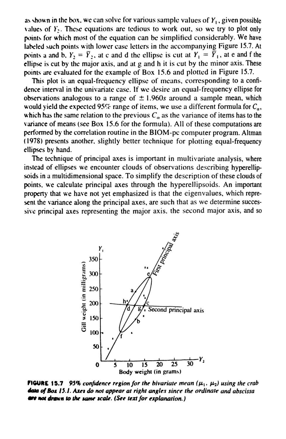
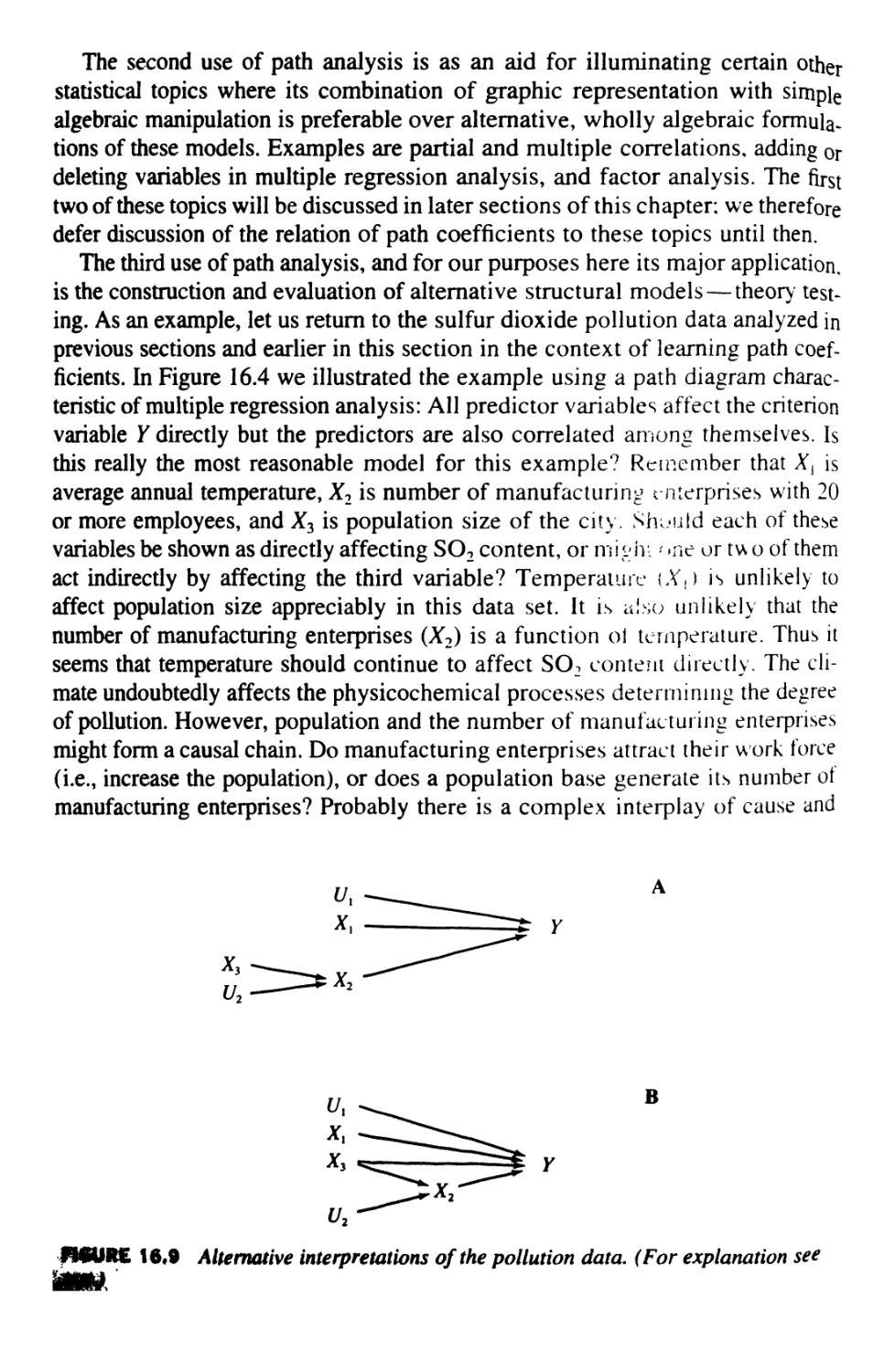
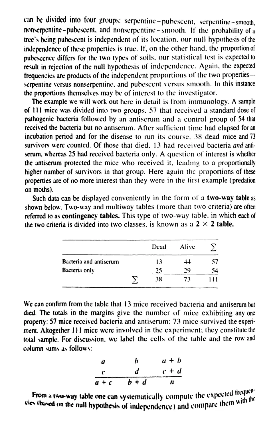
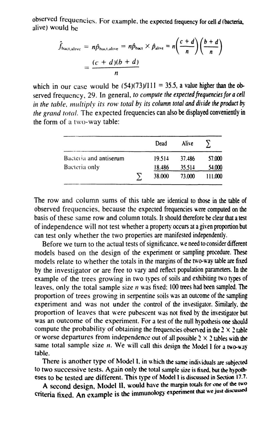
/


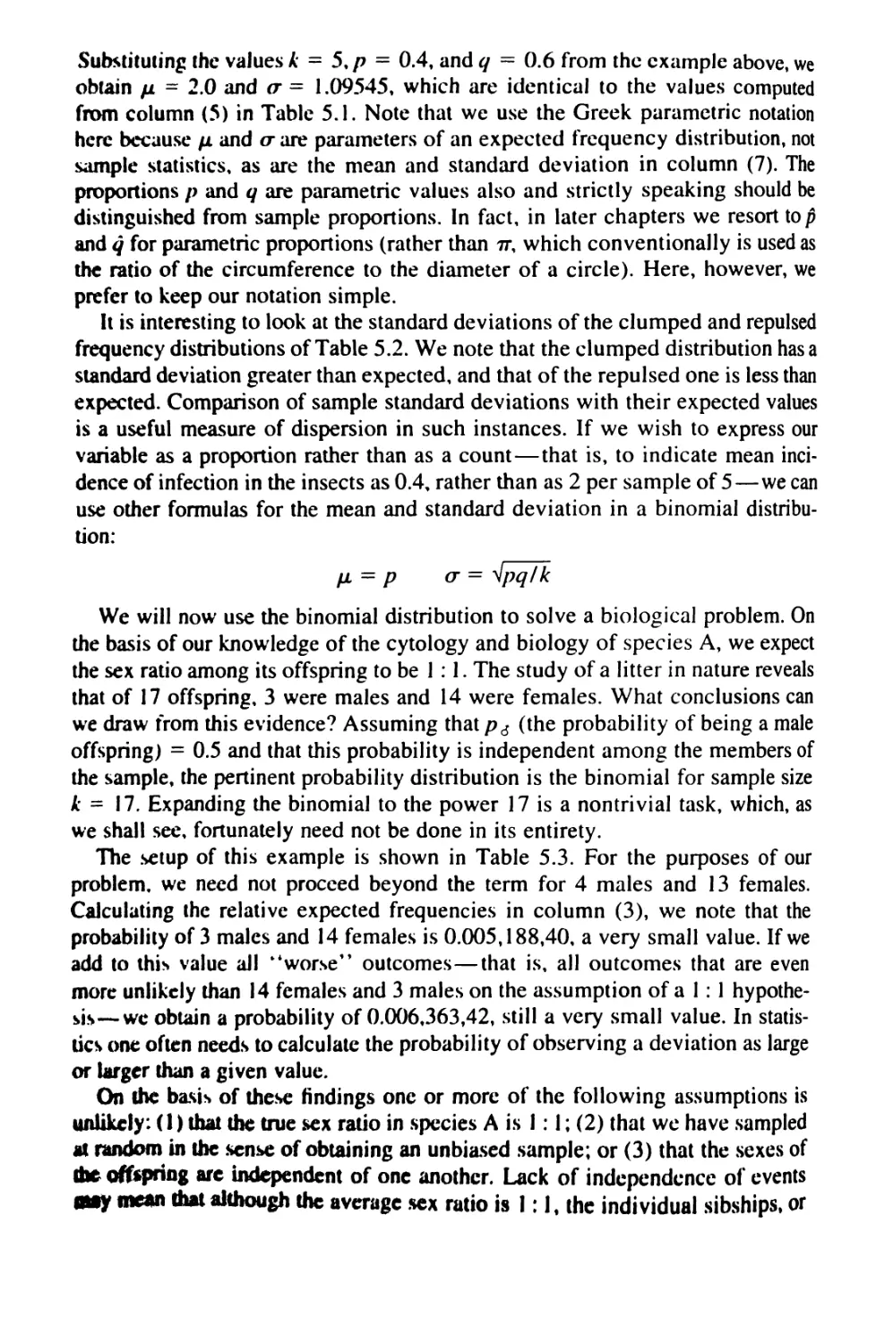
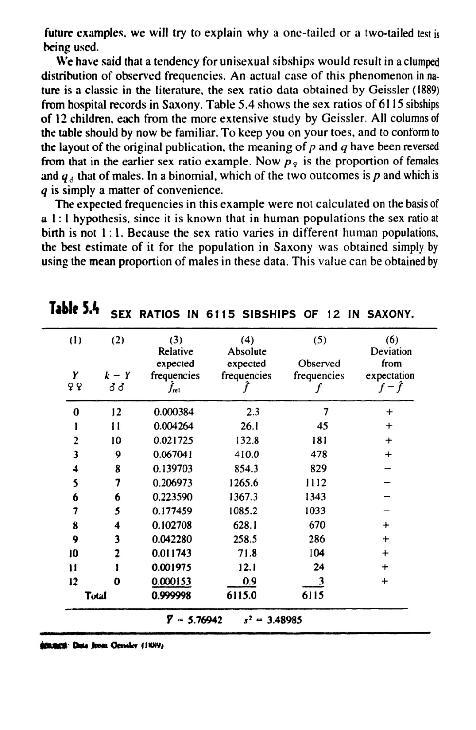


Author: Sokal Robert R. Rohlf F. James
Tags: statistics biometrics
ISBN: 978-0-7167-2411-7
Year: 1995


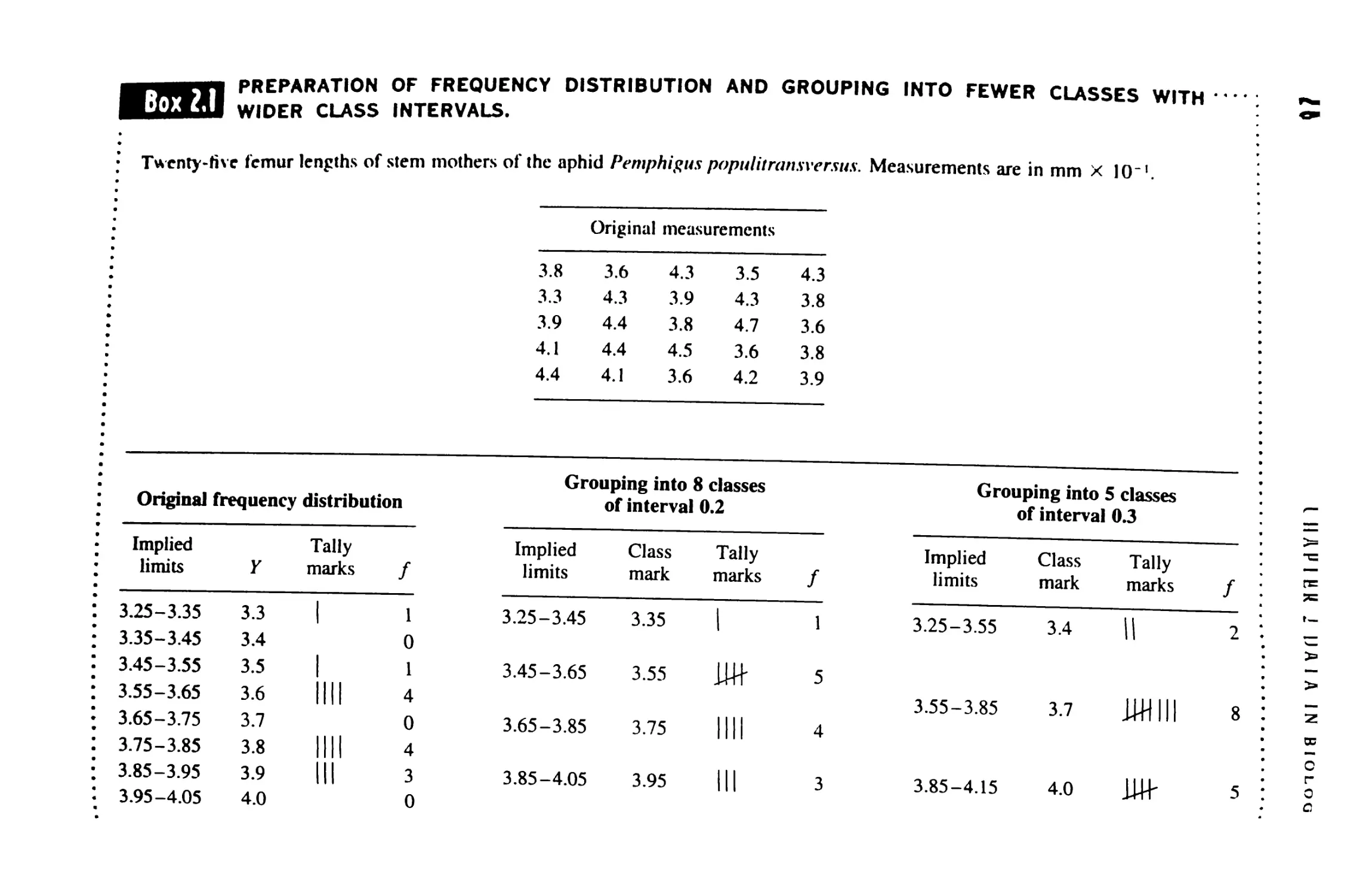
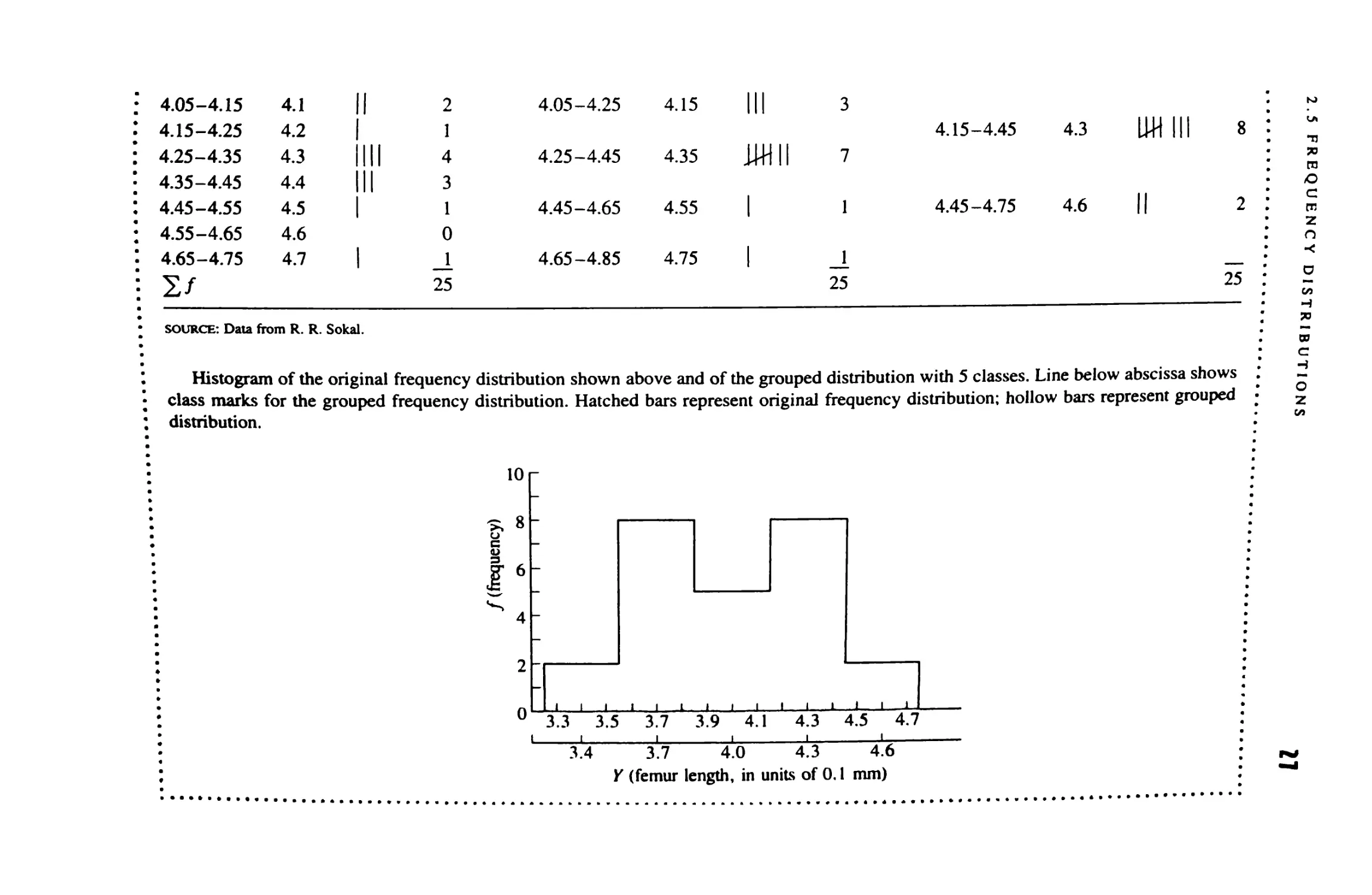
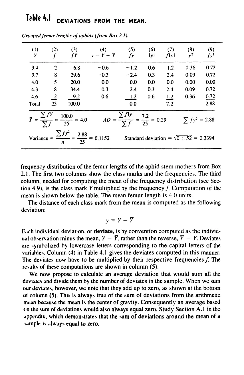
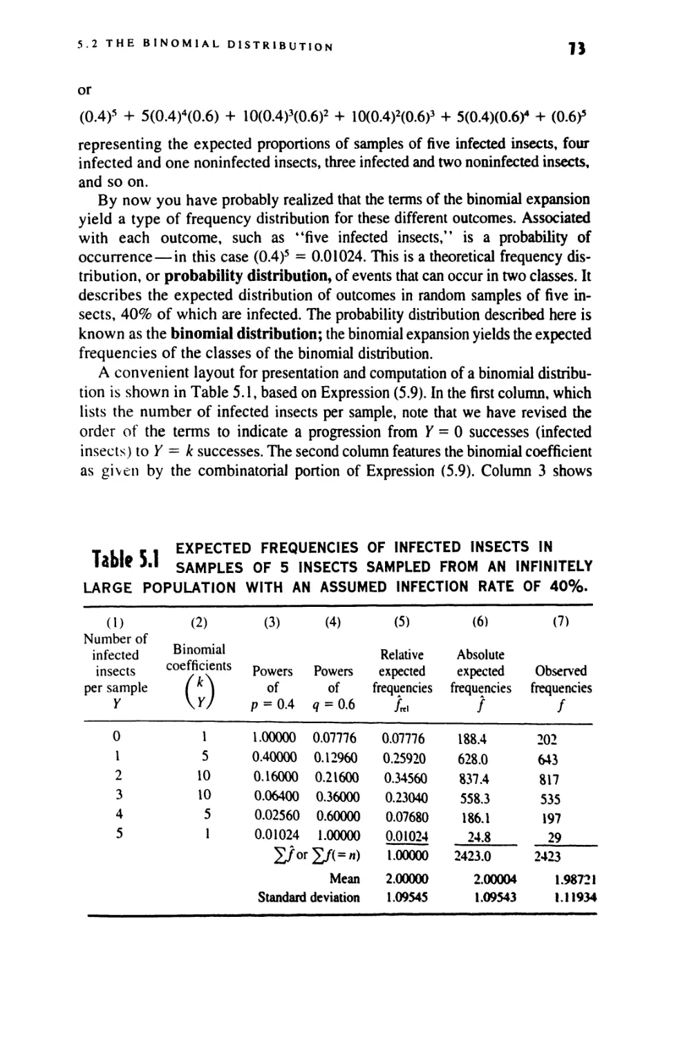
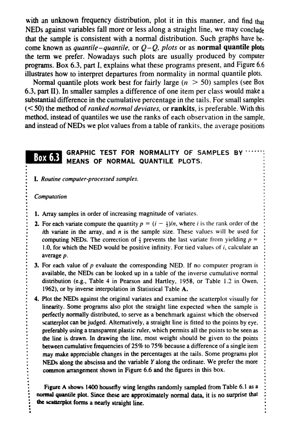
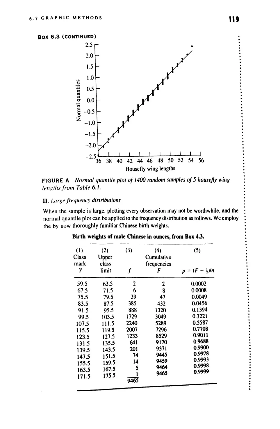
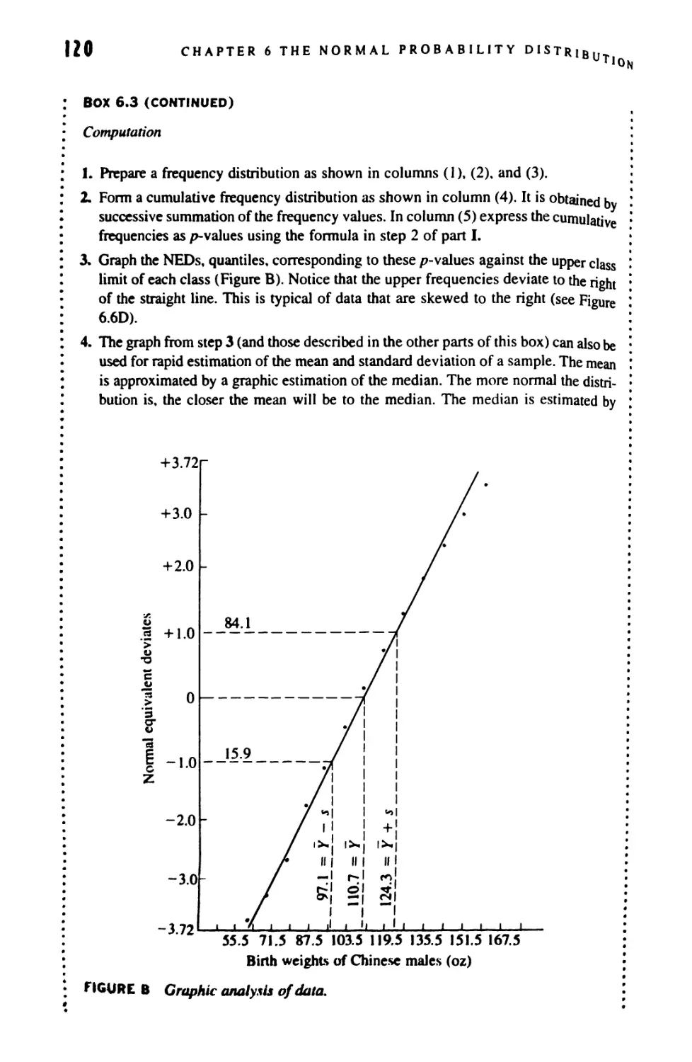
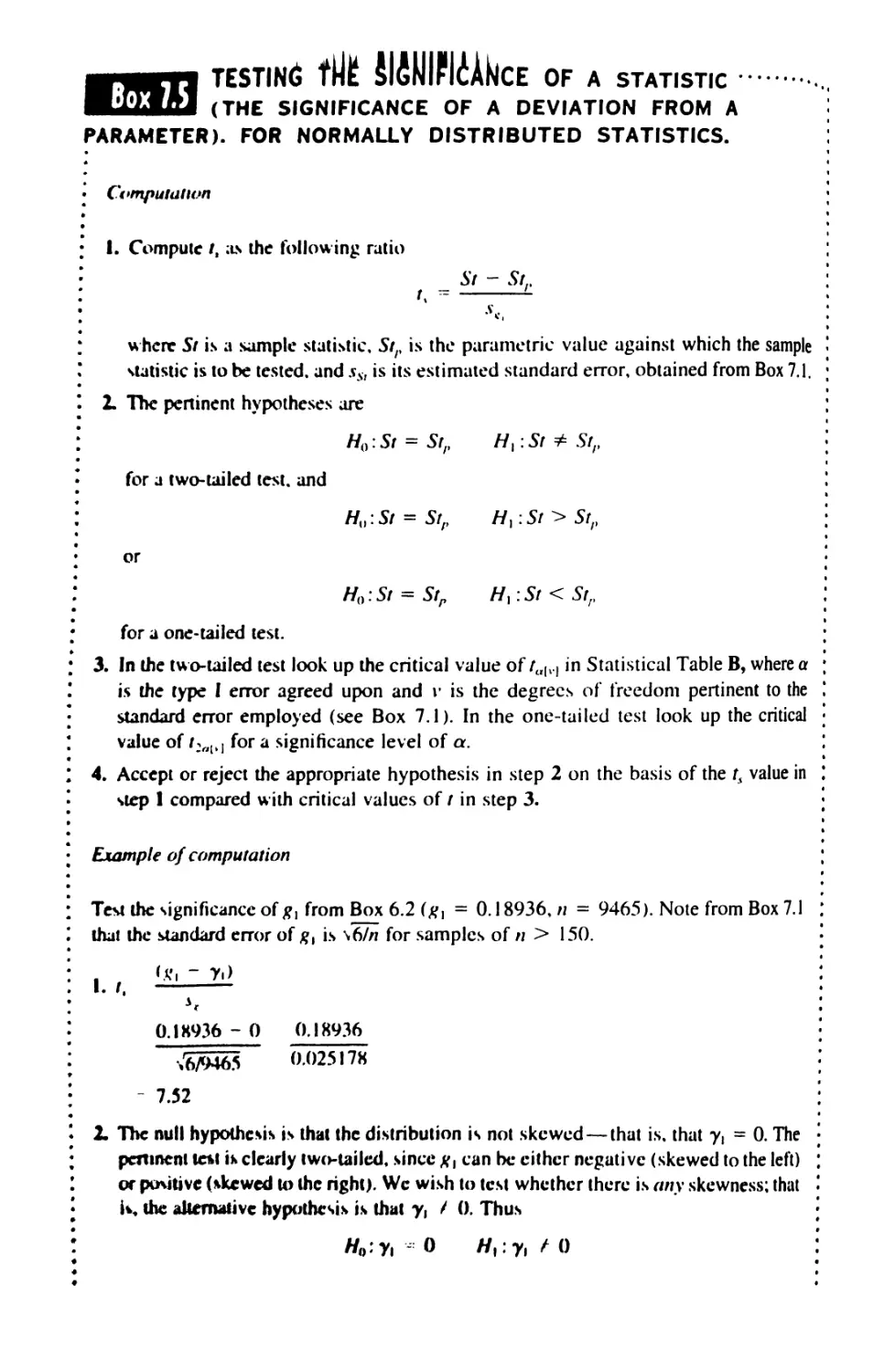
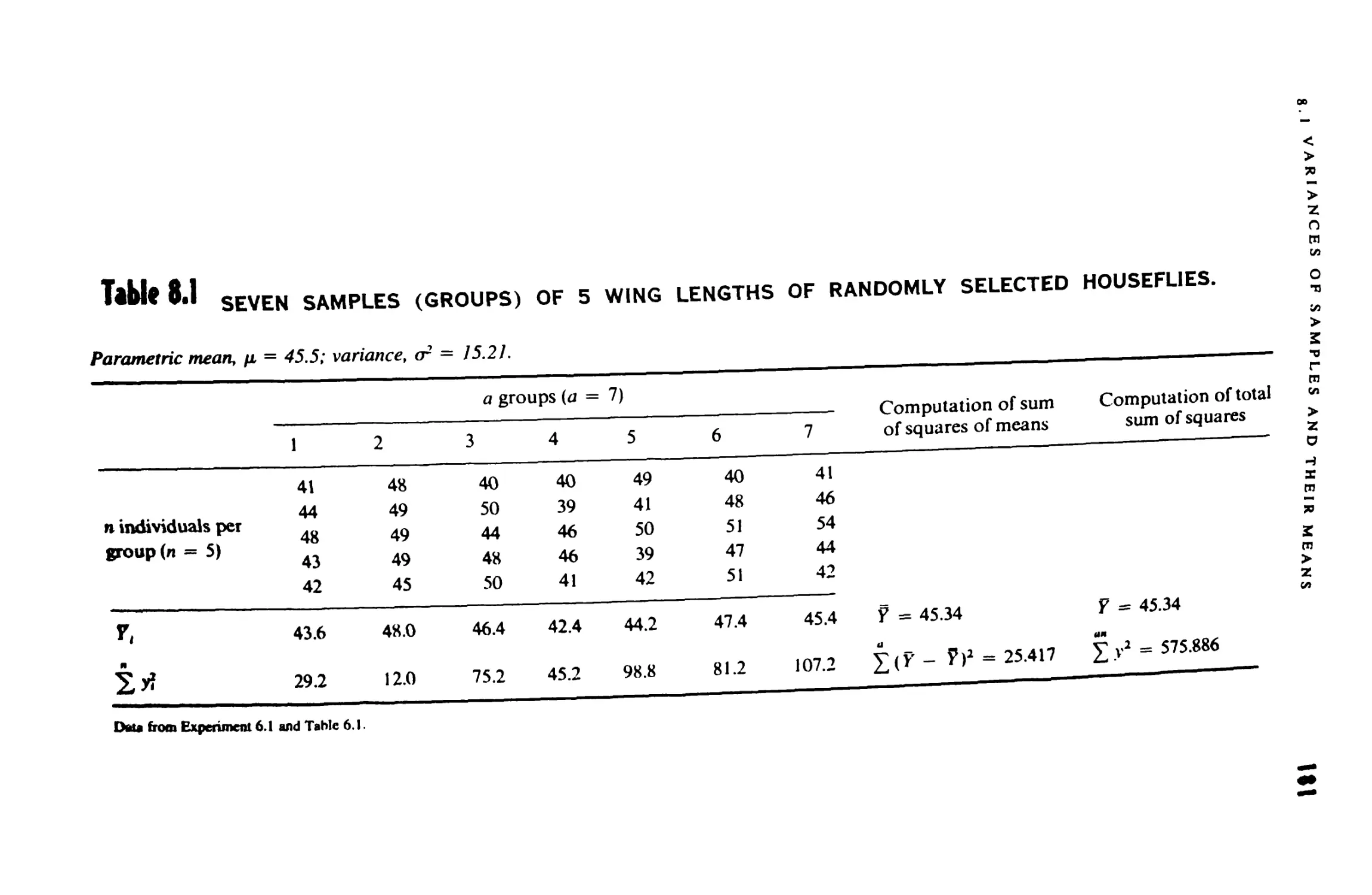
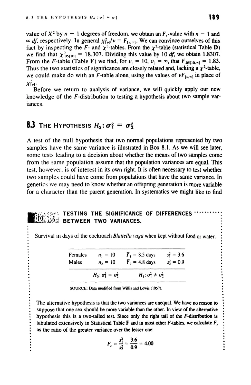
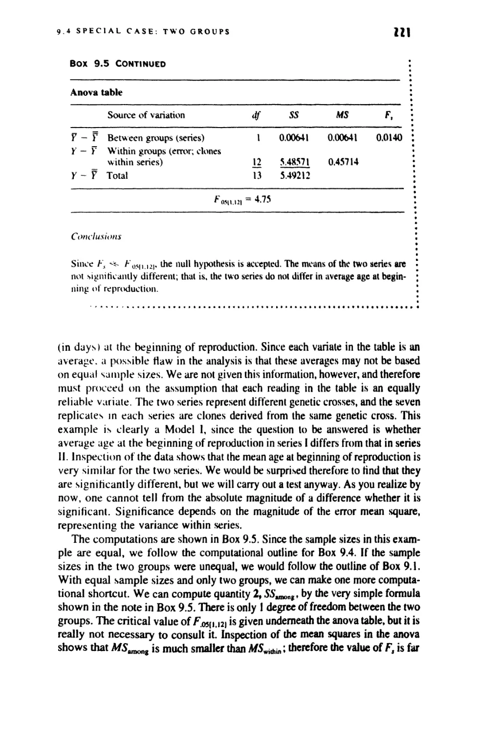
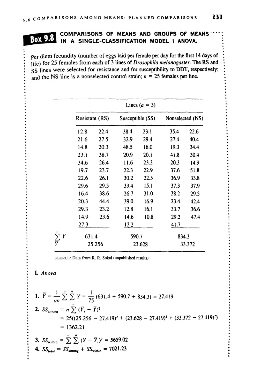
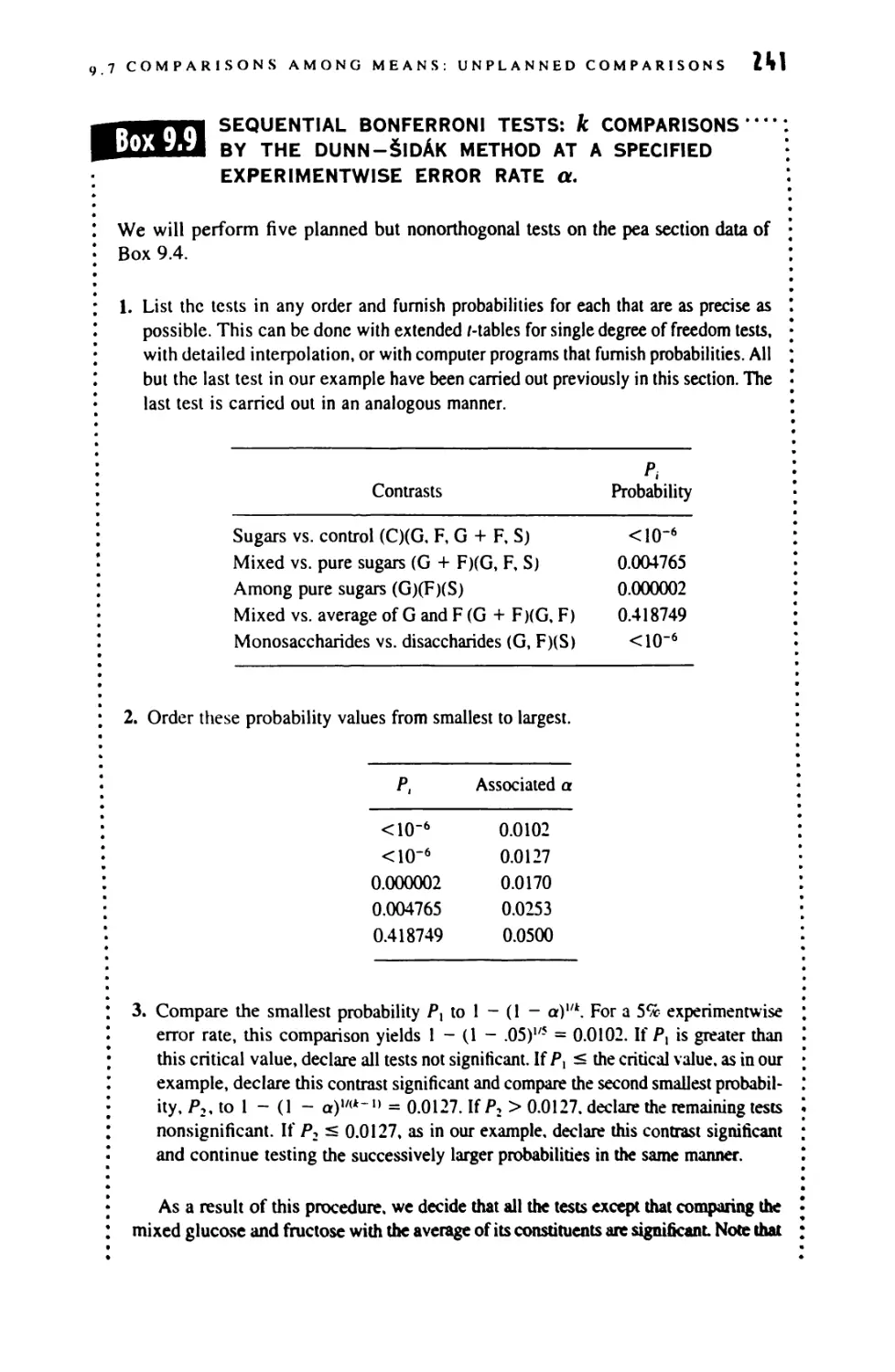
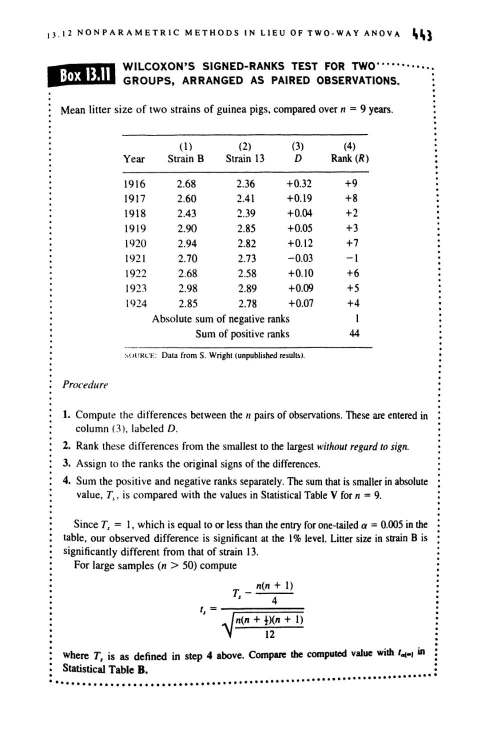
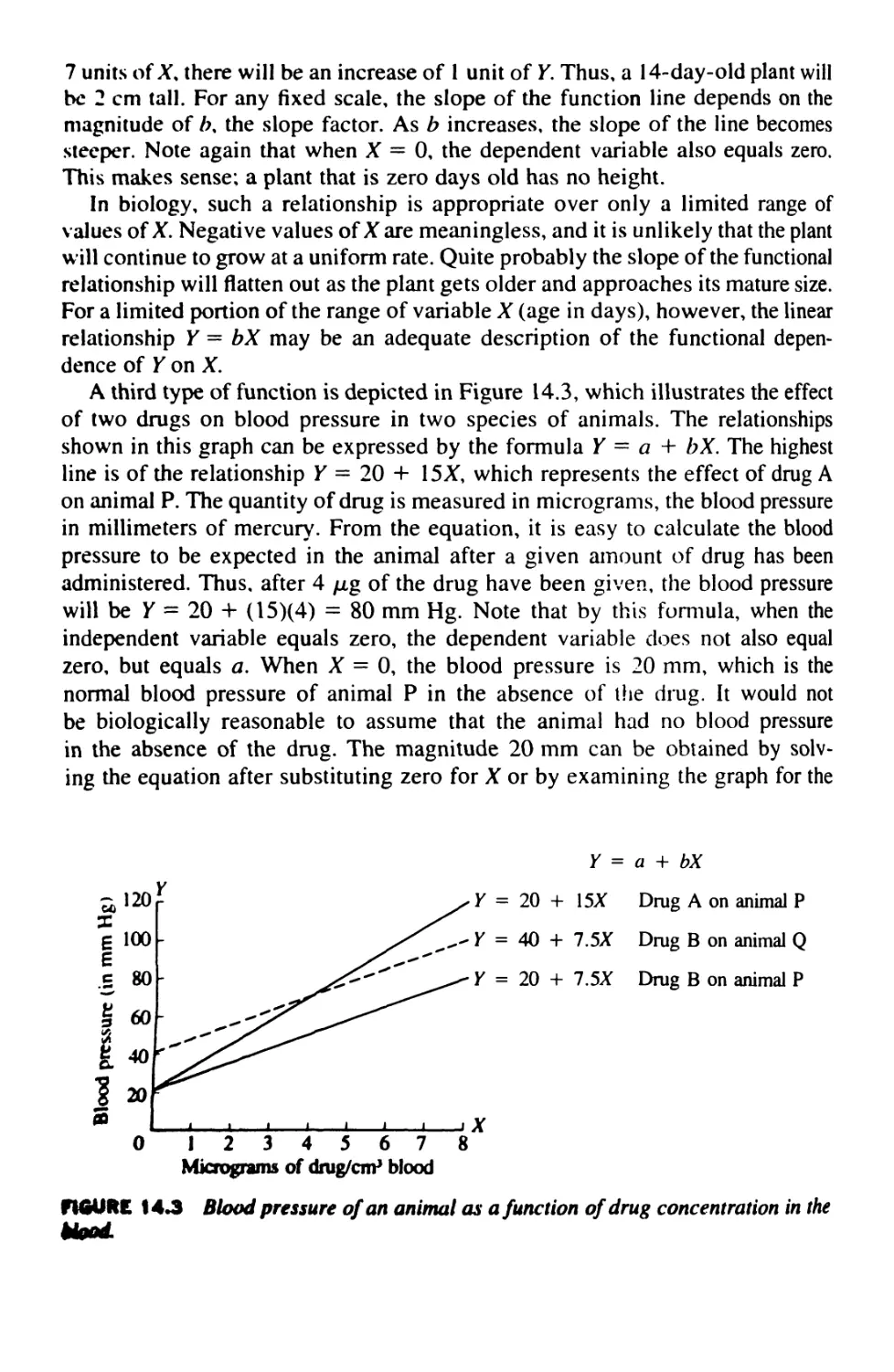
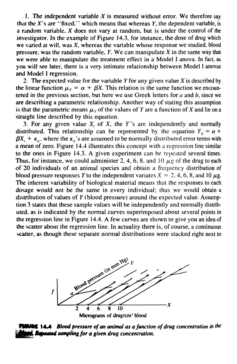
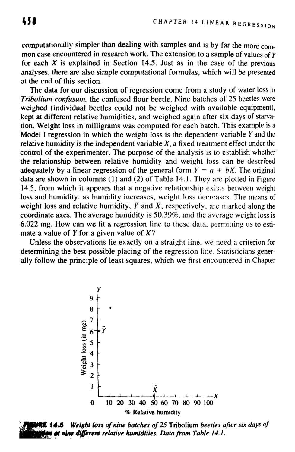
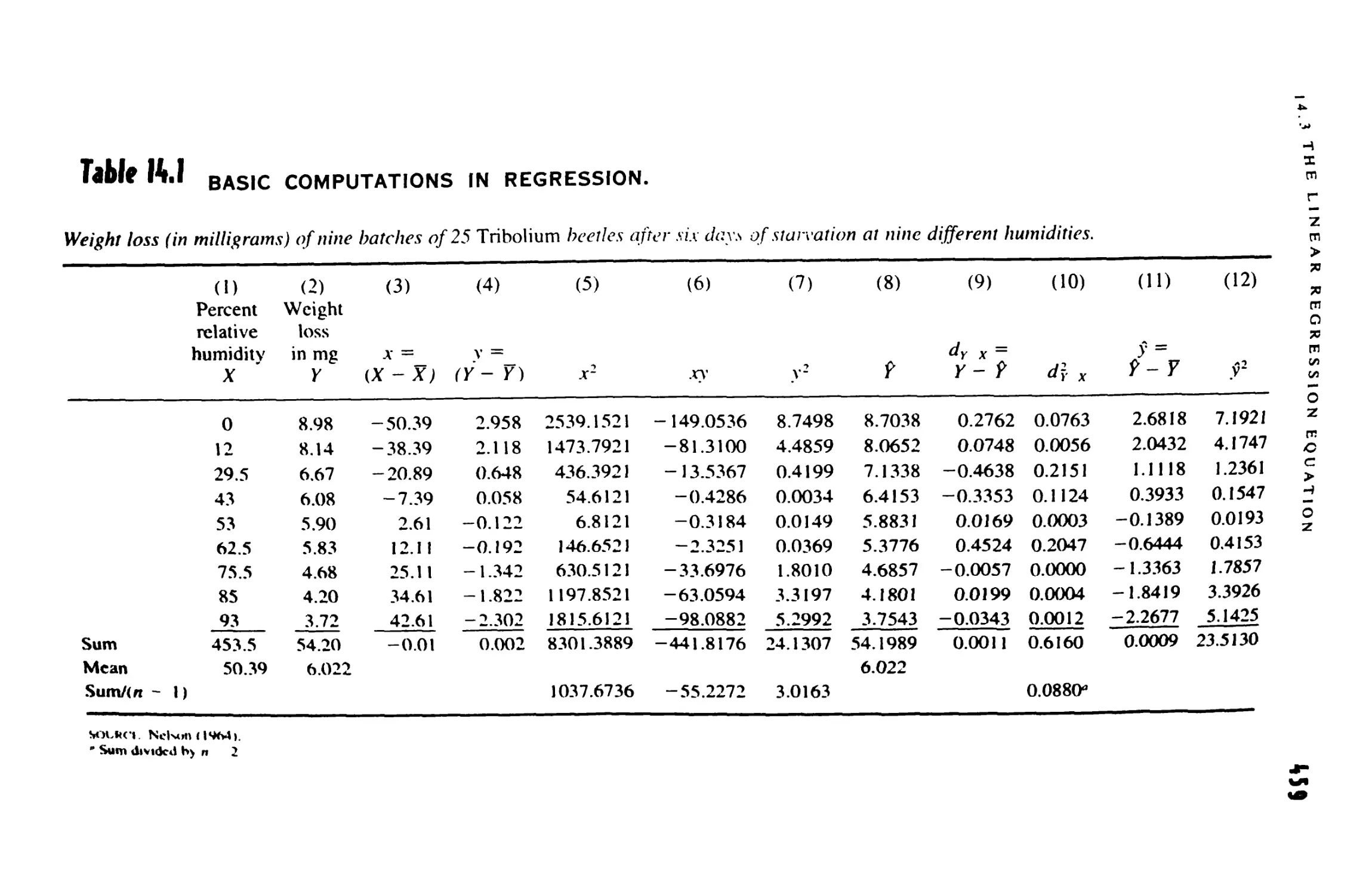
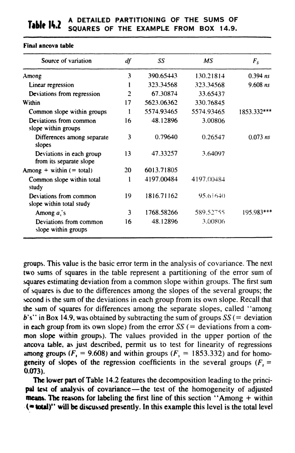
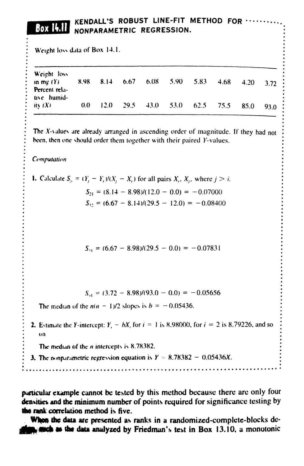
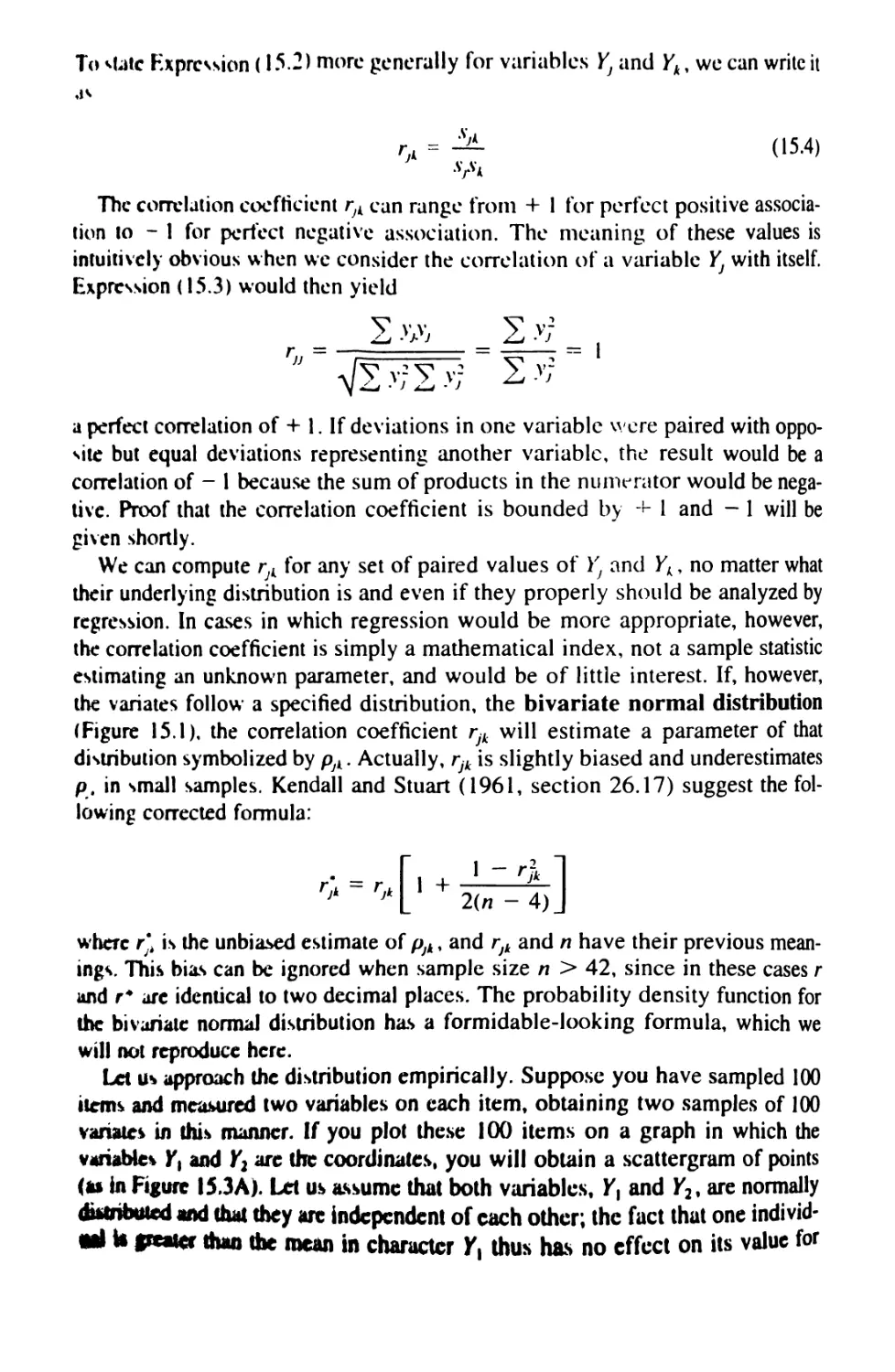
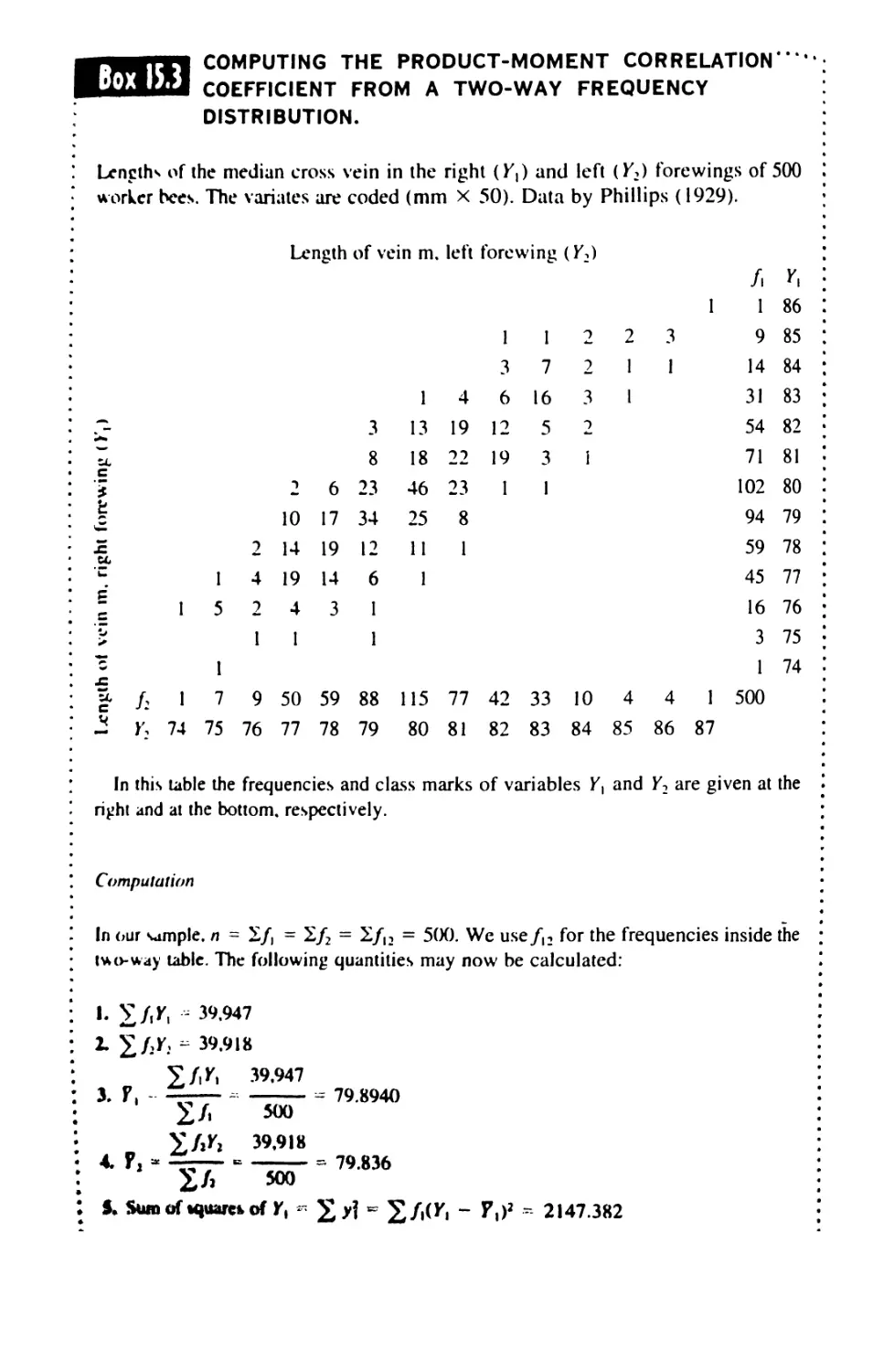
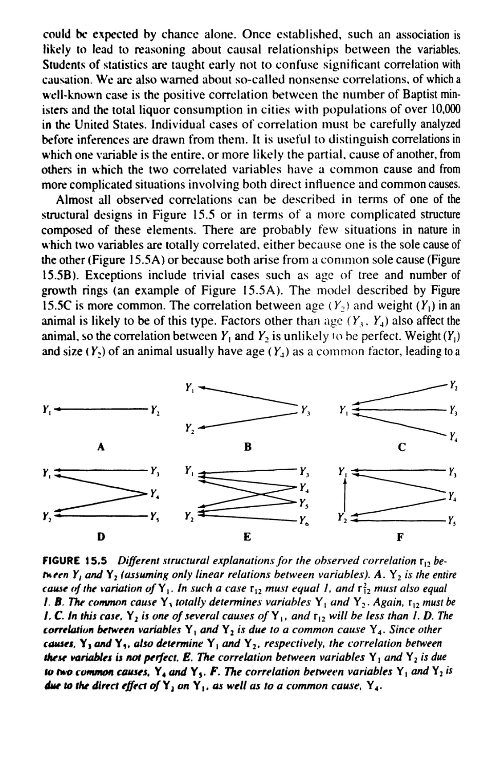
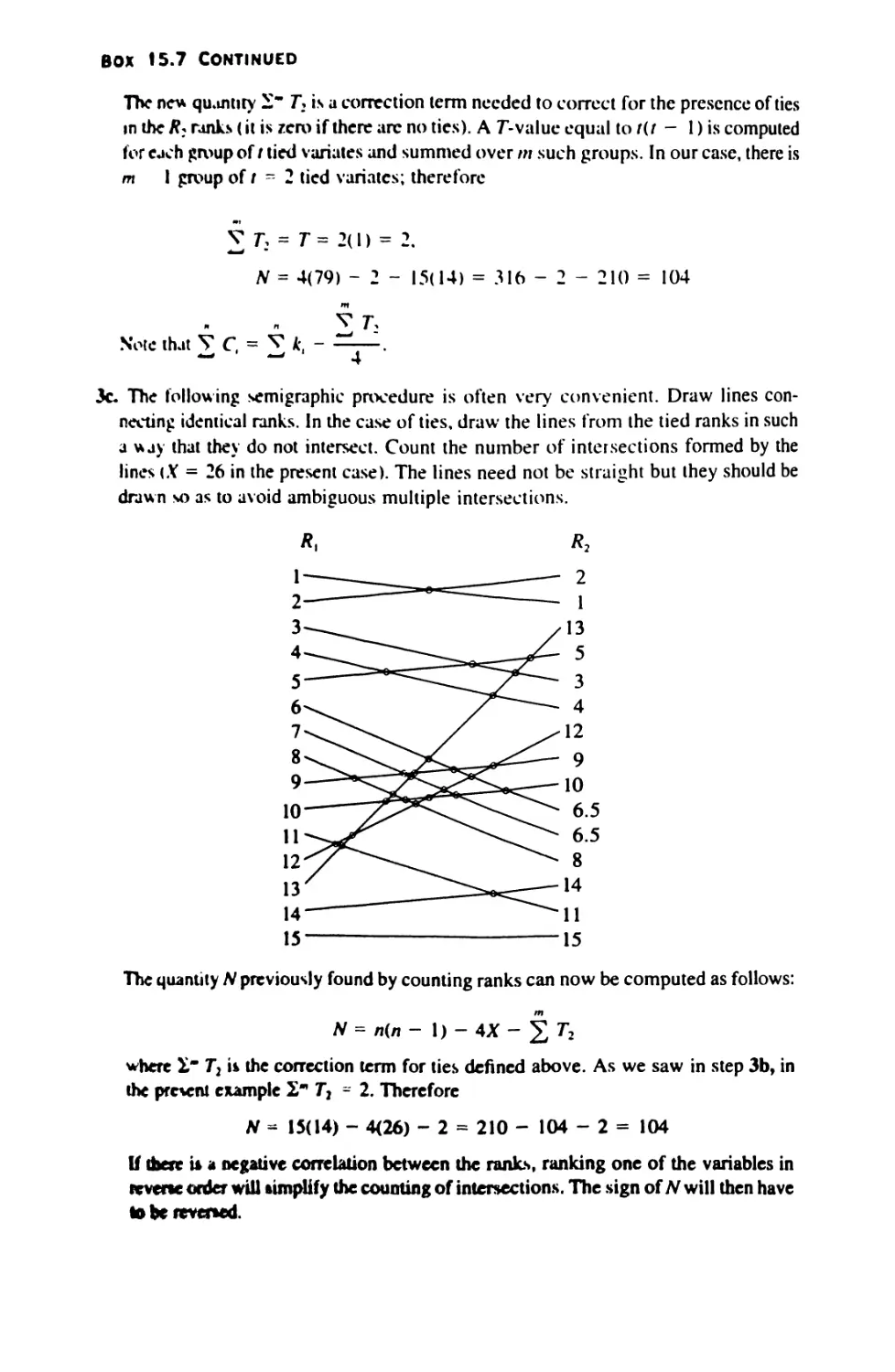
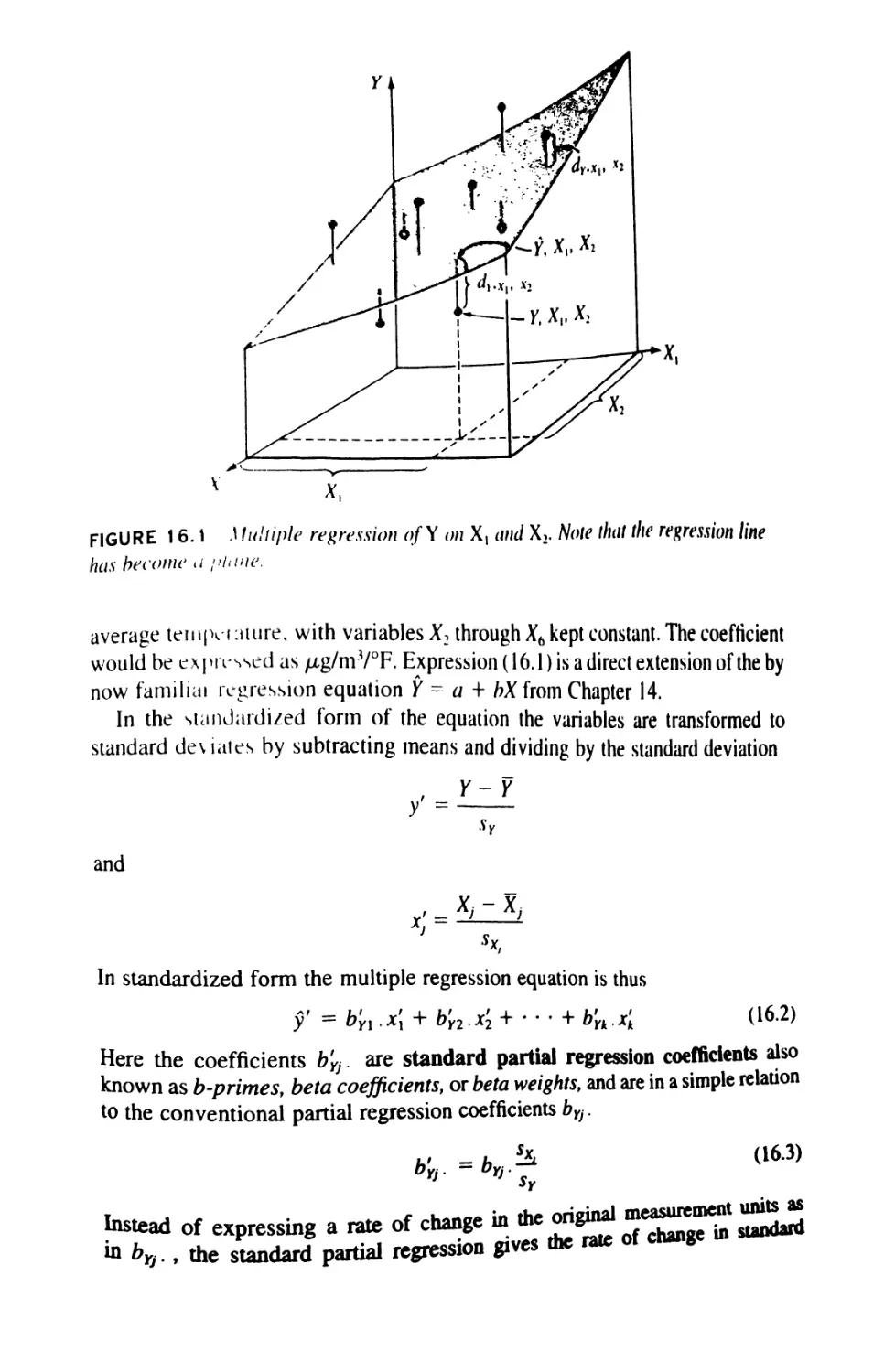
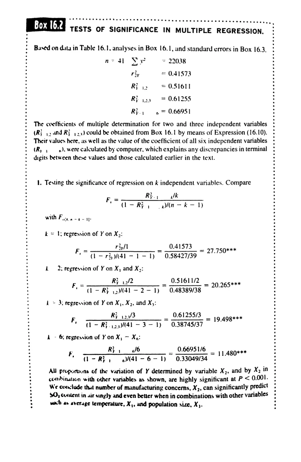
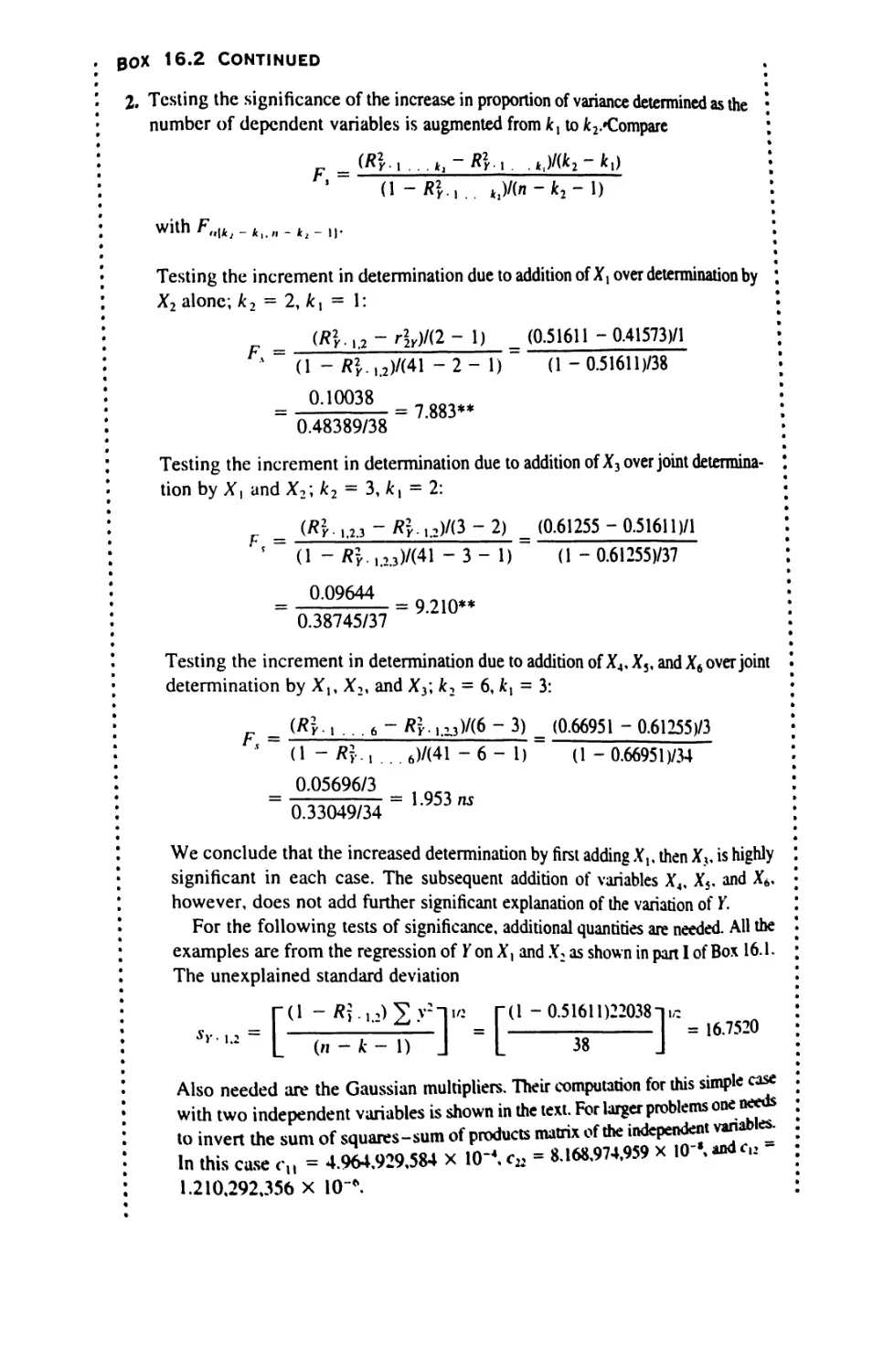
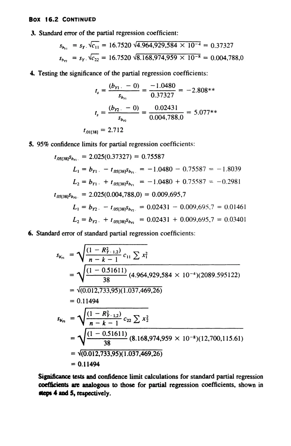
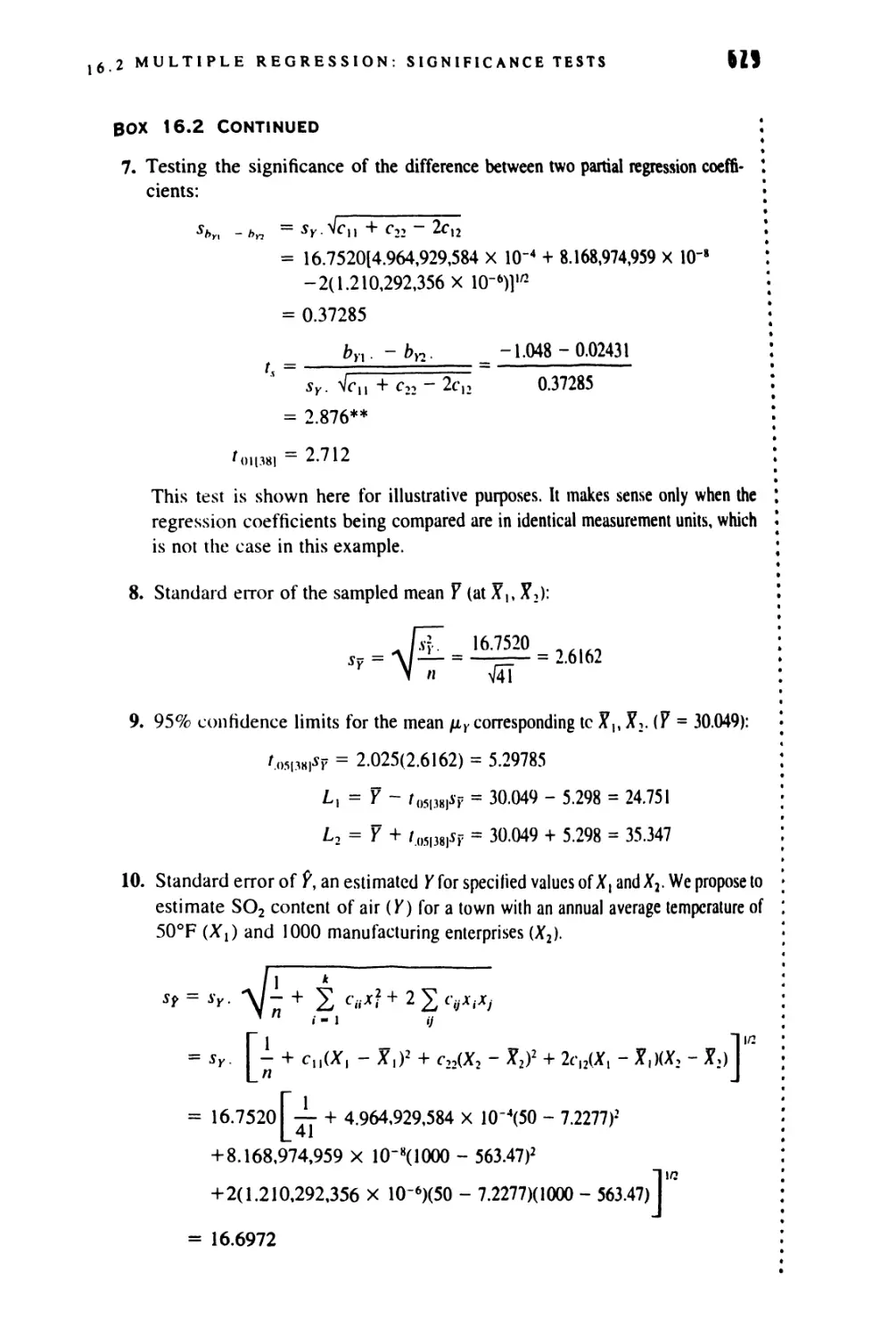
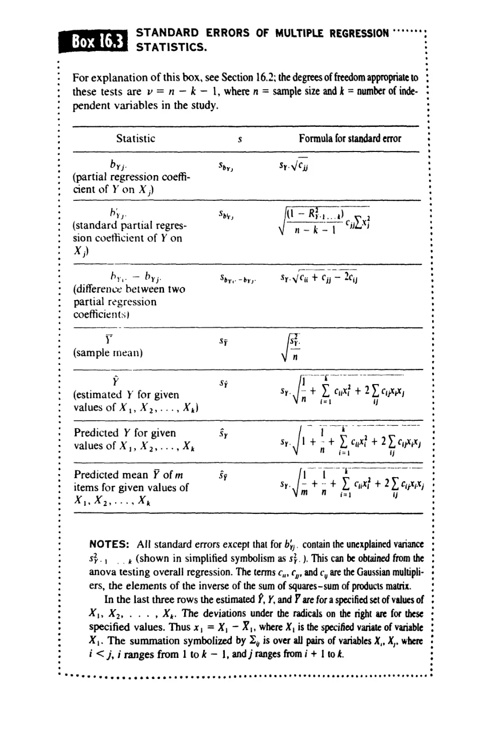
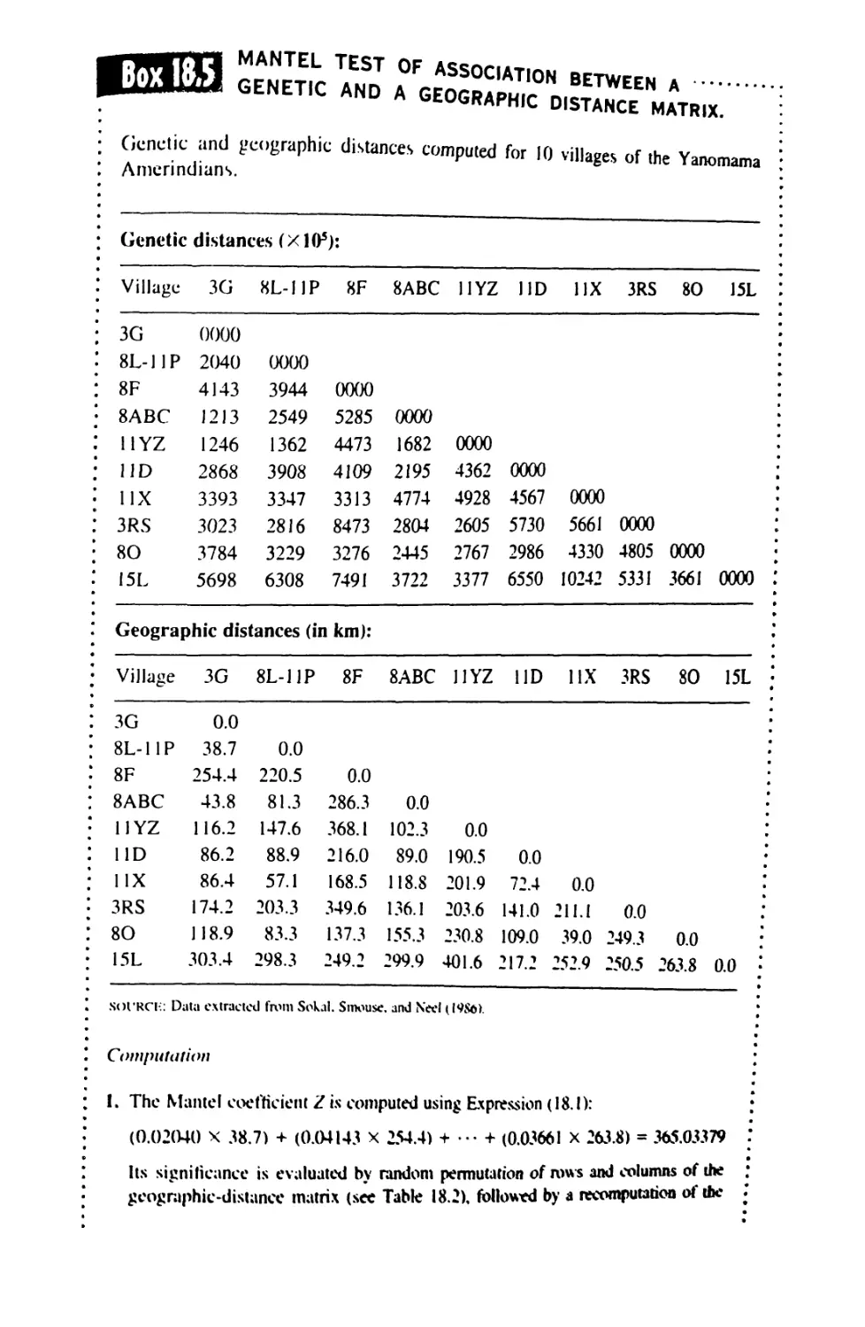
Text
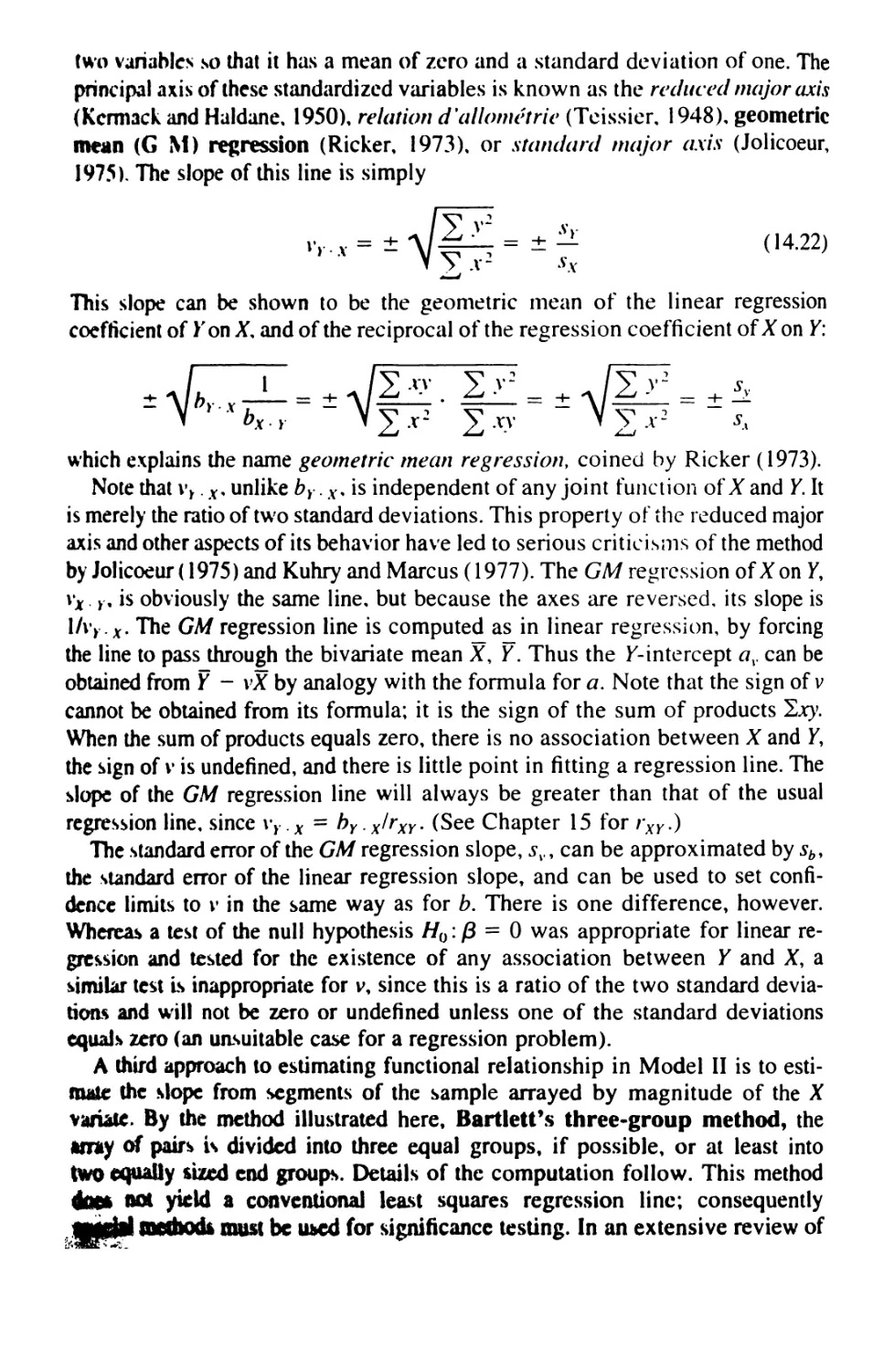
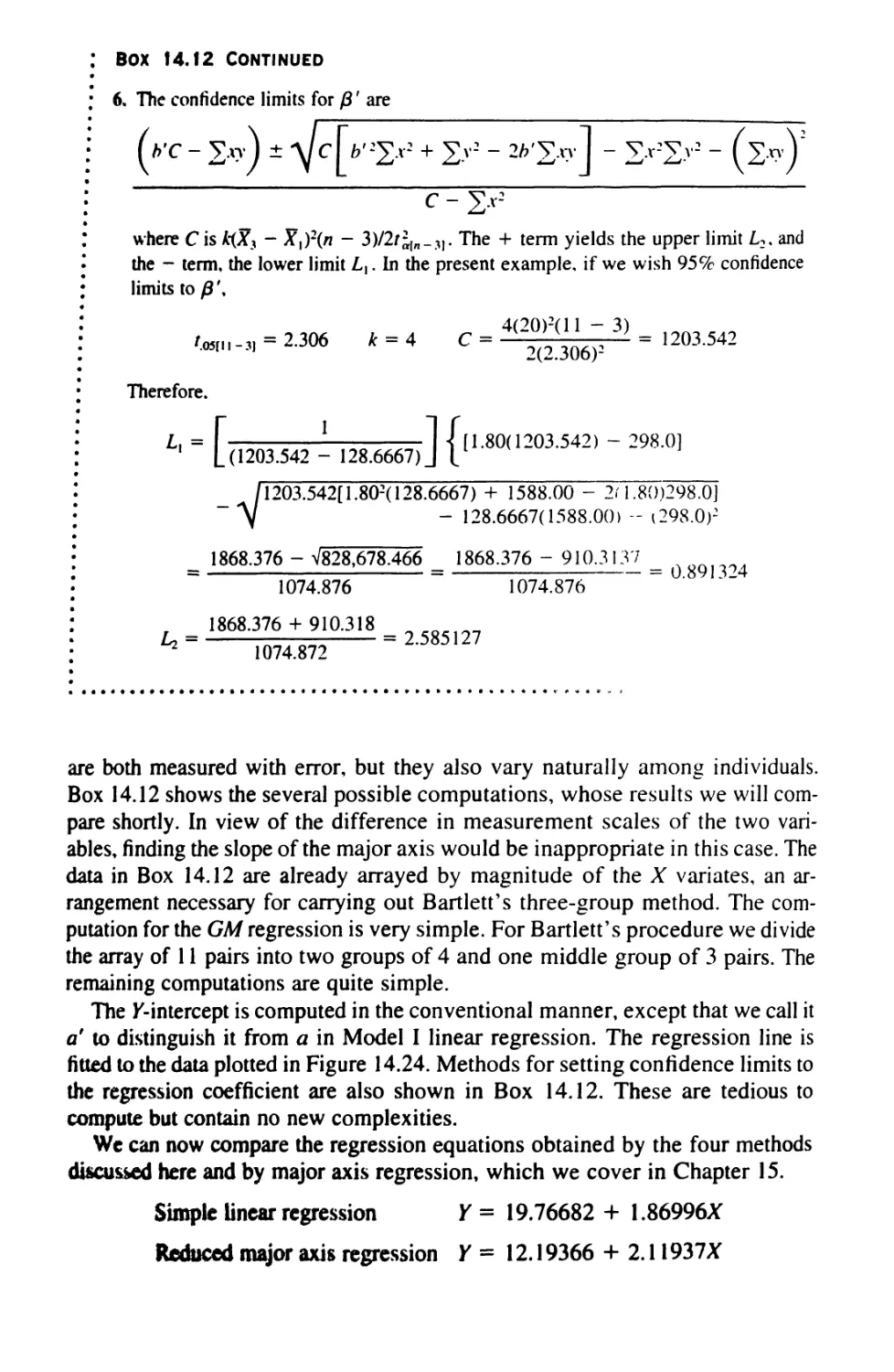
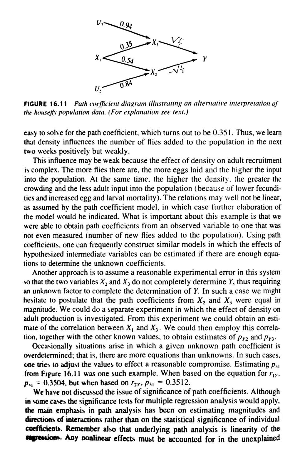
IOMETRY
THE PRINCIPLES AND PRACTICE OF
STATISTICS IN BIOLOGICAL RESEARCH
THIRD EDITION
Robert R. SOKAL and F. James ROHLF
State University of New York at Stony Brook
W. H. FREEMAN AND COMPANY
New York
Library of Congress Cataloging-in-Publication Data
Sokal, Robert R.
Biometry the principles and practice of statistics in biological research / Robert R.
Sokal and F. James Rohlf.—3d ed.
p. cm.
Includes bibliographical references (p. 850) and index.
ISBN-13: 978-0-7167-2411-7
ISBN-10: 0-7167-2411-1
1. Biometry. I. Rohlf, F. James, 1936— . II. Title. ZH323.5.S63 1995
574'.0r5195—dc20 94-11120
CIP
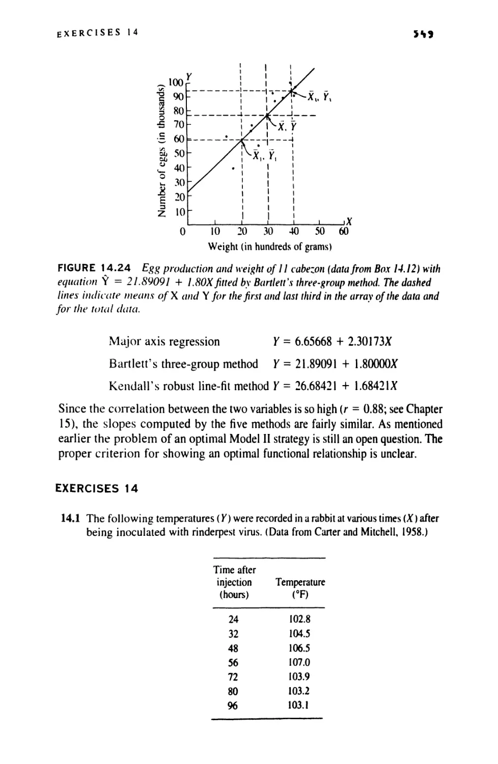
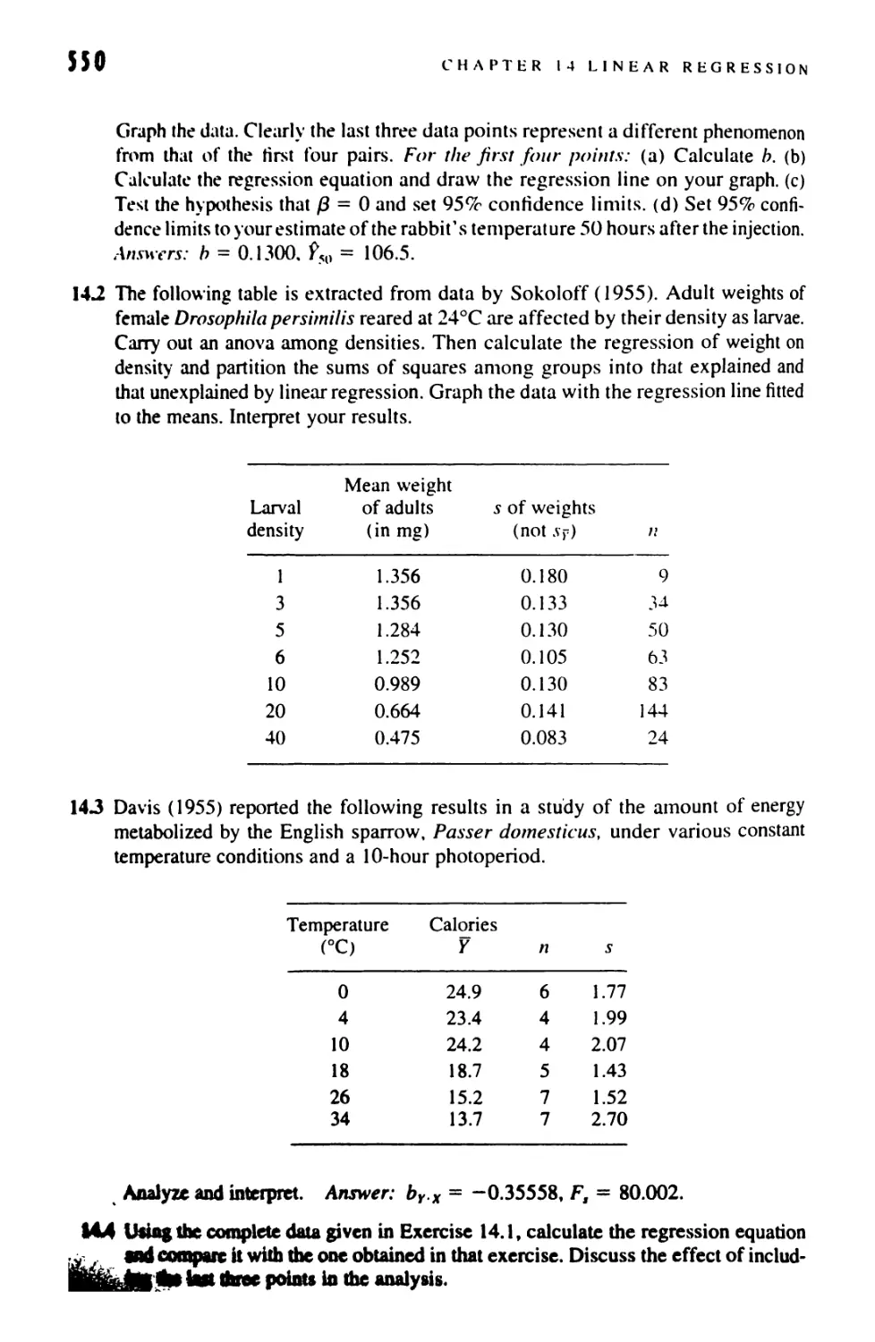
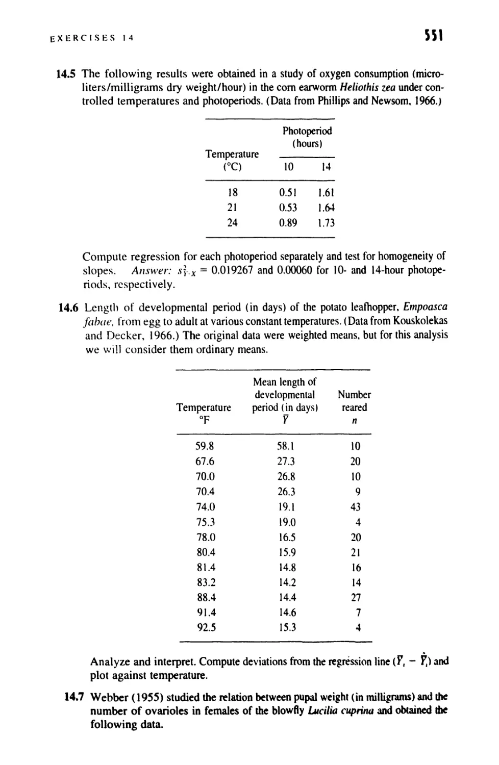
t 1995, 1981, 1969 by W. H. Freeman and Company. All rights reserved.
No part of this book may be reproduced by an mechanical, photographic, or electronic
process, or in the form of a phonographic recording, nor may it be stored in a retrieval
system, transmitted, or otherwise copied for public or private use, without written
permission from the publisher.
Printed in the United States of America
Eleventh printing
W. H. Freeman and Company
41 Madison Avenue
New York, NY 10010
Houndmills, Basingstoke, RG21 6XS, England
www.whfrccman.com
To our parents of blessed memory
Klara and Siegfried Sokal
Harriet and Gilbert Rohlf
CONTENTS
PREFACE xiii
NOTES ON THE THIRD EDITION xvii
INTRODUCTION 1
1.1 Some Definitions 1
1.2 The Development of Biometry 3
1.3 The Statistical Frame of Mind 5
DATA IN BIOLOGY
2.1
2.2
2.3
2.4
2.5
Samples and Populations
Variables in Biology
Accuracy and Precision of Data
Derived Variables
Frequency Distributions
THE HANDLING OF DATA
3.1
3.2
3.3
Computers
Software
Efficiency and Economy in Data Processing
DESCRIPTIVE STATISTICS
4.1
4.2
4.3
4.4
4.5
4.6
The Arithmetic Mean
Other Means
The Median
The Mode
The Range
The Standard Deviation
8
10
13
16
19
33
34
35
37
39
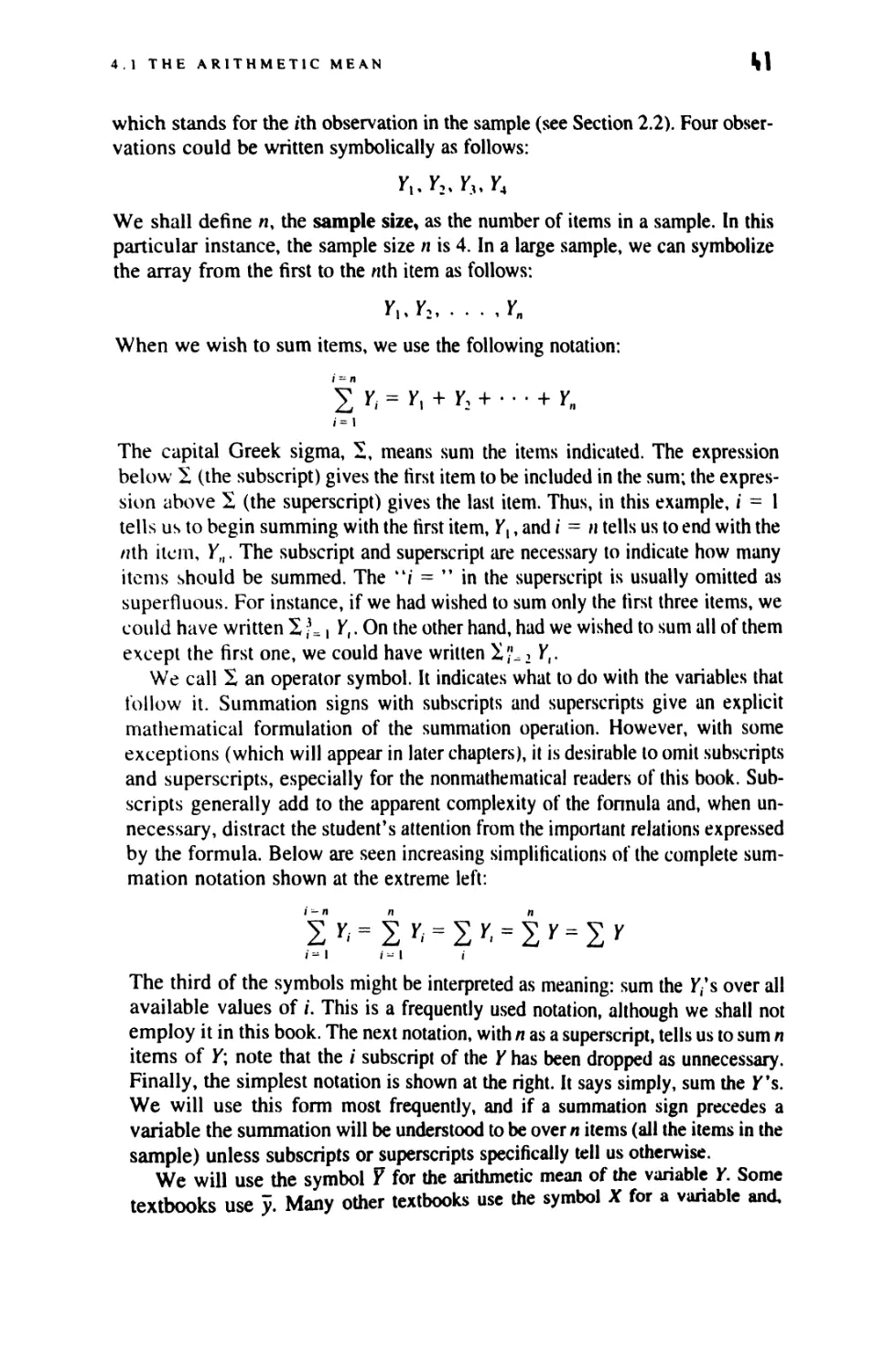
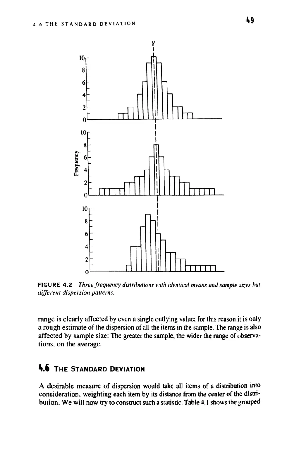
40
43
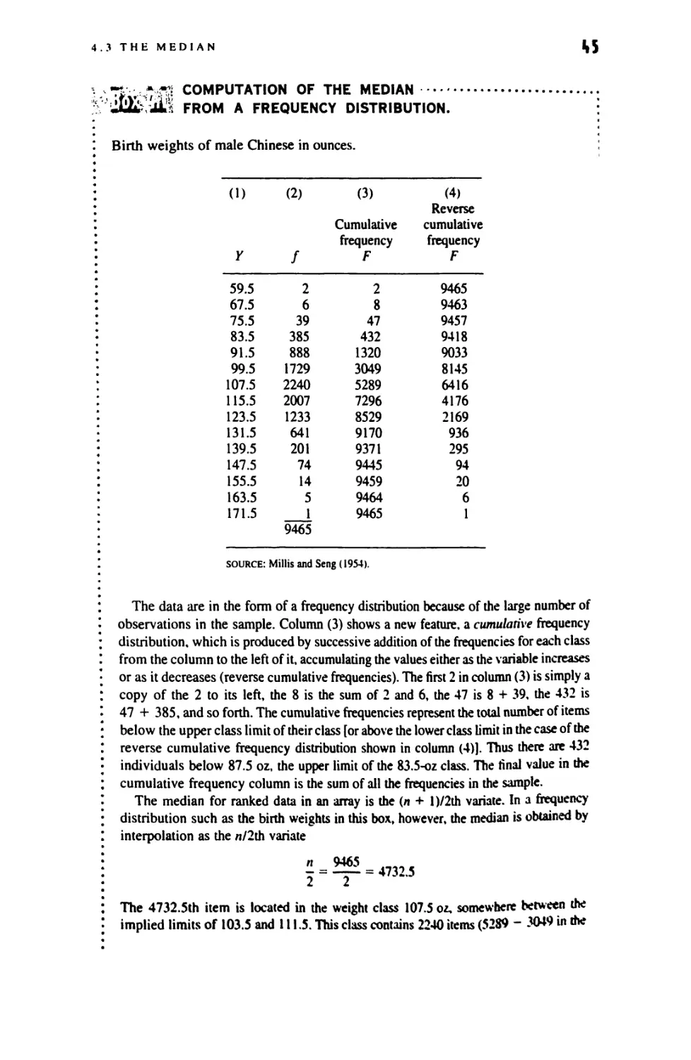
44
47
48
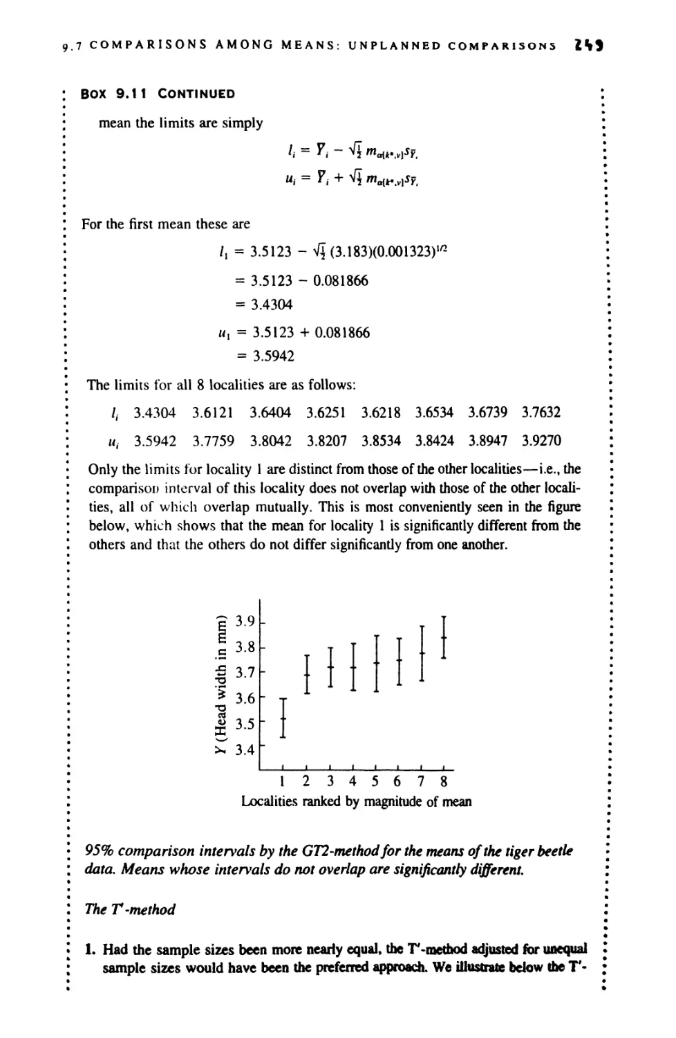
49
vii
CONTENTS
4.7 Sample Statistics and Parameters 52
4.8 Coding Data Before Computation 53
4.9 Computing Means and Standard Deviations 54
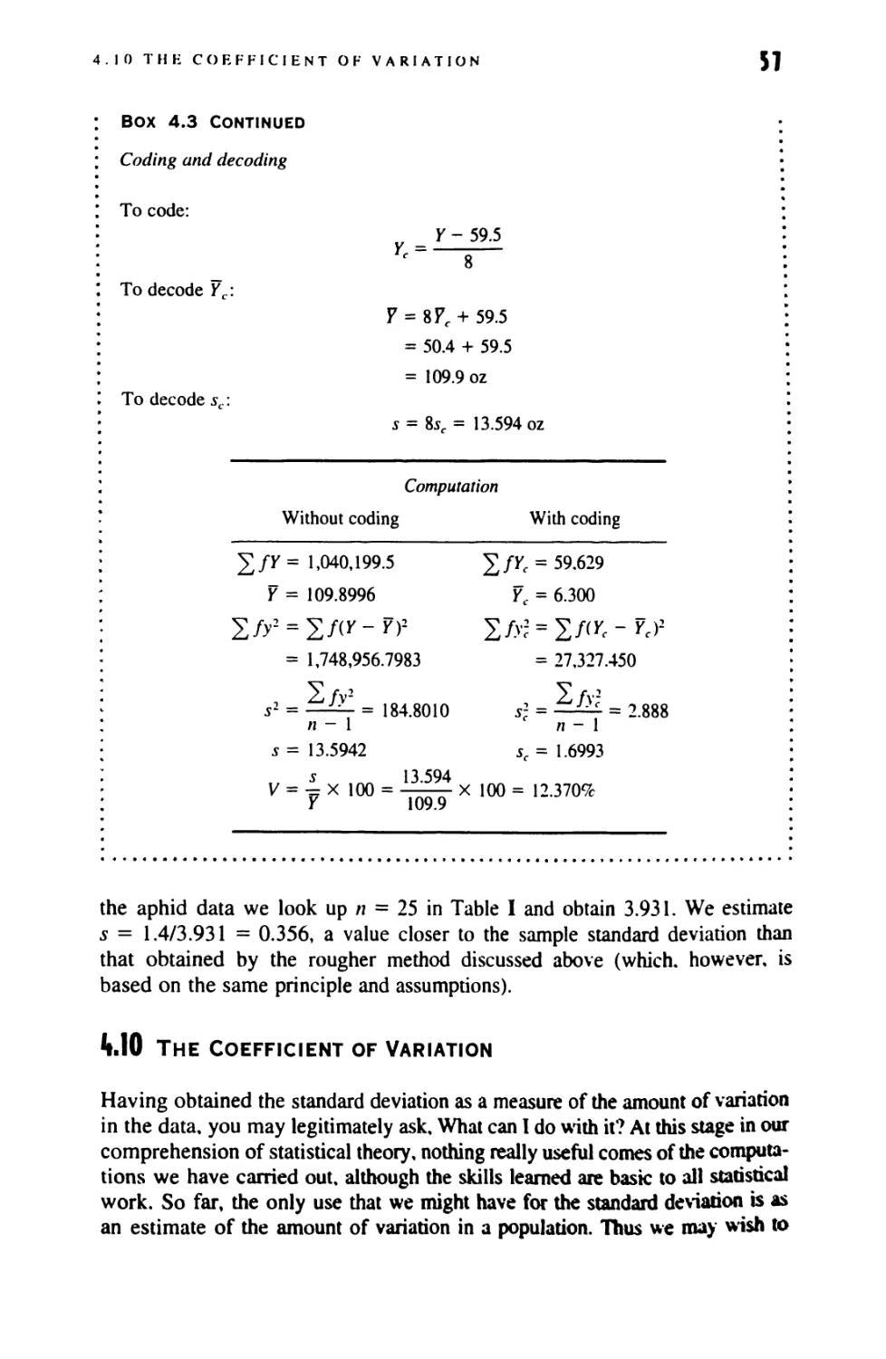
4.10 The Coefficient of Variation 57
5 INTRODUCTION TO PROBABILITY DISTRIBUTIONS:
BINOMIAL AND POISSON 61
5.1 Probability, Random Sampling, and Hypothesis Testing 62
5.2 The Binomial Distribution 71
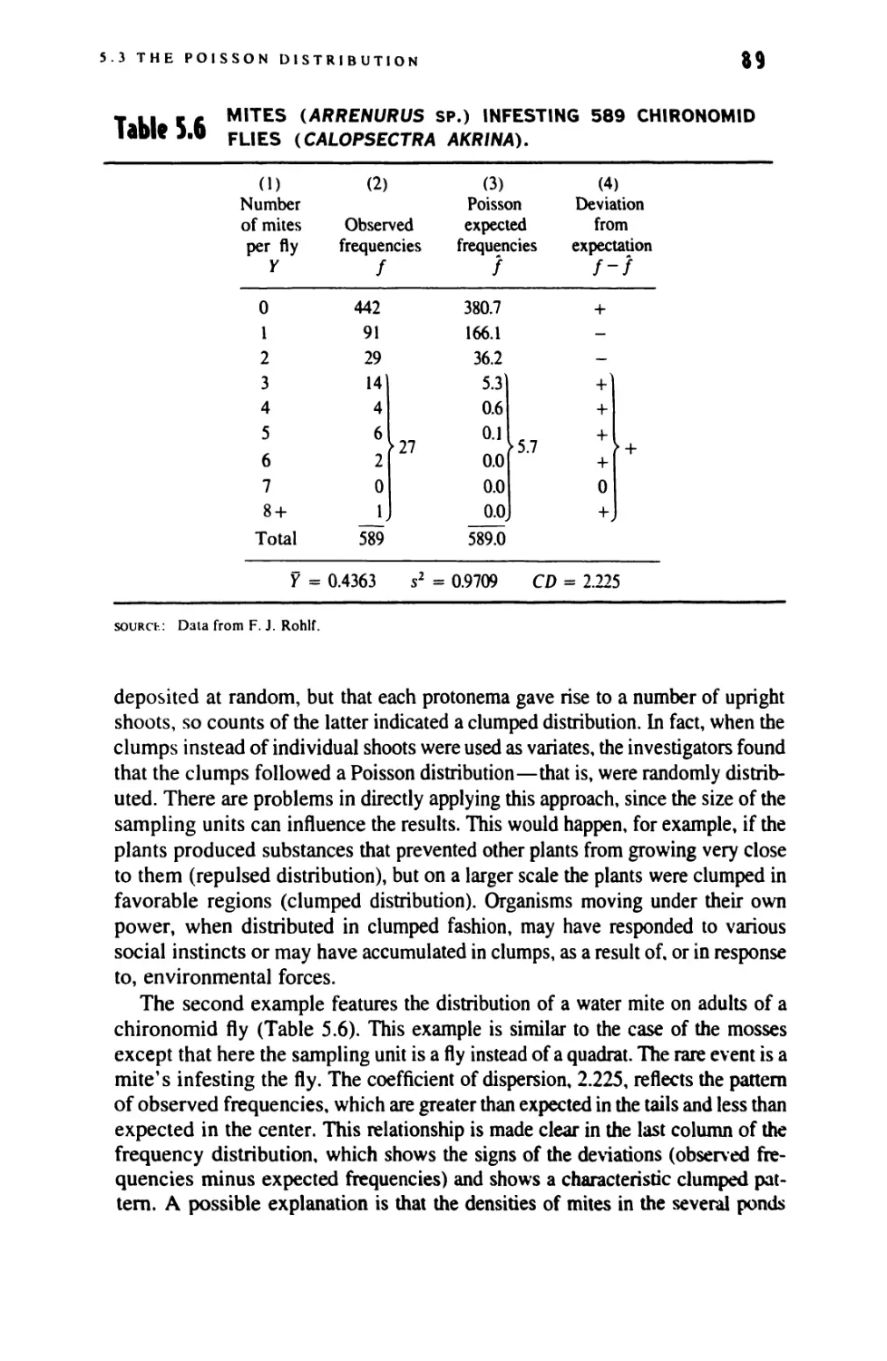
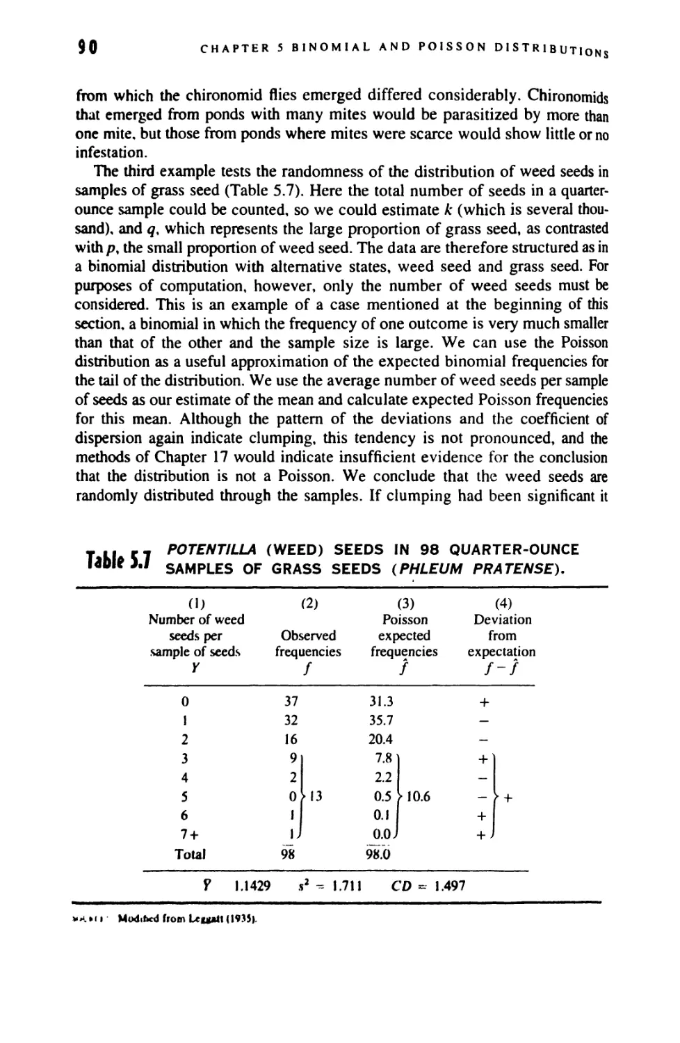
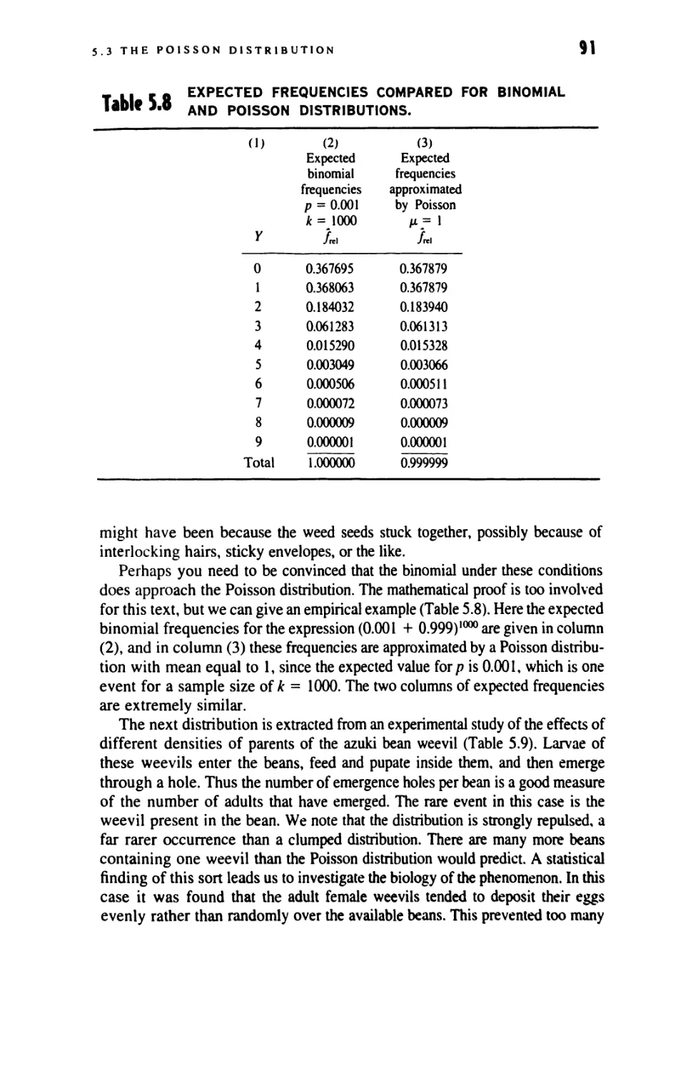
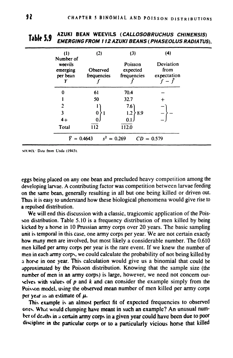
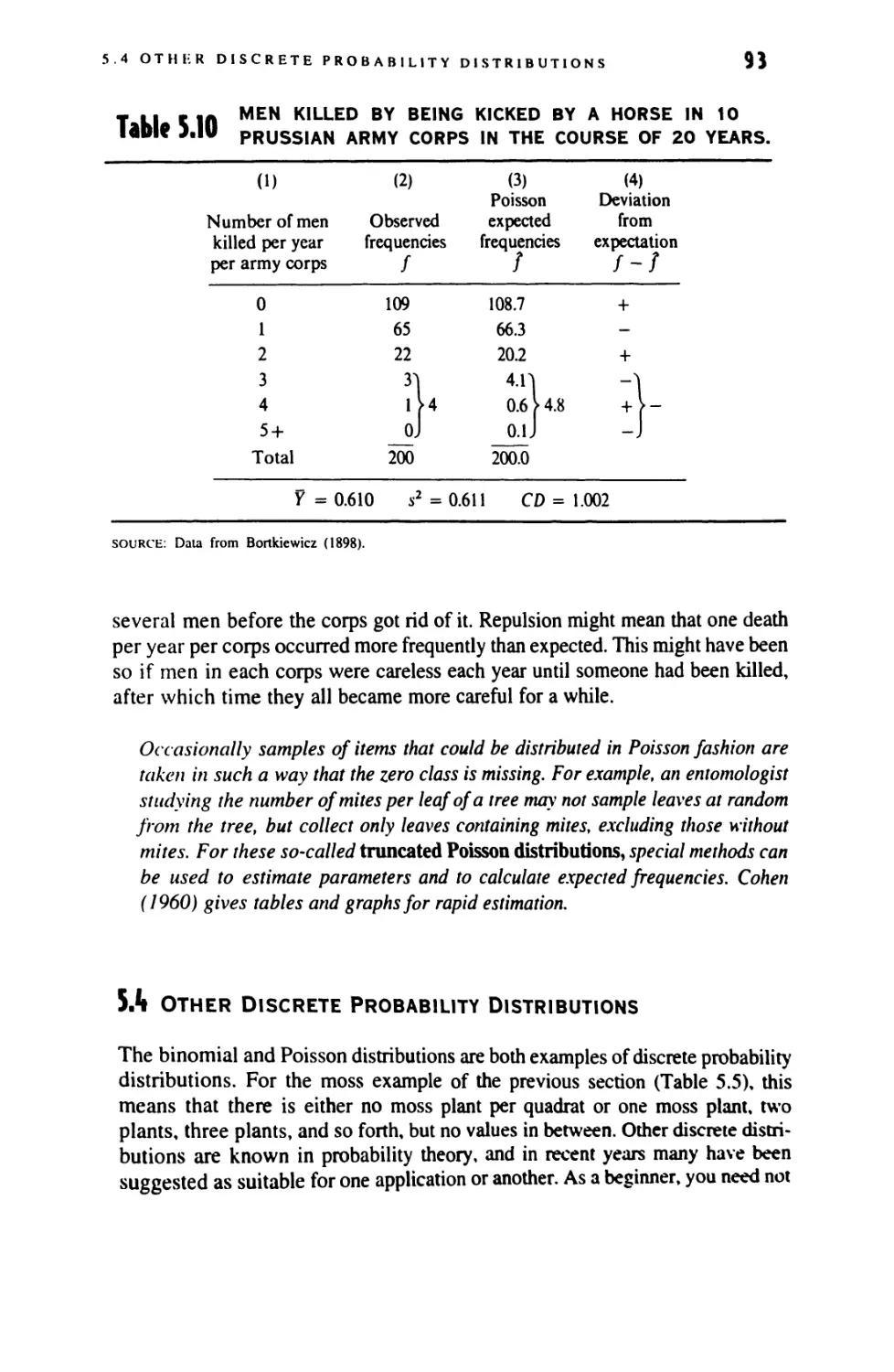
5.3 The Poisson Distribution 81
5.4 Other Discrete Probability Distributions 93
6 THE NORMAL PROBABILITY DISTRIBUTION 98
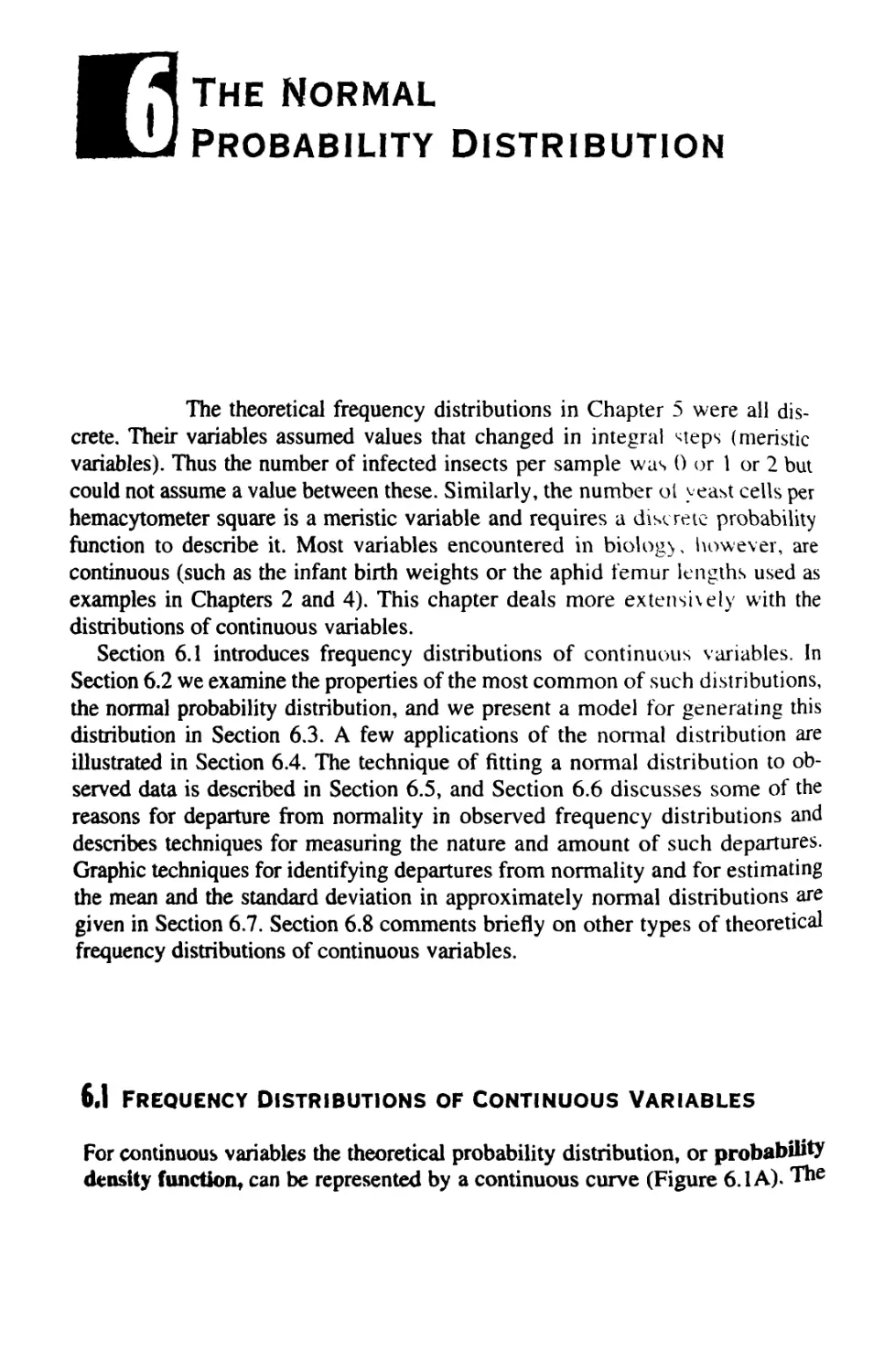
6.1 Frequency Distributions of Continuous Variables 98
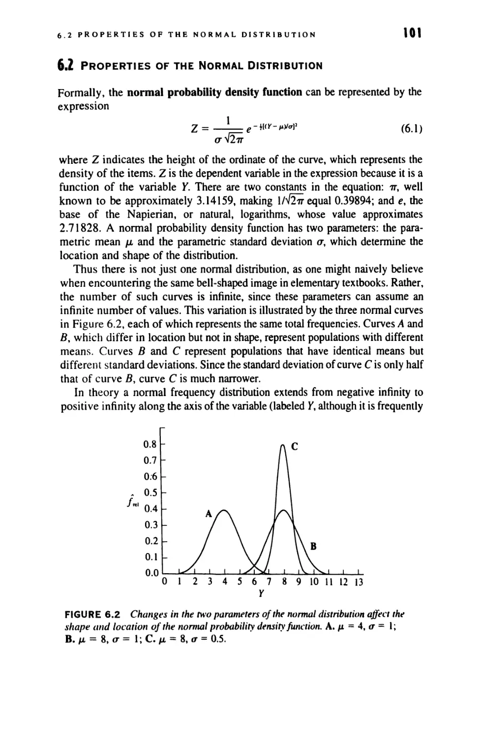
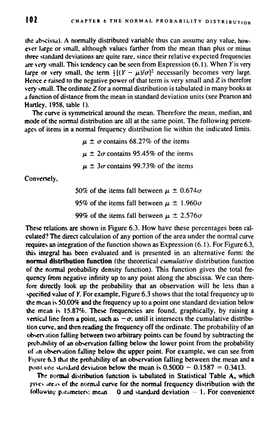
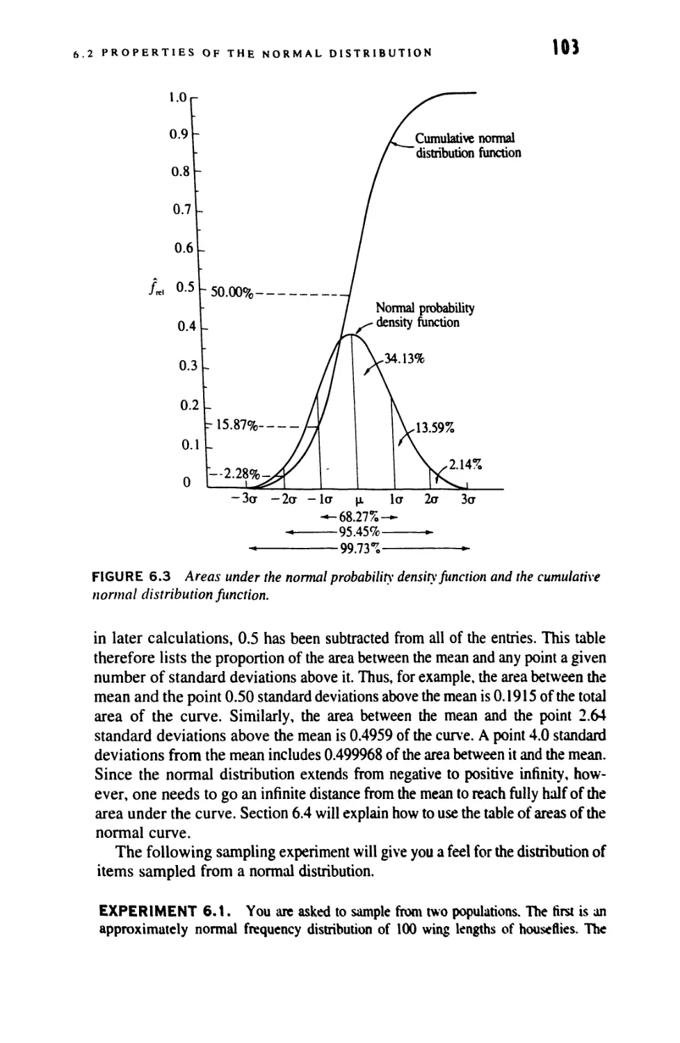
6.2 Properties of the Normal Distribution 101
6.3 A Model for the Normal Distribution 106
6.4 Applications of the Normal Distribution 109
6.5 Fitting a Normal Distribution to Observed Data 111
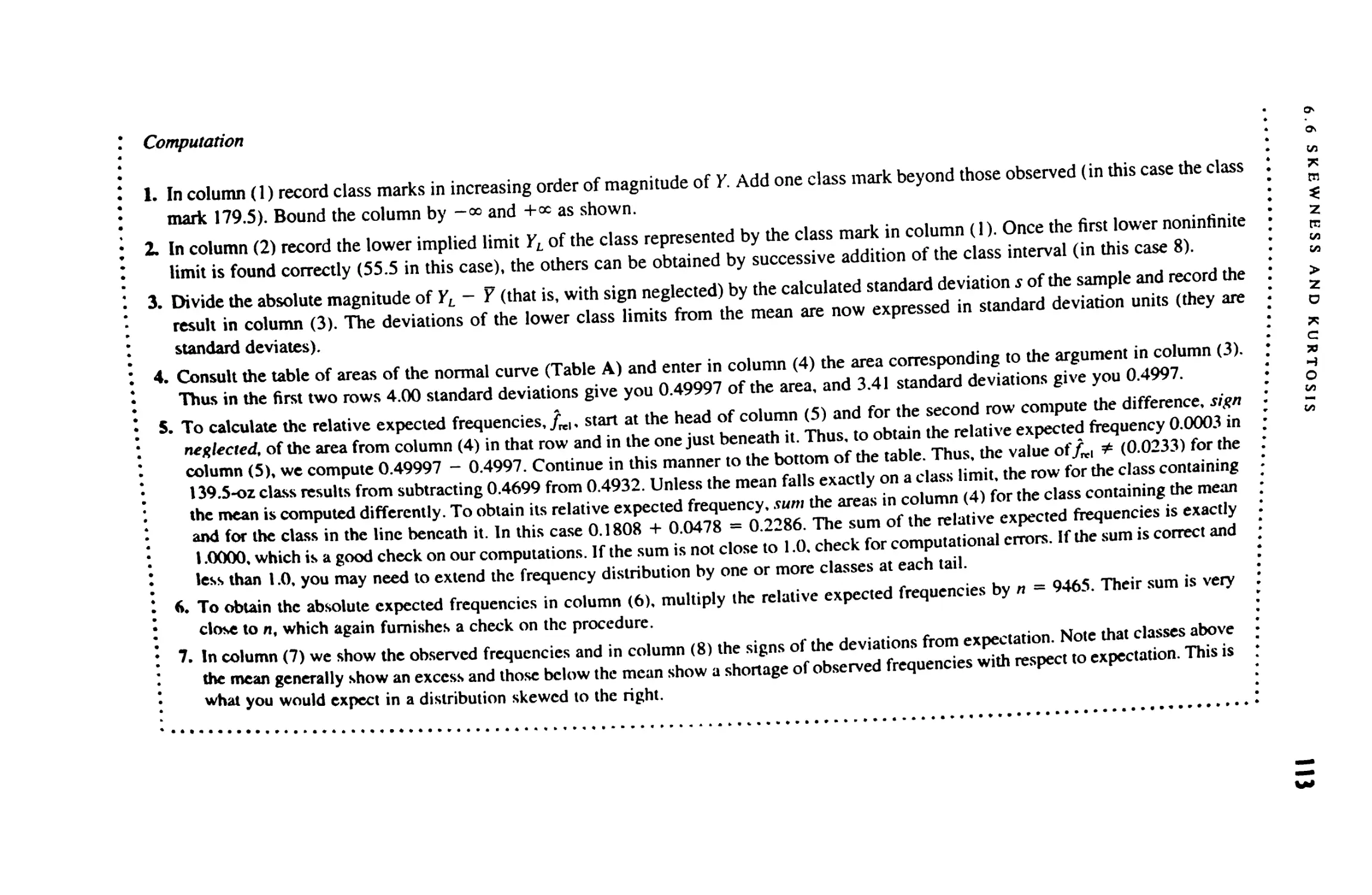
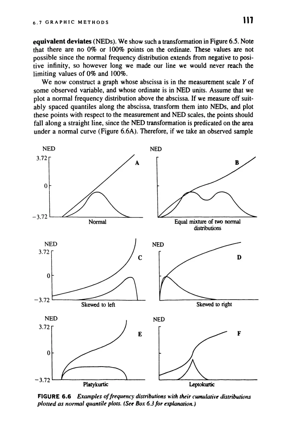
6.6 Skewness and Kurtosis 111
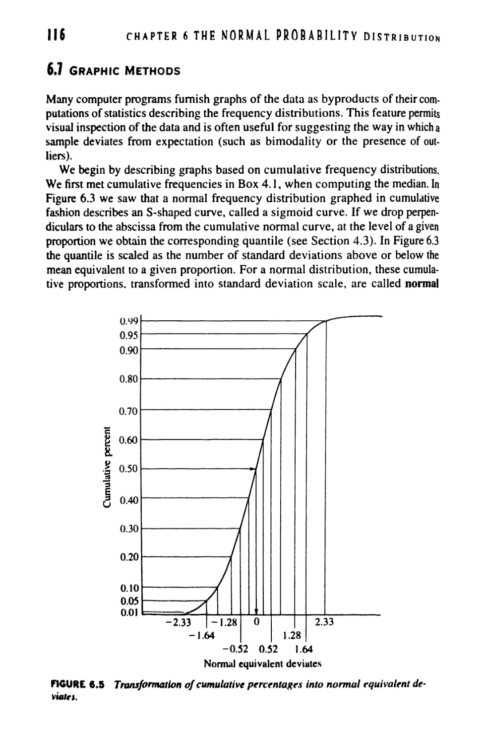
6.7 Graphic Methods 116
6.8 Other Continuous Distributions 123
7 ESTIMATION AND HYPOTHESIS TESTING 127
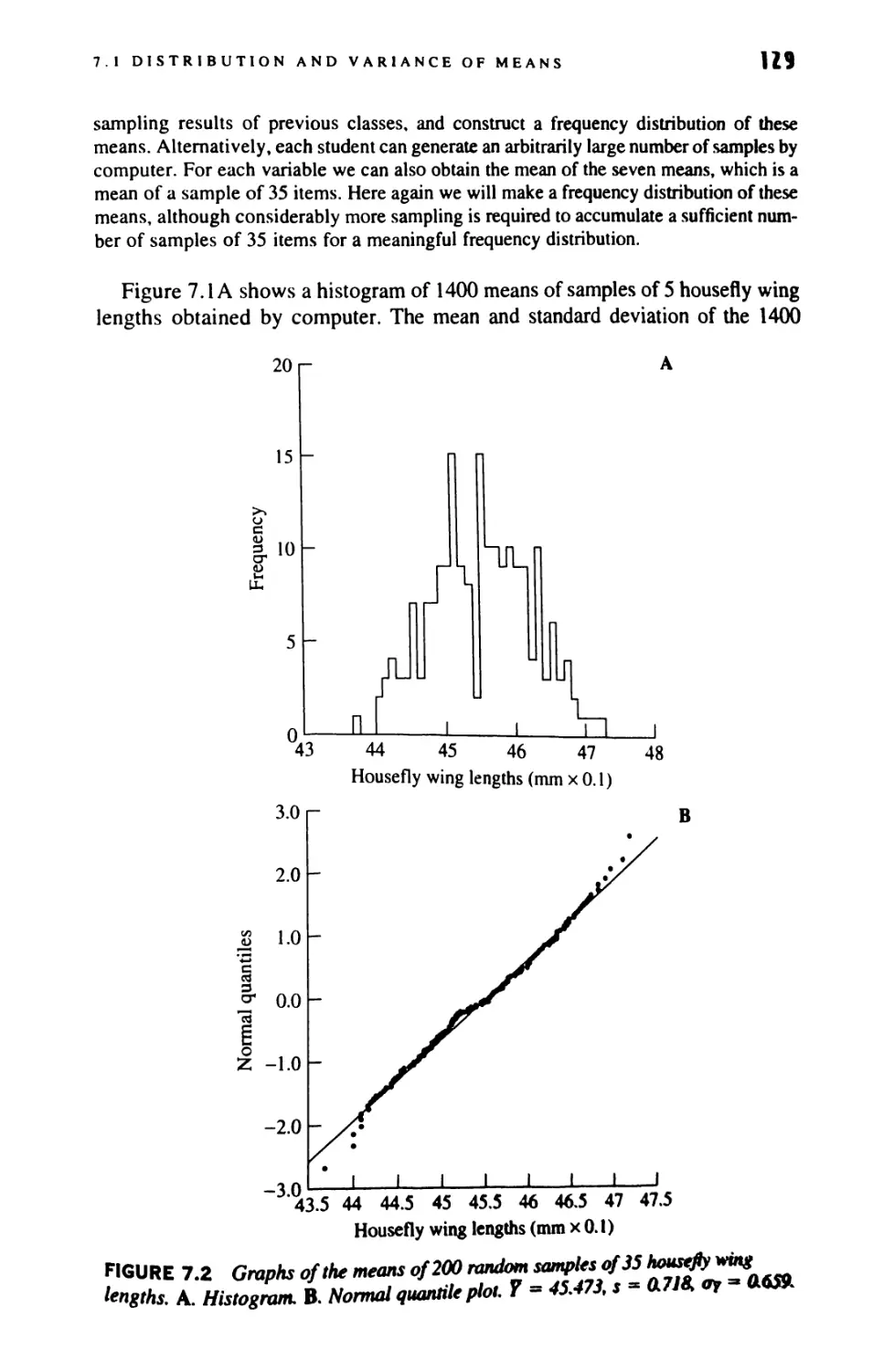
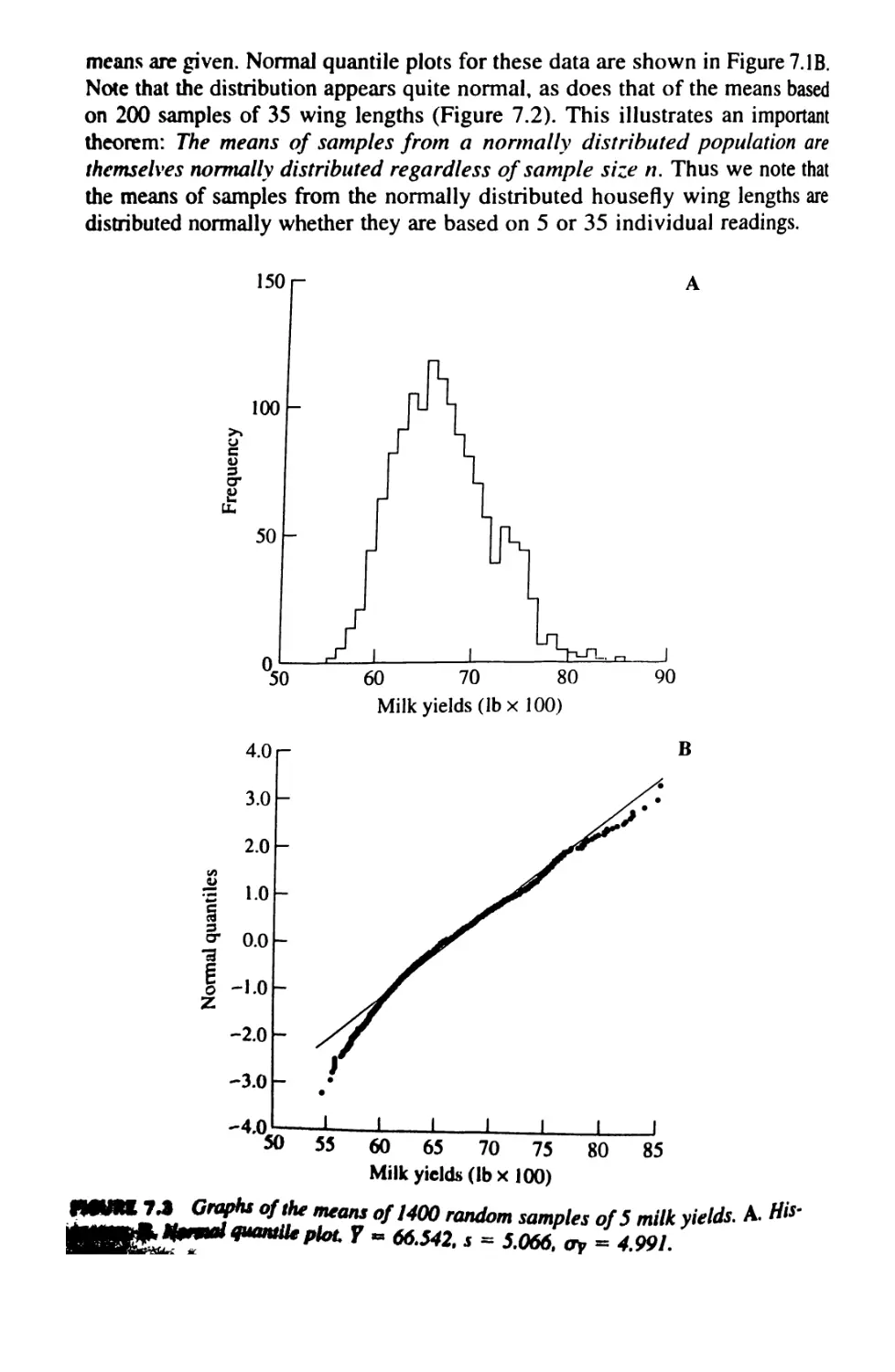
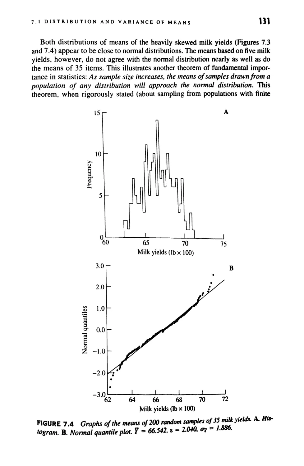
7.1 Distribution and Variance of Means 128
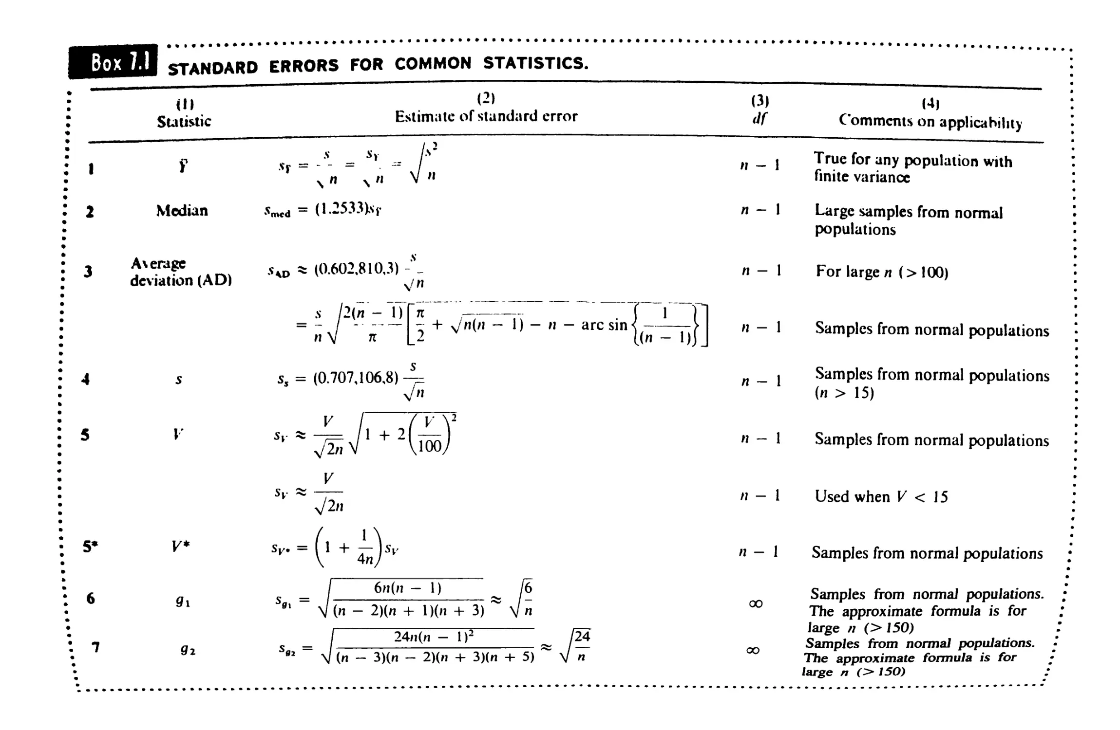
7.2 Distribution and Variance of Other Statistics 136
7.3 Introduction to Confidence Limits 139
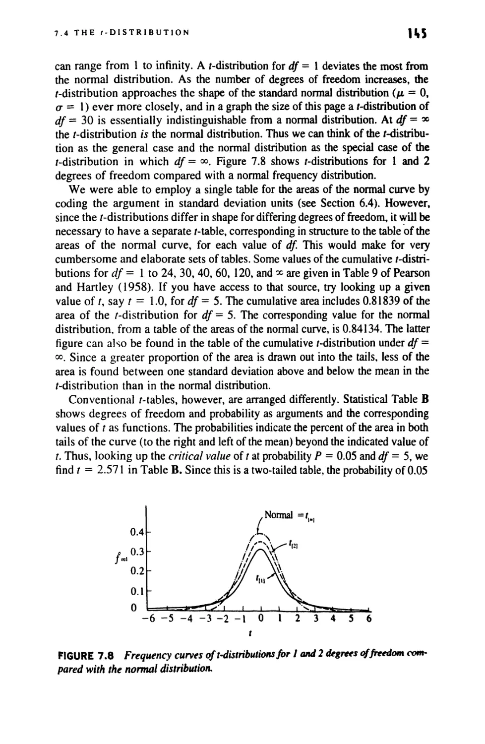
7.4 The /-Distribution 143
7.5 Confidence Limits Based on Sample Statistics 146
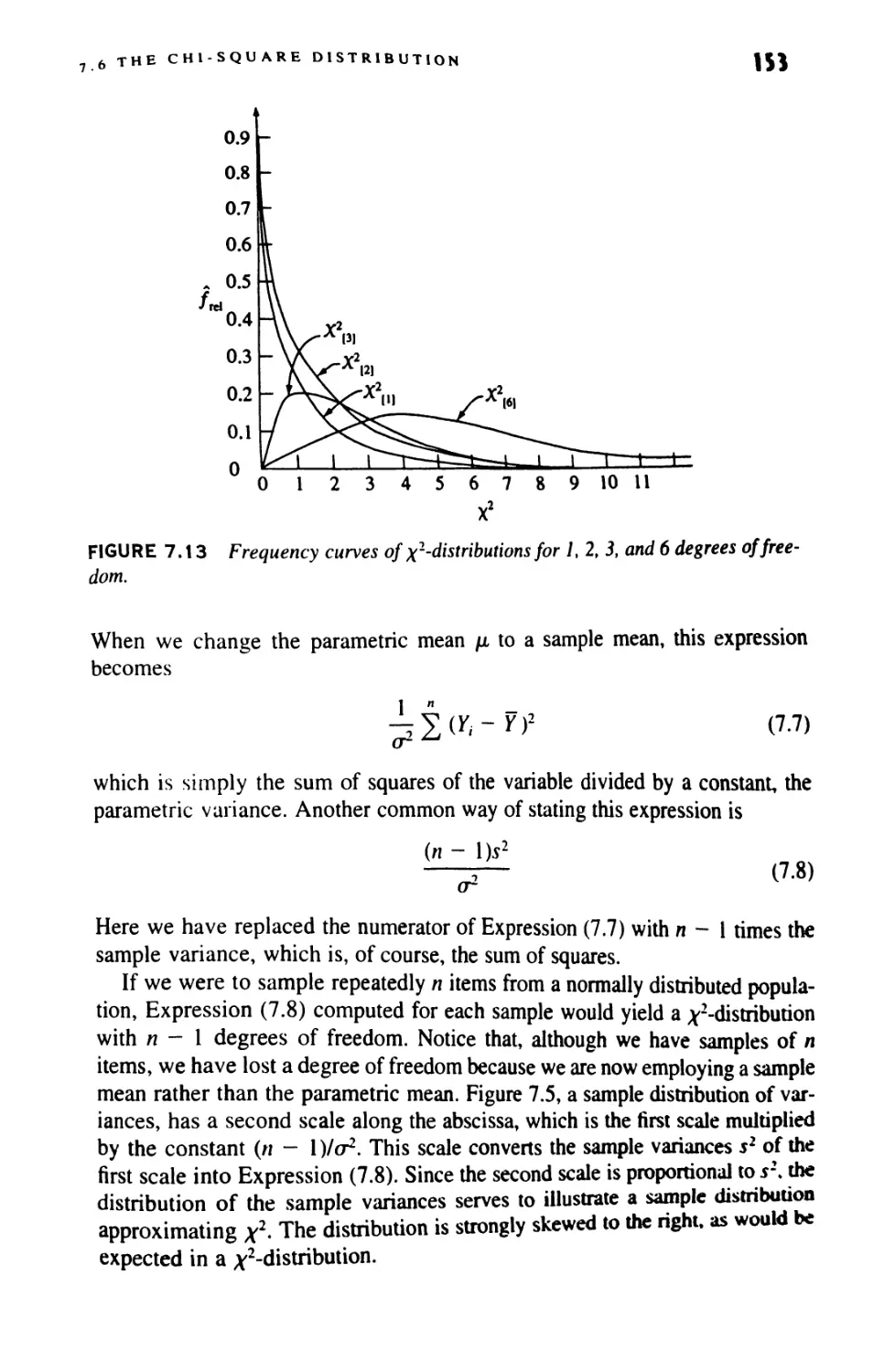
7.6 The Chi-Square Distribution 152
7.7 Confidence Limits for Variances 154
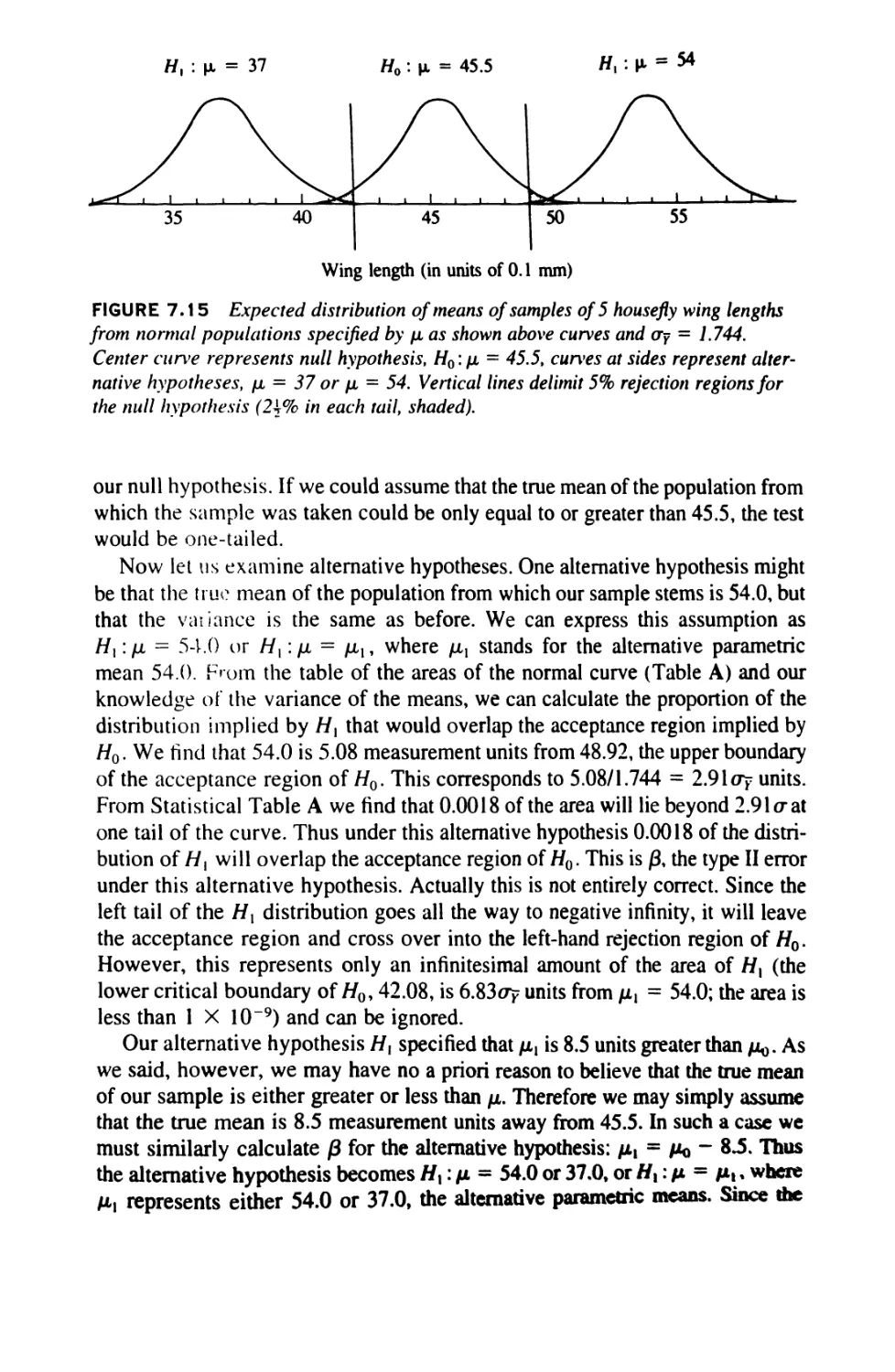
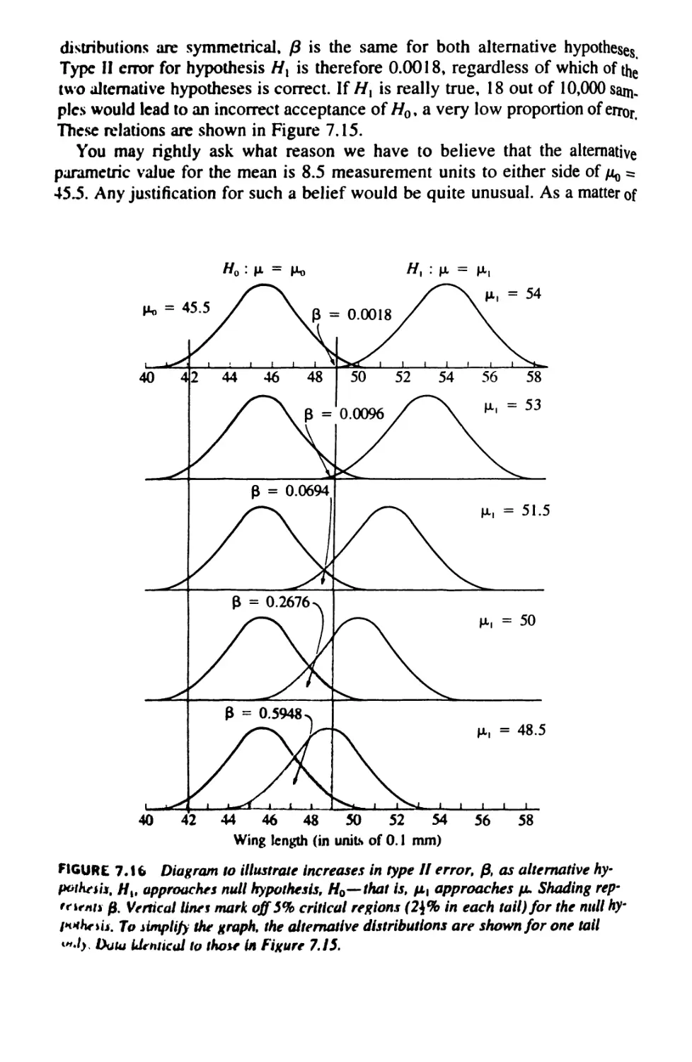
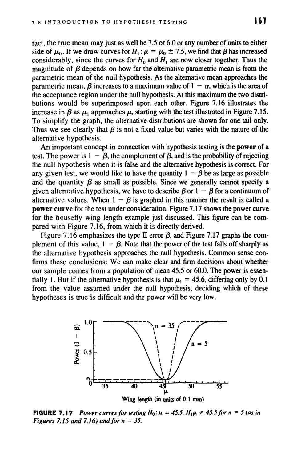
7.8 Introduction to Hypothesis Testing 157
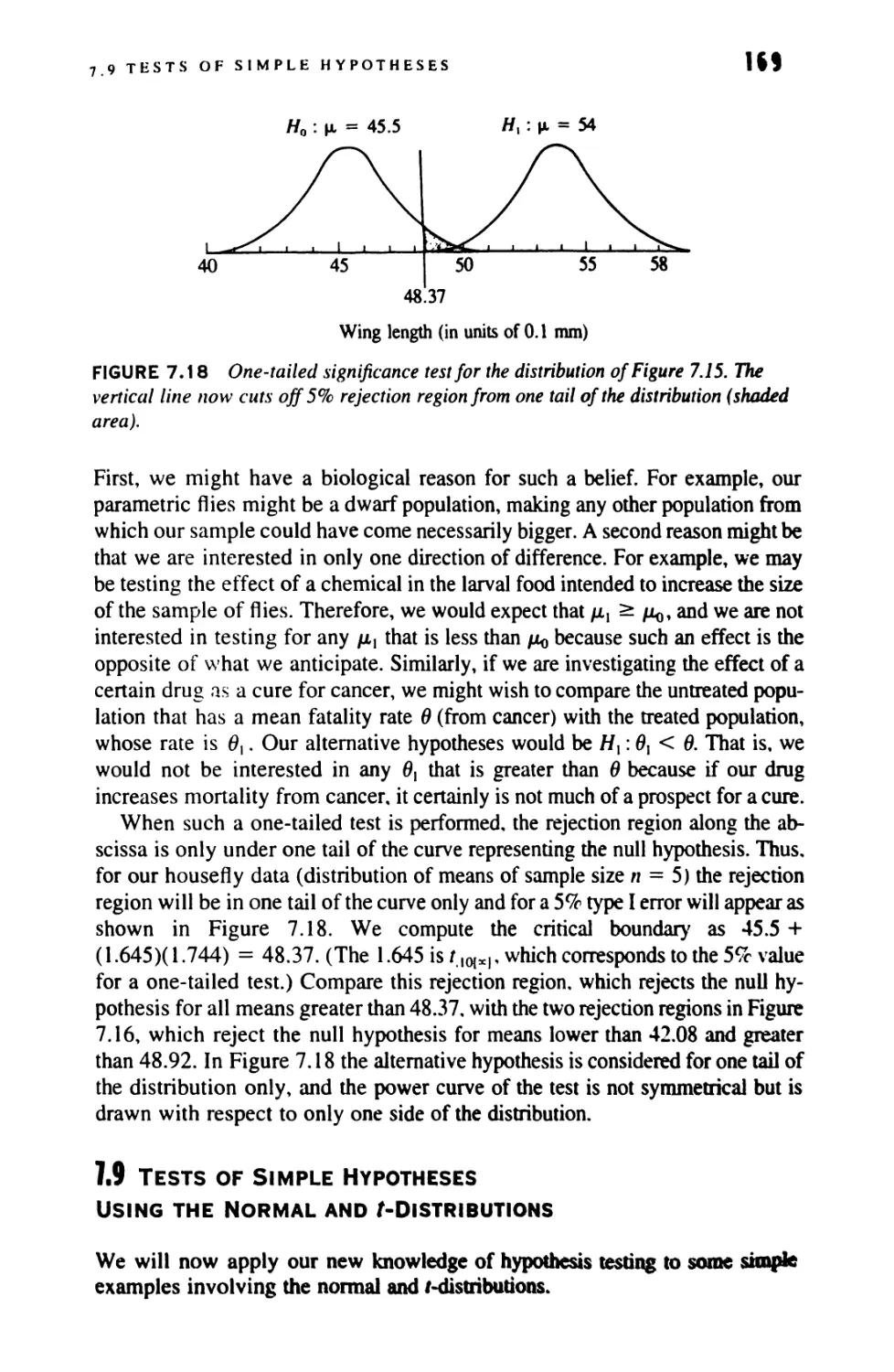
7.9 Tests of Simple Hypotheses Using the Normal and
/-Distributions 169
7.10 Testing the Hypothesis H0: a2 = <j\ 175
8 INTRODUCTION TO THE ANALYSIS
OF VARIANCE 179
8.1 Variances of Samples and Their Means 180
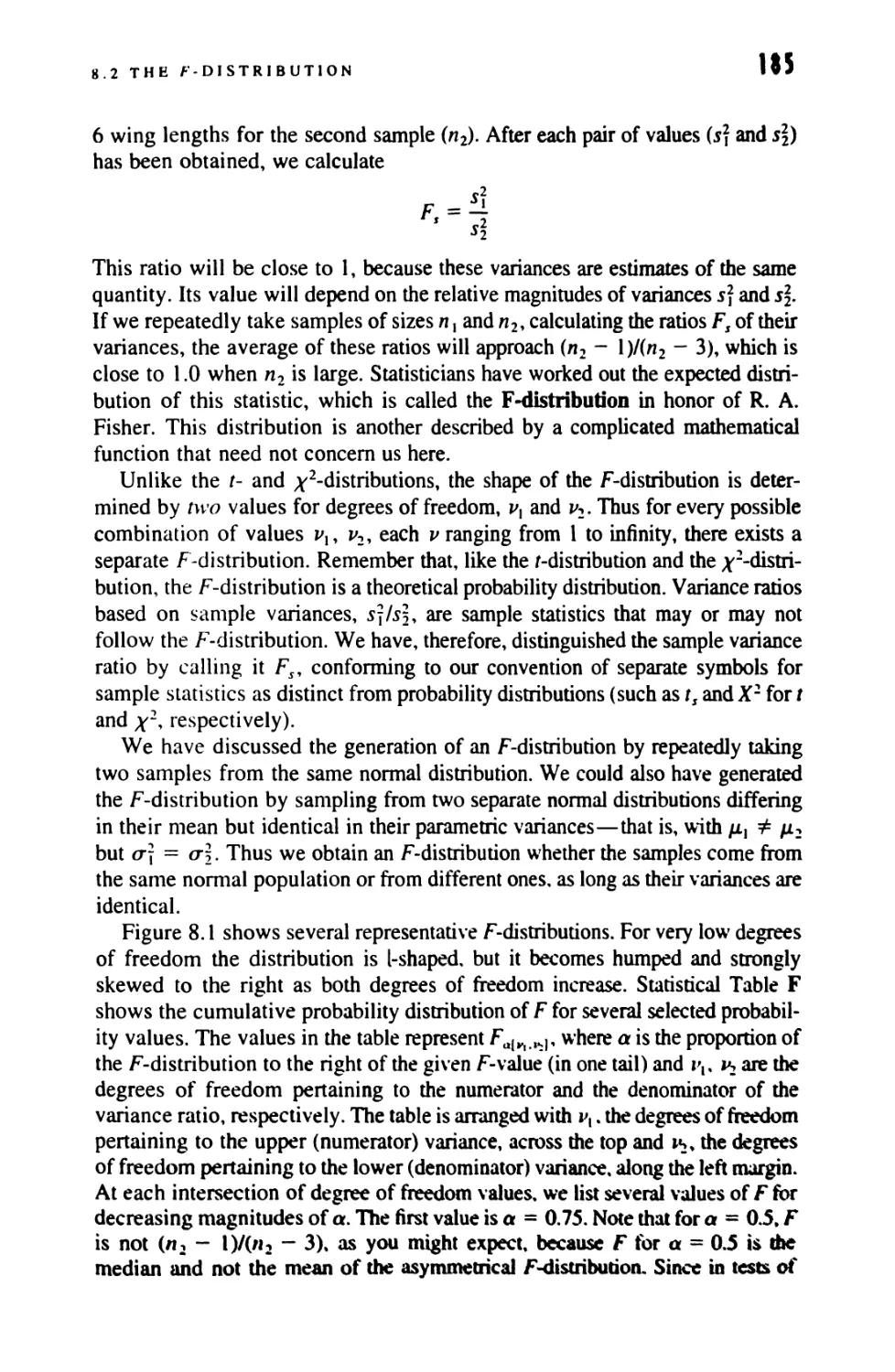
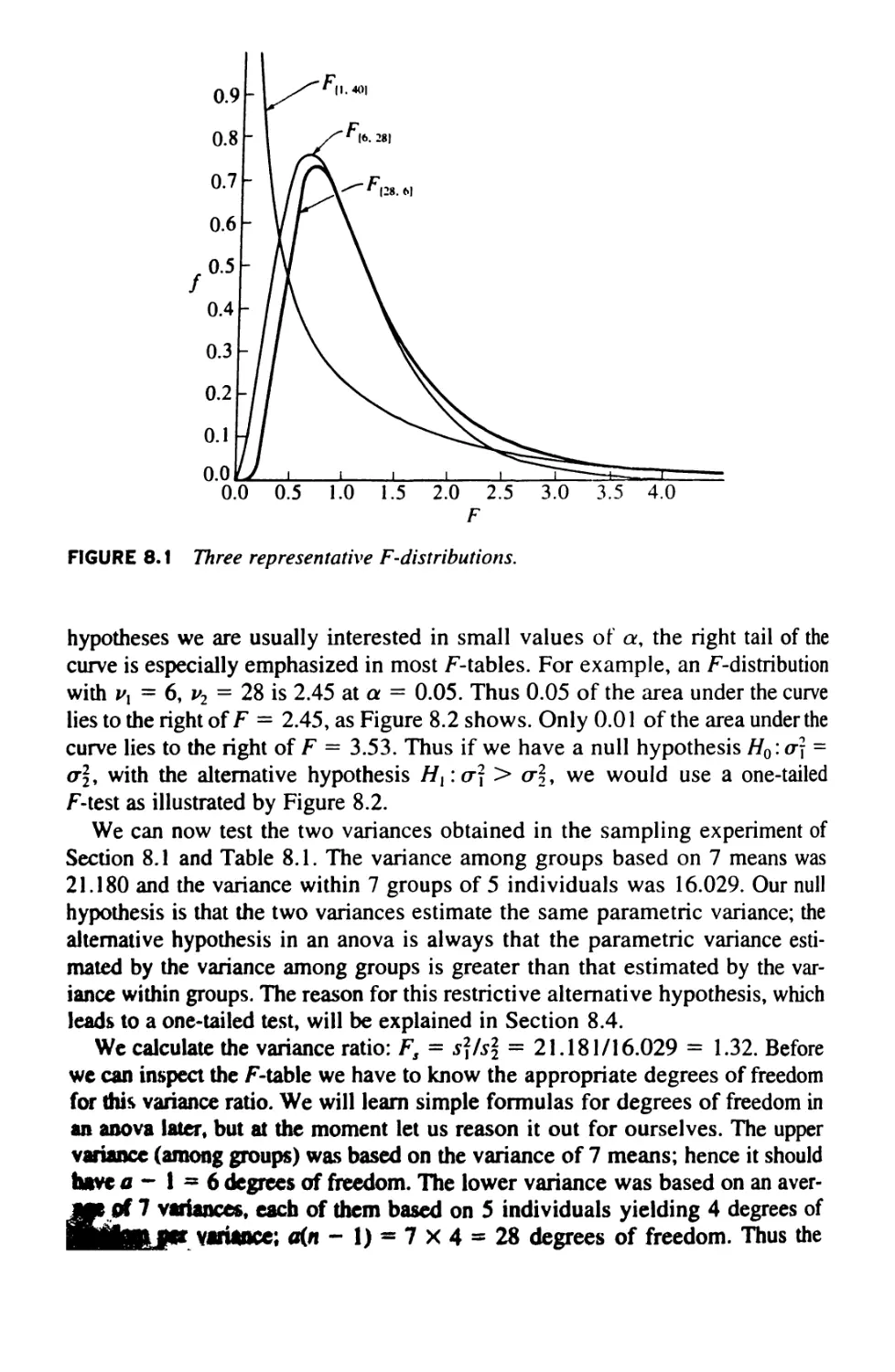
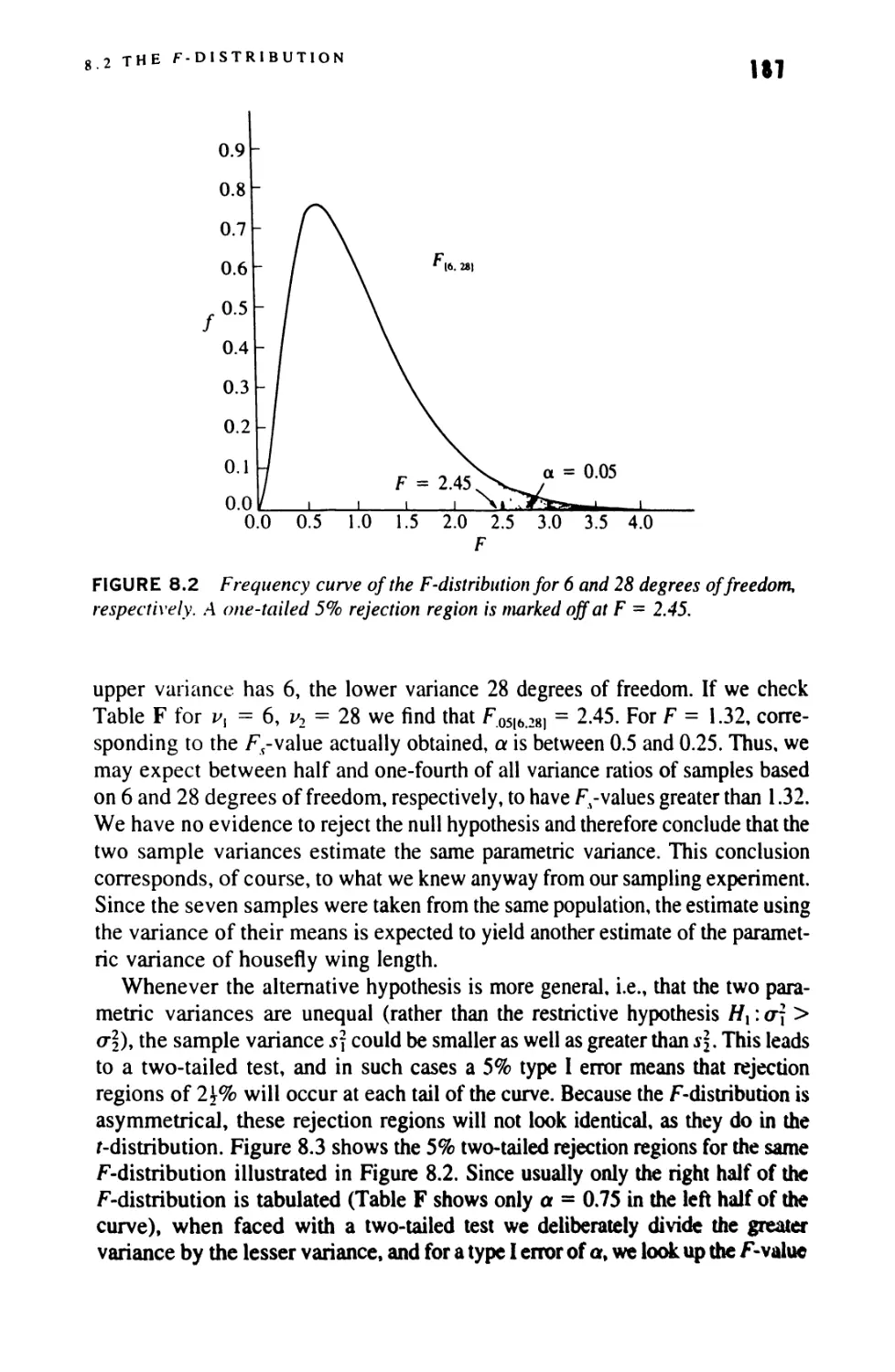
8.2 The F-Distribution 184
8.3 The Hypothesis H0: <r2= <r\ 189
s
ix
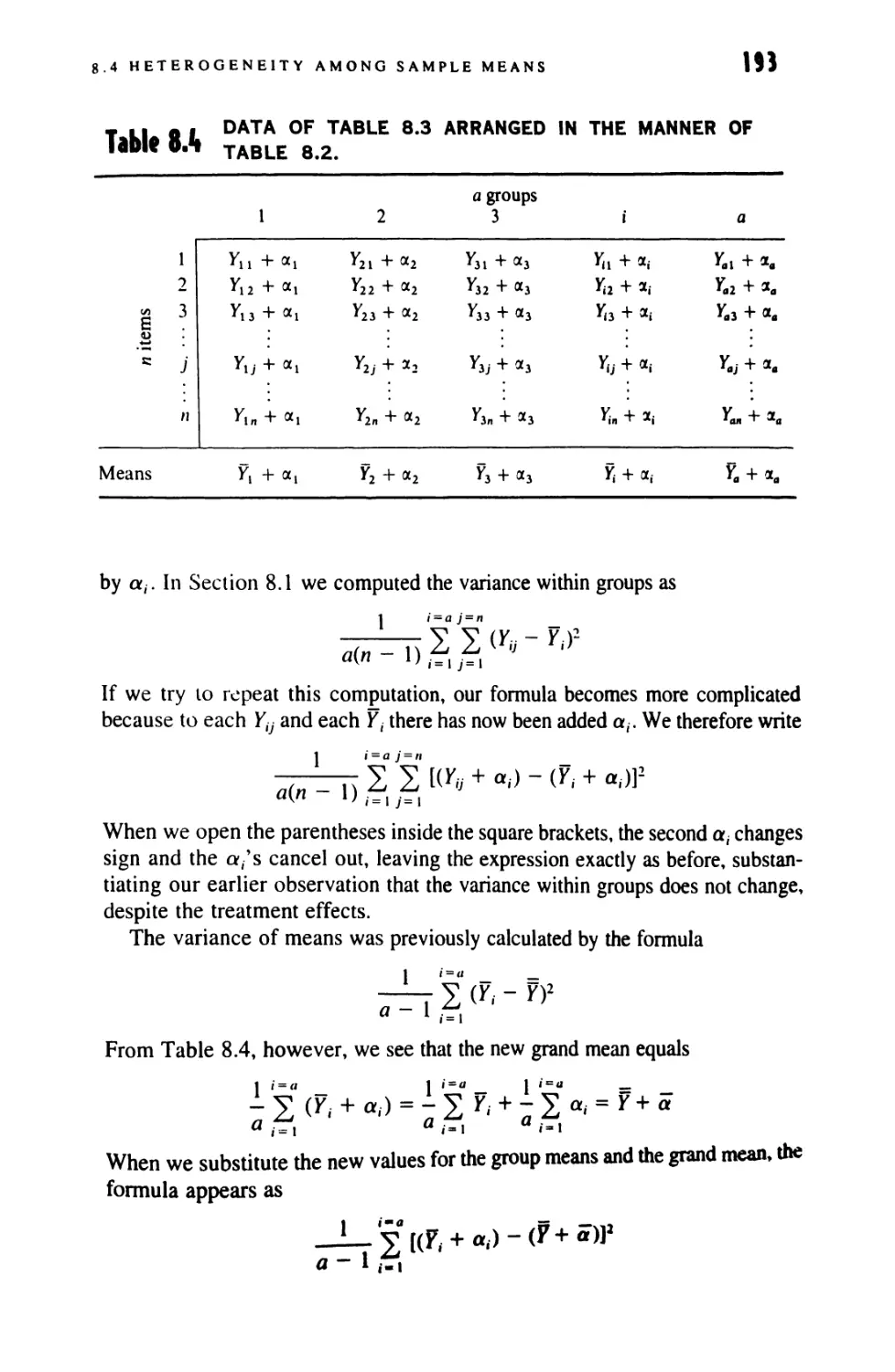
8.4
8.5
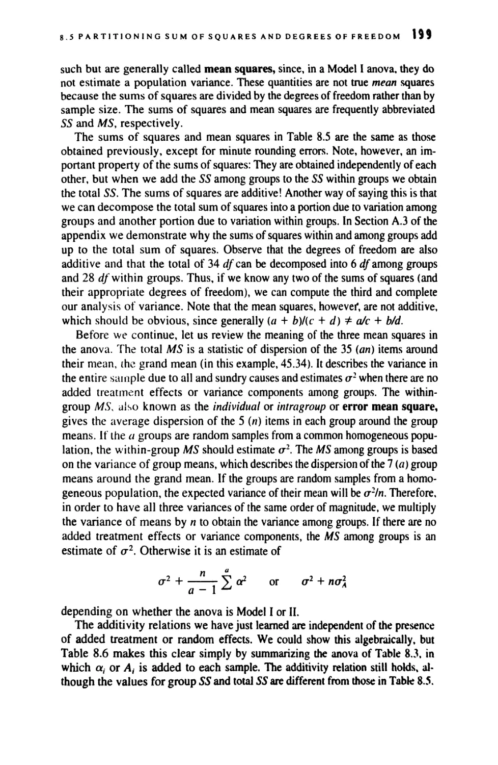
8.6
8.7
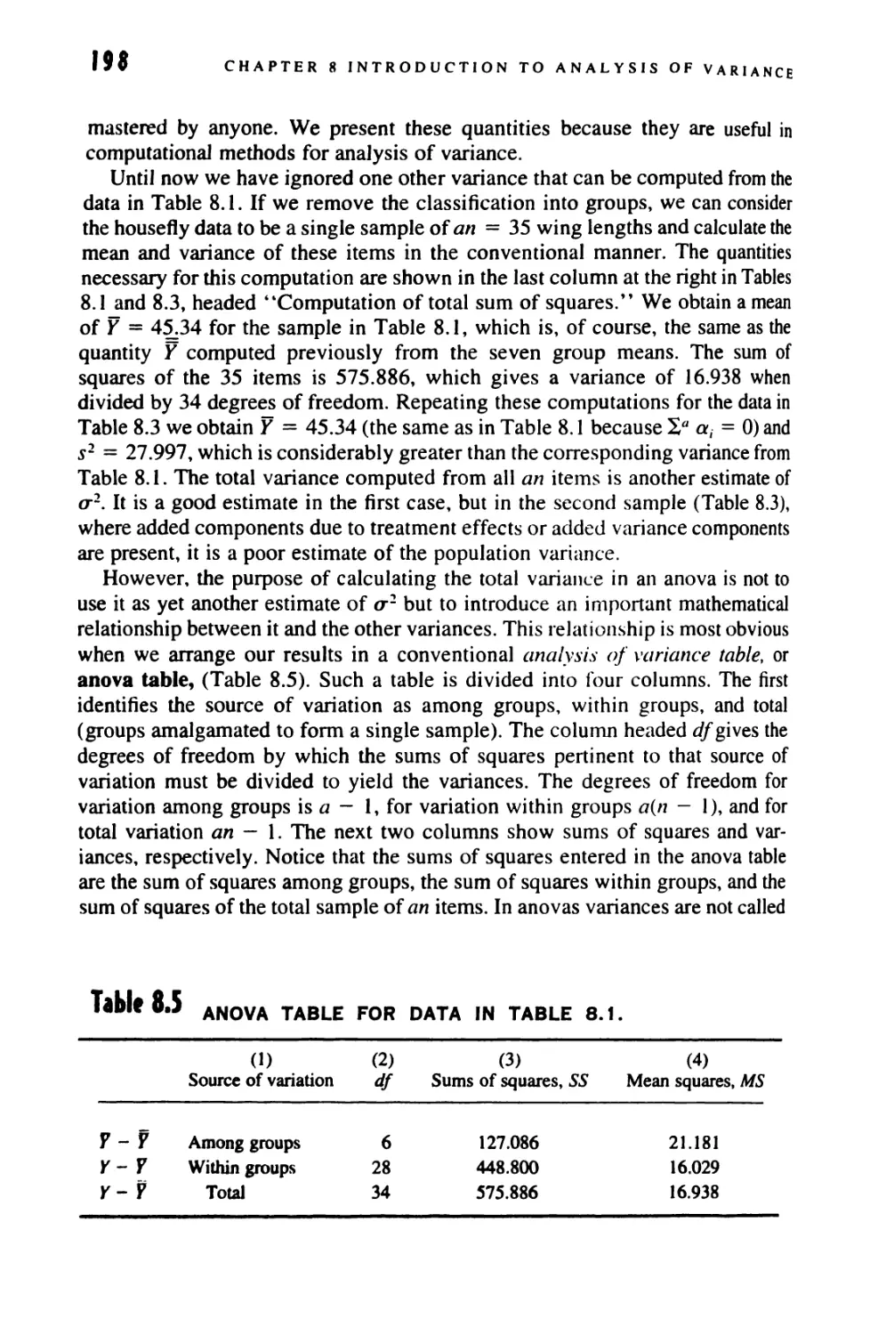
Heterogeneity Among Sample Means
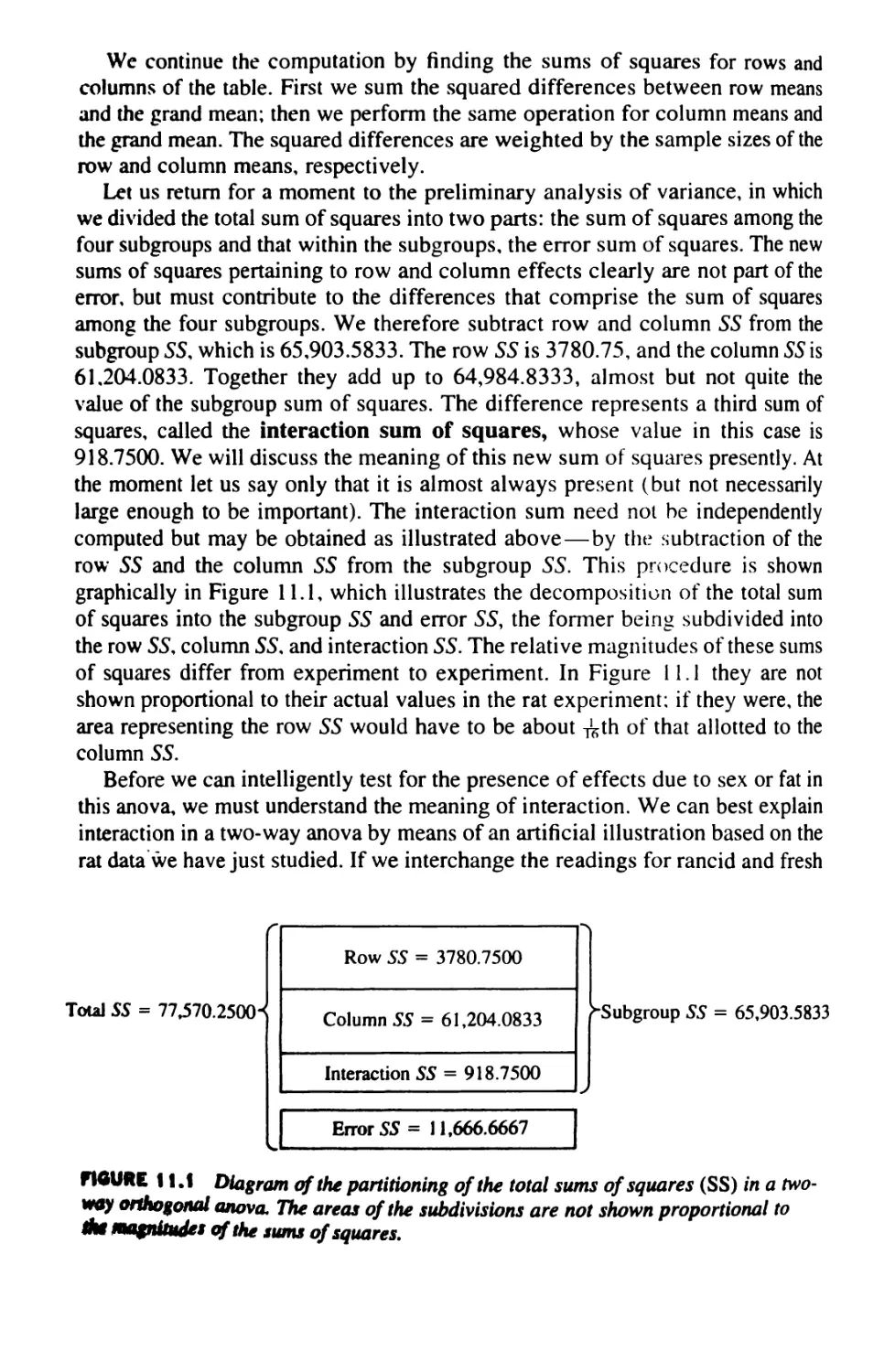
Partitioning the Total Sum of Squares and Degrees
of Freedom
Model 1 Anova
Model 11 Anova
190
197
201
203
9 SINGLE-CLASSIFICATION ANALYSIS
OF VARIANCE 207
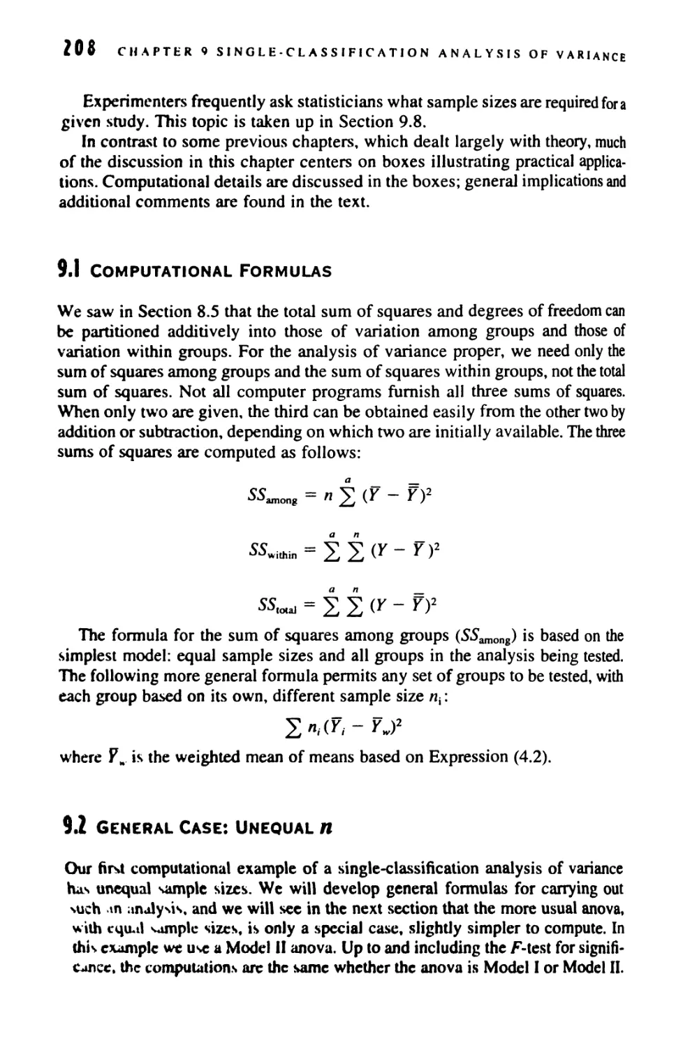
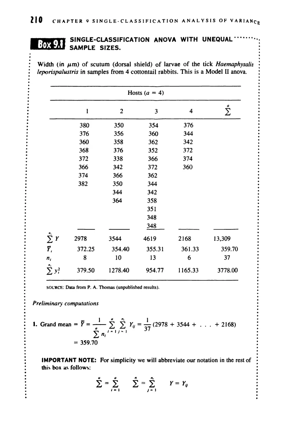
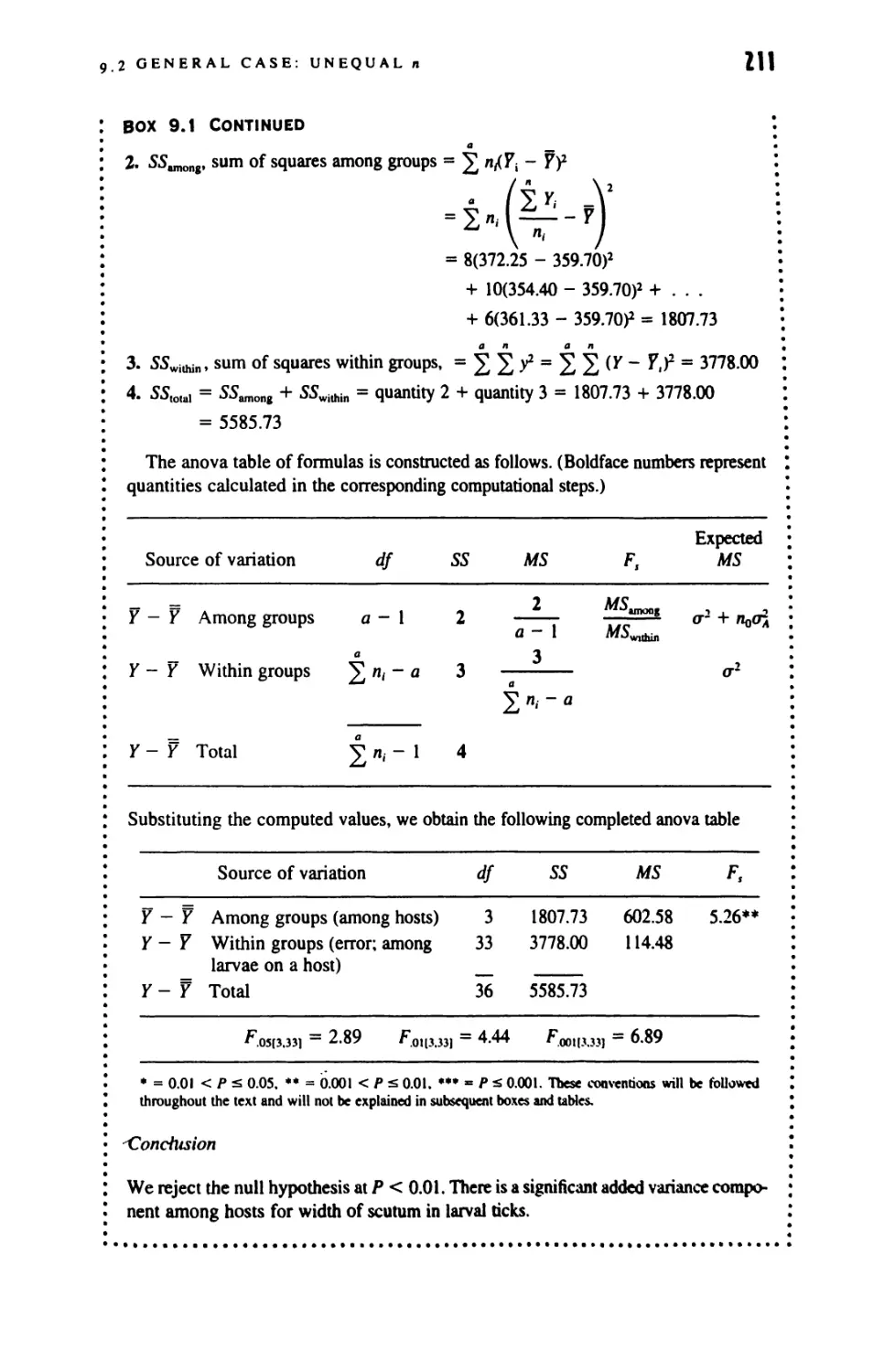
9.1 Computational Formulas 208
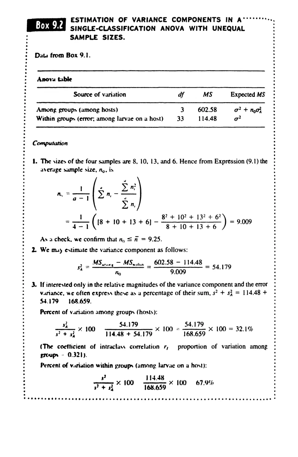
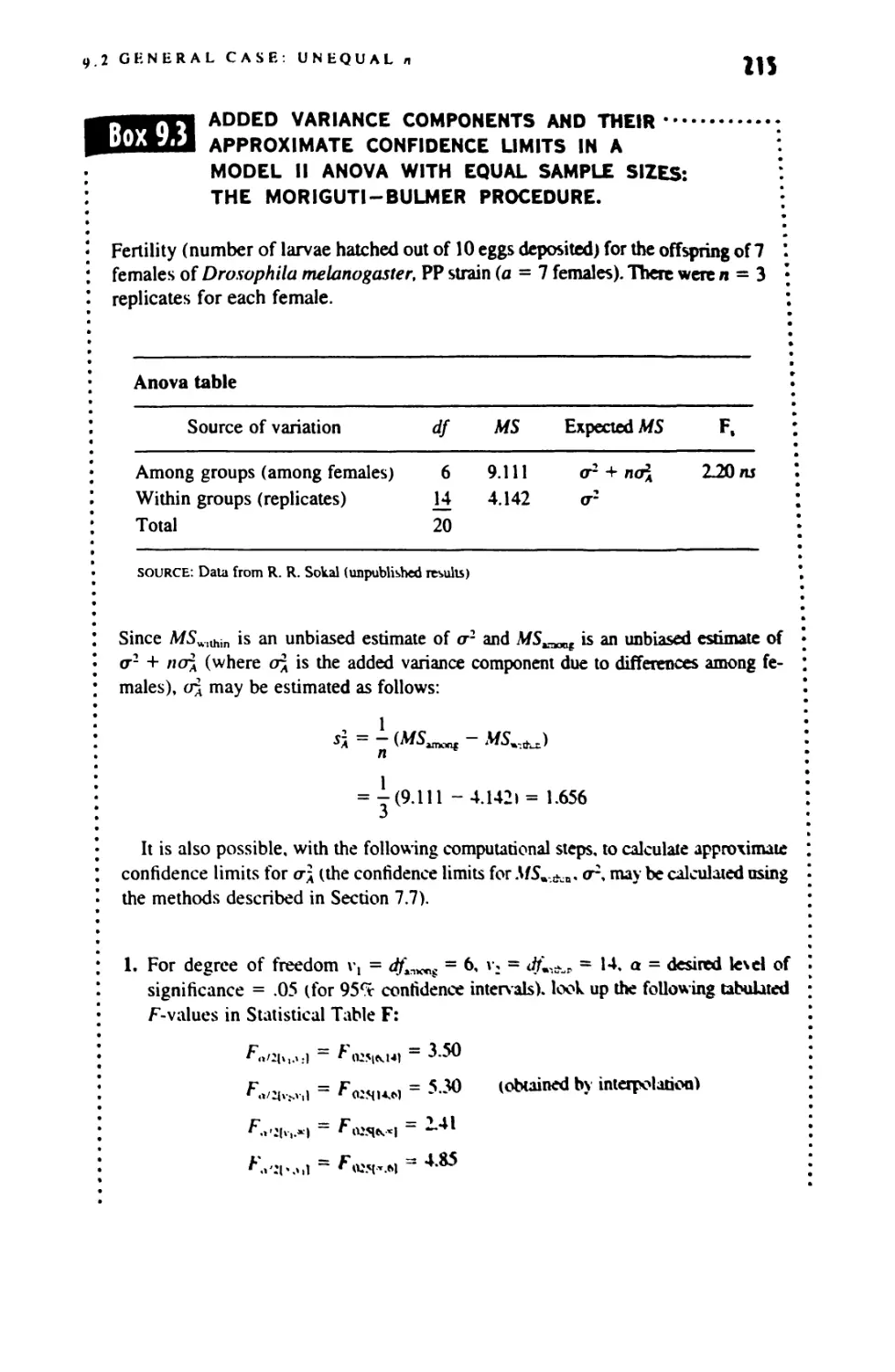
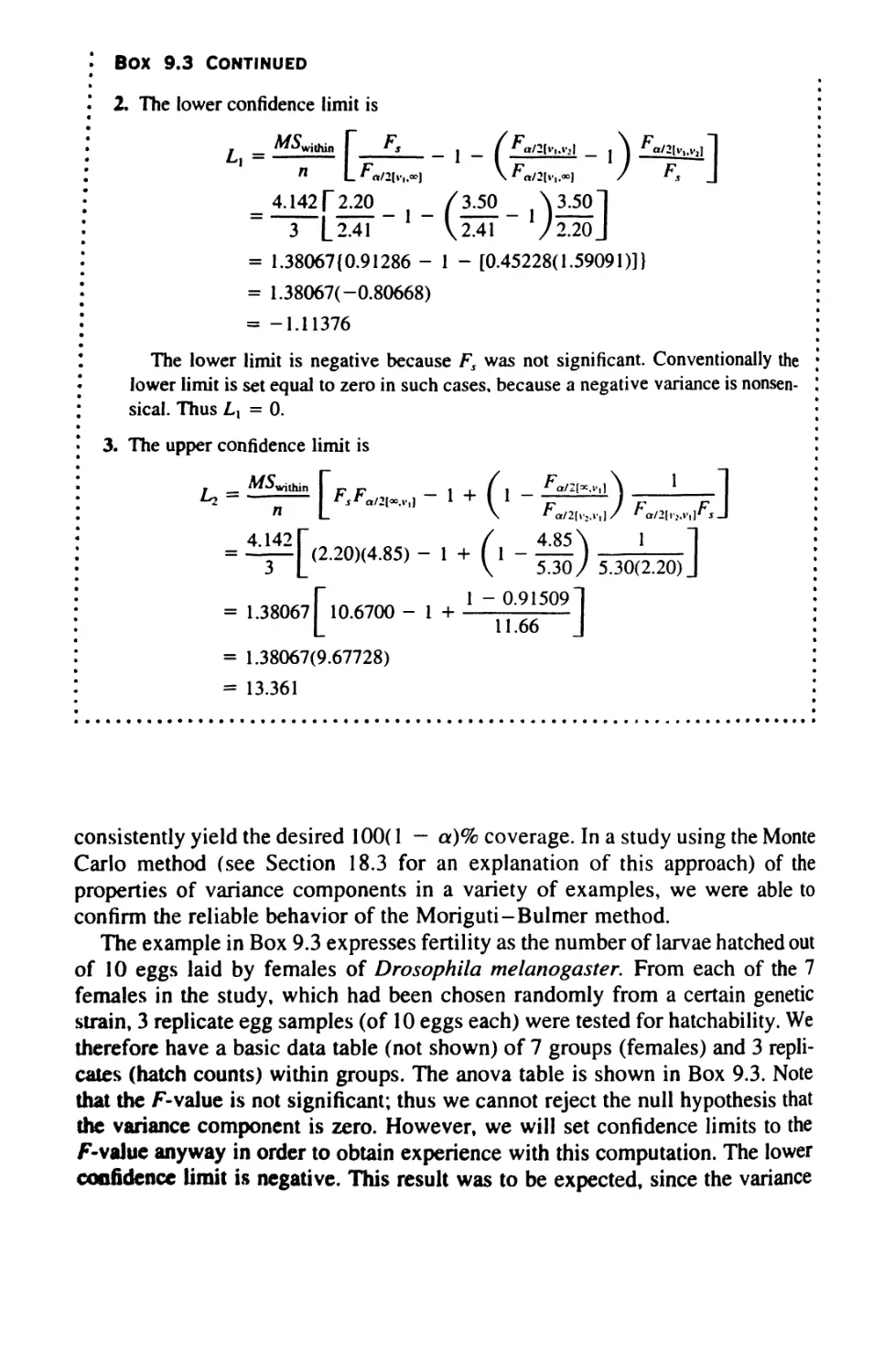
9.2 General Case: Unequal n 208
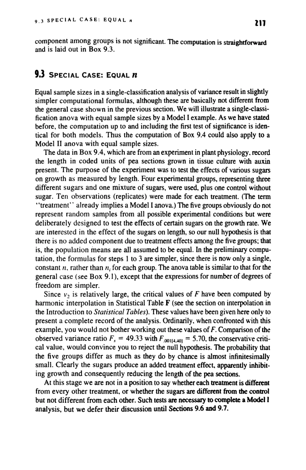
9.3 Special Case: Equal n 217
9.4 Special Case: Two Groups 219
9.5 Special Case: A Single Specimen Compared
With a Sample 227
9.6 Comparisons Among Means: Planned Comparisons 229
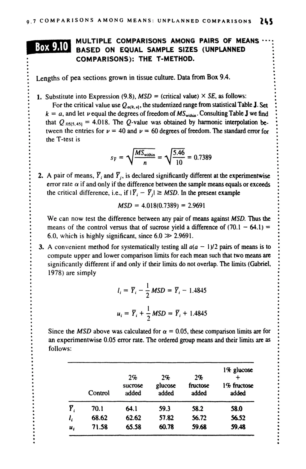
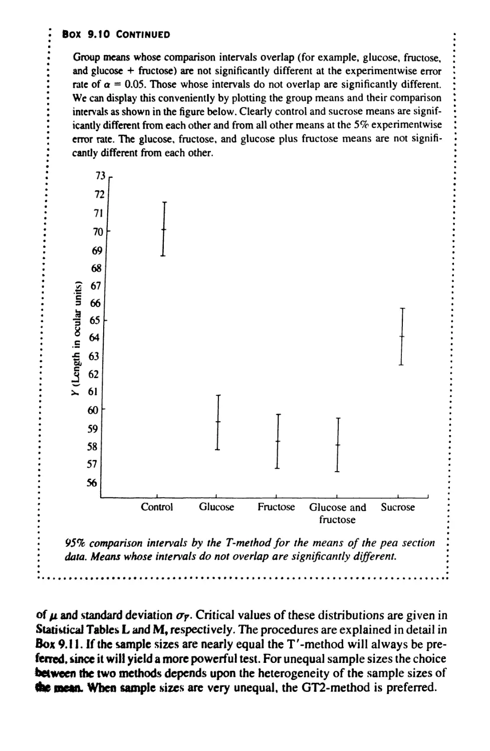
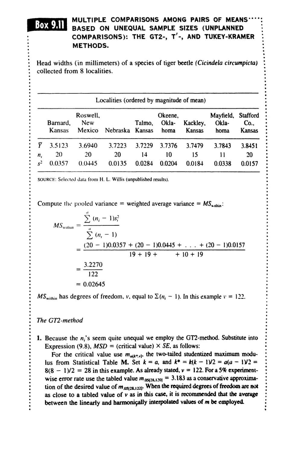
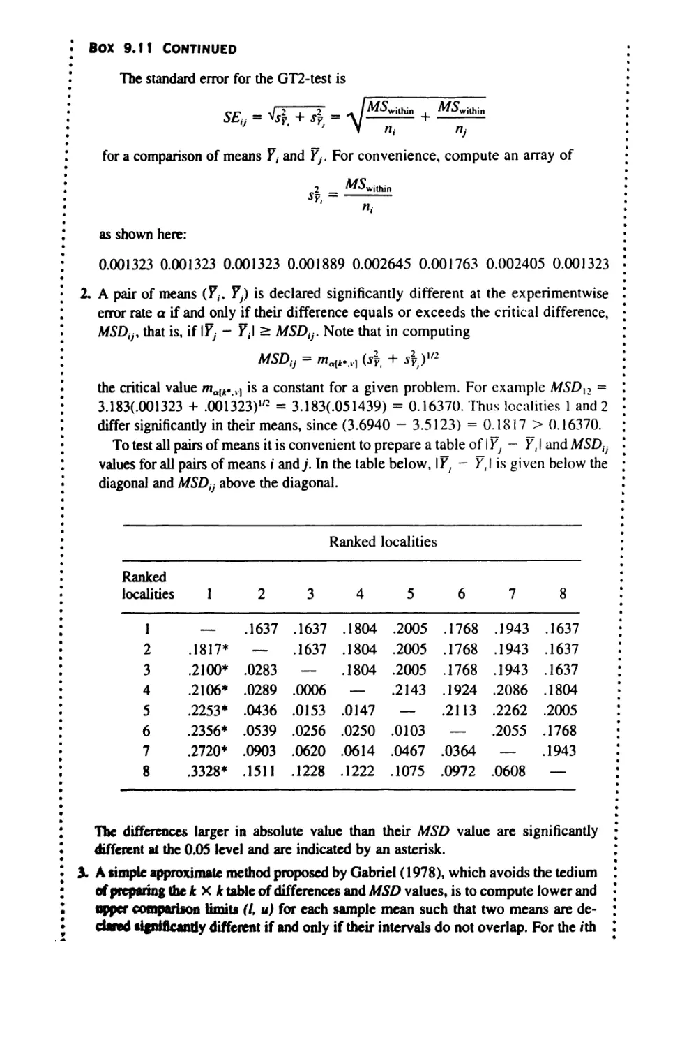
9.7 Comparisons Among Means: Unplanned Comparisons 240
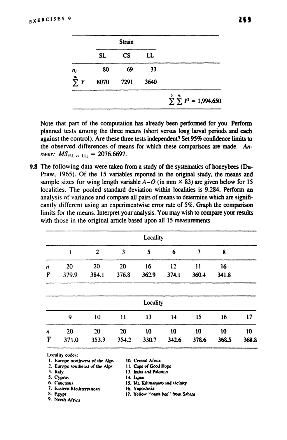
9.8 Finding the Sample Size Required for a Test 260
10 NESTED ANALYSIS OF VARIANCE 272
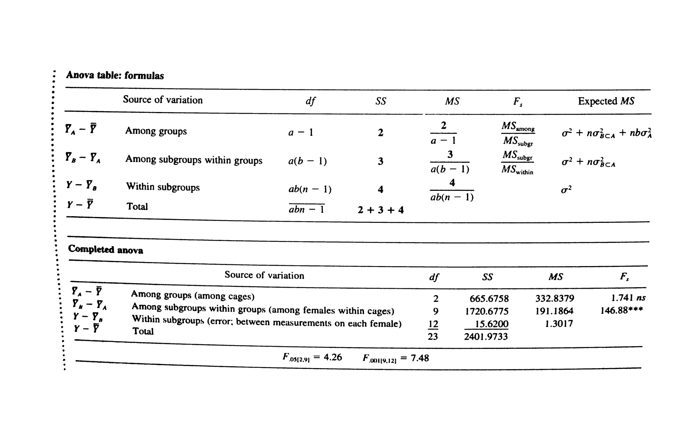
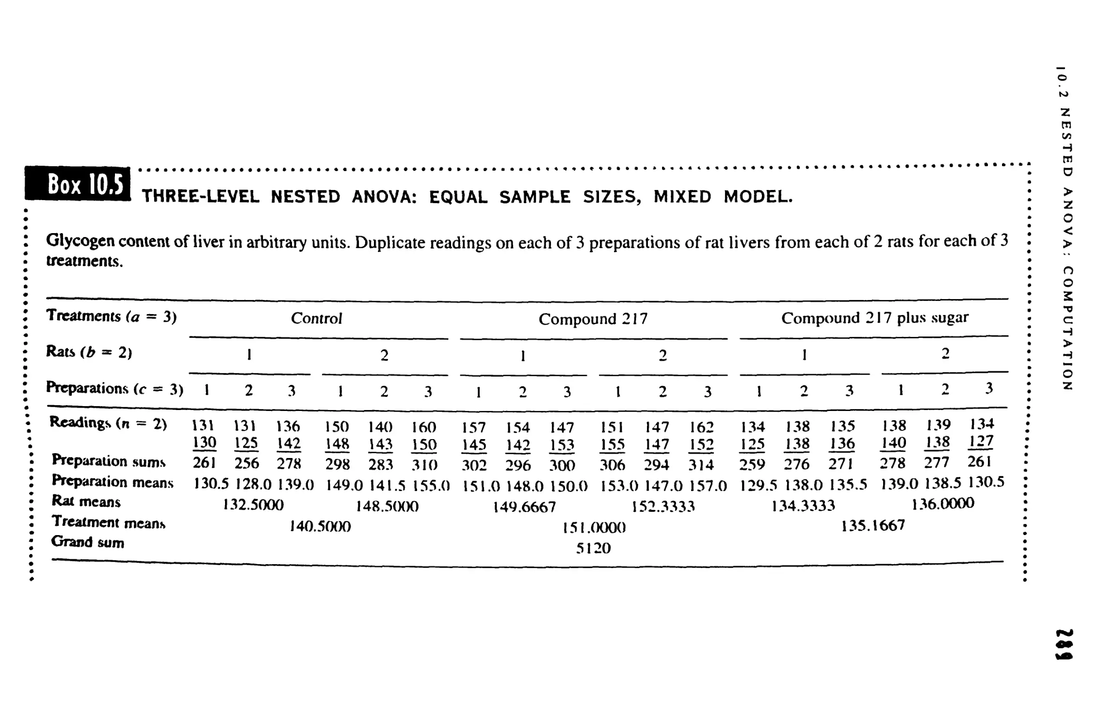
10.1 Nested Anova: Design 272
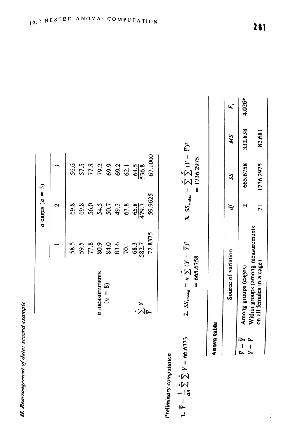
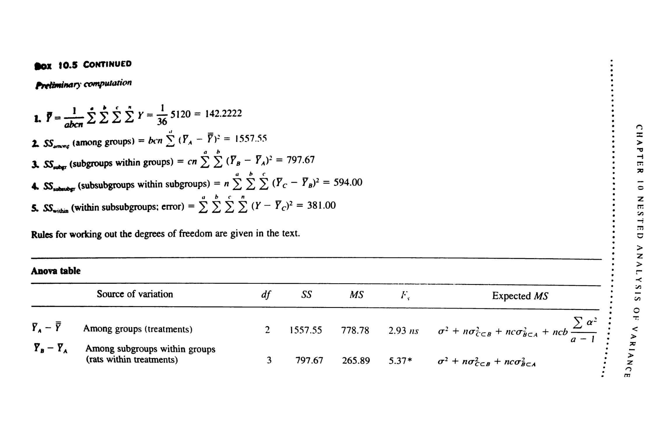
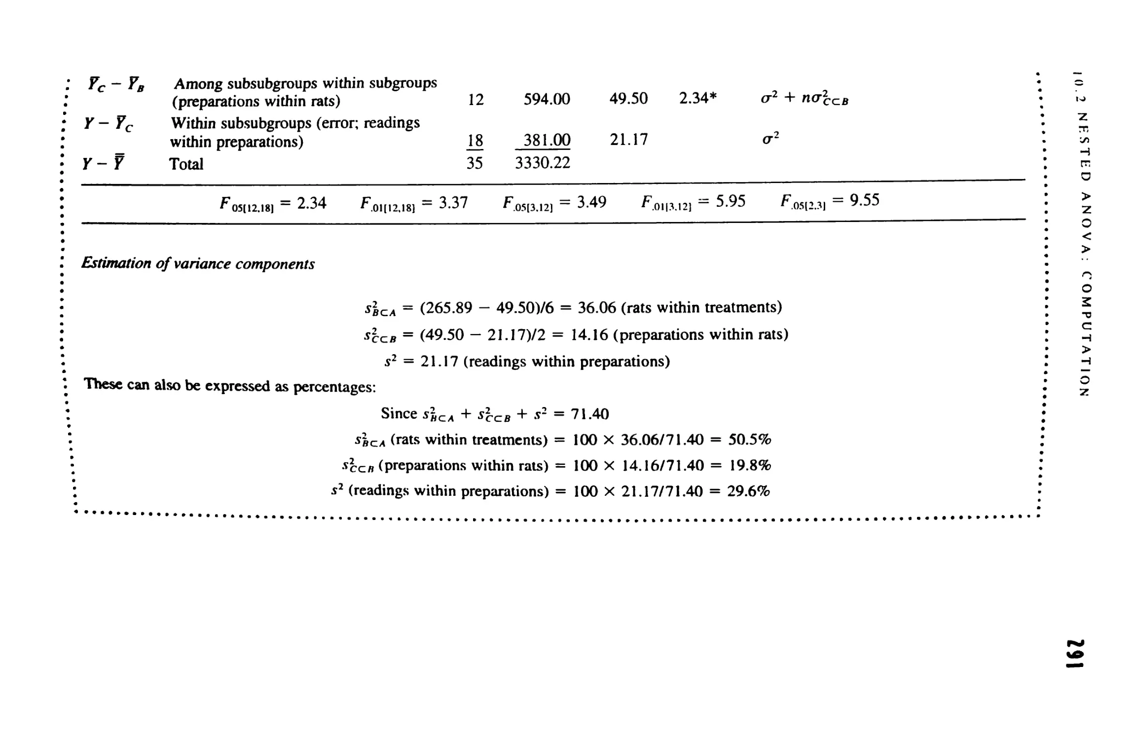
10.2 Nested Anova: Computation 275
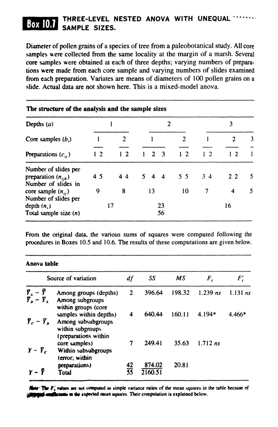
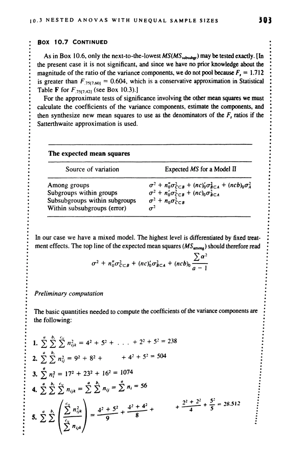
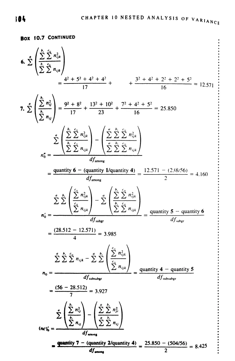
10.3 Nested Anovas With Unequal Sample Sizes 292
10.4 The Optimal Allocation of Resources 309
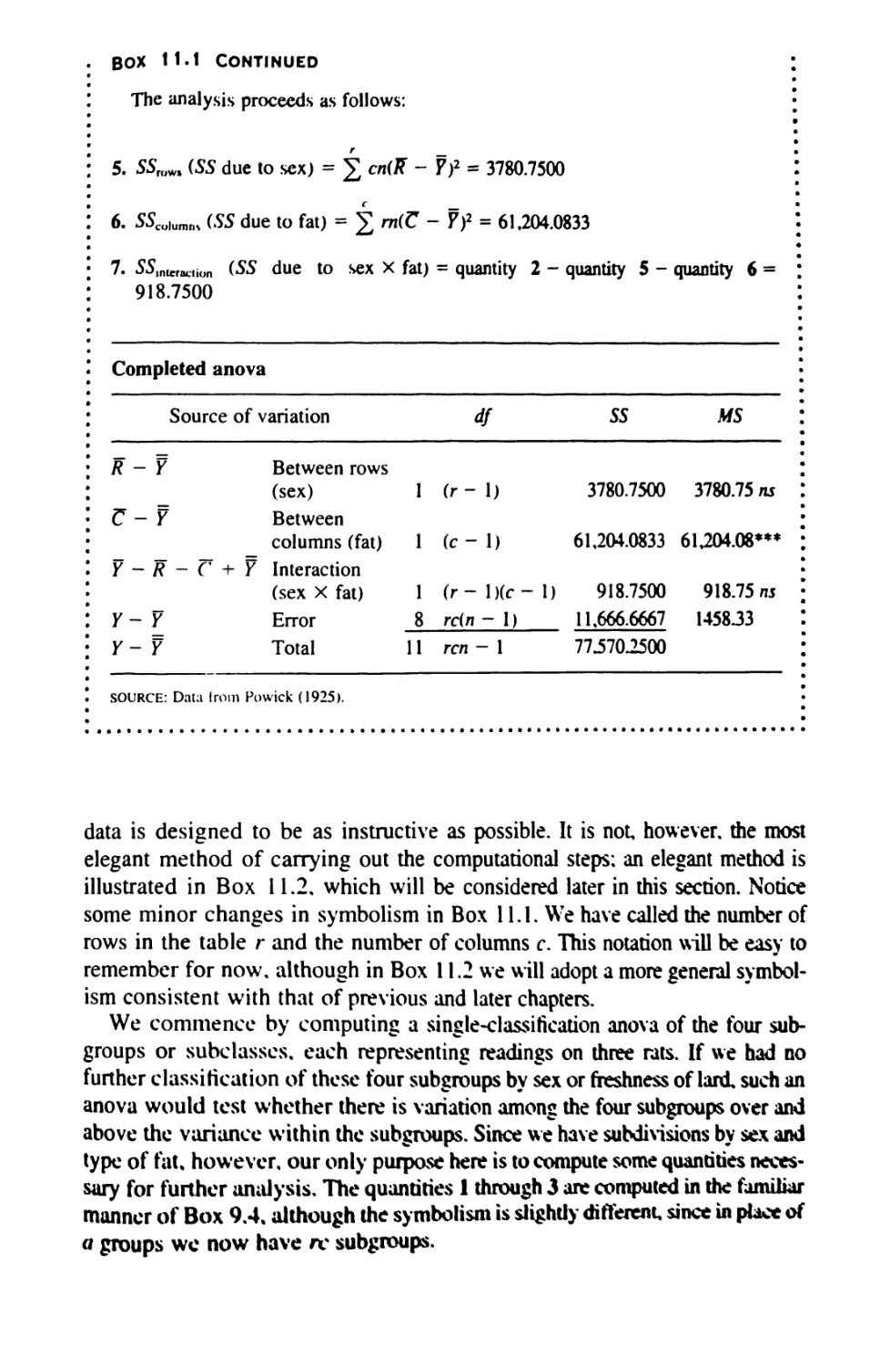
11 TWO-WAY ANALYSIS OF VARIANCE 321
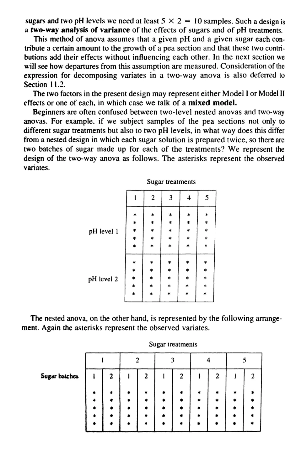
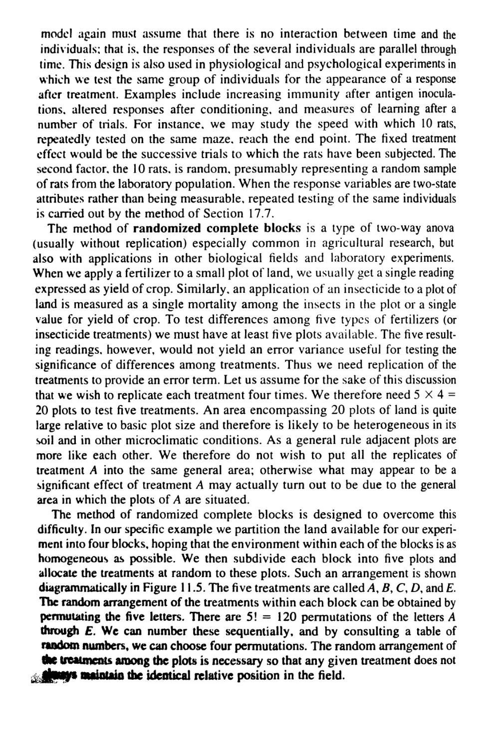
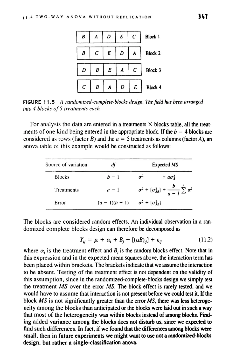
11.1 Two-Way Anova: Design 321
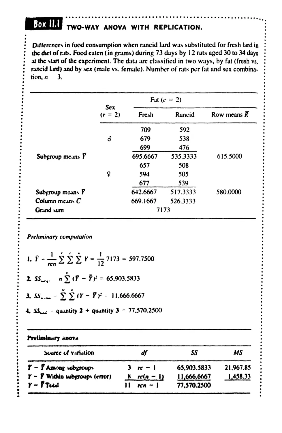
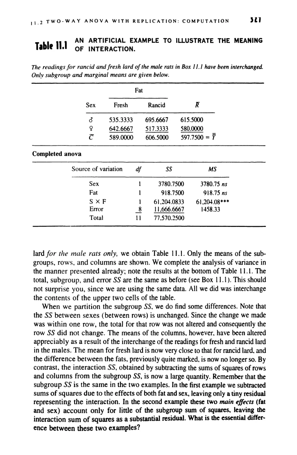
11.2 Two-Way Anova With Equal Replication: Computation 323
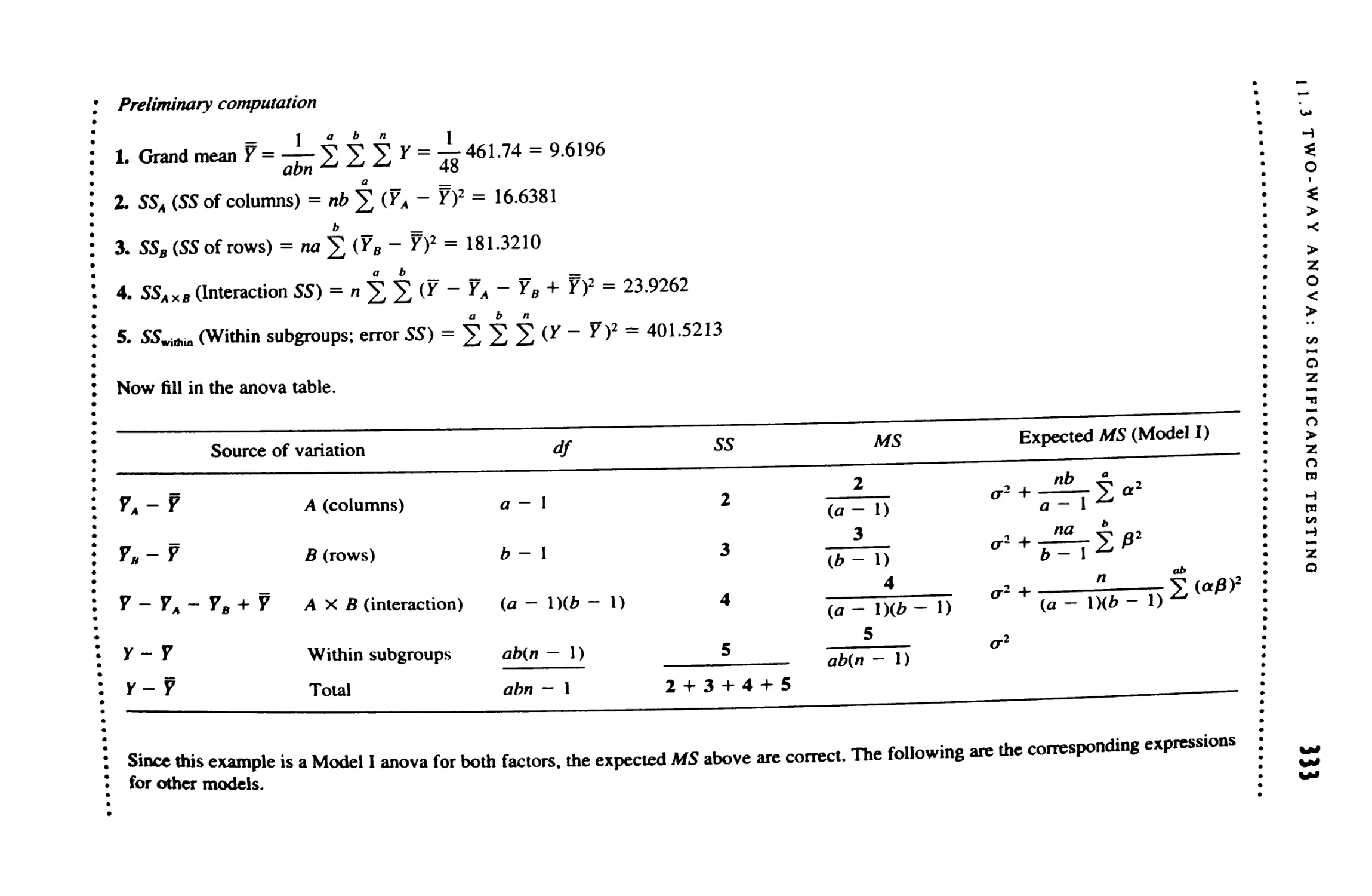
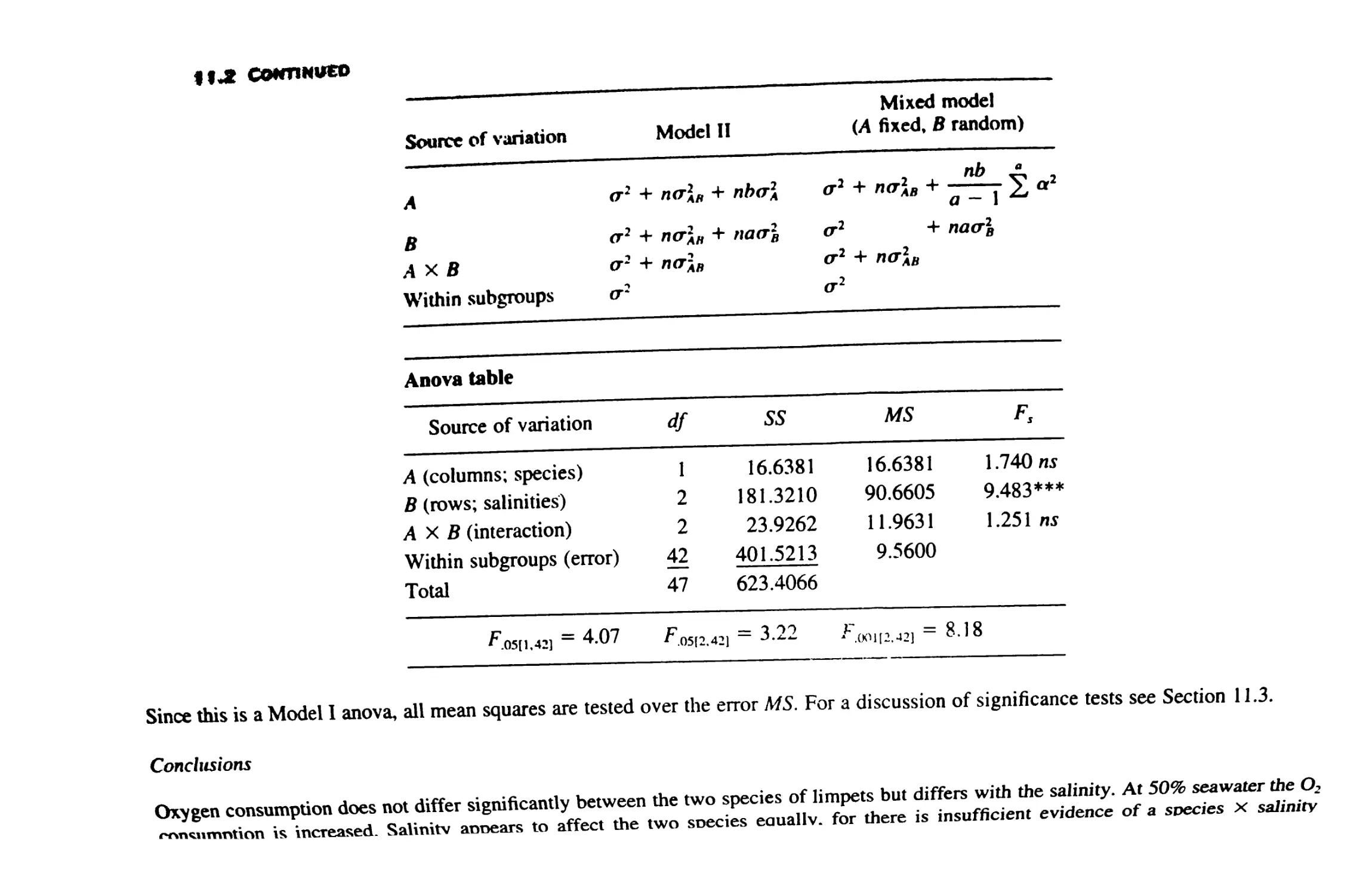
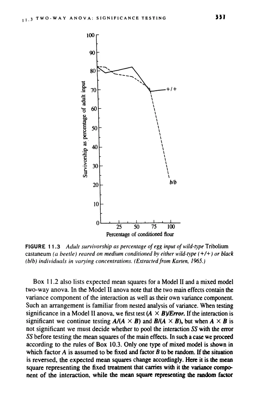
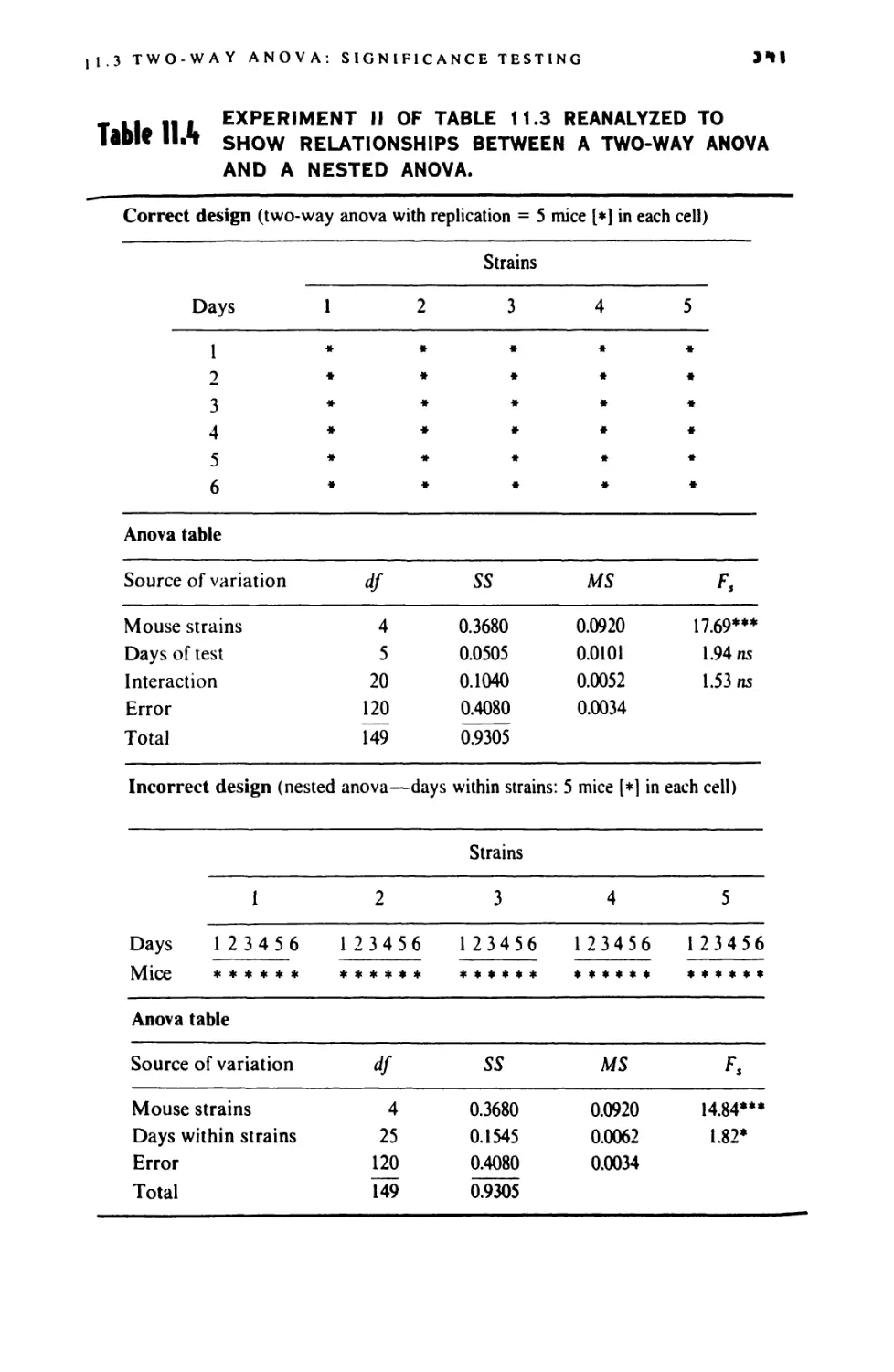
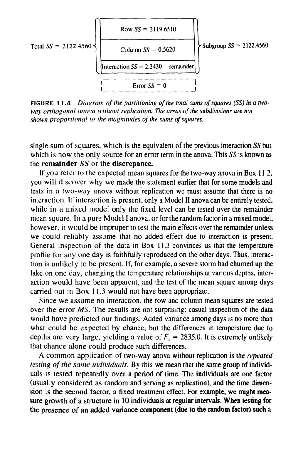
11.3 Two-Way Anova: Significance Testing 331
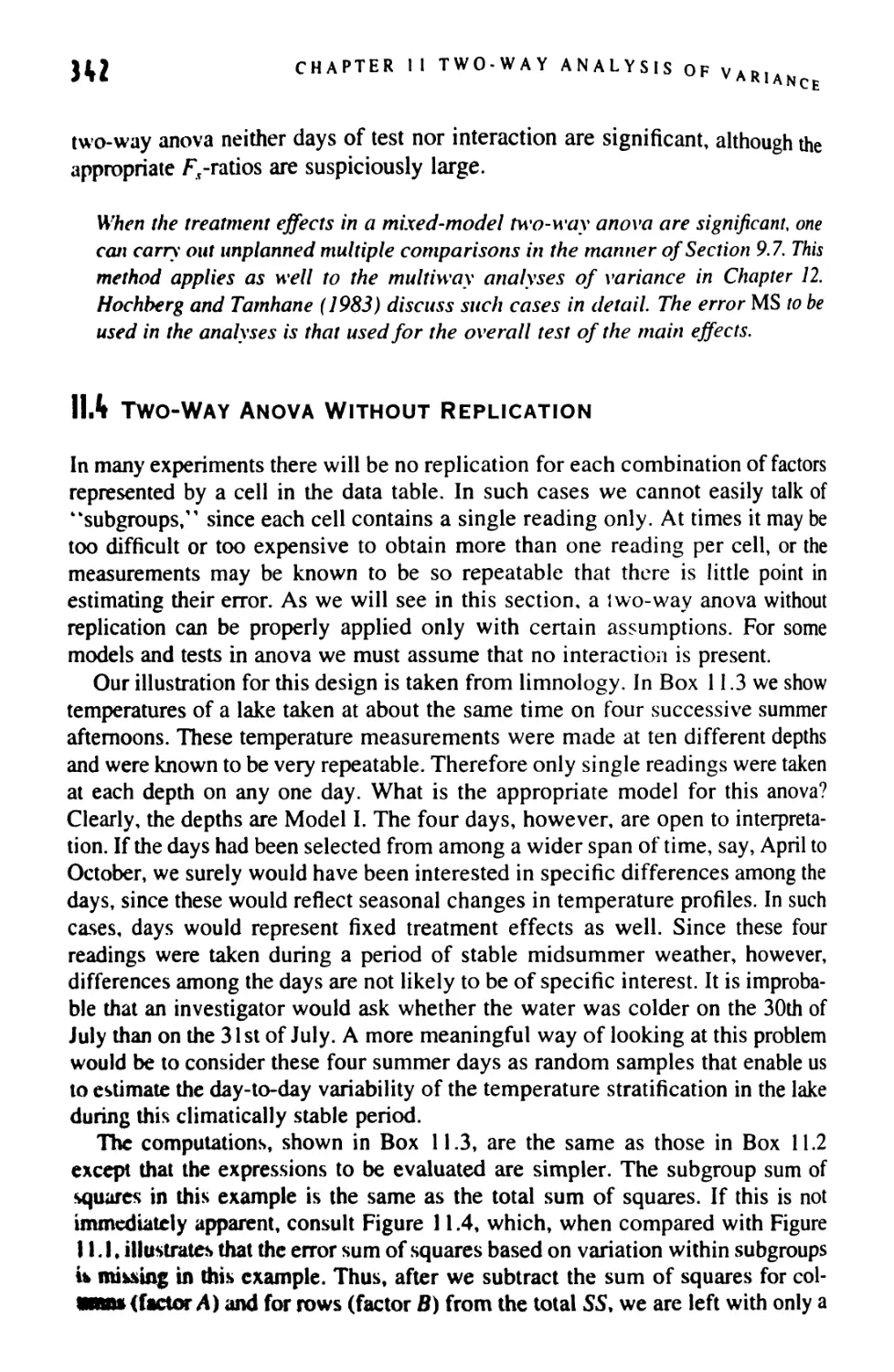
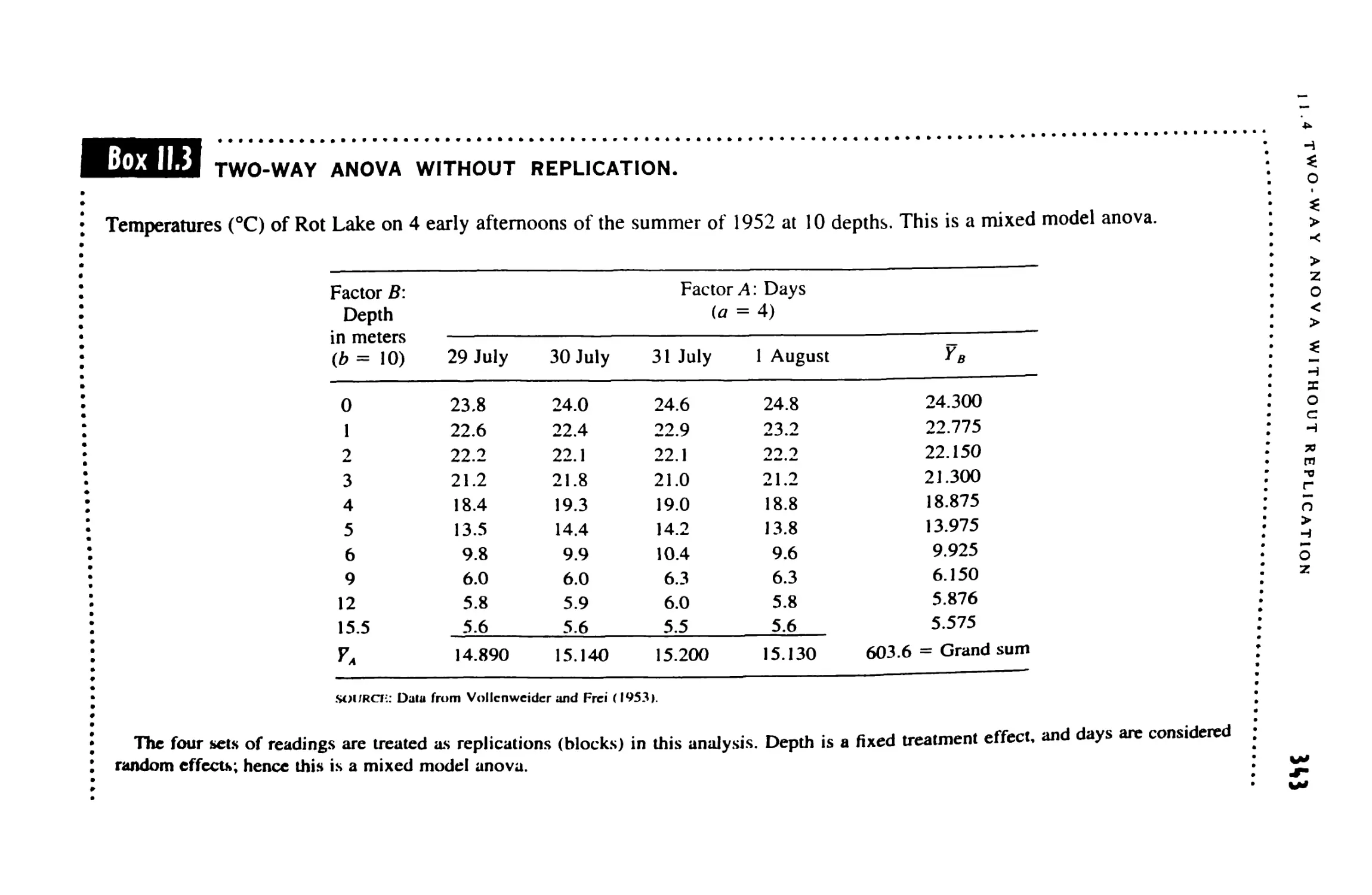
11.4 Two-Way Anova Without Replication 342
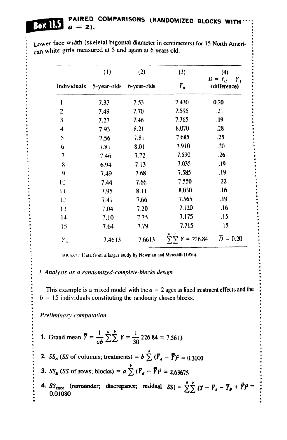
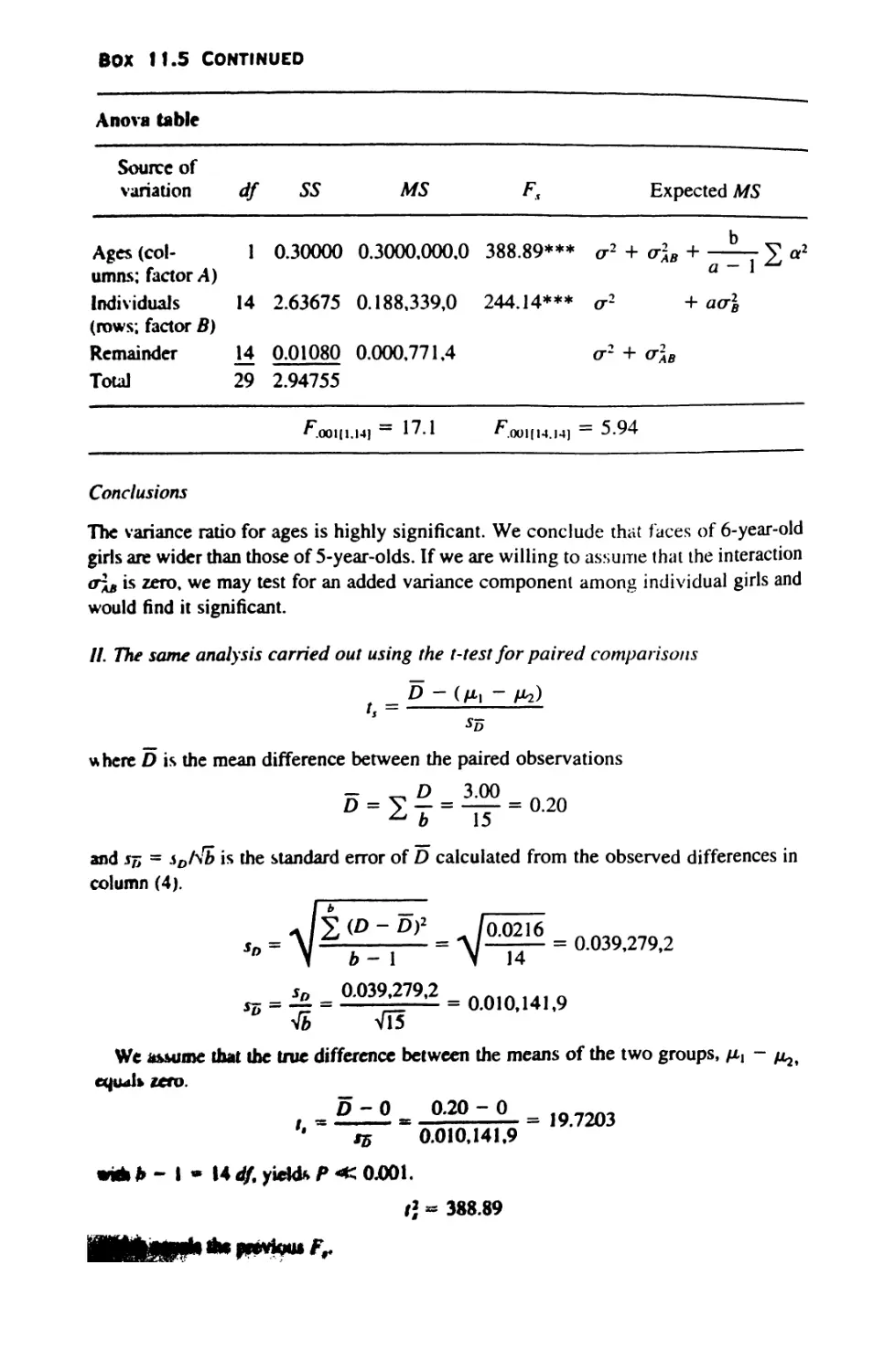
11.5 Paired Comparisons 352
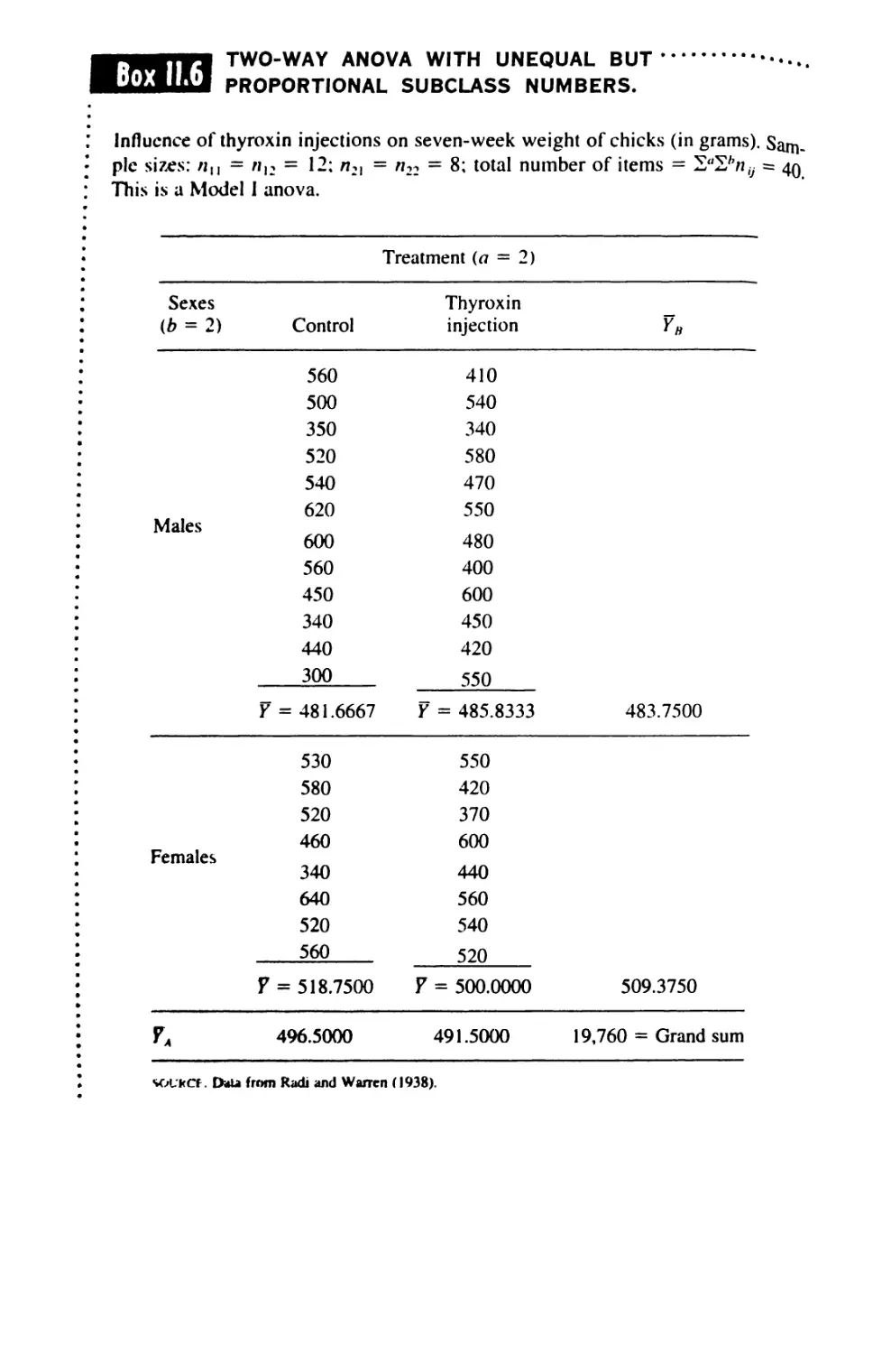
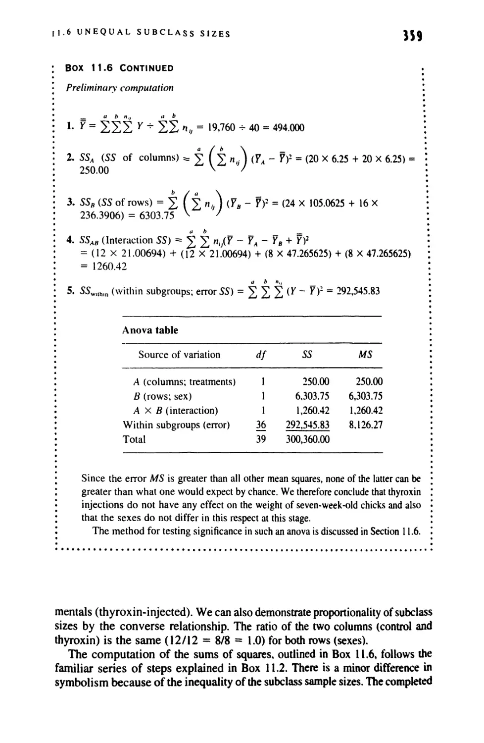
11.6 Unequal Subclass Sizes 357
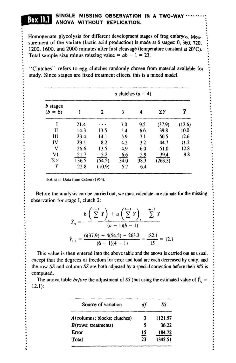
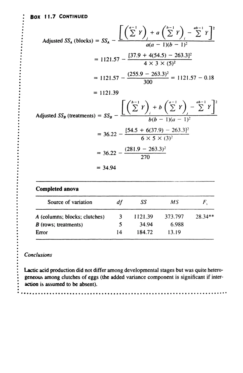
11.7 Missing Values in a Randomized-Blocks Design 363
12 MULTIWAY ANALYSIS OF VARIANCE 369
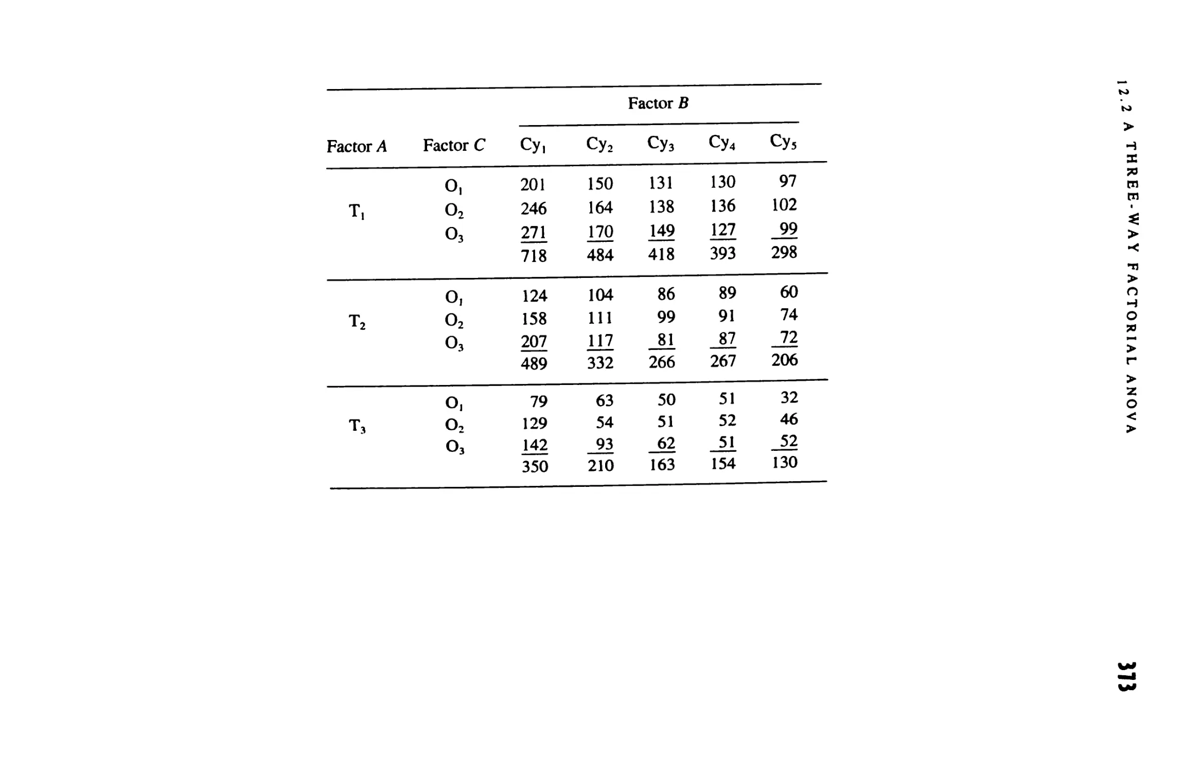
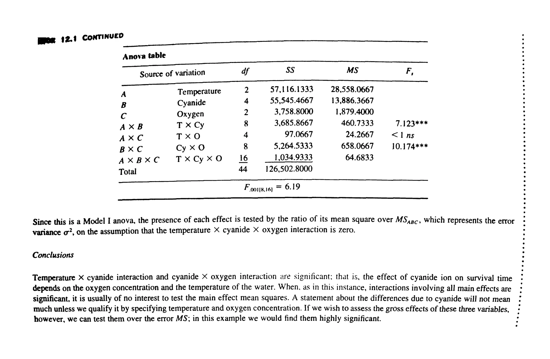
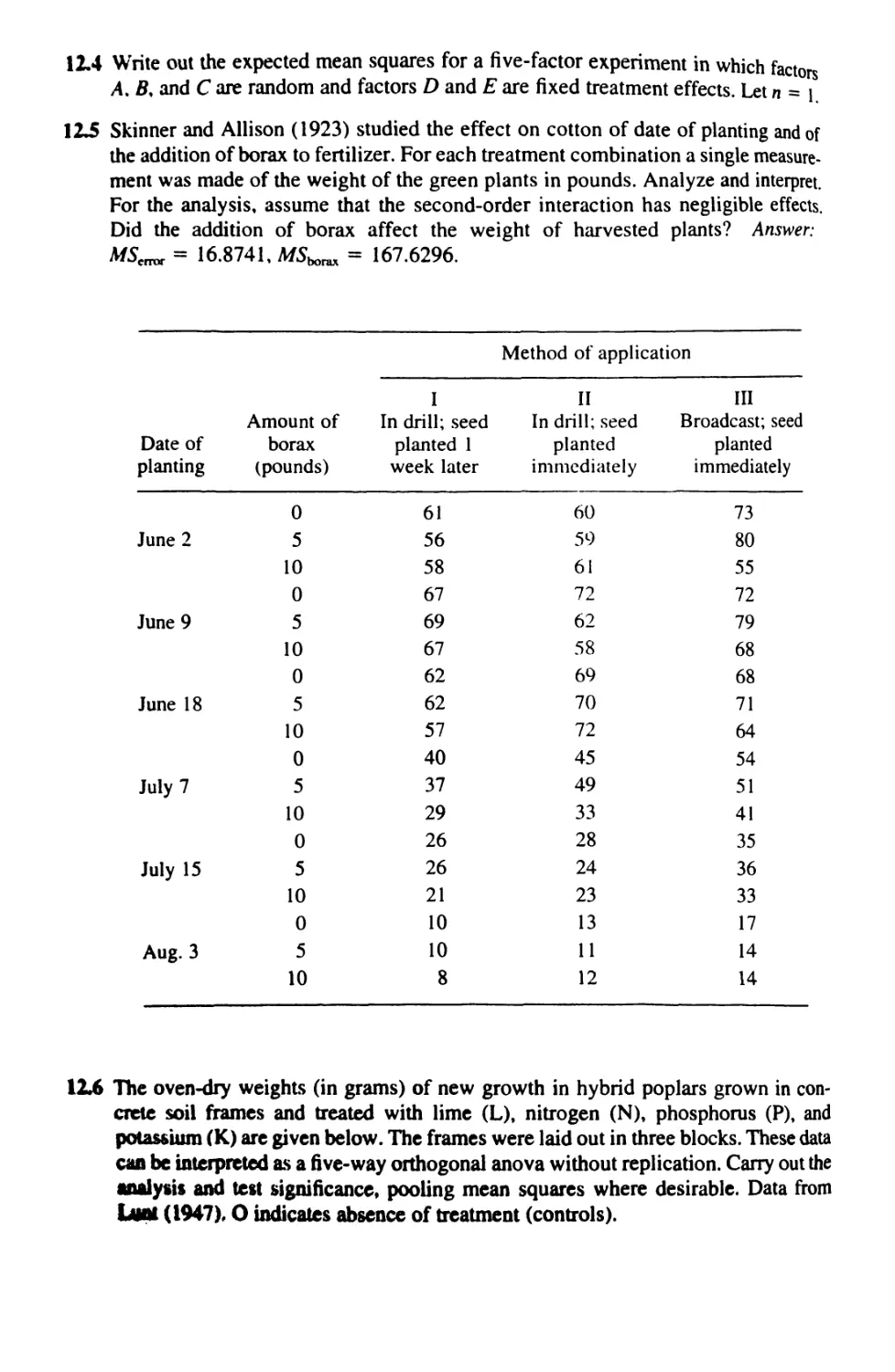
12.1 The Factorial Design 369
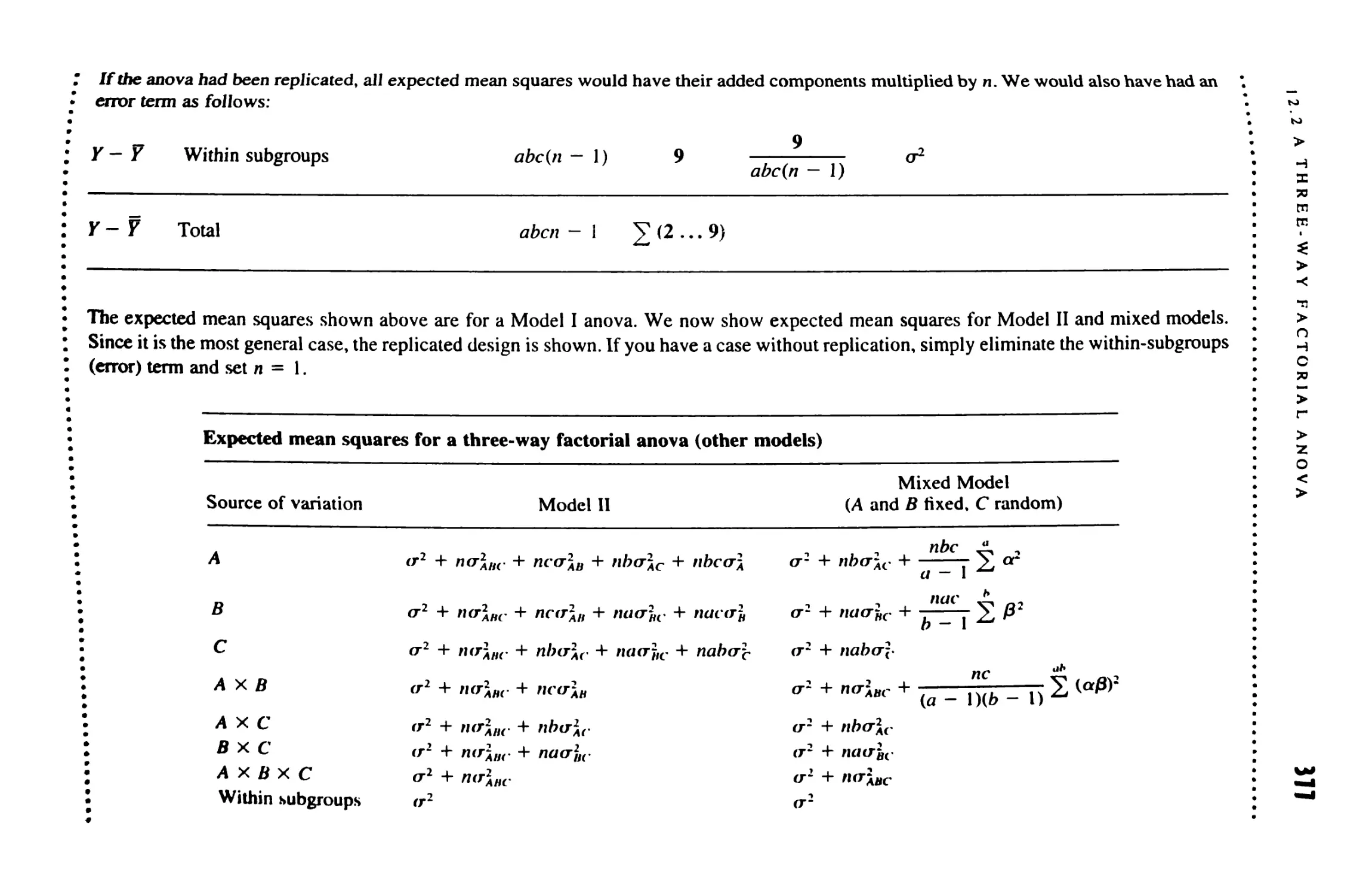
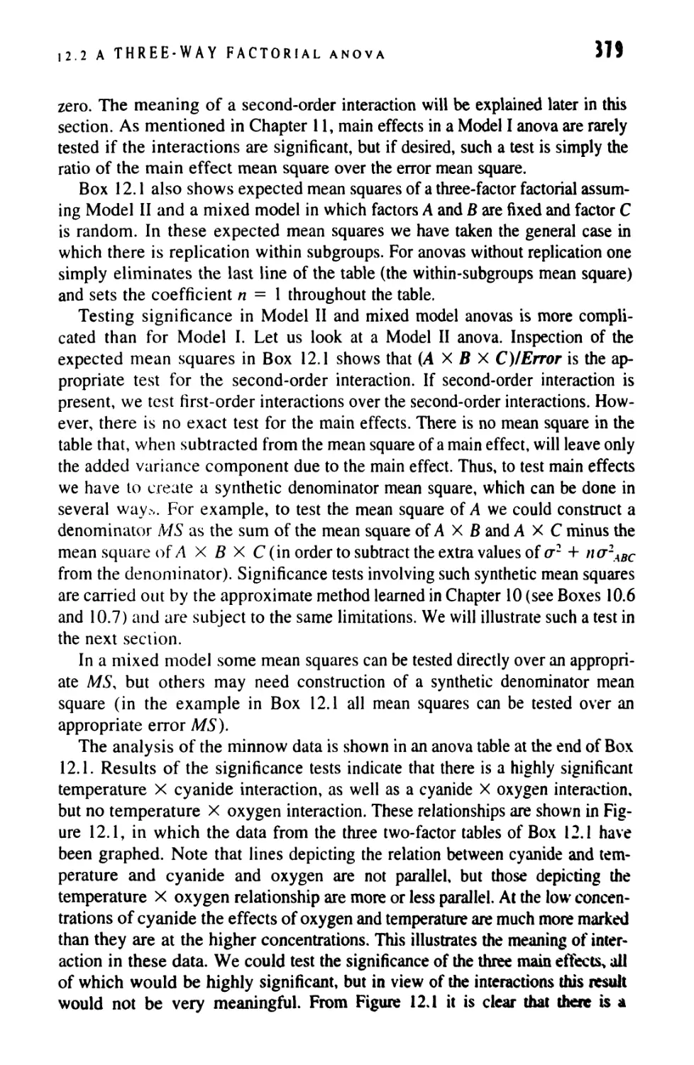
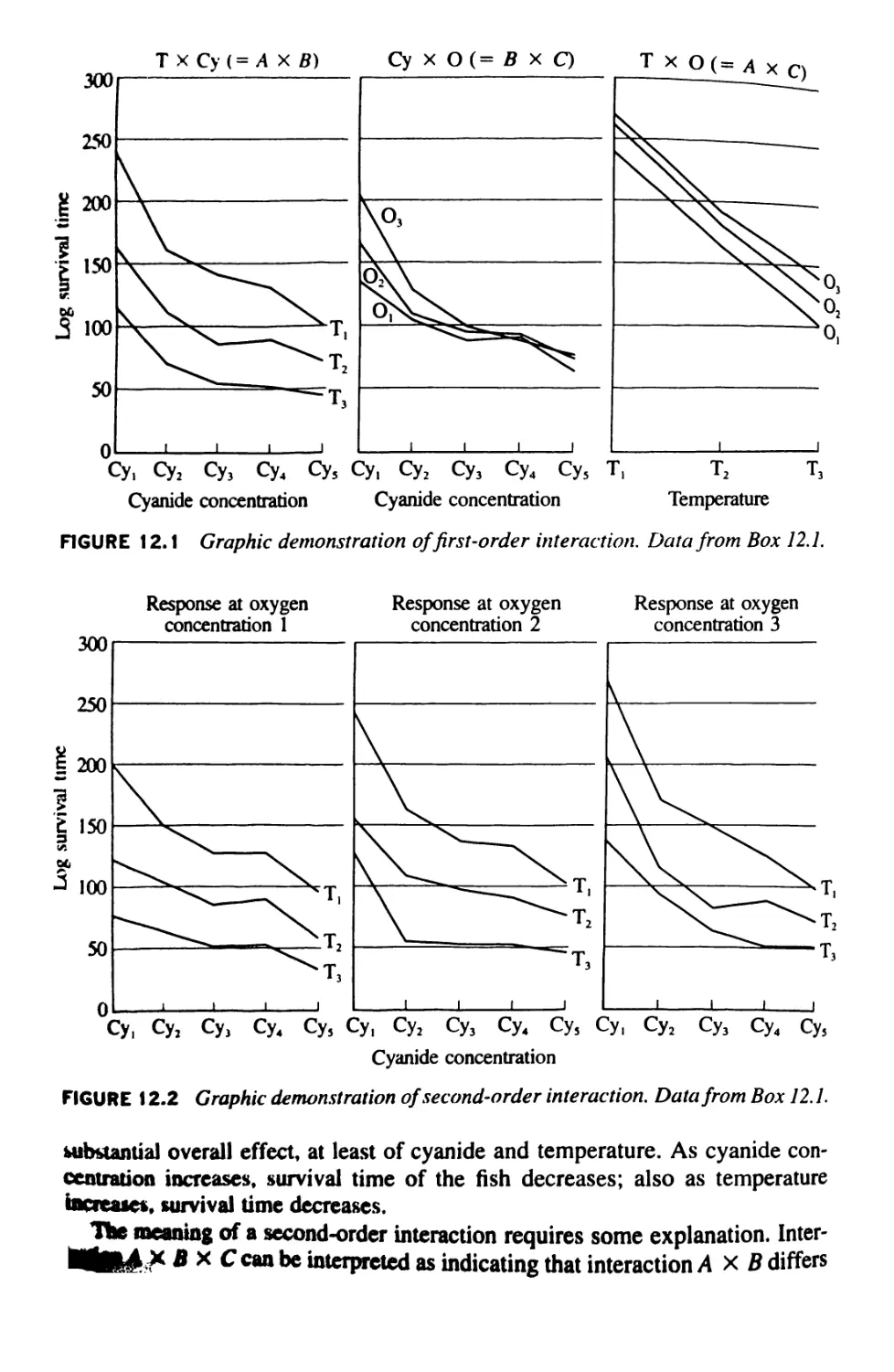
12.2 A Three-Way Factorial Anova 370
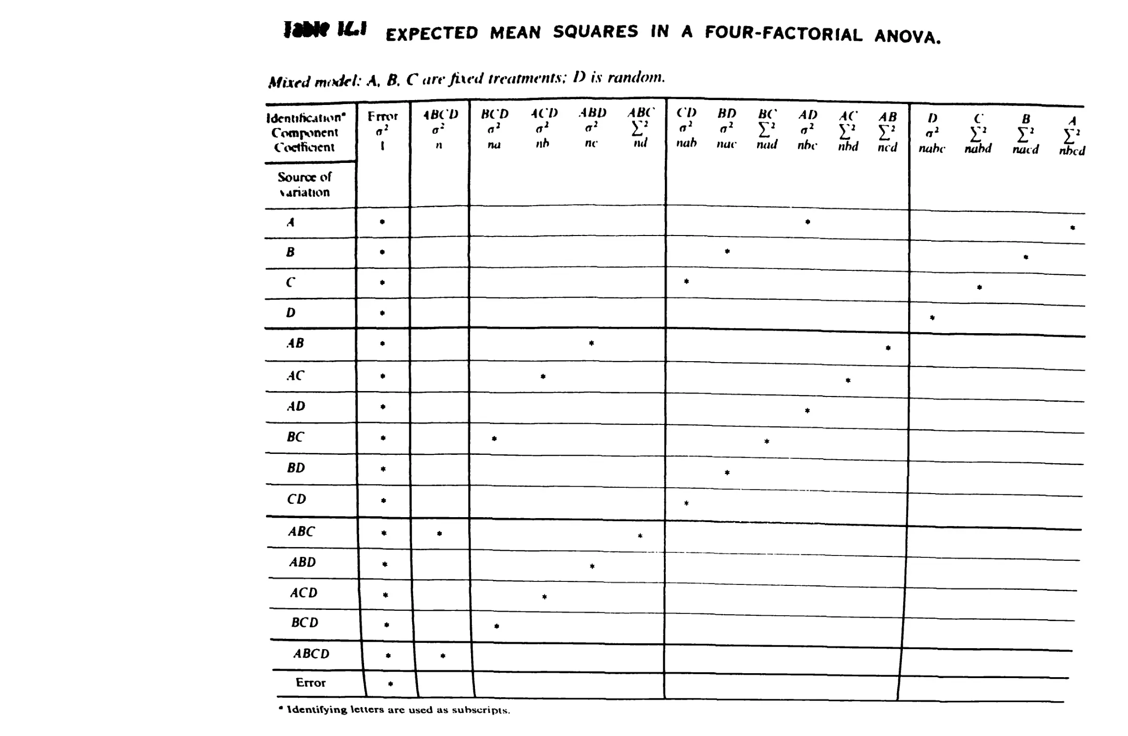
12.3 Higher-Order Factorial Anovas 381
12.4 Other Designs 385
12.5 Anovas by Computer 3#7
CONTKNTs
1} ASSUMPTIONS OF ANALYSIS OF VARIANCE 392
13.1 A Fundamental Assumption 393
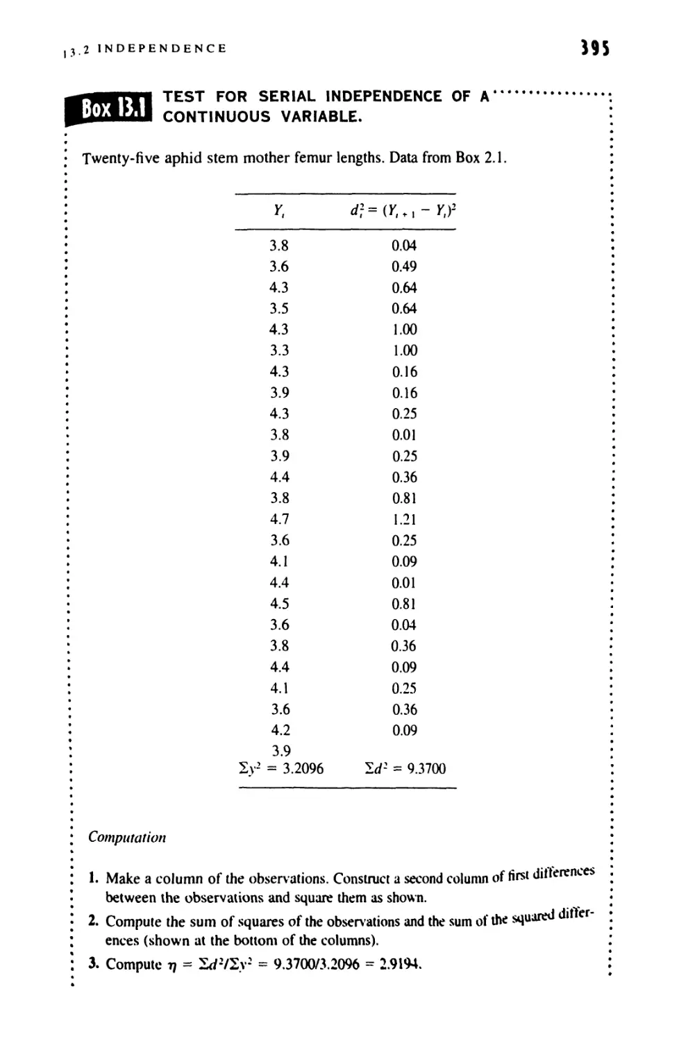
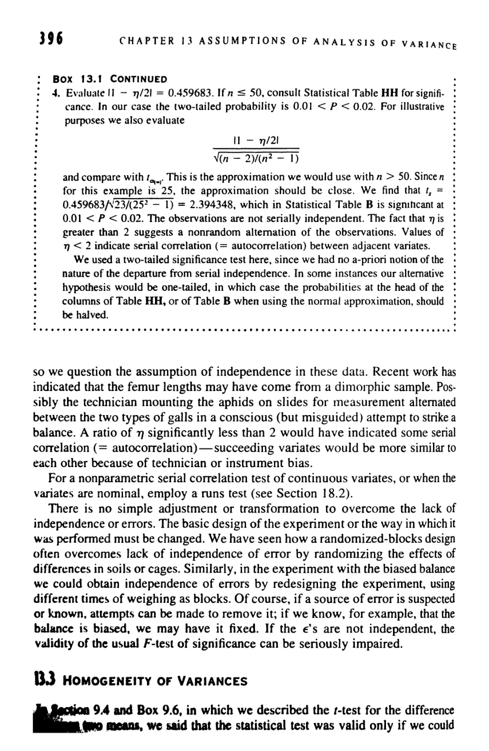
13.2 Independence 393
13.3 Homogeneity of Variances 2%
13.4 Normality 495
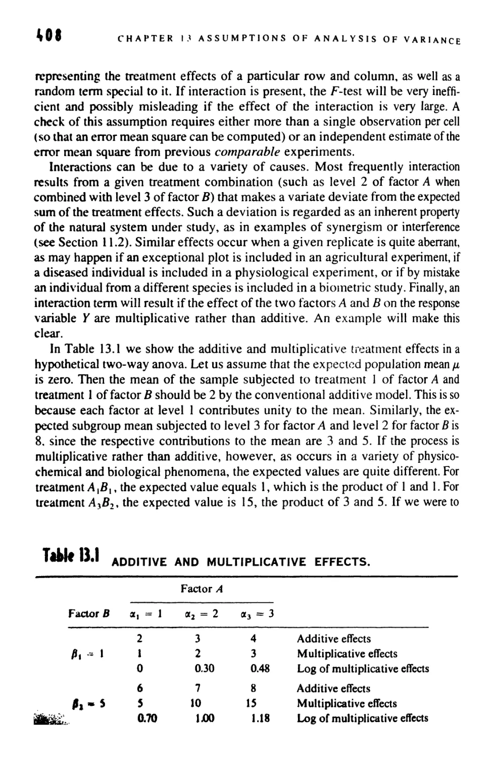
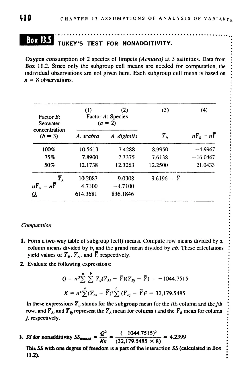
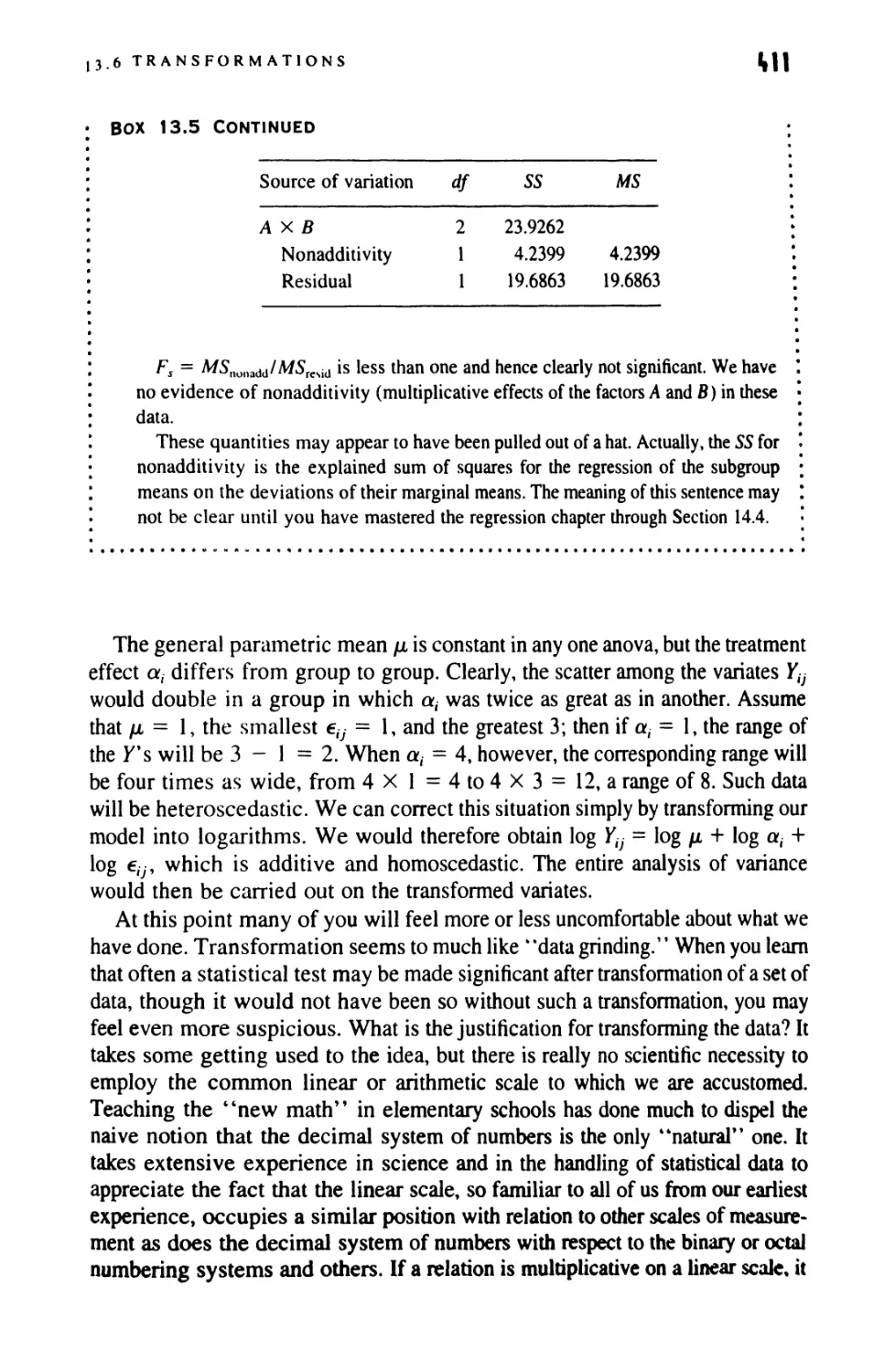
13.5 Additivity 407
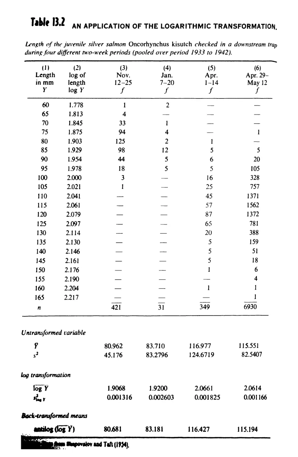
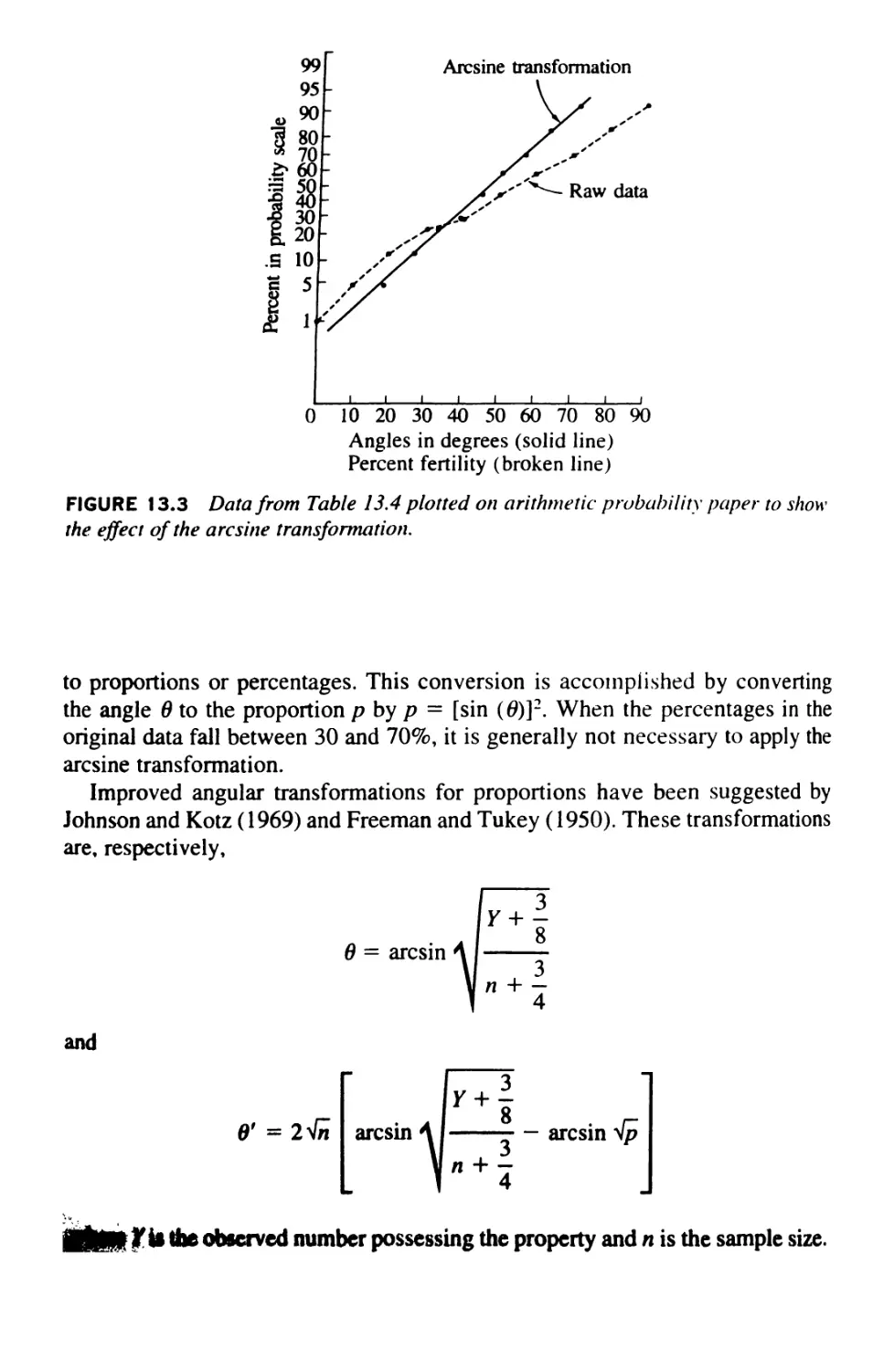
13.6 Transformations 499
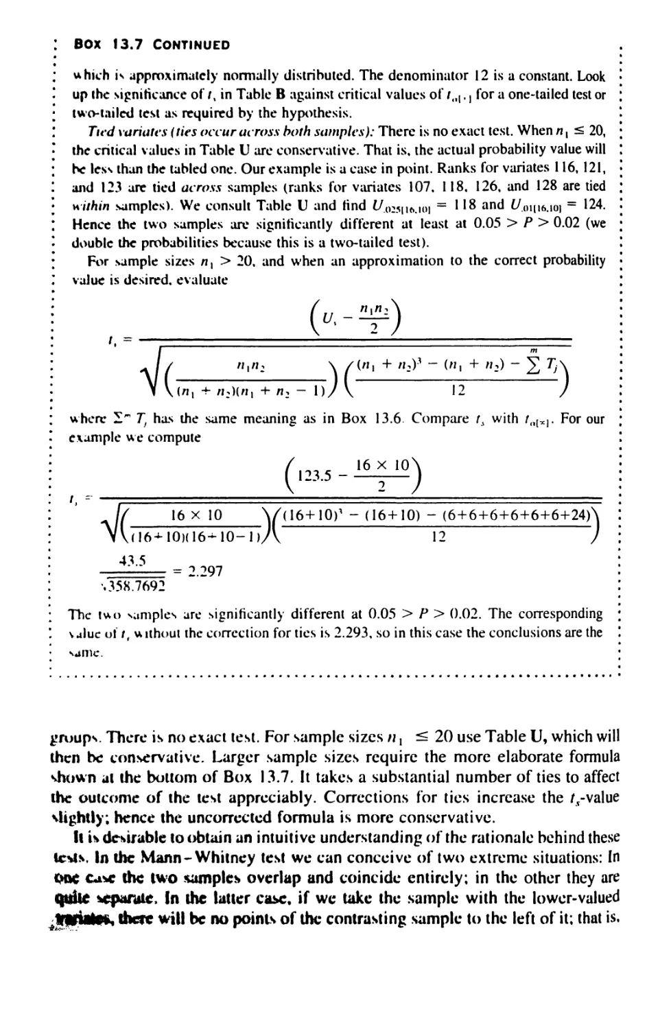
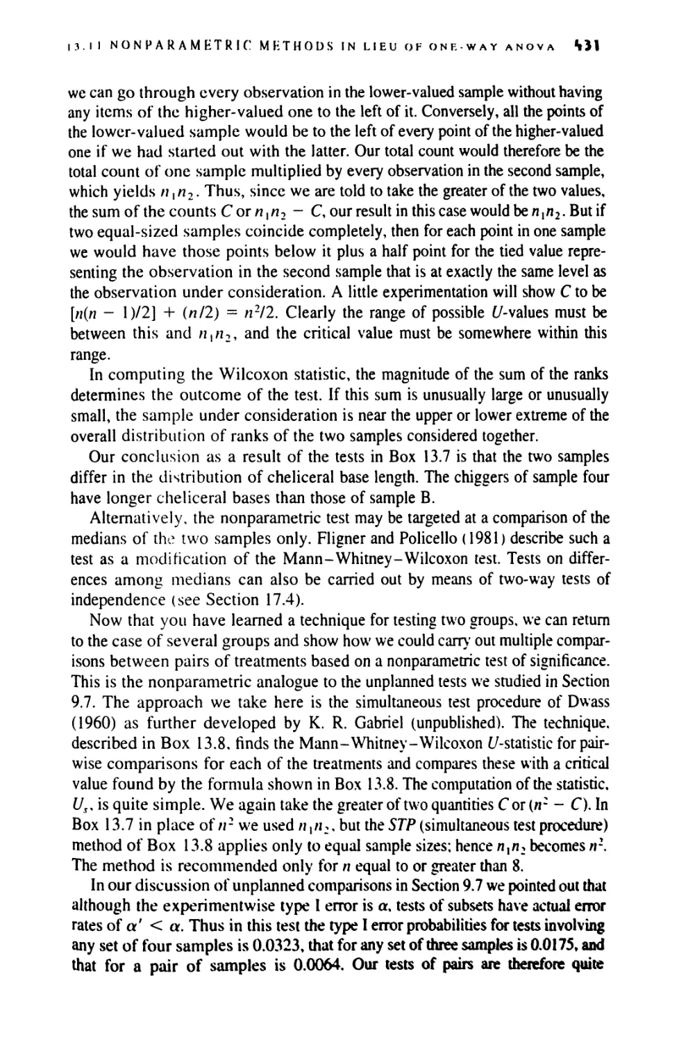
13.7 The Logarithmic Transformation 413
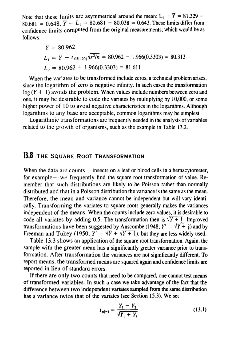
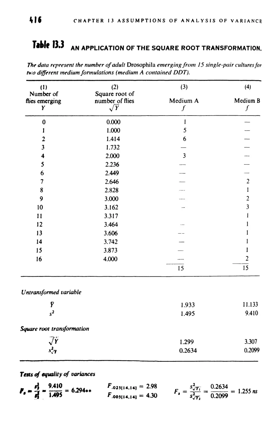
13.8 The Square-Root Transformation 415
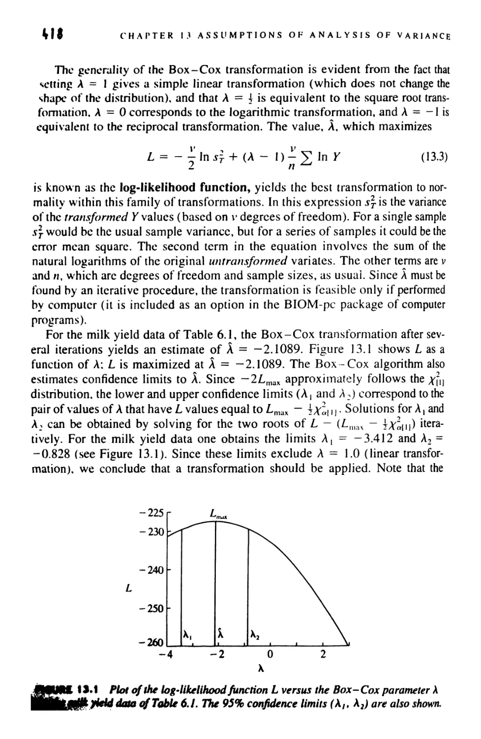
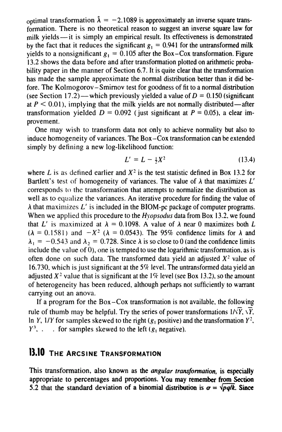
13.9 The Box-Cox Transformation 417
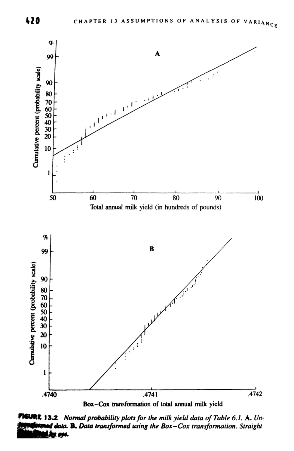
13.10 The Arcsine Transformation 419
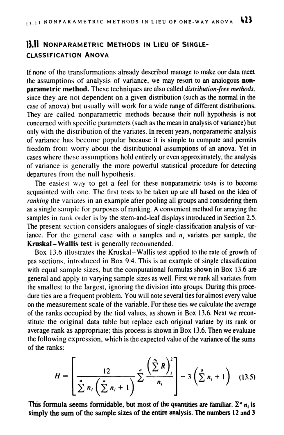
13.11 Nonparametric Methods in Lieu of Single-
Classification Anovas 423
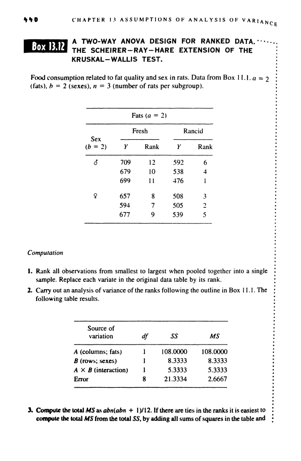
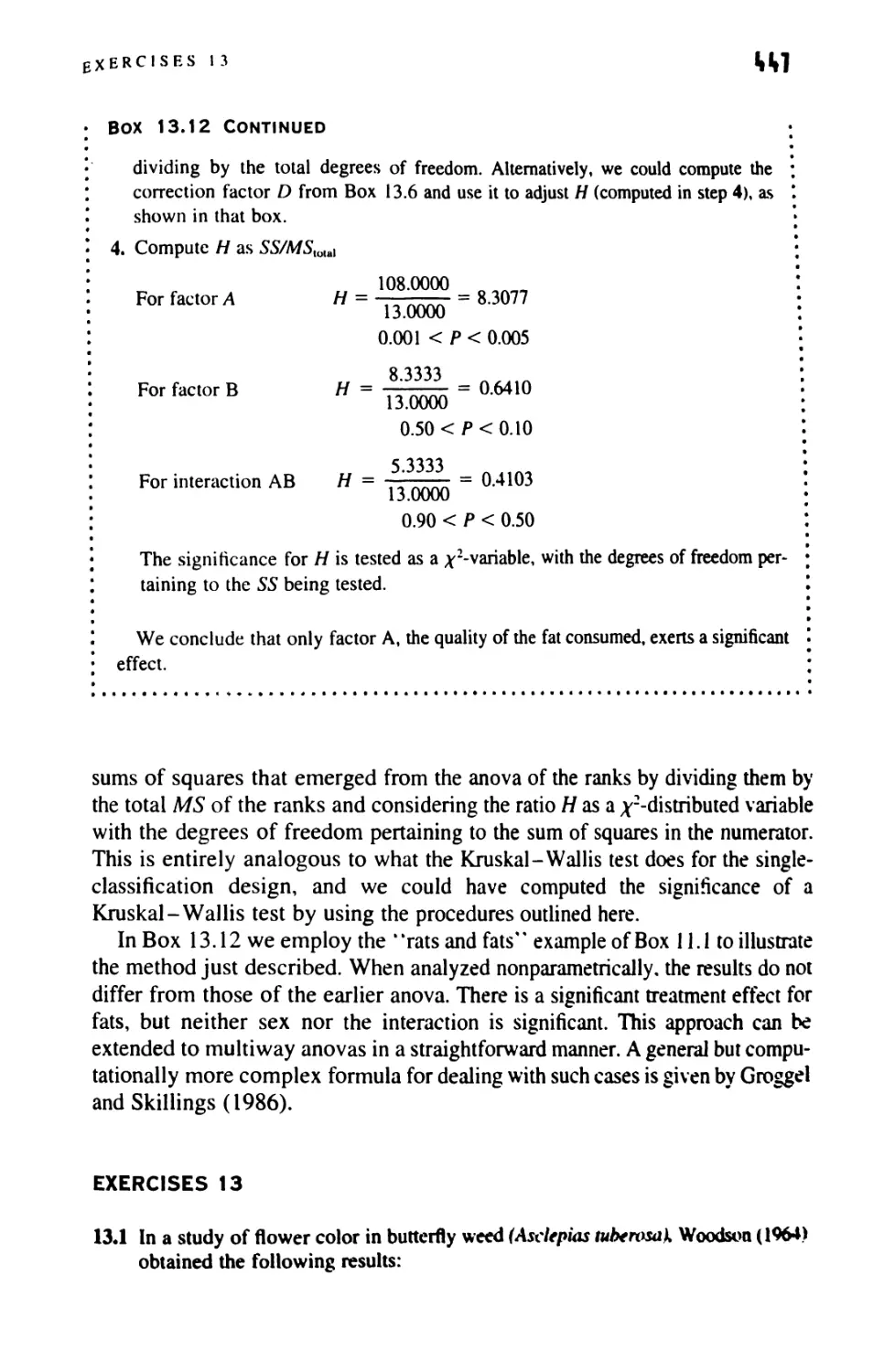
13.12 Nonparametric Methods in Lieu of Two-Way Anova 440
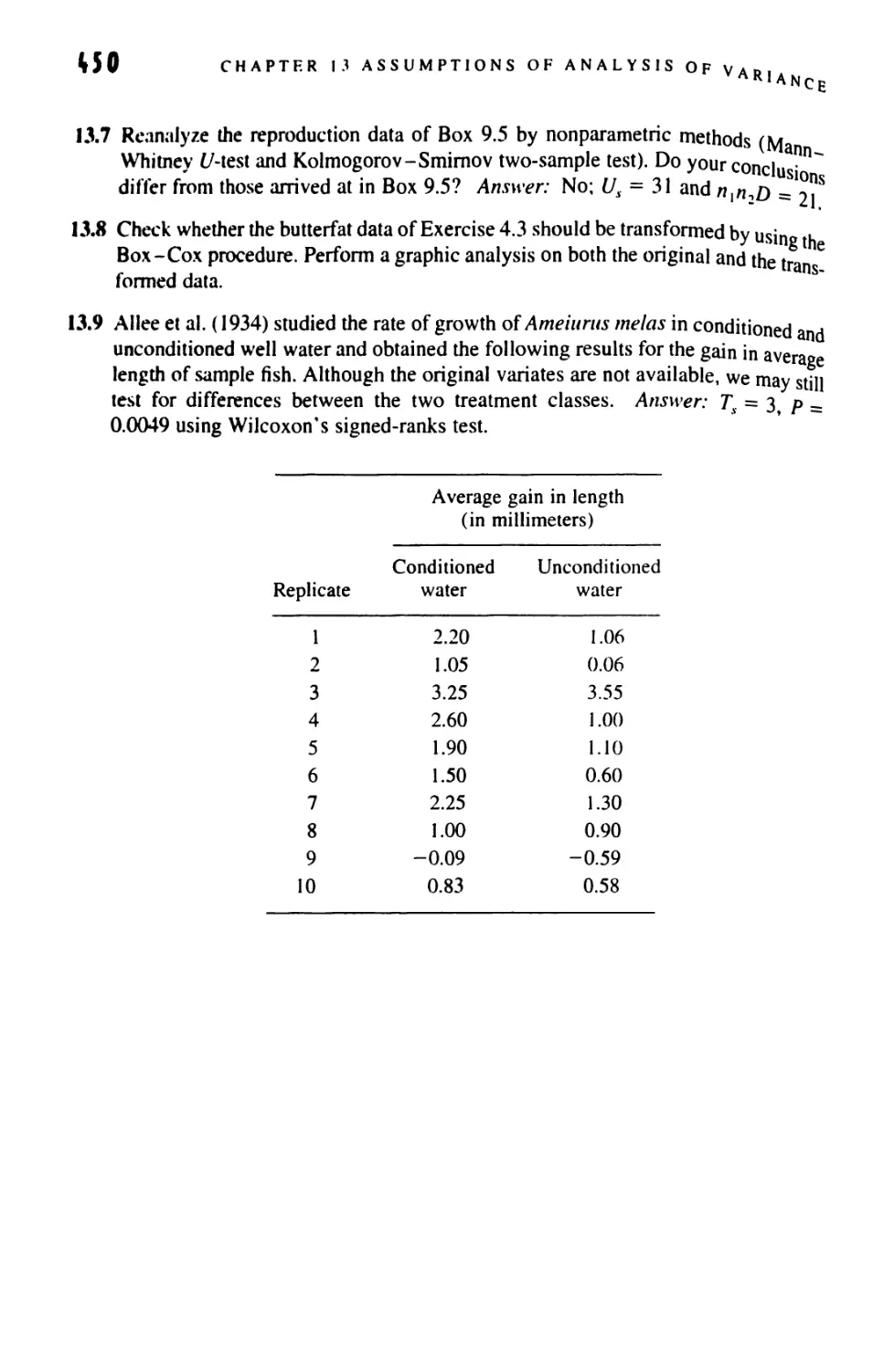
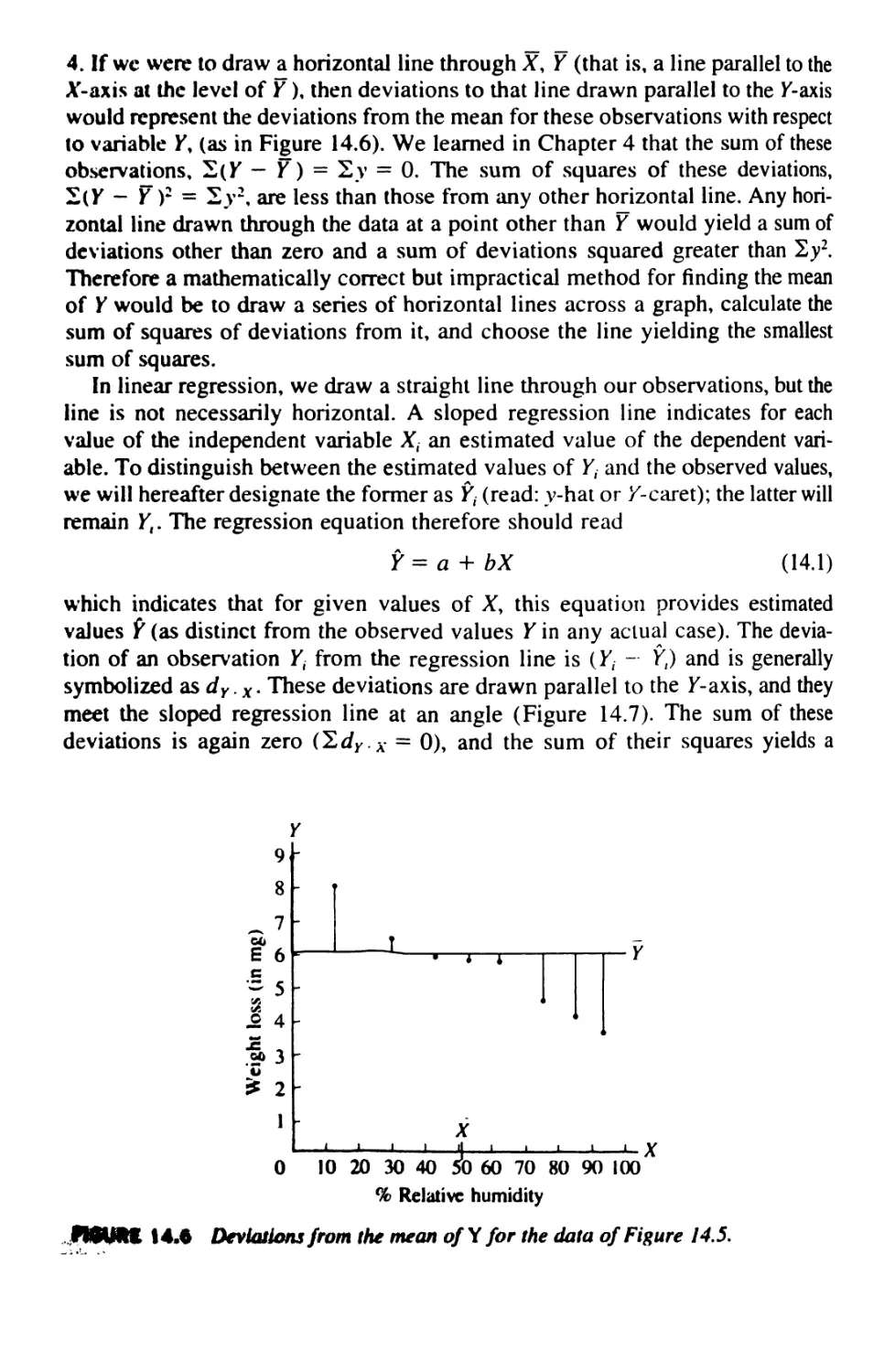
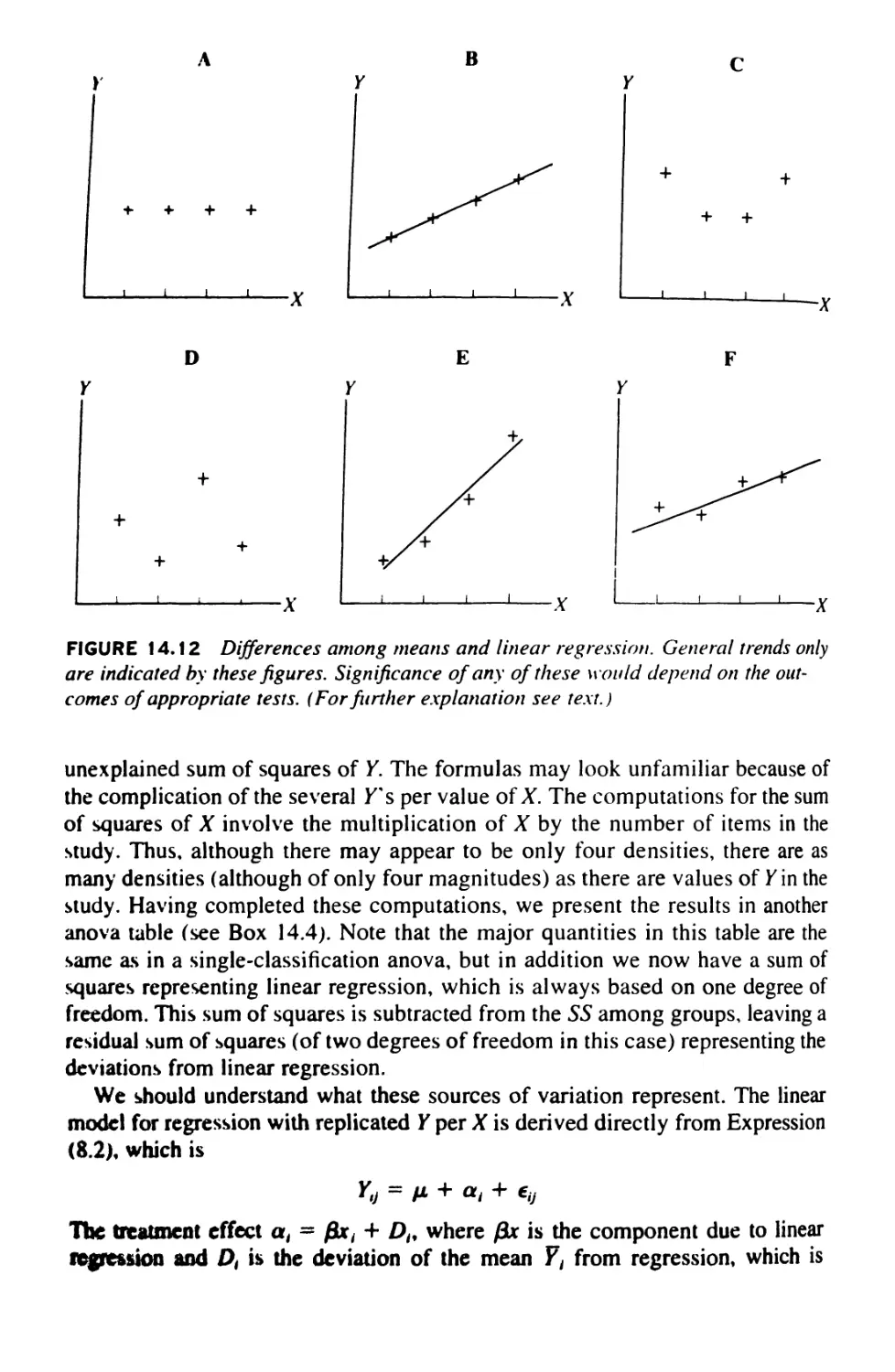
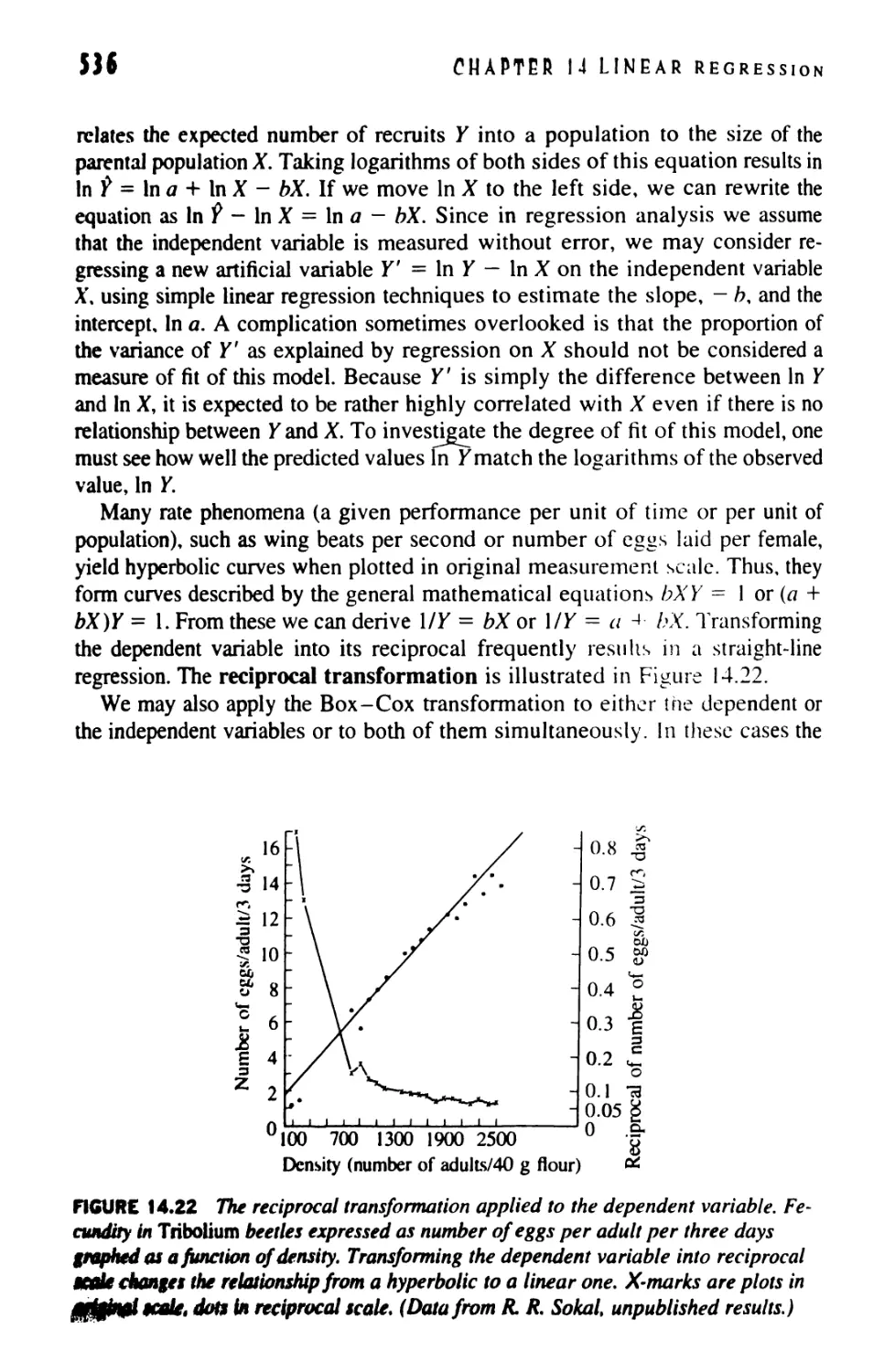
ft LINEAR REGRESSION 451
14.1 Introduction to Regression 452
14.2 Models in Regression 455
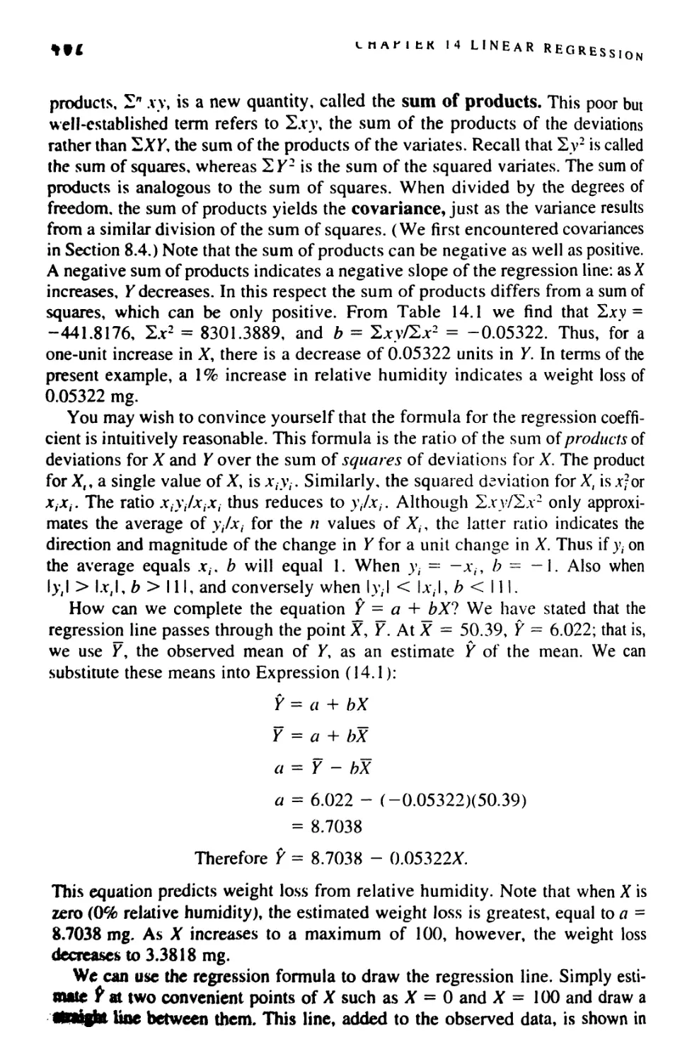
14.3 The Linear Regression Equation 457
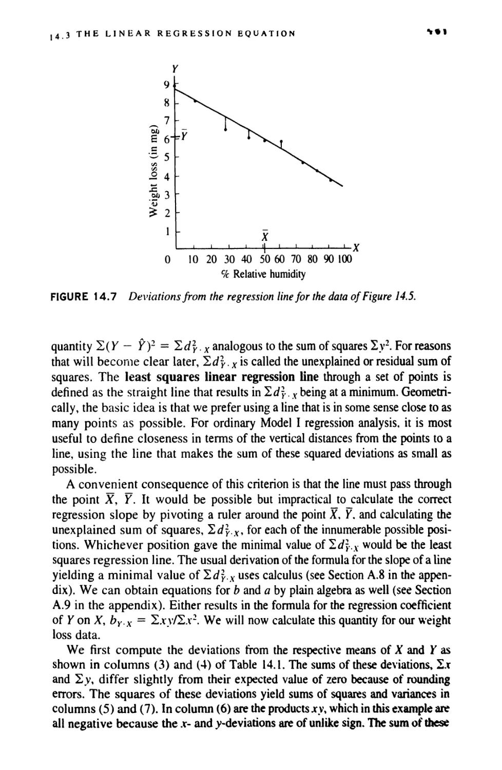
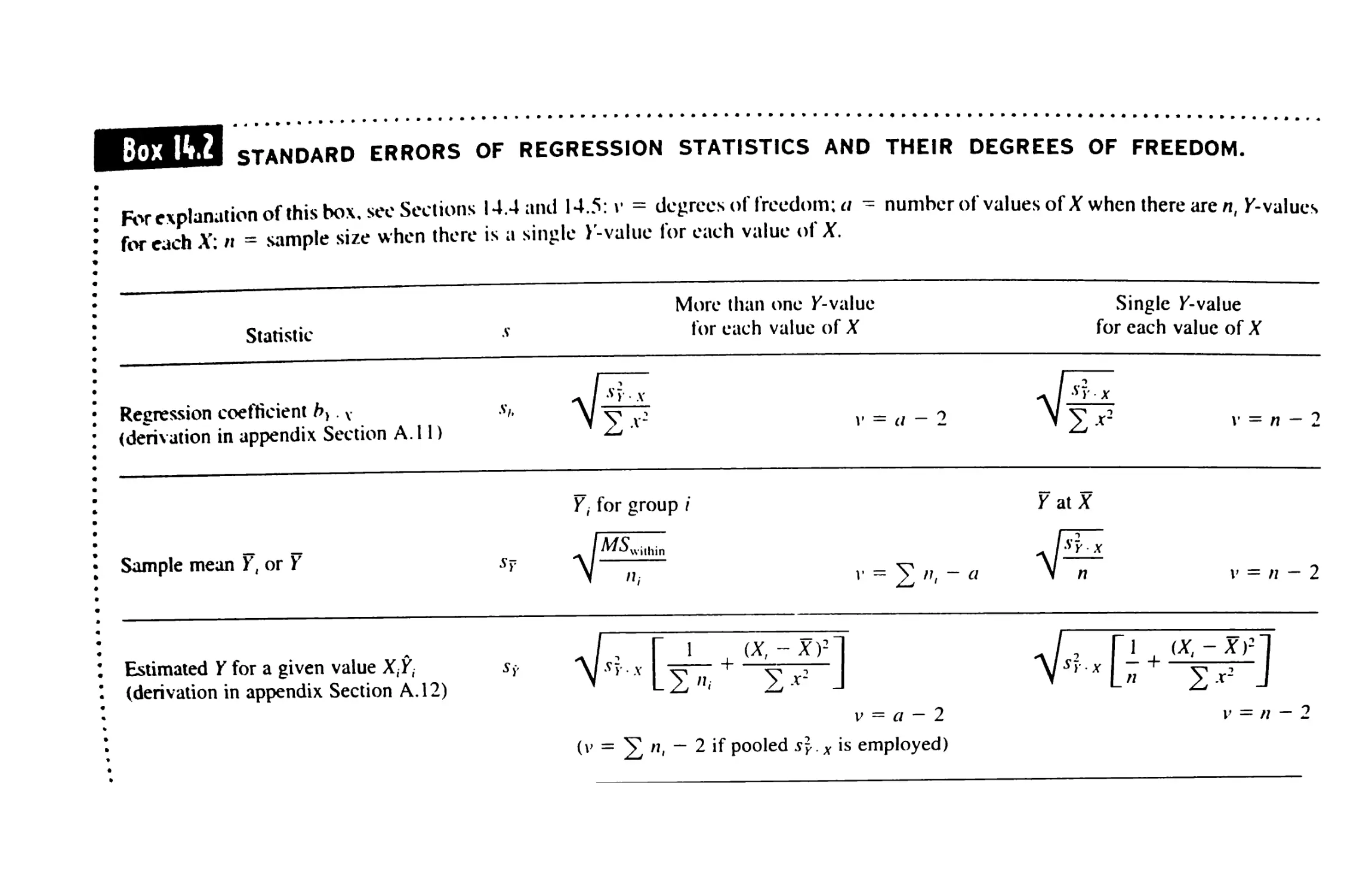
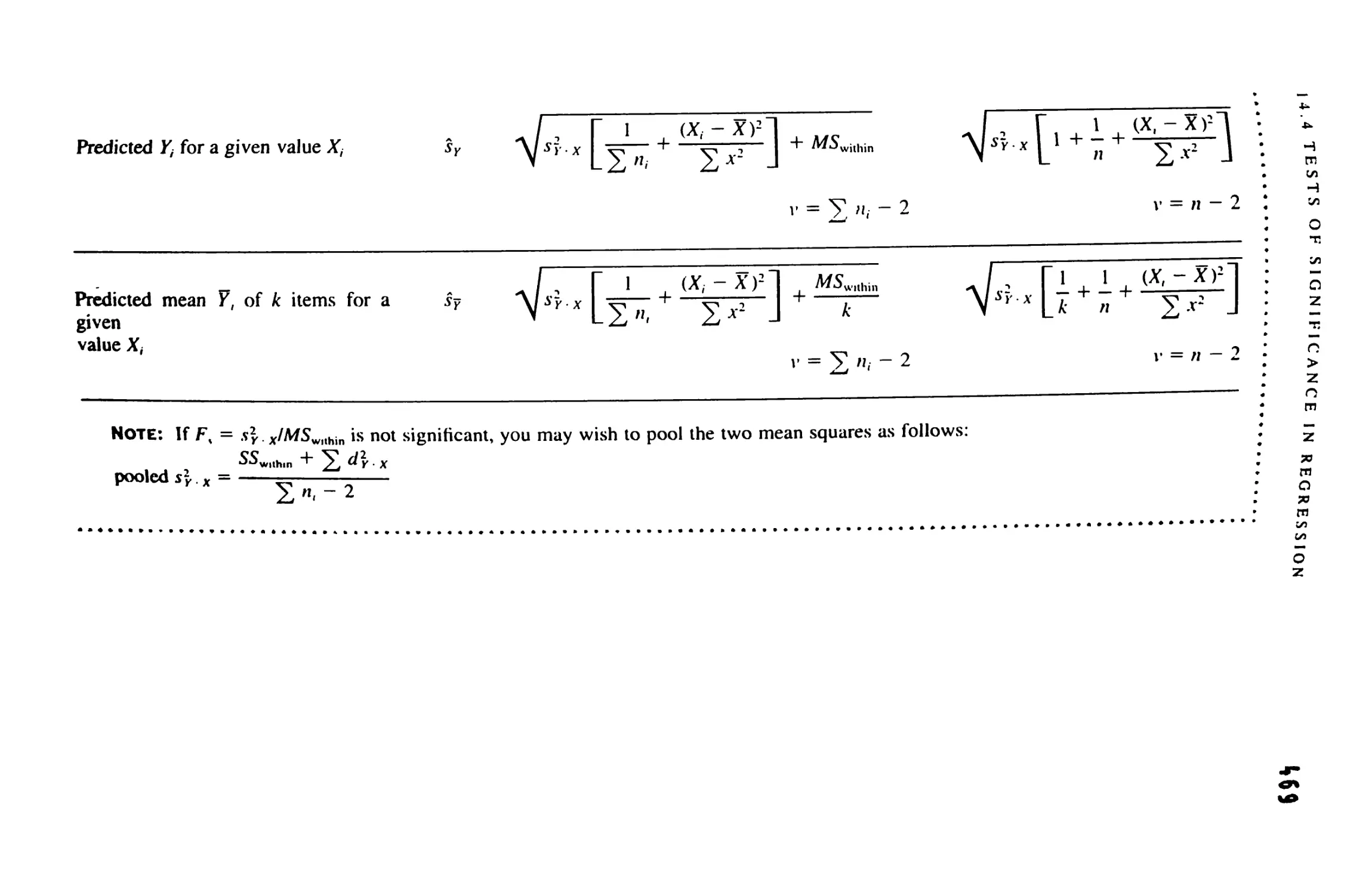
14.4 Tests of Significance in Regression 466
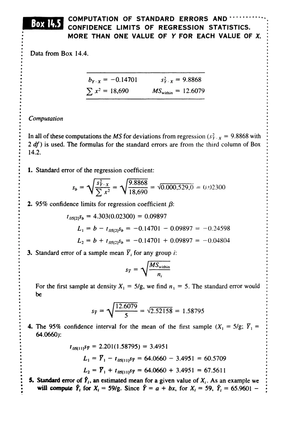
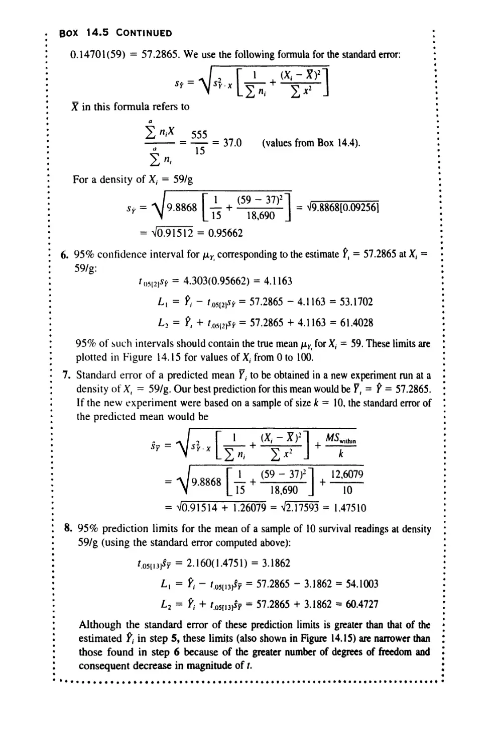
14.5 More Than One Value of Y for Each Value of X 476
14.6 The Uses of Regression 486
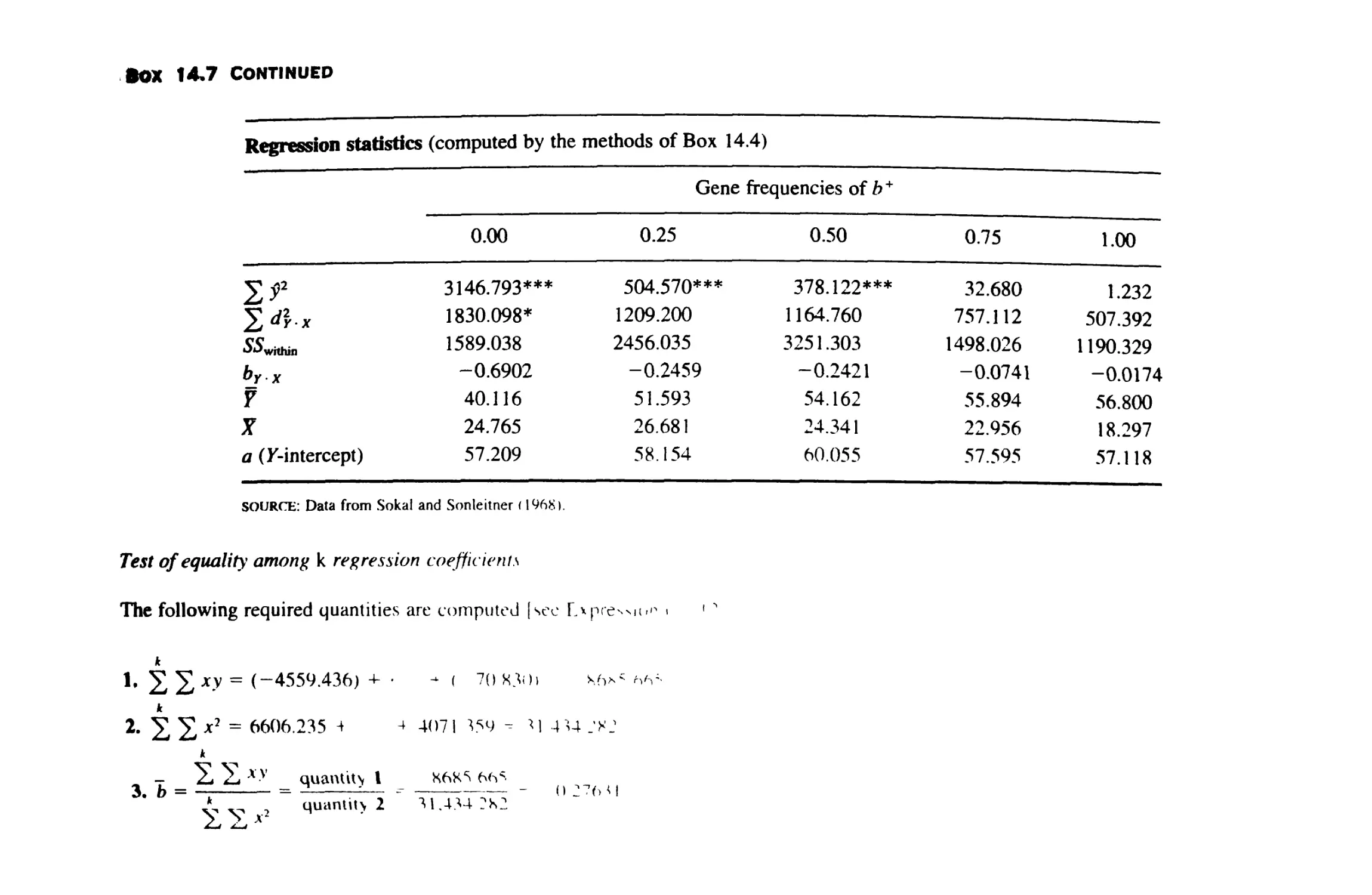
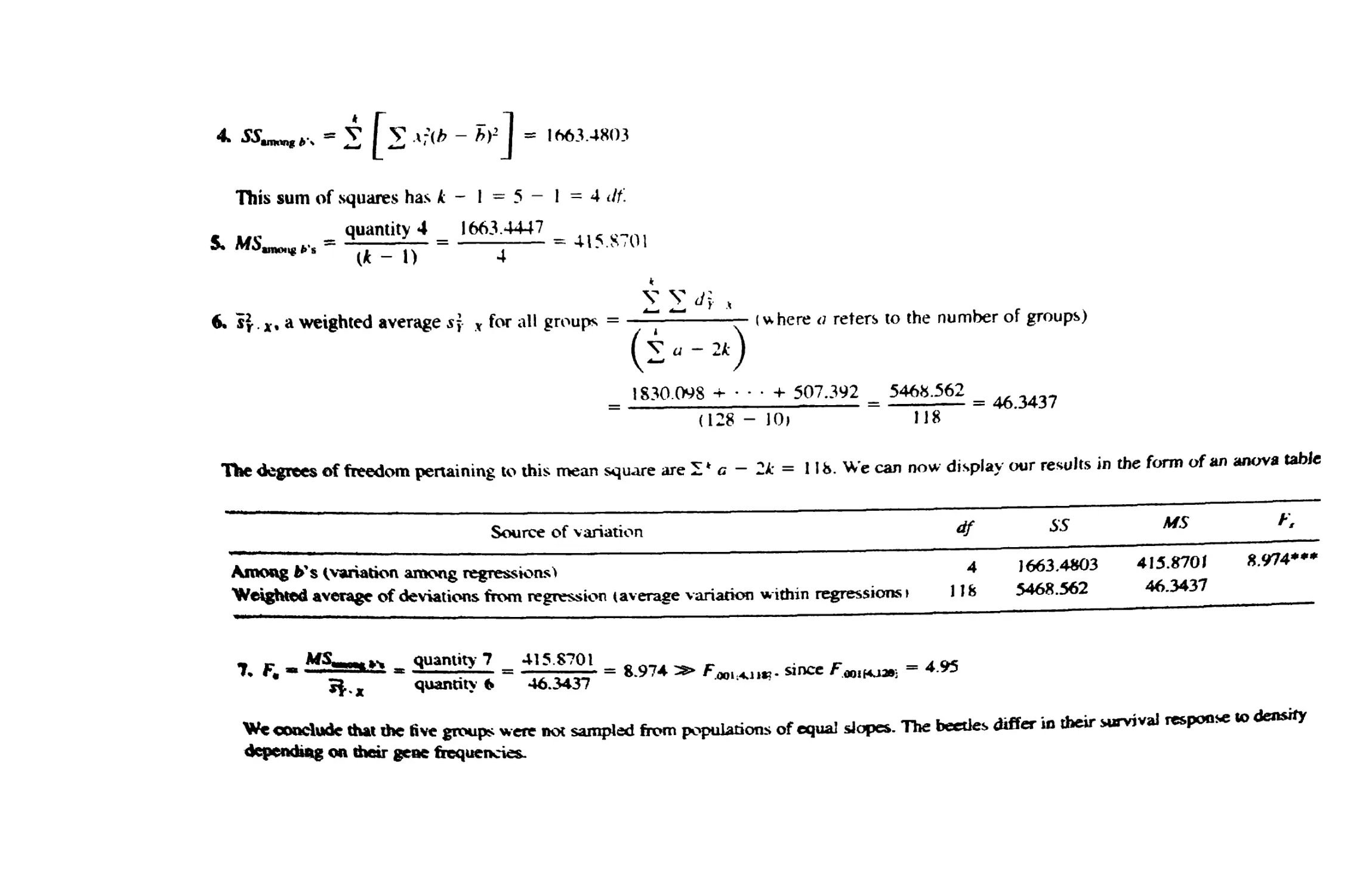
14.7 Estimating X from Y 491
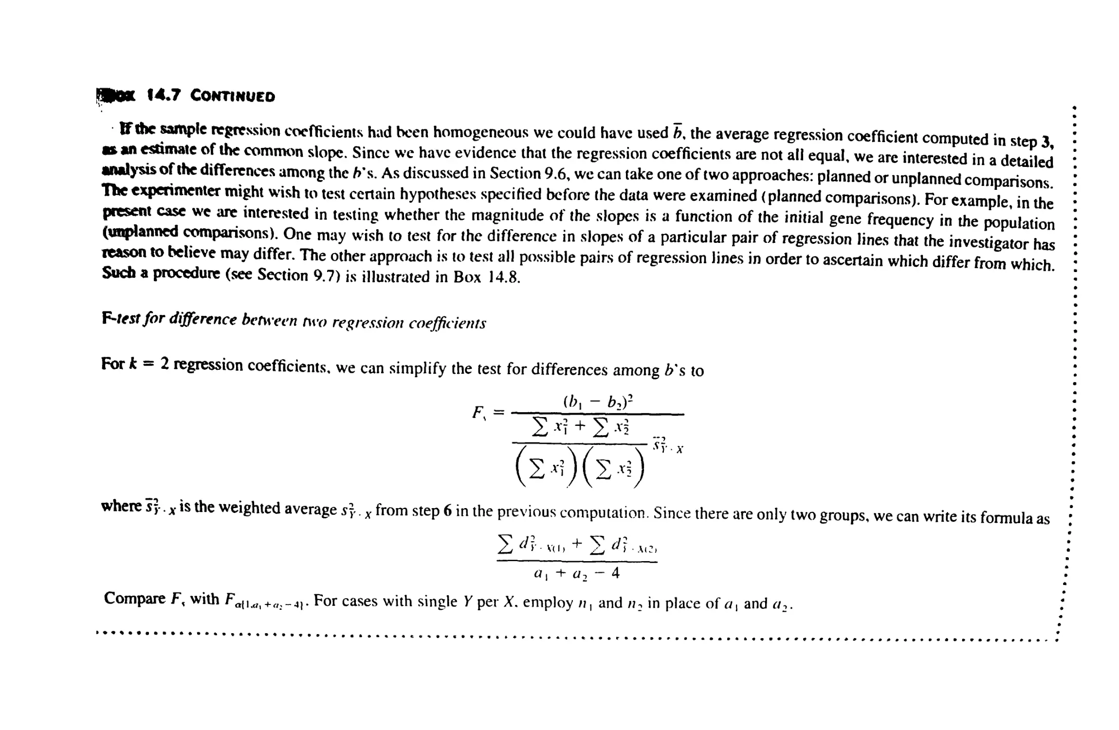
14.8 Comparing Regression Lines 493
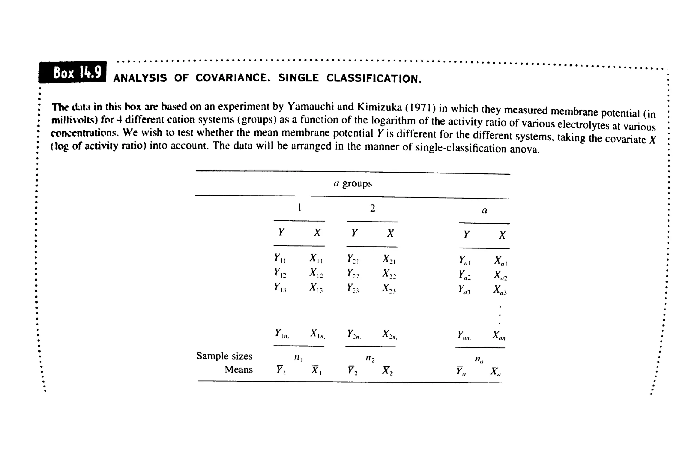
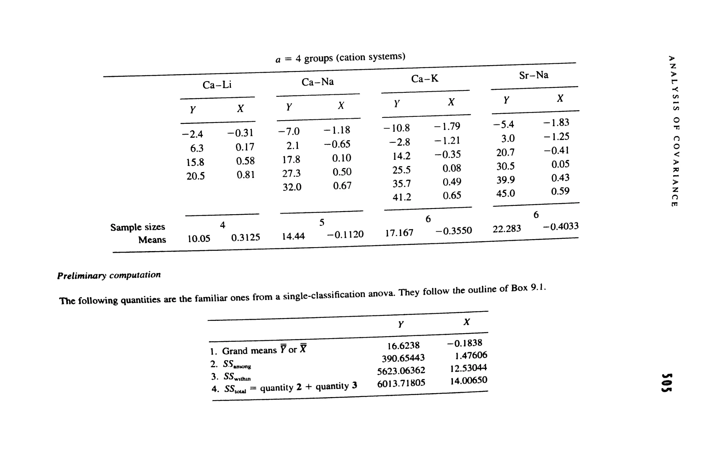
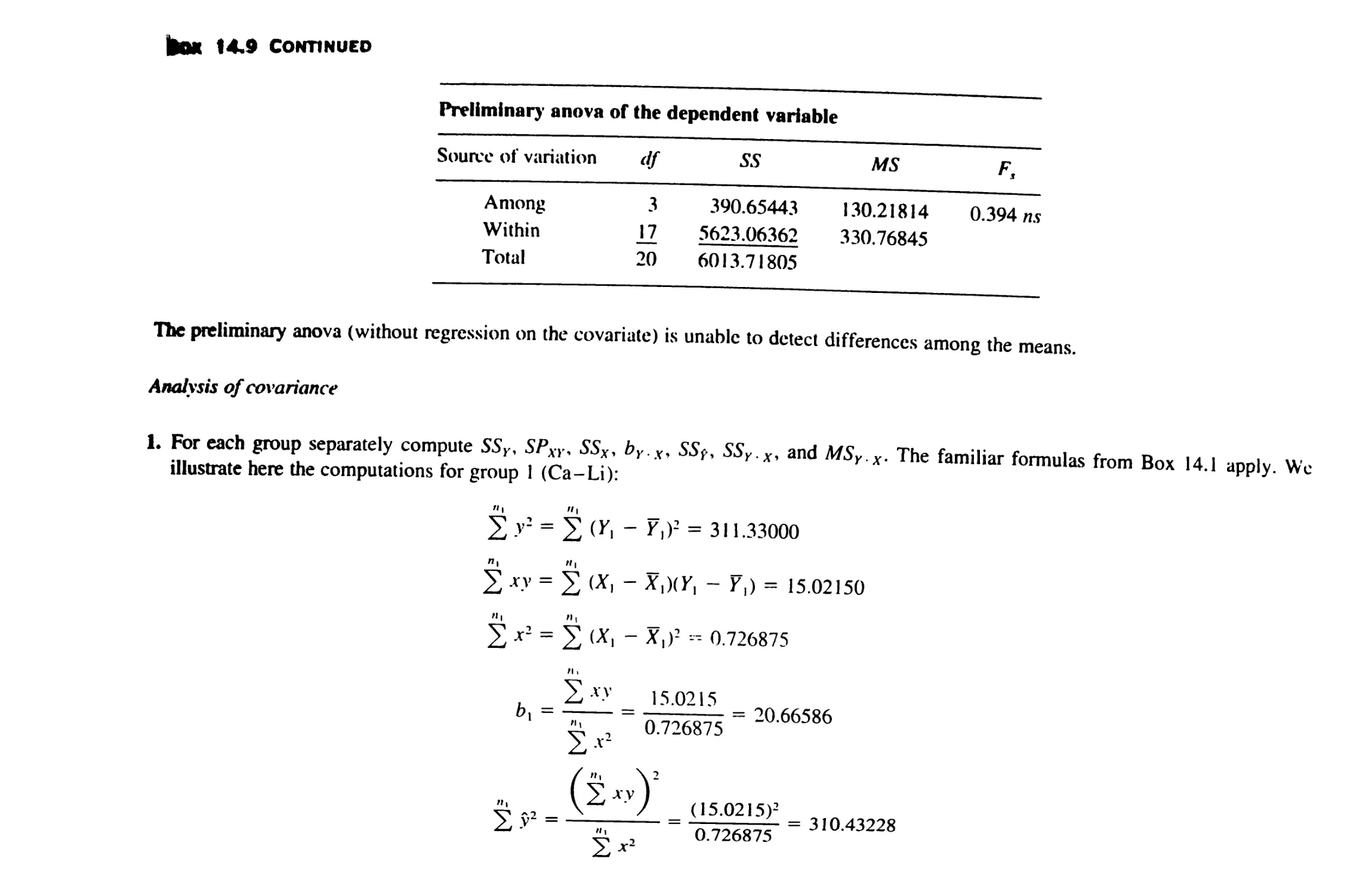
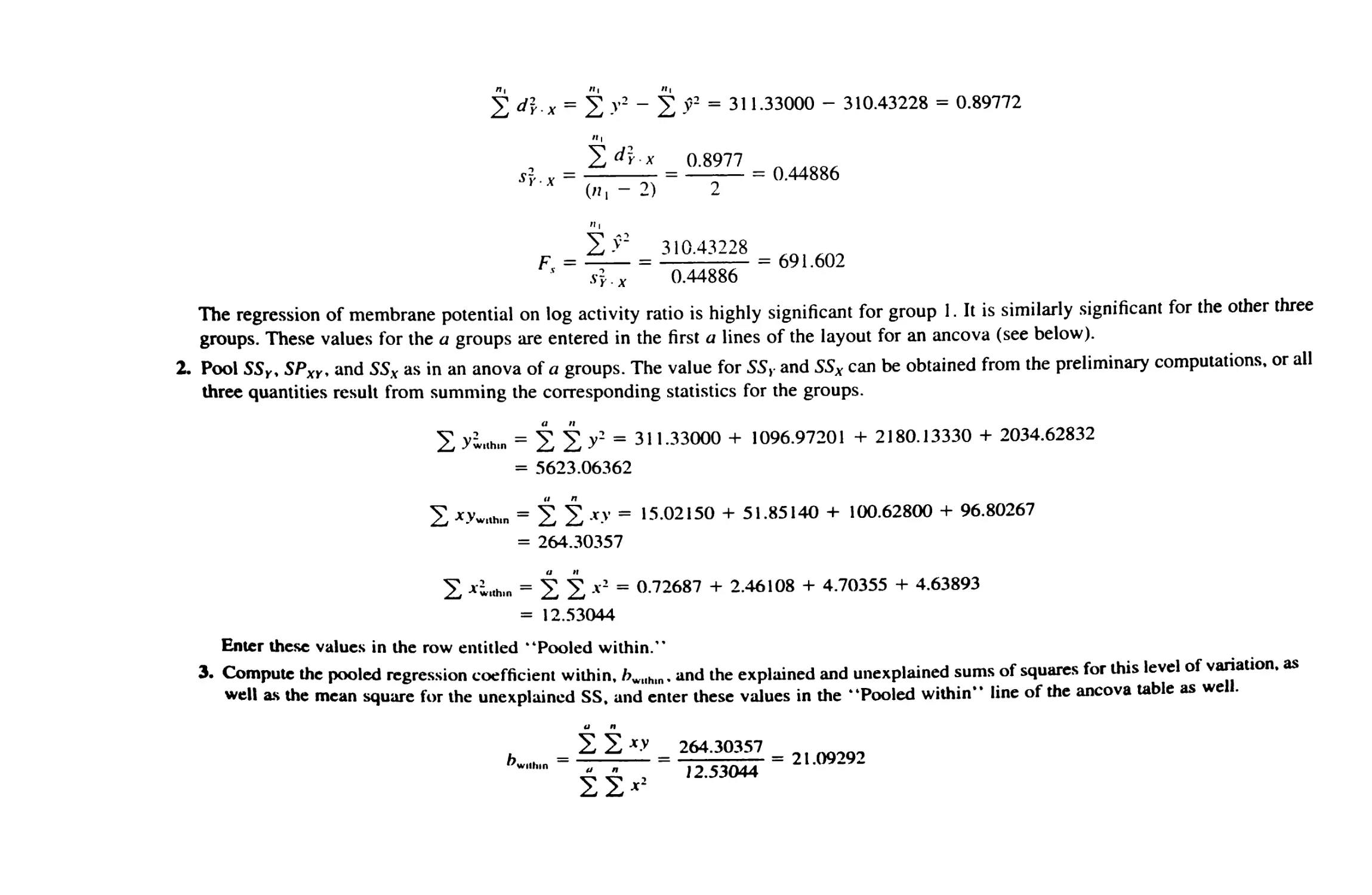
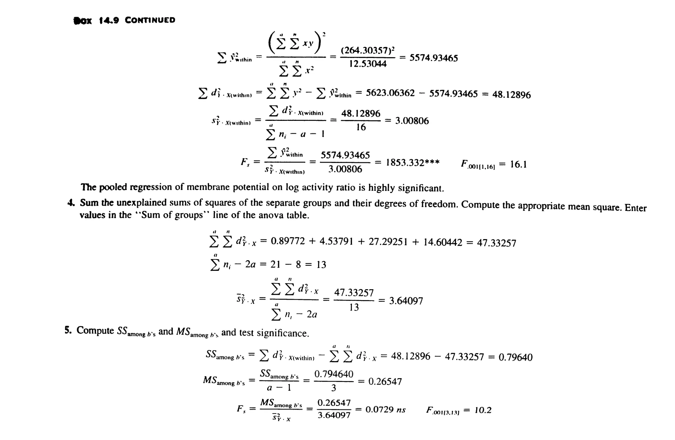
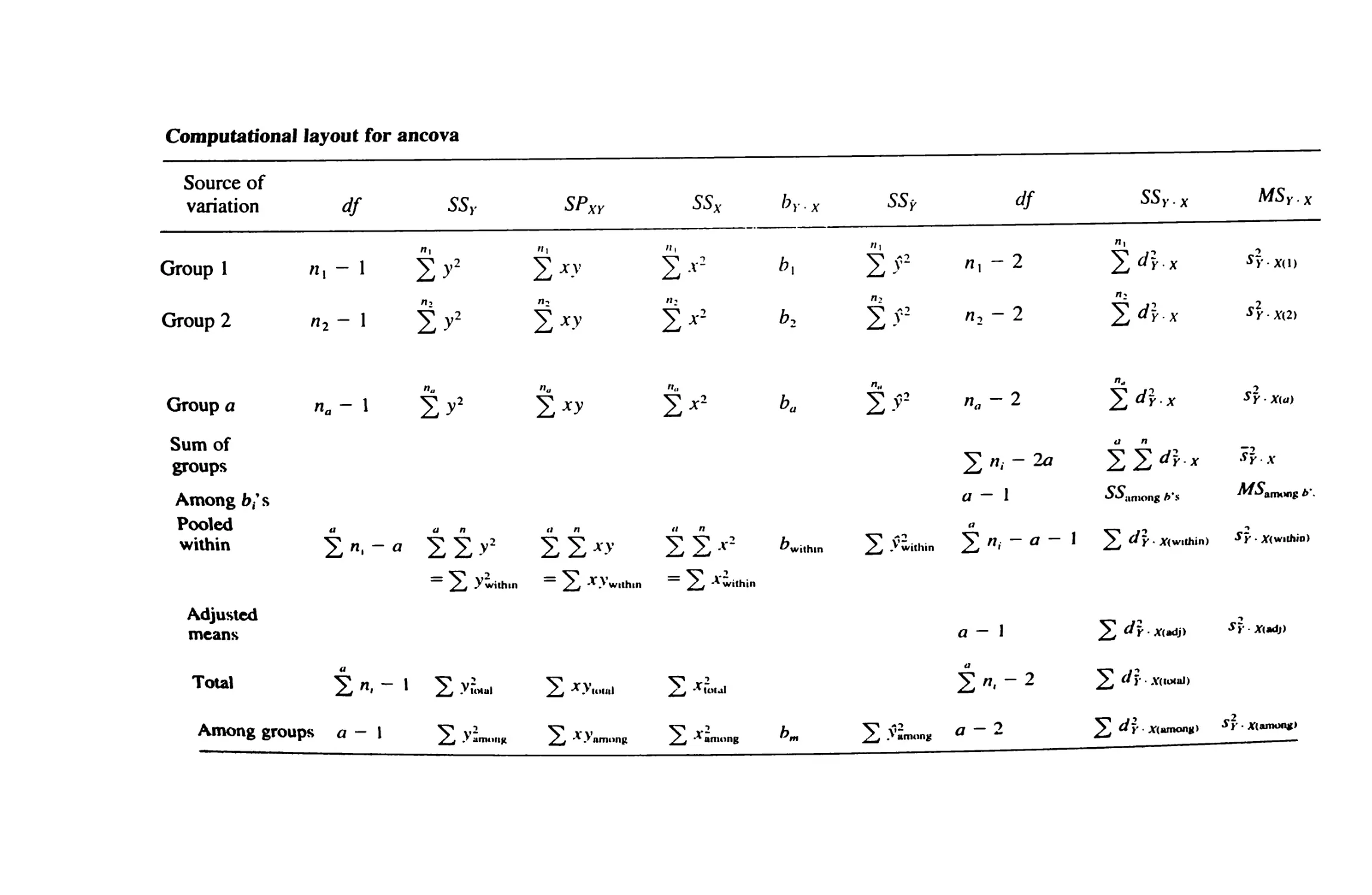
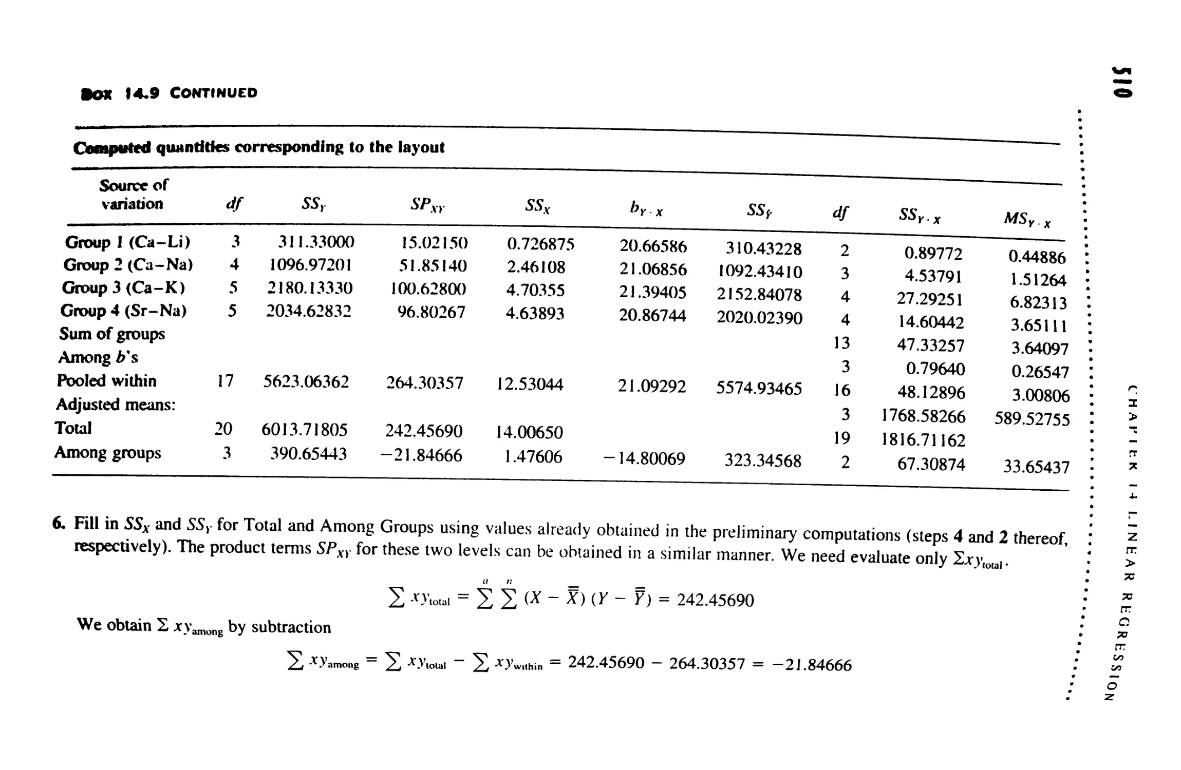
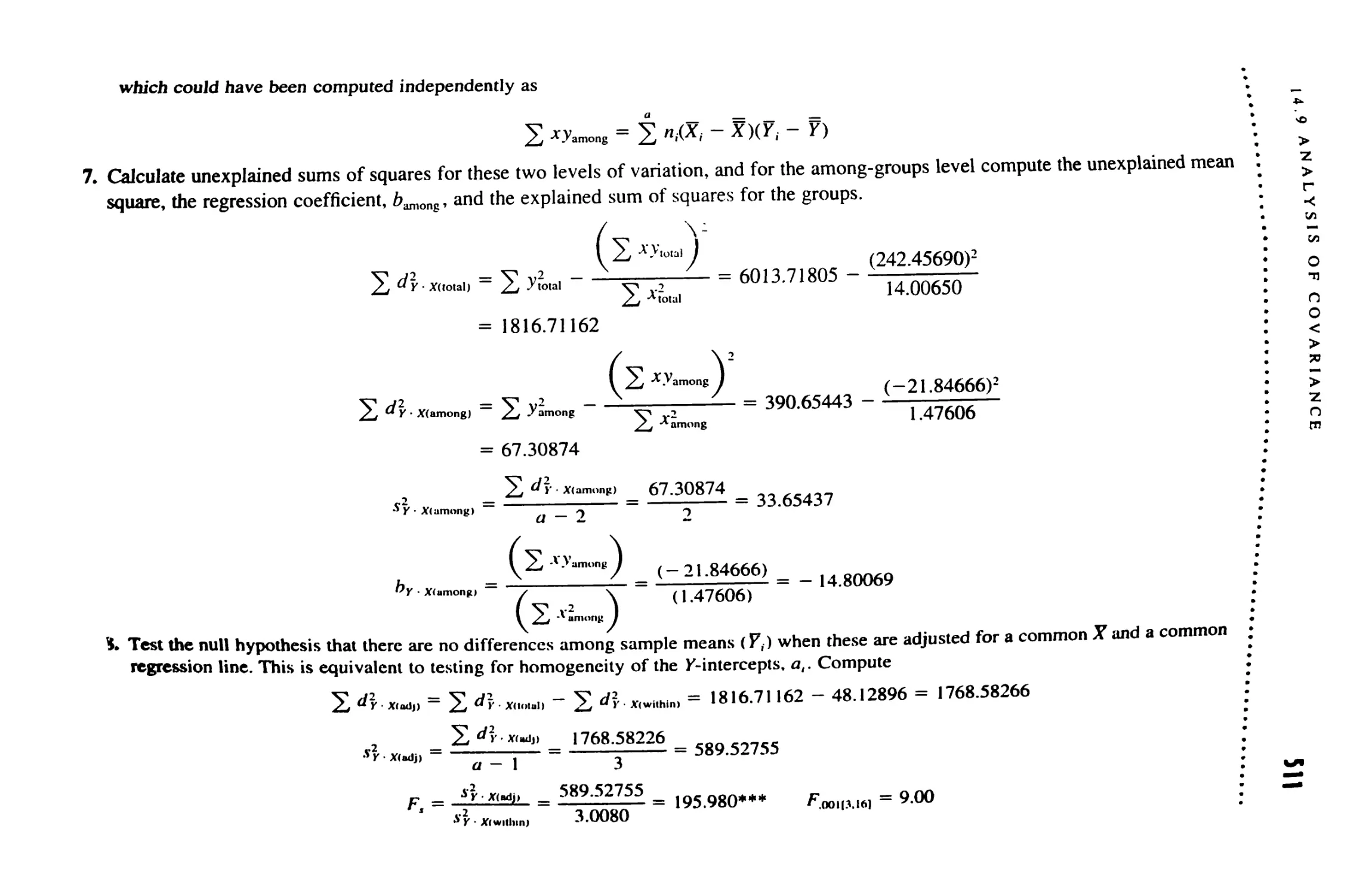
14.9 Analysis of Covariance 499
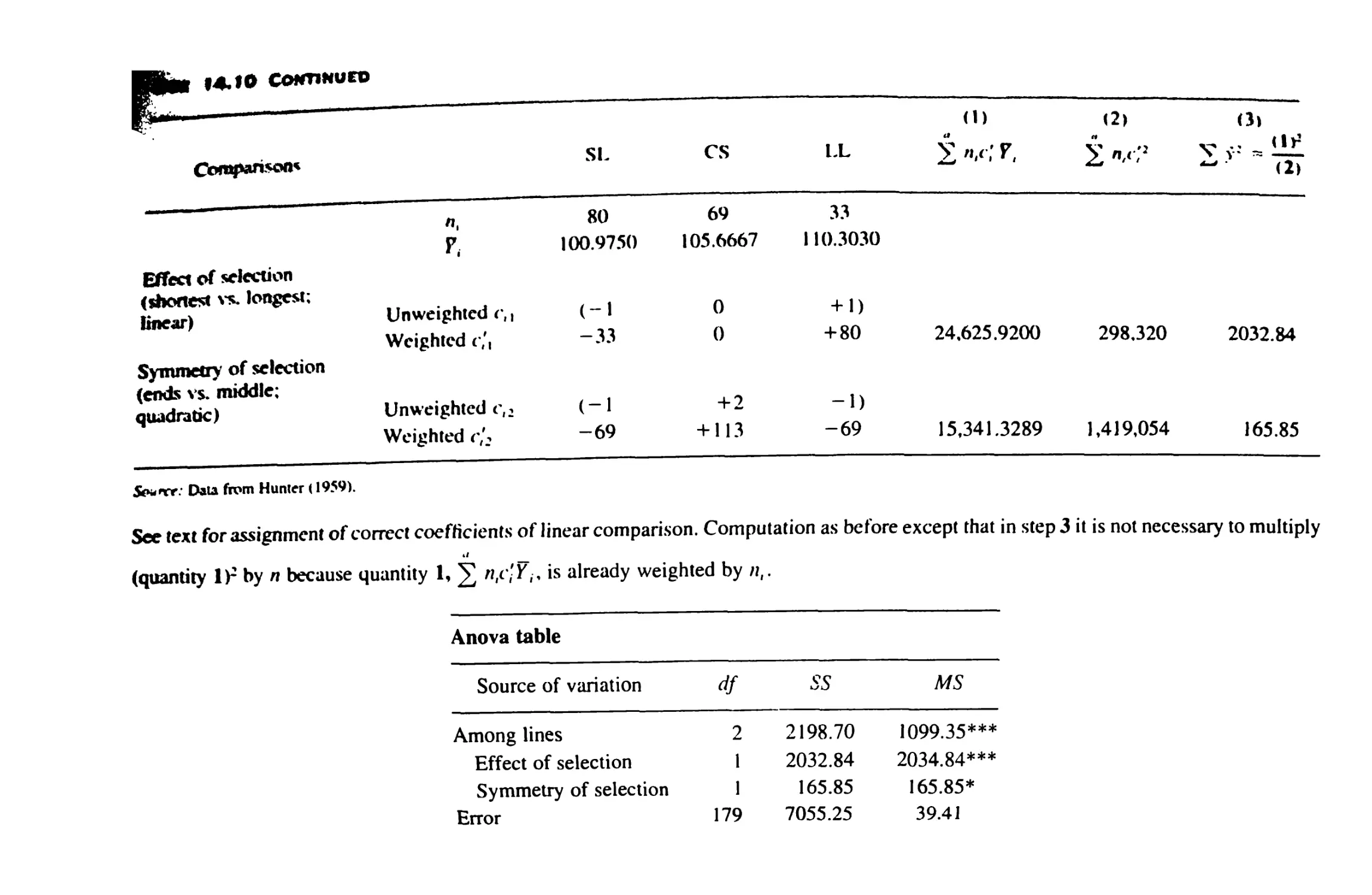
14.10 Linear Comparisons in Anovas 521
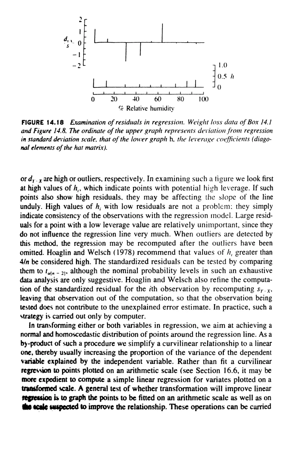
14.11 Examining Residuals and Transformations
in Regression 531
14.12 Nonparametric Tests for Regression 539
14.13 Model II Regression 541
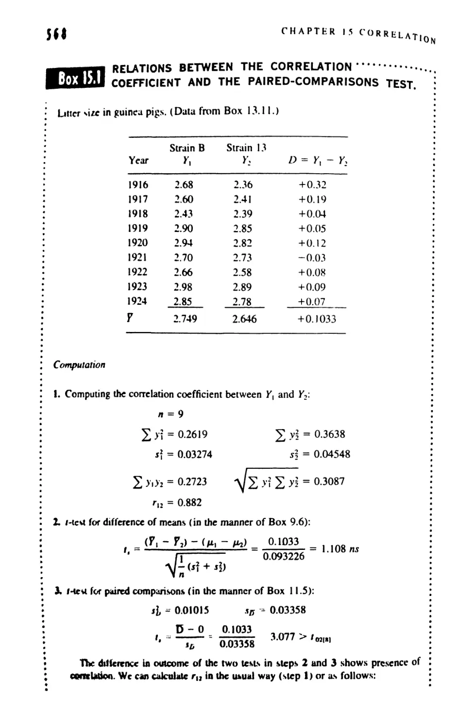
1$ CORRELATION 555
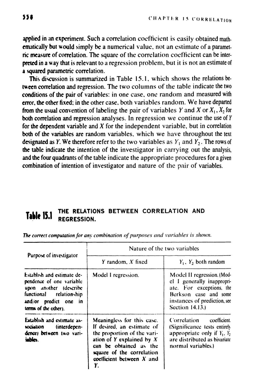
15.1 Correlation and Regression 556
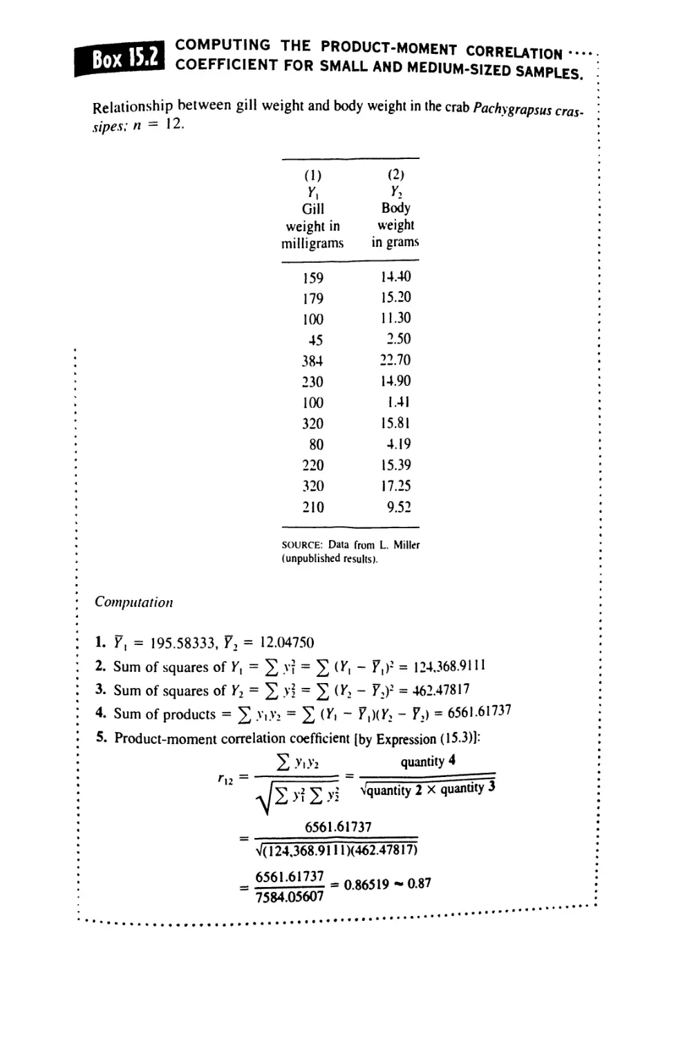
15.2 The Product-Moment Correlation Coefficient 559
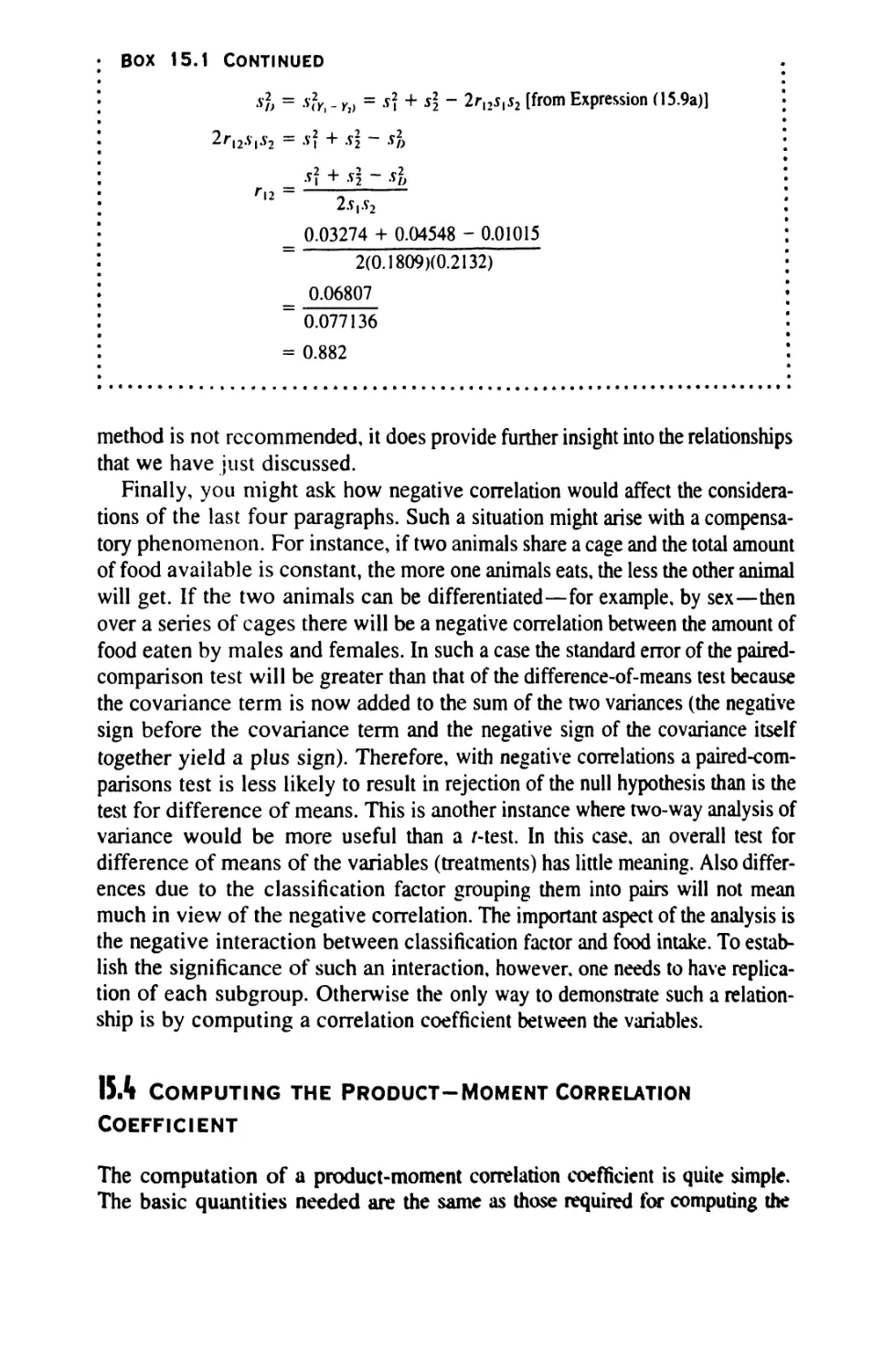
15.3 The Variance of Sums and Differences 567
15.4 Computing the Product-Moment Correlation
Coefficient 569
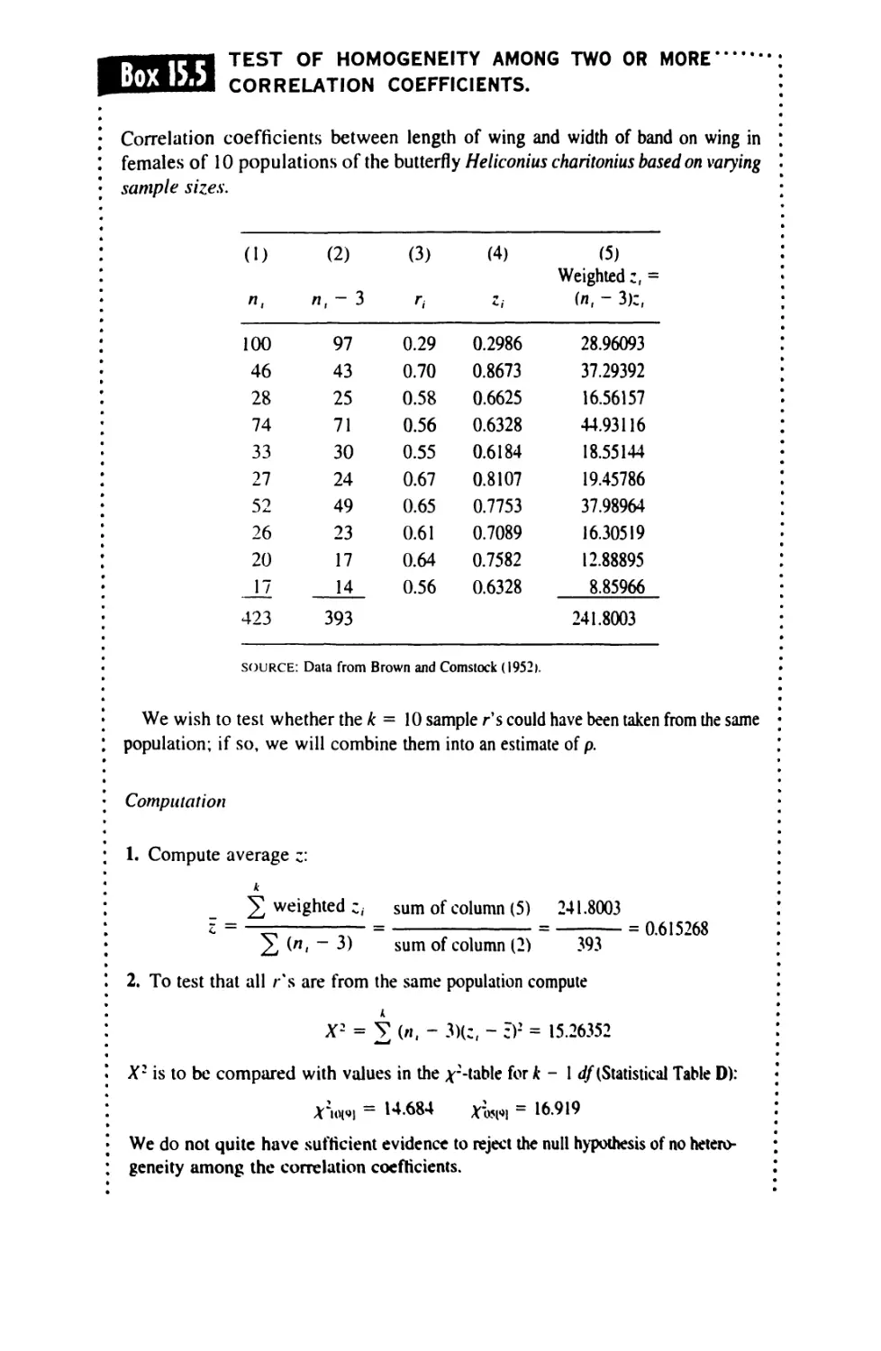
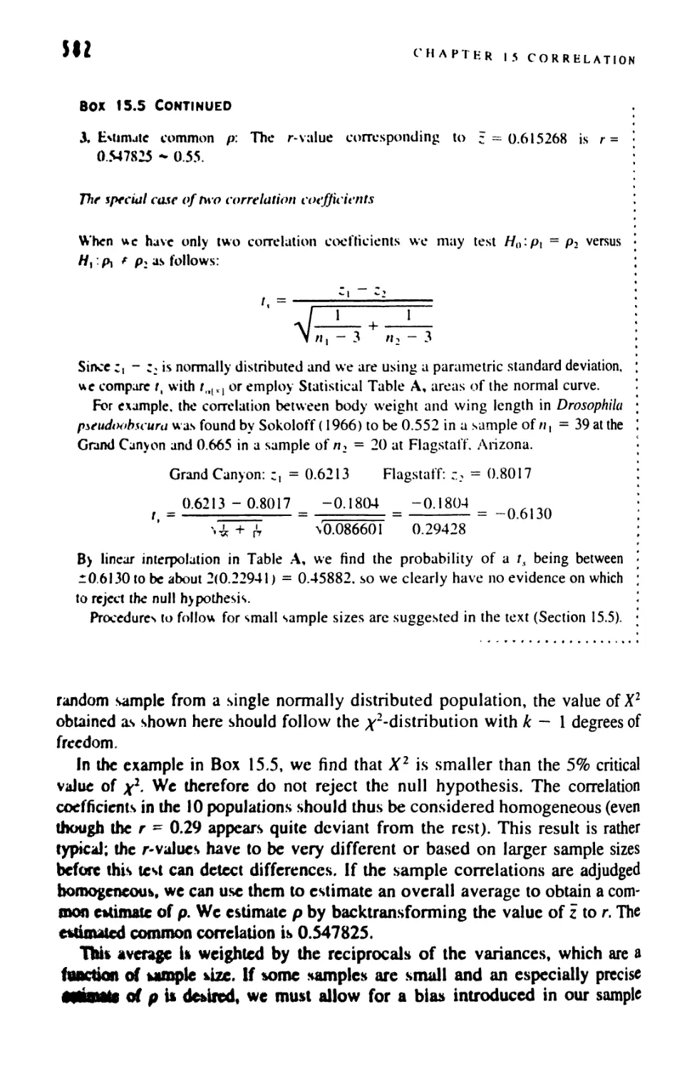
15.5 Significance Tests in Correlation 574
15.6 Applications of Correlation 583
15.7 Principal Axes and Confidence Regions 586
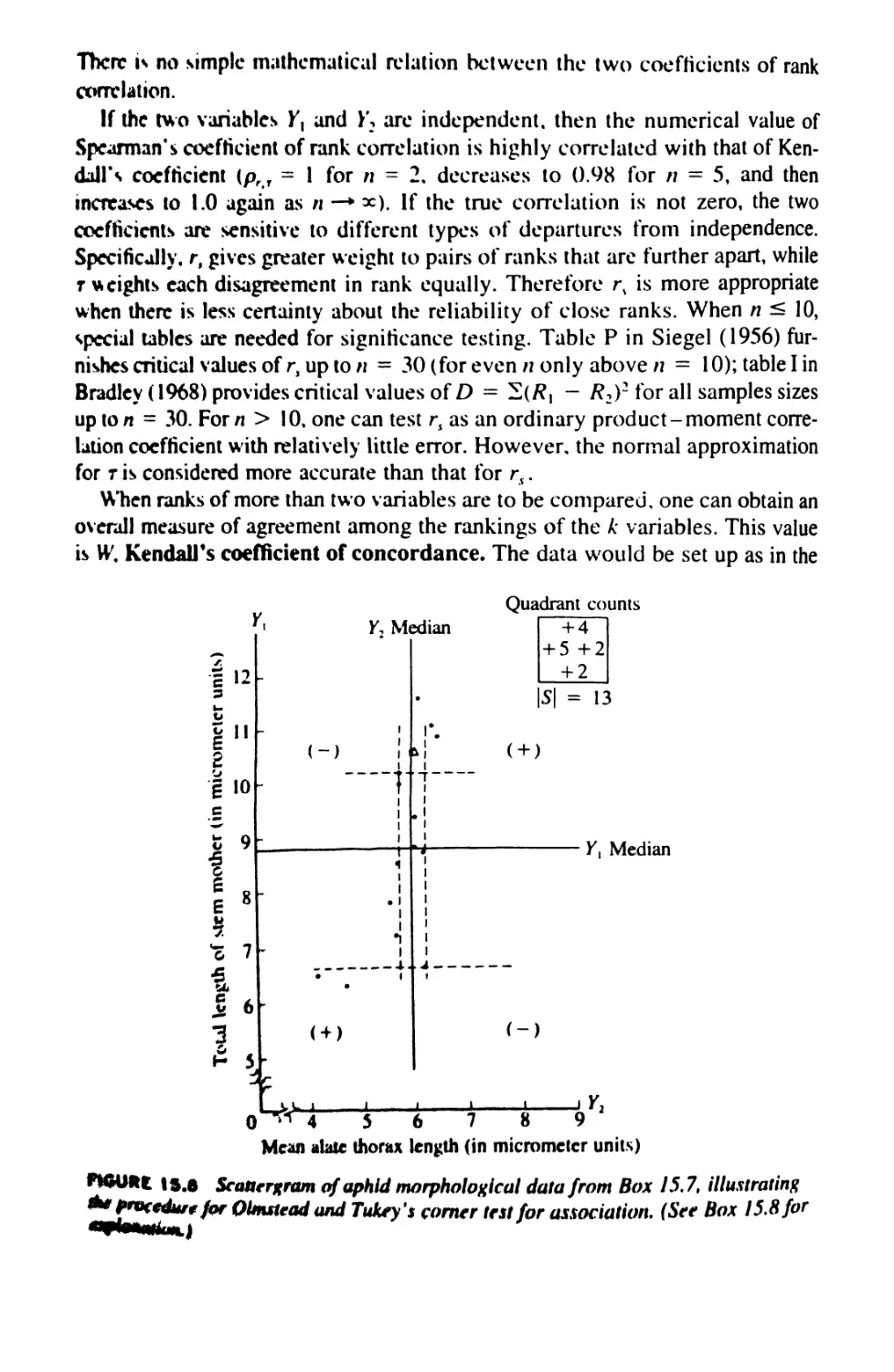
15.K Nonparametric Tests for Association 593
CON TKN TS
XI
16 MULTIPLE AND CURVILINEAR REGRESSION 609
16.1 Multiple Regression: Computation 610
16.2 Multiple Regression: Significance Tests 623
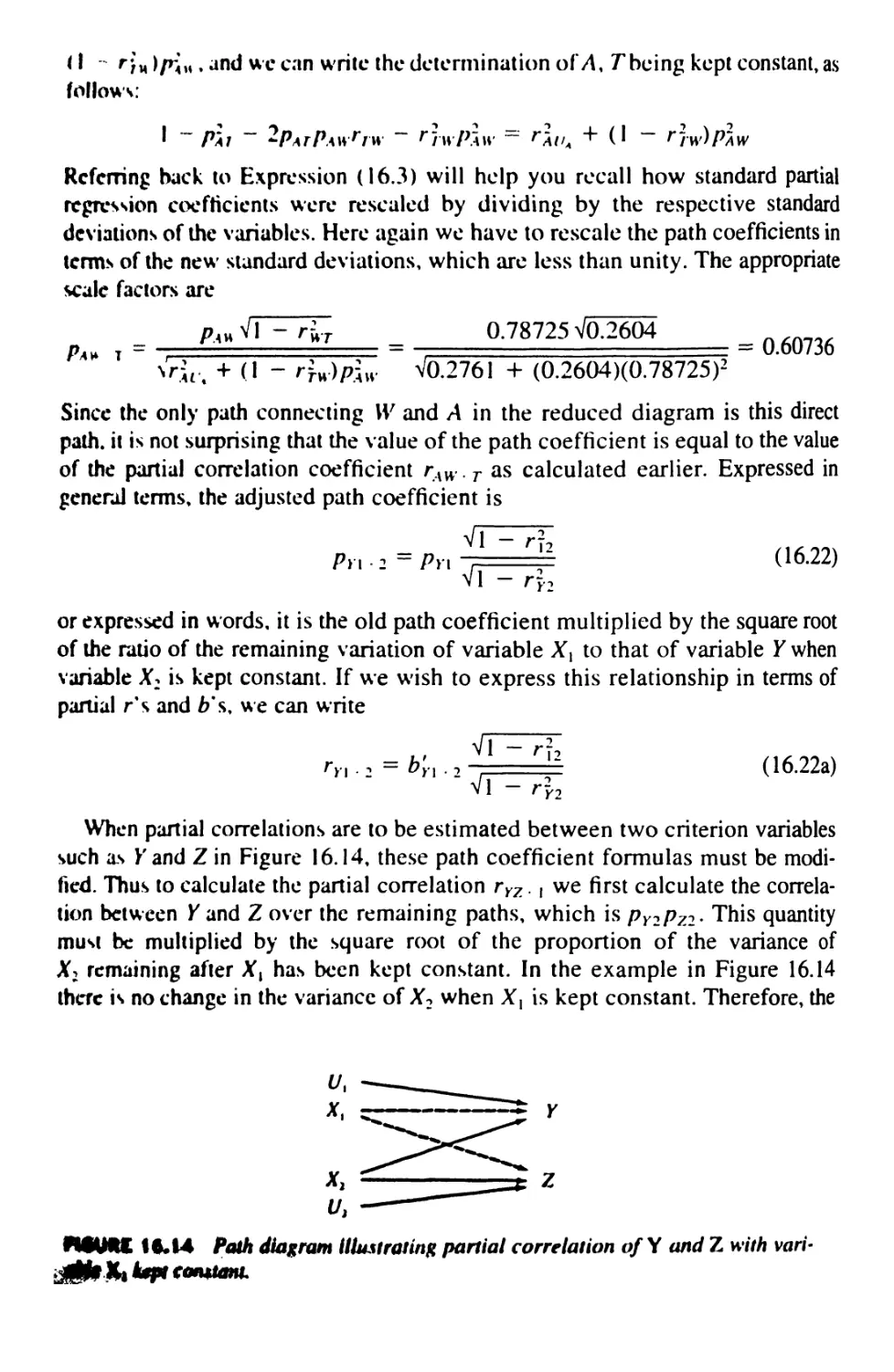
16.3 Path Analysis 634
16.4 Partial and Multiple Correlation 649
16.5 Choosing Predictor Variables 654
16.6 Curvilinear Regression 665
16.7 Advanced Topics in Regression and Correlation 678
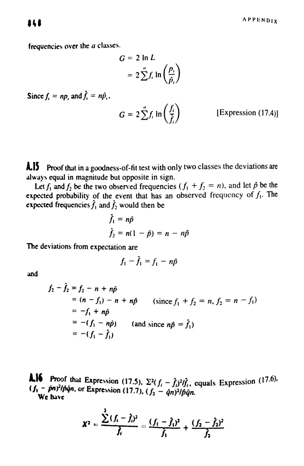
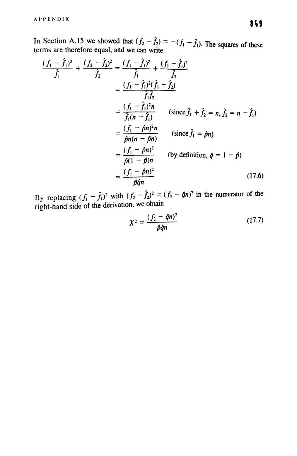
17 ANALYSIS OF FREQUENCIES 685
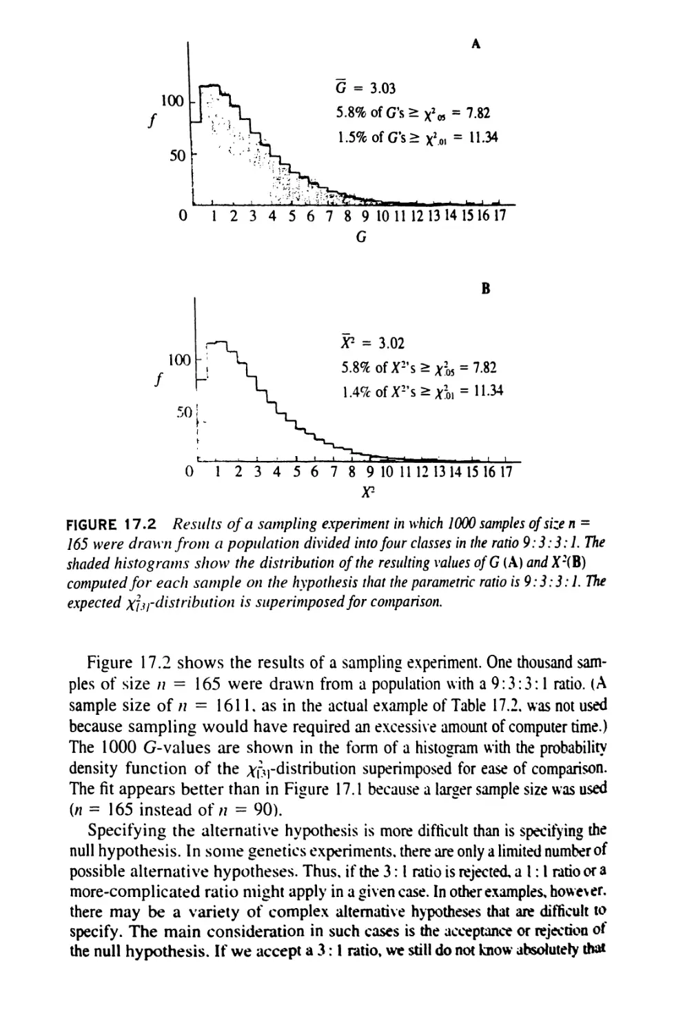
17.1 Introduction to Tests for Goodness of Fit 686
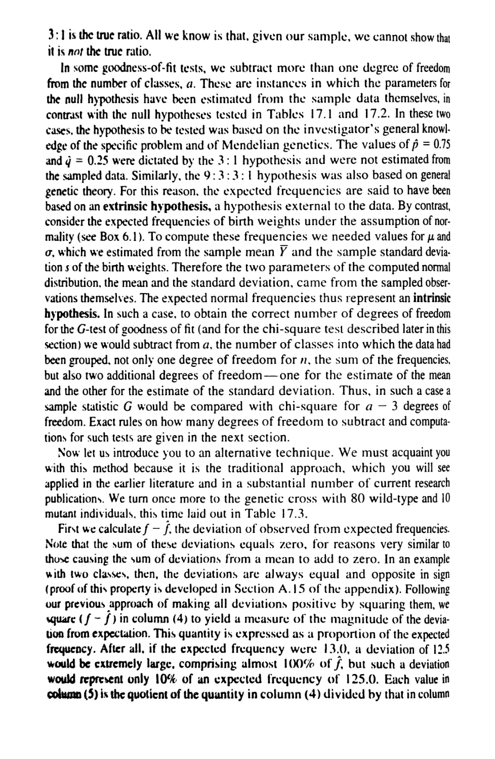
17.2 Single-Classification Tests for Goodness of Fit 697
17.3 Replicated Tests of Goodness of Fit 715
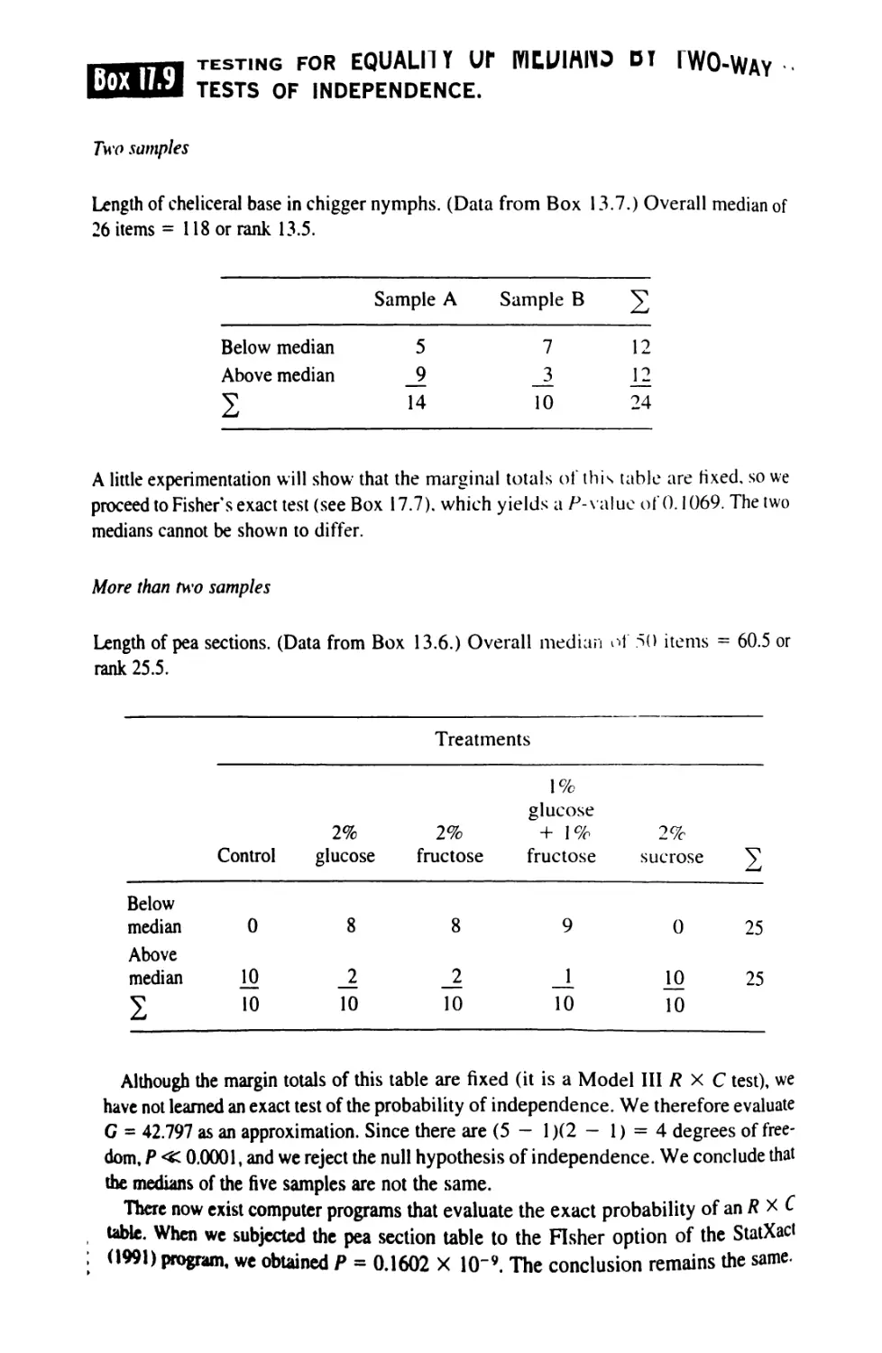
17.4 Tests of Independence: Two-Way Tables 724
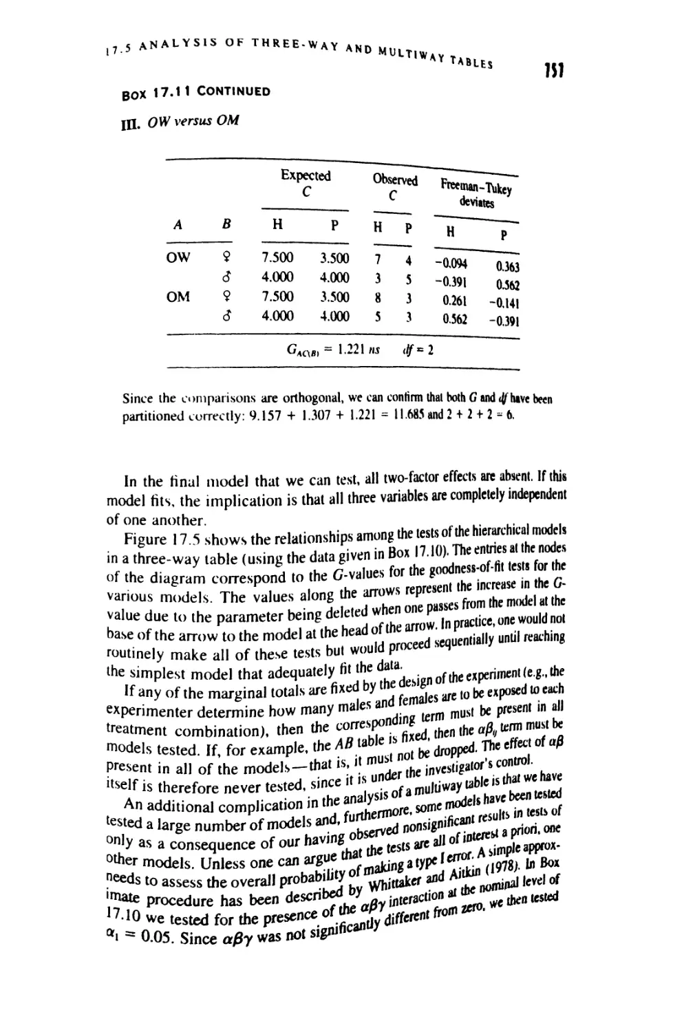
17.5 Analysis of Three-Way and Multiway Tables 743
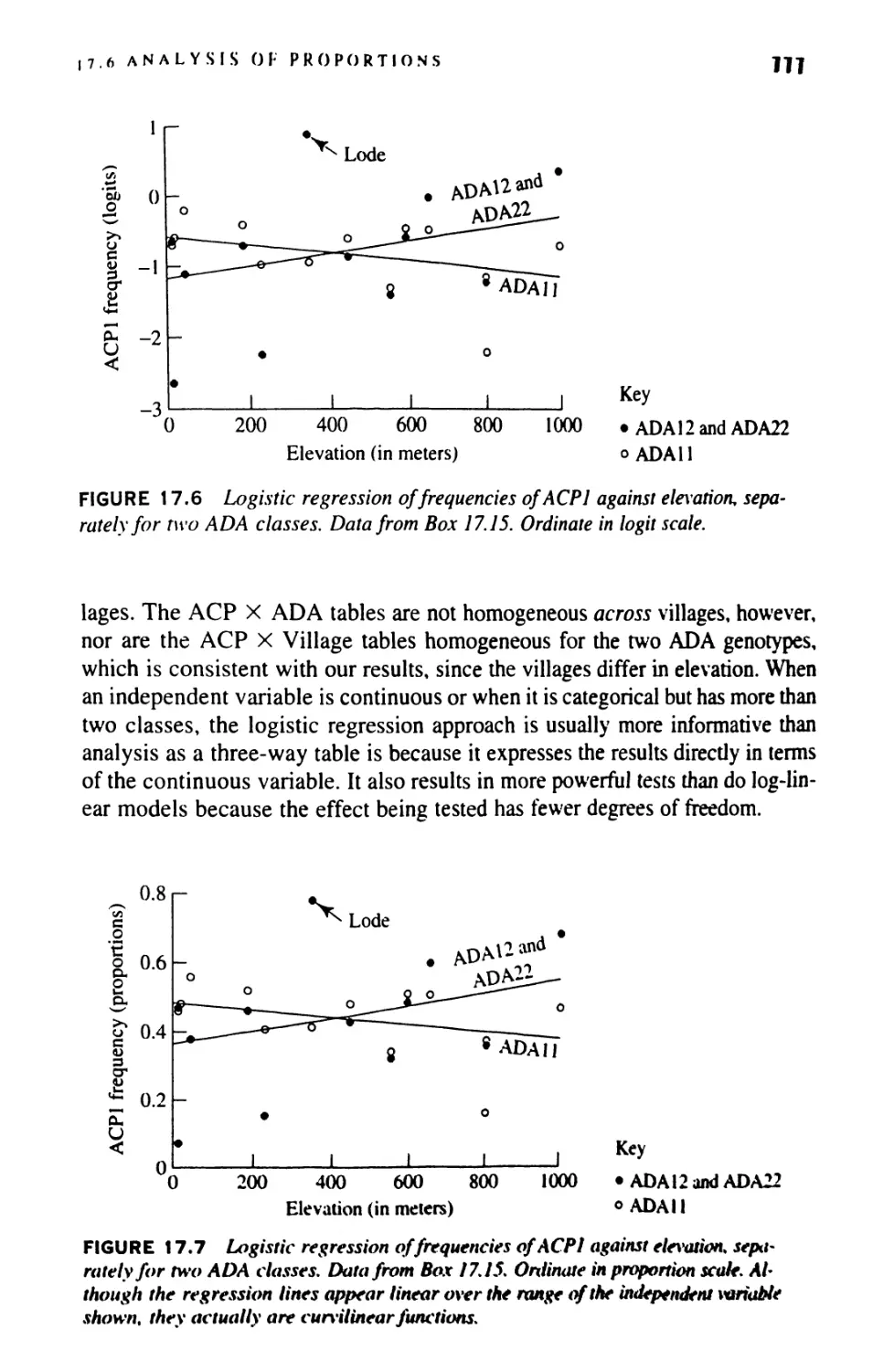
17.6 Analysis of Proportions 760
17.7 Randomized Blocks for Frequency Data 778
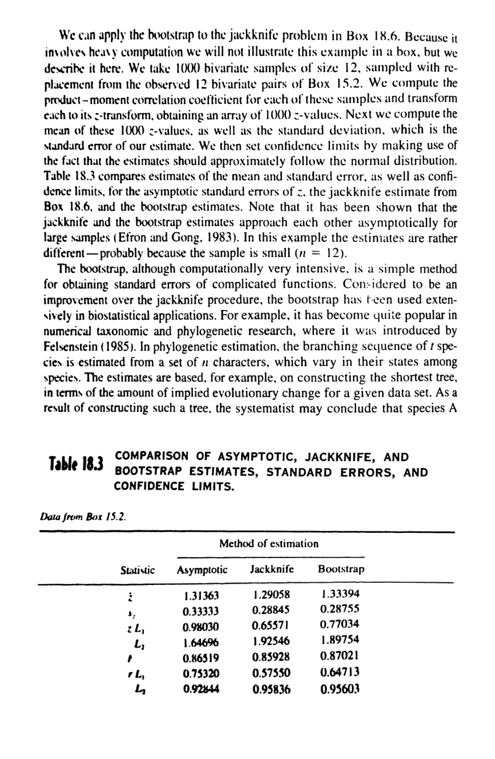
18 MISCELLANEOUS METHODS 794
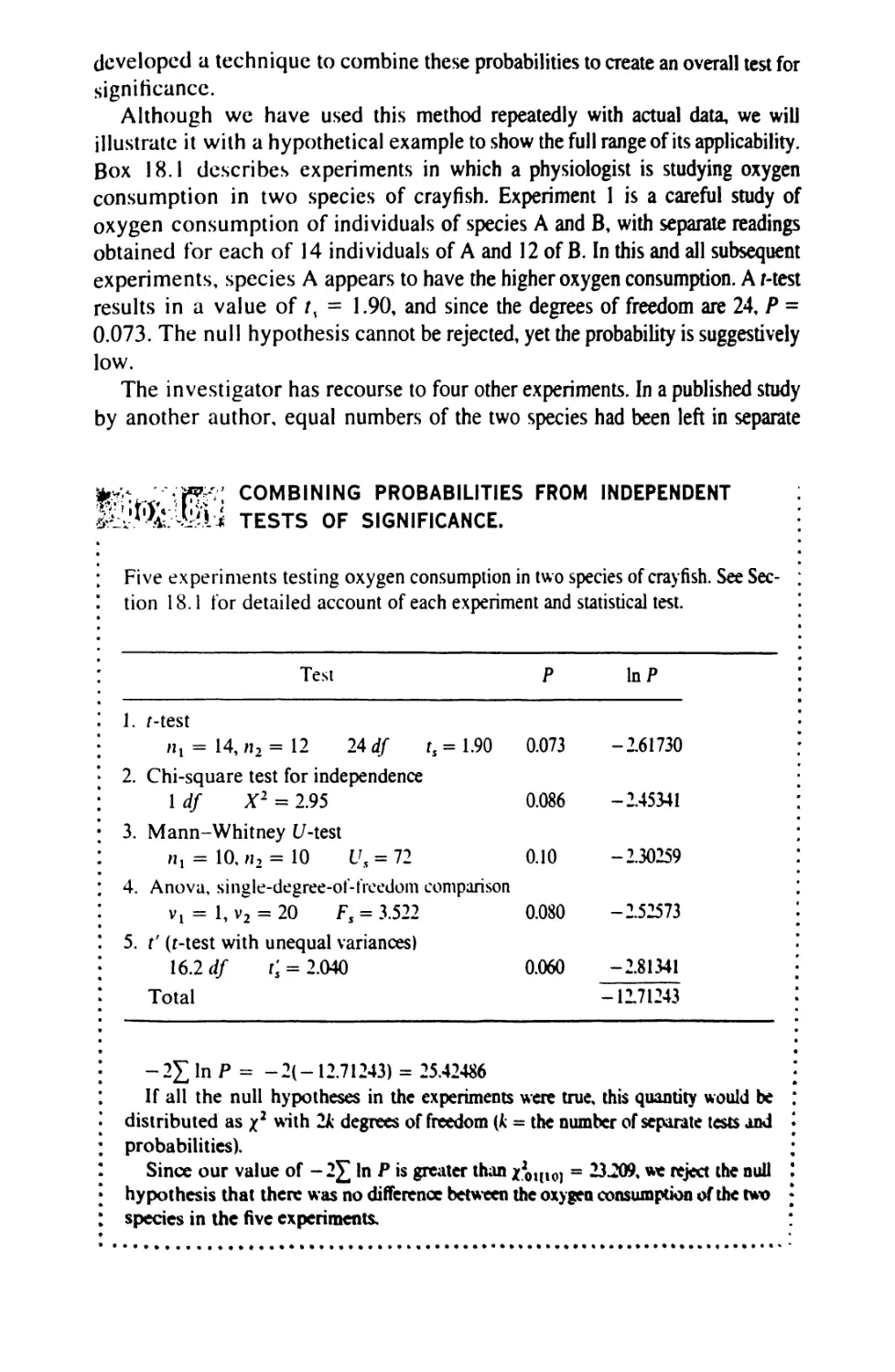
18.1 Combining Probabilities From Tests of Significance 794
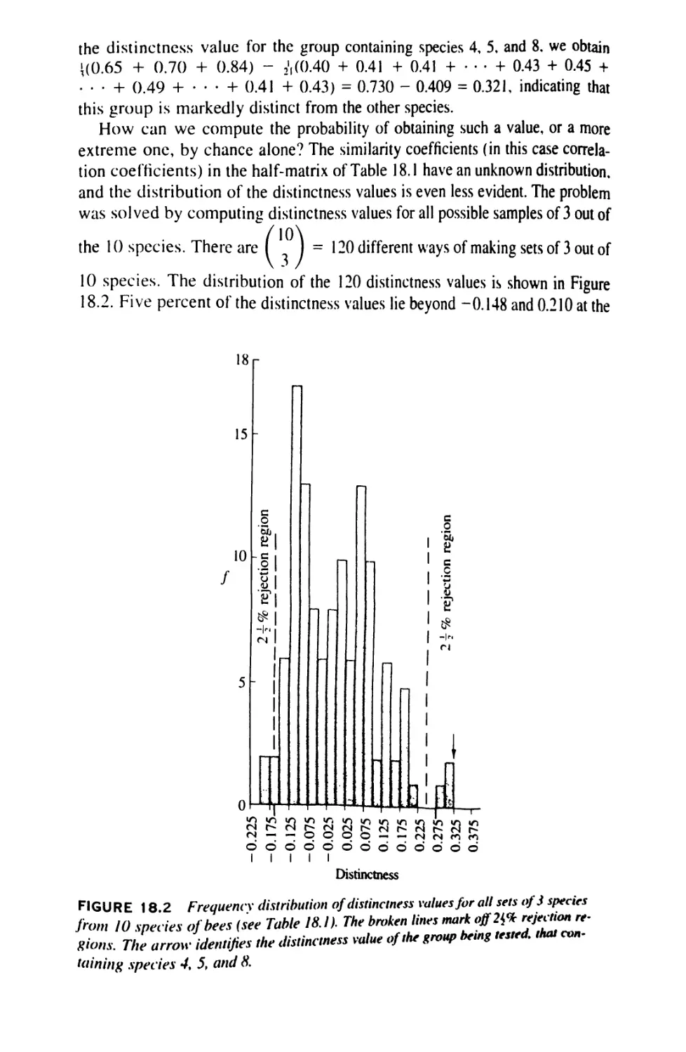
18.2 Tests for Randomness of Nominal Data: Runs Tests 797
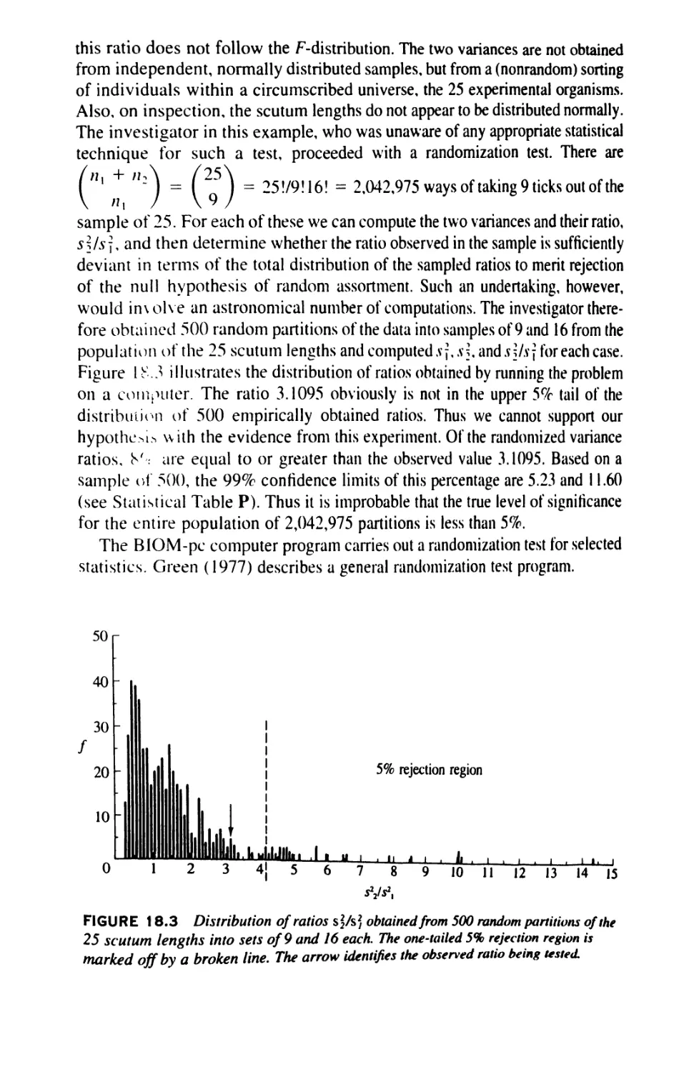
18.3 Randomization Tests 803
18.4 The Jackknife and the Bootstrap 820
18.5 The Future of Biometry: Data Analysis 825
APPENDIX: MATHEMATICAL PROOFS 833
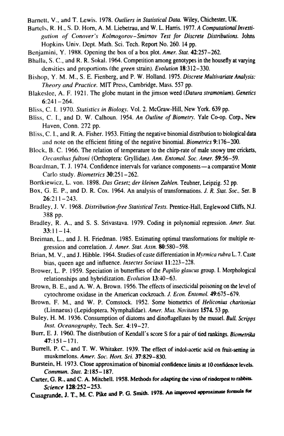
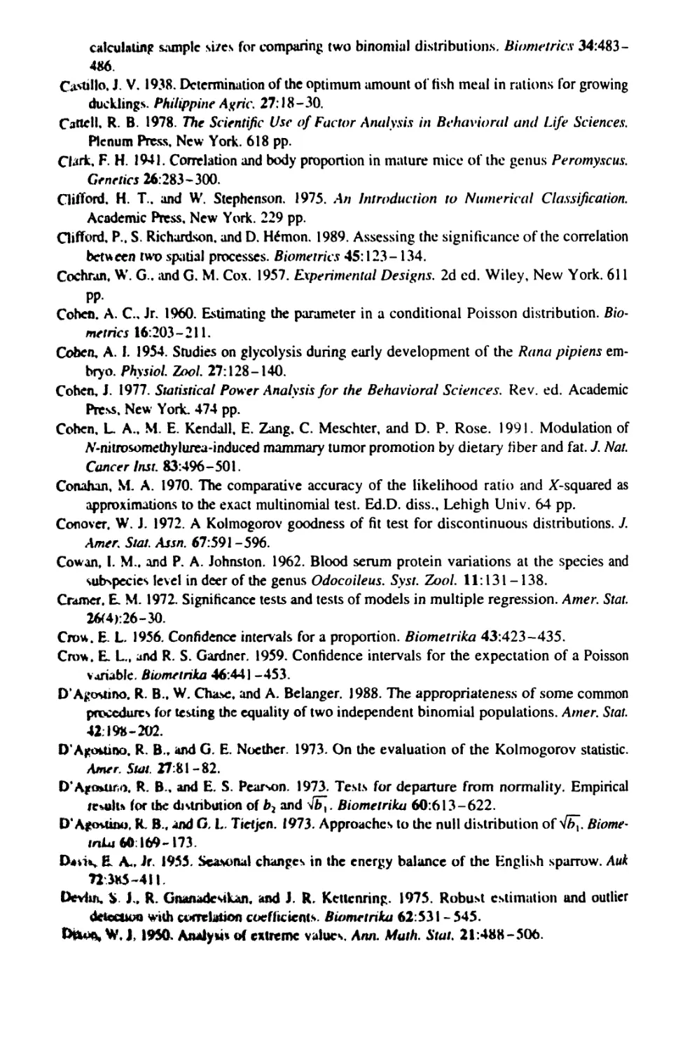
BIBLIOGRAPHY 850
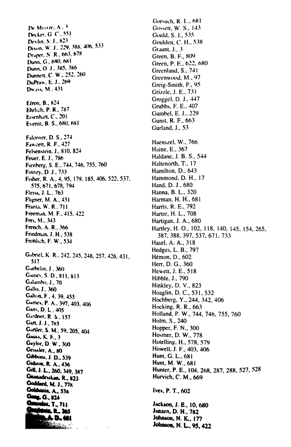
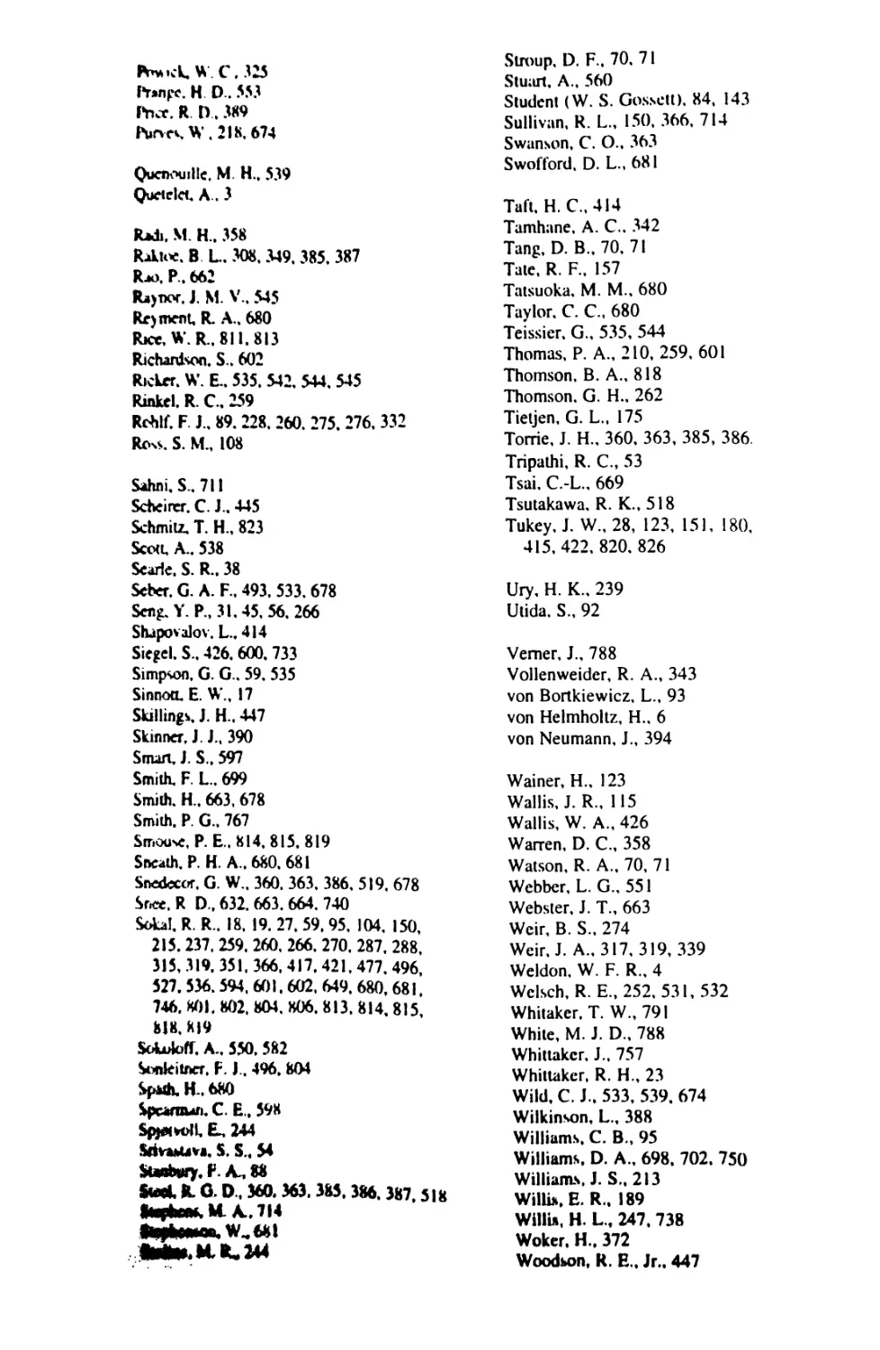
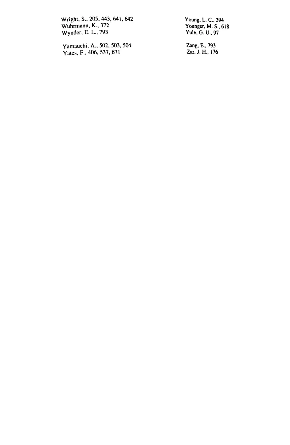
AUTHOR INDEX 865
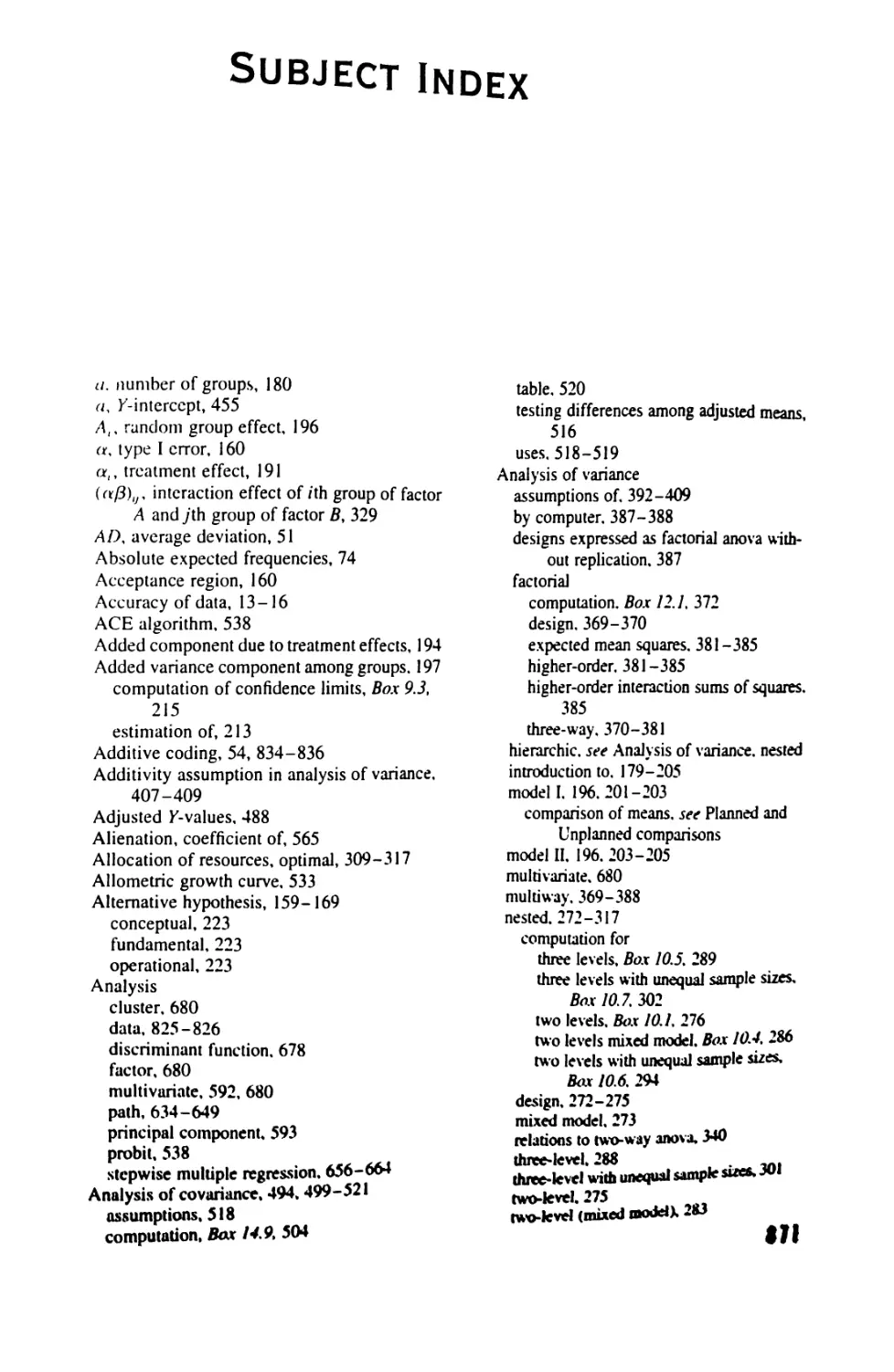
SUBJECT INDEX
871
PREFACE
The success of the first two editions of Biometry among teachers,
students, and others who use biological statistics has encouraged us to prepare this
extensively revised Third Edition.
We wrote and have revised this book because we feel that there is a need for an
up-to-date text aimed primarily at the academic biologist—a text that develops the
subject from an elementary introduction up to the advanced methods necessary
nowadays for biological research and for an understanding of the published
literature. Many available texts represent the outlook and interests of agricultural
experiment stations. This is quite proper in view of the great application of statistics in this
field; in fact, modem statistics originated at such institutions. However, personal
inclination and the nature of the institution at which we teach cause us to address
ourselves to general biologists, ecologists, geneticists, physiologists, and other
biologists working largely on nonapplied subjects in universities, research institutes, and
museums. Considerable overlap exists between the needs of these two somewhat
artificially contrasted groups and, of necessity, some of our presentation will deal
with agricultural experimentation. More broadly, the statistical methods treated here
are useful in many applied fields, including medicine and allied health
sciences. Since it is a well-known pedagogical dictum that people learn best by familiar
examples, we have endeavored to make our examples as pertinent as possible for our
readers.
Much agricultural and biological work is by its very nature experimental. This
book, while furnishing ample directions for the analysis of experimental work, also
stresses descriptive and analytical statistical study of biological phenomena. These
powerful methods are often overlooked and sometimes, by implication, the validity
of nonexperimental biological work is put in doubt. We think that descriptive,
analytical, and experimental approaches are all of value, and we have tried to strike a
balance among them. This approach will be appreciated by workers in applied fields
such as the health sciences where ethical, financial, or other considerations may
prevent free use of direct experiment.
The readers we hope to interest are graduate students in biological departments
who require a knowledge of biometry as part of their profesional training and pn>-
Xili
Icvsional biologists in universities, museums, and research positions who for one
reason or another did not obtain biometric training during their student careers—that
is. people who need to acquire knowledge largely in an aulodidactic way. This book
has been designed to serve not only as a text to accompany a lecture course but also
as a complete volume for self-study.
We aim to instill in our students an ability to think through biological research
problems in such a way as to grasp the essentials of the experimental or analytical
setup, to know which types of statistical tests to apply in a given case, and to carry
out the computations required. A modicum of statistical theory has to be presented to
introduce the subject matter, but once this is done, further knowledge of statistical
theory is acquired as part of the learning process in solving statistical problems,
rather than as a preamble to their solution. Because of limitations of time and the
minimal mathematical preparation of most students, discussion of theory must be
curtailed and some methods are presented almost entirely in *'cookbook" style.
Cher the years we have found that students with very limited mathematical
backgrounds can handle biometry excellently. There is remarkably little correlation
between innate mathematical ability and capacity to understand the ordinary biometric
methodologies. By contrast, in our experience a very high correlation exists between
success in the biometry course and success in the chosen field of biological
specialization. Teachers should encourage students who feel they have no mathematical
aptitude, since it does not apply to the study of applied statistics.
We must make our apologies to the mathematical statisticians who may chance on
this volume. Compromises had to be made on occasion between precise definitions
as required by mathematical statistics and formulations of theory that teaching
experience has shown to be most easily understood by beginning classes. In judging our
effort, allowance should be made for such changes and circumscriptions.
To make our book more useful to the autodidactic reader, we have employed a
more direct and personal style than is customary in textbooks of this sort. No book
can replace a dedicated and able teacher, but we have tried to make our written
approach a* similar as we can to our classroom manner.
ARRANGEMENT OF THIS BOOK
Since this book deviates in several important ways from the customary statistics
teiibook. we would like to point out the differences so that the prospective reader
ma) derive the maximum benefit from its use. Subject matter is arranged in chapters
^nJ sections, numbered by the conventional decimal numbering system: The number
K-forc the decimal point refers to the chapter, the number after the point to the
section Topics can be referred to in the table of contents as well as in the index. The
ubtcs arc also numbered with the decimal system: The first number denotes the
cltuf \cr. ihc second the number of the table within the chapter.
Cerum special tables art designated ^boxes'* and are numbered as such, again
u*my the dcctm.il system. The boxes serve a double function. First, they illustrate
&H«fK!iati<rtnal methods for solving various type* of biometric problems and can
PREFACE
XV
therefore be used as convenient patterns for computation. The boxes usually contain
all the steps necessary — from the initial setup of the problem to the final result;
hence to students familiar with the book, the boxes can serve as quick summary
reminders of the technique. A second important use of the boxes relates to their
origin as mimeographed sheets handed out in a biometry course at the University of
Kansas. In the allowed lecture time the instructor would not have been able to convey
even as much as half the subject matter covered in the course (or in this book) if the
material contained in the sheets had to be put on the chalkboard. Asking the students
to refer in class to their biometry sheets (now the boxes in this book) saved much
time, and, incidentally, students were able to devote their attention to understanding
the content of the sheets rather than to copying them. Instructors who employ this
book as a text may wish to use the boxes in a similar manner.
Figures are numbered by the same decimal system as tables and boxes. A similar
numbering system is also used for (sampling) experiments, (mathematical)
expressions, and (homework) exercises.
Since the emphasis in this book is on practical applications of statistics to biology,
discussions of statistical theory are deliberately kept to a minimum. However, we
feel that some exposure to statistical theory is a good idea for any biologist, so we
have provided some in various places. Derivations are given for a number of
formulas but these are consigned to the appendix, where they should be studied and
reworked by the student.
We present what we consider the minimum statistical knowledge required for a
Ph.D. in the biological sciences at the present time. This material is of equal
importance for basic research and for applications in areas such as medicine and allied
health sciences. The most important topics treated are the simple distributions
(binomial, Poisson, and normal), simple statistical tests (including nonparametric tests),
analysis of variance through factorial analysis, analysis of frequencies, simple and
multiple regression, and correlation. This is more material than is covered in most
elementary texts, yet even this much is usually not sufficient to treat even the
common problems of everyday biological research. To enable the reader to become
acquainted with some advanced methods, we have therefore introduced at
appropriate places throughout the book so-called signpost paragraphs, set in italics and
bordered by a grey bar to the left. Signpost paragraphs explain some of the advanced
methods and their application and refer the reader to books and papers that we have
found to be most useful in explaining a given technique in simple and instructive
fashion. We hope that these signposted discussions will open up the wider field of
statistics for the readers of this book and permit them at the very least to consult
professional statisticians intelligently.
Homework exercises for students reading this book in connection with a biometry
course (or studying on their own) are given at the end of each chapter. In keeping
with our own convictions, these are largely real research problems. Some of them,
therefore, require a fair amount of computation for their solution.
We have been dissatisfied with the customary placement of statistical tables at the
end of textbooks of biometry and statistics. Users of these books and tables are
constantly inconvenienced by having to turn back and forth between the text material
xvl
P R B F A C 12
chi a certain method and the table necessary for the test of significance or for some
other computational step. Occasionally, the tables are interspersed throughout a
textbook at sites of their initial application; they are then difficult to locate, and
turning back and forth in the book is not avoided. Constant users of statistics,
therefore, generally use one or more sets of statistical tables, not only because such
handbooks usually contain more complete and diverse statistical tables than do the
textbooks, but also to avoid the constant turning of pages in the latter.
When we first planned this textbook, we thought we would eliminate statistical
tables altogether, asking readers to furnish their own from those available. However,
for pedagogical reasons, it was found desirable to refer to a standard set of tables, and
we consequently undertook to furnish them, bound separately from the text. The
SidtiMical Tables, Third Edition (Rohlf and Sokal, W. H. Freeman and Company,
1995), are identified by boldface letters (for example, Table A).
In preparing the First and Second Editions of this book, we had the benefit of
constructive criticism from two colleagues. Professor K. R. Gabriel (University of
Rochester) and Professor R. C. Lewontin (Harvard University) read the entire
manuscript and commented in detail on all aspects of the book. Many of their suggestions
ucre incorporated and have contributed significantly to any merit the book
possesses. An equally thorough editorial job was carried out by Dr. Michel Kabay (then
of the University de Moncton in New Brunswick, Canada). Professors F. J.
Sonleitner (University of Oklahoma), Theodore J. Crovello (then of the University of
Notre Dame), and Albert J. Rowell (University of Kansas) also furnished many
detailed comments on the text of the First Edition. Many students in various
biometry classes also contributed comments on several versions of the text. Since not all
suggestions were accepted, the reviewers named here cannot be held responsible for
errors and other failings in the book.
Wc arc obligated to the many generations of biometry students who have enabled
us to try out our ideas for teaching biometry and whose responses and criticism have
guided us in de\eloping our course. It has been a never-ending source of satisfaction
tti sec these students appropriate biometric techniques as their own and employ them
.ictivcl) in their researches.
Prcp.ir.ition of the Third Edition was greatly facilitated by Barbara Thomson, who
*ond processed all the changes and new materials for the manuscript and helped with
chc^kin^ the proofs. Her familiarity with the book made her assistance invaluable.
Doiulj DiGiov.inni assisted with various tasks during the final stages of proofing and
u^ciin^'.
To Juhc v,c owe a continuing debt of gratitude for her forebearance during the
Jor»K |*.kn<>dN of ycvtation of three editions of this book.
Robert R. Sokal
F. James Rohlf
July 1994
NOTES ON THE THIRD EDITION
We trust that the changes in the Third Edition of Biometry, outlined
here, will substantially enhance the book's utility.
When the First Edition was published in 1969, most calculations in biometry were
carried out on mechanical desk calculators. Electronic desk calculators were just
beginning to make an appearance. The availability of handheld pocket calculators
was still several years away. Heavy, repetitive calculations were carried out on large
mainframe computers. By now, most statistical computations, except for very large
tasks, are carried out on personal computers or work stations, making obsolete the
desk calculator formulas we furnished in the text and in the boxes of earlier editions
of the book. We have replaced these formulas with simpler structural formulas that
readers will find easier to understand because they furnish direct expressions of the
nature of the computation. Furthermore, these structural formulas can usually be
programmed directly for digital computers and are typically not subject to the same
magnitude of rounding error as desk calculator equations.
Removing the desk calculator formulas featured in the previous editions freed up
a substantial amount of space, which we have used to introduce a number of new-
topics that persons embarking on a study or practice of biometry in the 1990s need to
learn. Here we list the new topics in the sequence of their appearance in the book.
Additional homework exercises have been included as practice in all new methods
and as further practice in earlier methods.
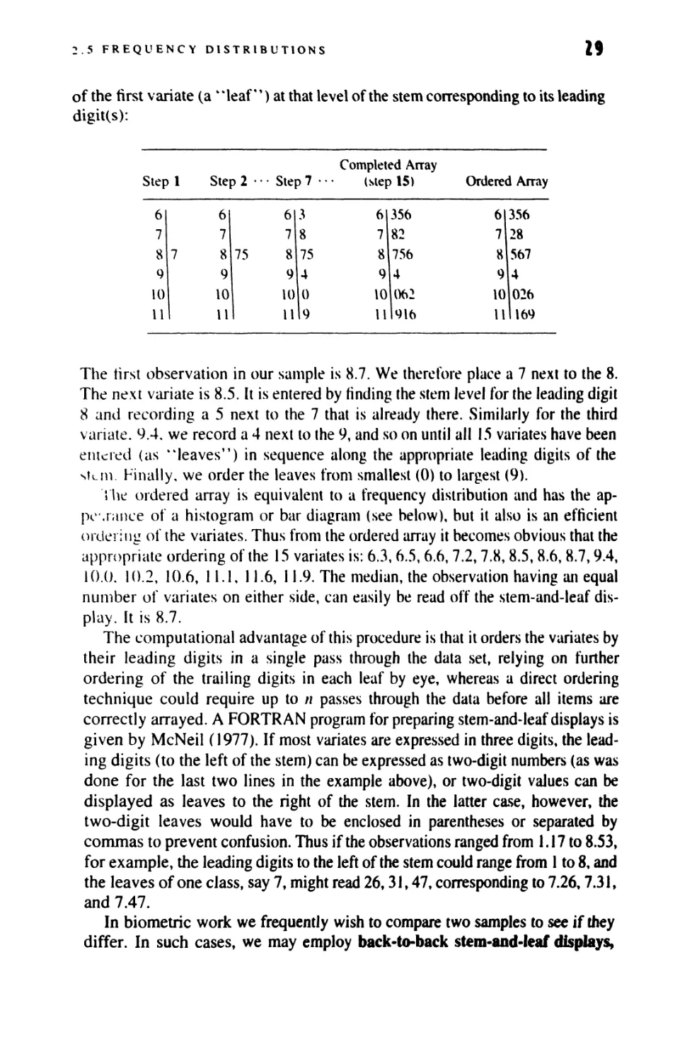
In Section 2.5 we now feature back-to-back stem-and-leaf displays for comparing
two samples. Chapter 3, on the handling of data, has been rewritten to keep abreast of
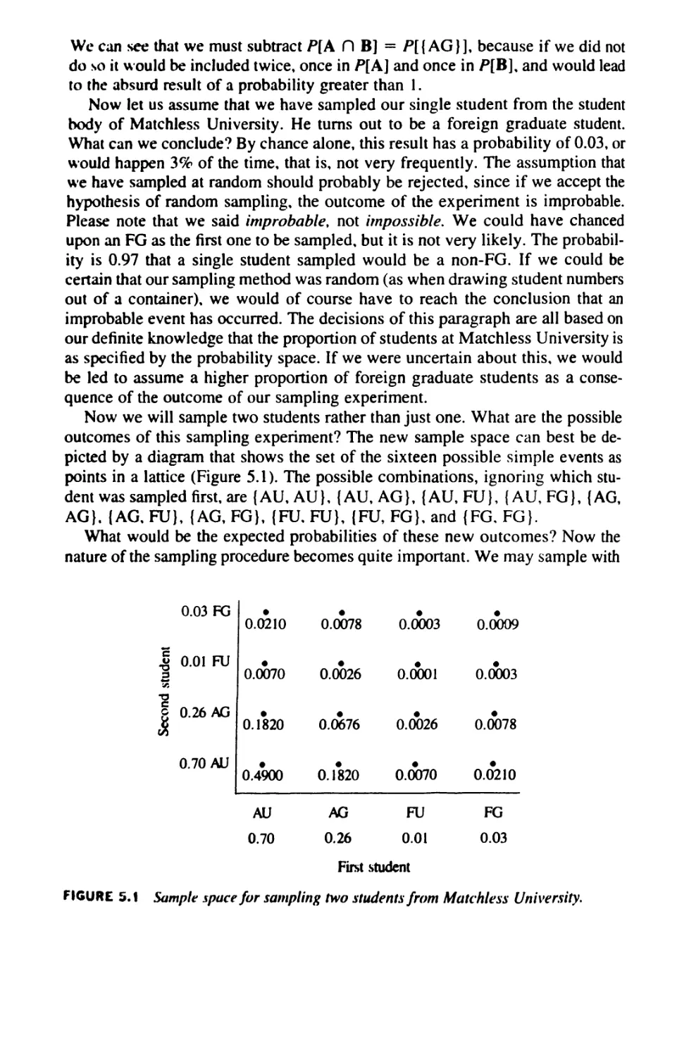
the developments in computing hardware and software. Section 5.1, on probability,
has been revised extensively and now includes Bayes' theorem. We now feature
boxplots and quantile-quantile plots in Sections 6.5 and 6.7, respectively. The
Bonferroni method of multiple testing is now given in Section 9.6. In Chapter 13 we
feature a test of independence of errors in a sequence of continuous variates (Section
13.2), a test for the difference betwen two counts (Section 13.8), and a nonparametric
test for replicated two-way analysis of variance (Section 13.12). New features of the
chapter on regression. Chapter 14, are regression through the origin (Section 14.4K
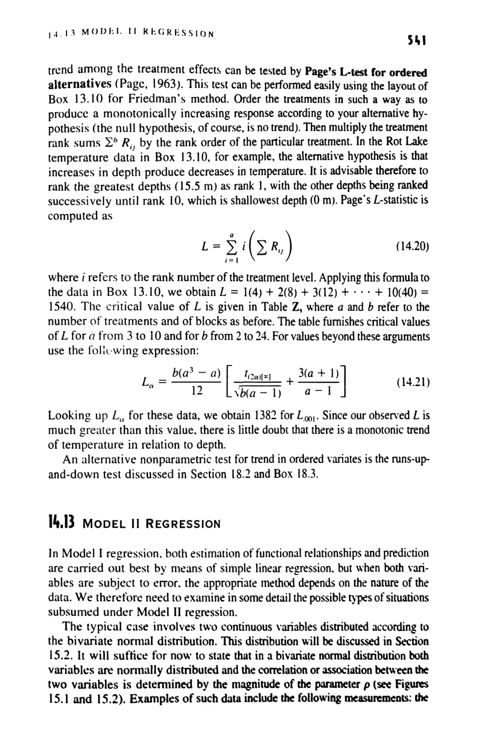
the logistic equation and logits (Section 14.11), and Kendall's robust line-fit method
xvli
xvlll
NOlliS ON TII h THIRD HDITION
(Section 14.13). In Section 16.5 we feature Kruskal's method for determining the
rcUivc importance of predictor variables in multiple regression. Chapter 17,
"Analysts of Frequencies," contains many changes. In Section 17.2 we present a revised
Kolinogoro>-Smirnov test using Khamis's adjustment; in Section 17.4 we have
added three methods, a nonparametric test of equality of medians, multiple
comparisons in R x C frequency tables, and the phi coefficient of association for a 2 X 2
table. An entirely new Section 17.6, on the analysis of proportions, covers the log-
odds ratio, the Mantel-Haens/el procedure, and logistic regression and mentions
BcrVson's fallacy, Ncyman's example, and Simpson's paradox. Finally, a revised
McNcmar test, in which the order of presentation of stimuli is tested, is featured in
Section 17.7. Extensive changes have also been made in Chapter 18, "Miscellaneous
Methods," In addition to mentioning meta-analysis in Section 18.1. wc feature the
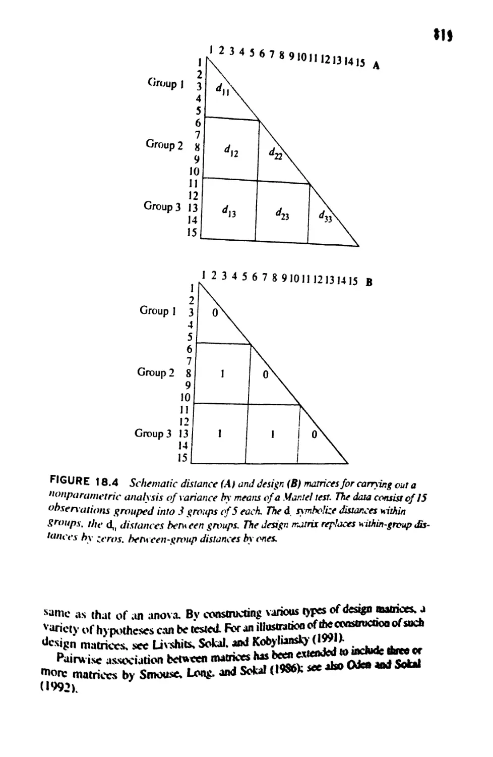
Mantel test for comparing two dissimilarity matrices and isotonic regression in
Section 18.3 and the widely used bootstrap procedure in Section 18.4.
Recent statistical literature has presented many improvements of standard statis-
licui tests by transformations of data and corrections to the test statistics. In
mentioning some of these and omitting others, we have tried to strike a balance between
adding every suggestion in the literature and ignoring them all. The danger in
preparing a new edition of a text such as this is adding too many minute changes,
making it difficult for the reader to see the main outlines of the methods and to decide
among the various alternatives offered. Too many methods are confusing to the
novice. Inevitably, houever, the book has become more diverse and the number of
topics has increased.
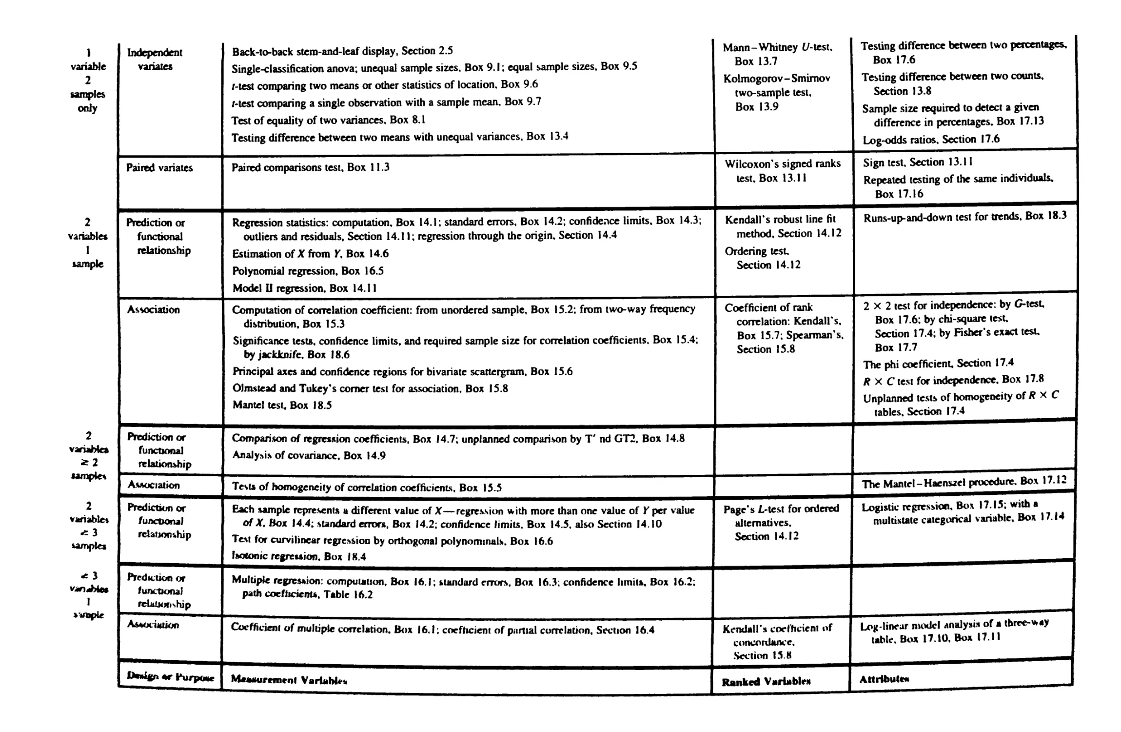
The tabular guides to types of problems encountered frequently in biological
research, found in the endpapers, have been updated to include the new methods
introduced in the Third Edition.
Accompanying the publication of the Third Edition is a new version (3.0) of the
BIOM-pc programs. These programs are based on the Third Edition and feature the
major methods the new edition lists. The programs have been made easier to use and
more powerful. Written by F. James Rohlf. the programs are distributed by Exeter
Software. 100 North Country Road, Building B, Setauket. New York 11733.
The Third Edition continues to reflect our many years of experience teaching
biometry to classes of graduate students in various departments in the life, health,
and earth sciences at the University of Kansas, the University of California, Santa
Barbara, the Slate University of New York at Stony Brook, and various universities
Abroad. In these courses wc have emphasized "doing." For the last twenty years or
>o chat students have been taught to use computer programs. By a series of
assignments they are then taught how to solve biological problems statistically, both by
thinking through the nature of the problem and by carrying out the computations.
ftatrwtmg homework exercises to those that are simple to do (hence not time-
consuming) was an approach we rejected even during the era of the mechanical
etkulaior. With the present general availability of computers, there is no further
mm to shkld students from real-life data. Students have to be taught the solution
NOTES ON THE THIRD EDITION
XIX
of real biological problems involving complicated and copious data, similar to those
that would be obtained in an actual research project.
The fear expressed by some teachers that students would not learn statistics well if
they were permitted to use canned computer programs has not been realized in our
experience. A careful monitoring of achievement levels before and after the
introduction of computers in the teaching of our course revealed no appreciable change in
students' performance.
Robert R. Sokal
F. James Rohlf
July 1994
mKLl Introduction
Dear Reader:
If you are starting your study of this book without looking at the preface, we
respectfully but firmly urge you to turn back and read it. We realize that prefaces
are often uninspiring reading. However, the preface in this book contains
important information for the user. In it we explain our reasons for writing this book
and describe the audience we address. More important, however, we explain our
philosophy of teaching statistics and how we expect the arrangement of this book
to meet our objectives. Unless the system of the book is understood, we fear that
you are not likely to receive full benefit from reading it. Thank you.
The Authors
This introductory chapter is concerned with setting the stage for your study of
biometry. First we define the field itself (Section 1.1). Then we cast a necessarily
brief glance at its historical development (Section 1.2). Section 1.3 concludes the
chapter with a discussion of the attitudes someone trained in statistics brings to
biological research. The application of statistics to biology has revolutionized
not only the methodology of research but the very interpretation of the
phenomena under study. The effects this philosophical attitude has had and is having on
biology are outlined briefly. We hope that the reader of this book will absorb and
appropriate some of these points of view.
1.1 Some definitions
Scientific etiquette demands that a field be defined before its study is begun. The
Greek roots of "biometry" are bios ("life") and metron ("measure"): hence
biometry is literally the measurement of life. For the purposes of this book
biometry is conceived in a very broad sense. We define it as the application of
statistical methods to the solution of biological problems. As seen in Section 1.2,
the original meaning of biometry was much narrower and implied a special field
I
I
CHAPTER 1 INTRODUCTION
rcl.itcd lo the study of evolution and natural selection; however, the wider
definition is customary now. Biometry is also called biological statistics or simply
hinstatistics.
Our definition tells us that biometry is the application of statistics to biologi-.
cil problems, but the definition leaves us somewhat up in the air, since
"statistics" has not been defined. Statistics is a science that by name at least is well
known even to the layperson, who quite often unjustly abuses the term. The
number of definitions you can find is limited only by the number of books you
wish to consult. In its modern sense we might define statistics as the scientific
study of data describing natural variation. All parts of this definition are
important and deserve emphasis.
Scientific study: We are concerned with the commonly accepted criteria of
validity of scientific evidence. Objectivity in presenting and evaluating data and
the general ethical code of scientific methodology must constantly be in
evidence if the old canard that "figures never lie, only statisticians do" is not to be
revived.
Data: Statistics generally deals with populations or groups of individuals;
hence it deals with quantities of information, not with a single datum. Thus the
measurement of a single animal or the response from a single biochemical test
will generally not be of interest; unless a sample of animals is measured or
several such tests are performed, statistics ordinarily can play no role. (We are
old-fashioned enough to insist that "data" be used only in its plural sense,
despite the latest dictionaries.) Unless the data of a study can be quantified in one
way or another, they are not amenable to statistical analysis. The data can be
measurements (the length or width of a structure or the amount of a chemical in a
body fluid) or counts (the number of bristles or teeth, or frequencies of different
qualitative states such as mutant eye colors). Types of variables will be discussed
in greater detail in Chapter 2.
Natural variation: We use this term in a wide sense to include all those events
that happen in animate and inanimate nature not under the direct control of the
investigator, plus those that are evoked by the scientist and are partly under his or
her control, as in an experiment. Different biologists concern themselves with
different levels of variation; other kinds of scientists with yet different levels; but
all scientists agree that variation in the chirping of crickets, the number of peas in
a pod, and the age at maturity in a chicken is natural. The heartbeat of rats in
response to adrenalin or the mutation rate in maize after irradiation may still be
considered natural, even though the researcher has manipulated the phenomenon
in an experiment. The average biologist, however, would not consider variation
in ibe number of color television sets bought by persons in different states in a
given year to be natural, although sociologists or human ecologists might, thus
deeming it worthy of study. The qualification "variation in nature" is included
in the definition of statistics largely to make certain that the phenomena studied
arc not jutoitru/y ones that are entirely under the will and control of the re-
*weber, such a* the number of animals employed by the experimenter.
1.2 THE DEVELOPMENT OF BIOMETRY
3
The word statistics is also used in another, related sense: as the plural of the
noun statistic, which refers to any one of many computed or estimated statistical
quantities, such as the mean, the standard deviation, or the correlation
coefficient. Each one of these is a statistic. (By extension, the term statistic has also
been used to indicate figures or pieces of data—that is, the individuals or items
of data to be defined. This is the way the word is used in the familiar warning to
the careless driver not to become a statistic. This is not, however, a
recommended use of the word.)
1.2 The development of Biometry
The nature of this book and the space at our disposal do not permit us to indulge
in an extended historical review. The origin of modern statistics can be traced
back to the seventeenth century, when it derived from two sources. The first of
these related to political science and developed as a quantitative description of
the various aspects of the affairs of a government or state (hence the term
statistics). This subject also became known as political arithmetic. Taxes and
insurance caused people to become interested in problems of censuses, longevity, and
mortality. Such considerations assumed increasing importance, especially in
England, as the country prospered during the development of its empire. John
Graunt (1620-1674) and William Petty (1623-1687) were early students of
vital statistics, and others followed in their footsteps.
At about the same time came the development of the second root of modern
statistics: the mathematical theory of probability engendered by the interest in
games of chance among the leisure classes of the time. Important contributions
to this theory were made by Blaise Pascal (1623-1662) and Pierre de Fermat
(1601-1665), both Frenchmen. Jacques Bernoulli (1654-1705), a Swiss, laid
the foundation of modern probability theory as Ars Conjectandi, published
posthumously. Abraham de Moivre (1667-1754), a Frenchman living in England,
was the first to combine the statistics of his day with probability theory in
working out annuity values. De Moivre also was the first to approximate the
important normal distribution through the expansion of the binomial.
Subsequent stimulus for the development of statistics came from the science
of astronomy, in which many individual observations had to be digested into a
coherent theory. Many of the famous astronomers and mathematicians of the
eighteenth century, such as Pierre-Simon de Laplace (1749-1827) in France and
Carl Friedrich Gauss (1777-1855) in Germany were among the leaders in this
field. Gauss's lasting contribution to statistics is the development of the method
of least squares, which will be encountered later in this book in a variety of
forms. Gauss already realized the importance of his ideas to any situation in
which errors in observations occur.
Perhaps the earliest important figure in biometric thought was Adolphe
Quetelet (1796-1874), a Belgian astronomer and mathematician, who combined
ihc theory and practical methods of statistics and applied them to problems of
biology, medicine, and sociology. He introduced the concept of the *'average
nun" and was the first to recognize the significance of the constancy of large
numbers— an idea of prime importance in modern statistical work. He also developed
the notion of statistical variation and distribution.
Much progress was made in the theory of statistics by mathematicians in the
nineteenth century, but this development is of less interest to us than is the work
of Francis Galton (1822-1911), a cousin of Charles Darwin. Galton has been
oiled the father of biometry and eugenics (a branch of genetics), two subjects
that he studied intcrrelatedly. The publication of Darwin's work and the
inadequacy of Darwin's genetic theories stimulated Galton to try to solve the problems
of heredity. Galton's major contribution to biology is his application of statistical
methodology to the analysis of biological variation, such as the analysis of
variability and his study of regression and correlation in biological
measurements. His hope of unraveling the laws of genetics through these procedures was
in vain. He started with the most difficult material and with the wrong
assumptions. His methodology however, has become the foundation for the application
of statistics to biology.
A contemporary of Galton's, Florence Nightingale (1820-1910), was the first
distinguished female statistician. In addition to being the founder of modern
nursing, for which she is universally famous, she was an excellent
mathematician who pioneered the compilation and graphic presentation of vital and
medical statistics.
Karl Pearson (1857-1936) at University College, London, became interested
in the application of statistical methods to biology, particularly in the
demonstration of natural selection, through the influence of W. F. R. Weldon (1860-
1906). a zoologist at the same institution. Weldon, incidentally, is credited with
coining the term biometry for the type of studies he pursued. Pearson continued
in ihc tradition of Galton and laid the foundation for much of descriptive and
correlational statistics. The dominant figure in statistics and biometry in the
twentieth century has been Ronald A. Fisher (1890-1962). His many
contributions to statistical theory will become obvious even to the casual reader of this
book. We will acquaint you with the contributions of many of this century's
other eminent statisticians as we discuss the topics they developed.
At prcsctit, statistics is a broad and extremely active field, whose applications
touch almost every science and even the humanities. New applications for
statistics arc constantly being found, and no one can predict from what branch of
sUitivtics new applications to biology will be made. The prospective student of
biolojticd statistics need not be overwhelmed by the formidable size of the field,
but slK-uld be a* arc that statistics is a constantly changing and growing science
*n& »n this respect is quite different from a subject such as elementary algebra or
*rirt»rwiicti). Methods of teaching these subjects may have changed in the last
Mty >car\, but not ihc basic principles and theorems. Some of the methods
resettled in ihu took were published only recently in the technical literature.
1.3 THE STATISTICAL FRAME OF MIND
5
Time-honored methods such as tests for normality and statistics of skewness and
kurtosis, after a period of disuse, are again commonly employed, because
highspeed computers make their calculation feasible. Other techniques, such as the
chi-square test and the /-test, may become obsolete for a variety of reasons. The
entire field of data analysis has become possible only recently, since me
development of inexpensive, high-speed computation.
Anyone would be rash to try to predict the scope and practice of biometry 20
years from now. Whatever its nature, however, biometry is more than likely to
occupy an even more commanding position in biology in the next century than it
does now.
1.3 The Statistical Frame of Mind
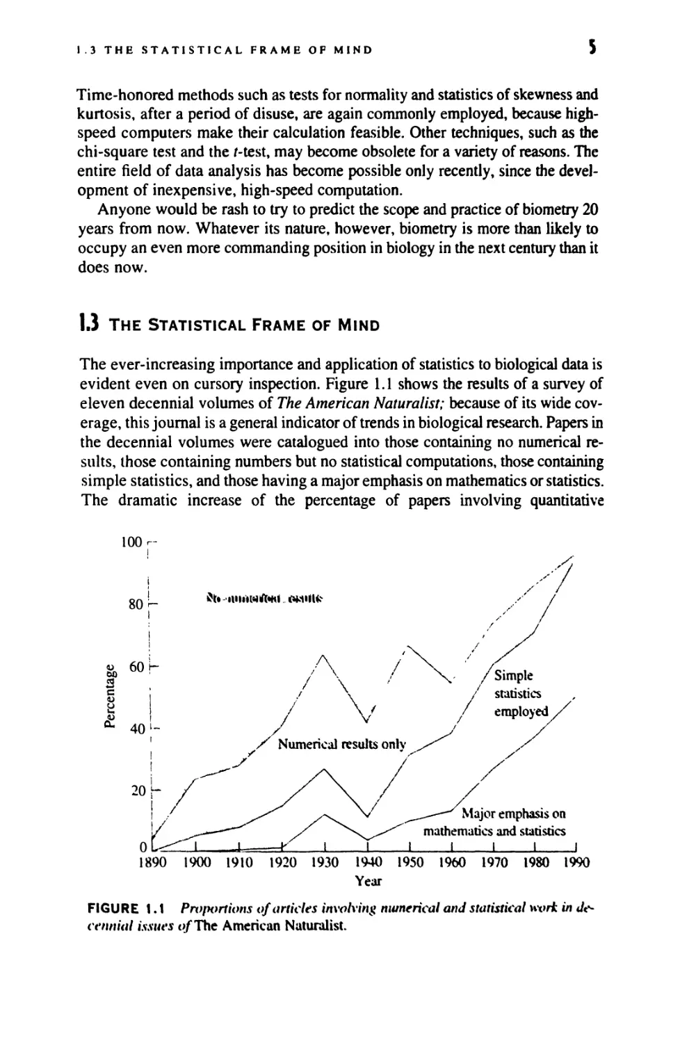
The ever-increasing importance and application of statistics to biological data is
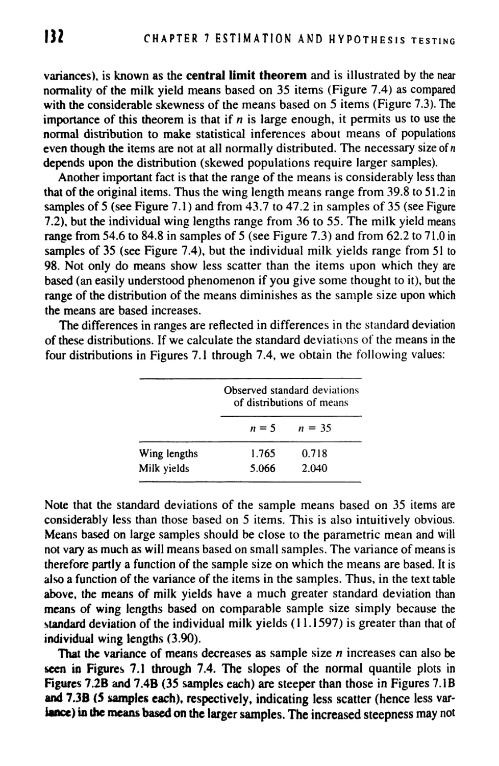
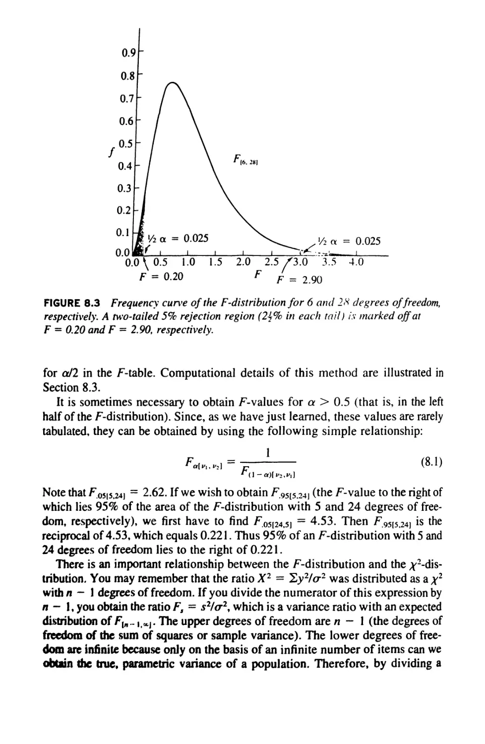
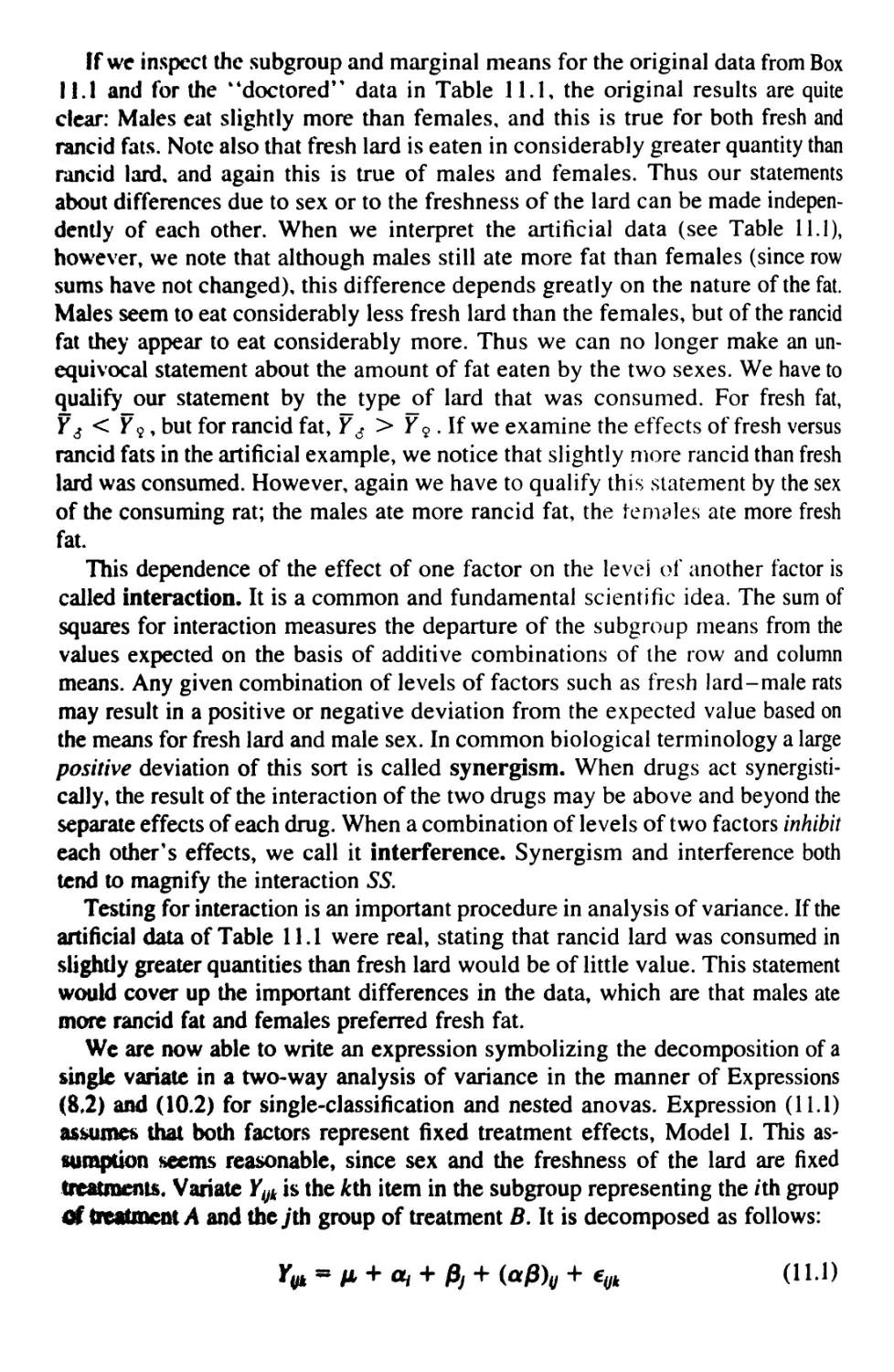
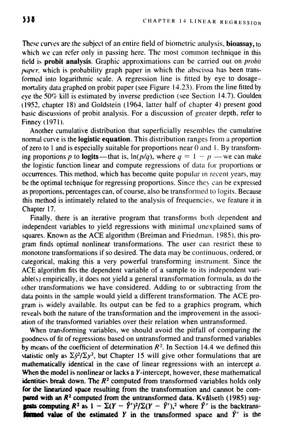
evident even on cursory inspection. Figure 1.1 shows the results of a survey of
eleven decennial volumes of The American Naturalist; because of its wide
coverage, this journal is a general indicator of trends in biological research. Papers in
the decennial volumes were catalogued into those containing no numerical
results, those containing numbers but no statistical computations, those containing
simple statistics, and those having a major emphasis on mathematics or statistics.
The dramatic increase of the percentage of papers involving quantitative
oL^ru j v i i i i i i i
1890 1900 1910 1920 1930 1940 1950 1960 1970 1980 1990
Year
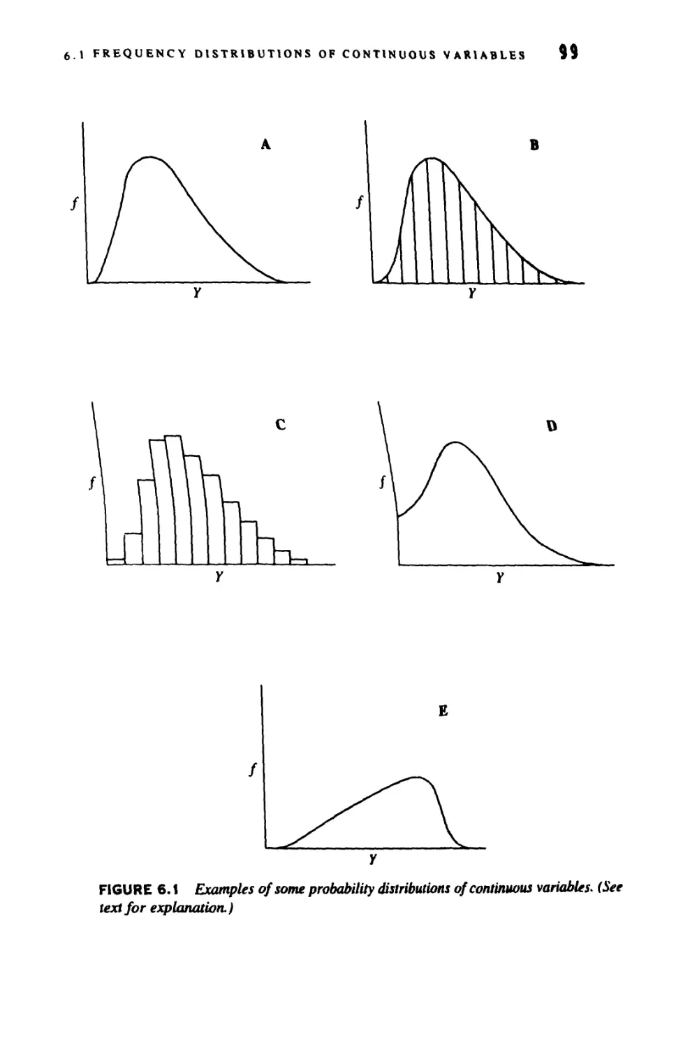
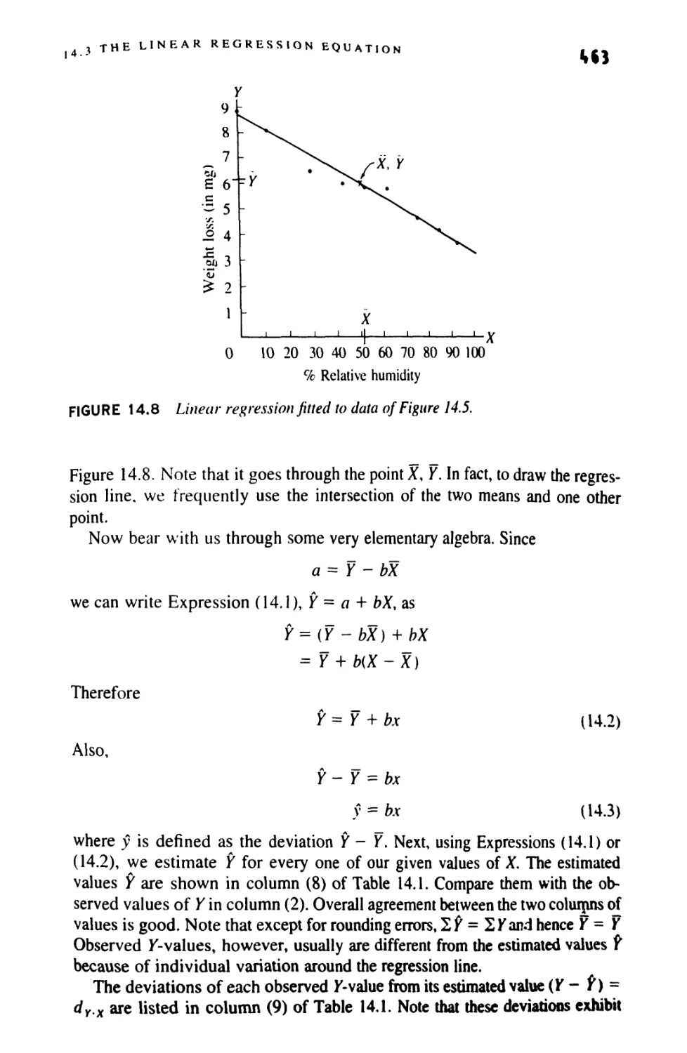
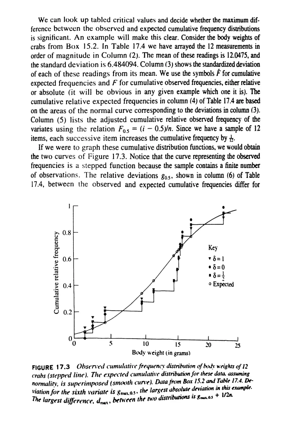
FIGURE 1.1 Proportions of articles involving numerical and statistical wort in
decennial issues t)/The American Naturalist.
t»
WMI0N
.*r^rn:*chcs is shown clearly in the graph, in spite of the fluctuation to be
expected in a sample of this sort. By 1990, 96% of the papers published during the
yc.ir employed some statistical tests or were more heavily statistical or mathe-
rn.itical. This trend can be observed in most biological journals.
Why has there been such a marked increase in the use of statistics in biology?
It is apparently a result of the realization that in biology the interplay of causal
and response variables obeys laws that are not in the classic mold of nineteenth-
century physical science. In that century, biologists such as Robert Mayer,
Hermann von Helmholtz, and others, in trying to demonstrate that biological
processes were nothing but physicochemical phenomena, helped create the
impression that the experimental methods and natural philosophy that had led to
such dramatic progress in the physical sciences should be imitated fully in
biology. Regrettably, opposition to this point of view was confounded with the
vitalistic movement, which led to unproductive theorizing.
Thus, many biologists even to this day have retained the tradition of strictly
mechanistic and deterministic concepts of thinking, while physicists, as their
science became more refined and came to deal with ever more "elementary"
particles, began to resort to statistical approaches. In biology most phenomena
arc affected by many causal factors, uncontrollable in their variation and often
unidentifiable. Statistics is needed to measure such variable phenomena with a
predictable error and to ascertain the reality of minute but important differences.
Whether biological phenomena are in fact fundamentally deterministic and only
the variety of causal variables and our inability to control these make these
phenomena appear probabilistic, or whether biological processes are truly
probabilistic, as postulated in quantum mechanics for elementary particles, is a deep
philosophical question beyond the scope of this book and the competence of the
authors. The fact remains that most biological phenomena can be discussed only
within a probabilistic framework.
A misunderstanding of these principles and relationships has given rise to the
attitude of some biologists that if differences induced by an experiment or
observed in nature are not clear on plain inspection (and therefore not in need of
statistical analysis), they are not worth investigating. This attitude is also related
to the search for all-or-none responses, common in fields such as molecular
biology. There are still a few legitimate fields of inquiry in which, from the
naiurc of the phenomena studied, statistical investigation is unnecessary. When
all animals given injections of a pathogenic organism contract the disease, while
none of the controls fall ill, statistical testing is hardly needed. Much more
frequent, however, are investigations, such as those determining the relation
bci^een smoking and heart disease, where the variability of the outcomes
necessities statistical analysis.
We should stress that statistical thinking is not really different from ordinary
di wjplined scientific thinking with which we try to quantify our observations. In
taUvtkx wc express our decree of belief or disbelief as a probability rather than
*> * Wue, general statement For example, biologists often make statements
1.3 THE STATISTICAL FRAME OF MIND
1
such as "species A is larger than species B" or "females are more often found
sitting on tree M rather than on tree N." Such statements can and should be
expressed more precisely in quantitative form. The human mind is a remarkable
statistical machine, absorbing many facts from the outside world, digesting
these, and regurgitating them in simple summary form. From our experience we
know that certain events occur frequently, others rarely. "Someone smoking
cigarette" is a frequently observed event; "someone slipping on banana peer* is
rare. We know from experience that Japanese are, on the average, shorter than
Englishmen and that Egyptians are, on the average, darker than Swedes. We
associate thunder with lightning almost always, flies with garbage cans
frequently in the summer, but snow with the southern Californian desert extremely
rarely. All such knowledge comes to us as a result of our lifetime experience,
both directly and through that of others by direct communication or through
reading. All these facts have been processed by that remarkable computer, the
human brain, which furnishes an abstract. This summary is constantly under
revision, and though occasionally faulty and biased, it is on the whole
astonishingly sound; it is our knowledge of the moment.
Although statistics arose to satisfy the needs of scientific research, the
development of its methodology in turn has affected the sciences in which statistics is
applied. Thus, in a positive feedback loop, statistics, created to serve the needs of
natural science, has itself affected the philosophy of the biological sciences.
Consider the following two examples. First, analysis of variance has had a
tremendous effect in influencing the types of experiments researchers carry out; the
whole field of quantitative genetics, one of whose problems is the separation of
environmental from genetic effects, depends upon the analysis of variance for its
realization, and many of the concepts of quantitative genetics have been built
directly around the analysis of variance. Second, the techniques of multivariate
analysis have given rise to numerous studies designed especially to exploit their
ability to analyze many variables simultaneously.
■ldData in Biology
In Section 2.1 we explain the statistical meaning of "sample" and
"population/' terms used throughout this book. Then we come to the types of
conations obtained from biological research material, with which we shall
perform the computations in the rest of this book (Section 2.2). In obtaining data
uc shall run into the problem of the degree of accuracy necessary for recording
the data. This problem and the procedure for rounding off figures are discussed
in Section 2.3, after which we will be ready to consider in Section 2.4 certain
kinds of derived data, such as ratios and indices, frequently used in biological
science, which present peculiar problems with respect to their accuracy and
distribution. Knowing how to arrange data as frequency distributions is
important, because such arrangements permit us to get an overall impression of the
shape of the variation present in a sample. Frequency distributions, as well as the
presentation of numerical data, are discussed in the last section (2.5) of this
chapter.
LI Samples and Populations
Wc sh-ill now define a number of important terms necessary for an understanding
o! biological data. The data in a biomctric study arc generally based on
individual observations which are observations or measurements taken on the small-
r\t sampling unit. These smallest sampling units frequently, but not necessarily,
arc also individuals in the ordinary biological sense. If we measure weight in 100
f-»ts, ihtn the weight of each rat is an individual observation; the hundred rat
*ci^hts together represent the sample of observations, defined as a collection of
i'Jiiiilual ob\enations selected by a specified procedure. In this instance, one
individual cbMrrvation K based on one individual in a biological sense—that is,
*»i*c r.a Huuever, if wc had studied weight in a single rat over a period of time,
tt»c vrnplc tkf individual observations would be all the weights recorded on one
M a vuvccssivc times. Id a study of temperature in ant colonics, where each
colony is a basic sampling unit, each temperature reading for one colony is an
individual observation, and the sample of observations is the temperatures for all
the colonies considered. An estimate of the DNA content of a single mammalian
sperm cell is an individual observation, and the corresponding sample of
observations is the estimates of DNA content of all other sperm cells studied in one
individual mammal. A synonym for individual observation is "item."
Up to now we have carefully avoided specifying the particular variable being
studied because "individual observation" and "sample of observations" as we
just used them define only the structure but not the nature of the data in a study.
The actual property measured by the individual observations is the variable, or
character. The more common term employed in general statistics is variable. In
evolutionary and systematic biology however, character is frequently used
synonymously. More than one variable can be measured on each smallest sampling
unit. Thus, in a group of 25 mice we might measure the blood pH and the
erythrocyte count. The mouse (a biological individual) would be the smallest
sampling unit; blood pH and cell count would be the two variables studied. In
this example the pH readings and cell counts are individual observations, and
two samples of 25 observations on pH and erythrocyte count would result.
Alternatively, we may call this example a bivariate sample of 25 observations,
each referring to a pH reading paired with an erythrocyte count.
Next we define population. The biological definition of mis term is well
known: It refers to all the individuals of a given species (perhaps of a given life
history stage or sex) found in a circumscribed area at a given time. In statistics,
population always means the totality of individual obsenarions about which
inferences are to be made, existing anywhere in the world or at least within a
definitely specified sampling area limited in space and rime. If you take five
humans and study the number of leucocytes in their peripheral blood and you are
prepared to draw conclusions about all humans from this sample of five, then the
population from which the sample has been drawn represents the leucocyte
counts of all humankind—that is, all extant members of the species Homo
sapiens. If, on the other hand, you restrict yourself to a more narrowly specified
sample, such as five male Chinese, aged 20. and you are restricting your
conclusions to this particular group, then the population from which you are sampling
will be leucocyte numbers of all Chinese males of age 20. The population in this
statistical sense is sometimes referred to as the universe. A population may refer
to variables of a concrete collection of objects or creatures—such as the tail
lengths of all the white mice in the world, the leucocyte counts of all the Chinese
men in the world of age 20, or the DNA contents of all the hamster sperm cells in
existence—or it may refer to the outcomes of experiments—such as all the
heartbeat frequencies produced in guinea pigs by injections of adrenalin. In the
first three cases the population is finite. Although in practice it would be
impossible to collect, count, and examine all white mice, all Chinese men of age 20, or
all hamster sperm cells in the world, these populations are finite. Certain smaller
populations, such as all the whooping cranes in North America or all the pocket
j^phers in a pi\cn colony, may lie within reach of a total census. By contrast, an
experiment can be repeated an infinite number of times (at least in theory). An
experiment such as the administration of adrenalin to guinea pigs could be re-
pc.iicd as long as the experimenter could obtain material and his or her health and
p.ilicncc held out. The sample of experiments performed is a sample from an
infinite number that could be performed. Some of the statistical methods to be
dc\eloped later make a distinction between sampling from finite and from
infinite populations. However, although populations are theoretically finite in most
applications in biology, they are generally so much larger than samples drawn
from them that they can be considered as de facto infinitely sized populations.
hi VARIABLES IN BIOLOGY
Enumerating all the possible kinds of variables that can be studied in biological
research would be a hopeless task. Each discipline has its own set of variables,
which may include conventional morphological measurements, concentrations
of chemicals in body fluids, rates of certain biological processes, frequencies of
certain events (as in genetics and radiation biology), physical readings of optical
or electronic machinery used in biological research, and many more. We assume
that persons reading this book already have special interests and have become
acquainted with the methodologies of research in their areas of interest, so that
the variables commonly studied in their fields are at least somewhat familiar. In
any case, the problems for measurement and enumeration must suggest
themselves to the researcher, statistics will not, in general, contribute to the discovery
and definition of such variables.
Some exception must be made to this statement. Once a variable has been
chosen, statistical analysis may demonstrate it to be unreliable. If several
variables arc studied, certain elaborate procedures of multivariate analysis can assign
weights to them, indicating their value for a given procedure. For example, in
taxonomy and various other applications, the method of discriminant functions
can identify the combination of a series of variables that best distinguishes
between two groups (see Section 16.7). Other multivariate techniques, such as
canonical variates analysis, principal components analysis, or factor analysis,
can specify characters that best represent or summarize certain patterns of
variation (Kiranowski, 1988; Jackson, 1991). As a general rule, however, and
particularly within the framework of this book, choosing a variable as well as defining
the problem to be solved is primarily the responsibility of the biological re-
M*icl>er.
A more precise definition of variable than the one given earlier is desirable.
It U a property with respect to which individuals in a sample differ in some
awmainable way. If the property docs not differ within a sample at hand or
4t tcau amonj; the samples being studied, it cannot be of statistical interest*
H<U\£ entirely uniform, such a property would also not be a variable from the
2.2 VARIABLES IN BIOLOGY
u
etymological point of view and should not be so called. Length, height, weight,
number of teeth, vitamin C content, and genotypes are examples of variables in
ordinary, genetically and phenotypically diverse groups of organisms. Warm-
bloodedness in a group of mammals is not a variable because they are all alike in
this regard, although body temperature of individual mammals would, of course,
be a variable. Also, if we had a heterogeneous group of animals, of which some
were homeothermic and others were not, then body temperature regulation (with
its two states or forms of expression, "warm-blooded" and 4'cold-blooded")
would be a variable.
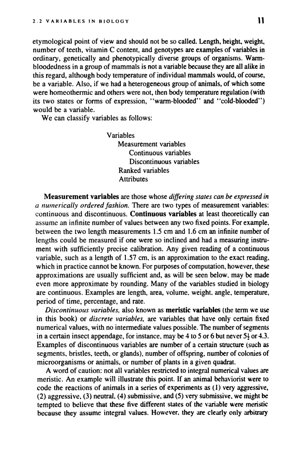
We can classify variables as follows:
Variables
Measurement variables
Continuous variables
Discontinuous variables
Ranked variables
Attributes
Measurement variables are those whose differing states can be expressed in
a numerically ordered fashion. There are two types of measurement variables:
continuous and discontinuous. Continuous variables at least theoretically can
assume an infinite number of values between any two fixed points. For example,
between the two length measurements 1.5 cm and 1.6 cm an infinite number of
lengths could be measured if one were so inclined and had a measuring
instrument with sufficiently precise calibration. Any given reading of a continuous
variable, such as a length of 1.57 cm, is an approximation to the exact reading,
which in practice cannot be known. For purposes of computation, however, these
approximations are usually sufficient and, as will be seen below, may be made
even more approximate by rounding. Many of the variables studied in biology
are continuous. Examples are length, area, volume, weight, angle, temperature,
period of time, percentage, and rate.
Discontinuous variables, also known as meristic variables (the term we use
in this book) or discrete variables, are variables that have only certain fixed
numerical values, with no intermediate values possible. The number of segments
in a certain insect appendage, for instance, may be 4 to 5 or 6 but never 5$ or 4.3.
Examples of discontinuous variables are number of a certain structure (such as
segments, bristles, teeth, or glands), number of offspring, number of colonies of
microorganisms or animals, or number of plants in a given quadrat.
A word of caution: not all variables restricted to integral numerical values are
meristic. An example will illustrate this point. If an animal behaviorist were to
code the reactions of animals in a series of experiments as (1) very aggressive,
(2) aggressive, (3) neutral, (4) submissive, and (5) very submissive, we might be
tempted to believe that these five different states of the variable were meristic
because they assume integral values. However, they are clearly only arbitrary
n
CHAPTER 2 DATA IN BIOLOGY
points (class marks, see Section 2.5) along a continuum of aggressiveness; the
only reason that no values such as 1.5 occur is that the experimenter did not wish
to subdivide the behavior classes too finely, either for convenience or because of
.in inability to determine more than t\wc subdivisions of this spectrum of
behavior with precision. Thus, this variable is clearly continuous rather than meristic,
as it might have appeared at first sight.
Some variables cannot be measured but at least can be ordered or ranked by
their magnitude. Thus, in an experiment one might record the rank order of
emergence of ten pupae without specifying the exact time at which each pupa
emerged. In such a case we would code the data as a ranked variable, the order
of emergence. Special methods for dealing with ranked variables have been
developed, and several are described in this book. By expressing a variable as a
series or ranks, such as 1,2, 3, 4, 5, we do not imply that the difference in
magnitude between, say, ranks 1 and 2 is identical to or even proportional to the
difference between 2 and 3. Such an assumption is made, however, for
measurement variables, discussed above.
Variables that cannot be measured but must be expressed qualitatively are
called attributes, also known as categorical or nominal variables. Attributes are
properties such as black or white, pregnant or not pregnant, dead or alive, male or
female. When such attributes are combined with frequencies, they can be treated
statistically. Of 80 mice, for instance, we may state that four are black and the
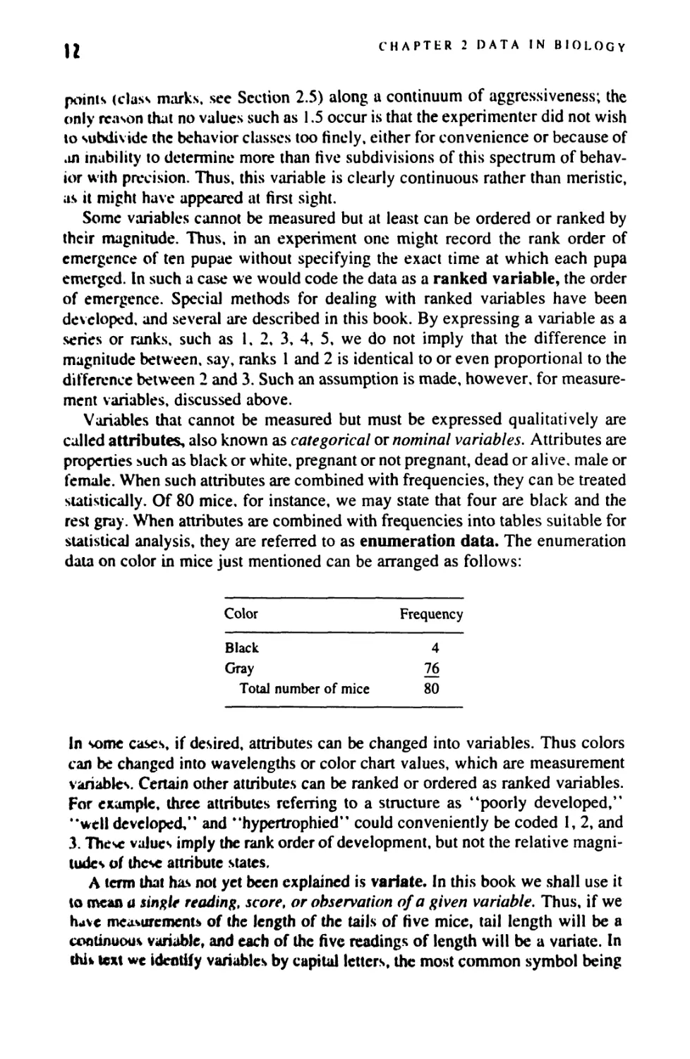
rest gray. When attributes are combined with frequencies into tables suitable for
statistical analysis, they are referred to as enumeration data. The enumeration
data on color in mice just mentioned can be arranged as follows:
Color Frequency
Black 4
Gray 76
Total number of mice 80
In some cases, if desired, attributes can be changed into variables. Thus colors
can be changed into wavelengths or color chart values, which are measurement
variables. Certain other attributes can be ranked or ordered as ranked variables.
For example, three attributes referring to a structure as "poorly developed,"
"well developed,'* and "hypertrophied" could conveniently be coded 1, 2, and
3. These values imply the rank order of development, but not the relative
magnitudes of these attribute states,
A term that has not yet been explained is vallate. In this book we shall use it
to mean a single reading, score, or observation of a given variable. Thus, if we
have measurement* of the length of the tails of five mice, tail length will be a
continuous variable, and each of the five readings of length will be a variate. In
chit text we identify variables by capital letters, the most common symbol being
2.3 ACCURACY AND PRECISION OF DATA
13
Y. Thus Y may stand for tail length of mice. A variate will refer to a given length
measurement; Y, is the measurement of tail length of the ith mouse, and Yx is the
measurement of tail length of the fourth mouse in our sample. The use of the
terms variable and variate differs somewhat from author to author; frequently the
two terms are used synonymously.
2.3 ACCURACY AND PRECISION OF DATA
Scientists are generally aware of the importance of accuracy and precision in
their work, and it is self-evident that accuracy must extend to the numerical
results of their work and to the processing of these data. Because of the great
diversity of approaches employed in different disciplines of biology, it seems
futile to attempt to furnish specific rules for obtaining data accurately. We should
make certain, however, that whatever the method of obtaining data, it is
consistent, so that given the same observational or experimental setup, different
numerical readings of the same structure or event would be identical or within
acceptable and predictable limits of each other.
Accuracy and precision are used synonymously in everyday speech, but in
statistics we distinguish between them. Accuracy is the closeness of a measured
or computed value to its true value; precision is the closeness of repeated
measurements of the same quantity to each other. A biased but sensitive scale might
yield inaccurate but precise weight readings. By chance an insensitive scale
might result in an accurate reading, but the reading would be imprecise, since
another weighing of the same object would be unlikely to yield an equally
accurate weight. Unless there is bias in a measuring instrument, precision will
lead to accuracy. We need therefore mainly be concerned with the former.
Precise variates are usually but not necessarily whole numbers. Thus, when
we count four eggs in a nest, there is no doubt about the exact number of eggs in
the nest if we have counted correcdy; it is four, not three or five, and clearly it
could not be four plus or minus a fractional part. Meristic variables are generally
measured as exact numbers. Seemingly, continuous variables derived from
meristic ones can, under certain conditions, also be exact numbers. For instance,
ratios of exact numbers are themselves also exact. If in a colony of animals there
are 18 females and 12 males, the ratio of females to males is 1.5, a continuous
variate but also an exact number.
Most continuous variables, however, are approximate: The exact value of the
single measurement, the variate, is unknown and probably unknowable. The last
digit of the measurement stated should imply precision, that is, the limits on the
measurement scale between which we believe the true measurement to lie. Thus
a length measurement of 12.3 mm implies that the true length of the structure lies
somewhere between 12.25 and 12.35 mm. Exactly where between these implied
limits the real length is we do not know. Some might object to defining the limits
of the number as 12.25 to 12.35 mm because the adjacent measurement of 12.2
it
CHAPTER 2 DATA IN BIOLOGY
would imply limits of 12.15 to 12.25. Where then, they would ask, would a true
measurement of 12.25 fall? Would it not equally likely fall in either of the two
classes 12.2 and 12.3, clearly an unsatisfactory state of affairs? For this reason
some authors define the implied limits of 12.3 as 12.25 to 12.34999. . . . Such
an argument is correct, but when we record a number as either 12.2 or 12.3 we
imply that the decision whether to put it into the higher or lower class has already
been made. This decision was not made arbitrarily, but presumably was based on
the best available measurement. If the scale of measurement is so precise that a
value of 12.25 would clearly have been recognized, then the measurement
should have been recorded originally to four significant figures. Implied limits
therefore always carry one figure beyond the last significant one measured by the
observer.
Hence it follows that if we record the measurement as 12.32, we are implying
that the true value lies between 12.315 and 12.325. If this is what we mean, there
is no need to add another decimal figure to our original measurements. If we add
another figure, we imply an increase in precision. We see therefore that accuracy
and precision in numbers is not an absolute concept, but is relative. Assuming
there is no bias, a number becomes increasingly accurate as we are able to write
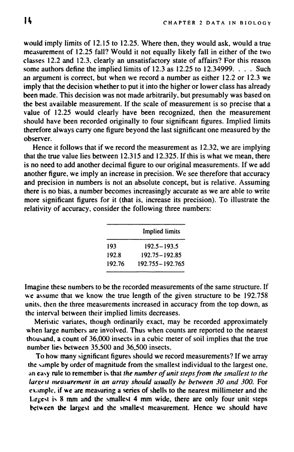
more significant figures for it (that is, increase its precision). To illustrate the
relativity of accuracy, consider the following three numbers:
Implied limits
193
192.8
192.76
192.5-193.5
192.75-192.85
192.755-192.765
Imagine these numbers to be the recorded measurements of the same structure. If
we assume that we know the true length of the given structure to be 192.758
units, then the three measurements increased in accuracy from the top down, as
the interval between their implied limits decreases.
Meristic variates, though ordinarily exact, may be recorded approximately
when large numbers are involved. Thus when counts are reported to the nearest
thousand, a count of 36,000 insects in a cubic meter of soil implies that the true
number lies between 35,500 and 36,500 insects.
To how many significant figures should we record measurements? If we array
the sample by order of magnitude from the smallest individual to the largest one,
an easy rule to remember is that the number of unit steps from the smallest to the
largest measurement in an array should usually be between 30 and 300. For
example, if wc arc measuring a series of shells to the nearest millimeter and the
largest is 8 mm and the smallest 4 mm wide, there are only four unit steps
between the largest and the smallest measurement. Hence wc should have
2.3 ACCURACY AND PRECISION OF DATA
IS
measured our shells to one more significant decimal place. Then the two extreme
measurements might have been 8.2 mm and 4.1 mm, with 41 unit steps between
them (counting the last significant digit as the unit); this would have been an
adequate number of unit steps. The reason for such a role is that an error of 1 in
the last significant digit of a reading of 4 mm would constitute an inadmissible
error of 25%, but an error of 1 in the last digit of 4.1 is less than 2.5%. By
contrast, if we had measured the height of the tallest of a series of plants as 173.2
cm and that of the shortest of these plants as 26.6 cm, the difference between
these limits would comprise 1466 unit steps (of 0.1 cm each), which are far too
many. We should therefore have recorded the heights to the nearest centimeter,
as follows: 173 cm for the tallest and 27 cm for the shortest, yielding 146 unit
steps between.
Using the rule stated above, we will record two or three digits for most
measurements. On occasion, however, more digits will be necessary—when the
leading digits are constant, as in the following example. In a representative series
of pH readings measured with great precision, the highest value might be 7.456
and the lowest value 7.434. The first two digits of such measurements are
constant for pH readings of the material under study. It is therefore necessary to use
three decimal places to obtain an adequate amount of variation for analysis. The
perceptive reader may have noticed that the number of unit steps from lowest to
highest variate in the pH example was only 22, or less than 30 given as the lower
limit for the desired number of steps. This rule, as are all such rules of thumb, is
to be taken with a grain of statistical salt. These rules are general guidelines but
not laws whose mild infraction would immediately invalidate all further work.
With some experience, an appropriate adherence to these rules becomes second
nature to the biologist engaging in statistical analysis.
The last digit of an approximate number should always be significant: that is.
it should imply a range for the true measurement of from half a unit step below to
half a unit step above the recorded score, as illustrated earlier. This rule applies
to all digits, zero included. Zeros should therefore not be written at the end of
approximate numbers to the right of the decimal point unless they are meant to
be significant digits. The measurement 7.80 implies the limits 7.795 to 7.805. If
7.75 to 7.85 is meant to be implied, the measurement should be recorded as 7.8.
When the number of significant digits is reduced, we carry out the process of
rounding numbers. The rules for rounding are very simple. A digit to be rounded
is not changed if it is followed by a digit less than 5. If the digit to be rounded is
followed by a digit greater than 5 or by 5 followed by other nonzero digits, it is
increased by one. When the digit to be rounded is followed by a 5 standing alone
or followed by zeros, it is unchanged if it is even but increased by one if it is odd.
The reason for this last rule is that when such numbers are summed in a long
series, we should have as many digits raised as are being lowered on the average:
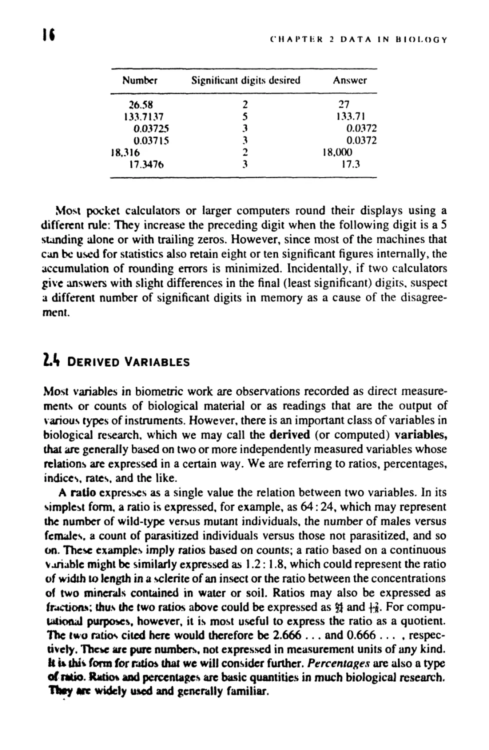
these changes would therefore balance out. Practice these rules by rounding the
following numbers to the indicated number of significant digits:
If
(' II A P T li R 2 DATA IN BIOLOGY
Number Significant digits desired Answer
26.58
133.7137
0.03725
0.03715
18.316
17.3476
2
5
3
3
2
3
27
133.71
0.0372
0.0372
18.000
17.3
Most pocket calculators or larger computers round their displays using a
different rule: They increase the preceding digit when the following digit is a 5
standing alone or with trailing zeros. However, since most of the machines that
can be used for statistics also retain eight or ten significant figures internally, the
accumulation of rounding errors is minimized. Incidentally, if two calculators
give answers with slight differences in the final (least significant) digits, suspect
a different number of significant digits in memory as a cause of the
disagreement.
U Derived Variables
Most variables in biometric work are observations recorded as direct
measurements or counts of biological material or as readings that are the output of
various types of instruments. However, there is an important class of variables in
biological research, which we may call the derived (or computed) variables,
thai are generally based on two or more independently measured variables whose
relations are expressed in a certain way. We are referring to ratios, percentages,
indices, rates, and the like.
A ratio expresses as a single value the relation between two variables. In its
simplest form, a ratio is expressed, for example, as 64:24, which may represent
the number of wild-type versus mutant individuals, the number of males versus
females, a count of parasitized individuals versus those not parasitized, and so
on. These examples imply ratios based on counts; a ratio based on a continuous
variable might be similarly expressed as 1.2:1.8, which could represent the ratio
of width lo length in a sclerite of an insect or the ratio between the concentrations
of two minerals contained in water or soil. Ratios may also be expressed as
fraction-*; thus the two ratios above could be expressed as $} and fj. For
computational purposes, however, it is most useful to express the ratio as a quotient.
The two ratios cited here would therefore be 2.666 ... and 0.666 ....
respectively. These are pure numbers, not expressed in measurement units of any kind.
H u thfc form for ratios that we will consider further. Percentages are also a type
of fatso. Ratio* and percentages are basic quantities in much biological research.
Th*y « widely used and generally familiar.
2.4 DHKFVKD VARIABLES
11
Not all derived variables are ratios or percentages. The term index is used in a
general sense for derived variables, although some would limit it to the ratio of
one anatomic variable divided by a larger, so-called standard variable. For
instance, in a study of the cranial dimensions of cats, Haltenorth (1937) divided all
measurements by the basal length of the skull. Thus each measurement was a
proportion of the basal length of the skull of the cat being measured. Another
example of an index in this sense is the well-known cephalic index in physical
anthropology. Conceived in the wide sense, an index could be the average of two
measurements—either simply, such as \ (length of A + length of #), or in
weighted fashion, such as ^[(2 X length of A) + length of B]. An index may
refer to the summation of a series of numerically scored properties. Thus, if an
animal is given six behavioral tests in which its score can range from 0 to 4, an
index of its behavior might be the sum of the scores of the six tests. Similar
indices have been described for determining the degree of hybridity in organisms
(the hybrid indices of various authors).
Rates are important in many experimental fields of biology. The amount of a
substance liberated per unit weight or volume of biological material, weight gain
per unit time, reproductive rates per unit population size and time (birth rates),
and death rates would fall in this category. Many counts are really ratios or
rates—the number of pulse beats observed in one minute or the number of birds
of a given species found in some quadrat. In genera], counts are ratios if the unit
over which they are counted is not natural, as, for example, an arbitrary time or
space interval.
As we shall see, there are some serious drawbacks to the use of ratios and
percentages in statistical work. In spite of these disadvantages, the use of these
variables is deeply ingrained in scientific thought processes and is not likely to
be abandoned. Furthermore, ratios may be the only meaningful way to interpret
and understand certain types of biological problems. If the biological process
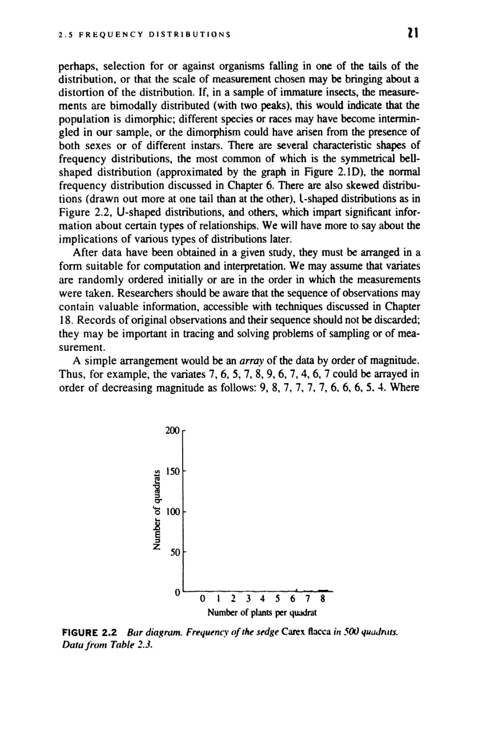
being investigated operates on the ratio of the variables studied, one must
examine this ratio to understand the process. Thus, Sinnott and Hammond (1935)
found that inheritance of the shapes of the squash Cucurbita pepo could be
interpreted by a form index based on a length-width ratio, but not in terms of the
independent dimensions of shape. Similarly, the evolution of shape in many
burrowing animals is a function of the cross-sectional profile of the animal rather
than of a single dimension. Selection affecting body proportions will be found to
exist in the evolution of almost any organism when properly investigated.
The disadvantages of using ratios are several: First is their relative inaccuracy.
Let us return to the ratio |^ and recall from the previous section that a
measurement of 1.2 indicates a true range of measurement of the variable from 1.15 to
1.25; similarly, a measurement of 1.8 implies a range from 1.75 to 1.85. We
realize therefore that the true ratio may vary anywhere from fi? to f$, or 0.622
and 0.714, respectively. We note a possible maximal error of 4.2% if 1.2 were an
original measurement: (1.25 - 1.2V1.2; the corresponding maximal error for the
ratio is 7.0%: (0.714 - 0.667)/0.667. Furthermore, the best estimate of a ratio is
18
CHAPTER 2 DATA IN BIOLOGY
nol usually the midpoint between its possible ranges. Thus in our example, the
midpoint between the implied limits is 0.668 and the true ratio is 0.666 . . . , a
difference that here is only slight, but that in other instances could be greater. In
many cases, therefore, ratios are not as accurate as measurements obtained
directly. This liability can be overcome by empirical determinations of the
variability of ratios through measures of their variance (described later in this book).
A second drawback to ratios and percentages is that they may not be
approximately normally distributed (see Chapter 6), as required by many statistical tests.
This difficulty frequently can be overcome by transformation of the variable (see
Chapter 13). Another disadvantage of ratios is that they do not provide
information on how the two variables whose ratio is being taken are related. Often more
may be learned by studying the variables singly first and then examining their
relation to each other (bivariate and multivariate analysis).
POSSIBLE PERCENTAGES OF PERIPHERAL PUPATION IN
VIALS SEEDED WITH 10 DROSOPHILA EGGS.
Experimental results show number of peripheral pupae in the numerator, total number of
pupae in the denominator.
Percent
00
10
11
12
14
17
20
22
25
29
30
33
38
40
43
44
50
Possible experimental results
yielding this percentage
0 0 0 0 0
TO> 9* J- 7» 5'
0 0 0 0 0
5» 7» T« ?« T
1
1
9
i
I
7
*
A. 4
2
9
hi
i
J. it. i 1
i
tU
7
t
*.U.M
Percent
56
! 57
60
62
! 67
70
71
75
78
80
83
86
88
89
90
100
Possible experimental results
yielding this percentage
5
7
4
7
6 3
TO' T
5
6 4 2
?' 5» 7
7
TO
5
7
M
7
8 4
T0» 7
5
s
6
7
7
*
*
«. *. I. h t.
1 *> i. h +
KJUttOL hwo • *iud> by SoUl (1966).
2.5 FREQUENCY DISTRIBUTIONS
19
Finally, when ratios involve enumeration data or meristic variables,
occasionally they give rise to curious distributions. As an example, we cite the
percentages obtained from an experiment performed many years ago by Sokal. In
this experiment 10 Drosophila eggs were put in a vial and the positions of the
pupae noted after pupation. Some pupae pupated at the margin or the wall of the
vials; these were called peripheral. Others, which pupated away from the wall,
were called central. Ideally there should have been 10 pupae—if all the eggs had
hatched and there had been no larval mortality whatsoever. In fact, however,
because of natural mortality and because of errors in preparing the vials, 10
pupae were not always found. The logical minimum number of survivors on
which a result could be reported was one pupa. The proportion of peripheral
pupae was then calculated by dividing the number of such pupae in a vial by the
total number of pupae found in that vial. Although ratios thus obtained are
continuous variables in appearance, they are not so in fact, because certain values
can never be obtained. For instance, by limiting the maximum number of pupae
to 10, we cannot obtain percentages of peripheral pupation between 0 and 10% or
between 90 and 100%, as Table 2.1 shows. Also, we see that some percentages
are given by several ratios, others by only one: 33% is obtained by i or § or j, but
57% can be obtained only by having 4 out of 7 pupae peripheral. Table 2.1 shows
which values are more likely to be encountered if we make the simplest
assumption—that there is an equal probability for any given experimental
outcome. In using ratios of meristic variates or of counts, such discontinuities and
peculiarities of distribution must be taken into account. The problem in this
instance was solved in transforming the data to probits (see Section 14.11).
2.S Frequency Distributions
If we were to sample a population of birth weights of infants, we could represent
each measurement by a point along an axis denoting magnitude of birth weights.
This example is illustrated in Figure 2.1A for a sample of 25 birth weights. If we
sample repeatedly from the population and obtain 100 birth weights, we
probably will have to place some of these points on top of other points in order to
record them all correctly (Figure 2.IB). As we continue sampling additional
hundreds and thousands of birth weights (Figure 2.1C, D), the assemblage of
points will continue to increase in size and will assume a fairly definite shape.
The curve tracing the outline of the mound of points approximates the
distribution of the variable. Remember that a continuous variable such as birth weight
can assume an infinity of values between any two points on the abscissa. The
refinement of our measurements determines how fine the number of recorded
divisions between any two points along the axis are.
The distribution of a variable is of considerable biological interest. A
distribution that is asymmetrical and drawn out in one direction tells us that there is.
20
CHAPTER 2 DATA IN BIOLOGY
i ii ii i i nil
I ■ ll.l
25
. I. ...il..i .i.llililillillli 1l.iIL.ii i ,i.i ■
100
iiniiiti
500
11.11 ..111 ■ l
20
10
0> Juu.
2000
1111.11
60 70 80 90 100 110 120 130 140 150 160
Birth weight (oz)
FIGURE 2.1 Sampling from a population of birth weights of infants (a continuous
\ariabU\. A. A uiinpU of 25. B. A sample of 100. C. A sample of 500. D. A sample of
2VfjO.
2.5 FREQUENCY DISTRIBUTIONS
21
perhaps, selection for or against organisms falling in one of the tails of the
distribution, or that the scale of measurement chosen may be bringing about a
distortion of the distribution. If, in a sample of immature insects, the
measurements are bimodally distributed (with two peaks), this would indicate that the
population is dimorphic; different species or races may have become
intermingled in our sample, or the dimorphism could have arisen from the presence of
both sexes or of different instars. There are several characteristic shapes of
frequency distributions, the most common of which is the symmetrical bell-
shaped distribution (approximated by the graph in Figure 2.ID), the normal
frequency distribution discussed in Chapter 6. There are also skewed
distributions (drawn out more at one tail than at the other), l-shaped distributions as in
Figure 2.2, U-shaped distributions, and others, which impart significant
information about certain types of relationships. We will have more to say about the
implications of various types of distributions later.
After data have been obtained in a given study, they must be arranged in a
form suitable for computation and interpretation. We may assume that variates
are randomly ordered initially or are in the order in which the measurements
were taken. Researchers should be aware that the sequence of observations may
contain valuable information, accessible with techniques discussed in Chapter
18. Records of original observations and their sequence should not be discarded;
they may be important in tracing and solving problems of sampling or of
measurement.
A simple arrangement would be an array of the data by order of magnitude.
Thus, for example, the variates 7, 6, 5, 7, 8, 9, 6, 7, 4, 6, 7 could be arrayed in
order of decreasing magnitude as follows: 9, 8, 7, 7, 7, 7, 6, 6, 6, 5, 4. Where
200 r
a 150h
or
*S lOoL
E
1 50
0 012345678
Number of plants per quadrat
FIGURE 2.2 Bar diagram. Frequency of the sedge Carex flacca in 500 quadmts.
Data from Table 2.3.
n
CHAPTER 2 DATA IN BIOLOGY
there are some variates of the same value, such as the 6\s and 7\s in this fictitious
example, a time-saving device might immediately have occurred to you—
namely, to list a frequency for each of the recurring variates: 9, 8, 7(4 X), 6(3 X),
5.4. Such shorthand notation is one way to represent a frequency distribution,
which is simply an arrangement of the classes ofvariates with the frequencies of
each class indicated. Conventionally, a frequency distribution is stated in tabular
form, as follows for the above example:
Variable Frequency
Y f
9 1
8 1
7 4
6 3
5 1
4 1
This case is an example of a quantitative frequency distribution, since Y is
clearly a measurement variable. However, arrays and frequency distributions
need not be limited to such variables. We can make qualitative frequency
distributions of attributes. In these, the various classes are listed in some logical or
arbitrary order. For example, in genetics we might have a qualitative frequency
distribution as follows:
f
A- 86
aa 32
This distribution tells us that there are two classes of individuals, those identified
by the A- phenotypc, of which 86 were found, and the homozygote recessive
aa. of which there were 32 in the sample. In ecology it is quite common to have a
species list of inhabitants of a sampled ecological area. The arrangement of such
tables is usually alphabetical. An example of an ecological list constituting a
qualitative frequency distribution of families is shown in Table 2.2. In this
instance the families of insects are listed alphabetically; in other cases the sequence
may be by convention, as for the families of flowering plants in botany.
A quantitative frequency distribution based on meristic variates is shown in
Tabic 2.3. This example comes from plant ecology; the number of plants per
quadrat sampled are listed at the left in the variable column; the observed
frequency k shown at the right
2.5 FREQUENCY DISTRIBUTIONS
23
Table 2.2 A qualitative frequency distribution.
Number of individuals of Heteroptera tabulated by family in total samples from a summer
foliage insect community.
Observed
frequency
Family /
Alydidae
Anthocoridae
Coreidae
Lygaeidae
Miridae
Nabidae
Neididae
Pentatomidae
Piesmidae
Reduviidae
Rhopalidae
Saldidae
Thyreocoridae
Tingidae
Total Heteroptera
2
37
2
318
373
3
5
25
1
3
2
1
10
69
851
source: Data from Whittaker (1952).
Quantitative frequency distributions based on a continuous variable are the
most commonly employed frequency distributions, and you should become
thoroughly familiar with them. An example is shown in Box 2.1. It is based on 25
femur lengths of stem mothers (one of the life history stages) of a species of
aphids. The 25 readings (measured in coded micrometer units) are shown at the
top of the box in the order (reading down columns) in which they were obtained
as measurements. The readings could have been arrayed according to their
magnitude, but this intermediate step is not necessary in order to proceed to a
frequency distribution. We have therefore not shown an array in Box 2.1, but have
immediately set up the data in a frequency distribution. The variates increase in
magnitude by unit steps of 0.1. The frequency distribution is prepared by
entering each variate in turn on the scale and indicating a count by a conventional tally
mark. When all of the items have been tallied in the corresponding class, the
tallies are converted into numerals indicating frequencies in the next column.
Their sum is indicated by 2/.
Let us look at what we have achieved in summarizing our data. The original
25 variates are now represented by only 15 classes. We find that variates 3.6,3.8,
21 CHAPTI-R 2 DATA IN BIOLOGY
Tiki* 71 A QUANTITATIVE FREQUENCY DISTRIBUTION BASED ON
liDlf Li MER|STIC VARIATES.
Sumbrr of plants of the sedge Carex (\i\cca found in 500 quadrats.
No. of plants
per quadrat
0
1
2
3
4
5
6
7
8
Total
Observed
frequency
/
181
118
97
54
32
9
5
3
1
500
v>i rcf. Data from Archibald (1950).
and 4.3 have the highest frequencies. However, we also note that there are
several classes, such as 3.4 or 3.7, which are not represented by a single aphid.
This gives the frequency distribution a drawn-out and scattered appearance. The
reason is that we have only 25 aphids, too few to put into a frequency distribution
with 15 classes. To obtain a more cohesive and smooth-looking distribution, we
have to condense our data into fewer classes. This process is known as grouping
of classes of frequency distributions; it is illustrated in Box 2.1 and described in
the following paragraphs.
What we are doing when we group individual variates into classes of wider
range is only an extension of the same process that took place when we obtained
the initial measurement. Thus, as we saw in Section 2.3, when we measure an
aphid and record its femur length as 3.3 units, we imply that the true
measurement lies between the range from 3.25 to 3.35 units but that we were unable to
measure to the second decimal place. In recording the measurement initially as
3.3 units we estimated that it fell within this range. Had we estimated that it
exceeded the value of 3.35, for example, we would have given it the next higher
score, 3.4. Therefore all the measurements between 3.25 and 3.35 were in fact
grouped into the class identified by the class mark or class midpoint 3.3. Our
daM Interval was 0.1 units. If we now make wider class intervals, we are doing
nothing but extending the range within which measurements are placed into
one class.
2.5 FREQUENCY DISTRIBUTIONS
2S
Referring to Box 2.1 will clarify this process. We group the data twice to
emphasize the flexibility of the process. In the first example of grouping, the
class interval has been doubled in width; that is, it was made to equal 0.2 units. If
we start at the lower end, the implied class limits will now be from 3.25 to 3.45,
the limits for the next class from 3.45 to 3.65, and so forth.
Our next task is to find the class marks. This task was quite simple in the
frequency distribution shown at the left side of Box 2.1, in which the original
measurements had been used as class marks. However, now we are using a class
interval twice as wide, and the class marks are calculated by taking the midpoint
of the new class intervals. Thus to find the class mark of the first class we take
the midpoint between 3.25 and 3.45, which is 3.35. Note that the class mark has
one more decimal place than do the original measurements. Do not believe that
we have suddenly achieved greater precision. Whenever we designate a class
interval whose last significant digit is even (0.2 in this case), the class mark will
carry one more decimal place than the original measurements do. On the right
side of the table in Box 2.1 the data are grouped once again, using a class interval
of 0.3. Because its last significant digit is odd, the class mark now shows as many
decimal places as the original variates do, the midpoint between 3.25 and 3.55
being 3.4.
Once the implied class limits and the class mark for the first class have been
determined, the others can be written down by inspection without any special
computations. Simply add the class interval repeatedly to each of the values.
Thus, starting with the lower limit 3.25, by adding 0.2 we obtain 3.45,3.65.3.85,
and so forth; similarly for the class marks, we obtain 3.35, 3.55, 3.75, and so
forth. It should be obvious that the wider the class intervals, the more compact,
but also the less precise, the data become. However, looking at the frequency
distribution of aphid femur lengths in Box 2.1, we notice that the initial chaotic
structure is simplified by grouping. When we group the frequency distribution
into five classes with a class interval of 0.3 units, it becomes notably bimodal
(that is, it possesses two peaks of frequencies).
In setting up frequency distributions, from 12 to 20 classes should be
established. This rule need not be adhered to slavishly but should be employed with
some of the common sense that comes from experience in handling statistical
data. The number of classes depends largely on the size of the sample studied.
Samples of less than 40 to 50 should rarely be given as many as 12 classes, since
that would provide too few frequencies per class. On the other hand, samples of
several thousand may profitably be grouped into more than 20 classes. If the
aphid data of Box 2.1 need to be grouped, they should probably not be grouped
into more than 6 classes.
When the sample size is small or the class intervals are wide, the general
impression one obtains of a frequency distribution may depend in part on exactly
how the class limits are defined. Shifting the class limits may remove the
appearance of bimodality or change the apparent location of the mode.
Box 2.1
PREPARATION OF FREQUENCY DISTRIBUTION AND GROUPING INTO FEWER CLASSES WITH
WIDER CLASS INTERVALS.
Twenty-rive femur lengths of stem mothers of the aphid Pemphigus populitrcmsversus. Measurements are in mm X 10'.
3.8
3.3
3.9
4.1
4.4
Original
3.6
4.3
4.4
4.4
4.1
measurements
4.3
3.9
3.8
4.5
3.6
3.5
4.3
4.7
3.6
4.2
4.3
3.8
3.6
3.8
3.9
Original frequency distribution
Implied
limits
3.25-3.35
3.35-3.45
3.45-3.55
3.55-3.65
3.65-3.75
3.75-3.85
3.85-3.95
3.95-4.05
Y
3.3
3.4
3.5
3.6
3.7
3.8
3.9
4.0
Tally
marks
1
1
mi
mi
in
/
i
0
1
4
0
4
3
0
Grouping into 8 classes
of interval 0.2
Implied Class Tally
limits mark marks
3.25-3.45
3.45-3.65
3.65-3.85
3.85-4.05
3.35
3.55
3.75
3.95
Wf
1
5
4
3
Grouping into 5 classes
of interval 0.3
Implied Class Tally
limits mark marks
3.25-3.55
3.4
3.55-3.85 3.7 JJ-H111 8
3.85-4.15 4.0 JJ4f 5
• 4.05-4.15 4.1 || 2
4.05-4.25 4.15 |||
3
J 4.15-4.25 4.2 | 1 4.15-4.45 4.3 \\\\ ||| 8 i
I 4.25-4.35 4.3 |||| 4 4.25-4.45 4.35 iWII 7 :
\ 4.35-4.45 4.4 III 3 |
J 4.45-4.55 4.5 | 1 4.45-4.65 4.55 | 1 4.45-4.75 4.6 || 2 ."
• 4.55-4.65 4.6 0 ;
j 4.65-4.75 4.7 | J_ 4.65-4.85 4.75 | 1 _ ]
\ X/ 25 25 25 j
• SOURCE: Data from R. R. Sokal. •
'. Histogram of the original frequency distribution shown above and of the grouped distribution with 5 classes. Line below abscissa shows :
I class marks for the grouped frequency distribution. Hatched bars represent original frequency distribution; hollow bars represent grouped •
; distribution.
: io r
: S 8
• c
i ^J
* 2
• 0
I t
1 i i i i i t i i i i i i i i i
3.3 3.5 3.7 3.9 4.1 4.3 4.5 4.7
i i i i i i
3.4 3.7 4.0 4.3 4.6 :
• Y (femur length, in units of 0.1 mm)
o
c
cr
2
n
■<
H
50
O
2
28
CHAPTER 2 DATA IN BIOLOGY
If the original data provide us with fewer classes than we think we should
have, then nothing can be done if the variable is meristic, since this is the nature
of the data in question. With a continuous variable, however, a scarcity of classes
indicates that we probably have not made our measurements with sufficient
precision. If we had followed the rule on number of significant figures stated in
Section 2.3, this could not have happened.
Whenever there are more than the desired number of classes, grouping should
be undertaken. When the data are meristic, the implied limits of continuous
variables are meaningless. Yet with many meristic variables, such as a bristle
number varying from 13 to 81, it would probably be wise to group them into
classes, each containing several counts. This grouping can best be done by using
an odd number as a class interval so that the class mark representing the data is a
whole rather than a fractional number. Thus if we were to group the bristle
numbers 13, 14, 15, and 16 into one class, the class mark would have to be 14.5, a
meaningless value in terms of bristle number. It would therefore be better to use
a class ranging over 3 bristles or 5 bristles, giving the integral values 14 or 15 as
class marks.
Grouping data into frequency distributions was necessary when computations
were done by pencil and paper or with mechanical calculators. Nowadays even
thousands of variates can be processed efficiently by computer without prior
grouping. However, frequency distributions are still extremely useful as a tool
for data analysis, especially in an age where it is all too easy for a researcher to
obtain a numerical result from a computer program without ever really
examining the data for outliers (extreme values) or for other ways in which the sample
may not conform to the assumptions of the statistical methods. For this reason
most modern statistical computer programs furnish some graphic output of the
frequency distribution of the observations.
An alternative to setting up a frequency distribution with tally marks as shown
in Box 2.1 is the so-called stem-and-leaf display suggested by Tukey (1977).
The advantage of this technique is that it not only results in a frequency
distribution of the variates of a sample, but also presents them in a form that makes a
ranked (ordered) array very easy to construct. It also effectively creates a list of
these values—and is very easy to check, unlike the tallies, which can be checked
only by repeating the procedure. This technique is therefore useful in computing
the median of a sample (see Section 4.3) and in computing various nonparamet-
ric statistics that require ordered arrays of the sample variates (see Sections 13.11
and 13.12).
Let us first learn how to construct the stem-and-leaf display. In Box 15.7 we
feature measurements of total length recorded for a sample of 15 aphid stem
mothers. The unordered measurements are reproduced here: 8.7, 8.5, 9.4, 10.0,
6.3,7.8,11.9,6.5,6.6,10.6,10.2,7.2,8.6,11.1, 11.6. To prepare a stem-and-leaf
display we write down the leading digit or digits of the variates in the sample to
the left of a vertical line (the * 'stem'') as shown below; we then put the next digit
2.5 FREQUENCY DISTRIBUTIONS
29
of the first variate (a k Meaf'') at that level of the stem corresponding to its leading
digit(s):
Step
6
7
8
9
10
11
> 1 Step 2 •
61
7
7 8
9
1 10
75
1 111
• Step 7 •
613
7 8
8 75
94
10 0
lll9
Completed Array
(step 15)
61356
7
8
9
10
82
756
4
,062
lll916
Ordered Array
61
7
8
9
356
28
567
|4
101026
111 169
The first observation in our sample is 8.7. We therefore place a 7 next to the 8.
The next variate is 8.5. It is entered by finding the stem level for the leading digit
8 and recording a 5 next to the 7 that is already there. Similarly for the third
variate. 9.4, we record a 4 next to the 9, and so on until all 15 variates have been
entered (as "leaves") in sequence along the appropriate leading digits of the
stem. Finally, we order the leaves from smallest (0) to largest (9).
The ordered array is equivalent to a frequency distribution and has the ap-
pc.ranee of a histogram or bar diagram (see below), but it also is an efficient
ordering oi the variates. Thus from the ordered array it becomes obvious that the
appropriate ordering of the 15 variates is: 6.3, 6.5, 6.6, 7.2,7.8,8.5, 8.6, 8.7,9.4,
10.0. 10.2, 10.6, 11.1, 11.6, 11.9. The median, the observation having an equal
number of variates on either side, can easily be read off the stem-and-leaf
display. It is 8.7.
The computational advantage of this procedure is that it orders the variates by
their leading digits in a single pass through the data set, relying on further
ordering of the trailing digits in each leaf by eye, whereas a direct ordering
technique could require up to n passes through the data before all items are
correctly arrayed. A FORTRAN program for preparing stem-and-leaf displays is
given by McNeil (1977). If most variates are expressed in three digits, the
leading digits (to the left of the stem) can be expressed as two-digit numbers (as was
done for the last two lines in the example above), or two-digit values can be
displayed as leaves to the right of the stem. In the latter case, however, the
two-digit leaves would have to be enclosed in parentheses or separated by
commas to prevent confusion. Thus if the observations ranged from 1.17 to 8.53,
for example, the leading digits to the left of the stem could range from 1 to 8, and
the leaves of one class, say 7, might read 26,31,47, corresponding to 7.26,7.31,
and 7.47.
In biometric work we frequently wish to compare two samples to see if they
differ. In such cases, we may employ back-to-back stem-and-leaf displays,
30
CHAPTER 2 DATA IN BIOLOGY
illustrated here:
Sample A
94
988642
88866531
10
11
12
Sample B
05778
16
013
This example is taken from Box 13.7 and describes a morphological
measurement obtained from two samples of chiggers. By setting up the stem in such a
way that it may serve for both samples, we can easily compare the frequencies.
Even though these data furnish only three classes for the stem, we can readily see
that the samples differ in their distributions. Sample A has by far the higher
readings.
When the shape of a frequency distribution is of particular interest, we may
often wish to present the distribution in graphic form when discussing the results.
This is generally done with frequency diagrams, of which there are two common
types. For a distribution of meristic data we use a bar diagram, as shown in
Figure 2.2 for the sedge data of Table 2.3. The abscissa represents the variable
(in our case the number of plants per quadrat), and the ordinate represents the
frequencies. What is important about such a diagram is that the bars do not touch
each other, which indicates that the variable is not continuous.
By contrast, continuous variables, such as the frequency distribution of the
femur lengths of aphid stem mothers, are graphed as a histogram, in which the
width of each bar along the abscissa represents a class interval of the frequency
distribution and the bars touch each other to show that the actual limits of the
classes are contiguous. The midpoint of the bar corresponds to the class mark. At
the bottom of Box 2.1 are histograms of the frequency distribution of the aphid
data, ungrouped and grouped. The height of the bars represents the frequency of
each class. To illustrate that histograms are appropriate approximations to the
continuous distributions found in nature, we may take a histogram and make the
cla^s intervals more narrow, producing more classes. The histogram would then
clearly fit more closely to a continuous distribution. We can continue this
process until the class intervals approach the limit of infinitesimal width. At this
point the histogram becomes the continuous distribution of the variable.
Occasionally the class intervals of a grouped continuous frequency distribution are
unequal. For instance, in a frequency distribution of ages, we might have more
detail on the different stages of young individuals and less accurate
identification of the apes of old individuals. In such cases, the class intervals for the
older a^c groups would be wider, those for the younger age groups, narrower.
In representations of such data, the bars of the histogram are drawn with
dtttctcnl uidlhs.
EXERCISES 2
11
75 100 125 150
Birth weight (oz)
175
FIGURE 2.3 Frequency polygon. Birth weights of 9465 male infants. Chinese third-
class patients in Singapore, 1950 and 1951. (Data from Millis and Seng, 1954.)
Figure 2.3 shows another graphic mode of representing a frequency
distribution of a continuous variable—birth weight in infants. This is a frequency
polygon, in which the heights of the class marks in a histogram are connected by
straight lines. As we shall see later the shapes of frequency distributions as seen
in these various graphs can reveal much about the biological situations affecting
a given variable.
EXERCISES 2
2.1 Differentiate between the following pairs of terms and give an example of each, (a)
Statistical and biological populations, (b) Variate and individual, (c) Accuracy and
precision (repeatability), (d) Class interval and class mark, (e) Bar diagram and
histogram, (f) Abscissa and ordinate.
2.2 Round the following numbers to three significant figures: 106.55, 0.06819, 3.0495,
7815.01, 2.9149, and 20.1500. What are the implied limits before and after
rounding? Round these same numbers to one decimal place.
2.3 Given 200 measurements ranging from 1.32 to 2.95 mm, how would you group them
into a frequency distribution? Give class limits as well as class marks.
2.4 Group the following 40 measurements of interorbital width of a sample of domestic
pigeons into a frequency distribution and draw its histogram (data from Olson and
Miller, 1958). Measurements are in millimeters.
12.2
10.7
12.1
10.8
12.9
11.5
11.9
11.6
11.8
11.3
10.4
10.4
11.9
11.2
10.7
10.7
11.6
11.6
10.8
12.0
11.1
11.9
11.0
12.4
12.3
13.3
11.9
11.7
12.2
11.2
10.2
11.8
11.8
10.5
10.9
11.3
11.8
ll.l
11.6
11.1
2.5 How precisely should you measure the wing length of a species of mosquitoes in a
study of geographic variation, if the smallest specimen has a length of about 2,8 mm
and the largest a length of about 3.5 mm?
3.1 Computers
Since the publication of the first edition of Biometry, a revolution in the types of
equipment available for performing statistical computations has occurred. The
once standard, electrically driven, mechanical desk calculators that were used for
routine statistical calculations in biology have completely disappeared. They
were replaced first by a wide variety of electronic calculators (ranging from
pocket to desktop models). Except for very simple computations, their use has
now been largely replaced by computers. Although some calculators are capable
of performing Mests, regression analysis, and similar calculations, they are now
used most often just for making rough checks or for manipulating results from a
computer.
Calculators range from devices that can only add, subtract, multiply, and
divide to scientific calculators with many mathematical and statistical functions
built in. Tlieir principal limitation is that they usually can store only limited
amounts of data. This means that one must reenter the data in order to try
an alternative analysis (e.g., with various transformations, with outliers
removed, and so on). Reentry is very tedious and greatly increases the chance
for error.
It is difficult to know where to draw the line between the more sophisticated
electronic calculators and digital computers. There is a continuous range of
capabilities from programmable calculators through palm-top microcomputers,
notebook and laptop computers, desktop microcomputers, workstations, and
minicomputers, to large-scale mainframe and supercomputers. The largest are
usually located in a central computation center of a university or research
laboratory.
Programmable calculators are usually programmed in languages unique to the
manufacturer of the device. This means that considerable effort may be required
to implement an analysis on a new device, which limits the development of
software. Even so, collections of statistical programs (often donated by other
users) arc usually available. These collections do not, however, compare to the
depth of libraries of programs available for most computers. Although
computers can be programmed in t4machine language*' specific to each line of
computers, programs are now usually written using standard high-level languages
such as BASIC, C, FORTRAN, or Pascal, enabling the accumulation of large
libraries of programs.
Computers consist of three main components: the central processing unit
(which performs the calculations and controls the other components), the
memory (which stores both data and instructions), and peripheral devices (which
handle the input of data and instructions, the output of results, and perhaps
intermediate storage of data and instructions). Different devices vary
considerably in the capabilities of these three components. In a simple calculator, the
processor is the arithmetic unit that adds, subtracts, multiplies, and divides
and the memory may consist of only a few registers, each capable of storing a
3.2 SOFTWARE
33
10-digit number. The only peripheral devices may be the keyboard for entering
the data and a light-emitting diode (LED) or liquid crystal (LCD) display.
At present, standard microcomputers usually have 4 X 10⁶ to 8 X 10⁶ eight-
bit numbers or characters (bytes) of main memory, 300 X 106 bytes of disk
storage, and can perform about 1.8 X 10⁶ average floating-point operations
(arithmetic operations on numbers with a decimal place) per second. Large
mainframe computers now have capabilities such as 500 X 106 bytes of main
memory and 2 X 109 bytes of secondary storage. They can process 800 X 106
floating-point operations per second. There are also specialized computers
consisting of many processors tied together to work on a single problem that can
achieve even faster combined processing speeds. Of course, with the rapid
developments in computing technology over the past few years, we expect these
numbers to be out of date by the time this book is in print and to seem very small
by the time this book is next revised. These figures are given just for comparison.
Because of aggressive marketing, most users are quite impressed with recent
developments in microcomputers and workstations. The equally impressive
developments in supercomputers needed for the solution of many large-scale
problems are not as visible.
The ever-increasing speed of computation is important for many applications.
Computers perform no operations that could not, in principle, be done by hand.
However, tasks that large-scale computers can perform in a matter of seconds
might take thousands of years for humans to complete. Computer hardware is
also very reliable. It is unlikely that a person working on a very long calculation
would not make an error somewhere along the way unless time were allowed for
independent checking of all results. It is now possible to solve problems that one
would scarcely even have contemplated before computers were developed.
Generally speaking, the largest and fastest computers are the most efficient
and economical for carrying out a given computation, but other factors often
influence the decision of what computing hardware is used. Availability is, of
course, very important. Because of their cost, very large-scale computers are
located only at major universities or laboratories, and their use is shared among
hundreds or thousands of authorized users. These computers can, however, be
accessed easily from anywhere in the world via terminals or microcomputers
attached to high-speed networks. Most statistical analyses require relatively little
computation, so the capabilities of a large-scale computer are not needed. (There
may be more overhead associated with making the connection to such a
computer than with the actual arithmetic.) Often the most important factor is the
availability of appropriate software, which is discussed in the next section.
1.2 software
The instructions to a computer are known as the program, and the persons who
specialize in the writing of computer programs are known as programmers.
Writing instructions in the generally unique language for each model of
computer is a very tedious task and is now seldom done by programmers concerned
with software written for statistical applications. Fortunately, programs called
compilers have been developed to translate instructions written in simple,
general purpose, problem-oriented languages into the machine language for a
particular computer. Some of the best-known compilers are BASIC, C, FORTRAN,
and Pascal. FORTRAN is one of the oldest computer languages and is still very
popular for numerical calculations, including large-scale vector and parallel
computations on many supercomputers. There are also programs called
interpreters that compile and execute each instruction as it is entered, which can be
very convenient for developing software that is changed often and adapted to
different applications. The best-known interpreter is for the BASIC language.
Many new computer languages which simplify the development of software
for particular types of applications are now available. There are, for example,
several powerful systems with built-in commands for statistical, matrix, and
graphical operations. Recently systems have been developed that allow the user
to write a program by pointing to objects (icons representing input devices or
files, particular mathematical operations, statistical analyses, various types of
graphs, etc.) on the computer screen and then drawing connections between them
to indicate the flow of information between objects (e.g., from an input file, to a
particular statistical analysis, to a graph of the results). Menus and dialogue
boxes are used to specify various options for the properties of the objects. This
object-oriented programming approach means that a user no longer has to be a
programmer in order to create software appropriate for a certain specialized task.
It does, however, make it essential for a researcher to be computer literate.
The material presented in this book consists of relatively standard statistical
computations, most of which have been programmed as part of many different
statistical packages. The BIOM-pc software for IBM PC compatible computers
was developed by one of us (FJR) to carry out the computations for most of the
topics covered in this book. An older version, written in FORTRAN, can be
adapted to run on other computers, including mini and mainframe computers.
(These programs are available from Exeter Software, 100 North Country Road,
Sclauket. New York 11733.)
The specific steps used during computations on the computer depend on the
particular computer and software used. At one time, when using centralized
computer centers, one had to employ a batch mode of computations. In such an
environment, one left card decks of programs and data to be run when computer
time was available; printed output was returned hours later or even the next day.
Now large computer centers can be accessed via computer terminals (simple
devices that consist of just a keyboard and a CRT screen and operate only under
the control of the remote computer) or microcomputers that use software that
emulates the properties of a computer terminal.
Thi* new environment permits an Interactive mode of computation in which
4» compute* responds rapidly to each user input. The connections can be via
3.3 E I- I- I C I K N C Y AND ECONOMY IN DATA PROCESSING > I
directly connected lines, dial-up phone lines, or various types of network
connections allowing convenient access to the resources of a large computer no
matter where the computer is physically located. An important limitation of this
mode of computing is the speed of communication between the user and the
remote computer. Speed limits applications such as interactive graphics (real
time rotation of three-dimensional objects), as well as the practicality of
applications such as word processing, in which the screen is reformatted as each
character is typed and in which very little actual computation is performed.
Although communication speeds are increasing rapidly, these operations are
more efficient if performed locally. This is one of the reasons for the popularity
of powerful microcomputers and personal workstations where it is practical to
have convenient, easy-to-use, and elegant graphical user interfaces. Other
reasons for the popularity of small, powerful computers are more psychological.
The user generally feels more free to experiment because there are no usage
charges, nor the formality of passwords, computer allocations, and logging on to
a computer at a remote center. The most important factor in choosing a system
should be simply the availability of software to perform the desired tasks. An
enormous quantity of software for personal computers has been developed in
recent years.
33 Efficiency and Economy in Data Processing
From the foregoing description it may seem to the reader that a computer should
always be preferred over a calculator. This is usually die case, but simpler
calculations can often be done more quickly on a calculator. (One may be done before
most computers finish booting.) On the other hand, even simple computations
often need to be checked or repeated in a slightly different way. It is very
convenient not to have to reenter the input more than once and to have a printed
record of all input and operations performed leading to a given result.
The difficult decision is not whether to use a computer but which computer
and software to use. Software for most of the computations described in this
book is available on most computers. Thus, the choice of hardware usually is
determined by factors such as the type of computer already present in one's lab.
The computations described in this book can be performed on but do not require
large-scale computing systems (except, possibly, for very large randomization
tests. Mantel tests, and other complex computations). It is no longer necessary or
even efficient for most users to write their own software, since there is usually an
overwhelming array of choices of software that can be used for statistical com-
putations. Not all software, however, is of the same quality. There can be
different degrees of rounding error, or the software may sometimes produce erroneous
results because of bugs in the program. It is a good idea to check a software
package by using standard data sets (such as the examples in the boxes in this
)S
CHAPTtR 3 THE HANDLING of data
text) before running one's own data. One should also read published reviews of
ihe software before purchasing it.
Most statistical software can be classified into one of the following major
groups (some major packages combine the features of two or more groups):
specialized single-operation programs, command language-driven programs,
menu-driven programs, and spreadsheets. The earliest statistical software was
developed for the batch-computing environment. The program would read a
previously prepared file of data, perform a single type of analysis, and then
output the results (which usually would include many possible analyses in case
they might interest the user).
Alternatively, large statistical packages were developed that combined many
types of analysis. With such a package, the user selects the particular operations
desired using statements in an artificial command language unique to that
software. This type of software requires time to set up the data and to learn the
commands and various options needed for a particular analysis, but it is usually a
very efficient mode for processing large datasets. These programs also usually
offer the widest selection of options. User-friendly, menu-driven programs
permit rapid data input and feature easy options for performing standard statistical
analyses. Options can be conveniently selected from lists in menus or in dialogue
boxes. Some packages combine the advantages of these last two modes by letting
the user employ a menu system to prepare the command file needed to carry out
the desired analysis.
Although spreadsheet programs are not often used for statistical calculations
in biology, their very different mode for computation is often useful. They might
be viewed as the computer generalization of the calculator. They simulate a large
sheet of paper that has been divided into cells. Each cell can contain a value
entered by the user or a result of a computation based on other cells in the
spreadsheet. The operations used to produce a particular numerical result or
graph are remembered by the program. If an input cell is changed by the user, the
consequent changes in the results are immediately recomputed and displayed.
This feature makes it very easy to experiment with data and see the results of
alternative analyses.
A danger inherent in computer processing of data is that the user may simply
obtain the final statistical results without observing the distribution of the var-
iaies (in fact without even seeing the data if they are collected automatically by
various data acquisition devices). One should take advantage of any options
available to display the data that could lead to interesting new insights into their
nature, or to the rejection of some outlying observations, or to suggestions that
the data do not conform to the assumptions of a particular statistical test. Most
sLiiisiical packages are capable of providing such graphics. We strongly urge
research workers to make use of such operations.
Another danger is chat it is too easy to blindly use whatever tests are provided
with a particular program without understanding their meanings and
assumptions (Searic, I9K9). The availability of computers relieves the tedium of
compulation, but not the necessity to understand the methods being employed.
Descriptive statistics
An early and fundamental stage in any science is the descriptive
stage. Until the facts can be described accurately, analysis of their causes is
premature. The question what must come before how. The application of
statistics to biology has followed these general trends. Before Francis Galton could
begin to think about the relations between the heights of fathers and those of their
sons, he had to have adequate tools for measuring and describing heights in a
population. Similarly, unless we know something about the usual distribution of
the sugar content of blood in a population of guinea pigs, as well as its
fluctuations from day to day and within days, we cannot ascertain the effect of a given
dose of a drug upon this variable.
In a sizable sample, obtaining knowledge of the material by contemplating all
the individual observations would be tedious. We need some form of summary to
deal with the data in manageable form, as well as to share our findings with
others in scientific talks and publications. A histogram or bar diagram of the
frequency distribution is one type of summary. For most purposes, however, a
numerical summary is needed to describe the properties of the observed
frequency distribution concisely and accurately. Quantities providing such a
summary are called descriptive statistics. This chapter will introduce you to some of
them and show how they are computed.
Two kinds of descriptive statistics will be discussed in this chapter: statistics
of location and statistics of dispersion. Statistics of location describe the
position of a sample along a given dimension representing a variable. For example,
we might like to know whether the sample variates measuring the length of
certain animals lie in the vicinity of 2 cm or 20 cm. A statistic of location must
yield a representative value for the sample of observations. However, such a
statistic (sometimes also known as a measure of central tendency) does not
describe the shape of a frequency distribution. This distribution may be long or
very narrow; it may be humped or U-shaped; it may contain two humps, or it
may be markedly asymmetrical. Quantitative measures of such aspects of
frequency distributions are required. To this end we need to define and study
statistics of dispersion.
m
39
40
CHAPTER 4 DESCRIPTIVE STATISTICS
The arithmetic mean described in Section 4.1 is undoubtedly the most
important single statistic of location, but others (the geometric mean, the harmonic
mean, the median, and the mode) are mentioned briefly in Sections 4.2, 4.3, and
4.4. A simple statistic of dispersion, the range, is briefly noted in Section 4.5, and
the standard deviation, the most common statistic for describing dispersion, is
explained in Section 4.6. Our first encounter with contrasts between sample
statistics and population parameters occurs in Section 4.7, in connection with
statistics of location and dispersion. Section 4.8 contains a description of
methods of coding data to simplify the computation of the mean and standard
deviation, which is discussed in Section 4.9. The coefficient of variation (a statistic
that permits us to compare the relative amount of dispersion in different samples)
is explained in the last section (4.10).
The techniques that will be at your disposal after you have mastered this
chapter are not very powerful in solving biological problems, but they are
indispensable tools for any further work in biometry.
IMPORTANT NOTE: We will encounter the use of logarithms in this chapter for
the first time. To avoid confusion here and in subsequent chapters, common
logarithms have been abbreviated consistently as log, and natural logarithms as
In. Thus, log x means log10 x and In x means log,, x.
U the Arithmetic Mean
The most common statistic of location should be familiar. It is the arithmetic
mean, commonly called the mean or average. The mean is calculated by
summing all the individual observations or items of a sample and dividing this sum
by the number of items in the sample. For instance, as the result of a gas analysis
in a respirometer, an investigator obtains the following four readings of oxygen
percentages:
14.9
10.8
12.3
23.3
Sum = 61.3
The investigator calculates the mean oxygen percentage as the sum of the four
items divided by the number of items—here, by 4. Thus the average oxygen
percentage is
61.3
Mean = —- = 15.325%
4
Calculating a mean presents the opportunity for learning statistical
symbolism. We have already seen that an individual observation is symbolized by 1%
4.1 THE ARITHMETIC MEAN
M
which stands for the ith observation in the sample (see Section 2.2). Four
observations could be written symbolically as follows:
We shall define w, the sample size, as the number of items in a sample. In this
particular instance, the sample size n is 4. In a large sample, we can symbolize
the array from the first to the nih item as follows:
Yt.Y2 Yn
When we wish to sum items, we use the following notation:
2 Yt, = Yx + Y2 + • • • + Yn
i= 1
The capital Greek sigma, S, means sum the items indicated. The expression
below 2 (the subscript) gives the first item to be included in the sum; the
expression above £ (the superscript) gives the last item. Thus, in this example, i - 1
tells us to begin summing with the first item, Y{, and i = n tells us to end with the
/?th item, Y„. The subscript and superscript are necessary to indicate how many
items should be summed. The *'/ = " in the superscript is usually omitted as
superfluous. For instance, if we had wished to sum only the first three items, we
could have written X f =, Y,. On the other hand, had we wished to sum all of them
except the first one, we could have written X "^ 2 Y,.
We call X an operator symbol. It indicates what to do with the variables that
follow it. Summation signs with subscripts and superscripts give an explicit
mathematical formulation of the summation operation. However, with some
exceptions (which will appear in later chapters), it is desirable to omit subscripts
and superscripts, especially for the nonmathematical readers of this book.
Subscripts generally add to the apparent complexity of the formula and, when
unnecessary, distract the student's attention from the important relations expressed
by the formula. Below are seen increasing simplifications of the complete
summation notation shown at the extreme left:
The third of the symbols might be interpreted as meaning: sum the y/s over all
available values of /. This is a frequently used notation, although we shall not
employ it in this book. The next notation, with n as a superscript, tells us to sum n
items of Y\ note that the / subscript of the Y has been dropped as unnecessary.
Finally, the simplest notation is shown at the right. It says simply, sum the Y's.
We will use this form most frequently, and if a summation sign precedes a
variable the summation will be understood to be over n items (all the items in the
sample) unless subscripts or superscripts specifically tell us otherwise.
We will use the symbol F for the arithmetic mean of the variable Y. Some
textbooks use y. Many other textbooks use the symbol X for a variable and.
consequently, use X or.v for the mean. In agreement with several modern texts
wc have adopted K, for reasons that will be explained in Chapter 14. Statistical
symbolism is, regrettably, still far from uniform, although laudable progress
toward uniformity has been made in recent years. We will try to point out from
time to time common alternative symbolisms to those presented in the text to
prepare you for encounters with the statistical writings of others.
Our newly acquired knowledge of symbols enables us to write the formula for
the arithmetic mean:
F = — (4.1)
;/
This formula tells us to sum all (//) items and divide the sum by //.
The mean of a sample represents the center of the observations in the sample.
if you were to draw a histogram of an observed frequency distribution on a sheet
of cardboard, then cut out the histogram and lay it flat against a blackboard,
supporting it with a pencil beneath, chances are that it would be out of balance,
toppling left or right. If you moved the supporting pencil point to a position about
which the histogram would exactly balance, this point of balance would be the
arithmetic mean. In fact, this would be an empirical method of finding the
arithmetic mean of a frequency distribution.
It is often necessary to average means or other statistics that may differ in their
reliabilities because they are based on different sample sizes or for other reasons.
In such cases a weighted average needs to be computed. A general formula for
calculating the weighted average of a set of values K, is as follows:
n
where n variates, each weighted by factor w,, are being averaged. The values of
Y, in such cases are unlikely to represent variates. They are more likely to be
sample means, F,, or other statistics of different reliabilities.
The simplest case in which statistics need to be averaged is when the K, are not
individual variates but are means. Thus if the following three means are based on
differing sample sizes:
V,
3.85
5.21
4.70
n,
12
25
8
(heir weighted average using sample sizes n, as weights w, will be
- (12X3.85) + (25X5.21) + (8)(4.70) 214.05 A^
Y' 12 + 25 + 8 -4T~ ^4-76
4.2 OTHhR MEANS
H
In this example, computation of the weighted mean is exactly equivalent to
adding up all the original measurements and dividing the sum by the total
number of the measurements. Thus the sample with 25 observations, will influence
the weighted average in proportion to the size of the sample. With data such as
those displayed in Table 2.1, we might wish to weight each percentage by its
sample size. Clearly, a value of 33% is more reliable when based on nine pupae
than it is when based on three pupae.
Occasionally it is desirable to employ an unweighted average, which in this
case would be (3.85 + 5.21 + 4.70)/3 = 4.59. This type of average would be
appropriate if we considered each sample mean equally important and wished to
represent the entire range of variation of the variable without weighting each
mean by the size of its sample.
kl other Means
We will see in Chapters 13 and 14 that variables are sometimes transformed into
their logarithms or reciprocals. If we calculate the mean of such a transformed
variable and then change the mean back into the original scale, this mean will not
be the same as if we had computed the arithmetic mean of the original variable.
The resulting means have special names in statistics. The back-transformed
mean of a logarithmically transformed variable is called the geometric mean
(GM). It is computed as
GMY = antilog - £ log Y (4.3)
which indicates that the geometric mean GMY is the antilogarithm of the mean of
the logarithms of variable Y. Since adding logarithms is equivalent to
multiplying their antilogarithms, another way of representing this quantity is
GMY = 'llYJ.Yy-- Y„ (4.4)
The geometric mean permits us to become familiar with the product operator
symbol: capital pi, H Just as £ symbolizes summation of the items that follow it,
so does II symbolize the multiplication of the items that follow it. Subscripts and
superscripts of the product operator have exactly the same meaning as in the
summation case. Thus Expression (4.4) for the geometric mean can be rewritten
more compactly as follows:
GA/i = mU (4.4a)
For any but very small samples, computing the geometric mean by Expression
(4.4a) is impractical; thus this computation is carried out by transforming the
variates into logarithms.
The reciprocal of the arithmetic mean of reciprocals is called the harmonic
mean. If we symbolize it by //,, the formula for the harmonic mean can be
u
CHAPTER 4 DESCRIPTIVE STATISTICS
written in concise form (without subscripts and superscripts) as
wr^T (45)
You may wish to convince yourself that the geometric mean and the harmonic
mean of the four oxygen percentages at the beginning of Section 4.1 are 14.65%
and 14.09%, respectively. Unless the individual items do not vary, the geometric
mean is always less than the arithmetic mean, and the harmonic mean is always
less than the geometric mean.
Some beginners in statistics have difficulty accepting the fact that measures of
location or central tendency other than the arithmetic mean are permissible or
even desirable. They feel that the arithmetic mean is the "logical" average and
that any other mean would distort the data. This attitude raises the question of the
proper scale of measurement for representing data; this scale is not always the
linear scale familiar to everyone, but is sometimes by preference a logarithmic or
reciprocal scale. If you have doubts about this question, they may be allayed in
Chapter 13, where we discuss the reasons for transforming variables.
*i3 The Median
The median (A/), a statistic of location occasionally useful in biological
research, is defined as the value of the variable (in an ordered array) that has an
equal number of items on either side of it. Thus, the median divides a frequency
distribution into two halves. In the following sample of five measurements:
14, 15, 16, 19, 23
M = 16, since the third observation has an equal number of observations on both
sides of it. We can visualize the median easily if we think of an array from largest
to smallest—for example, a row of men lined up by their heights. The median
individual is the person having an equal number of men on his right and left
sides. His height will be the median height of the sample considered. This
quantity is evaluated easily from a sample array with an odd number of individuals.
When the number in the sample is even, the median is conventionally calculated
as the midpoint between two variates—the (n/2)th and the [(nil) + l]th variate.
Thus, for the sample of four measurements:
14, 15, 16, 19
the median would be the midpoint between the second and third items, or 15.5.
Whenever one value of a variate occurs more than once, problems may de-
\clop in locating the median. Computing the median becomes more involved
because all the members of a given class in which the median is located have the
s.tmt class mark. Computation of the median of a frequency distribution, either
* ith Uk- class rrtirks of the original variate or with variates grouped into wider
classes, is illustrated and explained in Box. 4.1.
3 THE MEDIAN
u
n•■;..*£$ COMPUTATION OF THE MEDIAN
Jji Jin FROM A FREQUENCY DISTRIBUTION.
Birth weights of male Chinese in ounces.
(1)
Y
59.5
67.5
75.5
83.5
91.5
99.5
107.5
115.5
123.5
131.5
139.5
147.5
155.5
163.5
171.5
(2)
/
2
6
39
385
888
1729
2240
2007
1233
641
201
74
14
5
1
9465
(3)
Cumulative
frequency
F
2
8
47
432
1320
3049
5289
7296
8529
9170
9371
9445
9459
9464
9465
(4)
Reverse
cumulative
frequency
F
9465
9463
9457
9418
9033
8145
6416
4176
2169
936
295
94
20
6
1
source: Millis and Seng (1954).
The data are in the form of a frequency distribution because of the large number of
observations in the sample. Column (3) shows a new feature, a cumulative frequency
distribution, which is produced by successive addition of the frequencies for each class
from the column to the left of it, accumulating the values either as the variable increases
or as it decreases (reverse cumulative frequencies). The first 2 in column (3) is simply a
copy of the 2 to its left, the 8 is the sum of 2 and 6, the 47 is 8 + 39, the 432 is
47 + 385, and so forth. The cumulative frequencies represent the total number of items
below the upper class limit of their class [or above the lower class limit in the case of the
reverse cumulative frequency distribution shown in column (4)]. Thus there are 432
individuals below 87.5 oz, the upper limit of the 83.5-oz class. The final value in the
cumulative frequency column is the sum of all the frequencies in the sample.
The median for ranked data in an array is the (n + l)/2th variate. In a frequency
distribution such as the birth weights in this box, however, the median is obtained by
interpolation as the n/2th variate
The 4732.5th item is located in the weight class 107.5 oz, somewhere between the
implied limits of 103.5 and 111.5. This class contains 2240 items (5289 - 3049 in the
Box 4.1 Continued
cumulative frequency column), and item 4732.5 is the 4732.5 - 3049 -- 1683.5th item
in it Assuming equal distribution of items in the class, we consider item 4732.5 to be
1683.5
= 0.7516 of the total class interval,
or 75.16rc of the distance from the lower class limit to the upper class limit. Since each
class interval is 8.0 oz, the median item is 0.7516 X 8.0 = 6.013 oz above the lower
class limit (103.5 oz); that is, the median birth weight is located at 103.5 + 6.013 =
109.513 oz. The median could also have been computed from the other direction. For
this approach we would use the reverse cumulative frequency column to compute
4732.5 - 4176 = 556.5. Thus the median would be
556.5
335o -02484
of a class interval, or 1.987 oz (0.2484 X 8.0), below the upper class limit (111.5 oz).
The end result. 111.5 - 1.987 = 109.513 oz, is the same.
The median is just one of a family of statistics dividing a frequency
distribution into equal proportions. It divides the distribution into two halves. Quartiles,
on the other hand, cut the distribution at the 25%, 50%, and 75% points—that is,
at points dividing the distribution into first, second, third, and fourth quarters by
area (and frequencies). The second quartile is, of course, the median. (There are
also quintiles. deciles, and percentiles, dividing the distribution into 5, 10, and
100 equal portions, respectively.) A general term for such quantities is quantiles.
Medians are most often used for distributions that do not conform to the
standard probability models and that thus require nonparametric methods (see
Chapter 13). Sometimes the median is a more representative measure of location
than is the arithmetic mean. Such instances almost always involve asymmetric
distributions. An often-quoted example from economics is a suitable measure of
location for the "typical" salary of an employee of a corporation. The very high
salaries of the few senior executives shift the arithmetic mean, the center of
gravity, toward a completely unrepresentative value. The median, on the other
hand, is little affected by a few high salaries; it gives the particular point on the
salary scale above which and below which lie 50% of the salaries in the
corporation.
In biology, an example in which the application of a median is preferred over
the arithmetic mean is in populations showing skewed distribution, such as
weights. Thus the median weight of American males 50 years old may be a more
meaningful statistic than the average weight. The median is also important in
cme% where it may be difficult or impossible to obtain and measure all the items
of a sample necessary to calculate a mean. Consider the following example: An
animal bchaviomt is studying the time it takes for a sample of animals to
perform a certain behavioral step. The variable measured is the time from the
4.4 T H li MODE
hi
beginning of the experiment until each individual has performed. What the be-
haviorist wants to obtain is an average time of performance. Such an average
time, however, could be calculated only after records have been obtained on all
the individuals. It may take a long time for the slowest animals to complete their
performance, longer than the observer wishes to spend looking at them.
Moreover, some of them may never respond appropriately, making the computation of
a mean impossible. Therefore, a convenient statistic of location to describe these
animals may be the median time of performance, or a related statistic, such as the
75th or 90th percentile. Thus, as long as the observer knows the total sample size,
measurements for the right-hand tail of the distribution are not needed. Similar
examples are the responses to a drug or poison in a group of individuals (the
median lethal or effective dose, LD50 or £D50) or the median time for a mutation
to appear in a number of genetic lines.
knk The Mode
The mode refers to the most "fashionable0 value of the variable in a frequency
distribution, or the value represented by the greatest number of individuals. On a
frequency distribution, the mode is the value of the variable at which the curve
peaks. In grouped frequency distributions the mode as a point does not have
much meaning. Identifying the modal class is usually sufficient. In biology, die
mode does not have many applications.
Distributions with two peaks (equal or unequal in height) are called bimodal;
those with more than two peaks are multimodal. In those rare distributions that
are U-shaped, we refer to the low point at the middle of the distribution as an
antimode.
In evaluating the relative merits of the arithmetic mean, the median, and the
mode, we must keep a number of considerations in mind. The mean is generally
preferred in statistics, since it has a smaller standard error than do other statistics
of location (see Section 7.2), is easier to work with mathematically, and has an
additional desirable property (see Section 7.1): It tends to be distributed normally
even if the original data are not. A disadvantage of the mean is that it is markedly
affected by outlying observations, whereas the median and mode are not. The
mean is generally more sensitive to changes in the shape of a frequency
distribution, so if a statistic reflecting such changes is desired, die mean may be
preferred.
In unimodal, symmetrical distributions die mean, the median, and the mode
are all identical. A prime example of this is the well-known normal distribution
of Chapter 6. In a typical asymmetrical distribution such as the one in Figure 4.1,
the relative positions of the mode, median, and mean are generally these: The
mean is closest to the drawn-out tail of the distribution, the mode is farthest away
from the tail, and the median is in between these. An easy way to remember this
sequence is to recall that they occur in alphabetical order from the longer tail of
the distribution.
M
CHAPTER 4 DESCRIPTIVE STATISTICS
201-
,8r
16h
14
12
10
8
6
4
2l-
I 18
Lih
J I L
J_
n = 120
J I I I I I I I L
3.4 3.6 3.8 4.0 4.2 4.4 4.6 4.8 5.0
Percent butterfat
FIGURE 4.1 An asymmetrical frequency distribution (skewed to the right) showing
location of the mean, median, and mode. Percent butterfat in 120 samples of milk
(from a Canadian cattle breeder's record book).
The Range
We now turn to measures of dispersion or spread. Figure 4.2 demonstrates that
distributions that look radically different may possess the identical arithmetic
mean. Other ways of characterizing distributions must thus be found.
A simple measure of dispersion is the range, the difference between the
largest and the smallest items in a sample. The range of the four oxygen
percentages from Section 4.1 is
Range = 23.3 - 10.8 = 12.5%
and the range of the birth weights in Box 4.1 is
Range = 171.5 - 59.5 = 112.0oz
Since the range is a measure of the span of the variates along the scale of the
variable, it is expressed in the same units as the original measurements were. The
4.6 THE STANDARD DEVIATION
M
lUr
8[
61
4
2
o'
10
8
1 6
I4
2
0
10
8
6
4
2
n
—1 1
r~1 1 1
mull 1
L_
1 1 M
■ill m—n
: m
r rrl III
1 111ii 11IIII
r n
r M
t dlili
II III III 11111
1
III 111II111111
FIGURE 4.2 Three frequency distributions with identical means and sample sizes but
different dispersion patterns.
range is clearly affected by even a single outlying value; for this reason it is only
a rough estimate of the dispersion of all the items in the sample. The range is also
affected by sample size: The greater the sample, the wider the range of
observations, on the average.
1.6 The Standard deviation
A desirable measure of dispersion would take all items of a distribution into
consideration, weighting each item by its distance from the center of the
distribution. We will now try to construct such a statistic. Table 4,1 shows the grouped
Table ^.1 DEVIATIONS FROM THE MEAN.
Gwuprd femur lengths ofaphids {from Box 2.1).
(1)
Y
3.4
3.7
4.0
4.3
4.6
Total
(2)
/
2
8
5
8
2
25
(3)
6.8
29.6
20.0
34.4
9.2
100.0
(4)
v = Y - 7
-0.6
-0.3
0.0
0.3
0.6
(5)
fy
-1.2
-2.4
0.0
2.4
1.2
0.0
(6)
Ivl
0.6
0.3
0.0
0.3
0.6
(7)
/Ivl
1.2
2.4
0.0
2.4
12
7.2
(8)
->
V"
0.36
0.09
0.00
0.09
0.36
(9)
fy2
0.72
0.72
0.00
0.72
0.72
2.88
„ 2/*' 100.0 2/'-vl 7.2 _ ,
2 ^y2 ^ 88
Variance = — = -^-- = 0.1152 Standard deviation = V0.1152 = 0.3394
n 25
frequency distribution of the femur lengths of the aphid stem mothers from Box
2.1. The first two columns show the class marks and the frequencies. The third
column, needed for computing the mean of the frequency distribution (see
Section 4.9), is the class mark Y multiplied by the frequency/. Computation of the
mean is shown below the table. The mean femur length is 4.0 units.
The distance of each class mark from the mean is computed as the following
deviation:
y = Y - 7
Each individual deviation, or deviate, is by convention computed as the
individual observation minus the mean, Y — Y, rather than the reverse, Y — Y. Deviates
are symbolized by lowercase letters corresponding to the capital letters of the
variables. Column (4) in Table 4.1 gives the deviates computed in this manner.
The deviates now have to be multiplied by their respective frequencies /. The
results of these computations are shown in column (5).
Wc now propose to calculate an average deviation that would sum all the
deviates and divide them by the number of deviates in the sample. When we sum
our deviates, however, wc note that they add up to zero, as shown at the bottom
of column (5). This is always true of the sum of deviations from the arithmetic
mean because the mean is the center of gravity. Consequently an average based
on the sum of deviations would also always equal zero. Study Section A.l in the
appendu, which demonstrates that the sum of deviations around the mean of a
sample is always equal to zero.
4.6 THE STANDARD DEVIATION
51
What we are really interested in, however, is the distance from a given variate
to the mean. To this end we compute these distances as the absolute values (also
known as values with sign neglected) of the deviates. Such values are considered
to be positive whether their actual signs are positive or negative. An absolute
quantity is symbolized by placement between two vertical lines, as shown at the
head of column (6) in Table 4.1. In column (7) these deviates are again
multiplied by their frequencies. The sum of these deviates, 7.2, is shown at the foot of
the column. The mean deviation, or average deviation (abbreviated AD), is then
computed as shown at the bottom of Table 4.1. Its value is 0.29 in the original
units of measurement. This statistic, once very popular, has now been almost
entirely abandoned in favor of the standard deviation, discussed below.
An alternative way of measuring deviations from the mean is in terms of
squared distances from the mean. The sums of such squared deviations have
desirable mathematical properties, which we will discuss later. Column (8) lists
the squared deviates, all of which are, of course, positive. Finally, column (9)
shows the squared deviates multiplied by their frequencies—that is, column (8)
multiplied by column (2). The sum of these squared deviates is 2.88. This sum is
a very important quantity in statistics, known for short as the sum of squares and
identified symbolically as ly2. In Table 4.1 the sum of squares is symbolized as
2/V2, but the/is usually omitted, since the 2 indicates summation over all die
items possible. Another common symbol for the sum of squares is SS.
The next step is to obtain the average of the n squared deviations. The
resulting quantity is known as the variance or the mean square:
S y2 2.88
Variance = = ——• = 0.1152
n 25
The variance is a measure of fundamental importance in statistics, and we will
employ it throughout this book. At the moment we need only remember diat
because of the squaring of the deviations, die variance is expressed in squared
units. To undo the effect of the squaring we now take the positive square root of
the variance and obtain the standard deviation:
Standard deviation = + A/ —— = 0.3394
A standard deviation is expressed in the original units of measurement, since it is
a square root of the squared units of the variance.
IMPORTANT NOTE: The formula you have just learned is not the one generally
employed for computing a standard deviation. A correction for bias must still be
applied; it is presented in the next section.
You may have noticed that we have avoided assigning any symbol to either
the variance or the standard deviation. We now explain why.
SI
CHAPTER 4 DESCRIPTIVE STATISTICS
M Sample Statistics and Parameters
Up to now we have calculated statistics from samples without giving too much
thought to what these statistics represent. When correctly calculated, a mean and
standard deviation are always absolutely true measures of location and
dispersion for the samples on which they are based. Thus the true mean of the four
oxygen percentage readings in Section 4.1 is 15.325%. The standard deviation of
the 25 femur lengths in Table 4.1 is 0.3394 units when the items are grouped as
shown. However, rarely in biology (or in statistics in general for that matter) are
we interested in measures of location and dispersion only as descriptive
summaries of the samples we have studied. Almost always we are interested in the
populations from which the samples were taken. We therefore would like to
know, for example, not the mean of the particular four oxygen percentages, but
the true oxygen percentage of the universe of readings from which the four
readings were sampled. Similarly, we would like to know the true mean femur
length of the population of aphid stem mothers, not merely the mean of the 25
individuals we measured. When studying dispersion we generally wish to learn
the true standard deviations of the populations, not those of the samples. These
population statistics, however, are unknown and (generally speaking) are
unknowable. Who would be able to collect all the stem mothers of this particular
aphid population and measure them? Thus we must use sample statistics as
estimators of population statistics, or parameters.
It is conventional in statistics to use Greek letters for population parameters
and Roman letters for sample statistics. Thus the sample mean, F estimates /i,
the parametric mean of the population. Similarly, a sample variance, symbolized
by 52, estimates a parametric variance, symbolized by a2. Such estimators should
be unbiased. By this we mean that samples (regardless of the sample size), taken
from a population with a known parameter, should give sample statistics which,
when averaged, will give the parametric value. An estimator that does not do so
is called biased.
The sample mean Y is an unbiased estimator of the parametric mean /jl. The
sample variance as computed in Section 4.6, however, is not unbiased. On the
average it will underestimate the magnitude of the population variance o2. To
overcome this bias, mathematical statisticians have shown that when sums of
squares are divided by n - 1 rather than by n, the resulting sample variances are
unbiased estimators of the population variance. For this reason variances are
usually computed by dividing the sum of squares by n — 1. The formula for the
standard deviation is therefore customarily given as follows:
m
(4.6)
In the case of the aphid stem mother data (sec Table 4.1), the standard
deviation vtould thus be computed as
4.8 CODING DATA BEFORE COMPUTATION
S3
s = ^-jj- = 0.3464
This value is only slightly larger than our previous estimate of 0.3394. Of course,
the greater the sample size, the less difference there will be between division by n
and division by n - 1. Regardless of sample size, however, it is good practice to
divide a sum of squares by n - 1 when computing a variance or standard
deviation. It should be assumed that the symbol s2 refers to a variance obtained by
division of the sum of squares by the degrees of freedom, as the quantity n - 1
is generally called. The only time when division of the sum of squares by n is
appropriate is when the interest of the investigator is limited to the sample at
hand and to its variance and standard deviation as descriptive statistics of the
sample, in contrast to using these as estimates of the population parameters. In
the rare cases in which the investigator possesses data on the entire population
division by n is justified because then the investigator is not estimating a
parameter, but is evaluating it. Thus, for example, the variance of the wing lengths of
all adult whooping cranes would be a parametric value; similarly, if the IQs of all
winners of the Nobel Prize in physics had been measured, their variance would
be a parameter, since it is based on the entire population.
Unfortunately, even though s2 is an unbiased estimate of <r, its square root, s,
consistently underestimates o-(Gurland and Tripathi, 1971). This problem can be
corrected for by multiplying s by the correction factor Cn:
_ [(/i - l)/2]"T[(n - l)/2]
r(n/2)
F(n) is the gamma function, defined as Jo [In (1/a)]""1 dx. It can be found in
mathematical tables or as subroutines for computer programs. This correction
factor is given in Statistical Table II for sample sizes up to n = 30. For small n,
the correction can be important (C5 = 1.0638). With larger n. die correction
becomes much smaller (C30 = 1.00866) and unimportant. For n > 30, the
approximation C*«* 1 + [4(n - l)]"1 is sufficiently accurate. In the case of die
aphid stem mother data, the unbiased estimate of a would be 0.3500.
••.8 Coding Data Before Computation
Coding the original data is a far less important subject at the present time, when
efficient computational devices are readily available, than it was in earlier days,
when it was essential for carrying out most computations. By coding we mean
the addition or subtraction of a constant number to the original data and/or the
multiplication or division of these data by a constant. Data may need to be coded
because they were originally expressed in too many digits or are very large
numbers that may cause difficulties and errors during data handling. Coding can
J^
i Mai 11:i\ i i'i..ii i\ir 11 Yb STATISTICS
therefore simplify computation appreciably, and for certain techniques, such as
polynomial regression (see Section 16.6), it can be very useful to reduce
rounding error (Bradley and Srivaslava, 1979). The types of coding shown here are
linear transformations of the variables. Persons using statistics should know the
effects of such transformations on means, standard deviations, and any other
statistics they intend to employ.
Additive coding is the addition or subtraction of a constant (since subtraction
is addition of a negative number). Similarly, multiplicative coding is the
multiplication or division by a constant (since division is multiplication by the
reciprocal of the divisor). Combination coding is the application of both additive and
multiplicative coding to the same set of data. In Section A.2 of the appendix we
examine the consequences of the three types of coding for computing means,
variances, and standard deviations.
For the case of means, the formula for combination coding and decoding is the
most generally applicable one. If the coded variable is Yc = D(Y + C), then
f
where C is an additive code and D is a multiplicative code. Additive codes have
no effect, however, on the sums of squares, variances, or standard deviations.
The mathematical proof is given in Section A.2, but this can be seen intuitively
because an additive code has no effect on the distance of an item from its mean.
For example, the distance from an item of 15 to its mean of 10 would be 5. If we
were to code the variates by subtracting a constant of 10, the item would now be
5 and the mean zero, but the difference between them would still be 5. Thus if
only additive coding is employed, the only statistic in need of decoding is the
mean. Multiplicative coding, on the other hand, does have an effect on sums of
squares, variances, and standard deviations. The standard deviations have to be
divided by the multiplicative code, just as had to be done for the mean; the sums
of squares or variances have to be divided by the multiplicative codes squared
because they are squared terms, and the multiplicative factor became squared
during the operations. In combination coding the additive code can be ignored.
An example of coding and decoding data is shown in Box 4.3.
*t.9 Computing Means and Standard Deviations
Tltrec steps arc necessary for computing the standard deviation: (J) finding Sy2.
die sum of squares, (2) dividing by n - I to give the variance, and (3) taking the
Mjiurc root of the variance to obtain the standard deviation. The procedure used
to compute the fcum of squares in Section 4.6 can be expressed by the following
formula:
2y'«2<r- fv
(4.7)
4.9 COMPUTING MEANS AND STANDARD DEVIATIONS 55
When the data are unordered, the computation proceeds as in Box 4.2, which is
based on the unordered aphid femur length data shown at the head of Box 2.1.
Occasionally original data are already in the form of a frequency distribution,
or the person computing the statistics may want to avoid manual entry of large
numbers of individual variates, in which case setting up a frequency distribution
is also advisable. Data already arrayed in a frequency distribution speed up the
computations considerably. An example is shown in Box 4.3. Hand calculations
are simplified and data entry into computers is less tedious (and hence there will
be less chance for input errors) by coding to remove the awkward class marks.
We coded each class mark in Box 4.3 by subtracting 59.5, the lowest class mark
of the array. The resulting class marks are the values 0, 8, 16, 24, 32, and so on.
Dividing these values by 8 changes them to 0, I, 2, 3, 4, and so on, which is the
desired format, shown in column (3). Details of the computation are given in Box
4.3.
Computer programs that compute the basic statistics Y, 52, s, and others that
we have not yet discussed are furnished in many commercially available
programs. The BIOM-pc program version 3 accepts raw, unordered observations as
input, as well as data in the form of a frequency distribution.
An approximate method for estimating statistics is useful when checking the
results of calculations because it enables the detection of gross errors in
computation. A simple method for estimating the mean is to average the largest and
smallest observations to obtain the midrange. For the aphid stem mother data of
Box 2.1, this value is (4.7 + 3.3)/2 = 4.0, which happens to fall almost exacdy
on the computed sample mean (but, of course, this will not be true of other data
sets). Standard deviations can be estimated from ranges by appropriate division
of the range:
For samples
10
30
100
500
1000
of
divide the range by
3
4
5
6
64
The range of the aphid data is 1.4. When this value is divided by 4 we get an
estimate of the standard deviation of 0.35, which compares not too badly with the
calculated value of 0.3657 in Box 4.2.
A more accurate procedure for estimating statistics is to use Statistical Table
I, which furnishes the mean range for different sample sizes of a normal
distribution (see Chapter 6) with a variance of one. When we divide the range of
a sample by a mean range from Table I, we obtain an estimate of the
standard deviation of the population from which the sample was taken. Thus, for
Box U
CALCULATION OF Y AND S FROM UNORDERED DATA
I Based on aphid
." Computation
: n = 25; V Y =
: i. Vr = ^(>
: 2 y2
? c- — —
n - 1
: 3. j = V0.1337 =
femur le
100.1: F
'- P>- =
3.2096
24
= 0.3657
ngth data.
= 4.004
= 3.2096
= 0.1337
unordered.
as shown
at the ht
ad of Box 2.1.
Box U
CALCULATION OF V, S, AND V
FROM A FREQUENCY DISTRIBUTION.
Birth weights of male Chinese in ounces (from Box 4.1).
(1)
Class mark
Y
59.5
67.5
75.5
83.5
91.5
99.5
107.5
115.5
123.5
131.5
139.5
147.5
155.5
163.5
171.5
(2)
/
2
6
39
385
888
1729
2240
2007
1233
641
201
74
14
5
1
9465 = n
(3)
Coded class mark
Yt
0
1
2
3
4
5
6
7
8
9
10
11
12
13
14
sovnck: MiUit «iid Seng (1954).
4 . I 0 T H K C O E F F I C I E N T O F V A R I A T I O N 57
Box 4.3 Continued
; Coding and decoding
'. To code:
\ To decode Yc:
I To decode sc:
r,= Y-
F = 8FC
- 59.5 ".
8 :
+ 59.5 :
= 50.4 + 59.5 :
= 109.9 oz :
S = 85c =
Comp/i
* Without coding
: 2fY =
: y =
] 2/y2 =
]
: s2 =
* s =
: y =
1,040,199.5
109.8996
2/<y-
F)2
1,748,956.7983
2/v2 _
n - 1
13.5942
^X 100
184.8010
_ 13.594
109.9
= 13.594 oz :.
tation \
With coding '
%fYc = 59,629 :
Ye = 6.300 i
2fy2 = 2f^-?c)2 \
= 27,327.450 \
c2 - *^c — n 88ft •
Sc -1.000
n - 1 I
5, = 1.6993 ;
X 100 = 12.370% ;
the aphid data we look up n = 25 in Table I and obtain 3.931. We estimate
s = 1.4/3.931 = 0.356, a value closer to the sample standard deviation than
that obtained by the rougher method discussed above (which, however, is
based on the same principle and assumptions).
••.10 The Coefficient of Variation
Having obtained the standard deviation as a measure of the amount of variation
in the data, you may legitimately ask. What can I do with it? At this stage in our
comprehension of statistical theory, nothing really useful comes of the
computations we have carried out, although the skills learned are basic to all statistical
work. So far, the only use that we might have for the standard deviation is as
an estimate of the amount of variation in a population. Thus we may wish to
compare the magnitudes of the standard deviations of similar populations to see
whether population A is more or less variable than population B. When
populations differ appreciably in their means, however, the direct comparison of their
variances or standard deviations is less useful, since larger organisms usually
vary more than smaller ones. For instance, the standard deviation of the tail
lengths of elephants is obviously much greater than the entire tail length of a
mouse. To compare the relative amounts of variation in populations having
different means, the coefficient of variation, symbolized by V (or occasionally
CI'), has been developed. This coefficient is simply the standard deviation
expressed as a percentage of the mean. Its formula is
, ^ X 100
v = —— (4-8)
For example, the coefficient of variation of the birth weights in Box 4.3 is
12.379c, as shown at the bottom of that box. The coefficient of variation is
independent of the unit of measurement and is expressed as a percentage. The
coefficient of variation as computed above is a biased estimator of the population
V. The following estimate V* is corrected for bias:
v*= I1 +z~) v (4,9)
In small samples this correction can make an appreciable difference. Note that
when using Expression (4.9), the standard deviation used to compute V should
not be corrected using Cn because this would result in an overcorrection. Note
also that the correction factor approximates C„, the correction factor used in
Section 4.7.
Coefficients of variation are used extensively when comparing the variation
of two populations independent of the magnitude of their means. Whether the
birth weights of the Chinese children (see Box 4.1) are more or less variable than
the femur lengths of the aphid stem mothers (see Box 2.1) is probably of little
interest, but we can calculate the latter as 0.3656 X 100/4.004 = 9.13%, which
would suggest that the birth weights are more variable. More commonly, we
might wish to test whether a given biological sample is more variable for one
character than for another. For example, for a sample of rats, is body weight
more variable than blood sugar content? Another frequent type of comparison,
especially in systematics, is among different populations for the same character.
If, for instance, we had measured wing length in samples of birds from several
localities, we might wish to know whether any one of these populations is more
variable than the others. An answer to this question can be obtained by
examining the coefficients of variation of wing length in these samples.
Employing the coefficient of variation in a comparison between two variables
or two population* assumes that the variable in the second sample is proportional
to thai in the first, Thus we could write X, « kY2% where * is a constant of
jjgpotktftality* If two variables ait related in this manner, their coefficients of
EXERCISES 4
59
variation should be identical. Thisshould be obvious if we remember that k is a
multiplicative code. Thus Yx = kY2 and s, = ks2, and consequently
_\00s± _ 100ib2 _ 10052 _
Vl" F, " kY2 ~ F2 ~V>
If the variables are transformed to logarithms (see Section 13.7), the relationship
between them can be written as In Yx = In k + In Y2, and since In k is a constant,
the variances of In Yx and In Y2 are identical. This relation can lead to a test of
equality of coefficients of variation (see Lewontin, 1966; Sokal and Braumann,
1980).
At one time systematists put great stock in coefficients of variation and even
based some classification decisions on the magnitude of these coefficients.
However, there is little, if any, foundation for such actions. More extensive
discussion of the coefficient of variation, especially as it relates to systematics,
can be found in Simpson et al. (1960), Lewontin (1966), Lande (1977), and
Sokal and Braumann (1980).
EXERCISES 4
4.1 Find the mean, standard deviation, and coefficient of variation for the pigeon data
given in Exercise 2.4. Group the data into ten classes, recompute F and s, and
compare them with the results obtained from the ungrouped data. Compute the
median for the grouped data. Answer: For ungrouped data, F = 11.48 and s =
0.69178.
4.2 Find Y, s, V, and the median for the following data (milligrams of glycine per
milligram of creatinine in the urine of 37 chimpanzees; from Gartler et al.. 1956).
.008
.025
.011
.100
.018
.036
.060
.155
.056
.043
.070
.370
.055
.100
.050
.019
.135
.120
.080
.100
.052
.110
.110
.100
.077
.100
.110
.116
.026
.350
.120
.440
.100
.133
.300
.300
.100
4.3 The following are percentages of butterfat from 120 registered three-year-old
Ayrshire cows selected at random from a Canadian stock record book.
4.32 4.24 4.29 4.00 3.96 4.48 3.89 4.02 3.74 4.42
4.20
4.23
4.27
4.60
3.66
3.97
3.97
3.94
4.07
4.22
4.10
3.87
4.67
4.38
4.38
4.10
3.97
4.20
3.89
3.58
3.47
4.09
4.10
3.74
4.49
3.72
4.38
4.20
4.51
4.58
3.93
3.92
4.09
4.00
4.25
4.05
3.99
4.16
4.41
3.86
3.99
4.20
4,91
4.34
4.33
4.28
3.97
4.00
3.77
4.31
4.36
4.17
3.89
3.95
4.09
3.81
4.03
4.32
4.46
4.40
3.70
4.18
3.82
4.60
4.38
4.88
4.33
4.42
4.67
4.82
4.06
3.83
4.24
3.70
4.38
4.12
4^8
4.16
4.09
4.11
3.91
4.08
4.24
4.05
4.33
4.14
432
3.98
3.88
4.15
4.24
4.71
3.66
4.30
4.05
4.06
4.66
4.35
3.86
4.81
4.29
5.00
3.%
4.70
4.17
3.56
3.89
3.97
3.91
4.58
60
CHAPTER 4 DESCRIPTIVE STATISTICS
(a) Calcuate P, s. and V directly from the data, (b) Group the data in a frequency
distribution and again calculate P. s% and V. Compare the results with those of (a).
How have the results been affected by grouping? Also calculate the median.
Answer: For ungrouped data P = 4.16608, ^ = 0.30238, V = 7.25815.
4.4 What effect would adding the constant 5.2 to all observations have upon the
numerical values of the following statistics: F, j\ V, average deviation, median, mode, and
range? What would be the effect of adding 5.2 and then multiplying the sums by 8.0?
Would it make any difference in the above statistics if we multiplied by 8.0 first and
then added 5.2?
4.5 Estimate jx and cr using the midrange and the range (see Section 4.9) for the data in
Exercises 4.1, 4.2, and 4.3. How well do these estimates agree with the estimates
given by F and 5? Answer: Estimates of /li and a for Exercise 4.2 are 0.224 and
0.1014, respectively.
4.6 Show that the equation for variance can also be written as
, 2 Y- - nY2 ^ Y2
5- = or
n - \ n - 1
4.7 Apply the Cn correction to the estimated standard deviation of the data in Exercise
2.4. Also compute the unbiased estimate of the coefficient of variation, V*.
Comment on the importance of these corrections. Answer: s/C40 = 0.69621, V* =
6.06365.
K Introduction to Probability
Distributions: Binomial and
Poisson
Section 2.5 was our first discussion of frequency distributions. For
example, Table 2.3 shows a distribution for a meristic, or discrete
(discontinuous) variable, the number of sedge plants per quadrat. Examples of
distributions for continuous variables are the femur lengths of aphid stem mothers in
Box 2.1 or the human birth weights in Box 4.3. Each of these distributions
informs us about the absolute frequency of any given class and permits
computation of the relative frequencies of any class of variable. Thus, most of the
quatlrats contained either no sedges or just one or two plants. In the 139.5-oz
class of birth weights, we find only 201 out of the 9465 babies recorded: that is.
approximately only 2.1% of the infants are in that birth-weight class.
Of course, these frequency distributions are only samples from given
populations. The birth weights represent a population of male Chinese infants from a
given geographical area. If we knew our sample to be representative of that
population, however, we could make all sorts of predictions based on the
frequency distribution of the sample. For instance, we could say that approximately
2.1% of male Chinese babies born in this population weigh between 135.5 and
143.5 oz at birth. Similarly, we might say that the probability of the weight at
birth of any one baby in this population being in the 139.5-oz birth class is quite
low. If each of the 9465 weights were mixed up in a hat, and we pulled one out,
the probability that we would pull out one of the 201 in the 139.5-oz class would
be very low indeed—only 2.1%. It would be much more probable that we would
sample an infant of 107.5 or 115.5 oz, since the infants in these classes are
represented by the frequencies 2240 and 2007, respectively.
Finally, if we were to sample from an unknown population of babies and find
that the very first individual sampled had a birth weight of 170 oz, we would
probably reject any hypothesis that the unknown population was the same as that
sampled in Box 4.3. We would arrive at this conclusion because in the
distribution in Box 4.3, only one out of almost 10,000 infants had a birth weight thai
high. Although it is possible to have sampled from the population of male
Chinese babies and obtained a birth weight of 170 oz, the probability that the first
individual sampled would have such a value is very low indeed. It is much more
(2 CHAPTER 5 BINOMIAL AND POISSON DISTRIBUTIONS
reasonable to suppose that the unknown population from which we are sampling
is different in mean and possibly in variance from the one in Box 4.3.
We have used this empirical frequency distribution to make certain
predictions (with what frequency a given event will occur) or make judgments and
decisions (whether it is likely that an infant of a given birth weight belongs to this
population). In many cases in biology, however, we will make such predictions
not from empirical distributions, but on the basis of theoretical considerations
that in our judgment are pertinent. We may feel that the data should be
distributed in a certain way because of basic assumptions about the nature of the forces
acting on the example at hand. If our observed data do not sufficiently conform
to the values expected on the basis of these assumptions, we will have serious
doubts about our assumptions. This is a common use of frequency distributions
in biology. The assumptions being tested generally lead to a theoretical
frequency distribution, known also as a probability distribution.
A probability distribution may be a simple two-valued distribution such as the
3:1 ratio in a Mendelian cross, or it may be a more complicated function that is
intended to predict the number of plants in a quadrat. If we find that the observed
data do not fit the expectations on the basis of theory, we are often led to the
discovery of some biological mechanism causing this deviation from
expectation. The phenomena of linkage in genetics, of preferential mating between
different phenotypes in animal behavior, of congregation of animals at certain
favored places or, conversely, their territorial dispersion are cases in point. We
will thus make use of probability theory to test our assumptions about the laws of
occurrence of certain biological phenomena. Probability theory underlies the
entire structure of statistics, a fact which, because of the nonmathematical
orientation of this book, may not be entirely obvious.
In Section 5.1 we present an elementary discussion of probability, limited to
what is necessary for comprehension of the sections that follow. The binomial
frequency distribution, which not only is important in certain types of studies,
such as genetics, but is fundamental to an understanding of the kinds of
probability distributions discussed in this book, is covered in Section 5.2. The Poisson
distribution, which follows in Section 5.3, is widely applicable in biology,
especially for tests of randomness of the occurrence of certain events. Both the
binomial and Poisson distributions are discrete probability distributions. Some
other discrete distributions are mentioned briefly in Section 5.4. The entire
chapter therefore deals with discrete probability distributions. The most common
continuous probability distribution is the normal frequency distribution,
discussed in Chapter 6.
5.1 Probability, Random Sampling, and Hypothesis Testing
We will start this discussion with an example that is not biomedical or biological
in the strict sense. We have often found it pedagogically effective to introduce
5.1 PROBABILITY, SAMPLING. AND HYPOTHESIS TESTING 51
new concepts through situations thoroughly familiar to the student, even if the
example is not relevant to the general subject matter of biometry.
Let us imagine ourselves at Matchless University, a state institution
somewhere between the Appalachians and the Rockies. Its enrollment figures yield
the following breakdown of the student body: 70% of the students are American
undergraduates (AU), 26% are American graduate students (AG), and the
remaining 4% are from abroad. Of these, 1% are foreign undergraduates (FU) and
3% are foreign graduate students (FG). In much of our work we use proportions
rather than percentages as a useful convention. Thus the enrollment consists of
0.70 AUs, 0.26 AGs, 0.01 FUs, and 0.03 FGs. The total student body,
corresponding to 100%, is represented by the figure 1.0.
If we sample 100 students at random, we expect that, on the average, 3 will be
foreign graduate students. The actual outcome might vary. There might not be a
single FG student among the 100 sampled or there may be quite a few more than
3, and the estimate of the proportion of FGs may therefore range from 0 to
greater than 0.03. If we increase our sample size to 500 or 1000, it is less likely
that the ratio will fluctuate widely around 0.03. The larger the sample, the closer
to 0.03 the ratio of FG students sampled to total students sampled will be. In fact,
the probability of sampling a foreign student can be defined as the limit reached
by the ratio of foreign students to the total number of students sampled, as
sample size increases. Thus, we may formally summarize by stating that the
probability of a student at Matchless University being a foreign graduate student
is P[FG] = 0.03. Similarly, the probability of sampling a foreign undergraduate
isP[FU] = 0.01, that of sampling an American undergraduate is P[AU] = 0.70.
and that for American graduate students, P[AG] = 0.26.
Now imagine the following experiment: We try to sample a student at random
from the student body at Matchless University. This task is not as easy as might
be imagined. If we wanted to do the operation physically, we would have to set
up a collection or trapping station somewhere on campus. And to make certain
that the sample is truly random with respect to the entire student population, we
would have to know the ecology of students on campus very thoroughly so that
we could locate our trap at a station where each student had an equal probability
of passing. Few, if any, such places can be found in a university. The student
union facilities are likely to be frequented more by independent and foreign
students, less by those living in organized houses and dormitories. Fewer foreign
and graduate students might be found along fraternity row. Clearly we would not
wish to place our trap near the International Club or House because our
probability of sampling a foreign student would be greatly enhanced. In front of the
bursar's window we might sample students paying tuition. The time of sampling
is equally important, in the seasonal as well as the diurnal cycle. There seems no
easy solution in sight.
Those of you who are interested in sampling organisms from nature will
already have perceived parallel problems in your work. If we were to sample
only students wearing turbans or saris, their probability of being foreign students
6t
CHAPTER 5 BINOMIAL AND POISSON DISTRIBUTIONS
would be almost 1. We could no longer speak of a random sample. In the familiar
ecosystem of the university these violations of proper sampling procedure are
obvious to all of us, but they are not nearly so obvious in real biological instances
that are less well known.
How should we proceed to obtain a random sample of leaves from a tree, of
insects from a field, or of mutations in a culture? In sampling at random we are
attempting to permit the frequencies of various events occurring in nature to be
reproduced unaltered in our records; that is, we hope that on the average the
frequencies of these events in our sample will be the same as they are in the
natural situation. Another way of stating this goal is that in a random sample we
want every individual in the population being sampled to have an equal
probability of being included in the sample.
We might go about obtaining a random sample by using records representing
the student body, such as the student directory, selecting a page from it at random
and a name at random from the page. Or we could assign an arbitrary number to
each student, write each on a chip or disk, put these in a large container, stir well,
and then pull out a number.
Imagine now that we sample a single student by the best random procedure
we can devise. What are the possible outcomes? Clearly the student could be
either an AU, AG, FU. or FG. This set of four possible outcomes exhausts the
possibilities of the experiment. This set, which we can represent as {AU, AG,
FU, FG}, is called the sample space. Any single experiment would result in only
one of the four possible outcomes (elements) in the set. Such an element in a
sample space is called a simple event. It is distinguished from an event, which is
any subset of die sample space. Thus in the sample space defined above {AU),
{AG}, {FU}, or {FG} are each simple events. The following sampling results
are some of the possible events: {AU, AG, FU}, {AU, AG, FG}, {AG, FG},
{AU, FG}. The meaning of these events, in order, implies being an American, an
undergraduate, or both; being an American, a graduate student, or both; being a
graduate student; being an American undergraduate or a foreign graduate
student. By the definition of event, simple events, as well as the entire sample space,
are also events.
Given the sampling space described above, the event A = {AU, AG}
encompasses all possible outcomes in the space yielding an American student.
Similarly, the event B = {AG, FG} summarizes the possibilities for obtaining a
graduate student. The intersection of events A and B, written ADB, describes
only the events that are shared by A and B. Clearly only AG qualifies, as can be
seen here:
A = {AU, AG}
B= {AG, FG}
Thus A H B is the event in the sample space that gives rise to the sampling of an
American graduate student. When the intersection of two events is empty, as in
5.1 PROBABILITY, SAMPLING. AND HYPOTHESIS TESTING 65
B fl C, where C = {AU,FU}, the events Band Care mutually exclusive. These
two events have no common element in the sampling space.
We may also define events that are unions of two other events in the sample
space. Thus A U B indicates that A or B or both A and B occur. As defined
above, A U B describes all students who are Americans, graduate students, or
are both (American graduate students).
This discussion of events makes the following relations almost self-evident.
Probabilities are necessarily bounded by 0 and 1. Therefore,
0<P[A]<1 (5.1)
The probability of an entire sample space is
P[S] = 1 (5.2)
where S is the sample space of all possible events. Also, for any event A, the
probability of it not occurring is 1 - P[A]. This is known as the complement
rule:
P[AC] = 1 - P[A] (5.3)
where Ac stands for all events that are not A.
Why are we concerned with defining sample spaces and events? Because
these concepts lead us to useful definitions and operations regarding the
probability of various outcomes. If we can assign a number 0 ^ p ^ 1 to each simple
event in a sample space such that the sum of these ps over all simple events in
the space equals unity, then the space becomes a (finite) probability space. In
our example, the following numbers were associated with the appropriate simple
events in the sample space:
{AU,AG,FU,FG}
{0.70,0.26,0.01,0.03}
Given this probability space, we are now able to make statements regarding the
probability of given events. For example, what is the probability of a student
sampled at random being an American graduate student? Clearly it is
P[[ AG}] = 0.26. What is the probability that a student is either American or a
graduate student? The general formula for the union of the probabilities of events
A and B is
P[A U B] = P[A] + P[B] - P[A fl B] (5.4)
In terms of the events defined earlier, the answer is
P[A U B] = P[{AU, AG}] + P[{AG, FG}] - P[|AG|]
= 0.% + 0.29 - 0.26
= 0.99
We can see that we must subtract P[A flB) = P[[ AG}], because if we did not
do so it would be included twice, once in P[A] and once in P[B]% and would lead
to the absurd result of a probability greater than 1.
Now let us assume that we have sampled our single student from the student
body of Matchless University. He turns out to be a foreign graduate student.
What can we conclude? By chance alone, this result has a probability of 0.03, or
would happen 3% of the time, that is, not very frequently. The assumption that
we have sampled at random should probably be rejected, since if we accept the
hypothesis of random sampling, the outcome of the experiment is improbable.
Please note that we said improbable, not impossible. We could have chanced
upon an FG as the first one to be sampled, but it is not very likely. The
probability is 0.97 that a single student sampled would be a non-FG. If we could be
certain that our sampling method was random (as when drawing student numbers
out of a container), we would of course have to reach the conclusion that an
improbable event has occurred. The decisions of this paragraph are all based on
our definite knowledge that the proportion of students at Matchless University is
as specified by the probability space. If we were uncertain about this, we would
be led to assume a higher proportion of foreign graduate students as a
consequence of the outcome of our sampling experiment.
Now we will sample two students rather than just one. What are the possible
outcomes of this sampling experiment? The new sample space can best be
depicted by a diagram that shows the set of the sixteen possible simple events as
points in a lattice (Figure 5.1). The possible combinations, ignoring which
student was sampled first, are {AU, AU}, {AU, AG}, {AU, FU}, {AU, FG}, {AG,
AG}. {AG, FU}, {AG, FG}, {FU, FU}, {FU, FG}, and {FG, FG}.
What would be the expected probabilities of these new outcomes? Now the
nature of the sampling procedure becomes quite important. We may sample with
0.0210 0.0078 0.0003 0.0009
0.0070 0.0026 0.0001 0.0003
0.1820 0.0676 0.0026 0.0078
0.4900 0.1820 0.0070 0.O210
AU AG FU FG
0.70 0.26 0.01 0.03
First student
FIGURE 5.1 Sample space for sampling two students from Matchless University.
0.03 FG
% 0.01 FU
g 0.26 AG
X
0.70 AU
or without replacement; that is, we may return the first student sampled to the
population or may keep him out of the pool of individuals to be sampled. If we do
not replace the first individual sampled, the probability of sampling a foreign
graduate student will no longer be exactly 0.03. We can visualize this easily.
Assume that Matchless University has 10,000 students. Since 3% are foreign
graduate students, there must be 300 FG students at the university. After
obtaining a foreign graduate student in the first sample, this number is reduced to 299
out of 9999 students. Consequently, the probability of sampling an FG student
now becomes 299/9999 = 0.0299, a slightly lower probability than the value of
0.03 for sampling the first FG student. If, on the other hand, we return the
original foreign student to the student population and make certain that the
population is thoroughly randomized before being sampled again (that is, give
him a chance to lose himself among the campus crowd or, in drawing student
numbers out of a container, mix up the disks with the numbers on them), the
probability of sampling a second FG student is the same as before—0.03. In
fact, if we continue to replace the sampled individuals in the original population,
we can sample from it as though it were an infinitely sized population.
Biological populations are, of course, finite, but they are frequently so large
that for purposes of sampling experiments we can consider them effectively
infinite, whether we replace sampled individuals or not. After all, even in this
relatively small population of 10,000 students, the probability of sampling a
second foreign graduate student (without replacement) is only minutely different
from 0.03. For the rest of this section, we will assume that sampling is with
replacement, so the probability of obtaining a foreign student will not change.
There is a second potential source of difficulty in this design. We not only
have to assume that the probability of sampling a second foreign student is equal
to that of the first, but also that these events are independent. By independence
of events we mean that the probability of one event is not affected by whether or
not another event has occurred. In the case of the students, having sampled one
foreign student, is it more or less likely that the second student we sampled is
also a foreign student? Independence of the events may depend on where we
sample the students or on the method of sampling. If we sampled students on
campus, it is quite likely that the events are not independent; that is. having
sampled one foreign student, the probability that the second student we sample is
foreign increases, since foreign students tend to congregate. Thus, at Matchless
University the probability that a student walking with a foreign graduate student
is also an FG would be greater than 0.03.
Events D and E in a sample space are defined as independent whenever
P[D n E] = P[D]P[E] (5.5)
The probability values assigned to the sixteen points in the sample space of
Figure 5.1 have been computed to satisfy this condition. Thus letting P[D] equal
the probability that the first student sampled is an AU—that is, P[{AU,AU:,
AU,AG,, AU,FU,, AU,FG2)]—and P[E] equal the probability that the second
(8 CHAPTER 5 BINOMIAL AND POISSON DISTRIBUTIONS
student is an FG—that is, P[[ AU,FG2, AG,FG2, FU,FG2, FG,FG2}]—we note
that the intersection D D E is {AU,FG2}. This event has a value of 0.0210 in the
probability space of Figure 5.1. We find that this value is the product of
PUAV]PUFG)] = 0.70 X 0.03 = 0.0210. These mutually independent
relations have been deliberately imposed upon all points in the probability space.
Therefore, if the sampling probabilities for the second student are independent of
the type of student sampled first, we can compute the probabilities of the
outcomes simply as the product of the independent probabilities. Thus the
probability of obtaining two FG students is Pl{FG}]P[[FG}] = 0.03 X 0.03 = 0.0009.
The probability of obtaining one AU and one FG student in the sample might
seem to be the product 0.70 X 0.03. However, it is twice that probability. It is
easy to see why. There is only one way of obtaining two FG students, namely by
sampling first one FG and then again another FG. Similarly, there is only one
way to sample two AU students. However, sampling one of each type of student
can be done by first sampling an AU followed by an FG or by first sampling an
FG followed by an AU. Thus the probability is 2P[{ AU }]/>[{ FG}] = 2 X
0.70 X 0.03 = 0.0420.
If we conducted such an experiment and obtained a sample of two FG
students, we would be led to the following conclusions: Since only 0.0009 of the
samples (9/100th of 1%, or 9 out of 10,000 cases) would be expected to consist
of two foreign graduate students, obtaining such a result by chance alone is quite
improbable. Given that P[(FG}] = 0.03 is true, we would suspect that sampling
was not random or that the events were not independent (or that both
assumptions—random sampling and independence of events —were incorrect).
Random sampling is sometimes confused with randomness in nature. The
former is the faithful representation in the sample of the distribution of the events
in nature; the latter is the independence of the events in nature. Random
sampling generally is or should be under the control of the experimenter and is
related to the strategy of good sampling. Randomness in nature generally
describes an innate property of the objects being sampled and thus is of greater
biological interest. The confusion between random sampling and independence
of events arises because lack of either can yield observed frequencies of events
differing from expectation. We have already seen how lack of independence in
samples of foreign students can be interpreted from both points of view in our
example from Matchless University.
Expression (5.5) can be used to test whether two events are independent. It is
well known that foreign students at American universities are predominantly
graduate students, quite unlike the situation for American students. Can we
demonstrate this for Matchless University? The proportion of foreign students at
the university P[F) = PIFU] + P[FG] = 0.04 and of graduate students is
P[G] ~- PfAGJ + P[FG] = 0.29. If the properties of being a foreign student and
of being a graduate student were independent, then P[FG] would equal
?IF\P[GI In fact, it does not, since 0.04 X 0.29 = 0.0116, not 0.03, the actual
5.1 PROBABILITY, SAMPLING. AND HYPOTHESIS TESTING 69
proportion of foreign graduate students. Thus nationality and academic rank are
not independent. The probability of being a graduate student differs depending
on the nationality: Among American students the proportion of graduate students
is 0.26/0.96 = 0.27, but among foreign students it is 0.03/0.04 = 0.75.
This dependence leads us directly to the notion of conditional probability.
We speak of the conditional probability of event A, given event B, symbolized as
P[AIB]. This quantity can be computed as follows:
Let us apply this formula to our Matchless University example. What is the
conditional probability of being a graduate student, given that the student is
foreign? We calculate P[G\F] = P[G O F)/P[F] = 0.03/0.04 = 0.75. Thus,
75% of the foreign students are graduate students. Similarly, the conditional
probability of being a graduate student, given that the student is American, is
0.26/0.96 = 0.2708, a much lower value. Only 27.08% of the American students
are graduate students.
Here is another example that requires Expression (5.6) for conditional
probability: Let C be the event that a person has cancer and P[C] denote the
probability that a particular population has cancer (and P[CC] = 1 - P[C], the
probability of not having cancer). In epidemiology P[C] is known as the prevalence of
the disease. Let T be the event that a certain diagnostic test is positive, i.e., that it
indicates that a person has cancer. Upon receiving a positive test result for a
patient, what the physician would like to know is P[C IT], the probability that the
patient has cancer, given that the results were positive. Applying Expression
(5.6) yields
However, the information that one collects to determine the reliability of such
tests is not usually in the form required by the above equation. Results are
collected from tests on individuals known to have cancer and on those known to
be cancer-free. Then the proportion of positive tests results among the known
cancer cases—/'[TIC]—is determined. Epidemiologists call this proportion the
sensitivity of the test. This value ideally is close to 1. The proportion of negative
test results for cancer-free persons—P[TCICC]—is determined next. This value
is known as the specificity of the test. Again, this value should be as close to I as
possible. It follows that P[TICC], the probability of a positive result in cancer-
free patients equals 1 - P[TCICC], the one-complement of the specificity.
From Expression (5.7), by interchanging C and T we can show that
P[C fl T] = P[TIC]P[C]. The probability of an event such as T can be written
as
P[T] = P[T\C]P[C] + P[TICC]/>[CC]
which is the sum of the probabilities of having a positive test among those who
have cancer and among those who do not have cancer—each weighted by the
frequencies of the two populations. Substituting these two results into
Expression (5.7) yields
PICIT1 = P[T\C]P[C]
1 J P[TIC]P[C] + PITICC]P[CC]
This expression is known as Bayes' theorem and can be generalized to allow
for an event C having more than just two states (the denominator is summed over
all events C, rather than just C and its complement). This famous formula,
published posthumously by the eighteenth-century English clergyman Thomas
Bayes, has led to much controversy over the interpretation of the quantity
P[C\T).
Earlier we defined "probability" as the proportion that an event occurs out of
a large number of trials. In the current example we have only a single patient,
who either does or does not have cancer. The patient does not have cancer some
proportion of the time. Thus the meaning of P[CIT] in this case is the degree of
one's belief, or the likelihood that this patient has cancer. It is this alternative
interpretation of probability and the question of how it should be applied to
statistics that is controversial. Kotz and Stroup (1983) give a good introduction
to the idea that probability refers to uncertainty of knowledge rather than of
events.
Consider the following example, in which Bayes* theorem was applied to a
diagnostic test. The figures are based on Watson and Tang (1980). The
sensitivity of the radioimmunoassay for prostatic acid phosphatase (R1A-PAP) as a test
for prostatic cancer is 0.70. Its specificity is 0.94. The prevalence of prostatic
cancer in the white male population is 35 per 100,000, or 0.00035. Applying
these values to Expression (5.8), we find
P[C\T) =
P[T\C]P[C]
P[T\C]P[C] + P[TICC]P[CC]
0.70 X 0.00035
(0.70 X 0.00035) + [(1 - 0.94)(1 - 0.00035)]
= 0.0041
The rather surprising result is that the likelihood that a white male who tests
positive for the RIA-PAP test actually has prostate cancer is only 0.41%. This
probability is known in epidemiology as the positive predictive value. Even if
the tert had been much more sensitive, say, 0.95 rather than 0.70, the positive
predictive value would have been low—0.55 percent. Only for a perfect test
(Lc.» sensitivity and specificity both ~ I) would a positive test imply with
certainty that the patient had prostate cancer.
The paradoxically low positive predictive value is a consequence of its
dependence on the prevalence of the disease. Only if the prevalence of prostatic
5.2 THE BINOMIAL DISTRIBUTION
11
cancer were 7895 per 100,000 would there be a 50:50 chance that a patient with
a positive test result has cancer. This is more than 127 times the highest
prevalence ever reported from a population in the United States. Watson and Tang
(1980) use these findings (erroneously reported as 1440 per 100,000) and further
analyses to make the point that using the RIA-PAP test as a routine screening
procedure for prostate cancer is not worthwhile.
Readers interested in extending their knowledge of probability should refer to
general texts such as Galambo (1984) or Kotz and Stroup (1983) for a simple
introduction.
5.2 The Binomial Distribution
For the discussion to follow, we will simplify our sample space to consist of only
two elements, foreign and American students, represented by {F, A}, and ignore
whether they are undergraduates or graduates. Let us symbolize the probability
space by {p, q\y where p = P[F], the probability of being a foreign student, and
q = f*lA], the probability of being an American student. As before, we can
compute the probability space of samples of two students as follows:
{FF, FA,AA)
{p2,2pq, q- }
If we were to sample three students independently, the probability space of the
sample would be
{FFF, FFA, FAA, AAA}
{ p3 , 3p2q. lpq\ q} }
Samples of three foreign or three American students can be obtained in only one
way, and their probabilities are p3 and g\ respectively. In samples of three,
however, there are three ways of obtaining two students of one kind and one
student of the other. As before, if A stands for American and F stands for foreign,
then the sampling sequence could be AFF, FAF, and FFA for two foreign
students and one American. Thus the probability of this outcome will be 3p2</.
Similarly, the probability for two Americans and one foreign student is 3pq2.
A convenient way to summarize these results is by the binomial expansion,
which is applicable to samples of any size from populations in which objects
occur independently in only two classes—students who may be foreign or
American, individuals who may be dead or alive, male or female, black or white,
rough or smooth, and so forth. This summary is accomplished by expanding the
binomial term (p + <?)*, where k equals sample size, p equals the probability of
occurrence of the first class, and q equals the probability of occurrence of the
second class. By definition, p + q = 1; hence q is a function of p: q = j _
We will expand the expression for samples of A' from 1 to 3: p'
For samples of 1 (p + qV = p + q
For samples of 2 (p + q)2 = p2 + 2pq + q2
For samples of 3 (p + qf = p3 + 3p2q + 3pq2 + q*
These expressions yield the same outcomes discussed previously. The
coefficients (the numbers before the powers of p and q) express the number of ways a
particular outcome is obtained.
A general formula that gives both the powers of p and qy as well as the
binomial coefficients, is
0)
prqk-Y = *; pr({ - p)k-v (5<9)
y H Y\(k - Y)\ F V F)
In this formula it, p, and q retain their earlier meaning, while Y stands for the
number or count of "successes/' the items that interest us and whose probability
of occurrence is symbolized by p. In our example, Y designates the number of
C)
foreign students. The expression ( I stands for the number of combinations
that can be formed from k items taken Y at a time. This expression can be
evaluated as k\/[Y\(k - Y)\], where ! means factorial. In mathematics, k
factorial is the product of all the integers from 1 up to and including k. Thus: 5! =
1X2X3X4X5= 120. By convention, 0! = 1. In working out fractions
containing factorials, note that a factorial always cancels against a higher
factorial. Thus 5!/3! = (5 X 4 X 3!)/3! = 5X4. For example, the binomial
coefficient for the expected frequency of samples of 5 students containing 2 foreign
-0-
students is I I = 5!/2!3! = (5 X 4)/2 = 10.
Now let us turn to a biological example. Suppose we have a population of
insects, exactly 40% of which are infected with a given virus X. If we take
samples of it = 5 insects each and examine each insect separately for the
presence of virus, what distribution of samples could we expect if the probability of
infection of each insect in a sample were independent from that of other insects
in the sample? In this case p = 0.4, the proportion infected, and q = 0.6, the
proportion not infected. The population is assumed to be so large that the
question of whether sampling is with or without replacement is irrelevant for practical
purposes. The expected frequencies would be the expansion of the binomial:
(p + q)k = (0.4 + 0.6)5
With the aid of Expression (5.9) this expansion is
p5 + 5p4q + 10pV + 10pV + 5p?4 + q*
5.2 THE BINOMIAL DISTRIBUTION
13
or
(0.4)5 + 5(0.4)4(0.6) + 10(0.4)3(0.6)2 + 10(0.4)2(0.6)3 + 5(0.4)(0.6)4 + (0.6)5
representing the expected proportions of samples of five infected insects, four
infected and one noninfected insects, three infected and two noninfected insects,
and so on.
By now you have probably realized that the terms of the binomial expansion
yield a type of frequency distribution for these different outcomes. Associated
with each outcome, such as "five infected insects/* is a probability of
occurrence—in this case (0.4)5 = 0.01024. This is a theoretical frequency
distribution, or probability distribution, of events that can occur in two classes. It
describes the expected distribution of outcomes in random samples of five
insects, 40% of which are infected. The probability distribution described here is
known as the binomial distribution; the binomial expansion yields the expected
frequencies of the classes of the binomial distribution.
A convenient layout for presentation and computation of a binomial
distribution is shown in Table 5.1, based on Expression (5.9). In the first column, which
lists the number of infected insects per sample, note that we have revised the
order of the terms to indicate a progression from Y = 0 successes (infected
insects) to Y = k successes. The second column features the binomial coefficient
as given by the combinatorial portion of Expression (5.9). Column 3 shows
EXPECTED FREQUENCIES OF INFECTED INSECTS IN
SAMPLES OF 5 INSECTS SAMPLED FROM AN INFINITELY
LARGE POPULATION WITH AN ASSUMED INFECTION RATE OF 40%.
Table 5.1
(1)
Number of
infected
insects
per sample
Y
0
1
2
3
4
5
(2)
Binomial
coefficients
C)
1
5
10
10
5
1
(3)
Powers
of
p = 0.4
1.00000
0.40000
0.16000
0.06400
0.02560
0.01024
S/oi
(4)
Powers
of
4 = 0.6
0.07776
0.12960
0.21600
0.36000
0.60000
1.00000
•Z/(=")
Mean
Standard deviation
(5)
Relative
expected
frequencies
L
0.07776
0.25920
0.34560
0.23040
0.07680
0.01024
1.00000
2.00000
1.09545
(6)
Absolute
expected
frequencies
/
188.4
628.0
837.4
558.3
186.1
24.8
2423.0
2.00004
1.09543
(7)
Observed
frequencies
/
202
643
817
535
197
29
2423
1.98721
1.11934
7*
CHAPTER 5 BINOMIAL AND POISSON DISTRIBUTIONS
increasing powers of/? from p° top5, and column (4) shows decreasing powers of
q from q5 to q°. The relative expected frequencies, which are the probabilities
of the various outcomes, are shown in column (5). We label such expected
frequencies/^.,. They are the product of columns (2), (3), and (4), and their sum is
equal to 1.0, since the events in column (1) exhaust the possible outcomes. We
see from column (5) that only about \% of the samples are expected to consist of
5 infected insects, and 25.9% are expected to contain 1 infected and 4 nonin-
fected insects. We will now test whether these predictions hold in an actual
experiment.
EXPERIMENT 5.1. Simulate the case of the infected insects by using a table of
random numbers such as Statistical Table FF. These are randomly chosen one-digit
numbers in which each digit 0 through 9 has an equal probability of appearing. The
numbers are grouped in blocks of 25 for convenience. Such numbers can also be obtained
from random number keys on some pocket calculators and by pseudorandom number-
generating algorithms in computer programs. Since there is an equal probability for any
one digit to appear, you can let any four digits (say 0, 1,2, 3) stand for the infected insects
and the remaining digits (4,5,6,7, 8,9) stand for the noninfected insects. The probability
that any one digit selected from the table represents an infected insect (that is, a 0, 1,2, or
3) is therefore 40% or 0.4, since these are four of the ten possible digits. Also, successive
digits are assumed to be independent of the values of previous digits. Thus the
assumptions of the binomial distribution should be met in this experiment. Enter the table of
random numbers at an arbitrary point (not always at the beginning!) and look at
successive groups of five digits, noting in each group how many of the digits are 0, 1,2, or 3.
Take as many groups of five as you can find time to do, but no fewer than 100 groups.
(Persons with computer experience can easily generate the data required by this exercise
without using Table FF. There are also some programs that specialize in simulating
sampling experiments.)
Column (7) in Table 5.1 shows the results of such an experiment by a
biometry class. A total of 2423 samples of five numbers were obtained from
Statistical Table FF, and the distribution of the four digits simulating the percentage of
infection is shown in this column. The observed frequencies are labeled/. To
calculate the expected frequencies for this example, we multiplied the relative
expected frequencies,/rc,, of column (5) by n = 2423, the number of samples
taken. These calculations resulted in absolute expected frequencies, /, shown
in column (6). When we compare the observed frequencies in column (7) with
the expected frequencies in column (6), we note general agreement between the
two columns of figures. The two distributions are illustrated in Figure 5.2. If the
observed frequencies did not fit expected frequencies, we might believe that the
lack of fit was due to chance alone. Or we might be led to reject one or more of
the following hypotheses: (1) that the true proportion of digits 0, 1,2, and 3 is 0.4
(rejection of this hypothesis would normally not be reasonable, for we may rely
on the fact that the proportion of digits 0, 1,2, and 3 in a table of random
5.2 THE BINOMIAL DISTRIBUTION
15
900
800
700
^600
§ 500
I400
300
200
100
ill
n
Observed frequencies
□ Expected frequencies
0 12 3 4 5
Number of infected insects per sample
FIGURE 5.2 Bar diagram of observed and expected frequencies given in Table 5.1.
numbers is 0.4 or very close to it); (2) that sampling was random; and (3) that
events are independent.
These statements can be reinterpreted in terms of the original infection model
with which we started this discussion. If, instead of a sampling experiment of
digits by a biometry class, this had been a real sampling experiment of insects,
we would conclude that the insects had indeed been randomly sampled and that
we had no evidence to reject the hypothesis that the proportion of infected insects
was 40%. If the observed frequencies had not fit the expected frequencies, the
lack of fit might be attributed to chance or to the conclusion that the true
proportion of infection is not 0.4, or we would have to reject one or both the following
assumptions: (1) that sampling was at random, and (2) that the occurrence of
infected insects in these samples was independent.
Experiment 5.1 was designed to yield random samples and independent
events. How could we simulate a sampling procedure in which the occurrences
of the digits 0, 1,2, and 3 were not independent? We could, for example, instruct
the sampler to sample as indicated previously, but every time he found a 3, to
search through the succeeding digits until he found another one of the four digits
standing for infected individuals and to incorporate this in the sample. Thus,
once a 3 was found, the probability would be 1.0 that another one of the indicated
digits would be included in the sample. After repeated samples, this procedure
would result in higher frequencies of classes of two or more indicated digits and
in lower frequencies than expected (on the basis of the binomial distribution) of
classes of one event. Many such sampling schemes could be devised. It should be
clear that the probability of the second event occurring would be different tYom
and dependent on that of the first.
How would we interpret a large departure of the observed frequencies from
expected frequencies in another example? We have not yet learned techniques
for testing whether observed frequencies differ from those expected by more
than can be attributed to chance alone. This topic will be taken up in Chapter 17.
Assume that such a test has been carried out and that it has shown that our
observed frequencies are significantly different from the expected frequencies.
Two main types of departure from expectation are likely: (1) clumping and (2)
repulsion, shown in fictitious examples in Table 5.2. In real examples we would
have no a priori notions about the magnitude of p, the probability of one of the
two possible outcomes. In such cases it is customary to obtain p from the
observed sample and to calculate the expected frequencies using the sample p. This
would mean that the hypothesis thatp is a given value cannot be tested, since by
design the expected frequencies will have the same p value as the observed
frequencies. Therefore, the hypotheses tested are whether the samples are
random and the events independent.
The clumped frequencies in Table 5.2 have an excess of observations at the
tails of the frequency distribution and consequently a shortage of observations at
the center. Such a distribution is also called contagious. Remember that the total
number of items must be the same in both observed and expected frequencies in
order to make them comparable. In the repulsed frequency distribution there are
more observations than expected at the center of the distribution and fewer at the
tails. These discrepancies are most obvious in columns (4) and (6) of Table 5.2,
Table 5.2
ARTIFICIAL DISTRIBUTIONS TO ILLUSTRATE CLUMPING
AND REPULSION.
Expected frequencies from Table 5.1.
(1)
Number of
infected insects
per sample
Y
0
1
2
3
4
5
£/or/i
Mean
SUfwlj/U deviation
(2)
Absolute
expected
frequencies
f
188.4
628.0
837.4
558.3
186.1
24.8
2423.0
2.00004
1.09543
(3)
Clumped
(contagious)
frequencies
/
225
703
663
558
227
47
2423
2.00000
1.20074
(4)
Deviation
from
expectation
+
+
-
0
+
+
(5)
Repulsed
frequencies
/
143
618
943
548
157
14
2423
2.00000
1.01435
(6)
Deviation
from
expectation
-
-
+
-
-
-
5.2 THE BINOMIAL DISTRIBUTION
11
where the deviations of observed from expected frequencies are shown as plus or
minus signs. (These two types of distributions are also called overdispersed and
underdispersed, but there has been some confusion in the literature about the
meaning of these terms, so we will not use them here.)
What do these phenomena imply? In the clumped frequencies more samples
were entirely infected (or largely infected) and similarly more samples were
entirely noninfected (or largely noninfected) than you would expect if
probabilities of infection were independent. This result could be due to poor sampling
design. If, for example, the investigator, in collecting samples of five insects,
always tended to pick out like ones—that is, infected ones or noninfected
ones—then such a result would likely appear. If the sampling design is sound,
however, the results become more interesting. Clumping would then mean that
the samples of five are in some way related—that is, if one insect is infected,
others in the same sample are more likely to be infected. This relation could be
true if the insects came from adjacent locations in a situation in which neighbors
are easily infected. Or the insects could be siblings exposed simultaneously to a
source of infection. Or the infection could spread among members of a sample
between the time the insects are sampled and the time they are examined.
The opposite phenomenon, repulsion, is more difficult to interpret
biologically. There are fewer homogeneous groups and more mixed groups in such a
distribution, which implies a compensatory phenomenon: If some of the insects
in a sample are infected, the others in the sample are less likely to be. If the
infected insects in the sample could transmit immunity to their associates in the
sample, such a situation could arise logically, but it is biologically improbable. A
more reasonable interpretation of such a finding is that for each sampling unit
there are a limited number of pathogens available and that once several insects
have become infected, the others go free of infection simply because there is no
more infectious agent. This situation is unlikely in microbial infections, but in
situations in which a limited number of parasites enter the body of the host,
repulsion is more reasonable.
From the expected and observed frequencies in Table 5.1, we may calculate
the mean and standard deviation of the number of infected insects per sample.
These values are given at the bottom of columns (5), (6), and (7) in Table 5.1. We
note that the means and standard deviations in columns (5) and (6) are almost
identical and differ only trivially because of rounding errors. Column (7),
however, being a sample from a population whose parameters are the same as those
of the expected frequency distribution in columns (5) or (6), differs. The mean is
slightly smaller and the standard deviation is slightly greater than in the expected
frequencies. If we wish to know the mean and standard deviation of expected
binomial frequency distributions, we need not go through the computations
shown in Table 5.1. The mean and standard deviation of a binomial frequency
distribution are, respectively,
/i = kp a = Jkpq
Substituting Che values k = 5%p = 0.4, and q = 0.6 from the example above, we
obtain p. = 2.0 and cr = 1.09545, which are identical to the values computed
from column (5) in Table 5.1. Note that we use the Greek parametric notation
here because p and cr are parameters of an expected frequency distribution, not
sample statistics, as are the mean and standard deviation in column (7). The
proportions p and q are parametric values also and strictly speaking should be
distinguished from sample proportions. In fact, in later chapters we resort to/5
and q for parametric proportions (rather than 7r, which conventionally is used as
the ratio of the circumference to the diameter of a circle). Here, however, we
prefer to keep our notation simple.
It is interesting to look at the standard deviations of the clumped and repulsed
frequency distributions of Table 5.2. We note that the clumped distribution has a
standard deviation greater than expected, and that of the repulsed one is less than
expected. Comparison of sample standard deviations with their expected values
is a useful measure of dispersion in such instances. If we wish to express our
variable as a proportion rather than as a count—that is, to indicate mean
incidence of infection in the insects as 0.4, rather than as 2 per sample of 5—we can
use other formulas for the mean and standard deviation in a binomial
distribution:
fi = p cr = Apqlk
We will now use the binomial distribution to solve a biological problem. On
the basis of our knowledge of the cytology and biology of species A, we expect
the sex ratio among its offspring to be 1 :1. The study of a litter in nature reveals
that of 17 offspring, 3 were males and 14 were females. What conclusions can
we draw from this evidence? Assuming that p6 (the probability of being a male
offspring) = 0.5 and that this probability is independent among the members of
the sample, the pertinent probability distribution is the binomial for sample size
k = 17. Expanding the binomial to the power 17 is a nontrivial task, which, as
we shall see, fortunately need not be done in its entirety.
The setup of this example is shown in Table 5.3. For the purposes of our
problem, we need not proceed beyond the term for 4 males and 13 females.
Calculating the relative expected frequencies in column (3), we note that the
probability of 3 males and 14 females is 0.005,188,40, a very small value. If we
add to this value all "worse" outcomes—that is, all outcomes that are even
more unlikely than 14 females and 3 males on the assumption of a 1: 1
hypothesis— wc obtain a probability of 0.006,363,42, still a very small value. In
statistics one often needs to calculate the probability of observing a deviation as large
or larger than a given value.
On the basis of these findings one or more of the following assumptions is
unlikely: (1) that the true sex ratio in species A is I: I; (2) that we have sampled
at random in the sense of obtaining an unbiased sample; or (3) that the sexes of
cbe offspring are independent of one another. Lack of independence of events
my mean that although the average sex ratio is 1:1, the individual sibships, or
.2 THE BINOMIAL DISTRIBUTION
19
T M K \ S0ME EXPECTED FREQUENCIES OF MALES AND
Table >.J females for samples of 17 offspring on the
ASSUMPTION THAT THE SEX RATIO IS 1:1 [p< = 0.5, q? = 0.5;
(Ps + <?9)* = (0.5 + 0.5),7j.
(1) (2) (3)
Relative
expected
Y k - Y frequencies
6 6 9 9 fni
0 17
1 16
2 15
3 14
4 13
litters, are largely unisexual—that is, the offspring from a given mating tend to
be all (or largely) males or all (or largely) females. To confirm this hypothesis we
would need to have more samples and then examine the distribution of samples
for clumping, which would indicate a tendency for unisexual sibships.
We must be very precise about the questions we ask of our data. There are
really two questions we can ask about the sex ratio: (1) Are the sexes unequal in
frequency so that females appear more often than males? and (2) Are the sexes
unequal in frequency? We may be concerned with only the first of these
questions, since we know from past experience that in this particular group of
organisms the males are never more frequent than females. In such a case the
reasoning followed above is appropriate. However, if we know very little about this
group of organisms and if our question is simply whether the sexes among the
offspring are unequal in frequency, then we have to consider both tails of the
binomial frequency distribution; departures from the 1:1 ratio could occur in
either direction. We should then consider not only the probabilities of samples
with 3 males and 14 females (and all worse cases) but also the probability of
samples of 14 males and 3 females (and all worse cases in that direction). Since
this probability distribution is symmetrical (becausep6 = qq = 0.5), we simply
double the cumulative probability of 0.006,363,42 obtained previously, which
results in 0.012,726,84. This new value is still very small, making it quite
unlikely that the true sex ratio is 1:1.
This is your first experience with one of the most important applications of
statistics—hypothesis testing. A formal introduction to this field will be
deferred until Section 7.8. We simply point out here that the two approaches just
described are known as one-tailed tests and two-tailed tests, respectively.
Students sometimes have difficulty knowing which of the two tests to apply. In
0.000,007,63]
0.000,129,71
0.001,037,68 I
0.005,188,40 J
0.018,157,91
0.006,363,42
future examples, we will try to explain why a one-tailed or a two-tailed testis
being used.
We have said that a tendency for unisexual sibships would result in a clumped
distribution of observed frequencies. An actual case of this phenomenon in
nature is a classic in the literature, the sex ratio data obtained by Geissler (1889)
from hospital records in Saxony. Table 5.4 shows the sex ratios of 6115 sibships
of 12 children, each from the more extensive study by Geissler. All columns of
the table should by now be familiar. To keep you on your toes, and to conform to
the layout of the original publication, the meaning ofp and q have been reversed
from that in the earlier sex ratio example. Now p9 is the proportion of females
and q 6 that of males. In a binomial, which of the two outcomes is p and which is
q is simply a matter of convenience.
The expected frequencies in this example were not calculated on the basis of
a I: I hypothesis, since it is known that in human populations the sex ratio at
birth is not 1:1. Because the sex ratio varies in different human populations,
the best estimate of it for the population in Saxony was obtained simply by
using the mean proportion of males in these data. This value can be obtained by
Table 5A
SEX RATIOS IN 6115 SIBSHIPS OF 12 IN SAXONY.
(1)
Y
99
0
1
2
3
4
5
6
7
8
9
10
11
12
(2)
it - Y
66
12
11
10
9
8
7
6
5
4
3
2
1
0
Tvtai
(3)
Relative
expected
frequencies
L
0.000384
0.004264
0.021725
0.067041
0.139703
0.206973
0.223590
0.177459
0.102708
0.042280
0.011743
0.001975
0.000153
0.999998
(4)
Absolute
expected
frequencies
f
2.3
26.1
132.8
410.0
854.3
1265.6
1367.3
1085.2
628.1
258.5
71.8
12.1
09
6115.0
(5)
Observed
frequencies
/
7
45
181
478
829
1112
1343
1033
670
286
104
24
3
6115
(6)
Deviation
from
expectation
f-f
+
+
+
+
-
-
-
-
+
+
+
+
+
F - 5.76942 s2 = 3.48985
feUM* Om «w* Otmfcr (Jttttfj
calculating the average number of females per sibship (F = 5.76942) for the
6115 sibships and converting this into a proportion. This value is 0.480,785.
Consequently, the proportion of males = 0.519,215. In the deviations of the
observed frequencies from the absolute expected frequencies shown in column
(6) of Table 5.4, we notice considerable clumping. There are many more
instances of families with all female or all male children (or nearly so) than
independent probabilities would indicate. The genetic basis for this is not clear,
but it is evident that there are some families that "rlin to girls'* and similarly
others that "run to boys/* Other evidence of clurjiping is the fact that s2 is
much larger than we would expect on the basis ofxthe binomial distribution
[a2 = kpq = 12(0.480785)0.519215 = 2.99557]. j
There is a distinct contrast between the data in Taole 5.1 and those in Table
5.4. In the insect infection data of Table 5.1, we had a hypothetical proportion of
infection based on outside knowledge. In the sex ratio data of Table 5.4 we had
no such knowledge; we used an empirical value of p obtained from the data,
rather than a hypothetical value external to the data. The importance of this
distinction will become apparent later. In the sex ratio data of Table 5.3, as in
much work in Mendelian genetics, a hypothetical value of p is used.
An alternative, efficient method for calculating expected binomial
frequencies is given in Box 5.1. The instructions are self-explanatory. Program BIOM-
pc includes an option for computing expected binomial frequencies.
53 The poisson Distribution
In the typical application of the binomial, we had relatively small samples (2
students, 5 insects, 17 offspring, 12 siblings), in which two alternative states
occurred at varying frequencies (American and foreign, infected and nonin-
fected, male and female). Quite frequently, however, we study cases in which
sample size k is very large, and one of the events (represented by probability q) is
much more frequent than the other (represented by p). We have seen that the
expansion of the binomial (p + q)k is quite tiresome when k is large. Suppose
you had to expand the expression (0.001 + 0.999)1000. In such cases we are
generally interested in one tail of the distribution only. This is the tail represented
by the terms
p^fypV-^fypV-'.fypY-*. ■ ■ ■
The first term represents no rare events and k frequent events in a sample of it
events, the second term represents 1 rare event and k - 1 frequent events, the
third term 2 rare events and it - 2 frequent events, and so forth. The expressions
of the form ( . I are the binomial coefficients, discussed in the previous section.
Box 5.1
COMPUTING EXPECTED BINOMIAL FREQUENCIES
(MODIFIED FROM BLISS AND CALHOUN, 1954).
Insect data of Table 5.1: p (probability of being infected) = 0.4; q (probability 0f
being noninfected) = 0.6; k (sample size) = 5.
(1)
Number of
infected
insects per
sample of
5 insects
Y
0
1
2
3
4
5
(2)
Number of
noninfected
insects per
sample of
5 insects
k- Y
5
4
3
2
1
0
(3)
Relative
expected
frequencies
/re.
0.07776
0.25920
0.34560
0.23040
0.07680
0.01024
Computation
1. Calculate a quotient Q = plq to five significant decimal places, Q = 0.4/0.6 =
2/3 = 0.66667.
2. Calculate the first relative expected frequency for Y = 0, fKh = qk = (0.6)5 =
0.07776.
3. Multiply/reli by n (number of samples in the study) if you want absolute expected
frequencies and enter the product as/,, the first value in the/column. (In our case,
since we want relative expected frequencies, we multiply by 1 and enter 0.07776 in
the/rei column.)
4. The subsequent expected frequencies/ from/2 to/*+, can be computed as
ii-->-<-^r)
Thus, in this case
fi = /.2(5/1) = (0.07776) (2/3) (5) = 0.25920
h = /2G(4/2) = (0.25920) (2/3) (2) = 0.34560
U = /3e(3/3) = (0.34560) (2/3) (1) = 0.23040
h =f4Q(2/4) = (0.23040) (2/3) (0.5) = 0.07680
h =fsQ(U5) = (0.07680) (2/3) (0.2) = 0.01024
Note the regular progression of the third factor from kl\ to \lk, the numerator and
denominator being decreased and increased, respectively, by unity at each step.
Each expected frequency is computed from the previous one, so accuracy is
important.
5. Ad a final check, sum the expected frequencies to obtain 1 or n.
•»••«•«•««•••••••«••••••••••«•««•••••••■•«•••••••••••«••••«••••••«•«•<
5.3 THE POISSON DISTRIBUTION
83
Although the desired tail of the curve could be computed by the method of Box
5.1, as long as sufficient decimal accuracy is maintained, it is far easier in such
cases to compute another distribution, the Poisson distribution, which closely
approximates the desired results. A suggestion for the use of this approximation
is that the Poisson may be used to approximate the binomial when the probability
of the rare event p < 0.1 and the product of sample size and probability kp < 5.
The Poisson distribution is also a discrete frequency distribution of the
number of times a rare event occurs. In contrast to the binomial distribution,
however, the number of times that an event does not occur is infinitely large. For our
purposes, a Poisson variable will be studied in either a spatial or temporal
sample. Examples of the former are the number of moss plants in a sampling quadrat
on a hillside or the number of parasites on an individual host; examples of the
latter are the number of mutations occurring in a genetic strain in the time
interval of one month or the reported cases of influenza in one town during one
week.
The Poisson variable, V, will be the number of events per sample. It can
assume discrete values from 0 on up. To be distributed in Poisson fashion, the
variable must have two properties: (1) Its mean must be small relative to the
maximum possible number of events per sampling unit. Thus the event should be
"rare." This requires that the sampling unit should be of sufficient size. For
example, a quadrat in which moss plants are counted must be large enough that a
substantial number of moss plants would occur there physically if the biological
conditions favored the development of moss plants in the quadrat. A quadrat of
1 cm2 would be far too small for mosses to be distributed in Poisson fashion.
Similarly, a time span of 1 minute would be unrealistic for reporting new
influenza cases in a town, but within 1 week a great many such cases could occur. (2)
An occurrence of the event must be independent of prior occurrences within the
sampling unit. Thus, the presence of one moss plant in a quadrat must not
enhance or diminish the probability of other moss plants developing in the
quadrat. Similarly, the fact that one influenza case has been reported must not affect
the probability of subsequent influenza cases being reported. Events that meet
these conditions (rare and random events) should be distributed in Poisson
fashion.
The purpose of fitting a Poisson distribution to numbers of rare events in
nature is to test whether the events occur independently of each other. If they do,
they will follow the Poisson distribution. If the occurrence of one event enhances
the probability of a second such event, we obtain a clumped or contagious
distribution. If the occurrence of one event impedes that of a second such event
in the sampling unit, we obtain a repulsed, spatially or temporally uniform
distribution. The Poisson distribution can be used as a test for randomness or
independence of distribution not only spatially but also in time, as the examples that
follow show.
This distribution, named after the French mathematician Simeon-Denis
Poisson, who described it in 1837, is an infinite series whose terms add to one (as
must be true for any probability distribution). The series can be represented as
J M_ J£_ J^_ jS_ jx^
e» ' 1 \e* ' 2.V * V.e»% 4\e» ' " ' ' * r\e»
(5.10)
which arc the relative expected frequencies corresponding to the following
counts of the rare event Y:
0, 1,2, 3,4 r,...
Thus, the first term represents the relative expected frequency of samples
containing no rare event; the second term, one rare event; the third term, two rare
events; and so on. The denominator of each term contains e*, where e is the base
of the natural, or Napierian, logarithm, a constant whose value, accurate to five
decimal places, is 2.71828. We recognize fM as the parametric mean of the
distribution; it is a constant for any given problem. The exclamation mark after the
coefficient in the denominator means ''factorial," as explained in the previous
section.
One way to learn more about the Poisson distribution is to apply it to an actual
case. At the top of Box 5.2 is a well-known result from early statistical literature
Box 5.2
CALCULATION OF EXPECTED POISSON FREQUENCIES.
Yeast cells in 400 squares of a hemacytometer: Y = 1.8 cells per square; n = 400
squares sampled.
(1)
Number of
cells per
square
Y
0
1
2
3
4
5
6
7
H
9 +
(2)
Observed
frequencies
/
75
103
121
54
30
IJ
2
1
0
lJ
400
f17
(3)
Absolute
expected frequencies
/
66.1
119.0
107.1
64.3
28.9
10.4
3.1
0.8
0.2
H4.5
o.oJ
39979
(4)
Deviation from
expectation
f-f
+
-
+
-
+
+ ^
-
+
-
[ +
+J
^M.f 2kludrnl(IV07|
.3 THE POISSON DISTRIBUTION
«S
BOX 5.2 (CONTINUED)
Computation—Flow of computation based on
Expression (5.11) multiplied by n, since •
we wish to obtain absolute expected frequencies,/.
1. Obtain e7 by using an exponential key on your calculator or an exponential function I
in your computer program.
2 r .! _J?L
j0 ef 6.0496
3. 7i = ht - 66.12(1.8)
4 7,-7,1-119^
5.73 = 72l=107.1l(li
*.h-h\-«*!$)
Y (\ 8^
'•'•■'•T-Ml,
«./..,,!= ^(L*
| ,/,-4=^)
i ">•'•-><! """Or)
• Total
■ /9 and beyond
er = ei.8
= 66.12
= 119.02
J = 107.11
j= 64.27
= 28.92
| = 10.41
) = 3.12
= 0.80
= 0.18
39955
0.05
= 6.0496
. Note that each term, starting with step 3, consists of multiplying the previous term bv i
• the mean and dividing by /,
the index of/
that tests the distribution of yeast cells in 400 squares of a hemacytometer, a
counting chamber used in counting blood cells and other microscopic structures
suspended in liquid. Column (1) lists the number of yeast cells observed in each
hemacytometer square and column (2) gives the observed frequency—the
number of squares containing a given number of yeast cells. Note that 75 squares
contained no yeast cells, but that most squares held either 1 or 2 cells. Only 17
squares contained 5 or more yeast cells.
Why would we expect this frequency distribution to be distributed in Poisson
fashion? We have here a relatively rare event, the frequency of yeast cells per
86
CHAPTER 5 BINOMIAL AND POISSON DISTRIBUTIONS
hemacytometer square, the mean of which has been determined as 1.8. That is,
on the average there are 1.8 cells per square. Relative to the amount of space in
each square and the number of cells that could have come to rest in any one
square, the number found is low indeed. We might also expect that the
occurrence of individual yeast cells in a square is independent of the occurrence of
other yeast cells. This is a commonly encountered class of results to which the
Poisson distribution is applied.
The mean of the rare event is the only quantity that we need to know to
calculate the relative expected frequencies of a Poisson distribution. Since we do
not know the parametric mean of the yeast cells in this problem, we employ an
estimate (the sample mean) and calculate expected frequencies of a Poisson
distribution whose fx equals the sample mean of the observed frequency
distribution of Box 5.2. It is convenient for the purpose of computation to rewrite
Expression (5.10) as the following recursion formula:
/=/-i(j) fori =1,2 where f0 = e~Y (5.11)
Note that the parametric mean \i has been replaced by the sample mean F.
Each term developed by this recursion formula is mathematically exactly the
same as its corresponding term in Expression (5.10). It is important to make no
computational error, since in such a chain multiplication the correctness of each
term depends on the accuracy of the term before it. Expression (5.11) yields
relative expected frequencies. If, as is more usual, absolute expected frequencies
are desired, simply set the first term/0 to nle?, where n is the number of samples,
and then proceed with the computation as before. The computation is illustrated
in Box 5.2, and the expected frequencies so obtained are listed in column (3) of
the frequency distribution.
What have we learned from this computation? When we compare the
observed frequencies with the expected frequencies, we notice quite a good fit of
our observed frequencies to a Poisson distribution of mean 1.8. A statistical test
for goodness of fit will be given in Chapter 17. No clear pattern of deviations
from expectation is shown. We cannot test a hypothesis about the mean because
the mean of the expected distribution was taken from the sample mean of the
observed variates. As in the binomial distribution, clumping or aggregation
would mean that the probability that a second yeast cell will be found in a square
is not independent of the presence of the first one, but is higher. This dependence
would result in a clumping of the items in the classes at the tails of the
distribution, so there would be some squares with many cells.
The biological interpretation of the dispersion pattern varies with the problem.
In this example the yeast cells seem to be randomly distributed in the counting
chamber, indicating thorough mixing of the suspension. Unless the proper
suspension fluid is used, however, red blood cells often will stick together because
of an electrical charge. This so-called rouleaux effect would be indicated by
clumping of the observed frequencies.
5.3 THE POISSON DISTRIBUTION
81
Note that in Box 5.2, as in the subsequent tables giving examples of the
application of the Poisson distribution, we group the low frequencies at one tail
of the curve, uniting them by means of a bracket. This grouping tends to simplify
the patterns of distribution, but the main reason for it is related to the tests for
goodness of fit (of observed to expected frequencies), discussed in Section 17.2.
For these tests, no expected frequency/should be less than 5.
Before we turn to other examples we need to learn a few more facts about the
Poisson distribution. You probably noticed that in computing expected
frequencies we needed to know only one parameter—the mean of the distribution. By
comparison, in the binomial we needed two parameters, p and k. Thus the mean
completely defines the shape of a given Poisson distribution. It follows, then,
that the variance is a function of the mean; in a Poisson distribution we have a
simple relationship between the two: fi = <r2, the variance being equal to the
mean. The variance of the number of yeast cells per square based on the observed
frequencies in Box 5.2 equals 1.965, not much larger than the mean of 1.80,
indicating again that the yeast cells are distributed approximately in Poisson
fashion, that is, randomly. This relationship between variance and mean suggests
a rapid test of whether an observed frequency distribution is distributed in
Poisson fashion even without fitting expected frequencies to the data. We simply
compute a coefficient of dispersion:
co-'j
This value will be near 1 in distributions that are essentially Poisson, >1 in
clumped samples, and <1 in cases of repulsion. In the yeast cell example,
CD = 1.092. Computer program BIOM-pc includes an option for expected
Poisson frequencies.
Figure 5.3 will give you an idea of the shapes of the Poisson distributions of
different means. It shows frequency polygons (the lines connecting the mid-
l.Or
a. o.8
freq
1 0.6
8.
$ 0.4
*
I 0.2
u
06
0
\^\i = 0.1
i/41=!
MA^1"2
A/v^v/*^
r Nj >^><
= 3
10
0 2 4 6 8 10 12 14 16 18
Number of rare events per sample
FIGURE 5.3 Frequency polygons of the Poisson distributions for various values of
the mean.
it CHAPTER 5 BINOMIAL AND POISSON DISTRIBUTIONS
points of a bar diagram) for five Poisson distributions. For the low value of
ji - 0.1, ihc frequency polygon is extremely l-shaped, but with an increase in
the value of/i, the distributions become humped and eventually nearly
symmetrical.
We conclude our study of the Poisson distribution by considering several
examples from diverse fields. The first example, which is analogous to that of the
>east cells, is from an ecological study of mosses of the species Hypnum schre-
beri invading mica residues of china clay (Table 5.5). These residues occur on
deposited "dams" (often 5000 yd2 in area), on which the ecologists laid out 126
quadrats. In each quadrat they counted the number of moss shoots. Expected
frequencies are again computed, using the mean number of moss shoots,
F = 0.4841, as an estimate of fi. There are many more quadrats than expected at
the two tails of the distribution than at its center. Thus, although we would expect
only approximately 78 quadrats without a moss plant, we find 100. Similarly,
while there are 11 quadrats containing 3 or more moss shoots, the Poisson
distribution predicted only 1.7 quadrats. By way of compensation the central
classes are shy of expectation. Instead of the nearly 38 expected quadrats with
one moss plant each, only 9 were found, and there is a slight deficiency also in
the 2-mosses-per-quadrat class. This case is another illustration of clumping,
which was encountered first in the binomial distribution. The sample variance
s2 = 1.308, much larger than Y = 0.4841, yields a coefficient of dispersion
CD = 2.702.
Searching for a biological explanation of the clumping, the investigators
found that the protonemata, or spores, of the moss were carried in by water and
Table 5.5
NUMBER OF MOSS SHOOTS (HYPNUM SCHREBERI) PER
QUADRAT ON CHINA CLAY RESIDUES (MICA).
(1)
Number of
moss shoots
per quadrat
Y
0
1
2
3
4
5
6 +
Total
Y
(2)
Observed
frequencies
/
100
9
6]
8
1
0
2J
> 17
126
0.4K41 a2 -
(3)
Absolute
expected
frequendes
77.7
37.6
9.1
1.5
0.2
0.0
0.0J
H0.8
126.1
1.308 CD -
(4)
Deviation
from
expectation
/-/
+
—
—'
+
+
0
+ J
> +
2.702
vs.* n'3 p/4 1**1 B*mr>. «itd Suiibury (IV5I>
5.3 THE POISSON DISTRIBUTION
89
Table 5.6
MITES (ARRENURUS SP.) INFESTING 589 CHIRONOMID
FLIES (CALOPSECTRA AKRINA).
(1)
Number
of mites
per fly
Y
0
1
2
3
4
5
6
7
8 +
Total
F =
(2)
Observed
frequencies
/
442
91
29
141
4
6
2
0
1,
►27
589
0.4363 s2 --
(3)
Poisson
expected
frequencies
380.7
166.1
36.2
sS
0.6
0.1
0.0
0.0
0.0,
►5.7
589X)
= 0.9709 CD
(4)
Deviation
from
expectation
+
-
-
+|
+
+
+
0
+,
► +
= 2.225
souRCfc: Data from F. J. Rohlf.
deposited at random, but that each protonema gave rise to a number of upright
shoots, so counts of the latter indicated a clumped distribution. In fact, when the
clumps instead of individual shoots were used as variates, the investigators found
that the clumps followed a Poisson distribution—that is, were randomly
distributed. There are problems in directly applying this approach, since the size of the
sampling units can influence the results. This would happen, for example, if the
plants produced substances that prevented other plants from growing very close
to them (repulsed distribution), but on a larger scale the plants were clumped in
favorable regions (clumped distribution). Organisms moving under their own
power, when distributed in clumped fashion, may have responded to various
social instincts or may have accumulated in clumps, as a result of, or in response
to, environmental forces.
The second example features the distribution of a water mite on adults of a
chironomid fly (Table 5.6). This example is similar to the case of the mosses
except that here the sampling unit is a fly instead of a quadrat. The rare event is a
mite's infesting the fly. The coefficient of dispersion, 2.225, reflects the pattern
of observed frequencies, which are greater than expected in the tails and less than
expected in the center. This relationship is made clear in the last column of the
frequency distribution, which shows the signs of the deviations (observed
frequencies minus expected frequencies) and shows a characteristic clumped
pattern. A possible explanation is that the densities of mites in the several ponds
90 CHAPTER 5 BINOMIAL AND POISSON DISTRIBUTIONS
from which the chironomid flies emerged differed considerably. Chironomids
that emerged from ponds with many mites would be parasitized by more than
one mite, but those from ponds where mites were scarce would show little or no
infestation.
The third example tests the randomness of the distribution of weed seeds in
samples of grass seed (Table 5.7). Here the total number of seeds in a quarter-
ounce sample could be counted, so we could estimate k (which is several
thousand), and q% which represents the large proportion of grass seed, as contrasted
with p, the small proportion of weed seed. The data are therefore structured as in
a binomial distribution with alternative states, weed seed and grass seed. For
purposes of computation, however, only the number of weed seeds must be
considered. This is an example of a case mentioned at the beginning of this
section, a binomial in which the frequency of one outcome is very much smaller
than that of the other and the sample size is large. We can use the Poisson
distribution as a useful approximation of the expected binomial frequencies for
the tail of the distribution. We use the average number of weed seeds per sample
of seeds as our estimate of the mean and calculate expected Poisson frequencies
for this mean. Although the pattern of the deviations and the coefficient of
dispersion again indicate clumping, this tendency is not pronounced, and the
methods of Chapter 17 would indicate insufficient evidence for the conclusion
that the distribution is not a Poisson. We conclude that the weed seeds are
randomly distributed through the samples. If clumping had been significant it
Table 5.7
POTENTILLA (WEED) SEEDS IN 98 QUARTER-OUNCE
SAMPLES OF GRASS SEEDS (PHLEUM PRATENSE).
(1)
Number of weed
seeds per
sample of seeds
Y
0
1
2
3
4
5
6
7 +
Total
? 1.1429
(2) (3)
Poisson
Observed expected
frequencies frequencies
/ /
37 31.3
32 35.7
16 20.4
9
2
7.8
2.2
0|l3 0.5
1 0.1
\) 0.0 J
10.6
98 98.0
s2 -= 1.711 CD - 1.497
(4)
Deviation
from
expectation
f-f
+
-
-
+ ]
-
~f +
+
+ J
v^.mi Modified from Uupit (1933).
5.3 THE POISSON DISTRIBUTION
91
Table S.8
EXPECTED FREQUENCIES COMPARED FOR BINOMIAL
AND POISSON DISTRIBUTIONS.
(1)
Y
0
1
2
3
4
5
6
7
8
9
Total
(2)
Expected
binomial
frequencies
p = 0.001
k = 1000
L
0.367695
0.368063
0.184032
0.061283
0.015290
0.003049
0.000506
0.000072
0.000009
0.000001
1.000000
(3)
Expected
frequencies
approximated
by Poisson
M=l
/rc.
0.367879
0.367879
0.183940
0.061313
0.015328
0.003066
0.000511
0.000073
0.000009
0.000001
0.999999
might have been because the weed seeds stuck together, possibly because of
interlocking hairs, sticky envelopes, or the like.
Perhaps you need to be convinced mat the binomial under these conditions
does approach the Poisson distribution. The mathematical proof is too involved
for this text, but we can give an empirical example (Table 5.8). Here the expected
binomial frequencies for the expression (0.001 + 0.999)1000 are given in column
(2), and in column (3) these frequencies are approximated by a Poisson
distribution with mean equal to 1, since the expected value for/? is 0.001, which is one
event for a sample size of k = 1000. The two columns of expected frequencies
are extremely similar.
The next distribution is extracted from an experimental study of the effects of
different densities of parents of the azuki bean weevil (Table 5.9). Larvae of
these weevils enter the beans, feed and pupate inside them, and then emerge
through a hole. Thus the number of emergence holes per bean is a good measure
of the number of adults that have emerged. The rare event in this case is the
weevil present in the bean. We note that the distribution is strongly repulsed, a
far rarer occurrence than a clumped distribution. There are many more beans
containing one weevil than the Poisson distribution would predict. A statistical
finding of this sort leads us to investigate the biology of the phenomenon. In this
case it was found that the adult female weevils tended to deposit their eggs
evenly rather than randomly over the available beans. This prevented too many
SI
CHAPTER 5 BINOMIAL AND POISSON DISTRIBUTIONS
T •. r0 AZUKI BEAN WEEVILS (CALLOSOBRUCHUS CH1NENSIS)
I iW ). J EMERGING FROM I12 AZUKI BEANS (PHASEOLUS RADIA TUS).
(I)
Number of
weevils
emerging
0
1
2
3
4 +
Total
(2)
(3)
112.0
(4)
Poisson Deviation
Observed expected from
per bean frequencies frequencies expectation
Y f f f-f
? = 0.4643 s2 = 0.269 CD = 0.579
VXRCL D.ita from Utida (1943).
eggs being placed on any one bean and precluded heavy competition among the
developing larvae. A contributing factor was competition between larvae feeding
on the same bean, generally resulting in all but one being killed or driven out.
Thus it is easy to understand how these biological phenomena would give rise to
a repulsed distribution.
We will end this discussion with a classic, tragicomic application of the
Poisson distribution. Table 5.10 is a frequency distribution of men killed by being
kicked by a horse in 10 Prussian army corps over 20 years. The basic sampling
unit is temporal in this case, one army corps per year. We are not certain exactly
how many men are involved, but most likely a considerable number. The 0.610
men killed per army corps per year is the rare event. If we knew the number of
men in each army corps, we could calculate the probability of not being killed by
a horse in one year. This calculation would give us a binomial that could be
approximated by the Poisson distribution. Knowing that the sample size (the
number of men in an army corps) is large, however, we need not concern
ourselves with values of p and k and can consider the example simply from the
Poisson model, using the observed mean number of men killed per army corps
per year as an estimate of /i.
This example is an almost perfect fit of expected frequencies to observed
ones. What would clumping have meant in such an example? An unusual
number of deaths in a certain army corps in a given year could have been due to poor
discipline in the particular corps or to a particularly vicious horse that killed
5.4 OTHER DISCRETE PROBABILITY DISTRIBUTIONS
93
T kl CM MEN K,LLED BY BE,NG KICKED BY A HORSE IN 10
I able ).IU PRUSSIAN ARMY CORPS IN THE COURSE OF 20 YEARS.
(1)
Number of men
killed per year
per army corps
0
1
2
3
4
5 +
Total
F =
(2)
Observed
frequencies
/
109
65
22
1}
14
oJ
200
0.610 s2 =
(3)
Poisson
expected
frequencies
/
108.7
66.3
20.2
4.H
0.6 > 4.8
O.lJ
200.0
0.611 CD =
(4)
Deviation
from
expectation
/-/
+
-
+
-1
+ r
-J
1.002
source: Data from Bortkiewicz (1898).
several men before the corps got rid of it. Repulsion might mean that one death
per year per corps occurred more frequently than expected. This might have been
so if men in each corps were careless each year until someone had been killed,
after which time they all became more careful for a while.
Occasionally samples of items that could be distributed in Poisson fashion are
taken in such a way that the zero class is missing. For example, an entomologist
studying the number of mites per leaf of a tree may not sample leaves at random
from the tree, but collect only leaves containing mites, excluding those without
mites. For these so-called truncated Poisson distributions, special methods can
be used to estimate parameters and to calculate expected frequencies. Cohen
(1960) gives tables and graphs for rapid estimation.
SA other Discrete Probability Distributions
The binomial and Poisson distributions are both examples of discrete probability
distributions. For the moss example of the previous section (Table 5.5), this
means that there is either no moss plant per quadrat or one moss plant, two
plants, three plants, and so forth, but no values in between. Other discrete
distributions are known in probability theory, and in recent years many have been
suggested as suitable for one application or another. As a beginner, you need not
concern yourself with these, but it might be well for you to be familiar by name at
Ic-i^t with those we will discuss here briefly.
The hypergeometric distribution is the distribution equivalent to the
binomial ca,MT but sampled from a finite population without replacement. In Section
5.1 uc estimated the probability of finding a second foreign student in Matchless
University. We pointed out that if there are 10,000 students at Matchless
University, 400 of whom are foreign, then the probability of sampling one foreigner
iv indeed 0.04. Once a foreign student has been sampled, however, the
probability of sampling another foreign student is no longer 0.04 (even when
independent) but is 399/9999, or 0.0399. This probability would be 0.04 only with
replacement—that is, if we returned the first foreign student sampled to the
university population before we sampled again.
The binomial distribution is entirely correct only in cases of sampling with
replacement or with infinite population size (which amounts to the same thing).
For practical purposes, when small samples are taken from large populations, as
in the case of Matchless University, these populations can be considered infinite.
But if you have a population of 100 animals, 4% of which carry a mutation, a
sample of one mutant reduces the population to 3 out of 99, or from 4% to 3.03%.
Thus repeated samples of 5 from this population would follow not the binomial
distribution but a different distribution, the hypergeometric distribution. The
individual terms of the hypergeometric distribution are given by the expression
cr)G?f)
which gives the probability of sampling r items of the type represented by
probability p out of a sample of Jfc items from a population of size N. The mean and
variance of a hypergeometric distribution are kp and kpq(N - k)l(N - 1).
Note that the mean is the same as that of the binomial distribution, and the
variance is that of the binomial multiplied by (N - k)/(N - 1). When N is very
lar^c as compared with k. this term is approximately 1, expected since the
hypergeometric distribution approximates the binomial. The expected frequencies for
any stable distribution arc tedious to compute. We suggest using a digital
compiler with facilities for double-precision arithmetic to evaluate expected
hypergeometric frequencies for a sizable distribution.
In biology, sampling of small samples from a finite distribution occurs in
certain problems of evolutionary genetics. Another application is in mark-
JRapture stujics, in which a certain proportion of a population is caught,
luailcd, released, and subsequently recaptured, leading to estimates of the num-
***' *4 the cduic pi^pulatton.
A number t>f probability distributions have been employed as underlying
**«tiuiwj modetv fcr c*x\ of wnMiinn dtolrihiiiinn Thr difficulty tf
EXERCISES 5
95
fitting these varies with the distribution. Greig-Smith (1964) gives a
nontechnical account of the application of these distributions to ecology and provides
references that may lead the interested reader deeper into the subject. More-
quantitative accounts are given by Pielou (1977) and Krebs (1989). Many
ecological examples of the application of contagious distributions are given in
Williams (1964).
We have used the binomial and Poisson distributions to test whether given
data are random or whether they show marked departure from random
expectations—either clumping or repulsion. In some cases it may seem
unreasonable to assume random occurrences. In social organisms, for example,
aggregation is a given. Statisticians and biologists have developed models for such
cases which lead to the so-called contagious distributions. Although we cannot
discuss these in detail in this volume, we mention two here briefly.
The negative binomial distribution has been used probably more frequently
than any other contagious distribution. The theoretical conditions that would
give rise to a negative binomial distribution are discussed by Bliss and Calhoun
(1954), who also give methods of calculating expected frequencies. The account
in Bliss and Fisher (1953) is somewhat more rigorous. Krebs (1989) describes
methods for estimation and significance testing and provides computer software
for the calculations.
The logarithmic distribution (or logarithmic series) has been used
extensively in studying the distribution of taxonomic units in faunal samples. This
distribution has been employed frequently by C. B. Williams (see Williams,
1964). Johnson and Kotz (1969) give general information on many types of
discrete distributions.
EXERCISES 5
5.1 In humans the sex ratio of newborn infants is about 1009 9 :105d d. If we were to
take 10,000 random samples of 6 newborn infants each from the total population of
such infants for one year, what would be the expected frequency of groups of 6
males, 5 males, 4 males, and so on? Answer: For 4 males/ = 2456.5.
5.2 Show algebraically why the computational method of Box 5.1 works.
5.3 The two columns below give fertility of eggs of the CP strain of Drosophila melano-
gaster raised in 100 vials of 10 eggs each (data from R. R. Sokal). Find the expected
frequencies, assuming that the mortality for each egg in a vial is independent. Use the
observed mean. Calculate the expected variance and compare it with the observed
variance. Interpret the results, knowing that the eggs of each vial are siblings and that
the different vials contain descendants from different parent pairs. A/mw;
o-2 = 2.417.^ -6.628.
Number of Eggs
Hatched
Y
0
1
2
3
4
5
6
7
8
9
10
Number c
/
1
3
8
10
6
15
14
12
13
9
9
5.4 Calculate Poisson expected frequencies for the frequency distribution given in Table
2.3 (number of plants of the sedge Carexflacca found in 500 quadrats).
5.5 The Army Medical Corps is concerned over the intestinal disease X. From previous
experience they know that soliders suffering from the disease invariably harbor the
pathogenic organism in their feces and that for all practical purposes every diseased
stool specimen contains these organisms. The organisms are never abundant,
however, and thus only 20% of all slides prepared by the standard procedure contain
some of them (we assume that if an organism is present on a slide, it will be seen).
How many slides per stool specimen should the laboratory technicians prepare and
examine to ensure that if a specimen is positive, it will be erroneously diagnosed
negative in less than 1% of the cases (on the average)? On the basis of your answer
would you recommend that the Corps attempt to improve their diagnostic methods?
Answer: 21 slides.
5.6 A cross is made in a genetic experiment in drosophila in which it is expected that
one-fourth of the progeny will have white eyes and one-half will have the trait called
singed bristles. Assume that the two gene loci segregate independently, (a) What
proportion of the progeny should exhibit both traits simultaneously? (b) If 4 flies are
sampled at random, what is the probability that they will all have white eyes? (c)
What is the probability that none of the 4 flies will have either white eyes or singed
bristles? (d) If 2 flies are sampled, what is the probability that at least one of the flies
will have white eyes or singed bristles or both traits?
5.7 Readers who have had a semester or two of calculus may wish to try to prove that
Expression 5.9 tends to Expression 5.10 as k becomes indefinitely large (and p
becomes infinitesimal, so that /i = kp remains constant).
hint: ( 1 ) -* t'" as n -* *>
EXERCISES 5
91
5.8 Summarize and compare the assumptions and parameters on which the binomial
and Poisson distributions are based.
5.9 The two columns below present an accident record of 647 women working in a
munitions plant during a five-week period reported by Greenwood and Yule (1920).
The sampling unit is one woman during this period. The model assumes that the
accidents are not fatal or very serious and thus do not remove the individual from
further exposure. Compute the expected frequency distribution for number of
accidents per woman. Do the observed frequencies fit these expectations? Can you
come up with an explanation for your findings? Calculate and interpret the
coefficient of dispersion. Answer: CD = 1.488.
Number of
accidents
per woman
Y
0
1
2
3
4
5+
Total
Observed
frequencies
/
447
132
42^
21]
3>26
647
5.10 Population geneticists work with a variable called gene frequency, which is the
proportion of an allele found in the gametes of a population. Thus if a genetic locus
has two alternative alleles, A and a, p is the gene frequency or proportion of A. and
q = 1 - p is the gene frequency of a. In an insect population, the gene frequency of
A is 0.6. If mating is random in the population, what will be the frequencies (that is,
the proportions) of the three possible genotypes: AA, Aa, and aal
HINT: Random mating can be considered as sampling two gametes at random from
the gametic pool. The formula that will solve this problem describes the most
fundamental relation in population genetics, known as the Hardy-Weinberg Law.
5.11 In Exercise 5.10, allele A is dominant over allele a, so genotypes AA and Aa are
phenotypically indistinguishable. When a geneticist examines a single dominant
specimen from the population, what is the probability that the specimen is a hetero-
zygote? Answer: P[AalD] = 0.5714.
I A The Normal
U Probability Distribution
The theoretical frequency distributions in Chapter 5 were all
discrete. Their variables assumed values that changed in integral ^teps (meristic
variables). Thus the number of infected insects per sample was 0 or 1 or 2 but
could not assume a value between these. Similarly, the number ot yeast cells per
hemacytometer square is a meristic variable and requires a discrete probability
function to describe it. Most variables encountered in biolog}, however, are
continuous (such as the infant birth weights or the aphid femur lengths used as
examples in Chapters 2 and 4). This chapter deals more extensively with the
distributions of continuous variables.
Section 6.1 introduces frequency distributions of continuous variables. In
Section 6.2 we examine the properties of the most common of such distributions,
the normal probability distribution, and we present a model for generating this
distribution in Section 6.3. A few applications of the normal distribution are
illustrated in Section 6.4. The technique of fitting a normal distribution to
observed data is described in Section 6.5, and Section 6.6 discusses some of the
reasons for departure from normality in observed frequency distributions and
describes techniques for measuring the nature and amount of such departures.
Graphic techniques for identifying departures from normality and for estimating
the mean and the standard deviation in approximately normal distributions are
given in Section 6.7. Section 6.8 comments briefly on other types of theoretical
frequency distributions of continuous variables.
6.1 Frequency Distributions of Continuous Variables
For continuous variables the theoretical probability distribution, or probability
density function, can be represented by a continuous curve (Figure 6.1 A). The
6.1 FREQUENCY DISTRIBUTIONS OF CONTINUOUS VARIABLES 49
FIGURE 6. t Examples of some probability distributions of continuous variables* (See
text for explanation.)
100 CHAPTER 6 THE NORMAL PROBABILITY DISTRIBUTION
height of the curve gives the density for a given value of the variable. By density
we mean the relative concentration of variates along the K-axis (as indicated in
Figure 2.1). Note that the K-axis is the abscissa (horizontal axis) in the figure, and
the frequency /, or the density, is the ordinate (vertical axis). To compare the
theoretical with the observed frequency distribution, the two must be divided
into corresponding classes, as shown by the vertical lines' in Figure 6.IB.
Probability density functions are defined so that the expected frequency of
observations between two class limits (vertical lines) is represented by the area between
these limits under the curve. The total area under the curve is therefore equal to
the sum of the expected frequencies (1.0 or n, depending on whether relative or
absolute expected frequencies were calculated).
When forming a frequency distribution of observations of a continuous
variable, the choice of class limits is arbitrary because all values of a variable are
theoretically possible. In a continuous distribution one cannot evaluate the
probability of the variable being exactly equal to a given value such as 3 or 3.5. One
can only estimate the frequency of observations falling between two limits
because the area of the curve corresponding to any point along the curve is an
infinitesimal.
The usual way to graph continuous distributions is in the form of a histogram
—that is, to make each of the segments in Figure 6.IB into rectangles of the
same width, as shown in Figure 6.1C. As long as each class interval is the same
width, the height of each rectangle is directly proportional to its area, and the
frequency of each class may be read directly off the ordinate.
Thus in order to calculate expected frequencies for a continuous distribution,
we must calculate the proportions of the area under the curve between the class
limits. In Sections 6.2, 6.4, and 6.5 we will see how this is done for normal
frequency distributions.
Continuous frequency distributions may start and terminate at finite points
along the K-axis, as in Figure 6.1 A, or one or both ends of the curve may extend
indefinitely, as in Figures 6.ID and 6.IE. The idea of an area under a curve,
when one or both ends go to infinity, may trouble those of you not acquainted
with the calculus. Fortunately, however, this is not a great conceptual stumbling
block, since in all the cases that we will encounter the tail of the curve
approaches the K-axis rapidly enough that the portion of the area beyond a certain
point is, for all practical purposes, zero, and the frequencies it represents are
infinitesimal.
We may fit continuous frequency distributions to some sets of meristic data,
such as, for example, the number of teeth in an organism. In such cases we have
reason to believe that underlying biological variables causing the differences in
numbers of the structure are continuous, even though expressed as a discrete
Vairiable.
Wc will now discuss the most important probability density function in
statistics, the normal frequency distribution.
6.2 PROPERTIES OF THE NORMAL DISTRIBUTION
101
6.2 Properties of the Normal Distribution
Formally, the normal probability density function can be represented by the
expression
1
Z =
0-V27T
e-H(K-/xVa]J
(6.1)
where Z indicates the height of the ordinate of the curve, which represents the
density of the items. Z is the dependent variable in the expression because it is a
function of the variable Y. There are two constants in the equation: 7r, well
known to be approximately 3.14159, making 1/V27T equal 0.39894; and e, the
base of the Napierian, or natural, logarithms, whose value approximates
2.71828. A normal probability density function has two parameters: the
parametric mean \l and the parametric standard deviation o\ which determine the
location and shape of the distribution.
Thus there is not just one normal distribution, as one might naively believe
when encountering the same bell-shaped image in elementary textbooks. Rather,
the number of such curves is infinite, since these parameters can assume an
infinite number of values. This variation is illustrated by die three normal curves
in Figure 6.2, each of which represents the same total frequencies. Curves A and
B, which differ in location but not in shape, represent populations with different
means. Curves B and C represent populations that have identical means but
different standard deviations. Since the standard deviation of curve C is only half
that of curve B, curve C is much narrower.
In theory a normal frequency distribution extends from negative infinity to
positive infinity along the axis of the variable (labeled Yy although it is frequently
10 u 12 13
FIGURE 6.2 Changes in the two parameters of the normal distribution affect the
shape and location of the normal probability density function. A. p = 4, a = 1;
B. pi = 8, a = 1; C. pi = 8, a = 0.5.
10? CHAPTER 6 THE NORMAL PROBABILITY DISTRIBUTION
the abscissa). A normally distributed variable thus can assume any value,
however large or small, although values farther from the mean than plus or minus
three standard deviations are quite rare, since their relative expected frequencies
are very small. This tendency can be seen from Expression (6.1). When Y is very
large or very small, the term \[(Y - (jl)/&\2 necessarily becomes very large.
Hence e raised to the negative power of that term is very small and Z is therefore
very small. The ordinate Z for a normal distribution is tabulated in many books as
a function of distance from the mean in standard deviation units (see Pearson and
Hartley. 1958, table 1).
The curve is symmetrical around the mean. Therefore the mean, median, and
mode of the normal distribution are all at the same point. The following
percentages of items in a normal frequency distribution lie within the indicated limits.
/ll ± a* contains 68.27% of the items
fx ± lor contains 95.45% of the items
fi ± 3a contains 99.73% of the items
Conversely,
50% of the items fall between /x ± 0.614a
95% of the items fall between /jl ± 1.960cr
99% of the items fall between /x ± 2.516a
These relations are shown in Figure 6.3. How have these percentages been
calculated? The direct calculation of any portion of the area under the normal curve
requires an integration of the function shown as Expression (6.1). For Figure 6.3,
this integral has been evaluated and is presented in an alternative form: the
normal distribution function (the theoretical cumulative distribution function
of the normal probability density function). This function gives the total
frequency from negative infinity up to any point along the abscissa. We can there-
fort directly look up the probability that an observation will be less than a
specified value of Y. For example. Figure 6.3 shows that the total frequency up to
the mean is 50.00% and the frequency up to a point one standard deviation below
the mean is 15.87%. These frequencies are found, graphically, by raising a
vertical line from a point, such as -a*, until it intersects the cumulative
distribution curve, and then reading the frequency off the ordinate. The probability of an
observation falling between two arbitrary points can be found by subtracting the
probability of an observation falling below the lower point from the probability
of .in observation falling below the upper point. For example, we can see from
Figure 6.3 thai the probability of an observation falling between the mean and a
point one ^undard deviation below the mean is 0.5000 - 0.1587 = 0.3413.
The normal distribution function is tabulated in Statistical Table A, which
pises ot<m\ of the normd curve for the normal frequency distribution with the
following p^mmcicrs: mean 0 and standard deviation -- 1. For convenience
6.2 PROPERTIES OF THE NORMAL DISTRIBUTION
103
Cumulative normal
distribution function
- 3a - 2a - la u. la 2a 3a
— 68.27% —
- 95.45% -
99.73%
FIGURE 6.3 Areas under the normal probability density function and the cumulative
normal distribution function.
in later calculations, 0.5 has been subtracted from all of the entries. This table
therefore lists the proportion of the area between the mean and any point a given
number of standard deviations above it. Thus, for example, the area between the
mean and the point 0.50 standard deviations above the mean is 0.1915 of the total
area of the curve. Similarly, the area between the mean and the point 2.64
standard deviations above the mean is 0.4959 of the curve. A point 4.0 standard
deviations from the mean includes 0.499968 of the area between it and the mean.
Since the normal distribution extends from negative to positive infinity,
however, one needs to go an infinite distance from the mean to reach fully half of the
area under the curve. Section 6.4 will explain how to use the table of areas of the
normal curve.
The following sampling experiment will give you a feel for the distribution of
items sampled from a normal distribution.
EXPERIMENT 6.1. You are asked to sample from two populations. The first is an
approximately normal frequency distribution of 100 wing lengths of houseflies. The
101 chaptlr 6 THE NORMAL PROBABILITY distri
T*Me 6.1 POPULATIONS OF WING LENGTHS AND MILK YIELDS.
Column I. Rank number. Column 2. Lengths (in mm X I0~l) of 100 wings of house/lies
arrascd in order of magnitude; fL = 45.5, a2 = 15.21, a = 3.90; distribution is
approximately normai Column 3. Total annual milk yield (in hundreds of pounds) of 100 two-year-
old registered Jersey cows arrayed in order of magnitude; /i = 66.61, a2 = 124.4779, <r =
11.1597; distribution departs strongly from normality.
(II
01
02
03
04
05
06
07
OS
09
10
11
12
13
14
15
16
17
1H
19
20
(2)
36
37
38
38
39
39
40
40
40
40
41
41
41
41
41
41
42
42
42
42
(3)
51
51
51
53
53
53
54
55
55
56
56
56
57
57
57
57
57
57
57
57
Ml)
21
22
23
24
25
26
27
28
29
30
31
32
33
34
35
36
37
38
39
40
(2)
42
42
42
43
43
43
43
43
43
43
43
44
44
44
44
44
44
44
44
44
(3)
58
58
58
58
58
58
58
58
58
58
58
59
59
59
60
60
60
60
60
61
(1)
41
42
43
44
45
46
47
48
49
50
51
52
53
54
55
56
57
58
59
60
(2)
45
45
45
45
45
45
45
45
45
45
46
46
46
46
46
46
46
46
46
46
(3)
61
61
61
61
61
62
62
62
62
63
63
63
64
65
65
65
65
65
67
67 ,
1
MO
61
62
63
64
65
66
67
68
69
70
71
72
73
74
75
76
77
78
79
80
(2)
47
47
47
47
47
47
47
47
47
48
48
48
48
48
48
48
48
49
49
49
(3)
67
67
68
68
69
69
69
69
69
60
70
72
73
73
74
74
74
74
75
76
(1)
81
82
83
84
85
86
87
88
89
90
91
92
93
94
95
96
97
98
99
100
(2)
49
49
49
49
50
50
50
50
50
50
51
51
51
51
52
52
53
53
54
55
(3)
76
76
79
80
80
81
82
82
82
82
83
85
87
88
88
89
93
94
96
98
vn kit Column 2 D.»i4 adapted from Sokal and Hunter (19SS). Column 3 — Data from Canadian government
second population deviates strongly from normality. It is a frequency distribution of the
loul annual milk yield of 100 Jersey cows. Both populations are shown in Table 6.1. You
arc to vojnptc from them with replacement in order to simulate sampling from an infinite
pupubuofL Obtain samples of 35 items from each of the two populations by obtaining
t*o sea of 35 two-digit random numbers from the table of random numbers (Statistical
Tabic FF), with which you became familiar in Experiment 5.1. Write down the random
number* in block* of 5, and copy next to them the value of Y (for either wing length or
tiiilk )icU) corresponding to the random number. An example of such a block of 5
number* 4*4 the computation* required for it, based on the housefly wing lengths, is
%\u+ti here:
ERTIES OF THE NORMAL DISTRIBUTION
105
Wing
Random length
number Y
16 41
59 46
99 54
36 44
21 42
Y = 45.4
s= 5.1769
By calculating Y and s separately for each sample of 5 and then jointly for each sample
of 35, we obtain quantities that will be useful to us in the next chapter. Therefore,
preserve your data carefully! Sampling experiments such as this one can be performed
more efficiently by computer. The BIOMLAB program, for example, can draw samples
from various theoretical distributions and can calculate means, variances, and so on for
each sample.
In this experiment consider the 35 variates for each variable as a single
sample, without breaking them down into groups of 5. Since the true mean and
standard deviation (/x and or) of the two distributions are known, you can
calculate the expression (K, - /z)/o- for each variate Yt. Thus for the first housefly
wing length sampled above, you compute
41 ~ 45.5
—T^T-= — 11538
3.90
This result means that the first wing length is 1.1538 standard deviations below
the true mean of the population. The deviation from the mean measured in
standard deviation units is called a standardized deviate, or standard deviate.
The arguments of Statistical Table A, expressing distance from die mean in units
of o\ are called standard normal deviates. Group all 35 variates in a frequency
distribution; then do the same for milk yields. Since you know die parametric
mean and standard deviation, you need not compute each deviate separately, but
can simply write down class limits in terms of the actual variable, as well as in
standard deviation form. The class limits for such a frequency distribution are
shown in Table 6.2. Combine the results of your sampling with those of your
classmates and study the percentage of the items in the distribution one, two. and
three standard deviations to each side of the mean. Note the marked differences
in distribution between the housefly wing lengths and the milk yields.
106 CHAPTER 6 THE NORMAL PROBABILITY DISTRIBUTIoN
T kl d ? SETUP F0R RECORDING FREQUENCY DISTRIBUTIONS Op
I able 6.1 STANDARD DEVIATES, (Y, - fJL)/or, FOR SAMPLES OF
EXPERIMENT 6.1.
Wing lengths Milk yields
Class Included Class Included
limit variates / limit variates /
-3(7 -3(7
-2J<7 -2\a
36. 37
-2a -2(7
38. 39
-14(7 -11(7
40. 41
-(7 — a
42. 43
36
38,
40.
42.
44,
46,
48,
50.
52,
54,
. 37
, 39
41
43
45
47
49
51
53
55
fi = 45.5 fi = 66.61
46, 47
\a ±(7
48, 49
(7 (7
50. 51
H<7 H(7
52, 53
la 2(7
54, 55
21(7 2±(7
3(7 3(7
+ X +00
51-55
56-61
62-66
67-72
73-77
78-83
84-88
89-94
95-98
63 A MODEL FOR THE NORMAL DISTRIBUTION
When we study continuous frequency distributions in nature, we find that a large
proportion of them approximate the normal distribution. Why? There are several
ways of generating the normal frequency distribution from models based on
elementary assumptions. Many of these require more mathematics than we
expect of our readers. We therefore use a largely intuitive approach, which we have
found of heuristic value.
Let us consider a binomial distribution of the familiar form (p + q)k, in which
A becomes indefinitely large. What type of biological situation could give rise to
6.3 A MODEL FOR THE NORMAL DISTRIBUTION
101
such a binomial distribution? An example is one in which many factors
cooperate additively to produce a biological result. The following hypothetical case is
perhaps not too far removed from reality. The intensity of skin pigmentation in
an animal is due to the summation of many factors, some genetic, others
environmental. To simplify this example let us assume that every factor can occur in
two states only: present or absent. When the factor is present it contributes one
unit of pigmentation to skin color, but it contributes nothing to pigmentation
when it is absent. Each factor, regardless of its nature or origin, has the same
effect, and the effects are additive; if three out of five possible factors are present
in an individual, the pigmentation intensity would be three units (the sum of
three contributions of one unit each). Let us also assume that each factor has an
equal probability of being present or absent in a given individual. Thus, pF =
0.5, the probability of the factor being present, while qf = 0.5, the probability of
the factor being absent.
With only one factor (k = 1), expansion of the binomial (pF + qf)] would
yield the following two pigmentation classes among the animals:
F f pigmentation classes
0.5 0.5 expected frequency
1 0 pigmentation intensity
Half the animals would have intensity 1, the other half 0. With k = 2 factors
present in the population (the factors are assumed to occur independently of each
other), the distribution of pigmentation intensities would be represented by the
expansion of the binomial (pF + qf)2\
FF
0.25
2
Ff
0.50
1
ff
0.25
0
pigmentation classes
expected frequency
pigmentation intensity
One-fourth of the individuals would have pigmentation intensity 2, one-half 1,
and the remaining one-fourth 0.
The expected frequencies for four, six, and ten factors are graphed as
histograms in Figure 6.4 (rather than as bar diagrams, as they should be drawn). They
approach the familiar bell-shaped outline of the normal frequency distribution
(see Figures 6.2 and 6.3). Were we to expand the expression for k = 20, our
histogram would be so close to a normal frequency distribution that we could not
show the difference between them on a graph the size of this page. Of course,
simply stating that the expected frequencies of the binomial approach the shape
of a normal probability distribution is not acceptable matheinaticaj proof. The
0.5
0.4
r 0.3
J id
0.2
0.1
n
-
r~
Four factors
n
12 3 4
Six factors
A
0.4
0.3
'0.2
0.1
0
L
h
Ten factors
0 12 3 4
5 6
Y
7 8 9 10
FIGURE 6.4 Histograms showing relative expected frequencies of Y, the
pigmentation intensity fork = 4, 6, and 10 factors. These frequencies are based on the
expansion of the binomial (0.5 + 0.5)*.
mathematically inclined reader will find a relatively simple proof of this
proposition in Section 2.7 of Ross (1985). Readers not so inclined must take it on faith
that the model postulated above, the result of many factors acting independently
and additively, will approach normality. At the beginning of this procedure,
however, we made some severely limiting assumptions for the sake of
simplicity. Let us now return to these and see if we can remove them.
1. The two states of the factors occur in equal frequency—that is, p = q>
Whenp * q, the distribution also approaches normality as k approaches infinity.
This is intuitively difficult to see because when p ¥* q the histogram is
asymmetrical at first. It can be shown mathematically, however, that when k, p, and q
arc such that kpq > 3, the normal distribution will be closely approximated.
2. Factors occur in two states only—present or absent. In a more
realistic situation factors would occur in several states, one state making a large
64 APPLICATIONS OF THE NORMAL DISTRIBUTION
10)
contribution, a second state making a smaller contribution, and so forth. It can
also be shown, however, that the multinomial (p + q 4- r 4- • • • 4- zf
approaches the normal frequency distribution as k approaches infinity.
3. Each factor has the same effect. In reality, different factors may be present
in different frequencies and also may have different quantitative effects. As long
as these are additive and independent, normality is still approached when k
approaches infinity.
Lifting these restrictions makes the assumptions leading to a normal
distribution compatible with innumerable biological situations. It is therefore not
surprising that many biological variables are approximately normally distributed.
Let us summarize the conditions that tend to produce normal frequency
distributions: (1) if there are many factors that are single or composite; (2) if these
factors are independent in occurrence; (3) if the factors are independent in effect
—that is, if their effects are additive; and (4) if they make equal contributions to
the variance. The fourth condition we are not yet in a position to discuss and we
mention it here only for completeness; it will be discussed in Chapter 8.
6A APPLICATIONS OF THE NORMAL DISTRIBUTION
The normal frequency distribution is the most widely used distribution in
statistics, and we will have recourse to it in a variety of situations. For the moment we
may subdivide its applications as follows:
1. We sometimes have to know whether a given sample is distributed
normally before we can apply a certain test to it. To test a sample for normal
distribution, we have to calculate expected frequencies for a normal curve of the
same mean and standard deviation. The next section will show you how to do
this, and Section 6.7 provides some shortcuts.
2. Knowing whether a sample is distributed normally may confirm or reject
certain underlying hypotheses about the nature of the factors affecting the
phenomenon studied. Refer to the conditions for normality in a frequency
distribution (see Section 6.3). Thus if we find a given variable to be distributed normally,
we have no reason for rejecting the hypothesis that the causal factors affecting
the variable are additive and independent and of equal variance. On the other
hand, departures from normality may indicate that certain forces, such as
selection, are affecting the variable under study. Skewness of milk-yield data may
reflect the fact that these were records of selected cows and that substandard milk
cows were not included in the records. Bimodality (see Section 4.4) may indicate
a mixture of observations from two populations. Even though measurement
variables from a sample are distributed normally, areas and volumes from such
samples will not be distributed normally. This is because products and nonlinear
transformations of normally distributed variables will not themselves be
distributed normally. In many cases transformations of nonnormal variables (see
Chapter 13) change the distribution of the transformed variable to normality.
110 CHAPTER 6 THli NORMAL PROBABILITY DlSTRI
3. If we assume a given distribution to be normal, we may make predictions
and tests of given hypotheses based upon this assumption. The following is an
example of such an application:
Recall the birth weights of male Chinese children, last illustrated in Box 4.3.
The mean of this sample of 9465 birth weights is 109.9 oz, and its standard
deviation is 13.593 oz. Sampling at random from the birth records of this
population, what is the chance of obtaining a birth weight of 151 oz or heavier?
Such a birth weight is considerably above the mean of our sample (the
difference is 151 - 109.9 = 41.1 oz). With a difference in ounces, however, we
cannot consult the table of areas of the normal curve. We must standardize
the difference—that is, divide it by the standard deviation to convert it into a
standard deviate. When we divide the difference by the standard deviation we
obtain 41.1/13.593 = 3.02. Thus a birth weight of 151 oz is 3.02 standard
deviation units greater than the mean.
Assuming that the birth weights are distributed normally, we may consult the
table of areas of the normal curve (Table A), where we find a value of 0.4987 for
3.02 standard deviations. This value means that 49.87% of the area of the curve
lies between the mean and a point 3.02 standard deviations from it. Conversely,
0.0013 or 0.13% of the area lies beyond 3.02 standard deviation units above the
mean. Thus, assuming that we have a normal distribution of birth weights and
that (7 = 13.593, only 0.13%, or 13 out of 10,000 of the infants, would have a
birth weight of 151 oz or a weight greater than the mean. That a single sampled
item from that population would deviate by so much from the mean is quite
improbable. If a random sample of one such weight was obtained from the
records of an unspecified population, we might therefore be justified in doubting
that the observation came from the population known to us.
The probability in this example was calculated from one tail of the
distribution. We found the probability that an individual is 3.02 standard deviations
greaterthan the mean. If we have no prior knowledge that the individual will be
either heavier or lighter than the mean but are merely concerned with how
different it is from the population mean, an appropriate question would be,
Assuming that the individual belongs to the population, what is the probability of
observing a birth weight of an individual as deviant from the mean in either
direction? This probability, which must be computed by using both tails of the
distribution, can be obtained simply by doubling the previous probability, since
the normal curve is symmetrical. Thus, 2 X 0.0013 = 0.0026. This value, too, is
so small that we would conclude that a birth weight as deviant as 151 oz is
unlikely to have come from the population represented by our sample of male
Chinese children.
Wc can learn one more important point from this example. Our assumption
has been that the birth weights are distributed normally. Inspection of the
frequency distribution in Box 4.3, however, shows that the distribution is assym-
metrical. tapering to the right. Although there are eight classes above the mean
class, there arc only six classes below it. In view of this asymmetry, conclusions
6.6 SKEWNESS AND KURTOSIS
111
about one tail of the distribution would not necessarily pertain to the second tail.
We calculated that 0.13% of the items would be found beyond 3.02 standard
deviations above the mean, which corresponds to 151 oz. Our sample, however,
contains 20 items (14 + 5 + 1) beyond the 147.5-oz class, the upper limit of
which is 151.5 oz. These 20 items (out of the 9465 total) constitute
approximately 0.21% of the sample, more than the 0.13% expected from the normal
frequency distribution. Although finding a single birth weight as heavy as 151 oz
would still be improbable, conclusions based on the assumption of normality
might be in error if the exact probability were critical for a given test. Our
statistical conclusions are only as valid as our assumptions about the data.
6.5 Fitting a Normal Distribution to Observed Data
A normal distribution is fitted as a curve superimposed upon an observed
frequency distribution in the form of a histogram usually only when graphic
facilities (plotters) are available. Ordinates are computed by modifying Expression
(6.1) to conform to a frequency distribution:
Z = —=e-WY-YUs\- (£->)
5\27T
In this expression n is the sample size and i the class interval of the frequency
distribution. (We show the normal curve superimposed upon the Chinese birth-
weight data in Figure 6.7A.)
More common is the technique of calculating expected frequencies for a
normal distribution of the same mean and standard deviation as the observed
sample. This is the same approach we used for calculating expected binomial or
Poisson frequencies (see Chapter 5). The procedure is shown in Box 6.1 for the
frequency distribution of birth weights of male Chinese children (see Box 4.3).
As with the binomial and Poisson distributions, we have not yet learned a
technique for testing the departures from expectation (see Chapter 17). General
inspection shows that the data do not fit a normal distribution very well, but seem
skewed to the right (see Section 6.6). Graphic comparisons of observed and
expected frequencies are discussed in Section 6.7.
6.6 SKEWNESS AND KURTOSIS
The previous section showed how to calculate expected frequencies for a normal
distribution. In many cases an observed frequency distribution departs obviously
from normality; thus statistics that measure the nature and amount of departure
are useful. We will emphasize two types of departure from normality. One is
skewness, which is another name for asymmetry; skewness means that one tail
2.2
I
w "-' r~ r .w' . " r~ . r~ r- .^ r- . r .— .^ .■—' si
-J ^ <-«
LnLftLftLft(-/«<-*(-/«<-*<-*Lft',y»LftC*LftLft
£»
8 borobvb^boro^-^'pb^tjbo
ojj^^av^Joovo^-ro-jch'w*
;8:
Si I
pppppppppppppppppp
QQOvOvOvOOnO^-^OOL^L^OOsOvOnOO
ooooooooooooooo
bbbbb-wtJ-bbbbo
OOOMa^-tOsHOW-OO
2.3 3 57
7ur
i
ooowoo^^>JOtJ
4^ U» ^ ^ ^ *- ©*-*-■
^- N> N> —
'-rt U +. tJ - ff\ L« O U O -
p p vo 4^ p sj <j vo w jo p p y« o n>
— to ro —
N)CMOOS)>J00W
►-nJO^WO^WOOOOW
++++IIII++I+III
^3
IT
3
JC
~ 3
O
rt
'■r-
-*>
3
icie
Krea
expc
* t
o
Q.
rt
xpec
ted
Rcla
s.
<
o
V
bsol
ute
29
5-8.
o ri
5 3 r- oo
' si
§ 3
'Misia AxniavaoMd ivwaoN am. v h3ijvhd {||
Computation
1. In column (!) record Cass marks in increasing order of magnitude of Y. Add one Cass mark beyond those observed (in this case the class
3. Divide the absolute magnitude of YL - ? (that is, with sign neglected!, by the «,cu,ated ^^^ tSJ^^y -
result in column (3). The deviations of the lower class limits from the mean are now expressed
Thus in the first two rows 4.00 standard deviations give you 0.49997 of the area, and 3.41 sta difference, sign
5. To calculate the relative expected frequencies. /„,. start at the head of column (5) andIfor the ^^^^^^
neglected, of the area from column (4) in that row and in the one just benertut Thus to ob am ,he „to pec ^ ^^ ^ ^
column (5). we compute 0.49997 - 0.4997. Continue in this manner to the bo wm of the "b^ ' ™ m row for me class containing
X 39.5-oz class results from subtracting 0.4699 from 0.4932. Unless the mean fall exactly on a^ J*. ^ mean
the mean is computed different.y. To obtain its relative expected frequency ,*m ^^'^^e expected frequencies is exacUy
and for the class in the line beneath it. In this case 0.1808 + 0.0478 - 0 2286 ^^^Som, e£K. ,f the sum is correct and
1.0000. which is a good check on our compulations. If the sum » no. close to 1.0. check^for compu.,ona
less than 1.0. you may need to extend the frequency distribution by one or more classes at each .a... ^ ^ ^ ^
6. To obuin the absolute expected frequencies in column (6). multiply .he relative expected frequences by
close to n, which again furnishes a check on the procedure. ^^ ^ c,asses above
7. In column (7) we show the observed frequencies and in column (8) the signs of the dev,^°n™ "^ res„ct to expec.ation. This is
the mean generally show an excess and those below the mean show a shortage of observed frequences w.tn pe
what you would expect in a distribution skewed to .he right.
IK CMAPUR 6 THI: NORMAL PROBABILITY Distribution
of the curve is drawn out more than the other. In such curves the mean and the
median do not coincide. Curves are called skewed to the right or left, depending
upon whether the right or left tails are drawn out.
The other type of departure from normality, kurtosis, is a more complicated
change in distribution. If a symmetrical distribution is considered to have a
center, two shoulders, and two tails, kurtosis describes the proportions found in
the center and in the tails in relation to those in the shoulders. A leptokurtic
curve has more items near the center and at the tails, with fewer items in the
shoulders relative to a normal distribution with the same mean and variance. A
ptatykurtic curve has fewer items at the center and at the tails than the normal
curve but has more items in the shoulders. A bimodal distribution is an extreme
platykurtic distribution.
Both skewness and kurtosis are vague concepts (as, incidentally, are location
and dispersion, or scale) with many ways of being evaluated. For a review of
approaches to kurtosis, see Balanda and MacGillivray (1988). In this book we
use the conventional sample statistics for measuring skewness and kurtosis,
called #, and g2<to represent population parameters y, and y1. Their
computation is tedious and should always be done by computer. Program BIOM-pc
computes gx and g2 when evaluating basic statistics for both ungrouped and
grouped data.
The formulas for g, and g2 involve moment statistics. A central moment in
statistics, as in physics, is (\/n)1.n(Y — K)r, the average of the deviations of all
items from the mean, each raised to the power r. The first central moment,
(1//!)!(Y - F), always equals zero, as we saw in Section 4.6. The second
moment. (l//j)S(y - F)2, is the variance. The statistic g, is the third central
moment divided by the cube of the standard deviation, (1//253)2(K - F )\ and g2 is 3
less than the fourth central moment divided by the fourth power of the standard
deviation, (l//i.s4)£( Y - F )4 - 3. The computation of these two statistics is
outlined in Box 6.2 for the birth weights of Chinese males. Just as the sample
variance had to be corrected for bias by dividing 2(y - Y )2 by n - 1 rather than
n, so sample #, and g2 need to be corrected to allow for similar bias. These
corrections are complicated and are included in Box 6.2. These statistics can also
be computed for ungrouped data, in which case the formulas in Box 6.2 would
simply drop the/'s.
In a normal frequency distribution both y, and y2 are zero. A negative g,
indicates skewness to the left, a positive #, skewness to the right. A negative g2
indicates platykurtosis, while a positive g2 shows leptokurtosis. Thus a repulsed
distribution would have a positive g2, but a clumped distribution should have a
negative g2- The absolute magnitudes of #, and g2 do not mean much; these
statistics have to be tested for ''significance'* by methods yet to be learned (see
Section 7.9 and Box 7.5). It appears that the birth weights in Box 6.2 are skewed
to the right (weights generally arc skewed in this manner) and that a very slight
tendency to leptokurtosis is also present.
When only small samples arc taken from highly skewed populations l#, I will
tend to underestimate I y, I. since in a sample of size n it can be shown that
6.6 SKEWNESS AND KURTOSIS 115
pffltfrl
COMPUTATION OF g, AND g2 FROM A FREQUENCY1
DISTRIBUTION.
These computations are based on the birth weights of male Chinese in ounces,
arranged as in the first two columns of Box 4.3.
Basic sums
/i = 2/= 9465 2Y=2fY= 1,040,199.5
Y = - 2fY = 109.8996 Zy2 = 2f(Y - 7 )2 = 1,748,956.7983
n
Zy* = Zf(Y - F)3 = 4,501,097.3779
Sv4 = Zf{Y - F)4 = 998,109,887.1459
Computation
ls: = ljl= 1.748,956.7983
/i - 1 9464
5 = 13.5942
3.5: =
n£y3 _ 9465(4,501,097.3779)
- l)(/i - 2)53 ~ (9464)(9463)( 13.594:
(/i + l)n 2 v4 3(/i - 1):
2" *' (/i - l)(/i - 2)53 (9464)(9463)(13.5942)3 °18936
l« - \)(n - 2)(n - 3)sA (n - 2)(/i - 3)
(9466)(9465)(998,109,887.1459) 3(9464):
(9464)(9463)(9462)(13.5942)4 (9463)(9462)
= 0.08913
4. If the variable Y has been coded, g, and g2 do not require decoding, since they are
scale-free. In a normal frequency distribution y, and y2 are both zero. A negative g,
indicates skewness to the left, a positive g, skewness to the right. A negative g2
indicates platykurtosis, and a positive g, shows leptokurtosis.
Compare these results with the graphic analysis in Box 6.3.
|g, I < >/h (Wallis et aL 1974). For the sample of 5 milk yields corresponding to
the random numbers in the instructions for Experiment 6.1, g, = 1.944, which is
close to its upper bound, V5 = 2.236. Similar problems exist with estimates of y>
in small samples from highly kurtotic populations. The bounds on g2 are
-2(/i -I)
^ 82 ^ n
/i-3
Thus large samples must be obtained to estimate adequately the parameters of
strongly skewed or kurtotic populations.
116 chapter 6 THE NORMAL PROBABILITY distr IBUTION
6.7 graphic methods
Many computer programs furnish graphs of the data as byproducts of their
computations of statistics describing the frequency distributions. This feature permits
visual inspection of the data and is often useful for suggesting the way in which a
sample deviates from expectation (such as bimodality or the presence of
outliers).
We begin by describing graphs based on cumulative frequency distributions.
We first met cumulative frequencies in Box 4.1, when computing the median. In
Figure 6.3 we saw that a normal frequency distribution graphed in cumulative
fashion describes an S-shaped curve, called a sigmoid curve. If we drop
perpendiculars to the abscissa from the cumulative normal curve, at the level of a given
proportion we obtain the corresponding quantile (see Section 4.3). In Figure 6.3
the quantile is scaled as the number of standard deviations above or below the
mean equivalent to a given proportion. For a normal distribution, these
cumulative proportions, transformed into standard deviation scale, are called normal
0.1>9
0.95
0.90
0.80
0.70
| 0.60
8.
| 0.50
0.40
0.30
0.20
0.10
0.05
0.01
/
0
-1.64
1.28
2.33
-0.52 0.52 1.64
Normal equivalent deviates
FIGURE 6.5 Transformation of cumulative percentages into normal equivalent
deviate*.
6.7 GRAPHIC METHODS
111
equivalent deviates (NEDs). We show such a transformation in Figure 6.5. Note
that there are no 0% or 100% points on the ordinate. These values are not
possible since the normal frequency distribution extends from negative to
positive infinity, so however long we made our line we would never reach the
limiting values of 0% and 100%.
We now construct a graph whose abscissa is in the measurement scale Y of
some observed variable, and whose ordinate is in NED units. Assume that we
plot a normal frequency distribution above the abscissa. If we measure off
suitably spaced quantiles along the abscissa, transform them into NEDs, and plot
these points with respect to the measurement and NED scales, the points should
fall along a straight line, since the NED transformation is predicated on the area
under a normal curve (Figure 6.6A). Therefore, if we take an observed sample
NED
-3.72
Normal
Equal mixture of two normal
distributions
-3.72
Skewed to left
Skewed to right
-3.72
Platykurtic
Leptokurtic
FIGURE 6.6 Examples of frequency distributions with their cumulative distributions
plotted as normal quantile plots. (See Box 6.3 for explanation.)
with an unknown frequency distribution, plot it in this manner, and find that
NEDs against variables fall more or less along a straight line, we may conclude
that the sample is consistent with a normal distribution. Such graphs have
become known as quantile-quantile, or Q-Q, plots or as normal quantile plots
the term we prefer. Nowadays such plots are usually produced by computer
programs. Box 6.3, part I, explains what these programs present, and Figure 6.6
illustrates how to interpret departures from normality in normal quantile plots.
Normal quantile plots work best for fairly large (n > 50) samples (see Box
6.3, part II). In smaller samples a difference of one item per class would make a
substantial difference in the cumulative percentage in the tails. For small samples
(< 50) the method of ranked normal deviates, or rankits, is preferable. With this
method, instead of quantiles we use the ranks of each observation in the sample,
and instead of NEDs we plot values from a table of rankits, the average positions
Box 6.3
GRAPHIC TEST FOR NORMALITY OF SAMPLES BY
MEANS OF NORMAL QUANTILE PLOTS.
I. Routine computer-processed samples.
Computation
1. Array samples in order of increasing magnitude of variates.
2. For each variate compute the quantity p = (i - \)ln, where / is the rank order of the
ith variate in the array, and n is the sample size. These values will be used for
computing NEDs. The correction of { prevents the last variate from yielding p -
1.0, for which the NED would be positive infinity. For tied values of /, calculate an
average p.
3. For each value of p evaluate the corresponding NED. If no computer program is
available, the NEDs can be looked up in a table of the inverse cumulative normal
distribution (e.g., Table 4 in Pearson and Hartley, 1958, or Table 1.2 in Owen,
1962), or by inverse interpolation in Statistical Table A.
4. Plot the NEDs against the original variates and examine the scatterplot visually for
linearity. Some programs also plot the straight line expected when the sample is
perfectly normally distributed, to serve as a benchmark against which the observed
scatterplot can be judged. Alternatively, a straight line is fitted to the points by eye,
preferably using a transparent plastic ruler, which permits all the points to be seen as
the line is drawn. In drawing the line, most weight should be given to the points
between cumulative frequencies of 25% to 75% because a difference of a single item
may make appreciable changes in the percentages at the tails. Some programs plot
NEDs along the abscissa and the variable Y along the ordinate. We prefer the more
common arrangement shown in Figure 6.6 and the figures in this box.
Figure A shows 1400 housefly wing lengths randomly sampled from Table 6.1 as a
normal quantile plot. Since these are approximately normal data, it is no surprise that
the scatterplot forms a nearly straight line.
GRAPHIC METHODS
119
BOX 6.3 (CONTINUED)
2.5
-2 5
' 36 38 40 42 44 46 48 50 52 54 56
Housefly wing lengths
FIGURE A Normal quantile plot of 1400 random samples of 5 housefly wing
lengths from Table 6.1.
II. luirge frequency distributions
When the sample is large, plotting every observation may not be worthwhile, and the
normal quantile plot can be applied to the frequency distribution as follows. We employ
the by now thoroughly familiar Chinese birth weights.
Birth weights of male Chinese in ounces, from Box 4.3.
(1)
Class
mark
Y
59.5
67.5
75.5
83.5
91.5
99.5
107.5
115.5
123.5
131.5
139.5
147.5
155.5
163.5
171.5
(2)
Upper
class
limit
63.5
71.5
79.5
87.5
95.5
103.5
111.5
119.5
127.5
135.5
143.5
151.5
159.5
167.5
175.5
(3)
/
2
6
39
385
888
1729
2240
2007
1233
641
201
74
14
5
1
9465
(4)
Cumulative
frequencies
F
2
8
47
432
1320
3049
5289
7296
8529
9170
9371
9445
9459
9464
9465
(5)
p = (F - l)/n
0.0002
0.0008
0.0049
0.0456
0.1394
0.3221
0.5587
0.7708
0.9011
0.9688
0.9900
0.9978
,111
120
CHAPTER 6 THE NORMAL PROBABILITY DISTRIBUt
on
BOX 6.3 (CONTINUED)
Computation
1. Prepare a frequency distribution as shown in columns (1), (2), and (3).
2. Fonn a cumulative frequency distribution as shown in column (4). It is obtained bv
successive summation of the frequency values. In column (5) express the cumulative
frequencies as /rvalues using the formula in step 2 of part I.
3. Graph the NEDs, quantiles, corresponding to these ^-values against the upper class
limit of each class (Figure B). Notice that the upper frequencies deviate to the right
of the straight line. This is typical of data that are skewed to the right (see Figure
6.6D).
4. The graph from step 3 (and those described in the other parts of this box) can also be
used for rapid estimation of the mean and standard deviation of a sample. The mean
is approximated by a graphic estimation of the median. The more normal the
distribution is, the closer the mean will be to the median. The median is estimated by
c
Z
+3.72
+3.0
+2.0
+ 1.0
0
-1.0
-2.0
-3.0
-
-
84.1
15.9
ml
l 1 A 1
A
/1
•/ '
7 ^
/ H
r m
*!
1
1 1 I1
\>n
II
©
-L—!
7 l
+ 1
1^1
III
CO
a!
II1! 1
/ .
/•
i 1 1 1 1
55.5 71.5 87.5 103.5 119.5 135.5 151.5 167.5
Birth weights of Chinese males (oz)
HGVRE B Graphic analysis of data.
GRAPHIC METHODS
121
BOX 6.3 (CONTINUED)
dropping a perpendicular from the intersection of the 0 point on the ordinate and the
cumulative frequency curve to the abscissa (see Figure B). The estimate of the mean
of 110.7 oz is quite close to the computed mean of 109.9 oz.
5. The standard deviation is estimated by dropping similar perpendiculars from the
intersections of the -1 and the +1 points with the cumulative curve, respectively.
These points enclose the portion of a normal curve represented by \i ± <r. By
measuring the difference between these perpendiculars and dividing this value by 2, we
obtain an estimate of one standard deviation. In this instance the estimate is s =
13.6, since the difference is 27.2 oz divided by 2. This is a close approximation to the
computed value of 13.59 oz.
III. Small samples (n < 50)
Femur lengths of aphid stem mothers, from Box 2.1: n = 25.
(1)
Y
3.3
3.5
3.6
3.6
3.6
3.6
3.8
3.8
3.8
3.8
3.9
3.9
3.9
(2)
Rankits
from
Table H
-1.97
-1.52
-1.26
-1.07
-0.91
-0.76
-0.64
-0.52
-0.41
-0.30
-0.20
-0.10
0.00
(3)
Rankits
allowing
for ties
-1.97
-1.52
-1.00
-1.00
-1.00
-1.00
-0.47
-0.47
-0.47
-0.47
-0.10
-0.10
-0.10
(1)
Y
4.1
4.1
4.2
4.3
4-3
1 4.3
4.3
4.4
4.4
4.4
4.5
4.7
(2)
Rankits
from
Table H
0.10
0.20
0.30
0.41
0.52
0.64
0.76
0.91
1.07
1.26
1.52
1.97
(3)
Rankits
allowing
for ties
0.15
0.15
0.30
0.58
0.58
0.58
0.58
1.08
1.08
1.08
1.52
1.97
Computation
1. Enter the sample arrayed in increasing order of magnitude in column (1). In column
(2) put corresponding rankits from Statistical Table H. The table gives only the
rankits for the half of each distribution greater than the median for any sample size.
The other half is the same but is negative in sign. All samples containing an odd
number of variates (such as this one) have 0 as the median value. The rankits for this
example are looked up under sample size n = 25.
2, A special problem illustrated in this example is the case of ties, or variates of
identical magnitude. In such a case we sum the rankit values for the corresponding
ranks and And their mean. Thus the -1.00 occupying lines 3 to 6 in column (3) is the
BOX 6.3 (CONTINUED)
average of rankits - 1.26, - 1.07, -0.91, and -0.76 in column (2), which are th
third, fourth, fifth, and sixth rankits for a sample of 25. respectively. Care must be
taken when ties include the median, because then we must sum positive as well as
negative rankits. For example, four rankits of values -0.24. -0.14, -0.05, and
+0.05. respectively, would give an average rankit of -0.095.
X The rankit values (ordinate) are plotted against the variable (abscissa) (see Figure
C). and a straight line is fitted by eye. The values do not lie exactly on a straight line
and there is some suggestion of bimodality in the data, as is also shown in the figure
at the bottom of Box 2.1.
4. Mean and standard deviation can be computed as shown in part II.
3.5 4.0 4.5 5.0
Femur length (in units of 0.1 mm)
HCURE C Graphic analysis of aphid femur length data using rankits.
6.8 OTHER CONTINUOUS DISTRIBUTIONS
12)
in standard deviation units of the ranked items in a normally distributed sample
of n items. We could obtain these values empirically by sampling from a
standard normal distribution, one whose mean /i = 0, and whose variance (and
standard deviation) is a = o2 = 1. If we sample 5 variates from such a
distribution, order them from lowest to highest variates, and record their scores, we
might get a sample as follows: -1.8, -0.6, -0.1, +0.9, +2.1. If we repeat this
process many times we can calculate the average score of the first item in the
ordered sample, of the second, and so forth. Statistical Table H shows these
average standardized scores, or rankits. We find the rankits for a sample of 5 to
be -1.163, -0.495,0.0,0.495, 1.163.
These rankits have a variety of uses; one is for testing normality of a
frequency distribution, as we will show in a moment. When rankits are plotted
against a ranked array of a normally distributed variable, the points will again lie
in a straight line. An illustration of the application of rankits to testing for
normality and for obtaining estimates of \l and cris shown in Box 6.3, part III.
Figure 6.6 may again be used to interpret the meaning of the resulting curves.
Not too much reliance should be placed on single samples, but repeated trends in
different samples are likely to be meaningful.
Often we want to compare observed frequency distributions with their
expectations without resorting to cumulative frequency distributions. An example is
the superimposition of a normal curve on the histogram of an observed frequency
distribution as discussed in Section 6.5. In Figure 6.7A we show the frequency
distribution of birth weights of male Chinese from Box 6.1 with the ordinates of
the normal curve superimposed. An excess of observed frequencies appears at
the right tail because of the skewness of the distribution.
Many people find it difficult to compare the heights of bars against the arch of
a curve. For this reason John Tukey (see Wainer, 1974) suggested that the bars of
the histograms be suspended from the curve. Their departures from expectation
are then obvious against the straight abscissa of the graph. Such a hanging
histogram is shown in Figure 6.7B. The departure from normality is now much
clearer.
Because important departures frequently occur in the tails of a curve, it has
been suggested that square roots of expected frequencies should be compared
with the square roots of observed frequencies. Such a hanging rootogram is
shown in Figure 6.7C. Note the accentuation of the departure from normality.
Finally, one can also use this technique for comparing expected with observed
histograms. Figure 6.7D shows the same data plotted in this manner. Square
roots of frequencies are again shown. The excess of observed over expected
frequencies in the right tail of the distribution is quite evident.
6.8 Other Continuous Distributions
Statisticians have described numerous continuous probability functions and
studied their properties. Some observed nonnormal distributions can be made
124
CHAPTER 6 THE NORMAL PROBABILITY DISTRid.
' k,bUTion
24O0t
1600
800
rt
rf
A
fh
^
h
bsu
59.5
91.5 123.5
Ounces
155.5
59.5
91.5 123.5
Ounces
155.5
2400
1600 h
800
B
Vf
50
40
30
20
10
59.5
91.5 123.5
Ounces
155.5
Ml
0^-
59.5
91.5 123.5
Ounces
155.5
FIGURE 6.7 A. Histogram of the observed frequency distribution of birth weights of
male Chinese from Box 6.1 with the expected normal curve superimposed. B. The data
in A displayed as a hanging histogram. Frequency bars, narrowed so that they are
represented by a single line at the midpoint of each class, are suspended from the
expected normal curve. Lines that do not reach the abscissa indicate deficiencies from
expectations. Lines extending below the abscissa indicate observed frequencies in
excess of expectation. C. The data in B shown as a hanging rootogram. Observed and
expected frequencies are given as square roots of the actual vaiues. Departures from
expectation in the tails of the distribution are thus accentuated. D. Comparison of the
observed and expected frequencies for the birth weight data in A. The histogram of the
skyline indicates the expected frequencies; that of the 4 inverted skyline*' indicates the
observed frequencies. Both frequencies are given in square roots of actual values.
Where the inverted skyline does not reach the abscissa, there are fewer observed than
expected frequencies. Wherever it reaches below the abscissa, there is an excess of
observed frequencies over expected frequencies.
EXERCISES 6
US
normal by transformation to a suitable scale (see Chapter 13). A common
example is the lognormal distribution, which becomes normally distributed when the
variates Y, are transformed to Y\ = In Yt. Quite frequently, morphological
variables are lognormally distributed. Even when a variable is normally distributed,
various statistics obtained from it (such as the variance) are not normally
distributed. We will study several of these distributions and their applications in
subsequent chapters.
EXERCISES 6
6.1 Perform the following operations on the data of Exercise 2.4. (a) If you have not
already done so, make a frequency distribution from the data and graph the results in
the form of a histogram, (b) Compute the expected frequencies for each class based
on a normal distribution, with /x = F and <r = s. (c) Graph the expected frequencies
in the form of a histogram and compare them with the observed frequencies, (d)
Comment on the degree of agreement between observed and expected frequencies.
6.2 Carry out the operations in Exercise 6.1 on the transformed data generated in
Exercise 2.6.
6.3 Assume that the petal length of a population of plants of species X is normally
distributed with a mean of \i - 3.2 cm and a standard deviation of a = 0.8. What
proportion of the population would be expected to have a petal length (a) greater than
4.5 cm? (b) greater than 1.78 cm? (c) between 2.9 and 3.6 cm? Answer: (a) =
0.0521, (b) = 0.9620, and (c) = 0.3373.
6.4 Perform a graphic analysis on the data of Exercises 2.4 and 2.6; examine for
normality and estimate the mean and standard deviation. Use a table of rankits (Statistical
Table H).
6.5 Compute g, and g2 for the data in Exercises 2.4 and 2.6. Do your results agree with
what you would expect on the basis of the graphic analyses performed in Exercise
6.4? Answer: For Exercise 2.4, g, = 0.2981 and g2 = 0.0512.
6.6 Perform a graphic analysis (normal quantile plot) of the butterfat data in Exercise
4.3. In addition, plot the data with the abscissa in logarithmic units. Compare the
results of the two analyses. Draw hanging rootograms for these two distributions.
6.7 The following data are total lengths (in centimeters) of a collection of bass from a
southern lake. Make a histogram of the data, compute g{ and g2% and perform the
graphic tests. Try to diagnose the departure from normality, if any. Answer:
Suggestion of bimodality, g{ = -0.03691, g2 = 1.42854.
29.9
19.1
41.4
17.2
40.2
34.7
13.6
13.3
37.8
33.5
32.2
37.7
19.7
18.3
24.3
12.6
30.0
19.4
19.1
39.6
29.7
27.3
37.4
24.6
19.4
38.2
23.8
18.6
39.2
16.2
33.3
18.0
24.7
36.8
31.6
33.7
20.4
33.1
20.1
38.2
|26 CHAPTER 6 THE NORMAL PROBABILITY DISTrid.
1 ** i o u XI
ley conskta.,.
what one would expect in sampling from a normal distribution?
6J& Perform a graphic analysis on the following measurements. Are thev cnn«ic»
. - i-i : i:— r 1 j:..._:i___.. _ « J "Mbient With
11.44
15.81
5.60
12.88
9.46
14.20
11.06
21.27
6.60
7.02
9.72
10.42
10.25
6.37
8.18
6.26
5.40
11.09
7.92
3.21
8.74
1253 674
3-21 6.50 X
8.74 m
6.9 Compute a normal quantile plot for the milk-yield data of Table 6.1. What d
learn from this graph? e
Estimation and
- Hypothesis Testing
You are now ready for two very important steps toward learning
statistics. In this chapter we provide methods for answering two fundamental
statistical questions that all biologists must answer repeatedly in the course of
their work: (1) How reliable are the results? (2) How probable is it that the
differences between observed results and those expected on the basis of a
hypothesis are due to chance alone? The question of reliability is answered by
setting confidence limits to sample statistics. The second question involves
hypothesis testing. Both subjects belong to the field of statistical inference. The
subject matter in this chapter is fundamental to an understanding of all the
subsequent chapters. We therefore urge you to study the material until it has been
thoroughly mastered.
In Section 7.1 we consider the form of the distribution of means and their
variance. In Section 7.2 we examine the distributions and variances of statistics
other than the mean. This discussion brings us to the general subject of standard
errors—statistics measuring the reliability of an estimate. Confidence limits
provide bounds to our estimates of population parameters. We develop the idea
of a confidence limit in Section 7.3 and show its application to samples where the
true standard deviation is known. However, one usually deals with small, more
or less normally distributed samples with unknown standard deviations, in which
case the /-distribution must be used. We introduce the /-distribution in Section
7.4. The application of / to the computation of confidence limits for statistics of
small samples with unknown population standard deviations is shown in Section
7.5. Another important distribution (chi-square) is explained in Section 7.6 and
then applied to setting confidence limits for the variance in Section 7.7. The
theory of hypothesis testing is introduced in Section 7.8 and applied to a variety
of cases exhibiting the normal or /-distributions in Section 7.9. Finally* Section
7.10 illustrates hypothesis testing for variances by means of the chi-square
distribution.
127
7.1 Distribution and Variance of means
We commence our study of the distribution and variance of means with a
sampling experiment.
EXPERIMENT 7.1. You were asked to retain from Experiment 6.1 the means of the
seven samples of 5 housefly wing lengths and the seven similar means of milk yields. We
can collect these means from every student in a class, possibly adding them to the
40 42 44 46 48 50
Housefly wing lengths (mm x 0.1)
52
B
38
40 42 44 46 48 50
Housefly wing lengths (mm x 0.1)
52
1'IJ^ ■'IS11 °nT rand°m SamPUs °f5 housefly wing
A. M#*«m. B NormalquantiUplot 7 - 45.473. /= 1.761{of = 1.744.
7.1 DISTRIBUTION AND VARIANCE OF MEANS
129
sampling results of previous classes, and construct a frequency distribution of these
means. Alternatively, each student can generate an arbitrarily large number of samples by
computer. For each variable we can also obtain the mean of the seven means, which is a
mean of a sample of 35 items. Here again we will make a frequency distribution of these
means, although considerably more sampling is required to accumulate a sufficient
number of samples of 35 items for a meaningful frequency distribution.
Figure 7.1A shows a histogram of 1400 means of samples of 5 housefly wing
lengths obtained by computer. The mean and standard deviation of the 1400
20 r
15
a l0
-3.0
j
1
J_
43 44 45 46 47
Housefly wing lengths (mm x 0.1)
48
43.5 44 44.5 45 45.5 46 46.5 47
Housefly wing lengths (mm x 0.1)
47.5
FIGURE 7.2 Graphs of the means of 200 random samples of 35 housefly **«*
lengths.*. Histogram. B. Normal quantile plot F - 4M» J - tt7J* or - M*
means are given. Normal quantile plots for these data are shown in Figure 7.IB.
Note that the distribution appears quite normal, as does that of the means based
on 200 samples of 35 wing lengths (Figure 7.2). This illustrates an important
theorem: The means of samples from a normally distributed population are
themselves normally distributed regardless of sample size n. Thus we note that
the means of samples from the normally distributed housefly wing lengths are
distributed normally whether they are based on 5 or 35 individual readings.
150 r
50
60 70 80
Milk yields (lb x 100)
4.0 r
3.0
2.0
4>
■c 10
§
§" 0.0
■a
I -i.o
z
-2.0 h
-3.0 h
-4.0
J_
50 55 60 65 70 75
Milk yields (lb x 100)
80 85
7* Graphs of the means of 1400 random samples of 5 milk yields. A. Hi*
^»--*mUephL 7 m MM. s - 5.066, ay - 4.991.
7.1 DISTRIBUTION AND VARIANCE OF MEANS
m
Both distributions of means of the heavily skewed milk yields (Figures 7.3
and 7.4) appear to be close to normal distributions. The means based on five milk
yields, however, do not agree with the normal distribution nearly as well as do
the means of 35 items. This illustrates another theorem of fundamental
importance in statistics: As sample size increases, the means of samples drawn from a
population of any distribution will approach the normal distribution. This
theorem, when rigorously stated (about sampling from populations with finite
I5r
10
5h
U
nl
a
Uin
_L
h
60 65 70
Milk yields (lb x 100)
75
62
64 66 68 70
Milk yields 0b x 100)
FIGURE 7.4 Graphs of the means of 200 random samples ^J5^>iMk X "*
togram. B. Normal quantile plot, 7 = 66.542, s = 1040. oy - I-«*
132 CHAPTER 7 ESTIMATION AND HYPOTHESIS testing
variances), is known as the central limit theorem and is illustrated by the near
normality of the milk yield means based on 35 items (Figure 7.4) as compared
with the considerable skewness of the means based on 5 items (Figure 7.3). The
importance of this theorem is that if n is large enough, it permits us to use the
normal distribution to make statistical inferences about means of populations
even though the items are not at all normally distributed. The necessary size of n
depends upon the distribution (skewed populations require larger samples).
Another important fact is that the range of the means is considerably less than
that of the original items. Thus the wing length means range from 39.8 to 51.2 in
samples of 5 (see Figure 7.1) and from 43.7 to 47.2 in samples of 35 (see Figure
7.2), but the individual wing lengths range from 36 to 55. The milk yield means
range from 54.6 to 84.8 in samples of 5 (see Figure 7.3) and from 62.2 to 71.0 in
samples of 35 (see Figure 7.4), but the individual milk yields range from 51 to
98. Not only do means show less scatter than the items upon which they are
based (an easily understood phenomenon if you give some thought to it), but the
range of the distribution of the means diminishes as the sample size upon which
the means are based increases.
The differences in ranges are reflected in differences in the standard deviation
of these distributions. If we calculate the standard deviations of the means in the
four distributions in Figures 7.1 through 7.4, we obtain the following values:
Wing lengths
Milk yields
Observed standard deviations
of distributions of means
n = 5
1.765
5.066
n = 35
0.718
2.040
Note that the standard deviations of the sample means based on 35 items are
considerably less than those based on 5 items. This is also intuitively obvious.
Means based on large samples should be close to the parametric mean and will
not vary as much as will means based on small samples. The variance of means is
therefore partly a function of the sample size on which the means are based. It is
also a function of the variance of the items in the samples. Thus, in the text table
above, the means of milk yields have a much greater standard deviation than
means of wing lengths based on comparable sample size simply because the
standard deviation of the individual milk yields (11.1597) is greater than that of
individual wing lengths (3.90).
That the variance of means decreases as sample size n increases can also be
seen in Figures 7.1 through 7.4. The slopes of the normal quantile plots in
Figures 7.2B and 7.4B (35 samples each) are steeper than those in Figures 7.IB
and 7.3B (5 samples each), respectively, indicating less scatter (hence less
variance) in the means based on the larger samples. The increased steepness may not
7.1 DISTRIBUTION AND VARIANCE OF MEANS
m
be obvious on casual inspection because both ordinate and abscissa have been
rescaled in Figures 7.2B and 7.4B over those of Figure 7.1B and 7.3B,
respectively.
The expected value of the variance of sample means can be calculated. By
expected value we mean the average value to be obtained by infinitely repeated
sampling. Thus if we were to take samples of a means of n items repeatedly and
were to calculate the variance of these a means each time, the average of these
variances would be the expected value. We can visualize the mean as a weighted
average of the n independently sampled observations with each weight w, equal
to 1. From Expression (4.2):
_ 2 wtYi
Y = —
we obtain the weighted mean. Section A.2 in the appendix tells us that when
variates are multiplied by a factor, say w, their variance will be w V. We defer to
Section 15.3 (and A. 12) the proof that the variance of the sum of independent
variates are multiplied by a factor, say w, their variance will be w2s2. We defer to
Section 15.3 (and A. 13) the proof that the variance of the sum of independent
variables y, -I- Y2 + . . + Yn equals a] + a] + . . . + v\ = lna2. By
Var \2 w^ = 2 wfaj (7.1)
where aj is the variance of Yt.
If we change 2"^, to a weighted mean by dividing by 2nwiy it follows that
,2 _
2*M
N'
If we assume that the variances a] are all equal to a2, the expected variance of
the mean is
<*«
Since the Y( are all individual variates, their weights w, are equal to one, and
r n2 n
Consequently the expected standard deviation of means is
131 CHAPTER 7 ESTIMATION AND HYPOTHESIS TESTING
This formula makes it clear that the standard deviation of means is a function of
the standard deviation of items, as well as of the sample size of means. The
greater the sample size, the smaller the standard deviation of means. In fact, as
sample size increases to a very large number, the standard deviation of means
becomes vanishingly small. This makes good sense. Very large sample sizes,
averaging many observations, should yield estimates of means less variable than
those based on a few items.
When working with samples from a population we do not, of course, know the
parametric standard deviation a of the population, but can only obtain a sample
estimate, j, of it. Also, we would be unlikely to have numerous samples of size n
from which to compute the standard deviation of means directly. Therefore, we
usually have to estimate the standard deviation of means from a single sample by
using Expression (7.2a), substituting s for a:
sy = ^= (7.3)
Thus we obtain, from the standard deviation of a single sample, an estimate of
the standard deviation of means we would expect were we to obtain a collection
of means based on equal-sized samples of n items from the same population. As
we shall see, this estimate of the standard deviation of a mean is a very important
and frequently used statistic.
Table 7.1 illustrates some estimates of the standard deviations of means that
might be obtained from random samples of the two populations that we have
been discussing. The means of 5 samples of wing lengths based on 5 individuals
ranged from 43.6 to 46.8, their standard deviations from 1.095 to 4.827, and the
estimate of standard deviation of the means from 0.490 to 2.159. Ranges for the
other categories of samples in Table 7.1 similarly include the parametric values
of these statistics. The estimates of the standard deviations of the means of the
milk yields cluster around the expected value, since they are not dependent on
normality of the variates. However, in a particular sample in which by chance the
sample standard deviation is a poor estimate of the population standard deviation
(as in the second sample of 5 milk yields), the estimate of the standard deviation
of means is equally wide of the mark.
We should emphasize one difference between the standard deviation of items
and the standard deviation of sample means: If we estimate a population standard
deviation through the standard deviation of a sample, the magnitude of the
estimate will not change as we increase the sample size. We may expect that the
estimate will improve and will approach the true standard deviation of the
population; however, its order of magnitude will be the same, whether the sample is
based on 3, 30, or 3000 individuals, as Table 7.1 clearly shows. The values
of 5 are closer to a in the samples based on n = 35 than in samples of n = 5. Yet
the general magnitude is the same in both instances. The standard deviation
ef mean*, however, decreases as sample size increases, as is obvious from
7.1 DISTRIBUTION AND VARIANCE OF MEANS
1)5
T kl 7 1 MEANS> STANDARD DEVIATIONS, AND STANDARD
Table f.l DEVIATIONS OF MEANS (STANDARD ERRORS) OF 5
RANDOM SAMPLES OF 5 AND 35 HOUSEFLY WING LENGTHS AND
JERSEY COW MILK YIELDS.
parametric values for the statistics are given in the sixth line of each category.
(1)
F
(2)
s
(3)
*F
Wing lengths
45.8
45.6
n = 5 43.6
44.8
46.8
H = 45.5
45.37
45.00
,i = 35 45.74
45.29
45.91
H = 45.5
1.095
3.209
4.827
4.764
1.095
a = 3.90
3.812
3.850
3.576
4.198
3.958
a = 3.90
o? =
a?
0.490
1.435
2.159
2.131
0.490
= 1.744
0.644
0.651
0.604
0.710
0.669
= 0.659
Milk yields
66.0
61.6
n = 5 67.6
65.0
62.2
M = 66.61
65.429
64.971
n = 35 66.543
64.400
68.914
/< = 66.61
6.205
4.278
16.072
14.195
5.215
a = 11.160
11.003
11.221
9.978
9.001
12.415
a = 11.160
a?
*i
2.775
1.913
7.188
6.348
2.332
= 4.991
1.860
1.897
1.687
1.521
2.099
• = 1.886
Sampled from Table 6.1.
136 CHAPTER 7 ESTIMATION AND HYPOTHESIS TESTING
Expression (7.3). Thus, means based on 3000 items will have a standard
deviation only one-tenth that of means based on 30 items, as illustrated here:
V3000 V30xVT00 V30X10
Since s = V? is a biased estimate of o\ Sy will also be biased. If an unbiased
estimate is desired, Sy can be corrected by the same procedure as that described
in Section 4.7.
7.2 Distribution and Variance of Other Statistics
Just as we obtained a mean and a standard deviation from each sample of the
wing lengths and milk yields, so we could also have obtained other statistics
from each sample, such as variance, median, coefficient of variation org,. After
repeated sampling and computation we would have frequency distributions for
these statistics and would be able to compute their standard deviations just as we
150 r
! ! .' ! ("'
i i i i i
-i)*2 ; ; : !
a2 ■
i i i i i
j i i i i
15.21 30.42 45.63 60.84
FMJftE 7 A Histograms of variances (solid line) based on 1400 samples of housefly
*% lengths from Table 6.1 and of expected \\a\ distribution (dotted line). Abscissa is
7.2 DISTRIBUTION AND VARIANCE OF OTHER STATISTICS 151
did for the frequency distribution of means. In many cases the statistics are
distributed normally, as was true for the means. In other cases the statistics will
be distributed normally only if they are based on samples Irom a normally
distributed population, or if they are based on large sample, or if both these
conditions hold. Figure 7.5 shows a frequency distribution of the variances from
the 1400 samples of 5 housefly wing lengths (see Figure 7.1). Notice that the
distribution is strongly skewed to the right, which is characteristic of the
distribution of variances of small samples.
Standard deviations of statistics are generally known as standard errors.
Beginners sometimes get confused by an imagined distinction between standard
deviations and standard errors. The standard error of a statistic such as the mean
(or g,) is the standard deviation of a distribution of means (or g,'s) for samples of
a given sample size n. Thus the terms standard error and standard deviation are
used synonymously with the following exception: It is not customary to use
standard error as a synonym for standard deviation of items in a sample or
population. Standard error or standard deviation has to be qualified by referring
to a given statistic, such as the standard deviation of gl% which is the same as the
standard error g,. Used without any qualification, "standard error*'
conventionally implies the standard error of the mean. "Standard deviation'* used without
qualification generally means standard deviation of items in a sample or
population. Having means, standard deviations, standard errors, and coefficients of
variation in a table signifies that arithmetic means, standard deviations of items
in samples, standard deviations of their means (= standard errors of means), and
coefficients of variation are displayed. The following summary of terms may be
helpful:
Standard deviation = s = A/^ y7(n - 1)
Standard deviation of a statistic St
= standard error of a statistic St = sSl
Standard error = standard error of a mean
= standard deviation of a mean = sy
Standard errors are usually not obtained from a frequency distribution by
repeated sampling but are estimated from only a single sample and represent the
expected standard deviation of the statistic if a large number of such samples had
been obtained. Remember that we estimated the standard error of a distribution
of means from a single sample in this manner in the previous section.
Box 7.1 lists the standard errors of common statistics. Column (I) lists the
statistic whose standard error is described; column (2) shows the formula for the
estimated standard error; column (3) gives the degrees of freedom on which the
standard error is based (their use is explained in Section 7.5); column (4)
provides comments on the range of application of the standard error. The uses of
these standard errors will be illustrated in subsequent sections.
Box 7.1
STANDARD ERRORS FOR COMMON STATISTICS.
: i
: 2
• 3
: 4
: 5
: 5*
: 6
: 7
(!)
Statistic
T
Median
A\erage
deviation (AD)
s
V
V*
9\
92
(2)
Estimate of standard
5med = (1.2533)xf
5^, * (0.602,810,3) -*_
- s l2{n " l)
- + V"(» -
ss = (0.707,106,8)-^
V
sv. = (l + !),„
/ 6/1<;? ~ *)
"gi V(n - 2)(n + l)(n + 3) ~
/ 24n(n - l)2
Sfl2 ~ \}{n - 3)(n - 2)(/i + 3)(n
n-
J!
+ ~5)
error
m - arc sin < -
V n
(3)
df
n - l
n - l
« - l
1 11
'- DJJ
n - 1
« - 1
/? - 1
n - 1
/z - 1
00
oo
(4)
Comments on applicability
True for any population with
finite variance
Large samples from normal
populations
For large n (>100)
Samples from normal populations
Samples from normal populations
(n > 15)
Samples from normal populations
Used when V < 15
Samples from normal populations
Samples from norma] populations.
The approximate formula is for
large n (> 150)
Samples from normal populations.
The approximate formula is for
large n (> 150)
7.3 INTRODUCTION TO CONFIDENCE LIMITS
m
73 INTRODUCTION TO CONFIDENCE LIMITS
The sample statistics we have been obtaining, such as mean, standard deviation,
or g,, are estimates of the population parameters pt, o\ or y,, respectively. So far
we have not discussed the reliability of these estimates. First we want to know
whether the sample statistics are unbiased estimators of the population
parameters, as discussed in Section 4.7.
But knowing, for example, that Y is an unbiased estimate of \i is not enough.
We would like to find out how reliable a measure of \i it is. Of course, what we
really wish to know is the magnitude of /i, <r2, and other parameters. This is an
impossible task, however, unless we sample exhaustively. Thus the true values
of the parameters almost always remain unknown, and we commonly estimate
the reliability of a sample statistic by setting confidence limits to it.
To begin our discussion of this topic, let us start with the unusual case of a
population whose parametric mean and standard deviation are known to be ft and
o\ respectively. The mean of a sample of n items is symbolized by F. The
expected standard error of the mean is oi^n. As we have seen, the sample means
will be normally distributed. Therefore, from Section 6.2, the region from
1.96a/V/j below fi to 1.96aWw above /a includes 95% of the sample means of size
n. Another way of stating this is by the ratio (F - fi)/(oi^n). This ratio is the
standard deviate of a sample mean from the parametric mean. Since they are
normally distributed, 95% of such standard deviates will lie between -1.96 and
+1.96. We can express this statement symbolically as follows:
p\ -1.96 <^-^< +1.961 =0.95
I oNn J
This expression means that the probability P that the sample means Y will differ
by no more than 1.96 standard errors al^n from the parametric mean \i equals
0.95. The expression in brackets is an inequality, all terms of which can be
multiplied by a/4n to yield
f 1.96(7 _ 1.96<rl
\ =-*(r-M>*+—J
I V/i \/i J
We can rewrite this expression as
f 1.96<r _ 1.96</l
because -a < b < a implies a ^ -fc > -<j, and this can be written as -a ^
-b < «. Finally, we can transfer -F across the inequality signs, just as in an
equation it could be transferred across the equal sign to yield the final desired
expression:
,(F *s,srtl*}.W ,,.4,
or
P[ V - \.96(T? < /x < Y + \.96o-y) = 0.95 (7.4a)
Thus the probability, P, is 0.95 that the term F - 1.96o-p is less than or equal to
the parametric mean /i and that the term F + 1.96ov is greater than or equal to /i.
Wc will call these two terms, F - \.96oy and F + 1.96ov, L, and L2,
respectively, representing the lower and upper 95% confidence limits of the mean.
Another way of stating the relationship implied by Expression (7.4a) is that if
we repeatedly obtained samples of size // from the population and constructed
these limits for each, we could expect 95% of the intervals between these limits
to contain the true mean, and only 5% of the intervals would miss fi. The interval
from L, to L: is called a confidence interval.
If you were not satisfied to have the confidence interval contain the true mean
only 95 limes out of 100, you might employ 2.576 as a coefficient in place of
1.960. You may remember that 99% of the area of the normal curve lies between
/i ± 2.576(7 (see Section 6.2). Thus, to calculate 99% confidence limits,
compute the two quantities L, = F - 2.576oWh and L2 = F + 2.576oWw as lower
and upper confidence limits, respectively. In this case, 99 out of 100 confidence
intervals obtained in repeated sampling would contain the true mean. The new
confidence interval is wider than the 95% interval (since we have multiplied by a
greater coefficient).
If you were still not satisifed with the reliability of the confidence limit you
could increase it, multiplying the standard error of the mean by 3.291 in order to
obtain 99.9% confidence limits. This value (or 3.891 for 99.99% limits) can be
found by inverse interpolation in an extensive table of areas of the normal curve
(for example, table 1 in Pearson and Hartley, 1958) or directly in a table of the
inverse of the normal probability distribution (for example, table 1.2 in Owen,
1962). The new coefficient would widen the interval further. Notice that you can
construct confidence intervals that will be expected to contain fi an increasingly
greater percentage of the time. First you would expect to be right 95 times out of
100, then 99 times out of 100, and finally 9999 times out of 10,000. But as your
confidence increases, your statement becomes vaguer and vaguer, since the
confidence interval lengthens. Consider the following example.
We obtain a sample of 35 housefly wing lengths from the population of Table
6.1 with known mean (/i = 45.5) and standard deviation (a = 3.90). Let us
awume that the sample mean is 44.8. We can expect the standard deviation of
means based on samples of 35 items to be a? = al^n = 3.90/V35 = 0.6592. We
compute confidence limits as follows:
Lower limit is L, = 44.8 - (1.960)(0.6592) = 43.51
Upper limit is L2 = 44.8 + (1.960)(0.6592) = 46.09
Remember that this is an unusual case, in which we happen to know the true
mean of the population (/i ~ 45.5), and hence we know that the confidence
7.3 INTRODUCTION TO CONFIDENCE LIMITS
mi
limits enclose the mean. We expect 95% of such confidence intervals obtained in
repeated sampling to include the parametric mean. We could increase the
reliability of these limits by going to 99% confidence intervals, replacing 1.960 in
the above expression by 2.576 and obtaining L, = 43.10 and L2 = 46.50. We
would have greater confidence that our interval covers the mean, but we would
be much less certain about the true value of the mean because of the wider limits.
By increasing the degree of confidence still further, say to 99.99%, we would be
virtually certain that our confidence limits (L, = 42.24, L2 = 47.36) contain the
population mean, but the bounds enclosing the mean would be so wide as to
make our prediction far less useful than previously.
EXPERIMENT 7.2. For the seven samples of 5 housefly wing lengths and the seven
similar samples of milk yields last worked with in Experiment 7.1 (Section 7.1), compute
95% confidence limits to the parametric mean for each sample and for the total sample
based on 35 items. Base the standard errors of the means on the parametric standard
deviations of these populations (housefly wing lengths: a = 3.90; milk yields: a =
11.1597). Record how many in each of the four classes of confidence limits (wing lengths
and milk yields, n = 5 and n = 35) were correct—that is, contained the parametric mean
of the population. Pool your results with those of other class members. (Alternatively,
you may obtain 200 samples using a computer program.)
We tried the experiment by computer for 200 samples of 35 wing lengths
each, computing confidence limits of the parametric mean by employing the
parametric standard error of the mean, dy ~ 0.6592. Figure 7.6 shows these 200
confidence intervals plotted parallel to the ordinate. Of these, 194 (97.0%) cross
the parametric mean of the population. This should give you a concrete idea of
the reliability of confidence limits.
To reduce the width of the confidence interval, we have to reduce the standard
error of the mean, which since ay = aWn, can be done only by reducing either
the standard deviation of the items or by increasing the sample size. The first of
these alternatives is frequently not available. If we are sampling from a
population in nature, ordinarily we have no way of reducing its standard deviation. In
many experimental procedures, however, we may be able to reduce the variance
of the data. For example, if we are studying heart weight in rats and find that its
variance is rather large, we might be able to reduce this variance by taking rats of
only one age group, in which the variation of heart weight would be considerably
less. Thus, by controlling one of the variables of the experiment, the variance of
the response variable, heart weight, is reduced. Similarly, by keeping
temperature or other environmental variables constant in a procedure, we can frequendy
reduce the variance of our response variable and hence obtain more precise
estimates of population parameters.
A more common way to reduce the standard error is by increasing sample
size. It is obvious from Expression (7.2a) thai as n increases, the standard error
IW
CHAPTER 7 ESTIMATION AND HYPOTHESIS TESTl
150
Number of trials
FIGURE 7.6 Ninety-five percent confidence intervals of means of 200 samples of 35
housefly wing lengths, based on parametric standard errors, ay. The heavy horizontal
line is the parametric mean fi. The ordinate represents the variable.
decreases: hence as n approaches infinity, the standard error and the lengths of
confidence intervals approach zero. This relationship ties in with what we have
already learned: In samples whose size approaches infinity, the sample mean
approaches the parametric mean.
We must guard against a common mistake in expressing the meaning of the
confidence limits of a statistic. When we have set lower and upper limits (L, and
/->♦ respectively) to a statistic, we imply that the probability of this interval
covering the mean is 0.95 or, expressed in another way, that on the average, 95
out of 100 confidence intervals similarly obtained would cover the mean. We
cannot \tate that there is a probability of 0.95 that the true mean is contained
within any particular observed confidence limits, although this may seem to be
^yin*? the same thing. The last statement is incorrect because the true mean is a
parameter, hence it is a fixed value and is therefore either inside or outside of the
interval. It c.mnot be inside a particular interval 95% of the time. It is important,
tfvfcforc, to learn the correct statement and meaning of confidence limits.
Up to now we have considered only means based on normally distributed
V4iitptc\ vkiih known parametric standard deviations. We can, however, extend
7.4 THE /-DISTRIBUTION
1H
the methods we have learned to samples from populations with unknown
standard deviations but where the population is known to be normally distributed and
the samples are large, say n > 100. In such cases, we use the sample standard
deviation for computing the standard error of the mean.
When the samples are small (n < 100) and we lack knowledge of the
parametric standard deviation, however, we must consider the reliability of our
sample standard deviation, which requires making use of the so-called ror Student's
distribution. We will learn how to set confidence limits using the /-distribution in
Section 7.5. First, however, we must become familiar with this distribution.
1A THE f-DlSTRiBUT!ON
The deviations Y - fi of sample means from the parametric mean of a normal
distribution are themselves distributed normally. If these deviations are divided
by the parametric standard deviation, (F - /iVo-p, they are still distributed
normally, with jjl = 0 and a = 1. In fact, they form a standard normal distribution
(see Section 6.7). Subtracting the constant \i from every Y, is simply an additive
code (see Section 4.8) and will not change the form of the distribution of sample
means, which is normal (see Section 7.1). Dividing each deviation by the
constant ay reduces the variance to unity, but it does so proportionally for the entire
distribution, so that its shape is not altered and a previously normal distribution
remains so.
If, on the other hand, we had calculated the variance sj of each of the samples
and calculated the deviation for each mean F, as (Yt, - fi)/sy, where Sy stands
for the estimate of the standard error of the mean of the ith sample, we would
have found the distribution of the deviations to be wider and flatter than the
normal distribution. This distribution is illustrated in Figure 7.7, which shows the
ratio (F, - fi)/syi for the 1400 samples of 5 housefly wing lengths of Figure 7.1.
The new distribution is wider than the corresponding normal distribution
because the denominator is the sample standard error rather than the parametric
standard error and thus will sometimes be smaller, at other times greater, than
expected. This increased variation will be reflected in the greater variance of the
ratio (F - fji)fsy. The expected distribution of this ratio, called the
/-distribution, is also known as Student's distribution after W. S. Gossett who first
described it publishing under the pseudonym "Student/1 The /-distribution is a
function with a complicated mathematical formula that need not be presented
here.
Note that the sample standard deviation s that enters into the denominator of
the /-ratio must not be corrected for bias by multiplying by C„ in the manner of
Section 4.7. The /-distribution itself allows for the bias inherent in the estimate
of s.
Like the normal distribution, the /-distribution is symmetric and extends from
negative to positive infinity. It differs from the normal distribution, however, in
IU
CHAPTER 7 ESTIMATION AND HYPOTHESIS TESTING
300 f
200
Jl,
r
J
lOOh
-6 -5
-1 0 1
3 4
4.0 r
FIGURE 7.7 Distribution of quantity t, = (Y - fjL)/s? along abscissa computed for
1400 samples of 5 housefly wing lengths A. Histogram. B. Normal quantile plot.
that it assumes different shapes depending on the number of degrees of freedom.
By degrees of freedom is meant the quantity n - 1, where n is the sample size
upon which a variance has been based. Remember that the quantity /i - 1 is the
divisor in obtaining an unbiased estimate of the variance from a sum of squares
J*»Section 4,7). The number of degrees of freedom pertinent to a given f-distri-
bttfoii ait the same as the number of degrees of freedom of the standard devia-
«* to the ratio (P - Ms?. Degrees of freedom (abbreviated 4f or sometimes v)
7.4 THE /-DISTRIBUTION
US
can range from 1 to infinity. A /-distribution for df = 1 deviates the most from
the normal distribution. As the number of degrees of freedom increases, the
r-distribution approaches the shape of the standard normal distribution (fi = 0,
a = 1) ever more closely, and in a graph the size of this page a r-distribution of
df = 30 is essentially indistinguishable from a normal distribution. At df = *
the r-distribution is the normal distribution. Thus we can think of the
r-distribution as the general case and the normal distribution as the special case of the
r-distribution in which df'= °°. Figure 7.8 shows r-distributions for 1 and 2
degrees of freedom compared with a normal frequency distribution.
We were able to employ a single table for the areas of the normal curve by
coding the argument in standard deviation units (see Section 6.4). However,
since the r-distributions differ in shape for differing degrees of freedom, it will be
necessary to have a separate r-table, corresponding in structure to the table of the
areas of the normal curve, for each value of df This would make for very
cumbersome and elaborate sets of tables. Some values of the cumulative
r-distributions for df - 1 to 24, 30, 40, 60, 120, and * are given in Table 9 of Pearson
and Hartley (1958). If you have access to that source, try looking up a given
value of r, say t = 1.0, for df = 5. The cumulative area includes 0.81839 of the
area of the r-distribution for df = 5. The corresponding value for the normal
distribution, from a table of the areas of the normal curve, is 0.84134. The latter
figure can also be found in the table of the cumulative r-distribution under df =
°°. Since a greater proportion of the area is drawn out into the tails, less of the
area is found between one standard deviation above and below the mean in the
r-distribution than in the normal distribution.
Conventional r-tables, however, are arranged differently. Statistical Table B
shows degrees of freedom and probability as arguments and the corresponding
values of t as functions. The probabilities indicate the percent of the area in both
tails of the curve (to the right and left of the mean) beyond the indicated value of
r. Thus, looking up the critical value of r at probability P = 0.05 and df = 5, we
find r = 2.571 in Table B. Since this is a two-tailed table, the probability of 0.05
Normal =r
FIGURE 7.8 Frequency curves oft-distributions for I and 2 degrees of freedom
compared with the normal distribution.
means that 0.025 of the area in each tail will be beyond a /-value of 2.571. Recall
thai the corresponding value for infinite degrees of freedom (for the normal
curve) is 1.960. Only those probabilities generally used are shown in Table B.
You should become very familiar with looking up /-values in this important
table. A fairly conventional symbolism is /„M, meaning the tabled /-value for v
degrees of freedom and proportion a in both tails (a/2 in each tail), which is
equivalent to the /-value for the cumulative probability of 1 — a/2. Try looking
up some of these values to become familiar with the table. For example,
convince yourself that r05(7,% toi{?]% t02\\o\* and /05M correspond to 2.365, 5.841,
2.764, and 1.960, respectively.
We will now use the /-distribution to set confidence limits to means of small
samples.
7.3 Confidence Limits Based on Sample Statistics
Armed with knowledge of the /-distribution, we are now able to set confidence
limits to the means of samples from a normal frequency distribution whose
parametric standard deviation is unknown. The limits are computed as L, =
F - /afn_ uSy and L2 = Y + tQ[n_]}Sy for confidence limits of probability P -
I - a. Thus, for 95% confidence limits we use values of / 05[n _ ,}. We can rewrite
Expression (7.4a) as
P[L, ^fi^L2}=P{7- ta[n-x]sy < ix < F + taln.xl5y} = \-a (7.5)
Box 7.2 shows an example of the application of this expression. The following
sampling experiment should help convince you of the appropriateness of the
/-distribution for setting confidence limits to means of samples from a normally
distributed population with unknown o\
EXPERIMENT 7.3. Repeat the computations and procedures of Experiment 7.2 (in
Section 7.3). but base standard errors of the means on the standard deviations computed
for each sample and use the appropriate /-value in place of a standard normal deviate.
Figure 7.9 shows 95% confidence limits of 200 sampled means of 35 housefly
wing lengths, computed with / and Sy rather than with the normal curve and cry as
in Figure 7.6. Note that 191 (95.5%) of the 200 confidence intervals cross the
parametric mean.
We can use the same technique for setting confidence limits to any statistic, as
long as the statistic follows the normal distribution. This technique applies in an
approximate way to all the statistics of Box 7.1. Thus, for example, we may set
flOnfidfWWC limits to the coefficient of variation of the aphid femur lengths of
7.5 CONFIDENCE LIMITS BASED ON SAMPLE STATISTICS \K1
Box 7.2
CONFIDENCE LIMITS FOR /A.
Aphid stem mother femur lengths (from Boxes 2.1 and 4.2): Y = 4.004; s =
0.366; n = 25.
Values for /o(„_ij from a two-tailed r-table (Statistical Table B), where 1 - a is the
proportion expressing confidence and n - 1 is the degrees of freedom:
'.05[24j = 2.064 *.01I24, = 2.797
The 95% confidence limits for the population mean, /x, are given by the equations
_ s
L{ (lower limit) = Y - r.05[n-i) —
yjn
The 99%
= 4.004- (2.064-
= 3.853
L2 (upper limit) = Y + r.osi-- n—=
= 4.004 + 0.151
= 4.155
confidence limits are
L{ = Y — £.oi[24) —p
/ 0.366\
= 4.004- f 2.797-=:
= 3.799
L2 = Y + r.0i(24) -=
= 4.004 + 0.205
= 4.209
iJ=
= 4.004
4.004-
-0205
Boxes 2.1 and 4.2. These are computed as
P[V* - '«*.-u*v * Vp* V* + *«„.„*.} = 1 - a
where VF stands for the parametric value of the coefficient of variation* Since the
standard error of the coefficient of variation appioximately equals sv = vH2n
us
CHAPTER 7 ESTIMATION AND HYPOTHESIS
TEs
T'Nc
150
Number of trials
FIGURE 7.9 Ninety-Jive percent confidence intervals of means of 200 samples of 35
housefly wing lengths, based on sample standard errors, Sy. The heavy horizontal line
is the parametric mean p.. The ordinate represents the variable.
and.5v. = (1 + M4n)sv, we proceed as follows:
1005 100(0.3656)
4.004
= 9.1309 = 9.13
V* =
( ' + T- ) V = ( 1 + —^— ) 9.1309 = 9.2222 ~ 9.22
V 4/i/ \ 4(25)/
9.1309 9.1309
*v = , = ^rrrr = 12913
V2~3<25 7.0711
• = ( 1 + — J sv = 1.01 (1.2913) = 1.3042
^*l " ' 05124 l^V
= 9.2222 -(2.064X1.3042)
* 9.2222 - 2.6919
= 6.5303 - 6.53
7.5 CONFIDENCE LIMITS BASED ON SAMPLE STATISTICS U9
L2 = * + t.0S\2A\sV
= 9.2222 + 2.6919
= 11.9141 ~ 11.91
The distribution of the coefficient of variation is quite sensitive to departures
from normality in the distribution of Y, so this procedure should not be used
when Y is markedly nonnormally distributed.
When sample size is very large or when a is known, the distribution is
effectively normal. Rather than turn to the table of areas of the normal curve,
however, we usually use fa,x], the /-distribution with infinite degrees of freedom.
Although confidence limits are a useful measure of the reliability of a sample
statistic, they are not commonly given in scientific publications; instead, the
statistic ± its standard error is cited. Thus, you will frequently see column
headings such as "Mean ± SE," indicating that the reader is free to use the
standard error to set confidence limits if so inclined. It should be obvious to you
from studying the f-distribution that you cannot set confidence limits to a statistic
without knowing the sample size on which it is based, since n is necessary to
compute the correct degrees of freedom. Thus, one should not cite means and
standard errors without also stating sample size n. (The abbreviation SEM, for
standard error of the mean, has become common in computer printouts.)
You must also be careful in interpreting such tables of results. Often they are
cited as "Mean and Standard Deviation." The meaning of standard deviation is
ambiguous here. Is it the standard deviation of the items or the standard deviation
of their mean? Desirable headings for F ± Sy are "Means and Their Standard
Errors" or "Means and Their Standard Deviations." If the heading says
"Means and Standard Deviations" one would ordinarily assume s, not sy. Also,
if for any reason you wish to cite confidence limits, do not give them as
"Statistic ± l(Confidence Interval)" because readers would confuse this with
the conventional "Mean ± Standard Error"; state limits as Lx and L2*
respectively.
It is important to state a statistic and its standard error to a sufficient number
of decimal places. The following rule of thumb helps. Divide the standard error
by three, then note the decimal place of the first nonzero digit of the quotient;
give the statistic significant to that decimal place and provide one further
decimal for the standard error. This rule is quite simple, as an example will illustrate.
If the mean and standard error of a sample are computed as 2.354 ± 0.363,
we divide 0.363 by 3, which yields 0.121. Therefore, die mean should be
reported accurate to one decimal place, and the standard error should be reported
accurate to two decimal places. Thus we report this result as 2.4 ± 0.36. If, on
the other hand, the same mean had a standard error of 0.243, dividing this
standard error by 3 would have yielded 0.081, and the first nonzero digit would
have been in the second decimal place. Thus the mean should have been
reported as 2.35 ± 0.243.
150 CHAPTER 7 ESTIMATION AND HYPOTHESIS TESTING
I
ft
i
40
3.0
2.0
1.0
i
—H' '
i
'■!!
1 1
'ill
• i
1 1
*!,*
i
1
! 1
1
-OL
— A
--B
- bwb
■ •
1 kJ—J
40 80 160 320 640
Density (log scale)
1280 2560
FIGURE 7.10 Weights of four strains of houseflies in pure culture at varying
densities. Means and their 95% confidence limits are shown. The abscissa, density in
logarithmic scale, refers to number of eggs per 36 g of medium. The four strains are
indicated bx different patterns of lines, as shown at upper right. (Data from Sullivan and
Sokal 1965.)
Graphic representations of the means of samples often indicate confidence
limits by a simple method (Figure 7.10). A common alternative is to use wide
bars with error bars superimposed on them. We show two versions of such
graphs in Figure 7.11. This format is appropriate for frequency data, as in the
example we show. Representing means and their standard errors of continuous
8.
c
Q.
o
c
o
3
or
OUi
90
80
70
60
50
40
30
20
10
-
r-
-
-
1
\jL^ , .1 - .,.—1.C X
1
1
Wild type
Mutant
FIGURE 7.11 Examples of error bars showing one standard error above the mean
<kfi) or one standard error above and below the mean (right) for the observed fre-
qmencie* given in Table 17. L We assume that these frequencies (counts) are Poisson
$0#bvri and thttr standard errors (= standard deviations) are the square roots of
7.5 CONFIDENCE LIMITS BASED ON SAMPLE STATISTICS 151
variables in this way, however, tends to mislead the reader into assuming the bars
are frequencies (as in Figures 2.2 or 5.2). There are two ways of indicating the
error bar or * 'whisker." The one shown on the left in Figure 7.11 marks off one
standard error above the mean; the one on the right marks off two standard
errors, one above, the other below the mean. We prefer the right-hand version
because most people find it difficult to mentally reflect die error bar below the
mean. This recommendation, however, requires that the bar be white, or at least
not solid black, so that the whisker beneath the mean is visible. You can see that
there is no perfect solution for this scheme.
A more elaborate scheme, which has become quite common recently, is the
method of boxplots (Tukey, 1977; McGill et al., 1978). A boxplot generally
accompanies computer output of basic statistics programs. Such plots for two
data sets are shown in Figure 7.12. The sample is represented as a box whose top
and bottom are drawn at the lower and upper quartiles. The box is divided at the
median. The length of the box is known as the interquartile range. A vertical
line is drawn from the top of the box to the largest observation within 1.5
interquartile ranges of the top. A comparable line is drawn from the bottom to the
smallest observation within 1.5 interquartile ranges of the bottom. All
observations beyond these limits are plotted individually. Observations more than 3
interquartile ranges away from the box are given special prominence. The great
16r-
15r
13
"So 11
10
9
8
7
6
5
4
3
2
1
0
Medium A
A B
T
16 p
15
14
13
12
11
£ 10
■c 9
i 8
Birth Order B
1 8
FIGURE 7.12 A. Boxplots of number of flies emerging from different media (Table
13.3). B Boxplots of birth weight data from Exercise 9J.
lit CHAPTER 7 ESTIMATION AND HYPOTHESIS tp
utility of boxplots is that they furnish measures of location (the median line),
dispersion (the length of the box and the distance between the upper and lower
whiskers), skewness (asymmetry of the upper and lower portions of the box,
asymmetry of the upper and lower whiskers, or inequalities in the number of
extreme individual observations plotted), and long-drawn-out tails (distance
between the ends of the whiskers in relation to the length of the box). Boxplots are
useful when two or more samples must be compared, as in both Figures 7.12A
and 7.12B. In Figure 7.12A we note very clearly that more flies emerged from
medium B than from medium A. There is no overlap between the two
distributions. In Figure 7.12B we note that the birthweights of firstborns appear to be
lighter than those of birth order 8. The lengths of the whiskers and the larger
number of observations in the upper tails of the distributions show that the data
are skewed to the right. This is to be expected in birth weights. For further
elaborations of boxplots see Benjamini (1988).
7.6 The Chi-Square Distribution
Another continuous distribution of great importance in statistics is the
distribution of x1 (read chi-square). We need to learn it now in connection with the
distribution and confidence limits of variances.
The chi-square distribution is a probability density function whose values
range from zero to positive infinity. Thus, unlike the normal distribution or /, the
function approaches the ^2-axis asymptotically only at the right-hand tail of the
curve, not at both tails. The function describing the ^-distribution is
complicated and will not be given here. As in the case of t, there is not merely one
^-distribution, but one distribution for each number of degrees of freedom.
Therefore, x2 is a function of v, the number of degrees of freedom. Figure 7.13
shows probability density functions for the ^-distributions for 1, 2, 3, and 6
degrees of freedom. Notice that the curves are strongly skewed to the right,
l-shaped at first, but more or less approaching symmetry for higher degrees of
freedom.
We can generate a ^-distribution from a population of standard normal
deviates. Recall that we standardize a variable Yt by subjecting it to the operation
(Yt - fi)fa (see Section 6.2). Let us symbolize a standardized variable as Y\ =
{Yt - ii)/a. Now imagine repeated samples of a? variates Y{ from a normal
population with mean ft and standard deviation a. For each sample we transform
every variate K, to Y\, as defined above. The quantities 2" Y-2 computed for each
sample will be distributed as a ^-distribution with n degrees of freedom. Using
the definition of Y\, we can rewrite 2n Y\* as
6 THE CHI-SQUARE DISTRIBUTION
IS)
10 11
FIGURE 7.13 Frequency curves of x2-distributions for I, 2, 3, and 6 degrees of
freedom.
When we change the parametric mean p to a sample mean, this expression
becomes
iiw-r*1
(7.7)
which is simply the sum of squares of the variable divided by a constant, the
parametric variance. Another common way of stating this expression is
(n - \)s2
a-
(7.8)
Here we have replaced the numerator of Expression (7.7) with n - 1 times the
sample variance, which is, of course, the sum of squares.
If we were to sample repeatedly n items from a normally distributed
population, Expression (7.8) computed for each sample would yield a ^-distribution
with n - 1 degrees of freedom. Notice that, although we have samples of n
items, we have lost a degree of freedom because we are now employing a sample
mean rather than the parametric mean. Figure 7.5, a sample distribution of
variances, has a second scale along the abscissa, which is the first scale multiplied
by the constant (n - O/cr2. This scale converts the sample variances s2 of the
first scale into Expression (7.8). Since the second scale is proportional to $\ the
distribution of the sample variances serves to illustrate a sample distribution
approximating *2. The distribution is strongly skewed to the right, as would be
expected in a ^-distribution.
Figure 7.5 also shows the absolute expected frequencies of a ^-distribution
for 4 degrees of freedom. The observed and expected frequencies do not agree
well. There are more observations near the low values of x2> probably because
the housefly wing length data of Table 6.1 are not quite normal. They do not
extend from -oo to +<* but only from -2.44cr to +2.44a\ Means sampled from
these data apparently were approximately normally distributed, but these ratios
seem more sensitive to a departure from normality in the original population. In
order to bring the population closer to normality we would have had to furnish a
base population n = 1000 or more, rather than the mere 100 wing lengths of
Table 6.1.
The expected frequencies are obtained from tables (for example, Table 7 in
Pearson and Hartley, 1958) or by direct computation of the cumulative
frequencies of the ^-distribution. Values of x2 anc* v (degrees of freedom) serve as
arguments, and the portion of the area of the curve to the right of a given value of
X1 and for the given df is the function. Extensive tables of this sort are too
cumbersome and also do not furnish the exact probability levels customarily
required. Therefore, conventional ^-tables, such as Statistical Table D, give
these common probabilities and degrees of freedom as arguments and list the \2
corresponding to the probability and the Jfas the functions. Each chi-square in
Table D is the value of \2 beyond which the area under the ^-distribution for v
degrees of freedom represents the indicated probability. Just as we used
subscripts to indicate the cumulative proportion of the area, as well as the degrees of
freedom represented by a given value of r, we subscript \2 as follows: ^(l]
indicates the Rvalue to the right of which is found proportion a of the area
under a ^-distribution for v degrees of freedom.
Let us learn how to use Table D. Looking at the distribution of \h\* we note
that 90% of all values of x2i\ would be to the right of 0.211, but only 5% of all
values of x2i\ would be greater than 5.991. Mathematical statisticians have
shown that the expected value of x2v\ (the mean of a ^-distribution) equals its
degrees of freedom v. Thus the expected value of a ^-distribution is 5. When
we examine 50% values (the medians) in the ^2-table, we notice that they are
generally lower than the expected values (the means). Thus for x2s] the 50% point
is 4.351, which illustrates the asymmetry of the ^-distribution: The mean is to
the right of the median. Our first application of the ^-distribution will be in the
next section. Its most extensive use, however, will occur in Chapter 17.
7.7 Confidence Limits for Variances
Wc saw in the last section that the ratio (n - UsVo2 is distributed as x2 with
n - 1 degrees of freedom. We take advantage of this fact when we set
confidence limits to variances.
We can make the following statement about the ratio (n - DsVa2-
p(y2 - (" ~ U*2 - ,.2 1=1 -«
r | AC(l-(o/2))l/i-ll — , — AT(aA2)ln-U | l «
This expression is similar to those in Section 7.3 and implies that the probability
P that the indicated boundary values of x2n-\\ cover this ratio is 1 - a. Simple
algebraic manipulation of the quantities in the inequality within brackets yields
Jfi-JSl^^^l^SL}-,-. (7.9)
1^(0/2)1^-11 A7l-(o/2))l/i-l|J
Since (n - \)s2 = 2 y2, we can simplify Expression (7.9) to
f Zr Zr 1
I X{a/2)[n - 11 X(\-{an))[n- \\)
(7.10)
This expression still looks formidable, but it means simply that if we divide the
sum of squares 2 v2 by the two values of X\n-\\ bounding 1 - a of the area of
the x\n -1 j-distribution, the two quotients will enclose the true value of the
variance a2 with a probability of P = 1 - a.
A numerical example will make this clear. Suppose we have a sample of 5
housefly wing lengths with a sample variance of s2 = 13.52. If we wish to set
95% conlidence limits to the parametric variance, we evaluate Expression (7.10)
for the sample variance s2. We first calculate the sum of squares for this sample:
4 X 13.52 = 54.08. Then we look up the values for #2o25(4] and x2915\a\• Since
95% conlidence limits are required, a in this case is equal to 0.05. These x2'
values span between them 95% of the area under the #:-curve. They correspond
to 11.143 and 0.484, respectively, and the limits in Expression (7.10) then
become
L, = 54.08/11.143 and L2 = 54.08/0.484
or
L,=4.85 and L2= 111.74
This confidence interval is very wide, but we must not forget that the sample
variance is, after all, based on only 5 individuals. Note also that the interval is
asymmetrical around 13.52, the sample variance, in contrast to the confidence
intervals encountered earlier, which were symmetrical around the sample
statistic.
This method is called the equal tails method because an equal amount of
probability is placed in each tail (for example, 2$%). It can be shown that in view
of the skewness of the distribution of variances, this method does not yield the
shortest possible confidence intervals. One may wish the confidence interval to
be "shortest" in the sense that the ratio LJLy be as small as possible. Box 7.3
shows how to obtain these shortest unbiased confidence intervals for a2 using
■"VffFFI CONFIDENCE LIMITS FOR cr2. METHOD OF SHORTEST"
BiYifffl UNBIASED CONFIDENCE INTERVALS.
: Aphid stem mother femur lengths (from Boxes 2.1 and 4.2): n = 25; s2 = 0.1337.
• The factors from Statistical Table O for r = /i — 1 = 24 df and confidence coefficient
; I - a = 0.95 arc
j /, = 0.5943 /, = 1.876
and for a confidence coefficient of 0.99 they are
/, = 0.5139 f2 = 2.351
The 95°0 confidence limits for the population variance, <x\ are given by the equations
Li = (lower limit) = j\s2 = 0.5943(0.1337) = 0.07946
L2 = (upper limit) = f2s2 = 1.876(0.1337) = 0.2508
The 99°0 confidence limits are
Lx = J\s2 = 0.5139(0.1337) = 0.06871
L2 = j2s2 = 2.351(0.1337) = 0.3143
Wrjmrn CONFIDENCE LIMITS FOR p, THE BINOMIAL
■ iYillll PARAMETER, AND A, THE MEAN OF THE POISSON
DISTRIBUTION. METHOD OF SHORTEST UNBIASED CONFIDENCE
INTERVALS.
I Binomial parameter, p
I In Section 5.2 we described a sibship consisting of 17 offspring, 3 males and 14 fe-
• males. The proportion of males is 3/17 = 0.1765. If we look up the 95% shortest
: unbiased confidence limits for k = 17 and Y = 3 in Table P, we find Lt = 0.0499 and
' L2 ~ 0.4165. The limits are broad, indicating uncertainty in the location of the true
; proportion (although we can be confident in excluding 0.5).
• Poisson parameter, A
: In a bacterial culture, six mutations of a certain type were found in one generation.
I What tat the Wfr confidence limits of the mean? According to Table N, 99% limits are
: LK * 1.786 and L3 « 15.813. Such intervals have a 99% chance of including the true
\ mean number of mutations.
7.8 INTRODUCTION TO HYPOTHESIS TESTING
hi
Statistical Table O, based on the method of Tate and Klett (1959). With the help
of Table O, which gives (n - 1 )lx\\n - \\> where p is an adjusted value of a/2 or
1 - a/2 designed to yield the shortest unbiased confidence intervals, the
computation is very simple and much faster than calculating confidence limits by
means of \2-
Similar shortest unbiased confidence limits can be found for binomial
parameters p and for the mean A of a Poisson variable. Box 7.4 shows the simple
computation by means of tables based on methods described in Crow (1956) and
Crow and Gardner (1959).
7.8 Introduction to Hypothesis Testing
The most frequent application of statistics in biological research is to test a
hypothesis. Statistical methods are important in biology because results of
experiments are usually not clear-cut and therefore need statistical tests to support
decisions between alternative hypotheses. A statistical test examines a set of
sample data and, on the basis of an expected distribution of the data, leads to a
decision about whether to accept the hypothesis underlying the expected
distribution or reject that hypothesis and accept an alternative one. The nature of the
tests varies with the data and the hypothesis, but the same general philosophy of
hypothesis testing is common to all tests. Study the material in this section very
carefully because it is fundamental to an understanding of every subsequent
chapter in this book!
Lei us consider again the sample of 17 animals of species A, 14 of which were
females and 3 of which were males, which we discussed in Section 5.2. If our
question is whether this litter could have come from a population with a true sex
ratio of 1 :1, we can visualize the following experiment. First we must create an
infinitely sized population, half of whose members are females, the other half
males. From this we can now repeatedly sample litters of 17 animals and
examine how often we obtain a result of 14 females and 3 males. Since assembling an
infinite population is impossible, we accomplish the same result with a finite
population by sampling with replacement. This approach to hypothesis testing
through randomization, almost always carried out by computer, is very common
today, and, as we will see in Chapter 18, is the preferred approach in many cases.
In the example with the litter of 17 animals, however, we can simplify our task
by relying on probability theory, using what we learned about the binomial
distribution in Chapter 5. Assuming that the litter was sampled at random from a
binomially distributed population, we concluded from Table 5.3 that if the sex
ratio in the population was 1:1 (p9 = q^ = 0.5), the probability of obtaining a
sample with 14 females and 3 males is 0.005188, making it very unlikely that
such a result could be obtained by chance alone. We learned that it is
conventional to include all ''worse*% outcomes—that is, all those that deviate even
more from the outcome expected on the hypothesisp? = qs = 0.5, Including all
worse outcomes, the probability is 0.006363, still a very small value. This
computation is based on the one-tailed test, in which we are interested only in
departures from the 1:1 sex ratio that show a preponderance of females. If we have no
preconception about the direction of the departures from expectation, we must
calculate the probability of obtaining a sample as deviant as 14 females and 3
males in either direction from expectation—that is, the probability either of
obtaining a sample of 3 females and 14 males (and all worse samples) or of
obtaining 14 females and 3 males (and all worse samples). Such a test is two-
tailed, and since the distribution is symmetrical, we can simply double the
previously discussed probability to yield 0.012726.
What does this probability mean? Our hypothesis is thatp$ = q6 = 0.5. Let
us call this hypothesis //0, the null hypothesis, which is the hypothesis under
test. It is called the null hypothesis because it states that there is no real
difference between the true value of p in the population from which we sampled and
the hypothesized value of p = 0.5. For instance, in the current example we
believe that our sample does not exhibit a 1: 1 sex ratio only because of sampling
error. As stated earlier, this probability was computed on the assumptions that
the litter was sampled at random, that the population of samples is binomially
distributed, and that p = 0.5. In singling out the last assumption as the null
hypothesis and considering it to be improbable in view of the outcome of the
experiment, we are implicitly expressing our confidence in the validity of the
other two assumptions. If the litter was not sampled at random and/or the data
were not binomially distributed, the probability of obtaining the observed
outcome would be seriously in error. When carrying out a statistical test, we usually
make several assumptions associated with the test. The investigator chooses
which of these to make the null hypothesis and which others to consider valid
assumptions.
If the null hypothesis p9 = q6 = 0.5 is true, then approximately 13 samples
out of 1000 will be as deviant or more deviant than this one in either direction by
chance alone. Thus, it is quite possible to have arrived at a sample of 14 females
and 3 males or 14 males and 3 females by chance, but it is not very probable,
since so deviant an event would occur only about 13 out of 1000 times, or 1.3%
of the time. If we actually obtain such a sample, we may make one of two
decisions: that the null hypothesis is true (that is, the sex ratio is 1:1) and that the
sample obtained by us just happened to be one of those in the tail of the
distribution, or that so deviant a sample is too improbable an event to justify acceptance
of the null hypothesis—that is, that the hypothesis about the sex ratio being 1:1
is not true.
Either of these decisions may be correct, depending upon the truth of the
matter. If the 1:1 hypothesis is correct, then the first decision (to accept the null
hypothesis) will be correct If we decide to reject the hypothesis under these
circumstances, wc commit an error. The rejection of a true null hypothesis is
CiUed g type I error. On the other hand, if the true sex ratio of the population is
^ffttF fan I: I, the first decision (to accept the 1:1 hypothesis) is an error, a
so-called type II error, which is the acceptance of a false null hypothesis.
Finally, if the 1:1 hypothesis is not true and we do decide to reject it, then again
we make the correct decision. Thus, there are two kinds of correct decisions,
accepting a true null hypothesis and rejecting a false null hypothesis, and two
kinds of errors, type I, rejecting a true null hypothesis, and type II, accepting a
false null hypothesis. The relationships between hypotheses and decisions can be
summarized as follows:
1
Null hypothesis „ .
^ False
Null hypothesis
Accepted Rejected
1 Correct decision Type I error
Type II error Correct decision 1
Before we carry out a test, we have to decide what magnitude of type I error
(rejection of true hypothesis) we will allow. There will always be some samples
that by chance are very deviant. The most deviant of these are likely to mislead
us into believing the null hypothesis to be untrue. If we permit 5% of samples to
lead us into a type I error, then we will reject 5 out of 100 samples from the
population, deciding that these are not samples from the given population. In the
distribution under study, this means that we would reject all samples of 17
animals containing 13 of one sex and 4 of the other sex, as you can see by
referring to column (3) of Table 7.2, where the expected frequencies of the
outcomes on the hypothesis p9 = q6 = 0.5 are shown. This table is an extension
of Table 5.3, which showed only a tail of the distribution. Actually, you would
obtain a type I error slightly less than 5% if you summed relative expected
frequencies for both tails starting with the class of 13 of one sex and 4 of the
other. Summing the frequencies in Table 7.2, the relative expected frequency in
the two tails is 2 X 0.024,520,9 = 0.049,041,8. In a discrete frequency
distribution, such as the binomial, we cannot calculate errors of exactly 5% as we can in
a continuous frequency distribution, where we can measure off exactly 5% of the
area. If we decide on an approximate 1% error, we reject the hypothesis p$ = q6
for all samples of 17 animals having 14 or more of one sex (from Table 7.2 we
find that the/rel in the tails sum to 2 X 0.006,362,9 = 0.012,725,8). Thus, the
smaller the type I error we are prepared to accept, the more deviant a sample has
to be for us to reject the null hypothesis H0. Your natural inclination might be to
have as little error as possible. You may decide to work with an extremely small
type I error, such as 0.1% or even 0.01%, accepting the null hypothesis unless the
sample is extremely deviant. The difficulty with such an approach is that
although guarding against an error of the first kind, you might be falling into an
error of the second kind (type II), accepting the null hypothesis when in fact it is
not true and an alternative hypothesis Hx is true. We will show later in the
discussion how this comes about.
160 CHAPTER 7 ESTIMATION AND HYPOTHESIS TESTING
T kl 7 > RELATIVE EXPECTED FREQUENCIES FOR SAMPLES OF
libit I.L 17 ANIMALS UNDER TWO HYPOTHESES.
Binomial distribution.
(1)
9$
17
16
15
14
13
12
11
10
9
8
7
6
5
4
3
2
1
0
(2)
0
1
2
3
4
5
6
7
8
9
10
11
12
13
14
15
16
17
Total
(3)
/re.
0.000,007,6
0.000,129,7
0.001,037,6
0.005,188,0
0.018,158,0
0.047,210,7
0.094,421,4
0.148,376,5
0.185,470,6
0.185,470,6
0.148,376,5
0.094,421,4
0.047,210,7
0.018,158,0
0.005,188,0
0.001,037,6
0.000,129,7
0.000,007,6
1.000,000,2
(4)
/re,
0.001,015,0
0.008,627,2
0.034,508,6
0.086,271,5
0.150,975,2
0.196,267,7
0.196.267,7
0.154,210.4
0.096,381,5
0.048,190,7
0.019,276.3
0.006,133,4
0.001,533,3
0.000,294,9
0.000,042,1
0.000,004,2
0.000,000,2
0.000,000,0
0.999,99^9
First let us learn some more terminology. A type I error is most frequently
expressed as a probability and is symbolized by a. When expressed as a
percentage it is known as the significance level. Thus a type I error of a = 0.05
corresponds to a significance level of 5% for a given test. When we cut off areas
proportional to a, the type I error, on a frequency distribution, the portion of the
abscissa under the area that has been cut off is called the rejection region, or
critical region, of a test, and the portion of the abscissa that would lead to
acceptance of the null hypothesis is called the acceptance region. Figure 7.14A
is a bar diagram showing the expected distribution of outcomes in the sex ratio
example, given H0. The dashed lines separate approximate 1% rejection regions
from the 99% acceptance region.
Now let us take a closer look at the type II error, the probability of accepting
the null hypothesis when it is false. If you try to evaluate the probability of a type
II error, you immediately run into a problem. If the null hypothesis HQ is false,
7.8 INTRODUCTION TO HYPOTHESIS TESTING
Ul
Critical or
rejection
*--region—
a
- Acceptance region -
1
Critical or
rejection
-j—region—
01 231456789 10 11 12 13|14 15 16 17
i
Number of females in samples of 17 animals
B
0.2 p
0.15
/«.
0.05
T"1"^
Jl
Jk
0 1 2 3 j4 5 6 7 8 9 10 11 12 13J14 15 16 17
Number of females in samples of 17 animals
FIGURE 7.14 Expected distributions of outcomes when sampling 17 animals from
two hypothetical populations. A. H0:p9 = qS = I B. //,:/? 9 = 2q6 = \. Dashed
lines separate rejection, or critical, regions from the acceptance region of the
distribution of A. Type 1 error a equals approximately 0.01.
some other hypothesis //, must be true. But unless you can specify Hx, you are
not in a position to calculate a type II error. Consider the following example.
Suppose in our sex ratio case we have only two reasonable possibilities—(1) our
old hypothesis H0:p9 = q6, or (2) an alternative hypothesis Hx\p^ = 2q6,
which states that the sex ratio is 2:1 in favor of females, sop9 = $ and q$ = $.
We now have to calculate expected frequencies for the binomial distribution
(P? + q<$)k = (* + i)1710 fiid toe probabilities of the outcomes under this
hypothesis. These frequencies are shown graphically in Figure 7.14B and are
tabulated and compared with expected frequencies of the earlier distribution in Table
7.2.
Suppose we had decided on a type I error of a ■» 0.01, as shown in Figure
7.14A. At this significance level we would accept the H0 for all samples of 17
having 13 or fewer animals of one sex. Approximately 99% of all samples will
fall into this category. However, what if H0 is not true and //, is true? Clearly,
from the population represented by hypothesis //,, we could also obtain
outcomes in which one sex was represented 13 or fewer times in samples of 17. We
have to calculate what proportion of the curve representing hypothesis //, will
overlap the acceptance region of the distribution representing hypothesis //0. In
this case we find that 0.8695 of the distribution representing //, overlaps the
acceptance region of H0 (see Figure 7.14B). Thus, if //, is really true (and H0
correspondingly false), we would erroneously accept the null hypothesis 86.95%
of the time. This percentage corresponds to the proportion of samples from //,
that fall within the limits of the acceptance regions of H0. This proportion is
called /3, the type II error expressed as a proportion. In this example j3 is quite
large. A sample of 17 animals is clearly unsatisfactory to discriminate between
the two hypotheses. Although 99% of the samples under H0 would fall in the
acceptance region, 87% would do so under //,. A single sample that falls in the
acceptance region would not enable us to reach a decision between the
hypotheses with a high degree of reliability. If the sample had 14 or more females, we
would conclude that //, was correct. If it had 3 or fewer females we might
conclude that neither H0 nor //, was true. As //, approaches H0 (as in //, :p9 =
0.55, for example), the two distributions would overlap more and more and the
magnitude of /3 would increase, making discrimination between the hypotheses
even less likely. Conversely, if//, represented p9 = 0.9, the distributions would
be much farther apart and type II error /3 would be reduced. Clearly, then, the
magnitude of j3 depends, among other things, on the parameters of the alternative
hypothesis //, and cannot be specified without knowledge of these parameters.
When the alternative hypothesis is fixed, as in the previous example
(//, :p, = 2q^), the magnitude of the type I error a we are prepared to tolerate
will determine the magnitude of the type II error /3. The smaller the rejection
region a in the distribution under //0, the greater the acceptance region 1 - a in
this distribution. The greater 1 - a, however, the greater its overlap with the
distribution representing //,, and hence the greater /3. Convince yourself of this
in Figure 7.14. By moving the dashed lines outward we are reducing the critical
regions representing type I error a in diagram A. But as the dashed lines move
outward, more of the distribution of //, in diagram B will lie in the acceptance
region of the null hypothesis. Thus, by decreasing a we are increasing /3 and in a
sense defeating our own purposes.
In most applications, scientists want to keep both of these errors small, since
they do not wish to reject a null hypothesis when it is true, nor do they wish to
accept it when another hypothesis is correct. We will see what steps can be taken
to decrease fi while holding a constant at a preset level. Note, however, that there
arc special applications, often nonscientific, in which one type of error is less
serious than the other, and our strategy of testing or method of procedure would
obviously take this into account. Thus, if you were a manufacturer producing a
certain Hem according to specifications (which correspond to the null hypothesis
7.8 INTRODUCTION TO HYPOTHESIS TESTING
163
in this case), you would wish to maximize your profits and to reject as few as
possible, which is equivalent to making a small. That is why in industrial
statistics a is known as producers9 risk. You might not be as concerned with samples
that come from a population specified by the alternative hypothesis //, but that
appear to conform with H0 because they fall within its acceptance range. Such
products could conceivably be marketed as conforming to specification H0. On
the other hand, as a consumer you would not mind so much a large value of a,
representing a large proportion of rejects in the manufacturing process. You
would, however, be greatly concerned about keeping /3 as small as possible,
since you would not wish to accept items as conforming to //0, which in reality
were samples from the population specified by //, that might be of inferior
quality. For this reason /3 is known in industrial statistics as consumers9 risk.
Let us summarize what we have learned up to this point. When we have to
carry out a statistical test, we first specify a null hypothesis HQ and establish a
significance level that corresponds to a probability of a for a type I error. In the
case of the sex ratios, we defined f/0:P? = <7d anc* a ^ 0.01. Having done this,
we take a sample and test whether the sample statistic is within the acceptance
region of the null hypothesis. Our sample turned out to be 14 females and 3
males. Since this sample statistic falls beyond the acceptance region, we reject
the null hypothesis and conclude that this sample came from a population in
which /?o =£ q6 .
If we can specify an alternative hypothesis, we can calculate the probability of
type II error. In this case Hx :p9 = 2q6 and /3 = 0.8634. This is the probability
of accepting the null hypothesis when, in fact, the alternative hypothesis is true.
In certain special situations in which the alternative hypotheses can be clearly
specified, as in genetics and in this example, one might then test the previous
alternative hypothesis, changing it into the null hypothesis. Thus, we might now
wish to test whether the true sex ratio is 29 9:16. From Figure 7.14B it is obvious
that the probability of 14 males and 3 females is very small and can be ignored.
The probability of obtaining 14 or more females under the new null hypothesis is
1 - (3 of the old alternative hypothesis, as illustrated in Figure 7.14B. Hence this
probability would be 0.1366 and, if we accept a = 0.05, we cannot reject the
new null hypothesis.
Significance levels can be varied at will by the investigator. The choices are
limited, however, because for many tests cumulative probabilities of the
appropriate distributions have not been tabulated. One must use published probability
levels, which are commonly 0.05, 0.01, and 0.001, although several others are
occasionally encountered. When a null hypothesis has been rejected at a
specified level of a, we say that the sample is significantly different from the
parametric or hypothetical population at probability P < a. Generally, values of a
greater than 0.05 are not considered to be statistically significant A
significance level of 5% {P = 0.05) corresponds to one type I error in 20 trials, a level
of \% (P = 0.01) to one error in 100 trials. Significance levels less than Vi
(P < 0.01) are nearly always adjudged significant; those between 5# and \c.l
may be considered significant at the discretion of the investigator. Since
statistical significance has a special technical meaning (H0 rejected at P < a), we shall
use the adjective significant only in this sense; its use in scientific papers and
reports, unless such a technical meaning is clearly implied, should be
discouraged. For general descriptive purposes synonyms such as important, meaningful,
marked, noticeable, and others can serve to underscore differences and effects.
A brief remark on null hypotheses represented by asymmetrical probability
distributions is in order here. Suppose our null hypothesis in the sex ratio case
had been H0:p9 = J, as discussed above. The distribution of samples of 17
offspring from such a population is shown in Figure 7.14B. Because this
distribution is clearly asymmetrical, the critical regions have to be defined
independently. For a given two-tailed test we can either double the probability P of a
deviation in the direction of the closer tail and compare 2P with a, the
conventional level of significance; or we can compare P with a/2, half the conventional
level of significance. In the latter case, 0.025 is the maximal value of P
conventionally considered significant.
We review now what we have learned by means of a second example, this
time involving a continuous frequency distribution—the normally distributed
housefly wing lengths from Table 6.1—of parametric mean /.i = 45.5 and
variance a2 = 15.21. Means based on 5 items sampled from these are also
distributed normally (see Figure 7.1). Assume that someone presents you with a single
sample of 5 housefly wing lengths and you wish to test whether it could have
come from the specified population. Your null hypothesis will be M0: fi = 45.5
or H0:}i = Hq, where /i is the true mean of the population from which you
sampled and ^ stands for the hypothetical parametric mean of 45.5. Assume for
the moment that we have no evidence that the variance of our sample is very
much greater or smaller than the parametric variance of the housefly wing
lengths. (If it were, it would be unreasonable to assume that our sample comes
from the specified population. There is a critical test of the assumption about the
sample variance, which we will discuss later.) The curve at the center of Figure
7.15 represents the expected distribution of means of samples of 5 housefly wing
lengths from the specified population. Acceptance and rejection regions for a
type I error a = 0.05 are delimited along the abscissa. The boundaries of the
rejection regions are computed as follows (remember that t[00] is equivalent to the
normal distribution):
Li = Mo - '.osi-jtfK = 45.5 - (1.96)(1.744) = 42.08
and
L2 = /io + '.osi^F = 45.5 + (1.96)(1.744) = 48.92
Thus we would consider it improbable for means less than 42.08 or greater than
48.92 to have been sampled from this population. For such sample means, we
would therefore reject the null hypothesis. The test we are proposing is two-
trikd because we have no a priori assumption about the possible alternatives to
//, : \i = 37
H0 : |jl = 45.5
//, : ^ = 54
Wing length (in units of 0.1 mm)
FIGURE 7.15 Expected distribution of means of samples of 5 housefly wing lengths
from normal populations specified by \x as shown above curves and ory — 1.744.
Center curve represents null hypothesis, H0:fi = 45.5, curves at sides represent
alternative hypotheses, /x = 37 or fi = 54. Vertical lines delimit 5% rejection regions for
the null hypothesis (2\% in each tail, shaded).
our null hypothesis. If we could assume that the true mean of the population from
which the sample was taken could be only equal to or greater than 45.5, the test
would be one-tailed.
Now let us examine alternative hypotheses. One alternative hypothesis might
be that the true mean of the population from which our sample stems is 54.0, but
that the vaiiance is the same as before. We can express this assumption as
//, :/jl = 54.0 or //, :/x = tij, where ^ stands for the alternative parametric
mean 54.0. From the table of the areas of the normal curve (Table A) and our
knowledge of the variance of the means, we can calculate the proportion of the
distribution implied by //, that would overlap the acceptance region implied by
H0. We find that 54.0 is 5.08 measurement units from 48.92, the upper boundary
of the acceptance region of H0. This corresponds to 5.08/1.744 = 2.91<rp units.
From Statistical Table A we find that 0.0018 of the area will lie beyond 2.91(7 at
one tail of the curve. Thus under this alternative hypothesis 0.0018 of the
distribution of//, will overlap the acceptance region of HQ. This is /3, the type II error
under this alternative hypothesis. Actually this is not entirely correct. Since the
left tail of the //, distribution goes all the way to negative infinity, it will leave
the acceptance region and cross over into the left-hand rejection region of H0.
However, this represents only an infinitesimal amount of the area of //, (me
lower critical boundary of//0,42.08, is 6.83<rp units from iix = 54.0; the area is
less than 1 X 10"9) and can be ignored.
Our alternative hypothesis //, specified that /x, is 8.5 units greater than /u^. As
we said, however, we may have no a priori reason to believe that the true mean
of our sample is either greater or less than /x. Therefore we may simply assume
that the true mean is 8.5 measurement units away from 45.5. In such a case we
must similarly calculate /3 for the alternative hypothesis: Mi = /*o ~ 8.5. Thus
the alternative hypothesis becomes Hx: fi = 54.0 or 37.0, or Hx: p = Mi«where
Mi represents either 54.0 or 37.0, the alternative parametric means. Since the
distributions are symmetrical, 0 is the same for both alternative hypotheses
Type II error for hypothesis Hx is therefore 0.0018, regardless of which of the
two alternative hypotheses is correct. If Hx is really true, 18 out of 10,000 san>
pics would lead to an incorrect acceptance of//0, a very low proportion of error.
These relations are shown in Figure 7.15.
You may rightly ask what reason we have to believe that the alternative
parametric value for the mean is 8.5 measurement units to either side of /^ =
45 J. Any justification for such a belief would be quite unusual. As a matter of
#o: n = Mo
Mo = 45.5
40 40 44 46 48
50 52 54 56 58
M-. = 53
= 51.5
|x, = 50
= 48.5
40 42 44 46 48 50 52 54
Wing length (in units of 0.1 mm)
56 58
FIGURE 7.16 Diagram to illustrate increases in type II error, ft, as alternative hy-
pothtih, Hit approaches null hypothesis, H0—that is, fit approaches p~ Shading rep-
rtirttn 0. Vertical lines mark off 5% critical regions (2\% in each tail) for the null hy-
l«*h*%b. To simplify the graph, the alternative distributions are shown for one tail
™J) Dout identical to tho%e in Figure 7.15.
7.8 INTRODUCTION TO HYPOTHESIS TESTING
161
fact, the true mean may just as well be 7.5 or 6.0 or any number of units to either
side of /Zo. If we draw curves for //,: /x = m ± 7.5, we find that /3 has increased
considerably, since the curves for H0 and //, are now closer together. Thus die
magnitude of /3 depends on how far the alternative parametric mean is from the
parametric mean of the null hypothesis. As the alternative mean approaches the
parametric mean, /3 increases to a maximum value of 1 -a, which is the area of
the acceptance region under the null hypothesis. At this maximum the two
distributions would be superimposed upon each other. Figure 7.16 illustrates the
increase in /3 as /i, approaches /x, starting with the test illustrated in Figure 7.15.
To simplify the graph, the alternative distributions are shown for one tail only.
Thus we see clearly that /3 is not a fixed value but varies with the nature of the
alternative hypothesis.
An important concept in connection with hypothesis testing is the power of a
test. The power is 1 — >3, the complement of /3, and is the probability of rejecting
the null hypothesis when it is false and the alternative hypothesis is correct. For
any given test, we would like to have the quantity 1 - /3 be as large as possible
and the quantity /3 as small as possible. Since we generally cannot specify a
given alternative hypothesis, we have to describe /3 or 1 - )3 for a continuum of
alternative values. When 1 — /3 is graphed in this manner the result is called a
power curve for the test under consideration. Figure 7.17 shows the power curve
for the housefly wing length example just discussed. This figure can be
compared with Figure 7.16, from which it is directly derived.
Figure 7.16 emphasizes the type II error /3, and Figure 7.17 graphs the
complement of this value, 1 - /3. Note that the power of the test falls off sharply as
the alternative hypothesis approaches the null hypothesis. Common sense
confirms these conclusions: We can make clear and firm decisions about whether
our sample comes from a population of mean 45.5 or 60.0. The power is
essentially 1. But if the alternative hypothesis is that it, = 45.6, differing only by 0.1
from the value assumed under the null hypothesis, deciding which of these
hypotheses is true is difficult and the power will be very low.
ot-L
0 35 40 43 50 S5~~
Wing length (in units of 0.1 mm)
FIGURE 7.17 Power curves for testing H0: M = 45.5. H^fi * 45.5 for n = 5 (as in
Figures 7.75 and 7.16) and for n = 35.
Ill CHAPTER 7 ESTIMATION AND HYPOTHESIS testing
To improve the power of a given test (that is, decrease /3) while keeping a
constant for a stated null hypothesis, we must increase sample size. If, instead of
sampling 5 wing lengths we had sampled 35, the distribution of means would be
much narrower. Thus rejection regions for the identical type I error would now
commence at 44.21 and 46.79. Although the acceptance and rejection regions
would remain the same proportionately, the acceptance region would become
much narrower in absolute value. Previously we could not, with confidence,
reject the null hypothesis for a sample mean of 48.0. Now, when based on 35
individuals, a mean as deviant as 48.0 would occur only 15 times out of 100,000
and the hypothesis would, therefore, be rejected.
What has happened to type II error? Since the distribution curves are not as
wide as before, they overlap less. If the alternative hypothesis //,: /i = 54.0 or
37.0 is true, the probability that the null hypothesis could be accepted by mistake
(type II error) is infinitesimally small. If we let /x, approach /^,, /3 will increase,
of course, but it will always be smaller than the corresponding value for sample
size n = 5. This comparison is shown in Figure 7.17, where the power for the
test with n = 35 is much higher than that for n = 5. If we were to increase our
sample size to 100 or 1000, the power would be increased stili further. Thus we
reach an important conclusion: If a given test is not sensitive enough, we can
increase its sensitivity ( = power) by increasing sample size.
There is yet another way of increasing the power of a test. If we cannot
increase sample size, we may increase the power by changing the nature of the
test. Different statistical techniques testing roughly the same hypothesis may
differ substantially in both the magnitude and the slopes of their power curves.
Tests that maintain higher power levels over substantial ranges of alternative
hypotheses are clearly to be preferred. The popularity of the nonparametric tests
mentioned in several places in this book has grown not only because of their
computational simplicity but in many cases also because their power curves are
less affected by failure of assumptions than are those of the parametric methods.
Nonparametric tests, however, have lower overall power than do parametric
ones, when all the assumptions of the parametric test are met.
While on the subject of different tests we should discuss briefly the size of a
test. When we follow the protocols of a given statistical test and decide on a
specified type I error a, the correctness of that value depends on how sensitive
the lest is to departures from its assumptions in the sample analyzed. The
intended type I error rate may be only nominal, and the actual error rate—termed,
somewhat infelicitously, the size of the test—may be greater or smaller. In the
former case we speak of a liberal test (i.e., we reject the null hypothesis more
often than we should), the latter case represents a conservative test (i.e., we
reject the null hypothesis less often).
Let us look briefly at a one-tailed test. The null hypothesis is H0: /io = 45.5 as
before. The alternative hypothesis, however, assumes that we have reason to
believe that the parametric mean of the population from which our sample has
been taken cannot be leas than ^ = 45.5. If it is different from that value, it can
bi only greater than 45.5. We might have two grounds for such an hypothesis.
7.9 TESTS OF SIMPLE HYPOTHESES
H9
1 ^s
40
//0 : p, - 45.5
1 | , | i i _l
45
f ifeb
50
H,: * = 54
55
58
48.37
Wing length (in units of 0.1 mm)
FIGURE 7.18 One-tailed significance test for the distribution of Figure 7.15. The
vertical line now cuts off 5% rejection region from one tail of the distribution (shaded
area).
First, we might have a biological reason for such a belief. For example, our
parametric flies might be a dwarf population, making any other population from
which our sample could have come necessarily bigger. A second reason might be
that we are interested in only one direction of difference. For example, we may
be testing the effect of a chemical in the larval food intended to increase the size
of the sample of flies. Therefore, we would expect that /x, ^ /io, and we are not
interested in testing for any /x, that is less than /to because such an effect is the
opposite of what we anticipate. Similarly, if we are investigating the effect of a
certain drug as a cure for cancer, we might wish to compare the untreated
population that has a mean fatality rate 0 (from cancer) with the treated population,
whose rate is 0,. Our alternative hypotheses would be Hx: 0, < 6. That is, we
would not be interested in any 0, that is greater than 0 because if our drug
increases mortality from cancer, it certainly is not much of a prospect for a cure.
When such a one-tailed test is performed, the rejection region along the
abscissa is only under one tail of the curve representing the null hypothesis. Thus,
for our housefly data (distribution of means of sample size n = 5) the rejection
region will be in one tail of the curve only and for a 5% type I error will appear as
shown in Figure 7.18. We compute the critical boundary' as 45.5 +
(1.645)(1.744) = 48.37. (The 1.645 is rl0{x), which corresponds to the 59c value
for a one-tailed test.) Compare this rejection region, which rejects the null
hypothesis for all means greater than 48.37, with the two rejection regions in Figure
7.16, which reject the null hypothesis for means lower than 42.08 and greater
than 48.92. In Figure 7.18 the alternative hypothesis is considered for one tail of
the distribution only, and the power curve of the test is not symmetrical but is
drawn with respect to only one side of the distribution.
7.9 Tests of Simple Hypotheses
Using the Normal and NDistributions
We will now apply our new knowledge of hypothesis testing to some simple
examples involving the normal and /-distributions.
Yx
F
~ Vv
a
~ Md
The first test is fairly uncommon. Given a single variate K, or a sample mean
F. wc wish to know whether it differs significantly from a parametric mean
p —fhat is, whether it could have been sampled from a population with
parameter 11 for the character in question. Such a test assumes that we know the
parametric mean of a population, which is not the usual case. It is more likely that/i
represents a generally accepted standard or one promulgated by a government
control or inspection agency. Examples might be the mean percentage of butter-
fat in a type of milk, or the mean number of microorganisms permitted in a grade
of milk or in a vaccine. In systematics, a certain mean may represent a species or
Nubspecies population, and we might test whether a given sample can be
considered pan of that population.
If we know the variance of the standard or parametric population, and if the
variable is distributed normally the test is straightforward. Either
(7.11)
u
or
F- Un
(7.12)
(Ty
would be distributed normally. As an example, we will test whether a single
housefly with wing length of 43 units belongs to the population we are familiar
with (/1 = 45.5, a = 3.90). We compute Expression (7.11):
43-45.5 -2.5 „^f
= = -0.64
3.90 3.90
We ignore the negative sign of the numerator, since this is a two-tailed test, so it
is immaterial in which direction the item deviates from the mean. This is a
two-tailed test because the question posed is whether the sample could belong to
the population (H().fi = 45.5). The alternative hypothesis is that the sample
belongs to a population whose mean is either greater than or less than 45.5
(//,:/i * 45.5). Since the individual reading is 0.641 standard deviations from
the mean, the table of areas of the normal curve (Statistical Table A, with linear
interpolation) informs us that 0.2392 of the items under the normal curve lie
between /!<, and 0.641 standard deviations, and hence 0.2608 of the items lie
beyond 0.641 standard deviations on one side of the mean; thus 0.5216 of the
items will be 0.641 or more standard deviations from the mean on both sides of
the distribution. Therefore, by any of the conventional levels of significance (5%
or Iffc), we would accept the null hypothesis and conclude that the housefly wing
length of 43 units belonged to the specified population. Ordinarily we would
limply use the /-table (Statistical Table B) and look up df = ». We would note
tfctf ij^ » 0.126 and fj,*, » 0.674. Therefore the probability of such a devia-
1 It between 0 JO and 0.90, but closer to 0.50, as we found more accurately
" fttbk of the areas of the normal curve,
7.9 TESTS OF SIMPLE HYPOTHESES
111
Similarly, a sample of 100 milk yields that gave a mean of 70.05 could be
tested to determine whether it belonged to the population of Table 6.1 (/x =
66.61, er = 11.1597). We compute Expression (7.12),
70.05 - 66.61 = 3.44 = Q8
11.1597/VlOO 1.11597
and find that the sample mean is 3.08 standard deviations above the parametric
mean. Only 0.0011 of the area of the normal curve (from Table A) extends
beyond 3.08 standard deviations, and even when doubled for the two-tailed test
appropriate in this case (0.0022 or 0.22% of the area of the curve), the percentage
is much smaller than permitted at the conventional level of significance. We are
led to reject the null hypothesis in this case. The mean based on the sample of
100 items does not seem to belong to the parametric population we know.
Now let us proceed to a test that is similar except that we do not know the
parametric standard deviation. Government regulations prescribe that the
standard dosage in a certain biological preparation should be 600 activity units per
cubic centimeter. We prepare 10 samples of this preparation and test each for
potency. We find that the mean number of activity units per sample is 592.5 units
per cubic centimeter and the standard deviation of the samples is 11.2. Does our
sample conform to the government standard? Stated more precisely, our null
hypothesis is H0: jx =)Lt0. The alternative hypothesis is that the dosage is not
equal to 600, or Hx: \x # y^. We calculate the significance of the deviation
Y -/Ay expressed in standard deviation units. The appropriate standard deviation
of means (the standard error of the mean), not the standard deviation of items,
because the deviation is that of a sample mean around a parametric mean. We
therefore calculate Sy = s/V/i = 11.2/VTo = 3.542. We next test the deviation
(F - iJL{))/sy. We saw in Section 7.4 that a deviation divided by an estimated
standard deviation will be distributed according to the /-distribution with n - 1
degrees of freedom. We therefore write
This expression indicates that we would expect this deviation to be distributed as
a /-variate. Note that in Expression (7.13) we wrote ts. In most textbooks you will
find this ratio simply identified as /, but in fact the /-distribution is a parametric
and theoretical distribution that generally is only approached, but never equaled,
by observed, sampled data. This may seem a minor distinction, but readers
should be quite clear that in any hypothesis testing of samples we are only
assuming that the distributions of the tested variables follow certain theoretical
probability distributions. To conform with general statistical practice, the
/-distribution should really have a Greek letter (such as t), with / serving as the
sample statistic. Since this would violate long-standing practice, however, we
prefer to use the subscript 5 to indicate the sample value.
The test is very simple. We calculate Expression (7.13),
592.5- 600 = Z1L=_2A2 ,/=„_1=9
3.542 3.542 J
and compare it with the expected values for / at 9 degrees of freedom. Since the
/-distribution is symmetrical, we ignore the sign of ts and always look up its
positive value in Table B. The two values on either side of ts = 2.12 are tom =
2.26 and 110(9] = 1.83. These are /-values for two-tailed tests, appropriate in this
instance because the alternative hypothesis is that /x =£ 600; that is /i can be
smaller or greater. The significance level of our value of t, appears to be between
59c and 10%; if the null hypothesis is true, the probability of obtaining a
deviation as great or greater than 7.5 is somewhere between 0.05 and 0.10. By
conventional levels of significance this probability is insufficient for declaring the
sample mean as significantly different from the standard. We thus accept the null
hypothesis. In conventional language we would report the results of the
statistical analysis as follows: 'The sample mean is not significantly different from the
accepted standard/" Such a statement in a scientific report should always be
backed up by a probability value, and the proper presentation is 0.10>P>0.05,
which means that the probability of such a deviation is between 0.05 and 0.10.
Another way of saying this is that the value of ts is not significant (frequently
abbreviated ns).
Asterisks often appear after the computed value of the significance test—for
example, ts = 2.86** . The symbols generally represent the following
probability ranges:
* = 0.05 >P> 0.01 ** = 0.01 > P> 0.001 *** = P < 0.001
However, since some authors occasionally imply other ranges by these asterisks,
the meaning of the symbols must be specified in each scientific report.
It might be argued that in the case of the biological preparation, the concern of
the tester should not be whether the sample differs significantly from a standard,
but whether it is significantly below the standard. This may be one of those
biological preparations in which an excess of the active component is of no harm
but a shortage would make the preparation ineffective at the conventional
dosage. Then the test becomes one-tailed, performed in exactly the same manner
except that the critical values of / for a one-tailed test are at half the probabilities
of the two-tailed test. Thus 2.26, the former 0.05-value, becomes /.025[9|> and
1.83, the former 0.10-value, becomes tm9]9 making our observed /rvalue of 2.12
'Significant at the 5% level*' or, more precisely stated, significant at 0.05 >
P > 0.025. If we are prepared to accept a 5% significance level, we would
consider the preparation significantly below the standard.
You may be surprised that the same example, employing the same data and
significance tests, can lead to two different conclusions, and you may begin to
wonder whether some of the things you hear about statistics and statisticians are
not* after all correct. The explanation lies in the fact that the two results are
answers to different questions. If we test whether our sample is significantly
different from the standard in either direction, we must conclude that it is not
different enough for us to reject the null hypothesis. If, on the other hand, we
exclude from consideration the fact that the true sample mean /x could be greater
than the established standard /z0, the difference as we find it appears significant
It is obvious from this example that in any statistical test one must clearly state
whether a one-tailed or a two-tailed test has been performed, if the nature of the
example is such that there could be any doubt about the matter. We should also
point out that such a difference in the outcome of the results is not necessarily
typical. It is only because the outcome in this case is in a borderline area between
clear significance and nonsignificance. Had the difference between sample and
standard been 10.5 activity units, the sample would have been unquestionably
significantly different from the standard by the one-tailed or the two-tailed test.
The promulgation of a standard mean is generally insufficient for establishing
a rigid standard for a product. If the variance among the samples is sufficiently
large, establishing a significant difference between the standard and the sample
mean will never be possible. This point is important and should be quite clear to
you. Remember that the standard error can be increased in two ways—by
lowering sample size or by increasing the standard deviation of the replicates. Both
of these are undesirable aspects of any experimental setup. Yet, in the relatively
rare cases where the purpose of the investigator is to show no difference rather
than to show a significant difference, this result can be obtained superficially
simply by having a large enough error due to small sample size or to poor
technique. One of us once had to review a research article, the main point of
which was that the unpleasant side effects of drug B (newly developed) were no
different from those of drug A (which was well established). The writers of the
article used the appropriate statistical test but used it on only very few
individuals. They apparently failed to understand that by using few enough individuals
you could never refute the null hypothesis (that effect of drug B equals effect of
drug A). One needs to calculate beforehand the sample size necessary to establish
differences of a given magnitude at a certain level of significance (see Section
9.8).
The test described earlier for the biological preparation leads us to a general
test for the significance of any statistic—that is, for the significance of a
deviation of any statistic from a parameter—which is illustrated in Box 7.5. Such a
test applies whenever the statistics are expected to be distributed normally. When
the standard error is estimated from the sample, the /-distribution is used.
However, since the normal distribution is just a special case, t[x]< of the /-distribution,
most statisticians uniformly apply the /-distribution with the appropriate degrees
of freedom from 1 to infinity.
In Box 7.5, as an example, we are testing the significance of g{; that is, we are
testing whether the deviation of the observed value of gt is significantly different
from the expected value of y{ for a normal distribution, which is zero. The
significance of a number of coefficients, such as ;,, g2* regression coefficients.
TESTIN6 OF A STATISTIC '
(THE SIGNIFICANCE OF A DEVIATION FROM A
PARAMETER). FOR NORMALLY DISTRIBUTED STATISTICS.
Box 7.S
C« imputation
I. Compute /, ;in the following ratio
St - St,.
where St is a sample statistic. Str is the parametric value against which the sample
statistic is to be tested, and ss, is its estimated standard error, obtained from Box 7.1.
2. The pertinent hypotheses are
H():St = Str Hr-St * Str
for a two-tailed test, and
H0:St = Stp //,:5/> Str
or
H0:St = Stp Hx:St < Srr
for a one-tailed test.
3. In the two-tailed test look up the critical value of /„M in Statistical Table B, where a
is the type I error agreed upon and r is the degrees of freedom pertinent to the
standard error employed (see Box 7.1). In the one-tailed test look up the critical
value of /:,,M for a significance level of a.
4. Accept or reject the appropriate hypothesis in step 2 on the basis of the ts value in
step 1 compared w ith critical values of / in step 3.
Example of computation
Test the significance of £, from Box 6.2 (#, = 0.18936, // = 9465). Note from Box 7.1
that the standard error of #, is \6//z for samples of // > 150.
I. /.
0.1H936 - 0 0.18936
V6W65 0.025178
- 7.52
2. The null hypothesis is that the distribution is not skewed — that is. that y, = 0. The
pertinent tett is clearly two-tailed, since #, can be cither negative (skewed to the left)
or positive (skewed to the right). We wish to test whether there is any skewness; that
It, the alternative hypothesis is that y, / 0. Thus
//«:y. 0 //,:<y, M)
BOX 7.5 (CONTINUED)
3. The appropriate number of degrees of freedom employed with s^ is «(see Box 7.1).
Wc therefore employ critical values of / with degrees of freedom v = *:
/o5M = 1.960 r0iw = 2.576 /«,.,*, = 3.291
4. rx = 7.52*** (P < 0.001). This expression is a terse symbolism for stating that the
observed g] is significant at P < 0.001. Actually, #, is significant at far less than
P < 0.001, since 7.52 is so much larger than the critical value 3.291. We indicate
this by the doubled less than sign. The probability is thus much less than one in a
thousand that a g] as observed can be sampled from a population in which y, equals
zero (no skewness). We accept the alternative hypothesis and conclude that y, =£ 0.
Since #, is positive, this indicates that y, > 0; that is, the birth weights are skewed to
the right. Thus the distribution of the birth weights is asymmetrical, drawn out at the
right tail.
and correlation coefficients, is tested in this manner, by the appropriate standard
error. Values of g, and g2 based on small samples are only approximately
normally distributed. For critical tests of such values consult D% Agostino and Tiet-
jen (1973) and D'Agostino and Pearson (1973).
In Box 7.5 the conclusions are stated in statistical shorthand (the conventional
way in which such results are reported in the scientific literature) and in terms of
the actual detailed implications of the test, which you should understand
thoroughly before reading further.
7.10 Testing the hypothesis H0:a2 = <rl
The method of Box 7.5 can be used only if the statistic is distributed normally. In
the case of the variance this is not so. As we saw in Section 7.6, sums of squares
divided by er2 follow the ^-distribution. Therefore, testing the hypothesis that a
sample variance is different from a parametric variance requires that we employ
the ^-distribution.
Let us use the biological preparation of the last section as an example. We
were told that the standard deviation based on 10 samples was 11.2. Therefore
the variance must have been 125.44. Suppose the government postulates that the
variance of samples from the preparation should be no greater than 100.0. Is our
sample variance significantly above 100.0? Remembering from Expression (7.8)
that (n - l)s2/(T2 is distributed as #f„- h- we proceed as follows. We first
calculate
X^ = (,i-i)5-/(7-
= (9)125.44/100
= 11.290
Note that we compute the quantity X2 rather than x2* again to emphasize that we
are obtaining a sample statistic that we shall compare to the parametric
distribution. The use of X2 to denote the sample statistic approximating a ^-distribution
has become quite widely established. Following the general outline of Box 7.5
we next establish our null and alternative hypotheses, which are H0:a2 ^ a2Q
and//,: a2 > 0-5; that is, we are to perform a one-tailed test. The critical value of
X2 is found next as xi\>\* where a indicates the type I error and v the pertinent
degrees of freedom. Quantity a represents the proportion of the ^-distribution
to the right of the given value as described in Section 7.6, and you see now why
we used the symbol a for that portion of the area; it corresponds with the type I
error. For 9 degrees of freedom we find in statistical Table D that
*3wi = 16.919 A-'iom = 14.684 x2*m = 8-343
Notice that the probability of getting a x2 as large as 1 1.290 is therefore higher
than 0.10 but less than 0.50, assuming that the null hypothesis is true. Thus X2 is
not significant at the 59c level: we have no basis for rejecting the null hypothesis,
and we must conclude that the variance of the 10 samples of the biological
preparation may be no greater than the standard permitted by the government. If
we had decided to test whether the variance is different from the standard,
permitting it to deviate in either direction, the hypotheses for this two-tailed test
would have been H0:a2 = 0% and Hx\a2 =£ o-(2}, and a 5% type I error would
have yielded the following critical values for the two-tailed test:
*2TOI9i = 2.700 *2o25f9, = 19.023
The values represent chi-squares at points cutting off 2\% rejection regions at
each tail of the ^-distribution. A value of x2 < 2.700 or > 19.023 would have
been evidence that the sample variance did not belong to this population. Our
value of X2 - 11.290 would have led again to an acceptance of the null
hypothesis.
In the next chapter we will introduce another significance test to test the
hypotheses about variances of this section. This test is the mathematically
equivalent F-test, which is a more general test, allowing us to test the hypothesis that
two sample variances come from populations with equal variances.
Investigators who wish to test the null hypothesis H0 \o-2 = al may wish to know
how large a sample they should use to test this hypothesis with a specified power.
An example of how to determine the appropriate sample size is featured in Zar
(1984. section 8J 2).
EXERCISES 7
7J Differentiae between type I and type II errors. What do we mean by the power of a
tUitUttcal test?
EXERCISES 7
in
7.2 Since it is possible to test a statistical hypothesis with a sample of any size, why are
larger sample sizes preferred?
7.3 The 95% confidence limits for /i as obtained in a given sample were 4.91 and
5.67 g. Is it correct to say that 95 times out of 100 the population mean, /i, falls
inside the interval from 4.91 to 6.57 g? If not, what would the correct statement be?
7.4 Set 95% confidence limits to the means in Table 7.1. Are these limits all correct?
(That is, do they contain /it?)
7.5 Set 99% confidence limits to the mean, median, coefficient of variation, variance,
and g2 for the birth weight data given in Boxes 4.1, 4.3, and 6.2 Answer: The
lower limits are 109.540, 109.060, 12.136, 178.698, and -0.0405, respectively.
7.6 In Section 5.3 the coefficient of dispersion was given as an index of whether or not
data agree with a Poisson distribution. Since in a true Poisson distribution the mean,
/i, equals the parametric variance, or2% the coefficient of dispersion is analogous to
Expression (7.8). Using the weed seed data from Table 5.7, test the hypothesis that
the true variance is equal to the sample mean—in other words, that we have
sampled from a Poisson distribution (in which the coefficient of dispersion should equal
unity).
7.7 In a study measuring bill length of the dusky flycatcher, Johnson (1966) found that
the bill length for the males had a mean of 8.14 ± 0.021 and a coefficient of
variation of 4.67%. On the basis of this information, infer how many specimens
must have been used. Answer: n = 328.
7.8 In a study of mating calls in the tree toad Hyla ewingi, Littlejohn (1965) found the
note duration of the call in a sample of 39 observations from Tasmania to have a
mean of 189 ms and a standard deviation of 32 ms. Assign 95% confidence
intervals to the mean and to the variance.
7.9 Using the method described in Exercise 7.6, test the agreement of the observed
distributions to Poisson distributions by testing the hypothesis that the true
coefficient of dispersion equals unity for the data of Tables 5.5, 5.6, 5.9, and 5.10. Note
that in these examples the chi-square table is not adequate, so approximate critical
values must be computed using the method given with Statistical Table D. Section
8.3 presents an alternative significance test that avoids this problem. Answer: For
the data in Table 5.6, (n - 1) X CD = 1308.30. x2tosim m 656.61.
7.10 In direct klinokinetic behavior relating to temperature, animals turn more often in
the warm end of a gradient and less often in the cold end, but the direction of turning
is random. In a computer simulation of such behavior, the following results were
found. The mean position along a temperature gradient was found to be -1.352.
The standard deviation was 12.267, and n equaled 500 individuals. The gradient
was marked off in units: Zero corresponded to the middle of the gradient the
starting point of the animals; minus corresponded to the cold end; and plus cone*
sponded to the warmer end. Test the hypothesis that direct klinokinetic behavior did
not result in a tendency toward aggregation in either the warm or the cold end; that
is, test the hypothesis that /x> the mean position along the gradient, was zero.
178 chapter 7 estimation and hypothbv
ISTEstINq
7.11 Distinguish between power and size of a test.
7.12 Box 9.4 shows the effects of 5 treatments on growth in plant tissue cult
each sample prepare a boxplot. Line up the boxplots to permit compari ^ ^0r
the treatments. SOn am°ng
7.13 We observe 10 weed seeds in a 2-ounce sample of grass seeds. Estimate th
dence limits of the number of weed seeds per ounce of grass seed. C°n^
7.14 Prepare a boxplot for the birth weight data of Boxes 4.1, 4.3, and 6.2 Wh
learn from inspecting this plot? ° ^ou
f*l Introduction to
Li Analysis of Variance
This chapter focuses on the analysis of variance, a method,
developed by R. A. Fisher, that is fundamental to much of the application of statistics
in biology and especially to experimental design. Analysis of variance is used to
test for differences among sample means and differences among linear
combinations of means. Its name is derived from the fact that variances are used to
measure the differences among means. A simple application of the analysis of
variance is to test whether two or more sample means could have been obtained
from populations with the same parametric mean. Where only two samples are
involved, the r-test has traditionally been used to test significant differences
between means. The analysis of variance, however, is a more general test, which
permits testing two samples as well as many, and we are therefore introducing it
at this early stage in order to equip the reader with a powerful weapon for his or
her statistical arsenal. We will discuss the r-test for two samples as a special case
in Section 9.4.
A knowledge of analysis of variance is indispensable to any modern biologist,
and after you have mastered it, you will undoubtedly use it many times to test
scientific hypotheses. The analysis of variance, however, is more than a
technique for statistical analysis. Once it is understood, analysis of variance is a tool
that can provide an insight into the nature of variation of natural events, into
Nature in short, which is possibly of even greater value than the knowledge of
the method as such. Like other models in science, however, analysis of variance
may create constructions of nature in the mind of the scientist that give rise to
misleading or unproductive conclusions. See Lewontin (1974) for an in-depth
discussion of this issue.
In Section 8.1 we approach this subject via familiar ground, the sampling
experiment of the housefly wing lengths. From these samples we will obtain two
independent estimates of the population variance. We digress in Section 8.2 to
introduce yet another continuous distribution, the F-distribution. needed for the
significance test in analysis of variance. Section 8.3 is another digression, in
which we show how the F-distribution can be used to test whether two samples
have the same variance. We are then ready for Section 8.4, in which we examine
179
the effects of subjecting the samples to different treatments. Section 8.5
describes the partitioning of sums of squares and their degrees of freedom, the actual
analysis of variance. Sections 8.6 and 8.7 take up in a more formal way the two
scientific models for which the analysis of variance is appropriate, the so-called
fixed treatment effects model (Model I) and the variance component model
(Model II).
Except for Section 8.3, the entire chapter is largely theoretical. We will
postpone the practical details of computation until Chapter 9. A thorough
understanding of the material in Chapter 8 is necessary, however, for working out the
examples of analysis of variance in Chapter 9.
One final comment: Professor J. W. Tukey of Princeton University has
contributed many a well-turned phrase or term (in addition to many important
theoretical concepts) to the field of statistics. The abbreviation anovci for "analysis of
variance'f is one of them, and it quickly became standard. We will use anova
interchangeably with analysis of variance throughout the text.
8.1 Variances of Samples and Their Means
In this section we discuss analysis of variance in terms of the familiar sampling
experiment of housefly wing lengths (see Experiment 6.1 and Table 6.1), in
which we combined seven samples of 5 wing lengths to form samples of 35. We
have reproduced one such sample in Table 8.1. The seven samples of 5, here
called groups, are listed vertically in the upper half of the table. Before we
explain Table 8.1 further, we must become familiar with some additional
terminology and symbolism for dealing with this kind of problem. We call our
samples groups; they are sometimes called classes or other names that we will learn
later. In any analysis of variance problem we will have two or more such samples
or groups, and the symbol a will represent the number of groups. Thus in this
example a — 1. Each group or sample is based on n items as before; in Table 8.1,
n = 5. The total number of items in the table is a times n, which in this case
equals 7 X 5, or 35.
In an anova, summation signs can no longer be as simple as heretofore. We
can sum either the items of one group only or the items of the entire table. We
therefore have to use superscripts with the summation symbol. In line with our
policy of using the simplest possible notation whenever this is not likely to lead
to misunderstanding, we will use 2nX to indicate the sum of the items of a group
and ST to indicate the sum of all the items in the table. The mean of each group,
symbolized by Flt is shown in the row underneath the horizontal dividing line
and is computed simply as ST,//!. The bottom row in Table 8.1 contains 2"y?»
the mm of squares of 7, separately for each group.
Fran each of these sums of squares we can obtain an estimate of the
populate! variance of housefly wing length. Thus in the first group 2V = 29.2.
Table $.1 SEVEN SAMPLES (GR0UPS) OF 5 W.NG LENGTHS OF RANDOMLY SELECTED HOUSEFLIES.
Parametric mean, /i = 45.5; variance, a2 = 15.2 J. _
a groups (a = 7)
Computation of sum Computation of total
7 of squares of means sum of squares
n individuals per
group (n
T>
n
2*
= 5)
41
44
48
43
42
43.6
29.2
48
49
49
49
45
48.0
12.0
40
50
44
48
50
46.4
75.2
40
39
46
46
41
42.4
45.2
49
41
50
39
42
44.2
98.8
40
48
51
47
51
47.4
81.2
41
46
54
44
42
45.4
107.2
? =
I<*
<
>
3D
>
z
n
m
>
r
m
>
z
D
H
m
>
•z
? = 45.34
£(F_>V = 25.417 h1- S1Sm
Data from Experiment 6.1 and Table 6.1.
Therefore our estimate of the population variance is
n - \ 4
a rather low estimate compared to what we know the true variance to be. Since
we have a sum of squares for each group, we could obtain an estimate of the
population variance from each of these. It stands to reason, however that we
would get a better estimate if we averaged these separate variance estimates in
some way. We can obtain this value by computing the weighted average of the
variances using Expression (4.2) in Section 4.1. Actually, in this instance a
simple average would suffice, since each estimate of the variance is based on
samples of the same size. We prefer to give the general formula, however, which
works equally well for this case and for instances of unequal sample sizes, where
the weighted average is necessary.
In this case each sample variance s} is weighted by its degrees of freedom,
w, — n, - 1, resulting in a sum of squares (2 v?), since (/i, - \)s} = 2y?. Thus
the numerator of Expression (4.2) is the sum of the sums of squares. The
denominator is E"(n, - 1) = 7 X 4% the sum of the degrees of freedom of each group.
The average variance therefore is
n 29.2 + 12.0 + 75.2 + 45.2 + 98.8 + 81.2 + 107.2 448.8
s2 = — = —— = 16.029
28 28
This quantity is an estimate of 15.21, the parametric variance of housefly wing
lengths. We might call this estimate, based on 7 independent estimates of
variances of groups, the average variance within groups or simply variance within
groups. Note that we use the expression within groups, although in previous
chapters we used the term variance of groups. The reason is that the variance
estimates used for computing the average variance have up to now all come from
sums of squares measuring the variation within one column. As we will see, one
can also compute variances among groups, cutting across group boundaries.
To obtain a second estimate of the population variance we treat the seven
group means, F, as though they were a sample of seven observations. The
resulting statistics are shown in the lower right of Table 8.1, headed ' 'Computation of
sum of squares of means." There are seven means in this example; in the general
case there will be a means. First we compute K, the grand mean of the group
means, as F = J.aYla. The sum of the seven means is SflF = 317.4 and the
grand mean is F = 45.34, a fairly close approximation to the parametric mean
ft - 45,5. The sum of squares represents the deviations of the group means from
the grand mean, 1a(7 - F)2f which, when evaluated, is 25.417.
From the sum of squares of the means we obtain a variance among the
mean* in the conventional way as follows: 2"(F - ?)2l(a - I). We divide by
a - t rather than n - 1 because the sum of squares was based on a items
(meant). Tbu* variance of the means s} = 25.417/6 = 4.2362. We learned in
g.l VARIANCES OF SAMPLES AND THEIR MEANS ■•*
Expression (7.2) that when randomly sampling from a single population,
and hence
a2 = nay
Thus, we can estimate a variance of items by multiplying the variance of means
by the sample size on which the means are based (assuming we have sampled at
random from a common population). When we do this for our present example,
we obtain s2 = 5 X 4.2362 = 21.181. This value is another estimate of the
parametric variance 15.21. It is not as close to the true value as the previous
estimate based on the average variance within groups, but this is to be expected
since it is based on only 7 "observations." To distinguish it from the variance of
means from which it was computed, as well as from the variance within groups
with which it will be compared, we will call this variance the variance among
groups; its value, n times the variance of means, is an independent estimate of
the parametric variance a2 of the housefly wing lengths. It may not be clear at
this stage why the two estimates of a2 that we have obtained, the variance within
groups and the variance among groups, are independent. We ask you to take on
faith that they are.
Let us review what we have done so far by expressing in a more formal way
the data table for an anova and the computations carried out up to now. Table 8.2
is a generalized table for data such as the samples of housefly wing lengths. Do
not be put off by the unfamiliar notation! Each individual wing length is
represented by K, subscripted to indicate its position in the data table. The wing length
of they th fly from the /th sample or group is given by Yjj. Thus you will notice
T kl fi ? °ATA ARRANGED F0R SIMPLE ANALYSIS OF VARIANCE,
I able 0.£ smGLE CLASSIFICATION, COMPLETELY RANDOMIZED.
a groups
1 2 3 ■•
V)
F
itei
e
1
2
3
J
n
>'..
Yx*
y.3
Y,.>
*i.
*2.
Y»
Y2i
n,
y\.
>i.
>«
Y»
*?'
Yu
>;.
Yn
Ya
»«
>-
Y.i
Y.2
Y4i
Y.j
1-
Means ? F, ?2 F3 ?t £
Ill CNAI'TI-.R S INTRODUCTION TO ANALYSIS OF VARIANCE
that the first subscript changes with each column representing a group in the
table, and the second subscript changes with each row representing an individual
item. (Those of you familiar with matrix algebra may wonder why the subscript
notation here is the reverse of the one in that Held. It is simply a well-established
usage in anova, and we prefer not to change it.) Using this notation we can
compute the variance of sample 1 as
7^-r 2>, - f,>=
The variance within groups, which is the average variance of the samples, is
computed a*
1 i - a j - n _
Note the double summation. It means that we first set / = 1 (/ being the index of
the outer 2), when we start with the first group. We sum the squared deviations
of all items from the mean of the first group, changing index j of the inner 2 from
I to n in the process. We then return to the outer summation, set / = 2, and sum
the squared deviations for group 2 from./ = 1 loj = n. This process is continued
until i, the index of the outer 2, is set to a. In other words, we sum all the squared
deviations within one group first and add this sum to similar sums from all the
other groups. The variance among groups is computed as
Now that we have two independent estimates of the population variance, what
shall we do with them? We might wish to find out whether they do in fact
estimate the same parameter. To test this hypothesis we need a statistical test that
will evaluate the probability that the two sample variances are from the same
population. Such a test employs the F-distribution, which we discuss in the next
section.
12 THE F-DISTRIBUTION
Let us devise yet another sampling experiment. This one is quite tedious if done
by hand, so wc won't ask you to carry it out. Assume that you are sampling at
random from a normally distributed population, such as the housefly wing
lengths with mean /* and variance a2. The sampling procedure consists of first
tampli&g n, items and calculating their variance s], followed by sampling n2
item* and calculating their variance sj. The degrees of freedom of the two
variance* are v% -- n, - 1 and Vj ~ n2 - 1. Sample sizes n, and n2 may or may
•M be equal to each other but are Axed for any one sampling experiment. Thus,
^§g£0|ppte, we might always sample 8 wing lengths for the first sample (n,) and
8.2 THE F-DISTRIBUTION
l$5
6 wing lengths for the second sample (n2). After each pair of values (s] and s\)
has been obtained, we calculate
This ratio will be close to 1, because these variances are estimates of the same
quantity. Its value will depend on the relative magnitudes of variances s] and s\.
If we repeatedly take samples of sizes n, and n2y calculating the ratios Fs of their
variances, the average of these ratios will approach (n2 - \)l(n2 - 3), which is
close to 1.0 when n2 is large. Statisticians have worked out the expected
distribution of this statistic, which is called the F-distribution in honor of R. A.
Fisher. This distribution is another described by a complicated mathematical
function that need not concern us here.
Unlike the t- and ^-distributions, the shape of the F-distribution is
determined by two values for degrees of freedom, i>, and v2. Thus for every possible
combination of values vx, v2, each v ranging from 1 to infinity, there exists a
separate F-distribution. Remember that, like the /-distribution and the
^-distribution, the F-distribution is a theoretical probability distribution. Variance ratios
based on sample variances, s\h\, are sample statistics that may or may not
follow the F-distribution. We have, therefore, distinguished the sample variance
ratio by calling it F5, conforming to our convention of separate symbols for
sample statistics as distinct from probability distributions (such as ts and X2 for /
and x2* respectively).
We have discussed the generation of an F-distribution by repeatedly taking
two samples from the same normal distribution. We could also have generated
the F-distribution by sampling from two separate normal distributions differing
in their mean but identical in their parametric variances—that is, with /i, ^ /x2
but a] = a\. Thus we obtain an F-distribution whether the samples come from
the same normal population or from different ones, as long as their variances are
identical.
Figure 8.1 shows several representative F-distributions. For very low degrees
of freedom the distribution is l-shaped, but it becomes humped and strongly
skewed to the right as both degrees of freedom increase. Statistical Table F
shows the cumulative probability distribution of F for several selected
probability values. The values in the table represent Fu(Fi.,,,, where a is the proportion of
the F-distribution to the right of the given F-value (in one tail) and vl% p, are the
degrees of freedom pertaining to the numerator and the denominator of the
variance ratio, respectively. The table is arranged with i\. the degrees of freedom
pertaining to the upper (numerator) variance, across the top and *s the degrees
of freedom pertaining to the lower (denominator) variance, along the left margin.
At each intersection of degree of freedom values, we list several values of F for
decreasing magnitudes of a. The first value is a = 0.75. Note that for a = 0.5. F
is not (/ii - l)/(/i2 ~ 3), as you might expect, because F for a = 0.5 is the
median and not the mean of the asymmetrical F-distribution. Since in tests of
FIGURE 8.1 Three representative F-distributions.
hypotheses we are usually interested in small values of a, the right tail of the
curve is especially emphasized in most F-tables. For example, an F-distribution
with *>, = 6, v2 = 28 is 2.45 at a = 0.05. Thus 0.05 of the area under the curve
lies to the right of F — 2.45, as Figure 8.2 shows. Only 0.01 of the area under the
curve lies to the right of F = 3.53. Thus if we have a null hypothesis H0: a] =
cr\, with the alternative hypothesis Hx:a]> o-?, we would use a one-tailed
F-test as illustrated by Figure 8.2.
We can now test the two variances obtained in the sampling experiment of
Section 8.1 and Table 8.1. The variance among groups based on 7 means was
21.180 and the variance within 7 groups of 5 individuals was 16.029. Our null
hypothesis is that the two variances estimate the same parametric variance; the
alternative hypothesis in an anova is always that the parametric variance
estimated by the variance among groups is greater than that estimated by the
variance within groups. The reason for this restrictive alternative hypothesis, which
leads to a one-tailed test, will be explained in Section 8.4.
We calculate the variance ratio: Fs = s]ls\ = 21.181/16.029 = 1.32. Before
we can inspect the F-table we have to know the appropriate degrees of freedom
for this variance ratio. We will learn simple formulas for degrees of freedom in
an anova later* but at the moment let us reason it out for ourselves. The upper
variance (among groups) was based on the variance of 7 means; hence it should
have a - 1 * 6 degrees of freedom. The lower variance was based on an aver-
pf 7 variances, each of them based on 5 individuals yielding 4 degrees of
variance; o(/i-l) = 7x4 = 28 degrees of freedom. Thus the
2 THE F-DISTRiBUTlON
m
0.9
0.8
0.7
0.6
0.5
0.4
0.3
0.2
0.1
0.0
0
-
-
r j
[■ \
N
.0
i
0.5
i
1.0
M6. 28)
F = 2.45^N^
__J 1 \|'a
1.5 2.0 2.5
F
a = 0.05
3.0 3.5 4.0
FIGURE 8.2 Frequency curve of the F-distribution for 6 and 28 degrees of freedom,
respectively. A one-tailed 5% rejection region is marked ojfatF= 2.45.
upper variance has 6, the lower variance 28 degrees of freedom. If we check
Table F for i/, = 6, v2 = 28 we find that Fmt.2*\ = 2.45. For F = l-32*
corresponding to the Fv-value actually obtained, a is between 0.5 and 0.25. Thus, we
may expect between half and one-fourth of all variance ratios of samples based
on 6 and 28 degrees of freedom, respectively, to have Fr values greater than 1.32.
We have no evidence to reject the null hypothesis and therefore conclude that the
two sample variances estimate the same parametric variance. This conclusion
corresponds, of course, to what we knew anyway from our sampling experiment.
Since the seven samples were taken from the same population, the estimate using
the variance of their means is expected to yield another estimate of the
parametric variance of housefly wing length.
Whenever the alternative hypothesis is more general, i.e., that the two
parametric variances are unequal (rather than the restrictive hypothesis Hl:a\>
cr?), the sample variance s] could be smaller as well as greater than s\. This leads
to a two-tailed test, and in such cases a 5% type I error means that rejection
regions of 2\% will occur at each tail of the curve. Because the F-distribution is
asymmetrical, these rejection regions will not look identical, as they do in the
r-distribution. Figure 8.3 shows the 5% two-tailed rejection regions for the same
F-distribution illustrated in Figure 8.2. Since usually only the right half of the
F-distribution is tabulated (Table F shows only a = 0.75 in the left half of the
curve), when faced with a two-tailed test we deliberately divide the greater
variance by the lesser variance, and for a type I error of or, we look up the F-value
0.9
Vi a = 0.025
0.0 \^5 1.0 1.5 2.0 2.5/3.0 "3.5 4.0
F = 0.20 F F = 2.90
FIGURE 8.3 Frequency curve of the F-distribution for 6 and IS degrees of freedom,
respectively. A two-tailed 5% rejection region (2{% in each tail) is marked off at
F = 0.20 andF = 2.90, respectively.
for a/2 in the F-table. Computational details of this method are illustrated in
Section 8.3.
It is sometimes necessary to obtain F-values for a > 0.5 (that is, in the left
half of the F-distribution). Since, as we have just learned, these values are rarely
tabulated, they can be obtained by using the following simple relationship:
1
a[vi.v2]
F<
(8.1)
1 -a)[u2,vi]
Note that F0sis,24] = 2.62. If we wish to obtain F95l5>24] (the F-value to the right of
which lies 95% of the area of the F-distribution with 5 and 24 degrees of
freedom, respectively), we first have to find F05[24,5j = 4.53. Then F_95[52A] is the
reciprocal of 4.53, which equals 0.221. Thus 95% of an F-distribution with 5 and
24 degrees of freedom lies to the right of 0.221.
There is an important relationship between the F-distribution and the
^-distribution. You may remember that the ratio X2 = Xy2/a2 was distributed as a x1
with n - 1 degrees of freedom. If you divide the numerator of this expression by
n - 1, you obtain the ratio Fs = s2/a2, which is a variance ratio with an expected
distribution of F{„.. ,i0tJ. The upper degrees of freedom are n - 1 (the degrees of
freedom of the sum of squares or sample variance). The lower degrees of
freedom are infinite because only on the basis of an infinite number of items can we
obtain the true, parametric variance of a population. Therefore, by dividing a
8.3 THE HYPOTHESIS H0 : a\ = a\
189
value of X2 by n — 1 degrees of freedom, we obtain an F5-value with n - 1 and
oo df, respectively. In general x\^v = *V.*i- We c*n convince ourselves of this
fact by inspecting the F- and *2-tables. From the ^2-table (statistical Table D)
we find that ;ro5Moi = 18.307. Dividing this value by 10 df, we obtain 1.8307.
From the F-table (Table F) we find, for vx = 10, v2 = x» tna* ^.osuo,*!
= 1.83.
Thus the two statistics of significance are closely related and, lacking a ^2-table,
we could make do with an F-table alone, using the values of vF[v^\ in place of
xu-
Before we return to analysis of variance, we will quickly apply our new
knowledge of the F-distribution to testing a hypothesis about two sample
variances.
83 The Hypothesis H0:ct? = cr\
A test of the null hypothesis that two normal populations represented by two
samples have the same variance is illustrated in Box 8.1. As we will see later,
some tests leading to a decision about whether the means of two samples come
from the same population assume that the population variances are equal. This
test, however, is of interest in its own right. It is often necessary to test whether
two samples could have come from populations that have the same variance. In
genetics we may need to know whether an offspring generation is more variable
for a character than the parent generation. In systematics we might like to find
Wtfr.y^"^ TESTING THE SIGNIFICANCE OF DIFFERENCES
RiQLMs BETWEEN TWO VARIANCES.
: Survival in days of the cockroach Blattella vaga when kept without food or water. :
Females >?, = 10 F, = 8.5 days s\ = 3.6
Males /i2 = 10 F2 = 4.8 days £ = 0.9
SOURCE: Data modified from Willis and Lewis (1957).
The alternative hypothesis is that the two variances are unequal. We have no reason to
suppose that one sex should be more variable than the other. In view of the alternative
hypothesis this is a two-tailed test. Since only the right tail of the F-distribution is
tabulated extensively in Statistical Table F and in most other F-tables, we calculate F3
as the ratio of the greater variance over the lesser one:
F =£1 = 1^ = 4.00
* ^ 0.9
Box 8.1 Continued
Because the test is two-tailed, we look up the critical value /^h ,.»•;.]♦ where a is the type
I error accepted, v, = /i, - 1 and v2 = ru - 1, the degrees of freedom for the upper
and lower variance, respectively. Whether we look up F^^.,.,.,, or F^^ Vi, depends on
whether sample 1 or sample 2 has the greater variance and was placed in the numerator.
From Table F we find F025l9t9) =
4.03,
F.05i9,9j ~~ 3.18, and F \0[9m9) ~~ 2.44. Because
this is a two-tailed test we double these probabilities. Thus, the F-value of 4.03
represents a probability of a = 0.05, since the right-hand tail area of a = 0.025 is matched
by a similar left-hand area to the left of F915[9,9] = \IF.025(9.9] = 0.248. Therefore,
assuming the null hypothesis is true, the probability of observing an F- value greater than
4.00 and smaller than 1/4.00 = 0.25 is 0.10 > P > 0.05. Strictly speaking, the two
sample variances are not significandy different—the two sexes were equally variable
in their duration of survival. The outcome is close enough to the 5% significance level,
however, to make us suspicious that the variances were in fact different. It would be
desirable to repeat this experiment in the hope that more decisive results would emerge.
out whether two local populations are equally variable. In experimental biology
we may wish to demonstrate under which of two experimental setups the
readings will be more variable. In general, the less variable setup would be preferred;
if both setups were equally variable the experimenter would pursue the one that
is simpler or less costly to undertake.
The test employed is usually a two-tailed test, since the alternative hypothesis
is generally Hx: a] =£ or\.
%S HETEROGENEITY AMONG SAMPLE MEANS
We will now modify the data of Table 8.1 (see Section 8.1). Suppose these seven
groups of houseflies did not represent random samples from the same population
but resulted instead from the following experiment: Each sample was reared in a
separate culture jar and the medium in each of the culture jars was prepared in a
different way. Some had more water added, others more sugar, yet others more
solid matter. Let us assume that sample 7 represents the standard medium against
which we propose to compare the other samples. The changes in the medium
affect the sizes of the flies that emerge from it; the sizes of the flies in turn affect
the wing lengths we have been measuring.
We shall assume the following effects resulting from treatment of the
medium:
Medium 1 —decreases average wing length of a sample by 5 units
2—decreases average wing length of a sample by 2 units
3—does not change average wing length of a sample
4—increases average wing length of a sample by 1 unit
8.4 HETEROGENEITY AMONG SAMPLE MEANS
191
5—increases average wing length of a sample by 1 unit
6—increases average wing length of a sample by 5 units
7—(control) does not change average wing length of a sample
We will symbolize the effect of treatment i as a,. (Please note that this use of a is
not related to its use as a symbol for type I error. There are, regrettably, more
symbols needed in statistics than there are letters in the Greek and Roman
alphabets.) Thus a, assumes the following values for these treatment effects:
a, = -5 a4 = 1
a2 = -2 a5 = 1
a3 = 0 a6 = 5
a7 = 0
Note that 2" a, = 0; that is, the sum of the effects cancels out. This cancellation
is a convenient property that is generally postulated but it is unnecessary for our
argument. We can now modify Table 8.1 by adding the appropriate values of a,
to each sample. In sample 1 the value of a, is -5, so the first wing length, 41,
now becomes 36; the second wing length, 44, becomes 39; and so on. For the
second sample as is _2, changing the first wing length from 48 to 46. Where a,
is 0, the wing lengths do not change; where a, is positive, they are increased by
the magnitude indicated. The changed values can be inspected in Table 8.3,
which is arranged identically to Table 8.1.
We now repeat our previous computations. We calculate the sum of squares of
the first sample and find it to be 29.2. If you compare this value with the sum of
squares of the first sample in Table 8.1, you find the two values to be identical.
Similarly, all other values of Y.nyj, the sum of squares of each group, are
identical to their previous values. Why is this so? The effect of adding a, to each group
is simply that of an additive code, since a,- is constant for any one group. Section
A.2 in the appendix shows that additive codes do not affect sums of squares or
variances. Therefore, not only is each separate sum of squares the same as
before, but the average variance within groups is still 16.029. Now let us
compute the variance of the means. It is 100.617/6 = 16.770, a value much higher
than the variance of means found before, 4.236. When we multiply by n = 5 to
get an estimate of cr2, we obtain the variance of groups, which now is 83.848, no
longer even close to an estimate of a2. We then repeat the F-tesi with the new
variances and find that Fs = 83.848/16.029 = 5.23, which is much greater than
the critical value of Fm6,2&] = 2.45. In fact, the observed value of Fs is greater
than F.0Q5I6.28] = 4-02. Clearly, the upper variance, representing the variance
among groups, has become significantly larger. The two variances are most
unlikely to represent the same parametric variance.
What has happened? Table 8.4 explains by representing Table 8.3
symbolically in the manner that Table 8.2 represented Table 8.1. Note that each grcmp
has a constant a, added and that this constant changes the means of these groups
A1 DATA OF TABLE 8.1 WITH FIXED-TREATMENT EFFECTS a, OR RANDOM EFFECTS A ADDED
TO EACH SAMPLE
a, or Af
n individuals per
group (n = 5)
a groups (a = 7)
m
2yf
38.6
29.2
46.0
12.0
46.4
75.2
43.4
45.2
45.2
98.8
52.4
-5
36
39
43
38
37
_2
46
47
47
47
43
0
40
50
44
48
50
+ 1
41
40
47
47
42
+ 1
50
42
51
40
43
+ 5
45
53
56
52
56
0
41
46
54
44
42
45,
107.:
Computation of sum
of squares of means
Computation of
total sum of
squares
Y = 45.34
X(F- P)2 = 100.617
Y = 45.34
an
X.v2 =951.886
x
>
H
m
70
70
O
O
G
O
H
H
O
>
2
>
r
<
O
8.4 HETEROGENEITY AMONG SAMPLE MEANS
19)
Table 8.4
DATA OF TABLE 8.3 ARRANGED IN THE MANNER OF
TABLE 8.2.
items
s:
Means
1
2
3
J
n
1
In +«i
y12 + «j
^13 + OC,
Yij + «i
^In + «1
F| +«|
2
y21 + a2
y22 + a2
^23 + «2
y2j- + a2
y2n + *i
?2 + «2
a groups
3
y3l + a3
^32 + «3
^33 + «3
y>j + «3
^3n + «3
?3 + «3
i
I'll + «i
152 + *
*» + "i
VfJ + af
L + ».
? + «,
a
lit + *.
V.2 + ».
ni + <*.
r., +«.
*- + *.
£ + «.
by a,. In Section 8.1 we computed the variance within groups as
1 i=aj=n _
If we try lo repeat this computation, our formula becomes more complicated
because to each Yi} and each F, there has now been added a,. We therefore write
When we open the parentheses inside the square brackets, the second a, changes
sign and the a/s cancel out, leaving the expression exactly as before,
substantiating our earlier observation that the variance within groups does not change,
despite the treatment effects.
The variance of means was previously calculated by the formula
From Table 8.4, however, we see that the new grand mean equals
1 i = a 1 i-a 1 / = <i
When we substitute the new values for the group means and the grand mean, the
formula appears as
■ l ■g[(F, + ^)-(y+g>f
191 CHAPTER X INTRODUCTION TO ANALYSIS OF v
AR,ANce
which in turn yields
—!—J [(Ff-- V) + (a, -a)]2
a - 1 ~
Squaring the expression in the square brackets, we obtain the terms
—l— 2 <f, - ?)2 + —^ 2 («, - *)2 + —=-r 2 <F< - P)<«.- -«)
The first of these terms we recognize immediately as the previous variance of the
means, jrf. The second is a new quantity but is familiar by general appearance as
a variance or at least a quantity akin to a variance. The third expression is a new
type, a so-called covariance, which we have not yet encountered. We will not be
concerned with it at this stage except to say that in cases such as this one, where
the magnitude of treatment effects a, is assumed to be independent of the K, to
which they are added, the expected value of this quantity is zero; hence it would
not contribute to the new variance of means.
The independence of the treatment effects and the sample means is an
important concept. If we had not applied different treatments to the medium jars, but
simply had treated all jars as controls, we would still have obtained differences
among the wing length means. These are the differences found in Table 8.1 with
random sampling from the same population. By chance some of these means are
greater, some are smaller. In planning the experiment we had no way of
predicting which sample means would be small and which would be large. Therefore, in
planning our treatments we had no way of matching up large treatment effect,
such as that of medium 6, with the mean that by chance would be the greatest, as
that in sample 2. Also, the smallest sample mean (sample 4) is not associated
with the smallest treatment effect. Only if the magnitude of the treatment effects
were deliberately correlated with the sample means (this would be difficult to do
in the experiment designed here) would the third term in the expression, the
covariance, have an expected value other than zero.
We have seen that the first quantity is simply the variance of means as
described before. The second quantity clearly is added as a result of the treatment
effects and is analogous to a variance but cannot be called such since it is not
based on a random variable but rather on deliberately chosen treatments largely
under our control. By changing the magnitude and nature of the treatments we
can more or less alter this variance-like quantity at will. We shall, therefore, call
it the added component due to treatment effects. Since the a,'s are coded so
that a 0, we can rewrite the middle term as
J fa I i*-a J «
— 2 ««--«)' = — 2f- —Z«'
In analysis of variance we multiply the variance of the means by n to estimate
the parametric variance of the items. As you know, we call the quantity obtained
8.4 HETEROGENEITY AMONG SAMPLE MEANS
195
in this way the variance of groups. When we do this for the case in which
treatment effects are present, we obtain
Thus we see that the estimate of the parametric variance of the population is
increased by the quantity
n a
a- 1 ^
which is n times the added component due to treatment effects. We found the
variance ratio Fs to be significantly greater than could be reconciled with the null
hypothesis. It is now obvious why. We were testing the variance ratio expecting
to find F approximately equal to a1!a1 = 1. In fact, however, the expected ratio
is
n a
a2
It is clear from this formula, deliberately displayed in this lopsided manner, that
the F-test is sensitive to the presence of the added component due to treatment
effects.
At this point you have an additional insight into the analysis of variance. The
method permits us to test whether there are added treatment effects—that is, to
test whether a group of means can be considered random samples from the same
population or whether we have sufficient evidence to conclude that the
treatments that have affected each group separately have resulted in shifting these
means sufficiently so that they can no longer be considered samples from the
same population. If the latter is true, an added component due to treatment
effects will be present and may be detected by an F-test in the significance test of
the analysis of variance.
In such a study we are generally not interested in the magnitude of
n °
but we are interested in the magnitude of the separate values of a,. In our
example these are the effects of different formulations of the medium on wing
length. If instead of housefly wing length we were measuring blood pressure in
samples of rats, and the different groups had been subjected to different drugs or
different doses of the same drug, the quantities a, would represent the effects of
drugs on the blood pressure, the issue of interest to the investigator. We may also
be interested in studying differences of the type a, - a:, leading us to the
question of the significance of the differences between the effects of any two
types of medium or any two drugs. But we are a little ahead of our story.
|$( CHAJ'TIK * INTRODUCTION TO ANALYSIS OF VARIANCE
AnaJy\is of variance that involves treatment effects of the type just studied is
called a Model I anoviu In Section 8.6 Model I will be defined precisely. There
is another model, called a Model II anovu, in which the added effects for each
group arc not fixed treatments but are random effects—that is, we have not
deliberately planned or fixed the treatment for any one group, and the effects on
each group are random and only partly under our control.
Suppose that the seven samples of houseflies in Table 8.3 represented the
oft spring of seven randomly selected females from a population reared on a
uniform medium. There would be genetic differences among these females,
which their seven broods would reflect. The exact nature of these differences is
unclear and unpredictable. Before measuring them, we have no way of knowing
whether brood 1 would have longer wings than brood 2, nor have we any way of
controlling this experiment so that brood 1 would grow longer wings. As far as
we can ascertain, the genetic factors for wing length are distributed in an
unknown manner in the population of houseflies (we might hope that they are
distributed normally), and our sample of seven is a random sample of these
factors.
Another example of a Model II anova is that instead of making up our seven
cultures from a single batch of medium, we have prepared seven batches
separately, one right after the other, and are now analyzing the variation among the
batches. We would not be interested in the exact differences from batch to batch.
Even if we measured these, we would not be in a position to interpret them. Not
having deliberately varied batch 3, we have no idea why it should produce longer
wings than batch 2, for example. We would, however, be interested in the
magnitude of the variance of the added effects. Thus, if we used seven jars of medium
derived from one batch, we could expect the variance of the jar means to be <r2/5,
since there were 5 flies per jar. When based on different batches of medium,
however, the variance could be expected to be greater, because all the
imponderable accidents of formulation and environmental differences during medium
preparation Out make one batch of medium different from another would come
into pl-iy. Interest would focus on the added variance component arising from
differences among batches. Similarly, in the first example we would be
interested in the added variance component arising from genetic differences among
the females.
We *ill now ukc a quick look at the algebraic formulation of the Model 0
-tnova. In Tabic 8.3 the first row at the head of the data columns shows not only
° vl. n " U "* symbo1 wc wi» usc for a ™dom Snwp effect. We use
a captu letter to mdiaue that ^ cffcct js a variab|c As wi|h ^ ^^
cftcctv »c will consider the sum of the random effects to be zero:
~t*< X 0
^?^ I* lw csUnuacK of lh* Population variance is the
w i. weept that in pUe of a, we imagine /\, substituted in Tabic
8.5 PARTITIONING SUM OF SQUARES AND DECREES OP FREEDOM 197
8.4. The estimate of the variance among means now represents the quantity
The first term is the variance of means s\ as before, and the last term is the
covariance between the group means and the random effects Ah the expected
value of which is zero (as before) because the random effects are independent of
the magnitude of the means. The middle term is a true variance, since A, is a
random variable. We symbolize it by s\ and call it the added variance
component among groups. In the previous two examples, this term would represent
the added variance component among females or among medium batches. The
existence of this added variance component is tested for by the F-tesL If the
groups are random samples, we may expect F to approximate a2/or2 - 1, but
with an added variance component die expected ratio is
Note that a\, the parametric value of s\, is multiplied by n, since we have to
multiply the variance of means by n to obtain an independent estimate of the
variance of the population.
In a Model II anova we are not interested in the magnitude of any A, or in
differences such as Ax - A2, but we are interested in the magnitude of &\ and its
relative magnitude with respect to a2, which is generally expressed as the
percentage \0()s\/(s2 + si). Since the variance among groups estimates cr + na\,
we can calculate s\ as
- (variance among groups - variance within groups)
= - [(s2 + ns\) - s2] = - (ns\) = s2A
n n
If we interpret the example in Table 8.3 as a Model II anova, s\ =
K83.848 - 16.029) = 13.56. This added variance component among groups is
100 x 13.56 1356
16.029 + 13.56 29.589
= 45.83*
of the sum of the variances among and within groups.
Model II anovas will be discussed formally in Section 8.7; the methods of
estimating variance components are treated in detail in the next chapter.
8.5 Partitioning the Total Sum
of Squares and Degrees of Freedom
You may be discouraged to find more algebraic formulas ahead in this section,
but these describe only simple properties and. given a little vrood will, con be
198 CHAPTER 8 INTRODUCTION TO ANALYSIS OF VARIANCE
mastered by anyone. We present these quantities because they are useful in
computational methods for analysis of variance.
Until now we have ignored one other variance that can be computed from the
data in Table 8.1. If we remove the classification into groups, we can consider
the housefly data to be a single sample of an = 35 wing lengths and calculate the
mean and variance of these items in the conventional manner. The quantities
necessary for this computation are shown in the last column at the right in Tables
8.1 and 8.3, headed "Computation of total sum of squares." We obtain a mean
of F = 45.34 for the sample in Table 8.1, which is, of course, the same as the
quantity 7 computed previously from the seven group means. The sum of
squares of the 35 items is 575.886, which gives a variance of 16.938 when
divided by 34 degrees of freedom. Repeating these computations for the data in
Table 8.3 we obtain F = 45.34 (the same as in Table 8.1 because Sfl a, = 0) and
s2 = 27.997, which is considerably greater than the corresponding variance from
Table 8.1. The total variance computed from all an items is another estimate of
a2. It is a good estimate in the first case, but in the second sample (Table 8.3),
where added components due to treatment effects or added variance components
are present, it is a poor estimate of the population variance.
However, the purpose of calculating the total variance in an anova is not to
use it as yet another estimate of a2 but to introduce an important mathematical
relationship between it and the other variances. This relationship is most obvious
when we arrange our results in a conventional analysis of variance table, or
anova table, (Table 8.5). Such a table is divided into four columns. The first
identifies the source of variation as among groups, within groups, and total
(groups amalgamated to form a single sample). The column headed dfgives the
degrees of freedom by which the sums of squares pertinent to that source of
variation must be divided to yield the variances. The degrees of freedom for
variation among groups is a - 1, for variation within groups a(n - 1), and for
total variation an — 1. The next two columns show sums of squares and
variances, respectively. Notice that the sums of squares entered in the anova table
are the sum of squares among groups, the sum of squares within groups, and the
sum of squares of the total sample of an items. In anovas variances are not called
ANOVA TABLE FOR DATA IN TABLE 8.1.
(1) (2) (3) (4)
Source of variation df Sums of squares, SS Mean squares, MS
7-7 Among groups 6 127.086 21.181
Y-7 Within groups 28 448.800 16.029
Y-7 Total 34 575.886 16.938
8.5 PARTITIONING SUM OF SQUARES AND DEGREES OF FREEDOM 199
such but are generally called mean squares, since, in a Model I anova, they do
not estimate a population variance. These quantities are not true mean squares
because the sums of squares are divided by the degrees of freedom rather than by
sample size. The sums of squares and mean squares are frequently abbreviated
SS and MS, respectively.
The sums of squares and mean squares in Table 8.5 are the same as those
obtained previously, except for minute rounding errors. Note, however, an
important property of the sums of squares: They are obtained independently of each
other, but when we add the SS among groups to the SS within groups we obtain
the total SS. The sums of squares are additive! Another way of saying this is that
we can decompose the total sum of squares into a portion due to variation among
groups and another portion due to variation within groups. In Section A.3 of the
appendix we demonstrate why the sums of squares within and among groups add
up to the total sum of squares. Observe that the degrees of freedom are also
additive and that the total of 34 dfcan be decomposed into 6 df among groups
and 28 df within groups. Thus, if we know any two of the sums of squares (and
their appropriate degrees of freedom), we can compute the third and complete
our analysis of variance. Note that the mean squares, howevef, are not additive,
which should be obvious, since generally (a + b)/(c + d) =£ aJc + b/d.
Before we continue, let us review the meaning of the three mean squares in
the anova. The total MS is a statistic of dispersion of the 35 (an) items around
their mean, the grand mean (in this example, 45.34). It describes the variance in
the entire sample due to all and sundry causes and estimates a2 when there are no
added treatment effects or variance components among groups. The within-
group MS, also known as the individual or intragroup or error mean square,
gives the average dispersion of the 5 (n) items in each group around the group
means. If the a groups are random samples from a common homogeneous
population, the within-group MS should estimate a2. The MS among groups is based
on the variance of group means, which describes the dispersion of the 7 (a) group
means around the grand mean. If the groups are random samples from a
homogeneous population, the expected variance of their mean will be cr2ln. Therefore,
in order to have all three variances of the same order of magnitude, we multiply
the variance of means by n to obtain the variance among groups. If there are no
added treatment effects or variance components, the MS among groups is an
estimate of a2. Otherwise it is an estimate of
n a
cr2 H ^ Gf2 or a2 + na\
depending on whether the anova is Model I or II.
The additivity relations we have just learned are independent of the presence
of added treatment or random effects. We could show this algebraically, but
Table 8.6 makes this clear simply by summarizing the anova of Table 8.3. in
which a, or A{ is added to each sample. The additivity relation still holds,
although the values for group 55* and total SS are different from those in Table 8.5.
£VV CHAPTER 8 INTRODUCTION TO ANALYSIS OF VARIANCE
UWt 9.0 AN0VA TABLE FOR DATA IN TABLE 8.3.
(1) (2) (3) (4)
Source of variation df Sums of squares, SS Mean squares, MS
7-7 Among groups 6 503.086 83.848
Y - 7 Within groups 28 448.800 16.029
Y-7 Total 34 951.886 27.997
Another way of looking at the partitioning of the variation is to study the
deviation from means in a particular case. Referring to Table 8.1, we can look at
the wing length of the first individual in the seventh group, which is 41. Its
deviation from its group mean is
Y7l - F7 = 41 - 45.4 = -4.4
The deviation of the group mean from the grand mean is
F7 - F = 45.4 - 45.34 = 0.06
and the deviation of the individual wing length from the grand mean is
y7l - F=41 - 45.34 = -4.34
Note that these deviations are additive. The deviation of the item from the group
mean and that of the group mean from the grand mean add to the total deviation
of the item from the grand mean. These deviations are stated algebraically as
(Y - F) + (F - F) = (Y - Y). Squaring and summing these deviations iovan
items will result in
an a an
X 2(Y ~ yf +n 2(F " F>2 = 2 <y ~ F)2
Before squaring, the deviations were in the relationship a + b = c. After
squaring we would expect them to be in the form a2 + b2 + 2ab = c2. What happened
to the cross-product term corresponding to lab? This is
an a n
2 ^ (Y - Y)(Y -F) = 2^[(F-F)^(K- F)]
a covariance-type term that is always zero, since Xn(Y - F) = 0 for each of the
a groups (see proof in Section A.l of the appendix).
Wc identify the deviations represented by each level of variation at the left
margins of the anova tables (see Tables 8.5 and 8.6). Note that the deviations add
up correctly: The deviation among groups plus the deviation within groups
equate die total deviation of items in the analysis of variance, (?-?) +
(ir-F)«(y-F). '
8.6 MODEL I ANOVA
201
8.6 Model I anova
We have already mentioned the two different models in analysis of variance. An
important point is that the basic setup of data, as well as the computation and
significance test, in most cases is the same for both models. The purposes of
analysis of variance differ for the two models, as do some of the supplementary
tests and computations following the initial significance test. The two models
were first defined by Eisenhart (1947). Although analysis of variance dates back
to the 1930s, the distinction between the models had not been made in earlier
work.
Let us now try to resolve the variation found in an analysis of variance case.
This process will not only lead us to a more formal interpretation of anova but
will also give us a deeper understanding of the nature of variation itself. For this
discussion we will refer to the housefly wing lengths of Table 8.3. We ask the
following question: What makes any given housefly wing length assume the
value it does? The third wing length of the first sample of flies is 43 units. How
can we explain such a reading?
Knowing nothing else about this individual housefly, our best guess as to its
wing length is the grand mean of the population, which we know to be /x = 45.5.
However, wc have additional information about this fly. It is a member of group
1, which has undergone a treatment shifting the mean of the group downward by
5 units. Therefore, a, = -5, and we would expect our individual K13 (the third
individual of group 1) to measure 45.5 - 5 = 40.5 units. In fact, however, it is
43 units, which is 2.5 units above this latest expectation. To what can we ascribe
this deviation? To individual variation of the flies within a group because of the
variance of individuals in the population (a2 = 15.21). All the genetic and
environmental effects that make one housefly different from another housefly come
into play to produce this variance.
By means of carefully designed experiments we might learn something about
what causes this variance and attribute it to certain specific genetic or
environmental factors. We might also be able to eliminate some of the variance. For
instance, by using only full sibs (brothers and sisters) in any one culture jar, we
would decrease the genetic variation in individuals, and undoubtedly the
variance within groups would be smaller. However, it is hopeless to try to eliminate
all variance completely. Even if we could remove all genetic variance, there
would still be environmental variance, and even in the most improbable case in
which we could remove both, there would remain measurement error; thus we
would never obtain exactly the same reading, even on the same individual fly.
The within-groups MS always remains as a residual, greater or smaller from
experiment to experiment—part of the nature of things. This is why the within-
groups variance is also called the error variance or error mean square. It is not an
error in the sense of someone having made a mistake, but in the sense of
providing you with a measure of the variation you have to contend with when trying
to estimate significant differences among the groups. The error variance is
composed of deviations for each individual, symbolized by eijy the random
component of theyth individual variate in the /th group. In our case, €i3 = 2.5, since
the actual observed value is 2.5 units above its expectation of 40.5.
We will now state this relationship more formally. In a Model I analysis of
variance we assume that the differences among group means, if any, are due to
the fixed treatment effects determined by the experimenter. The purpose of the
analysis of variance is to estimate the true differences among the group means.
Any single variate can be decomposed as follows:
Y, = fM + a,- + eij (8.2)
where / = 1 a,j=\ //, e,y represents an independent, normally
distributed variable with mean e/y = 0, and variance a\ = a2. Therefore a given
reading is composed of the grand mean /jl of the population, a fixed deviation a,
of the mean of group / from the grand mean /x, and a random deviation e,y of the
yth individual of group / from its expectation, which is (/x -f a,). Remember that
both a, and eu can be either positive or negative. The expected value (mean) of
the €jfs is zero, and their variance is the parametric variance of the population,
or2. For all the assumptions of the analysis of variance to hold, the distribution of
€u must be normal.
In a Model I anova we test for differences of the type a} - a2 among the
group means by testing for the presence of an added component due to
treatments. If we find that such a component is present, we reject the null hypothesis
that the groups come from the same population and accept the alternative
hypothesis that at least some of the group means are different from each other,
which indicates that at least some of the a/s are unequal in magnitude. Next we
generally wish to test which a/s are different from each other. This is done by
significance tests, with alternative hypotheses such as //,:«,> a2 or
H\ :i(ai + a2) > ai- 1° words, these test whether the mean of group 1 is
significantly greater than the mean of group 2, or whether the mean of group 3 is
smaller than the average of the means of groups 1 and 2.
Some examples of Model I anovas in biological disciplines follow. An
experiment in which we try the effects of different drugs on batches of animals results
in a Model I anova. We are interested in the results of the treatments and the
differences between them. The treatments are fixed and determined by the
experimenter. The same is true when we test the effects of different doses of a
given factor—for example, a chemical or the amount of light to which a plant
has been exposed, or temperatures at which culture bottles of insects have been
reared. The treatment does not have to be entirely understood and manipulated
by the experimenter; as long as it is fixed and repeatable, Model I will apply.
Comparing the birth weights of the Chinese children in a hospital in Singapore
with weights of Chinese children born in a hospital in China would also be a
Model 1 anova. The treatment effects then would be ' 'China versus Singapore,"
which sums up a whole series of different factors, genetic and environmental—
8.7 MODEL II ANOVA
203
some known to us but most of them not understood. However, this is a definite
treatment that we can describe and also repeat; namely, we can, if we wish, again
sample birth weights of infants in Singapore as well as in China.
Another example of a Model I anova is the study of body weights for several
age groups of animals. The treatments would be the ages, which are fixed. If we
find that there is a significant difference in weight among the ages, we might
follow this up with the question of whether there is a difference from age 2 to age
3 or only from age 1 to age 2. To a very large extent Model I anovas are the result
of an experiment and of deliberate manipulation of factors by the experimenter.
However, the study of differences such as the comparison of birth weights from
two countries, although not an experiment proper, also falls into this category.
The null hypothesis in a Model I anova can be written as H0: a, = as =
• • • = aa. What this means in words is that the different levels of the treatment
do not differ in their effect on variable Y. This does not say, however, that the
treatment variable itself has no effect on the observed variable, but only that
differences in the level or quality of the treatment do not affect the response.
Thus we emphasize contrasts of the type (a, - as) among the groups. Accepting
the null hypothesis implies that (ax - a2) = 0 and all other contrasts among
treatment levels are equally zero, but the factor itself may well have an effect on
the variable. Thus different oxygen concentrations may have no effect on the
heartbeat of samples of animals, yet the presence of oxygen is essential—in its
absence the heartbeat would drop to zero. What Model I anova tests is the
differential effects of the treatment.
Let us review once more the idea of decomposing an individual reading, using
the birth weights as an example. An individual birth weight of an infant in
Singapore can be thought of as consisting of the parametric mean /i of the birth
weights of all Chinese children plus the treatment effects of being in Singapore
a,, plus a random component eIy, which represents the genetic and
environmental differences making this individual infant deviate from its population mean.
8.7 Model II Anova
The structure of variation in a Model II anova is similar to that in Model I:
YtJ = fM + A, + eu (8.3)
where / = 1 a, j = 1 n% e.-y represents an independent, normally
distributed variable with mean e tj = 0 and variance a\ = cr:, and A, represents a
normally distributed variable, independent of all c's, with mean A = 0 and
variance a\. The main distinction is that in place of fixed treatment effects a,,
we now consider random effects A,, which differ from group to group. Since the
effects are random, it is futile to estimate the magnitude of these random effects
for any one group, or the differences from group to group, but we can estimate
204 CHAPTER 8 INTRODUCTION TO ANALYSIS OF VARIANCE
their variance, the added variance component among groups a\. We test for its
presence and estimate its magnitude s\, as well as its percentage contribution to
the variation in a Model II analysis of variance.
The following examples illustrate applications of Model II anova. Suppose we
wish to determine the DNA content of rat liver cells. We take five rats and make
three preparations from each of the five livers obtained. The assay readings will
be for a = 5 groups with n = 3 readings per group. The five rats presumably are
sampled at random from the colony available to the experimenter. They must be
different in various ways, genetically and environmentally, but we have no
definite information about the nature of these differences. Thus, if we learn that rat 2
has slightly more DNA in its liver cells than rat 3, we can do little with this
information, because we are unlikely to have any basis for following up this
problem. We will, however, be interested in estimating the variance of the three
replicates within any one liver and the variance among the five rats; that is, we
want to know if there is variance &\ among rats in addition to the variance a2
expected on the basis of the three replicates. The variance among the three
preparations presumably arises only from differences in technique and possibly
from differences in DNA content in different parts of the liver (unlikely in a
homogenate). Added variance among rats, if it existed, might be due to
differences in ploidy or related phenomena. The relative amounts of variation among
rats and "within" rats (= among preparations) would guide us in designing
further studies of this sort. If there were little variance among the preparations
and relatively more variation among the rats, we would need fewer preparations
and more rats. On the other hand, if the variance among rats were proportionally
smaller, we would use fewer rats and more preparations per rat. We will discuss
the efficient planning of experiments in Section 10.4.
In a study of the amount of variation in skin pigment in human populations we
might wish to look at different families within a homogeneous racial group and
brothers and sisters within each family. The variance within families would be
the error mean square, and we would test for an added variance component
among families. We would expect an added variance component cr\ because
there are genetic differences among families that determine amount of skin
pigmentation. We would be especially interested in the relative proportions of the
two variances a2 and cr\ because they would provide us with important genetic
information. From our knowledge of genetic theory we would expect the
variance among families to be greater than the variance among brothers and sisters
within a family.
These examples illustrate the two types of problems involving Model II
anovas that are most likely to arise in biological work. One type is concerned
with the general problem of the design of an experiment and the magnitude of the
experimental error at different levels of replication, such as error among
replicates within rat livers and among rats, error among batches or experiments, and
so forth. The other relates to variation among and within families, among and
EXERCISES 8
205
within females, among and within populations, and so forth, being concerned
with the general problem of the relation between genetic and phenotypic
variation.
It is sometimes difficult to decide whether a given study is a Model I or Model
II anova. The distinction depends not on the nature of the factor differentiating
the groups but on whether levels of that factor can be considered a random
sample of more such levels or are fixed treatments whose differences the
investigator wishes to contrast. Thus the factor * 'years" might simply be a kind of
replication in which it would be a random factor. On the other hand, one might be
interested in specific years because of events that occurred in those years, which
would make years a fixed factor.
In the next chapter we will practice computing analyses of variance using
several different examples. These examples will provide an opportunity to
distinguish cases of Model I and Model II anovas and to learn the proper way of
analyzing each model and of presenting the results of such analyses.
EXERCISES 8
8.1 In a study comparing the chemical composition of the urine of chimpanzees and
gorillas (Gartler et al., 1956), the following results were obtained: For 37
chimpanzees the variance for the amount of glutamic acid in milligrams per milligram of
creatinine was 0.01082 (see Exercise 4.2). A similar study based on six gorillas
yielded a variance of 0.12442. Is there a significant difference between the variability
in chimpanzees and gorillas? Answer: Fs = 11.499, ^.025(5.36) **
2.90.
8.2 Show that it is possible to represent the value of an individual variate as follows:
Y,j = (Y) + (F,r - F) + (Yh, - F,). What do each of the terms in parentheses
estimate in a Model I anova and in a Model II anova?
8.3 The following data are from an experiment by Sewall Wright in which he crossed
Polish and Flemish giant rabbits and obtained 27 F, rabbits. These were inbred, and
112 F2 rabbits were obtained. We have extracted the following data on femur length
of these rabbits
F2
n
27
112
F
83.39
80.50
s
1.65
3.81
Is there a significantly greater amount of variability in femur lengths among the F:
than among the F, rabbits? What well-known genetic phenomenon is illustrated by
these data? Answer: Yes; segregation and recombination.
8.-1 For the data
variate into its
in Table 8.3, make tables to represent partitioning of th
>a.u..v ...iv, its three components: F, (P, - F), and (Yij - p.j T * e Valueofea.
consist of 35 values, all equal to the grand mean. In the'second tabf ^ ^ Win
given column will be equal to the difference between the mean of ft*" Cntries >n
ihe grand mean. The last table will consist of the deviations of each i ft C°lumn and
from its column mean. These tables represent estimates of the individ T^1 Variate
of Expression (8.2). Compute the mean and sum of squares for each tKOmp0nenis
^^1J Single-Classification
■El Analysis of Variance
We are now ready to study applications of the analysis of variance.
This chapter deals with the simplest kind of anova, single-classification
analysis of variance, in which the groups of samples are classified (grouped) by only a
single criterion. Both interpretations of the seven samples of housefly wing
lengths studied in the last chapter, different medium formulations (Model I) and
progenies of different females (Model II), would represent a single criterion for
classification. Other examples are different temperatures at which groups of
animals were raised or different soils in which samples of plants have been
grown.
Section 9.1 restates the basic computational formulas for analysis of variance,
based on the topics covered in the previous chapter. Section 9.2 gives an example
of the general case with unequal sample sizes, since all groups in the anova need
not necessarily have the same sample size. We will illustrate this case using a
Model II anova. Some computations unique to a Model II anova—estimating
variance components and setting confidence limits to them—are also shown.
Since the basic computations for the analysis of variance are the same in either
model, it is not necessary to repeat the illustration with a Model I anova. Model I
is featured in Section 9.3, which shows the computational simplification
resulting from equal sample sizes. Formulas become especially simple for the two-
sample case, as we will see in Section 9.4. In this case a Mest can be applied as
well, and we shall show that it is mathematically equivalent to an analysis of
variance F-test when there are only two groups. Section 9.5 illustrates another
special case, the comparison of a single specimen with a sample.
When a Model I analysis of variance has been found to be significant, leading
to the conclusion that the means are not from the same population, we wish to
test the means in various ways to discover which pairs of means are different
from each other and whether the means can be divided into groups that are
significantly different from each other. These so-called multiple comparisons
tests are covered in Sections 9.6 and 9.7. Section 9.6 deals with planned
comparisons designed before the test is run, and Section 9.7 discusses a-posteriori tests
that suggest themselves to the experimenter as a result of his or her analysis.
w
208 CHAPTER 9 SINGLE-CLASSIFICATION ANALYSIS OF VARIANCE
Experimenters frequently ask statisticians what sample sizes are required for a
given study. This topic is taken up in Section 9.8.
In contrast to some previous chapters, which dealt largely with theory, much
of the discussion in this chapter centers on boxes illustrating practical
applications. Computational details are discussed in the boxes; general implications and
additional comments are found in the text.
9.1 Computational Formulas
We saw in Section 8.5 that the total sum of squares and degrees of freedom can
be partitioned additively into those of variation among groups and those of
variation within groups. For the analysis of variance proper, we need only the
sum of squares among groups and the sum of squares within groups, not the total
sum of squares. Not all computer programs fiirnish all three sums of squares.
When only two are given, the third can be obtained easily from the other two by
addition or subtraction, depending on which two are initially available. The three
sums of squares are computed as follows:
SSamong = " £ (7 " F)2
sswithin = £i(r-f)2
sscocaj = £ £ (y - ?y
The formula for the sum of squares among groups (S^ong) is based on the
simplest model: equal sample sizes and all groups in the analysis being tested.
The following more general formula permits any set of groups to be tested, with
each group based on its own, different sample size nx:
2>,(F,-FJ2
where 7H is the weighted mean of means based on Expression (4.2).
9.2 General Case: Unequal n
Our first computational example of a single-classification analysis of variance
has unequal sample sizes. We will develop general formulas for carrying out
such m analysis, and we will see in the next section that the more usual anova,
with equal sample sizes, is only a special case, slightly simpler to compute. In
this example we use a Model II anova. Up to and including the F-test for
significance, the computations are the same whether the anova is Model I or Model II.
9.2 GENERAL CASE: UNEQUAL n
209
We will identify the stage in the computations at which the operations change
depending on the model.
The example, shown in Box 9.1, concerns a series of morphological
measurements of the width of the scutum (dorsal shield) of samples of tick larvae
obtained from four different host individuals of the cottontail rabbit. These four
hosts were obtained at random from one locality. We know nothing about their
origins or their genetic constitution. They represent a random sample of the
population of host individuals from the given locality. We would not be in a
position to interpret differences between larvae from any given host, since we
know nothing of the origins of the individual rabbits. Population biologists are
nevertheless interested in such analyses because they provide an answer to the
following question.
Are the variances of means of larval characters among hosts greater than
expected on the basis of variances of the characters within hosts? We can
calculate the average variance of width of larval scutum on a host. This will be our
"error" term in the analysis of variance. We then test the observed mean square
among groups and see if it contains an added component of variance. What
would such an added component of variance represent? The mean square within
host individuals (that is, of larvae on any one host) represents genetic differences
among larvae and differences in environmental experiences of these larvae.
Added variance among hosts demonstrates significant differentiation among the
larvae possibly due to differences among the hosts affecting the larvae or to
genetic differences among the larvae (assuming each host carries a family of
ticks, or at least a population whose individuals are more related to each other
than they are to tick larvae on other host individuals). The emphasis in this
example is on the magnitudes of the variances. In view of the random choice of
hosts, this is a clear case of a Model II anova.
Note that in order to compute quantity 2, we feature the means of the four
groups in Box 9.1. Because this is a Model II anova, however, the means hold no
interest for us except as an aid to computation. We are not interested in the
individual means or possible differences among them. Of course, a reason for
ignoring this advice appears at the beginning of the analysis. One might wish to
look at the group means to spot outliers, which might represent readings in error.
The computation is illustrated in Box 9.1. After quantities 2 through 4 have
been evaluated, they are entered into an anova table, as shown in the box.
General formulas for such a table are shown first, followed by a table filled in with
actual values for the specific example. We note 3 degrees of freedom among
groups, since there are four host individuals, and 33 # within groups (the sum of
7, 9, 12, and 5 degrees of freedom for groups 1 through 4, respectively). Note
that the mean square among groups (A/Samong) is considerably greater than the
error mean square (A/Swllhin)* giving rise to suspicion that an added variance
component is present. If MSAm^ is equal to or less than AfSulAl0, we do not
bother going on with the analysis, for we would not have evidence for the
presence of an added variance component. You may wonder how SIS* ,^ con be
210 CHAPTER 9 SINGLE-CLASSIFICATION ANALYSIS OF VARlANCfi
Box 9.1
SINGLE-CLASSIFICATION ANOVA WITH UNEQUAL*
SAMPLE SIZES.
Width (in /Ltm) of scutum (dorsal shield) of larvae of the tick Haemaphysalis
leporispalustris in samples from 4 cottontail rabbits. This is a Model II anova.
Hosts (a = 4)
2*
?,
"/
5>?
i
380
376
360
368
372
366
374
382
2978
372.25
8
379.50
2
350
356
358
376
338
342
366
350
344
364
3544
354.40
10
1278.40
3
354
360
362
352
366
372
362
344
342
358
351
348
348
4619
355.31
13
954.77
4
376
344
342
372
374
360
2168
361.33
6
1165.33
a
2
13,309
359.70
37
3778.00
SOURCE: Data from P. A. Thomas (unpublished results).
Preliminary computations
1. Grand mean = F = —!— Y Y Yu = ^- (2978 + 3544 + . . . + 2168)
z,n*
= 359.70
IMPORTANT NOTE: For simplicity we will abbreviate our notation in the rest of
this box as follows:
2-i £ = i *=**
/-i y-i
.2 GENERAL CASE: UNEQUAL n
21!
BOX 9.1 CONTINUED
a __
2. SSamong. sum of squares among groups ^^nfY.-Yf
= 8(372.25 - 359.70)2
+ 10(354.40 - 359.70)2 + . . .
+ 6(361.33 - 359.70)2 = 1807.73
an an
3. 55wilhin, sum of squares within groups, = £ £ ^ = X 2 (yf"" ^ = 37780°
4. 55^ = 55^0^ + SSwmn = quantity 2 + quantity 3 = 1807.73 + 3778.00
= 5585.73
The anova table of formulas is constructed as follows. (Boldface numbers represent
quantities calculated in the corresponding computational steps.)
Expected
Source of variation df SS MS Ft MS
Y-Y Among groups
Y-Y Within groups
Y-Y Total
Substituting the computed values, we obtain the following completed anova table
Source of variation df SS MS Fs
Y-Y Among groups (among hosts) 3 1807.73 602.58 5.26**
Y-Y Within groups (error; among 33 3778.00 114.48
larvae on a host)
Y-Y Total 36 5585.73
^.05[3.331 = 2.89 F.OH3.33) = 4.44 F.OOU3.33] = 6.89
* = 0.01 < P * 0.05. ** = 0.001 < P * 0.01. **♦ = /» £ 0.001. These conventions will be followed
throughout the text and will not be explained in subsequent boxes and tables.
^Conchtsion
We reject the null hypothesis at P < 0.01. There is a significant added variance
component among hosts for width of scutum in larval ticks.
a - 1 2 — a- + noO*
a - 1 M SwHhin
a 3
2>,-a 3 a2
2 n, - fl
Vii,-! 4
212 CHAPTER 9 SINGLE-CLASSIFICATION ANALYSIS OF VARIANCE
less than A/Swithin- Remember that these two values are independent estimates. If
there is no added variance component among groups, the estimate of the variance
among groups is as likely to be less as it is to be greater than the variance within
groups.
Expressions for the expected values of the mean squares are also shown in the
first anova table of Box 9.1. These are the expressions you learned in the
previous chapter for a Model II anova, with one exception: In place ofn is %
Since sample size n, differs among groups in this example, no single value of n is
appropriate in the formula. We therefore use an average n\ this, however, is not
simply /7, the arithmetic mean of the ai/s, but is
which is an average usually close to, but always less than n, unless sample sizes
are equal, in which case n0 = n. Mathematical statisticians have determined that
the appropriate mean value of n for the expected mean square among groups is n0
as defined here.
The critical 5%, 1%, and 0.1% values of Fare shown below the second anova
table in Box 9.1 (2.89, 4.44, and 6.89, respectively). You should confirm them
for yourself in Table F. Note that the argument v2 = 33 is not given. You must
therefore interpolate between arguments representing 30 and 40 degrees of
freedom, respectively. The values in Box 9.1 we computed using harmonic
interpolation (see section on interpolation in the Introduction to Statistical Tables). It is
frequently not necessary, however, to carry out such an interpolation. One can
simply look up the "conservative" value of F, which is the next tabled F with
less degrees of freedom—in our case Fa{X30]y which is 2.92 for a = 0.05 and
4.51 for a = 0.01. The observed value of Fs is 5.26, considerably greater than
the interpolated as well as the conservative value of F0i. We therefore reject the
null hypothesis (H0:al = 0) that there is no added variance component among
groups and that the two mean squares estimate the same variance, allowing a
type I error of less than 1 %. We accept instead the alternative hypothesis of the
existence of an added variance component a\.
What is the biological meaning of this conclusion? The ticks on different host
individuals differ more from each other than do individual ticks on any one host
either because of some modifying influence of individual hosts on the ticks
(biochemical differences in blood, differences in the skin, differences in the
environment of the host individual; all of them are rather unlikely in this case) or
because of genetic differences among the ticks. The ticks on each host may
represent a sibship (the descendants of a single pair of parents), and thus the
differences of the ticks among host individuals could represent genetic
differences among families; or selection may have acted differently on the tick
9.2 GENERAL CASE: UNEQUAL n
213
populations on each host; or the hosts may have migrated to the collection
locality from different geographic areas in which the ticks differ in width of
scutum. Of these possibilities, genetic differences among sibships seem most
reasonable, in view of the biology of the organism.
The computations up to this point would have been identical in a Model I
anova. (If this had been Model I, the conclusion would have been that there is a
significant treatment effect rather than an added variance component.) Now,
however, we must complete the computations appropriate to a Model II anova.
These may include estimating the added variance component, computing its
confidence limits, and calculating percentage variation at the two levels.
Computer programs often include the computations for variance components,
regardless of whether the anova is Model I or Model II, rather than have the user
specify which model is intended. The user must then decide on the correct model
and should ignore variance components when these are inappropriate. Our
computer program for single-classification and nested anovas operates in this way.
The steps for computing the variance components for the example in Box 9.1
are given in Box 9.2. The expressions for the expected mean squares in the anova
table show how the variance component among groups a2A and the error variance
a2 are obtained. Of course, since the values that we obtain are sample estimates,
they are written as s\ and s2. We are frequently interested not so much in the
absolute values of these variance components as in their relative magnitudes. For
this purpose we sum these two values and express each as a percentage of this
sum. Thus s2 + s2A = 114.48 + 54.179 = 168.659, ands2 andsJ arc 67.9% and
32.1% of this sum, respectively.
Relatively more variation occurs within groups (larvae on a host) than among
groups (hosts). The proportion of the variation among groups is also known as rh
the coefficient of intraclass correlation. A high value of this coefficient means
that most of the variation in the sample is among groups. A value of unity would
indicate that all of the variance in the sample is among groups—i.e., that there is
no variance within groups. In such a case, all the individuals within each group
would be identical. This coefficient is a measure of the similarity, or correlation.
among the individuals within a group relative to the amount of differences found
among the groups. This meaning is not the sense in which we use correlation
nowadays, and the percentage variation among and within groups seems a more
expressive way to represent this statistic.
Formulas for computing exact confidence intervals of variance components
from an anova with unequal sample sizes have not been developed. We can
compute such limits, however, by means of the bootstrap procedure, which is
discussed in Section 18.4, where we take up this very problem as an example. In
the meantime, for the sake of completeness, we show in Box 9.3 an example of
the direct computation of confidence limits for another anova with equal sample
sizes. The method used here is the Moriguti-Bulmer procedure recommended
by Boardman (1974). Several other procedures have been proposed but
accenting to Boardman only this method and another one by Williams ami Tuke>
Box 9.2
ESTIMATION OF VARIANCE COMPONENTS IN A"
SINGLE-CLASSIFICATION ANOVA WITH UNEQUAL
SAMPLE SIZES.
Dau from Box 9.1.
Anov«i table
Source of variation
Among groups (among hosts)
Within groups (error, among larvae on a host)
df
3
33
MS
602.58
114.48
Expected MS
a2 + n0ai
a2
Computation
1. The sizes of the four samples are 8. 10, 13, and 6. Hence from Expression (9.1) the
a\erage sample size, n^. is
1 / 82 + 102 + 132 + 62\
= I |8 + 10 + 13 + 6] ) = 9.009
4 - 1 \l J 8+10+13 + 6 /
As a check, we confirm that /i0 < n = 9.25.
2. We ma) estimate the variance component as follows:
, M^« ~ MS^in 602.58- 114.48
r*a Z = 9^5^ = 54179
3. If interested only in the relative magnitudes of the variance component and the error
variance, we often express these as a percentage of their sum, s2 + s\ = 114.48 +
54.179 16*659.
Percent of variation among groups (hosts):
_jL^ x ,oo *±121 x 100 = ^L X 100 = 32.1%
j- ♦ si 114.48 + 54.179 168.659
(The cocfticieoi of intraclass correlation r, proponion of variation among
group* - 0.321).
Percent of variation within groups (among larvae on a host):
*J ! 14.48
* 100 x 100 67.9%
i* + jJ 168.659
.2 GENERAL CASE. UNEQUAL n
215
ADDED VARIANCE COMPONENTS AND THEIR
APPROXIMATE CONFIDENCE LIMITS IN A
MODEL II ANOVA WITH EQUAL SAMPLE SIZES:
THE MORIGUTI-BULMER PROCEDURE.
Fertility (number of larvae hatched out of 10 eggs deposited) for the offspring of 7
females of Drosophila melanogaster, PP strain (a = 1 females). There were n = 3
replicates for each female.
Anova table
Source of variation df MS Expected MS Ft
cr + no\ 2 20 ns
Among groups (among females)
Within groups (replicates)
Total
6
14
20
9.111
4.142
SOURCE: Data from R. R. Sokal (unpublished results)
Since M5w:lhin is an unbiased estimate of a2 and MS^^^ is an unbiased estimate of
a2 + norA (where crA is the added variance component due to differences among
females), o\ may be estimated as follows:
Sa^-WS^-MS^)
= ^(9.111 -4.1421= 1.656
It is also possible, with the following computational steps, to calculate approximate
confidence limits for a\ (the confidence limits for SIS*.*.** cr2, may be calculated using
the methods described in Section 7.7).
1. For degree of freedom v, = d£n>ong = 6, v: = Jf«,^r = 14, a = desired le\el of
significance = .05 (for 95^ confidence intervals), look up the following tabulated
F-values in Statistical Table F:
Faf2[x^:) ~ $ 0:.VO4l = ^-50
Frt^,v,, = F01HM = 5.30 (obtained by interpolation)
BOX 9.3 CONTINUED
2. The lower confidence limit is
L _ ^within I Fs _ j _ ( Fg/2[Vl.V2\ _ j J Fan[VhVl] 1
n L ^a/Zli',,*] \ ^rtt/2[vl.oo] / ^, J
= 4.142 T 2.20 _ _ /3.50 _ \3.50~l
3 L^.41 * \2.41 / 2.20 J
= 1.38067(0.91286 - 1 - [0.45228(1.59091)]}
= 1.38067(-0.80668)
= -1.11376
The lower limit is negative because Fs was not significant. Conventionally the
lower limit is set equal to zero in such cases, because a negative variance is
nonsensical. Thus Lx = 0.
3. The upper confidence limit is
j, = ^SSl \F,F^ - 1 + (l - £2=*i) T^rl
1 L V /\,/2|,:.,,] / ^0/21,,.,,!^ J
:[(2.2W4^5) - 1 + (, - ^) 335^]
4.142
[1 - 0.915091
10.6700 - 1 4- ——
11.66 J
= 1.38067(9.67728)
= 13.361
consistently yield the desired 100(1 - a)% coverage. In a study using the Monte
Carlo method (see Section 18.3 for an explanation of this approach) of the
properties of variance components in a variety of examples, we were able to
confirm the reliable behavior of the Moriguti-Bulmer method.
The example in Box 9.3 expresses fertility as the number of larvae hatched out
of 10 eggs laid by females of Drosophila melanogaster. From each of the 7
females in the study, which had been chosen randomly from a certain genetic
strain, 3 replicate egg samples (of 10 eggs each) were tested for hatchability. We
therefore have a basic data table (not shown) of 7 groups (females) and 3
replicates (hatch counts) within groups. The anova table is shown in Box 9.3. Note
that the F-value is not significant; thus we cannot reject the null hypothesis that
the variance component is zero. However, we will set confidence limits to the
F-value anyway in order to obtain experience with this computation. The lower
confidence limit is negative. This result was to be expected, since the variance
9.3 SPECIAL CASE: EQUAL n
211
component among groups is not significant. The computation is straightforward
and is laid out in Box 9.3.
93 Special Case: Equal n
Equal sample sizes in a single-classification analysis of variance result in slightly
simpler computational formulas, although these are basically not different from
the general case shown in the previous section. We will illustrate a
single-classification anova with equal sample sizes by a Model I example. As we have stated
before, the computation up to and including the first test of significance is
identical for both models. Thus the computation of Box 9.4 could also apply to a
Model II anova with equal sample sizes.
The data in Box 9.4, which are from an experiment in plant physiology, record
the length in coded units of pea sections grown in tissue culture with auxin
present. The purpose of the experiment was to test the effects of various sugars
on growth as measured by length. Four experimental groups, representing three
different sugars and one mixture of sugars, were used, plus one control without
sugar. Ten observations (replicates) were made for each treatment. (The term
4'treatment'' already implies a Model I anova.) The five groups obviously do not
represent random samples from all possible experimental conditions but were
deliberately designed to test the effects of certain sugars on the growth rate. We
are interested in the effect of the sugars on length, so our null hypothesis is that
there is no added component due to treatment effects among the five groups; that
is, the population means are all assumed to be equal. In the preliminary
computation, the formulas for steps 1 to 3 are simpler, since there is now only a single,
constant n, rather than n-x for each group. The anova table is similar to that for the
general case (see Box 9.1), except that the expressions for number of degrees of
freedom are simpler.
Since v2 is relatively large, the critical values of F have been computed by
harmonic interpolation in Statistical Table F (see the section on interpolation in
the Introduction to Statistical Tables). These values have been given here only to
present a complete record of the analysis. Ordinarily, when confronted with this
example, you would not bother working out these values of F. Comparison of the
observed variance ratio Fs = 49.33 with Fook-uo] = 5.70, the conservative
critical value, would convince you to reject the null hypothesis. The probability that
the five groups differ as much as they do by chance is almost infinitesimally
small. Clearly the sugars produce an added treatment effect, apparently
inhibiting growth and consequently reducing the length of the pea sections.
At this stage we are not in a position to say whether each treatment is different
from every other treatment, or whether the sugars are different from the control
but not different from each other. Such tests are necessary to complete a Model I
analysis, but we defer their discussion until Sections 9.6 and 9.7.
Box 9.4
SINGLE-CLASSIFICATION ANOVA WITH EQUAL
SAMPLE SIZES.
The effect of different sugars on length, in ocular units (XO.l 14 = mm), of pea
sections grown in tissue culture with auxin present; n = 10 (replications per
group). This is a Model 1 anova.
Observations,
i.e., replications
1
2
3
4
5
6
7
8
9
10
n
Y
Control
75
67
70
75
65
71
67
67
76
68
701
70.1
2%
glucose
added
57
58
60
59
62
60
60
57
59
61
593
59.3
Treatments (a
2%
fructose
added
58
61
56
58
57
56
61
60
57
58
582
58.2
= 5)
1 % glucose
+
1 % fructose
added
58
59
58
61
57
56
58
57
57
59
580
58.0
2%
sucrose
added
62
66
65
63
64
62
65
65
62
67
641
64.1
SOURCE: Data from W. Purves (unpublished results).
Preliminary computations
- 1 a " 1
1. Grand mean =F= — X Y ^ = ttt (701 4- 593 4- + 641) = 61.94
an ^ ^ 50
a
2. SSvnjnt, sum of squares among groups, = n ^ (F - F)2 = 1077.32
an an
3. S3wu*. sum of squares within groups, = ^Z ^ y2 = ^ ^ (Y - 7)2 = 245.50
4. SSu^ = SS^^ + SS^n = quantity 2 + quantity 3 = 1077.32 + 245.50 = 1322.82
9.4 SPECIAL CASE: TWO GROUPS Z13
: Box 9.4 Continued
Anova table: formulas
Source of variation df SS MS Fs Expected MS
Y - Y Among groups a - \ 2 ——* a- + X a"
a - 1 MS^xn a - 1 ^
Y-Y Within groups a(n - 1) 3 — *2
- a(n - 1)
Y-Y Total an - 1 4
Completed anova table
Source of variation df SS MS Fs
Y-Y Among groups (among 4 1077.32 269.33 49.33***
treatments)
Y-Y V/ithin groups (error, repli- 45 245.50 5.46
cates)
Y-Y Total 49 1322.82
^.05[4.45] ~ 2.58 ^.0114.45] ~ 3.77 ^.00114.451 ~ 5.57
Conclusions
Since P <$c 0.001, there is a highly significant added component due to treatment
effects in the mean square among groups (treatments). The different sugar treatments
clearly have a significant effect on growth of the pea sections.
See Sections 9.6 and 9.7 and Boxes 9.8 through 9.12 for the completion of a Model I
analysis of variance—i.e., to determine which means are significantly different from
each other.
9A Special Case: Two Groups
A frequent test in statistics is to establish the significance of the difference
between two means, which can be done easily by means of an analysis of
variance for two groups. Box 9.5 shows this procedure for a Model I anova, the
more frequent model in the two-sample case. If the assumptions of a Model II
anova are met, however, it too can be carried out for two groups.
Box 9.5 shows the results of an experiment with water fleas, Daphnia longi-
spina, in which the onset of reproductive maturity is measured as the average age
Box 9.5
SINGLE-CLASSIFICATION ANOVA WITH TWO GROUPS'
WITH EQUAL SAMPLE SIZES.
Average age (in days) at beginning of reproduction in Daphnia longispina (each
variate is a mean based on approximately similar numbers of females). Two series
derived from different genetic crosses and containing 7 clones each are compared;
n = 7 clones per series. This is a Model I anova.
Series {a = 2)
n
Y
s2
I
7.2
7.1
9.1
7.2
7.3
7.2
7.5
52.6
7.5143
0.5047
II
8.8
7.5
7.7
7.6
7.4
6.7
1_.2_
52.9
7.5571
0.4095
SOURCE: Data by Ordway from Banu
(1939).
Preliminary computation
1. Grand mean = F=^VyK = -i- (52.6 + 52.9) = 7.5357
2/i ^ ^ 14
2. SS^ = «i(F-F)2 = 0.00641
3. SSwilhin = £ 5>2 = 5.48571
4. SSurt = quantity 2 + quantity 3 = 5.49214
NOTE: With only two equal-sized groups, the SSum0n* can be computed directly by
the following simple formula, avoiding calculation of quantity 2:
ssmKMt = ^(7,-72y
= I (7.5143 - 7.5571)2 = 0.00641
9.4 SPECIAL CASE: TWO GROUPS lj|
BOX 9.5 CONTINUED
Anova table
Source of variation <jf SS MS F$
? - f Between groups (series) I 0.00641 0.00641 0.0140
Y — Y Within groups (error; clones
within series) \1 5.48571 0.45714
Y-Y Total 13 5.49212
J1"omi.121 ~ 4-75
Conclusions
Since t\ <s> /,'0.sIU2|« the null hypothesis is accepted. The means of the two series are
not significantly different; that is, the two series do not differ in average age at
beginning of reproduction.
(in days) at the beginning of reproduction. Since each variate in the table is an
average, a possible flaw in the analysis is that these averages may not be based
on equal sample sizes. We are not given this information, however, and therefore
must proceed on the assumption that each reading in the table is an equally
reliable variate. The two series represent different genetic crosses, and the seven
replicates in each series are clones derived from the same genetic cross. This
example is clearly a Model 1, since the question to be answered is whether
average age at the beginning of reproduction in series I differs from that in series
II. Inspection of the data shows that the mean age at beginning of reproduction is
very similar for the two series. We would be surprised therefore to rind that they
are significantly different, but we will carry out a test anyway. As you realize by
now, one cannot tell from the absolute magnitude of a difference whether it is
significant. Significance depends on the magnitude of the error mean square,
representing the variance within series.
The computations are shown in Box 9.5. Since the sample sizes in this
example are equal, we follow the computational outline for Box 9.4. If the sample
sizes in the two groups were unequal, we would follow the outline of Box 9.1.
With equal sample sizes and only two groups, we can make one more
computational shortcut. We can compute quantity 2,55wnong, by the very simple formula
shown in the note in Box 9.5. There is only 1 degree of freedom between the two
groups. The critical value of Fmu2\ is given underneath the anova table, but it is
really not necessary to consult it. Inspection of the mean squares in the anova
shows that MS^^ is much smaller than MS^m; therefore the value of F, is far
below unity, and so we cannot estimate an added component due to treatment
effects between the series. In cases where A/5among — MSwithin» we do not usually
bother to calculate Fs because the analysis of variance could not possibly be
significant.
This example is unusual in that the mean square between groups is very much
lower than that within groups. You may wonder whether these two could really
be estimates of the same parametric variance, as they are supposed to be
according to theory. Let us test whether the two variances are equal. Our null
hypothesis is that //0:tf"among = ^"within and the alternative hypothesis is //,: <r^mong *
^within-1° view of the alternative hypothesis, this is a two-tailed test analogous to
that in Box 8.1. We calculate Fs = M5within/M5among = 0.45714/0.00643 =
71.09. Since F025[i2.i] = 977, we accept H0 and conclude that the two mean
squares are estimates of the same parametric variance. We should not be
surprised that there is such a great discrepancy between the variance estimates.
After all, the mean square between groups is based on only 1 degree of freedom.
Some statisticians would object to the procedure just described on the grounds
that after a one-tailed test has been made with the alternative hypothesis
(//,: crlmonz > ^within) and the null hypothesis has been accepted, it is not valid to
retest the data with another alternative hypothesis (//,: c^mong =£ crjvithin). The net
effect of such a procedure is that of a two-tailed test, with twice the intended type
I error. A second alternative hypothesis should therefore be tested only with
great caution.
A mean square among groups significantly lower than the error mean square
would mean either that an unusual event has occurred by chance (type I error) or
that the group means are less variable than they should be on the basis of the
variation of their items. A low mean square can occur whenever items are not
sampled at random but are sampled with a type of compensatory bias. A grocer
filling baskets of strawberries may not wish to fill them at random but may fill
them so that the smaller, less desirable strawberries are at the bottom of each
basket, larger, more attractive ones are on top on view to the customer. Filling
the strawberry baskets in this way would result in considerable within-basket
variance of strawberry size, but remarkable constancy in means among baskets
(if the grocer has done a thorough job of biased filling of baskets), so that the
mean square among groups (baskets) would be remarkably low. In theory at
least, MSan^g would be zero if the grocer is able to fill each basket with an
identical assortment of strawberries.
In scientific work similar poor sampling may result from unrecognized biases
that cause the person doing the sampling to compensate unconsciously for
obvious deviations from what he or she believes to be the norm. When biased
sampling can be ruled out, the underdispersion of sample means may be due to a
compensation effect in the natural phenomenon under study. Whenever
resources for a process are limited, some individuals may obtain a large part and
other* may have to be satisfied with only a small part. Thus, if there is a limited
•pace in which to live, several large individuals may occupy most of it, leaving
9.4 31-CCIAL CASE: TWO GROUPS
ZZJ
space for only a few small ones. This phenomenon is related to the idea of
repulsion encountered in the binomial distribution (see Section 5.2). Situations
such as these indicate that the basic assumptions of an anova are not met (see
Chapter 13), and ordinarily one would not continue the anova.
The reader should not confuse two distinct sets of null and alternative
hypotheses that can be considered in connection with an example such as the two strains
of water fleas. We have just discussed the one-sidedness of the alternative
hypothesis //,: almong > cr^ithin. We might refer to this hypothesis and its
accompanying null hypothesis as operational hypotheses, since they are related to the
set of necessary computational operations. That is, to carry out an analysis of
variance we have to calculate a mean square among groups and test whether it is
greater than the mean square within groups. Thus we use an operationally one-
tailed hypothesis, and it is for this reason that the F-table (Statistical Table F) is
presented as a one-tailed table. These operational hypotheses, however, should
be distinguished from fundamental hypotheses, or conceptual hypotheses,
which are concerned with the nature of the original experiment or analysis
undertaken. In the water flea example, we had no a priori reason for the mean of
strain I to be greater than or less than that of strain II, so we applied a two-sided
alternative hypothesis //, : /t, # /i„. Had there been reason to formulate the
conceptual alternative hypothesis in a one-sided manner, say //,: /x, > ii„, then the
critical value of F to be looked up in Table F should have been for probability
2a, where the desired type I error is a. Keep the distinction between a conceptual
and an operational alternative hypothesis in mind; we will refer to other
conceptually one-sided tests from time to time. Note that for analyses of variance with
more than a single degree of freedom in the numerator of an F-statistic (a > 2
groups), a one-sided conceptual alternative hypothesis cannot be defined.
Another method of solving a Model I two-sample analysis of variance is a
/-test of the differences between two means. This /-test is the traditional method
of solving such a problem, and may already be familiar to you from previous
acquaintance with statistical work. It has no real advantage in ease of either
computation or understanding, and as you will see below, it is mathematically
equivalent to the anova that was just computed in Box 9.5. The /-test is presented
here mainly for completeness. It would seem too much of a break with tradition
not to have the /-test in a biometry text.
In Section 7.4 we learned about the /-distribution and saw that a /-distribution
of n - 1 d/could be obtained from a distribution of the term (F, - /a)^,-, where
Sfi has n - 1 degrees of freedom and F is normally distributed. The numerator of
this term represents a deviation of a sample mean from a parametric mean, and
the denominator represents a standard error for such a deviation. The expression
QW2)-(„,-*)
' L n,+n2-2 J V «i«j /
IL1 CHAPTER 9 SINGLE-CLASSIFICATION ANALYSIS OF VARIANCE
is also distributed as ;. Expression (9.2) looks complicated, but it really has the
same structure as the simpler term for /. The numerator is a deviation, this time
not between a single sample mean and the parametric mean, but between a single
difference between two sample means, F, and F2, and the true difference
between the means of the populations represented by these means. In a test of this
sort our null hypothesis is that the two samples come from the same population;
that is, they must have the same parametric mean. Thus the difference /i,_- /i^js
assumed to be zero. We therefore test the deviation of the difference F, - F2
from zero. The denominator of Expression (9.2) is a standard error, the standard
error of the difference between two means, jp, _ p2. The left portion of the
denominator (in square brackets) is a weighted average of the variances of the two
samples, sj and s^ computed in the manner of Section 8.1. The right term of the
standard error is the computationally easier form of (1//2,) + (l//z2), which is the
factor by which the average variance within groups must be multiplied to convert
it into a variance of the difference of means. The analogy of multiplying a sample
variance s2 by l//i to transform it into a variance of a mean s \ should be obvious.
The test as outlined here assumes equal variances in the two samples. This
assumption has been made with all the analyses of variance we have carried out
thus far, although we have not stressed this. If the variances of the two samples
are significantly different from each other, other methods have to be applied.
These methods are discussed in Section 13.3, where we also present the tests for
checking whether several variances are equal. With only two variances, equality
may be tested by the procedure in Box 8.1.
When sample sizes are equal in a two-sample test, Expression (9.2) simplifies
to
= (F, - F2) - (M, - M m
1 n
which is the formula applied in Box 9.6 to the water flea example of Box 9.5.
When the sample sizes are unequal but rather large and hence the differences
between n, and nt - 1 are relatively trivial, Expression (9.2) reduces to the
simpler
V n2 nx
The derivation of Expressions (9.3) and (9.4) from Expression (9.2) is shown in
Section A.4 of the appendix. The pertinent degrees of freedom for Expressions
(9.2) and (9.4) are /i, + n2 - 2 and for Expression (9.3) df is 2(n - 1). When the
calculation is done by computer, there is, of course, no reason to use the
approximation.
Box 9.6
A r-TEST OF THE HYPOTHESIS THAT TWO SAMPLE"'
MEANS COME FROM A POPULATION WITH EQUAL fi;
ALSO CONFIDENCE LIMITS OF THE DIFFERENCE
BETWEEN TWO MEANS.
Average age at beginning of reproduction in Daphnia. Data from Box 9.5.
This test assumes that the variances in the populations from which the two samples
were taken are identical. If in doubt about this hypothesis, test by the method of Box
8.1, and if variances of the two samples are highly significantly different do not employ
this test but carry out the test shown in Section 13.3.
The appropriate formula for /, is one of the following:
Expression (9.2), when sample sizes are unequal and n, or n2 or both are small (< 30):
df = n, + n2 - 2
Expression (9.3), when nx and n2 are identical (regardless of size): df=2(n- 1)
Expression (9.4), when n, and n2 are unequal but large (>30): df = n, + n2 ~ 2
For the present data, since sample sizes are equal, we choose Expression (9.3):
(F, - 72) - (Ml - /i,)
', =
-y^W + jf)
Since we are testing the null hypothesis that /x, - y^ = 0, we replace /x, - ^ in this
equation by zero. Thus
7.5143 - 7.5571 -0.0428 -0.0428
V(0.5047 + 0.4095)/7 VO.9142/7 0-3614
The degrees of freedom for this example are 2(n - 1) = 2 X 6 = 12. The critical
value (from Table B) of /.05[i2j = 2.179. Since the absolute value of our observed /, is
less than the critical /-value, the means are found to be not significandy different, which
is the same result as was obtained by the anova of Box 9.5.
A comparison of the results of the present /-test with those of the F-test of Box 9.5
shows close correspondence. We have learned that F[u.l} = /[,,,. Since ts = -0.1184,
t] = 0.0140, which is equal to the /yvalue from Box 9.5.
Confidence limits of the difference between two means
Lx = (F, - F2) - talv]S?t. ?}
Li = (Pi " r2) + 'om*F, - F:
In this case Y{ - Y2= ~ 0.0428, tMm = 2.179, and s?l _ j»2 = 0.3614 as computed
earlier as the denominator of the /-test. Therefore
L, = -0.0428 - (2.179)(0.36I4) = -0.8303
Ls = -0.0428 + (2.179X0.3614) = 0.7447
The 95% confidence limits contain the zero point (no difference)* as was to be
expected, since the difference F, - F: was found to be not significant.
The test of significance for differences between means using the r-test is
shown in Box 9.6. This is a two-tailed test because our alternative hypothesis is
//,: /ij =£ fjb2. The results of this test are identical to those of the anova in Box
9.5: the two means are not significantly different. We mentioned earlier that
these two results are in fact mathematically equivalent. We can show this most
simply by squaring the obtained value for fA, which should be identical to the
F5-value of the corresponding analysis of variance. Since ts = - 0.1184 in Box
9.6, t] = 0.0140. This value equals the Fs obtained in the anova of Box 9.5.
Why? We will show two reasons for this. We learned that t{v] = (F - /i)/5p,
where v is the degrees of freedom of the variance of the mean s\\ therefore
tfv] = (F — /x)2/5p. However, this expression can be regarded as a variance ratio.
The denominator is clearly a variance with v degrees of freedom. The numerator,
also a variance, is a single deviation squared, which represents a sum of squares
possessing 1 rather than zero degrees of freedom (since it is a deviation from the
true mean /i rather than from a sample mean). A sum of squares based on 1
degree of freedom is also a variance. Thus t2 is a variance ratio; specifically,
/[V] = F[Uv]. as we have already seen. In Section A.5 of the appendix we
demonstrate algebraically that the t2 obtained in Box 9.6 and the /•>value obtained in
Box 9.5 are identical quantities.
We can also demonstrate the relationship between / and F numerically from
the Statistical Tables. In Table F we find that Fmum = 4.96. This value should
be equal to r205[10]. The square root of 4.96 is 2.227 and when we look up f 05(10J in
Table B we find it to be 2.228, which is within acceptable rounding error of
2.227. Since t approaches the normal distribution as its degrees of freedom
approach infinity, Fa[Uv] approaches the distribution of the square of the normal
deviate as v —* ^.
The relation between t2 and F leads to another relation. We have just learned
that when v, = l,Fhtl,, = tfV2]. We know from Section 8.2 that XuJv\ = *Wj-
Therefore, when v, = 1 and v2 = ^, \\\\ = ^n,»] = ff*j. This relation can be
demonstrated from Tables D, F, and B:
*2o5(., =3.841
/Wj = 3.84
fa,,., = 1.960 /205f3C] = 3.8416
The interrelationships between the r- and F-distributions (as well as the normal
and ^-distributions) are evident in a diagrammatic view of an f-table, as shown
in Figure 9.1.
The /-test for differences between two means is useful when we wish to set
confidence limits to such a difference. Box 9.6 shows how to calculate 95%
confidence limits for the difference between the series means in the Daphnia
example. The appropriate standard error and degrees of freedom depend on
whether Expression (9.2), (9.3), or (9.4) is chosen for ts. We are not surprised to
find thai the confidence limits of the difference in this case enclose the value of
9.5 SINGLE SPECIMEN COMPARED WITH SAMPLE
111
1
2
•
2 •
•
•
oo
1 2
•
•
•
,2[v2] '
•
t1
1 M *
•
•
Flv,,v2l
•
X2|v,l/Vl
•
•
OO
•
FIGURE 9.1 The leftmost column of this diagram of an F-table represents F[lV]],
which equals t2[Vi]. The bottom row is FlV|X), which equals *2(v,Ai- ^ entry 'n tne
lower left hand corner is the intersection ofF[lVz] and F[v^]t which is Fllx, and equals
r>,
zero, ranging from -0.8303 to +0.7447. This condition must be true when a
difference is found to be not significantly different from zero. We can interpret
from this situation that we cannot exclude zero as the true value of the difference
between the means of the two series. In fact, this confidence interval contains all
parameter values for the difference between two means, for which hypotheses
would not be rejected.
Had the alternative hypothesis been one-sided conceptually, as for example
//,: /Xi > fin, then we should have employed the /-table using probability 2a for
an intended type I error of a.
9.5 Special Case: A Single Specimen Compared With a Sample
A type of significance test quite frequent in taxonomy, but also of use in other
fields, is whether a single specimen sampled at random could belong to a given
population. If the parameters and distribution of the population are known, this
test presents no new features. Thus in the case of a normal distribution with mean
/x and standard deviation cr, if we sample a single specimen and measure it for
the variable in question, recording it as Yx, we can test whether it belongs to the
population by considering (K, - /x)/cras a standard normal deviate (see Section
6.2) and inspecting its magnitude in the table of areas of the normal curve
(Statistical Table A).
If the population is known to us only through a sample, however, the way to
deal with this problem is to consider it a two-sample case similar to the one
discussed in Section 9.4. The new aspect here is that one of the samples is
represented by only a single variate, so it does not contribute to the degrees of
freedom or to the estimate of the variance within groups. An example of such a
test is shown in Box 9.7. The appropriate formula is
y, - F, - (At, - ^)
t5 = - , (9.5)
—
where Yx is the single specimen, Y2 is the sample mean, s2 is the sample standard
deviation, and n2 is the sample size. Expression (9.5) is easily obtained from
Box 9.7
COMPARISON OF A SINGLE OBSERVATION WITH THE
MEAN OF A SAMPLE.
Wing lengths (in millimeters) of a sample of mosquitos, Aedes canadensis, from
Minnesota and a single specimen from Kansas. Data from F. J. Rohlf (unpublished
results).
A special case of the method of Box 9.6, in which one of the two samples contains only
one observation, so the variance of that sample cannot be estimated.
The modified formula is Expression (9.5):
( _ Yi ~ *2 ~ (Mi ~ /^)
df=n2- 1
Sample from Minnesota:
Y 4.02 3.88 3.34 3.87 3.18
n = 5 F = 3.658
s2 = 0.1387 s = 0.3725
Single variate from Kansas:
/, =
y, = 3.02
3.02 - 3.658 - 0 -0.64 -0.64
= -1.5684
0.3725 V(5 + l)/5 0.3725X1.09544 0.40805
df=5- 1 =4
Wj = 2-776 '.KM = 2.132 /2o[4j = 1-533
The probability of obtaining a variate as extreme as 3.02 mm is between 0.20 and
0.10 under the null hypothesis that both samples were from the same statistical
population. We therefore accept the null hypothesis and conclude that the Kansas specimen
could well have come from a population whose wing length did not differ from that of
the Minnesota population. In view of the small sample size, the conclusion could also
be eta we do not have sufficient evidence to reject the hypothesis that the Kansas
tpedmtn came from a population with the same mean as the Minnesota population.
Expression (9.2) by substituting V, for Yx, and 1 for n,. The pertinent degrees of
freedom are as before: n, + n2 - 2, which reduces to n2 - 1.
The problem in Box 9.7 is whether a single mosquito collected in Kansas
could belong to a population with the same mean wing length as the Minnesota
mosquito population. This example is a two-tailed test because our alternative
hypothesis is that the mean of the Kansas population from which the single
specimen comes could be greater or less than that of the Minnesota population
(Hl.fil ± fi2).
The results from Box 9.7 show that between 10 and 20% of wing lengths
sampled from the Minnesota population would be as far from the Minnesota
mean in either direction as is the Kansas specimen. We therefore do not have
sufficient evidence to reject the null hypothesis, and we conclude that the Kansas
population does not differ in wing length from the Minnesota population.
Note that such a test has few, if any, direct taxonomic implications. It does not
prove or disprove the assertion that the Kansas specimen is in the same species,
subspecies, or in any other taxon with the Minnesota population. The Kansas
specimen could well be in another genus and still not be different in wing length.
Conversely, although there may be a statistical difference in wing length
between the Kansas population and the Minnesota population for a variety of
reasons it may not be wise to recognize this specimen in any formal sense as a
taxonomically distinct unit. In conventional taxonomy, criteria for specific
distinction are usually not statistical but biological (Mayr and Ashlock, 1991).
Criteria for subspecies may involve tests for spatial homogeneity with respect to
many characters rather than simple tests of significance.
Occasionally the comparison of single individuals with sample means is of
individuals that are very deviant from their sample mean. This situation involves
considerations of statistical theory that are beyond the scope of this text. If you
wish to carry out such tests for outliers, consult Barnett and Lewis (1978), Dixon
and Massey (1969), or Gumbel (1954), who have treated this problem in depth.
9.6 Comparison Among Means: Planned Comparisons
After the initial significance test we complete a Model II anova by estimating the
added variance components. We usually complete a Model I anova of more than
two groups by examining the data in greater detail, testing which means are
different from which other means or which groups of means are different from
other such groups or from single means. Two-sample cases, such as the example
of Box 9.5 examining the average age of water fleas in two series, are of no
interest here. Their mean square between groups possesses only one degree of
freedom and admits of only one test—i.e., do the two means differ?
When the number of groups, a, is greater than two, however, further tests are
possible and usually are of interest- Thus the data in Box 9.4 on length of pea
sections show a significant difference among the five treatments (based on 4
degrees of freedom). Although we conclude that the means are not all equal, we
do not know which ones differ from which other ones. This leads us to the
subject of tests among pairs and groups of means. For example, we might test the
control against the average of the 4 experimental treatments representing added
sugars. The question to be tested would be, Does the addition of sugars have an
effect on length of pea sections? We might also test for differences among the
sugar treatments. A reasonable test might be the average of the pure sugars
(glucose, fructose, and sucrose) versus the mixed sugar treatment (1% glucose,
1% fructose).
An important point about such tests is that they are designed and chosen
independently of the results of the experiment. They should be planned before
the experiment has been carried out and the results obtained. Such comparisons
are thus called planned comparisons, or a-priori comparisons. By contrast,
after the experiment has been carried out we might wish to compare certain
means that we notice to be markedly different. For instance, sucrose with a mean
of 64.1 appears to have had less of a growth-inhibiting effect than fructose with a
mean of 58.2 (see Box 9.4). We might therefore wish to test whether there is a
significant difference between the effects of fructose and sucrose. Such
comparisons, which suggest themselves as a result of the completed experiment, are
called unplanned comparisons (also known as a poster ion, or multiple
comparisons). They include tests of the comparisons between jJl possible pairs of
means. When there are a means, there can, of course, be a{a - l)/2 possible
comparisons between the means. The reason we make this distinction between
planned and unplanned comparisons is that the tests of significance appropriate
for the two are different. A simple analogous example will explain why.
Let us assume we have sampled from an approximately normal population of
heights of men. We have computed their mean and standard deviation. If we
sample two men at a time from this population, we can predict the difference
between them on the basis of ordinary statistical theory. Some men will be very
similar, others relatively different. Their differences will be distributed normally
with a mean of 0 and an expected variance of 2cr2, for reasons explained in
Section 15.3. Thus, a large difference between a randomly sampled pair of men
will have to be a sufficient number of standard deviations greater than zero in
order for us to reject our null hypothesis that the two men come from the
specified population.
If, on the other hand, we were to look at the heights of the people before
sampling them and then take pairs that seem to be very different, we would
repeatedly obtain differences between pairs of men that are several standard
deviations apart. Such differences would be outliers in the expected frequency
distribution of differences, and time and again we would reject our null
hypothesis when in fact it is true. The men would have been sampled from the same
population, but because they would not have been sampled at random but would
have been inspected before being sampled, the probability distribution on which
OUT hypothesis rested would no longer be valid. Obviously the tails in a large
9.6 COMPARISONS AMONG MEANS: PLANNED COMPARISONS 2J1
sample from a normal distribution will be anywhere from 5 to 7 standard
deviations apart, and if we deliberately take individuals from each tail and compare
them, they will appear to be highly significantly different from each other, even
though they belong to the same population.
When we select means differing greatly from each other in an analysis of
variance, we are doing exactly the same thing as taking a tall and a short man
from the frequency distribution of heights. If we wish to know whether these
differ significantly, we cannot use the ordinary probability distribution on which
the analysis of variance rested; we have to use special tests of significance.
Unplanned tests will be discussed in the next section. In this section we
concentrate on how to carry out comparisons planned before the execution of the
experiment.
In carrying out planned comparisons we first must decide how many and
which comparisons to carry out. If the sum of the degrees of freedom of the
comparisons does not exceed the a - 1 degrees of freedom among groups, and if
the set of planned comparisons exhibits a property known as orthogonality
(explained later in this section), we should use the method of orthogonal
comparisons. There arc two ways of computing orthogonal comparisons: We can
subdivide the treatment sum of squares and the treatment degrees of freedom into
separate comparisons, carrying these out as part of the analysis of variance, using
F-tests as tests of significance, or we can carry out /-tests for comparisons
between two groups. The /-tests, however, are mathematically equivalent to
corresponding h -tests (for the same reason that F-tests and r-tests were equivalent in
Section 9.4), and we prefer the F-tests because of their simplicity and elegance
and because they tie in well with the overall anova.
The general rule for making a planned comparison is simple and relates to the
rule for obtaining the sum of squares for any set of groups (see Section 9.1). To
compare k groups of any size nh compute SS = 2\ (K, - F)2, where the
summation is over the k groups, Yt is the mean of each group, and Y = 2/1,-KyS/i,-
is the average over the k groups. The following example will illustrate.
Table 9.1 lists the means and sample sizes of the experiment with the pea
sections first discussed in Box 9.4. We now wish to test whether the controls are
different from the four treatments representing addition of sugar. There will thus
be two groups, the control group and the "sugars" group. The mean of the
sugars group is 59.9, and its sample size is 40. We therefore compute
^(control vs. sugars) "~* 2j "iV*i ~~ * /
= 10(70.1 - 61.94)2 + 40(59.9 - 61.94)-
= 832.32
In this case Y is the same as for the anova because it involves all the groups of the
study. The result is a sum of squares for the comparison between these two
groups. Since a comparison between two groups has only 1 degree of freedom*
the sum of squares is also a mean square. This mean square is tested over the
( . MEANS, GROUP SUMS, AND SAMPLE SIZES FROM THE
!i' DATA IN BOX 9.4.
Length of pea sections (in ocular units) grown in tissue culture. Coefficients of linear
comparisons are also given for two comparisons.
J °t) glucose
*• o — o ' *• o
glucose fructose 1°0 fructose sucrose
Control added added added added T
?
n
Comparisons
Control vs.
treatments (c,,)
Mixed vs.
pure sugars iclZ)
70.1
10
+ 4
0
59.3
10
-1
-1
58.2
10
-1
—+
58.0
10
-1
+ 3
64.1
10
-1
-1
(61.94= Y)
50
error mean square of the anova to give the following comparisons:
MS
r __ l¥l'-'(control vs. sugars)
MS,
within
832.32
5.46
05(1.45)
4.05
^.01fl,45] ~~ 7.23
= 152.44
^.ooi[i.45] ~~ 12-4
This comparison is highly significant, showing that the additions of sugars
significantly retarded the growth of the pea sections.
Next we test whether the mixture of sugars is significantly different from the
pure sugars. We first calculate the mean of the pure sugars
59.3 + 58.2 + 64.1
60.5333
We use a simple average since the sample sizes are equal. Then we evaluate the
new grand mean (of all sugars):
59.3 + 58.2 + 58.0 + 64.1
= 59.9
Thufc,
•&**■
SUi^t^^ = ,0<58.0 - 59.9)2 + 30(60.5333 - 59.9)2
* 48.13
9.6 COMPARISONS AMONG MEANS: PLANNED COMPARISONS 2)5
Here the Y is different because it is based on the sugars only. The appropriate test
statistic is
r> *™*^ (mixed sugars vs. pure sugars) __ ^Q'l-3 __ q q/^
A*Swilhin 5.46
This result is significant in view of the critical values of Fa[1451 given above.
A final test is among the three pure sugars. This mean square has 2 degrees of
freedom, since it is based on three means. Thus we compute
^(among pure sugars) = 10(59.3 - 60.5333)2 + 10(58.2 - 60.5333)2
+ 10(64.1 - 60.5333)2 = 196.87
M<\ = (amonS Pure suga"> _ l^.O/ __ g« .--
IVlO(among purc sugars) ir ~ 70.*tJJ
P _ *™^(among pure sugars) _ "0»*QJ = 1 Q ftt
^5wilhin 5.46
This Fs is highly significant, since F00112.45] = 8.09.
We conclude that the addition of the three sugars retards growth in the pea
sections, that mixed sugars affect the sections differently from pure sugars, and
that the pure sugars are significantly different among themselves, probably
because of the sucrose, which has a far higher mean. We cannot test the sucrose
against the other two, because that would be an unplanned test, which suggested
itself to us only after we had looked at the results. Such a test requires the
methods discussed in the next section.
Our a-priori tests might have been quite different, however, depending
entirely on our initial hypotheses. Thus, we alternatively could have planned to test
control versus sugars initially, followed by disaccharides (sucrose) versus
monosaccharides (glucose, fructose, glucose + fructose), followed by mixed
versus pure monosaccharides, and finally by glucose versus fructose.
The pattern and number of planned comparison tests are determined by one's
hypotheses about the data. There are certain restrictions, however, if the
comparisons are to be orthogonal. As stated earlier, we should not use up more than
the a — 1 degrees of freedom among the groups, and we should structure the
tests in such a way that each comparison tests an independent relationship among
the means (as was done in the sugars example). For example, we would prefer
not to test if means one, two, and three differed if we had already found that
mean one differed from mean three, since significance of the latter implies
significance of the former. The following discussion provides rules for establishing
the orthogonality of the planned comparisons.
At the bottom of Table 9.1 are two rows of coefficients of linear
comparisons labeled c^. The subscript i refers to the group (1, 2, . . . , i, . . . , a) in
the anova, while j identifies the particular linear comparison (I, Z . . . •
7, . . . , a - 1). How are these coefficients determined? For convenience, they
231 CHAPTER 9 SINGLE-CLASSIFICATION ANALYSIS of v
vARlANCE
are usually expressed as integers, although they may be fractional. For any one
comparison, the coefficients must sum to zero when weighted by the sample
sizes of the groups; 2;'= , /i,^ = 0. The purpose of the first row of coefficients is
to test whether the control is different from the mean of the four treatment
groups. Note that to indicate the contrast, the four treatment groups are given a
minus sign and the control group is given a plus sign. To obtain the mean of the
four treatment groups we have to compute the following: j(K2 + ^3 + ^4 +
F5). Thus, each treatment mean is weighted by a coefficient of j, as contrasted
with the coefficient 1 for the control. To avoid fractions we multiply the
coefficients by 4.
An easy way of working out the coefficient to be assigned to each sum in a
linear comparison is to assign it the integer representing the number of samples
in the contrasted set. In this example there is a control set and a sugar set. The
control set has one sample; the sugar set has four samples. Therefore we assign a
coefficient of 4 to the control set and a coefficient of 1 to each member of the
sugar set. The signs of the two sets must be unlike, but computationally it makes
no difference whether the plus is assigned to the l's or to the 4.
To reinforce what we have just learned, let us work out rhe second row of
coefficients in Table 9.1. We now wish to contrast mixed sugars and pure sugars,
that is, to test the mean of the three pure sugars against the single mixed sugar,
leaving out the control group altogether. Since the control group does not enter in
this comparison, we assign it a value cl2 — 0. The comparison is between
#Y2 + F3 + Y5) and Y4. By the rule of thumb given here, the single mixed
sugar is assigned a coefficient of 3 and the pure sugars each a coefficient of 1,
since the comparison is between a set of three pure sugars and a set of one mixed
sugar. Again, we assign negative signs to the l's and a plus sign to the 3, but we
could just as well switch the signs around.
A table of coefficients permits an easy test for orthogonality of comparisons.
On the basis of such a table two comparisons are orthogonal if and only if the
sum of the sample sizes times the products of their coefficients equals zero, or
expressed as a formula, 2?=, nfticlk — 0. The subscripts j and k refer to two
separate comparisons and / to the various groups. Let us test the two comparisons
in Table 9.1, which we have just completed. Since n{ is constant (=10) for all
groups, this factor can be ignored.
(4 X0) + (-1 X -1) + (-1 X -1) + (-1 X 3) + (-1 X -1) = 0
This calculation shows that these two comparisons are orthogonal. The minor
complications of specifying the coefficients when sample sizes are unequal are
presented in Section 14.10.
A property of an orthogonal set of comparisons is that their sums of squares
add up to the sum of squares among groups. The three sums of squares we have
obtained thus far, based on 1,1, and 2 dff respectively, together add up to the sum
of iquares among treatments of the original analysis of variance based on 4
degrees of freedom:
•^(control vs. sugars) ~~ o32.32
•^(mixed vs. pure sugars) "~ ^°«1J
^ (among pure sugars) "" l^O.O/
^ b (among treatments) "~* 1U / /. J Z
1
1
2
4
This property illustrates once again the elegance of analysis of variance. The
treatment sums of squares can be decomposed into separate parts that are sums of
squares in their own right, with degrees of freedom pertaining to them. One sum
of squares measures the difference between the controls and the sugars, the
second that between the mixed sugars and the pure sugars, and the third the
remaining variation among the three sugars. We can present all of these results as
an anova table, as Table 9.2 shows.
As an example of a rtcworthogonal set of comparisons, we replace
£S<mixed sugar vs. pure sugars) vvith the SS for the average of glucose and fructose versus
glucose and fructose mixed. What would be the coefficients of linear
comparisons for this test? Since control and sucrose are not involved in the comparison,
they are assigned values of zero. The average of the two pure sugars is
represented by l's for the sugars, the mixed sugar by a 2 to balance the number of
samples in the contrasted set. Thus the coefficients are 0, 1, 1, -2, 0. Although
this comparison is orthogonal to the first of our tests (control versus treatments),
it is not orthogonal to the test of mixed versus pure sugars. To confirm these
statements, we may compute (4 X 0) + (-1 X 1) + (-1 X 1) + (-1 x -2)
+ (-1X0) = 0 and (0 X 0) + (-1 X 1) + (-1 x 1) + (+3 X -2) +
(-1 X 0) = -8. The second sum of products is not equal to zero, confirming
the nonorthogonality of mixed versus pure sugars to the average of glucose and
fructose versus mixed sugars in the same set.
... 0) ANOVA TABLE FROM BOX 9.4 WITH TREATMENT SUM
Iable y.L 0F squares decomposed into orthogonal
COMPARISONS.
Source of variation
Treatments
Control vs. sugars
Mixed vs. pure sugars
Among pure sugars
Within
Total
SS
1077.32
832.32
48.13
196.87
245.50
1322.82
df
4
1
I
2
45
49
MS
269.33
832.32
48.13
98.43
5.46
Fs
49.33***
152.44***
8.82**
18.03***
To calculate the sum of squares for the comparison, we first compute the
mean of glucose and fructose: (59.3 + 58.2)/2 = 58.75. Then we obtain the
grand mean of glucose, fructose, and mixed sugars: (59.3 + 58.2 + 58.0)/3 =
58.5. Finally, SS for the average of glucose and fructose versus glucose and
fructose mixed is calculated as follows:
20(58.75 - 58.5)2 + 10(58.0 - 58.5)2 = 3.75
With 3.75 replacing 48.13 (see Table 9.2), the sums of squares obviously will no
longer add up to 1077.32.
Now let us apply these techniques to another example. Box 9.8 shows egg-
laying records from 25 females of three genetic lines of Drosophila, two selected
for resistance and susceptibility to DDT, the third a nonselected control line. The
data show that average fecundity is considerably higher in the nonselected line.
Since we are interested in differences among the lines, each of which was treated
in a specific manner, this is clearly a Model I anova. The computations are the
same as for Box 9.4, which also was a Model I single-classification anova with
equal sample sizes. The steps are shown less fully because we assume that you
are by now familiar with the basic computations of the analysis of variance. The
anova table shows a highly significant difference among lines. The three critical
values are no longer given, but the three asterisks indicate a probability of P <
0.001 assuming that the null hypothesis is correct.
The investigator planned to test two hypotheses: Did the selected lines (RS
and SS) differ in fecundity from the nonselected line (NS)? Second, did the line
selected for resistance differ in fecundity from that selected for susceptibility?
These hypotheses form a set of orthogonal comparisons and are tested in the
manner you just learned. The results show that the selected lines have a
significantly different (lower) fecundity from that of the nonselected line and that the
two selected lines do not differ from each other in fecundity. These data are
tabulated in Box 9.8 in a new anova table, which includes both one-degree-of-
freedom tests. Again you can see that the sums of squares are additive, together
yielding the sum of squares among lines. Note also that this anova table is given
in more abbreviated form than earlier ones to show you how such tables are
published in the literature. The F's are not given in this table, nor is the total sum
of squares. As you will see later, sometimes even the sums of squares are not
stated, leaving only the essential information: the degrees of freedom and the
mean squares.
When the planned comparisons are not orthogonal (note that when they
involve more than a - I degrees of freedom they cannot be orthogonal), we carry
out the tests as shown here but adjust the values of the type I error a. If the
comparisons are nonorthogonal, they lack independence. Thus if the outcome of
a single such comparison is significant, the outcomes of subsequent comparisons
might more likely be significant as well, and decisions based on conventional
6 COMPARISONS AMONG MEANS. PLANNED COMPARISONS 111
Box 9.8
COMPARISONS OF MEANS AND GROUPS OF MEANS
IN A SINGLE-CLASSIFICATION MODEL I ANOVA.
per diem fecundity (number of eggs laid per female per day for the first 14 days of
life) for 25 females from each of 3 lines of Drosophila melanogaster. The RS and
SS lines were selected for resistance and for susceptibility to DDT, respectively;
and the NS line is a nonselected control strain; n = 25 females per line.
i*
Y
Resistant (RS)
12.8
21.6
14.8
23.1
34.6
19.7
22.6
29.6
16.4
20.3
29.3
14.9
22.4
27.5
20.3
38.7
26.4
23.7
26.1
29.5
38.6
44.4
23.2
23.6
27.3
631.4
25.256
Lines (a = 3)
Susceptible (SS)
38.4
32.9
48.5
20.9
11.6
22.3
30.2
33.4
26.7
39.0
12.8
14.6
12.2
23.1
29.4
16.0
20.1
23.3
22.9
22.5
15.1
31.0
16.9
16.1
10.8
590.7
23.628
Nonselected (NS)
35.4
27.4
19.3
41.8
20.3
37.6
36.9
37.3
28.2
23.4
33.7
29.2
41.7
834
22.6
40.4
34.4
30.4
14.9
51.8
33.8
37.9
29.5
42.4
36.6
47.4
k3
33.372
source: Data from R. R. Sokal (unpublished results).
I. Anova
1. y = —fJfJY = ^7 (631.4 + 590.7 + 834.3) = 27.419
an ^ ^ 75
2. SS^ = * 2 (P, - ?)2
= 25((25.256 - 27.419)2 + (23.628 - 27.4I9)2 + (33.372 - 27.419)2)
= 1362.21
3. SSwmn = 2 2 & ~ ?i)2 = 565902
4. SSlow. = SS^ + SSwithin = 7021.23
BOX 9.6 CONTINUED
Anova table
Source of variation df SS MS Fs
7-7 Among groups (among 2 1362.21 681.11 8.67*
genetic lines)
Y - 7 Within groups 72 5659.02 78.60
Y- 7 Total 74 7021.23
II. Planned rests among the means
There were two interesting a-priori hypotheses. Their rationale is discussed in the
text.
1. //():M(RSandSS) = MNS "1 •' M(RSandSS) ^ MnS
The mean for RS and SS is (25.256 + 23.628)/2 = 24.442. The grand mean is
quantity 1 from part I.
£Wss)wns = 50(24.442 - 27.419)2 + 25(33.372 - 27.419)2 = 1329.08
Because there is only one df Tor this comparison, SS = MS.
The significance test for this hypothesis is
P __ MS<rs + ss)vs.ns __ 1329.08 _ |fig|!|c+
MSwithin 78.60
Since F.ooin.a)] = 12.0, the comparison is highly significant. We can reject the null
hypothesis far below the 0.1 % level.
2. H0: fi*s = Mss Hx'- Mrs ^ Mss
Since, in this case, the two groups to be compared have equal sample sizes,
instead of testing them with the equation
#!„(?„ - 7)2 + nss(7ss - F)2
we may use a similar equation for the sum of squares, first learned in Box 9.5:
SS^n, = 2(7<«~ Fns)2 = y (25.256 - 23.628)2 = 33.13
There is one df tot this comparison, and again SS = MS.
The significance lest for this hypothesis is
F m *fo*«ss = 33J2 =
MSwUkm 78.60
which i» not lignificam.
9.6 COMPARISONS AMONG MEANS: PLANNED COMPARISONS Hi
BOX 9.8 CONTINUED
Anova table
Source of variation df SS MS
Among groups (among genetic lines) 2 1362.21 681.11***
Selected vs. nonselected lines 1 1329.08 1329.08***
RSvs. SS 1 33.13 33.13 ns
Within groups (error; females within
genetic lines) 72 5659.02 78.60
levels of significance might be in doubt. For this reason we employ a
conservative approach in which one lowers the type I error of the statistic of significance
for each comparison so that the probability of making any type I error at all in the
entire series of tests does not exceed a. This probability is called the experi-
mentwise error rate. Assuming that an investigator plans to make k
independent significance tests, each using a critical value corresponding to a significance
level of a \ then the probability of making no type I errors in any of the k tests is
(1 - a')k. The experimentwise error rate (i.e., the probability of making at least
one type I error) is then a = 1 - (1 - a')k. In order to achieve a specified
experimentwise error rate, a, this equation can be solved for a' to yield
a' = 1 - (1 - a)1'*
This method has been called the Dunn-Sidak method by Ury (1976), who
showed that employing a' for each comparison results in a conservative test
(experimentwise error rate ^ a) when the individual significance tests are not
independent. (It is exact when the tests are independent.)
Applying this approach to the pea section data from Box 9.4 let us assume that
the investigator has good reason to test the comparisons between the following
treatments, given here in abbreviated form: (C) vs. (G, F, S, G + F); (G, F, S) vs.
(G + F); (G) vs. (F) vs. (S); and (G, F) vs. (G + F). The four tests to be
undertaken in this series require that each individual test be adjusted to a
significance level of
a' = 1 - 1(1 - 0.05),/4 = 0.01274
for an experimentwise error rate of a = 0.05. Thus the critical values for the
F,-ratios of these comparisons are F.01274U.431 or F.oi274(2.45] & appropriate. Such
nonstandard values of a are not found in any F-tables. We can circumvent this
problem for critical values of Fa{UV2] by making use of the relationship
Fav.v2) = tl'M- These values can be found by turning to Statistical Table C,
which contains critical values of /„•(,,, for experimentwise error rate a and
IhH ( HAPTI R q SINGLK-CUSSIFIf ATION ANALYSIS of variance
degrees of freedom v, for k comparisons. For critical values of F„-u.uX,3],where
v, 2r 2. there arc no exact tables available, so one must cither interpolate in the
/■-table between the bracketing values of a or use a computer program to
compute the desired critical value. Alternatively one can use the next lower tabled
value of a for a conservative test.
In spite of the change in critical value, the conclusions concerning the first
three tests are unchanged. The last test, the average of glucose and fructose
versus a mixture of the two, is not significant, since Fs = 3.75/5.46 = 0.687.
Adjusting the critical value is a conservative procedure; individual comparisons
are less likely to be significant using this approach.
An alternative method for limiting the overall experimentwise error rate is to
test each comparison using a significance level of a" = alk. This is called the
Bonferroni method. It has been shown to be slightly more conservative (its
experimentwise error rate is smaller) than the Dunn-Sidak method. The
Bonferroni method is still used occasionally, since the calculation of a" is slightly
simpler than that of a . However, unless the number of comparisons k yields a
tabled probability value of a", interpolation may be messy, and it is far easier to
use the Dunn-Sidak method with Table C. Note also that the Bonferroni
method, the Dunn-Sidak method, and other similar approaches are frequently
referred to as Bonferroni techniques, using the term in a more inclusive sense.
Some may be tempted to use the Bonferroni method, since a" values are more
likely to correspond to those in standard tables. For example, at the a = 0.05
le\el. if one is fortunate enough to require k = 5 comparisons, then a" = 0.01
and one can look up critical values in standard tables. An investigator should not
be tempted, however, to use a particular number of comparisons just to avoid the
bother of interpolation or using special tables.
The approaches we have just described have the desired property of
controlling the probability of making any type I error at all using a set of k significance
tests. As a consequence, each individual test is rather conservative if k is not
small. The power of the tests is thus low if more than one null hypothesis is false.
Holm (1979) developed a sequential test that increases the power of the
individual tests when the overall null hypothesis is rejected. Although the original
proposal was based on the Bonferroni method, we describe it in Box 9.9 in terms
of the Dunn-Sidak method, since the latter method results in slightly less
conservative tests.
Using an experimentwise error approach we can also set confidence limits to
means and differences between means. We discuss this topic in Section 14.10.
9.7 Comparisons among means: Unplanned Comparisons
The development of proper methods for testing hypotheses that are suggested by
inspection of the results of analysis of variance has occupied the attention of
tuuuicbm Kince the 1950s. Several different approaches have been proposed,
97 COMPARISONS AMONG MEANS: UNPLANNED COMPARISONS lk\
SEQUENTIAL BONFERRONI TESTS: fe COMPARISONS '"'
BY THE DUNN-SlDAK METHOD AT A SPECIFIED
EXPERIMENTWISE ERROR RATE a.
We will perform five planned but nonorthogonal tests on the pea section data of
Box 9.4.
List the tests in any order and furnish probabilities for each that are as precise as
possible. This can be done with extended /-tables for single degree of freedom tests,
with detailed interpolation, or with computer programs that furnish probabilities. All
but the last test in our example have been carried out previously in this section. The
last test is carried out in an analogous manner.
Contrasts
P,
Probability
Sugars vs. control (C)(G, F, G + F, S)
Mixed vs. pure sugars (G + F)(G, F, S)
Among pure sugars (G)(F)(S)
Mixed vs. average of G and F (G + F)(G, F)
Monosaccharides vs. disaccharides (G, F)(S)
<10"6
0.004765
0.000002
0.418749
<10"6
2. Order these probability values from smallest to largest.
p,
<10"6
<10"6
0.000002
0.004765
0.418749
Associated a
0.0102
0.0127
0.0170
0.0253
0.0500
Compare the smallest probability P, to 1 - (1 - cr)1'*. For a 5% experimentwise
error rate, this comparison yields 1 - (1 - .05)1'5 = 0.0102. If P, is greater than
this critical value, declare all tests not significant. If P, ^ the critical value, as in our
example, declare this contrast significant and compare the second smallest
probability, P2, to 1 - (1 - cr)i/<*-» = 0.0127. If P2 > 0.0127. declare the remaining tests
nonsignificant. If P2 ^ 0.0127, as in our example, declare this contrast significant
and continue testing the successively larger probabilities in the same manner.
As a result of this procedure, we decide that all the tests except that comparing the
mixed glucose and fructose with the average of its constituents are significant. Note that
IW CHAPTER « SINGLE-CLASSIFICATION ANALYSIS OF VARIANCE
f BOX 9.9 CONTINUED
• these results do not differ from what we had already established. Nevertheless this I
; procedure is preferable, because it is the correct test when the tests exhibit nonortho- •
\ penality (which must be the case whenever more tests are made than there are degrees ;
■ of freedom among groups). Furthermore, the use of a blanket Dunn-Sid&k probability !
: of I - (1 - a)Xk for all tests is less powerful than this sequential procedure. ;
; NOTE: Much of the labor involved in this procedure can be eliminated when one •
! can place the tests in order of their probability without having to compute the :
probabilities. For example, if all the tests are based on pairs of means with equal '
sample sizes (unlike the present example), one can order the tests by the observed ;
differences in means and then make the series of tests using Table C with k' = k, !
k - \ stopping as soon as a test is nonsignificant. •
and a complete consensus has not yet been achieved on which method to employ.
There have been so many diverse approaches because the problem of testing all
of the "interesting" differences—those differences among means that loom
large in the observed sample—is subject to a variety of interpretations. We will
present a few techniques that appear to be reasonable on the basis of current
knowledge and that should suffice for most problems.
Most unplanned multiple comparisons tests adopt a conservative approach in
that they employ experimentwise error rates for the type I error. The experi-
mentwise error rate of "making any type I error at all" means making such an
error in the overall test of significance of the anova or in any of the subsidiary
comparisons among means or sets of means needed to complete the analysis of
the experiment. As already noted in the previous section, although the
probability of any error at all is a, the probability of error for any particular test of some
subset, such as a test of the difference among three or between two means, is
necessarily less than a. The significance level a' for any one test may be much
less than the experimentwise a, and if there are many means in the anova this
actual error a' may be ibth, ^th, or even ^th of the experimentwise a (Gabriel,
1964). For this reason the tests employing experimentwise error rates are
conservative. That is, they are not very sensitive to differences of individual means
or differences within small subsets. Obviously not many differences are going to
be considered significant if a' is minute. This is the price one pays for testing
unplanned comparisons.
One way of canying out unplanned comparisons of means is to test
potentially significant differences among all possible pairs of means. In an anova with
a means there could be a(a - l)/2 such comparisons. We might reasonably be
Motivated to adopt Mich a philosophy if we intended to test the difference be-
jMfgltf* largest and the smallest mean and between some other pairs of means
■■MF iPdtffer greatly. Although we may carry out only a few such tests (far
9.7 COMPARISONS AMONG MEANS: UNPLANNED COMPARISONS 1KI
fewer than the a(a — l)/2 possible such comparisons), in choosing the most
different pair we have implicitly surveyed all possible pairs.
Many methods examine the difference between each pair of means. If such a
test were a planned comparison one could test it as
.- <r--H-'»-»L (,.6)
V[fe + ^)MS-]
or for equal sample sizes as
■ C,-7 >-(„,-„) (Ma)
" n
^^within
with the same number of degrees of freedom as possessed by the error mean
square. Although in any one test fewer individuals may be involved than in the
full anova, the number of degrees of freedom is based on A/5within. This is an
important difference from previous f-tests.
If we assume that fix - p^ - 0 and set fs equal to ta[v], Expression (9.6a) can
be arranged to read
I Yx - Y2\ = ta[Y] ^ MSwilhin = LSD (9.7)
It should be obvious that the quantity \YX - f2l is the difference of means that
will just be significant between any pair of means in a study with equal sample
sizes at a probability a. Any two means that differ by at least this amount will,
when put into Expression (9.6), give a significant value of ts. This quantity is
called the least significant difference (LSD) and has much appeal because it is a
single value which, once computed, permits the investigator to look at any pair of
means and tell whether they are significantly different. In the Drosophila
example of Box 9.8 we can compute
-V!
LSD = r.0i[72] V- A«wilhin = 2.646 X 2.507 = 6.634
Thus any two means that we planned to compare and that differ by 6.634 or more
are significantly different from each other at P^O.01. The LSD indicates
(correctly) that the nonselected line differs from either selected line in fecundity,
but that the two selected lines are not different from each other. As we have
pointed out already, however, such an approach is valid for planned
comparisons only.
To generalize the procedure to include unplanned comparisons, we rewrite the
formula for the LSD as
MSD = (critical value) X SE
(9.8)
where MSD stands for minimum significant difference, the critical value refers
to the statistical distribution appropriate to the given test and SE is the
appropriate standard error. Most of the tests discussed below will be based on this general
formula, but the critical values and the standard errors will vary from test to test.
One such critical value is Qa[ktXV a special statistic for significance testing,
called the studentized range, and shown in Statistical Table J. This table gives
critical values for the distribution of Range/s for k normally distributed items,
where s is an independent estimate of the standard deviation of the items. The
table has two arguments: Across the top is A\ the number of items in the range,
and along the left margin is \\ the degrees of freedom of the standard deviation.
The studentized range could be employed if we wanted to test the largest
observed difference in our set of means, since we would in effect be testing the
significance of the range of the means. Analogous to Expression (9.8) a
minimum significant range could be defined as
MSR = Qalk.>■]^J^^ (9.9)
Note that the standard error in the equation has changed also. But this difference
is only apparent. The missing 2 from inside the square root is incorporated in the
value of Q. For the special case k = 2 (when there are only 2 means in the entire
anova). MSR is the same as LSD because Qa[2.V) = V2/a(l].
When there are more than two means in an anova, the maximum difference
between these means is the range of the sample means.
For all tests of any pair of means we set k = a and v = a(n — 1). Then for the
pea sections of Box 9.4,
MSR = G.osi5.45iV^p = 4.018VO546 = 2.969
This MSR can be used to test the range of all means, as well as differences
between any pair of means, for equal sample sizes (n) only. This technique has
various names. In our first edition we called it the range STP procedure, also
known as Tukey's honestly significant difference method. In the recent literature
the term T-method has become widely used. In Box 9.10 we show an
application of the T-method to the pea section data.
When sample sizes are unequal, the strategy to be pursued is still not settled.
Techniques for unequal sample sizes employ modifications of the critical values
and of the standard errors. In recent years two techniques for testing all
differences between pairs of means have been widely recommended: the T'-method
tSpjfrtvol) and Sloline. 1973), which employs the studentized augmented
r*ftft distribution Q' as a critical value, and the GT2-method (Hochberg,
1974), which employs the studentized maximum modulus distribution m. The
ttNlmtaffl marimum modulus is the maximum over k comparisons of the
*£pprity If* ~ tiliif. The P, arc assumed to be normally distributed with a mean
9.7 COMPARISONS AMONG MEANS: UNPLANNED COMPARISONS l^J
^JMI'Tn MULTIPLE COMPARISONS AMONG PAIRS OF MEANS"-
P»f!yl)JIUl BASED ON EQUAL SAMPLE SIZES (UNPLANNED
COMPARISONS): THE T-METHOD.
'. Lengths of pea sections grown in tissue culture. Data from Box 9.4.
• 1. Substitute into Expression (9.8), MSD = (critical value) X SE, as follows:
: For the critical value use Qalk> „,, the studentized range from statistical Table J. Set
k = a, and let v equal the degrees of freedom of MS^^n. Consulting Table J we find
: that Q.05(5.451 = 4.018. The fi-value was obtained by harmonic interpolation
between the entries for v = 40 and v = 60 degrees of freedom. The standard error for
• the T-test is
j ,? = A^ = Ag = 0.7389
\ 2. A pair of means, F, and F,-, is declared significantly different at the experimentwise
\ error rate a if and only if the difference between the sample means equals or exceeds
| the critical difference, i.e., if IF, - F,l > MSD. In the present example
! MSD = 4.018(0.7389) = 2.9691
• We can now test the difference between any pair of means against MSD. Thus the
I means of the control versus that of sucrose yield a difference of (70.1 - 64.1) =
• 6.0, which is highly significant, since 6.0 » 2.9691.
• 3. A convenient method for systematically testing all a(a - 1 )/2 pairs of means is to
! compute upper and lower comparison limits for each mean such that two means are
• significantly different if and only if their limits do not overlap. The limits (Gabriel,
I 1978) are simply
: /, = Yi-]-MSD = P,- 1.4845
I 2
i ", = Yi + ]-MSD= F,+ 1.4845
« 2
I Since the MSD above was calculated for a = 0.05, these comparison limits are for
• an experimentwise 0.05 error rate. The ordered group means and their limits are as
: follows:
vt
u
ut
Control
70.1
68.62
71.58
2%
sucrose
added
64.1
62.62
65.58
2%
glucose
added
59.3
57.82
60.78
2%
fructose
added
58.2
56.72
59.68
1% glucose
+
1% fructose
added
58.0
56.52
59.48
Box 9.10 Continued
Group means whose comparison intervals overlap (for example, glucose, fructose,
and glucose + fructose) are not significantly different at the experimentwise error
rate of a = 0.05. Those whose intervals do not overlap are significantly different.
We can display this conveniently by plotting the group means and their comparison
intervals as shown in the figure below. Clearly control and sucrose means are
significantly different from each other and from all other means at the 5% experimentwise
error rate. The glucose, fructose, and glucose plus fructose means are not
significantly different from each other.
73
-f
71
70
69
68
67
66
65
64
■£ 63
J 62
x 61
60
59
58
57
56
Control
Glucose
Fructose
Glucose and
fructose
Sucrose
95% comparison intervals by the T-method for the means of the pea section
data. Means whose intervals do not overlap are significantly different.
of/x and standard deviation ay. Critical values of these distributions are given in
Statistical Tables L and Mf respectively. The procedures are explained in detail in
Box 9.11. If the sample sizes are nearly equal the T'-method will always be
preferred, iince it will yield a more powerful test. For unequal sample sizes the choice
between the two methods depends upon the heterogeneity of the sample sizes of
*e meto. When sample sizes are very unequal, the GT2-method is preferred.
Box 9.11
MULTIPLE COMPARISONS AMONG PAIRS OF MEANS'"
BASED ON UNEQUAL SAMPLE SIZES (UNPLANNED
COMPARISONS): THE GT2-, T'-, AND TUKEY-KRAMER
METHODS.
Head widths (in millimeters) of a species of tiger beetle (Cicindela circumpicta)
collected from 8 localities.
Localities (ordered by magnitude of mean)
Roswell, Okeene, Mayfield, Stafford
Barnard, New Talmo, Okla- Kackley, Okla- Co.,
Kansas Mexico Nebraska Kansas homa Kansas noma Kansas
F 3.5123 3.6940 3.7223 3.7229 3.7376 3.7479 3.7843 3.8451
n, 20 20 20 14 10 15 11 20
s2 0.0357 0.0445 0.0135 0.0284 0.0204 0.0184 0.0338 0.0157
SOURCE: Selected data from H. L. Willis (unpublished results).
Compute the pooled variance = weighted average variance = MSwlthin:
MSW
5>,-u
_ (20 - 1)0.0357 + (20 - 1)0.0445 + . . . + (20 - 1)0.0157
19+19+ +10+19
_ 3.2270
122
= 0.02645
A/Swiihin nas degrees of freedom, i\ equal to Z(/i, - 1). In this example v = 122.
The GT2-method
Because the /i/s seem quite unequal we employ the GT2-method. Substitute into
Expression (9.8), MSD = (critical value) X SE% as follows:
For the critical value use m^. vJ, the two-tailed studentized maximum
modulus from Statistical Table M. Set k = a, and ** = *(*- 1V2 = a{a - 1V2 =
8(8 - 1 )/2 = 28 in this example. As already stated, v = 122. For a 5% experiment-
wise error rate use the tabled value mos^iw) = 3.183 as a conservative
approximation of the desired value of rn.os12g.122j- When *** required degrees of freedom are not
as close to a tabled value of v as in this case, it is recommended that the average
between the linearly and harmonically interpolated values of m be employed
BOX 9.11 CONTINUED
The standard error for the GT2-test is
' \ ^1, fly
for a comparison of means F, and Fy. For convenience, compute an array of
2 M^within
5p =
ni
as shown here:
0.001323 0.001323 0.001323 0.001889 0.002645 0.001763 0.002405 0.001323
2. A pair of means (F(, Yj) is declared significantly different at the expertmentwise
error rate a if and only if their difference equals or exceeds the critical difference,
AfSD,,, that is, if IF, - F,l > A/SD,,. Note that in computing
MSDU = ma[krv] (si + s2Fy)"2
the critical value ma[k. v] is a constant for a given problem. For example MSDn =
3.183(.001323 + .001323),/2 = 3.183(.051439) = 0.16370. Thus localities 1 and 2
differ significantly in their means, since (3.6940 - 3.5123) = 0.1817 > 0.16370.
To test all pairs of means it is convenient to prepare a table of I )'7 - Y, I and MSD^
values for all pairs of means i and/ In the table below, IF, - Y, I is given below the
diagonal and MSDU above the diagonal.
Ranked localities
Ranked
localities 1 2 3 4 5 6 7 8
1
2
3
4
5
6
7
8
—
.1817*
.2100*
.2106*
.2253*
.2356*
.2720*
.3328*
.1637
—
.0283
.0289
.0436
.0539
.0903
.1511
.1637
.1637
—
.0006
.0153
.0256
.0620
.1228
.1804
.1804
.1804
—
.0147
.0250
.0614
.1222
.2005
.2005
.2005
.2143
—
.0103
.0467
.1075
.1768
.1768
.1768
.1924
.2113
—
.0364
.0972
.1943
.1943
.1943
.2086
.2262
.2055
—
.0608
.1637
.1637
.1637
.1804
.2005
.1768
.1943
—
The differences larger in absolute value than their MSD value are significantly
different at the 0.05 level and are indicated by an asterisk.
3. A simple approximate method proposed by Gabriel (1978), which avoids the tedium
of preparing the * X * table of differences and MSD values, is to compute lower and
tipper comparison limits (I, u) for each sample mean such that two means are
declared tignificandy different if and only if their intervals do not overlap. For the ith
9.7 COMPARISONS AMONG MEANS: UNPLANNED COMPARISONS ZH3
t BOX 9.1 1 CONTINUED
\ mean the limits are simply
j /,. = Ytf - <[ ma(ft.iVj5Fi
I ", = ?i + >5 ^al^.vl^F,
I For the first mean these are
': /, = 3.5123
: = 3.5123
| = 3.4304
• ii| = 3.5123 + 0.081866
! = 3.5942
\ The limits for all 8 localities are as follows:
: /, 3.4304 3.6121 3.6404 3.6251 3.6218 3.6534 3.6739 3.7632
• w, 3.5942 3.7759 3.8042 3.8207 3.8534 3.8424 3.8947 3.9270
• Only the limits for locality 1 are distinct from those of the other locahties—i.e., the
I comparison interval of this locality does not overlap with those of the other locali-
| ties, all of which overlap mutually. This is most conveniendy seen in the figure
: below, which shows that the mean for locality 1 is significantly different from the
others and that the others do not differ significandy from one another.
mill1
i
_i i i i i i » i
12 3 4 5 6 7 8
Localities ranked by magnitude of mean
95% comparison intervals by the GT2-method for the means of the tiger beetle
data. Means whose intervals do not overlap are significantly different
The T-method
V^(3.183)(0.001323)I/2
0.081866
| 3.9
| 3.8
I 3.7
* 3.6
|3.5
:* 3.4
1. Had the sample sizes been more nearly equal, the T-method adjusted for unequal
sample sizes would have been the preferred approach. We illustrate below the T-
BOX 9.M CONTINUED
method applied to the geographic variation data in the tiger beetles, although the
disparity in sample sizes makes it likely that the GT2-mcthod will have greater
power.
Substitute into Expression (9.8), MSD = (critical value) X S£, as follows: For
the critical value use Q'a{Lv^ the studentized augmented range from Statistical Table
L. Set it = a. and employ the degrees of freedom of M5wllhl„ for v. In this case k = 8,
and v = 122 as noted earlier. Consulting Table L, we find Q^^ni) = 4.363. This
value will be constant for all tests.
The standard error for unequal sample sizes is
,J V min(n,, n})
Thus for the comparison of the means of localities 3 and 4, min (20, 14) = 14, and
we compute
SEyA = A/002645 = V0.001889 = 0.04347
Therefore
A/SD34 = 4.363(0.04347) = 0.1896
2. A pair of means (P,» 7) is declared significantly different at the cxperimentwise
error rate a if and only if their difference equals or exceeds the critical difference
MSDt)% i.e., if IF, - 7,\ > MSDtJ. Note that the critical value Q'a[Ul is a constant for
a given problem.
Thus, for example, in the comparison between means F3 and YA, the actual
difference lP4 - F3I = 0.0006 <3C 0.1896, and the two means are clearly not significantly
different. Note that the MSD for this comparison by the T'-method is greater than
that obtained for the same comparison by the GT2-method (for which MSDXA =
0.1804 can be found in the it X it table featured earlier in this box). The higher value
of the MSD confirms that in this case with markedly unequal sample sizes, GT2 is
more powerful than the T'-method. In borderline cases all values of MSDU would
have to be computed by both methods (another k = k table should be set up for the
T'-method). and the lesser of the two values of MSDU would be chosen. It is possible
that in a single analysis, one test may be more powerful for some comparisons,
whereas the other test may be more powerful for other comparisons.
3. As in step 3 of the GT2-method, one can compute approximate comparison limits to
the sample means by the T'-method. For the ith mean the limits are
ut=Yt + - Q'ulkMs?i
If the sample sizes are approximately equal, one can compare the means graphically,
ftt before, la thii example, however, the sample sizes are substantially different, so
tilts method should not be used.
7 COMPARISONS AMONG MEANS: UNPLANNED COMPARISONS 2S1
BOX 9.1 1 CONTINUED '.
The Tukey-Kramer Method I
1. Another method that can be applied to these data is the Tukey-Kramer procedure. ;
Substitute into Expression (9.8), MSD = (critical value) X 5£, as follows: For the ;
critical value use QalKv], the studentized range from Statistical Table J. Set k = a, j
and employ the degrees of freedom of MS^^ for v. In this case k = 8, and v = 122 •
as noted before. In Table J we find that !2.o5[8.i22j = 4.362. This value will be used I
for all tests. •
The equation for computing the standard error is ]
A |AfsWI«n(- + -) ;
«.-y f-^
Thus for the comparison of the means of localities 3 and 4,
= V0.001606 = 0.040074
Therefore
MSDyA = 4.362(0.040074) = 0.17480
2. A pair of means (F(, F,) is declared significandy different at the experimentwise
error rate a if and only if their difference equals or exceeds the critical difference
MSDijt i.e., if IF, — P,l > MSDjj.
For example, means F3 and F4 are not significandy different, since lF4 - F3I =
0.0006 <£C 0.17480. Note that the MSD for this comparison is smaller than that
obtained for the same comparison by both the GT2- and the T'-methods and thus
yields the most powerful test of the three tests examined
To test all pairs of means it is most convenient to prepare a table of IF, - F,l and !
MSDjj values, as was shown for the GT2-method: ;
Ranked localities
1 2 3 4 5 6 7 8
1
2
3
4
5
6
7
8
—
.1817*
.2100*
.2106*
.2253*
.2356*
.2720*
.3328*
.1586
—
.0283
.0289
.0436
.0539
.0903
.1511
.1586
.1586
—
.0006
.0153
.0256
.0620
.1228
.1748
.1748
.1748
—
.0147
.0250
.0614
.1222
.1943
.1943
.1943
.2077
—
.0103
.0467
.1075
.1713
.1713
.1713
.1864
.20tt
—
.0364
.0972
.1883
.1883
.1883
.2021
.2192
.1991
—
.0608
.1586
.1586
.1586
.1748
.1943
.1713
.1883
—
' BOX 9.11 CONTINUED
• The IF, - r,l values arc given below the diagonal, and MSDl} values are given
; ahove ihc diagonal. Differences larger in absolute value than their MSD value are
.' significant at the 0.05 level and are marked with an asterisk. In this case the results
• .ire the same as those obtained using the GT2-method.
A third, older method for unequal sample sizes was revived by Dunnett
(1980), following a simulation study. This method, the Tukey-Kramer
procedure, employs the studentized range but uses average sample sizes in the
standard errors. Dunnetf s results suggest that the T'- and GT2-methods are too
conservative, whereas the Tukey-Kramer method yields results which, while
still conservative, are much closer to the intended significance level a. The
Tukey-Kramer method is also given in Box 9.11. When in doubt about which
method to use, carry out all three procedures and employ the one that yields the
smallest MSD. Choice of the method that gives the best result (i.e., the smallest
MSD) is valid, since the decision is not based upon a consideration of sample
statistics but only upon the sample sizes. All three methods of multiple
comparisons are carried out by the BIOM-pc computer program.
A fourth technique for testing all differences between pairs of means, the
Welsch step-up procedure (Welsch, 1977), employs a stepwise approach. The
means are arrayed in order of magnitude. Then pairs of adjacent means are tested
for significant differences. Only if this test is not significant for a given pair does
one proceed to test larger subsets of adjacent means that include the pair. Larger
subsets of size j are tested only if smaller subsets contained in them are not
significant. The procedure differs from others discussed in this section in that the
error rate for each test is adjusted to reflect the size of the subset being tested.
The adjustment is computed as a, = a{j/k), where a, is the type I error for
testing a range of 7 adjacent means. The test is illustrated in Box 9.12 for equal
sample sizes only. Because of the adjustment of the critical value for the subset
size, the Welsch procedure has greater power than the T- and GT2-methods
discussed above. This method does not, however, permit the construction of
simultaneous confidence limits to differences or of graphical tests by comparison
limits. Since the T- and GT2-methods are very simple and fast, many workers
prefer them to the Welsch test, even though they are less powerful. The BIOM-
pc computer program carries out the Welsch test.
In addition to testing pairs of means, the investigator may wish to make
certain unplanned contrasts among means suggested by the results of the
experiment To carry out such tests we employ the coefficients of linear comparisons
introduced in the previous section. In Box 9.13 we feature three approaches—
ft* Scbefft method, the T-mcthod, and the GT2-method. The Schefft method is
MNft powerful when a and v are both small and most coefficients of linear
.7 COMPARISONS AMONG MEANS: UNPLANNED COMPARISONS 25J
Box 9.12
MULTIPLE COMPARISONS AMONG MEANS BASED ON'
EQUAL SAMPLE SIZES (UNPLANNED TESTS): THE
WELSCH STEP-UP PROCEDURE.
Lengths of pea sections grown in tissue culture. Data from Box 9.4.
1. First calculate the standard error of a group mean, using the error mean square
(A/Swithin) from the anova as a pooled estimate of the variance among items within a
group:
= ^MS^ = ^J5A6 = ^,_ = Q 73g9
This standard error is based on a(n - 1) = 45 degrees of freedom (the df of
^Swithm)-
2. Next calculate the minimum significant ranges, MSRj, for subranges of j = 2,
3, . . , k means. These are ranges of means analogous to minimum significant
differences (MSD) and are defined as
MSRj (for k groups) = Qa^v]Sy
In this expression Qa is the studentized range tabled for nonstandard probabilities
a} = ai^) (except fory = k - 1, where ak _ , = a). Its value can be found in
Statistical Table K. Harmonic interpolation is necessary for v = 45.
For an experiment wise error rate or = 0.05, v = 45 degrees of freedom, and k set
equal to a = 5, the a/s, Q's, and MSR's are the following:
ai
ft*
MSRj
2
.02
3.41
2.52
j
3
.03
3.77
2.79
4
.05
3.77
2.79
5
.05
4.07
3.00
The group means are then arrayed in order of magnitude:
Glucose
+
Fructose
58.0
Fructose
72
58.2
Glucose
7,
59.3
Sucrose Control
64.1 70.1
The sequence of steps for testing is as follows:
1. Compare ranges of adjacent pairs of means with MSR (orj = 2* which equals 152.
BOX 9.12 CONTINUED
F5 - F4 = 70.1 - 64.1 = 6.0 > 2.52
P4 - f3 = 64.1 - 59.3 = 4.8 > 2.52
F3 - F: = 59.3 - 58.2 = 1.1 < 2.52
F2 - F, = 58.2 - 58.0 = 0.2 < 2.52
We do not test any wider range that includes the significant ranges (F5 - F4) and
(F4 - F3), since any range including a significant subrange is declared significant
by this test.
2. Compare the range of three means with MSR for j = 3, which equals 2.79. For
example, F, - F, = 59.3 - 58.0 = 1.3 < 2.79, so this group is considered
homogeneous.
Our conclusions can be summarized as /*, = y^ — \xy < /jl4 < /is. Conclusions
are often shown diagrammatically by underlining the means that are not
significantly different:
Glucose
+
Fructose Fructose Glucose Sucrose Control
J7, F2 F3 F4 Fs
58.0 58.2 59.3 64.1 70.1
comparisons c, are nonzero. With equal or nearly equal sample sizes, the T-
method will be the best method, while in other cases the GT2-method should be
employed. Borderline cases may again require trying all three methods to find
the most sensitive one. The computations are not difficult and are laid out in
detail in Box 9.13.
The Scheffd test, as carried out in Box 9.13, is mathematically equivalent to
the sum of squares simultaneous test procedure (SSSTP) prominently featured in
our first edition as an a-posteriori multiple-comparison method (see discussion
below). The relation between the Scheffe test and SS-STP is analogous to that
between the r-test and the F-test.
More than just pairs of means and contrasts between averages based on two
groups of means may be of interest to an investigator examining the results of an
analysis of variance. Are certain partitions of the set of means significantly
heterogeneous? To return to the pea section example, it seems that control differs
from sucrose, which in turn differs from the three other sugar treatments; but
these three seem homogeneous—that is, they do not differ. Many hypotheses
similar to the on' just stated could be tested. A conservative method that tests all
possible sets of comparisons among means with an experimentwise error rate a
U the turn of squares simultaneous test procedure (SS-STP) proposed by
97 COMPARISONS AMONG MEANS: UNPLANNED COMPARISONS 2SS
M-JHfTCl CONFIDENCE LIMITS AND TESTS OF UNPLANNED
Pifi)lUIH CONTRASTS AMONG MEANS USING THE SCHEFFE,
T-, AND GT2-METHODS.
■ Length of pea sections grown in tissue culture. Data from Box 9.4.
: 1. Set up the desired contrasts. For example, in the pea section data the mean for
" sucrose is considerably higher than the average of the other sugars. The contrast
; would be as follows. (For convenience the coefficients c, have been scaled so that
! their sum in each direction equals unity, but the coefficients could have been
written 0, 1, 1, 1, -3.)
Y
n,
c,
Control
70.1
10
0
2%
glucose
added
59.3
10
1/3
2%
fructose
added
58.2
10
1/3
1% glucose
+
\% fructose
added
58.0
10
1/3
2%
sucrose
added
64.1
10
-1
2 n'c>
= 0
The contrast between the means is C, computed as follows:
C = 2 cJi = 0 + j(59.3) + ±(58.2) + i(58.0) - 1(64.1) = -5.60
2. For simultaneous confidence limits and tests of significance with experimentwise
error, the most efficient method depends upon a, the number of means, i\ the
degrees of freedom of A/Swithin, and the particular contrast being tested. Generally
the Scheffe procedure will be the most powerful (yield the shortest intervals) for
small values of a and v and contrasts with nonzero c, for most of the means. The
T-method will be best if the sample sizes are equal or nearly equal. In other cases
the GT2-method (or the Gabriel approximation) should be used. To be certain one
has selected the optimal method (with the shortest interval), all three methods
should be tried in critical studies.
2a. Scheffe method
The simultaneous 100(1 - a)9c confidence limits for a contrast C = lc,7, are
C±[(n- DFol41_U:ir54
where
( ci\in
sc = ( AfSwidun £ ^\)
BOX 9.13 CONTINUED
In this example
= [5.46(0.13333)]'* = 0.85324
so the limits to C = -5.6 are
-5.6 ± [(5 - 1)F05[4,45,]"20.85324 = -5.6 ± (4(2.58)),/20.85324
= -5.6 ± 2.741
Since the limits (-8.341, -2.859) exclude zero, C is significantly different from
zero.
2b. The T-method
The simultaneous 100(1 - a)% confidence limits for a contrast are
Note that the critical value is £?, the studentized range from Statistical Table J,
rather than Q\ the studentized augmented range from Table L. The standard error
is computed as follows: Let c+ and c~ denote those c,-\s that are positive and
negative, respectively. Then
sc = [MSwmnVn max (^ ■£. " 2 T=\
I V/I, V/iJ
?c = (S.46)"2 max {-±r + -L + -L, -^}
LVTo VTo VIo VToJ
= 2.3367 max {0.31623, 0.31623}
= 0.73892
After obtaining Gofa.vj by interpolating in Table J, the 95% limits are computed as
-5.6 ± 4.018(0.73892) = -5.6 ± 2.969
These limits (-8.569 to -2.631) are slightly wider than those found using the
Scheffe* method. When a and v are not small, one expects the Scheffe limits to be
wider and hence to provide a less powerful test.
2c The GTl-method
The simultaneous 100(1 - a)% confidence limits for a contrast, C, are
C ± ma[k*.vjJc
where the standard error sc is computed as follows. (As in the T-method let c? and
c; denote the positive and negative coefficients, respectively.)
*c - WS^* li "J'
In our example
9.7 COMPARISONS AMONG MEANS: UNPLANNED COMPARISONS 251
BOX 9.13 CONTINUED
The summation in the numerator is over all possible combinations of a positive c,
with a negative cr The summation in the denominator is over all c,.
m [~ (i)(- DUf + tOT + [- W(- D(A + A)"2] + (- ftX- IX* + A),/21
5c ( j i(0 + i + i+ 1 + 1-11)
= 2.3367 TO ""*' = 2.3367(0.2),/2
t(2)
= 1.0450
After ma[k.v] is obtained from Table M, the 95% limits are computed as
-5.6 ± 2.937(1.0450) = -5.6 ± 3.069
These limits (-8.669, -2.531) are even wider than the limits obtained by the
T-method, which is to be expected since the sample sizes are equal.
3. Gabriel (1978) proposed a simple approximation to the T or GT2 confidence limits
for a contrast making use of the comparison limits given in Box 9.11. The limits are
and
where r,+ and c," are the positive and negative coefficients of linear comparison,
respectively, and /, and m, are the lower and upper comparison limits as shown in
Boxes 9.10 and 9.11. In our example, because the sample sizes are equal, we apply
the T-method and make use of the comparison limits from Box 9.10. We obtain
/ = [K57.82) + 1(56.72) + 4(56.52)] - 1-1165.58 = 57.02 - 65.58 = -8.56
u = [K60.78) + 4(59.68) + j(59.48)] - 1-1162.62 = 59.98 - 62.62 = -2.64
The approximate 95% limits are quite close to the exact ones obtained by the
T-method in Step 2b. If sample sizes are unequal, these approximate limits require
much less effort when many contrasts are to be tested.
Gabriel (1964), which is an extension of the Scheffe" method. "All possible sets
of comparisons" subsumes all pairs of means, all possible contrasts between
groups of means, and all possible partitions of the a means—a very large
number of tests indeed.
The rationale of the SS-STP method can be developed as follows. In a single-
classification anova, the implication of an overall significant result is that
MSman (9.10)
MSy
'within
250 CHAPTER 9 SINGLE-CLASSIFICATION ANALYSIS OF VARIANCE
Since MS^MS^ = SS^JKa - l)A/5wilhin], we can rewrite Expression
(9.10) as
SSimont; ^ (fl ~ 1 )MSVfithinFa[a _ , ,„<„ _ , „ (9.11)
For example, in Box 9.4, where the anova is significant, 55umong = 1077.32.
Substituting into Expression (9.11), we obtain
1077.32 > (5 - 1)(5.46)(2.58) = 56.35
It is therefore possible to compute a critical SS value for a test of significance of
an anova.
Another way of calculating overall significance, then, is to see whether
■SSamong {S greater than this critical SS. It is of interest to investigate why the
SSamong is as large as it is and to test for the significance of the contributions made
to this SS by differences among the sample means. This was discussed in the
previous section, where separate sums of squares were computed based on
comparisons among means planned before the data had been examined. A
comparison was called significant if its /vratio was greater than Fct[k _, „(„ _ ni, where
it is die number of means being compared. We can now also state this in
terms of sums of squares. An SS is significant if it is greater than
(A: — 1 )MSMli1hinFi^ a _, Mln _ ] )j.
The tests we just described were unplanned comparisons. Following a
procedure applied in other unplanned comparisons, we set k = a in the last formula,
no matter how many means we compare. Thus the critical value of the SS will be
larger dian in the previous method, making it more difficult to demonstrate the
significance of a sample SS. We do this to allow for the fact that we choose for
testing die differences between group means that appear to be contributing
substantially to the significance of the overall anova.
We are now able to test any differences between means and groups of means
diat attract our attention. For example, are the three sugar treatments other than
sucrose different from each other? To test this, we compute the SS among these
diree means by die usual formula:
SS = n£ (Y, ~ ^)2 = 10[(59.3 - 58.5)2 + (58.2 - 58.5)2 +
(58.0 - 58.5)2] = 10 X 0.98 = 9.8
Note that die grand mean Y = 58.5 is computed only from the three means
involved in this contrast, not from all five means in the pea section data. The
differences among diese means are not significant because this 55 is less than die
critical SS (56.35) calculated earlier.
The sucrose mean looks suspiciously different from the means of the other
sugars. To test this we compute
SS = 10(64.1 - 59.9)2 + 30(58.5 - 59.9)2 = 235.2
Note that the grand mean, 59.9, is calculated from the four means involved in die
Wtttt, and that 58.5 is the mean of the three sugars other than sucrose. The
§M| XI i$ greater than the critical SS. We conclude, therefore, that sucrose
9.7 COMPARISONS AMONG MEANS: UNPLANNED COMPARISONS 259
retards growth significantly less than the other sugars do. We may continue in
this fashion, testing all the differences that look suspicious or even testing all
possible sets of means, considering them 2, 3,4, and 5 at a time. This approach
may require a computer if there are more than 5 means to be compared, since
very many tests could be made. Computer program BIOM-pc carries out such
tests.
The diagrammatic representation of the results of a multiple comparisons test
will not always be as simple as those in Boxes 9.10 and 9.11. Often there are no
clear boundaries (gaps) between sets of means not significantly different from
each other, and such sets overlap. For example, in the following data, which
represent means of the character thorax width for the aphid Pemphigus populi-
transversus studied in 23 localities in eastern North America, the means are
arrayed by order of magnitude in coded units and the lines beside them represent
nonsignificant sets of means. Sokal and Rinkel (1963) employed this symbolism
at the margin of a geographic distribution map to provide an easy visual test of
significance of any pair of means. When there are too many overlapping lines,
they are difficult to keep apart by eye and a different technique (illustrated here
on the right) is preferable (Sokal and Thomas, 1965).
25
37
39
39
45
45
47
47
47
49
50
50
50
54
55
55
57
58
58
59
62
62
72
25—39
37—57
39—58
45—62
55—72
Any pair of means enclosed by the range of any one line is not significantly
different. Thus means 47 and 50 are not different from each other because they
2(0 CHAPTER 9 SINGLE-CLASSIFICATION ANALYSIS OF VARIANCE
arc enclosed in the range 39 to 58, but means 39 and 62 are different from each
other because there is no range that encloses them both.
Although all the procedures described here lead to the same conclusions in the
pea section data (see Boxes 9.4, 9.10, 9.12, and 9.13), such agreement need not,
in general, occur. When the tiger beetle data in Box 9.11 were analyzed by the
SS-STP, we found the following pattern of significances:
Locality rank 12 3 4 5 6 7 8
Y 3.5123 3.6940 3.7223 3.7229 3.7376 3.7479 3.7843 3.8451
*Z 3*
which is not consistent with the results indicated in Box 9.11, even though all
these methods are testing the same null hypothesis: equality of means. Since
sample sizes are unequal, means in nonsignificant sets are not necessarily
adjacent, as indicated by the double-headed arrows. A reason for this difference is
that SS and simultaneous confidence limit tests differ in their sensitivity to
various alternative hypotheses.
To forestall confusion about the various methods of multiple comparisons
among means presented in this and the previous section, we summarize current
recommendations about their application in Table 9.3.
The subject of multiple comparisons is an active research field, and new methods
will undoubtedly be developed in the future. Among the methods not covered in
this text, perhaps the best known is the Student-Newman Keuls (SNK)
procedure, which is another multiple-range procedure and which is computationally
identical to the Welsch step-up procedure (see Box 9.12), except for the use of
another table of critical values. Computational steps for the SNK procedures are
illustrated in the first edition of this book (Sokal and Rohlfi 1969). Gill (1978)
discusses a procedure attributed to Dunnett that compares all treatment means
with a control in a Model I anova.
9.6 Finding the Sample Size Required for a test
Statisticians are frequently asked how large a sample must be for an experiment.
Regrettably, there is usually no simple answer. Without an estimate of the
variability of the items, no answer at all can be given. The statistician needs to know
what the experimenter wishes to test. Does he wish to establish a significant
4ttfaencc between means or to estimate the variance of the items to assign
MMqpoItouts to a single mean? Given a precise statement of the problem,
^VHMk^tPWfffmd^ a number of computational solutions. In the case of
9.8 FINDING THE SAMPLE SIZE REQUIRED FOR A TEST
261
Table 9.3
RECOMMENDATIONS CONCERNING SUITABLE MULTIPLE
COMPARISONS TESTS IN ANALYSIS OF VARIANCE.
Type of Number k of Method
comparisons comparisons Method3 Qualifications described in
Planned orthogonal k < (a - 1)
Orthogonal
decomposition of MSamong
Section 9.6
Planned nonorthog- Less than all
onal and unplanned pairwise
comparisons
k<2ULZll
Dunn-Sidak method
Bonferroni method
Sequential Dunn-
Sidak method
Section 9.6
Section 9.6
Box 9.9
All pairwise
comparisons
k = k* =
a(a - 1)
T-method
T'-method
GT2-method
Tukey-Kramer
method
Welsch method
Equal sample Box 9.10
sizes
Nearly equal Box 9.11
sample sizes
Unequal sam- Box 9.11
pie sizes
Unequal sam- Box 9.11
pie sizes
Equal sample Box 9.12
sizes
All possible
contrasts
k>°±zJl
Scheffe method
T-method
GT2-method
Small a and Box 9.13
v% most c, are
nonzero
Equal or Box. 9.13
nearly equal
sample sizes
Unequal sam- Box 9.13
pie sizes
All possible
sets of
comparisons
a(a- 1)
k »-^——-
SS-STP
Section 9.7
• All methods employ experimentwise error rates except the orthogonal decomposition, whkh employs comparisonwise
error rates.
262 CHAPTER 9 SINGLE-CLASSIFICATION ANALYSIS OF VARIANCE
a-posteriori tests there is again some disagreement about whether to obtain ex-
perimentwise error rates or single-test error rates, but we will be concerned only
with a-priori tests here.
We will present a simple test that provides an answer to the most common
question: How big a sample size must I obtain in order to be able to show that if a
true difference 8 exists, it is significant at a significance level a, with a
probability P that the significance will be found? The formula for this test is shown near
the top of Box 9.14, where the meaning of each symbol is explained. To use this
formula, we must specify the true standard deviation <r, which can be estimated
from a preliminary analysis. Thus it is always necessary to have a prior idea of
how variable the data are.
For example, assume that you are about to start a study of the geographic
variation of birds, that wing length is one of the characters you will measure, and
that you wish to know how many specimens of birds to study per locality. You
must have studied at least a few localities previously by analysis of variance to
estimate the within-locality variance of wing length for this particular species of
bird. Similarly, for an experiment in which you are going to determine the
glycogen content of rat livers, you must have several prior determinations to
estimate their variance before you can calculate how many replicates you will
need.
Next you need to establish 8, the smallest true difference you desire to detect.
If you are interested in picking up only a very crude difference (a large value of
5), you will need relatively few specimens; but for a fine difference (a small
value of 5), a large sample is required. The significance level at which you are
prepared to consider two means significantly different is a; the desired
probability that a significant difference will be found (if it exists and is as small as 8) is P.
This probability is, of course, the power 1 — /3 of the significance test. One
property of the formula in Box 9.14 is that we do not need to have actual values
for a and 8 but need to know only their ratio. The example in the box makes this
clear. We only know the coefficient of variation and the percentage of difference
we want to detect. We can therefore write (6 X F)/(5 X F) = 6/5 = 1.2, since
this is the ratio of a 6% coefficient of variation over a 5% difference of means.
The mean Y cancels out and a ratio of 1.2 results.
The example in Box 9.14 is solved in iterative fashion; that is, we enter a
value for n into the formula and use it to obtain a better estimate of n. We need a
first estimate of n because without it, we would not know the degrees of freedom
and could not look up / in Statistical Table B. Once we have such an estimate,
however far off, we can then get a better estimate by applying the formula, using
it to look up a better value of /, and so on. Iterative procedures are frequently
employed in mathematics when a direct solution for a term is difficult or
impossible.
If you are not familiar with iteration, an analogy from Thomson (1951) may
help. This is the problem of Robinson Crusoe wishing to make a wooden lathe.
To do so he needs to have wheels and spindles, but he needs a lathe to make
9.8 FINDING THE SAMPLE SIZE REQUIRED FOR A TEST 263
WW
FINDING SAMPLE SIZE REQUIRED AND POWER FOR'
AN ANOVA.
I. Number of replications needed to detect a given "true"
difference between two means
From previous studies you know that the coefficient of variation of wing length of a
species of bird is about 6%. You plan to study four populations by analysis of variance.
How many measurements need be made from each population to be 80% certain of
detecting a 5% difference between two of the four means at the 1% level of
significance? Since a = 4, the error MS will have v = 4(n - 1) degrees of freedom.
The appropriate formula is
n~2 (f) I'-m + '*i-*m)2
where n = number of replications
a = true standard deviation
8 = The smallest true difference that you want to detect. (Note: It is necessary to
know only the ratio of a to 8, not their actual values.)
v = degrees of freedom of the sample standard deviation (VMSwilhln) with a
groups and n replications per group
a = significance level (such as 0.05)
P = desired probability that a difference will be found to be significant (if it is as
small as 8). This is the intended power of the test.
ta[v] and r2(, _P)[v] = values from a two tailed /-table with v degrees of freedom
and corresponding to probabilities of a and 2(1 - P),
respectively. Note: If P = I then /, = 0.
Iterative solution
We try an initial value of n = 20 as a reasonable guess. Then v = 4(20 - 1) = 4 X
19 = 76. Since V = 6%, s = 6F/100. We wish 8 to be 5% of the mean; that is, 8 =
57/100. Using s as an estimate of a; we obtain oi8 = (6F/100)/(5F/100) = 675. Thus
2
Roi[761 + ^2(1 -0.80)176])
642 + 0.847]2 = 2(1.44)12.171 = 35.1
Next we try n = 35, making v = 4(35 - 1) = 136:
n > 2(1.44)[2.612 + 0.845]2 = 2.88(11.95) = 34.4
We round up to n = 35 to be conservative. This is the same as the previous solution,
indicating that we have iterated to stability. It appears that 35 replications per
population sample are necessary.
Box 9.14 Continued
II. Finding the required sample size and estimating the power of
an anow
To estimate sample size for the overall anova, we employ a graphic method. To use
these graphs (see Statistical Table GG) we must evaluate a quantity </>, related to the
parameter of the noncentral F-distribution. The method for computing this quantity
depends on the question asked of the data. First let us imagine that the investigator who
carried out the pea section experiments of Box 9.4 wishes to do a new series of a = 6
treatments and wants to know how many replicates are needed to achieve a power of
1 - P = 0.80 at the a = 0.05 level of significance, assuming a difference 8 of at least
10.0 ocular units between the most different means.
The formula for <£ is (n82/2as2)in. Since the formula includes /i, the desired result,
we will make a first guess that the previously employed sample size // = 10 is a good
number to employ. Thus <f> = [(10)(10.0)2/(2)(6)(5.46)]* = 3.91. The intended degrees
of freedom among treatments is v, = a - 1 = 5, so we employ the graph in Table GG
for v, = 5. The abscissa features two scales for <f>\ one for a = 0.05, the other for
a = 0.01. We choose the one for a = 0.05 and look for the curve that is closest to
v2 = a{n - 1) = 6(9) = 54 degrees of freedom. Clearly the power is near 100%. We
can therefore drastically reduce the sample size n if we are statisfied with a power of
80%.
Let us try n = 2. Then <f> = [(2)(10.0)2/(2)(6)(5.46)],/2 = 1.75. Jn this case v2 =
6(2 - 1) = 6, and the power approximates 56%, lower than intended. Raising the
sample size to n = 3 increases the power to approximately 92%. Thus, to be
conservative, the investigator should use 3 replicates each for the 6 treatments.
NOTE: It should be obvious that we can also use this approach to find the power of
an intended test when the sample size is known but other parameters are unspecified.
Sometimes the investigator wishes to know the power of an anova that has already
been carried out. In such a case, the appropriate formula is
, f(fl - l)(MSamong - MSwilhin)
This formula assumes that the true difference among groups is equal to the observed
difference. Suppose we wish to know the power with which the original pea section
anova had been carried out. We compute <f> = [(5 - 1)(269.33 - 5.46)/(5.46)],/2 =
6.22. Even at a = 0.01 this value of <f> is off the graph. The power of this anova is
effectively 100%. largely because of the great replicability (small MSwithin) of these
data.
these. So Robinson Crusoe fashions a crude wheel by whittling with a knife,
constructing a crude lathe with the wheel. He now can prepare a slightly better
wheel from which he constructs a better lathe, which yields a yet better wheel,
and won. Such iterative procedures are often convergent; that is, they give
JKmaiitgly better estimates. Even if you make a mistake in the computations
EXtnv."--
265
along the way, you will only be slowed down in finding the right solution. The
correct procedure should always home in on the correct answer eventually.
Note that the left portion of the expression in Box 9.14, 2(6/5)2 = 2(1.44) =
2.88, remains constant, while the expression in square brackets changes. For the
first iteration we guess a sample size of n = 20, and the solution of the equation
yields an estimate of n = 35.1. Substituting this value into the expression we
arrive at n = 34.4 after the second iteration. We round up to n = 35 to be
conservative. Thus we conclude that for a study of these bird wing lengths and
for the percentage of difference required, as well as for the other specifications of
the problem (a and P), 35 birds per locality sample should be adequate.
A little experimentation with this equation will show that it is not too sensitive
to changes in a and P but is very sensitive to change in the ratio of a/5, indicating
that very large samples are required to detect small differences. We can also see
that any refinement of experimental technique that reduces a decreases the
sample sizes required or increases the possibility of detecting smaller differences.
This computational technique is strictly correct only for a test between two
means within an anova of a means. If we wish to know the sample size n required
for the overall anova for a given a, and P = 1 - /3, or conversely wish to know
the power P of an anova, given a fixed sample size /i, we have two options. We
can use a computer program to carry out the far more complex computations and
iterations (a review of such programs is found in Goodstein, 1989), or we can
turn to some classic graphs, which provide approximate answers. The second
part of Box 9.14 provides instructions on how to use these graphs based on the
method of Pearson and Hartley (1951). We show how to estimate both the
sample size n and the power P of an anova.
EXERCISES 9
9.1 The following is an example with easy numbers to help you become familiar with
the analysis of variance. A plant ecologist wishes to test the hypothesis that the
height of plant species X depends on the type of soil it grows in. He measures the
height of 3 plants in each of 4 plots representing different soil types, all 4 plots
being contained in an area two miles square. His results are tabulated below.
(Height is given in centimeters.) Does your analysis support this hypothesis?
Answer: Fs = 6.950, F05l3.8| = 4.07.
Plots
Observation
number 12 3 4
1 15 25 17 10
2 9 21 23 13
3 4 19 20 16
92 The following are measurements (in coded micrometer units) of the thorax length
of the aphid Pemphigus populitransversus. The aphids were collected in 28 galls on
the Cottonwood. Populus deltoides. Four alate (winged) aphids were randomly
selected from each gall and measured. The alate aphids of each gall are mostly
isogenic (identical twins), being descended parthenogenetically from one stem
mother. Thus, any variance within galls should be due to environment only.
Variance among different galls may be due to differences in genotype and also to
environmental differences among galls. If this character, thorax length, is affected
by genetic variation, significant intergall variance must be present. The converse is
not necessarily true; significant intergall variance need not indicate genetic
variation; it could as well be due to environmental differences (data from Sokal, 1952).
Analyze the variance of thorax length. Is there significant intergall variance? Give
estimates of the added component of intergall variance, if present, and set
confidence limits to it. What percentage of the variance is controlled by intragall and
what percentage by intergall factors? Discuss your results.
Gall No.
1.
2.
3.
4.
5.
6.
7.
8.
9.
10.
11.
12.
13.
14.
6.1.
6.2,
6.2,
5.1,
4.4.
5.7.
6.3.
4.5.
6.3,
5.4,
5.9.
5.9.
5.8.
5.6,
Thorax
6.0,
5.1,
6.2,
6.0,
4.9,
5.1,
6.6,
4.5.
6.2,
5.3,
5.8.
5.9.
5.9.
6.4,
length
5.7,
6.1,
5.3,
5.8.
4.7.
5.8,
6.4,
4.0,
5.9,
5.0,
6.3,
5.5,
5.4.
6.4,
6.0
5.3
6.3
5.9
4.8
5.5
6.3 1
3.7
6.2
5.3
5.7
5.5
5.5
6.1
Gall No.
15.
16.
17.
18.
19.
20.
21.
22.
23.
24.
25.
26.
27.
28.
6.3,
5.9,
5.8,
6.5,
5.9,
5.2,
5.4,
4.3,
6.0,
5.5,
4.0.
5.8,
4.3,
6.1,
Thorax length
6.5,
6.1,
6.0,
6.3,
5.2,
5.3,
5.5,
4.7,
5.8.
6.1.
4.2,
5.6.
4.0,
6.0,
6.1.
6.1.
5.9,
6.5.
5.7.
5.4,
5.2,
4.5,
5.7,
5.5,
4.3
5.6,
4.4,
5.6,
6.3
6.0
5.7
7.0
5.7
5.3
6.3
4.4
5.9
6.1
4.4
6.1
4.6
6.5
9J MM* and Seng (1954) published a study on the relation of birth order to the birth
weights of infants. The data below on first-born and eighth-born infants are ex-
ttftctcd from a table of birth weights of male infants of Chinese third-class patients
MA* Kttding Kerbau Maternity Hospital in Singapore in 1950 and 1951.
EXERCISES 9
261
Birth weight
(lb:oz)
3:0—3:7
3:8—3:15
4:0—4:7
4:8—4:15
5:0—5:7
5:8—5:15
6:0—6:7
6:8—6:15
7:0—7:7
7:8—7:15
8:0—8:7
8:8—8:15
9:0—9:7
9:8—9:15
10:0—10:7
10:8—10:15
Birth order
1 8
—
2
3
7
111
267
457
485
363
162
64
6
5
—
—
T932
—
—
—
4
5
19
52
55
61
48
39
19
4
—
1
307
Which birlh order appears to be accompanied by heavier infants? Is this difference
significant? Can you conclude diat birth order causes differences in birth weight?
(Computational note: The variable should be coded as simply as possible.)
Re-analyze, using the r-test, and verify that t] = Fs. Answer: t, = 11.016.
9.4 The following cytochrome oxidase assessments of male Periplaneta roaches in
cubic millimeters per ten minutes per milligram were taken from a larger study by
Brown and Brown (1956):
Sy
24 hours after methoxychlor injection 5 24.8 0.9
Control 3 19.7 1.4
Are the two means significantly different?
9.5 The following data are measurements of five random samples of domesiic pigeons
collected during the months of January, February, and March in Chicago in 1955.
The variable is the length from the anterior end of the narial opening to the dp of the
bony beak and is recorded in millimeters. Data from Olson and Miller (1958).
Samples
5.4 5.2 5.5 5.1 5.1
5.3 5.1 4.7 4.6 5.5
5.2 4.7 4.8 5.4 5.9
4.5 5.0 4.9 5.5 6.1
5.0 5.9 5.9 5.2 5.2
5.4 5.3 5.2 5.0 5.0
3.8 6.0 4.8 4.8 5.9
5.9 5.2 4.9 5.1 5.0
5.4 6.6 6.4 4.4 4.9
5.1 5.6 5.1 6.5 5.3
5.4
4.1
5.2
4.8
4.6
5.1
5.7
5.1
4.7
6.5
5.1
4.5
5.3
4.8
5.3
4.8
4.9
6.0
4.8
5.7
5.3
5.1
4.9
5.8
5.0
5.7 5.1 5.4 5.5 5.6
5.9 5.4 4.9 5.8 6.1
5.8 5.8 4.7 5.6 5.1
5.0 5.8 4.8 5.5 4.8
5.0 5.9 5.0 5.0 4.9
Are the five samples homogeneous? Answer: Fs = 1.977, df = 4, 95.
M M a study such as that given in Exercise 9.5 on pigeons were to be repeated with
only two samples (one a control and the other representing pigeons fed a special
diet), what sample size should be used to be 80% certain of observing a true
difference between two means as smaJJ as a tenth of a millimeter at the 5% level of
«gnjlicance? Assume that the error variance in this new experiment would be the
^roc as In the previous one.
' L^JUWCf (,959' <ktatkd data unpublished) selected two strains of Dmsophila
A u!!f * *** for shon i*™*11*™**(SL) md onc fof ,onS ,arvaJ Pcriods (LL)'
iJ^r**4 comrol ^raio (CS) was also maintained. At generation 42 the fol-
^J^p* were obtained for the larvd period (measured in hours). Analy/e and
EXERCISES 9
its
1/
n,
SL
80
8070
Strain
CS
69
7291
LL
33
3640
£ £ )* = 1.994,650
Note that part of the computation has already been performed for you. Perform
planned tests among the three means (short versus long larval periods and each
against the control). Are these three tests independent? Set 95% confidence limits to
the observed differences of means for which these comparisons are made.
Answer: MS(SLvSmLL) = 2076.6697.
9.8 The following data were taken from a study of the systematics of honeybees (Du-
Praw, 1965). Of the 15 variables reported in the original study, the means and
sample sizes for wing length variable A-0 (in mm X 83) are given below for 15
localities. The pooled standard deviation within localities is 9.284. Perform an
analysis of variance and compare all pairs of means to determine which are
significantly different using an experimentwise error rate of 5%. Graph the comparison
limits for the means. Interpret your analysis. You may wish to compare your results
with those in the original article based upon all 15 measurements.
Locality
n
7
1
20
379.9
2
20
384.1
3
20
376.8
5
16
362.9
6
12
374.1
7
11
360.4
8
16
341.8
Locality
n
?
9
20
371.0
10
20
353.3
11
20
354.2
13
10
330.7
14
10
342.6
15
10
378.6
16
10
3683
17
10
368.8
Local it> codes:
1. Europe northwest of the Alp*
2. Europe southeast of the Alps
3. Italv
5. Cypcu*
6. Caucasus
7. Eastern MeUiterranean
8. R^ypt
* Nonh Africa
ia Central Africa
IK Ope of Good Hope
13. fata »d feints
14. Japan
LV Ml Kitinutyuu 1*] \xioicy
l& Yufiv&m
17, Ydto" "oasb he*" (tan Solum
$S The following data were taken from a study of blood protein variations in deer
(Cowan and Johnston, 1962). The variable is the mobility of scrum protein fraction
// expressed a* JO"* cm-TV • s.
Samples
1 Sitka
2 California blacktail
3 Vancouver Island blacktail
4 Mule deer
5 Whitctail
7
2.8
2.5
2.9
2.5
2.8
■>r
0.07
0.05
0.05
0.05
0.07
n " 12 for each mean. Perform an analysis of variance and a multiple-comparisons
test using a variety of procedures. Compare the results of the various unplanned
multiple-comparisons tests. Which method is preferred in this example?
Answer: A/S^a = 0.0416, maximal nonsignificant sets (at P = 0.05) are samples
(I, 3, 5) ax>d (2, 4) by the SS-STP procedure. The corresponding sets for the T-
roethod (the preferred method) are (I, 5), (2, 4), and (3).
9.10 In a stud)' of the effect of density on dry weight of hybrid houseflies, Bhalla and
Sokal (1964) obtained the following results. Density is given as number of
individuals per 36 grams of medium; the means 7 are stated in milligrams and are based on
5 replicates.
Density
40
80
160
320
640
I2K0
2560
7
3.23
2.63
2.24
1.57
1.40
0.73
0.74
•*F
0.146
0.153
0.141
0.047
0.201
0.031
0.065
Ctrry out an analyst* of variance. Earlier experiments had demonstrated the effect
of density on percent emergence of these flics to be the following: density 40—
mtwptiiiul; densities 80 to 320—optimal; density 640—some stress; densities
I2W and 2560—severe sirens. Design an orthogonal set of comparisons to test
whether difference* in stress on these housellies affect their dry weights.
BXERCISES 9
111
9.11 An investigator testing the effect of two heavy metal ions on the growth of rainbow
trout established the following treatment classes:
1. Control
2. Copper, low concentration
3. Copper, high concentration
4. Zinc, low concentration
5. Copper and zinc, both at low concentrations
6. Copper and zinc, both at high concentrations
Give an example of a set of orthogonal single-degree-of-freedom comparisons and
a set of nonorthogonal comparisons. Answer: One such set of orthogonal
comparisons is:
Control
-5
0
0
0
0
Cu low
1
2
1
0
1
Cuhigh
1
2
1
0
-1
Zn low
1
2
-2
0
0
Cu
+ Zn low
1
-3
0
-1
0
Cu + Zn high
1
-3
0
+ 1
0
9.12 Estimate the power of the analysis of variance carried out in Exercise 9.7.
9.13 What sample size should be used in a new density experiment based on Exercise
9.10? The investigator plans to use 5 densities, wishes to establish a significant
(0.01) difference of at least 1.0 between the most distant means, and desires a power
of 80%. Answer: A sample size of n = 5 yields power of about 93^.
NESTED ANALYSIS OF VARIANCE
In this chapter we discuss an extension of single-classification
anova to handle cases where each class or group is divided into two or more
randomly chosen subgroups. Section 10.1 explains the reasons for employing
such a design. Section 10.2 shows the computation for subsamples of equal size.
Some complications ensue when subsamples are of unequal sizes; these are
treated in Section 10.3. Section 10.4 introduces the concept of relative efficiency
of designs. We consider in this final section how best to plan an experiment to
obtain a maximum amount of information for any given investment of effort and
money.
10.1 Nested Anova: Design
The simple design of a single-classification anova (see Chapter 9) is frequently
insufficient to represent the complexity of a given experiment and to extract all
the relevant information from it. This chapter deals with cases in which each
major grouping or class is divided into randomly chosen subgroups. Thus for
each of the seven batches of medium from Section 8.4 we might prepare five
jars, and a sample of houseflies could be reared from each of these jars. Each
group in such an analysis would represent a type of medium, each subgroup ajar
for one medium, and the items in a subgroup would be the individual flies being
measured from each jar.
What other information do we obtain from such a design? In an experiment
with a single jar for each different medium formulation, we can never be certain
that observed differences among the flies in different jars are due to different
formulations. Ecological and other unintentional differences among the jars
could result in morphological differences among the flies, which would have
occurred even if the same formulation had been used in all of the jars. The only
way to separate these two effects is to have two or more jars for each medium
fonnuUtion, If we do not find any differences among the jars within medium
no
10.1 NESTED ANOVA: DESIGN
213
formulations—beyond what we should expect on the basis of the amount of
variation observed within ajar—we can ascribe differences among the media to
their formulations. Even if we find a significant amount of added variance
among the jars within a formulation, however, we can still test whether the
variation among the media is greater than that to be expected on the basis of the
observed variation among the jars that were treated alike. If the tested mean
square is significant, we can conclude that differences among medium
formulations are present above and beyond differences expected among jars.
We call the analysis of such a design a nested analysis of variance because
the subordinate classification is nested within the higher level of classification.
Thus, in our example the jars are subordinate to the medium formulations. The
design is also often called a hierarchic analysis of variance. A crucial
requirement of this type of analysis is that groups representing a subordinate level of
classification be randomly chosen. Thus the replicate jars within one medium
formulation must not be deliberately picked to represent certain microenviron-
ments. The subordinate level of a nested anova is always Model II. The highest
level of classification in a nested anova may be Model I or Model II. If it is
Model II, we speak of a pure Model II nested anova. If the highest level is
Model I, we called it a mixed model nested anova.
There are two general classes of applications of nested anova. The first is
similar to the hypothetical example just discussed. This class commonly is used
to ascertain the magnitude of error at various stages of an experiment or an
industrial process. In the hypothetical housefly example we wish to know
whether there is substantial variation among jars as well as among flies within
jars, and we need to know the magnitude of this variation to enable us to test the
magnitude of the added component due to treatments (= different formulations
of medium). Nested anovas are not limited to the two levels discussed so far. We
can divide the subgroups into subsubgroups, and even further, as long as these
are chosen randomly.
Thus we might design an experiment in which we test the effect of five drugs
on the quantity of pigment in the skin of an animal. The five drugs and one
control (six groups) are the major classification and clearly are fixed treatment
effects (Model I). For each drug we might use f\\e randomly selected rats. These
would provide a measure of variance of rats within a drug class or of * 4rats within
drugs," as one would say in statistical jargon. From each rat we might take three
small skin samples at random from its ventral side. This presents us with a new-
subordinate level of variation—skin samples within rats. Each skin sample is
macerated and divided into two lots, which are hydrolyzed separately. This level
is hydrolysates within skin samples. Finally, the quantity of pigment might be
read as an optical density, and two replicate readings might be made of each
hydrolysate. The basic error variance would be the variance of the replicate
readings per hydrolysate, but we would also have estimates of the variance
between hydrolysates within one skin sample, among skin samples within one
rat, and among rats within one drug.
These variance estimates are important in designing similar experiments
because they indicate at which level of the experiment most of our sampling efforts
should be concentrated. The most variable aspect of our experiment will need the
greatest replication or will need better experimental control. Thus if we find that
the two hydrolysates show the greatest proportion of variance, our method of
hydrolysis clearly is not standardized enough and should be improved, or if this
is impossible, we should divide each macerated skin sample into more lots to
provide several more hydrolysates. We discuss this topic in greater detail in
Section 10.4. The drug-rats-skin samples-hydrolysates-optical density
example discussed here is clearly a mixed model nested anova, with drugs
representing the fixed treatment effect and all other levels representing the random
effects.
The second major use of a nested analysis of variance is in cases that are
usually pure Model II. Such cases frequently are from the field of quantitative
genetics, where we wish to know the magnitude of the variance attributable to
various levels of variation in a study. Systematists interested in discovering the
sources of variation in natural populations also use this type of approach. To
illustrate such an application, we propose an experiment in which separate litters
by the same mother have been sired by different fathers. If there are ten females
(dams), each with five litters sired by five different males (sires), the variance
can be subdivided into that among dams, that among sires within the same dam,
and that among offspring within the same sire. Genetic theory (using the
statistical consequences of Mendelian genetics) can predict the relative magnitudes of
such components on various assumptions. One of the aims of the science of
quantitative genetics has been to verify such predictions and analyze departures
from them. A similar approach can be used in geographic variation studies in
which variances among samples within one locality and among localities can be
estimated and may lead to important conclusions about the population
distribution pattern of an organism. For further information on the application of
analysis of variance to quantitative genetics, refer to the very readable account by
Falconer (1981) and the more extended treatment by Weir (1990).
Before we compute an actual nested anova, we should examine the linear
model upon which it is based. In Expressions (8.2) and (8.3) we gave equations
for decomposing variates in a single-classification anova for Model I and Model
II, respectively. For a two-level nested anova (Model II) this equation becomes
Yuk = fi + Ai + BiJ+ eijk (10.1)
where YIJk is the itth observation in the 7th subgroup of the /th group, \i is the
parametric mean of the population, A, is the random contribution for the /th
group of the higher level A, fl/y is the random contribution for the 7th subgroup
(level B) of the rth group, and elJk is the error term of the ifcth item in the jth
•ttbgroup of the /th group. We assume that Alf BlJy and euk are distributed nor-
MDy, with means of zero and variances of a*A, o£Ci4, and a2 respectively. We
JMJl* I***0* *Jon rather than oj, to indicate that the variance is of level B
,o.2 NESTED ANOVA: COMPUTATION
21$
within level A. We shall use A,ByC as subscripts for levels of variance
components. Statistical workers frequently use letters that help them remember
the meaning of variance components. For example, o% might signify genetic
variance, crD variance among dogs, and so on. In a textbook, however, a uniform
and logical system is necessary.
When the model is mixed (that is, the highest level has fixed treatment effects)
we decompose a variate as follows:
>V = /i + a, + ^ + e^ (10.2)
This expression is the same as Expression (10.1) except that a, is a fixed
treatment effect, unlike A{ in the earlier model. Expressions (10.1) and (10.2) can be
expanded to further levels, which are identified by C, D, and so forth, with the
subscripts extended to /, m, and so on.
We will now compute a nested anova.
I0.Z Nested Anova: Computation
The example we have chosen to illustrate the computation of a nested analysis of
variance is of a pure Model II anova as described in Section 10.1. This anova
studies the percentage of phenotypic variation at two sampling levels. The data,
on rearing field-caught mosquito pupae (Aedes intrudens) in the laboratory, were
obtained by Rohlf. Twelve female pupae were brought into the laboratory and
divided at random into three rearing cages, in which four pupae each were
reared. The purpose of dividing them among different cages was to see whether
the differences among cages would add variance to the overall variation among
females that is due to their presumable genetic and ecological differences. The
structure of the experiment and of the analysis, therefore, is three cages of four
females each. Length of the left wing was measured on each female, and the
measurement was repeated once, the mosquitoes being presented to the measurer
in a random order so as not to bias the results. The measurements are shown at
the top of Box 10.1.
Since this is a pure Model II nested anova, the means of groups and subgroups
are not of interest. They are furnished, however, in Box 10.1 to explain both
notation and computation. Rather than employing the more precise notation Ytj
and Yi for subgroup and group means, respectively, we use the simpler YB and YA
to indicate levels B and A. The sum of squares of groups (cages) is computed as
in the single-classification anova of Chapter 9. In step 1 we compute the grand
mean of all the observations in the usual way^In step 2 the deviations of the
a = 3 group means YA from the grand mean F are squared and summed, and
then multiplied by their sample sizes (nb), since we need sums of squares of
groups rather than of means. Because there are a group means, the degrees of
freedom pertaining to the sum of squares of groups is a - 1, in this case 2. Next,
in step 3, we compute the sum of squares of subgroups within groups. The
Box 10.1
TWO-LEVEL NESTED ANOVA: EQUAL SAMPLE SIZES.
ndepcmfent meaMirement.s of the left wings of each of 4 female mosquitoes (Aedes intrudens) reared in each of 3 cages; b = 4
fcmll'ev The data are given in micrometers. This is a Model II anova.
Measurements
</» = 2)
Subgroup sums
Subgroup means
Group means
1
2
1
58.5
59.5
118.0
59.0
Cage
2
1
3
77.8 84.0
80.9 83.6
158.7 167.6
79.35 83.8
72.8375
4
70.1
68.3
138.4
69.2
Groups of females (a
1
69.8
69.8
139.6
69.8
Cage
2
2
3
56.0 50.7
54.5 49.3
110.5 100.0
55.25 50.0
59.9625
= 3)
4
63.8
65.8
129.6
64.8
1
56.6
57.5
114.1
57.05
Cage 3
2
3
77.8 69.9
79.2 69.2
157.0 139.1
78.5 69.55
67.1000
4
62.1
64.5
126.6
63.3
SOURCE: Data from F. J. Rohlf (unpublished results).
Preliminary computation
1. Grand mean F=--yny= 66.6333
abn
2. SS^ (among groups) = nb £ (FA - f)2 = 665.6758
a b — _
3. SS^ (subgroups within groups) = n ]T ]T (YB - YA)2 = 1720.6775
abn _
4- SSwiAin (within subgroups; error SS) = ^ ^ ^ {Y - YB)2 = 15.6200
Aiiova table: formulas
F.-F
F,-F,
Y-7.
r-7
Source of variation df
Among groups a - 1
Among subgroups within groups a(b - 1)
Within subgroups ab(n — 1)
Toi*l abn - 1
SS
2
3
4
2 + 3 + 4
MS Fs
2 MSamong
a - 1 A*Ssubgr
3 AfSsubgr
a(b- \) MSwi(hin
4
ab(n - 1)
->
cr
a2
Expected MS
+ nvicA
Completed
ft"?
:
anova
Source of variation
Among groups (among cages)
Among subgroups within groups (among females within cages)
Within subgroups (error; between measurements on each female)
Total
^03[2.9) = 4.26
*^00l IV.12J —
df SS
2 665.6758
9 1720.6775
\2 15.6200
23 2401.9733
7.48
MS
332.8379
191.1864
1.3017
Fs
1.741 ns
146.88***
10.1 Continued
Clmeittskms
Then i* (to evidence iP > 0.05) for a variance component among cages, but there is a highly significant (P « 0.001) added variance
component among females for wing length in these mosquitoes.
From the components of the expected mean squares shown in the anova table presenting general formulas, we can derive a procedure for
estimating the variance components:
Within subgroups (error; between measurements on each female) = s2 = 1.3017
Among subgroups within groups (among females within cages) = s2RCA = MSm*v ~ MS*i*to = 191.1864 - 1.3017 = 949424
, , MSanu>ng - A/5suhgr 332.8379-191.1864
Among groups (among cages) = sA = —*—*— *-^ = = 17.7064
Since we arc frequently interested only in their relative magnitudes, the variance components can be expressed as percentages of the sum of
their variances:
s2 + slCA + s2 = 1.3017 + 94.9424 + 17.7064 = 113.9505
100 X 1.3017
s- represents = 1.14%
113.9505
2 100 X 94.9424
4ca represents —n — = 83.32%
100 X 17.7064
sA represents = 15 54%
113.9505
,0.2 NESTfcU AINUVA: COMPUTATION
279
deviations between subgroup means YB and group means YA are squared and
summed for the b subgroups within a group and over the a groups. To turn this SS
of means into one of groups, we multiply by n, the sample size of each subgroup.
The degrees of freedom in each subgroup are b - 1, where b is the number of
subgroups per group. Since there are a groups, the df for subgroups within
groups is a(b — 1), which for the example in Box 10.1 is 9. Finally, in step 4 we
compute the error sum of squares, the variation within subgroups. This value is
the sum of the squared deviations of the items Y from the subgroup means YB%
the summation extending over all subgroups and all groups. Because there are n
items per subgroup, there are n - 1 degrees of freedom for each of the ab
subgroups in the experiment. Thus, the error df is computed as ab(n - 1), which
here is 12.
We now arrange the sums of squares in an anova table as shown in Box 10.1.
Mean squares are obtained as before by dividing the sums of squares by their
respective degrees of freedom. Note that the total SS is merely the sum of the
other three sums of squares and that the degrees of freedom are similarly
additive. The total SS is the quantity you would obtain if you calculated the sum of
squares of the entire dataset of abn items. Its df would necessarily be abn - 1,
which can easily be shown to be the sum of the three separate degrees of freedom
a - 1, a(b - 1), and ab(n - 1). As is our practice, general formulas are shown
first, followed by the specific example. Notice especially the expected mean
squares in a nested anova. The variance for each level above the error contains
within it the variances of all levels below. Thus the expected variance of
subgroups within groups is cr + na2BCA, which resembles the familiar expression
from a single-classification anova. The only new aspect is that oj, has changed to
a2BCA to symbolize that it is the variance of level B within level A. The expected
mean square among groups contains the terms below it plus nbo^. From these
expected mean squares the tests of significance are obvious.
For reasons explained later in this section, we always test lower levels before
testing upper levels. Thus we first test AfSsubgr/MSWIIhin for the significance of
o2BCA and then test MSAmong/MSS{ibgT for the existence of o^. In the example of Box
10.1 we find an added variance component among females within cages, which
is highly significant with an Fs value of 146.88, corresponding to a probability of
type I error far less than 1%. When we test the cages over the A/5subgr however,
we find the F5-ratio to be only 1.741, which is not significant at a = 0.05. Thus
we have no reason to reject the null hypothesis H0:a\ = 0. Although the
females differed from each other for genetic reasons, or possibly because of
different environmental experiences before being brought into the laboratory or during
development, the fact that they were reared in different cages did not add
significant variation to their wing lengths.
It is instructive to rearrange these nested data in two ways, each time
creating a different single-classification anova. In part I of Box 10.2 we show ihe
first of these arrangements, in which we ignore the fact that the data are
divided into three cages but simply treat each of the 12 females as one group in a
Sox \0.2
ANALYSES OF REARRANGED DATA FOR A TWO-LEVEL NESTED ANOVA.
Data from Box 10.1.
/. Rrttrnmsemeni of data: first example
n (measurements)
7
1
f 58.5
1 59.5
118.0
59.0
2
77.8
80.9
158.7
79.35
3
84.0
83.6
167.6
83.8
4
70.1
68.3
138.4
69.2
5
69.8
69.8
139.6
69.8
a females {a — 12)
6
56.0
54.5
110.5
55.25
7
50.7
49.3
100.0
50.0
8
63.8
65.8
129.6
64.8
9
56.6
57.5
114.1
57.05
10
77.8
79.2
157.0
78.5
11
69.9
69.2
139.1
69.55
12
62.1
64.5
126.6
63.3
Preliminary computation
1. F= — f Y Y = 66.6333
an ^ ^
2. SSamong = n%(Y-Y)2
= 2386.3533
3. SSwlthm = £ X <y " y>2
= 15.6200
Anova table
Source of variation
Y — Y Among groups (females)
Y — Y Within groups (between
measurements on each female)
df
11
12
ss
2386.3533
15.6200
MS
216.9412
1.3017
Fs
166.66**
II. Rearrangement of data: second example
Preliminary computation
1. F=-L
an
n measurements
(h = 8)
n
2^
Y
1
58.5
59.5
77.8
80.9
84.0
83.6
70.1
68.3
582.7
72.8375
a cages {a = 3)
2 3
69.8 56.6
69.8 57.5
56.0 77.8
54.5 79.2
50.7 69.9
49.3 69.2
63.8 62.1
65.8 64.5
479.7 536.8
59.9625 67.1000
2 2 Y = 66.6333 2. SSt
among = * £ {Y ~ Y)2
= 665.6758
3. 55wjlhin = 2S(y- F>2
= 1736.2975
Anova table
Source of variation
df
SS
MS
F>
7 — Y Among groups (cages)
Y - F Within groups (among measurements
on all females in a cage)
2
21
665.6758
1736.2975
332.838
82.681
4.026*
vinplc-clarification anova. Convince yourself that the data at the head of Box
10.2 air the name as those at the head of Box 10.1. Now we simply have a = 12
fcmilcs. each of which was measured n - 2 times. The fact that these 12 females
tome from three cages is hidden by this arrangement of the data. The analysis of
variance of this table is straightforward, and the quantities shown beneath it yield
Che ensuing anova table.
The error mean square in the resulting anova table represents variance within
females, which estimates the average variance between the two measurements
for each female. The upper mean square represents variance among females, but
in this arrangement of the data it confounds two sources of variation: the
differences among females within a cage and possible differences from cage to cage.
Note that this mean square yields a highly significant Fs = 166.66, which would
occur with an infinitesimal probability if the null hypothesis were correct.
Obviously this mean square should have been broken down into its components,
representing variation of females within a cage and that among cages. It is
reassuring to find this mean square significant because this tells us that there is
evidence of some significant differentiation at either or both of the upper levels
of variation in the study. No differences among the females, whether inherent or
because of the different cages, would have been reflected in the simplified
analysis we have just considered.
The second rearrangement of the data of Box 10.1 is shown in part II of Box
10.2. We can remove the division into subgroups and simply treat data as a
single-classification anova of items within the higher level of classification. This
procedure yields eight measurements in each of three cages. Sample sizes a and n
now assume new values and should not be confused with the same symbols used
in part I of Box 10.2. The analysis of variance shows significant variation among
cages, but only at the 59£ level. The error term in this anova represents a mixture
of variances among measurements and among females in a cage. One way of
interpreting a nested classification is as a further partitioning of the 55 within
groups of a single-classification anova. Thus, in this case we separate variation
between measurements of one female from variation among females in a cage.
You may wonder why the MS among cages yields significant results in the
second anova of Box 10.2 but does not do so in Box 10.1. The reason is that we
tested it over a different, smaller error term. The error term in the second anova
of Box 10.2 is a mixture of the mean squares from the two lower levels of the
analysis of variance in Box 10.1. If you added the two sums of squares and their
degrees of freedom, you would obtain 1736.2975, the SSwithtn of the second anova
of Box 10.2, and 21 error degrees of freedom. This error term, however,
confounds two separate sources of variation: the variation among measurements
with 12 degrees of freedom and a sum of squares of 15.6200, and differences
among females within cages with 9 degrees of freedom and a sum of squares of
172Q4H73. Clearly, if each cage is represented by several females, the mean
HP* anong the latter rousl be included in the error term.
This Model II nested anova is completed by estimating the three variance
components as shown in Box 10.1. The operations are simple extensions of the
method of estimating variance components presented in Chapter 9. When we
divide the overall variation into percentages attributable to each level, the error
variance (measurements within one female) represents only 1.14% of the total
variation. The measurements evidently did not differ much from each other, and
in future work it would probably suffice to measure each wing only once. Most
of the variation (83.32%) represents variation among females (within cages),
presumably largely genetic but possibly also environmental, as already
discussed.
You may question the 15.54% of variance among cages. Having decided
earlier that there is no added variance component among cages, why did we
estimate it at all? One reason is to provide a general outline of all the
computations in the box, so that you can use the example as a model for others you will
carry out in your research, but a more important reason is that, even though we
were not in a position to reject the null hypothesis, we cannot prove that there is
not a small contribution to the variance from cage differences. If we had had
more degrees of freedom (more cages), perhaps we could have shown such a
difference to be significant. Thus we might quite legitimately estimate the
variance component and calculate its percentage contribution to the total variation,
since the computation gives the best estimate of this variance component if it
does indeed exist.
In the example in Box 10.1 the test for subgroups within groups was
significant; hence we used the mean square for subgroups as a divisor to test for
differences among groups. What should we have done, however, if we had
accepted the null hypothesis that there were no differences among subgroups?
From the expected mean squares in Box 10.1 we see that, in that case, the MS>ubcr
estimates cr2, as does M5uilhin. One might well pool these two estimates of a2 to
obtain a better estimate of a2 based on more degrees of freedom. Statisticians do
not agree about the conditions under which mean squares should be pooled and
about the desirability of pooling. The experimenter cannot go wrong by not
pooling, but increasing the reliability of the error estimate can improve the
confidence placed in the conclusions. Such pooling is done by dividing the sum of
the sums of squares by the sum of the degrees of freedom of the implicated
sources of variation. A conservative set of rules for pooling is illustrated in
Box 10.3.
Our second illustration of nested anova makes use of a design that is perhaps
the most common in the literature: a two-level mixed model, shown in Box 10.4.
The groups represent different strains of houseflies, some known to be DDT-
resistant, others not. The investigators wanted to test whether there were
differences in various morphological characters among these strains and to see
whether these differences could be related to DDT resistance. Since the
morphology of flies is generally quite labile, depending substantially on environmental
nPfFfl RULES FOR POOLING MEAN SQUARES IN ANOVA
l.fTlUJFl (WHEN INTERMEDIATE-LEVEL MS IS NONSIGNIFICANT).
Notation
Levels of
variation
3
2
1
df
dfy
dh
df
SS
SS,
SS2
55,
MS
MS,
MS2
M5,
Variance
estimated
<H
<r\
o~]
The question often arises in anovas whether to pool two mean squares, in different lines
of an anova table, that appear to be estimates of the same quantity. Research workers
like to do this, since the pooled mean squares have more degrees of freedom, but
because the actual population parameters estimated by the mean squares are unknown,
it is difficult to know when one should pool. The rules listed here were proposed by
Bancroft (1964).
Dichotomous key to the rules for pooling mean squares
1. (a) On the basis of prior knowledge (from related experiments), (j\I&\ is thought to
be small (between 1 and 2) 2
(b) No prior knowledge of cn/ay, or ratio thought to be large (>2). Set a, = 0.75
{Note: If o\lo\ is actually small, the significance levels of the subsequent tests
will be affected. For this reason many statisticians recommend that one never
pool.) 3
2. (a) df, > df2 and df/, > 5 X df2. Set a, = 0.50 3
(b) Relations not as stated above. Set a, = 0.25 3
3. (a) h\ = M5:/M5, is significant at P < a,. Do not pool. Test MS, over MS2 or MS,
as indicated by anova procedure. Use conventional levels of significance.
(b) F, = M52/M5, is not significant at P< a,. Pool; that is, test MS, over
(55: + SSx)/(df2 + dfi) at conventional levels of significance.
The following hypothetical examples illustrate these rules. Assume that the anova
tables below represent Model II nested anovas, so A/53 should be tested over MS2. It is
in such examples that pooling is most frequently applied, when permissible, because df2
is usually small, and by pooling MS2 with A/5, we can increase our degrees of freedom.
Example A
Level df SS MS
3 1 50 50
2 10 250 25
1 20 400 20
.2 NF.STED ANOVA: COMPUTATION
285
Box 10.3 Continued
Assume no prior knowledge of <r\l&\. Therefore, according to 1(b) set ax - 0.75.
Fs = MS2/MSl = 25/20 = 1.25 is greater than FJ5[l(m] = 0.656; hence according to
3(a) do not pool and test M53 over MS2. Fs = 50/25 = 2, which is less than F.wiuoi =
4.96 and therefore not significant.
Example B
Level
3
2
1
df
1
10
20
SS
50
100
400
MS
50
10
20
Assume no prior knowledge of o\l&\. According to 1(b) set a, = 0.75. Fs =
MSjfMSi = 10/20 = 0.5, which is less than F15ll020) = 0.656. Therefore according
to 3(b) one may pool and test MS3 over (SS2 + 55,)/(J/: + df) = (100 + 400)/
(10 + 20) = 16.67. Fs = 50/16.67 = 3.00, which is less than Fmuo] = 4.17 and
therefore not significant. Note that if we had not pooled, we would have found that
Fs = MSyIMS2 = 50/10 = 5.00, which is greater than Fmuo] = 4.96 and therefore
significant. Although this test using a pooled error MS is therefore less powerful than
the test one would perform without pooling, presumably the pooled error MS is a better
estimate of the population variance a2.
Example C
Level
3
2
1
df
1
10
20
SS
100
250
400
MS
100
25
20
On the basis of prior knowledge we believe 0-5/0-7 to be small. We therefore choose
option 1(a) and proceed to decision 2. Since df3 = 1 is not ^df2= 10 and dfx = 20 is
not > 5 X df2 = 5 X 10 = 50, we follow 2(b) and set a, = 0.25. F, = 25/20 = 1.25
is not significant compared with F^tio^oi = L40. Therefore according to 3(b) we test
MSy over the pooled error MS = (250 + 400)/(10 + 20) = 650/30 = 21.67. F, =
MSi/MS^m = 100/21.67 = 4.615 > F0511.30] = 4.17 and is therefore significant. If
we had not pooled, we would have found that F, = 100/25 = 4.0, which is less than
F.051UO] = 4.96.
These rules can also be used for pooling in orthogonal analyses of variance (see
Chapter 11), in which the treatment mean square has to be tested over the error mean
square. In such cases MS} is tested over MS}. whose degrees of freedom might be
increased by pooling it with MS2 (the interaction mean square) if these niJes permit.
Box 10.4
TWO-LEVEL NESTED ANOVA: MIXED MODEL.
Pi*h. hou«rlv strains differing sienificantly in DDT resistance were tested for morphological differences. Three jars of each strain
^^weoared. and all jars were incubated together. Eight females were taken from each jar after all the adults had emerged. The
d^-teranaryzed here is setae number on the third abdominal sternum. To conserve space, original variates are not shown. We give
onl> the means foreach jar: «(number of items per subgroup) = 8;/>(number of subgroups per group) = 3;a(numberof groups) = 8;
a/vt<total sample size) = 192.
Strain
LDD
OL
NH
RKS
Jar
1
2
3
1
2
3
1
2
3
1
2
3
Jar
means
27.000
27.750
26.625
33.375
38.125
31.250
27.500
26.625
28.500
31.750
31.750
35.250
Strain
means
27.1250
34.2500
27.5417
32.9167
Strain
LC
RH
NKS
BS
Jar
1
2
3
1
2
3
1
2
3
1
2
3
Jar
means
28.500
26.875
27.000
29.500
30.375
28.250
30.125
29.625
31.750
27.875
25.625
27.500
Strain
means
27.4583
29.3750
30.5000
27.0000
Preliminary computation
Y = 29.5208
SS^ = 1323.42
SS^= 357.25
. SS^, = 4663.25
Anova tabic
FA-7
Y
Among strains
(groups)
Among jars
within strains
(subgroups
within groups)
Within jars
(error)
Total
7 V
16
168
191
? Total 191 6343.92
Source of variation df SS MS
1323.42 189.06
357.25 22.33
y~F» ^^ 168 4663,25 27.76
SOLJRCF/. Dau from Sokal and Hunter (1955).
F,
Expected MS
g 47*** a2 + na2BcA + nb a _ i
cr2 + n(T%c.A
influence when they are immature, three jars of the same medium were prepared
for each strain in order to separate the differences among strains from the
variances among separate jars. Clearly, if each strain is reared in only one jar, we
cannot separate differences among jars from differences among strains. The
character reported here is setae number on the third abdominal sternum.
The data in Box 10.4 are in abbreviated form. Setae on eight females were
counted per jar, but only the means of these eight counts are given in the table;
the individual variates are omitted to conserve space. Therefore, the sum of
squares within jars (quantity 4, provided) cannot be computed from the
information furnished. This is a nested anova because the jars were allocated at random,
three to a strain. The quantities necessary for the computation are shown in the
box, as is the completed anova. The box shows that there is no evidence for an
added variance component among the jars, since the mean square among jars is
less than that within jars. It appears therefore that differences in the microclimate
of the jars do not affect setae number in these flies. This is not true, however, of
other characters. Sokal and Hunter (1955) found that many measurements of
lengths of structures, such as wing length, were strongly affected by variation
among the jars within strains.
In this way we learn about the differential responses of various characters to
environmental conditions. Should we pool A/5subgr with M5within before testing the
significance of A/S^ong? Consulting Box 10.3, we make no assumption about the
ratio of the two variances and set a, = 0.75. Fs = MSsubgT/MSwilhin = 0.804,
which is clearly significant at a, = 0.75, since even Fm75{2QmX] = 0.773 < Fv.
Note that to avoid interpolation, we use the F-value for the next higher tabled
degrees of freedom in place of F15[l6J681, because F-values below 1 increase as
their degrees of freedom increase, while those above 1 show the reverse
relationship. In view of the significance of the variance ratio, we do not pool and test
MS^xng/MS^bp at the conventional level of significance. We find the mean
square among strains highly significant. Since the highest level of classification
is Model I, we would ordinarily complete the analysis of these data with multiple
comparisons (Sections 9.6 or 9.7), using MSsubgr as the error term.
We now take up a three-level nested anova. The example that we have chosen
is a mixed model; the highest level of classification is Model I, and the next two
levels of classification are randomly chosen subgroups and subsubgroups
(Model II). Box 10.5 features data on the glycogen content of rat livers. The
measurement is in arbitrary units. Duplicate readings were made on each of three
preparations of rat livers from each of two rats for three different treatments, as
thown in the box. The setup of the data should by now be familiar. Note that we
have a new symbol, c, the number of subsubgroups per subgroup, which in this
cmc equal* 3, If you were to have yet lower level classifications, you could
Mfrndttcc ftytnbols d, e, and so on.
TTheprcttntiaary computations in Box 10.5 follow the same pattern as those in
Sfcl^J^ge^t we And the grand mean in step 1, followed by the SS of
^^■■■MMM whMii groups, wibsubgroups within subgroups, and within
Box I0.S
THREE-LEVEL NESTED ANOVA: EQUAL SAMPLE SIZES, MIXED MODEL.
Glycogen content of liver in arbitrary units. Duplicate readings on each of 3 preparations of rat livers from each of 2 rats for each of 3
treatments.
Treatments (a = 3)
Rats (b * 2)
Preparations (c = 3)
Readings (n = 2)
Preparation sums
Preparation means
Rat means
Treatment means
Grand sum
1
131
130
261
1
2
131
125
256
Control
3
136
142
278
130.5 128.0 139.0
132.5000
1
150
UR
298
2
2
140
143
283
3
160
150
310
149.0 141.5 155.0
140.5000
148.5000
1
157
145
302
1
2
154
142
296
Compound 2
3
147
153
300
151.0 148.0 150.0
149.6667
1
151
155
306
17
2
2
147
147
294
3
162
152
314
153.0 147.0 157.0
151.0000
5120
152.3333
1
134
J25
259
Compound 217 pi
1
2
138
J38
276
3 1
135 138
136 140
271 278
us sugar
2
2 3
139 134
138 J_27
277 261
129.5 138.0 135.5 139.0 138.5 130.5
134.3333
135.1667
136.0000
2
m
gQX 10.5 CONTINUED
trtHminary computation
^^isis^5120^422222
* SS*^ (among groups) = ben V (7A - F): = 1557.55
X SSvfitx (subgroups within groups) = en ]T ]T (Ffl - Fj2 = 797.67
u b c
4. SS^rf*^ (subsubgroups within subgroups) = w ^ ^ ^ (Fc - Ffl)2 = 594.00
a b c n
5. SSwidun (within subsubgroups; error) = 2 S S S (K ~ ^)2 = 381.00
Rules for working out the degrees of freedom are given in the text.
Anova table
Source of variation
df
SS
MS
/\
Expected MS
YA-Y
Among groups (treatments)
FB - FA Among subgroups within groups
(rats within treatments)
2 1557.55 778.78 2.93 ns a2 + nalaB + nea2BCA + neb
3 797.67 265.89 5.37* o-2 + na2c<ZB + nc*iCA
I-2
a - \
Fc - FB Among subsubgroups within subgroups
(preparations within rats) 12 594.00 49.50
Y — Fc Within subsubgroups (error; readings
within preparations) IS 381.00 21.17
Y-Y Total 35 3330.22
2.34*
a2 + n<j2c<ZB
rn
>
2
O
<
>
o
-o
c
H
>
o
05(12.18]
= 2.34
^.01(12,18] *~ 3.37
.05(3.12]
= 3.49 F.0,,,,,, = 5.95
^.05(2.3] — 9.55
Estimation of variance components
4ca = (265.89 - 49.50V6 = 36.06 (rats within treatments)
s2c<zb = (49.50 - 21.17)/2 = 14.16 (preparations within rats)
s2 = 21.17 (readings within preparations)
These can also be expressed as percentages:
Since s2H(ZA + s2CCB + s2 = 71.40
4ca (rats within treatments) = 100 X 36.06/71.40 = 50.5%
4c/. (preparations within rats) = 100 X 14.16/71.40 = 19.8%
s2 (readings within preparations) = 100 X 21.17/71.40 = 29.6%
in
CHAPTER 10 NESTED ANALYSIS OF variance
subsubgroups in steps 2 to 5. The formulas are given in the box. It is easy to
construct additional formulas if yet another level of variation is added.
The number of degrees of freedom could be provided by formula as in Box
10.1. We feel it is more profitable, however, to reason it out for the individual
case. There are a = 3 treatments and hence a - 1 = 2 degrees of freedom
among groups (treatments). There are b = 2 rats in each treatment,
corresponding to b - 1 = 1 degree of freedom for rats in each treatment. Since there are
a = 3 treatments, we have a(b - 1) = 3 dfiov subgroups within groups (rats
within treatments). From each rat were made c = 3 preparations, yielding
c - 1 = 2 degrees of freedom for preparations within one rat. Since there were
ab - 6 rats in the study, we have ab(c — 1) = 12 Jf among subsubgroups within
subgroups (preparations within rats). Finally, n = 2 readings per preparation
yield n - 1 = 1 df per preparation, and since there are abc = 18 preparations in
the study, there are abc(n — 1) = 18 ^within subsubgroups, corresponding to
the error term (readings within preparations). These degrees of freedom, shown
in the anova table in Box 10.5, total 35, as they should, since there are abcn = 36
readings in all.
The anova table is shown in Box 10.5. We proceed to test each mean square
over the one immediately beneath it, starting with the subsubgroups. Since the
mean squares of subsubgroups and subgroups are significant, the question of
pooling does not arise, and the treatment mean square is tested over that of
subgroups. The F-ratio for the latter test, however, is not large enough to be
significant. We conclude that although there is significant added variance among
preparations within rats and among rats within treatments, we cannot establish
significant differences among treatments. Note that this test is based on very few
degrees of freedom. We might suspect that there really are differences among the
treatments but that we cannot pick them up with so few degrees of freedom. We
would be tempted to repeat this experiment using more rats per treatment and
might well be able to demonstrate significant differences among the treatments.
We will return to this example in Section 10.4 to examine the efficiency of its
design.
103 Nested Anovas With Unequal Sample Sizes
Regrettably, we do not always have equal sample sizes in an experiment or a
study that lends itself to a nested anova. The complications arising from unequal
replication are sufficiently annoying to urge us to design our work in such a way
that we have equal sample sizes whenever possible. The basic principles of a
nested anova are the same, even when sample sizes are unequal. However, there
we three additional problems: (1) more complex and cumbersome notation is
pUdsd. (2) computations become much more tedious, and (3) there are no exact
UlUtfftatifcaace (and the approximate tests can be very inexact). The second
10.3 NESTED ANOVAS WITH UNEQUAL SAMPLE SIZES 293
of these considerations is becoming less important as more and more of the
computational work is carried out by sophisticated computer programs.
If we were to provide the fully correct mathematical symbolism, including
subscripts for the variates and subscripts and superscripts for the summation
signs, the formulas would look forbiddingly complex for what is essentially a
simple computational setup. Let us look at an example of a two-level nested
anova with unequal sample sizes to see what the notational and computational
problems are. Box 10.6 records such a study, carried out on the blood pH of
mice. In this experiment 15 female mice (dams) were successively mated over a
period of time to either two or three males (sires). These sires were different for
the 15 dams; thus a total of 37 sires was employed. The litters resulting from
each mating were kept separate and the blood pH of female members of these
litters was determined. The number of female offspring in these litters ranged
from three to five.
The data are arranged in the data table in Box 10.6, which shows individual
readings, as well as litter means (the means of the several readings for each
litter), litter sizes, dam means (the means of the readings for the several litters of
any one dam), the sample sizes on which these dam means are based (the sum of
litter sizes), and finally the grand sum of all readings as well as the total sample
size of 160 readings. There are a = 15 groups (dams) in this study, each of them
containing b, subgroups (sires), where the / refers to the dam number. Thus bn is
the number of sires of dam number 7, which equals 3. The number of replicates
(individual mice in a litter) must be symbolized with two subscripts, nij% where i
refers to the dam number and j to the sire number of dam /. Thus n12 is the
sample size of the number of female offspring from the mating of dam 7 and
sire 2, which equals 5. The number of replicates for the /th dam is given as nt
which is computed as S''*/?,-,. Thus the first dam has 4 + 4 = 8 offspring.
To express symbolically how many sires there are in the study we have to write
2abi = 37, and to find out how many mice were measured in the entire study we
have to sum the number of mice in each litter for all sires and over all dams
as2fl2*'/i0-= 160.
The computations are straightforward and are given in Box 10.6. The degrees
of freedom can be worked out directly from the table. There are 15 dams,
and hence 14 degrees of freedom among groups; there are 37 sires within
dams, which lose one degree of freedom per dam, so their df = 37 - 15 = 22.
The within-subgroups degrees of freedom are based on 160 mice belonging
to 37 litters, and hence losing 37 degrees of freedom, which yields 123 df By
formula, the degrees of freedom could be obtained as a - 1, 2"fr, - a% and
I"!*' nu - 2"fc,, respectively.
The first significance test is of the A/5subgr to test for the presence of the
subgroups variance component. Note that Fs = 1.470 < f>05(24,»i = 152;
therefore it must be <F.osi22.i23)' the correct critical value. Should we pool MS^^
with AfSwithm? No assumption is made about the variance ratio (see Box 10,3),
Or 10.6
TWO-LEVEL NESTED ANOVA WITH UNEQUAL SAMPLE SIZES.
11 5 fern lie mice within litters resulting from matings of 2 or 3 different sires to each of 15 dams. The data have been
8!£?JTIbrnctinc 7 o'and then multiplying by 100. a = 15 dams: h, = 2 or 3 sires per dam where / = I. . a: n„ = 3.4. or 5
5?,2SSSS«^wh«/- I. -and,- .. ./vThisisaMode.Uanova.
Dam
number
—J
2
3
4
5
6
7
Sire
number
|
2
1
2
1
2
3
1
2
1
2
3
1
2
3
1
2
3
1
48
48
45
50
40
45
40
38
37
44
49
48
54
44
43
41
47
53
Blood pH readings
of individual
2
48
53
43
45
45
33
47
48
31
51
49
59
36
47
52
42
36
40
3
52
43
49
43
42
40
40
46
45
49
49
59
36
48
50
36
43
44
mice
4
54
39
40
36
48
46
47
41
51
50
40
48
46
47
38
40
5
40
47
52
39
41
45
Litter
size
nu
4
4
5
4
4
4
5
3
4
5
4
3
4
4
5
4
5
5
Litter
mean
1 "./
^--2^
nU k -1
50.50000
45.75000
43.40000
43.50000
43.75000
41.00000
44.20000
44.00000
38.50000
49.40000
49.25000
55.33333
41.50000
46.75000
46.00000
41.50000
41.00000
44.40000
Sample
size of
dam mean
b,
n< = 2) "v
8
9
13
7
12
13
14
Dam
mean
J b, n,j
"i j=\ k=l
48.12500
43.44444
43.07692
40.85714
50.83333
44.84615
42.357J4
8
9
10
11
12
13
14
15
I
2
1
2
1
2
1
2
1
2
1
2
3
1
2
3
1
2
3
52
40
40
42
39
50
52
56
50
52
39
43
46
50
44
42
47
45
51
53
48
34
37
31
44
54
39
45
43
37
38
44
53
45
48
49
42
51
48
50
37
46
30
40
52
52
43
38
33
44
37
51
39
45
45
52
53
40
45
40
41
45
56
49
44
33
43
54
43
52
51
43
51
45
51
48
53
48
49
42
48
42
32
51
3
5
4
4
5
4
5
5
5
4
5
3
4
4
4
5
5
5
5
51.00000
45.80000
39.00000
41.25000
37.80000
44.75000
53.40000
48.80000
46.20000
41.50000
38.80000
41.66667
45.25000
49.25000
45.00000
46.80000
45.20000
44.40000
50.20000
8
8
9
10
9
12
13
15
47.75000
40.12500
40.88889
51.10000
44.11111
41.66667
47.00000
46.60000
Grand sum £ £ § r(/t
i-\j-\ *-l
a b,
Total sample size ^ ^ nu
7197
160
of the analysis is within litters, among litters due to different sires (sires within dams), and among dams.
1
ffe# COKTINUCO
- CrmpMtnru*n
F_ l V^ V I'-—7197 = 44.98125
t Gf*ad mean F - -7-7; 2,2,2-' 150
1 SS_ (anu>n,^ups, = V/MrA - P)- 1780.74
3. SW (subgroups within groups) = 2 S 'M1^ " Y*)2 = 800-237
4. SS^*,. (within subgroups; error 55) = ]£ 2 2 (K ~ 'V = 3042-533
Anova table
r~T~
y-F»
K-F
F.a5i24,«»i =
Source of variation
Among groups (dams)
Among subgroups (sires within dams)
Within subgroups (error; among mice of one
litter—that is, from one sire)
Total
df
14
22
123
159
SS
1780.174
800.237
3042.533
5622.944
1.52, therefore Fs = Af5subgr/Af5within with 22 and 123 d/cannot be signi
mean squares, but test M5among over M5subgr.
MS
127.155
36.374
24.736
ficant. By the
f,ot(f:)
3.496
(3.473**)a
1.470 ns
rules of Box 10.3
Expected MS
a2 + n'Q<r2B(-A + {nb)0<r2
a2 + n0a2CA
a2
, we do not pool these two
■ Since the coefficient n0 is not equal to n^ there is no MS over which we can test MS^,^ exactly. See below how this value of F's has been obtained.
Tests of significance
As shown at the bottom of the anova table above, M5subgr is tested directly over MSwithin. It is not significant.
The coefficients of the variance components in a two-level nested anova with unequal sample sizes are calculated as follows:
ci b.
\. ^^ n„ =4 + 4+ +5 + 5= 160
2' 2 E "u = 4" + 42 + + 52 + 52 = 708
3. ^ (2 *.j\ = 82 + 92 + + I32 + 152 = 1800
»/i4\=41±£+51±£+ + 5^5^£ = 6569()
^\ '] 8 9 15
v 1 %a±\ ^ s »?>
^ I ft. I u k,
, = \X"o/ 2 2"" = quantity 4 - (quantity 2/quantity 1) = 65.690 - (708/160) = 4
"/among 4/among
k ^ ""' / _ quantity 1 - quantity 4 _ 160 - 65.690 _
HKuhgr ^/suhgr
2, 2, no
a fc,
^v _ ^ S w» = quantity 1 - (quantity 3/quantity 1) _ 160 - (1800/160) =
4/ among "/among 14
Solving for estimates of the 3 unknown variance components:
MSunonB = 127.155 = s2 + 4.376*^ + 10.625s*
^W = 36.374 = s2 + 4.287*^
MSwllhm = 24.736 = s2
00* 10.6 CONTINUED
Therefore
5> = AfS^H,„ = 24.736
, MS^ - MS»mn _ 36.374 - 24.736 _ 2?15
ncA ~~ 4.287 4.287
2 MS^S - MSwlth,n - 4.3764c, _ 127.155 - 24.736 - (4.376)(2.715) _
5* = 10625 10625 8521
Before we can perform a test of significance for MS^m* we must check whether the given data satisfy the Gaylor and Hopper (1969)
conditions under which the Satterthwaite approximation can be used. First verify that df%ubgr < 100 and that dfsubgr < 2dfwilhin. In this case,
since i^p = 22 and 2dfwilhin = 246, the conditions are satisfied. Next test that the ratio R is greater than the criterion C.
R= _
Hq nQ Mb within
4.T7fi 36.374
= 72.302
(4.376 - 4.287) 24.736
C = F.V25W-«*u.df«*„\ X F.5[dftuhtr,dfwtlhm)
= 2.08(0.975) = 2.03
Since R > C, it is safe to use Satterthwaite's approximation. (If these conditions were not met, only the simple approximate test, Fs =
MSBnoog/AfSsubg, could be made.) For Satterthwaite's approximation, one evaluates the following weights
w, = —= 1.0208
w, = 1 - w2 = -0.0208
which are used to compute a new, synthetic denominator:
MSs'ubgr = vv,MSwithin + w2M5subgr
= -0.0208(24.736) + 1.0208(36.374)
= 36.616
This mean square is equal to
*2 + n'0s2BCA = 24.736 + 4.376(2.715) = 36.617
(within rounding error). The Satterthwaite formula for the degrees of freedom of the reconstituted mean square MS'suhgt is
, (MS;ubEr)2
ubgr (wiAfSwUhin)2 + (w2M5subsr)2
"/within "/subgr
(36.616)2
(-0.0208 X 24.736)2 (1.0208 X 36.374)
123 + 22
1340.7315
0.2647 1378.6799
123 22
1340.7315 1340.7315
" 0.0022 + 62.6673 62.6694
= 21.39-21
Finally,
MSmm,_ 127.154 ,
1 MSi»„ 36.617
Since this value is greater than F, = 3.17 (the conservative critical value employed to avoid interpolation for P,,,,,^««»
Table F). there is a significant variance componcnl among dams, but as we have seen, there is no added variance among m
and F, -- 1.470 » F75|24.x| = 0.793, the approximate critical value. We do not
pool and plan to test A/5among over A/5subgr.
Unequal sample sizes present problems for additional significance tests. Not
only must average sample sizes be computed (using a method similar to the
special formula learned in Box 9.2), but a glance at the expected mean squares of
the anova table in Box 10.6 shows that the average coefficients of the same
variance components do not correspond at different levels. Notice that o^Ci4 has
n0 as a coefficient in A/5subgr, but has another quantity, i/q, as a coefficient in
MSjmong- Tte formulas for these coefficients are also shown in Box 10.6. In this
example, the coefficients have similar values—4.287 for n0 and 4.376 for n'0—
but in other examples they can differ considerably. Next we estimate the three
unknown variance components—within subgroups, among subgroups within
groups, and among groups—by simple substitutions as shown in Box 10.6.
Thus a general problem arises from unequal sample sizes: There are no exact
tests of significance for testing the upper k — 1 levels in a A~!evel nested anova.
Box 10.6 shows that the ratio Fs = A/5among/M5subgr does not simply estimate
(nb)0(r\% since n0 ¥= ri0. We can test significance by synthesizing a new
denominator mean square (employing what is commonly referred to as the Satterthwaite
approximation) against which to test the mean square of groups. This
denominator mean square. MS'subgr% has slGA multiplied by n'0 = 4316 instead of n0 =
4.287 as before. We now obtain a variance ratio F's = 3.473 whose significance
must be evaluated against a critical value of F. The degrees of freedom of the
denominator mean square are then calculated. First we rewrite the new mean
square as a linear combination of the previous mean squares, as shown in Box
10.6. Then we calculate df'suhgT from the coefficients of the old mean squares,
which in this case is 21.39. To be conservative we use 21 degrees of freedom for
the denominator mean square and compare Fs = 3.473 with Fmi4t2i\> In
Statistical Table F we find that F0lU22l] = 3.17, showing the added variance
component among dams to be highly significant.
The test based on the Satterthwaite approximation can be unreliable when n0
is different from n'0 and o^Ci4 is small in comparison to a2 (Gaylor and Hopper,
1969; Boardman, 1974). Gaylor and Hopper (1969) suggest two rules for
deciding when the Satterthwaite approximation can be used. These are given in Box
10.6. The conditions implied by these rules are satisfied for the example in Box
10,6. If these conditions are not met, then probably the only test one can do is the
ordinary F-test (A/Samong/AfSsubgr). Using the Satterthwaite approximation when
the required conditions are not satisfied tends to yield excessively conservative
tevts (in some Monte Carlo simulations we have observed a type I error of 0.4%
at an intended 5% level of significance). This subject requires more theoretical
work so that at least good approximate tests can be made in all cases.
The biological interpretation of this example is interesting. Since sires within
damtdid not show an added variance component, significant differentiation does
mat i«em to depend on the sires. Either the sires came from an inbred strain and
^Ht identical genetically, or the variance among dams, but not among sires, can
,0.3 NESTED ANOVAS WITH UNEQUAL SAMPLE SIZES
301
be explained through maternal effects. In this way the analysis of variance can be
of great help in suggesting further research in problems of genetics.
The next example is a three-level nested anova with unequal sample sizes.
This analysis is carried out not for a planned experiment but to analyze a series of
data that had accumulated in the laboratory. The data are diameters of pollen
grains of a species of tree that were deposited in deep layers at the margin of a
marsh. Samples of this pollen were analyzed; the variable measured was mean
diameter of 100 pollen grains found on one slide. That the basic variate in this
study is a mean need not concern us here. The pollen samples were grouped into
three depths—the highest-level category in this study—which clearly are fixed
treatment effects; hence this is a Model I anova. For the first two depths two core
samples each had been obtained, but three were available for the third depth.
Varying numbers of preparations had been made from these core samples and
varying numbers of slides examined from these preparations. The structure of the
analysis is shown in the table in Box 10.7; to conserve space the data themselves
are not given. The core samples within depths and the preparations within these
samples can be considered to have been obtained at random; for this reason the
analysis becomes a mixed model nested anova.
Although not shown in Box 10.7, the computations (given the data) could
easily be derived from a combination of Boxes 10.5 and 10.6. The result of these
computations is the anova table in Box 10.7. The purpose of Box 10.7 is to show
the analysis of this table because of the complexities of testing significance and
estimating variance components in an example with unequal sample sizes. The
first significance test is exact, MS of subsubgroups over the error A/5, which in
this case is not significant but is large enough according to the rules in Box 10.3
to contraindicate pooling.
Since both MSsUbsllbgr and MSs'ubgr satisfy the criteria, the Satterthwaite
approximation can be used with MSsubgr and A/Samong to test for corresponding variance
components (only the former was found to be significant). Again we find that F
and F' are similar. A Monte Carlo study of this design shows that if crBCA were
equal to zero then the F'-test would have been excessively conservative. Out of
1000 replications of this design, only 0.4% were declared significant at the 5%
level, and none were significant at the \% level. The F-test yielded the correct
probabilities. Thus the Satterthwaite approximation cannot be used uncritically.
The estimation of the variance components is also shown in detail in Box 10.7.
No new procedures are introduced; they simply become more involved because
of the extra level of variation. Since this is a mixed model, the highest level is
Model I, and we do not estimate a variance component for it but simply test the
significance of added treatment effects. The box shows computation of a
variance component for this level simply to complete the outline of all necessary
computations for other examples that might be pure Model II.
The conclusions from the analysis are that there is a significant added
variance component among subgroups (core samples), while neither of the other
two mean squares yields significant results. We therefore conclude that Che
Box 10.7
THREE-LEVEL NESTED ANOVA WITH UNEQUAL
SAMPLE SIZES.
Diameter of pollen grains of a species of tree from a paleobotanical study. All core
samples were collected from the same locality at the margin of a marsh. Several
core samples were obtained at each of three depths; varying numbers of
preparations were made from each core sample and varying numbers of slides examined
from each preparation. Variates are means of diameters of 100 pollen grains on a
slide. Actual data are not shown here. This is a mixed-model anova.
The structure of the analysis and the sample sizes
Depths {a) 1
Core samples (bt) 1
Preparations (cy) 12 12 123 12 12 12 1
Number of slides per
preparation (nijk) 45 44 544 55 34 22 5
Number of slides in
core sample (ni}) 9 8 13 10 7 4 5
Number of slides per
depth (n.) 17 23 16
Total sample size (n) 56
From the original data, the various sums of squares were computed following the
procedures in Boxes 10.5 and 10.6. The results of these computations are given below.
Anova table
Source of variation df SS MS Fs F's
7A-7 Among groups (depths) 2 396.64 198.32 1.239 ns 1.131 ns
7j, - 7A Among subgroups
within groups (core
samples within depths) 4 640.44 160.11 4.194* 4.466*
7C ~ 7H Among subsubgroups
within subgroups
(preparations within
core samples) 7 249.41 35.63 1.712 ^
Y - 7C Within subsubgroups
(error; within
preparations) 42 874.02 20.81
Y-¥ Total 55 2160.51
H*H- IV f\ ****** *n not computed a* timple variance ratios of the mean squares in the table because of
0fiQ04frik*m* m tt* e*fw1*d mean Kjuam. Their computation is explained below.
10.3 NESTED ANOVAS WITH UNEQUAL SAMPLE SIZES
303
BOX 10.7 CONTINUED
[In
the
As in Box 10.6, only the next-to-the-lowest A/5(A/5subsubgr) may be tested exactly,
the present case it is not significant, and since we have no prior knowledge about
magnitude of the ratio of the variance components, we do not pool because Fs = 1.712
is greater than FJ5[7m = 0.604, which is a conservative approximation in Statistical
Table F for FJS[7A2] (see Box 10.3).]
For the approximate tests of significance involving the other mean squares we must
calculate the coefficients of the variance components, estimate the components,
then synthesize new mean squares to use as the denominators of the Fs ratios if
Satterthwaite approximation is used.
and
the
The expected mean squares
Source of variation Expected MS for a Model II
Among groups a2 + n'i(rlCB + (nc^aicA + {ncb)Q(T2A
Subgroups within groups a2 + n'Qv2CCB + (nc)0alCA
Subsubgroups within subgroups a2 + nQ(TiCB
Within subsubgroups (error) a2
In our case we have a mixed model. The highest level is differentiated by fixed
treatment effects. The top line of the expected mean squares (^/5among) should therefore read
a2 + nlcrlCB + (hc)q(tIca + (ncb)0
a - 1
Preliminary computation
The basic quantities needed to compute the coefficients of the variance components are
the following:
1- 2 £ I "U = 42 + * + . • . + ? + 5-' = 238
1 2 2 "S = 92 + 82 + + 42 + 5- = 504
3. 2 nf = 172 + 232 + 162 = 1074
a b, c,, a b, * _,
. + i. = 28.512
CHAPTER 10 NESTED ANALYSIS OF Vapi.
akiANce
10.7 CONTINUED
21 *U
r. <\.
42 + 52 + 42 + 42 y + Ar + 2: + 22 + 52
+ +
17 16
2 nl \ 92 + 82 132 + 102 72 + 42 + 52
= 12.571
*• I 17 23 16
b, c,j \ jab,
I 2 24* 1 / 2 2 2 "J*
= 25.850
22".;*/ \222"
/;*
= 4.160
"/among
quantity 6 - (quantity 1/quantity 4) _ 12.571 - (238/56)
~df 2
**J among ^
ii(H-i(4t*
\Z "»>*/ \Z 2. nu*/ _ quantity 5 - quantity 6
"/subgr "/subgr
J28.5.2- 12.571) = 3_985
2 2 2 ".;* - 2 2 I -—
\Z '>*/ _ quantity 4 — quantity 5
"/subsubgr "/subsubgr
, (56- 28.512) = 3^7
ifVff
\2".>/ \SS"^
H/wnung
quantity 7 - (quantity 2/quantity 4) ^ 25.850 - (504/56) = g 425
0.3 NESTED ANOVAS WITH UNEQUAL SAMPLE SIZES 30S
BOX 10.7 CONTINUED
quantity 4 - quantity 7
''/suhgr "/subgr
56 - 25.850
= 7.538
.2"-
OK"/?),, =
[quantity 4 - (quantity 3/quantity 4)]
among
56- (1074/56, _|M||
To solve for estimates of the 4 unknown variance components, we must solve the 4
simultaneous equations in which the 4 variances are the unknowns
MSMnoni, = 198.32 = s2 + 4.160^ca + 8.425^CA + 18.41 h2
A
MSsubv = 160.11 = s2 + 3.985^* + 7.538s JCi4
Therefore
^•SsubMibgr
^^within
52
f2
^/JCA
= 35.63 =
= 20.81 =
= MSwllhin
s2 + 3.921s2CCB
s2
= 20.81
_ A^subsubgr ~ A^within _ 35.63 ~ 20.81
3.927 3.927
_ MSsubgr
_ 160.11
MSWj,hjn 3.9855^Cfl
7.538
- 20.8^- [(3.985)(3.774)] _
= 3.774
7.538 - ,6485
Variance components may also be expressed as percentages:
Since s2BCA + s2CCb + *2 = 41.069
sbca (core samples within depths) = 100 X 16.485/41.069 = 40.1%
sc<zb (preparations within core samples) = 100 X 3.774/41.069 « 9.2%
52(slides within preparations) * 100 X 20.81/41.069 = 50.7%
Box 10.7 Continued
In this example there is no s2A because the highest-level classification is due to fixed
treatment effects. However, we show the computation of s% here to provide a complete
pattern for all computations in a Model II three-level anova.
, _ MS-*- - MSwam. - 4.16Qjj.ci, - 8.425*
5 A ~~
18.411
198.32 - 20.81 - [(4.160X3.774)] - [(8.425)( 16.485)]
18.411
= 1.245
Tests of significance
MS«*m*p mav ** lested directly OVer Mo within*
F,-£« = ,.712 «
5 20.81
Following the rules in Box 10.3 we do not pool.
Before we can test MSiXihgr we must check whether the Satterthwaite approximation
can be used, as was done in Box 10.6.
First we verify that dfsubsubgT = 7 < 2 dfwmn = 2(42) = 84. Then we compute the
ratio.
R = ( "° ^ MS™^« = ( 3985 ^ 3563 = H7657
\nj - nj MS^n \3.985 - 3.927/ 20.81
This value is to be compared to the criterion
C = ^025[dfwiaun.dftubtaH,] X ^.5[J/.ubtubfr. dfv,xhm)
= ^.025[42,7J * F.5[7A2]
= 4.31(0.922) = 3.974
Since R > C it is safe to use the Satterthwaite approximation given below.
If these conditions were not met, then one would have to carry out the approximate
test F, = M5Mjhfr/Af5lub,ubfr (which in this case happens to give very similar results).
For ihe Satterthwaite approximation compute the weights:
"o _ 3.985 _
W2 = \ o~*7 1.0148
2 n0 3.927
Wl = l - w2 = -0.0148
11* new tynthcfcized mean square is
^$Lb*Atr ~ M'i ^'within "*" W2 MS.obwbgr
- -0.0148(20.81) + 1.0148(35.63)
• 35.8493
0.3 NESTED ANOVAS WITH UNEQUAL SAMPLE SIZES
307
Box 10.7 Continued
Its degrees of freedom are computed as
dj subsubgr
(MSsubsubgr)
*f/wilhin "/subsubgr
(35.8493)2
[-0.0148(20.80]^ [1.0148(35.63)]2
42
1285.1723
186.7668
= 6.88 - 7
F; = J^^ = j6ai1 = 4466
Subsubgr 35.8493
The critical value is F.0S[4J] = 4.12, so the subgroup MS (among core samples within a
depth) is significant.
Similar procedures are used to test MS^^. First check that dfamong = 2 <
2 d/subgr = 2(4) = 8. Then compute the now much more complex ratio
R = n0(nc)'0MSillHT
[/iS(/ir)0 + (nc)'0n0 - n0(nc)0 - {nc)ono]MSwmn + [(flf)X ~ "oWo) MS^^
3.927(8.425)160.11
[4.160(7.538) + 8.425(3.927) - 3.927(7.538) - 8.425(3.985)]20.81
+ [8.425(3.985) - 4.160(7.538)]35.63
5297.2353
= = 50.296
1.2677(20.81) + 2.2155(35.63)
The criterion C is now
C = Fm0i25[jf^mn,MiKubr).jf^] x Fs[JfaJb%itJf^.ti^ttix]
= ^.025[49.4] X ^.5[4.49]
= 8.38(0.852) = 7.140
Since R > C we may use the Satterthwaite approximation again. Compute the
weights
(ncX _ 8^25
(w)o 7.538
„; w<nl_±UQ (1.1177)3.985 _
W'4 = 70 ' ~^T " 3.927 " ~T527 °-0749
M., = | - w5 ~ vi'4 = 1 - 1.1177 - (-0.0749) = -0.0428
Af5s'uhKr = H'lAfSwilhin + H4A/«SsuhMihfT + H'uMS^*!,
= -0.0428(20.80-0.0749(35.63) + 1.1177(160.10
= 175.3956
BOX 10.7 CONTINUED
The F' value is therefore
MS.
F[ =
iinuwg
MS[uHt
198.32
= 1.131
175.3956
It is unlikely that such a small F-value is significant, but we compute the degrees of
freedom just to check.
df'subp ~
WSsubgr)2
(H'sAfSwuhH,)2 (u'4M5subsubgr)2 (u'5M5subgr)2
"/within "/subsubgr "/subyr
(175.3956)2
[-0.0428(20.81)]2 [-0.0749(35.63)]2 [1.1177(160.11)]2
42 7 4
30763.6165
8007.2546
= 3.842 ~ 4
Therefore the critical value of the F's given above is F05(2.4] = 6.94, and F[ is clearly
nonsignificant.
diameter of the pollen grains shows added variance among core samples but not
among preparations and does not differ for the depths recorded in this study.
Thus there must be some local heterogeneity in this character, and different core
samples appear to yield different pollen samples. This heterogeneity is reflected
in the percentage of variation attributable to the several levels: 40.1% among
core samples, 9.2% among preparations within core samples, and 50.7% among
slides within preparations. The preparations seem to represent core samples with
high replicability, but the techniques for making slides and measuring the pollen
grains on them merit further examination and refinement in view of the high
percentage of variation of that level. Similarly, these results show substantial
variation among core samples. Each depth should be adequately sampled by
cores.
The general method of analysis of nested anovas is the same for any number of
levels. To enable you to generate coefficients for variance components for cases
wish unequal samples sizes other than those discussed in this section, general
rule* are given in Raktoe et ai (1981).
Nttfed anovas with more than three levels are usually carried out by com-
Mtafcftaptm BlOM-pc performs the computations described in Sections 10.2
10.4 THE OPTIMAL ALLOCATION OF RESOURCES
309
and 10.3. It computes nested anovas up to 10 levels, and in the case of unequal
sample sizes, with and without the Satterthwaite approximation.
I0A The Optimal Allocation of Resources
In Box 9.14 we learned a method for estimating the sample size necessary to
detect a given difference between means. In the designs implied by nested
analyses of variance this problem is more complex. Before we can determine how
many replications to use, we must decide how these replications should be
structured. Take the experiment of Box 10.5 as an example. We wish to test for
differences among treatments, and each treatment is represented by one or more
rats. But how should these rats be represented? Recall that three preparations
were made from each rat liver and two readings taken on each preparation.
Would it have been wiser to take four readings per preparation but only one
preparation per rat, or would it have been better to take five preparations from
one rat liver but only one reading per preparation? Only after making such
decisions can we solve for required sample size (number of rats per treatment) in
the manner of Box 9.14.
We approach the problem of optimal allocation of resources by determining
the expected variance of means of various designs. In a Model I
single-classification analysis of variance (as in Box 9.4) the anova is structured as follows:
Treatments (groups) o- + n
a — 1
Replicates (within groups) a2
The estimated error variance is s2, and the expected variance of a group mean is
s\ = s2ln, which is simply the familiar formula for the variance of the mean.
In a mixed model two-level nested anova (as in Box 10.4) the expected mean
squares are structured as follows:
V 2
Treatments (groups) a2 + ncrBCA + nb -
a- 1
Subgroups within groups a2 + no2BCA
Replicates within subgroups a2
and the variance of group means can be estimated as MS^Inb, which yields
where s2 and slCA are estimates of a2 and <t£c*» respectively. Note that the error
variance is now divided by nb, the total number of variates on which a subgroup
mean is based, while the variance component of subgroups within groups is
divided only by b. the number of subgroups constituting a mean.
In a mixed model three-level nested anova (as in box 10.5), expected mean
squares have the following structure:
Treatments (groups) a2 + na2c<ZB + nc(T2BCA + neb——
Subgroups within groups cr + norzCB + nccr2B(ZA
Subsubgroups within subgroups cr2 + ncr2C(ZB
Replicates within subsubgroups a2
with 5:, s2CCB% and s2B(ZA estimating variance components for increasing
hierarchic levels. The expected variance of a group mean based on b subgroups, c
subsubgroups, and n replicates within subsubgroups is MSsvb^lncb, which yields
s]1 = JL + ££££ + £kd (10.4)
neb cb b
The variances of group means are expectations of the variances among means
sampled from identical populations. They do not therefore include added
treatment or random effects among groups. Thus we always divide the MS just below
MS4imon^ by the number of replicates on which a group mean is based, yielding s},
as shown in Expressions (10.3) and (10.4).
The following example will make these formulas more meaningful to you. In
a hypothetical pharmacological experiment testing the effects of various drugs,
each drug was tested on several rats. Several replicated readings of the chemical
composition of each rat's blood were made. A mixed model two-level nested
anova (among treatments, among rats within treatments, readings within rats)
resulted in the following variance component estimates:
Among rats sB(ZA = 25
Readings within rats s2 = 100
We will now contrast two of many possible designs for further research with
thefce drugs. In design (I) we propose to employ b = 10 rats per treatment, and to
make n = 2 readings on each rat. The expected variance of treatment means (if
no added treatment effects are present) can be obtained from Expression (10.3):
2/i 100 25 „M
■''"l = 2ino + -nr7-50
DeMgn (2) might consist of 2 rats per treatment, but with 9 readings on each rat.
lu expected variance would be
nm -•»+»-,,«
r 9X2 2
Thus design (2) would have a considerably greater variance than design (1) and,
all other considerations being equal, would be less desirable because it would be
far less sensitive than design (1) to differences among treatment means.
To compare two designs we compute the relative efficiency (RE) of one
design with respect to the other. RE is a ratio, usually expressed as a percentage,
of the variances resulting from the two designs. The design whose variance is in
the denominator is the one whose relative efficiency is being evaluated. Thus we
measure the relative efficiency of design (2) with respect to design (1) by
RE = J^-1x 100 (10.5)
S'y(2)
In the previous example the relative efficiency of design (1) with respect to
design (2) is
_ 100s2F(2) 100X18.06 ^AO/w
RE = —-^ = — = 240.8%
sf(\) 7.50
The increase in efficiency on changing from design (2) to design (1) is
240.8% - 100% = 140.8%
The meaning of relative efficiency can be explained as follows. If we take the
design whose relative efficiency is being measured and divide its replication by
RE (expressed as a ratio), the resulting design will be as sensitive as the original
design with which it is being compared. Thus in the pharmacological experiment
if we take 10/2.408 = 4.153 rats per treatment (with 2 readings per rat), we will
get a denominator MS for testing the treatment MS approximately equal to that of
design (2), 2 rats with 9 readings per rat. The equality is only approximate
because the denominator mean squares are based on different degrees of freedom
that affect the sensitivity of the design. Also, we obviously cannot apportion
4.153 rats per treatment, but would need to settle for 4 rats.
The relative efficiency of one design with respect to another is not very
meaningful, however, unless the relative costs of obtaining the two designs are
taken into consideration. Clearly, if one design is twice as efficient as another
(that is, has half the other's variance) but at the same time is ten times as
expensive to achieve, we might not choose it. To introduce the idea of cost we
write a so-called cost function, which tells us the cost per treatment class. For a
two-level mixed model,
C = bcBCA + nbcRCB (10.6)
where C is the cost per treatment class, cBCA is the cost of one subgroup unit,
crcb is the cost of one replicate reading within a subgroup, and b and n have their
familiar meanings.
Let us assume for the pharmacological experiment that the cost of one
subgroup unit (the cost of buying and feeding one rat) is cBCa = $15. Similarly,
suppose the cost of one replicate within the subgroup (the price of one blood test
on a rat) iscKCH = $3; then the total cost of design (1) by Expression (10.6) will
he
C(l) = (10 x $15) + (10 x 2 X $3) = $210
and of design (2)
C(2) = (2 X $15) + (2 X 9 X $3) = $84
Although more efficient than design (2), design (1) costs considerably more: It is
210/84 = 2.50 times more expensive. Thus the cost efficiency of design (1) with
respect to design (2) is 2.408/2.50 = 0.9632—i.e., the first design is slightly less
efficient than the second.
We now ask two questions: (a) For a given amount of money per treatment
class what is the optimal (most efficient) design? (b) What is the least expensive
design for obtaining a given variance of a treatment mean? To answer these
questions we need one more formula:
"=V?? (,o-7)
which yields the optimal number of replicates n per subgroup unit—that is, a
number that will result in minimal cost and minimal variance.
Expression (10.7) shows that the optimal number of replicates per subgroup
depends on the ratio of costs of the two levels, as well as on the ratio of their
variance components. If the costs (= effort) of obtaining a replication at either
hierarchic level are the same, Expression (10.7) becomes the ratio of the standard
deviations corresponding to the variance components. Expression (10.7) may
yield n < 1. In such a case we set n = 1, since obviously we must have at least
one reading per subgroup. A rat will be of no use to us in the pharmacological
experiment unless we take at least one blood sample from it! Cases in which
the optimal number of replicates per subgroup is < 1 are those in which
variance among subgroups is great and the error variance is relatively small. In our
problem
/15 X 100 [7500 r— A An^
n = \~^ ^ = \/-=7- = ^20 = 4.472
\ 3 X 25 \ 75
Therefore the optimal number of readings per rat is 4, ignoring the decimal
fraction. Thus we answer questions (a) and (b) as follows:
(a) Assume that we wish to spend the same amount of money as in design (1),
that is, $210. What is the optimal design at this cost? We substitute the known
values in Expression (10.6) and solve for b:
c = bcBCA + nbcRCB
210 = (b X 15) + (4 X b X 3) = 21b
b = 210/27 = 7.778 ~ 8
Thus 8 rats with 4 readings per rat should yield the most efficient way of
spending approximately $210. Note that we said "approximately," for obviously we
cannot use a fractional number of rats or blood samples, which would be
necessary to yield an exact cost of $210. To check our results we calculate the new cost
of the design, which is
C = (8 X $15) + (4 X 8 X $3) = $216
close to the figure of $210 we aimed at. We can show that the new design is more
efficient than the old one. We calculate the new variance of a treatment mean
based on 8 rats and 4 blood tests per rat by substituting in Expression (10.3):
Y 8X4 8
The new variance is smaller than that of design (1) at nearly the same cost. The
relative efficiency,
7.50 X 100
RE = — = 120%
6.25
has increased by 20%, but the increase in cost is only 2.9%. Clearly the new
design is preferable, even though design (1) was relatively not a bad design to
start with.
The process may also be shown graphically. The solid line in Figure 10.1 is a
graph of the cost equation $210 = $ 15b + $3nb and represents all combinations
of n and b that would yield an experiment costing $210. The dotted lines
represent the equation s\ = \00/nb + 25/b for various values of s}. All intersections
between the line for cost = $210 and equations for the various s}'s give the s},
m, and b for all possible experiments costing $210. What we want in this case is
the one with the smallest s}. One can see that no line representing an experiment
with s\ < 6.41 can intersect the cost equation, so s\ = 6.41 is the best we can
expect. These two lines intersect at n = 4 and b = 7.8 (^8), which is the best
combination of n and b for our requirements.
(b) If we wish to achieve a given variance, as, for example, the value of 18.06
resulting from design (2), what is the least expensive way to do so? We substitute
the known and given terms in Expression (10.3) and solve for b:
s? = - +
£1 + SBCA
nb b
100 25
18.06 = — + —
Ab b
100 + (4 X 25)
b =
Ab
iOO_+J20_28~3
4 X 18.06
m
CHAPTER 10 NESTED ANALYSIS of v
aRiance
Solid line: b =
210
15 + 3/T
since $210 = $\5b + $3 x nb
Dashed lines: b = —-— - 25/s-y
since s2y = \0Q/nb - 25/b
~" s2y = 5.00
r s2-Y = 6.41
5-7 = 7.00
Cost = $210
FIGURE 10.1 Equations for cost and estimated variance of a group mean in a two-
level anova.
Thus 3 rats with 4 readings per rat will give the most economic design for a
treatment mean square approximating 18.06. When we check this result we find
s\ =
100 25 ^^
— + — = 16.67
(3X4) 3
which is a value less than the aimed-at variance (because we used whole
numbers of replicates), but the new cost would be
C = (3 X $15) + (4 X 3 X $3) = $81
Thus a 6% decrease in cost would be accompanied by an 8% increase in relative
efficiency. This result may also be determined graphically by finding the
smallest cost equation that intersects the line of the equation for the desired s\.
Box 10.8 summarizes the computations of optimal allocation of resources for
two and three levels of sampling. The formulas in the latter case are similar to
thoM* in the former and should be self-explanatory.
1
0.4 THE OPTIMAL ALLOCATION OF RESOURCES
m
OPTIMAL ALLOCATION OF RESOURCES IN TWO- AND*
THREE-LEVEL SAMPLING: OUTLINE OF PROCEDURE.
Two levels
In a study of variation in the aphid Pemphigus populitransversus, Sokal (1962)
measured the forewing length of each of 2 alates for each of 15 galls from each of 23
localities in eastern North America: n = 2; b = 15. The estimates of the variance
components were:
Galls within localities s2BCA = 10.507
Within galls s2 = 6.813
In this instance the costs of obtaining another gall or another alate in the same gall are
roughly equal. Therefore cRCB = cBCA.
Optimum sample size n per subgroup is computed from Expression (10.7):
„ = J-^4- = a/SI = ^484 = 0.805
V c„CBslCA V 10.507
Although n < 1 we must use at least one alate per gall in further studies. The number of
galls to be measured depends on the desired variance of locality means:
, _ 6.813 10.507
S'T ~ TVb + ~T~
Thus the variance of a locality mean based on 10 galls would be
6.813 10.507
+ ——- = 0.6813 + 1.0507 = 1.7320
1 X 10 10
Three levels
In Box 10.5 we studied the effect of 3 treatments on glycogen content in rat livers. The
experiment was structured into b rats within treatments {s2BCA = 36.1). c preparations
within rats (slCB = 14.2), and n readings within preparations {s2 = 21.1). Let us
assume that a rat costs cBCA = $5, a preparation cCCB = $20, and a reading cRCC = $2.
Extending Expression (10.6) for two-level samples, the cost C of a treatment class for a
given design is
C = bcBCA + cbcCCB + ncbcRCC
where b, c, and n are the number of replicates at the B, C, and lowest levels, and cBCA.
cCCb* and cRCC are the costs per replicate at these levels, respectively.
Expression (10.7) yields
_ ^JcbcaSccb = / CccbS2
' cccbsbca ' ckccsccb
as the optimal number of replicates c and n in the subgroups and subsubgroups,
respectively.
Box 10.8 Continued
Solving for our case, we get
\20X36.1 \722
V20X 21.2 /424X) ,
^ r-T- = \Hz~T = >^930 = 3.864
2 X 14.2 V 28.4
Thus employing 4 readings per preparation and 1 preparation per rat will give us the
most efficient design.
If we can spend $200 per treatment, we substitute this amount in the cost formula
above and solve for 6:
200 = (6 X 5) + (1 X 6 X 20) -I- (4 X 1 x 6 X 2) = 56 + 206 + 86
200
b = -^ = 6.06
33
We should use 6 rats per treatment, make 1 preparation from each rat, and carry out 4
readings on each preparation.
If we wish to obtain the most efficient design for a given variance, say 22, we
proceed as follows. Substituting in Expression (10.4) and solving for b we get
2 _ _£ , SCCB , SBCA
neb cb b
21.2 14.2 36.1 21.2 + 4(14.2 + 36.1)
22 = + + =
4X1X6 1X6 b 46
222.4 _ 222.4 _
~ 4 X 22 " 88 ~2'
We decide to take 3 rats per treatment.
Thus our expected variance of a treatment mean based on 3 rats, 1 preparation, and 4
readings is
si = —— + —— + — = 1.767 + 4.733 + 12.03 = 18.533
7 4X1X3 1X3 3
This value is not exactly 22, since 6 = 3 is fairly far from the exact solution to the
equation (6 = 2.53). Cost for this design would be
C = (3 X 5) + (1 X 3 X 20) + (4 X 1 X 3 X 2) = $99
Let u& compare this with the original design in Box 10.5, in which we employed 2
rat* per treatment 3 preparations per rat, and 2 readings per preparation. By Expression
(10.4) this yields the following expected MS of means
212 + J*2- + **± = 1.767 + 2.367 + 18.050 = 22.183
2x3X2 3X2 2
j : lflm we mtaiply by neb » 12 we obtain MS^ = 266.20, which differs from the
value of 265.89 because of rounding errors. The relative efficiency
tXERClSES 10
*u
BOX 10.8 CONTINUED
of the optimal design computed above is RE = 22.183/18.533 = 119.7%. The cost of
the design in Box 10.5 is thus
C = (2 X 5) + (3 X 2 X 20) + (2 X 3 X 2 X 2) = $154
55.6% higher than the optimal design. Clearly 1 preparation per rat and 4 readings per
preparation are a more efficient allocation of resources for this study.
We should point out that whenever the cost of an experiment is of little
consideration, but the design of the most efficient experiment (lowest variance)
for a given total number of observations is important, the most efficient
procedure will always be to take a single observation for each of the subgroups; that is,
set n = 1 in a two-level anova and both n and c = 1 in a three-level anova. This
design is also often used when the cost of making measurements (such as
concentrations of various metals in environmental monitoring programs) is very
expensive. But, of course, such studies would yield no information on the
magnitude of variation at lower levels, nor information on the statistical distribution
of the variable.
EXERCISES 10
10.1 J. A. Weir (unpublished results) took blood pH readings on mice of two strains that
had been selected for high and low blood pH and obtained the following data on
male litter mates. Only litters with at least 4 males were considered, and 4 males
were selected at random whenever more than 4 males were present in a litter. Data
are presented on seven litters for each strain. Analyze the data, test whether the pHH
(high) strain has a higher average pH value than the pHL (low) strain (a one-sided
test), and compute variance components and percent variation among males within
litters and litters within strains. Answer: Percent variation of litters within
strains = 23.40%, Fs = 2.222 with df= 12. 42.
Strain
pHH
Litter
code number
387
388
389
401
402
7.43
7.39
7.53
7.39
7.48
pH readings
7.38
7.46
7.50
7.39
7.43
7.49
7.50
7.63
7.44
7.47
7.49
7.55
7.47
7.55
7.44
404 7.43 7.55 7.44 7.50
405 7.49 7.49 7.51 7.54
(Table awiinurtf tm page J18.)
Litter
Strain code number pH readings
392
408
413
414
415
434
446
7.40
7.35
7.51
7.46
7.48
7.43
7.53
7.46
7.40
7.39
7.53
7.53
7.40
7.47
7.43
7.46
7.42
7.49
7.52
7.48
7.50
7.42
7.38
7.43
7.45
7.43
7.47
7.53
10.2 Hasel (1938) made a study of sampling practices in timber surveys. The variate
studied is board feet of timber in a ponderosa pine forest. He studied 9 sections,
each subdivided into 4 quarter sections [each of which can be subdivided into 4
forty-acre tracts, or 16 ten-acre tracts, or 32 five-acre tracts, or 64 basic plots (of
two-and-a-half acres)]. If sampling and distribution of timber were entirely at
random, no added variance should exist beyond the basic plots.
Interpret the analysis of variance given below and isolate variance components.
If it is standard practice among lumbermen to sample 16 basic plots of a forest, how
would you (with the limited information at your disposal, and assuming that cost is
not important) recommend that the plots be distributed in order to make efficient
comparisons in a new experiment to compare differences between forests?
Sampling all plots within the same forty-acre tract or sampling only one basic plot per
section are the two extremes. Compute their efficiencies relative to each other. To
keep the notation uniform, identify variance components as follows: s2 for basic
plots, 55 for fives. s20 for tens, s2^ for forties, s2Q for quarter sections, and s2s for
sections.
Source of variation
Between sections
Quarter sections within sections
Forties within quarter sections
Tens within forties
Fives within tens
Basic plots within fives
Total
df
8
27
108
432
576
1152
2303
SS
109,693.35
57,937.40
66,569.53
161,109.77
121,940.82
133,337.74
650,588.61
After trying several intermediate solutions between the extreme sampling
procedures, you will have convinced yourself that sampling one basic plot per section is
die most efficient (in terms of obtaining the lowest variance). This method,
however, which involves sampling from 16 different sections of land, would require
QOBMderabte work and travel. Thus, to assume that cost is unimportant is not
realised* tht* problem, since work and travel must be equated to cost. Design a sam-
EXERCISES 10
m
pling procedure that would involve less travel but would still result in a small
variance of the mean (<50.0).
10.3 The following are unpublished results from a study by R. R. Sokal on geographic
variation in the aphid Pemphigus populitransversus. Mean length for antennal
segment IV of stem mothers was computed for each of 75 localities in eastern North
America. The means were grouped and coded 1 through 8. The data were
subdivided according to drainage system along which the localities occur. A hierarchic
classification was set up as follows: The drainages were divided into three coasts:
East Coast, Gulf Coast, and Great Lakes. Each coast was subdivided into a number
of areas, one of which, the Mississippi area, was further subdivided into ten river
systems. Analyze the data to determine whether differences in the length of
antennal segment IV occur among the coasts. At what hierarchic level is there the
greatest amount of variation? Interpret your findings. This problem might appear to be a
Model I anova throughout. For our purposes, however, the areas and river systems
are considered random samples from the available equivalent sampling units, and
the emphasis is on the relative amounts of variation at these hierarchic levels. The
data are presented in summary form for ease of computation.
Coast
East
Gulf
Great Lakes
Area
New England
Hudson
Chesapeake Bay
North Carolina
Florida
East
Central
Mississippi
a b, ctJ
River system
Red
Arkansas
Lower Mississippi
Illinois
Missouri
Upper Mississippi
Lower Ohio
Tennessee-Cumberland
Wabash
Middle Ohio
1.4 _
««- = 2 2 1 2 <?* ~ f>: B 226.74667
ni]k
3
2
2
1
1
4
4
2
7
10
6
3
6
5
3
2
7
7
«.*
2Y,ju
13
12
11
4
1
14
12
6
29
33
32
15
34
13
9
9
27
39
Answer: A/Saivosc coasts ~~
4.0133; EMS for this MS is <r + 2.533<r£CA ■
3.544o-$cc; sjcc is negative.
10.4 How could you improve the design of Weir's experiment (Exercise 10.1) using the
same number of mice he did? First assume that costs are not important, then rework
)*0
CHAPTER 10 NESTED ANALYSIS of variance
the problem, assuming that the extra cost of obtaining an additional litter of mice is
,«bout three times the cost of measuring an additional mouse. Were your
improvements worthwhile? That is, if the difference between the means of the two strains
were the same in the new experiment as it was in the previous one, would you now
expect to be able to reject the null hypothesis?
10.5 Hanna (1953) studied hair pigment concentration (measured with a
spectrophotometer and expressed as optical densities) in 39 pairs of monozygous and 40 pairs of
dizygous twins. Two hair samples were taken from each person and hydrolyzed
separately. Three readings were taken for each sample. Throughout the study,
samples were randomized to avoid bias in reading optical densities.
Monozygous Dizygous
twins twins
Source of variation df MS df MS
Among pairs 38 2676.1734 39 2509.9174
Between twins within pairs 39 44.2005 40 307.0163
Between samples within twins 78 3.2133 80 2.5451
Among readings within samples (error) 312 0.0662 320 0.0334
Complete the analysis of variance and estimate the added variance components.
Compare and interpret the differences in the estimated variance components for
monozygous and dizygous twins. Answer: sfCP equals 6.8312 for the
monozygous twins and 50.7452 for the dizygous twins.
I Two-way
Li Analysis of Variance
This chapter covers designs in which the effects of two factors are
considered simultaneously. Single-factor analyses were discussed in Chapter 9.
Although Chapter 10 tested subclasses representing a separate source of
variation, these were hierarchic, or nested within the major classification. In this
chapter the two sources of variation are of equal rank. Thus we can group the
variates by two separate kinds of treatments—for example, different doses of a
drug and different temperatures at which these drugs are tested. Section 11.1
gives further details of this design. The computation of such an anova for
replicated subclasses (more than one variate per subclass or factor combination) is
shown in Section 11.2, which also contains a discussion of the meaning of
interaction as used in statistics. Significance testing in a two-way anova is the
subject of Section 11.3. Section 11.4 discusses two-way anovas without
replication (only a single variate per subclass). The well-known method of paired
comparisons is treated in Section 11.5 as a special case of a two-way anova without
replication. Section 11.6 deals with complications arising from unequal subclass
sizes in a two-way anova, and Section 11.7 presents a method for analyzing the
design of Section 11.4 in which values for some subclasses are missing.
11.1 Two-way anova: design
From the single-classification anova of Chapter 9 we progress to the two-way
anova of this chapter by a single logical step. Individual items may be grouped
into classes representing the different possible combinations of two treatments or
factors. The experiment testing five sugar treatments on pea sections (see Box
9.4), for example, could be carried out at two different pH levels. In this case we
would want to know not only whether sucrose induced a different growth than
the control medium did, but also whether pH treatment 1 affected the pea
sections differently from treatment 2. Obviously each combination of factors should
be represented by a randomly chosen sample of pea sections. Thus for five
321
sugars and two pH levels we need at least 5X2= 10 samples. Such a design is
a two-way analysis of variance of the effects of sugars and of pH treatments.
This method of anova assumes that a given pH and a given sugar each
contribute a certain amount to the growth of a pea section and that these two
contributions add their effects without influencing each other. In the next section we
will see how departures from this assumption are measured. Consideration of the
expression for decomposing variates in a two-way anova is also deferred to
Section 11.2.
The two factors in the present design may represent either Model I or Model II
effects or one of each, in which case we talk of a mixed model.
Beginners are often confused between two-level nested anovas and two-way
anovas. For example, if we subject samples of the pea sections not only to
different sugar treatments but also to two pH levels, in what way does this differ
from a nested design in which each sugar solution is prepared twice, so there are
two batches of sugar made up for each of the treatments? We represent the
design of the two-way anova as follows. The asterisks represent the observed
variates.
Sugar treatments
pH level 1
pH level 2
1
*
*
*
*
*
*
*
*
*
*
2
*
*
*
*
*
*
*
*
*
*
|3
*
*
*
*
*
*
*
*
*
*
4
*
*
*
*
*
*
*
*
*
*
1 5
! *
*
*
*
*
*
*
*
*
*
The nested anova, on the other hand, is represented by the following
arrangement. Again the asterisks represent the observed variates.
Sugar treatments
Sugar batches
1
1
*
4
*
♦
♦
2
2
1
2
3
1
*
*
*
*
*
2
*
*
*
*
*
1 4
1
*
*
*
*
*
2
*
*
*
*
*
5
1
*
*
*
*
*
2
*
*
*
*
*
,,2 TWO-WAY ANOVA WITH REPLICATION: COMPUTATION 523
Why can't we rearrange these data into a two-way table with batches at right
angles to sugar treatments as in the first table? And why not nest the pH levels
inside sugar treatments, as in the second table? The reason is that the first (two-
way) arrangement implies that the two pH classes are common to the entire
study—that is, that pH level 1 is logically the same for all the sugar treatments
and so is pH level 2, although their effects may not be the same for all sugars for
the variable tested. Arranging the pH levels nested within each sugar treatment
would imply that the two pH levels per treatment were random samples from all
possible such levels and that pH level 1 in treatment 1 is not the same as pH level
1 in treatment 2, which is, of course, nonsense for these data. Conversely, if we
tried to arrange the data from the nested analysis as a two-way anova, we would
imply that batches 1 and 2 had the same meaning for all the strains in the
experiment. This is not so. Batch 1 for treatment 1 has no closer relation to batch
1 in treatment 2 than it does to batch 2 in that treatment. Batches 1 and 2 are
simply arbitrary designations for the two randomly prepared sugar solutions that
represent each treatment. By contrast, if all batches labeled 1 were prepared on
one day, while all batches labeled 2 were made on the following day, the kT'
and ' 'T' would represent common information for the study that should properly
be arranged as a two-way anova.
The critical question to be asked is always, Does the arrangement of the data
into a two-way table correctly imply a correspondence across the classes? If
there is a correspondence across classes, the two-way design is appropriate. If
there is no correspondence across classes and we recognize that the factor
represents only random subdivisions of the classes of another factor (as the batches
within treatments), we have a nested anova.
This example also illustrates the difficulty in carrying out the laboratory
procedure in a manner compatible with the statistical design. In order to have two
levels of pH for each sugar treatment, one must make up two batches. Thus the
random variation due to batches within a sugar treatment is confounded with the
effect of pH. To be a proper two-way design, each pH-sugar combination would
have to be prepared independently (and in a random order to guard against subtle
biases).
We will now illustrate the computation of a two-way anova. You will obtain
closer insight into the structure of this design as we explain the computations.
11.2 Two-way anova With Equal Replication: Computation
We will explain the computation of a two-way anova using the simplest possible
example—two factors, each divided into two classes. In a study of the inactiva-
tion of the effects of vitamin A by rancid fat it became important to study
differences in food consumption when rancid lard was substituted for fresh lard
in the diet of rats. Box 11.1 shows the results of an experiment conducted on 12
rats, 6 males and 6 females, in which 3 randomly selected individuals of each sex
were fed fresh lard, and the other 3 rancid lard. The following analysis of these
Box II.I
TWO-WAY ANOVA WITH REPLICATION,
Difference* in food consumption when rancid lard was substituted for fresh lard in
tbe diet of rats. Food eaten (in grams) during 73 days by 12 rats aged 30 to 34 days
at the stun of the experiment. The data are classified in two ways, by fat (fresh vs.
rancid la/d) and by sex (male vs. female). Number of rats per fat and sex
combination, n 3.
Subgroup means F
Subgroup means F
Column means C
Grand sum
Sex
ir=2)
6
9
Fat (c
Fresh
709
679
699
695.6667
657
594
677
642.6667
669.1667
= 2)
Rancid
592
538
476
535.3333
508
505
539
517.3333
526.3333
7173
Row means K
615.5000
580.0000
Preliminary compulation
I. f - — V V V Y = -?- 7173 = 597.7500
rcn ■" *" ** 12
2- *W " £ <? ~ JV = 65.903.5833
3. «._ - £ 2 (Y - ?)' -- 11.666.6667
4. SS^ - quality 2 + quantity 3 =■ 77.570.2500
Prflimlo-try tno*.*
Source of variation
f - F Amoftjc vub^roojH
K - f With** tubgrouf* (error)
f-fTciUi
<*/
3 /r- 1
8 rrjn - 1)
II «-«-!
55
65.903.5833
11.666.6667
77.570.2500
A/5
21.967.85
1.458.33
Box 11*1 Continued
The analysis proceeds as follows:
r
5. SSr„w» (SS due to sex) = £ cn(R - P)2 = 3780.7500
6. SScu]umfls (SS due to fat) = £ rn(C - 7? = 61.204.0833
7. SSinIerattion (55 due to sex x fat) = quantity 2 - quantity 5 - quantity 6 =
918.7500
Completed anova
Source of variation df SS MS
R - Y Between rows
(sex) 1 (r-1) 3780.7500 3780.75 ns
U - 7 Between
columns (fat) 1 (c - 1) 61,204.0833 61,204.08***
7 - R - C + F Interaction
(sex X fat) 1 (r- \)(c~ 1) 918.7500 918.75 ns
Y-Y_ Error 8 rein - 1) 11,666.6667 1458J3
Y - 7 Total 11 rcn - 1 77.5702500
SOURCE: Data I mm Powick (1925).
data is designed to be as instructive as possible. It is not, however, the most
elegant method of carrying out the computational steps; an elegant method is
illustrated in Box 11.2, which will be considered later in this section. Notice
some minor changes in symbolism in Box 11.1. We have called the number of
rows in the table /• and the number of columns c. This notation will be easy to
remember for now, although in Box 11.2 we will adopt a more general
symbolism consistent with that of previous and later chapters.
We commence by computing a single-classification anova of the four
subgroups or subclasses, each representing readings on three rats. If we had no
further classification of these four subgroups by sex or freshness of lant such an
anova would test whether there is variation among the four subgroups over and
above the variance within the subgroups. Since we have subdivisions by sex and
type of fat, however, our only purpose here is to compute some quantities
necessary for further analysts. The quantities 1 through 3 are computed in the familiar
manner of Box 9.4% although the symbolism is slightly different, since in place of
a groups wc now have re subgroups.
We continue the computation by finding the sums of squares for rows and
columns of the table. First we sum the squared differences between row means
and the grand mean; then we perform the same operation for column means and
the grand mean. The squared differences are weighted by the sample sizes of the
row and column means, respectively.
Let us return for a moment to the preliminary analysis of variance, in which
we divided the total sum of squares into two parts: the sum of squares among the
four subgroups and that within the subgroups, the error sum of squares. The new
sums of squares pertaining to row and column effects clearly are not part of the
error, but must contribute to the differences that comprise the sum of squares
among the four subgroups. We therefore subtract row and column SS from the
subgroup 55, which is 65,903.5833. The row SS is 3780.75, and the column 55 is
61,204.0833. Together they add up to 64,984.8333, almost but not quite the
value of the subgroup sum of squares. The difference represents a third sum of
squares, called the interaction sum of squares, whose value in this case is
918.7500. We will discuss the meaning of this new sum of squares presently. At
the moment let us say only that it is almost always present (but not necessarily
large enough to be important). The interaction sum need not be independently
computed but may be obtained as illustrated above—by the subtraction of the
row 55 and the column 55 from the subgroup SS. This procedure is shown
graphically in Figure 11.1, which illustrates the decomposition of the total sum
of squares into the subgroup SS and error SS, the former being subdivided into
the row 55, column 55, and interaction SS. The relative magnitudes of these sums
of squares differ from experiment to experiment. In Figure 11.1 they are not
shown proportional to their actual values in the rat experiment; if they were, the
area representing the row SS would have to be about -^th of that allotted to the
column 55.
Before we can intelligently test for the presence of effects due to sex or fat in
this anova, we must understand the meaning of interaction. We can best explain
interaction in a two-way anova by means of an artificial illustration based on the
rat data we have just studied. If we interchange the readings for rancid and fresh
Total SS = 77,570.2500-S
Row SS =
Column SS =
Interaction SS
3780.7500
61,204.0833
= 918.7500 |
Error SS = 1
1,666.6667 1
f Subgroup SS = 65,903.5833
FIGURE fi.i Diagram of the partitioning of the total sums of squares (SS) in a two-
way orthogonal anova. The areas of the subdivisions are not shown proportional to
Ifc* magnitudes of the sums of squares.
2 TWO-WAY ANOVA WITH REPLICATION: COMPUTATION HI
Table 11.1
AN ARTIFICIAL EXAMPLE TO ILLUSTRATE THE MEANING
OF INTERACTION.
The readings for rancid and fresh lard of the male rats in Box 11.1 have been interchanged.
Only subgroup and marginal means are given below.
Sex
6
9
C
Fresh
535.3333
642.6667
589.0000
Fat
Rancid
695.6667
517.3333
606.5000
R
615.5000
580.0000
597.7500 = F
Completed anova
Source of variation
Sex
Fat
S X F
Error
Total
df
1
1
1
8
11
SS
3780.7500
918.7500
61,204.0833
11,666.6667
77,570.2
!500
MS
3780.75 ns
918.75 ns
61,204.08***
1458.33
lard for the male rats only, we obtain Table 11.1. Only the means of the
subgroups, rows, and columns are shown. We complete the analysis of variance in
the manner presented already; note the results at the bottom of Table 11.1. The
total, subgroup, and error SS ait the same as before (see Box 11.1). This should
not surprise you, since we are using the same data. All we did was interchange
the contents of the upper two cells of the table.
When we partition the subgroup 55, we do find some differences. Note that
the SS between sexes (between rows) is unchanged. Since the change we made
was within one row, the total for that row was not altered and consequently the
row SS did not change. The means of the columns, however, have been altered
appreciably as a result of the interchange of the readings for fresh and rancid lard
in the males. The mean for fresh lard is now very close to that for rancid lard, and
the difference between the fats, previously quite marked, is now no longer so. By
contrast, the interaction SS, obtained by subtracting the sums of squares of rows
and columns from the subgroup 55, is now a large quantity. Remember that the
subgroup SS is the same in the two examples. In the first example we subtracted
sums of squares due to the effects of both fat and sex, leaving only a tiny residual
representing the interaction. In the second example these two main effects (fat
and sex) account only for little of the subgroup sum of squares, leaving the
interaction sum of squares as a substantial residual. What is the essential
difference between these two examples?
ff wc inspect the subgroup and marginal means for the original data from Box
11.1 and for the "doctored" data in Table 11.1, the original results are quite
clear: Males eat slightly more than females, and this is true for both fresh and
rancid fats. Note also that fresh lard is eaten in considerably greater quantity than
rancid lard, and again this is true of males and females. Thus our statements
about differences due to sex or to the freshness of the lard can be made
independently of each other. When we interpret the artificial data (see Table 11.1),
however, we note that although males still ate more fat than females (since row
sums have not changed), this difference depends greatly on the nature of the fat.
Males seem to eat considerably less fresh lard than the females, but of the rancid
fat they appear to eat considerably more. Thus we can no longer make an
unequivocal statement about the amount of fat eaten by the two sexes. We have to
qualify our statement by the type of lard that was consumed. For fresh fat,
73 < F9, but for rancid fat, Y6 > K9 . If we examine the effects of fresh versus
rancid fats in the artificial example, we notice that slightly more rancid than fresh
lard was consumed. However, again we have to qualify this statement by the sex
of the consuming rat; the males ate more rancid fat, the females ate more fresh
fat.
This dependence of the effect of one factor on the levei of another factor is
called interaction. It is a common and fundamental scientific idea. The sum of
squares for interaction measures the departure of the subgroup means from the
values expected on the basis of additive combinations of the row and column
means. Any given combination of levels of factors such as fresh lard-male rats
may result in a positive or negative deviation from the expected value based on
the means for fresh lard and male sex. In common biological terminology a large
positive deviation of this sort is called synergism. When drugs act synergisti-
cally, the result of the interaction of the two drugs may be above and beyond the
separate effects of each drug. When a combination of levels of two factors inhibit
each other's effects, we call it interference. Synergism and interference both
tend to magnify the interaction SS.
Testing for interaction is an important procedure in analysis of variance. If the
artificial data of Table 11.1 were real, stating that rancid lard was consumed in
slightly greater quantities than fresh lard would be of little value. This statement
would cover up the important differences in the data, which are that males ate
more rancid fat and females preferred fresh fat.
We are now able to write an expression symbolizing the decomposition of a
single variate in a two-way analysis of variance in the manner of Expressions
(8,2) and (10.2) for single-classification and nested anovas. Expression (11.1)
assumes that both factors represent fixed treatment effects, Model I. This
assumption seems reasonable, since sex and the freshness of the lard are fixed
treatments. Variate YiJk is the kth item in the subgroup representing the /th group
Of treatment A and theyth group of treatment B. It is decomposed as follows:
>V - /i + a, + fy + (aj3)„ + €„* (11.1)
where /ll equals the parametric mean of the population, a, is the fixed treatment
effect for the /th group of treatment A, /J, is the fixed treatment effect of the;th
group of treatment By (a/3),y is the interaction effect in the subgroup representing
the /th group of factor A and the 7th group of factor fl, and eijk is the error term of
the A:th item in subgroup ij. We make the usual assumption that eijk is distributed
normally with a mean of 0 and a variance of a2. If one or both of the factors are
Model II, we replace the a, and /3, in the formula by A{ and By, respectively.
In previous chapters we learned that each sum of squares represents a sum of
squared deviations. What deviations does an interaction SS represent? Let us
refer back to the anovas of Box 11.1. The variation among subgroups is
represented by Y — Y, where Y stands for the subgroup means_and F for the
grandjiiean. When we subtract the deviations due to rows R - Fand columns
C — Y from those of subgroups, we obtain
(Y-?)-(R-?)-(C-Y) = Y-?-R + ?-C + ?
= F-R-C + F
This complicated expression is the deviation due to interaction. When we
evaluate one such expression for each subgroup, square it, sum these squares, and
multiply the sum by n, we obtain the interaction 55. This partition of the
deviations also holds for their squares because the sums of the cross products of the
separate terms cancel out.
The deviations leading to the sums of squares are shown in Table 11.2.
Calculate some of these deviations to confirm for yourself where they come from.
Notice the large deviations due to interaction and their alternating signs, minus in
the left upper and right lower quadrants and plus in the right upper and left lower
quadrants. A simple method for revealing the nature of the interaction in the data
is to inspect the means of the original data table. The original data (see Box
11.1), showing no interaction, would yield the following pattern of relative
magnitudes:
Fresh Rancid
6 >
9 >
The relative magnitudes of the means in the artificial example (see Table 11.1)
yielding interaction can be summarized as follows:
Fresh Rancid
6 <
9 >
TaMtlKZ DEVIATIONS FROM MEANS.
Artificial data of Table 11.1. Differences from values obtained in Box 11.1 and Table 11.1 are
due to rounding errors.
Fat
Sex Fresh Rancid R - Y
-62.4167
-71.4167
+44.9167
+71.4167
+97.9167
+ 71.4167
-80.4167
-71.4167
r - P -8.7500 +8.7500
Left upper number in each quadrant: Y - Y (= subgroups). Right lower number in each
quadrant: 7 - R - C + F(= interaction). R - 7 ( = rows); C - Y (= columns).
n £ (7 - 7)2 = 65,903.5833 n £ (F - R - C + f)2 = 61,204.0833
When the pattern of signs expressing relative magnitudes is not uniform, as in
the second table here, interaction is indicated. As long as the pattern of means is
uniform, as in the first table, interaction may not be present. However,
interaction is often present without change in the direction of the differences; only the
relative magnitudes may be affected. In any case the statistical test needs to be
performed to test whether the deviations are larger than can be expected from
chance alone.
In summary, when the effect of two treatments applied together cannot be
predicted from the average responses of the separate factors, statisticians call this
phenomenon interaction and test for the presence of its effect by means of an
interaction mean square. This is a very common scientific relationship. If we say
that the effect of density on the fecundity or weight of a beetle depends on its
genotype, we imply that a genotype X density interaction is present. If the
geographic variation of a parasite depends on the nature of the host species it attacks,
we *peak of a host X locality interaction. If the effect of temperature on a
metabolic process is independent of the effect of oxygen concentration, we say that
temperature X oxygen interaction is absent.
Wc will di&cuss significance testing in a two-way anova in the next section.
We now proceed to a formal presentation of an efficient computational method
for carrying out Mich an anova. Before doing so, however, we should point out
iMt computational steps 5 and 6 of Box 11.1 could have been shortened by
113 TWO-WAY ANOVA: SIGNIFICANCE TESTING 551
employing the simplified formula for a sum of squares between two groups
illustrated in Box 9.5. In an analysis with only two rows and two columns the
interaction SS can be computed directly as
- (sum of means of one diagonal - sum of means on the other diagonal)2
which, when carried out to a sufficient number of decimal places, would yield
the correct value 2(695.6665 + 517.3333 - 642.6667 - 535.3333)2 = 918.75
for the data of Box 11.1.
The computations for a two-way anova with replication are illustrated in Box
11.2. In this example the oxygen consumption of two species of limpets was
measured at three concentrations of seawater. The two species represent one
factor, and the three concentrations of seawater are the other. Since both factors
are fixed treatment effects, this is a Model I anova. The outline of the
computations, shown step by step in Box 11.2, follows the familiar format of previous
analyses. We fill in the analysis of variance table and proceed to the tests of
significance described in the next section.
11.3 Two-way Anova: Significance Testing
Before we can test hypotheses about the sources of variation isolated in Box
11.2, we must become familiar with the expected mean squares for this design.
In the anova table of Box 11.2 we first show the expected mean squares for
Model I, both species differences and seawater concentrations being fixed
treatment effects. Incidentally, this model would also be appropriate for the earlier
example of fat consumption in rats (sex and freshness of lard are fixed
treatments). Note that the within-subgroups or error MS again estimates the
parametric variance of the items. The most important fact to remember about a Model I
anova is that the mean square at each level of variation carries only the added
effect due to that level of treatment; except for the parametric variance of the
items, it does not contain any term from a lower line. Thus the expected MS of
factor A contains only the parametric variance of the items plus the added term
due to factor A, but does not also include interaction effects. In Model I the
significance test is therefore simple and straightforward. Any source of variation
is tested by the variance ratio of the appropriate mean square over the error A/5.
Thus for the appropriate tests we employ variance ratios A/Error, B/Error, and
(A X B)/Error, where each boldface term signifies a mean square. Thus A =
MSA, Error = MSwithin.
When we apply these tests to the example of Box 11.2, we are led to reject the
null hypothesis that factor B. salinity, has no effect. However, we cannot
similarly reject null hypotheses concerning factor A or the interaction. Using the
conventional verbal shorthand of research publications, we find "salinity
significant* while species and salinity X species interaction are not.*' We conclude
QBDB TWO-WAY ANOVA WITH
Ovvcen consumption rates of 2
measured is M OJm* drybody i
Model I anova.
REPLICATION.
species of limpets, Acmaea scabra and A. digitalis, at 3 concentrations of seawater. The variable
weight/min at 22°C. There are 8 replicates per combination of species and salinity (/i = 8). This is ii
Factor fl: Seawater
concentration
0 = 3)
100%
75%
50%
FA
Factor A:
Acmaea
scabra
7.16 8.26
6.78 14.00
13.60 16.10
8.93 9.66
F = 10.5612
5.20 13.20
5.20 8.39
7.18 10.40
6.37 7.18
F = 7.8900
11.11 10.50
9.74 14.60
18.80 11.10
9.74 11.80
F= 12.1738
10.2083
; Species
= 2)
Acmaea
digitalis
6.14 6.14
3.86 10.00
10.40 11.60
5.49 5.80
F = 7.4288
4.47 4.95
9.90 6.49
5.75 5.44
11.80 9.90
F = 7.3375
9.63 14.50
6.38 10.20
13.40 17.70
14.50 12.30
F = 12.3262
9.0308
Yb
8.9950
7.6138
12.2500
461.74 = Grand sum
SOURCE: Data from F. J. Rohlf (unpublished results).
Preliminary computation
1. Grand mean 7 = -J- j\ Y Y Y = -^461.74 = 9.6196
abn ^ w w 48
2. SSA (SS of columns) = nb ]£ (YA ~ 7)2 = 16.6381
b _ _
3. 55fl (55 of rows) = wj (yB - Y)2 = 181.3210
a b _ _ _ =
4. SSAXB (Interaction SS) = n £ £ (K - YA - YB + K)2 = 23.9262
5. 55^ (Within subgroups; error SS) = ^ ^ ^ (Y - 7)2 = 401.5213
Now fill in the anova table.
7A-7
7,-7
7~7A-
Y - 7
Y- 7
Source of variation
A (columns)
B (rows)
■ 7B + 7 A X B (interaction)
Within subgroups
Total
df
a - I
b - 1
(a - \)(b -
ab(n - 1)
abn — 1
1)
SS
2
3
4
5
2+3+4+5
MS
2
(a- 1)
3
(b- 1)
4
(a- 1)0-
5
ab(n - 1)
1)
Expected MS (Model I)
(a - D(* - 1)
tr2
■
Since this example is a Model I anova for both factors, the expected MS above are correct. The following are the corresponding expression
for other models.
f %Jt COWTIHUtO
Source of variation
A
B
AX B
Within subgroups
a2
a2
a2
->
Model II
+ n<r\B + nba\
+ n(rAH + "Mb
+ "^
Mixed model
(A fixed, B random)
0"2 + w<r5* +
a2 +
cr2 + n<r\B
a2
nb a
a- \ ^
naa\
Anova table
Source of variation
A (columns; species)
B (rows; salinities)
A X B (interaction)
Within subgroups (error)
Total
J\Q5[1.421 = 4.07
df SS
1 16.6381
2 181.3210
2 23.9262
42 401.5213
47 623.4066
r.0512.421 J ^-
MS
16.6381
90.6605
11.9631
9.5600
F5
1.740/w
9.483***
1.251 ns
'' .001 [2.42] = 8.18
Since this is a Model 1 anova, all mean squares are tested over the error MS. For a discussion of significance tests see Section 11.3.
Conclusions
Oxygen consumpuon does not differ significantly between the two species of limpets but differs with the salinity. At 50% seawater the Oz
<*rm«mrmtkm is increased. Salinitv anoears to affect the two SDecies eauallv. for there is insufficient evidence of a st>ecies X salinity
11.3 TWO-WAY ANOVA: S I G N 1 F1C A N C E TESTING
335
that the differences in oxygen consumption are induced by varying salinities, and
there does not appear to be sufficient evidence for species differences in oxygen
consumption. The following tabulation of the relative magnitudes of the means
(in the manner of the previous section)
Seawater concentrations
100%
75%
50%
A. scabra
A. digitalis
>
>
<
<
shows that the pattern of signs in the two lines is identical. This representation
may be misleading, however, since the mean of A. scabra is far higher at 100%
seawater than at 75%, but that of A. digitalis is only very slightly higher.
Although the oxygen consumption curves of the two species appear far from
parallel (Figure 11.2), this suggestion of a species X salinity interaction cannot be
shown to be significant when compared to the within-subgroups variance.
Finding a significant difference among salinities does not conclude the analysis. The
data suggest that at 75% seawater, oxygen consumption decreases. This can be
tested by the methods of Section 9.7; however, a preferred method of analysis for
response curves of this type will be presented in Section 16.6.
When we test the anova of fat consumption in rats (see Box 11.1), we
notice again that only one mean square (between columns, representing fats) is
12.5 r
310.0
5 7.5 h
f
£5.0
-L
A. scabra
A. digitalis
JL
25 50 75 100
% Seawater
FIGURE 11.2 Oxygen consumption by two species of limpets at three salinities. Data
from Box J 1,2.
significant. We conclude, therefore, that the apparent difference in fat
consumption between males and females in rats is not significant, but that the higher
consumption of fresh as compared with rancid lard is highly significant. Absence
of interaction means that this relation is the same in both sexes. When we analyze
the results of the artificial example in Table 11.1, we find only the interaction MS
significant. Thus we would conclude that the response to freshness of lard differs
in the two sexes. This conclusion would be supported by inspection of the data,
which would show that males preferred rancid fat and females preferred fresh
fat.
In the artificial example the effects of the two factors (main effects) are not
significant in any case. However, many statisticians would not even test them
after finding the interaction mean square to be significant, since in such a case an
overall statement for each factor would have little meaning, (e.g., Kempthorne,
1975). A simple statement of preference for either rancid or fresh lard would be
unclear. The presence of interaction makes us qualify our statements: Rancid fat
is preferred by males, and fresh fat is preferred by females. Similarly, interaction
in the example of Box 11.2 would have meant that the pattern of response to
changes in salinity differed in the two species. We would consequently have to
describe separate, non-parallel response curves for the two species. In such a
case planned and unplanned multiple-comparisons tests could be carried out to
test differences among subgroup means separately for each species. When
interaction is present, the relative magnitudes of the sums of squares for the main
effects and the interaction depend on the particular levels of the main effects
chosen. In the limpet experiment illustrated in Figure 11.2, if we had chosen
seawater concentrations ranging only between 50% and 75%, there would have
been an increased effect of salinity, little if any species effect, and only a small
interaction effect. Had we selected the range from 75% to 100%, the salinity
factor would have been diminished, while species and interaction effects would
have been large.
It may occasionally become important to test for overall significance in a
Model I anova in spite of the presence of interaction. Take, for example, the
situation illustrated by Figure 11.3, which shows the effects of increasing
proportions of two types of "conditioned" flour in fresh flour on the survival of
wild-type Tribolium castaneum beetles. Conditioned flour is medium that has
been heavily contaminated by waste products of the beetles. The two types of
flour were conditioned by two different strains of beetles. The shapes of the
response curves are quite different. Undoubtedly there is interaction between the
strains conditioning the medium and the concentrations of the conditioned flour
aft these affect survival of the beetles. Yet the overall effects of increasing the
proportion of conditioned flour are quite clear. As the concentration of
conditioned flour increases, survival decreases in conditioned flour from both sources.
To support this contention we might wish to test the mean square among con-
jM&fom (ova the error MS), regardless of whether the interaction effect
3 TWO-WAY ANOVA: SIGNIFICANCE TESTING
331
25 50 75 100
Percentage of conditioned flour
FIGURE 1 1.3 Adult survivorship as percentage of egg input of wild-type Tribolium
castaneum (a beetle) reared on medium conditioned by either wild-type (+/+j or black
(bib) individuals in varying concentrations. (Extracted from Karten, 1965.)
Box 11.2 also lists expected mean squares for a Model II and a mixed model
two-way anova. In the Model II anova note that the two main effects contain the
variance component of the interaction as well as their own variance component.
Such an arrangement is familiar from nested analysis of variance. When testing
significance in a Model II anova, we first test (A X B)/Error. If the interaction is
significant we continue testing A/(A X B) and B/(A X B\ but when A X B is
not significant we must decide whether to pool the interaction SS with the error
55 before testing the mean squares of the main effects. In such a case we proceed
according to the rules of Box 10.3. Only one type of mixed model is shown in
which factor A is assumed to be fixed and factor B to be random. If the situation
is reversed, the expected mean squares change accordingly. Here it is the mean
square representing the fixed treatment that carries with it the variance
component of the interaction, while the mean square representing the random factor
UJ CHAPTKR II TWO-WAY ANALYSIS OF VARIANCE
contains only the emu variance and its own variance component and does not
include the interaction component. We therefore test the MS of the random main
effect over the error but test the fixed treatment MS over the interaction if the
interaction is significant or if Box 10.3 contraindicates pooling; otherwise we
test over the pooled error.
You may wonder how to write the formulas for expected mean squares for
cases other than those given in the boxes. We will learn general formulas for
these in Section 12.3.
The expected mean squares for mixed-model anovas presented earlier are not
the only ones suggested for this case. Alternative models do exist that are beyond
the level of this book. The formulation chosen here is the one most frequently
encountered in the literature. However, readers are warned that they need to
know w hich formulation is employed by the computer program they are using:
The various formulations will yield different results that could lead to different
conclusions.
An example of a Model II two-way anova is featured in Table 11.3. The data
represent measurements of blood pH of mice. Five inbred strains were measured
repeatedly. In experiment I, the mice were tested every other day for seven test
periods, and in experiment II they were tested at six weekly intervals. The
purpose of these experiments was to estimate the proportion of the variation that is
genetic. This is an example of a Model II analysis because the experimenter was
not concerned with the differences between specific strains but was considering
the five strains to be a "random" sample of the inbred mouse strains available.
The sampling periods are considered to be random as well, since the investigator
did not wish to establish that day 1 produced blood pH values different from
those of day 2, but merely tried to estimate the magnitude of fluctuations in blood
pH over the period studied. There is no reason to believe in a directed trend of the
blood pH over the period of the study.
Table 11.3 shows the expected mean squares of the two experiments, with the
actual coefficients of the variance components. The symbolism differs somewhat
from that given for Model II in Box 11.2. It is important that you become familiar
with some variations in usage. Instead of using A and B as symbols for the two
factors, we use M and D to represent mouse strains and days, respectively.
Mnemonic notation like this is frequently used. In such cases investigators often
also use a different symbolism for the coefficients; m might be used for a and d
for b (to correspond to M and D, respectively). Notice also that the source-of-
variation column (copied from the original publication) does not have
prepositions such as "among" or "between" and also that the error term is described as
"mice treated alike," which is what the error term represents in the present
experiment: variation among mice of a given strain within a given day. You will
have to become used to such differences in naming the sources of variation.
Significance testing in this example proceeds as follows. We first test interac-
jMlM***** ccror. this is nonsignificant in both experiments. Following the rules
.3 TWO-WAY ANOVA: SIGNIFICANCE TESTING
))9
Table 11.3
A MODEL II TWO-WAY ANOVA WITH REPLICATION.
Strain differences and daily differences in blood pH for 5 inbred strains of mice. In experiment
I samples of 2 mice from each strain were tested every other day until 7 such groups had been
tested; in experiment II samples of 5 mice from each strain were tested 6 times at one-week
intervals. Only the anova tables are shown.
Experiment I (a = 5, b =
Source of variation
Mouse strains
Days of test
Interaction
Mice treated alike (error)
Experiment II (a = 5, b -
Source of variation
Mouse stiains
Days of lost
Interaction
Mice treated alike (error)
7, n = 2)
df MS
4 0.0427
6 0.0148
24 0.0038
35 0.0037
= 6, n = 5)
df MS
4 0.0920
5 0.0101
20 0.0052
120 0.0034
Fs
11.24***
3.89**
1.03 ns
Fs
17.69***
1.94 ns
1.53 ms
Expected MS
a2 + 2a\w + 14<72w
a1 + lolto + 10ffJ
a1 + 2a2MD
a1
Expected MS
O1 + 5flrJfD + 30<r£,
o1 + 5<TmD + 25or£
<r2 + 5otmD
cr
Variance components
Strains
Days
Interaction
Error
Experiment I
0.00278 36.4%
0.00110 14.4%
0.00005 0.7%
0.0037 48.5%
Experiment II
0.00289 42.2%
0.00020 2.9%
0.00036 5.3%
0.0034 49.6%
source: Data from Weir (1949).
interaction and error variances, we continue to test the main effects over the
interaction. Actually, even had we pooled the two sums of squares, the results
would not be substantially different. In experiment I, mouse strains and days of
test have highly significant variance components. In experiment II, however,
only mouse strains have such a component. The differences between the two
experiments are reflected in the magnitudes of the estimated variance
components given at the bottom of Table 11.3 as absolute values and as percentages.
The error variance is remarkably alike in the two experiments, showing that
the techniques were well controlled and gave comparable results in both
experiments. The major difference between the experiments is that a substantial
percentage (14.4%) of variation is among days in experiment I, but this variance
component comprises only 2.9% of the overall variation in experiment II.
Clearly there are more fluctuations when readings are taken every two days. A
far-fetched explanation might be that there is a rhythmic fluctuation in blood pH
values with regular cycles every seven days. In such a case samples taken every
other day would fluctuate widely, while those taken once a week would be very
constant. There is, however, no evidence for such a phenomenon in these mice.
Experiments I and II were run during different seasons, however, and it is quite
possible that during the 14 days necessary for experiment I there were
considerable day-to-day fluctuations in climate. An inquiry to the investigator revealed
that the mice were not maintained in temperature-controlled rooms; hence daily
fluctuations during experiment I might have resulted in this large value of the
variance. During the 42 days of experiment II the weather might have been
considerably more constant. Although these explanations may be incorrect, they
illustrate how an anova furnishes insight into the structure of an experiment as
well as clues to further questions to be asked and experiments to be undertaken.
A simple rearrangement of the data of Table 11.3 will provide some insight
into the relations between two-way and nested anovas. In the design of
experiment II in this table, 5 strains were observed on 6 separate days. In each strain 5
mice had their blood pH measured on one day. This design is shown at the top of
Table 11.4. We arrange it as a two-way anova because the days are common
factors throughout the analysis. Day 1 is the same day for strain 1 as it is for
strain 3. The anova table for this experiment is reproduced once more in Table
11.4, showing also the numerical values for the sums of squares.
Suppose, however, that we had misinterpreted this experiment. We might
have thought that the days were nested within the strains, as shown in the next
design in Table 11.4. Such a design implies that we randomly chose six days on
which to measure the blood pH of each strain and that the six days chosen for the
tests on strain 1 were different from the test days for strain 2, and so on. If we had
randomly chosen the days without any thought of making day 1 the same for all
the strains, a nested analysis would have been appropriate. Taking the same data
and analyzing them (incorrectly, in view of the actual nature of design) as a
two-level nested anova, we obtain the anova table shown at the bottom of Table
11.4. Note that the subordinate level (subgroups within groups, which is days
within strains in this example) is the summation of two levels from the two-way
anova. Degrees of freedom and sums of squares of "days of test" and
"interaction" add to the corresponding values for "days within strains." Thus in a
hierarchic analysis of variance the subordinate level represents not only
differences among the subgroups but also the interaction term. If differences among
days exist but the nature of these differences varies from strain to strain, we
would have a substantial contribution to interaction. This would not be
separately detectable in the nested anova but would contribute to the magnitude of the
wbgroups-within-groups SS. When we incorrectly consider this example as a
UHfed anova, the days within strains MS is significant at the 5% level, but in the
I 1.3 TWO-WAY ANOVA: SIGNIFICANCE TESTING
111
Table HA
EXPERIMENT II OF TABLE 11.3 REANALYZED TO
SHOW RELATIONSHIPS BETWEEN A TWO-WAY ANOVA
AND A NESTED ANOVA.
Correct design (two-
Days
■way
1
anova
with
2
replication = 5
Strains
3
mice
M
4
in each
cell)
5
Anova table
Source of variation
df
SS
MS
F,
Mouse strains
Days of test
Interaction
Error
Total
4
5
20
120
149
0.3680
0.0505
0.1040
0.4080
0.9305
0.0920
0.0101
0.0052
0.0034
17.69***
1.94n5
1.53n5
Incorrect design (nested
anova—days
within strains:
5 mice [*] in
each cell)
Strains
1
Days 12 3 4 5 6
Mice ******
2
123456
******
3
123456
******
4
123456
******
5
123456
******
Anova table
Source of variation
df
SS
MS
f,
Mouse strains
Days within strains
Error
Total
4
25
120
T49
0.3680
0.1545
0.4080
0.9305
0.0920
0.0062
0.0034
14.84***
1.82*
)12 CHAPTER 11 TWO-WAY ANALYSIS OF vARiA
two-way anova neither days of test nor interaction are significant, although the
appropriate /^-ratios are suspiciously large.
When the treatment effects in a mixed-model two-way anova are significant, one
cati carry out unplanned multiple comparisons in the manner of Section 9.7. This
method applies as well to the multiway analyses of variance in Chapter 12.
Hochberg and Tamhane (J983) discuss such cases in detail. The error MS to be
used in the analyses is that used for the overall test of the main effects.
HA Two-way Anova Without Replication
In many experiments there will be no replication for each combination of factors
represented by a cell in the data table. In such cases we cannot easily talk of
k'subgroups/' since each cell contains a single reading only. At times it may be
too difficult or too expensive to obtain more than one reading per cell, or the
measurements may be known to be so repeatable that there is little point in
estimating their error. As we will see in this section, a two-way anova without
replication can be properly applied only with certain assumptions. For some
models and tests in anova we must assume that no interaction is present.
Our illustration for this design is taken from limnology. In Box 11.3 we show
temperatures of a lake taken at about the same time on four successive summer
afternoons. These temperature measurements were made at ten different depths
and were known to be very repeatable. Therefore only single readings were taken
at each depth on any one day. What is the appropriate model for this anova?
Clearly, the depths are Model I. The four days, however, are open to
interpretation. If the days had been selected from among a wider span of time, say, April to
October, we surely would have been interested in specific differences among the
days, since these would reflect seasonal changes in temperature profiles. In such
cases, days would represent fixed treatment effects as well. Since these four
readings were taken during a period of stable midsummer weather, however,
differences among the days are not likely to be of specific interest. It is
improbable that an investigator would ask whether the water was colder on the 30th of
July than on the 31st of July. A more meaningful way of looking at this problem
would be to consider these four summer days as random samples that enable us
to estimate the day-to-day variability of the temperature stratification in the lake
during this climatically stable period.
The computations, shown in Box 11.3, are the same as those in Box 11.2
except that the expressions to be evaluated are simpler. The subgroup sum of
squares in this example is the same as the total sum of squares. If this is not
immediately apparent, consult Figure 11.4, which, when compared with Figure
11.1, illustrates that the error sum of squares based on variation within subgroups
it mining in this example. Thus, after we subtract the sum of squares for col-
ana* (factor A) and for rows (factor fl) from the total SS, we are left with only a
Box 11.3
Temperatui
TWO-WAY ANOVA
es (°C) of Rot Lake on
Factor B:
Depth
in meters
(b = 10)
0
1
2
3
4
5
6
9
12
15.5
v*
WITHOUT
REPLICATION.
4 early afternoons of the
29 July
23.8
22.6
22.2
21.2
18.4
13.5
9.8
6.0
5.8
5.6
14.890
30 July
24.0
22.4
22.1
21.8
19.3
14.4
9.9
6.0
5.9
5.6
15.140
summer of 1952 at 10
Factor A
(a =
31 July
24.6
22.9
22.1
21.0
19.0
14.2
10.4
6.3
6.0
5.5
15.200
Soi/RCi:: Data from Vollcnwcidcr and Frei (1953).
The four sets of readings are treated as replications (blocks)
random effects; hence this is a mixed model anova
in this analysis
: Days
4)
1 August
24.8
23.2
22.2
21.2
18.8
13.8
9.6
6.3
5.8
5.6
15.130
depths.
This is a mixed model anova.
YB j
24.300 i
22.775 ;
22.150 f
21.300 :
18.875 •
13.975 :
9.925 :
6.150 |
5.876 :
5.575 •
603.6 = Grand sum :
. Depth is a fixed treatment effect, and days are considered :
BOX 11.3 CONTINUED
Preliminary computation
1. Grand mean F = \ V V Y = i 603-6 = ,509°
2. «, (55 of columns) « b £ (F,, - F)-' = 0.5620
b _
3. SSB{SS of rows) = a 2 (P, - F)-1 = 2119.6510
a b _
4. 55^ (remainder; discrepance) = £2 (F - YA - YB + F)2 = 2.2430
Anova table
Source of variation df SS MS Fs Expected MS
YA-Y
YB-Y
Y-YA-YB+Y
Y- Y
A (columns; days)
B (rows; depths)
Error (remainder;
discrepance)
Total
3
9
27
39
0.5620
2119.6510
2.2430
2122.4560
0.1873
235.5168
0.0831
2.255 ns
2835.0***
(T2 + bd\
a
^ + ^ + rfr2^
(T2 + a2
Conclusions
Highly significant decreases in temperature occur as depth increases. To test days we must assume interaction between days and depths to be
zero. No added variance component among days can be demonstrated.
Total SS = 2122.4560 <
Row 55 = 2119.6510
pv
Column 55 = 0.5620
Interaction 55 = 2.2430 = remainder
j Error 55 = 0
1
1
VSubgroup 55 = 2122.4560
FIGURE 1 1.4 Diagram of the partitioning of the total sums of squares (SS) in a two-
way orthogonal anova without replication. The areas of the subdivisions are not
shown proportional to the magnitudes of the sums of squares.
single sum of squares, which is the equivalent of the previous interaction SS but
which is now the only source for an error term in the anova. This SS is known as
the remainder SS or the discrepance.
If you refer to the expected mean squares for the two-way anova in Box 11.2,
you will discover why we made the statement earlier that for some models and
tests in a two-way anova without replication we must assume that there is no
interaction. If interaction is present, only a Model II anova can be entirely tested,
while in a mixed model only the fixed level can be tested over the remainder
mean square. In a pure Model I anova, or for the random factor in a mixed model,
however, it would be improper to test the main effects over the remainder unless
we could reliably assume that no added effect due to interaction is present.
General inspection of the data in Box 11.3 convinces us that the temperature
profile for any one day is faithfully reproduced on the other days. Thus,
interaction is unlikely to be present. If, for example, a severe storm had churned up the
lake on one day, changing the temperature relationships at various depths,
interaction would have been apparent, and the test of the mean square among days
carried out in Box 11.3 would not have been appropriate.
Since we assume no interaction, the row and column mean squares are tested
over the error MS. The results are not surprising; casual inspection of the data
would have predicted our findings. Added variance among days is no more than
what could be expected by chance, but the differences in temperature due to
depths are very large, yielding a value of Fs = 2835.0. It is extremely unlikely
that chance alone could produce such differences.
A common application of two-way anova without replication is the repeated
testing of the same individuals. By this we mean that the same group of
individuals is tested repeatedly over a period of time. The individuals are one factor
(usually considered as random and serving as replication), and the time
dimension is the second factor, a fixed treatment effect. For example, we might
measure growth of a structure in 10 individuals at regular intervals. When resting for
the presence of an added variance component (due to the random factor) such a
model again must assume that there is no interaction between time and the
individuals; that is, the responses of the several individuals are parallel through
time. This design is also used in physiological and psychological experiments in
which we test the same group of individuals for the appearance of a response
after treatment. Examples include increasing immunity after antigen
inoculations, altered responses after conditioning, and measures of learning after a
number of trials. For instance, we may study the speed with which 10 rats,
repeatedly tested on the same maze, reach the end point. The fixed treatment
effect would be the successive trials to which the rats have been subjected. The
second factor, the 10 rats, is random, presumably representing a random sample
of rats from the laboratory population. When the response variables are two-state
attributes rather than being measurable, repeated testing of the same individuals
is carried out by the method of Section 17.7.
The method of randomized complete blocks is a type of two-way anova
(usually without replication) especially common in agricultural research, but
also with applications in other biological fields and laboratory experiments.
When we apply a fertilizer to a small plot of land, we usually get a single reading
expressed as yield of crop. Similarly, an application of an insecticide to a plot of
land is measured as a single mortality among the insects in the plot or a single
value for yield of crop. To test differences among five types of fertilizers (or
insecticide treatments) we must have at least five plots available. The five
resulting readings, however, would not yield an error variance useful for testing the
significance of differences among treatments. Thus we need replication of the
treatments to provide an error term. Let us assume for the sake of this discussion
that we wish to replicate each treatment four times. We therefore need 5X4 =
20 plots to test five treatments. An area encompassing 20 plots of land is quite
large relative to basic plot size and therefore is likely to be heterogeneous in its
soil and in other microclimatic conditions. As a general rule adjacent plots are
more like each other. We therefore do not wish to put all the replicates of
treatment A into the same general area; otherwise what may appear to be a
significant effect of treatment A may actually turn out to be due to the general
area in which the plots of A are situated.
The method of randomized complete blocks is designed to overcome this
difficulty. In our specific example we partition the land available for our
experiment into four blocks, hoping that the environment within each of the blocks is as
homogeneous as possible. We then subdivide each block into five plots and
allocate the treatments at random to these plots. Such an arrangement is shown
diagrammatically in Figure 11.5. The five treatments are called A, By C, D, and E.
The random arrangement of the treatments within each block can be obtained by
permuuaing the five letters. There are 5! = 120 permutations of the letters A
through £. We can number these sequentially, and by consulting a table of
random numbers, we can choose four permutations. The random arrangement of
Ae treatments among the plots is necessary so that any given treatment does not
^ jfpQf* maintain the identical relative position in the field.
11.4 TWO-WAY ANOVA WITHOUT REPLICATION
W
1 B 1
A 1
D 1
£ 1
C
5
C
£
D
A
D
B
£
A
C
C
B
A
D
E
Block 1
Block 2
Block 3
Block 4
FIGURE 11.5 A randomized-complete-blocks design. The field has been arranged
into 4 blocks of 5 treatments each.
For analysis the data are entered in a treatments X blocks table, all the
treatments of one kind being entered in the appropriate block. If the b = 4 blocks are
considered as rows (factor B) and the a - 5 treatments as columns (factor A), an
anova table of this example would be constructed as follows:
Source of variation
df
Expected MS
Blocks
Treatments
Error
b- 1
a- 1
(Tl + av\
v2 + [<Tab] + :
a- J ^
(a- \)(b- 1) <t2 + [<t\b]
The blocks are considered random effects. An individual observation in a
randomized complete blocks design can therefore be decomposed as
Yij = ii + a,- + Bj + [(aB)tj] + €,y
(11.2)
where a, is the treatment effect and Bj is the random blocks effect. Note that in
this expression and in the expected mean squares above, the interaction term has
been placed within brackets. The brackets indicate that we assume the interaction
to be absent. Testing of the treatment effect is not dependent on the validity of
this assumption, since in the randomized-complete-blocks design we simply test
the treatment MS over the error MS. The block effect is rarely tested, and we
would have to assume that interaction is not present before we could test it. If the
block MS is not significantly greater than the error MS, there was less
heterogeneity among the blocks than anticipated or the blocks were laid out in such a way
that most of the heterogeneity was within blocks instead of among blocks.
Finding added variance among the blocks does not disturb us, since we expected to
find such differences. In fact, if we found that the differences among blocks were
small, then in future experiments we might want to use not a randomized-blocks
design, but rather a single-classification anova.
The randomized-complete-blocks design may also be applied to experiments
other than the agricultural ones for which it was first developed. If an experiment
is too big to be undertaken at one time, it may have to be carried out over a period
of days (each day representing a block), or it may have to be carried out in
different laboratories (each serving as a block). When treatments are applied to
different age classes of animals, these classes can become blocks. Whenever the
environment in which the experiment is to be carried out or the research
materials may be heterogeneous, these can be subdivided into more-homogeneous
blocks and the experiment carried out and analyzed as randomized complete
blocks.
One reason that the effects of blocks are rarely tested has already been
explained: Unless we can be reasonably certain that there is no interaction variance
component in our error term, we have no denominator mean square over which
to test the block MS. But there is a second reason for our hesitancy. In our
discussions so far, we have not emphasized an important consideration of two-
way anova. In strict application, a two-way anova should be completely
randomized. For example, to carry out the two-way anova on pea sections discussed
earlier (see Section 11.1), we should assemble 100 dishes ol pea sections and
randomly allocate each to one of five sugar treatments and two pH levels so as to
achieve 10 replicates for each treatment combination. Contrast this with the
agricultural experiment. Before we apply our five fertilizer treatments to each of
the four blocks of land, each block will have to be prepared by plowing, sowing
seed, dressing soil, and so forth. This operation is unique for each block: given
the vagaries of human performance it cannot be exactly repeated for the same
block in succeeding years. Thus there is a random error deviation attached to
each of the blocks due to the single and distinct instance of preparation each
represents in the study. On assigning the various plots to the study, we are free to
randomly assign a plot to any one treatment, but we are not free to randomly
assign a plot to any one block since the five plots within any one block are
limited to that block. This restriction on the variation causes a random error
deviation peculiar to each block, which in turn generates an error variance
component <j\ that attaches itself to the block means square. This added error
variance has been called restriction error by Anderson and McLean (1974b). The
block means square is then represented by a2 + acr\ + aa2B and there is no
suitable denominator mean square to test it over even if the interaction variance
component is assumed to be absent. Thus caution should be exercised whenever
a randomized-complete-blocks experiment is analyzed. Do not test the block MS
when restriction error is present.
Restriction error is not limited to randomized complete blocks but also applies
to two-way anovas with replication. In such cases, the variance component due
to restriction error will attach itself to the mean square of the main effect within
which the restriction error operates. Such a main effect can be either a fixed
treatment or a random effect. Let us review the cases that we have encountered
JO ftr. The hypothetical example of the pea sections should not have any
restriction error if carried out properly as discussed earlier. It is unlikely in most
experimental setups, however, that the test conditions will be replicated 100
times. Hence there will be a restriction error attached to one of the mean squares
in the study. The example of food consumption by male and female rats (see Box
11.1) has the possibility of restriction error. One cannot randomly assign a rat to
one type of fat and one sex. Rats come prepackaged by nature into males and
females; thus any randomization of the rats for the experiments must be carried
out within each sex, not across the entire study. However, we would expect that
restriction error in this example would be negligible. There is little error in
choosing a male or a female and there should be little error in choosing males and
females repeatedly, unlike error in the repeated tilling of the same block of
agricultural land. The same sort of reasoning applies to the example from Box
11.2 in which two species of limpets were subjected to three salinities.
Randomization can take place only within any one species. Nevertheless, again, there
should be little if any restriction error due to sampling within one species. We
would not hesitate, therefore, to test species as well as salinities, as we have
done.
The analysis in Table 11.4 studying blood pH in mice is also a similar design.
Assuming th.it all mice were living at the beginning of the experiment, any one
mouse could be randomly assigned to the various time periods (days) when it is
to be tested, but randomization could be only within any one strain. Assuming
that the genetic factors determining blood pH are stable in these strains, we can
ignore restiu tion error. But what if this were not the case? In a model such as this
example, the presence of restriction error variance component a\ would simply
be confounded with the strain variance component cr2M and would inflate our
estimate of the latter. There might be more hesitation in testing a fixed treatment
main effect confounded with a restriction error variance component because in
an extreme case an apparent treatment effect might be entirely due to restriction
error, with no differences in means resulting from treatment differences.
In the example of water temperature for different depths on different days in
Rot Lake (see Box 11.3), the error is restricted by depths having to be tested on
any one day. Had a different test been run on any one date, different results
would probably have been obtained. Since days are a random component,
however, we need not be overly concerned about restriction error here other than to
realize that our estimate of the variance component among days may be inflated
by the presence of restriction error. In this particular example, an added variance
component among days could not be demonstrated.
It is important to note that each treatment must he present in every block. If this
cannot be done, or when one has too many treatments, different combinations of
treatments are applied to a series of blocks. In such cases a more complex
analysis must be carried out. Such designs, called incomplete blocks, are described in
Raktoe et al. (1981) and in Gill (1978, Chapter 6|
Box IU
EXAMPLE OF A RANDOMIZED-COMPLETE-BLOCKS
EXPERIMENT.
Mean dry weights (in milligrams) of 3 genotypes of beetles, Tribolium castaneum
reared at a density of 20 beetles per gram of flour. Four series of experiments
represent blocks.
b series
(b blocks;
b-4)
1
2
3
4
YA
+ +
0.958
0.971
0.927
0.971
0.9568
Anova table
Source of variation
MSB
MS,
MSE(RB)
Series
Genotypes
Error
+b
0.986
1.051
0.891
1.010
0.9845
df
3
2
6
a genotypes (
bb
0.925
0.952
0.829
0.955
0.9153
SS
0.021391
0.009717
0.004184
a = 3)
Yb
0.9563
0.9913
0.8823
0.9787
1 1.426 = Grand sum
MS h\
0.007131) 10.23**
0.004859 6.97*
0.000697
Estimate of error variance in a completely randomized design following Expression
(11.3):
b(a- \)MSE{RB) + (b - \)MSB
ab- 1
MS,
EiCR)
8 X 0.000697 + 3 X 0.007130
11
= 0.002452
Relative efficiency of randomized-complete-blocks error variance MSE(RB) with respect
to completely randomized error variance MSE(CR)
RE= l00xMS*cv = 35L6%
MSE{RB)
When the degrees of freedom of the mean squares from which the relative efficiency is
calculated are less than 20 (degrees of freedom of MSE(RB) = 6 in our case), we use a
correction factor for RE (Cochran and Cox, 1957). Calculate
(df** + WfCR + 3)
(dfkH + 3)(dfCR + 1)
Box 11-4 Continued
where dfCR and dfRB are the degrees of freedom of MStACR) and MSE{rb)> respectively, and
multiply it times the RE. In our case
(6+lX» + 3),(7Xj2),
(6 + 3)(9 +1) (9 X 10)
RE = 351.6 X 0.93333 = 328.2%
soi'RCb: Data from Sokal and Karten (1%4).
An example of a randomized-complete-blocks experiment is shown in Box
11.4. This example is based on data extracted from a more extensive experiment
by Sokal and Karten (1964) in which dry weights of three genotypes of Tribo-
lium castaneum beetles were recorded. The experimental work involved
measuring other variables and was very laborious. Therefore, the requisite amount of
replication could not be carried out at one time, and four series of experiments,
several months apart, were undertaken. Within one series of experiments the
order of weighing different genotypes was random, thus yielding a randomized-
complete-blocks design with four blocks (series) and three treatments
(genotypes).
The anova table in Box 11.4 shows that there is a significant difference in
weight among the genotypes: The heterozygotes are the heaviest, followed by
the wild type, with the homozygous mutant weighing the least. In Box 11.4 we
have not actually tested the differences between pairs of means by multiple-
comparison tests. From the analysis shown we know only that the three means
jointly are heterogeneous. Sokal and Karten, however, tested these differences
and found them significant. In analogy to our earlier reasoning for the days mean
square in the blood pH of mouse strains (see Table 11.3), we would consider
series to be a random factor. The restriction error, if any, would be within
genotypes, since samples of beetles cannot be randomly assigned to any one
genotype. However, as in our earlier reasoning on sexes of rats, species of limpets,
and strains of mice, we assume that the restriction error due to genotypes would
be negligible. Beetles would be assigned to any one series on the assumption that
the supply of beetles of any one genotype remains homogeneous throughout the
study.
The significant effect of series implies that environmental factors among the
series, minor changes in technique, or other factors were such that differences in
weight resulted. By separating out this heterogeneity we were able to perform a
much more sensitive test. Had we ignored differences among series and simply
analyzed these data as four random replicates for each genotype, our error
variance would have been that for a completely randomized design:
_ Ha - l)MSE(HB) + (b- \)MSB
ab- 1
MS*at> = T ■ — (11-3)
In this expression MSE(Cr) is the expected error mean square in the completely
randomized design, MSE(RB) is the observed error mean square in the random-
ized-blocks design, and MSB is the observed mean square among blocks. This
formula is derived in Section A.6 in the appendix. In Box 11.4 this value is
MSeicr) = 0.002452, which is considerably greater than the observed error in the
randomized-blocks design, MSE(RB) = 0.000697. We can now calculate the
relative efficiency of the randomized-blocks error variance with respect to the
completely randomized error variance. This calculation is shown at the bottom of
Box 11.4, where we note that randomized blocks in this case are 328.2% as
efficient as the completely randomized design. Clearly it was well worthwhile to
divide the experiment into series (blocks) and to segregate the variance due to
series.
The computer program BIOM-pc can be used to perform the computations
described in Sections 11.2 and 11.4. Section 12.5 gives a general description of
the use of this program for anova.
11.5 Paired Comparisons
The randomized-complete-blocks designs studied in the previous section mav
differ in the number of rows (blocks) and treatment classes. One special case,
however, is common enough to merit discussion in a separate section. This
special case is that of randomized complete blocks in which there are only two
treatments or groups (a = 2), known as paired comparisons because each
observation for one treatment is paired with one for the other treatment. This pair is
composed of the same individuals tested twice or of two indi\ iduals with
common experiences so that we can legitimately arrange the data as a two-way
anova.
Let us elaborate on this point. Suppose we test the muscle tone of a group of
individuals, subject them to severe physical exercise, and measure their muscle
tone once more. Since the same group of individuals will have been tested twice,
we can arrange our muscle tone readings in pairs, each pair representing readings
on one individual (before and after exercise). Such data are appropriately treated
by a two-way anova without replication, which in this case would be a paired-
comparison test because there are only two treatment classes. This "before-and-
after treatment'' comparison is a very frequent design leading to paired
comparisons. Another design simply measures two stages in the development of a group
of organisms, with time serving as the treatment intervening between the two
stages. The example in Box 11.5 is of this nature. This study measures lower face
width in a sample of girls five years old and in the same sample of girls when
they arc six years old. The paired comparison is for each individual girl, between
her face width when she is five years old and her face width at six years.
Paired comparisons often result from dividing an organism or other individual
unit %o that half receives treatment 1 and the other half treatment 2, which may be
^310
PAIRED COMPARISONS (RANDOMIZED BLOCKS WITH
a = 2).
Lower face width (skeletal bigonial diameter in centimeters) for 15 North
American white girls measured at 5 and again at 6 years old.
Individuals
1
2
3
4
5
6
7
8
9
10
11
12
13
14
15
yA
en
5-year-olds
7.33
7.49
7.27
7.93
7.56
7.81
7.46
6.94
7.49
7.44
7.95
7.47
7.04
7.10
7.64
7.4613
(2)
6-year-olds
7.53
7.70
7.46
8.21
7.81
8.01
7.72
7.13
7.68
7.66
8.11
7.66
7.20
7.25
7.79
7.6613
(3)
T.
7.430
7.595
7.365
8.070
7.685
7.910
7.590
7.035
7.585
7.550
8.030
7.565
7.120
7.175
7.715
££ Y = 226.84
(4)
0 = Y>2 - Ytl
(difference)
0.20
.21
.19
.28
.25
.20
.26
.19
.19
.22
.16
.19
.16
.15
.15
D = 0.20
soi kc t Dala from a larger sludy by Newman and Mercdilh (1956).
/. Analysis as a randomized-complete-blocks design
This example is a mixed model with the a = 2 ages as fixed treatment effects and the
b = 15 individuals constituting the randomly chosen blocks.
Preliminary computation
1. Grand mean F = \ 77 Y = ^- 226.84 = 7.5613
ab ^^ 30
2. SSA (SS of columns; treatments) = b ]T (YA - F)2 = 0.3000
b _
3. SSB (SS of rows; blocks) = a £ (YB - F)2 = 2.63675
*• SS«tor (remainder; discrepance; residual SS) = V V (Y - F - 7$ + 7f =
0.01080 *** A
BOX 11.5 CONTINUED
Anova table
Source of
variation df SS MS Fx Expected MS
Ages (col- 1 0.30000 0.3000,000,0 388.89*** a2 + a\B + —^— £ a2
limns; factor A) a \
Individuals 14 2.63675 0.188,339,0 244.14*** <j2 + a<j\
(rows; factor B)
Remainder ]4 0.01080 0.000,771,4 <j2 + v\B
Total 29 2.94755
^.ooui.uj = 17.1 ^.ooiim.m] = 5.94
Conclusions
The variance ratio for ages is highly significant. We conclude that faces of 6-year-old
girls arc wider than those of 5-year-olds. If we are willing to assume that the interaction
a^g is zero, we may test for an added variance component among individual girls and
would find it significant.
//. The same analysis carried out using the t-test for paired comparisons
_ D - (/a, - /i^)
so
tthcre D is the mean difference between the paired observations
- ^ D 3.00
D = 2- = —= 0.20
and sj; = sD/\b is the standard error of D calculated from the observed differences in
column (4).
^TTT—V—-a
i.-a-^-aoiftuij
V6 Vis
.039,279,2
We teMime that ihc true difference between the means of the two groups, \lx - ^
,,-°Z°= a2°-° =19.7203
S3 0.010,141.9
w+b- I « 14 # yield*/><*: 0.001.
rj « 388.89
\**ptt*kwFf.
the control. For example, if we wish to test the strength of two antigens or
allergens in a random sample of volunteers, we might inject one into each arm of
a single individual and measure the diameter of the red area produced. It would
not be wise from the point of view of experimental design to test antigen 1 on
half the individuals and antigen 2 on the other half. These individuals may be
differentially susceptible to these antigens and we may learn little about the
relative potency of the antigens, since this would be confounded by the
differential responses of the subjects. This (undesirable) design would consequently
result in a large variance, which in turn would make it difficult to reject the null
hypothesis of no difference, unless that difference was very large.
A much better design is to inject antigen 1 into the left arm and antigen 2 into
the right arm of a group of n individuals and to analyze the data as a random-
ized-complete-blocks design with n rows (blocks) and 2 columns (treatments). It
is probably immaterial whether an antigen is injected into the right or left arm,
but if we were designing such an experiment and knew little about the reaction of
humans to antigens we might, as a precaution, randomly allocate antigen 1 to the
left or right arm for different subjects and antigen 2 to the opposite arm. Note,
however, that such a design should not be used if there is some interaction effect
due to both antigens being injected in the same person. There could, for example,
be a difference depending on which antigen is injected first. A similar example is
the testing of some plant viruses by rubbing a certain concentration of the virus
over the surface of a leaf and counting the resulting lesions. Since different
leaves are differentially susceptible, a conventional way of measuring the
strength of the virus is to wipe it over half of the leaf on one side of the midrib,
rubbing the other half of the leaf with a control or standard solution.
Another design leading to paired comparisons occurs when the treatment is
given to two individuals sharing a common experience, whether genetic or
environmental. For example, a drug or a psychological test might be given to groups
of twins or sibs, one of each pair receiving the treatment, the other one not.
Finally, the paired-comparison technique may be used when the two
individuals to be compared share a single experimental unit and are thus subjected to
common environmental experiences. If we have a set of rat cages, each of which
holds two rats, and we are trying to compare the effect of a hormone injection
with that of a control, we might inject one of each pair of rats with the hormone
and use its cage mate as a control. This design would yield a 2 X n anova in
which the n cages would represent the blocks.
One reason for featuring the paired comparisons test in a separate section is
that it alone among the two-way anovas without replication has an equivalent
and traditional alternative method of analysis, the /-test for paired comparisons,
which we will discuss after we have illustrated how to approach this problem by
the method of randomized complete blocks.
The paired-comparison case in Box 11.5 analyzes face widths of five- and
six-year-old girls, as already mentioned. The question posed is whether the faces
of six-year-old girls are significantly wider than those of five-year-old girls.
The data for 15 individual girls are shown in columns (1) and (2) of Box 11.5.
The marginal means are furnished in column (3) and below columns (1) and (2).
The computations for the two-way anova without replication in Box 11.5 are the
same as those already shown for Box 11.3. Remember that since there is no
replication, the total sum of squares is identical to the subgroup sum of squares.
The anova table shows that there is a highly significant difference in face width
between the two age groups. If interaction is assumed to be zero, there is a large
added variance component among the individual girls, undoubtedly representing
genetic as well as environmental differences.
The other method of analyzing paired comparisons designs is the well-known
/-test for paired comparisons. It is simple to apply and is illustrated in part II of
Box 11.5. This method tests whether the mean of sample differences between
pairs of readings in the two columns is significantly different from a hypothetical
mean, zero under the null hypothesis. The standard error over which this mean is
tested is the standard error of the mean difference. The difference column
(column (4) of the data table) must be calculated. The computations are
straightforward, and the conclusions are the same as for the two-way anova. This is another
instance in which we obtain the value of Fs when we square the value of ts (see
Section A.7 in the appendix for a proof).
Although the paired-comparisons r-test is the traditional method of solving
this type of problem, we prefer the two-way anova. Its computation is no more
time-consuming and has the advantage of providing a measure of the variance
component among the blocks. This is useful knowledge because if there is no
significant added variance component among blocks, one might simplify the
analysis and design of future, similar studies by employing a completely
randomized anova.
In the example in Box 11.5 we see again how important it is that we control
the blocks (individuals) in this design. We could simply have analyzed these data
as a completely randomized anova or as a r-test of the difference between two
means. If we had done so we would have found that the two age groups are not
significantly different. A completely randomized anova would yield an F5-ratio
for ages of 3.172, which is not greater than FQ5{X2z]' We could have predicted
such an outcome. If we estimate the completely randomized error mean square
by Expression (11.3) from the anova table in Box 11.5, we obtain a value of
MSUCk) = 0.091318, which yields a relative efficiency of
0.000771
for the paired-comparisons (= randomized-blocks) design over the completely
randomized design, a tremendous improvement. Consequently, it does not
surprise us that failure to allow for differences among individual girls will lead us to
Woaeous results about the differences in face width.
11.6 UNEQUAL SUBCLASS SIZES
551
11.6 Unequal Subclass Sizes
All of the examples of two-way anovas that we have considered thus far have
had equal sample sizes for each subclass. Even with the best of intentions,
however, an investigator often simply cannot produce such a balanced design. A
given single replicate may be lost or ruined, or the data may vary naturally
beyond the control of the investigator. For instance, in an experiment on the
effects of treatment of parents on weight of their offspring, the number of
offspring per parent is likely to differ among parents and will not be under the
control of the investigator.
How can we analyze such data? As we will see, the analysis of two-way
anovas with unequal subclass sizes is more complicated than any we have taken
up so far. All other things being equal, we try to avoid such problems, sometimes
even at the expense of losing some information. Thus if in an analysis with four
rows and three columns we have at least seven replicates per subclass, but in
some subclasses there are eight or nine replicates, we might be tempted to reduce
the sample size of all subclasses to seven and proceed by the methods learned in
the previous sections. Such a procedure is legitimate only if the subclass sample
size itself does not affect the variable under study. For example, the number of
offspring per mother might affect their weight. Another consideration is that in
some experiments the number of replicates per subclass may itself be affected by
the treatments and be a variable of interest to the investigator.
One way to deal with such problems is by the analysis of covariance, which
we discuss in Section 14.9. Removal of any individuals from subclasses (to
equalize sample sizes) must be done at random, and each individual within a
subclass must have an equal likelihood of being removed in the process of
reducing sample size. In some instances, reducing the subclasses to a common
sample size is not advisable because error variance is very great and all available
degrees of freedom are needed for the analysis of variance or because the
original data were scarce and expensive to obtain and the time and expense of a
complete analysis would be insignificant in comparison with the cost of
obtaining the data. If the readings were measurements of fossils collected as the result
of a long and expensive expedition to a distant land, clearly the investigator
would wish to use every specimen, even though subclass sizes would be unequal.
One instance of unequal subclass sizes is relatively simple to analyze: a two-
way anova with unequal but proportional subclass sizes (numbers) in which the
ratios of the sample sizes of any one pair of rows are the same for all columns (or
conversely, the ratios of sample sizes of any pair of columns are the same for all
rows). Box 11.6 illustrates a simple example, an experiment studying the effect
of thyroxin injections versus a control on the weight of seven-week-old chicks.
These effects were studied for 12 male chicks and 8 female chicks each. Note
that the ratio of number of males over females (the two rows), which is 12/8 =
1.5, is the same for both columns—for die controls as well as for the expert-
Box 11.6
TWO-WAY ANOVA WITH UNEQUAL BUT
PROPORTIONAL SUBCLASS NUMBERS.
Influence of thyroxin injections on seven-week weight of chicks (in grams).
Sample sizes: /i,, = w,2 = 12: n2] = n22 = 8: total number of items = S^w,-,- = 4q
This is a Model 1 anova.
Treatment (a = 2)
Sexes
(b = 2)
Males
Females
rA
Y
7
Control
560
500
350
520
540
620
600
560
450
340
440
300
= 481.6667
530
580
520
460
340
640
520
560
= 518.7500
496.5000
Y
V
Thyroxin
injection
410
540
340
580
470
550
480
400
600
450
420
550
= 485.8333
550
420
370
600
440
560
540
520
= 500.0000
491.5000
Yb
483.7500
509.3750
19,760 = Grand sum
voL'kC*. Data from Radi and Warren (1938).
11.6 UNEQUAL SUBCLASS SIZES
159
Box 11.6 Continued
Preliminary computation
L f = iSS y - ti *„ = 19,760 -5- 40 = 494.000
2. 55^ (55 of columns) ^ V ( V „ ) tfA - Yf = (20 X 6.25 + 20 X 6.25) ••
250.00 V /
3. SSB (SS of rows) = £ ( £ "«, ) (FB - F)2 = (24 X 105.0625 + 16 X
236.3906) = 6303.75 V '
* _
4. 55^fl (Interaction SS)^^^ "'fi ~ FA - FB + y)2
= (12 X 21.00694) + (12 X 21.00694) + (8x 47.265625) + (8x 47.265625)
= 1260.42
5. SSwl{h}n (within subgroups; error 55) = £ £ £ (F - F): = 292,545.83
A nova table
Source of variation J/ 55 MS
A (columns; treatments) 1 250.00 250.00
B (rows; sex) 1 6,303.75 6,303.75
A X B (interaction) 1 1,260.42 1,260.42
Within subgroups (error) 36 292,545.83 8,126.27
Total 39 300,360.00
Since the error MS is greater than all other mean squares, none of the latter can be
greater than what one would expect by chance. We therefore conclude that thyroxin
injections do not have any effect on the weight of seven-week-old chicks and also
that the sexes do not differ in this respect at this stage.
The method for testing significance in such an anova is discussed in Section 11.6.
mentals (thyroxin-injected). We can also demonstrate proportionality of subclass
sizes by the converse relationship. The ratio of the two columns (control and
thyroxin) is the same (12/12 = 8/8 = 1.0) for both rows (sexes).
The computation of the sums of squares, outlined in Box 11.6, follows the
familiar series of steps explained in Box 11.2. There is a minor difference in
symbolism because of the inequality of the subclass sample sizes. The completed
analysis of variance is shown at the end of the box. It needs no special testing
because the error variance in this example is far greater than the treatment mean
squares.
However, how should we liave tested if the treatment mean squares had been
greater than the error variance? We would follow the procedure of Section 113,
illustrated in Box 11.2. There is only one other complication: The coefficients of
the variance components differ for each level of variation. We first encountered
this phenomenon in Section 10.3, when we worked out examples of nested
analysis with unequal subclass sizes. Whenever a given mean square has to be tested
over the error variance, this difference in coefficients is of no importance because
it does not enter into the equation. However, as soon as we test over interaction
(Model II and fixed treatment effects of a mixed model), we have to allow for the
differences in coefficients. The evaluation of these coefficients is somewhat
tedious and we will not present it here. The reader who runs into such a problem
should consult Snedecor and Cochran (1967, section 16.4), where an example is
worked out in great detail.
In two-way anovas with disproportional as well as unequal subclass sizes the
computational procedures are considerably more complicated and beyond the
scope of this text. The reason for the complication is that such analyses are no
longer orthogonal—that is, the separate effects are not independent and their
sums of squares do not add up to yield the total sums of squares. The reader faced
with an anova with disproportional and unequal sample sizes is advised to consult
Steel and Torrie (1980, chapter 18) and Snedecor and Cochran (1989, chapter
20), where this subject is treated in some detail. These computations were once
discouragingly tedious, but now they can be carried out routinely and efficiently
by means of a computer.
Several of the widely available statistical program libraries, such as SAS,
BMDP, SYSTAT, or SPSS feature such programs. The solutions are based on the
general linear hypothesis, a unified method for dealing with anova and
regression, and on iterative approximate estimation techniques. The difficulty is that
there are several (at least five) ways of testing null hypotheses concerning the
main effects and the interactions. All these methods give identical results when
the design is balanced, but as soon as it becomes unbalanced, the results differ.
Commercially available programs usually allow one to choose among at least
some of these alternative ways of testing the null hypothesis. For example, the
widely used SAS programs provide four different types of sums of squares for the
unbalanced case. Persons with unbalanced designs may wish to consult
professional statisticians before embarking on their analyses. For a readable discussion
of this case, see Herr and Gaebelein (1978). More recently, exact solutions have
been furnished for the Model 11 case (Khuri and Littell 1987) and the mixed
model (GaUo and Khuri. 1990).
Box 11.1
SINGLE MISSING OBSERVATION IN A TWO-WAY
ANOVA WITHOUT REPLICATION.
Homogenate glycolysis for different development stages of frog embryos.
Measurement of the variate (lactic acid production) is made at 6 stages: 0, 360, 720,
1200, 1600, and 2000 minutes after first cleavage (temperature constant at 20°C).
Total sample size minus missing value = ab - 1 = 23.
"Clutches" refers to egg clutches randomly chosen from material available for
study. Since stages are fixed treatment effects, this is a mixed model.
a clutches (a = 4)
b stages
(b = 6)
I
II
III
IV
V
VI
Y
1
21.4
14.3
23.4
29.1
26.6
21.7
136.5
22.8
2
13.5
14.1
8.2
13.5
5.2
(54.5)
(10.9)
3
7.0
5.4
5.9
4.2
4.9
6.6
34.0
5.7
4
9.5
6.6
7.1
3.2
6.0
5.9
38.3
6.4
1Y
(37.9)
39.8
50.5
44.7
51.0
39.4
(263.3)
F
(12.6)
10.0
12.6
11.2
12.8
9.8
SOURC h: Data from Cohen (1954).
Before the analysis can be carried out, we must calculate an estimate for the missing
observation for stage I, clutch 2:
t =
(a-l \ /b-l \ ab-\
(a- \)(b- I)
„ _ 6(37.9) + 4(54.5) - 263.3 _ 182.1 _
Yu (6-1X4-1) = "IT" '-1
This value is then entered into the above table and the anova is carried out as usual,
except that the degrees of freedom for error and total are each decreased by unity, and
the row SS and column 55 are both adjusted by a special correction before their MS is
computed.
The anova table before the adjustment of SS (but using the estimated value of 9it -
12.1):
Source of variation
A (columns; blocks; clutches)
ZJ(rows; treatments)
Error
Total
df
3
5
15
23
55
1121.57
36.22
184.72
1342.51
Box f 1.7 Continued
[(s'0/-(2'0,-"f"]'
Adjusted SSA (blocks) = ^ - a(a - \ )(b - 1 )-
= i •?• S7 - P7-9 + 4(54.5) - 263.3J-
1 4X3X(5)2
- 1121^7-(255-9-263-3^ 112137-aig
300
= 1121.39
Adjusted SSB (treatments) = SSB -
= 36.22
[CsO.+'CsO.-s''']'
[54.5
(281.9
b(b - \)(a - \y
+ 6(37.9) - 263.3]2
6 X 5 x (3)2
- 263.3)2
= 36.22
270
= 34.94
Completed anova
Source of variation
A (columns; blocks; clutches)
B (rows; treatments)
Error
df
3
5
14
SS
1121.39
34.94
184.72
MS
373.797
6.988
13.19
Fs
28.34**
Conclusions
Lactic acid production did not differ among developmental stages but was quite
heterogeneous among clutches of eggs (the added variance component is significant if
interaction is assumed to be absent).
11.7 Missing Values in a Randomized-Blocks Design
Another irregularity that may be encountered (for some of the same reasons as
those explained in the previous section) is the problem of missing values in a
two-way analysis without replication. Since there is no replication, a missing
value means that one of the factor combinations is not represented in the
analysis. Box 11.7 shows such an example, in which the amount of lactic acid
production is measured in frog embryos of six developmental stages. The embryos had
been obtained from four different egg clutches, which for the purposes of this
experiment could be considered to have been randomly obtained; the
developmental stages represent fixed treatments. The anova is therefore a mixed model.
In this example the missing value is that for stage I, clutch 2. Such a situation
may have come about from accidental loss of this replicate or because in this
clutch all the individuals had already developed into stage II. The first step in
solving such a problem is to find an estimated value Y^ for the missing variate,
which we do by means of the estimation equation shown in Box 11.7. Evaluating
this formula tor the present example, we obtain an estimated lactic acid
production of 12.1 units for stage I, clutch 2. The column and row sums used in this
estimation equation are the sums of the row and column in which the missing
value occurs, r or this reason the summation signs carry the indices a - 1 and
b - 1. After the missing value has been estimated, the computations proceed as
previously indicated (see Box 11.3). The resulting anova table is in Box 11.7.
However, a Luther adjustment to the sums of squares has to be made. This
adjustment lor both main effects is also shown in Box 11.7. The adjustment for
SSB is small and that for 55^ is quite trivial, but in other instances this would not
necessarily be so. Note that in the completed anova one degree of freedom has
been removed from the error 55 and from the total SS because of the missing
value. Since the missing value was estimated from the marginal totals, it
obviously does not represent an independent degree of freedom. Thus, although this
is a 6 X 4 table, the total degrees of freedom are only 22.
When two values are missing in a randomized-complete-blocks design, a similar
but iterative procedure is used. This procedure is described in Steel and Torrie
(1980, section 9.6) and Snedecor and Cochran (1989, section 15.3). Other
possible approaches (such as the analysis of covariance) are suggested by these refer-
ences as well.
EXERCISES 1 1
11.1 Swansonetal. (1921) determined soil pH for various soil samples from Kansas. An
extract of their data (acid soils) is shown here.
County
Finney
Montgomery
Doniphan
Jewell
Jewell
Shawnee
Cherokee
Greenwood
Montgomery
Montgomery
Cherokee
Cherokee
Cherokee
Soil type
Richfield silt loam
Summit silty clay loam
Brown silt loam
Jewell silt loam
Colby silt loam
Crawford silty clay loam
Oswego silty clay loam
Summit silty clay loam
Cherokee silt loam
Oswego silt loam
Bates silt loam
Cherokee silt loam
Neosho silt loam
Surface pH
6.57
6.77
6.53
6.71
6.72
6.01
4.99
5.49
5.56
5.32
5.92
6.55
6.53
Subsoil pH
8.34
6.13
6.32
8.30
8.44
6.80
4.42
7.90
5.20
5.32
5.21
5.66
5.66
Do subsoils differ in pH from surface soils (assume that there is no interaction
between localities and depth for pH reading)? Answer: Fs = 0.894 with 1 and 12
degrees of freedom.
1L2 The following data were extracted from a Canadian record book of purebred dairy
cattle. Random samples of 10 mature (five-year-old and older) and 10 two-year-old
cows were taken from each of 5 breeds (honor roll, 305-day class). The average
butterfat percentages of these cows were recorded, yielding a total of 100 butterfat
percentages, broken down into 5 breeds and into 2 age classes. The 100 butterfat
percentages are given below. Analyze and discuss your results.
Breed
Holstein-
Ayrshire Canadian Guernsey Friesian Jersey
Mature 2-yr Mature 2-yr Mature 2-yr Mature 2-yr Mature 2-yr
3.74
4.01
3.77
3.78
4.10
4,06
4.27
3*4
4 11
42$
4.44
4.37
4.25
3.71
4.08
3.90
4.41
4.11
4.37
3J3
3.92
4.95
4.47
4.28
4.07
4.10
4.38
3.98
4.46
5.05
4.29
5.24
4.43
4.00
4.62
4.29
4.85
4.66
4.40
4.33
4.54
5.18
5.75
5.04
4.64
4.79
4.72
3.88
5.28
4.66
5.30
4.50
4.59
5.04
4.83
4.55
4.97
5.38
5.39
5.97
3.40
3.55
3.83
3.95
4.43
3.70
3.30
3.93
3.58
3.54
3.79
3.66
3.58
3.38
3.71
3.94
3.59
3.55
3.55
3.43
4.80
6.45
5.18
4.49
5.24
5.70
5.41
4.77
5.18
5.23
5.75
5.14
5.25
4.76
5.18
4.22
5.98
4.85
6.55
5.72
EXERCISES 1 1
US
11.3 Kingetai. (1964) gave the following results for a study of the amount of cotton (in
grams) used for nesting material in both sexes of two subspecies of the deer mouse
Peromyscus maniculatus.
P. m. P. m.
gracilis bairdii
6 Y 2.9 Y 1.7
s 1.4 5 0.9
n 24 n 24
9 F 2.6 F 2.1
5 1.0 S 1.0
n 26 n 26
Analyze and interpret. Note that you will have to compute the error mean square as
a weighted average of the individual variances. Answer: MSXX = 0.0624,
MSwithln= 1.1845.
11.4 Blakeslee (1921) studied length/width ratios of second seedling leaves of two types
of Jimsonweed called globe (G) and nominal (N). Three seeds of each type were
planted in 16 pots. Is there sufficient evidence to conclude that globe and nominal
differ in length/width ratio?
Pot
identification
number
16533
16534
16550
16668
16767
16768
16770
16771
16773
16775
16776
16777
16780
16781
16787
16789
1.67
1.68
1.38
1.66
1.38
1.70
1.58
1.49
1.48
1.28
1.55
1.29
1.36
1.47
1.52
1.37
G
1.53
1.70
1.76
1.48
1.61
1.71
1.59
1.52
1.44
1.45
1.45
1.57
1.22
1.43
1.56
1.38
Types
1.61
1.49
1.52
1.69
1.64
1.71
1.38
1.68
1.58
1.50
1.44
1.44
1.41
1.61
1.56
1.40
2.18
2.00
2.41
1.93
2.32
2.48
2.00
1.94
1.93
1.77
2.06
2.00
1.87
2.24
1.79
1.85
N
2.23
2.12
2.11
2.00
2.23
2.11
2.18
2.13
1.95
2.03
1.85
1.94
1.87
2.00
2.08
110
2.32
2.18
2.60
2.00
1.90
2.00
2.16
2.29
2.10
2.08
1.92
1.80
2.26
2.23
1.89
2.00
11.5 The mean length of developmental period (in days) for 3 strains of houseflies at 7
densities is given below (data from Sullivan and Sokal, 1963).
Density
per container
60
80
160
320
640
1280
2560
OL
9.6
10.6
9.8
10.7
11.1
10.9
12.8
Strains
BELL
9.3
9.1
9.3
9.1
11.1
11.8
10.6
bwb
9.3
9.2
9.5
10.0
10.4
10.8
10.7
Do these flies differ in developmental period with density and among strains? You
may assume lack of strain X density interaction. Answer:
MSeTTOT = 0.3426,
AfSa
= 1.3943.
11.6 The following data were presented by French (1976) in a study on energy utilization
of the pocket mouse (Perognathus longimembhs) during hibernation at different
temperatures.
Restricted food
Ad libitum food
8°C
18°C
8°C
18°C
Energy Energy Energy Energy
Animal used Animal used Animal used Animal used
no. (kcal/g) no. (kcal/g) no. (kcal/g) no. (kcal/g)
1
2
3
4
F
(SE>
62.69
54.07
65.73
62.98
61.37
(2.53)
5
6
7
8
9
10
11
12
7
(SE)
72.60
70.97
74.32
53.02
46.22
59.10
61.79
61.89
62.50
(3.49)
13
14
15
16
7
(SE)
95.73
63.95
144.30
144.30
112.07
(19.71)
17
18
19
20
21
22
23
24
7
(SE)
101.19
76.88
74.08
81.40
66.58
84.38
118.95
118.95
90.30
(7.17)
EXERCISES 1 1
367
Although the sample sizes are unequal, they happen to be proportional. Is there
evidence that the amount of food available affects the amount of energy consumed
at different temperatures during hibernation?
11.7 Suppose that the reading for density 640 and strain BELL are missing in the data of
Exercise 11.5. Can you still analyze the data? Do your results correspond to those
obtained in the earlier exercise? Answer: MScnOT = 0.3398, MS^ita = 1.5350.
11.8 In a study of the infestation of potato tubers by the aphid Rhopalosiphoninus latysi-
phon, Haine (1955) investigated the following 14 varieties of potatoes, which differ
in their time of maturation.
No.
1
2
3
4
5
6
7
8
9
10
11
12
13
14
Variety
Biene
Heida
Bohms Mittelfriihe
Monika
Johanna
Condor
Ostbote
Falke
Bevelander
Erdgold
Ackersegen
Primula
Sieglinde
Vera
Time of maturation
medium late
medium late
medium early
medium late-late
medium early-medium late
medium early-medium late
medium late
medium late-late
medium early-medium late
medium late
late
very early
early
very early
Mean counts of aphids [transformed as log (Y + 1); see Section 13.7] at 8 times
during one year are given in the table below.
Varieties
1
2
3
4
5
6
7
8
Oct.
0.23
0.00
0.34
1.13
0.21
0.00
0.12
0.11
Nov.
1.06
0.31
0.55
1.43
1.22
0.00
0.65
0.4 i
Dec.
1.63
0.63
0.40
1.40
1.28
0.08
0.37
0.87
Jan.
1.76
0.66
0.55
1.45
1.10
0.24
0.60
0.88
Feb.
1.60
0.93
0.36
1.51
0.86
0.24
0.94
1.28
Mar.
2.04
1.51
0.64
2.13
1.36
1.16
1.41
1.68
Apr.
2.04
2.67
2.09
1.92
2.26
1.79
2.30
1.87
May
1.93
2.31
2.14
2.02
2.44
2.01
1.98
2.17
(Table continued on page 368.)
Varieties
9
10
11
12
13
14
Oct.
0.06
0.06
0.22
0.75
0.23
1.19
Nov.
0.38
0.60
0.66
1.48
0.79
1.62
Dec.
0.04
0.28
1.02
1.42
0.37
1.90
Jan.
0.27
0.63
1.08
1.39
0.43
1.65
Feb.
0.26
0.61
0.91
1.18
0.65
1.90
Mar.
0.70
0.97
1.31
1.79
1.03
2.02
Apr.
^220
2 17
1.93
1.93
2.34
2.27
2.34
2.28
1.77
2.09
2.25
2.22
Cany out an analysis of variance. Design an orthogonal set of comparisons to
whether potatoes differing in time of maturation differ in their aphid infestatio ^
Multiway Analysis
of Variance
We now extend the two-way analysis of variance of the previous
chapter to the simultaneous consideration of three or more factors. In Section
12.1 we briefly discuss the nature of the design and the new problems
encountered during the analysis. A three-factor (three-way) anova is illustrated in
Section 12.2. Section 12.3 treats multiway anovas with more than three main effects.
Section 12.4 enumerates some of the more common experimental designs, other
than those already learned, that might be employed by readers of this book.
Appropriate instances for application are given and references to a detailed
exposition of each design are cited. Finally, in Section 12.5, we discuss computer
methods for ihe analysis of variance.
IZ.I The Factorial Design
In Chapter 1 1 we analyzed the effects of two factors on a sample. There is no
reason, however, to restrict the design of such an analysis to a consideration of
only two factors. Three or more factors may be analyzed simultaneously using a
method often called factorial analysis of variance. In the example in the next
section we will analyze the effects of temperature, oxygen concentration, and
cyanide ion concentration on survival time in minnows. The number of main
effects is theoretically unlimited. An analysis involving as many as five main
effects, however, is a rarity because even without replication within a subgroup,
the number of experimental units necessary becomes very large, and it is
frequently impossible or prohibitive in cost to carry out such an experiment. By
way of illustration, imagine an experiment with only three factors. If each of the
three factors were divided into four classes or levels, we would have to carry out
the experiment on4X4X4 = 64 experimental units to represent each
combination of factors. This is a substantial number. You will realize that this would
not permit any measurement of the basic experiment error and we would have to
employ an interaction term as an estimate of experimental error (on the
assumption that no added interaction effect is present). In the minimal case of two levels
369
per factor, a five-factor factorial anova would require 25 = 32 experimental
units, even for a single replicate.
There are also logistical difficulties with such large experiments. It may not
be possible to run all the tests in one day or to hold all of the material in a single
controlled environmental chamber. Thus treatments may be confounded with
undesired effects if different treatments are applied under not quite the same
experimental conditions.
Another problem that accompanies a factorial anova with several main effects
is the large number of possible interactions. We saw that a two-way anova
(two-factor factorial) had only one interaction, A X B. A three-factor factorial
has three first-order interactions, A X fi, A x C, and B X C; it also has a
second-order interaction, A X B X C. A four-factor factorial has six first-
order interactions, A X B, A X C, A X D, B X C, B X D. and C X D\ four
second-order interactions, AXBXC,AXBXDyAXCXD, and B X C X D,
and one third-order interaction, A X B X C X D. These numbers go up
rapidly. k\/[(m + l)\(k — m - 1)!] mth-order interactions exist in a A-factor
factorial, representing the number of combinations of m + 1 items out of the A factors.
Not only is the computation of these interactions tedious, but the testing of their
significance and, more importantly, their interpretation L-ecome exceedingly
complex.
The assumptions underlying multiway anova are the saip-j as those for two-
way anova. The expected value for a single observation in a (replicated) three-
factor case in which all three main effects, A, B, and C, are fixed treatment effects
(Model I) is
YiJkI = /i + af- + pj + yk + (aj8)l7 + (ay)ik + (f3y)jk + (af3y)l/k + eljkl
where /x equals the parametric mean of the population; a,, (3r and yk are the
fixed treatment effects for the ithjth, and kth groups of treatments A, £, and C
respectively; (a/3)/,, (ay)ik, and (Py)Jk are first-order interaction effects in the
subgroups represented by the indicated combinations of the /th group of factor A,
theyth group of factor B, and the kth group of factor C; (a(5y)ljk is the second-
order interaction effect in the subgroup representing the ith, yth, and kth groups
of factors A, B, and C, respectively; and eijkl is the error term of the /th item in
subgroup ijk. This expression is analogous to Expressions (8.2), (10.2), and
(11.1). As before, all the main effects may be random (Model II), or only some of
them may be, in which case the factorial anova is a mixed model.
In the next section we will analyze a three-way factorial to illustrate the
procedures and the problems encountered.
tti A Three-way factorial anova
& we describe here comes from a study of pollution by factory ef-
ittve*tigators measured the effects of different concentrations of
W«*
cyanide ion on the survival time of minnows. Five concentrations of cyanide
were combined with three concentrations of oxygen and three temperatures. The
details of the experiment are given in Box 12.1. For each combination of factors,
10 replicate fishes were examined. The data shown here, however, are only the
means of the 10 readings and thus do not provide an estimate of within-subgroup
variance.
The basic data are tabulated in the second table of Box 12.1. Note that since
this is a three-factor example, the third factor (oxygen concentration) is arranged
within each class or level of the first factor (temperature) because we are limited
by the two-dimensionality of the printed page. This arrangement, however, does
not imply a nested anova; the factors define a three-dimensional table.
Next we arrange the data as three two-way tables of means. We will
symbolize the means of these tables by YAtty YAC, and YHC. These tables are produced by
summing all levels of the third factor for each two-factor combination and
dividing by the number of levels. Thus, the value for temperature level 2 against
cyanide level 3 is the sum of all the oxygen concentrations for that combination
of temperature and cyanide, divided by 3, the number of oxygen concentrations.
In this case YUH< = FM,, = (86 + 99 + 81) 3 3 - 88.6667. The means along
the margins of these tables symbolized by YAt YH, and Y( are the means for each
level of the indicated factor, averaged over all levels of the other two factors.
They can he most easily obtained by averaging the means of type YA0 over the
appropriate row or column of the two-way tables. Necessarily, the marginal
means for the same factor are identical in different tables. Finally we need a
symbol lor the observations in the body of the three-way table. Since they are
means, we label them YAhC.
The computations in Box 12.1 are longer than those of previous anovas but
are not more complicated. The deviations for the sums of squares are obtained
from values in both the original data tables and the two-way tables. Note that in
this example there is no replication for each subgroup; hence there will be no
error mean square and, as in the example of Box 11.3, the subgroup 55 is the
same as the total SS. Thus step 9 is not carried out in the present example but
would be undertaken in a three-way anova with replication.
The layout of the anova table is shown next in Box 12.1. Note that the source
of variation is subdivided into three main effects, A, fl, and C; three first-order
interactions, A X B, A X C, and B X C; and one second-order interaction,
A X B X C. Had there been replication in these data, we would also have had a
within-subgroups (error) line below the second-order interaction. The
experiment with the minnows is clearly Model I. Therefore, the expected mean squares
in the table consist simply of the error variance a2 and die added effect due to
treatment for the particular source of variation. The significance test is very
simple. The mean square for any source of variation is tested over the enror mean
square. Since we do not have a pure measure of error in this example* we must
use the second-order interaction mean square on the assumption that the added
effect due to the A X B X C interaction l^iafiyy/ia - IK* - 0(e - 1) is
THREE-WAY ANOVA WITHOUT REPLICATION
(A 5 X 3 X 3 FACTORIAL ANOVA).
Time to intoxication by cyanide in Phoxinus lacvis, a European minnow, using 5 concentrations of CN - ion, 3 oxygen con
*nd 3 temperatures. The variable is a transformation into logarithms of readings in minutes of survival time, coded and sum^d ^^
replicate fishes. Instead of presenting means, we furnish the sums, representing means coded X 10, as given in the original hr ^
cion.
Factor A
(a = 3)
Temperatures
in°C
T, 5
T2 15
T3 25
Factor B
(b = 5)
CN" concentrations
in mg CN~/€
Cy,
Cy2
Cy3
Cy4
Cy5
0.16
0.8
4.0
20.0
100.0
Factor C
(c = 3)
Oxygen concentrations
in mg 02/e
O, 1.5
02 3.0
03 9.0
SOURCE: Data by Wuhrmann and Woker (1953).
this example all three main effects are fixed treatments; it is therefore a Model I
Factor A
T,
T2
T3
Factor C
o,
02
03
o,
o2
03
o,
O.
03
Cy,
201
246
271
718
124
158
207
489
79
129
142
350
Cy2
150
164
170
484
104
111
117
332
63
54
93
210
Factor B
Cy3
131
138
149
418
86
99
81
266
50
51
62
163
Cy4
130
136
127
393
89
91
87
267
51
52
51
154
Cy5
97
102
99
298
60
74
72
206
32
46
52
130
H
X
73
m
m
k
>
>
o
H
O
>
r
>
2
o
<
>
12.1 COWTINUETO
Par ease in computation, rearrange the data in three two-way tables of means as shown here. The value in each cell of -
represents the mean of the items for the particular two-factor combination over all levels of the third factor Thus the value Viq'iiv? ^^
AXB table represents the combination T, X Cy, averaged for the three oxygen concentrations O,, 02. and O, as follows nm I ^C
27!) + 3 = 239.3333. The marginal means arc computed from the bodies of the two-way tables and are used in computation
T*v~way tables of means
T,
T2
T3
Fc
Cy, Cy
A X B (T X Cy i
Cy3
T, 239.3333 161.3333 139.3333
T. 163.0000 110.6667 88.6667
T, 116.6667 70.0000 54.3333
F* 173.0000 114.0000 94.1111
A X C (T X 0 in this example)
o,
141.8000
92.6000
55.0000
96.4667
02 03
157.2000 163.2000
106.6000 112.8000
66.4000 80.0000
110.0667 118.6667
Ya
154.0667
104.0000
67.1333
108.4000
in this example)
Cy,
Cy2
Cy3
Cy4
Cy5
Yr
Cy4
131.0000
89.0000
51.3333
90.4444
Cy,
99.3333
68.6667
43.3333
70.4444
B X C (Cy X O i
o,
134.6667
105.6667
89.0000
90.0000
63.0000
96.4667
02
177.6667
109.6667
96.0000
93.0000
74.0000
110.0667
?A
154.0667
104.0000
67.1333
108.4000
in this example)
o3
206.6667
126.6667
97.3333
88.3333
74.3333
J J8.6667
YB
113.0000
U 4.0000
94.1111
90.4444
10.4444
108.4000
The expressions for first-, second-, and third-order interaction SS in a four-factor factorial anova are
SSAB = ncd^ J) (YAB -YA-YB+ F)2
SSABC = /m/j) 2 t (F,flC - F„ - F,c - FflC + FA + FB + Fc - F)2
SW> = /i j; 2 t 2 (?**«> ~ iW " Flfi0 - F,C7, - 7HCr -r VAB + F,c + FAD + FBr + YBD + FCD
- YA - YB-YC-YD+ YY-
Note the regular alternation of signs before the terms. Note also, that since the example in this box is a three-factor anova, only the first two
expressions are used. In a three-factor anova, omit the coefficient d in SSAB and SSABC.
In the formulas below we include n, sample size per subgroup, to make the presentation general. Because in the present example n = 1, it
could have been omitted.
Preliminary computation
1. Grand mean F = V V V = 4878 - 45 = 108.4000
abcn ^ *** ***
2. SSA (SS of temperatures) = nbc 2 (F„ - F)2 = 57,116.1333
h _
3. SSB (SS of cyanide concentrations) = nac 2 (YB - Y)2 = 55,545.4667
4. SSC (SS of oxygen concentrations) = nab 2 <Pr - ?)2 = 3758.8000
ah _ _
5. SSAB (temperature X cyanide interaction SS) = nc 2 2 &** ~ Y* " ^ + ^ = 3685-8667
6. SSAC(temperature X oxygen interaction SS) = nb^^ (YAC - YA - Yc + F)2 = 97.0667
h t _ _
7. SSac (cyanide X oxygen interaction SS) = na 2 2 (F«r ~ F« ~ >V + F)2 = 5264.5333
S. SSw(temperature X cyanide X oxygen interaction SS)
=" t i £ <*v - *** - *V - JV + f, + p. + fc - ry = 1034.9333
H
30
m
m
>
>
n
H
O
TO
>
r
>
z
o
<
>
%lmt h. imp|c is an anova without replication, there is no SS„Htn. However, if there had been
Tbe computation of these quantities is self-evident.
Now fill >n the anova table.
Source of variation
dt SS MS Expected MS (Model I)
Main effects
3 ac *
fc-r c c-i 4 £—^ ^ + __s^
First-order interactions
(F.C-FA-FC+F) AXC (a-lXc-l) 6 fa _ ^ _ |} a^—ji—j^
a*
*c
(F»c-F,-Fc+F) BXC (*-lXc-D 7 (, _ 1)(c _ 1} ^ + (, - 1Xc - ,) 2 <^
Second-order interaction
('ABC ^AB ^AC _ 8 1**
If the anova had been replicated, all expected mean squares would have their added components multiplied by n. We would also have had an
error term as follows:
V — F Within subgroups
abc(n — 1)
abc(n — 1)
Y - F Total
aben - 1 2 (2 • • • 9>
The expected mean squares shown above are for a Model I anova. We now show expected mean squares for Model II and mixed models.
Since it is the most general case, the replicated design is shown. If you have a case without replication, simply eliminate the within-subgroups
(error) term and set n = 1.
Expected mean squares for a three-way factorial anova (other models)
Source of variation
Model II
Mixed Model
(A and B fixed, C random)
B
C
A X B
A X C
B X C
A X BX C
Within subgroups
it2 + no-\liC + nca-2Ali + t\ba-2AC + nbca-\
a2 + tur2AHC + nc(T2Ali + nao-2HC + nac(T2H
o~2 + mr2Altc + nb(j\r + naa-2,c + nabo-2c
tr2 + na\M. + nca\H
(T2 + MT2IIC + nbirAr
(r2 + mr2Altr + nav]H
,r2
nbc » ,
a- + nbdAC + —-j- 2 a*
nac
b - 1
o~2 + nab&i-
(a - \)(b - I)
ah
2 ^>2
o-2 + nbo~2AC
it2 + /iacr£(<
o-2
ffc! CONTINUED
Anova table
Source of variation 4f SS MS Fs
A
C
AXB
AXC
BXC
AX BXC
Total
Temperature
Cyanide
Oxygen
T X Cy
T X 0
Cy X O
T X Cy X O
2
4
2
8
4
8
44
57,116.1333
55,545.4667
3,758.8000
3,685.8667
97.0667
5,264.5333
1,034.9333
126,502.8000
28,558.0667
13,886.3667
1,879.4000
460.7333
24.2667
658.0667
64.6833
7.123***
<1 ns
10.174***
^.00118.16] — 6.19
Since this is a Model I anova, the presence of each effect is tested by the ratio of its mean square over MSABC> which represents the error
variance <r2, on the assumption that the temperature X cyanide X oxygen interaction is zero.
Conclusions
Temperature X cyanide interaction and cyanide X oxygen interaction are significant; that is, the effect of cyanide ion on survival time
depends on the oxygen concentration and the temperature of the water. When, as in this instance, interactions involving all main effects are
significant, it is usually of no interest to test the main effect mean squares. A statement about the differences due to cyanide will not mean
much unless we qualify it by specifying temperature and oxygen concentration. If we wish to assess the gross effects of these three variables,
however, we can test them over the error MS\ in this example we would find them highly significant.
12.2 A THREE-WAY FACTORIAL anova
319
zero. The meaning of a second-order interaction will be explained later in this
section. As mentioned in Chapter 11, main effects in a Model I anova are rarely
tested if the interactions are significant, but if desired, such a test is simply the
ratio of the main effect mean square over the error mean square.
Box 12.1 also shows expected mean squares of a three-factor factorial
assuming Model II and a mixed model in which factors A and B are fixed and factor C
is random. In these expected mean squares we have taken the general case in
which there is replication within subgroups. For anovas without replication one
simply eliminates the last line of the table (the within-subgroups mean square)
and sets the coefficient n = 1 throughout the table.
Testing significance in Model II and mixed model anovas is more
complicated than for Model I. Let us look at a Model II anova. Inspection of the
expected mean squares in Box 12.1 shows that (A X B X C)lError is the
appropriate test for the second-order interaction. If second-order interaction is
present, we test first-order interactions over the second-order interactions.
However, there is no exact test for the main effects. There is no mean square in the
table that, when subtracted from the mean square of a main effect, will leave only
the added variance component due to the main effect. Thus, to test main effects
we have to create a synthetic denominator mean square, which can be done in
several way... For example, to test the mean square of A we could construct a
denominator MS as the sum of the mean square of A X 8 and A X C minus the
mean square of A X B X C (in order to subtract the extra values of a-2 + n<r2ABC
from the denominator). Significance tests involving such synthetic mean squares
are carried out by the approximate method learned in Chapter 10 (see Boxes 10.6
and 10.7) and are subject to the same limitations. We will illustrate such a test in
the next section.
In a mixed model some mean squares can be tested directly over an
appropriate MS, but others may need construction of a synthetic denominator mean
square (in the example in Box 12.1 all mean squares can be tested over an
appropriate error MS).
The analysis of the minnow data is shown in an anova table at the end of Box
12.1. Results of the significance tests indicate that there is a highly significant
temperature X cyanide interaction, as well as a cyanide X oxygen interaction,
but no temperature X oxygen interaction. These relationships are shown in
Figure 12.1, in which the data from the three two-factor tables of Box 12.1 have
been graphed. Note that lines depicting the relation between cyanide and
temperature and cyanide and oxygen are not parallel, but those depicting the
temperature X oxygen relationship are more or less parallel. At the low
concentrations of cyanide the effects of oxygen and temperature are much more marked
than they are at the higher concentrations. This illustrates the meaning of inter-
action in these data. We could test the significance of the three main effects, all
of which would be highly significant, but in view of the interactions this result
would not be very meaningful. From Figure 12.1 it is clear that that is a
T X C> (= A X B)
Cy x 0(= B x O
T X Q(=4
Cy, Cy2 Cy3 Cy4 Cy5 Cy, Cy2 Cy3 Cy4 Cy5 T, T2 T3
Cyanide concentration Cyanide concentration Temperature
FIGURE 12.1 Graphic demonstration of first-order interaction. Data from Box 12.1.
Response at oxygen
concentration 1
Response at oxygen
concentration 2
Response at oxygen
concentration 3
J i
"Cy, Cy, Cy, Cy4 Cy$ Cy, Cy2 Cy3 Cy4 Cy$ Cy, Cy2 Cy3 Cy4 Cy3
Cyanide concentration
FIGURE 12.2 Graphic demonstration of second-order interaction. Data from Box 12.1.
substantial overall effect, at least of cyanide and temperature. As cyanide
concentration increases, survival time of the fish decreases; also as temperature
increase*, survival time decreases.
The meaning of a second-order interaction requires some explanation. Inter-
"^ * ,X B X Ccan be interpreted as indicating that interaction A X B differs
12.3 HIGHER-ORDER FACTORIAL ANOVAS
391
depending on the level of factor C (or A X C depending on level of factor B, and
so on). We can see this in Figure 12.2. The three panels of this figure depict the
relationship between cyanide concentration and temperature separately for each
oxygen concentration. Contrast this figure with the first panel of Figure 12.1, in
which these relations were summarized for the whole experiment. One way of
interpreting second-order interactions is to compare the three panels of Figure
12.2. Strong interaction would be reflected in marked differences in the patterns
of the three temperature lines among the panels. Although some slight
differences are evident, we assume that they were not of sufficient magnitude to have
led to significant second-order interaction effects. Of course, we have no way of
testing this assumption without an estimate of the error variance.
12.3 Higher-order Factorial Anovas
It follows from the previous section that raising the number of factors above
three will increase the complexity of the analysis considerably. Not only must
there be more experimental units to provide at least one replicate per
experimental condition, but there will be many interaction terms to be evaluated and
interpreted. Writing down the expected mean square and testing the significance of
each source of variation in the anova is more complex than in any example that
we have tackled so far. If you carefully follow the rules we will describe,
however, you should not have too much difficulty.
Assume that you have a four-factor factorial without replication. We label the
factors A, B, C, and D. Assume further that factors Ay fl, and C are fixed
treatment effects (Model I) and factor D is random. The number of levels for each
corresponding main effect will be a, by c, and d.
One problem is to write down the expected mean squares for any model anova
involving any number of factors. You were shown these mean squares for three
cases of a three-way anova in Box 12.1. We have found the following scheme
helpful for writing down the expected mean squares, as well as for subsequent
significance testing. The arrangement is illustrated in Table 12.1, and the steps
are as follows. First write the sources of variation along the left margin of the
intended table, leaving three lines free at the top. Next copy the same sources
across the top line labeled Identification, starting with the error at the left and
going to the topmost main effect at the right. Each symbolizes a component of
variation for either an error, an interaction, or a main effect. Note that we left out
the multiplication sign between letters in interaction terms for simplicity of
notation. Block out by means of heavy lines the various levels of the sources of
variation (main effects, first-order interactions, second-order interactions, third-
order interaction, and error) in columns as well as in rows of the table.
The second line across the top of the table indicates whether the component in
question is an added component due to treatment (symbolized by 22) or a
variance component (symbolized by a1). In a pure Model I anova all components.
MM* U.I EXPECTED MEAN SQUARES IN A FOUR-FACTORIAL ANOVA.
Mixed model: A, B, C tin-fixed treatments; D is random.
Identification"
Component
Coefficient
Source of
sanation
A 1
B 1
C 1
D 1
AB 1
AC 1
AD
BC
BD
CD
ABC
ABD
ACD
BCD
ABCD
Frror
1
4 BCD
a2
n '
*
1 *
BCD AID ABO ABC
na nh nc nd
*
*
*
*
*
*
1 *
Error 1 * 1 1
CD BD BC AD AC AB
<t2 a2 Y.2 «2 t2 t2
1 nab nuc nad nbc nhd ncd
♦
*
*
*
*
*
*
*
*
If) C BT
"' r r i>
nabc nahd nacd nbed
*
*
*
*
I
. I
" Identifying \cucrs arc used as subscripts.
l2 3 HIGHER-ORDER FACTORIAL ANOVAS
m
except the one representing error, are I2. In a pure Model II, all components are
a2. In a mixed model, any component whose identification does not contain a
letter representing a random effect is an added component due to treatment; all
others are variance components. Thus, in the example of Table 12.1, since the
interaction component AC does not contain the random effect D, it is an added
component due to treatment and is identified by 22. By contrast, interaction
component ACD, which contains D, is a variance component identified by a2.
Next we work out the coefficients for each component other than the error
variance. These coefficients can be written down by a very simple rule. The
maximum possible coefficient is nabcd. Omit from this formula any letters
whose corresponding capitals occur in the first line. Thus, for the component
ABD, the coefficient is nc. Similarly, for the component of B% the coefficient is
nacd. In anovas without replication, we can set n = 1 and ignore it when writing
down the coefficients. We are now able to write down any component in its
proper form with the correct coefficients. Thus the component of the interaction
ACD from Table 12.1 is nba2ACD, and that component for the main effect C is
nabd 2y2/(c - 1). Remember that added components due to treatment are
labeled by Greek letters and are always divided by the corresponding degrees of
freedom.
We now determine the complete expected mean square for any source of
variation by considering the following five rules. (1) All sources of variation
contain the error variance as shown by an asterisk in that column. (2) They also
contain the component corresponding to their name. For example, the main
effect B contains the component for fl, and interaction A X B X C contains the
component for ABC. The appropriate asterisks form a diagonal across the table
starting at the lower left with the error mean square, and no mean square will
have any component to the right of this diagonal.
Next, examine all components located between the error component and the
final component in each line. (3) Consider only those in blocks to the left of the
block of the final component. Thus, if you are working out a first-order
interaction, consider only second- and higher-order interactions, and so on. (4) In the
blocks of interest, consider only the components that contain within them all the
letters identifying the final component. Thus, for main effect B consider only AB%
BC, and BD, as well as all higher-order interactions containing B\ do not consider
AC, AD, or CD. For interaction BC consider only ABC, BCD, and ABCD. The
final rule: (5) If any of the letters in the interaction terms being considered (other
than those identifying the final component in each line) represent a fixed
treatment effect, this component is not included in the expected MS; if all letters
represent random effects, include the component.
Now let us apply these rules. In a pure Model I anova all letters represent fixed
effects. It is obvious therefore by rule (5) that all components except the final
component in the line [rule (2)] and the error variance [rule (I)] will be omitted
from each expected mean square. The result is the characteristic expected mean
squares of a Model I anova containing only the error variance and the component
repainting a given source of variation (see Box 12.1). By contrast, a pure
Model II anova contains all possible interaction terms. In a four-factor Model II
anova with replication, the expected mean square for factor B would therefore
read
^ + "Cabcd + Mvicn + nc<r2ABD + nda\BC + nacaBD + nad<rBC
+ ncdor\B + nacdv\
Expected mean squares of mixed model anovas depend on the particular
combination of fixed and random factors. We will compute several mean squares
in the mixed model example of Table 12.1 to make certain that the rules are
understood. The mean square oM, a fixed treatment effect, will lead to
consideration of three first-order interactions containing an A [rules (3) and (4)]. AB
and AC include letters representing fixed factors B and C and hence are omitted
[rule (5)], but since D is a random factor, the AD term is retained. Any second- or
third-order interaction including A also contains at least one letter representing a
fixed effect. Thus, ABD contains BD in addition to A\ although D is random, B is
fixed, so the component is excluded [rule (5)]. Therefore, the expected mean
square of A (EMS^) consists of three components, as indicated by the asterisks in
Table 12.1.
EMSA = a2 + nbca\D H Xa2
The expected mean square for main effect D contains only the error variance and
the final component, since all other letters represent fixed effects and their
components would be omitted [rule (5)]. Finally, let us work out the expected mean
square for the first order interaction A X B. We find AB contained in the second
order terms ABC and ABD [rule (4)]. In ABC the letter C represents a fixed
effect; hence the term is omitted [rule (5)]. In ABD the D is a random factor, so
the term is included.
All included terms are represented by asterisks in Table 12.1. When filled in
completely, the table is useful for pointing out how significance tests for given
sources of variation should be carried out. From Table 12.1 it is clear that we
would test the main effect of C over the C X D mean square or the interaction
B / C over theflXCXD interaction MS. The mixed model in Table 12.1 is a
relatively simple case. If two of the main effects had been random, the situation
would have been more complicated. One of the problems frequently encountered
in Model II or mixed factorials is that there is no appropriate error term against
which lo test a given mean square. For instance, in the expected mean squares of
the Model II anova shown near the end of Box 12.1, there is no exact test for the
expected mean square of main effect B. The appropriate significance test must be
carried out by an approximate procedure balancing the variance components as
fallowt:
MSAB + MSBC — MSABC
I2.4 OTHER DESIGNS
39>
where the appropriate degrees of freedom for the denominator mean square have
to be calculated, as in Box 10.6.
Another complication in calculating multifactor factorials is the computation
of the higher-order interactions. We saw in Box 12.1 how this is done for a
three-way anova. For higher-order interactions similar arrangements into sub-
tables of the original data table may be useful for interpreting direct
computational formulas for the interaction sums of squares. Box 12.1 gives formulas for
calculating first-through third-order interactions (in a four-factor factorial), from
which the reader should have no difficulty generating yet higher-order
interactions in factorial anovas of any number of factors. Note the regular alternation of
plus and minus signs.
The following shorthand notation for indicating the nature of the factorial design
is frequently used. A three-factor factorial with each factor expressed at two
levels is indicated as a 2 X 2 X 2 factorial or 23 factorial. A two-way anova with
each factor at three levels is a 32 factorial. A 2 X 3 X 4 factorial has three
factors—one at two levels, another at three levels, and the third at four levels.
For many standard factorials, especially efficient computational methods have
been developed, although their importance is lessening with the increasing use of
computers. Factorial anovas involving treatments at only two levels can be
computed with special elegance. Complete computations for a 2 X 2 factorial two-
way anova, each factor at two levels with replication, are illustrated in Steel and
Torrie (1980, section 15.3). Raktoeetal. (1981) discuss the general 2k case, asdo
Dunn and Clark (1974, chapter 8).
MM Other Designs
The analyses of variance that we have studied up to now are only an introduction
to the field of experimental design, which covers a great variety of designs
developed in response to the needs of experimental scientists. A detailed
consideration of these is beyond the scope of this book. Therefore, if your experiments do
not seem to fit the simple designs already discussed, we strongly urge you to
consult a professional statistician. However, we will briefly outline some of the
more common designs, the reasons for using them, and sources for in-depth
discussion and computational outline.
In Chapter 11 we first became acquainted with the randomized-complete-
blocks design, in which the rows of a two-way anova represent blocks of an
experimental layout. In many instances it becomes necessary to lay out two-
dimensional blocks. The most obvious cases are agricultural experiments, where
fields may be heterogeneous not only in a north-south direction, but also in an
east-west direction. In such a case, to test a single treatment (factor) at k levels,
the Latin square design is especially appropriate. We divide the field into k row
blocks and k column blocks as shown in Figure 12J. Each level of the treatment
Drier *■ Wetter
Low N content
High N content
FIGURE 12.3 An example of four chemical treatments (T, through T4) laid out in a
field according to a Latin square design to control known nitrogen content and
moisture gradients.
T, is replicated only once in a given row or column. For analysis of a Latin square
experiment, see Steel and Torrie (1980, sections 9.10 to 9.14) and Dunn and
Clark (1974, chapter 6).
This design need not be restricted to agricultural research. Suppose we wish to
make quantitative chemical analyses of four related substances in a search for
chemical differences among them. The analysis of a single sample is a tedious
procedure that takes all day and ties up one analytical apparatus. Assuming that
we have four such apparatuses in our laboratory, we can now run our analyses
over four days, arranging the four treatments in the manner of a Latin square;
that is, any one substance would be tested only once on any one day and only once
in any one apparatus. The resulting anova table would yield effects representing
day-to-day differences as well as differences among apparatuses, but the mean
square of greatest interest would be that relating to differences among the four
substances.
Another common design is the split plot design, which is for two (or more)
factors. Each level of one factor (factor A) is assigned to a whole plot within a
block, and each plot is subdivided into as many subplots as there are levels in B,
which are then randomly allocated to these subplots. Two different error mean
squares are computed: one, expected to be larger, for the plots, and a smaller one
for the subplots. This design yields more precise information on the factor
allocated to the split plots or subplots at the expense of losing information on the
factor assigned to the whole plots. For instance, we may be studying the
differences between five genetic strains at three temperatures. The three temperatures
may be produced in different temperature chambers in one laboratory. The five
genetic strains may be in separate culture bottles in the chambers. The reader
may ask why such an analysis could not be done as a simple factorial of strains
against temperatures. It could indeed, but it would require 15 different
temperature chambers, one for each combination of temperature and strains. The
discussion of restriction errors from the previous chapter applies here (see Section
\ 11 A). Split plot designs are quite often incorrectly analyzed as factorial anovas.
| They are discussed in many texts. We find the discussion in Snedecor and
\tT
T,
T2 .
T4
T<
T2
T,
T,
' T}
T,
T4
T2
' T2
7-4
T,
T,\
Cochran (1989, section 16.15) quite clearly presented, and Steel and Torrie
(1980) devote a whole chapter (16) to this subject.
Many other designs are found in textbooks of experimental design. For
example, when in a design for which a randomized block is appropriate, we find it
impossible to include all treatments in every block because of the amount of work
or space, we must use an incomplete block design. If only a fraction of
combinations of factors (not all of them) are tested in a factorial design, it is called a
fractional factorial. The proper design of such experiments is complex, requiring
certain assumptions for the analyses to be meaningful. Restriction errors (see
Section 11.4) are especially important in more complicated designs. A simple
book on experimental design is Pearce (1965). Of the more comprehensive texts
on experimental design, we expect that nonstatistical readers will find Raktoe et
al. (1981), Montgomery (1966), and Gill (1978) the most readable. Other texts at
an intermediate level are Ogawa (1974), Anderson and McLean (1974a), and
Lindeman (1974).
12.5 Anova by Computer
By now you should be impressed by the number of possible designs in analysis
of variance. For most of the common designs the computations are relatively
simple and straightforward when there are equal sample sizes. The main
difficulty in writing programs for analysis of variance is to make them general
enough. One would not wish to write separate programs for each possible type of
analysis of variance.
Hartley (1962) has suggested the simple method of using a factorial anova
without replication and with an indefinite number of factors (as many as
necessary) to represent many other designs on the computer—that is, although our
actual analysis may follow a different design, we present our data laid out as
though they were a factorial anova and proceed to analyze them in that manner.
This method results in replication being represented as a (dummy) factor. One
can analyze the data as a factorial anova without replication and use the results of
that anova to reconstitute the proper anova table for the design we had originally
intended.
This strategy is made clear by Table 12.2, which lists the steps to be taken
when using the BIOM-pc computer programs for some of the common designs
we have studied. Look at the single-classification anova with equal n in the first
row of this table. As you will recall from Section 9.3, such an anova has a groups
and n items per group. We set up the data as though the groups were factor A of
the factorial and the replicated items factor fl, giving them the appearance of a
two-way anova without replication, as in Box 11.2. The simulated factors are
listed in the second column of Table 12.2. In the last column we are told how to
reconstitute the degrees of freedom and sums of squares of the intended anova
table. For our example, # and SS among groups are simply the corresponding
(. COMPUTATION OF VARIOUS ANOVA DESIGNS IN THE
■* FORM OF A FACTORIAL ANOVA WITHOUT REPLICATION.
For use with computer programs such as BIOM-pc.
Design
Single-classification anova
(equal n)
a groups
n items per
group
Two-way anova
with replication
a columns
b rows
n replicates
Nested anova
a groups
b subgroups
per group
n items per
subgroup
Simulated factors
Groups = A
Items = B
Columns = A
Rows = B
Replicates = C
Groups = A
Subgroups = B
Items = C
Intended anova table in terms of SS and df
of factorial anova
Groups = A
Within (error) = B + (AB)
Columns = A
Rows = B
Interaction = {AB)
Within subgroups = C -t- {AC) + (BC) + (ABC)
Groups = A
Subgroups within
groups --= B + [AB)
Within subgroups = C + (AC) + (BC) + (ABC)
source: Modified from Hartley (1962).
degrees of freedom and sums of squares for A; the within (error) term for degrees
of freedom or sums of squares is the sum of the B term and the AB interaction.
The other designs can be analyzed similarly. A little study of the relationships
will show you how they were derived and will also give you interesting
information about the relationships among the various designs. This scheme permits the
computation of a great variety of balanced designs (with no missing replicates),
using a single simple anova program. For further details, consult Hartley (1962).
More-comprehensive programs also exist that automatically evaluate the
various SS and df for many different designs. They usually allow the design to be
expressed as a linear model using a simple notation similar to that of Table 12.2.
They also allow for unequal numbers of observations in each cell (a topic beyond
tbe scope of this book). Widely available programs include those that are part of
tbe Biomedical Computer Programs (BMDP) (Dixon, 1985), those in SPSS
J$Mj$,tho*e in SAS (1988), and those in SYSTAT (Wilkinson, 1989).
EXERCISES 12
12.1 Price (1954) investigated the survival of Bacterium tularense in lice under three
relative humidities (RH 100%, 50%, and 0%), four temperatures (37, 29, 20, and
4°C), and on three substrates (killed lice, starved lice, and louse feces). Two
replicate experiments were run. Write out the expected mean squares and make the
appropriate tests of significance. Interpret. Answer: EMS for MST is a2 +
hsah + ehsZr2/(t - 1).
Analysis of variance
Source of variation
Main effects
Experiments (E)
Humidities (H)
Substrates (S)
Temperatures (T)
First-order interactions
EX H
EXS
EXT
HX S
HXT
SXT
Second-order interactions
EX HXS
EX H XT
E X S X T
H X SXT
Third-order interaction
E X H X S X T
df
1
2
2
3
2
2
3
4
6
6
4
6
6
12
12
MS
0.1108
0.7613
0.0376
3.1334
0.1185
0.1266
0.0060
0.1985
0.0666
0.0654
0.0130
0.0601
0.0206
0.0475
0.0517
12.2 Analyze the data of Box 11.1 as if the experiment had been in the form of a
three-factor anova without replication; that is, let three rats in each subgroup
represent a dummy factor. In the resulting anova table show which SS and df must be
pooled in order to obtain the correct results shown at the end of Box 1 l.l
12.3 Analyze the data given in Box 10.1 as if the experiment followed the form of a
three-factor anova without replication. To do this you must introduce the dummy
factors "females" (with four levels) and "measurements" (with two levels). In the
resulting anova table indicate which SS and J/must be pooled in order to obtain the
correct anova. Answer: SS among females within cages = SS females + 55, v e
12.4 Write out the expected mean squares for a five-factor experiment in which factors
,4. B% and C are random and factors D and E are fixed treatment effects. Let n = i
\1S Skinner and Allison (1923) studied the effect on cotton of date of planting and of
the addition of borax to fertilizer. For each treatment combination a single
measurement was made of the weight of the green plants in pounds. Analyze and interpret.
For the analysis, assume that the second-order interaction has negligible effects.
Did the addition of borax affect the weight of harvested plants? Answer:
MScnor = 16.8741, MSbonx = 167.6296.
Date of
planting
June 2
June 9
June 18
July 7
July 15
Aug. 3
Amount of
borax
(pounds)
0
5
10
0
5
10
0
5
10
0
5
10
0
5
10
0
5
10
I
In drill; seed
planted 1
week later
61
56
58
67
69
67
62
62
57
40
37
29
26
26
21
10
10
8
Method of application
II
In drill; seed
planted
immediately
60
59
61
72
62
58
69
70
72
45
49
33
28
24
23
13
11
12
III
Broadcast; seed
planted
immediately
73
80
55
72
79
68
68
71
64
54
51
41
35
36
33
17
14
14
12.6 The oven-dry weights (in grams) of new growth in hybrid poplars grown in
concrete soil frames and treated with lime (L), nitrogen (N), phosphorus (P), and
potassium (K) are given below. The frames were laid out in three blocks. These data
can be interpreted as a five-way orthogonal anova without replication. Carry out the
analysts and test significance, pooling mean squares where desirable. Data from
i (1947), O indicates absence of treatment (controls).
EXERCISES 12 }91
Treatments
Blocks O P PK K NK N NP NPK
1 13.9 14.2 14.7 13.6 31.7 57.9 49.5 49.7
2 14.3 22.8 12.8 12.7 25.6 21.7 35.5 38.\
3 15.8 22.1 13.3 15.5 25.7 31.0 30.7 36.3
Treatments
Blocks L LP LPK LK LNK LN LNP LNPK
1 15.3 11.8 17.8 16.6 41.2 43.0 63.8 53.4
2 19.4 23.2 21.4 20.1 59.3 62.5 59.7 53.5
3 15.9 22.7 20.6 15.1 32.0 37.1 41.3 58.5
Assumptions of
Analysis of Variance
We have blithely proceeded to study design after design in analysis
of variance without bothering to discuss whether the analysis is appropriate and
its test of significance reliable for a given set of data. In this chapter we will
examine the underlying assumptions of the analysis of variance, methods for
testing whether these assumptions are valid, the consequences if the assumptions
are violated, and steps to be taken if the assumptions cannot be met. By taking up
the fundamental assumptions of anova last in our consideration of the subject, we
may seem to be building the superstructure before the foundation. Rigorous
mathematical treatment clearly demands statement of the model prior to a
treatment of the subject. Yet we have found that the generally nonmathematical
audiences we have been addressing learn the concepts more easily if they first
understand the structure and purpose of analysis of variance and are able to carry
out the computations. We should stress, however, that before carrying out an
anova on an actual research problem you should reassure yourself that the
assumptions listed in this chapter seem reasonable, and if they are not, you should
carry out one of several possible alternative steps to remedy the situation.
Section 13.1 refreshes your memory on a fundamental assumption, random
sampling. In each of the next four sections we explain a special assumption of
analysis of variance, describe a procedure for testing it, briefly discuss the
consequences if the assumption does not hold, and (if it doesn't) give instructions on
how to proceed. Section 13.2 treats the assumption of independence, 13.3
homogeneity of variance, 13.4 normality, and 13.5 additivity.
In many cases departure from the assumptions of analysis of variance can be
rectified by transformation of the original data into a new scale. Section 13.6
gives a brief general introduction to transformations. The next four sections
discuss some useful transformations. Section 13.7 decribes the logarithmic
transformation, 13.8 the square root transformation, 13.9 the Box-Cox
transformation, and 13.10 the arcsine or angular transformation.
When transformations are unable to make the data conform to the assump-
lions of analysis of variance, other techniques of analysis, analogous to the
IE
13.2 INDEPENDENCE
393
intended anova, must be employed. These are the nonparametric or distribution-
free techniques, which are sometimes used by preference even when the
parametric method (anova in this case) can be legitimately emplo > cd. Ease of
computation and a preference for the generally simple assumptions of the
nonparametric analyses cause many research workers to turn to them. When the
assumptions of the anova are met, however, these methods are less powerful than
analysis of variance. Section 13.11 examines several nonparametric methods in
lieu of single-classification anova and Section 13.12 features nonparametric
methods in lieu of two-way anova.
13.1 A FUNDAMENTAL ASSUMPTION
All anovas require that sampling of individuals be random. Thus, in a study of
the effects of three doses of a drug (plus a control) on five rats each, the five rats
allocated to each treatment must be selected at random. If the five rats employed
as controls are either the youngest or the smallest or the heaviest rats, while those
allocated to some other treatment are selected in some other way, the results are
not apt to yield an unbiased estimate of the true treatment effects. Nonrandom-
ness of sample selection may well be reflected in lack of independence of the
items (see Section 13.2), in heterogeneity of variances (Section 13.3), or in
nonnormal distribution (Section 13.4). Adequate safeguards to ensure random
sampling during the design of an experiment or when sampling from natural
populations are essential.
B.2 Independence
An assumption stated in each explicit expression for the expected value of a
variate [for example, Expression (8.2) was Yu = /i + a,- + €,7] is that the error
term €,7 is a random normal variable. In addition, for completeness we should add
that it is assumed that the e's are independently and identically (see Section 13.3)
distributed.
Thus, if the variates within any one group are arranged in a logical order
independent of their magnitude (such as the order in which the measurements
were obtained), we expect the €,/s to succeed each other in a random sequence.
Consequently, we assume a long sequence of large positive values followed by
an equally long sequence of negative values to be quite unlikely. We would also
not expect positive and negative values to alternate with regularity.
How could departures from independence arise? An obvious example is an
experiment in which the experimental units are plots of ground laid out in a field.
In such a case adjacent plots of ground often give similar yields. It would thus be
important not to group all the plots containing the same treatment into an
adjacent series of plots, but rather to randomize the allocation of treatments among
391 CHAPTER 13 ASSUMPTIONS OF ANALYSIS OF VARIANCE
the experimental plots. The physical process of randomly allocating the
treatments to the experimental plots ensures that the £\s will be independent.
Lack of independence of the e's can result from correlation in time rather than
in space. In an experiment we might measure the effect of a treatment by
recording weights often individuals. The balance we use may suffer from a
maladjustment that results in giving successive underestimates, compensated for by
several overestimates. Conversely, compensation by the operator of the balance may
result in regularly alternating over- and underestimates of the true weight. Here
again randomization may overcome the problem of nonindependence of errors.
For example, we may determine the sequence in which individuals of the various
groups are weighed according to some random procedure.
Both of these examples—the spatial and the temporal—are instances of
positive autocorrelation, the self-similarity of variates adjacent in space or time.
Regular alternation of positive and negative errors is a manifestation of negative
autocorrelation.
Independence of errors in a sequence of continuous variates may be tested as
first proposed by the well-known mathematician John von Neumann (von
Neumann et al., 1941), with critical values tabulated by Young (1941). The test is
based on successive differences between normal variates, a\ = K/+ , — Yh which
are squared. In Section 15.3 you will learn why the expected sum of such squared
differences is twice the sum of squares of variable Y if the variates are
independent. Thus in the case of independent errors the ratio 17 = £d2/2/v2 should
approximate 2. If there are sequences of similar variates, their differences will be
less than what they would have been if the variates were randomly ordered, and
the ratio rj will be less than 2. Conversely, if there is a nonrandom alternation of
the magnitudes of the variates, the variance of the differences will be greater than
expected and tj will be greater than 2. In Statistical Table HH we expanded a
shorter table of critical values of 11 - 17/21 by Young (1941) up to a sample size
of n = 50. When n > 50 we can use the normal approximation
II - 77/2I
V(* - 2)l(n2 - 1)
The computations are summarized in Box 13.1, where we examine the
sequence of 25 numbers representing the aphid stem mother femur lengths from
Box 2.1. We compute first differences to match all but the last observation; then
we square and sum these d\. The result is an estimate of E</2 = 9.3700. When
we divide this value by the sum of squares of the femur lengths (2/y2 = 0.1337),
wc obtain 17 * 2,9194. Since, rj > 2, a nonrandom alternation of variates is
indicated. Computing 11 - 17/21, we obtain 0.459683, which in Table HH yields
• two-ujkd p < 0,02 for n = 25. Had this example been based on more than 50
ObtervMioa*, we could have tested it by using the normal approximation. If we
^H-fe «y cm*, wc obtain /, = 2.394, which yields 0.01 < P < 0.02. We
HHlM^KItp obierYatioQft occur in a sequence that appears to be nonrandom,
I
3.2 INDEPENDENCE
395
Box B.I
TEST FOR SERIAL INDEPENDENCE OF A'
CONTINUOUS VARIABLE.
Twenty-five aphid stem mother femur lengths. Data from Box 2.1.
Y,
3.8
3.6
4.3
3.5
4.3
3.3
4.3
3.9
4.3
3.8
3.9
4.4
3.8
4.7
3.6
4.1
4.4
4.5
3.6
3.8
4.4
4.1
3.6
4.2
3.9
ly2 = 3.2096
d2={Yt^-Ytf
0.04
0.49
0.64
0.64
1.00
1.00
0.16
0.16
0.25
0.01
0.25
0.36
0.81
1.21
0.25
0.09
0.01
0.81
0.04
0.36
0.09
0.25
0.36
0.09
Id2 = 9.3700
Computation
1. Make a column of the observations. Construct a second column of first differences
between the observations and square them as shown.
2. Compute the sum of squares of the observations and the sum of the squared i
ences (shown at the bottom of the columns).
3. Compute tj = 2</-72v2 = 9.3700/3.2096 = 2.9194.
396 CHAPTER 13 ASSUMPTIONS OF ANALYSIS OF VARIANCE
: Box I3.t Continued
J 4. Evaluate II - rj/2\ = 0.459683. If n < 50, consult Statistical Table HH forsignifi- \
cancc. In our case the two-tailed probability is 0.01 < P < 0.02. For illustrative ;
purposes we also evaluate ;
ii - tj/21 ;
V(/i - 2)/(n2 - 1) •
and compare with t^. This is the approximation we would use with n > 50. Since n \
for this example is 25, the approximation should be close. We find that /, = |
0.459683/\'23/(252 - 1) = 2.394348, which in Statistical Table B is significant at ;
0.01 < P < 0.02. The observations are not serially independent. The fact that rj is !
greater than 2 suggests a nonrandom alternation of the observations. Values of ;
17 < 2 indicate serial correlation (= autocorrelation) between adjacent variates. !
We used a two-tailed significance test here, since we had no a-priori notion of the •
nature of the departure from serial independence. In some instances our alternative ;
hypothesis would be one-tailed, in which case the probabilities at the head of the !
columns of Table HH, or of Table B when using the normal approximation, should ;
be halved. [
so we question the assumption of independence in these data. Recent work has
indicated that the femur lengths may have come from a dimorphic sample.
Possibly the technician mounting the aphids on slides for measurement alternated
between the two types of galls in a conscious (but misguided) attempt to strike a
balance. A ratio of 17 significantly less than 2 would have indicated some serial
correlation (= autocorrelation)—succeeding variates would be more similar to
each other because of technician or instrument bias.
For a nonparametric serial correlation test of continuous variates, or when the
variates are nominal, employ a runs test (see Section 18.2).
There is no simple adjustment or transformation to overcome the lack of
independence or errors. The basic design of the experiment or the way in which it
was performed must be changed. We have seen how a randomized-blocks design
often overcomes lack of independence of error by randomizing the effects of
differences in soils or cages. Similarly, in the experiment with the biased balance
we could obtain independence of errors by redesigning the experiment, using
different times of weighing as blocks. Of course, if a source of error is suspected
or known, attempts can be made to remove it; if we know, for example, that the
balance is biased, we may have it fixed. If the £'s are not independent, the
validity of the usual F-test of significance can be seriously impaired.
B3 HOMOGENEITY OF VARIANCES
JhykMiOQ 94 and Box 9.6, in which we described the /-test for the difference
Hnn4H> Rttaiii, we said that the statistical test was valid only if we could
assume that the variances of the two samples were equal. Although we have not
stressed it so far, this assumption that the e,/s have identical variances also
underlies the equivalent anova test for two samples—and in fact any type of
anova. Equality of variances in a set of samples is an important precondition for
several statistical tests. Synonyms for this condition are homogeneity of
variances or homoscedasticity, a jawbreaker that makes students in any biometry
class sit up and take notice. The term is coined from Greek roots meaning equal
scatter; the converse condition (inequality of variances among samples) is called
heteroscedasticity. Because we assume that each sample variance is an estimate
of the same parametric error variance, the assumption of homogeneity of
variances makes intuitive sense.
We have already seen how to test whether two samples are homoscedastic
prior to a r-test of the differences between two means or a two-sample analysis of
variance: We use an F-test for the hypotheses H0: a] = a\ and Hx\a] i= a] (see
Section 8.3 and Box 8.1). Markowski and Markowski (1990) point out that the
reliability of these tests depends on the normality of the underlying distributions,
but they make no suggestions for cases in which the normality assumption is
violated. When the two sample sizes are equal, these authors also state that the
/-test is insensitive to the heterogeneity of the variances, making preliminary
tests of equality of the two variances unnecessary.
When there are more than two groups, Bartlett's test for homogeneity of
variances is frequently suggested. This test is illustrated in Box 13.2 on lengths
of molars lor samples of eight species of fossil mammals. The computation is
explained in the box. The final statistic of significance is X2y which is compared
with a critical value of chi squared. Note that the samples are highly heterosce-
dastic and that an ordinary analysis of variance is therefore not appropriate in this
case. Regrettably, Bartlett's test is unduly sensitive to departures from normality
in the data (see Section 13.4), and a significant X2 may therefore indicate non-
normality rather than heteroscedasticity. For this reason many statisticians no
longer recommend Bartlett's test when the normality of the distribution is in
doubt.
There is also a "quick and dirty" method which, while not quite as efficient,
is preferred by many because of its simplicity. This method is Hartley's (1950)
Fmax-test. This test uses a statistic that is the ratio of the largest to the smallest of
several sample variances. Critical values are given in Statistical Table G. The
^max-test shown in Box 13.2 corroborates the findings of the more exact test by
Bartlett. The variances are significantly heterogeneous.
An alternative test for heteroscedasticity, which is less sensitive to departures
from normality (Martin and Games, 1977), is the log-anova or Schefft-Box
test. To carry out this test one forms subsamples of the variates in each group of
an anova and separately calculates the variance of each subsample. These
resulting variances are transformed to their natural logarithms, upon which a single-
classification anova is carried out. If the resulting anova is significant, the
variances among groups are significantly greater than would be expected on the
Box 13.2
TESTS OF HOMOGENEITY OF VARIANCES.
Lengths of the third molar of 8 species of the condylarth Hyopsodus.
Samples
(a = 8)
I
2
3
4
5
6
7
8
df
(1)
17
12
16
15
7
10
9
9
95
(2)
0.0707
0.1447
0.0237
0.0836
0.2189
0.1770
0.0791
0.2331
(3)
In sf
-2.649310
-1.933093
-3.742280
-2.481712
-1.519140
-1.731606
-2.537042
-1.456288
SOURCE: Data from Olson and Miller (1958).
BanUtt's test fur homogeneity of variances
1. Convert the a = 8 variances to their natural logarithms.
2. Sum the degrees of freedom:
j^(nt - I) = 17 + 12 + • • • + 9 = 95
3. Compute a weighted average variance:
% 2 (n> " {)s' 17(0.0707) + 12(0.1447) + • • • + 9(0.2331)
0.112459
95
an J ttnds it logarithm. In 0.112459 = -2.185167
4. Compute a weighted <*um of the logarithms of the variances:
Y<„, - |) In if 17(-2.649310) + I2(-1.933093) + •
- -229.227545
+ 9(-1.456288)
5.
*' [i<"<~ 1>]ln52-i>, - I) In j,2
'• (quantity 2 X quantity 3) - quantity 4
* 95 (- 2.185167) - (- 229.227545) 21.636721
3 HOMOGENEITY OF VARIANCES
399
]
3(a- 1)
1
A ' «_
^ n,-\ « 1
r i i ii
— + — + ••• + -- —
BOX 13.2 CONTINUED
After X2 is divided by a correction factor, quantity 6 below, it is distributed as
X\a - H wncn ^o *s true- Since tnis ^ctor is usually only slightly greater than unity,
there is no need to apply it unless the X2 lies slightly above the borderline of
significance.
Since ^20„7, = 18.475, our value of X2 is clearly significant, and the correction
factor is unlikely to change this decision. We compute it simply to illustrate the
formula.
Correction factor C = 1 +
= ! + J_ [0.725877] = 1.034566
Adiusted X2 = — = mmi = 20.914 with a - 1 = 7 df
Adjusted* c 1034566
Since *20l[7| = 18.475, we conclude that the variances of the eight samples are
heterogeneous.
Find the greatest variance, s^ = 0.2331, and the smallest, $2un = 0.0237. Then
compute the maximum variance ratio: s^Js^ = 0.2331/0.0237 = 9.84. Table G
(cumulative probability distribution of Fmax o(fli „ _ ,,) assumes that the df of all variances are
equal, but we can make an approximate test using the lesser of the degrees of freedom
of the two variances needed in computing the variance ratio (h8 - 1 =9).
Fmax05[89) = 8.95, so the observed variance ratio would be considered significant at
P < 0.05. The variances of the eight samples are heterogeneous.
The log-anova rest for homogeneity of variance (Scheffe-Box test)
Because this test requires original variates, it cannot be applied to data such as the molar
lengths featured earlier in this box. in which only means and variances of each sample
are given. The test is therefore illustrated with another example, the scutum widths of
tick larvae from Box 9.1.
1. The n, observations in each groups are randomly divided into m, subsamples. The
number of subsamples, m„ should approximate Vwj, and the nv for each subsample
(sample size of the yth subsample of group i) should be taken as equal as possible.
Applying these rules to the data in Box 9.1, the following arrangement of the
variates is obtained.
100 CHAPTER 13 ASSUMPTIONS OF ANALYSIS OF VARIAN
Box 13.2 Continued
"i
mi
Zfj = In sfaij)
z,
2
1
372
380
382
368
374
366
360
376
8
3
3.332(2)
2.853(2)
4.852(1)
3.444
4.342
Hosts (
2
364
358
342
356
338
344
350
376
366
350
10
3
4.862(2)
4.431(2)
5.098(3)
4.840
a = 4)
3
348
351
362
372
344
352
360
362
366
354
342
358
348
13
4
3.995(2)
5.338(2)
2.234(2)
3.892(3)
3.868
4
342
372
374
376
344
360
6
2
5.772(2)
5.545(2)
5.658
2. Compute the sample variance s}j separately for each of the subsamples and let
Z„ = In sfr These values of Z0 are shown below for each group followed by their
degrees of freedom v0 = n0 — 1 in parentheses.
3. Carry out an analysis of variance of die ZtJ weighted by their respective degrees of
freedom
2>i - »>/)(Z/ - Z)2
MS^ = —j = 4.9060
MSwmm = ±^ = 1.6240
2 («/ -1)
l3.3 HOMOGENEITY OF VARIANCES
tu
Box 13.2 Continued
where
m, a m,
Z, = and Z =
' m, am,
s M5wllhm 1.6240
Since F()S,,i8, = 4.07, the observed ratio is not significant, and we conclude that the
variances are homogeneous.
basis of the average variances within groups—in other words, the groups are
heteroscedastic. There is one minor complication in carrying out the anova of the
logarithmic transforms: they are weighted by their degrees of freedom to allow
for unequal subsample sizes. The details of the computation are shown at the end
of Box 13.2, where the Scheffe-Box test is applied to the scutum widths of tick
larvae from Box 9.1. The significance test at the end of the procedure indicates
acceptance of the null hypothesis—the variances of the measurements do not
appear to differ among the four hosts. The analysis of these data by anova is thus
justified. The BIOM-pc package of computer programs carries out the three tests
of homogeneity of variances discussed here.
What could be the reasons for the heteroscedasticity in the fossil mammals?
Some of the populations may inherently vary more than others. Some species
may be relatively uniform for one character, while others are quite variable for
the same character. In an anova representing the results of an experiment, one
sample may well have been obtained under less standardized conditions than the
others and hence has a greater variance. There are also many cases in which the
heterogeneity of variances is a function of an improper choice of measurement
scale. With some measurement scales, variances vary as functions of means.
Thus differences among means bring about heterogeneous variances. For
example, in variables following the Poisson distribution, the variance is equal to the
mean, so populations with greater means therefore have greater variances. Such
departures from the assumption of homoscedasticity can often be easily
corrected by a suitable transformation, as discussed later in this chapter.
A very rapid first inspection for heteroscedasticity checks for correlation
between the means and variances or between the means and the ranges of the ratio
s2/Y or slY = V will be approximately constant for the samples. If means and
variances are independent, these ratios will vary widely.
The consequences of moderate heterogeneity of variances are not too serious
for the overall test of significance, but single degree-of-freedom comparisons
may be far from accurate.
Box 13.3
APPROXIMATE TEST OF EQUALITY OF MEANS WHE
THE VARIANCES ARE HETEROGENEOUS. UNPLANNED
COMPARISONS AMONG PAIRS OF MEANS USING THE
GAMES-HOWELL METHOD.
Length of the third molar of 8 species of the condylarth Hyopsodus. Samples a
listed by magnitude of P. The data were given in part in Box 13.2.
(1)
Samples
(a = 8)
1
2
4
3
5
6
7
8
(2)
18
13
16
17
8
11
10
10
(3)
3.88
4.61
4.73
4.79
4.92
4.96
5.20
6.58
(4)
.0707
.1447
.0836
.0237
.2189
.1770
.0791
.2331
(5)
.00393
.01113
.00522
.00139
.02736
.01609
.00791
.02331
(6)
(n, - 1)
.000,000,907
.000,010,325
.000,001,820
.000,000,121
.000,106,958
.000,025,892
.000,006,952
.000,060,373
Computation
1. Make a table giving n, F, and s2 for each sample as shown above in columns (2)
through (4). It is most convenient to arrange the samples according to the magnitude
of their means.
2. Compute the variance of each mean, sp, and the quantity (sf)2/(n - 1) for each
sample as shown in columns (5) and (6).
3. The minimum significant difference, MSDijt between any pair (/, j) of means is given
by the following expression (from Games and Howell, 1976).
MSD0 = G^-j (52F, + s2?jy<2
where
v* =
(4)2 , fop.)2
(nt- 1) (n,-- 1)
is the special weighted average degrees of freedom based on the quantities in
column* (5) and (6) above. The critical value Qa[ktY^ is obtained from the table of the
studentized range. Statistical Table J.
For the comparison P8 - P, = 6.58 - 3.88 = 2.70 (the most deviant pair of
means) the A/S/>, j is computed as follows:
(0.00393 + 0.02331)2
(0.000,000,907 + 0.000,060,373)
(0.027424)2
0.000,061,280
12.11
3 HOMOGENEITY OF VARIANCES
HO)
BOX 13.3 CONTINUED
In Table J we interpolate to obtain C031s.12.n1 = 5.111. The MSD is then \
MSDX% = 5.119(0.00393 + 0.02331)1'2 !
= 5.119(0.16505) :
= 0.8435 t
The means of samples 1 and 8 are clearly significantly different at a 5% experiment- '.
wise level of significance. •
4. One may systematically test the differences between all pairs of means, most conve- •
niently by making a table of the difference between each pair of means and then \
comparing it with a table of MSDi} values, as was done in Box 9.11.
0 .5851 .4403 .3417 .9609 .7060 .5548 .8435
.73* 0 .6098 .5528 1.0043 .7867 .6750 .9088
.85* .12 0 .3879 .9806 .7150 .5735 .8529
/ 3
5
6
7
8
.91*
1.04*
1.08*
1.32*
2.70*
.18
.31
.35
.59
1.97*
.06
.19
.23
.47
1.85*
0
.13
.17
.41
1.79*
.9861
0
.04
.28
1.66*
.6879
1.0402
0
.24
1.62*
.5281
.9907
.7628
0
1.38*
.8338
1.1120
.9576
.8867
0
The differences F, - Fy are given below the diagonal, and the corresponding MSDi}
values for an experimentwise 0.05 level of significance are given above the
diagonal. Differences greater than MSD are indicated with an asterisk.
From this table we conclude that the means for samples 1 and 8 differ from each
other and from all other means and that the differences between the means for
samples 2 through 7 do not differ significantly at the a = 0.05 experimentwise level
of significance.
What can we do if our data are inherently heteroscedastic? We may cany out
an approximate test of equality of means on the assumption of heterogeneity of
variances as shown in Box 13.3 (based on Games and Howell, 1976). The
method performs unplanned comparisons between pairs of means using a stu-
dentized range with specially weighted average degrees of freedom and a
standard error based on the averages of the variances of the means. We find that
means for samples 1 and 8 differ from each other and from the other means
(samples 2 to 7), which do not differ among themselves. The BIOM-pc package
of computer programs carries out this test.
tOt CHAPTER 13 ASSUMPTIONS Vf ANALYSIS OP vARl
ANci
Box 13.4
WELCH'S APPROXIMATE f-TEST OF EQUALITY OF -
THE MEANS OF TWO SAMPLES WHOSE VARIANCES
ARE ASSUMED TO BE UNEQUAL.
Comparison of chemical composition of the urine of apes. Milligrams of glutarn
acid per milligram of creatinine.
Sy
Chimpanzees 37 0.115 0.017
Gorillas 6 0.511 0.144
source: Data from Gartler et al. (1956).
First we reconstruct the variances of the two samples: s2 = sf X n
Chimpanzees j2 = (0.017)2 X 37 = 0.010693
Gorillas s2 = (0.144)2 X 6 = 0.124416
By the method of Box 8.1, Fs = 0.124416/0.010693 = 11.64. Since Fooi,5joi =
5.53, it is not necessary to interpolate for the exact degrees of freedom. It is most
improbable (P <3C 0.001) that the two variances were sampled from the same
population. We therefore cannot use the Mests of Section 9.4 and Box 9.6 and use the
following approximate test instead:
, = (F, - F2) - (/x, - fi2)
V^1
where t[ is expected to be distributed approximately as t' when the null hypothesis is
true and the other quantities have their conventional meaning.
The critical value of \'a for type I error a is computed as
s\ si
fa[v,) + fafi-iJ 2 , 2
*<* ■> t 2,2
n} n2
We compute
(0.115-0.511) -0.396
*t —
VC0.017)2 + (0.144)2 V0.000289 + 0.020736
-0.396 -0.396
= . = = -2.73
V0.021025 01450
s'«« tm{Mt] = 2.028 and /Wl = 2.571, s\t = 0.000289, and s\, = 0.020736,
2.028(0.000289) + 2.571(0.020736) „ cgLA
m 0.021025
HOMOGENEITY OF VARIANCES
<i05
BOX 13.4 CONTINUED
Since \t's\ > /'05, we conclude that the two means are significantly different. The
gorillas excrete more glutamic acid in their urine than do the chimpanzees.
Note that the formula for the critical value t'a is a weighted average whose value must
lie between ra[vA and ta[Vi]. Therefore, if, as in our case, /; is greater than the ta for the
smaller number of degrees of freedom, we need not calculate t'a but can accept x\ to be
significant. Conversely, if x\ is smaller than tQ for the larger number of degrees of
freedom, we can declare it not significant without further test. Only when x\ lies
between /a(V|, and ta[vA do we need calculate t'a.
When the sizes of the two samples are equal, n, = n2 = n, we can simplify the
formula for t's to
., ^ (Fi - ?2) - (Mi - Mi)
*j ,
which equals Expression (9.3) (see Section 9.4), where the variances were assumed to
be equal. For the homoscedastic case, however, df - 2{n - 1). In this case with
unequal variances the appropriate df — n - 1.
We apply the formula to the survival time of the female and male roaches of Box 8.1.
Although we found these variances not to be significantly different, we might have
reason to suspect that the variances of males and females were in fact different. Since
the test of the present box is always more conservative man that of Box 9.6, in which we
assume homoscedasticity, we might feel safer to assume a] # a\. We repeat the
original data:
Females (/i, = 10) P, = 8.5 days s] = 3.6
Males (n2 =10) F2 = 4.8 days 55 = 0.9
,' = (8>5 " 4'8) = JlL = 3-7 = 5 52
* VS~(3.6 + 0.9) V045 0.6708
In view of the critial value fooi^ = 4.781, the longer survival of females is clearly
significant.
When there are only two means to be tested (see Section 9.4), we frequently
test the hypothesis of equality of means by a /-test. Such a test assumes the
equality of the two sample variances. When this assumption is not valid, we can
perform Welch's approximate t-test, which is illustrated in Box 13.4. This test
calculates an approximate r-value, /5\ for which the critical value is calculated as
a weighted average of the critical values of / based on the corresponding degrees
of freedom of the two samples. The computation is quite simple. Gans (1991)
recommends using Welch's test in cases of two-sample tests, whether heterosce-
dastic or not, and Markowski and Markowski (in a comment published below
Gans's letter) concur that this test might be advisable for normally distributed
tOfi
CHAPTER 13 ASSUMPTIONS OF ANALYSIS OF VARIANCE
data, but that other tests are better when the parent distributions differ from the
normal.
A related test based on fiducial probability is the Behrens-Fisher test, which
can be found in the explanatory comments for table VI in Fisher and Yates
(1963). Unplanned multiple-comparison tests based on unequal variances are
presented by Hochberg (1976) and Games and Howell (1976).
13A Normality
We have assumed that the error terms, £iy, of the variates in each sample will be
independent, that the variances of the error terms of the several samples will be
equal, and, finally, that the error terms are distributed normally. To test this last
assumption we compute normal expected frequencies from the observed data
and test the departure of the observed from the expected distributions. In Section
17.2 you will be introduced to two tests, the G-test and the Kolmogorov-
Smirnov test for goodness of fit, either of which could routinely be applied to
each sample in an anova. The BIOM-pc package of computer programs does just
that. Alternatively, a graphic test as illustrated in Section 6.7 might be applied to
each sample separately. Testing for y, = 0 and y2 = 0 (see Section 7.9) is a
partial test for normality. When the size of each sample is quite small, one can
test normality for the entire analysis by computing the standardized deviates
(Y,j - Yt)lsi separately for each sample /, pooling the resulting deviates, and
testing them for normality by any of the techniques mentioned here.
When examining a sample for normality, an investigator may notice single
extreme variates, or outliers. These may be due to errors of measurement, to
recording or transcription errors, to admixture of one or more individuals from a
population different from the one under study, and so forth. If the investigator
can assume that the population is normally distributed, then tests are available
for detecting outliers. For sample sizes up to n = 25 we can use a test devised by
Dixon (1950). We show how to apply this test using the data from Exercise 9.5.
On examining the variates for the five samples, we discover that the lowest
variate for sample 1 is 3.8, considerably below most other variates in the sample.
Might this be an outlier?
To carry out Dixon's test, order the n variates from low to high or from high to
low, so that the first variate, K,, is the suspected outlier. Then consult Statistical
Table CC. Here we find that for samples of size 20, the critical ratio should be
computed as
^■fcgtf f | is the suspected outlier and the other subscripted values of Y are the
iHHtl} variate* u> an ordered array of the variates with the first being the
13.5 ADD1T1 V 1TY ■ Q-|
suspected outlier. For sample 1 we obtain
22 5.8 - 3.8
For a = 0.10 Table CC shows that the critical value of this ratio is 0.401. Hence,
we conclude that the suspected outlier is not sufficiently deviant to justify its
deletion from the sample. Table CC is one-tailed. For a two-tailed test, double
the values of a.
For sample sizes beyond the scope of Table CC (n > 25), we can use the test
(F, - Y)/sy where Yx is the suspected outlier, F is the sample mean, and s is the
sample standard deviation. Critical values for this ratio have been computed by
Grubbs (1969) and can be looked up in Statistical Table DD. As an example we
may examine the 37 urine samples of chimpanzees from Exercise 4.2. Is either
the smallest or the largest extreme variate an outlier? We test (0.008 - 0.115)/
0.10404 = - 1.028 and (0.440 - 0.115)/0.10404 = 3.124. The second of these
deviations is significant at a two-tailed probability of 0.05.
When outliers have been detected, they can be removed if external
consideration of the sampling procedure and of the experimental design warrant it; an
alternative procedure would be to winsorize the data. In winsorization the
outliers in an ordered array are replaced by their neighboring values. Thus in the
chimpanzee example, the abnormally high reading of 0.440 from Exercise 4.2
would be replaced by the next highest adjacent value, 0.370. The mean is then
computed from the winsorized sample. It has been shown that for samples from
normal distributions, the relative efficiency of estimating means by this
technique is above 90% whenever sample sizes are greater than 5.
The consequences of nonnormality of error are not too serious, since means
will follow the normal distribution more closely than the distribution of the
variates themselves (a consequence of the central limit theorem; see Section 7.1).
Only very skewed distributions would have a marked effect on the significance
level of the F-test or on the efficiency of the design. The best way to correct for
lack of normality is to carry out a transformation that will make the data
normally distributed, as explained in later sections of this chapter. If no simple
transformation is satisfactory, a nonparametric test, as carried out in Sections
13.11 and 13.12, should be substituted for the analysis of variance.
B.5 Additivity
In two-way or higher-order anova without replication it is necessary to assume
that interaction is not present if one is to make tests of the main effects in a Model
I anova. This assumption of no interaction in a two-way anova is sometimes also
referred to as the assumption of additivity of the main effects. By this we mean
that any single observed variate can be decomposed into additive components
400 CHAPTER 13 ASSUMPTIONS OF ANALYSIS OF VARIANCE
representing the treatment effects of a particular row and column, as well as a
random term special to it. If interaction is present, the F-test will be very
inefficient and possibly misleading if the effect of the interaction is very large. A
check of this assumption requires either more than a single observation per cell
(so that an error mean square can be computed) or an independent estimate of the
error mean square from previous comparable experiments.
Interactions can be due to a variety of causes. Most frequently interaction
results from a given treatment combination (such as level 2 of factor A when
combined with level 3 of factor B) that makes a variate deviate from the expected
sum of the treatment effects. Such a deviation is regarded as an inherent property
of the natural system under study, as in examples of synergism or interference
(see Section 11.2). Similar effects occur when a given replicate is quite aberrant,
as may happen if an exceptional plot is included in an agricultural experiment, if
a diseased individual is included in a physiological experiment, or if by mistake
an individual from a different species is included in a biometric study. Finally, an
interaction term will result if the effect of the two factors A and B on the response
variable Y are multiplicative rather than additive. An example will make this
clear.
In Table 13.1 we show the additive and multiplicative treatment effects in a
hypothetical two-way anova. Let us assume that the expected population mean \i
is zero. Then the mean of the sample subjected to treatment 1 of factor A and
treatment 1 of factor B should be 2 by the conventional additive model. This is so
because each factor at level 1 contributes unity to the mean. Similarly, the
expected subgroup mean subjected to level 3 for factor A and level 2 for factor B is
8, since the respective contributions to the mean are 3 and 5. If the process is
multiplicative rather than additive, however, as occurs in a variety of physico-
chemical and biological phenomena, the expected values are quite different. For
treatment A,fi,, the expected value equals 1, which is the product of 1 and l.For
treatment A,fl2, the expected value is 15, the product of 3 and 5. If we were to
TaWf 13.1 ADDITIVE AND MULTIPLICATIVE EFFECTS.
Factor A
Factor B a, = 1 a2 = 2 a3 = 3
3 4 Additive effects
2 3 Multiplicative effects
0.30 0.48 Log of multiplicative effects
7 8 Additive effects
10 15 Multiplicative effects
1XX) 1.18 Log of multiplicative effects
fit - 1
*»-*
2
1
0
6
5
0.70
13.6 TRANSFORMATIONS
ii09
analyze multiplicative data of this sort by a conventional anova, we would find
that the interaction sum of squares would be greatly augmented because of the
nonadditivity of the treatment effects. In this case, there is a simple remedy. By
transforming the variable into logarithms (see Table 13.1), we are able to restore
the additivity of the data. The third item in each cell gives the logarithm of the
expected value, assuming multiplicative relations. Notice that the increments are
strictly additive again (SSA x B = 0). As a matter of fact, on a logarithmic scale we
could simply write a, = 0, a2 = 0.30, a3 = 0.48, j3, = 0, ft = 0.70. This is a
good illustration of how transformation of scale, discussed in detail in later
sections of this chapter, helps us meet the assumptions of analysis of variance.
If we wish to ascertain whether the interaction found in a given set of data can
be explained in terms of multiplicative main effects, we can perform a test
devised by Tukey (1949), which is illustrated in Box 13.5. This test is also useful
when testing for nonadditivity in a two-way Model I anova without replication in
experiments where it is reasonable to assume that interaction, if present at all,
could be due only to multiplicative main effects. Tukey's test partitions the
interaction sum o( squares into one degree of freedom due to multiplicative
effects of the main effects and a residual sum of squares to represent the other
possible interactions or to serve as error in case the anova has no replication. The
computations are straightforward. We find that in this example (oxygen
consumption of two species of limpets), which did not have any significant
interaction, the single-degree-of-freedom SS for nonadditivity due to multiplicative
effects is also not significant. If the test for nonadditivity had been significant
and the residual SS nonsignificant, then an analysis of log oxygen consumption
would be preferred, since it would yield a simpler analysis. The BIOM-pc
program contains Tukey's test for nonadditivity.
13.6 Transformations
If the evidence indicates that the assumptions for an analysis of variance or a
r-test cannot be maintained, two courses of action are open to us. We may carry
out a different test not requiring the rejected assumptions, such as the
distribution-free tests in lieu of anova discussed at the end of this chapter; or we may
transform the variable to be analyzed in such a manner that the resulting
transformed variates meet the assumptions of the analysis. Let us look at a simple
example of what transformation will do. A single variate of the simplest type of
anova (completely randomized, single classification, Model I) decomposes as
follows: Yij = fM + at? + €,7. In this model the components are additive with the
error term £,, distributed normally. However, we might encounter a situation in
which the components were multiplicative in effect, where Yu = tia&j, the
product of these three terms. If we fitted the standard anova model as given here
to these data, the observed deviations from the group means would lack normal*
ity and homoscedasticity.
110 CHAPTER 13 ASSUMPTIONS OF ANALYSIS OF VARIANc
Box 13.5
TUKEY'S TEST FOR NONADDITIVITY.
Oxygen consumption of 2 species of limpets (Actnaea) at 3 salinities. Data from
Box 11.2. Since only the subgroup cell means are needed for computation, the
individual observations are not given here. Each subgroup cell mean is based on
n = 8 observations.
Factor B:
Seawater
concentration
100%
75%
50%
YA
n?A ~ nY
ft
(1)
Factor A:
A. scabra
10.5613
7.8900
12.1738
10.2083
4.7100
614.3681
(2)
Species
= 2)
A. digitalis
7.4288
7.3375
12.3263
9.0308
-4.7100
836.1846
(3)
?B
8.9950
7.6138
12.2500
9.6196 = 7
(4)
n?B - n?
-4.9967
-16.0467
21.0433
Computation
1. Form a two-way table of subgroup (cell) means. Compute row means divided by a,
column means divided by &, jind the grand mean divided by ab. These calculations
yield values of 7By 7A% and F, respectively.
2. Evaluate the following expressions:
Q = «3i) 2 W< ~ YKYbj ~Y) = -1044.7515
* = n^(7Ai - F)22 (YBj - Y)2 = 32,179.5485
In these expressions 7tJ stands for the subgroup mean for the ith column and the^'th
row, and YM and 7Bj represent the 7A mean for column i and the 7B mean for column
j, respectively.
y SS for oonadditivity SSt
Kn
(-1044.7515)2
= 4.2399
(32,179.5485 X 8)
Thi> SS with one degree of freedom is a part of the interaction SS (calculated in Box
\\2).
,3.6 TRANSFORMATIONS l,||
• BOX 13.5 CONTINUED
Source of variation df SS MS
AX B 2 23.9262
Nonadditivity 1 4.2399 4.2399
Residual 1 19.6863 19.6863
Fs = A/Snonadd/MSrcsid is less than one and hence clearly not significant. We have
no evidence of nonadditivity (multiplicative effects of the factors A and B) in these
data.
These quantities may appear to have been pulled out of a hat. Actually, the SS for
nonadditivity is the explained sum of squares for the regression of the subgroup
means on the deviations of their marginal means. The meaning of this sentence may
not be clear until you have mastered the regression chapter through Section 14.4.
The general parametric mean /x is constant in any one anova, but the treatment
effect a, differs from group to group. Clearly, the scatter among the variates Yi}
would double in a group in which a, was twice as great as in another. Assume
that fi = 1, the smallest eu - 1, and the greatest 3; then if a, = 1, the range of
the Y's will be 3 - 1 = 2. When a, = 4, however, the corresponding range will
be four times as wide, from 4 X 1 = 4 to 4 X 3 = 12, a range of 8. Such data
will be heteroscedastic. We can correct this situation simply by transforming our
model into logarithms. We would therefore obtain log Yi} = log \i + log a, +
log €jj, which is additive and homoscedastic. The entire analysis of variance
would then be carried out on the transformed variates.
At this point many of you will feel more or less uncomfortable about what we
have done. Transformation seems to much like "data grinding." When you learn
that often a statistical test may be made significant after transformation of a set of
data, though it would not have been so without such a transformation, you may
feel even more suspicious. What is the justification for transforming the data? It
takes some getting used to the idea, but there is really no scientific necessity to
employ the common linear or arithmetic scale to which we are accustomed.
Teaching the "new math" in elementary schools has done much to dispel the
naive notion that the decimal system of numbers is the only "natural" one. It
takes extensive experience in science and in the handling of statistical data to
appreciate the fact that the linear scale, so familiar to all of us from our earliest
experience, occupies a similar position with relation to other scales of
measurement as does the decimal system of numbers with respect to the binary or octal
numbering systems and others. If a relation is multiplicative on a linear scale, it
VI2 CHAPTER 13 ASSUMPTIONS OF ANALYSIS OF VARIANCE
may make much more sense to think of it as an additive system on a logarithmic
scale. The square root of a variable is another frequent transformation. The
square root of the surface area of an organism may be a more appropriate
measure of the fundamental biological variable subjected to physiological and
evolutionary forces than is the area. This concept is reflected in the normal
distribution of the square root of the variable as compared to the skewed distribution of
areas. In many cases experience has taught us to express experimental variables
not in linear scale but as logarithms, square roots, reciprocals, or angles. Thus,
pH values are logarithms, and dilution series in microbiological titrations are
expressed as reciprocals. As soon as you are ready to accept the idea that the
scale of measurement is arbitrary, you simply have to look at the distributions of
transformed variates to decide which transformation most closely satisfies the
assumptions of the analysis of variance before carrying out an anova.
A fortunate fact about transformations is that very often several departures
from the assumptions of anova are simultaneously cured by the same
transformation to a new scale. Simply by making the data homoscedastic, we often also
make them approach normality and insure additivity of the treatment effects.
When a transformation is applied, tests of significance arc performed on the
transformed data, but estimates of means are usually given in the familiar un-
transformed scale. Since the transformations discussed in this chapter are
nonlinear, confidence limits computed in the transformed scale and changed back to
the original scale would be asymmetrical. Stating the standard error in the
original scale would therefore be misleading. In reporting results of research with
variables that require transformation, you must furnish means in the untrans-
formed scale followed by their (asymmetrical) confidence limits rather than by
their standard errors.
An easy way to find out whether a given transformation will yield a
distribution satisfying the assumptions of the anova is to plot the cumulative
distributions of the several samples against a probability scale. By changing the scale of
the second coordinate axis from linear to logarithmic, square root, or any other
scale, we can see whether a previously curved line, indicating skewness,
straightens out to indicate normality (you may wish to refresh your memory on
these graphic techniques, which we studied in Section 6.7). We can look up class
limits on transformed scales or, easier still, use a variety of available probability
graph papers whose second axis is in logarithmic, angular, or other scale. Thus
we not only test whether the data become more normal through transformation,
but we can also get an estimate of the standard deviation under transformation as
measured by the slope of the estimated line. The assumption of homoscedasticity
implies that the slopes for the several samples should be the same. If the slopes
are very heterogeneous, homoscedasticity has not been achieved. Alternatively,
we can examine goodness-of-fit tests for normality (see Chapter 17) for the
aaatples under various transformations. The transformation that yields the
g^flyil 0¥tr all samples will be chosen for the anova. It is important that the
13.7 THE LOGARITHMIC TRANSFORMATION
M)
transformation not be selected on the basis of giving the best anova results, since
such a procedure would distort the significance level.
Four transformations will be discussed here: the logarithmic transformation
(Section 13.7), the square root transformation (Section 13.8), the Box-Cox
transformation (Section 13.9), and the angular or arcsine transformation (Section
13.10). Two other transformations will be taken up in connection with regression
analysis in Section 14.11.
13.7 The Logarithmic Transformation
The most common transformation is the conversion of all variates into
logarithms, usually common logarithms. Whenever the mean is positively correlated
with the variance (greater means are accompanied by greater variances), the
logarithmic transformation is likely to remedy the situation and make the
variance indepenJmt. of the mean. Frequency distributions skewed to the right are
often made moiv symmetrical by transformation to logarithmic scale. We saw in
the previous section and in Table 13.1 that logarithmic transformation is also
called for vvhci. effects are multiplicative.
Table 13.2 illustrates the effect of a logarithmic transformation. These data
are lengths of juvenile silver salmon, checked in a downstream trap during four
different two-week periods. Note that the variances increase as the means do.
This relation could have been foreseen from the increase in range of each sample
with increase in mean if one compared samples based on approximately the same
number of fish, such as the first and third samples. As soon as the variates are
transformed to logarithms, the variances of the samples become independent of
their means. In most cases this transformation also removes heteroscedasticity;
in this particular example the heterogeneity among the variances is reduced but
not eliminated—differences among the periods could be tested by the nonpara-
metric techniques discussed in Section 13.11. To report these data, you should
transform the means back into linear scale by looking up their antilogarithms.
Remember that a statement of the standard error is of no value in these data.
Rather, you first compute confidence limits in logarithmic scale, transform the
confidence limits back to linear scale, and report the reliability of your sample
estimate as such. Thus for the first sample (n = 421) we would report the mean
and 95% confidence limits as follows:
7 = antilog (logT) = antilog (1.9068) = 80.681
Lx = antilog [.log? - 'o5[42oWS?ogy/*] = antilog [1.9068 - 1.966(0.001768)]
= antilog (1.9033) = 80.038
Li = antilog [1.9068 + 1.966(0.001768)] = antilog (1.9102) = 81.329
IMt 13.2
AN APPLICATION OF THE LOGARITHMIC TRANSFORMATION.
Length of the juvenile silver salmon Oncorhynchus kisutch checked in a downstream trap
during four different two-week periods (pooled over period 1933 to 1942).
(1)
Length
in mm
Y
60
65
70
75
80
85
90
95
100
105
110
115
120
125
130
135
140
145
150
155
160
165
n
(2)
log of
length
logy
1.778
1.813
1.845
1.875
1.903
1.929
1.954
1.978
2.000
2.021
2.041
2.061
2.079
2.097
2.114
2.130
2.146
2.161
2.176
2.190
2.204
2.217
Untransformed variable
?
s2
log transformation
15£T
*i«r
BockHransformed means
•tftfogdogY)
(3)
Nov.
12-25
/
1
4
33
94
125
98
44
18
3
1
—
—
—
—
—
—
—
—
—
—
—
—
42F
80.962
45.176
1.9068
0.001316
80.681
(4)
Jan.
7-20
/
2
—
1
4
2
12
5
5
—
—
—
—
—
—
—
—
—
—
—
—
—
—
31
83.710
83.2796
1.9200
0.002603
83.181
(5)
Apr.
1-14
/
—
—
—
—
1
5
6
5
16
25
45
57
87
65
20
5
5
5
1
—
1
—
349
116.977
124.6719
2.0661
0.001825
116.427
(6)
Apr. 29-
Mayl2
/
—
—
—
1
—
5
20
105
328
757
1371
1562
1372
781
388
159
51
18
6
4
1
1
6930
115.551
82.5407
2.0614
0.001166
115.194
■Mffi^^—»^
TiA(IW).
Note that these limits are asymmetrical around the mean: L2 - F = 81.329 -
80.681 = 0.648, Y - Lx = 80.681 - 80.038 = 0.643. These limits differ from
confidence limits computed from the original measurements, which would be as
follows:
Y = 80.962
lx = Y - r.05[42oi^ = 80.962 - 1.966(0.3303) = 80.313
L2 = 80.962 + 1.966(0.3303) = 81.611
When the variates to be transformed include zeros, a technical problem arises,
since the logarithm of zero is negative infinity. In such cases the transformation
log (Y + 1) avoids the problem. When values include numbers between zero and
one, it may be desirable to code the variates by multiplying by 10,000, or some
higher power of 10 to avoid negative characteristics in the logarithms. Although
logarithms to any base are acceptable, common logarithms may be simplest.
Logarithmic transformations are frequently needed in the analysis of variables
related to the growth of organisms, such as the example in Table 13.2.
13.8 The Square Root Transformation
When the data are counts—insects on a leaf or blood cells in a hemacytometer,
for example — we frequently find the square root transformation of value.
Remember that such distributions are likely to be Poisson rather than normally
distributed and that in a Poisson distribution the variance is the same as the mean.
Therefore, the mean and variance cannot be independent but will vary
identically. Transforming the variates to square roots generally makes the variances
independent of the means. When the counts include zero values, it is desirable to
code all variates by adding 0.5. The transformation then is Vy + j. Improved
transformations have been suggested by Anscombe (1948; Y' = VF+ £) and by
Freeman and Tukey (1950; J" = V? + VFTT), but they are less widely used.
Table 13.3 shows an application of the square root transformation. Again, the
sample with the greater mean has a significantly greater variance prior to
transformation. After transformation the variances are not significantly different. To
report means, the transformed means are squared again and confidence limits are
reported in lieu of standard errors.
If there are only two counts that need to be compared, one cannot test means
of transformed variables. In such a case we take advantage of the fact that the
difference between two independent variates sampled from the same distribution
has a variance twice that of the variates (see Section 15.3). We set
»^--^=4 (I3.D
416
CHAPTER 13 ASSUMPTIONS OF ANALYSIS OF VARIANCE
Table 13.3
AN APPLICATION OF THE SQUARE ROOT TRANSFORMATION.
The data represent the number of adult Drosophila emerging from 15 single-pair cultures for
two different medium formulations (medium A contained DDT).
(1)
Number of
flics emerging
y
0
1
2
3
4
5
6
7
8
9
10
11
12
13
14
15
16
V ^transformed variable
T
s2
Square root transformation
7y
*Jr
(2)
Square root of
number of flies
Vy
0.000
1.000
1.414
1.732
2.000
2.236
2.449
2.646
2.828
3.000
3.162
3.317
3.464
3.606
3.742
3.873
4.000
(3)
Medium A
/
1
5
6
—
3
—
—
—
—
—
-
-
—
—
—
—
L5
1.933
1.495
1.299
0.2634
(4)
Medium B
/
—
—
—
—
—
—
—
2
1
2
3
2
15
11.133
9.410
3.307
0.2099
Tests of equality of variances
6294**
^.023114.14) = 2.98
^.005114.141 = 4.30
^ = ^ = ^=,,55.
13.9 THE BOX-COX TRANSFORMATION
Ml
TABLE 13.3 CONTINUED
Back-transformed (squared) means
(7?)2
95/o confidence limits
L-1 = y/Y — f.05'S'vT
L2 = \[Y + r.os-V?
Back-transformed (squared) confidence
L\
Ll
1.687
1.299 - 2.145 -
= 1.015
1.583
? /mrifs
1.030
2.507
/0.2634
15~
3.307
10.937
-2.145^
= 3.053
3.561
9.324
12.681
/0.2099
15
SOURCE: Data from K. R. Sokal (unpublished results).
In this equation K, and Y2 are the two counts; they are also the best estimates of
the parametric means /i, and ^ of counts from which the individual counts were
sampled. Recall that for Poisson distributions \i - <r\ thus Expression (13.1)
becomes
Yi-Yi
I =
<2?
Let us illustrate this with an example. During a given week two counties with
approximately equal populations reported 17 and 32 new influenza cases. Do
these figures indicate different morbidities in these two counties? Applying
Expression (13.1), we obtain
17 ~32 15 o,.,
ts= . - — = -2.143
V17 + 32 7
which is significant at 0.02 < P < 0.05 (two-tailed test).
13.9 The Box-Cox Transformation
Often one has no a-priori reason for selecting a specific transformation. Rather
than simply trying various transformations to find out which one works best, Box
and Cox (1964) developed a procedure for estimating the best transformation to
normality within the family of power transformations:
r = (KA- DM (forA*0) (13.2)
r = lnK (forA = 0) (13.2a)
416 CHAPTER 13 ASSUMPTIONS OF' ANALYSIS OF VARIANCE
The generality of the Box-Cox transformation is evident from the fact that
setting A = 1 gives a simpJe linear transformation (which does not change the
shape of the distribution), and that A = 4 is equivalent to the square root
transformation. A = 0 corresponds to the logarithmic transformation, and A = -1 is
equivalent to the reciprocal transformation. The value, A, which maximizes
L = - ^ In jj. + (A - I) - ^ In Y (13.3)
is known as the log-likelihood function, yields the best transformation to
normality within this family of transformations. In this expression s\ is the variance
of the transformed Y values (based on v degrees of freedom). For a single sample
s\ would be the usual sample variance, but for a series of samples it could be the
error mean square. The second term in the equation involves the sum of the
natural logarithms of the original untransformed variates. The other terms are v
and m, which are degrees of freedom and sample sizes, as usuai. Since A must be
found by an iterative procedure, the transformation is feasible only if performed
by computer (it is included as an option in the BIOM-pc package of computer
programs).
For the milk yield data of Table 6.1, the Box-Cox transformation after
several iterations yields an estimate of A = —2.1089. Figure 13.1 shows L as a
function of A: L is maximized at A = —2.1089. The Box -Cox algorithm also
estimates confidence limits to A. Since —2Lmax approximately follows the x]\\
distribution, the lower and upper confidence limits (A, and X2) correspond to the
pair of values of A that have L values equal to Lmax — \\i\ \ j • Solutions for A, and
A: can be obtained by solving for the two roots of L - (Lmax - \xlii}) itera-
tively. For the milk yield data one obtains the limits A, - -3.412 and A2 =
-0.828 (see Figure 13.1). Since these limits exclude A = 1.0 (linear
transformation), we conclude that a transformation should be applied. Note that the
-225
-230
-240
L
-250
-260
-4-2 0 2
X
13*1 Plot of the log-likelihood function L versus the Box-Cox parameter A
0k yield data of Table 6.1. The 95% confidence limits (A,, A2) are also shown.
optimal transformation A = -2.1089 is approximately an inverse square
transformation. There is no theoretical reason to suggest an inverse square law for
milk yields—it is simply an empirical result. Its effectiveness is demonstrated
by the fact that it reduces the significant gx = 0.941 for the untransformed milk
yields to a nonsignificant g, = 0.105 after the Box-Cox transformation. Figure
13.2 shows the data before and after transformation plotted on arithmetic
probability paper in the manner of Section 6.7. It is quite clear that the transformation
has made the sample approximate the normal distribution better than it did
before. The Kolmogorov-Smirnov test for goodness of fit to a normal distribution
(see Section 17.2)—which previously yielded a value of D = 0.150 (significant
at P < 0.01), implying that the milk yields are not normally distributed—after
transformation yielded D - 0.092 (just significant at P = 0.05), a clear
improvement.
One may wish to transform data not only to achieve normality but also to
induce homogeneity of variances. The Box-Cox transformation can be extended
simply by defining a new log-likelihood function:
V = L-\X2 (13.4)
where L is as defined earlier and X2 is the test statistic defined in Box 13.2 for
Bartlett's test of homogeneity of variances. The value of A that maximizes V
corresponds to the transformation that attempts to normalize the distribution as
well as to equalize the variances. An iterative procedure for finding the value of
A that maximizes L' is included in the BIOM-pc package of computer programs.
When we applied this procedure to the Hyopsodus data from Box 13.2. we found
that L' is maximized at A = 0.1098. A value of A near 0 maximizes both L
(A = 0.1581) and -X2 (A = 0.0543). The 95% confidence limits for A and
A, = -0.543 and A2 = 0.728. Since A is so close to 0 (and the confidence limits
include the value of 0), one is tempted to use the logarithmic transformation, as is
often done on such data. The transformed data yield an adjusted X2 value of
16.730, which is just significant at the 57c level. The untransformed data yield an
adjusted X2 value that is significant at the \7c level (see Box 13.2), so the amount
of heterogeneity has been reduced, although perhaps not sufficiently to warrant
carrying out an anova.
If a program for the Box-Cox transformation is not available, the following
rule of thumb may be helpful. Try the series of power transformations 1AT, \K
In Y, MY for samples skewed to the right (g, positive) and the transformation Y2.
y\ . . for samples skewed to the left (g, negative).
13.10 The Arcsine Transformation
This transformation, also known as the angular transformation, is especially
appropriate to percentages and proportions. You may remember from Section
5.2 that the standard deviation of a binomial distribution is a = "ipqik. Since
wo
CHAPTER 13 ASSUMPTIONS OF ANALYSIS OF VARI
99
1 8°
70
60
Z 50
H 40
X 30
f 20
I 10
50
J
60 70 80 90
Total annual milk yield (in hundreds of pounds)
100
.4740 .4741
Box-Cox transformation of total annual milk yield
.4742
JWtt 13.2 Normal probability plots for the milk yield data of Table 6. L A. Un-
I data. B. Data transformed using the Box-Cox transformation. Straight
13.10 THE ARCSINE TRANSFORMATION
«1
\i-p,q — 1 — p, and k is constant for any one problem, in a binomial
distribution the variance is a function of the mean. The arcsine transformation prevents
this dependence.
The arcsine transformation finds 6 = arcsin ^p, where p is a proportion. The
term arcsin is synonymous with inverse sine or sin"1, which stands for the angle
whose sine is the given quantity. The function is available in most pocket
calculators and computer languages. Thus, for the proportion 0.431 we find 41.03°,
the angle whose sine is V0.431.The arcsine transformation stretches out both
tails of a distribution of percentages or proportions and compresses the middle.
An example of its application is shown in Table 13.4, where percent fertilities in
a sample of 100 vials of 10 eggs each are shown for a strain of Drosophila.
Figure 13.3 shows that the distribution is not normal (it is platykurtic; see
Section 6.6). When the percentages are transformed to angles in column (2) of Table
13.4, the distribution closely approximates the normal. The expected variance of
such a distribution of arcsines is a] = 1802/47r2/z = 820.7/zi, where 6 represents
the angles in which the arcsines are expressed. When 0 is measured in radians
rather than degrees, a2d = l/4/i. To report means, we need to convert them back
Table BA
AN APPLICATION OF THE ARCSINE TRANSFORMATION.
Percent fertility of eggs of the CP strain of Drosophila melanogaster raised in 100 viab of 10
eggs each.
(1)
% fertility
lOOp
0
10
20
30
40
50
60
70
80
90
100
(2)
arcsin yfp
0
18.43
26.57
33.21
39.23
45.00
50.77
56.79
63.43
71.57
90.00
(3)
/
1
3
8
10
6
15
14
12
13
9
9
100
(4)a
Cumulative
frequencies
F
1
4
12
22
28
43
57
69
82
91
100
source: Data from Sokal (1966); see Figure 13.3.
* Needed for preparation of Figure 13.3.
Arcsine transformation
10 20 30 40 50 60 70 80
Angles in degrees (solid line)
Percent fertility (broken line)
90
FIGURE 13.3 Data from Table 13.4 plotted on arithmetic probability paper to show
the effect of the arcsine transformation.
to proportions or percentages. This conversion is accomplished by converting
the angle 6 to the proportion p by p = [sin (0)]2. When the percentages in the
original data fall between 30 and 70%, it is generally not necessary to apply the
arcsine transformation.
Improved angular transformations for proportions have been suggested by
Johnson and Kotz (1969) and Freeman and Tukey (1950). These transformations
are, respectively,
6 — arcsin
and
0' = 2<n
arcsin
— arcsin Vp
fM the observed number possessing the property and n is the sample size.
l3.il NONPARAMETRIC METHODS IN LIEU OF ONE-WAY ANOVA H25
13.11 NONPARAMETRIC METHODS IN LlEU OF SINGLE-
CLASSIFICATION ANOVA
If none of the transformations already described manage to make our data meet
the assumptions of analysis of variance, we may resort to an analogous non-
parametric method. These techniques are also called distribution-free methods,
since they are not dependent on a given distribution (such as the normal in the
case of anova) but usually will work for a wide range of different distributions.
They are called nonparametric methods because their null hypothesis is not
concerned with specific parameters (such as the mean in analysis of variance) but
only with the distribution of the variates. In recent years, nonparametric analysis
of variance has become popular because it is simple to compute and permits
freedom from worry about the distributional assumptions of an anova. Yet in
cases where these assumptions hold entirely or even approximately, the analysis
of variance is generally the more powerful statistical procedure for detecting
departures from the null hypothesis.
The easiest way to get a feel for these nonparametric tests is to become
acquainted with one. The first tests to be taken up are all based on the idea of
ranking the variates in an example after pooling all groups and considering them
as a single sample for purposes of ranking. A convenient method for arraying the
samples in rank order is by the stem-and-leaf displays introduced in Section 2.5.
The present section considers analogues of single-classification analysis of
variance. For the general case with a samples and /i, variates per sample, the
Kruskal-Wallis test is generally recommended.
Box 13.6 illustrates the Kruskal-Wallis test applied to the rate of growth of
pea sections, introduced in Box 9.4. This is an example of single classification
with equal sample sizes, but the computational formulas shown in Box 13.6 are
general and apply to varying sample sizes as well. First we rank all variates from
the smallest to the largest, ignoring the division into groups. During this
procedure ties are a frequent problem. You will note several ties for almost every value
on the measurement scale of the variable. For these ties we calculate the average
of the ranks occupied by the tied values, as shown in Box 13.6. Next we
reconstitute the original data table but replace each original variate by its rank or
average rank as appropriate; this process is shown in Box 13.6. Then we evaluate
the following expression, which is the expected value of the variance of the sums
of the ranks:
H =
12 t(H
Li»i(i»'+»)
-3(i>,+i)
(13.5)
This formula seems formidable, but most of the quantities are familiar. 2" n, is
simply the sum of the sample sizes of the entire analysis. The numbers 12 and 3
Kl\ CHAPTER 13 ASSUMPTIONS OF ANALYSIS OF variance
arc constants in every problem, and (2"' /?), is the sum of the ranks for the /th
group.
The statistic H as shown by Expression (13.5) is appropriate for data without
tics but must be divided by a correction factor D when ties are present. This
:orrection factor is computed from a formula shown in Box 13.6. Because H is a
variance, it is distributed approximately as Xw - \\ f°r lar^e samples when the null
■TMfTTX KRUSKAL-WALLIS TEST (A TEST FOR DIFFERENCES":
■ JYilrA'l OF LOCATION IN RANKED DATA GROUPED BY
SINGLE CLASSIFICATION).
Effect of different sugars on growth of pea sections. Data from Box 9.4: a = '•
5 groups: n, = number of items in group / (in this example sample sizes are equal, ;
n, = n = 10). I
Computation •
1. Rank all observations from smallest to largest when pooled together into a single ;
sample. In case of ties, compute the average ranks. For example, the 4 variates !
Y = 59 represent ranks 18, 19, 20, and 21. Their average rank therefore equals •
(18 + 19 + 20 + 21)/4 = 19.5. ■
Average
Rank Rank
* *
7 i
14 i
r i
2
. 3
f 4
5
6
7
8
9
JO
r 11
12
13
I!l
15
16
ll7
Y
56
56
56
57
57
57
57
57
57
57
58
58
58
58
58
58
58
Average
Rank Rank
19.5 <
23.5 i
27.5 i
31.5 i
r is
19
20
[21
r22
23
24
,25
r26
27
28
,29
r30
31
32
133
34
Y
59
59
59
59
60
60
60
60
61
61
61
61
62
62
62
62
63
Average
Rank Rank Y
37.5 i
42.5 <
1
48.5 \
1
35 64
f36 65
37 65
I 38 65
[39 65
40 66
r41 67
42 67
43 67
L44 67
45 68
46 70
47 71
^48 75
^49 75
50 76
3jl NONPARAMETRIC METHODS IN LIEU OF ONE-WAY ANOVA HI 5
BOX 13.6 CONTINUED
2. Replace each observation in the original data table by its rank or average rank.
Co
Y
75
67
70
75
65
71
67
67
76
68
/ "
(s*
ntrol
\
).
Rank
48.5
42.5
46
48.5
37.5
47
42.5
42.5
50
45
450.0
2%
glucose
added
Y
57
58
60
59
62
60
60
57
59
61
Rank
7
14
23.5
19.5
31.5
23.5
23.5
7
19.5
27.5
196.5
Treatments
2%
fructose
added
Y
58
61
56
58
57
56
61
60
57
58
Rank
14
27.5
2
14
7
2
27.5
23.5
7
14
138.5
1% glucose
+ 1% fructose
added
Y
58
59
58
61
57
56
58
57
57
59
Rank
14
19.5
14
27.5
7
2
14
7
7
19.5
131.5
2%
sucrose
added
Y
62
66
65
63
64
62
65
65
62
67
Rank
31.5
40
37.5
34
35
31.5
37.5
37.5
31.5
J2.5
358.5
3. Sum the ranks separately for each group. Enter in row (2n> /?),. For example.
( E R ) = 485 + 425 + ' ' * + 50 + 45 = 450.0
4. Compute Expression (13.5). The numbers 12 and 3 are constants.
// =
12
,(H
L(i*)(i-')
\ |~450.02
+ i) L io
n,
(i,+1)
12
50(50
12
196.52 358.52
+ + • • • +
'-]
10 10
(40,610.9) - 3(51) = 191.110 - 153 = 38.110
3(50 + 1)
50(51)
5. Since there were ties, this H value must be corrected by dividing it by
m
2Tj
D=\~
(i-.-i)i ».(£«.+»)
BOX 13.6 CONTINUED
where 7} is a function of the tj, the number of variates tied in theyth group of ties. (This
t has no relation to Student's t.) The function is 7} = tj - tj, computed most easily as
(tj - \)tj(tj + 1). Since in most cases the tied group will range from t = 2 to t = 10
ties, we give a small table of T over this range; the summation of T} is over the m
different ties.
',
T,
2
6
3
24
4
60
5
120
6
210
7
336
8
504
9
720
10
990
For example, for the first tied group in the table of ranks, r, = 3, since there are 3
variates of equal magnitude.
The r/s for the present example are shown below, together with the corresponding
r/s:
0 3 7 74444442
7} 24 336 336 60 60 60 60 60 60 6
£ 7} = 24 + 336 + • • • + 6 = 1062
„ , 1062 1062 1062
D= \ - — —— = 1 = 1 -
(50 - 1)50(50 + 1) 49(50)51 124,950
= 1 - 0.00850 = 0.99150
H 38.110
Adjusted H = — = -t-tt-tt = 38.437
J D 0.99150
If the null hypothesis (that the a groups do not differ in "location") is true, H is
distributed approximately as x\a- \\ • Since H is much greater than
A"oo5[4j — 14.860, we
may confidently reject the null hypothesis and conclude that different sugars affect the
rate of growth of pea sections differentially. Box 13.8 gives a method for unplanned
testing of differences among treatments.
hypothesis is true. For tests at a = 0.10 or a = 0.05, the x2 approximation is
very good even with n as small as 5. For a = 0.01, however, the test is
conservative for small values of n\ it rejects less than 1% of the tests if the hypothesis is
true (personal communication from K. R. Gabriel, based on an unpublished
Monte Carlo study). When a = 3 and the sample sizes n{ are each less than five,
the statistic H is not distributed as chi square. An exact distribution has been
tabled and can be found in Kmskal and Wallis (1952) or in Siegel and Castellan
(1988; table O).
If the populations are not different from each other, we expect their rank sums
to be approximately the same (allowing for differences in sample size where
such exist). Note in the example of Box 13.6 that we decisively reject the null
hypothesis, which is that the true *'location" of the several populations is the
same. By location in this context we refer to the rank-ordered positions of the
individual variates along the measurement- or Y-axis. The null hypothesis is that
each of the a groups contains a random allocation of all available ranks. The
alternative hypothesis is that the ranks differ among the groups. The conclusion
reached by the Kruskal-Wallis test is the same as that reached by the regular
anova in Box 9.4. The BIOM-pc program package performs the Kruskal-Wallis
test.
When the test is between only two samples (such a design would give rise to a
/-test or anova with two classes), we employ either of two nonparametric tests,
which yield the same statistic and give the same results the Mann-Whitney
U-test or the Wilcoxon two-sample test. The null hypothesis is that the two
samples come from populations having the same location. Each of these is
applied in Box 13.7 to data that are morphological measurements on two samples
of chigger nymphs. The Mann-Whitney IMest as illustrated in Box 13.7 is a
semigraphical test and is quite simple to apply. It is especially convenient when
the data are already graphed and there are few items in each sample. The display
of data for anovas as a series of dots has other advantages as well. It permits the
investigator to determine at a glance whether the assumptions of normality and
homoscedasticity are reasonable, and also whether the null hypothesis of
identical group means appears to hold. Systematic testing of data by such an approach
(especially for randomized-blocks designs) has been suggested by Fawcett
(1990), which should be consulted for further details.
Note that the methods of Box 13.7 do not require that each individual
observation represent a precise measurement. As long as you can order the
observations you are able to perform these tests. Thus, for example, suppose you placed
some meat out in the open and studied the arrival times of individuals of two
species of blowflies. You could record exactly the time of arrival of each fly,
starting from a point zero in time when the meat was set out. On the other hand,
you might simply rank arrival times of the two species, noting that individual 1
of species B came first, 2 individuals from species A next, then 3 individuals of
B, followed by the simultaneous arrival of one of each of the two species (a tie),
and so forth. Although such ranked or ordered data cannot be analyzed by the
parametric methods studied earlier, the techniques of Box 13.7 are entirely
applicable.
The method of calculating the sample statistic Us for the Mann-Whitney and
the Wilcoxon tests is straightforward, as shown in Box 13.7. When there are no
tied observations across the two groups, the critical values for Ua{nin^ are given
by Statistical Table U, which is adequate for cases in which the larger sample
size n{ < 20. The probabilities in Table U assume a one-tailed test. For a two-
tailed test you should double the value of the probability shown in that table.
When h, > 20, compute the expression shown near the bottom of Box 13.7.
Since this expression is distributed as a normal deviate, consult the table of /
(Table B), for ta[oc] using one- or two-tailed probabilities, depending on your
hypothesis. A further complication arises from tied observations across the two
Box 13.7
MANN-WHITNEY (ATEST AND WILCOXON TWO-
SAMPLE TEST FOR TWO SAMPLES (RANKED
OBSERVATIONS, NOT PAIRED).
Two samples of nymphs of the chigger Trombicula lipovskyi. Variate measured is
length of cheliceral base stated as micrometer units.
(1)
Y
104
109
112
114
116
118
118
119
121
123
125
126
126
128
128
128
(2)
Sample A
Rank (/?)
2
7
9
10
11.5
13.5
13.5
15
17.5
19.5
21
22.5
22.5
25
25
25
259.5 = J) R
(3)
Y
100
105
107
107
108
111
116
120
121
123
(4)
Sample B
Rank (/?)
1
3
4.5
4.5
6
8
11.5
16
17.5
ISA
91.5 = £*
SOURCE: Data from D. A. Crossley (unpublished results).
Designate sample size of the larger sample as n, and that of the smaller sample as n2. In
this ca^e, a, = 16, n2 = 10. If the two samples are of equal size, it does not matter
which is designated as 1.
There are two equivalent procedures for carrying out a test of equality of "location"
of two samples.
The Mann-Whitney V-test
1. Lilt the observations from the smallest to the largest in such a way that the two
uunple* may be compared easily. A convenient method is to make a graph as shown
ben.
Box 13.7 Continued
Sample B
Sample A * * *
* * ****♦♦*♦♦*
100 110 120 130
2. For each observation in one sample (it is convenient to use the smaller sample),
count the number of observations in the other sample that are lower in value (to the
left). Count I for each tied observation. For example, there are zero observations in
sample A less than the first observation in sample B; 1 observation less than the
second, third, fourth, and fifth observations in sample B; 2 observations in A less
than the sixth in B; 4 observations in A less man the seventh in B, but one is equal
(tied) with it, so we count 4^. Continuing in a similar manner, we obtain counts of 8.
8+, and 94. The sum of these counts C = 36*. The Mann-Whitney statistic I/, is 11 it-
greater of the two quantities C and n,n2 — C, in this case 361 and (16 X 10) -
36^= 123*.
The Wilcoxon two-sample test
1. Rank all of the observations together from low to high, as shown in columns (2) and
(4) above. Give average ranks in the case of ties.
2. Sum the ranks of the smaller sample (sample size n2).
3. Compute the Wilcoxon statistic as
n,(n, + 1) £ 10(10-I- 1) n
c = "i"2 + -—;—- - S R = l6<l0) + -^ 9l-5
= 160 + 55 - 91.5 = 123.5
where n, is the size of the larger sample and n2 is the size of the smaller. This statistic
must be compared with n ,/i2 ~ C and the greater of the two quantities chosen as a
test statistic U,. In this case, 160 - 123.5 = 36.5, so we use 123.5, which is
identical to the value obtained in the Mann-Whitney test.
Testing the significance of Us
No tied variates in samples (or variates tied within one or both groups only): When
n i < 20, compare Us with the critical value for Va{nx .„,, in Statistical Table U. The null
hypothesis is rejected if the observed value is too large.
In cases where n, > 20, calculate the following quantity:
u'-~r)
/w,/i2(/i, + n2 + 1)
\ 12
Box 13.7 Continued
which is approximately normally distributed. The denominator 12 is a constant. Look
up the significance of tx in Table B against critical values of tn[., for a one-tailed test or
two-tailed test as required by the hypothesis.
Tied vanities (ties occur across both samples): There is no exact test. When h, < 20,
the critical values in Table U are conservative. That is, the actual probability value will
he less than the tabled one. Our example is a case in point. Ranks for variates 116, 121,
and 123 are tied across samples (ranks for variates 107, 118, 126, and 128 are tied
within samples). We consult Table U and find C/.o25[ic».ioi === 118 and £/.oi[i6.ioi =
124.
Hence ihe two samples are significantly different at least at 0.05 > P > 0.02 (we
double the probabilities because this is a two-tailed test).
For sample sizes /i, > 20, and when an approximation to the correct probability
value is desired, evaluate
t. ~
("■-'-¥)
V \(/i, + /i:)(w, + n2 - \)J \
(/i, + n2)3 -(/!, + //,) - £ 7}>
when: Zm Tl has the same meaning as in Box 13.6 Compare ts with /n(x|. For our
example we compute
(123.5-!^)
\\( 16 x 10 Y
\\(!6+10)(16-M0-l)A
(16+10^ - (16+10) - (6+6+6+6+6+6+24)\
12 )
43.5
= 2.297
.358.7692
The two samples are significantly different at 0.05 > P > 0.02. The corresponding
value u! /, without the correction for ties is 2.293, so in this case the conclusions are the
groups. There is no exact test. For sample sizes n, < 20 use Table U, which will
then be conservative. Larger sample sizes require the more elaborate formula
shown at ihe bottom of Box 13.7. It takes a substantial number of ties to affect
ihe outcome of the test appreciably. Corrections for ties increase the /,-value
vltghtly; hence the uncorrected formula is more conservative.
It U desirable to obtain an intuitive understanding of the rationale behind these
te*ts. In the Mann-Whitney test we can conceive of two extreme situations: In
One case the two samples overlap and coincide entirely; in the other they are
quilt separate, In ihe latter case, if we take the sample with the lower-valued
, there will be no points of the contrasting sample to the left of it; that is.
13.11 NONPARAMETRIC MKTHODS IN LIEU of one-way anova SJ1
we can go through every observation in the lower-valued sample without having
any items of the higher-valued one to the left of it. Conversely, all the points of
the lower-valued sample would be to the left of every point of the higher-valued
one if we had started out with the latter. Our total count would therefore be the
total count of one sample multiplied by every observation in the second sample,
which yields n, n2. Thus, since we are told to take the greater of the two values,
the sum of the counts Cornln2 - C, our result in this case would be nxn2. But if
two equal-sized samples coincide completely, then for each point in one sample
we would have those points below it plus a half point for the tied value
representing the observation in the second sample that is at exactly the same level as
the observation under consideration. A little experimentation will show C to be
[n(n - l)/2] + (nil) = n2/2. Clearly the range of possible ^/-values must be
between this and nxn2, and the critical value must be somewhere within this
range.
In computing the Wilcoxon statistic, the magnitude of the sum of the ranks
determines the outcome of the test. If this sum is unusually large or unusually
small, the sample under consideration is near the upper or lower extreme of the
overall distribution of ranks of the two samples considered together.
Our conclusion as a result of the tests in Box 13.7 is that the two samples
differ in the distribution of cheliceral base length. The chiggers of sample four
have longer cheliceral bases than those of sample B.
Alternatively, the nonparametric test may be targeted at a comparison of the
medians of the two samples only. Fligner and Policello (1981) describe such a
test as a modification of the Mann-Whitney-Wilcoxon test. Tests on
differences among medians can also be carried out by means of two-way tests of
independence (see Section 17.4).
Now that you have learned a technique for testing two groups, we can return
to the case of several groups and show how we could carry out multiple
comparisons between pairs of treatments based on a nonparametric test of significance.
This is the nonparametric analogue to the unplanned tests we studied in Section
9.7. The approach we take here is the simultaneous test procedure of Dwass
(1960) as further developed by K. R. Gabriel (unpublished). The technique,
described in Box 13.8, finds the Mann-Whitney-Wilcoxon (/-statistic for pair-
wise comparisons for each of the treatments and compares these with a critical
value found by the formula shown in Box 13.8. The computation of the statistic.
{/,, is quite simple. We again take the greater of two quantities Cor (n2 - C). In
Box 13.7 in place of n2 we used n xn2, but the STP (simultaneous test procedure)
method of Box 13.8 applies only to equal sample sizes; hence /i,/i2 becomes n2.
The method is recommended only for n equal to or greater than 8.
In our discussion of unplanned comparisons in Section 9.7 we pointed out that
although the experimentwise type I error is a, tests of subsets have actual error
rates of a' < a. Thus in this test the type I error probabilities for tests involving
any set of four samples is 0.0323, that for any set of three samples is 0.0175, and
that for a pair of samples is 0.0064. Our tests of pairs are therefore quite
\}i CHAPTER 13 ASSUMPTIONS OF ANALYSIS OF VARIANC
Box 13.8
NONPARAMETRIC MULTIPLE COMPARISONS BY STP '
(AN UNPLANNED TEST FOR EQUAL SAMPLE SIZES).
This method is based on U, the Mann-Whitney statistic, and requires equal sample
sizes, with n > 8.
The technique is applied to the data on pea sections in Box 13.6. As in the ordinary
Mann-Whitney test, it is simplest to prepare a graph of the data as shown below (see
also Box 13.7).
Control (C)
2°0 glucose (G) * * *
* * * * * *
TQ fructose (F) * * * *
* * * * *
* * * *
1°0 glucose
+ 1°0 fructose (G + F)
* *
* * *
* * * *
2"0 sucrose (S) * *
* * * * * *
55 60 65 70 75
For each pair of samples, compute Us as follows. For each observation in one sample,
count the number of observations in the other samples that are lower in value (to the
left). Count a 1 for each tied observation. For example, control (C) versus glucose (G):
10 observations in G are below the first observation in C, 10 observations in G are less
than the second observation in C, and so on. The sum of the counts is" C(C, G) = 10 +
10 + • • + 10 = 100. Obviously, the same sum will be found for C(C, F) and C(C,
G + F).
QCt S) = 6i + 9i + 9i + 9i + 10 + 10 + 10 + 10 + 10 + 10 = 95
C(G, F) = 3 + 3 + 5i + 7 + 7 + 1\ + 7j + 71 + 9 + 10 = 67
C(G. G + F) = 2J + 21 + 51 + 8 + 8 + 94-9 + 9 + 9± + 10 = 73
C(G. S) = 0 + 0 + 0 +0 + 0 + 0 + 0 + 0 + 0+ 1J= H
C(F, G + F) = \ + i + 2J + 2\ + 51 + 5J + 5* + 9 + % + 9\ = 501
C(F. S): Ail points of F are below those of 5, so the count must be the minimum
po**ibkr. namely, zero. This is also true of C(G + F, S).
Tbc greater of the two quantities C or (n2 - C) is now entered as Us into the table
f (n I* the sample ftize for each group).
II NONPARAMETRIC METHODS IN LIEU OF ONE-WAY ANOVA l|3J
Box 13.8 Continued
Summary of Ut values ;
C G F G + F 5
C
G
F
G + F
S
* Significant at an experimentwise error rate of
0.05 by test described below
The critical value for Us is:
Ua[a.n) T + Ga|«i.x]W
where a is the number of samples, n is the number of observations within each sample,
and Qa[a^ is the a significance level for the studentized range for a groups and x J/(see
Statistical Table J).
In our case
102 /[2(10) + 1] /IT
<W.o, = — + (3-858)10 Y \A = 50 + 38.58 <^-
= 50 + 38.58 V0875 = 50 + 36.09 = 86.09
All Us-values equal to or greater than this are significant and have been marked with an
asterisk in the table above. All sets cf groups containing a significant Ut between at
least one pair are significantly heterogeneous. Thus, we find that the set (G, F, G + F)
is not significantly heterogeneous. Since C and S were heterogeneous with any other
treatment, any set containing either C or S (or both) would be significantly
heterogeneous. The data therefore break up into the following partition:
(G, F, G + F) (S) (C)
This is the same conclusion that was reached in Box 9.10 and Section 9.7, although
such complete agreement cannot always be expected.
When there are tied observations across groups as in the example here, the formula
for the critical value is not quite correct. The square rooted term should be changed to
V(2/i)3 - In - 2 TJ
2/i(2n - 1)24
requiring a recomputation of each value of t/^, for each pair of samples. However,
since the correction due to ties is generally quite small, and the critical values computed
by the simpler formula are conservative, we did not trouble to adjust for ties.
**■•••••••••»•»•••••••■••••••••••••••••••••«««•»••••••■••«••••••••••»••
X
100*
100*
100*
95*
X
67
73
98l/2*
50l/2
100*
100*
J(2ii+1)
\-24~
l)t CHAPTKR 13 ASSUMPTIONS OF ANALYSIS OF VARiAN
conservative. The computations are simple and lead to the conclusion that
glucose, fructose, and the mixed sugar are not different from each other, but are
different from sucrose, which in turn is different from the control. This is the
same conclusion that was reached in Box 9.10, but of course this nonparametric
method need not always give the same conclusion as a corresponding anova.
Two additional points should be noted. We tested all pairwise comparisons in
this example because of certain statistical properties of the STP in the
nonparametric case. When significant pairs are members of larger sets, these larger sets
must themselves be significant and, conversely, significant larger sets cannot be
broken up into pairs all of which are nonsignificant. That is, there must be at least
one significant pair causing the significance of the larger set. Therefore, by
knowing which pairs are nonsignificant we can construct the maximally
nonsignificant sets, as we have done in this example. The second point is that while the
Kruskal-Wallis test of Box 13.6 is a generalization of the Wilcoxon two-sample
test employed in the STP. it is not based on the same test criterion. Therefore,
although this is unlikely, a nonsignificant Kruskal-Wallis analysis among
several groups might yield at least some significant pairs when investigated by the
nonparametric STP of Box 13.8.
The Kruskal-Wallis and Mann-Whitney tests are based on ranks and
measure differences in location. A nonparametric test that tests differences between
two distributions is the Kolmogorov-Smirnov two-sample test. Its null
hypothesis is that the two samples are distributed identically; thus the test is
sensitive to differences in location, dispersion, skewness, and so forth. This test is
quite simple to carry out. It is based on the unsigned differences between the
relative cumulative frequency distributions of the two samples. Expected critical
values can be looked up in a table or approximated. Comparison between
observed and expected values leads to decisions about whether the maximum
difference between the two cumulative frequency distributions is significant. Box
13.9 gives some examples.
First we show the application of the method to small samples (both nl and
n: ^ 25). We apply the test to the example from Box 13.7, where two samples of
chigger nymphs were measured for length of cheliceral base. We use the symbol
F for cumulative frequencies, which are summed with respect to the class marks
shown in column (1) and give the cumulative frequencies of the two samples in
columns (2) and (3). Relative expected frequencies are obtained by division by
the respective sample sizes in columns (4) and (5), and column (6) features the
absolute difference between relative cumulative frequencies. The maximum
unsigned difference is 0.475 which is multiplied by n{n2, yielding 76. The critical
value for (his statistic can be found in Statistical Table W, which furnishes
critical values for the two-tailed two-sample Kolmogorov-Smirnov test. We
obtain ft|ji:D|ti - 76 and n,n2Do5 = 84. There is a 10% probability of obtain-
J*f Ifae observed difference by chance alone, and we conclude that the two
IjMte^P Ml differ significantly in their distributions. This contradicts the
HHJMliJfcQifcaat difference by the Mann-Whitney (/-test in Box 13.7.
— — O O O O O
m O \0 00 s) Q\ Ul
osww^-oovovooooO'-juiui^.^U)u>bJroto
O O O Q
U> N> — O
O O O O
OOOOOOvOsOOO-O^-J-JONONONONONLfiLnt^^tOtO*— ►— *— ^- *-
000000000000000000000000
ts>K>ooO»c^K)hJOoooroKioOoooo^-nv-n'-^ioroK)roio
pppppppppooooppoppppppp
88888888888888888888888
wwi>)<-*<-ftOOOoOOroc»oooOtoto<-n<-n<-ftOoc»c»oooooOOO
T
CO
CO
CD
3 ~
00
a I >j
.? LM
evil
I
.? \yi
fi?
rt
2
""
II
ON
rT
II
O
o
V
V
o
3
o»
ngt
=r
o
:hel
iceral bast
3
O
3*
00
ger
3
3
phs
=r
o
d
00
o
X
*_
"*J
S>
J-1
5?
to
^
-*t
?
Q
to
j3
2// S
amples (b
©
:s-
a
""
&
4
K>
IA
NO
»--*
m1
■ ^3
kJ
™*
(/) -1 *
> m o
2 ^ C
^ =* 5
r ■* o
GOROV-
IG DIFF
ES OF
o m i
o a) c/>
z m 2
H Z =
- o ^
C </> O
o <
(/) z H
22o
CD </> i
00 H CO
pi ;o >
50 m 2
< 2 ^
> ^ r
h H pi
TES"
ONS
ONS.
O^
S)t CHAPTER 13 ASSUMPTIONS OF ANALYSIS OF varianc
BOX 13.9 CONTINUED
Procedure
1. Form cumulative frequencies F of the items in samples 1 and 2. Thus in column (2)
note that there are 3 measurements in sample A at or below 112.5 micrometer units.
By contrast there are 6 such measurements in sample B [column (3)].
2. Compute relative cumulative frequencies by dividing frequencies in columns (2) and
(3) by n, and n:. respectively, and enter in columns (4) and (5).
3. Compute d, the absolute value of the difference between the relative cumulative
frequencies in columns (4) and (5), and enter in column (6).
4. Locate the largest unsigned difference D. It is 0.475.
5. Multiply D by nxn2. We obtain (16)(10)(0.475) = 76.
6. Compare nxn2D with its critical value in Table W, where we obtain a value of 84 for
P = 0.05. We accept the null hypothesis that the two samples have been taken from
populations with the same distribution. The results of the Kolmogorov-Smirnov
two-sample test contrast with the moderately significant difference by the Mann-
Whitney IMest in Box 13.7. The Kolmogorov-Smirnov test is less powerful than
the Mann-Whitney IMest with respect to the alternative hypothesis of the latter,
i.e., differences in location. However, the Kolmogorov-Smirnov test examines
differences in both shape and location of the distributions and is thus a more
comprehensive test.
An alternative computational scheme, which is more efficient but perhaps less
instructive for the novice, was proposed by Gideon and Mueller (1978). Pool both
samples into a single array. For the chigger data just considered this would yield
Y
100
104
105
107
107
108
109
111
H2
U4
116
116
ill
Running sum
-16
-6
-22
-18
-54
-70
-60
-76
-66
-56
-A6
-62
-XL
Y
118
119
120
121
121
123
123
125
126
126
128
128
128
Running
-42
-32
-48
-28
-54
-44
-60
-50
-40
-30
-20
-10
0
JMifc that all member* of sample A have been underlined for convenience.
1 3 . 1 1 NONPARAMETRIC METHODS IN LIEU OF ONE-WAY ANOVA Ml
; Box 13.9 Continued
• Next compute a running sum for which you add n2 whenever an item from sample A
". is encountered and subtract n, whenever the item is from sample B. The running sum is
• shown alongside the arrayed variates. Cross out running sums for all but the last of each
; set of tied values. The largest unsigned running sum is nxn2D = 76, as before.
\ II. Approximate test for two larger samples (both sample sizes
• between 26 and 40, or n, or n2 > 40).
\ Compute D as shown in part I and test as follows. Using Expression (13.6) compute
n\nl
• where
• For equal sample sizes the formula for Da simplifies to KaJl/n. These critical values
'. are for two-tailed tests.
1 Whenever /z, = n2 = n and 26 < n < 40, the exact distribution of D can be looked up
• in Table 15.4 of Owen (1962). The quantity tabled there is actually the cumulative
; probability distribution corresponding to values of nD (called nr in Owen's table). This
'. table is intended for a two-tailed test.
• III. Approximate test for two frequency distributions (large
; sample sizes). Length of silver salmon at two time periods.
I Data from Table 13.2.
'. «, = 421, «2 = 349
(1) (2) (3) (4) (5) (6) (7)
Length Upper Nov. Apr.
in mm class limit 12-25 1-14
60
65
70
75
80
85
90
95
62.5
67.5
72.5
77.5
82.5
87.5
92.5
97.5
Fx
1
5
38
132
257
355
399
417
F2
0
0
0
0
1
6
12
17
0.002
0.012
0.090
0.314
0.610
0.843
0.948
0.990
F2
"2
0
0
0
0
0.003
0.017
0.034
0.049
d =
n, n2
0.002
0.012
0.090
0.314
0.607
0.826
0.914
fc$
41*-0
BOX 13.9 CONTINUED
<!)
Length
in mm
100
105
no
115
120
125
130
135
140
145
150
155
160
(2)
Upper
class limit
102.5
107.5
112.5
117.5
122.5
127.5
132.5
137.5
142.5
147.5
152.5
157.5
162.5
(3)
Nov.
12-25
Fi
420
421
421
421
421
421
421
421
421
421
421
421
421
(4)
Apr.
1-14
F2
33
58
103
160
247
312
332
337
342
347
348
348
349
(5)
0.998
1.000
1.000
1.000
1.000
1.000
1.000
1.000
1.000
1.000
1.000
1.000
1.000
(6)
F2
"2
0.095
0.166
0.295
0.458
0.708
0.894
0.951
0.966
0.980
0.997
0.997
0.997
1.000
d =
~(7)
nx n2 \
0.903
0.834
0.705
0.542
0.292
0.106
0.049
0.034
0.020
0.003
0.003
0.003
0
Procedure
1. Form cumulative frequency distributions F from the frequencies in the two samples
(shown in Table 13.2). Column (2) gives the upper class limits. In column (3) we
note 5 fish at or below 67.5 mm. These were obtained by adding 1 (for 60 mm) and 4
(for 65 mm).
2. Compute relative cumulative frequencies by dividing frequencies in columns (3) and
(4) by /?, and n2% respectively, and enter in columns (5) and (6).
3. Compute d, the absolute difference between the relative cumulative frequencies in
columns (5) and (6) and enter in column (7).
4. Locale the largest unsigned difference D. In this case D = 0.941.
5. Critical values D(t for D are found from Expression (13.6) as given in part II.
where
-V[FTf)I
That for or - 0.05 KM * 1.35810. and for a = 0.01 ff0l = 1.62762.
BOX 13.9 CONTINUED
In this case
/421 -I- 349
Dm = 1.35810 ^____ = 1.35810(0.072392)
= 0.098316
D0I = 1.62762(0.072392) = 0.11783
The unsigned difference D = 0.941 » O0, = 0.118, so we conclude that the two
samples come from populations with (very) different distributions. The critical value
Dn is intended for a two-tailed test. When n, = n2 = n the formula for Da simplifies
to
D° = K-^l
However, the two tests differ in their sensitivities to different alternative
hypotheses — the Mann-Whitney (/-test is sensitive to the number of
interchanges in rank necessary to separate the two samples (shift in location),
whereas the Kolmogorov-Smirnov test measures differences in the entire
distributions of the two samples and is thus less sensitive to differences in location
only.
A more efficient algorithm for the same test is featured next (see Box 13.9).
The instructions are given for the exact test and for an approximate test that can
be used when sample sizes exceed 25. An approximate two-tailed critical value
for the test statistic D can be computed as
D. - *.a/^ (IM>
\ nxn->
where
4F1
The final example in Box 13.9 is for large samples arrayed in frequency
distributions. The data are the lengths of silver salmon from Table 13.2. We have
chosen the samples for two time periods, November and April, and are testing
whether these differ in distribution of body length. The columns are computed as
in the earlier example, and the critical value Da is computed by Expression
(13.6). We see from Box 13.9 that the maximum unsigned difference D =
0.941 » D.oi = 0.118, and thus we reject the null hypothesis that the two
samples come from populations with the same distribution. An underlying
assumption of all Kolmogorov-Smirnov tests (goodness-of-fit tests by means of this
statistic are treated in Chapter 17) is that the variables studied are continuous.
13.12 NONPARAMETRIC METHODS IN LlEU OF TWO-WAY ANOVA
Nonparametric tests exist for randomized blocks, the most common design for
two-way analysis of variance. The tests are for designs in which, if they were to
be done by anova, one factor would be Model I, and the other factor would
represent the blocks in the experiment. A Model II design, estimating the
variance components, would clearly not be appropriate in a test based on ranks,
since we are concerned only with location of the various samples in the overall
ranking.
The test illustrated in Box 13.10 is Friedman's method for randomized
blocks. This example involves the lake temperature data from Box 11.3, where
they were used to illustrate the computation of a randomized-blocks anova
without replication. Recall that the four dates are considered blocks and the depths
are the treatment effects. In Friedman's method the variates are ranked within
each block, as shown in Box 13.10. Note that because of the regularity of the
thermal stratification of the lake, the ranking for the four days is entirely
uniform. We sum the ranks for each of the treatment groups and compute a statistic
X2. identical to H in Box 13.6. Again X2 is distributed as \lt- u, where a is the
number of treatments (depths in this example). This value will be maximal in our
example because the ranks are ordered uniformly in each of the blocks. In an
example in which the variates were not as uniformly ranked in each block, the
marginal sums (row sums in this case) would not be as high or as low as in this
instance but would tend more toward intermediate values. Since these sums are
being squared, the large values exert a disproportionate influence upon the
sample statistic X2.
We conclude that the effect of depth on water temperature is highly
significant, which agrees with our earlier finding by analysis of variance. At the end
Box 13.6 we also show how to carry out multiple comparisons among the
groups, and we find that, despite the high overall significance of the data, none of
the comparisons can be declared significant. This result illustrates the sharp
decrease in power due to both the recoding of the variates as ranks and the
decrease in pairwise a in the multiple-comparisons test. Had we carried out the
multiple-comparisons test parametrically using the T-method, all but 4 of the 45
pairwise comparisons would have been significant at P < 0.01.
A special case of randomized blocks is the paired-comparisons design,
discussed in Section 11.5 and illustrated in Box 11.5. This design can be carried out
by Friedman's test, but a more widely used method is Wilcoxon's signed-ranks
test, which is applied in Box 13.11 to a new example. The data are mean litter
sizes in two strains of guinea pigs kept in large colonies during the years 1916
through 1924. Each of these values is the average of many litters. Note the
parallelism in the changes in the variable in the two strains. During 1917 and
1918 (war years for the United States), a shortage of caretakers and food resulted
in a decrease in the number of offspring per litter. As soon as better conditions
JMmed, the mean litter size increased again. Notice that a subsequent drop in
I
3.12 NONPAR AMETRIC METHODS IN LIEU OFTWo-way anova SSI
Box tt.10
FRIEDMAN'S METHOD FOR RANDOMIZED BLOCKS.
Temperatures (°C) of Rot Lake on 4 early afternoons of the summer of 1952 at 10
depths. Data from Box 11.3.
Depth
in meters
(a - 10)
0
1
2
3
4
5
6
9
12
15.5
29 July
23.8
22.6
22.2
21.2
18.4
13.5
9.8
6.0
5.8
5.6
Days {b
30 July
24.0
22.4
22.1
21.8
19.3
14.4
9.9
6.0
5.9
5.6
= 4)
31 July
24.6
22.9
22.1
21.0
19.0
14.2
10.4
6.3
6.0
5.5
1 August
24.8
23.2
22.2
21.2
18.8
13.8
9.6
6.3
5.8
5.6
Procedure
The four sets of readings are treated as blocks in this analysis.
1. Assign ranks to items within each of the b = 4 blocks (columns in this case)
separately, resulting in the table that follows. If there are ties, treat them in the
conventional manner (by average ranks). There are a = 10 treatments (depths; rows in this
case).
Depth
in meters
0
1
2
3
4
5
6
9
12
15.5
29 July
10
9
8
7
6
5
4
3
2
1
30 July
10
9
8
7
6
5
4
3
2
1
Days
31 July
10
9
8
7
6
5
4
3
2
I
1 August
10
9
8
7
6
5
4
3
2
1
5X
40
36
32
28
24
20
16
12
8
4
hhl CHAPTER 13 ASSUMPTIONS OF ANALYSIS of variANc
Box 13.10 Continued
2. Sum the ranks for each of the a = 10 groups (rows in the present case) = 2* Rir
This yields values such as 40, 36, 32, ... .
3. Compute
*'-[3*m>iCN']-5,(*+,)
12 (402 + 362 + • • • + 82 + 42) - 3(4)(10 + 1)
I0(4)(10 + 1)
=-7^(6160) - 132 = 36.000
440
This value is to be compared with xl,-w Since *5ooim = 27.877, our observed
value is significant at P < 0.001, as was to be expected in view of the consistency of
the data.
Multiple comparisons
We can again carry out multiple comparisons among the treatment means. The
procedure is that of Box 13.8. The only difference is that in the formula for the critical
value of Us we replace the quantity n by bn, where b is the number of blocks and n is the
number of replicates per subgroup (block per treatment). In the frequent cases where
each treatment-block combination is not replicated (as in the example of this box),
n = 1 and b replaces the n of the formula in Box 13.8. In this example the formula for
the critical value of Us is
b2 „ . 12b + 1
Ua[a.b\ T" + Qa[a*\b
2 ^«i«.*i" \j 24
J
42 /2(4) + 1
= _ + 4.474(4) " '
4
2 V 24
= 18.9590
Inspection of the values in the table reveals that the observations are virtually non-
overlapping between adjacent depths. Therefore the value of C is 4 + 4 + 4 + 4= 16
between each pair [except for C(9,12) which is 3^ + 31 + 4 + 4 = 15]. It therefore
appears that none of the comparisons can be declared significant, despite the high
overall significance of the analysis.
1922 is again mirrored in both lines, suggesting that these fluctuations are
environmentally caused. It is therefore appropriate that the data be treated as
randomized blocks, with years as blocks and the strain differences as the fixed
treatments.
Column (3) in Box 13.11 lists the differences on which a conventional
pNd^omparisoiw west could be performed. For Wilcoxon's test these
l3.i2 N0NPARAMETR1C METHODS IN LIEU OF TWO-WAY ANOVA l|L)
Box 13.11
WILCOXON'S S1GNED-RANKS TEST FOR TWO
GROUPS, ARRANGED AS PAIRED OBSERVATIONS.
Mean litter size of two strains of guinea pigs, compared over n = 9 years.
Year
1916
1917
1918
1919
1920
1921
1922
1923
1924
(1)
Strain B
2.68
2.60
2.43
2.90
2.94
2.70
2.68
2.98
2.85
Absolute sum
Sum
(2)
Strain 13
2.36
2.41
2.39
2.85
2.82
2.73
2.58
2.89
2.78
(3)
D
+0.32
+0.19
+0.04
+0.05
+0.12
-0.03
+0.10
+0.09
+0.07
of negative ranks
of positive ranks
(4)
Rank (R)
+9
+8
+2
+3
+7
-1
+6
+5
+4
1
44
source: Data from S. Wright (unpublished results).
Procedure
1. Compute the differences between the n pairs of observations. These are entered in
column (3), labeled D.
2. Rank these differences from the smallest to the largest without regard to sign.
3. Assign to the ranks the original signs of the differences.
4. Sum the positive and negative ranks separately. The sum that is smaller in absolute
value, T,, is compared with the values in Statistical Table V for n = 9.
Since Ts = 1, which is equal to or less than the entry for one-tailed a = 0.005 in the
table, our observed difference is significant at the 1% level. Litter size in strain B is
significantly different from that of strain 13.
For large samples (n > 50) compute
ts =
n{n + 1)
* A
jn(n + j)(n +1)
where Ts is as defined in step 4 above. Compare the computed value with t^ in
Statistical Table B.
differences are ranked without regard to sign, so the smallest absolute difference
is ranked 1, and the largest absolute difference (of the nine differences) is ranked
9. Tied ranks are computed as averages as usual. After the ranks have been
computed the original sign of each difference is assigned to the corresponding
rank. The sum of the positive or of the negative ranks, whichever one is smaller
in absolute value, is then computed (it is labeled Ts) and is compared with the
critical value 7* in Statistical Table V for the corresponding sample size. In view
of the significance of the rank sum, it is clear that strain B has a litter size
different from that of strain 13. This test is very simple to carry out, but it is, of
course, not as efficient as the corresponding parametric r-test, which is preferred
if the necessary assumptions hold. Note that one needs at least six differences in
order to carry out Wilcoxon's signed-ranks test. In six paired comparisons, all
differences must be of like sign for the test to be significant at the 5% level.
For a large sample an approximation to the normal curve is available which is
given in Box 13.11. Note that the absolute magnitudes of these differences play a
role only as they affect the ranks of the differences.
A still simpler test is the sign test, in which we count the number of positive
and negative signs among the differences (omitting all differences of zero). We
then test the hypothesis that the n plus and minus signs are sampled from a
population in which the two kinds of signs are present in equal proportions, as
might be expected if there were no true difference between the two paired
samples. Such sampling should follow the binomial distribution, and the test of the
hypothesis that the parametric frequency of the plus signs is/) = 0.5 can be made
in a number of ways. Let us learn these methods by applying the sign test to the
guinea pig data of Box 13.11. There are nine differences, of which eight are
positive and one is negative. We could follow the methods of Section 5.2
(illustrated in Table 5.3) in which we calculate the expected probability of sampling
one minus sign in a sample of nine on the assumption of p = q = 0.5. The
probability of such an occurrence and all ''worse" outcomes equals 0.0195.
Since we have no a-priori notions that one strain should have a greater litter size
than the other, this is a two-tailed test and we double the probability to 0.0390.
Clearly, this is an improbable outcome, and we reject the null hypothesis that
p = <j = 0.5.
Since the computation of the exact probabilities is tedious, a second approach
is to make use of Statistical Table Q, which furnishes critical values for selected
parametric proportions. The first part of Table Q gives values for p = 0.5,
appropriate for the sign test. We reduce sample size n by one for each omitted zero
difference sign. There are none in our example. We find for n = 9 that 1 minus
and 8 plus signs are critical values at 5%. To yield a 2% significance level we
would have required 0 minus and 9 plus signs. We conclude that the guinea pig
strains differ in mean litter size at the 5% level. The percentages at the head of
Table Q are for a two-tailed test. Had our results been 1 plus sign and 8 minus
tign*, we could have employed the table in an identical manner. If our alternative
tgpothesis bad been that strain B has larger litters than strain 13, we could have
halved the percentages at the head of the table, used the critical value for the
appropriate tail of the distribution, and recorded a one-tailed significance level of
2.5%. Obviously, such a one-tailed test would be carried out only if the results
were in the direction of the alternative hypothesis. Thus, if the alternative
hypothesis were that strain 13 in Box 13.11 had greater litter size than strain Bt we
would not have bothered testing this example at all, since the observed
proportion of years showing this relation was less than half. For samples greater than
100 one may need to interpolate in Table Q.
For larger samples, we can also use the normal approximation to the binomial
distribution as follows:
o> ^kpq
substituting the mean and standard deviation of the binomial distribution (see
Section 5.2). In our case, we let n stand for K and assume that p = p = 0.5.
Therefore,
Y-\n Y- \n
The value of ts is then compared with folx) in Statistical Table B, using one tail or
two tails of the distribution as warranted. When the sample size n > 12, this
approximation is satisfactory. For a more accurate approximation of the
binomial confidence limits consult Burstein (1973).
A third approach would be to test the departure from expectation/? = q = 0.5
by one of the methods of Chapter 17.
We can employ the sign test also for slightly more complicated hypotheses. If
the two columns of data in a paired-comparisons case are labeled K, and Y2,
respectively, we can test whether the response K, is greater than Y2 by K units.
Simply evaluate the difference D = Y] -(Y2 + K) and carry out a sign test on
the signs of the D-values. A second hypothesis might be that the response K, is
greater than Y2 by 100/?%. In such a case the sign test should be performed on the
differences D = Yx - (1 + p)Y2.
When the two-way anova is replicated and both factors are fixed treatment
effects, we can employ an extension of the Kruskal-Wallis test devised by
Scheirer et al. (1976). The procedure is simple. Treat all the observations in the
basic data table as a single array and rank them. Then replace the ranks in the
data table and carry out a two-way anova on the ranks as though they were die
variates. The expected variance of any array of n ranks is n(n + I )/12. Convince
yourself that this statement is true by calculating the sum of squares of a small
array and dividing it by n - 1 to obtain the mean square. Since the A/5 computed
by this formula is constant for any given number n of ranks, we can consider it a
parameter. Recall from Section 7.6 that the chi-square distribution is the ratio of
a sum of squares divided by a parametric variance. Therefore we can test the
* * 0 CHAPTER 13 ASSUMPTIONS OF ANALYSIS OF VAR|A
Box 13.12
A TWO-WAY ANOVA DESIGN FOR RANKED DATA.
THE SCHEIRER-RAY-HARE EXTENSION OF THE
KRUSKAL-WALLIS TEST.
Food consumption related to fat quality and sex in rats. Data from Box WA.a = 2
(fats), b = 2 (sexes), n = 3 (number of rats per subgroup).
Fats (a = 2)
Sex
ib = 2)
6
9
Y
709
679
699
657
594
677
Fresh
Rank
12
10
11
8
7
9
Rancid
Y
592
538
476
508
505
539
Rank
6
4
1
3
2
5
Computation
1. Rank all observations from smallest to largest when pooled together into a single
sample. Replace each variate in the original data table by its rank.
2. Carry out an analysis of variance of the ranks following the outline in Box 11.1. The
following table results.
Source of
variation df SS MS
A (columns; fats) 1 108.0000 108.0000
B (rows; sexes) 1 8.3333 8.3333
A X B (interaction) 1 5.3333 5.3333
Error 8 21.3334 2.6667
3. Compute the total MS a* abniabn + 1 )/12. If there are ties in the ranks it is easiest to
compute the total MS from the total SS, by adding all sums of squares in the table and
XERCISES 13
Wl
Box 13.12 Continued
dividing by the total degrees of freedom. Alternatively, we could compute the
correction factor D from Box 13.6 and use it to adjust H (computed in step 4), as
shown in that box.
4. Compute H as
For factor A
For factor B
SS/MSlolai
For interaction AB
H
H
H
108.0000 o ^Mn
= = 8.3077
13.0000
0.001 < P < 0.005
= ™"L = 0.6410
13.0000
0.50 <P< 0.10
= »»L = 0.4103
13.0000
0.90 < P < 0.50
The significance for H is tested as a #2-variable, with the degrees of freedom
pertaining to the SS being tested.
We conclude that only factor A, the quality of the fat consumed, exerts a significant
effect.
sums of squares that emerged from the anova of the ranks by dividing them by
the total MS of the ranks and considering the ratio H as a ^-distributed variable
with the degrees of freedom pertaining to the sum of squares in the numerator.
This is entirely analogous to what the Kruskal-Wallis test does for the single-
classification design, and we could have computed the significance of a
Kruskal-Wallis test by using the procedures outlined here.
In Box 13.12 we employ the "rats and fats" example of Box 11.1 to illustrate
the method just described. When analyzed nonparametrically, the results do not
differ from those of the earlier anova. There is a significant treatment effect for
fats, but neither sex nor the interaction is significant. This approach can be
extended to multiway anovas in a straightforward manner. A general but
computationally more complex formula for dealing with such cases is given by Groggel
and Skillings (1986).
EXERCISES 13
13.1 In a study of flower color in butterfly weed (Asclepias lubtrvsak Woodson (1964)
obtained the following results:
Itf CHAPTER 13 ASSUMPTIONS OF ANALYSIS OF Vad,
v *kiance
Geographic
region Y n s
CI 29.3 226 4.59
SW2 15.8 94 10.15
SW3 6.3 23 1.22
The variable recorded was a color score (ranging from 1 for pure yellow to 40 for
deep orange red) obtained by matching flower petals to sample colors in Maerz and
Paul's Dictionary of Color. Analyze and interpret (note that the standard deviations
appear unequal). Answer: vf 2 = 108.8; all are significantly different at P = 0.05
using the method of Games and Howell (see Box 13.3).
13.2 The number of bacteria in 1 cm3 of milk from 3 cows was counted at 3 intervals
(data from Park et al., 1924), yielding the following results:
At time of milking After 24 hours After 48 hours
Cow No. 1 12,000 14,000 57,000
2 13,000 20,000 65,000
3 21,500 31,000 106,000
(a) Calculate means and variances for the three periods and examine the relation
between these two statistics. Transform the variates to logarithms and compare
means and variances based on the transformed data. Discuss.
(b) Carry out an anova on transformed and untransformed data. Discuss your
results.
(c) Analyze the data by Friedman's method for randomized blocks.
133 Allee and Bowen (1932) studied survival time of goldfish (in minutes) when placed
in colloidal silver suspensions. Experiment no. 9 involved 5 replications, and
experiment no. 10 involved 10 replicates. Do the results of the two experiments
differ? Addition of urea, NaCl, and Na2S to a third series of suspensions apparently
prolonged the life of the fish.
Va*
Experiment
210
180
240
210
Colloidal silver
No. 9
Experiment No. 10
150
180
210
240
Urea and
salts added
330
300
300
420
EXERC1SES 13
U)
Colloidal silver
Urea and
Experiment No. 9 Experiment No. 10 salts added
210 240 360
120 270
180 360
240 360
120 300
150 120
Analyze and interpret. Check assumptions of normality and equality of variances.
Compare anova results with those obtained using the Kruskal-Wallis test.
Answer: H = 12.0047.
13.4 In a study of a sea cucumber (Stichopus sp.) measurements were made of the
lengths of "buttons" (in micrometer units) in samples of tissue from 3 body
regions for 2 specimens (data from David Olsen, unpublished results).
Body regions
Specimen
Dorsal Lateral Ventral
No. 2
No. 9
115
88
100
96
88
81
75
90
95
99
91
84
98
87
91
108
90
96
119
88
102
80
77
91
85
92
90
100
100
91
89
73
100 '
111
94
88
110
91
97
95
92
90
90
93
85
113
1 92
96
85
88
90
91
91
82
91
112
90
105
91
92
96
98
80
93
96
91
117
104
91
81
90
114
90
87
128
104
105
91
85
80
72
89
91
111
91
96
85
90
82
89
93
81
124
92
108
107
98
80
83
90
Are the variances homogeneous? Are the distributions normal? Make histograms
for the data in each cell of the two-way table and perform graphic analyses. Analyze
by a two-way anova. Why can you show the effect of body regions to be
significant? Is there anything disturbing about these data?
13.5 Test for a difference in surface and subsoil pH in the data of Exercise 11.1, using
Wilcoxon's signed-ranks test. Answer: Ts = 38; P > 0.10.
13.6 Reanalyze the birth weight data of Exercise 9.3 by using the Kolmogorov-Smimov
two-sample test.
150 CHAPTER 13 ASSUMPTIONS OF ANALYSIS OF Vad.
v arUnce
13.7 Reanalyze the reproduction data of Box 9.5 by nonparametric methods (M
Whitney Latest and Kolmogorov-Smimov two-sample test). Do yourconclu "^
differ from those arrived at in Box 9.5? Answer: No; Us. = 31 and n^D = ??S
13.8 Check whether the butterfat data of Exercise 4.3 should be transformed by using rh
Box-Cox procedure. Perform a graphic analysis on both the original and the tra &
formed data.
13.9 Allee et al. (1934) studied the rate of growth of Ameiurus melas in conditioned and
unconditioned well water and obtained the following results for the gain in averae
length of sample fish. Although the original variates are not available, we may still
test for differences between the two treatment classes. Answer: Ts = 3 p =
0.0049 using WiJcoxon's signed-ranks test.
Replicate
1
2
3
4
5
6
7
8
9
10
Average gain in length
(in millimeters)
Conditioned
water
2.20
1.05
3.25
2.60
1.90
1.50
2.25
1.00
-0.09
0.83
Unconditioned
water
1.06
0.06
3.55
1.00
1.10
0.60
1.30
0.90
-0.59
0.58
I Linear Regression
We now turn to the simultaneous analysis of two variables. Even
though we may have considered more than one variable at a time in the studies
we have described thus far (e.g., seawater concentration and oxygen
consumption in Box 11.2, or depth and water temperature in Box 11.3), our actual
analyses were of only one variable. Frequently, however, we measure two or more
variables on each individual; we would therefore like to be able to express more
precisely the nature of the relationships between these variables. Thus we come
to the subjects of regression and correlation. In regression we estimate the
relationship of one variable with another by expressing one in terms of a linear
(or a more complex) function of the other. We also use regression to predict
values of one variable in terms of the other. In correlation analysis, which is
sometimes confused with regression, wc estimate the degree to which two
variables vary together. Chapter 15 deals with correlation, and we will postpone our
effort to clarify the relation and distinction between regression and correlation
until then. The variables involved in regression and correlation are continuous
or, if meristic, are treated as though they were continuous (see Chapter 2). If the
variables arc qualitative (that is, if they are attributes), the methods of regression
and correlation cannot be used.
In Section 14.1 we review mathematical functions and introduce the new
terminology required for regression analysis. Section 14.2 follows with a
discussion of the appropriate statistical models for regression analysis. The basic
computations in simple linear regression are shown in Section 14.3, which outlines
the computation for the case of one dependent variate for each independent
variate. Tests of significance and computation of confidence intervals for
regression problems are discussed in Section 14.4, where we also discuss how to fit a
regression line through the origin. Section 14.5 presents the case with several
dependent variates for each independent variate.
Section 14.6 summarizes regression and discusses the various uses of
regression analysis in biology. In this section we also show how to estimate the relative
efficiency of experimental designs in which more than one variable is measured.
Section 14.7 examines a procedure known as inverse prediction, in which the
most probable value of the independent variate is estimated from an observed
dependent variate. In Section 14.8 we test differences among two or more
regression coefficients. These tests lead to the analysis of covariance featured in
Section 14.9. In this technique, group means in an anova of a dependent variable
are first adjusted for differences in a second, independent variable before being
tested for homogeneity.
In Section 14.10 we relate regression to the analysis of variance, showing how
the sums of squares and degrees of freedom among groups can be partitioned
into single-degree-of-freedom contrasts, and we demonstrate that these contrasts
are really regression computations. Linear regression can be treated as such a
contrast, and the residual degrees of freedom can be used to test for departures
from linearity in the regression relationship. Section 14.11 describes how to
examine residuals from regression to detect outliers or systematic departures
from the regression line. We also show how transformation of scale can
straighten out curvilinear relationships for ease of analysis. When transformation
cannot linearize the relation between variables, an alternative approach is a non-
parametric test for regression. Such tests are illustrated in Section 14.12.
Most methods we have described here assume that the independent variable is
measured without error. When both variables are measured with error, the so-
called Model II case, techniques for estimating regression equations differ, as we
will see in Section 14.13.
ft.l INTRODUCTION TO REGRESSION
Much scientific thought concerns the relations between pairs of variables
hypothesized to be in a cause-and-effect relationship. We will not discuss here the
philosophical requirements for establishing whether the relationship between
two variables is really one of cause and effect. We will be content with
establishing the form and significance of functional relationships between two
variables, leaving the demonstration of cause-and-effect relationships to the
established procedures of the scientific method. A function is a mathematical
relationship enabling us to predict what values of variable Y correspond to given
values of a variable X. Such a relationship, generally written as Y = /(X), is
familiar to all of us from our general scientific and cultural experience.
Nevertheless, as an introduction to the subject of regression, we will briefly review
(unctions.
The simplest type of regression follows the equation Y = X, as illustrated in
Figure 14.L This graph shows the number of growth rings on a tree as a function
of age in years (by drawing this as a continuous function we are assuming we can
estimate fractions of growth rings corresponding to fractions of years). Although
the graph is self-explanatory, let us nevertheless examine the properties of the
taction Y * X. Whatever the value of X (age in years), the value of Y (number
0fRWlh ring*) will be of corresponding magnitude. Thus, if the tree is 10 years
,4.1 INTRODUCTION TO REGRESSION
Y
35
§p 30
v
*> 20
| 15
| 10
5|- s
ui—i ! 1 i i i i y
0 5 10 15 20 25 30 35
Age (in years)
FIGURE 14.1 Number of growth rings on a tree as a function of age. An example of
the simplest type of regression.
old, it will have 10 growth rings. When X = 0, Y also equals zero, and the line
describing the function goes through the origin of the coordinate system
illustrated in Figure 14.1, indicating that a tree zero years old has no growth rings, a
reasonable fact in terms of the biology of trees. Clearly, with the relationship
Y = X we can predict accurately the number of growth rings, given the age of a
tree. We call the variable Y the dependent variable and X the independent
variable. The magnitude of Y depends on the magnitude of X and can therefore
be predicted from the independent variable, which presumably is free to vary.
Remember that although a cause is always considered an independent variable
and an effect a dependent variable, a functional relationship observed in nature
may not be a cause-and-effect relationship. It is conventional in statistics to label
the dependent variable Y and the independent variable X.
Figure 14.2 shows another functional relationship, indicated by the equation
Y = bX. Here the independent variable X is multiplied by a coefficient />, a slope
factor. In this example, which relates the height of a plant in centimeters to its
age in days, the slope factor b = ) = 0.143, which means that for an increase of
Y = bX
b = j = 0.143
Y = 0.14JLV
Y = X
■5 i|
So
10 15 20 25
Age (in days)
FIGURE 14.2 Height of a plant as a function of age.
7 units of X, there will be an increase of 1 unit of Y. Thus, a 14-day-old plant will
be 2 cm tall. For any fixed scale, the slope of the function line depends on the
magnitude of />, the slope factor. As b increases, the slope of the line becomes
steeper. Note again that when X = 0, the dependent variable also equals zero.
This makes sense; a plant that is zero days old has no height.
In biology, such a relationship is appropriate over only a limited range of
values of X. Negative values of X are meaningless, and it is unlikely that the plant
will continue to grow at a uniform rate. Quite probably the slope of the functional
relationship will flatten out as the plant gets older and approaches its mature size.
For a limited portion of the range of variable X (age in days), however, the linear
relationship Y = bX may be an adequate description of the functional
dependence of Y on X.
A third type of function is depicted in Figure 14.3, which illustrates the effect
of two drugs on blood pressure in two species of animals. The relationships
shown in this graph can be expressed by the formula Y = a + bX. The highest
line is of the relationship Y = 20 + 15X, which represents the effect of drug A
on animal P. The quantity of drug is measured in micrograms, the blood pressure
in millimeters of mercury. From the equation, it is easy to calculate the blood
pressure to be expected in the animal after a given amount of drug has been
administered. Thus, after 4 ^g of the drug have been given, the blood pressure
will be Y = 20 + (15)(4) = 80 mm Hg. Note that by this formula, when the
independent variable equals zero, the dependent variable does not also equal
zero, but equals a. When X = 0, the blood pressure is 20 mm, which is the
normal blood pressure of animal P in the absence of the drug. It would not
be biologically reasonable to assume that the animal had no blood pressure
in the absence of the drug. The magnitude 20 mm can be obtained by
solving the equation after substituting zero for X or by examining the graph for the
Y = a + bX
Y = 20 + 15X Drug A on animal P
^ Y = 40 + 7.5X Drug B on animal Q
Y = 20 + 7.5X Drug B on animal P
12 3 4 5 6 7 8
Micrograms of drug/cm3 blood
FIGURE 14*3 Blood pressure of an animal as a function of drug concentration in the
14.2 MODELS IN REGRESSION
H>>
intersection of the function line with the X-axis. This point yields the magnitude
of a* which is therefore called the Y-intercept.
The two other functions in Figure 14.3 show the effects of varying both a, the
y-intercept, and /?, the slope. In the lowest line, Y = 20 + 7.5X, the ^-intercept
remains the same, but the slope has been halved. This line represents the effect of
a different drug, B, on the same organism, P. Obviously, when no drug is
administered, the blood pressure should be at the same K-intercept, since the identical
organism is being studied. However, different drugs, are likely to exert different
hypertensive effects, as reflected by the different slopes. The third relationship
(the broken line) also describes the effect of drug B, which is assumed to remain
the same, but the experiment is carried out on a different species, Q, whose
normal blood pressure is assumed to be 40 mm Hg. Thus, the equation for the
effect of drug B on species Q is written as Y = 40 4- 7.5X. Note that this line is
exactly parallel to the one studied previously, since it has the same slope.
You have probably noticed that the equation represented in Figure 14.3, Y =
a + bXy is the most general linear equation and contains within it the two
simpler versions from Figures 14.1 and 14.2. In Y = Wwe simply assume that
a = 0; in Y = X, a = 0 and 6 = 1.
Those of you familiar with analytical geometry will have recognized the slope
factor b as the slope of the function Y = a + fcX, generally symbolized by m. If
you know calculus, you will, of course, recognize b as the derivative of that same
function (dYlclX = b). In biometry, b is called the regression coefficient and the
function is called a regression equation. The origin of the word "regression"
lies in biometric studies made by Francis Galton in which the literal meaning of
regression as "returning to" or "going back to" was appropriate; however, the
accepted meaning in statistics now relates to the dependence of the means of
variable Y on the independent variable X by some mathematical equation. When
we wish to stress that the regression coefficient is of variable Yon variable X, we
write b Y. x • If ever we wish to regress X on Y (when this is legitimate), the proper
symbol for the regression coefficient is bx. K.
IU MODELS IN REGRESSION
In any real example, observations do not lie perfectly along a regression line but
scatter along both sides of the line. This scatter is usually due to inherent, natural
variation of the items (genetically and environmentally caused) and to
measurement error. Thus in regression a functional relationship does not mean that given
X the value of Y must be a + bX, but rather that the mean (or expected value) of
Yisa + Wf.
The appropriate computations and significance tests in regression involve the
following two models. The more common of these. Model I regression, is
especially suitable in experimental situations. It is based on four assumptions:
1. The independent variable X is measured without error. We therefore say
that the X\s are "fixed," which means that whereas V\ the dependent variable, is
a random variable, X does not vary at random, but is under the control of the
investigator. In the example of Figure 14.3, for instance, the dose of drug which
wc varied at will, was X, whereas the variable whose response we studied, blood
pressure, was the random variable, Y. We can manipulate X in the same way that
we were able to manipulate the treatment effect in a Model I anova. In fact, as
you will see later, there is a very intimate relationship between Model I anovas
and Model I regression.
2. The expected value for the variable Y for any given value X is described by
the linear function fiy = a + /3X. This relation is the same function we
encountered in the previous section, but here we use Greek letters for a and /?, since we
are describing a parametric relationship. Another way of stating this assumption
is that the parametric means fxy of the values of Y are a function of X and lie on a
straight line described by this equation.
3. For any given value X, of X, the K's are independently and normally
distributed. This relationship can be represented by the equation Y^ = a +
fiX, + eX}. where the e,/s are assumed to be normally distributed error terms with
a mean of zero. Figure 14.4 illustrates this concept with a regression line similar
to the ones in Figure 14.3. A given experiment can be repeated several times.
Thus, for instance, we could administer 2, 4, 6, 8, and 10 /xg of the drug to each
of 20 individuals of an animal species and obtain a frequency distribution of
blood pressure responses Kto the independent variates X = 2, 4, 6, 8, and 10 /ig.
The inherent variability of biological material means that the responses to each
dosage would not be the same in every individual; thus we would obtain a
distribution of values of Y (blood pressure) around the expected value.
Assumption 3 states that these sample values will be independently and normally
distributed, as is indicated by the normal curves superimposed about several points in
the regression line in Figure 14.4. A few curves are shown to give you an idea of
the scatter about the regression line. In actuality there is, of course, a continuous
scatter, as though these separate normal distributions were stacked right next to
2 4 6 8 10
Micrograms of drug/cm* blood
fWMM 14.4 Blood pressure of an animal as a function of drug concentration in the
HjgA ftprtiftrf sampling for a given drug concentration.
each other, since there are an infinite number of possible intermediate values of X
between any two dosages. In the rare cases in which the independent variable is
discontinuous, the distributions of Y are physically separate from each other and
occur only along the points of the abscissa that correspond to independent var-
iates. An example of such a case is the weight of offspring (Y) in litters of mice.
There may be three or four offspring per litter, but there would be no
intermediate value of A' representing 3.25 mice per litter.
Not every experiment has more than one value of Y for each value of X. In
fact, the basic computations we will learn in the next section apply to only one
value of Y per Xy since this is the more common case. Even in such instances,
however, the basic assumption of Model I regression is that the single variate of
Y corresponding to the given value of X is a sample of size 1 from a population of
independently and normally distributed variates.
4. The final assumption is familiar: The samples along the regression line are
homoscedastic; that is, they have a common variance, a2, which is the variance
of the e's in the expression for assumption 3. Thus we assume that the variance
around the regression line is constant and hence is independent of the magnitude
ofXor Y.
Many regression analyses in biology do not meet die assumptions of Model I
regression. Frequently both X and Y are subject to natural variation and/or
measurement erro! Also the variable X may not be fixed, that is, under control of the
investigator. Suppose we sample a population of female flies and measure wing
length and total weight of each individual. We might be interested in studying
wing length as a function of weight or we might wish to predict wing length for a
given weight. In this case the weight, which we treat as an independent variable,
is not fixed and certainly not the 4'cause" of differences in wing length. The
weights of the flies vary for genetic and environmental reasons and are also
subject to measurement error. The general case in which both variables show
random variation is called Model II regression. Some of the computations for
estimating functional relationships and prediction are modified in this model,
which is discussed further in Section 14.13.
In Model II regression, the appropriate regression line may vary depending on
whether functional relationship or prediction is die aim of the investigator. It is
therefore important to keep this aim clearly in mind. In Model I regression (the
familiar 4 'regression" of statistics texts and research articles), however, the same
equation serves both purposes. In the discussion that follows, which is devoted to
Model I regression, we therefore do not stress the distinction between these aims.
We now turn to the rationale behind the computational steps in Model I
regression.
1*1.3 The Linear Regression Equation
To learn the basic computations of a Model I linear regression, we choose an
example with only one Y-value per independent variate X, since this example is
43*
CHAPTER 14 LINEAR REGRESS,oN
computationally simpler than dealing with samples and is by far the more
common case encountered in research work. The extension to a sample of values of Y
for each X is explained in Section 14.5. Just as in the case of the previous
analyses, there are also simple computational formulas, which will be presented
at the end of this section.
The data for our discussion of regression come from a study of water loss in
Tribolium confusum, the confused flour beetle. Nine batches of 25 beetles were
weighed (individual beetles could not be weighed with available equipment),
kept at different relative humidities, and weighed again after six days of
starvation. Weight loss in milligrams was computed for each batch. This example is a
Model I regression in which the weight loss is the dependent variable Y and the
relative humidity is the independent variable Xy a fixed treatment effect under the
control of the experimenter. The purpose of the analysis is to establish whether
the relationship between relative humidity and weight loss can be described
adequately by a linear regression of the general form Y = a + bX. The original
data are shown in columns (1) and (2) of Table 14.1. They are plotted in Figure
14.5, from which it appears that a negative relationship exists between weight
loss and humidity: as humidity increases, weight loss decreases. The means of
weight loss and relative humidity, Y and X, respectively, aie marked along the
coordinate axes. The average humidity is 50.39%, and the average weight loss is
6.022 mg. How can we fit a regression line to these data, permitting us to
estimate a value of Y for a given value of X?
Unless the observations lie exactly on a straight line, we need a criterion for
determining the best possible placing of the regression line. Statisticians
generally follow the principle of least squares, which we first encountered in Chapter
9
8
~ 7
on
!6+P
£4
1
-l-X
0 10 20 30 40 50 60 70 80 90 100
% Relative humidity
!4«5 Weight loss of nine batches of 25 Tribolium beetles after six days of
tit nbif different relative humidities. Data from Table 14.1.
Table 14.1
BASIC COMPUTATIONS IN REGRESSION.
Weight loss (in milligrams) of nine hatches of 25 Tribolium heetles after six days of starvation at nine different humidities.
Sum
Mean
SumAn -
(I)
Percent
relative
humiditv
X
0
12
29.5
43
53
62.5
75.5
85
93
453.5
50.39
1)
(2)
Weight
loss
in mg
Y
8.98
8.14
6.67
6.08
5.90
5.83
4.68
4.20
3.72
54.20
6.022
(3)
x =
iX-X)
-50.39
-38.39
-20.89
-7.39
2.61
12.11
25.11
34.61
42.61
-0.01
(4)
(Y- Y)
2.958
2.118
0.648
0.058
-0.122
-0.192
-1.342
-1.822
-2.302
0.002
(5)
X2
2539.1521
1473.7921
436.3921
54.6121
6.8121
146.6521
630.5121
1197.8521
1815.6121
8301.3889
1037.6736
(6)
.rv
-149.0536
-81.3100
-13.5367
-0.4286
-0.3184
-2.3251
-33.6976
-63.0594
-98.0882
-441.8176
-55.2272
(7)
y2
8.7498
4.4859
0.4199
0.0034
0.0149
0.0369
1.8010
3.3197
5.2992
24.1307
3.0163
(8)
?
8.7038
8.0652
7.1338
6.4153
5.8831
5.3776
4.6857
4.1801
3.7543
54.1989
6.022
(9)
dY x =
Y- ?
0.2762
0.0748
-0.4638
-0.3353
0.0169
0.4524
-0.0057
0.0199
-0.0343
0.0011
(10)
d\ x
0.0763
0.0056
0.2151
0.1124
0.0003
0.2047
0.0000
0.0004
0.0012
0.6160
0.0880"
(ID
y =
2.6818
2.0432
1.1118
0.3933
-0.1389
-0.6444
-1.3363
-1.8419
-2.2677
0.0009
(12)
V"
7.1921
4.1747
1.2361
0.1547
0.0193
0.4153
1.7857
3.3926
5.1425
23.5130
SOURO. Nclvm(l%4|.
" Sum divide a h^ „ 2
4. If we were to draw a horizontal line through X, F (that is, a line parallel to the
X-axis at the level of Y), then deviations to that line drawn parallel to the /-axis
would represent the deviations from the mean for these observations with respect
to variable /, (as in Figure 14.6). We learned in Chapter 4 that the sum of these
observations, £(/ — F) = 2v = 0. The sum of squares of these deviations,
Z(/ - F)2 = £y2, are less than those from any other horizontal line. Any
horizontal line drawn through the data at a point other than 7 would yield a sum of
deviations other than zero and a sum of deviations squared greater than 2y2.
Therefore a mathematically correct but impractical method for finding the mean
of Y would be to draw a series of horizontal lines across a graph, calculate the
sum of squares of deviations from it, and choose the line yielding the smallest
sum of squares.
In linear regression, we draw a straight line through our observations, but the
line is not necessarily horizontal. A sloped regression line indicates for each
value of the independent variable X, an estimated value of the dependent
variable. To distinguish between the estimated values of /, and the observed values,
we will hereafter designate the former as /, (read: y-hat or /-caret); the latter will
remain Y,. The regression equation therefore should read
Y = a + bX
(14.1)
which indicates that for given values of X, this equation provides estimated
values F(as distinct from the observed values Kin any actual case). The
deviation of an observation /, from the regression line is (/, — /,) and is generally
symbolized as dY. x. These deviations are drawn parallel to the /-axis, and they
meet the sloped regression line at an angle (Figure 14.7). The sum of these
deviations is again zero C2dyx = 0), and the sum of their squares yields a
V
r
[■
1 L.
L_
» ■
—■—r~
X
-j i)
_
~l
/
J 1 1 1 L_
9
8
_ 7
GO
E 6
c
- 5
3
.2 4
% 3
£ 2
0 10 20 30 40 50 60 70 80 90 100
% Relative humidity
14.6 Deviations from the mean of Y for the data of Figure 14.5.
3 THE LINEAR REGRESSION EQUATION
N*l
J-X
0 10 20 30 40 50 60 70 80 90 100
c/c Relative humidity
FIGURE 14.7 Deviations from the regression line for the data of Figure 14.5.
quantity 2(y — Y)2 = *Ld\. x analogous to the sum of squares E v2. For reasons
that will become clear later, *Ld\. x is called the unexplained or residual sum of
squares. The least squares linear regression line through a set of points is
defined as the straight line that results in ^d\.x being at a minimum.
Geometrically, the basic idea is that we prefer using a line that is in some sense close to as
many points as possible. For ordinary Model I regression analysis, it is most
useful to define closeness in terms of the vertical distances from the points to a
line, using the line that makes the sum of these squared deviations as small as
possible.
A convenient consequence of this criterion is that the line must pass through
the point X, F. It would be possible but impractical to calculate the correct
regression slope by pivoting a ruler around the point X, F. and calculating the
unexplained sum of squares, Hd\.x> for each of the innumerable possible
positions. Whichever position gave the minimal value of 1d\.x would be the least
squares regression line. The usual derivation of the formula for the slope of a line
yielding a minimal value of 2dp.x uses calculus (see Section A.8 in the
appendix). We can obtain equations for b and a by plain algebra as well (see Section
A.9 in the appendix). Either results in the formula for the regression coefficient
of Y on X, byx = 2jcv/2.v2. We will now calculate this quantity for our weight
loss data.
We first compute the deviations from the respective means of X and Y as
shown in columns (3) and (4) of Table 14.1. The sums of these deviations, S.t
and 2>\ differ slightly from their expected value of zero because of rounding
errors. The squares of these deviations yield sums of squares and variances in
columns (5) and (7). In column (6) are the products orv, which in this example are
all negative because the .r- and ^-deviations are of unlike sign. The sum of these
*?£
LMAflbK 14 LINEAR REGRESSION
products, S" .vv, is a new quantity, called the sum of products. This poor but
well-established term refers to S.vv, the sum of the products of the deviations
rather than SXK, the sum of the products of the variates. Recall that 2y2 is called
the sum of squares, whereas 2K2 is the sum of the squared variates. The sum of
products is analogous to the sum of squares. When divided by the degrees of
freedom, the sum of products yields the covariance, just as the variance results
from a similar division of the sum of squares. (We first encountered covariances
in Section 8.4.) Note that the sum of products can be negative as well as positive.
A negative sum of products indicates a negative slope of the regression line: asX
increases, Y decreases. In this respect the sum of products differs from a sum of
squares, which can be only positive. From Table 14.1 we find that £xy =
-441.8176, 2r2 = 8301.3889, and b = Sjcv/Sjc2 = -0.05322. Thus, for a
one-unit increase in X, there is a decrease of 0.05322 units in Y. In terms of the
present example, a 1% increase in relative humidity indicates a weight loss of
0.05322 mg.
You may wish to convince yourself that the formula for the regression
coefficient is intuitively reasonable. This formula is the ratio of the sum of products of
deviations for X and Y over the sum of squares of deviations for X. The product
for X,, a single value of X, is A,y,. Similarly, the squared deviation for X, is xjor
J,*,. The ratio A,}',/.*,*-, thus reduces to v,/a,. Although ZxyfZx2 only
approximates the average of v,/a, for the n values of X,, the latter ratio indicates the
direction and magnitude of the change in Y for a unit change in X. Thus if y, on
the average equals .r,. b will equal 1. When y, = -a,, b = -1. Also when
ly,l > Lr,l, b > 111, and conversely when ly,l < Ia,I, b < 111.
How can we complete the equation Y = a + bXl We have stated that the
regression line passes through the point X, F. At X = 50.39, / = 6.022; that is,
we use y, the observed mean of Yy as an estimate Y of the mean. We can
substitute these means into Expression (14.1):
Y = a + bX
Y = a + bX
a= Y - bX
a = 6.022 - (-0.05322X50.39)
= 8.7038
Therefore Y = 8.7038 - 0.05322X.
This equation predicts weight loss from relative humidity. Note that when X is
zero (0% relative humidity), the estimated weight loss is greatest, equal to a =
8.7038 mg. As X increases to a maximum of 100, however, the weight loss
decreases to 3.3818 mg.
We can use the regression formula to draw the regression line. Simply
estimate 9 at two convenient points of X such as X = 0 and X = 100 and draw a
•tottgbt line between them. This line, added to the observed data, is shown in
3 THE LINEAR REGRESSION EQUATION
Y
9^
8
7 1
S 6"
c
- 5
'X.
'X.
o 4
•2 T
QJj 3
£ 2
FK
-
-
1 r *
I i i—i—i—l)—i—i—i—i—\—x
0 10 20 30 40 50 60 70 80 90 100
% Relative humidity
FIGURE 14.8 Linear regression fitted to data of Figure 14.5.
Figure 14.8. Note that it goes through the point X, F. In fact, to draw the
regression line, we frequently use the intersection of the two means and one other
point.
Now bear with us through some very elementary algebra. Since
a = Y - bX
we can write Expression (14.1), Y = a + bX, as
Y=(Y - bX) + bX
= Y + b(X-X)
Therefore
Y=Y + bx (14.2)
Also,
Y - F = bx
y = bx (14.3)
where y is defined as the deviation Y - Y. Next, using Expressions (14.1) or
(14.2), we estimate Y for every one of our given values of X. The estimated
values Y are shown in column (8) of Table 14.1. Compare them with the
observed values of Y in column (2). Overall agreement between the two coluipns of
values is good. Note that except for rounding errors, 2 ? = SKand hence F = F
Observed K-values, however, usually are different from the estimated values t
because of individual variation around the regression line.
The deviations of each observed Y-value from its estimated value (Y - F) =
dY.x are listed in column (9) of Table 14.1. Note that these deviations exhibit
in
CHAPTIiR 14 LINFiAR REGRESSION
one of the properties of deviations from a mean: They sum to zero except for
rounding errors. Thus ~</> v = 0, just as Ev = 0. Next, we compute in
column (10) the squares of these deviations and sum them to give a new sum of
squares. 2J2 v = 0.6160. A comparison of 2(K - F)2 = E.y2 = 24.1307 with
X()' - P): = U: v = 0.6160 shows that the new sum of squares is much less
than the previous one. What has caused this reduction? Allowing for its
relationship with X has eliminated most of the variance of Y from the sample. Remaining
is the residual or unexplained sum of squares Srf2,.*, which expresses that
portion of the total SS of Y which is not accounted for by differences in X. This
value is unexplained with respect to X. The difference between the total, 55,Sy2,
and the unexplained SS, Id];-.A:, is not surprisingly called the explained sum of
squares or the sum of squares due to regression, 2 v2, and is based on the
deviations v = Y - Y. The computation of these deviations and their squares is
shown in columns (11) and (12) of Table 14.1. Note that Sy approximates zero
and that Zv: = 23.5130. Adding the unexplained 55 (0.6160) to this value
results in Sy: = 2v: + ^d2)X — 24.1290, which is equal (except for rounding
errors) to the independently calculated value of 24.1307 in column (7).
We will return to the meaning of the unexplained and explained sums of
squares later. We retain the terms "explained" and "unexplained" for
regression sums of squares in this book because they are well established, but we must
strongly caution the reader not to read too much into them. The explanation
refers to how well the function Y = a + hX fits the observed data, not
necessarily to any causal explanation of variable Y by variable X.
For the regression equation in case where there is a single value of Y for each
value of X, the regression coefficient 2jcv/2.v2 can be computed as follows:
V (X-X)(K- Y)
by.x = ; = (14.4)
£(X-X)2
We have already learned that the numerator of this expression is called the sum
of products of X and K, and we recognize the denominator as the sum of squares
ofX.
To compute regression statistics, we need eight quantities initially: /?, 2X, 2K,
X, P. E.t2, 2 v\ and Sjry. From these quantities the regression equation is
calculated as shown in Box 14.1, which also illustrates computation of the explained
sum of squares, 2y2 = X(f - Y)2, and the unexplained sum of squares,
EJJ x ~ £(K - ?f. There are also convenient formulas for these two
quantities, but they have to be used with caution because they may be sensitive to
rounding errors. That
fay)*
Box 1W
COMPUTATION OF REGRESSION STATISTICS. SINGLE"
VALUE OF Y FOR EACH VALUE OF X.
Data from Table 14.1.
Weight
loss in mg
(Y) 8.98 8.14 6.67 6.08 5.90 5.83 4.68 4.20 3.72
Percent
relative
humidity
(X) 0 12.0 29.5 43.0 53.0 62.5 75.5 85.0 93.0
Computation
1. Compute sample size, sums, means, sums of squares, and the sum of products.
/; = 9
^ X = 453.5 £ Y = 54.20
X = 50.389 7 = 6.022
^ x2 = 8301.3889 £ y2 = 24.1306
^ jcv = X (X - X){Y - 7) = -441.8178
2. The regression coefficient is
]>>.v _ -441.8178
£.v2 8301.3889
3. The ^-intercept is
a = 7 - bYXX = 6.022 - (-0.05322X50.389) = 8.7040
4. The explained sum of squares is
Sf = J(y-F)-or
^ a- = -^r^r = ^n^r^r = -0.05322
= (-441.8178)2 =
5>2 8301.3889
5. The unexplained sum of squares is
2<'i .v = S^y" ^^ = 0.6161
lit
CHAPTER 14 LINEAR regression
is demonstrated at the end of Section A.9 in the appendix. The term subtracted
from 2iv2 is the explained sum of squares, as we show here:
(2>)'
2r = "T^
M'
(14.6)
The BIOM-pc package of computer programs calculates linear regression with
one or more values of Y per value of X.
RA Tests of Significance in Regression
Up to now we have interpreted regression as a method for providing an estimate,
K,, given a value of Xt. Regression can also be interpreted as a method for
accounting for some of the variation of the dependent variable Y in terms of
variation of the independent variable X. The SS of a sample of /-values, 2y2, is
computed by summing and squaring deviations, v = Y — Y. Figure 14.9 shows
that the deviation y can be decomposed into two parts, y and dYX- Figure 14.9
also shows that the deviation y = Y — Y represents the deviation of the
estimated value Y from the mean of Y. The height of y is clearly a function of x. We
have already seen that y = bx [see Expression (14.3)]. Those of you familiar
with analytical geometry will recognize this expression as the point-slope form
of the equation. If b% the slope of the regression line, were steeper, y would be
I4*t Schematic diagram showing the reiations involved in partitioning the
r pftki dependent variable.
14.4 TESTS OF SIGNIFICANCE IN REGRESSION
Ul
relatively larger for a given value of x. The remaining portion of the deviation y,
dYx> represents the residual variation of the variable Y after the explained
variation has been subtracted. We can see that y = y + dYX by writing out these
deviations explicitly: Y - 7 = (Y - F) + (Y - Y).
For each of these deviations we can compute a corresponding sum of squares.
From Expression (14.5) we obtain
M
2y2 = ^-f + ldlx
Of course, 2 v2 corresponds to y, ^d2Y.x to dYX, and
corresponds to v (as shown in the previous section). Thus we are able to partition
the sum of squares of the dependent variable in regression in a way analogous to
the partition of the total 55 in analysis of variance (see Section 8.5). You may
wonder how the additive relation of the deviations can be matched by an additive
relation of their squares without the presence of any cross products. Simple
algebra (see Section A. 10 in the appendix) shows that the cross products cancel
out. The magnitude of the unexplained deviation (dY.x) is independent of the
magnitude of the explained deviation (v) just as in anovas the magnitude of the
deviation of an item from the sample mean is independent of the magnitude of
the deviation of the sample mean from the grand mean. This relationship
between regression and analysis of variance can be carried further. We can
undertake an analysis of variance of the partitioned sums of squares as follows:
f-
Y -
Y -
Source of variation
■ F
- Y
- Y
Explained (estimated
Y from mean of Y)
Unexplained, error
(observed Kfrom
estimated Y)
Total (observed Y
from mean of Y)
df
I
n - 2
n - 1
Vf
2 dlx
2r
55
= V(K-
= 10'-
= 2 r -
= 20'-
- T)1
- Y)1
'2r
-TV-
MS
4
*l\
4
Expec
<*i v +
<n,v
ted A/5
0=2 jr
The explained mean square or mean square due to linear regression,
measures the amount of linear variation in Y accounted for by variation of X. The
explained mean square is tested over the unexplained mean square, which
measures the residual variation and is used as an error MS. The mean square due
Box IU
STANDARD ERRORS OF REGRESSION STATISTICS AND THEIR DEGREES OF FREEDOM.
For explanation of this box, sec Sections 14.4 and 14.5: v = degrees of freedom \a - number of values of X when there are n, K-values
for each X: n = sample size when there is a single >-value for each value of X.
Statistic
Regression coefficient /?,. Y
(derivation in appendix Section A. 11)
Sample mean Y, or Y
Estimated Y for a given value X,Y, sY
(derivation in appendix Section A. 12)
More than one K-value
for each value of X
Single K-value
for each value of X
Vft
vs
v = n
Yj for group /
VMSwM
2».
KatX
V¥
/! " 2
v = a — 2
(v = ^ n, — 2 if pooled s^.x is employed)
V^IPp]
Predicted Yt for a given value X{
Predicted mean F, of k items for a
given
value Xt
Note: If Fs = s\ x/MSwlthin is not
■^within "" y. d y . x
oooled v2 — — - .
pvnjicu i r A —
SK
Sy
significant,
"V-J) X ^ + U , + MSwithin
v = Y, ;i,- - 2
/ r i (x, -x)2"i M5wllhin
*\|4.x[i
Ml
you may wish to pool the two mean squares as follows:
n Xx~ J :
v = n - 2 :
v = // - 2 :
m
o
z
>
z
o
o
;©
o
z
wo
CHAPTER 14 LINEAR REGRESSION
10 linear regression, sr, is based on one degree of freedom, and consequently
n - 2 df remain for the error MS, since the total sum of squares possesses n - 1
degrees of freedom. The test is of the null hypothesis H0:(3 = 0. Carrying out
such an anova on the weight loss data of Box 14.1 produces the following results:
Source of variation df SS MS Fs
Explained—due to linear
regression 1 23.5145 23.5145 267.18***
Unexplained—error around
regression line 7 0.6161 0.08801
Total 8 24.1306
The significance test is Fs = s\ls\.x. The observed value of Fs shows that a large
and statistically significant portion of the variation of Y has been explained by
regression on X. We can estimate this portion by the fraction 2;y2/2y2 =
23.5145/24.1306 = 0.9745. Thus 97.45% of the variation of y can be explained
by the variation of X. This ratio is known as the coefficient of determination (see
Section 15.2), and symbolized by r2 or R2.
We now proceed to the computation of the standard errors for various
regression statistics, their employment in tests of hypotheses, and the computation of
confidence limits. Box 14.2 lists these standard errors in two columns. The left
column is for the case of more than one y-value for each value of X which will
be discussed in Section 14.5. The right column is for the case with a single
y-value for each value of X. The first row of the table gives the standard error of
the regression coefficient, which is simply the square root of the quotient of the
unexplained variance divided by the sum of squares of X. Note that the
unexplained variance s2Y.x is a fundamental quantity that is a part of all standard errors
in regression. The standard error of the regression coefficient permits us to test
various hypotheses and to set confidence limits to our sample estimate of j3, since
it is normally distributed if the dYX are normally distributed. The computation of
sh is illustrated in step 1 of Box 14.3, using the weight loss example of Box 14.1.
The significance test illustrated in step 2 tests the "significance" of the re-
gression coefficient; that is, it tests the null hypothesis that the sample value of b
comes from a population with a parametric value j3 = 0 for the regression
coefficient. This is a /-test, the appropriate degrees of freedom being n - 2 = 7. If
we cannot reject the null hypothesis, there is no evidence that the regression is
significantly deviant from zero in either the positive or negative direction. Our
conclusions for the weight loss data are that a highly significant negative
regression is present. In Section 9.4 we saw that t2 = F. The square of t5 = -16.345
from Box 14.3 is 267.16, which (within rounding error) equals the value off,
fPMMn the anova earlier in this section. The significance test in step 2 of Box
Box H3
SIGNIFICANCE TESTS AND COMPUTATION OF
CONFIDENCE LIMITS OF REGRESSION STATISTICS.
SINGLE VALUE OF Y FOR EACH VALUE OF X.
Based on standard errors and degrees of freedom of Box 14.2; using example of
Box 14.1.
n = 9 X = 50.389 F = 6.022
bY.x= -0.05322 ^ A'2 = 8301.3889
S^x 0.6161
•v- = ^r—=0-08801
Computation
1. Standard error of the regression coefficient:
I si v / 0.08801 ,
v" = yf? ' imum = *™« = <"»«»■'
2. Testing whether regression coefficient (3 = 0:
{h - 0) -0.053,22
''" —= a55w56f=-,6-M5
tim7] = 5.408 P< 0.001
3. 95% confidence limits for regression coefficient:
tml]sh = 2.365(0.003,256,1) = 0.00770
Lx=b- f .os,7|.*i, = -0.05322 - 0.00770 = -0.06092
L2 = b + tmi]sh = -0.05322 + 0.00770 = -0.04552
4. Standard error of the sampled mean F (at X):
fsj~x / 0.08801
= yJUL = y—-— = 0.098,888,3
5. 95% confidence limits for the mean tiY corresponding to J (F = 6.022):
tm7is? = 2.365(0.098,888,3) = 0.2331-71
Li = 7- r.05,7,5F = 6.022 - 0.2339 = 5.7881
L2 = 7 + tmi]s? = 6.022 + 0.2339 = 6.2559
6. Standard error of ?% an estimated Y for a given value of X,:
BOX 14.3 CONTINUED
For example, forX, = 100% relative humidity.
s9 = *W 0.08801 ^
(100 - 50.389)2
8301.3889 J
= V0.08801 [040760] = V0.035873 = 0.18940
7. 95% confidence limits for /jly corresponding to the estimate Y, = 3.3817 at X, =
100% relative humidity:
tm7]Sy = 2.365(0.18940) = 0.44793
^i = ?,- ~ ro5n)Sy = 3.3817 - 0.4479 = 2.9338
L2 = t + tm7]sr = 3.3817 + 0.4479 = 3.8296
8. Standard error of a predicted mean Y, to be obtained in a new experiment run at
Xj = 100% relative humidity. Our best prediction for this mean would be F, =
fi = 3.3817. If the new experiment were based on a sample M/e of k = 5, the
standard error of the predicted mean would be
= -\l 0.08801
1 1 (100 - 5().3K^r
5 9 8301.3889""
= V0.08801 [0.60760] = V0.05347 = 0.2 , i 24
9. 95% prediction limits for a sample mean of 5 weight losses at 100' < relati\e
humidity (using the standard error computed above):
'Wr = 2.365(0.23124) = 0.5469
Li = t,- tx)5[7]Sy = 3.3817 - 0.5469 = 2.834S
^2 = ?i + 'osm^F = 3.3817 + 0.5469 = 3.9286
14.3 could, of course, also have been used to test whether b is significantly
different from a parametric value /3 other than zero.
Setting confidence limits to the regression coefficient presents no new
features. The computation is shown in step 3 of Box 14.3. Since sb is small, the
confidence interval is narrow. The confidence limits are shown in Figure 14.10
as dashed lines representing the 95% bounds of the slope. Note that the
regression line, as well as its confidence limits, pass through the means JFor X and Y.
Variation in b therefore rotates the regression line about the point X, F.
Next we calculate a standard error for the observed sample mean Y. Recall
from Section 7.1 that s\ = s\ln. Now that we have regressed Y on X, however,
we «e able to account for (that is, hold constant) some of the variation of Y in
IRQEB* Of the variation of X. The variance of Y around the point X9 Y on the
14.4 TESTS OF SIGNIFICANCE IN REGRESSION
HJ
L i i 1 1 i—i 1—i—i—i_X
0 10 20 30 40 50 60 70 80 90 100
(/c Relative humidity
FIGURE 14.10 95c/c confidence limits to the slope of the regression line of Figure 14.8.
regression line is less than s2}■; it is s].x. At X we may therefore compute
confidence limits of V, using as a standard error of the mean sy - V.vJ-.x//i with n - 2
degrees of iivedom. This standard error is computed in step 4 of Box 14.3, and
95r/r confidence limits for the sampled mean V at X are calculated in step 5.
These limits (5.7881 —6.2559) are considerably narrower than the confidence
limits for the mean based on the conventional standard error .vr, which would be
from 4.687 to 7.357. Thus, knowing the relative humidity greatly reduces the
uncertainty in weight loss.
The standard error for Y is only a special case of the standard error for any
estimated value Y along the regression line. A new factor now enters the error
variance. The magnitude of this factor is in part a function of the distance of a
given value X, from its mean X. The farther away X, is from its mean, the greater
will be the error of estimate. This factor is shown in the third row of Box 14.2 as
the deviation X, - X, squared and divided by the sum of squares of X. The
standard error for an estimate Y, for a relative humidity X, = 100% is given in
step 6 of Box 14.3. The 95% confidence limits for /^, the parametric value
corresponding to the estimate Yh are shown in step 7. Note that the width of the
confidence interval is 3^8296 - 2.9338 = 0.8958, considerably wider than the
confidence interval at X calculated in step 5, which was 6.2559 - 5.7881 =
0.4678. If we calculate a series of confidence limits for different values of X,, we
obtain a biconcave confidence belt (Figure 14.11). The farther away from the
mean we get, the less reliable are our estimates of Y because of the uncertainty
about the true slope, /3, of the regression line.
Furthermore, the linear regressions that we fit are often only rough
approximations to more complicated functional relationships between biological
variables. Very often there is an approximately linear relation along a certain range
of the independent variable, beyond which range the slope changes rapidly. For
example, the pulse of a poikilothermic animal is directly proportional to
temperature over a range of tolerable temperatures, but beneath and above this range the
- 95% prediction limits (it = 5)
-95% confidence limits
0 10 20 30 40 50 60 70 80 90 100
% Relative humidity
FIGURE 14.1 1 95% confidence limits to regression estimates for data of Figure 14.8.
pulse eventually decreases as the animal freezes or suffers heat prostration.
Hence common sense indicates that one should be cautious about extrapolating
from a regression equation, especially if one has any doubts about the linearity of
the relationship.
The confidence limits for a, the parametric value of c/, are a special case
(X, = 0) of the confidence limits for jjl^, and the standard error of a is therefore
In certain situations, we may require that a regression line pass through the
origin. This would be proper for cases in which the parametric K-intercept a is
really zero, as in growth curves where the size of a structure is effectively zero at
age zero, or in biochemical work where none of a substance is produced by time
zero. Fitting a regression through the origin would be supported if the confidence
limits for a include zero. In such a case the computations are modified so that the
regression line, instead of passing through the bivariate mean (X, Y), is forced to
pass through the origin of the coordinate system (0, 0). The deviations in the
regression formulas, therefore, are taken from the origin; thus a deviation such as
Y - Y becomes Y — 0 = Y. The formula for the regression coefficient
consequently modifies Expression (14.4) as follows:
YXY
by* = Y^ (14J)
and the regression equation becomes 9 = bYX X. For the unexplained sum of
squares in regression through the origin, we modify Expression (14.5):
2 <**., = 2 r2-
(2 x*y
2*2
(14.8)
and for the explained SS we do the same with Expression (14.6):
lf = ^YF~ (14-9)
The total SS for Y necessarily becomes 2 Y2. Since the sums of squares do not
center on the mean, we do not lose a degree of freedom for that parameter. Thus,
for regression through the origin, the three mean squares 4, s\, and s\.x possess
/?, 1, and n - 1 degrees of freedom, respectively.
To evaluate standard errors for regression statistics, modify the formulas in
Box 14.2 by replacing 2a2 and X with EX2 and 0, respectively, and employ them
with n - 1 degrees of freedom. Keep in mind the following caution about using
the explained proportion of the total sum of squares in cases where the intercept
is zero: The statistic has to be computed in a different way, with the formula
SKVSK2, and cannot be compared with its counterpart for the model with a
nonzero intercept. For more on this topic see Kvalseth (1985).
The last two standard errors in Box 14.2 have somewhat different
applications. They relate to predications made on the basis of the regression equation.
Once you hrive established a functional relationship between two variables, as
between weight loss and relative humidity in this example, you can use this
equation to predict the outcome of future experiments. If, for example, you wish
to run another batch of Tribolium beetles at 100% relative humidity, your best
estimate for the weight loss would be Y = 3.3817 mg, based on the regression
equation of Box 14.1. You should expect a standard error greater than that of
the estimate Y because the error variance of weight losses within the new
sample at X, = 100% relative humidity has been added. The formula in the fourth
row of Box 14.2 is what is given most frequently in statistics texts, but it is
of limited usefulness because it describes the expected variance of the sample
items — that is, your prediction of the variance of future individual weight loss
readings.
More useful is the formula in the last row of the box, which describes the
standard error of the predicted sample mean based on k items. Thus, if you were
to repeat the experiment on weight loss and run five batches of beetles at 100%
relative humidity, you could expect the standard error of your sample mean of
the five batches to be 0.23124 as calculated in step 8 of Box 14.3. The prediction
limits for the sample mean are shown in step 9. Note that they are wider than the
confidence limits of the corresponding estimated value Y for the relative
humidity X, = 100%. The biconcave prediction belts, graphed in Figure 14.11, are
wider than the confidence belts of the estimated ^-values. As the size of
the intended sample increases, the standard error diminishes and the
prediction limits approach the confidence limits shown in step 7. When the sample
size decreases to unity, one computes the prediction limits from the standard
error in the fourth row in Box 14.2. These prediction limits yield bounds for the
sample items.
W6
CHAPTER 14 LINEAR REGRESSION
In the next section we show how to compute regression when there is more
than one V-value per value of X. We also show the computation of standard
errors for such cases based on the formulas in the third column of Box 14.2.
\k.5 More Than One Value of Y For Each value of X
We now take up the case of Model I regression as originally defined in Section
14.2 and illustrated by Figure 14.4. For each value of the treatment X we sample
Y repeatedly, obtaining a sample distribution of /-values at each of the chosen
points of X. The example we use here is an experiment from Sokal's laboratory
in which Tribolium beetles were reared from eggs to adulthood at four different
densities. The percentage survival to adulthood was calculated for varying
numbers of replicates at these densities. Following Section 13.10, these percentages
were given arcsine transformations which are listed in Box 14.4. These values
are more likely to be normal and homoscedastic than are percentages. The
arrangement of these data is very much like that of a single-classification Model I
anova. There are four different densities and several replicated survival values at
each density. We would like to determine whether there are differences in
survival among the four groups and whether we can establish a regression of
survival on density.
Our first approach is to carry out an analysis of variance, using the methods of
Section 9.2 and Box 9.1. The possible outcomes are illustrated in Figure 14.12.
An analysis of variance that is not significant indicates that the means are not
significantly different from each other (see Figure 14.12A). It would thus seem
unlikely that a regression line fitted to these data would have a slope significantly
different from zero. However, although both analysis of variance and linear
regression test the same null hypothesis—equality of means — the regression
test is more powerful (less type II error; see Section 7.8) against the alternative
hypothesis that there is a linear relationship between the group means and the
independent variable X. Thus, when the means increase or decrease slightly as X
increases, they may not be different enough for the mean square among groups to
be significant by an anova, yet a significant regression may be found. When we
find a marked regression of the means on X (Figure 14.12B), we usually find a
significant difference among the means by an anova. We cannot turn this
argument around, however, and say that a significant difference among means as
shown by an anova necessarily indicates that a significant linear regression can
be fitted to these data. In Figure 14.12C the means follow a U-shaped function (a
parabola). Although the means would likely be significantly different from each
other, a straight line fitted to these data would be a horizontal line halfway
between the upper and the lower points. For such data, linear regression can
explain only very little of the variation of the dependent variable. A curvilinear
regression (see Section 16.6), however, would fit these data and remove most of
the variance of K A similar case is shown in Figure 14.12D, in which the means
describe a periodically changing phenomenon, rising and falling alternatively.
(BBSS
COMPUTATION OF REGRESSION WITH MORE THAN"
ONE VALUE OF Y PER VALUE OF X. GENERAL CASE
WITH UNEQUAL SAMPLE SIZES.
The variates Y are arcsine transformations of the percentage survival of the beetle
Triboliuni castaneum at 4 densities (X = number of eggs per gram of flour
medium).
Survival (in degrees)
5/g
61.68
58.37
69.30
61.68
Density
20/g
68.21
66.72
63.44
60.84
= X
4)
50/g
58.69
58.37
58.37
100/g
53.13
49.89
49.82
69.30
n, 5 4 3 3
7, 64.0660 64.8025 58.4767 50.9467
2>
SOUKC I . Data from Sokal (1967).
Anova computation
The steps are the same as those described in Box 9.1.
1. Grand mean 7 = —!— ]T Y Y = 60.5207
2. 55among = 2 ",(Y, ~ 7)2 = 423.7016
3. SSwllhin = S £ Wv ~ yf = 138.6867
4. 55(olai = quantity 2 + quantity 3 = 562.3883
Anova table
Source of variation
Y — 7 Among groups
Y - 7 Within groups
Y- 7 Total
df
3
n
14
55
423.7016
138.6867
562.3883
MS
141.2339
12.6079
F,
11.20**
The groups differ significantly.
BOX 14.4 CONTINUED
We proceed to test whether the differences among the survival values can be
accounted for by linear regression on density. If
Fs < 7 Fallen,-a]
a — \ "
regression cannot be significant.
Computation for regression analysis
5. Sum of squares of X = £ x2 = £ ntXi ~ *)2 = 18,690
6. Sum of products = £ .vv = J) n,(Xt - X){7, - 7) = -2747.62
7. Explained sum of squares = Y r = Y i,-(^i ~ Y)2 = ———-—
_ (quantity 6)2 _ (-2747.62)
= 403.9281
quantity 5 18.690
8. Unexplained sum of squares = ^ d2Y.x
= ii(^- h2 = ssMnmtv - v_v>
= quantity 2 - quantity 7
= 423.7016 - 403.9281 = 19.7735
Completed anova table with regression
Source of
variation df SS MS Fs Expected MS
Y-Y Among 3 423.7016 141.2339 11.20** a2 + —3- £ a2
densities a
(groups)
9 - 7 Linear 1 403.9281 403.9281 40.86* a2 + n0a2D + fP^x1
regression
7-9 2 19.7735 9.8868 < 1 ns a2 + n0a2D
Deviations from
regression
Y-7 Within 11 138.6867 12.6079 a2
groups
Y-Y Total 14 562.3883
In addition to the familiar mean squares, MS,^^ and MSwllhin, we now have the
mean square due to linear regression, MS?, and the mean square for deviations
BOX 14.4 CONTINUED
from regression, MSYX (= sY x). To test if the deviations from linear regression
are significant, compare the ratio Fs = MSY.xlMS^n with Fa[a_2^Hi.a]. Since
we find that Fs< 1, we accept the null hypothesis that the deviations from linear
regression are zero. Using the rules of Box 10.3, we do not pool AfSwllhin with s\.x.
To test for linear regression, we therefore test MSy over the mean square of
deviations from regression sYX, and since Fs = 403.9281/9.8868 = 40.86 is
greater than Fi)5[],2\ = 18.5, we reject the null hypothesis that there is no regression,
or that (3 = 0. If we had pooled, we would have compared the ratio Fs = MSYI
s\.x = 403.9281/12.1892 = 33.14 with Fm{U)] = 17.8 and would have reached
the same conclusion.
9. Regression coefficient (slope of regression line) = bY x - -=—
__ quantity 6 _ -2747.62
quantity 5 18,690
= -0.14701
10. ^-intercept = a = Y - bY.xX
= quantity 1 - I quantity 9 X
5>^
= 60.5207 - (-0.14701K37.0000) = 65.96004
Thus, the regression equation is ? = 65.96004 - 0.14701X.
Again the regression line for these data has slope zero. A curvilinear (cyclical)
regression could also be fitted to such data, but our main purpose in showing this
example is to indicate that there could be heterogeneity among the means of Y
apparently unrelated to the magnitude of X. Remember that in real examples you
rarely get a regression as clear-cut as the linear case in 14.12B or the curvilinear
one in 14.12C, nor will you necessarily get heterogeneity of the type shown in
14.12D, in which any straight line fitted to the data would be horizontal. You are
more likely to get data in which linear regression can be demonstrated, but which
will not fit a straight line well. The residual deviations of the means around linear
regression might be removed by changing from linear to curvilinear regression
(as is suggested by the pattern of points in Figure 14.12E) or they remain as
inexplicable residual heterogeneity around the regression line, as suggested in
Figure 14.12F.
We carry out the computations by first following the familiar outline for
analysis of variance and obtain the anova table in Box 14.4. The three degrees of
freedom among the four groups yield a mean square that would be highly
significant if tested over the within-groups mean square. Next we cany out the
additional steps for the regression analysis. We compute the sum of squares of X,
the sum of products of X and K, the explained sum of squares of K and the
A B
> Y Y
_j i i i_
_l I I L
-x
FIGURE 14.12 Differences among means and linear regression. General trends only
are indicated by these figures. Significance of any of these would depend on the
outcomes of appropriate tests. (For further explanation see text.)
unexplained sum of squares of Y. The formulas may look unfamiliar because of
the complication of the several K's per value of X. The computations for the sum
of squares of X involve the multiplication of X by the number of items in the
study. Thus, although there may appear to be only four densities, there are as
many densities (although of only four magnitudes) as there are values of Y in the
study. Having completed these computations, we present the results in another
anova table (see Box 14.4). Note that the major quantities in this table are the
same as in a single-classification anova, but in addition we now have a sum of
squares representing linear regression, which is always based on one degree of
freedom. This sum of squares is subtracted from the 55 among groups, leaving a
residual sum of squares (of two degrees of freedom in this case) representing the
deviations from linear regression.
We should understand what these sources of variation represent. The linear
model for regression with replicated Y per X is derived directly from Expression
(8.2), which is
Y0 = fi + a, + €0
The treatment effect a, = 0*, + Dh where fix is the component due to linear
regression and Dt is the deviation of the mean 7t from regression, which is
assumed to have a mean of zero and a variance of <r2D. Thus we can write
Ytj = M + fr. + D, + eu (14.10)
The SS due to linear regression represents the portion of the 55 among groups
that can be explained by linear regression on X. The 55 due to deviations from
regression represents the residual variation or scatter around the regression line
(see Figure 14.12). The 55 within groups is a measure of the variation of the
items around each group mean. The expected mean squares for each source of
variation are given in the completed anova table in Box 14.4.
We first test whether the mean square for deviations from regression
(MSY. x = si. x) is larger than the within-groups MS by computing the variance
ratio of MSY. x over the within-groups MS. In our case, the deviations from
regression are clearly not significant, since the mean square for deviations is less
than that within groups. This situation is analogous to testing mean squares for
subgroups in a hierarchic anova, and in view of the nonsignificance of the mean
square for deviations, we might consider pooling it with the error MS. We follow
the rules in Box 10.3. Since we have no prior knowledge of the variance ratio,
and Fs > F 75, we do not pool. We now test the mean square for regression, MSY,
over the mean square for deviations from regression and find MSY to be
significantly greater. Thus linear regression on density has clearly removed some of the
variation of survival values. When pooling, we test the regression mean square
over the pooled mean square representing the 55 of deviations from regression
and within-groups SS. Had we done so in this case, we would have obtained the
same result. We should caution you again about confusing significance and
importance when reporting a test result. If the result is not (statistically)
significant, then you have not substantiated that any difference exists. If it is significant,
it is important only if its effect is large. In this case the effect of density is both
significant and important, since most of the variance of percentage survival is
accounted for by the variation in density.
Significance of the mean square for deviations from regression could mean
either that Y is a curvilinear function of X or that there is a large amount of
random heterogeneity around the regression line (see Figure 14.12): actually a
mixture of both conditions may prevail. If the MSY. x% is significant and curvilin-
earity is suspected, a curvilinear regression (see Section 16.6) may be fitted. If
heterogeneity is responsible for a significant MSYX. we use it as the
denominator mean square against which to test the significance of linear regression.
You may wonder how the terms in this example are related to those in the
earlier example with a single Y for each value of X (see Box 14.1). Obviously the
single degrees of freedom for sum of squares due to linear regression correspond
in the two examples because there is no replication in the earlier example,
however, we have no independent estimate of error of the Ts for a given value of X.
Thus the unexplained sum of squares with n - 2 degrees of freedom in the
nonreplicated example subsumes the deviation sum of squares with a - 2
degrees of freedom, as well as the error sum of squares with I-/?, - a degrees of
freedom in the replicated case. The total sum of squares with n - 1 degrees of
Tot.tl J
SS \
Single ) per A
[ Linear regression SS
| Unexplained SS
' Within-groups SS '
Replicated YpcrX
Linear regression SS
Deviations from regression SS
Within-groups SS
I Among-
J groups SS
.Tom
55
FIGURE 14.13 Diagrammatic representation of the partitioning of the total sums of
squares (SS) in two regression designs—single Y per X and more than one Y per X—
corresponding to Boxes 14.1 and 14.4. The areas of the subdivisions are not shown
proportional to the magnitudes of the sums of squares.
freedom in the nonreplicated case is equivalent to the sum of squares among
groups with a - 1 degrees of freedom in the replicated example. Thus in the
nonreplicated case we are unable to separate the two sources of variation-
deviations from regression and error among K's for a given value of X—just as
in an analogous case in a two-way anova we were unable to separate interaction
and error variance in a completely randomized blocks design, whereas we were
able to achieve this separation in a two-way anova with replication (see Chapter
11). These relations are shown in Figure 14.13.
We complete computation of the regression coefficient and regression
equation as shown at the end of Box 14.4. Our conclusions are that as density
increases, sunival decreases and that this relationship can be expressed by a linear
regression of the form Y = 65.9601 - 0A4101X, where X is density per gram
and Y is the arcsine transformation of percentage survival (Figure 14.14).
We will now compute standard errors and confidence limits for the example
we have just discussed. The pertinent standard errors are found in the third
column of Box 14.2. Since we decided not to pool the mean square for deviations
from regression with the within-groups mean square, we use the former with its 2
degrees of freedom and the MSwllWin with its 11 df The appropriate degrees of
70
!i 60
50
>
2
4-J 1-
-J 1-
2 0 I0 203O4O5060 70 8O90 100
Density (number of eggs/g of medium)
2f*j** !4,! 4 U**ar regression fitted to data of Box 14.4. Sample means are iden-
freedom for the standard errors are given in Box 14.2. In other cases, if we did
pool, we would use the pooled mean square of deviations around regression
throughout when s\. x is called for in Box 14.2. The computation of the standard
error of the regression coefficient and the 95% confidence limits of/3 is shown in
steps 1 and 2 of Box 14.5. We calculate the standard error of the sample mean Yt
for any one group / based on the A/Swilhin. Thus in step 3 we compute the standard
error for the mean survival of 64.0660 at density 5/g as 1.58795 (expressed in
degrees; remember this is an arcsine transformation), and the 95% confidence
limits computed in step 4 are 60.5709 to 67.5611.
Next we estimate the mean survival Y, for another value of the density, say
X, = 59/g. Note that this value of Xt was not one of the four employed in the
original experiment. As long as X (density) is a continuous variable, we can
estimate Y for any biologically reasonable value of X that does not involve undue
extrapolation beyond the range of observed X-values. The estimate of Yt for
X, = 59/g can be obtained from the regression equation and yields a survival
value of 57.2865°. In step 5 we calculate the standard error of the estimated
mean, followed by the confidence limits for the estimated mean (53.1702 to
61.4028) in step 6. Next we predict the mean that we would obtain in another
experiment. At density 59/g our best estimate for such a survival value is, of
course, again the regression estimate of 57.2865°. However, the standard error is
as shown in the last row of the table in Box 14.2. Let us assume that the mean to
be obtained in our next experiment will be based on 10 replicates. In steps 7 and
8 we obtain the standard error for the predicted mean (Sy = 1.4751) and
prediction limits of 54.1003 and 60.4727, which in this unusual case are narrower than
the confidence limits for the estimated mean obtained previously because of the
greater number of degrees of freedom of the standard error and consequent
decrease of t. Confidence and prediction bands around the regression line are
shown in Figure 14.15.
.1 \
95c/c confidence limits
95c/c prediction limits (it = 10)
-J I I L.
c „ 50 100 '
K Density (number of eggs/g of medium)
FIGURE 14.15 Confidence limits to regression estimates for data of Figure 14J4%
Note the unusual circumstance in which the confidence limits are outside the
prediction limits, a phenomenon that occurs here because in this problem the latter are
based on substantially more degrees of freedom.
Box ft.5
COMPUTATION OF STANDARD ERRORS AND
CONFIDENCE LIMITS OF REGRESSION STATISTICS.
MORE THAN ONE VALUE OF Y FOR EACH VALUE OF X.
Data from Box 14.4.
bYX = -0.14701 s2Y.x = 9.8868
2>2= 18,690
Computation
In all of these computations the MS for deviations from regression (s2Y. x = 9.8868 with
2 df) is used. The formulas for the standard errors are from the third column of Box
14.2.
1. Standard error of the regression coefficient:
V4.Y Z9.8868 i
# - Vf^690 - «^° - ^300
U U2
2. 95% confidence limits for regression coefficient /3:
'.05[2i*6 = 4.303(0.02300) = 0.09897
L}= b- t05[2]sb = -0.14701 - 0.09897 = -0.24598
L2 = b + /05I2J^ = -0.14701 + 0.09897 = -0.04804
3. Standard error of a sample mean F, for any group /:
IT
For the first sample at density X, = 5/g, we find n] = 5. The standard error would
be
-Vs
6079 ,
■ = V2.52158 = 1.58795
4. The 95% confidence interval for the mean of the first sample (X, = 5/g; Y{ =
64.0660):
'osiuj'P = 2.201(1.58795) = 3.4951
L, = F, - t05[]l]s? = 64.0660 - 3.4951 = 60.5709
L2 = F, + tmu]s? = 64.0660 + 3.4951 = 67.5611
5* Standard error of f/t an estimated mean for a given value of X,. As an example we
will compute t, for X, = 59/g. Since f = a + bxy for X, = 59, F, = 65.9601 -
Box 14.5 Continued
0.14701(59) = 57.2865. We use the following formula for the standard error.
X in this formula refers to
-<^^W\
2".
For a density of X, = 59/g
2n'^ 555
— = = 37.0 (values from Box 14.4).
s, = ^9.8868 [-L + (^8693q} J = ^9.8868(0.09256]
= V0.91512 = 0.95662
6. 95% confidence interval for fxY corresponding to the estimate tt = 57.2865 at X, =
59/g:
tiwW = 4.303(0.95662) = 4.1163
L\ = ?t ~ rows? = 57.2865 - 4.1163 = 53.1702
L2 = f, + tm2p? = 57.2865 4- 4.1163 = 61.4028
95% of such intervals should contain the true mean iiYi for X, = 59. These limits are
plotted in Figure 14.15 for values of X, from 0 to 100.
7. Standard error of a predicted mean V, to be obtained in a new experiment run at a
density of X, = 59/g. Our best prediction for this mean would be F, = ? = 57.2865.
If the new experiment were based on a sample of size k = 10, the standard error of
the predicted mean would be
4
4x
'9.886
1 (X,.-X)2]
8
" 1 (59- 37)2~
.15 18,690
Af5wllhin
k
1 12,6079
J 10
= V0.91514+ 1.26079 = V2.17593 = 1.47510
8. 95% prediction limits for the mean of a sample of 10 survival readings at density
59/g (using the standard error computed above):
'.oWf = 2.160(1.4751) = 3.1862
£1 = ?i ~ 'oWf = 57.2865 - 3.1862 = 54.1003
£2 = Z + tmnfr = 57.2865 + 3.1862 = 60.4727
Although the standard error of these prediction limits is greater than that of the
estimated f, in step 5, these limits (also shown in Figure 14.15) are narrower than
those found in step 6 because of the greater number of degrees of Freedom and
consequent decrease in magnitude of /.
If the sample sizes for the separate values of X are equal, we can simplify the
formulas for the various sums of squares. For example, the formula for the sum
of products (step 6 in Box 14.4) becomes n 2" (X, - XXF, - F). Almost all
such computations are carried out by computers nowadays, making these
simplifications largely irrelevant but significance tests for the various regression
statistics could be carried out by using the formulas in Box 14.2, simplifying
whenever possible to take advantage of the equality of sample sizes.
K.6 The Uses of regression
We have been so busy learning the mechanics of regression analysis that we have
not given much thought to the applications of regression. In this section we will
discuss six more or less distinct types of applications. All are discussed in terms
of Model I regression. When applying these techniques, be careful that the four
assumptions listed in Section 14.2 are correct. From a logical and philosophical
point of view, some of these applications also fit a Model II case. The
computational procedures would then differ as discussed in Section 14.13.
The first application of regression is the study of causation. If we wish to
know whether variation in a variable Y is caused by changes in another variable
X. we manipulate X in an experiment to see whether we can find statistical
evidence for a linear relation of Y on X. Causation is a complex, philosophical
idea that we will not go into here. You have undoubtedly been cautioned from
your earliest scientific experience not to confuse concomitant variation with
causation. When variables vary together, this covariation may be by chance or
both variables may be functions of another variable These cases are usually
examples of Model II regression. When we manipulate one variable and find that
such manipulations affect a second variable, we generally are satisfied that the
variation of the independent variable X is the cause of the variation of the
dependent variable Y (not the cause of the variable!). Even here however, it is
best to be cautious. When we find that heart rate in a cold-blooded animal is a
function of ambient temperature, we may conclude that temperature is one of the
causes of differences in heart rate. Other factors may also be affecting heart rate.
Sometimes we make the mistake of inverting the cause-and-effect
relationship. Such a mistake in this case is unlikely, since suggesting that heart rate
affects the temperature of the general environment seems immediately
unreasonable. If we were testing two chemical substances in the blood, however, we
might more easily be mistaken about the cause-and-effect relationship. If these
iwo chemicals are related by a feedback relationship, then administration of
chemical A, the precursor, might increase production of chemical B, the product.
Injection of chemical Bf however, might inhibit production of the precursor. If
we did not know which was the precursor and which the product, we might be
pBttfuted about cause-and-effect relationships here. Despite these cautions, re-
■Hto •Mtyws is a common device for screening out causal relationships.
Although a significant regression of Y on X does not prove that changes in X are
the cause of variations in Y, the converse statement is true. When we find no
significant regression of Y on X, we may infer that deviations of X do not affect Y.
Note, however, the possibility of type II error. There may indeed be an effect of
X on Y that cannot be substantiated because the sample size of the study is
inadequate.
The description of scientific laws is a second general application of regression
analysis. The aim of science is mathematical description of relations between
variables in nature, and regression analysis permits us to estimate functional
relationships between variables. These functional relationships do not always
have clearly interpretable biological meaning. Thus, in many cases it may be
difficult to assign a biological interpretation to the statistics a and b, or their
corresponding parameters a and j3. When we are able to do so, we have a
structural mathematical model, one whose components have clear scientific
meaning. Mathematical curves that are not structural models are also of value in
science. Most regression lines are empirically fitted curves, in which the
functions simply represent the best mathematical fit (by a criterion such as least
squares) to an observed set of data. The constants necessary to fit these curves
may not possess any clear inherent meaning. Biologists generally do not like
empirically fitted curves. When they adequately describe the relations between
natural phenomena, however, empirically fitted curves are of value as temporary
devices until enough insight into the phenomena is obtained to postulate a
hypothesis from which a structural model can be constructed. Structural models are
preferred for many reasons, although they may actually not be markedly better
predictors than are empirically fitted curves over the observed range in which the
line is being fitted.
Successful prediction of an expected value of Y for a given value of X is a
third aspect of regression analysis and has been suggested as one justification for
employing empirically fitted curves. Prediction is frequently an objective of
applied research. Associated with prediction is estimating the difference between
observed and expected values in the dependent variate; these differences can
lead to the discovery of atypical values, that is, outliers, which are due to inho-
mogeneity of samples or measurement errors. Although correct structural
mathematical models should be better at prediction than empirically fitted curves
are—especially for extrapolation beyond the range of X's observed in the
sample—empirical curves are frequently of great utility. Examples from the
history of science are not hard to find. Good empirical formulas for the motions
of the heavenly bodies were available in the time of Copernicus and Kepler; the
Newtonian ideas on gravitation altered the nature of the formulas but improved
the prediction only relatively mildly. Subsequent improvements in the structural
formulas have continued to lessen the error of prediction. A biological analogue
relates to the use for many years of heart-muscle extract as a simulated antigen
in the Wassermann test for syphilis. Although there seems to be no logical
or biological reason why such an extract should provide an antigen for a
htt
CHAPTER 14 LINEAR REGRESSION
spirochete-induccd disease, the method proved to be reasonably reliable. It is
with the same sort of philosophy that we often use regression equations to
describe scientific laws, knowing full well that the structure of the equations may
not represent the workings of nature.
Comparison of dependent varieties is another application of regression. As
soon as it is established that a given variable is a function of another one, as in
Box 14.4, where we found the survival of beetles to be a function of density, we
can ask how strong this relation is. In the beetle example, for instance, we ask to
what degree the observed difference in survival between two samples of beetles
is a function of the density at which they have been raised. Comparing beetles
raised at very high density (and expected to have low survival) with those raised
under optimal conditions of low density would be unfair. This same point of
view makes us hesitate to compare the mathematical knowledge of a fifth-grader
with that of a college student. Since we could undoubtedly obtain a regression of
mathematical knowledge on years of schooling in mathematics, we should be
comparing how far a given individual deviates from his expected value based on
such a regression. Thus, relative to other classmates and to age group, the fifth-
grader may be far better than is the college student relative to his/her peer group.
This consideration suggests that we calculate adjusted Y-vahtes that allow for the
magnitude of the independent variable X. A conventional way of calculating
such adjusted K-values is to estimate the K-value one would expect if the
independent variable were equal to its mean X and the observation retained its
observed deviation (dY.x) from the regression line. Since Y = Y when X = X, the
adjusted K-value can be computed as
Y*6i = Y + dY.x= Y-bx (14.11)
Let us apply this formula to the data of Table 14.1. Comparing the weight loss in
the Tribolium sample raised at 29.5% relative humidity (Y = 6.67 mg) and that
at 62.5% relative humidity (Y = 5.83 mg), we are led to conclude that weight
loss in the more humid environment was less by 0.84 mg. According to our
regression line, we expect 7.1338 mg weight loss at 29.5% RH, while at 62.5%
RH we expect a loss of 5.3776 mg. Thus, the expected difference should be
greater (and it is, 1.76 mg). To calculate adjusted Y values for these two relative
humidities, we need the following quantities:
Xt 29.5 62.5 %RH
K, 6.67 5.83 mg
f, 7.1338 5.3776 mg
dYX -0.4638 0.4524 mg
Y^ = F -I- dy.x 5.558 6.474 mg
^gWWbcring thai F = 6.022, we obtain the adjusted K-values using Expression
■HK&3Jme adjusted values lead to interpretations different from those based
on the observed ^-values. We now find a higher adjusted weight loss at the
higher humidity. What does this mean? It indicates that the sample used in the
experiment at the higher humidity happened to deviate strongly above the
regression line. It lost more weight than was expected. On the other hand, the
sample at 29.5% relative humidity had a lower weight loss than expected. Thus,
although overall weight loss was greater at the lower humidity, adjusted weight
loss allowing for the regression relationship is quite the reverse for these two
samples: The sample of beetles tested at 62.5% RH lost relatively more weight
than the sample at the lower humidity.
In this manner, adjusted means are useful for making comparisons among
dependent variates after allowing for differences among independent variates
that affect them. For the standard error of an adjusted mean, we use the standard
error of estimated Y for a given value of X,, shown in the third row of Box 14.2.
Sometimes we do not even bother to calculate adjusted Y. We can simply state
dYX and compare the unexplained deviations among the variates. A large and
positive unexplained deviation means that this individual or sample lies
considerably above expectation by regression; a negative value of d). v indicates the
converse. Since the deviations dY. x are in absolute measurement units, it may be
desirable to divide them by sY. x to obtain standardized scores. These are quite
frequently used in educational statistical research to provide an estimate in
standard deviation units of an individual's relative standing with respect to his/her
group, allowing for an independent variable such as age or amount of education.
Differences among adjusted ^-values are not necessarily scientifically
meaningful. They may merely represent random error around the regression line—the
result of unknown and probably unknowable factors differentiating the
responses of the individuals concerned. Such differences may, however, reflect
biologically meaningful distinctions among the individuals leading to
recognition of new and important causal factors. Statistical analysis cannot by itself
distinguish between these alternatives. Further experimentation and analysis are
required to reveal these new insights.
Statistical control is an application of regression that is not widely known
among biologists and represents a scientific philosophy that is not well
established in biology outside agricultural circles. Biologists frequently categorize
work as descriptive or experimental, implying that only the latter can be
analytical. Statistical approaches applied to descriptive work can in some instances,
however, take the place of experimental techniques quite adequately—
occasionally they are even to be preferred. These approaches are attempts to
substitute statistical manipulation of a concomitant variable for control of the
variable by experimental means. An example will clarify this technique.
Assume that we are studying the effects of diet on blood pressure in rats. We
find that the variability of blood pressure in our rat population is considerable,
even before we introduce differences in diet. Further study reveals that the
variability is due largely to differences in age among the rats of the experimental
population. This relationship can be demonstrated by a significant linear
190
CHAPTER 14 LINEAR RegrEssion
regression of blood pressure on age. Thus, to reduce the variability of blood
pressure in the population, we should keep the age of the rats constant. The
reaction of most biologists at this point would be to repeat the experiment using
rats of only one age group; this is a valid, commonsense approach, which is part
of the experimental method. An alternative approach using the analysis of co-
variance (see Section 14.9) is superior in cases in which holding the variable
constant is impractical or too costly. For example, we could continue to use rats
of variable ages and simply record the age of each rat as well as its blood
pressure. Then we could regress blood pressure on age and use an adjusted mean
as the basic blood pressure reading for each individual. We could then evaluate
the effect of differences in diet on these adjusted means, or we could analyze the
effects of diet on unexplained deviations, dY. x, after the experimental blood
pressures were regressed on age (which amounts to the same thing).
What are the advantages of such an approach? Sometimes it is impossible to
secure adequate numbers of individuals all of the same age. By using regression
we can use all the individuals in the population. Employing statistical control
assumes that recording the independent variable X is relatively easy and that this
variable can be measured without error, which would be generally true of such a
variable as age of a laboratory animal. Statistical control may also be preferable
because we obtain information over a wider range of both Y and X and because
we add to our knowledge about the relations between these two variables, which
would not happen if we restricted ourselves to a single age group. Furthermore,
when the assumed additivity of treatment effects does not hold, this fact can be
learned only over a range of age groups. Suppose, for example, that the effect of
diet on blood pressure is noticeable only in older rats and not in younger ones.
Clearly we would not discover this unless we used rats of different age groups.
Regression permits us to predict what the variance of an organism would be
under statistical or experimental control. Instead of s\, the previous variance of
K, we can now use the unexplained residual variance s\. x. By regressing YonX
we increase the information per individual by 100(sp/sp. x ~ ' )%• This quantity
is very much like the relative efficiency in design discussed in Section 10.4. In
calculating relative efficiency in regression, we customarily take the ratio of total
variance over unexplained variance.
Let us work out an example with the survival values of Box 14.4. Since these
data are structured into variance among densities and within densities, we have
to be careful which variance we use here. The variance among densities was
reduced by regression on density, and we should compare it with the
unexplained mean square around regression, referred to in Box 14.4 as "the mean
square of deviations from regression." The relative efficiency is computed
toRE « (MSamoog X 100)/MSYX = (141.2339 X 100)/9.8868 = 1428.5%. We
could improve the efficiency of our design by 1428.5 - 100 = 1328.5% by
recording the density at which the beetles were raised and by regressing survival
,_tit40*sity. If information on density were easily available, this procedure would
)4 7 ESTIMATING X FROM V
H91
be well worthwhile. A similar increase in efficiency would result from using
only beetles reared at the previous mean density.
Finally, substitution of variables is a special application of regression that
may occasionally be useful. Suppose we are interested in a response variable that
is very difficult or expensive to measure. For example, assume that we wish to
measure blood pressure in mice, which might be quite complex with the
equipment at our disposal. Assume further that after much effort we have accurately
measured the blood pressures of 25 mice of known, but differing ages. After
regressing blood pressure on age, we find that a substantial portion of the
variance of blood pressure was a function of age. Instead of continuing to measure
blood pressure, we could simply record the ages of the mice and predict blood
pressure from them. Obviously this approach would not be as efficient as
measuring the blood pressure directly. If our initial experiment has been carried out
properly, however, we might be able to predict to a satisfactory degree of
accuracy what the blood pressures of mice should be, given their age distribution. We
might, therefore, have to use a greater number of mice to predict blood pressure
from age than if we measured the blood pressure, but it may be much more
economical to record the ages of large samples of mice than to measure the blood
pressures of smaller samples. Whenever the dependent variable is difficult and
costly to measure, consider substituting variables.
H.7 Estimating X from Y
Occasionally we have a problem in which we know the value of Y for an
individual and wish to estimate the corresponding value of X. This problem may
appear simple, requiring only that we reverse the regression equation to write an
equation of the type X = a' + bx. YY, where a + a' and bx ■ y = 2*v/2y2. Such
an approach would be improper, however, because our initial assumptions were
that X is measured without error and Y is the dependent, random, and normally
distributed variable. Unless the situation is reversed, it is not legitimate to regress
X on Y. The appropriate procedure is simple, although the computations
(outlined in Box 14.6) are tedious.
Since Y, = a + byxXh we can estimate X, by rearranging this equation to
yield X, = (K, - a)/bYX. In Box 14.6 we assume that the weight loss in a sample
of 25 Tribolium beetles is 7 mg. We wish to estimate the relative humidity X, at
which these beetles were kept, assuming that the experimental setup was the
same as before. Following the formula just given, we estimate the relative
humidity at 32.0124%. It is not appropriate to assign standard errors to such an
estimate, but there is a method for providing it with confidence limits. Since
computational formulas for these limits are unwieldy, we divide the computation
into three steps. First we compute quantity D as defined in Box 14.6; then we
proceed to a second quantity, //. The limits are relatively simple functions of D
\n
CHAPTER 14 LINEAR REGRESS10
Box K.6
ESTIMATING X FROM Y.
Data from Table 14.1 and Box 14.1.
Given a weight loss reading of K, = 7 mg for a sample of 25 Thbolium beetles, what
can we infer about the relative humidity under which they were kept (assuming that the
experimental setup was identical to that previously used)?
Since ft; = a + bY.xXi%
(y,-^ = 7.0 - 8.7037
bYX -0.05322
The 95% confidence limits of this estimate are computed as follows:
We define a quantity D as
D = br x - /2o5[n-2j^ = (-0.05322)2 - (2.365)2(0.0032561)2 = 0.002773
where n = 9, the number of samples (of beetles) in the previous study (see Table 14.1),
and another quantity H as
(r,. - Y)2
VT / 1\ (7.0 - 6.022)2~|
0.08801 (0.002773) ( 1 + - ) + — —-—
L V 9/ 8301.3889 J
2.365
0.002773
= 852.8669V0.08801 [0.0030811 + 0.0001152]
= 852.8669W0.00028131 = 852.8669(0.016772) = 14.30428
The 95% confidence limits are
D
H
^ ™~ (~0.05322)(7 - 6.022)
= 50389 + O002773 1430428
= 50.389 - 18.76998 - 14.30428 = 31.619 - 14.30428 = 17.315
L, = X + Y'* ' - + H = 31.619 + 14.30428 = 45.923
D
Note that the limits are symmetrical about TL + [bY.x(Yf ~ Y)/D]y not about #, =
(Y, - a)lbY x.
If we wish to estimate Xt for a F, based on a sample of size n in a regression analysis
with more than one K-value per value of X (as in Box 14.4, for example), H becomes
where a is the significance level chosen, s\. x is the MS of deviations around regression
(or a pooled MS ), a is the number of groups in the anova, and v is the number of degrees
of freedom for s\ x.
14.8 COMPARING REGRESSION LINES
493
and H, as shown in the box. However, note that these confidence limits are
unusual in one respect—they are not symmetrical around the estimate %t, but are
symmetrical around another value, X + [bY. x(y, - Y )/D], which is close to #,
but not identical to it. By the way, all values of t in Box 14.6 are shown as t^ to
provide 95% confidence limits. For other 100(1 - a)% confidence limits, you
should use tn. Note the wide confidence interval: 17.3 to 45.9% relative humidity
after rounding (the estimate X, should also be rounded to 32.0% RH).
Box 14.6 also provides a formula that is appropriate when the estimate of X is
based on an initial study of replicated K-values per single value of X and there is
more than one value of Y from which to estimate #,-. This method of estimating X
from Y, also called inverse prediction is applied frequently in the statistical
analysis of dosage-mortality problems in bioassay. Such a study involves a
regression of cumulative mortalities of organisms on dosage of a substance. Thus
dosage X, will cause a mortality of K, percent; dosage X2 > X,, a mortality of
Y2 > Yx percent; X3 > X2, a mortality of Y3 > Y2 percent; and so forth. At a
certain dosage, mortality is 100%; the entire sample of organisms is killed.
Frequently, such data are transformed—the mortalities to a so-called probit
scale (see Section 14.11) and the dosages to logarithms to make the regression of
mortality on dosage linear. A common measure of the potency of the substance
(or of the tolerance of the organisms) is the dosage required to kill 50% or 95%
of the organisms. Such a point is called an LD50 or LD95 of the organisms, the
50% or 95% lethal dose. This problem is clearly one of inverse prediction: Given
a value of K, namely 50% or 95% mortality, estimate a corresponding value of X,
the dosage. Confidence limits to the estimate are set in the manner indicated
above.
If the inverse prediction is applied to a regression equation through the origin, the
formula changes. Consult Seher (J977, Section 7.3) in this instance.
Hi.8 Comparing Regression Lines
Often an investigator obtains two or more regression lines from similar data and
wishes to know whether the functional relationships described by the regression
equations are the same. For example, the scientist may have established a
regression of blood pressure on age in a sample of animals and may now wish to
compare this regression equation with those in three other samples, each of
which has been subjected to a different diet or drug. The basic design of such a
test is the single-classification analysis of variance. There will be a samples,
representing the treatment groups and the control. There is one major new aspect,
however. In previous analyses we encountered only one variable, K In this
example Y would be the blood pressure. In addition, however, for each reading of
Y we also have a reading of X, the age of the animal. Thus two separate analyses
of variance are possible, one for each variable, as well as a joint analysis—the
analysis of covariance between X and Y. Such an analysis in its complete form is
called the analysis of covariance and is discussed in Section 14.9.
In this section we examine a preliminary step in an analysis of covariance:
testing two or more regression lines for homogeneity of slope. Why would we be
interested in testing differences between regression slopes? We might find that
different toxicants yield different dosage—mortality curves or that different
drugs yield different relationships between dosage and response (see, for
example, Figure 14.3). In the example we discuss here, genetically differing cultures
yielded different responses to increasing density, an important fact in
understanding the effect of natural selection in these cultures. The regression slope of
one variable on another is as fundamental a statistic of a sample as is the mean or
the standard deviation; when comparing samples it may be as important to
compare regression coefficients as it is to compare these other statistics. Another
reason for testing differences among slopes is that the homogeneity of regression
slopes is an important assumption in the analysis of covariance.
We have deliberately chosen a complicated example so that you can review
some of the things you have learned about regression in previous sections. The
steps in testing the equality of slopes are explained extensively in Box 14.7; only
a few comments are necessary here. The example is taken from a study of the
effects of increasing densities of eggs (independent variable X) on survival to
adulthood (dependent variable Y) in Tribolium beetles. This experiment was
performed in cultures at five gene frequencies of b ~, the wild-type allele of the
black locus. Varying numbers of replicates, somewhat below 100, were used for
each gene frequency. Some of the replicates were run at the same densities;
therefore the methods of Box 14.4 for repeated K-values for the same value of X
had to be employed for the separate regression analyses at each gene frequency.
Some preliminary computations and the basic regression analyses are shown in
Box 14.7. From these we learn that only gene frequency 0.00 has a significant
added component in survival values due to differences among densities (groups),
but a significant regression of survival on density could be demonstrated for the
0.00, 0.25, and 0.50 gene frequencies. Heterogeneity among the means of
residuals around the regression line was observed at gene frequency 0.00, which
showed marked departure from linearity in the response of survival to density.
The remaining statistics necessary for the test of equality among the regression
coefficients are also shown in the table in Box 14.7.
To test for equality among k regression coefficients, we need a sum of squares
among regression coefficients, which we obtain by the following formula:
SSamong/,s = :£[£*2(*-£)2] (1412)
where 5 is the pooled or common slope and is equal to
b = - = _
22*2 2 2*
Box 14.7
TESTS FOR EQUALITY OF SLOPES OF SEVERAL REGRESSION LINES.
The effect of varying density on survival of beetles to adulthood. Angular transformations of proportion surviving to adulthood (Y) in
Tribolium castaneum regressed on density of egg input (X). Beetles reared at 5 gene frequencies in 40 g of flour. These data had more
than one replicate (K-value) per density X and were initially analyzed in the manner of Box 14.4, separately for each gene frequency.
Preliminary computation
The voluminous original data are not shown here, but the basic statistics, as well as the results of separate regression analyses for each of the
five gene frequencies of b+, are supplied in the following table. The computations are as explained in Box 14.4. Asterisks, representing
significance values as employed conventionally, are appended to sums of squares. To conserve space, neither mean squares nor degrees of
freedom are shown. Significance of the 55among (of Y) indicates that survival proportions differ among the various densities. If the explained
SS is significant, then the regression of survival on density is significant for that gene frequency. Significance of the unexplained SS (tested
over SS^ro,) indicates residual heterogeneity of means around the regression line, which could be due to added effects that influence various
densities differentially. In this case, the heterogeneity of 2 d\. x at gene frequency 0.00 is due to nonlinearity of survival response to density.
Regression statistics (computed by the methods of Box 14.4)
Gene frequencies of b +
0.00
a
a (no. of groups) 25
2 x2 6606.235
2 *y -4559.436
SS.,™, 4976.891***
0.25
94
30
8346.426
-2052.158
1713.770
0.50
91
27
6452.440
-1561.988
1542.882
0.75
90
26
5957.822
-441.253
789.792
1.00
64
20
4071.359
-70.830
508.624
BOX 14.7 CONTINUED
Regression statistics (computed by the methods of Box 14.4)
%f
J,<ft-x
•^within
by X
7
X
a (y-intercept)
0.00
3146.793***
1830.098*
1589.038
-0.6902
40.116
24.765
57.209
Gene
0.25
504.570***
1209.200
2456.035
-0.2459
51.593
26.681
58.154
frequencies of b+
0.50
378.122***
1164.760
3251.303
-0.2421
54.162
24.341
60.055
0.75
32.680
757.112
1498.026
-0.0741
55.894
22.956
57.595
1.00
1.232
507.392
1190.329
-0.0174
56.800
18.297
57.118
SOURCE: Data from Sokal and Sonleitner (1%8).
Test of equality among k regression coefficients
The following required quantities are computed [see Lxpres
k
*• £ X *-v = (-4559.436) + • - ( 70 S30» x^ nV
k
2. ]T ^ x1 = 6606.235 + 4 4071 ^sy -- *\ 4^4 _>-
k
^ - Z. Zj x v quanUtv I K6KS f^s
X b = —L = :— 0 :^ < 1
* , quantil> 2 "^ 1.434 ?S2
* %»,»•* -2(2 x<ib ~ h)11 = ,663 -4803
This sum of squares has k - 1 = 5 - 1 = 4 Jf.
5. HS^n-Sj^-!"^- 415.870.
£ 2 ^ <
6. 5J „ a weighted average sj , for all groups = — — (where a refers 10 the number of groups)
(i«- 2*)
1830.098 + • - • + 507.392 _ 5468.562 = ^ 3437
(128 - 10) 118
The degrees of freedom pertaining to this mean square are I * a - 2k = 118. We can now display our results in the form of an anova table
Source of variation
df SS MS K
Amo^rtiwiatkmai^ * 1663.4803 415.870/ 8.974"
"Weighted average of deviations from regression (average variation within regressions» 118 5468.562 46.343
<• r AJS--yu.T. Quantity 7 415.8701 «,*.,, ,- r- -^<w
7% f; • r*-gr» « 3 JL- = alirt = 8.974 » Fjoi^w,. since FmiKUB- - 495
Jj.<JC quannty * 46.3437
Wc conclude that the five groups were not sampled from populations of equal slopes. The beetles differ in their survival response to density
depending on their gene frequencies.
moan 14.7 Continued
as an
ff the sample regression coefficients had been homogeneous we could have used fc, the average regression coefficient computed in step 3
__ an estimate of the common slope. Since we have evidence that the regression coefficients are not all equal, we are interested in a detailed'
analysis of the differences among the />'s. As discussed in Section 9.6, we can take one of two approaches: planned or unplanned comparisons
The experimenter might wish to test certain hypotheses specified before the data were examined (planned comparisons). For example, in the
present case we are interested in testing whether the magnitude of the slopes is a function of the initial gene frequency in the population
(unplanned comparisons). One may wish to test for the difference in slopes of a particular pair of regression lines that the investigator has
reason to believe may differ. The other approach is to test all possible pairs of regression lines in order to ascertain which differ from which
Such a procedure (see Section 9.7) is illustrated in Box 14.8.
F-testfor difference between two regression coefficients
For * = 2 regression coefficients, we can simplify the test for differences among b's to
/\ =
2>T + 2>3
where 1].x is the weighted average s\. x from step 6 in the previous computation. Since there are only two groups, we can write its formula as
a, + a2 - 4
Compare F% with Fa,I<tfi+w,_4]. For cases with single Y per X. employ /?, and n2 in place of #, and a2.
t4.9 ANALYSIS OF COVARIANCE
«»
Following the outline in Box 14.7 we are led to the conclusion that the five
groups were not sampled from populations with equal slopes. The layout in Box
14.7 can, of course, be adapted to simpler types of problems in which each
sample for which a regression coefficient has been computed has only one Yper
value of X. Such adaptations are not difficult.
Since we know that the regressions are different, we might wish to test
whether the regression slopes are themselves a function of the differences in the
criterion variable defining each class. In this case the criterion variable is gene
frequency. We perform the test by calculating a linear regression of each value of
b on the gene frequency of its sample. (If you are interested in carrying out this
specialized operation, refer to Box 14.8 in previous editions of this book.)
A similar example is regression of growth (Y) on time (X) at different
temperatures. Growth rates (byx) might differ and be linear functions of the
temperatures.
At the end of Box 14.7 is a simple test for the significance of the difference
between two regression coefficients. This significance can be tested either by a
/-test or by an F-test. The test shown there is an F-tesl.
In Box 14.8 we show an unplanned test of all k regression coefficients to
examine their differences for significance. In this special example, there is very
little purpose in performing the unplanned test because the planned tests were
adequate to interpret the data. However, we show how this test can be done when
no planned tests suggest themselves, such as regressions induced in different
samples by qualitatively different treatments (no criterion variable), and when it
is still impoitant to screen the response curves for parallelisms and differences.
The method involves minimum significant differences obtained by the T'-,
GT2-, and Tukey- Kramer methods by analogy to the procedures illustrated in
Box 9.11; the simple computations are laid out completely in Box 14.8.
H.9 Analysis of Covariance
An analysis of covariance (abbreviated ancova, for consistency with "anova")
tests a dependent variable Y for homogeneity among group means in a design
similar to that of the closely related analysis of variance. Before being tested for
homogeneity, however, the means are adjusted for the groups' differences in the
independent variable X, now also known as the covariate. This adjustment is
carried out using linear regression procedures. One way of visualizing the
structure of analysis of covariance is to think of the variates for each group as being
separately regressed on X, with all the regression lines of the groups having a
common (pooled) slope. The main significance test in an ancova is a test of
homogeneity of the ^-intercepts, an for all the groups. Since an ancova requires
the slopes of the regression lines being fitted in each group to be parallel we first
have to test the assumption of parallelism of slopes of Y on X for all the groups,
as we did in Section 14.8.
flflTn UNPLANNED COMPARISONS AMONG A SET OF
■ T/ilifVl REGRESSION COEFFICIENTS.
Data from Box 14.7.
Computation
1. Calculate the standard error of a regression coefficient b{ using ~s\. x, the weighted
average unexplained variance for all groups (quantity 6 from Box 14.7).
where S.vpis the sum of squares of X for the /th group. Thus
V 46.3437
6606355 =°08376
The other standard errors are computed in a similar manner and are shown in the
table below.
b,
0.00
-0.6902
6606.235
0.08376
Gene frequencies of b*
0.25 0.50 0.75
-0.2459 -0.2421 -0.0741
8346.426 6452.440 5957.822
0.07452 0.08475 0.08820
1.00
-0.0174
4071.359
0.10669
2. By analogy with Box 9.11, we have to decide among the T'-, the GT2-, and the
Tukey-Kramer methods. When the Sjrf's are very similar, T' will be more powerful
than the GT2-method. An alternative method, for unequal Xvp's, is the Tukey-
Kramer method. In borderline situations all three methods should be tried, and the
one yielding the shortest minimum significant difference, MSD, should be adopted.
In the rare case in which all the 2jc?*s are equal we can employ the T-method (see
Box 9.10).
3. Substitute into Expression (9.8), MSD = (critical value) X SE, as follows. For the
T'-method
MSDh = Q'a[kv]m2i\[shi, sb)
where Q is a value from the studentized augmented range distribution in statistical
Table L.
For the GT2-method
MSD, = m^sl + si?"
where /w^.^ is a value from Che studentized maximum modulus distribution in
Table NL As in our earlier consideration of these distributions (see Box 9.11), k = a,
9 ANALYSIS OF COVAR1ANCE
JOI
BOX 14.8 CONTINUED
k* = k(k - l)/2 = a{a - l)/2, and vis the degrees of freedom of s\. x( in this case
118).
For the Tukey-Kramer method
MSD,-Qn[£±£]
where Qa[k,v] is a value from the studentized range distribution in Table J. The
arguments k and v assume the same values as in step 3.
A pair of regression coefficients, b, and br is declared significantly different at the
experimentwise error rate a if and only if their difference equals or exceeds the
critical difference MSDijy that is, if \b, - bj\ > MSDtj. For example, comparing
regression coefficients 1 and 2 by the T'-method yields
MSDl2 = G05(5.,,8i max[0.08376, 0.074521
= 3.917(0.08376)
= 0.32809
The same comparison by the GT2-method yields
MSDr_ = wi.o5|io.ii8i(*S1 + sl)m
= 2.849(0.083762 + 0.074522)"2
= 2.849(0.11211)
= 0.31941
By the Tukey-Kramer method we get
MSDn = Q 05(5.118)
|-(£L±ii!]'
= 3.918[0.079275]
= 0.31060
The critical value for the GT2-method is smaller than that given by the T'-method,
since the Sjc2's are sufficiently unequal. The value for the Tukey-Kramer method is
smallest. All other pairs of regression coefficients can be tested in a similar manner.
5. To avoid the recomputation of MSD0 for each comparison, we can conveniently use
Gabriel's approximate method (see Box 9.11), in which comparison intervals are
constructed such that two regression coefficients are significantly different if and
only if their intervals do not overlap.
For the T'-method
/, = b{ - KKtfuj*.
M, = b, + iQ'a[k.>\Sb,
For the GT2-method
l, = b, - >/i"ia(*v*.
M, = bj + Vlfflapvft
Box 14.8 Continued
In the present example the GT2-method yields narrower intervals:
/, -0.8589 -0.3960 -0.4128 -0.2518 -0.2323
w, -0.5215 -0.0958 -0.0714 0.1036 0.1975
These limits are plotted in the figure that follows. It is clear that 6, differs from the
others, which are not significantly different from one another at the 5% experiment-
wise error rate.
0.2
0
line)
regression
o o
*s
I "°-6|
-0.8
-1 [
l
L
—i 1 i i i
0 0.25 0.5 0.75
Gene frequencies of /r
1.0
95% comparison inter\>als by the GT2-method for the regression coefficients of
survival on density (see Box 14.7). The computation of these intervals is shown
in step 5 of this box. Regression coefficients whose intervals do not overlap are
significantly different.
The example we have chosen is based on an experiment by Yamauchi and
Kimizuka (1971) in which the membrane potential was measured for four
different cation systems (groups) as a function of the logarithm of activity ratio of
various electrolytes. The activity ratio was varied by using different
concentrations of the cations. Although the purpose of the original study was simply to
determine the slope of the regression of membrane potential (in millivolts) on the
logarithm of the activity ratio, the data can also serve as an example for the
analysis of covariance. We wish to test whether the mean membrane potential is
different for the four different groups. As Figure 14.16 shows, the four groups
jNjpear to be quite distinct. As we will see, however, when we analyze these data
Y
St)
>
E
c
V3
[e3
C
O
8.
W
i
E
E
c
^
o
£
50
40
30
20
10
0
-10
-20
-2-1 0 1
log activity ratio
FIGURE 14.16 Membrane potential for fon r different cation systems as a function of
the logarithm of the activity ratio of the various electrolytes at various concentrations.
Separate linear regression lines have been fitted to each cation system. (Data from Ya-
mauchi and Kimizuka, 1971).
using a single-classification anova, we are unable to demonstrate differences
among the means because of a broad overlapping of the millivolt values of the
membrane potential caused by the large range of activity ratios used for each
group (cation system). It is clear, however, that if the activity ratios had been
held constant in the four groups, demonstrating the difference among the means
of membrane potential would not be difficult. One way of looking at an analysis
of covariance is that it attempts to simulate the results that would have been
obtained had a constant value been used for the independent variable X. If the
regression lines for each group are parallel, then a test for equality of the K-inter-
cepts is equivalent to testing the differences of the means in the simulated
experiment with constant X.
We limit our treatment of analysis of covariance in this text to the
single-classification, completely randomized design. Each group is a sample of n, pairs of
values of Y and X, as shown at the beginning of Box 14.9. The arrangement in the
box allows for unequal sample sizes nh which exist in this example; the
computations can be simplified when sample sizes are equal. The expression
symbolizing the decomposition of a single variate in a single-classification ancova in the
manner of Expressions (8.2), (10.2) and (11.1) is as foUows:
K^/i + a. + i^^^-^ + c, (14.13)
Box 14.9
ANALYSIS OF COVARIANCE, SINGLE CLASSIFICATION.
The data in this box are based on an experiment by Yamauchi and Kimizuka (1971) in which they measured membrane potential (in
millivolts) for 4 different cation systems (groups) as a function of the logarithm of the activity ratio of various electrolytes at vario
concentrations. We wish to test whether the mean membrane potential Y is different for the different systems, taking the covariate1*
(log of activity ratio) into account. The data will be arranged in the manner of single-classification anova.
a groups
Y
Y»
y,2
Yu
1
X
*..
*I2
*.J
2
Y
Yi,
Y22
Y*
X
X2i
*;;
*2.l
Y
Y„,
Ya2
Yai
a
X
Xai
Xt,2
X*
Y,„ X,„
Sample sizes n,
Ha
Means Yx Xx Y2 X2 F X,
a = 4 groups (cation systems)
Sample sizes
Means
Ca-
Y
-2.4
6.3
15.8
20.5
4
10.05
Li
X
-0.31
0.17
0.58
0.81
0.3125
Ca-Na
Y X
-7.0 -1.18
2.1 -0.65
17.8 0.10
27.3 0.50
32.0 0.67
5
14.44 -0.1120
(
Y
-10.8
-2.8
14.2
25.5
35.7
41.2
17.167
Ca-
6
K
X
-1.79
-1.21
-0.35
0.08
0.49
0.65
-0.3550
Y
-5.4
3.0
20.7
30.5
39.9
45.0
22.283
Sr-Na
X
-1.83
-1.25
-0.41
0.05
0.43
0.59
6
-0.4033
Preliminary computation
Tbe lowing quantities are the famiUar ones from a single-dassincation anova. They follow the outline of Box 9.1.
1.
2.
3.
4.
55^ = quantity 2 + quantity 3
16.6238
390.65443
5623.06362
6013.71805
-0.1838
1.47606
12.53044
14.00650
jtoft t4,9 CONTINUED
Preliminary anova of the dependent variable
Source of variation df SS MS F
Among 3 390.65443 130.21814 0.394 ns
Within ]7 5623.06362 330.76845
Total 20 6013.71805
The preliminary anova (without regression on the covariate) is unable to detect differences among the means.
Analysis ofcovariance
1. For each group separately compute 55K, SPXY, 55x, bYX, SSY, SSY.X, and MSYX. The familiar formulas from Box 14.1 apply. We
illustrate here the computations for group 1 (Ca-Li):
Sv^S^i " F,)2 = 311.33000
n\ "i
2 xy = £ (X, - *\W\ - F,) = 15.02150
]T x2 = ]T (X, - X,)2 ---- 0.726875
ZA-V 15.0215
(*")"
S*2-- = T^g = 3'0.43228
^ ' ^ , 0.726875
2>-
2 d\ x = 2 v2 - 2) y2 = 311.33000 - 310.43228 = 0.89772
Hd2Yx 0.8977
(w. " 2)
= 0.44886
S> 310.43228
Fv = —— = = 691.602
s\.x 0.44886
The regression of membrane potential on log activity ratio is highly significant for group 1. It is similarly significant for the other three
groups. These values for the a groups are entered in the first a lines of the layout for an ancova (see below).
2. Pool SSY, SPXY, and SSX as in an anova of a groups. The value for SSy and SSX can be obtained from the preliminary computations, or all
three quantities result from summing the corresponding statistics for the groups.
2 yw„hln = 2 2 r = 3i 1.33000 + 1096.97201 + 21 so. 13330 + 2034.62832
= 5623.06362
2 *vw.th,n = 22 *>' = 15.02150 + 51.85140 + 100.62800 + 96.80267
= 264.30357
2 A'w,.hm = 22 A'2 = °-72687 + 2.46108 + 4.70355 + 4.63893
= 12.53044
Enter these values in the row entitled 'Tooled within."
3. Compute the pooled regression coefficient within, bwllhin, and the explained and unexplained sums of squares for this level of variation, as
well as the mean square for the unexplained SS. and enter these values in the "Pooled within" line of the ancova table as well.
a n
2 S W 264.30357
" " 12 53044
^ 2 x2 J2.53G44
= 21.09292
•OX 14.9 CONTINUED
V « = V^" ^ Xy) = (264.30357)2
^.vi.ihin 12.53044
2 2*~
= 5574.93465
2 ^» v(whh,n, = 22 .v2 ~ 2 >'wi,hin = 5623.06362 - 5574.93465 = 48.12896
2 d2r-.viwiihtn) 48.12896
2 "■~ " ~ «
vf V(unhin) T7 3.00806
f, = r = ~v™«r™ = 1853.332*** fooUM61 = 16.1
2 ^wi,hm _ 5574.93465
£}--X(within) 3.00806
The pooled regression of membrane potential on log activity ratio is highly significant.
4. Sum the unexplained sums of squares of the separate groups and their degrees of freedom. Compute the appropriate mean square. Enter
values in the 4%Sum of groups" line of the anova table.
a n
2Erf" = 0.89772 + 4.53791 + 27.29251 + 14.60442 = 47.33257
a
2", ~ 2cr = 21 - 8 = 13
a n
2 2<^* 47.33257
sy x = —a = = 3.64097
2",-2*
5. Compute SS^^^ and MSamong/,.s and test significance.
a ii
SSm»„g»-s = 2 rfK-«w,ih,n) ~ ]£ 5>? * = 48.12896 - 47.33257 = 0.79640
SSmmtb.t 0.794640
a - 1
MS„ng,s = r±=M£i = -7— = 0.26547
r _ MS--**-. _ 0.26547
' ~- 3^4097" ~ °0729 "S Fo0"1'" = ,0-2
Computational layout for ancova
Source of
variation
Group 1
Group 2
df
SSr
SPv
ssx
n, ~ 1
n, ~ 1
n->
If
l*y
5>2
55c-
n->
2?
df
«,-2
n, -2
SSy
2dr-*
MSY
si.}
yy-w>
Group a
Sum of
groups
Among 6,'s
Pooled
within
Adjusted
means
Total
nn - 1
1 y2 l*y
2>2
±nt-a ±±y> ±±xy ±±x*
2^t y within 2Lj .^'within 2Li wiltl
2 "• ~ ' ^ vu».
2*>v
/ , -*Toiul
Among groups a - 1 £ vL.„.K 2 *?.»»«„ X *«
2>
2^
55,
among A's
■*£ • X{a)
2«,-2a 22<^* **•*
A/5,
'among £'.
among * »n
2 .^within 2 "'~ ° ~ I 2 ^■^w.lhin) Jr-^wilhio)
feMt 14.9 CONTINUED
CDmpiitcd quantities corresponding to the layout
Source of
variation
Group 1 (Ca-Li)
Group 2 (Ca-Na)
Group3(Ca-K)
Group 4 (Sr-Na)
Sum of groups
Among b's
Pooled within
Adjusted means:
Total
Among groups
4f
3
4
5
5
17
20
3
SSy
311.33000
1096.97201
2180.13330
2034.62832
5623.06362
6013.71805
390.65443
SPxr
15.02150
51.85140
100.62800
96.80267
264.30357
242.45690
-21.84666
SSX
0.726875
2.46108
4.70355
4.63893
12.53044
14.00650
1.47606
by x
20.66586
21.06856
21.39405
20.86744
21.09292
-14.80069
SSy
310.43228
1092.43410
2152.84078
2020.02390
5574.93465
323.34568
df
2
3
4
4
13
3
16
3
19
2
SSy. x
0.89772
4.53791
27.29251
14.60442
47.33257
0.79640
48.12896
1768.58266
1816.71162
67.30874
MSy.x
0.44886
1.51264
6.82313
3.65111
3.64097
0.26547
3 00806
589.52755
33.65437
6. Fill in SSX and SSY for Total and Among Groups using values already obtained in the preliminary computations (steps 4 and 2 thereof,
respectively). The product terms SPX) for these two levels can be obtained in a similar manner. We need evaluate only I,xyloUil.
We obtain 2 xymgmi by subtraction
2 v>'totai = *ZyZ(X~ X)(Y - Y) = 242.45690
2 *>'among = 2 x>'™*\ ~ X ^w,«hm = 242.45690 - 264.30357 = -2J.84666
which could have been computed independently as
2 *Vamong = £ A2,(X, ~ f )(F, - F)
7. Calculate unexplained sums of squares for these two levels of variation, and for the among-groups level compute the unexplained mean
square, the regression coefficient, fr^ng* ar*d the explained sum of squares for the groups.
^2 *>■«*»» J (242.45690)2
2 </*-««* = 2 yL, - ^ = 6013.71805 - 140Q650
= 1816.71162
yZxyam0nsJ _ __ (-21.84666)2
= 67.30874
2 ^>' X(among) 67.30874
2 ^Y ■ X(among) ~ 2 ^among ^ r2 390.65443 ^ .47606
**-x«among, = —= = ^ = 33.65437
(S.v>w)
(-21.84666) = _,4.80069
/ \ (1.47606)
I £j -* among 1
». Test the null hypothesis that there are no differences among sample means (F,) when these are adjusted for a common X and a common
regression line. This is equivalent to testing for homogeneity of the K-intercepts, a,. Compute
2 <**■*.* = 2 dl-x, - 2 **•*««-» = 181671162 - 48.12896 = 1768.58266
4 2^ = J76i|8i26 = 58952755
a — \ 3
F> = 4«^, _ 589^7f5 = 195W* FMllMm = 9.00
SY Xl within) J.UUoU
BOX 14.9 CONTINUED
The results can be summarized in an analysis of covariance table as shown here.
Final ancova table
Source of variation
Adjusted means (among «,\s)
Error (deviations from a
common slope)
df
3
16
SS
1768.5827
48.1290
MS
589.5276
3.0081
Fs
195.980***
Conclusions
The membrane potentials differ very significantly among the four cation systems when log activity ratios are kept constant. There is a
significant heterogeneity of the means around their regression slope.
,4.9 ANALYSIS OF COVARIance
513
Variate Yu is theyth item in the ith group; fi is the grand_mean of the population,
a, is the fixed treatment effect for group^; P^mMij ~~ X,) is the effect explained
by the difference of the variate X,-, from X„ its mean for X; and etJ is, as usual, the
random deviation. Note that the slope is the parametric value for the pooled
regression within groups.
The symbolic table of variates is followed by the symbolic sample sizes and
means of each group. The raw data (obtained by digitizing a figure in the original
paper) are given next in Box 14.9, together with their sample sizes and means.
We then carry out a preliminary anova of the dependent variable, membrane
potential. The computations are not shown in Box 14.9, but the numbered steps
indicated there are the same as those in Box 9.1 (single-classification anova with
unequal sample sizes); they should present no difficulty. The result of the
preliminary analysis of variance is shown in the next table. The groups (cation
systems) do not differ significantly, backing up our earlier statement that mean
membrane potentials for the four cation systems were not differentiated,
presumably because of overlap of the variates.
The computational layout of an analysis of covariance (shown in tabular form
later in Box !4.9) is more complicated than that for an anova. We will learn its
construction by filling in the required values systematically. In step 1, we enter
the necessary statistics for computing regression separately for each group. We
show formulas for group 1 only. The computations are straightforward, as is the
significance test for the amount of variance explained by regression. The
resulting values for the four groups are entered in the table of computed quantities
corresponding to the layout for an ancova.
What have we learned so far? We have studied the relation between
membrane potential and log activity ratio separately for each of the four cation
systems. We find a highly significant regression in all four cases. This level of
significance, is a prerequisite to an analysis of covariance, and we detail it here
for the sake of completeness. Had there been no significant regression in any of
the groups, it would be less likely (though not impossible) for this particular
independent variable to account for differences in the dependent variable.
Let us return to the central question of an ancova: Are there differences among
groups for the dependent variable when differences among groups in the
independent variable are taken into account? Suppose the regressions for the four
groups had yielded results such as those in Figure 14.17A. We cannot predict the
magnitude of the variable Y for a given value of X without specifying the group
for which the prediction is to be made. This situation is the classic picture of
interaction, first encountered in Chapter 11. Any meaningful comparison of the
sample means F, must assume that the regression slopes are parallel as shown in
Figure 14.17B. Here the expected differences among the four groups are
constant for any value of X. Thus we might usefully carry out an analysis of variance
on adjusted means, which can be most conveniently represented by the K-imer-
cepts, at.
A i Ai A3 A 4
A J Ai A ^ Aj
F,
K,
Y,
Y,
' c
1 ..._L. 1 1
A, A2 A3 A4
FIGURE 14.17 Schematic diagrams to illustrate null hypotheses tested in analysis of
covariance. Four samples representing the same pair of variables are shown. The
means of each variable for each sample are indicated along the axes of each graph.
A. Separate regression lines fitted to each sample are not parallel. H0:/3, = /32 =
/33 = /34 is rejected. B. Separate regression lines fitted to each sample are parallel but
their Y -intercepts differ. H0:a, = as = a3 = a4 is rejected. C. All four regression
lines coincide, although bivariate means do not. The samples have a common
regression slope ft and a common Y-intercept a.
The assumption that the separate regression slopes of the groups do not differ
but represent a single slope is fundamental to the analysis of covariance, and its
test precedes any further tests. We test this hypothesis by means of steps 2 to 5 in
Box 14.9. In an analysis of covariance by computer, such as by the BIOM-pc
package of computer programs, all possible tests are carried out because such a
procedure is simple and practical. In our discussion here, however, we will detail
each step for instructive purposes.
First we pool the data for the four groups, obtaining pooled sums of squares
and corns of products within groups, as shown in step 2. These values are entered
ji d* iooova table in the labeled "Pooled within/* From these values, we
14.9 ANALYSIS OF COVARIANCE
51S
compute the pooled regression coefficient in the customary manner (step 3),
obtaining 21.09292, a weighted average of the separate values for the four
groups. This regression is highly significant when tested by computing the
explained and unexplained sums of squares and mean squares and performing the
F-test. The sums of squares and mean squares are also entered in the * Tooled
within" line of the ancova table. Next we sum the unexplained sums of squares
of the four separate groups as well as their degrees of freedom (step 4). This
quantity and its mean square are entered in the "Sum of groups" line of the
ancova table.
When we compare this sum of squares, labeled I"!"^. Y, with the
unexplained sum of squares of the pooled data within groups, 2dy-.X(within), we find
the latter to be greater than the former. Why? The sum of the separate
unexplained sums of squares represents least squares estimates around separate
regression lines, one for each group. The least squares criterion ensures that fitting
the separate regression lines to each group produces a better fit than does fitting a
line of average slope to each of the four groups. The difference between these
sums of squares is due to differences among the regression slopes for the
separate groups and is computed in step 5. If the slopes were identical, the two
unexplained sums of squares would also be the same and the sums of squares due
to differences among fc's would be zero. We test the mean square among fc's
against the weighted average unexplained MS for groups, fY. Y, and obtain a
nonsignificant value of Fs = 0.0729. (In fact, the fit is almost too good to be
true: The probability of obtaining regression slopes in such close agreement or
better is less than 0.001.) We accept the null hypothesis that the separate
regressions of membrane potential on log activity ratio for each group do not differ in
slope. The regression equation for the average regression based on the pooled-
within covariance is found by substituting the grand means for X and Y obtained
from the grand totals (step 1 of the preliminary computation) in the customary
formula for a:
a= f - /?withinf = 16.6238 - 21.09292(-0.1838) = 20.50075
Fitting a single regression line through the entire data set is not usually of
interest in itself, but the quantities obtained are needed for the computations that
follow. Using the same equation, one can compute K-intercepts for each of the
groups separately by passing a regression line with the common slope through
the group means. Thus </, = F, - fouithinXr The results in this example are
ax = 3.4585
a2 = 16.8024
a3 = 24.6550
aA = 30.7898
The analysis of covariance will test whether these intercepts are homogeneous,
that is, whether they could have been sampled from a common population.
Before we carry out this test we need to calculate some other quantities. In
step 6 we find the total sum of squares and the sum of squares among groups for
Kand X according to the analysis of variance. These quantities have already been
obtained in the preliminary computations and need only be entered in the
appropriate lines of the ancova table. Similarly, we need to compute the total sum of
products and the sum of products among groups. To do this we use a formula
analogous to that used in analysis of variance, which is shown in step 6. Next we
calculate unexplained sums of squares for both of these levels (Total and Among
Groups). For the among-groups level we can also compute an unexplained mean
square, a regression coefficient, and an explained sum of squares. These
straightforward computations are shown in step 7.
The main null hypothesis in analysis of covariance is that there are no
differences among sampled means Y{ when these are adjusted for a common mean of X
and a common regression line. This hypothesis is illustrated in Figure 14.17C,
which shows a single regression line with, necessarily, a single K-intercept. In
such a case, the means of the dependent variable Y differ only as the means of the
independent variable X differ. For the test we need to know the sum of squares
for adjusted means 2d^ v<adj>> which is the difference between the unexplained
sum of squares of the totals 2dp.X(lolal) and the unexplained sum of squares
pooled within groups 2rfJ.X(wilhin). Remember that 2rfp.X(lolal) represents
deviations from a single regression line fitted to the entire data set, whereas
^k x<within) is the sum of deviations around four separate regression lines with a
common slope. Thus the difference between these sums of squares represents the
only contrast between these two models—the potential differences in K-inter-
cepts of the four separate regression lines. The mean square corresponding to the
sum of squares for adjusted means is tested over the pooled within-groups mean
square and, as shown in step 8, is highly significant. Thus we cannot assume a
single regression line for these data. There is heterogeneity in membrane
potential among the four cation systems when the log activity ratio is kept constant.
The cation systems do affect membrane potential differentially.
It is customary in analysis of covariance to calculate adjusted means based on
the pooled regression coefficient bwithin. The formula for such an adjusted mean,
YM]) = F, - ftwilhin(X, - 1) (14.14)
is similar to that of Yddi of Expression (14.11). We can calculate F,(adj) using
fcwlthin = 21.09292 and X = 2fl2"X/2"Ai, = -3.86/21 = -0.1838 from Box
14.9. The calculations yield the following values for the four cation systems.
■*/ « i * i(adj)
Ca-Li 0.3125 10.05 -0.4184
Ca-Na -0.1120 14.44 12.9255
Ca-K -0.3550 17.167 20.7781
Sr-Na -0.4033 22.283 26.9129
)11
When the membrane potential of each cation system is adjusted for log activity
ratio, the differentiation among the four becomes much more marked. Note that
the activity ratios chosen for each cation system are such that their means
decrease in the array, creating the mistaken impression that there might be a
negative regression of membrane potential on log activity ratio. This is only an
artifact, however, the slope />among is negative in this example solely because of
the choice of ranges of activity ratios. The standard error of an adjusted mean is
»-b-*^{l+*4*Z)\
1/2
It is used with t at 2*77, — a — 1 degrees of freedom.
We may wish to test the significance of the differences among the adjusted
means. Fundamentally this procedure is not different from the
multiple-comparison techniques discussed in Sections 9.6 and 9.7. The choice between the T'-
and GT2-methods depends on relative equalities of the quantities
/I , (*,-X)2\
\ni X Vwiihin /
2 *wi,
rather than of n, as before. Since it would be quite unusual for these quantities to
be equal or nearly equal, the GT2-method is likely to be chosen most often.
Because computation of the MSD by the GT2-method is tedious, in this case we
recommend the approximate comparison intervals due to Gabriel (see Box 9.11).
They are computed here as
Fftadj) ± "ft "Uk's^Y,^ (14.15)
where ma[k*v] is the studentized maximum modulus from Table M with k* =
k(k - l)/2 = a(a — l)/2, and the appropriate degrees of freedom v are those
pertaining to s2Y. x(wilhin), namely S"/if- - a - \. The formula for 5p^ , the
standard error of an adjusted mean, is as given above.
As an example let us compute the 95% comparison limits for the adjusted
mean of Ca-Li. Substituting into Expression (14.15), we obtain
-0.4184 ±<\mmbAb]Sy^
= -0.4184 ± VI (2.969) L.^mn) [i + ^-^1 T
f |~1 (0.3125 - (-0.1838))2! ll/2
= -0.4184 ± ,2.0994, (3.00806 [- + i j^L- J )
= -0.4184 ± 1.8908
'■ = -2.3092 m. = 1.4724
Computing similar intervals for the other adjusted means would reveal that the
comparison intervals of all four adjusted means do not overlap, confirming the
significance of the differences between them on the basis of unplanned multiple
comparisons as well as for the planned overall test of Box 14.9.
Several uses of the analysis of covariance should have occurred to you by
now. A common application is to increase precision. For example, in a study of
the final weight of an animal, the initial weight is often also recorded. By
adjusting final weight for initial weight, we can increase the precision of the analysis.
Experimenters make such adjustments often simply by manipulating the
variables—in the preceding example, for instance by employing weight gain,
the difference between final and initial weights. These simple adjustments,
however, are based on the assumption that /3, the regression of one on the other,
equals exactly 1. Analysis of covariance has the advantage of being able to
produce a better adjustment, since it fits regression lines to the actual data instead
of employing a hypothetical slope of unity.
An ancova may help to remove the effects of disturbing variables from an
anova. For example, when students of unequal backgrounds are subjected to
different tests, ancova can adjust for the differences in background. The example
in Box 14.9 also falls into this category.
A third purpose of ancova is to reveal causal relations. Suppose, in each of
four different countries, we group males over 50 years old into tive groups of
alcohol consumers ranging from no consumption to high consumption, and we
record the frequency of heart attacks in these populations for all 20 groups (five
each in four countries). If large initial differences in heart attack rates among the
countries vanish after the means are adjusted by an ancova, we have strong
evidence that alcohol consumption affects the frequency of heart attacks. An
ancova also permits a test of regression slopes of means against regression slopes
of individuals. Finally, analysis of covariance can be used in an anova to estimate
missing values. Refer to Steel and Torrie (1980, section 17.11) for an application
of this technique.
Turning next to a brief discussion of the assumptions of analysis of
covariance, we would first like to reiterate the assumption of homogeneity of the
slopes of the regression lines. If there is serious discrepancy between the slopes
for the various groups, the test for the homogeneity of adjusted means is
meaningless. Two nonparallel lines can, however, be compared over a particular range
of interest by a test proposed by Tsutakawa and Hewett (1978). A second
assumption of an ancova is linearity of the response. The heterogeneity of adjusted
means, which we have assumed to be due to chemical difference, could also be
the result of nonlinearity of the responses of the dependent on the independent
variable. An ancova is based on a linear model. When this model fails, inferences
about the null hypothesis will be in error. We could investigate nonlinearity of
response before carrying out the ancova by employing the methods of Section
16.6.
Other assumptions of analysis of covariance include those of the appropriate
designs of analysis of variance as well as of linear regression analysis. Thus
covariance analysis is based on Model I regression. The covariate is to be
measured without error and under the control of the investigator. In many
applications of analysis of covariance, however, this is not strictly correct. For example,
consider again the study of final weight in animals as the result of a treatment.
Although we attempt to obtain greater precision in the results by recording initial
weights of the animals as covariates and carrying out an ancova, the initial
weights of animals are rarely, if ever, measured without error and are not likely
to be under the control of the investigator. Such instances and others in which the
investigator aims to obtain further insight into causal relationships in a given
system by keeping a covariate constant are more appropriately studied by the
method of partial correlations and other multivariate techniques (see Chapter
15). Although the analysis of covariance seems to be a useful technique for
gaining insights into the interrelation of variables, we must wait until Model II
regression techniques in ancova are developed before we can recommend its
application to such cases.
Analysis of covariance is employed not only for single-classification designs,
but also for more-complex designs. This subject is treated in greater depth in
Snedecor and Cochran (1989, chapter 18) and in Bliss (1970, chapter 20). The
discussion that follows will help you understand how to carry out an ancova in
one of these designs. Single-classification analysis of covariance for one
covariate is performed by our package of computer programs.
It will be useful to review the new concepts in this section by considering the
detailed partitioning of the sums of squares undertaken in the computational
steps of the analysis of covariance of Box 14.9. For pedagogical reasons the
partitioning is shown in greater detail in Table 14.2 than is necessary for the
usual ancova. We start out with a single-classification design in which samples
of the dependent variate Y were divided into groups. The variation among groups
is summarized by the sum of squares among groups in the first line of the table.
Whenever there are differences in the means of the covariate Xy we can regress
the group means F, on the group means Xt in a manner similar to that of Box
14.4. In an idealized ancova example, one would expect the means of the
covariates to be the same for all treatment groups; in reality, however, this is rarely the
case, so the investigator can carry out a regression of the means of Y on the
means of X. The sum of squares explained by such a linear regression is shown in
the second line of Table 14.2, and the deviations from the computed regression
are given in the third line. The mean square for linear regression is tested over
that for deviations, and for the MS deviations is tested over MS^* in the fourth
line of Table 14.2.
The variation of Y pooled within groups can be explained in large part by the
common slope of Y and X computed from the within-groups sums of squares and
sums of products. A principal reason for the variation of Ts within groups is that
their associated covariates (the X's) vary. When the explained sum of squares,
due to regression on the common slope within groups (shown in line 5), is
subtracted from the within-groups sum of squares, we are left with the
unexplained sum of squares representing deviations from the common slope within
I A DETAILED PARTITIONING OF THE SUMS OF
^ SQUARES OF THE EXAMPLE FROM BOX 14.9.
Final ancova table
Source of variation
Among
Linear regression
Deviations from regression
Within
Common slope within groups
Deviations from common
slope within groups
Differences among separate
slopes
Deviations in each group
from its separate slope
Among + within (= total)
Common slope within total
study
Deviations from common
slope within total study
Among a.'s
Deviations from common
slope within groups
df
3
1
2
17
1
16
3
13
20
1
19
3
16
SS
390.65443
323.34568
67.30874
5623.06362
5574.93465
48.12896
0.79640
47.33257
6013.71805
4197.00484
1816.71162
1768.58266
48.12896
MS
130.21814
323.34568
33.65437
330.76845
5574.93465
3.00806
0.26547
3.64097
4197.00484
95.h 1640
589.52^
3.00806
Fs
0.394 ns
9.608 ns
1853.332***
0.073 ns
195.983***
groups. This value is the basic error term in the analysis of covariance. The next
two sums of squares in the table represent a partitioning of the error sum of
squares estimating deviation from a common slope within groups. The first sum
of squares is due to the differences among the slopes of the several groups; the
second is the sum of the deviations in each group from its own slope. Recall that
the sum of squares for differences among the separate slopes, called ''among
fcV in Box 14.9, was obtained by subtracting the sum of groups SS (= deviation
in each group from its own slope) from the error SS (= deviations from a
common slope within groups). The values provided in the upper portion of the
ancova table, as just described, permit us to test for linearity of regressions
among groups (F$ = 9.608) and within groups (Fs = 1853.332) and for
homogeneity of slopes of the regression coefficients in the several groups (Fs =
0.073).
The lower part of Table 14.2 features the decomposition leading to the
principal lew of analysis of covariance—the test of the homogeneity of adjusted
mean*. The reasons for labeling the first line of this section " Among + within
(« toUl)M will be discussed presently. In this example this level is the total level
of variation of the variable Y and represents the entire study (all a samples) with
the distinctions between the groups removed. A common single regression line
can be fitted to the entire data set. The sum of squares explained by the slope of
such a line is shown in the second line of this part of the ta Je and the sum of
squares of deviations from the common slope in the third line. The latter
(unexplained) sum of squares summarizes all the variation around the common
regression line, representing unexplained variation around regression as well as
differences among the treatment means. The unexplained sum of squares is again
partitioned into that among ^-intercepts (adjusted means or treatment effects)
and that representing deviation from the common slope within groups—that is,
the error term in ancova that we encountered already in the upper part of the
table. Recall that the sum of squares among the ^-intercepts is found by
subtracting the unexplained sum of squares within groups (deviations from the
common slope within groups) from the total unexplained 55 (deviations from the
common slope within the total study).
Now we will explain why the first line in the lower part of Table 14.2 is
labeled "Among + within (= total)." In this single-classification design, the
total level is identical to the sum of 55among and 55wlthin, no matter if 55total is
obtained by summing these two sums of squares or by independent calculation.
With a moiv complicated design, however, such as a two-way analysis of covar-
iance, we arc faced with the problem of having to study adjusted means
separately for rows, columns, and even the interaction. In more-complex designs
obviously there are more main effects and interactions to test. By computing a
sum of squares -that is the sum of the 55 of the particular effect of interest plus the
error 55, calculating an unexplained sum of squares for this summed level, and
then subtracting from this unexplained 55 the unexplained sum of squares of the
error level, we will obtain the correct contrast—that is, the sum of squares due to
differences among adjusted means for the particular effect that is being
considered. Thus in an ancova for a randomized-complete-blocks designs, we could
sum the sums of squares (and products) for treatments and discrepance
(remainder) and compute an unexplained sum of squares for this level; we could
also independently compute the unexplained sum of squares for the discrepance.
We could then obtain the difference, between these two unexplained sums of
squares. This difference would be the appropriate sum of squares for testing the
differences among the adjusted treatment means. Knowledge of this particular
relationship should make it possible to construct and test balanced ancova
designs similar to the ones encountered in the analyses of variance in earlier
chapters.
1*1.10 Linear Comparisons in Anovas
In previous sections we noted the close relationship between regression and
analysis of variance. The closeness of this relationship will become even more
Ul CHAKlbK 14 LINEAR REGRESS,oN
obvious in the present section. Our discussion here relates to planned tests in
analysis of variance, which were introduced in Section 9.6. Recall that we were
able to subdivide the sum of squares and the degrees of freedom among groups
into separate sums of squares, each based on a single degree of freedom and
furnishing certain desired information about the overall differences in the
analysis of variance. The sum of squares among groups (treatments) could be
decomposed into a set of orthogonal single-degree-of-freedom comparisons—that
is, their SS and df were independent of each other and additive (added up to
the SS and df among groups). An important idea put forth by R. A. Fisher
is that all degrees of freedom and sums of squares in an anova eventually can
be partitioned into single degrees of freedom with corresponding sums of
squares that can be identified with certain contrasts. Not all of these contrasts
will be scientifically meaningful, and it is generally not practical to carry out
so complete a decomposition of the sums of squares; yet the general idea
has considerable attraction and, as we will see in this section and in Section
16.6, in many cases we can probe deeply into the nature of the treatment
and interaction sums of squares by means of individual-degree-of-freedom
comparisons.
We will now provide a more general method, related to regression, for
performing such individual-degree-of-freedom comparisons, at the same time
laying the groundwork for the study of orthogonal polynomials (see Section 16.6).
If the subject matter of Section 9.6 has by now become vague, we urge you to
reread it before proceeding.
In Section 14.5 (replicated K's for each value of X) we studied a single,
classification anova in which survival of Tribolium beetles was regressed on
density. The density classes were the groups of the anova, but at the same time
these classes had numerical values of their own. Thus one density was 5/g,
another 20/g, and so forth. Quite natural, therefore, we considered density an
independent variable X, and we regressed the survival values Y on density X.
However, we can also carry out a regression of response variable Y in an anova in
which the groups are not expressly quantified. We do this by employing dummy
variables to symbolize the groups and then regressing the response means y, on
these dummy variables. This sounds like a futile exercise, but establishing a
significant regression of Y on a carefully chosen dummy variable can yield
important analytical insights. An example will clarify this point.
Refer to the pea section data that was introduced in Box 9.4. Table 9.1
featured the means for these data together with coefficients of linear comparison for
two orthogonal contrasts, sugars versus control and mixed versus pure sugars.
We will employ these coefficients as dummy variables. The significance tests for
these contrasts, which in Section 9.6 were carried out as conventional analyses of
variance, are now carried out as regressions on these dummy variables. Instead
of the usual formula for the explained sum of squares, (Lxy)2I^Zx2, we can write
m analogous formula for an explained SS for regression of Y on the dummy
,4.|0 LINEAR COMPARISONS IN ANOVAS
521
variable c
a
omitting the subscripts from c„ for simplicity. Note that the dummy variable c is
already written in lower case; it is a deviate as well as a variate because its sum
and mean are zero. Since 2"c = 0, (lacy)2ll<'c2 can be written as
[jc(F-F)]2 _[icF-FJc]: {icyj
The final step is to multiply the sum of squares by n to make it equivalent to a
sum of squares of groups, not of means, thereby making it compatible with the
rest of the anova to which it belongs. Therefore the final formula for the
explained SS based on a linear comparison is
»(icY)2
—^ (14.16)
Now we apply Expression (14.16) to the two planned comparisons of Table
9.1. We compute
10[(4 X 70.1) + (-1 X 59.3) + (-1 X 58.2) + (-1 X 58.0)
+ (-1 X64.1)]2
■*• [42 + (-l): + (-l)- + (-l)2 + (-l):]
= i0MO8F =
20
and
10[(0 X 70.1) + (-1 X 59.3) + (-1 X 58.2) + (3 X 58.0)
+ (-1 X64.1)]2
+ [02 + (-l)2+ (-])2 + 32 + (-l):]
12
If you check back, you will find that these sums of squares for the difference
between treatments and the control and between the pure and mixed sugars are
521
CHAPTER 14 LINEAR REGREssio
the same as were found in Section 9.6. These values are incorporated into the
anova as was shown there and prove to be significant.
Why do we go to all this trouble when we were able to carry out such an
analysis by the more conventional method of obtaining sums of squares learned
in Section 9.6? Although explaining how to evaluate a sum of squares from a
linear comparison of treatments as shown here took some time, the setup of the
data and the computation are generally simpler than the corresponding
techniques of Box 9.8, once the idea has been mastered. A major advantage of the
new technique is that it permits a comprehensive view of all comparisons
through the table of coefficients, which often helps avoid inconsistencies.
Furthermore, the coefficients enable us to test the orthogonality of the comparisons,
as illustrated in Section 9.6. Finally, understanding the use of these coefficients
will facilitate part of our study of curvilinear regression in Chapter 16.
Box 14.10 shows some examples of individual-degree-of-freedom
comparisons that have been completely worked out. Let us emphasize again that these
are all planned comparisons. The first example, the per diem fecundity in three
selected lines of drosophila, comes from Box 9.8. First we test selected lines
against nonselected lines. The coefficients are 1 for both RS and SS because
there is one line in the contrasted set. The NS line however, has a coefficient of 2,
since there are two lines, RS and SS, in its contrasted set. We arbitrarily assign a
plus sign to one of the contrasted sets and a minus sign to the other. In testing
resistant lines against susceptible lines, we set RS = +1 and SS = -1 and
assign a coefficient of zero to the nonselected line, which is not involved in this
test. The computations are straightforward and are outlined in Box 14.10. The
results are the same as in Box 9.8. We find a significant difference in fecundity
due to selection, but no difference in fecundity between the two selected lines.
The next analysis in Box 14.10 is a more extensive study in which the number
of abdominal bristles in eight strains of houseflies differing in DDT resistance is
analyzed. The strains are arranged in four groups according to their degree of
resistance to the toxicant. This study was undertaken in the hope of finding a
morphological correlate for DDT resistance, such as bristle number, that could
be used (by inverse prediction) to indicate the resistance status of a housefly
population. This example is a nested analysis of variance in which differences
among jars within strains, as well as differences among strains were tested. The
overall analysis of variance shows, however, that only differences among strains
are highly significant; the number of bristles was not affected by environmental
variations in the culture medium among different jars. Following the rules in Box
10,3, we do not pool the two mean squares but test the linear comparisons over
the mean square of jars within strains. We now wish to partition the 55 among
strains based on seven degrees of freedom into separate single-degree-of-free-
dom comparisons to learn more about the differences in this study. For example,
the firsi comparison suggested by the design of the study is resistant versus
mmststam strains—that is, groups 1 and 2 versus groups 3 and 4. The coeffi-
Hg^iprchU comparison are S for members of groups 1 and 2 because there are
Box IUO
PLANNED INDIVIDUAL-DEGREE-OF-FREEDOM COMPARISONS OF MEANS IN ANALYSIS OF
VARIANCE.
Per diem fecundity in Drosophila melanogaster. Data from anova of Box 9.8 (equal n): a = 3; n = 25.
Comparisons
Selected vs. nonselected
Resistant vs. susceptible
Resistant Susceptibi
(RS)Line (SS) Line
7 25.256 23.628
c,x +1 +1
ci2 +1 -1
Anova table
Source of variation
Strains
Selected vs. nonselected
Resistant vs. susceptible
Error
c
df
2
1
1
72
Nonselected
(NS)Line
33.372
_2
0
SS
1362.21
1329.08
33.13
5659.02
(1)
2-y
-17.860
1.628
MS
681.10***
1329.08***
33.13 ns
78.60
(2)
2-
6
2
(3)
2f = n(\)2/2
1329.08
33.13
Computation
See text for method of assigning correct coefficients of linear comparison.
l- X c? = (1 X 25.256) + (|X 23.628) + (-2 X 33.372) = -17.860 and (1 X 25.256) + (-1 X 23.628) = 1.628
BOX 14.10 CONTINUED
2,Vr = <l): + <!>2 + (~2>: = 6 and (I)2 + ("D2 = 2
^ 2 v* = ^quantity 1 ^/quantity 2 = 25(- 17.860)76 = 1329.08 and 25(1.628)2/2 = 33.13
Partitioning degrees of freedom in a larger example (degrees of freedom for strains not completely subdivided)
Abdominal bristle number in housefly strains. Strains are subdivided on the basis of resistance to DDT: a = 8 strains; n = 24 flies per strain.
Meaningful comparisons
Group 1
Strongly
resistant
OL
Group 2
Slightly
resistant
LDD RKS
Strains
Group 3
Normal
RH LC
BS
Group 4
Susceptible
NKS NH
(1)
a
2cY
(2) (3)
2 f2 "(1)7(2)
Y 34.2500 27.1250 32.9167 29.3750 27.4583 27.0000 30.50000 27.5417
Resistant vs. nonresistant strains
Group 1 vs. group 2
LDD vs. RKS (within group 2)
Group 3 vs. group 4
Among strains of group 3
NKS vs. NH (within group 4)
c,-, +5 +5 +5 -3 -3 -3 -3
cl2 +2 -1 -1 0 0 0 0
cl3 0 +1 -1 0 0 0 0
ci4 0 0 0+2+2+2 -3
(SS for 2 df\ compute in conventional manner as shown below)
cl5 0 0 0 0 0 0+1
-3 45.8335 120 420.14
0 8.4583 6 286.17
0 -5.7917 2 402.53
-3 -6.4585 30 33.37
-1 2.9583 2 105.02
k
Among strains of group 3 SS = £ /i,(r, - Y)2 = 24(29.3750
+ 24(27.0000 - 27.9444)2
Note that 27.9444 is the mean of
- 27.9444)2 + 24(27.4583 - 27.9444)2 \
= 76.20 (MS significant at P < 0.05) ;
group 3.
SOURCE: Data from Sokal and Hunter (1955).
Anova table ;
Source of variation
Strains
Resistant vs. nonresistant
Group 1 vs. group 2
LLD vs. RKS (within group 2)
Group 3 vs. group 4
Among strains of group 3
NKS vs. NH (within group 4)
Jars within strains
Within jars
df
1
1
1
1
1
2
1
16
168
Strains and all linear contrasts are tested over the mean square for jars within
rules of Box 10.3 we decided not to pool it with the mean square within jars.
Individual-dexree-of-freedom comparisons in an anova with unequal n
Length of larval period (in hours) in lines of Drosophila melanogaster
control strain (CS).
SS
1323.42
420.14
286.17
402.52
33.37
76.20
105.02
357.25
4663.25
MS i
189.06*** •
420.14*** I
286.17*** :
402.53*** \
33.37 ns \
38.10 ni- •
105.02 ns I
22.33 ns J
27.76 ;
strains. Although this MS is not significant, following the :
selected for short (SL) and long (LL) larval period compared with the \
14,10 COWTlHOtD
n> (2) O)
SL CS LL V „,<■' ?, V ntc? V v- - —
Cc*nf>*n*on* — ** ~ (2)
80 69 33
P, 100.9750 105.6667 110.3030
Effect of selection
(shortest vs. longest; Q +J)
«--..* Unweighted r,, (-1 u ^"
ttnc*n Weighted <,', -33 0 +80 24,625.9200 298,320 2032.84
Symmetry of selection
(ends vs. middle; _.
quadratic) Unweighted cl2 (-1 +2 1)
Weighted r':
-69 +113 -69 15,341.3289 1,419,054 165.85
Soyrcr: Data from Hunter (1959).
See text for assignment of correct coefficients of linear comparison. Computation as before except that in step 3 it is not necessary to multiply
(quantity l)2 by n because quantity 1, ^ n,ciYi*IS already weighted by /?,.
Anova table
Source of variation
Among lines
Effect of selection
Symmetry of selection
Error
df
2
1
1
179
SS
2198.70
2032.84
165.85
7055.25
MS
1099.35***
2034.84***
165.85*
39.41
14.10 LINEAR COMPARISONS IN ANOVAS
529
five strains comprising the contrasted set, groups 3 and 4; and, conversely, 3 for
members of groups 3 and 4 because there are three strains in groups 1 and 2.
Similar considerations govern the choice of coefficients for the other
comparisons. The computations at the right side of the table in Box 14.10, which are no
different fromihe previous calculations, are not discussed in detail.
We find that resistant flies differ from nonresistant ones in bristle number, that
the very resistant group 1 differs from the slightly resistant group 2, and that
group 2 is heterogeneous, since strain LDD is significantly different from strain
RKS. The difference between group 3 and group 4 is not significant. The
investigator had no logical basis for designing contrasts within group 3, consisting of
three strains with two degrees of freedom among them. He therefore calculated
the sum of squares pertaining to the two degrees of freedom among the three
strains in the conventional manner, as shown at the bottom of the table in Box
14.10. The mean square among the three strains of group 3 is not significant.
Finally, we find no difference between the two strains of group 4.
We may conclude that selection for resistance has affected abdominal bristle
number variously in different strains, apparently raising it the most in the highly
resistant strain, whereas among the nonresistant strains there are no differences
for this variable. We might wish to consider one further contrast, between groups
2 and 3, which cannot be orthogonal to the previous contrasts, since they already
used up the available 7 degrees of freedom. Because the data have already
been divided into groups 1 and 2 versus groups 3 and 4, a contrast between
groups 2 and 3 can no longer be orthogonal. We can easily convince ourselves
of this fact by accumulating the products of the coefficients of the first row
with those for the new contrast (let us call them c/6): 2 CnClb = (5 X 0) +
(5X3) + (5 X 3) + (-3 X -2) + (-3 X -2) + (-3 X -2) + (-3 X 0) +
(-3 X 0) = 48. Since these products do not sum to zero, they are not
orthogonal. A test of a set of such nonorthogonal contrasts can be carried out by the
procedures described in Box 9.12.
The last example in Box 14.10 shows the minor complications that arise when
sample sizes are unequal. The data are length of larval period in three strains of
Drosophila melanogaster, one selected for short larval period (SL), one for long
larval period (LL), and a control strain (CS). The sample sizes and sums are
given in the first table. The simplest way of carrying out the computations for
such a case is first to write down the "unweighted" coefficients as if the sample
sizes were the same to give us a general idea of the contrasts we would like to
compute. Note that the first contrast, strain SL versus strain LL, tests the overall
effect of selection. If the strains selected for short and long larval period were not
different, selection clearly would have been ineffective. The second comparison
tests the symmetry of the results of selection. If selection for short larval period
was as effective as selection for long larval period, then the control (unselected)
strain should be exactly halfway between the two. This symmetry can be tested
by comparing the control strain with the average of the short and long strains.
Having established the contrasts, we now replace the unweighted coefficients by
otherv weighted according to sample sizes. The weighted coefficients, c- and r,2,
for each member of one set is the total sample size of the contrasted set. Thus, for
the first comparison, the weighted coefficient for SL is the sample size of the
contrasted LL; conversely, for the LL it is the sample size of the contrasted SL.
In the second comparison, the weighted coefficient for both SL and LL is 69, the
sample size of the contrasted CS, and the weighted coefficient for CS is the sum
of the sample sizes of the contrasted lines, SL and LL, 80 4- 33 = 113. The signs
of these coefficients are the same as those of the unweighted coefficients. The
rest of the computations are as before, except that in step 3 we need not multiply
the numerator by n because the coefficients are already weighted by sample size.
The resulting anova table shows that there is a clear difference in length of larval
period between the strains selected in opposite directions for this variable, and
also that their distance from the nonselected control strain is not symmetrical.
We can estimate multiple confidence limits for means and contrasts by means
of coefficients of linear comparison. Such a set of confidence limits is computed
with an experimentwise error rate a so that all k confidence intervals that the
investigator intends to construct contain the parameter with an overall
probability of 1 - a. Note that these are confidence limits. They are thus not intended for
significance tests based on testing overlaps between intervals, as are the
comparison limits of Section 9.7. To set these multiple confidence limits for contrasts,
employ Expression (14.17) for equal sample sizes:
£ €,?, ± >aM V(- £ cj) MSwilhin (14.17)
and Expression (14.18) for unequal sample sizes:
£ CJ, ± ta.M A/ ( £ £l) A/Swithin (14.18)
Multiple confidence limits for means are set as
^'"■wV^f* H4.18m)
For the special case of the contrast between two means based on equal sample
sizes Expression (14.17) simplifies to
(Yx - Y2) ± ta.[ain - ,„ -y ^ MSwllhin (14.19)
In all four cases a' - 1 - (1 - a)m where k is the number of contrasts
intended. Wc do not have to compute a' but can look up tn. directly in Table C as
'<**.*•
Note thai the length of the confidence interval differs for different contrasts
sizes* As an example, let us set confidence limits to the difference
\ selected and nonselected lines (the first contrast in the first example
14.11 RESIDUALS AND TRANSFORMATIONS IN REGRESSION *>1
of Box 14.10). We assume that we had planned to set two confidence intervals at
a confidence level of 95%. From Statistical Table C we find that f 05/21721 =
2.284. Following Expression (14.17), we compute
[(+0(25.256) + (+1)(23.628) + (-2)(33.372)]
± 2.284 A/[J- (12 + \i + (-2)2)1 78.60 = -17.860 ± 9.920
Hi.ll Examining Residuals and Transformations in
Regression
In Section 14.5 we stressed that the nature of the departure of points from linear
regression gives us a clue to interpeting the goodness of fit. The modern
tendency has been to carry out some examination of residuals in addition to the
significance tests that we have already learned. Such an examination may detect
outliers in a sample. Removal of such outliers may improve the regression fit
considerably. One might also detect systematic departures from regression that
can be adjusted by transformation of scale or by fitting a curvilinear regression
line.
Two common procedures are used for such an examination. The first is to
compute leverage coefficients (also known as the diagonal elements of the hat
matrix; Hoaglin and Welsch, 1978) to match each dependent variate K,. These
coefficients are computed as
1 , (X,-X)~
n 2 .v2
for / = 1 . . n. The values of /j„ which range from near 0 to 1. give an
indication of the leverage of a given value of X,—that is. the influence of the
corresponding response value /, on the estimated value K,. Note that the
quantities hi are the same quantities as those in square brackets in the formula for s? in
Box 14.2. They are functions of the magnitude of the departure for any given
value X, for its mean; thus values of y, corresponding to deviant variates X,
(deviant from their mean X, that is) are given greater weight in determining the
fit of the line. For more than one value of Y per X, a single h, is computed per X,,
and 1/2h, replaces \ln in the formula for /?,.
Examining the h-x values, however, is not sufficient. The second procedure is
to compute and plot the standardized residuals from the regression line, which
are the unexplained deviations dY.x divided by sY.x{l ~ /»i)l/2* in order to put
them into a standard deviation scale. Both sets of quantities have been computed
for the weight loss data of Box 14.1 and are shown in Figure 14,18. Although
several of the residuals seem suspiciously large, suggesting that a parabola might
have fit the data better, by the criteria that we will describe shortly none of the A,
s
L
1.0
0.5 //
J0
20
40
60
80
100
Relative humiditv
FIGURE 14.18 Examination of residuals in regression. Weight loss data of Box 14.1
and Figure 14.8. The ordinate of the upper graph represents deviation from regression
in standard deviation scale, that of the lower graph h, the leverage coefficients
(diagonal elements of the hat matrix).
oidyx arc high or outliers, respectively. In examining such a tigure we look first
at high values of/i,, which indicate points with potential high leverage. If such
points also show high residuals, they may be affecting the slope of the line
unduly. High values of A, with low residuals are not a problem: they simply
indicate consistency of the observations with the regression model. Large
residuals for a point with a low leverage value are relatively unimportant, since they
do not influence the regression line very much. When outliers are detected by
this method, the regression may be recomputed after the outliers have been
omitted. Hoaglin and Welsch (1978) recommend that values of h, greater than
4//i be considered high. The standardized residuals can be tested by comparing
them to ta[n _ 2], although the nominal probability levels in such an exhaustive
data analysis are only suggestive. Hoaglin and Welsch also refine the
computation of the standardized residual for the ith observation by recomputing sY.x*
leaving that observation out of the computation, so that the observation being
tested does not contribute to the unexplained error estimate. In practice, such a
strategy is carried out only by computer.
In transforming either or both variables in regression, we aim at achieving a
normal and homoscedastic distribution of points around the regression line. As a
by-product of such a procedure we simplify a curvilinear relationship to a linear
one. thereby usually increasing the proportion of the variance of the dependent
variable explained by the independent variable. Rather than fit a curvilinear
regression to points plotted on an arithmetic scale (see Section 16.6, it may be
more expedient to compute a simple linear regression for van ates plotted on a
transformed scale. A general test of whether transformation will improve linear
ftgfe*iion is to graph the points to be fitted on an arithmetic scale as well as on
; mtpected to improve the relationship. These operations can be carried
out either by computer graphics or with suitably scaled graph paper. If the
function straightens out and the systematic deviation of points around a visually
fitted line is reduced, the transformation is worthwhile. If a suitable
transformation cannot be found, methods of nonlinear least squares analysis may have to be
employed. Such procedures are beyond the scope of this book. See Seber and
Wild (1989) for a recent account. Programs for such analyses are found in Dixon
(1985).
We will discuss briefly a few of the transformations common in regression
analysis. Square root and arcsine transformations (see Sections 13.8 and 13.10,
respectively) are not mentioned here, but they are also effective in regression
cases involving data suited to such transformations (as in Box 14.7).
The logarithmic transformation is the most frequently used. Usually we
transform the dependent variable Y. This transformation is indicated when
percentage changes in the dependent variable vary directly with changes in the
independent variable. Such a relationship is represented by the equation Y =
aehXy where a and b are constants and e is the base of the natural logarithm.
Transformation results in the equation log Y = log a + b(\og e)X. In this
expression log e is a constant that, when multiplied by £, yields a new constant
factor b\ which is a regression coefficient in the new scale. Similarly, log a is a
new ^-intercept, a'. We can then simply regress log KonXto obtain the function
log Y = a' + b'X and obtain all our prediction equations and confidence
intervals in this form. Figure 14.19 shows an example of transforming the dependent
variate to logarithmic form, which results in considerable straightening of the
response curve.
A logarithmic transformation of the independent variable X in regression is
effective when proportional changes in the independent variable produce linear
responses in the dependent variable. An example is the decline in weight of an
organism as density increases, where the successive increases in density need to
be in a constant ratio to effect equal decreases in weight. This example belongs to
a well-known class of biological phenomena, another example of which is the
Weber-Fechner law in physiology and psychology, which states that a stimulus
has to be increased by a constant proportion to produce a constant increment in
response. Figure 14.20 illustrates how logarithmic transformation of the
independent variable results in the straightening of the regression line. For
computation we transform X into logarithms.
Logarithmic transformation for both variables applies to situations in which
the true relationship can be described by the formula Y = aXb. The curve
described by this relationship becomes straight when both variables are
transformed to the logarithmic scale, as Figure 14.21 shows. The regression equation
is fogT = log a + b log X, and the computation is carried out in the
conventional manner. This equation is the well-known allometric growth curve,
applicable in many organisms where the ratio between increments in structures of
different size remains roughly constant, yielding a relatively great increase of
150 [
100
6
50 h
o-^Ho"
20
c
160
120
Sf 80
U
40
0 TO
15
20
25
FIGURE 14.19 Logarithmic transformation of a dependent variable in regression.
Chirp rate as a function of temperature in males of the tree cricket Oecanthus fultoni.
Each point represents the mean chirp rate per minute for all group observations at a
given temperature in °C. A. Original data. B. Y \s plotted on logarithmic scale. (Data
from Block. 1966.)
i
/
-»X
II) 20 30 40 50 60 70
Retell brightness <Ume\)
7
6
5
4
3
i
Y
B
. 1 1 — .1-1 J 1—
I 2 3 4 5 7 10 20 30 50 70
Relative brightness (times) in log scale
FfCUftC 14.20 Logarithmic transformation of the independent variable in regres-
n. Electrical response as a function of Illumination in cephalopod eyes. /t. Original
> JK. H*h plotted on logarithmic nvale. A proportional increase in X (relative
toe linear electrical response Y. (Data from Frflhlich, 1921.)
|4.ll RhSIDU ALS AND TRANSFORMATIONS in r egress ion
7.2
6.6
6.0
5.4
| 4.8
5 4.2
.£ 3.6
f. 3.0[-
*2.4
1.8
1.2
0.6
8.0 r
~ 1.0
§•0.1
0.01
^r^'T
_L
0.001
0 100 200 300 400 500 600 700
Length (in millimeters)
10 100 1000
Length (in millimeters; log scale)
FIGURE 14.21 Logarithmic transformation of both variables in regression. Weight
versus length in the cabezon Scorpaenichthys marmoratus. A. Original data. B. X s
and Y's plotted on logarithmic scale. (Data from O'Connell. 1953.)
one variable with respect to the other on a linear scale. Examples are the greatly
disproportionate growth of organs in some organisms, such as the antlers of deer
or horns of stage beetles, with respect to their general body sizes. Note that the
symbolism we use here is the converse of the conventional symbolism for allo-
metric growth because we think it is important to retain the symbol a for V-inter-
cept and b for the regression coefficient. For comparison of structures subject to
allometric growth, it is best to compare adjusted and transformed means after the
allometric organ has been regressed on some measure of general body size. The
analysis of allometric growth relationships is a subject of considerable depth that
we cannot pursue here. Simpson et al. (1960) present an elementary discussion of
this topic: Teissier (1960) and Gould (1966, 1975) give more advanced reviews
of the field.
With models that are more complicated one may transform the variables, as
well as rearrange the equation slightly to put it into a form amenable to ordinary
linear regression analysis. For example, studies of population growth sometimes
involve a slightly more complicated functional relationship that requires a
double logarithmic transformation. The Ricker function f = aXe~M (Ricker, 1954)
536
CHAPTER 14 LINEAR regression
relates the expected number of recruits Y into a population to the size of the
parental population X. Taking logarithms of both sides of this equation results in
In f = In a + In X - bX. If we move In X to the left side, we can rewrite the
equation as In f - In X = In a - bX. Since in regression analysis we assume
that the independent variable is measured without error, we may consider
regressing a new artificial variable Y' = In Y — In X on the independent variable
A\ using simple linear regression techniques to estimate the slope, - /?, and the
intercept. In a. A complication sometimes overlooked is that the proportion of
the variance of Y' as explained by regression on X should not be considered a
measure of fit of this model. Because Y' is simply the difference between In Y
and In X, it is expected to be rather highly correlated with X even if there is no
relationship between Y and X. To investigate the degree of fit of this model, one
must see how well the predicted values In Ymatch the logarithms of the observed
value, In Y.
Many rate phenomena (a given performance per unit of time or per unit of
population), such as wing beats per second or number of eggs laid per female,
yield hyperbolic curves when plotted in original measurement scale. Thus, they
form curves described by the general mathematical equations bXY = 1 or (a +
bX)Y = 1. From these we can derive \IY = bX or MY = a -»■ bX. Transforming
the dependent variable into its reciprocal frequently results in a straight-line
regression. The reciprocal transformation is illustrated in Figure 14.22.
We may also apply the Box-Cox transformation to either the dependent or
the independent variables or to both of them simultaneously. In these cases the
0.1
0.05 g
1 0 .&
Density (number of adults/40 g flour) &>
FIGURE 14.22 The reciprocal transformation applied to the dependent variable.
Fecundity in Tribolium beetles expressed as number of eggs per adult per three days
graphed as a function of density. Transforming the dependent variable into reciprocal
tade changes the relationship from a hyperbolic to a linear one. X-marks are plots in
00n0l$coUt don In reciprocal scale. (Data from R. R. Sokal, unpublished results.)
14.11 RESIDUALS AND TRANSFORMATIONS IN REGRESSION 557
log-likelihood function to be maximized is as given earlier (see Section 13.9). In
the present case, sf is the variance of the deviations from regression, s\. x Jrom
the regression analysis carried out on the transformed data. Estimating A and
setting confidence limits are as described earlier. If we have more than one Kfor
each X and we are concerned with heteroscedasticity, we can maximize V using
Expression (13.4).
Some cumulative curves can be straightened by the probit transformation.
Refresh your memory on the cumulative normal curve shown in Figure 6.5 and
discussed in Section 6.7. Remember that by changing the ordinate into normal
equivalent deviates (NEDs), we were able to make the cumulative distribution
function of a normally distributed variable linear. Probits are simply normal
equivalent deviates coded by the addition of 5.0, which avoids negative values
for most deviates. The probit value 5.0 corresponds to a cumulative frequency of
50%, probit value 6.0 corresponds to a cumulative frequency of 84.13%, and
probit value 3.0 corresponds to a cumulative frequency of 2.27%. Probit tables,
giving the probit equivalents of cumulative percentages, are available in Fisher
and Yates (1963) and Pearson and Hartley (1958).
Figure 14.23 shows mortality percentages for increasing doses of an
insecticide. These percentages represent differing points of a cumulative frequency
distribution. With increasing dosages an ever greater proportion of the sample
dies, until at a high enough dose the entire sample is killed. If the doses of
toxicants are transformed into logarithms, often the tolerances of many
organisms to these poisons are distributed approximately normally. These
transformed doses are often called dosages. Increasing dosages lead to a cumulative
normal distribution of mortalities, often called dosage—mortality curves.
Y A
ioo r
fsoP
£25p
L—i 1 1 x
0 10 20 30 0.1 0.5 12 5 10 30
Dose Dose (log scale)
FIGURE 14.23 Dosage-mortality data illustrating an application of the probit
transformation. Data are mean mortalities for two replicates. Twenty Drosophila melano-
gaster per replicate were subjected to seven doses of an "unknown" insecticide in a
class experiment. A. Original data. B. Probit transformation. The point at dose 0.1
that yielded 0% mortality has been assigned a probit value of 2.5 in lieu of-x, which
cannot be plotted.
538
CHAPTER 14 LINliAR REGRESSION
These curves are the subject of an entire field of biometric analysis, bioassay, to
which we can refer only in passing here. The most common technique in this
field is probit analysis. Graphic approximations can be carried out on probit
paper, which is probability graph paper in which the abscissa has been
transformed into logarithmic scale. A regression line is fitted by eye to dosage-
mortality data graphed on probit paper (see Figure 14.23). From the line fitted by
eye the 5(Kr kill is estimated by inverse prediction (see Section 14.7). Goulden
(1952, chapter 18) and Goldstein (1964, latter half of chapter 4) present good
basic discussions of probit analysis. For a discussion of greater depth, refer to
Finney (1971).
Another cumulative distribution that superficially resembles the cumulative
normal curve is the logistic equation. This distribution ranges from a proportion
of zero to 1 and is especially suitable for proportions near 0 and 1. By
transforming proportions p to logits—that is, \n(p/q), where q = 1 - p —we can make
the logistic function linear and compute regressions of data for proportions or
occurrences. This method, which has become quite popular in recent years, may
be the optimal technique for regressing proportions. Since thev can be expressed
as proportions, percentages can, of course, also be transformed to logits. Because
this method is intimately related to the analysis of frequencies, we feature it in
Chapter 17.
Finally, there is an iterative program that transforms both dependent and
independent variables to yield regressions with minimal unexplained sums of
squares. Known as the ACE algorithm (Breiman and Friedman. 1985), this
program finds optimal nonlinear transformations. The user can restrict these to
monotone transformations if so desired. The data may be continuous, ordered, or
categorical, making this a very powerful transforming instrument. Since the
ACE algorithm fits the dependent variable of a sample to its independent
variable^) empirically, it does not yield a general transformation formula, as do the
other transformations we have considered. Adding to or subtracting from the
data points in the sample would yield a different transformation. The ACE
program is widely available. Its output can be fed to a graphics program, which
reveals both the nature of the transformation and the improvement in the
association of the transformed variables over their relation when untransformed.
When transforming variables, we should avoid the pitfall of comparing the
goodness of fit of regressions based on untransformed and transformed variables
by means of the coefficient of determination R2. In Section 14.4 we defined this
statistic only as EyVSy2, but Chapter 15 will give other formulations that are
mathematically identical in the case of linear regressions with an intercept a.
When the model is nonlinear or lacks a K-intercept, however, these mathematical
identities break down. The R2 computed from transformed variables holds only
for the linearized space resulting from the transformation and cannot be
compared with an R2 computed from the untransformed data. Kv&lseth (1985) sug-
fOtocomputingR1 as i - 2(K - t)2fr(Y - Y')2 where ?' is the backtrans-
tamed value of the estimated Y in the transformed space and T is the
backtransformed mean. Kv&lseth (1985) and Scott and Wild (1991) discuss these
problems in some detail.
IU2 NONPARAMETRIC TESTS FOR REGRESSION
When transformations are unable to make the relationship between the
dependent and independent variables linear, the investigator may wish to carry out a
simpler nonparametric test in lieu of regression analysis. We show Kendall's
robust line-fit method in Box 14.11 (Kendall and Gibbons, 1990, Section 13.4).
We order the X and K-values by the magnitude of X. Then we compute a slope 5y/
for every pair of X-values, X{ and Xr by the following formula:
y,- y,
S = —
" x,-x,
where / ranges from 1 to // - 1 andy > i. There will be n{n - l)/2 such slope
estimates Sn. The nonparametric estimate b of the slope j3 is the median of the
5,,-values. To estimate the K-intercept, compute the n values of K, - bX, and
again choose the median. Using this approach, we find a regression equation of
Y = 8.78382 - 0.05436X for the weight loss/relative humidity data of Box 14.1.
This equation is close to the estimate given in that box.
An appropriate significance test for b is the ordering test (Quenouille, 1952),
which is equivalent to Kendall's rank correlation coefficient (see Box 15.7) and
can be carried out most easily as such. According to this procedure we first rank
variates X and Y. Then we arrange the independent variable X in increasing order
of ranks and calculate the Kendall rank correlation of Y with X. The
computational steps are shown in Box 15.6. If we carry out this computation for the
weight loss data of Box 14.1 (reversing the order of percent relative humidity, X,
which is negatively related to weight loss, K), we obtain a quantity N = 72.
which is significant at P < 0.01 (see Table S).
We conclude that there is a significant trend of weight loss as a function of
relative humidity. The ranks of the weight losses are a perfect monotonic
function on the ranks of the relative humidities. Consequently, b is significant.
Noether (1985) described a direct significance test for b obtained by Kendall's
robust line-fit method, but since it too is related to Kendall's rank correlation, we
limit ourselves to presenting the latter method. If we do not need either a
prediction equation or a functional relationship, but simply want to know whether the
dependent variable Y is a monotonically increasing (or decreasing) function of
the independent variable X> we can simply carry out the rank correlation test.
Such a test could also be applied to means in a single-classification analysis of
variance that are assumed to represent a trend on Xt such as the data in Box 14.4,
where survival was considered a function of density. Note, however, that this
KENDALL'S ROBUST LINE-FIT METHOD FOR
NONPARAMETRIC REGRESSION.
Wetpht loss data of Box 14.1.
Weicht loss
inmVm 8.98 8.14 6.67 6.08 5.90 5.83 4.68
Percent
relume humid-
it) f.Vi 0.0 12.0 29.5 43.0 53.0 62.5 75.5
The A'-xalues arc already arranged in ascending order of magnitude. If they had not
been, then one should order them together with their paired K-values.
Computation
1. Calculate Sn = ()) - Y,)/(X, - X,) for all pairs X„ XJt where; > /.
5:i = (8.14 - 8.98)/(12.0 - 0.0) = -0.07000
5,: = (6.67 - 8.14)7(29.5 - 12.0) = -0.08400
5>, = (6.67 - 8.98)7(29.5 - 0.0) = -0.07831
.V... - (3.72 - 8.98)/(93.0 - 0.0) = -0.05656
The median of the n(n - 1 )/2 slopes is h = - 0.05436.
2. Estimate the ^'-intercept: Y, ~ bX, for / - I is 8.98000, for / = 2 is 8.79226, and so
on
The median of the n intercepts is 8.78382.
}, The i>»npjrametnc regression equation is Y - 8.78382 - 0.05436A\
pufuculax example cannot be tested by this method because there arc only four
dentate* and the minimum number of points required for significance testing by
the rank correlation method is five.
W^oo the data are presented as ranks in a randomized-complcte-blocks de-
^ta^Mcb m *• data analyzed by Friedman's test in Box 13.10. a monotonic
4.20 3.72
85.0 93.0
4 | 3 MO DM. II RhCiRKSSION
sti
trend among the treatment effects can be tested by Page's L-tcst for ordered
alternatives (Page, 1963). This test can be performed easily using the layout of
Box 13.10 for Friedman's method. Order the treatments in such a way as to
produce a monotonically increasing response according to your alternative
hypothesis (the null hypothesis, of course, is no trend). Then multiply the treatment
rank sums 2* RtJ by the rank order of the particular treatment. In the Rot Lake
temperature data in Box 13.10, for example, the alternative hypothesis is that
increases in depth produce decreases in temperature. It is advisable therefore to
rank the greatest depths (15.5 m) as rank 1, with the other depths being ranked
successively until rank 10, which is shallowest depth (0 m). Page's L-statistic is
computed as
is\£'(2*.y) (14-20>
where / refers to the rank number of the treatment level. Applying this formula to
the data in Box 13.10, we obtain L = 1(4) + 2(8) + 3(12) + • • • + 10(40) =
1540. The critical value of L is given in Table Z, where a and b refer to the
number of treatments and of blocks as before. The table furnishes critical values
of L for a from 3 to 10 and for b from 2 to 24. For values beyond these arguments
use the following expression:
12 l\b(a- 1) fl"l J
Looking up La for these data, we obtain 1382 for Loo,. Since our observed L is
much greater than this value, there is little doubt that there is a monotonic trend
of temperature in relation to depth.
An alternative nonparametric test for trend in ordered variates is the runs-up-
and-down test discussed in Section 18.2 and Box 18.3.
14.13 Model II Regression
In Model I regression, both estimation of functional relationships and prediction
are carried out best by means of simple linear regression, but when both
variables are subject to error, the appropriate method depends on the nature of the
data. We therefore need to examine in some detail the possible types of situations
subsumed under Model II regression.
The typical case involves two continuous variables distributed according to
the bivariate normal distribution. This distribution will be discussed in Section
15.2. It will suffice for now to state that in a bivariate normal distribution both
variables are normally distributed and the correlation or association between the
two variables is determined by the magnitude of the parameter p (see Figures
15.1 and 15.2). Examples of such data include the following measurements: the
length of both left and right wings in each individual of a sample of bees; the
height of each person, as well as his score on an achievement test, in a sample of
men: or the strength of muscle contraction and the naturally varying
concentration of a particular cation in the blood of individuals in a sample of frogs. In all
these cases, the variables vary naturally (individual differences are genetic and/
or are environmentally caused), but there will likely be additional error due to
measurement. The proportion of measurement error varies with the variable and
depends on the circumstances of the study. Rarely do we encounter no
measurement error. Fortunately, analysis of cases with error due only to inherent
variability proceeds in the same manner as that of cases with error due to inherent
variability plus measurement error, so we need not be concerned with
measurement error as a distinct source of variation.
A second case of Model II regression arises when the sample does not follow
a bivariate normal distribution for either or both of two reasons. First,
approximately equal frequencies may be sampled along one of the axes. Thus, in a study
relating chest width of men to their height, for example, we may set up classes
for the height distribution and sample approximately equal frequencies of men
for each height class in an attempt to have equal replication over the range of the
observed data. Second, if the underlying parent population is not a bivariate
normal distribution, the sample will reflect this departure from normality. Again
the proportion of measurement error varies for different variables and studies.
Many biological examples fall into this class.
A third case is quite rare in the biological sciences. Both variables lack natural
variability and are subject to measurement error only. Most such instances come
from the physical sciences; an example is measurements of the same piece of
metal for conductivity at different uncontrolled temperatures in an attempt to
establish a functional relation between these two variables. In such cases
prediction could be carried out by simple linear regression, but the functional
relationship would be biased (b would be lower in absolute value). Methods for
estimating the functional relationship depend on whether the ratio between the
measurement errors of Y and X is known. This problem is discussed by Mandel
(1964. Section 12.5) and by Ricker (1973). Since its relevance to biometry is
slight, we will not pursue it further here.
There is one special case of apparent Model II regression that permits us to
apply Model I methods for tests of significance. This is the so-called Berkson
case, in which independent variables are subject to error but are controlled by the
experimenter. This situation occurs frequently in experimental work. You may
have been uneasy earlier about applying Model I regression to cases in which
different doses of a hormone or different densities are applied to organisms. How
can we be sure that such independent variables are applied without error? Not
only will we have error in administering the dose of hormone or reading the
density, but surely the effective dose or density (the dose or density directly
uMencttng with the organism) will not necessarily be the ones that we intend.
lb*, there U an error 6 that attaches itself to each of our intended independent
variates X. We can now write X = £ + 6, where X is the intended or nominal
value of the independent variate, £ is the actual or effective value, and 5 is the
error term making the difference between the intended and actual variates. In this
model, X and 8 are not expected to be correlated, since there is no reason to
suppose, according to our model, that the magnitude of the intended variate and
its error of application should be correlated. We may, therefore, use the ordinary
Model I regression procedures to estimate slope without bias, and in such cases
prediction and functional relationship can be obtained using simple linear
regression. A readable discussion of these problems is found in Mandel (1964,
Section 12.5).
Research on and controversy over Model II regression continues, and
definitive recommendations are difficult to make. Much depends on the intentions of
the investigator. If the regression line is being fitted mainly for purposes of
prediction, then simple linear regression techniques (the Model I design already
studied) are generally applied. Some further remarks on the distinction between
prediction and functional relationship are, however, in order. Because in Model I
regression the least squares simple regression equation Y = a + bX is
appropriate for both purposes (prediction and determining functional relationship),
investigators are tempted to use the line obtained in Model II cases interchangeably
as well. If one has an equation relating Y to X, why not predict Yfor a given value
of X? Unbiased estimates of Y given X, and minimal-width confidence belts
around the estimates of Y, however, are not generally given by functional
equations that best describe the joint variation of two random variables. Thus
investigators who wish to determine the mutual slope of two random variables and the
^-intercept of that slope (i.e., their functional relation), should not attempt to use
the resulting equation to predict values of Y given X.
The reason that special techniques are necessary for Model II regression is
that estimates of slopes of Y on X when both are subject to error are biased.
Several approaches have been suggested to overcome the problem. When both
variables are in the same units of measurement, determining the slope of the
major axis (or principal axis) of the bivariate sample has been suggested. This
method requires a knowledge of correlation techniques, so we postpone its
presentation to Section 15.7, where it is employed to compute confidence ellipses
for bivariate normal samples. We also illustrate in Section 15.7 how the
confidence limits of the slope of the major axis can be computed. When the two
variables have different units of measurement, the slope of the major axis is
generally meaningless and another technique for Model II regression should be
employed. When the units of measurement are predetermined and nonarbitrary,
however, this criticism does not apply and the slope of the major axis might be a
suitable measure of functional relationship among the variables. In moiphomet-
ric work logarithmically transformed variables are often employed, and their
functional relationship is estimated by the slope of the major axis.
Another way to overcome the scale dependence of the major axis is to
standardize variables before the slope is computed—that is, to transform each of the
two variables so that it has a mean of zero and a standard deviation of one. The
principal axis of these standardized variables is known as the reduced major axis
(Kcrmack and Haldane, 1950), relation d'allometrie (Teissier, 1948), geometric
mean (G M) regression (Ricker, 1973), or standard major axis (Jolicoeur,
1975). The slope of this line is simply
This slope can be shown to be the geometric mean of the linear regression
coefficient of )'on X, and of the reciprocal of the regression coefficient of Xon Y:
which explains the name geometric mean regression, coined by Ricker (1973).
Note that vhV, unlike bY.x. is independent of any joint function of X and Kit
is merely the ratio of two standard deviations. This property of the reduced major
axis and other aspects of its behavior have led to serious criticisms of the method
by Jolicoeur (1975) and Kuhry and Marcus (1977). The GM regression of Xon y,
vx. Y, is obviously the same line, but because the axes are reversed, its slope is
Uvy.x- The GM regression line is computed as in linear regression, by forcing
the line to pass through the bivariate mean X, Y. Thus the K-intercept av can be
obtained from F - vX by analogy with the formula for a. Note that the sign of v
cannot be obtained from its formula; it is the sign of the sum of products Xry.
When the sum of products equals zero, there is no association between X and Y,
the sign of v is undefined, and there is little point in fitting a regression line. The
slope of the GM regression line will always be greater than that of the usual
regression line, since vY.x = bYX/rXY. (See Chapter 15 for rXY.)
The standard error of the GM regression slope, sv, can be approximated by sb,
the standard error of the linear regression slope, and can be used to set
confidence limits to v in the same way as for b. There is one difference, however.
Whereas a test of the null hypothesis H0: /3 = 0 was appropriate for linear
regression and tested for the existence of any association between Y and X, a
similar test Is inappropriate for v, since this is a ratio of the two standard
deviations and will not be zero or undefined unless one of the standard deviations
equals zero (an uasuitable case for a regression problem).
A third approach to estimating functional relationship in Model II is to
estimate the slope from segments of the sample arrayed by magnitude of the X
variate. By the method illustrated here, Bartlett's three-group method, the
«T*y of pairs is divided into three equal groups, if possible, or at least into
two equally sized end groups. Details of the computation follow. This method
doe* not yield a conventional least squares regression line; consequently
IMftii method* most be used for significance testing. In an extensive review of
14.13 MODEL II REGRESSION
5H5
regression analysis, Ricker (1973) argues that Bartlett's method and related
techniques yield biased estimates of functional relationships and that the GM
regression should be preferred on theoretical and empirical grounds. Kuhry and
Marcus (1977) also criticize Bartlett's procedure as being unduly sensitive to
errors in the ranked variable X, resulting in faulty rankings, which in turn
produce a negative bias in the slope estimate.
Alternatively, one could use Kendall's robust line-fit method (see Section
14.12). Rayner (1985) reviewed several methods of Model II regression and
presented two others, the general structural relation and the structural
relation. Refer to Rayner (1985) for the formulas for these methods, which are
complex. Rayner shows that simple linear regression, major axis, reduced major
axis, and structural relation methods all are special cases of the general structural
relation. This knowledge is helpful conceptually, but not computationally.
Rayner's article concludes with some recommendations, which we have cast in
the form of a taxonomic key and present as Table 14.3.
We illustrate the computation of Model II regression in Box 14.12. The data
are from a sample of 11 fish whose weights before spawning and subsequent egg
production were recorded. We want to estimate the functional relationship
between number of eggs (Y) and weight of unspawned fish (X). These variables
iqui* i-i.j rules FOR CHOOSING A MODEL II REGRESSION METHOD.
(Adapted from Rayner, 1985).
Polychotomous key
l.(a) Definite causality relation between
variables
(b) Causality relation between variables
unknown or nonexistent
2.(a) Error variances are known and > 0;
covariance of errors known and * 0
(b) Magnitude of error variances not
known but their ratio is; errors un-
correlated
(c) Error variation not known and cannot
be estimated
3.(a) Dimensions and sizes differ
(b) Similar dimensions and sizes
Employ simple linear regression (if the X
variable is also known to be free of error,
you can use standard error and confidence
bands)
2
Employ general structural relation (Ravner,
1985) *
Employ structural relation (Rayner, 1985)
3
Employ reduced major axis
Employ major axis
MODEL II REGRESSION.
Weights (X) of unspawned female cabezon (a California fish, Scorpaenichthys
marmoratus) and the number of eggs they subsequently produced (Y). Sample size,
n = 11.
(1)
weight
rarest 100 g)
X
14
17
24
25
27
33
34
37
40
41
42
(2)
eggs
(in thousands)
Y
61
37
65
69
54
93
87
89
100
90
97
Both variables are subject to error. It is desired to establish a funciional relationship
between number of eggs produced and weight before spawning.
I. Simple linear regression
The following quantities are used for comparison; some are also necessary for the
computations illustrated in part II.
n = 11
^ x2 = 932.54545 £ y2 = 4188.72727 £ -^ = 1743.81818
X = 30.36364 F = 76.54545 bYX = 1.86996
a = 19.76832 syx = 10.15363 sh = 0.33250
95% confidence limits for 0: L, = 1.118, ^ = 2.622.
IL Reduced major axis (geometric mean regression)
vYX = V2y2/2jc2 = V4188.72727/932.54545 = 2.11937
a, = 12.19366 sv = sb = 0.33250
95% confidence limits for v: L, = 1.36726, Z^ = 2.871485.
4.13 MODEL II REGRESSION
SM
Box 14.12 Continued
III. Bartlett's three-group method
Computation
1. Arrange data by magnitude of X.
2. Divide the data pairs into thirds: k - n/3 - 11/3 = 3.66 ~ 4. If, as in this case, n is
not evenly divisible by 3, the first and the last third should have the same sample size
k. Find the means X, and F, for the first third, Y, and F3 for the last third, and J? and
7 for the total data.
First third
x. y,
14 61
17 37
24 65
25 69
Means 20.0 58.0
Middle third
*2
27
33
34
31.3333
Y2
54
93
87
78.0
Last third
X, V\
37 89
40 100
41 90
42 97
40.0 94.0
3. The slope of the regression line is
,, Y,-Y, 94.0 - 58.0 36.0
b' = -J—=r- = = = 1 80
X>-Xx 40.0-20.0 20.0
4. The Y-intercept is
a' = Y - b'X = 76.54545 - (1.80)30.36364 = 21.89091
Hence, the functional relationship is
? = a' + h'X = 21.89091 + 1.80X
Figure 14.24 shows this line, fitted to the 11 data points. Had the data been
inappropriately analyzed as a Model I regression, the equation would have been rather
similar:
?= 19.768+ 1.870X
5. For confidence limits of /3', the following statistics, which are the pooled sums of
squares and sum of products of the three groups, must be computed:
2 *2 = £ £ <* ~ y>2 = 128'6667
2 ** = £ £ <* ""lKK " F) = 29800
BOX 14.12 CONTINUED
6. The confidence limits for /3' are
where C is *(X, - Xx)\n - 3)l2t2a{n_y]. The + term yields the upper limit L2, and
the - term, the lower limit L,. In the present example, if we wish 95% confidence
limits to p\
ten i-3j = 2.306 k = 4 C = _ = 1203.542
4(20)2(11 - 3)
2(2.306)2
Therefore.
I, = \ [1.80(1203.542) - 298.0]
1 L (1203.542 - 128.6667) J 1
-V
1203.542[1.802( 128.6667) + 1588.00 - 2.' 1.80)298.0]
- 128.6667(1588.00) -- (298.0)-
= 1868.376 - V828,678.466 = 1868.376 - 910.3137 = ^
1074.876 ~ 1074.876
1868.376 + 910.318
^ 1074.872
are both measured with error, but they also vary naturally among individuals.
Box 14.12 shows the several possible computations, whose results we will
compare shortly. In view of the difference in measurement scales of the two
variables, finding the slope of the major axis would be inappropriate in this case. The
data in Box 14.12 are already arrayed by magnitude of the X variates, an
arrangement necessary for carrying out Bartlett's three-group method. The
computation for the GM regression is very simple. For Bartlett's procedure we divide
the array of 11 pairs into two groups of 4 and one middle group of 3 pairs. The
remaining computations are quite simple.
The K-intercept is computed in the conventional manner, except that we call it
a* to distinguish it from a in Model I linear regression. The regression line is
fitted to the data plotted in Figure 14.24. Methods for setting confidence limits to
the regression coefficient are also shown in Box 14.12. These are tedious to
compute but contain no new complexities.
We can now compare the regression equations obtained by the four methods
discussed here and by major axis regression, which we cover in Chapter 15.
Simple linear regression Y = 19.76682 + 1.86996X
Reduced major axis regression Y = 12.19366 + 2.11937X
EXERCISES 14
>«
^100,
1 *>
3 80
o „
■S 70
■S 60
§» 50
£ 40
o ^
u. 30
| 20
1 10
Y
-
-
- /
-
-
1 1 <
1 >
1 ' ' .
i i y
i I •/ i
• 1/ i
! /Nx, y
_ _.__Z. ' __4
/ |Vs*y v !
/ . \ i •
■ i .
i ■ <
i i i
i i i
l l i
iiii
-*i. >\
i.
_jX
0 10 20 30 40 50 60
Weight (in hundreds of grams)
FIGURE 14.24 Egg production and weight of 11 cabezon {data from Box 14.12) with
equation Y = 21.8909] 4- 1.80Xfitted by Bartlett's three-group method. The dashed
lines indicate means of X and Y for the first and last third in the array of the data and
for the total data.
Major axis regression Y = 6.65668 4- 2.30173X
Bartlett's three-group method Y = 21.89091 4- 1.80000X
Kendall's robust line-fit method Y = 26.68421 4- 1.68421X
Since the coiTelation between the two variables is so high (r = 0.88; see Chapter
15), the slopes computed by the five methods are fairly similar. As mentioned
earlier the problem of an optimal Model II strategy is still an open question. The
proper criterion for showing an optimal functional relationship is unclear.
EXERCISES 14
14.1 The following temperatures (Y) were recorded in a rabbit at various times (X) after
being inoculated with rinderpest virus. (Data from Carter and Mitchell, 1958.)
Time after
injection
(hours)
24
32
48
56
72
80
96
Temperature
<°F)
102.8
104.5
106.5
107.0
103.9
103.2
103.1
550
CHAPTER 14 LINEAR REGRESSION
Graph the data. Clearly the last three data points represent a different phenomenon
from that of the first four pairs. For the first four points: (a) Calculate b. (b)
Calculate the regression equation and draw the regression line on your graph, (c)
Test the hypothesis that @ = 0 and set 957c confidence limits, (d) Set 95%
confidence limits to your estimate of the rabbit's temperature 50 hours after the injection.
Answers: b = 0.1300, f50 = 106.5.
142 The following table is extracted from data by Sokoloff (1955). Adult weights of
female Drosophila persimilis reared at 24°C are affected by their density as larvae.
Carry out an anova among densities. Then calculate the regression of weight on
density and partition the sums of squares among groups into that explained and
that unexplained by linear regression. Graph the data with the regression line fitted
to the means. Interpret your results.
Larval
density
1
3
5
6
10
20
40
Mean weight
of adults
(in mg)
1.356
1.356
1.284
1.252
0.989
0.664
0.475
5 of weights
(not sy)
0.180
0.133
0.130
0.105
0.130
0.141
0.083
n
9
34
50
63
83
144
24
14J Davis (1955) reported the following results in a study of the amount of energy
metabolized by the English sparrow. Passer domesticus, under various constant
temperature conditions and a 10-hour photoperiod.
Temperature
(°C)
0
4
10
18
26
34
Calories
Y
24.9
23.4
24.2
18.7
15.2
13.7
n
6
4
4
5
7
7
s
1.77
1.99
2.07
1.43
1.52
2.70
Analyze and interpret. Answer: bYX = -0.35558, F, = 80.002.
144 Using the complete data given in Exercise 14.1, calculate the regression equation
and compare it with the one obtained in that exercise. Discuss the effect of includ-
\ points to the analysis.
EXERCISES 14
SSI
14.5 The following results were obtained in a study of oxygen consumption (micro-
liters/milligrams dry weight/hour) in the corn earworm Heliothis zea under
controlled temperatures and photoperiods. (Data from Phillips and Newsom, 1966.)
Temperature
(°C)
18
21
24
Photoperiod
(hours)
10
0.51
0.53
0.89
14
1.61
1.64
1.73
Compute regression for each photoperiod separately and test for homogeneity of
slopes. Answer: s2Y.x = 0.019267 and 0.00060 for 10- and 14-hour
photoperiods, respectively.
14.6 Length of developmental period (in days) of the potato leafhopper, Empoasca
fabae, from egg to adult at various constant temperatures. (Data from Kouskolekas
and Decker, 1966.) The original data were weighted means, but for this analysis
we will consider them ordinary means.
Temperature
°F
59.8
67.6
70.0
70.4
74.0
75.3
78.0
80.4
81.4
83.2
88.4
91.4
92.5
Mean length of
developmental
period (in days)
P
58.1
27.3
26.8
26.3
19.1
19.0
16.5
15.9
14.8
14.2
14.4
14.6
15.3
Number
reared
n
10
20
10
9
43
4
20
21
16
14
27
7
4
Analyze and interpret. Compute deviations from the regression line (P, - 7t) and
plot against temperature.
14.7 Webber (1955) studied the relation between pupal weight (in milligrams) and the
number of ovarioles in females of the blowfly Lucilia cuprina and obtained die
following data.
552
CHAPTER 14 LINEAR regression
Pupal weight
6.30
7.91
8.20
8.25
8.65
9.48
16.08
18.15
21.70
23.12
21.88
26.20
28.82
32.00
Number of ovarioles
62
76
81
80
83
105
142
152
184
186
182
230
193
260
Both variables are subject to error, but the count of the number of ovarioles is
probably fairly accurate and could be used as the independent variable in a Model I
regression. The equation needed, however, is a prediction equation for the number
of ovarioles, given the pupal weight, because it is technically far easier to weigh a
pupa than to dissect an adult and count the number of ovarioles. Estimate the
number of ovarioles expected in a female pupa weighing 25 mg and set 95%
confidence limits to your estimate. Answer: 95% confidence limits are 173.2
and 236.0.
14.8 Given the lower face widths (skeletal bigonial diameter in centimeters) for the 15
North American white females at ages 5 and 6 (see Box 11.5), evaluate their
functional relationships by a Model II regression analysis. Also compute a
prediction equation for face width at age 6 in terms of face width at age 5.
14.9 The experiment in Exercise 14.3 was repeated using a 15-hour photoperiod,
yielding the following results.
iperature
(°C)
0
10
18
26
34
Calories
7
24.3
25.1
22.2
13.8
16.4
n
6
7
8
10
6
s
1.93
1.98
3.67
4.01
2.92
Tttt for tbe equality of slopes of the regression lines for the 10- and 15-hour
fbtift-pcriodfr. Comment on tbe results. Answer: F, = 0.003.
oooooooooo
bobbbo^-o
tOOOOtOOOON)
W n- Os -^ i- k- n- O0LnO\xJ
sC OO — O OO ^J OO
•J ^ OO N) W 4^
8 S S
2 8
O O |-
b b ^p
_ o -j
W Wi N)
o o o
© b ©
© o © p © p © © © p ©
o o
OOQOQOOOQ©~i*>0©04*>
•-'~-^N>OOU>OJt-ns0004^,-»J©v©~-
ON -«J
o to ©
i- u> '^
2 S
-p»
o — p
:— io on
ON IO ON
UJ <-» >-J
ppppoooooo —
lo w ^- fo ^ -
— ^- ^ '>>-» K) O <-* -P»> -fc*
io<-*ooo-j<-»j.P*-oooco^
ON U 4k U t v| ^
o o o o o
8 8 S 2 8
-J to o <-* to
O* ro
u 2 i* ki ^ ^ ^ 'J «^>
OO — © Lft O © © ©
tow*— roppOpp4~ppp
t ijj vo ^j — b '■*> io b * o° *J 2
df>vO^-n — '^jOn-JUJUjIO'OO
O C-* © <-t»O<-»<-»O0nOO0n
X £
DO
a
I
2 °°
3.
3
-a
o
lii
1/1 -i
OQ
Q5 S
HI
to
Iflf
11
ll
I-?
E3
OO
5
3 a. c* & rc v«-
p
it
It
If
I!
fl-
ti
ii
it
5 c
3 5
3 rt
g. S- 3
c ^ DO
a> c x
3 Q. ~
-I
r » ~
o S 3"
2 <* -.
3 £ n»
it
HI
3 §•€
-j» O 3
2. p
ill!
Ifl|
•I
73
n
Answer: For the bird data bY.x = 1.03059 and vr.x = 1.07284; for mammals the
corresponding values are 1.10295 and 1.11272. The differences are not significant
at the 5% level.
14.12 The following data were extracted from a larger study by Castillo (1938)
concerned with determining the optimum amount of fish meal to be used as a
supplement in rations for young growing ducklings.
Amount of fish meal
5% 10% 15% 20%
F
46.5
151.6
287.1
545.9
634.1
X
1
5
8
11
12
F
67.8
142.8
365.2
637.7
855.9
X
2
4
7
10
12
Y
52.2
190.8
367.2
547.8
1012.8
X
1
4
6
7
n
Y
100.0
249.2
525.0
942.8
1210.2
X
2
4
6
9
12
X = age in weeks.
F = mean weight in grams (the original variates are not
available, n varied from 11 to 46).
Does the amount of fish meal affect the rate of growth? Since the relationship
between A'and Fis obviously not linear, the Y variable should be transformed (try
Y' = yin). Test for differences among adjusted means. If the overall test is
significant, then use the GT2-method to test differences between pairs of adjusted
means.
14.13 Carry out a nonparametric test for regression on the data in Exercise 14.7.
14.14 J. Calaprice (unpublished results) studied the effect of crowding on weight (in
grams) of Salmo trutta, the brown trout. The fish were subjected to 4 densities:
175, 350,525, and 700 per container. From each container 25 fish were sampled at
random and weighed. The mean weights at the four densities are given below. A
preliminary analysis of variance, also given below, showed that the densities
differed in mean weight. Calculate the regression of weight on density for these trout
and test its significance.
Density
Mean weight
175
3.51224
350 .
3.71020
525
2.92680
700
2.53960
Anova table
Source of variation
df
SS
MS
F,
Among densities 3 21.63688 7.21229 6.944**
Within densities 96 99.71534 1.03870
Toul 99 121.35222
CORRELATION
In this chapter we continue our discussion of bivariate statistics.
Chapter 14 dealt with the functional relation of one variable to the other; here we
discuss the measurement of the amount of association between two variables.
This general topic is called correlation analysis.
It is not always obvious which type of analysis—regression or correlation—
one should employ in a given problem. This topic has produced considerable
confusion in the minds of investigators and also in the literature. We will try to
make the distinction between these two approaches clear at the outset, in Section
15.1. In Section 15.2 you will be introduced to the product-moment correlation
coefficient, the common correlation coefficient of the literature. We will derive a
formula for this coefficient and present some of its theoretical background. The
close mathematical relationship between regression and correlation analysis, as
well as the algebraic relations between the r-test for paired comparisons and
correlation, will be examined in Section 15.3. A fair amount of algebra is
involved, but none of it is difficult, and its mastery will improve your overall
understanding of several topics in this and previous chapters.
The computation of a product-moment correlation coefficient is the subject
of Section 15.4. Section 15.5 presents tests of significance involving correlation
coefficients. After this introduction to correlation coefficients, we discuss their
applications in Section 15.6.
Section 15.7 examines some special computations with bivariate scatter-
grams, yielding the so-called principal axes of the ellipse of scattered points and
the construction of concentric ellipses based on an observed sample of points. In
Section 15.8 we offer several nonparametric methods for association to use when
the necessary assumptions for tests involving correlation coefficients do not
hold, or when quick but less than fully efficient tests are preferred for reasons of
convenience.
When variables are nominal or categorical, the measures of association
discussed in this chapter cannot be applied. Near the end of Section 17.4 we show
how to compute a coefficient of association, the phi coefficient, between two
categorical variables, each with two classes.
0
555
15,1 Correlation and Regression
Correlation and regression are often confused. Quite frequently correlation
problems are treated as regression in the scientific literature, and the converse is
equally tme. There are several reasons for this confusion. First, the mathematical
relations between the two methods of analysis are quite close. Algebraically,
one can easily move from the formula for one to the formula for the other; hence
the temptation to do so is great. Second, earlier texts did not make the distinction
between the two approaches sufficiently clear, and the resulting confusion
persists. Finally, although the approach chosen by an investigator may be correct for
his/her intentions, the data available for analysis may make one or the other of
the techniques inappropriate.
Let us examine these points at length. The many and close mathematical
relations between regression and correlation will be detailed in Section 15.2. It
suffices for now to state that for any given problem, most of the computational
steps are the same, whether one carries out a regression or a correlation analysis.
Recall that the fundamental quantity required for regression analysis is the sum
of products. This same quantity is the base for computing the correlation
coefficient. Because there are some simple mathematical relations between regression
coefficients and their corresponding correlation coefficients, the temptation
exists to compute a correlation coefficient corresponding to a given regression
coefficient. As we will see later, this approach would be wrong unless our
intention at the outset was to study association and the data were appropriate for such
a computation.
An analogy from analysis of variance comes to mind. Recall the fundamental
distinctions in purpose of Model I and Model II anovas (see Chapter 8). The
compulations for the two models, however, were almost the same, in some cases
up to and including the initial significance tests. Only subsequent to these
preliminary tests did the procedural paths separate. In Model I we estimated means,
subdivided the differences among treatments into separate comparisons, and
established confidence limits. In Model II we estimated variance components.
Although it would be perfectly possible to carry out the computation for
estimating a variance component in a Model I anova, the quantity obtained would not be
an added variance component, but rather a fixed sum of squares whose
magnitude is determined by treatment effects. Calling it a variance component would
serve no useful purpose. Conversely, testing the significance between the means
of random samples in a Model II anova by individual degrec-of-freedom
comparisons might yield some significant pairs, but establishing such differences
would be meaningless in a Model II because of the random sampling of the
groups.
In d Mmilar manner we can easily compute a correlation coefficient from data
thitwert properly analyzed by Model I regression, but such a coefficient is
"*J"j|*k** »* an estimate of any population correlation coefficient. Con-
**wy* <hu tor which correlations could have been properly computed easily
yield a Model I regression equation of one variable on the other, but such a slope
would be biased; the appropriate equation depends on the purpose of the
investigator and the nature of the variables.
Let us then look at the intentions or purposes behind the two types of analyses.
In regression we intend to describe the dependence of a variable Y on an
independent variable X. As we have seen, we employ regression equations to support
hypotheses regarding the possible causation of changes in Y by changes in X, to
predict Y in terms of X, and to explain some of the variation of Yby X, by using
the latter variable as a statistical control. Studies of the effects of temperature on
heart rate, nitrogen content of soil on growth rate in a plant, age of an animal on
blood pressure, or dose of an insecticide on mortality of an insect population are
typical examples of regression for these purposes.
In correlation, by contrast, we generally want to determine whether two
variables are interdependent, or covary—that is, vary together. We do not express
one as a function of the other. There is no distinction between independent and
dependent variables. With the pair of variables whose correlation is studied, one
may well be the cause of the other, but we neither know nor assume this. A more
typical (but not essential) assumption is that both variables are effects of a
common cause. What we wish to estimate is the degree to which these variables
vary together. For example, we might be interested in the correlation between
arm length and leg length in a population of mammals or between body weight
and egg production in female blowflies or between days to maturity and number
of seeds in a weed. Reasons for demonstrating and measuring association
between pairs of variables need not concern us yet. We will discuss this topic in
Section 15.6. All we need to know now is that when we wish to establish the
degree of association between pairs of variables in a population sample,
correlation analysis is the proper approach.
Even if we attempt the correct method for our purposes, we may run afoul of
the nature of the data. For example, in an attempt to establish cholesterol content
of blood as a function of weight, we may take a random sample of men of the
same age group, obtain each individual's cholesterol content and weight, and
regress the former on the latter. However, both these variables will have been
measured with error. Individual variates of the supposedly independent variable
X were not deliberately chosen or controlled by the experimenter. The
underlying assumptions of Model I regression do not hold, and fitting a Model I
regression to the data is not legitimate, although you will have no difficulty finding
instances of such improper practices in the published research literature. If what
we want is an equation describing the dependence of Y on X, we should carry out
a Model II regression. If it is the degree of association between the variables
(interdependence) that is of interest, however, we should cany out a correlation
analysis, for which the data in this example are suitable. The converse difficulty
is trying to obtain a correlation coefficient from data that are properly computed
as a regression—that is, when X is fixed. An example is heart rate of a poiki*
lotherm as a function of temperature, where several temperatures have been
>>•
C\\ APT! R I 5 C'ORRELATIO
applied in an experiment. Such a correlation coefficient is easily obtained
mathematically but would simply be a numerical value, not an estimate of a
parametric measure of correlation. The square of the correlation coefficient can be
interpreted in a way that is relevant to a regression problem, but it is not an estimate of
a squared parametric correlation.
This discussion is summarized in Table 15.1, which shows the relations
between correlation and regression. The two columns of the table indicate the two
conditions of the pair of variables: in one case, one random and measured with
error, the other fixed; in the other case, both variables random. We have departed
from the usual convention of labeling the pair of variables Y and X or X,, X2 for
both correlation and regression analyses. In regression we continue the use of Y
for the dependent variable and X for the independent variable, but in correlation
both of the variables are random variables, which we have throughout the text
designated as Y. We therefore refer to the two variables as Yx and Y2. The rows of
the table indicate the intention of the investigator in carrying out the analysis,
and the four quadrants of the table indicate the appropriate procedures for a given
combination of intention of investigator and nature of the pair of variables.
TiUe 15.1
THE RELATIONS BETWEEN CORRELATION AND
REGRESSION.
The correct computation for any combination of purposes and variables is shown.
j
Purpose of investigator \
fcsiabhsh and estimate
dependence of one variable
upon another (describe
functional relationship
and/or predict one in
tenm of the other).
fc*uHuh and estimate as-
todation
(interdependence j between two van-
Nature of the two variables
Y random, X fixed
Model 1 regression.
Meaningless for this case.
If desired, an estimate of
the proportion of the
variation of Y explained by X
i can be obtained as the
ftquurc of the correlation
coefficient between A' and
Y{, Y2 both random
Model 11 regression.
(Model I generally
inappropriate. For exceptions, the
Berk son ease and some
instances of prediction, see
Section 14.13.)
Correlation coefficient.
(Significance tests entire!)
appropriate only if V',, )\
are distributed as bivariate
normal variables.)
15.2 THE PRODUCT - MOMENT CORRELATION COEFFICIENT 553
15.2 The Product-Moment Correlation Coefficient
There are many correlation coefficients in statistics. The most common is the
product-moment correlation coefficient, the current formulation of which
was worked out by Karl Pearson. We will derive its formula using an intuitive
approach similar to the one we used to introduce the regression coefficient (see
Section 14.3).
Because it is a measure of covariation, the sum of products is likely to be
the basic quantity from which the formula for the correlation coefficient is
derived. We will label the variables whose correlation is to be estimated as Yx
and Y2. Their sum of products, therefore, will be Sv^s and their covariance
1yxy2l{n — 1) = s,2. The latter quantity is analogous to a variance, that is, a sum
of squares divided by its degrees of freedom.
A standard deviation is expressed in original measurement units, such as
inches, grams, or cubic centimeters. Similarly, a regression coefficient is
expressed as units of Y per unit of X, such as 5.2 grams per day. A measure of
association, however, should be independent of the original scale of
measurement so that we can compare the degree of association in one pair of variables
with that in another. One way to eliminate units is to divide the covariance by the
standard deviations of variables Yx and K2:
7, Vi>2
(15.1)
12 (/I - l)SySy2
This expression is the formula for the product-moment correlation coefficient
rYlY, between variables Yx and Y2. Simplifying the symbolism, we obtain
'"-r^rr—— (15-2)
This notation is adequate unless you have two-digit variable numbers, in which
case commas are necessary. For example, r12.14 is the correlation between
variables y,2 and Yu. Expression (15.2) can be rewritten in another common form.
Since
W/i - 1 = V.r> - 1) = y^-j- (n - 1) = ^?
we can rewrite Expression (15.2) as
2 yxy*
r12 = , (15.3)
To ^Utc Expression (15.2) more generally for variables K, and Yk, we can write it
as
rjk = ^- (15.4)
The correlation coefficient r)k can range from + 1 for perfect positive
association «o - 1 for perfect negative association. The meaning of these values is
intuitively obvious when we consider the correlation of a variable Yj with itself.
Expression (15.3) would then yield
£ yj) _ £ yj _
a perfect correlation of + 1. If deviations in one variable were paired with
opposite but equal deviations representing another variable, the result would be a
correlation of - 1 because the sum of products in the numerator would be
negative. Proof that the correlation coefficient is bounded by + 1 and - 1 will be
given shortly.
We can compute rjk for any set of paired values of Y} and Yk, no matter what
their underlying distribution is and even if they properly should be analyzed by
regression. In cases in which regression would be more appropriate, however,
the correlation coefficient is simply a mathematical index, not a sample statistic
estimating an unknown parameter, and would be of little interest. If, however,
the variates follow a specified distribution, the bivariate normal distribution
(Figure 15.1), the correlation coefficient rjk will estimate a parameter of that
distribution symbolized by pjk. Actually, rjk is slightly biased and underestimates
p. in small samples. Kendall and Stuart (1961, section 26.17) suggest the
following corrected formula:
•>-*[,+5^>]
where r*4 is the unbiased estimate of pjk, and rJk and n have their previous
meanings. This bias can be ignored when sample size n > 42, since in these cases r
and r* arc identical to two decimal places. The probability density function for
the bivariate normal distribution has a formidable-looking formula, which we
will not reproduce here.
Let us approach the distribution empirically. Suppose you have sampled 100
items and measured two variables on each item, obtaining two samples of 100
vana^ in this manner. If you plot these 100 items on a graph in which the
variables Yt and Y2 are the coordinates, you will obtain a scattergram of points
(as in Figure 15.3A). Let us assume that both variables, K, and K2, are normally
Attributed and that they arc independent of each other; the fact that one individ-
*l W greater than the mean in character y, thus has no effect on its value for
FIGURE 15.1 Bivariate normal frequency distribution. The parametric correlation p
between variables Y, and Y2 equals zero. The frequency distribution may be visualized
as a bell-shaped mound.
variable Y2. This same individual may therefore be greater or less than the mean
for variable Y2. If there is absolutely no relation between Yx and Y2 and if the two
variables are standardized to make their scales comparable, the outline of the
scattergram is roughly circular. Of course, for a sample of 100 items, the circle
would be only imperfectly outlined; the larger the sample, the more clearly could
one discern a circle with the central area around the intersection F,, F2 heavily
darkened because of the aggregation there of many points. Continued sampling
requires superimposing new points upon previous points. If you visualize these
points in a physical sense, such as grains of sand, a mound peaked in the shape of
a bell would gradually form. This three-dimensional realization of a normal
distribution is shown in perspective in Figure 15.1. Regarded from either
coordinate axis, the mound has a two-dimensional appearance, with the outline of a
normal distribution curve, the two views giving the distributions of Yx and Y2,
respectively.
If we assume that the two variables Yx and Y2 are not independent but are
correlated positively to some degree, then an individual that has a large value of
Yx is likely to have a large value of Y2 as well. Similarly, a small value of Yx will
likely be associated with a small value of Y2. Were you to sample items from
such a population, the resulting scattergram (shown in Figure 15.3D) would be
elongated in the form of an ellipse because the parts of the circle that formerly
included individuals high for one variable and low for the other (and vice versa)
would now be scarcely represented. Continued sampling (with the sand grain
model) yields a three-dimensional elliptical mound (Figure 15.2). If correlation
is perfect, all the data would fall along a single regression line (the identical line
would describe the regression of Yx on Y2 and of Y2 on Yx). In a physical model
they would be represented by a flat, essentially two-dimensional normal curve
lying on this regression line.
The shape of the outline of the scattergram and of the resulting mound is a
function of the degree of correlation between the two variables, which is the
parameter pjk of the bivariate normal distribution. By analogy with Expression
FIGURE 15.2 Bivariate normal frequency distribution. The parametric correlation p
between variables Y, and Y: equals 0.9. The bell-shaped mound of Figure J 5.1 has
become elongated.
(15.2), the parameter pJk can be defined as
where ajL is the parametric covariance of variables Yj and Yk, and o) and ak are
the parametric standard deviations of variables Y} and Yk, respectively, as before.
When two variables are distributed according to the bivariate normal
distribution, a sample correlation coefficient rjk estimates the parametric correlation
coefficient pJk. We can make some statements about the sampling distribution of
pik and set confidence limits to it.
Regrettably, the elliptical shape of scattergrams of correlated variables is not
usually very clear unless either large samples have been taken or the parametric
correlation p}i is high. To illustrate this point, we show in Figure 15.3 several
graphs illustrating scattergrams resulting from samples of 100 items from
bivariate normal populations with differing values of pjk. Note that when pjk = 0
(Figure I5.3A), the circular distribution is only very vaguely outlined. A much
larger sample is required to demonstrate the circular shape of the distribution
more clearly. No substantial difference is visible in Figure 15.3B, where pjk =
03. Because we know that this graph depicts a positive correlation, we can
visualize a positive slope in the scattergram, but without this knowledge the
positive tlopc would be difficult to detect visually. The shape in Figure 15.3G
where pA - 0.5, is clearer but still does not exhibit an unequivocal trend. In
general, correlation cannot be inferred from inspecting scattergrams based on
fcunpte* from populations with p^ between - 0.5 and + 0.5 unless the sample is
very Urge. %*y, 500. The graph in Figure 15.3G, also sampled from a population
«**» * 0-5 but based on a sample of 500, illustrates this point. Here the
J**1" *»* and elliptical outline of the scattergram are quite evident. Figure
4r
3
2|
1
-1
:*?;^-.-?-
-3
-3 -2
0
FIGURE 15.3 Jto^»i^s>h^
values of the parametric correlation coefficient p. Sample sue n i « _ q ?
exceptG,wheren = 500.A.p = 0.B.p = 0.3.C.p = 0.5.P.p "'• -f
F- P = 0.9. G. p = 0.5.
m
CHAPTER 15 CORRELATION
l5.3D.basedonp/A = 0.7 and/? = 100, shows the trend. (Figure 15.3E, based on
the same magnitude of pyA, represents the equivalent negative correlation.)
Finally. Figure 15.3F, representing a correlation of pjK = 0.9, shows a tight
association between the variables, reasonably approximating an ellipse of points.
Now let us return to the equation for the sample correlation coefficient shown
in Expression (15.3). Squaring both sides results in
T7-. =
2 v? 2 >-i
2>i
Look at the left term of the last expression. It is the square of the sum of products
of variables Y{ and Y2, divided by the sum of squares of V,. If this were a
regression problem, this term would be the formula for the explained sum of
squares of variable Y2 on variable Yx% Sy?. Using the symbolism that we used for
regression (see Chapter 14), we would get 2y2 = (Sjcy)2/2.v2. Thus, we can write
, in
rh = ^r-T (15.6)
The square of the correlation coefficient, therefore, is the ratio of the explained
sum of squares of variable Y2 divided by the total sum of squares of variable Y2
or, equivalently,
r2n = =-r (15.6a)
which could be derived as easily as Expression (15.6) was. Remember that since
we are not really regressing one variable on the other, explaining K, by Y2 is just
as legitimate as the other way around. This ratio is a proportion between zero and
one. This range becomes obvious after a little contemplation of the meaning of
this formula. The explained sum of squares of any variable must be smaller than
its total sum of squares. In other words, if all the variation of a variable has been
explained, its explained sum of squares can be as great as the total sum of
squares, but no greater. When none of the variance can be explained by the other
variable with which the covariance has been computed, the explained sum of
squares is at its lowest value, zero. Thus, we obtain an important measure of the
proportion of the variation of one variable determined by the variation of
the other. This quantity, the square of the correlation coefficient, rf2, is called the
coefficient of determination.
Wc encountered the coefficient of determination in Section 14.4. It ranges
i mto to 1 and must be positive regardless of whether the correlation coef-
tft negative or positive. Incidentally, here is proof that the correlation
15.2 THE PRODUCT-MOMENT CORRELATION COEFFICIENT J6J
coefficient cannot vary beyond - 1 and + 1. Since its square is the coefficient of
determination, and we have just shown that the bounds of the latter are zero to 1,
obviously the bounds of its square root are ± 1.
The coefficient of determination is also useful when one is considering the
relative importance of correlations of different magnitudes. As Figure 15.3
shows, the rate at which the distributions of the scatter diagrams vary from a
circular outline to an elliptical outline seems to be more directly proportional to
r2 than to r. Thus, in Figure 15.3B, with p2 = 0.09, the correlation is difficult to
detect visually. By the time we reach Figure 15.3D, with p2 = 0.49, however, the
presence of correlation is very apparent.
The coefficient of determination may be useful in regression analysis also.
Recall that in a regression we used an anova to partition the total sum of squares
into explained and unexplained sums of squares. After such an analysis of
variance has been carried out, one can obtain the ratio of the explained sums of
squares over the total SS as a measure of the proportion of the total variation that
has been explained by the regression. As we explained in Section 15.1, however,
the square root of such a coefficient of determination would not be meaningful as
an estimate of the parametric correlation of these variables.
We can invert Expression (15.6) and use it to compute the explained and
unexplained sum of squares in cases where we know the coefficients of
correlation or determination. Thus, given a sample in which you know that the
correlation between two variables is r12, and given the total sum of squares of variable
V! as Svy, you can compute the explained SS as Svj = r222v: and the
unexplained SS as 2 d y.2 = (1 — ry2)2v2 and subject these to an analysis of variance.
The quantity 1 - r22 is sometimes known as the coefficient of nondetermina-
tion because it expresses the proportion of variance of a variable that has not
been explained by another variable. The square root of this coefficient, \1 - r22,
is known as the coefficient of alienation, measuring the lack of association
between variables K, and Y2.
We will now examine some mathematical relations between the coefficients
of correlation and regression. At the risk of sounding redundant, we stress again
that the ease of converting one coefficient into the the other does not mean that
the two types of coefficients can be used interchangeably on the same type of
data. An important relationship between the correlation coefficient and the
regression coefficient can be derived as follows from Expression (15.3):
2 -vi.v2 2 >'i>'2 1
Multiplying the numerator and the denominator of this expression by \'2y{, we
obtain
see
CHAPTER 15 CORRELATION
Dividing the numerator and denominator of the right-hand term of this
expression by V/i - 1, we obtain
fc,.,— (15.7)
s^
(15.7a)
(15.7b)
In these expressions b2. i is the regression coefficient for variable Y2 and Yx. The
correlation coefficient is thus the regression slope multiplied by the ratio of the
standard deviations of the variables. The correlation coefficient may therefore be
regarded as a standardized regression coefficient. If the two standard deviations
are identical, the regression and correlation coefficients will also be identical.
A second relation between the two coefficients is the following: multiplying
together the b2., and £, 2 terms of Expression (15.7b), we obtain
U U J2 *l _ 2
02-1*1-2 _ r\2 — r\2 r\2
Therefore,
rI2= ±<b2^b^2 (15.8)
Thus if wc know the two regression coefficients, we can easily compute the
correction coefficient as the geometric mean (see Section 4.2) of the two
regression coefficients. The sign of the correlation coefficient will be that of the
regression coefficients and is, of course, determined by the sign of the sum of
products TLy\yi*
If the two regression lines are drawn on the same graph, correlation is a
measure of the angle between them. If this angle is a right angle, there can be no
correlation in the data; the result is a circular scattcrgram. If this angle is very
small, then correlation is very high. In the case of perfect correlation, the two
regression lines coincide, and the angle between them becomes zero.
lit Section 15.4 we will learn efficient methods of computing correlation
coefficient*.
Similarly, we
and hence
rl2 =
2 y#*
= 2rf
could demonstrate thai
*2,
r12
St
\= rl2 —
m
m
i
- h *2
sl
and i,.2 =
15.3 THE VARIANCE OF SUMS AND DIFFERENCES
SSI
15.3 The Variance of Sums and Differences
Having engaged in Section 15.2 in more than the usual amount of algebra for this
book, we hope the reader is in a frame of mind to tolerate a little more. Now that
we know about the coefficient of correlation, some of the earlier work on paired
comparisons (see Section 11.5) can be put into proper perspective. In Section
A. 13 of the appendix we show that the variance of a sum of two variables is
s2(Yi + Yt) = 5> + 52 + 2r12V2 (15.9)
where sx and s2 are standard deviations of Yx and K2, respectively, and r12 is the
correlation coefficient between these variables. Similarly, for a difference
between two valuables, we obtain the following equation for variance:
s\Yx_y2) = s} + s\- 2rnsxs2 (15.9a)
Expression (15.9) indicates that if we make a new composite variable that is
the sum of two other variables, the variance of this new variable will be the sum
of the variances of the variables of which it is composed plus an added term,
which is a function of the standard deviations of these two variables and of die
correlation between them. Section A. 13 shows that this added term is twice the
covariance of K, and Y2. When the two variables being summed are uncorrelated,
this added covariance term will also be zero, and the variance of the sum will
simply be the sum of the variances of the two variables. This is why, in an anova
or in a r-test of the difference between the two means, we had to assume the
independence of the two variables to permit us to add their variances. Otherwise
we would have had to allow for a covariance term.
By contrast, in the paired-comparisons technique we expect correlation
between the variables, since each pair shares a common experience. The guinea pig
data in Box 15.1, which we analyzed by a nonparametric technique in Box 13.11,
make this point clearer. First we calculate the correlation coefficient between
variables Yx and Y2 and find it to be quite high, 0.882. If these data were
(improperly) analyzed by a r-test for difference of means (see Section 9.4), the
result, as shown in step 2 of Box 15.1, would not be significant because the
standard error for the r-test is too large, being based on the sum of the variances
of the two variables without subtracting a term to account for the correlation. The
paired-comparison test (see Section 11.5 and Box 11.5) automatically subtracts
such a term, resulting in a smaller standard error and consequently in a larger
value of rv, since the numerator of the ratio remains the same. Thus, whenever
correlation between two variables is positive, the variance of their differences
will be considerably smaller than the sum of their variances; this is why the
paired-comparison test must be used in place of the r-test for difference of means.
These considerations are equally true for the corresponding analyses of variance:
single-classification and two-way anova.
At the bottom of Box 15.1 we show how to estimate the correlation coefficient
from the variances of the variables and of their differences. Although this
5(1 CHAPTER 15 CORRBLATlo,
Box 15.1
RELATIONS BETWEEN THE CORRELATION
COEFFICIENT AND THE PAIRED-COMPARISONS TEST.
Litter mzc in guinea pigs. (Data from Box 13.11.)
Year
1916
1917
1918
1919
1920
1921
1922
1923
1924
7
Strain B
Fi
2.68
2.60
2.43
2.90
2.94
2.70
2.66
2.98
2.85
2.749
Strain 13
y\
2.36
2.41
2.39
2.85
2.82
2.73
2.58
2.89
2.78
2.646
D = K, - Y2
+0.32
+ 0.19
+0.04
+0.05
+0.12
-0.03
+ 0.08
+ 0.09
+0.07
+0.1033
Computation
1. Computing the correlation coefficient between K, and Y2.
n = 9
£>•? = 0.2619 2>* = 0-3638
s\ = 0.03274 s\ = 0.04548
£ >,>2 = 0.2723 ^2 >'? 2 >2 = °'3087
rl2 = 0.882
2. Mctf for difference of means (in the manner of Box 9.6):
, (?t - T2) - (Mi ~ M2) _ 0.1033 _ , ino_
'' = O093226-1-108"5
^df + *i)
3. f-tcu for paired comparisons (in the manner of Box 11.5):
ij, - 0.01015 SB - 0.03358
D-0 0.1033 ,,„_
f-a — "003358 3077"'<™
The difference in outcome of the two tests in steps 2 and 3 shows presence of
amUtfofi. Wc can calculate rn in the usual way (step 1) or as follows:
Box 15.1 Continued
sj, = sjYi _ Yj) = s] + s\ - 2rl2s,s2 [from Expression (15.9a)]
2rl2.vhv2 = 5f + s\ - s%
_ •*? + sj - si
rn = 2,,,2
0.03274 + 0.04548 - 0.01015
2(O.1809)(0.2I32)
0.06807
~ 0.077136
= 0.882
method is not recommended, it does provide further insight into the relationships
that we have just discussed.
Finally, you might ask how negative correlation would affect the
considerations of the last four paragraphs. Such a situation might arise with a
compensatory phenomenon. For instance, if two animals share a cage and the total amount
of food available is constant, the more one animals eats, the less the other animal
will get. If the two animals can be differentiated—for example, by sex—then
over a series of cages there will be a negative correlation between the amount of
food eaten by males and females. In such a case the standard error of the paired-
comparison test will be greater than that of the difference-of-means test because
the covariance term is now added to the sum of the two variances (the negative
sign before the covariance term and the negative sign of the covariance itself
together yield a plus sign). Therefore, with negative correlations a
paired-comparisons test is less likely to result in rejection of the null hypothesis than is the
test for difference of means. This is another instance where two-way analysis of
variance would be more useful than a /-test. In this case, an overall test for
difference of means of the variables (treatments) has little meaning. Also
differences due to the classification factor grouping them into pairs will not mean
much in view of the negative correlation. The important aspect of the analysis is
the negative interaction between classification factor and food intake. To
establish the significance of such an interaction, however, one needs to have
replication of each subgroup. Otherwise the only way to demonstrate such a
relationship is by computing a correlation coefficient between the variables.
ISA Computing the Product-Moment Correlation
Coefficient
The computation of a product-moment correlation coefficient is quite simple.
The basic quantities needed are the same as those required for computing the
regression coefficient (see Section 14.3). Box 15.2 illustrates the computation
The example is based on a sample of 12 crabs in which gill weight, K,, and body
weight. Y:% have been recorded. We wish to know whether there is a correlation
between the weight of the gill and that of the body, the latter representing a
measure of overall size. The existence of a positive correlation might lead you to
conclude that a bigger-bodied crab, with its resulting greater amount of
metabolism, would require larger gills to provide the necessary oxygen. The correlation
coefficient computed in Box 15.2 (0.87) agrees with the clear slope and narrow
elliptical outline of the scattergram for these data (Figure 15.4).
This example has another interesting feature: It is an example of a part-whole
correlation. Although only a small fraction of the total, gill weight is a part of
body weight, and the correlation is therefore between two variables, one of
which is a part of another. We can rewrite these variables as follows: K, is gill
weight as before, but K2, the body weight, is made up of K0, body weight minus
gill weight, and Yx, gill weight. Since Y2 = Y0 + Yx, Y] and Y2 should be
correlated positively to some degree because Yx is part of Y2 and will clearly be
correlated positively with itself. The correlation between K, and Y2 depends on
the degree of correlation between Y0 and Yx and can be predicted from the
formula
S\ "*" ^01^0
Vsg + 2r0Xsos] + s]
(15.10)
400r
350
E 300
2
06
= 250
E
§200
JZ
'I 150
O 100
50
±rY2
0 5 10 15 20 25 30
Body weight (in grams)
HGURE 15.4 Scattergram for the crab data of Box 15.2.
Box 15.2
COMPUTING THE PRODUCT-MOMENT CORRELATION —
COEFFICIENT FOR SMALL AND MEDIUM-SIZED SAMPLES.
Relationship between gill weight and body weight in the crab Pachygrapsus cras-
sipes; n = 12.
(1)
Y>
Gill
weight in
milligrams
159
179
100
45
384
230
100
320
80
220
320
210
(2)
Y2
Body
weight
in grams
14.40
15.20
11.30
2.50
22.70
14.90
1.41
15.81
4.19
15.39
17.25
9.52
source: Data from L. Miller
(unpublished results).
Computation
1. F, = 195.58333, F2 = 12.04750
2. Sum of squares of K, = £ v? = £ (K, - F,)2 = 124,368.9111
3. Sum of squares of Y2 = £ y\ = JJ(Y2- Y2)2 = 462.47817
4. Sum of products = £ Vi.v2 = £ (K. - F,)(K2 - F2) = 6561.61737
5. Product-moment correlation coefficient [by Expression (15.3)]:
2-Vi>'2 quantity 4
r\2 =
yj^yilyi
Vquantity 2 X quantity 3
6561.61737
V( 124,368.9110(462.47817)
6561 6I737 = 0.86519- 0.87
7584.05607
Box u.»
COMPUTING THE PRODUCT-MOMENT CORRELATION'
COEFFICIENT FROM A TWO-WAY FREQUENCY
DISTRIBUTION.
Lengths of the median cross vein in the right (K,) and left (Y2) forewings of 500
worker bees. The variates are coded (mm X 50). Data by Phillips (1929).
Length of vein m. left forewing (KO
!*■»
ZL
5
C4
iZ
£
>
w
c
1
/: 1
)\ 74
2
1 4
5 2
1
1
7 9
75 76
->
10
14
19
4
1
50
77
6
17
19
14
3
59
78
3
8
23
34
12
6
1
1
88
79
1
13
18
46
25
11
1
115
80
4
19
22
23
8
1
77
81
1
3
6
12
19
1
42
82
1
7
16
5
3
1
33
83
2
2
3
2
1
10
84
2
1
1
4
85
1
3
1
4 1
86 87
/. Yx
1 86
9 85
14 84
31 83
54 82
71 81
102 80
94 79
59 78
45 77
16 76
3 75
1 74
500
In this table the frequencies and class marks of variables K, and Y2 are given at the
ri^ht and at the bottom, respectively.
Computation
In our sample, n = £/, = 2/2 = 2/,2 = 500. We use/,2 for the frequencies inside the
two-way table. The following quantities may now be calculated:
I- V/.P. " 39,947
I ^f.Y: ^ 39.918
V/.K, 39,947
3. P, —— - 79.8940
£/i 500
2/^ 39,918
S* Sumofujuamof Y< « £ y] « ^y^K, - F,)2 =-- 2147.382
5#4 COMPUTING THE CORRELATION COEFFICIENT
57}
BOX 15.3 CONTINUED
6. Sum of squares of Y2 = £ y\ = £/2(K2 - F:)2 = 2110.552
7. Sum of products of K, and K2 = £ yxy2 = £/,2^i " F,)(K2 - F2) = 1782.308
8. Correlation coefficient = r,2 =
quantity 7
^quantity 5 X quantity 6
1782.308
V(2147.382)(2110.552)
= 0.837202 * 0.837
Thus, the correlation of a part with a whole is a function of j, and sQ, the standard
deviations of the part and of the whole minus that part, as well as of r01, the
correlation between these variables. When the correlation r01 = 0, the formula
for a part-whole correlation simplifies to
1 (15.10a)
VI + (sllsi)
and the correlation is then simply a function of the ratio of the variances. If, in
addition to no correlation between the part and its complement, the variances
were equal, then the formula for the part-whole correlation would simplify to
r12 = 1/Vl + 1 = 1/V2 = 0.707, which shows that when two parts are equally
variable, the correlation of one part with their sum will be quite high. In the past,
such correlations were considered spurious. They are not spurious, however, but
rather are logical consequences of the way in which the variables were defined.
As long as we keep this in mind, there is nothing necessarily wrong with
calculating such correlations, except that one should not be surprised to find a sizable
correlation of a part with a whole. When the part has a much smaller variance
than the whole, Expression (15.10) shows that the expected value of the part-
whole correlation is not likely to be great unless r0, is substantial.
Sometimes data for correlation analysis are given in the form of two-way
frequency distributions for reasons very much the same as those enumerated in
Section 2.5 for simple frequency distributions. The calculation of the sums of
squares and the sum of products must then be redesigned so that the sums of
squares are computed from the marginal totals and the sum of products is
computed from the cells of the two-way table.
The data in Box 15.3 are wing vein lengths from the right and left forewings
of 500 worker bees. Obviously, we would expect a correlation between these
variables. Larger bees are expected to have larger wings on both sides of the
m
C'H APTLR I 5 CORRELATION
My. and wing vein length reflects wing size. The degree to which the right and
left sides arc correlated is a measure of developmental homeostasis. Although
thevr particular data are quite old, measuring the degree of symmetry of
organisms by correlating bilaterally paired organs has received considerable attention
in recent years. The computational steps for obtaining the basic quantities from
ihc two-way frequency distribution are illustrated in Box 15.3. Once the basic
quantities have been obtained, the rest of the computation of the correlation
coefficient is the same as in Box 15.2. We find the correlation to be quite high;
yet remember that a correlation of 0.837202 yields a lower coefficient of
determination (0.7009). Thus, only 10c/c of the variance of wing vein length on one
side is accounted for by variation of the wing vein length on the opposite side.
Many correlation programs exist. The BIOM-pc computer program performs
this operation. We should stress, however, that it is important to examine a
scartergram of the points as part of the analysis. Inspection may reveal that the
scatter of points, rather than circular or elliptical, shows a peculiar shape that
might be improved by transformation. Most computer programs display a bivar-
iate scattergram. In addition, the discussion of leverage coefficients in Section
14.11 in conjunction with regression applies also to correlation. Outliers
seriously affect values of a sample correlation coefficient.
The advantage of the computer becomes especially noticeable when more
than two variables have been recorded for each item. For p variables the outcome
of the study will beap Xp correlation matrix—that is, a table of correlation
coefficients of variable 1 against variable 2, variable 1 against variable 3, and so
on until variable 1 is correlated with variable p. This process is followed by the
correlation of 2 against 3,2 against 4, and so on up to 2 against p. The final value
in the correlation matrix is the correlation of variable p — 1 against variable/?.
Computing such correlation matrices in the precomputer days was a very
difficult and tedious procedure, often taking several months for sizable studies. The
ea.se with which correlation matrices can now be obtained has given impetus to
considerable research employing multivariate analysis, some of which is
discussed in Chapter 16.
15*5 Significance Tests in Correlation
The movt common significance test determines whether a sample correlation
coefficient could have come from a population with a parametric correlation
coefficient of zero. The null hypothesis is, therefore, H0:p = 0, implying that
the (wo variable* are uncorrected. If the sample comes from a bivariate normal
dutribution and p ~ 0, the standard error of the correlation coefficient is
The null hypothesis is tested as a r-test with n - 2 degrees of freedom:
Note that this standard error applies only when p = 0, so it cannot be applied to
testing a hypothesis that p is a specific value other than zero. The /-test for the
significance of r is mathematically equivalent to the /-test for the significance of
b. This similarity is analogous to the situation in Model I and Model II single-
classification anovas, where the same F-test establishes the significance
regardless of the model.
Significance tests following this formula have been carried out systematically
and are tabulated in Statistical Table R, which permits a sample correlation
coefficient to be tested for significance without further computation. Box 15.4
illustrates tests of the hypothesis HQ:p = 0, using Table R, as well as the /-test
discussed above.
For p close to ± 1.0, the distribution of sample values of r is markedly
asymmetrical, and, although a standard error has been found for r in such cases, it
should not be applied unless the sample is very large (n > 500). To overcome
this difficulty, we transform r to a function :. developed by R. A. Fisher. The
formula for z is
:=Mr^) "5">
You may recognize this expression as : = tanh-1 r. the formula for the
inverse hyperbolic tangent of r. This function is found on most statistical pocket
calculators. Inspection of Expression (15.11) will show that when r = 0. :
also equals zero, since \ In 1 equals zero. As r approaches I, however, (1 + f)l
(1 - r) approaches infinity; consequently.: approaches infinity. Therefore,
substantial differences between r and : occur at the higher values for r. Thus, when
r = 0.115, z = 0.11551; for r = -0.531 we obtain : = -0.59154: and when
r = 0.972, z = 2.12730. Note by how much : exceeds r in this last pair of
values. The inverse function, r = tanh c. yields values of r given a value of c.
Thus, z = 0.70 corresponds to r = 0.60437. and : = - 2.76 corresponds to
r= -0.99202.
The advantage of the ^-transformation is that whereas correlation
coefficients are distributed in skewed fashion for values of p * 0. the values of : are
approximately normally distributed for any value of its parameter, which we call
C (zeta), following the usual convention. The expected variance of c is
(7:? = —?— (15.12)
n - 3
TESTS OF SIGNIFICANCE, CONFIDENCE LIMITS, AND"
REQUIRED SAMPLE SIZES FOR CORRELATION
COEFFICIENTS.
Tru of the null hypothesis H0: p = 0 versus //,: p ^ 0
The simplest procedure is to consult Statistical Table R, where the critical values of r
arc tabulated for df = n - 2 from 1 to 1000. If the absolute value of the observed r is
greater than the tabulated value in the column for two variables, we reject the null
hvpc»ihe\U.
Examples: — In Box 15.2 we found the correlation between body weight and gill
weight to be 0.86519. based on a sample of n = 12. For 10 degrees of freedom the
critical values arc 0.576 at the 5rr level and 0.708 at the 1 % level of significance. Since
the observed correlation is greater than both of these, we can reject the null hypothesis,
//..:p = 0.atP<0.0l.
In Box 15.3 we obtained the correlation r = 0.837202, based upon n = 500
observations. This value is far greater than the critical values (0.088 and 0.115) given in Table
R. Again we reject the null hypothesis that p = 0 at P <$c 0.01.
Table R is based upon the following test, which may be carried out when the table is
not available or when an exact test is needed at significance levels or at degrees of
freedom other than those furnished in the table. The null hypothesis is tested by means
of the /-distribution (with n - 2 df) by using the standard error of r. When p = 0,
5, = \(1 - r2)l(n - 2)
Therefore.
/, = (r } = rV(n - 2)/(l - r2)
n(I - r2)l(n - 2)
For the dau of Box 15.2. this value would be
/, 0.86519 \(12 - 2)/(l - 0.865192) = 0.86519 V 10/0.25145
- 0.86519 V39.76993 = 0.86519 (6.30634) = 5.45618 > /00I|I0,
Fi< a one-tailed test the 0.10 and 0.02 values of / should be used for 5% and 1%
Mfcniticancc tests, respectively. Such tests would apply if the alternative hypothesis
*crc Hx. p > 0 or f/,: p < 0. rather than //,: p / 0.
When n it greater than 50, we can also make use of the z-transformation described in
UV text For the data of Box 15.3. since <xf -= 1/Vn - 3, we test
Str&c i u distributed normally and we are using a parametric standard deviution. we
wenptfe tt with i^M or employ Statistical Tabic A* ureas of the normal curve. For
.5 SIGNIFICANCE TESTS IN CORRELATION
511
BOX 15.4 CONTINUED
r = 0.837202,z = 1.21174and/1 = 1.21174 >/497 = 27.01402. In the table of areas of
a normal curve (Table A), this value yields a very small probability «10"6).
For n < 50 (or in critical cases when n < 100), more exact procedures using z are
given in the last section of this box.
Test of the null hypothesis H(): p = p,, where p, * 0
To test this hypothesis we cannot use Table R or the /-test given above, but must make
use of the z-transformation.
Suppose we wish to test the null hypothesis H0:p= +0.50 versus //,:p * +0.50
for the data of Box 15.3. We would use the following expression:
ts = -^=L= = (z-0<^3
where z and £ are the ^-transformations of r and p, respectively. Again we compare rs
with /a[x, or look it up in Table A. Using the tanh"1 function, we find
For r = 0.837202 := 1.21174
For p = 0.500 [ = 0.54931
Therefore
t, = (1.21174 - 0.54931)(V497) = 14.76807
The probability of obtaining such a value of ts by random sampling is P < 10"6 (see
Table A). It is most unlikely that the parametric correlation between right and left wing
veins is 0.5.
Confidence limits
Un> 50, we can set confidence limits to r using the ^-transformation. First we convert
the sample r to z, set confidence limits to c, and then transform these limits back to the
r-scale. The following calculations determine 95% confidence limits for the data of Box
15.3 (r = 0.837202; z = 1.21174; a = 0.05):
^, = .-ral^ = :-^L=1.21174-i^
V^7! N497
= 1.21174-0.08792 = 1.12383
L, = c + -LgaaL = i 21174 + 0.08792 = 1.29966
vTT^l
We retransform these c-values to the r-scale by means of the tanh function:
L, - 0.80890 and L> ^ 0.86164
are the 95% confidence limits around r = 0.837.
lit
CHAPTER 15 CORRELATION
Box 15.4 Continued
Sample size needed to detect a true difference between an
ohsrnrd and an expected correlation
To be 90*r certain that the null hypothesis, H0\p = 0, will be rejected at the 1 % level of
significance \*hen Ip, I ^ 0.6. we should employ sample size n. This sample size can be
found by the following formula, which is Expression (10.3.5) in Cohen (1977):
„= ('"M*/(|-r>MY + 3
where n = desired sample size, or = intended significance level, P = desired
probability that the null hypothesis will be rejected when Ip,I > a set value, and f, = the
^-transformation of the expected value p,.
For the present example, we find by consulting Table B and computing £, = tanh"1
p, = 0.6931 that
/ 2.576 + 1.282 V
n = I " , ) + 3 = 33.98
V 0.6931 /
We therefore need a sample of 34 paired observations to meet the specified conditions.
The use of the z-transformation when sample sizes n < 50
For small samples, calculating exact probabilities is difficult. The following modified
^-transformation has been suggested by Hotelling (1953) for use in small samples:
a..
= z
=
3c
4(n
1
+
r
The distribution of z* is closer to a normal distribution than is z. We do not know for
how small a sample size this transformation is adequate, but most likely it should not be
used for n < 10. As an example, z* and a., are computed for the data of Box 15.2:
0.86519
n =
<3z + r) _
1 Mn-\)
1.31363
1
V^T
12 z--
1.31363 -
= 1.31363
3(1.31363) + 0.86519
4(11)
- 0.10923 = 1.20440
.... — - Ainiri
yfu
3.31662
— u.juij i
The difference* between z and z* and between their standard errors are slight and are
unponaitt only for critical tcu* near the borderline of significance. For example, to test
&e **iU hypothec H0.p • 0 vefMi* Hx :p / 0,
15.5 SIGNIFICANCE TESTS IN CORRELATION
SI 9
BOX 15.4 CONTINUED
where (* is the z*-transformation applied to the p of the null hypothesis:
(3f+p)
f* = r
An
which equals zero since f and p are both zero. Again we compare t, with r^x, or look it
up in Table A. Applying this formula to the gill-weight-body-weight correlation of
Box 15.2, we obtain
ts = (1.20440) VTT = 1.20440 (3.31662) = 3.99454 P < 0.001
If we had used the ordinary z-transformation, our result would have been
ts = (z- 0^^ = 1.31363\9 = 3.94088
leading to the same conclusion as before.
We can use Expressions (15.13) and (15.14) to set confidence limits to p in small
samples. These limits can be backtransformed from limits expressed as :* by
employing Expression (15.15).
This approximation is adequate for sample sizes n > 50 and tolerable even when
n ^ 25. An interesting aspect of the variance of z evident from Expression
(15.12) is that it is independent of the magnitude of r and is simply a function of
sample size n. Where the significance tests or confidence limits are critical and a
better approximation is desired, Hotelling (1953) recommends another
transformation, z*, which is computed as follows:
3: + r
Its variance is given as
1
*? = —r (i5.i4)
n - 1
This expression is actually another approximation for a more involved
expression but should be satisfactory for sample sizes n > 10. The back transformation
is carried out by
r = 4(n - \)(z- z*) - 3c (15.15)
As Box 15.4 shows, for sample sizes greater than 50 we can also use the :-trans-
formation to test the significance of a sample r employing the hypodiesis
W0: p = 0. In the second section of Box 15.4 we show the test of a null
hypothesis that p ± 0. We may hypothesize that the true correlation between two
variables is a given value p different from zero. Hypothesis about the expected
correlation between two variables are frequent in genetic work, and we ma> »i.n
no
CHAPTER 15 CORRELATION
lo lest observed data against such a hypothesis. Although there is no a-priori
reason to assume that the true correlation between vein lengths of the right and
left wings of the bees is 0.5, we show the test of such a hypothesis to illustrate the
method. Corresponding to p = 0.5 is £, the parametric value of z—that is, the
^transformation of p. Note that the probability that the sample r of 0.837 could
have resulted from a population with p = 0.5 is vanishingly small.
Next in Box 15.4 we show how to assign confidence limits to a sample
correlation coefficient r. We use the z-transformation, which will result in
asymmetrical confidence limits when these are retransformed to r-scale, as when
setting confidence limits with variables subjected to square root or logarithmic
transformations. We also show how to determine the sample size needed to
detect that a sample correlation is different from a given expected value. The
approach is quite similar to that in Box 9.14, except that the solution is found
direcdy. not iteratively. since the appropriate degrees of freedom for the z-trans-
formation are invariably infinity.
Occasionally we measure two variables in several samples and obtain
correlation coefficients for each sample. It may be of interest to know whether these
correlation coefficients can be considered samples from a population exhibiting
a common correlation among the variables. One way of stating the null
hypothesis is to say that the it sampled correlation coefficients are homogeneous and
estimate a common parametric value of p. Such problems arise occasionally in
systematica, where taxonomic differentiation results in differences in correlation
between body structures. Thus, not only do characters vary among taxa, or
geographically within a taxon, but the correlation between pairs of characters also
changes in different populations. The example in Box 15.5 illustrates the test of
homogeneity among correlation coefficients. In this case the variables are wing
length and width of a band on the wing in females of 10 populations of a species
of butterfly. These 10 populations were taken from different islands and
localities in the Caribbean. Note that the sample correlation coefficients differ
considerably, from a low of 0.29 to a high of 0.70. The computations are quite simple
and in effect consist of calculating a weighted sum of squares of the z-values
corresponding to the correlation coefficients. This sum of squares is called X2
and is distributed as \2 with it — 1 degrees of freedom.
The reason that the weighted sum of squares of z should be distributed as xl
may not be immediately obvious. This sum of squares is the quantity
r"2(i^j)'-i *-««-'■>■
The denominator in the parentheses is the parametric standard deviation of z, o-..
If we had equal sample sizes, and thus equal standard deviations, we could
rewrite thin expression as (l/cr?)2A(z - z)2. In this form the expression is
analogous to Expression (7.7), (l/cri)2(K, - J7)2, which, as you may recall, followed
the jf2-diaribuiion with n - I degrees of freedom. Thus, if the z's represent a
Box 15.5
TEST OF HOMOGENEITY AMONG TWO OR MORE*
CORRELATION COEFFICIENTS.
Correlation coefficients between length of wing and width of band on wing in
females of 10 populations of the butterfly Heliconius charitonius based on varying
sample sizes.
(1)
",
100
46
28
74
33
27
52
26
20
17
423
(2)
",-3
97
43
25
71
30
24
49
23
17
14
393
(3)
n
0.29
0.70
0.58
0.56
0.55
0.67
0.65
0.61
0.64
0.56
(4)
*'■
0.2986
0.8673
0.6625
0.6328
0.6184
0.8107
0.7753
0.7089
0.7582
0.6328
(5)
Weighted :, =
(n, - 3):,
28.96093
37.29392
16.56157
44.93116
18.55144
19.45786
37.98964
16.30519
12.88895
8.85966
241.8003
source: Data from Brown and Comstock (1952).
We wish to test whether the k = 10 sample r's could have been taken from the same
population; if so, we will combine them into an estimate of p.
Computation
1. Compute average z:
k
2 weignted Zi sum of column (5) 241.8003
X K ~ 3) sum of column (2) 393
2. To test that all r's are from the same population compute
0.615268
X2 = V («, - 3)(;, - I)2 = 15.26352
X2 is to be compared with values in the *:-table for it - 1 (//(Statistical Table D):
;n0(gi = 14.684 x\w\ = 16.919
We do not quite have sufficient evidence to reject the null hypothesis of no
heterogeneity among the correlation coefficients.
Ul
A PTER | 5 CORRELATION
Box 15.5 Continued
X Estimate common p: The r-value corresponding to 3 = 0.615268 is r =
0.547825 - 0.55.
The special case of two correlation coefficients
When we have only two correlation coefficients we may test Hn:p\ = p2 versus
H\ P\ * Pi as follows:
V/1,-3 n2 - 3
Since :, - :: is normally distributed and we are using a parametric standard deviation,
we compare r, with r„M or employ Statistical Table A, areas of the normal curve.
For example, the correlation between body weight and wing length in Drosophila
pseudaobscura was found by Sokoloff (1966) to be 0.552 in a sample of n, = 39 at the
Grand Canyon and 0.665 in a sample of n2 = 20 at Flagstaff, Arizona.
Grand Canyon: ;, = 0.6213 Flagstaff: :: = 0.8017
0.6213-0.8017 -0.1804 -0.1804 n£t^
r, = :=== = - = = -0.6130
\i + h \0.086601 0.29428
B) linear interpolation in Table A, we find the probability of a ts being between
±0.6130 to be about 2(0.22941) = 0.45882. so we clearly have no evidence on which
to reject the null hypothesis.
Procedures to follow for small sample sizes are suggested in the text (Section 15.5).
random sample from a single normally distributed population, the value of X2
obtained as shown here should follow the ^-distribution with k — 1 degrees of
freedom.
In the example in Box 15.5, we find that X2 is smaller than the 5% critical
value of x1' We therefore do not reject the null hypothesis. The correlation
coefficients in the 10 populations should thus be considered homogeneous (even
though the r - 0.29 appears quite deviant from the rest). This result is rather
typical; the r-values have to be very different or based on larger sample sizes
before this test can detect differences. If the sample correlations are adjudged
homogeneous, we can use them to estimate an overall average to obtain a
common euimatc of p. We estimate p by backtransforming the value of z to r. The
estimated common correlation is 0.547825.
This average U weighted by the reciprocals of the variances, which are a
Inaction of sample size. If some samples are small and an especially precise
Mtimli of p U desired, we must allow for a bias introduced in our sample
15.6 APPLICATIONS OF CORRELATION
m
estimate £. An unbiased estimate, zu, is given by
P
Zu Z 2(n - 1)
Note that to obtain such an estimate we need to know p, which is usually
impossible; if we did know p, then we would, of course, not be interested in zu. We
therefore obtain a more approximate estimate of £ from the sample r by the
following formula:
_ r
Zu~Z~ 12^1)
These biases are of the same general type as the bias in estimating the population
variance as 5/y2/n, first encountered in Section 4.7. In practice we would correct
the estimate z by subtracting from it
£ («,■ - 3)
For the example in Box 15.5 this correction amounts to 0.006848, which results
in a new estimate of z = 0.615268 - 0.006848 = 0.60842. The new estimate of
r is, therefore, 0.543014, which is only slightly different from the original r of
0.547825. Although the literature cautions against applying the homogeneity
test (and the two-sample test discussed next) to data with small samples, it gives
no clear instructions on what constitutes a small sample or on how to proceed in
such cases.
A test for the significance of the difference between two sample correlation
coefficients is a special case of the test for homogeneity among rs and can be
carried out in the manner just described. A simpler procedure is shown at the end
of Box 15.5. A standard error for the difference is computed and tested against a
table of areas of the normal curve (Table A). In the example in Box 15.5 the
correlation between body weight and wing length in two Drosophila populations
was tested, and the difference in correlation coefficients between the two
populations was found not significant. The formula given is an acceptable
approximation when the smaller of the two samples is greater than 25. It is also
frequently used with even smaller sample size, as this example shows.
15.6 Applications of Correlation
The purpose of correlation analysis is to measure the intensity of association
observed between two variables and to test whether this correlation greater than
could be expected by chance alone. Once established, such an association is
likely to lead to reasoning about causal relationships between the variables.
Students of statistics are taught early not to confuse significant correlation with
causation. We are also warned about so-called nonsense correlations, of which a
well-known case is the positive correlation between the number of Baptist
ministers and the total liquor consumption in cities with populations of over 10,000
in the United States. Individual cases of correlation must be carefully analyzed
before inferences are drawn from them. It is useful to distinguish correlations in
which one variable is the entire, or more likely the partial, cause of another, from
others in which the two correlated variables have a common cause and from
more complicated situations involving both direct influence and common causes.
Almost all observed correlations can be described in terms of one of the
structural designs in Figure 15.5 or in terms of a more complicated structure
composed of these elements. There are probably few situations in nature in
which two variables are totally correlated, either because one is the sole cause of
the other (Figure 15.5 A) or because both arise from a common sole cause (Figure
15.5B). Exceptions include trivial cases such as age of tree and number of
growth rings (an example of Figure 15.5A). The model described by Figure
15.5C is more common. The correlation between age (Y2) and weight (Yx) in an
animal is likely to be of this type. Factors other than age (K3. YA) also affect the
animal, so the correlation between Yx and Y2 is unlikely to be perfect. Weight (K,)
and size (Y2) of an animal usually have age (Y4) as a common factor, leading to a
FIGURE 15.5 Different structural explanations for the observed correlation r,2 be-
r*een Yt and Y2 (assuming only linear relations between variables). A. Y2 is the entire
came of the variation o/Y,. In such a case r,2 must equal I, and rf2 must also equal
!. B. The common cause Y, totally determines variables Y, and Y2. Again, r,2 must be
I, C. In this case, Y2 is one of several causes ofY{, and r,2 will be less than 1. D. The
correlation between variables Y, and Y2 is due to a common cause Y4. Since other
comes. Yj and Y5, also determine Y, and Y2. respectively, the correlation between
these variables is not perfect. E. The correlation between variables Yj and Y2 is due
to f»« common causes, Y4 and Yj. F. The correlation between variables Y| and Y2 is
due to ike direct effect of Y2 on Y|. as well as to a common cause, Y4.
model such as that in Figure 15.5D. Most correlations in nature are likely to be of
the type shown in Figure 15.5E, in which two or more common causes (YA and
y5) lead to correlation of variables Y} and Y2. Correlation between morphological
parts in organisms is surely of this type, with many morphogenetic forces
exerting an influence on the correlated variables. The next degree of complexity is
shown in Figure 15.5F, where the correlation between Yx and Y2 is due both to the
direct effect of one of the variables (Y2) as well as to a common cause (v4).
These relationships can be even more complicated. Adult weight and length
of developmental period, for example, are correlated in many insects. There is a
direct effect of length of developmental period on adult weight: The longer the
immature insect feeds, the heavier the adult will be. The density at which the
insects were reared, however, affects both larval period and weight. A high
density reduces the weight because the food supply decreases, but generally
increases the developmental period. Thus, the same common cause increases one
but lowers the other of the two correlated variables, hence decreasing the
correlation caused by the direct effect of density on weight. Models of this type can
rapidly become quite complex, including instances of mutual causation between
two variables.
The establishment of a significant correlation does not tell us which of these
structural models is appropriate. Further analysis is needed to distinguish
between models. Path analysis (see Section 16.3) is especially well suited to the
study of models such as those of Figure 15.5.
The traditional distinction of real versus nonsense or illusory correlation is of
little use. In the supposedly legitimate correlations, the relations were of the
types shown in Figure 15.5 and causal connections were known or at least
believed to be clearly understood. In so-called illusory correlations, no
reasonable connection between the variables can be found; or if one is demonstrated, it
is of no real interest or may be shown to be an artifact of the sampling procedure.
For example, the correlation between Baptist ministers and total liquor
consumption is simply a consequence of city size. The larger the city, the more
Baptist ministers it will contain on the average and the greater the liquor
consumption will be. Because city size determines both variables, this case is really
an example of Figure 15.5D, correlation due to a common cause. The correlation
is of little interest to anyone studying either the distribution of Baptist ministers
or the consumption of alcohol. Some correlations have time as the common
factor, and processes that change with time are frequently likely to be correlated,
not because of any functional biological reasons but simply because the change
with time in the two variables under consideration happens to be in the same
direction. Thus, size of an insect population increasing through the summer may
be correlated with the height of some weeds, but this association may simply be a
function of the passage of time. There may be no ecological relation between the
plant and the insects.
Perhaps the only correlations properly called nonsense or illusory are those
assumed by popular belief or scientific intuition that, when tested by proper
statistical methodology using adequate sample sizes, are found to be not
significant. Thus, if we can show that there is no significant correlation between the
amount of saturated fats eaten and the degree of atherosclerosis, we can consider
this correlation to be illusory. Remember also that when testing significance of
correlations at conventional levels of significance, you must allow for type I
error (see Section 7.8), which will otherwise cause a certain percentage of
correlations to be judged significant when in fact the parametric value of p = 0.
Correlation coefficients have a history of extensive use and application dating
back to the English biometric school at the turn of the century. Recently this
technique has been applied somewhat less frequently as biological research has
become more experimental. In experiments in which one factor is varied and the
response of another variable to the deliberate variation of the first is examined,
the method of regression is more appropriate, as has already been discussed.
Large areas of biology and of other sciences remain, however, where the
experimental method is not suitable because variables cannot be brought under control
of the investigator. There are many areas of ecology, systematics, evolution, and
other fields in which experimental methods are difficult to apply. As yet the
weather cannot be controlled, nor can historical evolutionary factors be altered.
Nevertheless, we need to understand the scientific mechanisms underlying these
phenomena as much as we understand those in biochemistry or experimental
embryology. In such cases, correlation analysis is a preliminary descriptive
technique to estimate the degrees of association among the variables involved.
Other techniques such as factor analysis, briefly discussed in Section 16.7, lead
to additional analytical insights into the mechanisms of such phenomena even
without applying the experimental method.
15.7 Principal Axes and Confidence Regions
We have used the correlation coefficient as a measure of intensity of association
between two variables in a bivariate scattergram of the type in Figure 15.3.
Occasionally it is of interest to characterize the trend of the scattered points by a
line. A measure of the reliability of the bivariate mean is also desirable. Simple
confidence limits are not adequate, since points on the scattergram can vary in
two dimensions. Instead we refer to confidence regions around the sample mean
(P,, ?,) and around individual observations in the scattergram. In the past,
research workers often used regression lines to characterize two-way scattergrams.
With correlation analysis, however, in which both variables are random, regres-
iion lines arc not appropriate. Moreover, deciding which of the two variables to
regress on the other would be difficult. Sometimes both regression lines are
shown cutting through the scattergram, and the viewer can visualize a trend line
intermediate between them. The method of principal axes described in this
section provides a single axis to represent the trend expressed by the scattergram
and U preferred for other reasons as well, several of which we will mention. We
noted to Section 14.13 that the slope of this axis has been suggested as one of the
ways of estimating the slope of the functional relationship in Model II regression
when both variables are in the same units of measurement.
We saw in Section 15.2 that the bivariate normal distribution can be
represented by concentric ellipses describing the topography of a bell-shaped mound.
In the univariate work of Chapter 6 we assumed that observed samples had been
taken from a normal distribution and, consequently, calculated expected
frequencies (areas under the normal curve). Analogously, we will calculate ellipses
in these data representing various volumes under the bell-shaped surface of the
bivariate normal distribution. In effect, the ellipses are the contour lines of the
three-dimensional model of Figure 15.2. In the univariate case, we assigned
confidence limits to the mean and calculated expected frequencies for normal
distributions whose mean and standard deviation were identical to the sample
statistics. These calculations required two parameters: a fixed point, the mean \i
for which our best estimate is F, and a measure of variation, the standard
deviation cr, which we estimate as s. The corresponding values necessary in the
bivariate case are the sample mean (K,, Y2), the standard deviations 5, and s2, and die
covariance sl2. Recall from analytical geometry that an ellipse can be described
by two principal axes, the major axis and the minor axis at right angles to each
other, the major axis being the longest possible axis of the ellipse. Once the
required parameters are estimated, we can draw ellipses around the mean.
Our first task, therefore, is to find the slope and equation of the major axis
from a sample. A criterion of fitting a regression line through bivariate data is
that it must pass through X, Y) and that the 55 of the deviations of the observed
y-values from regression is minimal (see Section 14.3). These deviations are
parallel to the K-axis (see Figure 14.7). A corresponding criterion for locating the
principal axis is that the 55 of deviations, which represent perpendiculars to the
principal axes, be at a minimum. These perpendiculars take into consideration
the deviation of a given point with respect to both F, and F2 (Figure 15.6). By
>\
FIGURE 15.6 Equal-frequency ellipse in which principal and minor axes and
deviations of an observation (Y,. Y:) from these axes are shown. Note that the deviations
are measured in a direction perpendicular to the principal and minor axes rather than
perpendicular to the abscissa, as was done in regression analysis.
$11
CHAI'TltR 15 CORRELATION
contrast, with repression the deviation was measured with respect only to K, but
not to X.
The equation of the principal axis defined in this way is K, = K, + b}(Y2 -
F:). The expression involves the means of the two variables and /?,, the slope of
the principal axis. This slope is computed from bx = .v,2/(A, — s}), where sn is
the covariance SyxyJ(n - 1), .vf is the variance of Yx, and A, is a new quantity
defined as follows in terms of variances and covariance of V, and Y2:
A, = M-v? + si + V(jJ + si)1 - 4(s2tsl - s]2)]
The slope. b:, of the minor axis, which is at right angles to the slope of the major
axis, can be found easily as b2 = — \lbx. Details of the computation are given in
Box 15.6.
To describe the shape of an ellipse, we must also know the ratio of the lengths
of its major and minor axes. This ratio is VA,/A2, where A2 = s] + si - A,. In
mathematics and statistics A, and A2 are important quantities, known by many
names. Among other terms, they are called eigenvalues, latent roots, or
characteristic roots of the variance-covariance matrix of X, and Y2. In the type of
problem we are discussing here, the eigenvalues are quantities analogous to
variances; A, and A2 measure variability along the major and minor axes,
respectively. The major and minor axes are known as eigenvectors, latent vectors, or
characteristic vectors. In data that are highly correlated and consequently
represented by a very narrow, elongated ellipse, most of the variance can be accounted
for by the major axis; in this case the value of A, would be very great with respect
to the magnitude of A2. If the quantities A, and A2 are equal, the major and minor
axes would be of equal length, the data would be represented by a circle, and
hence there would be no correlation between the variables. In Figure 15.7 the
major and minor axes do not appear to be orthogonal (at right angles) because Yx
and )\ arc not drawn to the same scale. In Figure 15.6, however, where both axes
are of identical scale, the orthogonality is evident.
Step 5 of Box 15.6 illustrates the computation of approximate confidence
limits to the slope of the principal axis. This calculation is based on the
approximate procedure for small samples proposed by Jolicoeur (1968), exact only for
lor^e n. With small n and low r. H may be > 1 and as a result the limits will not
exist.
Step 6 of Box 15.6 shows a method for finding confidence ellipses for the
bivariatc mean (/*,, fi7). Since two variables are involved, we cannot state
univariate confidence intervals, but need to identify a confidence region describing
an ellipse around the point (F, t 72). The shape of the ellipse is a function of the
correlation between the variables, and the size (area) of the ellipse is a function
of the confidence coefficient I - a. The equation describing the ellipse is shown
in Box 15,6. Wc expect 100(1 - a)% of such ellipses to contain the true mean
0&t, Mi)- Drawing an ellipse is a tedious procedure because it requires plotting a
mfficktu number of points to be able to draw a curve connecting them. By
aJMliliiiiugwrft*mple estimates of F, and ft, and 72 for ^, and evaluating Ca
,5 7 PRINCIPAL AXES AND CONFIDENCE REGIONS 389
PRINCIPAL AXES AND CONFIDENCE REGIONS FOR A'
BIVARIATE SCATTERGRAM.
Data from Box 15.2.
1. Compute s], s\, s 12, F,, and F2 .Using the sums of squares and cross products given
in Box 15.2, wc find
yy\ 124,368.9167
5? = = = 11,306.26515
1 n - 1 11
T y\ 462.4782
s\ = = = 42.04347
2 n - 1 11
Y ylV2 6561.6175
sl2 = = = 596.51068
n - \ 11
T K, 2347
F, = = = 195.58333
n 12
X Yi 144.57
F2 = = = 12.04750
/i 12
2. The eigenvalues (see text) are found as follows (note that s:r_ is the square of the
covariance .vn):
Let D = M(.vf + *l)2 ~ Ms]s] - s],) = 11.327.22290. Then
c: -i_ c: a. n
A,=^ §—- = 11.337.76550
and
A, = £L±iLl£= 10.54261
A: = .s'i x x; - A(
3. The slope of the principal axis is
/>, = 'Vi: . = lS.93t%33
A, - a-.
The equation o( this axis is
>'. = F, + />,(>•; T:) = -32.55208 + 18.93633 >\
and ii is plotted in Figure 15.7.
4. The slope of the minor axis lat right angles to the principal axis) is
/>, - ^ ■= -0.0528
BOX 15.6 CONTINUED
The equation of the minor axis thus is
K, = F, + b,(Y2 - F:) = 196.21954 - 0.05281 Y,
5. 95rr confidence limits for /3,, the slope of the principal axis:
!<.,// = ^05|l.w-2)
[(A,/A2) + (A2/A,) - 2J(/i - 2)
4.96
[(11,337.76550/10.54261) + (10.54261/11,337.76550) - 2]H)
= 0.000,462,073
and
= Vtt?
(1 - H)
= 0.021,500,846
The 95c'c confidence limits to the slope /3, are
b, -A 18.936-0.0215 18.9145
Lx = —■ = = = H 44197
1 +M 1 + 18.936(0.0215) 1.407
bt+A 18.936 + 0.0215 18.9575 nt rt_
L, = — = = = 3 .97729
■ 1 - M 1 - 18.936(0.0215) 0.59287
Shortcut using trigonometric functions:
L, = tan (arctan b] - I arcsin 2 V77)
Z,-, = tan (arctan £| + ? arcsin 2V77)
6. Confidence ellipses for the bivariate mean (/x,, /io): The confidence region
describes an ellipse around the point (F,, F2). The equation for a 100(1 - a)%
confidence region is
P\s](Y2 - M- - 25I2(K, - toKYi ~ At2) + slM - M.)2 ^ CJ = 1 - «
sphere /x, is the true mean for Y], y* is the true mean for Y2, and
A,A2(k - 1)2
n(n - 2)
For a 95'/fc confidence region applied to our example, Cm would be computed as
follows:
*Wi«i = 4.10
_ _ (11,337.76550)( 10.54261)( 12 - 1)2 ^ A m
115 12(12 - 2)
- 89,846.44602
The umplcm way 10 make u^c of the confidence region is to graph its boundary.
Several tbortcuu art possible by computing the coordinates of particular points for
•web mewt of the equation above reduces to zero.
C„ : — ^[2.*-2)
Box 15.6 Continued
The following are the coordinates of points a ,0 „ on Rgure ., .
a. Y2=Y2= 12.0475 8 ":
K| = Y' + Vff = 241.8109
b. Y2 = F2 = 12.0475
y, = 7'~ \7? = l49'3557
c K2 = F, + a/% = ,48665
F, = F, = 195.5833
d. F2 = F, - ^ = 9 2285
F, = F, = 195.5833
e. Y,= Y,+
V^nr^=I6-9158
F, = F, + Z7,(y2 - y2) = 287.7707
f" ^=Fi-a/T77%TT- = 7.1792
A2(l + b])
Y\ = >". + bx(Y2 - Y2) = 103.3959
g- Y2 = Y2 + A/W|C" , = 14.8586
V A,(I + fc§)
F, = F, + fc2(y2 - F2) = 195.4349
h. F, = F, - a / 9: = 9 0^64
" V A,(1+65)
F, = F, + b2(Y2 - Y2) = 195.7318
When these points are plotted and the axes drawn, it becomes apparent that the
two axes will not appear to be at right angles unless >', and Y2 are drawn to the same
scale. This was not practical for Figure 15.7. since the units of measurement were
very different.
It is sometimes of interest to draw "equal-frequency ellipses" to describe the
covariation found in a sample. Such an ellipse is the bivariate analogue of the
100( 1 - a)c/c expected range of items in a univariate distribution. One can construct
an ellipse so that it encloses about 100(1 - <*)* of the observations in the given
sample. To do this, set
r A,A2(* - 1)2 p
and use the procedures described in step 6 for confidence regions.
as shown in the box. we can solve for various sample values of K,, given possible
values of Y:. These equations are tedious to work out, so wc try to plot only
points for which most of the equation can be simplified considerably. We have
labeled such points with lower case letters in the accompanying Figure 15.7. At
points a and b, Y2 = F:, at c and d the ellipse is cut at K, = F,, at e and f the
ellipse is cut by the major axis, and at g and h it is cut by the minor axis. These
points arc evaluated for the example of Box 15.6 and plotted in Figure 15.7.
This plot is an equal-frequency ellipse of means, corresponding to a
confidence interval in the univariate case. If we desire an equal-frequency ellipse for
observations analogous to a range of ± 1.960.? around a sample mean, which
would yield the expected 95c/c range of items, we use a different formula for Ca,
which has the same relation to the previous Crt as the variance of items has to the
variance of means (see Box 15.6 for the formula). All of these computations are
performed by the correlation routine in the BIOM-pc computer program. Altman
(1978) presents another, slightly better technique for plotting equal-frequency
ellipses by hand.
The technique of principal axes is important in multivariate analysis, where
instead of ellipses we encounter clouds of observations describing hyperellip-
soids in a multidimensional space. To simplify the description of these clouds of
points, we calculate principal axes through the hyperellipsoids. An important
property that we have not yet emphasized is that the eigenvalues, which
represent the variance along the principal axes, are such that as we determine
successive principal axes representing the major axis, the second major axis, and so
_ 350
I 300
1 250
£ 200
* 150
01-1"""5 10 J5 20 25 3CT/2
Body weight (in grams)
FIGURE 15.7 95% confidence region for the bivariate mean (fi{, fa) using the crab
data of Bom 15.1. Axe* do not appear at right angles since the ordinate and abscissa
*** not dm** to the tame scale. (See text for explanation.)
Ay i^A Second principal axis
forth of the hyperellipsoid, we are successively finding the orthogonal axis that
accounts for the greatest, second greatest, and successively smaller amounts of
variation. This technique is called principal component analysis, a branch of
multivariate analysis, which is discussed in Section 16.7.
15.8 NONPARAMETRIC TESTS FOR ASSOCIATION
Remember that the product-moment correlation coefficient describes the linear
component of relations between two variables. Depending on the nonlinearity
and the range of values used in computing the coefficient, even a strictly
deterministic phenomenon may have a nonsignificant linear correlation. For example,
the correlation between X and Y for the relation Y = (X - 5)2 in the range
1 < X ^ 10 is r = 0.37 (not significant at 5% for a sample size of 10). For the
range 11 < X < 20, however, r = 0.99, which is highly significant.
When we know that our data do not conform to a bivariate normal
distribution, but we wish to test for the significance of association between the two
variables, one method of analysis is to rank the variates and calculate a
coefficient of rank correlation. This approach belongs to the general family of non-
parametric methods we encountered in Chapter 13. where we learned methods
for analyses of ranked variates paralleling anovas. In other cases especially
suited to ranking methods, we cannot measure the variable on an absolute scale,
but only on an ordinal scale. This limitation is typical of data in which we
estimate relative performance, as in assigning positions in a class. For example,
we can say that A is the best student. B the second best student. C and D are both
equal to each other and next best, and so on. Two instructors may independentiy
rank a group of students, and we can then test whether these two sets of rankings
are independent, which one would not expect if the judgments of the instructors
are based on objective evidence. Of greater biological interest are the following
examples. We might wish to correlate order of emergence in a sample of insects
with a ranking in size, or order of germination in a sample of plants with rank
order of flowering. A geneticist might predict the rank order of performance of a
series of n genotypes he synthesizes and wants to show the correlation of his
prediction with the rank orders of the realized performance of these genotypes. A
taxonomist might wish to array n organisms from those most like form X to those
least like it. Will a similar array prepared by a second taxonomist be significandy
correlated with the first—that is. are the taxonomic judgments of the two
observers correlated?
There are several rank correlation coefficients. In Box 15.7 we present
Kendall's coefficient of rank correlation, generally symbolized by r (the Greek
letter tau), although it is a sample statistic, not a parameter. The formula for
Kendall's coefficient of rank correlation is t = N/n(n - I), where /i, as usual, is
the sample size and N is a count of ranks that can be obtained in a variety of ways
(we show three simple approaches in Box 15.7). If a second variable, Y2% is
perfectly correlated with the first variable, K, ♦ then the Krvariates should be in
Box 15.7
KENDALL'S COEFFICIENT OF RANK CORRELATION, T.
Computation of a rank correlation coefficient between the total length (K,) of 15
aphid stem mothers and the mean thorax length (Y2) of their parthenogenetic
offspring (based on measurement of four alates, or winged forms); n = 15 pairs of
observations. Measurements are in micrometer units.
(1)
Stem
mother
(2)
y,
(3)
K,
(4)
y2
(5)
Ri
(1)
Stem
mother
(2)
y>
(3)
R,
(4)
K;
(5)
R:
1
2
3
4
5
6
7
8.7
8.5
9.4
10.0
6.3
7.8
11.9
8
6
9
10
1
5
15
5.95
5.65
6.00
5.70
4.70
5.53
6.40
9
4
10
6.5
2
3
15
8
9
10
11
12
13
14
15
6.5
6.6
10 6
lo.:
7.:
K.6
11.1
1 1.6
■>
12
I 1
4
13
14
4.18
6.15
5.93
5.70
5 68
6.13
6 30
6.03
1
13
8
6.5
5
12
14
11
SOURCE: Data from a more extensive study by R. R. Sokal (unpublished kmUs
Computation
1. Rank variables Y] and Y2 separately and then replace the original \ariaies with the
ranks (assign average ranks in the case of ties). These ranks are listed in columns (3)
and (5) above. Because they were tied, the 4th and 11th variates of \ariable Y: were
assigned an average rank of 6.5.
2. Write down the n ranks of one of the two variables in order, paired w ith the rank
values assigned for the other variable (as shown in the next table). It only one
variable has ties, order the pairs by the variable without ties (as in the present
example). If both variables have ties, it does not matter which of the variables is
ordered. There are three equivalent methods for computing the rank correlation
coefficient.
3a. The conventional method is to obtain a sum of the counts C,, as follows. Examine
the first value in the column of ranks R2 paired with the ordered column. In our case.
this is rank 2. Count all ranks subsequent to it that are higher than the rank being
considered. In this example, count all ranks greater than 2. There are 14 ranks
following the 2, and all of them except rank 1 are greater than 2. Therefore, we count
a score of C, = 13. Now we look at the next rank (rank 1) and find that all 13
subsequent ranks are greater than it; therefore, C2 is also equal to 13. C3, however, is
equal to 2 because only ranks 14 and 15 are higher than rank 13. Continue in this
manner, taking each rank of the variable in turn and counting the number of higher
ranks subsequent to it This procedure can usually be done in one's head, but we
5 8 NONPARAMETRIC TESTS for association
*9»
BOX 15.7 CONTINUED
show it here explicitly so that the method will be entirely clear. In the case of ties,
count a \. Thus, for C,0, there are 44 ranks greater than the first rank of 6.5.
tf.
1
2
3
4
5
6
7
8
9
10
11
12
13
14
15
Ri
2
1
13
5
3
4
12
g
10
(*5
f)S
V
14
1 1
15
Subsequent ranks greater than pivotal
13,5,3,4, 12,9, 10,6.5,6.5,8,14,
13,5,3,4, 12,9, 10,6.5,6.5,8,14,
14, 15
12,9, 10,6.5,6.5,8, 14, 11,15
4, 12,9, 10,6.5,6.5,8, 14, 11.15
12,9, 10,6.5,6.5,8, 14, 11,15
14, 15
10, 14, 11, 15
14. 11, 15
(6.5), 8, 14, 11, 15
8. 14, 11, 15
14, 11, 15
15
15
rank R2
IK
IK
15
15
Counts C,
13
13
2
9
10
9
2
4
3
4i
4
3
1
1
0
78* = £ C,
We then compute the following quantity:
/V = 4^f(- n(n - 1) = 4(784) " 15(14) = 314 - 210 = 104
3b. An equivalent procedure, which is simpler when there are no ties in the /?, ranks, is
lo look at each rank in the R2 column not in the order in which they appear in the
column, but in numerical order, crossing out the rank after we are done with it. With
each rank in succession, we count the number of ranks ik() that are not crossed out,
no matter of what magnitude, that appear to the right of (or below) rank /. In this
example, we start with rank 1 (the second rank in the R2 column). Since 13 ranks
appear below rank 1 and none of these ranks have been crossed out yet, A, - 13. We
cross out rank 1. Next we look at rank 2. Since rank 1 has been crossed out, k2 also
equals 13. We cross out rank 2. Since 10 ranks follow rank 3, A, = 10. and so on. We
compute the sum of all the counts:
2*, = 13+ 13+ 10 + 9 + 9 + 5 + 4 + 3 + 4 + 3+1+2 + 2 + 1+0
= 79
The quantity N is now defined as
BOX 15.7 CONTINUED
The new quantity -*" 7\ is a correction term needed to correct for the presence of ties
in the R: ranks (it is zero if there arc no ties). A T- value equal to /(/ - 1) is computed
for each group of/tied variates and summed over m such groups. In our case, there is
m 1 group of / = 2 tied variates; therefore
V 7\ = T = 2( I) = 2.
N = 4(79) - 2 - 15(14) = 316 - 2 - 210 = 104
V 7\
Note that V C, = V *( - r!—
w ~^ 4
3c The following semigraphic procedure is often very convenient. Draw lines
connecting identical ranks. In the case of ties, draw the lines from the tied ranks in such
a *ay that they do not intersect. Count the number of intersections formed by the
lines iX = 26 in the present case). The lines need not be straight but they should be
drawn so as to avoid ambiguous multiple intersections.
15 15
The quantity N previously found by counting ranks can now be computed as follows:
N = n(n- 1)-4X- £ T2
where lr T} i& the correction term for ties defined above. As we saw in step 3b, in
the prevent example lm T2 - 2. Therefore
N - 15(14) - 4(26) - 2 = 210 - 104 - 2 = 104
If there U a negative correlation between the ranks, ranking one of the variables in
Kverte order will simplify the counting of intersections. The sign of N will then have
to be feraied.
BOX 15.7 CONTINUED
4. The Kendall coefficient of rank correlation, t, can be found as follows:
= N
nr/i-D-ir.J^ndi-D-S7":]
where Em 7, and Sm T2 are the sums of correction terms for ties in the ranks of
variable Y] and Y1% respectively, defined as in step 3b. In our example 2W Tx = 0,
since there were no ties in the ranks #,; 2W 7, = 2 because of one group of f = 2
tied ranks R2.T = tit - 1) = 2(2 - 1) = 2. Had there been more groups of ties, we
would have summed the 7"s. Thus,
104
t = = 0.4976
V[15(14)][15(14)-2]
If there are no ties, the equation can be simplified to
N
n(n ~ 1)
J. S. Smart (personal communication) suggests the following treatment for ties.
When it is believed that the ties are real, as for example scores of error-free integers,
then the procedure described above is appropriate. When it is believed that the ties
are only apparent, however, because differences in items are being obscured by
limitations on precision of measurement or judgment, then it would be appropriate to
average the correlation coefficient over all possible ways of assigning untied ranks
to the tied observations. This result can be obtained directly by using formula
N/n(n - 1), where the numerator is the N corrected for ties as shown above and the
denominator is the one appropriate for the case without ties. It could be argued that
the present example falls into the second category. The aphids are probably not truly
tied in length, but the measurement device was unable to discriminate at a more
precise level. Thus T = 104/15( 14) = 0.4952. a very slight decrease in the strength
of the association.
5. To test significance for sample sizes > 40, we can use a normal approximation to
test the null hypothesis that the true value of r = 0:
t 0.4976
\2(2/i + 5V9/i(m - 1) \2[2(15)-r51/9(I5)(I4)
= 2.59 compared with f^,,
When we look up this value in Statistical Table A (areas of the normal curve), we
find the probability of such a tK arising by chance to be 0.00% (both tails).
When n s£ 40. the approximation gi\en here is not adequate, and Statistical Table S
must be consulted. The table gives various (two-tailed) critical values for a = 4 to 40.
These are exact only if there are no ties. If there are ties, a special table must be
consulted (see Burr. I960).
<[
S!l
CHAPTER 15 CORRKLATION
the same order as the K,-variatcs. If the correlation is less than perfect, however,
the order of the K2-variates will not entirely correspond to that of the K,. The
quantity N measures how well the second variable corresponds to the order of the
fir\L It has a maximal value of n(n - 1) and a minimal value of - n(n - 1). The
following sample will make this clear. Suppose we have a sample of five
individuals that have been arrayed by rank of variable Yx :
K, 12 3 4 5
Y2 13 2 5 4
Note that the ranking by variable Y2 is not totally concordant with that by Yx. One
of the techniques in Box 15.7 (step 3a) is to count the number of higher ranks
following any given rank, sum this quantity for all ranks, multiply the sum, 2"C,,
by 4. and subtract from it a correction factor //(// - 1) to obtain a statistic N. For
variable Yx we find SnC, = 44-3 + 2+1+0=10; then we compute N =
XlrC, - n(n - 1) = 40 - 5(4) = 20 to obtain the maximum possible score
N = n(n - 1) = 20. Obviously, Yx being ordered is always perfectly concordant
with itself. For K:, however, we obtain 2"C, = 4 + 2 + 2 + 0 + 0 = 8, and
N = 4(8) - 5(4) = 12. Since the maximum score of N is //(/? - 1) = 20 and the
observed score 12, an obvious coefficient suggests itself as
n
N 4S C> " "(" ~ J) 12
r = = = — = 0.6
n(n - 1) n(n - 1) 20
Kendall's r is the converse of another coefficient called the coefficient of
disarray, equal to -N/n(n - 1), which measures the degree to which two sets of
rankings are in disarray, or not ordered in the same way. Frequently, ties present
minor computational complications, which are dealt with in Box 15.7, where the
correlation is between total body size of aphid stem mothers and mean thorax
length of their offspring. In this case, there was no special need to turn to rank
correlation except that there is some evidence that these data are bimodal and not
normally distributed. The significance of r for sample sizes greater than 40 can
easily be tested by a standard error shown in Box 15.7. For sample sizes up to 40
look up critical values of N in Table S. This table is exact for samples without ties
only. A tabic featuring ties is given in Burr (1960). The normal approximation
given in step 5 of Box 15.7 is not conservative and should be used with some
caution.
Another rank correlation coefficient was devised by Charles E. Spearman. It is
computed for data arranged in a manner similar to that described in Box 15.7. Most
simply, Spearman's coefficient, r,, can be computed as the product-moment corre-
Uion cocfbcscnt of the two columns of ranks. In the absence of ties, rt can also be
computed from the differences between the ranks of paired variables, as follows:
rf * 1 tt^
«(n2 - 1)
OLMSTEAD AND TUKEY'S CORNER TEST FOR
ASSOCIATION.
A graphic "quick and dirty" method for determining the presence but not the
magnitude of correlation. Data from Box 15.7: n = 15.
1. Prepare a scattergram of the data to be tested. The scattergram in Figure 15.8 shows
total length of stem mother along the ordinate, K,, and mean thorax length of alates
along the abscissa, Y2.
2. Draw the medians of Yx and Y2 into the scattergram. When n is an odd number, the
median lines will run across the median item of each array. When n is an even
number, the median lines will pass between the pair of central variates of each array.
Label the upper right and lower left quadrants + and the upper left and lower right
quadrants -, respectively.
3. Apply a ruler to the left side of the scattergram. Note the leftmost point and the sign
of the quadn-.nt in which it is located. Now slowly move the rule to the right. Count 1
for each point, including the first, preceded by the sign of the quadrant in which it is
located. Stop counting as soon as you reach a point that crosses the median
perpendicular to your rule (the K, median in this case). In other words, if your first point is
+ 1, stop counting when you reach a negative point or vice versa. Enter the count
("quadrant count") of your points preceded by the appropriate sign at the left side of
a square table.
Repeat this procedure starting at the bottom of the scattergram. Enter the quadrant
count at the bottom of the table. Continue with the right side and top of the
scattergram and enter quadrant counts at the right and top sides of the table, respectively.
Following this procedure on the scattergram in Figure 15.8, we obtain +5 for the
left quadrant, +2 for the bottom, and +2 for the right. Obtaining the top quadrant
count involves some complications. Since the sample size is odd in this example,
two points will lie on the medians (unless the same point is the median observation
for both variables). The fourth point from the top lies on the Y2 median at >', = 10.6.
In such a case, we are told to ignore this point (as well as the point on the K, median
at Y2 = 5.95) and replace them by a single point at >', = 10.6 and Y2 = 5.95. This
new point is marked by a triangle in the figure. The top quadrant count becomes +4.
The broken lines in Figure 15.8 have been drawn to indicate the limits across
which points change sign.
4. Sum the four quadrant counts, take the absolute value of this "quadrant sum,*' and
read the probability from Statistical Table T. In the present example the absolute
value of the quadrant sum I SI = 13. which is significant at 0.02. Thus, it is quite
improbable that the association observed is due to sampling error.
NOTE: Another complication, not encountered in our example, occurs when on
moving the rule inward, we are faced with a tie—two or more points on the same
level and carrying opposite signs. In such a case, count the number of points in the
tied group with the same sign as the quadrant counts and divide by (I + the number
of points with the opposite sign). In the case of two tied points, this will give \.
There \s no simple mathematical relation between the two coefficients of rank
correlation.
If the two variables K, and Y2 are independent, then the numerical value of
Spearman's coefficient of rank correlation is highly correlated with that of
Kendall's coefficient (prT = 1 for n = 2, decreases to 0.98 for n = 5, and then
increases to 1.0 again as n —► x). if the true correlation is not zero, the two
coefficients are sensitive to different types of departures from independence.
Specifically, r, gives greater weight to pairs of ranks that are further apart, while
freights each disagreement in rank equally. Therefore r, is more appropriate
when there is less certainty about the reliability of close ranks. When n < 10,
special tables are needed for significance testing. Table P in Siegel (1956)
furnishes critical values of rs up to n = 30 (for even n only above/? = 10); table I in
Bradley (1968) provides critical values of D = 2(/?, - R2)2 for all samples sizes
up to n = 30. For n > 10, one can test rs as an ordinary product-moment
correlation coefficient with relatively little error. However, the normal approximation
for t is considered more accurate than that for r5.
When ranks of more than two variables are to be compared, one can obtain an
overall measure of agreement among the rankings of the k variables. This value
is W, Kendall's coefficient of concordance. The data would be set up as in the
r,
2
| 10
fc 9
E
*
G
f
e
1
Y2 Median
(-)
< + >
»-*-
Quadrant counts
+ 4
+ 5 +21
+ 2
5| = 13
( + )
Y, Median
(-)
Jji
0 ~T" 4 5 6 7 8 9
Mean alait thorax length (in micrometer units)
J*0** I*-* Scattergrwn of aphid morphological data from Box 15.7, illustrating
^^iti"**0' 0UMead and Tukt>s w**r **tfor association. (Ste Box 15.8 for
EXERCISES 15
(01
second table of Box 13.10 (Friedman's method for randomized blocks). We
could ask the following question for that example: Do the temperature rankings
at the 10 depths agree for the four days of the study? The formula of the
coefficient of concordance is
W = —^— (15.16)
kin - \)
where X2 is as defined in Box 13.10, k is the number of variables, and n is the
number of items per variable. Note that in the symbolism of Box 13.10, k = b
and n = a. Thus for the example of the temperatures of Rot Lake, we find
W = 36/4(9) = 1.000. Values of W can range from 0 to 1. It should not surprise
us that there is perfect concordance among the temperature readings, since this
fact is obvious on visual inspection of the data. The significance test for Wis the
same as that for Friedman's method: X2 is compared with x\n-w
It is sometimes desirable to establish the significance of die association
between two variables not by computation, but by inspection of a scattergram.
Olmstead and Tukey's corner test for association is designed for this purpose
and permits a significance test for plotted points, regardless of whether the exact
numerical values are known to the investigator. The method is described in Box
15.8 and illustrated in Figure 15.8.
EXERCISES 15
15.1 Graph the following data in the form of a bivariate scatter diagram. Compute the
correlation coefficient and set 959c confidence intervals to p for these data from a
study of geographic variation in the aphid Pemphigus populitrans\ersus. The
values in the data table represent locality means based on equal sample sizes for 23
localities in eastern North America. The variables, extracted from Sokal and
Thomas (1965), are expressed in millimeters, y, = tibia length: Y2 = tarsus length.
The correlation coefficient will estimate correlation of these two variables over
localities. Answer: r = 0.910.
Locality code number >', }\
1
->
3
4
5
6
7
8
9
10
0.631
0.644
0.612
0.632
0.675
0.653
0.655
0.615
0.712
0.626
0.140
0.139
0.140
0.141
0.155
0.148
0.146
0.136
0.159
0.140
Locality code number Yx Y2
11
12
13
14
15
16
17
18
19
20
21
22
23
0.597
0.625
0.657
0.586
0.574
0.551
0.556
0.665
0.585
0.629
0.671
0.703
0.662
0.133
0.144
0.147
0.134
0.134
0.127
0.130
0.147
0.138
0.150
0.148
0.151
0.142
IMPORTANT NOTE: The significance of this correlation, calculated in the usual
way. is likely to be overstated because these data are spatially autocorrelated (Sokal
and Oden. 1978a, b). That is, individual localities are not truly independent
observations, but nearby localities tend to be similar. Clifford, Richardson, and Hemon
(1989) present a method of correcting the statistical significance of correlation
coefficients based on spatially autocorrelated data.
15.2 This two-way frequency distribution was presented by Band and Ives (1963) in a
study of viability of different combinations of chromosomes in drosophila. Each
variate represents means of paired cultures run at two temperatures.
*hj r
1£ L
30 f
32
U
°«28
3 24
>
20
16
12
L
i
1—
l
l
2
1
J
1
2
3
1 1
LL
1
1
4
2
2
1
1
1
3'
6
7
7
5
2
1
1
51
4
7
4
1
2
J_L
3
3
4
9
3
1
1
1
1
1
3
3
3
2
Tf
1
1
2
2
2
2
1
1
1
1
1
1
Ll
11
1
**^
12 16 20 24 28 32
Viability at XT C
36 40
Note that the figures given in the margin are class limits, not class marks (see
Section 2.5). Compute the correlation coefficient. Test the null hypothesis p = 0
against the alternative hypothesis p > 0.
15.3 The following data were extracted from a larger study of Brower (1959) on specia-
tion in a group of swallowtail butterflies. Morphological measurements are in
millimeters coded X 8.
Species
Papilio
multicaudatus
Papilio
rutulus
Specimen
number
1
2
3
4
5
6
7
8
9
10
11
12
13
14
15
16
17
18
19
20
21
22
23
24
25
26
27
28
29
30
31
32
Yi
Length of
8th tergite
24.0
21.0
20.0
21.5
21.5
25.5
25.5
28.5
23.5
22.0
22.5
20.5
21.0
19.5
26.0
23.0
21.0
21.0
20.5
22.5
20.0
21.5
18.5
20.0
19.0
20.5
19.5
19.0
21.5
20.0
21*5
20.5
Y2
Length of
superuncus
14.0
15.0
17.5
16.5
16.0
16.0
17.5
16.5
15.0
15.5
17.5
19.0
13.5
19.0
18.0
17.0
18.0
17.0
16.0
15.5
11.5
11.0
10.0
11.0
11.0
11.0
ll.O
10.5
ll.O
11.5
10.0
PO
l««v
Species
Papilio
rut u I us
(continued)
Papilio
glaucus
Specimen
number
33
34
35
36
37
38
39
40
41
42
43
44
45
47
48
49
50
51
52
53
54
55
56
57
58
64
65
66
67
68
69
70
71
72
73
74
75
76
77
78
79
Yi
Length of
8th tergite
20.0
21.5
17.5
21.0
21.0
21.0
19.5
19.0
18.0
21.5
23.0
22.5
19.0
22.5
21.0
17.5
19.0
18.0
19.0
19.0
21.0
19.0
21.0
19.0
17.5
23.5
16.0
19.5
17.0
16.0
18.0
18.5
19.0
16.5
18.5
17.5
19.5
18.5
19.0
20.5
17.0
Y2
Length of
superuncus
10.5
12.5
12.0
12.5
11.5
12.0
10.5
11.0
11.5
10.5
11.0
11.5
13.0
14.0
12.5
9.0
9.0
10.0
8.0
8.5
8.5
9.0
9.5
9.5
9.0
10.5
9.5
10.0
7.0
8.0
9.0
8.5
8.5
8.5
9.5
9.5
8.0
8.0
9.0
9.0
9.5
Species
Papilio
glaucus
(continued)
Papilio
eurymedon
Specimen
number
80
81
82
83
84
85
86
87
88
89
90
91
92
93
94
95
96
97
98
99
100
101
102
103
104
105
106
107
108
109
110
111
112
113
114
115
116
117
118
Y>
Length of
8th tergite
18.5
16.5
17.5
19.0
18.5
18.5
17.5
18.5
16.5
23.0
22.0
18.0
21.5
18.5
20.5
21.0
21.0
22.5
18.0
17.5
17.5
17.0
18.5
19.5
16.0
17.0
17.5
19.0
19.0
19.0
21.0
19.5
19.5
19.5
19.0
19.5
21.5
16.5
21.5
i
Y2
Length of
superuncus
9.0
9.0
9.0
9.0
7.5
8.5
9.0
9.5
11.0
9.0
8.0
10.0
9.0
9.0
8.0
10.0
8.0
9.5
10.0
11.5
11.5
11.0
11.5
10.0
11.5
10.5
10.5
10.5
12.0
11.5
11.0
10.5
10.5
9.5
10.5
12.0
11.5
11.0
13.5
u MM~«;*c TV
Compute the correlation coefficient separate^ u» ^T ^iUorunibu,
neityofthe four correlation coefficients. Ans»*r. r»
15.4 Graph the data for Papilio iflaucus in Exercise 15.3 in the form of a scatter diagram.
(a) Compute the principal and minor axes, (b) Draw the 95% equal frequency
ellipse for the scatter diagram, (c) Draw the 95% confidence ellipse for the bivariate
meuntji,. fi:).
15.5 TeM for the presence of association between tibia length and tarsus length in the
data of Exercise 15.1 using (a) Olmstead and Tukey's corner test of association and
(b) Kendall's coefficient of rank correlation. Answer: \S\ = 27.
15.6 The following four correlation coefficients are extracted from a paper by Clark
(1941). They represent correlations between skull width and skull length in four
samples of the deer mouse. Peromyscus nuiniculatus sonoriensis, from different
localities. Can we consider the four sample r's to have come from a single
population with parametric correlation p? If so, what is your estimate of p?
n r
Miller Canyon. Ariz. 71 0.68
Winslow, Ariz. 54 0.54
San Felipe, Calif. 83 0.56
Victorville, Calif. 57 0.43
15.7 The following table of data is from an unpublished morphometric study of the
cottonwood, Populus deltoides, by T. J. Crovello. One hundred leaves from one tree
were measured when fresh and after drying. The variables shown are fresh leaf
width (>'i) and dry leaf width (V2), both in millimeters. Group the data in a two-way
frequency distribution and calculate r. Answer: For the ungrouped data r =
0.974.
y^
90
88
55
100
86
90
82
78
115
100
110
84
76
too
r\
88
87
52
95
83
88
77
75
109
95
105
78
71
97
Yx
94
83
90
90
91
88
98
98
89
90
105
95
100
104
Y2
87
81
88
84
90
86
94
94
85
86
102
90
93
99
r.
86
98
100
70
100
105
95
95
93
95
95
104
81
85
Y2
80
90
98
65
96
98
88
90
89
97
90
99
78
83
Y, Y2 Y, Y2 Yx Yz
110
95
99
104
92
80
110
105
101
95
80
103
108
113
90
97
107
112
101
95
105
90
98
100
92
82
106
97
98
91
76
97
103
110
85
93
106
115
98
91
84
85
89
118
104
105
113
106
87
100
108
101
92
84
89
120
96
97
86
78
81
92
110
97
100
108
100
83
96
103
97
90
85
85
111
86
94
83
108
112
%
98
83
103
107
72
105
80
99
108
86
94
106
98
100
95
108
103
106
90
93
78
98
104
67
100
75
95
102
84
92
104
104
96
90
102
15.8 Buley (1936) studied the relative consumption of diatoms and dinoflagellates by the
California sea mussel, Mytilus californianus. Test whether the four variables listed
are concordant in their pattern of variation during the course of the study.
Date
9/5
9/7
9/13
9/15
9/19
10/5
10/7
10/11
10/13
10/19
Average
numbers of diatoms and dinoflagellates
In plankton hauls
Diatoms/*
seawater
7,340
6.960
1,160
1,380
1,480
3,960
3.080
80
240
100
DinonV(
seawater
860
480
480
820
340
1.300
1,860
6,500
5,300
2,040
In mussel stomachs
Diatoms per
mussel
3.525
13,000
2.450
897
2,500
2.000
850
525
1.575
4,900
Dinofl. per
mussel
20.200
37.750
32,700
37.790
53.125
100,350
38.940
691.650
363,860
260,725
(01
CHAPTER 15 CORRELATION
Date
10/21
1CV26
11/3
11/11
11/19
11/22
12/2
12/9
12/16
12/23
12/29
1/6
1/13
1/20
1/27
2/3
2/11
2/18
2/25
3/3
3/10
3/16
3/23
3/27
3/28
3/31
Total
Average numbers of diatoms and dinoflagellates
In plankton hauls
Diatoms/f
seawater
480
220
640
40
0
220
180
1,020
120
820
20
100
8,800
940
240
1.100
27,400
11,240
103,040
179,760
7,940
20
7.720
55,920
601.980
628,000
1.663.740
Dinofl.tf
seawater
1,820
4.300
2,160
3,260
1,380
740
260
340
160
260
40
300
300
300
0
80
20
60
40
80
40
280
100
420
300
3,200
40.220
In mussel stomachs
Diatoms per
mussel
500
1.860
300
130
625
175
1,500
700
3,333
1,300
1,400
4,000
1,300
550
1,100
850
2,500
650
2,600
1,550
2,400
400
400
50
1,150
16,800
80,345
Dinofl. per
mussel
350,950
241,350
137,000
780,018
59,437
26,370
5,000
1,566
11,000
2,066
930
430
1,150
800
750
500
850
150
250
200
900
2,000
1,550
50
3,400
5,800
3,271,557
Count* arc average* for 25 liter* of seawater and 5 mussel stomachs for each date.
fl Multiple and
Curvilinear Regression
A corollary to the uses of regression for studying causation and
prediction (as described in Section 14.6) is its application to reduce the
unexplained error variance of a variable. Prior to regression on X. all of s2Y, the
variance of F, is ''unexplained." After regression, the unexplained or residual
variance, si. Y, is smaller. We could visualize regressing the unexplained
deviations dy. x on a third variable Z in order to remove more of the variance of Y. We
would then obtain a new residual variance of Y, s\. Xz* in which the portion of the
fluctuations of Y determined by X and by Z has been removed. The new residual
deviations dY xz would be those that neither X nor Z could explain. This process
could go on indefinitely. In fact, this process of successively regressing a
dependent variable Y on a series of independent variables, X,Z,W or more
conventionally, X,, X2, X3, . . . , is analogous to the fundamental process of
science. Scientists examine a phenomenon, study its variation, and successively
reduce its unexplained variation as more and more of its causes are understood.
We might state tongue-in-cheek that the aim of science is to reduce residual
variances <j\ . x> to zero.
Regressing a variable Y on a series of independent variables could be done by
successively regressing deviations in the manner we just described. Generally,
however, if we suspect several variables of being functionally related to K. we try
to regress Y on all of them simultaneously. This technique is called multiple
regression. It computes the least squares best-fitting linear function of two or
more independent variables. Multiple regression is explained in Section 16.1,
and computations are illustrated for two and three independent variables. Tests
of significance in multiple regression are discussed and illustrated in Section
16.2.
In Section 16.3 we discuss path analysis, which is an important technique in
its own right and which will help your understanding of various methods
employed in this chapter. Path analysis is a method for studying the direct and
indirect effects of one set of variables taken as causes on another set taken as
effects.
iOf
Just as we were able to extend the subject of regression to more than two
independent variables, so are we able to study correlations between pairs of
variables, other variables being held constant. This topic, partial correlation, and
a related topic, multiple correlation, are covered in Section 16.4. In Section 16.5
we discuss how to choose predictor variables in multiple regression studies.
Section 16.6 introduces curvilinear regression for relationships between \ari-
ables that cannot be expressed as straight lines. Finally, in Section 16.7 we
mention briefly some advanced topics in the general area of multivariate anal>-
sis, referring to sources where these topics can be pursued in depth.
Although the distinction between Model I and II regression (see Section 14.2)
also applies to the methods discussed in this chapter, techniques for handling
Model II cases have not been developed. Therefore, exercise caution in
interpreting the results obtained by the Model I techniques of this chapter when the
assumptions of that model have not been met.
16.1 Multiple Regression: Computation
There are two main purposes of multiple regression an*r, ' »;.. i to establish
a linear prediction equation that will enable a better p» :, ;. .» ,>t a dependent
variable Y than would be possible by any single indepon u - ^hle A 1 >pi
cally, one aims for that subset of all possible predictor \.a,. j ! > that predicts a
significant and appreciable proportion of the variance of } u jo-mil' oil adequac>
of prediction against the cost of measuring more predictor \ ai tahk s The second
purpose of multiple regression is to estimate and tit a .structural model to
"explain" variation in the observations of Kin terms of the independent \ ariables A
Among a set of putative causal variables, which ones affect the dependent
variable significantly and appreciably, and what are the estimates of the relative
magnitudes of the contributions of the independent variables? To examine these
goals, consider the following example.
Table 16.1 shows data on air pollution in 41 American cities. The dependent
variable is the annual arithmetic mean concentration of sulfur dioxide expressed
in micrograms per cubic meter. When data were available, means for three years.
1969, 1970, and 1971, were averaged. The predictor variables are two human
ecological variables—number of manufacturing enterprises employing 20 or
more workers (X2), and population size (X3)—and four climatic averages for
weather stations at these cities: average annual temperature (X,), average annual
wind speed (X4), average annual precipitation (X5), and average number of days
with precipitation per year (X6).
The multiple regression equation can be stated in two distinct but interrelated
ways, the conventional and the standardized form. The conventional equation is
? = a + bn.Xl + fcr2.X2 + • ■ ■ + bYk.Xk (16.1)
. AIR POLLUTION (S02 CONTENT OF AIR) IN 41 U.S.
•' CITIES ASSOCIATED WITH SIX ENVIRONMENTAL
VARIABLES.
Cities
phoenix
Little Rock
San Francisco
Denver
Hartford
Wilmington
Washington
Jacksonville
Miami
Atlanta
Chicago
IndianapoliN
Des Moiiks
Wichita
Louis\ille
New Orleans
Baltimore
Detroit
Minneapolis
St. Paul
Kansas City
St. Louis
Omaha
Albuquerque
Albany
Buffalo
Cincinnati
y
10
13
12
17
56
36
29
14
10
24
no
28
17
8
30
9
47
35
29
14
56
14
11
46
11
23
*i
70.3
61.0
56.7
51.9
49.1
54.0
57.3
68.4
75.5
61.5
50.6
52.3
49.0
56.6
55.6
68.3
55.0
49.9
43.5
54.5
55.9
51.5
56.8
47.6
47.1
54.0
*i
213
91
453
454
412
80
434
136
207
368
3344
361
104
125
291
204
625
1064
699
381
775
181
46
44
391
462
v3
582
132
716
515
158
80
757
529
335
497
3369
746
201
277
593
361
905
1513
744
507
622
347
244
116
463
453
*4
6.0
8.2
8.7
9.0
9.0
9.0
9.3
8.8
9.0
9.1
10.4
9.7
11.2
12.7
8.3
8.4
9.6
10.1
10.6
10.0
9.5
10.9
8.9
8.8
12.4
7.1
x,
7.05
48.52
20.66
12.95
43.37
40.25
3H.89
54.47
59.80
48.34
34.44
38.74
30.85
30.58
43.11
56.77
41.31
30.96
25.94
37.01)
35.89
30.18
7.77
33.36
36.11
39.04
*6
36
too
67
86
127
114
111
116
128
115
122
121
103
82
123
113
111
129
137
99
105
98
58
135
166
132
Notes:
y -SO2 content of air in micrograms per cubic meter.
Xx —Average annual temperature in F.
X2—Number of manufacturing enterprises employing 20 or more workers.
-^3—Population size (1970 census); in thousands.
X^~~ Average annual wind speed in miles per hour.
X5—Average annual precipitation in inches.
*6—Average number of days with precipitation per year.
Data compiled from several government publications. Cities are in alphabetical order by
state.
TABLE 16.1 CONTINUED
Cities
Cleveland
Columbus
Philadelphia
Pittsburgh
Providence
Memphis
Nashville
Dallas
Houston
Salt Lake City
Norfolk
Richmond
Seattle
Charleston
Milwaukee
Mean
5
Y
65
26
69
61
94
10
18
9
10
28
31
26
29
31
16
30.049
23.472
*i
49.7
51.5
54.6
50.4
50.0
61.6
59.4
66.2
68.9
51.0
59.3
57.8
51.1
55.2
45.7
55.763
7.2277
*2
1007
266
1692
347
343
337
275
641
721
137
96
197
379
35
569
463.10
563.47
*3
751
540
1950
520
179
624
448
844
1233
176
308
299
531
71
717
608.61
579.11
*4
10.9
8.6
9.6
9.4
10.6
9.2
7.9
10.9
10.8
X.7
10.6
7.6
V4
(- -~
1 1 s
9.44 V)
1 4_'X<,
v5
34.99
37.01
39.93
36.22
42.75
49.10
46.00
35.94
48.19
1547
44.6<S
42.59
3K 79
40.75
29 07
36 769
ii 77:
A'6
155
134
115
147
125
105
119
78
103
89
116
115
164
148
123
113.90
26.51)6
where the estimate of the dependent variable Y is a function o( k independent
variables X,, X2, . . . , Xk. A coefficient such as b)f denotes the regression
coefficient of Yon variable X; that one would expect if all the other variables in
the regression equation had been held constant experimentally. It is called a
partial regression coefficient. The period in the subscript of such coefficients
separates the two labeled variables (dependent and independent variables) from
other independent variables that are held constant. In those cases where the
period terminates the subscript, all other independent variables in the study are
held constant. Figure 16.1 is a diagrammatic representation of a multiple
regression of Y on two independent variables, X, and X2. The shaded area represents
the regression plane, which is a generalization of the regression line from
Chapter 14. The plane is situated so as to minimize the sum of squared vertical
distances from the points to the plane. The slope or tilt of the plane is determined
by the partial regression coefficients that correspond to the slope of the plane in
the X, and in the X2 directions. Such coefficients express the rate of change of
variable Kper unit of variabley with all other variables in the study held constant.
Thus, if for the example in Table 16.1 we compute bYl. 2 6, the partial
regression coefficient yields the rate of change of S02 concentration as a function of
FIGURE 16. \ :\ fultiple regression ofY on X, and X2. Note that the regression line
has become ii >>l<tue.
average tem|vi mure, with variables X2 through Xb kept constant. The coefficient
would be expressed as /ig/m3/°F. Expression (16.1) is a direct extension of the by
now familial regression equation Y = a + fcXfrom Chapter 14.
In the standardized form of the equation the variables are transformed to
standard de\ laies by subtracting means and dividing by the standard deviation
y =■
Y- Y
and
In standardized form the multiple regression equation is thus
f = bYl.x[ + bfY2.x2+'-+b'Yk.xfk
(16.2)
Here the coefficients b'Yj are standard partial regression coefficients also
known as b-primes, beta coefficients, or beta weights, and are in a simple relauon
to the conventional partial regression coefficients bYj
by; . - by
5K
(16.3)
Instead of expressing a rate of change in the original ™£™g jjjj
in bYj., the standard partial regression gives the rate of change in stand**
deviation units of Y per one standard deviation unit of X} (all other X variables
kept constant, of course). One advantage of standard partial regression
coefficients is that their magnitudes can be compared directly to show the relative
standardized strengths of the effects of several independent variables on the
same dependent variable. This property eliminates the effect of differences in
measurement scale for different independent variables. Standard partial
regression implies that the range of variation in the independent variables is
comparable to that expected to be encountered in future studies.
In standard form, the familiar simple linear regression equation would be
y' = b'YXx' (16.4)
We saw in Section 15.2 that the standard regression coefficient b\ x equals the
correlation coefficient rXY [see Expression (15.7)]. Thus another way of looking
at a correlation coefficient is as the slope in standard deviation units of Y on X or
X on Y. Standard partial regression coefficients, howevei. aie not equal to the
partial correlation coefficients, which we will discuss in Section 16 4.
Many multiple regression analyses require computation < i r.nih conventional
and standard partial regression coefficients, and most c^'.i'Hu programs
routinely furnish both types of coefficients. Once the stai.i.s , -.'u^ unions of the
variables are known, one type of coefficient is easily nai.^i ■- . .-<! into the other.
Computing conventional and standard partial regression ^tiKienis directly.
however, requires different equations.
The computation of the bYj. is based on the same [ ;uu ipics as those in
ordinary regression. As in simple linear regression, we want the coefficients that
minimize the sum of squared errors Y — Y. The derivation of these coefficients
involves the calculus of vector variables and results in a series of simultaneous
linear equations. These equations are called normal equations, and they can be
written as follows for the general case:
Xl
x2
xt
s] bYl
sl2bY\
+
+
x2
S\2&Y2 •
$2 bY2
+
+
+
+
xk
SikbYk
Slkbyk
= Si
(16.5)
Xk slkbYl. + s2kbY2. + + slby
Note the regularities in these equations, which are presented so that the variables
and coefficients line up as in a table or matrix. The rows of the table are labeled
for the independent variables, as are the first k columns of the table. The last
column is labeled for the dependent variable Y. The partial regression
coefficients are lined up in columns, and there are k such values of bYj. , which are the
unknowns in a normal equation. The coefficients in the equations are variances.
sh and covariances, s^, of the independent variables Xl9 . . . , Xk. The right-
hand sides of the equations are covariances between variables X, and Y. The
■ g\ along the diagonal correspond to the covariances of each variable
with itself. Because there are k equations for k unknowns, we can solve for the
regression coefficients using a variety of standard procedures.
When we want standardized partial regression coefficients, we can set up an
analogous set of normal equations by replacing the b^. by bYj., setting all
variances to unity, and replacing all covariances by correlation coefficients. We
will show here the method used to determine standard partial regression
coefficients to enable the reader to solve small problems with a desk or pocket
calculator.
Although eventually we will employ all six predictor variables in our
example, we shall first try to account for the amount of pollution Y in terms of two
variables — average temperature (X,) and number of manufacturing enterprises
(X:)— then in terms of three variables, the two already mentioned and
population size (XY). We will proceed in this fashion to explain the method for simple
cases, where the amount of computation is moderate. Problems involving four or
more independent variables nowadays are almost never carried out without a
computer, an-.i the reader usually need not be concerned whether the program
solves the honnal equations for variances and covariances or for correlations.
Compuu.uen oi the multiple regression on two (and three) independent
variables is e^i-..ioed in Box 16.1. The normal equations for the two variables in
standard!/ ^ -oim are:
rnby\ ■ + b'Y1 ■ ~ i'iy
We can solve tor the /?-primes by the customary algebraic techniques for solving
simultaneous equations. Box 16.1 gives explicit solutions for the standard partial
regression coefficients in terms of the known correlation for two and three
independent variables. These solutions are based on the determinantal method for
solving simultaneous equations. No solution is possible if r)2 = ± I. In step 2of
part I we obtain b'Yi.2 = -0.3227 and hY1., = 0.5835. Since these are standard
partial regression coefficients they express the average change in standard
deviation units of the dependent variable Y for one standard deviation unit of each
independent variable, the other one being kept constant. Thus if we consider
towns with the same number of manufacturing enterprises (variable X2 kept
constant), bYl. 2 = -0.3227 means that for an increase of one standard deviation
of annual temperature, there will be a decrease in the S02 pollution by roughly
one-third of its standard deviation. By contrast, the number of factories increases
pollution; when cities are compared at die same temperature (average annual
temperature, Xx, kept constant), an increase of one standard deviation in number
of enterprises will result in a corresponding increase of 0.5835 standard
deviations of S02. The positive effect of manufacturing is greater in absolute
magnitude than the negative effect of temperature.
Because the standard partial regression coefficients are free of the original
measurement scale, they are generally used to estimate the relative importance of
the influence of each of the set of independent variables being considered in the
Box 16.1
MULTIPLE REGRESSION FOR TWO AND THREE
INDEPENDENT VARIABLES.
Data from Table 16.1, where means and standard deviations are also furnished.
I. Two independent variables
We propose to regress S02 content of air, Y, on average temperature, Xu and
number of manufacturing enterprises, X2 •
1. Compute the correlations among the three variables concerned following the
procedures of Box 15.2. We obtain
r12 = -0.1900
r1Y = -0.4336
r2Y = 0.6448
2. Formulas for the standard partial regression coefficient ire a> shown below.
These are solutions to the normal equations [Expression (16 <S)j As *-l 2 approaches
unity the denominator must be computed with extra preu^ n
_ (r1Y - r2Yrl2) _ [-0.4336 - (0.644SH N00)]
n'2 ~ (1 - r\2) ~ [l_-7-0 t9(Kh' |
-0.3111
= = -0.3227
0.9639
_ (r2y - rlYrl2) _ [0.6448 - (-0.4336)(-0.1900)]
b*2'1 ~ (1 - r\2) ~ 0.9639
0.5624
= = 0.5835
0.9639
3. The multiple regression equation in standard format is
y' = -0.3227X'! + 0.5835x'2
4. Conventional partial regression coefficients, based on Expression (16.3):
*«W„., £ =-0.3227(|^) =-,.0480
sY __/23.472
^2-i = ^2i — = 0.5835 -—— = 0.02431
sX2 \563A1J
5. The ^-intercept is
a = ? - bri.2Xx - bY2.xX2
= 30.049 - (-1.0480)(55.763) - (0.02431)(463.10)
- 77.231
.1 MULTIPLE REGRESSION: COMPUTATION
611
BOX 16.1 CONTINUED
The prediction equation is
? = 77.231 - \Xmxx + 0.02431X2
II. Three independent variables
Multiple regression of Y on X,, and X2 explained in part I, as well as on X,,
population size.
1. The necessary correlations among the four variables are
Y
*i
*7
*3
y
i
-0.4336
0.6448
0.4938
*i
1
-0.1900
-0.0627
v2
1
0.9553
*3
1
2. Formulas for the standard partial regression coefficients. Compute
0=1 + 2(r12r13r23) - rj2 - r]t - rj3 ^
= 1 + 2[(-0.1900)(-0.0627)(0.9553)] - (-0.1900)
- (-0.0627)2 - (0.9553)2
= 0.07013
6V,.,, = [(l-^.r + ^»-r»,r» + ,r,,r,r"riir,,1/D
= {[1 - (0.9553)2](-0.4336)
+ [(0.9553)(0.4938) - 0.6448](-O.I900)
+ [(0,553)(0.6448,-0.4938],-0.0627,}/0.070.3
= -0.01267/0.07013 = -0.1807
*,.t,-w-i*»**"--'» "•■t"""-'"""'
, ir, _ i-o.oo7)'](o.<*w , „,__.
BOX 16.1 CONTINUED
.1 The multiple regression equation in standard format is
?' -0.IS07.V', + 1.7111*; - 1.1522.vj
4, ConNcniion.il partial regression coefficients, based on Kxpression (16.3):
sv /2147">\
^n a.3 Ari-2.3 - -0.1807( "J " )= -0.5868
h /23.472\
bn ».3 - ^2-1.3 = 1.711l(^ ,U 0.07128
sx* \563.47/
k ., *i /23.472\
*» ,: = b„.u2^ = -U522^i9Aij= -0.04670
5. The >'-interccpt is
d -- T - brx 2 iXl - bY2l 5X2 - bYil 2,?3
- 30.049 - (-0.5S68)(55.763) - (0.07128)(463.10) - (-0.04670)(608.61)
- 5S.183
The prediction equation is
V = 58.183 - 0.5868*! + 0.07128X, - 0.04670X3
equation. In this example, manufacturing appears to affect S02 pollution more
than average temperature does. In the next section we will present a test for the
significance of the difference between two Z?-primes. In Box 16.1 we write the
multiple regression equation in step 3 of part I in standardized form. This is the
equation that would have been obtained if all three variables had been
transformed to standard deviates before the computation. Workers concerned with
best estimates of the population standard partial regression coefficients, $\r ,
ma> wish to apply a correction suggested by Mayer and Younger (1976).
Next v*e obtain the conventional partial regression coefficients by inverting
Expression (16.3), shown as step 4 in part I of Box 16.1, which yields fcn : =
-1 .(MHO and bn , ~ 0.02431. Note that bri. and bY2. are in original
measurement units. Thus bri 2 - 1.0480 /ig/m V°F. To complete the multiple
regression equation we replace K, X,, and X2 by F, X,, and X2, and solve for a, the
K-inlcrecpt Wc obtain a 77.231 in step 5 and can now write out the entire
multiple regression equation in terms of original measurement units as
9 - 77.231 - 1.0480X, + 0.0243 \X2
Ncto that wk%% the independent variables arc measured in comparable units,
fm CMQQt bfer toe Importance of an effect from convenUonal partial regression
coefficients; numerically X, now seems to have a greater effect than X2 does, but
we have seen that exactly the converse is true when 6-primes are considered.
Next we turn to a computation involving three independent variables. In
addition to X, and X2, we will include the variable X3 from Table 16.1. This variable
is population size (to the nearest thousand) in the 1970 census. How can we
predict S02 content of the air in terms of this variable and the previous two? The
problem is worked out in part II of Box 16.1. The explicit solutions for the three
standard partial regression coefficients are given in step 2; they are far more
complicated than those for only two independent variables. Although formulas
for multiple regression coefficients involving more independent variables could
be given, they are much too tedious to evaluate without a computer program. The
formulas involve division by a quantity D, which is the determinant of the
correlation matrix of the independent variables. By referring to the two-variable
case you will see that there, too, a constant divisor (also the determinant) was
employed for each coefficient. This is because the solution of the normal
equations was carried out by means of determinants. The method of determinants is
not recommended for solving multiple regression equations involving more than
three independent variables because this approach is cumbersome and very
sensitive to rounding errors. We will discuss the recommended procedure later in
this section.
Inspection of the standard multiple regression equation (step 3 of part I or II
in Box 16.1) reveals three points of interest. Standard partial regression
coefficients can be greater than one (one standard deviation change in the independent
variable may effect more than one standard deviation change in the dependent
variable). More important, the value of bYj. for Yand X,- depends on which other
independent variables have been kept constant. Introducing population size X3
into the equation not only changed the partial regression coefficients on
temperature and number of manufacturing establishments, but also altered their relative
magnitudes. The reason for this effect is that the independent variables are
correlated with each other. Later in this chapter we will see exactly how this
correlation affects the standard partial regression coefficients. For now it is
important to remember that as we add or drop independent variables, we have to
recompute the entire problem with a new set of normal equations, a tedious task
impractical without a computer when there are four or more independent
variables. The third point is that the sign of a partial regression coefficient need not
be the same as that of the correlation between the two variables concerned Note
that r^Y = 0.4938, while b'y}.,: = -1.1522. Such a disparity is not possible in
simple linear regression, where the sign of the covariance in the numerator
determines the sign of both the correlation and the regression coefficients.
Again, this phenomenon is due to correlation among independent variables and
will be discussed later in this chapter.
A corollary to the last two points is that partial regression coefficients may
differ in sign and magnitude depending on which independent variables are
kept constant. ReadenTwith an appreciation for graphic rather than arithmetic
relations may find the illustration in Mullett (1972) instructive. One can plot the
three variables
Y x, x2
-5 -4 3
-7 -2 3
-1 -2 1
-3 0 1
3 0-1
1 2 -1
7 2-3
5 4-3
as simple linear regressions of Yon Xx to obtain the graph < j Figure 16.2A, which
shows the least squares equation Y = \.5XX fitted to the r dam It we compute
the partial regression coefficient of Y on X{ with A\ fi\tr<J. \.c obtain a slope of
bY\2 = —1.0. We can easily compute the four regj-s,iv>p lines of Y on A",.
corresponding to these four values of X2. Line segments iepesenting these
regression lines are shown in Figure 16.2B. Note that th- slopes of the partial
regression coefficients are now negative, while the overall slope of Y on ,Y, is
positive. The least squares fit of Yon X, given X2 constant is thus quite different
from the least squares fit of Y on X, without any second independent variable
kept constant.
The new equation based on three variables shows that number of lactones still
affects S02 content of air most strongly, but that temperature is no longer
important when factories and population size are kept constant. However, the new
variable, population size, now affects S02 importantly /// a negative direction.
This seems counterintuitive at first. Should we not expect more pollution in more
populous cities? Remember, however, that this is a partial regression. In cities
with the same average temperature and number of factories (i.e., with these
variables kept constant), an increase in population size probably implies a larger
residential area, hence less S02 emissions per unit volume of air. We will return
to the interpretation of this case later. The conventional partial regression
coefficients and the multiple regression equation are found in steps 4 and 5,
respectively, in part II of Box 16.1. The equation Y = 58.183 - 0.5868X, +
0.07128X2 - 0.04670X3 permits prediction of the S02 content of air for a city
with given values for the three variables. Thus in Phoenix, where the average
annual temperature is 70.3°F and there are 213 manufacturing establishments
with 582,000 inhabitants (see Table 16.1), we would expect
f = 58.183 - (0.5868)(70.3) + (0.07128)(213) - (0.04670)(582)
* 4.9 /ig S02/m3
Y 0
•II
Y 0
FIGURE 16.2 Compa rison of simple linear and partial regression in an artificial
data set. A. Simple linear regression ofY on X,. B. The partial regression of\ on X„
with variable X2 held constant for the four distinct values ofX2. The variates upon
which this figure is based are given in the text.
The observed value is 10 p.g S02/m3. As in simple linear regression, some
observations are closer to the predicted values, others farther away from them.
The goodness of fit will be estimated by means of the unexplained sum of
^uares, as shown in Section 16.2. ,
The BIOM-pc package of statistical computer V*^?™**^
equations by matrix methods. The program computes standard and conventional
partial regression coefficients, the K-intercept, and other statistics necessary for
interpreting the multiple regression equation. Most computer programs solve the
normal equations, either in the form already familiar (i.e., solving for fc-primes
when correlation coefficients are given), or in another form in which
conventional partial regression coefficients bYj. replace the standard ones, sums of
products SjCjjc, and 2jc,y replace the correlations ru and rlT, respectively, and sums
of squares Sjc? replace ru (equals unity) in the diagonal entries. Thus
Xx X2 Xk Y
Xi *n.2*i + ^2-2*1*2 + + brk.^xlxk = ]£*,)•
X2 bn^xxx2 + bY2.^xl + + bYk.^x2xk = 2>2v
Xk bYl.^x{xk + bY2.^x2xk + + hn y.\:k = ^xky
(16.7)
The only difference between this expression and Expression (16.5) is that the
latter is divided by n - 1 to change sums of squares and proJucis into variances
and covariances. Those of you familiar with elementary maiiix algebra (Green
and Carrol, 1978, is a good introduction oriented toward statistical application*)
will be able to see that the equations in Expression (16.7) can he expressed in
matrix form as
Ab = c (16.8)
where A is the sum of squares-sum of products matrix (a square, symmetrical
matrix of dimension fc), b is the column vector of unknown partial regression
coefficients, and c is the column vector of sums of products of the k independent
variables with the dependent variable Y. To solve for b, we write the equation as
b = A-'c (16.9)
Thus we can find the regression coefficients by premultiplying c by the inverse
of the sum of squares-sum of products matrix. The solution by Expression
(16.9) is useful because, as you will see in the next section, the elements of the
inverse matrix A"1 are needed to compute standard errors for most statistics in
multiple regression. These elements of A"1 are usually called Gaussian
multipliers and are symbolized by cu and Cy for diagonal and off-diagonal elements,
respectively. Since A"1 is also a square, symmetrical matrix of dimension k,
there will be k diagonal elements, cn, . . . ,ctt, and k(k - l)/2 different off-
diagonal dements, ctJ = c,,. Because calculating the inverse of a sizable matrix is
practical only by computer, we will not concern ourselves here with the details of
toeconqnitatiorL
16.2 Multiple Regression: Significance Tests
In Section_14.4 we learned how to compute a sum of squares for the deviations
v = Y - Y of the predicted values from the mean in a linear regression. This
explained sum of squares, 2v:, was also used to test significance of the
regression by analysis of variance, and in Section 15.2 we saw that the ratio If-Hy2
expresses the proportion of the variation of Y due to variation in X. This
proportion was called the coefficient of determination, which in simple linear
regression was shown to be r2X), the square of the correlation coefficient between the
two variables.
We could predict a value of Y for each triplet of values of X,, X2, and X3 of the
example in Section 16.1, evaluate the deviation y = 9- F, and compute
2y:i.:.3« the sum of squares of Vexplained by variables X,,X_i,andX,. The ratio
Syr, ;/I\: is known as the coefficient of multiple determination. It is
generally symbolized by R]., k and is an estimate of the proportion of the
variation o\ ) jointly explained by variables X, through Xk. A more practical way
of computing this coefficient is by the following formula, which we state without
proof:
A? i k = rnh\\ + ri)'b\: + " ' ' + rkYb'n. (16.10)
Thus, for the i\vo independent variables in part I of Box 16.1, we get
My i.2 ~ r\yl)y\ 2 + r2Y^Y2i
- (-0.4336X-0.3227) + (0.6448)(0.5835)
= 0.5162
This value of R1 shows that almost 52% of the total variation of S02 in the air is
explained by average annual temperature and number of manufacturing
establishments (in the population of cities from which our 41 cities are a sample).
Remember that the significance test for linear regression was carried out by an
anova and that in Section 15.2 we learned one of several ways to compute the
explained and unexplained sums of squares. We showed there that Ir =
r2XYZy2 and that 2d\. x = (1 - r£K)2y2. These formulas can easily be derived
from Expression (15.6), r}2 = ly22/ly22 = Iflly2. In a similar manner we can
compute the sum of squares of Y due to regression on X,, . . . , Xk:
£ft...* = **.... .^y2 (l61l>
as well as the sum of squares unexplained by these variables:
The square root of the coefficient of multiple determination is the coefficient
of multiple correlation (see Section 16.4).
m rHAPTFR 16 MU1.11rLr. A11N I UR V11.1 NkAR RGcreSs,on
Now let us use these coefficients in an overall significance test of the
multiple repression. We proceed as in the analysis of variance for linear regression in
Section 14.4. What will be the degrees of freedom for Syr, *, the sum of
squares of >' explained by variables X, through AY? In the case of simple linear
regression we counted one degree of freedom for Sy2 due to regression on X.
Now that we have k separate X-variables, we allocate k degrees of freedom to
~v:i k. What remains is SrfJ., k with /i - k - 1 dj\ which agrees with
the earlier instance in which the unexplained SS had n - 2 df\ since in that case
Jt ~ 1 (see Section 14.4). We will use these facts to test for the significance of the
multiple regression of SO: on temperature and manufacturing enterprises in Box
16.1. Earlier in this section we computed R] , 2 = 0.5162. Hence 1 - R\. x2 =
0.4838. The total sum of squares for SO: is 22,038 (computation not shown). We
can therefore obtain the explained and unexplained sums of squares by simple
multiplication using Expressions (16.11) and (16.12): Syr, k = 0.5162 X
22,038 = 11.376 and St/;.,., = 0.4838 X 22,038 = 10.662.'We display the
computation in conventional anova format:
Source of variation
Explained—due to regression
on A', and X2
Unexplained—error around
regression plane
df
2
38
SS
11,376
10,662
MS
5688
280.58
Fs
20.27***
The value of F% tells us that we can safely reject the null hypothesis.
In multiple regression analysis we will want to carry out repeatedly tests such
as the one just completed. Even for one and the same example we will want to
test the effects of a single independent variable, of two variables, and of k
variables. A look at the F% value just obtained will show us how we can simplify
the computation further. We computed
' 2<ii, knn-k-\)
From Expressions (16.11) and (16.12), however,
- **■> ^yVk
'" (1 - R\ , t)£v2/(«-A- 1)
~i\-R\.''1 Mn-k-X) (16,3)
Thu* for significance tests wc need only compute the coefficients of multiple
determination and their complements, the coefficients of multiple nondeter-
Mfaattt*, and compare their ratio (properly weighted by degrees of freedom) to
,6.2 MULTIPLE REGRESSION: S I G N 1 FI C A NC E TESTS
on
These calculations are shown in step 1 of Box 16.2. Note that the values of the
coefficients of determination in Box 16.2 were obtained by computer and
therefore differ slightly from values that would be calculated from Box 16.1 because
of rounding errors. Variable X2, number of manufacturing enterprises, has the
highest correlation of any independent variable with Y, the S02 content of air
(r2Y = 0.6448). We might try to explain /entirely in terms of X2. The coefficient
of determination r\Y = 0.41573 and is highly significant by the F-test shown in
Box 16.2. When we regress KonX, as well as X2 we obtain R\. i>2 = 0.51611,an
appreciable increase over the 0.41573 due to X2 alone. Again, this coefficient is
highly significant. In Box 16.2 we also show that including X3 among the
independent variables raises R2 to 0.61255; including all available independent
variables (Xx - X6) further raises the coefficient of determination to 0.66951. All
regressions tested are highly significant.
What hypotheses are we testing with these tests? There are two
mathematically equivalent ways of looking at this matter. We test H0:p]■., k = 0,
which is to say that the parametric R2 equals zero and none of the variation of Y
can be explained by X,, . . . , Xk. Alternatively, we test HQ:pY\- = Pyi =
• • • = (iYk. = 0, that is, that all of the partial regression coefficients are equal to
zero.
The tests carried out in step 1 of Box 16.2 raise new questions that are almost
self-evident and lead to significance tests for additional independent variables.
Since X2 determined a significant proportion of the variation of Y. it is not
surprising that the variation explained by X! and X2 together should also be
significant, since the explained sum of squares increases as additional
independent variables are included in the regression equation. But is the observed
increase in the explained sum of squares itself significant? If we compute an
explained sum of squares based on a larger number, k2. of independent variables
and subtract from it an explained sum of squares based on a smaller number of
variables, fc,, the resulting difference. Iy:, A; - - vr, kr is a sum of
squares pertaining to the added explanation due to variables XA._, Xk:.
This sum of squares possesses it2 - k{ degrees of freedom and can be tested
against the unexplained sum of squares 7LdY., k. with n - fc: - 1 df. We are
thus partitioning the explained SS with the greater number of variables into two
sums of squares—one due to the effect of the first t, variables and one due to the
effect of the additional k2 - k{ variables, with the t, variables held constant.
Rather than set the tests up as formal analyses of variance, we can again use the
shortcut employed in Expression (16.13) and write
You should be able to derive this formula easily from the tacts already given.
These tests are carried out on the air pollution data from Table 16.1 in step 2 of
Box 16.2. The increases in determination are significant for the additions of X,
and then of X, to X:. Adding variables X*. X5, and X*. however, increases the
Box 16.2
TESTS OF SIGNIFICANCE IN MULTIPLE REGRESSION.
Based on data in Table 16,1. analyses in Box 16.1, and standard errors in Box 16.3.
n -r 41 V .v: - 22038
riY -0.41573
R] ,.: = 0.51611
R] i..\j = 0.61255
/?j , ft = 0.66951
The coefficients of multiple determination for two and three independent variables
[R] ,_, and R\ ,:,) could be obtained from Box 16.1 by means of Expression (16.10).
Their values here, as well as the value of the coefficient of all six independent variables
(/?, , „). were calculated by computer, which explains any discrepancies in terminal
digits between these values and those calculated earlier in the text.
I. Testing the significance of regression on it independent variables. Compare
F /?; , jk
' (1 - R2Y , k)/(n - k - 1)
withF,,, „-*_„.
k - I: regression of Kon X2:
F, = rM = °41573 = 27.750-*
' (1 - r?,)/(41 - 1 - 1) 0.58427/39
k 2; regression of Y on X, and X2:
F - *L-* = Q51611/2 - 2o.265***
' (1 - R\ u)/(41 - 2 - 1) 0.48389/38
1 - 3, regression of Y on X,, X2, and Xy\
R\ ,,,/3 = 0.61255/3 = 498„,
' (I - R] uj)/(41 - 3 - 1) 0.38745/37
A 6; regression of Y on X, - Xh:
Rj , Jt = 0.66951/6 = nm„*
' (I - R\ , 6)/(41 - 6 - 1) 0.33049/34
AU proportion* of the variation of Y determined by variable X2, and by X2 in
ccnibiiuucm *ith other variables as shown, are highly significant at P < 0.001.
Wc cixwlude that number of manufacturing concerns, X2, can significantly predict
SOj cuttem in air tuigly ^kJ even bcUer when in combinations with other variables
«*i> *> average tcmpcralurc. X|t and population size. X,.
gOX 16.2 CONTINUED
2. Testing the significance of the increase in proportion of variance determined as the
number of dependent variables is augmented from kx to fc2.*Compare
(1 -R\.x.. kl)l{n-k2-\)
withFa|A;_Ai /1_t2_,).
Testing the increment in determination due to addition of X, over determination by
X2 alone; k2 = 2, kx = 1:
(*k. i,2 " *-2k)/(2 - 1) _ (0.51611 -0.41573)/!
Fs
(1 - R\ i.2)/C41 - 2 - 1) (1 - 0.5161D/38
= 7.883**
0.48389/38
Testing the increment in determination due to addition of X3 over joint
determination by X, and X2; k2 = 3, /c, = 2:
(/?2K. I23 - /?2K.,,)/(3 - 2) (0.61255 - 0.51611)/1
Fr = ' " '" -
(1 - R\ i.2j)/(41 - 3 - 1) (1 - 0.61255)/37
0.09644
0.38745/37
9.210**
Testing the increment in determination due to addition of X4, X5, and X6 over joint
determination by X,, X2, and X3; k2 = 6, kx = 3:
F __ (R2y- i .., 6 " R2y ijjV(6 - 3) _ (0.66951 - 0.61255)/3
s (1 " R2r i . . . 6V(41 - 6 - 1) (1 - 0.6695D/34
0.05696/3
0.33049/34
= 1.953 ns
We conclude that the increased determination by first adding X,, then X3, is highly
significant in each case. The subsequent addition of variables X4, X5, and X6,
however, does not add further significant explanation of the variation of Y.
For the following tests of significance, additional quantities are needed. All the
examples are from the regression of Y on X, and X; as shown in pan I of Box 16.1-
The unexplained standard deviation
r(l -/??.,,)Y vhw r(l-0.51611)22038-|i*
•r-u - [ „-/-»] " [ 5 J " l6,SM
Also needed are the Gaussian multipliers. Their computation for this simple case
with two independent variables is shown in the text. For larger problems oneneeds
to invert the sum of squares-sum of products matrix of the independent vanabus.
In this case c„ = 4.964,929,584 X 10'\ ca - 8.168,974,959 x Hrt-d*, -
1.210,292,356 X 10"'.
BOX 16.2 CONTINUED
3. Standard error of the partial regression coefficient:
jNl = sY.^l= 16.7520 V4.964,929,584 X 10"4 = 0.37327
shn = sY.^c72= 16.7520 V8.168,974,959 X 10"8 = 0.004,788,0
4. Testing the significance of the partial regression coefficients:
._(»,,-0)_ -1-0480 __2>80g„
5.077**
oi[38] = 2.712
0.37327
0) _ 0.02431
0.004,788,0
'.0
5. 95% confidence limits for partial regression coefficients:
'.05(38]^,. = 2.025(0.37327) = 0.75587
£i =bYl. - r05[38]^rt. = -1.0480 - 0.75587 = -1.8039
£2 = bYl. + r05[38]^n = -1.0480 + 0.75587 - -0.2981
'.o5[38]^„ = 2.025(0.004,788,0) = 0.009,695,7
Li= bn. - tm3S]sbn = 0.02431 - 0.009,695,7 = 0.01461
L2 = bY2. + t05[3S]sbn = 0.02431 + 0.009,695,7 = 0.03401
6. Standard error of standard partial regression coefficients:
r2
V
(1 5161 !2 (4.964,929,584 X 10-4)(2089.595122)
38
= V(0.012,733,95)(l. 037,469,26)
= 0.11494
r2
*2
(1 _^|J^ii) (g.168,974,959 X 10-8)(12,700,115.61)
3o
= V(0.012,733,95)(1.037,469,26)
= 0.11494
Significance tests and confidence limit calculations for standard partial regression
coefficients are analogous to those for partial regression coefficients, shown in
tfept 4 and 5, respectively.
2 MULTIPLE REGRESSION: S IGN IFIC ANCE TESTS (Z9
BOX 16.2 CONTINUED
7. Testing the significance of the difference between two partial regression
coefficients:
= sY.^cu + c22 - 2cn
= 16.7520(4.964,929,584 X 10"4 + 8.168,974,959 X 10'8
-2(1.210,292,356 X lO"6)]"2
= 0.37285
^i- -bn. _ -1.048-0.02431
ts =
sY. Vc,, + c22-2c,2 0.37285
= 2.876**
'011381 = 2.712
This test is shown here for illustrative purposes. It makes sense only when the
regression coefficients being compared are in identical measurement units, which
is not the case in this example.
8. Standard error of the sampled mean F (at X,, Y2):
!L = l^o = 26162
n >/4f
9. 95% confidence limits for the mean /Xy- corresponding tc Yh X2. (F = 30.049):
'.<»|38]*F = 2.025(2.6162) = 5.29785
L] = Y~ t05ms? = 30.049 - 5.298 = 24.751
^2 = Y + /.<»i38i*F = 30.049 + 5.298 = 35.347
10. Standard error of ?, an estimated Y for specilied values of X, and X2. We propose to
estimate S02 content of air (K) for a town with an annual average temperature of
50°F (X{) and 1000 manufacturing enterprises (X2).
1 n i - 1 ij
= sy. - + cn(X, - X,)2 + c22(X2 - X2)2 + 2c12(X, - X,)(X2 - JF>)
= 16.7520 ^- + 4.964,929,584 X 10"4(50 - 7.2277)2
'4,959 X 10-8(1000 - 563.47)2
+ 8.168,974,959 X 10-8(1000 - 563.47)2
+2(1.210,292,356 X 10"6)(50 - 7.2277)(1000 - 563.47)
= 16.6972
Using the variance s$. and the Gaussian multipliers, we can set standard errors
and confidence limits to various statistics related to multiple regression. The
necessary standard errors are listed in Box 16.3.
The first row of Box 16.3 shows the standard error of the partial regression
coefficient for the regression of Y on A}, all other independent variables being
kept constant. Its computation is illustrated in step 3 of Box 16.2, while in step 4
of the same box we show the by now familiar r-test for significance of the partial
regression coefficients. Both coefficients are highly significant: Temperature
and manufacturing enterprises both explain S02 content of air, each significantly
affecting the dependent variable when the other is kept constant. Note that in
contrast to simple linear regression, the significance test of the regression
coefficients does not follow from that of the overall regression (the anova test in step 1
of Box 16.2). The anova tests whether both X, and X2 explain a significant
proportion of the variance of Y. If this were the case, we still would not know
whether Xx or X2 or both are significantly related to Y. For example, we saw in
step 1 of Box 16.2 that all six independent variables significantly explained Y. If
we tested the partial regression coefficients, however, we would find that only
those on Xx, X2, and X3 are significant. The standard errors of the partial
regression coefficients also permit setting of confidence limits tcr partial regression
coefficients in a manner by now familiar. The procedure is illustrated in step 5 of
Box 16.2.
The standard error of standard partial regression coefficients is computed by
the formula in the second row of Box 16.3. Sample computations are shown in
step 6 of Box 16.2. Tests of significance (not shown) given identical results to
those on partial regression coefficients. Thus the standard errors of /^-primes
simply allow for the standardizations. The fact that the standard errors of b'Y2 i in
this case have identical numerical values (within rounding error) is a peculiarity
of the case with two independent variables. When there are more than two such
variables, the standard errors differ. We can set confidence limits to b-primes in
the customary manner.
The factors CjfLxjin the equations for sb>Yj (see Box 16.3) are called the
variance inflation factors (VIF) (Marquardt, 1970), since they represent the factor
by which the standardized unexplained variance (1 — R2)/(n - k - 1) is
inflated because of the pattern of intercorrelation among the independent variables.
If the independent variables are uncorrelated, the VIF will equal unity. In the
present case (with r12 = -0.19), they are equal to 1.037,469,26. As the
independent variables become more highly correlated, the factors can become much
larger. When the factors are greater than 100, the ordinary single precision
arithmetic on most computers will not permit a sufficiently accurate solution of the
normal equations (Snee, 1973).
Although the test makes sense only when the independent variables
concerned are in the same units of measurement, we may wish to test differences
between pairs of partial regression coefficients. A standard error for such
STANDARD ERRORS OF MULTIPLE REGRESSION
STATISTICS.
For explanation of this box, see Section 16.2; the degrees of freedom appropriate to
these tests are v = n - k - 1, where n = sample size and Jt = number of
independent variables in the study.
Statistic
by,
(partial regression
coefficient of V on Xj)
b\j
(standard partial
regression coefficient of Y on
Xj)
hy, - by}.
(difference between two
partial regression
coefficients)
V
(sample mean)
Y
(estimated Y for given
values of Xl9 X2,..., Xk)
Predicted Y for given
values of Xly X2i..., Xk
Predicted mean Y of m
items for given values of
X!, A2> . • . , Xk
s
V,
**>
hYr-bY}-
s?
*Y
$y
Sf
Formula for standard error
Wci/
VV^ + ty-ku
J!
V" 1=1 u
NOTES: All standard errors except that for b'Yj. contain the unexplained variance
Sy., k (shown in simplified symbolism as s\.). This can be obtained from the
anova testing overall regression. The terms c„, cu, and cv are the Gaussian
multipliers, the elements of the inverse of the sum of squares-sum of products matrix.
In the last three rows the estimated 9, K, and F are for a specified set of values of
Xly X2, . . • , Xk. The deviations under the radicals on the right are for these
specified values. Thus jc, = X, - %i, where X{ is the specified variate of variable
X{, The summation symbolized by 20 is over all pairs of variables Xlf Xr where
i < j9 i ranges from 1 to k - 1, and; ranges from i + 1 to it.
differences is shown in the third row of Box. 16.3, and its use is illustrated in step
7 of Box 16.2, although il.s employment in this particular case is not of interest.
Change in SO, per degree Fahrenheit cannot readily be compared with change
per number of manufacturing enterprises.
The other standard errors in Box 16.3 correspond to those for simple linear
regression in Box 14.2. which are illustrated in Box 14.3. A new, smaller
standard error of Y can be computed, leading to narrower confidence limits (see
steps 8 and 9 of Box 16.2). When we wish to construct confidence "belts"
around ihe plane, we need to take the deviation of the specified values of X, and
A\ from their respective means into consideration, as was done in simple linear
regression. The formulas are more complicated, however, because the partial
regression coefficients are not independent of each other and because in addition
lo the Gaussian multipliers lhat furnish their variance (remember that s\.Cjj is the
variance for bh ). we need those that provide their covariance (.vp.c,-,). The
confidence surfaces are closest to the plane at ,Y,, A\ and curve away from it as Xx and
A': depart from their respective means. The computations for the standard error
of an estimated Y for specified values of Xj and those for the standard error of
predicted sample mean based on m items are shown in steps 10 and 12,
respectively, and compulations of confidence or prediction limits based on the standard
errors in steps 11 and 13, respectively, of Box 16.2.
16.3 Path Analysis
For ihe remainder of our discussion on multiple regression a different point of
view will be useful. In this section we will introduce a powerful analytical tool
known as path analysis, which is well worth studying for its own sake as well as
for the light it sheds on multiple regression.
Wc could represent the relations between S02 content of air and the three
independent variables. A',, A\, X,, as shown in Figure 16.3. This representation
implies that ihese independent variables are immediate causes of the dependent
variable Y. Wc know lhat this is not irue. Complicated demographic,
environmental, and physicochemical factors determine the sulfur dioxide concentration
in any given city, and all the cauiions aboul cause-and-effect relationships voiced
in Sections 14.6 and 15.6 apply here as well. Nevertheless, it is convenient to
consider ihe model in this simplistic manner for the insights it gives us about the
mathematical relationships between the variables. In addition to causal
relationship, wc make another assumption, namely that the independent and dependent
variables arc related by a linear and additive model such as the multiple regres-
uoo equationv in Expressions (16.1) and (16.2). Rather than use the terms
independent *nd dependent variables, which carry with them definite assumptions
ivbttof to Model I regression thai arc generally not met in path analysis, we will
InfMttiy employ the more neutral terms predictor and criterion variables,
FIGURE 16.3 Path diagram showing three uncorrelatedpredictor (independent)
variables, X,, X2, and X^, and a residual variable, U, affecting one criterion
(dependent) variable, Y.
respectively—terminology that is common in multiple regression and path
analysis in the social sciences.
Diagrams such as Figure 16.3 are known as path diagrams and obey the
following conventions. Cause-and-effect relationships are depicted by one-
headed arrows. The criterion variables are generally indicated as completely
determined — that is, all the factors contributing to the total variation of variable
Y are drawn in. Since in most instances one does not know, and has no hope of
ever knowing, all the factors that explain the variation of a given dependent
(criterion) variable, these unknown factors are lumped together as a single,
unknown, residual variable (shown as U in Figure 16.3). The effect of this pooled
variable on Y cannot be interpreted in terms of direction, but we can ascribe to it
the proportion of the total variance of Y not determined by the other causal
variables. In fact, this is a familiar quantity. If we consider the total variance of Y
to be 1, then the proportion of the variance due to U is r[->, which is die
coefficient of determination between Y and U. The proportion that is determined by U
is the proportion not determined by X,, X:. and X3. Therefore, r:ir)■= 1 -
R2y • 1.2.3 * the coefficient of nondetermination of Y by X,. X2. and X3.
One other assumption is implied by the diagram in Figure 16.3. Because the
bases of the arrows from variables X,, X:. X3. and synthetic variable U are not
connected, it is implied that they are uncorrelated—that they are independent
causes. Such an assumption is plausible in certain situations: in this specific
case, however, it is not. Furthermore, we know empirically that there are
correlations among the three predictor variables—low correlation between
temperature and the others but a very high correlation (0.9553) between number of
manufacturing enterprises (X:) and population size (X3). Thus the model in
Figure 16.3 cannot describe our data, but we will pursue this simplistic model for a
little while longer to explore its consequences. Let us therefore begin by
assuming that there are no correlations among A',. X:. A\. and U.
In such a case, what is the independent effect of X, on K? By independent
effect, we mean the effect in the absence of the other predictor variables X: and
X3. This problem is by now familiar—such an effect can be quantified by a
partial regression coefficient. Because we will want to compare the magnitudes
of such effects for different factors, we will employ standard partial regression
coefficients. The effect of X, on Y is thus expressed as b'n y. The effects of the
other two predictor variables can be quantified similarly by the appropriate *•
primes. How do we obtain these? Remembering the normal equations of
Expression (16.6), we can write in standardized form
byi • 2,3 "*" r\2^Y2 1.3 "*" rl3^>'3 1.2 = r\Y
rl2*H • 2.3 + Kl ■ 1.3 + r2*bYS • 1.2 = r2Y (16.15)
rl3^Yl ■ 2.3 "*■ r23^Y2 ■ 1.3 "*" ^>'3 1.2 = r3>'
We do not have to use simultaneous equations or matrix methods, however, to
solve these equations. We have assumed (incorrectly, but for purposes of
completing our study of Figure 16.3) that the causal variables are not correlated. Lack
of correlation would make rx2 = rI3 = r23 = 0, so all terms involving these
correlation coefficients on the left-hand side of the equations vanish. We can
therefore write down the solution of the equations by inspection: bYX. 2,3 = rlY,
bY2 1.3 = r2Y% and bY3.2 3 = r3r.. Thus the standard partial regression
coefficients in this special case are equal to the correlation coefficients of the two
variables concerned.
In Expression (15.7) we showed that if the simple linear regression coefficient
bYX is standardized by dividing by the appropriate standard deviations, we
obtain the correlation coefficient rXY. Thus it follows that for the special case of
Figure 16.3, bYX . 2>3 = rlY = b'YX\ there are similar relations for the other two
variables. When you think about it, this makes a good deal of sense. Since the
causal variables X,, X2, and X3 are here assumed to be independent, the effect of
X, on Y with X2 and X3 kept constant (b'YX. 2 3) should be no different from the
effect of Xx on Y when X2 and X3 are not considered (bYl), which, as we have
seen, is the same as the correlation between Xx and Y.
In path analysis, the standard partial regression coefficient that estimates the
strength of the relationship between cause Xx and effect Y is called a path
coefficient and is symbolized by pY1. From what we have learned already about
path analysis we can make the first useful conclusion: In the case of independent
causes, a path coefficient is equal to the correlation between the predictor and the
criterion variable.
Thus in Figure 16.3 pYX = rXYj pY2 = r2Y, and pY3 = r3Y. What proportion of
the variance of Y is determined by X,? Obviously, the answer is the proportion
estimated by the coefficient of determination rfy, which equals pYX. Since the
predictor variables are not correlated, the proportion of the total variance that
each one determines is additive, and we can therefore write the following
equation for the total determination of the variance of Y:
P2y\ + P\i + Ph + rlY = 1 (16.16)
Sometimes you may encounter path diagrams for which the strength of the effect
of the unknown variable U on the criterion variable Y is given as pYU = rUY =
(1 - R\.)xn. This expression is all right as long as we keep in mind that variable
V does not exist as an entity but rather is a composite of all the unknown sources
16.3 PATH ANALYSIS
t)l
of unexplained variation, so any single effect ascribed to it is meaningless,
except as a measure of the amount of unexplained variation.
Now we will make the model more realistic for our data—we will consider
correlated causes. In Figure 16.4, variables X,, X2, and X3 are connected by
double-headed arrows. In path diagrams such arrows indicate correlation
between predictor or causal variables. What is the correlation between X, and Y
now? In the first line of the normal equations of Expression (16.15), the
correlations rI2 and r,3 are now not equal to zero, and to obtain the standard partial
regression coefficients we have to solve the normal equations. These equations
also show us, however, how to evaluate the correlation between predictor and
criterion variables by means of path coefficients. If we rewrite the first normal
equation in terms of path coefficients, we obtain rlY = pYl + rl2pY2 + rx^pn.
This expression leads directly to the general rule for finding the correlation
between two variables in a path diagram: The correlation between two variables
is the sum of the products of the chains of path coefficients or correlations along
all of the paths by which they are connected.
In evaluating the correlation between X, and Kin Figure 16.4, then, the first
path between them is the direct one, pYl, the second is the indirect one via X2,
which is t {,pY2, while the third is an indirect path viaX3, rnpYi. Note that you
cannot consider the chain r]2r23pYi to contribute to the correlation rlY via X3.
Only the common causes behind the correlation r13 contribute via X3, not the
common causes behind the correlation r23. The correlation r,3 is indicated in
Figure 16.4 by the outer double-headed arrow between X, and X3. The following
simple rule prevents such errors in evaluating correlation coefficients: In a chain
connecting two variables, no more than one double-headed arrow (correlation
between predictor variables) is permitted. Knowing the values of the
correlations represented by the double-headed arrows and of the path coefficients (the
standard partial regression coefficients obtained in step 2 of Box 16.1), we can
compute the correlation between any X and Y. Using our newly learned rules for
obtaining correlations, we can write the equation for finding the correlation r1Y:
r2Y = PY2 + r\lPYl + ^23Pn
= 1.7111 +(-0.1900)(-0.1807) + (0.9553)(-1.1522)
= 0.6447
Within rounding error, this result is the same as the value of 0.6448 computed
from the original data (see Box 16.1).
FIGURE 16.4 Path diagram showing three correlated predictor variables, Xt, X2,
and X3, and an independent variable, U, affecting one criterion variable, Y.
The equation tells us something about the components of a correlation
coefficient. In this particular system, the correlation between X2 and Y is made up not
only of the direct contribution of A\ to Y (the path coefficient pY2), but also of
common causes between A': and any other variables in the system that have a
direct effect on >'. These additional contributions from common causes tend to
increase the correlation between the two variables concerned, except in cases
uhcre either the paths or the correlation due to common causes are negative. In
such cases, compensating effects tend to dampen the variation of the criterion
variable and hence decrease correlation.
Note also that some of the path coefficients are larger than 1. This is so
because, as noted in Section 16.1, no limitation was set on the magnitude of
standard partial regression coefficients. If a coefficient is larger than 1, however,
the predictor variable must be connected to the criterion variable through at least
one other chain of opposite sign and of a magnitude that confines the total
correlation between them to the limits of - 1 and + 1 for correlation coefficients.
Next we develop the formula for total determination of variable Y in the path
diagram of Figure 16.4. Remembering the additive model for these paths, we can
write Y = Xi + X2 + A3 + U. Thus the variance of Y must be a function of the
variances of these variables. We have already examined the variance of a sum
(see Section 15.3), and the formula we need now is merely an extension of
Expression (15.9). We can write
2 PI, + 2 2 PnPrfo + rlr = » <1617)
where 1, is summation of all / (1 k) causal variables and 2f>- is
summation over all pairs of causal variables X,, X,-, where / < j and / ranges from 1 to
it - 1, while j ranges from / + 1 to it. In words, this formula indicates that the
total variance of Y (which in standardized scale equals unity) is the sum of the
squares of the path coefficients along all paths leading to K, added to twice the
sum of the products of the path coefficients along all paths leading to Y
multiplied by their correlations for all possible pairs of predictor variables. We will
now compute the determination of variable Y for the example in Figure 16.4.
Evaluating the formula just given, we obtain
P> i + Pr: + Ph + 2(Pr\PY2r\2 + PnPr3ri* + PyiPy^t) + r2UY
- (-0.1807)2 + (1.71 ll)2 + (-1.1522)2
+ 2[(-0.1807)(1.7111)(-0.1900) + (-0.1807)(- 1.1522)( -0.0627)
+ (1.711 IK- 1.1522)(0.9553)] + 0.38745
- 1.0001
The icMil! agrees within rounding error with the expected value of 1. Note that in
Expression 06-17) the terms expressing determination by known causes,
j-irti + 2S„ PnPffu* equal the coefficient of determination, R2. 1 his rela-
w^Wp 4» obvious, since r%Y is the coefficient of nondetermination and
FIGURE 16.5 Path diagram showing two criterion variables, Y and!, which are
correlated by having the common predictor variables X, and X2. Variable X, is
completely determined by uncorrected predictor variables, X3 andX^.
We must explore three more situations before we can apply our new
knowledge of path analysis. We may wish to express the value of a path coefficient in
terms of its constituent paths. An example is shown in Figure 16.5. The path
from X3 to Y goes via X,. What is the value forpn? We can write the prediction
equation 1 or Y as follows: y' = pYUlu[ + pY\X\ + Pyzx^ us^S notation for
standardized variables. Similarly,.*! = piyx'3 + pXAx\. Substituting x\ into the
equation for v'. we obtain
y' = PyuM'\ + Pn(Pi3*3 + P\a^\) + Pyixi
= Pyu/\ + Py\P\i*i + Py\P\axa + Pyi*i
Thus the standard partial regression coefficient of Y on X3, which is the path
coefficient pK3, is shown to be the product pnPi3- Consequendy the proportion
of the variance of Y due to X3, p J-3, must be p ], p j3. Thus a compound path is
the product of the constituent paths. This is true even when paths are
bidirectional, as in Figure 16.6, where one of the paths from KtoZis viaX, and X:. Note
that this path, symbolized as pY[i2\z> is not *e correlation r>7; it is just one
constituent in that correlation, which we will discuss presently. In such a
bidirectional path, at most one two-headed arrow representing a correlation
coefficient may be included.
FIGURE 16.6 Path diagram showing two criterion variables, Y and Z» which art
correlated by having the common correlated causes, X,, X2> andXy.
hgurc 16.5 also illustrates another important relationship—common
independent causes. Two criterion variables are determined by two (or more)
predictor variables, plus those representing unexplained variation. For the moment
we need not be concerned that one of these variables, A',, is determined by even
more remote causes, A\ and A4. Both A, and A: affect Kand Z, and the correlation
between }' and Z is due to these two common causes only. We can therefore
cmplo\ the rules slated earlier that the correlation between two variables is the
sum of all the paths connecting them, and we compute the two bidirectional
palhs p)Ul/ and pulx/ as the products of their constituent paths. Thus, pYil)Z =
pup/x andph:i/ = PyiP/2^ yielding rY/ = pY{p/A + pY2P/.2* antl the general
relation is
ry/ = ^PnPzi (l618)
for all common independent causes, /. since the predictors in Figure 16.5 are not
correlated, the total determination of Y or Z presents no new problems. Thus, to
express the loial determination of K, we can write
Pi\ + Ph + r2UxY = 1
or, if wc wish to express A, in terms of X3 and X4, we obtain
Ph + PU + Ph + r2UxY = 1
Finally, we evaluate a correlation in terms of common correlated causes as
shoun in Figure 16.6. The correlation between KandZis still the sum of all paths
connecting them, but now there are many paths, nine to be specific. The formula
for this case is
r>/ = Pr\P/i + P\iPn + PrsPzi + Pv\Pz2r\2 + PyiP/a'h + PvxPz^n
+ P)\P/\r\y + PviPzyr2y + Py)Pz2r2i
The first ihree terms are bidirectional paths connecting Y and Z via A,, X2, and
A,, respectively. The next two involve paths from YtoZ via the correlation r12.
Note that there are two such paths: from Y through X, and X2 to Z, or from YtoX2
iuXl and Z Different path coefficients are involved each time; the only common
clement is (he correlation rl2. Note, however, that in any one bidirectional path
chc correlation occurs only once. Confirm for yourself how the remaining four
terms arc obtained by tracing the paths in the figure. The formula can be
generalized to
'*/ ' X P*Pa + X IPyiP* + PyjPju)^ (16.19)
The determination of ihc variance of cither Y or Z presents no new features.
The rok% for expressing correlations and determinations by path coefficients
m wmmariied in Table 16.2, which gives general formulas that might serve as
MWftoidc aide*.
Table 16.2
SUMMARY FORMULAS FOR PATH COEFFICIENTS.
Correlation
Determination
One criterion variable
Independent causes"
Correlated causes*
Chains0
Two criterion variables
Independent causes0
Correlated causes'1
rJY = pYj
r>Y = Pyj + I ruPYi
rjY = Pyj = PnPij
rYz = X PnP*
ryz = X PnPZi
i
+ Y,(PYiPzj+PrjPzi)rij
1 =IPri + ^r
i
/Votes:
X is summation over all i (1 • • • k) causal variables.
i
X is summation over all i (\ ■ ■ • k) causal variables except for;.
X is summation over all pairs of causal variables A',. X} where i < j,,' ranges from 1 to Jk - 1
'' and; ranges from i + 1 to k.
" See Figure 16.3
6 See Figure 16.4
c See Figure 16.5
d See Figure 16.6
You now know the essential features of path coefficients and path analysis. To
understand the subject fully, however, we must review some special situations a
few of which we will present later as the need arises. Now that we have achieved
a reasonable mastery of the subject, though, what can we do with it? Path
coefficients were first introduced by Sewall Wright in the early 1920s as a device for
evaluating the contributions of various factors in complicated interaction
systems in animal breeding, physiology, and related subjects. Path coefficients
proved useful for predicting correlations in various fields, especially in popuia-
genetics. Although this use of path coefficients has «
predicting the consequences
rtecnt years in favor of newer techniques, there has been a marked resurgence in
the application of path analysis to problems testing structural models. Social
scientists have discovered path analysis and arc now among its most active users.
In biology, too, there is a growing renaissance of path analysis for model testing,
its original purpose.
There arc three major uses of path analysis. The first is to predict correlation
in systems where the strengths of component parts are known. Most such
situations occur in population genetics, and we will not discuss them here. For more
information on this subject see Li (1975, 1976) and Wright (1968, 1969). We
will illustrate a different application of path analysis. The example is artificial,
but we chose it lo illustrate an important theoretical point. Suppose you wish to
predict the correlation between the sums and differences of two random
variables. Assume that you have sampled n pairs of numbers from a table of random
numbers (such as Statistical Table FF) and you have arrayed them into columns,
X, and X:. We now generate two new columns, S = X, + X2 and D = X, - X2.
What is the correlation between variables S and D, which are both completely
determined by variables X, and X2? Although this problem can be solved
algebraically, solving it by path coefficients is even simpler. The relationship is
diagrammed in Figure 16.7. Since S and D are both completely determined by X,
and X;, there is no need for a residual path from unknown factors U for either
variable, and we can write the following equations for the determination of the
two variables, respectively: p2sx + p^> = 1 and p2DX + p\n = 1. In view of the
equal determination by the two predictor variables, all squared coefficients equal
0.5, and the path coefficients are VI. We make/?D2 negative, since it is a negative
contribution to D. Because X, and X2 are independent random variables, they are
not correlated and we can predict the correlation between S and D, using the
formula for independent common causes from Table 16.2. Thus we obtain
rSo = PsxPdx + PsiPm = V^ • VI + V^ • (~VI) = 0
The results may surprise you. The two variables S and D show no correlation.
The positive contribution toward the correlation by X, is negated by the negative
contribution due to X2. Thus if you can specify a model exactly (and it need not
be such a simple model as this) and if you are familiar with the rules for handling
path coefficients, evaluating resulting correlations is a very simple task.
PttUM lt.7 Path diagram illustrating computation of the correlation between sums
This example illustrates another important point. When you observe a low or
zero correlation between two variables, you cannot really be certain that they
have no common causes without further study of the underlying structure of the
model. Here wc have a completely determined model; yet if you had no insight
into the structure, you would assume that S and D had no common predictors.
This notion can be extended to high positive or negative correlations as well. We
do not know how many underlying common causes contribute to establishing
any observed correlation; in many cases there may be positive as well as negative
contributions, some of which will cancel each other out.
A related example, presented by Hamilton (1987), is explained here in terms
of path coefficients. We encounter two independent variables, Xx andX2, that are
only weakly correlated with a dependent variable Y. The correlation of KwithX2
is 0.4341, but that of Y with X, is essentially zero (0.0025). The correlation
between the two independent variables, however, is very strong and negative
(-0.8998). The relations are shown in Figure 16.8. We work out the path
coefficients using by now familiar procedures and arrive atpn = 2.0650 and pn =
2.2922. When we compute the determination of Y, we find that p^ +pp2 +
2pYipY2ri2 already yields an R2 of 1, leaving essentially nothing to be determined
by Pyu, ^e remaining unknown factors. Thus, what appeared to be a case of
weak correlation between the X-variables and Y when judged by zero-order
correlation is actually a case of complete determination of the criterion variable
by the predictor variables. As Hamilton (1987) points out, this example
illustrates the often counterintuitive nature of multivariate relationships. In addition,
such cases almost always have negative relations in a chain of their paths, in this
case in the correlation between Xx and X2. In this system, both predictor
variables, Xj and X2, strongly affect the criterion variable, but because of their tight
negative linkage, they dampen each other's effects, producing weak or no pair-
wise correlations with the criterion variable. Nevertheless, they completely
determine the variation of Y.
V
X,\ I
f ^^*
-0.8998 Y
FIGURE 16.8 Path coefficient diagram for the example presented by Hamilton
(1987). For explanation see text.
The second use of path analysis is as an aid for illuminating certain other
statistical topics where its combination of graphic representation with simple
algebraic manipulation is preferable over alternative, wholly algebraic formula-
tions of these models. Examples are partial and multiple correlations, adding or
deleting variables in multiple regression analysis, and factor analysis. The first
two of these topics will be discussed in later sections of this chapter; we therefore
defer discussion of the relation of path coefficients to these topics until then.
The third use of path analysis, and for our purposes here its major application,
is the construction and evaluation of alternative structural models — theory
testing. As an example, let us return to the sulfur dioxide pollution data analyzed in
previous sections and earlier in this section in the context of learning path
coefficients. In Figure 16.4 we illustrated the example using a path diagram
characteristic of multiple regression analysis: All predictor variables affect the criterion
variable Y directly but the predictors are also correlated among themselves. Is
this really the most reasonable model for this example? Remember that Xl is
average annual temperature, X2 is number of manufacturing enterprises with 20
or more employees, and X3 is population size of the city. Should each of these
variables be shown as directly affecting S02 content, or mi^hi < »ne or tw o of them
act indirectly by affecting the third variable? Temperature (A",) is unlikely to
affect population size appreciably in this data set. It is also unlikely that the
number of manufacturing enterprises (X2) is a function oi temperature. Thus it
seems that temperature should continue to affect SO, content directly. The
climate undoubtedly affects the physicochemical processes determining the degree
of pollution. However, population and the number of manufacturing enterprises
might form a causal chain. Do manufacturing enterprises attract their work force
(i.e., increase the population), or does a population base generate its number of
manufacturing enterprises? Probably there is a complex interplay of cause and
B
U2
fMURE 16,9 Alternative interpretations of the pollution data. (For explanation see
effect, but a reasonable model worth investigating is one in which population
size partly determines the number of manufacturing enterprises and enterprises
partly determine SO: content.
The model in Figure 16.9 A assumes that the population (XO does not directly
engage in activities affecting the sulfur dioxide concentration in the air. Its
influence is solely on increasing the number of manufacturing enterprises, which in
turn release pollutants. The model as specified allows for correlation between X3
and X2 but not for correlation between either of these and X,. We are encouraged
in constructing this model by the observed low correlations r,: and rlu which are
-0.1900 and -0.0627, respectively. We have available to us (in part II of Box
16.1) the observed correlations among the three predictor variables and of the
three with >', the SO: concentration. We therefore wish to work out the path
coefficients tor ihe diagram in Figure 16.9A to see how well they reproduce the
observed correlations. First we write specification equations for all the path
coefficients as follows:
/>>, = rlv= -0.4336
Py2 = r2Y = 0.6448
/>2* = r2, = 0.9553
Of the conclations of the three predictor variables with Y, two are simply equal
to their corresponding path coefficients and must be correct because we
designated them by the observed values. The correlation ru - py} - ftj/^-j.
however, is a product of two of these designated path coefficients. When we estimate
r}y in this manner, we obtain (0.9553)(0.6448) - 0.6160. This estimate of r]Y is
poor, since the observed correlation in Box 16.1 is 0.4938.
We can compute the coefficient of nondetermination r2U]Y from the formula for
complete determination of K, which is
Pn + Py2 + r1UlY= I
Since we know the path coefficients, r2UiY is the only remaining unknown in the
equation. We estimate r2UiY - 0.3962, slightly higher than the coefficient of
nondetermination implied by the multiple regression model (in Box 16.2,
R2r i.2,3 = 0.61255; hence 1 - R\. I2,3 = 0.3874). Thus on the basis of
reproduction of the observed correlation and by the percent variation of Y that has
been determined, we conclude that the model of Figure 16.9A is not satisfactory.
Perhaps we should have allowed for correlations among predictor variables, or
the paths in the diagram may have been linked incorrectly.
In Figure 16.9B we propose another model for the same example.
Temperature (Xj) still independently affects S02 content. Population size, however, now
affects pollution in two ways, indirectly through number of manufacturing
enterprises, as before, but also directly. It is quite plausible that large numbers of
people cause S02 to be liberated in the air through activities other than
manufacturing enterprises. Note again that Xx is not correlated with either Jf3 or Xv We
obtain the following specification equations for the relations expressed in Figure
16.9B:
/>>. - rn ---- - 0.4336
r*r - P2*Py2 + Pr\
r2Y = Py2 + P2*Py\
Note that />>, is the same as before, but the paths from X2 and X3 have changed
because of the configuration of the path diagram. To solve for pY2 and pY3 we
solve ihc two simultaneous equations shown here. The results are pY2 = 1.9802
and/>n = - 1.3979. These values differ appreciably from those obtained for
the mtxlel in Figure 16.9A because the two models differ structurally. If we try
now to reconstitute correlations r2Y and /-,>., we find that the predictions match
the observations perfectly. This, however, is no cause for satisfaction. In a
triangular relationship such as that among Y, X2. and X? in Figure 16.9B, we can
always solve exactly for the values of the path coefficients, but we have no
independent test of these estimates. However, we can estimate the amount of
variance of Y determined by the model.
The equation for the determination of Y is
Pn + Pi? + Py2 + IPysPuPyi + r2VxY = 1
Substituting known values of path coefficients, we obtain the coefficient of
nondetermi nation r2VY = 0.2254. This model thus explains even more of the
variation than the standard multiple regression model of Figure 16.4. Note that
one of our predictions is not fulfilled. We thought X3 would have an independent
positive effect on pollution; people by their numbers and activities would
produce more S02. The very opposite seems to be the case. Although people
contribute to pollution through increased number of manufacturing enterprises,
which in turn pollute the air, the independent effect of X3 on Y is strongly
negative. Do people tend to clean up air? Paradoxically, yes. We are concerned
with the effect of people when X2, number of manufacturing enterprises, is held
constant. Of the cities in Table 16.1, those with large numbers of people but with
the number of manufacturing enterprises kept constant tend to be those with
Urge "bedroom communities," so, all other things being equal, they contribute
\c*\ to pollution than do nonresidential occupants. Note also that the effects of
people and manufacturing enterprises as indicated by the absolute magnitudes of
those path coefficients are greater than that of temperature (—0.4336).
Apparently, the lower the temperature, the more sulfur dioxide is produced. This
correlation may be related to increased use of fossil fuels. These two models are,
of course, far from exhaustive, but comparing them should give you some feel
for what we can do with such models. Remember that you have already observed
correlations Among all variables and that you are merely trying to reproduce
titt* correlation* by a heuri&tic path diagram. We now turn to another example
J»ito*tf*ie Mime different points.
3 PATH ANALYSIS
IM
In a laboratory study of fluctuations in housefly populations, biweekly
censuses resulted in counts of live flies and counts of flies that had died during the
previous two weeks. If, instead of the census of live adults, we record the change
in adult number since the last census (and call this variable Y), the density of the
population at the previous census (calling it Xx), and the number of flies that died
during the two-week period (calling it X2), we can represent the interrelations by
the path diagram in Figure 16.10, which represents one hypothesis. The diagram
implies that density (Xx) determines mortality iX2) in the population and that this
mortality contributes to the decrease in population size. Through its effect on
fecundity, however, density also affects population size directly. The observed
correlations for these data are as follows: rlY= -0.134, r2Y = -0.573, and
r12 = 0.540; from these values, by procedures that should by now be familiar, we
obtain the path coefficients that are indicated in the diagram.
From the diagram, then, density appears to affect the number of flies dying
(X2), which in turn has a strong negative effect on the population size eventually
recorded. At the same time, density has a mild positive effect on the change in
population size. Y. We might wish to change the model by including a variable
not directly observed: the number of adult flies emerging in the population cage
during the two-week period. We can argue convincingly that, except for
experimental error, the change during the two weeks must reflect the balance between
recruitment (newly emerged adult flies) and adult death. If we designate
recruitment by X3, we can write Y = X3 - X2, not allowing for experimental error. On
this assumption, birth and death make equal contributions to the variance of Y
and we can write by definition that the paths from X3 to X2 and from X} to Fare
+ V+ and - \T, respectively, as they were in the path diagram of Figure 16.7. In
the path diagram for this new model (Figure 16.11), the unexplained factor
completing the determination of Y has been removed, since presumably X2 and
X3 completely determine Y. Now X2 and X3 are determined by unexplained
factors, together with their common cause X, (density). For this path diagram, we
lack the value for path p3l from density to the unrecorded recruitment variable.
We can obtain this value easily, however, from the equation for the correlation.
r\r = Pi\ Pyi + P2\Py2 • In this equation all variables but p31 are known, and it is
FIGURE 16.10 Path coefficient diagram illustrating causal relationships u
housefly population study. (For explanation see text,)
FIGURE 16.11 Path coefficient diagram illustrating an alternative interpretation of
the housefly population data. {For explanation see text.)
easy to solve for the path coefficient, which turns out to be 0.351. Thus, we learn
that density influences the number of flies added to the population in the next
two weeks positively but weakly.
This influence may be weak because the effect of density on adult recruitment
is complex. The more flies there are, the more eggs laid and the higher the input
into the population. At the same time, the higher the density, the greater the
crowding and the less adult input into the population (because of lower
fecundities and increased egg and larval mortality). The relations may well not be linear,
as assumed by the path coefficient model, in which case further elaboration of
the model would be indicated. What is important about this example is that we
were able to obtain path coefficients from an observed variable to one that was
not even measured (number of new flies added to the population). Using path
coefficients, one can frequently construct similar models in which the effects of
hypothesized intermediate variables can be estimated if there are enough
equations to determine the unknown coefficients.
Another approach is to assume a reasonable experimental error in this system
so that the two variables X2 and X3 do not completely determine Yy thus requiring
an unknown factor to complete the determination of Y. In such a case we might
hesitate to postulate that the path coefficients from X2 and X3 were equal in
magnitude. We could do a separate experiment in which the effect of density on
adult production is investigated. From this experiment we could obtain an
estimate of the correlation between X, and X3. We could then employ this
correlation, together with the other known values, to obtain estimates of pY2 andpy3.
Occasionally situations arise in which a given unknown path coefficient is
ovcrdetermined; that is, there are more equations than unknowns. In such cases,
one tries to adjust the values to effect a reasonable compromise. Estimating p3I
from Figure 16.11 was one such example. When based on the equation for rXY,
Pn - 0.3504, but when based on r2K, p3, = 0.3512.
We have not discussed the issue of significance of path coefficients. Although
in some cases the significance tests for multiple regression analysis would apply,
the main emphasis in path analysis has been on estimating magnitudes and
directions of interactions rather than on the statistical significance of individual
coefficient*. Remember also that underlying path analysis is linearity of the
Ofretfciofifc' Any nonlinear effects must be accounted for in the unexplained
i8t,te"„byl:sX«ra,iono,v^btew"iii»^--^-
16A Partial and Multiple Correlation
A partial correlation coefficient measures the correlation between any pair of
r^w ^ Speuified variables'hav^n held constant. For exLple,
ables r2, K and Y5 are held constant. We can keep these other variables constant
expenmentally or statically, and either method should give equj „, S
cai control. It might not be immediately obvious why correlations should differ
<5 sn 1, f u5' h°WeVer'the reasons wi» bec0™ obvious. In Figure
K ffwe caK. ^ rn ^T "' "* ^ **«*«** °" the common <Z
beclTthet P^ delation r12.4, we should expect this to be zero
va^ Keenin "° Tv" ^ Yl ^ Y>Sh°uld te elated when y4 does not
SS n«^ f 4 C°nStant " FigUrC 155E W°Uld enhanCe * relative
™g ' enCC °l COmmon cause y5 on K, and y„ because a larger propor-
Tm,hy 7C °/Ki fdK> rd now be accoumed for b* * c«
element Y5 If both K4 and y5 are kept constant, the partial correlation r
would again be zero. Partial correlations are simple toLpute£*ZS£
variables are involved The formula for the partial correlation between S*
r, and Y2, with vanable Y, held constant, is
r — ' '- '13'23
M2-3 _
We will illustrate the computation of a partial correlation coefficient with ,„
r *= 0 75 r ™ 0 S Th 8th °f aWen"al Se?ment 3 W): r„. = 0.86
bigger aphid will have longer wing Ld bn f" ^t0 ^ **~*«is"a
developmental factor hoZTZ^f *?™T h *« ^^ special
quest.on by means of parual correlations. Following Expression (16.20?we can
r _ rAH ~ rATrn 0.85 - (0.75X0.86)
V(l ~ rjr)(l - r2n,) V[l - (0.75)J][1 - (0.86)^1
= 0.60736
The partial correlation between antcnnal segment 3 length and wing length, with
thom length kept constant, is 0.61. Thus, although thorax length is known to be
.in adequate predictor of general size, it is insufficient for explaining the
correlation between wing length and antcnnal segment 3 length. Other common causes
muvt contribute to the correlation between these two morphological variables.
The partial correlation just computed is a first-order partial correlation
coefficient (the ordinary product-moment correlation r,: is known as a zero-order
correlation). We can also compute higher-order partial correlation coefficients.
The second order partial correlation between variables K, and Y2 with K3 and Y4
kept constant is
\'(1 - n4.,)(l - r24..,)
From this formula we should have no difficulty constructing formulas for other
second-order partial correlations or even higher-order partial correlations.
However, coefficients of partial correlation of higher orders are rarely calculated; the
exception comes about when just one coefficient for two specific variables is the
subject of interest. When a large matrix of correlation coefficients is available,
methods for decomposing it—such as multiple regression analysis, path
analysis, or principal-component or factor analysis—are preferable (see Section
16.7). Figure 16.12 illustrates the meaning of partial correlation graphically.
Wc can obtain further insight into the nature of partial correlation and the
basis for Expression (16.20) by depicting the relationship by means of a path
diagram. In Figure 16.13 we show the relations between the three morphological
variables as if thorax and wing length were causes of antennal segment 3 length.
This choice is arbitrary; we could have shown wing length as the criterion with
;mtcnnal segment 3 and thorax length as predictors. Given the three known
correlation coefficients, we can work out the path coefficients pAW and pAT by the
methods of Section 16.3. The path coefficients are pAW = 0.78725 and pAT -
0.072965, while the coefficients of nondetermination are as follows: r2U/KA =
0.27611, n.* r[ff - 0.2604.
We will now evaluate the partial correlation rAW. r. In this partial correlation T
(thorax length) is considered constant. By making it constant we alter the pattern
of action in the path diagram. We eliminate path pAT and the resulting diagram is
much simpler. The broken lines in Figure 16.13 show paths and correlations that
vanish when thorax length is assumed to be constant.
To obtain the partial correlation of W with /\, variable T kept constant, we
recompute the path from WloA under the new conditions. Remember that a path
coefficient is a standard partial regression coefficient. It thus measures the
strength of a relationship as a proportion of the total standard deviation. In
OAftdanlued variables, variances equal 1. With one variable kept constant, how-
cm, the variances uf neither A nor W remain at unity. The new variance of Was
* proportion of the old variance u I - rj^. r7UmW 0,2604. The old variance
mA *** Bftfy* fend fey the formula for determining the variance of a variable in u
j LJ_!
\c/
._!/
-T^r.
'/
FIGURE 16.12 Geometric interpretation of partial correlation. A three-dimensional
equal-frequency ellipsoid is shown at center with its two-dimensional projections
(shadows) shown on each wall. Cutting through the figure at the point Y2 = C (a
constant) is a plane. The trace of the ellipsoid on this plane is an equal-frequency ellipse
(the central shaded ellipse). This ellipse represents the covariation in variable Y, and
Y3 when variable Y2 is held constant at C. The magnitude of the partial correlation
between Y, and Y3 is reflected in the shape of this ellipse. The more elongate this
ellipse is, the higher the partial correlation is. The slxapes of the three elliptical shadows
on the walls represent the ordinary correlations between the pairs of variables
defining these walls.
path diagram (see Section 16.3) we write
1 = Pat + Paw + ^PatPaw^ + r\Vi
What remains of this variance when T is kept constant? All terms involving T
vanish, leaving the unexplained variation r2AL< and the contribution due to the one
remaining path coefficient, p^w. But not all of p2AW remains. Remember that we
have just seen that the effect of W has been diminished by the disappearance
of the correlation rTW. Thus the remaining determination of A due to W is
FIGURE 16.13 Path diagram illustrating partial comLitiw ttfwing length and an*
tenna length, with thorax length kept constant
(I r JM )/r^u , and we can write the determination of A, jT being kept constant, as
follows:
1 ~ pit ~ 2pArpAWrrw - r2nyp2AW = r\lu + (I - r\w)p\w
Referring back to Expression (16.3) will help you recall how standard partial
regression coefficients were rescaled by dividing by the respective standard
deviations of the variables. Here again we have to rescale the path coefficients in
terms of the new standard deviations, which are less than unity. The appropriate
scale factors are
P.^^^rwr _ 0.78725 VO2604 = 0 60736
<r\L. + (I - rfH)Wu V0.2761 + (0.2604)(0.78725)2
Since the only path connecting W and A in the reduced diagram is this direct
path, it is not surprising that the value of the path coefficient is equal to the value
of the partial correlation coefficient rAW.T as calculated earlier. Expressed in
general terms, the adjusted path coefficient is
Vl - r2
Pn.2=Pn7== (16.22)
Vl - r\2
or expressed in words, it is the old path coefficient multiplied by the square root
of the ratio of the remaining variation of variable Xx to that of variable Y when
variable X2 is kept constant. If we wish to express this relationship in terms of
partial r's and 6's, we can write
Vl — r2
ryi.2 = b'ri.2 '2 (16.22a)
Vl - r22
When partial correlations are to be estimated between two criterion variables
such as >'and Z in Figure 16.14, these path coefficient formulas must be
modified. Thus to calculate the partial correlation rY7., we first calculate the
correlation between Y and Z over the remaining paths, which is PyiPzi- This quantity
must be multiplied by the square root of the proportion of the variance of
X; remaining after Xl has been kept constant. In the example in Figure 16.14
there is no change in the variance of X2 when X, is kept constant. Therefore, the
? Y
t Z
fWtttt ft, 14 Path diagram Illustrating partial correlation of Y and Z with vari-
jftl*Xik*pt«m*tanL
proportion of X2 remaining is 1, andpnfe^ multiplied by unity. Just as we had
to adjust for the remaining proportion of variation of variable Kin Expression
(16.22), we now have to adjust for the remaining variations of both Y andZ. This
adjustment signifies that a given correlating force may be more or less important
depending on how much of the variation of Y or Z remains. Keeping X, constant
in this instance reduces the determination of Y to 1 - p\\ and that of Zto 1 -
pr/A. Thus we can write the formula for the desired partial correlation by
inspection as follows:
_ PnPnfi)
rYZ 1 _ r
VI -ph\\ -p|,
To test the significance of a partial correlation coefficient, one can proceed as
in Box 15.4 for ordinary correlation coefficients, except that an adjustment must
be made in the degrees of freedom for the number of variables held constant. To
test the null hypothesis that pyz., . m = 0 we compute
Vn - 2 - m
1 rYZ 1 . . . m
and test against ta[n _ 2 _;w], where m is the number of variables kept constant. We
can also use the ^-transformation (see Section 15.5), but its standard error is now
modified to 1/V/? — 3 — m where m is again the number of variables kept
constant.
We should briefly mention /?> . i . . *, the coefficient of multiple
correlation, which is the positive square root of the coefficient of multiple
determination. Since the latter ranges from 0 to 1. the multiple correlation coefficient can
assume only positive values from zero to unity. This range distinguishes the
multiple correlation coefficient from the ordinary correlation coefficient, which
ranges from - 1 to + 1. The coefficient of multiple correlation is a measure of
how well the predicted values Y{ fit the observations >',. If we were to compute
the entire array of values Y, and calculate a correlation between Y, and the
observations Yj, the resulting correlation coefficient ry) would equal /?>., ^ which
is indeed a correlation coefficient. This relation also holds for the bivariate case.
Thus rYY = rXT% where Y is the estimate due to regression on X.
Our discussion of the coefficients of multiple correlation and determination
must include one additional point. When RY.X k is estimated in the
conventional way, it tends to overestimate pj., t. the parametric coefficient of
determination because the least squares estimates of the partial regression
coefficients are fitted on the assumption that the variances and covariances in the
normal equations (Expression (16.6)] are true values. In fact, they are only
estimates. In the anova test of significance of the multiple regression (see Section
16.2), this fact is allowed for by dividing the explained and unexplained sums
of squares by the appropriate degrees of freedom. R}., 4, however, is
computed from sums of squares and is not so corrected. It is customary therefore
lev compute
Hi . *<adj.) I - <l - **■ . a> (^ "_ k[ -j (16.23)
an adjusted coefficient of multiple determination. This value, corrected for the
degrees of freedom, is always less than the R2Y , k estimated from the sums of
squares of the anova. The adjustment will be drastic when // is small and k is
relatively large. By manipulating the terms in Expression (16.23) we can even
show that for lou values of p\ and of w, the introduction of additional
independent variables actually decreases R\ (adj.), although the values of estimated R\.
tend to increase as the number of independent variables is augmented from kx to
k2. This phenomenon is the reason that many statisticians recommend that n
equal or exceed 30*, a condition not frequently met in biological research.
We can use Statistical Table R to look up the significance of an estimated
Rt , k for k < 4. just as we used this table to test the significance of a simple
correlation r,:. If we wish to test RY., 2 from Box 16.2, for example, we proceed
as follows. In the box we find RZY. I>2 = 0.51611; hence RY. ,2 = 0.7184. This
value is greater than the critical values in Table R (0.397 and 0.481) for two
independent variables and v = 35; the actual v = n — m - n — k — 1 = 41 -
2 ~ 1 = 38, but there is no need to interpolate in the table in view of the
magnitude of the multiple correlation coefficient. The null hypothesis that pY. \2 = 0
can be rejected.
In closing this section we would like to contrast the path coefficient approach
with the partial correlation approach. With path coefficients we make an explicit
a-priori model of the system and then estimate the strength of the links given that
model. The advantage of path coefficients is that all of the assumptions are made
explicitly, and it becomes clear that inferences are a function of the underlying
model. When we make different path coefficient models of the same process, we
come up with quite different coefficients. By contrast, when we compute partial
correlations, we often assume that we are carrying out ' 'objective" and model-
free computations. Partial correlations are also not model-free, however, because
certain variables are isolated as the ones to be kept constant. Partial correlations
are a specific interpretation of relations among the variables concerned.
16.5 Choosing predictor Variables
Multiple regression analysis, like simple linear regression, is used both for
prediction and for establishing functional relations among the variables (structural
modelv). Prediction is the more frequent application in multiple regression, and
various techniques have been developed that attempt in a systematic manner to
tiad the best set of predictor variables. By * 'best' * is usually meant some
combination of parsimony and adequacy of prediction. That is* one wishes to predict
4* value of variable Y twing us few predictor variables as possible while at the
same time making 2(K - Y)2 as small as possible. These requirements conflict
with each other: Increasing the number of variables will explain more of the
variance of K, but there is usually a point of diminishing reiu.ns beyond which
additional variables are able to explain only a small amount o; additional
variation of Y. Thus the aim is to omit variables that do not make an appreciable
contribution.
A complication in such endeavors is that every time a new independent
(predictor) variable is added or removed from a given data set, another column of
contrasts is added or removed from the set of normal equations. As we saw in
Box 16.1 ,b'Yx. 2 ^ b'YX .2i, and the equations have to be recomputed. Fortunately,
this is easily accomplished nowadays with fast computers.
There are two basic strategies for choosing a set of predictor variables. One
approach is to start with a single variable and then add variables one at a time
until adding variables does not produce an appreciable increase in the coefficient
of determination. This process is known as forward selection. A criterion for the
order in which to add variables is necessary. The obvious approach is to add the
variable whose addition would produce the largest increment in R2. We can
accomplish this task in two ways without having to recompute the solutions to
the normal equations for all possible combinations of variables. Given that it
predictor variables have already been selected, one can add next die variable,/
(among those not yet part of the set of predictors) that has the highest partial
correlation rYj., k. By calculating partial correlations for all possible
candidates, we can determine which variable has the strongest partial correlation.
A second common approach is to compute the Fs-value corresponding to a test
of the significance of the increment of R2 due to die addition of a new variable.
This quantity is known as the "F-to-enter" value. The variable with the largest
F-to-enter value is added first, but only if that particular F-value is significant at
a specified nominal level. The partial-r criterion and Fs criterion are the same in
that they choose the same predictor—diey ?it monotone functions of one
another. After a given variable has been added, die normal equations are solved
again; the new partial regression coefficients are computed, along widi die new
values of partial correlations and/or F-to-enter values for die remaining
candidates for entry into the set of predictor variables. The next variable to be selected
is chosen by the same criterion as before—that is. die highest partial correlation
or highest F-to-enter value. How do we know when to stop adding variables?
The general rule is to stop when the F-to-enter value becomes nonsignificant at a
specified nominal probability level (die "F-to-enter" value).
The logical alternative to forward selection is to include initially all of the
predictor variables in the multiple regression equation and then to drop those
whose removal does not appreciably lower the determination of K This process
is called backward elimination. Again, the partial correlation coefficient
between each predictor variable and the criterion variable, with die other predictor
variables held constant, is useful. The variable with the smallest partial
correlation is removed first from the set of predictor variables. One can also compute an
'7 -to rcmoxc" value lor each predictor variable. In this case, we stop removing
\arublc\ when the /Mo-remove value becomes significant at a specified nominal
level (ihc '•/Mo-remove" level).
Both strategies — forward selection and backward elimination — suffer a
m.ijor drawback. Once a variable has been added in forward selection it remains
in ihc predictor set even though the added variable may contribute little to the
determination of >'when other variables are taken into consideration. Similarly,
once a variable has been deleted in backward elimination it stays out of the
predictor set even though it may become a good predictor at a later stage when
many other predictors have been eliminated. This possible instability depends
upon the patterns of intercorrelations among the predictor variables. If we drew
path diagrams for the different constellations of predictor variables as they relate
10 the criterion variable, we would notice that the set of paths that needs to be
traced to evaluate the correlations between predictors and criterion variable
*ould change materially depending on the subset of predictor variables chosen
for a given solution. To overcome some of these difficulties, the stepwise
procedure has been suggested.
The stepwise procedure is carried out either in the forward or in the backward
direction, as explained above. After some variables have been added (or deleted,
depending on the type of solution), however, the data set is scanned for any
added sariables that should now be deleted (or for any deleted variables that
should be added again). Let us apply this method to the pollution data with six
independent variables from Table 16.1. In Box 16.4 we show edited results of
such an analysis. For the previous edition of this book, we computed the values
with the stepwise multiple regression program of MIDAS, the statistical program
package available at the University of Michigan. For the present edition, we
confirmed these results by means of SAS, a widely used statistical package.
Predictor variables are considered for addition (or deletion) in the order of
highest (or lowest) partial correlations with the criterion variable. The decisions on
uheiher to add or remove a variable are based on P-to-enter (or P-to-remove)
values.
The usual significance levels in a stepwise multiple regression problem are
approximate at best. In testing a large number of the possible combinations of
predictor variables, we are carrying out unplanned tests (comparable to the
unplanned multiple-comparison tests of Section 9.7), but the probabilities are
conventionally determined as if we were performing planned tests. Thus the P-to-
citfcr or P-to-rcmove values should not be interpreted as conventional levels of
significance.since they may greatly underestimate the correct probabilities. Most
computer programs allow the user to specify the P-to-enter or P-to-remove
value* We have specified 0.05 for the P-to-cntcr value and 0.10 for the P-to-re-
movc value. Since the method is only heuristic, the user can experiment freely
with other values. We should also point out that with a large number of predictor
widble* only a relatively small number of combinations of variables out of the
iBttlpotiible are tevted by the program. Thus it is possible that the program will
M|tam«r Ibe bp* solution.
Air pollution data from Table 16.1. Regression of Y (S02 content of air) on
variables X, through X(). (For explanation see text.)
Forward selection procedure (P < 0.05 to add, P > 0.10 to remove)
Step 1. Regression on X2:
Anova table
Source of variation
Explained
Unexplained
Total
df
1
39
40
Ry. 2 =
SS
9161.7
12,876
22,038
0.41573 Rr
MS
9161.7
330.16
.2 = 0.64477
F, P
27.750 <0.0001
Table of coefficients
Predictor variables
a
x2
rY,
0.64477
Remaining variables
x.
a or by.
17.611
0.026859
^•2
-0.41451
-0.54035
-0.07911
0.09843
0.37556
SE
(of a or b)
3.6916
0.0050987
P
0.0078
0.0003
0.6275
0.5457
0.0169
P Decision
<0.0001
<0.0001 retain
Decision
hold
add
do not add
do not add
hold
Step 2. Regression on X2 and A\:
Anova table
Source of variation
df
SS
SIS
Explained
Unexplained
Total
i
38
40
12,921
9116.6
22,038
6460.6
239.91
26.929
<0.000l
*i
0.58632 Rru = 0.76572
SE P
Predictor variables ry,.} a or bYiJ (of a or b) (for a or b) Decision
a 26.325 3.8404 < 0.0001
A\ 0.67301 0.082434 0.014697 < 0.0001 retain
A', -0.54035 -0.056607 0.014300 0.0003 retain
Remaining variables rYi. 2,3 P Decision
X, -0.25179 0.1220 do not add
X4 -0.12695 0.4412 do not add
X5 0.12752 0.4391 do not add
Xb 0.27411 0.0913 do not add
Program terminates.
Backward elimination procedure (P ^ 0.05 to add, P ^ 0.10 to remove)
Step 1. Regression on all predictor variables (X{ to X6):
Anova table
Source of variation df SS MS Fs P
Explained 6 14,755 2459.1 11.480 < 0.0001
Unexplained 34 7283.3 214.21
Total 40 22,038
R2Yl . 6 = 0.66951 RYl ... 6 = 0.81824
Table of coefficients
Predictor SE P
variables rYt. a or bYl. (of a or b) (for a or b) Decision
a
*.
*2
x,
x4
x,
x*
-0.33040
0.57727
-0.40665
-0.28788
0.23542
-0.05501
111.73
-1.2679
0.064918
-0.039277
-3.1814
0.51236
-0.052050
47.318
0.62118
0.015748
0.015133
1.8150
0.36276
0.16201
0.0241
0.0491
0.0002
0.0138
0.0887
0.1669
0.7500
do not remove
do not remove
do not remove
do not remove
hold
remove
Remaining variables
None
Step 2. Regression on X, to X5:
'. Anova table
; Source of variation
\ Explained
; Unexplained
• Total
• Ry i
df SS
MS
F> P j
5 14,733 2946.5 14.117 <0.0001 \
35 7305.4 208.73 '.
40 22,038 |
5 = 0.66851 RYl 5 = 0.81762
- Table of coefficients ;
: Predictor
! variables rYi.
\ a
: X, -0.41472
• X2 0.57651
\ X, -0.40666
I XA -0.28303
• X5 0.31156
a or bYi.
100.15
-1.1213
0.064887
-0.039335
-3.0824
0.41947
' Remaining variables rYi
: ^
; Program terminates.
: NOTE: These results '<
SE
(of a or b)
30.175
0.41586
0.015545
0.014937
1.7656
0.21624
• 1-5
P \
(for a or b) Decision
0.0022 :
0.0107 do not remove ;
0.0002 do not remove |
0.0125 do not remove !
0.0896 do not remove ;
0.0605 do not remove '
P Decision ;
-0.05501 0.7500 do not add \
ire edited from
computer output. \
An alternative exploratory strategy, available in many computer programs, is
to request the subset of m < k independent variables that best predict a given
dependent variable by multiple linear regression. The program will try all
possible combinations of m variables and select the one that yields the highest R2 (or a
specified number of combinations yielding the highest /^-values)* Note,
however, that even the best-fitting model for a particular dataset may not be the
"true'' model. No statistical method can be relied upon to select the true model
automatically. Statistical procedures such as multiple regression can be used to
explore alternative models and to test consistency of a particular model with the
data. Achieving good models requires building them from relevant theories that
suggest appropriate predictor variables connected by plausible functional
relationships.
In Box 16.4 a variable will be added to the set of predictors if adding it yields a
partial regression corresponding to a nominal significance of P < 0.05. By
contrast, a variable in the set of predictors will be removed only if the nominal
significance of its partial regression coefficient is P > 0.10. The order in which
acceptable variables are added or undesirable ones are dropped is by decreasing
or increasing magnitude of the partial correlation coefficient (which is correlated
with the nominal significance level of the partial b). Box 16.4 shows the forward
solution first. In the analysis of variance of step 1, variable X2 has been chosen
because its correlation with the variable Y is the highest of any predictor variable
in the study (0.6448). Regressing Y on X2 explains 0.41573 of the variance of Y,
and the regression is nominally highly significant. Following the anova table is a
table of partial correlation coefficients of the remaining variables with Y and of
the nominal significance values of the partial regression coefficients that would
be computed for each of these variables were it to be added to the present
predictor set, which thus far includes only variable X2. From this list variables
X,. X3. and Xt might be considered candidates for admission, and of these,
variable X3 should be considered first because its partial correlation is the
strongest. Accordingly, the program recomputes the multiple regression
equation for variables X2 and X3, both of which have significant partial regression
coefficients, and which together explain 0.58632 of the total variance of Y. The
values of the remaining partial correlations have changed appreciably, as have
the nominal significance values of the standard partial regression coefficients.
Since none of the latter have P-values less than 0.05, the program stops adding
variables. A check of the variables in the set reveals that both variables have
P-values less than 0.10, so none are removed. At this point the program stops and
prints out a summary of the activity carried out during the stepwise regression
program. In this instance only two variables were added and none was deleted.
The second half of Box 16.4 shows the backward elimination of variables by
(he stepwise procedure for the same example. We start with the regression of Y
on all six variables. A significant proportion of the variation (0.66951) is
explained by all six. The partial correlation coefficients are listed in the table
following the anova table, as are the significance values of the partial regression
coefficients. Only X,, X2, and X3 appear to have significant partial regressions
with Y when all six variables are considered. We remove the variable with the
weakest partial correlation, namely X6. Removing it lowers the proportion
explained only trivially to 0.668S1 but raises the partial correlations, lowering the
probability values of the significance tests for the partial regression coefficients.
Thus, after X6 has been removed from the multiple regression, the partial
regression coefficients of X, through X5 all have associated P-values that are less than
0.10. although two (X4 and X5) have probability values between 0.0S and 0.10.
. JMfctot toem not nominally significant by conventional standards. The program
parameters as we have specified them, however, would not remove variables
unless P > 0.10. The program also tests whether any of the removed variables
should be readmitted, but since only variable X6 has been removed and its partial
correlation coefficient has a P-value >0.05, it remains outside and the program
terminates.
We have thus obtained two different solutions by the forward and backward
techniques using the parameters for adding and removing variables as stated
earlier. We can easily see why the particular criteria for admission and removal
have led to these disparate results. If we had made the criteria for admission and
rejection more similar to each other—say, 0.05 to admit and 0.06 to remove—
we would expect the backward selection to remove variables X4 and X5 as well,
leaving regression on X,, X2, and X3. In such a regression, the partial regression
coefficient of K on X, has a P-value of 0.122, which even by the old criterion
would indicate that variable X, should be removed This process would have
ended in a solution identical to the one obtained by forward selection. The
relative indeterminacy of these stepwise regression analyses should be obvious.
In Boxes 16.1 and 16.2 we built up the regression by first regressing KonX, and
X2 and were able to show that adding X3 provided a significant increase in
percent of determination. Had we started with X2. however, then added X3, and
then X,, the addition of X, would not have resulted in a nominally significant
increment in determination. Indeed, the stepwise regression procedure (with our
stated parameters) would remove X, from a set containing die predictor variables
X,, X2, and X,. Variable X, is average annual temperature. When some of the
other weather variables, X4, X5. and X6. are added to the set, as in the backward
solution, then the partial effect of X, suddenly becomes quite large, and unless
we remove the weather variables, X, continues to retain an important effect
Thus one cannot assume that the subset of variables found by a stepwise
regression program necessarily corresponds to the most important set of
variables. The addition or deletion of a variable can sometimes cause a complete
change in the membership of the predictor set. One should not lose sight of the
purpose of stepwise multiple regression analysis, which is simply to find the
smallest set of predictor variables that does an adequate job of prediction.
Variables left out of the predictor set are not necessarily unimportant (they may
simply be correlated with other variables in the predictor set).
To run a stepwise regression program, we must furnish the program with an
upper limit on the number of iterations the program is permitted to take. A
situation can easily develop where die program gets into a loop, adding one
variable in one step and removing it in the next step. Limits for the criterion for
addition and removal that are too close together may lead to such a situation.
Decisions to employ or reject variables need not be made only on the basis of
nominal statistical significance and importance. Considerations such as ease of
observation, cost of obtaining the variable, and so on also play an important role.
When an investigator is faced with a substantial number of putative predictor
variables and has to decide which to include and which to omit, it is uefal to
know the consequences of the possible types of decisions. As we have seen,
much will depend on the correlation structure of the variables, but some general
principles have been summarized by Rao (1971). In a multiple regression
situation in which the "truth" is known — that is, all the variables that contribute to
an explanation of the dependent variable are known — the omission of a variable
specified by the truth introduces bias to least squares estimates but reduces their
variances. By contrast, including an irrelevant variable — that is, a predictor
variable in addition to the truth—does not produce bias in the least squares
estimates but does increase the variance and mean square error of all least
squares estimates. Thus unless a complete prediction equation is desired,
omission of a variable that contributes little may be a favored procedure, since the
smallest estimates of mean square error would be preferable over those that are
unbiased. By contrast, adding variables that are not in the true specifications may
decrease efficiency because of the increase in mean square errors.
After you have decided which subset of independent variables to employ to
predict the dependent variable Y. you may wish to rank the independent variables
in the order of their importance for predicting Y. This problem does not have a
unique solution. We have already seen one way of ranking variables: We can
employ the absolute magnitude of the standard paitial regression coefficients to
indicate an order of importance. The complication is that when the independent
variables are correlated, the relative magnitude of a coefficient depends on the
other variables being considered at the same time. The discussion in Section 16.1
about the example in Figure 16.2 illustrates how the importance of a variable
depends upon the other variables being held constant. Kruskal (1987) suggested
using an average of squared partial correlation coefficients. He computes the
average of the squared partial correlations between Y and X, with all possible
combinations of the other independent variables held constant, e.g., r\x, r\x . 2,
r>, y, . . , r\x .,, r]x 23, . . . , r\x. 23 k. There are 2{k ~ ]) such
combinations for each of the k independent variables. By this criterion, the variable with
the highest average is considered the most important, that with the next highest is
the second most important, and so on.
For the city pollution data of Table 16.1, we obtained the following averages
(each based on 32 correlations) for the six variables: 0.16161, 0.40433,0.25043,
0.03251.0.W080, and 0.08159. The ranking is: 3, 1, 2, 6, 5,4. The ranking based
on the ht values (computed from b, values shown in the results of step 1 of the
backward elimination procedure in Box 16.4) are 3, 1,2, 5, 4, 6. The ranking
based on the partial correlations shown in the same table are 3, 1,2,4, 5,6. These
rankings agree only for the three most important variables. Kruskal points out
thai his procedure is appropriate only when the independent variables are
random, a condition which actually violates the Model I regression assumption.
In practice unbiased least squares estimates are not often used for the regression
coefficients ( fij. Whenever we use a procedure to obtain a solution with a reduced
timber of variables, we compromise the least squares principle by setting some
coefficients equal to zero. If the variables eliminated correspond to variables that
have no effect in the true model, then we may expect this solution to be a better
predictor in future samples even though we obtain a worse fit in the observed
sample. Other types of biased estimation methods, such as ridge regression and
latent root regression analysis, have been proposed. These methods are designed
to yield more satisfactory predictive models when one is analyzing data in which
the independent variables are too highly intercorrelated (a problem referred to as
the ' 'multicollinearity problem''). The ridge regression method is easy to
understand. A small constant, k (the ridge coefficient), is added to the diagonal
elements of the coefficient matrix on the left-hand side of the normal equations,
yielding (XXX + kl)b = XXY. The next step is to investigate the effect of using
small positive values for k(k = 0 yields the ordinary least squares solution).
Marquardt and Snee (1975) give an example in which the ridge regression
technique yields a much better prediction equation than the one obtained by ordinary
least squares. Latent root regression analysis is a more complex technique and
involves the regression of the dependent variable onto the principal axes of the
correlation matrix consisting of both the dependent and the independent
variables. This method should result in an improved prediction equation when the
independent variables are highly correlated [and this high correlation cannot be
explained by the joint correlation of the independent variables with the dependent
variable). The details of these biased regression techniques are beyond the scope
of the present text. We should consider these more advanced techniques when
analyzing data sets for which the variance inflation factors are large (>10).
Marquardt and Snee (1975) present an introduction to ridge regression. Latent
root regression is described by Webster, Gunst. and Mason (1974). Hocking
(1976) and Draper and Smith (1981) give useful suneys of the entire field.
Equally important is the relation between number of variables and number of
observations. The number of observations must be at least one greater than the
number of independent variables for a solution to be possible; much larger
sample sizes are desirable in order to obtain good estimates of the population
parameters. Far too many studies of multiple regression have been carried out in
biology using few observations and many different predictor variables. The
number of variables chosen and number of observations should be such that the
adjustment to the explained coefficient of determination discussed in Section
16.4 results in a very small percentage decrease.
In carrying out ordinary or stepwise multiple regression analysis, we must
consider the model being tested. As we saw in Section 16.2, the overall
significance test of multiple regression involves the null hypothesis thatpf, * = 0
and that j8n . = j3> 2. = •■•=&*. =0. What if the null hypothesis is
rejected? Rejection does not imply diat all partial regression coefficients are
significant. When tested separately, some of them indeed may not be significantly
different from zero. In fact, occasionally none of the bYi. are significant, even
though the overall test of multiple regression is significant. In such a case each of
ibc independent variables is making its own contribution, but the effect of each
variable is so slight that it takes their combined effects to result in a significant
regression equation. It might not be possible in such a case to eliminate variables
and still obtain a significant regression. By contrast, the overall test may not be
significant even though all or some of the partial regression coefficients are
significant.
It must be clearly understood in such a model what is being tested by the
significance test of an individual partial regression coefficient. The null
hypothesis is that the dependent variable >' can be explained by a multiple regression
model in uhich the particular variable A', being tested has a partial regression
coefficient of value zero against the dependent variable. Looking simultaneously
at two or more such tests in a single multiple regression table, however, is not
legitimate because independent variables are typically correlated. Only when
independent variables are uncorrected (orthogonal) with each other are the tests
of indiv idual regression coefficients independent. Wc saw in Section 16.3 how
inclusion or exclusion of a predictor variable affects the magnitude of the
remaining path coefficients. After the significance test of one partial regression
coefficient, the remaining partial regression coefficients arc affected in a similar
manner. Thus when evaluating the significance of single variables one should
proceed in a stepwise fashion in order to be able to judge significance tests for
single regression coefficients one variable at a time. Situations in which the
overall test is not significant but some individual regression coefficients are
significantly different from zero might lead us to conclude that the significant
independent variables should be included in a prediction equation. The overall
nonsignificance of the results, however, would indicate that there is no evidence
that the chosen set of predictor variables has any predictability. This problem is
discussed in greater detail by Cramer (1972).
IMPORTANT NOTE: Before accepting the results of a multiple regression
analysis you should attempt to validate the adequacy of the solution. If you know
enough about the phenomena under study, compare the predictions (?) and the
coefficients ibu ) with biological theory. For example, ask whether the signs of
the coefficients are reasonable. You can also check the reasonableness of
extrapolations made using the model. Often theory does not provide enough
information to verify the reasonableness of the solution. The solution should then be
tested using additional data. These data could be a portion of the data already
available (which has not been used in the computations), or additional data could
be collected specifically for testing the model. Testing the multiple regression
model using new data is very important because multiple regression analysis is
mi powerful that it is able to capitalize on chance patterns in the observed sample
la achieve a small j\ . Future predictions, however, may be quite poor if the
original sample data arc not representative of the population. Validation is
especially useful when the stepwise multiple regression analysis yields very different
ftitatte* for the 0\ as one adds or deletes variables. Snee (1977) gives a general
&:•**! <* wcdiodU for validating regression models.
16.6 Curvilinear Regression
In Figure 14.12 we saw that a linear regression is not always sufficient to account
for differences among sample means. Often there are significant deviations
around linear regression. You learned to test the significance of such deviations
in Section 14.5. Figures 14.12Eand 14.12F illustrate the difference in types of
deviations around regression. The former appears to be a curvilinear trend; the
latter seems to represent added heterogeneity without any apparent regularity,
which might arise from a situation such as the following. Suppose we measure
the weight of four samples of mice, each sample representing a different age
group. We would expect the weights to be different. If we also fed the four
samples different rations, however, we could expect the sample means to deviate
significantly around the regression on age because of the differences in amount
or quality of food eaten.
Instead of being linear, the relation between weight and age might best be
described by fitting a curvilinear regression, which can be expressed as a
polynomial function of the following general form:
Y = a + bX + cX2 + dX3 + — (16.24)
Such an exp.r\ ssion uses increasing powers of X. the independent variable, and a
different regression coefficient preceding each power of X. Note that this form of
the equation is formally identical with the multiple regression equation
[Expression (16.1 )j. The independent variables X,, X: Xk are now replaced by
powers of X, that is, X1, X2 Xk. We will make use of this relationship in
computing the coefficients of the powers of X.
A curvilinear regression equation that involves only terms of X and X2 will
yield a parabola. As the power of X increases, the curve becomes more and more
complex and will be able to fit a given set of data increasingly well. With each
added power of X, however, the mean square over which the regression MS must
be tested loses another degree of freedom. Remember that the test for linear
regression employs a mean square for deviations from regression based on a - 2
degrees of freedom. When there are only a = 5 means to be regressed, the
highest-order polynomial we can tit is a cubic, since a cubic polynomial would
leave us with an A/5 for deviations with a single degree of freedom (5 - 2 -
1-1 = 1). Even when there are many groups, fifth and even higherpowers are
fitted only occasionally. For most biological work, terms of X no higher than
cubic are used.
Generally, such polynomial regressions are empirical fits. That is. in most
cases we cannot read structural meaning into the terms of X2 and X\ We simply
use them to obtain a better-fitting regression line to a set of points for any of the
purposes mentioned in Section 14.6. Since our aim is to find the best-tilting line,
we first tit a linear regression to a set of data, then see if we can remo\e a
significant portion from the residual sum of squares by adding a quadratic tetra
to the regression equation. We do the same for the cubic and possibly for higher
terms. Curve fitting is often, therefore, a sequential addition algorithm with a
significance test for each increase in powers of X to find out whether a significant
improvement in fit has been made. Of course, if we had some a priori basis for
expecting, say, a quadratic relationship, then we should proceed directly to test
this. As we increase the number of terms in the polynomial, the coefficients of
the powers of X also change, just as the partial regression coefficients changed as
we added independent variables in stepwise multiple regression analysis. To be
precise in symbolism, we should write the first three polynomial regressions as
follows:
Y = a0 + b0X
Y = ax +btX + cxX2
Y = a2 + b2X + c2X2 + d2X3
where in most cases a0 =£ ax i=- a2y b0 i=- bx =£ b2y and c, =£ c2.
Computing a polynomial regression using multiple regression analysis is
straightforward. If no special computer program for polynomial regression is
available, then a multiple regression program can be employed with the
independent variable X taking the place of Xx in the multiple regression analysis and
the successive powers X29 X3, . . . , Xk taking the place o\ A2. X3, , Xk,
respectively. Serious numerical problems can arise, however, when one goes
beyond cubic regression. One way to minimize these problems is to code the
X-variable so that it has a mean of zero and its sum of squares equals 1.
Box 16.5 shows the result of a multiple regression analysis of gene
frequencies in a mussel as a function of distance along the shore line. The data are given
as arcsine-transformed allele frequencies (Y) regressed on distance of the sample
from Southport, Connecticut. The program was instructed to furnish the first five
powers of X. The analysis of variance and the coefficients for powers 1 through 5
are shown in Box 16.5. Note that none of the coefficients of the quintic equation
is significant when judged by its standard error, but overall the quintic equation
removes a significant amount of the variation of variable Y (93%). This result
does not correspond to the results of the first anova table in Box 16.5, which tests
the explained sums of squares in a successive, incremental manner. Will the
addition of a quartic or quintic term explain a significant added proportion of the
variance? By contrast, the coefficients indicate the partial contributions of the
separate terms, given that a quintic equation has been fitted to the data.
It appears from the anova, however, that adding powers beyond the cubic does
not significantly increase the coefficient of determination, which is 0.91119 for
the cubic equation. The equation needed to be recomputed using only X, X2, and
X3. The results are shown in the second half of Box 16.5. The polynomial
regression equation is
f = 26.22325 - 0.94408X + 0.042145X2 - 0.000350X3
Now the separate partial regression coefficients are significant when judged by
their standard errors. The cubic equation is illustrated in Figure 16.15. The line
«61
Box 16.S
POLYNOMIAL REGRESSION.
Frequency of the Lap94 allele (in samples of Mytilus edulis) regressed on the
location of the population. Location of the population expressed in miles east of
Southport, Connecticut. The allele frequencies have been transformed using the
angular transformation.
Frequency of allele Lap^iY) Miles east of Southport, Conn. (X)
0.155
0.15
0.165
0.115
0.11
0.16
0.17
0.355
0.43
0.305
0.315
0.46
0.545
0.47
0.45
0.51
0.525
9
11
17
18.5
25
36
40.5
42
44
45
51
54
55.5
57
61
67
source-:: Unpublished data by R. K. Koehn (graph shown in Koehn, 1978).
Testing the polynomials up to the fifth power
Anova table
Source of variation
Explained
Linear
Quadratic
Cubic
Quartic
Quintic
Unexplained
Total
Ri -
df
5
11
16
SS
1588.6071
1418.3746
57.2773
85.1075
11.8538
15.9939
124.2671
1712.8742
= 0.92745 RY.
MS
317.7214
1418.3746
57.2773
85.1075
11.8538
15.9939
11.2970
= 0.96304
F,
28.124***
125.553***
5.070*
7.534*
1.049
1.416
ftOi I6.S COKTlNUfO
Table of cocfliclcnts
Kiu cr\ of .V
a
X
A:
AM
V4
r
ti or />tj
222401
1.04*1.167.3
0.151.721.35
O.O06.555.5
-0.tXXU03.3l3
0.000,000.351.848
st:
[of u or b)
4.20617
1.36982
0.13422
5.05596 X 10 »
8.08923 X 10 5
4.63791 X 10 7
$t*Iu$u>n vf cubic (\>l\tu>mnil
A not j table
Source of variation Jf
SS
MS
/\
Explained
Unexplained
Toul
3 1560.7594 520.2531
13 152.1148 11.7011
16 1712.8742
0.91119 /?, =0.95456
44.462***
Table or coefficients
Po* crs of X
a
X
X2
x%
a or bt,
26.22325
-0.94408
0.042145
-0 000350
st:
(of a or b)
3.07616
0.38040
0.01244
0.0001706
6u the data fairly well (which wc expected, since the coefficient of
determination \\ no Urge, 0,91119). The considerations affecting the interpretation and
choice of power of the polynomial regression arc quite similar to those discussed
octf the cod of the previous section.
Another useful way of examining the goodness of lit is to look at the rcsidu-
lb* * procedure introduced in conjunction with simple linear regression in
10.0 20.0 30.0 40.0 50.0 60.0
Miles east of Southport, Connecticut
FIGURE 16.15 A cubic polynomial fined to the data from Box 16.5 on gene
frequency in the blue mussel, Mytilus edulis, as a function of distance from Southport
Connecticut.
Section 14.11. Figure 16.16 shows the standardized residuals to the linear and to
the cubic fits for the example in Figure 16.15. Note that the residuals to the linear
fit still show considerable trend, which is removed by fitting a polynomial to the
third degree, for which the residuals are not patterned
The coefficients of the powers of the predictor variable are not customarily
tested for significance, but if desired, such a test can be carried out exactly as in
multiple regression analysis. Typically, one would retain lower powers of Xup to
the highest power one wishes to test. If. on the other hand, there is evidence that
only a higher power of X relates meaningfully to the dependent variable Y, while
lower powers have no effect and no biological meaning, then the lower powers
could be omitted. For such tests a stepwise multiple regression program would
be entirely appropriate. Recall, however, that in Section 16.5 we cautioned
against accepting the P-values employed in stepwise multiple regression as
anything more than indicators of the importance of a given variable. For similar
reasons we cannot easily ascribe significance to the coefficients for a given
power of X. Furthermore. Hurvich and Tsai (1990) point out that if a given
dataset is used to determine a specific model (i.e., the polynomial function to be
fitted), one cannot also use the same dataset to establish significance and/or
confidence bounds for the regression estimates. In a simulation study Hurvich
and Tsai showed that actual coverage rates (confidence coefficients) were
substantially below nominal rates. They suggested randomly splitting the dataset
into two (not necessarily equally sized) portions, determining the model in one
portion, and canyinc out estimates and significance tests using the second
portion. Before accepting a given polynomial solution as anything more than a
4.0
2.0
4*
00 I
~» I » 1 » ♦ 1 \-9 1 1
-2.0
-4.0
0.0 14.0 28.0 42.0 56.0 70.0
Miles cast of Southport, Connecticut
4.0 r
2.0
0.0
-2.0^
-40
B
-*—9—•——I 1 1 1 ^ H—r~*
0.0
70.0
14.0 28.0 42.0 56.0
MiJcs cast of Southport, Connecticut
FIGURE 16.16 Plots of standardized residuals for the Mytilus edulis data of Box
to y A- fteudiuih from lintar regression. B. Residuals from cubic regression.
description of the observed sample, empirical testing of the coefficients as
described in the previous section is advisable.
Smce high correlations among the independent variables can lead to
considerable founding errors when the calculations arc done by computer, it is often
^2^ «x power* of X - X rather than of X. This substitution reduces the
2J^^* between odd and even powers to zero (but even powers will still be
to «y ewe, double or higher precision arithmetic is essential.
Curvilinear regression by fitting a polynomial in X can be carried out by the
BIOM-pc package of computer programs.
By using orthogonal polynomials, we can circumvent the recomputation of
coefficients as powers are added to a polynomial equation. Expression (1624) is
replaced by another polynomial regression equation,
? = A + B& + C£2 + D& + • • (16.25)
where the capital letters again are constant coefficients analogous to regression
coefficients, and the f/s are coefficients of special orthogonal polynomials of X;
that is, the £/s are complicated functions of the powers of X. These coefficients
are uncorrelated with each other; by contrast, the powers of X in Expression
(16.24) are clearly correlated. Thus S§ = 0 and 2 §£ = 0. As a result the S
matrix is diagonal, which makes the normal equations trivial to solve. Since they
are orthogonal, it is possible to add successive terms to the equation until no
significant improvement in fit is obtained. Using the simple procedures
presented in this book, orthogonal polynomials can be used only for data in
which the values of the independent variable X are evenly spaced with an equal
number of replicates.
There arc separate sets of these orthogonal polynomials for each sample size n
and for increasing powers of X. In Statistical Table EE we list orthogonal
polynomials that permit the fitting of maximally third-degree regression equations to
sample sizes up to n = 12. Coefficients for sample sizes up to 75 are found in
Fisher and Yates (1963, table XXID). Pearson and Hartley (1958, table 47)
furnish coefficients for fitting sixth-degree equations up to sample size 52. Since
the polynomial coefficients are frequently fractional, they are multiplied by the
coefficients A, furnished underneath each column of polynomials in Table EL
The sum of squares of the polynomials, a convenient quantity for computation, is
also provided. Remember that since the sum and hence the mean of each column
of polynomial coefficients is zero, their sum of squares I (§ - f)2 is just the
sum of their squares Sfj. The coefficients that have been multiplied by A; are
generally symbolized £,'. The coefficients listed in Table EE are not the only sets
of orthogonal polynomials, but they are those commonly employed for
curvilinear regression.
These orthogonal polynomials are used as dummy variables on which Y is
regressed in the manner presented in Section 14.10. They are one type of
coefficient of linear comparisons, whose values for different powers of Xare mutually
orthogonal for any given sample size n. The unweighted coefficients in the
example on length of larval period in Drosophila melanogaster (see Box 14.10)
are actually orthogonal polynomial coefficients. By successively regressing the
K-values on linear, quadratic, cubic, and higher coefficients, we learn whether
the data show significant curvilinear regression and to what degree.
Box. 16.6 illustrates such a computation for the trout data from Exercise
14.14, which are set up in the manner of the linear comparisons of Box 14.10, As
coefficients of linear comparison, we use the coefficients of the orthogonal
polynomials given in Table EE for n = 4 points. The computation of the explained
BJUU
I (•«* I HIV • w«-
ORTHOGONAL POLYNOMIALS.
Fll fc| |
This method applies to equally spaced A'-valucs with equal sample sizes at each X.
(Trrut d.iu from iixcrcise 14.14; length o\ trout regressed on density; a =4,
n 2$l The coefficients tor the orthogonal polynomials are found in Statistical
T.iblc EE under sample size 4. since there are four means being regressed. These
coefficients »ire used in linear comparisons of the type carried out in Box 14.10.
Regression 175
De
350
isily
r 3.51224 3.71020 2.
Linear i\, - 3
Quadratic c,v, 1
Cubic i\ -1
Completed anoa
Source of variation
Among densities
Linear regression
-1
-1
3
Quadratic regression
Cubic regression
Within densities
df
3
1
1
1
96
A
525 700
92680 2.53960
1 3
-1 1
-3 1
SS
21.63688
17.12471
2.14008
2.37209
99.71535
(1)
YcY
-3.70132
-0.58516
1.37756
MS
7.212
17.124
2.140
2.372
1.039
(2)
2<-2
20
4
20
/\
6.941
16.481
2.060
2.283
(3)
£v2 =
/i(D2/(2)
17.12471 :
2.14008 •
2.37209 :
*# •
***
ns •
ns !
sum of squares due to the linear, quadratic, and cubic components is as shown in
Box 14,10 and is not discussed further here. The completed anova is shown at the
bottom ol Box 16.6. It is obvious that there is a significant difference among
densities, and there is a highly significant mean square for linear regression. If
>ou tamed out Exercise 14.14, however, you would have found the linear
regression to be nonsignificant. How can we explain this discrepancy?
If we test fur successively higher orders of polynomials we use the residual
AfS 4s a denominator mean square. Since the residual MS is large in this example,
*c hnd linear regression not significant. If, on the other hand, we decide to test
j-pnofi lor several individual-dcgree-of-freedom comparisons, we assume by
implication that there is no random heterogeneity around linear regression and
tt^t the departures from linearity are due to the curvilinear functional relation-
^ip*. Wc then UcM over the error MS. The model changes, and the interpreta-
*** ttaagct accordingly. Decomposing the SS for deviations around linear
regression into quadratic and cubic terms showed neither term to be signfflcant,
which is not surprising in view of the lack of significance of the MS for
deviations. Thus, a linear regression seems adequate to describe the relation between
length of trout and density at which it has been reared.
We restrict our discussion of orthogonal polynomials in relation to curvilinear
regression to testing for degree of curvilinearity. Although it is possible to obtain
a curvilinear regression equation expressed in terms of orthogonal polynomials
as given by Expression (16.25), there seems little point in doing so since the
polynomial can be evaluated by a multiple regression program. Furthermore,
converting the orthogonal polynomial equation into the usual powers of X is
complex and subject to rounding errors.
We can also use orthogonal polynomials to decompose an interaction sum of
squares into single-degree-of-freedom contrasts. An example of this application
is shown in Box 16.7, which is largely self-explanatory. The analysis is a typical
two-way anova with replication (see Chapter 11) with significant interaction
between the two factors (presence or absence of auxin and number of hours in
sucrose) affecting growth of pea sections. There is no overall linear regression of
length of pea sections on number of hours in sucrose, but when we partition the
interaction and test for the difference in linear regression on hours in sucrose
between those samples run with auxin and those without auxin, we find a highly
significant difference of the linear component. This difference is clear from
Figure 16.17, which shows that number of hours in sucrose increased the length
7.5
Z 1
6.5
S3
H 5
•Without auxin
i With auxin
-x.
4 6
Hours in sucrose
10
FIGURE 16.17 Mean lengths of pea sections grown with or without auxin and
treated with sugar for varymg /vn^. Datafnw flat /&7.
Oox 16.7
rnniinw.,...- --w-fT*T ^NOVA
BY MEANS OF ORTHOGONAL POLYNOMIALS.
Lengths of pea sections in millimeters after 20 hours of growth in tissue culture
The sections had been subjected to two treatments: (1) presence or absence of
auxin and (2) various periods of time in the presence of sucrose. Ten sections were
run per treatment combination.
Subgroup
Auxin
means
0
for treatment combinations based
Hours
2 4
in sucrose
6
on
8
10 items
10
Absent 58.9 61.7 65.2 67.1 68.7 70.7
Present 73.5 69.8 67.4 64.7 64.2 65.0
7 66.20 65.75 66.30 65.90 66.45 67.85
SOIRCE. Data from W. Purves (unpublished results).
The means are plotted in Figure 16.17. A two-way anova yielded the following
results:
Anova table
Source of variation df SS MS Fs
Time in sucrose
Auxin
Time x Auxin interaction
Within subgroups
5
1
5
108
56.5417
126.0750
1584.4750
3304.9917
11.3083
126.0750
316.8950
30.6018
<1 ns
4.120*
10.355**
In view of the significant interaction, it is not especially interesting to partition the
sums of squares for the effect of time in sucrose, but this procedure is done here because
the sums of squares explained by linear, quadratic, and cubic regression are needed for
subsequent computations.
Computation proceeds in the manner of Box 14.10: n = 10 observations per time
period; a - 6 time periods; b = 2 auxin treatments.
X = hours in sucrose (I) (2) (3)
2*2 =
Comparisons 0 2 4 6 8 10 £rP £r2 n(l)2/(2)
F 66,20 65.75 66.30 65.90 66.45 67.85
liucuicj -5-3-1 I 3 5 9.95 70 28.2864
Quadratic (r^) 5 -1 -4 -4 -I 5 9.25 84 20.3720
Cubic (r^) -5 7 4-4-7 5 4.95 180 2.7225
51.3809 - £
6 CURVILINEAR REGRESSION
115
Box 16.7 Continued
The coefficients of linear comparisons are the orthogonal polynomial coefficients from
Statistical Table EE for sample size 6.
SS for deviations from cubic regression
= SS (time in sucrose) - SS (linear + quadratic + cubic)
= 56.5417 - 51.3809 = 5.1608
None of the regression terms is significant. Since the sums of squares unexplained
after regression was quite small, higher polynomials were not fitted
There is only one degree of freedom for the effects of auxin; therefore no further
partitions are possible. The interaction SS has 5 df, however, so it is possible to
subdivide this SS further to see whether a particular aspect of the interaction is more
important than others.
There are many logical ways to partition the interaction, depending upon the nature
of the factors. One way would be to study the differences in the linear, quadratic, cubic,
and possibly higher regressions in the two treatments. To do this, perform the analysis
carried out in the first part of this box on the column means separately for each row
treatment as follows.
Without auxin
X = hours in sucrose (1) (2) (3)
a
Comparisons 0 2 4 6 8 10 %cY ^c1 n(l)2/(2)
F 58.9 61.7 65.2 67.1 68.7 70.7
Linear (ciL) -5-3-1 1 3 5 81.9 70 958.2300
Quadratic (c^) 5 -1 -4 -4 -1 5 -11.6 84 16.0190
Cubic (clC) -5 7 4-4-7 5 2.4 180 0.3200
With auxin
X = hours in sucrose (1) (2) (3)
^ Sf =
Comparisons 0 2 4 6 8 10 £cF £c2 ii( 1)^(2)
7 73.5 69.8 67.4 64.7 64.2 65.0
Linear (ciL) -5 -3-1 1 3 5 -62.0 70 549.1429
Quadratic^,) 5-1-4-4-15 30.1 84 107,*»J
Cubic (clC) -5 7 4-4 -7 5 U ISO 3.1250
BOX 16.7 CONTINUED
To u-u if uV two treatments differ in the slope of their regression lines, add together the
uira* of square explained by the separate regressions for each treatment row and
Mjkract the sums of squares explained by the common regression line (computed from
the column touls). Calculated in this manner, each SS has b - 1 degrees of freedom.
SS^.^ -* 958.2300 + 549.1429 - 28.2864 = 1479.0865
F% 1479.0865/30.6018 = 48.333**
The slope of the regression of pea section length on hours in sucrose (linear
regression) differs, depending on the presence or absence of auxin. To test if the shapes of the
two line* also differ, we perform similar operations on the sums of squares explained by
higher-order regression terms (in this case quadratic and cubic terms).
S£_ „ = 16.0190 + 107.8583 - 20.3720 = 103.5053
F, = 103.5053/30.6018 = 3.382(0.1 > P > 0.05)
SS^..-^ = 0.3200 + 3.1250 - 2.7225 = 0.7225
Ft < I ns
Since the 55explained by the remaining terms is so small (1584.4750 - 1479.0865 -
103.5053 - 0,7225 = 1.1607), it is not worthwhile to compute the individual sums of
squares for higher-order components of the time X auxin interaction (Fs < 1). Ifanyof
tbe*c sums of squares were significant, we could conclude that the lines differed in
shape.
Complete ujxnu table
Source of variation
ScjbfroupN
Time in sucrose
Timet
Tiro*,,
Timer
rV^uJ
Aulifi
Tww X Auxin
TifiK* >' AujUi)
Tm*y >: Auun
TutKr X A«ui»
ftet«ftu*f
4
II
5
1
1
1
2
1
5
1
1
1
2
m
119
I^Hniln mil
SS
1767.0917
56.5417
28.2864
20.3720
2.7225
5.1608
I26XT750
1584,4750
1479.0865
103,5053
0,7225
1.1607
3304,9917
MS
11.3083
28.2864
20.3720
2.7225
2.5804
126.0750
316.8950
1479.0865
103.5053
0.7225
0.5804
30.6018
F,
<1 ns
< 1 ns
<1 ns
<1 ns
< I ns
4.120*
10.355**
48.333**
3.382(0.1 >P>0.05)
<\ ns
<\ n$
of pea sections without auxin but decreased the length of those with auxin. When
the data are considered together, as they would be in an overall analysis of
variance, time in sucrose does not seem to affect the length of the pea sections,
which is an entirely misleading finding. Thus the careful study of interactions is
frequently repaid with considerable insight into the mechanism of a given
scientific process.
Remember that the method we have presented using tables of orthogonal
polynomials can be applied only with equally spaced values of X and equally
replicated samples of Y. Unequal sample sizes and unequally spaced values of X
require more complicated procedures if orthogonal polynomials are to be fitted.
Remember also that one common way of circumventing the computations of
curvilinear regression is to transform the data to linearity, as discussed in Section
14.11.
Although the functions described in this section have been curvilinear, Le.t not
straight lines, they have all been of the form
Y = a + bX + cX: + dX3 + ■•• + e (16.26)
where the coefficients a, b, c, d, . . . estimate parameters a, 0, 7, & ... and e
is the error term. Although the curve described by this function is not linear, the
parameters of the function are. The unknown parameters to be estimated are in a
simple additive relationship. There are other equations, however, whose
parameters are nonlinear. Examples are
Y = e"~bx:-<» (16.27)
and
Y = a - be* + e (16.28)
We can handle Expression (16.27) by transforming to natural logarithms,
yielding
In Y = a + bX: + e (16.27a)
and solving the new equation by ordinary least squares methods. litis function is
therefore called an intrinsically linear equation. There is no transformation,
however, that will make Expression (16.28) linear. If we wish to fit this equation
to a dataset by least squares for the residual terms e we must carry out complex
computational procedures known as nonlinear regression* Why would one wish
to do so? In some cases the investigator may have direct knowledge of die true
(nonlinear) structure of the process, or the theory governing it may require a
nonlinear equation. In some cases, although the equation may he intrinsically
linear, i.e.. transformable, the error terms c may be distributed normally onh in
the original scale. Gene exchange between populations as a function of distance.
size of organisms as a function of time, or crop yield as a function ofammni of
fertilizer may be functions of this type. Altemathrh. m many studies me houU
hie to interpret the results in terms of the original, untransformvd variables. In
such cases, Uhk tumlinear regression is a feasible approach.
There is no direct least squares solution to such equations. Rather, an iterative
approach (available in many program packages) is required. There are several
methods for approaching the least squares solution — the method of steepest
decent and Slarquardt's method, among others—which the user of the program
selects. Problems that arise not infrequently with this approach include the
iterator prtx'ess reaching total minima and not yielding the global least squares
solution, or the parameter estimates ' 'blowing up'' unless new, reduced estimates
art fed to the program. An example of fit ting parameters to an asymptotic
regression, such as tfuit described by Expression (16.28) is given in Snedecor and
Cochran (1989, sections 19.7 and 19.8). For a more extensive discussion, see
Draper and Smith (1981, chapter 10). An advanced treatment of nonlinear
regression is found in Seber and Wild (1989).
16.7 Advanced Topics in Regression and Correlation
As you may have gathered from the three chapters devoted to them regression and
correlation analysis are important subjects in statistics and invaluable tools in
biometric work. Many other techniques had to be omitted to keep this book a
reasonable length. In this section we briefly describe several other important
methods to give you some idea of their applications and refer you to suitable
references where you may learn more about the techniques if you find that your
Hork requires them.
Although developed by R. A. Fisher in the 1930s, only recently, as computers
ha\e become more available has discriminant function analysis been applied
much in biology, especially in systematics. The basic problem that this technique
solves b easy to understand. Suppose we have samples from two populations
representing, for example, different sexes, species, or disease states. We measure
a character and find that although the means of the two distributions are not
identical, the distributions overlap considerably. On the basis of this one
character, then, ne could not, with any degree of certainty, identify' an unknown
specimen at belonging to one or the other of the two populations. If a second character
were measured, it might also differentiate the populations somewhat, but not
absolutely. A discriminant function is shown in Figure 16.18, in which samples of
two species of limpets are plotted against two characters, X, and X2, comtnonly
used by tax¬msts. On the basis of either X, or X:, assigning an unknown
specimen to either of the two species with any reasonable degree of certainty
wcmld be impossible. The degree of overlap of the histograms along the two
| coordinate axes makes this abundantly clear.
I Oiscriminant function analysis constructs a new variable Z. which is a linear
jfmttion ofvariables X, and X, This function is of the form Z 2 A,X,, which is
4fc* equation of a tine cutting across the intermixed cluster of points representing
> Acmaea scabra
• Acmaea digitalis
■40" 50
A. digitalis
Ratio of apico-foontal distance to the length of the shefl x KX)
FIGURE 16.18 A discriminant function. Histograms for Acmaea (figitalis below
abscissa and to left of ordinate; those for Acmaea scabra abo\e abscissa and to rigfa of
ordinate. (For explanation see text.)
the two species. This function is defined in such a way thai members of one
population will have high values for Z and members of the other will have low
values. Figure 16.18 shows a line drawn parallel to the discriminant function on
which a histogram of the Z-values (discriminant function scores) has been
graphed. Note that the histograms do not overlap except for a single individual of
Acmaea scabra Tlie discriminant function has served admirably to separate the
two groups. Given a new. unknown specimen belonging to one of these iw
species, you could measure its X, and X:, calculate a nm \xdue ofZ employing
the previously calculated coefficients A; and A^ and assign the new indhidual to
one of the two groups. Tlxere are also techniques for estimating the expected
accuracy of such assignments.
One way of computing a discriminant function is to use multiple regression, If
all members of the first group are coded Y4 = /, and all members of the second
group are coded Y, = - /, we can compute a multiple regression equanon </Y
on all independent variables Xj. 7V multiple regression equation then yields the
least squares best predictor ofgroup membership, here symbolized by variable Y-
As you can see, this procedure is wry useful when we need to assign unknown
specimens to previously recognized groups. Such situations arise in monomk
identification whtre MM htlW fcVfl /OT/)M.l'IV M/tfWwW. ///flJTtf W «»/ been
established, discriminant functions are of no assistance; other techniques,
collectively colled numerical taxonomy (Sncath and Sokal, 1973), have to be employed
(see the emi of this section).
Discriminant function analysis can save time and money. Using a complicated
or expensive technique, a researcher may be able to determine definitively the sex
of an immature form of an insect. Discriminant function analysis, however,
enables the allocation of an immature to one sex or the other simply by the
measurement of several easily and inexpensively obtained external characteristics.
Descriptions of discriminant functions are found in most books on multivariate
analysis, including Hand (1981) and Morrison (1990). Computer programs for
discriminant functions are widely available (e.g., in SAS, BMDP, SPSS, SYSTAT,
NTSYSpc. and many other packages).
The discriminant function is a topic in the general area of multivariate
analysis, the branch of statistics dealing with the simultaneous variation of two or more
dependent variables. As computer facilities have become widely available and
microcomputers more powerful, these methods are ever more widely applied, and
by now various rypes of multivariate analyses are among the arsenal of most
research biologists. The degree of statistical sophistication required for work of
this type is still considered relatively high, however, and is beyond the scope of
this text. One technique of note is multivariate analysis of variance, manovafor
short, which carries out a generalization of an anova for cases in which several
dependent variables have been measured for two or more samples. Introductions
to multivariate analysis with applications in biology appear in Pielou (1984),
Morrison (1990), and Reyment (1991). Everitt and Dunn (1992) is a good
introduction to multivariate methods. More-comprehensive coverage is provided by
Green (1978), Hand and Taylor (1987), Tatsuoka (1988), Krzanowski (1988),
and Jackson (1991).
Exploratory studies looking for structure in multivariate data often start with a
correlation matrix, which is a symmetrical table of correlation coefficients for
each \ ariable with all others (see Section 15.4). Such a matrix serves as a point of
departure for many statistical techniques. Given the standard deviations of each
variable, we can obtain covariances.
From a matrix of correlations may emerge patterns of structure. Various
methods of grouping the variables according to the magnitudes and
interrelationships among their correlations liave been developed. These methods are
known generally as cluster analysis. Early attempts at cluster analysis date back
la the turn of the century, but recently there have been extensive developments in
this field. Everitt (1980) gives a good introduction to cluster analysis.
Comprehensive reviews arc provided by Anderberg (1973), Sneath and Sokal (1973),
Hanson (1975). and Spdth (1975).
Whcrtas cluster analysis groups variables tlxat are highly correlated with each
mhtr <md excludes from a cluster those that are not, factor analysis aims to
express covariation in terms ofk underlying factors that explain a large part of
the variance and covariance of the original variables. In this model, the variables
are considered linear combinations of the underlying factors. The number of
factors considered is usually much lower than the number of variables in the
study. There are several methods of factor analysis, most of them quite complex
and time-consuming. The advent of computers, however, has made the wide use of
factor analysis feasible. Introductory texts include Mulaik (1972), Harmon
(1976), Kim and Mueller (1978), and Gorsuch (1983). In biology, the goals of
factor analysis are (1) resolving complex relationships into the interaction of
fewer and simpler factors, whether they are physiological and environmental
variables underlying behavioral correlations, or morphometric trends underlying
morphological correlations, and (2) isolating and identifying causal factors
behind biological correlations. For an example of the second see Sokaletal. (1980).
A discussion of the application of factor analysis to work in biological systematics
appears in Sokal (1965). A comprehensive discussion of factor analysis as a
scientific tool is given by Cattell (1978).
The analysis of matrices representing similarities or dissimilarities among
taxonomic units has, in recent years, developed into an extensive field of research
called numerical taxonomy. Tliis quantitative method is defined as the numerical
evaluation of the affinity or similarity between taxonomic units and the ordering
of these units into taxa on the basis of their affinities. One procedure in numerical
taxonomy consists of computing similarity or dissimilarity matrices, sometimes
composed of correlation coefficients, and clustering these matrices into
taxonomic systems based on the values they contain. Another procedure estimates
evolutionary branching sequences from data matrices using principles such as
parsimony, maximum likelihood, or arbitrary heuristics. All these procedures
require a considerable amount of computation. This is a rapidly moving field
Interested readers should consult Sneath and Sokal (1973), Clifford and
Stephenson (1975), Gordon (1981), Dunn and Everitt (1982), and Swofford and Olsen
(1990), as well as current literature in the journals Systematic Biology.
Evolution, Journal of Molecular Evolution, and Cladistics. The statistical background
required for numerical taxonomy is such tfiat readers of this book should have
little difficulty in applying the methods.
EXERCISES 16
16.1 The following correlation matrix was taken from a stud) of the effect of growth
rates, timing of breeding, and territory size on the survival of chicks of the
glaucous-winged gull (Hunt and Hunt, 1976V Survival was estimated as percent chkk
survival to 500 g; grow th rate is expressed as grams gained per day; and territory
size is in square meters.
Growth Hatching Territory
Survival rate dale size
>
A',
A:
x>
Survival
Growth rale
Hatching date
Territory si/c
1.00
0.42
-0.16
0.10
1.00
-0.22
0.19
1.00
-0.44
1.00
104
Which variable is the single best predictor of survival? Which variable has the
Urgot vUndardi/cd partial regression coefficient? Answer: b'ri. 2y — 0.40536.
16J Use polynomial regression to predict S02, given population size, using the data
from Tabic 16.1 (>', and A\). What degree polynomial should be used? How well
does it tit? Arc the deviations from the regression line what one would expect?
16J The following data arc from an unpublished study by J. Lcvinion. This experiment
measured sediment ingestion, estimated by the cumulative number (Y) of fecal
pellets made of sedimentary particles by the mud snail Hydrohia minuta. As all of
the available sedimentary grains are exhausted, the rate of accumulation slowed.
1
2
3
4
5
6
7
H
9
Time
in hours
X
6
6
6
12
12
12
18
lh
18
Cumulative
number of
pellets
Y
119
111
87
348
210
272
438
778
548
10
11
12
13
14
15
16
17
18
Time
in hours
X
24
24
24
42
42
42
78
78
78
Cumulative
number of
pellets
Y
774
896
670
896
729
886
763
954
954
LV polynomial regrevvion to predict Y as a function of X. Plot the data showing the
felted linear, quadratic, cubic, and quartic curves. Plot the standardized residuals
fft»m the*: curve*. Comment on the fit of the quartic curve to these data. Answer:
M\ , - 0.5636, *\ m 0.8961. t -338.90W + 75.7313X - 1.5446X2 +
Qjxmx\
The falto*ifi| data cm growth of Hudson River striped buss are from Exhibit
UT-+9 *d UT-5Q of the 1978 Hudtoti River adjudicatory bearings. Perform a
multiple regression analysis of incremental growth (chanee inmM, t
last half of July to last half of August, using the three indeje!^.? Zg
gree rise" is 4°C divided by the number of days it took the river temperature to rise
from 16°C to 20°C. The variable F-, is a standardized measure of flow in the river.
Year
1965
1966
1967
1968
1969
1970
1972
1973
1974
1975
1976
Incremental
growth
Y
23.7
18.3
27.8
18.5
7.9
15.3
21.2
21.8
22.1
25.2
25.1
Population
density
x,
1.2
10.0
4.2
1.3
32.1
16.7
9.7
28.6
9.5
18.3
11.3
Degree
nsc
*2
0.3077
0.4444
0.4000
0.1818
0.2105
0.1820
0.2667
OiOOO
0.1540
0.4444
0.4444
Fi
x3
-3.2356
-1.3405
-15533
0.0070
-0.1987
-1.1177
4.3428
1.8497
0.8988
1.0978
5.1556
16.5 Mark et al. (1958) present the following data on the passage of thiobarbiturates
from the blood plasma into the brain.
Time
(in minutes)
X
3
3
30
30
60
60
Log plasma
concentranon
*i
2.3324
2.2406
2.1399
2.1553
2.0864
2.0531
Log brain
concentration
>';
1.8808
1.8633
1.9912
2.0128
11173
11335
Assuming the path model X -►}', -► K:> estimate the path coefficients and percent
determination of V\ by this model. Answer: p:i = -1.0605.
1^6 Represent the data given in Exercise 16,1 in terras of a path coefficient mode!. Dra*
the diagram and show all path coefficients. Express the correlation between
survival and territory sue in terms of path coefficients*
*> Asmundson (1931) prints «he following stat«dcsb«doo707cKd*.^
Variable
Mean Standard deviation
1. Length (mm)
2. Breadth (mm)
3. Maximum-minimum diameter (mm)
4. Length X 100/brcadth
5. Weight of yolk (g)
6. Weight of albumen (g)
7. Weight of shell (g)
56.93
41.00
0.17
71.83
16.10
31.52
5.63
3.02
1.51
0.14
4.05
2.11
3.98
0.83
Correlations
1
2
3
4
5
6
7
X
0.208
-0.092
-0.758
0.428
0.582
0.279
X
0.116
0.431
0.476
0.726
0.570
X
0.166
-0.131
0.105
0.008
X
-0.103
-0.079
0.118
X
0.197
0.091
X
0.611
X
Which variable is the best single predictor of the weight of the egg yolk (variable
5)? Develop a prediction equation for the weight of the egg yolk. Consider various
subsets of the variables in order to find the smallest set of variables that enables a
good prediction. Give the final prediction equation in both the standardized and the
conventional form. Set 95% confidence limits to your estimates. Compute the
variance inflation factors for the various models considered. Answer: rj2 = 0.2266,
^5 12/j = 0.6734, b'5l. 267 = 0.81754, VIF for variable 4 when using all 6 predictors
is 16.1485.
16.8 Evaluate rXY in the following path diagram.
16.9 Recalculate the multiple regression of the air pollution data of Table 16.1 after
receding X, as X\ - KXX, - 40), X4 as X'4 =-- 10(X4 - 5), and X, as XJ = 100X3.
Us4 the Uatistic% thai need uncoding and furnish formulas for doing so.
Analysis of Frequencies
Almost all our work so far has dealt with estimating parameters and
testing hypotheses for continuous variables. This chapter focuses on tests of
hypotheses about frequencies. Biological variables may be distributed into two
or more classes, depending on a criterion such as arbitrary class limits in a
continuous variable or a set of mutually exclusive attributes. An example of the
former is a frequency distribution of birth weights (a continuous variable that is
divided into an arbitrary number of contiguous classes); an example of the latter
is a qualitative frequency distribution such as the frequency of individuals of 10
different species obtained from a soil sample. For any such distribution we may
hypothesize that it was sampled from a population in which the frequencies of
the various classes represent certain parametric proportions of the total
frequency.
We need a test of goodness of fit for our observed frequency distribution to
the expected frequency distribution representing our hypothesis. We first
realized the need for such a test in Chapters 5 and 6, where we calculated expected
binomial, Poisson, and normal frequency distributions but were unable to decide
whether an observed sample distribution departed significantly from the
theoretical one. In Section 17.1 we introduce the idea of goodness of fit, discuss the
types of significance tests that are appropriate and the basic rationale behind
them, and develop general computational formulas for these tests.
Section 17.2 illustrates computations for goodness of fit when the data are
arranged by a single criterion of classification, as in a one-way quantitative or
qualitative frequency distribution. This test applies to cases expected to follow
one of the well-known frequency distributions such as the binomial, Poisson, or
normal distribution. It also applies to expected distributions following other laws
suggested by the scientific subject matter under investigation, such as, for
example, tests of goodness of fit of observed genetic ratios against expected Mende-
lian frequencies. The goodness-of-fit tests discussed in this section are the G,
chi-square, and Kolmogorov-Smimov tests.
An interesting property of the G-test statistic is its additivity: The results of
several G-tests can be summed to yield meaningful results. Also, overall G-tests
DJ
MS
can be partitioned into separate G-tests representing individual degrees of free-
dom in a manner analogous to that practiced in anova. Such procedures are
discussed in Section 17.3, which deals with pooled, total, and interaction G.
We proceed to significance tests of frequencies in two-way classifications—
called tests of independence. Section 17.4 discusses various two-way
classifications, including the common tests of 2 X 2 tables in which each of two criteria of
classification are used to divide the frequencies into two classes, yielding a
four-cell table. Procedures for analyzing such data, including the G-test, Fisher's
exact test, and the traditional chi-square test are presented. We also show how to
compute a measure of association (the phi coefficient) from a 2 X 2 table.
Section 17.5 discusses procedures for testing frequency distributions classified on
the basis of more than two criteria.
Section 17.6 reexamines 2X2 and R X C contingency tables from the point
of view of proportions. The logit transformation of such proportions is stressed,
and odds ratios and their logarithms as a way of expressing the relative success
rates of different criteria of classification are introduced. This section also covers
the relation of these quantities to logistic regression, which is a useful regression
technique for proportions. The Mantel-Haenszel procedure for obtaining overall
odds ratios from replicated 2X2 contingency tables is shown. Section 17.6 also
presents methods for testing the difference between two percentages and for
estimating sample sizes when planning experiments for such a test. Section 17,7
deals with goodness-of-fit tests in two-way classifications in which successive
columns of the two-way table represent repeated measurements of the same
individuals rather than different individuals, as in the examples from Section
17.4. This design is analogous to the randomized-blocks design of Section 11.4.
Although we mention and illustrate chi-square tests in several sections of this
chapter, we emphasize the G-statistic throughout. The former is a traditional way
of analyzing such cases, but as we will explain, G has theoretical advantages
over X2 in addition to being computationally simpler, not only by computer but
also on most calculators.
17.1 Introduction to Tests for Goodness of Fit
Your by now extensive experience with statistical hypothesis testing should
make the basic idea of a goodness-of-fit test easy to understand. Assume that a
geneticist has carried out a crossing experiment between two Fx hybrids and
obtains an F2 progeny of 90 offspring, 80 of which appear to be wild-type and 10
of which are the mutant phenotype. The geneticist assumed dominance and
expected a 3:1 ratio of the phenotypes, but the actual ratio is 80/10 = 8:1.
Expected values for p and q are p = 0.75 and q = 0.25 for the wild-type and
mutant, respectively. Note that we use the caret (generally called "hat" in
statistics) to indicate hypothetical or expected values of the binomial proportions.
We have not used Greek letters here to symbolize parameters, because they
would be awkward. The observed proportions of these two classes are p = 0.89
and q = 0.11, respectively. Another way of noting the contrast between
observation and expectation is to state it in frequencies: The observed frequencies are
/, = 80 and f2 = 10 for the two phenotypes; expected frequencies are/i =
pn = 0.75(90) = 67.5 and f2 = qn = 0.25(90) = 22.5, respectively, where n
refers to the sample size of offspring from the cross. Note that when we sum the
expected frequencies, they yield 67.5 + 22.5 = 90 = n, as they should.
The obvious question is whether the deviation from the 3:1 hypothesis
observed in our sample is of such a magnitude as to be improbable. In other words,
do the observed data differ enough from the expected values to cause us to reject
the null hypothesis? For this example, you already know two methods for
coming to a decision about the null hypothesis. This is a binomial distribution in
which p is the probability of being a wild type and q is the probability of being a
mutant. We can work out the probability of obtaining an outcome of 80 wild-
type phenotypes and 10 mutants, as well as all "worse" cases for/5 = 0.75 and
q = 0.25, in a sample of n — 90 offspring. We use the conventional binomial
expression, {p + qY\ except that p and q are hypothesized, and we replace the
symbol k by fu which we adopted in Chapter 5 as the appropriate symbol for the
sum of all the frequencies in a frequency distribution. In this example, we have
only one sample, so what would ordinarily be labeled k in the binomial is, at the
same time, n. Such a problem was illustrated in Table 5.3 and Section 5.2. We
can compute the cumulative probability of the tail of the binomial distribution by
the method of Box 5.1. The result is a probability of 0.000849 for all outcomes as
deviant or more deviant from the hypothesis. Note that this is a one-tailed test,
the alternative hypothesis being that there are more wild-type offspring than the
Mendelian hypothesis would postulate. Assuming p = 0.75 and q = 0.25, the
observed sample is, consequently, a very unusual outcome, and we conclude that
there is a significant deviation from expectation.
A less time-consuming approach based on the same principle is to look up
confidence limits for the binomial proportions as we did for the sign test in
Section 13.12. Interpolation in Statistical Table P shows that for a sample of
n = 90, an observed percentage of 89% would yield approximate 999c
confidence limits of 78 and 96 for the true percentage of wild-type individuals.
Clearly, the hypothesized value of p = 0.75 is beyond the 997c confidence
bounds.
Now, let us develop a third approach to evaluating the null hypothesis by a
goodness-of-fit test. Table 17.1 illustrates how we might proceed. In the first
column are the observed frequencies/representing the outcome of the
experiment. Column (2) shows the observed frequencies as (observed) proportions p
and q computed as fxln and fJn, respectively. Column (3) lists the expected
proportions for the particular null hypothesis being tested. In this case, the
hypothesis is a 3 :1 ratio, corresponding to expected proportions p = 0.75 and
%Mf UA DEVELOPING THE G-TEST (LIKELIHOOD RATIO TEST) FOR GOODNESS OF FIT.
Ob*er\eJ aruf expected frequencies from the outcome of a genetic cross, assuming a J: 1 ratio of phenorypes amonx
the offspring.
Phenotypes
Wild t>pc
Mutant
Sum
(1)
Observed
frequencies
/
SO
10
90
(2)
Observed
proportions
n
8
P = 9
1
1.0
(3)
Expected
proportions
p and q
p = 0.75
q = 0.25
(4)
Expected
frequencies
/
pn = 67.5
qn = 22.5
90"()
(5)
Ratio
f
7
1.185185
0.444444
(6)
"■(?)
13.59192
-8.10930
In L = 5.48262
,7.1 INTRODUCTION TO TESTS FOR GOODNESS OF FIT f|)
q = 0.25, as we have seen. Column (4) gives the expected frequencies, which we
have already calculated for these proportions as/, = pn = 0.75(90) = 67iand
f2 = qn = 0.25(90) = 22.5.
The log-likelihood ratio test for goodness of fit may be developed as follows.
Using Expression (5.9) for the expected relative frequencies in abinomial
distribution, we compute two quantities of interest to us here:
(s)(sns)"-«»-»
The first quantity is the probability of observing the sampled results (80 wild
types and 10 mutants) on the hypothesis that/5 = p—that is. that the population
parameter equals the observed sample proportion. The second quantity is the
probability of observing the sampled results assuming that p = J. as per the
Mendelian null hypothesis. Note that these expressions yield the probabilities for
the observed outcomes only, not for observed and all worse outcomes. Thus.
P = 0.000,551,8 is less than the earlier computed P = 0.000.849. which is the
probability of 10 and fewer mutants, assuming p = i and q = \.
The first probability (0.132,683,8) is greater than the second
(0.000,551,754,9), since the hypothesis is based on the observed data. If the
observed proportion p is equal to the proportion p postulated under the null
hypothesis, then the two computed probabilities will be equal and their ratio, L
will equal 1. The greater the difference between/? andp (the expected proportion
under the null hypothesis), the higher the ratio will be (the probability based on p
is divided by the probability that is based on p or that is defined by the null
hypothesis). This relationship indicates that the ratio of these two probabilities or
likelihoods can be used as a statistic to measure the degree of agreement between
sampled and expected frequencies. A test based on such a ratio is called a
likelihood ratio test. In our case, L = 0.132,683,8/0.000,551.754,9 = 240.4761.The
theoretical distribution of this ratio is. in general, complex and poorly known. It
has been shown, however, that the distribution of
G = 21nL (17.1)
can be approximated by the \ ^distribution when sample sizes are large (for a
definition of *'large" in this case, see Section 17.2), The appropriate number of
degrees of freedom is I. Why? As Table 17.1 shows, there are two frequency
cells for these data. Together they have to add to 90. The outcome of the
sampling experiment could have been any number of mutants from 0 to 90, but the
number of wild types consequently would have to be constrained so that the total
would add up to 90. One of the cells in the table is free to vary, the other is
constrained. Hence, there is one degree of freedom.
In our ca\c.
G 2\nL 2(5.48262) 10.96524
If *e compare this observed value with a ^--distribution with one degree of
freedom, we find that the result is significant (P < 0.001). We thus reject the
3:1 hypothesis and conclude that the proportion of wild types is greater than
0.75. The geneticist must, consequently, look for a mechanism explaining this
departure from expectation.
Notation for the log-likelihood ratio test is not yet standardized. The symbol
2/ is sometimes used for G. The letter / is used because G can be interpreted as
twice the amount of information present in the sample for distinguishing
between the/) of the null hypothesis and that of the alternative hypothesis. The term
"information" is used here in the sense defined in the field of information
theory. Interested readers with a knowledge of mathematical statistics may find
Kullback (1959) interesting in this regard. Employing the G-test (= 2/-test)—
as the log-likelihood ratio test is also called—does not require any special
mathematical sophistication, however, and as we shall see, this method has some
considerable advantages over the traditional chi-square tests.
We will now develop a simple computational formula for G Referring to
Expression (5.9), we can rewrite the two probabilities computed earlier as
(;,)
M* (17.2)
and
but
(;>
V: (17.2a)
L =
(;>" • ©"(I)'
Since/, - np and/, = np% and similarly f2 = nq and/2 = nq,
L
and
(my
\nL /,ln(4) +/?ln(^-) (17.3)
Tte computational steps implied by Expression (17.3) arc shown in columns (5)
«*M6)trf Table 17 J Column (5) contains the ratios of observed over expected
frequencies. These ratios would be 1 in the unlikely case of a perfect fit of
observations to the hypothesis. In such a case, the logarithms of these ratios, in
column (6), would be 0, as would their sum. Consequently G, which is twice the
natural logarithm of L, would be 0, indicating a perfect fit of the observations to
the expectations.
Next, let us study the distribution of G. Suppose our expectation of a3:1 ratio
is correct. What would be the distribution of the sample statistics G if we took a
series of samples of 90 items from a population in proportions 3:1 and tested
them against the 3 : 1 hypothesis? If the sample came out exactly in a 3:1 ratio
(mathematically impossible for 90 items), then our value of G would be zero.
The greater the departure from expectation, the greater the value of G. Figure
17.1A shows the expected distribution of G's for all possible samples of 90 items
from a binomial population specified asp = 0.75 and q = 0.25. On the
distribution of G we have superimposed the probability density function of the
^-distribution for one degree of freedom, broken up into corresponding classes for ease
of comparison. There is general agreement between the two distributions. The
G-values appear to be distributed approximately as \2 WM one degree of
freedom.
The test for goodness of fit can be applied to a distribution with more than two
classes. Table 17.2 shows the outcome of a dihybrid cross in tomato genetics in
which the expected ratio of phenotypes is 9:3:3:1. The table is set up as before,
with expected frequencies calculated as/ = ptn, where the values of p, are the
expected probabilities for the a = 4 classes. Since the probabilities of all
possible outcomes sum to 1, 2a pi, = 1. The values of p, for this example arep, = £,
0.5 (•
0.4
4,0.3
0.2
O.lh
A
G= 1.003
5.04% of Gs > x205 = 3.84
1.01%ofG's > x:o. = 6.64
0.5 H
°-4l
U
B
A~ = 1.000
5.04* ofA^Jra, = 3.84
0.71^tofX2s>X:o. =6.W
^ I J L.
5 6 7 8 9 10 11
G
4 5 6 7 8 9 10 11
A~
FIGURE 17.1 Expected distribution ofG and X:for all possible samples of size n =
90 drawn from a binomial population with p = 0.75, The shaded histograms show the
distribution of the resulting values ofG (A) and X: (B) computed for tach sample on
the hypothesis that j> = 0.75 and$ - 0,25. Tlie espectex!xj,f-Astributioniss»perim^
posed for comfHirison*
Tiki* 17) THE G-JEST fW WWn*~» » wn ,y,UKE THAN
IWW \U TW0 CLASSES>
Ohsenedand expected frequencies in a dihybrid cross between tall, potato-leaj tomatoes and
Jwarf. cut-leaf tomatoes.
Phenot>pes
Tail cut-leaf
Tail potato-leaf
Dwarf, cut-leaf
Dwarf, potato-leaf
Sum
(1)
Observed
frequencies
/
926
288
293
104
1611
(2)
Expected
frequencies
/
906.1875
302.0625
302.0625
100.6875
1611.000
(3)
Ratio
/
1.021864
0.953445
0.969998
1.032899
(4)
"■6)
20.02752
-13.72996
-8.92517
3.36640
In L = 0.73879
sofia: Data from MacArthur (1931).
Pi ~ ft- Py ~ 1*- ^d Pa = -re. Again, we calculate ratios of observed over
expected frequencies in column (3) and/In {f/f) in column (4). The sum of the
values in column (4) yields In L = 0.73879; hence G = 2 In L = 1.478. This
operation can be expressed by the following general computational formula,
whose derivation, based on the multinomial expectations (for more than two
classes), is shown in Section A. 14 in the appendix:
= 2i/,„(i)
(17.4)
Thus the formula can be seen as the sum of the independent contributions of
departures from expectation [In (fjf{)] weighted by the frequency of the
particular class (/).
How can we evaluate the outcome of our test for goodness of fit? We need to
know how many degrees of freedom there are in this example to be able to
compare the observed value of G with the appropriate ^-distribution. We now
have four classes constrained by a sum. Thus, any three of them can vary freely,
but the fourth class must constitute the difference between the total sum and the
sum of the first three. Thus, in a case with four classes we have three degrees of
freedom, and in general when we have a classes, we have a - 1 degrees of
freedom.
In Statistical Table D (chi-squarc), under three degrees of freedom we find the
probability of obtaining a jtf,rvalue > 1.478 to be slightly more than 50%. We
therefore have no reason for rejecting the null hypothesis. Insofar as we can tell.
the dihybnd cross of Table 17.2 follows the expected 9:3:3:1 ratio.
A
G = 3.03
5.8%ofC's>x2o5 = 7.82
1.5%ofCfs> x2o. = 11-34
0 1 2 3 4 5 6 7 8 9 10 11121314 151617
G
B
r-i X2 = 3.02
100 k L, 5m Qf x2,s > ^ = 7 g2
"" L| 1.4% of X2,s > *201 = 11.34
0 1 2 3 4 5 6 7 8 9 10 1112 1314 15 16 17
X1
FIGURE 17.2 Results of a sampling experiment in which 1000 samples of size n =
165 were drawn from a population divided into four classes in the ratio 9:3:3:1. The
shaded histograms show the distribution of the resulting values ofG (A) andXHB)
computed for each sample on the hypothesis that the parametric ratio is 9:3:3:1. The
expected xjirdistribution is superimposed for comparison.
Figure 17.2 shows the results of a sampling experiment. One thousand
samples of size n = 165 were drawn from a population with a 9:3:3:1 ratio. (A
sample size of n = 1611. as in the actual example of Table 17.2. was not used
because sampling would have required an excessive amount of computer time.)
The 1000 G-values are shown in the form of a histogram with the probability
density function of the ^-distribution superimposed for ease of comparison.
The fit appears better than in Figure 17.1 because a larger sample size was used
(n = 165 instead of n = 90).
Specifying the alternative hypothesis is more difficult than is specifying the
null hypothesis. In some genetics experiments, there are only a limited number of
possible alternative hypotheses. Thus, if the 3:1 ratio is rejected, a I: I ratio or a
more-complicated ratio might apply in a given case. In other examples, however,
there may be a variety of complex alternative hypotheses that are difficult to
specify. The main consideration in such cases is the acceptance or rejection of
the null hypothesis. If we accept a 3:1 ratio, we still do not know absolutely that
3:1 is the true ratio. All we know is that, given our sample, wc cannot show that
it is not the true ratio.
In some goodness-of-fit tests, we subtract more than one degree of freedom
from the number of classes, a. These are instances in which the parameters for
the null hypothesis have been estimated from the sample data themselves, in
contrast with the null hypotheses tested in Tables 17.1 and 17.2. In these two
cases, the hypothesis to be tested was based on the investigator's general
knowledge of the specific problem and of Mendelian genetics. The values of p = 0.75
and q - 0.25 were dictated by the 3 : 1 hypothesis and were not estimated from
the sampled data. Similarly, the 9: 3 :3 : I hypothesis was also based on general
genetic theory. For this reason, the expected frequencies are said to have been
based on an extrinsic hypothesis, a hypothesis external to the data. By contrast,
consider the expected frequencies of birth weights under the assumption of
normality (see Box 6.1). To compute these frequencies we needed values for/i and
a, which we estimated from the sample mean Y and the sample standard
deviation 5 of the birth weights. Therefore the two parameters of the computed normal
distribution, the mean and the standard deviation, came from the sampled
observations themselves. The expected normal frequencies thus represent an intrinsic
hypothesis. In such a case, to obtain the correct number of degrees of freedom
for the C-test of goodness of fit (and for the chi-square test described later in this
section) we would subtract from a, the number of classes into which the data had
been grouped, not only one degree of freedom for /*, the sum of the frequencies,
but also two additional degrees of freedom — one for the estimate of the mean
and the other for the estimate of the standard deviation. Thus, in such a case a
sample statistic G would be compared with chi-square for a — 3 degrees of
freedom. Exact rules on how many degrees of freedom to subtract and
computations for such tests are given in the next section.
Now let us introduce you to an alternative technique. We must acquaint you
with this method because it is the traditional approach, which you will see
applied in the earlier literature and in a substantial number of current research
publications. We turn once more to the genetic cross with 80 wild-type and 10
mutant individuals, this time laid out in Table 17.3.
First we calculate/ - /, the deviation of observed from expected frequencies.
Note that the sum of these deviations equals zero, for reasons very similar to
those causing the sum of deviations from a mean to add to zero. In an example
*ith two classes, then, the deviations are always equal and opposite in sign
(proof of this property is developed in Section A. 15 of the appendix). Following
our previous approach of making all deviations positive by squaring them, we
square (/ - /) in column (4) to yield a measure of the magnitude of the
deviation from expectation. This quantity is expressed as a proportion of the expected
frequency. After all, if the expected frequency were 13.0, a deviation of 12.5
would be extremely large, comprising almost 100% of/ but such a deviation
would represent only 10% of an expected frequency of 125.0. Each value in
column (5) is the quotient of the quantity in column (4) divided by that in column
Table 17 I DEVEL0P|ng the chi-square test for goodness
Observed and expected frequencies from the outcome of a genetic cross, assuming aS: 1 ratio
of phenotypes among the offspring.
(1) (2) (3)
Deviations
Observed Expected from
Phenotypes frequencies frequencies expectation
/ ; /-/
Wild type 80 pn = 67.5 12.5 156.25 131481
Mutant 10 qn = 22.5 -12.5 156.25 6.94444
Sum 90 9O0 6~ .V2 = 9.25926
(2). Note that the magnitude of the quotient is greater for the second row (mutant
phenotypes), in which the / is smaller. The next step in developing the test
statistic is to sum these quotients, which yields a value of 9.25926, shown at the
foot of column (5).
What shall we call this new statistic? We have some nomenclatural problems
here. Many of you will have recognized this procedure as the so-called chi-
square test, regularly taught to beginning genetics classes. The name of the test
is too well established to make a change practical, but in fact, the quantity just
computed, the sum of column (5), could not possibly be a Rvalue. The
^-distribution is a continuous and theoretical frequency distribution, whereas our
quantity, 9.25926, is a sample statistic based on discrete frequencies. The latter
point is easily seen if you visualize other possible outcomes. For instance, we
could have had as few as zero mutants matched by 90 wild-type individuals
(assuming that the total number of offspring n = 90 remains constant), or we
could have had 1, 2, 3, or more mutants, in each case balanced by the correct
number of wild-type offspring to yield a total of 90. Observed frequencies
change in unit increments, and since the expected frequencies remain constant,
deviations, their squares, and the quotients are not continuous variables but can
assume only certain values.
The reason that this test has been called the chi-square test and that many-
persons inappropriately call the statistic obtained as the sum of column (5) a
chi-square is that the sampling distribution of this sum approximates that of a
^-distribution with one degree of freedom. We have previously encountered
cases of this sort. The G-statistic we just studied is distributed as approximately
chi-square. Similarly, Bartlett's test for homogeneity of variances (see Section
13.3) and the test for homogeneity of correlation coefficients (see Section 15.5)
both employ a sample statistic distributed approximately as a chi-square. Since
(4) (5)
Deviations
squared
</-/)2
i/-/)2
the sample statistic is not a chi-square, however, in these two tests we followed
the prevalent convention of labeling the sample statistic X2 rather than x2> We
will folio* the same practice here, although in one sense this is misleading. The
three tests just mentioned, the homogeneity tests for variances and correlation
coefficients and the goodness-of-fit test shown in Table 17.3, have only one
thing in common: Their sample statistic is approximately distributed as chi-
squarc. For this reason, we give the sample statistic a Latin letter resembling^2.
Structurally, however, the three tests are quite different, and to be strictly correct
we should provide each of these with a separate symbol to emphasize that the
three sample statistics are not the same. This approach was taken in the case of
the G-test. where the sample statistic is called G, although it is approximately
chi-square distributed. Since we have followed a policy of conservatism on
symbolism, we retain the X\ but the reader should be clear that the sample
statistic X1 in this chapter is for the test of goodness of fit and is not the same as
the X2 for homogeneity of either variances or correlations. Some authors have
called X2 (for goodness of fit) the Pearson statistic.
Why should the distribution of X2 as computed in Tabic 17.1 approximate that
of j2? Rigorous proof requires a knowledge of mathematical statistics beyond
the scope of this book, but we will provide two simple illustrations—one
through an inspection of the formula for X2 and the other empirically by means
of a sampling experiment. Let us express the computational steps of Table 17.3
as a formula:
r- = (/'-/')2 + </2-/2)2
/. h
2 (f - h2
= 2-L^hL (17.5)
Expression (17.5) is the summation of the two quotients of deviations squared
over expected frequencies. Using simple algebra, as shown in Section A.16of
the appendix we can change Expression (17.5) into
X' = (Jh^ (.7.6)
pqn
or
(f2 ~ ¥)
— — (17.7)
pqn
The numerator of cither of these expressions is the square of the deviation
between observed and expected frequencies in one class; the denominator is the
product of the expected probabilities/? and q multiplied by sample size n. Recall
Expression (7.6)
which describes the ^-distribution. Its numerator is a sum of squares, and its
denominator is a parametric variance. Now look at Expression (17.6) again. Its
numerator is a deviation from expectation squared, which is a sum of squares
with one degree of freedom. The denominator is the variance of the binomial
distribution, a parametric variance. It therefore appears quite reasonable from
Expression (17.6) that X2 as computed in Table 17.3 is distributed as chi-square
with one degree of freedom.
Empirically, we can show that the distribution of the X2-statistic is indeed
close to a chi-square distribution with one degree of freedom as we did for the
G-statistic. The results are graphed in Figure 17.1B. Note that discontinuity is
more apparent in X2 than in G. Also, G appears to follow the chi-square
distribution a bit more closely. The value of X2 = 9.25926 from Table 17.3, when
compared with the critical value of x2 (Statistical Table D). is highly significant
(P < 0.005). The chi-square test is always one-tailed. Since the deviations are
squared, negative and positive deviations both result in positive values o(X:.
Our conclusions are the same as with the G-test. In general, X2 will be
numerically similar to G.
We can apply the chi-square test for goodness of fit to a distribution with more
than two classes as well. We will practice this application on the dihybrid cross
in Table 17.2. Squared deviations and their quotients over expected frequencies
must now be summed for four classes. The operation can be described by the
formula
a ( f - f)2
X2 = Y Jl /l) (17.8)
which is a generalization of Expression (17.5). The sum of these quotients yields
a value of X2 = 1.46872. Again, this four-class example contains three degrees
of freedom, so we compare our observed X2 against x1}]-
In Table D (chi-square). under three degrees of freedom, we find the
probability of *[3| > 1.469 to be between 90^ and 5(F<-. We therefore have no reason
to reject the null hypothesis. As far as we can tell, the dihybrid cross of Table
17.2 follows the 9:3:3:1 ratio. In addition to the distribution of G-values.
Figure 17.2 shows the results of computing X2 for the sampling experiment with
four classes. Both distributions follow the ^-distribution closely.
Expression (17.8) can be applied to any chi-square test of goodness of fit,
although its use is somewhat cumbersome and requires the computation of
deviations, their squaring, and their division by expected frequencies overall of the
classes.
I7.Z Single-classification Tests for Goodness of fit
Before discussing in detail the computational steps involved in tests of goodness
of fit of single-classification frequency distributions, some remarks on die choice
of a test statistic are in order. We have already stated that the traditional method
lor such a test is the chi-square lest tor goodness of lit. The new approach by the
(i-UN. houcNer, has been recommended on theoretical grounds. The G'-test is
computational!) simpler, especially in complicated designs. The BlOM-pc
computer program uses G exclusively for goodness-of-lit tests. Box 17.1 demon-
>tratcs how to carry out a chi-square test so that you can understand published
results using this statistic. The more complex designs featured in later sections
employ the C-test exclusively.
The C- and chi-square tests can be applied to frequency distributions of
nominal variables as well as to those of continuous variables grouped suitably. For
continuous sample distributions, however, the preferred method is the
Kolmogorov-Smimov test. This simpler and more powerful procedure is
described at the end of this section.
The G-tcsts for goodness of fit for single-classification frequency
distributions are given in Box 17.1. which treats only cases in which the expected
frequencies are based on a hypothesis extrinsic to the data: There are a classes,
and the expected proportions in each class are assumed on the basis of outside
knowledge and are not functions of parameters estimated from the sample. We
start with the general case for any number of classes, where the number of
classes is symbolized by <j, to emphasize the analogy with analysis of variance.
The data are the results of a complicated genetic cross expected to result in an
18:6:6:2:12:4:12:4 ratio. In all, 241 progeny were obtained and classified
into the eight phenotypic classes. The expected frequencies can be computed
simply by multiplying the total sample size n by the expected probabilities of
occurrence. The overall fit to expectation is quite good. This is a test with an
extrinsic hypothesis because the genetic ratio tested is based on considerations
prior and external to the sample observations tested in the example.
We learned in the previous section that the value of G is to be compared with a
critical value of \2 for a - 1 degrees of freedom. Because the actual type I error
of C-tests tends to be higher than the intended level, a correction for G to obtain a
better approximation to the chi-square distribution has been suggested by
Williams (1976). He divides G by a correction factor q (not to be confused with a
proportion), which is computed as q = 1 + (a2 - l)/6/iv. Note that for the
extrinsic hypothesis v will always be a - 1. The effect of this correction is to
reduce the observed value of G slightly. When we compare our result with the
^-distribution, we find that the value of G obtained from our sample is not
significant. We do not have sufficient evidence to reject the null hypothesis and
arc led to conclude that the sample is consistent with the specified genetic ratio.
Especially in examples such as the one just analyzed, however, remember that
wc have not specified an alternative hypothesis; there are numerous alternative
hypotheses that also could not be excluded if we were to carry out a significance
test for them. We have not really proven that the data are distributed as specified;
*trc are various other genetic ratio hypotheses that could also be plausible.
No comprehensive study has determined how small a sample can be and still
be fcuiublc for the Gicsx of goodness of fit. The usual rule of thumb is that the
Box 17.1
TESTS FOR GOODNESS OF FIT.
SINGLE-CLASSIFICATION, EXPECTED FREQUENCIES
BASED ON HYPOTHESIS EXTRINSIC TO THE
SAMPLED DATA.
G-test
1. Frequencies divided into a ^ 2 classes
In a genetic experiment involving a cross between two varieties of the bean Phaseo-
lus vulgaris, Smith (1939) obtained the following results:
Phenotypes
(a = 8)
Purple/buff
Purple/testaceous
Red/buff
Red/testaceous
Purple
Oxblood red
Buff
Testaceous
Total
Obsened
frequencies
/
63
31
28
12
39
16
40
12
241
Expected
frequencies
/
67.78125
22.59375
22.59375
7.53125
45.18750
15.06250
45.18750
15.06250
241.00000
The expected frequencies / were computed on the basis of the expected ratio of
18:6:6:2:12:4: 12:4. Compute/as £/!. Thus,/ = p,n = ($) x 241 = 67.78125.
Employing Expression (17.4) we obtain:
-2[631nGsis)* - + ,;i,(iis)]
= 8.82396
Since our observed G = 8.824 < \\VV] = 14.067. we may consider thedataconsistent
with Smith's null hypothesis. n to r »<
Applying Williams's correction to G. to obtain a better approximation
compute
<r - 1
= ' + 6(241)
- 1.006224
C _ _8;823*>. = s 76^S
c«* a "7 " 1.006224
BOX 17.1 CONTINUED
1 Special case of frequencies divided into a 2 classes
For the G-test there is no special shortcut equation for the case in which a :~- 2.
In an A\ cross in drosophila the following 176 progeny were obtained, of which 130
\*erc wild-type flies and 46 were ebony mutants. Assuming that the mutant is an
autosomal recessive, one would expect a ratio of 3 wild-type flies to each mutant fly. To
test whether the observed results are consistent with this 3: 1 hypothesis, we set up the
data as follows.
Flies
Wild type
Ebony mutant
f
A = 130
/, = _46
n = 176
Computing G from Expression (17.4)
G = 2jft\n(
Hypothesis
p = 0.75
q = 0.25
, we obtain
f
pn = 132.0
qn = 44.0
176.0
Adjusted
f
130.5
45.5
176.0
-'['»*(£)♦«-(£)]
= 0.12002
Williams** correction for the two-cell case is a = 1 + —, which is
In
1 +—-—= 1.00284
2(176)
in this example.
C^ = G/q = 0.12002/1.00284 = 0.11968
Since G^ *< **<„ = 3.841 (Statistical Table D), we clearly do not have sufficient
evidence to reject our null hypothesis.
An Alternative adjustment discussed in Section 17.2 is the correction for continuity-
We calculate this adjustment by computing an adjusted observed frequency/, which is
changed to reduce the difference between the observed and the corresponding expected
frequencies by J. as shown in the table above. Then we employ Expression (17.4) as
before to obtain G^. This correction may be applied when n is less than about 200. The
compuUionx uc carried out a* described above, but using adjusted /'s instead of the
ongtful/*»(*e<ieM).
box i7.i continued
Note that G^ is now smaller because the continuity correction results in a more
conservative test.
Chi-square test
1. Frequencies divided into a ^ 2 classes
Employ Expression (17.8):
for the bean example featured earlier in this box:
v2 _ (63-67.78125)2 (31 - 22.59375)2 i (12 - 15.06250)*
X 6778125 + 22.59375 ' 15.06250 *W3W
This value is to be compared to a ^-distribution (Statistical Table D) with a - 1 df
(df= 8 - 1 = 7 in this example). Since X2 < x2osm = 14.067, the data may be
considered consistent v/ith the null hypothesis (as was concluded by the C-test).
2. Special case of frequencies divided into a = 2 classes.
Employ Expression (17.6):
or Expression (17.7):
Y2 _ (/2 " fo)2
Applying the chi-square test to the drosophila data tabled in this box by Expression
(17.6), ' J^
x2 = (130- 132.0)- _ 4.0 _
0.75 X0.25X 176 33.0 "" °*12121
Since X2 < *2o5II1 = 3.841 (Table D), we do not have sufficient evidence to reject our
null hypothesis.
Adjustment for small sample sizes in cases with a = 2 classes:
If Compute
n > 200 X2 by Expressions (17.5), (17.6), or (17.8)
200 £ n > 25 Xii, (continuity correction) by Expressions (17.50 or (I7.6CX
Note thai the adjustment will result in a conservative test
« < 25 Exact probabilities of the binomial as sho»n in TaMe 5J (Section
5.2), employing the method of Box 5^
• •• ••"
smallest/should be five or more. Whenever classes with expected frequencies of
levs than five occur, expected and observed frequencies for those classes arc
generally pooled with an adjacent class to obtain a joint class with an expected
frequency/> 5 (such a case is illustrated later in Box 17.2). Conahan (1970)
found (on the basis of an analysis of 126 equiprobable multinomial distributions)
that if/is > 10, G gives a good approximation to the exact multinomial
probability. She found that G was satisfactory (and better than X2) for a > 5 and/ > 3,
and she recommended the exact test when a ^ 5 and /' < 3 and for a < 5 and
;<5.
An exact test could be carried out in a manner quite similar to working out the
exact probabilities for the binomial distribution, as shown in Table 7.2. One first
calculates the probability of obtaining the observed outcome on the null
hypothesis. The general term for the multinomial distribution (for four classes) is given
by Expression (17.11) in Section 17.4. This expression could readily be extended
to any number of classes as required by the distribution to be tested. Unless the
probability of the observed outcome under the null hypothesis is already greater
than a, the specified type 1 error, the probabilities of all worse cases, must be
evaluated as in the binomial case discussed in Section 7.8. A definition of "all
worse cases" is not so simple in the multinomial distribution. The conventional
procedure is to sum all probabilities Pt < P0% where P, is the probability of other
outcomes under the null hypothesis and P0 is the probability of the observed
outcome under the null hypothesis. Such a computation could involve a
prodigious amount of calculation in all but trivial cases. The StatXact (1991)
program evaluates the exact probability of the null hypothesis in such cases.
When expected frequencies are unequal, Conahan's recommendations do not
directly apply but could be interpreted conservatively by applying them to the
smallest expected frequencies. Larntz (1978) compared X2 and G at just the 5%
level of significance and found that when 1.5 </< 4, G rejects the null
hypothesis much too often. Also when/ = 0 or 1, G is not a close approximation to
X2. Unfortunately this study did not consider the correction suggested by
Williams (1976). Monte Carlo simulations (see Section 18.3) that we performed
show that with this correction, the G-statistic approximates the ^-distribution
more closely than it does without it.
In a goodness-of-fit analysis involving more than two classes, as in the bean
example of Box 17.1, with eight classes, we may wish to probe deeper into the
nature and, ultimately, reasons for departure of some classes from expectation.
Such schemes are comparable to single-degree-of-frecdom decompositions in
analysis of variance (see Sections 9.6 and 9.7). As we did earlier, we must
distinguish between planned and unplanned tests. Certain planned tests—e.g.,
computing the goodness of fit for all single phenotypes (such as buff) together
vctmj* mixed phenotypes (such as purple/buff) also placed in one group—can
be carried out simply. Wc evaluate their significance with one degree of freedom
in the ordinary manner. By contrast, when we carry out tests suggested by the
***** of the overall analysis, wc have to use the Bonfcrroni or Dunn-SidAk
approach, and to obtain an experimentwise error rate a, we must carry out each
individual test at a critical probability of a' = a/k (Bonferroni) or a' = 1 -
(1 - a)Uk (Dunn-Sidak), where k is the number of intended tests. If we wish to
test all possible sets, we undertake a simultaneous test procedure using xl'u - \\
as the critical value for all tests carried out. This test will ensure an a
experimentwise error rate.
Next we consider the case for a = 2 cells. There is no special simplified
equation for the G-test. One employs the same general equation [Expression
(17.4)]. When Expression (17.4) is written explicitly for the two-cell case, it
corresponds to Expression (17.3) multiplied by 2.
In tests of goodness of fit involving only two classes, the values of G andX2,
as computed from Expressions (17.4) and (17.5), (17.6). or (17.7), typically
result in type I errors at a level higher than the intended one. Williams's
correction reduces the value of G and results in a more conservative test (see Box 17.1).
An alternative correction that has been used widely is the correction for
continuity, usually applied to make the value of G or X2 approximate the
^-distribution more closely. This correction consists of adding or subtracting 0.5 from the
observed frequencies in such a way as to minimize the value of G or X2. In the
case of the G-test we simply adjust the/-, changing them to reduce the difference
between them and the corresponding expected frequencies by one half. Then we
employ Expression (17.4) for G to obtain Gadj. In our experience, the correction
for continuity results in excessively conservative tests.
The two-cell example in Box 17.1 is a genetic cross with an expected 3:1
ratio. The G-test is adjusted by either Williams's correction or by the continuity
correction, but not by both. The latter yields the more conservative results. The
expected frequencies differ very little from the observed frequencies: it is no
surprise, therefore, that the resulting value of Gadj is far less than the critical value
of x2 at one degree of freedom. Inspection of the chi-square table reveals that
roughly 80% of all samples from a population with the expected ratio would
show greater deviations than the sample at hand. When we apply the continuity
correction to the computation of G for the genetic cross of Table 17.1, based on a
sample size of n = 90, we obtain Gad| = 10.01214. After Williams's correction
Gadj = 10.82987. Note that though the Gadj values are lower than the unadjusted
G, 10.96524, the significance level does not change, remaining at P < 0.005.
These corrections are recommended as routine by some, while others suggest
that they are necessary only for sample sizes n < 200. Actually, the corrections
make only a small difference in G or ,Y: even when sample sizes are below 200.
We have found the continuity correction too conservative and therefore
recommend that the Williams correction be applied routinely, although it will have
little effect when sample sizes are large. For sample sizes of 25 or less, work out
the exact probabilities as shown in Table 5.3 (see Section 5.2), employing the
method of Box 5.1.
The conceptual alternative hypothesis in this genetic cross with two progeny
Masses was HlV *p = i: thai is, the test was two-sided. s,nce we assumed ih,c
the proportion p of wild-type individuals could be less than or greater than the
expected proportion p = \. If our alternative hypothesis is that the proportion of
wild types could be only less than the expected 3, we should carry out a test of a
one-sided conceptual hypothesis, and the chi-square table should be entered in
the column for 2a if a type I error of a is desired. For a > 2 classes a simple
one-sided alternative hypothesis cannot be constructed. These same
considerations apply to the chi-square test with two classes, which we discuss next.
Having dealt with the problems in Box 17.1 by means of the G-test, we now
turn to the chi-square test, which appears in the second half of that box. We
employ Expression (17.8) to obtain X2 = 9.53389 for the bean example with
a = 8 classes. Again our test statistic is less than the critical value of \2-
The correction for continuity in the two-cell case with small sample sizes is
made for X2 by subtracting 0.5 from the absolute values of the deviation/-/,
yielding the following adjusted versions of the corresponding formulas, (the
letter C follows the expression numbers to indicate this correction).
X* = i (l/'"f "^ (17.5C)
Ji
*„."*-fT'-"1 07.6C,
pqn
Knowledge of the size and direction of deviations from expectation aids the
formulation of new hypotheses and experiments; inspection of/and of
deviations/ - /is therefore recommended.
Let us compare the results of all these methods for a test for goodness of fit in
a small sample. We will use the example of Table 5.3: a litter of 17 offspring, of
which 14 were females and 3 were males. We wish to test these data against a
hypothetical sex ratio of 1:1. By the rules we have enumerated here, we should
use the exact probability, which was worked out in Table 5.3 as 0.006,363,42,
the probability of a deviation as great or greater in one direction from the 1:1
hypothesis. We approximate the probability of a two-tailed test by doubling this
probability to yield P = 0.01273.
Applying the G-test to the example of Table 5.3, we obtain the following
results:
G (by Expression (17.4)]
-MS) ♦"<£)]
= 7.72303 P = 0.00545
G*, (by Williams's correction)
_ 7.72303
" 1.02941
***.->. * 7-50237 p = 0.00620
q (by the continuity correction)
-2[,3,,„(H)+3,^)]
= 6.27971 P = 0.01221
X* [by Expression (17.6)]
_ (14 - 8.5)2^
0.5 x 0.5 X n
= 7.11765 P = 0.00763
Xa2dj [by Expression (17.6C)]
_ (14- 8.5-1)?
0.5 X 0.5 X 17
= 5.88235 P = 0.01529
We looked up these probabilities in Statistical Table A, areas of the normal
curve, by entering the table with argument \G or \jX2 (since \^n = r^). In
this instance, there is no question by any of the tests that the results deviate
significantly from the 1:1 hypothesis. Although the probability resulting from
the G-test adjusted by the continuity correction is closest to the exact probability
in this case, we would expect Williams's correction to yield probabilities closer
to the exact values on the average. For both G and X1 the adjusted value yields
more nearly correct probabilities. In another experiment, carried out as described
earlier for Figure 17.1 but with the continuity correction applied to both G and
X2, the percentages of type I error for the G^ sampling experiment were smaller
than the intended 5% and 1% values (3.847c and 0.777c, respectively); the
percentages for X2dj were even smaller (2.76% and 0.71%, respectively).
Next we test the goodness of fit of frequencies arrayed in a single
classification where the expected frequencies are based on a hypothesis intrinsic to the
sampled data. Box 17.2 illustrates the computation using the sex ratio data in
sibships of 12 introduced in Table 5.4. Only the G-test is illustrated, but the
chi-square test could have been employed as well, using Expression (17.8).
Recall that the expected frequencies in these data are based on the binomial
distribution, with the parametric proportion of males p^ estimated from the
observed frequencies of the sample (p3 = 0.519,215). In Box 17.2 we employ
the simple computational formula [Expression (17.4)] for efficient computation.
The signs of the deviations are shown in column (5) of the table to indicate the
pattern of departures from expectation.
Two aspects make this computation different from that in part 1 of Box 17.1.
As we have explained, the G-test does not yield very accurate probabilities for
small/. The cells with/ < 3 (whena * 5)or^ < 5 (when* < 5>i£^£
^uped with adjacent classes so that the n-^^^^j^
°f classes results in a less powerful test with respect
Box 17.2
G-TEST FOR GOODNESS OF FIT.
SINGLE-CLASSIFICATION, EXPECTED FREQUENCIES
BASED ON HYPOTHESIS INTRINSIC TO THE
SAMPLED DATA.
Sex ratio in 6115 sibships of 12 in Saxony. (Data from Table 5.4.) Column (4)
gives the expected frequencies, assuming a binomial distribution. Computed
originally to one decimal place, they are given here to five decimal places to give
sufficient accuracy to the computation of G.
(1)
66
12
11
10
9
8
7
6
5
4
3
2
1
0
(2)
99
0
1
2
3
4
5
6
7
8
9
10
11
12
(3)
/
i)
181
478
829
1112
1343
1033
670
286
104
1}
6115 =
52
►27
= n
(4)
/
2.347271
26.08246 J
132.83570
410.01256
854.24665
1265.63031
1367.27936
1085.21070
628.05501
258.47513
71.80317
12.08884]
0.93284 J
6115.00000
28.42973
-13.02168
(5)
Deviation
from
expectation
+
+
+
-
-
-
-
+
+
+
+
Since expected frequencies/ < 3 for a = 13 classes should be avoided, we group the
classes at both tails with the adjacent classes to create classes of adequate size.
Corresponding classes of observed frequencies/ should be grouped to match. The number of
classes after grouping is a = 11.
Compute G by Expression (17.4):
G-2if,J*)-2\s2J-2—) + 181 in ( "" ) +
^ \f/ L \ 28.42973/ \ 132.83570/
+ 27 In
\ 13.02168/ J
= 94.87155
Since there are a = 11 classes, the degrees of freedom are maximally a - 1 = 10-
Because the mean/^ was estimated from the p6 of the sample however, another degree
of freedom is removed, and the sample G is compared to a ^-distribution with a - -
box 17.2 Continued
= 11 - 2 = 9 degrees of freedom. Applying Williams's correction to the observed G,
we obtain
<?=! +
(a2 ~ 1)
6nv
C 94.87155 nAO„M
c- = i = l^oow = 94-83709
Gadj = 94.83709 > x2ooi(9i = 27.877
The null hypothesis—that the sample data follow a binomial distribution—is
therefore rejected decisively.
Typically, the following degrees of freedom pertain to G-tests for goodness of fit
with expected frequencies based on a hypothesis intrinsic to the sample data {a is the
number of classes after grouping, if any):
Parameters estimated
Distribution from sample df
Binomial p a - 2
Normal \iya a - 3
Poisson /i a - 2
When the parameters for such distributions are estimated from hypotheses extrinsic to
the sampled data, the degrees of freedom are uniformly a - \.
These tests could also be carried out by the chi-square test, employing Expression
(17.8) and the same critical value of x2 as for the G-test.
that differ mostly in terms of expected frequencies in the tails of the distribution.
By these criteria the classes of/ at both tails of the distribution are too small. We
group them by adding their frequencies to those in contiguous classes as shown
in Box 17.2. Clearly, the observed frequencies must also be grouped to match the
grouping of expected frequencies. The number of classes a is the number after
grouping has taken place. In this case, a = 11.
The other new feature is the number of degrees of freedom considered for the
significance test. We always subtract one degree of freedom for the fixed sum
(here n = 6115). In addition, we subtract one degree of freedom for every
parameter of the expected frequency distribution estimated from the sampled dis-
inbution. In ihis case, we estimated /}., from the sample; therefore, a second
dcfltc of freedom is subiraclcd from a. making the (inal number of degrees of
freedom a - 2 11-2 9. Comparing the corrected sample value of
6'^ 94.83709 with ihe critical value of ,\: at 9 degrees of freedom, we find it
highly significant (P << 0.001, assuming that the null hypothesis is correct). We
therefore reject this hypothesis and conclude that the sex ratios are not binomi-
ally distributed. As is evident from the pattern of deviations, there is an excess of
vibshipv in which one sex or the other predominates. Had we applied the chi-
square lest to these data, the critical value would have been the same (xlwl
The G-test (and the chi-square test) for testing the goodness of fit of a set of
data to an expected frequency distribution can be applied not only to the
binomial distribution, but also to the normal, Poisson, and other distributions. For a
normal distribution we customarily estimate the two parameters jjl and a from
the sampled data. Hence the appropriate degrees of freedom are a - 3. In the
Poisson distribution, only one parameter, fi must be estimated, so the appropriate
degrees of freedom are a - 2. Remember that the critical issue is whether the
expected frequencies are based on an extrinsic or intrinsic hypothesis, not on
whether the test is against a normal distribution or some other distribution. An
investigator may have a hypothesis about the mean and standard deviation of a
distribution and make the expected normal frequencies conform to this
hypothesis. In such a case, the two extra degrees of freedom are not subtracted, so the
degrees of freedom would be only a - 1, since estimates of the parameters were
not obtained from the sample.
Conventional tests of goodness of lit specify the alternative hypothesis simply
as departures from expectation, hence they are one-sided. Occasionally one may
wish to test the alternative hypothesis that the observed frequencies are too
deviant or too close to the expected frequencies. In such a case, critical values for
chi-square should be looked up in columns 1 - a/2 and a/2 of the chi-square
uhlc when a type I error of a is desired.
A nonparametric test that is applicable to continuous frequency distributions,
where it has greater power than the C- or chi-square tests for goodness of fit, is
the Kotmogorov-Smirnov test The Kolmogorov-Smirnov test for goodness
of hi is especially useful with small samples. In such cases it is not necessary
(jduall) it is inadvisable) to group classes. We have already learned the general
approach of this test in the Kolmogorov-Smirnov two-sample test (see Section
13.11). As in its earlier application, this test is based on differences between two
cumulative relative frequency distributions, this time between an observed (F)
and an expected (/") distribution. An important difference is that since £ is a
oxHinuoit* function, the largest difference between / and /• is found by
computing differences both before and after each time F steps up. Hurler, Khamis, and
Uuibt 19S4) showed that one can allow for both differences by using (/ - 0.5)/"
« it* observed ettimilativc relative frequencies. Then </WM. ffm» + l/2"'
«fc*c w u the largest absolute difference between £ and h\
We can look up tabled critical values and decide whether the maximum
difference between the observed and expected cumulative frequency distributions
is significant. An example will make this clear. Consider the body weights of
crabs from Box 15.2. In Table 17.4 we have arrayed the 12 measurements in
order of magnitude in Column (2). The mean of these readings is 12.0475, and
the standard deviation is 6.484094. Column (3) shows the standardized deviation
of each of these readings from its mean. We use the symbols F for cumulative
expected frequencies and F for cumulative observed frequencies, either relative
or absolute (it will be obvious in any given example which one it is). The
cumulative relative expected frequencies in column (4) of Table 17.4 are based
on the areas of the normal curve corresponding to the deviations in column (3).
Column (5) lists the adjusted cumulative relative observed frequency of the
variates using the relation F05 = (/ - 0.5)//i. Since we have a sample of 12
items, each successive item increases the cumulative frequency by ^.
If we were to graph these cumulative distribution functions, we would obtain
the two curves of Figure 17.3. Notice that the curve representing the observed
frequencies is a stepped function because the sample contains a finite number
of observations. The relative deviations g05, shown in column (6) of Table
17.4, between the observed and expected cumulative frequencies differ for
* 0.8
0>
0>
0.6
i2
I °-4
g
U 0.2
10 15
Body weight (in grams)
20
25
FIGU RE 17.3 Obsened cumulative frequency distribution of body weights of 12
crabs (stepped line). The expected cumulative distribution for these data, assuming
nomalitw is superimposed (smooth tune). Data from Box 15.2 and Table 17.4.
Deviation for the sixth striate is vWs. "" largest absolute deviation in *»«««*
The largest difference. dn^ betoren the t*v distributions « Wm
Jtkkll.h KOLMOGOROV-SMIRNOV TEST FOR GOODNESS OF FIT USING DELTA ADJUSTMENT*
Cumulative expectedfrequencies (P) of botiy weight in grams of 12 crabs. (Data from Box 15.2.) Y - 12.0475; s * 6.484094.
(1)
1
1
2
3
4
5
6
7
8
9
10
11
12
<2)
1.41
2.50
4.19
9.52
11.30
14.40
14.90
15.20
15.39
15.81
17.25
22.70
(3)
-1.64055
-1.47245
-1.21181
-0.38980
-0.11528
0.36281
0.43992
0.48619
0.51549
0.58027
0.80235
1.64287
(4)
0.05045
0.07045
0.11279
0.34834
0.45411
0.64163
0.67000
0.68658
0.69690
0.71913
0.78882
0.94979
(5)
'on
0.04167
0.12500
0.20833
0.29167
0.37500
0.45833
0.54167
0.62500
0.70833
0.79167
0.87500
0.95833
(6)
0.00878
0.05455
0.09554
0.05667
0.07911
0.18330
0.12833
0.06158
0.01143
0.07254
0.08618
0.00854
(7)
0.0769231
0.1538462
0.2307692
0.3076923
0.3846154
0.4615385
0.5384615
0.6153846
0.6923077
0.7692308
0.8461538
0.9230769
(8)
0.0264731
0.0833962
0.1179792
0.0406477
0.0694946
0.1800915
0.1315385
0.0711954
0.0045923
0.0501008
0.0573338
0.0267131
(9)
0.00000
0.09091
0.18182
0.27273
0.36364
0.45455
0.54545
0.63636
0.72727
0.81818
0.90909
1.00000
(10)
0.05045
0.02046
0.06903
0.07561
0.09047
0.18708
0.12455
0.05022
0.03037
0.09905
0.12027
0.05021
rf„, = .Wos + 1/2" = 0.18330 + 1/24 = 0.22496
gm„x.o = 0.1800915
gmax., = 0.18708
"* —• u* FIT 7||
different values of %J^^^ T* maximum unsigned differ-
ence, gm^jo.5 ' U.183JU, is at the sixth variate, Y = 14.40. Had the difference
been in absolute rather than relative frequencies, it would have been necessary to
divide it by n to obtain g^. The maximum difference is dm = gmaSi5 +
l/2n = 0.22496. If the expected distribution had been based on an extrinsic
hypothesis, the appropriate test would have been to compare g^^ to its critical
value in Statistical Table X. In this table of the critical values of the
Kolmogorov-Smimov function, we would find that the 5% critical value for
n = 12 and 8 = 0.5 (see the next paragraph for an explanation of 5) is 033376.
Table X furnishes critical values of g^ for several values of a and for n up to
100. A formula for computing critical values for n > 100 is given in Table X and
in Box 17.3.
Khamis (1992) proposed a simple adjustment to the Kolmogorov-Smimov
test that in some cases greatly increases its power to detect departures from the
expected distribution. His S-corrected Kolmogorov-Smimov test is performed
by using F8 = (i - 8)/(n - 25 + 1) as the observed cumulative relative
frequency distribution and g5 as the test statistic. This test is performed twice: once
for 8 = 0 and once for 8 = 1. The results are shown in columns (7) through (10)
in Table 17.4. Note that the conventional test is equivalent to using 8 = 0*5.
These values are looked up in Table X, and the level of significance of the test is
taken as the smaller of the two probabilities. In our example, both g0 and g, yield
probabilities greater than 0.2 and it is impossible to tell which is smaller. The
observed distribution would be considered not significantly different (at an a
level somewhat larger than 0.2) if this were a test of an extrinsic hypothesis.
In a Monte Carlo study (see Section 18.3) Lilliefors (1967) pointed out that
the standard Kolmogorov-Smimov tables, such as Table X, are unduly
conservative for tests in which the expected normal frequencies were computed
using Y and s2 (i.e., fitted to an intrinsic hypothesis). In other words, the
probability of rejecting the null hypothesis is much smaller than the indicated value of
a using the critical values furnished in Table X. Thus, we have furnished new
critical values for the test, from Khamis (1992). in Statistical Table Y. The
example in Table 17.4 analyzing body weights of crabs is a case in point. The 5%
critical values of g8 for n = 12 and 8 = 0.5 is 0.20329, lower than before, but the
observed statistic, although significant at the 10^ level, is not significant at the
5% level. Using the S-correction. we compare g0 = 0.1800915 to 0.19318 and
S, = 0.18708 to 0.21809 and find them still not significant at the 5$ level. For
larger samples Gonzalez. Sahni. and Franta (1977) describe an efficient
algorithm for the Kolmogorov-Smimov test that eliminates the need to sort the
data.
Although the Kolmogorov-Smimov test as just earned out is properly
applied only to continuous functions without tied values, in a large sample one can
make an approximate test using data grouped into a frequency distribution. In
large samples, the effect of different values of 8 can be ignored. An example of
the Kolmogorov-Smimov test applied to a large sample (the birth weights of
Chinese children from Box 6.1) is shown in Box 17.3. The computation is
Box 17,3
KOLMOGOROV-SMIRNOV TEST FOR GOODNESS OF "
FIT. FREQUENCY DISTRIBUTION, HYPOTHESIS
EXTRINSIC OR INTRINSIC TO SAMPLED DATA.
In Box 6.1 (birth weights of Chinese children) the observed frequencies were
qualitatively compared to the frequencies expected on the basis of a normal
distribution with /i - F and it = s. The following procedure tests the significance of
this agreement.
1. Form cumulative frequency distributions for the observed frequencies and for the
expected frequencies (based on Boxes 6.1 and 6.3). For observed cumulative
frequencies, compute F05 = (F - 0.5)/n for relative observed frequencies or
F„, = F - 0.5 for absolute observed frequencies. Using absolute frequencies we
obtain the following:
(1)
Y
(oz)
59.5
67.5
75.5
83.5
91.5
99.5
107.5
115.5
123.5
131.5
139.5
147.5
155.5
163.5
171.5
(2)
^05
1.5
7.5
46.5
431.5
1319.5
3048.5
5288.5
7295.5
8528.5
9169.5
9370.5
9444.5
9458.5
9463.5
9464.5
(3)
t
2.8
22.7
118.3
468.5
1368.6
3021.2
5184.9
7204.7
8532.6
9180.0
9400.5
9454.5
9464.0
9464.9
9464.9
(4)
g0.5 = 1^0.5 ~ ^
1.3
15.2
71.8
37.0
49.1
27.3
103.6 *— largest difference
90.8
4.1
10.5
30.0
10.0
5.5
1.4
0.4
1 Compute #,M, the absolute value of the differences between the cumulative
frequencies (these values are given in column (4;), and locate ^1Mi(M, the largest difference
—in thisca.se J03.6.
For jKolulc frequencies, (he Kolmogorov-Smirnov test statistic is
largest difference Ha6
*"*" n 9465
Had wc used relative frequencies, wc would not have divided by n. In such a case, the
test lUUslk U juM the largeti difference.
Box 17.3 Continued
These data have been fitted to a cumulative normal distribution based on the sample
mean and standard deviation (an intrinsic hypothesis). The sample^ should be tested
against the adjusted critical Ka(adlt in Statistical Table Y. However, tabulated values are
furnished only for n < I(X), too small for the present example. For larger samples, an
asymptotic approximation is given in the table. For a = 0.05 it is 0.89196/V« - l/2/i
and for a = 0.01 it is 1.0427/Vh - \fln. In the present case,
_ 089196 _l_.omQI2
^°W^ " "V^f " 2(9465) " 000912
and
1.0427 1 _nA1A„
Since our observed #max is greater than the 19c critical value, we reject the null
hypothesis that the birth weights are normally distributed.
In the rarer cases of fitting observations to an extrinsic hypothesis we use the
standard Kolmogorov-Smirnov critical values in Statistical Table X for samples up to
n < 100. We would compare the value of ^ with the entries in Table X. We reject the
null hypothesis if the observed gm:iX is greater than the critical value of ga.
For larger samples, we can calculate critical values as follows (ignoring 8):
„/- In (a/2) 1
X In In
For a = 0.05, #a is 1.35810/\/i - l/2/i as shown at the end of Statistical Table X.
The Kolmogorov-Smirnov test is properly applied to continuous frequency
distributions only. It is conservative in the case of grouped data.
straightforward, using a frequency distribution instead of individual
observations. In this instance, we find differences between absolute cumulative
frequencies, which must be divided by // before they can be compared with the critical
values. Again, corrected critical values of ^ should be employed because the
data are fitted to an intrinsic hypothesis. Since Table Y furnishes values for
sample sizes up to // = 100 only, we use the asymptotic approximations given in
the table and in Box 17.3.
In practice it is not necessary to calculate all differences and find the largest
one; any difference greater than the critical value will make the test significant.
In this example we find that the observed maximum absolute difference is
greater than the Kc- critical value and reject the null hypothesis. The birth
Weights clearly do not follow the normal distribution. These conclusions agree
with our earlier findings that these data are skewed significantly (see Box 7.5)
and with the graphic test for departure from normality (see Box 6.3), Had the
expected frequencies been based on an extrinsic hypothesis, we would have
employed the ordinary- Kolmogorov-Smimov critical values in Table X. When
applied to grouped data in a frequency distribution, the Kolmogorov-Smirnov
test lends to be conservative; that is, the null hypothesis is rejected at a frequency
less than a (D'Agostino and Noether, 1973).
Although it assumes a continuously distributed variable, the Kolmogorov-
Smimov test is often used for a discrete variable because using standard table
results in a conservative test. A procedure for determining exact significance
levels when the Kolmogorov-Smirnov test is applied to discrete distributions is
explained by Conover (1972). Problems w ith computating the exact significance
levels are addressed by Bartels et al. (1977). For the relatively constrained case
in uhich the total number of discrete variates n < 30, the number of discrete
classes k s 10, and the expected frequencies/ are equal, Pettit and Stephens
(1977) furnish a table that gives critical values for S = max \F - F\. These
authors also report that their table provides a good approximation to the
distribution of S with unequal/, as long as the inequalities are not excessive. For small
samples with few classes, consulting this table might be the preferred way of
testing discrete frequency distributions.
The Kolmogorov-Smimov statistic can also be used for setting confidence
limits to an entire cumulative frequency distribution. By computing F05 ± ga05
for all values or classes of K, we obtain 100(1 - a)% confidence limits. The
95cf confidence limits of the cumulative distribution function of the crab body
weight data are shown in Figure 17.4. We expect 95% of such sets of confidence
limits to completely enclose the true cumulative frequency distribution.
10 IS
Body weight (in grams)
flftlMIC \1A Tht 9SV confidence interval for the observed cumulative frequency
\ if figure 17.1
The BIOM-pc package of computer programs performs the computations
described in this section. Goodness-of-fit tests of continuous variables for
normality are performed using g,, g2, and the Kolmogorov-Smirnov statistic.Tests
on frequency data arc performed using the G-test for goodness of fit to binomial,
Poisson, or arbitrary expected distributions or to simple ratios.
17.3 REPLICATED TESTS OF GOODNESS OF FIT
Frequently experiments leading to tests of goodness of fit are replicated. For
example, the data in Box 17.4 are from a genetic experiment on houseflies in
which eight replicate crosses were carried out, with the offspring expected in a
ratio of 9 wild-type to 7 pale-eyed flies. Although we could simply pool the
results from the eight progenies and test the hypothesis of a 9:7 ratio on the
grand totals, in doing so we lose information. The tests that can be performed on
such data are illustrated here in Box 17.4 (and later in Box 17.5), using die
C-test. Such a test is called an interaction or heterogeneity G-test
Corresponding chi-square tests can be performed, but these have the disadvantage that die X1
values are not completely additive, so the anovalike table given in step 6 of Box
17.4 would be only approximately correct.
The order of computations depends in part on die design of the experiment If
the replicates are obtained in sequence, widi an appreciable time interval
between each, the first logical step is likely to be a goodness-of-fit test of each
replicate. Thus, if the progenies were obtained a week aparL the investigator
usually would wish to carry out a significance test for each of the progenies as it
is obtained, reserving the overall analysis for the end of the experiment. On the
other hand, if the results are obtained simultaneously, the overall tests of
goodness of fit may be carried out first, with individual replicates analyzed if
warranted by the data and the interest of the investigator. In the example of Box
17.4, the data were collected essentially simultaneously, so we leave the analysis
of the separate progenies until later in die box (step 5). The final outcome of the
analysis is identical regardless of which way die problem is approached
First we test whether the outcomes of all die replicates (progenies in diiscase)
are homogeneous—that is, whether the sampled proportions (of wild types) in
the eight progenies could have come from a single population. If they arc not
uniform among replicates, the proportions are said to be heterogeneous. Five
hypothetical heterogeneous replicates might have the following relations between
the observed and expected proportions />, and/*! of wild type flies, respectively:
Pi > Pi
Pi > fix
Pi = /'i
Pi < h
Pl>Pi
Box IM
REPLICATED GOODNESS-OF-FIT TESTS (G-STATISTIC),
Numbers of wild-type (A/4) and pale-eyed (ge) flies in b = 8 progenies of the
housefly, Musca domestica. The expected ratio of the a = 2 phenotypic classes N+
and ge is 9:7.
Progeny N+ ge ^
83
77
110
92
51
48
70
85
616
47
43
96
58
31
61
42
ft6
444
130
120
206
150
82
109
112
151
1060 = n
SOl'RCE: Data from R. L. Sulli\an (unpublished results).
The order of computations may differ somewhat, depending on whether all replicates
are obtained simultaneously or over a period of time (see text for further discussion of
this issue). The resulting final analysis will be the same in any case. In this example the
progenies were obtained simultaneously; we therefore proceed immediately to an
overall analysis of the data, reserving tests of goodness of fit of individual progenies
for step 5.
Computation
1. The following quantities are necessary for the intended computations. They can be
obtained with the help of a natural logarithm function key on a calculator.
a. The sum of the/In/transforms of all frequencies in the table:
22 /ln/= 83 In 83 + 77 In 77 + • • • + 42 In 42 + 66 In 66
= 4502.74287
b. The sum of the/In/transforms of the column sums of the table:
£ (Z/) In (£/) = 616 Ul »i(> + 444 In 444
= 6663.26624
c The mm of the/In/transforms of the row sums of the table:
£(i/)ln(i/J 130 In 130+ .. + 151 In 151
5215.20530
Box 17.4 Continued
d. n\nn= (f^f) In ( 22 A = 1060 In 1060 = 7383.98564
2. Are the ratios of the progenies (replicates) homogeneous? Compute GH (G for
heterogeneity).
GH = 2[quantity a - quantity b - quantity c + quantity d]
= 2[4502.74287 - 6663.26624 - 5215.20530 + 7383.98564]
= 16.51394
The value is compared to a ^-distribution with (a - \)(b - 1) = (2 - 1)(8 - 1)
= 7 degrees of freedom. Since x2mn\ = 14.067, there is evidence that the ratios are
not all homogeneous among the progenies.
3. A second test is for goodness of fit to the 9:7 hypothesis for the pooled data, or all
eight replicates pooled together. These frequencies are 2*/, = 616 and 2% = 444.
The test is carried out conveniendy by Expression (17.4):
= 1.50039
This value is not significant when compared to a ^-distribution with a - 1 -
(number of parameters estimated from the sample) = 2-1-0=1 degree of
freedom.
4. Adding the G for heterogeneity to the pooled G, we obtain a total G:
GH + GP = GT= 16.51394 + 1.50039 = 18.01433
mthb(a — 1) = 8(2 - 1) = 8 degrees of freedom. This quantity can be used to test
whether the data as a whole fit the expected ratio. Since x2osm = 15.507, we
conclude that they do not. Since GH was significant and GP was small, we know that the
significance of GT is due to the significant heterogeneity. One of two analyses might
next be done, depending on the interests of the investigator. One is described in step
5; the other, an unplanned test of differences among the progenies using an STP
procedure, is described in Box 17.5.
5. Partitioning the total G into contributions due to individual samples. For each
sample compute G by Expression (17.4). For example, for progeny 1
T / 130 X9\ / 130X7\1
G = 2[83 fa. (83 + -j^-j + 47 .„ (47 + —) J
= 3.10069
This value has a - 1 - (number of parame<ers estimated from sampW - 2 -
1-0=1 degrees of freedom. It is not significant
BOX 17.4 CONTINUED
Wc can continue testing each progeny in this fashion. In doing so, we find only
progeny 6 significant, as shown here:
^ T / 109 X9\ / I09X7\1
= 6.53781*
Since the proportion of wild-type flies in progeny 6 equals 48/109 = 0.440, we
see that ihe discrepancy was in the direction of having too few wild-type flies
(A = ft = 0.5625).
As a computational check, we add the eight individual G \s and note that their sum
equals the total G (Cr = 18.01433) within rounding error.
6. We can summarize our results in the following tables (* = 0.01 < P < 0.05).
Progeny elf G
I
2
3
4
5
6
7
8
Total
1
I
i
1
1
1
1
1
8
3.10069
3.11166
0.67795
1.59162
1.19268
6.53781*
1.80182
0.00011
18.01434*
NOTE: If individual values of G have been computed first, the heterogeneity G
could have been obtained simply by subtracting pooled G from the total G (the sum
of the individual C's) and would not have needed to be computed independently as
in step 2.
By analogy with analysis of variance (see Chapter 11), we see immediately why
such heterogeneity could also be called interaction.
The test is shown in step 2 of Box 17.4. GH (heterogeneity G) is computed by
a formula analogous to the interaction formula in a two-way orthogonal anova.
F -# -C + F (see Section 11.2):
GH = 2(sum of/In/of frequencies in each cell of the table
- sum of /In /of column sums of frequencies
- sum of/ In /of row sums of frequencies
+ /in/of total number of items in the table]
Tests df G
Pooled 1 1.50039
Heterogeneity 7 16.51394*
Total 8 18.01433*
We find that wc must reject the null hypothesis for the data of Box 17.4 because
one or more of the progenies differ in outcome from the others. If we had simply
pooled all the data and carried out an overall test, we could not, of course, have
detected this heterogeneity.
The next test is carried out on the pooled frequencies, which means the eight
progenies are treated as though they were a single large progeny. The test is
exactly the same as that for a single classification, as shown in Section 17.2 using
Expression (17.4). We find that the pooled data do not deviate significantly from
expectation. This lack of deviation might surprise you in view of the significant
heterogeneity of the data, but it occurs when replicates are heterogeneous in such
a way that they tend to compensate for their respective deviations from
expectation.
We can illustrate this phenomenon with an artificial, deliberately exaggerated
example. Suppose we test sex ratios in six bottles of drosophila, three of which
have only male offspring and three only female offspring. If we pooled these data
(assuming that the number of male and female offspring were approximately the
same), we would be unable to reject the 50:50 sex ratio hypothesis for these
drosophila, although there clearly is no such sex ratio in these flies.
Heterogeneity in this example, would, of course, be highly significant.
The scientific relations expressed by these tests for heterogeneity and of
pooled data are of a fundamental nature and must be clearly understood. To
deepen and confirm your understanding of them, we furnish other hypothetical
examples on sex ratios in drosophila in which the differences are more subtle.
Four examples are given in Table 17.5.
In example A we have four progenies, each with a slight excess of females,
but each not significant by individual G-tests using Expression (17.4). Although
each individual G is suspiciously high, none is significant. When we add these
values of G together to obtain a total G, however, the test is significant at the
2.5% level. When considered together, suspicious results for individual
progenies yield an improbable total result. We conclude from the total G that obtaining
four sample progenies, each of which is as far from expectation as these are, is
unlikely. This finding is reinforced when we examine the pooled G. Since all
progenies deviate in the same direction, the pooled frequencies show this
deviation clearly and, being based on a larger sample size, yield a highly significant
value of G. To obtain the heterogeneity G, we subtract pooled from total G. The
resulting heterogeneity G of 0.07363 with 3 degrees of freedom is clearly not
significant, indicating that the deviations from expectation of the progenies are in
the same direction and are not significantly different from each other.
Example B has the same total frequencies as example A. but in progenies
2 and 4 the frequencies of males and females ha\e been reversed. The
individual values of G are necessarily the same as before !^'™ * n£1£
nificam. The total G. being the sum of the individual ™^C^M
*me as before, indicating that these progenies do.m. ^ ^ ^ ^ and
The important difference between examples A
M»I7J
HYPOTHETICAL REPLICATED TESTS OF GOODNESS OF
FIT ILLUSTRATING MEANING OF TOTAL, POOLED, AND
HETEROGENEITY G.
CrtnftnUiiiim of C u illuttrulrJ in Bor 17.4. uw/i y formulu\Jrom Hox 17.1. The null hypothesis
bring ItMrJ ii ii 50:50 srx ratio.
A
B
(
I)
Prcfrcnio
1
^
\
4
V
1
>
3
4
V
!
*»
3
«
V
1
i
)
4
I
*
59
5S
57
5S
232
59
42
57
40
I9S
59
58
72
73
262
52
V»
52
52
192
>
41
42
42
40
165
41
5S
42
5S
199
41
42
26
26
135
4>,
M
47
46
205
n
100
100
99
98
397
100
100
99
98
397
100
100
98
99
397
100
100
99
98
397
Total
Pooled
Heterogeneity
Total
Pooled
Heterogeneity
Total
Pooled
Heterogeneity
Total
Pooled
Heterogeneity
(if
1
1
1
1
4
1
3
i
;
l
l
4
1
3
1
1
1
I
4
I
3
I
I
1
1
4
1
3
G
3.25773 ns
2.57104 ns
2.28150 ns
3.32497 ns
11.43523 P< 0.025
11.36160 P < 0.001
0.07363 ns
3.25773 ns
2.57104 ns
2.28150 ns
3.32497 ns
11.43523 P< 0.025
0.00252 ns
11.43272 P< 0.01
3.25773 ns
2.57104 ns
22.46416 P < 0.001
23.2375! P < 0.001
51.53044 P< 0.001
41.35016 P< 0.001
10.18027 P< 0.025
0.16004 m
7.94580 P < 0.005
0.25263 ns
0.36758 ns
8.72605 m
0.42577 ns
8.3<X>28 P < 0.05
Iff
heterogeneity G. Since two of the progenies in B favor females and the other two
favor males, the pooled frequencies of males and females are almost identical.
The pooled G is therefore negligible, 0.00252, a suspiciously good fit, unlikely to
occur in actual, experimental data. Subtracting such a low pooled G from the
total G leaves a large heterogeneity G, indicating that the suspicious departures
from expectation are not in a uniform direction, but are in different directions, as
we know them to be.
Example C illustrates a case in which all three tests are significant. All four
progenies have an excess of females. The first two have only a small
(nonsignificant) excess, and the last two deviate highly significantly from expectation. The
total G is consequently highly significant. The pooled G, in view of the
consistent trend in favor of females, is also highly significant; and the heterogeneity G is
significant as well, showing that the trend, although in all cases favoring females,
is not uniform in magnitude.
Finally, in example D we show that the total G is an overall measure of the
departure from expectation of the several progenies. Whereas progeny 2 has a
significantly larger number of males, progenies 1,3. and 4 have slight,
nonsignificant excesses in favor of females. The total G, although suspiciously high, is not
significant; the fit of the other progenies was good enough that the departure
from expectation by progeny 2 was not sufficient to affect our overall judgment
based on the total G. The frequencies in the progenies tended to compensate for
each other, making the pooled G not significant but on subtraction, the
heterogeneity G is significant, indicating correctly that the data are heterogeneous,
although neither total nor pooled G had been significant
When G- values are to be summed or partitioned, neither the Williams nor the
continuity correction is used because adjusted G-values are not additive.
Returning to the example in Box 17.4. we now add heterogeneity G to pooled
G to obtain total G (step 4). We find that the data as a whole do not fit the
expected ratio. Occasionally GT is significant, even though G#and GP arc
nonsignificant but appreciable. In such a case we would be led to conclude that the
overall fit of the data to the hypothesis is poor, but we would be unable to
pinpoint the exact nature of the departure from expectation.
When we compute G separately for each replicate of the study, we find only
progeny 6 departing significantly from expectation, by having fewer wild-type
and more mutant flies. The analysis can be summarized by a table similar to an
anova table (step 6).
Having determined that the replicates are not homogeneous, we now want to
know the reason for this heterogeneity. Precisely which samples arc
homogeneous and which samples are different ftvmi the rest significantly enough to
cause the heterogeneity? Although sometimes we can locate sources of
heterogeneity by simple inspection, the routine procedures for canying out unplanned
tests to accomplish this task, outlined in Box 17.5. are usually necessary. For all
pairwisc (or fewer) unplanned comparisons we can employ an experiment*?*
error rate a and adjust the probability per comparison (as proposed by Sidflc: see
Section 9.6) to a = 1 - (1 - «>"*■ makin§ use of Statistical Table E and set.
ting k<Hb- l)/2. Alternatively, when comparisons will be made for all pos.
sible sets of replicates, use the simultaneous test procedure shown in Box 17.5.
In carrying out the computations we find that the significance of the
heterogeneity appears to be due to differences between progenies 1 and 2 on one hand and 6
on the other. The next step might be to try to determine why these progenies gave
different results. Perhaps the media in which they were reared were different, or
perhaps there were biological differences among their parents.
Although the replicated goodness-of-fit tests in Boxes 17.4 and 17.5 tested
a simple 9:7 ratio, these techniques can also be used for more complicated
■MRn UNPLANNED TESTS OF THE HOMOGENEITY OF
BlYillfti REPLICATES TESTED FOR GOODNESS OF FIT.
; When there is significant heterogeneity among replicates, the following techniques
.' can be used to test whether all replicates differ from one another or whether there
• are homogeneous sets of replicates differing from other such ->ri^ or from single
: replicates. We will use the housefly progenies of Box 17.4 lo illustrate the tech-
• nique.
When testing fewer than all pairwise unplanned comparisons, we can employ an
.' experimentwise error rate a and adjust the probability per comparison to a' =
■ 1 - (1 - a)x,k with k < b(b - 1 )/2. Thus let us assume we wish to make only four
; nonorthogonal comparisons. Then we employ a' = 1 — (1 — a)l/k = 1 - (0.95)1/4 =
' 0.01274. We need not be concerned with evaluating \2 f°r this probability because we
; can employ Statistical Table E, which gives us the critical value directly. We look up
• #a[u<)> where a is the experimentwise type I error rate, k is the number of intended
• comparisons, and v = (a - 1 )(b - 1), the degrees of freedom of the test (usually this
; will be a - 1). Thus x2of>[4.i) = 6.205, and any of the four intended tests whose G„ ^
! 6.205 will be considered significant.
; Alternatively, we may wish to test all pairs of replicates or the pairs that differ
I the most (which amounts to the same thing). In such a case consult Table E for :
; *MM' where k = bib - l)/2. Thus to compare all pairs of replicates in the eight ;
; housefly progenies, employ *2o5[28.n = 9.712 as a critical value. All values of GH \
! comparing pairs of replicates equal to or greater than this critical value will be j
; considered significant.
Finally, when we wish to test all possible sets (which requires a still more '.
I conservative procedure), we carry out a simultaneous test procedure, based on the •
; following critical value: For the heterogeneity test to be just significant at the a ;
\ level, GH must equal xUia - ix* - di- This value is used as the constant critical value •
• for G in the STP tests. In our case, a = 2 and b = 8; therefore ;t2o5|7| = 14.067 can ;
; be used a& a critical value if a 5% experimentwise error rate is accepted. The test !
• procedure consists of a heterogeneity test for all sets of replicates (progenies in this ;
: example) taken 2. 3, 4, ... at a time. If there are many replicates a computer j
• program is useful. Usually not all of these tests need to be carried out, however, as ;
; wewilldiow.
in
BOX 17.5 CONTINUED
The simultaneous test procedure
1. Compute the proportion of wild-type flies p, for each progeny. Reorder progenies bv
magnitude of p{.
(1)
Progeny
2
1
7
5
4
8
3
6
(2)
AT
77
83
70
51
92
85
110
48
(3)
&
43
47
42
31
58
66
96
61
(4)
I
120
130
112
82
150
151
206
109
(5)
Pi
0.642
0.638
0.625
0.622
0.613
0.563
0.534
0.440
2. Since progenies 2 through 4 (i.e., 1,2,4,5, and 7) have similar p/ sf we will test this
set first. Compute GH using the formula in step 2 of Box 17.4. The general layout of
the formula for this and subsequent values of GH will be GH = 2[(sum of/In/for
frequencies in the set) - (sum of /In /for column sums of the set) - (sum of/In/
for row sums of the set) 4- (/In/for total sum of the set)].
GH = 2[(77 In 77 + 43 In 43 + • • • + 58 In 58) - (373 In 373 + 221 In 221)
-(120 In 120+ 130 In 130 + ••• + 150 In 150) + (594 In 594)]
= 2[2456.78908 - 3401.74271 - 2848.69663 + 3793.80632]
= 0.31210
which is far less than our critical G05 = 14.067; this set of replicates therefore is
considered homogeneous.
3. We now try adding progeny 8 to our set (this progeny has the next lower value of p,).
In computing a new GH we can make use of some of the intermediate computations
already carried out. The new column totals are 373 + 85 = 458 and 221 + 66 =
287, and their sum is 745. Also we can recompute the new sum of/In/for the
frequencies in the set by adding the /In /for the new member to the sum for the
former set. Similarly the former sum of the row sums is incremented by the/ln/of
the new row.
GH = 2[(2456.78908 + 85 In 85 + 66 In 66) - (458 In 458 + 287 la 287)
-(2848.69663 + 151 In 151) + 745 In 745]
= 2[3110.93165 - 4430.37748 - 3606.30588 + 4926.97124]
= 2.43905
This set is also homogeneous.
BOX 17.5 CONTINUED
4. Progeny 3 has the next lower value of/>,. We add it to the set and recompute GH.
G„ - 2|t3l 10.93165 + 110 In 110 + 96 In 96) (568 In 568
+ 383 In 383) - (3606.30588 + 206 In 206) + 951 In 9511
= 2(4066.16192 - 5880.42237 - 4703.84837 + 652l.49587|
= 6.77410
Again, the set is homogeneous. It is also a maximally nonsignificant set, since the
test of the complete set yields a .significant GH of 16.51394, as shown in Box 17.4.
The results there show that adding progeny 6 to set (1,2, 3, 4, 5, 7, 8) would yield a
significantly heterogeneous set.
5. We could now try to rind a maximally nonsignificant set involving progeny 6.
Starting with progenies 6 and 3, we obtain
GH = 21(1101n 110 + ••• 61 In 61) - (158 In 158 + 157 In 157)
-(206 In 206 + 109 In 109) + 315 In 315]
= 2[ 1391.8112 - 1593.72061 - 1608.8994 + 1812.06038]
= 2.50317
This value of GH is not significant. Continuing in this fashion, we find that the set (3,
4. 5. 6. 7. and 8) is also maximally nonsignificant, since its GH (11.80127) would
increase to 14.44762 if we added progeny I.
Thus, ue may consider progenies {1, 2, 3, 4, 5, 7. and 8} and {3, 4, 5, 6,7, and 8} to
be homogeneous sets. Arraying the progenies by proportion of wild types (high to
lou.), we can summarize their relations as follows:
Progeny 2 17 5 4 8 3 6
The next question to address is why progenies 1 and 2 (high proportion of wild
types) were different from progeny 6 (low proportion of wild types).
situations, such as single-classification data with more than two classes,
including replicated goodness-of-tit tests to binomial or Poisson distributions.
Single-classification and replicated goodness-of-fit tests are performed by the
BIOM-pc package of computer programs. The unplanned simultaneous test
described in Box 17.5 is also performed.
IM Tests of Independence: Two-way Tables
The notion of statistical or probabilistic independence was introduced in Section
S.U where wc showed that if two events are independent, the probability of their
occurring together can be computed as the product of their separate probabilities.
For example, suppose that among the progeny of a certain genetic cross, the
probability of a corn kernel's being red is \ and the probability of a kernel's being
dented is \. Assuming statistical independence of these two characteristics, the
probability of obtaining a dented red kernel would be \ X \ = £.
The appropriate statistical test for the genetic problem is to test the
frequencies for goodness of fit to the expected ratios of 2 (red, not dented): 2 (not red,
not dented): 1 (red, dented): 1 (not red, dented). This would be a simultaneous
test of two null hypotheses: that the expected proportions are \ and} for red and
dented, respectively, and that these two properties are independent. The first null
hypothesis tests the Mendelian model in general. The second tests whether these
characters assort independently—that is, whether they are determined by genes
located in different linkage groups. Rejection of the second hypothesis is taken
as evidence that the characters are linked—that is, located nearby on the same
chromosome.
In many instances in biology the second hypothesis, concerning the
independence of two properties, is of great interest and the first hypothesis, regarding the
true proportion of one or both properties, is of little interest. In fact, often no
hypothesis regarding the parametric values p, can be formulated by the
investigator. We will cite several examples of such situations which lead to the test of
independence that we will present in this section. We employ this test whenever
we wish to test whether two different properties, each occurring in two states, are
dependent on each other. For instance, specimens of a certain moth may occur in
two color phases—light and dark. Fifty specimens of each phase may be
exposed in the open, subject to predation by birds. The number of surviving moths
is counted after a fixed interval of time. The proportion preyed upon may differ
in the two color phases. The two properties in this example are color and
survival. We can divide our sample into four classes: light-colored survivors. light-
colored prey, dark survivors, and dark prey. If the probability of being preyed
upon is independent of the color of the moth, the expected frequencies of these
four classes can be computed simply as independent products of the proportion
of each color (in our experiment, V) and the overall proportion preyed upon in the
entire sample. If the statistical test of independence that ue explain in this
section shows that the two properties are not independent, we will be led to conclude
that one of the color phases is more susceptible to predation than the other. In this
example, this issue is the one of biological importance: the exact proportions of
the two properties are of little interest. The proportion of the color phases is
arbitrary, and the production of survival is of interest here only insofar as it
differs for the two phases.
Another example relates to a sampling experiment carried out by a plant
ecologist. The first step is to obtain a random sample of 100 individuals of a
fairly rare species of tree distributed over an area of 400 square miles. For each
tree the ecologist notes whether it is rooted in a serpentine soil or not, and
whether the leaves are pubescent or smooth. Thus the sample of n - lOQ&ws
can be divided into four groups: serpentine-pubescent, serpentine-smooth,
nonserpentine-pubescent, and nonserpentine-smooth. If the probability of a
tree's being pubescent is independent of its location, our null hypothesis of the
independence of these properties is true. If, on the other hand, the proportion of
pubescence differs for the two types of soils, our statistical test is expected to
result in rejection of the null hypothesis of independence. Again, the expected
frequencies are products of the independent proportions of the two properties-
serpentine versus nonserpentine, and pubescent versus smooth. In this instance
the proportions themselves may be of interest to the investigator.
The example we will work out here in detail is from immunology. A sample
of 111 mice was divided into two groups, 57 that received a standard dose of
pathogenic bacteria followed by an antiserum and a control group of 54 that
received the bacteria but no antiserum. After sufficient time had elapsed for an
incubation period and for the disease to run its course, 38 dead mice and 73
survivors were counted. Of those that died, 13 had received bacteria
am/antiserum, whereas 25 had received bacteria only. A question of interest is whether
the antiserum protected the mice who received it, leading to a proportionally
higher number of survivors in that group. Here again the proportions of these
properties are of no more interest than they were in the first example (predation
on moths).
Such data can be displayed conveniently in the form of a two-way table as
shown below. Two-way and multiway tables (more than two criteria) are often
referred to as contingency tables. This type of two-way table, in which each of
the two criteria is divided into two classes, is known as a 2 X 2 table.
Bacteria and antiserum
Bacteria only
2
Dead
13
25
38
Alive
44
29
73
2
57
54
111
We can confirm from the table that 13 mice received bacteria and antiserum but
died. The totals in the margins give the number of mice exhibiting any one
property: 57 mice received bacteria and antiserum; 73 mice survived the
experiment, Altogether 111 mice were involved in the experiment; they constitute the
total sample. For discussion, we label the cells of the table and the row and
column sums as follows:
a b a + b
_r d v + d
a + c b + d n
From a two-way tabic one can systematically compute the expected ,a^hc
*H* <b*cd on the null hypothecs of independence) and compare them wi
observed frequencies. For example, the expected frequency for cell d (bacteria,
alive) would be
f * * _ (c + d\(b + d\
Aact.alivc = "Pbac.alivc ~ "Pbaci X PaJ.vc ~ n\~^~) \^~ J
(c + d)(b + d)
which in our case would be (54)(73)/l 11 = 35.5, a value higher than the
observed frequency, 29. In general, to compute the expected frequencies for a cell
in the table, multiply its row total by its column total and divide the product by
the grand total. The expected frequencies can also be displayed conveniently in
the form of a two-way table:
Bacieiiu and antiserum
Bacteria only
2
Dead
19.514
18.486
38.000
Alive
37.486
35.514
73.000
1
57.000
54.000
111.000
The row and column sums of this table are identical to those in the table of
observed frequencies, because the expected frequencies were computed on the
basis of these same row and column totals. It should therefore be clear that a test
of independence will not test whether a property occurs at a given proportion but
can test only whether the two properties are manifested independently.
Before we turn to the actual tests of significance, we need to consider different
models based on the design of the experiment or sampling procedure. These
models relate to whether the totals in the margins of the two-way table are fixed
by the investigator or are free to vary and reflect population parameters. In the
example of the trees growing in two types of soils and exhibiting two types of
leaves, only the total sample size /; was fixed; 100 trees had been sampled. The
proportion of trees growing in serpentine soils was an outcome of the sampling
experiment and was not under the control of the investigator. Similarly, the
proportion of leaves that were pubescent was not fixed by the investigator but
was an outcome of the experiment. For a test of the null hypothesis one should
compute the probability of obtaining the frequencies observed in the 2 X 2 table
or worse departures from independence out of all possible 2x2 tables with the
same total sample size //. We will call this design the Model I for a two-way
table.
There is another type of Model I. in which the same individuals are subjected
to two successive tests. Again only the total sample size is fixed, but the
hypotheses to be tested are different. This type of Model 1 is discussed in Section 17.7.
A second design. Model \h would have the margin totals for one of the two
criteria fixed. An example is the immunology experiment that w* just discussed
,n dcMil The number of mice given bacteria plus antiserum and the number
pitcn only bacteria were fixed by the experimenter at 57 and 54 animals,
respectively. The proportion that survived the experiment was free to vary, depending
on the effect of the treatment. In testing the null hypothesis of independence one
should compute the probability of getting the observed results or worse
departures from independence out of all possible two-way tables with the same
marginal totals for the two treatment classes.
The moth example cited at the beginning of this section is another instance of
a Model 11 test for independence. The investigator released 50 specimens of each
color phase; hence the marginal totals for color phase were lixed by the
experiment. The proportion that were prey depended on the natural forces involved and
was free to vary.
In a third model for the design of a 2 X 2 table, both margin totals are fixed by
the experiment. We have not yet encountered an example of this model. Assume
that we wish to investigate the preference of weevil larvae for two types of beans
differing in seed coats. The investigator places a fixed number of beans (100) in a
jar—50 of type A and 50 of type B. Then 70 first-instar larvae are added to the
jar. At these densities no more than one larva will attack any one bean. After
enough time has elapsed to permit each larva to enter a bean, a count is made of
how many beans of each type have been attacked by a weevil larva. Again, we
have four frequency classes of beans: A-attacked, B-attacked, A-not attacked,
and B-not attacked. The number of beans of both types and the total number of
beans that uere attacked were both fixed by the experimenter. (The number
attacked uas equal to the number of larvae released in the jar.) When testing the
null hypothesis of independence in this model, which we call Model III, we
should compute the probability of obtaining the observed frequencies and all
worse departures from independence out of all possible 2X2 tables with the
same margin totals for both criteria—bean type and presence or absence of
attacking lar\ae.
The tests of independence proposed for these 2X2 tables are of three kinds:
the G-test, an exact probability test known as Fisher's exact test, and the chi-
squarc test. Conventional formulations of the first two tests were designed
originally for specific models: The G-test, based on Expression (17.13) (and
illustrated later in Box 17.6). was intended for Model I; Fisher's exact test [see
Expression (17.14) and Box I7.7| was intended for Model III. The chi-square
test, which has been the most common test in the past, was not designed for any
particular model. The designs represented by the three models have not been
clear!) distinguished in textbooks of statistics* and research workers have been
applying each of the tests to all three models. The criteria for choosing among the
tcxtv have not been the model of the design, but rather the sample size and the
computational clfon involved. These criteria are no longer relevant. Fortunately.
ihc different techniques seem to provide similar results even when applied to the
inappropriate model.
Our recommendations for analyzing 2 x 2 tables are summarized in a* «.
lowing table:
Model Totals Recommended test
I not fixed G-test of independence
II fixed for one criterion G-test of independence
III fixed for both criteria Fisher's exact test
The G-test of independence tests the goodness of fit of the observed cell
frequencies to their expected frequencies. The equations for the standard G-test
of independence were designed for Model I and are based on a multinomial
distribution, which is a discrete probability distribution that is a generalization
of the binomial distribution to the case where an attribute has more than two
classes. We do not discuss the multinomial distribution in detail: interested
readers should refer to Ostle (1963; Section 5.12). The probability of observing
the cell frequencies a, b, c, and d% assuming a multinomial distribution, is
computed as follows:
n\
a\b\c\d\
mm -
If we assume that the row and column classifications are independent, this
expression changes to
n\ ({a + b)(a + c)
a\b\c\d\ \ n2
\a((a + b)(b + d)V
x f /(a + c)(c + d)V/{b + d)(c + J)V
(17.10)
If we compute the natural logarithm of the ratio of these two probabilities or
likelihoods, the result is
[" a"bhccdJn" 1
0 [_(« + bY • *\a + cY •'(/> + d)h~J{c + dY -•']
= a In a + b In b + c In c + </ In d + /; In n - {a + b) In (cj + />)
- (</ + c) \\\{a + c) - (/? + d)\\\{b + d) -(c + (/)ln(c + d) (17.11)
Multiplying Expression (17.11) by 2 produces G, which is approximately
distributed as x2 with one degree of freedom. In this manner we compute G directly
without having to calculate expected frequencies (/) first.
In this case also the actual type I error of the G-test tends to be higher than the
intended level. For this reason the Williams correction is recommended (see
Section 17.2). (Its formula for a 2 X 2 table is given in Box 17.6.) An alternative
correction, frequently recommended with small samples is Yates's correction for
continuity, which, as we saw in Section 17.2, adjusts the observed frequencies by
adding or subtracting 0.5 in such a way as to reduce each I f] - j\ I. In a 2 X 2 lest
of independence we add 0.5 to cells a and d and subtract 0.5 from cells b and c
when the quantity ad ~ be is negative. If this quantity is positive we subtract 0.5
from cells a and d and add 0.5 to cells b and c. Because this correction results in a
\ery conservative test, however, we prefer Williams's correction.
The observed G should be compared with \2 for one degree of freedom for
reasons that we will examine shortly.
Box 17.6 illustrates the G-test of independence (using the Williams and the
Yates corrections) applied to the plant ecology sampling experiment (discussed
earlier in this section) in which trees with one of two types of leaves were rooted
in one of tuo different soils. The result of the analysis shows clearly that we
cannot reject the null hypothesis of independence between soil type and leaf
type. The presence of pubescent leaves is independent of whether or not the tree
is rooted in serpentine soils.
The advent of easy, inexpensive computing has made it possible to solve
Model I problems exactly rather than by the G-test, which is only an
approximation. The program StatXact (1991) evaluates the probability of the observed
frequencies a% /?, c\ and d and all less probable ones occurring if the row and
column classifications are independent, usins the multinomial distribution.
When ue subject the plant ecology data to this program, we obtain a probability
of P - 0.3471 almost instantly. This exact procedure is, of course, preferable to
the G-test, which yields a slightly more liberal result (P = 0.2484 in this case).
The method designed especially for a Model III 2 x 2 table is Fisher's exact
test The computation is based on the hypergeometric distribution (see Section
5.4) with four classes. These probabilities are computed assuming that the row
and column classifications are independent (the null hypothesis) and that the row
and column totals are fixed. Fisher's exact test answers the following question:
Given two-way tables with the same fixed margin totals as the observed one.
what is the chance of obtaining the observed cell frequencies a% /?, c, and d and all
cell frequencies that represent a greater deviation from expectation?
The total number of ways in which a two-way table with fixed margin totals
can be obtained is
\« + bj\a + c)
n\ n\
(a + />)!(<• + d)\ Ui + c)\(h + d)\
This tola) is simply the product of ihc number of ways of taking {a + b) items
from n. multiplied by the number of combinations of (a + c) items taken from »
Prom the coefficients of the multinomial distribution it can be shown that there
*£n\ia\blcW, ways of obtaining the cell frequencies that wc observed. There-
iwtheprobabUiiyofobuiningU X 2 tabic with cell frequenciesa.b.c,^
ox 17.6
G-TEST OF INDEPENDENCE.
A plant ecologist samples 1 (X) trees of a rare species from a 400-square-mile area.
He records for each tree whether or not it is rooted in serpentine soils and whether
its leaves are pubescent or smooth. This represents a Model I design (only n is
fixed).
Soil
Serpentine
Not Serpentine
Totals
Pubescent
12
J6
28
Smooth
22
50
72
Totals
34
_66
100 = n
The conventional algebraic representation of this table is as follows:
2
a b a + b
c d c + d
^fl + c b + d a + b + c + d = n
Compute the following quantities:
1. 2 /In/for the cell frequencies
= 12 In 12 ^ 22 In 22 ^ 16 In 16 ^ 50 In 50
= 337.78438
2. ^/In/for the row and column totals
= 34 in 34 + 66.n 66 + 28.0 28,72.7.
= 797.63516
3. n In n = 100 In 100 = 460.51702
4. Compute G by multiplying Expression (17.11) by -
•*. -» ± nuantto' 3]
G = 2[quantity 1 - quantity - 4
= 21337.78438-797.63516+ ^.5W0-]
= 2(0.66624] = 1.33249
Williams's correction
Williams's correction for a 2 X 2 table is
</=/ +
BOX 17.6 CONTINUED
For these data we obtain
/100 100 ,\/lOO 100 \
q = 1 + — —
H 6(100)
= 1.02281
Gn} = G/q = 1.33249/1.02281 = 1.30277
Compare G^ with the critical value of \2 for one degree of freedom. Since our
observed G^ is much less than x\&\\\ - 3.841, we accept the null hypothesis that the
leaf type is independent of the type of soil in which the tree is rooted.
Yates's correction for continuity (an alternative correction)
Adjust the frequencies in the table as follows. If ad — be is positive, as it is in our
example, since (12 X 50) - (16 X 22) = 248, subtract * from a and d and add * to b
and c. Ifad - be were negative, we would add * to a and d and subtract * from b and c.
The new 2 X 2 table is
Soil
Serpentine
Not serpentine
Totals
Pubescent
11*
l§k
28
Smooth
22*
4?i
72
Totals
34
_66
100
Compute the following quantities:
*# X /to/for the cell frequencies
= 111 In Hi + 22| In 22* + 16* In 16* + 49* In
= 337.54418
Quantities 2 and 3 are the same as those earlier in this box.
4' c<*npute G^ by multiplying Expression (17.11) by 2:
G*, - 2|qnantity 1 - quantity 2 + quantity 3]
2(337.54418 - 797.63516 -- 460.51702) - 2(0.42604] = 0.85208
^ Co*P«ed with the critical value of *km, the observed G^ is not significant
is computed as the ratio of the two quantities given above. This expression can be
simplified to
(a + b)\(c + d)\(a + c)\(b + d)\
a\b\c\d\n\ ' ]
We must then compute the probability of all "worse" cases. The simplest
method is to list systematically all the worse cases, compute the probability of
each, and sum these probabilities. Since usually we are interested in a two-tailed
test, we should consider all worse cases in both tails, which is what the BIOM-pc
computer program does. When the computations are carried out by pocket
calculator, it may be convenient to compute the probability for the tail that contains
the observed result and double this probability. Computation using a calculator
can be simplified somewhat by noting that the numerator (products of factorials
of the marginal totals) and n! in the denominator are constant for all cases. Only
the frequencies a, b, c, and d change in each table.
Fisher's exact test is illustrated in Box 17.7, which shows the results of an
experiment with acacia trees and ants. All but 28 trees of two species of acacia
were cleared from an area in Central America. There were 15 trees of species A
and 13 of species B. These trees had been freed from ants by insecticide. Next 16
separate colonies of ant species X, obtained from cut-down trees of species A in
an area nearby, were brought in. The colonies were situated roughly equidistant
to the 28 trees and were permitted to invade them. The number of trees of each
species that was reinfested by ants was recorded. This experiment is clearly a
Model III problem, since the total number of trees of the two species and the
number of infested trees are both fixed. (The number of infested trees is fixed
because there are only 16 ant colonies and each colony can infest only one tree;
hence 12 trees must remain free of ants. No more than one colony will invade a
single tree.) From the results it appears that the invasion rate is much higher
for the acacia species A, in which these ants had lived before: there were
(13)(10())/15 = 86.7r/r invasions of species A. contrasted with (3)(100)/I3 =
23.1% invasions of species B. We conclude in Box 17.7 that the probability of
obtaining as bad a fit to expectation as shown in these data (or worse) is
approximately 0.002. We therefore reject the null hypothesis of independence and
conclude that the difference in invasion rate is related to the host species, acacia
species A being more attractive than species B.
The computations can be long if the sample is large. When the lowest cell
frequency in the table is greater than 10. the method is impractical without a
computer. When no margin total is greater than 15 (and consequently the total
sample size is no greater than 30), we do not have to carry out the computations
but can look up the probabilities in published tables. Table 38 of the Biometrika
Tables (Pearson and Hartley, 1958) serves this purpose; it appears in slightly
simpler form as Table I of Siegel (1956). More extensive tables were published
by Finney et al. (1963). Instructions for the use of these tables, which are
somewhat complicated, can be found in the cued sources.
Box 17.7
FISHER'S EXACT TEST OF INDEPENDENCE.
Invasion rate of two species of acacia trees by ant colonies. For details of this
experiment see text.
Acacia Invaded by
species Not invaded ant colony
A 2 13
B 19 _i
Totals 12 16
conventional algebraic representation of this table is
2
a b a + b
c d c + d
Totals
15
11
28
as follows:
2 a + c b + d a + b + c + d = n
Computation
We employ Expression (17.12). Many pocket and tabletop calculators now have
factorial keys that compute factorials up to the capacity of the machine, usually ^ 69! When
the numbers in a 2 x 2 table are in excess of this value or when a factorial key is not
available, employ a table of common logarithms of factorials, such as Table 1 in the 2nd
edition of the Rohlf and Sokal Statistical Tables.
1. Direct computation of Expression (17.12) yields/5 = 0.000,987,12. Assuming
independence of the invasion rate and the proportion of the two species of acacia trees, as
well as fixed margin totals, this value is the probability of obtaining the results of the
experiment by chance.
Because factorials yield such larger numbers, however, it is often more
convenient to evaluate Expression (17.12) in terms of logarithms. Most computer
programs employ this device transparent to the user. Here we show how to evaluate the
probability using common logarithms.
Compute the sum of transforms of the margin totals and subtract from it the
transform of the total frequency:
log (a + b)\ -
log (r + d)\ =
log(f> + d)\ -~
log (a + r)!
-log/i!
log 15! -
log 13! -
log 12!
log 16!
- log 28!
12.11650
9.79428
8.68034
13.32062
- 29.48414
14.42760
Box 17.7 Continued
2. In a manner similar to step 1 compute the sura of the transfonns of the observed cell
frequencies:
log a! = log 2!= 0.30103
logfc! = log 13!= 9.79428
logc! = log 10!= 6.55976
logd! = log 3!= 0.77815
17.43322
3. Subtract quantity 2 from quantity 1 and compute the antilogarithmof the result The
end result will be a probability (which must be < 1).
14.42760 - 17.43322 = - 3.00563
antilog - 3.00563 = 0.000,987,12
Next we compute the probability of all worse cases.
4. If ad - be is negative (as in the present example), decrease cells a and d by one and
add unity to cells b and c. In this new 2X2 table the cell frequencies depart even
more from expected frequencies (on die assumption of independence) than do the
experimental results.
Acacia Invaded by
species Not invaded ant colony
A 1 14 15
B U _2 13
£ 12 16 28
Note that the margin totals have remained the same. Thus the numerator of
Expression (17.12), quantity 1, will remain unchanged and we need only compute a new
value corresponding to the denominator, quantity 1
If ad - be had been positive, we would have decreased cells b and c by unity, and
increased cells a and d by the same amount.
By direct computation we obtained P = 0.000,038.46. To save space we do not
show steps 2 and 3 worked out in terms of logarithms.
5. Step 4 is repeated until one of the cell frequencies reaches zero. In the present
example this happens on the very next iteration.
Acacia
species
A
B
2
Not invaded
0
12
12
Invaded by
am colony
15
J
16
X
15
]3
28
By direct computation, P = 0.000.000,4273.
* BOX 17.7 COKTINUfO
A, Assuming mjcpcndcfwc of ihc invasion r.iic and ihc proportions o! the two species
of jckii tires, as ucll as lixcd margin totals, the total probability of obtaining the
result* of our expenrnent and all less likely outcomes is obtained by summing the
prokibilmes computed in steps 3, 4, and 5 and multiplying this sum by 2 (for a
tv>o-Uiled test)
H 2(0.000.987.12 + 0.000,038.46 + 0.000.000.43)
2(0.001.026.01) 0.002,052.02
The probability computed in this manner is still not "exact" because the distribution
of the probabilities associated ss ith the possible outcomes is not symmetrical. The
correct but more tedious procedure is to calculate the cumulative probability for the
second tail of the distribution in a manner analogous to the computation shown in this
box.
Wc suit *ith the most extreme case by setting to zero the smaller of the two
frequencies b or c (uith ad - be negative) or a or d (with ad - he positive). The other cell
frequencies are adjusted to preserse the margin totals. Compute the probability of the
scconj uil as in steps 2 and 3. Continue the calculation by repeating step 4 until the
probability of a resulting outcome exceeds that obtained in step 3 for the first tail. The
probability of obtaining the observed results assuming independence (for a two-tailed
\c<L) is the sum of the probabilities obtained from steps 3 through 5 earlier, plus the sum
of the nc*l> computed probabilities for the second tail, excluding the last one, which
exceeded the /lvalue for step 3 in die first tail. In this example the cumulative
probability fur the second tail i> 0.000.598.3 and the overall probability for the two-tailed test
thus is 0000.598.3 * 0.001,026 = 0.001.624.3. The discrepancy between the exact
solution and the consultative value obtained by doubling the one-tailed probability
increases uilh the difference between the two row or column totals.
Based on these results, we reject the null hypothesis that invasion rate is independent
of ihc h j\i species (at the 0.2'S level of significance).
If no computer is accessible the (7-tcst can be used to yield approximate
probabilities when sample sizes are so large that calculator operation is
impractical. When n is smaller, as in Box 17.7, the approximation is not so good. In this
example CAlj yields a probability of 0.000,698,68, whereas Fisher's exact test
yields a lvalue of 0.001,624,3.
The traditional method for testing independence in a 2 x 2 table is the chi-
tqtwt tea of independence. To carry out such a test we could compute
expected frequencies as shown earlier and apply Expression (17.8), but there is a
Butch ftimpter way. The equation
Xt « <* " ** (17.13)
(o + J>Xc + Ma + cXb + d)
can be derived from Expression (17.6). For the immunology experiment *im
which we introduced this section, this expression would yield
_ |(I3 X 29) - (44 X 25)]* X 111 _ 58,022,919 _
57 X 54 X 38 x 73 8,538372
Yates's adjustment for continuity is contained in the following expression:
(\ad - bc\ - n^jn
a,Jj la + b)(c + d)ia + c)(b + d) ]
Grizzle (1967) has shown that applying the Yates's correction to chi-square
tests with Models I and II almost always results in an unduly conservative test
(the type I error is much lower than desired). Yates's correction therefore seems
unnecessary even with quite small samples, such as n = 20. Applying
Expression (17.13 Y) to the immunology experiment yields X2^ = 5.79229,
substantially lower than 6.7955. Nevertheless, since X2A > X^,,, we conclude that
mortality in these mice is not independent of the presence of antiserum. Note that
the percentage mortality among animals given bacteria and antiserum is
(I3)( 100)/57 = 22.8%, considerably lower than the mortality of (25K100V54
= 46.3% among mice to whom only bacteria were administered. Clearly, the
antiserum has been effective in reducing mortality.
Tests of independence need not be restricted to 2 X 2 tables. In the two-way
cases considered in this section, we are concerned with only two properties, but
each of these properties may be divided into any number of classes. For example,
organisms may occur in four color classes and be sampled from three localities,
requiring a 4 X 3 test of independence. Such a test would examine whether the
color proportions exhibited by the margin totals are independent of the localities
at which the individuals were sampled. Such tests are often called R X C tests of
independence, R and C standing for the number of rows and columns in the
frequency table, respectively. Another example, examined in detail in Box 17.8,
concerns bright red color patterns found in samples of a species of tiger beetle on
four occasions during spring and summer. Of interest was whether the
percentage of bright red individuals changed significantly during the time of
observation. We therefore test whether the proportion of beetles colored bright red
(55.77r for the entire study) is independent of the time of collection.
As shown in step 5 of Box 17.8. the following is a simple general rule for
computing the G-test of independence:
G = 2[(V/In/for the cell frequencies)
- OS / 'n / f°r *e row ^ cotamn totals) + n In n]
You can compute these quantities directly. We can also apply the Williams
correction to estimates of G from R X C tables. The formula, now more
complicated, is given in Box 17.8. The adjustment in G is minor when the sample is
Box 17.8
R X C TEST OF INDEPENDENCE USING G-TEST.
Frequencies of color patterns of a species of tiger beetle (Cicindela fidgida) in
different seasons.
Season
(6 = 4)
Early spring
Late spring
Early summer
Late summer
Totals
Color pattern (c
Bright red
29
273
8
64
374
i = 2)
Not bright red
11
191
31
64
297
Totals
40
464
39
128
671 - n
°0 Bright red
72.5
58.8
20.5
50.0
55.7
SOURCE: (Data from H. L. Willis unpublished results).
Computation
1. Sum of transforms of the frequencies in the body of the coning;:nc> table
b a
= XX/ln/ = 29 In 29 + 11 In 11 + ■• + M In 6-* 3314.02462
1 Sum of transforms of the row totals = XI X M MX t'J
= 40 In 40 + • • • + 128 In 128 - 3760.40039
3. Sum of the transforms of the column totals = X ( X /) ln ( X f)
= 374 ln 374 + 297 ln 297 = 3906.71011
4. Transform of the grand total = n In n = 671 ln 671 = 4367.38409
5. G = 2[quantity 1 - quantity 2 - quantity 3 + quantity 4]
= 2[3314.02462 - 3760.40039 - 3906.71011 + 4367.38409] = 2 [14.29821]
= 28.59642
6. Williams's correction for an R X C table is
b
q=l +
■Er,-H*FH
6n(a - 1)(6 - 1)
= 1 +
- 1.01003
Ka»-+£HK^H
6(671X1X3)
Box 17.8 Continued
A simple (lower-bound) estimate of q is given by
t , (fl + W+t)
^=1+ *i
_ (2+1X4+1)
6(671)
= 1.00373
Using the more exact value for q,
Gadj = G/q = 28.59642/1.01003 = 28.312
We compare this value with a ^-distribution with (a - \){b - 1) degrees of
freedom, where a is the number of columns and b the number of rows in the table. In our
case, <//=(- - 1)(4- 1) = 3.
Since x\^w^\ ~~ 16-266, our G-value is significant at P <£ 0.001, and we must reject
the null hypculiesis that frequency of color pattern is independent of season.
large, as in this example; when computing by hand, the correction is necessary
only when total sample size is small and the observed G-value is of marginal
significance.
The results in Box 17.8 show clearly that the frequency of bright red color
patterns in these tiger beetles is dependent on the season. We note a decrease of
bright red beetles in late spring and early summer, followed by an increase again
in late summer. To find out whether the differences between successive points in
time are significant, we could subject these data to unplanned tests similar to
those in Box 17.5. In such an analysis we would test the independence of
selected subsets of the data.
You may have wondered about the relationship between the replicated good-
ness-of-fit tests in Box 17.4 and the R X C tests discussed here. The
computational outline for the heterogeneity statistic, GH, shown in Step 2 of Box 17.4, is
the same as that for the test statistic G in the/? X C test (step 5 of Box 17.8). Are
these quantities identical? Computationally speaking, they are. In fact, we could
obtain the G-value of an R X C test of independence by running the data as
though each row or column were one replicate of a series of replicated good-
ness-of-fit tests and obtaining the value of GH. In Box 17.4, however, we were
testing an extrinsic hypothesis, a 9:7 ratio that was applied to all eight replicates
(progenies) of the experiment. In the/? X C test of independence (Box 17.8),//*
hypothesis is based on the totals in the margin of the table. Thus we are testing
each row of the table as though it were a replicate against the hypothesis that
55.7% of the beetles have the bright red color pattern (and consequently 44.3%
do not have it).
The three models defined earlier apply to the R x C test of independence as
well. Thus the example in Box 17.8 is Model It since the investigator did not
limit the number of beetles to be collected at any one season and had no control
over the number of beetles in the two color classes. No methods have been
devised especially for Models II and III; such cases arc analyzed in the manner
described above. Note, however, that the StatXact (1991) program evaluates the
exact probability, or a Monte Carlo approximation thereof, for a Model I or
Model III R x C lest in a reasonably short lime.
The degrees of freedom for G-tests and chi-square tests of independence are
always the same and can be computed using the rules given earlier (see Section
17.2). There arc it cells in the table, but we must subtract one degree of freedom
for each independent parameter we have estimated from the data, and we must,
of course, subtract one degree of freedom for the observed total sample size, n.
We have also estimated a - 1 row probabilities and b — 1 column probabilities,
where a and ft are the number of rows and columns in the table, respectively.
Thus, there arc i - (a - I) - (ft - 1)- 1 = k — a ~ b + 1 degrees of
freedom for the test. Since k = a X ft, however, by substitution this expression
becomes (a x ft) - a - ft + 1 = (a - 1) X (ft - 1), the conventional
expression for the degrees of freedom in a two-way test of independence. Thus, the
degrees of freedom in the example of Box 17.8, a 4 X 2 case, was (4 - 1) X
(2 - I) = 3. In all 2 X 2 cases there is clearly only (2 - 1) X (2 - 1) = 1
degree of freedom.
Another name for test of independence is test of association. If two properties
are not independent of each other they are associated. Thus, in the example
testing relative frequency of two leaf types on two different soils we can speak of
an association between leaf types and soils. In the immunology experiment there
is a negative association between presence of antiserum and mortality.
Association is thus similar to correlation, but it is a more general term, applying to
attributes as well as to continuous variables.
The computations described in this section can be performed by the BIOM-pc
package of computer programs — both the Fisher's exact test, and the R X Ctest
for independence using the C-test.
Suggestions for graphic representation of two-way contingency tables have
been nude by Snec (1974). He depicts R X 2 tables by bars representing the
proportions of one of the binary properties with confidence limits superimposed
on the top of each bar. The confidence limits of the proportions are evaluated as
dticiused at the end of Section 13.12. For R X 3 tables an approximate
100(1 - a)% confidence region for the parameters of the multinominal
distribution of any given row is the set of points /),. /)2, /), satisfying the equation
/>■ Pi fa n
Tto itjpon can be represented on triangular graph paper,
It may be of interest to test subsets of an R X C table for homogeneity. These
tests can be carried out in a manner entirely analogous to the unplanned tests in
Box 17.5. Wc try to find the set of largest homogeneous tables, starting with
various (all, if possible) smallest tables, which of course are 2 x 2 tables. Those
that prove homogeneous are then augmented by another row or column, and
testing is continued until addition of another row or column makes the table
significant. From the final listing of maximal homogeneous subsets we can
construct a scheme of relations among the rows and columns of the overall table.
Such decomposition of a sizable R X C table requires extensive computation
and should be done by computer. The BIOM-pc program includes an optional
feature for an unplanned test of all subsets of rows and columns in an R X C
contingency table.
In the tests of i ndependence that we have discussed in this section, one way of
looking for suspected lack of independence is to examine the percentage
occurrence of one of the properties in the two classes based on the other property. For
example, we compared the percentage of smooth leaves on the two types of soils,
and we studied the percentage mortality with or without antiserum. This way of
looking at a lest of independence suggests another test of such data. Can we
develop a test for the significance of differences between two percentages?
Several such tests are found in the statistical literature. In our experience, however,
none of these tests can match the 2 x 2 G-test of independence in ease of
computation and/or closeness of the obsened type I error to the intended one. For
this reason we recommend the 2 X 2 G-test of independence to test the
significance of the difference between two percentages or proportions.
For a divergent opinion, see D'Agostino. Chase, and Belanger(1988). This
topic has received considerable attention from statisticians in recent years
(Little, 1989; Greenland, 1991). but no consensus on how to proceed has been
reached. The argument pivots on the correct model of the 2 X 2 table to be
analyzed—i.e., which margin totals are fixed. With intermediate to large sample
sizes, this issue is probably of only academic interest, but if n is small (say,
n < 25), the selection of the correct model may matter.
A 2 X 2 contingency table can be thought of as expressing the association
between the two nominal criteria that define the margins. In the immunology
example with bacteria and antiserum, the table expresses the association between
survival and the administration of antiserum. It is not surprising that statisticians
have developed a variety of coefficients of association for such data. We feature
only one of them, the phi coefficient, which is defined as
^ = ^— (17.14)
where X: is the test statistic from a chi-squarc test of the 2x2 table,
unadjusted for continuity, and n is the total sample si/e. The phi coefficient ranges
between 0 and I % and the positive or negative direction of the association can
mvir1 testing FOR EQUALITY Ur MLUIAH3 DT TWO-WAY
WMluI TESTS OF INDEPENDENCE.
Tuv samples
Length of cheliceral base in chigger nymphs. (Data from Box 13.7.) Overall median of
26 items = 118 or rank 13.5.
Sample A Sample B ^
Below median 5 7 12
Above median _9 3 12
^ 14 10 24
A little experimentation will show that the marginal totals of this table are fixed, so we
proceed to Fisher's exact test (see Box 17.7). which yields a P-value of 0.1069. The two
medians cannot be shown to differ.
More than two samples
Length of pea sections. (Data from Box 13.6.) Overall median of 50 items = 60.5 or
rank 25.5.
Treatments
1%
glucose
2% 2% + \%
Control glucose fructose fructose
Below
median 0 8 8 9 0 25
Above
median H) _2 _2 J_ K) 25
£ 10 10 10 10 10
Although the margin totals of this table are fixed (it is a Model III R X C test), we
have not learned an exact test of the probability of independence. We therefore evaluate
C = 42.797 as an approximation. Since there are (5 - 1)(2 - 1) = 4 degrees of
freedom, P <£ 0.0001, and we reject the null hypothesis of independence. We conclude that
the medians of the five samples are not the same.
There now exist computer programs that evaluate the exact probability of an R X C
, toMe. When we subjected the pea section table to the Fisher option of the StatXad
: (1991) program, we obtained P = 0.1602 X 10"9. The conclusion remains the same.
2%
sucrose
be ascertained from the sign of the determinant of the table, ad - be. By
substituting Expression (17.13) into Expression (17.14), we obtain a direct
computational formula for phi:
</> = (ad ~hC) — (17.15)
\'(« + b)(c + d)(a + c)(b + d)
This formulation ranges from -1 to +1, automatically attaching a sign to the
index. Evaluated for the bacteria and antiserum example, Expression (17.15)
yields
, (13 X 29-25X44)
4> = , = -0.247
V57 X 54 X 38 X 73
Because of the arrangement of the table, the association is negative. The phi
coefficient is only moderately strong. Specifically, the coefficient says that the
administration of only bacteria is negatively related to survival in the
experiment. If all antiserum-treated mice had survived and none of the bacteria-only
group were left alive, there would be perfect association. Substitution of a =
d = 0 into Expression (17.15) would yield -1.
Before we proceed to three-way tables, we should mention one more
application of the two-way table. We showed in Chapter 13 how, if the assumptions of
the analysis of variance are not met, we can carry out tests on ranks—the
Mann-Whitney /./-test for two samples and the Kruskal-Wallis test for several
samples. As we mentioned earlier, there are tests of location applied to ranked
data. A (weaker) test only of medians can be constructed as follows. For two or
more samples, evaluate the overall median of all samples. Then record for each
sample the number of observations below and above this overall median. Omit
observations lying exactly on the median. Finally, test these tables for
independence by the G-test. Rejection of the null hypothesis implies that the proportions
to each side of the overall median differ among the samples; hence the medians
of the samples also differ. Box 17.9 shows this test applied to two examples.
17.5 Analysis of Three-way and Multiway Tables
As with anovas where we proceeded from two-way classifications to three- and
four-way tables, in analysis of frequencies we can turn from a test of
independence in a two-way table to tests involving tables of three, four, or more
dimensions. Unfortunately, the analysis of higher-dimensional tables is much more
complicated than that of two-way tables, since we must test for more-complex
patterns of associations among various combinations of the factors.
In recent years the analysis of contingency tables has been based upon log-
linear models, which are the counterpart for attribute data to the linear model tor
continuous variables in analysis of variance and multiple regression. For a tWo
way contingency table we have (by analogy to a two-way anova) the model
In/,---/* + «, + ft + orfl, (17.16)
where/ is the expected frequency in row /, column./ of the two-way contingency
table, ii is the mean of the logarithms of the expected frequencies, a, and j3y are
the effects of categories i and 7 of factors A and B% respectively, and the a/3,
interaction term expresses the dependence of category / of factor A on category;
of factor fi. For a three-way table the log-linear model is
ln/yl = /i + a, + fi, + y4 + «j3„ + aylk + /3yM + afiyljk (17.17)
In contrast to the analysis of variance (where the main effects are of the most
interest), we are interested primarily in testing for the presence of interactions.
Thus, in the two-way contingency tables of the previous section we tested the
hypothesis that interaction is not present (H0: aptj = 0 for all //), since this is a
test of the independence of factors A and B. Testing for the significance of a term
in the log-linear model requires, in theory, fitting two models, one with the term
present and one with it omitted. The G-statistic for goodness of fit is computed
for each of the two models, and the difference between the G-values is used to
test the significance of the term being left out.
In many cases we can evaluate the G-statistics directly without having to
compute the expected frequencies explicitly. It is a good practice, however, to
compute the expected frequencies routinely, since this process permits
examination of the deviations between the observed and the expected frequencies for
each cell. The pattern of deviations may suggest additional models that should be
tested (as Box 17.10 later shows).
The expected frequencies for any model are functions of the smallest set of
marginal tables (one-way, two-way, and higher-dimensional tables of marginal
totals) sufficient to compute these frequencies. The marginal tables in this
minimal set are called configurations by Bishop, Fienberg, and Holland (1975). Thus,
for example, the expected frequencies when testing for independence in a two-
* ay table are a function of the products of the row and column sums. The test for
the three-way interaction in a three-way table is a function of the AB, BC, and AC
two-way tables. To find the minimal set of marginal totals needed, we examine
ihc log-linear model to be fitted. Starting with the highest-order terms in the
model, wc form a set consisting of marginal tables corresponding to the terms in
the model. If, for example, the term or/3,, is present, we include the AB two-way
table in the minimal set. Such a table would contain observed frequencies/^.
This symbol stands for the observed frequencies in row / and column) summed
over all the depths. If the marginal tables already in the minimal set correspond
to all the terms in the model, no additional tables arc needed. If there are still
terms in the model that lack corresponding margin tables, however, we next
cmutidcr lower-order terms and add marginal tables to the set until all terms in
the model are accounted for. Note that marginul tables need not be added if they
«* mfcndam (U., the marginal totals can be obtained from marginul tables
already in the set). For the model \nflJk = M + tt/ + ft + % + aft +
/\£ and AC margin tables would suffice because from these we can obtain tteap
and py totals, as well as the a, /3, and 7 totals. If the fiy term were not present in
the model, the marginal tables AB and C would suffice to estimate it
An iterative proportional-fitting algorithm can always be used to compute the
/. This algorithm consists simply of an iterative scaling of an initial estimate of/
until its marginal totals agree with those in the minimal set of marginal totals
used for the model. For some models/can be estimated directly. In such cases,
when the iterative procedure is used, it will converge after only a single iteration.
In the analysis of three-way tables (the only design taken up in detail in this
section) only the test for the ABC interaction requires the iterative procedure. AD
other estimated frequencies in a three-way table can be estimated directly.
Analyses of four-way and higher-dimensional tables require iterative solutions for
many of the tests. These analyses are not practical without a computer.
The example in Box 17.10 is an analysis of an experiment in which adult
drosophila were classified according to three factors: sex, whether they were
healthy or poisoned, and the location in which they had pupated. In this
experiment drosophila larvae were reared in a medium containing DDT. It was of
interest to learn whether the two sexes had different tolerances to the poison and
also whether the site where the fly had pupated (in the medium at the margin of
the medium, on top of the medium, or away from the medium on the wall of the
vial) affected its chance for subsequent survival.
In the analysis of a multiway table we test a hierarchy of models, starting with
the most complex. For example, as in a Model I three-way anova, in a three-way
table (see Box 17.10) we first test for the three-factor interaction. This tesi is
done by fitting a model with the aj3y terms deleted. This is a "partial
association" model between each pair of variables, implying that there are pairwise
associations between all of the factors but no joint associations between the three
factors considered simultaneously. Computing/directly is not possible; an
iterative proportional-fitting algorithm must be used, as shown in Box 17.10. Only
five iterations were needed for that example. The expected frequencies are then
compared with observed frequencies using the G-test. The very small G-value
obtained (1.365) indicates that we have little evidence for the presence of three-
factor interaction, so the aj3y term can safely be dropped from the model.
If the three-factor interaction term were significant, the degree of association
between any pair of variables would depend upon the different levels of a third
variable. For example, the significance could mean that the association between
factors A and B differs depending on the level of factor C (or that the association
between A and C depends upon B or that the association between B and C
depends upon .4). In such a case, we would not attempt to fit any simpler models,
but would make separate two-way tests of independence within each level of one
of the factors. . . . „f«...
Since the three-factor interaction is not significant «£ «"^£
'7.10. we test for the significance o^^^exptctedf^**-^^
Possible models with one two-factor eftect a
Box 17.10
ANALYSIS OF A THREE-WAY TABLE USING
LOG-LINEAR MODELS.
fcmcrged drosophila are classified according to three factors: pupation site, A (jn
the medium, IM; at the margin of the medium, AM; on the wall of the vial, Oty-
.indon top of the medium, OM); sex. H\ and mortality, C (healthy, H; poisoned, P)
Pupation site
(u - 4)
.4
IM
AM
OW
OM
Totals
VX kCt Data fro
(b
m R. R.
Sex
B
V
1
Sex
B
;
J
^
J
x
5
i
3
*)\
Morta
(c =
C
Healthy (H)
55
34
89
23
15
38
7
3
10
8
5
150
Sok.al (unpublished results
Totals
Mortality
C
).
Healthy Poisoncc
93
57
150
14
30
44
litv
2)
Poisoned (P)
1
6
17
23
1
5
6
4
5
9
3
3
6
44
Totals
107
87
194
Totals
61
51
112
24
20
44
11
8
19
11
8
19
T94
The second table is the B X C two-way table needed for the computations below: the
observed frequencies of set against mortality summed over the four pupation sites. Thc
o<hcr two-way table* (A Y B and A x C) arc shown as subtotals in the first tt*'Ct
NtilKftw uuilysc* can be performed on data such *s these. Following the sugg*sU°n
of Uthup* Bcoberg. aad Holland (1975). wc will test a scries of hierarchical mo*1*
BOX 17.10 CONTINUED
based on the log-linear model:
In fIJk = H + a, + P; + yk + aft, + ay* + 07/t + a0^ i
I. Test for three-factor interaction (test a/3y = 0) *
This is the only test in a three-way table for which the expected frequencies cannot be
calculated directly. One therefore employs the iterative proportional-fitting algorithm
to compute the fljk, which are to be compared to the/^ using the G-test
Computation
The procedure consists of adjusting an initial estimate of the flJk until their two-way
margin sums, fAB^,fA ^ c, and/+flC agree with the observed two-way margin sums/^,
/A + c, and/V/ir. The symbol/^* stands for the margin totals of an A Xfltable whose
cell frequencies fiyV for row i and column; are summed over all the depths. An A X B
table can be abstracted from the three-way table given at the beginning of this box. Thus
/,2+, the obscn'ed frequency for pupation site IM and sex <J summed over the two
mortalities, equals 51. The margin totals for this table are 112, 44, 19, and 19 for
pupation site,/,^, and (61 + 24+ 11 + 11 = 107) and (51 + 20 + 8 + 8 = 87)
for sex, f+B+. The latter margin frequencies, as well as those for mortality (/++c)» are
obtained more readily from the B X C two-way table shown below the three-way table.
Here the frequencies/^ are the observed values of column j and depth k summed over
the rows, and the margin totals f+BC represent the totals for factors B and C,
respectively. Since the computations are practical only when done by computer, we give
merely a general outline of the steps.
1. Computation of the initial estimates for/lt. A satisfactory initial estimate is simply
f<°) = JL = 194 = p J25
Jijk abc 4X2X2 "'
for all i\ j% and k. The zero superscript refers to thse original estimates.
2. AB adjustments. Form an AB two-way table of fr values (based on the current
estimate of fijk) by pooling the/^ values over factor C. Since each cell is the sum of
two values of /^ (for the healthy and poisoned categories of Factor C), pooling
yields ffl = 2 X 12.125 = 24.25 in each cell.
BOX 17.10 CONTINUED
New estimates./!^', are then computed using the following relationship:
For example.
and
r(0)'_ £«)) •/«/+
J ijk J ijk %())
J ij+
fZ = 12.125 2^5=30.5
fm = 12 125 = 40
J An lz'lz:) 24.25
These computations result in the following three-way table of estimated frequencies.
A
IM
AM
OW
OM
B
?
<J
?
J
?
c?
9
<J
c
H
30.5
25.5
12.0
10.0
5.5
4.0
5.5
4.0
P
30.5
25.5
12.0
10.0
5.5
4.0
5.5
4.0
3. Similar adjustments are made for the AC and then for the BC two-way tables.
The resulting three-way table of estimated frequencies at the end of the first
iteration is
A
IM
AM
OW
OM
B
?
<J
?
<J
?
<J
?
<J
C
H
54.632
34.231
23.361
14.589
6.525
3.556
8.483
4.623
P
7.163
16.099
1.871
4.192
2.979
5.825
1.986
3.883
BOX 17.10 CONTINUED
Test for convergence. Next the current/^ values are compared to those at the end of
the previous iteration (or the initial estimates/^'the first time we pass through step
4). If they agree to sufficient accuracy, we can stop; otherwise we must repeat the
ABy AC, and EC adjustments described in steps 2 and 3, using the current/^ values
as input to step 2. Note that if the estimates themselves are of special interest (rather
than simply the tests of significance), the iterations should be continued until the
maximum l/[£ - f\jk~ !)l is less than a tolerance, say 0.001.
Another convenient measure of convergence is the change in the C-statistic
computed at the end of each cycle of adjustments. We compute G in the conventional
manner: k ,
' fijl
2lEI/*i»lJ£)
as shown below. When |AG| is less than, say 0.001, one can stop. For the present
data the G and AG values and the maximum absolute difference between expected
frequencies obtained for five iterations were as follows:
Iteration
1
2
3
4
5
G
2.193
1.392
1.366
1.365
1.365
AG
—
-0.802
-0.025
-0.001
-0.000
max|/$-/n
42.507
0.884
0.120
0.023
0.005
The convergence was quite rapid (as is typical). The AG criterion often requires
fewer iterations than does the deviation between expected frequencies. Since G
always decreases monotonically, we can also stop when it falls below its critical
value. In the present case we could have stopped at iteration 1 because 2.193 is less
than*205,3, = 7.815.
The final table of estimates/JJ is shown here at the left, observed frequencies are in
the middle, and Freeman-Tukey deviates, described below, are on the right.
IM
AM
OW
OM
Expected
C
H
?
6
?
6
?
cJ
9
3
54.418
34.584
22.394
15.607
7.313
2.685
8.875
4.125
6.582
16.417
1.605
4.393
3.688
5.314
2.125
3.875
Observed
C
55
34
23
15
7
3
8
5
Freeman Tukey
deviates
0.112
-0.057
0.178
-0.091
-0.026
0.306
-0.213
0.502
-0.132
0.201
-0.310
0.376
0.267
-0.032
0.650
-0J30
BOX 17.10 CONTINUED
The G-test for goodness of fit yields
GAK= 2 il£/,,Jn(|j-- 1.365
Jljk/
which has {a - \){b - \)(c - 1) = (4 - 1)(2 - 1)(2 - 1) = 3 degrees of free-
dom. It is therefore not significant at the a = 0.05 level. If it had been significant
we would have used the Williams (1976) correction by dividing G by
. ^ (a2 - \)(b2 - l)(r: - 1) t , (a + \)(b + \)(c + 1)
q~ = ' + 6(a-l)(*-l)«--l)„ = ' + o^ = 103866
The more exact (/-value is more complex in this case. We are also reassured about
the lack of significance, since none of the individual Freeman -Tukey deviates,
VI/A + %k + 1 - ^4fik + 1, is large (although there does seem to be a pattern). The
deviates can be compared with
J^ = J^m = 0.849
\ abc \ 16
as an approximate criterion for being 4tlarge."
A significant G would indicate the presence of a three-way interaction (e.g., the
degree of association between sex and mortality differing for different pupation
sites). As in a three-way Model I anova, we would then have little interest in testing
the two-way interactions and the main effects.
IL Test for mo-factor interactions (conditional independence)
Since the afiy term is not significant, it is of interest to test the a/3, ay, and /3y terms.
Simple direct estimates exist for these tests.
1. Test for a$lf = 0. for all ij (test of independence of A and #, given the level of O-
The estimates are given by
7 _ fl + kf+Jk
Jijk ~f
7 + +a
Thus, for example.
and
> 89 x 93
"" —150— " 5518°
> 6 x 30
f411 ~ __ ., 4091
BOX 17.10 CONTINUED
Hi
A
IM
AM
OW
OM
B
*
4
ci
i
5
4
5
0
Expected
C
H
55.180
33.820
23.560
14.440
6.200
3.800
8.060
4.940
P
7.318
15.682
1.909
4.091
2.864
6.136
1.909
4.091
■"rcenuiQ.
The G-test for goodness of fit to the model is
a b c
JAB(C)
= 2
llls^f)
= 2.869 ns
This value has (a - \)(b - l)c = (4- 1)(2- 1 )2 = 6 degrees of freedom. Tlie
decrease in fit due to dropping the afi terms from the model is G^0 - G^ =
2.869 - 1.365 = 1.504, which has 6 - 3 = 3 degrees of freedom and is clearly not
significant. We conclude that A and B are independent at each level of factor C. As
before, the Freeman-Tukey deviates are also quite small.
Since direct estimates exist, we can also compute the G-values directly from
observed frequencies and sums by using a natural logarithm key.
= 2 [581.783 - 707.480-790.969 + 918.099]
= 2.866 ns
2. Test for ay,k = 0, for all ik (test of independence
The estimates are given by
0f.AandC,given4e^"'ffl)-
Thus, for example,
and
* J±l*~ 53.019
An - ^7
8J<J? * 1759
Box 17.10 Continued
A
IM
AM
OW
OM
B
V1
<f
$
0
9
0
$
Expected
C
H
53.019
33.414
20.860
13.103
9.561
5.241
9.561
5.241
P
7.981
17.586
3.140
6.897
1.439
2.759
1.439
2.759
Freeman Tukcy
deviates
H
0.302
0.143
0.506
0.565
-0.790
-0.955
-0.436
-0.001
P
-0.643
-0.081
-1.268*
-0.661
1.637*
1.216*
1.133
0.263
We can compute G by the test for goodness of tit or by direct computation as shown:
G.4C(B) - -
iiifij^fijk-iifu+^fij^
-Hf+jklnf+jk + 1/+;+ MV,+
= 2[581.783 - 673.499 - 790.968 + 888.527]
= 11.684
This quantity has (a - \)b(c - 1) = (4 - 1)2(2 - 1) = 6 degrees of freedom and
is not quite significant at the 0.05 level.
The Williams (1976) correction is
*"" 6(a - 1 )b(c - 1 )n
Hence G = 11.684/1.02577 = 11.390. The decrease in fit due to dropping ay from
the model is GAOH, - GABC = 11.684 - 1.365 = 10.319* with 6-3 = 3 degrees
of freedom and is significant at the 57c level. Note that for successive fitting, we do
not use the Williams correction.
The pattern (IM plus AM versus OW plus OM) of the residuals from the model
expressed as Frecman-Tukey deviates) is suspicious. To detect 4'large" deviates
we can compare their absolute values with the rough criterion
J¥*4
6(3.841)
= 1.200
16
Three of the deviates thus seem large, so it is of interest to partition GAC\m even
though the C-vaiue is not quite significant.
Three planned orthogonal comparisons can be made; they arc shown in Box
17.11.
I X Te* for fiy,» o for all J* (teM 0f independence of B and C given the level oM>.
box 17.10 CONTINUED
The estimates are given by
u
but to conserve space are not shown here.
The G-statistic can be computed directly using the equation
JBCiA)
= 2
a b c
tllfu^fijk~iifih]nftj.
a c a
= 2[581.783- 673.500 -707.480 +
= 15.334**
This quantity has a(b - l)(c - 1) = 4(2 - 1)(2 - 1) = 4 degrees of freedom
and is significant at the 0.01 level. The decrease in fit due to dropping ft- is 15338 -
1.365 = 13.973**, which has 4 - 3 = 1 degree of freedom We conclude that
factors B and C are not independent at each level of factor A.
III. Test for yj)i} = y.yik = Ofor all ij and ik
If two of the two-way independence terms (e.g., a/3,; and aylk) were deleted from me
log-linear model, it would be of interest to test for the complete independence of factor
A versus factors B and C; i.e., we would wish to test the model
ln^ = M + a, + A-+y* + ft*
The estimates are given by
k
J^U
where/+ + + =
Expected
C
Freeman-Tukcy
deviates
B
H
IM
AM
OW
OM
O
?
3
53.691
32.907
21.093
12.928
9.108
5.582
9.108
5.582
8.082
17.320
3.175
6.804
1.371
1938
1.371
2.938
0.211
0231
0455
0613
-0644
-1.098
-O290
-0.145
-0.678
-0.017
-1JS7
-0.626
1.690*
1.1M
1.186
0161
Box 17.10 Continued
(# can be computed directly by the equation
[a b c a be ~]
X X X fukln fuk - X ft+ +ln /*++ - X X /+;*ln /+;*+ w ln"
= 2[581.783 - 806.864 - 790.969 + 1021.964]
= 11.828 n.s
This quantity has (a - \)(bc - 1) = (4 - 1)[(2 X 2) - 1] = 9 degrees of freedom
and is not significant. We would therefore conclude that factor A is completely
independent of factors B and C. An examination of the residuals from the model expressed
as Freeman-Tukey deviates, however, indicates that the fit is not good and one of the
deviates is greater than the criterion:
v^=v^
84,1-U70
The pattern of the deviates is the same as that in part II, step 2 of this box (apparently
due to the lack of independence between the IM-plus-AM-vcrsus-OW-plus-OM
contrast and mortality).
IV. Test for a/3y = ayik = fiyjk = 0 for all ij, ik, and jk. (Test of
independence of A, B, and C).
If (3yjk had been found not significant in part II, step 3, we would next have tested for
the complete independence of all three factors. That is, we would have tested the model
InJk = /* + *, + ft* yk
The direct estimates for this model are given by
fijk ~
Ji+ + J+j+J++k
n~
G can be computed directly by the equation
|~ a b c a
ga,b.c = 2 XXX-/o*lnA* - Z/J++ ln/i+ +
-X/+j+ln/+J+ - I/++kln/++k + 2n\nn\
= 2[581.783 - 806.864 - 918.099 - 888.527 + 2(1021.964)]
= 24.442
This quantity has abc - a - b - c + 2 = 4(2)2 -4-2-24-2= 10 degrees of
freedom. We do not test it here because we already rejected this model in part II, step 3.
It is given here for completeness. The Williams correction factor is
aib2ci _ ai _ bi - c2 + 2
V™ = I + -77T 7 TZ7- = 1-02010
6(abc - a - b - c + 2)w
Box 17.10 Continued
V. Final log-linear model
The final log-linear model is
ln/,* = M + «, + 0, + 7* + Q7,* + 07,*
The estimated values, f,jk, for this model are given in part II, step 1, where the a0had
been omitted.
We conclude that variable A (pupation site) and B (sex) are conditionally
independent; that is, they are independent for each level of variable C (mortality). Both4 andfl
are associated with variable C, however. We also found that we could simplify the
model by condensing categories IM with AM and OW with OM, since the dependence
of mortality on pupation site was between these categories rather than within them.
Table 17.6 gives the estimates for the parameters in this final model. Their computation
and interpretation are explained in the text.
be estimated directly for these models, so the G-test for goodness of fit can also
be computed directly. We find that dropping the a/3 term results in a
nonsignificant GAH(C) --- 2.869. The increase in G (2.869 - 1.365 = 1.504 with6 -3 = 3
degrees of freedom) is also nonsignificant. The C-value from the model with the
ay term deleted is not quite significant at the 5% level; however, the increase
(11.684 - 1.365 = 10.319 with 6 - 3 = 3 degrees of freedom) is significant at
the 5% level. An examination of the deviations of observed from expected
frequencies reveals a suspicious pattern that supports the rejection of this model
even though the G-value is not quite significant. The critical value used to test
the deviates is a reasonable approximation. The value
V abc
suggested by Bishop, Fienberg, and Holland (1975) often results in a type I error
much greater than the nominal a. The j3y term is clearly significant. The increase
in G due to the deletion of /3y from the model is 15.338 - 1.365 = 13.973 with
4-3=1 degree of freedom. Because of the suspicious pattern of deviates
found in the test for ay = 0 and because more than one degree of freedom was
involved, we partition the G-test into three orthogonal comparisons as shown in
Box 17.11. We find that most of the deviation from the model is due to the
differences in factor C for the first two and the last two levels of factor ,4.
There are also three models with two of the two-factor effects absent—for
example, the model \nfijk = /x + a{[ + /}, + yk + /3fy. which implies that
variable A is completely independent of B and C but that variables B and C are
associated (i.e., not independent). Although an example of such a test is shown in
Box 17.10 to illustrate the method, it is not appropriate for the present data, since
we found ay as well as f3y to have significant effects.
~S*tffTf DECOMPOSITION OF A TEST FOR CONDITIONAL
JMibU INDEPENDENCE IN A THREE-WAY TABLE.
The drosophila data in Box 17.10 show a significant deviation from independen
of pupation site (A) and mortality (C) from sex (B). Since there are large residual*
we want to partition the GAC(B) into its logical components. For these data, thr
comparisons (which happen to be orthogonal) are relevant.
I. IM + AM versus OW + OM
The expected frequencies are computed as before, but using the condensed table of
observed frequencies given in the middle.
A
LM + AM
OW + OM
B
9
S
9
6
Expected
C
H P
73.879
46.517
19.121
10.483
11.121
24.483
2.879
5.517
Observed
C
H
78
49
15
8
P
7
22
7
8
Freeman-Tukey
deviates
H
0.500
0.394
0.930
0.724
P
-1.270
-0.460
1.937
1.025
The G-value for AC, given fl, is computed as before, but using only the frequencies in
the condensed table above.
GA«B) = 2(699.660 - 792.640 - 790.968 + 888.527)
= 9.157*
The degrees of freedom are also computed as before but equal (2 - 1)2(2 - 1) = 2
because there are only two levels for factor A in the condensed table.
II. IM versus AM
A
IM
AM
B
9
6
9
6
Expected
H
55.976
35.197
22.024
13.803
C
P
5.024
15.803
1.976
6.197
Observed
H
55
34
23
15
C
P
6
17
1
5
Freeman-
-Tukey
deviates
H
-0.097
-0.160
0.256
0.376
P
0.502
0.353
-0.570
-0.393
Gacib)= 1.307/15 df=2
17.5 ANALYSIS OF THREE.WAY AND M«lTlWA¥
,WAY TABLES
m
BOX 17.1 1 CONTINUED
III. OW versus
A
OW
OM
OM
B
9
6
9
6
Expected
C
H
7.500
4.000
7.500
4.000
P
3.500
4.000
3.500
4.000
G^ = 1.221
Observed
C
H P
7 4
3
8
5
ns
5
3
3
#-
Freeman-
devii
H
-0,094
-0.391
0.261
0.562
2
-Mcy
ites
P
0.363
0.562
-0.141
-0.391
Since the comparisons are orthogonal, we can confirm thai both G and $ have been
partitioned correctly: 9.157 + 1.307-1- 1.221 = 11.685 and 2 + 2 + 2 = 6.
In the final model that we can test, all two-factor effects are absent. If this
model fits, the implication is that all three variables are completely independent
of one another. ., ,. ... . .
Figure 17.5 shows the relationships among die tests or the h.erarcho model,
in a three-way table (using the data given in Box 17. W Tte «-*"J»
r . , *u r> .lJiipk for the eoodness-of-nt tests tor me
of the d.agram correspond .0 the C-values for die gooa ^ q
various models. The values along die f«* ^TslfrommenKKlelatmc
value due to the parameter being deleted when one pa * ^^^^
base of the arrow to the model at the head of th einow. V ^
routinely make all of these tests but would proceed seq
(he simplest model that adequately fit lned?ta. .ignof the experiment (e.g., the
If any of the marginal totals are fixed by tne «s^ ^ ^ ^ exposed w each
experimenter determine how many males ana ^ ^ pfesen, in a||
treatment combination), then the coupon™? ^ ^ tem) most be
models tested. If, for example, the >W tabI**£ ^^ m effect of aft
Present in all of the models-that is it mu* jnvestigato'^f™ .
**« therefore never ^^'J&J+^^iZ
An additional complication in the anai)< "^''"'ITtesb of
^sted a large number of models and. fu^m^^^
only as a consequence of our having; obse^ ^ ***£»£
other models. Unless one can argue ^atypel^S, ^Box
"eeds to assess the overall probably « ^^ and AJf^i ,eve| of
'•"ate procedure has been described oy jJ)ter8Ction at■* ^mested
17-10 we tested for the presence.<>'^different from *«■
a' = 0.05. Since a0r was not signify /
AB + AC + BC
1.365(3)
AB + AC,
15.338"<4K0
AB
24.298* *(7)
AC + BC
r*^y 2.869 (6)
24.442**(10)
Complete
interaction
Conditional
independence
Independence
Complete
independence
FIGURE 17.5 Diagrammatic representation of the hierarchical models tested in Box
17.10. The quantities at the nodes are G-values corresponding to the goodness-of-fit
tests from the various models tested. The quantities along the arrows correspond to the
differences in G-values between the model at the base of the arrow and the model at
the head of the arrow. These differences correspond to the G-value explained by the
parameters being deleted from the model. The values in parentheses are the degrees of
freedom associated with the corresponding G-values.
three models at a nominal level of a2 = 0.05. At this point the overall level of
significance was a = or, + (1 - ar,)a2 = 0.0975.
If more than two of the conditional independence models had been
non-significant, we would have tested for complete independence at the nominal level of
significance a3 = 0.05. In this case the overall level of significance would have
been raised to a = a, + (1 - ar,)as + (1 ~ «i)0 ~ ot2)a^ = 0.14263. In
order to avoid having such a large probability of a type I error, one may wish to
use smaller values for or,, as, an(* «} so that the overall level of significance is
closer to 0.05.
Up io now wc have dealt only with expected frequencies and goodness-of-fit
tests for the various models. It is also possible (and often of interest) to estimate
the parameters themselves in the log-linear model (i.e., the a,, /3, . . . values).
For any given model these values can easily be computed in the same way as in a
corresponding anova model without replication.
f-or the final log-linear model in Box 17.10 let
'* I"/,* - M + at + ft + yk + ayA + (}yJk
Then A is simply the mean of lljkCLlllijklabc). n* ^ effects arp . ,
deviates from the mean:*, = /, - £, ft = /, - £, andT=f u^S,mp,y
action terms are aylk = llk - /. - /4 + £ and jfy = lJk - /. J /t + A ^
merical values of the estimates are given in Table 17.6. As a check one may
verify that/,,, can be computed as exp[1.99531 + 1.07331 + (-006815) +
0.53032 + 0.16688 + 0.31292] = exp(4.01059j = 55.179. Compare this value
with 55.180 (identical within rounding error), given in the table of expected
frequencies in part II, step 1 of Box 17.10.
When one of the variables is of special interest and has only two categories
(such as mortality: healthy versus poisoned, in the present example), it is
convenient to express the results in terms of the log odds (see Section 17.6) of the
estimated incidences as a function of the other variables. For example, the
logarithmic estimated frequencies of the healthy flies are
Table 17.6
ln/01 = 7i + ay,i+ft}i
ESTIMATES OF THE PARAMETERS FOR THE LOG-
LINEAR MODEL In fyk = /i + a, + ft + yK + ay„ +
(3yJK FOR THE DATA OF BOX 17.10.
fi = 1.99531
a, = 1.07331, a2 = -0.02408. a3 = -0.48883. 2, = -056W0
/?, = -0.06815, p2 = 0.06815
7t = 0.53032, y, = -0.53032
Table of ay
1 0.16688 -0.16688
2 0.41323 -0.41323
3 -0.45702 0.45702
4 -0.12309 0.12309
Those of the poisoned flics are
ln/</2 = tt + otyi2 + PyJ2
Therefore, the log odds of being healthy versus poisoned are
\zif- = (7| - y2) + (ay,, - ayn) + (/37il - /3y,2)
where the term (7l - y2) is equal to 1.06064. This value indicates that the
overall odds ratio (or risk) of being in the healthy versus poisoned state is
exp( 1.06064) = 2.888. The second term, (a7ll - ay,2), is a function of pupation
site and takes on the following values: 0.33376 for IM, 0.82646 for AM,
-0.95006 for OW, and -0.24618 for OM. Thus the odds ratio is increased if the
position is IM or AM and is decreased if the position is OW or OM. The last
term, (j3y;, - 0y;:). gives the contribution of sex to the log odds: 0.62584 for 9,
-0.62584 for 6 (indicating that being female increases the chances of a fly
being in the healthy state). The relative risk of being healthy versus poisoned for
a female pupating in the medium is then exp( 1.06064 4- 0.33376 +
0.62584) = exp(2.02024) = 7.540 (which agrees with the direct computation
/iii//ip = 55.180/7.318 = 7.540 using the / given in part II, step 1 of Box
17.10)".
See Bishop, Fienberg. and Holland (1975) for methods to compute
approximate standard errors, as well as confidence limits of the parameters. Also
described is the testing of linear comparisons of the parameters in order to test
specific hypotheses. Ku and Kullback (1974) show the analysis of a three-way
and a four-way table.
The BlOM-pc program carries out an analysis of all models specified in
Figure 17.5 for a three-way contingency table.
17.6 analysis of Proportions
In Section 17.4, which dealt with two-way tables, our major emphasis was on
testing whether the two variables are independent. We will now present an
alternative, equally useful approach. We can focus on the proportions observed for
one class of the first variable in the classes of the second. Let us return to the
immunology example of Section 17.4 to clarify this point. Recall that 44 of 57
mice who received bacteria and antiserum survived, whereas the survival rate for
mice who received only bacteria was only 29 out of 54. We can express these
results as proportions and arrange them in a table, as shown here:
Dead Alive £
Bacteria and anti*crum p, 0.22807 </, 0.77193 10
Bacteria only p, 0.462% q2 0.53704 1.0
The survival proportion Under the treatment criterion is roughly 0.77; under
the controls it is 0.54. How should we express this difference? We could describe
it as a simple difference of 0.77 - 0.54 = 0.23, but that might not be meaningful
without referring to the magnitude of the proportions of occurrences being
compared. An example will make this clear. Suppose the difference were only 0.01.
If the survival proportion with bacteria alone were only 0.02, then an increase of
0.01 would be a change of 50%. If the survival proportion were 030, however,
the change would be only 2%. An alternative way of expressing the difference in
proportions is by stating them as odds ratios. If both bacteria and antiserum are
administered, the odds that the mouse will survive is the ratio qjp) to 1. In our
example this is 0.77193/0.22807 = 3.38462:1. A mouse is thus more than three
times as likely to survive than to die if it receives antiserum along with its
bacterial injection. The survival odds for the treatment with only bacteria are
q2/p2 = 0.53704/0.46296 = 1.16000:1. Thus without antiserum, the odds on
survival are only slightly greater than 1.
The ratio of these two odds is a useful way to compare the difference in
outcomes. We evaluate the odds ratio, w, as
^ = 138462
q2/p2 1.16000
Thus, the odds on survival are almost three times better when antiserum is given
than when it is withheld. When the odds ratio is one, obviously there is no
difference in the outcomes of the two treatments. Can we test the odds ratio for a
departure from the null case of 1.0? Such a test is equivalent to a test of
independence for a 2 X 2 table, so we can use the methods of Section 17.4. The
natural log transform of the odds ratio, commonly called the log-odds ratio, is an
important quantity that we will discuss shortly. Odds ratios are perhaps most
meaningful in Model II two-way tables where we compare the outcomes for the
two levels of the fixed treatment, but they have been used widely for the other
models as well. In many applications, e.g., epidemiology, both qx and q, are
usually small. In such cases, p2lpx = 1 and the quantity ^2, called the relative
risk, approximates the odds ratio a).
In Section 14.11 we introduced the logit transformation of a proportion p.
which is In (p/q). This transformation stretches out very small and very large
proportions and makes the relations between proportions and some causative
variables linear. We now realize that a logit is the natural logarithm of the odds
expressed by a given proportion. Logit q = In {q/pl Let us now examine the
difference between the logit transforms of two proportions:
</i q* q^P\
logit qy - logit q: = In - - In £ = In ~ = In «>
Note that the difference between the login equals the logonAm«f,the<xfc
ratioof the corresponding 2 x 2tabW^P=^2^SS
has made the loR-odds ratio a very popular stausn
between two proportions. The odds ratio to can be obtained from the |Og.0dds
r.»iio as «-»"'"M\ In the example of the mice, the odds ratio is 2.91778. The
corresponding log-odds ratio is In 2.91778 1.07082. This quantity is also the
difference between the logits of the two proportions In </,//;, - In qjp, =
In 3.38462 - In 1.16000 = 1.21924 - 0.14842 1.07082.
The odds ratio is easy to understand because it is in a * 'natural'' scale. An
odds ratio of 2.91778, for example, says that the odds that a mouse will survive
arc 2.91778 greater if antiserum is included in their injection. By transforming
the odds ratio into its logarithm, this simple interpretation is lost, but at the same
time we obtain a quantity that is approximately normally distributed. The larger
the log odds, the greater the difference between proportions. When the
proportions are equal, the odds ratio is 1 and the log-odds ratio is 0.
Note that when p = 0 or 1 the logit cannot be computed. One method to avoid
this problem is to use what are called empirical logits, ln((a + \)l(b + 4)),
where a and b are observed frequencies that add up to /j, the sample size. Another
method is simply to replace the zeros by a small constant (such as I) and to
decrease corresponding frequencies equal to the marginal totals by the same
amount to maintain the original margin totals.
For large samples, a good estimate of the standard error of the log-odds ratio
can be obtained from the formula
/I 1 1 1\,/2
For the mice data this value is 0.41729. Some authors prefer to add a continuity
correction by adding \_ to each of the four denominators in Expression (17.19).
When we evaluate this corrected standard error for the mice, we obtain the
slightly smaller value 0.41190. Approximate 95% confidence limits for the log
odds therefore are 1.07082 ± 1.96(0.41190), or 0.26350 and 1.87814. In odds-
ratio scale these limits correspond to 1.30147 and 6.54135. The antiserum has
clearly helped improve the odds for survival in the mice.
Another application of this standard error is to test the null hypothesis of no
difference between the observed odds ratio and an established standard. Suppose
a veterinarian is deciding whether to inoculate the mouse colony against the
bacterium in question by injecting antiserum but does not consider inoculation
with antiserum worthwhile unless the odds for survival upon infection with the
bacterium are at least eight times those for mice not inoculated with antiserum.
We compute
(In oi - In wj2 (1.07082 - In 8)2
:=: — 5.VVO
*L„ 0.41190*
This ratio of a single squared difference over an estimated variance is distributed
a> c hi-square with one degree of freedom. Since the true odds ratio is less than 8,
it may not be worthwhile to inoculate the mice.
For small samples, me standard error given b
very accurate Various techniques exist for ob^Sn(,7l9>^^be
computationally intensive and are used only withcomW' *im**' ™ **
readers should consult the review by Fleiss (1979). *°&m%'htcrcsted
We now turn to odds ratios computed from replicated 2 x 2 tables, which
may arise from a variety of designs. Here we will mention only two. In the first
design we consider the separate tables to be replicates sampled from the same
underlying population. For example, we may wish to test the incidence of heart
disease in samples from various cities. For each sample we have also recorded
whether the person was a smoker. Each 2 X 2 table then is smoker (yes/no)
versus heart disease (yes/no) for a given city. We would like to test the
homogeneity of the relation between the two variables over the cities (this is a test of
conditional independence, as discussed in Section 17.5), to construct a joint
estimate of the odds ratio from all the 2 X 2 tables (cities), and to test this
estimate against the null hypothesis of an odds ratio of 1.
In the second design we suspect that the odds ratio is affected by a covariate,
and we wish to control it by constructing separate 2X2 tables for different
classes of the covariate. For example, the immunologist who has been
inoculating mice with bacteria with or without antiserum suspects that the age of the
mice plays a role in the outcome of the test. The experimenter consequendy
divides the test mice into three groups by age—immature, mature, and old—
and divides each group roughly into two subgroups, experimental* and controls.
The questions posed to the results are the same as in the first design. We *ill
analyze an artificial example that extends the immunology experiment The data
and analysis are featured in Box 17.12.
Let us first establish the symbolism we will be using. We will designate the
cells and margins in each table using the nowr familiar a. ft, c, i and n notation.
Since there now are it = 3 tables, the frequencies of each table are subscripted to
indicate the number 1 it of the table or sampling stratum concerned. If we
examine the proportion alive after treatment in the three experiments in Box
17.12, we note an apparent trend toward increasing survival in the older animals.
Is this real? We first test whedier there is homogeneity in the odds ratios of the
three tables by calculating die odds ratio a>, of each table using Expression
(17.19) and then computing die natural logarithm of the u)r Heterogeneity of the
odds ratios, symbolized by X2„. is tested with the formula
X2h = 2 KOno), - iStfj (1720)
I
This quantity is a weighted sum of squares that is distributed as chi-square with
k - 1 (in this case, 2) degree of freedom. The weights \ are inversely proper-
tional to the variance of the log odds. In our example, X:H = 1118, uhich is not
significant despite the apparent trend toward higher survival with age. This test
does not take trend into account. To do s«x logistic regression, discussed later in
this section, must be used. The test of homogeneity of odds ratios is equivalents
Box 17.12
i to i ur nuiviuue.we.111 ui «»»■ imnuj run
REPLICATED 2X2 TABLES: THE MANTEL-HAENSZEL
Procedure
Three experiments on immature, mature, and old mice, testing survival of injection
with bacteria only versus injection with bacteria plus antiserum. There are / =
1 k strata. In this problem k = 3.
Bacteria only
Bacteria and
antiserum
2
Dead
26
21
47
Immature
Alive
29
34
63
2
55
55
110
Dead
43
21
64
Mature
Alive
41
58
99
2
84
79
163
Dead
15
8
23
Old
Alive
23
37
60
I
38
45
83
We examine the proportion alive in the 6 experimental groups (3 ages X 2 treatments)
to obtain an overview of the results.
Immature Mature Old
proportion alive proportion alive proportion alive
Bacteria only
Bacteria and
antiserum
0.527
0.618
0.488
0.734
0.605
0.822
Visual inspection indicates a trend toward higher survival in older mice, both with and
without antiserum.
Mantel-Haenszel procedure to test odds ratios for homogeneity.
1. Compute odds ratio a) for each table. Rather than employ a formula based on
proportions, such as Expression (17.18), these data can be computed most easily by the
following equation:
, _ (a + 0.5)(d + 0.5)
W ~ (b + 0.5)(c + 0.5)
which is expressed in terms of cell frequencies. This formula includes continuity
corrections of 0.5, which are indicated by the prime following the symbol for odds
ratio. Thus,
, (26.5X34.5)
(o[ = - = 1 44U66
1 (29.5)(21.5) ,'441400
2. Transform the values of a/ to their natural logarithms, In w'. The results are the
adjusted log-odds ratios. For example. In w\ = In 1.441466 = 0.365661.
3. Compute weights, u\ for the log odds. These weights are the reciprocals of the
variances of the log odds, again corrected for continuity, as indicated by the prime:
\a + 0.5 + b + 0.5 + c + 0.5 + d + 0.5/
Thus
(*b)+ Gfe)+ Gb)+ (i)
We summarize the quantities obtained in steps 1 through 3 in the following table.
a) In «' H-'
Immature 1.441466 0.365661 6.796651
Mature 2.852059 1.048041 9.034196
Old 2.909887 1.068114 3.977993
4. Next compute the weighted mean of the adjusted log odds, fin? by the following
formula:
2 wl In w,
In a/ = ' ^ ,
5. Finally, compute Expression (17.20), the weighted sum of squares of the adjusted
log odds:
X2H = X Win a>; - JiTa/)2]
This quantity is distributed as chi-square with k - 1 degrees of freedom. When we
compute this value for the data in this example we obtain X2H = 2.118, which is not
significant. We conclude that the log-odds ratios, and hence the odds ratios, are
homogeneous, despite what appears to be a trend toward higher survival in older
mice, and we are therefore encouraged to estimate an overall average odds ratio for
our experiments. If the odds ratios are heterogeneous, separate estimates for each
stratum (or at least for some strata) are indicated. To test for a trend we can use
logistic regression analysis (see text for explanation).
Mantel-Haenszel estimator and its significance.
6. First compute Expression (17.21):
Box 17.12 Continued
which is the Mantel- Haenszel estimator of the odds ratios for the three strata. Thus,
(26)(34)/ll()+ ••• + (!5)(37)/83
(29)(21)/110 + ••• + (23)(8)/83
2.303
We conclude that over the three experiments, the odds of survival for a mouse with
antiserum were 2.3 times those for mice with bacteria alone.
Finally, we test this ratio for significance. That is, we ask, Is the odds ratio greater
than 1? The formula for the Mantel-Haenszel statistic is cumbersome but
straightforward:
X\iH ~
h>, - V(« + /»,(</ + <),///, - 0.5
V (a + /?),(</ + c),(b + </),(<• + d),/(n' - tr),
This statistic is a function of the sums of one cell and of the margin totals of the k
tables. It also contains a continuity correction. It is distributed as chi-square with one
degree of freedom and tests the null hypothesis that there is no relationship between
the presence of the antiserum and survival. When evaluated for these data, XlfH =
13.110, which yields P < 0.001. We conclude that the two criteria are related in
these three studies, and that in consequence, the joint odds ratio is greater than 1.
the test of no three-factor interaction in a 2 X 2 X k three-way contingency
table. For the data in Box 17.12, the methods of Box 17.10 yield GABC = 2.161
(2.125 with Williams's correction).
The next step is to estimate the joint odds ratio for the three experiments,
using the formula
EM,/",
u>MH = - (17.21)
i
The subscript MH refers to Mantel and Haenszel (1959), who in a seminal paper
proposed this method of joint estimation, as well as a significance test for the
estimate. For the three 2X2 tables in Box 17.12, the Mantel-Haenszel estimate
*s ^sih = 2.303. On the average, then, antiserum increases the odds for survival
appreciably (2.303 times).
This estimate can be tested for difference from 1 (which would imply that on
average factors A and B are independent within strata) by the following equation:
X\,,<-
2d ~ 2(fl + b\ (a 4- c)/#i,
- 0.5 Y
7 (17.22)
2> + b)i (a 4- c), (b + d)( (c + d)il(n* - n2\
HI
which is distributed as chi-square with one degree of freedom. For the data in
Box 17.12 we obtain X2MH = 13.110, which is significant at P< 0.001. We
conclude that there is a highly significant increase in survival upon
administration of the antiserum at all ages. This hypothesis can also be tested by computing
Gab<o ~ GA/iC, which also has just 1 degree of freedom. For the present
example, this quantity is equal to 16.300 - 2.161 = 14.139. One advantage of the
Mantel-Haenszel test is that it can be carried out on 2 X 2 tables that contain
very few individual observations, as long as the overall sample size, 2,/i,,of all
strata is substantial.
It may be necessary to determine the sample size required for a test of equality
of proportions. The method described in Box 17.13 is based on principles similar
to those given in Box 9.14 and discussed in Section 9.8. The formula for n was
developed by Casagrande, Pike, and Smith (1978). It is an approximation that
enables an explicit expression for the sample size, so iteration is not necessary to
obtain a solution, as it was in Section 9.8. Box 17.13 also illustrates how to
estimate the required sample size for a test of the difference between two
proportions when one of them is theoretical rather than a sample value. This formula
would apply in a single-classification goodness-of-fit test with only two classes.
Finding sample sizes required for one-way classifications with more than two
classes, such as those discussed in Section 17.2. is difficult because of the great
variety of possible deviations from expectation.
Our final topic for this section is logistic regression. Many situations arise in
which researchers must investigate relations between a proportion and a
continuous variable (with perhaps other variables taken into account). Examples are
mortality as a function of dose of toxicant, morbidity as related to amount of
exposure, parasitism as a function of density of intermediate hosts of the
parasites, gene frequencies as affected by climatic variables, or survival as a function
of age (as in the mice example). Logistic regression has become popular in recent
years because it generalizes analyses of frequency data from the anovalike log-
linear models to the regressionlike models, often permitting additional insights
into data, as we will see.
Logistic regression relates the proportions p, of a dependent variable to an
independent variable X according to the following model:
To see what this function will look like for the logit transform of p. te evaluate
I - p from Expression (17.23):
1 + ,-^£f._j_- (i724)
Then
1 -/>
, + kx/(1 +£^U,-*M (17.25)
Box 17.1*
SAMPLE SIZE REQUIRED TO DETECT A GIVEN
"TRUE" DIFFERENCE BETWEEN TWO PROPORTIONS.
The rationale behind this method is discussed in Section 17.6. Given the
significance level a, wc want to estimate the sample si/.e, w, needed for a I - /3 chance of
detecting a difference between two true proportions />, and p2 (/?, > p2). Let
P = (Pi + P^
A = k.M \2/>(l - P) + t2^ V/>,(1 -p.) + />,(! -p2)]2
where f,t(«, and /:rt», arc critical values from a two-tailed /-table. Then
_ A[\ + Vl + 4(/>, -/>2)M"]2
MPi ~ p2)2
Let u\ apply this method to the following example: What sample size is required in each
of tuo samples if one wishes to be (1 - /3) = 0.80 (or 80%) certain of detecting a true
difterence between two proportions. />, = 0.65 and p2 = 0.55, at the a = 0.05 level of
significance?
_= (0.65,0.55) mQM
W = 1-960
20 = 2< 1 - 0.80) = 0.40
i.vl = 0.842
A = [1.960 \2(0.6)(0.4) + 0.842 V0.65(0.35) + 0.55(0.45)]2
= [1.960(0.69282) + 0.842(0.68920)J2
= 3.75676
Then
3.75676(1 + VI + 4(0.65 - 0.55J/3.75676)2
n " 4(0.65 - 0.55)2
15.81692
0.04
395.423/0
Thus 396 observations would be needed in each sample.
If wc vush 10 determine the sample size when one of the proportions is a theoretical
father than j sample value (as in genetic research), wc simply redefine the quantity A as
follow*;
** example. Mipp«>%c wc wont to plan un experiment in which the expected ratio is 3:1
<*«>,,, . o.75). What xamplc vi/c should wc use to be I - fi 0.80 (or 80%) sure«
; Box 17.13 Continued :
• detecting
; cancc?
' Then
another ratio, such as a 1:1 ratio (p2 = 0.50), at the a = 0.05 level of signifi- ;
A - [ 1.960 \'0.75(0.25) + 0.S42 \0.5(0.5)]2
= [1.960(0.43301) + 0.842(0.5)]2 \
= 1.61215 I
_ 1.61215(1 + \1 + 4(0.75 - 0.5QV1.61215]2 [
n 4(0.75 - 0.50)2 \
_ 8.32853 I
0.25 :
= 33.31413 :
! Therefore 34 observations are required. !
Consequently
ln(Tf^)=fl + W (l7i6)
Note that logit(p) = In [/?/(1 - p)] is related to X by simple linear regression
(see Section 14.11). Thus the logit is linear in its parameters, it may be
continuous, and it ranges from -*to +x. rather than from 0 to 1. The error around the
line, however, is not distributed normally.
Since the dependent variable is binomially rather than normally distributed,
the maximum-likelihood method is used to fit a regression line to logit-trans-
formed data rather than the least-squares method as described in Chapters 14 and
16. Recall the notion of likelihood we encountered in Section 17.1. The
maximum-likelihood method will result in the values for the parameters (a and b) that
make the observed values in our data set seem most probable. Unfortunately, the
solution to the nonlinear maximum-likelihood equations is complex and in
practice can be carried out iteratively only by computer. We therefore do not furnish
computational formulas in this book. We should point out that the maximum-
likelihood approach of fitting a regression line to bivariate or multivariate data is
the general and correct method. It just so happens that the least squares method
that we employed in Chapter 14 and 16 yields results that are mathematically
identical to the maximum-likelihood solution when the dependent variable is
distributed normally.
A typical locistic regression program, such as in the BIOM-pc package, yields
estimates for /and fc as we., as for ^^^^^^ZtZ
to compute and therefore not formulated h«t. The p.ognun usuauj
ratio of the coefficients over the standard errors to give an indication of the
significance of the results. Next, it shows the log-likelihood of the chosen fit,
given the estimates for parameters a and b. Finally, the program shows the
G-valuc of -In times the ratio of the log-likelihood of the observed data, given
their observed values as parameters, over the log-likelihood of the model with
the fined parameters. This G-valuc is approximately distributed as chi-square
with one degree of freedom and tests the hypothesis that there is no linear
relationship between the logit and die independent variable. Note that logistic
regression need not be restricted to a single independent variable, as shown in
Expression (17.26), but frequently is carried out as a multiple regression on
several independent variables.
An alternative significance test for a logistic regression is to examine the
ratios of the fitted coefficients over their standard errors and to evaluate these
ratios as normal deviates (i.e., as rM). This test, also known as the Wald test,
usually gives results that are similar to those obtained with the G-test.
Before we present an example of logistic regression, we will discuss the
meaning of a logistic regression coefficient. Note that the independent variable X
need not be continuous. It could also be a multistate ordinal or nominal variable,
or even a binary variable. It is the latter case that yields the simplest relationship.
Suppose we have a sample of n individuals, of whom a given number (a + b)
have lung cancer and a given number (c + d) do not; (a + c) individuals had
smoked, and (b + d) had not. Note that we have employed the familiar notation
of a 2 x 2 contingency table. We show such a table here:
Smoking
X = I X = 0
Y = I I pi\)
Lung
cancer
Y -0
I - e" "
I -f><\) =
1 + e" • "
p(0)
I + c
1 - />(()) =
1 + e"
b + d
a + b
+ d
In this uble. 1 stands for presence and 0 stands for absence of the X or Y property.
The values of p( 1) and /HO) arc the estimated proportions of lung cancer cases in
*mokro and nonsmokcrs, respectively. Recalling relations presented earlier in
thi* section, we note that the odds of lung cancer are p( 1)/(1 - /3( 1)) for smokers
and/XOVO - #0)) for nonsmokers. The formulas in the cells are the logistic
regrcsMom, derived from Expressions (17.25) and (17.26), when X in turn
assumes values of 1 and 0f respectively. Now recall that the odds ratio for a 2 X 2
p(\)/(\ -p(\))
£(0)/(l -p(0))
When we substitute the logistic regression terms forthe/Tsandcancel, weobuin
o) = eh\ thus,
In cj = b
We have obtained the important result that for a dichotomous independent
variable the logistic regression coefficient is the log-odds ratio, which is the
difference between the two logits. It follows that when we exponentiate the logistic
regression coefficient, we obtain an equation for the odds ratio for the data set in
question. Knowing that the logistic regression coefficient yields the log-odds
ratio for a difference of 1 in the units of the independent variable is useful for an
interpretation of the results, even though it is not a practical method for
computation.
When the independent variable is multistate categorical, with each of It states
representing a separate group of the independent variable, we can obtain a
solution by recoding it to it - 1 design variables for the k groups. Each design
variable is binary and assigns 1 to one of it - 1 groups and zero to all others.
That is, one group is considered a referent group, and all design variables code
zero for it. Consider the example in Box 17.14. which shows frequencies of die
ACPI genotypes A + BA at four Sardinian \illages. We consider the first
village, Fonni, to be the referent sample, and the other three samples are evaluated
with respect to it. The odds ratios are computed in a straightforward manner.
following the established formula. We find that Aritzu-Belvi and Lode have
substantially lower odds of possessing an A + BA genotype, but that Oristano
has a genotype pattern very similar to that of Fonni. Box 17.14 also shows the
design variables and the results of a multiple logistic regression of the genotype
frequencies on the design variables. Computationally, the first approach is
simpler, but the logistic regression enables us to test significance and set
confidence limits.
Finally, in Box 17.15 we examine a data set that has a continuous independent
variable. Sardinian villages were analyzed for genotype frequencies at the ACPI
locus (this is the complete data set from which the data in Box 17.14 *ere
extracted). An attempt was made to relate the frequency of this genotype to the
elevation of each village and to the genotype at the ADA locus, since interaction
was suspected. A multiple logistic regression program is essential for obtaining
results. Since an interaction between the etYects of ADA and elevation *as
found, separate locistic regressions were computed for each ADA class. The
regression coefficient for^the ADA effect, ^f*^.^ *2£
WWW. is . k*«4b ratio and h*~ *- •^^'.ST*
tion of 0 are larger than for the ADA 12 and
Box I7.lt
LOGISTIC REGRESSION WITH A MULTISTATE
CATEGORICAL INDEPENDENT VARIABLE.
Data (cutracicd fa>m the data set in Box 17.15) arc ACPI genotype frequencies in
(our S.irdinian villages, using only individuals with ADA 11 genotype.
A + BA
OaSer
V
Odds ratio,
, 0)
Log-odds, ratio. In w
Fbnni
34
66
100
1.0
0
Aritzu-Bclvi
13
94
107
0.26846
-1.31505
Village
Lode
34
85
119
0.77647
-0.25300
Oristano
62
123
185
0.97848
-0.02176
1
143
368
511
Computation
1. Since this table contains counts rather than proportions, we use the former to obtain
rxJJs ratios and log-odds ratios. For example, for Aritzu-Belvi versus Fonni
13 X 66
= 0.26846
34 x 94
Wc proceed similarly for each of the other two villages versus Fonni.
2. An alternative procedure is to subject the data to a multiple logistic regression
program, b> constructing three design variables as follows.
Design
variables
Village
fonni
Aritzu-Belvi
Lode
OrisUno
1
0
1
0
0
2 3
0 0
0 0
1 0
0 1
Tbe %«rub)cvf tmin? *fc rcicrcstort of the proportion A + BA genotypes, yield the
fatkxeiftg fctulu when %ubjcct*d to * logistic regression program.
Box 17.14 Continued
Village
Aritzu-Belvi
Lode
Oristano
byi-ji
-1.31505
- 0.25300
-0.02176
SEh
0.36349
0.29281
0.26234
bYlJJSEb
-3.61785
-0.86402
-0.08293
e*
0.26846
0.77647
0.97848
The partial regression coefficients are the log-odds ratios, and their exponents are
the odds ratios. The standard errors enable us to estimate confidence limits for the
log-odds ratios, and, by extension, for the odds ratios. The 95% confidence limits for
log-odds ratios are bYl.]k ± /.os[x]SE6; 95% confidence limits for odds ratios are
^0.57409 = j 77551 (This difference is not, however, significant.) The regression
coefficient of log odds on altitude (in meters), which is shown in Box 17.15, is
also a log-odds ratio, but for a difference in elevation of 1 meter, which is too
small to be of interest. We therefore multiply the estimates by a scale factor, say
c. The log-odds ratio then is cfc, and the odds ratio is ecb for units c times larger
than the original units. Units of 100 m seem much more convenient for these
data. We obtain a regression coefficient of 0.00090653 in Box 17.15 for the
ADAl 1 genotype and multiply this by 100 to yield the scaled log-odds ratio of
0.090653. When we exponentiate this value we obtain a scaled odds ratio of
1.09489. Thus for every increase in elevation of 100 m, the odds for the
designated ACPI genotypes increase by a factor of 1.09489. For the ADA 12 and
ADA22 genotypes we have a decrease in the odds for the designated ACPI
genotypes of e-0-052426 = 0.94892 per 100 meters.
Plots of the original data with the logistic regression lines are shown in
Figures 17.6 and 17.7 for logit and proportion scales, respectively. As in the
regression analyses described in Chapters 14 and 16, analyzing the residuals from the
fitted model is important. Removal of bad data points may greatly improve the
fit, and the pattern of deviations may suggest other explanatory variables that can
be added to the model. Note that the point for ADA for the village of Lode seems
to be an outlier. This point is based on a sample size of only seven, however, and
thus is not the most deviant point statistically.
It is interesting to compare these results with an analysis of these same data
(columns 4 and 5 of the first table in Box 17.15) as a 2 X 2 X 13 three-way
contingency table. If we use the methods of Box 17.10, we find that the three-
way interaction is not significant, nor is ACP X ADA independent within vtl-
Box IMS
LOGISTIC REGRESSION ANALYSIS.
Data arc ACPI ccnotvpc frequencies in 13 Sardinian villages, collected to
determine the relationship, if any. between genotype and elevation. Samples were
separated on lh? basis ol the ADA locus because it was believed there could be an
interaction between it and the ACPI locus.
(1)
Village
Fermi
Sculo
Aht/u-Bd\i
Burcci
Laxmsci
But)
kr/u
Lc^i
S<rdi!..>
OtUAa
YlllaWItl;U\
Tc*i.,!i
OivUn j
V* ♦ 1 U*-* t«rO
(2)
Elevation (m)
1000
797
796
(AS
590
550
442
345
228
185
45
15
10
1 &<«»,/., *„<{vM»J*r<J
(3)
ADA
ADA 12 & ADA22
ADAH
ADA12& ADA22
ADAH
ADA 12 & ADA22
ADAH
ADA 12 & ADA22
ADAH
ADA 12 & ADA22
ADAH
ADA 12 & ADA22
ADAH
ADA 12 & ADA22
ADAH
ADA12& ADA22
ADAH
ADA12& ADA22
ADAH
ADA 12 & ADA22
ADAH
ADA 12 & ADA22
ADAH
ADA12& ADA22
ADAH
ADA 12 Ac ADA22
ADAH
itvuJki
(4)
(5)
ACPI
A + BA
9
34
3
27
3
13
9
26
9
43
4
26
3
16
5
34
1
29
2
38
1
25
1
38
9
62
Other
6
66
10
85
10
94
9
41
16
69
16
93
7
29
2
85
8
75
6
56
3
31
14
69
17
123
(6)
n
15
100
13
112
13
107
18
67
25
112
20
119
10
45
7
119
9
104
8
94
4
56
15
107
26
185
-UJ»»
*■ IlT^H' **"* **mMon- «* «* «•* vorublcN muM he sclcclcd as Uic depen-
«W twMMr. r. W< wfcit 4i )Uw »wc of the ACPI locus and consider the pre***
Box 17.15 Continued
of the A or BA genotypes a "success" (Y = 1) and the presence of any other
genotypes a "failure" (Y = 0).
2. A design variable corresponding to the two states of the ADA variable, cohimn (3),
is coded 0 for the ADA 12 and ADA22 genotypes and 1 for the ADAH genotype.
Elevation, column (2), is used directly as an independent variable.
3. Design variables to allow testing for the presence of interaction between ADA and
elevation can be constructed in more than one way. The simplest method is to
multiply the independent variables for ADA and elevation together element by
element. The result is a variable that for samples with the ADA12 and ADA22
genotypes is 0 and for those with the ADAH genotype is equal to the village
elevation.
4. The inpu< to a logistic regression program thus consists of columns (4) and (5) as the
dependent variable and various combinations of independent variables
corresponding to the models of interest. The results are shown in the following table.
(Intermediate computations are not shown, since they involve an iterative solution of the
maximum-likelihood equations.)
(1)
Model
Constant
Constant + ADA
Constant + Elev
Constant + ADA + Elev
Constant + ADA + Elev + ADA X Elev
(2)
Log likelihood
-936.35665
-936.29661
-934.36246
-934.27078
-930.46984
(3)
G
67.74416***
67.62415***
63.75579***
63.57243***
55.97055***
(4)
4f
25
24
24
23
22
For all models the G-values from the goodness-of-fit test are significant, indicating
that additional independent variables are needed to fit the data completely.
Next we must compute the G-values corresponding to each effect we wish to test.
First we test for the presence of an interaction (as we would in a two-way anova).
The G-value corresponding to the effect of an ADA X Elev interaction is obtained
by computing the difference between the goodness-of-fit G-values for a model with
just the main effects (ADA + Elev) and a model with the main effects plus
interaction (ADA + Elev + ADA X Elev). In our case, G^^. = 6357243 -
55.97055 = 7.60188. This G-value has just I degree of freedom because we are
subtracting a G-value with 22 degrees of freedom from one with 23 degrees of
freedom. This G-value can also be computed as twice the difference between ihe log
likelihoods of the two models we are comparing.
The effect of ADA is computed by comparing the fit of the model with only ADA
against thai of the model with ADA + Elev. In our example. C^ - 67.62415 -
63.57243 - 4.05172. Sim**, the effect * *^*J^£^S
Box 17.15 Continued
C,^ 63.73579 - 63,57243 = 0.18336. The degrees of freedom are equal to 1 in
each case because we arc subtracting a G-vulue with 23 degrees of freedom from one
with 24 degrees of freedom. These results are shown in the following table.
(I)
Source
(2)
G
(3)
df
ADA (adj. for Elev)
Elev (adj. for ADA)
ADA X Elev
4.05172*
0.18336
7.60188**
1
Thus ihere is significant interaction between the ADA locus and elevation in their
effect on the frequency of the ACPI genotypes. As in a Model I two-way anova,
there is usually little interest in the tests for the main effects when an interaction
effect U present-
Since it Ls significant we want to investigate further this interaction between the
ADA locus and elevation. One approach is to regress elevation on ACPI separately
within each of the two ADA genotype classes. This can be done as two separate
regressions or simultaneously by replacing the independent variables used above for
elevation and for interaction by variables that are equal to elevation for samples
corresponding to a particular ADA class and zero otherwise. The log likelihood and
C-values will be the same as before, but now there will be separate parameters for
the logistic regression of elevation on ACPI within each ADA genotype class. The
resulting parameter estimates, their standard errors, and a significance test are shown
in the following table.
(1)
Parameter
Constant
ADA
Elev (for ADA -
EJev (for ADA '■
0)
1)
(2)
h
- 1.16084
0.57409
0.00094965
- 0.00052426
(3)
■V/,
0.29901
0.31371
0.00050983
0.00018528
(4)
/,
- 3.88249**
1.829992
1.862671
- 2.829569**
The* leuUfc indicate that the odds for the ACPI A + BA genotypes tend to
were** with elevation for individuals with the ADA 12 and ADA22 genotypes (but
K* up*ihcanjj>) with a factor of *»«*«*« | .000950 per meter increase in
elevation. On the ©dier hand, the odd* decrease significantly among individuals with the
ADA 11 poofype. Tte odd* for ACPI for the ADA 11 genotype change by the factor
fr+mAH* «. 0.99948 per meter increase in elevation.
,7.6 ANALYSIS OF PROPORTIONS
117
1 r
01)
O
c
.a
0*
U
-3
Lode
ADM2and #
ADA#-
200 400 600 800
Elevation (in meters)
1000
Key
• ADA12andADA22
oADAll
FIGURE 17.6 Logistic regression of frequencies of ACPI against elevation,
separately for two ADA classes. Data from Box 17.15. Ordinate in logit scale.
lages. The ACP X ADA tables are not homogeneous across villages, however,
nor are the ACP X Village tables homogeneous for die two ADA genotypes,
which is consistent with our results, since the villages differ in elevation. When
an independent variable is continuous or when it is categorical but has more than
two classes, the logistic regression approach is usually more informative than
analysis as a three-way table is because it expresses the results direcdy in terms
of the continuous variable. It also results in more powerful tests dian do
log-linear models because the effect being tested has fewer degrees of freedom.
0.8
e
o
"S
o
o
0.6
g 0.4
=3
cr
u
<
o
r
•
^Lode
O n
8
•
i i i
adaE^
o__—-—
1— o
8 ADAH
0
1 1
200 400 600 800
Elevation (in meters)
Key
1000 •ADA12andADA22
oADAll
FIGURE 17.7 Logistic regression of frequencies of ACPI against elevation, sepit-
ratelyfor two ADA classes. Data from Box 17.15. Ordinate in proportion scale.
Although the regression lines appear linear over the range of the independent variable
shown, they actually are curvilinear functions.
For more information on the application of logistic regression analysis to more-
complex designs (including generalizations to the case of dependent variables
with nu>re than two response categories), refer to Agresti (I WO). For interpreting
the results of logistic regression analyses. Hosmer and Lemeshow (I9S9) maybe
usefid.
in closing this section we would like to caution readers against complications that
may arise when some of the assumptions underlying tests of proportions are
violated. For example, if it is suspected that a factor X predisposes toward
disease A. and a retrospective study is carried out of patients with A in a hospital,
investigators frequently will assemble a control group manifesting disease B. //
the hospital admission rates differ for A and B. an apparent association may
result between A and X. even if they arc independent. This phenomenon is known
as Berkson's fallacy. Another possible complication is that prospective studies
(those that follow a cohort of individuals forward through time) and retrospective
studies (those that examine events that occurred prior to a study) may yield quite
different results as a function of differential duration and mortalities from
disease. This case is known as Neyman's example. Finally, when several 2X2
tables are aggregated, an odds ratio that is similar in the 2X2 tables may
become quite different when computed overall for a pooled contingency table.
Tliis case is known as Simpson's paradox. Workers \hould be aware of these
(only apparent) anomalies and guard against them when designing their
experiments. Goddard (1991) presents a readable discussion of these phenomena.
17.7 Randomized Blocks for Frequency Data
The tests of independence of Section 17.4 can be regarded as tests of the effect of
treatments on the percentage of an attribute. In that section, each treatment was
applied to independently and randomly selected individuals that were different
for the separate treatments. Thus, in the immunology example, two samples of
mice were taken and subjected to different treatments — bacteria alone, or
bacteria and antiserum. These mice had presumably been selected randomly from the
pool of animals available to the investigator. In the example dealing with the two
leaf types found on two different types of soils, the samples were obviously
separate, consisting of different groups of trees on the two soils.
Sometime* collecting data in this manner is neither possible nor desirable. For
example, consider an experiment that compares the phototactic response of a
vpectev of ticks under various experimental conditions. We could take a sample
of tick*, divide il into several groups, and test each group under a separate set of
coodtuom. What if wc knew, however, that the behavior of the organisms varies
tfcpttKtuig on factor* such as age or condition of the animal? In such a case, by
dtttcc mew obkr individuals may be placed into one group thun into the other,
17.7 KANDOMIZLD BLOCKS FOR frequency data 779
or some other sampling accident may take place. Thus treatment effects might be
confounded with heterogeneity of the experimental subjects. There are three
possible solutions to such a problem. If the factors causing heterogeneity (such
as age or prior condition) are known, we can try to keep them constant. Using
this approach, to obtain animals of uniform age we may have to select from a
large base population of animals of various ages, which could be difficult and/or
expensive.
If the factors causing heterogeneity of response are unknown, there are two
possible approaches. One is simply to take large enough samples to overcome
the heterogeneity. For obvious reasons, this solution is often not feasible nor
desirable.
The alternative procedure, which is the subject of this section, is to use the
same individuals for both treatments. Using this design, even if there is some
heterogeneity in the inherent responses to the organisms, one can still look for
and test for a significant change in their behavior due to the treatment. This same
experimental design was discussed in Section 11.4 (randomized blocks).
Whereas that section dealt with continuous variables that can be analyzed by
analysis of variance, however, here we are considering attributes for which we
can record only the frequency or percentage of individuals possessing a certain
characteristic. As in its previous application, the method here is based on the
correlation between treatments over blocks (which correspond to individuals in
the example above) and assumes the absence of treatment x block interaction.
Because frequently the same sample of individuals is exposed to two or more
treatments, this method is also known as repeated testing of the same
individuals. Another appropriate name for this technique is testing of correlated
proportions.
This design is also indicated when there is some reason to believe that a prior
treatment will affect the responses in a subsequent treatment. In such cases,
clearly the same sample must be used because the effects of one treatment have
to be compared with the effects of the prior treatment in the same individuals. An
example is conditioning or learning in animals. Given a certain stimulus,
individuals in a group of animals may or may not respond. If the same or a different
stimulus is given at a later time, the presence or absence of a response in these
animals may be conditioned by their previous response.
Our first example of repeated testing of the same individuals is the case of two
treatments (only one repetition of the test). For continuous variables, this design
is one of paired comparisons (see Section 11.5). This is a special case of
randomized blocks in which there are only two treatments; hence each individual or
block is tested twice. By analogy, for attributes we have the MeNemar test for
significance of changes. Box 17.16 shows an example in which 30 ticks were
each tested twice for their phototactic response—first in a 1-inch arena and then
in a 2-inch arena. The data consist of 30 paired scores. A plus was recorded if the
tick left the arena toward the light, a minus if it moved away from the light. The
RANDOMIZED BLOCKS FOR FREQUENCY DATA. "
(REPEATED TESTING OF THE SAME INDIVIDUALS
OR TESTING OF CORRELATED PROPORTIONS.)
InJiiiduiils tested r>Wic\ McNemar test for significance of changes
The response of the rabbit tick {Haemaphysalis leporispalustris) to light was
measured by placing individual ticks in arenas 1 or 2 inches in diameter and recording
whether the tick left the arena on the side toward (+) or away from (-) the light.
Each tick was scored first in the 1-inch arena and then in the 2-inch arena. Of
inlereM uxs uhclher the response of an individual to light would change depending
on the distance a tick had to crawl before its response was recorded.
The results con be summarized as follows:
2-inch arena
—
+
Totals
1-inch
-
8
9
17
arena
+
5
8
13
Totals
13
17
30
VKtCt Dj!j from V E. NeKon (unpublished results).
Svic thai the pattern of response appeared to reverse itself. In the 1 -inch arena 13 out
of 30 ucks turned touard the light, whereas 17 of the 30 did so in the 2-inch arena.
We bbel lbs cells of this table in the conventional manner:
J: JL
b a f b
d v f d
b f d n
We wt*Ji totrvt whether the change in proportion between the two trials is significant.
Tt* r»ull hyfMbcM* it thai the frequencies of the two type** of "chanpers" arc equal—
thM k thai the number of licks that followed a ( + ) response with a (• ) equaled those
fctio*iftg *<~) rc*f*-*>tc with 4 (♦), If this condition is squished, the proportions in the
a
■f r
£ a + f
17.7 RANDOMIZED BLOCKS FOR FREQUENCY DATA
HI
Box 17.16 Continued
two trials must be the same. Concisely stated, the null hypothesis is H0:{b - c) = 0.
The appropriate test statistic is computed by Expression (17.27):
-'["■(S)-"G9]
= 2[ - 1.68236 + 2.26183] = 1.15894
It is advisable to apply Williams's correction, which in this case is q = 1 + \ll(b + c).
Thus 1
^1 + 2a^=,°3571
G^ = G/q= 1.118
These G- values approximate the distribution of x1 with one degree of freedom. Clearly.
there is little evidence of a significant change in behavioral response.
Individuals tested three or more times. Cochran %s Q-test
The data are scores expressing the condition of 24 plants (Acacia cornigera) obsened
in three different months. All of these plants were from an experimental plot in which
the growing shoots had been deprived of the ant Pseudomyrmex ferruginea. which
normally lives within the stems. A positive rating represents a plant that has all or most
of its uppermost shoot apices still intact and in which most of the foliage does not show
the feeding damage of phytophagous insects. A negative rating represents a plant that
has all of its growing shoot apices eaten off and in which more than half of the foliage
shows severe damage. In the complete study (not shown here) there was also a control
plot.
1. The data arc arranged as a two-way table, using O's for negative ratings and ! *s for
positive ratings. The b = 24 rows (blocks) of this table correspond to the individual
plants scored, and the a = 3 columns (treatments) correspond to the repeated
scoring of these plants in different months.
BOX 17.16 CONTINUED
Individual
plants
(blocks)
1
2
3
4
5
6
7
8
9
10
11
12
13
14
15
16
17
18
19
20
21
22
23
24
Totals
Month in
March
0
0
0
0
0
0
0
0
0
15
which scored (treatments)
June
1
0
1
0
1
0
0
1
1
0
0
1
1
1
0
1
1
0
0
0
0
1
0
1
12
August
0
0
0
0
0
0
0
0
0
0
0
0
1
1
0
0
0
0
0
0
1
1
0
0
4
Totals
1
0
1
1
2
1
0
2
2
1
1
2
2
2
0
1
1
1
1
1
2
3
1
2
3l
SOURCE: Data from D. H. Janzen (unpublished results).
1 Compute the row and column sums and record them along the margins of the
table.
a b
1 Grand total of the frequencies in the table = £ £ Y = 31
b /a \2
4 Sum of the row sums squared = £ ( £ Y I
, \2 + Q2 4- l2 4- ••• + 22 = 53
BOX 17.16 CONTINUED
a /h \2
5. Sum of the column sums squared = £ I V y I = 152 -h 122 4- 42 = 385
6. Test statistic [Expression (17.28)] = Q
= t«-»)l«ilzy) -(i£y) 1
a b b 1 a \2
_ (a - \)[a x quantity 5 - (quantity 3)2]
(a x quantity 3) - quantity 4
_ (3 - 1)[3 x 385 - 312] 2(194)
~ ~"""(3 xTlT~53 "" ~40"
= 9.700**
1 his \ aluo is to be compared with a ^-distribution with a -- I = 2 degrees of
livedom Since Q = 9.700 > x\u[1] = 9.210, we reject the null hypothesis that the
proportion of plants in good condition remained the same as the season progressed,
ft is reasonable to conclude, therefore, that when the plants are deprived of their
protecting ants, their condition gradually deteriorates. Many of the plants in the
treatment plot died a few months later, but the control plot showed little change.
30 paired observations can be conveniently recorded in a 2 X 2 table as shown in
the box and repeated here:
2-inch arena
+
2
1-inch
-
8
9
17
arena
+
5
8
13
1
13
17
30
Unlike the situation in Section 17.4, where we were interested in the proportions
implied by the cells of the table, we are now more interested in the proportions in
the margins. For example, it is no longer of particular interest that 8 of the 17
ticks that had a negative response in the 1-inch arena also responded negatively
in the 2-inch arena. We are more interested in the fact that in the 1-inch arena 17
out of 30 ticks showed a negative reaction, whereas in the 2-inch arena 13 out of
30 ticks showed a negative reaction. We could rearrange the table as follows:
+ 2
1 -inch arena
2-inch arena
V
17
13
30
13
17
30
30
30
60
This arrangement would imply, however, that our sample size is n = 60 ticks,
twice the actual number of ticks involved. For this reason we cannot use the
methods of Section 17.4 on such data. The proportions within this second table
are not independent of one another; they are all based upon the same 30 ticks.
Inspecting the earlier table, we note that the difference between the
proportions in the margins is a function only of the number of ticks that are
"changers"—that responded differently to the second test (the 2-inch arena)
than they did to the first test. If there are no changers, or if the two types of
changers are equally frequent, the marginal frequencies will be the same for both
sets. In our example. 5 ticks changed from a positive to a negative reaction in the
2-inch arena, and 9 changed from a negative to a positive response. We may state
as our null hypothesis that the proportion of individuals reacting negatively will
be the same in both sizes of arenas. This statement implies that we expect the
frequencies of the two types of changers to be equal. We can easily construct a
G-test of this hypothesis. If we label the four cells of the table in the conventional
manner (a, b, c% d)% we can construct the following simple formula for G
(approximating x2 wM one degree of freedom):
This formula is derived easily from Expression (17.3). For the data in Box 17.16
G = 1.15894. Following our recommendation in Section 17.2 and Box 17.1, we
apply Williams's correction to G, although in this case, with a nonsignificant
G-value, the correction cannot affect the outcome. In the box we show that
G^ = 1.118. In view of the nonsignificance of G we accept the null hypothesis
that there is no significant change in response of the ticks between the 1-inch and
the 2-inch arenas.
When samples are small [ib + c) < 25], an "exact" binomial test is
recommended (note, however, that we have not followed this advice in Box 17.16).
Such a test is carried out as follows. If we let k equal b + c\ and let Y equal b or r,
whichever is greater, then the desired probability is twice the probability of
observing Kor more events of one type out of k from a binomial distribution with
p - q ^ 05. We can employ the methods of Section 13.12 to evaluate this
probability, cither computing the probability or inferring it from the confidence
ttmiu for p in Statistical Table P.
,7.7 RANDOMIZED BLOCKS FOR FREQUENCY DATA 11$
In the tick experiment described in Box 17.16, all ticks were tested first in the
1-inch arena and then in the 2-inch arena. The experimenter has therefore
confounded two possible effects, size of arena and order of test. The results suggest
that more ticks were light-positive in the 2-inch arena (but recall that we cannot
show this trend to be statistically significant). However, this potential effect
could be due to the fact that by the time ticks were placed into a 2-inch arena,
they had already been tested once before. If we wish to control for the possibility
of such an effect, we can subject half the ticks to the 1-inch arena first, followed
by the 2-inch arena, and reverse the order of arenas for the other half. Even
though we employ equal frequencies for the two orders of treatment, however,
we cannot be certain that these occur in equal frequency in the two types of
changers. How can we analyze such a situation? The following table is an
artificial data set intended to describe an imagined repetition of the tick experiment
with a larger number of ticks, 100:
2-inch arena
+
Totals
1 -inch
-
81
1
82
arena
+
9
9
18
Totals
90
10
100
The numbers in this example are based on an experiment by Gart (1969). who
developed the technique we are about to describe. In this data set there are only a
few light-positive responses among the ticks. Of 10 changers in this table. 9 are
positive in a 1-inch arena but negative in a 2-inch arena, and only 1 is negative,
then positive. When we carry out McNemar's test and calculate the exact one-
tailed probability of this outcome on the null hypothesis that the number of
changers in each direction is equal, we obtain P = 0.011. Thus there is evidence
that more ticks are light-positive in the 1-inch arena than in the 2-inch arena.
Until now we have not considered the order of presentation of the arenas. The
following table describes the minor diagonal of the 2 X 2 table above, i.e., the
changers by tabulating the responses to first and second stimuli (treatments)
against the order in which the two arenas were presented.
Positive response to first treatment
Positive response to second treatment
Order of administration
First 1-inch
then 2-inch
5
0
First 2-inch
then 1-inch
I
4
Totals
6
4
Note that the total n equals 10. the number of changers. If we carry out Fisher's
exact test (one-tailed) on this table (see Box 17.7), we obtain P - 0.0238, which
suggests that the response of the first versus the second treatment is not
independent of what the treatment is (i.e., 1-inch or 2-inch arena). From inspection of the
table ue conclude that the I-inch arena induces significantly more light-positive
responses. Now let us rearrange this table to indicate responses to the two arenas
as these relate to which one was offered first.
Positive response to 1-inch arena
Positive response to 2-inch arena
Totals
Order of administration
First 1-inch
then 2-inch
5
0
5
First 2-inch
then 1-inch
4
1
5
Totals
9
1
10
We obtain a table with the same total counts and column totals, but the row totals
have changed. A one-tailed Fisher's exact test yields P = 0.5. We conclude that
order of administration is independent of type of treatment and plays no role in
the response of the ticks.
/\ method fur comparing the changes in two groups, each tested twice, is
illustrated by Feuer and Kessler (1989). When the responses of the individuals can
occur in k = 3 or more classes, rather than the two that we have considered, and
the individuals are tested twice, the data can be arranged as a k X k square table.
The diagonal frequencies, fM, of this table would list the frequencies of individuals
that responded twice identically, and the off-diagonal frequencies, f^, would be
those in class \ for the first test and class } for the second test (or vice versa for
frequencies f ). Such a design could also arise when two judges classify the same
group of individuals into k classes, or when n males divided into k morphs mate
with an equal number of females divided into the same k morphs. Maxwell (1970)
show \ how the margin frequencies of such tables can be compared and how to test
the null hypothesis H„; f1} = t]t for all i and j.
When individuals have been tested three or more times for the presence or
absence of an attribute, a test analogous to the randomi/.cd-hlocks design is
possible. This test is called Cochran\s (Mcst. Its test statistic is based on a
model that differs from those used for previous G-tests. The original
observations 4ft replaced by unes and zeros (Y 1 corresponds to the presence of the
wtbtite; Y - 0 corresponds to the absence of the attribute). The resulting data
m «tatd in » two-way tabic and analyzed according to the standard equations
787
for a randomized-blocks design. For tests of significance, however, the usual test
statistic is modified so that the results are expected to follow the chi-square
rather than the F-distribution. If we let A stand for the columns (or the treatment
effects) and B for the rows (or blocks) of the randomized-blocks design (the
individuals), the test statistic Q is computed as follows:
G =
SSA
(ssU)Ui] - ssB)Hdfio^ - dfB)
Since the data consist only of ones and zeros, a great deal of simplification is
possible, resulting in the following equation:
(a- 1)
[a ( b \2 I a b \Z
a b b / a \2
(17.28)
Q is expected to follow the chi-square distribution with a - 1 degrees of
freedom (where a is the number of times each of the b individuals has been tested).
There does not appear to be a G-test equivalent to the Cochran 0-test.
In the second half of Box 17.16, Cochran's (?-test is applied to data showing
that acacias gradually deteriorate when the ants of a species that normally lives
within its stems are removed. The test shows that there is a significant change in
the frequency of plants in "good condition" when the plants are observed in
successive months after having been deprived of the ants which normally
prevent herbivores from feeding on the tender growing shoots. See Box 17.16 for
details.
EXERCISES 17
17.1 In an experiment to determine the mode of inheritance of the green mutant, 146
wild-type and 30 mutant offspring were obtained when F, generation houseflies
were crossed. Test whether the data agree with the hypothesis that the ratio of wild
types to mutants is 3:1. Answer: G^ = 6.43715. X^, = 5.523.
17.2 Locality A has been sampled extensively for snakes of species S. An examination
of the 167 adult males that have been collected reveals that 35 of these have
pale-colored bands around their necks. From locality B. 90 miles away, we obtain
a sample of 27 adult males of the same species. 6 of which show the bands. What is
the chance that both samples are from the same statistical population with respect
to frequency of bands?
17.3 Of 445 specimens of die butterfly Erebia epipsodea from mountainous areas,
2.59c have light color patches on their wings. Of 65 specimens from the prairie,
70.8rfr have such patches (unpublished data from P. R. Ehrlich). Is this difference
significant? Calculate the odds ratio. If you have access to a logistic regression
program, assign confidence limits to the odds ratio. Answer: G = 175 cu
ft, = 171.453. °15'
17.4 The following data on the sex ratios of adult long-billed marsh wrens in Seattle
were presented by Verner (1964).
1961
1962
Date
May 6
May 11
May 25
June 13
June 19
June 25
July 8
April 18
May 22
May 31
June 2
June 20
July 23
Males
14
14
14
13
13
12
9
8
6
6
6
8
7
Females
11
12
12
11
9
8
6
S
,s
7
8
Test whether there is a 1:1 sex ratio for each date and whether the observations on
different dates are homogeneous. If heterogeneity is indicated, perform an
unplanned test to obtain sets of dates homogeneous for sex ratios. Is there an\
evidence of heterogeneity between years?
17.5 In a study of polymorphism of chromosomal inversions in the grasshopper Mot-
aba scurra, Lewontin and White (1960) gave the following results for the
composition of a population at Royalla k4B," Australia, in 1958.
Chromosome CD
St/St St/Bl Bl/Bl
Chromosome EF Td/Td 22 96 75
St/Td 8 56 64
St/St 0 6 6
Are the frequencies of the three different combinations of chromosome EF
independent of those of the three combinations of chromosome CD? Answer: G =
7.396, gmin = 1.008008.
17.6 In this experiment, stem mothers of the aphid Myzus persicae were placed on one
of three diets one day before giving birth to nymphs (data from Mittler and Dadd,
1966). Test whether the percentage of nymphs that developed into winged forms
depends on the diet of the mother.
Type of diet % Winged forms n
Synthetic diet 100 216
Cotyledon % 'sandwich" 92 230
Free cotyledon 36 75
17.7 Test agreement of observed frequencies to those expected on the basis of a Poisson
distribution for the data given in (a) Table 5.5, (b) Table 5.6, (c) Table 5.7, (d)
Table 5.9. and (e) Table 5.10. Answer: (a) G = 40.152. When using more
precise values of /than are given in Table 5.5, one obtains G = 40.408.
17.8 Test agreement of observed frequencies to those expected on the basis of a
binomial distribution for the data given in Tables 5.1 and 5.2.
17.9 For the pigeon data of Exercise 2.4 test the agreement of the observed distribution
to a normal distribution by (a) using the Komolgorov-Smirnov test on the un-
grouped data and (b) using G-tests and chi-square tests for goodness of lit to the
expected frequencies calculated in Exercise 6.1. Answer: (a) D = 0.09386.
17.10 Repeat Exercise 17.9 with the pigeon data as transformed in Exercise 2.6. Use the
expected frequencies computed in Exercise 6.2.
17.11 Calculate expected normal frequencies for the butterfat data of Exercise 4.3. Test
the goodness of fit of the observed to the expected frequencies by means of the
Kolmogorov-Smirnov test. Answer: D = 0.06150.
17.12 If a standard drug cures disease X 60% of the time, what sample size would be
required in an experiment designed to have an 80% chance of detecting (at the 5%
level of significance) a new drug that would cure disease X (a) at least 65% of the
time, (b) at least 70% of the time, and (c) at least 80% of the time?
17.13 The following table of data is from a study of caste differentiation in the ant
Myrmica rubra by Brian and Hibble (1964).
Frequencies of larvae of two sizes in
weekly intervals
Week Small larvae
Colony 1 2
3
4
5
6
7
8
9
10
Colony 2 2
3
4
5
6
7
8
9
10
Colony 3 2
3
4
5
6
7
8
9
10
12
19
9
5
8
2
0
7
9
0
28
2
1
4
2
3
3
5
55
71
40
29
42
26
28
29
57
three colonies at
Large larvae
47
29
52
42
58
43
35
50
38
47
16
44
45
^
46
18
13
50
23
4
21
9
17
8
21
13
7
Arc the three factors 04 = larval size, B = colonies, and C = weeks) jointly »n*-
pendent? If not. test if the factors taken two at a time are independent. Is the degree
of association between weeks and larval size homogeneous over the tht*
ponies—that is. is there any interaction? Answer: G,fiC = 724.750, 42 41-
Om - 30.174. 16 J/(using the Williams correction; see Section 17.2).
17.14 In studying the effect of \9c indoleacetic acid in lanolin on fruit setting in musk-
melon. Bun-ell and Whitaker (1939) obtained the results in the following three-
way table.
Replication
1
2
3
4
5
Number of flowers that did or did not set fruit
Treatment
Fruit set
13
->
13
5
13
Fruit not set
10
10
1
6
5
Fruit set
5
1
6
5
6
Control
Fruit not set
23
7
10
9
14
Is the effect oi the treatment on fruit setting independent of the effect of different
replications? Within each treatment are the replicates independent of fruit setting?
Examine the Freeman-Tukey deviates for the model that tests for conditional
independence of treatment versus fruit setting, given the replicates.
17.15 A doctor had 25 patients who suffered from disease X during a recent epidemic.
Although antibiotic B appeared to have no curative value against X, only 6 out of
11 patients administered B developed secondary infections, but 11 out of 14
patients not given B developed such infections. Would the doctor be justified in
believing that the administration of B was benelicial to his patients? Compare the
results of the G-test (using Williams's correction) with those of the chi-square test
using the continuity correction. Calculate the odds ratio. If you have access to a
logistic regression program, assign confidence limits to the odds ratio.
Answer: X~ld} = 0.716.
17.16 In F2 crosses between progeny of yellow-green and chlorophyll-deficient strains
of lettuce, Whitaker (1944) obtained the following results.
Family number
15487
15395
15488
15396
15397
Yellow-green
482
92
28
256
J 58
Chlorophyll-deficient
156
40
12
96
47
Test agreement to a 3:1 ratio. Are the proportions of the two color types
homogeneous over the families?
17.17 Perform a logistic regression of the log odds of being male on dale, using the data
from Exercise 17.4. For the regression, replace the calendar dates with their
equivalent number of Julian days of the year. Test whether the relationship is the same
for both years.
17.18 In a study of the relationship between mammary tumors and dietary fiber and fat in
rats. Cohen et al. (1991) obtained the following data. (Each treatment class
contained 30 rats.)
Diet No. rats with tumors
High fat 27
High fat + fiber 20
Low fat 19
Low fat + fiber 14
Compute the odds ratios of interest and their confidence limits. Test whether there
is evidence of differences among the treatments. Also test whether the effect of fat
content of the diet is independent of the effect of fiber in the diet.
17.19 The following results from a logistic regression of the effects of sex, race, and tar
on the odds ratio for Kreyberg I lung cancer were extracted from the study by
Harris et al. 1993. The logistic regression coefficients have been adjusted for age,
year of diagnosis, alcohol consumption, body size, education, and other variables
in the original study. The regression coefficients for tar exposure are relative to
zero exposure.
Sex (F = 0, M
Race (black =
Variable
= 1)
0, white =
1)
Cumulative (lifetime) tar exposure (in
1-4
5-8
£8
Tar x Sex:
1-4.M
5-8. M
£8,M
kg):
Regression
0.05
0.48
1.94
3.02
3.76
0.23
0.58
0.58
E*tinut£ the odd* ratio for a white male who has accumulated 5 to 8 kg of tar in
lifetime. Compare this value with that of a black male who has accumulated
tunc amount of tar.
K X I; R C I S H S 17
19)
17.20 The following data were taken from a case-control study by Zang and Wynder
(1992) on the risk of lung cancer among cigarette smokers. Control individuals
were patients admitted to the same hospital on the same day, matched as far as
possible with respect to age and gender, but with different diagnoses. Adjustments
for age are not included here (as they were in the published study) in order to
simplify the computations.
Most recent number of
cigarettes per day
Never smoked
1-10
11-20
21-40
^41
Males
Kreyberg I
Lung cancer
15
36
133
226
127
Control
822
136
328
311
91
Females
Kreyberg I
Lung cancer
22
20
122
156
40
Control
941
118
193
115
17
Compute the odds ratios and log-odds ratios for having lung cancer relative to
those who have never smoked (separately for each sex). Illustrate graphically.
Analyze using the current level of smoking as a multistate categorical variable. Do
the two sexes show the same relationships?
17.21 Reanalyze Exercise 17.20 using logistic regression analysis with the current level
of smoking as an independent variable. Use the following arbitrary numerical
values for this variable for the classes: 0, 5.5, 15.5. 31.5, and 45.5. Do the two
sexes show the same relationship? Superimpose the logistic regression function on
a plot of the data, as in Figures 17.6 and 17.7.
Miscellaneous Methods
We conclude our introduction to biometry by presenting seven
methods that do not easily fit into any of the previous chapters. Five of them are
nonparametric tests of significance and all are useful in a variety of situations.
A method for combining the outcome of several experiments to obtain an
overall significance test of a given hypothesis is the topic of Section 18.1. In
Section 18.2 ue discuss runs tests, which test for randomness of nominal data in
a sequence of events. Section 18.3 introduces randomization tests, which are
extremely versatile for testing the significance of a variety o( statistics about
whose distribution we can make no assumptions for a randomization. The only
requirement test is random sampling of the data. This method is generally very
hea\y on computation and usually requires a digital computer. Often, however, it
is the technique of choice. After showing some applications of randomization
tests, we illustrate two special methods, isotonic regression and the Mantel test,
that require randomization tests for an evaluation of their significance.
The topic of randomization tests leads us naturally to Tukey\s jackknife and
Efron's bootstrap (Section 18.4), procedures that correct for bias in the estimate
of a statistic and also furnish an approximate standard error. Finally, in Section
18.5 we discuss the outlook for future developments in biometry and introduce
the concept of data analysis, which promises considerable progress in biometric
research.
18.1 Combining Probabilities from Tests of Significance
Combining probabilities from significance tests is a very useful technique, which
wc personally have employed repeatedly. A series of separate significance tests
on different sets of data may (est the same scientific (but not statistical)
hypothesis £acb test produces a probability value for the particular outcome, assuming
the ouM hypothec* to be correct. These probabilities may be low enough to
lOfgttl but not csUblnh statistical significance. Fisher (1954. Section 21.1)
m
developed a technique to combine these probabilities to create an overall test for
significance.
Although we have used this method repeatedly with actual data, we will
illustrate it with a hypothetical example to show the full range of its applicability.
Box 18.1 describes experiments in which a physiologist is studying oxygen
consumption in two species of crayfish. Experiment 1 is a careful study of
oxygen consumption of individuals of species A and B, with separate readings
obtained for each of 14 individuals of A and 12 of B. In this and all subsequent
experiments, species A appears to have the higher oxygen consumption. A f-test
results in a value of ts = 1.90, and since the degrees of freedom are 24, P =
0.073. The null hypothesis cannot be rejected, yet the probability is suggestively
low.
The investigator has recourse to four other experiments. In a published study
by another author, equal numbers of the two species had been left in separate
**'Vv'''W:: C0MB,N,NG PROBABILITIES FROM INDEPENDENT
~X\W£-M'i TESTS OF SIGNIFICANCE.
Five experiments testing oxygen consumption in two species of crayfish. See
Section 18.1 for detailed account of each experiment and statistical test.
1.
2.
3.
4.
5.
Test
f-test
Ml = 14,n2 = 12 24 df i
Chi-square test for independence
\df X2 = 2.95
Mann-Whitney l/-test
„, = 10, «2 = 10 Us = 12
Anova, single-degree-of-freedom i
Vl = l, V2 = 20 Fs = 3.522
f' (r-test with unequal variances)
16.2 df t's = 2.040
Total
s = 1.90
omparison
P
0.073
0.086
0.10
0.080
0.060
InP
-161730
-2.45341
-2.30259
-2.52573
-2.81341
-1171243
-2£ In P = -2(- 12.71243) = 25.42486
If all the null hypotheses in the experiments were true, this quantity would be
distributed as *2 with 2k degrees of freedom (k = the number of separate tests and
probabilities).
Since our value of -2£ In P is greater than jtomo = 23.209, we reject the null
hypothesis that there was no difference between the oxygen consumption of the two
species in the five experiments.
containers with the same volume of water, and the proportion of survivors had
been recorded after a fixed time interval. Fewer of species A survived, and the
significance of this result was tested by a ehi-square test for independence with
one degree of freedom, yielding X2 = 2.^5, corresponding to a probability of
0.086. The investigator undertakes a similar test; however, he puts only 10
individuals of each species into a flask, limits oxygen supply by pouring paraffin
over the surface, and studies time to death of each crayfish, assuming that those
with the greater oxygen consumption will die first. Although he has fairly exact
times of death for all crayfish, because of the uncertainty of the distribution of
this variable he prefers to analyze it by a nonparametric technique involving
ranking and employs the Mann-Whitney statistic. Although interpolation is
difficult in Statistical Table U, he obtains an approximate probability of 0.10 for
U% - 72 for this experiment.
A fourth study involving an analysis of separate batches of four species of
crayfish (including species A and B) leads to an analysis of variance. A single-
degree-of-freedom comparison between A and B yields a suggestive F,-value
with a corresponding P-value of 0.080. Finally, intrigued by all these results, the
physiologist undertakes yet another experiment involving measurements of
individual crayfish. Because he entrusts part of this experiment to an inaccurate
technician, however, the result is a much greater variance for the oxygen
readings for species A than those for species B, so a regular /-test cannot be applied.
Using the interpolated value (see Section 13.3 and Box 13.3), the investigator
obtains a value of /' = 2.040 at 16.2 degrees of freedom, corresponding to a
probability of 0.060. What can he conclude as a result of all these findings?
The computation is based on the fact that In P is distributed as - \x\i\or ~2 In
P is distributed as ^,:2). By evaluating twice the negative natural logarithm of
each of the five probabilities, considering each to be a x\z\* anc* summing these
values in the manner of Section 17.3, we obtain a total that can be looked up
under 10 degrees of freedom in this example, since there are two degrees of
freedom for each probability value. In Box 18.1, the resulting -2 2 In P% when
compared with j,:,0|, yields a probability between 0.01 and 0.001, leading to an
overall rejection of the null hypothesis. On the basis of all these experiments
together, then, we conclude that species A has a higher oxygen consumption than
does species B. Details of the computation arc furnished in Box 18.1
The usefulness of combining probabilities in this instance should be apparent.
This method can also be used when the separate significance tests to be
combined arc all of the same type but a joint overall statistical analysis is not
possible. For example, suppose we measure the differences in production of a
metabolite by two groups of mice, each with different diets. This experiment is
repeated three times for one-week intervals. The analysis could be set up as a
two-way anova with weeks as blocks and the two diets as the columns of the
table. It may be, however, that the replication of this experiment is unequal,
presenting the more complex problem of trying to solve a two-way anova with
wqual aod disproportion*! subclass numbers. Rather than do this, we ay wish
I X . 2 ThSTS l-OR KANDOMNfcSS OF NOMINAL DATA: RUNS TESTS 741
to carry out separate anovas or /-tests on each week, obtain the probability value
for each of the tests, and combine it in the manner just shown (of course, one
would not be able to test for interaction by this technique).
Fisher's method for combining probabilities has also been used by one of us
to show that patterns of genetic variation in human populations match patterns of
linguistic variation. These analyses were based on different sets of samples for
different genetic loci, so they could not be combined into a single overall
analysis. By obtaining a P-value for the test on each locus and then combining these
P-values by Fisher's method, we were able to conclude that overall genetic
variation is related to linguistic variation.
A limitation of this method is that the exact probability is required for each
significance test. Because the conventional statistical tables furnish only selected
probabilities, either inverse interpolation must be used in these tables or more-
comprehensive tables of the probability distribution functions must be consulted.
Alternatively, computer programs that calculate the tail areas are widely
available: they are included in the BIOM-pc package. Ling (1978) reviews procedures
for the /-, x2-, and F-distributions. When exact probability values are not
available, a conservative approach that avoids interpolation is to employ the next
higher tabled P. If -22lnP nevertheless emerges significant, we can be quite
firm in rejecting the null hypothesis.
Combining probabilities is a simple example from a wider array of techniques
that have become popular in recent years under the name of meta-analysis. These
techniques, which have been applied extensively in medical research and in
ecology, are used to reach overall conclusions about the variables of interest from
numerous results published in the relevant literature. Often such meta-analytic
studies include as many as 200 or more published papers. Interested readers
should refer to Hedges and Olkin (1985).
18.2 Tests for Randomness of Nominal Data: Runs Tests
In this section we discuss ways of testing whether events occur in a random
sequence or whether the probability of a given event is a function of the outcome
of a previous event. These tests, which are of great general usefulness, are known
as runs tests (for reasons that will become obvious shortly). Runs tests are best
introduced by an example. Consider the following familiar hypothetical case,
which has undisputable biological implications. Imagine a line of 20 youngsters
in front of a cinema box office, with an equal number of boys and girls. They
could be lined up in many ways based on the permutations of the 10 boys and 10
girls. We will not calculate exactly how many arrangements are possible, but will
concentrate on extreme departures from random arrangement. If these young*
sters were eight-year-olds, a natural arrangement would be 10 boys followed by
10 girls, .shown symbolically as
BBBBBBBBBBGGGGGGGGGG
Clearly, this arrangement is not random and would be quite unlikely to occur by
chance. The other extreme is an arrangement that would be likely in the same
gnoup of youngsters 10 years later:
BGBGBGBGBGBGBGBGBGBG
Note the regular alternation between the sexes. How can we devise a test for
these departures from randomness?
Let us call a sequence of one or more like elements preceded and followed by
unlike elements a run. The initial and terminal sequences, however, can only be
followed or preceded, respectively, by unlike elements. In our case the eight-
year-olds comprise two runs, one of 10 boys, followed by one of 10 girls. On the
other hand, the eighteen-v ear-olds comprise 20 runs, since each sequence
consists of a single individual preceded and/or followed by a member of the
opposite sex.
Statisticians have worked out the expected mean and distribution of the
number of runs in dichotomized samples containing //, individuals of one type and/i2
individuals of the other. The critical numbers of runs at boih tails of the
distribution of runs have been tabulated for unequal sample sizes between 2 and 20 for/i,
and //: and for equal sample sizes from n between 10 and 100 (see Statistical
Table AA). Any number of runs that is equal to or less than the desired critical
value at the left half of any row in the table or is equal to or greater than the
desired critical value in the right half of any row leads to a rejection of the
hypothesis of random arrangement. For larger samples, we use a normal
approximation to the expected value and standard deviation of the distribution of runs,
as shown in Box 18.2. We can then test whether the observed number of runs
de\iates significantly from the expected value, basing our conclusion on the
table of areas of the normal curve (Statistical Table A). For small samples, there
arc few computations, and even for large samples the computation is quite
simple.
Box 18.2 shows a runs test for dichotomized data, such as the sexual
composition of the box office line we examined earlier. There are three major
applications of the runs test for dichotomized data in biometric work.
The first of these is for a dichotomy that occurs naturally, as in differences
between two sexes, two color phases, two different species, and so on. The
ciampk in Box 18,2 is such a case. Among bees and wasps, fertilized eggs give
mc to females, unfertilized eggs to males. Females fertilize some of these eggs
by releasing sperm stored in the spermatheca during copulation, while laying
other* unfertilized, which result in mules. Are fertilized eggs laid randomly or do
ftey occur in batches? In Box 18.2 the sequence of male and female eggs is
Jkiwh, with run* underlined. There arc four runs. Consulting Table AA, we find
*»t if the sequence is random, the probability of as few as 4 runs or as many a*
A RUNS TEST FOR DICHOTOMIZED DATA.
A wasp produced 18 offspring in the following sequence, where F stands for
females (fertilized eggs) and M for males (unfertilized eggs); nl (females) = 12; n2
(males) = 6; r (number of runs) = 4 (sequences of one or more like elements
preceded and/or followed by unlike elements). The runs have been underlined.
F F F F F M M M F F F F F F F M M M
Critical values (P = 0.05) for r from Statistical Table AA:
Lower bound (from column 0.025) = r = 4
Upper bound (from column 0.975) = r = 13
We conclude that the two types of eggs were not laid in random sequence. The
eggs are laid in sequences of one sex. A sample value of r = 13 would have indicated
an alternating sequence of male and female eggs.
When one of two unequal sample sizes is greater than 20, we use a normal
approximation and test
_ r — //r _ r - \lnxn2 (n, + n2i] - 1
ar ^[2nln1(2nln2 - nx - n2)] [(n, + n2)2inx + n2 - 1)]
where //r is the expected number of runs, and ar is its standard deviation. For
n{ = n2 = n this formula simplifies to
= r-pr= [r-w-1]
ar N iidi - 11 (2m - 1)
We reject the null hypothesis at the 5(i level if/, is greater than 1.9601 using SiaiKiicaJ
Table A). For equal sample sizes, however. Table AA furnishes critical values for r up
to n = 100.
13 runs is only 0.05. We may therefore conclude that the two types of eggs were
not laid in a random sequence, but were laid in sequences of one sex. The boys
and girls lined up in front of the box office, discussed earlier are another
instance of naturally occurring dichotomies.
A second application of the runs test is for studying sequences of dichotomies
defined by the investigator—for example, the plus and minus signs representing
deviations from expectation in Table 5.4. the sex ratios in 6115 sibships of 12.
Recall that we fitted expected binomial frequencies to these data, discovering
that observed frequencies were higher than expected at the tails and deficient at
the center of the distribution. The C-test for goodness of fit discussed in Section
17.2 substantiated the departure from expectation by a significant value of G. By
looking only at the signs of the deviations, we are ignoring their magnitude. Thus
it is conceivable (but improbable) that we might have a sequence of positive
deviations for the first half of the distribution, followed by a sequence of
negative deviations, with all of these deviations being quite minute and the observed
data fitting their expectations quite faithfully. In cases where the lit to
expectation is satisfactory, however, pattern of pluses and minuses among the deviations
is much more likely to be random, and any departure from randomness,
especially in the direction of long sequences, will be matched by large deviations
from expectation.
Let us look at the pattern in column (6) o( Table 5.4. There are 9 plus signs
and 4 minus signs, and only 3 runs in the data. This result is significant at
P = 0.025. We conclude that the sequence of signs of the deviations is not
random. Of course, this test does not prove that these data do not fit the binomial
expectations. This was not the hypothesis being tested. The test does, however,
by an extremely simple method, suggest that all is not as expected in this instance
and leads us to further tests of various hypotheses.
The third major application of the runs test is for dichotomized data, the
so-called runs test above and below the median. This test is especially useful
in testing the random sequence of a series of observations. As you will recall, we
have stressed that independence of the observations is a fundamental assumption
of analysis of variance, without which the value of the significance test is put into
question (see Section 13.2). In Section 13.2 you were referred to a significance
test to be introduced later. This is the runs test above and below the median. We
find the median item in a given sample to be used for a r-test or an anova and
label all items above the median item + and all those below it - (any variates
equal to the median must be ignored). Then we array these items in their natural
order in the sample and undertake a runs test of the pluses and minuses. If
individual variates are independent of their predecessors — that is, the data are in
random order—die values above and below the median (the plus and minus
signs) should be in random sequence. If, on the other hand, the data lack
independence, there may be either more or fewer runs than expected.
It is ob\ious how a sequence over an area as, for example, a transect across a
held, might lack independence. Several plots might occur on a particularly rich
patch of ground followed by other plots on relatively infertile soil. A similar lack
of independence can occur in a temporal sequence. For example, a technician
weighing specimens for a given analysis might commit various types of errors.
He or she might have a bias for high readings, and would periodically over-
correct these by deliberate low readings, creating an unusual alternation of high
and low reading*—that is, a greater number of runs than expected. Or the
balance used for weighing may gradually go out of adjustment during the
experiment, yielding a trend in which all the later-weighed specimens would tend to be
tighter than the earlier-weighed specimens. This phenomenon would tend to
place eariier-weighed specimens above the median, and later-weighed ones
below the median. A similar trend would occur if the specimens had been dried
ta*2^f*fnm **** ^y wcrc dl removed before weighing, permitting them
**torb water from the atmosphere before being weighed. Specimens weighed
last would have had the greatest opportunity to absorb water and would likely be
heaviest. In a perfect linear trend, the plus or minus deviations from the median
would be in two groups to each side of the median. In such a case the runs test
provides a simple, distribution-free test for the significance of regression with a
null hypothesis simpler than that of the ordering test discussed in Section 14.12.
Neither test can substitute for regression analysis, of course, since it does not fit a
line or allow one to predict the dependent variable.
We will briefly consider a second type of runs test called runs up and down,
that is especially suited to trend data. If n items are ordered in their natural
sequence of occurrence and the sign of the difference from the previous value is
recorded for each item except the first, we can carry out a runs test on the
resulting sequence of n - 1 signs. These signs would all be alike if the data were
monotonically increasing or decreasing. Cyclical data would show more than the
number of runs expected in a random sequence of values. The expected
distribution of runs has been tabulated for sample sizes up to n = 25 (see Statistical
Table BB). The normal approximation shown in Box 18.3 is adequate for larger
samples.
Box 18.3 illustrates a test for runs up and down. The data are from a selection
experiment in which survival to the pupal stage was a measure of fitness,
possibly correlated with the progress of selection. According to the simple analysis of
this test, the results show no significant trend in successive differences. Visual
inspection of the data, however, indicates an apparent downward trend followed
by a recovery after generation 20 as Figure 18.1 shows. This discrepancy
illustrates two points: the need for careful statistical testing of what may appear
obvious, and that all runs tests apply to attributes only. Runs tests work with
dichotomized attributes, such as pluses and minuses or males and females, but
they take neither absolute magnitude nor order of magnitude into consideration.
u 100
a 90
5/5
C
g
70
60
50
40
30
20
ioh
10
20
Generation
30
40
FIGURE 18.1 Percent sunival to pupal stage in the CP line of Drosophila metano-
gaster selected for peripheral pupation site. (Data from SokaL 1966.)
Box 18.3
A RUNS TEST FOR TREND DATA (RUNS UP AND DOWN).
Percent survival to the pupal stage in 32 generations of a line of l)mxophila melun-
paster selected for central pupation site. The data are graphed in Figure 18.1.
Fiwn ihc differences between successive generations, the following set of signs is
obtained (the runs have been underlined): ( + ) and (-) indicate an increase or a
decrease, respectively, from the previous generation.
Generation I 2 3 4 5 6 7 S 9 10 11
Increase or decrease - + - + - + + -- +
Generation 12 13 14 15 16 17 18 19 20 21 22
Increase or decrease - + - + — _- — — + —
Generation 23 24 25 26 27 28 29 30 31 32
Increase or decrease +- + -- + -- + -
-** *« \ Dju from SoLiI il«*6i
Number of points or elements, n = 31. Number of runs (sets of like signs preceded or
followed bv unlike signs), r = 23. Since n > 25, we test /• by means of a normal
approximation:
r - iir _r - [(2/i - 1)3]
<*r v (I6/i - 29)/90
v. here /i,i\lhc expected number of runs and ar is its standard deviation. The numbers
in ihi* expression arc constants independent of the specific problem. In this example.
23 - [61/3] 23 - 20.333 = 2.667 ^ j |?|
'' N [16(31) - 29] m N 5.18X9 2.278
Ocarly. ibe number of runs is not significantly different from expectation (since /, is
Wvttun I.960). We cannot show any departure from a random trend in survival over
die 32 fenerations tested.
ObUifMH£ 5^ Aigfiifk'ance in this sample would require \Lr ± l.960cr, runs, which
writ <*t to 20.333 Z I 960(2.278} 15.87 or 24.80 runs. Thus, with 15 or fewer
r&n*e *i*uld have concluded that one or more systematic trends were exhibited by the
dot*. With 25 or more rum wc would be led to suspect a more or less regular alternation
c( difference** u ought be caused by a cyclical phenomenon.
h* Mifpfc w/c* n ?- 25 the significance of an observed number of runs can be
UA|M wpdifttd) "> SUiivttcjJ Table BB.
Therefore, a small positive deviation counts as much as a large positive
deviation. Had the experiment of Box 18.3 and Figure 18.1 been terminated at
generation 20, we could have shown a significant downward trend using ordinary
regression analysis, even though this trend cannot be shown by the runs test,
which uses less information from the data. With this caution, we readily
recommend runs tests as 4'quick and dirty" methods for assessing trends and
randomness. Runs tests are also useful when the investigator is unwilling to make
assumptions necessary for more elaborate tests, such as a regression analysis.
When ranks or actual measurements are not at hand, runs tests are often the only
practical alternatives.
18.3 Randomization Tests
As the quantitative analysis of biological data becomes ever more common, we
are frequently required to test for significance in situations where we know little
or nothing about the expected distribution of the variables or statistics being
tested, or where we know that the data to be analyzed do not meet the
assumptions required for the customary statistical tests. In such instances, the
randomization test, a nonparametric approach, has been found to be a powerful tool, and
because of its structural simplicity it has considerable appeal. A randomization
test involves three steps: (1) Consider an observed sample of variates or
frequencies as one of many possible but equally likely different outcomes that could
have arisen by chance. (2) Enumerate the possible outcomes that could be
obtained by randomly rearranging the variates or frequencies. (3) On the basis of
the resulting distribution of outcomes, decide whether the single outcome
observed is deviant (= improbable) enough to warrant rejection of the null
hypothesis. In other words, is the probability of obtaining an obsenation as deviant as
or more deviant than the single outcome less than the desired significance level
a? Although many randomization tests involve heavy computation, the general
availability of computers has made them feasible, so they are applied frequently.
For a comprehensive treatment of the subject, see Manly (1991).
There are two types of randomization tests, although the terminological
distinctions between them are not always made. Sometimes determining all the
possible outcomes in a given problem is feasible (either by probability theory or
by enumeration). We can then perform an exact randomization test and base
our decision on the proportion of outcomes that are as deviant as or more deviant
than the observed sample in one or both tails. If this proportion were less than,
say, a = 0.05. we would reject the null hypothesis. If the structure of the
problem is not too complicated, we can compute the number of possible outcomes
using probability theory. You are already familiar with two such examples. In
Section 5.2 we worked out the probability of sibships with 14 females and 3
males on the assumption that all simple events were equally likely (since the
assumed sex ratio was 50:50). In Section 17.4 we used Fisher's exact test to
evaluate the probability of a given outcome (and of more deviant outcomes),
assuming independence of two criteria of classification and the equal likelihood
of all possible distributions of the n observations into the four cells, given fixed
margin totals.
Let us consider an example of an exact randomization test in which we can
use probability theory. In a selection experiment in the flour beetle, Tribolium
castaneum. Sokal and Sonleitner (1%8) studied average deviations of zygotic
frequencies of eggs as compared with equilibrium expectations based on adults
of the parent generation. In one series, deviations were recorded for generations
2 through 8, as well as for generations 18 through 28; no observations were made
for generations 9 through 17. Preliminary results suggested that the eggs showed
an increase of mutant homozygotes and a decrease of wild-type homozygotes.
Was this trend uniform through the experiment or was it altered during the later
generations? The results showed that the deviation pattern, "decrease of wild
type — increase of mutants/1 included the seven early generations, as well as one
of the late generations. All other patterns of deviations, considered as a single
group, contained only late generations. These data suggest that there was a
distinctive pattern of deviations of zygotic frequencies during the early
generations. We can represent the results as follows:
pjnem of dev i ations Generations
DccnMvr of u i!d t> pe —
increase of mutants 2. 3, 4, 5, 6, 7, 8, 20 //, = 8
Other t>pcs of dcwjtions 18, 19. 21, 22, 23. 24, 25, 26, 27, 28 n2 = 10
Let us assume that the arrangement of the generations in the two deviation
groups of si/e 8 and 10 is due entirely to chance. In how many different ways can
*c arrange the total of 18 generations into two groups of S and 10 generations,
respectively0 This problem is simple if we remember some of what we learned in
Section 5,2. We can evaluate the number of different arrangements by
computing the number of u ays in which 8 items can be selected from 18 to form the first
dcvution group (of necessity leaving behind the second group of 10 items).
There arc ("' * "M ( J I8!/8!I0! 43,758 ways of setting up the
groups ax specified. Out of this very large number of possible arrangements, how
m*uiy could have rrwlted in the distribution of the items as shown in the original
taiupk (that i%, 7 early and I late generation in the first deviation group)? Sinee
thete arc 7 airly generation* and 11 late ones, there arc 11 ways in which 1 late
ftneraUofl can combine with the 7 early generations to form the sample of 8
up the 6r\l group of deviations. Thus, the probability of obtaining a
, •» ttmtMUl ** the one observed is 11 out of 43,758 outcomes, i.e., only
I X .} RANDOMI/.A'IIO N I h S T S
SOS
Since this is a two-tailed test (the late generations could favor deviations of
the first type), we must consider the probability of obtaining such deviant
samples in the other direction. In this case the other extreme is 0 early and 8 late
generations, with a probability of f J/( ) = 165/43758 = 0.003,770,7.
As mentioned in Chapter 17, an outcome is "worse*1 than another only if its
probability is less than or equal to the probability of the first outcome. Since the
event "0 early and 8 late" has a probability P = 0.003,770,7, which is greater
than P = 0.000,251,4 for the event "7 early and 1 late," we do not combine
these two probabilities. The probability for the two-tailed test is therefore
0.000,251,4. We must clearly reject our null hypothesis that the arrangement of
the early and late generations in the two groups of deviations is entirely at
random.
Suppose the outcome had not been so clear-cut and there had been 6 early
generations and 2 late ones in the sample of eight deviations of the first type.
'i
There are ( 1 = 7 ways of obtaining 6 early generations out of the 7 available,
and these have to be matched with 2 late generations, which can be taken in
J = 55 ways out of the 11 late ones. Therefore, there are 7 X 55 = 385
ways of obtaining 6 early and 2 late generations for a sample of 8 deviations.
Even this outcome would have represented only 385 out of 43,758 possible
outcomes, or a probability of 0.008.798. Considering the other tail, we must add
the probability 0.003,770,7 of 0 early and 8 late generations to give us a two-
tailed probability of 0.012,820,5. We still conclude that the arrangement is
unlikely to have arisen randomly.
A group of 8 deviations composed of 5 early and 3 late generations would
have a probability of 0.079,185.5, since there are 3465 ways of obtaining such an
arrangement. The cumulative two-tailed probability, including all worse
outcomes, would thus be 0.144,796,4, and we would be unable to reject the null
hypothesis of random allocation of the generations to the two types of deviations.
For the experiment we described, we therefore conclude that during the early
generations eggs were produced representing fewer wild-type and more mutant
genotypes than their parents, but that during later generations other types of
deviations prevailed.
In this example we were able to take advantage of our knowledge of
probability theory to forecast the outcome of repeated random selection of 8
deviations out of the universe of 18. We were not required to list all possible
types of outcomes of the sampling procedure, since we could directly calculate
the probability of the outcomes that interested us. In many randomization tests,
however, direct calculation is not possible because the statistic studied is 4
function of the vuriates such as the mean, standard deviation, gl% or even an
unconventional statistic.
) , SIMILARITY COEFFICIENTS (CORRELATION
'■' COEFFICIENTS) AMONG 10 SPECIES SELECTED FROM
THE HOPLITIS COMPLEX OF BEES.
Speeies ante numbers are shown at the margins of the half-matrix.
Species
Species
4
5
8
26
35
36
40
50
67
68
4
—
.65
.70
| .40
.41
.41
.17
.35
.36
.33
5
—
.84
.43
.45
.42
.39
.48
.37
.36
8
—
.49
.49
.48
.44
.52
.41
.43
26
—
.60
.52
.57
.45
.20
.18
35
—
.94
.42
.41
.25
.25
36
—
.29
.33
.29
.29
40
—
.51
.20
.19
50
—
.49
.46
67
—
.96
68
—
SOl RCE: Data from Sokal (1958).
To illustrate an exact randomization test based on enumeration, we have taken
a problem from numerical taxonomy. In this example we compute the
significance of an unconventional statistic. Table 18.1 is a half-matrix of correlation
coefficients indicating the degree of similarity among 10 species of bees whose
numerical code names are shown at the margins of the matrix. The correlation
coefficients are computed from a set of variates representing the characters of
these species. The matrix enables us to look up the similarity between any two
species. Thus, the similarity between species 26 and 36 is 0.52.
Conventional taxonomic work has resulted in species 4, 5, and 8 being
assigned to a single genus, Proteriades. We will now justify this judgment by
developing a criterion for distinctness of a group. By distinctness we mean a
measure of homogeneity or cohesion of the members of a group relative to their
similarity with other species. A very simple and intuitively obvious method for
determining distinctness is to take average similarity among the members of the
group (that is, the average similarity between species 4 and 5, 4 and 8, and 5 and
8) and subtract from it the average similarity of each of the species 4, 5, and 8
with all the other species that are not in this group. This calculation yields
a positive or negative value that indicates the distinctness of the original
group. The higher the positive value, the more distinct the group; that is,
similarity is high within the group and low with species outside the group.
Conversely, if the distinctness value is negative, the average similarity with
species outside of the group is higher than that within the group; hence there
would be little justification for its formal recognition. When we calculate
the distinctness value for the group containing species 4, 5, and 8, we obtain
U0.65 + 0.70 + 0.84) - ,',(0.40 + 0.41 + 0.41 + • • • + 0.43 + 0.45 +
• • • + 0.49 + • • • + 0.41 + 0.43) = 0.730 - 0.409 = 0.321, indicating that
this group is markedly distinct from the other species.
How can we compute the probability of obtaining such a value, or a more
extreme one, by chance alone? The similarity coefficients (in this case
correlation coefficients) in the half-matrix of Table 18.1 have an unknown distribution,
and the distribution of the distinctness values is even less evident. The problem
was solved by computing distinctness values for all possible samples of 3 out of
the 10 species. There are
(?)
120 different ways of making sets of 3 out of
10 species. The distribution of the 120 distinctness values is shown in Figure
18.2. Five percent of the distinctness values lie beyond -0.148 and 0.210 at the
18r
15
10
0
c
o
h
-ji
<-> i
■E\
n
k
c
o
e
c
-|r.
irfL
<n—«-;qqqq-« — (NtNf^ro
©©ooooooooooo
I I I I I
Distinctness
FIGURE 18.2 Frequency distribution of distinctness values for all sets of J species
from 10 species of bees (see Table 18.1). The bmken lines mark off 2^ rejection
regions. The arrow identifies the distinctness value of the group being tested, thai con-
tciining species 4% 5, and A
two tails of the distribution. Thus the distinctness value 0.321 of the group
containing species 4, 5, and 8 is significantly deviant. On the other hand, an
artificial group made up of species 4, 26, and 50 (which have been placed in
different genera) forms a group with little cohesion (distinctness = —0.039, not
significant according to Figure 18.2). Had this problem been larger (i.e., with
more possible outcomes), we might have decided to carry out a sampled
randomization test (which we will discuss shortly) by taking several hundred
samples and computing distinctness values for these, rather than for all outcomes. In
a similarity matrix among 100 species there are 161.700 possible sets of 3;
clearly we would not wish to compute a distribution of distinctness values for all
of them.
The second type of randomization test is a sampled randomization test. It is
used whenever the number of possible sampling outcomes is so large that total
enumeration is impractical. We take random samples, compute our statistic,
empirically find a distribution of this statistic, and decide on the significance of
our original observation. The following example illustrates this procedure. In an
experiment studying the effects of selection, 25 larval ticks were exposed to cold
shock treatment. Only 9 larvae survived. Measurements of the scutum (in
micrometers) were made for both dead and surviving larvae. The results are as
follows:
Surviving larvae /i, = 9, K, = 210.63, s] = 16.4025
211.3
211.9
209.5
Killed larvae
219.2
205.1
213.4
206.7
218.5
204.9
"2 = 16, F2 =
211.1
222.8
210.2
212.7
211.2
211.4
= 214.43, s| =
210.4
210.1
213.1
224.4
205.1
211.9
= 51.0036
219.5
218.4
204.6
229.2
The investigator hypothesized that variation in scutum length reflects general
genetic variability and that only ticks from a restricted portion of the genetic
spectrum would survive. This hypothesis would be supported if the variance of
scutum length of the sample of ticks surviving the cold shock is lower than that
for the ticks that were killed.
How can we test this hypothesis? We can calculate a variance, s], of the
scutum length of the 16 nonsurviving ticks and divide it by the variance, s2v
based on the 9 survivors. In the observed data, s] = 16.4025 and s? = 51.0036,
so s\ls\ * 3.1095. This value suggests that the hypothesis is justified. However,
this ratio does not follow the F-distribution. The two variances are not obtained
from independent, normally distributed samples, but from a (nonrandom) sorting
of individuals within a circumscribed universe, the 25 experimental organisms.
Also, on inspection, the scutum lengths do not appear to be distributed normally.
The investigator in this example, who was unaware of any appropriate statistical
technique for such a test, proceeded with a randomization test. There are
r?1 + n~ j = ( - j = 25!/9!16! = 2,042,975 ways of taking 9 ticks out of the
sample of 25. For each of these we can compute the two variances and their ratio,
s\ls]% and then determine whether the ratio observed in the sample is sufficiently
deviant in terms of the total distribution of the sampled ratios to merit rejection
of the null hypothesis of random assortment. Such an undertaking, however,
would involve an astronomical number of computations. The investigator
therefore obtained 500 random partitions of the data into samples of 9 and 16 from the
population of the 25 scutum lengths and computed s],s], and s\ls] for each case.
Figure 1 S3 illustrates the distribution of ratios obtained by running the problem
on a computer. The ratio 3.1095 obviously is not in the upper 5% tail of the
distribution of 500 empirically obtained ratios. Thus we cannot support our
hypothec* with the evidence from this experiment. Of the randomized variance
ratios, S'■- are equal to or greater than the observed value 3.1095. Based on a
sample of 500, the 99% confidence limits of this percentage are 5.23 and 11.60
(see Statistical Table P). Thus it is improbable that the true level of significance
for the entire population of 2,042,975 partitions is less than 5%.
The BlOM-pc computer program carries out a randomization test for selected
statistics. Green (1977) describes a general randomization test program.
5% rejection region
ii i i
10 11 12 13 14 15
jVj*.
FIGURE 18.3 Distribution of ratios s|/sj obtained from 500 random partitions of the
25 scutum lengths into sets of 9 and 16 each. The one-tailed 5% rejection region is
marked off by a broken line. The arrow identifies the observed ratio being tested.
Randomization tests are most useful when the statistic to be computed has an
unknown distribution or a distribution other than that required for the customary
tests of significance. The variance ratio and distinctness index discussed in this
section fall into this category. With the help o\' a computer we can apply this
randomization test to any statistic of interest — perhaps one generated especially
for the problem at hand, which measures some aspect of the data of particular
interest to us. In the past, the development of such a new statistic often required
considerable mathematical skill to find its expected distribution and critical
values. In some instances these problems proved intractable even for
experienced mathematical statisticians. By randomization tests and with the help of a
digital computer, a nonmathematician can empirically obtain a sampling
distribution of any statistic he or she cares to define and, as a result of this empirical
distribution, decide whether a given observation is significantly deviant from
expectation.
A randomization test can involve complicated functions and require the
processing of large amounts of data, which would be impossible without powerful
computational facilities. Without such approaches, there would be no hope of
establishing significance levels for these statistics. The tremendous power and
versatility o( some of these methods, such as the Mantel test described later in
this section, are undeniable.
Sampled randomization tests belong to the general category of Monte Carlo
methods in which complex mathematical and statistical problems are solved by
random sampling from a simulated population on a computer. We will present
one more example to illustrate the general Monte Carlo approach. Lewontin and
Felsenstein (1965) addressed the problem of chi-square tests of independence in
R x Cubles in which R = 2 and the expected frequencies in one of the rows are
very small (considerably below the minimum of 5 that is generally
recommended). They set up 54 different types of tables, varying the number of rows
and the marginal totals. For each type of table they randomly allocated
frequencies limited only by the marginal totals. From the table they computed X2 in the
conventional manner. Each randomization and X2-computation was repeated
5000 limes for each of the 54 types of tables. The resulting distributions of X2
were compared with chi-square distributions for the appropriate degrees of
freedom. From these experiments and comparisons, Lewontin and Felsenstein
concluded thai the probability of type I error given by the conventional chi-square
teM is. in general, conservative for 5 or more degrees of freedom, even when
expectations arc very small in each cell. This important reassurance to the
research worker carrying out a test of independence with low expectations in one
ruv. of the table could not easily have been obtained without computers and the
Monte Carlo method. Readers may recognize that the sampling experiments on
confidence limits and the G- and X:-statistics calculated by computer in Chapters
7 and 17 aHo fall into this general category. We conclude this section with
acc<*oU of luo special applications of randomization tests that are useful in
biology, bgUmtc icgrcsMoo and the Mantel test.
In Section 14.5 wc learned that a single-classification anova, whose groups
correspond to a measurement variable X, can be tested against a stricter
alternative hypothesis than that applied in the anova. The conventional alternative
hypothesis of anova is that at least one group mean differs from the others. The
stricter hypothesis relates to regression and states that the group means are a
linear function of the variable X. Many situations arise in science, however,
where the investigator is not prepared to posit such a strong alternative
hypothesis. He or she may be prepared to say only that the means are in monotonic order,
or weaker yet, that they are in isotonic order, meaning that designated means are
greater than or equal to, or less than or equal to each other. These situations
include not only cases in which the category differentiating the groups is a
quantitative variable, but also those in which it is a qualitative variable—for
example, the effects of different drugs for which the experimenter has a clear
notion of the ordering of their anticipated effects. In Sections 7.8 and 9.4 we
mentioned that when there are only two groups, you can increase the power of
the test considerably if you anticipate the direction of the differences and can
carry out a one-tailed significance test. There is no direct analogue of a one-
tailed test in an analysis of variance with many groups, but by specifying an
alternative hypothesis with ordered expectations, one can increase the power of
the analysis considerably. Gaines and Rice (1990), who have brought this
approach to the attention of biologists, have referred to it as isotonic regression.
In Box 18.4 we analyze the data set from Exercise 14.14, which gives the
weight of brown trout at four densities in increasing order. When we analyze
these data by analysis of variance, we detect differences among densities that are
statistically significant, but if you carried out Exercise 14.14. you found the
linear regression to be not significant. The data do not conform very well to a
linear regression model. In the second density, 350 fish/container, the weight of
the fish was higher than at the preceding lower density and at the succeeding
higher density. Could we have obtained significance if we had relaxed our
alternative hypothesis, asking only for isotonicity of the means? Note that for
analysis of variance, any inequality among the means, such as the ones observed in
this data set, enlarges the mean square among groups, thereby increasing its
significance. But, if the hypothesis that the investigator wishes to test is either
linear regression or isotonic regression, the excessive magnitude of the second
group should not contribute to the rejection of the null hypothesis because it
counters the expectations of the alternative hypothesis.
Box 18.4 illustrates isotonic regression analysis. In step 1 we specify an
alternative hypothesis. We describe only the simplest isotonic regression model:
other models are given in Gaines and Rice (1990). In step 2 we make the group
means conform to the expectations of the alternative hypothesis that the means
stay the same or decrease as density increases. Since /xX50 > /x,75, we average
M.vm) with its predecessor, making the remaining three groups Mm ♦ .w M.w and
M7UO- If this were insufficient to achieve the expected relationship, further
merging would be done until the array of means was isotonic. We now arrive at
ISOTONIC NfcbRLJJ""11
Effect of crowding on weight of Salmo trutta, the brown trout; X = number offish
per container; Y = weight in grams; n = 25 (observations per group); a = 4
groups. Original data omitted to conserve space.
Y,
175
3.51224
Density = X
350 525
3.71020 2.92680
700
2.53960
SOURCE: Unpublished data of J. Calaprice.
Completed
anova table with regression
Source of variation
7-7
9-7
7-f
Y-Y
Y-Y
Among densities
Linear regression
Deviations from regression
Within groups
Total
Computation
df
3
1
2
96
99
SS
21.63688
17.12471
4.51218
99.71534
121.35222
MS
7.21229
,7.12471
2.25609
1.03870
Fs
6.944**
7.590 ns
2.172 as
The null hypothesis of the anova is //0: /i, = /x2 = • • • = /xa. The alternative
hypothesis of the ordinary least squares regression as computed in the anova is
#,: fiY = a + bX- The simplest alternative hypothesis of isotonic regression as
employed here is //, :/li, > fx2 > • • • > /xay with at least one inequality retained. This
alternative hypothesis is appropriate for this example of density effects with a
negative regression slope. In the case of positive regression, the inequality signs would be
reversed.
We make the data conform to the specifications of the alternative hypothesis. Since
M175 < ^350* we amalgamate these two groups and compute their weighted mean:
— [(25 X 3.51224) + (25 X 3.71020)] = 3.61122
50
This procedure Is repeated (always starting at the same end of the array of means)
until the specifications are met. In our example, a single amalgamation, as shown, is
Mifftciem. We call the means of the new amalgamated sample 7f.
3. Compute a new test statistic, E2 = SS^/SS**, where 55amwg is based on the
m ^ a amalgamated means Yf:
21.14703
" 121.35222
= 0.17426
4. The general method for evaluating the probability of obtaining an E2 value equal to
or greater than the observed value is to perform a sampling experiment, since
available tables are limited to equal sample sizes and only a few groups. For the present
problem we drew 4 random samples of size 25 from the same normal distribution
10.000 times and then counted how often we obtained an E1 value that was equal to
or greater than the observed value. Thus we assume normality and homoscedasticity
v , ihe data. None of the samples from these data resulted in an E1 value larger than
the observed, so the probability is at most about I0~4.
m < a merged classes. In our case m = 3. In step 3 of Box 18.4 we compute the
sum of squares of groups for the /// groups and divide it by the total sum of
squares of the data set. The ratio between these two quantities is our test statistic,
E1. The distribution of E2 is a complicated function and has not been tabled,
except for the case of a few small equal-sized samples. Gaines and Rice (1990)
suggest that one determine the probability by a sampling experiment as
described in the box. Note that the outcome of the isotonic regression test is highly
significant at P < 0.0001, since none of the 10,000 random trials resulted in an
£2-value as large as that for the observed sample. Thus, although we cannot
claim a linear regression for the means, we can at least claim an isotonic decrease
in the means in response to increases in density. A randomization test to
determine the probability of the observed £2-value would also be possible. We would
perform a randomization test if we were concerned about the assumption of
normality and homoscedasticity for these data (but such a test would require
access to the original data, which were not available in this case).
Another test in which sampled randomization techniques are used is the
Mantel test (Mantel, 1967; Sokal, 1979), which applies to data expressed as
dissimilarities. In evolutionary biology and ecology, dissimilarity coefficients
are frequently used to measure the degree of difference between individuals,
populations, species, or communities. We have not yet encountered such
coefficients in this text. Sometimes distance coefficients are used (actual geographical
distances or multidimensional distances). The correlations between species of
. «j ciriicr in .his section, can cast ly nc tunicu imo u,ss.mi|aritics
bcCsd' h mmm I Then instead of indicating greater similarity. hlghJ
T*TJSrt£* would indicate greater diss.nu.anty Dissimilarities^
V"IUeS H nwn Piiicd strands of DNA in d.llerent spcc.es. from gcne J
^CTTS describe different population samples, or from morphology
Traeten. measu^d for individuals within a sample or among an array of sam.
2f^scs of learning the Mantel test, we will no, be concerned wi,h
5 flcrcn -nelxls for computing d.ss.m.lant.cs between a set of objects (=
f Sals, populations, species, commun.tics). but we wil assume these as
'",' ' Readers specializing in the hclds employing dissimilarities will know
h,w to compute them. If dissimilarities are computed between all pairs 0f „
duties these values can be arranged in an n X n dissimilarity matrix, which
because' it is symmetric, can be displayed as a half-matrix of „(„ - X)l{
elements. . .
A Mantel test is used to estimate the association between two independent
dissimilarity matrices describing the same set of entities and to test whether the
association is stronger than one would expect from chance. For example, we may
he interested in learning whether genetic distances between populations are
related to their morphological dissimilarity. We would construct a genetic-distance
matrix based on sequence similarity of nuclear or mitochondrial DNA, or on
gene frequencies for various loci estimated for these populations. We would also
construct a dissimilarity matrix based on morphological measurements. We
would then ask whether larger genetic distances are associated with larger
morphological dissimilarities. The Mantel test posits the null hypothesis that there is
no association between the elements in one matrix and those in the other.
Alternate scenarios include tests of whether differences in song patterns, measured
spcctrographically in local populations of birds, are related to genetic differences
between these populations; whether language differences in human populations
are related to genetic distances between them; and whether distances based on
species composition of different habitats are related to microclimatic differences
between these habitats. As we will see. the Mantel test is a very powerful
procedure that can test other biological questions that, at first sight, do not appear to
relate io dissimilarities but can be formulated to make them amenable to analysis
by this test.
The example wc will use to illustrate the Mantel test concerns genetic
distances and geographic distances (in kilometers) between all pairs of 10 human
populations. Are the genetic distances associated with the geographic distances?
TW a question of spatial differentiation. If these populations had differen-
uai«l ,n situ i, would stand to reason that geographically closer populations
7!t ^l ^, J *ene,ica»y- If. »n the other hand, the populations had
iS i* ^ ,hcn <"*<*«* inl<> ^" '"nt-nt locations, no such
^SLTt?*"' "? **•fw ^ """I*, shown in Box 18.5. arc from a
tt^taT^'iT1 ?Cd' ,W6» "',hc Yanomama Indians who live in»
border area between Bruy4| ^ Vcnc/Utf,>( s(udicd vCt)
Box 105
MANTEL TEST OF ASSoriA-riou
CENET.C AND A 0^™™^-
. ™«,«. „„u a GEOGRAPHIC DISTANCE MATR.X.
Genetic and ^(.graphic distances computed for 10 villages of the Yanomama
Amerindians.
Genetic distances (XlO5):
Village
3G
8L-11P
8F
8ABC
IIYZ
1JD
IIX
3RS
80
I5L
3G
0000
2040
4143
1213
1246
2868
3393
3023
3784
5698
8L-11P
0000
3944
2549
1362
3908
3347
2816
3229
6308
8F
0000
5285
4473
4109
3313
8473
3276
7491
8ABC
0000
1682
2195
4774
2804
2445
3722
IIYZ
0000
4362
4928
2605
2767
3377
IID
0000
4567
5730
2986
6550
1IX
0000
5661
4330
10242
3RS
0000
4805
5331
80
0000
3661
J5L
0000
Geographic distances (in km):
Village
3G
8L-11P
8F
8ABC
IIYZ
1 ID
1IX
3RS
80
15L
3G
0.0
38.7
254.4
43.8
116.2
86.2
86.4
174.2
118.9
303.4
8L-11P
0.0
220.5
81.3
147.6
88.9
57.1
203.3
83.3
298.3
SF
0.0
286.3
368.1
216.0
168.5
349.6
137.3
249.2
8ABC
0.0
102.3
89.0
118.8
136.1
155.3
299.9
IIYZ
0.0
190.5
201.9
203.6
230.8
401.6
soi'RCl-:: Data extracted from Sokal. S mouse, and N'eel (1936).
Computation
IID
0.0
72.4
141.0
109.0
217.2
IIX
0.0
211.1
39.0
252.9
3RS
0.0
249.3
250.5
80
0.0
263.8
15L
0.0
1. The Mantel coefficient Z is computed using Expression (18.1):
(0.02040 X 38.7) + (0.04143 X 254.4) + ••• + (0.03661 X 263.8) = 365.03379
Its significance is evaluated by random permutation of rows and columns of ihe
geographic-distance matrix (see Table 18.2), followed by a recomputation of the
"" '«-3 COHT,NOEO
. '' cl c<vfticicm This puvcdtirc is rcpcilcd many times, until a rclcrencc distri-
*u,ll!n *f /values has Kvn established. The observed /-value (in this case
• '• * 'g> is ihon compared uilh this relerence distribution.
tnc number of replicated randomizations is ;V, the cumulative short tail of the
distribution is C\ aluated as {nT + I )/{S ♦ lu here //, is the number ol randomized
/•\aluc\ equal to or above (or equal to or below) the observed value. In our case
"/ I. .V 24<)% and the ri^hthand tail of the distribution is ( I + I )/(249 + 1) =
0008.
3. Allcrnati\cl>. the correlation between the two matrices can be computed: r =
0.5IS40. The significance of this correlation can also be tested by random
permutation of rv>*\ and columns of the geographic -distance matrix and recalculation of the
correlation coefficient. If the same rows and columns are permuted as in step 1, the
numerical result will be identical. Otherwise, the results are likely to differ slightly.
intensively by J. V. Neel and his associates. These Amerindians are relatively
untouched by Western civilization. All together, 50 populations were studied,
but for this example we selected at random one sample from each of 8 village
clusters and 2 samples from the Parima village cluster, making a total of 10
samples. We maiched their genetic distances (based on 15 independent allele
frequencies) uith geographic distances between any two villages computed from
their geographical coordinates.
As we show in Box 18.5. the Mantel statistic Z is computed as follows:
z= s £ x>jyu (is.i)
. I , /. I
where X, and >', are elements of the two distance matrices X and Y, respectively.
This is called the Hadamard product of two matrices. It is the sum of the products
of corresponding off-diagonal elements in the two matrices. Thus, the
computation proceeds as shown in step 1 of Box 18.5, yielding 365.03379. If large
genetic distances XJ; match large geographic distances for corresponding
elements K.„ then the value of Z will be larger than average. Conversely, if there is a
negative association — that is, if large values of XtJ match small values of YtJ (and
vice vena)—then the quantity Z will be small. To lest whether the Z is an
tmuuuJl) deviant (statistically significant) value, wc can carry out a
randomization tc*l Whenever application of the Mantel lest involves a substantial number
of entitle* (more than seven), wc carry out a sampled permutation test in which
the elements of one matrix art randomly rearranged. We could permute tl*
d«ieiit^ofie of the matrices (it does not matter which one) rundomly. Jaj*
ofcvO^; i fa, ^ 499 raj|domiz4:i, va|ucs making ,hc observed *»
Vm m could evaluate the probability of ife observed value of
»17
noting its position in the distribution of randomized outcomes. We must permute
the n rows (and columns) of the matrix. Therefore, if we interchange entities 1
and 3, for example, these two rows and their corresponding columns in the
matrix must be interchanged in their entirety. We show such an interchange for a
5X5 matrix in Table 18.2. Since an 8 X 8 matrix will have 8! = 40,320
permutations, you can easily see why we take a sample of these permutations, rather
than enumerating them completely. Usually a few hundred or a few thousand
permutations are considered sufficient.
The Z-statistic is expressed in arbitrary units, and its implications are hard to
understand without a significance test. For this reason, workers often employ the
standardized Mantel coefficient, which is the product-moment correlation
between the elements of the two dissimilarity matrices. However, one cannot use
conventional significance levels for correlation coefficients, since the elements
of the matrices are not independent bivariate observations, as is assumed by
correlation theory. Instead we must enumerate the many permutations of rows
and columns of one of the matrices, computing a correlation coefficient each
time, and compare the observed coefficient against the reference distribution. A
product-moment correlation coefficient can be computed automatically by a
T k! 1ft 7 RANDOM PERMUTATION OF ROWS AND COLUMNS OF
IaDie lO.C A distance MATRIX.
A schematic 5X5 distance matrix is shown here, followed by a random permutation of its
rows and columns.
Distances
1 2 3 4 5
1 0
2 20 0
3 41 39 0
4 12 25 53 0
5 13 14 45 17 0
Random permutation of rows and columns
2 15 4 3
2 0
I 20 0
5 14 13 0
4 25 12 17 0
3 39 41 45 53 0
r ihc matrices arc lirM transformed by a suitable linear (rank.
M-artcl pro**"" " (hc .jpnirtconec level of a Mantel coefficient will be
rt^itrfK-n- w*"*^ ,,'„. lnc %landurdi/ed coefficient. You can sec that the
^^«rf*c Mantel test requires a high-speed computer.
te wrnplc in Bo* IS.5 we obtained a standardized Mantel statistic of
^<ruoVofihc association between genetic and geographic distances. The
'J^lf th.s observed value was estimated a, P 0.008. (We carried out
rw random permutations of the rows and columns of the geographic-distance
"auttix When the resulting correlation coefficients were arrayed in a frequency
distribution the observed >aluc. the 250th item in the distribution, ranked second
irom the right tail, yielding a probability of P 2/250 0.008). Spatial dis-
uik-c clear!) is correlated w iih genetic distance.
When the si/c of the distance matrix is substantial (say, of dimension greater
dun 50 < $01 the computer time required for computation of a sampled permu-
uuon test starts to become prohibitive. Mantel (1967) worked out an
approximate standard error for X. which is asymptotically normally distributed. We find
dut this standard error giscs good approximations to the sampled randomization
probability \olues. c»cn when matrices as small a.s 25 x 25 are analyzed. The
fcmiula lor thr standard error is complex and is not given here, but obtaining the
wcnihcjriv-c of a Mantel test by an asymptotic approximation is an option in most
compjter programs for the Mantel test. When the asymptotic approximation was
lf^licd to cur 10 Yanomuma samples, we obtained /, , - 2.21 S62. which yields
a proruMit) of P 0.01326. Although not as small as that obtained with the
rur-J?m permuiaii.>n test, the result is still significant by conventional criteria.
Wc Jlusf^i in ft; preceding discussion to the w ide applicability of the Mantel
lot. Wc ha\e four. J dut it can be used as an excellent nonparametric equivalent
t.! anoints of \arur;e as follows. Visualize a simple single-classification anova,
*ith u 3 picafH or J #i 5 replicates per group. Create a dissimilarity matrix
bct*ceft all pairs of 15 \arurcs. The elements can be as simple as absolute
dtrfcfcacc* Ktucen thi donates. If the dissimilarity matrix is arranged as shown
to f>*uie I&4A. >i>a -a Ul r. itice Out all within-group dissimilarities are found in
uunfuu Hibnutnccv. where** all die betucen-group dissimilarities are shown
* S*** u,bouuiccs (They uuuld he rectangular if sample sizes in the group*
icd,Ur"fv:* * cu *c cw»*t~ct a design matrix thai matches the structure of
P**to ttuarivM, ^irt. r»v«uure. u uiucrcnccs ociwiv.. ^~-r
**it*k the* ^k? V *!*** <**««»«» «* «he null hypothesis in un nnoval
^cirhceTwL *ln *? "^ »wnx will be assocu,cd with the Urg^
*****. ** ft^Jl!,7fm,> pcm,u,c »** *"d columns of one oM**
•*«*M^^*; *1** «» **t« arc necessarily associated with d»JJ
mT^ ■ l%m> *** ***» thai lb, power of Mich a tot i* *"* **
^,45<7«'I0HI2ISI4|,
J 2 3 4 5 6 7 8 9 1011J2 13 14 15 B
FIGURE 18.4 Schematic distance (A) and design (B) matrices for earning out a
nonparanietric analysis of variance fry means of a Mantel test. The data consist of IS
observations grouped into 3 groups of 5 each. The d, symbolize distances within
Sr<>iips. the d,, distances beru een groups. The design matrix replaces within-gwup <&-
tonevs by zeros, berween-group distances by <vi«.
same as that of an anova. Bv constructing various types of design mainces. a
variety of hypotheses can be tested R>r an iHasntk» of ^construction of sacb
design matrices, see Livshi* Sofcal. and H***^ <|2*
*irwi* association between r!tti££^o£i^
wore matrices by Smouse. Long, and Sokal (J9S6).s*alsou*e *joow
ISA The Jackknife and the Bootstrap
This section introduces two other general-purpose techniques that are useful for
analyzing either a novel statistic for which the mathematical distribution has not
been fully worked out or a more ordinary statistic for which the distributional
assumptions may not be true. In the previous section we obtained generality at
the cost of reduced power by using a nonparametric test based on the assumption
that all observed variates are equally likely. The jackknife technique is a
parametric procedure that allows us to reduce the bias in our estimate of the
population value for a statistic and provides a standard error for the statistic. The
standard error allows us to make Mests and to compute confidence intervals for
the statistic (assuming the statistic is at least approximately normally
distributed). Note that we are assuming normality for the jackknifed statistic, not for the
individual variates themselves.
The jackknife procedure was developed by Tukey as a rough-and-ready
statistical tool. Although there usually are more efficient specialized statistical
methods for a given problem, the jackknife procedure can be a handy statistical
tool despite its crudeness in some applications.
The idea is to split the observed data into groups (usually of size 1) and to
compute values of the desired statistic, each time ignoring a different one of the
groups of observations. The average of these estimates is used to reduce the bias
in the statistic, and the variability among these values is used to estimate its
standard error. An outline of the procedure is given in the first part of Box 18.6.
For statistics thai are bounded in range (such as a correlation coefficient, -1 ^
r s 1, or a variance, 5: ^ 0). the jackknife procedure usually works more
satisfactorily if the statistics are first transformed. For example, the jackknife
procedure is usually applied to Fisher's ^-transformations of the correlation
coefficients and to the logarithm of a variance or functions of variances.
An important application of the jackknife procedure is in testing whether a
correlation coefficient equals a specified nonzero value or in testing the equality
of two correlation coefficients. The usual procedure using the --transformation
(sec Box 15.4) is sensitive to a lack of normality. In order to jackknife r, we
consider the sample of n observations to consist of n pairs of variates (Kh Y2).
The correlations arc then computed with each such pair of variates ignored in
Cum. Thus r„, is the correlation based on all in - 1) pairs except (K,,, Y2i). This
correlation is transformed to z\ z ,. and then to "pseudovalues," <£,, which are
defined in step 3 of Box 18.6. The average of the </>\s is our jackknifed estimate
of z. which can be transformed back into a correlation coefficient as shown in
Box J8.6. In this particular example the jackknife estimate of p is similar to the
simple estimate based on all the data. The tests of significance and confidence
limit* arc also similar to those that would be obtained using the methods
described io Box 15.4,
Another application of this technique is in testing functions of sample
variance*, fw example, we can jackknife the statistic fi ln(.v,Av2) to test for the
TUKEY'S JACKKNIFE METHOD.
Computation
1. Compute the desired sampJe statistic, St. based upon the complete sample (of size n).
2. Compute the corresponding statistics 5/_, based upon the sample data with each of
the observations /' ignored in turn. If the sample size is very large, one may compute
the statistics corresponding to the deletion of groups of k observations and then
substitute the number of such groups for n in the following equations.
3. Compute the so-called pseudovalues, <£„ as follows:
<t>, = nSt - in - l)5/_,
4. The jackknifed estimate of the statistic is then simply
St = = $
n
5. The approximate standard error of Si is
\ n(n-\)
We may now assign approximate confidence limits to the statistic and perform
approximate /-tests. Usually s§ is considered to have n - I degrees of freedom. If
the statistic is such that the <£, can take on only a distinct values, however, the
degrees of freedom are taken as a - 1. For example, if one were to jackknife the
range, there would be only three different pseudovalues possible, generated by
dropping the smallest, the largest, or any intermediate value. In such a case a = 3. and
the degrees of freedom are 2.
Example
Test for the significance of the correlation coefficient and set 95^ confidence limits to
p using the data from Box 15.2. The jackknife procedure is applied to the :-transforma-
tion of r, which gives better results than r does.
1. The observed r based on ;i = 12 is 0.865186. The ^-transformation (tanh~V) yields
1.313.608.9.
2. The correlations r_, are then computed. For example r_, is computed using only
observations 2 through 12, r_: is computed using observations 1 and 3 through 12.
and so forth. The ^-transformations of r_, are shown in the following table,
along with their pseudovalues. 4>, = nz - {n - Dz.r For example 4>, ~
12(1.313,608,9) - 11(1.415,141,2) = 0.196,752.7.
BOX 18.6 CONTINUED
/
1
2
3
4
5
6
7
8
9
10
11
12
r-t
0.888.580.9
0.884.185.4
0.891.958.7
0.830.244.4
0.811.793,3
0.863,850,4
0.875,486,9
0.872,939,5
0.845.792.2
0.867,189.7
0.858.372,4
0.877,860,9
*» -I
1.415.141,2
1.394.630,3
1.431,427,1
1.188,922,5
1.132,265.8
1.308.322,8
1.356,106,5
1.345.300,7
1.241,181,3
1.321.634,0
1.287,127,8
1.366,363,8
<t>,
0.196.752,7
0.422,372,9
0.017.608,2
2.685,159,2
3.308,382,4
1.371,755,2
0.846,134,8
0.964,998.4
2.110,312,5
1.225,332,2
1.604,900,6
0.733,304,4
3. The jackknifed i is then simply $, which is 1.290,584,5. The inverse
^transformation yields an / value of 0.859.279,5, which is very similar to our original estimate.
4. The estimated standard error of * is Vj^/zi = 0.288,449,0 with // - 1 = 11 degrees
of freedom.
5. Testof//o:p = 0:
/, = (: - 0)/s*
= 1.290.584.5/0.288,449,0 = 4.474
which is to be compared to ta[n. ,,. Since rWMI,„ = 4.437, our r is significant at the
P < 0.00! level, as was found in Box 15.4.
i. The final step is to set confidence limits. First we set 95% confidence limits to (:
L\ = Z ~ 'm[||)*.<
= 1.290,584,5 - 2.201(0.288.449,0)
= 0.655.708,2
L2 = Z + /fri|ii)-t<
- 1.290,584,5 + 2.201(0.288,449.0)
-• 1.92546 J
Transformed back to correlation coefficient scale, the limits for p arc £, = 0.57550
L: * 0.95836. Thcve values happen to be very similar lo the limits we would have
obtained it we had used the methods in Box 15.4 (which are not considered very
rdubk for Mich small sample sizes).
equality of two variances. The jackknife procedure correctly estimates the
variability of ijl for all underlying distributions, whereas the F-test, Bartlett's test, and
related tests can be very inaccurate when the distributions are not normal (Miller,
1968). One can also jackknife In WS^g/A/5wirtljn) in a single-classification
anova. In this case the pseudovalues would be based on the deletion of groups
rather than of individual variates. Arvesen and Schmitz (1970) found the jack-
knife procedure to be more robust than the usual F-test for nonnormal
distributions and to be equivalent to the F-test when the distributions are normal.
The jackknife does not always work. For example, the distribution of the
jackknifed largest sample variate can be degenerate or nonnormal. The jackknife
is also not useful for correcting for the effects of outliers, since they seem to
affect the jackknifed estimate as much as they affect the original estimates.
Hinkley (1978) warns that the jackknifed c-transformation of the correlation
coefficient is quite sensitive to outliers. In such cases the jackknifed estimate of
the standard error is a severe underestimate. By examining the pseudovalues,
however, one can ascertain the effect of deleting variates. If the deletion of a
particular variate yields a pseudovalue very different fronuhe rest, that variate
should be tested to see if it is an outlier. The quantity <$> - <$>r which is the
sample influence function of Devlin, Gnanadesikan, and Kettennng (1975), is a
convenient measure of the influence that a given observation has on the statistic
being studied.
Miller (1974) reviews the statistical properties of the jackknife procedure and
provides an extensive bibliography. Manly (1977) gives an example of the
calculation of approximate variances for estimates of population parameters using
the jackknife procedure.
The bootstrap is a related technique for obtaining standard errors and
confidence limits of various statistics. The basic idea of the bootstrap is quite simple.
We take the sample for which we hope to estimate a parameter 7r using a sample
statistic p. This statistic can be as simple as the arithmetic mean (for which, of
course, analytical formulas are readily available, as we saw in Chapter 7, making
the bootstrap unnecessary) or as complicated as the statistics that we discussed
earlier in this section for the jackknife method. We compute p for the observed
sample. If the sample is of size //. we then carry out a random resampling
procedure by sampling with replacement using the n items from the observed
sample as a parent population. For each of these samples we estimate the desired
parametric statistic it. Because we are sampling with replacement, most samples
will contain two or more replicates of the same variate in the observed sample
and consequently will lack some of the variates from the observed sample. It has
been shown that the mean of estimated statistics from these bootstrapped
samples approximates the mean of the population, and that the standard deviation of
such an estimate approximates the standard error of the statistic as if we had
repeatedly sampled from the unknown population without replacement. This is
an extremely important result because it permits us to calculate standard errors
for all but a few refractory statistics (such as the sample median).
Wccan apply the bootstrap to the jackknifc problem in Box 18.6. Because it
imolvcs hea\\ computation we will not illustrate this example in a box, but we
describe it here. We take 11XX) bivariate samples of size 12, sampled with
replacement from the observed 12 bivariate pairs of Box 15.2. We compute the
product-moment correlation coefficient for each of these samples and transform
each to its transform, obtaining an array of 1000 --values. Next we compute the
mean of these 1000 c-values, as well as the standard deviation, which is the
standard error of our estimate. We then set confidence limits by making use of
the fact that the estimates should approximately follow the normal distribution.
Table 18.3 compares estimates of the mean and standard error, as well as
confidence limits, for the asymptotic standard errors of z, the jackknife estimate from
Box 18.6, and the bootstrap estimates. Note that it has been shown that the
jackknifc and the bootstrap estimates approach each other asymptotically for
large samples (Efron and Gong, 1983). In this example the estimates are rather
different—probably because the sample is small (/? = 12).
The bootstrap, although computationally very intensive, is a simple method
for obtaining standard errors of complicated functions. Considered to be an
improvement over the jackknife procedure, the bootstrap has t een used
extensively in biostatistical applications. For example, it has become quite popular in
numerical taxonomic and phylogenetic research, where it was introduced by
Felsenstein (1985). In phylogenetic estimation, the branching sequence of /
species is estimated from a set of n characters, which vary in their states among
species. The estimates are based, for example, on constructing the shortest tree,
in terms of the amount of implied evolutionary change for a given data set. As a
result of constructing such a tree, the systematist may conclude that species A
Ty i* * COMPARISON OF ASYMPTOTIC, JACKKNIFE, AND
IJMf 10.3 BOOTSTRAP ESTIMATES, STANDARD ERRORS, AND
CONFIDENCE LIMITS.
tkuajrvm Box 15.2.
cujvtic
4.
i,
zL,
L,
r
rL,
L,
Method of estimation
Asymptotic
1.31363
0.33333
0.98030
1.646%
0.86519
0.75320
0.92844
Jackknife
1.29058
0.28845
0.65571
1.92546
0.85928
0.57550
0.95836
Bootstrap
1.33394
0.28755
0.77034
1.89754
0.87021
0.64713
0.95603
and B are closer to each other than they are to other species—that is, that they
form a monophyletic taxon. How reliable is this taxon? Felsenstein suggested
sampling n characters with replacement from the original data set to create new
data sets from which new minimum-length trees are constructed. The result
would be a number, say, m = 100 trees. If 95% or more of the trees contain the
taxon {A, B}, then this branch of the tree is considered well substantiated. If, by
contrast, only 30% of the bootstrapped trees show that set, little reliance can be
placed on that portion of the taxonomic structure of the tree.
The BIOM-pc computer program carries out jackknife and bootstrap
computations for selected statistics.
18.5 The Future of Biometry: Data Analysis
Although we indicated in Chapter 1 that biometry is a rapidly changing field and
that it would be risky to try to anticipate its future development, we will
nevertheless offer at least a glimpse of one of the developments on the horizon. Our
discussion of randomization tests, the jackknife method, and the bootstrap
method in this chapter leads us naturally into an area of great promise known as
data analysis. Data analysis is defined as the systematic search through a set of
data to reveal information and relationships of interest. The procedures of data
analysis, although essentially numerical, are also experimental. In the previous
two sections, we were, in a manner of speaking, carrying out experiments with a
set of data. Data analysis consists of such techniques as transformations, to see
what effect they have on the distribution of a sample or on the relationships
between two variables in a sample: robust estimation, by minimizing the effects
of a certain percentage of the extreme observations; the examination of residuals
and influence functions; and especially graphic techniques, to suggest interesting
patterns in the data. In essence these techniques are nothing new. They have been
carried out by perceptive research workers and statisticians for many years. The
development of high-speed computation—and especially of interactive data
processing—however, permits an almost instantaneous reply to any query an
investigator wishes to ask of a set of data. Therefore the investigator can ask
many more questions, in the hope that some of them will yield insights through
results that can then be followed up with additional questions or with subsequent
experiments to elaborate and confirm new results.
Why should there be this emphasis on analyzing the actual research data
instead of computing statistics that are abstractions or summaries of these data?
More and more data are being obtained because of the enormous expansion of
scientific activity and the development of automatic data-gathering devices.
Research workers in many disciplines are confronted with masses of data the like of
which have never been reckoned with before. Digestion of these data presents a
serious challenge to the meaningful interpretation of underlying factors and
regularities. In addition, there is an ever-increasing tendency toward quantification
in all fields of human knowledge, as numerical methods enter fields previously
untouched by quantification. Most important, however, is the revolution in the
speed and capabilities of computing devices and in visual and graphic display
units lor the results of computation. At a computer terminal or workstation, it is
now easy to truncate a sample and automatically recompute means and standard
deviations or to transform a variable and study its new distribution curve, with all
of these computations being carried out essentially instantaneously. Many
attempts at data analysis, which previous researchers might wistfully have thought
of undertaking but abandoned because of the tremendous amount of labor in-
\olved, can now be accomplished. Clearly, much of this analysis will be useless
and wasted, but enough new information should emerge to give the overall
approach great promise.
We can view data analysis as the systematic and largely automated scrutiny of
sets of data to yield both summaries of and fresh insights into the relationships in
a given study. Tukey (1977) places special emphasis on the analysis of residuals
uhen earning out an anova or a regression analysis. In data analysis, as much
attention is paid to the residual deviations as to the main effects and interactions.
An unusually large or small deviation is examined critically to discover reasons
for such a deviation. Only with automatic computational devices is it feasible to
inspect, routinely and systematically, all residual deviations. Since these
deviations represent the remaining variability, they are, of course, the object of inquiry
for further scientific research. General rules and procedures for data analysis
cannot yet be given, inasmuch as the hardware and software necessary to carry
out such work are not yet sufficiently standardized. It is quite clear, however,
that data analysis will be a major aspect of future biometric work. One of the
problems encountered in data analysis is that the longer one spends adjusting the
data and checking various models, the less reliable the final statistical inferences
become for those data. Some workers unthinkingly apply various statistical tests
to the same data and then choose the test results that suit them best. Such a
procedure is analogous to selecting data to fit models and then presenting the
spectacularly accurate regression equation as if it represented a genuine random
sample.
EXERCISES 18
Part I. Exercises IK.I through 18.5 relate to the subject matter of Chapter 18.
18.1 An investigator believes that an increase in temperature speeds up development of
the immature insects she is studying. This is a one-tailed hypothesis; the null
hypothesis is that high and low temperatures produce equal developmental rate:
the alternative hypothesis is that high temperatures produce more rapid rates. In
the first experiment, 25 insects in individual containers are placed in each of two
temperature chamber* at low and high temperatures, respectively. The mean dc-
**top«*m*l time at the low temperature is 11.6 days, at ihe high temperature 7,4
days. Analysis of variance results in a value off, = 2.94. In a second experiment
the investigator constructs an ingenious device in which the rank order of pupation
in two experiments is recorded without the individuals being inspected twice a
day, as had been necessary in the first experiment. With these rank orders of 50
pupae in each of two temperature conditions, she is able to carry out a Mann-
Whitney (/-test of the observations, which suggests again that the individuals at
the higher temperature pupated earlier. The test statistic /, = 1.55. Finally, the
investigator wished to test so many individuals that neither of the previous two
experimental setups would have been practical. She therefore arbitrarily started
500 larvae at low temperature and 495 larvae at high temperature. Seven days later
203 individuals in the low-temperature chamber had pupated, and 241 individuals
of the high-temperature culture had pupated.
Do the individual tests each show significant acceleration of development at
higher temperatures? Do the three tests jointly show this? Answer: -21 In P =
16.738. 6 df, P < 0.025 (using G with Williams's correction for the third
experiment).
18.2 Compute the jackknife estimate of the biased estimate of the variance, 2 y2//i, for
the following data from Experiment 6.1 (see Table 6.1):
41 46 54 44 42
Compare your result with the usual unbiased estimate s\ Which variate has die greatest
influence on your sample estimate?
18.3 Compute the jackknife estimate of the coefficient of variation and its standard
deviation for the data of Exercise 4.2. Answer: V = 92.1462. 5V = 57.5.
18.4 Test the fit of the linear, quadratic, and cubic regression analyses performed in
Exercise 16.3 using a runs test on the signs of the deviations from regression.
18.5 Test for a trend in the flow variable F7 in Exercise 16.4 using the runs up and down
test and the runs above and below the median test. Comment on why they yield
different results for these data. Answer: 7 runs up and down; 2 runs above and
below median.
Part II. Exercises 18.6 through 18.41 range over the entire subject maner of the book.
These problems do not require any computation, but serve as review problems for the
student, who is required to indicate the appropriate method for a solution. The following
steps should be taken for each of the exercises that follow:
(a) State the statistical method appropriate for providing the solution, and why.
(b) Outline the setup of the data.
(c) Give formulas for computations.
(d) State degrees of freedom; if none applicable, state "none."
(e) Draw attention to any requirements to which the data must conform to be
tested by the method you have chosen, as well as to any corrections that might
need to be applied.
(0 Enumerate the specific answers that could emerge as the result of your
method,
(g) List any alternative method applicable.
18.6 A normal probability curve has been fitted to certain data. There are 15 classes,
Arc the deviations such as could be expected from accidents of sampling?
18.7 The amount of inorganic phosphorus in the blood plasma of 10 unrelated men is
determined from specimens taken every morning for two weeks. Are (here
differences among individuals and/or does the amount vary from morning to morning?
Would you expect the interaction to be negligible? If not, how would you design
the experiment to demonstrate interaction?
18JI An ecologist claims that there is a narrow optimum size for a burrowing animal,
abo\e or below which the animal is at a disadvantage. How could you investigate
this h>pothesis in a frequency distribution of 300 body diameters of this species?
18.9 You have data on the physical characteristics of 1221 sets of 4 siblings each.
Among other traits, you know whether each individual's eye color is blue or not.
Without studying any pedigrees how could you demonstrate that blue eyes are
controlled wholly or in part by genetic factors? (If we can prove that sibs are more
like each other than are randomly chosen individuals, we will consider this
sufficient evidence, although theoretically sibs could be more alike because of
common environment as well.)
18.10 Wc are measuring tarsal claw length of samples of male lice of species P taken
from 8 different individuals of host species X. Is there an added variance due to
differences between hosts? Remember that we are unlikely to obtain the same
number of lice from each host individual.
18.11 Counts are made of the number of mites found on blades of grass species G in the
sunlight and in the shade. Twenty blades of grass in the sun and 31 in the shade
were examined. The number of mites per blade varied from 3 to 32. Are there
more mites per blade in the shade?
18.12 An animal behaviorist is studying mating behavior in animal species X. Females
of equal ages are introduced singly into a mating cage, where they are exposed to
several males of known and demonstrable aggressiveness. In species X, however,
die female can accept or reject copulation at will. Thus the number of copulations
per unit time is an index of the female's submissiveness or sexual appetite. The
investigator tests 100 females, and they range from 0 to 11 matings per unit time,
with a mean of 3.2 matings. His hypothesis is that the females can be subdivided
into at least two races or groups differing in submissiveness. How can he support
his findings with an analysis of this experiment? Another way of looking at this
analysis is to ask what results the scientist would expect if copulations were
independent of the genetics of the female — that is, if they were merely a randomly
varying variable,
18.13 A study of respiration under the influence of drugs in salamanders yields data on 7
animals for each of 5 drugs and 7 control animals. The variates are volume of
oxygen consumed, and a preliminary investigation shows that the variances for
etch dru$ are anything but homogeneous. Before the investigator attempts to
cquattxe variance* by transformation, how could she test for differences among
to drop? If Mich differences arc not present, she might not think it worthwhile to
Ig^pWl time looking for a suitable transformation.
f. XhKCISfcS JK
izs
18.14 An investigator studying weight gain in rats on different diets is comparing two
groups of 20 rats each. Not only are the variances of the two samples different, but
the variates arc clearly not distributed normally. No transformation known to the
investigator appears able to take care of the difficulty. Suggest a method of testing
for differences in weight gain between the two samples.
18.15 Samples of moths were collected from four localities. The percentage of melanis-
tic individuals varied from sample to sample. Can the four samples be considered
as coming from a homogeneous population with regard to incidence of melanistic
forms? (You possess the original data from which the percentages were
calculated.) If not, are there any homogeneous subsets of localities?
18.16 An investigator wishes to demonstrate normality in a great number of frequency
distributions. Computer facilities are not available. None of the frequency
distributions has more than 20 items.
18.17 The lengths of 50 skulls of a certain species of field mouse from each of two
localities are measured. Is there a significant difference in average length?
(Variances of the two samples do not appear to differ greatly.)
18.18 You want to determine whether variations in body weight and amount of bile
pigment in urine are due to common causes. You have data on 1243 male white
Americans, ages 45 to 50.
18.19 The number of nests of bird species A per square mile of a certain forested area has
been determined on the basis of a study of 60 square miles. This bird is known to
be territorial (that is, nonrandomly distributed). How can you show this from your
data, and would data based on square mile units necessarily show the
phenomenon?
18.20 The mean number of dorsocentral bristles in dichaete Drosophila mebnogaster is
determined for flies emerging on each of five two-day intervals. Separate readings
are obtained for each of 12 replicate bottles. Can the whole set of data be treated as
if from a homogeneous population?
18.21 A biologist collects 357 specimens of a species of lizard in one locality. She
measures tail length on all of them. How many must she measure in the future
from any other locality so that she can pick up a significant difference equal to 5^
of the present mean tail length of her lizards?
18.22 The variation "banded" is found in the dragonfly species L Both males and
females show this variation. During an afternoon's intensive collection in a rice
paddy in the South, students in a field zoology class collect 117 mating pairs (in
copula). As each pair is collected, the students classify it into one of the following
four categories:
(a) both sexes common (unbanded) type
(b) both sexes banded
(c) 9 9 common, o* 6 banded
(d) 9 9 banded, 6 6 common
We wish to test whether mating was at random or whether these dragonflies prefer
to mate with their own type.
IfCU SiMy-scvcn held mice and 23 pocket gophers were collected from a certain area.
farmur length is measured for both species. Is length of the femur more variable in
the mice.'
18.24 Seven doses of chemical A (1. 2. 4, 8, 16, 32. and 64 mg) are administered to
thrct-day-old chicks. 15 chicks per dose. All 105 chicks are caged together and
distinguished by headstains denoting the dose. At the end of three weeks the
chicks are killed, and the glycogen content of the liver is determined separately for
each chick. Did changes in the dose have effects on glycogen content, and can this
relation be quantified? Is a linear equation adequate to describe the effect of a dose
of chemical A on glycogen content?
18^25 A botanist collects Hve samples of herbs of species B from different localities. The
sample sizes vary. The correlation between height of plant and number of flowers
has been calculated for all the samples and is significant for every one. Could the
correlation between height and flower number be the same for the f\ve localities?
If so. what estimate can you give of p?
I8J6 You would like to predict the total length of a cat from the length of its femur.
What are the confidence limits of your predicted value for a given femur length?
18.27 An investigator wishes to establish a correlation between number of ovarioles and
fecundity in drosophila. He first raises the female under optimal conditions,
counting her egg output over a two-week period. Then he removes her ovaries by
dissection, sections them, and counts the ovarioles. He has counted fecundity on
100 individuals but has sectioned only 25 ovaries to date. Before proceeding with
his work he would like to have reassurance that correlation occurs in his data.
What preliminary test would you suggest on the 25 paired readings amassed to
date?
18.28 An ecologist watches a bird nest to record the food brought in by the female for her
>oung. He can distinguish two size classes of insect prey, big and small.
Reviewing a sequence of 30 consecutive observations taken in the course of one afternoon
and containing 20 big and 10 small insects, he wonders whether the sequence of
size classes is random.
18.29 To lest one aspect of a new theory, an ecologist wished to compare two
populations for an unconventional statistic that was unlikely to be distributed normally
and for which the standard error was unknown.
18J0 The progeny of a cross was expected to yield dominants, heterozygotes, and re-
cirwivc* in a 1 ;2:1 ratio. Separate replicates were reared under five environmen-
ul conditions. Do the data fit the expected 1:2:1 ratio? Is there any evidence of
dUlcrertUaJ survivorship in the different environments?
tftjl A phATtwacologiM wishes to compare the effects of two drugs on the longevity of
taftttP. mainly to determine whkh drug has the greatest effect in shortening the
ifeMf^^ ****** fW>fd«l length of life in days) is not distributed normally.
L. XI. K( IS IS IK
831
The investigator wishes to complete the experiment in as short a time as possible,
but a few animals of each group live a very long time.
18.32 An immunologist compared the strength of two antigens by two separate tests. The
first test induced an all-or-nothing skin reaction and was analyzed by a 2 X 2 test
for independence. The second was a precipitin test, and the difference in turbidity
was analyzed by a /-test (after the variates had been transformed). Both tests were
inconclusive. How could an overall test of significance for both tests be
constructed?
18.33 A physiologist wishes to study the effect of different levels of a new drug on mice.
The response of the mice (gain in weight after two weeks) is expected to be
influenced somewhat by their initial weights.
18.34 An ecologist would like to determine which of a series of environmental variables
are the best predictors of the abundance of a species of plant.
18.35 We want to tit a linear model to a set of data in which it is assumed that variables A
and B determine (cause) a variable C, which in turn directly affects another
variable, D, which is also affected by variable A. How important is the indirect effect
on B on variable D? The correlations between all pairs of variables have been
computed.
18.36 You have a sample of 35 measurements of the height of a plant. You have
concocted an unusual statistic describing the bimodality of the distribution. You
would like to assign confidence limits to this statistic but do not know how to
construct a formula for a standard error. How would you proceed?
18.37 Refer to Exercise 18.22. Assume that you have shown that mating pairs are
preferentially of the same type. The data were obtained at the height of the season.
Suppose you also have similar data for the early and the late season. Are the
outcomes homogeneous, and if so. how can we estimate the preference jointly
from the three data tables?
18.38 An investigator has studied mating behavior in an insect species. This behavior
consists of a complex repertoire, which the ethologist has decomposed into some
20 steps. Samples from populations at 10 localities show differences in these steps,
and the investigator is able to devise a distance measure indicating the differences
in the repertoires of individuals from all pairs of the 10 localities. She would like to
know whether these behavioral distances are related to the geographic distances of
these populations.
18.39 Thirty patients with disease X were given a course of injections of drug D.
Another sample of 25 with the same disease were given a placebo injection. The
numbers of patients cured were recorded for both groups. How much more likely
is a patient to be cured by drug D than by the placebo? Set confidence limits to this
estimate.
18.40 Injection of sex hormone T brings on premature development of the reproductive
organs in an animal species. An investigator would like to investigate the relation
between dose of hormone and magnitude of effect (expressed as length of the
in
CHANIR I x Ml SCI I I. AN f. Oli.S Ml- I mods
rrpnxhkti\c organ) in samples of 20 animals per dose. He employs 10 doses
ranging from Icm to high. It is obvious, after the results are inspected, that the
function iv not linear, nor is the regression significant. Attempts to transform the
variables are not successful. The investigator would be satislied with a simpler
demonstration. Can it be shown that organ si/e is a nondecreasing function of
dose?
I&41 An insecticide is administered to 8 batches of 50 insects for 7 increasing doses and
one control. Calculate a regression equation for proportion mortality on dose and
set confidence limits to your slope estimate.
Appendix:
Mathematical Proofs
equal to zero^ DemonStration^thesumofthe deviations from the mean is
We must learn two common rules of statistical algebra. The first is that we can
open a pa.r of parentheses with a 2 sign in front of them by treats%
though it were a common factor: 6
2 (A, + B,) = (A, + 5,) + (A2 + B2) + --- + (An + B„)
= 04, + A, + • • • + An) + (Bl + B2 + • • • + Bn)
Therefore
2 W/ + b,) = 2 a, + J; a,
The second rule is that 2"=, C developed during an algebraic operation, where
C is a constant, can be computed as follows:
j^C = C + C + • ■ ■ + C (n terms)
;=i
= nC
Since in a given problem a mean is a constant value. 1"Y = wF. You can check
these rules using simple numbers. In the subsequent demonstration and others to
follow, whenever all summations are over n items, we have ^*£e»»-
tion by dropping subscripts for variables and supersets above summation
signs. ..
We wish to prove that Zv = 0. By definition,
_yy__=— | since/ — ,
=2r-2Y
Therefore 2v = 0. **3
12 Demonstration of the effects of additive, multiplicative, and combination
coding on means, variances, and standard deviations.
For this proof we must learn one more convention of statistical algebra. In
Section A.I we saw that 1C - nC. When the ^ precedes both a constant and a
variable, however, as in ICY, the constant can be placed before the X, since
2 CY, = CYX + CY2 + • • • + CYn
i
= C0\ + Y2 + ■ ■ ■ + )'„)
= c(£0
Therefore
2cY, = cy,Y,
Thus2CT= ClY.!C2y2 = C:2v:, and22YY = 2YZY(because both 2 and Y
are constants).
MEANS OF CODED DATA
ADDITIVE CODING. The variable is coded Yc = Y + C, where C is a constant,
the additive code. Therefore
£K, = £(>-+C) = £>- + ,,C
and
Y, = = + — = Y + C
n n n
To decode F,. subtract C from it and you will obtain F; that is, Y = YC- C.
MULTIPLICATIVE CODING. The variable is coded Y = DY, where D is a
consent, the multiplicative code. Therefore
and
o %Y. 2Y
i n
To decode ft, divide it by D and you will obtain F; that is, F ?JD.
COMBINATION CODING. The variable is coded Yc = D(Y + C), where C and
D arc constants, the additive and multiplicative codes, respectively. Therefore
and
y< = D + = DY + DC
n n n
To decode F,, divide it by D, then subtract C and you will obtain F; that is,
_ F
VARIANCES AND STANDARD DEVIATIONS OF CODED DATA
ADDITIVE CODING. The variable is coded Yc = Y + C, where C is a constant,
the additive code. By definition, y = Y - F, and
>v = n - r,
= [(y+C)-(y + C)] (as shown for means above)
= [Y+ C-Y -C]
= [Y-Y]
Therefore 2v; = 2v:, and 2y?/(n - 1) = 2y V(n - 1).
Thus additive coding has no effect on sums of squares, variances, or standard
deviations.
MULTIPLICATIVE CODING. The variable is coded \\ = DK where D is a
constant, the multiplicative code. By definition, y - > > •
v.= K-F,
= DY - dy (as shown for means above)
= D(V'-F)
rs7SSS£r-sla,'•*,",'*,',i,-l
that is. .v— s-liymis-sJP-
9)6
APPENDIX
COMBINATION CODING. The variable is coded Yc = D(Y + C), where C and
D are constants, the additive and multiplicative codes, respectively. By
definition, v = Y - y, and
v = Y - F
\c M. c I c
= [D(Y + C)
= [Z)r + dc
= D[Y - Y]
Therefore vr = D\\ as before.
Thus, in combination coding only the multiplicative code needs to be
considered when decoding sums of squares, variances, or standard deviations.
A.3 Demonstration that the sum of squares within groups and the sum of
squares among groups add to the total sum of squares in an a:ui- ^ of variance
(see Section 8.5).
By definition,
Add and subtract F, within the parentheses:
= i:i;K^- F/) + (Ff. - ?)v
Square and then remove outer parentheses:
= tl(YU - ?? + 2 22^ - FHF - F) + Vn,(Y1 - V)2
The middle term is equal to zero, since S'H^ - F,) is zero within each group.
Therefore, 55lotal = SSwilhin + SS,^.
AA Derivation of simplified formulas for the standard error of the difference
between two means.
The standard error squared, from Expression (9.2), is
- (DY + DC)] (as shown for means above)
- DY - DC]
APPENDIX g«|
When n, =«, = «, this expression simplifies to
Hw- l)^i + (/»- l)sn/2«\ = f(n - l)(.vf + .vl)(2)~l _ 1
L 2n-2 ]W) L 2(«-l)(„) ^J--^ + ^)
which is the square of the standard error of Expression (9,3).
When //, ^ /i2, but each is large enough that (h, - 1) ** «, and (>i2 - |) **
n2, the square of the standard error of Expression (9.2) simplifies to
[~"i*i + n2s]l /nx + n2\ = f~ a^ h^H iV{ A?
L «i + «: J\ «i«: / L"i": W|W.J m2 «i
which is the squared standard error of Expression (9.4).
A.5 Demonstration that t~ obtained from a test of significance of the difference
between two means (as in Box 9.6) is identical to the /y value obtained in a
single -classification anova. This derivation is for the simple case of two equal-
sized iiioups (as in Box 9.5).
Yl " Yl (from Box 9.6)
(Ki ~ Y2)2 /
1 / n n \ » "
(F, - F,)2 //(/*- IKK, -K2)2
/?(/?
In the two-sample anova,
= (F, - ff + (Y2 - ?)2
= (7 _ L±LY + (r2 - ?> + ^Y (since ? = (?> + W
(LsliY + flizliY
•II
"IX
Then
MStfiH.ng = n X A/SnM..m* "
= ?(F,-^
Af5""h,n ~ 2(n-l)
MS
p __ iri'-'among
?<'.
«[*(>'. '
- Y2)2
- Y2y-\
^Syi + S-vIJ/Wn-D]
_w(fi- 1)(F, - F2)2
= '7
A*6 Derivation of Expression (11.3) for the expected error mean square of a
completely randomized design estimated from the mean squares of a random-
ized-complete-blocks design.
Randomized-complete-blocks design
Source of variation
BlocLs
Treatments
Error
Total
df
b - 1
a- 1
(a - \)(b- 1)
ab- 1
MS
MSH
MSAiRB)
MSEiRB)
Expected MS
, , h ,
°"{RH)
Completely randomized design
Source of variation
df
MS
Expected MS
Treatment* a-\ MSwm a}CH) + —-^
T«Ul fl* - J
A l» P li N 1) I X
S3)
If wc assume that the total SS of the two designs is the same, we can write the
following identity where each side represents the total SS:
(b - \)MSH + (a- \)MSMm + (a- \)(b- \)MSEIKB)
= (a- hMSAICR, + a(b - l)MSHar,
Rewriting the identity in terms of the variance components of the expected
means squares, we obtain
(b - 1 )(<rjRB) + aa\) + (a - \) ( <B, + —- ^o2 J + (a - ))(b - \)a}m
= (a - 1) lafa, + -A_ ^V j + a{b _ i)<T?CR)
[(b- \) + (a - 1) + (a - \)(b - \)]<j}RB) + a(b - \)<r\ + fc^a2
= [(a- ]) + a(b- l)]a~a) + b^or
(ab - \)cr;KB) + a(b - l)crl = (ab - l)a-f«,
2 ^aib-l) ,
<Tfc*> = <«>, + af}_ { a'B
We rewrite this formula for a}CR, in terms of the mean squares. Since <7,:M, =
MSaRB) and <r2B = (MS„ - MSE{RB))la. we obtain
MSB - MSElRBl
MSaCR) = MSam + a(b - 1) a{ab-X)
MSB ,. ,, MSElRB,
= MSEiRB) + (b~ D^Tf " (/> " ^^H"
b(a- \)MSE{RB) + (b ' DMSb
ab- \
This is Expression (11.3).
A.7 Demonstration that,; obtained from ^^Z^S^^
(as in Box 11.5) is identical to the Rvalue for treatments obtained
anova without replication (same box). y _ H a^ «-
We will use the simpler 2* (K, - W m place of 2,,, (r„ ..
member that in such an anova a - 2.
= D - (M. ~ /^) (from Box 115)
'< 5/)
HO A,,''':N„I)(
where D = F, - Fj. Mi ~ M:is hypothesized to equal zero, and
V
£ l(K, - Y2) - (K, - Y2)\-
By squaring and rearranging a little, we can rewrite the expression for ts as
/>(/> — IMF, — Y,V-
'; = -* :
In a randomized-complete-blocks anova with a = 2 groups
MS
p _ 'rlJjtiKing
5 MSAB
In our case, since we have only two groups.
, = *s<P- P? = z '^ - = I(F, - ?2y-
MStH =
b- 1
Here F = (K, + F:)/2 because of equal sample size, and likewise Yj = (Fl; +
Y2l)f2. Since there are only two groups, we may drop the summation sign over a
and write out the two squared terms for each pair of observations:
.(r.-y.-r^ + LlLJ}
With a little rearrangement we find that
MSAa
b
^f{[<r„-^-F, + 1F,) + (-f4)]!
■[(*-*-'.4M-M)n
fcTTSllH^-F.J-KKy-F,)!2
+ l-H^v ~ P.) + \{YV - P2)]>)
AIMM-. NDIX
8U
The two terms in square brackets above are identical except for the sign, which is
not important since the terms are squared. The constant i may also now be
factored out (becoming }). We can therefore simplify this expression as follows:
J
Fs may now be written as follows:
[!*.-w]
F,= I
ft
—)2[lYv-Y*>-i7*-Y*
Kb .,,
:)]2
After canceling the two 2's and moving (b - 1) into the numerator, the
expression for Fs is identical to our expression for /; given above.
A.8 Derivation of the formulas for b and a in regression. This derivation
requires a knowledge of calculus.
We define
= %[Y - (a + bX)]2
= ^(Y~a-bX)1
To minimize 1d\. x with respect to the two parameters (a and b). we must first
take partial derivatives with respect to each:
-±-— = 2Z(Y-a-bX)(-D
da ^
= _2£r - „a - b%X]
d^dlx = ,y(Y-a-bX)(-X)
db "^
=-2[^XY - a^X - b^X']
_ »n/i cnlve the pair of simulta-
Next we set each partial derivative equal to zero and sol« tne p
neous linear equations for a and b.
\0 = ^Y->w-b2x
[O^^XY-aSX-b^X-
c
If we multiply the first equation by SX/h and then subtract it from the second
equation, we cancel out the term involving a:
0 = yXY-^-^-b^X2 + -^-
Thus
2X2Y
YXY-
^ n
b =
vx2- ——
^ n
The numerator of this expression
^XY- = ^XY-X^Y or ^XY - Y^X
Add and subtract FIX:
= JjXY-X^jY- F^X + Y^X
Factor out the summation signs and substitute 2XF for F2X:
= ^[(XY-XY) - (XY - FX)]
= 2[(X-X)y-(X-X)F]
= ]T(X-X)(y- F)
Since x = X-Xandy=y-F,
^(X - X)(Y - Y) = ^xy
By analogous derivation, the denominator of this expression, 2XK - (2X)2/«.
can be shown to equal S(X - X)(X - X) which equals 2x2. Therefore,
Given b we can solve for a from the first equation:
a_2Y b^X
n n
= ? -bZ
A.9 Derivation of the formulas for h ™a •
quires algebra only. ^ a ln regression. This derivation re-
We need to minimize Xw* A.
m»ze 2jr x< the unexplained sum of squares
= 2(K - a - W)2 (Since Y = a + bX)
~ •■ .and
" n n
Rearranging the terms, we obtain
Y n \ n n
+ —— + no1 - lay Y + 2abYX
n aj u
The first three terms can be rewritten as sums of squares (see Section A.3) or
sums of products (see Section 14.4). For the remaining six terms, we rewrite 1X
and 2K in terms of X and F, respectively. We obtain
2,d2y.x = 2 r - 2*2-v>'+ k1!,*2 + n?2 ~ 2h"*v + b2"^2
+ no1 - 2anY + lahnX
Factoring out n for the last six terms, we discover that they can be collected as
n(7-a- bXf
Therefore
2^ * = 2r - 2*2^ + *22*2 + n(F " a " b*y
By adding and subtracting (ZxyftSx2 we obtain
(2-xy)2 il-v? Uvrv + *^T-'
+ n(7-7-bXy-
= 2r --jp-+ 2x2lf? - b\ + "(Y ~ a ~ bX)2
If we wish to minimize ld2r. Y (barring trivial solutions), the two terms involving
b and a must equal zero. Hence, when 2c/J-.x is minimal, b = 2.ry/Sjc2 and
a = F - bX.
Also since the last two terms must equal zero for minimal ^d\.x we have
obtained as a by-product a derivation of an alternative formula:
24-x = 2-y2 " -y7~ [Expression (14.5)]
Demonstration that the sum of squares of the dependeni variable in
regression can be partitioned exactly into explained and unexplained sums of
squares, the cross products canceling out.
By definition (see Section 14.4),
y = y + drx
2>: = 2<> + <W = E.v2 + 2dlr.x + 2]£*/,.*
If we can show that lydy x = 0. then we have demonstrated the required
identity. Wc have
Uly
2-W> . : %bx(y " *■*> (since y = bx from Expression (14.3) and
dr.x = Y- ?=(Y- Y)-(Y- Y) =
>- 9= V - bx]
b%xy - b>2x'
^Xy
'b2*>' - * YP 2*2 («ncc f> = £ .ty / 2*2)
fc2*> " *£*>•
o
Therefore Zy* = ^ + y ««
Xr-7>-2<>-?> + 2(y_
9)2
A.II Derivation of the standard error of,
terror of a regression coefficient.
By factoring out y, we exnrpQQ rh«
devia.es Y - f/' """""""^^"^raciem^art^^^^
= 2 H«fv f where u-, = -iL J
Jv
y *
^ , (as shown in Box 14.2)
2*-
AB It Derivation of the variance of ?, the estimated value of Y for a given value
X. In the equations below, an X widiout a subscript signifies the given value of X
for which we wish to obtain £ the predicted value of Y. Values with subscripts of
A' and of x represent the observed variates and deviates of the sample.
First we must prove the identity 5Lry = 2LrK By substitution,
2(A - X){Y - F) = £ (AT - AT - AT - AY)
= 2[(X-X)Y-Y(X-X)]
= %xY - 7%(X - X) (but since^(A-^) = 0)
H(
Then
f-« + W {s\ncea = Y-bX)
= f-bX + i>X
- ^ andfo = ^-
= II + S?(X-X) (sinceF^ —
n 2*"
= 20 + (X-X)^)^ (since 2x>--S^
4- (X X
1 V V V-
where w, = - + [K K > -^r-
Assuming that the deviations from regression are uncomM^u .,,, *ilh the
^ne^riance * *. we obtain from Express.on (7.1)
s2f=2>^*
C2
Tl 2(X-X)^ (X-X)H, (since £.v, = 0. the middle
= I - + „Yx2 ^X' ~~5>r~_r ' * term in brackets vanisheb)
= (- + (X " ^Vy. x (as shown in Box 14.2)
JIB Proof that the variance of the sum of two variables is
Sk+Y2) = s] + s\ + 2rx2sxs2
where 5, and s2 are standard deviations of Yx and y2, respectively, and rl21S
parametric correlation coefficient between Y{ and Y2-
ApPENDIX
ifz=y, + y2>then u7
i r L «£u» + Fo
i J „ W + iy - t, - r,i>
= ^S^+^ + 2vLvJ=IS,f + ivrt + 2v
" «^- + ~S.Vi.v2
>7 + •« + 2il2 "
Since /,- - si:/.v,\,, however, we have
Thercloie.
4 = %,* rj - v? + ,? + 2,uS. v> (Expression (,5 9))
Similarly.
V/> = %, ,., = iVf + s2 .. 2r|2iV|iV2 (Expression (15.9a)l
A.l'l Proof that the general expression for the 6-test can be simplified to
Expression (17.4).
In general, G is twice the natural logarithm of the ratio of the probability of the
sample (with all parameters estimated from the data) and the probability of the
sample (assuming the null hypothesis is true). Assuming a multinomial
distribution, this ratio is
\P\Pl Pa
P'iP'VP'i
where/, is the observed fluency.,. i, *. *■£«^^rv*
expected nroDOrtion of class /, while n is sample s>*. die
expected proportion
•u
A P P It N D | x
frequencies over the a classes.
G = 2 In L
.&.*(*)
Since/ = n/>, and/ = np,,
G = 2^ft\nlj) lExpression (17.4)]
AJ5 Proof that in a goodness-of-fit test with only two classes the deviations are
always equal in magnitude but opposite in sign.
Lei/, and/2 be the two observed frequencies (/, + f2 = n)* and let p be the
expected probability of the event that has an observed frequency of/,. The
expected frequencies/, and/2 would then be
f\ = np
/> = n(\ - p) = n - np
The deviations from expectation are
f\ - f\ = f\ ~ np
and
/: ~ h = fi ~ n + np
= <n-fl)-n + np (since/, + f2 = n, f2 = n - /,)
= ~/i + np
= "(/i - np) (and since np =/,)
^ f^** ExPfc^°n (17.5), P(/ _^ aJs Expression (17-6).
(/, - /irf/jtp. or Expression (17.7), (/2 - 4„)V/tyi.
Wc have
2
APPENDIX
its
In Section A. 15 we showed that (f2 -/,) = -(ft _ }\ t^
. c i j ? Ji /i)- Hie squares of these
terms are therefore equal, and we can write
(/. -/.)2 , (fi-hf _ (/, -/,)2, (/, -/,)2
5 "! s 2 • " *
/. k /l /2
_(/.-/.)2(/.+/2)
— * *
/i/2
(/■ -/.)2"
(/, - pnfn
pn(n - pn)
(/, " Pn)1
= /,(„-/,) (since^' + A = ». A = « -/>)
(since/, = /5«)
(by definition, q = I - p)
p(l -p)n
= </'-^ (17.6)
pqn
By replacing (/, -/,)2 with (/2 -/2)2 = (fi ~ fr? in the numerator of the
right-hand side of the derivation, we obtain
x2 = (k ~ W (17.7)
pqn
BIBLIOGRAPHY
Agnesti. A. 1990. Categorical Dam Analysis. Wiley, New York. 558 pp.
Alice. W. C. and E. Bowen. 1932. Studies in animal aggregations: Mass protection against
colloidal silver among goldfishes. J. Exp. Zool. 61:185-207.
Alice, W. C. E. S. Bowen. J. C. Welty, and R. Oesting. 1934. The effect of homotypic
conditioning of water on the growth of fishes, and chemical studies of the factors
involved. 7. Exp. Zool. 68:183-213.
Altnun, D. G. 1978. Plotting probability ellipses. Appl. Star. 27:347-349.
Andcrberg. M. R. 1973. Cluster Analysis for Applications. Academic Press, New York. 359
PP
Anderson. V. L.. and R. A. McLean. 1974a. Design of Experiments. Marcel Dekker, New
York, 418 pp.
Anirrson. V. L.. and R. A. McLean. 1974b. Restriction errors: Another dimension in teaching
experimental statistics. Amer. Stat. 28:145-152.
Anwombc. F. J. 1948. The transformation of Poisson, binomial and negative binomial data.
Biometnka 35:246-254.
Archibald, E. E. A. 1950. Plant populations. II. The estimation of the number of individuals
per unn -irea of species in heterogeneous plant populations. Ann. Bot., N.S. 14:7-21.
Ancvrn, J. N . and T. H. Schmiu. 1970. Robust procedures for variance component problems
uvinj! ih: j.ckknife. Biometrics 26:677-686.
AuTiundvn, V. S. 1931. The formation of the hen's egg. Sci. Agric. 11(9), 50 pp.
B^Lindro, K P, and H. L. MacGillivray. 1988. Kurtosis: A critical review. Amer. Stat.
42111-119
Bitnciufi, T. A. 1964. Armlysis and inference for incompletely specified models involving the
tt«: of preliminary \e\Us) of significance. Biometrics 20:427-442.
fcwd, H. T. and P. T. Ivcv 1963. Genetic structure of populations. I. On the nature of the
*«**k toad ro the South Amherst population of Drosophila melanogaster. Evolution
I7I9H-2I5
lUitU. A M. 1919. Stwii,* on the Physiology, Genetics, and Evolution of Some dadoed
&™P* iMtittttkw of WaOiington, Dcpt. Genetics. Paper 39. 285 pp.
H**4 V A. SiwAwy. 195!. A tUuAtical study of plant distribution during »
ttd uAy devetopment of vegetation on china clny residues. / **'
Burnett, V., and T. Lewis. 1978. Outliers in Statistical Data. Wiley, Chichester, UK.
Bands, R. H., S. D. Horn, A. M. Licbetrau, and W. L. Harris. 1977. A Computational
Investigation of Conover's Kolmogorov-Smirnov Test for Discrete Distributions. Johns
Hopkins Univ. Dcpt. Math. Sci. Tech. Report No. 260. 14 pp.
Benjamini, Y. 1988. Opening the box of a box plot. Amer. Stat. 42:257-262.
Bhalla, S. C, and R. R. Sokal. 1964. Competition among genotypes in the housefly at varying
densities and proportions (the green strain). Evolution 18:312-330.
Bishop, Y. M. M., S. E. Fienberg, and P. W. Holland. 1975. Discrete Multivariate Analysis:
Theory and Practice. MIT Press, Cambridge, Mass. 557 pp.
Blakeslee, A. F. 1921. The globe mutant in the jimson weed (Datura stramonium). Genetics
6:241-264.
Bliss, C. I. 1970. Statistics in Biology. Vol. 2. McGraw-Hill, New York. 639 pp.
Bliss, C. I., and D. W. Calhoun. 1954. An Outline of Biometry. Yale Co-op. Corp., New-
Haven, Conn. 272 pp.
Bliss, C. I., and R. A. Fisher. 1953. Fitting the negative binomial distribution to biological data
and note on the efficient fitting of the negative binomial. Biometrics 9:176-200.
Block, B. C. 1966. The relation of temperature to the chirp-rate of male snowy tree crickets,
Oecanthus fultoni (Orthoptera: Gryllidae). Ann. Entomol Soc. Amer. 59:56-59.
Boaidman, T. J. 1974. Confidence intervals for variance components—a comparative Monte
Carlo study. Biometrics 30:251-262.
Bortkiewicz, L. von. 1898. Das Gesetz der kleinen Zahlen. Teubner, Leipzig. 52 pp.
Box, G. E. P., and D. R. Cox. 1964. An analysis of transformations. J. R. Stat. Soc, Ser. B
26:211-243.
Bradley, J. V. 1968. Distribution-free Statistical Tests. Prentice-Hall, Englewood Cliffs, N.J.
388 pp.
Bradley, R. A., and S. S. Srivastava. 1979. Coding in polynomial regression. Amer. Stat.
33:11-14.
Breiman, L., and J. H. Friedman. 1985. Estimating optimal transformations for multiple
regression and correlation. J. Amer. Stat. Assn. 80:580-598.
Brian, M. V., and J. Hibble. 1964. Studies of caste differentiation in Myrmica rubra L. 7. Caste
bias, queen age and influence. Insectes Sociaux 11:223-228.
Brower, L. P. 1959. Speciation in butterflies of the Papilio glaucus group. I. Morphological
relationships and hybridization. Evolution 13:40-63.
Brown, B. E., and A. W. A. Brown. 1956. The effects of insecticidal poisoning on the level of
cytochrome oxidase in the American cockroach. J. Econ. Entomol. 49:675-679.
Brown, F. M., and W. P. Comstock. 1952. Some biometrics of Heliconius charitonius
(Linnaeus) (Lepidoptera. Nymphalidae). Amer. Mus. Novitates 1574. 53 pp.
Buley, H. M. 1936. Consumption of diatoms and dinoflagellates by the mussel. BulL Scripps
Inst. Oceanography, Tech. Ser. 4:19-27.
Burr, E. J. 1960. The distribution of Kendall's score S for a pair of tied rankings. Biometrika
47:151-171.
Burrell, P. C, and T. W. Whitaker. 1939. The effect of indol-acetic acid on fruit-setting in
muskmelons. Amer. Soc. Hon, Sci. 37:829-830.
Burstein, H. 1973. Close approximation of binomial confidence limits at 10 confidence levels.
Common. Stat. 2:185-187.
Carter, G. R., and C. A. Mitchell. 1958. Methods for adapting the virus of rinderpest to rabbets.
Science 128:252-253.
Casagrunde. J. T.. M. C Pike and P. G. Smith. 1978. An improved approximate formula for
calculating sample si/es for comparing two binomial distributions. Biometrics 34:483-
486.
O*tillo. J. V. 1938. Determination of the optimum amount offish meal in rations for growing
ducklings. Philippine Ayric. 27:18-30.
Caticll, R- B. 1978. The Scientific Use of Factor Analysis in Behavioral and Life Sciences.
Plenum Press, New York. 618 pp.
Clark, F. H. 1941. Correlation and body proportion in mature mice of the genus Peromyscus.
Genetics 26:283-300.
GilTord. H. T.. and W. Stephenson. 1975. An Introduction to Numerical Classification.
Academic Press, New York. 229 pp.
Gifford, P., S. Richardson, and D. Hdmon. 1989. Assessing the significance of the correlation
between two spatial processes. Biometrics 45:123-134.
Cochran. W. G.. and G. M. Cox. 1957. Experimental Designs. 2d ed. Wiley, New York. 611
PP-
Cohen. A. C Jr. 1960. Estimating the parameter in a conditional Poisson distribution. Bio-
metrics 16.203-211.
Cohen, A. I. 1954. Studies on glycolysis during early development of the Rana pipiens
embryo. Physiol. ZooL 27:128 -140.
Cohen, J. 1977. Statistical Power Analysis for the Behavioral Sciences. Rev. ed. Academic
Press. New York. 474 pp.
Cohen, L A., M. E. Kendall, E. Zang, C. Meschter, and D. P. Rose. 1991. Modulation of
Af-nitrosomethylurea-induced mammary tumor promotion by dietary fiber and fat. J. Nat.
Cancer Inst. 83:496-501.
Conahan, M. A. 1970. The comparative accuracy of the likelihood ratio and X-squared as
approximations to the exact multinomial test. Ed.D. diss., Lehigh Univ. 64 pp.
Conover. W. J. 1972. A Kolmogorov goodness of fit test for discontinuous distributions. J.
Amer, Stat. Assn. 67:591 -596.
Cowan, I. M.. and P. A. Johnston. 1962. Blood serum protein variations at the species and
subspecies level in deer of the genus Odocoileus. Syst. Zool. 11:131 -138.
Cramer. E. M. 1972. Significance tests and tests of models in multiple regression. Amer. Stat.
26(4):26-30.
Cro*. E. L. 1956. Confidence intervals for a proportion. Biometrika 43:423-435.
Cro*. E. L„ and R. S. Gardner. 1959. Confidence intervals for the expectation of a Poisson
variable. Biometrika 46:441 -453.
D'Airosiino. R. B.. W. Chase, and A. Belanger. 1988. The appropriateness of some common
procedures for testing the equality of two independent binomial populations. Amer. Stat.
42:198-202.
D'Agottino. R. B., and G. E. Noether. 1973. On the evaluation of the Kolmogorov statistic.
Amer. Stat. 27:81-82.
D* Ajro*ur a R. B., and E. S. Pearson. 1973. Tests for departure from normality. Empirical
itMilu for the distribution of b2 and -fb\. Biometrika 60:613-622.
D'AgotfisHj, R. B., -wd G, L. Tieljcn. 1973. Approaches to the null distribution of V/v Biome-
mU 60:169-173.
D**K & A-, Jr. 1955. Seasonal changes in the energy balance of the English sparrow. Auk
72 3KS-4H.
Devlin, V J„ R. GnanadcMlun, and J. R, Kcttcnring. 1975. Robust estimation and outlier
detectkJQ with a>rrelation coefficients. Bumetrihi 62:531-545.
t>tfe*» W. J 19)0. Analyti* of extreme values. Ann. Math. Stat. 21:488-506.
• S3
Dixon, W. J., ed. 1985. BMDP Statistical Software. Univ. of Calif. Press, Berkeley. 734 pp.
Dixon, W. J., and F. J. Massey, Jr. 1969. Introduction to Statistical Analysis. 3d ed. McGraw-
Hill, New York. 638 pp.
Draper, N. R., and H. Smith. 1981. Applied Regression Analysis. 2d ed. Wiley, New York, 709
pp.
Dunn, G., and B. S. Everitt. 1982. An Introduction to Mathematical Taxonomy. Cambridge
Univ. Press, New York. 152 pp.
Dunn, O. J., and V. A. Clark. 1974. Applied Statistics: Analysis of Variance and Regression.
Wiley, New York. 387 pp.
Dunnett, C. W. 1980. Pairwise multiple comparisons in the homogeneous variance, unequal
sample size case. J. Amer. Stat. Assn. 75:789-795.
DuPraw, E. J. 1965. Non-Linnean taxonomy and the systematics of honeybees. Syst. Zool.
14:1-24.
Dv/ass, M. 1960. Some ^-sample rank-order tests. In Contributions to Probability and
Statistics, Essays in Honor of Harold Hotelling, ed. I. Olkin et al. Stanford Univ. Press,
Stanford, pp. 198-202.
Efron, B., and G. Gong. 1983. A leisurely look at the bootstrap, the jackknife, and
cross-validation. Amer. Stat. 37:36-48.
Eisenhart, C. 1947. The assumptions underlying the analysis of variance. Biometrics 3:1-21.
Everitt, B. S. 1980. Cluster Analysis. 2d ed. Halsted Press, New York. 136 pp.
Everitt, B. S., and G. Dunn. 1992. Applied Multivariate Data Analysis. Oxford Univ. Press,
New York. 304 pp.
Falconer, D. S. 1981. Introduction to Quantitative Genetics. 2d ed. Longman Press, New
York. 340 pp.
Fawcett, R. F. 1990. The alignment method for displaying and analyzing treatments in
blocking designs. Amer. Stat. 44:204-209.
Felsenstein, J. 1985. Confidence limits on phytogenies: An approach using bootstrap.
Evolution 39:1*3-191.
Feuer, E. J., and L. G. Kessler. 1989. Test statistic and sample size for a two-sample McNemar
test. Biometrics 45:629-636.
Finney, D. J. 1971. Probit Analysis. 3d ed. Cambridge Univ. Press, London. 333 pp.
Finney, D. J.t R. Latscha, B. M. Bennett, and P. Hsu. 1963. Tables for Testing Significance in a
2X2 Contingency Table. Cambridge Univ. Press, London. 102 pp.
Fisher, R. A. 1954. Statistical Methods for Research Workers. 12th ed. Oliver & Boyd,
Edinburgh, 356 pp.
Fisher, R. A., and F. Yates. 1963. Statistical Tables for Biological, Agricultural and Medical
Research. 6th ed. Oliver & Boyd, Edinburgh, 138 pp.
Fleiss, J. L. 1979. Confidence intervals for the odds ratio in case-control studies: The state of
the art. J. Chronic Diseases 32:69-77.
Fligner, M. A., and G. E. Policello. 1981. Robust rank procedures for the Fisher-Behrens
problem. J. Amer. Stat. Assn. 76:162-168.
Freeman, M. F.. and J. W. Tukey. 1950. Transformations related to the angular and the square
root. Ann. Math. Stat. 21:607-611.
French, A. R. 1976. Selection of high temperatures for hibernation by the pocket mouse,
Perignathus longimembris: Ecological advantages and energetic consequences. Ecology
57:185-191.
Frohlich. F. W. 1921. Grundziige einer Lehre vom Ucht- und Farbensinn, Em Beitrag zur
atlgemeinen Physiologie der Sinne. Fischer. Jena. 86 pp.
Gabriel, K. R. 1964. A procedure for testing the homogeneity of all sets of means in analysis of
variance. Biometrics 20:459-477.
Gabriel. K. R. 1978. A simple method of multiple comparisons of means. J. Amer. Stat. Assn.
73:724-729.
G-uncs, S. D., and W. R. Rice. 1990. Analysis of biological data when there are ordered
expectations. Amer. Nat. 135:310-317.
Galambo, J. 1984. Introduction to Probability Theory: Marcel Dekker, New York. 200 pp.
Gallo, J„ and A. I. Khuri. 1990. Exact tests for the random and fixed effects in an unbalanced
mixed two-way cross-classification model. Biometrics 46:1087- 1095.
Games, P. A., and J. F. Howell. 1976. Painvise multiple comparison procedures with unequal
A"s and/or variances: A Monte Carlo study. J. Educ. Stat. 1:113- 125.
Gans. D. L 1991. Preliminary test on variances. Amer. Stat. 45:258.
Gart, J. J. 1969. An exact test for comparing matched proportions in crossover designs.
Biomethka 56:75-80.
Gariler. S. M., I. L. Firschein, and T. Dobzhansky. 1956. Chromatographic investigation of
urinary ammo-acids in the great apes. Amer. J. Phys. Anthropol. 14:41 -57.
Gaylor, D. W.. and F. N. Hopper. 1969. Estimating the degrees of freedom for linear
combinations of mean squares by Satterthwaite's formula. Technometries 11:6^1-705.
Geissler, A. 1889. Beitrage zur Frage des Geschlechtsverhiiltnisses der Geborenen. Z. K.
Sachs. Stat. Bur. 35:1 -24.
Gideon, R. A., and D. E. Mueller. 1978. Computation of two-sample Smirnov statistics. Amer.
Stat. 32:136-137.
Gill, J. L 1978. Design and Analysis of Experiments in the Animal ami Medical Sciences.
3 \ols. Iowa State Univ. Press, Ames, Iowa. Vol. 1, 409 pp.: Vol. 2, 301 pp.; Vol. 3,
173 pp.
Goddard, M. J. 1991. Constructing some categorical anomalies. Amer. Stat. 45:129- 134.
Goldstein. A. 1964. Biostatistics. Macmillan, New York. 272 pp.
Gonzalez, T.. S. Sahni, and W. R. Franta. 1977. An efficient algorithm for the Kolmogorov-
Smirnov and Lilliefors tests. ACM Trans. Math. Software 3:60-64.
Goodstein R. 1989. Power and sample size via MS/PC-DOS computers. Amer. Stat. 43:253-
260.
Gordon, A. D. 1981. Classification: Methods for Exploratory Analysis of Multivariate Data.
Oupman and Hall. New York. 193 pp.
Gorvuch, R. L 1983. Factor Analysis. 2d ed. Lawrence Erlbaum Assoc. Hillsdale, N.J. 425 pp.
Gould, S. J. 1966. Allometry and size in ontogeny and phylogcny. Biol. Rev. 41:587-640.
Gould, S. J. 1975. Allometry in primates, with emphasis on scaling and the evolution of the
brain. Corurib. Primatol. 5:244-292.
GouWen.C. H. 1952. Methods of Statistical Analysis. 2d ed. Wiley, New York. 467 pp.
Green, B. F. 1977. A practical interactive program for randomization tests of location. /
Amer. Stal. Assn. 31:37-39.
Green, P. L.; with contributions by J. D. Carroll. 1978. Analyzing Multivariate Data. Dryden
fte*. Himdalc, HI. 519 pp.
Owen, P. E-. and J, D. Carroll 1978. Mathematical Tools for Applied Multivariate Analysis.
Actdcouc Prcu, New York 376 pp.
Oiwrinnd. & 1991, On the logical justification of conditional tests for two-by-two contin-
f*cy laMet.Amer.Stat, 45248-251.
'IWfii **•> *«40. U. Ytik. 1920. An inquiry into the nature of frequency-distributions of
Greig-Smith, P. 1964. Quantitative Plant Ecology. 2d ed. Butterworths, Washington, D.C. 256
pp.
Grizzle, J. E. 1967. Continuity correction in the X2-test for 2 X 2 tables. Amer. Stat.
21(4):28-32.
Groggcl, D. J., and J. H. Skillings. 1986. Distribution-free tests for main effects in multifactor
designs. Amer. Stat. 40:99-102.
Grubbs, F. E. 1969. Procedures for detecting outlying observations in samples. Technometrics
11:1-21.
Gumbel, E. J. 1954. Statistical theory of extreme values and some practical applications. U.S.
Govt. Printing Office, Washington, D.C. 51 pp.
Gurland, J., and R. C. Tripathi. 1971. A simple approximation for unbiased estimation of the
standard deviation. Amer. Stat. 25:30-32.
Haine, E. 1955. Biologisch-okologische Studien an Rhopalosiphoninus latysiphon D. Land-
wirtschaftsverlag, Hiltrup bei Miinster (Westf.) 58 pp.
Haltenorth, T. 1937. Die verwandtschaftliche Stellung der Grosskatzen zueinander. Z Simge-
tierk. 12:97-240.
Hamilton, D. 1987. Sometimes R2 > r;Xi + rj,,. Correlated variables are not always
redundant. Amer. Stat. 41:129-132.
Hand, D. J. 1981. Discrimination and Classification. Wiley, New York. 218 pp.
Hand, D. J., and C. C. Taylor. 1987. Multivariate Analysis of Variance and Repeated
Measures: A Practical Approach for Behavioural Scientists. Chapman and Hall. New York.
262 pp.
Hanna, B. L. 1953. On the relative importance of genetic and environmental factors in die
determination of human hair pigment concentration. Amer. J. Hum. Genet. 5:293-321.
Harman, H. H. 1976. Modern Factor Analysis. 3d ed. Univ. of Chicago Press, Chicago. 487
pp.
Harris, R. E., E. A. Zang, J. I. Anderson, and E. L. Wynder. 1993. Lung cancer risk associated
with cigarette smoking in black and white Americans. Internal. J. Epidern 22:592-599.
Harter, H. L., H. J. Khamis, and R. E. Lamb. 1984. Modified Kolmogorov-Smirnov tests for
goodness of fit. Comm. Stat. Simul. Comput. 13:293-323.
Hartigan, J. A. 1975. Clustering Algorithms. Wiley, New York. 351 pp.
Hartley, H. O. 1950. The maximum F-ratio as a short cut test for heterogeneity of variances.
Biometrika 37:308-312.
Hartley, H. O. 1962. Analysis of variance. In Mathematical Methods for Digital Computers,
Vol. 1, ed. A. Ralston and H. S. Wilf. Wiley. New York, pp. 221-230.
Hasel, A. A. 1938. Sampling error in timber surveys. J. Agric. Res. 57:713-737.
Hedges, L. B., and I. Olkin. 1985. Statistical Methods in Meta-Anahsis. Academic Press. New
York. 369 pp.
Herr, D. G., and J. Gaebelin. 1978. Nonorthogonal two-wav analysis of variance. Ps\vh. Bull.
85:207-216.
Hinkley, D. V. 1978. Improving the jackknife with special reference to correlation estimation.
Biometrika 65:13-21.
Hoaglin. D. C, and R. E. Welsch. 1978. The hat matrix in regression and ANOVA. Amer. Stat.
32:17-22.
Hochberg, Y. 1974. Some generalizations of the 7*-method in simultaneous inference. J. Mul-
fjwir. Anal. 4:224-234.
Hochberg. Y. 1976. A modification of the r-method of multiple comparisons for one-w*y
layout with unequal variances. / Amer Stat. Assn. 71:200-203.
ISf
■ IN I.lllliR APIIY
H<vhtvrp. Y., and A. C. Tamhanc. 1983. Multiple comparisons in a mixed model. Amer. Stat.
37:305-307.
Mocking. R. R. 1976. The analysis and selection of variables in linear regression. Biometrics
32:1-49
Malm. S. 1979. A simple sequentially rejective multiple test procedure. Scand. J. Stat. 6:65-
70.
Hosmcr. D. W.% ;ind Lcmeshott. S. 1989. Applied Logistic Regression. Wiley, New York. 307
PP
Hotelltng. H. 1953. New light on the correlation coefficient and its transforms. J. R. Stat. Soc.
Ser. B 15:193-232.
Hunt, G. L, and M. W. Hunt. 1976. Gull chick survival: The significance of growth rates,
timing of breeding and territory size. Ecology 57:62-75.
Hunter. P. E. 1959. Selection of Drosophila melanogaster for length of larval period. Z
VererbungsL 90:7-28.
Hurvich. C. M.. and C.-L. Tsai. 1990. The impact of model selection on inference in linear
regression. Amer. Stat. 44:214-217.
Jackson. J. E. 1991. 4 User's Guide to Principal Components. Wiley, New York. 569 pp.
Johnson. N. K. 1966. Bill size and the question of competition in allopatric and sympatnc
populations of dusky and gray flycatchers. Syst. Zool. 15:70-87.
Johnson. N. L., and S. Kotz. 1969. Distributions in Statistics: Discrete Distributions. Vol. 1.
Houghton Mifflin. Boston. 328 pp.
Jolicoeur, P. 1968. Interval estimation of the slope of the major axis of a bivariate normal
distribution in the case of a small sample. Biometrics 24:679-682.
Jolicoeur. P. 1975. Linear regressions in fishery research: Some comments. J. Fish. Res.
Board Can. 32:1491-1494.
Karten, I. 1965. Genetic differences and conditioning in Tribolium castaneum. Physiol. Zool.
38:69-79.
Kempthorne, O. 1975. Fixed and mixed models in the analysis of variance. Biometrics
31:473-486.
Kendall. M. G.. and J. D. Gibbons. 1990. Rank Correlation Methods. 5th ed. Edward Arnold,
London.
KendaJI. M. G., and A. Stuart. 1961. The Advanced Theory of Statistics. Vol. 2, Hafner, New
York. 676 pp.
Kcrmack. JC A., and J. B. S. Haldane. 1950. Organic correlation and allometry. Biometrika
37:30-41.
Khamii. H. J. 1990. The 6-corrected Kolmogorov-Smirnov test for goodness of fit. J. Stat.
Planning Inference 24:317-335.
Khanut, H J. 1992. The 6-corrccted Kolmogorov-Smirnov test with estimated parameters.
Nonparamtinc Stat. 2:17 - 27.
Khun, A, L, and R. C. Littell. 1987. Exact tests for the main effects variance components in an
unbalanced random two-way model. Biometrics 43:545-560.
Kim, J,-0„ and C. W. Mueller. 1978. Factor Analysis: Statistical Methods and Practical
ltu*y Sage, Beverly HilU. Calif, 88 pp,
Km*. J. A., D. Maa*. and R. G. Wcisman. 1964. Geographic variation in nest size among
ftpeeitt of Peromyuus. Evolution 18:230-234.
Koefan. R. K. 1978, Physiology and biochemistry of cn/.ymc variation: The interface of
ecology 40d population genetki. In Ecological Genetics: The Interface, cd. P. F. Brussard.
%i«0Br»Vc<l4*« New York, pp. 51-72.
BIBLIOGRAPHY
1ST
Kotz, S., and D. F. Stroup. 1983. Educated Guessing: How to Cope in an Uncertain World.
Marcel Dekker, New York. 187 pp.
Kouskolckas, C. A., and G. C. Decker. 1966. The effect of temperature on the rate of
development of the potato lcafhopper. Empoasca fabae. (Homoptera: Cicadellidae). Ann. Ento-
mol. Soc. Amer. 59:292-298.
Krcbs, C. J. 1989. Ecological Methodology. Harper and Row, New York. 654 pp.
Kruskal, W. 1987. Relative importance by averaging over orderings. Amer. Stat. 41:6-10.
Kruskal, W. H., and W. A. Wallis. 1952. Use of ranks in one-criterion variance analysis. J.
Amer. Stat. Assn. 47:583-621.
Krzanowski, W. J. 1988. Principles of Multivariate Analysis. Clarendon Press. Oxford. 563
pp.
Ku, H. H., and S. Kullback. 1974. Loglinear models in contingency table analysis. Amer. Stat.
28:115-122.
Kuhry, B., and L. F. Marcus. 1977. Bivariate linear models in biometry. Syst. Zool. 26:201-
209.
Kullback, S. 1959. Information Theory and Statistics. Wiley, New York. 395 pp.
Kvalseth, T. O. 1985. Cautionary note about R2. Amer. Stat. 39:279-285.
Lande, R. 1977. On comparing coefficients of variation. Syst. Zool. 26:214-217.
Larntz, K. 1978. Small-sample comparisons of exact levels for chi-squared goodness-of-fit
statistics. J. Amer. Stat. Assn. 73:253-263.
Leggatt, C. W. 1935. Contributions to the study of the statistics of seed testing. Proc. Internal
Seed Testing Assn. 5:27-37.
Lewontin, R. C. 1966. On the measurement of relative variability. Syst. Zool. 15:141-142.
Lewontin, R. C. 1974. The analysis of variance and the analysis of causes. Amer. J. Hum.
Genet. 26:400-411.
Lewontin, R. C, and J. Felsenstein. 1965. The robustness of homogeneity tests in 2 X n
tables. Biometrics 21:19-33.
Lewontin, R. C, and M. J. D. White. 1960. Interaction between inversion polymorphisms of
two chromosome pairs in the grasshopper, Moraba scurra. Evolution 14:116-129.
Li, C. C. 1975. Path Analysis—A Primer. Boxwood Press, Pacific Grove. Calif. 346 pp.
Li, C. C. 1976. First Course in Population Genetics. Boxwood Press, Pacific Grove. Calif.
631 pp.
Lilliefors, H. W. 1967. The Kolmogorov-Smimov test for normality with mean and variance
unknown. J. Amer. Stat. Assn. 62:399-402.
Lindeman, H. R. 1974. Analysis of Variance in Complex Experimental Designs. W. H.
Freeman, San Francisco. 352 pp.
Ling, R. F. 1978. A study of the accuracy of some approximations forr. x: and F tail
probabilities. J. Amer. Stat. Assn. 73:274-283.
Little, R. J. A. 1989. Testing the equality of two independent proportions. Amer. Stat. 43:283-
288.
Littlejohn. M. J. 1965. Premating isolation in the H\la ewingi complex. Evolution 19:2*4-
243.
Livshits, G.. R. R. Sokal, and E. Kobyliansky. 1991. Genetic affinities of Jewish populations.
Amer. J. Hum. Genet. 49:131-146.
Lunt. H. A. 1947. The response of hybrid poplar and other forest tree species to fertilizer and
lime treatment in concrete soil frames. / Agric. Res. 74:113-132.
MacArthur. J. W. 1931. Linkage studies with the tomato. III. Fifteen factors in six groups.
Trans. R. Can. Inst. 18:1-19.
Mendel, J »<*>4- 7*r Statistical Analysis of Experimental Data. Wiley, New York. 410 pp.
M,ml\. B. F. J. 1977. A further note on Kiritani and NukuMJJi'.s model for stage frequency data
including comments on the use of Tukey's jackknife technique for estimating variances.
Res. Pop. Ecol. 18:177-186.
Manl), B. F. J. 1^91. Randmonization and Monte Carlo Methods in Biology. Chapman and
Hall. New York. 281 pp.
Mantel. N. 1%7. The detection of disease clustering and a generalized regression approach.
Cancer Res. 27:209-220.
Mantel. N., and W. Haenszel. 1959. Statistical aspects of the analysis of data from
retrospects e studies of disease. J. Nat. Cancer Inst. 22:719-748.
Mart L. C. J. J. Burns, L. Brand, C. I. Campomanes, N. Trousof, E. M. Papper, and B. B.
Brodie. 1958. The passage of thiobarbiturates and their oxygen analogs into brain. J.
Pharmacol. Exp. Therap. 123:70-73.
Markowski, C. A., and E. P. Markowski. 1990. Conditions for the effectiveness of a
preliminary test of variance. Amer. Stat. 44:322-326.
Marquardt, D. W. 1970. Generalized inverses, ridge regression, biased linear estimation and
non-linear estimation. Technometrics 12:591-612.
Marquardt, D. W., and R. D. Snee. 1975. Ridge regression in practice. Amer. Stat. 29:3-20.
Martin, C. G.. and P. A. Games. 1977. Anova tests for homogeneity of variance: Nonnorma-
lity and unequal samples. J. Educ. Stat. 2:187-206.
Maxwell, A. E. 1970. Comparing the classification of subjects by two independent judges.
Brit. J. Psych. 116:651-655.
Mayer, L. S., and M. S. Younger. 1976. Estimation of standardized regression coefficients. J.
Amer. Stat. Assn. 71:154-157.
Mayr. E., and P. D. Ashlock. 1991. Principles of Systematic Zoology. 2d ed. McGraw-Hill,
New York. 475 pp.
McGill. R., J. W. Tukey, and W. A. Larsen. 1978. Variations of box plots. Amer. Stat.
32:12-16.
McNeil, D. R. 1977. Interactive Data Analysis. Wiley, New York. 186 pp.
Miller, R. 1968. Jackknifing variances. Ann. Math. Stat. 39:567-582.
Miller, R. G. 1974. The jackknife—a review. Biometrika 61:1-15.
Millis, J., and Y. P. Seng. 1954. The effect of age and parity of the mother on birth weight of
the offspring. Ann. Hum. Genet. 19:58-73.
Mitller, T. E., and R. H. Dadd. 1966. Food and wing determination in Myzus persicae (Ho-
moptcra: Aphidae). Ann. Entomol. Soc. Amer. 59:1162- 1166.
Montgomery, D. C. 1966. Design and Analysis of Experiments. Wiley, New York. 418 pp.
Morrison. D. F. 1990. Multivariate Statistical Methods. 3d ed. McGraw-Hill, New York. 495
PP
MuUik, S. A. 1972. The Foundations of Factor Analysis. McGraw-Hill, New York. 453 pp.
Mullet!, G. M. 1972. Graphical illustration of simple (total) and partial regression. Amer. Stat.
26<5;:25-27.
Nelson, V. E. 1964. The effects of starvation and humidity on water content in Triholiunt
cemfusum Duval (Coleoptera), Ph.D. diss., Univ. of Colorado. 111 pp.
NY* man, K. J., and H. V. Meredith. 1956. Individual growth in skeletal bigonial diameter
during the childhood period from 5 to 11 years of age. Amer. J. Anat. 99:157-187.
Notther.G. E. 1985. Elementary estimates: An introduction to nonparametrics. J. Educ Stai
1*211-222.
Gfcmm&X fc 193 J. The Ufe History of the Cabewn Scorpaenichthys martnoratus (Ayresh
jgjjI^PJf DK B* Owe. Fwb Bull. 93. 76 pp.
859
0dCnal^9•n2d75R'29(,.SOka,• '"2- A" inm,iga,i0n °f ^^ «—— — '■
Ogawa, J. 1974. Statistical Theory in the Analysis of Experimental Design. Marcel Delcker,
New York. 465 pp.
Olson, E. C, and R. L. Miller. 1958. Morphological Integration. Univ. of Chicago Press,
Chicago. 317 pp.
Ostlc, B. 1963. Statistics in Research. 2d ed. Iowa State Univ. Press, Ames, Iowa. 585 pp.
Owen, D. B. 1962. Handbook of Statistical Tables. Addison-Wesley, Reading, Mass. 580 pp.
Page, E. B. 1963. Ordered hypotheses for multiple treatments: A significance test for linear
ranks. J. Amer. Stat. Assn. 58:216-230.
Park, W. H., A. W. Williams, and C. Krumwiede. 1924. Pathogenic Microorganisms. Lea &
Febiger, Philadelphia. 811 pp.
Pearce, S. C. 1965. Biological Statistics. McGraw-Hill, New York. 212 pp.
Pearson, E. S., and H. O. Hartley. 1958. Biometrika Tables for Statisticians.Vol. 1. 2d ed.
Cambridge Univ. Press, London. 240 pp.
Pettit, A. N., and M. A. Stephens. 1977. The Kolmogorov-Smirnov goodness-of-fit statistic
with discrete and grouped data. Technometrics 19:205-210.
Phillips, E. F. 1929. Variation and Correlation in the Appendages of the Honeybee. Cornell
Univ. Agric. Exp. Sta. Mem. 121. 52 pp.
Phillips, J. R., and L. D. Newsom. 1966. Diapause in Heliothis zea and Heliothis virescens
(Lepidoptera: Noctuidae). Ann. Entomol. Soc. Amer. 59:154-159.
Pielou, E. C. 1977. Mathematical Ecology. Wiley, New York. 385 pp.
Pielou, E. C. 1984. The Interpretation of Ecological Data: A Classification and Ordination.
Wiley, New York. 263 pp.
Powick, W. C. 1925. Inactivation of vitamin A by rancid fat. J. Agric. Res. 31:1017-1027.
Prange, H. D., J. F. Anderson, and H. Rahn. 1979. Scaling of skeletal to body mass in birds and
mammals. Amer. Nat. 113:103-122.
Price, R. D. 1954. The survival of Bacterium tularense in lice and louse feces. Amer. J. Trop.
Med.Hyg.3:\19-m.
Quenouille, M. H. 1952. Associated Measurements. Academic Press, New York. 242 pp.
Radi, M. H., and D. C. Warren. 1938. Studies on the physiology and inheritance of feathering
in the growing chick. J. Agric. Res. 56:679-707.
Raktoe, B. L., A. Hedayat, and W. T. Federer. 1981. Factorial Designs. Wiley, New York.
209 pp.
Rao, P. 1971. Some notes on misspecification in multiple regressions. Amer. Stat. 25(5):37-
39.
Rayner, J. M. V. 1985. Linear relations in biomechanics: The statistics of scaling functions. 7.
Zool. (London), Ser. A 206:415-439.
Reyment, R. A. 1991. Multidimensional Paleobiology. Pergamon Press. Neu York. 377 pp.
Ricker, W. E. 1954. Stock and recruitment. J. Fish. Res. Board Can. 11:559-623.
Ricker, W. E. 1973. Linear regression in fishery research. J. Fisli Res. Board Can. 30:409-
434.
Ross, S. M. 1985. Introduction to Probability Models. 3d ed. Academic Press, Orlando, Fla.
502 pp.
SAS Institute. 1988. SAS/STAT™ Users Guide. Release 6.03 ed. SAS Institute, Cory, N.C.
1028 pp.
Scheirer. C. J., W. S. Ray. and N. Hare. 1976. The analysis of ranked data derived from
completely randomized factorial designs. Biometrics 32:429-434.
Scott. A., and C. Wild. 1991. Transformations and /?-. Amer. Star. 45:127-129.
5mnu1<\ S. R. 1989. Statistical computing packages: Some words of caution. Amer. Stat.
43:189-190.
Schcr. 0. A. F. 1977. Linear Regression Analysis. Wiley. New York. 465 pp.
Scher. G A. F.. and C. J. Wild. 1989. Nonlinear Regression. Wiley, New York. 768 pp.
Shapovalov. L.% and H. C. Taft. 1954. The Life Histories of the Steelhead Rainbow Trout
(Salmo gairdneri gairdneri) and Silver Salmon (Oncorhynchus kisutch) with Special
Reference to Waddell Creek, California, and Recommendations Regarding Their
Management Calif. Div. Fish Game, Fish Bull. 98. 375 pp.
Siegel. S. 1956. Nonparametric Statistics for the Behavioral Sciences. McGraw-Hill, New
York. 312 pp.
Sicgel, S., and N. J. Castellan, Jr. 1988. Nonparametric Statistics for the Behavioral Sciences.
2nd Ed McGraw-Hill. New York.
Simpson. G. G.. A. Roe, and R. C. Lewontin. 1960. Quantitative Zoology. Rev. ed. Harcourt,
Brace, New York. 440 pp.
Sinnott E. W.f and D. Hammond. 1935. Factorial balance in the determination of fruit shape
in Cucurbita, Amer. Nat. 64:509-524.
Skinner. J. J., and F. E. Allison. 1923. Influence of fertilizers containing borax on growth and
fruiting of cotton. J. Agric. Res. 23:433-445.
Smith, F. L. 1939. A genetic analysis of red seed-coat color in Phaseolus vulgaris. Hilgardia
12:553-621.
Smouse. P. E., J. C Long, and R. R. Sokal. 1986. Multiple regression and correlation
extensions of the Mantel test of matrix correspondence. Syst. Zool. 35:627-632.
Sneath, P. H. A., and R. R. Sokal. 1973. Numerical Taxonomy. W. H. Freeman, San Francisco.
573 pp.
Snedecor, G. W., and W. G. Cochran. 1967. Statistical Methods. 6th ed. Iowa State Univ.
Press, Ames, Iowa. 593 pp.
Snedecor, G. W.. and W. G. Cochran. 1989. Statistical Methods. 8th ed. Iowa State Univ.
Press, Ames, Iowa. 593 pp.
Snee, R. D. 1973. Some aspects of nonorthogonal data analysis. Part I. Developing prediction
equations. J. Quality Tech. 5:67-79.
Snee, R. D. 1974. Graphical display of two-way contingency tables. Amer. Stat. 28:9-12.
Snee, R. D. 1977. Validation of regression models: Methods and examples. Technometrics
19:415-428.
Sokal. R. R. 1952. Variation in a local population of Pemphigus. Evolution 3:296-315.
Sokal. R. R. 1958. Quantification of systematic relationships and of phylogenetic trends. Proc.
Tenth Internal. Congr. Entomol. 1:409-415.
Soiul, R, R. 1962. Variation and covariation of characters of alate Pemphigus populitransver-
iui in eastern North America. Evolution 16:227-245.
Solul. R. R. 1965. Statistical methods in systematics. Biol. Rev. (Cambridge) 40:337-391.
SoU!, R. R. 1966. Pupation site differences in Drosophila melanogaster. Univ. Kansas Sci.
BM 46:697-715.
SoUL R. R. 1967. A comparison of fitness characters and their responses to density in stock
and selected cultures of wild type and black Triboiium castaneum. Triholium Inf. Bull.
1*142-147.
Sokal, R. It 1979. Testing statistical significance of geographic variation patterns. Syst. ZooL
1*227-231.
Jjfetft. ft*. a«dC A. Bmumann. 1980. Significance te*ts for coefficients of variation and
lllggftN* poti*. Syst Zool. 29:50-66.
Sokal, R. R., and P. E. Hunter. 1955. A morphometric analysis of DDT-resistant and nonresls-
tant housefly strains. Ann. Entomol. Soc. Amer. 48:499-507.
Sokal, R. R., and I. Karten. 1964. Competition among genotypes in Tribolium castaneum at
varying densities and gene frequencies (the black locus). Genetics 49:195-211.
Sokal, R. R., and N. L. Oden. 1978a. Spatial autocorrelation in biology. 1. Methodology. Biol
J. Linn. Soc. 10:199-228.
Sokal, R. R., and N. L. Oden. 1978b. Spatial autocorrelation in biology. 2. Some biological
implications and four applications of evolutionary and ecological interest. Biol. J. Linn.
Soc. 10:229-249.
Sokal, R. R., N. L. Oden, B. A. Thomson, and J. Kim. 1993. Testing for regional differences in
means: Distinguishing inherent from spurious spatial autocorrelation by restricted
randomization. Geogr. Anal. 25:199-210.
Sokal, R. R., and R. C. Rinkel. 1963. Geographic variation of alate Pemphigus populitrans-
versus in eastern North America. Univ. Kansas Sci. Bull. 44:467-507.
Sokal, R. R., and F. J. Rohlf. 1969. Biometry: 1st ed. W. H. Freeman, San Francisco. 776 pp.
Sokal, R. R., F. J. Rohlf, E. Zang, and W. Osness. 1980. Reification in factor analysis: A
plasmode based on human physiology-of-exercise variables. Mult. Beh. Res. 15:181-
202.
Sokal, R. R., P. E. Smouse, and J. V. Neel. 1986. The genetic structure of a tribal population,
the Yanomama Indians. XV. Patterns inferred by autocorrelation analysis. Genetics
114:259-287.
Sokal, R. R., and F. J. Sonleitner. 1968. The ecology of selection in hybrid populations of
Tribolium castaneum. Ecol. Monogr. 38:345-379.
Sokal, R. R., and P. A. Thomas. 1965. Geographic variation of Pemphigus populitransversus
in eastern North America: Stem mothers and new data on alates. Univ. Kansas Sci Bull.
46:201-252.
Sokoloff, A. 1955. Competition between sibling species of the Pseudoobscura subgroup of
Drosophila. Ecol. Monogr. 25:387-409.
Sokoloff, A. 1966. Morphological variation in natural and experimental populations of
Drosophila pseudoobscura and Drosophila persimilis. Evolution 20:49-71.
Spiith, H. 1975. Cluster-Analyse-Algorithmen. R. Oldenbourg Verlag, Munchen. 217 pp.
Spjotvoll, E., and M. R. Stoline. 1973. An extension of the I-method of multiple comparison
to include the cases with unequal sample sizes. J. Amer. Stat. Assn. 68:975-978.
SPSS. 1990. SPSS Reference Guide. SPSS. Chicago. 949 pp.
StatXact. 1991. Version 2. Cytel Software Corp. Cambridge, Mass.
Steel, R. G. D., and J. H. Torrie. 1980. Principles and Procedures of Statistics. 2d ed.
McGraw-Hill, New York. 633 pp.
Student (W. S. Gossett). 1907. On the error of counting with a haemacytometer. Biomemka
5:351-360.
Sullivan, R. L., and R. R. Sokal. 1963. The effects of larval density on several strains of the
housefly. Ecology 44:120-\2>Q.
Sullivan, R. L., and R. R. Sokal. 1965. Further experiments on competition between strains of
houseflies. Ecology 46:172-182,
Swanson. C. O., W. L. Latshaw, and E. L. Tague. 1921. Relation of the calcium content of
some Kansas soils to soil reaction by the electrometric titration. J. Agric. Res. 20:855-
868.
Swofford, D. L., and G. J. Olsen. 1990. Phylogeny reconstruction. In Molecular Systematic*
ed D M. Hillis and C. Moritz. Sinauer Assoc., Sunderland Mass.. pp. 411-301.
Tate. R. R. and G. W. Klett. 1959. Optimal confidence intervals for the variance of a normal
distribution. J. Amer. Stat. Assn. 54:674-682.
Tatsuoka, M. M.; with contributions by P. R. Lohnes. 1988. Multivariate Analysis:
Techniques for Educational and Psychological Research. 2d ed. Macmillan, New York. 479
PP-
Teissier. G. 1948. La relation d'allometrie: Sa signification statistique et biologique. Biomet-
rics 4:14-48.
Teissier, G. 1960. Relative growth. In The Physiology of Crustacea, Vol. 1. ed. T. H.
Waterman. Academic Press, New York, pp. 537-560.
Thomson, G. H. 1951. The Factorial Analysis of Human Ability. 5th ed. Houghton Mifflin,
New York. 383 pp.
Tsutakawa, R. K., and J. E. Hewett. 1978. Comparison of two regression lines over a finite
interval. Biometrics 34:391 -398.
Tukey. J. W. 1949. One degree of freedom for non-additivity. Biometrics 5:232-242.
Tukey, J. W. 1977. Exploratory Data Analysis. Addison-Wesley, Reading, Mass. 688 pp.
Ury, H. K. 1976. A comparison of four procedures for multiple comparisons among means
(pairwise contrasts) for arbitrary sample sizes. Technometrics 18:89-97.
Udda, S. 1943. Studies on experimental population of the Azuki bean wee\ ii. CuHosobruchus
chinensis (L.) VIII. Statistical analysis of the frequency distribution rf the emerging
weevils on beans. Mem. Coll. Agric. Kyoto Imp. Univ. 54:1 -22.
Verner, J. 1964. Evolution of polygamy in the long-billed marsh wren. E\elmion 18:252-261.
Vollenweider, R. A., and M. Frei. 1953. Vertikale und zeitliche Verteilun^ uer Ldtf ahigkeit in
einem eutrophen Gewasser wahrend der Sommerstagnation. Schwn;. Z. Hydrol.
15:158-167.
von Neumann, J., R. H. Kent, H. R. Bellinson, and B. I. Hart. 1941. The mean square
successive difference. Ann. Math. Stat. 12:153-162.
Wainer, H. 1974. The suspended rootogram and other visual displays: An empirical
validation. Amer. Stat. 28:143-145.
Wallis, J. R., N. C. Matalas, and J. R. Slack. 1974. Just a moment! Water Resources Res.
10:3-11.
Watson, R. A., and D. B. Tang. 1980. The predictive value of prostatic acid phosphatase as a
screening test for prostatic cancer. New England J. Med. 303:497-499.
Webber, L. G. 1955. The relationship between larval and adult size of the Australian sheep
blowfly Lucilia cuprina (Wied.) Austral. J. Zool. 3:346-353.
Webster, J. T., R. F. Gunst, and R. L. Mason. 1974. Latent root regression analysis.
Technometrics 16:513-522.
Weir, B. S. 1990. Genetic Data Analysis: Methods for Discrete Population Genetic Data.
Sinauer Assoc. Sunderland, Mass. 377 pp.
Weir, J. A. 1949. Blood pH as a factor in genetic resistance to mouse typhoid. J. Inf. Dis.
84:252-274.
Welsch, R. E. 1977. Stepwise multiple comparison procedures. J. Amer. Stat. Assn. 72:566-
575.
Whiuker, T. W. 1944. The inheritance of chlorophyll deficiencies in cultivated lettuce. J.
Hered. 35:317-320.
Whsttakcr, J., and M. Aitkin. 1978. A flexible strategy for fitting complex log-linear models.
Biometrics 34:487-495.
Wbklaker, IL H. 1952. A study of summer foliage insect communities in the Great Smoky
MnynfiHH. Ecol. Monogr. 12:1 -44.
003
Wilkinson, L. 1989. SYSTAT: The System for Statistics. SYSTAT, Evanston, 111. 638 pp.
Williams, C. B. 1964. Patterns in the Balance of Nature. Academic Press, London. 324 pp.
Williams, D. A. 1976. Improved likelihood ratio tests for complete contingency tables. Bio-
met rika 63:33-37.
Willis, E. R., and N. Lewis. 1957. The longevity of starved cockroaches. J. Econ. Entomol
50:438-440.
Woodson, R. E., Jr. 1964. The geography of flower color in butterflyweed. Evolution 18:143-
163.
Wright, S. 1968. Evolution and the Genetics of Populations. Vol. I, Genetic and Biometric
Foundations. Univ. of Chicago Press, Chicago. 469 pp.
Wright. S. 1969. Evolution and the Genetics of Populations. Vol. 2, The Theory of Gene
Frequencies. Univ. of Chicago Press, Chicago. 511 pp.
Wuhrmann, K., and H. Woker. 1953. Uberdie Giftwirkungen von Ammoniak und Zyanidlo-
sungen mil verschiedener Sauerstoffspannung und Temperatur auf Fische. Schweiz. Z
Hxdrol. 15:235-260.
Yamauchi, A., and H. Kimizuka. 1971. Study of bi-ionic potentials. J. Theor. Biol. 30:285-
295.
Young, L. C. 1941. On randomness in ordered sequences. Ann. Math. Stat. 12:293-300.
Zang, F, A., and E. L. Wynder. 1992. Cumulative tar exposure: A new index for estimating
lung cancer risk among cigarette smokers. Cancer 70:69-76.
Zai, J. H. 1984. Biostatistical Analysis. 2d ed. Prentice-Hall, Englewood Cliffs, N. J. 718 pp.
Author Index
Agresti, A., 778
Aitkin, M., 757
Allee, W. C, 448, 450
Allison, F. E., 390
Altman, D. G., 592
Anderberg, M. R., 680
Anderson, V. L., 348, 387
Anscombe, F. J., 415
Archibald, E. E. AM 24
Arvesen, J. N., 823
Asnlock, P. D., 229
Asmundson, V. S., 683
Balandra, K. P., 114
Bancroft, T. A., 284
Band, H. T., 602
Banta, A. M., 220
Barnes, H., 88
Barnett, V., 229
Bartels, R. H., 714
Bayes, T., 70
Belanger, A., 740
Benjamini, Y., 152
Bernoulli, J., 3
Bhalla, S. C, 270
Bishop, Y. M. M., 744. 746, 755. 760
Blakeslce, A. F., 365
Bliss, CI., 95. 519
Block, B. C. 534
Boardman.T. J., 213,300
Bottini. E., 774
Bowen, E. S.. 448
Box, G. E. P.. 417
Bradley. J. V., 600
Bradley, R. A.. 54
Bruumann. C. A.. 59
Breiman. L.. 538
Brian. M. V.. 790
Brower. L. P.. 603
Brown. A. W. A.. 267
Brown, B. E., 267
Brown, F. M., 581
Buley, H. M., 607
B«rr, E. J., 597, 598
Bumell, P. c. 791
Burstein. H.. 445
Calaprice. J., 554, 812
Calhoun, D. W., 95
Carroll. J. D.. 622
Carter, G. R., 549
Casagrande, J. T., 767
Castellan. N. J., 426
Castillo, J. V.. 554
Cattell. R. B.. 681
Chase. W., 741
Clark. F. H.. 606
Clark, V. A., 385. 386
Clifford. H.T.. 602, 681
Clifford. P.. 602
Cochran. W. G.. 350, 360. 363. 387, 519. 678
Cohen, A. C, Jr.. 93
Cohen. A. I.. 361
Cohen, J., 578
Cohen. L. A.. 792
Comstock.W.P.,581
Conahan, M. A., 702
Conover.W.J..714
Cowan. 1. M-. 270
Cox.D.R.417
Cox. G. M., 350
Cramer. E. M.. 664
Crossley, D. A.. 428
Crovello. T. J.. 606
Crow, E L. 157
Dadd. R. H.. 789
DA«OSlinaR.B-.l75.7I4.74l
Darwin. C 4
D,vifcEA..Jt..550
De ftm* f- 3
IIS
pr Mcitrr. A- *
rVcicr. G C.55I
Df%lw.Vl..H23
f),wn. W J . 229. 3S8. 406. 533
Pripcf. N R.. <*3. 678
Dunn, G. 6*0. 681
Dunn.O J. 385.386
Dunncit.C.W..252.260
Duto*. E. J . 260
Du4%vM.43l
E/rpo, B.. 824
Ehrlich. P. R., 787
Encnhan, C. 201
E«nit, B. S.. 680. 681
Falconer, D. S.. 274
Fa*c*tt, R F..427
FcKcoMein. J.. 810. 824
Feucr. E. J., 786
F.enherg. S. E, 744. 746, 755. 760
Finney, D. J.. 733
Fi*hcr. R. A.. 4. 95, 179, 185, 406, 522, 537.
575.671.678.794
Fid*. J. L.. 763
Flipncr. M. A..43I
Fnnu. W.R..7II
Frcenun. M. F..4I5.422
Frn, M.. *43
French. A. R. 366
Fricdnun, J. H.. 538
Frohlich. F. W.. 534
Gabnel. K R.. 242, 245. 248, 257. 426 431
517
C*bdin. J , 360
Ciincs.S D. 811,813
CiLunbo, J.. 70
Calk>, J.. 360
CmIkhi. F, 4. 39. 455
G*me%, P. A.. 397. 403, 406
G*m. D. L . 405
Gardner. R $., 157
GM.J.J..7HS
C^rtWr. S. M. 59, 205 404
G**k K. F.. 3
G«yk<. D W.. 300
Gctkvler, A., 80
GiWxm*, J. D., 539
Gideon. R_ A.. 436
G^U-L. 260, i49. 3*7
Ow**fcuk*u R, K23
0*1***. A. 33a
<W 0.8X4
Gorsuch. R. I... 681
Gosscil. W. S.. 143
Gould, S. J.. 535
Gouldcn. C. H.. 538
Graunt. J.. 3
Green. B. F.. 800
Green, P. K.. 622, 680
Greenland. S.. 741
Greenwood, M.. ^7
Grcig-Smith. P., 95
Gri/./le.J. E., 731
Groggel, D. J.. 447
Grubbs. F. E., 407
Gumbel, E. J.. 229
Gunst, R. F., 663
Gurland, J., 53
Haenszel, W., 766
Haine, E.. 367
Haldane, J. B. S., 544
Haltenorth, T., 17
Hamilton, D., 643
Hammond, D. H., 17
Hand. D. J., 680
Hanna, B. L., 320
Harman, H. H., 681
Harris, R. E., 792
Harter, H. L., 708
Hartigan, J. A., 680
Hartley, H. O., 102, 118, 140, 145, 154, 265,
387,388,397,537,671,733
Hasel, A. A., 318
Hedges, L. B., 797
Hdmon, D., 602
Henr, D. G., 360
Hcwett, J. E., 518
Hibble, J., 790
Hinkley, D. V., 823
Hoaglin, D. C, 531,532
Hochberg, Y., 244, 342, 406
Hocking, R. R., 663
Holland, P. W., 744, 746, 755, 760
Holm. S.. 240
Hopper, F. N.. 300
Hosmer, D. W., 778
Hotclling. H.. 578. 579
Howell. J. K, 403, 406
Hunt, G. L.. 681
Hunt, M. W., 681
Hunter. P. E., 104, 268, 287, 288. 527, 528
Hurvich. C. M., 669
Ives. P. T.. 602
Jachon, J. E, 10. 680
Juucn, D. H.. 782
John*m,N. |C. 177
John**, N,L. 93,422
AUTHOR INDEX
Johnston, P. A., 270
Jolicocur, P., 544, 588
Karten, I., 337, 351
Kempthornc, O., 336
Kendall, M. G., 539, 560
Kcrmack, K. A., 544
Kesslcr, L. G., 786
Kcttenring, J. R., 823
Khamis, H. J., 708, 711
Khuri, A. I., 360
Kim, J., 818
Kim, J.-O., 681
Kimizuka, H., 502, 503, 504
King, J. A., 365
Klett, G. W., 157
Kobyliansky, E., 819
Koehn, R. K., 667
Kotz, S., 70, 71,95,422
Kouskolekas, C. A., 551
Krebs, C. J., 95
Kniskal, W. H., 426, 662
Krzanowski, W. J., 10,680
Ku. H. H., 760
Kuhry, B., 544, 545
Kullback, S., 690, 760
Kvalseth, T. O., 475, 538
Lamb, R. E., 708
Lande, R., 59
Laplace, P. S., 3
Larntz, K., 702
Leggatt, C. W., 90
Lemeshow. S., 778
Levinton, J., 682
Lewis, N., 189
Lewis, T., 229
Lewontin, R. C, 59, 179,788,810
Li, C. C, 642
Lilliefors, H. W.. 711
Lindeman, H. R., 387
Ling, R. R, 797
Littell, R. C, 360
Little, R.J. A., 741
Littlejohn. M. J., 177
Livshits, G., 819
Long, J. C. 819
Lunt. H. A.. 390
MacArthur. J. W.. 692
MacGillivray, H. L.. 114
Mandcl. J., 542
Manley. B. F. J.. 803, 823
Mantel. N.. 766. 813, 818
Marcus. L. F„ 544, 545
Mark. L. C. 683
Markowski,CA..397.405
Markowski.B.P..397,405
Marquardt, D. W„ 632, 663
Martin, C. G„ 397
Mason, R. L., 663
Massey, F. J„ Jr., 229
Maxwell, A. E., 786
Mayer, L. S., 618
Mayer, R., 6
Mayr, E., 229
McGill,R., 151
McLean, R. A., 348, 387
McNeal, D. R., 29
Meredith, H. V., 353
Miller, L., 571
Miller, R. G., 823
Miller, R.L., 31, 267, 398
Millis. J., 31.45.56,266
Mitchell, C. A., 549
Mittler, T. E., 789
Montgomery, D. C, 387
Morrison, D. F., 680
Mueller, C. W., 681
Mueller, D. E., 436
Mulaik. S. A..681
Mullen, G. M.. 620
Neel,J. V.. 814. 815, 816
Nelson, V. E., 459, 780
Newman. K. J., 353
Newsom. L. D., 551
Nightingale, F.. 4
Noether.G.E.539.714
O'Connell. C. P., 535
Oden.N.L.,602.818,819
Ogawa. J.. 387
Olkin, J.. 797
Olsen. D.. 449
01sen.G.J..681
Olson. EC. 31. 267. 398
Ordwav, K.. 220
Ostle.B.,729
Owen. D.B.. 118. 140. 437
Pace. E. B.. 541
Park. W.H.. 448
Pascal. B.. 3
I^eV^ 118.140.
Pearson, t. »•• '«-• ■'"
;65.537. 671. 733
Pearson. K.. 4,559
Penit.A.N..714
Perry. W.. 3
Phillips. E.F.. 572
Phillips. J. *•*>'
Pielou.EC.,95.680
Poisson.S.^:8'
fcnMcV. W. C. 325
Pwipc. H D . 553
Ph<*. R D.. 389
Purvey W. 218,674
QuciKHiille. M. H., 539
Oneida A. 3
Rjdi. M H.. 358
RAh*\ B L. 308, 349. 385. 387
Rjo. P.. 662
Ra)Dor. J. M. V.. 545
Rr> mem, R. A., 680
Rice,W.R..8ll.8l3
Richardson. S.. 602
Riclcr. W. L, 535. 542, 544, 545
Rinkel. R. C, 259
Rc*tf. F. J., 89.228, 260. 275. 276, 332
Ross. S. M., 108
Sahni,S.,7ll
Schcirtr.CJ.,445
Schmitz, T. H., 823
Scott, A.. 538
Searle. S. R.. 38
Scber. G. A. F.. 493. 533. 678
Scn^Y.P..31.45,56.266
Shapovalov. L.. 414
Siegel. S., 426,600.733
Simpson, G. G., 59, 535
Sinnoa. E. W., 17
Stalling*. J. H.. 447
Skinner J. J., 390
SnunJS.,597
Smith, F. L.. 699
Smith. H.. 663, 678
Smith. P. G.. 767
Sroouse, P. E.,814,815, 819
Sncath.P. H. A..680.681
Snedxor, G. W., 360. 363, 386, 519, 678
Sri*. R D„ 632. 663. 664. 740
Soka!, R. R.. 18. 19. 27. 59. 95, 104, 150
215.237. 259. 260, 266. 270, 287, 288
315, 319. 351. 366. 417. 421. 477, 496
527. 536.594. 601.602. M9, 680, 681 \
746. 801. 802. 8W. 806. 813. 814, 815*
818, KI9
SoWoff. A.. 550. 582
Swikiincr. F.).. 496. 804
SpMh.H-.680
Spttrouf..C.E..598
Spjrt voli, E., 244
fttva»uv«, S. S., 54
Sunbwy, F A., 88
Su* K O, D, 360. 363. 385. 386. 387 518
.M.A..7I4
.W..681
$«M* K« 244
Stroup, D. F.. 70. 71
Stuart, A.. 560
Student (W. S. Gossctt). 84. 143
Sullivan, R. L., 150.366,714
Swanson, C. O.. 363
Swofford. D. L., 681
Tafl, H. C.,414
Tamhane, A. C. 342
Tang, D. B., 70. 71
Tate, R. F., 157
Tatsuoka, M. M.. 680
Taylor, C. C, 680
Teissier, G., 535, 544
Thomas. P. A., 210, 259, 601
Thomson, B. A., 818
Thomson. G. H., 262
Tietjen, G. L.. 175
Torrie, J. H., 360, 363, 385, 386.
Tripathi, R. C, 53
Tsai, C.-L., 669
Tsutakawa, R. K., 518
Tukey, J. W., 28, 123, 151, 180,
415,422,820,826
Ury, H. K., 239
Utida, S., 92
Verner, J., 788
Vollenweider, R. A., 343
von Bortkiewicz, L., 93
von Helmholtz, H., 6
von Neumann, J., 394
Wainer, H., 123
Wallis, J. R., 115
Wallis, W. A., 426
Warren, D. C, 358
Watson, R. A., 70, 71
Webber, L. G., 551
Webster, J. T., 663
Weir, B. S., 274
Weir, J. A., 317, 319, 339
Weldon, W. F. R., 4
Wclsch, R. E., 252, 531,532
Whitaker.T. W., 791
White, M. J. D., 788
Whittakcr, J., 757
Whittaker. R. H., 23
Wild, C. J.. 533, 539. 674
Wilkinson, L.t 388
Williams. C. B„ 95
Williams. D. A., 698. 702. 750
Williams. J. S.. 213
Willi*. E. R.. 189
Willi*, H. L.f 247. 738
Woker. H.. 372
Woodhon, R. E.. Jr.. 447
Wright, S., 205, 443, 641, 642 Young, L. C, 394
Wuhrmann, K., 372 Younger, M. S., 618
Wynder, E. L., 793 Yule, G. U., 97
Yamauchi, A., 502, 503, 504
Yates, F., 406, 537,671
Zang, E., 793
Zar, J. H., 176
Subject index
a. number of groups, 180
«, K-interccpt, 455
A,, random group effect, 196
ex, type I error, 160
a,, treatment effect, 191
((k(3),j, interaction effect of /th group of factor
A and jth group of factor B, 329
AD, average deviation, 51
Absolute expected frequencies, 74
Acceptance region, 160
Accuracy of data, 13-16
ACE algorithm, 538
Added component due to treatment effects, 194
Added variance component among groups. 197
computation of confidence limits, Box 9.3,
215
estimation of, 213
Additive coding, 54, 834-836
Additivity assumption in analysis of variance,
407-409
Adjusted K-values, 488
Alienation, coefficient of, 565
Allocation of resources, optimal, 309-317
Allometric growth curve, 533
Alternative hypothesis, 159-169
conceptual, 223
fundamental, 223
operational, 223
Analysis
cluster, 680
data, 825-826
discriminant function, 678
factor, 680
multivariate. 592, 680
path, 634-649
principal component 593
probil, 538
stepwise multiple regression. 656-664
Analysis of covariance. 494, 499-521
assumptions. 518
computation. Box 14.9, 504
table, 520
testing differences among adjusted means
516
uses, 518-519
Analysis of variance
assumptions of, 392-409
by computer, 387-388
designs expressed as factorial anova
without replication. 387
factorial
computation. Box 12. J, 372
design, 369-370
expected mean squares, 381-385
higher-order. 381-385
higher-order interaction sums of squares.
385
three-way, 370-381
hierarchic, see Analysis of variance, nested
introduction to, 179-205
model I, 196.201-203
comparison of means, see Planned and
Unplanned comparisons
model II. 196. 203-205
multivariate, 680
multiway. 369-388
nested. 272-317
computation for
three levels. Box 10.5. 289
three levels with unequal sample sizes.
Box 10.7. 302
two levels. Box 10.1. 276
two levels mixed model. Box 10.4. 286
two levels with unequal sample sizes.
Box 10.6. 294
design, 272-275
mixed model. 273
celadons to two-way anova, 340
three-level. 288 .
three-level with unequal sample sues. Jui
two-level, 275
two-level (mixed modeJX 2KJ
III
Analyst* u( variance, nested {continued)
vuth unequal sample sizes, 292-309
partitioning of total sum of squares and
degrees of freedom. 197-200
rule* (or pooling mean squares. Box 10.3.
2K4
wnglc cUssthcation. 207-265
computation for
equal sample sizes. Box 9.4. 218
two groups with equal sample sizes.
Box 9.5. 220
unequal sample sizes. Box 9.1, 210
table. 19K
three-way, computation without replication,
Boil2.l. 372
two-way, 321-363
computation
vuth replication. Box I I.I. 324. Box
11.2, 332
without replication, floor 11.3. 343
design, 321-323
disproportional and unequal subclass
sizes. 360
mixed model. 322
model II with replication. 339
nonparametric methods in lieu of. 440-
447
relation* to nested anova, 340-342
with replication, 323-331
without replication, 342-352
missing observation, computation. Box
77.7.361
significance testing. 331-342
unequal but proportional subclass sizes,
357
computation. Box 11.6. 358
unequal subclass sizes, 357-360
Ancova. See Anal) sis of covariance
Angular transformation, 419-422
Aivn* See Analysis of variance
Anumooe. 47
A posteriori comparisons. 230
Approximate Mcst for equality of two means
a* Miming unequal variances, 405
computation, Box 13.4. 404
Approximate letf of equality of means
assuming unequal variances, 403
computation. Box 13.3, 402
A prum companion*. 230
AiCMite tramformauon, 419-422
Aft* of aunnal curve, 102-103
Art* under curve. 100
Aft&tMuc mean. 40-43
Ai»).2!
AJ»qcuikmi,74I
mmfmm**ric Ira* for, 593-601
Obi «Mi J »dTttUy\ corner^ 601
**M**»/5*599
Assumptions in analysis of variance. 392-409
additivity, 407-409
homogeneity of variances, 396-406
independence of errors, 393-396
normality. 406-407
randomness, 393
Attributes, 12
Autocorrelation, 394
Average
deviation. 51
unweighted. 43
variance within groups, 182
weighted, 42, 133
b, regression coefficient, 455
bYr, partial regression coefficient, 612
b\} . standard partial regression coefficient, 613
by x, regression coefficient of variable Y on
variable X, 455
/3, parametric value for regression coefficient,
470
/3, type II error, 162
/3,. fixed treatment effect ofyth group of
factor B, 328
Bar diagram, 30
Bartlett's test of homogeneity of variances, 397
computation. Box 13.2, 398
Bartlett's three-group method for model II
regression, 544-545
computation, Box 14.12, 546
Batch mode, 36
Bayes' theorem, 70
Behrens-Fisher test, 406
Belt
confidence, 473
prediction, 475
Berkson case, 542
Berkson's fallacy, 778
Biased estimator, 52
Bimodal distribution, 47, 114
Binomial distribution, 71-81, 687
clumping, 76
general formula, 72
repulsion. 76
Bioassay. 538
Biological statistics, 2
Biometry. I
history of, 3-5
BIOM-pc program. 36
Biostalistics, 2
Bivariate
mean, confidence ellipses for. 586-593
normal distribution, 560
scattergram
compulsion of equal frequency ellipse
for. Box 15.6, 389
computation of principal axes for, Box
Mo. 589
•T*
Blocks design
incomplete, 349, 387
randomized complete, 346-352
computation, Box 11.4, 350
Bonfcrroni method, 240, 702-703
sequential tests, computation, Box 9.9, 241
single-classification goodness of fit, 703
Bootstrap, 823-825
Box-Cox transformation, 417-419, 536
Box plots, 151
c,r coefficient of linear comparison, 233, 523,
530, 672
C„, correction for bias in s, 53, 58, 143
X2, chi-square, 152
X2a\u\> critical chi-square at probability level a,
and degrees of freedom v, 154
CD, coefficient of dispersion, 87
CV, coefficient of variation, 58
Calculator, electronic, 34
Causation, 486
Central limit theorem, 132
Central tendency, measure of, 39
Character, 9
Characteristic roots and vectors, 588
Chi-square distribution, 152-154, 175-176
Chi-square tables, 154
Chi-square test, 695, 704
for goodness of fit, 696, 704
with more than two classes, 697
single classification, expected
frequencies based on extrinsic hypothesis,
computation. Box 17.1, 699
for heterogeneity, 715
of independence, 736
degrees of freedom, 740
interaction, 715
Class
interval, 24
limits, implied, 13, 25
mark, 24
Classes in anova, 180
Classes, grouping of, 24
Clumped distribution, 76. 78, 83, 88, 114
Clumping
departure from binomial distribution, 76
departure from Poisson distribution. 88, 90,
92
Cluster analysis, 680
Cochran's (Mest. 786
computation, Box 17.16, 780
Coding of data, 53-54, 834-836
additive, 54. 807, 808
combination, 54, 808
multiplicative, 54. 807. 808
Coefficient of
alienation. 565
association. 741
concordance, Kendall's, 600
correlation, see Correlation coefficient
determination, 564
disarray, 598
dispersion, 87
intraclass correlation, 213
computation, Box 9.2, 214
leverage, 531
linear comparison, 233,523,530,672
multiple correlation, 653
multiple determination, 623,653
multiple nondetermination, 624
nondetermination, 565
partial correlation, 649
partial regression, 612
path, 636
rank correlation
Kendall's, 593
computation, Box 15.7, 594
Spearman's. 598
regression, 455, 565-566
standard partial regression, 613
variation, 57-59
standard error of, 138, 148
Combination coding, 54, 835, 836
Combining probabilities from independent
tests of significance, 794-797
computation. Box 18.1, 795
Comparison intervals, 246, 249, 517-518
Comparison limits, 245, 248-249, 257, 517-
518
computation, equal sample sizes. Box 9.10,
245
contrasts. Box 9.13, 257
unequal sample sizes. Box 9.11, 248
Comparison of
a single observation with the mean of a
sample, computation. Box 9.7. 248-
249
dependent variates in regression. 488
means
planned, 229-240
unplanned, 240-260
regression lines, 493-499
Comparisons
paired, 352-356. 567-569
computation. Box 11.5, 353
tests, multiple, 240-260
Compilers, 36
Computed variables, 16
Computer. 34-35
anova by, 387-388
language. 34
programs. 35-37
Conceptual alternative hypothesis* 223
Concordance, Kendall's coefficient of. 600
Confidence
Wt-473 .~ «ai
ellipses for the bivariate mean. 586-W
interval. 140
^CMt^*.*,*^**!47
fcrr^lf) 4 »*r>K.LAi »U'a«H*. 146- 15.
!**«*»*. f*r»-4«*.rf. £"l 7* 156
f*tf»*uy-ay444
rri*r*u> *•. oc*Hk-»«m». 471 4*3
t/rpcfJC^/^.4M
ifcu /^J. 471
uva cw*p *<*£** 213-217
v*w*x!tt-IS7
f^rf« i*Wa\, ifc«>c 7J. 156
*r£fc*it fc< * Kt *.<%»'.* «c*3rrfnm. etropo-
U**<*. Aur /5A 5**
Cc^-itx^' ftvfc&djty, t&
Center* »'j%c ic*. 16*
Cc*****'* nA. 163
C««**£» v» A*oiS.t)r;^ ?6» >J.94*95
Ci<A.f^riC) l>Me%. 726
6e^r<% di«mbutK«ft cf. 9* -100
G'.-irMK vflfUy^ wr^i q^^ 232-259
erttarf. *.*« /J.*, Jy*
***i**iM. S3
to «*/*/«* ?>, 7tl3, ?W
^0U»m\*9*, 7tt,7J7
Y«fe%'. frf t*mA*1"mtf, 730, 737
C****** fn*****, t^i»'t of. 779
***074.l*9
Ct^tctaiH^ <M«<-IIK>rni
ti*fftpuk»t***» of pruJiKi moment, 569-57.1
multiple, 653
partial 649
pa^KM-moiiu-nt. 559 566
loftliulafof, 559~5oO
coftiptjiaiKin lor Irtqucncy dtstribu*
ikfi, Jfoi 75 J, 572
computation lur small and medium
samples, itut /.5.2. 571
rank. 5*3-601
relation *ilh paired comparisons test, 567-
569
lest of homo^eneit) .imonjr, Hox 15.5. 581
lest of significance for, computation, Box
15.4, 576
Cost function. 311
Cosarunce. 194,462.559
anal)sis of. 363. 494. 4W 521
Co%ohale.499
Criterion variable, 634
Critical
number of runs. 798
region. 160
value. 145
value of rank sum in Wilcoxon's signed
rank* test. 444
value> of Mann-Whitney statistic, 427
Cumulative
distribution function. 102
normal cunc. 102- 103. 116- 117, 537
Curve
allometnc growth. 533
area under. 100
cumulative normal. 102 -103, 116- 117.
537
dosage-mortality, 537
empirically tilted. 487
pemer. 167
Curvilinear rc^re^sion, 665-678
testing for. Box I6A 672
d, M. unexplained deviation in repression,
463.467
«V. dc*fre% of freedom. 14-1
A, true difference. 262
*wrrctcd Kolrnoyofuv-Smimov lc*t
<xew*cyof, 13-16
***tu%tA§ K25-H26
c«ta* of. 53-54
^^tll^t of, 33
pttKf «*iitf of
*****>> in, 37 ~3X
cttMttwy Iit,)7-JH
ttaac*,46
***** «f««Kfetk«. 537
711
SUBJECT INDEX
175
Degrees of freedom, 53
Density, 98
Dependent variable. 453
Dependent variatcs, comparison of. 488
Derivative of a function, 455
Derived variables, 16-19
Description of scientific laws, 487
Descriptive statistics, 39-59
Design
completely randomized, compared with
randomized complete blocks, 350-
352. 838-839
experimental, 385
incomplete blocks, 349, 387
Latin square, 385
nested anova, 272-275
paired comparisons, 352-356, 440
randomized complete blocks, 346-352
computation. Box 11.3. 343
split plot, 386
Determination, coefficient of, 564
Deviate, 50
Freeman-Tukey, 750
normal equivalent, 116-117, 537
ranked normal. 118
standard. 105
standard normal, 105
Deviation
average, 51
mean. 51
from regression, mean square for. 481
standard, 51,54-57, 137
Deviations from the mean, sum of, 833
Dichotomized data, runs lest for.
computation. Box 18.2, 799
Difference
between two means, 219-227
confidence limits of, 226
compulation. Box 9.6, 225
significance of, 221
simplified formulas for standard error,
838
/-test for. computation. Box 9.6, 225
rf, equal to/7,, 839
between two variances, testing significance
of. computation, Box&l. 189
honestly significant, 244
least significant, 243
minimum significant, 244
significant, 163
true, 262
Differences among regression coefficients
unplanned tests, computation, &w /*•&
500
Disarray, coefficient of. $*&
Discrepance, 345
Discrete variaMea, 11
Discriminant functions, 678
Dupenion
coefficient of. 87
statistic* of. 39,48-59
Distribution
bimodaJ, 47. 114
binomial 71-81.687
bivanate normal 560
chi-square, 152-154
clumped, 76.78.83.88.114
contagious. 76,83.94-95
F-, 184-189
frequency, see Frequency distribution
function, cumulative and normal 102
hypergeometric. 94
leptokurtic, 114
logarithmic. 95
logDormal 125
of means. 128-136
multimodal 47
multinomial 729
negative binomial 95
normal 21.101-123
applications. 109-111
model for, 106-109
ordinate. 101, 111
overdispersed, 77
plarykurtic. 114
Poisson, 81-93
preparation of frequency. Box 11,26
probability. 61 73
repulsed, 76, 78,83,92,114
standard normal 123
Student's r-. 143-146
truncated Poisson, 93
underdispersed, 77
Distribudon-free methods. See Nwipararoetric
methods
Dosage-mortality curves, 537
Dosages, 537
DunrwSidaTc method, 239.702-703
€y. random deviation of the/th individual of
group 1202
7). serial independence statistic, 394
Economy in data processing. 37-38
Effects
main, 327
random group. 196
treatment. 191
Efficiency
in data processing. 37-38
relative. 311
Eigenvalues, 588
Eigenvectors. 588
EkctronkcifcuUtocs.34
Empirically fined curves. 487
Equal frequency effip**, 592
97*
Equal tails method of finding confidence
limits for sample variances, 155
Equality of
two means assuming unequal variances, 405
approximate /-test. 405
computation. Box 13.4, 404
two proportions, 726
two variances, test, 189-190
variances, assumption in anova, 396-406
Equation
multiple regression, 610-613
normal, 614. 615, 622
regression. 455, 460
Error
rate, experimentwise, 239
restriction, 348
standard, see Standard error
type I. 158-169
type II, 159-169
Errors, test for independence of, 394-396
computation. Box 13.1, 395
Estimate
of added variance components, Model II
anova, 213
computation. Box 9.2, 214
less than fully efficient
mean, 55, 120
standard deviation, 55, 120
of mean in regression
confidence limits for, 483
standard error of, 483
of value of K 460
ofX from y, 491-493
computation, Box 14.6, 492
of £, unbiased, 583
Estimators, unbiased, 52, 139, 560, 583
Events, independence of, 67
simple, 64
Exact randomization test, 803-808
Exact test
Fisher's, 730-736
computation, Box 17.7, 734
randomization, 803
single classification, 702
Expected
binomial frequencies, computation, Box
5.1, 82
frequencies
absolute, 74
relative, 74
mean squares
factorial anova, 381-385
four-factor factorial anova, 382
normaJ frequencies, computation, Box 6.1.
112
Poisson frequencies, computation. Box 5.2,
84
value, 133
- frrf,givenX.456
Experimental design, 385
Experimentwise error rate, 239
Dunn-Sida* method, 239
Extrinsic hypothesis, 694, 698
/, observed frequency, 74
/, absolute expected frequencies, 74
/rel, relative expected frequency, 74
F, variance ratio, 185
F5, sample statistics of F-distribution. 185
Fmax, maximum variance ratio, 399
F^-test, 397
computation, Box 13.2, 399
F-distribution, 184-189
F-test
one-tailed, 186
two-tailed, 187
Factor analysis, 586, 680
Factorial anova
computation, Box 12.1, 372
design, 369-370
fractional, 387
higher-order, 381-385
higher-order interaction sums of squares.
385
three-way, 370-381
without replication, to represent other
designs, 387-388
Factorial, mathematical operation, 72
Figures, significant, 14
Fisher's exact test, 730-736
computation, Box 17.7. 734
Fitting a normal distribution to observed data,
111-113
computation, Box 6.1, 112
Fractional factorial anova, 387
Freedom, degrees of, 53
Freeman-Tukey deviates, 750
Frequencies
absolute expected, 74
observed, 74
relative expected, 74
Frequency data, randomized blocks for, 778-
787
computation. Box 17.16, 780
Frequency distribution
computation of gx, and g2, Box 6.2. 115
computation of median, Box 4.1, 45
of continuous variables, 98-100
graphic test for normality. Box 6.3, 118
I-shaped, 21
meristic, 22
normal, 21, 101-123
conditions for, 109
preparation of, Box 2.1, 26
qualitative, 22
quantitative, 22, 23
two-way, 573
U-shaped, 21
subJtCl INDEX
•II
Frequency distributions, 19-31, 61-62
Frequency polygon, 31
Friedman's method for randomized blocks,
440
computation, Box 13.10, 441
Function, 452
derivative of, 455
discriminant, 678
probability density, 98
slope of, 453-455
Functional relationships, 452
Fundamental alternative hypothesis, 223
g,, measure of skewness, 114
g2, measure of kurtosis, 114
g\ andg,
computation in a frequency distribution,
Box 6.2, 115
G, sample statistic of log likelihood ratio test,
689, 690, 692
G„, heterogeneity G, 717, 718. 721
GP, pooled G, 717, 721
G7, total G, 717, 721
GM). geometric mean, 43
-y,, parametric measure of skewness, 114
y2, parametric measure of kurtosis, 114
G-test, 690
general expression, 847-848
for goodness of fit, single classification,
expected frequencies
based on extrinsic hypothesis,
compulation, Boa 17.7, 699
based on intrinsic hypothesis,
computation, Box J 7.2, 706
heterogeneity, 715
pooled and total, meaning of, 720
of independence, 729
degrees of freedom, 740
interaction, 715, 718
with Yates' correction, 730
Gaussian multipliers, 622, 631
General structural relation, 545
Geometric mean, 43
regression, 544
Goodness of fit tests
by chi-square, 697, 704-705
for more than two classes, 697
for two classes, 704, 848
by G-test, 689-695
introduction, 686-697
Kolmogorov-Smirnov test. Box 17.3, 712
replicated, 715-724
computation. Box 17.4, 716
unplanned tests, computation. Box J 7.5,
722
single classification, 697-715
Graph paper
probit, 538
Graphic methods
estimate of mean and standard deviation,
Box 6.3, 118
test for normality, 116-123
by normal quantile plots, Box 6.3, 118
Grouping of classes, 24
procedure illustrated, Box 2.1, 26
Groups
average variance within, 182
inanova, 180
variance among, 183
variance within, 182
GT2-method,244,261,499
computation, Box 9.11, 247, Bat 14.8, 500
h,, leverage coefficients, 531
tf, statistic for Kruskal-Wallis test, 423
H0, null hypothesis, 158
//,, alternative hypothesis, 159
H>, harmonic mean, 43
Hanging histogram, 123
Hanging rootogram, 123
Harmonic mean, 43
Heterogeneity
chi-square test for, 715
G-test for, 715
Heteroscedasticity, 397
Hierarchic analysis of variance. See Analysis
of variance, nested
Histogram, 30, 100
hanging, 123
History of biometry, 3-5
Homogeneity
among correlation coefficients, test of,
computation, Box 15.5, 581
of replicates tested for goodness of fit,
unplanned tests, computation, Box 17.5,
722
of variances
assumption in analysis of variance, 396-
406
tests, compulation, Box 13.2, 398
Homoscedasticity, 397
Honestly significant difference, 244
Hypereliipso/ds, 592
Hypergeometric distribution, 94
mean of, 94
Hypothesis
alternative, 159-J69
conceptual, 223
fundamental, 223
operational, 223
extrinsic, 694,698
intrinsic, 694, 705
null, 158-169
testing, 157-169
/, irformation, 690
fttt>**> corrdationv 5K3
Itn^H^ cIaiv limit*, I3. 25
Itvofnpta* Mock* design, 349, 387
Indcpc-ndenc*
avviimptH-Mi in analysis of variance, 393-3%
of event*, 67
exact lest of. see Fisher' % exact tcM
serial. 394-396
compuution. Box IS J, 395
test of
chi> square, 736
b>G.729
in inulu»a) table*, 743-760
R x C. 737
computation, flax /7.& 738
in three-way tables, computation. Box
17.10.1 Ad
in tvko-wa) tables, 724-743
Independent sariablc. 453
Index. 17
individual degree of freedom comparisons of
mean* in analysis of variance. Box
14.10,525
nonorthogonal. 235
orthogonal. 231.522
Individual mean square, 199
Individual observations, 8
Influence function. 823
Information. 690
Interaction. 326-331
chi-tquare lest for. 713
G-ie*tfor.718
partitioning of, in a two-way anova,
computation. Box 16.7. 674
second-order. 370. 379
turn of squares, 326
third-order. 370
Interactive mode, 36
foier&pendcnce, 557
Interference. 32X
Interpreter*, 36
Ifiiefqotftilc range, 151
Interwctv'jfi, 64
Ittcrvil
cW.24
cofnf»r>ion. 246.249.517-518
coondcoc*. 140
tt4r»cUi4 correlation, coefficient of. 213
ownpuuoon. Bom 9.2. 214
tttrajpcnin »cai» tqtuie, 199
UtriitMc hyfMfccMt. 694,70S
foten* predtctwi, 493
Uou«ikrtpe»tK*).*lI~Ht3
OWnpuUtK^ Hum /«.< *I2
b**9
, JWy UH&tt/«.6\$2t
A. sample size of a single binomial sample, 71
Kendall's coefficient of concordance, 600
Kendall's cocflicienl of rank correlation, 593
computation, Box 15.7, 594
Kendall's robust line-lit method, 539
computation, 540
Kolmogorov-Smimov test for goodness of fit,
708-715
compulation. Box 17.3, 712
^-corrected. 711
Kolmogorov-Smimov two-sample lest, 434-
439
computation. Box 13.9, 435
Kmskal-Wallis test, 423-427
computation. Box 13.6. 424
Scheirer-Ray-Hare extension, 445-447
computation, Box 13.12, 446
Kurtosis. 114
L likelihood ratio, 689
£,, lower confidence limit, 140
L;, upper confidence limit, 140
LD,o, median lethal dose, 47, 493
LSD, least significant difference, 243
Latent roots and vectors, 588
Latin square design, 385
Least significant difference, 243
Least squares, 460-461
Leptokurtic curve, 114
Level, significance, 160, 163
Leverage coefficients, 531
Liberal test, 168
Likelihood, 689
Likelihood ratio test, 689
Limits
comparison, see Comparison limits
confidence, see Confidence limits
implied class, 13, 25
prediction, 475, 483
Linear comparison
in anova, 521-531
coefficients of, 233. 522
Linear regression. See Regression
Location, statistics of. 39, 40-47
Log-anova test for homogeneity of variances,
397
computation. Box 13.2. 399
Logarithmic
distribution. 95
tramfomuition. 413-415, 533
Logistic equation. 538
Logistic regression, 767-778
continuous independent variable, Box
17.15,114
multistat* categorical independent variable.
Box 17.14. 772
LojtJt538.76l,769
empirical* 762
Log likelihood ratio test, 689-692
lA)g-linear models, 743-744
Lognormal distribution, 125
Log-odds, 759
w(,{k' h* student/zed maximum modulus, 244,
517
M, median, 44-47
MS, mean square, 199
MS?, mean square for regression, 481
MSy x, mean square for deviations from
regression, 481
MSD, minimum significant difference, 244
MSR, minimum significant range, 244
/z, parametric mean, 52
confidence limits for, computation, Box
7.2, 147
fjLr, expected value for variable /for any
given value of X, 456
Main effects, 327
Major axis
reduced, 544
standard, 544
Mann-Whitney U-lesl, 427-431
computation, Box 13.7, 428
Manova, multivariate analysis of variance, 680
Mantel test, 813-819
computation, Box 18.5, 815
Mantel-Haenszel
estimate, 766
test, Box 17.12, 764
Mark-recapture studies, 94
Mathematical model, structural, 487
Matrix, correlation, 574, 680
Maximum likelihood method, 769
McNemar test for significance of changes, 779
computation, Box 17.16, 780
Mean
approximate estimates of, 55
arithmetic, 40-43
deviation, 51
geometric, 43
graphic estimate of. Box 6.3, 118
harmonic, 43
of hypergeometric distribution, 94
methods for computing, 54-57
parametric, 52
of Poisson distribution, 87
range, 55
of a sample, comparison of a single
observation with, computation. Bat 9.7. 228
square, 51, 199
among groups. 199
for deviations from regression. 481
error. 199
explained. 467
individual, 199
intragroup. 199
due to linear regression, 467,481
total, 199
unexplained, 467
sum of the deviations from, 833
Means
in anova, individual degree of freedom
comparisons, computation, Box 14.10,
525
approximate test of equality assuming
unequal variances, 403
two means, computation, Box 13.4, 404
two or more means, computation. Box
13.3, 402
distribution of, 128-136
and ranges, correlation between, 401
/-test of the difference between two. 223-
227
compulation. Box 9.6, 225
variance among, 128-136, 182
and variances, correlation between, 401
Measure of central tendency, 39
Measurement variables, 11
Median, 44-47
computation in a frequency distribution,
fiat 4.1, 45
effective dose, 47
lethal dose, 47
runs lest above and below, 800
test for equality, Box 17.9, 742
Meristic
frequency distribution. 22
variables. 11
Meta-analysis, 797
Midrange, 55
Minimum significant difference, 244
Minimum significant range. 244
Missing observation in two-way anova
without replication, 361 -363
computation, fiat 11.7, 361
Mixed model
nested anova, 273
two-wav anova. 322
Mode, 47^48
Model I
anova. 196,201-203
regression
assumptions, 455-457
one Y per A', 457-476
several Ts per A\ 476-486
two-way frequencv table. 727, 740
Model II
anova, 196, 203-205
estimation of added variance component.
213
computation, fiat 9.2. 214
two-way with replication. 338-342
nested anova, 273
regression. 457.541-549. SS7-S5S
Mode) I!, irftrttion tatniinurdi
computation. Box 14 J2. 546
fw*-»i) frequency tabic, 727-728, 740
M<*fcl HI. rwo-wav frequency table, 728. 740
Modd. hierarchical, 757-759
Mode), structural mathematical, 487
Moment statistics, 114
MooK Carlo methods. 810
Morigua-Buimer procedure. Sre Confidence
limits for added variance components
Multimodal distributions. 47
Multinomial distribution, 730
Multiple comparisons tests. Ste Unplanned
comparisons
Multiple confidence limits. 530
Multiple correlation coefficient. 653
Multiple determination, coefficient of, 623.
653
Multiple nondetermination. coefficient of. 624
Multiple regression, 609.610-634
backward elimination procedure, 655
computation. Box 16.1,616
equation, 610-613
forward selection procedure. 655
overall significance lest. 624
significance tests, computation. Box 16.2,
626
standard errors, Box 16.3, 633
stepwise procedure. 656-664
Multiplicative coding. 54. 834. 835
Multivariate analysis. 592. 680
of variance. 690
Mold way analysis of variance, 369-385
Muluway tables, tests of independence in.
743-760
n, sample size, 41
n*, average sample size in analysis of
variance, 212
NED. normal equivalent deviate. 117
r. degrees of freedom, 144
Negative binomial distribution, 95
Netted anova. Set Analysis of variance, nested
Ncyman's example, 778
Nominal data. 12
NonaddiuVity: Tukey's lest for. 409
cumpuuuo*. Bai 13.5. 410
Nwdeuminaiion, coefficient of, 565
NfioonhofOfiaJ comparison* among means,
235-240.261
Noaparamctnc methods
m fat of tiftgk classification anova, 423-
439
la urn of two-way anova, 440-447
powtrot. 16*
rtuwHwout tot procedure. 431 -434
MftpitatMtt* box ISM. 432
mmkumcixbA, 593-601
unplanned test, 431-434
Nonsense correlations, 584, 585
Normal
curve
areas of, 102-103
cumulative, 102-103, 116-117, 537
height of ordinate, 101
deviates
ranked. 118
standard, 105
distribution, 21, 101-123
applications, 109- 111
bivariate, 560
computation of expected frequencies,
Box 6.1, 112
conditions for, 109
function, 102
model for. 106-109
ordinate of, 101, 111
properties of, 101 - 105
standard, 123
equations, 614, 615. 622
equivalent deviate, 116-117, 537
probability
density function, 101-105
quantile plots, 118
Normality
assumption of, in analysis of variance,
406-407
of a frequency distribution
graphic test by normal quantile plots,
Box 6.3, 118
testing departures from, Box 6.3, 118, 708-
714
Null hypothesis, 158-169
Number of replicates needed to detect given
true difference between means,
computation, Box 9.14, 263
Numerical taxonomy, 681, 806
a\,„, Mantel -Haenszel estimate of joint odds
ratio, 766
Object-oriented programming, 36
Observations, individual, 8
Observed data, fitting a normal distribution
to, 111-113
Observed frequencies, 74
Odds ratio, 761
joint, 766
test of homogeneity, Box 17.12, ItA
Mantel-Haenszel, 766
Olmstead and Tukcy's corner test for
association, 601
outline. Box 15.8, 599
One-tailed tests. 79, 168
Operational alternative hypothesis, 223
Optimal allocution of resources, 309-317
in multi-level sampling, computation, Box
10.8. 315
SUBJECT INDEX
Ml
Ordinate for a normal distribution, 101, 111
Orthogonal
comparisons, 231, 261
polynomials, 671 -678
single degree of freedom comparisons, 522
Outlier detection, 406
Overdispcrscd distributions, 77
/?, binomial probability, 71
/), parametric binomial probability, 78
P, probability, 63, 172, 262
<f), phi coefficient, 741-743
Paired comparisons, 352-356, 567-569
computation, Box 11.5, 353
nonparametric tests, 440-445
/-test for, 356
computation, Box 11.5, 354
related to correlation, 567 -5b9
/;, identical to F,, 837-838
Parameters, 52
Parametric
mean, 52
product-moment correlation coefficient,
560
regression coefficient, 456, 470
variance, 52
Part-whole correlation, 570
Partial correlation coefficient, 649
Partial regression coefficient, 612
Partitioning
among groups sum of squares, 235, 521 -
531
chi-square, 715
G, 715-721
interaction in a two-way anova,
computation. Box 16.7, 674
total sum of squares and degrees of
freedom, in anova, 197-200
Path analysis, 634-649
Path coefficient, 636
Path diagram, 635
Pearson statistic, X2, 696
Percentages, 17
drawbacks of, 17
testing equality of two, 741
sample size required, Box 17.13, 768
Percentiles. 46
Planned comparisons, 230
among means, 229-240
in single classification Model 1 anova,
computation. Box 9.8, 237. Box
14.10,525
Platykurtic curve. 114
Poisson distribution, 81-93
calculation of expected frequencies, Box
5.2, 84
mean, 87
truncated. 93
variance, 87
Polynomials, orthogonal, 671 -678
Pooling mean squares in anova, rales for. Box
10.3. 284
Population. 9
statistics, 52
Positive predictive value, 70
Power curve, 167
Power of an anova, 264
Power of a test, 167-168
Power transformation, 417
Precision of data. 13-16
Predicted mean in regression, standard error
for, 483
Predicted sample mean based on k items (in
regression), standard error of, 475
Prediction, 487, 557-558
belts, 475
inverse, 493
limits, 475, 483
for the sample mean, 475
Predictor variable(s), 634
choosing, 654
Prevalence, 69
Principal axes, 586-593
for a bivariate scattergram, computation.
Box 15.6, 589
Principal component analysis, 593
Probability, 63
conditional, 69
density function, 98
normal. 101-105
parameters. 101
distribution, 62, 73
graph paper, see Normal probability
space. 65
Probit
analysis, 538
graph paper. 538
transformation. 537
Probits. 537
Producers' risk, 163
Product-moment correlation coefficient,
559-566
computation of, 569-574
computation for frequency distribution. Box
15.3, 572
computation for small and medium
samples. Box 15.2, 571
formula for. 559-560
parametric, 560
Products, sum of. 462
Proportions, testing of correlated, 779
computation, Box 17.16, 780
Pseudovalue, 820
q% binomial probability, 71
4, parametric binomial probability* 78
Qm .i. studemued range, 244
<?£h. «udenti*d lamented range, 244
CMe%t„ Cochran \ 786
o*mpuuiion. Boi 17.16, 780
QualtUfive frequency distribution. 22
Quj/mle-quaruilc plots 1 IK
QttAMiks, 46
Quantitative frequency distribution. 22. 23
QiurtiW. 46
Qinntilev 46
rf number of sample iteim in a hypcrgeome-
mc distribution. 94
r(t coefficient of intrackus correlation. 213
r,. Speirmm's coefficient of rank correlation,
598
rA, product -moment correlation coefficient,
560
pM, parameter of product-moment correlation
coefficient, 560
R x C test of independence. 737
computation. Box 17.8. 738
A&. rtbme efficiency. 311
RinoVm group effect 196
Randornuation, tesu, 803-819
exjct W)3-808
umpled, 808-819
Rarvtemized complete blocks, 346-352
design. 346-M8
compared vwith completely randomized
design, 838-839
compulation. Box 11.3, 343
mining valuer in, 361 -363
for frequency data, 778-787
computation. Box 17.16. 780
Fncdnun'% method for. 440
compulation. Box 13.10. 441
lUwfcimnc^, test* for. 797-803
lUmictn number*. 74, 104
Rjrtjoro vimpling, 393
tUfifC. 4*-49
mean. 55
minimum ttgruncjnt. 244
nmulLtfvtxu icU procedure. 244
uwde«uod,244
•ugmcnled. 244
R*ni wrebf* *, 593-601
Krfvl*J!\ coefficient of. 593
otwpuuoon, ifeu /5.7. 594
Spearman'* codfbcient of. 598
ttjmkfd t*«tiul device*. 118
fUi**J v*rubk. 12
fUftittf tnU, 423
u*d to *a for iMjrnudny *nd minute
mm and «**hri deviation, fc,, 4J
1X1 '
Ratios. 16
drawbacks of. 17
Reciprocal transformation, 536
Reduced major axis, 544
Region
acceptance. 160
critical, 160
rejection, 160
Regression
analysis, stepwise multiple, 656-664
assumptions, Model I, 456-457
coefficient. 455, 565-566, 841
confidence limits for, 472, 483
parametric value for, 456, 470
partial, 612
standard error of, 468, 470, 483
standard partial, 613
test of significance of, 470
coefficients, unplanned comparisons
among, compulation. Box 14.8, 500
contrasted with correlation, 556-558
curvilinear, 665-678
equation
intrinsically linear, 677
linear, 455, 457-466
multiple, 610-613
estimation of X from Y, 491-493
computation. Box 14.6, 492
geometric mean, 544
introduction to, 452-455
isotonic. 811-813
computation, Box 18.4, 812
line, linear, 461
linear, mean square due to, 470
lines, comparison of, 493-499
test of equality of slopes, computation,
Box 14.7, 495
logistic, 767-778
computation, Box 17.15, 774
model I, several V's per X, 476-486
modelll. 457, 541-549
computation, Box 14.12, 546
more than one value of Y per X, 476-486
unequal sample sizes, computation, Box
14.4. 411
multiple, see Multiple regression
nonlinear. 677
nonparametric tests, 539-541
through the origin. 474
of regression coefficient on a criterion
variable. 499
significance tests in. 466-476
wnglc Y for each X, compulation, Box 14.1,
465
standard error
of observed &le mean, 473
of f, 473
***duA*m%. Box 14.2,41*
statistics
derivation of, 843
standard errors and confidence limits
more than one Y per X, computation,
Box 14.5, 484
single Y for each X, computation. Box
14.3, 472
transformations in, 532-539
uses of, 486-491
Rejection region, 160
Relation d'allomdtric, 544
Relationships, functional, 452
Relative efficiency, 311
Relative expected frequencies, 74
Remainder sum of squares, 345
Repeated testing of the same individuals, 345,
779
computation. Box 17. J6, 780
Replacement, in sampling, 67
Replicated goodness of fit tests, 715-724
computation, Box 17.4, 716
Repulsed distribution, 76, 78, 83, 92, 114
Repulsed, spatially or temporally uniform
distribution, 83
Repulsion, 76, 92
Residuals, examination of, 531-532
standardized, 531
Restriction error, 348
Risk
consumers', 163
producers', 163
relative. 761
Robust line-fit method, Kendall's, 539
Roots
characteristic, 588
latent. 588
Rounding, 15
Runs, 797
critical number of, 798
test, 797-803
above and below the median, 800
for dichotomized data, computation. Box
18.2. 799
for trend data, computation. Box 18.3, 802
up and down test, 801
computation. Box 18.3. 802
s, sample standard deviation. 52
s2. sample variance, 52
sl2, covariance of V, and Y>, 559
sA. sample estimate of added variance
component among groups, 197
sh, standard error of regression coefficient. 468
5f. standard error of the mean. 137
s\, mean square due to linear regression. 467
5,, standard error of predicted Y, for a given
value of X,. 468
Sr. standard error of predicted mean. 468
s2y x, unexplained mean square, 467
SE, See Standard error
SEM, standard error of the mean, 149
SS, sum of squares, 51, 199
SS-STP, sum of squares simultaneous test
procedure, 254
(7, parametric standard deviation, 53
cr2, parametric variance, 52
a\, parametric value of added variance
component, 197
cr\CA . parametric value of added variance
component of B in A% 21A
Sample, 8
influence function, 823
mean
prediction limits for, 475
standard error in regression, 483
standard error of, 137-138
size, 41
n required for a test, 260-265
required to detect a given difference
between
observed and expected correlation,
computation. Box 15.4, 578
two percentages, computation, Box
17.13, 768
space, 64
statistics, 52
variance, 52
Sampled randomization test, 808-819
Sampling, random, 393
Scattergram, bivariate, computation of equal-
frequency ellipse for, Box 15.6. 589
SchefT£-Box lest. See Log-anova test for
homogeneity of variances
Scheffe" method, 252. 261
Scheirer-Ray-Hare extension of the
Kruskal-Wallis test, 445-447
computation. Box 13.12. 446
Scientific laws, description of, 487
Second-order interaction, 370
Serial independence, 394-3%
computation. Box 13.1. 395
Sensitivity, 69
Shortest unbiased confidence intervals for
proportion and Poisson parameter. 157
computation. Box 7.4, 156
variance, 155
computation. Box 7.3. 156
Siddk. See Dunn-Sidik method.
Sign test, 444-445
Signed-ranks test. Wilcoxon's, 440-444
computation. Box 13.11, 443
Significance
of changes. McNemar's test for. 779
computation. Box 17.16. 780
of correlation coefficients, computation
Box 15.4, 576
Ill
.suujCLI 1 N D P V
tt oV diflemtt between two mc-uu. 221
tmh. 1*0.16 J
*uti»oc*l. 163
fcru*
cwtiNfttfiir probability from, 7*1-797
computation. &** /&'. W
m cwTrUrkn, 374-583
cwnpuunon. Box 1S.4. 576. Box I5.X
W
of the deviation of a ittfivuc from its pa-
nmeter. 173-175
CfimpttUttoo, Box 7J. 174
of regreviiofl vanities, computation. Box
l4J.41UBati4J.UX
of a ujBple variance from a parametric
variance. 175-177
of i Mn|k variate against a parametric
mean. 169-170
of a ftitbttc compulation. Box 7J. 174
difference. Wo. 243
figure*. 14
Simple event. 64
Simpvtt't paradox, 778
Simuhancou* tot procedure
for r*>mogeneify of rcpbcaies tested for
eoodne** of fit. 724
computation. Bar 17J. 722
r»Oftpa«mctru.\ 431 -434
compuuiioa. Box IJ.&. 432
turn of iq^i'ev 254-259
Smjje cla>uhc-iiion
*?****. \tt Aiuly\i% of variance, single
cUtuncution
*oodf,e%% of ht tea. «»* Goodness of fit
tir\m unjrte cUivihcation
Stifle degree of freedom oomp^nwxti. See
Individual degree of freedom compari-
•OA*
Smgje ob*<nuiK«o compared to mean of a
umplc. 227-229
compwutioo of. Bom 97, 228
*>ut. iutttple.4|
SI*W|lC%i.|||
M*-f* of1 function. 453-455
^on**t. 35-37
*P*«iaUy uniform ditinbutioo. 83
V*n*a*>' * ooefbeiem of rank correlation. 598
H-Kitort.tt
%** !*****&. 3*6
******* "aetata*. 573
****** tt*«A, 31.19*#
***** «M Iftftifom,^*^ 415-417
towri(»i^336
remainder. 345
subgroups within groups. 275
loud. 198
Standard
deviate. 105
deviation. 51, 54-57. 137
of a binomial distribution, 78
computation
frequency distribution. Box 4J, 56
unordered data. Box 4.2, 56
error. 137
of coefficient of variation, 138. 148
for common statistics. Box 7.1', 138
of difference between two means. 223-
224. 836-837
of estimated mean in regression. 468.483
of estimated value P. along regression
line. 468, 473. 633. 634
of mean. 133-136. 138
of multiple regression statistics. Box
16.3. 633
of observed sample mean in regression.
468. 473. 483. 633. 634
of partial regression coefficient, 632, 633
of predicted mean in regression, 468,
483. 633. 634
of predicted sample mean based on k
items. 468. 475. 483
of regression coefficient. 468, 470. 483
derivation. 845
of regression statistics. Box 14.2, 468
of standard partial regression coefficient.
632. 633
major axis. 544
normal deviate. 105
normal distribution. 123
partial regression coefficient, 613
Standardization, 110
Standardized deviate. 105
Standardized residual. 531
Statistic, 3
letting significance, Box 7.5, 174
Statistical
control. 489
significance. 163
conventional statement of, 172
thinking. 5-7
Sutivtic*. 2
biological. 2
descriptive. 39-59
of ditperMoo. 39. 48-59
of location. 39. 40-47
moment. 114
population. 52
taxnpJc, 52
Stem-»n4-le*f dkpUy, 28-29
back-to-back. 29
&epwi«c multiple fegreulofi onaJyU*. 656' 664
SUBJECT INDEX
US
computation, Box 16.4, 657
Stepwise test procedures, multiple
comparisons tests, 252
Structural mathematical model, 487
Structural relation, 545
Student-Ncwman-Keuls procedure, 260
Student's/-distribution, 143-146
Studcntized augmented range, 244
Studcntized maximum modulus, 244, 517
Studentized range, 244
Substitution of variables, 491
Sum of products, 462
Sum of squares, 51, 199
among groups, computational rule for, 208
computational formula, 54
of dependent variable, partitioning of, 467,
844
explained, 464
interaction, 326
simultaneous test procedure, 254-259
total, 198
unexplained, 464
Sum of two variables, variance of, 567, 846
Synergism, 328
/oM, critical values of Student's distribution
for v degrees of freedom, 146
ts, sample statistic off-distribution, 171
T, critical value of rank sum of Wilcoxon's
signed ranks test, 444
t, Kendall's coefficient of rank correlation, 593
/-distribution, Student's, 143-146
/-tables, 145
/-test
for difference between a single specimen
and a sample, 227-229
computation. Box 9.7, 228
for difference between two means, 223-227
computation, Box 9.6, 225
for equality of two means, approximate, 405
computation. Box 13.4, 404
for paired comparisons, 356
computation. Box 11.5, 353
21. sample statistic of log likelihood ratio test,
690
T-method, 244, 261
computation. Bat 9.10. 245, fiat 14.8, 500
r-method, 244,261.499
computation. Box 9.11, 247. Bat 14.8. 500
Tabic
contingency, 726
two-by-two frequency. 726
two-way frequency. 726
Taxonomy. numerical* 681. 806
Testing, hypothesis. 157-169
Testis)
of association. 741
nonpununctric, 593-601
Behrens-Fisher, 406
chi-square, 695, 704
conservative, 168
for correlated proportions, 779
computation, Box 17.16, 780
for curvilinear regression. Box 16.6, 672
of departures from normality, 116,708-714
of difference between two variances, 189-
190
computation. Box 8.1, 189
of equality
of means of two samples whose
variances are unequal, computation,
Box 13.4, 404
of medians, Box 17.9. 742
of odds ratios, Box 17.12, 764
of slopes of several regression lines,
computation. Box 14.7, 495
of two percentages, 741
exact randomization, 803-808
Fisher's exact 730-736
computation. Box 17.7, 734
for goodness of fit, introduction, 686-697
Kolmogorov-Smirnov, computation. Bar
17.3, 712
replicated, 715-724
computation. Bar 17.4, 716
single classification, 697-715
heterogeneity chi-square, 715
of homogeneity
among correlation coefficients,
computation. Box 75.5. 581
of variances, computation. Box 13.2. 398
BartJett's. 398
F^.399
log-anova, 399
Scheff*-Box, 399
of independence
chi-square, 736
multiway tables. 743-760
R x C. computation. Bar 17.8. 738
2x2. computation. Bar 17.6 731
three-way table, computation. Bar 17.10,
746
rwo-wav tables, 724-743
Wald. 770
interaction chi-square. 715
Kolmoeorov-Smimov goodness of fit,
708-715
computation. Bar 17.3. 712
6<orrected, 711
Kolmogorov-Smirnov two-sample, 434-
439
computation. Bar 13.9, 435
Kruskal-Wallis, 423-427
computation. Box ISA 424
liber*!, 168
likelihood ratio, 689
lit
SUBJECT INDEX
tof likelihood ratio. 689-692
Kfana-Whitne) U. compulation. Box 13.7.
42s
Mantel, 813-819
computation, A>t IS.5, 815
McNenur. 779
nonadditivit). Tukcy's, 409
computation. Box 13.5. 410
one-tailed. 79. 168-169
ordering. 539
Page'% L for ordered alternatives. 541
power of a, 167-168
randomization. 803 - 819
for randomness, 797-803
ranking. 423
repealed, of same individuals. 345. 779
nms, 797-803
above and below the median. 800
dichotomized data, computation. Box
18.2. 799
up and down. 801
compulation. Box 18.3. 802
sampled randomization, 803-819
of serial independence. Box 13.1. 395
sign. 444-445
of significance
combining probabilities from, 794-797
for correlation coefficients, computation.
Box 15.4, 576
in correlation, 574-583
of the regression coefficient, 470
of a statistic, computation. Box 7.5, 174
two-tailed, 79, 158
Wilcoxon's signed-ranks. 440-444
computation. Box 13.11, 443
Wilcoxon's two-sample, computation, Box
13.7,429
Third-order interaction, 370
Three-group method, BartJett's, for Model II
regression, 544-545
compulation. Box 14.12. 546
Three-lev el nexted anova, 2&8-292
compuuiion. Box 10.5, 289
with unequal sample sizes. 301-308
computation. Box 10.7, 302
Three-way f^ctorud anova, 370-381
Three-way table, analysis by log-linear
model*, 743-760
cumpuuuon. Bom 17.10. 746
Total mean square, 199
TouJ %um of Mjuarci. 198
Tratufarnution
MfuUr. 419-422
HtutK, 419*422
Boft-Co*, 417-419
tafirittynk, 413-413,333
to* 5*
power, 417
probit. 537
reciprocal. 536
square root. 415-417
Transformations, 409-422
in regression. 532-539
Treatment effects, 191
added component due to, 194
True difference. 262
Truncated Poisson distributions, 93
Tukey-Kramer method, 252, 261, 499
computation. Box 9.11,25\, Box 14.8, 500
Tukey's test for nonaddilivity, 409
computation. Box 13.5, 410
Two-by-two table, 726
Two-by-two tests of independence, 726-737
computation, 731, Box 17.7, 734
Two-sample lest, Wilcoxon's, 427-431
computation. Box 13.7, 429
Two-tailed F-test, 187
Two-tailed test, 79, 158
Two-way
analysis of variance, see Analysis of
variance, two-way
frequency distributions, 573
frequency table, 726
graphic representation, 740
Model I, 727
Model II, 727-728
Model III, 728
test of independence, 724-743
Type I error, 158-169
Type II error, 159-169
U,, Mann-Whitney sample statistic, 427
U-shaped frequency distributions, 21
IMcst, Mann-Whitney, 427-431
computation, Box 13.7, 428
Unbiased estimate of £, 583
Unbiased estimators, 52, 139, 560, 583
Underdisperscd distributions, 77
Unexplained mean square, 467
Unexplained sum of squares, 464
Union, 65
Unordered data, computation of F, and s,
from, Box 4.2, 56
Unplanned comparisons among means, 230,
240-260
diagrammatic representation, 246, 249,
259-260
GT2-method,244.26l,499
computation, Box 9.11, 247. Box 14.8,
500
T-mcthod, 244. 261
compulation, Box 9.10. 245, Box 14.8,
500
r-racthod.244,261,499
computation. Box 9.11,247. Box 14.8% 500
SUBJECT INDEX
887
Tukcy-Kramcr method, 252, 261,499
computation, Box 9.11, 247, Box 14.8,
500
Welsch step-up procedure, 252, 261
computation, Box 9.12, 253
Unplanned contrasts among means, 252-259
computation. Box 9.13, 255
GT2-mcthod, 254, 261
Schcffc method, 252, 261
Sum of squares simultaneous test
procedure, 254, 261
T-method, 252, 261
Unplanned tests
of homogeneity of replicates tested for
goodness of fit, 721-722
computation, Box 17.5, 722
of k regression coefficients, 499
computation. Box 14.8, 500
nonparametric, 431-434
computation, Box 13.8, 432
Unweighted average, 43
Up and down runs test, 801
V, coefficient of variation, 58
V*, corrected coefficient of variation, 58
Value, expected, 133
Variable. 9, 11
computed. 16
continuous, 11
criterion, 634
dependent, 453
derived, 16-19
discrete, 11
independent, 453
measurement, 11
meristic, 11
predictor, 634
ranked, 12
Variables, substitution of, 491
Variance, 51-53
among groups, 183
among means, 182
analysis of, see Analysis of variance
components
added among groups, 197
confidence intervals of, computation.
flat 9 J. 215
estimation of. Box 9.2, 214
confidence limits, 154-157
computation by shortest unbiased
confidence intervals. Box 7.3, 156
of a hypergeometric distribution, 94
of means, 128-136, 182
of a Poisson, 87
parametric, 52
sample, 52
of sum of two variables, 567-569
of 9, derivation, 845
within groups, 182
Variance inflation factors. 632
Variances
Bartlett's test for homogeneity of, 397
equality of, 396-406
tests of homogeneity of, computation, Box
13.2, 398
Variate, 12
Variation, coefficient of, 57-59
w,, weighting factor, 42
W, Kendall's coefficient of concordance, 600
Wald test, 770
Weber-Fechner law, 533
Weighted average, 42
Welsch step-up procedure, 252, 261
computation. Box 9.12, 253
Wilcoxon's signed-ranks test, 440-444
computation. Box 13.11, 443
Wilcoxon's two-sample test. 427-431
computation. Box 13.7, 429
Winsorizing. 407
X2, sample statistic of chi-square distribution,
176, 397,580,696-697
A^-test. See Chi-square test
v, deviation from the mean, 50
v. explained deviation from regression. 463
P,, estimated value of K,, 460
P. arithmetic mean, 41
7. mean of means, 182
K-intercept. 455
K-values. adjusted. 488
Yates' correction for continuity. 730, 737
;. transformation for r. 575
C, unbiased estimate of £, 583
:*. Hotelling's transformation for r, 579
Z, height of ordinate of normal curve, 101.111
Z. Mantel statistic. 816
£ parametric value of c. 575
KEY TO STATISTICAL METHODS
i
tariahk
I
MlTtpk
1
variable
samples
Drii** or Purpose
Examination of a
single sample
Comparison of a
single sample
with an
expected
frequency
distribution
Nested
classification
Two-way or
multi-way
classification
Mfammnml Variable
Procedure for grouping a frequency distribution. Box 2.1; stem-and-leaf display. Section 2.5; testing
for outliers. Section 13.4; boxplots. Section 7.5
Test for serial independence. Box 13.1
Computing median of frequency distribution. Box 4.1
Computing arithmetic mean: unordered sample. Box 4.2; frequency distribution, Box 4.3
Computing standard deviation: unordered sample. Box 4.2: frequency distribution. Box 4.3
Setting con6dence limits: mean. Box 7.2; variance. Box 7.3
Computing gi and g2. Box 6.2
Ranked Variables
Normal expected frequencies, Box 6.1
Goodness of fit tests: parameters from an extrinsic hypothesis. Box 17.1: from an intrinsic
hypothesis. Box 17.2
Kolmogorov-Smimov test of goodness of fit. Box 17.3
Graphic "tests" for normality: normal quantile plots and rankits. Box 6.3
Test of sample statistic against expected value. Box 7.5
Confidence limits for a percentage. Section
17.1
Confidence limits for binomial and Poisson
parameters, Box 7.4
Runs test for randomness in dichotomized
data. Box 18.2
Single classification anova: unequal sample sizes. Box 9.1: equal sample sizes. Box 9.4
Planned comparison of means in anova. Box 9.8; single degree of freedom comparisons of means.
Box 14.10; Dunn-Sidak and Bonferroni methods. Section 9.6: sequential Bonferroni tests. Box
9.9
Unplanned compari.son of means: T-method, equal sample sizes. Box 9.10: T". GT2. and Tukey -
Kramer, unequal sample sizes. Box 9.11; Welsch step-up, Box 9.12: STP lest. Section 9.7:
contrasts using Scheffe, T, and GT2. Box 9.13; multiple confidence limits. Section 14 10
Estimate variance components: unequal sample sizes. Box 9 2: equal sample sizes. Box 9 1
Setting confidence limits to a variance component. Box 9 3
Tests of homogeneity of variances. Box 13 2
Tests of equality of means when variances are heterogeneous. Box 1 3 *
Required sample size and power. Box 9 14
Nonparamelric test of equality ol medians. Box 17 <J
Two-level nested anova- equal sample si/es. Box 10 I. unequal sample M/e\. Box 10 h
Three-level nested ano\a equal sample sizes. Box 10 .V unequal sample sizes Box 10 ">
Two-way anova. with replication. Box 1 1.2. without replication. Box I I 3, unequal bur proportional
subclass sizes. Box 11.6; with a single missing observation. Box 1 1 7
Three-way anova. Box 12.1
More-than-three-way classification. Section 12 3 and Box 12 2
Tent for nonaddivity mi a (wo-way anova. Box 13 5
Kruskal-Wallistest,
Box 13.6
Unplanned comparison
of means by a
nonparametric STP,
Box 13.8
Friedman's method for
randomized blocks.
Box 13.10
Two-way replicated
anova. Box 13 12
Binomial expected frequencies. Box 5.1
Poisson expected frequencies, Box 5.2
Goodness of fit tests: parameters from an
extrinsic hypothesis. Box 17.1; from an
intrinsic hypothesis. Box 17.2
G-test for homogeneity of percentages.
Boxes 17.5 and 17.8
Comparison of several samples with an
expected frequency distribution. Box
17.4: unplanned analysis of replicated
tests of goodness of fit, Box 17.5
Three-way log-linear model. Box 17.9
Randomized blocks for frequency data
(repeated testing of the same individuals),
Box 17.16
variable
2
samples
only
2
variable*
I
sample
2
variable*
*2
«ampie%
2
variable*
sample*
-t 3
v*n«Me»
I
viropte
1 Independent
variaies
Paired variates
Prediction or
functional
Association
1 Prediction or
1 functional
1 relationship
1 Auociation
1 Prediction or
1 functional
1 relationship
1 Prediction or
functional
1 relationship
1 AMociatJon
| Pwfrn <w PurpoDc
Back-to-back stem-and-leaf display, Section 2.S
Single-classification anova; unequal sample sizes. Box 9.1; equal sample sizes. Box 9.5
/-test comparing two means or other statistics of location. Box 9.6
/-test comparing a single observation with a sample mean. Box 9.7
Testing difference between two means with unequal variances. Box 13.4
Paired comparisons test. Box 11.3
Regression statistics: computation. Box 14.1; standard errors. Box 14.2; confidence limits. Box 14.3;
outliers and residuals. Section 14.11; regression through the origin. Section 14.4
Polynomial regression. Box 16.5
Model II regression. Box 14.11
Computation of correlation coefficient: from unordered sample, Box 15.2; from two-way frequency
Significance tests, confidence limits, and required sample size for correlation coefficients. Box 15.4;
by jackkmfe. Box 18.6
Principal axes and confidence regions for bivariate scattergram. Box 15.6
Oliratead and Tukey's corner test for association. Box 15.8
Mantel test. Box 18.5
Comparison of regression coefficients, Box 14.7; unplanned comparison by V nd GT2, Box 14.8
Analysis of covariancc. Box 14.9
Test* of homogeneity of correlation coefficients. Box 15.5
Each sample represents a different value of X—regression with more than one value of Y per value
ofX. Box 14.4; standard error*, Box 14.2; confidence limits. Box 14.5. also Section 14.10
Test for curvilinear regression by orthogonal polynomials. Box 16.6
Isotonic regreuion. Box 18.4
Multiple regression: computation. Box 16.1; standard errors. Box 16.3; confidence limit*. Box 16.2;
path coefficient*, Table 16.2
Coefficient of multiple correlation. Box 16.1; coefficient of partial correlation. Section 16.4
M**iMM-emenl Variable
Mann-Whitney (/-test.
Box 13.7
Kolmogorov - Smimov
two-sample test.
Box 13.9
Wilcoxon's signed ranks
test. Box 13.11
Kendall's robust line fit
method. Section 14.12
Ordering test.
Section 14.12
Coefficient of rank
correlation: Kendall's,
Box 15.7; Spearman's.
Section 15.8
Page's L-tcst for ordered
alternatives.
Section 14.12
Kendall's coefficient of
concordance.
Section 15.8
Ranked Variable |
Testing difference between two percentages, 1
Box 17.6
Testing difference between two counts.
Section 13.8
Sample size required to detect a given
difference in percentages. Box 17.13
Log-odds ratios. Section 17.6
Sign test. Section 13.11
Repeated testing of the same individuals,
| Box 17.16 1
Runs-up-and-down test for trends. Box 18.3
1 2 x 2 test for independence: by C-test, 1
Box 17.6: by chi-square test.
Section 17.4; by Fisher's exact test.
Box 17.7
The phi coefficient. Section 17.4
jfxC test for independence. Box 17.8
Unplanned tests of homogeneity of R * C
tables. Section 17.4 j
The Mantel-Haentf el procedure. Box 17.12 |
Logistic regression. Box 17.15; with a 1
multistate categorical variable. Box 17.14 1
Log-linear model analysis of a three-vmy 1
tabic. Box 17.10. Box 17.11 1
Attribute* 1