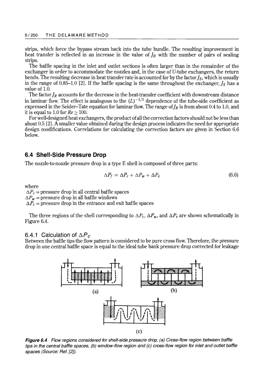
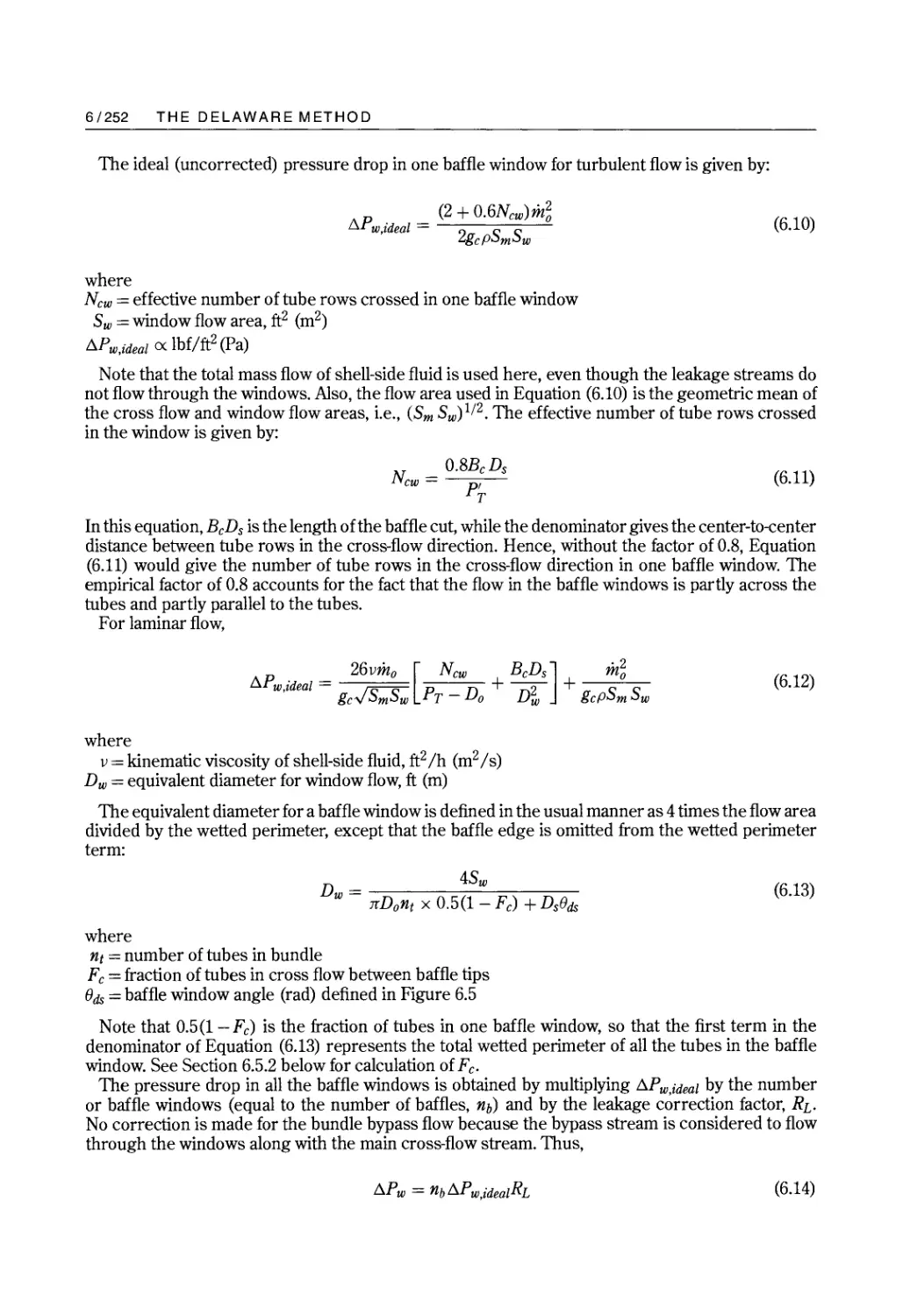
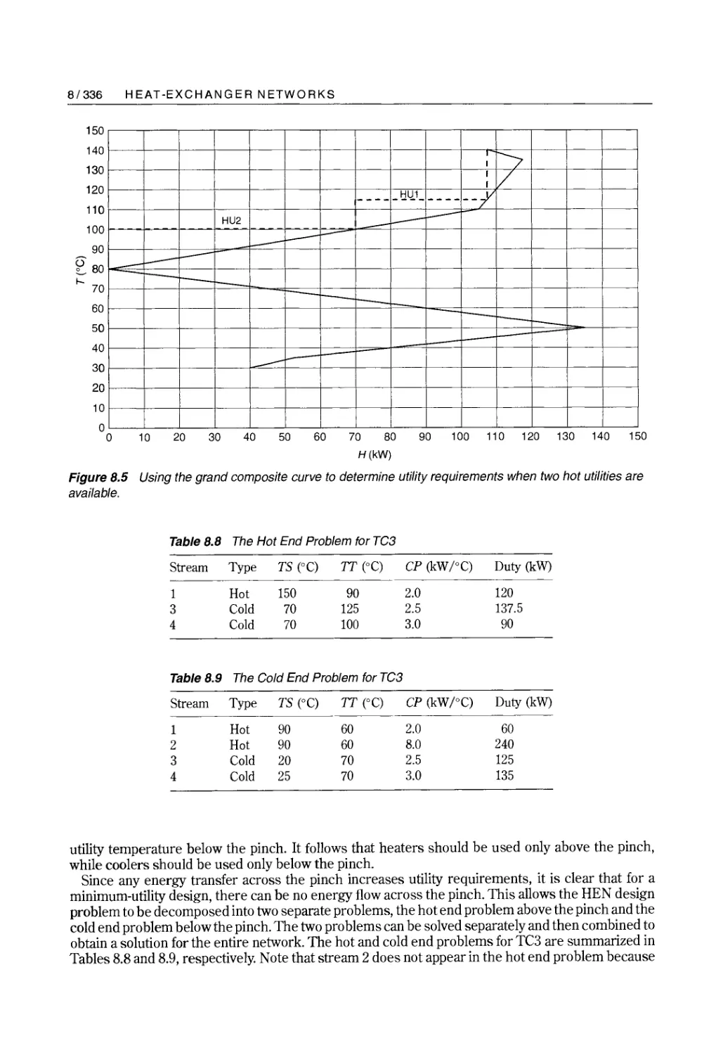
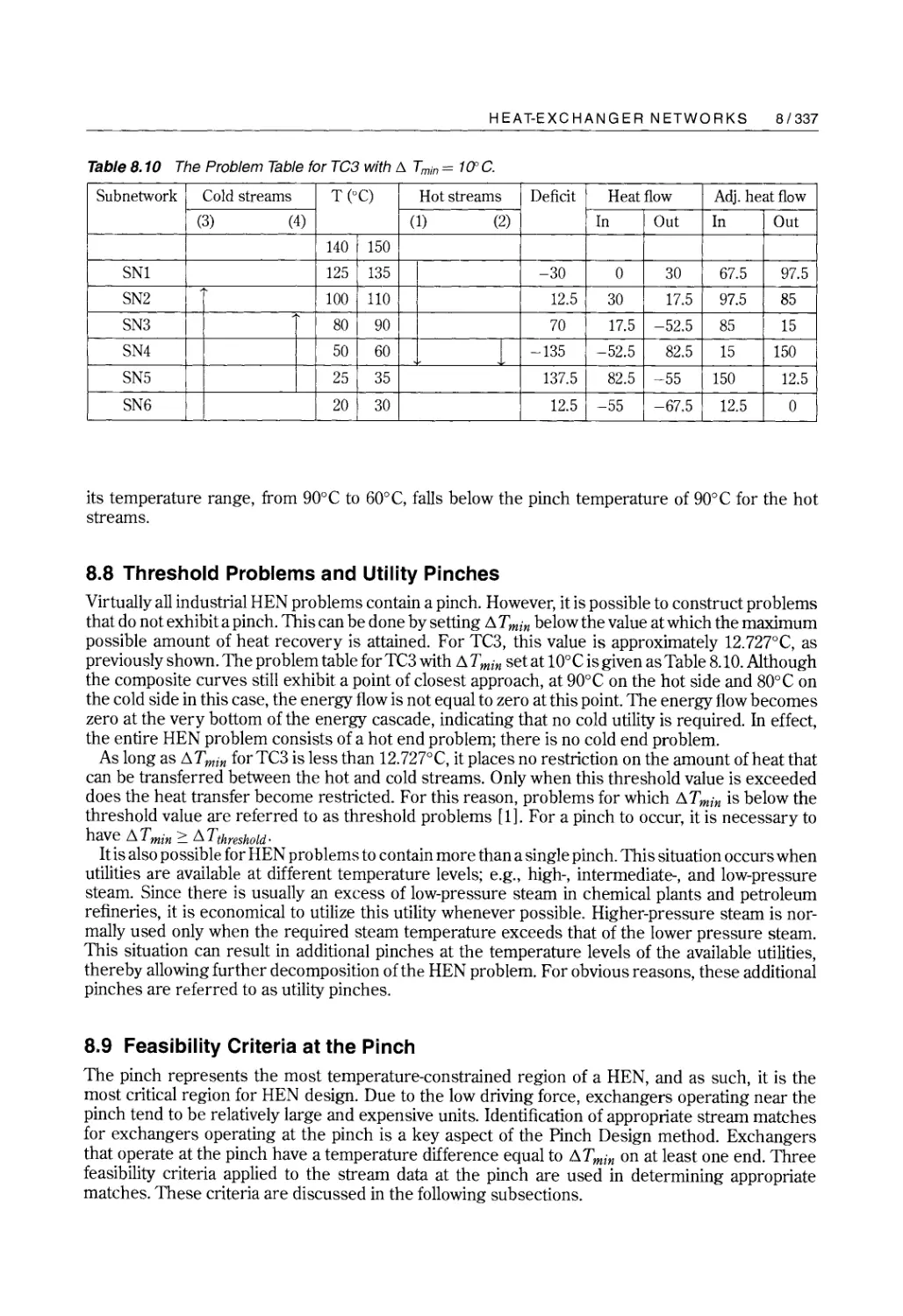
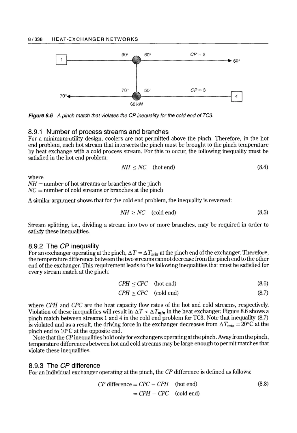
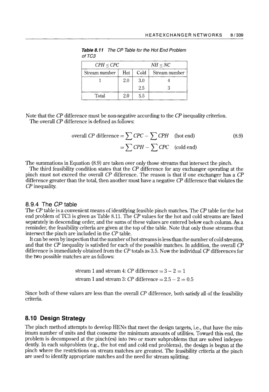
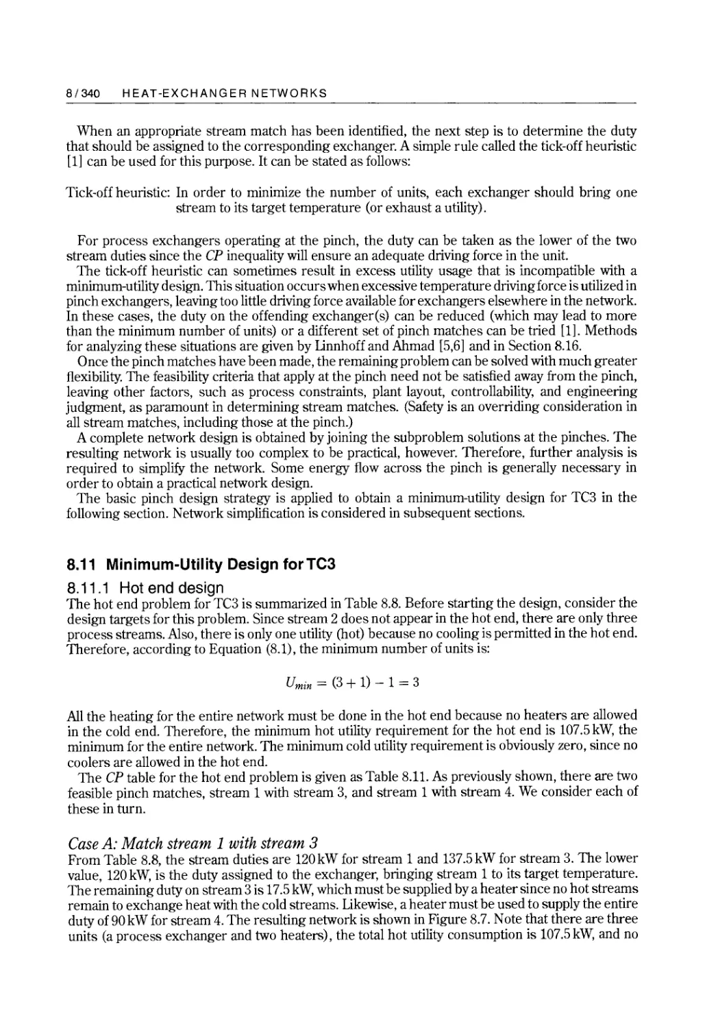
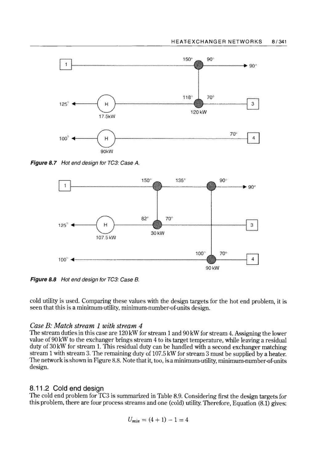
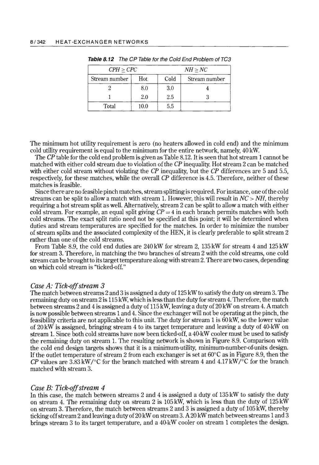
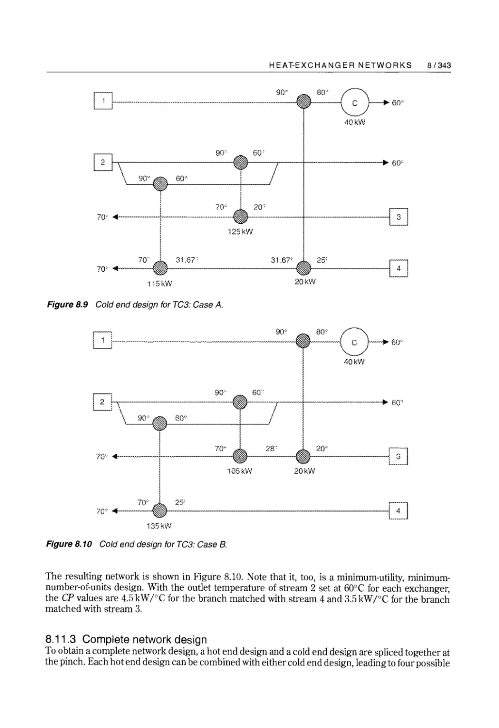
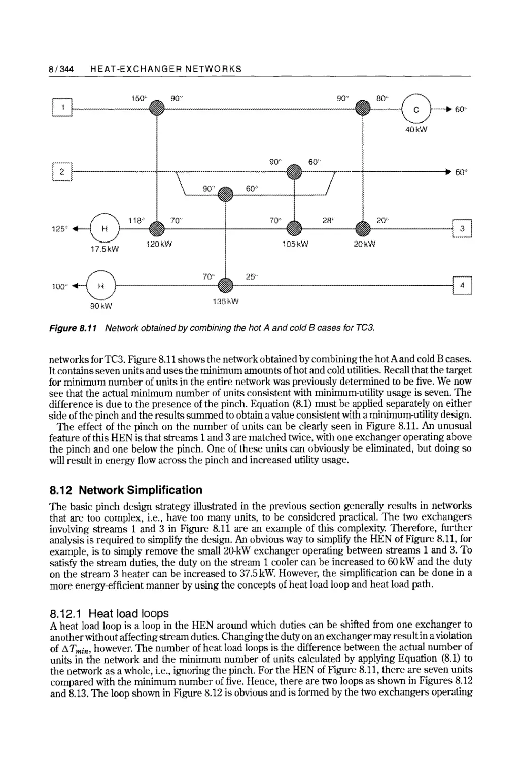
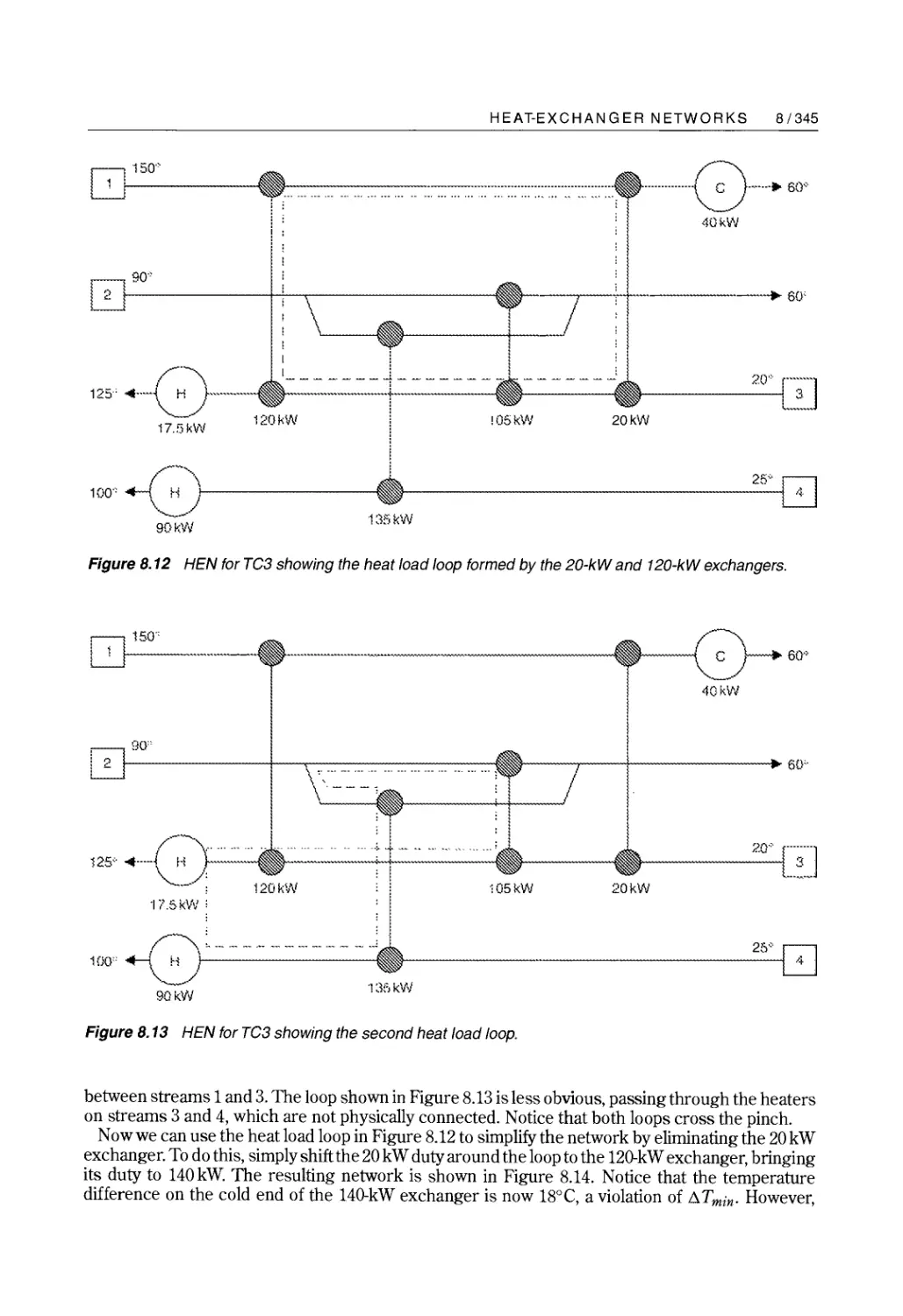
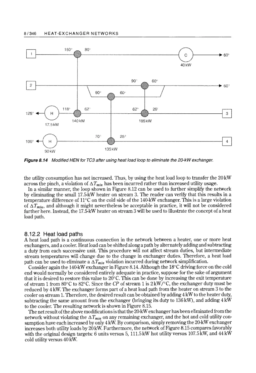
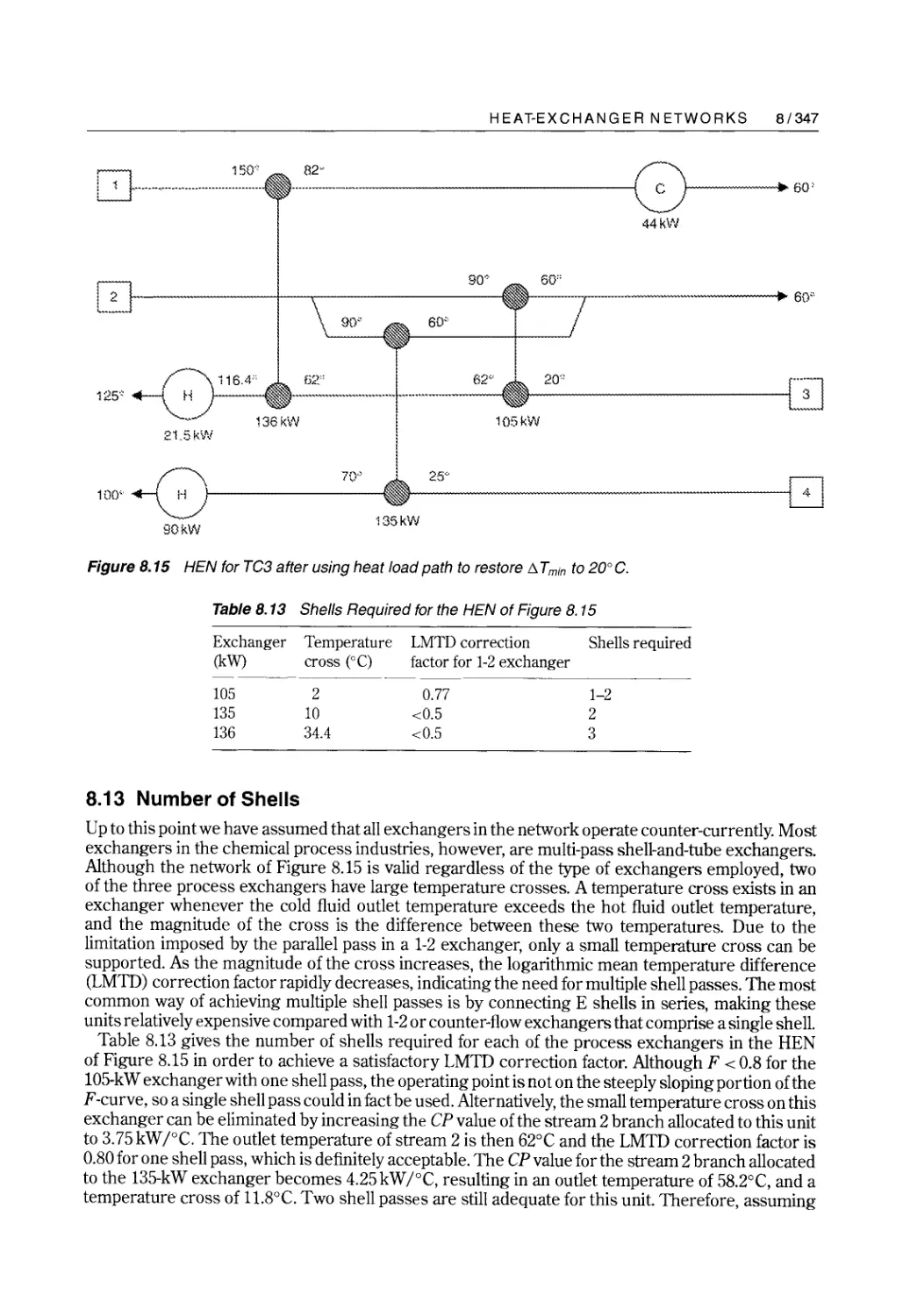
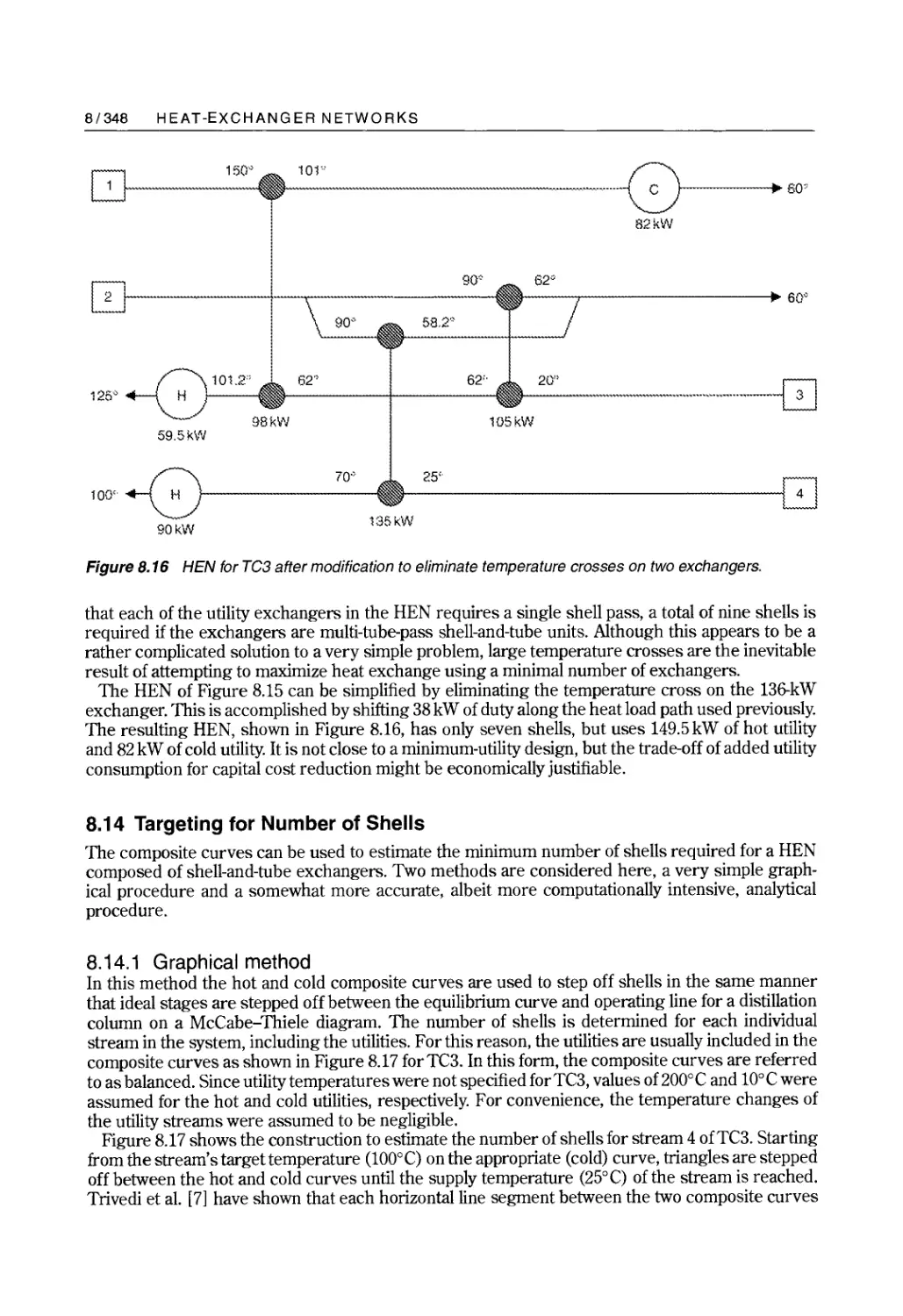
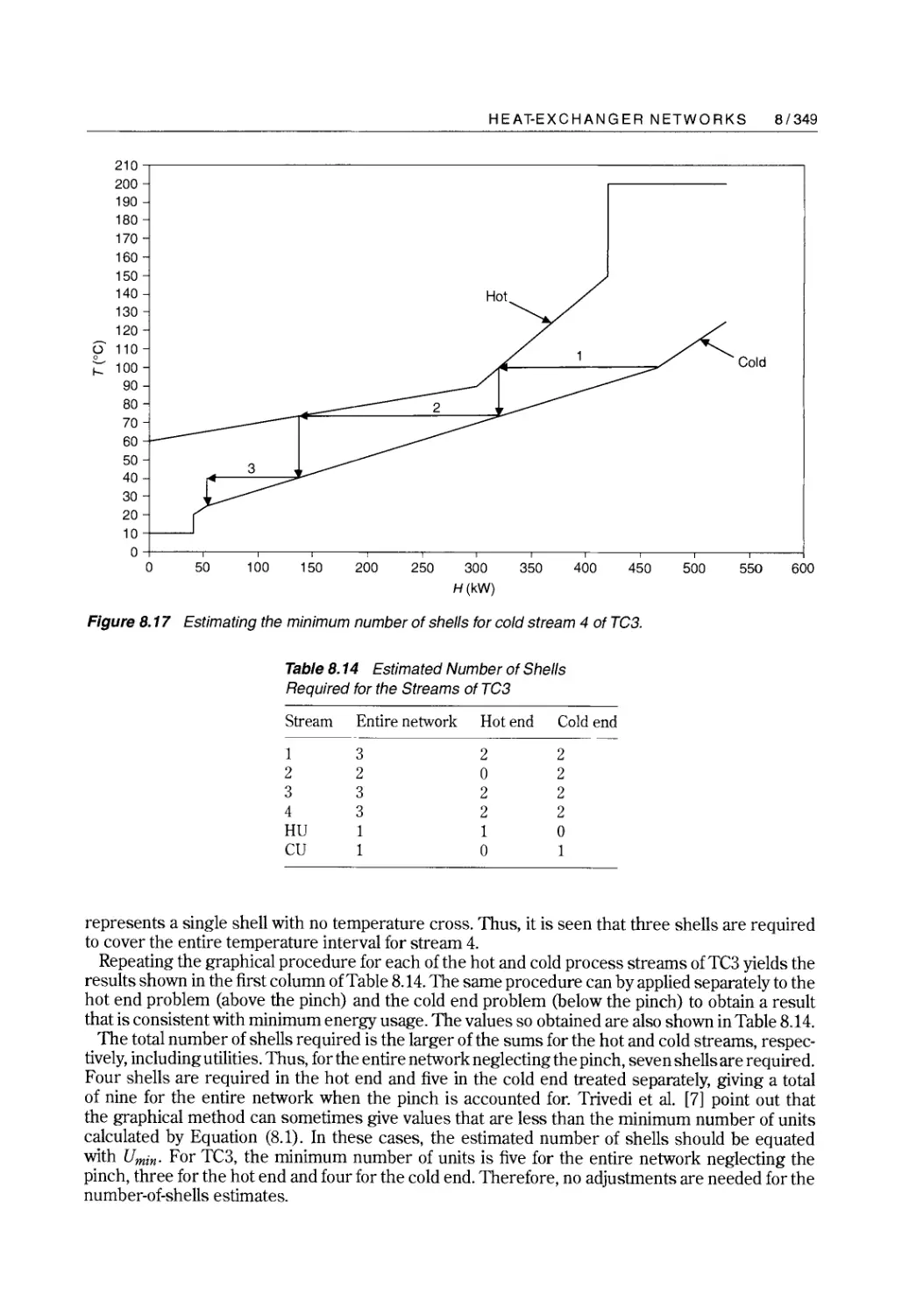
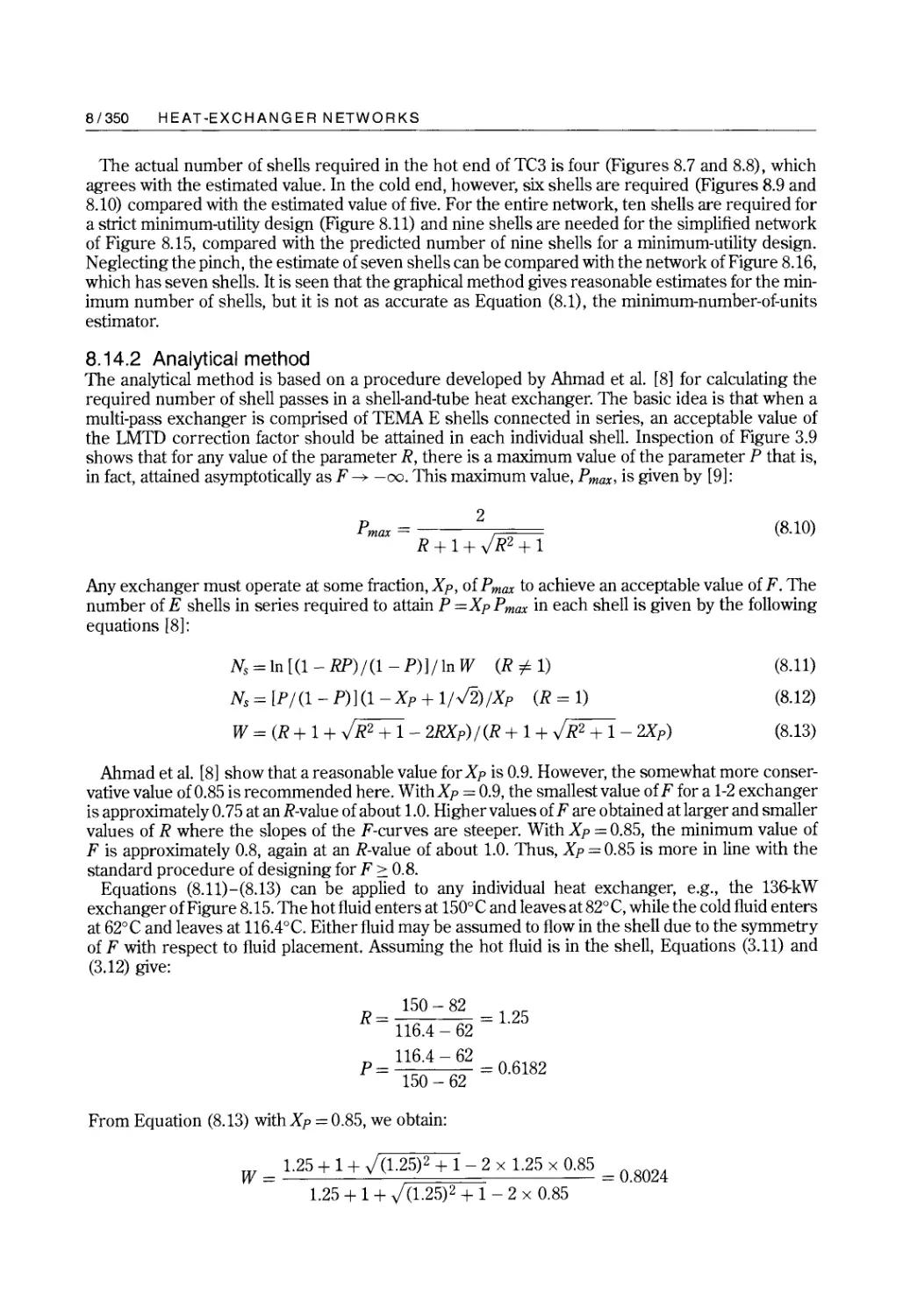
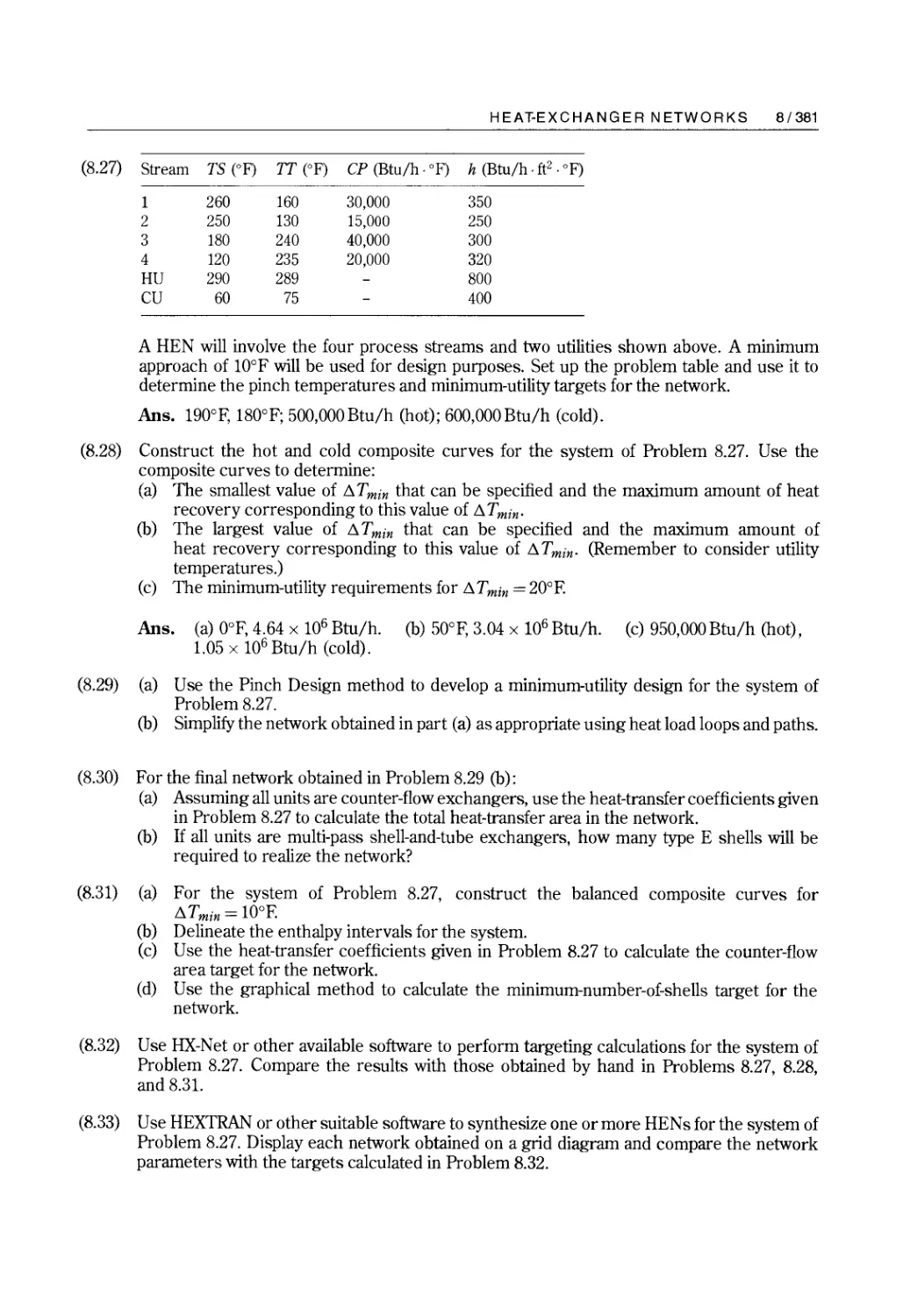
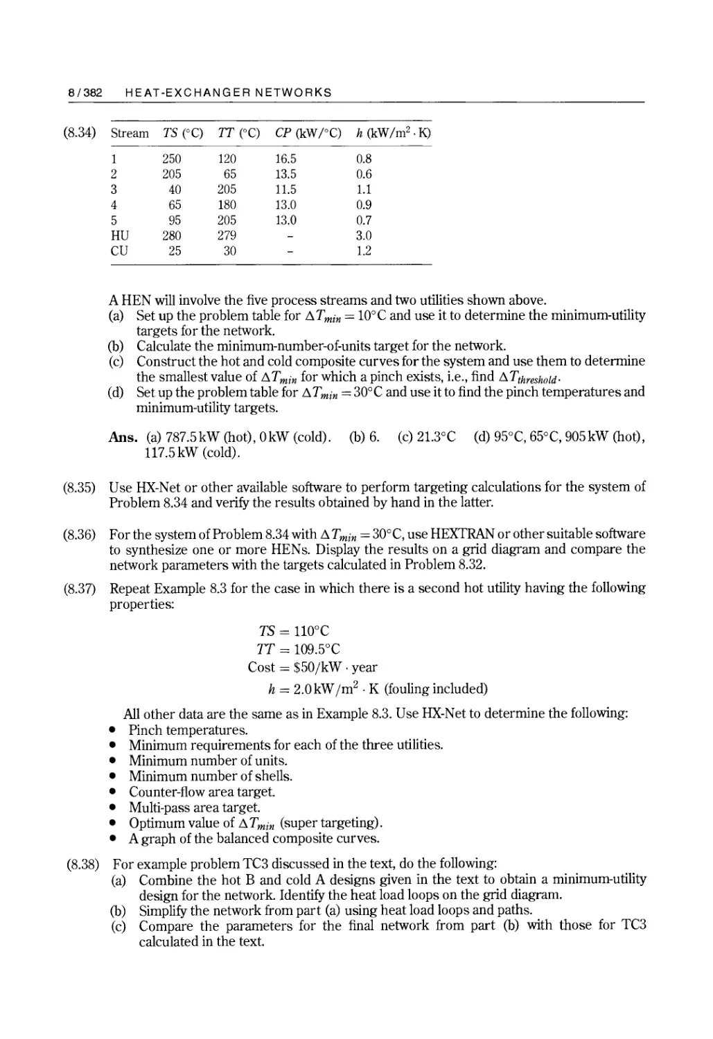
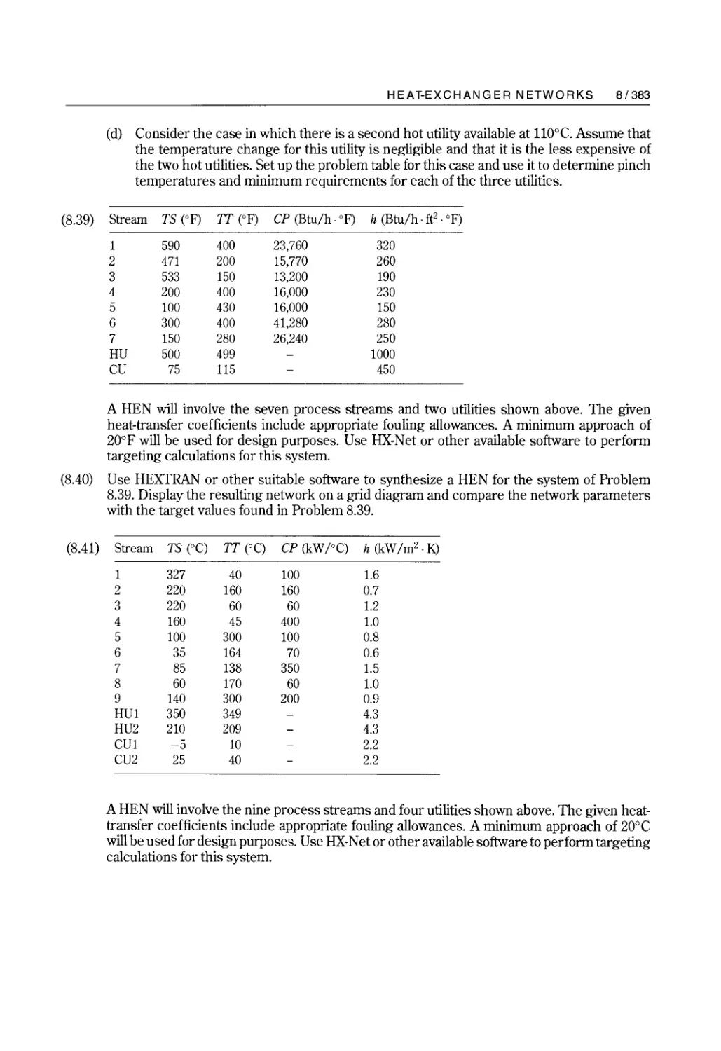
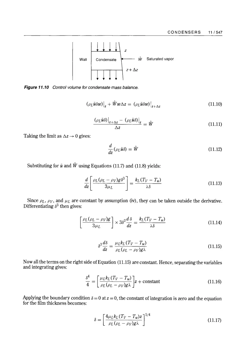
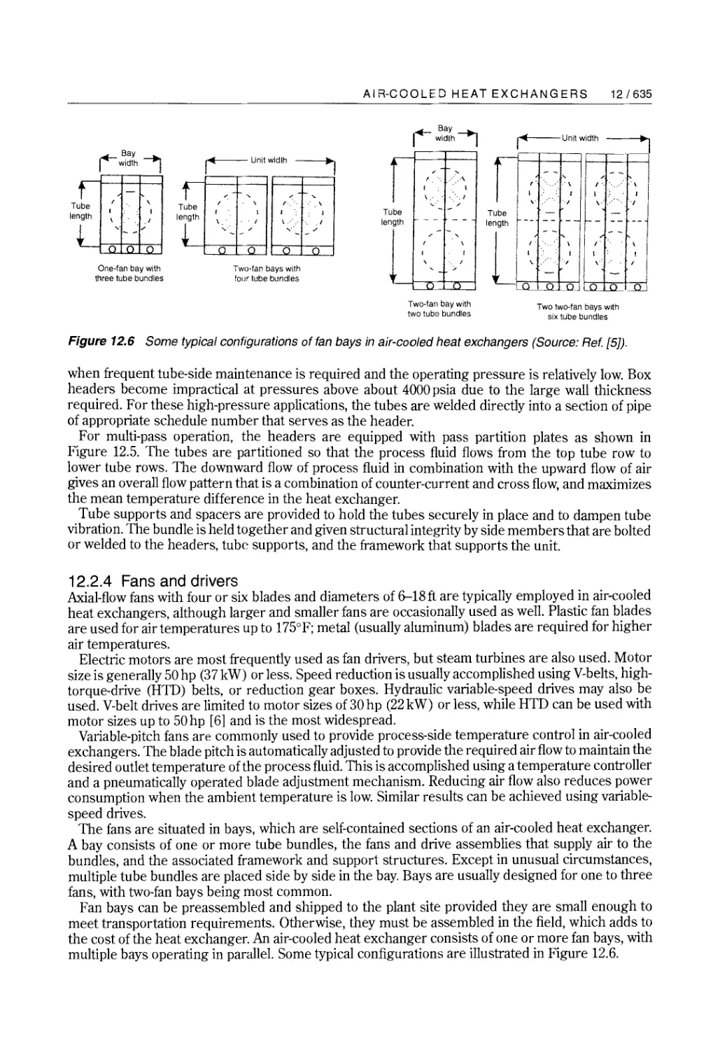
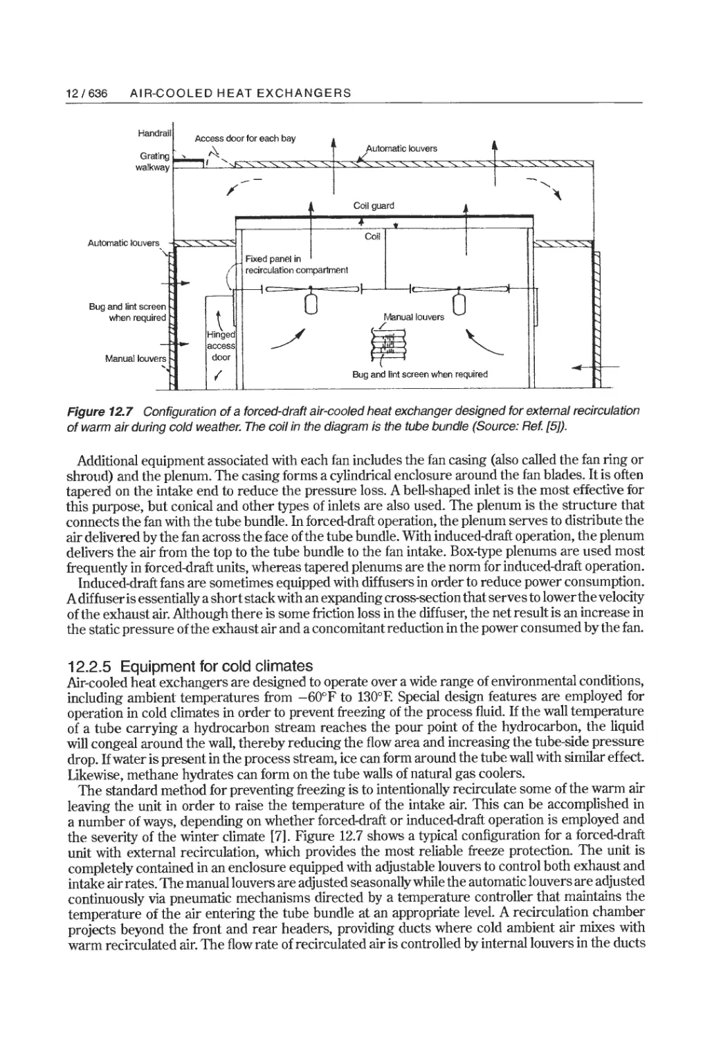
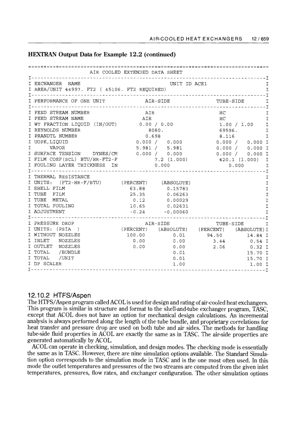
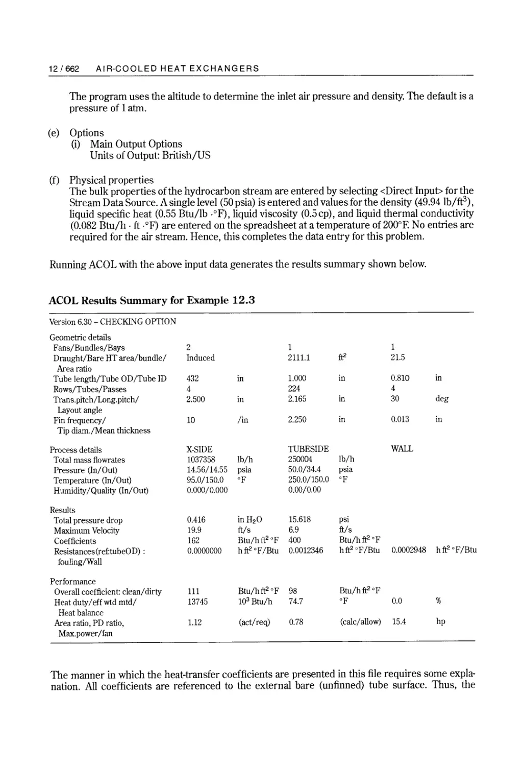
/


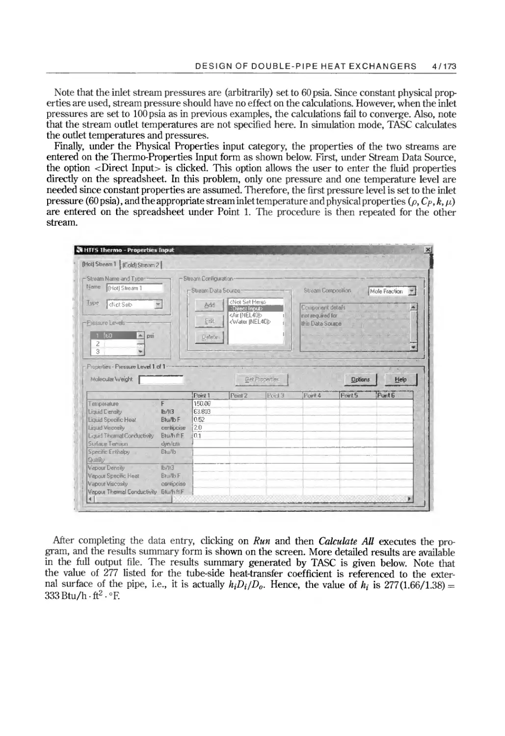
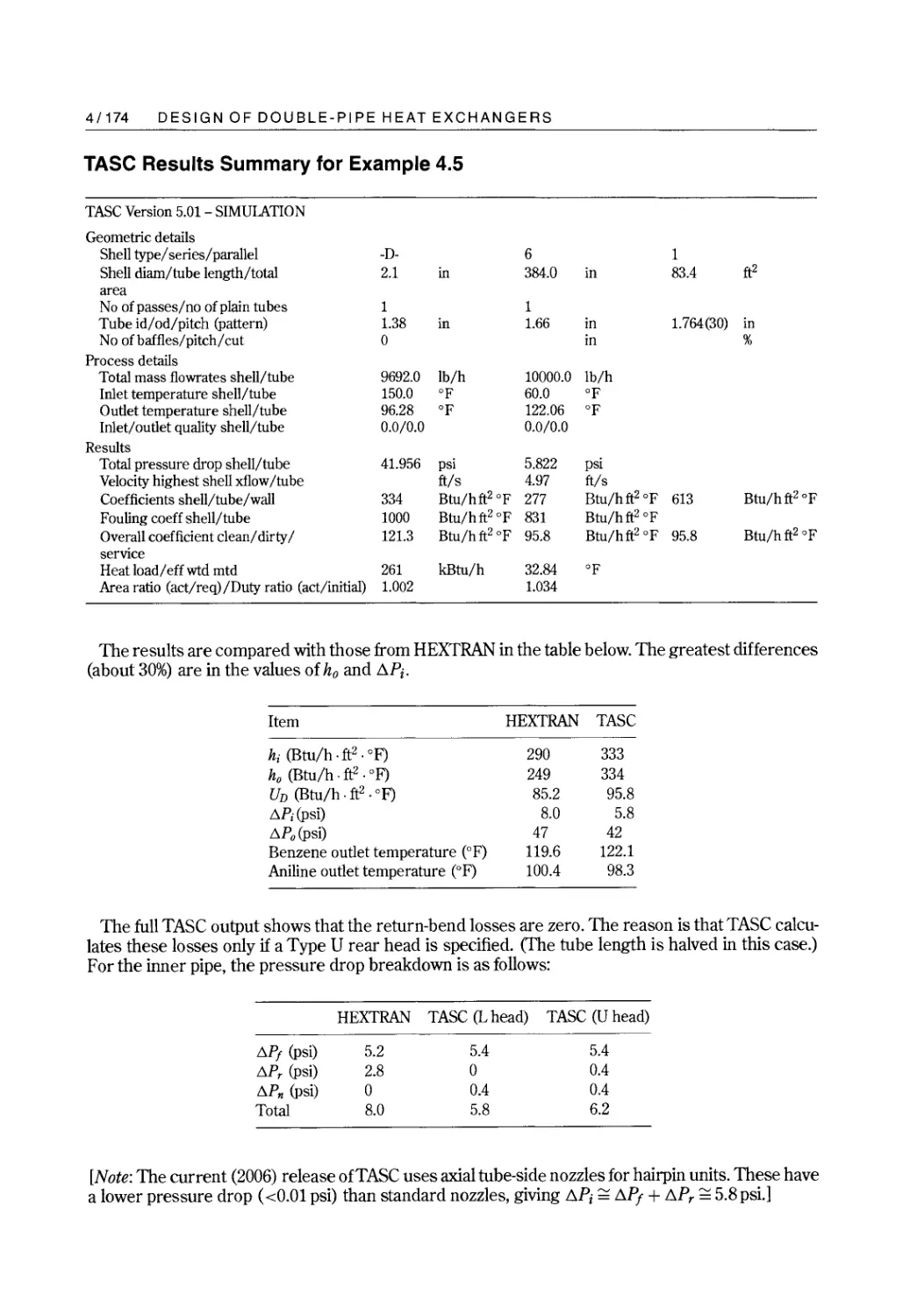
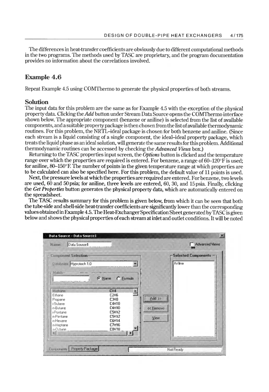
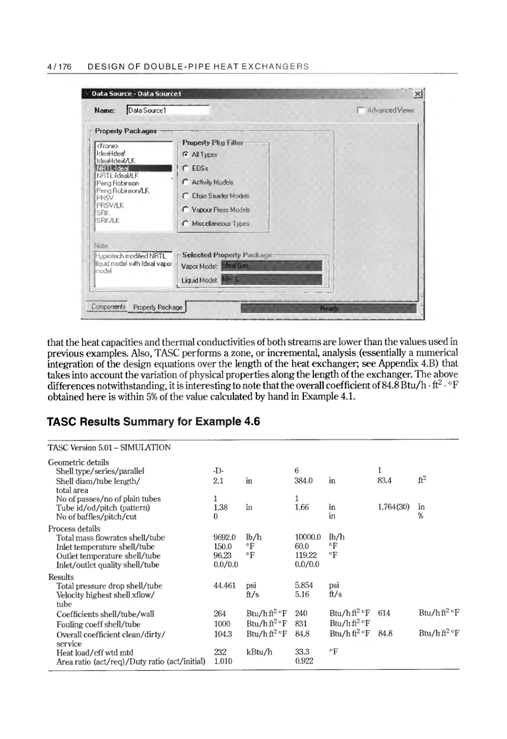


Text
Preface
This book is based on a course in process heat transfer that I have taught for many years. The course
has been taken by seniors and first-year graduate students who have completed an introductory
course in engineering heat transfer. Although this background is assumed, nearly all students need
some review before proceeding to more advanced material. For this reason, and also to make the
book self-contained, the first three chapters provide a review of essential material normally covered
in an introductory heat transfer course. Furthermore, the book is intended for use by practicing
engineers as well as university students, and it has been written with the aim of facilitating self-study.
Unlike some books in this field, no attempt is made herein to cover the entire panoply of heat trans-
fer equipment. Instead, the book focuses on the types of equipment most widely used in the chemical
process industries, namely, shell-and-tube heat exchangers (including condensers and reboilers),
air-cooled heat exchangers and double-pipe (hairpin) heat exchangers. Within the confines of a sin-
gle volume, this approach allows an in-depth treatment of the material that is most relevant from an
industrial perspective, and provides students with the detailed knowledge needed for engineering
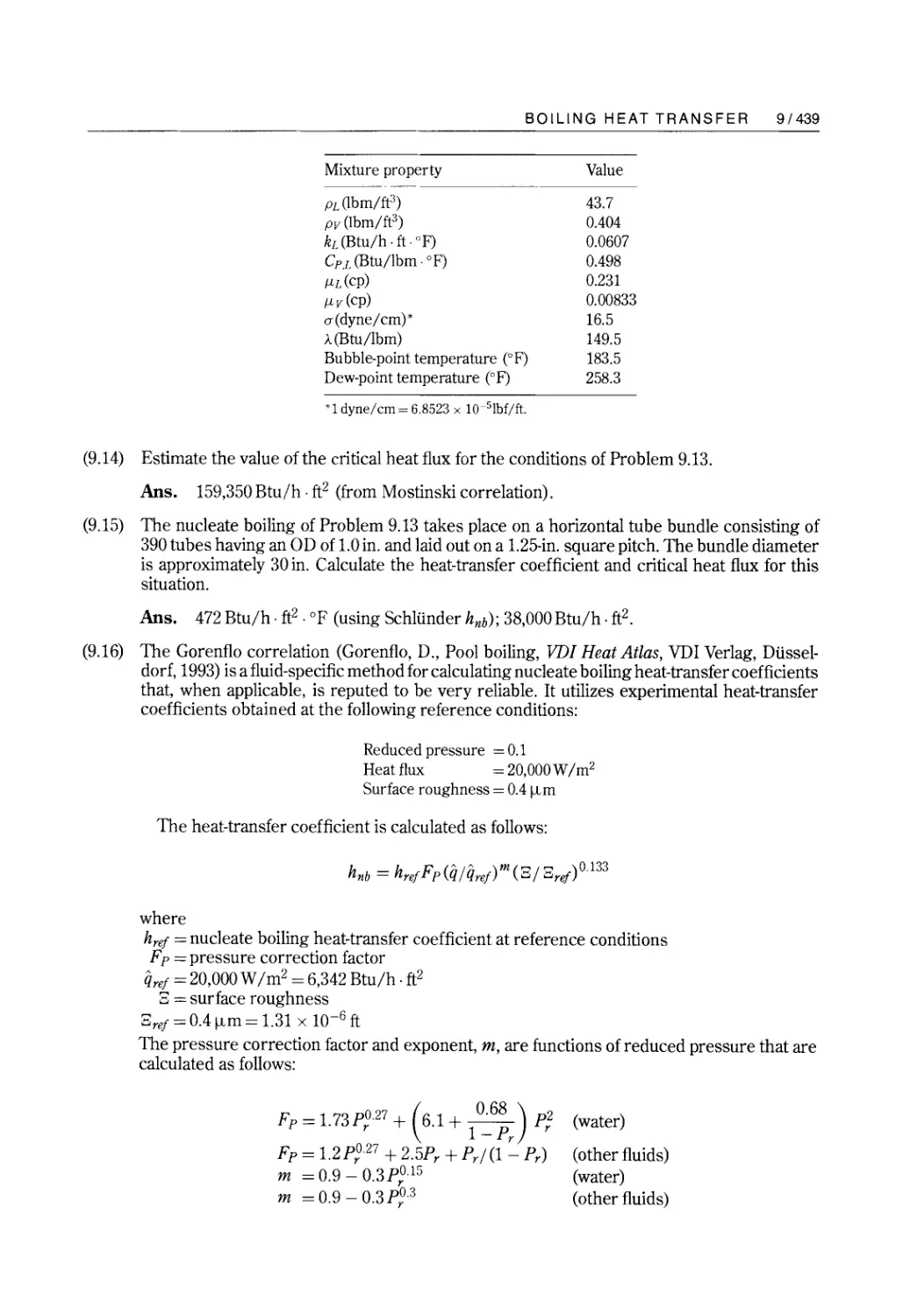
practice. This approach is also consistent with the time available in a one-semester course.
Design of double-pipe exchangers is presented in Chapter 4. Chapters 5-7 comprise a unit dealing
with shell-and-tube exchangers in operations involving single-phase fluids. Design of shell-and-tube
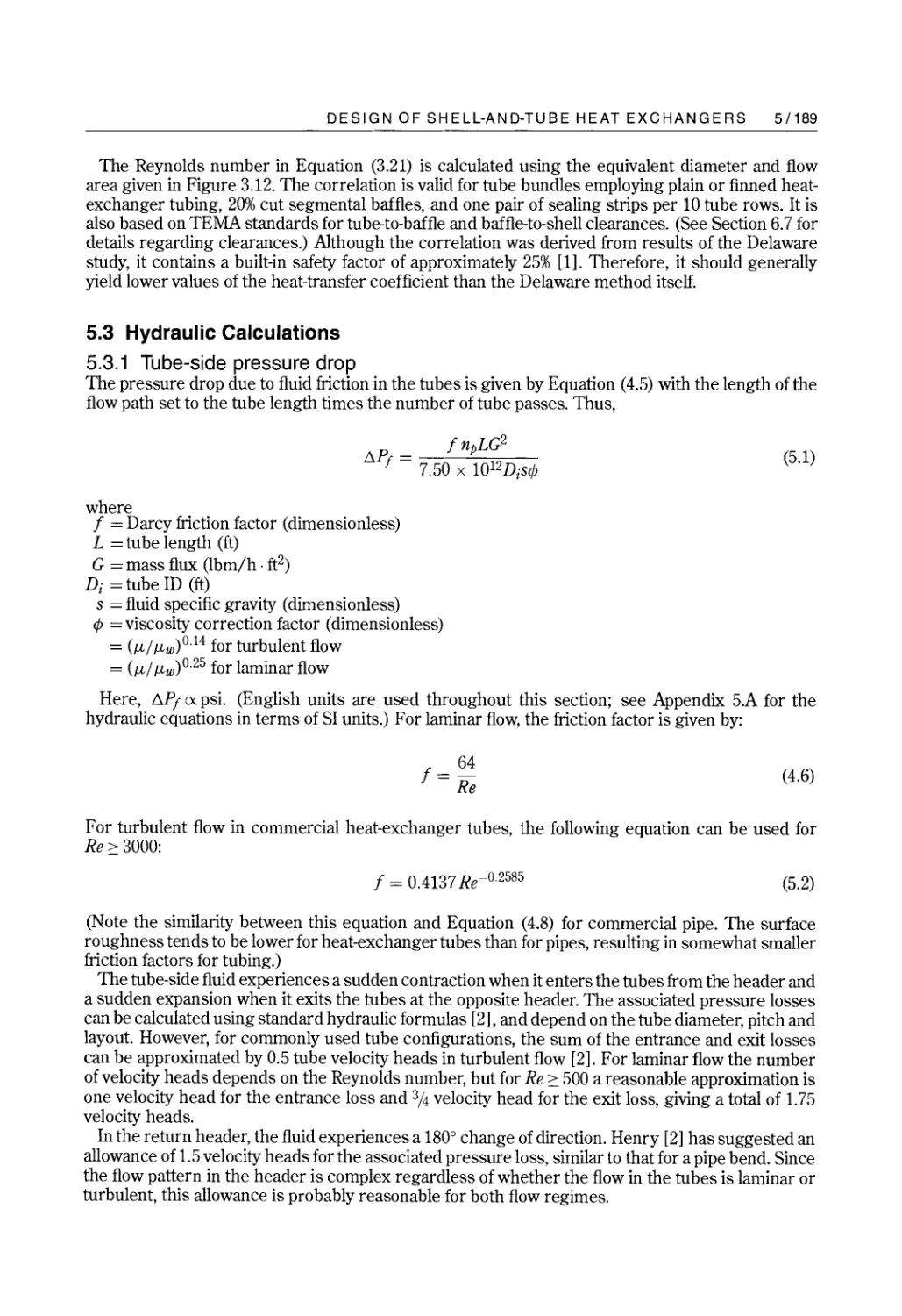
exchangers is covered in Chapter 5 using the Simplified Delaware method for shell-side calcula-
tions. For pedagogical reasons, more sophisticated methods for performing shell-side heat-transfer
and pressure-drop calculations are presented separately in Chapter 6 (full Delaware method) and
Chapter 7 (Stream Analysis method). Heat exchanger networks are covered in Chapter 8. I nor-
mally present this topic at this point in the course to provide a change of pace. However, Chapter
8 is essentially self-contained and can, therefore, be covered at any time. Phase-change operations
are covered in Chapters 9-11. Chapter 9 presents the basics of boiling heat transfer and two-phase
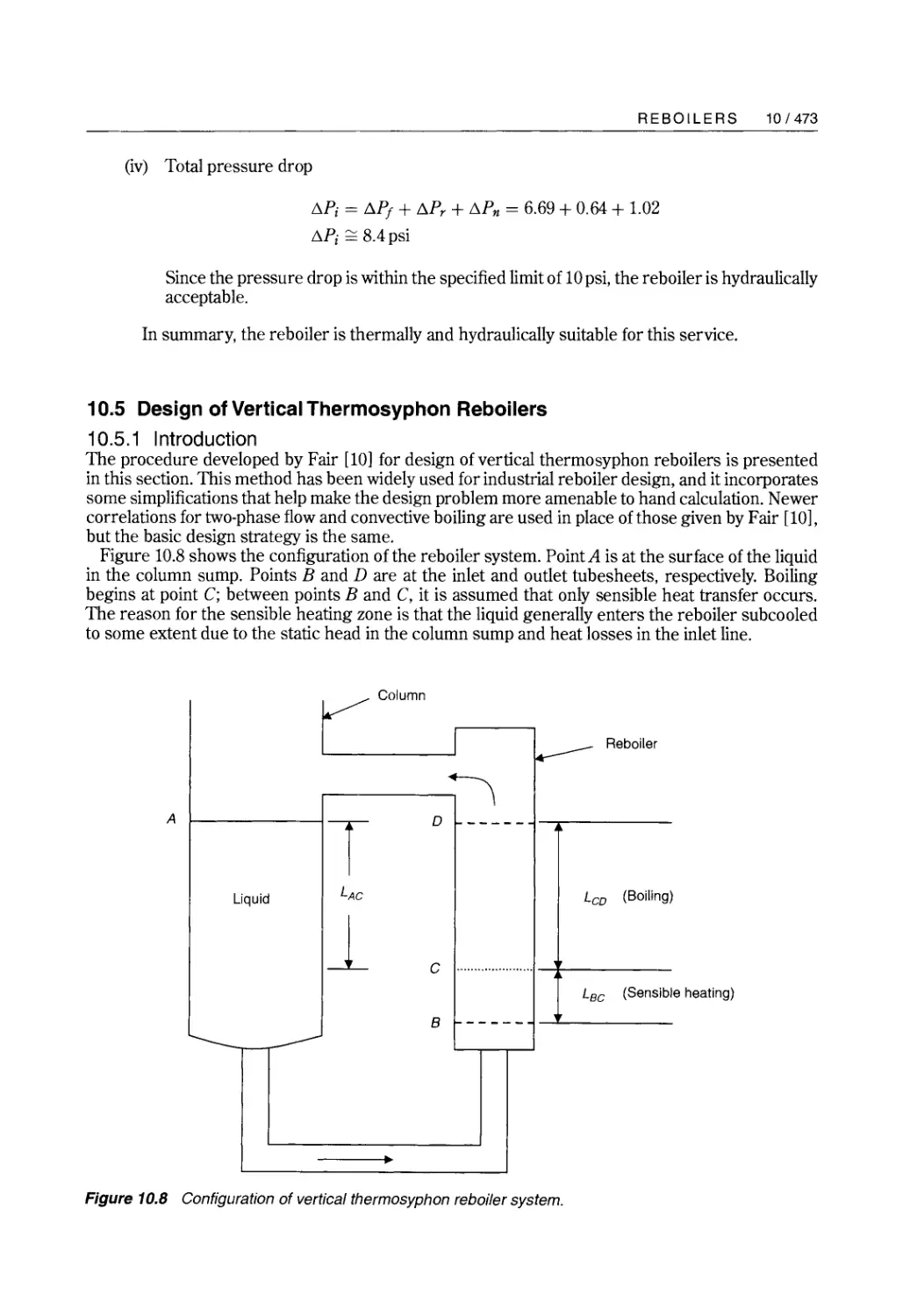
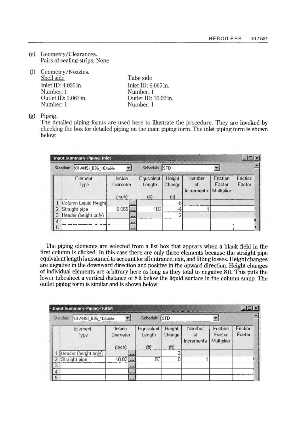
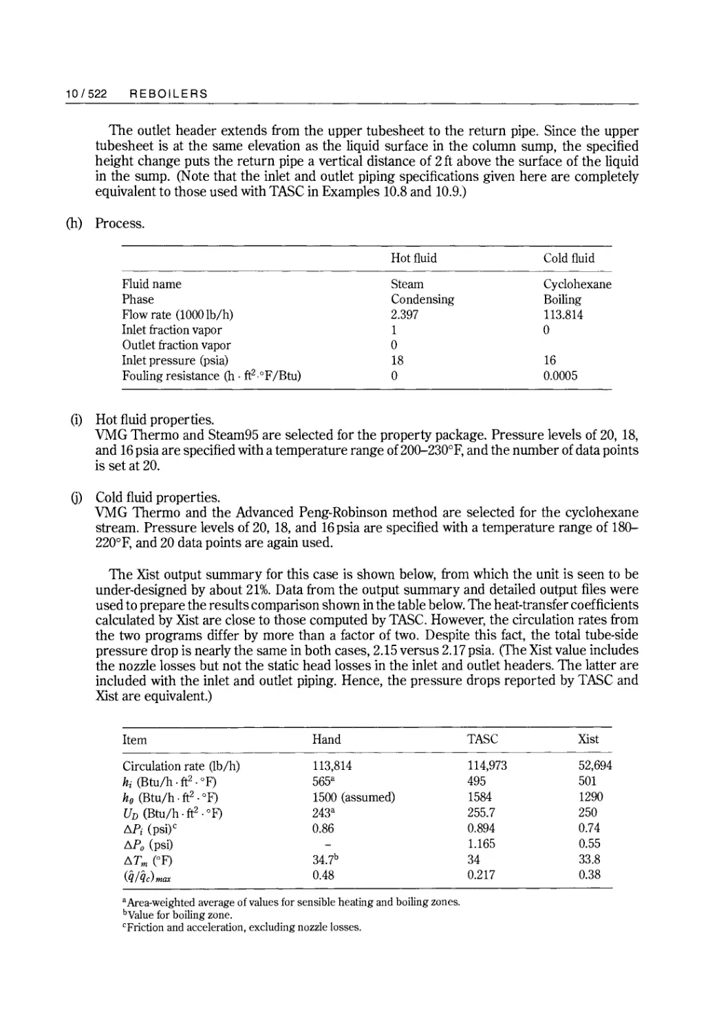
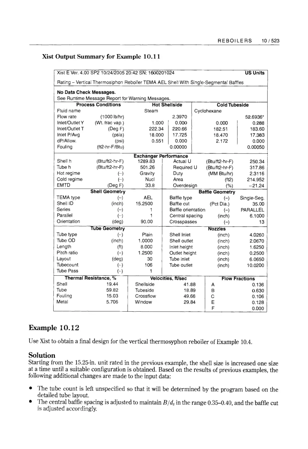
flow. The latter is encountered in both Chapter 10, which deals with the design of reboilers, and
Chapter 11, which covers condensation and condenser design. Design of air-cooled heat exchang-
ers is presented in Chapter 12. The material in this chapter is essentially self-contained and, hence,
it can be covered at any time.
Since the primary goal of both the book and the course is to provide students with the knowl-
edge and skills needed for modern industrial practice, computer applications play an integral role,
and the book is intended for use with one or more commercial software packages. HEXTRAN
(SimSci-Esscor), HTRI Xchanger Suite (Heat Transfer Research, Inc.) and the HTFS Suite (Aspen
Technology, Inc.) are used in the book, along with HX-Net (Aspen Technology, Inc.) for pinch
calculations. HEXTRAN affords the most complete coverage of topics, as it handles all types of heat
exchangers and also performs pinch calculations for design of heat exchanger networks. It does
not perform mechanical design calculations for shell-and-tube exchangers, however, nor does it
generate detailed tube layouts or setting plans. Furthermore, the methodology used by HEXTRAN
is based on publicly available technology and is generally less refined than that of the other software
packages. The HTRI and HTFS packages use proprietary methods developed by their respective
research organizations, and are similar in their level of refinement. HTFS Suite handles all types
of heat exchangers; it also performs mechanical design calculations and develops detailed tube
layouts and setting plans for shell-and-tube exchangers. HTRI Xchanger Suite lacks a mechanical
design feature, and the module for hairpin exchangers is not included with an academic license.
Neither HTRI nor HTFS has the capability to perform pinch calculations.
As of this writing, Aspen Technology is not providing the TASC and ACOL modules of the HTFS
Suite under its university program. Instead, it is offering the HTFS-plus design package. This
package basically consists of the TASC and ACOL computational engines combined with slightly
modified GUI's from the corresponding B]AC programs (HETRAN andAEROTRAN), and packaged
with the B]AC TEAMS mechanical design program. This package differs greatly in appearance and
to some extent in available features from HTFS Suite. However, most ofthe results presented in the
text using TASC and ACOL can be generated using the HTFS-plus package.
PREFACE ix
Software companies are continually modifying their products, making differences between the
text and current versions of the software packages unavoidable. However, many modifications
involve only superficial changes in format that have little, if any, effect on results. More substantive
changes occur less frequently, and even then the effects tend to be relatively minor. Nevertheless,
readers should expect some divergence of the software from the versions used herein, and they
should not be unduly concerned if their results differ somewhat from those presented in the text.
Indeed, even the same version of a code, when run on different machines, can produce slightly
different results due to differences in round-off errors. With these caveats, it is hoped that the
detailed computer examples will prove helpful in learning to use the software packages, as well as
in understanding their idiosyncrasies and limitations.
I have made a concerted effort to introduce the complexities of the subject matter gradually
throughout the book in order to avoid overwhelming the reader with a massive amount of detail
at anyone time. As a result, information on shell-and-tube exchangers is spread over a number of
chapters, and some of the finer details are introduced in the context of example problems, including
computer examples. Although there is an obvious downside to this strategy, I nevertheless believe
that it represents good pedagogy.
Both English units, which are still widely used by American industry, and SI units are used in this
book. Students in the United States need to be proficient in both sets of units, and the same is true
of students in countries that do a large amount of business with U.S. firms. In order to minimize
the need for unit conversion, however, working equations are either given in dimensionless form
or, when this is not practical, they are given in both sets of units.
I would like to take this opportunity to thank the many students who have contributed to this
effort over the years, both directly and indirectly through their participation in my course. I would
also like to express my deep appreciation to my colleagues in the Department of Chemical and
Natural Gas Engineering at TAMUK, Dr. Ali Pilehvari and Mrs. Wanda Pounds. Without their help,
encouragement and friendship, this book would not have been written.
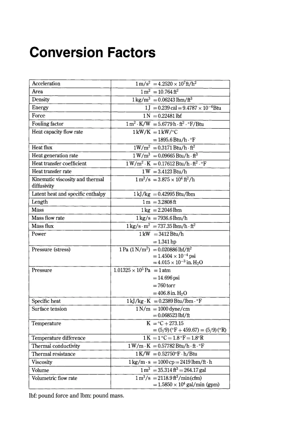
Conversion Factors
Acceleration 1 m/s 2 = 4.2520 x 10 7 ft/h 2
Area 1 m 2 = 10.764ft2
Density 1 kg/m 3 = 0.06243Ibm/ft3
Energy 1] = 0.239 cal = 9.4787 x 1O- 4 Btu
Force 1 N = 0.224811bf
Fouling factor 1 m 2 . K/W = 5.6779 h. ft2 . of /Btu
Heat capacity flow rate lkW/K =lkW/oC
= 1895.6 Btu/h. of
Heat flux lW/m 2 =0.3171Btu/h.ft2
Heat generation rate 1 W /m 3 = 0.09665 Btu/h. ft3
Heat transfer coefficient 1 W /m 2 . K = 0.17612 Btu/h. ft2 . of
Heat transfer rate 1 W = 3.4123 Btu/h
Kinematic viscosity and thermal 1 m 2 /s = 3.875 X 10 4 ft2/h
diffusivity
Latent heat and specific enthalpy 1 kJ /kg = 0.42995 Btu/lbm
Length 1 m = 3.2808ft
Mass 1 kg = 2.2046 Ibm
Mass flow rate 1 kg/ s = 7936.6Ibm/h
Mass flux 1 kg/s. m 2 = 737.35Ibm/h. ft2
Power 1 kW = 3412 Btu/h
= 1.341 hp
Pressure (stress) 1 Pa (1 N/m 2 ) = 0.020886Ibf/ft2
= 1.4504 x 10- 4 psi
= 4.015 x 10- 3 in. H2O
Pressure 1.01325 x 10 5 Pa = 1 atm
= 14.696 psi
= 760 torr
= 406.8 in. H20
Specific heat lkJ/kg.K =0.2389Btu/lbm.oF
Surface tension IN/m = 1000dyne/cm
= 0.068523Ibf/ft
Temperature K = °C + 273.15
= (5/9) (OF + 459.67) = (5/9) (OR)
Temperature difference lK =1°C=1.8°F=1.8°R
Thermal conductivity 1 W /m . K = 0.57782 Btu/h. ft. of
Thermal resistance 1 K/W = 0.52750°F . h/Btu
Viscosity lkg/m. s = 1000cp=2419Ibm/ft. h
Volume 1 m 3 = 35.314ft3 =264.17 gal
Volumetric flow rate 1 m 3 /s = 2118.9ft3 /min(cfm)
= 1.5850 x 10 4 gal/min (gpm)
lbf: pound force and Ibm: pound mass.
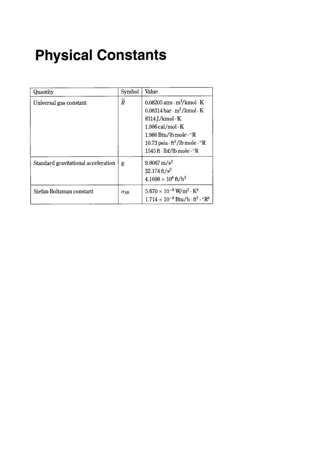
Physical Constants
Quantity Symbol Value
Universal gas constant R 0.08205 atm. m 3 /kmol. K
0.08314 bar. m 3 /kmol. K
8314J/kmol.K
1.986cal/mol. K
1.986 Btu/lb mole. oR
10.73 psia. ft3 /lb mole. oR
1545 ft .lbf/lb mole. oR
Standard gravitational acceleration g 9.8067m/s 2
32.174ft/s 2
4.1698 x 10 8 ft/h 2
Stefan-Boltzman constant uSB 5.670 x 10- 8 W/m 2 . K 4
1.714 x 10- 9 Btu/h. ft2. °R4
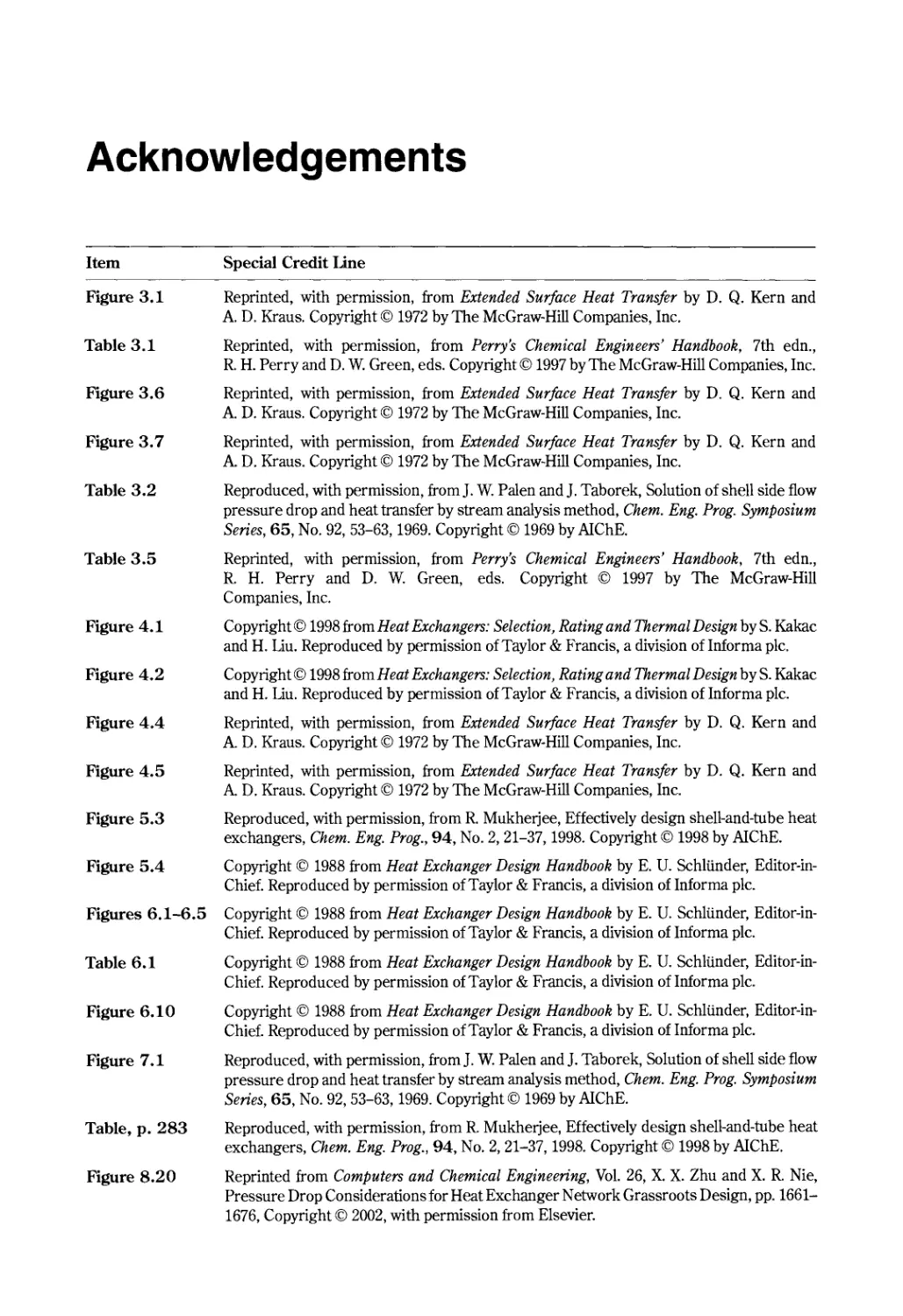
Acknowledgements
Item Special Credit line
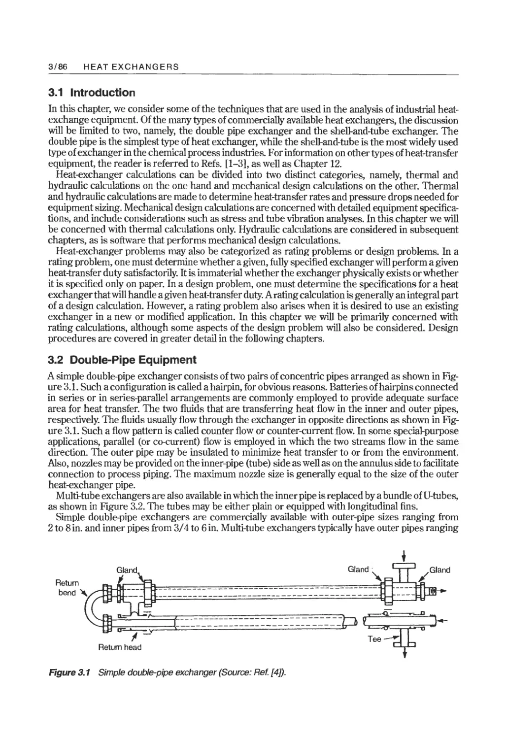
Figure 3.1 Reprinted, with permission, from Extended Surface Heat Transfer by D. Q. Kern and
A. D. Kraus. Copyright 1972 by The McGraw-Hill Companies, Inc.
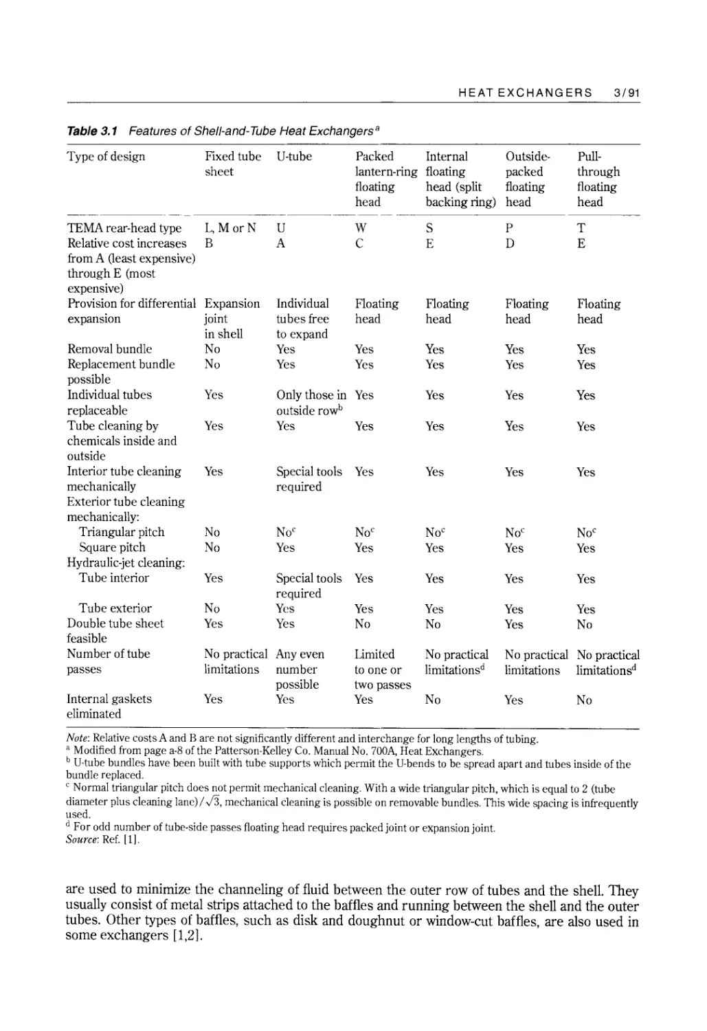
Table 3.1 Reprinted, with permission, from Perry's Chemical Engineers' Handbook, 7th edn.,
R. H. Perry and D. W. Green, eds. Copyright 1997 by The McGraw-Hill Companies, Inc.
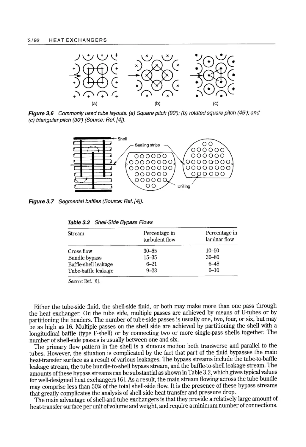
Figure 3.6 Reprinted, with permission, from Extended Surface Heat Transfer by D. Q. Kern and
A. D. Kraus. Copyright 1972 by The McGraw-Hill Companies, Inc.
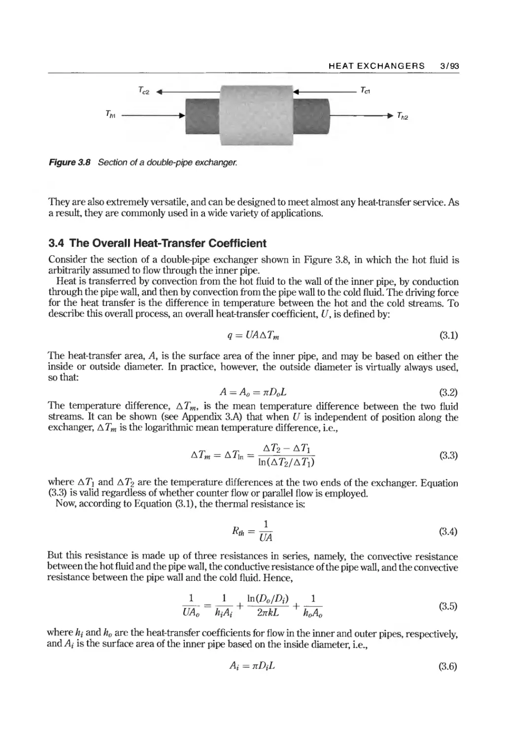
Figure 3.7 Reprinted, with permission, from Extended Surface Heat Transfer by D. Q. Kern and
A. D. Kraus. Copyright 1972 by The McGraw-Hill Companies, Inc.
Table 3.2 Reproduced, with permission, from J. W. Palen and J. Taborek, Solution of shell side flow
pressure drop and heat transfer by stream analysis method, Chem. Eng. Prog. Symposium
Series, 65, No. 92, 53-63, 1969. Copyright 1969 by AIChE.
Table 3.5 Reprinted, with permission, from Perry's Chemical Engineers' Handbook, 7th edn.,
R. H. Perry and D. W. Green, eds. Copyright 1997 by The McGraw-Hill
Companies, Inc.
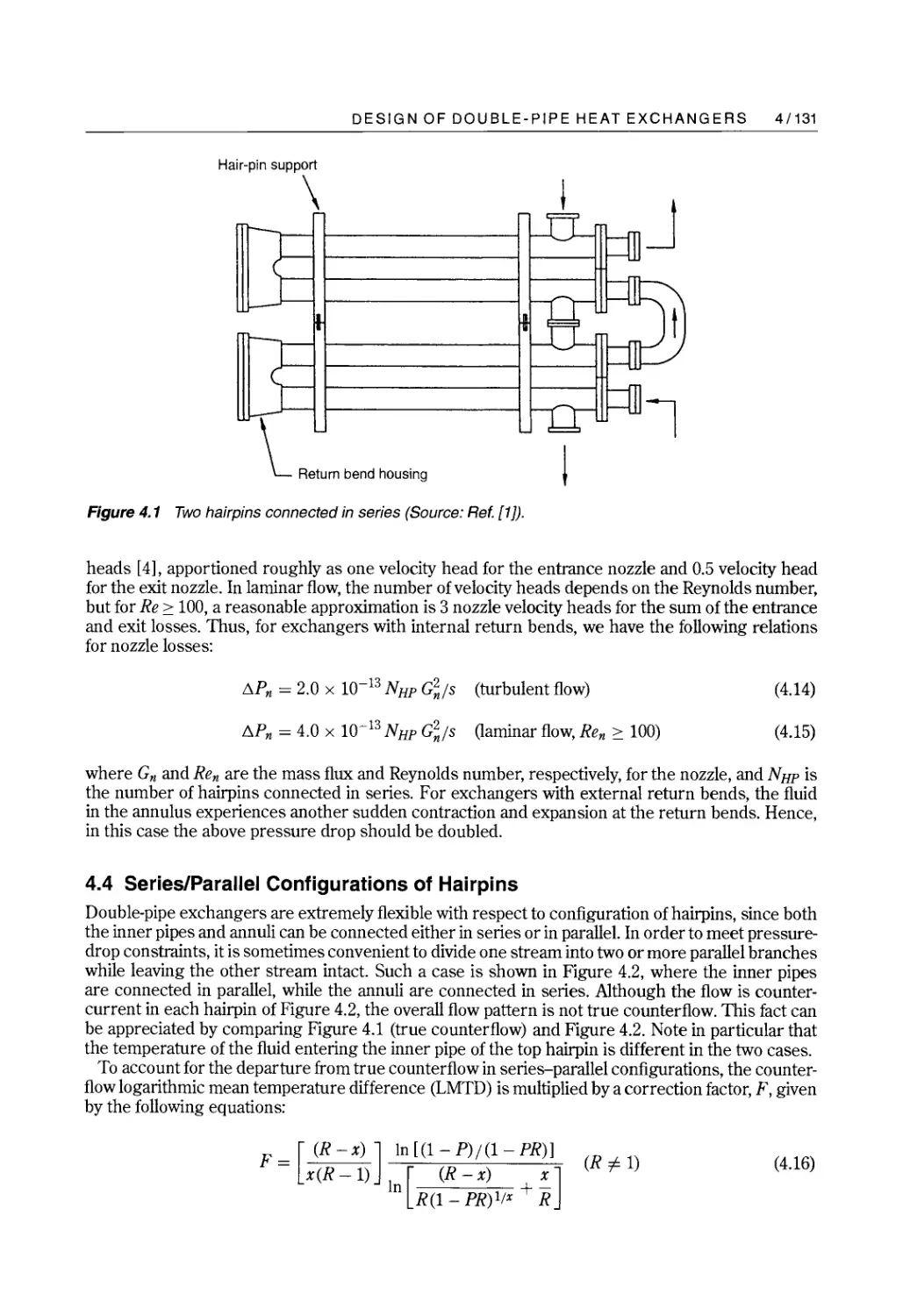
Figure 4.1 Copyright 1998 from Heat Exchangers: Selection, Rating and Thermal Design by S. Kakac
and H. Liu. Reproduced by permission of Taylor & Francis, a division of Informa pic.
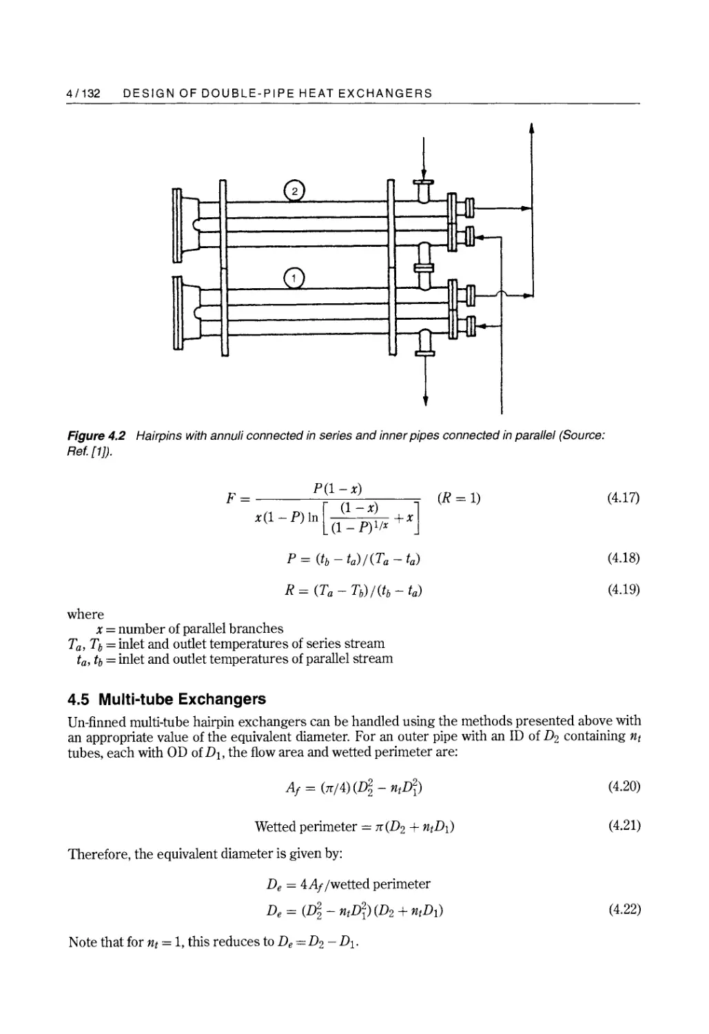
Figure 4.2 Copyright 1998 from Heat Exchangers: Selection, Rating and Thermal Design by S. Kakac
and H. Liu. Reproduced by permission of Taylor & Francis, a division of Informa pic.
Figure 4.4 Reprinted, with permission, from Extended Surface Heat Transfer by D. Q. Kern and
A. D. Kraus. Copyright 1972 by The McGraw-Hill Companies, Inc.
Figure 4.5 Reprinted, with permission, from Extended Surface Heat Transfer by D. Q. Kern and
A D. Kraus. Copyright 1972 by The McGraw-Hill Companies, Inc.
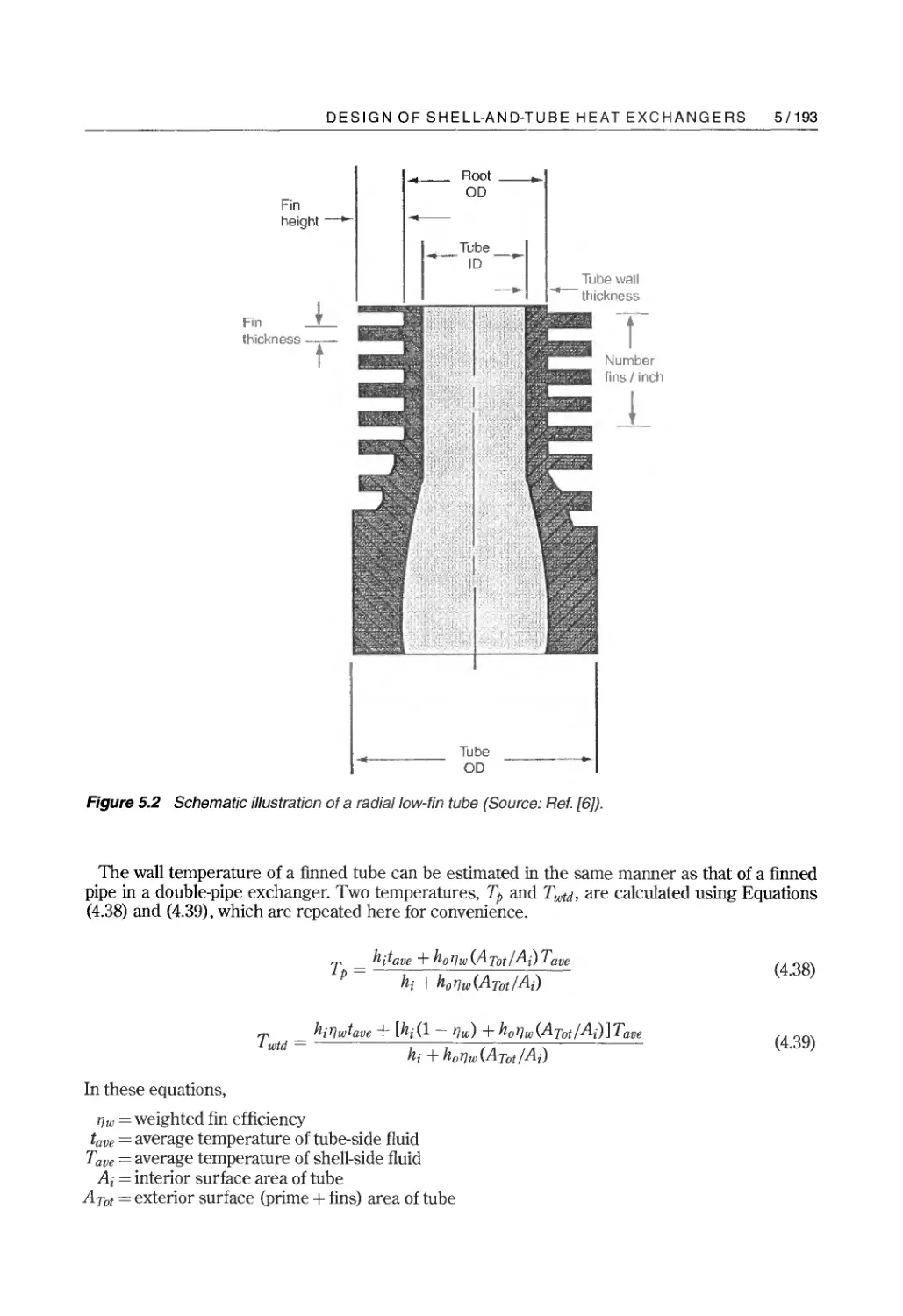
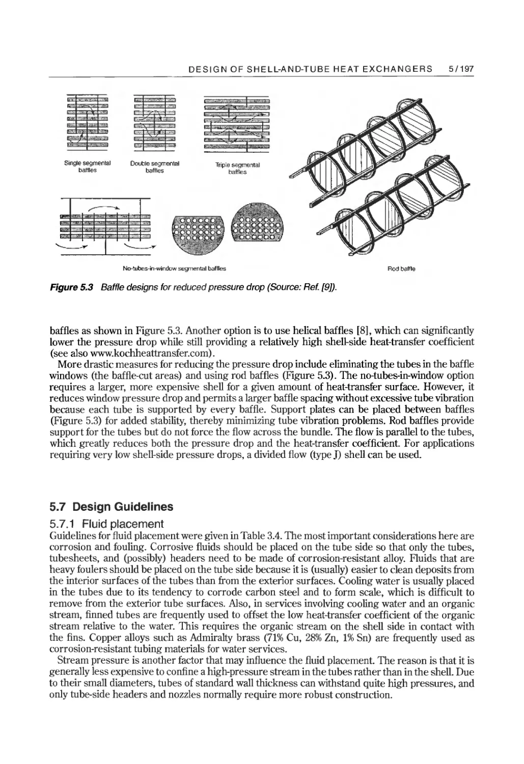
Figure 5.3 Reproduced, with permission, from R. Mukherjee, Effectively design shell-and-tube heat
exchangers, Chem. Eng. Prog., 94, No.2, 21-37, 1998. Copyright 1998 by AIChE.
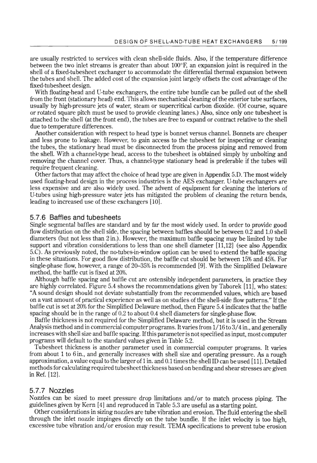
Figure 5.4 Copyright 1988 from Heat Exchanger Design Handbook by E. U. Schltinder, Editor-in-
Chief. Reproduced by permission of Taylor & Francis, a division of Informa pic.
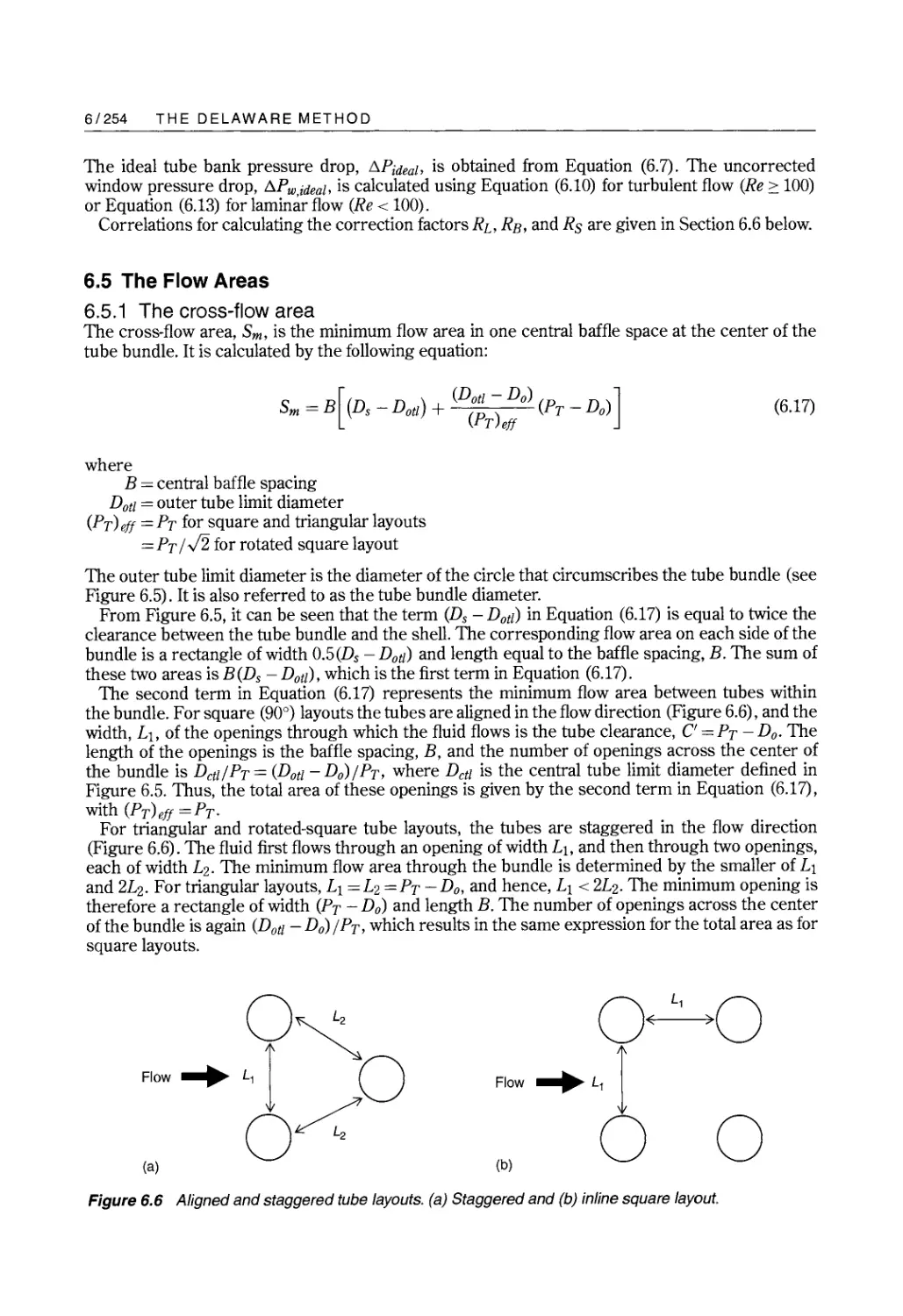
Figures 6.1-6.5 Copyright 1988 from Heat Exchanger Design Handbook by E. U. Schltinder, Editor-in-
Chief. Reproduced by permission of Taylor & Francis, a division of Informa pIc.
Table 6.1 Copyright 1988 from Heat Exchanger Design Handbook by E. U. Schltinder, Editor-in-
Chief. Reproduced by permission of Taylor & Francis, a division of Informa pIc.
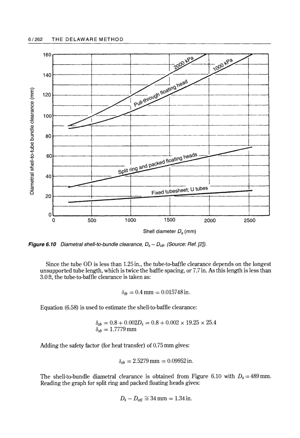
Figure 6.10 Copyright 1988 from Heat Exchanger Design Handbook by E. U. Schltinder, Editor-in-
Chief. Reproduced by permission of Taylor & Francis, a division of Informa pic.
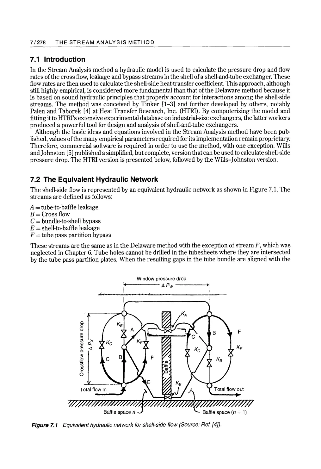
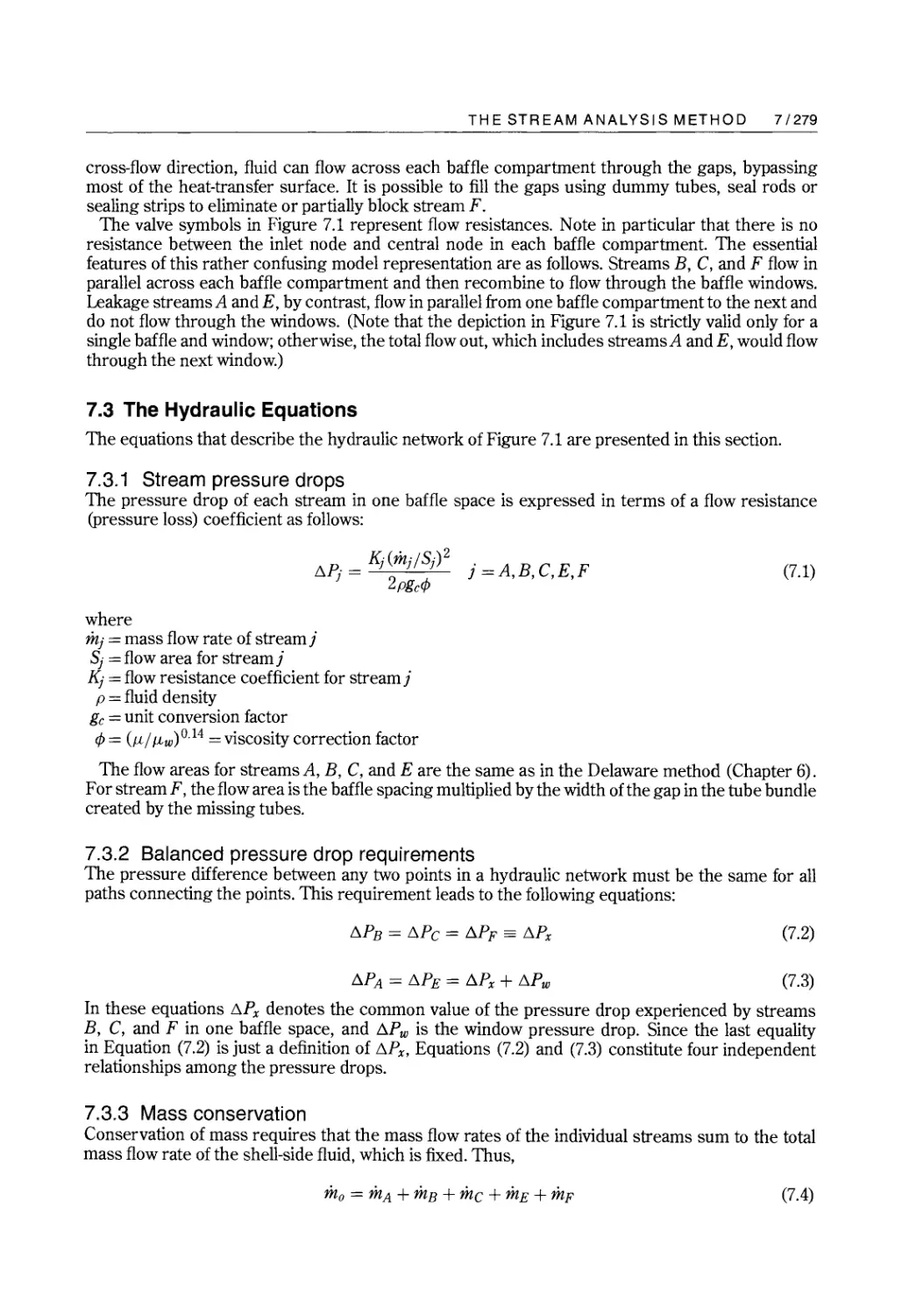
Figure 7.1 Reproduced, with permission, from]. W. Palen and]. Taborek, Solution of shell side flow
pressure drop and heat transfer by stream analysis method, Chem. Eng. Prog. Symposium
Series, 65, No. 92, 53-63, 1969. Copyright 1969 by AIChE.
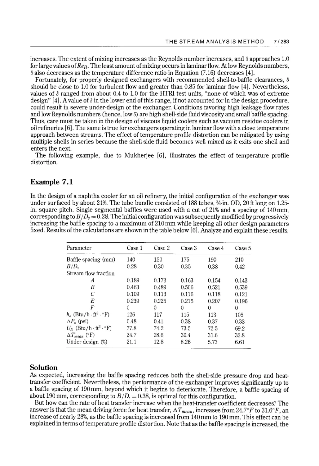
Table, p. 283 Reproduced, with permission, from R. Mukherjee, Effectively design shell-and-tube heat
exchangers, Chem. Eng. Prog., 94, No.2, 21-37,1998. Copyright 1998 by AIChE.
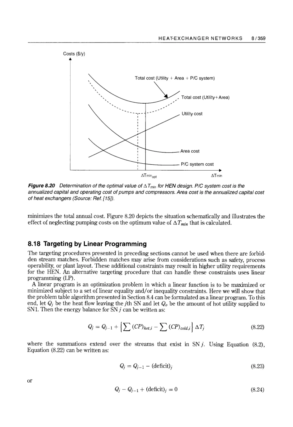
Figure 8.20 Reprinted from Computers and Chemical Engineering, Vol. 26, X. X. Zhu and X. R. Nie,
Pressure Drop Considerations for Heat Exchanger Network Grassroots Design, pp. 1661-
1676, Copyright 2002, with permission from Elsevier.
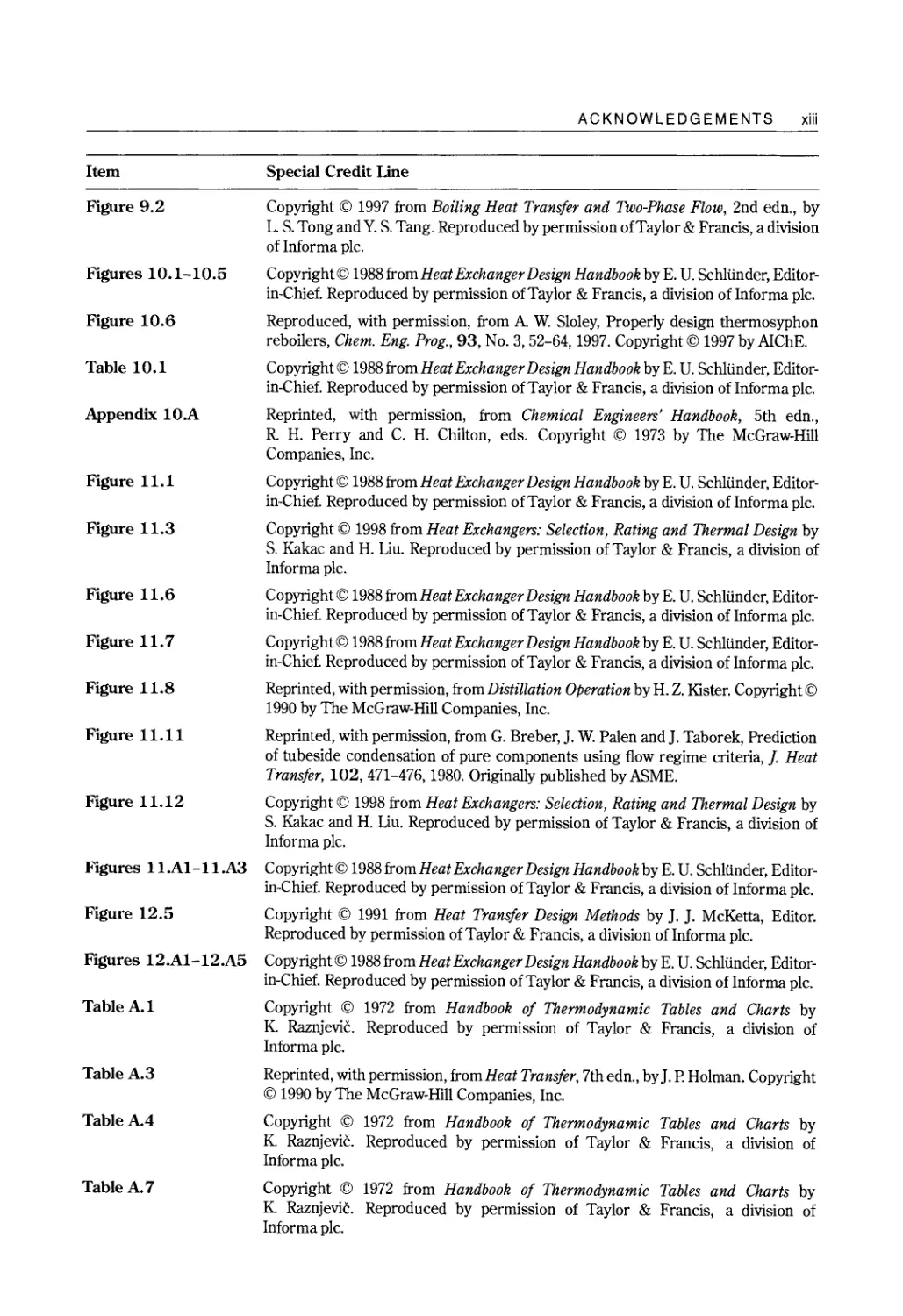
ACKNOWLEDGEMENTS xiii
Item Special Credit line
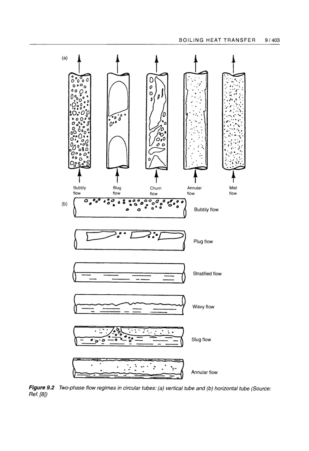
Figure 9.2 Copyright 1997 from Boiling Heat Transfer and Two-Phase Flow, 2nd edn., by
L. S. Tong and Y. S. Tang. Reproduced by permission of Taylor & Francis, a division
of Informa pic.
Figures 10.1-10.5 Copyright 1988 from Heat Exchanger Design Handbook by E. U. Schliinder, Editor-
in-Chief. Reproduced by permission of Taylor & Francis, a division of Informa pic.
Figure 10.6 Reproduced, with permission, from A W. Sloley, Properly design thermosyphon
reboilers, Chem. Eng. Prog., 93, No.3, 52-64,1997. Copyright 1997 by AIChE.
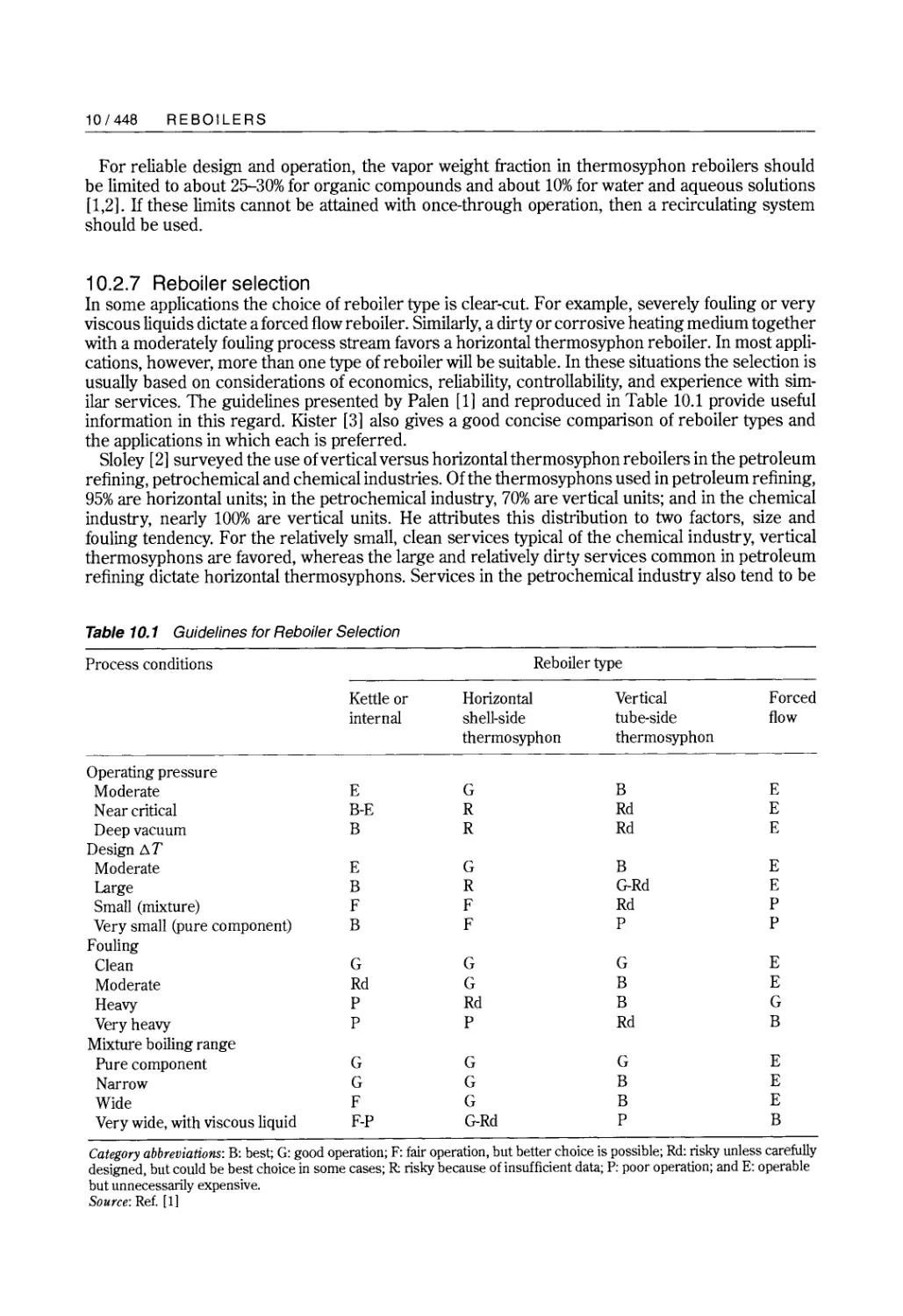
Table 10.1 Copyright 1988 from Heat Exchanger Design Handbook by E. U. Schliinder, Editor-
in-Chief. Reproduced by permission of Taylor & Francis, a division of Informa pIc.
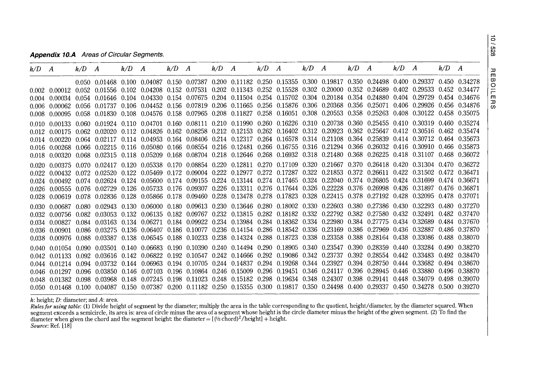
Appendix lOA Reprinted, with permission, from Chemical Engineers' Handbook, 5th edn.,
R. H. Perry and C. H. Chilton, eds. Copyright 1973 by The McGraw-Hill
Companies, Inc.
Figure 11.1 Copyright 1988 from Heat Exchanger Design Handbook by E. U. Schliinder, Editor-
in-Chief. Reproduced by permission of Taylor & Francis, a division of Informa pic.
Figure 11.3 Copyright 1998 from Heat Exchangers: Selection, Rating and Thermal Design by
S. Kakac and H. Liu. Reproduced by permission of Taylor & Francis, a division of
Informa pic.
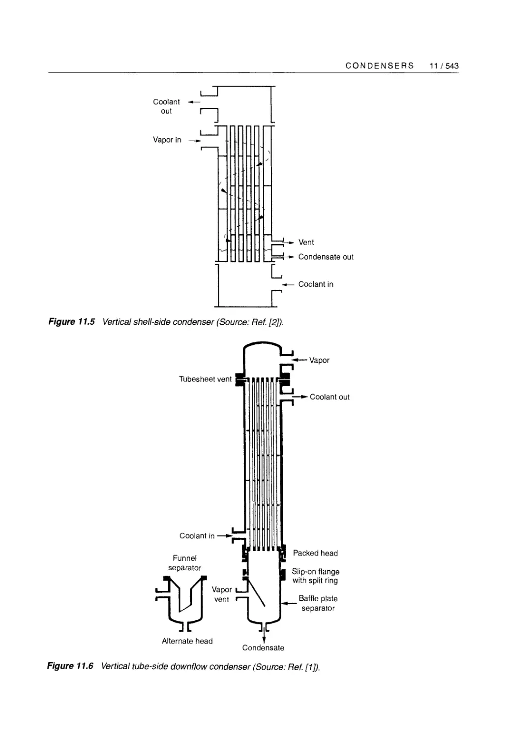
Figure 11.6 Copyright 1988 from Heat Exchanger Design Handbook by E. U. Schliinder, Editor-
in-Chief. Reproduced by permission of Taylor & Francis, a division of Informa pic.
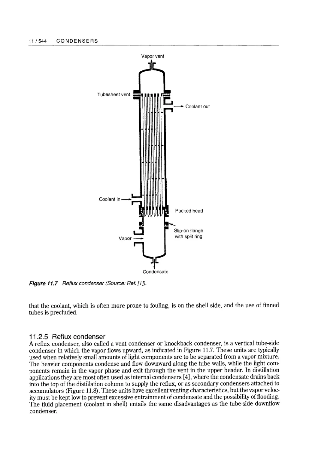
Figure 11.7 Copyright 1988 from Heat Exchanger Design Handbook by E. U. Schliinder, Editor-
in-Chief. Reproduced by permission of Taylor & Francis, a division of Informa pic.
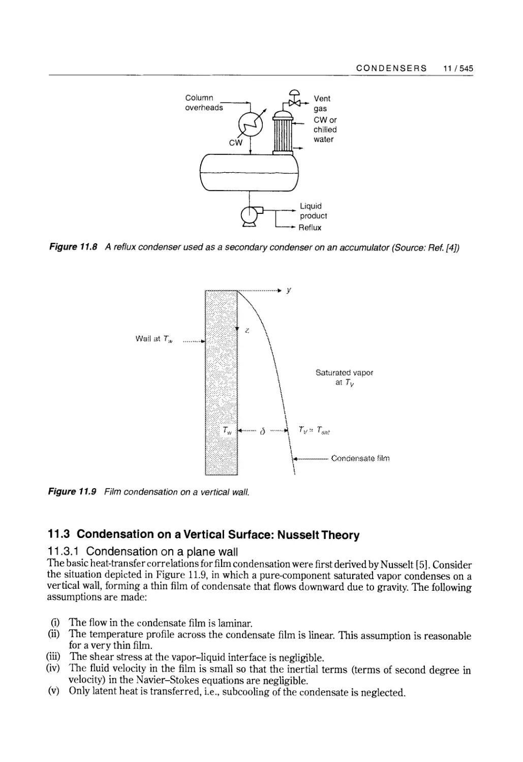
Figure 11.8 Reprinted, with permission, from Distillation Operation by H. Z. Kister. Copyright
1990 by The McGraw-Hill Companies, Inc.
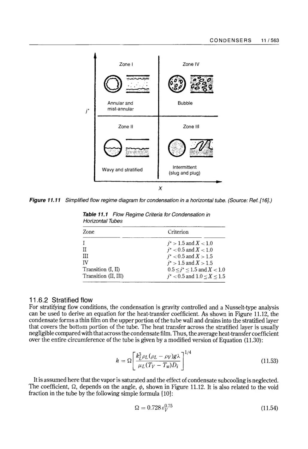
Figure 11.11 Reprinted, with permission, from G. Breber, ]. W. Palen and]. Taborek, Prediction
of tubeside condensation of pure components using flow regime criteria,]. Heat
Transfer, 102,471-476,1980. Originally published by ASME.
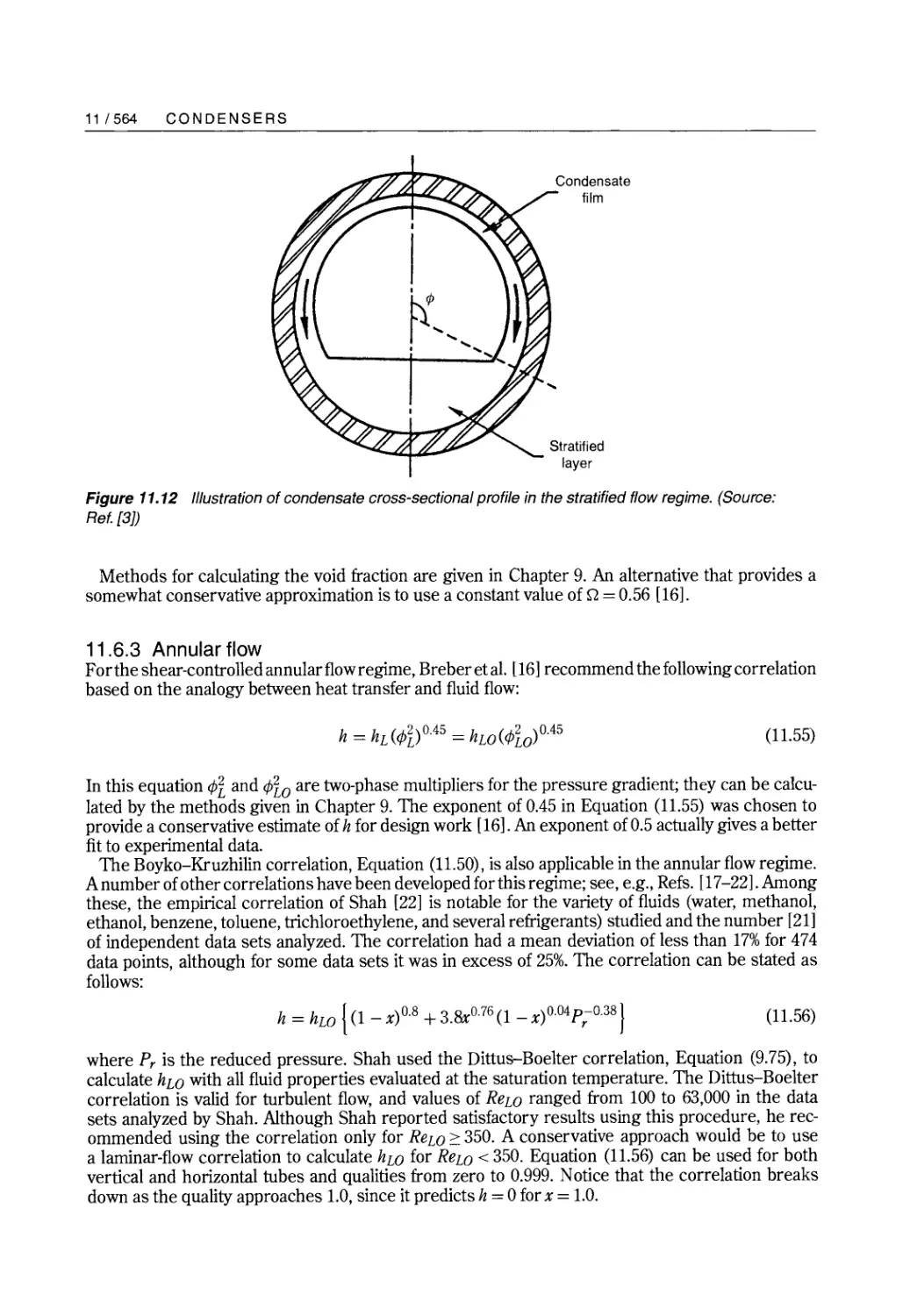
Figure 11.12 Copyright 1998 from Heat Exchangers: Selection, Rating and Thermal Design by
S. Kakac and H. Liu. Reproduced by permission of Taylor & Francis, a division of
Informa pic.
Figures 11.A1-11.A3 Copyright 1988 from Heat Exchanger Design Handbook by E. U. Schliinder, Editor-
in-Chief. Reproduced by permission of Taylor & Francis, a division of Informa pic.
Figure 12.5 Copyright 1991 from Heat Transfer Design Methods by ]. ]. McKetta, Editor.
Reprod uced by permission of Taylor & Francis, a division of Informa pic.
Figures 12.Al-12.A5 Copyright 1988 from Heat Exchanger Design Handbook by E. U. Schliinder, Editor-
in-Chief. Reproduced by permission of Taylor & Francis, a division of Informa pic.
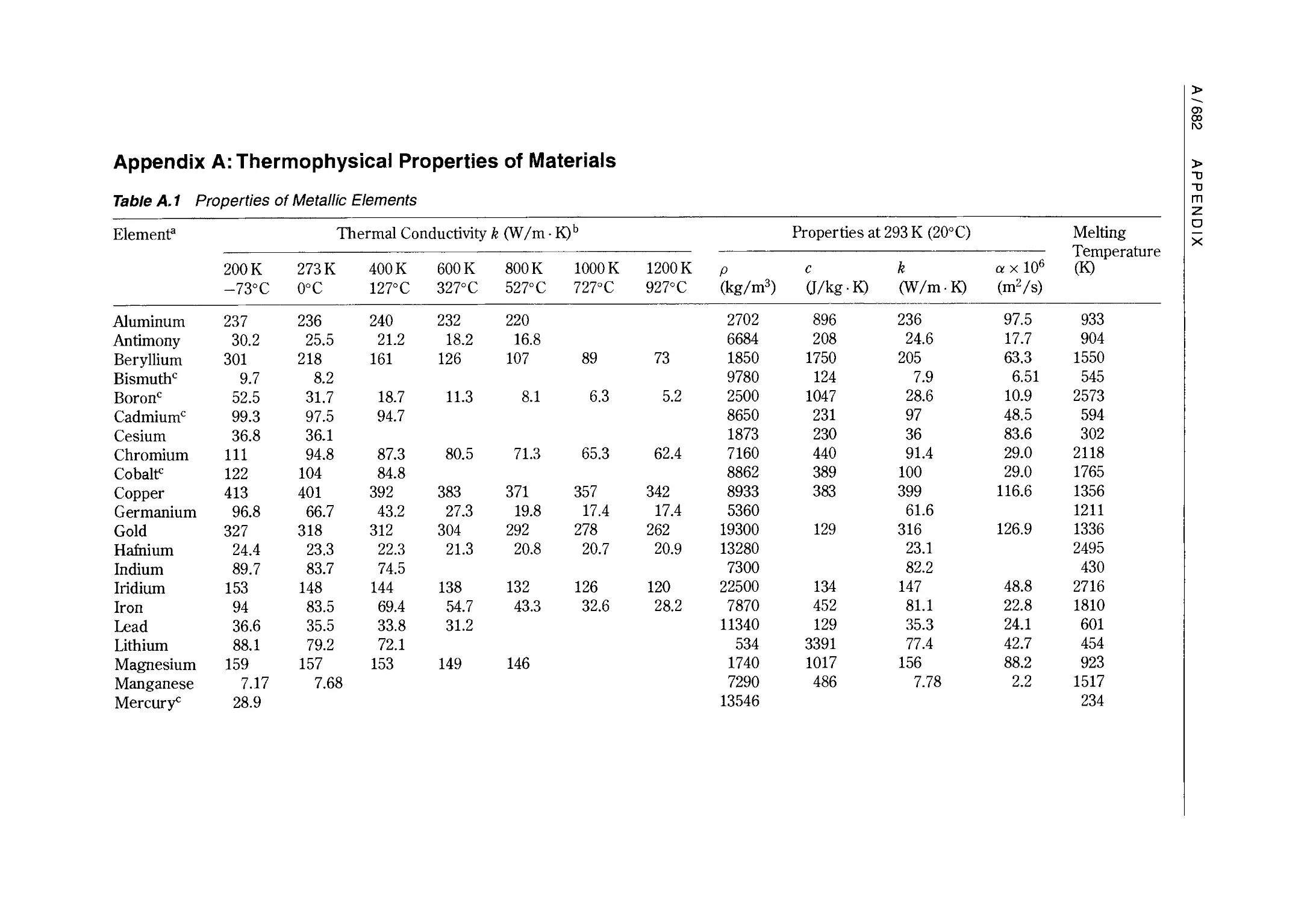
Table A.1 Copyright 1972 from Handbook of Thermodynamic Tables and Charts by
K Raznjevic. Reproduced by permission of Taylor & Francis, a division of
Informa pic.
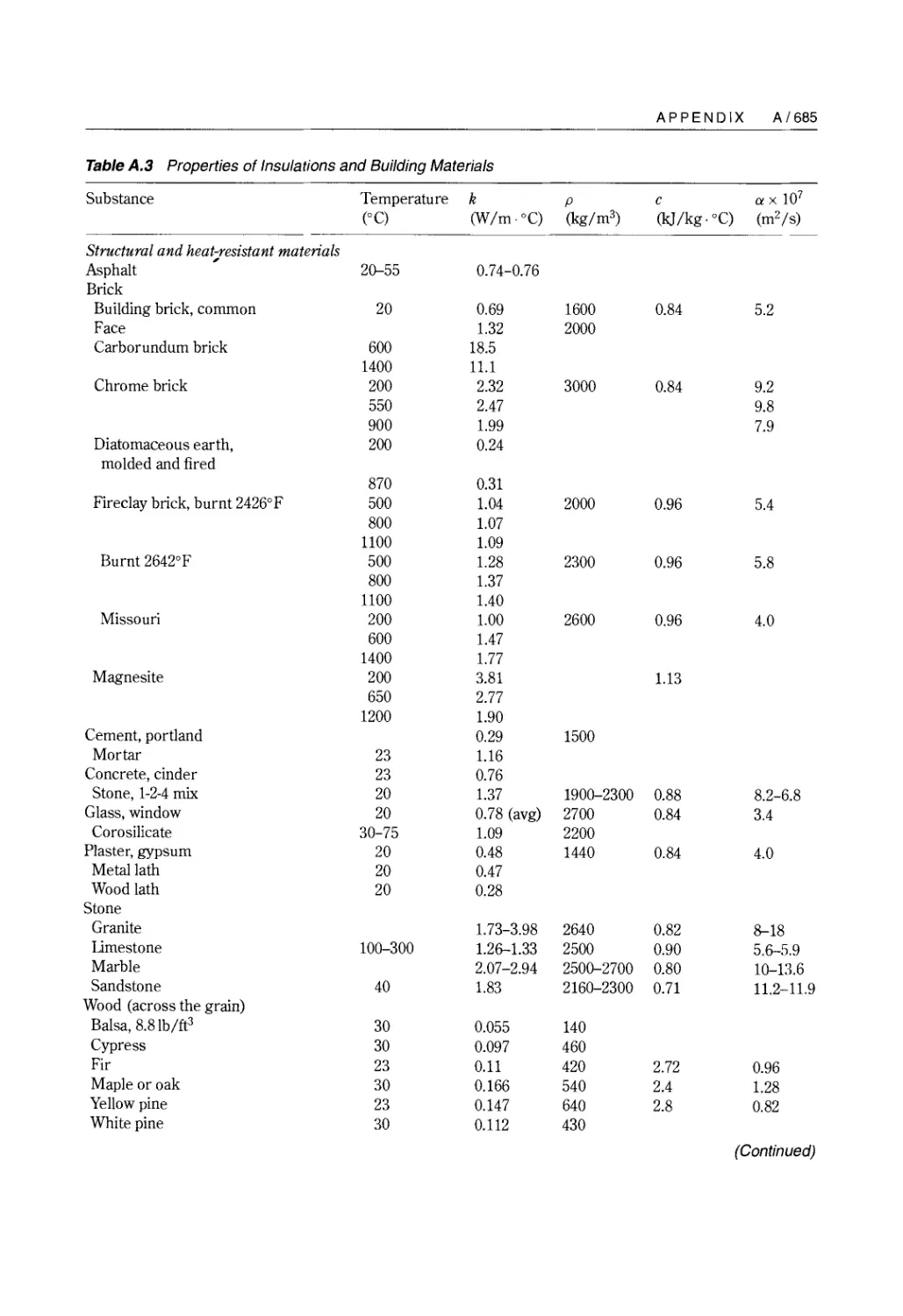
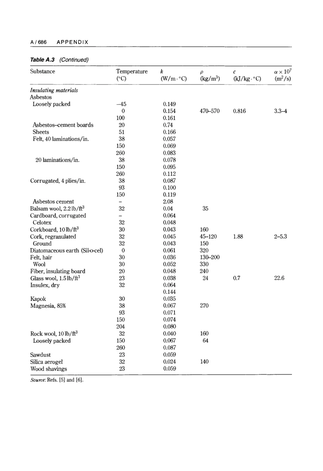
Table A.3 Reprinted, with permission, from Heat Transfer, 7th edn., by]. P. Holman. Copyright
1990 by The McGraw-Hill Companies, Inc.
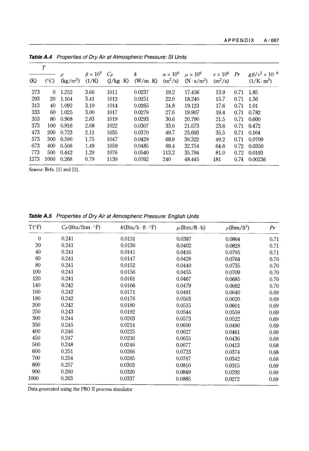
Table AA Copyright 1972 from Handbook of Thermodynamic Tables and Charts by
K. Raznjevic. Reproduced by permission of Taylor & Francis, a division of
Informa pIc.
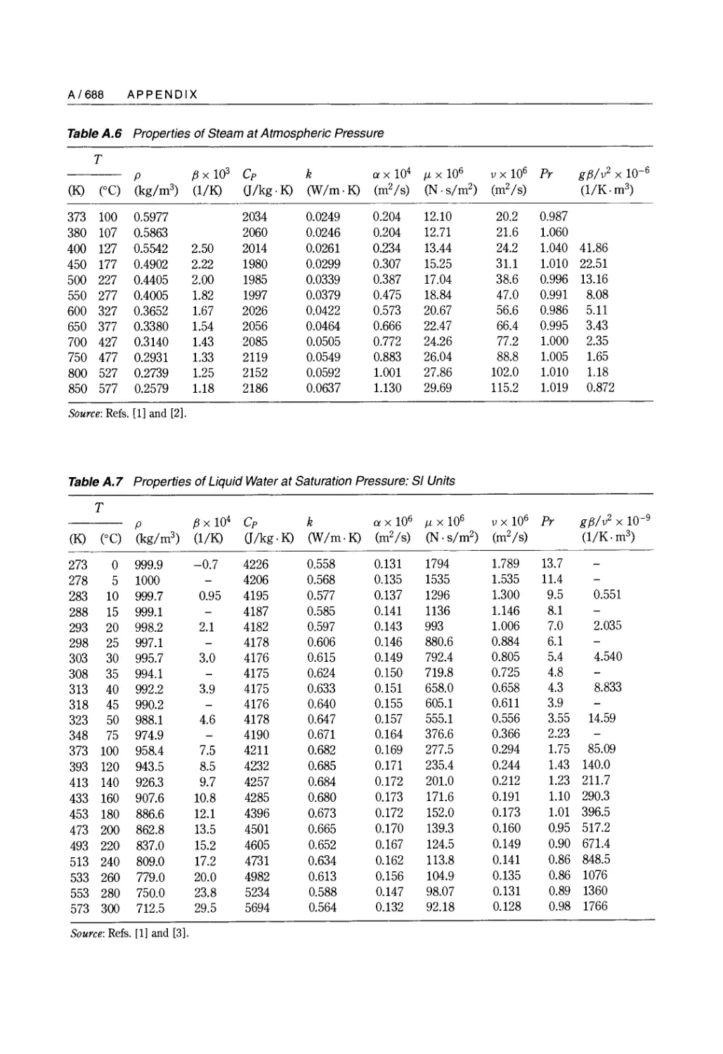
Table A.7 Copyright 1972 from Handbook of Thermodynamic Tables and Charts by
K Raznjevic. Reproduced by permission of Taylor & Francis, a division of
Informa pic.
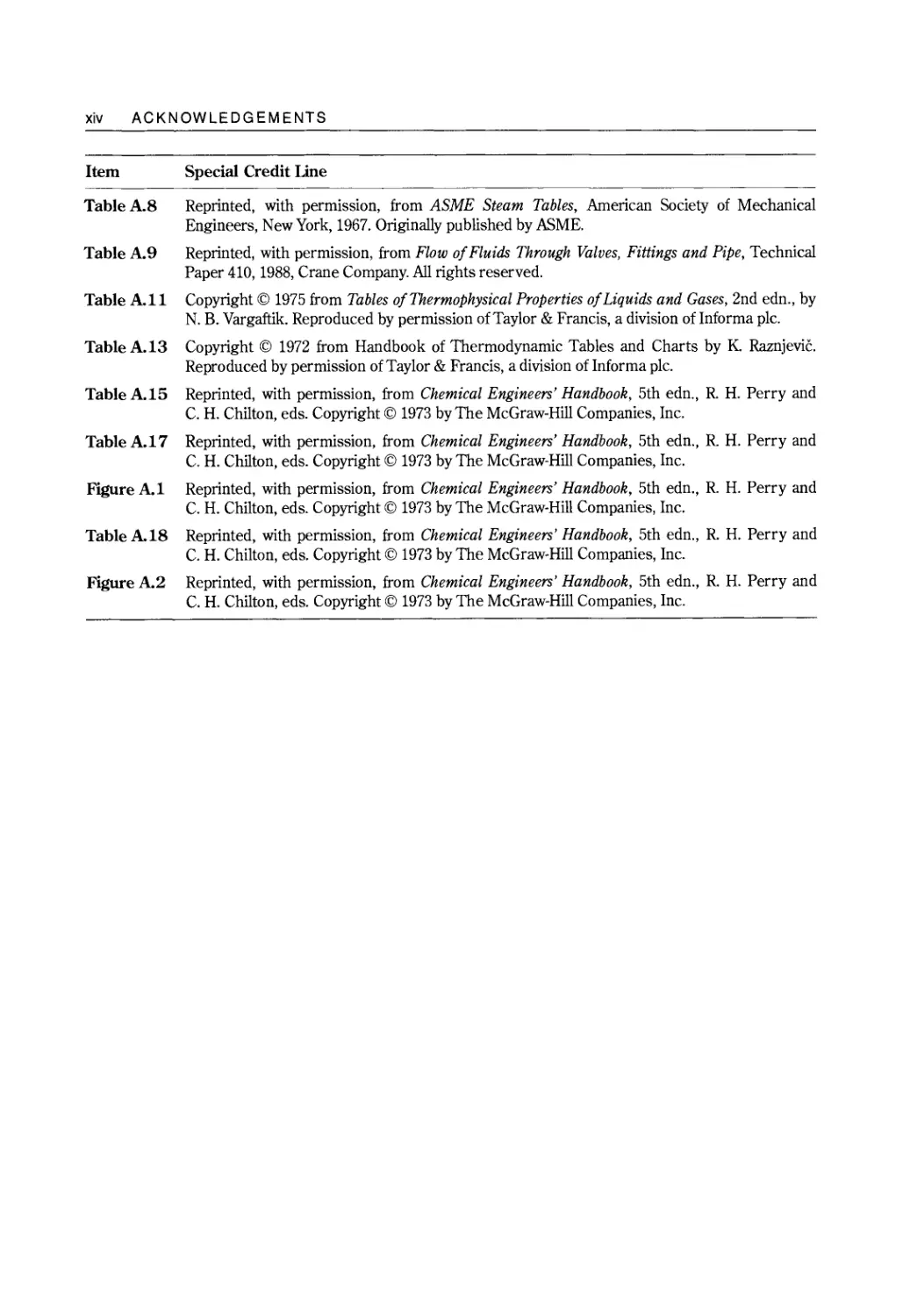
v ACKNOWLEDGEMENTS
Item Special Credit line
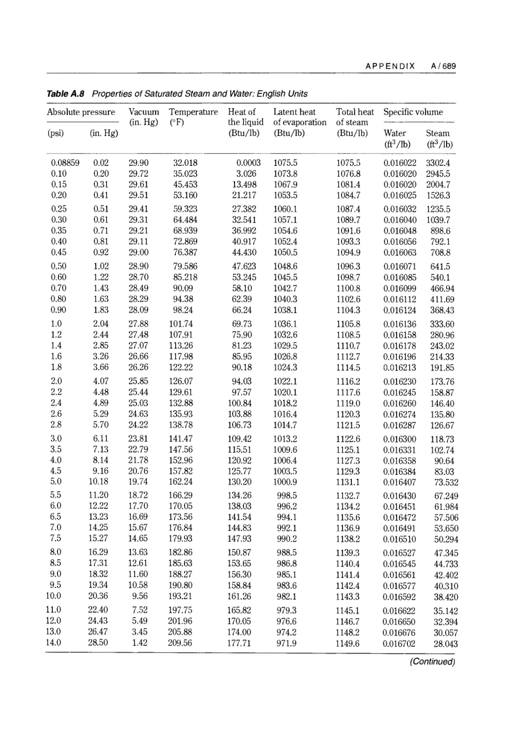
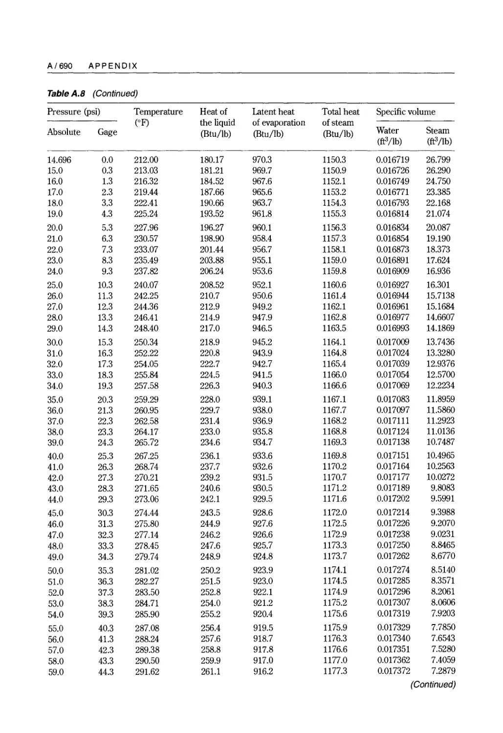
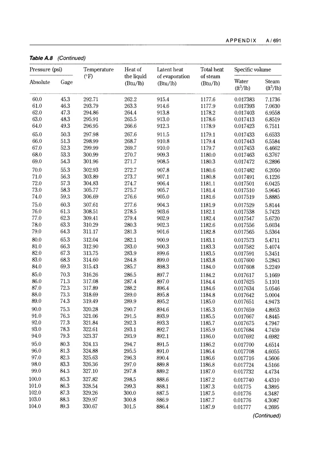
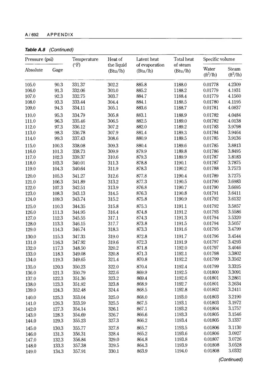
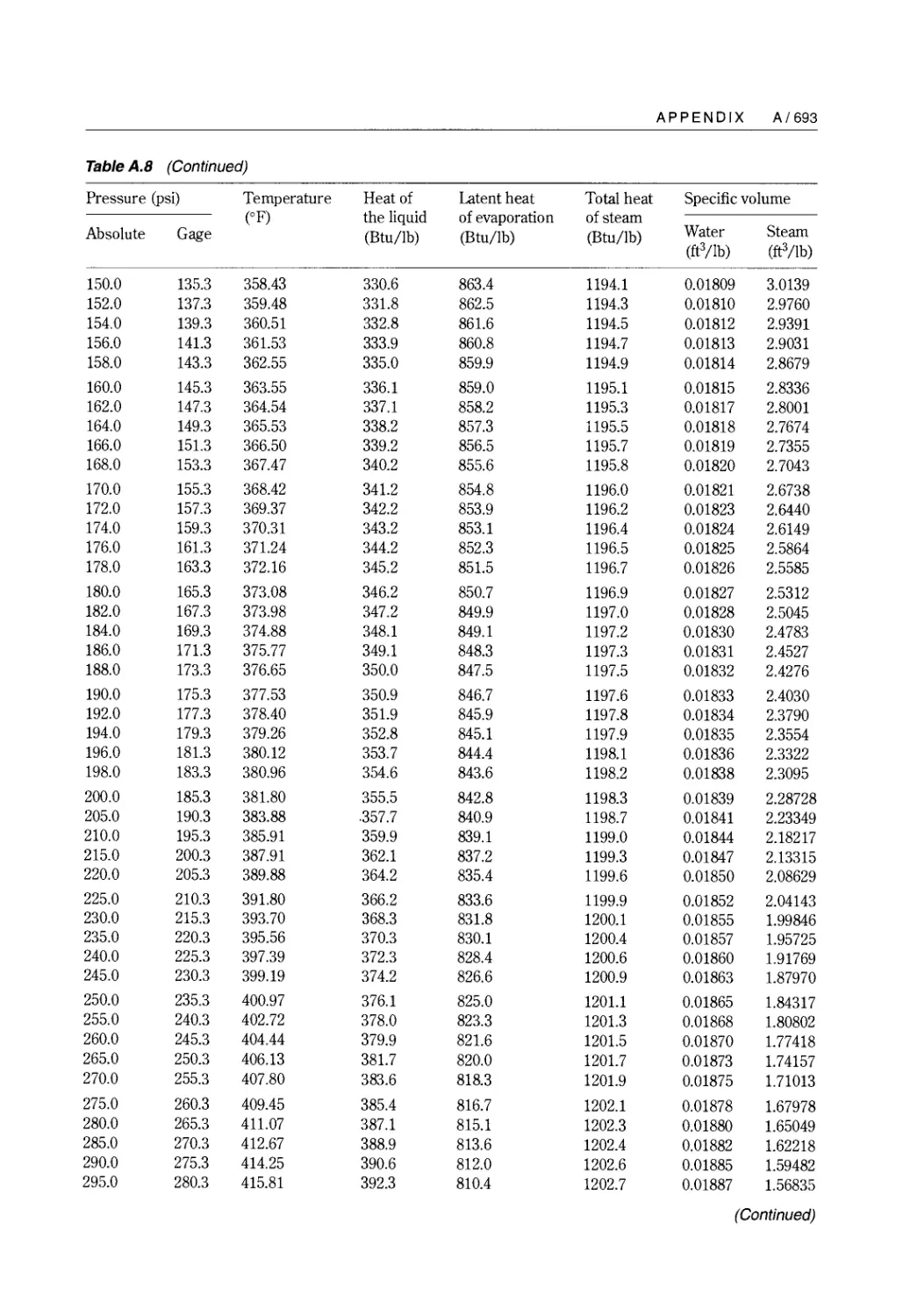
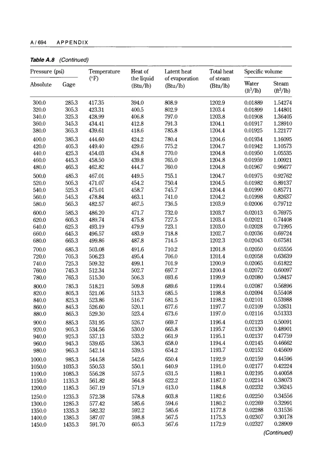
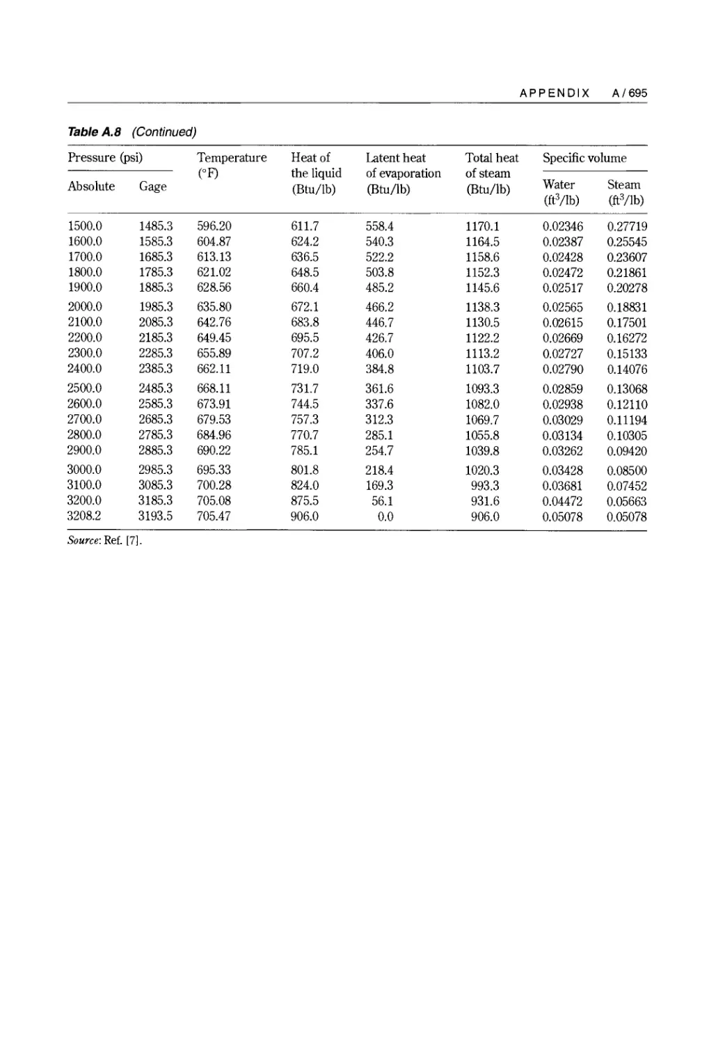
Table A.8 Reprinted, with permission, from ASME Steam Tables, American Society of Mechanical
Engineers, New York, 1967. Originally published by ASME.
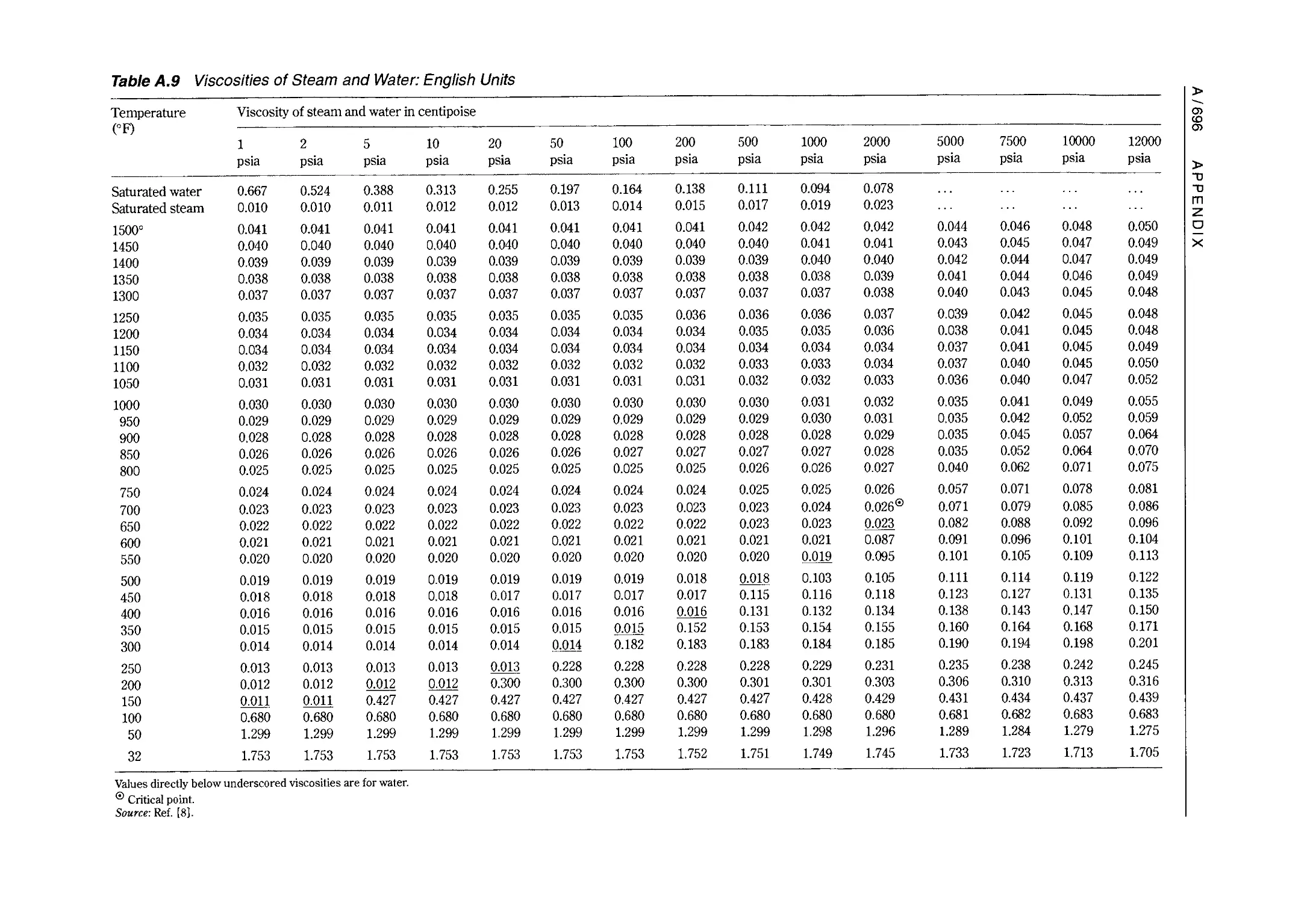
Table A.9 Reprinted, with permission, from Flow of Fluids Through Valves, Fittings and Pipe, Technical
Paper 410,1988, Crane Company. All rights reserved.
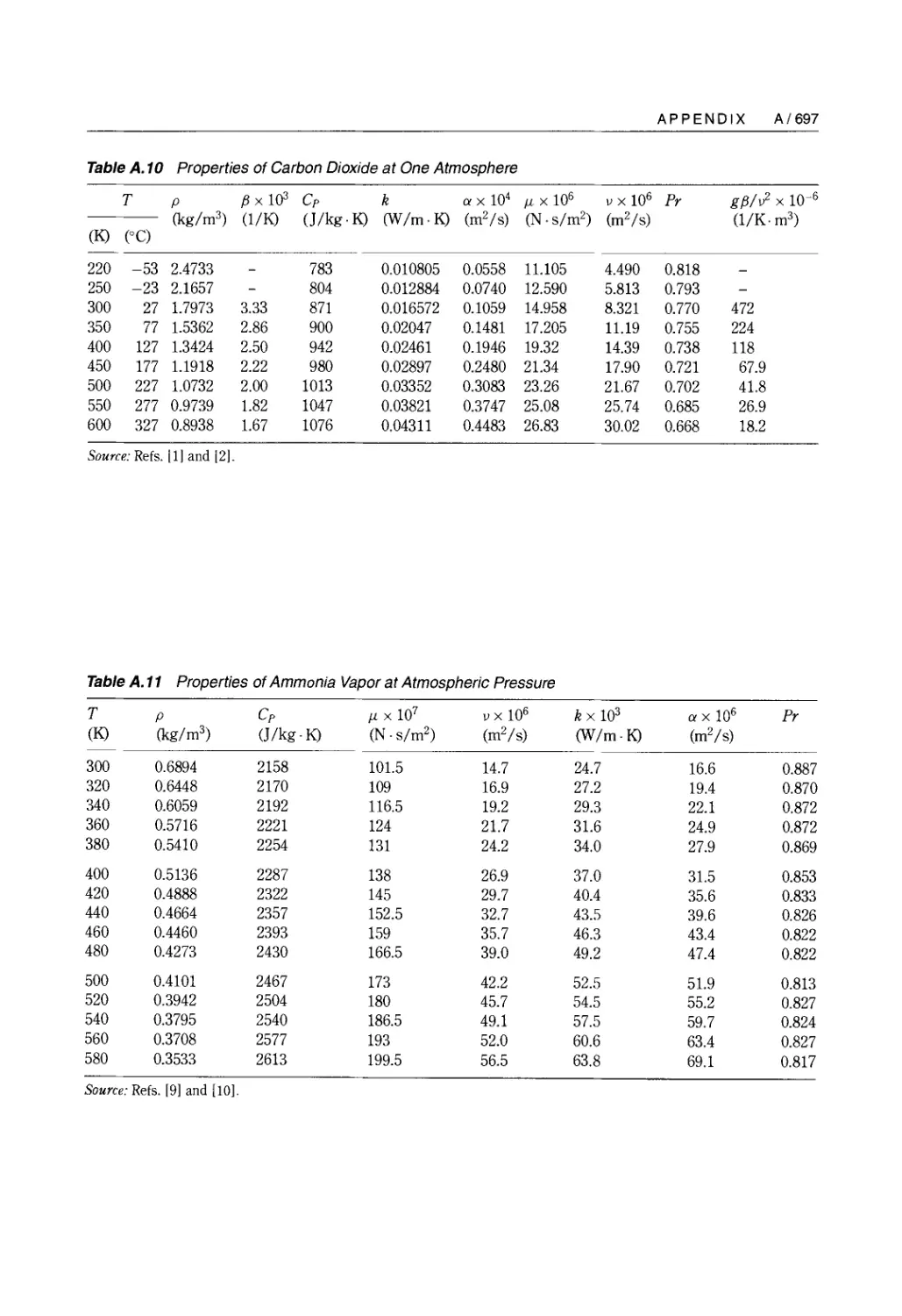
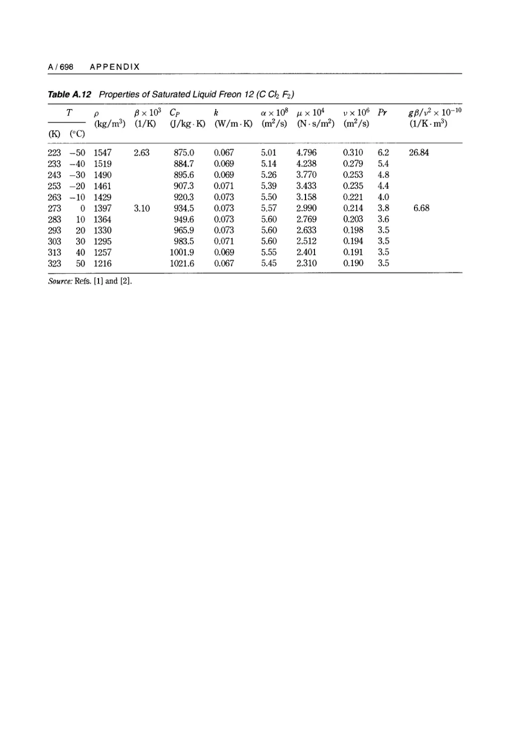
Table A.ll Copyright 1975 from Tables of ThermoPhysical Properties of Liquids and Gases, 2nd edn., by
N. B. Vargaftik. Reproduced by permission of Taylor & Francis, a division of Informa pic.
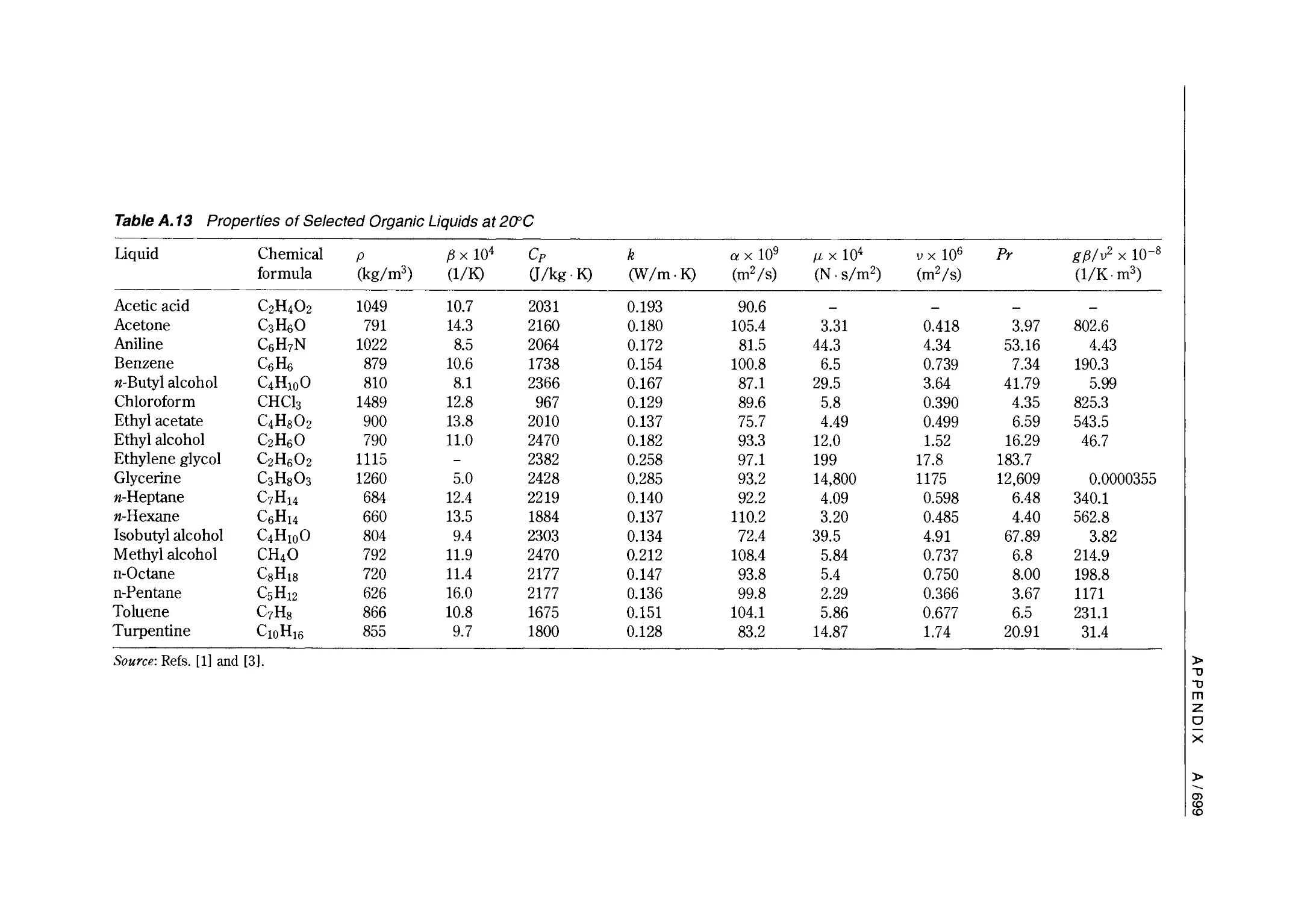
Table A.13 Copyright 1972 from Handbook of Thermodynamic Tables and Charts by K Raznjevic.
Reproduced by permission of Taylor & Francis, a division of Informa pic.
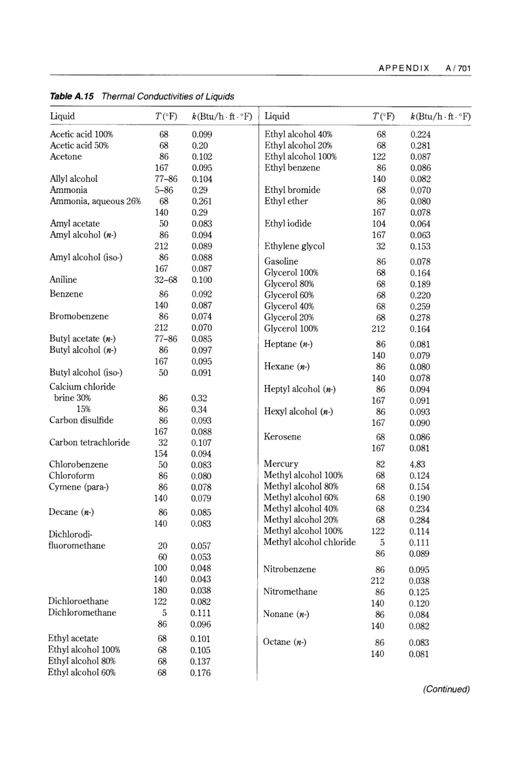
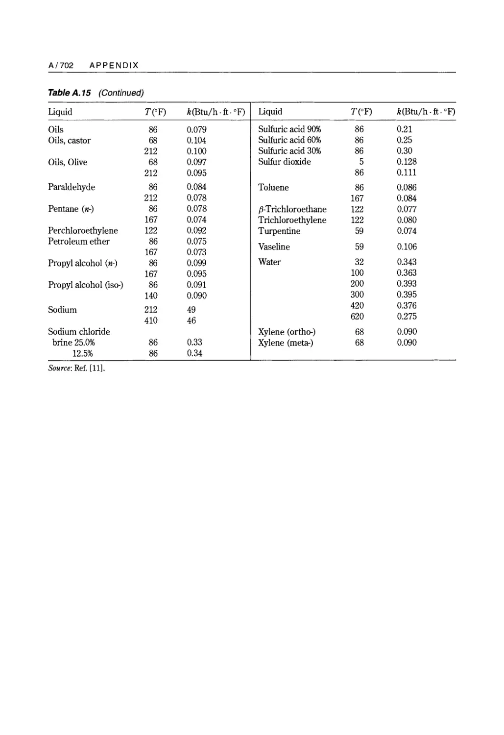
Table A.15 Reprinted, with permission, from Chemical Engineers' Handbook, 5th edn., R. H. Perry and
C. H. Chilton, eds. Copyright 1973 by The McGraw-Hill Companies, Inc.
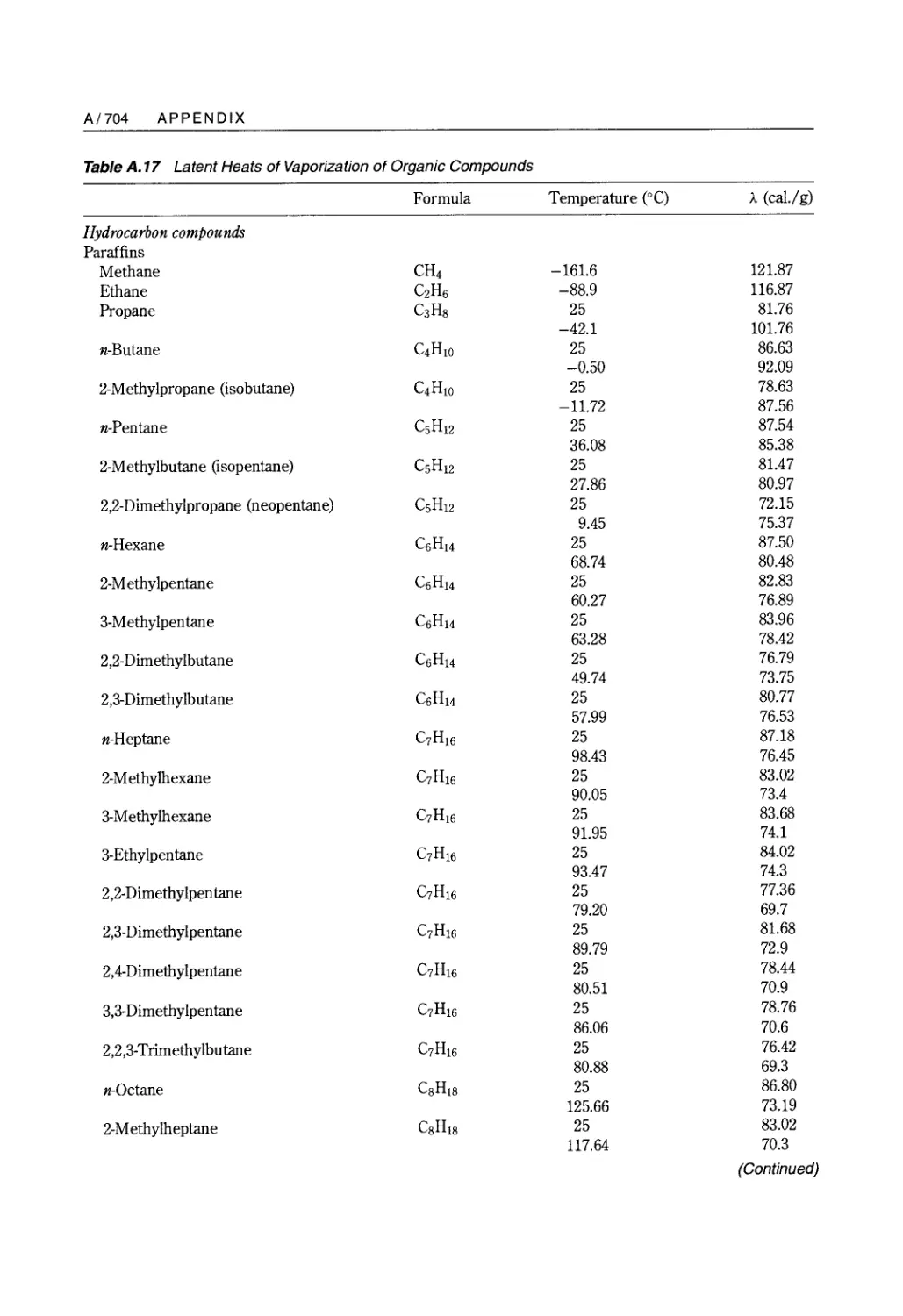
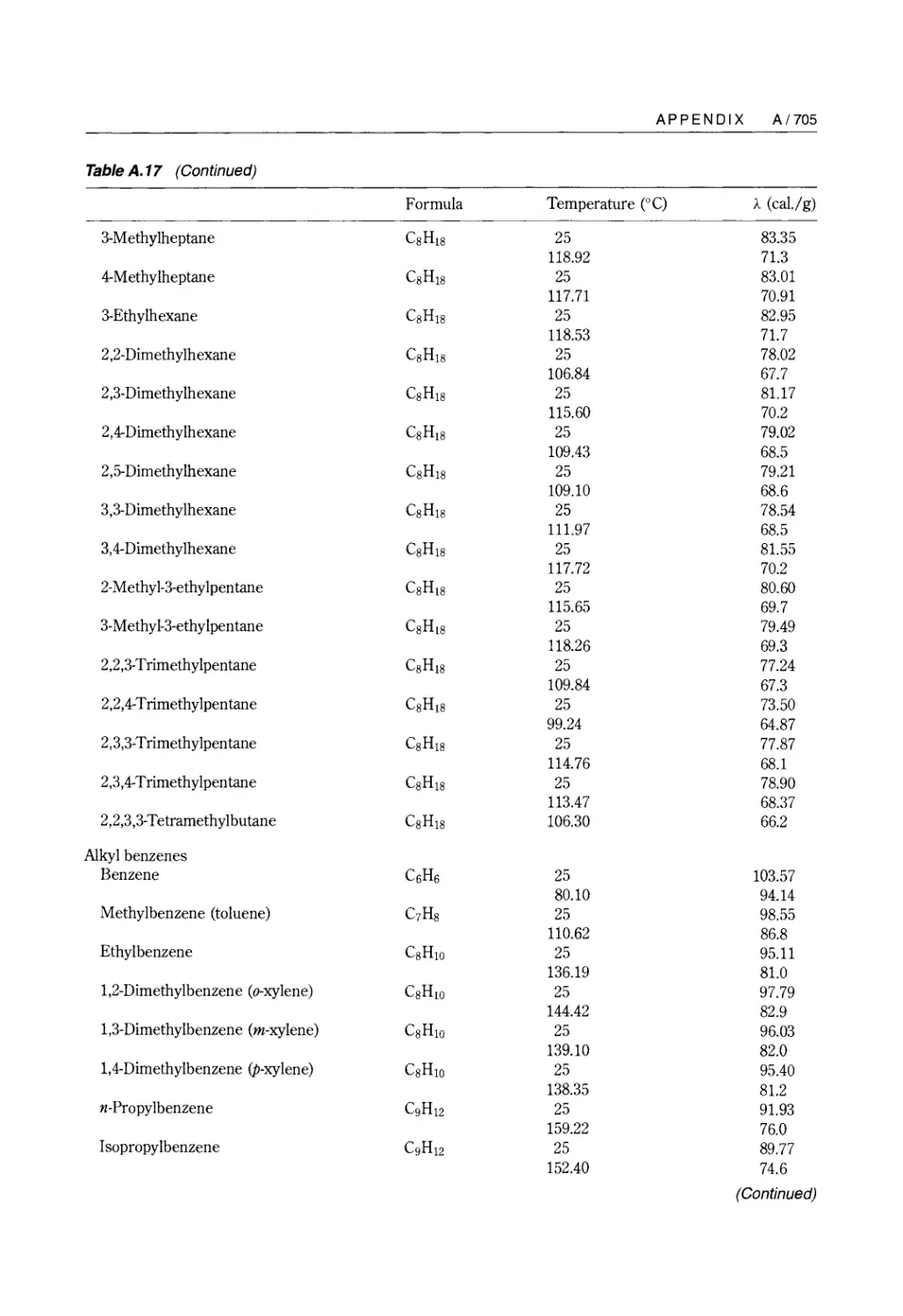
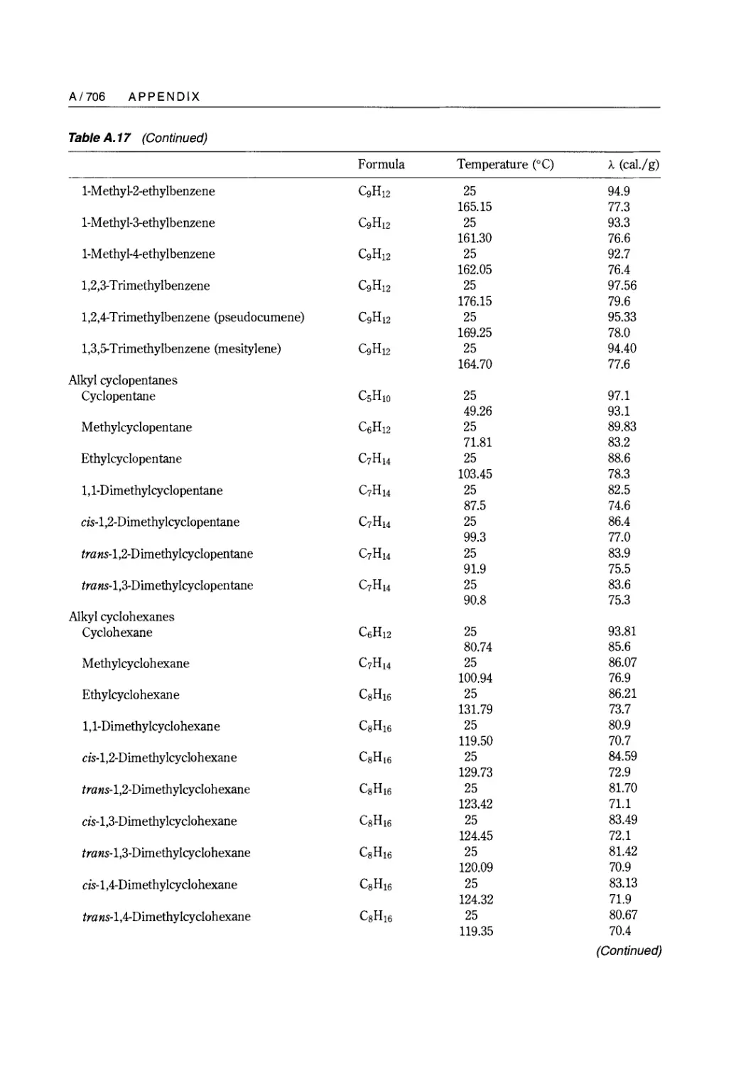
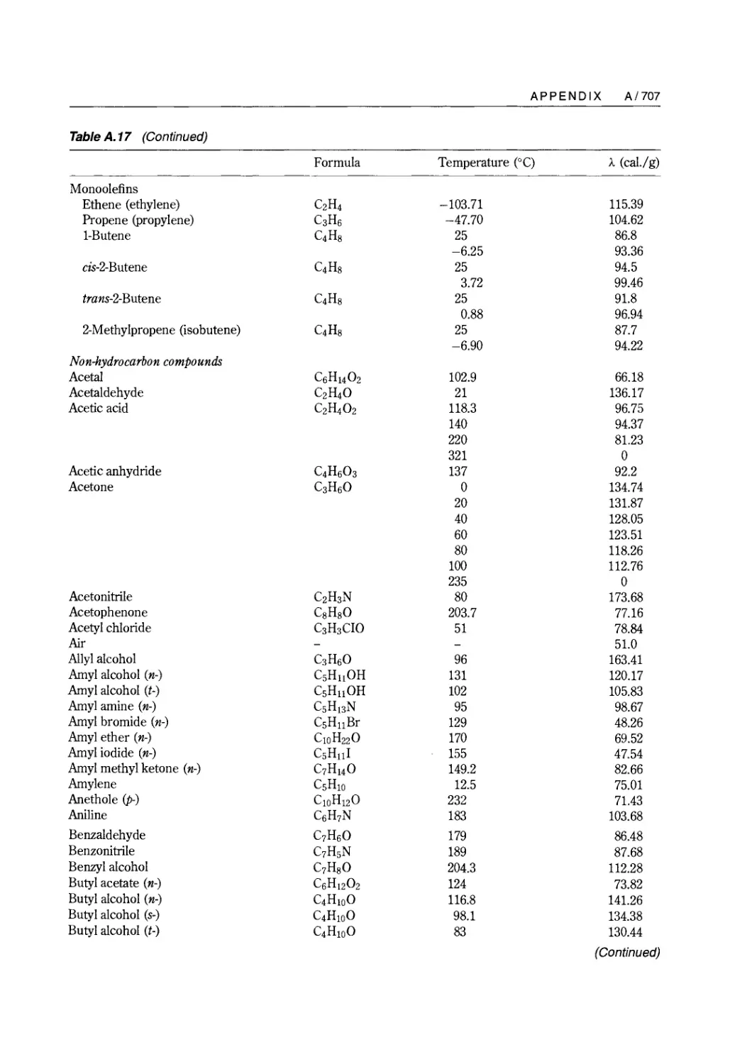
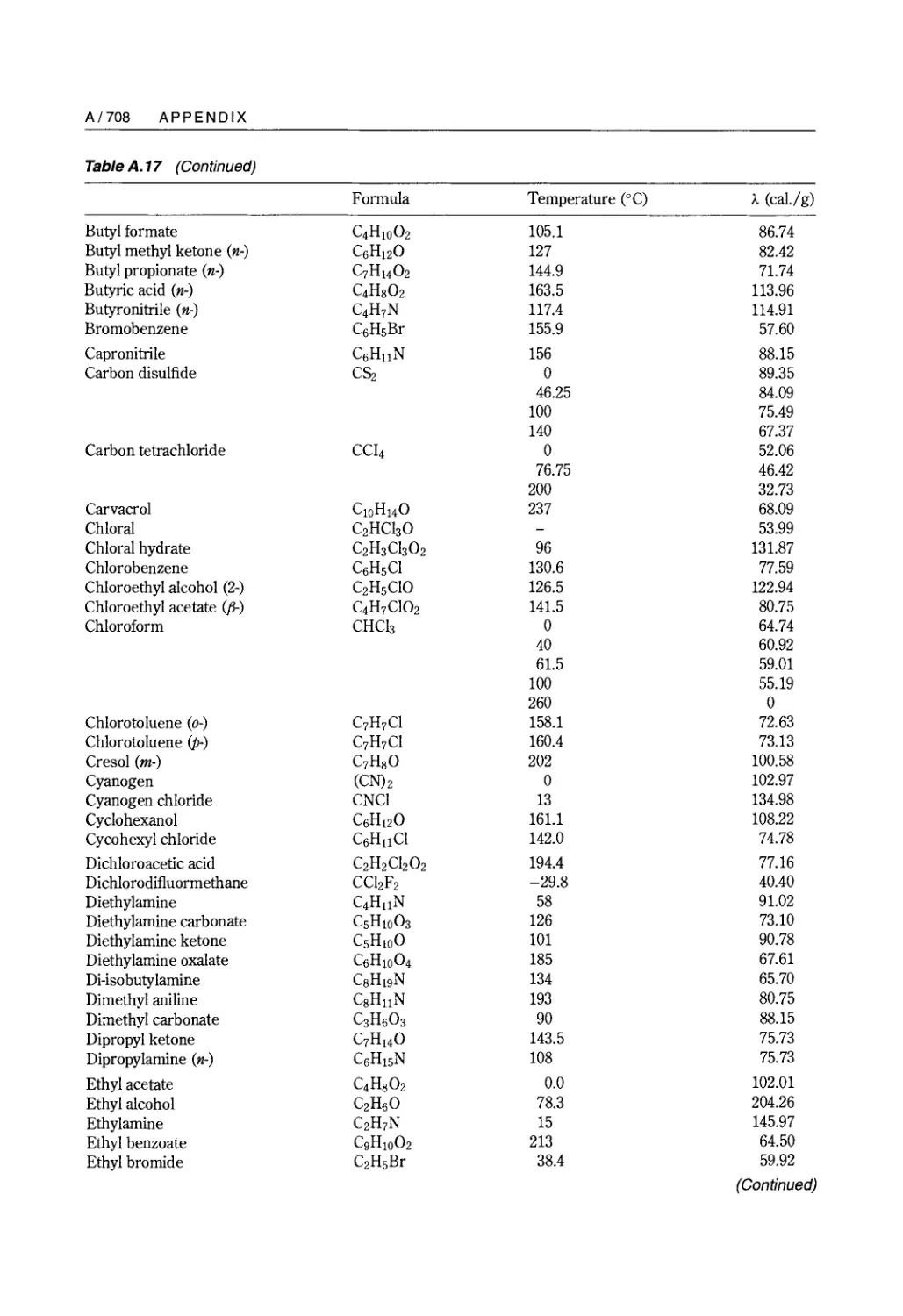
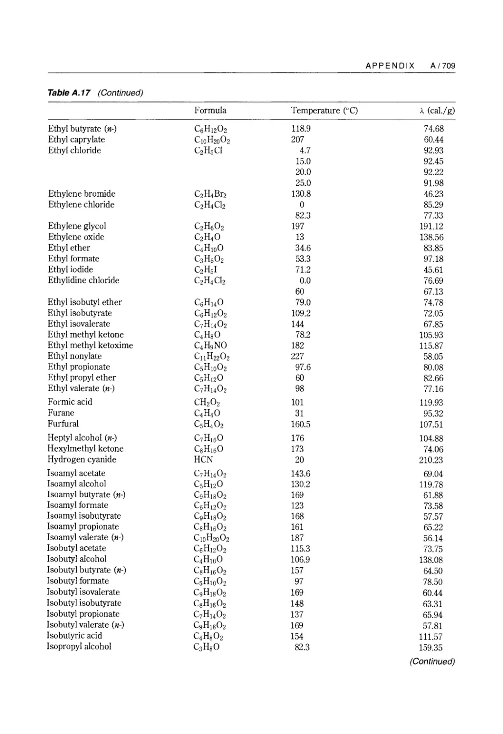
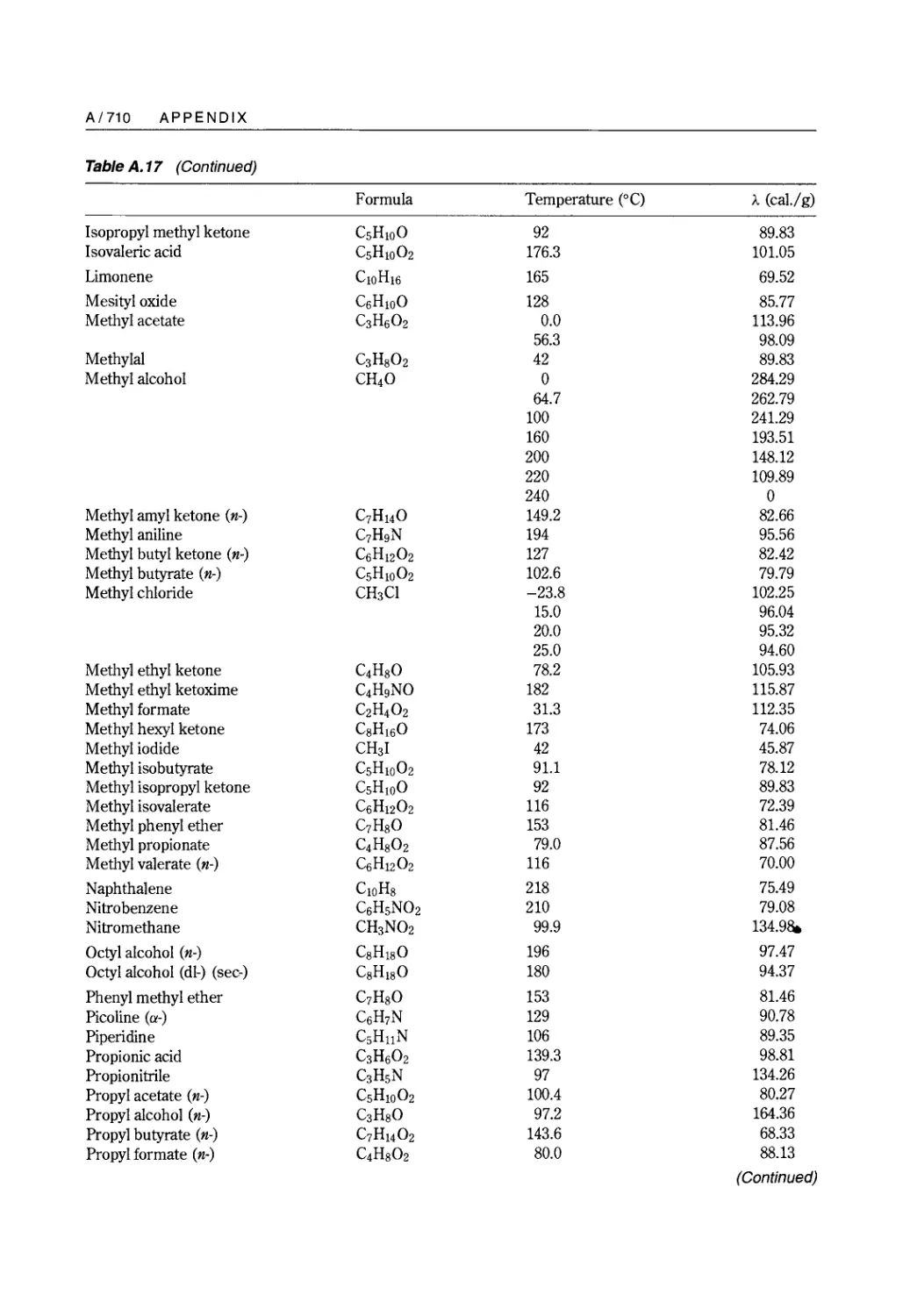
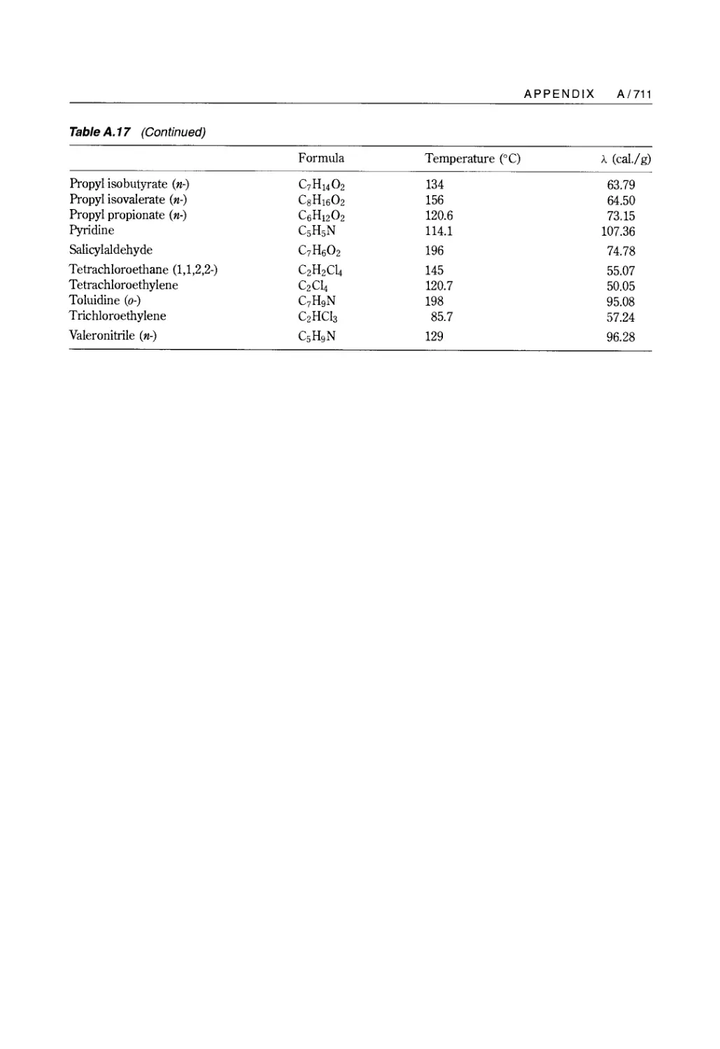
Table A.17 Reprinted, with permission, from Chemical Engineers' Handbook, 5th edn., R. H. Perry and
C. H. Chilton, eds. Copyright 1973 by The McGraw-Hill Companies, Inc.
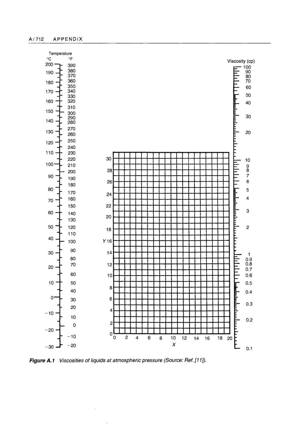
Figure A.1 Reprinted, with permission, from Chemical Engineers' Handbook, 5th edn., R. H. Perry and
C. H. Chilton, eds. Copyright 1973 by The McGraw-Hill Companies, Inc.
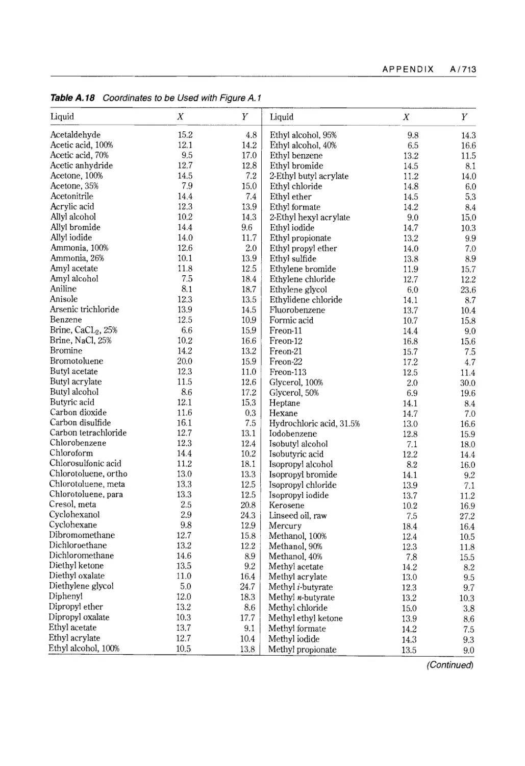
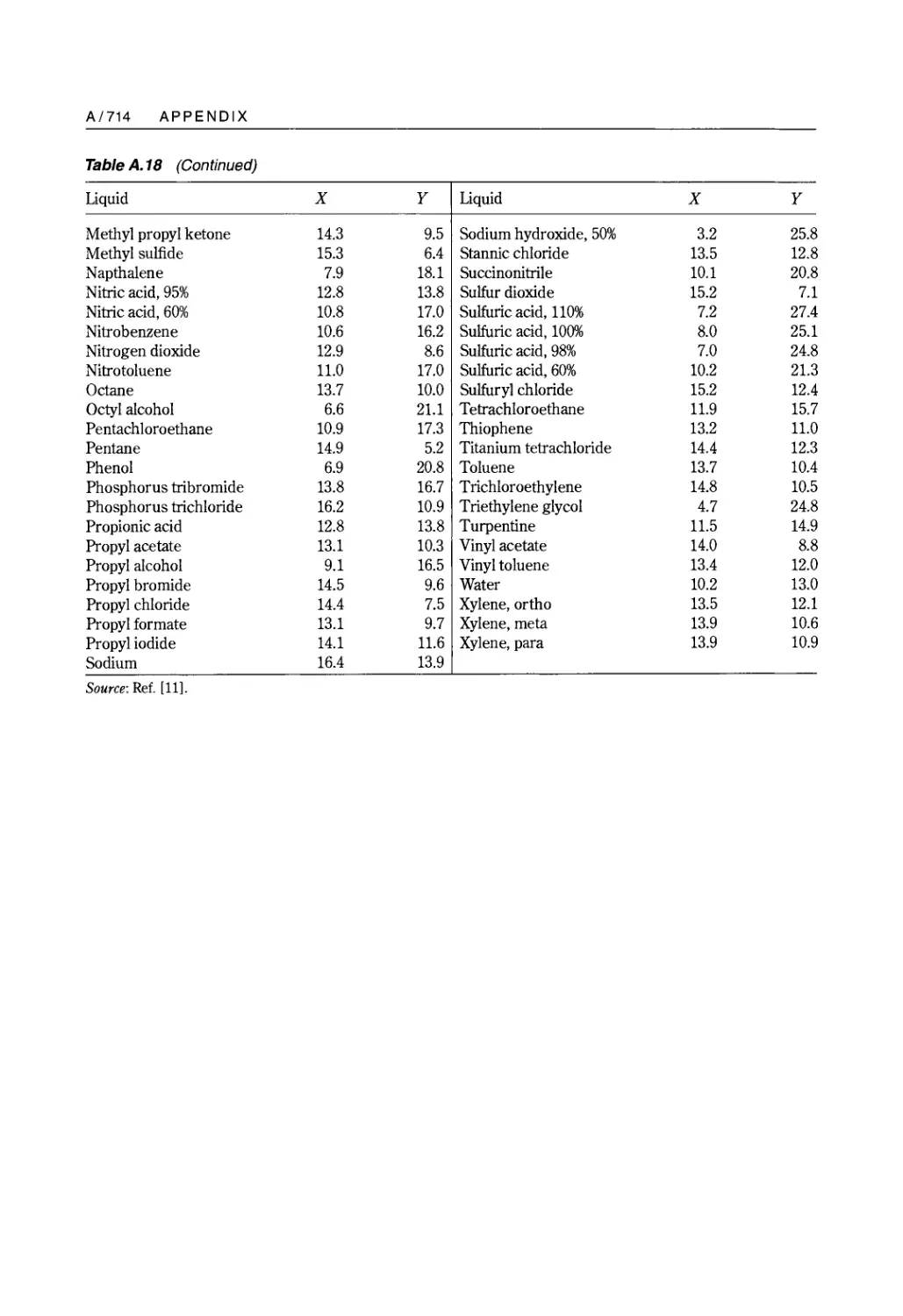
Table A.18 Reprinted, with permission, from Chemical Engineers' Handbook, 5th edn., R. H. Perry and
C. H. Chilton, eds. Copyright 1973 by The McGraw-Hill Companies, Inc.
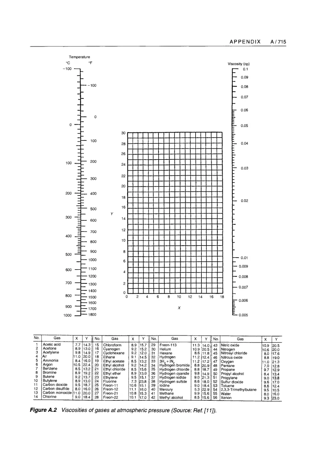
Figure A.2 Reprinted, with permission, from Chemical Engineers' Handbook, 5th edn., R. H. Perry and
C. H. Chilton, eds. Copyright 1973 by The McGraw-Hill Companies, Inc.
Table of Contents
1. Heat Conduction
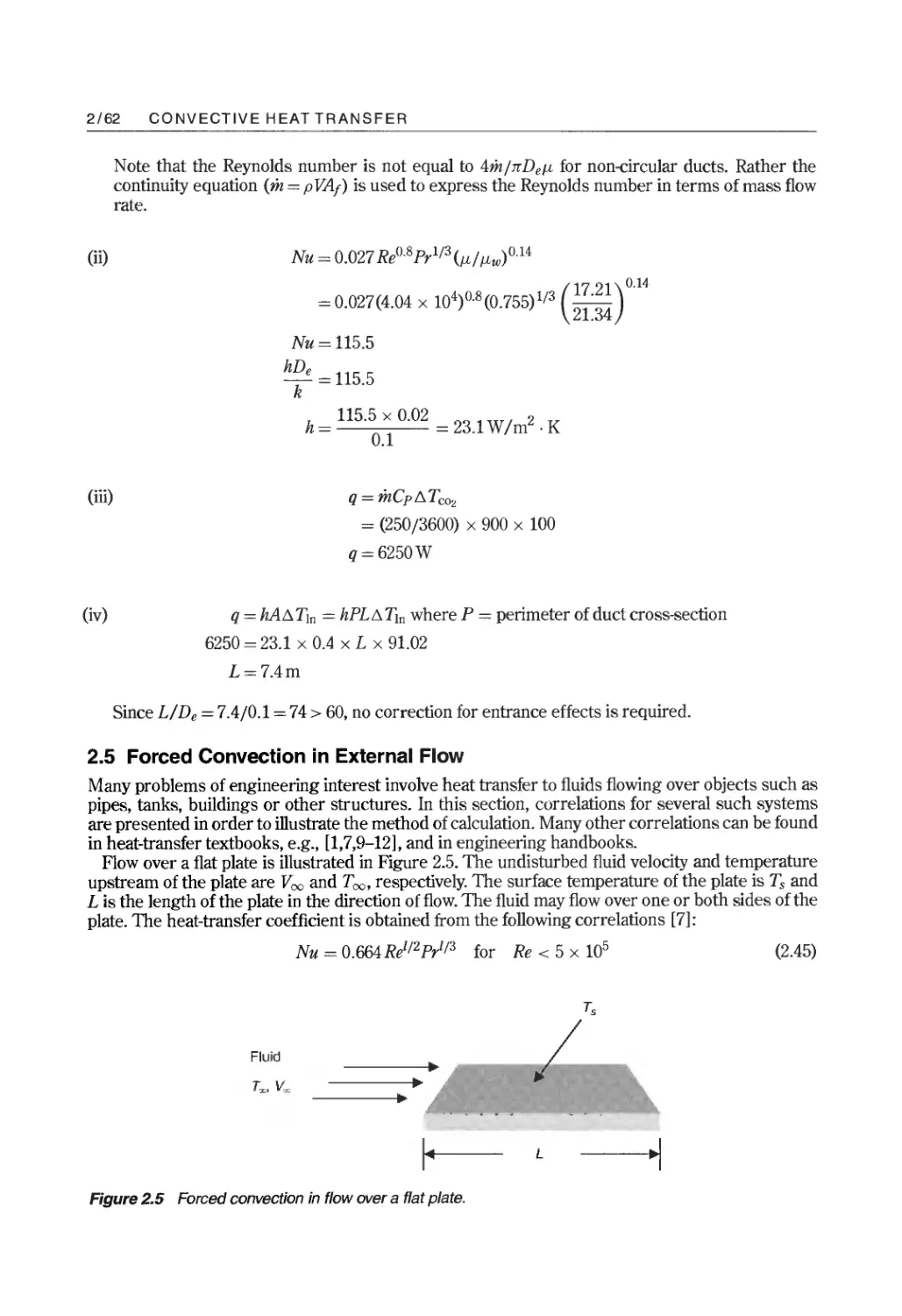
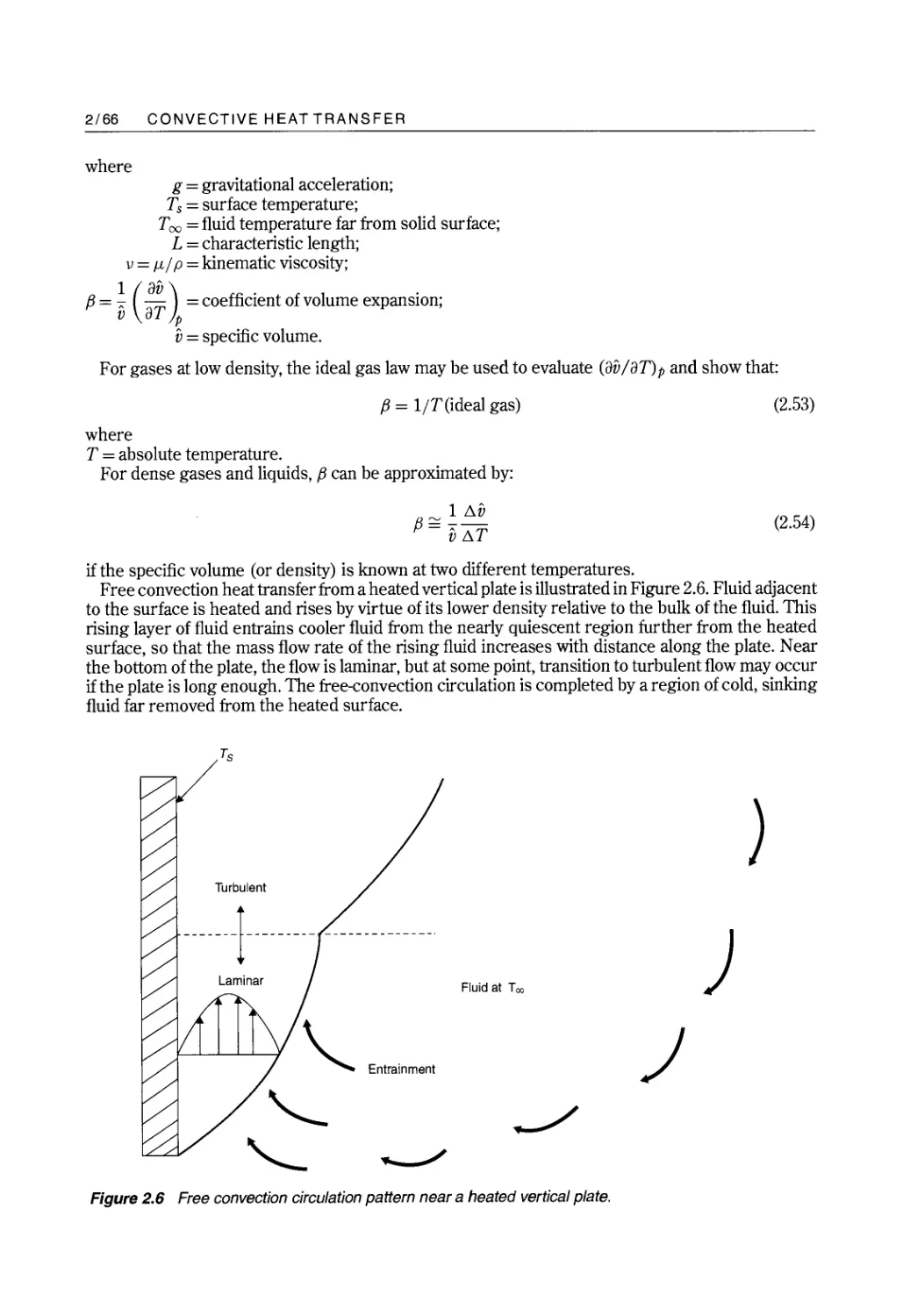
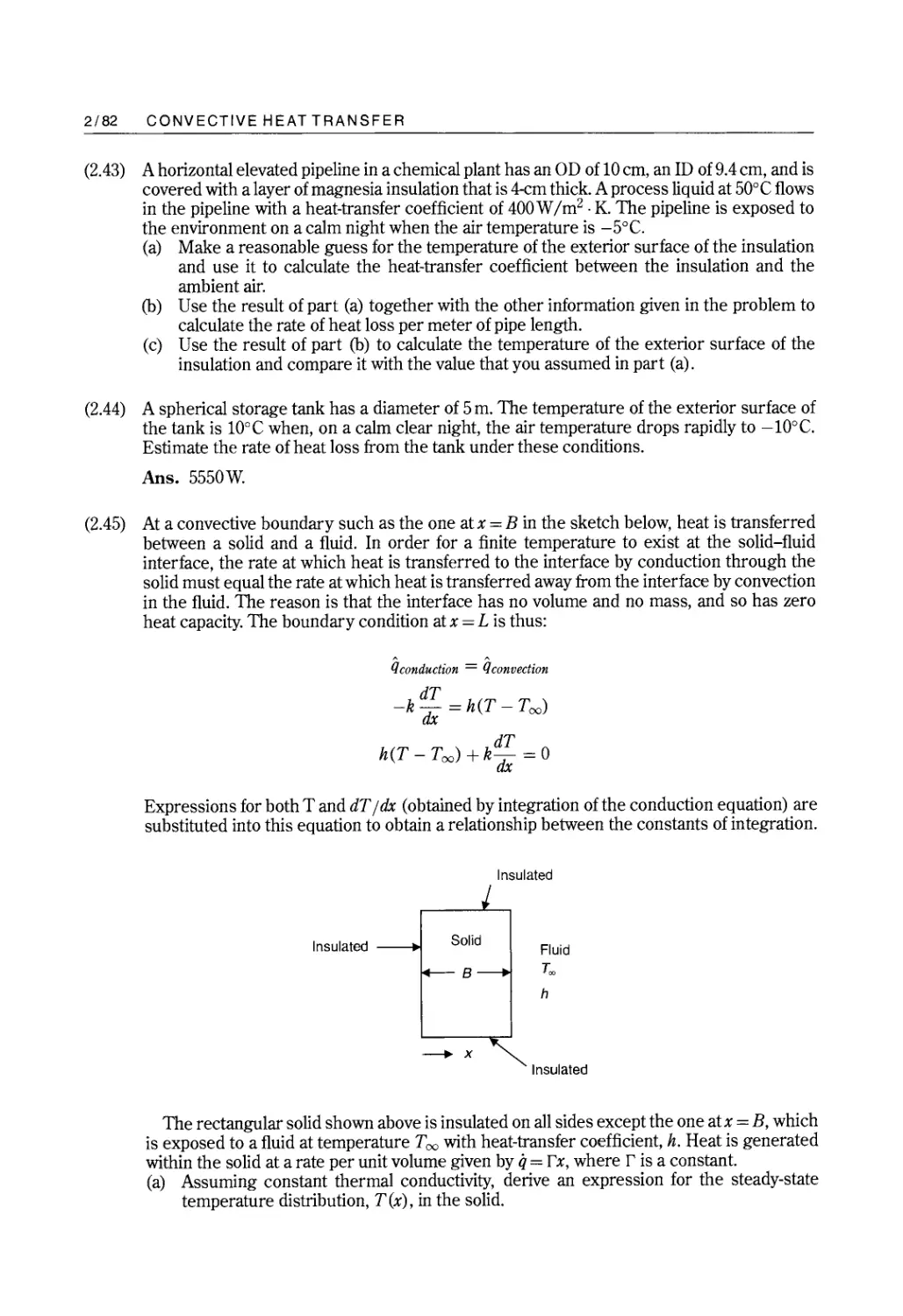
2. Convective Heat Transfer
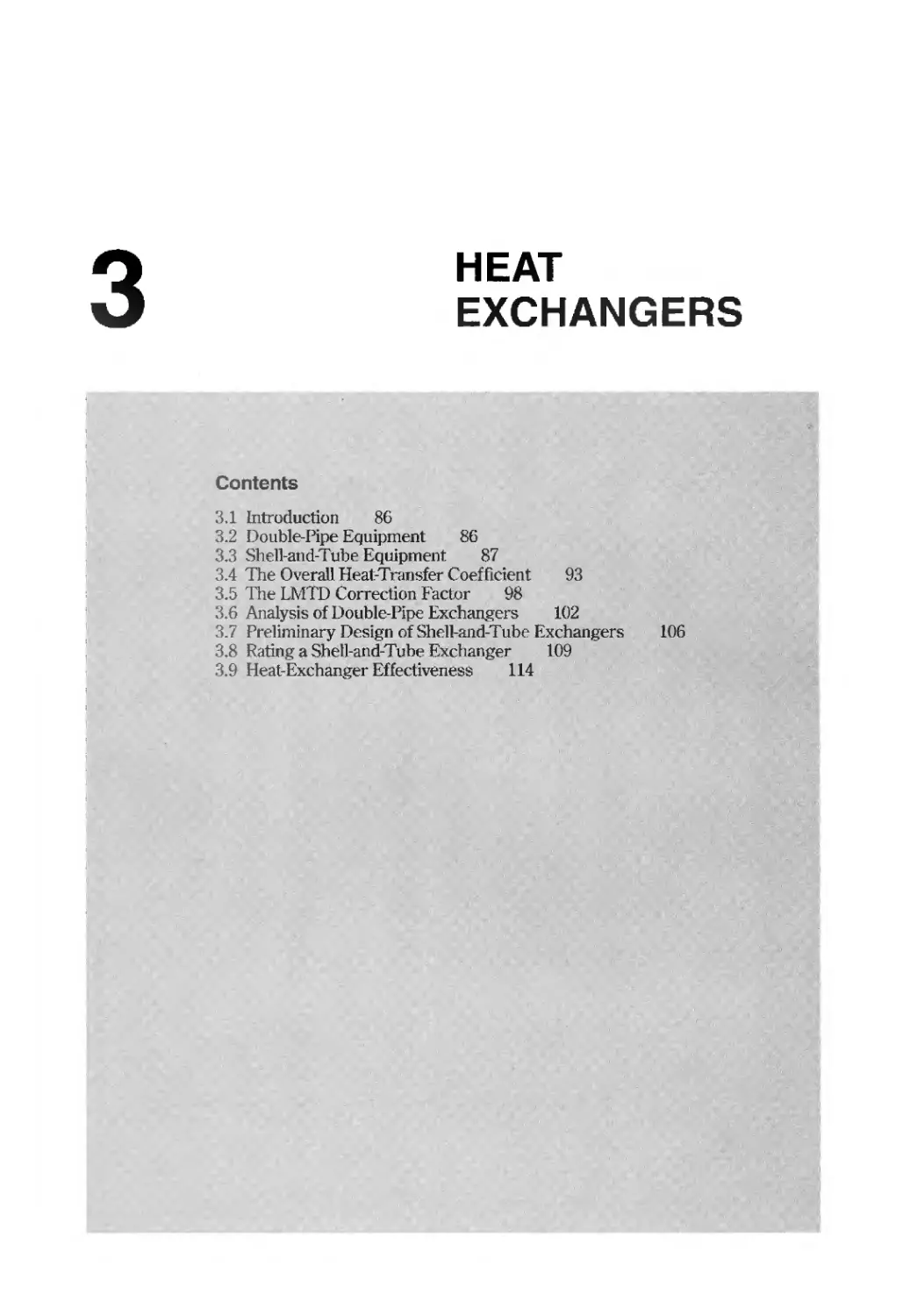
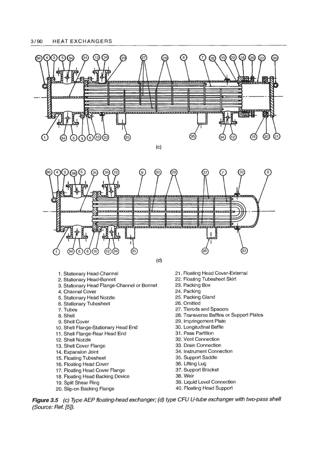
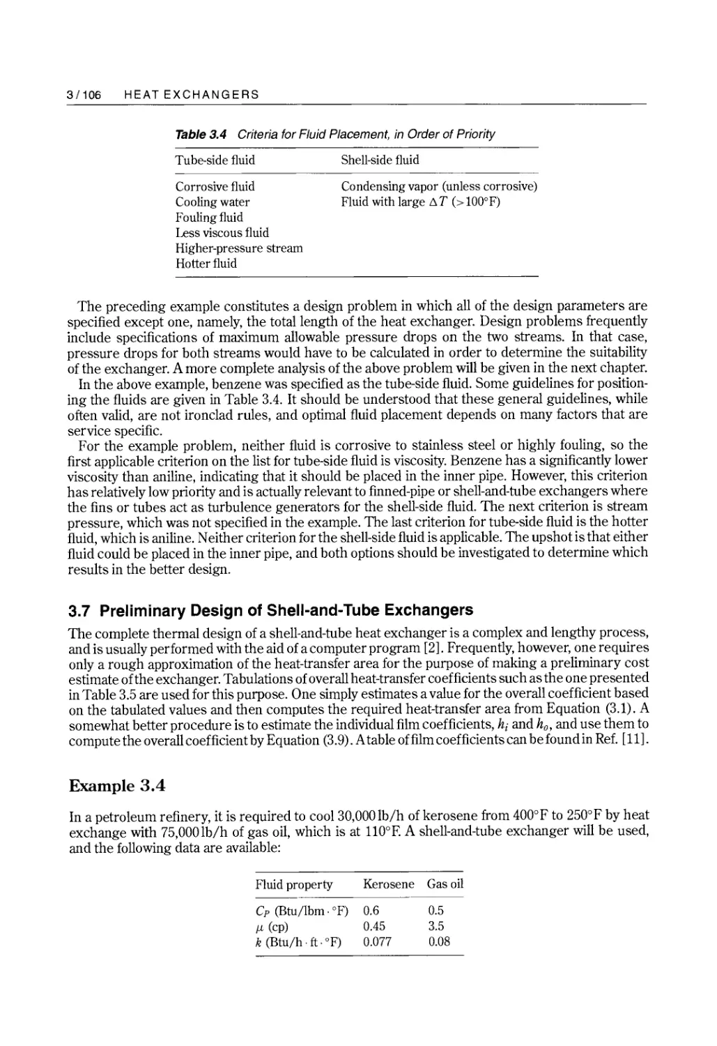
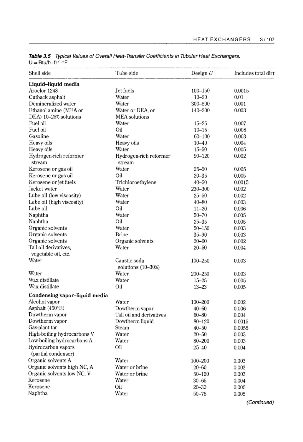
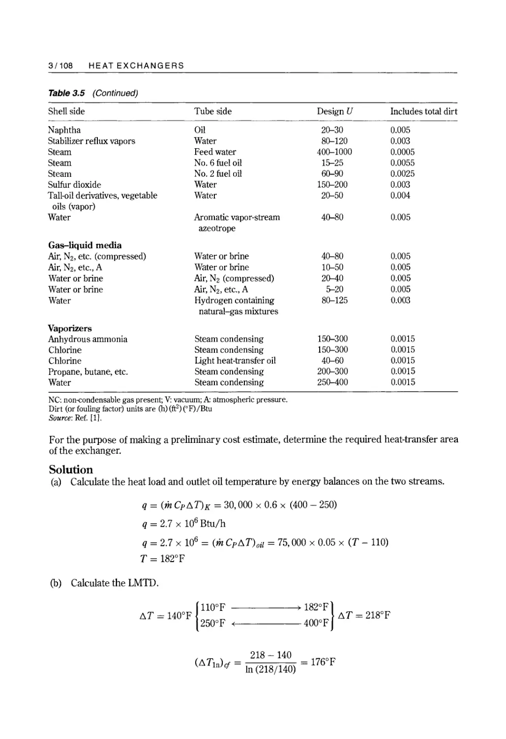
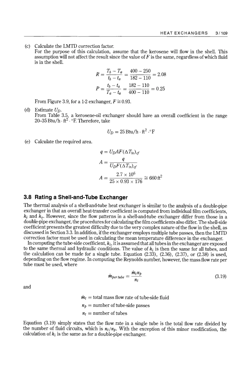
3. Heat Exchangers
4. Design of Double-Pipe Heat Exchangers
5. Design of Shell and Tube Heat Exchangers
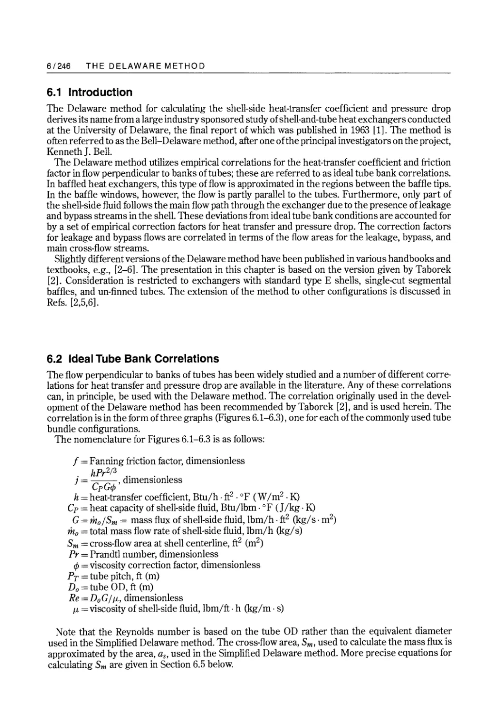
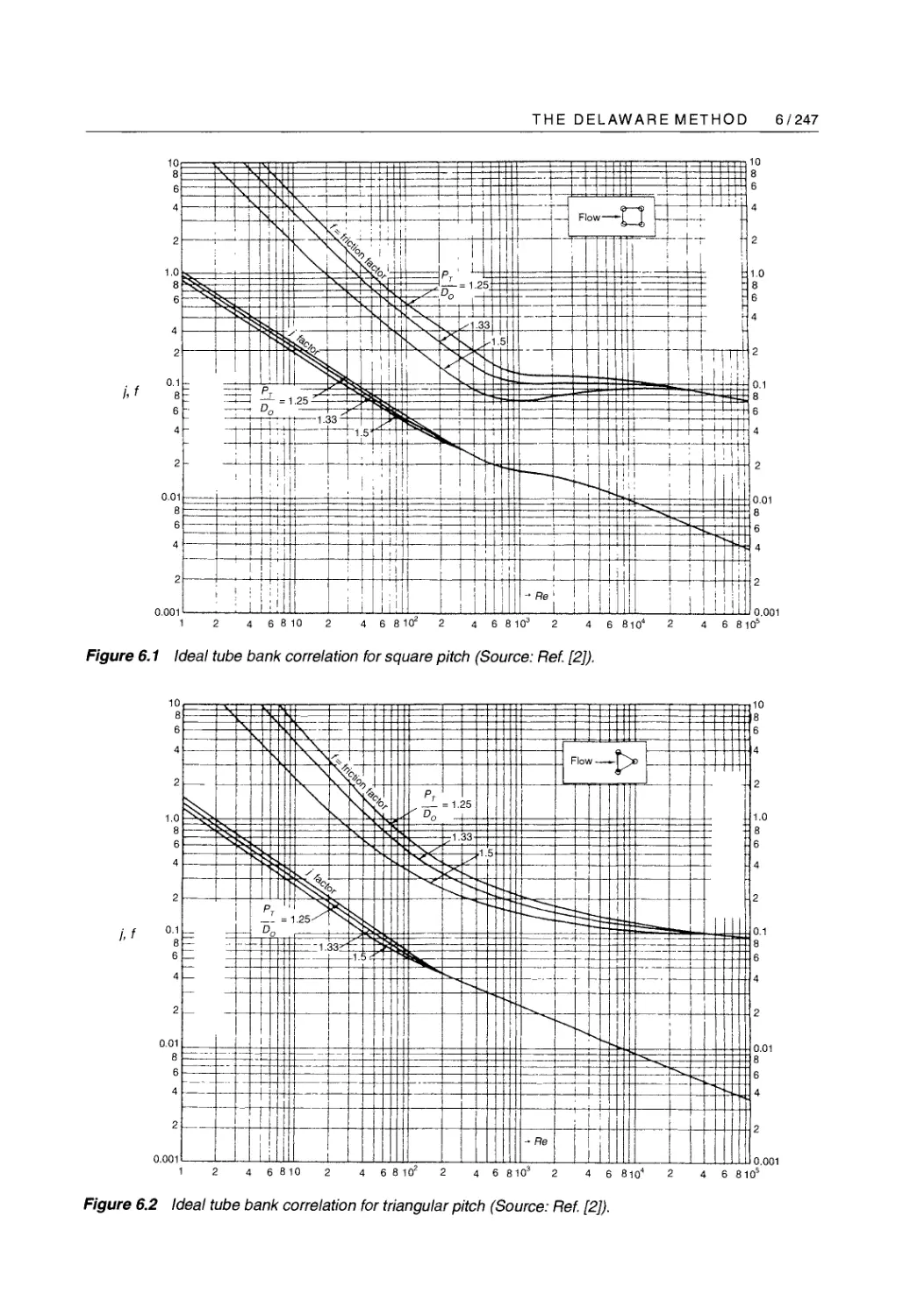
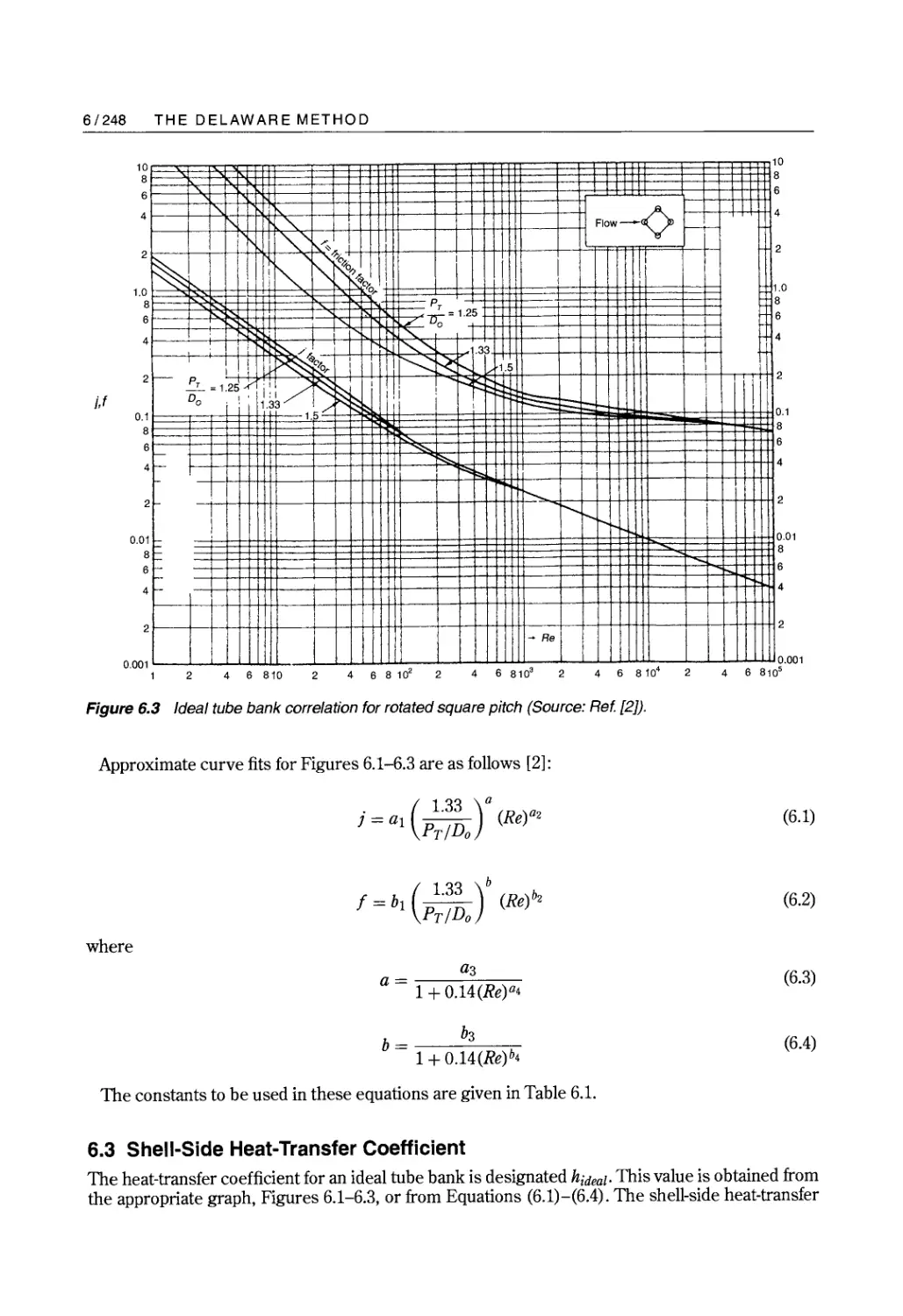
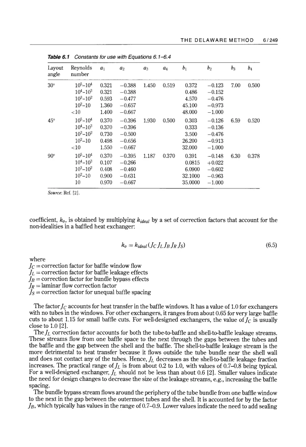
6. The Delaware Method
7. The Stream Analysis Method
8. Heat Exchanger Networks
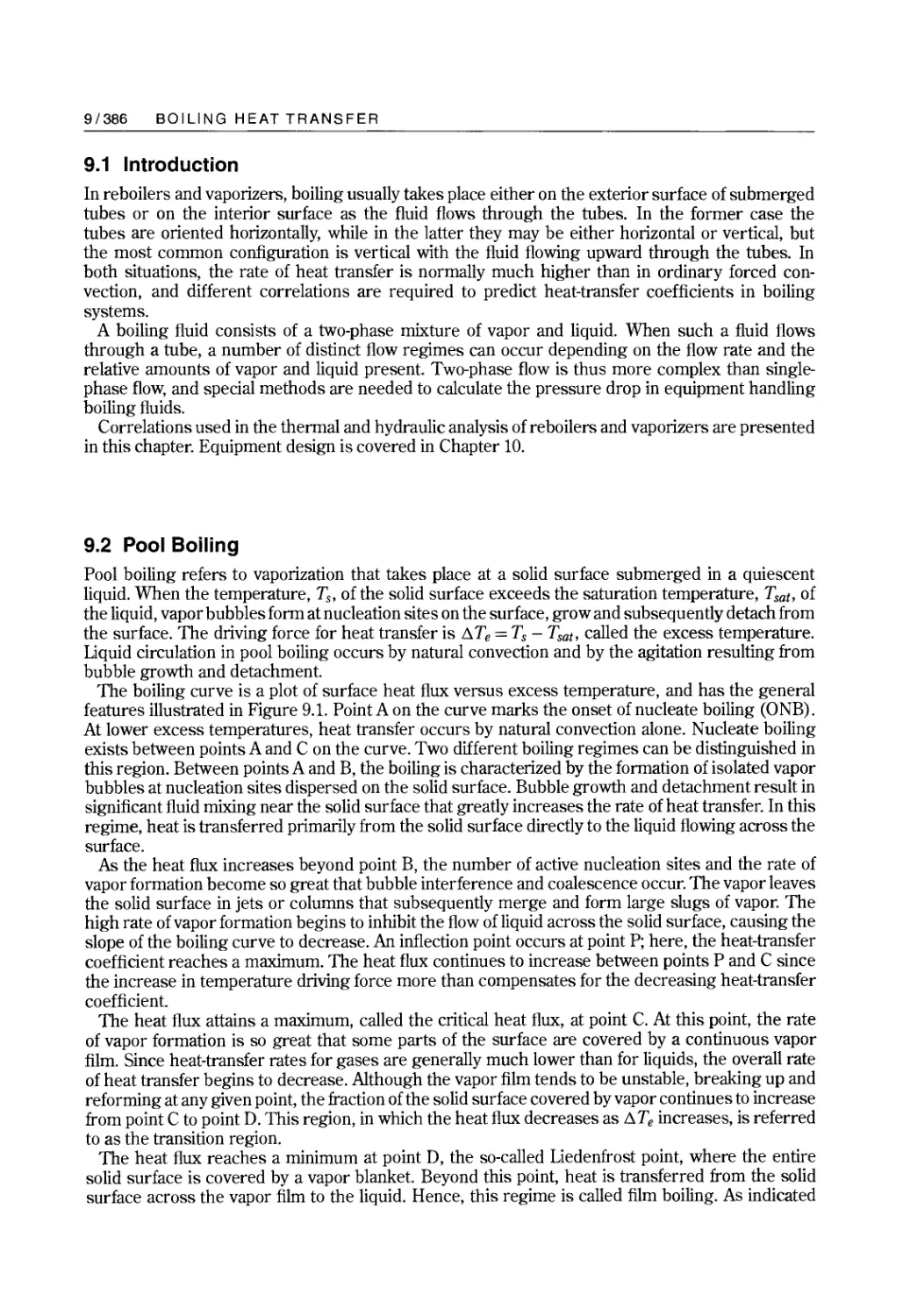
9. Boiling Heat Transfer
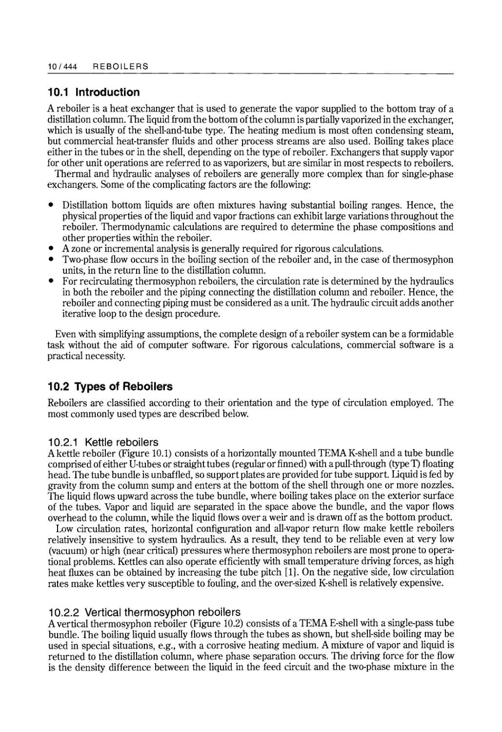
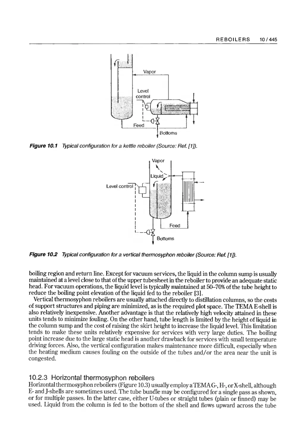
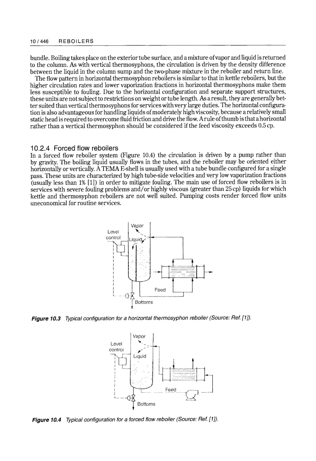
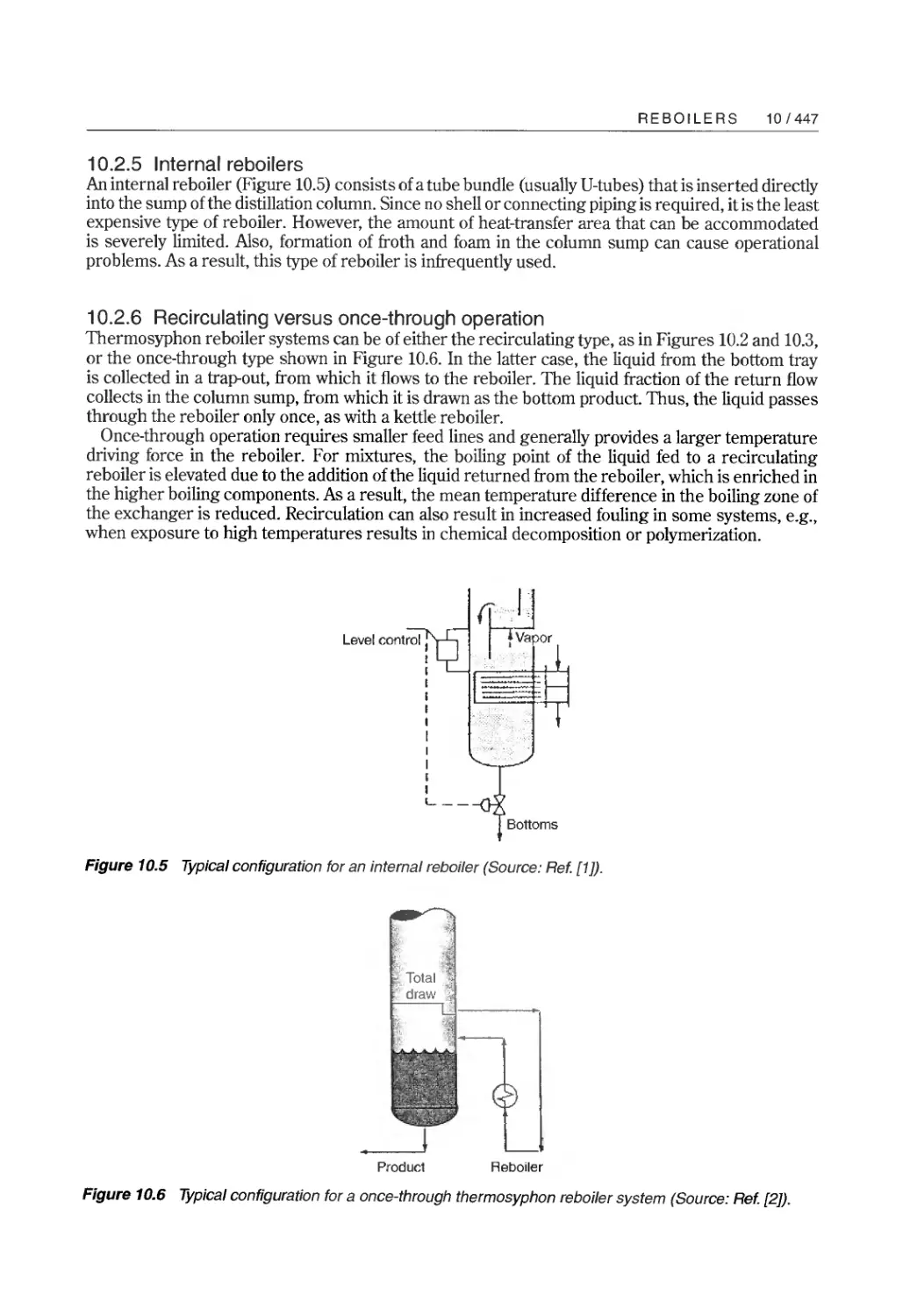
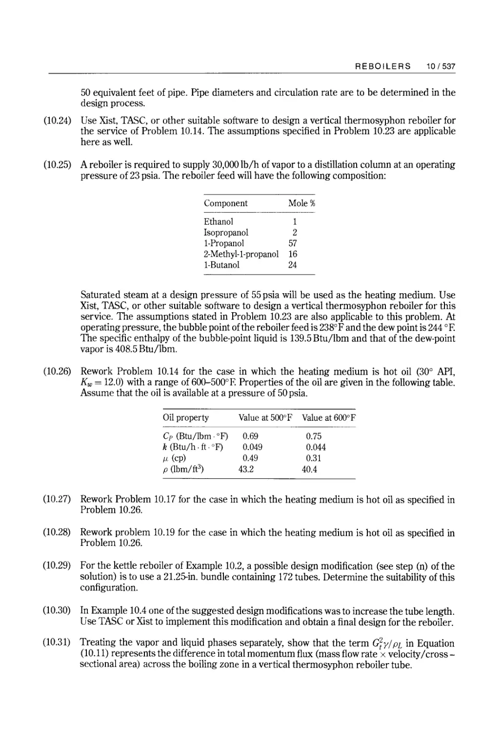
10. Reboilers
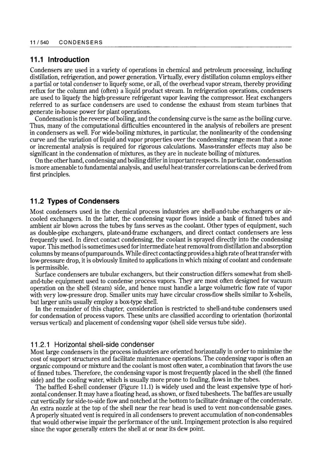
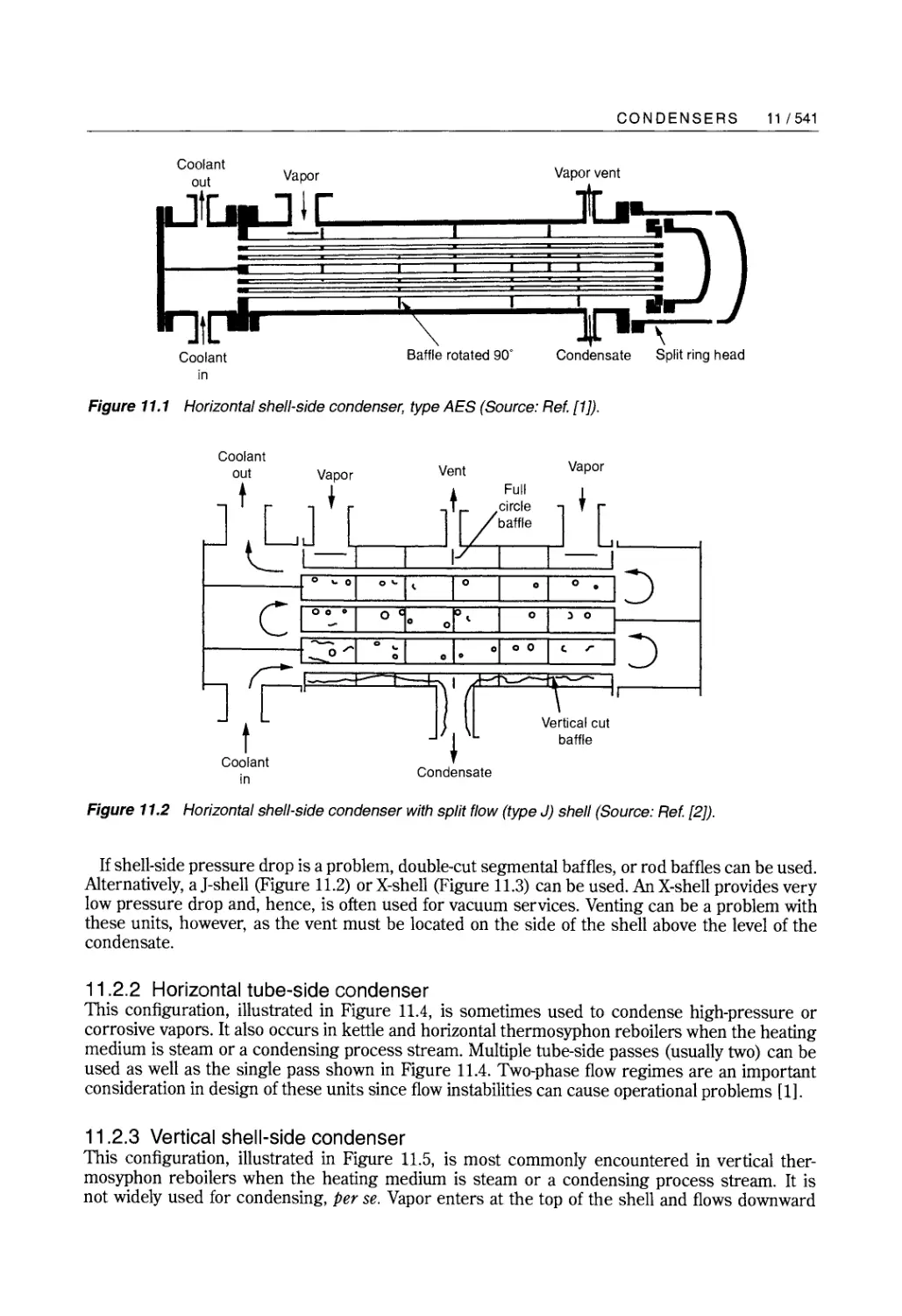
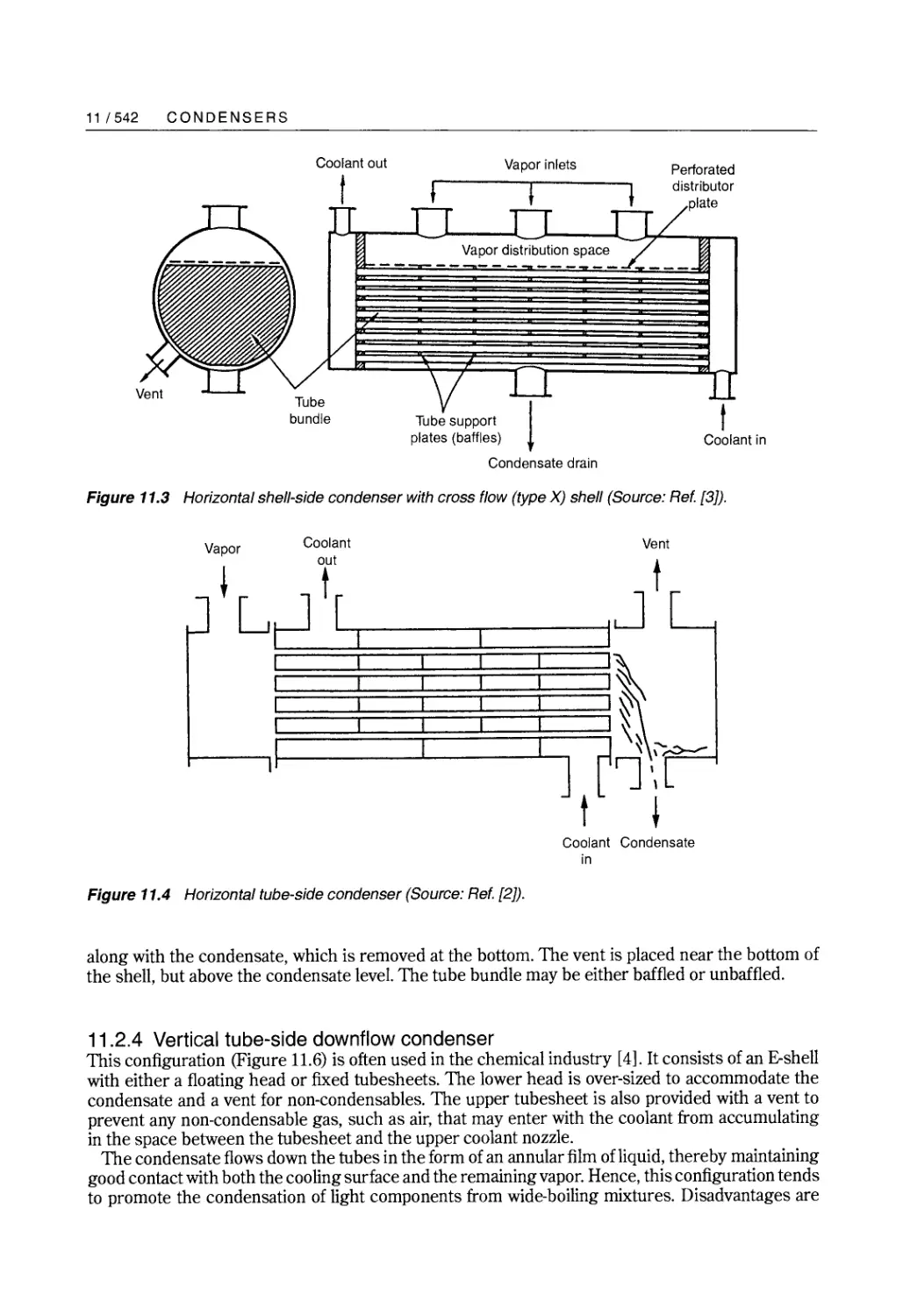
11. Condensers
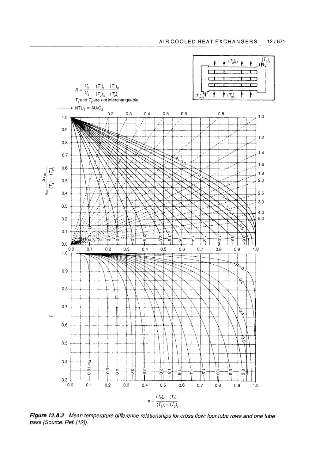
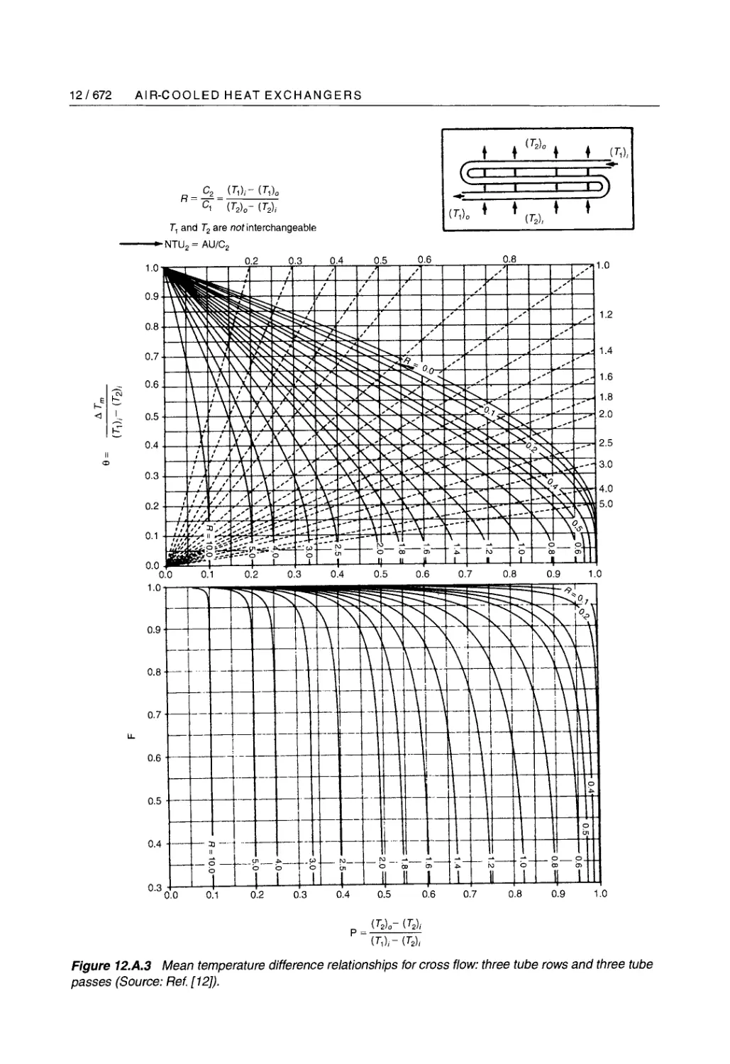
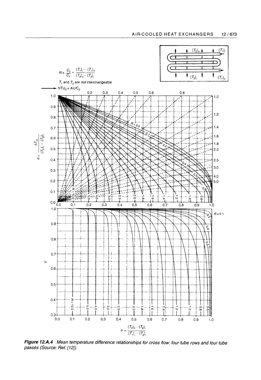
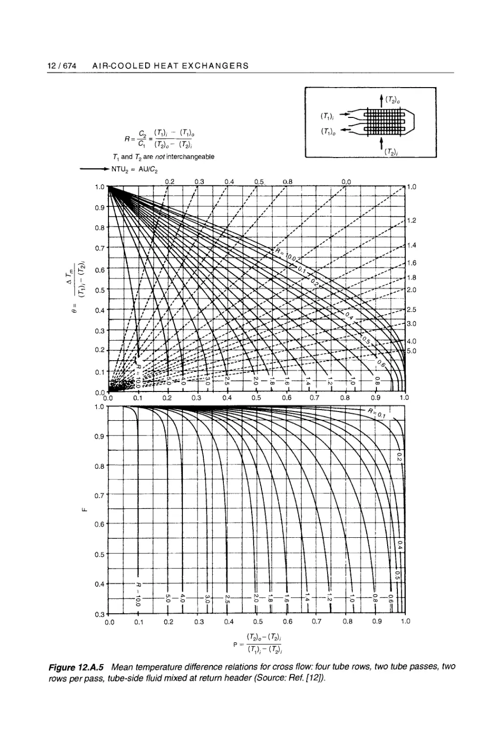
12. Air-Cooled Heat Exchangers
13. Appendix
1
HEAT
CONDUCTION
Contents
1.1 IntToduction 2
1.2 Fourier's Law of Heat Conduction 2
1.3 The Heat Conduction Equation 6
1.4 Thermal Resistance 15
1.5 The Conduction Shape Factor 19
1.6 Unsteady-State Conduction 24
1. 7 Mechanisms of Heat Conduction 31
1/2 HEAT CONDUCTION
1.1 Introduction
Heat conduction is one of the three basic modes of thermal energy transport (convection and
radiation being the other two) and is involved in virtually all process heat-transfer operations. In
commercial heat exchange equipment, for example, heat is conducted through a solid wall (often
a tube wall) that separates two fluids having different temperatures. Furthermore, the concept of
thermal resistance, which follows from the fundamental equations of heat conduction. is widely used
in the analysis of problems arising in the design and operation of industrial equipment. In addition,
many routine process engineering problems can be solved with acceptable accuracy using simple
solutions of the heat conduction equation for rectangular, cylindrical, and spherical geometries.
This chapter provides an introduction to the macroscopic theory of heat conduction and its engi-
neering applications. The key concept of thermal resistance, used throughout the text, is developed
here, and its utility in analyzing and solving problems of practical interest is illustrated.
1.2 Fourier's Law of Heat Conduction
The mathematical theory of heat conduction was developed early in the nineteenth century by
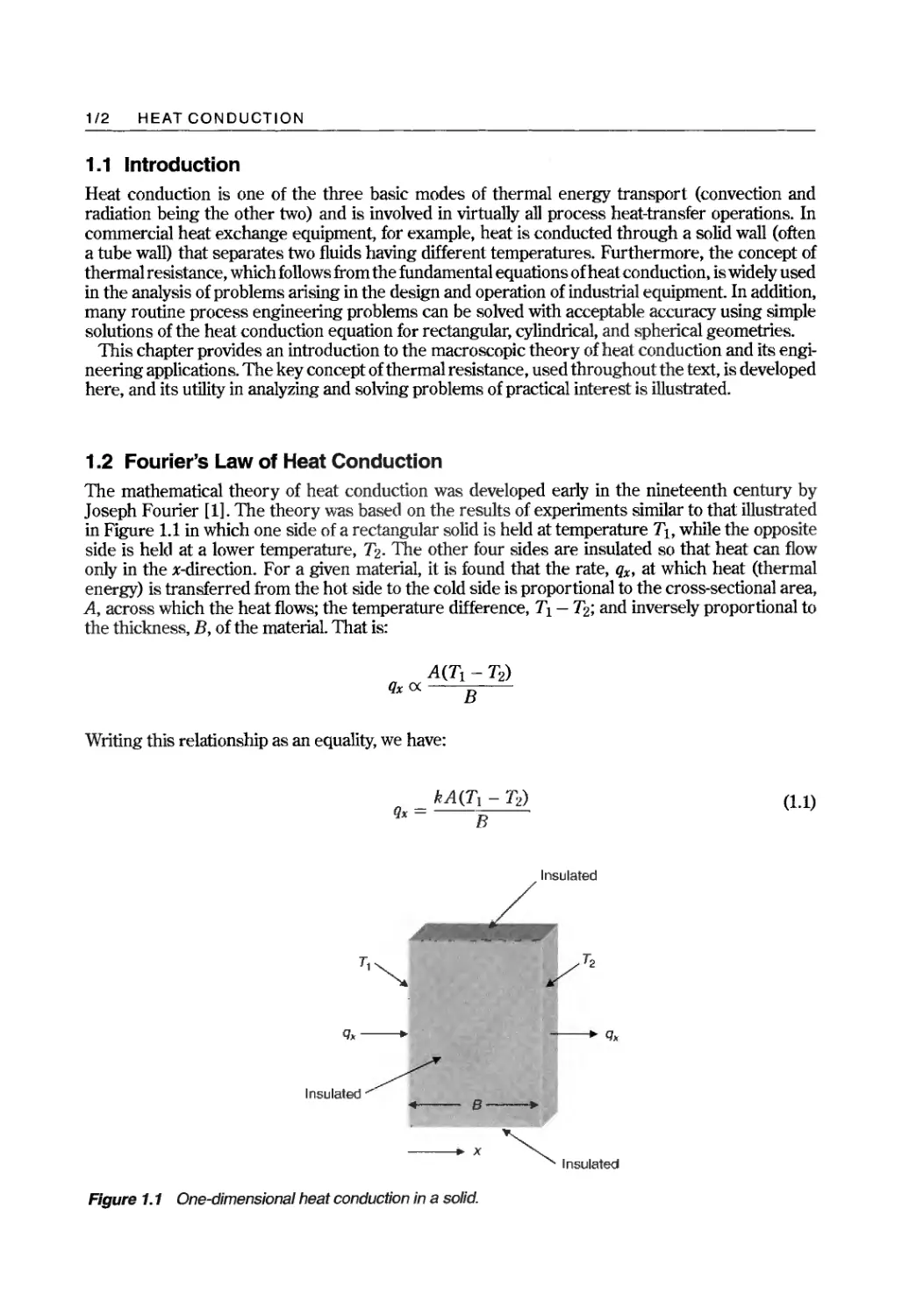
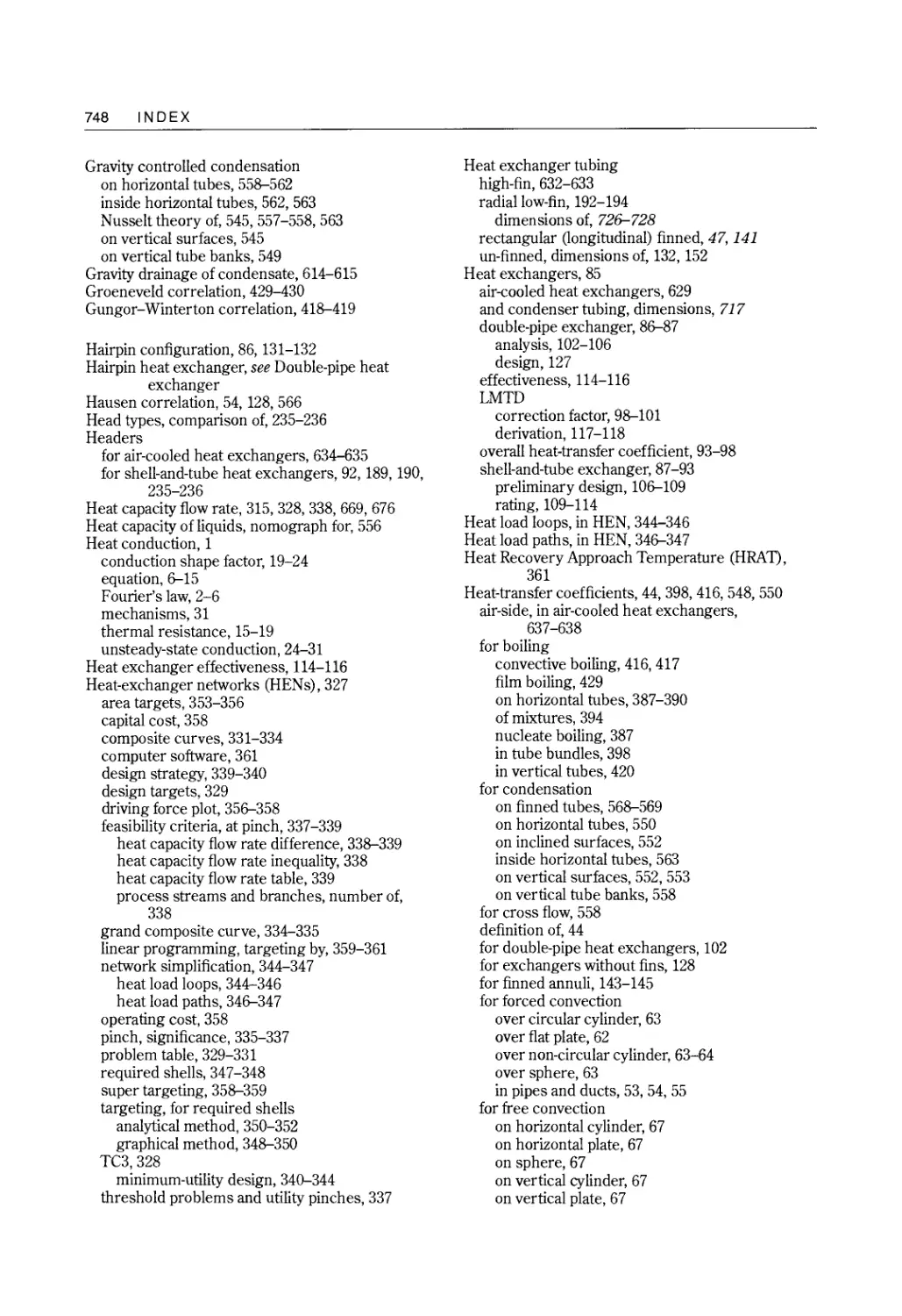
Joseph Fourier [1]. The theory was based on the results of experiments similar to that illustrated
in Figure 1.1 in which one side of a rectangular solid is held at temperature T 1 , while the opposite
side is held at a lower temperature, Tz. The other four sides are insulated so that heat can flow
only in the x-direction. For a given material, it is found that the rate, qx, at which heat (thermal
energy) is transferred from the hot side to the cold side is proportional to the cross-sectional area,
A, across which the heat flows; the temperature difference, Tl - Tz; and inversely proportional to
the thickness, B, of the material. That is:
A(T 1 - Tz)
qx ex B
Writing this relationship as an equality, we have:
kA(T 1 - Tz)
qx=--
B
(1.1)
Insulated
/
If.
TI
T 2
q,,-
q"
Insulated /'
-8-
. x
Insulated
Figure 1.1 One-dimensional heat conduction in a solid.
HEAT CONDUCTION 1/3
The constant of proportionality, k, is called the thermal conductivity. Equation (1.1) is also applicable
to heat conduction in liquids and gases. However, when temperature differences exist in fluids, con-
vection currents tend to be set up, so that heat is generally not transferred solely by the mechanism
of conduction.
The thermal conductivity is a property of the material and, as such, it is not really a constant, but
rather it depends on the thermodynamic state of the material, i.e., on the temperature and pressure
of the material. However, for solids, liquids, and low-pressure gases, the pressure dependence is
usually negligible. The temperature dependence also tends to be fairly weak, so that it is often
acceptable to treat k as a constant, particularly if the temperature difference is moderate. When the
temperature dependence must be taken into account, a linear function is often adequate, particularly
for solids. In this case,
k = a + bT
(1.2)
where a and b are constants.
Thermal conductivities of a number of materials are given in Appendices 1.A-1.E. Many other
values may be found in various handbooks and compendiums of physical property data. Process
simulation software is also an excellent source of physical property data. Methods for estimating
thermal conductivities of fluids when data are unavailable can be found in the authoritative book
by Poling et al. [2].
The form of Fourier's law given by Equation (1.1) is valid only when the thermal conductivity
can be assumed constant. A more general result can be obtained by writing the equation for an
element of differential thickness. Thus, let the thickness be x and let T = T 2 - Tl' Substituting
in Equation (1.1) gives:
T
qx = -kA-
M
(1.3)
N ow in the limit as x approaches zero,
T dT
--+-
x dx
and Equation (1.3) becomes:
dT
qx = -kA dx
(1.4)
Equation (1.4) is not subject to the restriction of constant k. Furthermore, when k is constant, it can
be integrated to yield Equation (1.1). Hence, Equation (1.4) is the general one-dimensional form of
Fourier's law. The negative sign is necessary because heat flows in the positive x-direction when
the temperature decreases in the x-direction. Thus, according to the standard sign convention that
qx is positive when the heat flow is in the positive x-direction, qx must be positive when dT Idx is
negative.
It is often convenient to divide Equation (1.4) by the area to give:
A A k dT
qx == qx 1 = - -
dx
(1.5)
where qx is the heat flux. It has units of J/s. m 2 = W/m 2 or Btu/h. ft2. Thus, the units of k are
W 1m. Kor Btu/h. ft. OF.
Equations (1.1), (1.4), and (1.5) are restricted to the situation in which heat flows in the x-direction
only. In the general case in which heat flows in all three coordinate directions, the total heat flux is
1/4 HEAT CONDUCTION
obtained by adding vectorially the fluxes in the coordinate directions. Thus,
----)0 ---+ ----+ ---..,..
q = qx i + qy j + qz k
(1.6)
-+ -+ --->
where q is the heat flux vector and i, j , k are unit vectors in the x-, y-, z-directions, respectively.
Each of the component fluxes is given by a one-dimensional Fourier expression as follows:
qx = _k aT q = _k aT qz = _k aT
ax y ay az
Partial derivatives are used here since the temperature now varies in all three directions. Substituting
the above expressions for the fluxes into Equation (1.6) gives:
(1.7)
-+ ( aT -+ aT -+ aT -+ )
q = -k - i + - j + - k
ax ay az
(1.8)
-+
The vector in parenthesis is the temperature gradient vector, and is denoted by V T. Hence,
-+
q = -kVT
(1.9)
Equation (1.9) is the three-dimensional form of Fourier's law. It is valid for homogeneous, isotropic
materials for which the thermal conductivity is the same in all directions.
Equation (1.9) states that the heat flux vector is proportional to the negative of the tempefature
gradient vector. Since the gradient direction is the direction of greatest temperature increase, the
negative gradient direction is the direction of greatest temperature decrease. Hence. Fourier's law
states that heat flows in the direction of greatest temperature decrease.
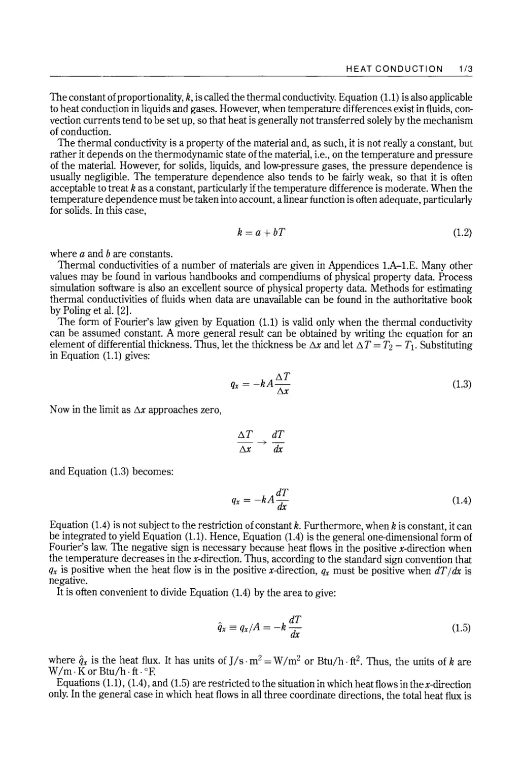
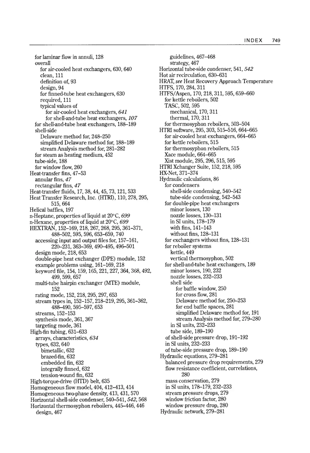
Example 1.1
The block of 304 stainless steel shown below is well insulated on the front and back surfaces, and
the temperature in the block varies linearly in both the x- andy-directions, find:
(a) The heat fluxes and heat flows in the x- and y-directions.
(b) The magnitude and direction of the heat flux vector.
15°C
5?
' 5cmr ·
1Dcm
1
1QOC
5°C
.
DOC
y
Lx
HEAT CONDUCTION 1/5
Solution
(a) From Table AI, the thermal conductivity of 304 stainless steel is 14.4 W /m. K. The cross-
sectional areas are:
Ax = 10 x 5 = 50cm 2 = 0.0050m 2
Ay = 5 x 5 = 25cm 2 = 0.0025m 2
Using Equation (1.7) and replacing the partial derivatives with finite differences (since the
temperature variation is linear), the heat fluxes are:
aT /1T ( -5 ) 2
qx = -k- = -k- = -14.4 - = 1440W/m
ax /1x 0.05
aT /1T ( 10 ) 2
qy = -k- = -k- = -14.4 - = -1440W/m
ay /1y 0.1
The heat flows are obtained by multiplying the fluxes by the corresponding cross-sectional
areas:
qx = qxAx = 1440 x 0.005 = 7.2W
qy = qyAy = -1440 x 0.0025 = -3.6 W
(b) From Equation (1.6):
-?
-? -?
q = qx i + qy j
-? -? -?
q = 1440 i -1440j
Iii = [(1440)2 + (-1440)2]0.5 = 2036.5W/m 2
The angle, e, between the heat flux vector and the x-axis is calculated as follows:
tane=qylqx = -1440/1440 = -1.0
e = -45 0
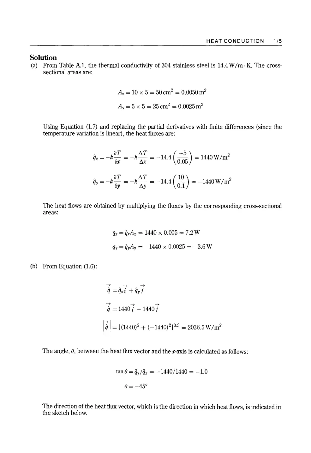
The direction of the heat flux vector, which is the direction in which heat flows, is indicated in
the sketch below.
1/6 HEAT CONDUCTION
y
x
q
1.3 The Heat Conduction Equation
The solution of problems involving heat conduction in solids can, in principle, be reduced to the
solution of a single differential equation, the heat conduction equation. The equation can be derived
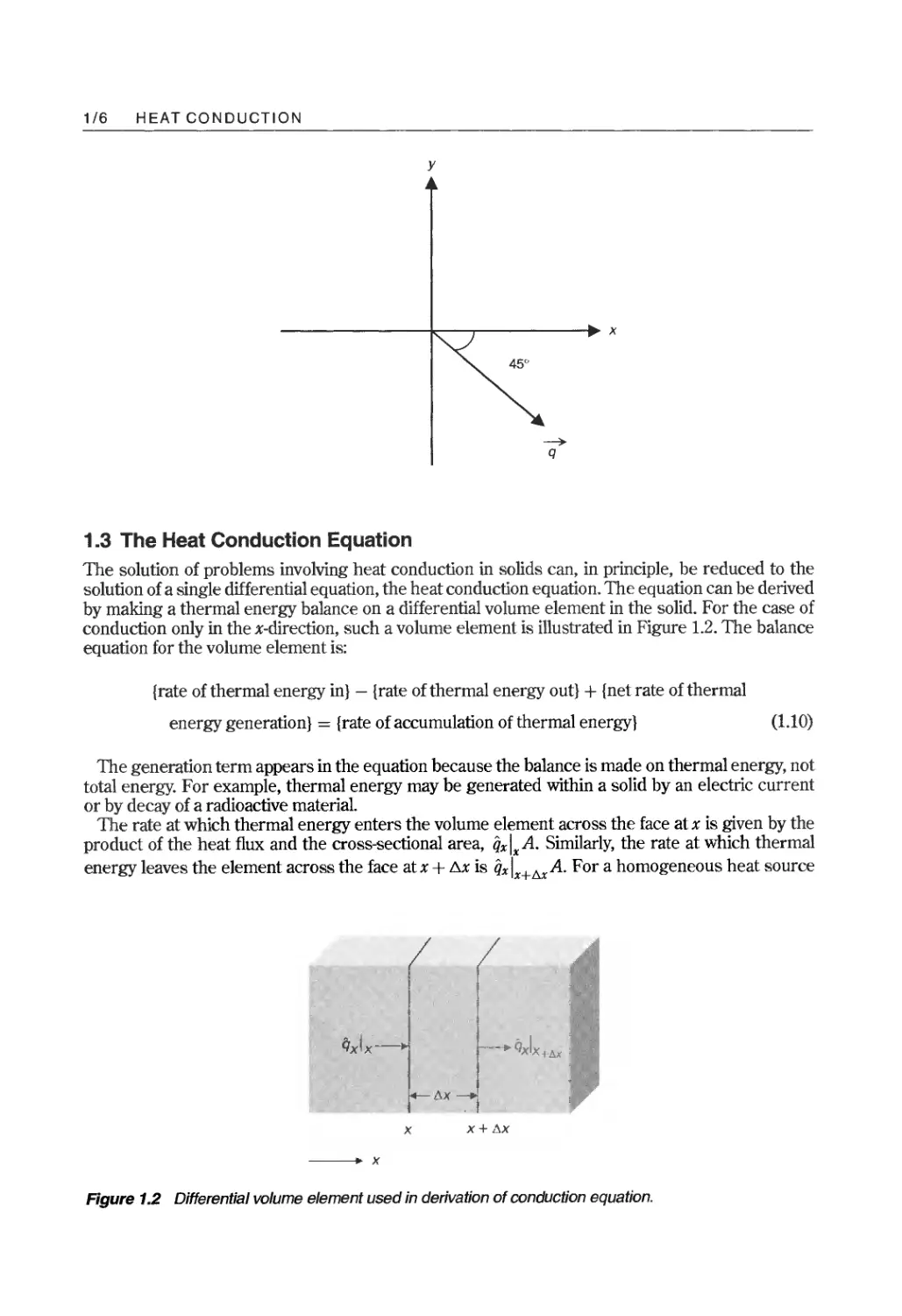
by making a thermal energy balance on a differential volume element in the solid. For the case of
conduction only in the x-direction, such a volume element is illustrated in Figure 1.2. The balance
equation for the volume element is:
{rate of thermal energy in} - {rate of thermal energy out} + {net rate of thermal
energy generation} = {rate of accumulation of thermal energy}
(1.10)
The generation term appears in the equation because the balance is made on thermal energy, not
total energy. For example, thermal energy may be generated within a solid by an electric current
or by decay of a radioactive material.
The rate at which thermal energy enters the volume element across the face at x is given by the
product of the heat flux and the cross-sectional area, qx Ix A. Similarly, the rate at which thermal
energy leaves the element across the face at x + /:o,.x is qxlx+MA. For a homogeneous heat source
c,xlx
-.qxlxl!!.x ;
!1x
X x+/>,x
. x
Figure 1.2 Differential volume element used in derivation of conduction equation.
HEAT CONDUCTION 1/7
of strength q per unit volume, the net rate of generation is qAM. Finally, the rate of accumulation
is given by the time derivative of the thermal energy content of the volume element, which is
pc(T - Tref)A x, where TreJ is an arbitrary reference temperature. Thus, the balance equation
becomes:
A A A . A aT
(qxlx - qxlx+L'.x) + q x = pC-AM
at
It has been assumed here that the density, p, and heat capacity, c, are constant. Dividing by A x
and taking the limit as x -+ 0 yields:
aT aqx.
pc- = -- +q
at ax
Using Fourier's law as given by Equation (1.5), the balance equation becomes:
pc aT = ( kaT ) +q
at ax ax
When conduction occurs in all three coordinate directions, the balance equation contains y- and
z-derivatives analogous to the x-derivative. The balance equation then becomes:
pC aT = ( kaT ) + ( kaT ) + ( kaT ) +q
at ax ax ay ay az az
(1.11)
Equation (1.11) is listed in Table 1.1 along with the corresponding forms that the equation takes in
cylindrical and spherical coordinates. Also listed in Table 1.1 are the components of the heat flux
vector in the three coordinate systems.
When k is constant, it can be taken outside the derivatives and Equation (1.11) can be
written as:
pc aT a 2 T a 2 T a 2 T q
--=-+-+-+-
k at ax 2 ay2 az 2 k
(1.12)
or
aT = V 2 T +
a at k
(1.13)
where a == k 1 pC is the thermal diffusivity and V 2 is the Laplacian operator. The thermal diffusivity
has units of m 2 / s or ft2/h.
1/8 HEAT CONDUCTION
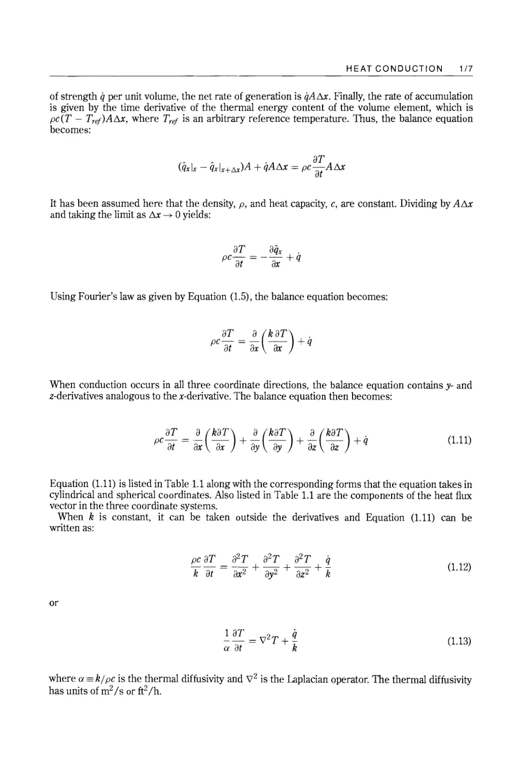
Table 1.1 The Heat Conduction Equation
A. Cartesian coordinates
aT a ( aT ) a ( aT ) a ( aT ) .
pc- = - k- + - k- + - k- + q
at ax ax ay ay az az
-?
The components of the heat flux vector, q, are:
qx = _k aT q = _k aT qz = _k aT
ax Y ay az
B. Cylindrical coordinates (r, cp, z)
z
, (x, y, z) = (r, <1>, z)
y
x
aT 1 a ( aT ) 1 a ( aT ) a ( aT ) .
pc- = - - k r- + - - k- + - k- + q
at r ar ar r 2 acp acp az az
--->
The components of q are:
aT -k aT q z = _ k aT
qr = -kar; q<l> = r acp ; az
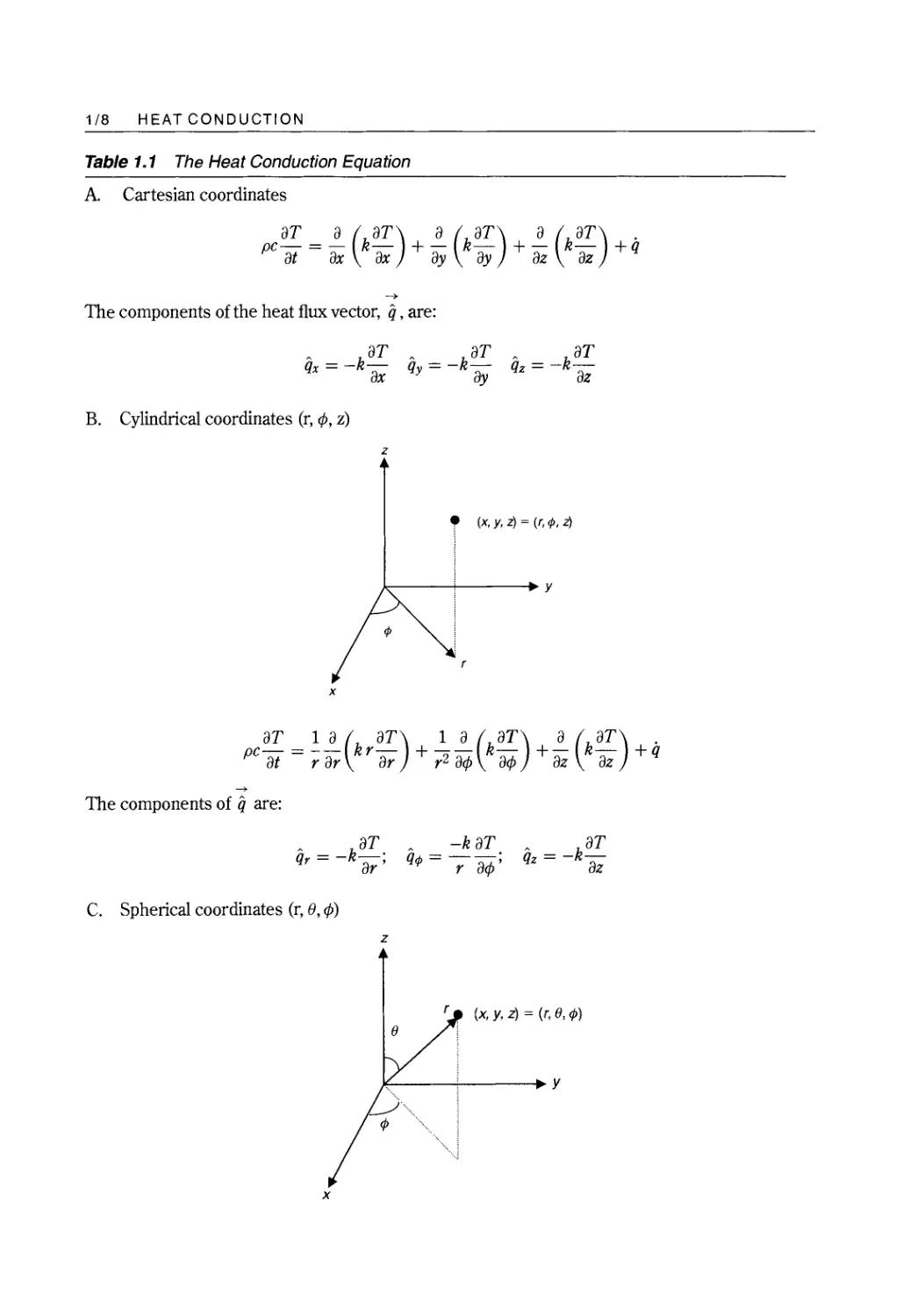
C. Spherical coordinates (r, e, cp)
z
(x, y, z) = (r, e, </»
e
y
x
HEAT CONDUCTION 1/9
aT 1 a ( Z aT ) 1 a ( aT )
pc- = -- kr - + -- ksine-
a t r Z ar ar r Z sin e ae ae
1 a (k aT ) .
+ - - +q
r Z sin z e acp acp
--+
The components of q are:
qr = -k aT ;
ar
kaT
qg = -riie;
k aT
qr/> = - rsin e acp
The use of the conduction equation is illustrated in the following examples.
Example 1.2
Apply the conduction equation to the situation illustrated in Figure 1.1.
Solution
In order to make the mathematics conform to the physical situation, the following conditions are
imposed:
(1) Conduction only in x-direction::::} T = T(x), so aT = aT = 0
ay az
(2) No heat source::::} q = 0
aT
(3) Steady state::::} - = 0
at
(4) Constant k
The conduction equation in Cartesian coordinates then becomes:
o = k aZT
ax z
dZT
or - = 0
dx z
(The partial derivative is replaced by a total derivative because x is the only independent variable
in the equation.) Integrating on both sides of the equation gives:
dT = C 1
dx
A second integration gives:
T = C1x + C z
Thus, it is seen that the temperature varies linearly across the solid. The constants of integration
can be found by applying the boundary conditions:
(1) Atx=O T=Tl
(2) At x = B T = Tz
The first boundary condition gives Tl = C z and the second then gives:
Tz = CrB + Tl
1/10 HEAT CONDUCTION
Solving for C I we find:
C I = Tz - TI
B
The heat flux is obtained from Fourier's law:
_ _ k dT _ - kC _ _ k (T z - T I ) _ (TI- T z )
qx - - I - - k
dx B B
Multiplying by the area gives the heat flow:
qx = qx A = kA(T r - Tz)
B
Since this is the same as Equation (1.1), we conclude that the mathematics are consistent with the
experimental results.
Example 1.3
Apply the conduction equation to the situation illustrated in Figure 1.1, but let k = a + bT, where a
and b are constants.
Solution
Conditions 1-3 ofthe previous example are imposed. The conduction equation then becomes:
0= (k : )
Integrating once gives:
k dT = C r
dx
The variables can now be separated and a second integration performed. Substituting for k, we
have:
(a + bT)dT = C r dx
bTz
aT + 2 = CIx + C z
It is seen that in this case of variable k, the temperature profile is not linear across the solid.
The constants of integration can be evaluated by applying the same boundary conditions as in the
previous example, although the algebra is a little more tedious. The results are:
bTz
C z = aT I + --t
C - (Tz - Tr) !!.... ( T z _ TZ )
I-a B +2B z I
HEAT CONDUCTION 1/11
As before, the heat flow is found using Fourier's law:
dT
qx = -kA- = -AC l
dx
A [ b 2 2 ]
qx = B a(T l - T2) + 2(T 1 - T 2 )
This equation is seldom used in practice. Instead, when k cannot be assumed constant, Equation
(1.1) is used with an average value of k. Thus, taking the arithmetic average of the conductivities at
the two sides of the block:
kave = k(Tl) + k(T 2 )
2
(a + bTl) + (a + bT 2 )
2
b
kave = a + 2 (Tl --r- T 2 )
Using this value of k in Equation (1.1) yields:
kaveA(T l - Tz)
qx=
B
= [a + b(T 1 : T 2 ) ] (TI- T 2 )
A [ b 2 2 ]
qx = B a(T I - T 2 ) + 2(T 1 - T 2 )
This equation is exactly the same as the one obtained above by solving the conduction equation.
Hence, using Equation (1.1) with an average value of k gives the correct result. This is a consequence
of the assumed linear relationship between k and T.
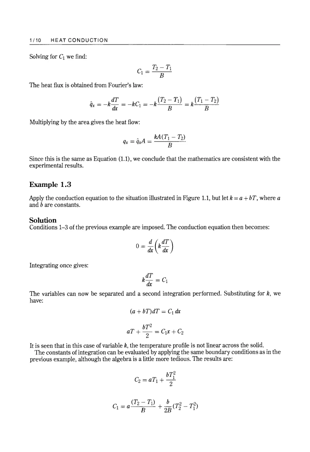
Example 1.4
Use the conduction equation to find an expression for the rate of heat transfer for the cylindrical
analog of the situation depicted in Figure 1.1.
Solution
T 1
Q,I/,
R 1
-------'
T 2
. q, !
...
R 2
1/12 HEAT CONDUCTION
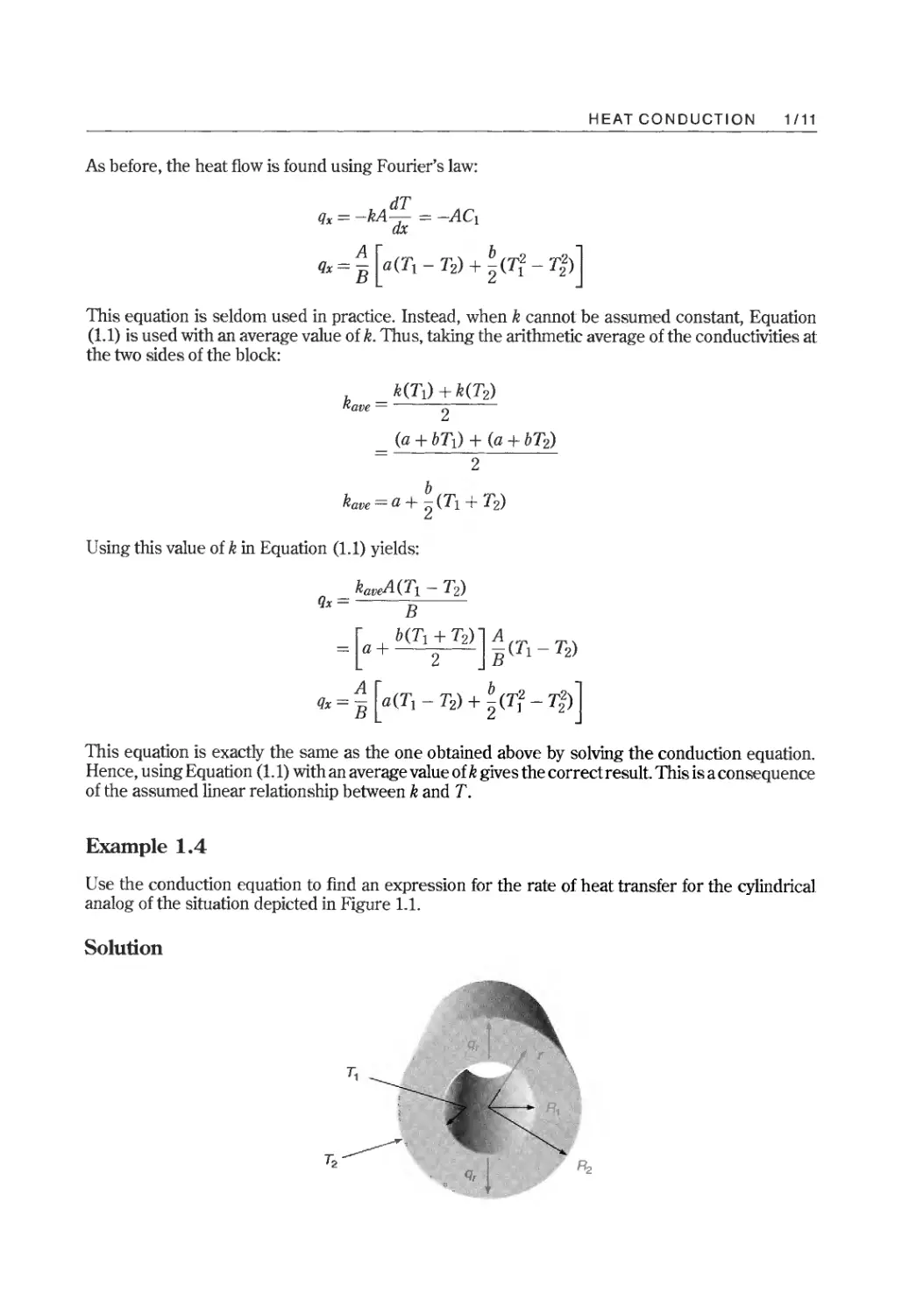
As shown in the sketch, the solid is in the form of a hollow cylinder and the outer and inner surfaces
are maintained at temperatures TI and Tz, respectively. The ends of the cylinder are insulated so
that heat can flow only in the radial direction. There is no heat flow in the angular (cp) direction
because the temperature is the same all the way around the circumference of the cylinder. The
following conditions apply:
(1) No heat flow in z-direction::::} aT = 0
az
(2) U if . d " aT 0
norm temperature m cf>- lrection::::} - =
acp
(3) No heat generation::::} q = 0
aT
(4) Steady state::::} - = 0
at
(5) Constant k
With these conditions, the conduction equation in cylindrical coordinates becomes:
( kr aT ) = 0
r ar ar
or
( r dT ) = 0
dr dr
Integrating once gives:
dT
r- = C I
dr
Separating variables and integrating again gives:
T = CIln r + C z
It is seen that, even with constant k, the temperature profile in curvilinear systems is nonlinear.
The boundary conditions for this case are:
(1) Atr=R I T=TI::::}TI=CIlnRI+CZ
(2) At r = Rz T = Tz ::::} Tz = CIln Rz + C z
Solving for C I by subtracting the second equation from the first gives:
C I = TI - Tz
InRI - InRz
TI - Tz
In (Rz/R I )
From Table 1.1, the appropriate form of Fourier's law is:
qr = _k dT = _k CI = k(T I - Tz)
dr r rln(Rz/R I )
The area across which the heat flows is:
Ar = 27rrL
where L is the length of the cylinder. Thus,
_ A _ 27rkL(T I - Tz)
qr - qr r - In (Rz/RI)
HEAT CONDUCTION 1/13
Notice that the heat-transfer rate is independent of radial position. The heat flux, however, depends
on r because the cross-sectional area changes with radial position.
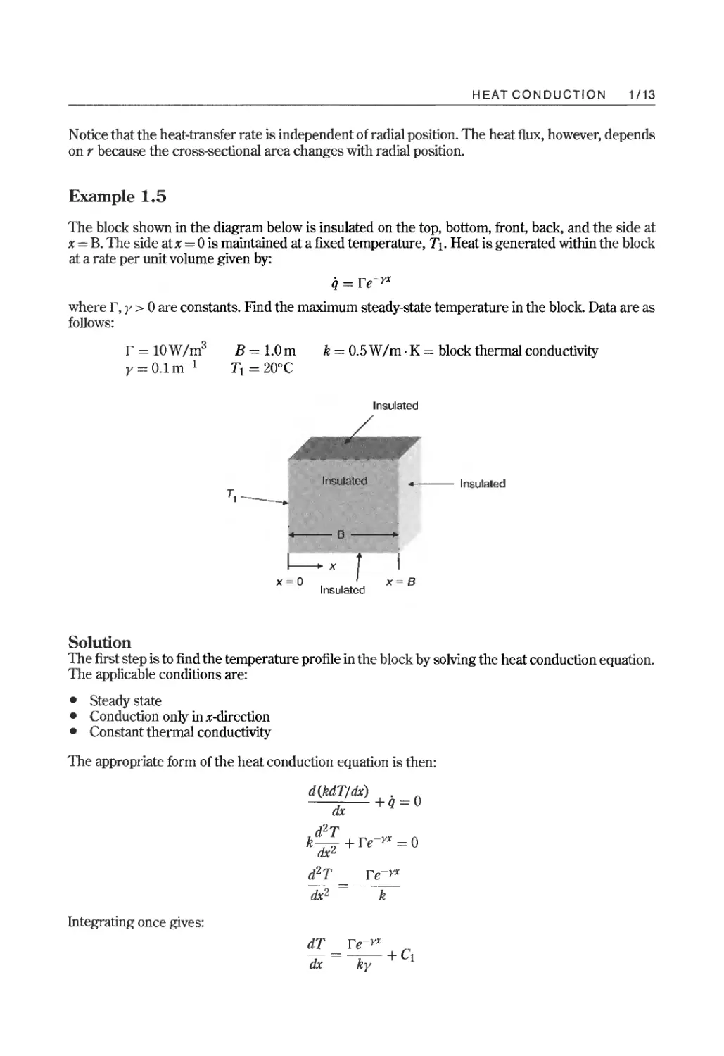
Example 1.5
The block shown in the diagram below is insulated on the top, bottom, front, back, and the side at
x = B. The side at x = 0 is maintained at a fixed temperature, Tl' Heat is generated within the block
at a rate per unit volume given by:
q = re- Yx
where r, y > 0 are constants. Find the maximum steady-state temperature in the block. Data are as
follows:
r = 10W/m 3
y = 0.lm- 1
B = 1.0 m
Tl = 20°C
k = 0.5 W 1m. K = block thermal conductivity
Insulated
/
1M
Insulated
4- - Insulated
T I __
B
x
r
x B
x 0
Insulated
Solution
The first step is to find the temperature profile in the block by solving the heat conduction equation.
The applicable conditions are:
· Steady state
· Conduction on]y in x-direction
· Constant thermal conductivity
The appropriate form of the heat conduction equation is then:
d(kdTjdx) + q = 0
dx
d 2 T
k- +re- Yx =0
dx 2
d 2 T
dx 2
re- YX
k
Integrating once gives:
dT re- YX
-=-+C 1
dx ky
1/14 HEAT CONDUCTION
A second integration yields:
re- YX
T = - ky2 + C 1 X + C 2
The boundary conditions are:
(1) Atx=O T=T1
dT
(2) Atx=B dx =0
The second boundary condition results from assuming zero heat flow through the insulated
boundary (perfect insulation). Thus, at x = L:
dT
qx = -kA dx = 0 ::::}
dT =0
dx
This condition is applied using the equation for dT/dx resulting from the first integration:
re- yB
0= kY + C1
Hence,
re- yB
C 1 = --
ky
Applying the first boundary condition to the equation for T:
re(O)
T 1 = - ky2 + C 1 (0) + C 2
Hence,
r
C 2 = Tl + ky2
With the above values for C 1 and C 2 , the temperature profile becomes:
r re- yB
T = T 1 + - (1 - e- YX ) - -x
ky2 ky
N ow at steady state, all the heat generated in the block must flow out through the un-insulated side
at x = O. Hence, the maximum temperature must occur at the insulated boundary, Le., at x = B.
(This intuitive result can be confirmed by setting the first derivative of T equal to zero and solving
for x.) Thus, setting x = B in the last equation gives:
r r BLe-yB
Tmax = T1 + 2(1- e- yB ) - k
ky y
Finally, the solution is obtained by substituting the numerical values of the parameters:
10 -0.1 10 x 1.0 e- 0 . 1
Tmax = 20 + 0.5(0.1)2 (1- e ) - 0.5 x 0.1
Tmax 29.4°C
HEAT CONDUCTION 1/15
The procedure illustrated in the above examples can be summarized as follows:
(1) Write down the conduction equation in the appropriate coordinate system.
(2) Impose any restrictions dictated by the physical situation to eliminate terms that are zero or
negligible.
(3) Integrate the resulting differential equation to obtain the temperature profile.
(4) Use the boundary conditions to evaluate the constants of integration.
(5) Use the appropriate form of Fourier's law to obtain the heat flux.
(6) Multiply the heat flux by the cross-sectional area to obtain the rate of heat transfer.
In each of the above examples there is only one independent variable so that an ordinary differential
equation results. In unsteady-state problems and problems in which heat flows in more than one
direction, a partial differential equation must be solved. Analytical solutions are often possible if
the geometry is sufficiently simple. Otherwise, numerical solutions are obtained with the aid of a
computer.
1.4 Thermal Resistance
The concept of thermal resistance is based on the observation that many diverse physical
phenomena can be described by a general rate equation that may be stated as follows:
FI Driving force
ow rate = .
Resistance
(1.14)
Ohm's Law of Electricity is one example:
I = Ii
R
(1.15)
In this case, the quantity that flows is electric charge, the driving force is the electrical potential
difference, E, and the resistance is the electrical resistance, R, of the conductor.
In the case of heat transfer, the quantity that flows is heat (thermal energy) and the driving force
is the temperature difference. The resistance to heat transfer is termed the thermal resistance, and
is denoted by Rth. Thus, the general rate equation may be written as:
/'<,.T
q=-
Rth
(1.16)
In this equation, all quantities take on positive values only, so that q and /'<,.T represent the absolute
values of the heat-transfer rate and temperature difference, respectively.
An expression for the thermal resistance in a rectangular system can be obtained by comparing
Equations (1.1) and (1.16):
kA(T 1 - Tz)
qx =
B
/'<,.T Tl - Tz
Rth Rth
(1.17)
B
Rth=-
kA
(1.18)
Similarly, using the equation derived in Example 1.4 for a cylindrical system gives:
2:rrkL(T 1 - Tz)
qr =
In (RzIR 1 )
Tl - Tz
Rth
(1.19)
1/16 HEAT CONDUCTION
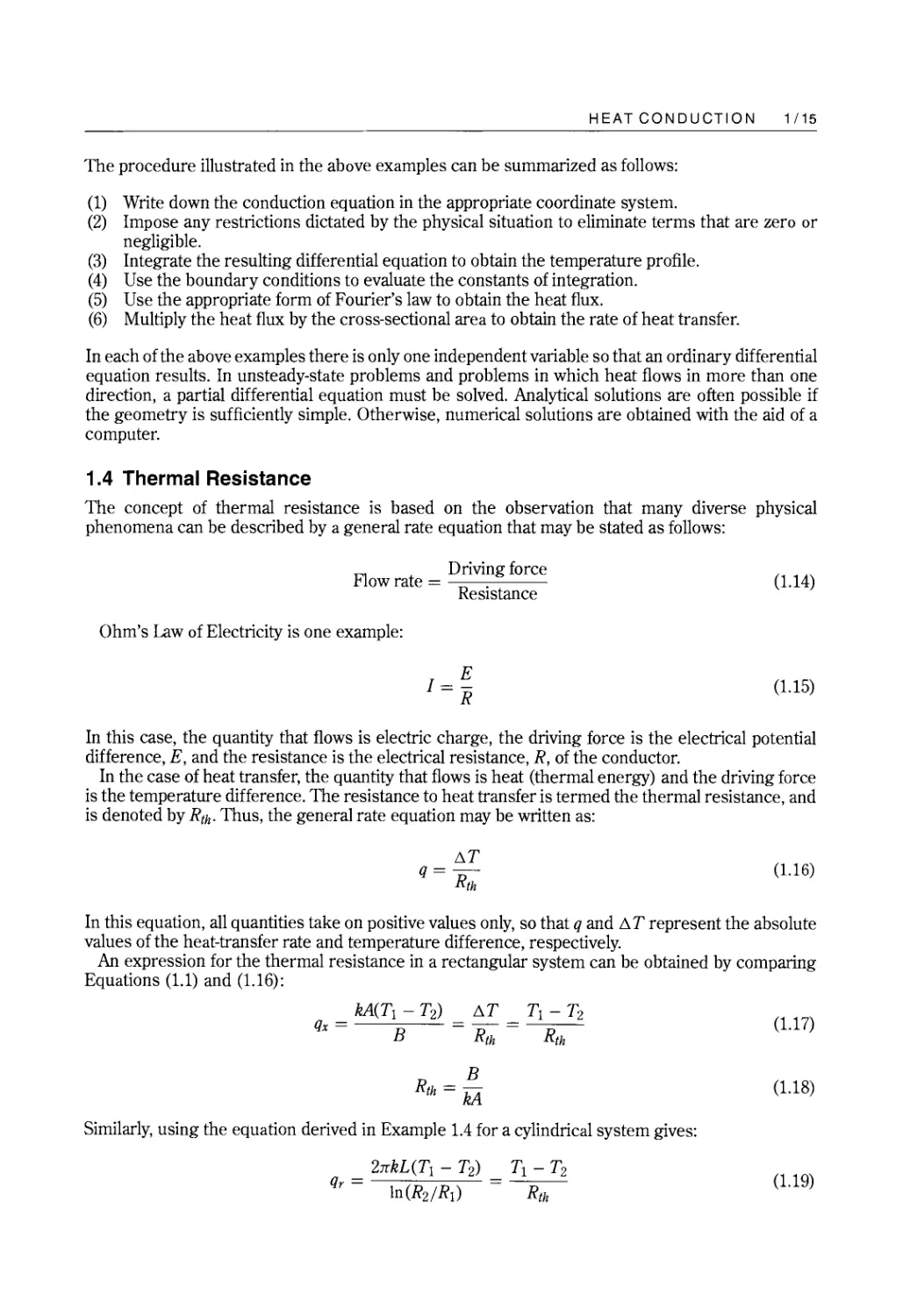
Table 1.2 Expressions for Thermal Resistance
Configuration
Conduction, Cartesian
coordinates
Rth
BlkA
Conduction, radial direction,
cylindrical coordinates
Conduction, radial direction,
spherical coordinates
Conduction, shape factor
Convection, un-finned surface
In (R 2 IR 1 )
2JT:kL
R 2 - Rl
4JT:k RIR2
Convection, finned surface
l/kS
l/hA
1
h7]wA
S = shape factor
h = heat-transfer coefficient
7]w = weighted efficiency of finned surface = + 7] Af
p + f
Ap = prime surface area
Af = fin surface area
7]f = fin efficiency
R _ In(R z IR 1 )
th - 2TrkL
These results, along with a number of others that will be considered subsequently, are summarized
in Table 1.2. When k cannot be assumed constant, the average thermal conductivity, as defined in
the previous section, should be used in the expressions for thermal resistance.
The thermal resistance concept permits some relatively complex heat-transfer problems to be
solved in a very simple manner. The reason is that thermal resistances can be combined in the
same way as electrical resistances. Thus, for resistances in series, the total resistance is the sum of
the individual resistances:
(1.20)
RTot = LRi
(1.21)
Likewise, for resistances in parallel:
RT" = ( l/Ri)-1
(1.22)
Thus, for the composite solid shown in Figure 1.3, the thermal resistance is given by:
Rth = R A + RBC + RD
(1.23)
where RBc, the resistance of materials Band C in parallel, is:
-1 RBRc
RBC = (lIRB + 11Rc) = R R
B+ C
(1.24)
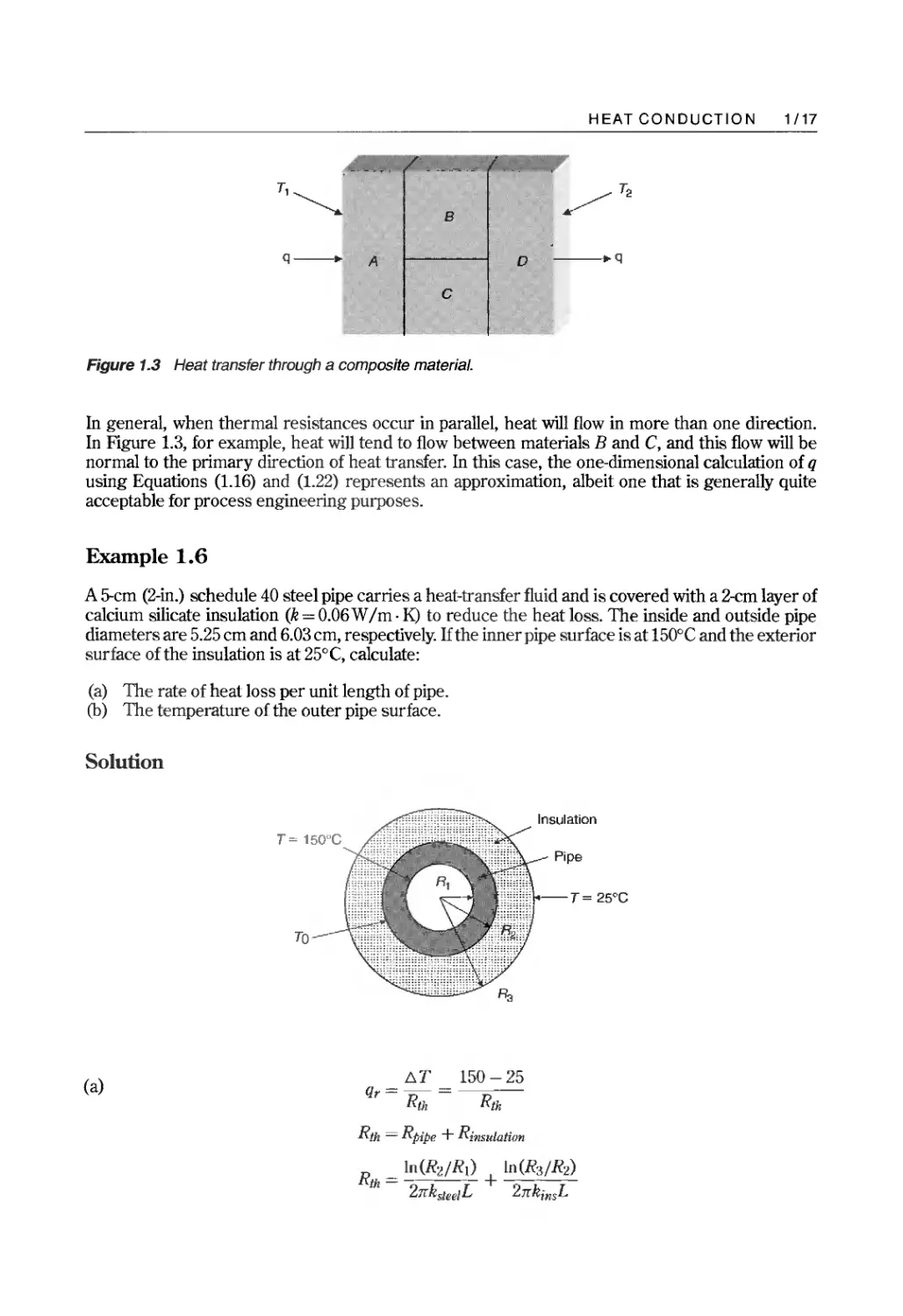
HEAT CONDUCTION 1/17
T1 B T2
q- A D . q
C
Figure 1.3 Heat transfer through a composite material.
In general, when thermal resistances occur in parallel, heat will flow in more than one direction.
In Figure 1.3, for example, heat will tend to flow between materials B and C, and this flow will be
normal to the primary direction of heat transfer. In this case, the one-dimensional calculation of q
using Equations (1.16) and (1.22) represents an approximation, albeit one that is generally quite
acceptable for process engineering purposes.
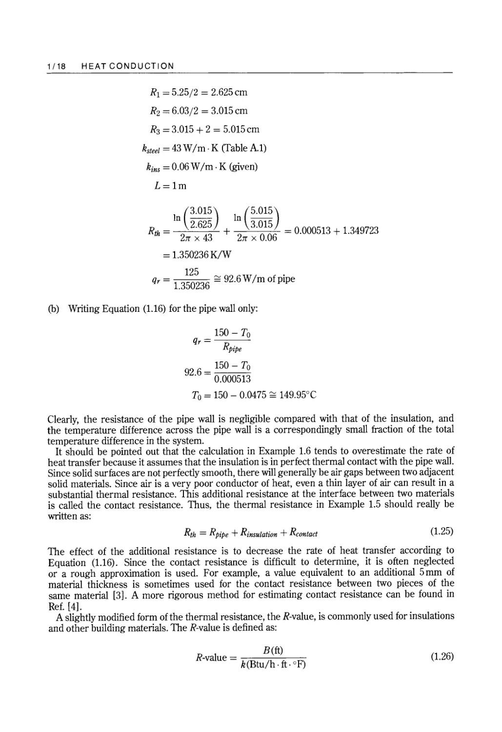
Example 1.6
A 5-cm (2-in.) schedule 40 steel pipe carries a heat-transfer fluid and is covered with a 2-cm layer of
calcium silicate insulation (k = 0.06W 1m. K) to reduce the heat loss. The inside and outside pipe
diameters are 5.25 cm and 6.03 cm, respectively. If the inner pipe surface is at 150°C and the exterior
surface of the insulation is at 25°C, calculate:
(a) The rate of heat loss per unit length of pipe.
(b) The temperature of the outer pipe surface.
Solution
TO
T = 25°C
T = 150°C
(a)
1:,.1'
qr = - =
Rill
150 - 25
Rtll
Rtll = Rpipe + Rillsulatiilll
Rth = ( R2/R 12 + (R3/R2 2
2Jrk stee iL 2JrkinsL
1/18 HEAT CONDUCTION
Rl = 5.25/2 = 2.625cm
Rz = 6.03/2 = 3.015 cm
R3 = 3.015 + 2 = 5.015 cm
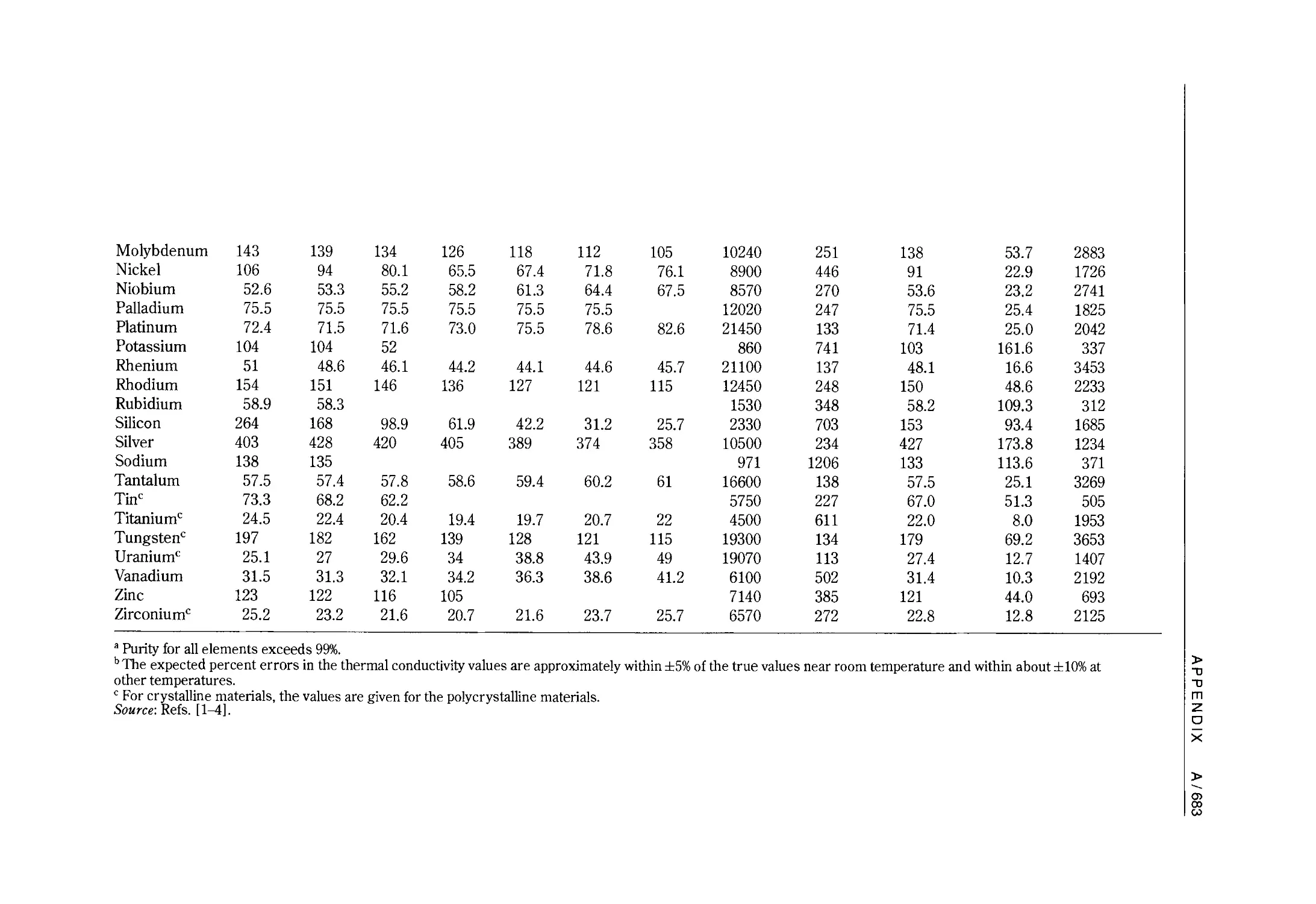
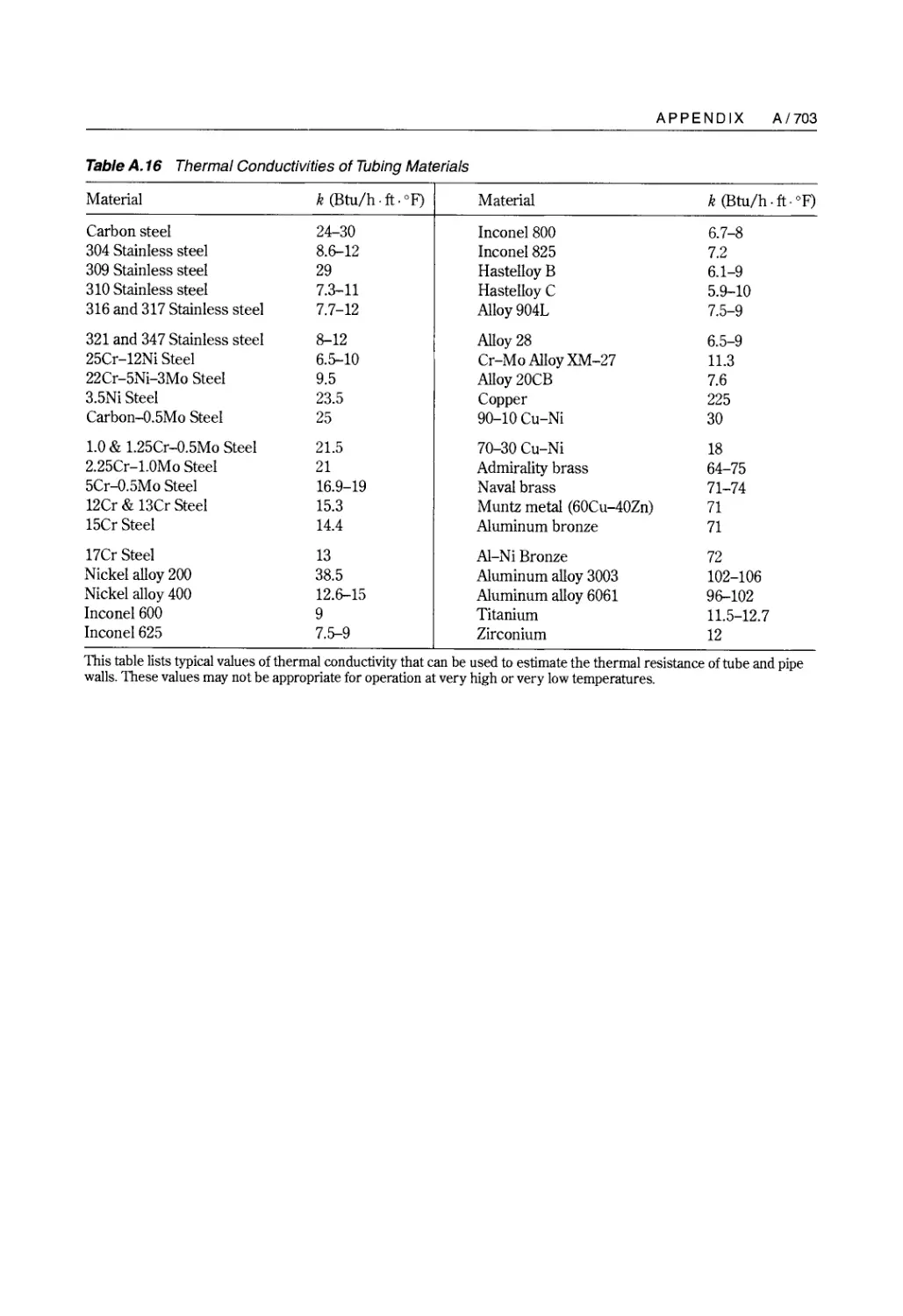
ksteet = 43 W 1m. K (Table AI)
k ins = 0.06 W 1m. K (given)
L=lm
In ( 3.015 ) In ( 5.015 )
Rth = 2Jl2 6 + 2Jl" ' 6 = 0.000513 + 1.349723
= 1.350236 K/W
qr = 1.3 36 92.6 W 1m of pipe
(b) Writing Equation (1.16) for the pipe wall only:
150 - To
qr =
Rpipe
150 - To
92.6 = 0.000513
To = 150 - 0.0475 149.95°C
Clearly, the resistance of the pipe wall is negligible compared with that of the insulation, and
the temperature difference across the pipe wall is a correspondingly small fraction of the total
temperature difference in the system.
It should be pointed out that the calculation in Example 1.6 tends to overestimate the rate of
heat transfer because it assumes that the insulation is in perfect thermal contact with the pipe wall.
Since solid surfaces are not perfectly smooth, there will generally be air gaps between two adjacent
solid materials. Since air is a very poor conductor of heat, even a thin layer of air can result in a
substantial thermal resistance. This additional resistance at the interface between two materials
is called the contact resistance. Thus, the thermal resistance in Example 1.5 should really be
written as:
Rth = RpiPe + Rinsutation + Rcontact
(1. 25)
The effect of the additional resistance is to decrease the rate of heat transfer according to
Equation (1.16). Since the contact resistance is difficult to determine, it is often neglected
or a rough approximation is used. For example, a value equivalent to an additional 5 mm of
material thickness is sometimes used for the contact resistance between two pieces of the
same material [3]. A more rigorous method for estimating contact resistance can be found in
Ref. [4].
A slightly modified form of the thermal resistance, the R-value, is commonly used for insulations
and other building materials. The R-value is defined as:
B(ft)
R-value= k(Btu/h.ft.oF)
(1. 26)
HEAT CONDUCTION 1/19
where B is the thickness of the material and k is its thermal conductivity. Comparison with Equation
(1.18) shows that the R-value is the thermal resistance, in English units, of a slab of material having
a cross-sectional area of 1 ft2. Since the R-value is always given for a specified thickness, the thermal
conductivity of a material can be obtained from its R-value using Equation (1.26). Also, since R-values
are essentially thermal resistances, they are additive for materials arranged in series.
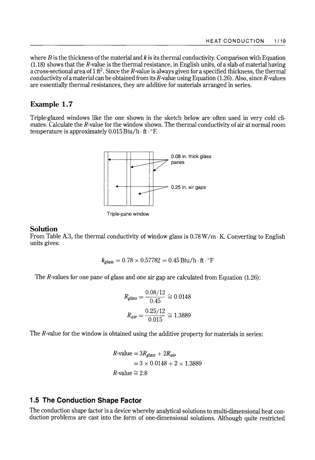
Example 1.7
Triple-glazed windows like the one shown in the sketch below are often used in very cold cli-
mates. Calculate the R-value for the window shown. The thermal conductivity of air at normal room
temperature is approximately 0.015 Btu/h. ft. oF.
0.08 in. thick glass
panes
0.25 in. air gaps
Triple-pane window
Solution
From Table A.3, the thermal conductivity of window glass is 0.78W /m. K. Converting to English
units gives:
k glass = 0.78 x 0.57782 = 0.45 Btu/h. ft. OF
The R-values for one pane of glass and one air gap are calculated from Equation (1.26):
0.08/12 '"
Rgl ass = 0.45 = 0.0148
0.25/12 '"
R air = 0.015 = 1.3889
The R-value for the window is obtained using the additive property for materials in series:
R-value = 3R g l ass + 2R a ir
= 3 x 0.0148 + 2 x 1.3889
R-value ;:: 2.8
1.5 The Conduction Shape Factor
The conduction shape factor is a device whereby analytical solutions to multi-dimensional heat con-
duction problems are cast into the form of one-dimensional solutions. Although quite restricted
1/20 HEAT CONDUCTION
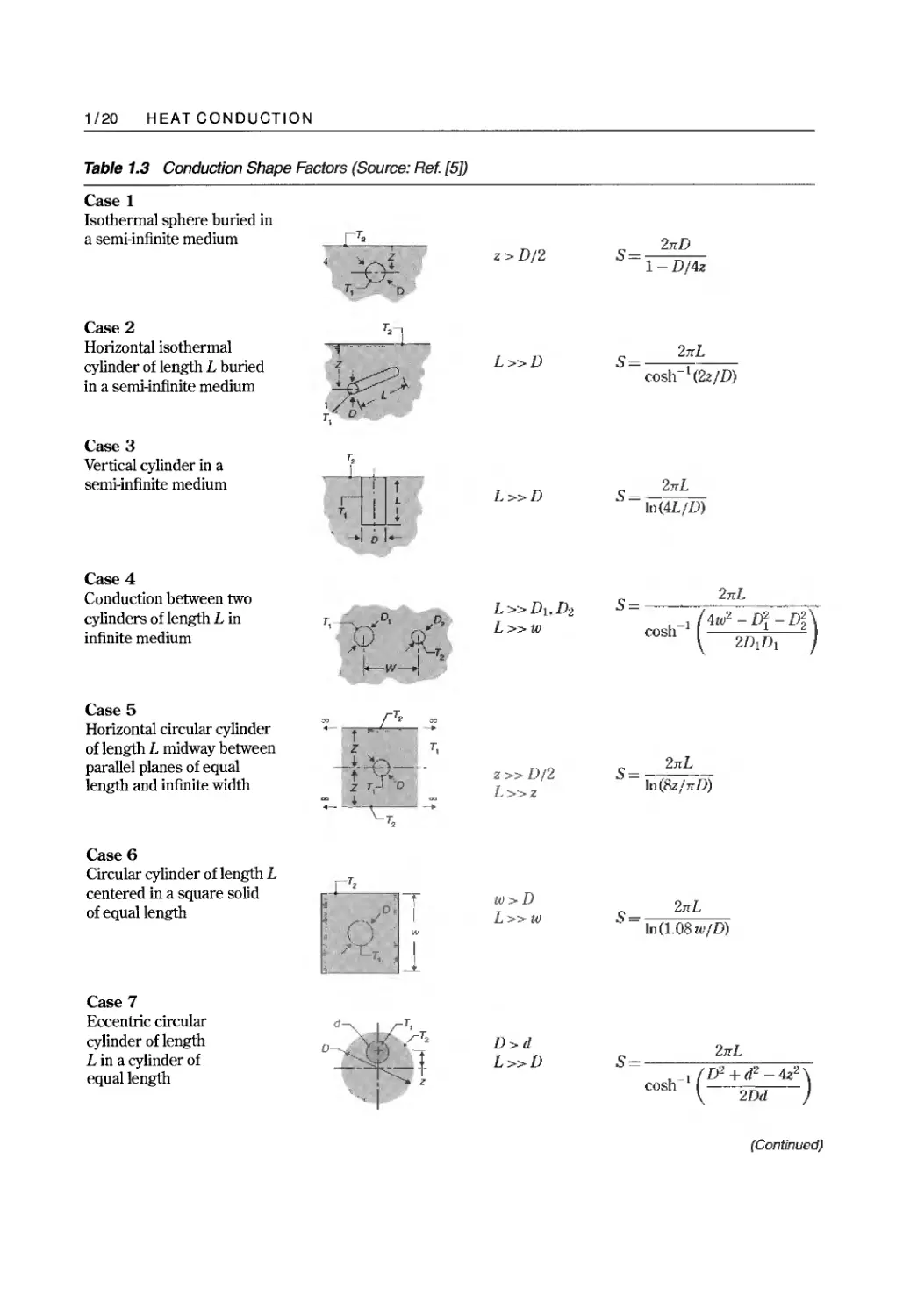
Table 1.3 Conduction Shape Factors (Source: Ref. [5])
Case 1
Isothermal sphere buried in
a semi-infinite medium
Case 2
Horizontal isothermal
cylinder of length L buried
in a semi-infinite medium
Case 3
Vertical cylinder in a
semi-infinite medium
Case 4
Conduction between two
cylinders of length L in
infinite medium
Case 5
Horizontal circular cylinder
of length L midway between
parallel planes of equal
length and infinite width
Case 6
Circular cylinder of length L
centered in a square solid
of equal length
Case 7
Eccentric circular
cylinder of length
L in a cylinder of
equal length
-T.
. -+
'-- "
T, D
T. I
"1
Z
j --;::: .'...
'''/L-
, / '\<----
, 0
T,
.
:Jilt
t, w t
.1 I..
T, y ...0, ..02
.. ,V :1)
.. T.
w-J 2
-;
t . ...
Z T,
ot_ -,_
t ....-r..._
z T,- 0
': _ _t
\.. T.
...
- T.
I ,.--:;:-
1 ,{D "
., L ·
T, .
.i
0__.. I r T . ,
-"-k - r T .
o y +. '-
. - f-
o .... z
I
z> D/2
L»D
L»D
L»D 1 .D 2
L»w
z» Dj2
L»z
w>D
L»w
D>d
L»D
s= 2nD
1- D/4z
S= L_
COSh-I (2zID)
s= _2nL_
In (4LI[))
s = 2nL _ _ _
I -I ( 4W2 - Di - D )
cos 1 2DIDI
2nL
S= - - - -
Inl8zlnl.J)
s = 2n L
In (1.08 wiD)
s=
2:rrL
_I ( 0 2 + d 2 - 4z 2 )
2Dd
cosh
(Continued)
HEAT CONDUCTION 1/21
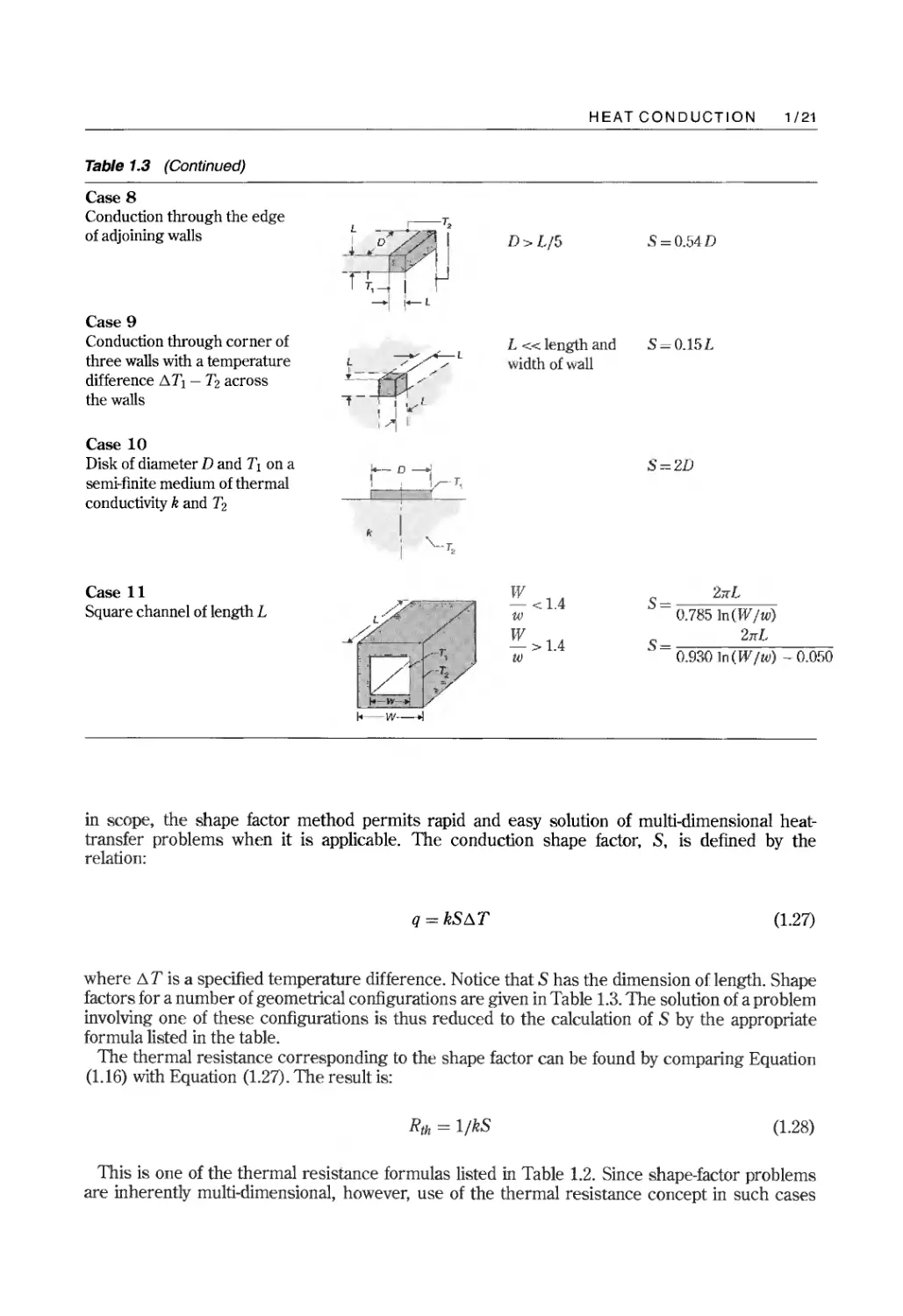
Table 1.3 (Continued)
Case 8
Conduction through the edge
of adjoining walls
Case 9
Conduction through corner of
three walls with a temperature
difference Tl - T 2 across
the walls
Case 10
Disk of diameter D and Tl on a
semi-finite medium of thermal
conductivity k and T 2
Case 11
Square channel of length L
-T.
L >';/" i
j '" ,/( I
-- t '. rJ
i T,--f
D>LI5
S=0.54D
I+-l
---+' ,...- l
l .,"/'"
-- . -
- - - .jJ-"
l' - ,- I ,.:-L
?'
L « length and
width of wall
5=0.15L
i""'-D----, T
r <
I I T _
S = 21J
"
'\.....T 2
/."'.'0 --:-
l" -.
/,
. .'
W
-<1.4
w
W
- > 1.4
w
S= '27<:L
O.785In(Wjw)
s= 2][L
0.930 In (W Iw) - 0.050
. r-=; . -T,
t . ./
fo""'--:-Oi /
I< w--->l
in scope, the shape factor method permits rapid and easy solution of multi-dimensional heat-
transfer problems when it is applicable. The conduction shape factor, S, is defined by the
relation:
q = kS T
(1.27)
where T is a specified temperature difference. Notice that S has the dimension of length. Shape
factors for a number of geometrical configurations are given in Table 1.3. The solution of a problem
involving one of these configurations is thus reduced to the calculation of S by the appropriate
formula listed in the table.
The thermal resistance corresponding to the shape factor can be found by comparing Equation
(1.16) with Equation (1.27). The result is:
Rth = IlkS
(1.28)
This is one of the thermal resistance formulas listed in Table 1.2. Since shape-factor problems
are inherently multi-dimensional, however, use of the thermal resistance concept in such cases
1/22 HEAT CONDUCTION
will, in general, yield only approximate solutions. Nevertheless, these solutions are usually entirely
adequate for process engineering calculations.
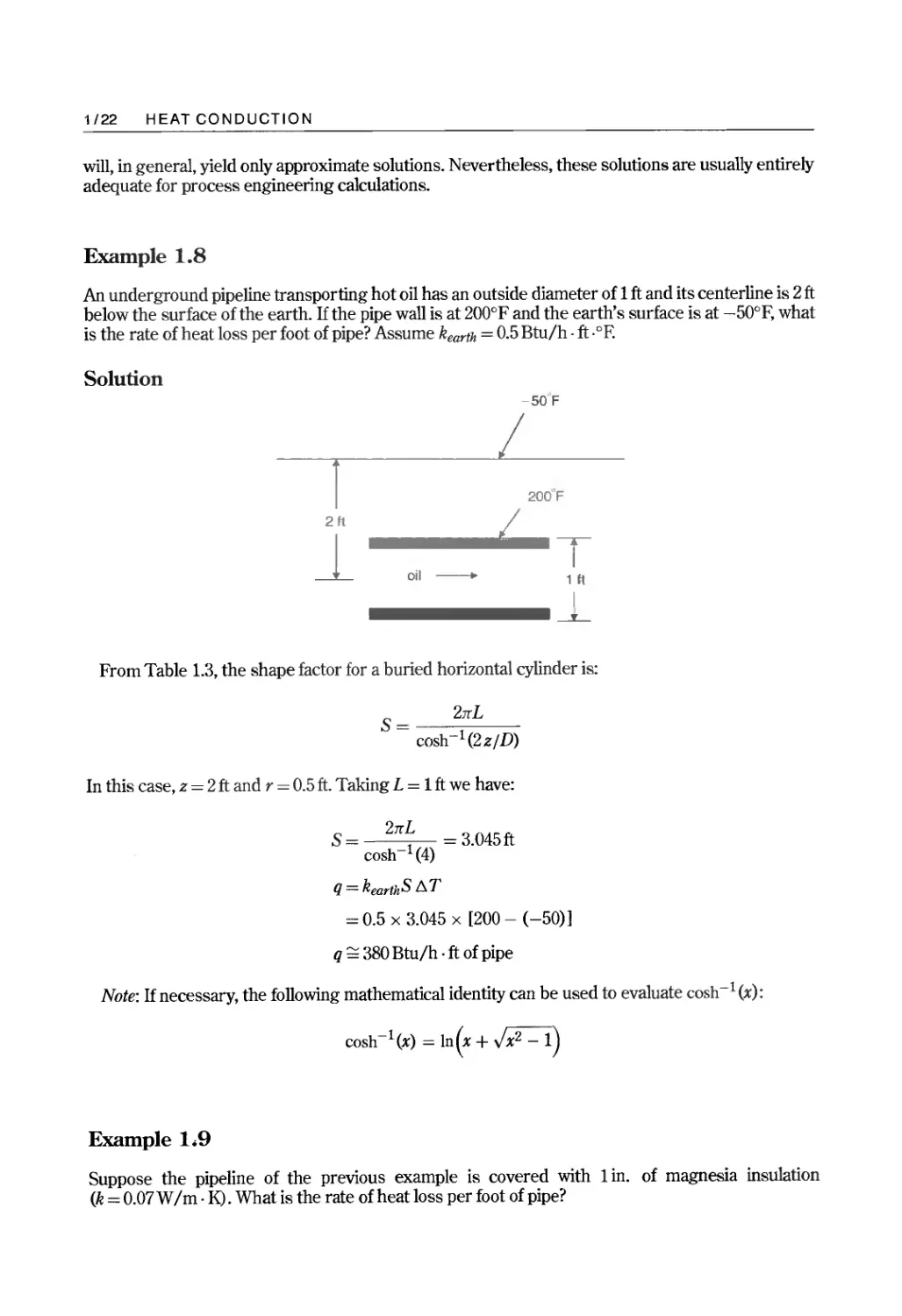
Example 1.8
An underground pipeline transporting hot oil has an outside diameter of 1 ft and its centerline is 2 ft
below the surface of the earth. If the pipe wall is at 200°F and the earth's surface is at -50°F, what
is the rate of heat loss perfoot of pipe? Assume kearth = 0.5 Btu/h . ft.°F.
Solution
i
2ft
-50 F
/
200F
I
T
oil-
1 f1
I
---L...
From Table 1.3, the shape factor for a buried horizontal cylinder is:
s = 2:rrL
cosh- l (2 zjD)
In this case, z = 2 ft and r = 0.5 ft. Taking L = 1 ft we have:
s = 2:rrL = 3.045 ft
cosh- l (4)
q = kearthS I1T
= 0.5 x 3.045 x [200 - (-50)]
q 380 Btu/h . ft of pipe
Note: If necessary, the following mathematical identity can be used to evaluate cosh- l (x):
COSh-l(X) = In (x + Jx 2 -1)
Example 1.9
Suppose the pipeline of the previous example is covered with 1 in. of magnesia insulation
(k =0.07W/m. K). What is the rate of heat loss per foot of pipe?
HEAT CONDUCTION 1/23
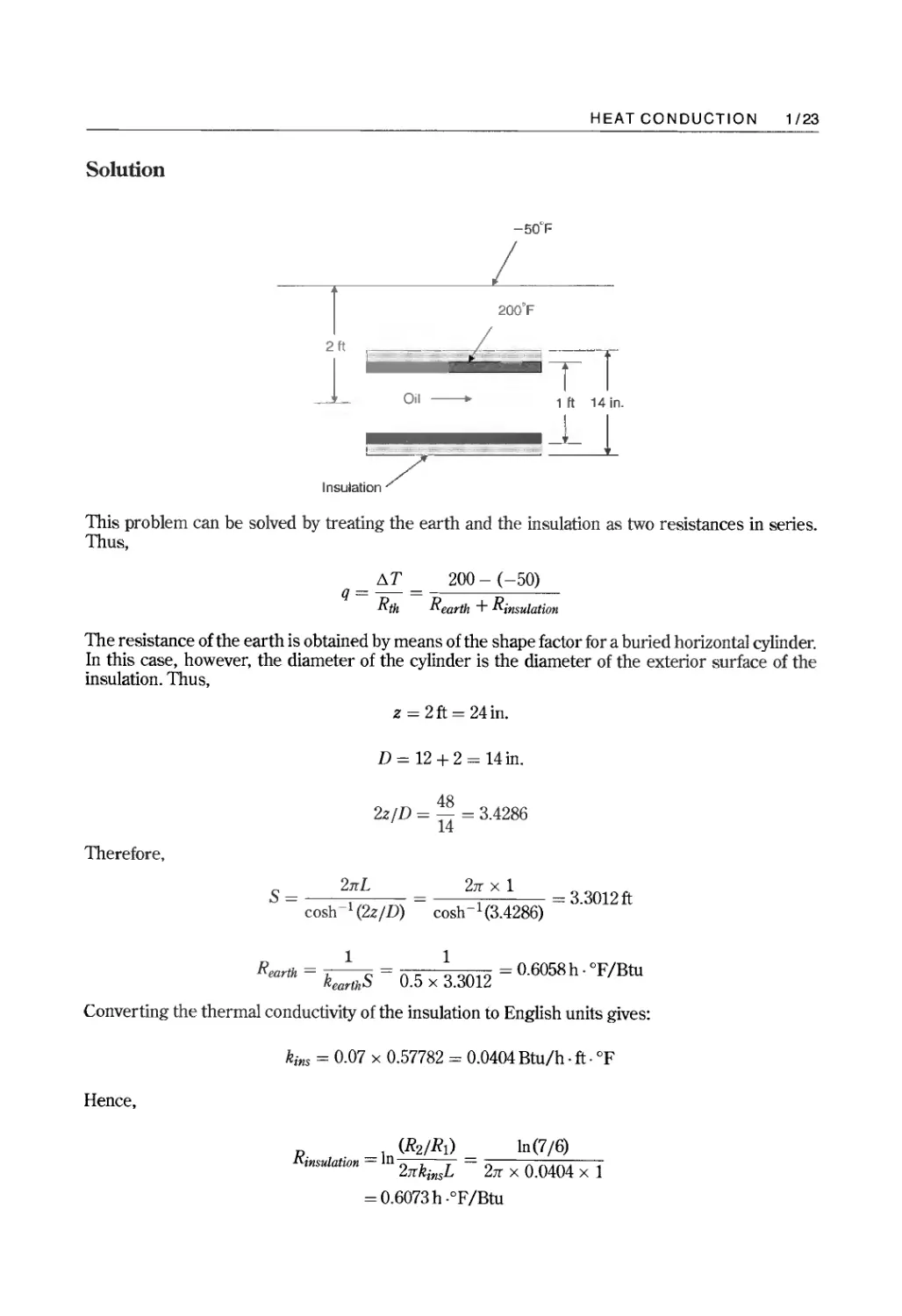
Solution
-50<F
r
2ft
l_
/
200'F
I-
T T
1 It 14 in.
Oil-
I
InSulati on. 7
This problem can be solved by treating the earth and the insulation as two resistances in series.
Thus,
!::"T 200 - (-50)
q---
- Rth - Rearth + Rinsulation
The resistance of the earth is obtained by means of the shape factor for a buried horizontal cylinder.
In this case, however. the diameter of the cylinder is the diameter of the exterior surface of the
insulation. Thus,
z = 2ft = 24 in.
D = 12 + 2 = 14 in.
48
2z/D = 14 = 3.4286
Therefore.
s = 2nL
cosh 1 (2z / D)
2n x 1 = 3.3012 ft
cosh -1 (3.4286)
Rearth = kea thS = 0.5 x .3012 = 0.6058 h . of /Btu
Converting the thermal conductivity of the insulation to English units gives:
k ins = 0.07 x 0.57782 = 0.0404 Btu/h . ft. of
Hence,
(R z /R 1 ) In (7 /6)
Rinsulation = In 2nkinsL = 2n x 0.0404 x 1
= 0.6073h .oF/Btu
1/24 HEAT CONDUCTION
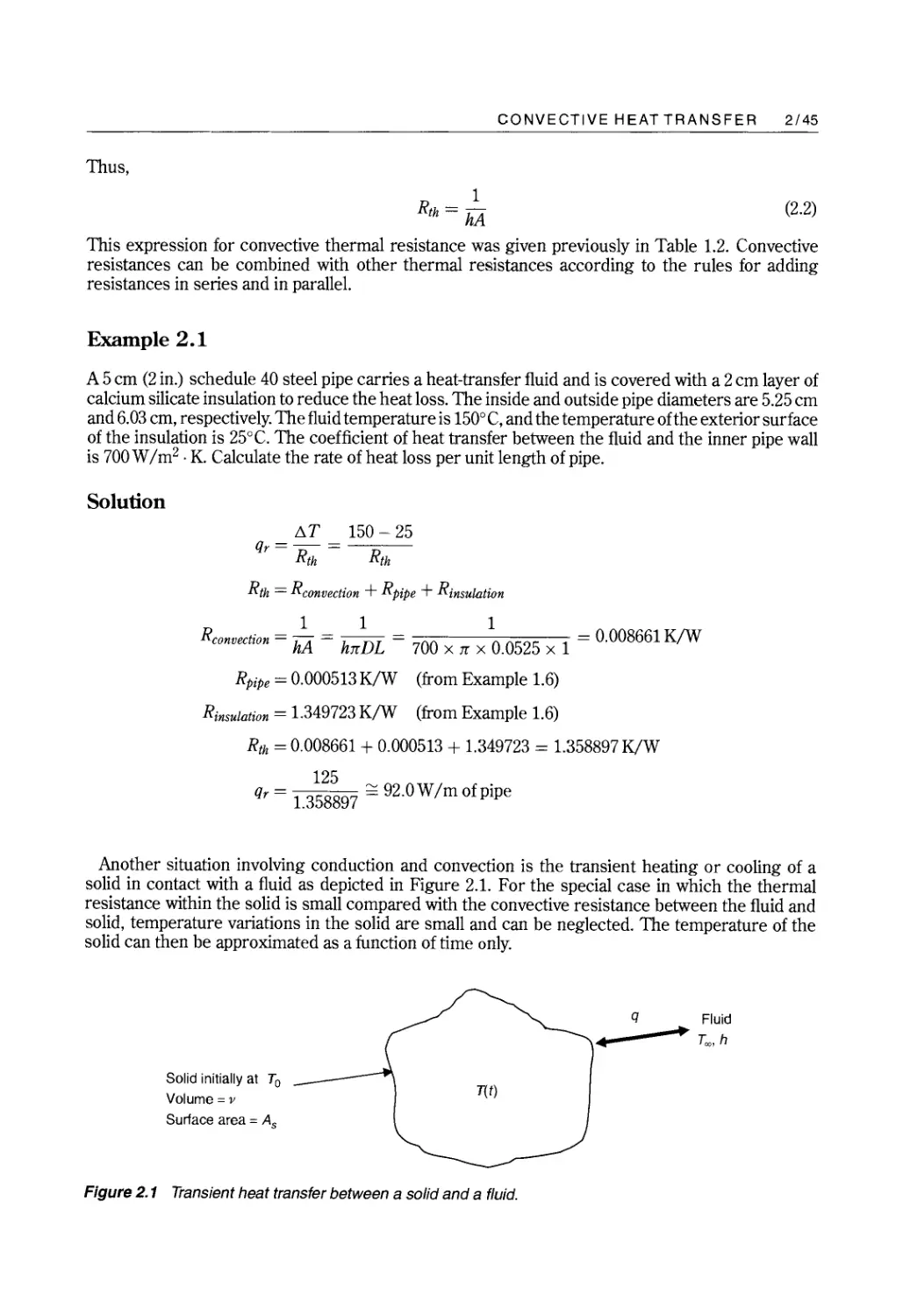
To infinity
Solid initially at To
qx
x
Surface at Ts
To infinity
To infinity
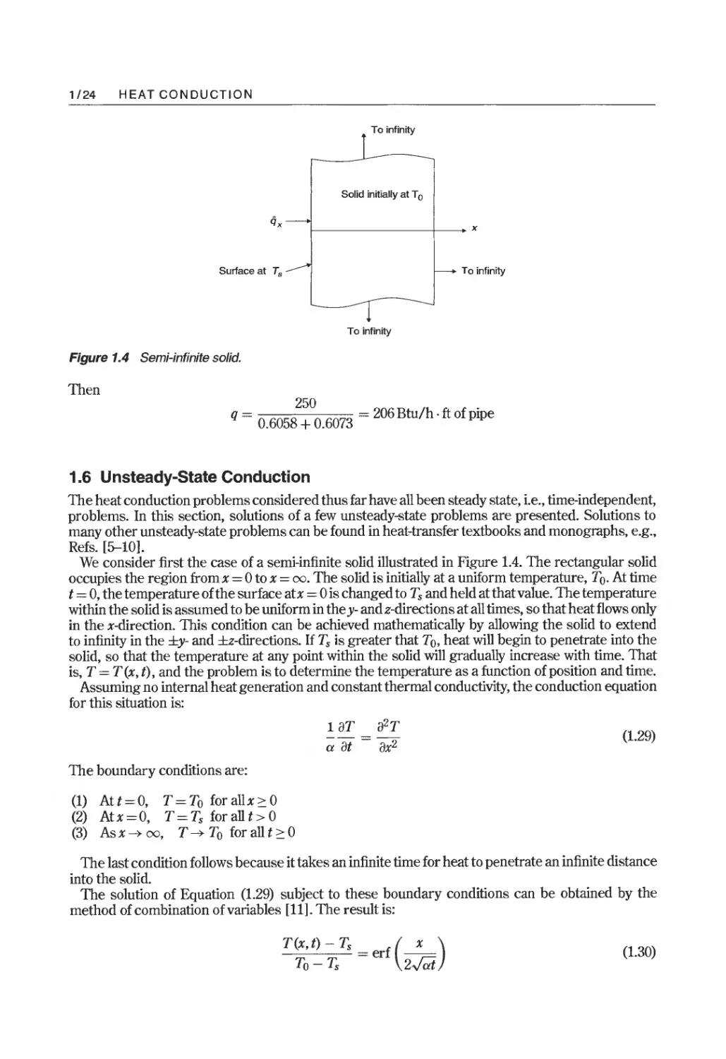
Figure 1.4 Semi-infinite solid.
Then
250
q = 0.6058 + 0.6073 = 206 Btu/h . ft of pipe
1.6 Unsteady-State Conduction
The heat conduction problems considered thus far have all been steady state, Le., time-independent,
problems. In this section, solutions of a few unsteady-state problems are presented. Solutions to
many other unsteady-state problems can be found in heat-transfer textbooks and monographs, e.g.,
Refs. [5-10].
We consider first the case of a semi-infinite solid illustrated in Figure 1.4. The rectangular solid
occupies the region from x = 0 to x = 00. The solid is initially at a uniform temperature, To. At time
t = 0, the temperature ofthe surface atx = 0 is changed to Ts and held atthatvalue. The temperature
within the solid is assumed to be uniform in the y- and z-directions at all times, so that heat flows only
in the x-direction. This condition can be achieved mathematically by allowing the solid to extend
to infinity in the y- and :I::z-directions. If Ts is greater that To, heat will begin to penetrate into the
solid, so that the temperature at any point within the solid will gradually increase with time. That
is. T = T(x, t), and the problem is to determine the temperature as a function of position and time.
Assuming no internal heat generation and constant thermal conductivity, the conduction equation
for this situation is:
1 aT a 2 T
---
a at ax 2
(1.29)
The boundary conditions are:
(1) At t = 0, T = To for all x :::: 0
(2) Atx=O, T=Ts forallt> 0
(3) As x 00, T To for all t :::: 0
The last condition follows because it takes an infinite time for heat to penetrate an infinite distance
into the solid.
The solution of Equation (1.29) subject to these boundary conditions can be obtained by the
method of combination of variables [11]. The result is:
T(x, t) - Ts = erf ( )
To - Ts 2M
(1.30)
HEAT CONDUCTION 1/25
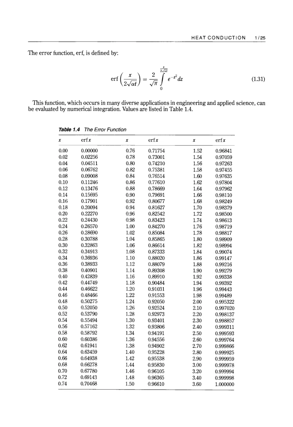
The error function, erf, is defined by:
x
2M
erf ( 2 ) = f e z2dz (1.31)
0
This function, which occurs in many diverse applications in engineering and applied science, can
be evaluated by numerical integration. Values are listed in Table 1.4.
Table 1.4 The Error Function
x erfx x erfx x erfx
0.00 0.00000 0.76 0.71754 1.52 0.96841
0.02 0.02256 0.78 0.73001 1.54 0.97059
0.04 0.04511 0.80 0.74210 1.56 0.97263
0.06 0.06762 0.82 0.75381 1.58 0.97455
0.08 0.09008 0.84 0.76514 1.60 0.97635
0.10 0.11246 0.86 0.77610 1.62 0.97804
0.12 0.13476 0.88 0.78669 1.64 0.97962
0.14 0.15695 0.90 0.79691 1.66 0.98110
0.16 0.17901 0.92 0.80677 1.68 0.98249
0.18 0.20094 0.94 0.81627 1.70 0.98379
0.20 0.22270 0.96 0.82542 1.72 0.98500
0.22 0.24430 0.98 0.83423 1.74 0.98613
0.24 0.26570 1.00 0.84270 1.76 0.98719
0.26 0.28690 1.02 0.85084 1.78 0.98817
0.28 0.30788 1.04 0.85865 1.80 0.98909
0.30 0.32863 1.06 0.86614 1.82 0.98994
0.32 0.34913 1.08 0.87333 1.84 0.99074
0.34 0.36936 1.10 0.88020 1.86 0.99147
0.36 0.38933 1.12 0.88079 1.88 0.99216
0.38 0.40901 1.14 0.89308 1.90 0.99279
0.40 0.42839 1.16 0.89910 1.92 0.99338
0.42 0.44749 1.18 0.90484 1.94 0.99392
0.44 0.46622 1.20 0.91031 1.96 0.99443
0.46 0.48466 1.22 0.91553 1.98 0.99489
0.48 0.50275 1.24 0.92050 2.00 0.995322
0.50 0.52050 1.26 0.92524 2.10 0.997020
0.52 0.53790 1.28 0.92973 2.20 0.998137
0.54 0.55494 1.30 0.93401 2.30 0.998857
0.56 0.57162 1.32 0.93806 2.40 0.999311
0.58 0.58792 1.34 0.94191 2.50 0.999593
0.60 0.60386 1.36 0.94556 2.60 0.999764
0.62 0.61941 1.38 0.94902 2.70 0.999866
0.64 0.63459 1.40 0.95228 2.80 0.999925
0.66 0.64938 1.42 0.95538 2.90 0.999959
0.68 0.66278 1.44 0.95830 3.00 0.999978
0.70 0.67780 1.46 0.96105 3.20 0.999994
0.72 0.69143 1.48 0.96365 3.40 0.999998
0.74 0.70468 1.50 0.96610 3.60 1. 000000
1/26 HEAT CONDUCTION
The heat flux is given by:
k(T s - To) 2
qx = ..;m;t exp (-X 1 4 at)
;rat
(1.32)
The total amount of heat transferred per unit area across the surface at x = 0 in time t is given by:
Q (T
A = 2k(T s - To)y
(1.33)
Although the semi-infinite solid may appear to be a purely academic construct, it has a number of
practical applications. For example, the earth behaves essentially as a semi-infinite solid. A solid
of any finite thickness can be considered a semi-infinite solid if the time interval of interest is
sufficiently short that heat penetrates only a small distance into the solid. The approximation is
generally acceptable if the following inequality is satisfied:
at
L2 < 0.1
(1.34)
where L is the thickness of the solid. The dimensionless group at / L 2 is called the Fourier number
and is designated Fo.
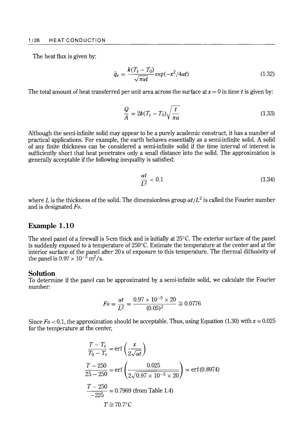
Example 1.10
The steel panel of a firewall is 5-cm thick and is initially at 25°C. The exterior surface of the panel
is suddenly exposed to a temperature of 250°C. Estimate the temperature at the center and at the
interior s rface of the fane! after 20 s of exposure to this temperature. The thermal diffusivity of
the panells 0.97 x 10- m 2 Is.
Solution
To determine if the panel can be approximated by a semi-infinite solid, we calculate the Fourier
number:
Fo = at = 0.97 x 10- 5 x 20 0.0776
L2 (0.05)2
Since Fo < 0.1, the approximation should be acceptable. Thus, using Equation (1.30) with x = 0.025
for the temperature at the center,
T-T s f( x )
-er -
To - Ts - 2.Jai
T - 250 = erf ( 0.025 ) = erf(0.8974)
25 - 250 2 V O.97 x 10- 5 x 20
T - 250
5 = 0.7969 (from Table 1.4)
-22
T 70.7°C
HEAT CONDUCTION 1/27
To infinity
Solid initially at To
qx
-qx
x
25
Ts
Ts
To infinity
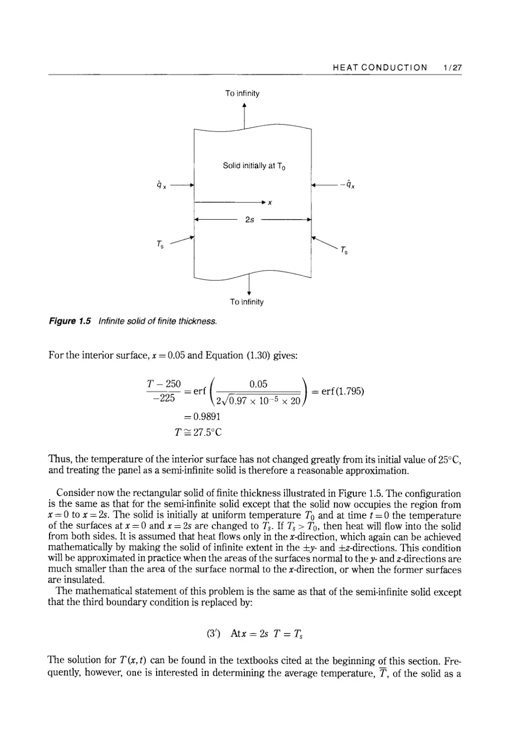
Figure 1.5 Infinite solid of finite thickness.
For the interior surface, x = 0.05 and Equation (1.30) gives:
T - 250 = erf ( 0.05 ) = erf(1.795)
-225 2 ) 0.97 x 1O 5 x 20
= 0.9891
T 27.5°C
Thus, the temperature of the interior surface has not changed greatly from its initial value of 25°C,
and treating the panel as a semi-infinite solid is therefore a reasonable approximation.
Consider now the rectangular solid of finite thickness illustrated in Figure 1.5. The configuration
is the same as that for the semi-infinite solid except that the solid now occupies the region from
x = 0 to x = 2s. The solid is initially at uniform temperature To and at time t = 0 the temperature
of the surfaces at x = 0 and x = 2s are changed to Ts. If Ts > To, then heat will flow into the solid
from both sides. It is assumed that heat flows only in the x-direction, which again can be achieved
mathematically by making the solid of infinite extent in the :!:y- and :!:z-directions. This condition
will be approximated in practice when the areas of the surfaces normal to the y- and z-directions are
much smaller than the area of the surface normal to the x-direction, or when the former surfaces
are insulated.
The mathematical statement of this problem is the same as that of the semi-infinite solid except
that the third boundary condition is replaced by:
(3') Atx = 2s T = Ts
The solution for T(x, t) can be found in the textbooks cited at the beginning of this section. Fre-
quently, however, one is interested in determining the average temperature, T, of the solid as a
1/28
HEAT CONDUCTION
function of time, where:
2s
- I f
T(t) = 2s T(x, t)dx
o
(1.35)
That is, T is the temperature averaged over the thickness of the solid at a given instant of time. The
solution for T is in the form of an infinite series [12]:
Ts - T
Ts - To
8 1 1
_(e- aFo + _e-9aFo + _e-25aFo + ... )
Jr2 9 25
(1.36)
where a = (Jr/2) 2 2.4674 and Fo=at/s 2 .
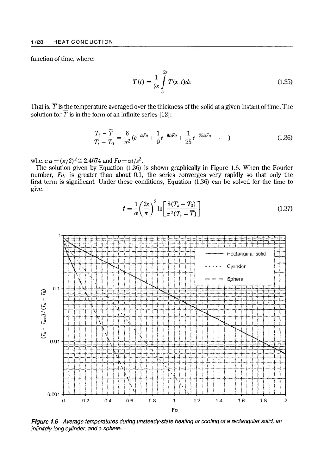
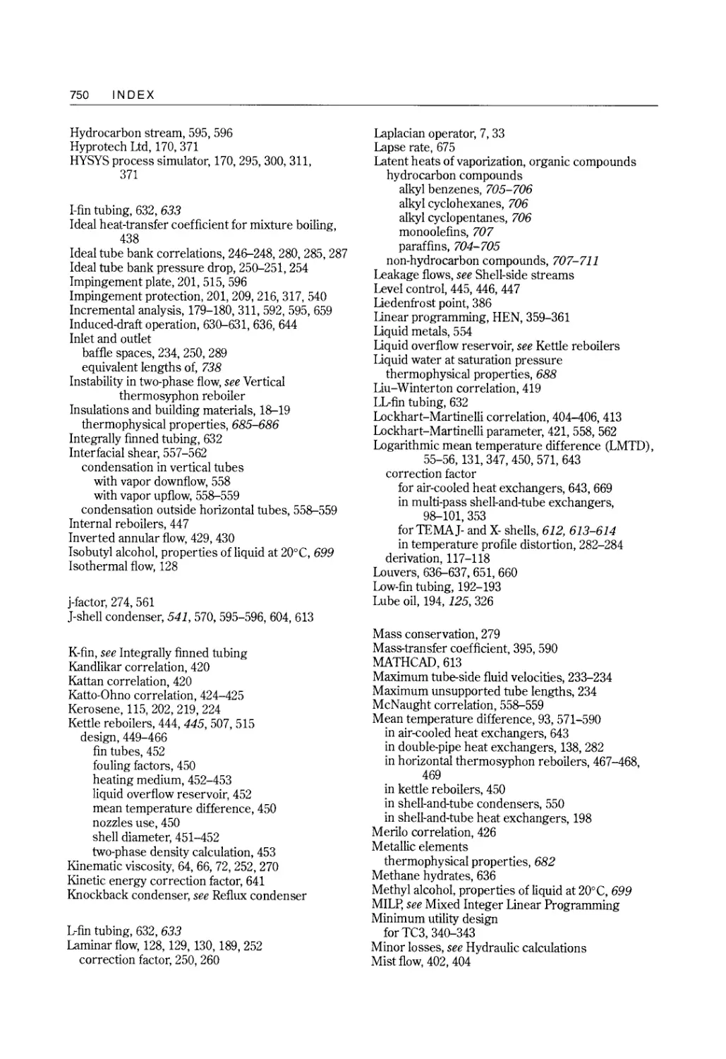
The solution given by Equation (1.36) is shown graphically in Figure 1.6. When the Fourier
number, Fo, is greater than about 0.1, the series converges very rapidly so that only the
first term is significant. Under these conditions, Equation (1.36) can be solved for the time to
give:
t = ( 2S ) 2 In [ 8(Ts - T!?J ]
a Jr Jr2(Ts-T)
(1.37)
;::? 0.1
!
--
-
..
!-"
!
0.01
\ rtETtrtf tTIITIT tI]1Ltl@I\ f? t: : :t +::t :1::l.:fl::F? d : 'fF
, ',\ : . 1 , : i \ 1 : ; \ : , \ \ i ; , : i. - Rectangular soh :'
1Wt1 IEffiE1T 1EEf Cylmdel tf
i ''\ i , \ \ , : \ 1 :, :; I \ i ' I \ i. - - - Sphere : l
=ldd ::rl ;:ElJJ lddjd:l::++=1 t i: :::f t :ff;;rtTt ."i i ft J
i"l =t1\r ""t r , .... --t ""'", \..."+.-r', '"'''''r-+-{-- --r ) ....
_... ' _ ............. .....{,_.i--,........,----. ...--.+-.. .....J....--.....t._ ....................,.......... """"..{"""""'''-''''--+''''''''::''''''' ''-'' ''''''-''t''-'-"", """l......"..}....."--+.............l.."--..}........,,..,,--- ,,,.,,-
; \ ' . 1. \ > . > \ ' , , ' ; , , , ' , ,. ,: \ , . , I ' ' , , ; , < . : ,
............... ....... ....."- ....... "".............:.""....:-....... .................. ................,t...... ..-......}'-.........r-........ ...."\\,,-....:............................ ---r.. ...... ---, -}-r i..-
j. Lt. lt t..l . t ...rt iJ.....I:..t..t..t l...t::i.". t:t.t.. t: i.nt: "t: Lt..t rrl w. rt +
, ii, I 1\, ! , I , " i I : i \ ! : , I , , i \ : ,\ :'::' " ! \ i
\ ' , . . 1 ' ;. , ' : \ ' \ ' '___}_ ... : , .'" : ! :.
"""I-----".... .. .............."\.........,..............-...........--+.................................\.-......V-.... ................ ...."'....--r' _....,..... \ . 1.
! I : ! , ,\ i , I : !' { I ! ! i I : I : [ ! : 1 ! i ! ! , ' , i ; , ! ! !
j 1 i ! ! ! ; \[ ! ! ] i !. ! ! i ! i ! i ) i ! ! if! ! ! I ! : ! ! ! ! i !
0.001
o
0 .)
.
0.4
0.6
0.8
'1.2
1.4
16
1.8
2
Fa
Figure 1.6 Average temperatures during unsteady-state heating or cooling of a rectangular solid, an
infinitely long cylinder, and a sphere.
HEAT CONDUCTION 1/29
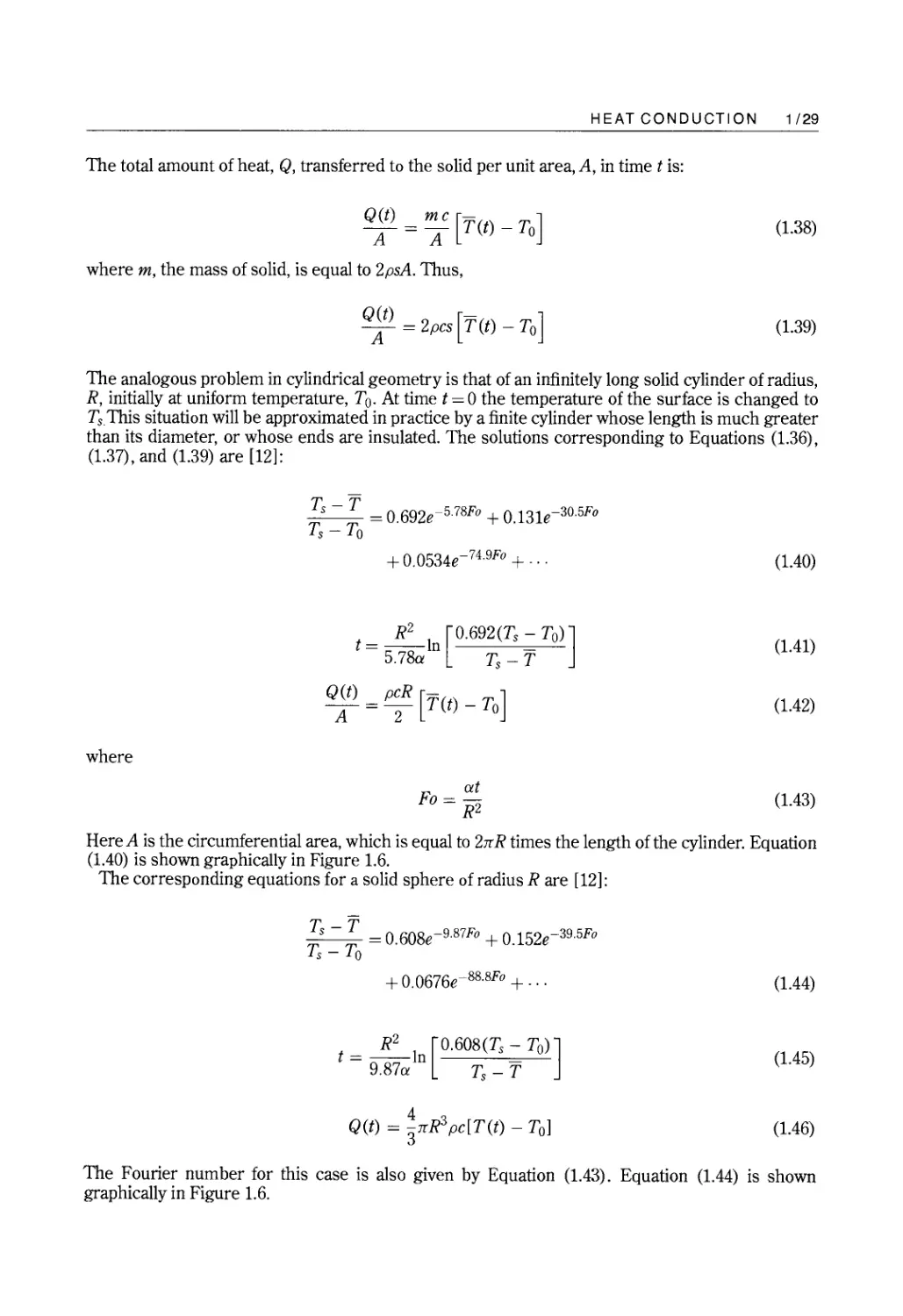
The total amount of heat, Q, transferred to the solid per unit area, A, in time tis:
Q t) = :c [T(t) _ To]
where m, the mass of solid, is equal to 2psA. Thus,
(1.38)
Q(t) [ -- ]
A = 2pcs T(t) - To
(1.39)
The analogous problem in cylindrical geometry is that of an infinitely long solid cylinder of radius,
R, initially at uniform temperature, To. At time t = ° the temperature of the surface is changed to
TsThis situation will be approximated in practice by a finite cylinder whose length is much greater
than its diameter, or whose ends are insulated. The solutions corresponding to Equations (1.36),
(1.37), and (1.39) are [12]:
;s -; = 0.692e-578Fo + 0.131e-30.5Fo
s - 0
+ 0.0534e-74.9Fo + .. .
(1.40)
R 2 [ 0.692(T s - To) ]
t=-ln
5.78a Ts - T
Q t) = p R [T(t) _ To]
(1.41)
(1.42)
where
Fo = at
R2
(1.43)
Here A is the circumferential area, which is equal to 2TrR times the length of the cylinder. Equation
(1.40) is shown graphically in Figure 1.6.
The corresponding equations for a solid sphere of radius R are [12]:
Ts - T = 0.608e-9.87Fo + 0. 152e-39.5Fo
Ts - To
+ 0.0676e-88.8Fo +.. .
(1.44)
t = ln [ 0.608(T s = To) ]
9.87a Ts - T
(1.45)
4
Q(t) = -TrR 3 pc[T(t) - To]
3
(1.46)
The Fourier number for this case is also given by Equation (1.43). Equation (1.44) is shown
graphically in Figure 1.6.
1/30 HEAT CONDUCTION
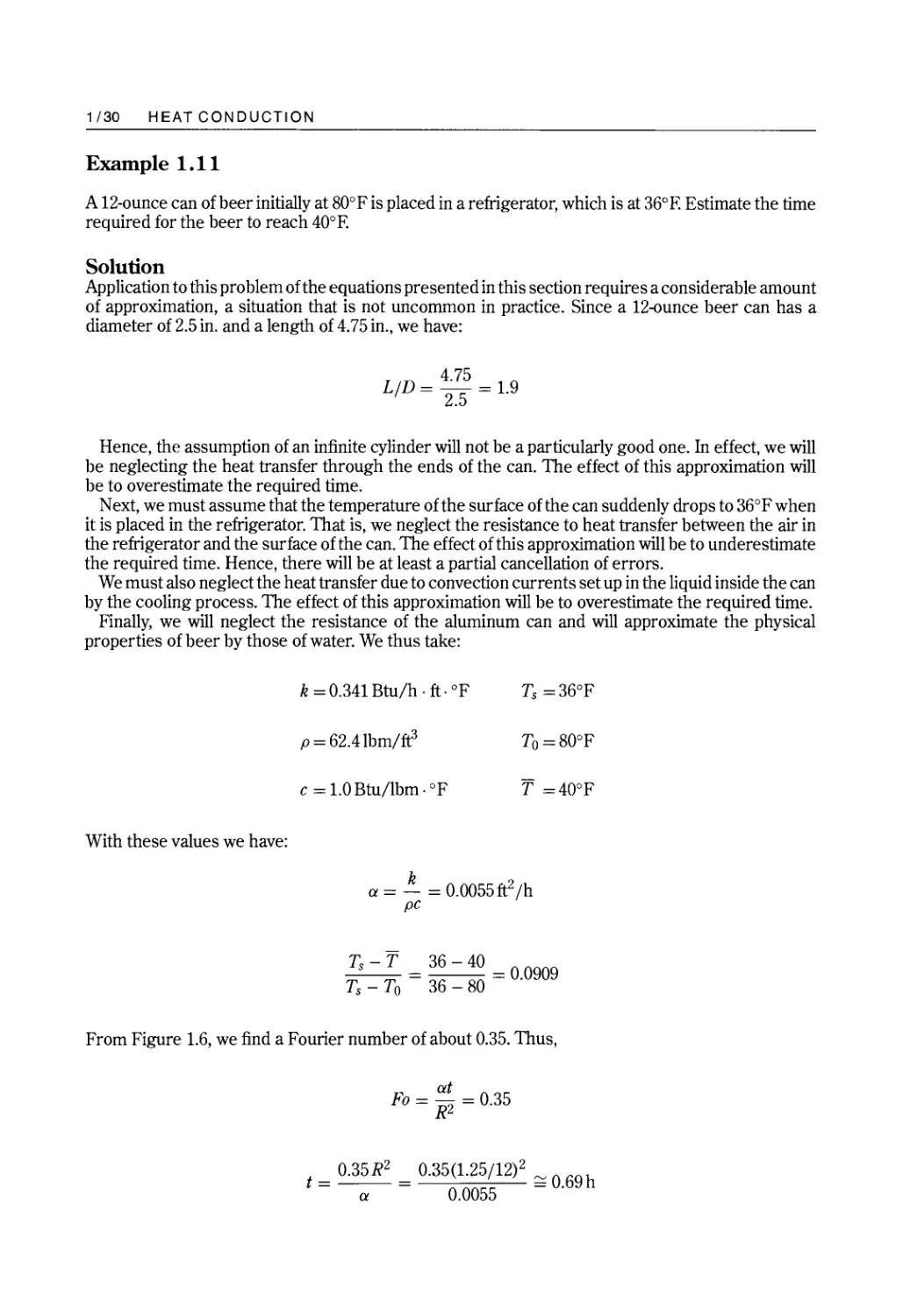
Example 1.11
A 12-ounce can of beer initially at 80°F is placed in a refrigerator, which is at 36°E Estimate the time
required for the beer to reach 40 0 E
Solution
Application to this pro blem of the equations presented in this section requires a considerable amount
of approximation, a situation that is not uncommon in practice. Since a 12-ounce beer can has a
diameter of 2.5 in. and a length of 4.75 in., we have:
L D = 4.75 = 9
1 2.5 1.
Hence, the assumption of an infinite cylinder will not be a particularly good one. In effect, we will
be neglecting the heat transfer through the ends of the can. The effect of this approximation will
be to overestimate the required time.
N ext, we must assume that the temperature ofthe surface of the can suddenly drops to 36°F when
it is placed in the refrigerator. That is, we neglect the resistance to heat transfer between the air in
the refrigerator and the surface of the can. The effect of this approximation will be to underestimate
the required time. Hence, there will be at least a partial cancellation of errors.
We must also neglect the heat transfer due to convection currents set up in the liquid inside the can
by the cooling process. The effect of this approximation will be to overestimate the required time.
Finally, we will neglect the resistance of the aluminum can and will approximate the physical
properties of beer by those of water. We thus take:
k = 0.341 Btu/h . ft. of
Ts = 36°F
p = 62.4lbm/ft 3
To = 80°F
c = 1.0 Btu/lbm . OF
T =40°F
With these values we have:
a = !!.. = 0.0055ft 2 /h
pc
Ts - T = 36 - 40 = 0.0909
Ts - To 36 - 80
From Figure 1.6, we find a Fourier number of about 0.35. Thus,
at
Fo = - = 0.35
R2
= 0.35R2 = 0.35(1.25/12)2 ;::; 0 69 h
t a 0.0055 .
HEAT CONDUCTION 1/31
Alternatively, since Fo > 0.1, we can use Equation (1.41):
t = ln [ O.692(Ts -= To) ]
5.78a Ts - T
(1.25/12)2 [ 0.629 ]
In -
5.78 x 0.0055 0.0909
t = 0.66 h
This agrees with the previous calculation to within the accuracy with which one can read the
graph of Figure 1.6. Experience suggests that this estimate is somewhat optimistic and, hence,
that the error introduced by neglecting the thermal resistance between the air and the can is
predominant. Nevertheless, if the answer is rounded to the nearest hour (a reasonable thing to do
considering the many approximations that were made), the result is a cooling time of 1 h, which
is essentially correct. In any event, the calculations show that the time required is more than a
few minutes but less than a day, and in many practical situations this level of detail is all that is
needed.
1.7 Mechanisms of Heat Conduction
This chapter has dealt with the computational aspects of heat conduction. In this concluding section
we briefly discuss the mechanisms of heat conduction in solids and fluids. Although Fourier's law
accurately describes heat conduction in both solids and fluids, the underlying mechanisms differ. In
all media, however, the processes responsible for conduction take place at the molecular or atomic
level.
Heat conduction in fluids is the result of random molecular motion. Thermal energy is the energy
associated with translational, vibrational, and rotational motions of the molecules comprising a
substance. When a high-energy molecule moves from a high-temperature region of a fluid toward
a region of lower temperature (and, hence, lower thermal energy), it carries its thermal energy
along with it. Likewise, when a high-energy molecule collides with one of lower energy, there is a
partial transfer of energy to the lower-energy molecule. The result of these molecular motions and
interactions is a net transfer of thermal energy from regions of higher temperature to regions of
lower temperature.
Heat conduction in solids is the result of vibrations of the solid lattice and of the motion of free
electrons in the material. In metals, where free electrons are plentiful, thermal energy transport by
electrons predominates. Thus, good electrical conductors, such as copper and aluminum, are also
good conductors of heat. Metal alloys, however, generally have lower (often much lower) thermal
and electrical conductivities than the corresponding pure metals due to disruption of free electron
movement by the alloying atoms, which act as impurities.
Thermal energy transport in non-metallic solids occurs primarily by lattice vibrations. In general,
the more regular the lattice structure of a material is, the higher its thermal conductivity. For exam-
ple, quartz, which is a crystalline solid, is a better heat conductor than glass, which is an amorphous
solid. Also, materials that are poor electrical conductors may nevertheless be good heat conductors.
Diamond, for instance, is an excellent conductor of heat due to transport by lattice vibrations.
Most common insulating materials, both natural and man-made, owe their effectiveness to air or
other gases trapped in small compartments formed by fibers, feathers, hairs, pores, or rigid foam.
Isolation of the air in these small spaces prevents convection currents from forming within the
material, and the relatively low thermal conductivity of air (and other gases) thereby imparts a low
effective thermal conductivity to the material as a whole. Insulating materials with effective thermal
conductivities much less than that of air are available; they are made by incorporating evacuated
layers within the material.
1/32 HEAT CONDUCTION
References
1. Fourier,]. B., The Analytical Theory of Heat, translated by A Freeman, Dover Publications, Inc., New
York, 1955 (originally published in 1822).
2. Poling, B. E.,]. M. Prausnitz and]. P. O'Connell, The Properties of Cases and Liquids, 5th edn, McGraw-Hill,
New York, 2000.
3. White, F. M., Heat Transfer, Addison-Wesley, Reading, MA, 1984.
4. Irvine Jr., T. F. Thermal contact resistance, in Heat Exchanger Design Handbook, Vol. 2, Hemisphere
Publishing Corp., New York, 1988.
5. Incropera, F. P. and D. P. DeWitt, Introduction to Heat Transfer, 4th edn, John Wiley & Sons, New York,
2002.
6. Kreith, F. and W. Z. Black, Basic Heat Transfer, Harper & Row, New York, 1980.
7. Holman,]. P., Heat Transfer, 7th edn, McGraw-Hill, New York, 1990.
8. Kreith, F. and M. S. Bohn, PrinciPles of Heat Transfer, 6th edn, Brooks/Cole, Pacific Grove, CA, 2001.
9. Schneider, P. ]., Conduction Heat Transfer, Addison-Wesley, Reading, MA, 1955.
10. Carslaw, H. S. and]. C. Jaeger, Conduction of Heat in Solids, 2nd edn, Oxford University Press, New York,
1959.
11. Jensen, v. G. and G. V. Jeffreys, Mathematical Methods in Chemical Engineering, 2nd edn, Academic
Press, New York, 1977.
12. McCabe, W. 1. and]. C. Smith, Unit Operations of Chemical Engineering, 3rd edn, McGraw-Hill, New
York, 1976.
Notations
A Area
At Fin surface area (Table 1.2)
Ap Prime surface area (Table (1.2)
Ar 2JrrL
Ax, Ay Cross-sectional area perpendicular to x- or y-direction
a Constant in Equation (1.2); constant equal to (Jr/2)z in Equation (1.36)
B Thickness of solid in direction of heat flow
b Constant in Equation (1.2)
c specific heat of solid
C 1 , C z Constants of integration
D Diameter; distance between adjoining walls (Table 1.3)
d diameter of eccentric cylinder (Table 1.3)
E Voltage difference in Ohm's law
erf Gaussian error function defined by Equation (1.31)
Fo Fourier number
h Heat-transfer coefficient (Table 1.2)
I Electrical current in Ohm's law
--->
Unit vector in x-direction
-?
J
k
-?
k
L
Q
q
qx, qy, qr
q=qlA
q
--->
q
Unit vector in y-direction
Thermal conductivity
Unit vector in z-direction
Length; thickness of edge or corner of wall (Table 1.3)
Total amount of heat transferred
Rate of heat transfer
Rate of heat transfer in X-, Yo, or r-direction
Heat flux
Rate of heat generation per unit volume
Heat flow vector
--->
HEAT CONDUCTION 1/33
q
R
Rth
R-value
r
S
s
T
T
t
W
w
X
Y
z
Heat flux vector
Resistance; radius of cylinder or sphere
Thermal resistance
Ratio of a material's thickness to its thermal conductivity, in English units
Radial coordinate in cylindrical or spherical coordinate system
Conduction shape factor defined by Equation (1.27)
Half-width of solid in Figure 1.5
Temperature
Average temperature
Time
Width
Width or displacement (Table 1.3)
Coordinate in Cartesian system
Coordinate in Cartesian system
Coordinate in Cartesian or cylindrical system; depth or displacement (Table 1.3)
Greek Letters
ex = kl pc Thermal diffusivity
r Constant in Example 1.5
y Constant in Example 1.5
!1T, !1x, etc. Difference in T, X, etc.
17 Efficiency
171 Fin efficiency (Table 1.2)
17w Weighted efficiency of a finned surface (Table 1.2)
e Angular coordinate in spherical system; angle between heat flux vector and
x-axis (Example 1.1)
p Density
cp Angular coordinate in cylindrical or spherical system
Other Symbols
v T Temperature gradient vector
2 La I . a 2 a 2 a 2 . C . d .
V' P aCIan operator = 2 + 2 + 2 m artesIan coor mates
ax ay az
-+ Overstrike to denote a vector
Ix Evaluated at x
Problems
(1.1) The temperature distribution in a bakelite block (k = 0.233 WI m . k) is given by:
T(x,y,z) = x 2 - 2l + z2 - xy + 2yz
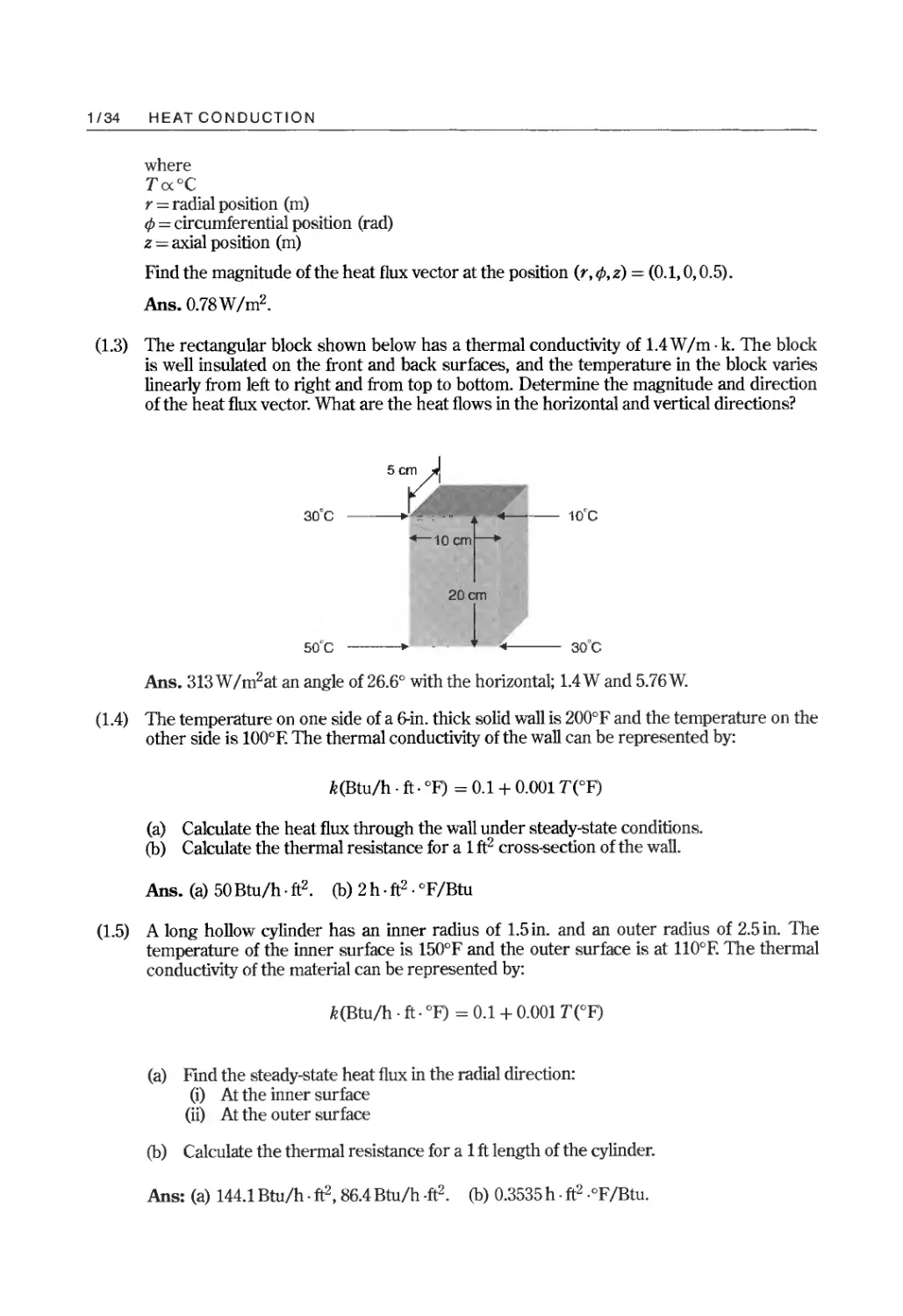
where T ex °C and x,y,z ex m. Find the magnitude of the heat flux vector at the point
(x,y,z) = (0.5, 0, 0.2).
Ans.0.252W/m 2 .
(1.2) The temperature distribution in a Teflon rod (k = 0.35 W 1m. k) is:
T(r,cp,z) = rsincp + 2z
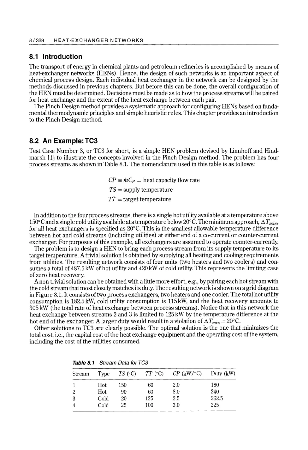
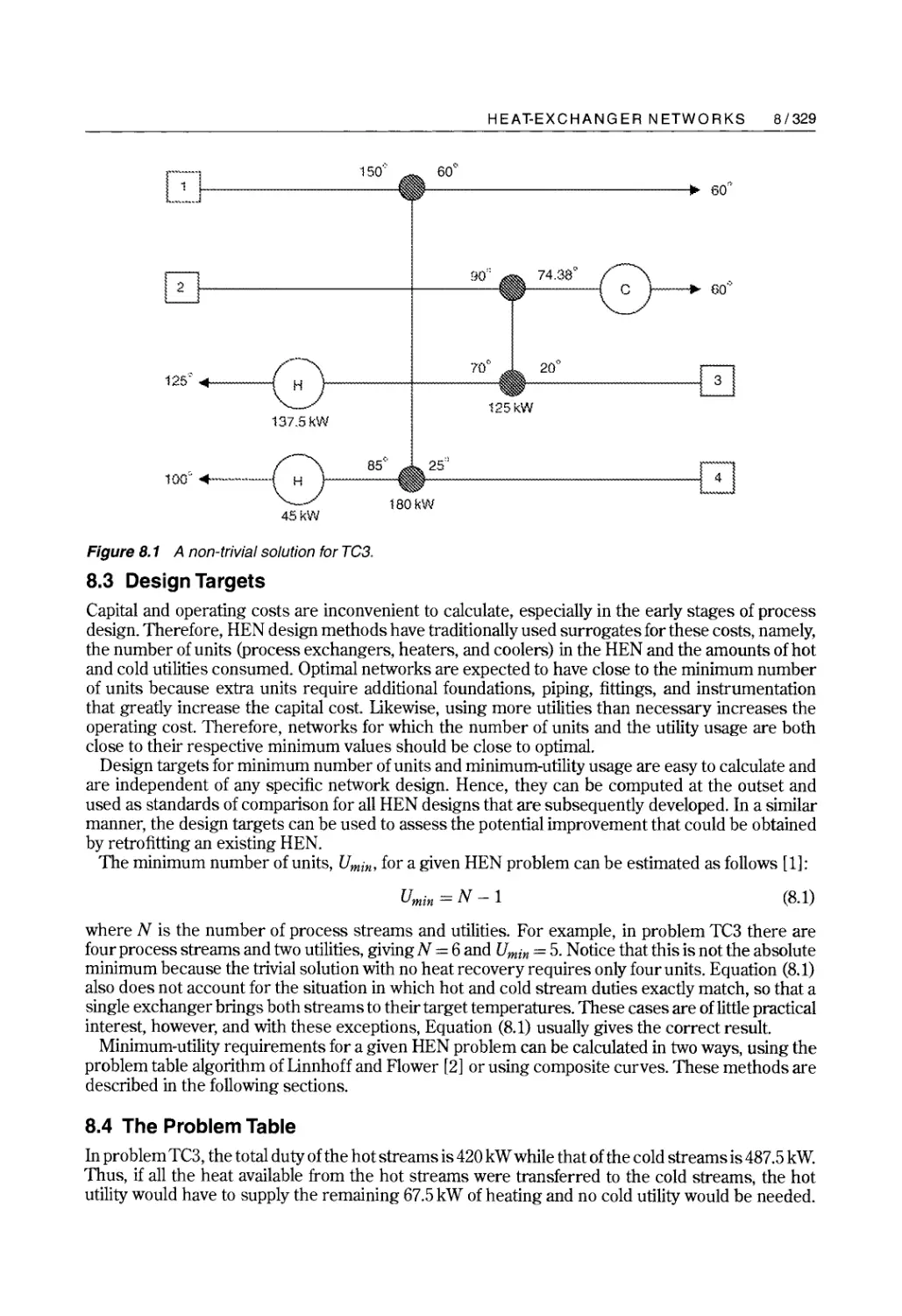
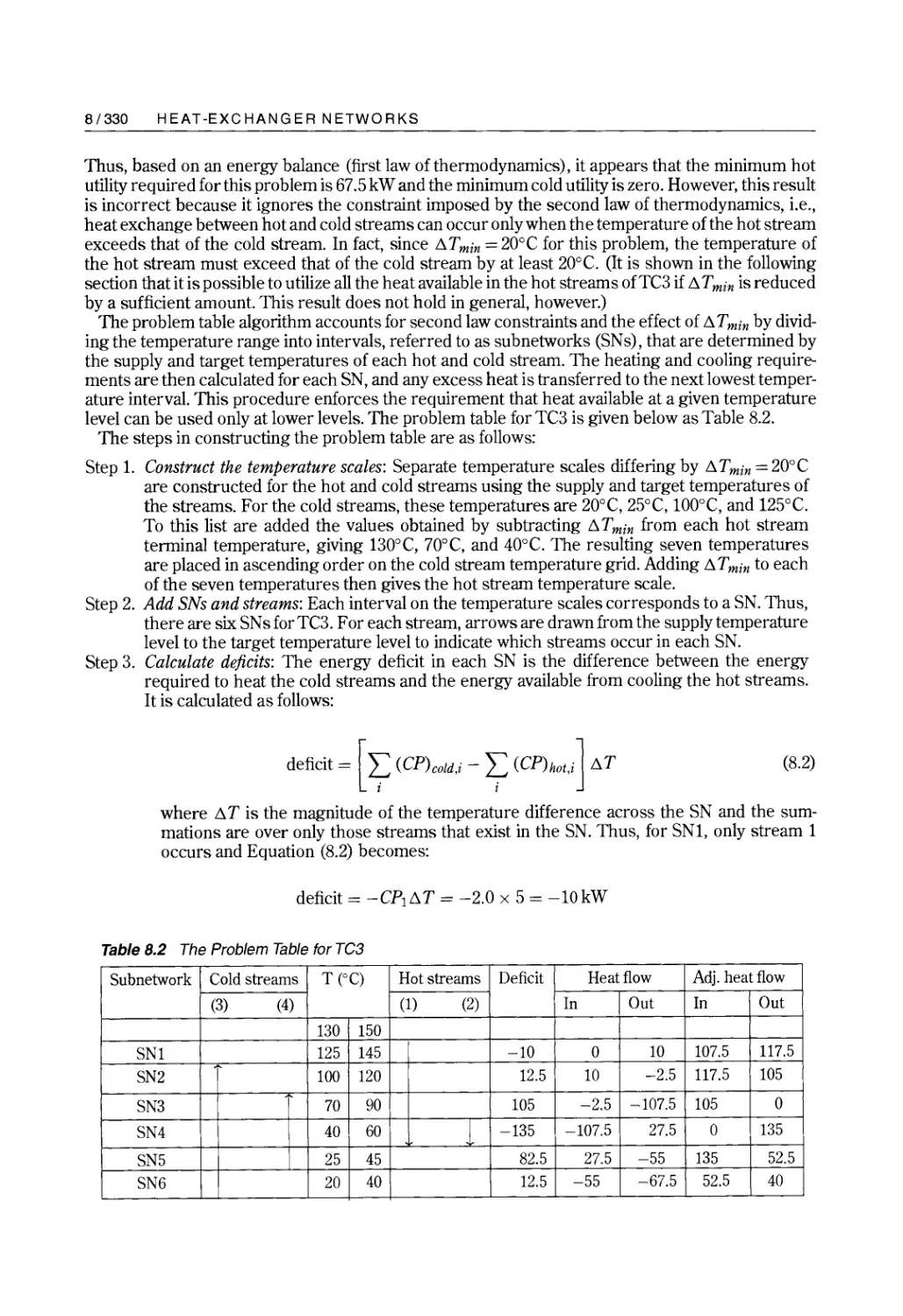
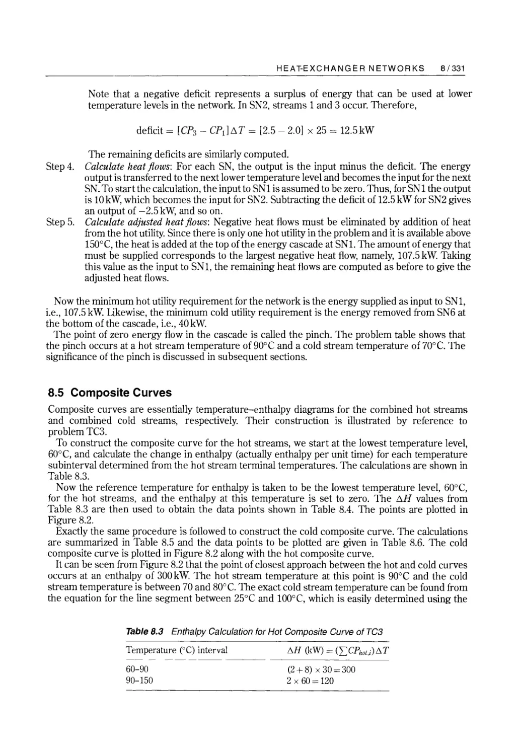
1/34 HEAT CONDUCTION
where
T(X°C
r = radial position (m)
l/J = circumferential position (rad)
Z = axial position (m)
Find the magnitude of the heat flux vector at the position (r,l/J,z) = (0.1,0,0.5).
Ans.0.78W/m 2 .
(1.3) The rectangular block shown below has a thermal conductivity of 1.4 W 1m. k. The block
is well insulated on the front and back surfaces, and the temperature in the block varies
linearly from left to right and from top to bottom. Determine the magnitude and direction
of the heat flux vector. What are the heat flows in the horizontal and vertical directions?
30°C
5' 0
· ':-1 '=r-- 10C
20cm
1
..
..
30C
50'C
Ans. 313 WI m 2 at an angle of 26.6° with the horizontal; 1.4 Wand 5.76 W.
(1.4) The temperature on one side of a 6-in. thick solid wall is 200°F and the temperature on the
other side is lOO°F. The thermal conductivity ofthe wall can be represented by:
k(Btu/h. ft. OF) = 0.1 + 0.001 TCOF)
(a) Calculate the heat flux through the wall under steady-state conditions.
(b) Calculate the thermal resistance for a 1 ft2 cross-section of the wall.
Ans. (a) 50 Btu/h . ft2. (b) 2 h . ft2 . OF IBtu
(1.5) A long hollow cylinder has an inner radius of 1.5 in. and an outer radius of 2.5 in. The
temperature of the inner surface is 150°F and the outer surface is at HOoF. The thermal
conductivity of the material can be represented by:
k(Btu/h. ft. OF) = 0.1 + 0.001 TCOF)
(a) Find the steady-state heat flux in the radial direction:
(i) At the inner surface
(ij) At the outer surface
(b) Calculate the thermal resistance for a 1 ft length of the cylinder.
Ans: (a) 144.1 Btu/h .ft2, 86.4 Btu/h .ft2. (b) 0.3535h .ft2 .0F/Btu.
HEAT CONDUCTION 1/35
(1.6) A rectangular block has thickness B in the x-direction. The side atx = 0 is held at temperature
Tl while the side at x = B is held at Tz. The other four sides are well insulated. Heat is
generated in the block at a uniform rate per unit volume of r.
(a) Use the conduction equation to derive an expression for the steady-state temperature
profile, T(x). Assume constant thermal conductivity.
(b) Use the result of part (a) to calculate the maximum temperature in the block for the
following values of the parameters:
Tl = 100°C k = 0.2W/m. k B = 1.0m
Tz = 0° C
r = 100W/m 3
( TZ - Tl r L ) rxz °
Ans. (a) T(x) = Tl + B + 2k x - 2k' (b) Tmax = 122.5 C atx=0.3m
(1. 7) Repeat Problem 1.6 for the situation in which the side of the block at x = 0 is well
insulated.
r
Ans. (a) T(x)=T z + 2k (BZ-x Z ). (b) T max =250°C
(1.8) Repeat Problem 1.6 for the situation in which the side of the block at x = 0 is exposed to an
external heat flux, q 0, of 20 W / m Z . Note that the boundary condition at x = 0 for this case
becomes
dT qo
dx k'
qo r z z
Ans. (a) T(x) = Tz + T(B -x) + 2k (B -x). (b) Tmax = 350°C
(1.9) A long hollow cylinder has inner and outer radii Rl and Rz, respectively. The temperature of
the inner surface at radius R 1 is held at a constant value, T 1 , while that of the outer surface at
radius Rz is held constant at a value of Tz. Heat is generated in the wall of the cylinder at a rate
per unit volume given by q = rr, where r is radial position and r is a constant. Assuming con-
stant thermal conductivity and heat flow only in the radial direction, derive expressions for:
(a) The steady-state temperature profile, T(r), in the cylinder wall.
(b) The heat flux at the outer surface of the cylinder.
Ans.
{ r 3 3 }
Tz - Tl + 9k (Rz -R 1 ) In (rIR 1 )
(a) T(r) = Tl + (r 19k) (Rr - r 3 ) + (
In Rzi R 1 )
(b) A _ r R k{T 1 - Tz - (r 19k)(R - Rr)}
qrlr=Rz - 3 + Rzln(RzIRl)
1/36 H EAT CON DUCTION
(1.10) Repeat Problem 1.9 for the situation in which the inner surface of the cylinder at Rl is well
insulated.
rR 3 l n (r IRz)
Ans. (a) T(r) = Tz - (r 19k) (R - r 3 ) + 1 3k
r ( R3 - R3 )
(b) Z 1
qrlr=Rz = 3Rz
(1.11) A hollow sphere has inner and outerradii Rl and Rz, respectively. The inner surface at radius
Rl is held at a uniform temperature T 1 , while the outer surface at radius Rz is held at tem-
perature Tz. Assuming constant thermal conductivity, no heat generation and steady-state
conditions, use the conduction equation to derive expressions for:
(a) The temperature profile, T(r).
(b) The rate of heat transfer, qr, in the radial direction.
(c) The thermal resistance.
Ans.
R1Rz (T 1 - Tz) ( - )
r Rl
(a) T (r) = Tl + R R .
z - 1
(b) - 47rkR1Rz (T 1 - Tz)
qr - .
Rz - Rl
(c) See Table 1.2.
(1.12) A hollow sphere with inner and outer radii Rl and Rzhas fixed uniform temperatures of Tl
on the inner surface at radius Rl and Tz on the outer surface at radius Rz. Heat is generated
in the wall of the sphere at a rate per unit volume given by q = rr, where r is radial position
and r is a constant. Assuming constant thermal conductivity, use the conduction equation
to derive expressions for:
(a) The steady-state temperature profile, T(r), in the wall.
(b) The heat flux at the outer surface of the sphere.
Ans.
3 3 ( 1 1 )
R1Rz{Tl - Tz - (r/12k)(R - R)} - - -
Z 1 r R
(a) T(r) = Tl + (r/12k)(Rr - r 3 ) + R R 1 .
Z - 1
rR 3 3
(b) qrlr=Rz = 4 + {kR1IRz(Rz - R 1 )} {Tl - Tz - (r/12k)(R z - R 1 )}.
(1.13) Repeat Problem 1.12 for the situation in which the inner surface at radial position Rl is well
insulated.
Ans.
(a) T(r) = T, + (rfl2k)(R! - r')+ ( r ) G2 - n.
(b) r(Ri - Ri)
qrlr=Rz = 4R z
z
HEAT CONDUCTION 1/37
(1.14) When conduction occurs in the radial direction in a solid rod or sphere, the heat flux must
be zero at the center (r = 0) in order for a finite temperature to exist there. Hence, an
appropriate boundary condition is:
dT
- = 0 at r = 0
dr
Consider a solid sphere of radius R with a fixed surface temperature, TR. Heat is gener-
ated within the solid at a rate per unit volume given by q = r 1 + r zr, where r 1 and r z are
constants.
(a) Assuming constant thermal conductivity, use the conduction equation to derive an
expression for the steady-state temperature profile, T(r), in the sphere.
(b) Calculate the temperature at the center of the sphere for the following parameter values:
R = 1.5m
k = 0.5W /m. K
rl = 20W/m 3
rz = lOW/m 4
TR = 20°C
Ans. (a) T(r) = T R + (r1l6k) (R z - rZ) + (rz/12k) (R3 - r 3 ). (b) 40.625°C.
(1.15) A solid cylinder of radius R is well insulated at both ends, and its exterior surface at r = R
is held at a fixed temperature, TR. Heat is generated in the solid at a rate per unit volume
given by q = r (1 - r I R), where r = constant. The thermal conductivity of the solid may be
assumed constant. Use the conduction equation together with an appropriate set of bound-
ary conditions to derive an expression for the steady-state temperature profile, T(r), in the
solid.
Ans. T(r) = T R + (r 136k) (5R z + 4r 3 1R - 9r z ).
(1.16) A rectangular wall has thickness B in the x-direction and is insulated on all sides except the
one at x = B, which is held at a constant temperature, Tw. Heat is generated in the wall at a
rate per unit volume given by q = r (B - x), where r is a constant.
(a) Assuming constant thermal conductivity, derive an expression for the steady-state
temperature profile, T(x), in the wall.
(b) Calculate the temperature of the block at the side x = 0 for the following parameter
values:
r = 0.3 x 10 6 W/m 4 B = O.lm
T w =90°C k=25W/m.K
( x 3 xZB B3 )
Ans. (a) T(x) = Tw + (rlk) (3 - 2 + 3 .
(b) 94°C.
(1.17) The exterior wall of an industrial furnace is to be covered with a 2-in. thick layer of high-
temperature insulation having an R-value of 2.8, followed by a layer of magnesia (85%)
insulation. The furnace wall may reach 1200°F, and for safety reasons, the exterior of the
magnesia insulation should not exceed 120°F. At this temperature, the heat flux from the
insulation to the surrounding air has been estimated for design purposes to be 200 Btu/h . ftz.
1/38 HEAT CONDUCTION
(a) What is the thermal conductivity of the high-temperature insulation?
(b) What thickness of magnesia insulation should be used?
(c) Estimate the temperature at the interface between the high-temperature insulation and
the magnesia insulation.
Ans. (a) k = 0.0595 Btu/h. ft. OR (c) 640 0 R
(1.18) A storage tank to be used in a chemical process is spherical in shape and is covered with a
3-in. thick layer of insulation having anR-value of 12. The tank will hold a chemical intermedi-
ate that must be maintained at 150 0 R A heating unit is required to maintain this temperature
in the tank.
(a) What is the thermal conductivity of the insulation?
(b) Determine the duty for the heating unit assuming as a worst-case scenario that the
exterior surface of the insulation reaches a temperature of 20 0 R
(c) What thermal resistances were neglected in your calculation?
Ans. (a) k = 0.02083 Btu/h. ft. oR (b) q 7900 Btu/h.
(1.19) A 4-in. schedule 80 steel pipe (ID = 3.826 in., OD = 4.5 in.) carries a heat-transfer fluid at
600°F and is covered with a lh-in. thick layer of pipe insulation. The pipe is surrounded by
air at 80 0 R The vendor's literature states that a I-in. thick layer of the pipe insulation has an
R -value of 3. Neglecting convective resistances, the resistance of the pipe wall, and thermal
radiation, estimate the rate of heat loss from the pipe per foot of length.
Ans. 453 Btu/h . ft pipe
(1.20) A pipe with an OD of 6.03 cm and an ID of 4.93 cm carries steam at 250°C. The pipe is cov-
ered with 2.5 cm of magnesia (85%) insulation followed by 2.5 cm of polystyrene insulation
(k = 0.025 W /m. K). The temperature of the exterior surface of the polystyrene is 25°C.
The thermal resistance of the pipe wall may be neglected in this problem. Also neglect the
convective and contact resistances.
(a) Calculate the rate of heat loss per meter of pipe length.
(b) Calculate the temperature at the interface between the two types of insulation.
Ans. (a) 63W/m of pipe. (b) 174.5°C.
(1.21) It is desired to reduce the heat loss from the storage tank of problem 1.18 by 90%. What
additional thickness of insulation will be required?
(1.22) A steel pipe with an OD of 2.375 in. is covered with a lh..in. thick layer of asbestos
insulation (k = 0.048 Btu/h . ft. OF) followed by a I-in. thick layer of fiberglass insulation
(k = 0.022 Btu/h . ft . OF). The temperature of the pipe wall is 600° F and the exterior surface
of the fiberglass insulation is at 1000R Calculate:
(a) The rate of heat loss per foot of pipe length.
(b) The temperature at the interface between the asbestos and fiberglass insulations.
Ans. (a) 110 Btu/h. ft pipe. (b) 47PR
HEAT CONDUCTION 1/39
(1.23)
A building contains 6000 ft2 of wall surface area constructed of panels shown in the sketch
below. The interior sheathing is gypsum wallboard and the wood is yellow pine. Calculate
the rate of heat loss through the walls if the interior wall surface is at 70°F and the exterior
surface is at 30°F.
Ans. 22,300 Btu/h
Pine 1.75 in.
Wallboard
Rock Brick
wool 13.25 in.
insulation
--+I ,. -I. -,
1 in. 3.5 in. 4 in.
(1.24) A 6in. schedule 80 steel pipe (OD = 6.62 in.) will be used to transport 450°F steam from a
boiler house to a new process unit. The pipe will be buried at a depth of 3 ft (to the pipe
centerline). The soil at the plant site has an average thermal conductivity of 004 Btu/h. ft. OF
and the minimum expected ground surface temperature is 20°F. Estimate the rate of heat
loss per foot of pipe length for the following Cases:
(a) The pipe is not insulated.
(b) The pipe is covered with a 2-in. thick layer of magnesia insulation.
Neglect the thermal resistance of the pipe wall and the contact resistance between the
insulation and pipe wall.
Ans. (a) 350 Btu/h. ft of pipe. (b) 160 Btu/h. ft of pipe.
(1.25) The cross-section of an industrial chimney is shown in the sketch below. The flue has a
diameter of 2 ft and the process waste gas flowing through it is at 400°F. If the exterior
surface of the brick is at 120°F, calculate the rate of heat loss from the waste gas per foot
of chimney height. Neglect the convective resistance between the waste gas and interior
surface of the flue for this calculation.
/+----- 4 ft
1
4ft
1
.1
Common
brick
Flue
Ans. 910 Btu/h. ft of chimney height.
(1.26) A new underground pipeline at a chemical complex is to be placed parallel to an existing
underground pipeline. The existing line has an OD of 8.9 cm, carries a fluid at 283 K and
is not insulated. The new line will have an OD of llo4cm and will carry a fluid at 335K
The center-to-center distance between the two pipelines will be 0.76 m. The ground at the
plant site has an average thermal conductivity of 0.7 W 1m . K In order to determine whether
the new line will need to be insulated, calculate the rate of heat transfer between the two
pipelines per meter of pipe length if the new line is not insulated. For the purpose of this
1/40 HEAT CONDUCTION
calculation, neglect the resistances of the pipe walls and the convective resistances between
the fluids and pipe walls.
Ans. 42 WI m of pipe length.
(1.27) Hot waste gas at 350°F will be transported from a new process unit to a pollution control
device via an underground duct. The duct will be rectangular in cross-section with a height
of 3 ft and a width of 5 ft. The top of the duct will be 1.25 ft below the ground surface, which
for design purposes has been assigned a temperature of 40°F. The average thermal con-
ductivity of the ground at the plant site is OABtu/h. ft. oF. Calculate the rate of heat loss
from the waste gas per foot of duct length. What thermal resistances are neglected in your
calculation?
The following shape factor for a buried rectangular solid is available in the
literature:
[ ( . 11 )] ..0.59 ( h'
S=2,756L In 1+;; '6)
L :."'> h,a,b
.O.fri1::
t "----:' - ...... 2 .
. t :Js
(1.28) An industrial furnace wall will be made of diatomaceous refractory brick (ex = 1.3228 x
10- 7 m 2 Is) and is to be designed so that the exterior surface will remain cool enough for
safety purposes. The design criterion is that the mid-plane temperature in the wall will not
exceed 400 K after 8 h of operation with an interior wall surface temperature of 1100 K.
(a) Assume that the furnace wall can be approximated as a semi-infinite solid. Calculate
the wall thickness required to meet the design specification assuming that the wall is
initially at a uniform temperature of 300 K.
(b) Using the wall thickness obtained in part (a), calculate the exterior wall surface
temperature after 8 h of operation.
(c) Based on the above results, is the assumption that the furnace wall can be approxi-
mated as a semi-infinite solid justified, Le., is the wall thickness calculated in part (a)
acceptable for design purposes? Explain why or why not.
Ans. (a) 26.8cm. (b) 301.7K.
(1.29) The steel panel (ex = 0.97 x 10- 5 m 2 Is) of a firewall is 5 cm thick and its interior surface
is insulated. The panel is initially at 25°C when its exterior surface is suddenly exposed
to a temperature of 250°C. Calculate the average temperature of the panel after 2 min of
exposure to this temperature.
Note: A wall of width s with the temperature of one side suddenly raised to Ts and the
opposite side insulated is mathematically equivalent to a wall of width 2 s with the temper-
ature of both sides suddenly raised to Ts. In the latter case, dT I dx = 0 at the mid-plane due
to symmetry, which is the same condition that exists at a perfectly insulated boundary.
Ans. 192°C.
HEAT CONDUCTION 1/41
(1.30) An un-insulated metal storage tank at a chemical plant is cylindrical in shape with a diameter
of 4 ft and a length of 25 ft. The liquid in the tank, which has properties similar to those of
water, is at a temperature of 70°F when a frontal passage rapidly drops the ambient temper-
ature to 40°F. Assuming that ambient conditions remain constant for an extended period of
time, estimate:
(a) The average temperature of the liquid in the tank 12 h after the frontal passage.
(b) The time required for the average temperature of the liquid to reach 50°F.
Ans. (a) 59°F. (b) 92 h.
(1.31) Repeat Problem 1.30 for the situation in which the fluid in the tank is
(a) Methyl alcohol.
(b) Aniline.
(1.32) Repeat Problem 1.30 for the situation in which the tank is spherical in shape with a diameter
of 4.2 ft.
Ans. (a) 63°F. (b) 207 h (From Equation (1.44). Note that Fo < 0.1.).
2
CONVECTIVE
HEAT TRANSFER
Contents
2.1 Introduction 44
2.2 Combined Conduction and Convection 44
2.3 Extended Surfaces 47
2.4 Forced Convection in Pipes and Ducts 53
2.5 Forced Convection in External Flow 62
2.6 Free Convection 65
2/44 CONVECTIVE HEATTRANSFER
2.1 Introduction
Convective heat transfer occurs when a gas or liquid flows past a solid surface whose temperature is
different from that of the fluid. Examples include an organic heat-transfer fluid flowing inside a pipe
whose wall is heated by electrical heating tape, and air flowing over the outside of a tube whose wall
is chilled by evaporation of a refrigerant inside the tube. Two broad categories of convective heat
transfer are distinguished, namely, forced convection and natural (or free) convection. In forced
convection, the fluid motion is caused by an external agent such as a pump or blower. In natural
convection, the fluid motion is the result of buoyancy forces created by temperature differences
within the fluid.
In contrast to conductive heat transfer, convective heat-transfer problems are usually solved by
means of empirical correlations derived from experimental data and dimensional analysis. The
reason is that in order to solve a convection problem from first principles, one must solve the
equations of fluid motion along with the energy balance equation. Although many important results
have been obtained by solving the fundamental equations for convection pro blems in which the flow
is laminar, no method has yet been devised to solve the turbulent flow equations entirely from first
principles.
The empirical correlations are usually expressed in terms of a heat-transfer coefficient, h, which
is defined by the relation:
q=hA!1T
(2.1)
In this equation, q is the rate of heat transfer between the solid surface and the fluid, A is the area
over which the heat transfer occurs, and !1 T is a characteristic temperature difference between
the solid and the fluid. Equation (2.1) is often referred to as Newton's Law of Cooling, even though
Newton had little to do with its development, and it is not really a physical law. It is simply a definition
of the quantity, h. Note that the units of h are W 1m 2 . K or Btulh . ft2 . oR
Equation (2.1) may appear to be similar to Fourier's Law of heat conduction. However, the coef-
ficient, h, is an entirely different kind of entity from the thermal conductivity, k, which appears
as the constant of proportionality in Fourier's Law. In particular, h is not a material property. It
depends not only on temperature and pressure, but also on such factors as geometry, the hydro-
dynamic regime (laminar or turbulent), and in turbulent flow, the intensity of the turbulence and
the roughness of the solid surface. Hence, the heat-transfer coefficient should not be regarded
as a fundamental quantity, but simply as a vehicle through which the empirical methods are
implemented.
From the standpoint of transferring heat, turbulent flow is highly desirable. In general, heat-
transfer rates can be ordered according to the mechanism of heat transfer as follows:
conduction < natural convection < laminar forced convection < turbulent forced convection
The reason that turbulent flow is so effective at transferring heat is that the turbulent eddies can
rapidly transport fluid from one area to another. When this occurs, the thermal energy of the fluid
is transported along with the fluid itself. This eddy transport mechanism is much faster (typically,
about two orders of magnitude) than the molecular transport mechanism of heat conduction.
The heat-transfer correlations presented in this chapter are valid for most common Newtonian
fluids. They are not valid for liquid metals or for non-Newtonian fluids. Special correlations are
required for these types of fluids.
2.2 Combined Conduction and Convection
Heat-transfer problems involving both conduction and convection can be conveniently handled by
means of the thermal resistance concept. Equation (2.1) can be put into the form of a thermal
resistance as follows:
q = hA!1T = !1T IRth
CONVECTIVE HEAT TRANSFER 2/45
Thus,
1
Rth = hA
(2.2)
This expression for convective thermal resistance was given previously in Table 1.2. Convective
resistances can be combined with other thermal resistances according to the rules for adding
resistances in series and in parallel.
Example 2.1
A 5 cm (2 in.) schedule 40 steel pipe carries a heat-transfer fluid and is covered with a 2 cm layer of
calcium silicate insulation to reduce the heat loss. The inside and outside pipe diameters are 5.25 cm
and 6.03 cm, respectively. The fluid temperature is 150°C, and the temperature ofthe exterior surface
of the insulation is 25°C. The coefficient of heat transfer between the fluid and the inner pipe wall
is 700 W 1m 2 . K. Calculate the rate of heat loss per unit length of pipe.
Solution
!1T 150 - 25
qr = - =
Rth Rth
Rth = Rconvection + R pipe + Rinsulation
1 1 1
Rconvection = hA = hlrDL = 700 x lr x 0.0525 x 1 = 0.008661 K/W
Rpipe = 0.000513 K/W (from Example 1.6)
Rinsulation = 1.349723 K/W (from Example 1.6)
Rth = 0.008661 + 0.000513 + 1.349723 = 1.358897 K/W
125 .
qr = 1.358897 92.0 W 1m of pipe
Another situation involving conduction and convection is the transient heating or cooling of a
solid in contact with a fluid as depicted in Figure 2.1. For the special case in which the thermal
resistance within the solid is small compared with the convective resistance between the fluid and
solid, temperature variations in the solid are small and can be neglected. The temperature of the
solid can then be approximated as a function of time only.
Solid initially at To
Volume = v
Surface area = As
q
Fluid
...
T,,,, h
+-
T(t)
Figure 2.1 Transient heat transfer between a solid and a fluid.
2/46 CONVECTIVE HEAT TRANSFER
A thermal energy balance on the solid gives:
{rate of accumulation of thermal energy} = {rate of heat transfer from fluid} (2.3)
dT
pvcdi = hAs (Too - T)
dT = hAs (Too - T)
dt pvc
where p, c, v, and As are, respectively, the density, heat capacity, volume, and surface area of the
solid.
The solution to this linear first-order differential equation subject to the initial condition that
T = To when t = 0 is:
(2.4)
( hAst )
T(t) = Too + (To - Too) exp --
pvc
(2.5)
The approximation T = T(t) is generally acceptable when the following condition is satisfied [1]:
h(vIAs)
< 0.1
k solid
(2.6)
where ksolid is the thermal conductivity ofthe solid. Equation (2.5) can also be applied to the transient
heating or cooling of stirred process vessels. In this case, the fluid inside the vessel is maintained
at a nearly uniform temperature by the mixing. The physical properties (p and c) of the fluid in the
vessel are used in Equation (2.5).
Example 2.2
A batch chemical reactor operates at 400 K and the contents are well mixed. The reactor volume
is 0.8 m 3 with a surface area of 4.7 m 2 . After the reaction is complete, the contents are cooled
to 320 K before the reactor is emptied. The cooling is accomplished with ambient air at 300 K
and h = 75W /m 2 . K. The agitator continues to operate during cool down. The reactor contents
have a density of 840 kg/ m 3 and a heat capacity of 2200 J /kg . K. Determine the cooling time
required.
Solution
Neglect the thermal capacity of the reactor vessel and heat loss by radiation. Also, neglect the
thermal resistance of the vessel wall and the convective resistance between the wall and the fluid in
the reactor. Equation (2.5) is then applicable since the reactor contents remain well mixed during
cooling.
( hAs t )
T(t) = Too + (To - Too) exp --
pvc
( 75 x 4.7t )
320 = 300 + (400 - 300) exp - 840 x 0.8 x 2200
t = 6,750s 1.9h
CONVECTIVE HEAT TRANSFER 2/47
2.3 Extended Surfaces
An important application involving both conduction and convection is that of heat-transfer fins, also
referred to as extended surfaces. Although fins come in a variety of shapes, the two most frequently
used in process heat exchangers are rectangular fins (Figure 2.2) and annular (radial or transverse)
fins (Figure 2.3). The basic idea behind fins is to compensate for a low heat-transfer coefficient,
h, by increasing the surface area, A. Thus, fins are almost always used when heat is transferred
to or from air or other gases, because heat-transfer coefficients for gases are generally quite low
compared with those for liquids. Since fins usually consist of very thin pieces of metal attached to
the primary heat-transfer surface (the prime surface), a relatively large amount of additional surface
area is achieved with a small amount of material.
All the heat transferred by convection from the fin surface must first be transferred by conduction
through the fin from its base, which is generally taken to be at the same temperature as the prime
Prime surface
at Ts
Fluid
h. T"
Ts
'\-
. .. =" b ....,.
q,Jx q,,!x+.<\x
-;: . It
x ----+1 /).x
L
I
)
w
Figure 2.2 Rectangular fin attached to a flat surface.
- ..11" f.--
Fluid
h, T",
Figure 2.3 Annular fin attached to a tube wall.
2/48 CONVECTIVE HEATTRANSFER
surface. Therefore, a temperature gradient must exist along the length of the fin, and as the distance
from the base of the fin increases, the temperature of the fin becomes closer to the temperature of
the surrounding fluid. As a result, the T for convective heat transfer decreases along the length of
the fin, and hence the extended surface is less effective in transferring heat than the prime surface.
In order to calculate the rate of heat transfer from a fin, it is necessary to determine the temperature
profile along the length of the fin. We consider a rectangular fin attached to a flat surface as depicted
in Figure 2.2, and make a thermal energy balance on a differential volume element. The following
assumptions are made:
. Steady state
. Heat transfer from fin surface by convection only (no radiation)
. No heat generation in the fin
. Constant thermal conductivity in the fin
. Negligible temperature difference across the thickness of the fin
. Negligible edge effects
The last two assumptions are justified because the fin is assumed to be very thin (like a knife
blade), and made of metal (a good heat conductor). Therefore, there is very little thermal resistance
between the top and bottom of the fin, and hence little temperature difference. Furthermore, the
fin width, W, is much greater than the thickness, t, and so nearly all the surface area resides on
the top and bottom of the fin. Hence, nearly all the convective heat transfer occurs at the top and
bottom surfaces, and very little occurs at the sides and tip of the fin. The upshot of all this is that
the temperature in the fin can be considered a function only of x, Le., T = T(x).
With steady state and no heat generation, the thermal energy balance on the control volume is
simply:
{rate of thermal energy in} - {rate ofthermal energy out} = 0
(2.7)
Heat enters the control volume by conduction at position x, and leaves by conduction at position
x + !lx and by convection at the surface of the control volume. Thus, the balance equation can be
written:
qx I A - qx I A - qev P x = 0
x X+M
(2.8)
where
A = W T = fin cross-sectional area
P = 2(W + T) = fin perimeter
Note that P x is the total surface area of the differential element. Dividing by !lx and taking the
limit as x --+ 0 yields:
A dqx P - 0
- - - qev -
dx
(2.9)
Now from Fourier's Law,
qx = _k dT
dx
and from Equation (2.1), the convective heat flux is:
iiev = h T = h(T - Too)
(2.10)
Substituting and utilizing the fact that k is constant gives:
d 2 T
kA dx 2 - hP(T - Too) = 0
(2.11)
CO NVECTIVE HEAT TRAN S FE R 2/49
or
d 2 T _ hP ( T _ T ) =0
dx2 kA 00
Equation (2.12) can be simplified by making the following definitions:
(2.12)
8=T-Too
(2.13)
m2 = hP = 2h(W + ,) 2h (since, « W)
kA kW, kr
(2.14)
(Note: The above approximation for m 2 is frequently used in practice.)
Making these substitutions and assuming that the fluid temperature, Too, is a constant yields:
d 2 8 2
- -m 8=0
dx 2
(2.15)
This equation is subject to the following boundary conditions:
1. Atx = 0,
8=Ts-Too
d8 = 0
dx
(2.16)
2. Atx=L,
The first condition results from the assumption that the temperature at the base of the fin is equal
to the prime surface temperature, Ts- The second condition follows from the fact there is very
little heat transfer from the tip of the fin. Setting the heat flux at the end of the fin to zero gives
dTldx = d81dx =0.
The general solution to Equation (2.15) can be expressed either as a sum of exponential functions
or as a sum of hyperbolic functions, but the latter is more convenient in this context:
8 = C 1 sinh(mx) + C 2 cosh(mx)
(2.17)
Applying the boundary conditions (2.16) gives:
C 1 = - (Ts - Too) tanh(mL)
C 2 = Ts - Too
With these results, the temperature profile along the fin becomes:
T = Too - (T s - Too) [tanh(mL) sinh(mx) - cosh (mx) ]
(2.18)
To find the rate of heat transfer from the fin, note that all the heat must enter the fin by conduction
at the base, where x = O. Therefore,
dT I
qfin = -kA-
dx x=o
(2.19)
2/50 CONVECTIVE HEAT TRANSFER
Differentiating Equation (2.18) and evaluating at x = 0 gives:
dT I
dx x=o =-m(Ts-Too)tanh(mL)
(2.20)
Substituting into Equation (2.19) gives:
qfin = kAm(T s - Too) tanh(mL)
or
qfin = (hPkA) 1/2 (Ts - Too) tanh (mL)
(2.21)
Now the maximum possible rate of heat transfer occurs when the entire fin is at the prime surface
temperature, Ts:
qmax = hPL(T s - Too)
The fin efficiency, "f)f, is defined as the ratio of qfin to qmax:
(2.22)
qfin (hPkA)1/2(Ts - Too) tanh(mL)
"f)f=-=
qmax hPL(T s - Too)
or
tanh (mL)
"f)f =
mL
(2.23)
The rate of heat transfer from the fin can now be expressed in terms of the fin efficiency as:
qfin = "f)fqmax
or
qfin = "f)fhAfinlTs - Tool (2.24)
where the surface area, Afin, is equal to PL for the rectangular fin, and absolute value signs have
been added to make qfin positive regardless of the direction of heat flow.
One further modification is made to the fin equations to account (approximately) for the heat
transfer from the fin tip, which was neglected in the above analysis. This is accomplished by, in
effect, adding the tip area to the periphery of the fin. To this end, the fin length is increased by an
amount, !1L, determined as follows:
P !1L = tip area = Wi
Wi Wi ",i
!1L = P = 2 (W + i) 2
(2.25)
The corrected length, Lc, defined by:
i
Lc = L + !1L = L + "2
(2.26)
is then used in place of L in Equations (2.23) and (2.24).
CONVECTIVE HEAT TRANSFER 2/51
The analysis of an annular fin is somewhat more complicated and the equation for fin efficiency
involves Bessel functions [1,2], making it inconvenient to use. However, the following simple
modification of Equation (2.23) provides a very good approximation for annular fins [3]:
tanh (m1fr)
"Y)f =
m1fr
(2.27)
where
1fr = (rz c - rl) [1 + 0.35 In (rzc!rr) ]
rr = inner radius of fin = external radius of tube (prime surface)
rz = outer radius of fin
rz c = rz + r:12 = corrected fin radius
The rate of heat transfer from the fin is given by
qfin = 2"Y)fhn(ric - rf)ITs - Tool
(2.28)
The factor of two in Equation (2.28) results from the fact that heat is transferred from both sides of
the fin.
The total rate of heat transfer from a finned surface is the sum of the heat-transfer rates from the
prime surface and from all of the fins. Thus,
q = qprime + qfins
=hAPrimelTs - Tool + WhAfinslTs - Tool
=h [ Aprim :o fAfins JATotlTs - Tool
(2.29)
q = h"Y)wATotlTs - Tool
(2.30)
where
A Tot = Aprime + Afins = total heat-transfer area.
. . A prime + "Y)f Afins
17w = wezghted efficzency = A
Tot
(2.31)
It follows from Equation (2.30) that the thermal resistance of a finned surface is:
1
Rth =
h"Y)wATot
(2.32)
This result was previously listed in Table 1.1.
Example 2.3
A rectangular aluminum alloy (Duralumin) fin is 2 in. long, 0.1 in. thick and 40 in. wide. It
is attached to a prime surface at 150°F and is surrounded by a fluid at 100°F with a heat
2/52 CONVECTIVE HEAT TRANSFER
transfer coefficient of 75 Btu/h . ftz . oF. Calculate the fin efficiency and the rate of heat transfer from
the fin.
Solution
k = 164 x 0.57782 = 94.76 Btu/h . ft. OF (Table A.2)
Z '" 2h 2 x 75
m = k-r = 94.76(0.1/ 1 2) = 189.95
m = .J189.95 = 13.78ft- 1
Lc =L + r:/2 = 2 + i O / 12 ) = 0.17083ft
mLc = 13.78 x 0.17083 = 2.354
Using Equation (2.23) with L replaced by Lc,
_ tanh(mLc) _ tanh(2.354) 0 4 7
"f)f - mLc - 2.354 -. 1
The rate of heat transfer from the fin is computed from Equation (2.24).
qfin = "f)fhPLclTs - Tool
P = 2(W + r:) = 2(40 + 0.1) 112 = 6.6833 ft
qfin = 0.417 x 75 x 6.6833 x 0.17083(150 - 100)
qfin ;:::; 1785 Btu/h
Example 2.4
A O.l-in. thick annular Duralumin fin with an external diameter of 3 in. is attached to a tube having
an external diameter of 2 in. The tube wall temperature is 150°F and the tube is surrounded by a
fluid at lOO°F with a heat-transfer coefficient of 75 Btu/h. ftz . oF.
(a) Calculate the fin efficiency and the rate of heat transfer from the fin.
(b) If the total heat-transfer surface consists of 75% fin surface and 25% prime surface, calculate
the weighted efficiency of the surface.
Solution
(a)
TubeOD = 2in.::::} rl = 1in.
Fin OD = 3 in. ::::} rz = 1.5 in.
rz c = rz + r:/2 = 1.5 + 0.1/2 = 1.55 in.
k = 94.76 Btu/h . ft. °F(from Example 2.3)
( 2h ) 0.5 ( 2 x 75 ) 0.5
m = kr: = 94.76(0.1/ 1 2) = 13.782ft- 1
1/1"= (rz c - rl)[l + 0.35 In (rZc!rl)] = (1.55 - 1.0)[1 + In(1.55/1.0)]
CONVECTIVE HEAT TRANSFER 2/53
"I/J = 0.63436 in. = 0.7258 ft
m"I/J = 13.782 x 0.05286 = 0.7258
From Equation (2.27), the fin efficiency is:
= tanh(m"I/J) = tanh(0.7258) = 0 855
rJf m"I/J 0.7258 .
The rate of heat transfer from the fin is given by Equation (2.28):
qfin = 2rJfh7r(ric - ri) ITs - Tool
= 2 x 0.855 x 757r[(1.55/12)2 - (1.0/12)2](150 - 100)
qfin ;::: 196 Btu/h
(b) The weighted efficiency is computed from Equation (2.31):
rJw = (Aprime/ATot) + rJj(Ajins/ATot)
= 0.25 + 0.855 x 0.75
rJw = 0.89
2.4 Forced Convection in Pipes and Ducts
Heat transfer to fluids flowing inside pipes and ducts is a subject of great practical importance.
Consequently, many correlations for calculating heat-transfer coefficients in this type of flow have
been proposed. However, the correlations presented below are adequate to handle the vast majority
of process heat-transfer applications. Correlations are given for each of the three flow regimes;
turbulent, transition, and laminar. The physical situation described by the correlations is depicted in
Figure 2.4. fluid enters the pipe at an average temperature Tbl and leaves at an average temperature
T b2 . (T b stands for bulk temperature. It is the fluid temperature averaged over the flow area.) The
pipe wall temperature is T wI at the entrance and T w2 at the exit. The fluid is either heated or cooled
as it flows through the pipe, depending on whether the wall temperature is greater or less than the
fluid temperature.
T wl
I
T w2
/
T bl ----..
T b2
Figure 2.4 Heat transfer in pipe flow.
2/54 CONVECTIVE HEAT TRANSFER
With respect to heat transfer in circular pipes, fully developed turbulent flow is achieved at a
Reynolds number of approximately 10 4 . For this flow regime (Re 2:: 10 4 ), the following correlation
is widely used:
Nu = 0.027 ReO. 8 Pr 1 / 3 (ILIILw)O.14
(2.33)
where
Nu == Nusselt Number == hD I k
Re == Reynolds Number==DV pilL
Pr == Prandtl Number= CPILlk
D = inside PiPe diameter
V = average fluid velocity
C p , IL, p, k = fluid properties evaluated at the average bulk fluid temperature
ILw = fluid viscosity evaluated at average wall temperature
The average bulk fluid temperature and average wall temperature are given by:
T _ Tb1 + Tb2
b,ave - 2
(2.34)
T _ T w 1 + T w 2
w,ave - 2
(2.35)
Equation (2.33) is generally attributed to Seider and Tate [4], although they did not explicitly
formulate it. The equation is frequently written with the coefficient 0.027 replaced by 0.023. The
latter value gives a somewhat more conservative estimate for the heat-transfer coefficient, which is
often desirable for design purposes. Both coefficients will be used in this book. Although this may
cause some consternation, it does reflect current practice, as both values are in common use.
Equation (2.33) is valid for fluids with Prandtl numbers between 0.5 and 17,000, and for pipes
with L/ D > 10. However, for short pipes with 10 < LID < 60, the right-hand side of the equation is
often multiplied by the factor [1 + (D I L) 2/3] to correct for entrance and exit effects. The correlation
is generally accurate to within :1:20% to :1:40%. It is most accurate for fluids with low to moderate
Prandtl numbers (0.5:s Pr:s 100), which includes all gasses and low-viscosity process liquids such
as water, organic solvents, light hydrocarbons, etc. It is less accurate for highly viscous liquids,
which have correspondingly large Prandtl numbers.
For laminar flow in circular pipes (Re < 2100), the Seider-Tate correlation takes the form:
Nu = 1.86[RePr DIL] 1/3 (ILl ILw)O.14
(2.36)
This equation is valid for 0.5 < Pr < 17,000 and (Re Pr D I L) 1/3 (ILl ILw)O.14 > 2, and is generally
accurate to within :1:25%. Fluid properties are evaluated at Tb ave except for ILw, which is evaluated
at Tw,ave. For (RePr DIL) 1/3 (ILIILw)o.14 < 2, the Nusseltnumber should be set to 3.66, which is the
theoretical value for laminar flow in an infinitely long pipe with constant wall temperature. Also,
at low Reynolds numbers heat transfer by natural convection can be significant (see Section 2.6
below), and this effect is not accounted for in the Seider-Tate correlation.
For flow in the transition region (2100 < Re < 10 4 ), the Hausen correlation is recommended [2,5]:
Nu = 0.116[Re 2 / 3 -125]Pr 1 / 3 (ILIILw)O.14[1 + (DIL)2/3]
(2.37)
Heat-transfer calculations in the transition region are subject to a higher degree of uncertainty
than those in the laminar and fully developed turbulent regimes. Although industrial equipment
CONVECTIVE HEATTRANSFER 2/55
is sometimes designed to operate in the transition region, it is generally recommended to avoid
working in this flow regime if possible. Fluid properties in Equation (2.37) are evaluated in the
same manner as with the Seider-Tate correlations.
An alternative equation for the transition and turbulent regimes has been proposed by
Gnielinski [6]:
Nu = UI8)(Re -l,OOO)Pr [1 + (DIL)2/3]
1 + 12.7JTi8(Pr 2 / 3 - 1)
(2.38)
Here,! is the Darcy friction factor, which can be computed from the following explicit approximation
of the Colebrook equation [7]:
f = (0.782 InRe - 1.51)-2
(2.39)
Equation (2.38) is valid for 2100 < Re < 10 6 and 0.6 < Pr < 2000. It is generally accurate to
within :I: 20%.
For flow in ducts and conduits with non-circular cross-sections, Equations (2.33) and (2.37)-
(2.39), can be used if the diameter is everywhere replaced by the equivalent diameter, De,
where
De = 4 X hydraulic radius = 4 x /low arealwetted perimeter
(2.40)
This approximation generally gives reliable results for turbulent flow. However, it is not recom-
mended for laminar flow.
The most frequently encountered case of laminar flow in non-circular ducts is flow in the annu-
lus of a double-pipe heat exchanger. For laminar annular flow, the following equation given by
Gnielinski [6] is recommended:
= 3 66 12(D D )08 0.19[1 + 0.14(D2ID 1 )0.5] [Re Pr Dei L ]0.8
Nu . +. 21 1 + 1+0.117[RePrDeiL]0467
(2.41)
where
Dl = outside diameter of inner pipe
D 2 = inside diameter of outer pipe
De = equivalent diameter=D2 - Dl
The Nusselt number in Equation (2.41) is based on the equivalent diameter, De.
All of the above correlations give average values of the heat-transfer coefficient over the entire
length, L, of the pipe. Hence, the total rate of heat transfer between the fluid and the pipe wall can
be calculated from Equation (2.1):
q = hA !'J.T]n
In this equation, A is the total heat-transfer surface area (;rDLfor a circular pipe) and !'J.T 1n is an
average temperature difference between the fluid and the pipe wall. A logarithmic average is used;
it is termed the logarithmic mean temperature difference (LMTD) and is defined by:
T !'J.Tl - !'J.T 2
!'J. In =
In (!'J. TII !'J.T 2 )
(2.42)
2/56 CONVECTIVE HEAT TRANSFER
where
!1T 1 = ITw1 - Tb11
!1T 2 = ITw2 - T b2 1
Like any mean value, the LMTD lies between the extreme values, !1T 1 and !1T 2 . Hence, when
!1 T1 and !1 T2 are not greatly different, the LMTD will be approximately equal to the arithmetic
mean temperature difference, by virtue of the fact that they both lie between !1T1 and !1T 2 . The
arithmetic mean temperature difference, !1Tave, is given by:
T !1T1 + !1T 2
!1 ave = 2
(2.43)
The difference between !1T]n and !1 Tave is small when the flow is laminar and Re Pr D / L > 10 [8].
Example 2.5
Carbon dioxide at 300 K and 1 atm is to be pumped through a 5 cm ID pipe at a rate of 50 kg/h.
The pipe wall will be maintained at a temperature of 450 K in order to raise the carbon dioxide
temperature to 400 K. What length of pipe will be required?
Solution
Equation (2.41) may be written as:
q = hA!1T 1n = hnDL!1Tl n
In order to solve the equation for the length, L, we must first determine q, h, and !1Tl n . The required
physical properties of CO 2 are obtained from Table A10.
Property
tt(N. s/m 2 )
CpO/kg. K)
k(W/m.K)
Pr
At Th,ave = 350 K
17.21 x 10- 6
900
0.02047
0.755
At Tw,ave =450K
21.34 x 10- 6
(i)
Re = DV p = 4m = 4 x (50/3600) = 2.06 x 10 4
IL nDIL n x 0.05 x 17.21 x 10- 6
Since Re > 10 4 , the flow is turbulent, and Equation (2.33) is applicable.
(ii)
Nu = 0.027 (Re) 0.8 Pr 1 / 3 (ILl ILw)0.14
Nu = 0.027(2.06 x 10 4 )°.8(0.755)1/3 ( : r.14 = 67.41
h = (kID)Nu = (0.02047/0.05) x 67.41
h = 27.6W/m 2 . K
CONVECTIVE HEATTRANSFER 2/57
(iii)
'T' /1T 1 - /1T 2
/11 In =
In (/1 Tri /1T 2 )
(450 - 300) - (450 - 400)
( 450 - 300 )
In 450 _ 400
/1T 1n = 91.02 K
100
In(3)
(iv) The rate of heat transfer, q, is obtained from an energy balance on the CO 2 .
q=mC p (/1Tko 2
= ( ) x 900 x (400 - 300)
3600
q= 1250W
(v)
q = hJrDL/1T 1n
L= q
JrDh/1T 1n
1250 = 317m
Jr x 0.05 x 27.6 x 91.02 .
Checking the length to diameter ratio,
3.17
LID = 0.05 = 63.4 > 60
Hence, the correction factor for short pipes is not required. Therefore, a length of about 3.2 m is
required. However, if it is important that the outlet temperature be no less than 400 K, then it is
advisable to provide additional heat-transfer area to compensate for the uncertainty in the Seider-
Tate correlation. Thus, if the actual heat-transfer coefficient turns out to be 20% lower than the
calculated value (about the worst error to be expected with the given values of Re and Pr), then a
length of
3.17
L = 0.8 = 3.96 4.0m
will be required to achieve the specified outlet temperature.
When the length of the pipe is known and the outlet temperature is required, an iterative solution
is usually necessary. A general calculation sequence is as follows:
(1) Estimate or assume a value of Tb2
Tbl + Tb2 TWI + T w2
(2) Calculate Tb, ave = 2 and T w,ave = 2
(3) Obtain fluid properties at Tb ave and /Lw
(4) Calculate the Reynolds number (Re = 4mIJrD/L for a circular duct)
(5) Calculate h from appropriate correlation
(6) Calculate /1 Tin
(7) Calculate q = hA/1T 1n
(8) Calculate new value of T b2 from q = mC p (Tb2 - Tbl)
(9) Go to Step 2 and iterate until two successive values of T b2 agree to within the desired
accuracy.
2/58 CONVECTIVE HEATTRANSFER
Example 2.6
10001bm/h of oil at 100°F enters a I-in. ID heated copper tube. The tube is 12 ft long and its inner
surface is maintained at 215°E Determine the outlet temperature of the oil. The following physical
property data are available for the oil:
C p = 0.5 Btu/lbm . of
p = 551bm/ft 3
IL = 1.5lbm/ft . h
k = 0.10 Btu/h . ft. OF
Solution
Since the temperature dependencies of the fluid properties are not given, the properties will be
assumed constant. In this case, the heat-transfer coefficient is independent of the outlet temperature,
and can be computed at the outset.
4m 4 x 1000
Re = - D = 1 12 1 5 = 10,186 ::::} turbulent flow
n IL nx I x.
k
h = D x 0.027 ReO. 8 Pr 1 / 3 (ILl ILw)0.14
h = 0027(10 186)0.8 ( 0.5 x 1.5 ) 1/3 (10)
(1/ 1 2) x., 0.1 .
h = 102 Btu/h . ft2 . of
In order to obtain a first approximation for the outlet temperature, Tb2, we assume Tln ;:; Tave.
Then,
q = mCp Toil = hnDL Tave
mCp (Tb2 - 100) = hnDL [ 115 + (2 5 - T b2 ) ]
Solving for Tb2,
1 [ 330 - n2 ]
1000 x 0.05(Tb2 - 100) = 102 x n x 12 x 12 x 2
500Tb2 - 50,000 = 52,873 - 160.2 T b2
660.2 Tb2 = 102,873
Tb2 = 155.8 OF
To obtain a second approximation for Tb2, we next calculate the LMTD:
T = 115 - (215 - 155.8) = 840F
In ( 115 )
In 215 _ 155.8
CONVECTIVE HEAT TRAN S FE R 2/59
Then,
q = hnDL/:).T]n
1
= 102 x n x 12 x 12 x 84
q = 26,917 Btu/h
But,
.q = mC p (n2 - 100)
26,917 = 1000 x 0.5(T b2 - 100)
T b2 = 154°F
This value is sufficiently close to the previous approximation that no further iterations are necessary.
Convergence of the iterative procedure, as given above, is often very slow, and it is then necessary
to use a convergence accelerator. Wegstein's method for solving a nonlinear equation of the form
x = f (x) is well suited for this purpose. The new value of Tb2 calculated in Step 8 of the iterative
procedure depends on the old value of T b2 used in Step 2, i.e.,
Tb2,new = F(Tb2,old)
where the function, F, consists of Steps 2 through 8. When the solution is reached, T b2 new = T b2 old,
so that: ' ,
Tb2.new = F(T b 2,new)
or
T = F (T)
which is the form to which Wegstein's method applies. The Wegstein iteration formula is:
(Ti - T i - 1 )
Ti+l = T i + ( T _ F ( T. ) )
1-1 1-1 _ 1
Ti - F(Ti)
(2.44)
where Ti-l, T i and Ti+l are three successive approximations to the outlet temperature, Tb2.
Example 2.7
Calculate the outlet temperature of the oil stream of Example 2.6 using Wegstein's method and an
initial guess of T b2 = 120°F.
Solution
Designate the initial approximation to the solution as To and set To = 120. A second approximation
is obtained by following the iterative procedure to get a new value of Tb2.
2/60 CONVECTIVE HEAT TRANSFER
h = 102 Btu/h . tt2 . of (from Example 2.6)
115 - (215 - 120) °
1in = In[115/(215 _ 120)] = 104.68 F
q = h7rDL Tln = 102 x 7r x 1/12 x 12 x 104.68 = 33,544 Btu/h
33,544 = q = mCp(TbZ - Tbl) = 500(nz - 100)
Tbz = 167.09°F
Now this value becomes both Tl and F(T o ), Le.,
Tl = 167.09 and F(T o ) = 167.09
To calculate F(T 1 ), repeat the above calculations with Tl as the initial guess for the outlet
temperature.
115 - (215 - 167.09) °
Tln = In[115/215 _ 167.09)] = 76.62 F
q = h7rDL TIn = 102 x 7r x 1/12 x 12 X 76.62 = 24,552 Btu/h
24,552 = q = 500(T b z - 100)
TbZ = 149. 10°F = F(T 1 )
We now have the following values:
To = 120 F(To) = 167.09
Tl = 167.09 F(Tl) = 149.10
The next approximation, Tz, is obtained from Wegstein's formula:
(T 1 - To)
Tz=Tl + [ To -F(To) -1 ]
Tl - F(Tl)
(167.09 - 120) °
Tz = 167.09 + [ 120 _ 167.09 _ 1 ] = 154.07 F
167.09 - 149.10
Next, F(Tz) is calculated in the same manner as F(1\).
T1 = 115 - (215 - 154.07) = 85.120F
In In[115/(215 - 154.07)]
q = 102 X 7r X 1/12 X 12 x 85.12 = 27,276 Btu/h
27,276 = 500(nz - 100)
TbZ = 154.55°F = F(Tz)
CONVECTIVE HEATTRANSFER 2/61
Applying Wegstein's formula again gives:
(T 2 - Tr)
T3 = T 2 + [ Tr - F(Tr) _ 1 ]
T 2 - F(T 2 )
(154.07 - 167.09) °
T3 = 154.07 + [ 167.09 _ 149.10 _ 1 ] = 154.41 F
154.07 - 154.55
Calculating F(T3) in the same manner as above:
T, = 115 - (215 - 154.41) = 84.91 0 F
In In[115/(215 - 154.41)]
q = 102 x Jr x 1/12 x 84.91 = 27,209 Btu/h
27,209 = 500(Tb2 - 100)
Tb2 = 154.42°F = F(T 3 )
The results are summarized below.
T i F(T i )
0 120.00 167.09
1 167.09 149.10
2 154.07 154.55
3 154.41 154.42
Since T3 = F (T 3 ) to four significant figures, the procedure has converged and the final result is
Tb2 = 154.4°F.
Example 2.8
Carbon dioxide at 300 K and 1 atm is to be pumped through a duct with a 10 cm x 10 cm square
cross-section at a rate of 250 kg/h. The walls of the duct will be at a temperature of 450 K What
distance will the CO 2 travel through the duct before its temperature reaches 400 K?
Solution
The required physical properties are tabulated in Example 2.5. The equivalent diameter is calculated
from Equation (2.40):
100
De = 4 x 40 = lOcm = O.lm
(i)
Re = De V p = De m = 0.1 x (250/3600) whereAt = flow area = 0.01 m2
f.L (.LAt 17.21 x 10- 6 x 0.01
Re = 4.04 x 10 4 ::::} turbulent flow
2/62 CONVECTIVE HEAT TRANSFER
Note that the Reynolds number is not equal to 4in/;rD e J.L for non-circular ducts. Rather the
continuity equation (in = p VAt) is used to express the Reynolds number in terms of mass flow
rate.
(ii)
Nu = 0.027 ReO. 8 Pr I/3 (J.L/ J.Lw)0.14
= 0.027(4.04 x 10 4 )°.8(0.755)1 / 3 ( : ) 0.14
Nu = 115.5
h e = 115.5
h = 115. 0.02 = 23.1 W 1m 2 . K
(iii)
q = inCp/}.T co2
= (250/3600) x 900 x 100
q = 6250W
(iv)
q = hAf}. TIn = hPLf}. Tin where P = perimeter of duct cross-section
6250 = 23.1 x 0.4 x L x 91.02
L=7.4m
Since LIDe = 7.4/0.1 = 74 > 60, no correction for entrance effects is required.
2.5 Forced Convection in External Flow
Many problems of engineering interest involve heat transfer to fluids flowing over objects such as
pipes, tanks, buildings or other structures. In this section, correlations for several such systems
are presented in order to illustrate the method of calculation. Many other correlations can be found
in heat-transfer textbooks, e.g., [1,7,9-12], and in engineering handbooks.
Flow over a flat plate is illustrated in Figure 2.5. The undisturbed fluid velocity and temperature
upstream of the plate are V 00 and Too, respectively. The surface temperature of the plate is Ts and
L is the length of the plate in the direction of flow. The fluid may flow over one or both sides of the
plate. The heat-transfer coefficient is obtained from the following correlations [7]:
Nu = 0.664 Rell2Prll3 for Re < 5 x 10 5 (2.45)
to
to
to
Ts
/
Fluid
T , V
I
L
"I
Figure 2.5 Forced convection in flow over a flat plate.
CONVECTIVE HEATTRANSFER 2(63
Nu = (0.037 ReO. 8 - 870)Pr 1 (3 for Re > 5 x 10 5 (2.46)
where
Nu = hL and Re = LVoop
k /L
Equation (2.45) is valid for Prandtl numbers greater than about 0.6. Equation (2.46) is applicable
for Prandtl numbers between 0.6 and 60, and Reynolds numbers up to 10 8 . In these equations all
fluid properties are evaluated at the film temperature, Tf, defined by:
Tf= Too+Ts
2
(2.47)
The heat-transfer coefficients computed from Equations (2.45) and (2.46) are average values for
the entire plate. Hence, the rate of heat transfer between the plate and the fluid is given by:
q = hAlTs - Tool
(2.48)
where A is the total surface area contacted by the fluid.
For flow perpendicular to a circular cylinder of diameter D, the average heat-transfer coefficient
can be obtained from the correlation [13]:
0.62 Re 1 (2Pr 1 (3 [ ( Re ) 5(8 ] 4/5
Nu = 0.3 + [1 + (0.4IPr)2(3Jl(4 1 + 282,000
(2.49)
where
hD
Nu=-
k
and
Re = DVoop
/L
The correlation is valid for Re Pr > 0.2, and all fluid properties are evaluated at the film tempera-
ture, Tf. The rate of heat transfer is given by Equation (2.48) with A = JrDL, where L is the length
of the cylinder.
For flow over a sphere of diameter D, the following correlation is recommended [14]:
( ) 025
Nu = 2 + (0.4 Re 1 (2 + 0.06 Re 2 (3)PrO. 4 :
(2.50)
where
hD
Nu=-
k
and
Re = DVoop
/L
All fluid properties, except /Ls, are evaluated at the free-stream temperature, Too. The viscosity, /Ls,
is evaluated at the surface temperature, Ts. Equation (2.50) is valid for Reynolds numbers between
3.5 and 80,000, and Prandtl numbers between 0.7 and 380.
For a gas flowing perpendicular to a cylinder having a square cross-section (such as an air duct),
the following equation is applicable [1]:
Nu = 0.102 ReO.675Prl(3
(2.51)
2/64 CONVECTIVE HEAT TRANSFER
The Nusselt and Reynolds numbers are calculated as for a circular cylinder but with the diameter,
D, replaced by the length of a side of the square cross-section. All fluid properties are evaluated at
the film temperature. Equation (2.51) is valid for Reynolds numbers in the range 5000 to 10 5 .
The equations presented in this (and the following) section, as well as similar correlations which
appear in the literature, are not highly accurate. In general, one should not expect the accuracy
of computed values to be better than :1:25% to :1:30% when using these equations. This limitation
should be taken into consideration when interpreting the results of heat-transfer calculations.
Example 2.9
Air at 20°C is blown over a 6 cm OD pipe that has a surface temperature of 140°C. The free-stream
air velocity is 10 m/ s What is the rate of heat transfer per meter of pipe?
Solution
For forced convection from a circular cylinder, Equation (2.49) is applicable. The film temper-
ature is:
Tf = Ts + Too = 140 + 20 = 800C
2 2
From Table A.4, for air at 80° C:
v = 21.5 x 10⁻⁶m 2 /s = kinematic viscosity
k =0.0293W/m. K
Pr = 0.71
Re=DVoolv = 0.06 x 10/(21.5 x 10- 6 ) = 2.79 x 10 4
Substituting in Equation (2.49) gives:
Nu = 0.3 + 0.62(27,900)1/2(0.71)1/3 [ 1 + ( 27,900 ) 5/8 ] 4/5
[ ( 0.4 ) 2/3 ] 1/4 282,000
1 + 0.71
Nu = 96.38
Nu x k 96.38 x 0.0293
h = ----n- = 0.06
h 47W/m2.K
The rate of heat transfer is given by Equation (2.48). Taking a length of 1 m gives:
q = hlrDL(T s - Too)
q = 47 x lr x 0.06 x 1.0(140 - 20)
q = 1065 1100 W per meter of pipe
Example 2.10
A duct carries hot waste gas from a process unit to a pollution control device. The duct cross-
section is 4 ft x 4 ft and it has a surface temperature of 140° C. Ambient air at 20° C blows
CONVECTIVE HEAT TRANSFER 2/65
across the duct with a wind speed of 10 ml s. Estimate the rate of heat loss per meter of duct
length.
Solution
The film temperature is the same as in the previous example:
Tf = 140 + 20 = 800C
2
Therefore, the same values are used for the properties of air. The Reynolds number is based on the
length of the side of the duct cross-section. Hence, we set:
D=4ft 1.22m
Re= DV oo = 1.22 x 10/(21.5 x 10- 6 ) = 5.674 x 10 5
])
The Reynolds number is outside the range of Equation (2.51). However, the equation will be used
anyway since no alternative is available. Thus,
Nu = 0.102 ReO. 675 Pr 1 / 3
= 0.102(5.674 x 10 5 )°.675(0.71)1/3
Nu = 696.5
k
h = 15 x 696.5
h = 0.0293 6 9 6 5 16 T W I 2. K
1.22 x. . m
The surface area of the duct per meter of length is:
A = PL = 4 x 1.22 x 1.0 = 4.88 m 2
Finally, the rate of heat loss is:
q = hA!1T
= 16.7 x 4.88 x (140 - 20)
q 9800 W 1m of duct length
2.6 Free Convection
Engineering correlations for free convection heat transfer are similar in nature to those presented in
the previous section for forced convection in external flows. However, in free-convection problems
there is no free-stream velocity, V oo , upon which to base a Reynolds number. The dimensionless
group that takes the place of the Reynolds number in characterizing free convection is called the
Grashof number, Gr, and is defined by:
Gr = gf3ITs - ToolL3
])2
(2.52)
2/66 CONVECTIVE HEAT TRANSFER
where
g = gravitational acceleration;
Ts = surface temperature;
Too = fluid temperature far from solid surface;
L = characteristic length;
v = jLl p = kinematic viscosity;
{3 = t ( : )p = coefficient of volume expansion;
iJ = specific volume.
For gases at low density, the ideal gas law may be used to evaluate (aiJ/aT)p and show that:
{3 = liT (ideal gas)
(2.53)
where
T = absolute temperature.
For dense gases and liquids, {3 can be approximated by:
1 iJ
{3 T
(2.54)
if the specific volume (or density) is known at two different temperatures.
Free convection heat transfer from a heated vertical plate is illustrated in Figure 2.6. Fluid adjacent
to the surface is heated and rises by virtue of its lower density relative to the bulk of the fluid. This
rising layer of fluid entrains cooler fluid from the nearly quiescent region further from the heated
surface, so that the mass flow rate of the rising fluid increases with distance along the plate. Near
the bottom of the plate, the flow is laminar, but at some point, transition to turbulent flow may occur
if the plate is long enough. The free-convection circulation is completed by a region of cold, sinking
fluid far removed from the heated surface.
Turbulent
)
-------1--------- --------------
Laminar
Fluid at Too
)
"
'--
"--
Entrainment
)
-....-/
Figure 2.6 Free convection circulation pattern near a heated vertical plate.
CONVECTIVE HEATTRANSFER 2/67
Heat-transfer coefficients for free convection from a heated or cooled vertical plate of height L
can be obtained from the correlation [15]:
! 2
_ 2 0.387(Gr Pr)1/6
Nu - (0.8 5 + [1 + (0.492IPr)9/16]8/27
(2.55)
The characteristic length used in the N usselt and Grashof numbers is the plate height, L. The
fluid properties, including {3, are evaluated at the film temperature, Tf, defined by Equation (2.47).
Equation (2.55) is valid for 0.1 :::::: Gr Pr:::::: 10 12 , and is accurate to within about :1:30%.
Equation (2.55) may also be used for free convection from vertical cylinders if the diameter-to-
height ratio is greater than (35/GrO. 25 ). For smaller values of D/L, the effects of surface curvature
become significant. However, a correction factor can be applied as follows [7]:
NUcylinder = NUPlate [1 + 1.43 ( D G 0.25 ) 09]
(2.56)
where NUplate is the Nusselt number calculated from Equation (2.55).
For free convection from a horizontal cylinder, a correlation similar to Equation (2.55) can be
used [16]:
( ! 2
N _ 0.387(Gr Pr)1/6
U - 0.60 + [1 + (0.559IPr)9/16]8/27
(2.57)
In this case, however, the characteristic length used in the Nusselt and Grashof numbers is the
diameter ofthe cylinder. Equation (2.57) is valid over the range 10 5 :::::: Gr Pr :::::: 10 12 . Fluid properties
are evaluated at the film temperature.
For free convection from horizontal plates, the following correlations are available [17,18]:
Upper surface hot or lower surface cool:
Nu = 0.54(Gr Pr)I/4 for 10 4 :::::: Gr Pr :::::: 10 7
Nu = 0.15(Gr Pr)1/3 for 10 7 :::::: Gr Pr :::::: 10 11
(2.58)
(2.59)
Upper surface cool or lower surface hot:
Nu = 0.27(Gr Pr)I/4 for 10 5 :::::: Gr Pr :::::: 1O 11
(2.60)
In these equations, fluid properties are again evaluated at the film temperature. The characteristic
length used in both the Nusselt and Grashof numbers is the surface area of the plate divided by its
perimeter.
For free convection from spheres, the following correlation is recommended [19]:
( ! 1/12
N 2 0.598(Gr Pr)1/4 7.44 x 10- 8 Gr Pr
U = + [1 + (0.469IPr)9/16]4/9 1 + [1 + (0.469IPr)9/16Jl6/9
(2.61)
The characteristic length is the sphere diameter and the correlation is valid for Gr Pr :::::: 10 13 and
0.6:::::: Pr:::::: 100. For larger values of the Prandtl number, better agreement with experimental data is
2/68 CONVECTIVE HEATTRANSFER
obtained by dropping the term in brackets raised to the 1/12th power. Fluid properties are evaluated
at the film temperature.
Correlations for free convection heat transfer in other geometrical configurations can be
found in the references cited at the end of the chapter. It should be noted that free convec-
tion effects can sometimes be significant in forced convection problems, especially in the case
of laminar flow at low Reynolds numbers. The relative importance of forced and free con-
vection effects can be determined by comparison of the Reynolds and Grashof numbers as
follows:
Re2/Gr » 1 : Forced convection predominates
Re 2 I Gr 1 : Both modes of heat transfer are significant
Re 2 /Gr « 1 : Free convection predominates
Furthermore, in situations where free convection predominates, radiative heat transfer is often
significant, even at relatively low temperatures. This is a consequence of the fact that heat-transfer
rates in free convection are typically much lower than in forced convection.
Example 2.11
A 12-ounce can of beer at 80°F is placed on end in a refrigerator which is at 36°F. Estimate the
value of the external heat-transfer coefficient for this situation. A 12-ounce beer can has dimensions
D=2.5in. andL=4.75in.
Solution
It will be assumed that the refrigerator blower is not running and that the can is not in contact
with any other item in the refrigerator. Under these conditions, the heat transfer will be by free
convection from a vertical cylinder. We have:
Ts = 80°F
Too=36°F
Tf = 80; 36 = 58°F = 14.440C
From Table A.4, we find by interpolation for air at 14.44°C:
g: = 1.496 x 10 8 K- 1 m- 3
v
k = 0.0247W /m. K
Pr = 0.71
The characteristic length is the height of the cylinder, i.e.,
L = 4.75in. = O.1207m
CONVECTIVE HEAT TRANSFER 2/69
Thus,
Cr= g: IT s - TooIL3
1J
= 1.496 x 10 8 ( 801 836 ) (0.1207)3
Cr = 6.430 x 10 6
Cr Pr = 6.430 x 10 6 X 0.71 = 4.566 X 10 6
Substituting in Equation (2.53) gives:
1 2
0.387 (4.566 X 10⁶) 1/6
Nu = (0.825 + [1 + (0.49 2 /0.71)9/16]8/27
Nu = 25
Now,
= 2.5 = 0.5263
L 4.75
and
35
CrO. 25
35 = 0 695
(6.430 x 10⁶)0.25 .
Therefore, Equation (2.54) should be used to correct for the effects of surface curvature.
Nu""""" Nu, t, [1 + 1. 43 ( Dd;o.25 ) 09]
[ ( 4.75 ) 0.9 ]
=25 1+1.43 6)025 =25[1.0749]
2.5(6.43 x 10 .
NUcylinder = 26.9
hL = 26 9
k .
= 26.9 x k = 26.9 x 0.0247 5.5W m 2 . K
h L 0.1207 I
h = 5.5 x 0.17612 0.97 Btulh . ft2 . OF
Example 2.12
A small holding tank in a chemical plant contains a corrosive liquid that is maintained at a
temperature of 120°F by means of an electrical heater. The heating element consists of
a refractory disk 2 ft in diameter situated at the bottom of the tank. Estimate the power
2/70 CONVECTIVE HEATTRANSFER
required to maintain the surface of the heating element at 160°F. The liquid properties are as
follows:
Property
v (ft2 /h)
k (Btu/h. ft.°F)
p (lbm/ft3)
Pr
At 140°F
0.023
0.4
69.3
4.8
At 60 0 F
70.0
Solution
The heat transfer is by free convection from a horizontal plate with the upper surface hot. We first
use the density data to estimate 13.
v = lip = 1/70 = 0.014286 ft3 jlbm at 60°F
v = lip = 1/69.3 = 0.014430ft 3 jlbm at 140°F
Vave = 0.5(0.014286 + 0.014430) = 0.014358ft 3 jlbm
1 f1v 1 (0.014430 - 0.014286)
13 Vave f1T = 0.014358 x (140 - 60)
13 = 0.000125(° R)-1
N ext, the characteristic length is calculated as the ratio of surface area to perimeter of the heating
element.
JrD 2 /4 D 2
L=AsIP= - = - = - =0.5ft
JrD 4 4
The Grashof number is calculated using the fluid properties at the film temperature:
Tf = Ts + Too = 160 + 120 = 1400F
2 2
gf3lTs - TooIL3 4.17 x 10 8 x 0.0001251160 -1201(.5)3
Gr = v 2 = (0.023)2
Gr=4.9267 x 10 8
Gr Pr = 4.9267 x 10 8 x 4.8 = 2.3648 x 10 9
For this value of Gr Pr, Equation (2.57) is applicable:
Nu = 0.15(Gr pr)1/3 = 0.15(2.3648 x 10⁹)1/3 = 199.84
199.84 x k 199.84 x 0.4 '" 160 B h ft 2 O F
h = = = tu/..
L 0.5
Jr (2) 2
q = hAf1T = h(JrD2/4) ITs - Tool = 160 x - (160 - 120)
4
q = 20,090 Btu/h
q= 20,090/3412 5.9kW
CONVECTIVE HEAT TRANSFER 2/71
References
1. Incropera, F. P and D. P DeWitt, Introduction to Heat Transfer, 4th edn, John Wiley & Sons,
New York, 2002.
2. Kern, D. Q. and A. D. Krause, Extended Surface Heat Transfer, McGraw-Hill, New York, 1972.
3. McQuiston, F. C. and D. R. Tree, Optimum space envelopes of the finned tube heat transfer surface,
Trans. ASHRAE, 78, 144-152, 1972.
4. Seider, E. N. and C. E. Tate, Heat transfer and pressure drop of liquids in tubes, Ind. Eng. Chem., 28,
1429-1435, 1936.
5. Hausen, H., Darstellung des Warmeuberganges in Rohren durch Verallgemeinert Potenzbeziehungen,
Z. VDI, Beih Verfahrenstech, 4, 91, 1943.
6. Gnielinski, v., Forced convection in ducts, in Heat Exchanger Design Handbook, Vol. 2, Hemisphere
Publishing Corp., New York, 1988.
7. White, F. M., Heat Transfer, Addison-Wesley, Reading, MA, 1984.
8. Taborek, ]., Design methods for heat transfer equipment-A critical survey of the state-of the art, in Heat
Exchangers: Design and Theory Sourcebook, N. Afgan and E. U. Schliinder, eds, McGraw-Hill, New York,
1974.
9. Holman,]. P, Heat Transfer, 7th edn, McGraw-Hill, New York, 1990.
10. Kreith, F. and W. Z. Black, Basic Heat Transfer, Harper & Row, New York, 1980.
11. Kreith, F. and M. S. Bohn, PrinciPles of Heat Transfer, Brooks/Cole, Pacific Grove, CA, 2001.
12. Mills, A. F., Heat Transfer, 2nd edn, Prentice-Hall, Upper Saddle River, NJ, 1999.
13. Churchill, S. W. and M. Bernstein, A correlating equation for forced convection from gases and liquids
to a circular cylinder in crossflow.]. Heat Transfer, 99, 300-306, 1977.
14. Whitaker, S., Forced convection heat transfer correlations for flow in pipes, past flat plates, single
cylinders, single spheres, and for flow in packed beds and tube bundles, AIChE]., 18, 361-371, 1972.
15. Churchill, S. W. and H. H. S. Chu, Correlating equations for laminar and turbulent free convection from
a vertical plate, Int.]. Heat Mass Transfer, 18, 1323-1329, 1975.
16. Churchill, S. Wand H. H. S. Chu, Correlating equations for laminar and turbulent free convection from
a horizontal cylinder, Int.]. Heat Mass Transfer, 18, 1049-1053, 1975.
17. Fujii, T and H. Imura, Natural convection heat transfer from a plate with arbitrary inclination, Int.]. Heat
Mass Transfer, 15,755-764,1972.
18. Goldstein, R. J.. E.M. Sparrow and D. C. Jones, Natural convection mass transfer adjacent to horizontal
plates, Int.]. Heat Mass Transfer, 16, 1025-1035, 1973.
19. Churchill, S. w., Free Convection around immersed bodies, in Heat Exchanger Design Handbook, Vol. 2,
Hemisphere Publishing Corp., New York, 1988.
Notations
A
Afin
Aprime
A Tot
As
C 1 , C z
C p
c
D
De
Dl
Dz
f
g
Gr
h
k
Area
Surface Area of fin
Prime surface area
Total area of finned surface
Surface area of solid
Constants of integration
Constant pressure heat capacity of fluid
Specific heat of solid
Diameter
Equivalent diameter
Outer diameter of inner pipe of an annulus
Inner diameter of outer pipe of an annulus
Darcy friction factor
Gravitational acceleration
Grashof number
Heat-transfer coefficient
Thermal conductivity
2/72
CONVECTIVE HEAT TRANSFER
L
Le
m
Nu
P
Pr
q
qr,qx
qfin
qfins
qrnax
qprime
q
qev
Re
Rth
r1,r2
r2e
T
Tb
Tf
To
Ts
Tw
Too
t
V
V oo
v
V
W
x
Length of fin
Corrected fin length
(hP lkA) 1/2 (2 hlkT) 1/2 = Fin parameter
Nusselt number
Perimeter of fin
Prandtl number
Rate of heat transfer
Rate of heat transfer in r- or x-direction
Rate of heat transfer from a single fin
Rate of heat transfer from all fins on a finned surface
Maximum possible rate of heat transfer from a fin
Rate of heat transfer from prime surface
Heat flux
Convective heat flux
Reynolds number
Thermal resistance
Inner and outer radii of annular fin
r2 + TI2 = Corrected fin radius
Temperature
Bulk fluid temperature
Film temperature
Initial temperature
Surface temperature
Temperature of pipe wall
Fluid temperature far from solid surface
Time
Fluid velocity
Fluid velocity far from solid surface
Volume
v I p = Specific volume
Width of fin
Coordinate in Cartesian coordinate system
Greek Letters
{3
!1 T, /).x
!1 Tave
!1Tl n
"f)f
"f)w
e
IL
ILw
ILoo
v
P
T
1/1
Problems
Coefficient of volume expansion
Difference in T or x
Arithmetic mean temperature difference
Logarithmic mean temperature difference (LMTD)
Fin efficiency
Weighted efficiency of finned surface
T-T oo
Fluid viscosity
Fluid viscosity at average temperature of pipe wall
Fluid viscosity at temperature Too
ILl p = Kinematic viscosity
Density
Fin thickness
Parameter in equation for efficiency of annular fins
(2.1) Apipe with an OD of6.03 cm and an ID of 4.93 cm carries steam at 250°C with a heat-transfer
coefficient of 200 W 1m 2 . K. The pipe is covered with 2.5 cm of magnesia (85%) insulation
CONVECTIVE HEAT TRANSFER 2/73
followed by 2.5 cm of polystyrene insulation (k = 0.025 W /m. K). The outer surface of the
polystyrene is exposed to air at a temperature of 20°C with a heat-transfer coefficient of
lOW /m 2 . K. What is the rate of heat loss per meter of pipe length? The resistance of
the pipe wall, contact resistances and thermal radiation effects may be neglected in this
problem.
Ans. 60W/m of pipe.
(2.1) Aplastic k = 0.5 W /m. K) pipe carries a coolant at -35°C with a heat-transfer coefficient of
300 W /m . K. The pipe ID is 3 cm and the OD is 4 cm. The exterior pipe surface is exposed
to air at 25°C with a heat-transfer coefficient of 20 W /m 2 . K. Radiative heat transfer may be
neglected in this problem.
(a) Calculate the rate of heat transfer to the coolant per meter of pipe length.
(b) Calculate the temperature of the exterior pipe surface.
(c) It is desired to reduce the rate of heat transfer by 90%. Will a 2 cm layer of magnesia
insulation be sufficient for this purpose?
Ans. (a) 114 W /m per meter of pipe. (b) -20.5°C.
(2.3)
A 2 in. schedule 40 steel pipe (ID = 2.067 in., OD = 2.375 in.) carries steam at 350°F with a
heat-transfer coefficient of 50 Btu/h . ft2 . OR The pipe is exposed to air at 70°F with a heat-
transfer coefficient of 2.0 Btu/h . ft2 . OR For safety reasons, as well as to conserve energy, it
is desired to insulate the pipe so that the temperature of the surface exposed to air will be
no greater than 120 0 R A commercial insulation vendor claims that using just 1/2 in. of his
"high-efficiency" insulation will do the job. Is his claim correct?
Notes:
1. The vendor's literature states that a 6-in. thick layer of "high-efficiency" insulation has
an R-value of 23.7.
2. The thermal resistance of the pipe wall may be neglected in this calculation. Also
neglect contact resistance and thermal radiation effects.
(2.4) Suppose the steam pipe of Problem 2.3 is a 4-in. schedule 40 steel pipe (ID =
4.026 in., OD = 4.5 in.). What thickness of "high-efficiency" insulation will be required in
this case?
(2.5) A 4-in. schedule 80 steel pipe (ID = 3.826 in., OD = 4.5-in.) carries a heat-transfer fluid
(T = 80°F, h = 200 Btu/h . ft2 . OF) and is covered with a 1/ 2 in. thick layer of pipe insulation.
The pipe is exposed to ambient air (T = 80°F, h = 10 Btu/h . ft2 . OF). The insulation vendor's
literature states that a I-in. layer of the pipe insulation has an R-value of 3. Neglecting the
resistance of the pipe wall and thermal radiation effects, calculate the rate of heat loss from
the pipe perfoot of length. Compare your answer with the result from Problem 1.19 in which
convective resistances were neglected.
Ans. 423 Btu/h . ft of pipe.
(2.6) A steel pipe (ID = 2.067 in., OD = 2.375 in.) is covered with a 1/ 2 in. thick layer of asbestos
insulation (k = 0.048 Btu/h. ft. OF) followed by a I-in. thick layer of fiberglass insulation
(k = 0.022 Btu/h. ft.°F). The fluid inside the pipe is at 600°F with h = 100 Btu/h . ft2.oF,
and the exterior surface of the fiberglass insulation is exposed to air at 100°F with
h = 5 Btu/h . ft2. OR Calculate the rate of heat loss per foot of pipe length. How does your
answer compare with the result from Problem 1.22 in which the convective resistances were
neglected?
2/74 CONVECTIVE HEATTRANSFER
(2.7) Consider again the building wall of Problem 1.23. Suppose the interior surface is exposed
to air at 70°F with h = 10 Btu/h. ft2 . OF while the exterior surface is exposed to air at 30°F
with h = 25 Btu/h . ft2 . oR Calculate the rate of heat loss for this situation and compare with
the result from Problem 1.23 in which the convective resistances were neglected.
Ans. 21,300 Btu/h.
(2.8) A consulting firm has designed a steam system for a new process unit at your plant. Super-
heated steam is delivered to the unit via a 3-in. steel pipe that has an ID of 3.068 in. and
an OD of 3.5 in. The steam is at 800°F with a heat-transfer coefficient of 100 Btu/h . ft2. oR
The pipe is covered with a 1/2-in. thick layer of Type I insulation having an R-value of 1,
followed by a I-in. thick layer of Type II insulation having an R-value of 4. The steam line will
be exposed to ambient air at 80°F with a heat-transfer coefficient of 5 Btu/h . ft2. OR Design
specifications call for the external surface temperature of the insulation to be no greater
than 110°F, and the manufacturer's literature states that Type I insulation is suitable for
temperatures up to 1200°F, while Type II insulation is suitable for temperatures up to 500 0 R
Your job is to evaluate the consulting firm's design. Proceed as follows:
(a) Calculate the rate of heat loss from the steam line per foot of pipe length that will
actually occur if the consulting firm's design is implemented.
(b) Calculate the appropriate temperatures needed to determine whether or not all design
and material specifications have been met.
(c) State whether or not the consulting firm's design is acceptable and the reason(s) for
your conclusion.
In these calculations, neglect the thermal resistance of the pipe wall, contact resistances,
and radiation effects.
(2.9) Consider again the underground waste gas duct of Problem 1.27. If the heat-transfer coef-
ficient for the waste gas is 25 Btu/h . ft. of, calculate the rate of heat loss from the waste gas
per foot of duct length.
Ans. 880 Btu/h . ft of length.
(2.10)
Consider again the industrial chimney of Problem 1.25. The heat-transfer coefficient for the
flue gas is 25 Btu/h . ft2. OF and the ambient air surrounding the chimney is at 60°F with
h = 10 Btu/h . ft2. ° R Calculate the rate of heat loss from the flue gas perfoot of chimney
height.
Ans. 1100 Btu/h . ft of height.
(2.11) A graphite heat exchanger is constructed by drilling circular channels in a solid
block of graphite. Consider a large graphite block (k = 800W /m. K) containing two 1-
in. diameter channels spaced 2 in. apart (center-to-center). A highly corrosive liquid
(T = 350°F, h = 120 Btu/h . ft2 . OF) flows through one channel and a coolant (T = 170°F,
h = 200 Btu/h . ft2. OF) flows in the other channel. Calculate the rate of heat transfer from
the corrosive liquid to the coolant per foot of exchanger length.
Ans. 3470 Btu/h. ft of length.
(2.12) A highly corrosive liquid is cooled by passing it through a circular channel with a diameter
of 5 cm drilled in a rectangular block of graphite (k = 800 W / m . K). Ambient air is blown
over the exterior of the block as shown in the sketch below. The heat-transfer coefficient
for the air is 100 W /m 2 . K, based on the total exterior surface area of the block. Calculate
the rate of heat loss from the liquid per meter of channel length.
Ans. 10,500W.
CONVECTIVE HEATTRANSFER 2175
Air
T = 25°C
h = 100W/m 2 .K
25cm ---+I
1
25cm
1
Graphite
block
Corrosive liquid
T = 300°C
h = 400 W/m 2 .K
(2.13) A pipeline to transport chilled water from the utility building to a process unit is being
designed at a chemical plant. The steel pipe will have an ID of 7.8 cm, an OD of 8.9 cm, and
will be buried with its centerline at a depth of 0.92 m. Chilled water will enter the pipe at
285 K with a flow rate of 1.2 kg/ s. The rate of heat transfer to the water is to be calculated
to determine if the pipe will require insulation. For design purposes, the ground surface
temperature is assumed to be 335 K and the pipe is assumed to be uninsulated. The process
unit is located 40 m from the utility building.
(a) Make a reasonable guess for the pipe wall temperature and use it to calculate the
heat-transfer coefficient for the water.
(b) Use the heat-transfer coefficient found in part (a), together with the design value for
ground surface temperature, to calculate the rate of heat transfer to the water per meter
of pipe length. (Do not use the wall temperature assumed in part (a) for this calculation
because it was just a guess. The correct value for Tw is unknown.)
(c) Use the result of part (b) to find the temperature of the water delivered to the process
unit.
(d) Check the value assumed for Tw in part (a) by calculating the pipe wall temperature.
Is the difference between assumed and calculated values large enough to warrant
further iteration?
(2.14) Chromium steel (p = 7836kg/m 3 , c= 520J/kg. K, k=45W/m. K) ball bearings are to be
heat treated by heating to 300°C followed by immersion in a quenching bath which is
maintained at 40°C. The heat-transfer coefficient between the bearings and the quenching
fluid is estimated to be 300W /m 2 . K, and the bearings are 4.0 cm in diameter.
(a) How long should the bearings be quenched to cool them to 80°C?
(b) The quenching bath consists of unused engine oil. Is the value given for the heat-
transfer coefficient in the problem statement reasonable? Give calculations to support
your answer.
Ans. (a) 170 s.
(2.15) At 7:15 PM a process upset at a chemical plant resulted in the accidental release of a haz-
ardous material to the atmosphere. The process was shut down, and an inspection revealed
a faulty heater on a holding tank in the process. The tank holds a chemical intermediate
which is normally maintained at 300°F by the heater, and a mechanical agitator keeps the
temperature uniform throughout the tank. It is known that if the temperature of the inter-
mediate drops below lOO°F, the process will not operate properly. Hence, it is postulated
that a failed heater is the cause of the accidental release. Plant records show that the heater
was operating normally at the start of the second shift (4:00 PM). The ambient temperature
2/76 CONVECTIVE HEAT TRANSFER
at the time of the accident was 50°F, and the heat-transfer coefficient between the ambient
air and the tank is estimated to have been 10 Btulh . £12 . oF. Properties of the chemical inter-
mediate and tank dimensions are given below. Are the data consistent with the hypothesis
that the failed heater caused the process upset?
Chemical intermediate properties
Cylindrical tank dimensions
p = 50 Ibm/ft3
C p = 0.5 Btu/lbm . of
k = 0.1 Btu/h. ft. of
D=lOft
Height = 15 ft
Notes:
(1) The agitator did not fail, so the temperature in the tank remained uniform at all
times.
(2) The bottom of the tank sits on a concrete pad, so assume heat transfer through the
side and top of the tank only.
(2.16) A prilling tower is a device which converts a liquid into a granular solid. The liquid is
formed into droplets by forcing it through nozzles at the top of the tower. As the droplets
fall under gravity, they are contacted by air blown upward through the tower. The droplets
cool and solidify as they fall, and the solid particles are collected at the bottom of the tower.
A key design parameter for a prilling tower is the time required for a droplet to cool and
solidify.
In a new chemical process, the liquid organic chemical product will be fed to a prilling
tower at 130°C. Preliminary design parameters include a droplet diameter of 6 mm, an air
temperature of 30°C, and a heat-transfer coefficient of 40 W 1m 2 . K between air and droplet.
The organic chemical has the following properties:
Melting point = 122°C
Liquid density = 1.3 gl cm 3
Heat capacity = 1,460 J /kg . K
Thermal conductivity = 0.42 W 1m. K
Latent heat of melting = 180 Jig
(a) Calculate h (v I As) I k for a droplet. Is T = T (t) a valid approximation for a droplet?
(b) Determine the time required for a droplet to reach the melting point.
(c) After the droplet has reached the melting point, estimate the additional time required
for complete solidification of the droplet. Neglect any effect of changes in physical
properties as solidification occurs.
(d) Is the specified value of 40W 1m 2 . K for the heat-transfer coefficient reasonable?
Assume a relative velocity of 10 mls between air and droplets, and give calculations to
support your answer.
Ans. (a) 0.095. (b) 4s. (c) 64s.
(2.17) A rectangular steel (k = 58.7W 1m. K) fin 25 mm thick and 150 mm long is attached to a wall
that is at 250°C. The ambient air around the fin is at 20°C and the heat-transfer coefficient
is 26 W 1m 2 . K Calculate:
(a) The fin efficiency.
(b) The rate of heat transfer from the fin per meter of fin width.
Ans. (a) 77.9%. (b) 1456W/m of width.
CONVECTIVE HEAT TRANSFER 2/77
(2.18)
A rectangular fin 1.0 ft long, 1.0 ft wide and 2 in. thick loses heat to the atmosphere at 70 0 E
The base of the fin is at 270 0 E If h = 2 Btu/h . ft2 . OF and the thermal conductivity of the fin
is 24 Btu/h . ft. of, find:
(a) The fin efficiency.
(b) The total rate of heat loss from the fin.
Ans. (a) 70.9%. (b) 709 Btu/h.
(2.19) An annular stainless steel (k = 16.6 W 1m. K) fin of thickness 5 mm and outside diameter
3cm is attached to a l-cm OD tube. The fin is surrounded by a fluid at 50°C with a heat-
transfer coefficient of 40 W 1m 2 - K. The tube wall temperature is 150°C. Calculate:
(a) The fin efficiency.
(b) The rate of heat transfer from the fin.
Ans. (a) 91%. (b) 6.4 W.
(2.20) The inner pipe of a double-pipe heat exchanger has an OD of 1.9 in. and contains 36
rectangular fins of the type shown in the sketch below. The fins are made of steel
(k = 34.9 Btu/h . ft. oF) and are 0.5 in. high and 0.035-in. thick. The pipe wall temperature
is 250°F and the fluid in the annulus surrounding the fins is at 150°F with a heat-transfer
coefficient of 30 Btu/h . ft2 . oF. Calculate:
(a) The fin efficiency.
(b) The rate of heat transfer from one fin per foot of pipe length.
(c) The prime surface area per foot of pipe length.
(d) The rate of heat transfer from the prime surface per foot of pipe length.
(e) The weighted efficiency of the finned surface.
(f) The total rate of heat transfer (from fins and prime surface).
(g) The heat duty for the exchanger is 390,000 Btu/h. What length of pipe is required to
satisfy this duty?
Ans. (a) 75%. (b) 194Btu/h. (c) 0.3924ft 2 . (d) 1177Btu/h.
(e) 77.8%. (f) 8.160Btu/h. (g) 48ft.
(2.21) A carbon steel (k=45W/m.K) heat exchanger tube has an outside diameter of 2.4cm
and contains 630 annular fins per meter of length. Each fin extends 0.16cm beyond the
exterior tube wall and has a thickness of 0.04cm. The fluid surrounding the tube is at 25°C
and the heat-transfer coefficient is 1200W 1m 2 . K. The tube wall temperature is 100°C.
Determine:
(a) The fin efficiency.
(b) The surface area of the fins per meter of tube length.
2/78 CONVECTIVE H EAT TRANSFER
(c) The prime surface area per meter of tube length.
(d) The weighted efficiency of the finned surface.
(e) The rate of heat transfer from the fins per meter of tube length.
(f) The rate of heat transfer from the prime surface per meter of tube length.
(g) The total rate of heat transfer per meter of tube length.
Ans. (a) 86.7%. (b) 0.183828m 2 . (c) 0.056398m 2 . (d) 89.8%.
(e) 14,344 W. (f) 5076W. (g) 19,420W.
(2.22) Annular steel fins (k = 56.7 W 1m. K) are attached to a steel tube that is 30 mm in external
diameter. The fins are 2 mm thick and 15 mm long. The tube wall temperature is 350 K and
the surrounding fluid temperature is 450 K with a heat-transfer coefficient of 75 W 1m 2 . K.
There are 200 fins per meter of tube length. Calculate:
(a) The fin efficiency.
(b) The fin surface area per meter of tube length.
(c) The prime surface area per meter of the tube length.
(d) The weighted efficiency of the finned surface.
(e) The rate of heat transfer per meter oftube length.
Ans. (a) 85%. (b) 0.9248m 2 . (c) 0.0565m 2 . (d) 86%. (e) 6330W.
(2.23) A finned heat exchanger tube is made of aluminum alloy (k = 186W 1m. K) and contains
125 annular fins per meter of tube length. The bare tube between fins has an OD of 50 mm.
The fins are 4 mm thick and extend 15 mm beyond the external surface of the tube. The
outer surface of the tube will be at 200°C and the tube will be exposed to a fluid at 20°C with
a heat-transfer coefficient of 40W 1m 2 . K. Calculate:
(a) The rate of heat transfer per meter of tube length for a plain (un-finned) tube.
(b) The fin efficiency.
(c) The fin and prime surface areas per meter of tube length.
(d) The weighted efficiency of the finned surface.
(e) The rate of heat transfer per meter of tube length for a finned tube.
(f) If the cost per unit length of finned tubing is 25% greater than for plain tubing, determine
whether plain or finned tubing is more economical for this service.
Ans. (a) 1130W. (b) 98.6% (c) 0.8946m 2 and 0.07854m 2 .
(d) 98.7%. (e) 6920W.
(2.24) A stream of ethylene glycol having a flow rate of 1.6kg/s is to be cooled from 350 to 310 K
by pumping it through a 3-cm ID tube, the wall of which will be maintained at a temperature
of 300 K. What length of tubing will be required?
Ans. 49 m.
(2.25) A small steam superheater will be made of %-in. schedule 80 stainless steel pipe which will
be exposed to hot flue gas from a boiler. 50lbm/h of saturated steam at 320°F will enter
the pipe and be heated to 380°F. Assuming that the pipe wall temperature will vary from
375°F at the steam inlet to 415°F at the outlet, calculate the length of pipe required for the
superheater.
Ans. 6.1 ft.
CONVECTIVE HEATTRANSFER 2/79
(2.26) Suppose that the steam superheater of Problem 2.25 has a length of 10ft and the wall
temperature is constant at 415°F over the entire length of the pipe. Using the value of the
heat-transfer coefficient calculated in Problem 2.24, estimate the temperature of the steam
leaving the superheater.
Ans. 405°F.
(2.27) A gas heater shown below in cross-section consists of a square sheet metal duct insulated
on the outside. A 5 cm OD steel pipe passes through the center of the duct and the pipe wall
is maintained at 250°C by condensing steam flowing through the pipe. Air at 20°C will be
fed to the heater at a rate of 0.35 kg/ s.
(a) Calculate the equivalent diameter for the heater.
(b) Calculate the length of the heater required to heat the air stream to 60°C.
Ans. (a) De = 0.1083 m. (b) 8.1 m.
Air
j.-- 15 em ---+1
1
15em
1
Insulated on
all four sides
Condensing steam
(2.28) Water at 20°C with a mass flow rate of 1.0 kg/ s enters an annulus formed by an inner pipe
having an OD of 2.5cm and an outer pipe having an ID of 10cm. The wall temperature of
the inner pipe varies from 80°C at the inlet to 100°C at the outlet. The outer surface of the
outer pipe is well insulated. Calculate the length of the annulus required to heat the water
to 75°C.
Ans. 75.3 m.
(2.29) A stream of ethylene glycol having a flow rate of 4000 lb/h is to be heated from 17°C to 37°C
by passing it through a circular annular heater. The outer pipe of the annulus will have an
ID of 5 cm and the inner pipe will have an OD of 4 cm. The exterior surface of the outer
pipe will be well insulated, while the inner pipe wall temperature will vary from 67°C at the
entrance to 87°C at the exit. The required length of the heater is desired. Assuming as a
first approximation that L = 20 m, calculate a second approximation for the length.
Ans. 20.8 m.
(2.30) 1001bm/h of oil at 130°F is needed for a process modification. The oil will be available at
70°F, so a plant engineer has designed a heater consisting of a I-in. ID tube, 10 ft long, the
wall of which will be maintained at 215°F by condensing steam. Will the heater work as
required? Properties of the oil may be assumed constant at the following values:
C p = 0.49 Btu/lbm . OF J.L = 1.42lbm/ft . h
k = 0.0825 Btulh . ft . of p = 55lbm/ft 3
2/80 CONVECTIVE H EAT TRANS FE R
(2.31) A stream of Freon-12 with a flow rate of 4000 lb/h is to be heated from - 20°C to 30°C for
use in a chemical processing operation. Available for this service is an annular heater 3.05 m
in length. The outer pipe of the annulus has an ID of 5 cm and an O.D. of 5.5 cm. The inner
pipe has an ID of 3.75 cm and an OD of 4 cm. When in operation, the walls of both pipes are
maintained at a constant temperature that can be set to any value between 30°C and 70°C.
Will the heater be suitable for this service?
(2.32) A feed stream to a chemical reactor consists of 0.2 kg/ s of ammonia vapor at 300 K. Prior
to entering the reactor, the ammonia is preheated by passing it through a rectangular duct
whose walls are heated to 500 K by hot process waste gas. The duct cross-section is 9 cm
by 20 cm, and it is 2.5-m long. At what temperature does the ammonia enter the reactor?
(2.33) An air preheater is required to heat 0.2 kg/ s of process air from 15°C to 115°C. The preheater
will be constructed from rectangular ducting having a cross-section of 7.5 cm by 15 cm. The
air will flow inside the duct and the duct walls will be maintained at 250°C by hot flue gas.
What length of ducting will be required?
(2.34) A cylindrical storage tank with a diameter of 4 m and a length of 10 m will hold a fluid whose
temperature must be maintained at 347 K. In order to size the heater required for the tank,
the following worst-case scenario is considered:
Ambient air temperature = -20°C
Wind speed = 20 m/ s
Tank wall temperature = 347 K
What size (kW) heater will be needed?
Ans. 400 kW.
(2.35) A viscous liquid is to be pumped between two buildings at a chemical plant in an above-
ground pipe that has an OD of 22 cm and is 110 m long. To facilitate pumping, the liquid
will be heated to 40°C in order to reduce its viscosity. The liquid flow rate will be 20 kg/ s
and the specific heat of the liquid is 1300 J/kg. K. Determine the temperature drop that the
liquid will experience over the length of the pipe under the following worst-case conditions:
Ambient air temperature = -lOoC
Wind speed = 14 m/ s
Pipe surface temperature = 37°C
Ans. 5.7°C.
(2.36) A surge tank to be used in a chemical process is spherical in shape with a diameter of 10ft.
The tank will hold a liquid that must be maintained at 180°F by means of a heating unit. The
following parameters have been established for design purposes:
Ambient air temperature = 20°F
Wind speed = 20 miles/hr.
Tank wall temperature = 180°F
(a) Estimate the duty (Btu/h) that the heater must supply.
(b) Comment on the probable accuracy of your estimate.
Ans. (a) 88,500 Btu/h.
(2.37) A duct is being designed to transport waste gas from a processing unit to a pollution con-
trol device. The duct will be 5 ft high, 6 ft wide, and 100 ft long. In order to determine
CONVECTIVE HEAT TRANSFER 2/81
whether the duct will need to be insulated, the rate of heat loss to the environment must
be estimated. Based on the following design conditions, compute the rate of heat loss from
the duct.
Average duct surface temperature = 250°F
Ambient air temperature = 10°F
Wind speed = 20 miles/hr.
Ans. 1.4 x 10 6 Btu/h.
(2.38) A pipeline at a chemical complex has an OD of 10 cm, an ID of 9.4 cm, and is covered with
a layer of insulation (k = 0.055 W /m . K) that is 4-cm thick. A process liquid at 50°C flows in
the pipeline with a heat-transfer coefficient of 400W /m. K. The pipeline is exposed to the
environment on a day when the air temperature is -20°C and the wind speed is 15m/s.
What is the rate of heat loss from the pipeline per meter of length?
Ans. 40 W.
(2.39) Consider again the graphite heat exchanger of Problem 2.12. What air velocity is required
to achieve the stated heat - transfer coefficient of 100 W / m 2 . K?
(2.40) An energy recovery system is being considered to preheat process air using hot flue gas.
The process requires air at BO°e. In the proposed energy recovery system, air at 25°C will
enter a rectangular duct with a flow rate of2kg/s. The duct dimensions are 1 m x 2 m x 6m
long. The duct walls will be maintained at a temperature of 250°C by hot flue gas flowing
over the outside of the duct. Estimate the air temperature that will be achieved with this
system and thereby determine whether or not the energy recovery system will satisfy the
process requirement.
(2.41) The surface temperature of the electronic chip shown below is 75°C and it is surrounded
by ambient air at 25°C. Calculate the rate of heat loss by natural convection from the upper
surface of the chip.
Ans. 0.17SW.
"
'" ---7--16 mm
)6 mm Chip carrier
r t
, "
. '1
(' l V I ' <- L
: 1 :
, ."
,
;
"L:
(2.42) A petrochemical storage tank is cylindrical in shape with a diameter of 6 m and a height
of 10 m. The surface temperature of the tank is lOoC when, on a calm clear night, the air
temperature drops rapidly to -lOoC. Estimate the rate of heat loss from the tank under
these conditions.
2/82 CONVECTIVE HEAT TRANSFER
(2.43) A horizontal elevated pipeline in a chemical plant has an 0 D of 10 cm, an ID of 9.4 cm, and is
covered with a layer of magnesia insulation that is 4-cm thick. A process liquid at 50°C flows
in the pipeline with a heat-transfer coefficient of 400W 1m 2 . K. The pipeline is exposed to
the environment on a calm night when the air temperature is -5°C.
(a) Make a reasonable guess for the temperature of the exterior surface of the insulation
and use it to calculate the heat-transfer coefficient between the insulation and the
ambient air.
(b) Use the result of part (a) together with the other information given in the problem to
calculate the rate of heat loss per meter of pipe length.
(c) Use the result of part (b) to calculate the temperature of the exterior surface of the
insulation and compare it with the value that you assumed in part (a).
(2.44) A spherical storage tank has a diameter of 5 m. The temperature of the exterior surface of
the tank is 100C when, on a calm clear night, the air temperature drops rapidly to -100C.
Estimate the rate of heat loss from the tank under these conditions.
Ans. 5550 W.
(2.45) At a convective boundary such as the one at x = B in the sketch below, heat is transferred
between a solid and a fluid. In order for a finite temperature to exist at the solid-fluid
interface, the rate at which heat is transferred to the interface by conduction through the
solid must equal the rate at which heat is transferred away from the interface by convection
in the fluid. The reason is that the interface has no volume and no mass, and so has zero
heat capacity. The boundary condition at x = L is thus:
qconduction = qconvection
dT
-k- =h(T-T oo )
dx
dT
h(T - Too) + k dx = 0
Expressions for both T and dT I dx (obtained by integration of the conduction equation) are
substituted into this equation to obtain a relationship between the constants of integration.
Insulated
Insulated Fluid
B Too
h
Insulated
----+ x
The rectangular solid shown above is insulated on all sides except the one atx = B, which
is exposed to a fluid at temperature Too with heat-transfer coefficient, h. Heat is generated
within the solid at a rate per unit volume given by q = rx, where r is a constant.
(a) Assuming constant thermal conductivity, derive an expression for the steady-state
temperature distribution, T(x), in the solid.
CONVECTIVE H EAT TRANSFER 2/83
(b) Calculate the temperature of the insulated boundary atx = 0 for the following parameter
values:
Too = 20°C k = 1.5W/m. K r = 50W/m 4
B = 2 m h = 30W 1m 2 . K
r B 2 r 3 3
Ans. (a) T(x) = Too + 2h + 6k (B -x). (b) 67.8°C.
(2.46) Consider the rectangular solid shown below that is insulated on four sides. The side at x = B
is held at a fixed temperature, T w, while the side at x = 0 is exposed to a fluid at temperature
Too. Heat is generated within the wall at a rate per unit volume given by q = rx, where r is
a constant. The thermal conductivity of the solid may be assumed constant.
(a) Formulate an appropriate set of boundary conditions for this configuration.
(b) Use the conduction equation to derive an expression for the steady-state heat flux, qx,
in the solid.
Insulated
Fluid
T
h
Tw
B
----+ x
(b) A _ rx2 h{k(Too- T w)-rB3/6}
Ans. qx - 2 + (k + B h) .
(2.47) A long solid cylindrical rod of radius R contains a heat source that generates heat per unit
volume at a rate q = rr, where r is a constant and r is radial position measured from the
centerline. The rod is completely surrounded by a fluid at temperature Too with heat-transfer
coefficient, h. Assuming heat flow only in the radial direction:
(a) Formulate an appropriate set of boundary conditions to be used with the heat
conduction equation.
(b) Derive an expression for the steady-state temperature profile, T(r), in the rod. State
any assumptions that you make in your derivation.
(c) Obtain an expression for the maximum temperature in the rod at steady state.
rR2 r(R3 - r 3 )
Ans. (b)T(r)=Too+ 3h + 9k .
(2.48) Repeat Problem 2.47 for a heat source of the form q = rlr.
Ans. (b) T(r)=Too+rlh+(rlk)(R-r).
(2.49) A long hollow cylinder has inner and outer radii Rl and R 2 , respectively. Heat is generated
in the cylinder wall at a uniform rate, r, per unit volume. The outer surface of the cylinder
is well insulated. A fluid flows through the inside of the cylinder to provide cooling. The
2/84 CONVECTIVE H EAT TRANSFER
fluid temperature is Too and the heat-transfer coefficient is h. Assuming constant thermal
conductivity, k, derive an expression for the steady-state temperature profile, T(r), in the
cylinder wall.
r(R -Ri) r(Ri-r2) rR ln(rIRl)
Ans. T(r) = Too + 2hR 1 + 4k + 2k .
(2.50) A solid sphere of radius R is immersed in a fluid with temperature Too and heat-transfer
coefficient h. Heat is generated within the sphere at a rate per unit volume given by q = rr,
where r is a constant and r is radial position measured from the center of the sphere.
Assuming constant thermal conductivity, k:
(a) Derive an expression for the steady-state temperature profile, T(r), in the sphere.
(b) Calculate the maximum temperature in the sphere under steady-state conditions for
the following parameter values:
R = 1.5m r = 100W/m 4 h = 100W/m 2 . K
k = 0.5W/m. K Too = 20°C
r R2 r(R3 - r 3 )
Ans.(a)T(r)=T oo + 4h + 12k . (b) 76.8°C.
3
HEAT
EXCHANGERS
Contents
3.1 Introduction 86
3.2 Double-Pipe Equipment 86
3.3 Shell-and-Tubf' Equipment 87
3.4 The Overall Heat-Transfer Coefficient 93
3.5 The LMTD Correction Factor 98
3.6 Analysis of Double-Pipe Exchangers 102
3.7 Preliminary Design of Shell-and-Tube Exchangers 106
3.8 Rating a ShelJ-and-Tubl:' Exchanger 109
3.9 Heat-Exchanger Effectiveness 114
3/86 HEAT EXCHANGERS
3.1 Introduction
In this chapter, we consider some of the techniques that are used in the analysis of industrial heat-
exchange equipment. Of the many types of commercial]y available heat exchangers, the discussion
will be limited to two. namely, the double pipe exchanger and the shell-and-tube exchanger. The
double pipe is the simplest type of heat exchanger, while the shell-and-tube is the most widely used
type of exchanger in the chemical process industries. For information on other types of heat-transfer
equipment, the reader is referred to Refs. [1-3], as well as Chapter 12.
Heat-exchanger calculations can be divided into two distinct categories, namely, thermal and
hydraulic calculations on the one hand and mechanical design calculations on the other. Thermal
and hydraulic calculations are made to determine heat-transfer rates and pressure drops needed for
equipment sizing. Mechanical design calculations are concerned with detailed equipment specifica-
tions, and include considerations such as stress and tube vibration analyses. In this chapter we will
be concerned with thermal calculations only. Hydraulic calculations are considered in subsequent
chapters, as is software that performs mechanical design calculations.
Heat-exchanger problems may also be categorized as rating problems or design problems. In a
rating problem, one must determine whether a given, fully specified exchanger will perform a given
heat-transfer duty satisfactorily. It is immaterial whether the exchanger physically exists or whether
it is specified only on paper. In a design problem, one must determine the specifications for a heat
exchanger that will handle a given heat-transfer duty. A rating calculation is generally an integral part
of a design calculation. However, a rating problem also arises when it is desired to use an existing
exchanger in a new or modified application. In this chapter we will be primarily concerned with
rating calculations, although some aspects of the design problem will also be considered. Design
procedures are covered in greater detail in the following chapters.
3.2 Double-Pipe Equipment
A simple double-pipe exchanger consists of two pairs of concentric pipes arranged as shown in Fig-
ure 3.1. Such a configuration is called a hairpin, for obvious reasons. Batteries of hairpins connected
in series or in series-parallel arrangements are commonly employed to provide adequate surface
area for heat transfer. The two fluids that are transferring heat flow in the inner and outer pipes,
respectively. The fluids usually flow through the exchanger in opposite directions as shown in Fig-
ure 3.1. Such a flow pattern is called counter flow or counter-current flow. In some special-purpose
applications, parallel (or co-current) flow is employed in which the two streams flow in the same
direction. The outer pipe may be insulated to minimize heat transfer to or from the environment.
Also, nozzles may be provided on the inner-pipe (tube) side as well as on the annulus side to facilitate
connection to process piping. The maximum nozzle size is generally equal to the size of the outer
heat-exchanger pipe.
Multi-tube exchangers are also available in which the inner pipe is replaced by a bundle ofU-tubes,
as shown in FIgUre 3.2. The tubes may be either plain or equipped with longitudinal fins.
Simple double-pipe exchangers are commercially available with outer-pipe sizes ranging from
2 to 8 in. and inner pipes from 3/4 to 6 in. Multi-tube exchangers typically have outer pipes ranging
+
v= -D )--
T "
Figure 3.1 Simple double-pipe exchanger (Source: Ref. [4J).
HEAT EXCHANGERS 3/87
.-
-......
,- ,
4. ;
1;. _ _
--
...
.
: !' ..;:
-
. .
...
..
.
. . .
I. . . \
\j. e. ,.
-... --
'"
:- i
- .
....
,-'
-
\."-. .
'-
Cross-section view Cross-section view of
of bare tubes inside shell fintubes inside shell
Rgure 3.2 Multi-tube hairpin exchanger (Source: Koch Heat Transfer Company, LP).
Shell
inlet
J..
Tube
outlet
t
r
"...
"-
J..[
Shell
outlet
f--......
t
Tube
inlet
Figure 3.3 Schematic illustration of a shell-and-tube heat exchanger with one shell pass and two tube
passes.
in size from 3 to 16 in. with tubing of various sizes. However, multi-tube units with outer-pipe sizes as
large as 36 in. are commercially available.
Double-pipe exchangers are commonly used in applications involving relatively low flow rates
and high temperatures or pressures, for which they are well suited. Other advantages include low
installation cost, ease of maintenance, and flexibility. Hairpins can easily be added to or removed
from an existing battery, or arranged in different series-parallel combinations to accommodate
changes in process conditions. Simple unfinned double-pipe exchangers tend to become unwieldy,
however, when heat-transfer areas greater than about 1000 ft2 are required. They are also relatively
expensive per unit of heat-transfer surface. Much larger heat-transfer areas are practical using
multi-tube units with finned tubes. In fact, multi-tube hairpin exchangers with heat-transfer areas in
excess of 12,000 ft2 have been built and are commercially available.
3.3 Shell-and- Tube Equipment
A shell-and-tube exchanger (Figure 3.3) consists of a bundle of tubes contained in a cylindrical
shell. The tubes may be permanently positioned inside the shell (fixed tube-sheet exchanger) or
3/88 HEAT EXCHANGERS
may be removable for ease of cleaning and replacement (floating-head or U-tube exchanger). In
addition, a number of different head and shell designs are commercially available as shown in
Figure 3.4.
The Tubular Exchanger Manufacturers Association (TEMA) employs a three-letter code to specify
the front-end, shell, and rear-end types. For example, a fixed tube-sheet type BEM exchanger is
FRONT END
STATIONARY HEAD TYPES
A
B
BONNET (INTEGRAL COVER)
N
C REMOVABLE
TUBE
BUNDLE
ONLY
JLl
CHANNEL INTEGRAL WITH TUBE-
SHEET AND REMOVABLE COVER
D
SPECIAL HGIH PRESSURE CLOSURE
SHELL TYPES
T
E
1
ONE PASS SHELL
F + _mnmm
TWO PASS SHELL
WITH LONGITUDINAL BAFFLE
G -- mI- ----
SPLIT FLOW
H I + -
DOUBLE SPLIT FLOW
T
J
1 1
DIVIDED FLOW
T
r( ,
,
K ,
,
-L 1
KETTLE TYPE REBOILER
X
CROSS FLOW
REAR END
HEAD TYPES
I: r-;?
L IT
FIXED TUBESHEET
LIKE "A" STATIONARY HEAD
M b
FIXED TUBESHEET
LIKE "B" STATIONARY HEAD
C"'"...."';'-,;.J
N . IT
FIXED TUBESHEET
LIKE "N" STATIONARY HEAD
P IT
OUTSIDE PACKED FLOATING HEAD
4\'\'
s ,.1.':7.!
_-:..- _..._......!===
FLOATING HEAD
WITH BACKING DEVICE
T O \'\",
.;:.:. -..! .,. =.
PULL THROUGH FLOATING HEAD
U U y
U-TUBE BUNDLE
C: :--1;:-,)
W
EXTERNALLY SEALED
FLOATING TUBE SHEET
Figure 3.4 TEMA designations for shell-and-tube exchangers (Source: Ref. [5]).
HEAT EXCHANGERS 3/89
shown in Figure 3.5(b). An internal-floating-head type AES exchanger is shown in Figure 3.5(a).
Shells are available with inside diameters in discrete sizes up to 120 in. Shells up to 24 in. in diameter
are generally made from steel pipes, while larger sizes are made from rolled steel plate. Some key
features of shell-and-tube exchangers are summarized in Table 3.1.
Heat exchanger and condenser tubing is available in a wide range of metals in sizes from 1/4 to 2 in.
outside diameter. Finned tubing is also available. The dimensions of plain tubing are listed in Table
B.1. Notice that the size designations for tubing are different from those of pipe (Table B.2). The
nominal outside diameter of a heat-exchanger tube is the actual diameter. Also, the wall thickness
is specified by the Birmingham Wire Gage (BWG) rather than by schedule number.
The tubes are arranged in the bundle according to specific patterns. The most common are square
(90°), rotated square (45°), and equilateral triangle (30°), as shown in Figure 3.6. The square and
rotated square layouts permit mechanical cleaning of the outsides of the tubes. The center-to-center
distance between tubes is called the tube pitch. The minimum distance between adjacent tubes is
the clearance. From Figure 3.6, it can be seen that the pitch is equal to the clearance plus the outside
diameter.
The tube bundle is usually supported against bending and vibrations by segmental baffles, as
shown in Figure 3.7. The baffle cut is the ratio of the height of the cutout segment to the inner
diameter (ID) of the shell. Thus, a 25% cut segmental baffle is one for which the height of the cutout
segment is one-fourth of the shell ID. The baffles also serve the function of directing the flow of the
shell-side fluid across the tube bundle, thereby enhancing the rate of heat transfer. Sealing strips
7
Figure 3.5 (a) Type AES floating-head exchanger; (b) type BEM fixed-tubesheet exchanger with conical
rear head (Source: Ref. [5]).
3/90 HEAT EXCHANGERS
(c)
1. Stationary Head-Channel
2. Stationary Head-Bonnet
3. Stationary Head Flange-Channel or Bonnet
4. Channel Cover
5. Stationary Head Nozzle
6. Stationary Tubesheet
7. Tubes
8. Shell
9. Shell Cover
10. Shell Flange-Stationary Head End
11. Shell Flange-Rear Head End
12. Shell Nozzle
13. Shell Cover Flange
14. Expansion Joint
15. Floating Tubesheet
16. Floating Head Cover
17. Floating Head Cover Flange
18. Floating Head Backing Device
19. Split Shear Ring
20. Slip-on Backing Flange
(d)
21. Floating Head Cover-External
22. Floating Tubesheet Skirt
23. Packing Box
24. Packing
25. Packing Gland
26. Omitted
27. Tierods and Spacers
28. Transverse Baffles or Support Plates
29. Impringement Plate
30. Longitudinal Baffle
31. Pass Partition
32. Vent Connection
33. Drain Connection
34. Instrument Connection
35. Support Saddle
36. Lifting Lug
37. Support Bracket
38. Weir
39. Liquid Level Connection
40. Floating Head Support
Figure 3.5 (c) Type AEP floating-head exchanger; (d) type CFV V-tube exchanger with two-pass shell
(Source: Ref. [5J).
HEAT EXCHANGERS 3/91
Table 3.1 Features of Shell-and- Tube Heat Exchangers 8
Type of design Fixed tube U-tube Packed Internal Outside- Pull-
sheet lantern-ring floating packed through
floating head (split floating floating
head backing ring) head head
-- ----
TEMA rear-head type L, M or N U W S P T
Relative cost increases B A C E D E
from A (least expensive)
through E (most
expensive)
Provision for differential Expansion Individual Floating Floating Floating Floating
expansion joint tubes free head head head head
in shell to expand
Removal bundle No Yes Yes Yes Yes Yes
Replacement bundle No Yes Yes Yes Yes Yes
possible
Individual tubes Yes Only those in Yes Yes Yes Yes
replaceable outside row b
Tube cleaning by Yes Yes Yes Yes Yes Yes
chemicals inside and
outside
Interior tube cleaning Yes Special tools Yes Yes Yes Yes
mechanically req uired
Exterior tube cleaning
mechanically:
Triangular pitch No Noc Noc NoC NoC NoC
Square pitch No Yes Yes Yes Yes Yes
Hydraulic-jet cleaning:
Tube interior Yes Special tools Yes Yes Yes Yes
required
Tube exterior No Yes Yes Yes Yes Yes
Double tube sheet Yes Yes No No Yes No
feasible
Number of tube No practical Any even Limited No practical No practical No practical
passes limitations number to one or limitations d limitations limitations d
possible two passes
Internal gaskets Yes Yes Yes No Yes No
eliminated
Note: Relative costs A and B are not significantly different and interchange for long lengths of tubing.
a Modified from page a-8 of the Patterson-Kelley Co. Manual No. 700A, Heat Exchangers.
b U-tube bundles have been built with tube supports which permit the U-bends to be spread apart and tubes inside of the
bundle replaced.
C Normal triangular pitch does not permit mechanical cleaning. With a wide triangular pitch, which is equal to 2 (tube
diameter plus cleaning lane) In, mechanical cleaning is possible on removable bundles. This wide spacing is infrequently
used.
d For odd number of tube-side passes floating head requires packed joint or expansion joint.
Source: Ref. [1].
are used to minimize the channeling of fluid between the outer row of tubes and the shell. They
usually consist of metal strips attached to the baffles and running between the shell and the outer
tubes. Other types of baffles, such as disk and doughnut or window-cut baffles, are also used in
some exchangers [1,2].
3/92 HEAT EXCHANGERS
,J '-.:J \J \J
2@fD0 -2 0
+) C!7-E!) 0 x) G
+' Q f;\
*.J0 G
.)
G
_' t;;\
(a) (b) (c)
Figure 3.6 Commonly used tube layouts. (a) Square pitch (9(],); (b) rotated square pitch (45'); and
(c) triangular pitch (3(],) (Source: Ref. (4}).
· Shell
"
Figure 3.7 Segmental baffles (Source: Ref. (4}).
Table 3.2 Shell-Side Bypass Flows
Stream
Percentage in
turbulent flow
Percentage in
laminar flow
Cross flow
Bundle bypass
Baffle-shell leakage
Tube-baffle leakage
30-65
15-35
6-21
9-23
10-50
30-80
6--48
0-10
Source: Ref. [6].
Either the tube-side fluid, the shell-side fluid, or both may make more than one pass through
the heat exchanger. On the tube side, multiple passes are achieved by means of U-tubes or by
partitioning the headers. The number of tube-side passes is usually one, two, four, or six, but may
be as high as 16. Multiple passes on the shell side are achieved by partitioning the shell with a
longitudinal baffle (type F-shell) or by connecting two or more single-pass shells together. The
number of shell-side passes is usually between one and six.
The primary flow pattern in the shell is a sinuous motion both transverse and parallel to the
tubes. However, the situation is complicated by the fact that part of the fluid bypasses the main
heat-transfer surface as a result of various leakages. The bypass streams include the tube-to-baffle
leakage stream, the tube bundle-to-shell bypass stream, and the baffle-to-shellleakage stream. The
amounts of these bypass streams can be substantial as shown in Table 3.2, which gives typical values
for well-designed heat exchangers [6]. As a result, the main stream flowing across the tube bundle
may comprise less than 50% of the total shell-side flow. It is the presence of these bypass streams
that greatly complicates the analysis of shell-side heat transfer and pressure drop.
The main advantage of shell-and-tube exchangers is that they provide a relatively large amount of
heat-transfer surface per unit of volume and weight, and require a minimum number of connections.
HEAT EXCHANGERS 3/93
T c2 ..
..
T C1
T h1
. T IJ2
Figure 3.8 Section of a double-pipe exchanger.
They are also extremely versatile, and can be designed to meet almost any heat-transfer service. As
a result, they are commonly used in a wide variety of applications.
3.4 The Overall Heat-Transfer Coefficient
Consider the section of a double-pipe exchanger shown in Figure 3.8, in which the hot fluid is
arbitrarily assumed to flow through the inner pipe.
Heat is transferred by convection from the hot fluid to the wall of the inner pipe, by conduction
through the pipe wall, and then by convection from the pipe wall to the cold fluid. The driving force
for the heat transfer is the difference in temperature between the hot and the cold streams. To
describe this overall process, an overall heat-transfer coefficient, U, is defined by:
q = UA/}.T m
(3.1)
The heat-transfer area, A, is the surface area of the inner pipe, and may be based on either the
inside or outside diameter. In practice, however, the outside diameter is virtually always used.
so that:
A = = nDoL (3.2)
The temperature difference, /}. T m, is the mean temperature difference between the two fluid
streams. It can be shown (see Appendix 3.A) that when U is independent of position along the
exchanger, /}. T m is the logarithmic mean temperature difference, i.e.,
/}. T 2 - /}. T 1
/}.Tm = /}.7in = (y. T)
In /}. 2/ /}. 1
(3.3)
where /}. T} and /}. T 2 are the temperature differences at the two ends of the exchanger. Equation
(3.3) is valid regardless of whether counter flow or parallel flow is employed.
Now, according to Equation (3.1), the thermal resistance is:
1
Rth = UA
(3.4)
But this resistance is made up of three resistances in series, namely, the convective resistance
between the hot fluid and the pipe wall, the conductive resistance of the pipe wall, and the convective
resistance between the pipe wall and the cold fluid. Hence,
1 1 In (Do/Di) 1
-=-+ +-
UA o hiAi 2nkL hoAo
(3.5)
where hi and ho are the heat-transfer coefficients for flow in the inner and outer pipes. respectively,
and Ai is the surface area of the inner pipe based on the inside diameter, Le.,
Ai = nDiL
(3.6)
3/94 HEAT EXCHANGERS
Multiplying Equation (3.5) by Ao and inverting yields:
U _ [ Do Do In (DoIDj) 1 ] -1
- -+ +-
hjDj 2k ho
(3.7)
Equation (3.7) is correct when the heat exchanger is new and the heat-transfer surfaces are clean.
With most fluids, however, a film of dirt or scale will build up on the heat-transfer surfaces over
a period of time. This process is called fouling and results in decreased performance of the heat
exchanger due to the added thermal resistances of the dirt films. Fouling is taken into account
by means of empirically determined fouling factors, R Dj and R Do , which represent the thermal
resistances of the dirt films on the inside and outside of the inner pipe multiplied by the respective
surface areas. Thus, for the inner dirt film:
RD'
R Dth = Y
I
(3.8)
Adding these two additional resistances to Equation (3.5) and proceeding as before yields:
U _ [ Do Do In (DoIDj) RDiDo R ] -1
D - h D. + 2k + h + D . + Do
I I 0 I
(3.9)
where U D is the overall coefficient after fouling has occurred. Design calculations are generally
made on the basis of UD since it is necessary that the exchanger be operable after fouling has
occurred. More precisely, the fouling factors should be chosen so that the exchanger will have a
reasonable operating period before requiring cleaning. The operating period must be sufficient to
ensure that exchanger cleanings coincide with scheduled process shutdowns. It should be noted
that the effect of the fouling factors in Equation (3.9) is to decrease the value of the overall heat-
transfer coefficient, which increases the heat-transfer area calculated from Equation (3.1). Hence,
fouling factors can be viewed as safety factors in the design procedure. In any case, it is necessary to
provide more heat-transfer area than is actually required when the exchanger is clean. As a result,
outlet temperatures will exceed design specifications when the exchanger is clean, unless bypass
streams are provided.
Fouling factors are best determined from experience with similar units in the same or similar
service. When such information is not available, recourse may be had to published data. The most
comprehensive tabulation of fouling factors is the one developed by TEMA, which is available in
Refs. [3,5]. The values given below in Table 3.3 are representative of the data available in the public
domain. It should be realized that there are very significant uncertainties associated with all such
data. Fouling is a complex process that can be influenced by many variables that are not specifically
accounted for in these tabulations.
Fouling can occur by a number of mechanisms operating either alone or in combination. These
include:
· Corrosion
Corrosion products such as rust can gradually build up on tube walls, resulting in reduced heat
transmission and eventual tube failure. This type of fouling can be minimized or eliminated by
the proper choice of corrosion-resistant materials of construction in the design process.
· Crystallization
Crystallization typically occurs with cooling water streams containing dissolved sulfates and
carbonates. Since the solubility of these salts decreases with increasing temperature, they
tend to precipitate on heat-transfer surfaces when the water is heated, forming scale. This
type of fouling can be minimized by restricting the outlet water temperature to a maximum of
110-125°F.
H EAT EX C H A N G E R S 3/95
Table 3.3 Typical Values of Fouling Factors (h. ff2 .0 FIBtu)
Cooling water streams a
. Seawater
. Brackish water
. Treated cooling tower water
. Municipal water supply
. River water
. Engine jacket water
. Distilled or demineralized water
. Treated boiler feedwater
. Boiler blowdown
0.0005-0.001
0.001-0.002
0.001-0.002
0.001-0.002
0.001-0.003
0.001
0.0005
0.0005-0.001
0.002
Service gas streams
. Ambient air (in air-cooled units)
. Compressed air
. Steam (clean)
. Steam (with oil traces)
. Refrigerants (with oil traces)
. Ammonia
. Carbon dioxide
. Flue gases
0-0.0005
0.001-0.002
0-0.0005
0.001-0.002
0.002
0.001
0.002
0.005-0.01
Service liquid streams
. Fuel oil
. Lubrication oil
. Transformer oil
. Hydraulic fluid
. Organic heat-transfer fluids
. Refrigerants
. Brine
0.002-0.005
0.001
0.001
0.001
0.001-0.002
0.001
0.003
Process gas streams
. Hydrogen
. Organic solvent vapors
. Acid gases
. Stable distillation overhead products
0.001
0.001
0.002-0.003
0.001
Process liquid streams
. Amine solutions
. Glycol solutions
. Caustic solutions
. Alcohol solutions
. Ammonia
. Vegetable oils
. Stable distillation side-draw and bottom products
0.002
0.002
0.002
0.002
0.001
0.003
0.001-0.002
Natural gas processing streams
. Natural gas
. Overhead vapor products
. C 3 or C 4 vapor (condensing)
. Lean oil
. Rich oil
. LNG and LPG
0.001
0.001-0.002
0.001
0.002
0.001
0.001
(Continued)
3/96 HEAT EXCHANGERS
Table 3.3 (Continued)
Oil refinery streams
. Crude oil b
- Temperature less than 250°F
- Temperature between 250°F and 350°F
- Temperature between 350°F and 450°F
- Temperature greater than 450°F
. Liquid product streams
- Gasoline
- Naphtha and light distillates
- Kerosene
- Light gas oil
- Heavy gas oil
- Heavy fuel oils
- Asphalt and residuum
. Other oil streams
- Refined lube oil
- Cycle oil
- Coker gas oil
- Absorption oils
0.002-0.003
0.003-0.004
0.004-0.005
0.005-0.006
0.001-0.002
0.001-0.003
0.001-0.003
0.002-0.003
0.003-0.005
0.003-0.007
0.007-0.01
0.001
0.002-0.004
0.003-0.005
0.002
a Assumes water velocity greater than 3 ft/ s. Lower values of ranges correspond to water temperature below about 120° F
and hot stream temperature below about 250°F.
b Assumes desalting at approximately 250°F and a minimum oil velocity of 2ft/s.
Source: Refs. [7,8] and www.engineeringpage.com.
. Decomposition
Some organic compounds may decompose when they are heated or come in contact with a
hot surface, forming carbonaceous deposits such as coke and tar. In cracking furnaces, partial
decomposition of the hydrocarbon feedstock is the objective and coke formation is an undesired
but unavoidable result.
. Polymerization
Polymerization reactions can be initiated when certain unsaturated organic compounds are
heated or come in contact with a hot metal tube wall. The resulting reaction products can
form a very tough plastic-like layer that can be extremely difficult to remove from heat-transfer
surfaces.
. Sedimentation
Sedimentation fouling results from the deposition of suspended solids entrained in many pro-
cess streams such as cooling water and flue gases. High fluid velocities tend to minimize the
accumulation of deposits on heat-transfer surfaces.
. Biological activity
Biological fouling is most commonly caused by micro-organisms, although macroscopic marine
organisms can sometimes cause problems as well. Cooling water and some other process
streams may contain algae or bacteria that can attach and grow on heat-transfer surfaces, form-
ing slimes that are very poor heat conductors. Metabolic products of these organisms can also
cause corrosion of metal surfaces. Biocides and copper-nickel alloy tubing can be used to inhibit
the growth of micro-organisms and mitigate this type of fouling.
It can be seen from Table 3.3 that the range of values of fouling factors spans more than an order of
magnitude. For very clean streams, values of 0.0005 h .ft2. of IBtu or less are appropriate, whereas
very dirty streams require values of 0.005-0.01 h . ft2 . 0 F / Btu. However, values in the range 0.001-
0.003 h . ft2 . of / Btu are appropriate for the majority of cases.
H EAT EX C H A N G E R S 3/97
Example 3.1
A double-pipe heat exchanger will be used to cool a hot stream from 350°F to 250°F by heating a
cold stream from 80°F to 120°F. The hot stream will flow in the inner pipe, which is 2-in. schedule 40
carbon steel with a thermal conductivity of 26 Btu/h . ftz . oF. Fouling factors of 0.001 h . ftz . of jBtu
should be provided for each stream. The heat-transfer coefficients are estimated to be hi = 200 and
ho = 350 Btu/h . ftz . of, and the heat load is 3.5 x 10 6 Btu/h.
(a) For counter-current operation, what surface area is required?
(b) For co-current operation, what surface area is required?
Solution
(a) Counter-current operation
From Equation (3.1) we have,
A= q
U D !J.lIn
A = 3.5 x 10 6
U D !J.lIn
Clearly, we must compute values of U D and !J.lIn in order to solve the problem. Counter flow
can be represented schematically as follows:
[ 3500F
!J.T = 230°F
120°F (
!J.T z - !J.T 1
!J.lIn=
In (!J. Tzi !J.T 1 )
) 2500F !
!J.T = 170°F
80°F
230 - 170
In(230/170) = 198.5°F
In order to compute U D from Equation (3.9), we first find Do and Di for 2-in. schedule 40 pipe.
From Table B.2, Di = 2.067 in. and Do = 2.375 in. Then,
U _ [ Do . Do In(DoIDz) RDiDo ] -1
D - hiDi + 2k + ho + D i + R Do
U [ 2.375 (2.375/ 12 ) x In(2.37 5 /2.067)
D= +
200 x 2.067 2 x 26
1 0.001 x 2.375 ] -1
+ 350 + 2.067 + 0.001
U D = [0.0057 + 0.0005 + 0.0029 + 0.0011 + 0.001]-1
Z
U D = 88.65 Btulh . ft .OF
Therefore,
A = 3.5 x 10 6 = Z z
88.65 x 198.5 198.9 ft - 199 ft
3/98 HEAT EXCHANGERS
(b) Co-current operation
For parallel flow, the value of D.1!n will be different.
D. T = 270°F {385 0:
) 2500F } D.T - 1300F
) 120°F -
rr D.Tz - D.T 1
D.l In =
In(D.Tzl D.T 1 )
270 - 130 = 191.5 0 F
In (270/130)
3.5 x 10 6 "-' z
A = 88.65 x 191.5 = 206.2 = 206 ft
This example illustrates the advantage of counter-current operation as opposed to co-current
operation. Although the difference between the modes of operation is small in this case, it is
not always so. In fact, if the outlet temperature of the cold stream were required to be 260°F
instead of 120°F, parallel flow would be impossible.
3.5 The LMTD Correction Factor
In multi-pass shell-and-tube exchangers, the flow pattern is a mixture of co-current and counter-
current flow, as the two streams flow through the exchanger in the same direction on some passes
and in the opposite direction on others. For this reason, the mean temperature difference is not
equal to the logarithmic mean. However, it is convenient to retain the LMTD by introducing a
correction factor, F, which is appropriately termed the LMTD correction factor:
D. T m = F(D.1!n)cf
(3.10)
Note that in this relationship, the LMTD is computed as if the flow were counter current. The LMTD
correction factor can be computed analytically for any number of shell-side passes and any even
number of tube-side passes as follows [9]:
Let
N = number of shell-side passes
R = Ta - Tb
tb - t a
p = tb - t a
Ta - t a
(3.11)
(3.12)
where
Ta = inlet temperature of shell-side fluid
Tb = outlet temperature of shell-side fluid
t a = inlet temperature of tube-side fluid
tb = outlet temperature of tube-side fluid
H EAT EX C H A N G E R S 3/99
For R 1= 1, compute:
= ( 1- RP ) l/N
a 1-P
(3.13)
a-I
5=-
a-R
(3.14)
JR2+1 In C1 :5 )
F=
R ) [ 2-5(R+1- JR2+1) ]
( - 1 In
2 - 5(R + 1 + JR2 + 1)
(3.15)
For R = 1, compute:
5= P
N - (N - 1) P
(3.16)
F= 5v'2
(1 _ 5) In [ 2 - 5(2 - v'2) ]
2 - 5 (2 + v'2)
(3.17)
Although not readily apparent, these equations are symmetric with respect to fluid placement, i.e.,
switching the two fluids between tubes and shell changes the values of R and P, but leaves F
unchanged. Also, F = 1.0 if either fluid is isothermal. The above relations are available in the form
of graphs that are convenient for making quick estimates [2,5,8,10]. The graphs corresponding to
one and two shell passes are given in Figures 3.9 and 3.10, respectively.
Configurations for which the calculated value of F is less than about 0.8 should not be used in
practice for several reasons. First, the heat transfer in such a case is relatively inefficient, being less
than 80% of that for a counter-flow exchanger. More importantly, the restriction on F is intended
to avoid the steeply sloping parts of the curves in Figures 3.9 and 3.10. There, small deviations
from simplifying assumptions (such as no heat loss and constant U) upon which the equations for
F are based, can result in an actual F-value much lower than the calculated value. Also, in these
regions large changes in F can result from small changes in P, making exchanger performance
very sensitive to any deviations from design temperatures. Examination of Figures 3.9 and 3.10
shows that the value of 0.8 is approximate; higher values of F are required at very large and small
R-values, for example. The value of Fcan be increased by increasing the number of shell passes,
up to a practical limit of about six. (Note, however, that the curves become steeper with increasing
number of shell passes, requiring still higher values of F.) In extreme cases, true counter flow, for
which F = 1.0, may be the only practical configuration.
Example 3.2
A fluid is to be heated from 100°Fto 160°F by heat exchange with a hot fluid that will be cooled from
230°F to 150°F. The heat-transfer rate will be 540,000 Btu/h and the hot fluid will flow in the tubes.
Will a 1-2 exchanger (i.e., an exchanger with one shell pass and a multiple of two tube passes) be
suitable for this service? Find the mean temperature difference in the exchanger.
3/100 HEAT EXCHANGERS
Solution
R = Ta - Tb = 100 - 160 = 0.75
fb - fa 150 - 230
p = fb - fa = 150 - 230 = 0.615
Ta - fa 100 - 230
From Figure 3.9 (or Equation (3.15»), F 0.72. Since F is less than 0.8, a 1-2 exchanger should
not be used. However, with two shell passes, it is found from Figure 3.10 that F 0.94. Hence,
an exchanger with two shell passes and a multiple of four tube passes will be suitable. Such an
exchanger is called a 2-4 exchanger. The mean temperature difference in the exchanger is easily
u..
0.8
o
-
o
o -",
o <i>
o .S?
.'"
0.1
02
0.3
0.4
0.5
p
0.6
0.7
0.8
0.9
1.0
Ts
t b
Is
Tb
Figure 3.9 LMTD correction factor for 1-2 exchangers (Source: Ret [8]).
HEAT EXCHANGERS 3/101
'.0
=+ ij R 0.'/
, 1; 4.. 0";
I .. .
. 0
J . . . 'i r <- o .v>
r 'V
! . .
"1 .. . 0
.. II: '-i o '6-
: ;.. . . 0 '6'
. 0 ....
. 0 '<9
-'" .'"
"" i j- '0
....
'" V; 0:> '" "'" '" '" '" ....t .... h''''
0 9 (:, 0 at. a '" a Co '"
0 0 0 . ,j .ill
I 4 . . .
.
t f
+j. i l : :.1 . .. .. .
.. . ..: +... ... ... . .
. 4 i 1 :L : 1 1 :;! f
.t. . »
r 1; : .:-; ..; . I H1t+tI
, ., .tr.
.f :;- , t, ;1 IJU
!j ,. : t
, it I : J t 111
!
0.9
0.8
IJ..
0.7
0.6
0.5
o
0.1
0.2
0.3
0.4
0.5
P
0.6
0.7
0.8
0.9
1.0
t b
t a
Tb
Figure 3.10 LMTD correction factor for 2-4 exchangers (Source: Ref. [8]).
computed as follows:
1 1000 F
T = 50°F
150°F (
) 160 0 F J
T = 70°F
230°F
( T,) - Tz - Tl _ 70 - 50 _ 5960F
In if - In (/},T z / /},T 1 ) - In (70/50) - .
/},Tm = F(/},lln)cf = 0.94 x 59.6 = 56°F
3/102 HEAT EXCHANGERS
3.6 Analysis of Double-Pipe Exchangers
The detailed thermal analysis of a double-pipe heat exchanger involves the calculation of the overall
heat-transfer coefficient according to Equation (3.9). The inside coefficient, hi, can be computed
using the equations for flow in circular pipes presented in Chapter 2, Le., Equation (2.33), (2.36),
(2.37), or (2.38), depending on the flow regime. The outside coefficient, ho, can be computed using
the equivalent diameter in Equation (2.33), (2.37), or (2.38) if the flow is turbulent or in the transition
region. If the flow in the outer pipe is laminar, then Equation (2.41) should be used.
Use of the Seider-Tate or Hausen equations requires the calculation of the viscosity correction
factor, cP = (f.1,/ f.1,w)O.14, which, in turn, requires that the average wall temperature of the inner pipe
be determined. An equation for the wall temperature can be derived by assuming that all the heat
is transferred between the streams at their average temperatures. Since hi and ho are calculated on
the basis of a clean exchanger, the temperature drop across the pipe wall is normally very small
and can be neglected. In the derivation, it will be assumed that the hot fluid is in the inner pipe, but
the final equation is independent of this assumption. The configuration is indicated schematically
in Figure 3.11, in which Tave and tave are the average temperatures of the fluids in the outer and
inner pipes, respectively, and Tw is the average wall temperature.
An energy balance gives:
q = hiAi(tave - Tw) = hoAo(Tw - Tave)
Solving for T w yields:
Tw = hiAitave + hoAoTave
hiAi + hoAo
Substituting A = nDL for the areas and rearranging, we obtain:
Tw = hitave + ho(Do/Di)Tave
hi + ho(DoIDi)
(3.18)
Use of Equation (3.18) involves an iterative procedure since Tw is required for the calculation of
hi and ho, and vice versa. However, a single iteration is usually sufficient. The values of hi and ho
are first computed by assuming that CPi and CPo are both unity. These preliminary values are used
in Equation (3.18) to compute Tw. The values of f.1,w for the two fluids are then obtained, and the
viscosity correction factors are calculated. These factors are then multiplied by the preliminary
values of hi and ho to obtain the final values of the film coefficients.
The thermal analysis of a double-pipe exchanger is illustrated in the following example.
q
. Tave
Cold fluid
(outer pipe)
Tw
. t ave ..
Hot fluid
(inner pipe)
Figure 3.11 Configuration for derivation of equation to estimate pipe-wall temperature.
H EAT EX C H A N G E R S 31 103
Example 3.3
10,000Ib/h of benzene is to be heated from 60°F to 120°F by heat exchange with an aniline stream
that will be cooled from 150 0 F to 100 0 F. A number of 16 ft hairpins consisting of 2 in. by 1.25 in.
schedule 40 stainless steel pipe (type 316, k = 9.4 Btu/h . ft. OF) are available and will be used for
this service. Assuming that the benzene flows in the inner pipe, how many hairpins will be required?
Solution
(a) Fluid properties at the average stream temperatures are obtained from Figures Al and A2,
and Table A 15.
Fluid property
Benzene (fave = 90°F) Aniline (T ave = 125°F)
JL (cp) 0.55
C p (Btu /lbm . OF) 0.42
k (Btu/h. ft. OF) 0.092
2.0
0.52
0.100
(b) Determine the heat load and aniline flow rate by energy balances on the two streams.
q = (mCp/':;.T)s = 10,000 x 0.42 x 60 = 252,000 Btu/h
252,000 = (mCp/':;.T)A = mA x 0.52 x 50
mA = 96921b/h
(c) Calculate the LMTD. (Counter-current flow is assumed.)
o { 60°F
/':;.T = 40 F 100 0 F (
40 - 30 0
/':;.7]n = In (40/30) = 34.76 F
) 11250;0 } /':;. T = 30 0 F
(d) Calculate hi assuming rfJi = 1.0.
1.38
D i = 12 = 0.115ft (From Table B.2)
R - 4m _ 4 x 10,000 _ 3 b I
e - J[ DiM - J[ x 0.115 x 0.55 x 2.419 - 8 ,217 tur u ent flow
Nu = hi i = 0.027 Reo 8 Pr1/3
k
hi = D. x 0.027 Reo 8 Pr 1/3
I
h = 0.092 x 0.027 ( 83 217 ) 08 ( 0.42 x 0.55 x 2.419 ) 1/3
I 0.115 ' 0.092
hi = 340 Btulh . ft2 .0 F
Note: The correction factorfor entrance effects can usually be omitted from the Seider-Tate and
Hausen equations when working with industrial heat-transfer equipment. For the inner pipe,
3/104 HEAT EXCHANGERS
the effect of the return bends on the heat transfer is minor, so it is reasonable (and conservative)
to use the entire length ofthe flow path in the correction term. Although this length is unknown
in the present instance, the exchanger will have at least one hairpin containing 32 ft of pipe.
Hence,
L 32
- > - = 278 > 60
Di - 0.115
Therefore, entrance effects are negligible in this case.
(e) Calculate ho assuming CPo = 1.0.
D 2 = 2.067in. } (From Table B.2)
Dl = 1.660 in.
De = D 2 - D 1 = (2.067 1.660) = 0.0339 ft
Flow area=Af = (D - Di) = 0.00826ft 2
R _ De(in/Af) _ 0.0339 X (9692/0.00826) _ 8222 .. fl
e - f.l, - 2.0 X 2.419 - :::} transition ow
Nu = hoDe = 0 116[Ri/ 3 -125] Pr 1 / 3 [1 + (DeI L )2/3]
k .
Neglecting entrance effects,
ho = e X 0.116 [Re 2 / 3 - 125]Pr 1 / 3
= x 0.116 x [(8222)2/3 _ 125] ( 0.52 x 2.0 x 2.419 ) 1/3
0.0339 0.1
ho = 283 Btu/h . ttZ .0F
Note: In the annulus the flow is disrupted at the return bends, so it is appropriate to use the
length of pipe in one leg of a hairpin to estimate entrance effects. Thus,
LIDe = 1610.0339 = 472 > 60
Hence, entrance effects are negligible. (Including the correction term in the Hausen equation
gives ho = 288 Btu/h. ft2 . of, and this does not alter the solution.)
(f) Calculate the pipe-wall temperature.
Tw = hjt ave +ho(Do/Di)Tave
hi + ho(Do/Dj)
T _ 340 x 90 + 283 x (1.6611.38) x 125
w - 340 + 283 x (1. 66 /1.38)
Tw = 108°F
HEAT EXCHANGERS 3/105
(g) Calculate CPi and CPo, and corrected values of hi and ho.
At 108°F,
ME = 0.47cpandMA = 2.4cp (from Figure AI)
. = ( 0.55 ) 0'14 = 1.0222
CPt 0.4 7
CPo = G: ) 0.14 = 0.9748
hi = 340(1.0222) = 348 Btu/h. ft2 .0F
ho = 283(0.9748) = 276 Btu/h . ft2 .0F
(h) Obtain fouling factors. A check of Table 3.3 shows no appropriate listings. However, these
organic process chemicals are expected to exhibit low fouling tendencies. Hence, we take
R Di = R Do = 0.001 h. ft2 .0F/Btu
(i) Compute the overall heat-transfer coefficient.
U _ [ Do Do In (DoID i ) RDiDo R ] -1
D - hiDi + 2k + ho + D i + Do
U = [ 1.66 (1.66/ 12 ) In (1.66/1.38) 0.001 x 1.66 0001 ] -1
D 348 x 1.38 + 2 x 9.4 + 276 + 1.38 +.
UD = 94 Btu/h . ft2 .OF
(j) Calculate the required surface area and number of hairpins.
q = UDA 71n
A= q
UD 7ln
A= 252,000 =77.12ft2
94 x 34.76
From Table B.2, the external surface area per foot of 1.25-in. schedule 40 pipe is 0.435 ft2.
Therefore,
L = 77.12 = 13ft
0.435 77.
Since each 16-ft hairpin contains 32 ft of pipe,
N b fh " 177.3
um er 0 mrpms = = 5.5 6
Thus, six hairpins will be required.
3/106
HEAT EXCHANGERS
Table 3.4 Criteria for Fluid Placement, in Order of Priority
Tube-side fluid
Shell-side fluid
Corrosive fluid
Cooling water
Fouling fluid
Less viscous fluid
Higher-pressure stream
Hotter fluid
Condensing vapor (unless corrosive)
Fluid with large t:. T (> lOO°F)
The preceding example constitutes a design problem in which all of the design parameters are
specified except one, namely, the total length of the heat exchanger. Design problems frequently
include specifications of maximum allowable pressure drops on the two streams. In that case,
pressure drops for both streams would have to be calculated in order to determine the suitability
of the exchanger. A more complete analysis of the above problem will be given in the next chapter.
In the above example, benzene was specified as the tube-side fluid. Some guidelines for position-
ing the fluids are given in Table 3.4. It should be understood that these general guidelines, while
often valid, are not ironclad rules, and optimal fluid placement depends on many factors that are
service specific.
For the example problem, neither fluid is corrosive to stainless steel or highly fouling, so the
first applicable criterion on the list for tube-side fluid is viscosity. Benzene has a significantly lower
viscosity than aniline, indicating that it should be placed in the inner pipe. However, this criterion
has relatively low priority and is actually relevant to finned-pipe or shell-and-tube exchangers where
the fins or tubes act as turbulence generators for the shell-side fluid. The next criterion is stream
pressure, which was not specified in the example. The last criterion for tube-side fluid is the hotter
fluid, which is aniline. Neither criterion for the shell-side fluid is applicable. The upshot is that either
fluid could be placed in the inner pipe, and both options should be investigated to determine which
results in the better design.
3.7 Preliminary Design of Shell-and-Tube Exchangers
The complete thermal design of a shell-and-tube heat exchanger is a complex and lengthy process,
and is usually performed with the aid of a computer program [2]. Frequently, however, one requires
only a rough approximation of the heat-transfer area for the purpose of making a preliminary cost
estimate ofthe exchanger. Tabulations of overall heat-transfer coefficients such as the one presented
in Table 3.5 are used for this purpose. One simply estimates a value for the overall coefficient based
on the tabulated values and then computes the required heat-transfer area from Equation (3.1). A
somewhat better procedure is to estimate the individual film coefficients, hi and ho, and use them to
compute the overall coefficient by Equation (3.9). A table of film coefficients can be found in Ref. [11].
Example 3.4
In a petroleum refinery, it is required to cool 30,000 lb/h of kerosene from 400°F to 250°F by heat
exchange with 75,000Ib/h of gas oil, which is at llO°F. A shell-and-tube exchanger will be used,
and the following data are available:
Fluid property Kerosene Gas oil
Cp (Btu/lbm. OF) 0.6 0.5
jk (cp) 0.45 3.5
k (Btu/h. ft. OF) 0.077 0.08
HEAT EXCHANGERS 3/107
Table 3.5 Typical Values of Overall Heat- Transfer Coefficients in Tubular Heat Exchangers.
U = Btu/h. ft 2 .OF
Shell side Tube side Design U Includes total dirt
liquid-liquid media
Aroclor 1248 Jet fuels 100-150 0.0015
Cutback asphalt Water 10-20 0.01
Demineralized water Water 300-500 0.001
Ethanol amine (MEA or Water or DEA, or 140-200 0.003
DEA) 10-25% solutions MEA solutions
Fuel oil Water 15-25 0.007
Fuel oil Oil 10-15 0.008
Gasoline Water 60-100 0.003
Heavy oils Heavy oils 10-40 0.004
Heavy oils Water 15-50 0.005
Hydrogen-rich reformer Hydrogen-rich reformer 90-120 0.002
stream stream
Kerosene or gas oil Water 25-50 0.005
Kerosene or gas oil Oil 20-35 0.005
Kerosene or jet fuels Trichloroethylene 40-50 0.0015
Jacket water Water 230-300 0.002
Lube oil (low viscosity) Water 25-50 0.002
Lube oil (high viscosity) Water 40-80 0.003
Lube oil Oil 11-20 0.006
Naphtha Water 50-70 0.005
Naphtha Oil 25-35 0.005
Organic solvents Water 50-150 0.003
Organic solvents Brine 35-90 0.003
Organic solvents Organic solvents 20-60 0.002
Tall oil derivatives, Water 20-50 0.004
vegetable oil, etc.
Water Caustic soda 100-250 0.003
solutions (10-30%)
Water Water 200-250 0.003
Wax distillate Water 15-25 0.005
Wax distillate Oil 13-23 0.005
Condensing vapor-liquid media
Alcohol vapor Water 100-200 0.002
Asphalt (450°F.) Dowtherm vapor 40-60 0.006
Dowtherm vapor Tall oil and derivatives 60-80 0.004
Dowtherm vapor Dowtherm liquid 80-120 0.0015
Gas-plant tar Steam 40-50 0.0055
High-boiling hydrocarbons V Water 20-50 0.003
Low-boiling hydrocarbons A Water 80-200 0.003
Hydrocarbon vapors Oil 25-40 0.004
(partial condenser)
Organic solvents A Water 100-200 0.003
Organic solvents high NC, A Water or brine 20-60 0.003
Organic solvents low NC, V Water or brine 50-120 0.003
Kerosene Water 30-65 0.004
Kerosene Oil 20-30 0.005
Naphtha Water 50-75 0.005
(Continued)
3 / 108
HEAT EXCHANGERS
Table 3.5 (Continued)
Shell side
Naphtha
Stabilizer reflux vapors
Steam
Steam
Steam
Sulfur dioxide
Tall-oil derivatives, vegetable
oils (vapor)
Water
Tube side
Oil
Water
Feed water
No.6 fuel oil
No.2 fuel oil
Water
Water
Aromatic vapor-stream
azeotrope
Gas-liquid media
Air, N 2 , etc. (compressed)
Air, N2, etc., A
Water or brine
Water or brine
Water
Water or brine
Water or brine
Air, N 2 (compressed)
Air, N 2 , etc., A
Hydrogen containing
natural-gas mixtures
Vaporizers
Anhydrous ammonia
Chlorine
Chlorine
Propane, butane, etc.
Water
Steam condensing
Steam condensing
Light heat-transfer oil
Steam condensing
Steam condensing
Design U
20-30
80-120
400-1000
15-25
60-90
150-200
20-50
40-80
40-80
10-50
20-40
5-20
80-125
150-300
150-300
40-60
200-300
250-400
Includes total dirt
0.005
0.003
0.0005
0.0055
0.0025
0.003
0.004
0.005
0.005
0.005
0.005
0.005
0.003
0.0015
0.0015
0.0015
0.0015
0.0015
NC: non-condensable gas present; V: vacuum; A:. atmospheric pressure.
Dirt (or fouling factor) units are (h) (ftZ) eF)/Btu
Source: Ref. [1].
For the purpose of making a preliminary cost estimate, determine the required heat-transfer area
of the exchanger.
Solution
(a) Calculate the heat load and outlet oil temperature by energy balances on the two streams.
q = (in CpD.T)K = 30,000 x 0.6 x (400 - 250)
q = 2.7 x 10 6 Btu/h
q = 2.7 x 10 6 = (in CpD.T)oil = 75,000 x 0.05 x (T - 110)
T = 182°F
(b) Calculate the LMTD.
! 110°F
D. T = l40°F
250 0 F (
) 1820F j
D.T = 218°F
400°F
218 - 140 °
(D.T1n)cf = In (218/140) = 176 F
H EAT EX C H A N G E R S 3/ 109
(c) Calculate the LMTD correction factor.
For the purpose of this calculation, assume that the kerosene will flow in the shell. This
assumption will not affect the result since the value of F is the same, regardless of which fluid
is in the shell.
R = Tb - Ta = 400 - 250 = 2.08
fb - fa 182 - 110
P = fb - fa = 182 - 110 = 0.25
Ta - fa 400 - 110
From Figure 3.9, for a 1-2 exchanger, F 0.93.
(d) Estimate U D.
From Table 3.5, a kerosene-oil exchanger should have an overall coefficient in the range
20-35 Btu/h . ft2 . 0 F. Therefore, take
UD = 25 Btu/h . ft2 .0F
(e) Calculate the required area.
q = UDAF(D.7in)cf
A= q
UDF(D.7in)cf
A = 2.7 x 10 6 660ft2
25 x 0.93 x 176
3.8 Rating a Shell-and- Tube Exchanger
The thermal analysis of a shell-and-tube heat exchanger is similar to the analysis of a double-pipe
exchanger in that an overall heat-transfer coefficient is computed from individual film coefficients,
hi and ho. However, since the flow patterns in a shell-and-tube exchanger differ from those in a
double-pipe exchanger, the procedures for calculating the film coefficients also differ. The shell-side
coefficient presents the greatest difficulty due to the very complex nature of the flow in the shell, as
discussed in Section 3.3. In addition, if the exchanger employs multiple tube passes, then the LMTD
correction factor must be used in calculating the mean temperature difference in the exchanger.
In computing the tube-side coefficient, hi, it is assumed that all tubes in the exchanger are exposed
to the same thermal and hydraulic conditions. The value of hi is then the same for all tubes, and
the calculation can be made for a single tube. Equation (2.33), (2.36), (2.37), or (2.38) is used,
depending on the flow regime. In computing the Reynolds number, however, the mass flow rate per
tube must be used, where
. intnp
mper tube = -
nt
(3.19)
and
int = total mass flow rate of tube-side fluid
np = number of tube-side passes
nt = number of tubes
Equation (3.19) simply states that the flow rate in a single tube is the total flow rate divided by
the number of fluid circuits, which is nt/np. With the exception of this minor modification, the
calculation of hi is the same as for a double-pipe exchanger.
3/110
HEAT EXCHANGERS
", d, (C') (B) /144P T
100
G =mla s --
d = 4 (axial flow area)
e Wetted perimeter -
", Flow area across bundle, ft2
B Baffle spacing. in
C p Heat capacity of fluid, Btu/1 b-oF ,/' ./
C' Clearance between adjacent tubes, in j
De Equivalent diameter, ft
de Equivalent diameter, in ./'
G Mass flux, 1bfft2-h /- O. /./
ho Film coefficient outside bundle, Btu/ft 2 -h.QF
d, Inside diameter of shell, m. 'Or
k Thermal conductivity, Btu/ft-h-oF
P T Tube pitch, in. ./ Xa'J-O'
m Weight flow of fluid, tbm
# Viscosity at the fluid temperature. 1 bfft-h /''0'"
#w Viscosity at the tube wall temperature, t bfft-h
I I I /
II Low-tJim) / ./ ./ I
Low fin Low fin
Plain tube 19 fins/in. 16 fins/in.
Tube 00 Pilch C', in. de. in. C', in. de. in. C', in. de. in.
3/4" 1"00.250 0.95 0.34 1.27 0.325 1.21
1" 1-1/4' 0 0.250 0.99 0.34 1.27 0.32 1.21
./ H/4" 1-9/16" 0 0.3125 1.23
....- ...../....- 1-1/2" 1-7/8" 0 0.375 1.4B
5/8" 13/16"0. 0.1875 0.535 0.278 0.82 0.2655 0.78
...- ......./ 3/4" 15/16"0. 0.1875 0.55 0.278 0.80 0.2655 0.75
-- 3/4" 1"0. 0.250 0.73 0.34 1.00 0.325 0.95
- 1" 1-1/4"0. 0.250 0.72 0.34 0.97 0.32 0.91!
_-I- ...... 1-1/4" 1-9/16"0. 0.3125 0.91
1-1/2" 1-7/8" 0. 0.375 1.08
ci
:i
L
'<
Q-;' [
.rL 10
II
---,
1
10
10 2
10 3
10'
10 5
10 6
Re= De G
)l
Figure 3.12 Correlation for shell-side heat-transfer coefficient. For rotated square tube layouts, use the
parameter values for square pitch and replace Pr with Pr/./2 in the equation for as (Source: Wolverine
Tube, Inc. Originally published in Ref. [4]).
The most rigorous method available for computing the shell-side coefficient, h o , is the stream
analysis method developed by Heat Transfer Research, Inc. (HTRl) [6]. The method utilizes an
iterative procedure to compute the various leakage streams in the shell, and therefore must be
implemented on a computer. Although the method has been described in the open literature [6],
some of the data needed to implement the method remain proprietary. The most accurate method
available in the public domain is the Delaware method [12,13]. Although the method is conceptually
simple, it is quite lengthy and involved, and will be presented in a later chapter.
The method that will be used here is a simplified version of the Delaware method presented in
Ref. [4]. Although not highly accurate, the method is very straightforward and allows us to present
the overall rating procedure without being bogged down in a mass of details. Also, the method has
a built-in safety factor, and therefore errors are generally on the safe side. The method utilizes the
graph of modified Colburn factor, jH, versus shell-side Reynolds number shown in Figure 3.12. All
symbols used on the graph are defined in the key. The graph is valid for segmental baffles with
a 20% cut, which is approximately the optimum cut [4]. It is also based on TEMA standards for
tube-to-baffle and baffle-to-shell clearances [5]. To use Figure 3.12, one simply reads jH from the
graph and then computes ho from
ho =jH ( J prl/3 ( :w y.14
An approximate curve fit to Figure 3.12, which is convenient for implementation on a pro-
grammable calculator or computer, is:
(3.20)
jH = 0.5(1 + B/ds)(0.08Reo.6821 + 0.7Reo. 1772 )
(3.21)
A general algorithm for thermal rating of a shell-and-tube heat exchanger is presented in Figure 3.13.
The algorithm is also applicable to other types of heat-exchange equipment with minor modifications.
The decision as to whether or not the exchanger is thermally suitable for a given service is based on
HEAT EXCHANGERS 3/111
a comparison of calculated versus required overall heat-transfer coefficients. The exchanger is suit-
able if the calculated value of the design coefficient, U D, is greater than or equal to the value, U req , that
is needed to provide the required rate of heat transfer. If the converse is true, the exchanger is "not
suitable". The quotation marks are to indicate that the final decision to reject the exchanger should
be tempered by engineering judgment. For example, it may be more economical to utilize an exist-
ing exchanger that is slightly undersized, and therefore may require more frequent cleaning, than to
purchase a larger exchanger. In principle, the rating decision can be based on a comparison of heat-
transfer areas, heat-transfer rates, or mean temperature differences as well as heat-transfer coeffi-
cients. In fact, all of these parameters are used as decision criteria in various applications. The algo-
rithm presented here has the advantage that the fouling factors, which are usually the parameters
with the greatest associated uncertainty, do not enter the calculation until the final step. Frequently,
one can unambiguously reject an exchanger in Step 3 before the fouling factors enter the calculation.
It should again be noted that the rating procedure given in Figure 3.13 includes only the ther-
mal analysis of the exchanger. A complete rating procedure must include a hydraulic analysis as
well. That is, the pressure drops of both streams must be computed and compared with the speci-
fied maximum allowable pressure drops. The tube-side pressure drop is readily computed by the
friction factor method for pipe flow with appropriate allowances for the additional losses in the
headers and nozzles. The calculation of shell-side pressure drop is beset with the same difficul-
ties as the heat-transfer coefficient. Each of the methods (Stream Analysis, Delaware, Simplified
Delaware) discussed above includes an algorithm for calculation of the shell-side pressure drop.
These procedures are presented in subsequent chapters.
(1) Calculate the required overall coefficient.
q
U req =
AF(/}.1]n)cf
(2) Calculate the clean overall coefficient.
u _ [ Do Do In (DoIDi) ] -l
C - h D. + 2k + h
I I 0
(3)
Is U c > U req ?
Continue
Exchanger is not suitable
(4) Obtain required fouling factors, R Di and RDo, from past experience or from Table 3.2. Then
compute:
R D =RDi(DoIDi) +R Do
(5) Calculate the design overall coefficient.
U D = (llU c + RD)-l
(6)
Is U o U req ?
Exchanger is thermally suitable Exchanger is "not suitable"
Figure 3.13 Thermal rating procedure for a shell-and-tube heat exchanger.
3/112 HEAT EXCHANGERS
The thermal rating procedure for a shell-and-tube heat exchanger is illustrated in the following
example.
Example 3.5
30,000Ib/h of kerosene are to be cooled from 400°Fto 250°Fby heat exchange with 75,000 lb/h of
gas oil which is at llO°F. Available for this duty is a shell-and-tube exchanger having 156 tubes in a
21t-in. ID shell. The tubes are I-in. OD, 14 BWG, 16ft long on a It-in. square pitch. There is one
pass on the shell side and six passes on the tube side. The baffles are 20% cut segmental type and
are spaced at 5-in. intervals. Both the shell and tubes are carbon steel having k = 26 Btu/h. ft. oF.
Fluid properties are given in Example 3.4. Will the exchanger be thermally suitable for this
service?
Solution
Neither fluid is corrosive, but the oil stream may cause fouling problems so it should be placed
in the tubes for ease of cleaning. Also, the kerosene should be placed in the shell due to its
large D. T.
Step 1: Calculate U req .
From Example 3.4, we have:
q = 2.7 x 10 6 Btu/h
F = 0.93
(D. TIn) if = 176°F
The surface area is obtained from the dimensions of the exchanger:
ft2
A = 156 tubes x 16 ft x 0.2618 ft b = 653 ft2
of tu e
Thus,
q
U req =
AF(D.7in)cf
2.7 x 10 6
653 x 0.93 x 176
U req = 25.3 Btu/h . ttZ .0 F
Step 2: Calculate the clean overall coefficient, Uc.
(a) Calculate the tube-side Reynolds number.
. 75,000 x 6
mpertube = 156 = 28851b/h
4 m 4 x 2885 243 . . .
Re = - = 34 = 6 :::} transitiOn regiOn
nDiJ.l, 3 5 2 419
n x 12 x . x .
HEAT EXCHANGERS 3/113
(b) Calculate hi.
Nu = h i : i = 0.116 [Re 2 / 3 - 125]Pr 1 / 3 (ILIILW)0.14 [1 + (DifL)2/3]
h. = 0.08 x 0.116 [(62 3)2/3 _ 25] ( 0.5 x 3.5 x 2.419 ) 1/3 1) [ 1 ( 0.834 ) 2/3 ]
' (0.834/12) 4 1 0.08 (+ 12 x 16
hi = 110 Btu/h . ft2 .0F
In this calculation, the viscosity correction factor was assumed to be unity since no data were
given for the temperature dependence of the oil viscosity.
(c) Calculate the shell-side Reynolds number.
From Figure 3.12, de = 0.99 in. and C' = 0.250 in.
De = d e l12 = 0.99112 = 0.0825ft
_ d s C' B _ 21.25 x 0.250 x 5 _ 0 6ft 2
as - 144P T - 144 x 1.25 - .147
G = in = 30,000 = 203 2941bm/h . ft2
as 0.1476 '
Re = De G = 0.0825 x 203,294 = 1 0
IL 0.45 x 2.419 5,4 7
(d) Calculate ho.
Bids = 5/21.25 = 0.235
From Figure 3.12, jH;:::: 40. [Equation (3.21) givesjH = 37.9.]
h _ . Pr1/3 ( ) 014 _ 40 x 0.077 ( 0.60 x 0.45 x 2.419 ) 1/3 )
o - JH De ILl ILw - 0.0825 0.077 (1
ho = 76 Btu/h. ft2 .0F
(e) Calculate U c .
n _ [ Do Do In (DoIDi) 1 ] -1 _ [ 1.0 (1.0/12) In (1.0/0.834) 1 ] -1
vc - - + + - - + + -
h,Di 2k ho 110 x 0.834 2 x 26 76
U c = 41.1 Btu/h. ft2 .oF
Since U c > U req , proceed to Step 3.
3/114 HEAT EXCHANGERS
Step 3: Obtain the required fouling factors.
In the absence of other information, Table 3.3 indicates fouling factors of 0.002-
0.003 h . ft2 . 0 F /Btu for kerosene and 0.002-0.005 h . ft2 . OF /Btu for gas oil. Taking 0.0025 for
kerosene and 0.0035 for gas oil gives:
R D = R o +R Do = 0'0 3: 1.0 + 0.0025 = 0.0067h. ft2 .oF/Btu
Step 4: Calculate UD.
UD = (llUc +RD)-l = (1/41.1 + 0.0067)-1 32 Btu/h . ft2 .oF
Since this value is greater than the required value of 25.3 Btu/h. ft2 . of, the exchanger is
thermally suitable. In fact, a smaller exchanger would be adequate.
In the above example, the average tube-wall temperature was not required because the variation
of fluid properties with temperature was ignored. In general, however, the wall temperature is
required and is calculated using Equation (3.18) in the same manner as illustrated for a double-pipe
exchanger in Example 3.3.
3.9 Heat-Exchanger Effectiveness
When the area of a heat exchanger is known and the outlet temperatures of both streams are to
be determined, an iterative calculation using Equation (3.1) and the energy balance equations for
the two streams is generally required. Since the calculations required for each iteration are quite
lengthy, the procedure is best implemented on a computer or programmable calculator. However,
in those situations in which the overall coefficient is known or can be estimated a Priori, the iterative
procedure can be avoided by means of a quantity called the heat-exchanger effectiveness.
The effectiveness is defined as the ratio of the actual rate of heat transfer in a given exchanger to
the maximum possible rate of heat transfer. The latter is the rate of heat transfer that would occur in
a counter-flow exchanger having infinite heat-transfer area. In such an exchanger, one of the fluid
streams will gain or lose heat until its outlet temperature equals the inlet temperature of the other
stream. The fluid that experiences this maximum temperature change is the one having the smaller
value of C == in Cp, as can be seen from the energy balance equations for the two streams. Thus, if
the hot fluid has the lower value of C, we will have Th,out = Tc,in, and:
qmax = inh CPh (Th,in - Tc,in) = Cmin (Th,in - Tc,in)
On the other hand, ifthe cold fluid has the lower value of C, then Tc,out = Th,in, and:
qmax = incCPc(Th,in - Tc,in) = Cmin(Th,in - Tc,in)
Thus, in either case we can write:
qmax = Cmin(Th,in - Tc,in) = CminD.Tmax
(3.22)
where D. T max = Th,in - Tc,in is the maximum temperature difference that can be formed from the
terminal stream temperatures.
HEAT EXCHANGERS
3/115
Now, by definition the effectiveness, e, is given by:
q q
e---
- qmax - Cmin!J.T max
(3.23)
Thus, the actual heat-transfer rate can be expressed as:
q = eCmin!J.Tmax
(3.24)
It can be shown (see, e.g., Ref. [14]) that for a given type of exchanger the effectiveness depends
on only two parameters, r and NTU, where:
r == CminlCmax
(3.25)
NTU == UAIC min (3.26)
Here, NTU stands for number of transfer units, a terminology derived by analogy with continuous-
contacting mass-transfer equipment. Equations for the effectiveness are available in the literature
(e.g., Ref. [14]) for various types of heat exchangers. Equations for the heat exchanger configu-
rations considered in this chapter are given in Table 3.6. Their use is illustrated in the following
example.
Example 3.6
Determine the outlet temperature of the kerosene and gas oil streams when the exchanger of
Example 3.5 is first placed in service.
Table 3.6 Effectiveness Relations for Various Heat Exchangers
r == CminlCmax NTU == UAIC min
Exchanger type
Effectiveness equation
Counter flow
1- exp[-NTU(I-r)]
E = (r < 1)
1- r exp[ -NTU(I- r)]
NTU
E= I+NTU (r=l)
1- exp[-NTU(I+r)]
l+r
Parallel flow
E=
1-2
[ ( l+eXP[-fJXNTU] )] -l
E=2 l+r+fJ
1- exp[ -fJ x NTU]
where fJ = v'1 + r 2
N-2N
E=[ Cl E:: )N -1] x [ Cl E:: )N -rr 1 (r<l)
NE*
E = 1 + (N _ I)E* (r = 1)
where f* is the effectiveness for a 1-2
exchanger with the same value of r but with (l/N)
times the NTU value
(For a 2-4 exchanger,
N = 2; etc.)
3/116 HEAT EXCHANGERS
Solution
We have:
Cker = (inCpher = 30,000 x 0.6 = 18,000 Btu/h .0F
Coil = (inCp)oil = 75,000 x 0.5 = 37,500 Btu/h .0F
Therefore,
Cmin = 18,000
C max = 37,500
r = CminlCmax = 18,000/37,500 = 0.48
When the exchanger is first placed in service, the overall coefficient will be the clean coefficient
computed in Example 3.5 (neglecting the effect of different average stream temperatures on the
overall coefficient). Thus,
41.1 x 653
NTU = UAICmin = 18000 = 1.4910
,
From Table 3.6, for a 1-2 exchanger:
2[1 ( l+exp[-t3xNTU] )] -l
e= +r+t3
1- exp[ -1'3 x NTU]
where
1'3 = VI + r 2 = ) 1 + (0.48)2 = 1.1092
Thus,
e = 2 x [ 1 + 0.48 + 1.1092 ( 1 + exp[-1.1092 x 1.4910] )] -1
1- exp[-1.1092 x 1.4910]
e = 0.6423
From Equation (3.24) we have:
q = e CminD.T max
q = 0.6423 x 18,000 x (400 - 110)
q = 3.35 x 10 6 Btu/h
The outlet temperatures can now be computed from the energy balances on the two streams.
q = 3.35 x 10 6 = (in CpD.Ther = 18,000 x D.T ker
D.Tker = 186°F
Tker,out = 400 - 186 = 214°F
q = 3.35 x 10 6 = (in CpD.T)oil = 37,500 x D.Toil
D. Toil = 89 0 F
TOil,out = 110 + 89 = 199°F
Thus, as expected, the exchanger will initially far exceed the design specification of 250°F for the
kerosene outlet temperature.
HEAT EXCHANGERS
3/117
References
1. R. H. Perry and D. W. Green, eds, Perry's Chemical Engineers' Handbook, 7th edn, McGraw-Hill, New
York, 1997.
2. Heat Exchanger Design Handbook, Hemisphere Publishing Corp., New York, 1988.
3. Kakac, S. and H. Liu, Heat Exchangers: Selection, Rating and Thermal Design, CRC Press, Boca Raton,
FL, 1997.
4. Kern, D. Q. and A. D. Kraus, Extended Surface Heat Transfer, McGraw-Hill, New York, 1972.
5. Standards of the Tubular Exchanger Manufacturers Association, 8th edn, Tubular Exchanger Manufactur-
ers Association, Inc., Tarrytown, NY, 1999.
6. Palen, J. w. andJ. Taborek, Solution of shell side flow pressure drop and heat transfer by stream analysis
method, Chem. Eng. Prog. Symposium Series, 65, No. 92, 53-63, 1969.
7. Chenoweth,]., Final report of HTRI/TEMA joint committee to review the fouling section of TEMA
Standards, Heat Transfer Research, Inc., Alhambra, CA, 1988.
8. Anonymous, Engineering Data Book, 11th edn, Gas Processors Suppliers Association, Tulsa, OK, 1998.
9. Bowman, R. A., A. C. Mueller and W. M. Nagle, Mean temperature difference in design, Trans. ASME,
62, 283-294, 1940.
10. Kern, D. Q., Process Heat Transfer, McGraw-Hill, New York, 1950.
11. Bell, K. ]., Approximate sizing of shell-and-tube heat exchangers, in Heat Exchanger Design Handbook,
VoL 3, Hemisphere Publishing Corp., New York, 1988.
12. Bell, K. J., Exchanger design based on the Delaware research program, Pet. Eng., 32, No. 11, C26, 1960.
13. Taborek,]., Shell-and-tube heat exchangers: single phase flow, in Heat Exchanger Design Handbook,
VoL 3, Hemisphere Publishing Corp., New York, 1988.
14. Holman,]. P, Heat Transfer, 7th edn, McGraw-Hill, New York, 1990.
Appendix 3.A Derivation of the Logarithmic Mean Temperature Difference
Use of the logarithmic mean temperature difference and the LMTD correction factor for the ther-
mal analysis of heat exchangers under steady-state conditions involves the following simplifying
assumptions:
· The overall heat-transfer coefficient is constant throughout the heat exchanger.
· The specific enthalpy of each stream is a linear function of temperature. For a single-phase fluid,
this implies that the heat capacity is constant.
· There is no heat transfer between the heat exchanger and its surroundings, Le., no heat losses.
· For co-current and counter-current flow, the temperature of each fluid is uniform over any cross-
section in the exchanger. For multi-tube exchangers, this implies that the conditions in every
tube are identical.
· For multi-tube, multi-pass exchangers, the conditions in every tube within a given pass are
identical.
· There is an equal amount of heat-transfer surface area in each pass of a multi-pass heat exchanger.
Although not strictly necessary, the equations and graphs commonly used to calculate the LMTD
correction factor for shell-and-tube exchangers are based on this assumption.
· There is no heat generation or consumption within the exchanger due to chemical reaction or
other causes.
· There is no heat transfer in the axial direction along the length of the heat exchanger.
N ow consider a counter-flow heat exchanger for which the temperatures of both streams increase
as one moves along the length of the exchanger from the cold end (1) to the hot end (2). The rate
of heat transfer between the fluids in a differential section of the exchanger is:
dq = U dA(T h - Tc) = U dA /}.T
(3.A.1)
where /}. T = Th - Tc is the local driving force for heat transfer and subscripts hand c denote the
hot and cold streams, respectively. For single-phase operation, the differential energy balances on
3/118 HEAT EXCHANGERS
the two streams are:
dq = ChdTh = CedTe
where C = in Cpo The stream energy balances over the entire exchanger are:
(3.A.2)
q = Ch (Th,a - Th,b) = C e (Te,b - Te,a)
(3.A.3)
where subscripts a and b denote inlet and outlet, respectively. Using Equation (3.A.2), the differential
of the driving force can be written as follows:
dq dq ( 1 1 )
d (t:,. T) = dTh - dTe = - - - = dq - - -
Ch C e Ch C e
(3.A.4)
Using this relationship along with Equation (3.A.1) gives:
d(t:,.T)
t:,.T
dq ( - ) = UdA ( _ 2. )
dqlUdA Ch C e
(3.A.5)
Integrating this equation over the length of the heat exchanger we obtain:
/::"Tz A
f d(t:,.T) = U ( - 2. ) f dA
t:,.T Ch C e
/::,. 0
In (t:,.Tz/ t:,.T 1 ) = u( h - J A
(3.A.6)
where
t:,. Tl = Th b - Te a = driving force at cold end of exchanger
, ,
t:,.Tz = Th,a - Te,b = driving force at hot end of exchanger
Substituting for Ch and C e from Equation (3.A.3) gives:
In (t:,.Tzl t:,.Tl) = UA { Th,a Th,b _ Te,b Te,a }
UA
= -{(Tha - T eb ) - (Thb - Tea)}
q , , , ,
UA
= -{t:,.T z - t:,.Tl}
q
It follows from this result that:
= UA { t:,. Tz - t:,. Tl } = UA t:,. T,
q In (t:,.Tz/ t:,.T 1 ) In
(3.A.7)
Equation (3.A. 7) is the desired result, demonstrating that the mean temperature difference in the
exchanger is the LMTD. The derivation for co-current flow is similar and requires only minor
modifications of the foregoing analysis.
Notations
HEAT EXCHANGERS 3/119
A
Ai
Ao
as
B
C
Cc,Ch
C max
C min
C'
Cp
CPc, CPh
D
De
Di
Do
D 1
D 2
de
d s
F
G
h
hi
ho
JH
k
L
m
mt
N
np
nt
NTU
Nu
P
PT
Pr
q
qmax
R
R D
R Di
R Do
Rth
Re
r
5
T
Ta
Tb
Tave
Surface area
nDiL = Interior surface area of pipe or tube
nDoL = Exterior surface area of pipe or tube
Flow area across tube bundle
Baffle spacing
mC p
Value of C for cold and hot stream, respectively
Larger of the values of m C p for hot and cold streams
Smaller of the values of m Cp for hot and cold streams
PT - Do = Clearance between tubes in tube bundle
Heat capacity at constant pressure
Heat capacity of cold and hot streams, respectively
Diameter
Equivalent diameter
Inside diameter of pipe or tube
Outside diameter of pipe or tube
Outside diameter of inner pipe of double-pipe heat exchanger
Inside diameter of outer pipe of double-pipe heat exchanger
Equivalent diameter expressed in inches
Inside diameter of shell
LMTD correction factor
Mass flux
Heat-transfer coefficient
Heat-transfer coefficient for inner (tube-side) fluid
Heat-transfer coefficient for outer (shell-side) fluid
(hoDeik) Pr- 1 / 3 (fLl fLw)-O.14 = Modified Colburn factor for shell-side heat transfer
Thermal conductivity
Length of pipe or tube
Mass flow rate
Total mass flow rate of tube-side fluid
Number of shell-side passes
Number of tube-side passes
Number of tubes in tube bundle
UAIC min = Number of transfer units
Nusselt number
Parameter used to calculate LMTD correction factor; defined by Equation (3.12)
Tube pitch
Prandtl number
Rate of heat transfer
Maximum possible rate of heat transfer in a counter-flow heat exchanger
Parameter used to calculate LMTD correction factor; defined by Equation (3.11)
Fouling factor
Fouling factor for inner (tube-side) fluid
Fouling factor for outer (shell-side) fluid
Thermal resistance
Reynolds number
CminlCmax = Parameter used to calculate heat-exchanger effectiveness
Parameter used in calculating LMTD correction factor; defined by Equation (3.16)
Temperature
Inlet temperature of shell-side fluid
Outlet temperature of shell-side fluid
Average temperature of shell-side fluid
3/120
HEAT EXCHANGERS
Te
Tea, Teb
Th' ,
Th a, Th b
T .
fa
fb
fave
U
Uc
UD
U req
Cold fluid temperature
Inlet and outlet temperatures of cold stream
Hot fluid temperature
Inlet and outlet temperatures of hot stream
Average temperature of tube wall
Inlet temperature of tube-side fluid
Outlet temperature of tube-side fluid
Average temperature of tube-side fluid
Overall heat-transfer coefficient
Clean overall heat-transfer coefficient
Design overall heat-transfer coefficient
Required overall heat-transfer coefficient
Greek Letters
ex Parameter used to calculate LMTD correction factor; defined by Equation (3.13)
f3 J1- r 2 = Parameter used in calculating heat-exchanger effectiveness
/}. T Temperature difference
/}. T m Mean temperature difference in a heat exchanger
/}. 7Jn Logarithmic mean temperature difference
(/}. T In) ef Logarithmic mean temperature difference for counter-current flow
/}. T max Th,in - Te,in = Temperature difference between inlet streams to a heat exchanger
/}.T 1 , /}.T 2 Temperature differences between the fluids at the two ends of a heat exchanger
t: Heat-exchanger effectiveness
t:* Parameter defined in Table 3.6 and used to calculate effectiveness of
shell-and-tube heat exchanger having multiple shell passes
f.l, Viscosity
f.l,w Fluid viscosity at average tube-wall temperature
cP Viscosity correction factor
CPi Viscosity correction factor for inner (tube-side) fluid
CPo Viscosity correction factor for outer (shell-side) fluid
Problems
(3.1) In a double-pipe heat exchanger, the cold fluid will enter at 30°C and leave at 60°C, while the
hot fluid will enter at 100°C and leave at 70°C. Find the mean temperature difference in the
heat exchanger for:
(a) Co-current flow.
(b) Counter-current flow.
Ans. (a) 30.83°C.
(3.2) In Problem 3.1 the inner pipe is made of 3-in. schedule 40 carbon steel (k = 45 W 1m. K).
The cold fluid flows through the inner pipe with a heat-transfer coefficient of 600 WI m 2 . K,
while the hot fluid flows in the annulus with a heat-transfer coefficient of 1000 W 1m 2 . K The
exchanger duty is 140 kW. Calculate:
(a) The average wall temperature of the inner pipe.
(b) The clean overall heat-transfer coefficient.
(c) The design overall heat-transfer coefficient using a fouling factor of 0.002 h . £12. of IBtu
for each stream. (Note the units.)
(d) The total length of pipe required in the heat exchanger for counter-current flow.
HEAT EXCHAN G E RS 3/121
(e) The total length of pipe required in the heat exchanger for co-current flow.
Ans. (a) 71.2°C. (b) 330W/m 2 .K. (c) 264W/m 2 .K. (d) 149m.
(3.3) A brine cooler in a chemical plant consists of a 1-2 shell-and-tube heat exchanger containing
80 tubes, each of which is I-in. OD, 16BWG and 15 ft long. 90,0001b/h of brine flows through
the tubes and is cooled from 16°F to 12°F. Ammonia enters the shell as a saturated liquid at
5°F and leaves as a saturated vapor at 5°F. The heat capacity of the brine is 0.7 Btu/lbm. oF.
Refrigeration equipment is commonly rated in tons of refrigeration, where by definition, 1 ton
of refrigeration is equal to 12,000 Btu/h.
(a) How many tons of refrigeration does the brine cooler deliver?
(b) How many square feet of heat-transfer surface does the cooler contain?
(c) Use Equations (3.11)-(3.17) to show that F = 1.0 for the brine cooler.
(d) Determine the value ofthe overall heat-transfer coefficient that is achieved in the brine
cooler.
Ans. (a) 21. (b) 314. (d) 91 Btu/h. ft2 . oF.
(3.4) The gas heater shown below in cross-section consists of a square sheet-metal duct insulated
on the outside and a steel pipe (5cm OD, 4.85cm ID, k = 56W/m. K) that passes through
the center of the duct. A heat-transfer fluid will flow in the pipe, entering at 500 K and leaving
at 450 K, with a heat-transfer coefficient of 200 W 1m 2 . K. Process air will enter the heater
at 300 K with a flow rate of 0.35 kg/s, leave at 350 K, and flow counter currently to the heat-
transfer fluid. The heat-transfer coefficient for the air has been calculated and its value is
55 W 1m 2 . K. Fouling factors of 0.00018 m 2 . K/W for the air stream and 0.00035 m 2 . K/W for
the heat-transfer fluid are specified.
(a) Calculate the value of the overall heat-transfer coefficient to be used for designing the
heater.
(b) What is the mean temperature difference in the heater?
(c) Calculate the required length of the heater.
Air.----- --..
-.j
11
I 15cm
1
1+-- 15cm
/
Insulated on
all four sides
\\
Heat transfer fluid
Ans. (a) 42 W 1m 2 . K. (c) 18 m.
(3.5) In a refinery 100,000 lb/h of fuel oil is to be cooled from 200°F to 100°F by heat exchange
with 70,0001b/h of cooling water that is available at 60°F. A shell-and-tube exchanger will be
used. The heat capacities are 0.6 Btu/lbm . 0 F for the oil and 1.0 Btu/lbm . 0 F for the water.
(a) Use stream energy balances to calculate the duty for the exchanger and the outlet
temperature of the cooling water.
(b) Determine whether or not a 1-2 exchanger can be used for this service. If not, how many
shell passes will be needed?
3/122 HEAT EXCHANGERS
(c) Refer to Table 3.5 and obtain an approximate value for the overall heat-transfer
coefficient. Use this value to calculate the heat-transfer surface area for the exchanger.
(d) If 3/4-in., 16 BWG tubes with a length of 20ft are used in the heat exchanger, how many
tubes will be required to supply the surface area calculated in part (c)?
Ans. (a) 5.4 x 10 6 Btu/h; 137.1°F.
(3.6) A shell-and-tube heat exchanger will be used to cool 200,000 lb/h of gasoline from 152°F to
80 0 F. Cooling water with a range of 60-100 0 F will be used. Heat capacities are 0.6 Btu/lbm . 0 F
for gasoline and 10 Btu/lbm. of for water.
(a) What flow rate of cooling water will be needed?
(b) How many E-shells will be required for the heat exchanger?
(c) Make a preliminary design calculation to estimate the heat-transfer surface area required
in the heat exchanger.
(d) If I-in. 14BWG tubes 25ft long are used, how many tubes will be needed to supply the
heat-transfer area computed in part (c)?
Ans. (a) 216,0001b/h. (b) 2.
(3.7) In a petrochemical complex 150,0001b/h of trichloroethylene is to be heated from 60°F
to 140°F using 90,0001b/h of kerosene that is available at 200°F. Heat capacities are
0.35 Btu/lbm. OF for trichloroethylene and 0.6 Btu/lbm. of for kerosene. A shell-and-tube
heat exchanger will be used for this service.
(a) Will a 1-2 heat exchanger be satisfactory? If not, how many shell-side passes should be
used?
(b) Make a preliminary design calculation to estimate the heat-transfer surface area required
in the heat exchanger.
(c) If the tube bundle is to consist of 1.25-in. 16 BWG tubes with a length of 16 ft, how many
tubes will the bundle contain?
(3.8) A counter-flow heat exchanger was designed to cool 13,000 lb/h of 100% acetic acid from 250 0 F
to 150°F by heating 19,000 lb/h of butyl alcohol from 100°F to 157°F. An overall heat-transfer
coefficient of 85 Btu/lbm. of was used for the design. When first placed in service, the acetic
acid outlet temperature was found to be 117°F. It gradually rose to 135°F over a period of
several months and then remained essentially constant, indicating that the exchanger was
over-sized.
(a) Use the design data to calculate the amount of heat-transfer surface area in the heat
exchanger.
(b) Use the initial operating data to calculate the value of the clean overall heat-transfer
coefficient.
(c) Use the final operating data to calculate the value of the overall heat-transfer coefficient
after fouling has occurred.
(d) Use the values of Uc and UD found in parts (b) and (c) to obtain the correct (exper-
imental) value of the total fouling factor, RD=R Di (DoIDi) +R Do , for the system.
Ans. (a) 121ft 2 . (b) 196Btu/h.ft2 .0F. (c) 121Btu/h.ft2.0F. (d) 0.0032h.ft2 .0F/Btu.
(3.9) A heat exchanger consists of two E-shells connected in series and contains a total of 488 tubes
arranged for four passes (two per shell). The tubes are I-in. OD, 16BWG with a length of
10ft. The heat exchanger was designed to cool a hot fluid from 250°F to 150°F using a cold
fluid entering at 100°F. When the exchanger was first placed in service, the hot fluid outlet
(3.10)
(3.11)
(3.12)
(3.13)
HEAT EX C H AN G E R S 3 / 123
temperature was 130°F, but it gradually increased to 160°F over several months and then
remained essentially constant. Fluid data are as follows:
Property
Hot fluid (tubes)
Cold fluid (she ll)
190,000
0.66
100
m (Ibm/h)
C p (Btu/lbm. OF)
Inlet temperature (OF)
130,000
0.55
250
(a) To the nearest square foot, how much heat-transfer surface does the heat exchanger
contain?
(b) Use the initial operating data to calculate the clean overall heat-transfer coefficient, U c .
(c) Use the final operating data to calculate the fouled overall heat-transfer coefficient, U D .
(d) Use the results of parts (b) and (c) to determine the experimental value of the total
fouling factor, R D ==-RDi (DoIDi) +R Do '
Ans. (a) 1,278 ft2. (b) 153 Btu/h . ft2 . oF. (c) 66 Btu/h . ft2 . OF. (d) 0.0086 h. ft2 . OF /Btu.
A hydrocarbon stream is to be cooled from 200°F to 130°F using 10,800Ib/h of water with
a range of 75-125°F. A double-pipe heat exchanger comprised of 25ft long carbon steel
hairpins will be used. The inner and outer pipes are 1.5- and 3.5-in. schedule 40, respectively.
The hydrocarbon will flow through the inner pi?e and the heat-transfer coefficient for this
stream has been determined: hi = 200 Btu/h . ft . OF. Fouling factors of 0.001 h . ft2 . of jBtu
for water and 0.002 h. ft2 . OF jBtu for the hydrocarbon are specified. How many hairpins will
be required?
An oil stream is to be cooled from 200°F to 100°F by heating a kerosene stream from 80°F to
160°F. A fouling factor of 0.002 h . ft2 . OF /Btu is required for each stream, and fluid properties
may be assumed constant at the values given below. Ten carbon steel hairpins are available
on the company's used equipment lot. Each hairpin is 20 ft long with inner and outer pipes
being - and 1.5-in. schedule 40, respectively. Will these hairpins be adequate for this service?
Property Oil Kerosene
m (Ib/h) 10,000 12,500
C p (Btu/lbm. oF) 0.6 0.6
k (Btu/h . ft . OF) 0.08 0.077
JL (cp) 3.2 0.45
Pr 58.1 8.49
For the double-pipe heat exchanger of Problem 3.10, calculate the outlet temperatures of the
two streams when the unit is first placed in service.
Available on the used equipment lot at a petrochemical complex is a shell-and-tube heat
exchanger configured for one shell pass and one tube pass, and containing 1500 ft2 of heat-
transfer surface. Suppose this unit is used for the trichloroethylene/kerosene service of
Problem 3.7, and that an overall heat-transfer coefficient of 100 Btu/h . ft2 . of is attained in
the exchanger. Compute the outlet temperatures of the two streams if they flow:
(a) Counter-currently.
(b) Co-currently.
Ans. (a) 165°F (trichloroethylene), 98°F (kerosene).
3/ 124 H E AT EX C H A N G E R S
(3.14) An organic liquid at 185°F is to be cooled with water that is available at 80°F. A double-pipe
heat exchanger consisting of six hairpins connected in series will be used. Each hairpin
is 20 ft long and is made with 2- and I-in. stainless steel (k = 9.4 Btu/h . ft . 0 F) pipes. Flow
rates and fluid properties, which may be assumed constant, are given below. The organic
liquid will flow through the inner pipe, and its heat-transfer coefficient has been determined:
hi = 250 Btu/h . ft2 . oF. The streams will flow counter-currently through the exchanger.
Property
Organic liquid Water
in (lb/h)
Cp (Btu/lbm. OF)
k (Btu/h. ft. oF)
f.L (cp)
Pr
11,765
0.51
7000
1.0
0.38
0.65
4.14
(a) Calculate the heat-transfer coefficient, ho, for the water.
(b) Calculate the clean overall heat-transfer coefficient.
(c) Determine the outlet temperatures of the two streams that will be achieved when the
heat exchanger is first placed in service.
(d) Calculate the average wall temperature of the inner pipe when the heat exchanger is
clean.
Ans. (a) 727Btu/h.ft2.0F. (b) 130Btu/h.ft2. 0 F. (c) 105°F (organic), 149°F (water).
(d) 121°F.
(3.15) A shell-and-tube heat exchanger consists of an E-shell that contains 554 tubes. The tubes
are I-in. OD, 16BWG with a length of 20ft, and the tube bundle is arranged for two passes.
Suppose that this heat exchanger is used for the gasoline/water service of Problem 3.6,
and that an overall heat-transfer coefficient of 100 Btu/h. ft2 . of is realized in the exchanger.
Calculate the outlet temperatures of the two streams and the exchanger duty under these
conditions.
Ans. 87.5°F (gasoline), 96°F (water), q = 7.738 x 10 6 Btu/h.
(3.16) For the gasoline/water service of Problem 3.6, it is proposed to use a heat exchanger consist-
ing of two E-shells connected in series. Each shell contains 302 tubes arranged for two passes.
The tubes are I-in. OD, 16 BWG with a length of 20ft. Assuming that an overall heat-transfer
coefficient of 100 Btu/h. ft2 . of is realized in the exchanger, what outlet temperature and
exchanger duty will be attained with this unit?
Ans. 79°F (gasoline), 101°F (water), q = 8.803 x 10 6 Btu/h.
(3.17) 18,000Ib/h of a petroleum fraction are to be cooled from 250°F to 150°F using cooling water
with a range of 85-120°F. Properties of the petroleum fraction may be assumed constant at
the following values:
Property
Value
Cp (Btu/lbm. of)
k (Btu/h. ft. OF)
f.L (cp)
p (lbm/ft3)
0.52
0.074
2.75
51.2
H E AT EX C H A N G E R S 3 / 125
A shell-and-tube heat exchanger with the following configuration is available:
Type: AES Tubes: % in. OD, 16 BWG, 20 ft long
Shell ID: 15.25in. Number of tubes: 128
Baffle type: segmental Number of tube passes: 4
Baffle cut: 20% Tube pitch: 1.0 in. (square)
Number of baffles: 50 Sealing strips: 1 pair
Shell material: carbon steel Tube material: Admirality brass (k = 64 Btu/h. ft. OF)
Fouling factors of 0.001 and 0.002 h . ft2 . OF /Btu are required for the cooling water and
petroleum fraction, respectively. Is the heat exchanger thermally suitable for this service?
(3.18) For the heat exchanger of Problem 3.17, calculate the outlet temperatures ofthe two streams
that will be attained when the exchanger is clean.
(3.19) 72,500Ib/h of crude oil are to be heated from 250°F to 320 0 F by cooling a lube oil from 450°F
to 340°F. Physical properties of the two streams may be assumed constant at the following
values:
Property Crude oil Lube oil
Cp (Btu/lbm. OF) 0.59 0.62
k (Btu/h. ft. OF) 0.073 0.067
jJ. (cp) 0.83 1.5
p (lbm/ft3) 47.4 48.7
It is proposed to use a carbon steel heat exchanger having the following configuration:
Type: AES Tubes: 1.0 in. OD, 14 BWG, 24 ft long
Shell ID: 29 in. Number oftubes: 314
Baffle type: segmental Number oftube passes: 6
Baffle cut: 20% Tube pitch: 1.25 in. (square)
N umber of baffles: 30 Sealing strips: one pair per 10 tube rows
The crude oil will flow in the tubes, and published fouling factors for oil refinery streams
should be used. Is the proposed unit thermally suitable for this service?
(3.20) For the heat exchanger of Pro blem 3.19, calculate the outlet temperatures of the two streams
that will be attained when the exchanger is clean.
(3.21) Repeat Example 3.3 with the fluids switched, i.e., with aniline in the inner pipe and benzene
in the annulus.
4
DESIGN OF
DOUBLE-PIPE
HEAT
EXCHANGERS
Contents
4.1 Introduction 128
4.2 Heat:rransfer Coefficients for Exchangers without Fins 128
4.3 Hydraulic Calculations for Exchangers without Fins 128
4.4 Series/Parallel Configurations of Hairpins 131
4.5 Multi-tube Exchangers 132
4.6 Ovel-.Surface and Over-Design 133
4.7 Finned-Pipe Exchangers 141
4.8 Heat-Transfer Coefficients and Friction Factors for Finned Annuli 143
4.9 Wall Temperature for Finned Pipes 145
4.10 Computer Software 152
4/128 DESIGN OF DOUBLE-PIPE HEAT EXCHANGERS
4.1 Introduction
The basic calculations involved in the thermal analysis of double-pipe heat exchangers were pre-
sented in the previous chapter. In the present chapter we consider the design of double-pipe units
in more detail. In particular, the hydraulic analysis alluded to in Chapter 3 is presented, and proce-
dures for handling finned-tube and multi-tube exchangers are given. Series-parallel configurations
of hairpins are also considered.
Design of heat-transfer equipment involves a trade-off between the two conflicting goals of low
capital cost (high overall heat-transfer coefficient, small heat-transfer area) and low operating cost
(small stream pressure drops). Optimal design thus involves capital and energy costs, which are
constantly changing. A simpler, albeit sub-optimal, procedure is to specify a reasonable pressure-
drop allowance for each stream and design the exchanger within these constraints. The pressure-
drop allowances determine (approximately) the trade-off between capital and operating costs. For
low-viscosity liquids such as water, organic solvents, light hydrocarbons, etc., an allowance in the
range of 7-20 psi is commonly used. For gases, a value in the range of 1-5 psi is often specified.
4.2 Heat-Transfer Coefficients for Exchangers without Fins
Heat-transfer correlations for pipes and annuli were presented in Section 2.4 and their application
to the analysis of double-pipe exchangers was illustrated in Section 3.6. The correlations that are
used in this chapter are repeated here for convenience.
For turbulent flow (Re 2: 10 4 ), the Seider-Tate equation is used in the form:
Nu = 0.023 ReO. 8 Pr 1 / 3 (f.-t I f.-tw) 0.14
(4.1)
This is the same as Equation (2.33) except that a coefficient of 0.023 is used here rather than 0.027.
As noted in Chapter 2, a coefficient of 0.023 is often preferred for design work.
For the transition region (2100 < Re < 10 4 ), the Hausen equation is used:
Nu = 0.116 [Re 2 / 3 - 125]Pr 1 / 3 (f.-t I f.-tw) 0. 14 [1 + (Di/L)2/3]
(2.37)
Equations (4.1) and (2.37) are used for both pipes and annuli, with the equivalent diameter replacing
Di, the pipe ID, in the case of an annulus.
For laminar flow (Re::::: 2100) in pipes, the Seider-Tate equation is used:
Nu = 1.86 [RePr Di/L] 1/3 (f.-tlf.-tw) 0.14
(2.36)
For laminar flow in annuli, Equation (2.41) should be used. Also, Equation (2.38) may be used for
the turbulent and transition regions in place of the Seider-Tate and Hausen correlations. However,
these equations are not used in this chapter.
4.3 Hydraulic Calculations for Exchangers without Fins
The main contribution to pressure drop in double-pipe exchangers is from fluid friction in the
straight sections of pipe. For isothermal flow, this pressure drop can be expressed in terms of the
Darcy friction factor,!, as:
f LpV2
D.Pf = -
2g c Di
(4.2)
where
L = pipe length
D i = pipe I D
p = fluid density
V = average fluid velocity
DES I G N OF DO U 8 L E - PIP E HEAT EX C H A N G E R S 4 / 129
This equation can be written in terms of the mass flux, C, and the specific gravity, s, of the fluid
by making the substitutions V = Clp and P = SPwater to give:
1 LC2
D.Pf =
2gcPwater D jS
(4.3)
The specific gravity of liquids is usually referenced to water at 4°C, which has a density
of 62.43Ibm/ft 3 . (The petroleum industry uses a reference temperature of 60 0 F, at which
Pwater = 62.37Ibm/ft 3 ; the difference in reference densities is insignificant in the present context.)
Also, in English units,
Ibm. ft/s2 slbm . ft/h 2
gc=32.174 lbf =4.16975 x 10 lbf
With these numerical values, Equation (4.3) becomes:
ILC2
D.P f =
5.206 x 10¹⁰ Djs
(4.4)
When Land D j are expressed in ft and C in Ibm/h.ft2, the units of D.Pf are Ibf/ft2.
A minor modification is made to this basic hydraulic equation by dividing the right side by 144cp,
where
cp = (Ii I liw) 0.14 for turbulent flow
cp = (iii liw)0.25 for laminar flow
The viscosity correction factor accounts for the effect of variable fluid properties on the friction
factor in non-isothermal flow, while the factor of 144 converts the pressure drop from Ibf/ft2 to psi.
With this modification, Equation (4.4) becomes:
1 LC2
D.Pf =
7.50 x 10¹²DiS<P
(4.5)
where
D.Pf ex psi
L,Di ex ft
C ex lbmlh . ft2
sJ, cp are dimensionless
See Appendix 4.A for the corresponding equation in terms of SI units. Equation (4.5) is also appli-
cable to flow in the annulus of a double-pipe exchanger if the pipe diameter, D i , is replaced by the
equivalent diameter, De.
The friction factor to be used with Equation (4.5) can be computed as follows. For laminar flow in
the inner pipe,
1 = 641Re
(4.6)
For laminar flow in the annulus,
1_ ( 64 )[ (1-K)2 ]
- Re 1 + K 2 + (1 - K2) Iln K
(4.7)
4/130 DESIGN OF DOUBLE-PIPE HEAT EXCHANGERS
where
K =D1fD2
D1 = OD of inner pipe
D2 = ID of outer pipe
For practical configurations, the term in square brackets in Equation (4.7) is approximately 1.5.
For commercial pipe and turbulent flow with Re 2: 3000, the following equation can be used for
both the pipe and the annulus:
f = 0.3673 Re-O.2314
(4.8)
Minor pressure losses due to entrance and exit effects and return bends are usually expressed
in terms of velocity heads. The grouping (V2/2g) has dimensions of length and is called a velocity
head. The change in pressure equivalent to one velocity head is:
t:.P = p(glgc)(V2/2g) = pV2/2gc
(4.9)
Expressing p and V in terms of sand G as above and dividing by 144 to convert to psi gives:
t:.P = ( 2g c PwaL x 144 ) ( 2 )
t:.P = 1.334 x 10- 13 C 2 /s
(4.10)
(4.11)
where t:.P has units of psi and G has units of Ibm/h.ft2. These units apply in the remainder of this
section. See Appendix 4.A for the corresponding results in terms of SI units.
In the return bend of a hairpin, the fluid experiences a 180 0 change of direction. The pressure
loss for turbulent flow in a long-radius 180 0 bend is given as 1.2 velocity heads in Ref. [1]. In laminar
flow, the number of velocity heads depends on the Reynolds number [2], but for Re between 500
and 2100, a reasonable approximation is 1.5 velocity heads. Kern and Kraus [3] recommend an
allowance of one velocity head per hairpin for the return-bend losses, which agrees fairly well with
the above value for turbulent flow.
When hairpins are connected in series as shown in Figure 4.1, both fluids make an additional 180 0
change of direction between the outlet of one hairpin and the inlet of the next. It follows that for
NHP hairpins connected in series, the total number of direction changes experienced by each fluid
is (2N HP -1). The total pressure drop resulting from these direction changes is thus:
t:.Pr = 1.6 x 10- 13 (2N H P -1)C2/s (turbulent flow)
t:.Pr = 2.0 x 1O- 13 (2N HP - 1)C 2 js (laminar flow, Re 2: 500)
(4.12)
(4.13)
Entrance and exit losses for flow through the inner pipes of double-pipe exchangers are gener-
ally negligible because connections to process piping are in line and losses are mainly due to size
mismatches, which are usually minor, between process and heat-exchanger pipes. An exception
occurs in multi-tube exchangers, where the fluid experiences a significant contraction as it enters
the individual tubes and a corresponding expansion as it exits the tubes at the outlet tubesheet. In
turbulent flow, the sum of these losses can be approximated by 1 tube velocity head per hairpin. In
laminar flow, the number of velocity heads varies with the Reynolds number [4].
On the annulus side, the fluid enters and leaves through standard nozzles where it experiences
a sudden expansion (entering) and contraction (leaving). These losses can be approximated using
the standard formulas for a sudden expansion and sudden contraction [4]. However, for turbulent
flow in the nozzles, the sum of the entrance and exit losses can be estimated as 1.5 nozzle velocity
DESIG N OF DOU BLE- PIP E HEAT EXCHANG E RS 4/131
Hair-pin support
\
J
\.- Re,"m beod ho",;og
l
Figure 4.1 Two hairpins connected in series (Source: Ref. (1 j).
heads [4], apportioned roughly as one velocity head for the entrance nozzle and 0.5 velocity head
for the exit nozzle. In laminar flow, the number of velocity heads depends on the Reynolds number,
but for Re 2: 100, a reasonable approximation is 3 nozzle velocity heads for the sum of the entrance
and exit losses. Thus, for exchangers with internal return bends, we have the following relations
for nozzle losses:
!J.Pn = 2.0 x 10- 13 N HP G /s (turbulent flow)
(4.14)
(4.15)
!J.Pn = 4.0 x 10- 13 NHP G /S (laminar flow, Re n 2: 100)
where G n and Re n are the mass flux and Reynolds number, respectively, for the nozzle, and N HP is
the number of hairpins connected in series. For exchangers with external return bends, the fluid
in the annulus experiences another sudden contraction and expansion at the return bends. Hence,
in this case the above pressure drop should be doubled.
4.4 Series/Parallel Configurations of Hairpins
Double-pipe exchangers are extremely flexible with respect to configuration of hairpins, since both
the inner pipes and annuli can be connected either in series or in parallel. In order to meet pressure-
drop constraints, it is sometimes convenient to divide one stream into two or more parallel branches
while leaving the other stream intact. Such a case is shown in Figure 4.2, where the inner pipes
are connected in parallel, while the annuli are connected in series. Although the flow is counter-
current in each hairpin of Figure 4.2, the overall flow pattern is not true counterflow. This fact can
be appreciated by comparing Figure 4.1 (true counterflow) and Figure 4.2. Note in particular that
the temperature of the fluid entering the inner pipe of the top hairpin is different in the two cases.
To account for the departure from true counterflow in series-parallel configurations, the counter-
flow logarithmic mean temperature difference (LMTD) is multiplied by a correction factor, F, given
by the following equations:
F = [ (R -X) ] In [(1- P)/(l- PR)] (R I- 1)
x(R - 1) [ (R - x) x ]
In +-
R(l - PR)l/x R
(4.16)
4/132 DESIGN OF DOUBLE-PIPE HEAT EXCHANGERS
2
Figure 4.2 Hairpins with annuli connected in series and inner pipes connected in parallel (Source:
Ref. [1]).
F= P(l-x) (R=l)
x(l _ P) In [ (1 - x / + X ]
(1 - P) x
(4.17)
P = (tb - fa) I(Ta - fa)
R = (Ta - n)/(fb - fa)
(4.18)
(4.19)
where
x = number of parallel branches
Ta, Tb = inlet and outlet temperatures of series stream
fa, fb = inlet and outlet temperatures of parallel stream
4.5 Multi-tube Exchangers
Un-finned multi-tube hairpin exchangers can be handled using the methods presented above with
an appropriate value of the equivalent diameter. For an outer pipe with an ID of Dz containing nt
tubes, each with OD of D I , the flow area and wetted perimeter are:
At = (nI4) (D - ntDi)
(4.20)
Wetted perimeter = n(Dz + ntDI)
Therefore, the equivalent diameter is given by:
(4.21)
De = 4At Iwetted perimeter
De = (D - ntDi) (Dz + ntDI)
(4.22)
Note that for nt = 1, this reduces to De =Dz - D I .
DES I G N 0 F DO U 8 L E - PIP E H E AT EX C H A N G E R S 4/ 133
4.6 Over-Surface and Over-Design
Over-surface is a measure of the safety factor incorporated in the design of a heat exchanger through
fouling factors and the use of standard equipment sizes. Since it deals directly with exchanger
surface area, it is easier to visualize than fouling factors and calculated versus required heat-transfer
coefficients. The percentage over-surface is defined as follows:
A-Ac
% over-surface = Ac x 100
(4.23)
where
A = actual heat-transfer surface area in the exchanger
Ac = calculated heat-transfer surface area based on U c
Over-surface depends on the relative magnitudes of the total fouling allowance and the film and
wall resistances. While values of 20-40% may be considered typical, higher values are not unusual.
Equation (4.23) is often applied with the surface area calculated using the design coefficient, UD,
rather than the clean coefficient. In this case the computed quantity is referred to as the over-
design; it represents the extra surface area beyond that required to compensate for fouling. Some
over-design (typically about 10% or less) is considered acceptable and (often) desirable, since it
provides an additional safety margin in the final design.
The design procedure for an un-finned double-pipe exchanger is illustrated by reconsidering the
benzene-aniline exchanger of Example 3.3. For completeness, the problem is restated here and
worked in its entirety. However, the reader may wish to refer to Example 3.3 for additional details.
(N ote that a coefficient of 0.027 was used in the Seider-Tate equation in Example 3.3, whereas a
value of 0.023 is used here.)
Example 4.1
10,000Ib/h of benzene will be heated from 60°F to 120°F by heat exchange with an aniline stream
that will be cooled from 150°F to 100°F. A number of 16-ft hairpins consisting of 2-in. by 1.25-in.
schedule 40 stainless steel pipe (type 316, k = 9.4 Btu/h. ft. oF) are available and will be used for
this service. A maximum pressure drop of 20psi is specified for each stream. The specific gravity
of benzene is 0.879 and that of aniline is 1.022. Determine the number and configuration of hairpins
that are required.
Solution
We begin by assuming that the hairpins are connected in series on both sides, since this is the
simplest configuration, and that the flow pattern is counter-current. We also place the benzene in
the inner pipe for the sake of continuity with Example 3.3. As discussed at the end of that example,
however, either fluid could be placed in the inner pipe.
First trial
(a) Fluid properties at the average stream temperatures are obtained from Figures Al and A2,
and Table A15.
Fluid property
Benzene (fave = gO°F) Aniline (T ave = 125°F)
JJ- (cp) 0.55
C p (Btu/lbm. OF) 0.42
k (Btu/h . ft. 0 F) 0.092
2.0
0.52
0.100
4/134 DESIGN OF DOUBLE-PIPE HEAT EXCHANGERS
(b) Determine the heat load and aniline flow rate by energy balances on the two streams.
q = (mCp!1T)B = 10,000 x 0.42 x 60 = 252,000 Btu/h
252,000 = (mCp!1T)A = mA x 0.52 x 50
mA = 96921b/h
(c) Calculate the LMTD.
40 - 30 °
!1T 1n = In (40/30) = 34.76 F
(d) Calculate hi assuming CPi = 1.0.
Di = 1.38/12 = 0.115ft (from Table B.2)
4m 4 x 10,000
Re = - = 0 5 5 2419 = 83,217 => turbulent flow
7TDiJ.l, 7T x .11 x O. 5 x .
k
hi = Di x 0.023Reo. 8 Pr 1 / 3
. = 0.092 0023 ( 8321 ) 0.8 ( 0.42 x 0.55 x 2.419 ) 1/3
h z 0.115 x. , 7 0.092
hi = 290 Btu/h . ftz . of
(e) Calculate ho assuming CPo = 1.0.
Dz = 2.067 in. } (from Table B.2)
D 1 = 1.660 in.
D - D _ D - 2.067 - 1.660 - 00339ft
e - 2 1 - 12 -.
7T ( Z 2 ft z
flow area == At = "4 D 2 - D 1 ) = 0.00827
R De (m/A t ) 0.0339 x (9692/0.00827) 8212 t . t ' fl
e = = = => ranSl IOn ow
f.l, 2.0 x 2.419
Using the Hausen equation with [1 + (De/L)z/3] = 1.0 gives:
ho = x 0.116[Re z / 3 - 125]Pr 1 / 3
De
0.1 [ 2/3 ( 0.52 x 2.0 x 2.419 ) 1/3
= - x 0.116 x (8212) - 125] 0 1
0.0339 .
ho = 283 Btu/h. ftZ . OF
DESIGN OF DOUBLE-PIPE HEAT EXCHANGERS 4/135
(f) Calculate the pipe wall temperature.
Tw = hit ave + ho(DoIDi)Tave
hi +ho(DoIDi)
T _ 290 x 90 + 283(1.66/1.38) x 125
w - 290 + 283 x (1.66/1.38)
Tw = 108.9°F
(g) Calculate CPi and CPo, and corrected values of hi and ho.
From Figure AI, at 108.9°F, ME = 0.47 cp and MA = 2.4 cpo Therefore,
CPi = (0.55/0.47)°.14 = 1.0222
CPo = ( 20 / 2 .4)°.14 = 0.9748
hi = 290(1.0222) = 296 Btulh . ft2 . of
ho = 283(0.9748) = 276 Btulh . ft2. of
(h) Obtain fouling factors. For liquid organic process chemicals such as benzene and aniline, a
value of 0.001 h. ft2. 0 F /Btu is appropriate.
(i) Compute the overall heat-transfer coefficient.
U _ [ Do Do In (DoIDi) RDiDo R ] 1
D - h D. + 2k + h + D. + Do
Z I 0 I
U _ [ 1.66 (1.66/ 12 ) In (1.66/1.38) 0.001 x 1.66 000 ] -1
D - 296 x 1.38 + 2 x 9.4 + 276 + 1.38 +. 1
U D = 89 Btulh . ft2 . OF
(j) Calculate the required surface area and number of hairpins.
q = UDA!J.7in
A= q
UD!J.7in
A = 252,000 = 81 ft2
89 x 34.76 .5
From Table B.2, the external surface area per foot of 1. 25-in. schedule 40 pipe is 0.435 ft2.
Therefore,
L = 81.5 = 187.4 ft
0.435
Since each 16-ft hairpin contains 32 ft of pipe,
N b fh " 187.4
um er 0 mrpms = "3"2 = 5.9 => 6
Thus, six hairpins are required.
4/136 DESIGN OF DOUBLE-PIPE HEAT EXCHANGERS
(k) Calculate the pressure drop for the benzene stream (inner pipe).
The friction factor is calculated from Equation (4.8):
f = 0.3673 Re-O.2314 = 0.3673 (83,217) 0.2314
f = 0.0267
Af = 0.0104 ft2 (fable B.2)
C = mlAf = 10,00010.0104 = 961,538Ibm/h. ft2
The pressure drop in the straight sections of pipe is calculated using Equation (4.5):
fLC 2
D.Pf =
7.50 x 10 12 D i scp
0.0267(6 x 32) (961, 538)2
7.50 x 10¹²(1.38/12) x 0.879 x 1.022
D.Pf = 6.1 psi
The pressure drop in the return bends is obtained from Equation (4.12):
D.P r = 1.6 x 10- 13 (2N HP - 1)C2/S
= 1.6 x 10- 13 (2 x 6 - 1)(961,538)2 / 0.879
D.P r = 1.85 psi
Since the nozzle losses associated with the inner pipes are negligible, the total pressure drop,
D.P i , is:
D.Pi = D.Pf + D.P r = 6.1 + 1.85 = 7.95;:::: 8.0psi
(1) Calculate the pressure drop for the aniline stream (annulus).
The friction factor is calculated from Equation (4.8):
f = 0.3673 Re-O.2314 = 0.3673(8212) -0.2314
f = 0.0456
C = mlAf = 9692/0.00827 = 1,171,9471bm/h. ft2
The pressure drop in the straight sections of pipe is again calculated using Equation (4.5) with
the pipe diameter replaced by the equivalent diameter:
fLC 2
D.P f =
7.50 x 10¹²Descp
0.0456(6 x 32)(1,171,947)2
7.50 x 10 12 x 0.0339 x 1.022 x 0.9748
D.Pf = 47.5psi
Since this value greatly exceeds the allowed pressure drop, the minor losses will not be calculated.
This completes the first trial.
DESIGN OF DOUBLE-PIPE HEAT EXCHANGERS 4/137
In summary, there are two problems with the initial configuration ofthe heat exchanger:
(1) The pressure drop on the annulus side is too large.
(2) The Reynolds number in the annulus is less than 10,000.
Since the dimensions of the hairpins are fixed in this problem, there are relatively few options for
modifying the design. Two possibilities are:
(1) Switch the fluids, Le., put the aniline in the inner pipe and the benzene in the annulus.
(2) Connect the annuli in parallel.
The effects of these changes on the Reynolds numbers and pressure drops can be estimated as
follows:
(1) Switch the fluids. Since the flow rates of the two streams are approximately the same, the
Reynolds numbers are essentially inversely proportional to the viscosity. Thus,
Rei -+ 83,217(0.55/2.0) 23,000
Reo -+ 8212(2.010.55) 30,000
Hence, switching the fluids will result in fully turbulent flow on both sides of the exchanger.
To estimate the effect on pressure drops, assume that the number of hairpins does not
change. Then the main factors affecting D.P are! and s. Hence,
D.P ! Is Re-O.2314 s-l
D.Pj,i -+ 6.1(23,000/83,000)-0.2314(1.022/0.879)-1 7 psi
D.Pj,o -+ 47.5(30,000/8200)-0.2314(0.879/1.022)-1 41 psi
Clearly, switching the fluids does not reduce the annulus-side pressure drop nearly enough to
meet the design specification (unless the number of hairpins is reduced by a factor of at least
two, which is very unlikely).
(2) Connect the annuli in two parallel banks. This change will have no effect on the fluid flowing
in the inner pipe. For the fluid in the annulus, however, both the flow rate and the length of
the flow path will be halved. Therefore,
Reo -+ 8212 x 1/2 4100
Assuming that the number of hairpins does not change,
D.Pj,o fG2 L
D.Pj,o -+ 47.5(4100/8200)-0.2314(1/2)2(1/2) 7psi
Apparently this modification will take care of the pressure-drop problem, but will push the
Reynolds number further into the transition region.
Although neither modification by itself will correct the problems with the initial design, in
combination they might. Hence, we consider a third alternative.
(3) Switch the fluids and connect the annuli in two parallel banks. The Reynolds numbers will
become:
Rei 23, 000
Reo 15, 000
4 1 138 DES I G N 0 F DO U 8 L E - PIP E H E AT EX C H A N G E R S
The pressure drops will become (assuming no change in the number of hairpins):
D.Pf,i 7 psi
D.Pf,o --+ 47.5(15,000/8200)-0.2314(1/ 2 )2(1/2) (0.879/ 1 .022) 6psi
It appears that this alternative will meet all design requirements. However, it is necessary to
perform the detailed calculations because hi, ho and the mean temperature difference will all
change, and hence the number of hairpins can be expected to change as well.
Second trial
(a) Calculate the LMTD correction factorfor the series/parallel configuration. Aniline in the inner
pipe is the series stream and benzene in the annulus is the parallel stream. Therefore,
Ta = 150°F t a = 60°F
Tb = 100°F tb = 120°F
P = (tb - ta) I (Ta - ta) = (120 - 60) I (150 - 60) = 0.6667
R = (Ta - Tb) I (tb - ta) = (150 - 100) I (120 - 60) = 0.8333
x = 2 (number of parallel branches)
Substituting into Equation (4.16) gives:
F = [ (0.8333 - 2) ] In [(1 - 0.6667) I (1 - 0.6667 x 0.8333)]
2(0.8333 - 1) [ (0.8333 - 2) ( 2 )]
In 0.8333(1 _ 0.6667 x 0.8333)1/ 2 + 0.8333
F = 0.836
(b) Calculate hi assuming cPj = 1.0.
4m 4 x 9692
Re = - = = 22,180 => turbulent flow
nDiI.t n x 0.115 x 2.0 x 2.419
k
hi = - x 0.023Reo.8Pr1/3
D.
I
= X 0023(22180)°.8(25.158)1/ 3
0.115' ,
hi = 176 Btulh . ft2. of
(c) Calculate ho assuming CPo = 1.0.
De (m/Af) 0.0339(5000/0.00827) 15 405 b 1 fl
Re = = = , => tur u ent ow
f.l, 0.55 x 2.419
h -!!..- x 0 023 ReO. 8 Pr 1/3
0- De .
= 0.092 x 0023 ( 15405 ) 0.8 ( 6.0764 ) 1/3
0.0339' ,
ho = 255 Btulh . ft2 . of
DES I G N 0 F DO U B L E - PIP E H EAT E XC H A N G E R S 4/ 139
(d) Calculate the pipe wall temperature.
= 176 x 125 + 255(1.66/1.38) x 90 103 0 F
Tw 176 + 255(1.66/1.38)
(e) Calculate <Pi and <Po, and corrected values of hi and ho.
At 103°F, fiA = 2.6 cp and fiB = 0.5 cp (Figure A. 1)
<Pi = (2.0/ 2 .6)°.14 = 0.9639
<Po = (0.55/0.5)°14 = 1.0134
hi = 176 x 0.9639 = 170 Btu/h . ft2 .0F
ho = 255 x 1.0134 = 258 Btu/h . ft2 .0 F
(f) Calculate U D .
_ [ Do Do In (DoIDi) R Di Do R ] -1
U D - hiDi + 2k + ho + Di + Do
= [ 1.66 + (1.66/12) In (1.66/1.38) + + 0.001 x 1.66 + 0.001 ] -1
170 x 1.38 2 x 9.4 258 1.38
U D = 69 Btu/h . ft2 .OF
(g) Calculate the required surface area and number of hairpins.
q = UDAFt:;.T in
A = q 252,000 = 125.7 ft2
UDF t:;.T 1n 69 x 0.836 x 34.76
L = 125.7 = 289ft
0.435
Number of hairpins = 2 3 8: = 9.0 9
Thus, nine hairpins are required. However, the equation for the LMTD correction factor is
based on the assumption that both parallel branches are identical. Therefore, use two banks
of five hairpins, for a total of ten hairpins.
(h) Calculate the pressure drop for the aniline stream (inner pipe).
f = 0.3673 Re-O.2314 = 0.3673 (22,180) -0.2314 = 0.03625
C = iniAl = 9692/0.0104 = 931,9231bmjh . ft2
P 0.03625(10 x 32) (931,923)2 9 .
t:;. 1= 7.50 x 10¹²(1.38/12) x 1.022 x 0.9639 = 11. pSi
t:;.Pr = 1.6 x 1O- 13 (2NHP - 1)C 2 /s
= 1.6 x 10- 13 (2 x 10 - 1)(931,923)2 / 1.022
4/140 0 ES I G N OF DOU BLE-PI P E HEAT EXCHANG E RS
D.P r = 2.6 psi
D.P i = D.Pf + D.P r = 11.9 + 2.6 = 14.5 psi
(i) Calculate the pressure drop for the benzene stream (annulus).
f = 0.3673 Re-O.2314 = 0.3673(15,405)-0.2314 = 0.03945
C = m/Af = 5000/0.00827 = 604,595Ibm/h. ft2
fLC 2
D.Pf =
7.50 x 10 12 D e s cp
0.03945(5 x 32) (604,595)2
7.50 x 10 12 x 0.0339 x 0.879 x 1.0134
D.Pf = 10.2 psi
D.P r = 1.6 x 1O- 13 (2N HP - 1)C 2 /s
= 1.6 x 10- 13 (2 x 5 - 1)(604,595)2/0.879
D.P r = 0.6 psi
Assume the nozzles are made from I-in. schedule 40 pipe having a flow area of 0.006 ft2 (fable
B.2). Then,
C n = mlAf = 5000/0.006 = 833,333Ibm/h. ft2
Assuming internal return bends, Equation (4.14) gives:
D.P n = 2.0 x 1O 13NHPC /S = 2.0 x 10- 13 x 5(833,333)2/0.879
D.P n = 0.79 psi
The total pressure drop for the benzene is:
D.P o = D.Pf + D.P r + D.P n
= 10.2 + 0.6 + 0.79
D.P o 11.6psi
G) Calculate the over-surface and over-design.
[ 1 ] -1 [ 1 ] -1
Uc= UD -RD,tot = 69 - 0 . 001 (1+1.66/1.38) = 81.4Btu/h.ft 2 .oF
Ac = q 252,000 107 ft2
UcFD.Tln 81.4 x 0.836 x 34.76
A = nDo L = 0.435 x (10 x 32) = 139 ft2
over-surface = (A -Ad/Ac = (139 - 107)/107 30%
The required surface area is 125.7 ft2 from Step (g). Therefore, the over-design is:
over-design = (139 -125.7)/125.7 = 10.6%
DESIGN OF DOUBLE-PIPE HEAT EXCHANGERS 4/141
'ff"'iL """':" :.. '__";"'j, ...,
- -
;"...
-. ';:'- - '1--:; :-i... .:.. .. I ,_ _
q. .
- T.... «.""." "... I,
:;,.
'-:----t;_ '!e.- .
.. - -- _!I:I-,o:.....:...:-.
, ; =.. : .:.;; ; }-;},
'- := -- =-
''''''''''k.;]!!,- !
.'
" C.. ". .11:.
(a)
(b)
Figure 4.3 (a) Rectangular fins on heat-exchanger pipes. (b) Cross-section of a finned-pipe exchanger
(Source: (a) Koch Heat Transfer Company, LP and (b) Ret [5J).
All design criteria are satisfied and the over-surface and over-design are reasonable; therefore, the
exchanger is acceptable. The final design consists of ten hairpins with inner pipes connected in
series and annuli connected in two parallel banks of five hairpins each. Aniline flows in the inner
pipe and benzene flows in the annulus.
4.7 Finned-Pipe Exchangers
4.7.1 Finned-pipe characteristics
The inner pipe of a double-pipe exchanger can be equipped with rectangular fins as shown in Figure
4.3. Although fins can be attached to both the internal and external pipe surfaces, external fins are
most frequently used. Pairs of fins are formed from U-shaped channels that are welded or soldered
onto the pipe, depending on the materials involved. An alternative method of attaching the fins
consists of cutting grooves in the pipe surface, inserting the fin material, and then peening the
pipe metal back to secure the fins. The fin material need not be the same as the pipe material;
for example, carbon steel fins can be attached to stainless steel pipes. Combinations of this type
are used when a corrosion resistant alloy is needed for the inner fluid but not for the fluid in the
annulus.
Dimensions of standard finned exchangers are given in Tables 4.1 and 4.2. The data are for
units employing schedule 40 pipe. Data for exchangers intended for high-pressure service and
employing schedule 80 pipe can be found in Ref. [6]. For units with a single inner pipe. the num-
ber of fins varies from 20 to 48, with fin heights, which are dictated by the clearance between
the inner and outer pipes, from 0.375 to 1.0 in. The fin thickness is 0.035 in. (0.889 mm) for
weldable metals. For soldered fins, the thickness is 0.0197 in. (0.5 mm) for heights of 0.5 in.
or less, and 0.0315in. (0.8mm) for heights greater than 0.5in. (7mm). For multi-tube units,
the number of fins per tube is either 16 or 20, and the fin height is generally less than in
units with a single inner pipe. The fin thickness is the same in both single and multi-tube
units.
4.7.2 Fin Efficiency
Heat-transfer fins were discussed in Chapter 2, where the fin height was referred to as the fin
length, denoted by the symbol. L. Since L is used in the present chapter to denote pipe length,
the symbol. b. will be used for fin height. Equation (2.23) for the efficiency of a rectangular fin
becomes:
tanh (mb c )
1]f=
mb c
(4.24)
4/142 DESIGN OF DOUBLE-PIPE HEAT EXCHANGERS
Table 4.1 Standard Configurations for Exchangers with a Single Finned Inner Pipe;
Standard Pressure (Schedule 40) Units
Nominal Outer pipe Outer Maximum Inner Inner pipe Fin
diameter thickness pipe OD number of pipe thickness height
(in.) (mm) (mm) fins OD (mm) (mm) (mm)
2 3.91 60.3 20 25.4 2.77 11.1
3 5.49 88.9 20 25.4 2.77 23.8
3 5.49 88.9 36 48.3 3.68 12.7
3 1 h 5.74 101.6 36 48.3 3.68 19.05
3Vz 5.74 101.6 40 60.3 3.91 12.7
4 6.02 114.3 36 48.3 3.68 25.4
4 6.02 114.3 40 60.3 3.91 19.05
4 6.02 114.3 48 73.0 5.16 12.7
Source: Ref. [7].
Table 4.2 Standard Configurations for Multi-tube Exchangers; Standard Pressure
(Schedule 40) Units
Nominal Pipe Pipe Number Number Tube Tube Fin
diameter thickness OD of tubes of fins OD thickness height
(in.) (mm) (mm) (mm) (mm) (mm)
4 6.02 114.3 7 16 19.02 2.11 5.33
4 6.02 114.3 7 20 22.2 2.11 5.33
6 7.11 168.3 19 16 19.02 2.11 5.33
6 7.11 168.3 14 16 19.02 2.11 5.33
6 7.11 168.3 7 20 20.04 2.77 12.7
8 8.18 219.1 19 16 19.02 2.11 8.64
8 8.18 219.1 19 20 22.2 2.11 7.11
8 8.18 219.1 19 20 25.4 2.77 5.33
8 8.18 219.1 19 16 19.02 2.11 7.11
8 8.18 219.1 19 20 22.2 2.11 5.33
Source: Ref. [7].
where
be = b + r:12 = corrected fin height
m = ( 2h o/kr:) 1/2
r: = fin thickness
k = fin thermal conductivity
ho = heat-transfer coefficient in annulus
The weighted efficiency of the entire finned surface is given by:
Aprime + 17fAjins
1)w =
A Tot
(2.31)
where
Ajins = 2ntNfbeL
Aprime = (nDo - Nfr:)nt L
A Tot = A prime + Ajins
DES I G N OF DaUB LE-P I PE HEAT EXCHAN G ERS 4/143
nt = number of finned pipes
Nt = number of fins on each pipe
Do = pipe OD
L = pipe length
4.7.3 Overall heat-transfer coefficient
The overall coefficient is based on the total external surface area, ATot, of the inner pipe. The
overall resistance to heat transfer is thus 1IUATot, and is the sum ofthe inner and outer convective
resistances, the conductive resistance of the pipe wall, and the resistances of the fouling layers (if
present). The outer convective resistance in a finned annulus is:
1
Rth =
h o 17w A Tot
(2.32)
Therefore, viewing R Do as a reciprocal heat-transfer coefficient, we have:
1 1 RDi In (DoIDi) 1 RDo
=-+-+ + +-
U Tot hiAi Ai 2nk p iPe L h o 17w A Tot 17 wA Tot
(4.25)
U [ ATot RDiATot A Tot In (DoIDi) 1 RDO ] -I
D= -+ + +-+-
hiAi Ai 2nk pipe L h o 17w 17w
where Ai = n DiL.
The equation for the clean overall coefficient is obtained by dropping the fouling terms:
(4.26)
n [ A Tot ATot In (DoIDi) 1 ] -1
vc= -+ +-
hiAi 2nk pipe L h o 17w
(4.27)
4.7.4 Flow area and equivalent diameter
Consider a finned annulus comprised of an outer pipe with ID of Dz and nt inner pipes, each with
OD of DI and containing Nt rectangular fins of height b and thickness i. The flow area and wetted
perimeter are:
n Z Z
At = "4 (Dz - ntDI) - ntNt bi
wetted perimeter = n (Dz + ntDI) + 2ntNtb
(4.28)
(4.29)
In the case of welded or soldered fins, these equations neglect the thickness of the channels where
they overlay the pipe surface.
The equivalent diameter is 0 btained in the usual way as 4 times the flow area divided by the wetted
perimeter:
n (D - ntDi) - 4ntNtbi
De=
n(Dz + ntDI) + 2ntNtb
(4.30)
4.8 Heat-Transfer Coefficients and Friction Factors for Finned Annuli
Heat-transfer coefficients and friction factors were determined experimentally in commercial
double-pipe fin-tube exchangers by Delorenzo and Anderson [5]. Their data were re-plotted by
Kern and Kraus [3], whose graphs are reproduced in Figures 4.4 and 4.5. Note that the quantity
plotted in Figure 4.5 is a Fanning friction factor that has been modified by dividing by the con-
version factor, 144 in. z /ft z . Therefore, the value from Figure 4.5 must be multiplied by a factor of
4/144
DESIGN OF DOUBLE-PIPE HEAT EXCHANGERS
100
70
50
...
? 30
-
I " 20
::t::t
-
_[M 10
-7
JI 5
-
I :
II
.2;
1
0.7
0.5
10
.,
/
./
1.#
I......
t;:::::;
=== -'2- b, \{\s
:(\s
3 0 \
I
50 100
500 1000
Re = DeG1fJ-
5000 10,000
40,000
Figure 4.4 Heat-transfer coefficients for finned annuli (Source: Ref. [3}).
0.01
"-
"'
"
""-
T---
t-
0.005
0.002
'"
.
--
1::.. 0.001
o
0.0005
c:
.2
:g 0 0002
LL .
0.0001
0.00005
0.00003
10
50 100
500 1 000
Re = DeG1fJ-
5000 10,000
40,000
Figure 4.5 Friction factors for finned annuli (Source: Ref. [3}).
4 x 144 = 576 to convert to a dimensionless Darcy friction factor for use in Equation (4.5). This
factor of 576 is included in the curve fits to the graphs given below:
jH = (0.0263 Reo 9145 + 4.9 x 10- 7 Re Z . 618 ) 1/3 (for 24 fins) (4.31)
jH = (0.0116Re1.03Z + 4.9 x 10- 7 ReZ.618) 1/3 (for 36 fins) (4.32)
f = 64 (Re:s 400) (4.33)
Re
f = 576 exp[0.08172 (1n Re)z - 1.7434lnRe - 0.6806] (Re > 400) (4.34)
DES I G N 0 F DO U 8 L E - PIP E H EAT E XC H AN G E R S 4 / 145
It should also be noted that the fins act to destabilize the laminar flow field, and as a result, the
critical Reynolds number is approximately 400 in the finned annulus. Therefore, if the annulus
is treated as an equivalent pipe with a critical Reynolds number of approximately 2100, both the
heat-transfer coefficient and friction factor will be underestimated for 400 < Re < 2100. It is also
remarkable to note that the friction factor in the laminar region follows the Fanning equation for
pipe flow (f = 161Re) rather than annular flow (f 24IRe).
The exchangers used by Delorenzo and Anderson contained 24, 28, or 36 fins per tube, and at
low Reynolds numbers the correlation for jH depends on the fin number. The effect is most likely
due to the fact that LIDe varied from 574 for the exchangers with 24 fins to 788 for the exchangers
with 36 fins. For Re::::: 1000, the difference between the two curves in Figure 4.4 is well accounted
for by a factor of (LIDe)-1/3. Therefore, it is suggested that Figure 4.4 (or Equations (4.31) and
(4.32)) be used in the following way. Use the curve (or equation) for 24 or 36 fins, whichever has
the LIDe value closest to the exchanger being calculated. Then, for Re::::: 1000 scale the computed
value ofjH by a factor of (LIDe)-1/3, i.e.,
. . ) [ (LIDe)Fig.4.4 ] 1/3
JH = (JH Fig.4.4 (LIDe)
(4.35)
where
(LI De) Fig. 4.4 = 788 (for 36 fins)
= 574 (for 24 fins)
For Reynolds numbers above 1000, the effect of fin number diminishes and the correction factor
in Equation (4.35) can be omitted. Note that the length used in this calculation is the length of a
hairpin, Le., the length of pipe in one leg of one hairpin.
4.9 Wall Temperature for Finned Pipes
The heat-transfer correlation of Delorenzo and Anderson contains a viscosity correction factor that
is calculated using a weighted average temperature, T wtd, of the extended and prime surfaces. The
temperature, Tp, of the prime surface is used to calculate the viscosity correction factor for the
fluid in the inner pipe. The derivation of the equations for the two pipe wall temperatures is similar
to the derivation of the wall temperature presented in Chapter 3. All of the heat is assumed to be
transferred between the streams at their average temperatures, t ave for the fluid in the inner pipe
and Tave for the fluid in the annulus. An energy balance gives:
q = hiAi(tave - T p ) = h o 17w A Tot(T p - Tave)
The weighted average temperature, Twtd, is defined by:
(4.36)
q = hoATot(7'wtd - Tave)
(4.37)
Solving these equations for Tp and Twtd yields:
T _ hit ave +ho17w(ATotlAi)Tave
p-
hi + ho 17w (A Totl Ai)
Twtd = hi7)w t ave + [hi(l- 17w) + ho17w(ATotlAi)]Tave
hi + ho17w(ATotlAi)
To reiterate, Tp is used to find <Pi and T wtd is used for <Po.
(4.38)
(4.39)
4/146 DESIGN OF DOUBLE-PIPE HEAT EXCHANGERS
The calculation of a finned-pipe exchanger is illustrated by the following example that involves
the design of an oil cooler [3]. Services, such as the one in this example, that transfer heat between
an organic stream and water (usually cooling water), are good candidates for finned exchangers.
The reason is that heat-transfer coefficients for water streams are often substantially higher than
those for organics.
Example 4.2
Design a heat exchanger to cool 18,000 lb jh of a petroleum distillate oil from 250° F to 150° Fusing
water with a temperature range of 85-120° F. A maximum pressure drop of 20 psi for each stream is
specified and a fouling factor of 0.002 h.ft2.oF /Btu is required for each stream. The exchanger will
use 25-ft long carbon steel hairpins with 3-in. schedule 40 outer pipes, 1.5-in schedule 40 inner pipes,
and internal return bends. Each inner pipe contains 24 carbon steel fins O.5-in. high and 0.035-in.
thick. Physical properties at the average stream temperatures are given in the following table. Note
that the oil viscosity is calculated from the equation:
[ 4495.5 ]
J-toil(CP) = 0.003024exp T(oR)
This result is obtained by fitting the relation:
J-t = ae fJ / T
using the two data points J-t = 4.8 cp at 150°F and J-t = 1.7 cp at 250°F.
Fluid property Oil at 200°F Water at 102HF
Cp (Btu/lb. OF) 0.52 1.0
k (Btu/h. ft. OF) 0.074 0.37
JL (cp) 2.75 0.72
Specific gravity 0.82 0.99
Pr 46.75 4.707
Solution
For the first trial, assume that the hairpins will be connected in series on both sides. Since the oil
stream is expected to have the lower heat-transfer coefficient, it must flow in the annulus where the
fins are located. Counter-flow is assumed.
(a) Energy balances.
q = (m Cp/':,.T)oil = 18,000 x 0.52 x 100 = 936,000 Btujh
936,000 = (mCp/':,.T)water = mwater x 1.0 x 35
mwater = 26,7 43lb jh
(b) LMTD.
130 - 65 °
/':,.T 1n = In (130j65) = 93.8 F
DESIGN OF DOUBLE-PIPE HEAT EXCHANGERS 4/147
(c) Calculate hi assuming CPi = 1.0.
For 1.5-in. schedule 40 pipe,
D i = 1. 61 in = 0.1342 ft (fable B.2)
4th 4 x 26,743
Re = _ D . = 0 3 2 072 2419 = 145,680 => turbulent flow
n 1M n x .1 4 x. x.
hi = (kIDi) x 0.023Re0 8 Pr 1 / 3
= (0.37/0.1342) x 0.023(145,680)°.8(4.707)1/3
hi = 1436 Btulh . ft2. of
(d) Calculate ho assuming CPo = 1.0.
From Table B.2,
D 2 = 3.068 in. (ID of 3-in. schedule 40 pipe)
D 1 = 1.9 in. (OD of 1.5-in. schedule 40 pipe)
For the finned annulus, the flow area and wetted perimeter are calculated from Equations
(4.28) and (4.29), respectively, with nt = 1:
At = (nI4) (D - Di) - ntNtb i
= (nI4) [(3.068)2 - (1.9)2] - 1 x 24 x 0.5 x 0.035
At = 4.1374in. 2 = 0.0287ft 2
wetted perimeter = n(D 2 + ntDl) + 2ntNtb
= n(3.068 + 1 x 1.9) + 2 x 1 x 24 x 0.5
wetted perimeter = 39.6074 in. = 3.3006ft
De = 4 x At Iwetted perimeter
De = 4 x 0.0287/3.3006 = 0.03478ft
G = thlAt = 18,00010.0287 = 627,178Ibm/h. ft2
Re = DeGIM = 0.03478 x 627,178/(2.75 x 2.419) = 3279
From Figure 4.4, jH 9.2. (Equations (4.31) and (4.32) both givejH = 9.4.)
Therefore,
ho =jH(kID e )Pr 1 / 3 = 9.2(0.074/0.03478)(46.75)1/3
ho = 70.5 Btu/h. ft2. of
4 1 148 0 E S I G N 0 F DO U 8 L E - PIP E H E AT EX C H A N G E R S
(e) Fin efficiency.
The fin efficiency is calculated from Equation (4.24) with k = 26 Btu/h. ft. of for carbon
steel fins:
( 2h o ) 1 / 2 ( 2 x 70.5 ) 1/2
m = h = 26 x (0.035/ 1 2) = 43.12ft
be = b + T/2 = (0.5 + 0.03512) /12 = 0.04313 ft
mb e = 43.12 x 0.04313 = 1.8598
171 = tanh (mb e ) = tanh (1.8598) = 0.5122
mb e 1.8598
The weighted efficiency of the finned surface is given by Equation (2.31):
APrime + 17fAjins
1Jw =
ATot
Ajins = 2ntNfbeL = 2 x 1 x 24 x 0.04313 x L = 2.07 L ft2
Aprime = (nDo - NfT)nt L
= ( n x 1.9 -1 4 x 0.035 ) x 1 xL = 0.43Lft2
ATot = Ajins + A prime = 2.50Lft 2
The total length of pipe in the heat exchanger is unknown, but since L cancels in
Equation (2.31), the areas per unit length can be used. Thus,
1Jw = 0.43 + 0.5122 x 2.07 0.60
2.50
(f) Wall temperatures.
The wall temperatures used to obtain viscosity correction factors are given by Equations
(4.38) and (4.39). The inside surface area ofthe inner pipe is:
Ai = nDiL = n x 0.1342 xL = 0.4216L ft2
Hence,
ATotiAi = 2.50/0.4216 = 5.93
Tp = hitave + ho1Jw(ATotlAi)Tave
hi + h o 1Jw(ATotl A i)
1436 x 102.5 + 70.5 x 0.6 x 5.93 x 200
1436 + 70.5 x 0.6 x 5.93
Tp = 117°F
T _ hi1Jw t ave + [hi (1- 1Jw) + ho1Jw(ATotlAi)]Tave
wtd -
hi + h o 1Jw(ATotl A i)
1436 x 0.6 x 102.5 + [1436 x 0.4 + 70.5 x 0.6 x 5.93] x 200
1436 + 70.5 x 0.6 x 5.93
Twtd = 150°F
DE S I G N OF DO US LE-PI PE HEAT EXCHAN G E RS 4/149
(g) Viscosity correction factors and corrected heat-transfer coefficients.
From Figure AI, the viscosity of water at 117°F is approximately 0.62 cpo Hence,
<Pi = (0.72/0.62)°.14 = 1.021
The oil viscosity at 150°F = 610 0 R is:
Moil = 0.003024 exp (4495.5/610) = 4.8 cp
Therefore,
<Po = (2.75/ 4 .8)°.14 = 0.925
The corrected heat-transfer coefficients are:
hi = 1436 x 1.021 = 1466 Btu/h . ft2 .0F
ho = 70.5 x 0.925 = 65 Btu/h . ft2 .0F
Steps (e)-(g) could be repeated using the new values of hi and h o , but iteration is usually
unnecessary. In the present case, recalculation yields 1)w = 0.61, Tp = 116°F, and Twtd = 149°F,
which leaves hi and ho essentially unchanged.
(h) Overall coefficient.
The overall coefficient for design is calculated from Equation (4.26):
U [ ATot RDiATot A Tot In (DoIDi) 1 R DO ] -l
D= -+ + +-+-
hi A i Ai 2n kpiPeL h o 1)w 1)w
_ [ 5.93 0 002 93 2.50 x Lln (1.9/1.61) 1 0.002 ] -1
- - +. x 5. + + + -
1466 2 x n x 26 xL 65 x 0.6 0.6
UD = 21.1 Btu/h. ft2 .0F
(i) Required heat-transfer surface and number of hairpins.
A = q = 936,000 = 473ft2
UDD.Trn 21.1 x 93.8
Area per hairpin = 2.50L = 2.50(25 x 2) = 125ft 2
Number of hairpins = 473/125 = 3.78 4
(j) Pressure drop for water (inner pipe).
At = 0.01414 ft2 lor 1.5-in. schedule 40 pipe (Table B.2)
G = mlAt = 26,743/0.01414 = 1,891,301Ibm/h . ft2
Re = 145,680 from Step (c)
I = 0.3673 Re-O.2314 = 0.3673 (145,680) -0.2314
I = 0.02345
4/150 DESIGN OF DOUBLE-PIPE HEAT EXCHANGERS
P f C2 L 0.02345 (1,891,301)2 x 4 x 50
D.f-
- 7.50 x 10¹²DiScp 7.50 x 10 12 x 0.1342 x 0.99 x 1.021
D.Pf = 16.50 psi
D.P r = 1.6 x 10- 13 (2N HP - 1)C 2 /s
= 1.6 x 10- 13 (2 x 4 - 1)(1,891,301)2/0.99
D.P r = 4.05 psi
D.P i = D.Pf + D.P r = 16.50 + 4.05 20.6 psi
(k) Pressure drop for oil (annulus).
From Step (d) we have:
Re = 3279
C = 627,178Ibm/h . ft2
De = 0.03478ft
The friction factor is calculated using Equation (4.34):
f = 576exp [0.08172 (ln Re)2 - 1.7434lnRe - 0.6806]
= 576exp [O.08172(ln3278)2 -1.7434In(3278) - 0.6806] = 0.04585
f C2L 0.04585(627,178)2 x 4 x 50
D.Pf =
7.50 x 10 12 D e scp 7.50 x 10 12 x 0.03478 x 0.82 x 0.925
D.Pf = 18.24 psi
D.P r = 1.6 x 10- 13 (2N HP - 1)C 2 /s
= 1.6 x 10- 13 (2 x 4 - 1) (627,178)2 / 0.82
D.P r = 0.54 psi
Assuming 2-in. schedule 40 nozzles having a cross-sectional area of 0.0233 ft2,
C n = 18,00010.0233 = 772,532Ibm/h. ft2
For the outlet nozzle, where the viscosity is highest, M = 4.8 cpo Hence,
Re n = DCn/M = (2.067/12) x 772,532/(4.8 x 2.419) = 11,460
Thus, the flow will be turbulent in both nozzles and Equation (4.14) is applicable.
D.P n = 2.0 x 1O-13NHPC /s = 2.0 x 10- 13 x 4(772,532)2/0.82
D.P n = 0.58 psi
Hence, the total pressure drop for the annulus is:
D.P o = 18.24 + 0.54 + 0.58 = 19.4 psi
DESIGN OF DOUBLE-PIPE HEAT EXCHANGERS 4/151
All design criteria are met, with the exception of !J.Pi = 20.6 psi, which is slightly above the
specified maximum pressure drop of 20 psi. This discrepancy is not large enough to be a
concern in most situations. If necessary, however, it could be eliminated by using hairpins of
length 24 ft rather than 25 ft.
0) Over-surface and over-design.
[ A Tot ATot In (DoIDi) 1 ] -1
U c = -+ +-
ho Ai 2nk pipe L h o 17w
= [ 5.93 + 2.50In(1.9/1.61) + 1 ] -1
1466 2 x n x 26 65 x 0.6
Uc = 31.0 Btu/h . ft2 .OF
Ac = q 936,000 = 322 ft2
U C !J.7in 31.0 x 93.8
A = 2.50L = 2.50 x 200 = 500ft 2
over-surface = (A - Ac) lAc = (500 - 322) 1322 55%
The required surface area is 473 ft2 from Step (i). Therefore, the over-design is:
over-design = (500 - 473) 1473 = 5.7%
The over-surface is relatively high and suggests that the exchanger may be over-sized. The
reason lies in the large value of the total fouling allowance:
R D = RDiATotiAi + R Do l17w = 0.002 x 5.93 + 0.00210.6
R D = 0.01519h. ft2 .0F IBtu
The high over-surface is simply a reflection of the large effect that internal fouling has on
the design overall heat-transfer coefficient. The effect is much greater in finned exchangers
because the ratio of external to internal surface area is so high (5.93 in this case versus 1.18 for
an un-finned 1.5-in. schedule 40 pipe). With the fouling factors specified in this example, the
two fouling resistances account for 30% of the total thermal resistance. Clearly, in the design
of finned exchangers, care must be exercised to ensure that an appropriate value is selected
for the inner fouling factor.
To summarize, for the problem as given, the final design consists of four hairpins connected in
series on both sides with water in the inner pipe and oil in the annulus.
In the preceding example it will be noticed that the fin efficiency was calculated based on a
clean surface. The effect of fouling on 171 can be accounted for by using an effective heat-transfer
coefficient, h [3, 6-8]:
h = (llh o + R Do )-l
(4.40)
Since h < h o , the effect offouling is to increase the fin efficiency. Therefore, neglecting the effect
of fouling on 171 gives a somewhat conservative estimate of UD. Furthermore, using h requires
a separate calculation using ho in order to obtain U c . In addition, if h is used in calculating U D ,
consistency then dictates that the temperatures used to obtain the viscosity correction factors
should be those at the exterior surfaces of the fouling layers. Finding those temperatures involves
a rather lengthy iterative calculation [3,7]. Thus, for hand calculations, it is justifiable to neglect
these complications and use the fin efficiency based on clean conditions.
4/152 DESIGN OF DOUBLE-PIPE HEAT EXCHANGERS
4.10 Computer Software
4.10.1 HEXTRAN
Essentially all heat-transfer equipment is designed using commercial and/or in-house computer
software packages. In this section we consider one such package, HEXTRAN, by SimSci-Esscor
(www.simsci-esscor.com).adivisionofInvensysSystems.Inc.This program is available as part of
the Process Engineering Suite that includes the PRO II chemical process simulator. Unique among
software packages devoted exclusively to heat-transfer operations, HEXTRAN is a flowsheet simu-
lator that employs the same extensive physical property data banks and thermodynamic routines
developed for PRO II. The program also interfaces with the widely used HTRI Xchanger Suite soft-
ware package, allowing the HTRI computational engines to be accessed and used to simulate heat
exchangers on a HEXTRAN flowsheet.
The double-pipe heat-exchanger module (DPE) in HEXTRAN handles exchangers with a single
inner pipe, either plain or finned. A separate module (MTE) is used for multi-tube hairpin exchang-
ers. Both of these modules operate only in rating mode. Therefore, design must be done wholly
by a trial-and-error procedure. Other HEXTRAN modules can operate in either design or rating
mode. The following examples explore some of the attributes of the double-pipe exchanger module
in HEXTRAN, version 9.1.
Example 4.3
Use HEXTRAN to rate the initial configuration (six hairpins in series) for the benzene-aniline
exchanger of Example 4.1, and compare the results with those obtained previously by hand.
Solution
After program startup, login is achieved by entering simsci for both the User Name and Password.
A new problem is then opened by entering flowsheet and database names. The flowsheet (shown
below) is easily constructed using the mouse to drag and drop icons from the palette at the right
of the screen to the drawing area. The items required for this problem are one double-pipe heat
exchanger and four process streams (two feeds and two products). The streams are connected to the
inlet and outlet ports of the heat exchanger by clicking and scrolling with the mouse. Right-clicking
on any object (a stream or unit) on the flowsheet brings up the edit menu with options that include
deleting or renaming the object, changing its configuration, and editing the data for the object. After
renaming the streams, the flowsheet for this problem appears as shown on the next page.
In order to facilitate comparison with the hand calculations, the physical property values from
Example 4.1 are used. Since the viscosity correction factors are close to unity in this problem,
the temperature variation of viscosity is neglected. The two feed streams are first defined as bulk
property streams by right-clicking on each stream in turn and selecting Change Configuration from
the pop-up edit menu. There are five types of streams in HEXTRAN:
· Compositional
. Assay
· Bulk Property
· Water/Steam
· Utility
A compositional stream (the default type) is one having a defined composition. For this type of
stream, methods must be chosen for generating thermodynamic and transport properties. An assay
stream is a petroleum stream for which a complete assay is available. A bulk property stream is
either one for which the average properties are known or a hydrocarbon stream for which the
properties can be estimated from known values of specific gravity and Watson characterization
factor (see Appendix E). A water/steam stream consists of pure water in the liquid and/or vapor
state, for which the thermodynamic properties are obtained from steam tables. Utility streams in
DESIGN OF DOUBLE-PIPE HEAT EXCHANGERS
4/153
. &'
.
c:.J1
:'''1
."- .
. . .
f-".. Ed" Dr_ .1npuI Run OutpIJI: OptlOn wivJc.w
D ri - -F.@._ - I ': ;"'--
.:.J IIIX.
- -
, " ...JldJ2tl ;
.."'.""" .... ... V ('\ 1'\ ;=J Dq, I UI nll .:.J P ..S'u1l1m
. ... [D) ,.:.
Sbet Tllbe HX
...
-' Air (.:I)QIQd HX
IANlllNE I t:i!:i:!J)
IDPEII RodB.lftlt. I«
QJ
IBENZENE I F"lV1oM Thbll! H
....
p ,.. tft,;Il HX
0 ;-
MJItI Tube IiV.
Ooubl PjJJlI! I«
e
£honl;lim
.1 I .
- .,1'''. F-"....."., ",. ...J.QJ29 """
- - - .....1..-. ;J [>
art GenArMW'Ig SoUiOn ....... M,.,
. <J ..:J
Sothct'i'd.
HEXTRAN are used only in pinch calculations (see Chapter 8). For this problem. the Bulk Property
option is selected.
The properties of the two feed streams are entered by selecting Edit Properties from the pop-up
edit menu or by double-clicking on the stream. The flow rate, feed temperature, and feed pressure
are entered on the Specifications form as shown below for benzene:
HydrwaroQI) '\.bpIJr Flowrate" " I
n-CMden:5-lble-!! Flol(.lr.!l; I
IbA>r
ijl
.. 1
,
]
1
. :" i . : 1 v Ectemzd Pro&- y S 5 I Aier3{1e \J31lJe51 V'" Pfcrtes I
Hyd'rooitl'Wl"J Uqui4 F'lowrne: 1 10000. Iblhr
Iblhr
(;''&Md:...rFlOOlI'3lIi'' IbJhr
r StIl':iiImFIo'lJl!'3l.Q
P«!ssu . psi...
TE:mpE!ratlJl'Ii!!: F
E<n: Pl'"E!sslJre (.(If Plnoh CzdclJlanons): I P:loliil
E:ct T-I!mptMur& (tor Pinch C.m\lIORIMt:): r- F
Uhtson I< Factor: I
r. API Gr.lvfty I
r S (!ifioGr.!YltV
O
t..ncel
Olelp
4/154 DESIGN OF DOUBLE-PIPE HEAT EXCHANGERS
HEXTRAN requires pressures as well as temperatures for the two feed streams. Since these
pressures were not specified in Example 4.1 (they are not needed for the calculations), a convenient
(albeit rather high for this service) value of 100 psia is arbitrarily assigned to each stream. On the
External Property Sets/Average Values form, the average stream values of specific heat, thermal
conductivity, viscosity, and density are entered by selecting each property name, in turn, from the
list box as shown below. Values of the first three properties for each stream are entered exactly as
given in Example 4.1. The densities (54.876Ibm/ft 3 for benzene and 63.803Ibm/ft 3 for aniline) are
obtained from the specific gravities given in Example 4.1. The densities, not the specific gravities,
must be entered here. Otherwise, HEXTRAN will assume that stream properties are to be estimated
using correlations for hydrocarbons as discussed in Appendix E.
. .
'. :
I
...... $pOOWO Ol""' ...... &tem.1 Property Set. I Awe e Value. 1 ..... Not.. I
Propli!rt l (jqlJi-d SpecifiC Heat .::.J
r Non.
t:' Ar;E:JiilgE:\J.iidtJE:
1 °_42
BTUfF-1b
r EO:tom31 Proport\' Sot .:.J
The parameters of the heat exchanger are specified by right-clicking on the unit and selecting
Edit Properties from the pop-up menu. This brings up the required forms and data are entered for
the tube side (inner pipe), shell side (annulus), and nozzles as shown below. A hairpin is modeled
as a single HEXTRAN shell with a length of 32 ft, the total length of pipe in both legs of the hairpin.
Thus. six shells in series are specified. One-inch schedule 40 nozzles having an ID of 1.049 in. are
assumed for the annulus, and no nozzles are specified for the inner pipe by un-checking the box
labeled Perform Nozzle Sizing and Pressure Drop Calculations.
On the materials form, type 316 stainless steel is selected from the list boxes for shell material and
tube material. Finally, on the Film Options form the tube-side and shell-side fouling factors (both
0.001 h.ft2.oF /Btu) are entered under Fouling Resistances.
When all required data have been entered for a stream or unit, the color of the corresponding
label on the flowsheet changes from red to black. The program is executed by clicking either Run
or the right-pointing arrowhead on the top toolbar.
The input (keyword) file generated by the graphical user interface (GUI) is given below. Many of
the items in this file are superfluous for this simulation, but are automatically included by the GUI
in every case. The main items are the STREAM DATA section, where the properties of the two inlet
streams are specified, and the UNIT OPERATIONS section, where the characteristics of the heat
DESIGN OF DOUBLE-PIPE HEAT EXCHANGERS
4/155
I. ". II:' Ii . ."
v rim- Opt oos-
V SpecmC=<J1lorJ.S
v Pre5$UI"I;: (Xop Oot1on
: .. .. <_! !. ..= ..]
!.o"",". 1t
('" O1.ft51d Diameter SpecJtJo::::Jllon
r
to
r
c;' NIJmina1 Plp.iI SizE: Sp.oa:o:;i1iQiJtiOf"l
NomjMJ Pipe Sill! (tI'C ,).
St;hEdull1!
v COS'[1fIg, I
V $hefJs:ide I
v Pnnt OptIOO5
V Noz:zle:l= I
V Notes
V Fins: I
i
2iI
Dogo.""". I I
V Mnll!::n
.. I I . ... ...
1£1
V Film- Options
V Spoaciticonlons;
v Drop Options
I V Tube:s:;id'li:
po h." U",
stJe1l9je
r In:!ide Dnu'1'1Id..t
6" NornirF;3 PitJa $tZI1I S:pedfiC:orI:i./Jn
Nomin:id F"ipQ Silt (rtohllil:::;):
SohN\Ao.
JlrlillilShQ11 r-:-- tt2
Shell
]
V Notes
V FinS" 1
Di3(11)(t$'1,jcS
V Milte-r1iJ1i
UK
C "c.1
H.1.o
V ...iM I I
...... S"' 115I(1""
V Pf1rn: Options
V Noziles: I
Flour (Ji.r'e"-lIJn" I Ci:lunt""lT;um!'nt .:J
I-Iots:k!e: J Stll.,llslde .:J
Ori8M:zion: I HoM20ntiili .:J
mber of Shells in SE:r1E:!>: r-,
riumlYtr of $Ioell;<; In Par.:J1Ie-I" "
OK
c._
Holp
4/156
DESIGN OF DOUBLE-PIPE HEAT EXCHANGERS
, . I 1,111[- 'II. f. I'
V Fdm Options I
V Specifications
V Pressure Drop IJptions
I V Tubesm I
Shellsrde
W Per10nn Hozzle Sizing and Pressure DIQP CalCIJlillions
inside Diameter
Inlet: 11 49____ in
Outlet: 1 1.049 _ in
I
I V COSlinj}
V Shellslde
1/ Print Options I V Notes
V No! es I V Fins I
Diagnostics
V MIIerial
Tubeside
r rfonn Nwzle Si1i and Pressure Drop Cilculatioos
Inside Diameter
!
I
rtJo' t
01<
Help I
Cancel I
exchanger are specified. The online help file contains a detailed explanation of the keyword code
used by HEXTRAN, much of which is self-evident. Note that dollar signs are used for comment state-
ments (which are ignored by the program) while an asterisk indicates that a statement is continued
on the next line. The input file is echo printed at the top of the output file along with any warnings
or error messages. The output file is accessed by selecting View Report from the Output menu. (fo
access the files directly, go to C:\ProgramFiles\SIMSCI\SIM4MEll \Server\ModeIApps, open the
folder bearing the name of the database followed by the folder bearing the flowsheet name. The input
and output files have the same name as the flowsheet with extensions .inp and .out, respectively.)
Results of the calculations are summarized in the Double Pipe Exchanger Data Sheet and Extended
Data Sheet, which are given below following the input file. This infonnation was extracted from the
HEXTRAN output file and used to prepare the following comparison between computer and hand
calculations:
Item
Hand calculation
HEXTRAN
83,202
8211
289.8
248.7
85.2
8.02
43.7
Rei
Reo
hi (Btu/h - ft2 - oF)
ho (Btu/h. ft2 . ° F)
U D (Btu/h. ft2 - oF)
t.Pj (psi)
Mo (excluding nozzles, psi)
83,217
8212
290*
283*
89*
8.09*
48.7**
*For c/J = 1.0.
**For c/J = 1.0 and including return losses.
DESIGN OF DOUBLE-PIPE HEAT EXCHANGERS 4/157
It can be seen that the HEXTRAN results for the inner pipe are in close agreement with the hand
calculations, but significant differences exist for the annulus, where the flow is in the transition
region. For Reynolds numbers between 2000 and 10,000 HEXTRAN uses linear interpolation to
calculate heat-transfer coefficients and friction factors. The heat-transfer coefficient (or friction
factor) is calculated for Re = 2000 and Re = 10,000 using the appropriate correlations for laminar
and turbulent flow, respectively. Linear interpolation between these two values is then used to obtain
h (or !) at the actual Reynolds number for the flow. In the present instance this procedure gives
lower values of h and! compared with the hand calculations. As a result, the target temperatures
for the two streams were not quite achieved in the simulation. For example, it can be seen from the
output data that the benzene outlet temperature was 119.6°Fversus 120°F as required by the design
specifications.
Actually, the close agreement between the pressure drops for the inner pipe is fortuitous.
Details of the methods used for pressure-drop calculations for double-pipe exchangers are not
specified in the HEXTRAN documentation. However, by running additional simulations in which
a hairpin was modeled as two or more HEXTRAN shells connected in series, it was possible
to separate the pressure drop in the straight sections of pipe from that in the return bends.
It was found that for shells connected in series, HEXTRAN uses 2 velocity heads per shell
for the return-bend losses in the annulus and 4 x (number of shells - 1) velocity heads for the
inner pipe return losses. For the present problem, this results in the following values for the
inner pipe:
Item Hand HEXTRAN
I'1.Pf (psi) 6.24 5.21
I'1.Pr (psi) 1.85 2.81
I'1.Pi (psi) 8.09 8.02
Clearly, the differences in D.Pf and D.P r will result in greater differences in D.Pi for different lengths
of pipe. In the present case with six hairpins in series, the D.Pi values calculated by HEXTRAN were
within 10% of the values calculated by hand for hairpins ranging in length from 8 to 32 ft.
HEXTRAN Input File for Example 4.3
$ GENERATED FROM HEXTRAN KEYWORD EXPORTER
$
$
$
TITLE PROJECT=EX4-3, PROBLEM=Benzene Heater, SITE=
$
DIME
General Data Section
English, AREA=FT2, CONDUCTIVITY=BTUH, DENSITY=LB/FT3, *
ENERGY=BTU, FILM=BTUH, LIQVOLUME=FT3, POWER=HP, *
PRESSURE=PSIA, SURFACE=DYNE, TIME=HR, TEMPERATURE=F, *
UVALUE=BTUH, VAPVOLUME=FT3, VISCOSITY=CP, WT=LB, *
XDENSITY=API, STDVAPOR=379.490
$
PRINT ALL, *
RATE=M
$
CALC PGEN=New, WATER=Saturated
$
4 / 158
DESIGN OF DOUBLE-PIPE HEAT EXCHANGERS
HEXTRAN Input File for Example 4.3 (continued)
$ Component Data Section
$
$
$ Thermodynamic Data Section
$
$
$Stream Data Section
$
STREAM DATA
$
PROP STRM=BENZENE, NAME=BENZENE, TEMP=60.00, PRES=lOO.OOO, *
LIQUID(W)=lOOOO.OOO, LCP(AVG)=0.42, Lcond(AVG) =0.092, *
Lvis(AVG)=0.55, Lden(AVG)=54.876
$
PROP STRM=3, NAME=3
$
PROP STRM=4, NAME=4
$
PROP STRM=ANILINE, NAME=ANILINE, TEMP=150.00, PRES=lOO.OOO, *
LIQUID(W)=9692.000, LCP(AVG)=0.52, Lcond(AVG) =0.1, *
Lvis(AVG)=2, Lden(AVG)=63.803
$
$ Calculation Type Section
$
SIMULATION
$
TOLERANCE TTRIAL=O.Ol
$
LIMITS AREA=200.00, 6000.00, SERIES=l, 10, PDAMP=O.OO, *
TTRIAL=30
$
CALC TWOPHASE=New, DPSMETHOD=Stream, MINFT=0.80
$
PRINT UNITS, ECONOMICS, STREAM, STANDARD, *
EXTENDED, ZONES
$
ECONOMICS DAYS=350, EXCHANGERATE=l.OO, CURRENCY=USDOLLAR
$
UTCOST OIL=3.50, GAS=3.50, ELECTRICITY=O.lO, *
WATER=0.03, HPSTEAM=4.l0, MPSTEAM=3.90, *
LPSTEAM=3.60, REFRIGERANT=O.OO, HEATINGMEDIUM=O.OO
$
HXCOST BSIZE=lOOO.OO, BCOST=O.OO, LINEAR=50.00, *
EXPONENT=0.60, CONSTANT=O.OO, UNIT
$
$ Unit Operations Data
DESIGN OF DOUBLE-PIPE HEAT EXCHANGERS
4/159
HEXTRAN Input File for Example 4.3 (continued)
$
UNIT OPERATIONS
$
DPE UID=DPEl
TYPE Old, HOTSIDE=Shellside, ORIENTATION=Horizontal, *
FLOW=Countercurrent, *
UESTIMATE=50.00, USCALER=l.OO
TUBE FEED=BENZENE, PRODUCT=3, *
LENGTH=32.00, *
NPS=1.25, SCHEDULE=40, *
MATERIAL=9, *
FOUL=O.OOl, LAYER=O, *
DPSCALER=l.OO
$
SHELL
FEED=ANILINE, PRODUCT=4, *
NPS=2.0, SCHEDULE=40, *
SERIES=6, PARALLEL=l, *
MATERIAL=9, *
FOUL=O.OOl, LAYER=O, *
DPSCALER=l.OO
$
TNOZZ
$
SNOZZ
$
CALC
NONE
ID=1.049, 1.049
TWOPHASE=New, *
MINFT=0.80
$
PRINT STANDARD, *
EXTENDED, *
ZONES
$
COST BSIZE=lOOO.OO, BCOST=O.OO, LINEAR=50.00, *
CONSTANT=O.OO, EXPONENT=0.60, Unit
$
$ End of keyword file. . .
4/160
DESIGN OF DOUBLE-PIPE HEAT EXCHANGERS
HEXTRAN OUtput Data for Example 4.3
==============================================================================
DOUBLE PIPE EXCHANGER DATA SHEET
1----------------------------------------------------------------------------1
I EXCHANGER NAME UNIT ID DPE1 I
I SIZE 2x 384 HORIZONTAL CONNECTED 1 PARALLEL 6 SERIES I
I AREA/UNIT 83. FT2 ( 83. FT2 REQUIRED) AREA/SHELL 14. FT2 I
1----------------------------------------------------------------------------1
I PERFORMANCE OF ONE UNIT SHELL-SIDE TUBE-SIDE I
1----------------------------------------------------------------------------1
I FEED STREAM NUMBER ANILINE BENZENE I
I FEED STREAM NAME ANILINE BENZENE I
I TOTAL FLUID LB /HR 9692. 10000. I
I VAPOR (IN/OUT) LB /HR O. / O. O. / 0 . I
I LIQUID LB /HR 9692./ 9692. 10000./ 10000.1
I STEAM LB /HR 0 . / 0 . 0 . I 0 . I
I WATER LB /HR 0 . / 0 . 0 . / 0 . I
I NON CONDENSIBLE LB /HR O. O. I
I TEMPERATURE (IN/OUT) DEG F 150.0 / 100.4 60.0 / 119.6 I
I PRESSURE (IN/OUT) PSIA 100.00 / 53.08 100.00 / 91.98 I
1----------------------------------------------------------------------------1
I SP. GR., LIQ (60F / 60F H20) 1. 023 / 1. 023 0.880 / 0.880 I
I VAP (60F / 60F AIR) 0.000 / 0.000 0.000 / 0.000 I
I DENSITY, LIQUID LB/FT3 63.803 / 63.803 54.876 / 54.876 I
I VAPOR LB/FT3 0.000 / 0.000 0.000 / 0.000 I
I VISCOSITY, LIQUID CP 2.000 / 2.000 0.550 / 0.550 I
I VAPOR CP 0.000 / 0.000 0.000 / 0.000 I
I THRML COND,LIQ BTU/HR-FT-F 0.1000 / 0.1000 0.0920 / 0.0920 I
I VAP BTU/HR-FT-F 0.0000 / 0.0000 0.0000 I 0.0000 I
I SPEC.HEAT,LIQUID BTU ILB F 0.5200 / 0.5200 0.4200 / 0.4200 I
I VAPOR BTU /LB F 0.0000 I 0.0000 0.0000 / 0.0000 I
I LATENT HEAT BTU /LB 0.00 0.00 I
I VELOCITY FT/SEC 5.10 4.87 I
I DP/SHELL(DES/CALC) PSI 0.00 / 7.82 0.00 / 1.34 I
I FOULING RESIST FT2-HR-F/BTU 0.00100 (0.00100 REQD) 0.00100 I
1----------------------------------------------------------------------------1
I TRANSFER RATE BTU/HR-FT2-F SERVICE 85.22 ( 85.21 REQD) , CLEAN 104.92 I
I HEAT EXCHANGED MMBTU /HR 0.250, MTD(CORRECTED) 35.2, FT 1.000 I
1----------------------------------------------------------------------------1
I CONSTRUCTION OF ONE SHELL SHELL-SIDE TUBE-SIDE I
1----------------------------------------------------------------------------1
I DESIGN PRESSURE/TEMP PSIA /F 175./ 200. 175./ 200. I
I NO OF PASSES: COUNTERCURRENT 1 1 I
I MATERIAL 316 S.S. 316 S.S. I
I INLET NOZZLE ID/NO IN 1.0/ 1 0.0/ 1 I
I OUTLET NOZZLE ID/NO IN 1.0/ 1 0.0/ 1 I
1----------------------------------------------------------------------------1
I TUBE: OD(IN) 1.660 ID(IN) 1.380 THK(IN) 0.140 NPS 1.250 SCHED 40 I
I TUBE: TYPE BARE, CONDUCTIVITY 9.40 BTU/HR-FT-F I
I SHELL: ID 2.07IN,NPS 2.000 SCHEDULE 40 I
I RHO-V2: INLET NOZZLE 3153.7 LB/FT-SEC2 I
1----------------------------------------------------------------------------1
DESIGN OF DOUBLE-PIPE HEAT EXCHANGERS
4/161
HEXTRAN OUtput Data for Example 4.3 (continued)
--============================================================================
DOUBLE PIPE EXTENDED DATA SHEET
1----------------------------------------------------------------------------1
I EXCHANGER NAME UNIT ID DPE1 I
I SIZE 2x 384 CONNECTED 1 PARALLEL 6 SERIES I
I AREA/UNIT 83. FT2 ( 83. FT2 REQUIRED) I
1----------------------------------------------------------------------------1
I PERFORMANCE OF ONE UNIT SHELL-SIDE TUBE-SIDE I
1----------------------------------------------------------------------------1
I FEED STREAM NUMBER ANILINE BENZENE I
I FEED STREAM NAME ANILINE BENZENE I
I WT FRACTION LIQUID (IN/OUT) 1.00 / 1.00 1.00 / 1.00 I
I REYNOLDS NUMBER 8211. 83202. I
I PRANDTL NUMBER 25.163 6.075 I
I UOPK,LIQUID 0.000 / 0.000 0.000 / 0.000 I
I VAPOR 0.000 / 0.000 0.000 / 0.000 I
I SURFACE TENSION DYNES/CM 0.000 / 0.000 0.000 / 0.000 I
I FILM COEF (SCL) BTU/HR-FT2-F 248.7 (1. 000) 289.8 (1. 000) I
I FOULING LAYER THICKNESS IN 0.000 0.000 I
1----------------------------------------------------------------------------1
I THERMAL RESISTANCE I
I UNITS: (FT2-HR-F/BTU) (PERCENT) (ABSOLUTE) I
I SHELL FILM 34.27 0.00402 I
I TUBE FILM 35.37 0.00415 I
I TUBE METAL 11.58 0.00136 I
I TOTAL FOULING 18.77 0.00220 I
I ADJUSTMENT 0.01 0.00000 I
1----------------------------------------------------------------------------1
I PRESSURE DROP SHELL-SIDE TUBE-SIDE I
I UNITS: (PSIA) (PERCENT) (ABSOLUTE) (PERCENT) (ABSOLUTE) I
I WITHOUT NOZZLES 93.04 7.28 100.00 1.34 I
I INLET NOZZLES 4.35 0.34 0.00 0.00 I
I OUTLET NOZZLES 2.61 0.20 0.00 0.00 I
I TOTAL /SHELL 7.82 1.34 I
I TOTAL /UNIT 46.92 8.02 I
I DP SCALER 1. 00 1. 00 I
1----------------------------------------------------------------------------1
I CONSTRUCTION OF ONE SHELL I
1----------------------------------------------------------------------------1
I TUBE:OVERALL LENGTH 32.0 FT ANNULAR HYD. DIA. 0.41 IN I
I NET FREE FLOW AREA 0.008 FT2 AREA RATIO (OUT/IN) 1.203 I
I THERMAL CONDo 9.4BTU/HR-FT-F DENSITY 501.10 LB/FT3I
1----------------------------------------------------------------------------1
Example 4.4
Use HEXTRAN to rate the final configuration (10 hairpins with inner pipes connected in series and
annuli connected in two parallel banks) for the benzene-aniline exchanger of Example 4.1, and
compare the results with those obtained previously by hand.
Solution
The modeling is done as in the previous example using bulk stream properties and one HEXTRAN
shell per hairpin. In order to accommodate the series-parallel configuration, however, each parallel
bank of hairpins is represented as a separate double-pipe heat exchanger, as shown in the diagram
4 / 162 DES I G N 0 F DO U 8 L E - PIP E H E AT EX C H A N G E R S
below. The flowsheet contains nine streams and four units (two heat exchangers, a stream divider
and a mixer). Each heat exchanger consists of five hairpins connected in series. Aniline flows
through the inner pipes and benzene flows through the annuli.
Aniline in
Benzene in
7
4
8
5
3
6
9
Benzene out
Aniline out
The input file generated by the HEXTRAN GUI is given below, followed by the data sheets for the
two exchangers from the HEXTRAN output file. The data sheets were used to prepare the following
comparison between computer and hand calculations:
Item
Hand calculation
Rei
Reo
hi (Btu/h. ft2 - 0 F)
ho (Btu/h. ft2 . OF)
UD (Btu/h. ft2. oF)
L'iP i (psi)
L'iPo (psi)
22,180
15,405
176*
255*
69.8*
14.0*
11. 7*
HEXTRAN
22,176
15,403
175.6
254.9
69.8
13.6
10.5
*For tjJ = 1.0.
It can be seen that the heat-transfer coefficients computed by HEXTRAN agree exactly with the
hand calculations, and the two sets of pressure drops are also in reasonable agreement, although
the difference on the shell side is about 10%. Note that since the two exchangers are connected in
series on the tube side, the total pressure drop for the aniline stream is the sum of the pressure
drops in the two units.
Finally, note that the benzene outlet temperature (after mixing) is the arithmetic average of the
outlet temperatures from the two exchangers. Thus,
TBenzeneout = (134.7 + 108.9)/2 = 121.8°F
Since this temperature exceeds the design specification of 120°F, the rating procedure indicates
that the series-parallel configuration is thermally and hydraulically suitable, in agreement with the
hand calculations.
DESIGN OF DOUBLE-PIPE HEAT EXCHANGERS 4/163
HEXTRAN Input File for Example 4.4
$ GENERATED FROM HEXTRAN KEYWORD EXPORTER
$
$
$
TITLE PROJECT=EX4-4, PROBLEM=Benzene Heater, SITE=
$
DIME
General Data Section
English, AREA=FT2, CONDUCTIVITY=BTUH, DENSITY=LB/FT3, *
ENERGY=BTU, FILM=BTUH, LIQVOLUME=FT3, POWER=HP, *
PRESSURE=PSIA, SURFACE=DYNE, TIME=HR, TEMPERATURE=F, *
UVALUE=BTUH, VAPVOLUME=FT3, VISCOSITY=CP, WT=LB, *
XDENSITY=API, STDVAPOR=379.490
$
PRINT ALL, *
RATE=M
$
CALC PGEN=New, WATER=Saturated
$
$ Component Data Section
$
$
$ Thermodynamic Data Section
$
$
$Stream Data Section
$
STREAM DATA
$
PROP STRM=l, NAME = 1 , TEMP=60.00, PRES=lOO.OOO, *
LIQUID(W)=lOOOO.OOO, LCP(AVG)=0.42, Lcond(AVG)=O.092, *
Lvis(AVG)=0.55, Lden(AVG)=54.876
$
PROP STRM=7, NAME = 7 , TEMP=150.00, PRES=lOO.OOO, *
LIQUID(W)=9692.000, LCP(AVG)=0.52, Lcond(AVG) =0.1, *
Lvis(AVG)=2, Lden(AVG)=63.803
$
PROP STRM=9, NAME = 9
$
PROP STRM=2, NAME = 2
$
PROP STRM=3, NAME = 3
$
PROP STRM=6, NAME = 6
$
PROP STRM=4, NAME = 4
$
PROP STRM=5, NAME = 5
$
PROP STRM=8, NAME = 8
$
4/164
DESIGN OF DOUBLE-PIPE HEAT EXCHANGERS
HEXTRAN Input File for Example 4.4 (continued)
$ Calculation Type Section
$
SIMULATION
$
TOLERANCE TTRIAL=O.Ol
$
LIMITS AREA=200.00, 6000.00, SERIES=l, 10, PDAMP=O.OO, *
TTRIAL=30
$
CALC
$
PRINT
TWOPHASE=New, DPSMETHOD=Stream, MINFT=0.80
UNITS, ECONOMICS, STREAM, STANDARD, *
EXTENDED, ZONES
$
ECONOMICS DAYS=350, EXCHANGERATE=1.00, CURRENCY=USDOLLAR
$
UTCOST OIL=3.50, GAS=3.50, ELECTRICITY=0.10, *
WATER=0.03, HPSTEAM=4.10, MPSTEAM=3.90, *
LPSTEAM=3.60, REFRIGERANT=O.OO, HEATINGMEDIUM=O.OO
$
HXCOST BSIZE=1000.00, BCOST=O.OO, LINEAR=50.00, *
EXPONENT=0.60, CONSTANT=O.OO, UNIT
$
$ Unit Operations Data
$
UNIT OPERATIONS
$
SPLITTER UID=SP1
STRMS FEED=l, PROD=2, 3
OPERATION FRAC=0.5, 0.5
$
DPE UID=DPE1
TYPE Old, HOTSIDE=Tubeside, ORIENTATION=Horizontal, *
FLOW=Countercurrent, *
UESTIMATE=50.00, USCALER=1.00
TUBE FEED=7, PRODUCT=8, *
LENGTH=32.00, *
NPS=1.25, SCHEDULE=40, *
MATERIAL=9, *
FOUL=O.OOl, LAYER=O, *
DPSCALER=1.00
$
SHELL
FEED=2, PRODUCT=4, *
NPS=2.0, SCHEDULE=40, *
SERIES=5, PARALLEL=l, *
MATERIAL=9, *
FOUL=O.OOl, LAYER=O, *
DPSCALER=1.00
$
TNOZZ NONE
$
DES I G N 0 F DO U 8 L E - PIP E H E AT EX C H A N G E R S 4 / 165
HEXfRAN Input File for Example 4.4 (continued)
SNOZZ ID=1.049, 1.049
$
CALC TWOPHASE=New, *
MINFT=0.80
$
PRINT STANDARD, *
EXTENDED, *
ZONES
$
COST
BSIZE=1000.00, BCOST=O.OO, LINEAR=50.00, *
CONSTANT=O.OO, EXPONENT=0.60, Unit
$
DPE UID=DPE2
TYPE Old, HOTSIDE=Tubeside, ORIENTATION=Horizontal, *
FLOW=Countercurrent, *
UESTIMATE=50.00, USCALER=1.00
TUBE FEED=8, PRODUCT=9, *
LENGTH=32.00, *
NPS=1.25, SCHEDULE=40, *
MATERIAL=9, *
FOUL=O.OOl, LAYER=O, *
DPSCALER=1.00
$
SHELL
FEED=3, PRODUCT=5, *
NPS=2.0, SCHEDULE=40, *
SERIES=5, PARALLEL=l, *
MATERIAL=9, *
FOUL=O.OOl, LAYER=O, *
DPSCALER=l.OO
$
TNOZZ NONE
$
SNOZZ ID=1.049, 1.049
$
CALC TWOPHASE=New, *
MINFT=0.80
$
PRINT STANDARD, *
EXTENDED, *
ZONES
$
COST
BSIZE=1000.00, BCOST=O.OO, LINEAR=50.00, *
CONSTANT=O.OO, EXPONENT=0.60, Unit
$
MIXER UID=M1
STRMS FEED=4, 5,
$
PROD=6
$ End of keyword file...
4/166
DESIGN OF DOUBLE-PIPE HEAT EXCHANGERS
HEXTRAN OUtput Data for Example 4.4
DOUBLE PIPE EXCHANGER DATA SHEET
1----------------------------------------------------------------------------1
I EXCHANGER NAME UNIT ID DPE1 I
I SIZE 2x 384 HORIZONTAL CONNECTED 1 PARALLEL 5 SERIES I
I AREA/UNIT 70. FT2 ( 70. FT2 REQUIRED) AREA/SHELL 14. FT2 I
1----------------------------------------------------------------------------1
I PERFORMANCE OF ONE UNIT SHELL-SIDE TUBE-SIDE I
1----------------------------------------------------------------------------1
I FEED STREAM NUMBER 2 7 I
I FEED STREAM NAME 2 7 I
I TOTAL FLUID LB /HR 5000. 9692. I
I VAPOR (IN/OUT) LB /HR 0./ O. 0./ O. I
I LIQUID LB /HR 5000./ 5000. 9692.1 9692. I
I STEAM LB /HR 0 . I 0 . 0 . / O. I
I WATER LB /HR 0 . / 0 . 0 . / O. I
I NON CONDENSIBLE LB /HR O. O. I
I TEMPERATURE (IN/OUT) DEG F 60.0 / 134.7 150.0 / 118.9 I
I PRESSURE (IN/OUT) PSIA 100.00 / 89.54 100.00 / 93.21 I
1----------------------------------------------------------------------------1
I SP. GR., LIQ (60F / 60F H20) 0.880 / 0.880 1.023 / 1.023 I
I VAP (60F / 60F AIR) 0.000 / 0.000 0.000 I 0.000 I
I DENSITY, LIQUID LB/FT3 54.876 / 54.876 63.803 / 63.803 I
I VAPOR LB/FT3 0.000 / 0.000 0.000 I 0.000 I
I VISCOSITY, LIQUID CP 0.550 / 0.550 2.000 I 2.000 I
I VAPOR CP 0.000 / 0.000 0.000 / 0.000 I
I THRML COND,LIQ BTU/HR-FT-F 0.0920 / 0.0920 0.1000 / 0.1000 I
I VAP BTU/HR-FT-F 0.0000 / 0.0000 0.0000 / 0.0000 I
I SPEC.HEAT,LIQUID BTU /LB F 0.4200 / 0.4200 0.5200 / 0.5200 I
I VAPOR BTU /LB F 0.0000 / 0.0000 0.0000 / 0.0000 I
I LATENT HEAT BTU /LB 0.00 0.00 I
I VELOCITY FT/SEC 3.06 4.06 I
I DP/SHELL(DES/CALC) PSI 0.00 / 2.09 0.00 / 1.36 I
I FOULING RESIST FT2-HR-F/BTU 0.00100 (0.00100 REQD) 0.00100 I
1----------------------------------------------------------------------------1
I TRANSFER RATE BTU/HR-FT2-F SERVICE 69.76 ( 69.77 REQD) , CLEAN 82.43 I
I HEAT EXCHANGED MMBTU /HR 0.157, MTD(CORRECTED) 32.3, FT 1.000 I
1----------------------------------------------------------------------------1
I CONSTRUCTION OF ONE SHELL SHELL-SIDE TUBE-SIDE I
1----------------------------------------------------------------------------1
I DESIGN PRESSURE/TEMP PSIA /F 175./ 200. 175./ 200. I
I NO OF PASSES: COUNTERCURRENT 1 1 I
I MATERIAL 316 S.S. 316 S.S. I
I INLET NOZZLE ID/NO IN 1.0/ 1 0.01 1 I
I OUTLET NOZZLE ID/NO IN 1.0/ 1 0.0/ 1 I
1----------------------------------------------------------------------------1
I TUBE: OD(IN) 1.660 ID(IN) 1.380 THK(IN) 0.140 NPS 1.250 SCHED 40 I
I TUBE: TYPE BARE, CONDUCTIVITY 9.40 BTU/HR-FT-F I
I SHELL: ID 2.07 IN,NPS 2.000 SCHEDULE 40 I
I RHO-V2: INLET NOZZLE 975.9 LB/FT-SEC2 I
1----------------------------------------------------------------------------1
DESIGN OF DOUBLE-PIPE HEAT EXCHANGERS
4/167
HEXTRAN OUtput Data for Example 4.4 (continued)
DOUBLE PIPE EXTENDED DATA SHEET
1----------------------------------------------------------------------------1
I EXCHANGER NAME UNIT ID DPE1 I
I SIZE 2x 384 CONNECTED 1 PARALLEL 5 SERIES I
I AREA/UNIT 70. FT2 ( 70. FT2 REQUIRED) I
1----------------------------------------------------------------------------1
I PERFORMANCE OF ONE UNIT SHELL-SIDE TUBE-SIDE I
1----------------------------------------------------------------------------1
I FEED STREAM NUMBER 2 7 I
I FEED STREAM NAME 2 7 I
I WT FRACTION LIQUID (IN/OUT) 1.00/1.00 1.00/1.00 I
I REYNOLDS NUMBER 15403. 22176. I
I PRANDTL NUMBER 6.075 25.163 I
I UOPK,LIQUID 0.000 / 0.000 0.000 / 0.000 I
I VAPOR 0 . 000 / 0 . 000 0 . 000 / 0 . 000 I
I SURFACE TENSION DYNES/CM 0.000 / 0.000 0.000 / 0.000 I
I FILM COEF(SCL) BTU/HR-FT2-F 254.9 (1.000) 175.6 (1.000) I
I FOULING LAYER THICKNESS IN 0.000 0.000 I
I----------------------------------------------------------------------------1
I THERMAL RESISTANCE I
I UNITS: (FT2-HR-F/BTU) (PERCENT) (ABSOLUTE) I
I SHELL FILM 27.37 0.00392 I
I TUBE FILM 47.78 0.00685 I
I TUBE METAL 9.48 0.00136 I
I TOTAL FOULING 15.37 0.00220 I
I ADJUSTMENT -0.02 0.00000 I
1----------------------------------------------------------------------------1
I PRESSURE DROP SHELL-SIDE TUBE-SIDE I
I UNITS: (PSIA ) (PERCENT) (ABSOLUTE) (PERCENT) (ABSOLUTE) I
I WITHOUT NOZZLES 91. 95 1. 92 100.00 1. 36 I
I INLET NOZZLES 5.03 0.11 0.00 0.00 I
I OUTLET NOZZLES 3.02 0.06 0.00 0.00 I
I TOTAL /SHELL 2.09 1.36 I
I TOTAL /UNIT 10.46 6.79 I
I DP SCALER 1. 00 1. 00 I
1----------------------------------------------------------------------------1
I CONSTRUCTION OF ONE SHELL I
1----------------------------------------------------------------------------1
I TUBE:OVERALL LENGTH 32.0 FT ANNULAR HYD. DIA. 0.41 IN I
I NET FREE FLOW AREA 0.008 FT2 AREA RATIO (OUT/IN) 1.203 I
I THERMAL CONDo 9.4BTU/HR-FT-F DENSITY 501.10 LB/FT3I
1----------------------------------------------------------------------------1
4/ 168
DESIGN OF DOUBLE-PIPE HEAT EXCHANGERS
HEXTRAN OUtput Data for Example 4.4 (continued)
DOUBLE PIPE EXCHANGER DATA SHEET
1----------------------------------------------------------------------------1
I EXCHANGER NAME UNIT ID DPE2 I
I SIZE 2x 384 HORIZONTAL CONNECTED 1 PARALLEL 5 SERIES I
I AREA/UNIT 70. FT2 ( 70. FT2 REQUIRED) AREA/SHELL 14. FT2 I
1----------------------------------------------------------------------------1
I PERFORMANCE OF ONE UNIT SHELL-SIDE TUBE-SIDE I
1----------------------------------------------------------------------------1
I FEED STREAM NUMBER 3 8 I
I FEED STREAM NAME 3 8 I
I TOTAL FLUID LB /HR 5000. 9692. I
I VAPOR (IN/OUT) LB /HR 0./ O. 0./ O. I
I LIQUID LB /HR 5000./ 5000. 9692./ 9692. I
I STEAM LB /HR 0 . / 0 . 0 . / 0 . I
I WATER LB /HR 0 . / 0 . 0 . / 0 . I
I NON CONDENSIBLE LB /HR O. 0 I
I TEMPERATURE (IN/OUT) DEG F 60.0 / 108.9 118.9 / 98.5 I
I PRESSURE (IN/OUT) PSIA 100.00/ 89.54 93.21/ 86.41 I
1----------------------------------------------------------------------------1
I SP. GR., LIQ (60F / 60F H20) 0.880 / 0.880 1.023 / 1.023 I
I VAP (60F / 60F AIR) 0.000 / 0.000 0.000 / 0.000 I
I DENSITY, LIQUID LB/FT3 54.876 / 54.876 63.803 / 63.803 I
I VAPOR LB/FT3 0.000 / 0.000 0.000 / 0.000 I
I VISCOSITY, LIQUID CP 0.550 / 0.550 2.000 / 2.000 I
I VAPOR CP 0.000 / 0.000 0.000 / 0.000 I
I THRML COND,LIQ BTU/HR-FT-F 0.0920 / 0.0920 0.1000 / 0.1000 I
I VAP BTU/HR-FT-F 0.0000 / 0.0000 0.0000 / 0.0000 I
I SPEC.HEAT,LIQUID BTU /LB F 0.4200 / 0.4200 0.5200 / 0.5200 I
I VAPOR BTU /LB F 0.0000 / 0.0000 0.0000 / 0.0000 I
I LATENT HEAT BTU /LB 0.00 0.00 I
I VELOCITY FT/SEC 3.06 4.06 I
I DP/SHELL (DES/CALC) PSI 0.00 / 2.09 0.00 / 1. 36 I
I FOULING RESIST FT2-HR-F/BTU 0.00100 (0.00100 REQD) 0.00100 I
1----------------------------------------------------------------------------1
I TRANSFER RATE BTU/HR-FT2-F SERVICE 69.76 ( 69.78 REQD) , CLEAN 82.43 I
I HEAT EXCHANGED MMBTU /HR 0.103, MTD(CORRECTED) 21.1, FT 1.000 I
1----------------------------------------------------------------------------1
I CONSTRUCTION OF ONE SHELL SHELL-SIDE TUBE-SIDE I
1----------------------------------------------------------------------------1
I DESIGN PRESSURE/TEMP PSIA /F 175./ 200. 150.1 200. I
I NO OF PASSES: COUNTERCURRENT 1 1 I
I MATERIAL 316 S.S. 316 S.S. I
I INLET NOZZLE ID/NO IN 1.0/ 1 0.0/ 1 I
I OUTLET NOZZLE ID/NO IN 1. 0/ 1 0.0/ 1 I
1----------------------------------------------------------------------------1
I TUBE: OD(IN) 1.660 ID(IN) 1.380 THK(IN) 0.140 NPS 1.250 SCHED 40 I
I TUBE: TYPE BARE, CONDUCTIVITY 9.40 BTU/HR-FT-F I
I SHELL: ID 2.07IN,NPS 2.000 SCHEDULE 40 I
I RHO-V2: INLET NOZZLE 975.9 LB/FT-SEC2 I
1----------------------------------------------------------------------------1
DESIGN OF DOUBLE-PIPE HEAT EXCHANGERS
4 / 169
HEXTRAN OUtput Data for Example 4.4 (continued)
------------------------------------------------------------------------------
------------------------------------------------------------------------------
DOUBLE PIPE EXTENDED DATA SHEET
1----------------------------------------------------------------------------1
I EXCHANGER NAME UNIT ID DPE2 I
I SIZE 2x 384 CONNECTED 1 PARALLEL 5 SERIES I
I AREA/UNIT 70. FT2 ( 70. FT2 REQUIRED) I
1----------------------------------------------------------------------------1
I PERFORMANCE OF ONE UNIT SHELL-SIDE TUBE-SIDE I
1----------------------------------------------------------------------------1
I FEED STREAM NUMBER 3 8 I
I FEED STREAM NAME 3 8 I
I WT FRACTION LIQUID (IN/OUT) 1.00 / 1.00 1.00 / 1.00 I
I REYNOLDS NUMBER 15403. 22176. I
I PRANDTL NUMBER 6.075 25.163 I
I UOPK,LIQUID 0.000 / 0.000 0.000 / 0.000 I
I VAPOR 0 . 000 / 0 . 000 0 . 000 / 0 . 000 I
I SURFACE TENSION DYNES/CM 0.000 / 0.000 0.000 / 0.000 I
I FILM COEF(SCL) BTU/HR-FT2-F 254.9 (1.000) 175.6 (1.000) I
I FOULING LAYER THICKNESS IN 0.000 0.000 I
1----------------------------------------------------------------------------1
I THERMAL RESISTANCE I
I UNITS: (FT2-HR-F/BTU) (PERCENT) (ABSOLUTE) I
I SHELL FILM 27.37 0.00392 I
I TUBE FILM 47.78 0.00685 I
I TUBE METAL 9.48 0.00136 I
I TOTAL FOULING 15.37 0.00220 I
I ADJUSTMENT - 0.03 0.00000 I
1----------------------------------------------------------------------------1
I PRESSURE DROP SHELL-SIDE TUBE-SIDE I
I UNITS: (PSIA ) (PERCENT) (ABSOLUTE) (PERCENT) (ABSOLUTE) I
I WITHOUT NOZZLES 91.95 1.92 100.00 1.36 I
I INLET NOZZLES 5.03 0.11 0.00 0.00 I
I OUTLET NOZZLES 3.02 0.06 0.00 0.00 I
I TOTAL /SHELL 2.09 1.36 I
I TOTAL /UNIT 10.46 6.79 I
I DP SCALER 1 . 00 1 . 00 I
1----------------------------------------------------------------------------1
I CONSTRUCTION OF ONE SHELL I
1----------------------------------------------------------------------------1
I TUBE:OVERALL LENGTH 32.0 FT ANNULAR HYD. DIA. 0.41 IN I
I NET FREE FLOW AREA 0.008 FT2 AREA RATIO (OUT/IN) 1.203 I
I THERMAL CONDo 9.4BTU/HR-FT-F DENSITY 501.10 LB/FT3I
1----------------------------------------------------------------------------1
4 / 170 0 E S I G N 0 F DO U 8 L E - PIP E H EAT EX C H AN G E R S
4.10.2 HTFS/ Aspen
The HTFS software was originally developed by the Heat Transfer and Fluid Flow Service Divi-
sion of the Atomic Energy Research Establishment, UK. The organization was later privatized and
eventually became a part of Hyprotech, Ltd., developer of the HYSYS chemical process simulator.
Hyprotech was subsequently assimilated by Aspen Technology, Inc. (www.aspentech.com). which
now markets the software as part of the Aspen Engineering Suite. The software interfaces with
HYSYS and the Aspen Plus process simulator so that the extensive thermodynamics and physical
properties (including petroleum properties) packages available in the simulators can be utilized.
When used on a stand-alone basis, the COMThermo package developed by Hyprotech, which is also
used in HYSYS, is implemented. It contains a full range of thermodynamic routines and a database
that includes over 1400 components.
The HTFS program called TASC handles both double-pipe and shell-and-tube exchangers. It
consists of two parts, T ASC Thermal, which performs thermal and hydraulic design and rating calcu-
lations, and TASC Mechanical, which performs mechanical design calculations. TASC Mechanical
is restricted to shell-and-tube exchangers, however. TASC thermal can handle both standard and
multi-tube hairpin units. Because the module is structured for shell-and-tube exchangers, many
of the input data items are irrelevant for double-pipe exchangers, making it somewhat confusing
to use. Also, some care must be taken to correctly interpret those parameters that do pertain to
double-pipe units. Use of the TASC module is illustrated by the following examples. Version 5.01
of the software is used here; later versions exhibit only minor, superficial changes in format and
produce nearly identical results.
Example 4.5
Use TASC to rate the initial configuration (six hairpins in series) for the benzene-aniline exchanger
of Example 4.1, and compare the results with those obtained previously using HEXTRAN.
Solution
The modeling is done using the physical property data from Example 4.1 to facilitate comparison
with the HEXTRAN results. English units are invoked by selecting Preferences on the File menu,
then clicking the Units tab and choosing US/British for all input blocks. Input data for this problem
are grouped into the following categories found on the Input menu:
. Start up
. Exchanger Geometry
. Bundle Geometry
. Nozzles
. Process
. Physical Properties
On the Start up form, Calculation Mode is set to either Checking or Simulation for a rating calcula-
tion; Simulation mode is used for this example. Checking the Basic Input Mode option simplifies the
data entry process by suppressing many of the input data items that are not relevant to double-pipe
exchangers.
On the Exchanger Geometry form (shown on the next page), the following settings are made:
Shell Type: Double Pipe Shell Inside Diameter: 2.067 in.
No. of Exchangers in Series: 6 Side for Hot Stream: Shell-side Hot
No. of Exchangers in Parallel: 1 Tube Material: 316 Stainless
The entries for front and rear head types on this form are left at the default settings. Also, note that
the number of exchangers in series and parallel refers to the number of hairpins. TASC sometimes
uses Type D and Type M shells in reference to standard and multi-tube hairpins; these are not
TEMA designations, however.
DESIGN OF DOUBLE-PIPE HEAT EXCHANGERS
4/171
.. I' 1;1 ...:r . .. .;. If ..::lQJ
".
Front End Head I Default ITEMA A] .:J K No.of E,.;changels 1 6
Type in Seriet
S hellT ype I Double Pipe .:J K No.of E!(changels 1 1
in Parallel
Rear End Head I Default ITEMA L) .::J K Shell Inside 1 2 . 067 in
Type Diameter
She!IOrlentation I Default IHonz.1 .:J x Side for Hot I Sheil-side Hot .:J
Stream
. Exchange, General Material Properties
Unilt: I US/Bntish
tiext
A I;. ,
QK
r , .
Help I
On the Bundle Geometry form, the following settings are made as shown below:
Tube Length: 384 in.
Tube Outside Diameter: 1.66 in.
Tube Wall Thickness: 0.14 in.
The remaining input parameters are ignored as they are irrelevant for double-pipe exchangers.
Note that the tube length is the total length of pipe in both legs of one hairpin.
. :. . - .....
..J.:1J
. Tube Length 1 384 In
End Length at Front In
Head
End Length at Rear In
Head
. Tube Pattern I Defaull (Tnangular) .:J
(angle to Flow)
, Tube Outside
Diametel
In
'TubeWall
Thickness
. Tube Pitch
11.66
1 °14
in
In
. Tube Detailt Bundle layout
'Transverse Sallies
UnIts. I US/Brdlsh
f:1ext
, I
QK
jrll ...
Help I
4/172
DESIGN OF DOUBLE-PIPE HEAT EXCHANGERS
On the Nozzles form, the shell-side nozzle functions are set to Inlet, Outlet, and Intermediate,
respectively, for nozzles 1, 2, and 3. The ID of each is set to 1.049 in. Intermediate nozzles are those
connecting pairs of hairpins, whereas inlet and outlet nozzles refer to the entrance and exit of the heat
exchanger as a whole. TASC does not have an option for omitting nozzles on the tube side. Therefore,
the ID of the tube-side nozzles (inlet, outlet, and intermediate) is set to 2.067 in., the largest value
allowed by the program, in order to minimize the nozzle pressure drop calculated by the program.
- I
-1:J1 2SI
1
Unit
Nozzle 1 Nozzle 2
Inlet ...-IOutlet ...
Delault (Plair:::.] DelauU (Plair ...
1 049 1. 049
Nozzle 3
Intermediate ..-
Default [Plair...
1 049
> Nozzle Fun"tion
Nozzle / Impingement T }lpe
Nozzle Intelnal Diameter
In
Uni!$: I US/British p" Show un s
tle
u I
.QK
n
!ielp J
Data are entered on the Process form as shown below:
- . . -
..::lQJ2Sl 1
!
I
Units i f1-to!l Stream 1 I (Cold) Stream 2
. Total M an Flow fblh 9692 110000
'Inlet Temperature 'F 150 60
. Outlet Temperature 'F
. Inlet Pre3Sule pS1a 60 60
. Eslimated Pfessure Drop psi
Inlet M a:>s Quality 0101 0 0
OUIlet Mass Quality o to 1 0 0
Fooling Resistance h I 'F/Btu 0. 001 0.001
Heat Load Btu/h 252000 252000
tlext
QK
., n I I
HOp I I
',.1
. Process
Un s: I US/Blitish W Show units
DESIGN OF DOUBLE-PIPE HEAT EXCHANGERS
4/173
Note that the inlet stream pressures are (arbitrarily) set to 60 psia. Since constant physical prop-
erties are used, stream pressure should have no effect on the calculations. However, when the inlet
pressures are set to 100 psia as in previous examples, the calculations fail to converge. Also, note
that the stream outlet temperatures are not specified here. In simulation mode, TASC calculates
the outlet temperatures and pressures.
Finally, under the Physical Properties input category, the properties of the two streams are
entered on the Thermo-Properties Input form as shown below. First, under Stream Data Source,
the option <Direct Input> is clicked. This option allows the user to enter the fluid properties
directly on the spreadsheet. In this problem, only one pressure and one temperature level are
needed since constant properties are assumed. Therefore, the first pressure level is set to the inlet
pressure (60 psia) , and the appropriate stream inlettemperature and physical properties (p, Cp, k, /1,)
are entered on the spreadsheet under Point 1. The procedure is then repeated for the other
stream.
(1-101) Str.em 1 I (Cold) St,,,,am 21
Stream Name and T ype- ---'----,
U"me I (Hol) Slream 1
I
. ...' . i ... iii . Ii. I
- Slream ConfiglNalion
Stream Data SOlllce
Stream CoInpo$ilion
I
I Mole Fraction .:J I
Jype I <NotSel> .:J
E",s>",e levels
rr[ 1 I
<All (t'IEl40!>
<WaleIINEl40)>
Component detailo
.,ot requred for
this Data Soulce
{Not Se Her-e
----1
Properbes - Pressure level 1 of 1 ..
MoleculalWelght I
. I
Qplions I
tielp I
Pointl IPo,,12 Pornl3 POIril 4 POint 5 PO,,! 6
T emperal",e F 15[,.,)[,
liQuid D ""s y IbIft3 C3.8m
li uid Sp",, ic He", Blu/lb F 052
lIquid V"co.,ly C:E'nhpc:Jl e 2.0
li uid Thelmal Cooducliv y Blull1f1F 01
Sutf,:II:e T en::;ion dyn/cm
Spec ic Enlh"lpy BluJIb - --
Quall\Y
Vapour Densily 1b1ll3
Vapoul Specific Heat BtuJIb F
V.PO\.lI Visco.,\y cenllj)OISe
,PO\.lI Thelrod Conductivity B1uJr It F
.-I
After completing the data entry, clicking on Run and then Calculate All executes the pro-
gram, and the results summary form is shown on the screen. More detailed results are available
in the full output file. The results summary generated by TASC is given below. Note that
the value of 277 listed for the tube-side heat-transfer coefficient is referenced to the exter-
nal surface of the pipe, Le., it is actually hiDiJDo. Hence, the value of hi is 277(1.66/1.38) =
333 Btu/h . ft2 . 0 F.
4/174 DESIGN OF DOUBLE-PIPE HEAT EXCHANGERS
TASe Results Summary for Example 4.5
TASC Version 5.01- SIMULATION
Geometric details
Shell type/ seriesl parallel -D- 6 1
She\1 diam/tube length/total 2.1 in 384.0 in 83.4 ft2
area
No of passe sino of plain tubes 1 1
Tube id/od/pitch (pattern) 1.38 in 1.66 in 1. 764 (30) in
No of baffles/pit chi cut 0 in %
Process details
Total mass flowrates shell/tube 9692.0 lb/h 10000.0 lb/h
Inlet temperature shell/tube 150.0 of 60.0 of
Outlet temperature shell/tube 96.28 of 122.06 of
Inlet/outlet quality shell/tube 0.0/0.0 0.0/0.0
Results
Total pressure drop shell/tube 41.956 psi 5.822 psi
Velocity highest shell xflow /tube ft/s 4.97 ft/s
Coefficients shell/tube/wall 334 Btu/hft 2 OF 277 Btu/h ft2 of 613 Btu/hft 2 °F
Fouling coeff shell/tube 1000 Btu/h ft2 of 831 Btu/hft 2 OF
Overall coefficient clean/ dirty / 121.3 Btu/hft 2 of 95.8 Btu/hft 2 of 95.8 Btu/hft 2 of
service
Heat load/ eff wtd mtd 261 kBtu/h 32.84 OF
Area ratio (act/req) IDuty ratio (act/initial) 1.002 1.034
The results are compared with those from HEXTRAN in the table below. The greatest differences
(about 30%) are in the values of ho and I1Pj.
Item
HEXTRAN TASC
hi (Btu/h. ft2 . oF)
ho (Btu/h. ft2 . oF)
UD (Btu/h. ft2 . oF)
I'1.P i (psi)
I'1.Po (psi)
Benzene outlet temperature (OF)
Aniline outlet temperature (OF)
290
249
85.2
8.0
47
119.6
100.4
333
334
95.8
5.8
42
122.1
98.3
The full TASC output shows that the return-bend losses are zero. The reason is that TASC calcu-
lates these losses only if a Type U rear head is specified. (The tube length is halved in this case.)
For the inner pipe, the pressure drop breakdown is as follows:
HEXTRAN TASC (L head) TASC (U head)
I'1.Pf (psi) 5.2 5.4 5.4
I'1.Pr (psi) 2.8 0 0.4
I'1.Pn (psi) 0 0.4 0.4
Total 8.0 5.8 6.2
[Note: The current (2006) release ofTASC uses axial tube-side nozzles for hairpin units. These have
a lower pressure drop «0.01 psi) than standard nozzles, giving I1Pj I1P t + I1Pr 5.8 psL]
DESIGN OF DOUBLE-PIPE HEAT EXCHANGERS 4/175
The differences in heat-transfer coefficients are obviously due to different computational methods
in the two programs. The methods used by TASC are proprietary, and the program documentation
provides no information about the correlations involved.
Example 4.6
Repeat Example 4.5 using COMThermo to generate the physical properties of both streams.
Solution
The input data for this problem are the same as for Example 4.5 with the exception of the physical
property data. Clicking the Add button under Stream Data Source opens the COMThermo interface
shown below. The appropriate component (benzene or aniline) is selected from the list of available
components, and a suitable property package is then chosen from the list of available thermodynamic
routines. For this problem, the NRTL-ideal package is chosen for both benzene and aniline. (Since
each stream is a liquid consisting of a single component, the ideal-ideal property package, which
treats the liquid phase as an ideal solution, will generate the same results for this problem. Additional
thermodynamic routines can be accessed by checking the Advanced Views box.)
Returning to the TASC properties input screen, the Options button is clicked and the temperature
range over which the properties are required is entered. For benzene, a range of 60-120°F is used;
for aniline, 8O-150 0 E The number of points in the given temperature range at which properties are
to be calculated can also be specified here. For this problem, the default value of 11 points is used.
Next, the pressure levels at which the properties are required are entered. For benzene, two levels
are used, 60 and 50 psia; for aniline, three levels are entered, 60, 30, and 15 psia. Finally, clicking
the Get Properties button generates the physical property data, which are automatically entered on
the spreadsheet.
The TASC results summary for this problem is given below, from which it can be seen that both
the tube-side and shell-side heat-transfer coefficients are significantly lower than the corresponding
values obtained in Example 4.5. The Heat-Exchanger Specification Sheet generated byTASC is given
below and shows the physical properties of each stream at inlet and outlet conditions. It will be noted
)... 'I I ... I
Name: I Data SOUTcel
r- AdvancedVI
-
'-Match
11 - ---- --,,--
Qatabases: I Hyprotech 1.0______ __ __ ___ ..:.J
-..... - -- I '
_.J .' (0"' Name r [ormula I
CH4
C2H6
C3H8
C4Hto
C4Hl0
C5H12
C5H12
C6H14
C7H16
CSH18 '.'
r Selected Components
AnTIine
Component Selection
Methane
I E,hane
Propane
i.Butane
n-S IJ!<!ne
i-Pentane
n-Pentane
n-Hexane
n-Heptane
n-Octane
4
I
I :: :::: }2 ] 1 :
«flemove I
Yiew I
,]
I Componenls Property Package
Not Ready
4/176
DESIGN OF DOUBLE-PIPE HEAT EXCHANGERS
lit: . 11 . ... .
29'
Name: I Daia Source1
r- AdvancedVie
Properly Packaget -,--'-:-- -
Propert.\' PkO FiUe.
All Types
<None>
IdedHdeo!
IdeaHdeaflLK
"1
.
NRTL-ldeaIJLK
Penfj Robirnon
Peng RobinwnJLK
PRSV
PRSV/LK
SRK
SRK/LK
I r EDSs
I
r Actlv,ty Mode
r Chao Seader Mo::le(g
r Va o.r Press Models
r Miscellaneous Types
I Note:
HYPlotedo modilied NRTL
l "Quid model w h Ideal vapor
model
. Selected Prope.ty Package
Vapor Model: '''."- .., _. "
Liquid Mode!. -:-T
L
j
II
I J
I
Compon:rls Properly Package I
that the heat capacities and thermal conductivities of both streams are lower than the values used in
previous examples. Also, TASC performs a zone, or incremental, analysis (essentially a numerical
integration of the design equations over the length of the heat exchanger; see Appendix 4.B) that
takes into account the variation of physical properties along the length of the exchanger. The above
differences notwithstanding, it is interesting to note that the overall coefficient of 84.8 Btu/h . ft2 . OF
obtained here is within 5% of the value calculated by hand in Example 4.1.
TAse Results Summary for Example 4.6
TASC Version 5.01- SIMULATION
Geometric details
Shell type/series/parallel -D- 6 1
Shell diam/tube length/ 2.1 in 384.0 in 83.4 ft2
total area
No of passes/no of plain tubes 1 1
Tube id/od/pitch (pattern) 1.38 in 1.66 in 1.764(30) in
No of baffles/pitch/cut 0 in %
Process details
Total mass flowrates shell/tube 9692.0 lb!h 10000.0 lb!h
Inlet temperature shell/tube 150.0 of 60.0 of
Outlet temperature shell/tube 96.23 of 119.22 of
Inlet/outlet quality shell/tube 0.0/0.0 0.0/0.0
Results
Total pressure drop shell/tube 44.461 psi 5.854 psi
Velocity highest shell xfIow / ft/s 5.16 ft/s
tube
Coefficients shell/tube/wall 264 Btu/hft2 OF 240 Btu/hft 2 °F 614 Btu/hft 2 of
Fouling coeff shell/tube 1000 Btu!h ft2 OF 831 Btu/hft 2 of
Overall coefficient clean/dirty / 104.3 Btu/h ft2 of 84.8 Btu/h ft2 OF 84.8 Btu/hft 2 of
service
Heat load/ eff wtd mtd 232 kBtu!h 33.3 °F
Area ratio (act/req)/Duty ratio (act/initial) 1.010 0.922
DESIGN OF DOUBLE-PIPE HEAT EXCHANGERS
4/177
TAse Heat Exchanger Specification Sheet for Example 4.6
Job No.
Customer Reference No.
Address Proposal No.
Plant Location Date Rev.
Service of Unit Example 4.6 Item No. OPHE
Size 21 I 3840 Type ADL Honzontal Connected I parallel 6 series
Surf.lUnit (Gross! 83.4 It' Shells/Unit 6 Surface/Shell (Gross) 139 [I'
PERFORMANCE OF ONE UNIT
Fluid Allocation Shell Side Tube Side
Fluid Name
Fluid Quantitv, Total Ib/h 9692 0 10000.0
Vapor
Liquid 9692 0 9692.0 10000.0 10000.0
Steam
Water
Noncondensable
Temperature (In/Oul) of 150.0 962 600 119.2
Density Ib/fP 61 5224 63.152 55.0943 52.6737
Viscositv centipoise I 58517 2.98597 0.6925 0.44614
Molecular Weight, Vapor
Molecular Weiaht, Noncondensable
Specific Heat Blu/lb."F 04584 0.433 0.3769 04077
Thermal Conductivity Blu/h.[I"F 00817 00653 00771 0.0722
Latent Heat Blu/lb
Inlet Pressure pSla 600 60.0
Velocilv Itls 5.16
Pressure Drop. Allow. I Calc. psi 06 /44.4613 0.6 5.6539
Foulina Resistance Imin.1 h.II,.oF/B!u o OOt 0.001 (0.0012 referred 10 00)
Heat Exchanoed 232312 Blu/h MTD 33.3 of
Transfer Rate. Service 84.8 Dirty 84.8 Clean 104.3 Bluth.II ,.oF
CONSTRUCTiON OF ONE SHELL Sketch (BunlNozz. Orientation)
<:hell Side Tube Side
OesITesl Pres. PSIQ 953 953 I
Design Temperalure OF 3300 3040 *
No. Passes per Shell 1
Corrosion Allowance - -- - ---
Connections Iin In. ns 2...Q7
Sizel I UI !fl. LO 201
Ratinqs Inl. In. n e ?n? I
Tube No. I 00 ! 66 m In. Thk 014 In. Lenath 364.0 In. Pitch 1.764 In. 30°
Tube Tvpe olaln Material 316 Slainiess
Shell 10 21 00 In Shell Cover (Integ.)(Remov.)
Channel or Bonnel Channel Cover
Tubesheet -Stalionary Tubesheet-Floating
Floatino Head Cover Impinaement Protection
Baffles-Cross 0 Tvoe Unbalfled %Cut Spacina c/c Inlet In
Baffles-Lana Seal Type
SUDDorts- Tube V.Bend Type
Bvpass Seal Arranaemenl Tube-Tubesheet Joint
Expansion Joint Type
rV2-lnlel Nozzle Bundle Entrance Bundle Exit
Gaskets Shell Side Tube Side
Floating Head
Code Requirements Tema Class R
WeiohVSheli 312 Filled wilh water 352 Bundle 75 Ib
Remarks:
4 / 178
DESIGN OF DOUBLE-PIPE HEAT EXCHANGERS
References
1. Kakac, S. and H. Liu, Heat Exchangers: Selection, Rating and Thermal Design, CRC Press, Boca Raton, FL,
1998.
2. R H. Perry and D. W. Green, eds, Perry's Chemical Engineers' Handbook, 7th edn, McGraw-Hill, New York,
1997.
3. Kern, D. Q. and A. D. Kraus, Extended Surface Heat Transfer, McGraw-Hill, New York, 1972.
4. Henry,]. A. R, Headers, nozzles and turnarounds, in Heat Exchanger Design Handbook, Vol. 2, Hemisphere
Publishing Corp., New York, 1988.
5. DeLorenzo, B. and E. D. Anderson, Heat transfer and pressure drop of liquids in double-pipe fin-tube
exchangers, Trans. ASME, 67, 697-702, 1945.
6. Guy, A. R, Applications of double-pipe heat exchangers, in Heat Exchanger Design Handbook, Vol. 3,
Hemisphere Publishing Corp., New York, 1983.
7. Kraus, A. D., A. Aziz and]. Welty, Extended Surface Heat Transfer, Wiley, New York, 2001.
8. Hewitt, G. F., G. 1. Shires and T. R Bott, Process Heat Transfer, CRC Press, Boca Raton, FL, 1994.
Appendix 4.A. Hydraulic Equations in SI Units
For convenience in solving pro blems formulated in metric units, the working equations for hydraulic
calculations are given below in terms of SI units. The starting point is Equation (4.3):
fLC 2
D.Pf =
2gcPwater D jS
In the SI unit system, gc = 1.0 and the density of water at 4°C is 1000 kgjm 3 . With these numerical
values, Equation (4.3) becomes:
fLC2
D.Pf = 2000Djs (4.A1)
This equation is modified by inclusion of the viscosity correction factor to obtain the following
equation for the friction loss in straight sections of pipe:
fLC 2
D.Pf = 2000Djscp
(4.A2)
where
D.Pf ex Pa
L,Dj ex m
C exkgjs. m 2
s,f, cp are dimensionless
The above units apply in all of the following equations.
The pressure drop associated with one velocity head is given by:
"p ( 2g,LJ ( )
(4.A3)
Substituting gc = 1.0 and Pwater = 1000 kg/m 3 yields:
D.P = 5.0 x 1O 4 C 2 js
(4.A4)
DESIGN OF DOUBLE-PIPE HEAT EXCHANGERS 4/179
The pressure drop in return bends is estimated using the following equations:
!J.Pr = 6.0 x 10- 4 (2NHP - 1)C 2 /s (turbulent flow)
!J.Pr =7.5 x 10- 4 (2NHP -1)C 2 /s (laminarflow,Re 2: 500)
( 4.A.5)
(4.A.6)
The following equations are used to estimate nozzle losses:
!J.Pn = 7.5 x 1O-4NHPC /s (turbulent flow)
!J.Pn = 1.5 x 10- 3 NHPC /s (laminar flow, Re n 2: 100)
(4.A. 7)
(4.A.8)
In Equations (4.A.5-4.A.8), NHP represents the number of hairpins connected in series.
Appendix 4.8. Incremental Analysis
It was noted in Appendix 3.A that the standard method for heat-exchanger analysis based on the
LMTD depends on a number of simplifying assumptions, two of which are:
(1) The overall heat-transfer coefficient is constant throughout the heat exchanger.
(2) The stream enthalpies vary linearly with temperature. For single-phase operation, this implies
constant heat capacities.
Although these conditions are never satisfied exactly in practice, analysis based on the LMTD is
often sufficiently accurate for exchangers involving only single-phase flow. However, the above two
assumptions are not generally applicable to operations involving a phase change, as in condensers,
vaporizers, and reboilers. Even with single-phase operation, the overall coefficient sometimes varies
greatly along the length of the exchanger. This may happen, for example, when the variation of fluid
viscosity is large enough to cause a change in flow regime from turbulent at one end of the exchanger
to laminar at the other end. In these situations an incremental (or zone) analysis is required.
The rate of heat transfer between the streams in a differential section of area dA in the heat
exchanger is:
dq = U dA(Tk - Tc)
(4.B.1)
where n and Tc are the local temperatures of the hot and cold streams, respectively. This equation
can be formally integrated over the heat-transfer area to obtain the total duty as follows:
qTot = l A U (Tk - Tc)dA
(4.B.2)
Alternatively, the heat-transfer area required to achieve a given duty, qTot, is obtained by solving
Equation (4.B.1) for dA and integrating:
i qTOI dq
A-
- 0 U (Tk - Tc)
(4.B.3)
In practice the integrals are evaluated numerically by discretizing the exchanger in terms of either
area or duty. In the latter case, for example, Equation (4.B.3) is replaced by:
A "" M. _ "" !J.qi
- L 1 - L U (Tk . - T -)
i i ,I C,I
(4.BA)
4/180
DESIGN OF DOUBLE-PIPE HEAT EXCHANGERS
where
qTot = L D.qi
(4.B.5)
The stream energy balances are used to calculate the local stream temperatures. For a single-phase
counter-flow exchanger in which the calculations are started at the cold end, the equations are:
D.qi = Ch,i(Th,i+l - Th,i) = Ce,i(Te,i+l - Te,i)
(4.B.6)
where C == m Cpo Similarly, the hydraulic equations are used to obtain local values of the stream
pressures. Fluid properties are evaluated at the local stream conditions and used to calculate the
local film and overall heat-transfer coefficients. For operations involving a phase change, additional
thermodynamic calculations are performed to determine the local flow rate and composition of
each phase. An example that illustrates the computational procedure for a condenser is given in
Section 11.10.
Computer programs use the results of the incremental analysis to calculate mean values of the
heat-transfer coefficients and temperature difference that are reported in the output summaries.
Details ofthe incremental calculations are generally given in the full output files. It should be noted
that for rating calculations involving counter-flow or multi-pass heat exchangers, the incremental
analysis involves iteration. Since the output stream pressures (and possibly the outlet temperatures
as well, depending on the input specifications) are unknown, at least one stream pressure (and
possibly a stream temperature) is unknown at each end of the exchanger. In order to start the
incremental calculations, however, the temperatures and pressures of both streams must be known
at one end of the exchanger. Hence, the missing values must be assumed and subsequently updated
iteratively until convergence is attained.
Many computer programs use the incremental method on all problems irregardless of whether it
is really needed. Although this method undoubtedly provides the most accurate representation of
the heat-transfer process, the overall accuracy is sti1llimited by the engineering correlations used
in the calculations. Furthermore, the incremental calculations sometimes fail to converge. This can
lead to the seemingly paradoxical situation in which a very sophisticated computer program fails to
solve a rather simple problem. Such was the case in Example 4.5 when the stream inlet pressures
were set at 100 psia.
Notations
A Heat-transfer surface area
Ac Calculated heat-transfer surface area based on clean overall heat-transfer
coefficient
Flow area
2ntNtbeL = Surface area of all fins in a finned-pipe heat exchanger
nDiL = Internal surface area of inner pipe in a double-pipe heat exchanger
Prime surface area in a finned-pipe heat exchanger
Aprime + Afins = Total heat-transfer surface area in a finned-pipe heat exchanger
Fin height
b + il2 = Corrected fin height
Value of mCp for cold and hot streams, respectively
Heat capacity at constant pressure
Diameter
Equivalent diameter
Internal diameter of inner pipe in a double-pipe heat exchanger
External diameter of inner pipe in a double-pipe heat exchanger
External diameter of inner pipe in an annulus
Internal diameter of outer pipe in an annulus
At
Afins
A-
I
Aprime
Atot
b
be
Ce,Ch
Cp
D
De
D.
I
Do
Dl
Dz
DESIGN OF DOUBLE-PIPE HEAT EXCHANGERS 4/181
F
f
G
G n
g
LMTD correction factor for series-parallel arrangement of hairpins
Darcy friction factor
inlAf = Mass flux
Mass flux in a nozzle
Gravitational acceleration 2 2
Ibm. £tIs kg. mls
Unit conversion factor = 32.174 lbf =1.0 N
Heat-transfer coefficient
Heat-transfer coefficient for inner pipe in a double-pipe heat
exchanger
Heat-transfer coefficient for annulus in a double-pipe heat exchanger
(h o + R Do )-l
(hoDelk) x Pr- 1 / 3 (ILl ILw)-O.14 = Modified Colburn factor for heat transfer
in the annulus of a double-pipe heat exchanger
Thermal conductivity
Pipe length
(2ho I k-r) 1/2 = Fin parameter
Mass flow rate
Number of fins on a finned pipe
Number of hairpins connected in series
Nusselt Number
Number of tubes in a multi-tube hairpin heat exchanger
Pressure; parameter used to calculate LMTD correction factor
Prandtl number
Rate of heat transfer
Total duty for a heat exchanger
Parameter used to calculate LMTD correction factor
Fouling factor for fluid in the inner pipe of a double-pipe heat
exchanger
Fouling factor for fluid in the annulus of a double-pipe heat exchanger
Reynolds number
Reynolds number for fluid in the inner pipe of a double-pipe heat
exchanger
Reynolds number for fluid in the annulus of a double-pipe heat
exchanger
Thermal resistance
Specific gravity
Temperature
Inlet temperature of series stream for series-parallel configuration
of hairpins
Average temperature of fluid in the annulus of a double-pipe heat
exchanger
Outlet temperature of series stream for series-parallel configuration
of hairpins
Temperature of cold stream
Temperature of hot stream
Average temperature of prime surface in a finned-pipe heat
exchanger
Average pipe wall temperature in an un-finned heat exchanger
Weighted average temperature of finned surface in a finned-pipe
heat exchanger
Inlet temperature of parallel stream in a series-parallel configuration
of hairpins
Average temperature of fluid in the inner pipe of a double-pipe heat
exchanger
gc
h
hi
ho
hi
o
JH
k
L
m
m
N f
N HP
Nu
nt
P
Pr
q
qTot
R
R Di
R Do
Re
Rei
Reo
Rth
s
T
Ta
Tave
Tb
Tc
Th
Tp
Tw
Twtd
fa
fave
4/182 DESIGN OF DOUBLE-PIPE HEAT EXCHANGERS
tb Outlet temperature of parallel stream in a series-parallel configuration of hairpins
Uc Clean overall heat-transfer coefficient
UD Design overall heat-transfer coefficient
V Average fluid velocity
x Number of parallel branches in a series-parallel configuration of hairpins
Greek Letters
Ci Parameter in exponential relationship for temperature dependence of liquid viscosity
f3 Parameter in exponential relationship for temperature dependence of liquid viscosity
D.P Pressure drop
D.Pf Pressure drop due to fluid friction in straight sections of pipe
D.Pf,i Frictional pressure drop in straight sections of inner pipe
D.Pf,o Frictional pressure drop in straight sections of annulus
D.Pi Total pressure drop for fluid flowing through inner pipe of double-pipe heat exchanger
D.P n Pressure loss in nozzles
D.P o Total pressure drop for fluid flowing through annulus of double-pipe heat exchanger
D.P r Pressure loss in return bends of double-pipe heat exchanger
D.1in Logarithmic mean temperature difference
171 Fin efficiency
1)w Weighted efficiency of finned surface
K D21Dl = Diameter ratio for annulus
f.l, Viscosity
f.l,w Fluid viscosity evaluated at average temperature of pipe wall
p Fluid density
i Fin thickness
cP Viscosity correction factor
CPi Viscosity correction factor for fluid in the inner pipe of a double-pipe heat exchanger
CPo Viscosity correction factor for fluid in the annulus of a double-pipe heat exchanger
Problems
(4.1)
In Example 4.1, repeat Steps (d)-(j) ofthe first trial using Equation (2.38) to calculate both hi
and ho. The correction for short pipes can be neglected, i.e., 1 + (D I L)2/3 1.0. Compared
with Example 4.1, what are the percentage differences in the values of hi and ho? Which
procedure is more conservative for design purposes?
(4.2)
A double-pipe heat exchanger consists of five hairpins connected in series. The hairpins are
each 20-ft long with 4-in. schedule 40 outer pipes, 2-in. schedule 40 inner pipes and internal
return bends. Nozzles are made of 2-in. schedule 40 pipe. 40,000 lb/h of a petroleum fraction
having the properties given below will flow in the annulus.
Petroleum fraction property Value
k (Btu/h . ft. OF)
f.l, (cp)
s
Pr
0.15
2.0
0.80
17.75
(a) Calculate the heat-transfer coefficient, h o , for the annulus.
(b) Calculate the total pressure drop, D.P o , for the annulus.
DESIGN OF DOUBLE-PIPE HEAT EXCHANGERS 4/183
(c) What percentage of the total pressure loss occurs in the nozzles?
(d) If schedule 40 pipe is used, what size nozzles would be required to keep the pressure
drop below 7 psi?
Ans. (a) 179 Btu/h. ft2 . oF. (b) 8.9 psi. (c) 41%. (d) 3-in. nozzles.
(4.3) A fluid with k = 0.173 W /m. K and Pr = 6 flows in a finned annulus having the following
configuration:
Length = 6.1 m Number of fins = 48
Outer pipe ID = 102.26 mm Fin height = 12.7 mm
Inner pipe OD = 73 mm Fin thickness = 0.889 mm
Calculate the heat-transfer coefficient and (Darcy) friction factor for a Reynolds number of:
(a) 100.
(b) 1000.
Ans.(a) h=45W/m 2 -K;!=0.64. (b)h=146W/m 2 .K;!=0.085.
(4.4) The petroleum fraction of Example 4.2 flows at a rate of 1200 lb/h in the annulus of a 4-in.
multi-tube hairpin exchanger having seven tubes, each with 20 fins. The fin thickness is
0.035 in. and the hairpin length is 15 ft. Other pipe and fin dimensions are given in Table 4.2.
Calculate the following:
(a) The flow area for the annulus.
(b) The equivalent diameter for the annulus.
(c) The Reynolds number for the oil.
(d) The heat-transfer coefficient for the oil.
(e) The friction factor for the oil.
(f) The friction loss per unit length in the annulus.
Ans. (a) 0.0521 ft2. (b) 0.0276ft. (c) 95.56. (d) 11.9 Btu/h. ft2. oF.
(e) 0.670. (f) 0.0021 psi/ft.
(4.5) A double-pipe heat exchanger consists of two hairpins connected in series. Each hairpin is
20 ft long with the following configuration:
Outer pipe: 4-in. schedule 40
Inner pipe: 2-in. schedule 40 with 36 fins
Fin height: 0.75 in.
Fin thickness: 0.035 in.
Nozzles: 2-in. schedule 40
Return bends: Internal
The petroleum fraction of Problem 4.2 will flow in the annulus at a rate of 20,000 lb/h.
(a) Calculate the heat-transfer coefficient, ho, for the annulus.
(b) Calculate the total pressure drop, !J.Po, for the annulus.
Ans. (a) 94 Btu/h. ft2 . oF. (b) 3.6 psi.
(4.6) An oil cooler will consist of three finned-pipe hairpins connected in series. The hairpins have
the following dimensions:
Length of one hairpin: 20 ft Fin thickness: 0.035 in.
Outer pipe: 2-in. schedule 10 Nozzles: I-in. schedule 40
Inner pipe: %-in. schedule 40 with 30 fins Return bends: Internal
Fin height: 0.5 in.
4/184 DESIGN OF DOUBLE-PIPE HEAT EXCHANGERS
12,000Ib/h of oil (p=55.2Ibm/ft 3 , fl,=7.5cp) will flow in the annulus. The maxi-
mum allowable pressure drop for the oil is 20 psi. Will the actual pressure drop be
acceptable?
(4.7) An alternate design for the oil cooler of Problem 4.6 consists of two hairpins connected in
series, each hairpin being 15 ft long. The outer pipes are 4-in. schedule 10, and each outer
pipe contains two 3ft-in. schedule 40 pipes with fins as described in Problem 4.6. Nozzles
and return bends are the same as in Problem 4.6. Will the oil pressure drop be acceptable
for this configuration?
(4.8) Ahot stream is to be cooled from 300°Fto 275°F in a double-pipe heat exchanger by heating
a cold stream from 100°F to 290 0 E In order to control pressure drops, the heat exchanger
will be comprised of three parallel banks of hairpins with the hot stream flowing in series
and the cold stream divided into three parallel branches. Calculate the mean temperature
difference for the heat exchanger.
Ans. 37.6°E
(4.9) 72,500Ib/h of oil (s = 0.75, fl, = 0.83 cp) will be cooled using a double-pipe heat exchanger
consisting of eight hairpins. Each hairpin is 20ft long with 3.5-in. schedule 40 outer pipe,
2-in. schedule 40 un-finned inner pipe, 2-in. schedule 40 nozzles and internal return bend.
The maximum allowable pressure drop for the oil is 8 psi. Determine whether the pressure
drop will be acceptable if:
(a) The oil flows through the inner pipes, which are connected in two parallel banks of four
hairpins each.
(b) The oil flows through the annuli, which are connected in two parallel banks of four
hairpins each.
(4.10) 50,000Ib/h of a fluid having a density of 531bm/ft 3 and a viscosity of 1.5 cp will flow in the
annulus of a double-pipe heat exchanger. The hairpins are 30ft long with 3-in. schedule
40 outer pipe, 1.5-in. schedule 40 inner pipe, internal return bends and 1.5-in. schedule 40
nozzles. A total of six hairpins will be used, and the maximum allowable pressure drop for
the stream is 12 psi. Determine which of the following configurations should be used in
connecting the annuli of the hairpins:
· Six hairpins in series
. Two parallel banks of three hairpins each
. Three parallel banks of two hairpins each
(4.11) In designing a double-pipe heat exchangerfor a particular service it is found thatthe pressure
drop for the stream flowing through the inner pipe is excessively high (35 psi) compared
with the allowable pressure drop (7 psi). It is decided to remedy the problem by using a
series-parallel configuration of hairpins. Assuming the same size and number of hairpins
are used, how many parallel branches should the stream be divided into if:
(a) The flow is turbulent?
(b) The flow is laminar?
(4.12) 15,000Ib/h of benzene will be heated from 80°F to 120°F by cooling a stream of ortho-
toluidine (C 7 HgN) from 160 0 F to 100 0 E Inlet pressures are 40 psia for ortho-toluidine and
50 psia for benzene. A maximum pressure drop of 15 psia is specified for each stream.
A number of used carbon steel hairpins are available for this service. The hairpins are
each 20ft long with 3-in. schedule 40 outer pipe, 1.5-in. un-finned schedule 40 inner pipe,
internal return bends and 2-in. schedule 40 nozzles. Properties of ortho-toluidine at 130°F
DESIGN OF DOUBLE-PIPE HEAT EXCHANGERS 4/185
are given below. Determine the number and configuration of hairpins required for this
service.
Or tho-toluidine property Value at 130°F
C p (Btu/lbm. oF)
k (Btu/h. ft. oF)
J1. (cp)
p (lbm/ft3)
Pr
0.48
0.081
1.85*
60.5
26.5
*Iog 1o J.l(cp) = 1085.1 ( T K) - 35 .46 ) .
(4.13) 92,500Ib/h of oil will be cooled from 230°F to 200°F by heating a process water stream
from 60°F to 100°F in a stainless steel (k = 9.4 Btu/h.ft.°F) double-pipe heat exchanger.
The hairpins to be used are each 20 ft long with 3.5-in. schedule 40 outer pipe, 2-in. schedule
40 un-finned inner pipe, 2-in. schedule 40 nozzles and internal return bend. Maximum
allowable pressure drops are 8 psi for the oil and 15 psi for the water. Inlet pressures are
50 psia for the oil and 60 psia for the water. Fouling factors of 0.002 and 0.001 h. ft2. ° F /Btu are
required for the oil and water streams, respectively. Properties of the oil may be assumed
constant at the values given below. Determine the number and configuration of hairpins to
be used for this service.
Oil property
Value
C p (Btu/lbm. oF)
k (Btu/h. ft. oF)
f1. (cp)
s
Pr
0.59
0.073
0.83
0.76
16.2
(4.14) An alternative design for the heat exchanger of Pro blem 4.13 is to be developed that utilizes
finned hairpins. The hairpin dimensions are the same as in Problem 4.13 except that each
inner pipe contains 24 fins of height 0.5 in. and thickness 0.035 in. Determine the number
and configuration of hairpins to be used in this case.
(4.15) Use HEXTRAN or other suitable software to solve Problem 4.12.
(4.16) Use HEXTRAN or other suitable software to solve Problem 4.13.
(4.17) Use HEXTRAN, TASC or other suitable software to solve Problem 4.14.
(4.18) 30,000 lb/h of kerosene will be heated from 75°Fto 110°F by cooling a gasoline stream from
160°Fto 135°F. For each stream the inlet pressure is 50psia and a maximum pressure drop
of 10 psi is specified. Published fouling factors for oil refinery streams should be used for
this application. Use HEXTRAN, TASC, or other suitable software to design a double-pipe
heat exchanger for this service.
Note: To begin, try using 3-in. by 1.5-in. schedule 40 hairpins. The dimensions ofthe hairpins
may be changed as necessary during the design process. However, only standard sizes
should be used.
4 / 186 0 E S I G N 0 F DO U 8 L E - PIP E H E AT EX C H AN G E R S
Property Gasoline Kerosene
Cp (Btu/lbm.oF) 0.55 0.48
k (Btu/h.ft.oF) 0.087 0.081
f-L (cp) 0.42 1.60
s 0.74 0.82
Pr 6.42 22.9
(4.19) 40,000 lb/h of a hydrocarbon liquid (30 0 API, Kw = 11.5) are to be cooled from 225°Fto 150°F
using water available from a municipal water system at 70 0 F and 65 psia. The inlet pressure
of the hydrocarbon is 50 psia and a fouling factor of 0.0025 h.ftz.oF /Btu is required for this
stream. The maximum pressure drop for each stream is 10 psi. Carbon steel is acceptable
for this application. Use HEXTRAN or other suitable software to design an un-finned hairpin
heat exchanger for this service.
(4.20) Use HEXTRAN or other suitable software to design a finned-pipe hairpin heat exchanger
for the service of Problem 4.19.
(4.21) 20,000Ib/h of lube oil (26 0 API, Kw = 12.2) will be cooled from 430°F to 350°F by heating a
light gas oil (33 0 API, Kw = 11.8) from 310°F to 370°F. The inlet pressure of each stream will
be 50 psia and maximum pressure drops of 15 psi for the lube oil and 10 psi for the gas oil
are specified. Design a double pipe heat exchanger for this service using:
(a) HEXTRAN.
(b) TASC with average stream properties generated by HEXTRAN or other software.
(4.22) 13,000Ib/h of amyl acetate (n-pentyl acetate, C 7 H 14 0 Z ) will be cooled from 150°F to 100°F
using 12,000 lb/h of amyl alcohol (l-pentanol, C 5 H 1Z O) which is available at 75°F. Inlet
pressures are 45 psia for the acetate and 55 psia for the alcohol. A maximum pressure drop
of 10 psi is specified for each stream. Use HEXTRAN, TASC or other suitable software to
design a double-pipe heat exchanger for this service.
(4.23) Use HEXTRAN, TASC, and/or other available software to rate the finned-pipe heat
exchanger designed by hand in Example 4.2. Compare the results from the computer
solution (s) with those from the hand calculations of Example 4.2.
(4.24) As noted in Example 4.3, HEXTRAN uses linear interpolation to compute heat-transfer coef-
ficients in the transition region. This method yields reasonable results and has the additional
advantage that the calculated coefficient is a continuous function of Reynolds number over
all flow regimes. For the initial configuration in Example 4.1 (hairpins connected in series,
aniline in annulus), use this method to calculate ko by proceeding as follows:
(a) Use Equation (2.41) to calculate the heat-transfer coefficient for the annulus at
Re = 2000. As noted in Example 3.3, the length, L, for the annulus should be taken
as the length of pipe in one leg of one hairpin, or 16 ft in this case.
(b) Use the Seider-Tate correlation for turbulent flow to calculate the heat-transfer
coefficient for the annulus at Re = 10,000.
(c) Use linear interpolation between the values calculated in parts (a) and (b) to obtain the
heat-transfer coefficient at the actual Reynolds number of 8218. Compare your result
with the value of 248.7 Btu/h.ftz.oF obtained from HEXTRAN in Example 4.3.
5
DESIGN OF
SHELL-AND-TUBE
HEAT
EXCHANGERS
Contents
5.1 Introduction ]88
5.2 Heat-Transfer Coefficients 188
5.3 Hydraulic Calculations 189
5.4 Finned Tubing 192
5.5 Tube-CountTables 194
5.6 Factors Affecting Pressure Drop 195
5.7 Design Guidelines 197
5.8 Design Strategy 201
5.9 Computer Software 2] 8
5/188 DESIGN OF SHELL-AND-TUBE HEAT EXCHANGERS
5.1 Introduction
Preliminary design- and thermal-rating calculations for shell-and-tube exchangers were presented
in Chapter 3. Both are used, along with hydraulic calculations, in the complete design of shell-
and-tube exchangers. As with double-pipe units, these exchangers are typically designed with
specified pressure-drop constraints on the two streams. Due to the greater complexity and vari-
ety of shell-and-tube configurations, however, there are more design variables that must be taken
into consideration. This complexity is also the source of computational difficulties on the shell
side, which were alluded to in Chapter 3. The upshot is that design of shell-and-tube equipment is
considerably more complicated than design of double-pipe exchangers.
In this chapter, the key aspects of shell-and-tube exchanger design are presented and illustrated
with examples involving both plain and finned tubing. The Simplified Delaware method is used
for shell-side calculations in order to keep the computations manageable. More sophisticated
computational methods are considered separately in subsequent chapters.
5.2 Heat-Transfer Coefficients
The heat-transfer correlations used in this chapter were presented in Section 2.4, Section 3.8, and
Section 4.2. They are repeated here for convenience.
For the tube-side heat-transfer coefficient, hi, the Seider-Tate and Hausen equations are used as
follows.
For Re 2: 10 4 ,
Nu = 0.023 ReO. 8 Pr 1 / 3 (f.1,/f.1,w) 0.14
(4.1)
For 2100 < Re < 10 4 ,
Nu = 0.116 [Re 2 / 3 -125]Pr 1 / 3 (f.1,/f.1,w)0.14[1 + (D/L)2/3]
(2.37)
For Re:s 2100,
Nu = 1.86 [RePrD/L] 1/3 (f.1,/f.1,w) 0.14
(2.36)
Alternatively, Equation (2.38) may be used for the turbulent and transition regions. The Reynolds
number in these correlations is calculated using the mass flow rate per tube:
. mtnp
mper tube = -
nt
(3.19)
where
mt = total mass flow rate of tube-side fluid
np = number of tube-side passes
nt = number of tubes
The shell-side heat-transfer coefficient, ho, is computed using the following curve fit to Figure
3.12 (note thatjH is dimensionless):
jH = 0.5(1 + Bids) (0.08 ReO.6821 + 0.7 Reo. 1772)
(3.21)
where
jH =- (h o D e /k)(Cpf.1,/k) -1/3 (f.1,/ f.1,w) -0.14
B = baffle spacing
d s = shell ID
De = equivalent diameter, in proper units, from Figure 3.12
DESIGN OF SHELL-AND-TUBE HEAT EXCHANGERS 5/189
The Reynolds number in Equation (3.21) is calculated using the equivalent diameter and flow
area given in Figure 3.12. The correlation is valid for tube bundles employing plain or finned heat-
exchanger tubing, 20% cut segmental baffles, and one pair of sealing strips per 10 tube rows. It is
also based on TEMA standards for tube-to-baffle and baffle-to-shell clearances. (See Section 6.7 for
details regarding clearances.) Although the correlation was derived from results of the Delaware
study, it contains a built-in safety factor of approximately 25% [1]. Therefore, it should generally
yield lower values of the heat-transfer coefficient than the Delaware method itself.
5.3 Hydraulic Calculations
5.3.1 Tube-side pressure drop
The pressure drop due to fluid friction in the tubes is given by Equation (4.5) with the length of the
flow path set to the tube length times the number of tube passes. Thus,
P f n p LC 2
f -
- 7.50 x 10¹²Djs<p
(5.1)
where
f = Darcy friction factor (dimensionless)
L = tube length (ft)
C = mass flux (lbm/h . ft2)
Dj = tube ID (ft)
S = fluid specific gravity (dimensionless)
<p = viscosity correction factor (dimensionless)
= (f.1,f Mw)O.14 for turbulent flow
= (MI Mw)O.25 for laminar flow
Here, Pf ex psi. (English units are used throughout this section; see Appendix 5.A for the
hydraulic equations in terms of SI units.) For laminar flow, the friction factor is given by:
f = 64
Re
(4.6)
For turbulent flow in commercial heat-exchanger tubes, the following equation can be used for
Re 2: 3000:
f = 0.4137 Re-02585
(5.2)
(Note the similarity between this equation and Equation (4.8) for commercial pipe. The surface
roughness tends to be lower for heat-exchanger tubes than for pipes, resulting in somewhat smaller
friction factors for tubing.)
The tube-side fluid experiences a sudden contraction when it enters the tubes from the header and
a sudden expansion when it exits the tubes at the opposite header. The associated pressure losses
can be calculated using standard hydraulic formulas [2], and depend on the tube diameter, pitch and
layout. However, for commonly used tube configurations, the sum of the entrance and exit losses
can be approximated by 0.5 tube velocity heads in turbulent flow [2]. For laminar flow the number
of velocity heads depends on the Reynolds number, but for Re 2: 500 a reasonable approximation is
one velocity head for the entrance loss and 3f4 velocity head for the exit loss, giving a total of 1.75
velocity heads.
In the return header, the fluid experiences a 180 0 change of direction. Henry [2] has suggested an
allowance of 1.5 velocity heads for the associated pressure loss, similar to that for a pipe bend. Since
the flow pattern in the header is complex regardless of whether the flow in the tubes is laminar or
turbulent, this allowance is probably reasonable for both flow regimes.
5 / 190
DESIGN OF SHELL-AND-TUBE HEAT EXCHANGERS
Combining the tube entrance, tube exit, and return losses gives an allowance for minor losses of
(2 np - 1.5) velocity heads for turbulent flow and (3.25 np - 1.5) velocity heads for laminar flow and
Re 2: 500. (Note that the first pass involves only tube entrance and exit losses, and not a return loss.)
For exchangers employing U-tubes, the situation is somewhat different because the tube entrance
and exit losses occur on alternate passes rather than on each pass. Furthermore, on even-numbered
passes, the return header is replaced by a 180 0 bend in the tubing. The pressure loss associated
with the latter can be treated the same as in a double-pipe exchanger by allowing 1.2 velocity heads
for turbulent flow and 1.5 velocity heads for laminar flow with Re 2: 500. This results in a minor loss
allowance of (1.6 np - 1.5) velocity heads for turbulent flow and (2.38 np - 1.5) velocity heads for
laminar flow with Re 2: 500.
The rather untidy situation regarding minor losses is summarized in Table 5.1. These values can
be compared with allowances reported elsewhere. The shell-and-tube module in the HEXTRAN
software package uses two velocity heads per pass for the tube side minor losses, which agrees
(except for the first pass) with the tabled value for turbulent flow and regular tubes. Bell and
Mueller [3] recommend an allowance of three velocity heads per pass. Kern [4] stated without
documentation that an allowance of four velocity heads per pass was appropriate for these losses,
and this value has often been cited by others, e.g., Ref. [1, 5]. Although Table 5.1 indicates that
Kern's allowance is conservative enough to cover nearly all situations, it appears to be excessive
for turbulent flow.
Equation (4.11) gives the pressure drop associated with one velocity head. If we denote by Cir the
number of velocity heads allocated for minor losses, then we obtain the following equation:
D.P r = 1.334 x 1O-13CirG2/s
(5.3)
where Cir is obtained from Table 5.1. Alternatively, Cir may be selected in accordance with one of
the other recommendations (Kern, Bell and Mueller, or HEXTRAN) cited above.
Each shell in a shell-and-tube exchanger contains an inlet and an outlet nozzle for the tube-side
fluid. The nozzle pressure drop can be estimated in the same manner as was done for double-pipe
exchangers in Chapter 4. In particular, Equations (4.14) and (4.15) are applicable if the number of
hairpins is replaced by the number of shells. Thus,
D.P n = 2.0 x 10- 13 NsG /s (turbulent flow)
(5.4)
D.P n = 4.0 x 10- 13 NsG /s Oaminar flow, Re n 2: 100)
(5.5)
where G n and Re n are the mass flux and Reynolds number, respectively, for the nozzles, and
N s is the number of shells connected in series. These equations give the total pressure drop, in
psi, for all the nozzles, assuming they are all the same. When the inlet and outlet nozzles differ
significantly in size and/or flow regime, each nozzle can be treated individually as discussed in
Section 4.3.
Table 5.1 Number of Velocity Heads Allocated for Minor
Losses on Tube Side
Flow regime
Regular tubes
2np - 1.5
3.25 np - 1.5
U-tubes
Turbulent
Laminar, Re ::: 500
1.6 np - 1.5
2.38 np - 1.5
DESIGN OF SHELL-AND-TUBE HEAT EXCHANGERS 5/191
5.3.2 Shell-side pressure drop
In the Simplified Delaware method the shell-side pressure drop is computed using the following
equation [1], which is similar to Equation (5.1):
P fC2ds(nb + 1)
D. f -
- 7.50 x 10 12 descp
(5.6)
where
f = friction factor (dimensionless)
C = mass flux = in I as (lbm/h. ft2)
as = flow area across tube bundle (ft2)
=d s C'BI(144P T )
d s = shell ID (in.)
C' = clearance (in.)
B = baffle spacing (in.)
P T = tube pitch (in.); replaced by P T 1.J2 for 45 0 tube layout
nb = number of baffles
de = equivalent diameter from Figure 3.12 (in.)
s = fluid specific gravity
cp = viscosity correction factor = (/1-/ fl,w) 0.14
D.Pf = pressure drop (psi)
The shell-side friction factor is given in Figure 5.1 in dimensional form. For use in Equation (5.6),
values from this figure must be multiplied by the factor 144 in. 2 /ft 2 , which is included in the following
linear interpolation formula:
f = 144{f1 - 1.25(1 - B /dsHf1 - h)}
(5.7)
0.10
I" " "'
'\.. ..." ('. .
l III I J 1111
, "- B =d s d s = 8.07 in.
'- 1St '0.
' ds 23l in.
/ - d s 42 in.
"-
:::'.:. ',;:::-
......
B 0.2 d s - - -
-
d, 8.07'o. - --
ds=15tin. 'I -
.-
d s = 23 tin.
! I and large
I I " I
100
1000 10,000
Re = De G/J.I.
100,000
1,000,000
c:J 0.01
.
---
S
is
tJ
c
0
13
Lt 0.001
0.0001
10
Figure 5.1 Shell-side friction factors (Source: Wolverine Tube, Inc. Originally published in Ref. [1}).
5/192 DESIGN OF SHELL-AND-TUBE HEAT EXCHANGERS
where
11 = friction factor from graph for Bids = 1.0
Iz = friction factor from graph for Bids = 0.2
Approximate curve fits for fi andlz are as follows, with d s in inches.
For Re :::: 1000,
fi = (0.0076 + 0.000166d s ) Re- O . 1Z5 (8:::::: d s :::::: 42)
Iz = (0.0016 + 5.8 x 1O- 5 d s ) Re- O . 157 (8:::::: d s :::::: 23.25)
(5.8)
(5.9)
For Re < 1000,
fi = exp[0.092 (In Re) Z - 1.48lnRe - 0.000526d; + 0.0478 d s - 0.338] (8:::::: d s :::::: 42) (5.10)
Iz = exp [0.123 (In Re)z - 1. 78ln Re - 0.00132 d; + 0.0678 d s - 1.34] (8:::::: d s :::::: 23.25) (5.11)
Note: In Equations (5.9) and (5.11), set d s = 23.25 for shell diameters greater than 23.25 in.
The pressure drop due to the shell-side nozzles can be estimated in the same manner as for the
tube-side nozzles using Equations (5.4) and (5.5).
5.4 Finned Tubing
The finned tubing used in shell-and-tube heat exchangers is often referred to as radial low-fin tubing.
It is made by an extrusion process in which the wall of a plain tube is depressed by stacks of disks.
The undisturbed portion of the tube wall between the disks forms the fins. The fins are actually
helical rather that radial, but they can be approximated as radial (annular) fins of rectangular profile
for computational purposes. Low-fin tubing is made in a variety of alloys and configurations. The
number of fins per inch of tube length ranges from 11 to 43; fin height varies from about 0.02 to
0.125 in., and fin thickness ranges from 0.01 in. to about 0.015 in.
A diagram of a section of low-fin tubing is given in Figure 5.2. The part of the tube underneath the
fins is called the root tube. The OD of the finned section is somewhat less than the diameter of the
plain tube from which it was formed, so finned tubes are interchangeable with plain tubes in tube
bundles. Both the ID and wall thickness of the finned section are less than those of the original tube.
The ends of the tubes are left un-finned so that they can be rolled into the tubesheets. Dimensions
of selected low-fin tubing from two manufacturers are given in Appendix B (fables B.3-B.5).
Equation (2.27) can be used to calculate the fin efficiency. The equation is repeated here for
convenience.
tanh (m1/1)
17[ =
m1/1
(2.27)
1/1 = (rz c - rl)[l + 0.351n (rzc!rl)]
(5.12)
where
m= (2k o lkr:)1/Z
rl = external radius of root tube
rz = outer radius of fin
rz c = rz + r:12 = corrected fin radius
k = thermal conductivity of fin
r: = fin thickness
ko = shell-side heat-transfer coefficient
DESIGN OF SHELL-AND-TUBE HEAT EXCHANGERS 5/193
-
Root_
00
Fin
height --
-
Tube
-10-
--
Tube wall
..- thickness
Fin
thickness T
.L
.i
-f-
- :
- ,,-
.'
,.
Number
fins! inch
--"....)".
'-:'0." .
.
J
0(
Tube
00
p
Figure 5.2 Schematic illustration of a radial low-fin tube (Source: Ref. [6}).
The wall temperature of a finned tube can be estimated in the same manner as that of a finned
pipe in a double-pipe exchanger. Two temperatures, Tp and Twtd, are calculated using Equations
(4.38) and (4.39), which are repeated here for convenience.
T _ hit ave + h o 17w (A TotlA i ) Tave
p-
hi + ho17w(ATotlAi)
(4.38)
T hi17wtave + [hi (1- t)w) + hot)w (ATotlA i )] Tave
wtd =
hi + hnt)w(ATotlA i )
(4.39)
In these equations,
17w = weighted fin efficiency
lave = average temperature of tube-side fluid
Tave = average temperature of shell-side fluid
Ai = interior surface area of tube
A Tot = exterior surface (prime + fins) area of tube
5/194
DESIGN OF SHELL-AND-TUBE HEAT EXCHANGERS
Tp is an estimate of the average temperature of the prime surface, Le., the root tube, and is used
to calculate the viscosity correction factor, CPi, for the tube-side fluid. Twtd represents a weighted
average of the extended and prime surface temperatures, and is used to calculate the viscosity
correction factor, CPo, for the shell-side fluid.
For tubing with 16 or 19 fins per inch, the clearance, C', and the equivalent diameter, De (or
de), that are used to calculate the shell-side heat-transfer coefficient and pressure drop are given in
Figure 3.12. For other configurations these parameters must be calculated. They are based on an
effective root-tube diameter obtained by adding to the root tube a cylinder whose volume is equal
to the total volume of the fins. The relevant equations are as follows:
Dr = W; + 4nfbr:(D r + b)]1/2
(5.13)
where
Dr = effective root tube diameter
Dr = diameter of root tube
nf = number of fins per unit length of tube
b = Y2 - Yl = fin height
C' = PT - Dr
(5.14)
4 R P2 _ nD 2
D - I-' T r
e - A
nDr
(5.15)
where
f3 = 1.0 for square and rotated square pitch
= 0.86 for triangular pitch
A final comment concerns the "low-fin limit" indicated on Figure 3.12 at a Reynolds number of
500. The explanation ofthis notation is as follows [1]:
"When a low shell-side Reynolds number is the result of a high mass velocity and high viscosity as opposed
to a low mass velocity and low viscosity some caution is suggested. Lube-oil coolers with oil on the shell side
and water on the tube side illustrate the point. Often there is no temperature control on the cooling water
so that in the wintertime water much below design temperature may be circulated. It might reduce the
temperature of the fins below the cloud point or pour point of the oil. This may cause a viscous, insulating
mass to set up at the tube circumference. The temperature of the wall, T jw, will always be higher than the
temperature of a plain tube for the same process conditions and equivalent coefficients. This is inherent in
the difference in outside-to-inside-surface ratios between low-fin and plain tubes. Nevertheless, the low-fin
tube is slightly more disposed toward insulating itself with liquids having high viscosities. The caution is
intended to make mandatory a check of the viscosity J-Lw against operating water temperatures as opposed
to design temperatures which may be considerably higher."
5.5 Tube-Count Tables
The number of tubes of a given size that can be accommodated in a given shell depends on many
factors, including number of tube passes, tube pattern and pitch, baffle cut, number of sealing
strips, head type, pressure rating, and tie-rod location [7]. The actual number of tubes contained in
a given shell also varies somewhat from one manufacturer to another. Although it is impractical to
account for all of these factors, tables of approximate tube counts are useful in the design process
for estimating the required shell size.
A set of tube-count tables is given in Appendix C. The values listed in the tables represent the
number of tube holes in each tubesheet, which is equal to the number of tubes in the case of regular
DESIGN OF SHELL-AND-TUBE HEAT EXCHANGERS 5/195
tubes. For U-tubes, however, the number of tube holes is twice the actual number of tubes. The
tables are based on the following criteria [7]:
· Tubes have been eliminated to provide entrance area for a nozzle with a diameter equal to 0.2 d s .
. Tube layouts are symmetrical about both horizontal and vertical axes.
· The distance from tube exterior surface to the centerline of pass partitions is 5/16 in for shells
with ID less that 22 in., and 3/8 in. for larger shells.
5.6 Factors Affecting Pressure Drop
An important aspect of heat-exchanger design is the control of pressure losses to stay within the
specifications on the two streams while achieving good heat transfer. In this section we consider
the design parameters that can be adjusted to control tube-side and shell-side pressure drop.
5.6.1 Tube-side pressure drop
The friction loss on the tube side is given by Equation (5.1), which shows that:
P f n p LC 2
f
D i
Furthermore, the mass flux, C, is the mass flow rate per tube (mnplnt) divided by the flow area per
tube (nD7/4). Substituting yields:
(5.16)
fLn 3
Pf -----P. (5.17)
n;Dl
The friction factor is inversely proportional to Reynolds number in laminar flow and proportional
to the -0.2585 power of Reynolds number in turbulent flow according to Equations (4.6) and (5.2).
Since:
Re = 4mper tube l!L
nDW ntDi
(5.18)
proportionality (5.17) becomes:
Ln 2 . 74
P p (turbulent flow)
f nj-74 D;.74
Ln 2
Pf ---L (laminar flow)
nt D4
I
(5.19)
(5.20)
Now for a given amount of heat-transfer surface and a specified tube BWG,
Ai = ntnDiL = constant
(5.21)
If the tube diameter is also specified, then nt is inversely proportional to the tube length, and
proportionalities (5.19) and (5.20) become:
Pf nt. 74 L 2.74 (turbulent flow) (5.22)
Pf ntL 2 (laminar flow) (5.23)
Thus, regardless of flow regime, the pressure drop is a strong function of both the tube length and
the number of tube passes.
5/196 DESIGN OF SHELL-AND-TUBE HEAT EXCHANGERS
5.6.2 Shell-side pressure drop
According to Equation (5.6), for the shell-side pressure drop:
P / G 2 d s (nb + 1)
f
de
(5.24)
The number of baffle spaces is approximately equal to the tube length divided by the baffle spacing
in consistent units, Le.,
nb+1 LIB
(5.25)
Also,
. .
G= m = m
as [ dsC'B ]
144P T
_ PT
dsC'B - dsB(PT - Do)
(5.26)
The equivalent diameter, de, depends on the tube size and pitch. For plain tubes, the relationship is
given by Equation (5.15) with Dr replaced by the tube OD. For square pitch,
de = 4(Pf - JTD /4)/(JTDo)
(5.27)
Combining Equations (5.24) to (5.27) yields:
/ Lp 2 D 2
P T 0
f B 3 d; (P T - Do)2 (Pf - JTD 14)
(5.28)
For given tube and shell diameters, this relation simplifies to:
/ Lp 2
P T
f B3(PT - Do)2(Pf - JTD /4)
(5.29)
Shell-side pressure drop is thus a strong function of the baffle spacing. Increasing B increases
the flow area across the tube bundle, which lowers the pressure drop. The dependence is not as
strong as might be inferred from the above relationship because the friction factor increases with
baffle spacing. The dependence of/on B is complex since/ increases directly with the ratio Bids
and indirectly through the Reynolds number. Nevertheless, the baffle spacing is the main design
parameter for controlling shell-side pressure drop.
Increasing the tube pitch also increases the flow area through the tube bundle and thereby lowers
the pressure drop. However, this tactic has the disadvantage of increasing the required shell size
and, hence, the cost of the heat exchanger. Therefore, the tube pitch is generally not used to control
pressure drop except in situations where no alternative is available.
Shell-side pressure drop also varies directly with the tube length. However, for a specified tube
diameter and a given amount of heat-transfer surface, reducing the tube length increases the number
of tubes in the bundle, which may require a larger shell. It also has a major impact on the tube-side
pressure drop.
There are additional ways to control shell-side pressure drop that are not accounted for in the
Simplified Delaware method. Increasing the baffle cut reduces the length of the cross-flow path
through the bundle, which reduces the pressure drop. In practice, however, this parameter is highly
correlated with the baffle spacing because an appropriate ratio of these parameters is necessary for
good flow distribution in the shell. (With the Simplified Delaware method, the baffle cut is fixed
at 20% and cannot be varied.) A similar effect can be achieved by using double- or triple-segmental
DESIGN OF SHELL-AND-TUBE HEAT EXCHANGERS 5/197
. .. . ....-.... 11 '....-...-
. . .". .
. .. . .. -'. ' . -' ..
. . .. . .
. . "i". -.' ..'.; . '"J.- '. .
. .'. '. -." . ." ; - . - '.
"." -' "., . . . . . - ..". I.....
-. . - . .. '..U
'. . y' ".. ." ,".". -" ....."...i. . . ... .
Single segmental
baNles
Double segmental
baffles
Triple segmental
baffles
--=+ -
--------....
--------....
No-tubes-in-window segmental baffles
Rod baffle
Figure 5.3 Baffle designs for reduced pressure drop (Source: Ref. [9]).
baffles as shown in Figure 5.3. Another option is to use helical baffles [8], which can significantly
lower the pressure drop while still providing a relatively high shell-side heat-transfer coefficient
(see also www.kochheattransfer.com).
More drastic measures for reducing the pressure drop include eliminating the tubes in the baffle
windows (the baffle-cut areas) and using rod baffles (Figure 5.3). The no-tubes-in-window option
requires a larger, more expensive shell for a given amount of heat-transfer surface. However, it
reduces window pressure drop and permits a larger baffle spacing without excessive tube vibration
because each tube is supported by every baffle. Support plates can be placed between baffles
(Figure 5.3) for added stability, thereby minimizing tube vibration problems. Rod baffles provide
support for the tubes but do not force the flow across the bundle. The flow is parallel to the tubes,
which greatly reduces both the pressure drop and the heat-transfer coefficient. For applications
requiring very low shell-side pressure drops, a divided flow (type J) shel1 can be used.
5.7 Design Guidelines
5.7.1 Fluid placement
Guidelines for fluid placement were given in Table 3.4. The most important considerations here are
corrosion and fouling. Corrosive fluids should be placed on the tube side so that only the tubes,
tube sheets, and (possibly) headers need to be made of corrosion-resistant alloy. Fluids that are
heavy foulers should be placed on the tube side because it is (usually) easier to clean deposits from
the interior surfaces of the tubes than from the exterior surfaces. Cooling water is usually placed
in the tubes due to its tendency to corrode carbon steel and to form scale, which is difficult to
remove from the exterior tube surfaces. Also, in services involving cooling water and an organic
stream, finned tubes are frequently used to offset the low heat-transfer coefficient of the organic
stream relative to the water. This requires the organic stream on the shell side in contact with
the fins. Copper alloys such as Admiralty brass (71% Cu, 28% Zn, 1% Sn) are frequently used as
corrosion-resistant tubing materials for water services.
Stream pressure is another factor that may influence the fluid placement. The reason is that it is
generally less expensive to confine a high-pressure stream in the tubes rather than in the shell. Due
to their small diameters, tubes of standard wall thickness can withstand quite high pressures, and
only tube-side headers and nozzles normally require more robust construction.
5/198
DESIGN OF SHELL-AND-TUBE HEAT EXCHANGERS
5.7.2 Tubing selection
The most frequently used tube sizes are % and 1 in. For water service, % in., 16 BWG tubes are
recommended. For oil Oiquid hydrocarbon) service, % in., 14 BWG tubes are recommended if
the fluid is non-fouling, while 1 in., 14 BWG tubes should be used for fouling fluids. Tube lengths
typically range from 8 to 30 ft, and sometimes longer depending on the type of construction and the
tubing material. A good value to start with is 16 or 20 ft.
5.7.3 Tube layout
Triangular and square layouts are the most common, but rotated square pitch is also used. A fourth
configuration, rotated triangular pitch, is seldom used. With triangular pitch the tubes are more
closely packed in the bundle, which translates to more heat-transfer surface in a given shell and
somewhat higher pressure drop and heat-transfer coefficient. However, the clearance between tubes
is typically the larger of 0.25 in. and 0.25D o , and with triangular pitch this is not sufficient to allow
cleaning lanes between the tube rows. Although chemical cleaning may be possible, triangular
pitch is usually restricted to services with clean shell-side fluids. Rotated square pitch provides
some enhancement in the heat-transfer coefficient (along with higher pressure drop) compared
with square pitch, while still providing cleaning lanes between the tubes. This configuration is
especially useful when the shell-side Reynolds number is relatively low Oess than about 2000).
To summarize, the most commonly used tube layouts are either triangular or square, with a pitch
of 1.0 in. (for 3/4-in. tubes) or 1.25 in. (for I-in. tubes).
5.7.4 Tube passes
For typical low-viscosity process streams, it is highly desirable to maintain fully developed turbu-
lent flow in the tubes. Although this may not be practical with high viscosity liquids, turbulent
flow provides the most effective heat transfer. Once the tube size and number of tubes have been
determined, the number of tube passes can be chosen to give an appropriate Reynolds number, Le.,
Re = 4mnp > 10 4
nDint f.-i -
(5.27)
Except for single-pass exchangers, an even number of tube passes is almost always used so
that the tube-side fluid enters and exits at the same header. With U-tubes, this is the only feasible
arrangement, and accommodating nozzles on internal (type S or1) floating heads in order to provide
an odd number of passes is very cumbersome.
Fluid velocity can also be used as a criterion for setting the number of tube-side passes. It is
desirable to maintain the liquid velocity in the tubes in the range of about 3-8 ft/ s. Too Iowa velocity
can cause excessive fouling, while a very high velocity can cause erosion of the tube wall. Some
material-specific maximum velocities are given in Appendix 5.B. Harder tubing materials, such as
steel, can withstand somewhat higher velocities than softer metals such as copper or aluminum, for
example. Maximum vapor velocities are also given in Appendix 5.B.
5.7.5 Shell and head types
Shell and head types were presented in Figure 3.3. The single pass type E shell is standard. If multiple
shell passes are required, as indicated by the logarithmic mean temperature difference(LMTD)
correction factor, E shells can be connected in series. Alternatively, a two-pass type F shell can be
used, although the longitudinal baffle may be subject to leakage. An F Shell can also be used with
two tube passes to obtain the equivalent of a 1-1 (true counter flow) exchanger. The other shell
types listed in Figure 3.3 are used for more specialized applications, including reboilers (G, H, K,
X) and units, such as condensers and gas coolers, that require low shell-side pressure drops (J, X).
The most important consideration with respect to head type is fixed tubesheet versus floating head.
A fixed-tubesheet design is cheaper and less prone to leakage. However, the tube bundle cannot
be removed to clean the exterior surfaces of the tubes. Therefore, fixed-tubesheet exchangers
DESIGN OF SHELL-AND-TUBE HEAT EXCHANGERS
5 / 199
are usually restricted to services with clean shell-side fluids. Also, if the temperature difference
between the two inlet streams is greater than about 100°F, an expansion joint is required in the
shell of a fixed-tubesheet exchanger to accommodate the differential thermal expansion between
the tubes and shell. The added cost of the expansion joint largely offsets the cost advantage of the
fixed-tubesheet design.
With floating-head and U-tube exchangers, the entire tube bundle can be pulled out of the shell
from the front (stationary head) end. This allows mechanical cleaning of the exterior tube surfaces,
usually by high-pressure jets of water, steam or supercritical carbon dioxide. (Of course, square
or rotated square pitch must be used to provide cleaning lanes.) Also, since only one tubesheet is
attached to the shell (at the front end), the tubes are free to expand or contract relative to the shell
due to temperature differences.
Another consideration with respect to head type is bonnet versus channel. Bonnets are cheaper
and less prone to leakage. However, to gain access to the tubesheet for inspecting or cleaning
the tubes, the stationary head must be disconnected from the process piping and removed from
the shell. With a channel-type head, access to the tubesheet is obtained simply by unbolting and
removing the channel cover. Thus, a channel-type stationary head is preferable if the tubes will
require frequent cleaning.
Other factors that may affect the choice of head type are given in Appendix 5.D. The most widely
used floating-head design in the process industries is the AES exchanger. U-tube exchangers are
less expensive and are also widely used. The advent of equipment for cleaning the interiors of
U-tubes using high-pressure water jets has mitigated the problem of cleaning the return bends,
leading to increased use of these exchangers [10].
5.7.6 Baffles and tubesheets
Single segmental baffles are standard and by far the most widely used. In order to provide good
flow distribution on the shell side, the spacing between baffles should be between 0.2 and 1.0 shell
diameters (but not less than 2 in.). However, the maximum baffle spacing may be limited by tube
support and vibration considerations to less than one shell diameter [11,12] (see also Appendix
5.C). As previously noted, the no-tubes-in-window option can be used to extend the baffle spacing
in these situations. For good flow distribution, the baffle cut should be between 15% and 45%. For
single-phase flow, however, a range of 20-35% is recommended [9]. With the Simplified Delaware
method, the baffle cut is fixed at 20%.
Although baffle spacing and baffle cut are ostensibly independent parameters, in practice they
are highly correlated. Figure 5.4 shows the recommendations given by Taborek [11], who states:
"A sound design should not deviate substantially from the recommended values, which are based
on a vast amount of practical experience as well as on studies of the shell-side flow patterns." If the
baffle cut is set at 20% for the Simplified Delaware method, then Figure 5.4 indicates that the baffle
spacing should be in the range of 0.2 to about 0.4 shell diameters for single-phase flow.
Baffle thickness is not required for the Simplified Delaware method, but it is used in the Stream
Analysis method and in commercial computer programs. It varies from 1/16 to 3/4 in., and generally
increases with shell size and baffle spacing. If this parameter is not specified as input, most computer
programs will default to the standard values given in Table 5.2.
Tubesheet thickness is another parameter used in commercial computer programs. It varies
from about 1 to 6 in., and generally increases with shell size and operating pressure. As a rough
approximation, a value equal to the larger of 1 in. and 0.1 times the shell ID can be used [11]. Detailed
methods for calculating required tubesheet thickness based on bending and shear stresses are given
in Ref. [12].
5.7.7 Nozzles
Nozzles can be sized to meet pressure drop limitations and/or to match process piping. The
guidelines given by Kern [4] and reproduced in Table 5.3 are useful as a starting point.
Other considerations in sizing nozzles are tube vibration and erosion. The fluid entering the shell
through the inlet nozzle impinges directly on the tube bundle. If the inlet velocity is too high,
excessive tube vibration and/or erosion may result. TEMA specifications to prevent tube erosion
5 / 200
DESIGN OF SH
ELL-AN D-TU
BE HEAT EXCHANGERS
50
,\\
,..' I I. I III /'"
1// 1 ,I I f l /. ,:..... .
Se C / / I. .
I . / l,
III ;" /..
40
30
:oR.
o
<5
CQ
1.0
Figure 54 R
(0, cond;"'Sing",::,mended baffle cut B BId,
pors (Source: Ref. [1 1 1 ' ' as a function of ba 1 .
j. e spacmg S
Table 52 . BG, (0, single
. Blanda'" Val -phase flow' G"
ues (Inches)' ' ,
B or Baffle Thickness in Class
affle spacing, inches R Heat Exchangers'
::;:24
hell ID, inches
8-14
15- 28 24-36
0.125 36-48
29-38 0.1875 0.1875 4"-",,
39-60 0.250 0.250 0.250
61-100 0.250 0.3125 0.375 0.375
. um um um um
c"'" Rtl,h 050 0.500 0.500
s'" , HEXrnJ;'::':'f " geo,rn11y "" : 0 0.625 0.625
S computer pro g r a reqUIrements of P e t I 0.750
ms. ro eum and 1
re ated proces .
Tabl """ 'Ppli,"""",.
e 5.3 G ui d I .
emes forS' .
Shell size I . h Izmg Nozzles
, nc es
4-10 Nominal nozzle d .
lameter' h
12-17.25 2 ,me e'
19.25-21.25 3
23-29 4
31-37 6
39-42 8
10
>60
0.375
0.500
0.625
0.625
0.750
DESIGN OF SHELL-AND-TUBE HEAT EXCHANGERS 5/201
are given in terms of the product of density Obm/ft 3 ) and nozzle velocity (ft/s) squared [12]:
p V; ::: 1500lbm/ft . s2 for non-abrasive single-phase fluids
:::500 lbm/ft . s2 for all other liquids, including bubble-point liquids
Beyond these limits (and for all other gases, including saturated vapors and vapor-liquid mixtures
regardless of the p V; value) an impingement plate is required to protect the tubes. This is a metal
plate, usually about 1;4-in. thick, placed beneath the nozzle to deflect the fluid and keep it from
impinging directly on the tubes. With impingement protection, values of p V; up to twice the above
values are acceptable [11]. For still higher nozzle velocities (or in lieu of an impingement plate)
an annular distributor can be used to distribute the fluid more evenly around the shell periphery
and thereby reduce the impingement velocity [11]. An impingement plate may not be adequate to
prevent tube vibration problems, and a larger nozzle or a distributor may be needed for this purpose
as well. Furthermore, impingement plates actually reduce the bundle entrance area, and as a result,
tubes near plate edges may be exposed to very high velocities that can cause them to fail. Thus,
impingement plates can sometimes be counterproductive. An alternative that can be used to avoid
this problem is to replace the first two rows of tubes with solid rods of diameter equal to the tube
OD. The rods serve to protect the tubes without reducing the bundle entrance area.
5.7.8 Sealing strips
The purpose of sealing strips is to reduce the effect of the bundle bypass stream that flows around
the outside of the tube bundle. They are usually thin strips of metal that fit into slots in the baffles
and extend outward toward the shell wall to block the bypass flow and force it back into the tube
bundle. They are placed in pairs on opposite sides of the baffles running lengthwise along the
bundle. Sealing strips are mainly used in floating-head exchangers, where the clearance between
the shell and tube bundle is relatively large. Typically, one pair is used for every four to ten rows
of tubes between the baffle tips. Increasing the number of sealing strips tends to increase the shell-
side heat-transfer coefficient at the expense of a somewhat larger pressure drop. In the Simplified
Delaware method, the number of sealing strips is set at one pair per ten tube rows.
5.8 Design Strategy
Shell-and-tube design is an inherently iterative process, the main steps of which can be summarized
as follows:
(a) Obtain an initial configuration for the heat exchanger. This can be accomplished by using the
preliminary design procedure given in Section 3.7 to estimate the required heat-transfer surface
area, along with the design guidelines and tube-count tables discussed above to completely
specify the configuration.
(b) Rate the design to determine if it is thermally and hydraulically suitable.
(c) Modify the design, if necessary, based on the results of the rating calculations.
(d) Go to step (b) and iterate until an acceptable design is obtained.
The design procedure is illustrated in the following examples.
Example 5.1
A kerosene stream with a flow rate of 45,0001b/h is to be cooled from 390°F to 250°F by heat
exchange with 150,000 lb/h of crude oil at 100°F. A maximum pressure drop of 15 psi has been speci-
fied for each stream. Prior experience with this particular oil indicates that it exhibits significant foul-
ing tendencies, and a fouling factor of 0.003 h. ft2 . of IBtu is recommended. Physical properties of
the two streams are given in the table below. Design a shell-and-tube heat exchanger for this service.
5/202 DES I G N 0 F SHE LL-A N D- TUB E H EAT EX C H A N G E R S
Fluid property Kerosene Crude oil
Cp (Btu/lbm. OF) 0.59 0.49
k (Btu/h. ft. OF) 0.079 0.077
(lbm/ft. h) 0.97 8.7
Specific gravity 0.785 0.85
Pr 7.24 55.36
Solution
(a) Make initial specifications.
(i) Fluid placement
Kerosene is not corrosive, but crude oil may be, depending on salt and sulfur contents
and temperature. At the low temperature of the oil stream in this application, however,
corrosion should not be a problem provided the oil has been desalted (if necessary).
Nevertheless, the crude oil should be placed in the tubes due to its relatively high fouling
tendency. Also, the kerosene should be placed in the shell due to its large /'), T of 140° F
according to the guidelines given in Table 3.4.
(ii) Shell and head types
The recommended fouling factor for kerosene is 0.001-0.003 h . ft2 . of /Btu (Table 3.3),
indicating a significant fouling potential. Therefore, a floating-head exchanger is selected
to permit mechanical cleaning of the exterior tube surfaces. Also, the floating tubesheet
will allow for differential thermal expansion due to the large temperature difference
between the two streams. Hence, a type AES exchanger is specified.
(iii) Tubing
Following the design guidelines for a fouling oil service, 1 in., 14 BWG tubes are selected
with a length of 20 ft.
(iv) Tube layout
Since cleaning of the tube exterior surfaces will be required, square pitch is specified
to provide cleaning lanes through the tube bundle. Following the design guidelines, for
1 in. tubes a tube pitch of 1.25 in. is specified.
(v) Baffles
Segmental baffles with a 20% cut are required by the Simplified Delaware method, but
this is a reasonable starting point in any case. In consideration of Figure 5.4, a baffle
spacing of 0.3 shell diameters is chosen, Le., Bids = 0.3.
(vi) Sealing strips
One pair of sealing strips per 10 tube rows is specified in accordance with the
requirements of the Simplified Delaware method and the design guidelines.
(vii) Construction materials
Since neither fluid is corrosive, plain carbon steel is specified for tubes, shell, and other
components.
(b) Energy balances.
q = (mCp/'),Ther = 45,000 x 0.59 x 140 = 3,717,000 Btulh
3,717,000 = (mCp/'),T)oil = 150,000 x 0.49 x /'),Toil
/'),T oil = 50.6°F
outlet oil temperature = 150.6°F
(c) LMTD.
( 11) = 239.4 - 150 = 191.20F
/'), In cf In (239.4/150)
DESIGN OF SHELL-AND-TUBE HEAT EXCHANGERS 5/203
(d) LMTD correction factor.
R = Ta - Tb = 390 - 250 = 2.77
fb - fa 150.6 - 100
p = fb - fa = 150.6 - 100 = 0.174
Ta - fa 390 - 100
From Figure 3.9 or Equation (3.15), for a 1-2 exchanger F 0.97. Therefore, one shell pass is
required.
(e) Estimate U D .
In order to obtain an initial estimate for the size of the exchanger, an approximate value for
the overall heat-transfer coefficient is used. From Table 3.5, for a kerosene/oil exchanger,
it is found that 20::: U D ::: 35 Btu/h. ft2 . oF. A value near the middle of the range is selected:
U D = 25 Btu/h . ft2. OF.
(f) Calculate heat-transfer area and number of tubes.
A = q 3,717,000
UDF(/'),T1n)cf 25 x 0.97 x 191.2
A = 801.7ft 2
A 801.7
nt = - =
nDoL n x (1/12) x 20
nt = 153
(g) Number of tube passes.
The number of tube passes is chosen to give fully developed turbulent flow in the tubes and a
reasonable fluid velocity.
Re = 4m(nplnt)
nD if.-L
D i = 0.834 in. = 0.0695ft (fable B.1)
R - 4 x 150,000(npjl53) _ 2 6 5
e- n x 0.0695 x 8.7 - 0 4. np
We want Re ::::: 10 4 and an even number of passes. Therefore, take np = 6.
Checking the fluid velocity,
v = m(nplnt) = (150,000/3600)(6/153) = 8.1ft/s
pnD7/4 0.85 x 62.43n(0.0695)2/4
The velocity is at the high end of the recommended range, but still
acceptable. Therefore, six tube passes will be used.
(h) Determine shell size and actual tube count.
From the tube-count table for 1 in. tubes on 11f4-in. square pitch (Table C.5), with six tube
passes and a type S head, the listing closest to 153 is 156 tubes in a 21 1 /4-in. shell. Hence, the
number of tubes is adjusted to nt = 156 and the shell ID is taken as d s = 21.25 in.
This completes the initial design of the heat exchanger. The initial design must now be rated
to determine whether it is adequate for the service. Since the temperature dependence of the
5/204 DESIGN OF SHELL-AND-TUBE HEAT EXCHANGERS
fluid properties is not available, they will be assumed constant; the viscosity correction factors
will be set to unity and the tube wall temperature will not be calculated.
(i) Calculate the required overall coefficient.
q
U req =
ntJTDo LF (D. 7in)cf
U req = 24.5 Btu/h . ft2 .0 F
3,717,000
156 x JT x (1.0/12) x 20 x 0.97 x 191.2
(j) Calculate hi.
Re = 4m(np/nt) = 4 x 150,000(6/156) = 12,149
JTDi/l, JT x 0.0695 x 8.7
hi = (k/D i ) x 0.023 ReO. 8 Pr 1 / 3 (fl,/fl,w)0.14
= (0.077/0.0695) x 0.023(12,149)°.8 (55.36) 1/3 (1.0)
hi = 180 Btu/h. ft2 .0 F
(k) Calculate ho.
B = 0.3 d s = 0.3 x 21.25 = 6.375 in.
as = dsC'B = 21.25 x 0.25 x 6.375 = 0.188ft 2
144PT 144 x 1.25
G=m/a s = 45,000/0.188 = 239,362Ibm/h. ft2
De = 0.99/12 = 0.0825 ft (from Figure 3.12)
Re = DeG/ fl, = 0.0825 x 239,362/0.97 = 20,358
Equation (3.21) is used to calculate the Colburn factor, jH.
jH = 0.5(1 + B/d s ) (0.08Reo.6821 + 0.7Reo.1772)
= 0.5(1 + 0.3) [0.08(20,538)°.6821 + 0.7(20,358)°.1772]
ill = 47.8
ho = jH (k/ De)Pr l / 3 (fl,/ fl,w)0.14
= 47.8 (0.079/0.0825) (7.24) 1/3 (1.0)
ho = 88.5 Btu/h . ft2 .0 F
(1) Calculate the clean overall coefficient.
[ Do Do In (Do/Di) 1 ] -1
Uc= -+ +-
hiDi 2k tu be ho
= [ 1.0 + (1.0/12) In (1.0j.834) + ] -1
180 x 0.834 2 x 26 88.5
Uc = 54.8 Btu/h. ft2 .0 F
Since Uc > U req , continue.
DESIGN OF SHELL-AND-TUBE HEAT EXCHANGERS 5/205
(m) Fouling factors
The fouling factor for the crude oil is specified as 0.003 h . ft2 . of IBtu, and from Table 3.3, a
value of 0.002 h . ft2 . of IBtu is taken for kerosene. Hence, the total fouling allowance is:
RDiDo 0.003 x 1.0 2 0
R D = -----n:- + RDo = 0.834 + 0.002 = 0.0056 h . ft . F IBtu
(n) Calculate the design overall coefficient.
U D = (llUc + R D )-1 = (1/54.8 + 0.0056)-1 = 41.9 Btujh. ft2 .0 F
Since UD is much greater than U req , the exchanger is thermally workable, but over-sized.
(0) Over-surface and over-design
It is convenient to perform the calculations using overall coefficients rather than surface areas.
The appropriate relationships are as follows:
over-surface = Uc/U req - 1 = 54.8/24.5 - 1 = 124%
over-design = UDIU req - 1 = 41.9/24.5 - 1 = 71 %
Clearly, the exchanger is much larger than necessary.
(P) Tube-side pressure drop
The friction factor is computed using Equation (5.2).
1= 0.4137 Re-0.2585 = 0.4137(12,149)-0.2585 = 0.03638
C = m(nplnt) = 150,000(6/156) = 1520 752 Ibm h. ft2
nD; 14 [n(0.0695)2/4J " I
The friction loss is given by Equation (5.1):
P I n p LC 2
f-
- 7.50 x 10 12 D i scp
0.03638 x 6 x 20 (1,520,752)2 = 22.8 psi
7.50 x 10 12 x 0.0695 x 0.85 x 1.0
The tube entrance, exit, and return losses are estimated using Equation (5.3) with Cir equal to
(2np - 1.5) from Table 5.1.
Pr = 1.334 x 10- 13 (2np - 1.5)C 2 /s = 1.334 x 10- 13 (10.5)(1,520,752)2 / 0.85
Pr = 3.81 psi
The sum of the two pressure drops is much greater than the allowed pressure drop.
Therefore, the nozzle losses will not be calculated.
(q) Shell-side pressure drop
The friction factor is calculated using Equations (5.7)-(5.9).
11 = (0.0076 + 0.000166 d s ) Re- 0 .125 = (0.0076 + 0.000166 x 21.25) (20,358) -0.125
11 = 0.00322 ft2/in 2
fz = (0.0016 + 5.8 x 1O- 5 d s ) Re- 0 .157 = (0.0016 + 5.8 x 10- 5 x 21.25) (20,358)-0157
fz = 0.000597 ft2/in 2
5/206 DESIGN OF SHELL-AND-TUBE HEAT EXCHANGERS
f = 144{/1 -1.25(1- Bids) (f1- h)}
= 144{0.00322 - 1.25(1 - 0.3) (0.00322 - 0.000597)}
f = 0.1332
The number of baffle spaces, nb + 1, is estimated by neglecting the thickness of the tubesheets.
The baffle spacing is commonly interpreted as the center-to-center distance between baffles, which
is technically the baffle pitch. In effect, the baffle thickness is accounted for in the baffle spacing.
(This interpretation is inconsistent with the equation for the flow area, as, where the face-to-face
baffle spacing should be used rather than the center-to-center spacing. However, the difference is
usually of little practical consequence and is neglected herein.) The result is:
nb + 1 LIB = (20 x 12)/6.375 = 37.65 38
The friction loss is given by Equation (5.6):
P fG2ds(nb+1)
f -
- 7.50 x 10 12 d e scp
Pf = 1. 06 psi
0.1332(239,362)2 x 21.25 x 38
7.50 x 10 12 x 0.99 x 0.785 x 1.0
The nozzle losses will not be calculated because the initial design requires significant modification.
This completes the rating of the initial design.
In summary, there are two problems with the initial configuration of the heat exchanger:
(1) The tube-side pressure drop is too large.
(2) The exchanger is over-sized.
In addition, the pressure drop on the shell-side is quite low, suggesting a poor trade-off between
pressure drop and heat transfer.
To remedy these problems, both the number of tubes and the number of tube passes can
be reduced. We first calculate the number of tubes required, assuming the overall heat-transfer
coefficient remains constant.
Areq = q 3,717,000 = 478ft 2
UDF( lln)cf 41.9 x 0.97 x 191.2
_ Areq _ 478 _ 2
(nt)req - nDoL - n(1.0/12) x 20 - 91.3 => 9
Taking four tube passes, the tube-count table shows that the closest count is 104 tubes in a 17.25-in.
shell. The effect of these changes on the tube-side flow and pressure drop are estimated as follows.
Re 12,149(4/6) (156/104) = 12,149
From Equation (5.19),
P n 2 . 74 n-1.74
f p t
Pf 22.8(4/ 6 )2.74(10 4 / 1 56)-1.74 = 15.2psi
Since these changes leave Re (and hence G) unchanged, the minor losses are easily calculated
using Equation (5.3).
Pr = 1.334 x 10- 13 (6.5) (1,520,752)2 /0 .85 = 2.36 psi
DESIGN OF SHELL-AND-TUBE HEAT EXCHANGERS 5/207
Thus, in order to meet the pressure-drop constraint, the tube length will have to be reduced
significantly, to about 15 ft when allowance for nozzle losses is included. The resulting under-
surfacing will have to be compensated by a corresponding increase in ho, which is problematic.
(Since Rei remains unchanged, so does hi.) It is left as an exercise for the reader to check the
viability of this configuration.
In order to further reduce the tube-side pressure drop, we next consider an exchanger with more
tubes. Referring again to the tube-count table, the next largest unit is a 19.25-in. shell containing a
maximum of 130 tubes (for four passes). The tube-side Reynolds number for this configuration is:
Re --+ 12,149(4/6) (1561130) = 9719
Reducing the number of tubes to 124 (31 per pass) gives Rei = 10,189. The friction loss then
becomes:
j'<.,Pf --+ 22.8(4/6)2.74(124/156)-1.74 = 11.2 psi
The minor losses will also be lower, and shorter tubes can be used in this unit, further assuring
that the pressure-drop constraint will be met. (The final tube length will be determined after the
overall heat-transfer coefficient has been recalculated.)
Thus, for the second trial a 19.25-in. shell containing 124 tubes arranged for four passes is specified.
Due to the low shell-side pressure drop, the baffle spacing is also reduced to the minimum of 0.2 d s .
(Using a baffle spacing at or near the minimum can cause excessive leakage and bypass flows on
the shell-side, resulting in reduced performance of the unit [9]. The low shell-side pressure drop in
the present application should mitigate this problem.)
Second trial
Based on the foregoing analysis, we anticipate that the exchanger will have sufficient heat-transfer
area to satisfy the duty. Therefore, we will calculate the overall coefficient, U D, and use it to determine
the tube length that is needed. The pressure drops will then be checked.
(a) Calculate hi
Re = 4m(nplnt) = 4 x 150,000(4/124) = 10 189
JrDiI Jr x 0.0695 x 8.7 '
hi = (kID i ) x 0.023Re0 8 Pr 1 / 3 (lLllLw)0.14
= (0.077/0.0695) x 0.023(10,189)°8(55.36)1/3(1.0)
hi = 156 Btu/h. ft2 .oF
(b) Calculate ho
B = 0.2 d s = 0.2 x 19.25 = 3.85 in.
dsC' B 19.25 x 0.25 x 3.85 2
as = 144P T = 144 x 1.25 = 0.103ft
G = mla s = 45,00010.103 = 436,8931bm/h . ft2
Re = De GIlL = 0.0825 x 436,893/0.97 = 37,158
jH = 0.5(1 + Bids) (0.08 ReO.6821 + 0.7 Reo. 1772)
= 0.5(1 + 0.2) [0.08(37,158)0.6821 + 0.7(37,158)°.1772]
5/208 DESIGN OF SHELL-AND-TUBE HEAT EXCHANGERS
jH = 65.6
ho =jH (k/De)pr 1 / 3 (/L//Lw) 0.14
= 65.6(0.079;0.0825) (7.24) 1/3 (1.0)
ho = 122 Btu/h . ft2 .oF
(c) Calculate UD
U [ Do Do In (Do/Dj) 1 R ] -1
D=-+ +-+D
hjDj 2 k tube ho
_ [ 1.0 (1.0/12) In (1.0/0.839) 1 ] -1
- 156 x 0.834 + 2 x 26 + 122 + 0.0056
U D = 46 Btu/h. ft2 .oF
(d) Calculate tube length.
q = UDntnDoLF(D.Tln)cf
L= q
UD n t nD o F (t:"lln)cj
3,717,000 4ft
= 13.
46 x 124n(1.0/12) x 0.97 x 191.2
Therefore, take L = 14 ft
(e) Tube-side pressure drop.
f = 0.4137 Rc-O.2585 = 0.4137 (10,189)-0.2585 = 0.03807
C = m(np/nt) = 150,000(4/124) = 1275 469 Ibm h. ft2
( nD 7/ 4 ) [n(0.0695)2/4] " /
P f n p LC 2 0.03807 x 4 x 14(1,275,469)2
t:"f-
- 7.50 x 10 12 D j sc/J 7.50 x 10 12 x 0.0695 x 0.85 x 1.0
t:"Pf = 7.83 psi
t:"Pr = 1.334 x 10- 13 (2np -1.5)C 2 /s = 1.334 x 10- 13 (6.5)(1,275,469)2/ 0 .85
t:"Pr = 1.66 psi
Table 5.3 indicates that 4-in. nozzles are appropriate for a 19.25-in. shell. Assuming schedule
40 pipe is used for the nozzles,
RC n = 4m = 4 x 150,000 = 65432
nDn/L n(4.026/12) x 8.7 '
C n = m/(nD /4) = 150,000/ [n(4.026/12)2 /4] = 1,696,744Ibm/h . ft2
Since the flow in the nozzles is turbulent, Equation (5.4) is applicable.
t:"Pn = 2.0 x lO-13NsC /s = 2.0 x 10- 13 x 1(1,696,744)2/ 0 .85
t:"Pn = 0.68 psi
DESIGN OF SHELL-AND-TUBE HEAT EXCHANGERS 5/209
The total tube-side pressure drop is:
!>"'P i = !>"'Pf + !>"'Pr + !>"'Pn = 7.83 + 1.66 + 0.68 = 10.17 10.2 psi
(f) Shell-side pressure drop.
Since Bids = 0.2, the friction factor is given by:
f = 14412 = 144(0.0016 + 5.8 x 10- 5 d s )Re- 0 .157
= 144(0.0016 + 5.8 x 10- 5 x 19.25) (37,158)-0.157
f = 0.07497
nB + 1 = LI B = (14 x 12) 13.85 = 43.6 => 43 (Rounded downward to keep B 2:: B min )
P f G 2 d s (nb + 1)
!>,., f -
- 7.50 x 10 12 d e scp
!>"'Pf = 2.03 psi
0.07497 (436,893)2 x 19.25 x 43
7.50 x 10 12 x 0.99 x 0.785 x 1.0
Since the flow rate of kerosene is much less than that of the crude oil, 3-in. nozzles should be
adequate for the shell. Assuming schedule 40 pipe is used,
Re n = 4th = 4 x 45,000 = 231 034 (turbulent)
nDnf.-i n(3.068/12) x 0.97 '
G = th 45,000 = 876 545 Ibm h. ft2
n (nD /4) [n(3.068/ 12 )2/4] , I
!>"'Pn =2.0 x 10⁻¹³NsG /s = 2.0 x 10- 13 x 1(876,545)2 / 0.785
!>"'Pn = 0.20 psi
Note: p V; = 1210 (lbm/ft3) (ft/s) 2 , so impingement protection for the tube bundle will not be
required to prevent erosion.
The total shell-side pressure drop is:
!>"'Po = !>"'Pf + !>"'Pn = 2.03 + 0.20 = 2.23 2.2 psi
(g) Over-surface and over-design.
U c = [lIU D - RD]-l = [1/46 - 0.0056r 1 = 62 Btulh . ft2 .oF
A = ntnDoL = 124n x (1.0/12) x 14 = 454ft 2
q 3,717,000 2 °
U req = AF(!>,.,T1n)cf 454 x 0.97 x 191.2 = 44 Btulh . ft . F
over-surface = Uc/ U req - 1 = 62/44 - 1 = 41 %
over-design = UDIU req - 1 = 46/44 - 1 = 4.5%
All design criteria are satisfied. The shell-side pressure drop is still quite low, but the shell-
side heat-transfer coefficient (122 Btulh . ft2 .oF) does not differ greatly from the tube-side
coefficient (156 Btulh . ft2 .0 F). The reader can also verify that the tube-side fluid velocity is
6.7ft/s, which is within the recommended range. Therefore, the design is acceptable.
5/210 DESIGN OF SHELL-AND-TUBE HEAT EXCHANGERS
Final design summary
Tube-side fluid: crude oil.
Shell-side fluid: kerosene.
Shell: Type AES, 19.25-in. ID
Tube bundle: 124 tubes, I-in. OD, 14 BWG, 14-ft long, on 1.25-in. square pitch, arranged for four
passes.
Heat-transfer area: 454 ft2
Baffles: 20% cut segmental type with spacing approximately 3.85 in.
Sealing strips: one pair per ten tube rows.
Nozzles: 4-in. schedule 40 on tube side; 3-in. schedule 40 on shell side.
Materials: plain carbon steel throughout.
Example 5.2
350,000Ibm/h of a light oil are to be cooled from 240°F to 150°F using cooling water with a range
of 85°F to 120 0 E A maximum pressure drop of 7 psi has been specified for each stream, and fouling
factors of 0.003 h. ft2 . OF /Btu for the oil and 0.001 h. ft2 .0F /Btu for the water are required. Fluid
properties are given in the table below. Design a shell-and-tube heat exchanger for this service.
Fluid property Oil at 195°F Water at 102.5°F
C p (Btu/lbm .0F) 0.55 1.0
k (Btu/h . ft .0F) 0.08 0.37
J-L (cP) 0.68' 0.72
Specific gravity 0.80 0.99
Pr 11.31 4.707
* J1,oi/(CP) = O.03388exp [1965.6jT(OR)].
Solution
(a) Make initial specifications.
(i) Fluid placement
According to Table 3.4, cooling water should be placed in the tubes even though the
required fouling factors indicate that the oil has a greater fouling tendency. Also, this
service (organic fluid versus water) is a good application for a finned-tube exchanger,
which requires that the oil be placed in the shell.
(ii) Shell and head types
With oil in the shell, the exterior tube surfaces will require cleaning. Therefore, a
floating-head type AES exchanger is selected. This configuration will also accommodate
differential thermal expansion resulting from the large temperature difference between
the two streams.
(iii) Tubing
Finned tubes having 19 fins per inch will be used. For water service, the design guidelines
indicate 3f4-in., 16 BWG tubes. A tube length of 16 ft is chosen.
The tubing dimensions in Table B.4 will be assumed for the purpose of this example.
The last three digits of the catalog number (or part number) indicate the average wall
thickness of the finned section in thousandths of an inch. Since a 16 BWG tube has a wall
thickness of 0.065 in., the specified tubing corresponds to catalog number 60-195065.
(iv) Tube layout
Square pitch is specified to allow mechanical cleaning of the tube exterior surfaces.
Following the design guidelines, for 3f4-in. tubes a pitch of 1.0 in. is specified.
DESIGN OF SHELL-AND-TUBE HEAT EXCHANGERS 5/211
(v) Baffles
Segmental baffles with a 20% cut are specified, and the baffle spacing is set at 0.3 shell
diameters.
(vi) Sealing strips
One pair of sealing strips per 10 tube rows is specified as required for the Simplified
Delaware method.
(vii) Construction materials
Admiralty brass (k = 64 Btulh . ft .oF) will be used for the tubes and navel brass for the
tubesheets. Plain carbon steel will be used for all other components, including the shell,
heads, baffles, and tube-pass partitions. Although the heads and pass partitions will be
exposed to the water, the corrosion potential is not considered sufficient to use alloys
for these components. Brass tubesheets are specified for compatibility with the tubes in
order to preclude electrolytic attack.
(b) Energy balances.
q = (mCpt:"T)oil = 350,000 x 0.55 x 90 = 17,325,000 Btulh
17,325,000 = (mCpt:"T)water = mwater x 1.0 x 35
mwater = 495,000 lbmlh
(c) LMTD.
120 - 65
(t:"T1n)cf = In (120/65) = 89.7°F
(d) LMTD correction factor.
R Ta - Tb 240 - 150 2
= = = 57
tb - t a 120 - 85 .
tb - t a 120 - 85
p = Ta - t a = 240 - 85 = 0.226
From Figure 3.9 or Equation (3.15), for a 1-2 exchanger F 0.93.
(e) Estimate U D .
Perusal of Table 3.5 indicates that the best matches are a kerosene-or-gas-oillwater
exchanger and a low-viscosity-Iube-oil/water exchanger, both with U D between 25 and
50 Btu/h. ft2 . oF. Therefore, assume U D = 40 Btu/h. ft2 . oF.
(f) Calculate heat-transfer area and number of tubes.
A= q
U D F(t:,,7in)cj
17,325,000 2
40 x 0.93 x 89.7 = 5192ft
From Table B.4, the external surface area of a 3;4-in. tube with 19 fins per inch is 0.507ft 2 per
foot of tube length. Therefore,
5192
nt = 0.507 x 16 = 640
5/212 DESIGN OF SHELL-AND-TUBE HEAT EXCHANGERS
(g) Number of tube passes.
Re = 4m(nplnt)
nDif.-i
D i = 0.495 in = 0.04125 ft (Table B.4)
Re = 4 x 495,000 (npI640) = 13707 n
n x 0.04125 x 0.72 x 2.419 ' p
Thus, one or two passes will suffice. For two passes, the fluid velocity is:
v = m(nplnt) = (495,000/3600) (2/640) = 5.2ftjs
pnD7/4 0.99 x 62.43n(0.04125)2/4
For one pass, V = 2.6 ft/ s (too low) and for four passes, V = 10.4 ft/ s (too high). Therefore,
two passes will be used.
(h) Determine shell size and actual tube count.
From the tube-count table for 3f4-in. tubes on I-in. square pitch (fable C.3), the closest count
is 624 tubes in a 31-in. shell.
This completes the initial design of the unit. The rating calculations follow.
(i) Calculate the required overall coefficient.
q
U req =
nt A Tot F (t:"lln)cf
17,325,000 = 41 Btulh . ft2 .OF
624 (0.507 x 16) x 0.93 x 89.7
(j) Calculate hi assuming CPi = 1.0.
Re = 4m(nplnt) = 4 x 495,000(2/624) = 28,117
nDif.-i n x 0.04125 x 0.72 x 2.419
hi = (kID i ) x 0.023Re0 8 Pr 1 / 3 (f.-iIf.-iw)0.14
= (0.37/0.04125) x 0.023(28,117)°.8(4.707)1/3(1.0)
hi = 1253 Btu/h . ft2 .oF
(k) Calculate ho assuming CPo = 1.0
B = 0.3d s = 0.3 x 31 = 9.3in.
C' = 0.34 in. (from Figure 3.12)
as = dsC' B = 31 x 0.34 x 9.3 = 0.681 ft2
144PT 144 x 1.0
G = mla s = 350,000/0.681 = 513,950Ibm/h. ft2
de = 1.27 in. (from Figure 3.12)
De = 1.27/12 = 0.1058ft
Re=DeGIf.-i = 0.1058 x 513,950/(0.68 x 2.419) = 33,057
DESIGN OF SHELL-AND-TUBE HEAT EXCHANGERS 5/213
iH = 0.5(1 + Bids) (0.08Re06821 + 0.7 Reo 1772)
= 0.5(1 + 0.3) [0.08(33,057)"6821 + 0.7(33,057)°.1772]
iH = 65.77
ho =iH(kIDe)pr 1 / 3 (f.-iIf.-iw)0.14
= 65.77(0. 08 / 0 .1058) (11.31) 1/3 (1.0)
ho = 112 Btu/h. ft2 .oF
0) Calculate fin efficiency.
The fin efficiency is calculated from Equations (2.27) and (5.12) with k = 64 Btu/h . ft2 . .a F for
Admiralty brass. Fin dimensions are obtained from Table BA.
r = fin thickness = 0.011 in. = 0.0009167ft
r1 = root tube radius = 0.625/2 = 0.3125 in.
r2 = r1 + fin height = 0.3125 + 0.05 = 0.3625 in.
r2c = r2 + r/2 = 0.3625 + 0.011/2 = 0.3680 in.
1/1 = (r2c - r1) [1 + 0.35 In (r2c!rr)] = (0.3680 - 0.3125) [1 + 0.351n (0.368010.3125)]
1/1 = 0.058676 in. = 0.0048897ft
m = (2hlkr)0.5 = (2 x 112164 x 0.0009167)°5 = 61.7903ft- 1
m1/1 = 61.7903 x 0.0048897 = 0.302136
_ tanh (0.302136) _ 1
17f - 0.302136 - 0.97
The weighted efficiency of the finned surface is given by Equation (2.31). The fin and prime
surface areas per inch of tube length are first calculated to determine the area ratios:
Ajins =2NJlr(r c - ri) = 19 x 2n[(0.3680)2 - (0.3125)2] = 4.5087in 2 .
Aprime = 2nr1 (L - Nfr) = 2n x 0.3125(1.0 - 19 x 0.011) = 1.5531 in 2 .
AjinslATot =4.5087/(4.5087 + 1.5531) = 0.744
Aprime!ATot = 1 - 0.744 = 0.256
17w = (Aprime!ATot) + 17f(AjinsIATot) = 0.256 + 0.971 x 0.744
17w = 0.978
(m) Calculate wall temperatures.
The wall temperatures used to obtain viscosity correction factors are given by Equations (4.38)
and (4.39). From Table BA, the ratio of external to internal tube surface area is A Tot!Ai = 3.91.
Hence,
T _ hitave + h o 17w (A Tot!A i ) Tave
p-
hi + ho 17w (A Tot! Ai)
1253 x 102.5 + 112 x 0.978 x 3.91 x 195
1253 + 112 x 0.978 x 3.91
Tp = 126.oF
5/214 DESIGN OF SHELL-AND-TUBE HEAT EXCHANGERS
'T' hi17w t ave + [hi (1 - 17w) + h o 17w (A TotlAi) ] Tave
1 wtd =
hi + h o 17w(A To tl A i)
1253 x 0.978 x 102.5 + [1253 x 0.022 + 112 x 0.978 x 3.91] x 195
1253 + 112 x 0.978 x 3.91
Twtd = 128°F
(n) Calculate viscosity correction factors and corrected heat-transfer coefficients.
From Figure AI, the viscosity of water at 126°F is approximately 0.58 cpo Hence,
CPi = (0.72/0.58)-0.14 = 1.031
The oil viscosity at 128°F = 588 0 R is:
fLoil = 0.03388 exp (1965.6/588) = 0.96 cp
Therefore,
CPo = (0.68/0.96)°.14 = 0.953
The corrected heat-transfer coefficients are:
hi = 1253 x 1.031 = 1292 Btulh . ft2 .0F
ho = 112 x 0.953 = 107 Btu/h . ft2 .0F
(0) Calculate the clean overall coefficient.
The clean overall coefficient for an exchanger with finned tubes is given by Equation (4.27):
TT [ A Tot ATot In (Do/Di) 1 ] -1
uc= -+ +-
hiAi 2n k tube L ho 17w
[ 3.91 8.112In(0.625/0.495) 1 ] -1
= -+ +
1292 2n x 64 x 16 107 x 0.978
U c = 77.7 Btu/h . ft2 .0F
Since Uc> U req , continue.
(P) Fouling allowance
RD = RDi(A TotlAi) + RDo/17w = 0.001 x 3.91 + 0.003/0.978
RD = 0.00698 h . ft2 .0 F /Btu
(q) Calculate the design overall coefficient
UD = (llUc + RD)-1 = (1/77.7 + 0.00698)-1 = 50.4 Btu/h . ft2 .0F
Since UD> U req , the exchanger is thermally workable, but somewhat over-sized (over-
design = 23%).
DESIGN OF SHELL-AND-TUBE HEAT EXCHANGERS 5/215
(r) Tube-side pressure drop
f = 0.4137 Re-02585 = 0.4137 (28, 117) -0.2585 = 0.02928
C = m(nplnt) = 495,000(2/624) = 1187170lbm h. ft2
( nD 7/ 4 ) [n(0.04125)2/4] " I
f n p LC 2 0.02928 x 2 x 16(1,187,170)2
f'<..p =
f 7.50 x 10 12 DiScp 7.50 x 10 12 x 0.04125 x 0.99 x 1.031
f'<..Pf = 4.18 psi
f'<..Pr = 1.334 x 10- 13 (2np - 1.5)C 2 Is = 1.334 x 10- 13 (2.5) (1, 187, 170)2/0.99
f'<..Pr = 0.475 psi
For a 31-in. shell, Table 5.3 indicates that 8-in. nozzles are appropriate. For schedule 40 nozzles,
R - 4m _ 4 x 495,000 _ 5 09
en - - - - 44 0
nDnf.-i n(7.981/12) x 0.72 x 2.419 '
C n = ml(nD /4) = 495,0001 [n(7.98/12)2/4] = 1,424,830Ib m /h . ft2
Since the nozzle flow is highly turbulent, Equation (5.4) is applicable:
f'<..Pn = 2.0 x lO-13NsC /S = 2.0 x 10- 13 x 1(1,424,830)2/0.99
f'<..Pn = 0.41 psi
The total tube-side pressure drop is:
f'<..Pi = f'<..Pf + f'<..Pr + f'<..Pn = 4.18 + 0.475 + 0.41;::: 5.1 psi
(s) Shell-side pressure drop
fl = (0.0076 + 0.000166 ds)Re-0125
= (0.0076 + 0.000166 x 31) (33,057) -0.125
fl = 0.00347ft2/in.2
h = (0.0016 + 5.8 x 10- 5 ds)Re-0.157
= (0.0016 + 5.8 x 10- 5 x 23.25) (33,057)-0.157
h = 0.000576ft2/in.2
f = 144{fl - 1.25(1- Blds)(fl- h)}
= 144(0.00347 - 1.25(1 - 0.3) (0.00347 - 0.000576)}
f = 0.135
nb + 1 =LIB = (16 x 12)/9.3 = 20.6 21
P f C 2 d s (nb + 1) 0.135(513,950)2 x 31 x 21
f'<..f-
- 7.50 x 10 12 d e scp 7.50 x 10 12 x 1.27 x 0.8 x 0.953
f'<..Pf = 3.20 psi
5/216 DESIGN OF SHELL-AND-TUBE HEAT EXCHANGERS
Assuming 8-in. schedule 40 nozzles are also used for the shell, we first check the Reynolds number
at the outlet conditions (T = 150°F) where the oil viscosity is highest.
fLoil = 0.03388 exp (1965.6/610) = 0.85 cp
. 4 x 350,000
Re n = 4m/nDnfL = n(7.981/12) x 0.85 x 2.419 = 325,872
Since the flow is turbulent, Equation (5.4) can be used to estimate the nozzle losses.
G n = m/(nD /4) = 350,000/[n(7.981/12)2 /4] = 1,007,456Ibm/h . ft2
D.P n = 2.0 x 1O-13NsG /s = 2.0 x 10- 13 x 1(1,007,456)2/0.8
D.P n = 0.25 psi
Note: p V; = 1, 569 (lbm/ft 2 ) (ft/s) 2 , so impingement protection will be required, which will increase
the pressure drop slightly. This could be avoided by using a larger diameter for the inlet nozzle.
The total shell-side pressure drop is:
D.P o = D.Pf + D.P n = 3.20 + 0.25 3.5 psi
This completes the rating of the initial configuration of the exchanger. To summarize, all design
criteria are satisfied, but the exchanger is larger than necessary.
The size of the unit can be reduced by decreasing the number of tubes and/or the tube length.
In order to determine the extent of the modifications required, we first calculate the required area
assuming that the overall coefficient remains unchanged.
q
Areq =
UDF (D. Tln)cf
17,325,000 = 4121 ft2
50.4 x 0.93 x 89.7
Next, we consider reducing the tube length while keeping the number of tubes fixed at 624. The
required tube length is:
L = 4121 ft2 = 13.0 ft
624 x 0.507ft 2 /ft
Since this change will not affect the heat-transfer coefficients and will reduce the pressure drops,
it is not necessary to repeat the rating calculations. The new pressure drops can be obtained by
using the length ratio (13/16) as a scale factor for the friction losses. The minor losses will not
change. For the tube side,
D.Pf = 4.18(13/16) = 3.40 psi
D.Pi = D.Pf + D.P r + D.P n = 3.40 + 0.475 + 0.41 4.3 psi
The calculation for the shell side is approximate because the requirement for an integral number
of baffles is ignored:
D.Pf 3.20(13/16) = 2.60 psi
D.P o = D.Pf + D.P n 2.60 + 0.25 2.9 psi
DESIGN OF SHELL-AND-TUBE HEAT EXCHANGERS 5/217
The over-surface for the modified design is next computed.
A = ntJTDoL = 624 x 0.507 x 13 = 4113ft 2
q 17,325,000 = 5 5B h . ft 2.o F
U req = AF( Tln)cf 4113 x 0.93 x 89.7 o. tu/
over-surface = UCIUreq -1 = 77.7/50.5 -1 54%
The over-surface is fairly high, but as was the case with the finned-pipe exchanger of Example 5.2,
this is simply a reflection of the high total fouling factor of 0.00698 h. ft2 . of /Btu that was required
for this exchanger.
The over-design for this unit is effectively zero since the actual tube length is equal to the required
tube length. If an additional safety margin is desired, the tube length can be increased. A length
of 14 ft, for example, provides an over-design of 7.7%, while both pressure drops remain well below
the specified maximum.
Finally, the reader can verify that the tube-side fluid velocity is 5.3 ft/ s, which is within the
recommended range. The final design parameters are summarized below.
Design summary
Tube-side fluid: cooling water.
Shell-side fluid: oil.
Shell: Type AES, 31-in. ID
Tube bundle: 624 tubes, 3f4-in. OD, 16 BWG, radial low-fin tubes, 19 fins per inch, 13-ft long, on I-in.
square pitch, arranged for two passes.
Heat-transfer area: 4113 ft2
Baffles: 20% cut segmental type with spacing approximately 9.3 in.
Sealing strips: one pair per 10 tube rows.
Nozzles: 8-in. schedule 40 on both tube side and shell side.
Materials: Admiralty brass tubes, naval brass tubesheets, all other components of plain carbon steel.
Now we consider modifying the initial design by reducing the number of tubes. If the tube length
and overall heat-transfer coefficient remain constant, the number of tubes required is:
nt = 4121 ft2 = 508
0.507 x 16 ft2 per tube
From the tube-count table, the closest match with two tube passes is 532 tubes in a 29-in. shell.
Reducing the number of tubes and the shell ID will cause both hi and ho to increase, so it may
be possible to reduce the tube length as well. It will also cause the pressure drops to increase.
To estimate the effect on tube-side pressure drop, note that from Equation (5.19), Pf nt1.74.
Therefore, assuming no change in the tube length,
Pf -+ 4.18(532/624)-1.74 = 5.52psi
Al . G -1
so, smce nt '
Pr -+ 0.475(532/624)-2 = 0.65 psi
Hence,
Pi -+ 5.52 + 0.65 + 0.41 = 6.6 psi
For the shell side, if we neglect the effect of the changes on the friction factor, then Equation (5.28)
shows that:
Pf B- 3 d s - 2
5/218
DES I G N OF SH ELL-AN D-TU BE H EAT EX CHAN G ERS
Since B = 0.3 d s , the pressure drop is proportional to the -5 power of shell ID. Hence,
j'<.,Pf 3.20(29/ 31 )-5 = 4.47 psi
Thus,
j'<.,Po 4.47 + 0.25 4.7psi
This configuration may provide a less expensive alternative to the one obtained above. To finalize
the design, the overall heat-transfer coefficient must be recalculated, the required tube length
determined, and the pressure drops checked, as was done for the second trial in Example 5.1. The
calculations are left as an exercise for the reader.
5.9 Computer Software
Commercial software packages for designing shell-and-tube exchangers include HTFS/ Aspen
(www.aspentech.com), B-JAC (www.aspentech.com), ProMax (www.bre.com), HTRI Xchanger
Suite (www.htri-net.com), and HEXTRAN (www.simsci-esscor.com). HEXTRAN is discussed in
this section; the HTFS/ Aspen and HTRI packages are considered in Chapter 7.
The shell-and-tube heat-exchanger module (STE) in HEXTRAN is very flexible. It can handle
all of the TEMA shell types with either plain or radial low-fin tubes. Both single-phase and two-
phase flows are accommodated on either side of the exchanger. Therefore, this module is used
for condensers, vaporizers, and reboilers as well as single-phase exchangers. Both un-baffled and
baffled exchangers are accepted, including the no-tubes-in window configuration.
The STE module can operate in either rating mode (IYPE=Old) or design mode (IYPE=New).
In design mode, certain design parameters are automatically varied to meet a given performance
specification (such as the heat duty or a stream outlet temperature) and pressure drop constraints.
The following parameters can be varied automatically:
· Number of tubes
· Number of tube passes
· Tube length
· Shell ID
. Number of shells in series and parallel
. Baffle spacing
. Baffle cut
Baffle spacing and baffle cut cannot be varied independently; they must be varied as a pair. As
previously noted, these two parameters are highly correlated in practice, and HEXTRAN takes this
correlation into account.
For applications in which the shell-side fluid does not undergo a phase change, the full Delaware
method is used to calculate the shell-side heat-transfer coefficient and pressure drop. There is also
an option (DPSMETHOD = Stream) to calculate the pressure drop using a version of the stream
analysis method. These methods will be discussed in more detail in subsequent chapters.
The STE module is not suitable for rod-baffle exchangers or for units, such as air-cooled exchang-
ers, that employ radial high-fin tubes. HEXTRAN provides separate modules for these types of
exchangers.
It is important to understand that the results generated by the STE module in design mode are
not necessarily optimal. Therefore, it is incumbent on the user to scrutinize the results carefully
and to make design modifications as necessary. The software does not eliminate the necessity of
iteration in the design process; it just makes the process much faster, easier and less error prone.
Use of the STE module in HEXTRAN version 9.1 is illustrated by the following examples.
Example 5.3
Use HEXTRAN to rate the final configuration obtained for the kerosene/crude-oil exchanger in
Example 5.1, and compare the results with those obtained previously by hand.
DESIGN OF SHELL-AND-TUBE HEAT EXCHANGERS 5/219
Solution
The procedure for problem setup and data entry is similar to that discussed in Example 4.3.
Under Units of Measure, the viscosity unit is changed from cp to lb/ft. h for convenience, and
the flow sheet is then constructed in the usual manner. The two feed streams are defined as
bulk property streams, and the hysical properties are entered on the appropriate forms. Note
that fluid density (49.008Ibm/ft for kerosene and 53.066Ibm/ft 3 for crude oil), not specific
gravity, must be entered. Since stream pressures were not given in Example 5.1 (they are not
needed for the calculations, but must be specified in HEXTRAN), a value of 50 psia is arbitrarily
assigned for each stream. Flow rates and temperatures of the feed streams are entered as given in
Example 5.1.
The physical parameters of the heat exchanger are entered on the appropriate forms exactly as
obtained from Example 5.1. In addition, on the Baffles form the baffle thickness is specified as
0.1875 in. (the default value) and the total tubesheet thickness as 4.0 in. (2.0 in. for each tubesheet),
in accordance with the design guidelines given in Section 5.7. Note that the total thickness of both
tubesheets must be entered, not the individual tubesheet thickness. Only the central baffle spac-
ing (3.85 in.) is specified; no value is entered for the inlet or outlet spacing. One pair of sealing
strips is also specified on this form. Finally, under Pressure Drop Options, the Two-Phase Film/DP
Method is set to HEXTRAN 5. Ox Method, and the Shell-side DP Method is set to Bell. (These set-
tings are translated to TWO PHASE = Old and DPSMETHOD = Bell in the input file under UNIT
OPERATIONS/STE/CALC.) With these settings, the program uses the Delaware method for both
shell-side heat transfer and pressure drop calculations.
The input file generated by the HEXTRAN GUI is given below, followed by the Exchanger Data
Sheet and Extended Data Sheet, which were extracted from the output file. Information obtained
from the data sheets was used to prepare the following comparison between computer and hand
calculations.
Item Hand calculation HEXTRAN
Rei 10,189 10,189
Reo 37,158 45,148
hi (Btu/h. ft2 . 0 F) 156 156.2
ho (Btu/h. ft2 . OF) 122 191.2
U D (Btu/h. ft2 . OF) 46 53.3
I'1 P i (psi) 10.2 10.06
I'1Po (psi) 2.2 2.10
The tube-side Reynolds number, heat-transfer coefficient, and pressure drop computed by HEX-
TRAN agree almost exactly with the hand calculations. There is also excellent agreement between
the shell-side pressure drops. However, there are significant differences in the shell-side Reynolds
numbers and heat-transfer coefficients calculated by the two methods. The difference in Reynolds
numbers is due to differences in the way Re is defined in the two methods. As expected, the Sim-
plified Delaware method gives a smaller value for the heat-transfer coefficient than does the full
Delaware method. However, the difference is somewhat greater than expected, amounting to about
36% of the HEXTRAN value. This difference is reflected in the kerosene outlet temperature com-
puted by HEXTRAN, 236°F versus the target temperature of 250°F. Thus, according to HEXTRAN,
the exchanger is over-sized. Also, notice that HEXTRAN adjusts the number of baffles and the end
spacing to account for the thickness of the tubesheets. The baffle spacing is interpreted as baffle
pitch since the tube length satisfies:
L = (nb - l)B + Bin + Bout + total tubesheet thickness
5 / 220
DESIGN OF SHELL-AND-TUBE HEAT EXCHANGERS
HEXTRAN Input File for Example 5.3
$ GENERATED FROM HEXTRAN KEYWORD EXPORTER
$
$
$
TITLE PROJECT=EX5-3, PROBLEM=KEROIL, SITE=
$
DIME
General Data Section
English, AREA=FT2, CONDUCTIVITY=BTUH, DENSITY=LB/FT3, *
ENERGY=BTU, FILM=BTUH, LIQVOLUME=FT3, POWER=HP, *
PRESSURE=PSIA, SURFACE=DYNE, TIME=HR, TEMPERATURE=F, *
UVALUE=BTUH, VAPVOLUME=FT3, VISCOSITY=LBFH, WT=LB, *
XDENSITY=API, STDVAPOR=379.490
$
PRINT ALL, *
RATE=M
$
CALC PGEN=New, WATER=Saturated
$
$ Component Data Section
$
$ Thermodynamic Data Section
$
$Stream Data Section
$
STREAM DATA
$
PROP STRM=KEROSENE, NAME=KEROSENE, TEMP=390.00, PRES=50.000, *
LIQUID(W)=45000.000, LCP(AVG)=0.59, Lcond(AVG)=0.079, *
Lvis(AVG)=0.97, Lden(AVG)=49.00B
$
PROP STRM=4, NAME=4
$
PROP STRM=OIL, NAME=OIL, TEMP=lOO.OO, PRES=50.000, *
LIQUID(W)=150000.000, LCP(AVG)=0.49, Lcond(AVG)=0.077, *
Lvis(AVG)=B.7, Lden(AVG)=53.066
$
PROP STRM=3, NAME=3
$
$ Calculation Type Section
$
SIMULATION
$
TOLERANCE TTRIAL=O.Ol
$
LIMITS AREA=200.00, 6000.00, SERIES=l, 10, PDAMP=O.OO, *
TTRIAL=30
$
CALC
$
PRINT
TWOPHASE=Old, DPSMETHOD=Bell, MINFT=O.BO
UNITS, ECONOMICS, STREAM, STANDARD, *
EXTENDED, ZONES
DESIGN OF SHELL-AND-TUBE HEAT EXCHANGERS
5 /221
HEXTRAN Input File for Example 5.3 (continued)
$
ECONOMICS DAYS=350, EXCHANGERATE=l.OO, CURRENCY=USDOLLAR
$
UTCOST OIL=3.50, GAS=3.50, ELECTRICITY=O.lO, *
WATER=0.03, HPSTEAM=4.10, MPSTEAM=3.90, *
LPSTEAM=3.60, REFRIGERANT=O.OO, HEATINGMEDIUM=O.OO
$
HXCOST BSIZE=lOOO.OO, BCOST=O.OO, LINEAR=50.00, *
EXPONENT=0.60, CONSTANT=O.OO, UNIT
$
$ Unit Operations Data
$
UNIT OPERATIONS
$
STE UID=STEl
TYPE Old, TEMA=AES, HOTSIDE=Shellside, ORIENTATION=Horizontal, *
FLOW=Countercurrent, *
UESTIMATE=50.00, USCALER=l.OO
TUBE FEED=OIL, PRODUCT=3, *
LENGTH=14.00, OD=l.OOO, *
BWG=14, NUMBER=124, PASS=4, PATTERN=90, *
PITCH=1.2500, MATERIAL=l, *
FOUL=0.003, LAYER=O, *
DPSCALER=l.OO
$
SHELL
FEED=KEROSENE, PRODUCT=4, *
ID=19.25, SERIES=l, PARALLEL=l, *
SEALS=l, MATERIAL=l, *
FOUL=0.002, LAYER=O, *
DPSCALER=l.OO
$
BAFF
segmental=Single, *
CUT=O. 20, *
SPACING=3.850, *
THICKNESS=0.1875, SHEETS=4.000
$
TNOZZ
$
SNOZZ
$
CALC
TYPE=Conventional, ID=4.026, 4.026, NUMB=l, 1
TYPE=Conventional , ID=3.068, 3.068, NUMB = 1 , 1
TWOPHASE=Old, *
DPSMETHOD=Bell, *
MINFT=0.80
$
PRINT STANDARD, *
EXTENDED, *
ZONES
$
COST BSIZE=lOOO.OO, BCOST=O.OO, LINEAR=50.00, *
CONSTANT=O.OO, EXPONENT=0.60, Unit
$
$ End of keyword file...
5 / 222
DESIGN OF SHELL-AND-TUBE HEAT EXCHANGERS
HEXTRAN OUtput Data for Example 5.3
SHELL AND TUBE EXCHANGER DATA SHEET
1---------------------------------------------------------------------------1
I EXCHANGER NAME UNIT ID STE1 I
I SIZE 19x 168 TYPE AES, HORIZONTAL CONNECTED 1 PARALLEL 1 SERIES I
I AREA/UNIT 444. FT2 ( 444. FT2 REQUIRED) AREA/SHELL 444. FT2 I
1---------------------------------------------------------------------------1
I PERFORMANCE OF ONE UNIT SHELL-SIDE TUBE-SIDE I
1---------------------------------------------------------------------------1
I FEED STREAM NUMBER KEROSENE OIL I
I FEED STREAM NUMBER KEROSENE OIL I
I TOTAL FLUID LB /HR 45000. 150000. I
I VAPOR (IN/OUT) LB /HR 0./ O. 0./ O. I
I LIQUID LB /HR 45000.1 45000. 150000. / 150000. I
I STEAM LB /HR 0 . / 0 . 0 . / O. I
I WATER LB /HR 0 . / 0 . 0 . / O. I
I NON CONDENSIBLE LB /HR O. O. I
I TEMPERATURE (IN/OUT) DEG F 390.0 I 236.2 100.0 / 155.6 I
I PRESSURE (IN/OUT) PSIA 50.00 / 47.90 50.00 / 39.94 I
1---------------------------------------------------------------------------1
I SP. GR., LIQ (60F / 60F H20) 0.785 / 0.785 0.850 / 0.850 I
I VAP (60F / 60F AIR) 0.000 / 0.000 0.000 / 0.000 I
I DENSITY, LIQUID LB/FT3 49.008 / 49.008 53.066 / 53.066 I
I VAPOR LB/FT3 0.000 / 0.000 0.000 / 0.000 I
I VISCOSITY, LIQUID LB/FT-HR 0.970 / 0.970 8.700 / 8.700 I
I VAPOR LB/FT-HR 0.000 / 0.000 0.000 / 0.000 I
I THRML COND,LIQ BTU/HR-FT-F 0.0790 / 0.0790 0.0770 / 0.0770 I
I VAP BTU/HR-FT-F 0.0000 / 0.0000 0.0000 / 0.0000 I
I SPEC.HEAT,LIQUID BTU /LB F 0.5900 / 0.5900 0.4900 / 0.4900 I
I VAPOR BTU /LB F 0.0000 / 0.0000 0.0000 / 0.0000 I
I LATENT HEAT BTU /LB 0.00 0.00 I
I VELOCITY FT/SEC 1.81 6.68 I
I DP/SHELL(DES/CALC) PSI 0.00 / 2.10 0.00 / 10.06 I
I FOULING RESIST FT2-HR-F/BTU 0.00200 (0.00200 REQD) 0.00300 I
1---------------------------------------------------------------------------1
I TRANSFER RATE BTU/HR-FT2-F SERVICE 53.32 ( 53.32 REQD) , CLEAN 76.01 I
I HEAT EXCHANGED MMBTU /HR 4.083, MTD(CORRECTED) 172.6, FT 0.954 I
1---------------------------------------------------------------------------1
I CONSTRUCTION OF ONE SHELL SHELL-SIDE TUBE-SIDE I
1---------------------------------------------------------------------------1
I DESIGN PRESSURE/TEMP PSIA /F 125./ 400. 125./ 400. I
I NUMBER OF PASSES 1 4 I
I MATERIAL CARB STL CARB STL I
I INLET NOZZLE ID/NO IN 3.1/ 1 4.0/ 1 I
I OUTLET NOZZLE ID/NO IN 3.1/ 1 4.0/ 1 I
1---------------------------------------------------------------------------1
I TUBE: NUMBER 124, OD 1.000 IN , BWG 14 , LENGTH 14.0 FT I
I TYPE BARE, PITCH 1.2500 IN, PATTERN 90 DEGREES I
I SHELL: ID 19.25 IN, SEALING STRIPS 1 PAIRS I
I BAFFLE: CUT .200, SPACING (IN) : IN 5.00, CENT 3.85, OUT 5.00,SING I
I RHO-V2: INLET NOZZLE 1210.3 LB/FT-SEC2 I
I TOTAL WEIGHT/SHELL,LB 3205.5 FULL OF WATER 0.738E+04 BUNDLE 2590.1 I
1---------------------------------------------------------------------------1
DESIGN OF SHELL-AND-TUBE HEAT EXCHANGERS
5/223
HEXTRAN OUtput Data for Example 5-3 (continued)
SHELL AND TUBE EXTENDED DATA SHEET
1---------------------------------------------------------------------------1
I EXCHANGER NAME UNIT ID STE1 I
I SIZE 19x 168 TYPE AES, HORIZONTAL CONNECTED 1 PARALLEL 1 SERIES I
I AREAl UNIT 444. FT2 ( 444. FT2 REQUIRED) I
1---------------------------------------------------------------------------1
I PERFORMANCE OF ONE UNIT SHELL-SIDE TUBE-SIDE I
1---------------------------------------------------------------------------1
I FEED STREAM NUMBER KEROSENE OIL I
I FEED STREAM NAME KEROSENE OIL I
I WT FRACTION LIQUID (IN/OUT) 1.00 / 1.00 1.00 / 1.00 I
I REYNOLDS NUMBER 45148. 10189. I
I PRANDTL NUMBER 7.244 55.364 I
I UOPK,LIQUID 0.000 / 0.000 0.000 / 0.000 I
I VAPOR 0 . 000 / 0 . 000 0 . 000 / 0 . 000 I
I SURFACE TENSION DYNES/CM 0.000 / 0.000 0.000 / 0.000 I
I FILM COEF (SCL) BTU/HR-FT2-F 191. 2 (1. 000) 156.2 (1. 000) I
I FOULING LAYER THICKNESS IN 0.000 0.000 I
1---------------------------------------------------------------------------1
I THERMAL RESISTANCE I
I UNITS: (FT2-HR-F/BTU) (PERCENT) (ABSOLUTE) I
I SHELL FILM 27.88 0.00523 I
I TUBE FILM 40.93 0.00767 I
I TUBE METAL 1 . 34 0 . 00025 I
I TOTAL FOULING 29.85 0.00560 I
I ADJUSTMENT 0.00 0.00000 I
1---------------------------------------------------------------------------1
I PRESSURE DROP SHELL-SIDE TUBE-SIDE I
I UNITS: (PSIA ) PERCENT) (ABSOLUTE) (PERCENT) (ABSOLUTE) I
I WITHOUT NOZZLES 90.07 1.89 92.82 9.34 I
I INLET NOZZLES 6.20 0.13 4.48 0.45 I
I OUTLET NOZZLES 3.72 0.08 2.69 0.27 I
I TOTAL /SHELL 2.10 10.06 I
I TOTAL /UNIT 2.10 10.06 I
I DP SCALER 1.00 1.00 I
1---------------------------------------------------------------------------1
I CONSTRUCTION OF ONE SHELL I
1---------------------------------------------------------------------------1
I TUBE:OVERALL LENGTH 14.0 FT EFFECTIVE LENGTH 13.67 FT I
I TOTAL TUBESHEET THK 4.0 IN AREA RATIO (OUT/IN) 1.199 I
I THERMAL CONDo 30.0BTU/HR-FT-F DENSITY 490.80 LB/FT3I
1---------------------------------------------------------------------------1
I BAFFLE: THICKNESS 0.188 IN NUMBER 41 I
1---------------------------------------------------------------------------1
I BUNDLE: DIAMETER 17.0 IN TUBES IN CROSSFLOW 70 I
I CROSSFLOW AREA 0.086 FT2 WINDOW AREA 0.142 FT2 1
1 TUBE-BFL LEAK AREA 0.033 FT2 SHELL-BFL LEAK AREA 0.022 FT2 1
1---------------------------------------------------------------------------1
5 / 224
DESIGN OF SHELL-AND-TUBE HEAT EXCHANGERS
Example 5.4
Use HEXTRAN to design a shell-and-tube heat exchanger for the kerosene/crude-oil service of
Example 5-1, and compare the resulting unit with the one designed previously by hand.
Solution
The STE module in HEXTRAN is configured in design mode by right clicking on the unit and
selecting Change Configuration from the pop-up menu. Exchanger parameters are set as in Example
5.3, except for the following items that are left unspecified to be calculated by the program: number
of tubes, tubesheet thickness, baffle spacing, number of sealing strips, and nozzle sizes. Design
constraints are set as shown below, and the kerosene outlet temperature (250°F) is given as the
design specification on the Specifications form.
. . 1.- .
2iI
V' }:::: : ..plopt .Tub.'id. :;'"t :: :::. 1 i '? i.iJ". J.....] .n:\PE r :i:;:::: I
Ml"limum M:a1( mlJm Shell'5:ldli' PIi!:5:'&un:t Drop-
Pro. I Sh.II' OO eooo 112 Mnimum M3!1dmum
BaWti:! SlUIcing: ;n (: per SbQU I I. , psi
10.3 r pe:r Se:rvioe I
(:' BOJffloQ Cut L1
SCiillm9 Factor: 1
r 9.lflo NFAA 1:1.14 'J 14
1 3 1 '0 Tube:S1,j(: Press:u Orop
Tube:s:ide Itlcity: ftfslI;:l::
Shli!lt lr:le Ui!locity: 1000 tt/siE'r..: Mnimum Mi:wTlum
SheD InS:ldi!!: Ol:ametoer: ". eo. in (:' pE:r Bundl'i!: I I. '15 'P zi
r per Service I
p StJeljs in Si!!:rie5 10 ScaliAg F a(:t(jr "
r SheDs: in Paraliel
Mnimum LMTD COrT4!otion Faotor .B
MmmlJm M:at; mlJm int: m nt
- 1 30 . 1 1 II
Tub. Length: 6.
TubiP P:;:;$:!;@S. 16 P
The HEXTRAN input file and Exchanger Data Sheets for this run (Run 1) are given below, and
the results are compared with the hand calculations in the following table. In all cases, the tubes are
I-in. O.D., 14 BWG, on 1.25-in. square pitch. Notice that the nozzle diameters are rounded to one
decimal place in the HEXTRAN output. The exact nozzle sizes determined by the program are the
same as used in the hand calculations. namely, 4-in. schedule 40 on the tube side and 3-in. schedule
40 on the shell side.
DESIGN OF SHELL-AND-TUBE HEAT EXCHANGERS 5 / 225
Item Hand Run 1 Run 2 Run 3
Shell ID (in.) 19.25 13.25 17.0 19.0
Number oftubes 124 47 79 99
Tube length (ft) 14 26 20 14
Number of tube passes 4 2 2 4
Baffle cut (%) 20 24.9 22.9 22.3
(Central) baffle spacing (in.) 3.85 6.14 6.00 6.18
Tube-side nozzle ID (in.) 4.026 4.0 4.0 4.0
Shell-side nozzle ID (in.) 3.068 3.1 3.1 3.1
Rei 10,189 13,441 7997 12,762
L'1 Pi (psi) 10.2 13.75 4.86 14.66
L'1 Po (psi) 2.2 3.55 1.74 1.04
Surface area (ft2) 454 322 419 366
All design criteria are met, but with a length of 26 ft and a diameter of only 13.25 in., the configu-
ration is awkward. In an attempt to obtain a more compact design, the maximum tube length was
changed from 30 to 20 ft. The results for this run (Run 2) are given in the above table. As can be
seen, the tube-side Reynolds number is in the transition region, which is undesirable.
A third run was made with the minimum number of tube passes set at four and the maximum
tube length set at 20 ft. The Exchanger Data Sheet for this run is given below and the results are
compared with those from the other runs in the table above. It can be seen that this run produced
a configuration very similar to the one obtained by hand, albeit with less heat-transfer area due to
the higher shell-side coefficient computed by HEXTRAN. Although the tube-side velocity is on the
high side at 8.36 ftls, it is acceptable with carbon steel tubes. Checking the appropriate tube-count
table (Table C.5) shows that a 17.25 in. shell should be adequate for a bundle containing 99 tubes.
Since HEXTRAN specifies a 19 in. shell for this bundle, it is apparent that it uses a different set of
tube-count data.
HEXTRAN Input File for Example 5.4, Run 1
$
GENERATED FROM HEXTRAN KEYWORD EXPORTER $
$
$
$
TITLE PROJECT=Ex5-4, PROBLEM=KEROIL, SITE=
$
DIME
General Data Section
English, AREA=FT2, CONDUCTIVITY=BTUH, DENSITY=LB/FT3, *
ENERGY=BTU, FILM=BTUH, LIQVOLUME=FT3, POWER=HP, *
PRESSURE=PSIA, SURFACE=DYNE, TIME=HR, TEMPERATURE=F, *
UVALUE=BTUH, VAPVOLUME=FT3, VISCOSITY=LBFH, WT=LB, *
XDENSITY=API, STDVAPOR=379.490
$
PRINT ALL, *
RATE=M
$
CALC PGEN=New, WATER=Saturated
$
5/226
DESIGN OF SHELL-AND-TUBE HEAT EXCHANGERS
HEXTRAN Input File for Example 5.4, Run 1 (continued)
$ Component Data Section
$
$
$ Thermodynamic Data Section
$
$
$Stream Data Section
$
STREAM DATA
$
PROP STRM=PS2, NAME=PS2
$
PROP STRM=OIL, NAME=OIL, TEMP=100.00, PRES=50.000, *
LIQUID(W)=150000.000, LCP(AVG)=0.49, Lcond(AVG)=0.077, *
Lvis(AVG)=8.7, Lden(AVG)=53.066
$
PROP STRM=PS4, NAME=PS4
$
PROP STRM=KEROSENE, NAME=KEROSENE, TEMP=390.00, PRES=50.000, *
LIQUID(W)=45000.000, LCP(AVG)=0.59, Lcond(AVG)=0.079, *
Lvis(AVG)=0.97, Lden(AVG)=49.008
$
$ Calculation Type Section
$
SIMULATION
$
TOLERANCE TTRIAL=O.Ol
$
LIMITS AREA=200.00, 6000.00, SERIES=l, 10, PDAMP=O.OO, *
TTRIAL=30
$
CALC
$
PRINT
TWOPHASE=New, DPSMETHOD=Stream, MINFT=0.80
UNITS, ECONOMICS, STREAM, STANDARD, *
EXTENDED, ZONES
$
ECONOMICS DAYS=350, EXCHANGERATE=1.00, CURRENCY=USDOLLAR
$
UTCOST OIL=3.50, GAS=3.50, ELECTRICITY=0.10, *
WATER=0.03, HPSTEAM=4.10, MPSTEAM=3.90, *
LPSTEAM=3.60, REFRIGERANT=O.OO, HEATINGMEDIUM=O.OO
$
HXCOST BSIZE=1000.00, BCOST=O.OO, LINEAR=50.00, *
EXPONENT=0.60, CONSTANT=O.OO, UNIT
$
$ Unit Operations Data
$
UNIT OPERATIONS
$
DESIGN OF SHELL-AND-TUBE HEAT EXCHANGERS 5/227
HEXTRAN Input File for Example 5.4, Run 1 (continued)
STE UID=STE1
TYPE New, TEMA=AES, HOTSIDE=Shellside, ORIENTATION=Horizontal, *
FLOW=Countercurrent, AREA=200.00, 6000.00, *
UESTIMATE=50.00, USCALER=1.00
TUBE
$
SHELL
$
BAFF
$
TNOZZ
$
SNOZZ
$
CALC
$
SPEC
$
PRINT
$
COST
FEED=OIL, PRODUCT=PS4, *
LENGTH=8.00, 30.00, 1.00, OD=1.000, *
BWG=14, PASS=2, 16, 2, PATTERN=90, *
PITCH=1.2500, MATERIAL=l, *
FOUL=0.003, LAYER=O, *
DPSCALER=1.00, DPSHELL=1.000, 15.000, VELOCITY=3.0, 10.0
FEED=KEROSENE, PRODUCT=PS2, *
ID=8.00, 60.00, SERIES=l, 10, *
MATERIAL=l, *
FOUL=O. 002, LAYER=O, *
DPSCALER=1.00, DPSHELL=1.000, 15.000, VELOCITY=O.O, 1000.0
Segmental=Single, *
CUT=0.20, 0.35, *
THICKNESS=0.1875
NUMB=l, 1
NUMB=l, 1
TWOPHASE=Old, *
DPSMETHOD=Bell, *
MINFT=O . 80
Shell, Temp=250.000000
STANDARD, *
EXTENDED, *
ZONES
$
$ End of keyword file...
BSIZE=1000.00, BCOST=O.OO, LINEAR=50.00, *
CONSTANT=O.OO, EXPONENT=0.60, Unit
5 / 228
DESIGN OF SHELL-AND-TUBE HEAT EXCHANGERS
HEXTRAN Output Data for Example 5.4, Run 1
SHELL AND TUBE EXCHANGER DATA SHEET
1----------------------------------------------------------------------------1
I EXCHANGER NAME UNIT ID STEI I
I SIZE 13x 312 TYPE AES, HORIZONTAL CONNECTED 1 PARALLEL 1 SERIES I
I AREAIUNIT 322. FT2 ( 322. FT2 REQUIRED) AREAl SHELL 322. FT2 I
1----------------------------------------------------------------------------1
I PERFORMANCE OF ONE UNIT SHELL-SIDE TUBE-SIDE I
1----------------------------------------------------------------------------1
I FEED STREAM NUMBER KEROSENE OIL I
I FEED STREAM NAME KEROSENE OIL I
I TOTAL FLUID LB /HR 45000. 150000. I
I VAPOR (IN/OUT) LB IHR O. / o. 0.1 o. I
I LIQUID LB IHR 45000.1 45000. 150000.1 150000. I
I STEAM LB IHR 0 . I 0 . 0 . / O. I
I WATER LB IHR 0.1 O. 0.1 o. I
I NON CONDENSIBLE LB IHR O. O. I
I TEMPERATURE (IN/OUT) DEG F 390.0 I 250.0 100.0 / 150.6 I
I PRESSURE (IN/OUT) PSIA 50.00 I 46.45 50.00 I 36.25 I
1----------------------------------------------------------------------------1
I SP. GR., LIQ (60F I 60F H20) 0.786 I 0.786 0.851 I 0.851 I
I VAP (60F I 60F AIR) 0.000 I 0.000 0.000 I 0.000 I
I DENSITY, LIQUID LB/FT3 49.008 / 49.008 53.066 I 53.066 I
I VAPOR LB/FT3 0.000 I 0.000 0.000 I 0.000 I
I VISCOSITY, LIQUID LB/FT-HR 0.970 I 0.970 8.700 I 8.700 I
I VAPOR LB/FT-HR 0.000 / 0.000 0.000 I 0.000 I
I THRML COND,LIQ BTU/HR-FT-F 0.0790 / 0.0790 0.0770 I 0.0770 I
I VAP BTU/HR-FT-F 0.0000 I 0.0000 0.0000 I 0.0000 I
I SPEC.HEAT,LIQUID BTU ILB F 0.5900 / 0.5900 0.4900 I 0.4900 I
I VAPOR BTU ILB F 0.0000 I 0.0000 0.0000 / 0.0000 I
I LATENT HEAT BTU ILB 0.00 0.00 I
I VELOCITY FT/SEC 2.35 8.81 I
I DP/SHELL(DES/CALC) PSI 15.00 I 3.55 15.00 I 13.75 I
I FOULING RESIST FT2-HR-F/BTU 0.00200 (0.00200 REQD) 0.00300 I
1----------------------------------------------------------------------------1
I TRANSFER RATE BTU/HR-FT2-F SERVICE 62.45 ( 62.45 REQD) , CLEAN 96.02 I
I HEAT EXCHANGED MMBTU IHR 3.717, MTD(CORRECTED) 184.8, FT 0.966 I
1----------------------------------------------------------------------------1
I CONSTRUCTION OF ONE SHELL SHELL-SIDE TUBE-SIDE I
1----------------------------------------------------------------------------1
I DESIGN PRESSURE/TEMP PSIA IF 125.1 400. 125./ 400. I
I NUMBER OF PASSES 1 2 I
I MATERIAL CARB STL CARB STL I
I INLET NOZZLE IDINO IN 3.11 1 4.01 1 I
I OUTLET NOZZLE IDINO IN 3.11 1 4.01 1 I
1----------------------------------------------------------------------------1
I TUBE: NUMBER 47, OD 1.000 IN, BWG 14 , LENGTH 26.0 FT I
I TYPE BARE, PITCH 1.2500 IN, PATTERN 90 DEGREES I
I SHELL: ID 13.25 IN, SEALING STRIPS 1 PAIRS I
I BAFFLE: CUT .249, SPACING (IN) : IN 7.67, CENT 6.14, OUT 7.67,SING I
I RHO-V2: INLET NOZZLE 1209.7 LB/FT-SEC2 I
I TOTAL WEIGHT/SHELL,LB 2759.5 FULL OF WATER 0.611E+04 BUNDLE 1926.1 I
1----------------------------------------------------------------------------1
DESIGN OF SHELL-AND-TUBE HEAT EXCHANGERS
5 / 229
HEXTRAN OUtput Data for Example 5.4, Run 1 (continued)
SHELL AND TUBE EXTENDED DATA SHEET
1----------------------------------------------------------------------------1
I EXCHANGER NAME UNIT ID STE1 I
I SIZE 13x 312 TYPE AES, HORIZONTAL CONNECTED 1 PARALLEL 1 SERIES I
I AREA/UNIT 322. FT2 ( 322. FT2 REQUIRED) I
1----------------------------------------------------------------------------1
I PERFORMANCE OF ONE UNIT SHELL-SIDE TUBE-SIDE I
1----------------------------------------------------------------------------1
I FEED STREAM NUMBER KEROSENE OIL I
I FEED STREAM NAME KEROSENE OIL I
I WT FRACTION LIQUID (IN/OUT) 1.00 / 1.00 1.00 / 1.00 I
I REYNOLDS NUMBER 44611. 13441. I
I PRANDTL NUMBER 7.244 55.364 I
I UOPK,LIQUID 0.000 / 0.000 0.000/0.000 I
I VAPOR 0 . 000 / 0 . 000 0 . 000 / O. 000 I
I SURFACE TENSION DYNES/CM 0.000 / 0.000 0.000 / 0.000 I
I FILM COEF(SCL) BTU/HR-FT2-F 249.2 (1.000) 195.0 (1.000) I
I FOULING LAYER THICKNESS IN 0.000 0.000 I
1----------------------------------------------------------------------------1
I THERMAL RESISTANCE I
I UNITS: (FT2-HR-F/BTU) (PERCENT) (ABSOLUTE) I
I SHELL FILM 25.07 0.00401 I
I TUBE FILM 38.40 0.00615 I
I TUBE METAL 1.57 0.00025 I
I TOTAL FOULING 34.96 0.00560 I
I ADJUSTMENT 0.00 0.00000 I
1----------------------------------------------------------------------------1
I PRESSURE DROP SHELL-SIDE TUBE-SIDE I
I UNITS: (PSIA ) (PERCENT) (ABSOLUTE) (PERCENT) (ABSOLUTE) I
I WITHOUT NOZZLES 94.13 3.34 94.75 13.03 I
I INLET NOZZLES 3.67 0.13 3.28 0.45 I
I OUTLET NOZZLES 2.20 0.08 1.97 0.27 I
I TOTAL /SHELL 3.55 13.75 I
I TOTAL /UNIT 3.55 13.75 I
I DP SCALER 1.00 1.00 I
1----------------------------------------------------------------------------1
I CONSTRUCTION OF ONE SHELL I
1----------------------------------------------------------------------------1
I TUBE:OVERALL LENGTH 26.0 FT EFFECTIVE LENGTH 25.82 FT I
I TOTAL TUBESHEET THK 2.1 IN AREA RATIO (OUT/IN) 1.199 I
I THERMAL CONDo 30.OBTU/HR-FT-F DENSITY 490.80 LB/FT3I
1----------------------------------------------------------------------------1
I BAFFLE: THICKNESS 0.125 IN NUMBER 49 I
1----------------------------------------------------------------------------1
I BUNDLE: DIAMETER 11.2 IN TUBES IN CROSSFLOW 25 I
I CROSS FLOW AREA 0.087 FT2 WINDOW AREA 0.128 FT2 I
I TUBE-BFL LEAK AREA 0.012 FT2 SHELL-BFL LEAK AREA 0.010 FT2 I
1----------------------------------------------------------------------------1
5/230
DESIGN OF SHELL-AND-TUBE HEAT EXCHANGERS
HEXTRAN Output Data for Example 5.4, Run 3
SHELL AND TUBE EXCHANGER DATA SHEET
1----------------------------------------------------------------------------1
I EXCHANGER NAME UNIT ID STE1 I
I SIZE 19x 168 TYPE AES, HORIZONTAL CONNECTED 1 PARALLEL 1 SERIES I
I AREAIUNIT 366. FT2 ( 366. FT2 REQUIRED) AREAl SHELL 366. FT2 I
1----------------------------------------------------------------------------1
I PERFORMANCE OF ONE UNIT SHELL-SIDE TUBE-SIDE I
1----------------------------------------------------------------------------1
I FEED STREAM NUMBER KEROSENE OIL I
I FEED STREAM NAME KEROSENE OIL I
I TOTAL FLUID LB IHR 45000. 150000. I
I VAPOR (IN/OUT) LB IHR 0.1 O. 0.1 O. I
I LIQUID LB IHR 45000.1 45000. 150000.1 150000. I
I STEAM LB IHR 0 . I 0 . 0 . I O. I
I WATER LB IHR 0 . I 0 . 0 . I O. I
I NON CONDENS IBLE LB /HR 0 . 0 . I
I TEMPERATURE (IN/OUT) DEG F 390.0 I 250.0 100.0 I 150.6 I
I PRESSURE (IN lOUT) PSIA 50.00 I 48.96 50.00 I 35.34 I
1----------------------------------------------------------------------------1
I SP. GR., LIQ (60F I 60F H20) 0.786 I 0.786 0.851 I 0.851 I
I VAP (60F I 60F AIR) 0.000 I 0.000 0.000 I 0.000 I
I DENSITY, LIQUID LB/FT3 49.008 I 49.008 53.066 I 53.066 I
I VAPOR LB/FT3 0.000 I 0.000 0.000 I 0.000 I
I VISCOSITY, LIQUID LB/FT-HR 0.970 I 0.970 8.700 I 8.700 I
I VAPOR LB/FT-HR 0.000 I 0.000 0.000 I 0.000 I
I THRML COND,LIQ BTU/HR-FT-F 0.0790 I 0.0790 0.0770 I 0.0770 I
I VAP BTU/HR-FT-F 0.0000 I 0.0000 0.0000 I 0.0000 I
I SPEC.HEAT,LIQUID BTU ILB F 0.5900 I 0.5900 0.4900 I 0.4900 I
I VAPOR BTU ILB F 0.0000 I 0.0000 0.0000 I 0.0000 I
I LATENT HEAT BTU ILB 0.00 0.00 I
I VELOCITY FT/sEC 1. 40 8.36 I
I DP/SHELL(DES/CALC) PSI 15.00 I 1.04 15.00 I 14.66 I
I FOULING RESIST FT2-HR-F/BTU 0.00200 (0.00206 REQD) 0.00300 I
1----------------------------------------------------------------------------1
I TRANSFER RATE BTU/HR-FT2-F SERVICE 54.98 ( 54.98 REQD) , CLEAN 79.80 I
I HEAT EXCHANGED MMBTU IHR 3.717, MTD(CORRECTED) 184.8, FT 0.966 I
1----------------------------------------------------------------------------1
I CONSTRUCTION OF ONE SHELL SHELL-SIDE TUBE-SIDE I
1----------------------------------------------------------------------------1
I DESIGN PRESSURE/TEMP PSIA IF 125.1 400. 125.1 400. I
I NUMBER OF PASSES 1 4 I
I MATERIAL CARB STL CARB STL I
I INLET NOZZLE IDINO IN 3.11 1 4.01 1 I
I OUTLET NOZZLE IDINO IN 3.11 1 4.01 1 I
1----------------------------------------------------------------------------1
I TUBE: NUMBER 99, OD 1.000 IN, BWG 14 , LENGTH 14.0 FT I
I TYPE BARE, PITCH 1.2500 IN PATTERN 90 DEGREES I
I SHELL: ID 19.00 IN, SEALING STRIPS 2 PAIRS I
I BAFFLE: CUT .223, SPACING (IN) : IN 8.63, CENT 6.18, OUT 8.63,SING I
I RHO-V2: INLET NOZZLE 1209.7 LB/FT-SEC2 I
I TOTAL WEIGHT/SHELL,LB 3155.9 FULL OF WATER 0.690E+04 BUNDLE 2166.7 I
1----------------------------------------------------------------------------1
DESIGN OF SHELL-AND-TUBE HEAT EXCHANGERS
5/231
HEXTRAN OUtput Data for Example 5.4, Run 3 (continued)
SHELL AND TUBE EXTENDED DATA SHEET
1----------------------------------------------------------------------------1
I EXCHANGER NAME UNIT ID STE1 I
I SIZE 19x 168 TYPE AES, HORIZONTAL CONNECTED 1 PARALLEL 1 SERIES I
I AREAIUNIT 366. FT2 ( 366. FT2 REQUIRED) I
1----------------------------------------------------------------------------1
I PERFORMANCE OF ONE UNIT SHELL-SIDE TUBE-SIDE I
1----------------------------------------------------------------------------1
I FEED STREAM NUMBER KEROSENE OIL I
I FEED STREAM NAME KEROSENE OIL I
I WT FRACTION LIQUID (IN lOUT) 1.00 I 1.00 1.00 I 1.00 I
I REYNOLDS NUMBER 28556. 12762. I
I PRANDTL NUMBER 7.244 55.364 I
I UOPK,LIQUID 0.000 I 0.000 0.000 I 0.000 I
I VAPOR 0 . 000 I 0 . 000 0 . 000 I 0 . 000 I
I SURFACE TENSION DYNESICM 0.000 I 0.000 0.000 I 0.000 I
I FILM COEF(SCL) BTU/HR-FT2-F 170.4 (1.000) 187.1 (1.000) I
I FOULING LAYER THICKNESS IN 0.000 0.000 I
1----------------------------------------------------------------------------1
I THERMAL RESISTANCE I
I UNITS: (FT2 -HR-F/BTU) (PERCENT) (ABSOLUTE) I
I SHELL FILM 32.38 0.00587 I
I TUBE FILM 35.36 0.00641 I
I TUBE METAL 1.39 0.00025 I
I TOTAL FOULING 30.88 0.00560 I
I ADJUSTMENT 0.00 0.00000 I
1----------------------------------------------------------------------------1
I PRESSURE DROP SHELL-SIDE TUBE-SIDE I
I UNITS: (PSIA ) (PERCENT) (ABSOLUTE) (PERCENT) (ABSOLUTE) I
I WITHOUT NOZZLES 79.86 0.83 95.07 13.94 I
I INLET NOZZLES 12.59 0.13 3.08 0.45 I
I OUTLET NOZZLES 7.55 0 . 08 1. 85 0 .27 I
I TOTAL ISHELL 1.04 14.66 I
I TOTAL IUNIT 1.04 14.66 I
I DP SCALER 1. 00 1. 00 I
1----------------------------------------------------------------------------1
I CONSTRUCTION OF ONE SHELL I
1----------------------------------------------------------------------------1
I TUBE:OVERALL LENGTH 14.0 FT EFFECTIVE LENGTH 13.80 FT I
I TOTAL TUBESHEET THK 2.4 IN AREA RATIO (OUT/IN) 1.199 I
I THERMAL CONDo 30.0BTU/HR-FT-F DENSITY 490.80 LB/FT3I
I----------------------------------------------------------------------------1
I BAFFLE: THICKNESS 0.188 IN NUMBER 25 I
1----------------------------------------------------------------------------1
I BUNDLE: DIAMETER 16.8 IN TUBES IN CROSSFLOW 52 I
I CROSSFLOW AREA 0.135 FT2 WINDOW AREA 0.201 FT2 I
I TUBE-BFL LEAK AREA 0.026 FT2 SHELL-BFL LEAK AREA 0.021 FT2 I
1----------------------------------------------------------------------------1
5 / 232
DESIGN OF SHELL-AND-TUBE HEAT EXCHANGERS
References
1. Kern, D. Q. and A. D. Kraus, Extended Surface Heat Transfer, McGraw-Hill, New York, 1972.
2. Henry,]. A. R, Headers, nozzles and turnarounds, in Heat Exchanger Design Handbook, vol. 2,
Hemisphere Publishing Corp., New York, 1988.
3. Bell, K ]. and A. C. Mueller, Wolverine Engineering Data Book II, Wolverine Tube, Inc.,
www.wlv.com. 2001.
4. Kern, D. Q., Process Heat Transfer, McGraw-Hill, New York, 1950.
5. Kakac, S. and H. Liu, Heat Exchangers: Selection, Rating and Thermal Design, CRC Press, Boca Raton,
FL, 1998.
6. HEXTRAN Keyword Manual, Invensys Systems, Inc., Lake Forest, CA, 2002.
7. R H. Perry and C. H. Chilton, eds, Chemical Engineers' Handbook, 5th edn, McGraw-Hill, New York,
1973.
8. Shah, R K and D. P. Sekulic, Fundamentals of heat exchanger design, Wiley, Hoboken, NJ, 2003.
9. Mukherjee, R, Effectively design shell-and-tube heat exchangers, Chem. Eng. Prog., 94, No.2, 21-
37, 1998.
10. R H. Perry and D. W. Green, eds, Perry's Chemical Engineers' Handbook, 7th edn, McGraw-Hill, New
York, 1997.
11. Taborek,]., Shell-and-tube heat exchangers, in Heat Exchanger Design Handbook, Vol. 3, Hemisphere
Publishing Corp., New York, 1988.
12. Standards of the Tubular Exchanger ManufacturersAssociation, 8th ed., Tubular Exchanger Manufacturers
Association, Inc., Tarrytown, NY, 1999.
Appendix 5.A Hydraulic Equations in SI Units
The working equations for hydraulic calculations given in Section 5.3 are reformulated here in terms
of SI units.
The pressure drop due to fluid friction in the tubes is calculated by the following equation:
P f n p LC 2
f-
- 2000Djscp
(5.A1)
where
Pf = pressure drop (Pa)
f = Darcy friction factor (dimensionless)
np = number of tube passes
L = tube length (m)
C = mass flux (kg Is. m 2 )
D i = tube ID (m)
s = fluid specific gravity (dimensionless)
cp = viscosity correction factor (dimensionless)
= (ILl ILw)O.14 for turbulent flow
= (ILl ILw)O.25 for laminar flow
The above units for pressure drop and mass flux apply in the equations that follow as well. The
minor losses on the tube side are estimated using the following equation:
Pr = 5.0 x 1O- 4 a r C 2 Is
(5.A2)
where ar is the number of velocity heads allocated for minor losses (fable 5.1). The pressure drop
in the nozzles is estimated as follows:
Pn = 7.5 X 10- 4 NsC /s (turbulent flow)
(5.A3)
DESIGN OF SHELL-AND-TUBE HEAT EXCHANGERS 5/233
j'<.,Pn = 1.5 x 10- 3 NsG /s Oaminar flow, Re n 100) (5.A4)
In these equations, N s is the number of shells connected in series.
The shell-side pressure drop, excluding nozzle losses, is computed using the following equation:
f G 2 d s (nb + 1)
j'<.,Pf =
2000D e scp
(5.A5)
where
j'<.,Pf = pressure drop (Pa)
f = shell-side friction factor (dimensionless)
G=mass flux=mla s (kg/s. m 2 )
as = flow area across tube bundle (m 2 )
=dsC'BIPT
d s = shell ID (m)
C' = clearance (m)
B = baffle spacing (m)
P T = tube pitch (m); replaced by P T I J2 for 45° tube layouts
nb = number of baffles
De = equivalent diameter from Fig. 3.12 (m)
s = fluid specific gravity (dimensionless)
cp = viscosity correction factor = (f..L I f..Lw) 0.14 (dimensionless)
Appendix 5.B Maximum Tube-Side Fluid Velocities
The data presented here are from Bell and Mueller [3]. The maximum velocities are based on
prevention of tube wall erosion and are material specific. They are intended to serve as a supplement
to the general guideline of V rnax = 8 £tIs for liquids given in Section 5.7.4.
Maximum velocities for water are given in Table 5.B.1. For liquids other than water, multiply the
values from the table by the factor (Pwater I Pfluid) ° 5 .
Table 5.8.1 Maximum Recommended Velocities for
Water in Heat-Exchanger Tubes
Tube material
V rnax (ft/s)
Plain carbon steel
Stainless steel
Aluminum
Copper
90-10 cupronickel
70-30 cupronickel
Titanium
10
15
6
6
10
15
>50
For gases flowing in plain carbon steel tubing, the following equation can be used to estimate the
maximum velocity:
1800
V rnax = (PM)0.5
(5.B.1)
5/234 DESIGN OF SHELL-AND-TUBE HEAT EXCHANGERS
where
V rnax = maximum velocity (ft/s)
P = gas pressure (psia)
M = molecular weight of gas
For tubing materials other than plain carbon steel, assume the maximum velocities are in the same
ratio as given in Table 5.B.1 for water.
For example, to estimate the maximum velocity for air at 50 psia flowing in aluminum tubes, first
calculate the velocity for plain carbon steel tubing using Equation 5.B.1:
1800
(Vrnax)cs = (50 x 29)0.5 = 43.7ft/s
Then multiply by the ratio (6/10) from Table 5.B.1 to obtain the velocity for aluminum tubing:
V rnax = 0.6 x 47.3 = 28.4 28ft/s
Appendix 5.C Maximum Unsupported Tube Lengths
In order to prevent tube vibration and sagging, TEMA standards specify maximum unsupported
tube lengths for two groups of materials. Material group A consists of steel, steel alloys, nickel,
nickel-copper alloys and nickel-chromium-steel alloys. Material group B consists of aluminum and its
alloys, copper and its alloys, and titanium alloys at their upper temperature limit. For tube diameters
between 19 mm and 51 mm, the standards are well-approximated by the following equations [11]:
Group A maximum unsupported length (mm) = 52 Do (mm) + 532
Group B: maximum unsupported length (mm) =46 Do (mm) + 436
(5.C.1)
(5.C.2)
These equations apply to un-finned tubes. The standards for finned tubes are more complicated,
but can be estimated by using the above equations with the tube OD replaced by the root-tube
diameter. The standards also include temperature limits above which the unsupported length must
be reduced [12]. For convenience, values computed from Equations (5.C.1) and (5.C.2) are tabulated
below.
Table 5.C.1 Maximum Unsupported Straight Tube Lengths in Inches (mm)
Tube OD
Material group A
Material group B
0.75 (19.1)
0.875 (22.2)
1.0 (25.4)
1.25 (31.8)
1.5 (38.1)
2.0 (50.8)
60 (1525)
66 (1686)
73 (1853)
86 (2186)
99 (2513)
125 (3174)
52 (1315)
57 (1457)
63 (1604)
75 (1899)
86 (2189)
109 (2773)
The baffle spacing is generally restricted to be no greater than half the tabled values because
tubes in the baffle windows are supported by every other baffle. However, the inlet and outlet baffle
spacings are often larger than the central baffle spacing. In this case, the central spacing must
satisfy the following relation:
B :s tabled value - max(Bin, Bout)
(5.C.3)
In practice, the actual unsupported tube length should be kept safely below (80% or less) the TEMA
limit.
DES IG N OF SHELL-AN D-TU BE HEAT EX CHANG ERS
5 / 235
Appendix 5.0 Comparison of Head Types for Shell-and-Tube Exchangers
Table 5.D. 1 Comparison of Stationary Head Types
Head type Advantages Disadvantages
A,L (1) Tubesheet easily accessible by removing (1) Most expensive type except for D
channel cover (2) Not well suited for high tube-side
(2) Head can be removed if unrestricted pressures; tube-side fluid can leak to
access to tubesheet is required environment through gasket at tube sheet
(3) Type L rear head used only with fixed
tubesheets
B,M (1) Low cost (1) Head must be disconnected from
(2) Removal of head provides unrestricted process piping and removed to access
access to tube sheet tubesheet
(3) Absence of channel cover eliminates (2) Not well suited for high tube-side
one external gasket where leakage to pressures; tube-side fluid can leak to
environment can occur environment through gasket at
tubesheet
(3) Type M rear head used only with fixed
tubesheets
C (1) Low cost (1) Head and tubesheet materials must be
(2) Tubesheet easily accessed by removing compatible for welding
channel cover (2) All tube-side maintenance must be
(3) Suitable for high pressures; channel done with channel in place
cover seal is the only external gasket (3) Used only with removable tube bundles
D (1) Least prone to leakage (1) Not cost effective unless tube-side
(2) Best option when product of channel pressure is high
diameter and tube-side pressure
exceeds about 86,000 in. . psia
N (1) Least expensive (1) Head, tube sheet and shell materials
(2) Tubesheet easily accessed by removing must be compatible for welding
channel cover (2) Used only with fixed tubesheets
(3) Suitable for high pressures; channel (3) All tube-side maintenance must be
cover seal is the only external gasket done with channel in place
5 / 236
DESIG N OF SH ELL-AN D-TU BE HEAT EXCHANG ERS
Table 5.D.2 Comparison of Floating-Head Types
Disadvantages
Head type
Advantages
(1) No internal gaskets where leakage
and fluid mixing can occur
p
S
(1) Largest heat-transfer area per shell
for an internal floating-head design
(2) Leakage is contained within shell
T
(1) Bundle can be removed without
removing rear shell cover or
disassembling floating head
(2) Leakage is contained within shell
(3) Good option for kettle reboilers
w
(1) Least expensive floating head design
(2) No internal gaskets where leakage
and fluid mixing can occur
(1) Shell-side fluid can leak through packing
to environment
(2) Shell-side T «600°F) and P (<300 psia)
are limited by packing
(1) Floating head must be disassembled to
remove tube bundle
(2) Single tube pass requires special
construction
(3) Leakage at internal gasket can result in
mixing of fluids
(1) Smallest heat-transfer area per shell
(2) Most expensive design
(3) Single tube pass requires special
construction
(4) Leakage at internal gasket can result in
mixing of fluids
(1) Both fluids can leak through packing to
environment
(2) Both tube-side and shell-side T (<375°F)
and P (<150--300 psia depending on
shell size) are limited by packing
(3) Maximum of 2 tube passes
U-tubes provide a less expensive alternative to a floating head. In common with type P and W
floating heads (and all stationary heads), U-tube bundles have no internal gaskets where leakage
and fluid mixing can occur. The main disadvantages are:
(1) Cleaning interior tube surfaces is more difficult due to U-bends.
(2) Except for outermost tubes in bundle, individual tube replacement is not practical.
(3) Cannot be used if a single tube pass is required.
Notations
A Heat-transfer surface area
Afins Surface area of fins
Ai nDiL = Internal surface area of tube
A prime Prime surface area
Areq Required heat-transfer surface area
A Tot Aprime + Afins = Total external surface area of a finned tube
as Flow area across tube bundle
B Baffle spacing
Be Baffle cut
Bin Inlet baffle spacing
DESIGN OF SHELL-AND-TUBE HEAT EXCHANGERS 5/237
Bout
Bwe
b
Cp
C'
D
De
D i
Dn
Do
Dr
Dr
de
d s
F
f
f1
h
e
en
h
hi
ho
iH
k
L
M
m
mt
N s
Nu
nb
nf
np
nt
(nt)req
P
Pr
P T
q
R
R D
R Di
RDo
Re
r1
r2
r2c
s
T
Tave
Tp
Outlet baffle spacing
Birmingham wire gage
Fin height
Heat capacity at constant pressure
Clearance between tubes in bundle
Diameter
Equivalent diameter
Internal diameter of tube
Internal diameter of nozzle
External diameter of tu be
External diameter of root tube
Effective root tube diameter
Equivalent diameter expressed in inches
Internal diameter of shell
LMTD correction factor
Darcy friction factor
Friction factor from Figure 5.1 for Bids = 1.0
Friction factor from Figure 5.1 for Bids = 0.2
Mass flux
Mass flux in nozzle
Heat-transfer coefficient
Tube-side heat-transfer coefficient
Shell-side heat-transfer coefficient
(hoDelk)Pr1/3 (f.-il f.-iw) -0.14 = Modified Colburn factor for shell-side heat-transfer
Thermal conductivity
Tube length
Molecular weight
Mass flow rate
Total mass flow rate of tube-side fluid
Number of shells connected in series
Nusselt number
Number of baffles
Number of fins per unit length of tube
Number of tube passes
Number of tubes in tube bundle
Required number of tubes
Pressure; parameter used to calculate LMTD correction factor
Prandtl number
Tube pitch
Rate of heat-transfer
Parameter used to calculate LMTD correction factor
Total fouling factor
Fouling factor for tube-side fluid
Fouling factor for shell-side fluid
Reynolds number
External radius of root tube
Outer radius of annular fin
r2 + r/2 = Corrected fin radius
Specific gravity
Temperature
Average temperature of shell-side fluid
Average temperature of prime surface in a finned-tube heat exchanger
5 /238
DESIGN OF SHELL-AND-TUBE HEAT EXCHANGERS
Twtd
t ave
U
Uc
UD
U req
V
V rnax
V n
Weighted average temperature of finned surface in a finned-tube heat exchanger
Average temperature of tube-side fluid
Overall heat-transfer coefficient
Clean overall heat-transfer coefficient
Design overall heat-transfer coefficient
Required overall heat-transfer coefficient
Fluid velocity
Maximum fluid velocity based on erosion prevention
Fluid velocity in nozzle
Greek Letters
Cir Number of velocity heads allocated for tube-side minor pressure losses
f3 Parameter in Equation (5.15)
f'<..p Pressure drop
f'<..Pf Pressure drop due to fluid friction in straight sections of tubes or in shell
f'<..Pi Total pressure drop for tube-side fluid
f'<..Pn Pressure drop in nozzles
f'<..Po Total pressure drop for shell-side fluid
f'<..Pr Tube-side pressure drop due to tube entrance, exit and return losses
f'<.. T Temperature difference
f'<.. lln Logarithmic mean temperature difference
(f'<.. TIn) cf Logarithmic mean temperature difference for counter-current flow
17f Fin efficiency
17w Weighted efficiency of finned surface
f.-i Viscosity
f.-iw Fluid viscosity evaluated at average temperature of tube wall
p Fluid density
T Fin thickness
cP Viscosity correction factor
CPi Viscosity correction factor for tube-side fluid
CPo Viscosity correction factor for shell-side fluid
1/r Parameter in equation for efficiency of annular fins
Problems
(5.1) Consider the following modified configuration for the kerosene/oil exchanger of
Example 5.1:
d s = 17.25 in.
nt = 104
np=4
Bids =0.2
tubes: I-in., 14 BWG on 1.25-in. square pitch
tube-side nozzles: 4-in. schedule 40
shell-side nozzles: 3-in. schedule 40
As discussed in Example 5.1, the values of Rei and hi are the same for this configuration as
for the initial configuration. Complete the design calculations for the modified configuration
by calculating the following:
(a) ho
(b) UD
(c) The required tube length, rounded upward to the nearest foot.
(d) f'<..Pi
DESIGN OF SHELL-AND-TUBE HEAT EXCHANGERS 5/239
(e) j'<.,Po
(f) Over-surface and over-design
(g) Tube-side velocity
Ans. (a) 141Btu/h.ft2.oE(b) 51Btu/h.ft 2 .oE (c) 15ft (d) 14.4 psi. (e) 3.4psi (f) 45% and
4.1%. (g)7.96ft/s
(5.2) A fixed-tubesheet heat exchanger will use % in. tubes, 20 ft long on 1 in. triangular pitch. It
will require two shell-side passes and a total of four tube-side passes. A minimum of 1100
tubes will be required to handle the heat duty. If standard type E shells are used:
(a) What size shells will be required?
(b) What will be the approximate tube count for the exchanger?
Ans. (a) d s = 27 in. (b) nt = 1148
(5.3) A shell-and-tube heat exchanger on the used equipment lot at a chemical plant has the
following configuration.
Shell
Type = AES
ID = 13.25 in.
Baffle type = segmental
Baffle cut = 20%
Baffle spacing = 5.3 in. (central)
= 8.7 in. (inlet! ou tlet)
N umber of baffles = 43
Nozzles: 3-in. schedule 40
Tube bundle
Number of tubes = 84
Tube OD = 0.75 in.
BWG= 16
Length = 20 ft
Number of passes = 6
Pitch = 1 in. (square)
Sealing strips: 1 pair
Nozzles: 3-in. schedule 40
It is contemplated to use this unit in a new service for which the shell-side fluid will have the
following properties:
Shell-side fluid property
Value
m (lb/h)
C p (Btu/lbm. OF)
k (Btu/h. ft. of)
JL (cp)
s
50,000
0.5
0.25
1.1
0.86
The tube-side fluid will be water with a flow rate of 30,000 lb/h and a range of 80°F to 120 0 E
A maximum pressure drop of 12 psi has been specified for each stream. Determine if the
exchanger will be hydraulically suitable for the service by calculating:
(a) The tube-side pressure drop
(b) The shell-side pressure drop
(c) The tube-side velocity
Ans. (a) 11 psi. (b) 2.9 psi. (c) 4.6ft/s.
5/240 DESIGN OF SHELL-AND-TUBE HEAT EXCHANGERS
(5.4) A shell-and-tube heat exchanger in a chemical process was designed to cool the shell-side
fluid to a specified temperature. When clean, the heat exchanger performs adequately, but
after two months of operation, the outlet temperature begins to rise above the design temper-
ature, which causes inefficient operation of down-stream equipment. A process engineer has
suggested that the problem can be solved by increasing the flow rate of the cold (tube-side)
fluid, which is available in excess. She has stated that this will improve the performance of
the exchanger by:
. Reducing fouling
. Increasing the heat-transfer coefficient
. Increasing the mean temperature difference in the unit
Comment on the engineer's proposed solution by addressing each of her three points as
follows:
. Is the argument reasonable? Why or why not?
. Are there possible fallacies in her reasoning?
Finally, discuss any potential adverse consequences that might be associated with the
proposed solution.
(5.5) The second design modification considered for the finned-tube heat exchanger of Example
5.2 was to use a 29-in. shell containing 532 tubes. Complete the design of this unit by following
the procedure outlined at the end of Example 5.2.
(5.6) 60,000Ib/h of a petroleum fraction will be cooled from 250°F to 150°F using water with a
range of 85°F to 120 0 E For each stream, the inlet pressure will be 50 psia and a maximum
pressure drop of 10 psi is specified. A fouling factor of 0.002 h . ft2 . of /Btu is required for
each stream. The petroleum fraction is not corrosive and its properties may be assumed
constant at the values given below.
Petroleum fraction property
Value
C p (Btu/lbm. OF)
k (Btu/h. ft. oF)
J-L (cp)
s
Pr
0.52
0.074
2.75
0.82
46.7
(a) Develop an initial configuration for a shell-and-tube heat exchanger with plain (un-
finned) tubes to meet this service.
(b) Perform the rating calculations for the initial configuration developed in part (a).
(c) Based on the results of the rating calculations in part (b), specify what changes, if any,
should be made to the configuration of the heat exchanger for the next trial.
(d) Use HEXTRAN or other available software to rate the initial configuration developed
in part (a).
(5.7) Work problem 5.6 for a shell-and-tube exchanger with finned tubes.
(5.8) 90,000Ib/h of benzene will be heated from 75°F to 145°F by cooling a stream of ortho-
toluidine from 230°F to 150 0 E Inlet pressures are 45 psia for ortho-toluidine and 50 psia for
benzene. A maximum pressure drop of 10 psi is specified for each stream. Properties of
ortho-toluidine at 190°F are given below.
DESIGN OF SHELL-AND-TUBE HEAT EXCHANGERS 5/241
o-Toluidine property
Value at 190°F
C p (Btu/lbm. OF)
k (Btu/h. ft. of)
JL (cp)
p (lbm/W)
Pr
0.51
0.0765
0.91*
58.6
14.7
* loglof1(cp) = 1085.1 { T( ) - 35 .46 } .
(a) Develop an initial configuration for a shell-and-tube heat exchanger to meet this service.
(b) Perform the rating calculations for the initial configuration developed in part (a).
(c) Based on the results of the rating calculations in part (b), specify what changes, if any,
should be made to the configuration of the heat exchanger for the next trial.
(d) Use HEXTRAN or other available software to rate the initial configuration developed
in part (a).
(5.9) 85,000 lb/h of amyl acetate (n-pentyl acetate, C 7 H 14 0 2 ) will be cooled from 175°Fto 125°Fby
heating a stream of amyl alcohol O-pentanol) from 75°F to 120°F. Inlet pressures are 45 psia
for the acetate and 50 psia for the alcohol. A maximum pressure drop of 7 psi is specified for
each stream. Specific gravities are 0.81 for the alcohol and 0.83 for the acetate.
(a) Develop an initial configuration for a shell-and-tube heat exchanger to meet this service.
(b) Perform the rating calculations for the initial configuration developed in part (a).
(c) Based on the results ofthe rating calculations in part (b), specify what changes, if any,
should be made to the configuration of the heat exchanger for the next trial.
(d) Obtain a final design for the heat exchanger.
(5.10) Develop an initial configuration for a shell-and-tube heat exchanger to meet the service of
problem 5.9 if the temperature ranges are 175°F to 100°F for amyl acetate and 80°F to 150°F
for amyl alcohol.
(5.11) 320,000Ib/h of oil (32° API, Kw = 12.0) will be cooled from 260°F to 130°F using treated
water from a cooling tower with a range of 80°F to 120°F. For each stream, the inlet pres-
sure will be 50 psia and a maximum pressure drop of 12 psi is specified. A fouling factor of
0.002 h. ft2 . OF /Btu is required for the oil stream, which is not corrosive. Properties of the
oil are given below.
Oil property
Value at 195°F
C p (Btu/lbm. oF)
k (Btu/h. ft. OF)
JL (cp)
p (lbm/ft 3 )
Pr
0.53
0.068
3.12*
50.5
58.8
*f1(Cp) = 0.00488 exp [4230.8jT(OR)].
(a) Develop an initial configuration for a shell-and-tube heat exchanger to meet this service. Use
plain (un-finned) tubes.
(b) Perform the rating calculations for the initial configuration obtained in part (a).
(c) Based on the results ofthe rating calculations in part (b), specify what changes, if any, should
be made to the configuration of the heat exchanger for the next trial.
(d) Obtain a final design for the heat exchanger.
5/242
DESIGN OF SHELL-AND-TUBE HEAT EXCHANGERS
(5.12)
Work problem 5.11 for a shell-and-tube exchanger with finned tubes. Use 90-10 copper-
nickel alloy tubes with 26 fins per inch.
150,000Ib/h of kerosene will be heated from 75°F to 120°F by cooling a gasoline stream
from 160°F to 120°F. Inlet pressure will be 50 psia for each stream and maximum pressure
drops of 7 psi for gasoline and 10 psi for kerosene are specified. Published fouling factors for
oil refinery streams should be used for this application. Stream properties may be assumed
constant at the values given below. Design a shell-and-tube heat exchanger for this service.
(5.13)
Property Gasoline Kerosene
C p (Btu/lbm. OF) 0.55 0.48
k (Btu/h. ft. OF) 0.087 0.081
J-L (cp) 0.45 1.5
s 0.74 0.82
Pr 6.88 21.5
(5.14)
(5.15)
Rate the initial configuration obtained for the acetate-alcohol heat exchanger in Problem 5.10.
60,000Ib/h of acetone will be cooled from 250°F to 100°F using 185,000 lb/h of 100% acetic
acid which is available at 90°F. Inlet pressures will be 100 psia for acetone and 50 psia for
acetic acid. A maximum pressure drop of 10 psi is specified for each stream.
(a) Develop an initial configuration for a shell-and-tu be heat exchanger to meet this service.
(b) Rate the initial configuration obtained in part (a).
(c) Use HEXTRAN or other available software to rate the configuration obtained in part (a).
Note: Particular care is required in selecting materials of construction for this application.
Corrosion rate data, such as the charts and tables presented in Chapter 23 of the 5th edition
of Chemical Engineers' Handbook, should be carefully analyzed as part ofthe decision-making
process.
(5.16) For the service of Problem 5.6, use HEXTRAN or other available software to design a shell-
and-tube heat exchanger using:
(a) Plain tubes
(b) Finned tubes.
(5.17) Use HEXTRAN or other available software to design a shell-and-tube heat exchanger for the
service of Problem 5.8.
(5.18) Use HEXTRAN or other available software to design a shell-and-tube heat exchanger for the
service of Problem 5.9.
(5.19) Use HEXTRAN or other available software to design a shell-and-tu be heat exchanger for the
service of Problem 5.10.
(5.20) Use HEXTRAN or other available software to design a shell-and-tube heat exchanger for the
service of Problem 5.11 using:
(a) Plain tubes
(b) 90-10 copper-nickel alloy tubes with 26 fins per inch.
(5.21) Use HEXTRAN or other available software to design a shell-and-tube heat exchanger for the
service of Problem 5.13.
(5.22) Use HEXTRAN or other available software to design a shell-and-tube heat exchanger for the
service of Problem 5.15.
DES I G N 0 F SHE L L-A N D- TUB E HE ATE X C H A N G E R S 5/243
(5.23) 250,000Ib/h of a hydrocarbon liquid (30 0 API, Kw = 11.5) are to be cooled from 225°F to
135°F using treated water from a cooling tower that is available at 80°F. The hydrocarbon
is not corrosive, but a fouling factor of 0.0025 h. ft2 . of /Btu is required for this stream.
Inlet pressure will be 50 psia for each stream with a maximum pressure drop of 10 psi. Use
HEXTRAN or other suitable software to design a shell-and-tube heat exchanger for this
service using:
(a) Plain tubes
(b) Finned tubes.
(5.24) 200,000Ib/h of lube oil (26 0 API, Kw = 12.2) will be cooled from 440°F to 350°F by heating a
light gas oil (33 0 API, Kw = 11.8) from 310 0 F to 370°F. The inlet pressure of each stream will
be 50 psia and maximum pressure drops of 15 psi for the lube oil and 10 psi for the gas oil
are specified. Design a shell-and-tube heat exchanger for this service using HEXTRAN or
other suitable software.
(5.25) A tube bundle consists of low-fin tubes containing 26 fins per inch laid out on a I-in. triangular
pitch. The fins have an average height of 0.049 in. and an average thickness of 0.013 in. The
diameter of the root tube is 0.652 in. Calculate the clearance and equivalent diameter to be
used in the Simplified Delaware Method.
Ans. 0.313 and 0.908 in.
(5.26) A tube bundle consists of I-in., 14 BWG, 26fpi low-fin tubes on a 1.25-in. square pitch. Tube
and fin dimensions are as given in Table B.5. Calculate the clearance and equivalent diameter
to be used in the Simplified Delaware Method.
Ans. 0.314 and 1.19in.
(5.27) In Examples 5.1 and 5.2 over-surface and over-design were calculated using the equations:
Uc
over-surface = - u - 1
req
d . UD 1
over- eSlgn = - -
U req
Show that these equations follow from the definitions of over-surface and over-design given
in Chapter 4.
(5.28) Use HEXTRAN or other available software to rate the final design obtained for the finned-
tube heat exchanger of Example 5.2. Compare the results of the computer calculations with
those of the hand calculations in Example 5.2.
6
THE DELAWARE
METHOD
Contents
6.1 Introduction 246
6.2 Ideal Tube Bank Correlations 246
6.3 Shell-Side Heat-Transfer Coefficient 248
6.4 Shell-Side Pressure Drop 250
6.5 The Flow Areas 254
6.6 Correlations for the Correction Factors 259
6.7 Estimation of Clearances 260
6/246 THE DELAWARE METHOD
6.1 Introduction
The Delaware method for calculating the shell-side heat-transfer coefficient and pressure drop
derives its name from a large industry sponsored study of shell-and-tube heat exchangers conducted
at the University of Delaware, the final report of which was published in 1963 [1]. The method is
often referred to as the Bell-Delaware method, after one ofthe principal investigators on the project,
Kenneth J. Bell.
The Delaware method utilizes empirical correlations for the heat-transfer coefficient and friction
factor in flow perpendicular to banks of tu bes; these are referred to as ideal tube bank correlations.
In baffled heat exchangers, this type of flow is approximated in the regions between the baffle tips.
In the baffle windows, however, the flow is partly parallel to the tubes. Furthermore, only part of
the shell-side fluid follows the main flow path through the exchanger due to the presence of leakage
and bypass streams in the shell. These deviations from ideal tube bank conditions are accounted for
by a set of empirical correction factors for heat transfer and pressure drop. The correction factors
for leakage and bypass flows are correlated in terms of the flow areas for the leakage, bypass, and
main cross-flow streams.
Slightly different versions of the Delaware method have been published in various handbooks and
textbooks, e.g., [2-6]. The presentation in this chapter is based on the version given by Taborek
[2]. Consideration is restricted to exchangers with standard type E shells, single-cut segmental
baffles, and un-finned tubes. The extension of the method to other configurations is discussed in
Refs. [2,5,6].
6.2 Ideal Tube Bank Correlations
The flow perpendicular to banks of tubes has been widely studied and a number of different corre-
lations for heat transfer and pressure drop are available in the literature. Any of these correlations
can, in principle, be used with the Delaware method. The correlation originally used in the devel-
opment of the Delaware method has been recommended by Taborek [2], and is used herein. The
correlation is in the form of three graphs (Figures 6.1-6.3), one for each of the commonly used tube
bundle configurations.
The nomenclature for Figures 6.1-6.3 is as follows:
f = Fanning friction factor, dimensionless
hPr 2 / 3
j = CpGcp ' dimensionless
h = heat-transfer coefficient, Btu/h. ft2 . OF (W /m 2 . K)
C p = heat capacity of shell-side fluid, Btu/lbm . 0 F (J /kg . K)
G = mo j Sm = mass flux of shell-side fluid, Ibm/h. ft2 (kg/ s . m 2 )
mo = total mass flow rate of shell-side fluid, lbm/h (kg/ s)
Sm = cross-flow area at shell centerline, ft2 (m 2 )
Pr = Prandtl number, dimensionless
cp = viscosity correction factor, dimensionless
P T = tube pitch, ft (m)
Do = tube OD, ft (m)
Re =DoGj fL, dimensionless
fL = viscosity of shell-side fluid, Ibm/ft. h (kg/m. s)
Note that the Reynolds number is based on the tube OD rather than the equivalent diameter
used in the Simplified Delaware method. The cross-flow area, Sm, used to calculate the mass flux is
approximated by the area, as, used in the Simplified Delaware method. More precise equations for
calculating Sm are given in Section 6.5 below.
THE DELAWARE METHOD
6/247
10
8
6
4
2
1.0
8
6
4
2
U 0.1
8
6
4
2
0.0 1
8
6
4
+-
10
8
6
"-
N" '\.W II
: i" : '" 10;. i '
I ' '\. ,t'I-' .'
I I '. l' ".6 i
I I ($>ct: i
0,,,
- -1 I i
-I Flow 0 H-_L
, II II--- -+
, . i I
4
I 2
I. ,
I I
I i
' I I II '
!, :' 1 i I I
I :-------I p ,
T 1.25
Do
-----:
, , I
I
I
1.0
8
6
4
. ---1---
-- t-- t--
I i
I
I I
. " .i-
N. '1"'"'- '-i. /1.33
i I I, "'V<-
I , : Iii ""-V k1'
,i I 1"-[ I'
-- 11 -- t
I
I II i
I i
-- I I 'i : ' II i
I II ! i II;:
III. I I
c/, . i
,:II
----c- p T
:=:;::::; Do 1.25 ------r- ,i---I----r ,
-+ fuF ": 1. 3 I I Y I&. :
-- I I 1 , ", T"1.5 r--r- ,''''''II.... "
: I I i , tt, - _ ' ,i I : K i
, I 11 rT 1 '! ,I.:!: II i I 1 [ ' r '
1'1' ; !:, I II : ' !! II
1.5 1
2
0.1
8
6
'1
I 4
I " I"
i I! i; I
t I I I I i 2
! I I Ii
" 'H----";'
I ! : ' i 11++--+
- -+-L ' 1111, '
I ' :.- ,
I I , ........ ,',
0.Q1
8
6
f---- -'
I
: ' ,
I ! II,: , I
. I ! Ii I i
, I IT I
I i 1" I i
':, I
4 6 810' 2
, I
r-- I
I --H--;-, I i ' . i I
' I, i I
I i : ,I I , I i ,I T'
. " I i
! i I 111 - Re; I , I: [I ,
I Iii : i I
!
4
.1 1
2
i i i:' I
I : III
I ' ; i : : Iii
2 4 6 8 10 2
4 6 810 4 2
2
: I;: I
I: i I ' I
0.001
4 6 810 5
0.001
1
4 6 810 3 2
Figure 6.1 Ideal tube bank correlation for square pitch (Source: Ref. [2]).
10
8
6
4
2
1.0
8
6
4
2
j, f 0.1
8
6
4
2
0.01
8
6
4
2
10
8
6
4
r-'
-- e---
"'
,,-- . i Flow_V i
'\, /'
"-
'\ \. . I
<'bb I
t--- t-- "" '\I'\"
P T
I 1'I"-<'-6" _ =1.25
Do
1.33
1.5
./,< .;x , ! ,
"'- --......' L
0"
--: -- I ---- ---
i P' )
__ = 1.25 ---.::
= -- Do --
= , --1.33", --= . -- --
- ----- T =tL ,
e---- , --- -- .
e---- : , - + t-- ---.
- ,
i I ,
- I
I I I --- I I I
,
,
---- . .-- ::r::
----- -- -=-- -- -- -I-
M-, -- -- -- --------l-"- , --
I I
, I
-- --- Ii i ,
I : i
'i r
I - Re : i
i:
2
1.0
8
6
4
2
0.1
8
6
4
2
0.Q1
8
6
4
2
0.001
1
4 6 8 10 4 2
0.001
4 6 810 5
4 6810' 2
4 6 810 3 2
46810 2
2
Figure 6.2 Ideal tube bank correlation for triangular pitch (Source: Ref. [2]).
6/248 THE DELAWARE METHOD
10 0
8 8
6 6
4 4
1
"- "- FlOW-V I-- '--
",,"," "
"' b i I
:"'" '" ""
K",, I
q. 1
P T
6" 15:" = 1.25
0
......
; ./" I.......... "- 1.33
I , R: :j
I 1.5
I--- I . , 0" I
P T 1.25 -<- 'j I ::')K i I
Do I' i:1 I,i ! r
. , I 1.33 , I I I
1.5"- -
I-
- """
r-.... ......1--- I
I
- Re
2 2
1
8 8
6 6
4
4
2
j,f
0.1
8
6
4
2
0.01
8
6
4
2
2
0.1
8
6
4
2
0.01
8
6
4
2
0.001
1
2
4 6 810
2
4 6 8 10' 2
4 6 810' 2
4 6 8 10 4 2
0.001
4 6 810 5
Figure 6.3 Ideal tube bank correlation for rotated square pitch (Source: Ref. [2]).
Approximate curve fits for Figures 6.1-6.3 are as follows [2]:
. ( 1.33 ) 0 (R ) 0
J = al - e 2
P T / Do
(6.1)
b
f = bl ( ) (Re)b2
PT / Do
(6.2)
where
a3
a=
1 + O.14(Re)04
(6.3)
b = b3
1 + O.14(Re)b 4
(6.4)
The constants to be used in these equations are given in Table 6.1.
6.3 Shell-Side Heat-Transfer Coefficient
The heat-transfer coefficient for an ideal tube bank is designated hideal. This value is obtained from
the appropriate graph, Figures 6.1-6.3, or from Equations (6.1)-(6.4). The shell-side heat-transfer
THE DELAWARE METHOD 6/249
Table 6.1 Constants for use with Equations 6.1-6.4
Layout Reynolds aj a2 a3 a4 b j b 2 b 3 b 4
angle number
30 0 10 5 _10 4 0.321 -0.388 1.450 0.519 0.372 -0.123 7.00 0.500
10 4 -10 3 0.321 -0.388 0.486 -0.152
10 3 -10 2 0.593 -0.477 4.570 -0.476
10 2 -10 1.360 -0.657 45.100 -0.973
dO 1.400 -0.667 48.000 -1.000
45 0 10 5 _10 4 0.370 -0.396 1.930 0.500 0.303 -0.126 6.59 0.520
10 4 -10 3 0.370 -0.396 0.333 -0.136
10 3 -10 2 0.730 -0.500 3.500 -0.476
10 2 -10 0.498 -0.656 26.200 -0.913
dO 1.550 -0.667 32.000 -1.000
90 0 10 5 _10 4 0.370 -0.395 1.187 0.370 0.391 -0.148 6.30 0.378
10 4 -10 3 0.107 -0.266 0.0815 +0.022
10 3 -10 2 0.408 -0.460 6.0900 -0.602
10 2 -10 0.900 -0.631 32.1000 -0.963
10 0.970 -0.667 35.0000 -1.000
Source: Ref. [2].
coefficient, h o , is obtained by multiplying hideaZ by a set of correction factors that account for the
non-idealities in a baffled heat exchanger:
ho = hideaz(]clLIBlRls)
(6.5)
where
Jc = correction factor for baffle window flow
lL = correction factor for baffle leakage effects
I B = correction factor for bundle bypass effects
lR = laminar flow correction factor
Is = correction factor for unequal baffle spacing
The factor Jc accounts for heat transfer in the baffle windows. It has a value of 1.0 for exchangers
with no tubes in the windows. For other exchangers, it ranges from about 0.65 for very large baffle
cuts to about 1.15 for small baffle cuts. For well-designed exchangers, the value ofJc is usually
close to 1.0 [2].
The lL correction factor accounts for both the tube-to-baffle and shell-to-baffle leakage streams.
These streams flow from one baffle space to the next through the gaps between the tubes and
the baffle and the gap between the shell and the baffle. The shell-to-baffle leakage stream is the
more detrimental to heat transfer because it flows outside the tube bundle near the shell wall
and does not contact any of the tubes. Hence, lL decreases as the shell-to-baffle leakage fraction
increases. The practical range of]r is from about 0.2 to 1.0, with values of 0.7-0.8 being typical.
For a well-designed exchanger, lL should not be less than about 0.6 [2]. Smaller values indicate
the need for design changes to decrease the size of the leakage streams, e.g., increasing the baffle
spacing.
The bundle bypass stream flows around the periphery of the tube bundle from one baffle window
to the next in the gap between the outermost tubes and the shell. It is accounted for by the factor
IB, which typically has values in the range of 0.7-0.9. Lower values indicate the need to add sealing
6/250 THE DELAWARE METHOD
strips, which force the bypass stream back into the tube bundle. The resulting improvement in
heat transfer is reflected in an increase in the value of IE with the number of pairs of sealing
strips.
The baffle spacing in the inlet and outlet sections is often larger than in the remainder of the
exchanger in order to accommodate the nozzles and, in the case of U-tube exchangers, the return
bends. The resulting decrease in heat transfer rate is accounted for by the factor Is, which is usually
in the range of 0.85-1.0 [2]. If the baffle spacing is the same throughout the exchanger, Is has a
value of 1.0.
The factor lR accounts for the decrease in the heat-transfer coefficient with downstream distance
in laminar flow. The effect is analogous to the (L)-1/3 dependence of the tube-side coefficient as
expressed in the Seider-Tate equation for laminar flow. The range oflR is from about 0.4 to 1.0, and
it is equal to 1.0 for Re :::: 100.
For well-designed heat exchangers, the prod uct of all the correction factors should not be less than
about 0.5 [2]. A smaller value obtained during the design process indicates the need for appropriate
design modifications. Correlations for calculating the correction factors are given in Section 6.6
below.
6.4 Shell-Side Pressure Drop
The nozzle-to-nozzle pressure drop in a type E shell is composed of three parts:
f'<..Pf = f'<..Pc + f'<..Pw + f'<..Pe
(6.6)
where
f'<..Pc = pressure drop in all central baffle spaces
f'<..p w = pressure drop in all baffle windows
f'<..Pe = pressure drop in the entrance and exit baffle spaces
The three regions ofthe shell corresponding to f'<..Pc, f'<..Pw, and f'<..Pe are shown schematically in
Figure 6.4.
6.4.1 Calculation of .6.P c
Between the baffle tips the flow pattern is considered to be pure cross flow. Therefore, the pressure
drop in one central baffle space is equal to the ideal tube bank pressure drop corrected for leakage
(a)
(b)
(c)
Figure 6.4 Flow regions considered for shell-side pressure drop. (a) Cross-flow region between baffle
tips in the central baffle spaces, (b) window-flow region and (c) cross-flow region for inlet and outlet baffle
spaces (Source: Ref. [2]).
THE DELAWARE METHOD 6/251
and bypass effects. The ideal tube bank pressure drop is given by:
P 2/idealNeG2
ideal =
gePCP
(6.7)
where
/ideal = ideal tube bank friction factor, dimensionless
N e = number of tube rows crossed between baffle tips, dimensionless
G = mo I Sm = mass flux, Ibm/h. ft2 (kg/ s . m 2 )
ge =4.17 x 10 8 (Ibm. ft/h 2 )/lbf= 1.0 (kg. m/s 2 )/N
P = fluid density, Ibm/ft 3 (kg/m 3 )
Pideal ex lbf Ift2 (Pa)
The number of tube rows crossed by the fluid between baffle tips is calculated as:
Ds (1 - 2Be)
N e = pi
T
(6.8)
where
Ds = shell ID, ft (m)
Be = (fractional) baffle cut, dimensionless
P = P T for square tube layout
= P T cos 8tp for triangular (8tp = 30°) and rotated square (8tp = 45°) tube layouts
The numerator in Equation (6.8) is the length of the baffle over which cross flow occurs (refer
to Figure 6.4(a)), while the denominator is the center-to-center distance between tube rows in the
flow direction, Le., the tube pitch projected onto the flow direction.
The pressure drop in all central baffle spaces is obtained by multiplying the ideal tube bank pres-
sure drop by correction factors to account for the leakage and bypass streams, and then multiplying
by the number of central baffle spaces. Thus,
Pe = (nb - 1) PideaIRLRB
(6.9)
where
nb = number of baffles
R L = leakage correction factor
RB = bypass correction factor
The correction factors R L and RB are analogous to the factors lL and] B for heat transfer. The
practical range ofR L is from about 0.1 to 1.0, with values of 0.4-0.6 being typical. For R B the practical
range is from about 0.3 to 1.0, with values of 0.4-0.7 being typical. As is the case for] B, values of R B
increase with the number of pairs of sealing strips.
6.4.2 Calculation of !1Pw
In the baffle windows the fluid undergoes a 180° change of direction (Figure 6.4 (b)). The Delaware
method allows 2 velocity heads for the associated pressure loss. There is an additional pressure
loss in the windows due to fluid friction. The latter is handled by empirical correlations, one each
for laminar (Re < 100) and turbulent (Re 2:: 100) flow. (The Reynolds number here is the same one
used in the ideal tube bank correlation.)
6/252 THE DELAWARE METHOD
The ideal (uncorrected) pressure drop in one baffle window for turbulent flow is given by:
p. _ (2 + 0.6New)m
,6, w.zdeal - 2 S S
geP m w
(6.10)
where
New = effective number of tube rows crossed in one baffle window
Sw = window flow area, ft2 (m 2 )
,6,P w,ideal ex Ibf/ft2 (pa)
Note that the total mass flow of shell-side fluid is used here, even though the leakage streams do
not flow through the windows. Also, the flow area used in Equation (6.10) is the geometric mean of
the cross flow and window flow areas, Le., (Sm Sw) 1/2. The effective number of tube rows crossed
in the window is given by:
N. _ 0. 8B e D s
ew - pi
T
In this equation, BeDs is the length of the baffle cut, while the denominator gives the center-to-center
distance between tube rows in the cross-flow direction. Hence, without the factor of 0.8, Equation
(6.11) would give the number of tube rows in the cross-flow direction in one baffle window. The
empirical factor of 0.8 accounts for the fact that the flow in the baffle windows is partly across the
tubes and partly parallel to the tubes.
For laminar flow,
(6.11)
P . _ 26vm o [ New BeDs ] m
,6, w.zdeal - + +
ge ../SmSw P T - Do Dw gepSm Sw
(6.12)
where
v = kinematic viscosity of shell-side fluid, ft2/h (m 2 Is)
Dw = equivalent diameter for window flow, ft (m)
The equivalent diameter for a baffle window is defined in the usual manner as 4 times the flow area
divided by the wetted perimeter, except that the baffle edge is omitted from the wetted perimeter
term:
Dw = 4S w
nDont x 0.5(1 - Fe) + Ds8ds
(6.13)
where
nt = number of tubes in bundle
Fe = fraction of tu bes in cross flow between baffle tips
8ds = baffle window angle (rad) defined in Figure 6.5
Note that 0.5(1- Fe) is the fraction of tubes in one baffle window, so that the first term in the
denominator of Equation (6.13) represents the total wetted perimeter of all the tubes in the baffle
window. See Section 6.5.2 below for calculation of Fe.
The pressure drop in all the baffle windows is obtained by multiplying ,6,P w.ideal by the number
or baffle windows (equal to the number of baffles, nb) and by the leakage correction factor, R L .
No correction is made for the bundle bypass flow because the bypass stream is considered to flow
through the windows along with the main cross-flow stream. Thus,
,6,P w = nb,6,P w,idealRL
(6.14)
THE DELAWARE METHOD 6/253
Ods
Os
(Inside shell diameter)
Figure 6.5 Segmental baffle geometry. Be = baffle cut (%) (Source: Ref. [2]).
6.4.3 Calculation of /:::"P e
The inlet and outlet baffle spaces differ in several respects from the central baffle spaces. As
previously mentioned, the baffle spacing in one or both of the end zones may differ from the
central baffle spacing in order to accommodate the shell-side nozzles or the return bends in U-tube
exchangers. Also, the number of tube rows crossed in the end baffle spaces includes the rows
in one baffle window, in addition to the tube rows between the baffle tips (refer to Figure 6.4(c)).
Finally, the correction for leakage is not applicable to the inlet and outlet spaces because the leakage
streams have not yet developed at the inlet and have already rejoined the main flow at the outlet.
The pressure drop in the entrance and exit baffle spaces is obtained by correcting the ideal
pressure drop given by Equation (6.7) for the additional number of tube rows crossed, for the
altered baffle spacing, and for the effects of the bundle bypass stream. The result is:
( New )
f'<..Pe = 2f'<.. P ideaZ 1 + N e RBRS
(6.15)
where Rs = correction factor for unequal baffle spacing.
The practical range of Rs is from about 0.3 to 1.0. When the baffle spacing is uniform throughout
the shell, the value of Rs is 1.0.
6.4.4 Summary
Equations (6.6), (6.9), (6.14), and (6.15) can be combined to give the following equation for shell-side
pressure drop (excluding nozzle losses):
f'<..Pf = [(nb - l)f'<.. P ideaZ R B + nbf'<..Pw,ideazJRL + 2f'<..Pideaz(1 + New/Ne)RBRS (6.16)
6/254 THE DELAWARE METHOD
The ideal tube bank pressure drop, t:"Pideal, is obtained from Equation (6.7). The uncorrected
window pressure drop, t:"Pw,ideal, is calculated using Equation (6.10) for turbulent flow (Re 2: 100)
or Equation (6.13) for laminar flow (Re < 100).
Correlations for calculating the correction factors RL, RB, and Rs are given in Section 6.6 below.
6.5 The Flow Areas
6.5.1 The cross-flow area
The cross-flow area, Sm, is the minimum flow area in one central baffle space at the center of the
tube bundle. It is calculated by the following equation:
[( ) (Dati - Do) ]
Sm = B Ds - Dati + () (P T - Do)
PT eff
(6.17)
where
B = central baffle spacing
Dati = outer tube limit diameter
(P T ) eff = PT for square and triangular layouts
= PT I J2 for rotated square layout
The outer tube limit diameter is the diameter of the circle that circumscribes the tube bundle (see
Figure 6.5). It is also referred to as the tube bundle diameter.
From Figure 6.5, it can be seen that the term (Ds - Dati) in Equation (6.17) is equal to twice the
clearance between the tube bundle and the shell. The corresponding flow area on each side of the
bundle is a rectangle of width 0.5(D s - Dati) and length equal to the baffle spacing, B. The sum of
these two areas is B(D s - Dati), which is the first term in Equation (6.17).
The second term in Equation (6.17) represents the minimum flow area between tubes within
the bundle. For square (90°) layouts the tubes are aligned in the flow direction (Figure 6.6), and the
width, Ll, of the openings through which the fluid flows is the tube clearance, C' = PT - Do. The
length of the openings is the baffle spacing, B, and the number of openings across the center of
the bundle is Dctil PT = (Dati - Do) I PT, where Dctl is the central tube limit diameter defined in
Figure 6.5. Thus, the total area of these openings is given by the second term in Equation (6.17),
with (P T ) eff = PT.
For triangular and rotated-square tube layouts, the tubes are staggered in the flow direction
(Figure 6.6). The fluid first flows through an opening of width Ll, and then through two openings,
each of width L2. The minimum flow area through the bundle is determined by the smaller of Ll
and 2L2. For triangular layouts, L 1 =L2 =PT -Do, and hence, L 1 < 2L2. The minimum opening is
therefore a rectangle of width (P T - Do) and length B. The number of openings across the center
of the bundle is again (Dati - Do) I P T , which results in the same expression for the total area as for
square layouts.
(a)
o
I 0
o
Flow
0 < L 1
"L,I
o
> 0
Flow....
(b)
o
Figure 6.6 Aligned and staggered tube layouts. (a) Staggered and (b) inline square layout.
THE 0 E LAW ARE M ET HOD 6 / 255
For rotated-square layouts, L 1 = -/2PT - Do and L2 = P T - Do. With the dimensions used in
standard tube layouts, 2L 2 < L 1 in this case. Therefore, the minimum flow area per opening is
2B(PT -Do), and the number of openings across the center of the bundle is (D otl - D o )/(-/2PT).
Hence, the total flow area within the bundle is given by the second term in Equation (6.17) with the
factor of -/2 included in (PT)eff'
6.5.2 Tube-to-baffle leakage area
The holes in the baffles through which the tubes pass are slightly larger in diameter than the tubes,
allowing leakage of fluid through the gaps from one baffle space to the next. The tu be-to-baffle
leakage area is the total area of the gaps in one baffle. Denoting the tube-to-baffle clearance by 8 t b,
the area of one gap is:
(Stbh = [(Do + 28tb)2 - D;J nDo8tb
4
(6.18)
The approximation in Equation (6.18) is valid because 8tb «Do.
Now the fraction of tubes that pass through one baffle is equal to the fraction, Fe, between the
baffle tips plus the fraction, Fw, in one baffle window. These quantities are related by:
Fe + 2Fw = 1.0
(6.19)
Therefore,
Fw = (1- Fe) 12
(6.20)
It follows that:
Fe + Fw = Fe + 0.5(1- Fe) = 0.5(1 + FJ
(6.21)
Hence, the total leakage area for one baffle is given by:
Stb = 0.5nDo8tbnt (1 + Fe)
(6.22)
The fraction of tubes in one baffle window is estimated as the fractional area of the circle of radius
Detl that lies in the window (refer to Figure 6.5). The central tube limit diameter, D etl , is the diameter
of the circle that passes through the centers of the outermost tubes in the bundle. It is obvious from
Figure 6.5 that:
Detl = Dotl - Do
(6.23)
The fractional area in the window depends on the angle (Jetl shown in Figure 6.5. The triangle formed
by the baffle edge and two radii oflength iDetl is shown in Figure 6.7. Also shown is the right triangle
formed by cutting the large triangle in half. The height of this triangle is half the length of the central
portion of the baffle, i.e., iDs (1 - 2Be). It can be seen from Figure 6.7 that:
( 1 ) _ i D s(1- 2Be) _ Ds(l - 2Be)
cos '2 (Jetl - 1 -
'2 Detl Detl
(6.24)
Solving for (Jetl gives:
2 -1 [ Ds(1- 2B e ) ]
(Jet! = COS D
etl
(6.25)
6/256 THE DELAWARE METHOD
Baffle edge
Y2Ds(1-2Bc)
Figure 6.7 Baffle geometry used far calculating the fraction, Fw, of tubes in ane baffle window;
Be = fractional baffle cut.
Now the length of the baffle edge in the small triangle of Figure 6.7 is Detl sin( Betl), and this is
equal to one-half the base of the large triangle. Thus, the area of the large triangle is:
Atriangle = base x height
Atriangle = Detl sin ( Betl) [ Ds(l- 2Be)]
Multiplying and dividing by Detl on the right side of this equation gives:
1 2 . ( 1 ) [ Ds(1-2Be) ]
Atriangle = J,Detl sm 2 B et! D
et!
(6.26)
Using Equation (6.24), Equation (6.26) can be written as:
Atriangle = iD t! sin ( Betl) cos ( Bet!)
(6.27)
Using the double-angle formula,
sin Bet! = 2 sin ( Betl) cos ( Betl)
(6.28)
Combining Equations (6.27) and (6.28) yields:
Atriangle = ftD tl sin Betl
(6.29)
The area of the circular sector subtended by angle Betl is:
n 2 Betl 1 2
Aseetor = 4:Detl 2n = gDetl Betl
(6.30)
where Betl is in radians. Now the area of the circle lying in the baffle window is:
Asector - Atriangle = ftD tl (Betl - sin Betl)
(6.31)
Finally, the fractional area lying in the window is equated with Fw:
F _ Aseetor - Atriangle
w-
Aeircle
(6.32)
THE DELAWARE METHOD 6/257
Substituting for the areas gives:
D tl (8 et l - sin 8 e tl)
Fw = 2
(nI4) Detl
or
1 .
Fw = 2n (8 e tl - sm8 e tl)
(6.33)
From Equation (6.19),
Fe = 1 - 2Fw
Combining Equations (6.33) and (6.34) yields:
(6.34)
1
Fe = 1 + - (sin 8etl - 8 e t!)
n
(6.35)
In summary, the calculation of the tube-to-baffle leakage area involves the following steps:
· Calculate 8et! using Equation (6.25).
· Calculate Fe using Equation (6.35).
· Calculate Stb using Equation (6.22).
6.5.3 Shell-to-baffle leakage area
The shell-to-baffle leakage area, Ssb, is shown in Figure 6.8. Denoting the clearance between the
baffle and shell by 8sb and noting that 8sb «Ds, the leakage area can be written as follows:
( 2n-8 ds )
Ssb = nDs8sb 2n
(6.36)
or
Ssb = Ds8sb (n - a.58ds)
where the baffle window angle, 8ds (Figure 6.5), is expressed in radians.
(6.37)
l
l
I
I
\ /
\,. / /
........X' /.
/ '---------'(
, ,
Baffle ' \ Shell
Figure 6.8 Shell-to-baffle leakage area. The shaded region between the baffle and shell is the leakage
area, Ssb.
6/258 THE DELAWARE METHOD
The baffle geometry in Figure 6.7 remains valid if Detl and 8etl are replaced by Ds and 8ds,
respectively. It follows that:
( 1 ) Ds(l- 2Be)
cos 2 8 ds = 1 = 1 - 2Be
2 D S
(6.38)
and
8ds = 2cos- 1 (1- 2Be)
(6.39)
6.5.4 The bundle bypass flow area
The bundle bypass flow area, Sb, is the area between the outermost tubes and the shell at the shell
centerline in one central baffle space. It is part of the cross-flow area, Sm, and in fact is represented
by the first term in Equation (6.17). Thus,
Sb = B(D s - Datl)
(6.40)
6.5.5 The window flow area
The flow area in one baffle window, Sw, is the gross window area, Swg, minus the area occupied by
the tubes in the window. The gross window area is the open area between the shell and the baffle
edge formed by the baffle cuts (Figure 6.9). It is equal to the area of the circular sector subtended
by angle 8ds minus the area of the triangle formed by the baffle edge and two radii of length 0.5D s .
The derivation is the same as that for Equation (6.31) with Detl and 8etl replaced by Ds and 8ds,
respectively. Thus,
Swg = D;(8ds - sin8ds) (6.41)
The area occupied by the tubes in the window is simply the cross-sectional area per tube times
the number of tubes in the window:
Atubes = ntFw(JTD /4)
(6.42)
The window flow area is given by:
Sw = Swg - Atubes
(6.43)
Gross window area
Shell
Baffle
Figure 6.9 Gross window area; Be = fractional baffle cut.
THE DELAWARE METHOD 6/259
Substituting from Equations (6.41) and (6.42) gives:
Sw = k D ;(8ds - sin8ds) - intFwnD
(6.44)
6.6 Correlations for the Correction Factors
6.6.1 Correction factor for baffle window flow
The correction factor, Ie, expresses the effect on heat transfer of flow in the baffle windows. It
depends on the number of tubes in the windows versus the number in cross flow between the baffle
tips, which is determined by the baffle cut, Be, and the diametral ratio Ds I Det/. The correction factor
is correlated in terms of a single parameter, Fe, the fraction of tubes in cross flow between the baffle
tips. For the practical range of baffle cuts (15-45%), the correlation is well represented by a linear
relationship [2]:
Ie = 0.55 + O.72F e
(6.45)
6.6.2 Correction factors for baffle leakage
The correction factors, lL and RL, express the effects of the tu be-to-baffle and shell-to-baffle leakage
streams on heat transfer and pressure drop, respectively. Both factors are correlated in terms of
the following area ratios:
Ssb
rs =
Ssb + Stb
(6.46)
Ssb + Stb
rz =
Sm
The correlations are well approximated by the following equations [2]:
(6.47)
lL = 0.44(1 - rs) + [1 - 0.44(1 - rs)] exp( -2.2rz)
(6.48)
R L = exp [-1.33(1 + rs) (rz)?]
(6.49)
where
p = 0.8 - 0.15(1 + rs)
(6.50)
6.6.3 Correction factors for bundle bypass flow
The correction factors, IB and RB, express the effects of the bundle bypass flow on heat transfer
and pressure drop, respectively. Both factors depend on the ratio, Sb/Sm, of bypass flow area to
cross-flow area, and the number of pairs of sealing strips. The latter enters the correlation as the
ratio, rss:
rss = NsslN e
(6.51)
where
N ss = number of pairs of sealing strips
N e = number of tube rows crossed between baffle tips
The correlations can be expressed in terms of the following equations [2]:
IB = exp[ -Cj(SbI S m)(l- J2rss) ]
IB = 1.0
for rss < 0.5
for rss 2: 0.5
(6.52)
6/260 THE DELAWARE METHOD
where
q = 1.35 for Re < 100
= 1.25 for Re ::::: 100
RB=exp[-CR(SbISm)(l- 2rss) ]
RB = 1.0
for rss < 0.5
for rss ::::: 0.5
(6.53)
where
C R = 4.5 for Re < 100
= 3.7 for Re::::: 100
6.6.4 Correction factors for unequal baffle spacing
The correction factors,]s and Rs, depend on the inlet baffle spacing, Bin, the outlet baffle spacing,
Bout, the central baffle spacing, B, and the number of baffles, nb. They are calculated from the
following equations [2]:
Is = (nb -1) + (Bini B) (l-nl) + (Bout/B)(1-n 1 )
(nb - 1) + (Bin I B) + (Bout/B)
(6.54)
where
nl = 0.6 for Re ::::: 100
nl = j for Re < 100
Rs = 0.5[(BIB in ) (2-nz) + (BIBout) (2-n z )]
(6.55)
where
n2 =0.2 for Re::::: 100
n2 = 1.0 for Re < 100
Note that for Bin = Bout = B, Equations (6.54) and (6.55) give Is = Rs = 1.0.
6.6.5 Laminar flow correction factor
The correction factor, lR, accounts for the fact that in laminar flow the heat-transfer coefficient
decreases with downstream distance, which in the present context is interpreted as the number of
tube rows crossed. The correlating parameter is the total number, Net, of tube rows crossed in the
entire exchanger, Le., in the inlet, outlet, and central baffle spaces, and in the baffle windows. Thus,
Net = (nb + 1) (N e + New)
(6.56)
where N e and New are given by Equations (6.8) and (6.11), respectively.
The correlation for lR is as follows [2]:
lR = (10IN et )0.18 for Re :s 20
lR = 1.0 for Re ::::: 100
(6.57)
For 20 < Re < 100, lR is calculated by linear interpolation between the above values.
6.7 Estimation of Clearances
Determination of the flow areas (Section 6.5) requires the values of three clearances, namely,
the tube-to-baffle clearance, 8 t b, the shell-to-baffle clearance, 8 s b, and the bundle-to-shell diametral
clearance, Ds - Dati' When rating an existing exchanger, these values may be available from the
THE DELAWARE METHOD 6/261
manufacturer's drawings and specifications. When the latter are unavailable, and for all design
calculations, the clearances must be estimated. The estimation procedures given here are based
on the recommendations of Taborek [2], which incorporate Tubular Exchanger Manufacturers
Association (fEMA) standards and prevailing practice.
The TEMA specifications [7] for tube-to-baffle clearance are based on tube bundle assembly and
tube vibration considerations, and depend on the tube size. For tube OD greater than 1.25 in., 8tb is
specified as 0.4 mm. For tubes with OD of 1.25 in. or less, the specified clearance depends on the
longest unsupported tube length in the exchanger. If this length is less than 3.0 ft, then 8tb = 0.4 mm;
otherwise, 8tb = 0.2 mm.
The longest unsupported length occurs for tubes that pass through the baffle windows, and is
equal to twice the baffle spacing for exchangers with evenly spaced baffles. If the inlet and/ or outlet
baffle spaces are larger than the central baffle spaces, as is often the case, the longest unsupported
length is the larger of the inlet and outlet spacings plus the central baffle spacing.
The shell-to-baffle clearance reflects manufacturing tolerances for both the shell and the baffles.
The average clearance specified by TEMA [7] can be represented by the following linear function
of shell diameter [2]:
8 s b(mm) = 0.8 + 0.002D s (mm)
(6.58)
To account for out-of-roundness tolerances in both the shell and the baffles, a safety factor of
0.75 mm is often added to the value of 8sb calculated from Equation (6.58). Although this practice
provides a conservative estimate for the heat-transfer coefficient, the larger clearance results in a
smaller (non-conservative) value for the calculated pressure drop.
The shell-to-bundle clearance depends on shell diameter, head type, and in some cases, the design
operating pressure. In order to accommodate the rear head, floating-head units require larger
clearances than fixed-tubesheet and U-tube exchangers. Pull-through floating-head units require
the largest clearances to provide room for the rear-head bolts, the size of which increases with the
design operating pressure. Recommended values for the diametral shell-to-bundle clearance are
given in Figure 6.10.
Application of the Delaware method is illustrated in the following example.
Example 6.1
Use the Delaware method to calculate the shell-side heat-transfer coefficient and pressure drop for
the final configuration of the kerosene/crude oil exchanger of Example 5.1. Compare the results
with those obtained previously using the Simplified Delaware method and HEXTRAN.
Solution
(a) The following data are obtained from Example 5.1.
Exchanger type = AES
Shell-side fluid = kerosene
Mass flow rate of kerosene = 45,000 Ib /h
Ds = 19.25 in.
nt = 124
Do = 1.0 in.
L = 14 ft
P T = 1.25 in. (square)
B = Bin = Bout = 3.85 in.
Be = 0.2 = fractional baffle cut
nb = 42
N ss IN e =O.l
(b) Estimate leakage and bypass clearances.
6/262 THE DELAWARE METHOD
160
140
E 120
.S-
Q)
(.)
s::
ca
.....
ca 100
Q)
C3
"C
s:: 80
::J
.c
Q)
.c
.a
60
Q)
C/)
(1j 40
.....
Q)
E
ca
(5 20
0
0
. \leads
d \\oa\\Og
d nac\<.e
. g aO t"
S?\i\ nO
Fixed tubeshe et ; U tubes
500
1000
1500
2000
2500
Figure 6.10 Oiamefral shell-fo-bundle clearance, Os - Dati. (Source: Ref. [2]).
Shell diameter Os (mm)
Since the tube OD is less than 1.25 in., the tube-to-baffle clearance depends on the longest
unsupported tube length, which is twice the baffle spacing, or 7.7 in. As this length is less than
3.0ft, the tube-to-baffle clearance is taken as:
0tb = O.4mm = 0.015748 in.
Equation (6.58) is used to estimate the shell-to-baffle clearance:
Osb = 0.8 + 0.002D s = 0.8 + 0.002 x 19.25 x 25.4
Osb = 1.7779mm
Adding the safety factor (for heat transfer) of 0.75 mm gives:
Osb = 2.5279mm = 0.09952 in.
The shell-to-bundle diametral clearance is obtained from Figure 6.10 with Ds = 489 mm.
Reading the graph for split ring and packed floating heads gives:
Ds - Dotl 34 mm = 1.34 in.
THE DELAWARE METHOD 6/263
The outer tube limit and central tube limit diameters follow from this value:
Dotl = Ds - 1.34 = 19.25 - 1.34 = 17.91 in.
Det! = Dotl - Do = 17.91 - 1.0 = 16.91 in.
(c) Calculate the flow areas.
(i) Cross-flow area
The cross-flow area is calculated from Equation (6.17):
[ (Dotl - Do) ]
Sm = B (Ds - Dot!) + (P T ) elf (PT - Do)
= 3.85 [ 1.34 + (17. \ 1.0) (1.25 - 1.0) ]
Sm = 18.18 in. 2 = 0.1262 ft2
(ii) Tube-to-baffle leakage area
Equation (6.25) is first used to calculate the value of angle 8 e t!:
_ 2 -1 [ Ds(l- 2Be) ] _ 2 -1 [ 19.25(1- 2 x 0.2) ]
8etl - cos D - cos 6 91
et! 1 .
8etl = 1.6378 rad
Next, the fraction of tubes in cross flow is calculated from Equation (6.35):
1 1
Fe = 1 + - (sin 8etl - 8 e t!) = 1 + - (sin 1.6378 - 1.6378)
n n
Fe 0.7963
The tube-to-baffle leakage area is given by Equation (6.22):
Stb = 0.5nDo8tbnt (1 + Fe)
= 0.5n x 1.0 X 0.015748 X 124(1 + 0.7963)
Stb = 5.5099 in. 2 = 0.03826 ft2
(iii) Shell-to-baffle leakage area
Equation (6.38) is first used to calculate the value of angle 8ds:
8ds = 2 cos -1 (1 - 2Be) = 2 cos -1 (1 - 2 X 0.2)
8ds = 1.8546 rad
The shell-to-baffle leakage area is given by Equation (6.37):
Ssb = Ds8sb (n - 0.58ds) = 19.25 x 0.09952(n - 0.5 x 1.8546)
Ssb = 4.24205 in. 2 = 0.02946 ft2
(iv) Shell-to-bundle bypass flow area
The bypass flow area is given by Equation (6.40):
Sb = B(D s - D otl ) = 3.85 x 1.34 = 5.1590in. 2 0.03583ft 2
6/264 THE DELAWARE METHOD
(v) Window flow area
The fraction of tubes in one baffle window is calculated from Equation (6.19):
Fw = 0.5(1 - Fe) = 0.5(1 - 0.7963) = 0.10185
The window flow area is calculated using Equation (6.44):
Sw = D;(iJds - siniJds) - intFwnD
= (19.25)2 (1.8546 - sin 1.8546) - i x 124 x 0.10185 x n(1.0)2
Sw = 31.5192in. 2 = 0.2189ft 2
(d) Ideal tube bank correlations.
G = mo = 45,000 = 356 577lb h . ft2
Sm 0.1262 ' m/
From Example 5.1, the viscosity of kerosene is 0.97Ibm/ft . h. Thus,
R = D G = (1.0/12) x 356,577 = 30 634
e 0 / f..L 0.97 '
Also,
PT/Do = 1.25/1.0 = 1.25
From Figure 6.1, j 0.0060 and f 0.09. (Equations (6.1) and (6.2) give j = 0.0063 and
f = 0.089.) The ideal tube bank heat-transfer coefficient is given by:
h . c G P -2/3
ideal = J P cp r
From Example 5.1, for kerosene:
Cp = 0.59 Btu/lbm . OF
Pr = 7.24
cp = 1.0 (constant fluid properties assumed)
Therefore, using thej-value read from Figure 6.1:
hideal =0.0060 x 0.59 x 356,577 x 1.0(7.24)-2/3
hideal = 337 Btu/h . ft2 . of
(e) Calculate the correction factors.
(i) Correction factor for baffle window flow
From Equation (6.45),
Ie = 0.55 + O.72F e = 0.55 + 0.72 x 0.7963
Ie = 1.1233
THE DELAWARE METHOD 6/265
(ii) Baffle leakage correction factors
The area ratios rs and rz are calculated from Equations (6.46) and 6.47):
rs = Ssb = 0.02946 = 0.43503
Ssb + Stb 0.02946 + 0.03826
= Ssb + Stb = 0.02946 + 0.03826 = 53 6 6 1
rz Sm 0.1262 O.
From Equation (6.50),
p = 0.8 - 0.15(1 + rs) = 0.8 - 0.15(1 + 0.43503)
p = 0.58475
The leakage correction factors for heat transfer and pressure drop are calculated from
Equations (6.48) and (6.49):
fL = 0.44(1 - rs) + [1 - 0.44(1 - rs)] exp( -2.2rz)
= 0.44(1 - 0.43503) + [1 - 0.44(1 - 0.43503)] exp( -2.2 x 0.53661)
fL = 0.4794
R L = exp[ -1.33(1 + rs)(rz)p]
= exp[ -1.33(1 + 0.43503) (0.53661)°.58475]
RL = 0.2655
Note: The value of]L is well below 0.6, indicating that the baffle spacing may be too small.
In Example 5.1, the baffle spacing was set to the minimum because the shell-side pressure
drop was very low. (Omitting the safety factor of 0.75 mm in Dsb givesfL = 0.5410.)
(iii) Bundle bypass correction factors
The correction factors for the bundle bypass flow are given by Equations (6.52) and (6.53)
with rss = NsslN c = 0.1:
IB =exp[-Cj(SbI S m)(l- J 2r ss) ]
= exp[ -1.25(0.03583/0.1262)(1- m)]
IB = 0.8630
R B = exp[-CR(SbISm) (1- J2rss) ]
= exp[ -3.7 (0.03583/0.1262) (1- m)]
R B = 0.6465
(iv) Correction factors for unequal baffle spacing
Since Bin = Bout = B, bothIs and Rs are equal to 1.0.
(v) Laminar flow correction factor
Since Re > 100,jR = 1.0.
6/266 THE DELAWARE METHOD
(f) Calculate the shell-side heat-transfer coefficient.
The shell-side coefficient is given by Equation (6.5):
ho =hideaIUc!LIBlRIs)
= 337(1.1233 x 0.4794 x 0.8630 x 1.0 x 1.0)
= 337(0.4647)
ho = 156.6 Btu/h . ft2 . of
Note: The overall correction factor is outside the acceptable range (greater than 0.5). The
leakage correction factor, fL, is by far the most significant. (Omitting the safety factor in
Osb gives an overall correction factor of 0.5244. The corresponding value of ho is 169.9 Btu/
h . ft2 . oF.)
(g) Calculate the shell-side pressure drop.
(i) Number of tube rows crossed
The number oftube rows crossed between baffle tips is calculated using Equation (6.8):
N _ Ds(l - 2Be) _ 19.25(1 - 2 x 0.2)
e - Py - 1.25
N e = 9.24
The effective number of tube rows crossed III one baffle window is given by
Equation (6.11):
N _ 0. 8B e D s
ew- pi
T
New = 2.464
0.8 x 0.2 x 19.25
1.25
Neither N e nor New is rounded to the nearest integer.
(ii) Ideal tube bank pressure drop
From Example 5.1, the density of kerosene is 49Ibm/ft3. The ideal tube bank pressure
drop for one baffle space is given by Equation (6.7):
f'<..p. _ 2fideal N e C2
tdeal- ,/,
geP'I-'
f'<..Pideal = 1O.351b f /ft 2
2 x 0.09 x 9.24 x (356,577)2
4.17 x 10 8 x 49 x 1.0
(iii) Ideal window pressure drop
Since the flow is turbulent, the ideal pressure drop in one baffle window is calculated
from Equation (6.10):
(2 + 0.6New)m
f'<..p w,ideal = 2 S S
geP m w
f'<..p w,ideal = 6.241b f /ft 2
(2 + 0.6 x 2.464) (45,000)2
2 x 4.17 x 10 8 x 49 x 0.1262 x 0.2189
THE DELAWARE METHOD 6/267
(iv) Nozzle-to-nozzle pressure drop.
Equation (6.16) gives the shell-side pressure drop between nozzles:
f'<..Pf = [(nb - l)f'<..P i deaZ R B + nbf'<..Pw,ideaz]R L + 2f'<..PideaZ (1 + NcwINc)RBRs
= [41 x 10.35 x 0.6465 + 42 x 6.24] x 0.2655 + 2 x 10.35(1 + 2.464/9.24)
x 0.6465 x 1.0
f'<..Pf = 159.4lbf/ft 2 = 1.11 psi
(v) Pressure drop in nozzles.
The pressure-drop calculation for the nozzles is the same as in the Simplified Delaware
method. Hence, from Example 5.1 we obtain:
f'<..Pn = 0.20 psi
(vi) Total shell-side pressure drop
f'<..Po = f'<..Pf + f'<..Pn = 1.11 + 0.20 = 1.31 psi
The results of the calculations are summarized in the following table, along with results
obtained previously using the Simplified Delaware method and HEXTRAN.
Item Simplified Delaware HEXTRAN
Delaware method method
ho (Btu/h. ft2 . oF) 122 156.6 191.2
t>.Po (psi) 2.2 1.31 2.10
Reo 31,158 30,634 45,148
Sm (ft2) 0.1262 0.086
Sib (ft2) 0.03826 0.033
Ssb (ft2) 0.02946 0.022
Sw (ft2) 0.2189 0.142
Dati (inches) 17.91 17.0
Fe 0.7963 0.565
Tubes in cross flow 99 70
Comparing the Delaware method with the Simplified Delaware method, the difference in heat-
transfer coefficients is about 22%, which is close to the expected value of 25% due to the safety
factor built into the simplified method. Both methods are in agreement that the shell-side
pressure drop is quite low, although the difference between the two methods is large on a
percentage basis. The Simplified Delaware method gives a conservative value of pressure
drop compared with the full method. The Reynolds numbers do not agree exactly because Re
is defined differently in the two methods.
Comparing the Delaware and HEXTRAN results, there are significant differences despite the
fact that HEXTRAN uses a version of the Delaware method. The two heat-transfer coefficients
differ by about 20%. The discrepancy is in large part due to different ideal tube bank correlations.
HEXTRAN uses the correlation presented by Gnielinski et al. [8] for the ideal tube bank heat-
transfer coefficient. The difference in pressure drops is large on a percentage basis and may
6/268 THE DELAWARE METHOD
be partly due to the correlation used by HEXTRAN for the ideal tube bank friction factor. The
correlation is not identified in the HEXTRAN documentation.
The difference in Reynolds numbers calculated by HEXTRAN and the Delaware method
is due to the difference in cross-flow areas. HEXTRAN adjusts the cross-flow area for the
presence of sealing strips by not including the bundle bypass flow area, which amounts to
about 0.06 ft2 with the clearance used by HEXTRAN. Without sealing strips it gives a cross-
flow area of 0.145 ft2 and a Reynolds number of 26,586, which differ from the values obtained
by hand mainly due to the difference in clearances. HEXTRAN does not use this Reynolds
number in calculating the heat-transfer coefficient because the correlation given by Gnielinski
et al. is based on an entirely different definition of Reynolds number.
The difference in tube-to-baffle leakage areas is due to the different values of Fe. Back
calculation using 5th = 0.033 ft2 and Fe = 0.565 gives 8th = 0.396 0.4 mm, demonstrating that
HEXTRAN uses the TEMA specification for tube-to-baffle clearance.
The difference in shell-to-baffle leakage areas is primarily due to the 0.75-mm safety factor
for shell-to-baffle clearance used in the hand calculation. Without the safety factor, the hand
calculation would have given a leakage area of 0.0207 ft2, which is close to the HEXTRAN value.
The difference in window areas is due to the different values of Fe. With fewer tubes in cross
flow between baffle tips, HEXTRAN calculates more tubes in the window with correspondingly
less free area. The window area of 0.142 ft2 is consistent with Fe = 0.565.
The small fraction of tubes in cross flow is the most puzzling aspect of the HEXTRAN results.
With only 70 tubes in cross flow, there are 54 tubes in the windows, Le., 27 tubes in each window.
However, for the specified exchanger with 1.O-in. tubes on 1.25-in. square pitch and 20% baffle
cut, a single baffle window can accommodate only about 15 tubes. Therefore, the number
(12-13 tubes) estimated in the hand calculation is reasonable, whereas the number (27 tubes)
found by HEXTRAN is physically impossible. This observation casts doubt on the validity of
the entire HEXTRAN calculation.
There are other inconsistencies in the results produced by HEXTRAN, one of which
is shown in the table below. Significantly different values of the heat-transfer coefficient
are obtained for the three possible combinations of TWO PHASE and DPSMETHOD. (For
TWO PHASE = New, HEXTRAN automatically takes DPSMETHOD = Stream, regardless of
the user-specified pressure-drop method.) Since this problem involves single-phase flow, nei-
ther the method used for two-phase flow calculations nor the method used to calculate pressure
drop should have any effect on the calculated value of the heat-transfer coefficient.
1WOPHASE
Old
Old
New
DPSMETIIOD
ho (Btu/h . ft2 . OF)
191.2
394.1
223.4
Bell
Stream
Stream
These observations emphasize the need to scrutinize results obtained from even well-
established commercial software, and the importance of using standardized test problems
for validation purposes. It is not unusual for errors to be introduced when a new version of
a software product is developed. For this reason, testing and validation should be performed
whenever a new version of an existing code is obtained.
References
1. Bell, K J., Final report of the cooperative research program on shell-and-tube heat exchangers, University of
Delaware Engineering Experiment Station Bulletin No.5, 1963.
2. Taborek, J., Shell-and-tube heat exchangers, in Heat Exchanger Design Handbook, Vol. 3, Hemisphere
Publishing Corp., New York, 1988.
THE DELAWARE METHOD
6 / 269
3. R. H. Perry and D. W. Green, eds, Perry's Chemical Engineers' Handbook, 7th edn, McGraw-Hill, New
York, 1997.
4. Hewitt, G. F., G. 1. Shires and T. R. Bott, Process Heat Transfer, CRC Press, Boca Raton, FL, 1994.
5. Bell, K ]. and A. C. Mueller, Wolverine Engineering Data Book II, Wolverine Tube, Inc., www.wlv.com.
2001.
6. Shah, R. K. and D. P. Sekulic, Fundamentals of Heat Exchanger Design, Wiley, Hoboken, NJ, 2003.
7. Standards of the Tubular Exchanger ManufacturersAssociation, 8th edn, Tubular Exchanger Manufacturers
Association, Inc., Tarrytown, NY, 1999.
8. Gnielinski, A., A. Zukauskas and A. Skrinska, Banks of plain and finned tubes, in Heat Exchanger Design
Handbook, Vol. 2, Hemisphere Publishing Corp., New York, 1988.
Notations
A Area
a, aI, az, Curve-fit parameters for Figures 6.1-6.3
a3, a4
B
Be
Bin
Bout
b, b 1 , b z ,
b 3 , b 4
Cj
Cp
CR
Detl
Do
Dotl
Ds
Dw
Fe
Fw
f
/ideal
G
ge
h
ho
hideal
IB
Jc
lL
lR
Is
J
Ll,Lz
mo
N e
Net
New
N ss
nb
nt
Baffle spacing
Baffle cut
Inlet baffle spacing
Outlet baffle spacing
Curve-fit parameters for Figures 6.1-6.3.
Parameter in correlation for IB, Equation (6.52)
Heat capacity at constant pressure
Parameter in correlation for RB, Equation (6.53)
Central tube limit diameter
Outside diameter oftube
Outer tube limit diameter
Inside diameter of shell
Equivalent diameter for window flow
Fraction of tubes in cross flow between baffle tips
Fraction of tubes in one baffle window
Fanning friction factor
Fanning friction factor for ideal tube bank flow
molSm = Mass flux of shell-side fluid based on cross-flow area
Unit conversion factor = 4.17 x 10 8 Ibm. ft/h z .lbf= 1.0 kg . m/sz. N
Heat-transfer coefficient
Shell-side heat-transfer coefficient
Ideal tube bank heat-transfer coefficient
Heat-transfer correction factor for bundle bypass effects
Heat-transfer correction factor for effect of baffle window flow
Heat-transfer correction factor for baffle leakage effects
Heat-transfer correction factor for laminar flow
Heat-transfer correction factor for unequal baffle spacing
hPr Z / 3
CpGcp = Colburn factor for heat transfer
Clearances between tubes in aligned and staggered tube layouts, Figure 6.6
Mass flow rate of shell-side fluid
Number of tube rows crossed in flow between two baffle tips
Total number of tube rows crossed in flow through shell
Effective number of tube rows crossed in flow through one baffle window
Number of pairs of sealing strips
Number of baffles
Number of tubes in bundle
6 / 270
THE DELAWARE METHOD
nl
n2
P
Pr
P T
pi
T
(P T )eff
p
RB
Re
RL
Rs
rl
rs
rss
Sb
Sm
Ssb
Stb
(Stb) 1
Sw
Swg
Parameter in correlation for Is, Equation (6.54)
Parameter in correlation for Rs, Equation (6.55)
Pressure
Prandtl number
Tube pitch
Tube pitch parallel to flow direction
PT (for square and triangular layouts) or PT /"j2 (for rotated square layout)
0.8 - 0.15(1 + rs) = Parameter in correlation for RL, Equation (6.49)
Pressure-drop correction factor for bundle bypass effects
DoG/ f..L = Shell-side Reynolds number
Pressure-drop correction factor for baffle leakage effects
Pressure-drop correction factor for unequal baffle spacing
Parameter in correlations for lL and RL, defined by Equation (6.47)
Parameter in correlations for lL and RL, defined by Equation (6.46)
Nss/N e
Bundle bypass flow area
Cross-flow area
Shell-to-baffle leakage area
Tube-to-baffle leakage area
Tube-to-baffle leakage area for one tube
Window flow area
Gross window area
Greek Letters
/}.P e
/}.P e
/}.Pf
/}.Pideal
/}.P n
/}.P o
/}.P w
/}.P w,ideal
8sb
8tb
8et!
8ds
8tp
f..L
v
P
cp
Total pressure drop in all central baffle spaces
Sum of pressure drops in the entrance and exit baffle spaces
Nozzle-to-nozzle shell-side pressure drop
Ideal tube bank pressure drop
Pressure drop in nozzles
Total shell-side pressure drop
Total pressure drop in all baffle windows
Pressure drop in one baffle window, uncorrected for baffle leakage effects
Shell-to-baffle clearance
Tube-to-baffle clearance
Angle defined in Figure 6.5 and given by Equation (6.25)
Baffle window angle defined in Figure 6.5 and given by Equation (6.39)
Tube layout angle
Viscosity
Kinematic viscosity
Fluid density
Viscosity correction factor
Problems
(6.1) Use the data given below to calculate the shell-side heat-transfer coefficient and nozzle-to-
nozzle pressure drop by the Delaware method. Neglect the corrections for unequal baffle
spacing.
Shell-side fluid properties
m = 1.382kg/s
Cp = 2800J/kg. K
f..L = 5 x 10- 4 N . s/m 2
p = 1200 kg/m 3
Pr=3.5
THE DELAWARE METHOD 6/271
Shell-side geometry
Cross-flow area: 0.035096 m 2
Tube-to-baffle leakage area: 0.006893 m 2
Shell-to-baffle leakage area: 0.003442 m 2
Bundle bypass flow area: 0.004088 m 2
Flow area in one baffle window: 0.0255 m 2
Fraction of tubes in cross flow: 0.66
Number of tube rows crossed between baffle tips: 12
Effective number of tube rows crossed in one window: 3.2
Number of baffles: 15
Tube OD: 0.0254m
Tube pitch: 0.033782 m (square)
Sealing strips: none
Ans. ho = 450 W /m 2 . K, D.Pf = 40 Pa
(6.2) Use the data given below to calculate the shell-side heat-transfer coefficient by the Delaware
method. Neglect the correction for unequal baffle spacing.
Data
Shell-side Reynolds number: 20,695
Ideal tube bank heat-transfer coefficient: 376 Bth/h . ft2 . of
Tube-to-baffle leakage area: 0.074194 ft2
Shell-to-baffle leakage area: 0.037048 ft2
Bundle bypass flow area: 0.044002 ft2
Fraction of tubes in cross flow: 0.657
Sealing strips: None
Ans. 220 Bth/h . ft2 . OF
(6.3) Use the following data to calculate the shell-side heat-transfer coefficient and nozzle-to-nozzle
pressure drop by the Delaware method. Neglect the corrections for unequal baffle spacing.
Shell-side fluid properties
m = 6.3kg/s
Cp = 2500J/kg. K
f..L = 0.0015 N . s/m 2
p=850kg/m 3
Pr = 23.7
Shell-side geometry
Shell ID: 0.7874m
Bundle diameter: 0.7239m
Number of tubes: 368
Number of tubes between baffle tips: 232
Tube OD: 0.0254 m
Tube pitch: 0.0318 m
Tube layout: rotated square (45°)
Number of baffles: 29
Baffle cut: 20%
Central baffle spacing: 0.1575 m
Sealing strips: none
Tube-to-baffle leakage area: 0.0095 m 2
Shell-to-baffle leakage area: 0.0039 m 2
Ans. D.Pf = 1900 Pa
6/272 TH E DELAWARE METHOD
(6.4) Consider again the heat-transfer service of Problem 5.3. In addition to the data given in that
problem the following information has been obtained from blueprints and manufacturer's
specifications.
Number of tubes between baffle tips: 60
Tube-to-baffle clearance: 0tb = 0.007874 in.
Shell-to-baffle clearance: Osb = 0.07874 in.
Shell-to-bundle diametral clearance: 0.6 in.
(a) What is the value of the outer tube limit diameter?
(b) Calculate the cross-flow area for the shell-side fluid.
(c) Calculate the tube-to-baffle leakage area.
(d) Calculate the shell-to-baffle leakage area.
(e) Calculate the bundle bypass flow area.
(f) Use the Delaware method to calculate the shell-side heat-transfer coefficient.
(g) What is the value ofthe correction factor,]s, for unequal baffle spacing?
(h) Use the Delaware method to calculate the shell-side pressure drop.
Ans. (a) 12.65in. (b) 0.13158ft 2 . (c) 0.00902ft 2 . (d) 0.01604ft 2 . (e) 0.02208ft 2 .
(f) 435 Btu/h. ft2 . oF. (g) 0.98135.
(6.5) Use the following data to calculate the shell-side heat-transfer coefficient and pressure drop
by the Delaware method. Neglect the corrections for unequal baffle spacing.
Shell-side fluid Properties
m=15kg/s
C p = 2500 J Ikg . K
f.-i = 5 x 10- 4 N . s/m 3
Shell-side geometry
Cross-flow area: 0.05 m 2
Tube-to-baffle leakage area: 0.01 m 2
Shell-to-baffle leakage area: 0.005 m 2
Bundle bypass flow area: 0.005 m 2
Flow area in one baffle window: 0.03 m 2
Fraction of tubes in cross flow: 0.5
Number of tube rows crossed between baffle tips: 10
Effective number of tube rows crossed in one window: 5
Number of baffles: 90
Tube OD: 0.0254 m
Tube pitch: 0.0381 m (triangular)
Sealing strips: one pair
Nozzle ID: 0.1282m
p=900kg/m 3
Pr = 4.0
(6.6) A shell-and-tube heat exchanger has the following specifications:
Shell ID = 0.635 m Tube-baffle clearance: Otb = 0.2 mm
Number of tubes = 454 Shell-baffle clearance: Osb = 2.75 mm
Tube OD = 0.0191 m Shell-bundle diametral clearance = 25 mm
Tube pitch = 0.0254 m Sealing strips: none
Tube layout = Triangular (30°) Shell-side nozzles: ID = 0.0779 m
Number of baffles = 29
Baffle spacing = 0.254 m
Baffle cut = 25%
THE 0 E LAW ARE M ET HOD 6 /273
The shell-side fluid properties are:
in =7kg/s p=800kg/m 3
Cp = 2200J/kg. K Pr = 22.0
f.-i = 0.001 N . s/m 2
Calculate the following:
(a) The outer tube limit and central tube limit diameters.
(b) The cross-flow area and bundle bypass flow area.
(c) The heat-transfer and pressure-drop correction factors for the bypass flow.
(d) The number of tube rows crossed between baffle tips and the effective number of tube
rows crossed in one baffle window.
(e) The ideal cross-flow pressure drop in one baffle space.
(f) The actual (non-ideal) pressure drop in one baffle space.
(g) The shell-side heat-transfer coefficient.
(h) The total shell-side pressure drop.
Ans. (a) 0.610 and 0.5909m. (b) 0.043577 and 0.00635m 2 . (c) 0.83 and 0.58
(d) N e = 14.4, New = 5.77. (e) 130 Pa. (f) 37 Pa.
(g) 425 W / m 2 . K. (h) 4640 Pa.
(6.7) A computer program was used to rate a shell-and-tube heat exchanger having the following
configuration:
Shell ID = 31 in.
Number of tubes = 368
Tube OD = LOin.
Tube pitch = 1.25 in. (square)
Shell-side nozzles: 3-in. sch. 40
Number of baffles = 29
Baffle spacing = 6.2 in.
Baffle cut = 20%
Sealing strips: none
The shell-side fluid properties are as follows:
m = 50, 000 lb Ih p = 53lbm/ft3
Cp =0.545 Btullbm . of Pr = 19.78
f.-i = 1.5 cp
The output file generated by the computer program contained the following data:
Bundle diameter = 28.5 in.
Cross-flow area = 0.346 ft2
Tube-baffle leakage area = 0.102 ft2
Shell-baffle leakage area = 0.042 ft2
Window area = 0.377 ft2
Tubes in cross flow = 232
Based on the data in the output file:
(a) What value did the program calculate for the fraction of tubes in cross flow?
(b) What value did the program use for the diametral shell-to-bundle clearance?
(c) What value did the program use for the shell-to-baffle clearance, 8sb?
(d) What flow area did the program use for the bundle bypass stream?
(e) Use the data from the program's output file to calculate the shell-side heat-transfer
coefficient by the Delaware method. Neglect the correction for unequal baffle spacing.
(f) Use the data from the program's output file to calculate the shell-side pressure drop by
the Delaware method. Neglect the correction for unequal baffle spacing.
6/274 THE DELAWARE METHOD
(g) If the inlet/outlet baffle spacing is 12 in., calculate the correction factors for unequal
baffle spacing.
Ans. (a) 0.63. (b) 2.5 in. (c) 0.1762 in. (d) 0.1076ft 2 . (e) 66 Btu/h. ft2 . OF.
(g) Is = 0.960, Rs = 0.305.
(6.8) Consider the modified design for the kerosene/oil exchanger of Problem 5.1. For this
configuration:
(a) Estimate values for the tube-to-baffle clearance, shell-to-baffle clearance and shell-to-
bundle diametral clearance.
(b) Use the values obtained in part (a) to calculate the shell-side heat-transfer coefficient
by the Delaware method.
(6.9) For a shell-and-tube heat exchanger employing radial low-fin tubes, the following modifica-
tions are made in the Delaware method [2]:
(1) The shell-side Reynolds number is calculated as follows:
Re = DreG/1L
where
Dre = Dr + 2nfbr = equivalent root-tube diameter
Dr = root-tube diameter
nf = number of fins per unit length
b = average fin height
r = average fin thickness
(2) The cross-flow area is calculated as follows:
S = B { D _ D + (Dot! - Do) (P T - Dre) }
m s ot! (P )
T eff
where Do =Dr +2b=fin OD.
(3) In all other calculations, Do is interpreted as the fin OD.
(4) The ideal tube bank friction factor obtained from Figures 6.1-6.3 is multiplied by a
correction factor of 1.4.
(5) If the shell-side Reynolds number is less than 1000, the Colburnj-factor obtained from
Figures 6.1-6.3 is multiplied by a correction factor, jef' given by the following equation:
jef = 0.566 + 0.001l4Re - 1.01 x 10- 6 Re 2 + 2.99 x 10- 10 Re 3
Consider the final configuration of the oil/water heat exchanger obtained in Example 5.2.
For this configuration:
(a) Estimate values for the tube-to-baffle clearance, shell-to-baffle clearance, and shell-to-
bundle diametral clearance.
(b) Calculate the shell-side heat-transfer coefficient by the Delaware method.
(c) Calculate the shell-side pressure drop by the Delaware method.
(d) Compare the results obtained in parts (b) and (c) with the corresponding values
calculated using the Simplified Delaware method in Example 5.2.
THE DELAWARE METHOD 6/275
(6.10) Consider the modified design for the oil/water heat exchanger of Problem 5.5. For this
configuration:
(a) Estimate values for the tube-to-baffle clearance, shell-to-baffle clearance, and shell-to-
bundle diametral clearance.
(b) Use the Delaware method as modified for finned-tube exchangers (see Problem 6.9) to
calculate the shell-side heat-transfer coefficient.
(6.11) A shell-and-tube heat exchanger has the following configuration:
Type: AEU Number of baffles = 11
Shell ID = 39 in. Baffle spacing = 15.6 in.
Number of tubes = 1336 Baffle cut = 35%
Tube OD = 0.75 in. Sealing strips: none
Tube pitch = 15/16 in. (triangular)
The shell-side fluid is a gas with the following properties:
m = 180,000 lb/h p = 0.8451bm/ft3
Cp = 0.486 Btullbm . OF Pr = 0.84
IL = 0.0085 cp
(a) Estimate values for the tube-to-baffle clearance, shell-to-baffle clearance, and shell-to-
bundle diametral clearance.
(b) Use the Delaware method to calculate the shell-side heat-transfer coefficient.
(c) Use the Delaware method to calculate the nozzle-to-nozzle pressure drop for the shell-
side fluid.
7
THE STREAM
ANALYSIS
METHOD
Contents
7.1 Introduction 278
7.2 TIle Equivalent Hydraulic Network 278
7.3 The Hydraulic Equations 279
7.4 Shell-Sidf'" PressurE' Drop 281
7.5 Sllf'I1-Sidf' Heat-Transfer Coefficient 281
7.6 Temperature Profile Distortion 282
7.7 The Wills-Johnston Method 284
7.8 Computer Software 295
7/278 THE STREAM ANALYSIS METHOD
7.1 Introduction
In the Stream Analysis method a hydraulic model is used to calculate the pressure drop and flow
rates of the cross flow, leakage and bypass streams in the shell of a shell-and-tube exchanger. These
flow rates are then used to calculate the shell-side heat-transfer coefficient. This approach, although
still highly empirical, is considered more fundamental than that of the Delaware method because it
is based on sound hydraulic principles that properly account for interactions among the shell-side
streams. The method was conceived by Tinker [1-3] and further developed by others, notably
Palen and Taborek [4] at Heat Transfer Research, Inc. (HTRI). By computerizing the model and
fitting it to HTRI's extensive experimental database on industrial-size exchangers, the latter workers
produced a powerful tool for design and analysis of shell-and-tube exchangers.
Although the basic ideas and equations involved in the Stream Analysis method have been pub-
lished, values of the many empirical parameters required for its implementation remain proprietary.
Therefore, commercial software is required in order to use the method, with one exception. Wills
and Johnston [5] published a simplified, but complete, version that can be used to calculate shell-side
pressure drop. The HTRI version is presented below, followed by the Wills-Johnston version.
7.2 The Equivalent Hydraulic Network
The shell-side flow is represented by an equivalent hydraulic network as shown in Figure 7.1. The
streams are defined as follows:
A = tube-to-baffle leakage
B = Cross flow
C = bundle-to-shell bypass
E = shell-to-baffle leakage
F = tube pass partition bypass
These streams are the same as in the Delaware method with the exception of stream F, which was
neglected in Chapter 6. Tube holes cannot be drilled in the tubesheets where they are intersected
by the tube pass partition plates. When the resulting gaps in the tube bundle are aligned with the
Window pressure drop
Pw )!
/ '
i.l .I
F
K F
Figure 7.1 Equivalent hydraulic network for shell-side flow (Source: Ref. [4]).
THE STREAM ANALYSIS METHOD 7/279
cross-flow direction, fluid can flow across each baffle compartment through the gaps, bypassing
most of the heat-transfer surface. It is possible to fill the gaps using dummy tubes, seal rods or
sealing strips to eliminate or partially block stream F.
The valve symbols in Figure 7.1 represent flow resistances. Note in particular that there is no
resistance between the inlet node and central node in each baffle compartment. The essential
features of this rather confusing model representation are as follows. Streams B, C, and F flow in
parallel across each baffle compartment and then recombine to flow through the baffle windows.
Leakage streams A and E, by contrast, flow in parallel from one baffle compartment to the next and
do not flow through the windows. (Note that the depiction in Figure 7.1 is strictly valid only for a
single baffle and window; otherwise, the total flow out, which includes streams A and E, would flow
through the next window.)
7.3 The Hydraulic Equations
The equations that describe the hydraulic network of Figure 7.1 are presented in this section.
7.3.1 Stream pressure drops
The pressure drop of each stream in one baffle space is expressed in terms of a flow resistance
(pressure loss) coefficient as follows:
K(m)S-)2
f'<..p.= J J J }=A,B,C,E,F
J 2pgccfJ
(7.1)
where
mj = mass flow rate of stream}
Sj = flow area for stream}
Kj = flow resistance coefficient for stream}
p = fluid density
gc = unit conversion factor
cfJ = (f.-il f.-iw)O.14 = viscosity correction factor
The flow areas for streams A, B, C, and E are the same as in the Delaware method (Chapter 6).
For stream F, the flow area is the baffle spacing multiplied by the width of the gap in the tube bundle
created by the missing tubes.
7.3.2 Balanced pressure drop requirements
The pressure difference between any two points in a hydraulic network must be the same for all
paths connecting the points. This requirement leads to the following equations:
f'<..PB = f'<..Pe = f'<..PF == f'<..Px
(7.2)
f'<..PA = f'<..PE = f'<..Px + f'<..Pw (7.3)
In these equations f'<..Px denotes the common value of the pressure drop experienced by streams
B, C, and F in one baffle space, and f'<..Pw is the window pressure drop. Since the last equality
in Equation (7.2) is just a definition of f'<..Px, Equations (7.2) and (7.3) constitute four independent
relationships among the pressure drops.
7.3.3 Mass conservation
Conservation of mass requires that the mass flow rates of the individual streams sum to the total
mass flow rate of the shell-side fluid, which is fixed. Thus,
mo = mA + mB + me + mE + mF
(7.4)
7/280 TH E STREAM AN AL YSIS M ETHO 0
7.3.4 Correlations for flow resistance coefficients
Each flow resistance coefficient, K;., is a function ofthe Reynolds number for streamj and the flow
geometry, Le.,
Kj = Kj(Rej,geometry) j =A,B, C,E,F
(7.5)
The empirical correlations used to represent these relationships are discussed in some detail by
Palen and Taborek [4]. However, complete details are publicly available only for the cross-flow
stream, for which the ideal tube bank correlation is used. Equating /}.P B with the ideal tube bank
pressure drop, /}.Pideal, from Equation (6.7) gives:
K B (mBI S m)2
2pgec/J
2fideal N e G2
gePc/J
(7.6)
Since in this context G= G B =mBISm, where Sm is the cross-flow area given by Equation (6.17), it
follows that
KB = 4N e fideal
(7.7)
where N e is the number of tube rows crossed between baffle tips, and fideal is the ideal tube bank
friction factor based on ReB =DoG B / IL
7.3.5 Window pressure drop
The pressure drop in one baffle window is calculated from the following equation [4]:
P _ 2 ( G ) 4fwNewG fJ
/}. w- a - +
2pge 2pgc
(7.8)
where
G w = mB+mC+mF
Sw
Sw = flow area in window
New = effective number of tube rows crossed in window
fw = ideal tube bank friction factor based on Re w =DoG w / f..L
a, fJ = empirical correction factors
The first term in Equation (7.8) is the pressure drop due to the 180 0 change of direction in the
window. The correction factor, a, varies from 1.0 for small baffle spacings to zero at very large
baffle spacings. Thus, the pressure drop due to the change of direction is equal to two velocity
heads for small baffle spacing and approaches zero for very large baffle spacing.
The second term in Equation (7.8) represents the friction loss in the window, and is equal to
the pressure drop in an ideal tube bank multiplied by the correction factor, fJ, that accounts for
non-ideal flow conditions in the window. For laminar flow, fJ is close to unity, but in turbulent flow
it is a function of the baffle-cut-to-baffle-spacing ratio, (Be/B) [4].
7.3.6 Window friction factor
The friction factor for window flow is obtained from an empirical correlation of the form
fw = fw (Re w , geometry)
(7.9)
This correlation is, again, the ideal tube bank correlation.
THE STREAM ANALYSIS METHOD 7/281
7.3.7 Summary
The equivalent hydraulic network is described by a set of 17 equations, consisting of:
. five stream pressure drop equations, Equation (7.1)
. four balanced pressure drop equations, Equations (7.2) and (7.3)
· one mass conservation equation, Equation (7.4)
· five correlations for the flow resistance coefficients, Equation (7.5)
· one equation for window pressure drop, Equation (7.8)
. one correlation for the window friction factor, Equation (7.9)
The equations are to be solved for the following 17 variables:
· fiveflowrates,mj (j=A,B,C,E,F)
· six pressure drops, f'<..Pw and f'<..P;' (j =A, B, C, E, F)
· five flow resistance coefficients, K;. (j =A,B, C,E,F)
· the window friction factor, fw
The stream flow rates and the pressure drops are the desired quantities, while the resistance
coefficients and friction factor are obtained as a necessary part of the solution procedure. Since
Equations (7.1), (7.5), (7.8), and (7.9) are nonlinear, an iterative procedure (described in Ref. [4])
is required to obtain the solution. However, the number of equations is small and the solution is
easily obtained on a computer.
7.4 Shell-Side Pressure Drop
The total shell-side pressure drop is the sum of the pressure drops, f'<..Px and f'<..P w, for each central
baffle space and baffle window, plus the pressure drops, f'<..P in and f'<..Pout, for the inlet and outlet
baffle spaces, plus the pressure drop, f'<..Pn, in the nozzles. Thus,
f'<..Po = (nb - l)f'<..P x + nbf'<..P w + f'<..Pin + f'<..Pout + f'<..Pn
(7.10)
The values of f'<..Px and f'<..p ware obtained from the solution of the hydraulic equations as discussed
above. Separate hydraulic calculations are required to obtain the values of f'<..Pin and f'<..Pout due to
differences in baffle spacing and number oftube rows crossed in the end baffle spaces. In addition,
the leakage streams join the cross-flow stream in the end baffle compartments, resulting in a higher
pressure drop across these compartments. The pressure drop in the nozzles is calculated in the
same manner as in the Delaware and Simplified Delaware methods.
7.5 Shell-Side Heat-Transfer Coefficient
The shell-side heat-transfer coefficient is calculated as a weighted average of the coefficients, hx
and hw, for cross flow and window flow, respectively.
ho = y(Fehx + 2Fwhw)
(7.11)
where
Fe = fraction of tubes in cross flow
F w = fraction of tubes in one baffle window
y = empirical correction factor
Calculation of Fe and F w is discussed in Chapter 6. Both hx and hw are obtained from the ideal
tube bank correlation using appropriate Reynolds numbers given below. The factor y accounts for
departures from ideal tube bank conditions. An additional correction factor, not shown in Equation
(7.11), is used to account for differences between the central baffle spaces and the end spaces [4].
7/282 TH E STREAM ANAL YSI S METHO 0
Each of the shell-side streams has a different degree of effectiveness for heat transfer, with the
cross-flow stream (B) being the most effective and the shell-to-baffle leakage stream (E) being the
least effective. The effectiveness of each stream for heat transfer in cross flow and in the windows is
accounted for by means of empirically determined effectiveness factors, Exj and Ewj. These factors
are incorporated in the Reynolds numbers used to calculate hx and hw. The Reynolds numbers,
designated Re ex and Reew, respectively, are computed as follows [4]:
Re ex = S D o (ExAFcmA + ExBmB + ExCmC + ExEmE + ExFmF)
mIL
(7.12)
Re ew = S D o (2EwAFwmA + EwBmB + EwCmC + EwEmE + EwFmF) (7.13)
wIL
Equations (7.11)-(7.13) contain a total of eleven empirical parameters, and Equation (7.8) contains
two additional parameters, a and f3. Furthermore, the correlations for the flow resistance coefficients
contain a number of constants that were back-calculated from the HTRI data bank. With this many
adjustable parameters, it is not surprising that the HTRI model provides a good representation of the
experimental data for shell-side heat transfer and pressure drop. Comparison of model predictions
with experimental data and with predictions of other methods is given in Ref. [4].
7.6 Temperature Profile Distortion
Since each of the shell-side streams has a different effectiveness for heat transfer, and since mixing
of these streams in the shell is incomplete, each stream exhibits a different temperature profile
along the exchanger. The cross-flow stream is the most effective for heat transfer, and therefore its
temperature profile lies closest to that of the tube-side fluid, resulting in the lowest driving force
for heat transfer. The least effective stream for heat transfer is the shell-to-baffle leakage stream,
which also experiences the least amount of mixing with the other streams. Hence, it experiences
the largest driving force for heat transfer. The net result of these different temperature profiles is
that the mean temperature difference in the exchanger can be less than that calculated using the
logarithmic mean temperature difference (LMTD) correction factor, which does not take account
of these effects. This phenomenon is referred to as temperature profile distortion.
In order to account for temperature profile distortion, Palen and Taborek [4] introduced another
correction factor, 0, into the calculation of the mean temperature difference:
D. T mean = of (D. 7in) cf
(7.14)
where F is the LMTD correction factor and the value of 0 ranges from a to 1.0. The overall rate of
heat transfer in the exchanger is then calculated as:
q = UAoF(D.7in)cf
(7.15)
An empirical correlation was developed for 0 of the form [4]:
_ ( n - t a mE R )
0-0 7'; 7'; ,-;-, eB
b - a mo
(7.16)
where
Ta = inlet temperature of shell-side fluid
Tb = outlet temperature of shell-side fluid
t a = inlet temperature of tube-side fluid
For the reasons indicated above, the shell-to-baffle leakage stream (E) is the most important for
temperature profile distortion effects, and the value of 0 decreases as the flow fraction of this stream
TH E STREAM ANAL YS IS METHOD 7/283
increases. The extent of mixing increases as the Reynolds number increases, and 8 approaches 1.0
for large values of Re B. The least amount of mixing occurs in laminar flow. At low Reynolds numbers,
8 also decreases as the temperature difference ratio in Equation (7.16) decreases [4].
Fortunately, for properly designed exchangers with recommended shell-to-baffle clearances, 8
should be close to 1.0 for turbulent flow and greater than 0.85 for laminar flow [4]. Nevertheless,
values of 8 ranged from about 0.4 to 1.0 for the HTRI test units, "none of which was of extreme
design" [4]. A value of 8 in the lower end of this range, if not accounted for in the design procedure,
could result in severe under-design of the exchanger. Conditions favoring high leakage flow rates
and low Reynolds numbers (hence, low 8) are high shell-side fluid viscosity and small baffle spacing.
Thus, care must be taken in the design of viscous liquid coolers such as vacuum residue coolers in
oil refineries [6]. The same is true for exchangers operating in laminar flow with a close temperature
approach between streams. The effect of temperature profile distortion can be mitigated by using
multiple shells in series because the shell-side fluid becomes well mixed as it exits one shell and
enters the next.
The following example, due to Mukherjee [6], illustrates the effect of temperature profile
distortion.
Example 7.1
In the design of a naphtha cooler for an oil refinery, the initial configuration of the exchanger was
under surfaced by about 21%. The tube bundle consisted of 188 tubes, %-in. OD, 20 ft long on 1.25-
in. square pitch. Single segmental baffles were used with a cut of 21% and a spacing of 140 mm,
corresponding to BIDs = 0.28. The initial configuration was subsequently modified by progressively
increasing the baffle spacing to a maximum of 210mm while keeping all other design parameters
fixed. Results of the calculations are shown in the table below [6]. Analyze and explain these results.
Parameter Case 1 Case 2 Case 3 Case 4 Case 5
Baffle spacing (mm) 140 150 175 190 210
BIDs 0.28 0.30 0.35 0.38 0.42
Stream flow fraction
A 0.189 0.173 0.163 0.154 0.143
B 0.463 0.489 0.506 0.521 0.539
C 0.109 0.113 0.116 0.118 0.121
E 0.239 0.225 0.215 0.207 0.196
F 0 0 0 0 0
ho (Btu/h. ft2 . OF) 126 117 115 113 105
I'1 P o (psi) 0.48 0.41 0.38 0.37 0.33
U D (Btu/h. ft2 . OF) 77.8 74.2 73.5 72.5 69.2
I'1 T mean (OF) 24.7 28.6 30.4 31.6 32.8
Under-design (%) 21.1 12.8 8.26 5.73 6.61
Solution
As expected, increasing the baffle spacing reduces both the shell-side pressure drop and heat-
transfer coefficient. Nevertheless, the performance of the exchanger improves significantly up to
a baffle spacing of 190 mm, beyond which it begins to deteriorate. Therefore, a baffle spacing of
about 190 mm, corresponding to BIDs = 0.38, is optimal for this configuration.
But how can the rate of heat transfer increase when the heat-transfer coefficient decreases? The
answer is that the mean driving force for heat transfer, /}"T mean, increases from 24.7° F to 31.6 0 F, an
increase of nearly 28%, as the baffle spacing is increased from 140 mm to 190 mm. This effect can be
explained in terms of temperature profile distortion. Note that as the baffle spacing is increased, the
7/284 THE STREAM ANALYSIS METHOD
flow rates of the leakage streams (Streams A and E) decrease, while the flow rate of the cross-flow
stream (Stream B) increases. As a result, there is less temperature profile distortion at the larger
baffle spacings. Consequently, the temperature profile distortion factor, 8, and hence, D.T mean ,
increases as the baffle spacing is increased. For the conditions of this example, the increase in
D. T mean outweighs the decrease in ho for baffle spacing up to 190 mm.
Note that these results could not be predicted by the Delaware or Simplified Delaware methods.
Only a version of the Stream Analysis method that accounts for temperature profile distortion is
capable of generating such results. In fact, the HTRI software package was used to perform the
calculations for this example [6].
7.7 The WiIIs-Johnston Method
Wills and Johnston [5], who were affiliated with HTFS, published a simplified set of correlations for
the flow resistance coefficients that permit a relatively simple solution of the hydraulic equations.
Iteration is required only for triangular tube layouts, and even then the computational requirements
are minimal. The method is available as an option (DPSMETHOD = Stream) for calculating shell-
side pressure drop in the HEXTRAN software package. Furthermore, the Stream Analysis algorithm
used in the HTFS Suite is (presumably) an enhanced version of this procedure. The basic method
described here is applicable to exchangers with type E or J shells, single segmental baffles, and
single-phase flow in the shell.
7.7.1 Streams and flow areas
The streams are the same as in the HTRI method except that the C and F streams are combined to
form a single bypass stream. Denoting this stream as CF, the streams are:
A = tube-to-baffle leakage
B = cross flow
CF = combined bypass flow
E = shell-to-baffle leakage
The cross flow and window flow areas are the same as in the Delaware method, namely, Sm and Sw,
respectively. The bypass flow area is the sum of the flow areas for the C and F streams. Denoting
this area as SbP, we have:
SbP = B(D s -Dati + N p 8 p )
(7.17)
where
B = central baffle spacing
Dati = outer tube limit diameter
N p = number of tube pass partitions aligned with the cross-flow direction
8 p = pass partition clearance
The flow areas for the two leakage streams are intentionally over estimated by neglecting the
effect of the baffle cut. This is done to improve the agreement between calculated and measured
pressure drop. Denoting these modified flow areas by St (tube-to-baffle leakage) and Ss (shell-to-
baffle leakage), the equations are:
St = nt nDo 8tb
Ss = nDs 8sb
(7.18)
(7.19)
where
nt = number of tubes in bundle
8tb = tube-to-baffle clearance
8sb = shell-to-baffle clearance
THE STREAM ANAL YSI S METHOD 7/285
The ideal tube bank correlation used by Wills and Johnston involves an additional area that will be
denoted as SBW. It is calculated as follows:
BD;tt (n - (Jotl + sin (Jott)
SBW = 4Ds (1 _ 2Be) - BN p 8 p
(7.20)
where
2 -1 [ D s (l - 2B e ) ]
(Jotl = cos D
at!
Here, Be is the fractional baffle cut and (Jot! is expressed in radians.
(7.21)
7.7.2 Pressure drops and stream flow rates
The pressure drop for each stream is written as:
Pj = jmJ j = A, B, CF, E
(7.22)
Comparison with Equation (7.1) shows that:
K
t. _ J
5J - S 2
2pge .cp
J
(7.23)
The viscosity correction factor, cp, is taken to be 1.0 in this method. The window pressure drop is
written in the same format:
P .2
w = w mw
(7.24)
N ow the flow rate in the window is the sum of the flow rates of the cross flow and bypass streams, Le.,
mw = mB + mCF
(7.25)
From Equation (7.22), the flow rates on the right-hand side can be expressed as:
mB = ( PB/ B)Y2
mCF = ( PcF/ CF)Y2
(7.26)
(7.27)
Referring to Figure 7.1, it is seen that:
PB = PCF = Px
(7.28)
Upon substitution, Equation (7.25) becomes:
. _ " p Y2 ( t-Y2 t-I/2 )
mw - u x 5B + 5CF
(7.29)
Solving for Px gives:
" p _ ( t-I/2 t-lh ) -2. 2 _ t . 2
u x - 5B + 5CF mw - 5Xmw
(7.30)
where
x == ( i/ + C;?)-2
(7.31)
7/286 TH E STREAM ANAL YS ISM ETHOD
From the balanced pressure drop conditions we have:
/>"'P A = />"'P E = />"'P x + />"'P w
(7.3)
Denote this common pressure drop by />"'P y and substitute for />"'P w , and />"'P x from Equations (7.24)
and (7.30) to obtain:
/>"'P y = ( w + x)m = ym
(7.32)
where
y == w + x
Now the total mass flow rate, mo, is given by:
(7.33)
mo = mA + mE + mw
(7.34)
Each flow rate on the right-hand side of this equation can be expressed in terms of />"'P y to obtain:
. _ A p lh ( 10-\12 10-112 10-\12 )
mo - u y SA + 5E + 5y
(7.35)
Solving for />"'P y gives:
A p _ ( 10-\12 10-\12 10-1/2 ) -2. 2 _ 10 . 2
u y - 5A + 5E + 5y mo - 50 m o
(7.36)
where
o == ( A\l2 + E/2 + ;y,r2 (7.37)
Notice that Equation (7.36) gives the total pressure drop for one baffle space and one baffle window
in terms of the flow resistances.
Next, Equations (7.36) and (7.22) are used to obtain the flow fractions ofthe two leakage streams.
We have:
/>"'P A = />"'P y
. 2 1o' 2
AmA = 50 m o
Therefore,
. . ( 10 ) 112
mAlm o = 5o/ A
(7.38)
Similarly,
mElm o = ( o/ E)lh (7.39)
In the same manner, the window flow fraction is obtained from Equations (7.32) and (7.36):
P . 2 10. 2
/>,., Y = ymW = 50 m o
mw/mo = ( O/ y)\l2 (7.40)
Finally, Equations (7.30) and (7.40) are used to obtain the flow fractions of the cross-flow and bypass
streams. For the cross-flow stream we have:
/>"'P B = />"'P x
10 . 2 1o' 2
5Bm B = 5X m w
THE S T REA MAN A L Y S ISM ET HOD 7/287
Substituting for mw from Equation (7.40) gives:
Bm = x( o/ y)m
(7.41)
Therefore,
mB = ( x O ) Y2
mo B y
Similarly, for the bypass stream we have:
f'<..PCF = f'<..Px
CF m F = x m = x( o/ y)m
(7.42)
mCF = ( x o ) 1/2 (7.43)
mo CF y
All the stream flow rates have now been expressed explicitly as simple functions of the flow resis-
tances alone. Therefore, once the resistances are known, the stream flow rates and pressure drops
can be easily computed.
7.7.3 Flow resistances
The resistances of the two leakage streams, the bypass stream and the window flow are assumed to
be independent of the stream flow rates. Therefore, these resistances can be treated as constants for
a given rating problem. Justification for these assumptions is given in Ref. [5]. Only the cross-flow
resistance need be treated as a variable in the calculations. It is obtained from an ideal tube bank
friction factor correlation and is a function of the cross-flow Reynolds number.
The cross-flow resistance
The cross-flow resistance is given by the following equation [5]:
3 ( mBDo ) -b
4aDoDsDv (1 - 2Bc) (P T - Do) - s-
t BW
5B -
- 2pgcS w
(7.44)
where
a = 0.061, b = 0.088 for square and rotated-square pitch
a = 0.450, b = 0.267 for triangular pitch
Dv = (QIP¥ - D )/Do
Ql = 1.273 for square and rotated-square pitch
= 1.103 for triangular pitch
Note that the Reynolds number in Equation (7.44) is based on SBW rather than the cross-flow
area, Sm, that is used in most ideal tube bank correlations. Also, notice that the Reynolds number
dependence is very weak for square and rotated-square tube layouts. For this reason, iteration is
not required to determine the value of B for these layouts. For these cases, mB can be set to 0.5 mo
in Equation (7.44). For triangular pitch, iteration is required to determine the values of mB and
B using Equations (7.42) and (7.44). A starting value of mB = 0.5 mo is used in Equation (7.44)
to calculate B, which is then used in equation (7.42) to calculate a new value of mB. Iteration is
continued until successive values of mB agree to within the desired accuracy. Convergence is usually
rapid [5]; therefore, the use of a convergence acceleration method is not required.
(7.45)
7/288 TH E STREAM ANAL YS ISM ETHOD
The bypass flow resistance
The bypass flow resistance is computed as follows [5]:
( 1 2B ) ( . D ) -0.025
0.3164 Ds - c mo e + 2N ss
0.2 P T /LSbp
CF =
2pgc S ;p
(7.46)
where
N ss = number of pairs of sealing strips
0.2 = 1.0 for square pitch
= 1.414 for rotated-square pitch
= 1. 732 for triangular pitch
De = equivalent diameter for the bypass flow
The equivalent diameter is given by the following equation:
De = 2Sbp
Ds - Dotl + 2B + Np(B + op)
(7.47)
Due to the small exponent on the Reynolds number in Equation (7.46), little error is introduced in
most cases by treating this term as a constant. The resulting simplified form of the equation is [7,8]:
( 1- 2Bc )
0.266D s P + 2N ss
t 0.2 T
sCF -
- 2pgc S ;p
The tube-to-baffle leakage flow resistance
The flow resistance for the tube-to-baffle leakage stream is given by the following equation [5],
which is based on data for flow through eccentric orifices:
(7.48)
(2Btf O tb) [0.0035 + 0.5 oOtb rO. 42 + 2.3(Btf o tb)-0.177
A = 2
2pg cS t
where Bt is the baffle thickness. A simplified form of this equation can also be used [7, 8]:
0.036Btfotb + 2.3(Btf o tb)-0.177
A -
- 2pgc S ;
(7.49)
(7.50)
The shell-to-baffle leakage flow resistance
The flow resistance for the shell-to-baffle leakage stream is given by an equation analogous to
(7.49) [5]:
(2Btfosb) [0.0035 + 0.52: oOSb r°.42 + 2.3 (Btfosb)-0.177
E = 2
2pgc S s
The simplified form analogous to Equation (7.50) is [7, 8]:
0.036Btfosb + 2.3(Btfosb)-0.177
E -
- 2pgcS
(7.51)
(7.52)
THE STREAM ANALYSIS METHOD 7/289
The window flow resistance
The window flow resistance is given by the following simple expression that is independent of the
flow rate [5]:
1.9 exp (0.6856 Sw ISm)
w = 2
2pgc S w
(7.53)
7.7.4 Inlet and outlet baffle spaces
The pressure-drop calculation in the end baffle spaces is modified to account for differences in
baffle spacing, number of tube rows crossed and flow distribution. The flow rate in the end spaces
is taken as the arithmetic mean of the window and total flow rates, i.e.,
me = 0.5(m o + mw)
(7.54)
where the subscript "e" denotes end baffle space, either inlet or outlet. The cross-flow resistance,
e, in the end spaces is estimated by the following equation [5]:
e = 0.5 x(BIBe)2 {I + Dotll[Ds(1- 2Bc)]}
(7.55)
where Be represents either the inlet or outlet baffle spacing.
Half the pressure drop in the end baffle windows is allocated to the end baffle spaces. The flow
resistance, we, in the end windows is calculated as follows [5]:
1.gexp [0.6856SwBI(SmBe)]
we = 2 S2
pgc w
(7.56)
The pressure drop in the inlet or outlet baffle space is then given by:
P .2 05 .2
,6, e = eme + . wemw
(7.57)
7.7.5 Total shell-side pressure drop
The total shell-side pressure drop is obtained by summing the pressure drops in all the central baffle
spaces and windows, the pressure drops in the inlet and outlet baffle spaces, and the pressure drops
in the nozzles. Thus,
,6,Po = (nb - 1) ,6,Py + ,6,Pin + ,6,Pout + ,6,Pn (7.58)
Here, nb is the number of baffles, and ,6,Pin and ,6,Pout are computed from Equation (7.57).
In order to improve the agreement between calculated and measured pressure drop at low
Reynolds numbers, Wills and Johnston [5] modified Equation (7.58) by introducing an empiri-
cal correction factor. The cross-flow Reynolds number based on the cross-flow area, Sm, is first
calculated:
R DomB
CB = - (7.59)
{..LSm
For RCB < 1000, the flow in some or all of the streams may not be fully turbulent, thus necessitating
use of a correction factor. The correction factor, 1/f, is computed as follows:
1/f = 3. 646Rc s o 19:J4 RCB < 1000
= 1.0 RCB 1000
(7.60)
7/290 THE STREAM ANALYSIS METHOD
Equation (7.58) is then modified by multiplying the nozzle-to-nozzle pressure drop by 1/1 to obtain:
D.P o = 1/1 [(nb - 1) D.Py + D.P in + D.Poud + D.P n
(7.61)
Wills and Johnston do not recommend using their method for ReB < 300. However, their data indi-
cate that for 100::: ReB < 300, the worst errors are on the high (safe) side. Therefore, a reasonable
lower limit for use of the method is ReB = 100.
Example 7.2
Use the Wills-Johnston method to calculate the shell-side pressure drop for the final configuration
of the kerosene/crude-oil exchanger of Example 5.1. Compare the results with those obtained
previously using the Delaware and Simplified Delaware methods.
Solution
(a) The following data are obtained from Examples 5.1 and 6.1:
Exchanger type =AES Be = 0.2
Shell-side fluid = kerosene nb = 42
Kerosene viscosity = 0.97 Ibm/ft. h N ss / N e = 0.1
Kerosene density = 49Ibm/ft3 0tb = 0.015748 in.
mo = 45,000 lb/h Osb = 0.09952 in.
Ds = 19.25 in. Dot! = 17.91 in.
nt = 124 Det! = 16.91 in.
np=4 Sm=0.1262ft 2
Do = 1.0 in. Sw = 0.2189 ft2
PT = 1.25 in. (square) Sb = 0.03583 ft2
B = Bin = Bout = 3.85 in. N e = 9.24
It is assumed that all tube-pass partitions are aligned normal to the cross-flow direction so that
the flow rate of the F stream is zero.
(b) Calculate the flow areas.
The bypass flow area is given by Equation (7.17) with N p = 0 (since the tube pass partitions
are normal to the cross-flow direction). Thus,
SbP = B(D s - Dot!) = Sb = 0.03583ft 2
The modified leakage flow areas are calculated from Equations (7.18) and (7.19):
St = nt nDoOtb = 124n x 1.0 x 0.015748
St =6.13475in. 2 = 0.04260ft 2
Ss = nDsOsb = n x 19.25 x 0.09952
Ss = 6.01854 in. 2 = 0.04180 ft2
To find the area SBW, angle Bot! is first calculated using Equation (7.21):
2 -1 [ D s (l - 2B e ) ]
Bot! = cos D
at!
_ 2 -1 [ 19.25(1- 2 x 0.2) ]
- cos 17.91
Bot! = 1. 73983 radians
THE STREAM ANALYSIS METHOD 7/291
Equation (7.20) is then used to compute SBW.
BD tl (n - Botl + sin Botl)
SBW = 4D s (1- 2Bc) - BNpo p
3.85(17.91)2(n -1.73983 + sin 1.73983)
= -0
4 x 19.25(1 - 2 x 0.2)
SBW = 63.8198in 2 = 0.44319ft 2
The cross-flow area, Sm, and window flow area, Sw, were obtained from Example 6.1, and
therefore are not calculated here.
(c) Calculate the flow resistances.
(i) The cross-flow resistance is given by Equation (7.44) with a = 0.061 and b = 0.088 for
square pitch. The value of Dv is first calculated from Equation (7.45):
Dv = (QIPf - D )IDo = [1.273(1.25)2 - (1.0)2J;1.0
Dv = 0.98906 in.
Setting mB to 0.5m o = 22,500 lb/h in Equation (7.44), we have:
3 ( mBDo ) -b
4aDoDsDv (1 - 2Bc) (PT - Do) - ----s-
t f..L BW
5B-
- 2pgcS w
4 x 0.061 x 1.0 x 19.25 x 0.98906(1 _ 2 x 0.2) (0.25)-3 ( 22,500 x 1.0 / 12 ) -0.088
0.97 x 0.44319
2 x 49 x 32.174(0.44319)2
B = 0.13778Ibf . s2/lbm 2 . ft2
(ii) The bypass flow resistance is calculated using the simplified expression given by Equation
(7.48). The number of pairs of sealing strips is first determined as follows:
N ss = (NssINc)N c = 0.1 x 9.24 = 0.924 ---+ 1
Equation (7.48) is then used with Q2 = 1.0 for square pitch:
( 1- 2Bc )
0.266D s + 2N ss
CF = Q2 P T
2pgcS p
0.266 x 19.25 ( 1 - 2 x 0.2 ) + 2 x 1
1.0 x 1.25
2 x 49 x 32.174(0.03583)2
CF = 1.10129lbf . s2/lbm 2 . ft2
7/292 THE STREAM ANALYSIS METHOD
(iii) The tube-to-baffle leakage flow resistance is obtained from Equation (7.50). The baffle
thickness, Bt, is 0.1875 in. from Table 5.2:
0.036Bti8tb + 2.3(B t I8 t b)-0.177
A = 2
2pgc St
0.036 x 0.1875/0.015748 + 2.3 (0.1875/0.015748)-0.177
2 x 49 x 32.174(0.04260)2
A = 0.334191bf . s2/lbm 2 . ft2
(iv) Equation (7.52) is used to calculate the shell-to-baffle leakage flow resistance:
0.036Bti8sb + 2.3(Bti8 s b)-0.177
E-
- 2pgc S ¥
0.036 x 0.1875/0.09952 + 2.3(0.1875/ 0 . 0 9952) -0.177
2 x 49 x 32.174(0.04180)2
E = 0.385521bf . s2/lbm 2 . ft2
(v) The window flow resistance is computed from Equation (7.53):
1.gexp (0.6856S w IS m )
w = 2
2p gc Sw
1.9 exp (0.6856 x 0.2189/0.1262)
2 x 49 x 32.174(0.2189)2
w = 0.0413041bf . s2/lbm 2 . ft2
(vi) Equation (7.31) is used to calculate x:
x = Wi/' + C 2)-2 = [(0.13778)-1/2 + (1.10129)-1/2]-2
x = 0.0751861bf . s2/lbm 2 . ft2
(vii) Equation (7.33) is used to calculate y:
y = w + h = 0.041304 + 0.075186
y = 0.116490 lbf . s2/lbm 2 . ft2
(viii) Finally, Equation (7.37) is used to calculate o:
t _ ( t- 1h t-\l2 t-\l2 ) -2
50 - 5A + 5E + 5y
= [(0.33419)-1/2 + (0.38552)-1/2 + (0.116490)-1/2]-2
o = 0.0254341bf . s2/lbm 2 . ft2
(d) Calculate the flow fractions.
THE STREAM ANALYSIS METHOD 7/293
The flow resistances are now used to calculate the flow fractions, starting with the cross-flow
stream. From Equation (7.42),
. . _ ( x o ) Y2 _ ( 0.075186 X 0.025434 ) Y2
mBlm o - B y - 0.13778 x 0.116490
mBlm o = 0.345
Since the tube layout is square, iteration is not required, and this value is accepted as final.
In a similar manner, Equation (7.43) is used to calculate the bypass flow fraction:
. . _ ( x o ) lh _ ( 0.075186 x 0.025434 ) 1/ 2
mCFlm o - - -
CF Y 1.10129 x 0.116490
mCFlm o =0.122
The leakage flow fractions are obtained from Equations (7.38) and (7.39):
mAlm o = ( o/ A)Y2 = (0.025434/0.33419)Y2 = 0.276
mE/mo = ( o/ E)Y2 = (0.025434/0.38552)Y2 = 0.257
Note that the sum of the flow fractions is 1.000.
Finally, the window flow fraction is given by Equation (7.40):
mwlmo = ( o/ y)'/2 = (0.025434/0.116490t2 = 0.467
Notice that the window flow fraction equals the sum of the cross-flow and bypass flow fractions.
(e) Calculate f'<..Py.
The total pressure drop in one baffle space and one baffle window is given by Equation
(7.36) :
f'<..Py = om; = 0.025434(45,000/3600)2
f'<..Py = 3.9741bf/ft 2
Note: The factor of 3600 converts the flow rate to lbm/ s.
(f) Calculations for the end baffle spaces.
The window flow rate is obtained from the window flow fraction:
mw = 0.467m o = 0.467(45,000/3600) = 5.83751bm/s
The flow rate in the end baffle spaces is given by Equation (7.54):
me = 0.5(m o + mw) = 0.5(45,000/3600 + 5.8375)
me = 9.168751bm/s
The flow resistance in the end spaces is calculated from Equation (7.55) with Be = B:
e = 0.5 x (B/Be) 2 {I + Dott! [Ds (1 - 2Bc)]}
= 0.5 x 0.075186(1.0)2{1 + 17.91/[19.25(1 - 2 x 0.2)]}
e = 0.0958871bf . s2/lbm 2 . ft2
7/294 TH EST REAM ANAL VS IS M ETHO 0
The flow resistance, we, in the end baffle windows is given by Equation (7.56). However, since
Be =B, this equation reduces to Equation (7.53) for w. Hence,
we = w = 0.0413041bf . s2/lbm 2 . ft2
N ow the pressure drop in each end space is calculated from Equation (7.57):
f'<..Pe = e m; + 0.5 we m
= 0.095887(9.16875)2 + 0.5 x 0.041304(5.8375)2
f'<..Pe = 8.7651bf/ft 2
(g) Calculate shell-side pressure drop.
First, the cross-flow Reynolds number is calculated according to Equation (7.59):
RC B = DomB = (1.0/ 12 ) (0.345 x 45,000)
f..LSm 0.97 x 0.1262 = 10,569
Since the Reynolds number is greater than 1000, the correction factor, 1/1, is equal to 1.0 from
Equation (7.60). The total shell-side pressure drop is then obtained from Equation (7.61).
f'<..Po = 1/1 [(nb - l)f'<..Py + f'<..Pin + f'<..Pout] + f'<..Pn
= 1.0[(42 - 1) x 3.974 + 8.765 + 8.765] + f'<..Pn
f'<..Po = 180.5 + f'<..Pn Ibf/ft 2 = 1.25 + f'<..Pn psi
From Example 5.1, the nozzle pressure drop is 0.20 psi. Hence,
f'<..Po = 1.25 + 0.20 = 1.45 psi
The following table compares this result with those obtained previously by other methods:
Method AP o (psi)
Wills-Johnston 1.45
Delaware 1.31
Simplified Delaware 2.2
HEXTRAN (DPSMETHOD = Bell) 2.10
HEXTRAN (DPSMETHOD = Stream) 2.11
All methods are consistent in predicting a small pressure drop for the exchanger. The Wills-
Johnston value is within about 10% of the value found by the Delaware method. However, it differs
by a large percentage from the value given by HEXTRAN (D PSMETH 0 D = Stream), even though
the latter uses the Wills-Johnston method. The anomalies discussed in Example 6.1 may be partly
responsible for the discrepancy.
The Wills-Johnston method predicts that the two leakage streams account for more than 50% of
the total shell-side flow. The large amount of leakage is consistent with the result obtained by the
Delaware method in Example 6.1. Recall that the leakage correction factor, Jr, was found to be
less that 0.6, indicating abnormally high flow fractions for the leakage streams. Note in particular
that the E stream, which is the least effective for heat transfer, accounts for approximately 25% of
the total flow.
TH E STREAM ANAL VS ISM ETH 00 7/295
7.8 Computer Software
7.8.1 HTRI
As previously noted, the HTRI software package, Xchanger Suite, is available only to member
companies, which include most major chemical, petroleum and engineering firms. The package
consists of eight major components, six of which perform design and rating calculations for the
following types of heat-transfer equipment: air-cooled heat exchangers and economizers (Xace),
fired heaters (Xfh), hairpin heat exchangers (Xhpe) , shell-and-tube heat exchangers (Xist) , jacketed-
pipe heat exchangers (Xjpe), and plate-and-frame heat exchangers (Xphe). The other two modules
develop detailed tube layouts (Xtlo) and perform flow-induced tube vibration analyses (Xvib) for
shell-and-tube exchangers. The software contains pure-component physical property data for a
large number of compounds, and includes a third-party thermodynamics package (VMG Thermo).
Hence, Xchanger Suite can be used on a stand-alone basis. It also interfaces with flowsheet simulator
software such as Aspen Plus, HYSYS, PRO II and HEXTRAN, so that the extensive physical property
data banks, property estimation methods, and thermodynamic routines available in these simulators
can be utilized as well. Handling exchangers with multiple shells of different sizes is also greatly
facilitated by utilizing the interface with a flowsheet simulator.
An educational version of Xc hanger Suite is available to universities for a nominal fee. This version
includes only three of the eight modules, Xace, Xist and Xphe. However, Xtlo is a part of Xist in
addition to being a separate program, and Xist also performs tube vibration analyses at strategic
points in the tube bundle. Thus, tube layouts and vibration analyses are still available, even though
Xtlo and Xvib cannot be used as stand-alone programs in the educational version.
Xist is a fully incremental program, utilizing three-dimensional incrementation for all TEMA shell
types. The heat exchanger is first divided into increments along the tube length. For baffled exchang-
ers, one increment is used for each baffle space unless a larger number is specified by the user. For
non-baffled exchangers, 20 increments are used, with the exception of X-shells (10 increments) and
K-shells (5 increments). Next, the exchanger is divided into rows (top to bottom) and sections (side
to side). The program uses enough rows and sections so that each three-dimensional subdivision of
the exchanger involves only one type of flow (window flow or cross flow) and one tube pass. Thermal
and hydraulic calculations are performed for each subdivision using local values of temperatures,
pressures and physical properties, and the individual results are integrated to obtain overall results
that are displayed in the output report files.
Xist can be run in anyone of three modes as specified on the Input Summary form shown in Figure
7.2. In rating mode, the user specifies inlet stream conditions, the exchanger geometry, and either
the duty or the outlet temperature of one stream. The program then uses energy balances to calculate
missing outlet temperatures and, if not given, the duty. Based on these temperatures and the given
geometry, the pressure drops and the achievable duty are computed along with the percentage
over-design. The latter is based on the computed achievable duty versus the specified (required)
duty; it is calculated as (UDI U req - 1) x 100. The program is most frequently used in this mode.
Simulation mode is similar to rating mode except that neither the duty nor the outlet temperatures
are specified. The program calculates the actual outlet temperatures, pressure drops and duty
based on the given exchanger geometry. This mode is equivalent to the HEXTRAN rating mode
(lYPE = Old).
In design mode, Xist finds the smallest exchanger that meets a given performance specification
and pressure drop constraints. Parameters that can be automatically varied are:
. Shell type and diameter
· Number of shells in series and parallel
· Number, diameter and length of tubes
· Number of tube passes
· Baffle type, cut and spacing
· Tube pitch
The range over which each parameter is allowed to vary is user specified.
7/296 THE STREAM ANALYSIS METHOD
Fi Edl v... [t'fJ.Jl T....... _.. ....
' DI II;II II£I alml_' .:.jEt:!:;.!j."_1 .)!;1't1Jlel Wltt'?l .
1..tJ , 1'5l II)I':}\lol ,
, ,
B-- 1",,,, SUflf1J..Y
g ; ometry
SO Pipng
m -EJ PrOC8"ii"ii
m l:5:r Hot Auid Pmp8rtiBs
ffi Ii[} Cold fl..d Pr_.be>
r QIl Des""
::tI .J.. Control
dQJ
c....MO<!e
Rltir'!l ("" Sirr<JoIion ("" O.,jgn
Ploces:s COfIdllioM-
FIow.iII. HotS.... c=J CcldTIb> r-' 11;JOO..,,,.,,
1",,"ln IeiV r-" r::-:-I r-'l c:='\l/OI!JNfi""",,"v-,
InIe!loUI..T C:: 1 c::J I i ' r:=JF
InIalp'.....'" L:::' r-:- I I i r- pw I psi
F lesi"""". r---::-: r---= ft2t.-FlEw
- Sf10II G:oo_y .'. - Sallie G:e<mOI
TEMAt:,>pe fE31"S3 I Type I S Io.egmenl.1
10 c::: inch I.' O,ie...."'" I PloQla"'el' .___.
D,.."laOOn I Horizon..1 Cut I
Hotllud I d. Spac,,", L _ j ,.".,
""10
IV "PI P':IjI '!'i Fl
T <-be Geoome>,y
Type
'I
.:d WalllhK:k ,. L
l.oYoo< ",,!Ie 1 3C
1 1
J .-.ch
.:.I dog,."
l.eo!)\h
.:.I It
Xlst 4.00
Figure 7.2 Input Summary screen in Xist, version 4.0.
There are seven major categories of input data for Xist as shown in the tree at the left of Figure 7.2.
Key geometrical parameters and process conditions can be entered and/or modified on the Input
Summary form. They can also be entered on the more detailed individual forms by expanding the
tree at the left of the screen. Exchanger geometry can be specified in great detail using individual
forms for the shell, tubes, baffles, nozzles, etc. However, many of the input parameters either have a
default value or can be calculated by the program. Text boxes for required input items are outlined
in red until a suitable value is entered.
In addition to geometry and process data, physical properties of the hot and cold fluids must be
supplied. As in TASC, this can be accomplished by entering bulk property data for the stream or
by specifying the composition of the stream and selecting a thermodynamic method to be used for
calculating mixture properties.
The Piping input category is used to specify the configuration of inlet and outlet pipingforreboilers.
It is not used for other applications.
The Design input category is used to specify which parameters are to be automatically varied in
design mode, and the allowed ranges of these parameters. It is not used when the program is run
in rating or simulation mode.
Under the Control input category, alternate computational methods can be chosen for certain
calculations performed by the program, the number of increments per baffle can be specified, and
default convergence tolerances can be over-ridden. For most applications, no input is required in
this category.
The use ofXist is illustrated in the following examples.
Example 7.3
Use the Xist module of the HTRl Xchanger Suite to rate the final configuration of the
kerosene/crude-oil exchanger of Example 5.1, and compare the results with those obtained
previously using other methods.
THE STREAM ANALYSIS METHOD
7/297
Solution
Since stream pressures were not given in Example 5.1, the inlet pressure is arbitrarily set at 50 psia
for each stream as in previous examples. Other input data are obtained from Example 5.1 and
entered on the appropriate forms, starting with the Geometry IShell form shown below. Rating
mode is selected for this problem and the shell ID is entered. Other items on this form, including
exchanger type (AES) and hot fluid location (shell side) are default settings.
EI Input Summ ry r
8, CiIJ Geometry
, CiIJ SheH
Rebo,ler
EtJ. II T bes
T bepass A""ng'"
.-@ T be Layout ,
!II Baffles
!I.! V ,i bl" Baffle Spa
.1¥0 Clearances
CO Nozzles
.. Nozzle Location
g Distrib tors
,.1., Impingemert
. Ootional
B:i Piping
ffi '0 P,ocess _
ffi.1Ll Hot FI id Properties
$ lC1 Cold FI ld Propert.es ..:.J
I .i-.I1IR - !
« Prevlou, I Next» I
-Care Mode
(0" A"bng
("" DeSign
("" Simulation
- Multp., 5heh
Nu,oo.,r of shoJI. in palallel /1 =.J
NumIJer of .hen. In .erie. / 1 .:.J
I
TEMA Type r
IA3 (E"3 n
'I
.:.J
I
- S hell Inside Diamet er
1 1925 _ i-uoh
Shell Orientation
.. Flow Direc on
(0" H"".onI,,1
Flow m 1 st tubeP/'"'' 1 Counte/cuuent .:.J
'1 Flow in tram I C,?unle ':.u" nt ..:J
("" Ve lCal
("" Inclined
Hot Fluid Loca!ion
r- Shell.ide [Out"d lube,}
("" T ubeoide Onoide tubes]
Next, tube-side data are entered on the Geometry ITubes form as shown below. Notice that the box
for rigorous tube count is checked. This is the default setting and instructs the program to generate
a detailed tube layout. The specified tube count of 124 is used in the calculations irregardless of
whether or not this box is checked.
B. Input Summary
8 CiIJ Geometry
, Shell
Reboder
!:B ]!j Tubes
Tubepass Arra-nger
@ Tube layout
!II Baffles
!I.! Vanable B ff'e Spa,
:.. 1rU Clearances '
CO Nozzles
. Nozzle LocatIon
Distributors
,.1., Impingement
Optional
EEl Piping
ffi 0 Proe"..
. 4 1 [fJ L:}.Hot f1:::t s £
I' «Prel'lOus " j
Tube Geometry I Tube Internal, I FJ CUlyeol
Type I PI It1 .:J T ube P ch
Tube OD 1 1 .:J mel, Pitch 11.25 inch
Ave'age ..all ti1;ckneoo 1 °.083 .:.J .J inch r Aalio 1 1 . 25 =.J
Bondi" G""""'fry - -
1 T ute feyC>JI. angle 1 90 detJ8e' T ubecount 1 124
I. T ub"Pllsoe. 1 4 .:J p: Rigorous lubecounl
Lenglh 11 4 ..:.J 1t
L
- T ute Met",ial
M..teMI 1 Calbon .teel _ _" .:J
Thermlll conducliv y Btulhr..fl-F Den.ity Iblft3
.
Ela,6e modulu. ' 1000 psi
r T epeled Tubes fOI Refw Condensation
I T apel ""gle d"9
J
.!l
7/298
THE STREAM ANALYSIS METHOD
The baffle cut, central spacing and thickness are entered on the Geometry/Baffles form as shown.
The number of baffles (42) is specified by setting the number of cross passes to 43. The latter is
the number of passes that the shell-side fluid makes across the tube bundle, which is equal to the
number of baffle spaces.
R Input Summary ::.
EiIlJ;ll Geometry
O:;ii Shell
Reboller
I1i Ii Tubes
! 9' . . . .. Tubepass Arrange
@ Tube Layout ;
:!I! Baffles :
!I! Van.ble Baffle Spa'
1rU Clear cnces.
CO Noz,",es
. Nozzla Location
@ DIstnbutor5
.J... Impingament
. Optional
If. Piping
:.E 0. Process _
T !LJ Hot Fluid Properties
$ lQ Cold Fluid Properties ...=J
.1 nil . " - - , I .!.I-
« P,..V""" I Next » I
Baffle Geome!l}'
Type 15 ingle segmental .:.J Window area
Cut orlenlatoo I P,og,am oets __ _ .:.J Cro paoses
Cut ) 20 __ % 01 she 10 Double-seg overlap
Bailie Spacing
1 pelcent
1 43 I I .
I
inch
Cenbal
1 385__ inch
r
Inlel spacing
Ouilet opacing
inch
Variable
M"ceUaneo\.l$
Thickness
1 01875
indl
Thrcl<ness attube hole I inch
Support plale' I b.flle spac.. I <=U a e .:J I :J
Windowo cut flom baffles IN 0 .:.J
Distance 110m langem 10 laol bailie inch
::.
P"ilsolseaILli9.lrlps " IU efSet
Seal.mp ...dlh I
Banle elea,,,,,,;e Iype I TEIvi.I\. _..
Block Bypa" Sue"",s
r A olream r F .Iream
I Cenbal pipe 00
Rho.V2 fOf NTIW cui desogn Iblll....el:
.
The Geometry/Clearances form is used to specify the number of pairs of sealing strips, which is
one in this case. For this problem, no other entries are required on this form.
B Input Scmmary
B CiIJ Gp.nmetry
. CiIJ Shell
f\eboi1er
EtJ ]!j Tubes
, @ rubepass Arranger
C) Tube laymJ::
:!I! Baffles
!I! Variable Baffle Spa
1rU Clear'" .
CO Nozzlas
I+- Nozzle LDcetion
D)stributors
.J... Imprngement
Optional
EEl c;;j Piping
8=1. 0. Process
rn ILl Hot Fluid Propert,es
.1' I
« P,evlOUO I Ne t » I
r E "Iaam
,
-
D,amelral Clemance. -
T "be-Io-ballie Inch
Balfle-to-shell inch
B undle-to-.hell mch
Heighl undel N zzle, -
Inlet inch
Oullel Inch
Liquid ouIlet ! inch
.:J I' _ :1
...Lh
.:.J
F SI,aam Sea! Redo
Number I Program Set .:.J 1:3
Diameter I .___.... inch
Nozzle data are entered next. The first entry on the Geometry/Nozzles form is the piping standard
to be used. With this entry and the schedule number, the program brings up a table of pipe sizes from
which the nozzle ID can be selected. The piping standard is used solely to provide this convenience
THE STREAM ANALYSIS METHOD
7/299
to the user. The default standard (number 01 on the list) corresponds to the most commonly used
plpmg.
i=J Input Summary
E;=: CiIJ Geometry
- CiIJ Shell
Reboller
IE :m Tubas
i ; ::: o::ranger
Ii! Baffles ;
-!i! Variable Baffle Spa
1f{I dearances
CO Nozzles
.. Nozzle Location I
Distributcrs
,.1., Impingement
Optional
EB Piping
EB 0 "rocess
EB ICl Hot Fluid Properties
EE! lQ Cold Fluid Properties
<I I . nA , -- - I
«PrevIous: I Ne>:t» t
.:.
Shell.ide T ube"de
Nozzle dand.rd I 01.AN5LB36_10 labl. .:.! I 01-ANSI_B36_1 o..abl. .:.!
Nozzle schedule I S h 40. .:.! 1 5ch40. .:.!
InleUD p .0.6B J 1 4 .0.26 J incl1
Number at each pos OOt> I ' ....oJ I ' ....oJ
..:J ..:J
DulleUO p 0.6B J 1 4 0.26 J Incl1
Number at each pos io" I ' ::tI I ' ::tI
lIqUid outlet I D 1 1 inch
-
Inlet type I Radial .:J
Du.le. type I Same_ aSlnlet .:J
Shellslde Nozzle localiDns
Rad,aI posllion on ohell 01 inlel nozzle
I ProgramDeci
.:J
.:.1
.:J
.:J
-
longlludinal pooilian on .hell 01 inlet nozzle 1 M re.r head
Radial po"lion on 0"",11 of rullel nozzle
I Program decldeo
I 'I-bend
Location of .-.o221e al U-bend
The total thickness of both tubesheets is entered on the Geometry/Optional form shown below. If
this value is not supplied, the program uses one-fifth of the shell ID for this item.
3-- Input Stn1mary
I$' CiIJ Geometry
. Shell
; - Rebode,
:t Tubes i
i @ . . .._ . Tub JJ..:I Arr.anYC!I.
@ Tube Layout ,
Ii! Baffles I
!i! Va,iable Baffle Soa
t'fl Clear n(es
CO Nozzles
.. Nozzle Location
DIstributors
-,.1., Impingement
Optional
:$ - Piping
11 0. Proces5 _
:B. ILl Hot Fluid Properties
<E -ILl COld Fluid properties £
'M
<It --- -..--, I
« Previous I N eo:l » I
E .changer Slyle I TEMA .:.!
T olal tubesheet Ihlckne!:S 1 4 Inch
T utesheel "lIowable <Ire.. I 1000p",
Doub1elub I No .:J
Shell e.p"n.,on loml I No .::J
Floatin head upporl plale 1 1'10 .:J
FulioUPPOfI alll-bend I No
Lon udinal baffle 1. 91h I It
InstAa.ed Iong u<f",a! boUle I No __
Design Condll:lons: -
Hot Cold
T emp.ratUie I F
Preestl"e ; I P.'9
Stream data and fouling factors are entered on the Process form as shown below. Notice that only
one outlet temperature (or the exchanger duty) need be given.
7/300
THE STREAM ANALYSIS METHOD
E:J Input Summ"ry
$. CiIJ Geometry
:E C Piping
.p & Proce..
EE lei Hot Fluid Properties
E!=: ILl Cold Fluid Propertie.
$: gjJ.. Design
r:t .L Control
« P,evlou$ J
Ne><\» I
Hor FUd Cold Fluod
Fluid neme I kerosene 1 011
Pl>3se I Allliqu'd .:J I AllliqUid .:J
Flow ,ale 1 45 1 150 1000-lblhl
Inlet I"dion vapor 1° 1° weight fraction vapm
Outlet fraction vapor 1 0 1 0 " weight !Iactim vapol
Inlet lemperalue 13 90 1 100 .J
Outlet 'empe'al....e 1 250 1 F
Inlet pressure 1 50 1 50 psia
Allowable pressu,e dlOp 1 15 1 15 psi
FruI"'Q ,e.i.tance IDOO2 10003 I ft2-fu-F IBlu
Foulmg la}'& rhickl1E'SO inch
Exchanger duty J MM B Iulhr
Dutjllliow m'Jlhplrer 1 1
Physical properties of the hot fluid (kerosene) are entered next. Several forms are needed to
accomplish this task, the first of which is used to specify the input option for the data. For bulk
property data, as we have in this case, the mixture properties via grid option is chosen. The component
by component option provides an alternate data entry method for bulk property streams, pure
components and ideal mixtures. (See Note below.) The third option, component and grid properties,
allows the user to override some stream properties generated from pure-component properties.
For a stream with defined composition, clicking on the Property Generator button accesses the
thermodynamics interface. If the HYSYS or PRO II process simulators are installed on the computer
running Xist, then the thermodynamic routines and physical property data banks of these programs
can be used directly in Xist. Alternatively, the VMG thermodynamic package can be selected.
b. Input Summ"ry
CiIJ Geometry
lB. Piping
iiJ. Co Prote..
8 Iu Hot Fluid Properties
, l.!IT&P
Heal Release
III! Property Grid
.i. Component.
Dew/Bubble
r:i:J. ILl Cold Fluid Properties
$ gjJ.. Design
t:+ .L Control
« Previous I
Neid» I
FluId name
I kerosene
Fluid comp'es.ibil y
PhY$ica1 Ploper\y Inpul OptiO!1-
Heat Rele",e Input Met.hod
,. Mi ure prapelties VI-' gild
(;" User s:pecitlP..d
r Componenl!:>,> component
r ;JJ.lt:'\..' II
r Component <!rid gnd prope,'ie.
II r I
I
Corrpo.itioo Unih-
r- Ma..
Flash T \lpe
r DIle'8nl,.1
r Mole.
r- Inlegtal
I r
Plope " Option.
T empelalu,e m!elpolatlon 1 Program .:J
P,operty Gene,er"!.. I
THE STREAM ANALYSIS METHOD 7/301
Temperature and pressure ranges for the bulk stream properties are specified on the T&P form.
At least one pressure and three temperatures must be entered. Since constant fluid properties are
used in this case, a single pressure level is sufficient. The temperatures must be entered in either
ascending or descending order. It is also important for the temperature range to include the tube
wall temperature at all points in the exchanger. Otherwise, the program will extrapolate the data
to obtain fluid properties at the wall temperature, and a warning message will be issued. With
constant fluid properties, the extrapolation would have no effect in the present case. In general,
however, extrapolation to the wall temperature should be avoided. The T&P form for the hot fluid
follows.
B Input SUJrfnarl'
$ O;DI Geometry
rn 0 Piping
8'1.0. ProceS5
S..1Ll Hoc Flu.d Properties
, U T&P
'Ii: Heat Release
. e Property Grid
. Components
. Dew}Bubble
[:f] lC1 Cold Fluid Properties
B=i QJL Design
rf] J. Control
< < Pre'o.:Jous
Pressure psra 50 .
Pmfile1 Pmfile2 Pmfile3 Profile 4 Profile 5 ......
Temperature 1 F 390
Temperature 2 F 250
T emperalure ::I F 150
Temperature 4 F
Temperature 5 F
Temperature 6 F
Temperature 7 F
Temperature B F
Temperature 9 F
Temperature 10 F
Temperature 1 t F
Temperalure 12 F
Temperature 13 F
Temperature 14 F
Temperature 15 F
Temperature 16 F
Temperature 17 F
Temperature 18 f
Temperature 19 F ...
4J J . .-.... t
-.," . "_n_ "n. n .- . -
?
Clea! Ah T emp"rature Dala I
Values of thermal conductivity (0.079 Btu/h.ft.°F), density (49.008Ibm/ft 3 ), heat capacity
(0.59Btu/lbm.oF) and viscosity (0.4008cp) are entered on the Property Grid form as shown
below.
The above procedure is repeated using identical forms for the cold fluid (crude oil). A single pres-
sure of 50 psia and temperatures of lOO°F, 150°F and 350°F are s ecified on the T&P form. Values of
thermal conductivity (0.077 Btu/h. ft. ° F), density (53.066Ibm/ft ). heat capacity (0.49 Btu/lbm. OF)
and viscosity (3.595cp) are then entered on the Property Grid form. This completes the data entry
for the present case.
Note: An alternate method for entering bulk property data is to select the component by compo-
nent option, proceed to the Components form, select <USER DEFINED> from the list and click
the Add button. This opens a form where the properties can be entered at one or two tempera-
tures; no pressure dependence can be specified. An option is included to generate hydrocarbon
properties based on user-supplied values of API gravity and the Watson characterization factor (see
Appendix E).
When all necessary data have been entered, the traffic signal icon on the tool bar shows a green
light, and clicking on the icon then executes the program. Upon completion, the Output Summary
is displayed on the screen. More detailed results are contained in a number of additional report
files. Warning messages, if any, are contained in the Runtime Messages report file.
7/302
THE STREAM ANALYSIS METHOD
CJ. Input Summ.ory
$ IQ;III Geometry
0 Piping
L'f i5+ Process
8 L Hot Fluid Properties
: l.!l T&P
1;.: Heat Release
III! Property Grid
.i. Components
'¥ Dew/Bubble
d:' ILl Cold Fluid Properties
E Illi.. Design
+; J, Control
« PrevIOus
cP
0.40OB
04008
OAOOB
390.00
:'5000
150.00
Oeal Selected Properly I
Clear All Propertie$ I
Pro t
L'quld Conducllvil
Liquid Den$ily
L,qLlid Heat Ca "...J
uired
Ye Yes
Ye$ Yes
y" Yeo
_._ -..-
LIQuid Cnllcal Pre1-sure
Liquid Cnlical T eroperalure
Liquid Ent alp
Liquid Lewi. Ntrrber
Liquid M,x'ure Latent Heat
Lrquld Surlace r enslon
Vapot Conductivil,y
Vapor Den$ily
Vapor Ent alpy
Vapor Heal Capad
Vapor Viscosity
L'quld Mole Fredlon.l
Liquid Mole Fr Bction. 2
Liquid Mole Fraction$ 3
L,quid Mole F r action$ 4
LIQuid Mole Fractions 5
..
.:.I
iiiiiiiiI
The Output Summary and warning messages for the present case are shown below. Three of the
messages involve violation of the TEMA specification for minimum baffle spacing. The warning for
the central baffle spacing is clearly incorrect since the value of 3.85 in. is exactly equal to the TEMA
minimum of 0.2 times the shell ID. This message is apparently due to a minor error in the computer
code; it can be eliminated by entering a slightly larger value of 3.85001 in.
The values calculated by Xist for the inlet and outlet baffle spacings are given in the detailed output
file as 3.6515 in. and 2.4985 in., respectively, both of which are below the 1EMA minimum. These
values satisfy the following equation for the tube length:
L = (nb - l)B + Bin + Bout + total tubesheet thickness
(7.62)
Xist Output Summary and Runtime Messages for Example 7.3
Xist EVer. 4.00 SP2 9/20/2005 18:18 SN: 1600201024 US Units
Rating - Horizontal Multipass Flow TEMA AES Shell With Single-Segmental Baffles
No Data Check Messages.
See Runtime Message Report for Warning Messages.
Process Conditions Hot Shellslde Cold Tubeside
Fluid name kerosene oil
Flow rate (1000-lb/hr) 45.0000 150.000
InleVOutiet Y (Wt. frac vap.) 0.000 0.000 0.000 0.000
InleVOutlet T (Deg F) 390.00 2SO.00 100.00 150.57
Inlet P/Avg (psi a) SO.OOO 49.009 SO.OOO 44.827
dP/Aliow. (psi) 1.983 15.000 10.346 5.000
Fouling (ft2-hr-F/Btu) 0.00200 0.00300
ExchangerPertonnance
Shellh (Btu/ft2-hr -F) 253.56 Actual U (Btu/ft2-hr-F) 65.57
Tube h (Btu/ft2-hr-F) 219.33 Required U (Btu/ft2-hr-F) 46.25
Hot regime (-) Sens. Liquid Duty (MM Btu/hr) 3.7166
Cold regime (-) Sens. Liquid Area (ft2) 443.662
EMTD (Deg F) 181.1 Overdesign (%) 41.75
THE STREAM ANALYSIS METHOD
7 / 303
Xist OUtput Summary and Runtime Messages for Example 7.3 (continued)
Shell Geometry Baffle Geometry
TEMA type H AES Baffle type (-) Single-Seg.
Shell 10 (inch) 19.2500 Baffle cut (pct Dia.) 20.00
Series (-) 1 Baffle orientation (-) PERPEND.
Parallel (-) 1 Central spacing (inch) 3.8500
Orientation (deg) 0.00 Crosspasses (-) 43
Tube Geometry Nozzles
Tube type (-) Plain Shell intel (inch) 3.0680
Tube 00 (inch) 1.0000 Shell outlet (inch) 3.0680
Length (It) 14.000 Inlet height (inch) 1.6875
Pitch ratio (-) 1.2500 Outlet height (inch) 1.6875
Layout (deg) 90 Tube inlet (inch) 4.0260
Tubecount H 124 Tube outlet (inch) 4.0260
Tube Pass (-) 4
Thermal Resistance, % Velocities, ftIsec Flow Fractions
Shell 25.84 Shellside 1.22 A 0.224
Tube 35.86 Tubeside 6.68 B 0.371
Fouling 36.71 Crossflow 2.04 C 0.135
Metal 1.599 Window 1.15 E 0.270
F 0.000
Unit ID 100 - WARNING MESSAGES (CALCULATIONS CONTINUE)
The B-stream flow fraction is very low. check the design.
The inlet spacing is less than the TEMA minimum.
The central spacing is less than the TEMA minimum.
The outlet spacing is less than the TEMA minimum.
In Example 5.1, the tubesheet thickness was neglected in calculating the number of baffles,
and hence the discrepancy. [Notice that the baffle thickness is not included in Equation (7.62),
indicating that the program interprets baffle spacing as center-to-center distance, i.e., as the baffle
pitch.]
By decreasing the number of cross passes from 43 to 42, the inlet and outlet spacings increase to
5.9374in. and 4.0626 in., respectively, which are above the minimum. However, two new warning
messages appear to the effect that the inlet and outlet spacings are below the recommended minimum
spacings. These messages persist until the number of cross passes is reduced to 37, giving inlet
and outlet spacings of 17.3668 in. and 11.8832 in., respectively. These values include allowances for
nozzles, flanges and bolts, plus adequate work spaces for welding the nozzles to the shell and bolting
the front and rear heads to the shell.
The results obtained with the HTRI method are compared with those from other methods in the
two tables below. The greatest differences are in the heat-transfer coefficients; the HTRI method
gives significantly higher (less conservative) values for both hi and ho. As a result, the exchanger
is over designed by about 42% according to the HTRI results.
Item Simplified Delaware Delaware HEXTRAN HTRl
hi (Btu/h. ft2.oF) 156 156.2 219.3
ho (Btu/h. ft2.oF) 122 156.6 191.2 253.6
6. P i (psi) 10.2 10.06 10.35
6.Po (psi) 2.2 1.31 2.11 1.98
7 / 304 THE STREAM ANALYSIS METHOD
Item Wills-Johnston HTRl
6. P o (psi) 1.45 1.98
Stream flow fraction
A 0.276 0.224
B 0.345 0.371
C 0.122 0.135
E 0.257 0.270
F 0 0
The flow fractions predicted by the Wills-Johnston method are in reasonably good agreement
with the HTRI values. For the A stream, the difference is about 23%; the differences are 10% or less
for the other streams. The two methods differ by about 27% in the shell-side pressure drop, however.
Results from both the Delaware and Stream Analysis methods indicate that the baffle spacing
may be too small, leading to large leakage flows and a very low cross-flow fraction. To investigate
this situation, several additional runs were made with Xist for central baffle spacings ranging from
0.2 to 0.3 shell diameters. The results are summarized in the following table.
Parameter Case 1 Case 2 Case 3 Case 4 Case 5
BIDs 0.20 0.21 0.22 0.25 0.30
Stream flow fraction
A 0.228 0.218 0.213 0.198 0.179
B 0.371 0.380 0.388 0.409 0.439
C 0.135 0.138 0.141 0.148 0.157
E 0.270 0.264 0.259 0.244 0.224
F 0 0 0 0 0
ho (Btu/h. ft2 . oF) 253.6 250.9 248.0 241.8 230.1
6.Po (psi) 1.98 1.84 1.70 1.48 1.10
UD (Btu/h. ft2 . OF) 65.57 65.39 65.19 64.75 63.88
6.Tmean ("F) 181.1 181.3 181.4 181. 7 182.2
Over-design (%) 41.75 41.48 41.15 40.47 38.91
It can be seen that exchanger performance decreases continuously as the baffle spacing increases.
The mean driving force increases with baffle spacing as expected, but the percentage increase is
small and insufficient to compensate for the decrease in the shell-side heat-transfer coefficient.
Factors contributing to this behavior are the very large mean driving force of approximately 180°F,
the large temperature approach (approximately lOO°F) and the high shell-side Reynolds number
(about 30,000). Thus, despite the large leakage flows and the very low cross-flow fraction, the
minimum baffle spacing is optimal for this unit.
Example 7.4
Use the Xist module of the HTRI Xchanger Suite to obtain a final design for the kerosene/crude-oil
exchanger of Example 5.1.
Solution
Xist is run in design mode for this case. Data entry is similar to that for the rating case in the previous
example:
(a) Geometry/Shell
The Case Mode is set to Design and the shell ID is left unspecified as it will be calculated by
the program. Other settings are the same as for the rating case.
THE STREAM ANALYSIS METHOD
7/305
(b) Geometry/Tubes
The tube OD (1 in.), pitch (1.25 in.), wall thickness (0.083in.), and layout angle (90 0 ) are
entered as before. The number of tube passes and the tube length specified here are irrelevant
because they will be varied during the calculations as specified on the Design form. Hence, the
default values can be used here. The number of tubes is left unspecified; it is to be calculated
by the program.
(c) Geometry/Baffles
No entries are made on this form. The number of baffles, the cut, spacing, and thickness are
to be calculated by the program.
(d) Geometry/Clearances
No entries are made on this form. The number of sealing strips is to be determined by the
program.
(e) Geometry/Nozzles
No entries are made on this form. The nozzle sizes are to be determined by the program.
(f) Geometry/Optional
The tubesheet thickness is left unspecified; it will be set by the program based on the calculated
shell size. The floating head support plate option is set to Ths. The purpose of this plate is to
support the weight of an internal floating head (type S or 1). It was omitted in the rating
calculation for consistency with the hand calculations and HEXTRAN. Since the support plate
is a full circle baffle, the tube length between the plate and the rear tubesheet (4 in. in Xist) is
ineffective for heat transfer. Hence, Xist reduces the effective tube length by 4 in. when this
option is selected.
(g) Process
The entries on this form are the same as for the rating case. The kerosene outlet temperature
and the allowable pressure drops constitute the design specifications.
(h) Fluid Properties
Hot and cold fluid properties are entered exactly as in the rating case.
(ij Deffign/Geometry
The parameters to be varied in the design calculations and their allowable ranges are specified
on this form as shown below. No restrictions are placed on the ranges of shell diameter and
EI Input Su",m"ry
Gill Geometry
rB 0 Pip,ng
LtI- 0 Process
b H£Jt Fluid Pmpertle'S
EB ILl Cold Fluid Properties
$" QIL Design
" Geometry
Q Constraints
Options
o W.ornlngs
III 1 C ntrol
, I Design G,id Plll meters
Minimum M05:K1IT1WTl Step$. Slep 5t2'e
, rv [s eU"d,"m t'i. r- r- r- r- "'''"
rv e.IFI,.pac;ng r- r- r- . r- inch
rv Tubepeose. I Even2.4. 6 "" ..:J
rv Tubelength rs-- ro-- . r- It
r Tubep chro\,o r- r- r- .r-
r Tubed,.metel r- r- r- .r- inch
; r SheHlype r r F r, r I' r r I r' r f
i r B"ffle typ"
r
, r
r'
r
r
Total number 01 combination.: r
-"
De i!71 run I,ype I ShmlcLit
< < pr;evious I Ne t) I
7/306
THE STREAM ANALYSIS METHOD
baffle spacing. Based on the results of previous examples, the minimum number of tube passes
is set to 4 and the range for tube length is specified as 8-20 ft with an increment of 1 ft.
The shortcut method is normally used for design calculations because it is much faster
than the rigorous method. This is the default setting. The program automatically performs a
rigorous rating calculation on the best exchanger configuration obtained in the design run to
ensure its validity.
0) Design/Consrrainffi
The allowable range for tube-side velocity is set at 3-8 ft/ s on this form as shown below.
EI Input Summary
$". Geometry
EEl. c;;;;j Piping
rn Co Process
rn.1L} Hot Fluid Properties
III ILl Cold Fluid Properties
B' QJL Design
: ;" Geometry
" Q Constraints
......Id Options
'-.. <:J Warnings
ffi ... C trol
Ple..w
Mi1irnuM Maximum
' _--11 I I' ll/re<:
.
drop allowed in inlet no.?2l I r % of tolal
e drop ;illowed '" oullet noz2l.. I , :r.ollot81
e drop allowed in quid oullet !1ozzles I % of 100ai
-
1 3 --- i- 1 8 a
. .
e dmp allowed in ",let nozzles I I . :r. oflolal .
.. r
e drop aI10wed in outlet rm2l.. I i. % of total
e drop allowed '" quid outlet roules I I %ollolal
-Hot Fluid
Velocity
Pr
Pr ur
PreS:8ur
- Cald Fluid
Velody
PresOU!
PressU'
.,. « Previous I Ne,t »
The Output Summary for the design run is given below. The exchanger consists of a 19.25-in.
shell containing 126 tubes with a length of 12 ft. This configuration is similar to the designs obtained
previously by hand and using HEXTRAN.
Xist Output Summary for Example 7.4: Design Run
Xist EVer. 4.00 SP2 9/21/200515:24 SN: 1600201024 US Units
Design - Horizontal Multipass Row TEMA AES Shell With Single-Segmental Baffles
No Data Check Messages.
See Runtime Message Report for Warning Messages.
Process Conditions Hot Shellside Cold Tubeslde
Fluid name kerosene oil
Flow rate (1000-lblhr) 45.0000 150.000
InleVOutlet Y (Wt. frac yap) 0.000 0.000 0.000 0.000
Inlet/Outlet T (Deg F) 390.00 250.00 100.00 150.57
Inlet P/Avg (psia) 50.000 49.313 50.000 45.094
dP/Allow. (psi) 1.373 15.000 9.812 15.000
Fouling (ft2-hr-F/Btu) 0.00200 0.00300
ExchangerPertormance
Shell h (Btu/ft2-hr-F) 231.49 Actual U (Btu/ft2-hr-F) 62.30
Tube h (Btu/ft2-hr-F) 203.60 Required U (BtuIft2-hr-F) 54.81
Hot regime (-) Sens. Liquid Duty (MM Btu/hr) 3.7166
Cold regime (-) Sens. Liquid Area (ft2) 374.262
EMTD (Deg F) 181.2 Overdesign (%) 13.67
THE STREAM ANALYSIS METHOD
7 I 307
Xist OUtput Summary for Example 7.4: Design Run (continued)
Shell Geometry Baffle Geometry
TEMA type (-) AES Baffle type (-) Single-Seg.
Shell 10 (inch) 19.2500 Baffle cut (Pct Dia.) 16.97
Series (-) 1 Baffle orientation (-) PER PEND.
Parallel (-) 1 Central spacing (inch) 4.0548
Orientation (deg) 0.00 Crosspasses (-) 29
Tube Geometry Nozzles
Tube type (-) Plain Shell inlet (inch) 3.0680
Tube 00 (inch) 1.0000 Shell outlet (inch) 3.0680
Length (ft) 12.000 Inlet height (inch) 1.6875
Pitch ratio (-) 1.2500 Outlet height (inch) 1.6875
Layout (deg) 90 Tube inlet (inch) 4.0260
Tubecount (-) 126 Tube outlet (inch) 4.0260
Tube Pass (-) 4
Thermal Resistance, % Velocities, ftIsec Flow Fractions
Shell 26.92 Shellside 1.15 A 0.234
Tube 36.69 T ubeside 5.59 B 0.363
Fouling 34.88 Crossflow 1.93 C 0.135
Metal 1.519 Window 1.41 E 0.268
F 0.000
The baffle cut of approximately 17% is within the acceptable range (15-45%), but below the preferred
range for single-phase fluids (20-35%). Based on the tube layout generated by Xist, the cut was
increased to 21% and the configuration was checked by running Xist in rating mode. For this run,
the actual tube layout generated by Xist was used. The layout contains 132 tubes, in contrast to the
tube count of 126 calculated by the program. The difference of six tubes is equal to the number of
tie rods calculated by Xist. The program does not place tie rods (or sealing strips) on the tube-layout
diagram. In order to use the actual tube layout in a rating calculation, the user must place these
items on the diagram by specifying which tubes are to be replaced by tie rods. This is done on the
Geometry/Tube Layout form shown below. Right-clicking on an item in the tube field brings up a
menu for modifying the item. Sealing strips can be added by right-clicking in the desired location
between the baffle and shell. The shaded circles on the tube-layout diagram represent tie rods.
EB ]!j Tubes
; . Tubepass Arranger
.@ TLbe laYDut
.!lI Baffles
variable Baffle Spa
.1rU Clear anl:es
cG Nozzles
:It Nozzle location
, .dj DistributDrs
,J., Impingement
, ... Optional
EB Piping
0"'10. Process
IL. Hot fkJid Properties
. . UI. T&P
.t;::: Heat Release
E Property Grid
. Components .=J
I I . I=;!D) I
Use lube uI dt"..,;"g e; 'rlpul . I Ye _ .:J .clear Dlawing I
.....- ....IIOC.
.I.....o;r...
:I...JIIII.._......
a_....._I. 1._.
...."'1.....111... ,''''._ rl.
: ,:,:::':' "' L ....n.
'.10;.'"
........1'u......\1"=
......0;:. ar..t":11I:11..,=, 11!;1I1
..._.<:;.oi....<:;:IIICIIoi:;.......d'J
..._.....i..... ...11;10
..._.....i-...I...,....";10
... -..... ...--
r ......g"'_......._...."'...I1..
...."'..........111...-......
'"
.....IIUIU.-c..
.'oIIli111 ._..
'oIIi1I:1.-.:"
. Ail I ....,..
.OClUllla....,.
'... aa ._
..
."
".
.
.
.
a....." _
"
'III oJ..::1:3 II...... o!I
Pili» .-q. ..I-<:
. .:I "
l. ..:II ..:II,
;I ;I .n
4- ;I .l.'!II
"......"':
.
.
.
....um..1;.:lu
III . iII..
. : ::.. '"
. r......IU'!:'..II:.I-.M
II 1I......'\'k.n:
3<;..1...111
c ..I.... .o ...'
7/308 THE STREAM ANALYSIS METHOD
Note: The purpose of tie rods is to hold the tube bundle assembly together. They are metal rods
that are screwed into the tubesheet at the stationary (front) end, pass through holes in the baffles,
and are fastened to the last baffle with lock nuts. Between the baffles, the rods are fitted with sleeves
that act as spacers to hold the baffles securely in place. The minimum number of tie rods required
by TEMA standards varies from 4 to 12 and the rod diameter varies from 3/8 to 5/8 in., depending
on the shell diameter. Tie rods and spacers also help block the bundle bypass flow area, and extra
sets may be installed for this purpose. However, they are not as effective as sealing strips in reducing
the bypass flow.
The results of the rating run show that the change in baffle cut has a very small effect on exchanger
performance, decreasing the over-design from 13.7% to 13.1%. Therefore, this configuration is
accepted as final.
The ribbon-banded tube layout generated by Xist has all ofthe pass partition lanes oriented normal
to the cross-flow direction, thereby eliminating the pass partition bypass stream. However, the tubes
are not allocated equally among the passes; passes one and four each contain 26 tubes, while passes
two and three each contain 37. As a result, the Reynolds number in passes 2 and 3 is about 8500,
which is in the transition region. This situation is not a major concern since the Reynolds number
is near the upper end of the transition region. Furthermore, the HTRI correlations are based on
a large amount of experimental data in the transition region and are considered reliable in this
regime.
Two other tube layout patterns are available for this unit, H-banded and quadrant. The H-banded
layout has nearly the same allocation of tubes among passes as the ribbon-banded layout. The
quadrant pattern (shown below) has nearly the same number of tubes in each pass, but with 134
tubes (plus 6 tie rods), the tube-side Reynolds number is still below 10,000.
Quadrant Tube Layout Generated by Xist: Baffle Cut of 23%
3.0680 inch
......(1) :(3j' -- ---
, 'ffi EE> EE> EE> : EE> EE> EE> 6J - -
/+ + + + + : + + + + +',
,+ EE> EE> EE> EE> EE> : EE> EE> EE> EE> EE> +,
" EE> EE> EE> EE> EE> EE> : EE> EE> EE> EE>EE> EE> "
:' EE> EE> EE> EE> EE> EE> : EE> EE> EE> EE> EE> EE> ...
If! EE> EE> EE> EE> EE> EE> : EE> EE> EE> EE> EE> EE> $
- -r---------------- L ---------------- 1 -
ff> EE> EE> EE> EE> EE> EE> : EE> EE> EE> EE> EE> EE> (j;J
.. EE> EE> EE> EE> EE> EE> : EE> EE> EE> EE> EE> EE> :
\, EE> EE> EE> EE> EE> EE> : EE> EE> EE> EE> EE> EE> :'
$ - - * . '
'4h::b w d::J\:::b : w EE> w EE> w'
-' _<?EE>EE> :EE>EE> 0J" @
---.8;EE>--.- 1 4
'.23
3.0680 Inch
The Reynolds number can be increased by eliminating some of the tubes. Although this is not
necessary in the present context, it is done here to illustrate how the tube layout can be modified in
Xist. Six tubes are converted to tie rods and another ten tubes are removed to obtain a bundle having
a total of 124 tubes with 31 tubes in each pass. One pair of sealing strips and four pass partition
seal rods (I-in. diameter) are also added in accordance with the values calculated by Xist for this
tube pattern. (The modified tube layout is shown at the end of this section.) In addition, the baffle
cut is increased to 23% to better conform with the tube layout. The program is then run in rating
mode using the modified tube layout as input. The Output Summary given below shows that the
exchanger performance is satisfactory with an over-design of 12%.
THE STREAM ANALYSIS METHOD
7 1 309
Xist OUtput Summary for Example 7.4: Rating Run with Modified Quadrant Layout
Xist EVer. 4.00 SP2 10/3/2005 16:56 SN: 1600201024 US Units
Rating - Horizontal Multipass Flow TEMA AES Shell With Single-Segmental Baffles
No Data Check Messages.
See Runtime Message Report for Warning Messages.
Process Conditions Hot Shells ide Cold Tubeside
Fluid name kerosene oil
Flow rate (1000-lb/hr) 45.0000 150.000
InleVOutlet Y (WI. frac vap.) 0.000 0.000 0.000 0.000
InleVOutiet T (Deg F) 390.00 250.00 100.00 150.57
Inlet P/Avg (psia) 50.000 49.325 50.000 45.355
dP/Aliow. (psi) 1.351 15.000 9.290 15.000
Fouling (ft2-hr-F/Btu) 0.00200 0.00300
Exchanger Performance
Shell h (Btu/ft2-hr-F) 211.66 Actual U (Btu/ft2-hr-F) 62.37
Tube h (Btu/ft2-hr-F) 219.33 Required U (Btu/ft2-hr-F) 55.71
Hot regime (-) Sens. Liquid Duty (MM Btu/hr) 3.7166
Cold regime H Sens. Liquid Area (ft2) 368.321
EMTD (Deg F) 181.1 Overdesign (%) 11.97
Shell Geometry Baffle Geometry
TEMA type (-) AES Baffle type (-) Single-Seg.
SheiliD (inch) 19.2500 Baffle cut (Pct Dia.) 23.00
Series (-) 1 Baffle orientation H PERPEND.
Parallel H 1 Central spacing (inch) 4.0548
Orientation (deg) 0.00 Crosspasses H 29
Tube Geometry Nozzles
Tube type H Plain Shell inlet (inch) 3.0680
Tube OD (inch) 1.0000 Shell outlet (inch) 3.0680
Length (ft) 12.000 Inlet height (inch) 2.0625
Pitch ratio H 1.2500 Outlet height (inch) 2.0625
Layout (deg) 90 Tube inlet (inch) 4.0260
Tubecount (-) 124 Tube outlet (inch) 4.0260
Tube Pass H 4
Thermal Resistance, % Velocities, ft/sec Flow Fractions
Shell 29.45 Shellside 1.17 A 0.207
Tube 34.11 Tubeside 6.68 B 0.348
Fouling 34.92 Crossflow 1.96 C 0.136
Metal 1.521 Window 0.96 E 0.262
F 0.047
Values of the final design parameters using both tube layouts are summarized in the following table.
The exchanger setting plan and tube layout diagrams generated by Xist are also shown below.
Item
Ribbon-banded
tube layout
Modified quadrant
tube layout
Exchanger type
Shell size (in.)
Surface Area (ft2)
N umber of tubes
Tube OD (in.)
Tube length (ft)
Tube BWe
Tube passes
AES
19.25
374
126
1.0
12
14
4
AES
19.25
368
124
1.0
12
14
4
(continued)
7/310
THE STREAM ANALYSIS METHOD
Item
Ribbon-banded
tube layout
Modified quadrant
tube layout
Tube pitch (in.)
Tube layout
Tubesheet thickness (in.)
Number of baffles
Baffle cut (%)
Baffle thickness (in.)
Central baffle spacing (in.)
Inlet baffle spacing (in.)
Outlet baffle spacing (in.)
Length beyond
support baffle (in.)
Sealing strip pairs
Seal rods
Tube-side nozzles
Shell-side nozzles
Tube-side velocity (ft/s)
6.P i (psi)
6.Po (psi)
Rei
Over-design (%)
1.25
Square
1.925*
28
21
0.1875
4.05
15.84
10.84
4
1.25
Square
1.925*
28
23
0.1875
4.05
15.84
10.84
4
1
o
4-in. schedule 40
3-m. schedule 40
8.0 (passes 1,4)
5.6 (passes 2,3)
9.8
1.3
12,150 (passes 1,4)
8540 (passes 2,3)
13.1
1
4
4-in. schedule 40
3-in. schedule 40
6.7
9.3
1.4
10,190
12.0
· Thickness of individual tubesheets.
Setting Plan and Tube Layouts for Example 7.4
f [ :r' ! -ml ! Ii! fl) 192 50t oh
L,! Iii i ' . i' I , LJj
r !.. r 12,000 It ......
3.06'80 ir:ch
//- : .:,-=-- ,
.' ,6';':"r+>$OAi:0
I.."T') "'(.:;J ___ 0..:..- .... '..
,"08JGJO(D8G00":'
I /E:XS8CBfB&EBeee8 '\ \
/ ,@ee81ee&)GXFJeee0J, \
i .,'S00<:DfDCS,ee00GC)E)'., \
B GO (-1)(j)(i) r:S(J)(+; (vG)Gj (+) do-,
-i- -00-&)cD0\:yct@G0 I)-6 6 -r i -
'\ ". Cf18{¥fl8:X-BC-£18::iCfJeE-Xf.J(-B.' /
\ '@C-98(B.C-f!C-B0)(flE:)E:)88::)@' I
\ ' : { I
\' C i 3Q.'(xp.nE)IT'80(T:'0 ' I
'..,, .- :" :-\-'<\.:..' * - -j --./-
, (!':h{00(rJ\j:;:i:,.,me " .
"". \,,!.... ,,., ..:.... \...:... 7 '.. //
,:,,'G;{j:J,0 })(v 9, ;./ /-4-'\
"<' T'; : j :':'>'" LL)
3.01380 " ch ''-...1. /
Ribbon banded
8 .oo 'f h _
_T+I.
./'--:" - ., ---:.............,
", '(08 0:8 '88" :
." i' .;- @ .;- (.f). +\ .,.,. q. 0,
,G0@ -4- 0( E-)00) + 0
t : @0080( 00:)(D6@ \ \
; 80G80J . ( E-)0m8E0 " \
.' 8e00JE¥I BQ)(t)(D08r
-1 :- Ge0)G-(ti( £-08@9(F -;1'
\ '. 80E089G1!'G@0@(Bm : /
' ,. 80eQ)CfW."B0G(f!8@1,' I
" P@ S:-i?SD,$ f- 0t }) D 511: /
'0001-H]:ecr:'@[)I:t;, /
'" CD$(B'0@@ ,'/
...:-- : ",. ,..'/ /1""
'-....:.,_j). _.,' '../ I 4,3 \
--,, /- (I!
l ' J . I
"..........,,; . \ 1 ' 2 I
3 0330 ,nch '-."
Modified Quadrant _J/
THE STREAM ANALYSIS METHOD 7/311
7.8.2 HTFS/Aspen
The software package developed by HTFS and currently available from Aspen Technology con-
tains six major programs for design and rating of the following types of heat-transfer equipment:
air-cooled heat exchangers (ACOL), plate-and-frame heat exchangers (APLE), fired heaters and
furnaces (FRAN), plate-fin brazed heat exchangers (MUSE), and shell-and-tube/hairpin heat
exchangers (TASe). As mentioned in Chapter 4, the TASC module consists of two interconnected
programs, TASC Thermal for thermal/hydraulic design/rating and TASC Mechanical for mechan-
ical design/rating. The former handles all thermal and hydraulic calculations; it also performs tube
vibration analyses and generates tube layouts. TASC Mechanical performs stress analyses on the
individual components of shell-and-tube exchangers; it also generates a complete list of parts and
material specifications for a new shell-and-tube heat exchanger. The HTFS software can be run on
a stand-alone basis or it can be accessed through the HYSYS or Aspen Plus process simulators.
As previously noted, T ASC uses a version of the Stream Analysis method for shell-side calculations.
It performs an incremental analysis and calculates the flow fractions of the shell-side streams in each
increment, or zone, along the length of the shell. All TEMA shell types are supported, as are bundles
with no-tubes-in-windows and rod-baffle arrangements.
TASC Thermal can be run in three different modes, called checking, simulation, and design. The
checking mode is similar to rating mode in Xist. Either checking or simulation mode can be used
to rate a heat exchanger. In either of these two modes, TASC generates a complete tube layout that
can be modified by the user, if necessary, to fit an existing tube layout. In design mode TASC finds
the optimal heat-exchanger configuration within a given set of constraints based on either minimum
cost or minimum heat-transfer area, as specified by the user.
Design and analysis of shell-and-tube heat exchangers using TASC is illustrated in the following
examples. Data entry is similar to that for double-pipe exchangers, as described in Examples 4.5
and 4.6.
Example 7.5
Use TASC to rate the final configuration of the kerosene/crude-oil exchanger of Example 5.1 and
compare the results with those obtained previously using other software.
Solution
The inlet pressures of both streams were (arbitrarily) set to 50 psia. Two runs were made, one with
an H-banded tube layout and the other with a ribbon-banded layout. The data that were entered on
each input form are listed below. Parameters not listed were either left at their default settings or
were left unspecified to be calculated by the software.
(a) Start up
Calculation Mode: Simulation
Basic Input Mode: Not checked
(b) Exchanger Geometry
(i) Exchanger General
Type: AES
No. Exchangers in Series: 1
No. Exchangers in Parallel: 1
Shell Inside Diameter: 19.25 in.
Side for Hot Stream: Shell side Hot
(ii) Exchanger Details
Tubesheet Thickness: 2 in.
Note: The thickness of one tubesheet is entered here, not the total thickness of both
tubesheets as in Xist and HEXTRAN.
7/312 THE STREAM ANALYSIS METHOD
(c) Bundle Geometry
(i) Tube Details
Tube Outside Diameter: 1 in. Tube Pattern: Square
Tube Wall Thickness: 0.083 in. Tube Length: 168 in.
Tube Pitch: 1.25 in.
(ii) Bundle Layout
Number of Tube-side Passes: 4
N umber of Sealing Strip Pairs: 1
Tube Layout Data: Revise from input
Pass partitions, Band Layout: H Banded (1st run); Ribbon Banded (2nd run)
(iii) Bundle Size
Tube Count (effective): 124
(iv) Transverse Baffles
Baffle Pitch: 3.85 in. Baffle Cut: 20%
Baffle Thickness: 0.1875 in. Number of Baffles: 42
Note: TASC distinguishes between baffle pitch and baffle spacing; the spacing is defined
as the face-to-face distance between baffles.
(v) Special Baffles/Supports
Support/Blanking Baffle: No
Note: The support baffle is omitted for consistency with previous calculations.
(d) Nozzles.
Inlet and outlet nozzles are specified for both the tube side and the shell side. For the tube
side, nozzle ID is 4.026 in.; for the shell side, it is 3.068 in.
(e) Process.
Hot stream
Cold stream
Total mass flow rate (lb/h)
Inlet temperature (OF)
Inlet pressure (psia)
Inlet mass quality
Outlet mass quality
Fouling resistance
(h. ft2 . of /Btu)
Heat load (Etu/h)
45,000
390
50
o
o
0.002
150,000
100
50
o
o
0.003
3,717,000
3,717,000
(f) Physical properties.
The physical property data were entered as in Example 4.5. For each stream, the Stream Data
Source was set to <Direct Input> and the data were entered on the spreadsheet at a single
pressure level (50 psia) and a single temperature (stream inlet temperature).
The results summaries for the two runs are given below along with the tube layout drawings
generated byTASC, which always include tie rods and, ifpresent, sealing strips. The H-banded layout
contains 120 tubes divided equally into 30 tubes per pass. Note that the vertical pass partition lane
is aligned with the cross-flow direction, so this arrangement produces an F leakage stream. TASC
automatically includes a seal on the in-line pass partition lane with each pair of sealing strips used.
The ribbon-banded layout contains 124 tubes and all pass partitions lanes are normal to the cross-
flow direction. However, two passes each contain 36 tubes while the other two passes each contain
26 tubes. As a result, the flow in the passes with 36 tubes is in the transition region. (It should be noted
that TASC ignores the unequal tube apportionment in performing the rating calculations.) Notice
that the H-banded layout yields a higher shell-side heat-transfer coefficient despite the presence of
the F stream, perhaps because the baffle cut is adjusted to 18% for compatibility with this layout.
THE STREAM ANALYSIS METHOD
7/313
TASC Tube Layouts for Example 7.5
H Sanded
Ribbon banded
..[ ;;,. .....................1
I
'-'.
< ::-:":':. L",
..':>; /
......'i _.
......::-...-
... . .::..-
//
.,' ..,"/
....' ...--
.,
:
_________2L
_..-.: .-:;....-.
TASC Results Summary for Example 7.5: H-Banded Layout
TASC Version 5.01 - SIMULATION
Geometric details
Shell type/ series/parallel AES 1 1
Shell diam/tube length/total area 19.3 in 168.0 in 454.5 ft2
No of passes/no of plain tubes 4 124
Tube id/od/pitch (pattern) 0.834 in 1.0 in 1.25 (90) in
No of baffles/pitch/cut 42 3.85 in 18 %
Process details
Total mass flowrates shell/tube 45000.0 lb/h 150000.0 lb/h
Inlet temperature shell/tube 390.0 of 100.0 of
Outlet temperature shell/tube 228.76 of 158.24 of
Inlet! outlet quality shell/tube 0.0/0.0 0.0/0.0
Results
Total pressure drop shell/tube 1.413 psi 9.545 psi
Velocity highest shell xfIow /tube 1.8 ft/s 6.8 ft/s
Coefficients shell/tube/wall 198 Btu/h ft2 of 162 Btu/h ft2 of 3930 Btu/h ft2 of
Fouling coeft shell/tube 500 Btu/h ft2 of 278 Btu/hft 2 of
Overall coefficient clean/ dirty/service 87.0 Btu/hft 2 of 58.5 Btu/hft 2 of 58.5 Btu/hft 2 of
Heat load/ eft wtd mtd 4281 kBtu/h 165.11 of
Area ratio (act/req) !Duty ratio (act/initial) 1. 000 1.152
TASC Results Summary for Example 7.5: Ribbon-Banded Layout
TASC Version 5.01 - SIMULATION
Geometric details
Shell type/series/parallel AES 1 1
Shell diam/tube length/total area 19.3 in 168.0 in 454.5 ft2
No of passes/no of plain tubes 4 124
Tube id/od/pitch (pattern) 0.834 in 1.0 in 1.25 (90) in
No of baffles/pitch/cut 42 3.85 in 20 %
7/314 THE STREAM ANALYSIS METHOD
TASC Results Summary for Example 7.5: Ribbon-Banded Layout (continued)
Process details
Total mass flowrates shell/tube 45000.0 Ib/h 150000.0 Ib/h
Inlet temperature shell/tube 390.0 of 100.0 of
Outlet temperature shell/tube 230.66 of 157.56 of
Inlet/outlet quality shell/tube 0.0/0.0 0.0/0.0
Results
Total pressure drop shell/tube 1.697 psi 9.545 psi
Velocity highest shell xflow/tube 2.17 ft/s 6.8 ft/s
Coefficients shell/tube/wall 184 Btu/hft 2 of 162 Btu/h ft2 ° F 3930 Btu/h ft2 of
Fouling coeff shell/tube 500 Btu/hft 2 of 278 Btu/hft 2 °F
Overall coefficient clean/dirty/service 84.2 Btu/hft 2 of 57.2 Btu/h ft2 of 57.2 Btu/hft 2 of
Heat load/effwtd mtd 4231 kBtu/h 166.87 of
Area ratio (act/req) /Duty ratio (act/initial) 1.000 1.138
TASC generates warning messages regarding the inlet and outlet baffle spacings similar to the
Xist warnings, although the minimum spacings recommended by T ASC are different: 8.7 in. for the
inlet and 12.7 in. for the outlet. The TASC results are compared with those obtained in previous
examples in the following tables, which were prepared using the full output file. Results obtained
with Xist using an H-banded tube layout are also included for comparison.
Xist TASC
Xist Ribbon TASC Ribbon
Item HEXTRAN H-Banded banded H-Banded banded
hi (Btu/h. ft2 . OF) 156.2 219.3 219.3 194 194
ho (Btu/h. ft2 . 0 F) 191.2 260.1 253.6 198 184
6.P i (psi) 10.06 10.35 10.35 9.55 9.55
6.Po (psi) 2.11 2.06 1.98 1.41 1.70
Xist Xist TASC TASC
Item Wills-Johnston H-Banded Ribbon banded H-Banded Ribbon banded
6.Po (psi) 1.45 2.06 1.98 1.41 1.70
Stream flow fraction
A 0.276 0.225 0.224 0.252 0.326
B 0.345 0.319 0.371 0.221 0.298
C 0.122 0.141 0.135 0.135 0.052
E 0.257 0.270 0.270 0.257 0.324
F 0 0.044 0 0.135 0
Hand
Clearance (in.) Example 6.1 Xist TASC
Tube-baffle (radial) 0.01575 0.01565 0.01565
Shell-baffle (radial) 0.09952 0.09375 0.095
Shell-bundle (D s - Dot/) 1.34 1.59 1.61
Pass partition (horizontal) 0.625 0.75
Pass partition (vertical) 0.625 1.5
The shell-side heat-transfer coefficient calculated by TASC is close to the HEXTRAN value and
considerably lower than that calculated by the HTRI method. The tube-side coefficient is within
THE STREAM ANALYSIS METHOD 7/315
13% of the HTRI value and is about 25% greater than the HEXTRAN value. (Note that the tube-
side coefficient of 162 given in the TASC output is actually hiDi/ Do.) The shell-side pressure drop
computed by TASC is within the range of values found by other methods, and for the H-banded
layout agrees almost exactly with the Wills-:- Johnston value. However, the flow fractions of the shell-
side streams computed byTASC differ greatly from the Wills-Johnston and HTRI values. As shown
in the third table above, the clearances used byTASC are similar to those used in the other methods,
with the exception of the vertical pass partition clearance in the H-banded layout. (The clearances
used in the Wills-Johnston method are those estimated in Example 6.1.) Therefore, the differences
in results must be attributed to differences in the correlations for the flow resistances used in the
three methods. Indeed, there is a systematic difference in the flow fractions calculated by Xist and
TASC; the warning message concerning abnormally low cross-flow fraction is issued by Xist when
the B-stream fraction is below 0.4, whereas the threshold is 0.3 for the same warning in TASC.
Example 7.6
Use T ASC to obtain a final design for the kerosene/crude-oil exchanger of Example 5.1.
Solution
The design procedure consists of the following steps:
· Run TASC in design mode to generate an approximate design.
· Rate the initial design by runningTASC in checking or simulation mode using the initial design
parameters.
· Modify the design as needed and re-rate until a configuration is obtained that is consistent with
the tube layout and that meets all design specifications.
· Run TASC Mechanical to perform the mechanical design calculations and generate a setting
plan for the exchanger.
· If no problems are identified in the mechanical design, the unit is acceptable; otherwise, further
modification and re-rating is required.
· Consider alternate designs.
Note: Items that require particular attention in TASC Mechanical include tubesheet thickness,
nozzle size and schedule number, and nozzle-baffle juxtaposition (as shown on the setting
plan) .
Input data used for the design run are as follows.
(a) Start up
Calculation Mode: Design
Basic Input Mode: Not checked
(b) Exchanger Geometry
(i) Exchanger General
Type: AES
Side for Hot Stream: Shell side Hot
(c) Bundle Geometry
(i) Tube Details
Tube Outside Diameter: 1 in.
Tube Wall Thickness: 0.083 in.
Tube Pitch: 1.25 in.
Tube Pattern: Square
Maximum Tube Length: 240 in.
Incremental Tube Length: 12 in.
Note: The maximum tube length of 240 in. is the default setting in TASC. Designing for min-
imum cost generally leads to units with large tube lengths and small shell diameters. Based
7/316 THE STREAM ANALYSIS METHOD
on plot space considerations, a maximum length of 20-25 ft is often imposed, especially with
floating-head and U-tube exchangers, for which space must be provided to pull the tube bun-
dle. In the present problem, we know from previous examples that with four tube passes, the
length of the exchanger will be less than 20 ft.
(ii) Bundle Layout
Minimum Number of Tube-side Passes: 4
Number of Sealing Strip Pairs: 1
(iii) Special Baffles/Supports
Support/Blanking Baffle: Yes
(d) Process.
(i) Process Data
Hot stream
Cold stream
Total mass flow rate (lb/h)
Inlet temperature (oF)
Outlet temperature eF)
Inlet pressure (psia)
Allowable pressure drop (psi)
Inlet mass quality
Outlet mass quality
Fouling resistance (h. ft2 . OF /Btu)
45,000
390
250
50
15
o
o
0.002
150,000
100
150.6
50
15
o
o
0.003
(ii) Process Constraints
Maximum Tube-side Velocity: 8ft/s
(e) Physical properties.
Same as example 7.5.
The TASC results summary for the design run is given below. Additional design data obtained
from the full output file are:
. Tubesheet thickness: 1.22 in.
. Baffle thickness: 0.1875 in.
. Length beyond support baffle: 6.38 in.
. Shell-side nozzles: 2.5-in. schedule 40 (2.469 in. ID)
. Tube-side inlet nozzle: 3.5-in. schedule 40 (3.548 in. ID)
. Tube-side outlet nozzle: 3-in. schedule 40 (3.068 in. ID)
TASC Results Summary for Example 7.6: Design Run
TASC Version 5.01 - DESIGN
Geometric details
Shell type/series/parallel AES 1
Shell diam/tube length/total area 17.3 in 156.0 in 354.0 ft2
N o.of passes/no.of plain tubes 4 104
Tube id/od/pitch (pattern) 0.834 in 1.0 in 1.25 (90) in
N o.of baffles/pitch/cut 40 3.51 in 15 %
Process details
Total mass flowrates shell/tube 45000.0 Ib/h 150000.0 Ib/h
Inlet temperature shell/tube 390.0 OF 100.0 of
THE STREAM ANALYSIS METHOD 7/317
TASC Results Summary for Example 7.6: Design Run (continued)
Outlet temperature shell/tube 250.0 of 150.6 of
Inlet/outlet quality shell/tube 0.0/0.0 0.0/0.0
Results
Total pressure drop shell/tube 3.416 psi 12.583 psi
Velocity highest shell xflow /tube 2.66 ft/s 7.96 ft/s
Coefficients shell/tube/wall 216 Btu!h ft2 OF 186 Btu/h ft2 OF 3930 Btu/h ft2 of
Fouling coeft shell/tube 500 Btu/h ft2 of 278 Btu/hft 2 of
Overall coefficient clean/ 97.5 Btu/hft2 of 63.1 Btu/h ft2 ° F 59.8 Btu/h ft2 of
dirty/service
Heat load/eft wtd mtd 3719 kBtu/h 184.88 of
Area ratio (act/req) 1.054
When the initial design configuration is rated by running it in simulation (or checking) mode, the
following problems are found:
· The actual tube count (H-banded layout) is 92, compared with the design value of 104.
· The tube-side nozzles are too small; the value of p V; exceeds the TEMA recommended limit.
. The end baffle spacings are too small.
. For the shell-side inlet nozzle, pV; = 2886. Either a larger nozzle or impingement protection is
required.
. The baffle cut is too small, having been adjusted byTASC to 14% for compatibility with the tube
layout.
To rectify these problems, the following changes are made for the next simulation run:
. The number of tubes is changed to 92.
. The tube-side nozzles are changed to 4-in. schedule 40.
· The shell-side nozzles are changed to 3-in. schedule 40.
· The number of baffles is reduced from 40 to 38.
· The baffle cut is changed to 20%.
With these settings, the problems with the nozzles and end baffle spacings are resolved, and TASC
adjusts the baffle cut to 22% (thereby placing one additional tube row in each window). However,
the kerosene outlet temperature is now 253°F, sO the exchanger is slightly under-surfaced. Also,
the tube-side velocity is 9.0ft/s.
Additional surface area can be obtained by increasing the tube length, but this will increase the
tube-side pressure drop, which is already near the maximum. Therefore, an additional pair of sealing
strips is included for the next trial in an attempt to increase the shell-side heat-transfer coefficient.
The results, given below, show that the kerosene outlet temperature is now about 248°F, which is
satisfactory.
TASC Results Summary for Example 7.6: Final Simulation Run
TASC Version 5.01- SIMULATION
Geometric details
Shell type/series/parallel AES 1 1
Shell diam/tube length/total area 17.3 in 156.0 in 313.1 ft2
No.of passes/no.of plain tubes 4 92
Tube id/od/pitch (pattern) 0.834 in 1.0 in 1.25 (90) in
No of baffles/pitch/cut 38 3.51 in 22 %
Process details
Total mass flowrates shell/tube 45000.0 Ib/h 150000.0 Ib/h
Inlet temperature shell/tube 390.0 of 100.0 of
7/318 THE STREAM ANALYSIS METHOD
TASC Results Summary for Example 7.6: Final Simulation Run (continued)
Outlet temperature shell/tube 247.96 of 151.31 of
Inlet/outlet quality shell/tube 0.0/0.0 0.0/0.0
Results
Total pressure drop shell/tube 1.72 psi 14.611 psi
Velocity highest shell xflow/tube 2.1 ft/s 9.0 ft/s
Coefficients shell/tube/wall 260 Btu/hft 2 of 205 Btu/hft 2 of 3910 Btu/h ft2 ° F
Fouling coeft shell/tube 500 Btu/h ft2 of 278 Btu/hft 2 of
Overall coefficient clean/ dirty/service 111.3 Btu/h ft2 of 68.6 Btu/h ft2 of 68.6 Btu/hft 2 of
Heat load/ eff wtd mtd 3771 kBtu/h 183.15 of
Area ratio (act/req) /Duty ratio (act/initial) 0.991 0.544
Running TASC Mechanical for this configuration reveals no additional problems, and therefore, it
is accepted as final. The only potential drawback is the high tube-side velocity in passes 1 and 4.
Although with steel tubes this unit is considered acceptable, a second design was developed having
a 19.25-in. shell. The same procedure was followed, starting with an initial process constraint of
7.5 ft/s for the tube-side velocity. Both designs are summarized in the following table. Tube layouts
and setting plans (from TASC Mechanical) are also shown. Cost estimates generated by TASC
indicate that the 19.25-in. exchanger is about 15% more expensive than the smaller unit.
The over-design is approximately 1% for each of these units. The tube length in the 19.25-in.
exchanger can be increased to provide a greater safety margin, if desired. A tube length of 13 ft, for
example, gives an over-design of about 100AJ. The same cannot be done with the 17.25-in. exchanger
without exceeding the maximum allowable tube-side pressure drop.
The overall configuration ofthe 19.25-in. exchanger obtained usingTASC is very similar to that of
the exchanger designed using Xist. However, there are significant differences in some parameters,
including tube layout, inlet baffle spacing and tu besheet thickness. It will be noticed that the surface
area reported by TASC is slightly larger than the value given by Xist, despite the fact that the TASC
exchanger has fewer tubes. The reason is that the area given by TASC is based on the total tube
length (12 ft in this case), whereas Xist uses the effective tube length to calculate the heat-transfer
area. The effective tube length used by Xist in this case is 11.346 ft, obtained by subtracting the total
tube sheet thickness (3.85 in) and the length beyond the support baffle (4 in) from the total tube
length. This is the length of the tubes that is effective in transferring heat.
Item
Design 1
Design 2
Exchanger type
Shell size (in.)
Surface area (ft2)
Number of tubes
Tube OD (in.)
Tube length (ft)
Tube BWG
Tube passes
Tube pitch (in.)
Tube layout
Tubesheet thickness (in.)
Number of baffles
Baffle cut (%)
Baffle thickness (in.)
Central baffle spacing (in.)
End baffle spacing (in.)
Length beyond support baffle (in.)
AES
17.25
313
92
1.0
13
14
4
1.25
Square
1.22
38
22
0.1875
3.51
9.20
6.38*
AES
19.25
377
120
1.0
12
14
4
1.25
Square
1.34
31
25
0.1875
3.87
9.91
6.61*
(continued)
THE STREAM ANALYSIS METHOD
7/319
Sealing strip pairs
Tube-side nozzles
Shell-side nozzles
Tube-side velocity (ft/s)
2
4 in. schedule 40
3 in. schedule 40
8.3 (passes 2,3)
9.9 (passes 1,4)
14.6
1.7
248
12,634 (passes 2,3)
15,041 (passes 1,4)
6.P i (psi)
6.Po (psi)
Kerosene outlet temp. (OF)
Rei
1
4 in. schedule 40
3 in. schedule 40
6.9
8.8
1.0
248
10,529
Setting Plan and Tube Layout for Design 1
* Includes the rear tubesheet thickness and length of tube projection beyond tubesheet.
:--..... ........................................ ...... ............ ......................... .Y.j?,4.E;!)..9. gt.;>II..... ...... .............. .mmmmmmm";
:: , ii, , ! ! ! ! i [ ! ! ! 1 ! ! i ! , \'
1111 1 1111111111 ! IIIIII11II1I11 1111111111111 !! I ))
' l ' .'. j ..-h-L 1 I.. L ..L..J......L.J.......L____L.L.--L...L i ! ! ; C@U J ..1'"< [ '[tfill-/
: ' .U U I.U i I i
,=i::b , I
: (fi>mmn3; 82mm ' mmmmn11:; ,,:J) ....................................................:..:::..
__.. 19.m__
PullIng Leng
.................. ...................... .....o........r........................
/<::--' . .. T '- -
....- ----- . ' ----....::-.....
/;/ r, ,', (L\ 0 (-\ ' '"
£Qool:)bQQ
: /. ()( )c)C)()()OOC) · .... \ \ ;:
: / I I '. \ 1"-:
! / iz= (''1 c .' ) <"') (-\ t ',+ r----- c ', (\ ('\ f) \ \ '" :
/, \..j' - \_/ \-..1 _J I \...J .J \..j \...j \j \ \ :
fl C) (j (] e) C) ! C)C)(]C]C]\\ !i
4 ------i\J\.J}.( )-C}-+...r-}C\.F'H'yJ.u-- .,.+L+
. , \...'/\""j\....J '- ,. . i '--- ......j '\...../ ....-...1 ".._, r ! ,
\\ OO()C)(): C)OOC)() If I:
, \. O . tOO, (', "'-, ,-' I ,-' ....-, i ) /\ C -, I' I I'
'. \ . I ) "-..) ( '\ )$, )u' I i r<.'<,,'" I . I'
\ \ \........... ,----. _/ i ........../ \... ,---. -/ /
\ . 1/ :
\ \ \ -HC)C)()()(JC]C)C)C) _ f '" '"
\. ". (--. (- () ( '(-- ) (----) ('-"'1 . 1/
"" '-....... .....j ....j Y '- \,j '-.j h
:::::" C) () () C) o/'"/z..................
.' f . '. !)'J '''1-.......- ...... '......... ///
,,,. '" w,,',., '. ! -" /
1.; ;;V?{ :'.. .A,........' ll........l.......lf: : .................._._................
7/320
THE STREAM ANALYSIS METHOD
Setting Plan and Tube Layout for Design 2
:............................................................................................ .1.7. . . .6X..g: t I!"".""...."."... ."..."',, .".."...... 'm" ."........"....".. .""...............
: :U:1 1 ;>:.1 .1.1. ........................................ ............... ....................1?3. ...m."..mmmmmmmmm"""..........................."'"1 :
i
f:
: i! I .: : Ii n i r------ n
! ,'I;> ,o.go,:f _ __"" _ - -T
C )
:" i : , \ , .
,,: \
: :: \
ii ) ,
! ! : j
:'"
130
'Pulling L 0ngtt
---- ---/>,. ) j]{ (I(;I(-) ;: !
-; / C ) C) C.: C) () () c> () (:' C) ( \\
i<:;;'.. () () () c:) () c} () () () ()() · \,\ '
t : \ \ r-..'::.
,/ / ...-.... . "\, (-\ /".... . '\ /. . \ \.
I \,,___/ ( ) \._L .. ) (_-' . ) ''-... - "} ( ) \
.t r './ " "
F ,/ \(...::.L.\....\\..L ('\ ,.
.::;.
'. . :
../ :::{ <...m.........L:
........... ....'..;... . . . . . -'.: :/./.
.........___-:.....'....... ..0--..-" .__.,
_ :'_ :L:t':..L::".. .._._ _n<---"
:l'\ES' 120 tu:':-{ _:
Sr. :'I, :a: ,:-,1 S :n
: fll ('Q.rn(':' t:y.7 L .:j ; A:
Exan,pft.': "1 :)
Note: In TASC the tube length satisfies the following relationship:
L = (nb - l)B + Bin + Bout + total tubesheet thickness + total tube outstand
(7.63)
where B is the central baffle spacing (the baffle pitch in TASC) ,Bin and Bout are the face-to-face
distances between the tubesheets and end baffles (the "endspaces" in TASC) plus half a baffle
THE STREAM ANALYSIS METHOD 7/321
thickness, and the tube outstand (or tube projection) is the extension of the tube beyond the
tubesheet. If a support baffle is present, the distance between this baffle and the inside face of the
rear tubesheet is added to the right side of Equation (7.63). (In this case, the corresponding end
baffle spacing, Bin or Bout, is measured from the support plate rather than the rear tubesheet.) TASC
uses a default value of 3 mm (0.12 in.) for the front outstand. The default for the rear outstand is
either 3 mm or zero, depending on exchanger configuration. The baffle spacings given in the design
summary table above and elsewhere in the text correspond to B, Bin, and Bout. In the present case,
Bin = Bout for both designs.
Note: The configuration of the tube-pass partitions in the four-pass H-banded layout is shown in
the following diagram.
8
e9
Front header
Rear header
References
1. Tinker, T, Shell-side Heat Transfer Characteristics of Segmentally Baffled Shell-and-tube Exchangers,
ASME Paper No. 47-A-130, American Society of Mechanical Engineers, 1947.
2. Tinker, T, Shell-Side Characteristics of Shell-and-tube Heat Exchangers, Parts I, II and III, Proc. General
Discussion on Heat Transfer, Institute of Mechanical Engineers, London, pp. 89-116, 1951.
3. Tinker, T, Shell-side characteristics of shell-and-tube heat exchangers-a simplified rating system for
commercial heat exchangers, Trans. Am. Soc. Mech. Engrs., 80, 36-52,1958.
4. Palen, J. Wand J. Taborek, Solution of shell side flow pressure drop and heat transfer by stream analysis
method, Chem. Eng. Prog. Symp. Series, 65, No. 92, 53-63, 1969.
5. Wills, M.]. N. and D. Johnston, A New and Accurate Hand Calculation Method for Shell-side Pressure
Drop and Flow Distribution, Proc. 22nd National Heat Transfer Conference, HTD VoL 36, American
Society of Mechanical Engineers, pp. 67-79, 1984.
6. Mukherjee, R., Effectively design shell-and-tube heat exchangers, Chem. Eng. Prog., 94, No.2, 21-37,
1998.
7. Wills, M. ]. N., A hand Calculation Method for Shells ide Pressure Drop and Flow Distribution in a Shell-
And-Tube Heat Exchanger, Report AERE-R11136, Atomic Energy Research Establishment, Harwell,
U.K, 1984.
8. Hewitt, G. F, G. 1. Shires and T R. Bott, Process Heat Transfer, CRC Press, Boca Raton, FL, 1994.
Notation
A Label for tube-to-baffle leakage stream
a Parameter in Equation (7.44)
B Label for cross-flow stream; (central) baffle spacing
Be Baffle cut
Be End (inlet or outlet) baffle spacing
Bt Baffle thickness
b Parameter in Equation (7.44)
C Label for bundle-to-shell bypass stream
CF Label for combined (bundle-to-shell and pass partition) bypass stream
Dell Central tube limit diameter
De Equivalent diameter for bypass flow
D i Internal diameter of tube
Do External diameter of tube
7/322
THE STREAM ANALYSIS METHOD
Dot!
Ds
Dv
E
F
Fe
Fw
fideal
fw
G
G B
G w
ge
h
hi
ho
hx
hw
Kj
L
m
me
"!j
mo
N e
New
N p
N ss
nb
np
nt
P
P T
Re
Rei
Rej
Re w
Re ew
Re ex
SBW
Sbp
Sj
Sm
Ss
St
Sw
T
Ta
Tb
t a
U D
V n
Outer tube limit diameter
Internal diameter of shell
(fJ1Pj, -D )/Do
Label for shell-to-baffle leakage stream
Label for tube pass partition bypass stream; LMTD correction factor
Fraction of tubes in cross flow between baffle tips
Fraction of tubes in one baffle window
Ideal tube bank friction factor for cross flow
Ideal tube bank friction factor for window flow
Mass flux
Mass flux for cross flow
Mass flux for window flow
U . . f Ibm.ft/s2 kg.m/s 2
mt conversIOn actor = 32.174 lbf = 1. 0 N
Heat-transfer coefficient
Tube-side heat-transfer coefficient
Shell-side heat-transfer coefficient
Heat-transfer coefficient for cross flow
Heat-transfer coefficient for window flow
Flow resistance coefficient for streamj(j =A,B, C, CF,E,F)
Tube length
Mass flow rate
0.5(m o + mw) = Effective mass flow rate in end baffle spaces
Mass flow rate of streamj(j =A,B, C, CF,E,F)
Total mass flow rate of shell-side fluid
Number of tube rows crossed between baffle tips
Effective number of tube rows crossed in one baffle window
Number of tube pass partitions aligned in cross-flow direction
Number of pairs of sealing strips
Number of baffles
Number of tube-side passes
Number of tubes in bundle
Pressure
Tube pitch
Reynolds number
Tube-side Reynolds number
Reynolds number for stream j (j = A, B, C, E, F)
Reynolds number for window flow
Effective Reynolds number for heat transfer in window flow
Effective Reynolds number for heat transfer in cross flow
Flow area defined by Equation (7.20)
Flow area for combined bypass stream
Flow area for streamj(j =A,B, C, CF,E,F)
Cross-flow area
Approximate flow area for shell-to-baffle leakage stream, defined by Equation (7.19)
Approximate flow area for tube-to-baffle leakage stream, defined by Equation (7.18)
Window flow area
Temperature
Inlet temperature of shell-side fluid
Outlet temperature of shell-side fluid
Inlet temperature of tube-side fluid
Design overall heat-transfer coefficient
Fluid velocity in nozzle
THE STREAM ANALYSIS METHOD 7/323
Greek Letters
a Empirical correction factor for window pressure drop, Equation (7.8)
/3 Empirical correction factor for window pressure drop, Equation (7.8)
y Empirical correction factor for shell-side heat-transfer coefficient, Equation (7.11)
I:lPe Pressure drop in end (inlet or outlet) baffle space
I:lP i Tube-side pressure drop
I:lP in Pressure drop in inlet baffle space
I:lPj Pressure drop for streamj(j =A,B, C, CF,E,F)
I:lPo Total shell-side pressure drop
I:lPout Pressure drop in outlet baffle space
I:lP w Pressure drop in one baffle window
I:lPx Pressure drop in one central baffle space
I:lPy I:lPx + I:lP w = Pressure drop across one baffle space and one baffle window
(l:l1]n) cf Logarithmic mean temperature difference for counter-current flow
I:l T mean Mean temperature difference in a heat exchanger
8 Temperature profile distortion factor
8 p Tube-pass-partition clearance
8sb Shell-to-baffle clearance
8tb Tube-to-baffle clearance
8wj Effectiveness of streamj(j =A, B, C, E, F) for heat transfer in baffle window
8 xj Effectiveness of stream j (j = A, B, C, E, F) for heat transfer in cross flow
(jot! Angle defined by Equation (7.21)
fL Viscosity
fLw Viscosity of fluid at average tube wall temperature
e Cross-flow resistance in end (inlet or outlet) baffle space
j Flow resistance for stream j (j = A, B, CF, E)
o Flow resistance defined by Equation (7.37)
w Flow resistance for baffle window
we Flow resistance in end (inlet or outlet) baffle window
x Flow resistance defined by Equation (7.31)
y w + x
p Fluid density
4> Viscosity correction factor
1/1 Correction factor for shell-side pressure drop, defined in Equation (7.60)
[21 Parameter in correlation for cross-flow resistance, Equation (7.44)
[22 Parameter in correlation for bypass flow resistance, Equation (7.46)
Problems
(7.1) The data given below pertain to the shell-side flow in a shell-and-tube heat exchanger. The
tube bundle consists of I-in. OD tubes laid out on 1.25-in. square pitch. The shell-side fluid
has a flow rate of 1.38kg/s and a density of 1,200kg/m 3 .
Stream
Flow Area (m 2 )
Flow resistance (kg- 1 m- 1 )
Cross flow
Bypass
Tube-baffle leakage
Shell-baffle leakage
Window flow
0.035096
0.007400
0.006893
0.003942
0.025500
3.1
23.6
12.0
48.0
7/324 TH E STR EAM ANAL YS I S METHOD
Use the Wills-Johnston method to calculate the following:
(a) The flow fraction of the cross-flow stream.
(b) The pressure drop across one baffle compartment. (This does not include the baffle
window.)
(c) The pressure drop in one baffle window.
(d) The pressure drop in one end (inlet or outlet) baffle space if B / Be = 0.6 and
e =0.90kg- 1 m- 1 .
(e) The nozzle-to-nozzle shell side pressure drop if the exchanger contains 20 baffles and
the flow regime for all shell-side streams is fully turbulent.
Ans. (a) 0.40. (b) 0.94 Pa. (c) 1.14 Pa. (d) 1.49 Pa. (e) 42.5 Pa.
(7.2) Rework Example 7.2 for the case in which one of the tube-pass partitions is aligned with the
cross-flow direction, as in an H-banded tube layout. Assume that the pass partition clearance
is equal to the tube OD.
(7.3) The data given below pertain to the shell-side flow in a shell-and-tube heat exchanger. The
tube bundle consists of 3;4-in. OD tubes laid out on 1.O-in. square pitch. The flow rate of the
shell-side fluid is 50,000Ib/h and its density is 55Ibm/ft3.
Stream
Flow Area (ft2)
. ( lbf. s2 )
Flow resistance 2 2
Ibm . ft
Cross flow
Bypass
Tube-baffle leakage
Shell-baffle leakage
Window flow
0.180
0.050
0.055
0.040
0.275
0.30
11.10
4.20
4.80
Use the Wills-Johnston method to calculate the following:
(a) The flow fractions of the cross flow, leakage and bypass streams.
(b) The pressure drop across one baffle compartment.
(c) The pressure drop in one baffle window.
(d) The pressure drop in one end (inlet or outlet) baffle space if B / Be = 0.5 and
lbf . s2
e = 0.1 1bm2 . ft2 '
(e) The nozzle-to-nozzle shell-side pressure drop if the exchanger contains 37 baffles and
the flow regime for all shell-side streams is fully turbulent.
Ans. (a) cross flow = 0.587, bypass = 0.096, tube-baffle leakage = 0.164, shell-baffle
leakage=0.153. (b) 19.4lbflft2. (c) 1.8lbflft2. (d)14.2Ibflft2. (e) 5.6 psi.
(7.4) Use the Wills-Johnston method to calculate the shell-side pressure drop for the heat
exchanger of problems 5.3 and 6.4. Assume that all tube pass partitions are oriented normal
to the cross-flow direction, so that N p = O.
(7.5) Use the Wills-Johnston method to calculate the shell-side pressure drop for the heat
exchanger of problem 6.6. Assume that all tube pass partitions are oriented normal to the
cross-flow direction, so that N p = O.
TH E STR EAM ANAL YS ISM ETHOD 7/325
(7.6) Use the Wills-Johnston method to calculate the shell-side pressure drop for the modified
configuration of the kerosene/ oil exchanger considered previously in problems 5.1 and 6.8.
Assume that all tube pass partitions are oriented normal to the cross-flow direction, so that
Np=O.
(7.7) Use the Wills-Johnston method to calculate the nozzle-to-nozzle shell-side pressure drop for
the heat exchanger of problem 6.11. Assume that the tube pass partition is oriented normal
to the cross-flow direction.
(7.8) Use the Xist module of the HTRI Xchanger Suite to design a heat exchanger with two tube
passes for the kerosene/ oil service of Example 5.1.
(7.9) Use the Xist module of the HTRI Xchanger Suite to design a heat exchanger for the service
of problem 5.6 with:
(a) Plain tubes.
(b) Finned tubes.
(7.10) Design a heat exchanger for the service of problem 5.8 using:
(a) Xist.
(b) TASC.
(7.11) Design a heat exchanger for the service of problem 5.9 using:
(a) Xist.
(b) TASC.
(7.12) Use the Xist module of the HTRI Xchanger Suite to design a heat exchanger for the service
of problem 5.11 with:
(a) Plain tubes.
(b) Finned tubes.
(7.13) Design a heat exchanger for the service of problem 5.13 using:
(a) Xist.
(b) TASC.
(7.14) Use the Xist module ofthe HTRI Xchanger Suite to design a heat exchanger for the service
of problem 5.23 with:
(a) Plain tubes.
(b) Finned tubes.
(7.15) Solve problem 5.5 using:
(a) Xist.
(b) TASC.
(7.16) Use TASC to design a heat exchanger for the service of problem 5.6 with:
(a) Plain tubes.
(b) Finned tubes.
(7.17) Design a heat exchanger for the service of problem 5.10 using:
(a) Xist.
(b) TASC.
(7.18) Use TASC to design a heat exchanger for the service of problem 5.11 with:
(a) Plain tubes.
(b) Finned tubes.
(7.19) Design a heat exchanger for the service of problem 5.15 using:
7/326 THE STREAM ANALYSIS METHOD
(a) Xist.
(b) TASC.
(7.20) Use TASC to design a heat exchanger for the service of problem 5.23. The hydrocarbon
properties at 180°F are as follows:
Hydrocarbon property
Value at 180°F
Cp (Btu/Ibm. OF)
k (Btu/h. ft. OF)
tt(cp)
p (lbm/ft3)
0.50
0.070
1.56
51.5
(7.21) Design a heat exchanger for the service of problem 5.24 using:
(a) Xist.
(b) TASC.
Average stream properties are given in the table below.
Property
Cp (Btu/lbm. OF)
k (Btu/h. ft. OF)
f.L (cp)
p (lbm/ft 3 )
Lube oil at 395°F
Gas oil at 340°F
0.63
0.056
2.75
47.5
0.60
0.058
0.63
46.3
(7.22) (a) Use Xist to rate the 17.25-in. kerosene/oil heat exchanger designed in Example 7.6. Is
the unit thermally acceptable? Is it hydraulically acceptable?
(b) Use Xist to rate the 19.25-in. kerosene/oil exchanger designed in Example 7.6. What is
the over-design for this unit according to Xist?
(7.23) (a) Consider again the kerosene/ oil heat exchanger designed in Example 7.4. This unit has
one pair of sealing strips. Use Xist to rate this design using the actual ribbon-banded
tube layout with 0, 2, and 3 pairs of sealing strips. Based on these calculations, what is
the optimal number of pairs of sealing strips for this exchanger?
(b) Repeat part (a) using TASC. Use a ribbon-banded tube layout with the tube count
determined byT ASC. Based on these calculations, what is the optimal number of sealing
strips for this exchanger? Is this result consistent with the results obtained in part (a)?
(7.24) Consider again the 19.25-in. heat exchanger designed in Example 7.6. This unit has an
H-banded tube layout with one pair of sealing strips. Use TASC to rate this design with 0,
2, and 3 pairs of sealing strips. Based on these calculations, what is the optimal number of
pairs of sealing strips for this exchanger?
(7.25) For the final configuration of the kerosene/oil exchanger of Example 5.1, use Equation
(2.38) to calculate the tube-side heat-transfer coefficient. Compare your result with the
values computed by Xist and TASC in Examples 7.3 and 7.5, respectively.
(7.26) A shell-and-tube heat exchanger has an LMTD of 50°F and an LMTD correction factor of
0.9. When the exchanger is rated using Xist, the program output shows an effective mean
temperature difference of 40.4°F. What is the explanation for the apparent discrepancy in
mean temperature difference?
8
HEAT-
EXCHANGER
NETWORKS
Contents
8.1 Introductuon 328
8.2 An Example: TC3 328
8.3 Design Targ ts 329
8.4 111e Problem Table 329
8.5 Composite Curves 331
8.6 The Grand Composite Curve 334
8.7 Signufiicance of the Pinch 335
8.8 Threshold Problems and DImly Pinches 337
8.9 Feasibility Criteria at the Pinch 337
8.10 Design Strategy 339
8.11 Minimum-Utility Design forTC3 340
8.12 Network Simplification 344
8.13 Number of She Us 347
8.14 Targeting for Number of Shells 348
8.15 Area Targets 353
8.16 Thf' Driving Force Plot 356
8.17 Sup rTargeting 358
8.18 Targeting by Linear Programming 359
8.19 Computer Software 361
8/328 HEAT-EXCHANGER NETWORKS
8.1 Introduction
The transport of energy in chemical plants and petroleum refineries is accomplished by means of
heat-exchanger networks (HENs). Hence, the design of such networks is an important aspect of
chemical process design. Each individual heat exchanger in the network can be designed by the
methods discussed in previous chapters. But before this can be done, the overall configuration of
the HEN must be determined. Decisions must be made as to how the process streams will be paired
for heat exchange and the extent of the heat exchange between each pair.
The Pinch Design method provides a systematic approach for configuring HENs based on funda-
mental thermodynamic principles and simple heuristic rules. This chapter provides an introduction
to the Pinch Design method.
8.2 An Example:TC3
Test Case Number 3, or TC3 for short, is a simple HEN problem devised by Linnhoff and Hind-
marsh [1] to illustrate the concepts involved in the Pinch Design method. The problem has four
process streams as shown in Table 8.1. The nomenclature used in this table is as follows:
CP == inC p = heat capacity flow rate
TS = supply temperature
IT = target temperature
In addition to the four process streams, there is a single hot utility available at a temperature above
150° C and a single cold utility available at a temperature below 20° C. The minimum approach, II T min,
for all heat exchangers is specified as 20°C. This is the smallest allowable temperature difference
between hot and cold streams (including utilities) at either end of a co-current or counter-current
exchanger. For purposes of this example, all exchangers are assumed to operate counter-currently.
The problem is to design a HEN to bring each process stream from its supply temperature to its
target temperature. A trivial solution is obtained by supplying all heating and cooling requirements
from utilities. The resulting network consists of four units (two heaters and two coolers) and con-
sumes a total of 487.5 kW of hot utility and 420 kW of cold utility. This represents the limiting case
of zero heat recovery.
A non-trivial solution can be obtained with a little more effort, e.g., by pairing each hot stream with
the cold stream that most closely matches its duty. The resulting network is shown on a grid diagram
in Figure 8.1. It consists of two process exchangers, two heaters and one cooler. The total hot utility
consumption is 182.5 kW, cold utility consumption is 115 kW, and the heat recovery amounts to
305 kW (the total rate of heat exchange between process streams). Notice that in this network the
heat exchange between streams 2 and 3 is limited to 125 kW by the temperature difference at the
hot end of the exchanger. A larger duty would result in a violation of II T min = 20°C.
Other solutions to TC3 are clearly possible. The optimal solution is the one that minimizes the
total cost, i.e., the capital cost of the heat exchange equipment and the operating cost of the system,
including the cost of the utilities consumed.
Table 8.1 Stream Data for TC3
Stream Type TS ("C) IT (0C) CP (kW/°C) Duty (kW)
1 Hot 150 60 2.0 180
2 Hot 90 60 8.0 240
3 Cold 20 125 2.5 262.5
4 Cold 25 100 3.0 225
HEAT-EXCHANGER NETWORKS
8 / 329
r" --
150"
60 0
60"
2
90"
60"
125'
"10 0
H
3
125 kW
1375kW
25"
4
Figure 8.1 A non-trivial solution for TC3.
8.3 Design Targets
Capital and operating costs are inconvenient to calculate, especially in the early stages of process
design. Therefore, HEN design methods have traditionally used surrogates for these costs, namely,
the number of units (process exchangers, heaters, and coolers) in the HEN and the amounts of hot
and cold utilities consumed. Optimal networks are expected to have close to the minimum number
of units because extra units require additional foundations, piping, fittings, and instrumentation
that greatly increase the capital cost. Likewise, using more utilities than necessary increases the
operating cost. Therefore, networks for which the number of units and the utility usage are both
close to their respective minimum values should be close to optimal.
Design targets for minimum number of units and minimum-utility usage are easy to calculate and
are independent of any specific network design. Hence, they can be computed at the outset and
used as standards of comparison for all HEN designs that are subsequently developed. In a similar
manner, the design targets can be used to assess the potential improvement that could be obtained
by retrofitting an existing HEN.
The minimum number of units, U min , for a given HEN problem can be estimated as follows [1]:
U min = N - 1
(8.1)
where N is the number of process streams and utilities. For example, in problem TC3 there are
four process streams and two utilities, giving N = 6 and U min = 5. Notice that this is not the absolute
minimum because the trivial solution with no heat recovery requires only four units. Equation (8.1)
also does not account for the situation in which hot and cold stream duties exactly match, so that a
single exchanger brings both streams to their target temperatures. These cases are of little practical
interest, however, and with these exceptions, Equation (8.1) usually gives the correct result.
Minimum-utility requirements for a given HEN problem can be calculated in two ways, using the
problem table algorithm of Linnhoff and Flower [2] or using composite curves. These methods are
described in the following sections.
8.4 The Problem Table
In problem TC3, the total duty of the hot streams is 420 kW while that of the cold streams is 487.5 kW.
Thus, if all the heat available from the hot streams were transferred to the cold streams, the hot
utility would have to supply the remaining 67.5 kW of heating and no cold utility would be needed.
8/330 HEAT-EXCHANGER NETWORKS
Thus, based on an energy balance (first law of thermodynamics), it appears that the minimum hot
utility required for this problem is 67.5 kW and the minimum cold utility is zero. However, this result
is incorrect because it ignores the constraint imposed by the second law of thermodynamics, Le.,
heat exchange between hot and cold streams can occur only when the temperature of the hot stream
exceeds that of the cold stream. In fact, since II T min = 20° C for this problem, the temperature of
the hot stream must exceed that of the cold stream by at least 20°C. (It is shown in the following
section that it is possible to utilize all the heat available in the hot streams ofTC3 if II T min is reduced
by a sufficient amount. This result does not hold in general, however.)
The problem table algorithm accounts for second law constraints and the effect of II T min by divid-
ing the temperature range into intervals, referred to as subnetworks (SN s), that are determined by
the supply and target temperatures of each hot and cold stream. The heating and cooling require-
ments are then calculated for each SN, and any excess heat is transferred to the next lowest temper-
ature interval. This procedure enforces the requirement that heat available at a given temperature
level can be used only at lower levels. The problem table forTC3 is given below as Table 8.2.
The steps in constructing the problem table are as follows:
Step 1. Construct the temperature scales: Separate temperature scales differing by II T min = 20° C
are constructed for the hot and cold streams using the supply and target temperatures of
the streams. For the cold streams, these temperatures are 20°C, 25°C, 100°C, and 125°C.
To this list are added the values obtained by subtracting II T min from each hot stream
terminal temperature, giving 130°C, 70°C, and 40°C. The resulting seven temperatures
are placed in ascending order on the cold stream temperature grid. Adding II T min to each
of the seven temperatures then gives the hot stream temperature scale.
Step 2. Add SNs and streams: Each interval on the temperature scales corresponds to a SN. Thus,
there are six SNs for TC3. For each stream, arrows are drawn from the supply temperature
level to the target temperature level to indicate which streams occur in each SN.
Step 3. Calculate deficits: The energy deficit in each SN is the difference between the energy
required to heat the cold streams and the energy available from cooling the hot streams.
It is calculated as follows:
deficit [ (CPJrold,i - (CPh"'i] j'"T
where llT is the magnitude of the temperature difference across the SN and the sum-
mations are over only those streams that exist in the SN. Thus, for SN1, only stream 1
occurs and Equation (8.2) becomes:
(8.2)
deficit = -CP1llT = -2.0 x 5 = -10kW
Table 8.2 The Problem Table for TC3
Subnetwork Cold streams T eC) Hot streams Deficit Heat flow Adj. heat flow
(3) (4) (1) (2) In Out In Out
130 150
SNI 125 145 -10 0 10 107.5 117.5
SN2 100 120 12.5 10 -2.5 117.5 105
SN3 70 90 105 -2.5 -107.5 105 0
SN4 40 60 J -135 -107.5 27.5 0 135
SN5 25 45 82.5 27.5 -55 135 52.5
SN6 20 40 12.5 -55 -67.5 52.5 40
HEAT-EXCHANGER NETWORKS 8/331
Note that a negative deficit represents a surplus of energy that can be used at lower
temperature levels in the network. In SN2, streams 1 and 3 occur. Therefore,
deficit = [CP 3 - CPdllT = [2.5 - 2.0] x 25 = 12.5kW
The remaining deficits are similarly computed.
Step 4. Calculate heat flows: For each SN, the output is the input minus the deficit. The energy
output is transferred to the next lower temperature level and becomes the input for the next
SN. To start the calculation, the input to SN1 is assumed to be zero. Thus, for SN1 the output
is 10 kW, which becomes the input for SN2. Subtracting the deficit of 12.5 kW for SN2 gives
an output of -2.5 kW, and so on.
Step 5. Calculate adjusted heat flows: Negative heat flows must be eliminated by addition of heat
from the hot utility. Since there is only one hot utility in the problem and it is available above
150°C, the heat is added at the top of the energy cascade at SN1. The amount of energy that
must be supplied corresponds to the largest negative heat flow, namely, 107.5 kW Taking
this value as the input to SN1, the remaining heat flows are computed as before to give the
adjusted heat flows.
Now the minimum hot utility requirement for the network is the energy supplied as input to SN1,
i.e., 107.5 kW Likewise, the minimum cold utility requirement is the energy removed from SN6 at
the bottom of the cascade, i.e., 40 kW
The point of zero energy flow in the cascade is called the pinch. The problem table shows that
the pinch occurs at a hot stream temperature of 90°C and a cold stream temperature of 70°e. The
significance of the pinch is discussed in subsequent sections.
8.5 Composite Curves
Composite curves are essentially temperature-enthalpy diagrams for the combined hot streams
and combined cold streams, respectively. Their construction is illustrated by reference to
problem TC3.
To construct the composite curve for the hot streams, we start at the lowest temperature level,
60°C, and calculate the change in enthalpy (actually enthalpy per unit time) for each temperature
subinterval determined from the hot stream terminal temperatures. The calculations are shown in
Table 8.3.
Now the reference temperature for enthalpy is taken to be the lowest temperature level, 60°C,
for the hot streams, and the enthalpy at this temperature is set to zero. The t!.H values from
Table 8.3 are then used to obtain the data points shown in Table 8.4. The points are plotted in
Figure 8.2.
Exactly the same procedure is followed to construct the cold composite curve. The calculations
are summarized in Table 8.5 and the data points to be plotted are given in Table 8.6. The cold
composite curve is plotted in Figure 8.2 along with the hot composite curve.
It can be seen from Figure 8.2 that the point of closest approach between the hot and cold curves
occurs at an enthalpy of 300kW The hot stream temperature at this point is 90°C and the cold
stream temperature is between 70 and 80°e. The exact cold stream temperature can be found from
the equation for the line segment between 25°C and 100°C, which is easily determined using the
Table 8.3 Enthalpy Calculation for Hot Composite Curve of TC3
Temperature eC) interval
60-90
90-150
t!.H (kW) = ('LCPhot,i)t!.T
(2 + 8) x 30 = 300
2 x 60 = 120
8/332 HEAT -EXCHAN G ERN ETWO RKS
Table 8.4 Data Points for Hot Composite
Curve of TC3
TeC)
60
90
150
H(kW)
o
300
420
160
150
140
130
120
110
100
90
0 80
i::-
70
60
50
40
30
20
10
7
Hot 7
/ /
/v 1/
Pinch: 90°C / /
'\. / ....--'
--- -- V ""--COld
-- -- ------
"-
-- Pinch: 77.273°C
00
400
450
500
200
250
H(kW)
300
350
50
100
150
Figure 8.2 Composite curves for TC3.
Table 8.5 Enthalpy Calculation for Cold Composite
Curve of TC3
Temperature eC) interval
6.H (kW) = (L CP cold ,i)6.T
2.5 x 5 = 12.5
(2.5 + 3) x 75 = 412.5
2.5 x 25 = 62.5
20-25
25-100
100-125
Table 8.6 Data Points for Cold Composite
Curve of TC3
T eC) H(kW)
20 0
25 12.5
100 425
125 487.5
HEAT-EXCHANGER NETWORKS 8/333
160
150
140
130
120
110
100
90
80
()
70
f-
60
50
40
30
20
10
H= 420kW
1/ -
Hot /
V H= 527.5kW
/
r-- /V
/
Pinch: 90°C / /
r-- 1/
------ ---- ""'Cold
......-----
--------
--------- ----
"" Pinch: 70°C
/"""
..--....-
H = 40 kW
I
o
o
50
100
150
200
250 300 350
H(kW)
400
450
500
550
600
Figure 8.3 Shifted composite curves for TC3.
data points in Table 8.5:
T = 22.727 + 0.18182H
(8.3)
Setting H = 300 in this equation gives T = 77.273°e. Thus, the minimum temperature difference
between the hot and cold curves is:
t:"Tmin = 90 - 77.273 = 12.727°C
This is less than the minimum approach of 20°C for TC3. Since the reference point for enthalpy was
set arbitrarily for each curve, either (or both) curve(s) can be shifted parallel to the H-axis. From
Figure 8.2, it can be seen that shifting the cold curve to the right will increase t:"Tmin' In order to
determine the minimum heating and cooling requirements, the value of t:" T min must be increased
to 20°e. This will occur when the cold curve is shifted so that its temperature atH = 300 kW is 70°e.
From Equation (8.3) we find that H = 260 kW when T = 70°e. Therefore, a shift of 40 kW will bring
the two curves into proper alignment, as shown in Figure 8.3.
The region where the hot and cold curves overlap represents (potential) heat exchange between
hot and cold process streams. In Figure 8.3 this region extends from H = 40 kW to H = 420 kW.
The difference, 380 kW, represents the maximum possible heat exchange for the network (with
t:" T min = 20°C). In the region from H = 0 to H = 40 kW; where only the hot curve exists, cold utility
must be used to cool the hot streams. The duty of 40 kW represents the minimum cold utility require-
ment for the network. Similarly, in the region from H = 420 kW to H = 527.5 kW; hot utility must be
used. The duty of 107.5 kW represents the minimum hot utility requirement for the network. The
point of closest approach between the hot and cold curves is the pinch. Thus, Figure 8.3 gives the
hot and cold stream temperatures at the pinch, 90°C and 70°C, respectively.
In Figure 8.2 it can be seen that the maximum possible amount of overlap between the hot and
cold curves is attained, and as previously determined, Ll T min = 12.727°e. The maximum possible
8/ 334
HEAT-EXCHANGER NETWORKS
Table 8.7 Data Points for Grand Composite
Curve of TC3
T (0C) H(kW)
140 107.5
135 117.5
110 105
80 0
50 135
35 52.5
30 40
heat recovery (420 kW) occurs in this situation. Any further reduction in llT min does not increase
the amount of heat that is recoverable. At the other extreme, by shifting the cold curve to the right
by 420 kW, the point of zero overlap between the hot and cold curves is reached. Here there is no
heat recovery and all heating and cooling is provided by utilities. The value of II T min at this point is
150°C - 20°C = 130°C. Thus, the practical range for II T min is 12.727-130°C. For any value in this
range, the maximum heat exchange and minimum-utility requirements can be determined from the
composite curves.
As II T min is decreased from its maximum value, the extent of heat recovery increases while the
amount and cost of utility usage decreases. At the same time, the surface area required for process
heat exchangers increases, due to greater total heat duty and smaller average driving force for heat
transfer. Thus, for any HEN problem there is an optimal value of llTmin that minimizes the total
cost. The procedure for estimating this optimum is referred to as super targeting [3,4].
It should be noted that the method of composite curves is applicable to systems in which the
stream en thaI pies are nonlinear functions of temperature, including those involving condensation
and boiling. Although the calculations are more complicated in these cases, there is no fundamental
problem in applying the method. The problem table algorithm presented in the previous section
can also be applied in these cases by using piecewise linear functions to approximate the nonlinear
temperature-enthalpy relationships.
8.6 The Grand Composite Curve
The grand composite curve is a plot of adjusted heat flow versus the average of the hot and cold
stream temperatures. The points to be plotted are obtained directly from the problem table, and for
TC3 are listed in Table 8.7. The data are plotted in Figure 8.4.
The grand composite curve embodies the same basic information as the problem table. The
intercept at 80°C on the temperature axis represents the pinch. The two end points of the curve
give the minimum hot and cold utility requirements. The various line segments that constitute the
graph display the magnitudes of heat sources and sinks and the temperature intervals over which
they occur. Net heat is produced by the system over temperature intervals where the line segments
slope downward and to the right. Conversely, net heat is consumed over intervals where the line
segments slope downward and to the left.
When utilities are available at different temperature levels, as is normally the case in chemical and
petroleum processing, these levels are indicated on the diagram to show their positions relative to
heat sources and sinks in the process. The grand composite curve thus serves as an aid in properly
matching utilities with process requirements. Another use is in process integration work, where
it is used to determine the appropriate placement of unit operations within the overall network
for effective energy utilization. Unit operations involving heat pumps, heat engines, distillation
columns, evaporators, furnaces, etc. that can be represented in terms of heat sources and sinks,
can be analyzed in this manner [3,4].
HEAT-EXCHANGER NETWORKS 8/335
150
140
130
120
110
100
90
2: 80
f- 70
60
50
40
30
20
10
o
o 10 20 30 40 50 60 70 80 90 100 110 120 130 140 150
H(kW)
---;
/
/
j..---
-
-- -
--
-- !..---
-
- -
I--- r---
- - t--
- -
- -
--- -
Figure 8.4 Grand composite curve for TC3.
As an example, suppose there is a second hot utility in TC3 that is available at a temperature of
110°C. For simplicity, we will assume that the temperature change for this utility is negligible, so
that it can be used to supply heat to cold streams at temperatures of 90°C or less. This temperature
corresponds to 100°C on the graph because the temperatures used for the grand composite curve
are averages of hot and cold stream temperatures. Using the procedure shown in Figure 8.5, it
is found that 70kW of hot utility could be supplied by the second utility (HU2), leaving 37.5kW
to be supplied by the hotter (and presumably more expensive) utility (HU1). The remaining cold
stream duty of 10 kW above the pinch is supplied by heat exchange with the hot streams. This heat
exchange is represented by the uppermost triangle in Figure 8.5.
8.7 Significance of the Pinch
The pinch is the point of closest approach between the hot and cold composite curves. It is also the
point of zero energy flow in a network with minimum-utility usage. The latter representation has
some important consequences for HEN design.
Referring to the problem table for TC3 (fable 8.2), suppose we transfer some energy across the
pinch, say 10 kW To do this, we simply increase all the adjusted heat flows in the last two columns
of the table by 10 kW The hot utility requirement is now 117.5 kW and the cold utility requirement
is 50 kW Thus, we see that transferring energy across the pinch increases both hot and cold utility
requirements. It therefore tends to be inefficient and expensive, and should generally be avoided
to the extent that is practical.
One way to transfer energy across the pinch is to put a heater below the pinch. In such a unit
heat is transferred directly from the hot utility, which is hotter than the pinch temperature, to a
cold stream that is colder than the pinch temperature. Thus, the heat flows from the hot utility
temperature, across the pinch to the cold stream temperature. Similarly, placing a cooler above
the pinch results in heat flow directly from the hot stream temperature above the pinch to the cold
8/336 HEAT-EXCHANGER NETWORKS
150
140
130
120
110
100
90
2: 80
f-
70
60
50
40
30
20
10
o
o 10 20 30 40 50 60 70 80 90 100 110 120 130 140 150
H(kW)
Figure 8.5 Using the grand composite curve to determine utility requirements when two hot utilities are
available.
1-
I
I /
I
- --- _1ill.1_ -- -- --;Y
HU2 -- --
-
- -
- --
-
-
- -
- -
-
---- I--
Table 8.8 The Hot End Problem tor TC3
Stream Type TS eC) IT (0C) CP (kW /0C) Duty (kW)
1 Hot 150 90 2.0 120
3 Cold 70 125 2.5 137.5
4 Cold 70 100 3.0 90
Table 8.9 The Cold End Problem for TC3
Stream Type TS (0C) IT eC) CP (kW /oC) Duty (kW)
1 Hot 90 60 2.0 60
2 Hot 90 60 8.0 240
3 Cold 20 70 2.5 125
4 Cold 25 70 3.0 135
utility temperature below the pinch. It follows that heaters should be used only above the pinch,
while coolers should be used only below the pinch.
Since any energy transfer across the pinch increases utility requirements, it is dear that for a
minimum-utility design, there can be no energy flow across the pinch. This allows the HEN design
problem to be decomposed into two separate problems, the hot end pro blem above the pinch and the
cold end problem below the pinch. The two problems can be solved separately and then combined to
obtain a solution for the entire network. The hot and cold end problems for TC3 are summarized in
Tables 8.8 and 8.9, respectively. Note that stream 2 does not appear in the hot end problem because
HEAT-EXCHANGER NETWORKS
8 / 337
Table 8.10 The Problem Table for TC3 with Ll T min = 1(J'G.
Subnetwork Cold streams T (oC) Hot streams Deficit Heat flow Adj. heat flow
(3) (4) (1) (2) In Out In Out
140 150
SNI 125 135 -30 0 30 67.5 97.5
SN2 100 110 12.5 30 17.5 97.5 85
SN3 80 90 70 17.5 -52.5 85 15
SN4 50 60 J -135 -52.5 82.5 15 150
SN5 25 35 137.5 82.5 -55 150 12.5
SN6 20 30 12.5 -55 -67.5 12.5 0
its temperature range, from 90°C to 60°C, falls below the pinch temperature of 90°C for the hot
streams.
8.8 Threshold Problems and Utility Pinches
Virtually all industrial HEN problems contain a pinch. However, it is possible to construct problems
that do not exhibit a pinch. This can be done by setting II T min below the value at which the maximum
possible amount of heat recovery is attained. For TC3, this value is approximately 12.727°C, as
previously shown. The problem table forTC3 with II T min set at lOoC is given as Table 8.10. Although
the composite curves sti11 exhibit a point of closest approach, at 90°C on the hot side and 80°C on
the cold side in this case, the energy flow is not equal to zero at this point. The energy flow becomes
zero at the very bottom of the energy cascade, indicating that no cold utility is required. In effect,
the entire HEN problem consists of a hot end problem; there is no cold end problem.
As long as II T min for TC3 is less than 12.727°C, it places no restriction on the amount of heat that
can be transferred between the hot and cold streams. Only when this threshold value is exceeded
does the heat transfer become restricted. For this reason, problems for which llTmin is below the
threshold value are referred to as threshold problems [1]. For a pinch to occur, it is necessary to
have II T min 2: II Tthreshold'
It is also possible for HEN problems to contain more than a single pinch. This situation occurs when
utilities are available at different temperature levels; e.g., high-, intermediate-, and low-pressure
steam. Since there is usually an excess of low-pressure steam in chemical plants and petroleum
refineries, it is economical to utilize this utility whenever possible. Higher-pressure steam is nor-
mally used only when the required steam temperature exceeds that of the lower pressure steam.
This situation can result in additional pinches at the temperature levels of the available utilities,
thereby allowing further decomposition of the HEN problem. For obvious reasons, these additional
pinches are referred to as utility pinches.
8.9 Feasibility Criteria at the Pinch
The pinch represents the most temperature-constrained region of a HEN, and as such, it is the
most critical region for HEN design. Due to the low driving force, exchangers operating near the
pinch tend to be relatively large and expensive units. Identification of appropriate stream matches
for exchangers operating at the pinch is a key aspect of the Pinch Design method. Exchangers
that operate at the pinch have a temperature difference equal to II T min on at least one end. Three
feasibility criteria applied to the stream data at the pinch are used in determining appropriate
matches. These criteria are discussed in the following subsections.
8/338 HEAT-EXCHANGER NETWORKS
90"
60"
Cpc.2
70"
60"
70"
50"
CP'" 3
4
60kW
Figure 8.6 A pinch match that violates the CP inequality for the cold end of TC3.
8.9.1 Number of process streams and branches
For a minimum-utility design, coolers are not permitted above the pinch. Therefore, in the hot
end problem, each hot stream that intersects the pinch must be brought to the pinch temperature
by heat exchange with a cold process stream. For this to occur, the following inequality must be
satisfied in the hot end problem:
NH :s NC (hot end)
(8.4)
where
NH = number of hot streams or branches at the pinch
NC = number of cold streams or branches at the pinch
A similar argument shows that for the cold end problem, the inequality is reversed:
NH 2: NC (cold end)
(8.5)
Stream splitting, i.e., dividing a stream into two or more branches, may be required in order to
satisfy these inequalities.
8.9.2 The CP inequality
For an exchanger operating at the pinch, II T = II T min at the pinch end of the exchanger. Therefore,
the temperature difference between the two streams cannot decrease from the pinch end to the other
end of the exchanger. This requirement leads to the following inequalities that must be satisfied for
every stream match at the pinch:
CPH :s CPC (hot end)
CPH 2: CPC (cold end)
(8.6)
(8.7)
where CPH and CPC are the heat capacity flow rates of the hot and cold streams, respectively.
Violation of these inequalities will result in II T < II T min in the heat exchanger. Figure 8.6 shows a
pinch match between streams 1 and 4 in the cold end problem for TC3. Note that inequality (8.7)
is violated and as a result, the driving force in the exchanger decreases from II T min = 20°C at the
pinch end to lOoC at the opposite end.
Note that the CP inequalities hold only for exchangers operating at the pinch. Away from the pinch,
temperature differences between hot and cold streams may be large enough to permit matches that
violate these inequalities.
8.9.3 The CP difference
For an individual exchanger operating at the pinch, the CP difference is defined as follows:
CP difference = CPC - CPH (hot end)
= CPH - CPC (cold end)
(8.8)
HEAT-EXCHANGER NETWORKS 8/339
Table 8.11 The CP Table for the Hot End Problem
ofTC3
CPH::; CPC NH::;NC
Stream number Hot Cold Stream number
1 2.0 3.0 4
2.5 3
Total 2.0 5.5
Note that the CP difference must be non-negative according to the CP inequality criterion.
The overall CP difference is defined as follows:
overall CP difference = L CPC - L CPH (hot end)
= L CPH - L CPC (cold end)
(8.9)
The summations in Equation (8.9) are taken over only those streams that intersect the pinch.
The third feasibility condition states that the CP difference for any exchanger operating at the
pinch must not exceed the overall CP difference. The reason is that if one exchanger has a CP
difference greater than the total, then another must have a negative CP difference that violates the
CP inequality.
8.9.4 The CP table
The CP table is a convenient means of identifying feasible pinch matches. The CP table for the hot
end problem ofTC3 is given as Table 8.11. The CP values for the hot and cold streams are listed
separately in descending order, and the sums of these values are entered below each column. As a
reminder, the feasibility criteria are given at the top of the table. Note that only those streams that
intersect the pinch are included in the CP table.
It can be seen by inspection that the number of hot streams is less than the number of cold streams,
and that the CP inequality is satisfied for each of the possible matches. In addition, the overall CP
difference is immediately obtained from the CP totals as 3.5. Now the individual CP differences for
the two possible matches are as follows:
stream 1 and stream 4: CP difference = 3 - 2 = 1
stream 1 and stream 3: CP difference = 2.5 - 2 = 0.5
Since both of these values are less than the overall CP difference, both satisfy all of the feasibility
criteria.
8.10 Design Strategy
The pinch method attempts to develop HENs that meet the design targets, Le., that have the min-
imum number of units and that consume the minimum amounts of utilities. Toward this end, the
problem is decomposed at the pinch(es) into two or more subproblems that are solved indepen-
dently. In each subproblem (e.g., the hot end and cold end problems), the design is begun at the
pinch where the restrictions on stream matches are greatest. The feasibility criteria at the pinch
are used to identify appropriate matches and the need for stream splitting.
8/340
HEAT-EXCHANGER NETWORKS
When an appropriate stream match has been identified, the next step is to determine the duty
that should be assigned to the corresponding exchanger. A simple rule called the tick-off heuristic
[1] can be used for this purpose. It can be stated as follows:
Tick-off heuristic: In order to minimize the number of units, each exchanger should bring one
stream to its target temperature (or exhaust a utility).
For process exchangers operating at the pinch, the duty can be taken as the lower of the two
stream duties since the CP inequality will ensure an adequate driving force in the unit.
The tick-off heuristic can sometimes result in excess utility usage that is incompatible with a
minimum-utility design. This situation occurs when excessive temperature driving force is utilized in
pinch exchangers, leaving too little driving force available for exchangers elsewhere in the network.
In these cases, the duty on the offending exchanger(s) can be reduced (which may lead to more
than the minimum number of units) or a different set of pinch matches can be tried [1]. Methods
for analyzing these situations are given by Unnhoff and Ahmad [5,6] and in Section 8.16.
Once the pinch matches have been made, the remaining problem can be solved with much greater
flexibility. The feasibility criteria that apply at the pinch need not be satisfied away from the pinch,
leaving other factors, such as process constraints, plant layout, controllability, and engineering
judgment, as paramount in determining stream matches. (Safety is an overriding consideration in
all stream matches, including those at the pinch.)
A complete network design is obtained by joining the subproblem solutions at the pinches. The
resulting network is usually too complex to be practical, however. Therefore, further analysis is
required to simplify the network. Some energy flow across the pinch is generally necessary in
order to obtain a practical network design.
The basic pinch design strategy is applied to obtain a minimum-utility design for TC3 in the
following section. Network simplification is considered in subsequent sections.
8.11 Min imum-Utility Design for TC3
8.11.1 Hot end design
The hot end problem for TC3 is summarized in Table 8.8. Before starting the design, consider the
design targets for this problem. Since stream 2 does not appear in the hot end, there are only three
process streams. Also, there is only one utility (hot) because no cooling is permitted in the hot end.
Therefore, according to Equation (8.1), the minimum number of units is:
Umin = (3 + 1) - 1 = 3
All the heating for the entire network must be done in the hot end because no heaters are allowed
in the cold end. Therefore, the minimum hot utility requirement for the hot end is 107.5kW, the
minimum for the entire network. The minimum cold utility requirement is obviously zero, since no
coolers are allowed in the hot end.
The CP table for the hot end problem is given as Table 8.11. As previously shown, there are two
feasible pinch matches, stream 1 with stream 3, and stream 1 with stream 4. We consider each of
these in turn.
Case A: Match stream 1 with stream 3
From Table 8.8, the stream duties are 120kW for stream 1 and 137.5kW for stream 3. The lower
value, 120 kW, is the duty assigned to the exchanger, bringing stream 1 to its target temperature.
The remaining duty on stream 3 is 17.5 kW, which must be supplied by a heater since no hot streams
remain to exchange heat with the cold streams. Ukewise, a heater must be used to supply the entire
duty of 90 k W for stream 4. The resulting network is shown in Figure 8.7. Note that there are three
units (a process exchanger and two heaters), the total hot utility consumption is 107.5 kW, and no
HEAT-EXCHANGER NETWORKS 8/341
125'" ...
8
150" 90"
___mnnnnnnnnnmnnmnnnnnnmm_nm___________ e
I
I
118' I 7(1' mmr::l
._.._......_.... -----_._-
120 kW
.. 90"
[2]
175kW
100' )
70 c m
nnnnnm---mmm-nmmnmmmn__m_ m_l_..::J
90kW
Figure 8.7 Hot end design for TC3: Case A.
125"
135"
90"
_______m_... 900
[2]
70 0
3
30kW
107.5 kW
100"
10D" ..._nmm___________________
90kW
Figure 8.8 Hot end design for TC3: Case B.
cold utility is used. Comparing these values with the design targets for the hot end problem, it is
seen that this is a minimum-utility, minimum-number-of-units design.
Case B: Match stream 1 with stream 4
The stream duties in this case are 120kW for stream 1 and 90kW for stream 4. Assigning the lower
value of 90 kW to the exchanger brings stream 4 to its target temperature, while leaving a residual
duty of 30kW for stream 1. This residual duty can be handled with a second exchanger matching
stream 1 with stream 3. The remaining duty of 107.5 kW for stream 3 must be supplied by a heater.
The network is shown in Figure 8.8. Note that it, too, is a minimum-utility, minimum-number-of-units
design.
8.11.2 Cold end design
The cold end problem forTC3 is summarized in Table 8.9. Considering first the design targets for
this problem, there are four process streams and one (cold) utility. Therefore, Equation (8.1) gives:
Umin = (4 + 1) - 1 = 4
8/342 HEAT-EXCHANGER NETWORKS
Table 8.12 The CP Table for the Cold End Problem of TC3
CPH::: CPC NH:::NC
Stream number Hot Cold Stream number
2 8.0 3.0 4
1 2.0 2.5 3
Total 10.0 5.5
The minimum hot utility requirement is zero (no heaters allowed in cold end) and the minimum
cold utility requirement is equal to the minimum for the entire network, namely, 40 kW.
The CP table for the cold end problem is given as Table 8.12. It is seen that hot stream 1 cannot be
matched with either cold stream due to violation of the CP inequality. Hot stream 2 can be matched
with either cold stream without violating the CP inequality, but the CP differences are 5 and 5.5,
respectively, for these matches, while the overall CP difference is 4.5. Therefore, neither of these
matches is feasible.
Since there are no feasible pinch matches, stream splitting is required. For instance, one of the cold
streams can be split to allow a match with stream 1. However, this will result in NC > NH, thereby
requiring a hot stream split as well. Alternatively, stream 2 can be split to allow a match with either
cold stream. For example, an equal split giving CP = 4 in each branch permits matches with both
cold streams. The exact split ratio need not be specified at this point; it will be determined when
duties and stream temperatures are specified for the matches. In order to minimize the number
of stream splits and the associated complexity of the HEN, it is clearly preferable to split stream 2
rather than one of the cold streams.
From Table 8.9, the cold end duties are 240 kW for stream 2, 135 kW for stream 4 and 125 kW
for stream 3. Therefore, in matching the two branches of stream 2 with the cold streams, one cold
stream can be brought to its target temperature along with stream 2. There are two cases, depending
on which cold stream is "ticked-off."
Case A: Tick-off stream 3
The match between streams 2 and 3 is assigned a duty of 125 kW to satisfy the duty on stream 3. The
remaining duty on stream 2 is 115 kW; which is less than the duty for stream 4. Therefore, the match
between streams 2 and 4 is assigned a duty of 115 kW, leaving a duty of 20 kW on stream 4. A match
is now possible between streams 1 and 4. Since the exchanger will not be operating at the pinch, the
feasibility criteria are not applicable to this unit. The duty for stream 1 is 60 kW, so the lower value
of 20kW is assigned, bringing stream 4 to its target temperature and leaving a duty of 40-kW on
stream 1. Since both cold streams have now been ticked-off, a 40-kW cooler must be used to satisfy
the remaining duty on stream 1. The resulting network is shown in Figure 8.9. Comparison with
the cold end design targets shows that it is a minimum-utility, minimum-number-of-units design.
If the outlet temperature of stream 2 from each exchanger is set at 60 a C as in Figure 8.9, then the
CP values are 3.83 kW lac for the branch matched with stream 4 and 4.17 kW lac for the branch
matched with stream 3.
Case B: Tick-off stream 4
In this case, the match between streams 2 and 4 is assigned a duty of 135 kW to satisfy the duty
on stream 4. The remaining duty on stream 2 is 105 kW, which is less than the duty of 125 kW
on stream 3. Therefore, the match between streams 2 and 3 is assigned a duty of 105 kW, thereby
ticking off stream 2 and leaving a duty of 20 kW on stream 3. A 20 kW match between streams 1 and 3
brings stream 3 to its target temperature, and a 40-kW cooler on stream 1 completes the design.
HEAT-EXCHANGER NETWORKS 8/343
90
8-..............u.u......m.m.u..mumum_um_.mumm '
130"
( \-.. tW
40kW
90" 60 '
o \ _ ---........-.-.. 60"
\ g(y 4:, t)Qo I /
I
i I I
i 70° .. 20"
70" +-...........m1 . ....m.........m.m..umuuuu.uum.mm r-;l
L. J
i 125 kW
70" I 31.67' 31.67' 25'
70"
j:'
4
115 kW
20kW
Figure 8.9 Cold end design for TC3: Case A.
C2:J.....u.uuum.......m....uuu.m....... m ..".
9\1. i GO'
( 60'"
40k'y\'
\
90'
50"
90"
BO.;;'
70"
20°
. I
im m_
70,' .um......._... --."..'
105kW 20kW
70';'
25
m m]
70'
«
135 kW
Figure 8.10 Cold end design for TC3: Case B.
The resulting network is shown in Figure 8.10. Note that it, too, is a minimum-utility, minimum-
number-of-units design. With the outlet temperature of stream 2 set at 60°C for each exchanger,
the CP values are 4.5 kW /oC for the branch matched with stream 4 and 3.5 kW;oC for the branch
matched with stream 3.
8.11.3 Complete network design
To obtain a complete network design, a hot end design and a cold end design are spliced together at
the pinch. Each hot end design can be combined with either cold end design, leading to four possible
8/344 HEAT-EXCHANGER NETWORKS
150'"
0-,--
90"
90"
an'. 0
""",-", C no..," 60""
40kW
125"
70'
I
I
I
!
7 . 25
135k.W
"" 60"
0--------..-...
"'\ .. ___..__u_.. ._..._u
20'"
----G
17.5kW
1D5kW
20kW
100" )
o
90kW
Figure 8.11 Network obtained by combining the hot A and cold B cases for TC3.
networks forTC3. Figure 8.11 shows the network 0 btained by combining the hot A and cold B cases.
It contains seven units and uses the minimum amounts of hot and cold utilities. Recall that the target
for minimum number of units in the entire network was previously determined to be five. We now
see that the actual minimum number of units consistent with minimum-utility usage is seven. The
difference is due to the presence of the pinch. Equation (8.1) must be applied separately on either
side of the pinch and the results summed to obtain a value consistent with a minimum-utility design.
The effect of the pinch on the number of units can be clearly seen in Figure 8.11. An unusual
feature of this HEN is that streams 1 and 3 are matched twice, with one exchanger operating above
the pinch and one below the pinch. One of these units can obviously be eliminated, but doing so
will result in energy flow across the pinch and increased utility usage.
8.12 Network Simplification
The basic pinch design strategy illustrated in the previous section generally results in networks
that are too complex, Le., have too many units, to be considered practical. The two exchangers
involving streams 1 and 3 in Figure 8.11 are an example of this complexity. Therefore, further
analysis is required to simplify the design. An obvious way to simplify the HEN of Figure 8.11, for
example, is to simply remove the small 20-kW exchanger operating between streams 1 and 3. To
satisfy the stream duties, the duty on the stream 1 cooler can be increased to 60 kW and the duty
on the stream 3 heater can be increased to 37.5 kW However, the simplification can be done in a
more energy-efficient manner by using the concepts of heat load loop and heat load path.
8.12.1 Heat load loops
A heat load loop is a loop in the HEN around which duties can be shifted from one exchanger to
another without affecting stream duties. Changing the duty on an exchanger may result in a violation
of II T min, however. The number of heat load loops is the difference between the actual number of
units in the network and the minimum number of units calculated by applying Equation (8.1) to
the network as a whole, i.e., ignoring the pinch. For the HEN of Figure 8.11, there are seven units
compared with the minimum number of five. Hence, there are two loops as shown in Figures 8.12
and 8.13. The loop shown in Figure 8.12 is obvious and is formed by the two exchangers operating
HEAT-EXCHAN G ER NETWORKS
8 / 345
150"
LJ
f
!
nnmnnnn :)'nn_. 60"'
40kW
90"
2
-=i-:-
----------------+ 60'
125' ...m. m-120' - -":::::"::"::1- - - - -- -':5kW
i
20"
3
20kW
--"
100" +( )
90kW
25" 0 .,
4
135kW
Figure 8.12 HEN for TC3 showing the heat load loop formed by the 20-kW and 120-kWexchangers.
150
------------------
60"
40kW
90"
60"
2
125" mn( ) ' , __. " .
\..:._; 120 kW
'1?5kW;
!
I
: : I
..-{r:) n. .n --- -- --- .n n. -- - -- ' 8
135kW
20" m;m]
',05kW
20kW
100"
25"'0
Figure 8.13 HEN for TC3 showing the second heat load loop.
between streams 1 and 3. The loop shown in Figure 8.13 is less obvious, passing through the heaters
on streams 3 and 4, which are not physically connected. Notice that both loops cross the pinch.
Nowwe can use the heat load loop in Figure 8.12 to simplify the network by eliminating the 20kW
exchanger. To do this, simply shift the 20 kW duty around the loop to the 120-kW exchanger, bringing
its duty to 140 kW. The resulting network is shown in Figure 8.14. Notice that the temperature
difference on the cold end of the 140-kW exchanger is now 18°C, a violation of !:lTmin. However,
8 / 346
HEAT-EXCHANGER NETWORKS
[]
150" 80'
_n___________________on_nnn.on.._..._........
i
---"""'\
0 _ )
40kW
60"
J
,,--.......-....+ fiO"
60'
"'---' 1 q', f q ,
'"'> 5 " H <0 .jr..'"
'r: ""'I: \ ..................-
. . 140kW
1l5kW
105kW
(-"'"" i'0' 2l';'
1 00'-' H .)-----.----.---- .....--.-
90k V 135kW
o
Figure 8.14 Modified HEN for TC3 after using heat load loop to eliminate the 20-kW exchanger.
the utility consumption has not increased. Thus, by using the heat load loop to transfer the 20kW
across the pinch, a violation of II T min has been incurred rather than increased utility usage.
In a similar manner, the loop shown in Figure 8.12 can be used to further simplify the network
by eliminating the small 17.5-kW heater on stream 3. The reader can verify that this results in a
temperature difference of 11°C on the cold side of the 140-kW exchanger. This is a large violation
of llTmin, and although it might nevertheless be acceptable in practice, it will not be considered
further here. Instead, the 17.5-kW heater on stream 3 will be used to illustrate the concept of a heat
load path.
8.12.2 Heat load paths
A heat load path is a continuous connection in the network between a heater, one or more heat
exchangers, and a cooler. Heat load can be shifted along a path by alternately adding and subtracting
a duty from each successive unit. This procedure will not affect stream duties, but intermediate
stream temperatures will change due to the change in exchanger duties. Therefore, a heat load
path can be used to eliminate a II T min violation incurred during network simplification.
Consider again the 140-kW exchanger in Figure 8.14. Although the 18°C driving force on the cold
end would normally be considered entirely adequate in practice, suppose for the sake of argument
that it is desired to restore this value to 20°C. This can be done by increasing the exit temperature
of stream 1 from 80°C to 82°C. Since the CP of stream 1 is 2 kW 1°C, the exchanger duty must be
reduced by 4 kW The exchanger forms part of a heat load path from the heater on stream 3 to the
cooler on stream 1. Therefore, the desired result can be obtained by adding 4 kW to the heater duty,
subtracting the same amount from the exchanger (bringing its duty to 136 kW), and adding 4 kW
to the cooler. The resulting network is shown in Figure 8.15.
The net result of the above modifications is that the 20-kW exchanger has been eliminated from the
network without violating the II T min on any remaining exchanger, and the hot and cold utility con-
sumption have each increased by only 4 kW By comparison, simply removing the 20-kW exchanger
increases both utility loads by 20 kW Furthermore, the network of Figure 8.15 compares favorably
with the original design targets: 6 units versus 5, 111.5 kW hot utility versus 107.5 kW, and 44 kW
cold utility versus 40 kW
HEAT-EXCHANGER NETWORKS
8/347
150"'
Duooouomoooomonmmmmmn
82 v
0)
44kW
... 60'
@-
90 0
60""
60"
I
25 c
62" . 20"
105 kIN
LiJ
f ">"
J _
21.5kW
10O'
90kW
70"
o
135kW
Figure 8.15 HEN for TC3 after using heat load path to restore Ll T min to 20 0 C.
Table 8.13 Shells Required for the HEN of Figure 8. 15
Exchanger
(kW)
Temperature LMTD correction
cross (CC) factor for 1-2 exchanger
Shells required
105
135
136
2
10
34.4
0.77
<0.5
<0.5
1-2
2
3
8.13 Number of Shells
Up to this point we have assumed that all exchangers in the network operate counter-currently. Most
exchangers in the chemical process industries, however, are multi-pass shell-and-tube exchangers.
Although the network of Figure 8.15 is valid regardless of the type of exchangers employed, two
of the three process exchangers have large temperature crosses. A temperature cross exists in an
exchanger whenever the cold fluid outlet temperature exceeds the hot fluid outlet temperature,
and the magnitude of the cross is the difference between these two temperatures. Due to the
limitation imposed by the parallel pass in a 1-2 exchanger, only a small temperature cross can be
supported. As the magnitude of the cross increases, the logarithmic mean temperature difference
(LMTD) correction factor rapidly decreases, indicating the need for multiple shell passes. The most
common way of achieving multiple shell passes is by connecting E shells in series, making these
units relatively expensive compared with 1-2 or counter-flow exchangers that comprise a single shell.
Table 8.13 gives the number of shells required for each of the process exchangers in the HEN
of Figure 8.15 in order to achieve a satisfactory LMTD correction factor. Although F < 0.8 for the
105-kW exchanger with one shell pass, the operating point is not on the steeply sloping portion of the
F -curve, so a single shell pass could in fact be used. Alternatively, the small temperature cross on this
exchanger can be eliminated by increasing the CP value of the stream 2 branch allocated to this unit
to 3.75 kW;oC. The outlet temperature of stream 2 is then 62°C and the LMTD correction factor is
0.80 for one shell pass, which is definitely acceptable. The CP value for the stream 2 branch allocated
to the 135-kW exchanger becomes 4.25 kW 1°C, resulting in an outlet temperature of 58.2°C, and a
temperature cross of 11.8°c. Two shell passes are stilI adequate for this unit. Therefore, assuming
8/348 HEAT-EXCHANGER NETWORKS
150
101"'
'''_'_'mn__ 60c
82kW
o
58.2'
60'
125"
62 0
"""'-"--" ----0
1 05 kIN
59.5kW
100'
90kW
70" 25'
4
135 kW
Figure 8.16 HEN for TC3 after modification to eliminate temperature crosses on two exchangers.
that each of the utility exchangers in the HEN requires a single shell pass, a total of nine shells is
required if the exchangers are multi-tube-pass shell-and-tube units. Although this appears to be a
rather complicated solution to a very simple problem, large temperature crosses are the inevitable
result of attempting to maximize heat exchange using a minimal number of exchangers.
The HEN of Figure 8.15 can be simplified by eliminating the temperature cross on the 136-kW
exchanger. This is accomplished by shifting 38 kW of duty along the heat load path used previously.
The resulting HEN, shown in Figure 8.16, has only seven shells, but uses 149.5 kW of hot utility
and 82 kW of cold utility. It is not close to a minimum-utility design, but the trade-off of added utility
consumption for capital cost reduction might be economically justifiable.
8.14 Targeting for Number of Shells
The composite curves can be used to estimate the minimum number of shells required for a HEN
composed of shell-and-tube exchangers. Two methods are considered here, a very simple graph-
ical procedure and a somewhat more accurate, albeit more computation ally intensive, analytical
procedure.
8.14.1 Graphical method
In this method the hot and cold composite curves are used to step off shells in the same manner
that ideal stages are stepped off between the equilibrium curve and operating line for a distillation
column on a McCabe-Thiele diagram. The number of shells is determined for each individual
stream in the system, including the utilities. For this reason, the utilities are usually included in the
composite curves as shown in Figure 8.17 for TC3. In this form, the composite curves are referred
to as balanced. Since utility temperatures were not specified forTC3, values of 200° C and 10° C were
assumed for the hot and cold utilities, respectively. For convenience, the temperature changes of
the utility streams were assumed to be negligible.
Figure 8.17 shows the construction to estimate the number of shells for stream 4 ofTC3. Starting
from the stream's target temperature (100°C) on the appropriate (cold) curve, triangles are stepped
off between the hot and cold curves until the supply temperature (25°C) of the stream is reached.
Trivedi et al. [7] have shown that each horizontal line segment between the two composite curves
HEAT-EXCHANGER NETWORKS 8/349
210
200
190
180
170
160
150
140
130
120
E 110
f- 100
90
80
70
60
50
40
30
20
10
o
o
Cold
50
100
150
200
250 300 350
H(kW)
400
450
500
550 600
Figure 8.17 Estimating the minimum number of shells for cold stream 4 of TC3.
Table 8.14 Estimated Number of Shells
Required for the Streams of TC3
Stream Entire network Hot end Cold end
1 3 2 2
2 2 0 2
3 3 2 2
4 3 2 2
HU 1 1 0
CU 1 0 1
represents a single shell with no temperature cross. Thus, it is seen that three shells are required
to cover the entire temperature interval for stream 4.
Repeating the graphical procedure for each of the hot and cold process streams ofTC3 yields the
results shown in the first column of Table 8.14. The same procedure can by applied separately to the
hot end problem (above the pinch) and the cold end problem (below the pinch) to obtain a result
that is consistent with minimum energy usage. The values so obtained are also shown in Table 8.14.
The total number of shells required is the larger of the sums for the hot and cold streams, respec-
tively, including utilities. Thus, for the entire network neglecting the pinch, seven shells are required.
Four shells are required in the hot end and five in the cold end treated separately, giving a total
of nine for the entire network when the pinch is accounted for. Trivedi et al. [7] point out that
the graphical method can sometimes give values that are less than the minimum number of units
calculated by Equation (8.1). In these cases, the estimated number of shells should be equated
with Umin. For TC3, the minimum number of units is five for the entire network neglecting the
pinch, three for the hot end and four for the cold end. Therefore, no adjustments are needed for the
number-of-shells estimates.
8/350 HEAT-EXCHANGER NETWORKS
The actual number of shells required in the hot end of TC3 is four (Figures 8.7 and 8.8), which
agrees with the estimated value. In the cold end, however, six shells are required (Figures 8.9 and
8.10) compared with the estimated value of five. For the entire network, ten she]]s are required for
a strict minimum-utility design (Figure 8.11) and nine shells are needed for the simplified network
of Figure 8.15, compared with the predicted number of nine she11s for a minimum-utility design.
Neglecting the pinch, the estimate of seven shells can be compared with the network of Figure 8.16,
which has seven shells. It is seen that the graphical method gives reasonable estimates for the min-
imum number of shells, but it is not as accurate as Equation (8.1), the minimum-number-of-units
estimator.
8.14.2 Analytical method
The analytical method is based on a procedure developed by Ahmad et al. [8] for calculating the
required number of shell passes in a shell-and-tube heat exchanger. The basic idea is that when a
multi-pass exchanger is comprised of TEMA E shells connected in series, an acceptable value of
the LMTD correction factor should be attained in each individual shell. Inspection of Figure 3.9
shows that for any value of the parameter R, there is a maximum value of the parameter P that is,
in fact, attained asymptotically as F -00. This maximum value, Pmax, is given by [9]:
2
Pmax =
R + 1 + J R2 + 1
(8.10)
Any exchanger must operate at some fraction, Xp, of Pmax to achieve an acceptable value of F. The
number of E shells in series required to attain P = Xp P max in each shell is given by the fo]]owing
equations [8]:
N s = In [(1- RP)/(l - P)]/ln W (R -::J 1)
N s = [P/(l- P)](l-Xp + l/h)/xp (R = 1)
W = (R + 1 + JR2 + 1 - 2RXp)/(R + 1 + JR2 + 1 - 2Xp)
(8.11)
(8.12)
(8.13)
Ahmad et a1. [8] show that a reasonable value for Xp is 0.9. However, the somewhat more conser-
vative value of 0.85 is recommended here. With Xp = 0.9, the smallest value of F for a 1-2 exchanger
is approximately 0.75 at an R-value of about 1.0. Higher values of F are obtained at larger and smaller
values of R where the slopes of the F-curves are steeper. With Xp = 0.85, the minimum value of
F is approximately 0.8, again at an R-value of about 1.0. Thus, Xp = 0.85 is more in line with the
standard procedure of designing for F :: 0.8.
Equations (8.11)-(8.13) can be applied to any individual heat exchanger, e.g., the 136-kW
exchanger of Figure 8.15. The hot fluid enters at 150°C and leaves at 82°C, while the cold fluid enters
at 62°C and leaves at 116.4°C. Either fluid maybe assumed to flow in the she]] due to the symmetry
of F with respect to fluid placement. Assuming the hot fluid is in the shell, Equations (3.11) and
(3.12) give:
R = 150 - 82 = 1.25
116.4 - 62
P = 116.4 - 62 = 0.6182
150 - 62
From Equation (8.13) with Xp = 0.85, we obtain:
W = 1.25 + 1 + J (1.25)2 + 1 - 2 x 1.25 x 0.85 = 0.8024
1.25 + 1 + J (1.25)2 + 1- 2 x 0.85
HEAT-EXCHANGER NETWORKS 8/351
210
200
190
180
170
160
150
140
130
120
0 110
k 100
90
80
70
60
50
40 6
30
20
10
0
0 50
2
100
150
200
250 300 350
H(kW)
400
450
500
550
600
Figure 8.18 Enthalpy intervals for TC3.
Table 8.15 Enthalpy Interval Data for TC3
Interval Streams Hot Cold Number
temperature ("C) temperature ("C) of shells
1 HU,3 200 100-125 0.1516
2 HU,3,4 200 91.82-100 0.0414
3 1,3,4 150-90 70-91.82 1.1729
4 1,2,3,4 90-65.25 25-70 1.2227
5 1,2,3 65.25-64 20-25 0.0767
6 1,2, CU 64-60 10 0.0406
The required number of shells is obtained from Equation (8.11):
N = In [(1- 1.25 x 0.6182)/(1- 0.6182)] = 3568 3
s In [0.8024] 2.
The result is rounded to the next largest integer, giving three shells, in agreement with the value
given previously in Table 8.13, which was based on the criterion F ::: 0.8.
In order to use Equations (8.11)-(8.13) to predict the number of shells required in a HEN, the
composite curves for the HEN are divided into enthalpy intervals as shown in Figure 8.18 for
TC3. For each interval, the terminal temperatures of the hot and cold curves are used as stream
temperatures to calculate the number of shells required in that interval. The data forTC3 are shown
in Table 8.15. Notice that the number of shells in each interval is not rounded to an integral value.
8/352 HEAT-EXCHANGER NETWORKS
Table 8.16 Shells Required for the Streams of
TC3: Analytical Method
Stream
N umber of Shells
Above pinch
Below pinch
HU
1
2
3
4
CU
Total
0.1930 --+ 1.0
1.1729
o
1.3659
1.2140
o
4.7531
o
1.3400
1.3400
1.2994
1.2227
0.0406 --+ 1.0
6.2021
The number of shells required for each stream, including the utilities, is now obtained by adding
the number of shells for each interval in which the stream occurs. This is done separately for
intervals above and below the pinch. If the number of shells for any stream turns out to be greater
than zero but less than one, it is reset to unity. The results forTC3 are given in Table 8.16.
Ahmad and Smith [10] have shown that the number of shells required for the network is given
by the following equation:
(N s ) Network = L (N s ) Stream j - L (N s ) Interval i
Streams Intervals
(8.14)
The first three intervals for TC3 are above the pinch, and the sum of the shells for these intervals is
1.3659. From Table 8.16, the sum of the shells required for the streams above the pinch is 4.7531.
Thus, the number of shells required for the network above the pinch is:
(Ns)above Pinch = 4.7531 - 1.3659 = 3.3872 =} 4
At this point, the number of shells is rounded to the next largest integer, giving a total of four shells
above the pinch. Below the pinch, the sum of the shells for intervals 4, 5, and 6 is 1.3400 and the
sum of the shells required for the streams is 6.2021. Therefore,
(Nshetow pinch = 6.2021 - 1.3400 = 4.8621 =} 5
The number of shells required for the entire network is the sum of the values required above
and below the pinch, or nine in this case. The analytical method can also be applied to the entire
network disregarding the pinch, but due to the additivity of shells over the intervals, the same
result is obtained except for rounding to integral values and (possibly) resetting of values to unity
for individual streams. For TC3, the sum of shells for the streams above and below the pinch is
10.9552 and the sum of shells for all six intervals is 2.7059, giving:
(Ns)network = 10.9552 - 2.7059 = 8.2493 =} 9
In this case, exactly the same result is obtained when the pinch is ignored. Comparison with results
obtained previously shows that both the graphical and analytical methods give the same number
of shells when the pinch is accounted for. This is not always the case, however, and in general, the
analytical method is considered to be the more reliable of the two [10].
HEAT-EXCHANGER NETWORKS 8/353
8.15 Area Targets
In order to determine the heat-transfer area in a HEN, it is necessary to perform a detailed design
of each unit in the network and then sum the areas of all the individual units. It is rather remarkable,
therefore, that it is possible to estimate the minimum area required for a HEN before even starting
the design process. The estimation procedure relies on estimates of heat-transfer coefficients for
individual streams such as the compilation presented by Bell [11].
Suppose we have estimates, hl and h 2 , for the film coefficients, including fouling al1owances,
of two streams. We can estimate the overal1 heat-transfer coefficient for a match between the two
streams by neglecting the tube wall resistance and setting the area ratio, Ao I Ai, equal to unity. With
these approximations, the equation for the design coefficient becomes:
UD;::: (11h 1 + 1/h 2 )-1
(8.15)
(Note that assuming AoIAi;::: 1.0 is reasonable for plain tubes, but not for finned tubes.)
N ow suppose that in a particular enthalpy interval on the composite curves for the HEN, these two
streams are the only streams. Assuming the streams are matched in a counter-current exchanger,
the heat-transfer area required for the interval is given by:
q llH ( 1 1 )
Ainterval = U D II n A 'T' h h
= +--;
(8.16)
where llH is the width of the enthalpy interval and II TIn is computed from the terminal temperatures
of the hot and cold composite curves on the interval. When the interval contains more than two
streams, Linnhoff and Ahmad [5] have shown that the area is given by:
1
Ainterval i = (llY: ). L (qj/hj)i
In! .
J
(8.17)
where qj is the duty for streamj in the ith interval and the summation extends over all streams that
exist in the ith interval. The minimum area required for the network is obtained by summing the
areas for all intervals.
When multi-pass shell-and-tube exchangers are used, Equation (8.17) is modified by introducing
the LMTD correction factor:
1
Ainterval i = F(llT ). L (qj/hj)i
! In!.
J
(8.18)
The LMTD correction factor should be computed based on the number of shells required for
the interval. For example, Table 8.15 shows that 1.2227 shells are required for interval 4 ofTC3.
Rounding to the next largest integer gives two shells, so F for this interval would be computed for
an exchanger with two E shells in series, Le., for a 2-4 exchanger.
To illustrate the procedure, heat-transfer coefficients were (arbitrarily) assigned to the streams
ofTC3 as shown in Table 8.17. The stream duties in each of the six intervals are given in Table 8.18.
The calculations were performed both for counter-flow exchangers and multi-pass shell-and-tube
exchangers, and are summarized in Table 8.19. The predicted minimum network area for counter-
flow exchangers is 33.74 m 2 and the value for multi-pass exchangers is 35.46 m 2 . These areas are
rather small because the stream duties specified for TC3 are smal1. Note that F = 1.0 for intervals
1, 2, and 6 because the utility streams were assumed to be isothermal.
8/354 HEAT-EXCHANGER NETWORKS
Table 8.17 Heat-transfer Coefficients
Assigned to Streams of TC3
Stream
h(kW/m 2 .K)
1.1
0.6
0.8
1.0
2.0
1.5
1
2
3
4
HU
CU
Table 8.18 Stream Duties (kW) in Enthalpy Intervals of TC3
Stream
Interval
1 2 3 4 5 6
62.5 45
120 49.5 2.5 8
198 10 32
62.5 20.45 54.55 112.5 12.5
24.55 65.45 135
40
HU
1
2
3
4
CU
Table 8.19 Area Targeting Calculations for TC3
Interval Streams LlT ln (0C) Shells F Counter-flow Multi-pass
area (m 2 ) area (m 2 )
1 HU,3 86.90 1 1.0 1.26 1.26
2 HU,3,4 104.04 1 1.0 0.70 0.70
3 1,3,4 35.76 2 0.9550 6.79 7.11
4 1,2,3,4 28.95 2 0.9416 22.47 23.87
5 1,2,3 42.10 1 0.9994 0.82 0.82
6 1,2,CU 51.97 1 1.0 1.70 1.7
Total 33.74 35.46
Details of the calculations for interval 4 are given here. From Table 8.15, the hot temperature
range is 90-65.25°C and the cold temperature range is 25-70°C. Therefore,
( 'F1 ) = (65.25 - 25) - (90 - 70) = 28 950C
II In cf In ( 65.25 - 25 ) .
90 - 70
Assuming that the hot stream is in the shell, Equations (3.11) and (3.12) give
R = 90 - 65.25 = 0 55
70 - 25 .
70 - 25
P = 90 _ 25 = 0.6923
HEAT-EXCHANGER NETWORKS 8/355
Since two shells are required in this interval, F is calculated for an exchanger with two shell
passes. From Equations (3.13) and (3.14),
= ( 1 - RP ) 1/2 = ( 1 - 0.55 x 0.6923 ) 1/2 = 1.41861
a 1 - P 1 - 0.6923
S = a-I = 1.41861 - 1 = 0.481933
a - R 1.41861 - .055
Also,
JR2 + 1 = J (0.55)2 + 1 = 1.14127
Substitution into Equation (3.15) gives the LMTD correction factor:
JR2 + U n C1 :S )
F=
(R _ 1) In [ 2 - S (R + 1 - JR2+i) ]
2 - S(R + 1 + JR2 + 1)
( 1 - 0.481933 )
1.14127 1 _ 0.6923 x 0.481933
(055 _ 1) In [ 2 - 0.481933(0.55 + 1- 1.14127 ]
. 2 - 0.481933(0.55 + 1 + 1.14127)
F = 0.9416
For interval 4, Equation (8.18) becomes:
1 ( ql q2 q3 q4 )
Ainterval4 = F4(L11]n)4 hI + h 2 + h3 + h4 4
The stream heat duties for interval 4 are obtained from Table 8.18, and the heat-transfer coefficients
from Table 8.17. Substituting gives:
A- _ 1 ( 49.5 19.8 112.5 135 )
znterval4 - 0.9416 x 28.95 1.1 + 0.6 + 0.8 + 1.0
Ainterval4 = 23.87 m 2
This is the area for multi-pass exchangers. Setting F4 = 1.0 in the above calculation gives the area
for counter-flow exchangers.
The target area can be compared with the area for the network of Figure 8.15, which was obtained
by the Pinch Design method. The area of each unit in the network can be calculated using the
film coefficients from Table 8.17 and Equation (8.15) for the overall coefficient. The calculations
are summarized in Table 8.20. For counter-flow exchangers, the total network area of 36.53 m 2 is
about 8% above the target value of 33. 74m 2 . For multi-pass shell-and-tube exchangers, the estimated
network area of 41.84 m 2 is about 18% above the target area of 35.46 m 2 .
8 / 356 H EAT-EXCHAN G ER NETWORKS
Table 8.20 Heat-transfer Area for the HEN of Figure 8.15
Unit Streams 6.1]n("C) UD (kW/m 2 . K) F Counter-flow Multi-pass
Area (m 2 ) Area (m 2 )
44-kW cooler I,CU 60.33 0.6346 1.0 1.15 1.15
21.5-kW heater HU,3 79.22 0.5714 1.0 0.47 0.47
90-kW heater HU,4 114.34 0.6667 1.0 1.18 1.18
136-kWexchanger 1,3 26.21 0.4632 0.8906 11.20 12.58
135-kWexchanger 2,4 26.80 0.3750 0.9157 13.43 14.67
lO5-kWexchanger 2,3 33.64 0.3429 0.7718 9.10 11.79
Total 36.53 41.84
8.16 The Driving Force Plot
The minimum area target described in the preceding section is based on temperature differences for
heat transfer that are obtained from the composite curves. Therefore, in order for a HEN design to
approach the target area, the temperature differences in individual exchangers should mimic those
ofthe composite curves. For exchangers operating at the pinch, the CP inequalities (8.6) and (8.7)
ensure that the temperature difference increases with distance from the pinch end of the exchanger.
This same general trend is exhibited by the composite curves, Le., the difference between the hot
and cold curves increases as one moves away from the pinch in either direction along the curves.
In fact, the trends would be identical if the CP ratio of the two streams in a pinch exchanger exactly
matched the CP ratio of the composite curves at the pinch. Thus, to approach minimum area in a
HEN design, exchangers operating at the pinch should satisfy the following condition [5]:
( CPH ) "-' ( CPhot composite )
CPC pinch exchanger - CP cold composite pinch
(8.19)
For example, consider the hot end problem for TC3, where stream 1 can be matched with either
stream 3 or stream 4. The CP ratios for these matches are as follows:
CPlICP 3 = 2/2.5 = 0.8
CPlICP 4 = 2/3 = 0.67
Above the pinch, stream 1 is the only hot stream, so the CP for the hot composite curve is 2 kW /0c.
The CP of the cold composite curve is the sum of the CP values for streams 3 and 4, or 5.5 kW /0c.
Therefore, the CP ratio for the composite curves at the pinch is:
CP hot composite/CPcold composite = 2/5.5 0.36
Although neither stream match closely approximates this value, the match between streams 1 and 4
is the better of the two.
The driving force plot provides a convenient means of examining the driving forces in individual
exchangers vis-a-vis the composite curves for both pinch and non-pinch exchangers. It is a plot of
the temperature difference between the hot and cold composite curves versus the temperature of
either the hot or cold streams. For TC3, the data needed to construct the plot are extracted from
Table 8.15 and shown in Table 8.21. The temperature differences are plotted against the cold stream
temperatures in Figure 8.19.
The driving forces for the two hot end pinch matches are also plotted in Figure 8.19, from which
it can be seen that the match between streams 1 and 4 conforms more closely to the driving force
HEAT-EXCHANGER NETWORKS
8/357
Table 8.21 Data for Constructing the Driving
Force Plot for TC3
Tcold (OC) That (0C) /').T (0C)
10 60 50
10 64 54
20 64 44
25 65.25 40.25
70 90 20
91.82 150 58.18
91.82 200 108.18
100 200 100
125 200 75
120
110
100
90
80
70
60
f-
<J
50
40
30
20
10
0
0
20 kW HEX
streams 1 and 3
J..
135kW HEX
streams 2 and 4
120 kW HEX
.. . : . :reams 1 and 3
., .' /
..... ,....-..-- :Jt(
....,
10
20
30
40
50
60 70 80
TCoid (OC)
90 1 00 11 0 120 1 30 1 40
Figure 8.19 The driving force plot for TC3.
obtained from the composite curves. It is also clear from the graph that both matches significantly
under-utilize the available driving force. Due to the simplicity of the problem, however, this under-
utilization does not cause a problem in completing the hot end design for TC3.
Two exchangers from the cold end design for Case B (Figure 8.10) are also shown in Figure 8.19.
The 135-kW pinch exchanger agrees closely with the driving force plot, but the 20-kW non-pinch
exchanger significantly over-utilizes the available driving force. Since the 20-kW exchanger was the
last process exchanger needed to complete the cold end design, the over-utilization does no harm
in this case.
The driving force plot can be used to guide the design process toward the minimum area target
and to analyze designs that are grossly over target. One reason for failure to achieve the desired
heat-transfer area is over-utilization of driving force due to use of the tick-off heuristic. In such
8/358
HEAT -EXCHANG ER NETWORKS
cases it may be necessary to reduce the duty on one or more exchangers to obtain a better fit
to the driving force plot. This procedure will generally result in more than the minimum num-
ber of units in the HEN. However, designs that achieve a good fit to the driving force plot while
maintaining the number of units within 10% of the minimum are usually within 10% of the area
target [5].
Although the driving force plot is intuitive and easy to use, the information that it provides is
qualitative in nature. A quantitative assessment of the area penalty incurred by the improper use of
driving force in a given match can be obtained by recalculating the area target after each successive
exchanger is added to the evolving network design. While such a procedure is inconvenient for
hand calculations, it is easily implemented in computer software.
8.17 Super Targeting
It has been shown in the preceding sections that for a given value of II T min, it is possible to estimate
the minimum number of units, minimum-utility usage, minimum number of shells, and minimum
heat-transfer area for a HEN. These values can be used to also estimate the minimum capital and oper-
ating costs of the HEN. All these estimates can be made prior to starting the actual design of the HEN.
Correlations for estimating the capital cost of heat exchangers are typically of the form:
cost = a + b (area)C
(8.20)
where a, b, and c are constants for a given type of heat exchanger, and the area to be used is
the heat-transfer surface area of the exchanger. Ahmad et al. [6] have shown that the minimum
capital cost of the HEN can be estimated by using the average area per shell in Equation (8.20) as
follows:
network cost = aUmin + bNs(Amin/Ns)C
(8.21)
where Umin, N s , and Amin are the target values for minimum number of units, minimum number
of shells, and minimum heat-transfer area, respectively. Note that the fixed cost, a, is included
only once per unit, regardless of the number of shells that comprise the unit. Ahmad et al. [6] and
Hall et al. [12] also show how other factors such as materials of construction, pressure ratings,
and different exchanger types can be included in the capital cost estimate. If counter-flow heat
exchangers are assumed, the number of shells equals the number of units and N s is replaced by
Umin in Equation (8.21).
The minimum annual operating cost for the HEN can be estimated as the annual utility cost for
a minimum-utility design. The other major factor involved in the operating cost is pumping cost,
which depends on the pressure drop experienced by the streams in each heat exchanger. Methods
for estimating these pressure drops are discussed in Refs. [13-15]. The heat exchanger design
equations are used to relate stream pressure drop to heat-transfer area and stream heat-transfer
coefficient. This is possible because both pressure drop and heat-transfer coefficient depend on
the stream velocity. In this way, the estimated heat-transfer coefficients for the streams are used
to estimate pressure drops for a given heat-transfer area. Although the accuracy of such estimates
is questionable, neglecting pressure-drop effects can lead to serious errors in HEN design [3,4].
Hence, it is preferable to use both utility and pumping costs in estimating the annual operating cost
for a HEN. With estimates of stream pressure drops, the capital cost for pumps and compressors
can also be estimated and included in the total cost estimate for the HEN [15].
By using a capital cost recovery factor to annualize the capital cost, the operating and capital costs
can be combined to obtain an estimate ofthe total annual cost of the HEN. These calculations can
be performed for different values of II T min within the range of feasible values determined from
the composite curves. The optimum value of II T min to use in designing the HEN is the one that
HEAT-EXCHANGER NETWORKS
8 I 359
Costs ($/y)
Total cost (Utility + Area + PIC system)
, Total cost (Utility+Area)
Utility cost
Area cost
PIC system cost
T minopt
Tmin
Figure 8.20 Determination of the optimal value of Ll T min for HEN design. PIC system cost is the
annualized capital and operating cost of pumps and compressors. Area cost is the annualized capital cost
of heat exchangers (Source: Ref. (lS]).
minimizes the total annual cost. Figure 8.20 depicts the situation schematically and illustrates the
effect of neglecting pumping costs on the optimum value of II T min that is calculated.
8.18 Targeting by Linear Programming
The targeting procedures presented in preceding sections cannot be used when there are forbid-
den stream matches. Forbidden matches may arise from considerations such as safety, process
operability, or plant layout. These additional constraints may result in higher utility requirements
for the HEN. An alternative targeting procedure that can handle these constraints uses linear
programming (LP).
A linear program is an optimization problem in which a linear function is to be maximized or
minimized subject to a set of linear equality and/or inequality constraints. Here we will show that
the problem table algorithm presented in Section 8.4 can be formulated as a linear program. To this
end, let Qj be the heat flow leaving the jth SN and let Qo be the amount of hot utility supplied to
SN1. Then the energy balance for SN j can be written as:
Qj = Qj-l + {I: (CPhot,i - I: (CP)COld,i} llTj
(8.22)
where the summations extend over the streams that exist in SN j. Using Equation (8.2),
Equation (8.22) can be written as:
Qj = Qj-l - (deficit)j
(8.23)
or
Qj - Qj-l + (deficit)j = 0
(8.24)
8/360 HEAT-EXCHANGER NETWORKS
Table 8.22 Solution to Linear
Program (8.26)
j Qj (kW)
0 107.5
1 117.5
2 105
3 0
4 135
5 52.5
6 40
Now for a problem with one hot and one cold utility and N SNs, QN is the heat flow to the cold
utility, i.e., the cold utility requirement. Therefore, to find the minimum-utility requirements for the
problem we need to minimize Qo and QN while satisfying the energy balance equation for each SN.
In addition, all the heat flows must be non-negative. These conditions can be stated mathematically
as follows:
min f = Qo + QN
subject to: Qj - Qj-l + (deficit)j = 0 (j = 1,2,... ,N)
Qj 0 (j = 0, 1, 2, . . . , N)
(8.25)
Notice that both the objective function, f, and the constraints are linear in the variables, Qj.
Therefore, this is a linear program.
The deficits forTC3 are given in Table 8.2. Substituting these values into (8.25) and setting N = 6
gives:
min f = Qo + Q6
subject to: Ql - Qo - 10 = 0
Q2 - Ql + 12.5 = 0
Q3 - Q2 + 105 = 0
Q4 - Q3 - 135 = 0
Q5 - Q4 + 82.5 = 0
Q6 - Q5 + 12.5 = 0
Qo, Ql, Q2, Q3, Q4, Q5, Q6 0
(8.26)
This linear program can be solved using any of the widely available LP software packages, such
as EXCEL Solver. The solution, given in Table 8.22, shows that the minimum hot and cold utility
requirements are 107.5 and 40 k\v, respectively, in agreement with the results obtained previously.
Notice that the heat flow leaving SN3 is zero, indicating that the pinch occurs between SN3 and
SN4, Le., at 70°C for the cold streams and 90°C for the hot streams.
HEAT-EXCHANGER NETWORKS 8/361
When the problem contains more that a single hot or cold utility, the total utility cost is mini-
mized rather than the total utility usage. The energy balance equations are also modified to allow
introduction of utilities at the appropriate SNs. More substantive modifications are required to
accommodate forbidden matches. In this case the problem is formulated as a mixed integer linear
program (MILP), Le., a linear program in which some variables take on only integer values. The
MILP arises from the introduction of binary variables used to track the stream matches in the SN s.
Each of these variables is equal to one if the two streams that it tracks are matched; otherwise, it is
equal to zero. Agood presentation ofthis topic can be found in the textbook by Biegler et al. [16];
the use of mathematical programming for the automatic synthesis of HENs is also covered in some
detail. Further information can be found in Refs. [15,17-20].
8.19 Computer Software
Commercial software packages for HEN design include SuperTarget by Linnhoff-March, a divi-
sion of KBC Process Technology, Ltd. (www.1inhoffmarch.com). Aspen Pinch and HX-Net from
Aspen Technology, Inc. (www.aspentech.com), and HEXTRAN by SimSci-Esscor (www.simsci-
esscor.com). With the exception of HEXTRAN, these packages are interactive programs that allow
the user to develop HEN designs on a grid diagram. They all have the capability to generate HEN
designs automatically as well. HEXTRAN and HX-Net are considered in the following subsections.
8.19.1 HEXTRAN
Commercialized in 1980, HEXTRAN is the oldest of the HEN design packages and by far the most
primitive. In Targeting mode it calculates minimum-utility targets and pinch temperatures, and
constructs composite and grand composite curves. A variety of other targeting plots can also be
generated. Although the program's graphing capability is minimal, all plots can be exported to
EXCEL for manipulation by the user.
In Synthesis mode, HEXTRAN automatically generates HEN designs using a dual temperature
approach method. The Heat Recovery Approach Temperature (HRAT) is the II T min used for calcu-
lating utility and heat recovery targets. The Exchanger Minimum Approach Temperature (EMAT)
is the II T min imposed on individual heat exchangers. Setting EMAT < HRAT allows some heat
transfer across the pinch, which is required for practical HEN configurations. The algorithm iden-
tifies feasible stream matches in each SN and then combines the SNs to obtain an initial network
configuration. Network simplification is accomplished by identifying and breaking heat load loops
until a configuration is obtained that approaches the minimum-number-of-units target [21]. Use of
the program for retrofit applications is discussed in Ref. [22].
The use of HEXTRAN for targeting and HEN design is considered in the following examples.
Example 8.1
Use HEXTRAN to perform targeting calculations for TC3 by proceeding as follows:
(a) Determine the range of II T min for heat recovery, i.e., HRAT.
(b) Find the minimum-utility requirements, maximum amount of heat recovery, and the hot and
cold stream temperatures at the pinch for a set of HRAT values covering the range found in
part (a).
Solution
(a) When HEXTRAN is run in targeting mode with HRAT set to zero, it calculates the feasible
range for HRAT. To begin, SI units are selected, the temperature unit is changed from Kelvin
to Celsius and the unit of time is changed from hour to second. Next, the Calculation Type is
set to Targeting, and under Calculation Options HRAT is set to zero (the default value).
8/362
HEAT-EXCHANGER NETWORKS
The flowsheet for this problem consists simply of six unconnected streams (four process
streams and two utility streams) as shown below:
.:;
_IDI
Proc:ess: St arn
[CD .:;
Shell :i!f'ld ThbQ HX
.AIr r'"o-..d H}:
t:2D)
Rod EI:i'lffle HX
Fiooe.d Tub!;: HX
Pllrt HE!1It HX
,-
fIh.d1IT HX
OOubilii Pip.. H)!
&
StlonCut H),:
r..M::
t>
Mxer
<J ,..:.1
-II .1 L
I I. lit-I
Fde Edi Draw Ir.pu\ Roo
- -
OUtplJ liQ _ IJIImdow H . __y
o Iii! 'If' @ 8- I T.rgetlng
.:J /X!
. . 60"
SJI
,Roo» 1. COil'" ... V ;...- C D 0... 1 100,/;' .:J
.dQl
I Model Ci""g .:J
.. [!]
..
..
..
..
..
--+
..
..
..
..
..
-
. t
I
...._
.d.QJ
Selel;'l:ed
The stream type is changed to Bulk Property for each of the four process streams and to
Utility for the two utility streams. The following data are entered for each process stream:
. Flow rate = 5 kg/ s (arbitrary)
. Pressure = 500 kPa (arbitrary)
· Temperature = Supply temperature
. Outlet (exit) temperature = Target temperature
. Stream duty as an average value
. Heat-transfer coefficient (W /m 2 . K) as an average value
I'
The stream flow rate and pressure are required by HEXTRAN but are not needed for this
problem, so the values were chosen arbitrarily. The unit for duty (MMkJ/s) is very large and
only one or two decimal places are typically printed in the output file. Therefore, to avoid loss
of significant figures, the stream duties are scaled by a factor of 10 5 (a factor of 10 6 causes
the program to hang up during execution). For example, the duty for stream 1 is entered
as 18MMkJ/s. This scaling does not affect the targeting calculations. The same results are
obtained when different scale factors and/or units are used. The default value (100 W /m 2 . K)
for heat-transfer coefficients can be used if estimated values are not available or if area estimates
are not required.
Required data for the utility streams are inlet and outlet temperatures and available duty.
HEXTRAN does not accept an isothermal utility stream, so for the hot utility, inlet and outlet
HEAT-EXCHANGER NETWORKS
8 / 363
temperatures of 200°C and 199°C are specified. For the cold utility, lOoC and 1O.1°C are used.
The duty for each utility is set at 50MMkJ/s (equivalent to 500kW in the original problem).
The input file generated by the HEXTRAN GUI is given below, followed by the relevant data
extracted from the output file. Under heat recovery limits, the range for HRATis seen to be from
12.5°C to 130 c C, corresponding to a threshold value of 12.5°C. In fact, the correct threshold
value was found by hand calculation to be 12.727° C. The output data for the composite curves
shows a minimum temperature difference of 12.7°C, which is correct to the given number of
significant figures.
HEXTRAN Input File for Example 8.1, Part (a)
$ GENERATED FROM HEXTRAN KEYWORD EXPORTER
$
$
$
TITLE PROJECT=EX8-1, PROBLEM=TARGETING, SITE=
$
DIME
General Data Section
SI, AREA=M2, CONDUCTIVITY=WMK, DENSITY=KG/M3, *
ENERGY=KJ, FILM=WMK, LIQVOLUME=M3, POWER=KW, *
PRESSURE=KPA, SURFACE=NM, TIME=SEC, TEMPERATURE=C, *
UVALUE=WMK, VAPVOLUME=M3, VISCOSITY=PAS, WT=KG, *
XDENSITY=DENS, STDVAPOR=22.414
$
OUTD
SI, AREA=M2, CONDUCTIVITY=WMK, DENSITY=KG/M3, *
ENERGY=KJ, FILM=WMK, LIQVOLUME=M3, POWER=KW, *
PRESSURE=KPA, SURFACE=NM, TIME=SEC, TEMPERATURE=C, *
UVALUE=WMK, VAPVOLUME=M3, VISCOSITY=PAS, WT=KG, *
XDENSITY=DENS, STDVAPOR=22.414, ADD
$
PRINT ALL, *
RATE=M
$
CALC PGEN=New, WATER=Saturated
$
$ Component Data Section
$
$ Thermodynamic Data Section
$
$Stream Data Section
$
STREAM DATA
$
PROP STRM=l, NAME=l, TEMP=150.00, PRES=500.000, *
TOUT=60.00, LIQUID(W)=5.000, Duty (AVG) =18, *
Film (AVG) =1100
$
PROP STRM=2, NAME=2, TEMP=90.00, PRES=500.000, *
TOUT=60.00, LIQUID(W)=5.000, Duty (AVG) =24, *
Film (AVG) =600
$
B / 364
HEAT-EXCHANGER NETWORKS
HEXTRAN Input File for Example 8.1, Part (a) (continued)
PROP STRM=3, NAME=3, TEMP=20.00, PRES=500.000, *
TOUT=125.00, LIQUID(W)=5.000, Duty(AVG)=26.25, *
Film(AVG)=BOO
$
PROP STRM=4, NAME=4, TEMP=25.00, PRES=500.000, *
TOUT=100.00, LIQUID(W)=5.000, Duty(AVG)=22.5, *
Film(AVG) =1000
$
UTILITY STRM=HU, TEMP=200.00, TOUT=199.00, FILM=2000.00, *
DUTY=50.00, BSIZE=92.90, BCOST=O.OO, LINEAR=53B.20, *
CONSTANT=O.OO, EXPONENT=0.60
$
UTILITY STRM=CU, TEMP=10.00, TOUT=10.10, FILM=1500.00, *
DUTY=50.00, BSIZE=92.90, BCOST=O.OO, LINEAR=538.20, *
CONSTANT=O.OO, EXPONENT=0.60
$
$ Calculation Type Section
$
TARGETING
$
SPEC HRAT=O. 00
$
PARAMETER FILM=100.00, ALPHA=1.00, EXPONENT=1.00, *
DELTA=O.OO
$
PRINT
$
ECONOMICS
DUTY, COMPOSITE, GRAND, SUMMARY
DAYS=350, EXCHANGERATE=1.00, CURRENCY=USDOLLAR, RATE=10.0, *
LIFE=30
$
HXCOST BSIZE=92.90, BCOST=O.OO, LINEAR=538.20, *
EXPONENT=0.60, CONSTANT=O.OO
$
$ End of keyword file...
HEXTRAN Results for Example 8.1, Part (a)
====== === =========================================== ========================
HEAT RECOVERY LIMITS
MAXI MUM MINIMUM
HRAT - DEG C 12.5 130.0
QPROCESS DUTY - MMKJ /SEC 42.0 0.0
QHEATING DUTY - MMKJ ISEC 6.8 48.8
QCOOLING DUTY - MMKJ ISEC 0.0 42.0
THEATING TEMPERATURE - DEG C 99.1 20.0
TCOOLING TEMPERATURE - DEG C 60.0 150.0
MTD - DEG C 24.0 130.0
============================= ======================== ========================
HEA EXCHANGERNETWORKS
8/365
HEXTRAN Results for Example 8.1, Part (a) (continued)
RUN NO. 1 HRAT = 0.0 DEG C PROCESS EXCHANGE DUTY
42.0000 MMKJ /SEC
------- TEMPERATURE (DEG C) -------- STREAMS
HOT COLD APPROACH ENTERING OR LEAVING
COMPOSITE COMPOSITE TEMPERATURE
150.0 99.1 50.9 1
146.0 97.6 48.4
142.0 96.2 45.8
138.0 94.7 43.3
134.0 93.3 40.7
130.0 91.8 38.2
126.0 90.4 35.6
122.0 88.9 33.1
118.0 87.5 30.5
114.0 86.0 28.0
110.0 84.5 25.5
106.0 83.1 22.9
102.0 81. 6 20.4
98.0 80.2 17.8
94.0 78.7 15.3
90.0 77.3 12.7 MIN 2
87.8 73.3 14.5
85.6 69.3 16.3
83.4 65.3 18.1
81.2 61. 3 19.9
79.0 57.3 21. 7
76.8 53.3 23.5
74.6 49.3 25.3
72 .4 45.3 27.1
70.2 41.3 28.9
68.0 37.3 30.7
65.8 33.3 32.5
63.6 29.3 34.3
61.4 25.3 36.1
61.2 25.0 36.2 4
60.2 21.0 39.2
60.0 20.0 40.0 1 2 3
------------------------ ----------------------------- ------------------------
------------------------------------------------------------------------------
SUMMARY OF CASES
TEMPERATURE SUMMARY TABLE
HRAT QPROCESS THEATING TCOOLING HOT APPROACH CLD APPROACH LMTD
DEG C MMKJ /SEC DEG C DEG C DEG C DEG C DEG C
0.0 42.00 99.1 60.0 90.0 77.3 24.0
DUTY SUMMARY TABLE
HRAT QPROCESS QHEATING QCOOLING QUTILITY AREA U-VALUE
DEG C MMKJ /SEC MMKJ /SEC MMKJ /SEC MMKJ /SEC M2 WATTS / M2-K
0.0 42.00 6.75 0.00 6.75 4267042. 409.6
------------------------------------------------------------------------------
------------------------------------------------------------------------------
8/366 HEAT-EXCHANGER NETWORKS
(b) A second run is made with the following set of HRAT values:
12.73 50.0
12.80 100.0
15.0 120.0
20.0 125.0
30.0 130.0
The summary of cases shown below was extracted from the output file and contains all the
required information for this problem. Note that the areas and duties must be divided by the
scale factor of 10 5 to obtain the correct values.
HEXTRAN Results for Example 8.1, Part (b)
TEMPERATURE SUMMARY TABLE
SUMMARY OF CASES
HRAT
DEG C
130.0
125.0
120.0
100.0
50.0
30.0
20.0
15.0
12.8
12.7
QPROCESS
MMKJ ISEC
0.00
1. 00
1. 80
5.80
21.50
32.50
38.00
40.55
41.65
41.65
DUTY SUMMARY TABLE
HRAT
DEG C
130.0
125.0
120.0
100.0
50.0
30.0
20.0
15.0
12.8
12.7
THEATING
DEG C
0.0
0.0
0.0
33.3
61. 8
81. 8
91. 8
96.5
98.5
98.5
TCOOLING
DEG C
150.0
145.0
141.0
121.0
80.5
69.5
64.0
61.5
60.4
60.4
HOT APPROACH
DEG C
0.0
145.0
141.0
121.0
90.0
90.0
90.0
90.0
90.0
90.0
CLD APPROACH
DEG C
0.0
20.0
20.0
20.0
40.0
60.0
70.0
74.6
76.6
76.6
LMTD
DEG C
0.0
125.5
122.1
107.6
60.7
40.6
31.1
26.7
24.7
24.7
QPROCESS QHEATING QCOOLING QUTILITY AREA U-VALUE
MMKJ /SEC MMKJ ISEC MMKJ /SEC MMKJ /SEC M2 WATTS / M2-K
0.00
1. 00
1. 80
5.80
21.50
32.50
38.00
40.55
41.65
41.65
48.75
47.75
46.95
42.95
27.25
16 .25
10.75
8.20
7.10
7.10
42.00
41. 00
40.20
36.20
20.50
9.50
4.00
1. 45
0.35
0.35
90.75
88.75
87.15
79.15
47.75
25.75
14.75
9.65
7.45
7.45
O.
17714.
35069.
109324.
804602.
1913414.
2959870.
3713650.
4129781.
4129781.
0.0
449.9
420.5
493.2
440.5
418.2
412.2
409.6
408.8
408.8
==============================================================================
Here again it can be seen that some of the results are surprisingly inaccurate. Two of the hot
stream pinch temperatures are offby one degree (141 versus 140 and 121 versus 120). Likewise,
HEAT-EXCHANGER NETWORKS 8/367
the cold stream pinch temperatures are inaccurate for HRATvalues of 15,12.8, and 12.73. The
hot and cold utility requirements for HRAT= 12.73 are 71 and 3.5kW, respectively, whereas
the correct values are approximately 67.5 k Wand zero. Although these minor discrepancies
may be of little practical significance, they nevertheless seem inexcusable considering that
accurate results are easily obtained by hand for this problem. The error in the area estimates
is more substantial. For HRAT = 20°C, the value of29.6 m 2 is about 10% below the counter-flow
area of 33.74m 2 obtained by hand in Table 8.19.
Example 8.2
Use HEXTRAN to design a HEN forTC3.
Solution
For this problem, HEXTRAN is run in synthesis mode with HRAT = 20°C. To obtain a practical
design, a value of EMAT must be selected that is less than HRAT. Two values of EMAT are tried,
17° C and 18° C. The HEXTRAN data from Example 8.1 are modified for this problem by changing the
Calculation Type to Synthesis and entering the desired values of HRAT and EMATunder Calculation
Options/Specifications. Note that both cases can be executed in a single HEXTRAN run. In addition,
under Calculation Options/Limits, the maximum area Rer shell is set to 5 x 10 6 m 2 , an absurdly large
value, in order to accommodate the scale factor of 10 5 applied to the stream duties. The resulting
input file generated by the GUI is shown below.
Data for the network generated with EMAT = 17°C were extracted from the output file and are
shown below following the input file. These data and the corresponding results for EMAT = 18°C
were used to construct the grid diagrams for the networks shown below following the output data.
Notice that both networks meet the minimum-utility targets for II T min = HRAT = 20°C, but have
smallll T min violations as allowed by the specified values of EMAT.
HEXTRAN Input File for Example 8.2
$ GENERATED FROM HEXTRAN KEYWORD EXPORTER
$
$
$
TITLE PROJECT=EXB-2, PROBLEM=SYNTHESIS, SITE=
$
DIME
General Data Section
SI, AREA=M2, CONDUCTIVITY=WMK, DENSITY=KG/M3, *
ENERGY=KJ, FILM=WMK, LIQVOLUME=M3, POWER=KW, *
PRESSURE=KPA, SURFACE=NM, TIME=SEC, TEMPERATURE=C, *
UVALUE=WMK, VAPVOLUME=M3, VISCOSITY=PAS, WT=KG, *
XDENSITY=DENS, STDVAPOR=22.414
$
OUTD SI, AREA=M2, CONDUCTIVITY=WMK, DENSITY=KG/M3, *
ENERGY=KJ, FILM=WMK, LIQVOLUME=M3, POWER=KW, *
PRESSURE=KPA, SURFACE=NM, TIME=SEC, TEMPERATURE=C, *
UVALUE=WMK, VAPVOLUME=M3, VISCOSITY=PAS, WT=KG, *
XDENSITY=DENS, STDVAPOR=22.414, ADD
$
PRINT ALL, *
RATE=M
$
CALC PGEN=New, WATER=Saturated
$
$ Component Data Section
$
8/368
H EAT-EXCHAN GE R NETWORKS
HEXTRAN Input File for Example 8.2 (continued)
$ Thermodynamic Data Section
$
$Stream Data Section
$
STREAM DATA
$
PROP STRM=l, NAME=l, TEMP=150.00, PRES=500.000, *
TOUT=60.00, LIQUID(W)=5.000, Duty (AVG) =18, *
Film (AVG) =1100
$
PROP STRM=2, NAME=2, TEMP=90.00, PRES=500.000, *
TOUT=60.00, LIQUID(W)=5.000, Duty (AVG) =24, *
Film (AVG) =600
$
PROP STRM=3, NAME=3, TEMP=20.00, PRES=500.000, *
TOUT=125.00, LIQUID(W)=5.000, Duty(AVG)=26.25, *
Film(AVG) =800
$
PROP STRM=4, NAME=4, TEMP=25.00, PRES=500.000, *
TOUT=100.00, LIQUID(W)=5.000, Duty(AVG)=22.5, *
Film (AVG) =1000
$
UTILITY STRM=HU, TEMP=200.00, TOUT=199.00, FILM=2000.00, *
DUTY=50.00, BSIZE=92.90, BCOST=O.OO, LINEAR=538.20, *
CONSTANT=O.OO, EXPONENT=0.60
$
UTILITY STRM=CU, TEMP=10.00, TOUT=10.10, FILM=1500.00, *
DUTY=50.00, BSIZE=92.90, BCOST=O.OO, LINEAR=538.20, *
CONSTANT=O.OO, EXPONENT=0.60
$
$ Calculation Type Section
$
SYNTHESIS
$
SPEC HRAT=20.00, 20.00, EMAT=17.00, 18.00
$
PARAMETER FILM=100.00
$
PRINT SPLIT=Short, UNSPLIT=Last
$
PLOT ALL
$
ECONOMICS DAYS=350, EXCHANGERATE=1.00, CURRENCY=USDOLLAR, RATE=10.0, *
LIFE=30
$
HXCOST BSIZE=92.90, BCOST=O.OO, LINEAR=538.20, *
EXPONENT=0.60, CONSTANT=O.OO
$
LIMITS MAXP=10, MAXS=10, MAXAREA=5000000.000000, *
MINFT=0.800000
$
$ End of keyword file...
HEAT-EXCHANGER NETWORKS
8 / 369
HEXfRAN Results for Example 8.2 with EMAT= 17°C
NETWORK WITHOUT STREAM SPLITTING FOR RUN NO. 1
HRAT = 20.0 DEG C EMAT = 17.0 DEG C
HEAT EXCHANGER SUMMARY - CONNECTIVITY DATA
------- HOT SIDE ------- COLD SIDE -------
UNIT STRM FROM/TO STRM FROM/TO
NUMBER ID UNIT ID UNIT
1 1 IN/ 3 4 2/0UT
2 2 IN/ 4 4 IN/ 1
3 1 1/0UT 3 4/501
4 2 2/500 3 IN/ 3
500 2 4/0UT CU
501 HU 3 3/0UT
HEAT EXCHANGER SUMMARY - TEMPERATURE DATA
------------- HOT SIDE ------------ ------------ COLD SIDE ------------
UNIT STRM TEMP(DEG C) FLOW STRM TEMP (DEG C) FLOW
NO. ID IN OUT RATIO ID IN OUT RATIO
1 1 150.0 / 109.5 1.000 4 73.0 / 100.0 1.000
2 2 90.0 / 72.0 1.000 4 25.0 / 73.0 1. 000
3 1 109.5 / 60.0 1.000 3 42.4 / 82.0 1.000
4 2 72.0 / 65.0 1.000 3 20.0 / 42.4 1.000
500 2 65.0 / 60.0 1.000 CU 10.0 / 10.1
501 HU 200.0 / 199.0 3 82.0 / 125.0 1.000
HEAT EXCHANGER SUMMARY - GENERAL DATA
UNIT DUTY AREA U-VALUE FT NUMBER OF SHELLS
NUMBER MMKJ /SEC M2 WATTS / M2-K SERIES PARALLEL
1 8.1000 404645.3 523.810 0.891 1 1
2 14.4000 1360883.7 375.000 0.957 2 1
3 9.9000 1200684.0 463.158 0.803 2 1
4 5.6000 453297.4 342.857 0.980 1 1
500 4.0000 178097.0 428.571 1.000 1 1
501 10.7500 199360.6 571.429 0.999 1 1
=============================================== ========= ====================
8 / 370
HEAT-EXCHANGER NETWORKS
HEN for TC3 Generated By HEXTRAN with EMAT= 17°C
150'
1095'
109.5"
60'
60"
90"
132"
2
125'+-0
107.5kW
82
3
99kW
56kW
100"
25"
4
81 kIN
144kW
HEN for 1'C3 Generated By HEXTRAN "\\ith Ej}L\T = 18°C
150'
7';'-'
7 ",0
.,
60°
60"
2
60°
125" H
107.5kW
82
3
66 kW
59kW
30l<.W
100'
72'
72"
25"
100'
4
84 kW
14'1 kW
With EMAT = 17°C, the network contains six units and no stream splits. The 99-kW and 144-kW
exchangers operate across the pinch and thus have b.T min violations. Only the 99-kW exchanger
has a significant temperature cross, and it requires two shells. The counter-flow area estimate for
this network is 34.46 m 2 , which is about 1.4% over target. For multi-pass exchangers, the estimated
area (calculated by hand) is 40.85 m 2 , which is approximately 15% over target. With six units, seven
shells, no stream splits, on-target utility usage, near minimum heat-transfer area, and only small
b. T min violations, this network is clearly superior to any of those obtained by hand.
HEAT-EXCHANGER NETWORKS 8/371
Notice that HEXTRAN uses two shells in series for the 144-kW exchanger. The reason is that the
minimum value for the LMTD correction factor was set at the default value of 0.8, whereas the actual
F-value for this unit is 0.789 with one shell pass. In fact, a single shell pass is adequate; checking
the operating point on Figure 3.9 shows that it does not lie on the steeply sloping part of the graph.
The higher F-value for this unit used by HEXTRAN results in a smaller network area. Re-running
with the minimum F -value set at 0.78 results in a network area of 40.86 m 2 , in agreement with the
value given above.
With EMAT = 18°C, a network without stream splitting was obtained comprising eight units
and nine shells. This network is not shown since it is clearly inferior to the one obtained with
EMAT = 17°C. A second network was obtained with stream 2 split into two branches as shown
above. It contains seven units and ten shells. The network obtained by hand and shown in Fig-
ure 8.14 also meets the minimum-utility targets with !:l T min = 18° C and stream 2 split into two
branches. However, the latter network contains only six units and nine shells, and is therefore
simpler than the configuration generated by HEXTRAN.
8.19.2 HX-Net
HX-Net was developed by Hyprotech, Ltd. and is now marketed by Aspen Technology, Inc. As
noted above, HX-Net is an interactive program that provides a grid diagram on which the user can
develop a HEN design. The software calculates targets for utility consumption, heat-transfer area,
and number of shells. It contains an MILP routine that is used for targeting when forbidden stream
matches are specified by the user. Super targeting is done based on the trade-off between the capital
cost of heat exchangers and utility costs; pressure-drop effects are neglected. The software also
generates composite curves, the grand composite curve, and driving force plots.
HX-Net can generate HEN designs automatically, starting either from scratch or from a partially
completed network developed by the user. The algorithm employs a two-stage procedure. In the first
stage, an MILP is solved to minimize an annualized cost function comprised of exchanger capital
cost and utility cost. The solution gives the optimal utility loads, stream matches and duties. Details
of the model are given by Shethna et al. [23]. In the second stage, another MILP is solved to obtain
a network configuration that conforms to the optimal stream matches and duties obtained in the
first stage. Unfortunately, the automatic design feature is not available with an academic license.
HX-Net interfaces with the HYSYS process simulator. It can, for example, automatically extract
data from a HYSYS flowsheet and set up the corresponding HEN on an interactive grid diagram.
Modifications made to the HEN can subsequently be implemented in the HYSYS flowsheet so
that their effect on the overall process can be evaluated. The HYSYS flowsheet must be modified
manually, however.
Example 8.3
Use HX-Net to perform targeting calculations for TC3. Use the following economic data:
Hot utility cost: $150/kW . year
Cold utility cost: $200/kW. year
Rate of return: 10%
Plant life: 5 years
Heat exchanger capital cost($) = 4000 + 7500 (area) 0.8
Solution
After starting HX-N et, select Tools on the toolbar, then Preferences, and under Variables set the units
to Energy Integration - SI. Then add new units as follows:
Energy: kW
M C p : kW 1°C
Heat-transfer coefficient: kW 1m 2 . °C
8/ 372
HEAT-EXCHANGER NETWORKS
Next, open a new Heat Integration Case and enter the data for the four process streams. In the
column labeled Clean RTC, enter the heat-transfer coefficients from Table 8.17, and enter zero
for the fouling factors. This will give the correct values for the stream coefficients, which are
automatically entered in the column labeled Film RTC. The columns labeled Flowrate and Effective
C p are left blank.
Now enter the data for the two utility streams, including unit costs. No flow rate, load, or heat
capacity data are required.
Next, select the Economics tab and set the default parameters for capital cost as follows:
a = 4000
b = 7500
c=0.8
Notice that the rate of return and plant life specified for this problem are the default values in HX-N et.
Clicking on the targeting icon opens the targets window shown below. The user can change the
value of /1 T min and new target values are automatically calculated. Notice that the target values for
utility usage, number of units (MER stands for Maximum Energy Recovery), number of shells. and
counter-flow area are in agreement with the hand calculations. However, the shell-and-tube target
area of 43.5 m 2 is significantly higher than the value of 35.46 m 2 calculated by hand. HX-N et clearly
overestimates this target because the optimal network generated by HEXTRAN in Example 8.2 has
an area of 40.85m 2 , which is 6% below the HX-Net value. The "sufficient" designation for heating
and cooling at the bottom of the targets form indicates that the temperature driving force between
the utility streams and process streams is greater than or equal to the specified value of II T min.
Example 8.3: Targets Window in HX-Net
. - "':r . .-
..J.QJ2<J
107.5
40.00
rPinch T ernperatuTe
33.7 Hot Cold I
43.5 90.0 C 70.0 C
I -foJumber of Unit T alge h
.. Total Minimum
Minimum for MER
Shells
I
5 :.
7,
9
2.517e+005 . I
2.413e+OO4 ' j l
1.052e+005 .
. -=
. Summary Ulllity T algets Range T arge\s
QTmin to. OO C Heating
Coofing
D
Super targeting is performed by clicking the Range Targets tab and entering the range of /1 T min
values desired and the increment to be used. The results shown in the graph below were obtained
with an increment of 1.0°e. From the graph, the optimum value of II T min for this problem is
approximately 24.5°e.
Various types of composite curve and driving force plots are available under the Plots/Tables tab;
several of these are shown below. By right-clicking on the plot area, the user can change the title,
axis labels, and format of each graph as desired. Graphs can be printed on a stand-alone basis or
included in a report generated by HX-Net. the contents of which are selected by the user.
HEAT-EXCHANGER NETWORKS 8/373
Example 8.3: Super Targeting Results from HX-Net
130000
---- 125000
.
.....
(/)
cu
Q)
<' 120000
.
><
Q) 115000
"0
c:
(iJ
0 110000
U
cu
(5
f- 105000
100000
10.0
Super Targeting
/
/
/
/
/
\ /'
\ /
\ ///
\
1\
", //.V
"
"
"" - ./--//
----
15.0
25.0
20.0
30.0
40.0
35.0
45.0
50.0
DeltaTmin (C)
Example 8.3: Targeting Graphs Generated by HX-Net
200
----
£ 150
:J
"@
Q) 100
Q.
E
Q)
f- 50
o
o
Balanced Composite Curves
100
200
600
300
Enthalpy (kW*)
400
500
8/374 HEAT-EXCHANGER NETWORKS
Example 8.3: Targeting Graphs Generated by HX-Net (continued)
Grand Composite Curve
140
120
Q:
Q) 100
.....
:J
a3
..... 80
Q)
Q.
E
Q) 60
r-
40
20
0 20 40 60 80 100 120 140
Enthalpy (kW*)
110
100
90
80
-
U 70
-
.... 60
'tJ
50
40
30
20
0 20 40 60 80 100 120 140
Tc (C)
Driving Force Plot - Cold
References
1. Linnhoff, B. and E. Hindmarsh, The pinch design method for heat exchanger networks, Chem. Eng. Sci.,
38,745-763,1983.
2. Linnhoff, B. and J. R. Flower, Synthesis of heat exchanger networks, AIChE j., 24, 633-654, 1978.
3. Linnhoff, B., Use pinch analysis to knock down capital costs and emissions, Chem. Eng. Prog., 18, No.8,
32-57, 1994.
4. Linnhoff, B., Pinch analysis - a state-of-the-art overview, Trans. IChemE, 71 (Part A), 503-522, 1993.
5. Linnhoff, B. and S. Ahmad, Cost optimum heat exchanger networks. 1. Minimum energy and capital
using simple models for capital cost, Compo Chem. Eng., 14,729-750,1990.
HEAT-EXCHANGER NETWORKS
8 / 375
6. Ahmad, S., B. Linnhoff and R. Smith, Cost optimum heat exchanger networks. 2. Targets and design for
detailed capital cost models, Compo Chem. Eng., 14,751-767,1990.
7. Trivedi, K. K.,]. R. Roach and B. K. O'Neill, Shell targeting in heat exchanger networks, AlChEj., 33,
2087-2090, 1987.
8. Ahmad, S., B. Linnhoff and R. Smith, Design of multipass heat exchangers: an alternative approach,
j. Heat Transfer, 110,304-309,1988.
9. Taborek,]., Mean temperature difference, in Heat Exchanger Design Handbook, Vol. 3, Hemisphere
Publishing Corp., New York, 1988.
10. Ahmad, S. and R. Smith, Targets and design for minimum number of shells in heat exchanger networks,
Chem. Eng. Res. Des., 67, 481-494,1989.
11. Bell, K. ]., Approximate sizing of shell-and-tube heat exchangers, in Heat Exchanger Design Handbook,
Vol. 3, Hemisphere Publishing Corp., New York, 1988.
12. Hall, S. G., S. Ahmad and R. Smith, Capital cost targets for heat exchanger networks comprising mixed
materials of construction, pressure ratings and exchanger types, Compo Chem. Eng., 14, 319-335, 1990.
13. Polley, G. T., M. H. Panjeh Shaki and E O. Jegede, Pressure drop considerations in the retrofit of heat
exchanger networks, Trans. IChemE, 68 (Part A), 211-220,1990.
14. Jegede, E O. and G. T. Polley, Optimum heat exchanger design, Trans. IChemE, 70 (Part A), 133-141,
1992.
15. Zhu, X. X. and X. R. Nie, Pressure drop considerations for heat exchanger network grassroots design,
Compo Chem. Eng., 26, 1661-1676, 2002.
16. Biegler, L. T., 1. E. Grossman and A. W. Westerberg, Systematic Methods of Chemical Process Design,
Prentice Hall, Upper Saddle River, NJ, 1997.
17. Cerda, J., A. W. Westerberg, D. Mason and B. Linnhoff, Minimum utility usage inheat exchanger network
synthesis - a transportation problem, Chem. Eng. Sci., 38, 373-387, 1983.
18. Floudas, C. A., A R. Ciric and 1. E. Grossman, Automatic synthesis of optimum heat exchanger network
configurations, AIChE j., 32, 276-290, 1986.
19. Yee, T. E, 1. E. Grossman and Z. Kravanja, Simultaneous optimization models for heat integration. 1. Area
and energy targeting and modeling of multistream exchangers, Compo Chem. Eng., 14, 1151-1164, 1990.
20. Yee, T E and 1. E. Grossman, Simultaneous optimization models for heat integration. II. Heat exchanger
network synthesis, Compo Chem. Eng., 14, 1165-1184, 1990.
21. Challand, T B., R. W. Colbert and C. K. Venkatesh, Computerized heat exchanger networks, Chem. Eng.
Prog., 5, No.7, 65-71,1981.
22. Jones, D. A, N. Y. Asuman and B. E. Tilton, Synthesis techniques for retrofitting heat recovery systems,
Chem. Eng. Prog., 10, No.7, 28-33,1986.
23. Shethna, H. A.,]. M. Jezowski and E]. L. Castillo, Anew methodology for simultaneous optimization of cap-
ital and operating cost targets in heat exchanger network design, App. Thermal Eng., 20, 1577-1587, 2000.
Notations
A
A min
a
b
C p
CP
CP j
CPC
CPH
c
EMAT
F
Fi
f
H
Heat-transfer surface area
Target for minimum heat-transfer area in a heat exchanger network
Constant in capital cost equation for heat exchangers, Equation (8.20)
Constant in capital cost equation for heat exchangers, Equation (8.20)
Heat capacity at constant pressure
mC p = Heat capacity flow rate
CP for streamj
CP for cold stream
CP for hot stream
Constant in capital cost equation for heat exchangers, Equation (8.20)
Minimum temperature approach for an individual heat exchanger in a network
LMTD correction factor
LMTD correction factor for enthalpy interval i
Objective function for linear program
Stream enthalpy per unit time
8/376
HEAT-EXCHANGER NETWORKS
HRAT
h
h.
/
m
N
N s
NC
NH
P
Pmax
qj
Qo
q
qj
R
S
T
TS
IT
UD
Umin
W
X p
Temperature approach for heat recovery
Heat-transfer coefficient with fouling allowance included
Heat-transfer coefficient, including fouling allowance, for streamj
Mass flow rate
Number of process streams and utilities in a network
Number of E shells connected in series
Number of cold streams or branches at the pinch
N umber of hot streams or branches at the pinch
Parameter used to calculate LMTD correction factor
Maximum value of P for a given value of R
Heat flow leaving jth subnetwork
Amount of hot utility supplied to first subnetwork
Rate of heat transfer
Rate of heat transfer in enthalpy interval j
Parameter used to calculate LMTD correction factor
Parameter used in calculating LMTD correction factor
Temperature
Supply temperature
llargetternperature
Design overall heat-transfer coefficient
Minimum number of units required in a heat exchanger network
Parameter defined by Equation (8.13)
P / P max
Greek Letters
ex Parameter used in calculating LMTD correction factor
!:lH Enthalpy difference (per unit time)
!:l T Temperature difference
!:l Tin Logarithmic mean temperature difference
(!:l7in)ct LMTD for counter-current flow
!:lT min Minimum temperature approach
Problems
(8.1) Stream TS (" C) IT (0C) CP (kW /0C) h (kW/m 2 . K)
1 220 150 2.0 1.1
2 240 60 3.0 0.6
3 50 190 2.5 0.8
4 100 210 4.0 1.0
HU 250 250 2.0
CU 20 25 1.5
A HEN will involve the four process streams and two utilities shown above. A minimum
approach of 10°C will be used for design purposes. Set up the problem table for the network
and use it to determine:
(a) The minimum hot and cold utility requirements.
(b) The hot and cold stream temperatures at the pinch.
Ans. (a) 135kW (hot), 25kW (cold). (b) llO°C and 100°e.
HEAT-EXCHANGER NETWORKS 8/377
(8.2) For the system of Problem 8.1:
(a) Construct the hot and cold composite curves.
(b) From the graph, determine the value of !:lT min that results in the maximum possible
heat recovery, and the value (in kW) of the maximum possible heat recovery.
(c) What is the largest value of !:l T min that can be specified for this system? (Remember to
account for the utility temperatures.)
Ans. (b) 1.67°C, 680kW. (c) 40°C.
(8.3) For the system of Problem 8.1, use the Pinch Design method to develop a minimum-utility
design for:
(a) The hot end problem.
(b) The cold end problem.
(c) The complete network.
(8.4) (a) For the HEN designed in Problem 8.3, what is the largest temperature cross in the
network?
(b) If the exchanger having the largest temperature cross is a shell-and-tube unit, how
many shells will it require?
Ans. (a) 87.5°C. (b) 6.
(8.5) For the system of Pro blem 8.1, the given heat-transfer coefficients include fouling allowances.
Use the given data to solve the following problems.
(a) For the enthalpy interval from 680 to 735 kW, the temperature ranges for the hot and
cold composite curves are:
Hot: 250°C
Cold: 181.54-190°C
Calculate the counter-flow area target for this interval.
(b) Repeat the calculation of part (a) for each of the remaining enthalpy intervals and
determine the counter-flow area target for the entire network.
Ans. (a) 1.37 m 2 .
(8.6) Use the analytical method to calculate the number-of-shells target for the system of
Problem 8.1.
(8.7) Use HX-Net or other available software to perform targeting calculations for the system of
Problem 8.1. Since the software will not accept an isothermal utility stream, use a value of
249°C for the target temperature of the hot utility. Compare the results with those obtained
by hand in Problems 8.1, 8.2, 8.5, and 8.6.
(8.8) Use HEXTRAN or other suitable software to synthesize one or more HENs for the system
of Problem 8.1. Since the software will not accept an isothermal utility stream, use a value of
249° C for the target temperature of the hot utility. Display each network that you obtain on
a grid diagram and compare each of the following parameters with the corresponding target
value found in Problem 8.7:
· Number of units
· Number of shells
· Hot and cold utility usage
8 / 378 HEAT-EXCHANGER NETWORKS
. Counter-flow area for the network
. Multi-pass area for the network
(8.9) Stream TS (OF) IT (OF) CP (Btu/h . OF) h (Btu/h . ft2 . oF)
1 250 120 10,000 120
2 200 100 40,000 150
3 90 150 30,000 100
4 130 190 60,000 125
HU 300 299 750
CU 70 85 200
A HEN will involve the four process streams and two utilities shown above. A minimum
approach of 10°F will be used for design purposes. Set up the problem table for the network
and use it to determine:
(a) The minimum hot and cold utility requirements.
(b) The hot and cold stream temperatures at the pinch.
Ans. (a) 700,000 Btu/h (hot); 600,000 Btu/h (cold). (b) 140°F and 130°F.
(8.10) For the system of Problem 8.9:
(a) Construct the hot and cold composite curves.
(b) From the graph determine the value of !:lTmin that results in the maximum possible
heat recovery, and the value of the maximum possible heat recovery.
(c) What is the largest value of !:l T min that can be specified for this system? What are the min-
imum hot and cold utility requirements and maximum energy recovery corresponding
to this value of !:l T min? (Remember to account for the utility temperatures.)
Ans. (b) OaF, 5.2 x 10 6 Btu/h. (c) 30°F, 1.7 x 10 6 Btu/h (hot), 1.6 x 10 6 Btu/h (cold),
3.7 x 10 6 Btu/h (MER).
(8.11) For the system of Problem 8.9, do the following:
(a) Set up the CP table for the hot end problem and use it to identify the feasible pinch
matches. Then develop a minimum-utility design for the hot end problem.
(b) Repeat part (a) for the cold end problem.
(c) Combine the hot and cold end designs from parts (a) and (b) to obtain a minimum-utility
design for the complete network.
(d) Determine the number of heat load loops that exist in the network. Then identify the
loops on your grid diagram.
(e) Simplify the network of part (c) by eliminating the unit with the smallest duty using heat
load loops and paths. For consistency, any unit whose duty falls below that of the unit
eliminated should also be eliminated.
(8.12) For the final network obtained in Problem 8.11 (e), assume that all units are multi-pass shell-
and-tube exchangers. How many type E shells will be required to realize this network?
(8.13) For the system of Problem 8.9, the given heat-transfer coefficients include fouling allowances.
Use the given data to calculate the minimum counter-flow area target for the network.
Ans. 4,000 ft2.
HEAT-EXCHANGER NETWORKS 8/379
(8.14) Use the analytical method to calculate the number-of-shells target for the system of
Problem 8.9.
Ans. 13.
(8.15) Use HX-Net or other available software to perform targeting calculations for the system of
Problem 8.9. Compare the results with those obtained by hand in Problems 8.9, 8.10, 8.13,
and 8.14.
(8.16) Use HEXTRAN or other suitable software to synthesize one or more HENs for the system
of Problem 8.9. Display each network that you obtain on a grid diagram and compare each
of the following parameters with the corresponding target value found in Problem 8.15.
. Number of units
· Number of shells
· Hot and cold utility usage
· Counter-flow area for the network
· Multi-pass area for the network
(8.17) Stream TS (0 C) 1T(OC) CP (kW /oC) Duty (kW)
1 280 60 3.0 660
2 180 20 4.5 720
3 20 160 4.0 560
4 120 260 6.0 840
HU 300 299
CU -20 -15
A HEN will involve the four process streams and two utilities shown above. A minimum
approach of 30°C will be used for design purposes. Set up the problem table for the network
and use it to determine the hot and cold stream temperatures at the pinch and the minimum-
utility targets for the system.
Ans. 150°C, 120°C, 475kW (hot), 455kW (cold).
(8.18) Construct the hot and cold composite curves for the system of Problem 8.17. Then use the
composite curves to determine the following to within graphical accuracy.
(a) The range of values that can be specified for II T min in this system.
(b) The maximum amount of heat exchange (kW) between hot and cold streams that is
theoretically possible.
(c) The minimum cold utility (kW) required for II T min = 20°C.
(d) The maximum amount of heat exchange (kW) that is possible for II T min = 20°C.
(e) The hot stream pinch temperature corresponding to a minimum hot utility requirement
of 620kW.
Ans. (a) 0-260°C. (b) 1150kW. (c) 380kW. (d) 1000kW. (e) 169°C.
(8.19) (a) Use the Pinch Design method to find a minimum-utility design for the system of
Problem 8.17.
(b) Modify the network obtained in part (a) by using a heat load path to eliminate the
temperature cross on one of the heat exchangers.
8/380 HEAT-EXCHANGER NETWORKS
(8.20) Stream TS eC) IT eC) CP (kW /0C) h(kW/m 2 .K)
1 180 40 2.0 0.9
2 150 40 4.0 1.2
3 60 180 3.0 1.0
4 30 105 2.6 0.7
HU 220 219 2.5
CU 0 15 1.6
A HEN will involve the four process streams and two utilities shown above. A minimum
approach of 20°C will be used for design purposes. Set up the problem table for the network
and use it to determine the pinch temperatures and minimum-utility targets.
Ans. 150°C, 130°C, 90kW (hot), 255kW (cold).
(8.21) For the system of Problem 8.20, construct the hot and cold composite curves. Then use the
composite curves to determine the following:
(a) The smallest value of !:l T min that can be specified and the maximum amount of heat
recovery corresponding to this value of !:l T min.
(b) The largest value of !:lTmin that can be specified and the maximum amount of heat
recovery corresponding to this value of !:lTmin' (Remember to account for the utility
temperatures.)
(c) The minimum-utility requirements for !:l T min = 10° C.
Ans. (a) O°C, 525kW. (b) 40°C, 405kW.
(8.22) (a) Use the Pinch Design method to develop a minimum-utility design for the system of
Problem 8.20.
(b) Simplify the network obtained in part (a) as appropriate using heat load loops and paths.
(8.23) For the final network obtained in Problem 8.22 (b):
(a) Assuming all units are counter-flow exchangers, use the heat-transfer coefficients given
in Problem 8.20 to calculate the total heat-transfer area in the network.
(b) If all units are multi-pass shell-and-tube exchangers, how many type E shells will be
required to realize the network?
(8.24) (a) For the system of Problem 8.20, construct the balanced composite curves for
!:l T min = 20° .
(b) Delineate the enthalpy intervals for the system.
(c) Use the heat-transfer coefficients given in Problem 8.20 to calculate the counter-flow
area target for the network.
(d) Use the graphical method to calculate the minimum-number-of-shells target for the
network.
(8.25) Use HX-Net or other available software to perform targeting calculations for the system of
Problem 8.20. Compare the results with those obtained by hand in Problems 8.20, 8.21,
and 8.24.
(8.26) Use HEXTRAN or other suitable software to synthesize one or more HENs for the system of
Problem 8.20. Display each network obtained on a grid diagram and compare the network
parameters with the targets calculated in Problem 8.25.
HEAT-EXCHANGER NETWORKS 8/381
(8.27) Stream TS (OF) IT ("F) CP (Btu/h . OF) h (Btu/h . ft2 . OF)
1 260 160 30,000 350
2 250 130 15,000 250
3 180 240 40,000 300
4 120 235 20,000 320
HU 290 289 800
CU 60 75 400
A HEN will involve the four process streams and two utilities shown above. A minimum
approach of lOaF will be used for design purposes. Set up the problem table and use it to
determine the pinch temperatures and minimum-utility targets for the network.
Ans. 190°F, 180°F; 500,000 Btu/h (hot); 600,000 Btu/h (cold).
(8.28) Construct the hot and cold composite curves for the system of Problem 8.27. Use the
composite curves to determine:
(a) The smallest value of II T min that can be specified and the maximum amount of heat
recovery corresponding to this value of llT min .
(b) The largest value of llT min that can be specified and the maximum amount of
heat recovery corresponding to this value of llT min . (Remember to consider utility
temperatures.)
(c) The minimum-utility requirements for II T min = 20°F.
Ans. (a) OaF, 4.64 X 10 6 Btu/h. (b) 50°F, 3.04 X 10 6 Btu/h. (c) 950,000 Btu/h (hot),
1.05 X 10 6 Btu/h (cold).
(8.29) (a) Use the Pinch Design method to develop a minimum-utility design for the system of
Problem 8.27.
(b) Simplify the network obtained in part (a) as appropriate using heat load loops and paths.
(8.30) For the final network obtained in Problem 8.29 (b):
(a) Assuming all units are counter-flow exchangers, use the heat-transfer coefficients given
in Problem 8.27 to calculate the total heat-transfer area in the network.
(b) If all units are multi-pass shell-and-tube exchangers, how many type E shells will be
required to realize the network?
(8.31) (a) For the system of Problem 8.27, construct the balanced composite curves for
II T min = lOaF.
(b) Delineate the enthalpy intervals for the system.
(c) Use the heat-transfer coefficients given in Problem 8.27 to calculate the counter-flow
area target for the network.
(d) Use the graphical method to calculate the minimum-number-of-shells target for the
network.
(8.32) Use HX-Net or other available software to perform targeting calculations for the system of
Problem 8.27. Compare the results with those obtained by hand in Problems 8.27, 8.28,
and 8.31.
(8.33) Use HEXTRAN or other suitable software to synthesize one or more HENs for the system of
Problem 8.27. Display each network obtained on a grid diagram and compare the network
parameters with the targets calculated in Problem 8.32.
8/382 HEAT-EXCHANGER NETWORKS
(8.34) Stream TS e C) IT eC) CP (kW /oC) h (kW/m 2 . K)
1 250 120 16.5 0.8
2 205 65 13.5 0.6
3 40 205 11.5 1.1
4 65 180 13.0 0.9
5 95 205 13.0 0.7
HU 280 279 3.0
CU 25 30 1.2
A HEN will involve the five process streams and two utilities shown above.
(a) Set up the problem table for II T min = 10°C and use it to determine the minimum-utility
targets for the network.
(b) Calculate the minimum-number-of-units target for the network.
(c) Construct the hot and cold composite curves for the system and use them to determine
the smallest value of II T min for which a pinch exists, Le., find II Tthreshold'
(d) Set up the problem table for llTmin = 30°C and use it to find the pinch temperatures and
minimum-utility targets.
Ans. (a) 787.5kW (hot), OkW (cold). (b) 6. (c) 21.3°C (d) 95°C, 65°C, 905kW (hot),
117.5kW (cold).
(8.35) Use HX-Net or other available software to perform targeting calculations for the system of
Problem 8.34 and verify the results obtained by hand in the latter.
(8.36) For the system of Pro blem 8.34 with II T min = 30°C, use HEXTRAN or other suitable software
to synthesize one or more HENs. Display the results on a grid diagram and compare the
network parameters with the targets calculated in Problem 8.32.
(8.37) Repeat Example 8.3 for the case in which there is a second hot utility having the following
properties:
TS = 110°C
IT = 109.5°C
Cost = $50/kW. year
h = 2.0kW 1m2. K (fouling included)
All other data are the same as in Example 8.3. Use HX-Net to determine the following:
. Pinch temperatures.
. Minimum requirements for each of the three utilities.
. Minimum number of units.
. Minimum number of shells.
. Counter-flow area target.
. Multi-pass area target.
. Optimum value of II T min (super targeting).
. A graph of the balanced composite curves.
(8.38) For example problem TC3 discussed in the text, do the following:
(a) Combine the hot B and cold A designs given in the text to obtain a minimum-utility
design for the network. Identify the heat load loops on the grid diagram.
(b) Simplify the network from part (a) using heat load loops and paths.
(c) Compare the parameters for the final network from part (b) with those for TC3
calculated in the text.
HEAT-EXCHANGER NETWORKS 8/383
(d) Consider the case in which there is a second hot utility available at 110°C. Assume that
the temperature change for this utility is negligible and that it is the less expensive of
the two hot utilities. Set up the problem table for this case and use it to determine pinch
temperatures and minimum requirements for each of the three utilities.
(8.39) Stream TS (OF) IT (OF) CP (Btu/h . OF) h (Btu/h . ft2 . OF)
1 590 400 23,760 320
2 471 200 15,770 260
3 533 150 13,200 190
4 200 400 16,000 230
5 100 430 16,000 150
6 300 400 41,280 280
7 150 280 26,240 250
HU 500 499 1000
CU 75 115 450
A HEN will involve the seven process streams and two utilities shown above. The given
heat-transfer coefficients include appropriate fouling allowances. A minimum approach of
20°F will be used for design purposes. Use HX-Net or other available software to perform
targeting calculations for this system.
(8.40) Use HEXTRAN or other suitable software to synthesize a HEN for the system of Problem
8.39. Display the resulting network on a grid diagram and compare the network parameters
with the target values found in Problem 8.39.
(8.41) Stream TS (OC) IT ("C) CP (kW /0C) h (kW /m 2 . K)
1 327 40 100 1.6
2 220 160 160 0.7
3 220 60 60 1.2
4 160 45 400 1.0
5 100 300 100 0.8
6 35 164 70 0.6
7 85 138 350 1.5
8 60 170 60 1.0
9 140 300 200 0.9
HUl 350 349 4.3
HU2 210 209 4.3
CUl -5 10 2.2
CU2 25 40 2.2
A HEN will involve the nine process streams and four utilities shown above. The given heat-
transfer coefficients include appropriate fouling allowances. A minimum approach of 20°C
will be used for design purposes. Use HX-Net or other available software to perform targeting
calculations for this system.
9
BOiliNG HEAT
TRANSFER
Contents
9.1 Introduction 386
9.2 Pool Boiling 386
9.3 Correlations for Nucleate Boiling 00 Horizontal Tube8 387
9.4 Two-Phase Flow 402
9.5 Convective Boiling in Tubes 416
9.6 Film Boiling 428
9/386 BOILING HEAT TRANSFER
9.1 Introduction
In reboilers and vaporizers, boiling usually takes place either on the exterior surface of submerged
tubes or on the interior surface as the fluid flows through the tubes. In the former case the
tubes are oriented horizontally, while in the latter they may be either horizontal or vertical, but
the most common configuration is vertical with the fluid flowing upward through the tubes. In
both situations, the rate of heat transfer is normally much higher than in ordinary forced con-
vection, and different correlations are required to predict heat-transfer coefficients in boiling
systems.
A boiling fluid consists of a two-phase mixture of vapor and liquid. When such a fluid flows
through a tube, a number of distinct flow regimes can occur depending on the flow rate and the
relative amounts of vapor and liquid present. Two-phase flow is thus more complex than single-
phase flow, and special methods are needed to calculate the pressure drop in equipment handling
boiling fluids.
Correlations used in the thermal and hydraulic analysis of reboilers and vaporizers are presented
in this chapter. Equipment design is covered in Chapter 10.
9.2 Pool Boiling
Pool boiling refers to vaporization that takes place at a solid surface submerged in a quiescent
liquid. When the temperature, Ts, of the solid surface exceeds the saturation temperature, Tsat, of
the liquid, vapor bubbles form at nucleation sites on the surface, grow and subsequently detach from
the surface. The driving force for heat transfer is I:lTe = Ts - Tsat, called the excess temperature.
Liquid circulation in pool boiling occurs by natural convection and by the agitation resulting from
bubble growth and detachment.
The boiling curve is a plot of surface heat flux versus excess temperature, and has the general
features illustrated in Figure 9.1. Point A on the curve marks the onset of nucleate boiling (ONB).
At lower excess temperatures, heat transfer occurs by natural convection alone. Nucleate boiling
exists between points A and C on the curve. Two different boiling regimes can be distinguished in
this region. Between points A and B, the boiling is characterized by the formation of isolated vapor
bubbles at nucleation sites dispersed on the solid surface. Bubble growth and detachment result in
significant fluid mixing near the solid surface that greatly increases the rate of heat transfer. In this
regime, heat is transferred primarily from the solid surface directly to the liquid flowing across the
surface.
As the heat flux increases beyond point B, the number of active nucleation sites and the rate of
vapor formation become so great that bubble interference and coalescence occur. The vapor leaves
the solid surface in jets or columns that subsequently merge and form large slugs of vapor. The
high rate of vapor formation begins to inhibit the flow of liquid across the solid surface, causing the
slope of the boiling curve to decrease. An inflection point occurs at point P; here, the heat-transfer
coefficient reaches a maximum. The heat flux continues to increase between points P and C since
the increase in temperature driving force more than compensates for the decreasing heat-transfer
coefficient.
The heat flux attains a maximum, called the critical heat flux, at point C. At this point, the rate
of vapor formation is so great that some parts of the surface are covered by a continuous vapor
film. Since heat-transfer rates for gases are generally much lower than for liquids, the overall rate
of heat transfer begins to decrease. Although the vapor film tends to be unstable, breaking up and
reforming at any given point, the fraction of the solid surface covered by vapor continues to increase
from point C to point D. This region, in which the heat flux decreases as I:l Te increases, is referred
to as the transition region.
The heat flux reaches a minimum at point D, the so-called Liedenfrost point, where the entire
solid surface is covered by a vapor blanket. Beyond this point, heat is transferred from the solid
surface across the vapor film to the liquid. Hence, this regime is called film boiling. As indicated
BOILING HEAT TRANSFER
9 / 387
Free convection
Boiling regimes
Nucleate Transition
Film
I-
-I'
'1
Isolated Jets and
bubbles columns
10 7
10 6
120
1000
-..
N
E
1
<0-
10 5
10 4 --
10 3
L1 Te = Ts - Tsat (OC)
Figure 9.1 Pool boiling curve for water at one atmosphere pressure. (Source: Ref. (1].)
in Figure 9.1, very high surface temperatures may be reached in film boiling, and consequently
radiative heat transfer can be significant in this regime.
Most reboilers and vaporizers are designed to operate in the nucleate boiling regime. Although
film boiling is sometimes employed, the much higher temperature driving force (corresponding
to a much lower heat-transfer coefficient) in this regime general1y makes it unattractive compared
with nucleate boiling. The transition region, with its unusual characteristic of decreasing heat flux
with increasing driving force, is always avoided in equipment design.
9.3 Correlations for Nucleate Boiling on Horizontal Tubes
Kettle, internal and horizontal thermo syphon reboilers (see Section 10.2) all involve boiling on
the external surfaces of tubes configured in horizontal bundles. Correlations for the heat-transfer
coefficient and critical heat flux in this geometry are presented in the following subsections.
9.3.1 Heat-transfer coefficients for pure component nucleate
boiling on a single tube
Nucleate pool boiling has been widely studied and many heat-transfer correlations have been pro-
posed for this regime. The presentation here is limited to several methods that have been among
the most widely used.
9/388 BOILING HEAT TRANSFER
The Forster-Zuber correlation
Published in 1955, the Forster-Zuber correlation is the oldest of the methods presented here. It is
usually stated in the following form [2,3]:
k O . 79 CO.45 p O . 49 g,0.25 11 TO.24 11 PO.75
h nb = 0.00122 L P,L Lee sat
a O . 5 IL .29 A 0.24 p 24
(9.1)
where
h nb = nucleate boiling heat-transfer coefficient, Btu/h. ft2 .oF(W /m 2 . K)
k L = liquid thermal conductivity, Btu/h. ft. of (W /m.K)
C p L = liquid heat capacity, Btu/lbm. °F(J/kg. K)
L = liquid density, Ibm/ft3 (kg/m 3 )
ILL = liquid viscosity, Ibm/ft. h(kg/m. s)
a = surface tension, Ibflft(N/m)
PV = vapor density, Ibm/ft3 (kg/m 3 )
A = latent heat of vaporization, Btu/lbm (J/kg)
gc = unit conversion factor = 4.17 x 10 8 Ibm . ft/lbf . h 2 (1.0 kg. m/N . s2)
llTe = Tw - Tsat, °F(K)
Tw = tube-wall temperature, °F(K)
Tsat = saturation temperature at system pressure, °F(K)
llPsat = Psat (T w) - Psat (T sat ), Ibflft2 (Pa)
Psat (T) = vapor pressure of fluid at temperature T, Ibflft2 (Pa)
Any consistent set of units can be used with Equation (9.1), including the English and SI units
shown above.
The Mostinski correlation
The Mostinski correlation is based on the principle of corresponding states and can be expressed
as follows:
h - 0 0 06 22 p069 q AO.7 F
nb-. c P
(9.2a)
where
h nb ex Btu/h . ft2 . OF
Pc = fluid critical pressure, psia
q = heat flux, Btu/h . ft2
F p = pressure correction factor, dimensionless
In terms of SI units, the above equation becomes [4]:
h nb = 0.00417 p .69qO.7Fp
(9.2b)
where
h nb ex W/m 2 . K
Pc ex kPa
qexW/m 2
An alternative form of the Mostinski correlation that is explicit in the temperature difference can
be obtained by making the substitution q = hnbll Te. The result corresponding to Equation (9.2a) is:
h = 4 33 x 10- 8 p 2 . 3 11 T 2 . 333 F 3 . 333
nb. c e p
(9.3a)
B 0 I LI N G H EAT T RAN S FER 9 / 389
where
hnb ex Btujh . ft2.oF
Pc ex psia
11 Te ex OF
In terms of SI units, the result is:
h - 1 167 X l 0- 8 p 2 . 3 A T 2 . 333 F 3 . 333
nb - . c L>. e p
(9.3b)
where
hnb exWjm 2 . K
Pc ex kPa
I1Te ex K
The pressure correction factor given by Mostinski is:
F p = 1.8P .17 + 4p;.2 + lOP;o
(9.4)
where
Pr = P I Pc = reduced pressure
Various modifications of this relationship have been suggested by other workers, and Palen [4]
recommends the following alternative expression for design purposes:
F p = 2.1P .27 + [9 + (1- p;)-l]p;
(9.5)
The Cooper correlation
Cooper [5] developed the following correlation, which is ofthe same general type as the Mostinski
correlation:
h nb = 21qo.67p .12(_loglOPr)-O.55M-05
(9.6a)
where M is the molecular weight of the fluid and the other terms and units are the same as in
Equation (9.2a). In terms of SI units, as in Equation (9.2b), the corresponding equation is:
h nb = 55qo.67p .12(_loglOPr)-O.55M-o.5
(9.6b)
A surface roughness term in the exponent on Pr has been omitted in Equation (9.6) because it is
usually dropped in practice.
The Stephan-Abdelsalam correlation
Stephan and Abdelsalam [6] used regression analysis to correlate a large set of experimental data
in terms of the following dimensionless groups of physical properties:
Zl = qd B
k L Tsat
(9.7)
2
CiLPL
Z2=-
gcadB
(9.8)
9 / 390 B 0 I LI N G H EAT T RAN S FER
Z3 = gcAd
ci
L
(9.9)
Z4 = PV/PL
(9.10)
Z5 = PL - PV
PL
(9.11)
where
[ 2gceJ ] 0.5
dB = 0.01468 c ( )
g PL - pv
(9.12)
dB = theoretical diameter of bubbles leaving surface, ft(m)
8c = contact angle in degrees
g = gravitational acceleration, ft/h 2 (ml s2)
gc = 4.17 x 10 8 Ibm . ft/lbf . h 2 = 1.0 kg. miN. s2
(XL = liquid thermal diffusivity, ft2 Is (m 2 Is)
q ex Btu/h . ft2 (W 1m2)
k L ex Btu/h . ft. of (W 1m. K)
Tsat ex ° R (K)
eJ ex lbf/ft (N/m)
PL, PV ex Ibm/ft3 (kg/m 3 )
A ex ft. lbf/lbm a Ikg)
Note that in this correlation the latent heat has units of ft .lbf/lbm in the English system
(1 Btu = 778 ft .lbf). The heat-transfer coefficient is given by the following equation:
hnbdB _ 0 23Zo.674Z0.35Z0.371Z0.297Z-1.73
k L -. 1 2 3 4 5
Fluids in the database were classified in four groups, each with a characteristic contact angle, as
shown in Table 9.1. Note that the group labels are somewhat misleading, as alcohols are included
in the hydrocarbon group and some of the light hydrocarbons are in the refrigerant and cryogenic
groups. A contact angle of 35° can be assumed for organic compounds that do not fit in any of the
listed groups.
Stephan and Abdelsalam [6] also gave separate correlations for each of the four fluid groups.
These group-specific correlations provide somewhat better fits to the data within each group than
does the general correlation, Equation (9.13).
The following example due to Hewitt et al. [2] illustrates the use of the above correlations.
(9.13)
Table 9.1 Fluid Groups and Contact Angles for
Stephan-Abdelsalam Correlation
Fluid group
Contact angle (l1 c )
Water
Hydrocarbons (including alcohols)
Refrigerants (including C02, propane, n-butane)
Cryogenic fluids (including methane, ethane)
45 0
35 0
35 0
1 0
BOILING HEAT TRANSFER 9/391
Example 9.1
Pure component nucleate boiling takes place on the surface of a I-in. 0 D horizontal tube immersed in
a saturated liquid organic compound. The tube-wall temperature is 453.7 K and the system pressure
is 310.3 kPa. Fluid properties are given in the table below. Calculate the heat-transfer coefficient
and wall heat flux using:
(a) The Forster-Zuber correlation.
(b) The Mostinski correlation.
(c) The Mostinski correlation with Palen's recommendation for Fp.
(d) The Cooper correlation.
(e) The Stephan-Abdelsalam correlation.
Flu id property
Vapor density (kg/ m 3 )
Liquid density (kg/m 3 )
Liquid heat capacity O/kg. K)
Liquid viscosity (kg/m. s)
Vapor viscosity (kg/m. s)
Liquid thermal conductivity (W /m. K)
Surface tension (dyne/cm)
Latent heat of vaporization a/kg)
Critical pressure (kPa)
Saturation temperature (K) at 310.3 kPa
Vapor pressure (kPa) at 453.7 K
Molecular weight
Value
18.09
567
2730
156 x 10- 6
7.11 X 10- 6
0.086
8.2
272,000
2550
437.5
416.6
110.37
Solution
(a) For the Forster-Zuber correlation, first calculate t:"T e and t:"Psat.
t:"T e = Tw - Tsat = 453.7 - 437.5 = 16.2K
t:"Psat = Psat (T w ) - Psat (T sat )
= 416.6 - 310.3
t:"Psat = 106.3 kPa = 106,300 Pa
All the physical properties appearing in the correlation are given in proper SI units except the
surface tension, which is:
a = 8.2 dyne/cm = 8.2 x 10- 3 Nlm
Substituting the appropriate values into Equation (9.1) yields:
kO.79CO.45 pO.49g,025 t:" TO.24 t:"pO.75
hnb = 0.00122 L P,L Lee sat
a 05 112. 29 A 0.24 p 24
0.00122 (0.086) ° 79 (2730) 0.45 (567) 0.49 (1. 0) 0.25 (16.2) 024 (106,300) 0.75
(8.2 x 10- 3 ) 05 (156 x 10- 6 ) 0.29 (272,000)0.24 (18.09) 0.24
hnb = 5512W 1m 2 . K
9/392 BOILING HEAT TRANSFER
The heat flux at the pipe wall is given by:
q = hnbb.Te = 5512 x 16.2 = 89,294 89,300Wjm 2
(b) For the Mostinski correlation, first calculate the pressure correction factor using
Equation (9.4).
310.3
Pr =PjPc = 2550 = 0.1217
F - 1 8pO. 17 + 4P1.2 + 10PlO
p-. r r r
F p = 1.8(0.1217)°.17 + 4(0.1217)1.2 + 10(0.1217)10 = 1.5777
Since b. Te = 16.2 K is known, use Equation (9.3b) to calculate the heat-transfer coefficient.
h - 116 7 x 10- 8 p 2 . 3 b. T 2 . 333 F 3 . 333
nb - . c e P
= 1.167 x 10- 8 (2550)2.3(16.2)2.333(1.5777)3.333
h nb =2421 Wjm 2 . K
The heat flux is calculated as before:
q = hnbb.Te = 2421 x 16.2 = 39,220W jm 2
(c) The calculation is the same as in part (b) except that Equation (9.5) is used to calculate the
pressure correction factor.
Fp = 2.lP .27 + [9 + (1 _ p;)-l] P;
=2.1(0.1217)°.27 + {9+ [1- (0.1217)2]-1} (0.1217)2
F p = 1.3375
h nb = 1.167 x 10- 8 (2550)2.3 (16.2)2.333 (1.3375) 3.333
hnb = 1396W jm 2 . K
q=hnbb.T e = 1396 x 16.2 = 22,615Wjm 2
(d) To use the Cooper correlation, substitute q = hnbb. Te in Equation (9.6b) to
obtain:
h nb = 55(hnbb.Te)0.67p .12(-10glOPr)-O.55M-o.15
Solving for h nb gives:
h - { 55b.To.67pO.12 ( _10 g P ) _0.55M_O. 15 } 3.03
nb - e r 10 r
= {55(16.2)0.67 (0.1217)0.12 (_ 10glO 0.1217) -0.55 (110.37) -0.5} 3.03
h nb = 23,214 W jm 2 . K
B 0 I LI N G H EAT T RAN S FER 9 / 393
The heat flux is then:
q = hnbb.Te = 23,214 x 16.2 376,070W/m 2
(e) For the Stephan-Abdelsalam correlation, the theoretical bubble diameter is calculated using
Equation (9.12). A contact angle of 35° is assumed for a non-cryogenic organic compound.
05 [ 3 ] 5
dB = 0.01468 c [ 2gca ] . = 0.0146 x 35 2 x 1.0 x 8.2 x 10-
g(PL - pv) 9.81(567 - 18.09)
dB = 8.918 x 1O- 4 m
The five dimensionless parameters are calculated using Equations (9.7)-(9.11). Since the heat
flux is unknown, it is retained in Zl.
Zl = qd B = q x 8.918 x 10- 4 = 2.370 x 1O-5q
kLTsat 0.086 x 437.5
Z2 = aZPL = (5.556 x 10⁻⁸)2 x 567 = 2.393 x 10⁻⁷
gcadB 1.0 x 8.2 x 10- 3 x 8.918 x 10- 4
Z _ gc Ad 1 _ 1.0 x 272,000(8.918 x 10⁻⁴)2 _ 7 00 13
3 - az - (5.556 x 10⁻⁸)2 - . 8 x 10
Z4 = pv I PL = 18.09/567 = 0.031905
Z5 = (PL - PV) / PL = (567 - 18.09) /567 = 0.9681
Substituting these values into Equation (9.13) yields:
hnbdB _ 0 23Z 0674 ZO.: 5 ZO.371 ZO.297 Z-173
k L -. 1 2 3 4 5
= 0.23(2.370 x 1O- 5 q)0.674(2.393 x 10- 7 )°.35(7.008 x 10 13 )°.371(0.031905)°.297 (0.9681)-173
h n :: B = 0.04402 q 0674
Substituting q = h nb b. Te = h nb x 16.2 gives:
hnb = (kLfdB) x 0.04402(16.2h n b)0.674
= (0.086/8.918 x 10- 4 ) x 0.04402(16.2)0.674h b674
hnb = 27.739h b674
h nb = 26,709W /m 2 . K
Finally, the heat flux is given by:
q = hnbb.Te = 26,709 x 16.2 = 432,686W/m 2
9 / 394
BOILING HEAT TRANSFER
The calculated values of the heat-transfer coefficient are summarized in the following table:
Correlation
h nb (W 1m 2 . K)
5512
2421
1396
23,214
26,709
Forster-Zuber
Mostinski
Modified Mostinski
Cooper
Stephan-Abdelsalam
The predictions of the various correlations differ by a huge amount, the ratio of largest to
smallest value being nearly 20. One reason for the wide variation is that nucleate boiling is very
sensitive to the precise condition of the surface on which boiling occurs. Although the factors
that govern the nucleation process are reasonably well understood (7-10), it is not practical
to specify the detailed surface characteristics required to rigorously model the phenomenon.
Even if this could be done, it would be of dubious utility in equipment design because the
surface characteristics change in an uncontrollable manner over time due to aging, corrosion,
fouling, cleaning procedures, etc. As a result, the variability exhibited by the calculated values
actually reflects the variability observed among the sets of experimental data upon which the
various correlations are based [2]. Fortunately, tests with commercial tube bundles indicate
that the effect of surface condition is much less pronounced in the operation of industrial
equipment [11]. Nevertheless, significant conservatism in equipment design is warranted by
the level of uncertainty in the fundamental boiling correlations.
9.3.2 Mixture effects
It is a well-established fact, based on experimental results, that the rate of heat transfer for nucleate
boiling of mixtures is lower than for pure substances. The reason is that the more volatile com-
ponents accumulate preferentially in the vapor bubbles, leaving the surrounding liquid enriched
in the less volatile (higher boiling) components. As a result, the temperature of the liquid in the
immediate vicinity of the heating surface increases and the effective driving force for heat transfer is
reduced. Furthermore, the concentration gradient generates a mass-transfer resistance in addition
to the thermal resistance. In fact, the apparent heat-transfer coefficient for a mixture can be lower
than for any of the pure components at equivalent conditions.
SchWnder [12] performed a fundamental analysis of the heat and mass transfer associated with
mixture boiling and derived the following equation for the heat-transfer coefficient:
I ) -1
A n-1
h nb = hideal 1 + (hideatlq) [1 - exp ( p f3 )] (Tsat,n - Tsat,i) (Yi - Xi)
(9.14)
where
n = number of components and the index of the highest boiling component
Tsat i = boiling point of pure component i at system pressure
Yi = mole fraction of component i in vapor
Xi = mole fraction of component i in liquid
f3 = 0.0002 m/s (SI units) = 2.36 ft/h (English units)
= approximate mass-transfer coefficient
BOILING HEAT TRANSFER
9 / 395
The coefficient, hideal, is an average of the pure component values that is calculated as follows:
[ n ] -1
hideal = L Xi I hnb,i
1=1
(9.15)
where hnb,i is the heat-transfer coefficient for pure component i.
Note that in Equation (9.14) un" represents both the number of components in the mixture and
the index of the component with the highest boiling point. Also, the vapor and liquid phases are
assumed to be in equilibrium. In general, thermodynamic calculations are required to determine
the phase compositions. For complex mixtures such as petroleum fractions, these calculations are
not feasible. Although it might be possible to use pseudo-components to represent these mixtures,
the validity of this procedure in conjunction with Equation (9.14) has not been established.
Thome and Shakir [13] derived a modified version of Equation (9.14) in which the boiling range of
the fluid replaces the term involving the phase compositions, making the method more convenient
to use. Their result is as follows:
hnb = hideal { 1 + (BR. hideal/q,) [1 - exp ( p fJ ) ]}-1
(9.16)
where
BR = T D - T B = boiling range
T D = dew-point temperature
TB = bubble-point temperature
fJ = 0.0003 m/s (SI units) = 3.54 ft/h (English units)
Notice that the value of the mass-transfer coefficient, fJ, is different from that in SchHinder's equation.
Thome and Shakir [13] also showed that hideal can be calculated with sufficient accuracy by using
mixture properties in a pure component correlation for the heat-transfer coefficient, rather than
using Equation (9.15). They used the Stephan-Abdelsalam correlation for this purpose. Since the
boiling range of petroleum fractions can be readily determined, Equation (9.16) is directly applicable
to these fluids.
Palen [4] presented a simple empirical method that involves a (multiplicative) mixture correction
factor that is applied to the heat-transfer coefficient calculated from the Mostinski correlation. The
correction factor, F m, is given by the following equation:
Fm = (1 + O.0176qo.15BRo.75)-1
(9. 17a)
Here, q ex Btulh . ft2 and BR ex°F. The corresponding equation in terms of SI units is:
Fm = (1 + 0.023q015BRo.75)-1
(9. 17b)
where q ex WI m 2 and BR ex K.
In conjunction with Equation (9.17), for Pr > 0.2 the pressure correction factor given by
Equation (9.5) is replaced by the following:
F = 1 8p o. 17
P . r
(9.18)
According to Palen [4], this pressure correction is necessary to ensure a conservative estimate for
the heat-transfer coefficient. For this reason, Equation (9.17) should not be used with any correlation
other than the Mostinski correlation, Equation (9.3), for calculating the heat-transfer coefficient.
9/396 BOILING HEAT TRANSFER
Equations (9.14) and (9.16), on the other hand, can be used with any method for calculating pure
component heat-transfer coefficients.
The following example is based on data from Ref. [12].
Example 9.2
Nucleate pool boiling takes place in a liquid consisting of 54.5 mol. % SF 6 (1) and 45.5 mol. % CCl 2 F 2
(2) at a pressure of 23 bar with a heat flux of 10 4 W 1m 2 . The vapor in equilibrium with the liquid
contains 71.1 mol.% SF 6. The liquid density of the mixture is 10 kmol!m 3 . At 23 bar, the boiling point
of SF 6 is 22°C and that of CCl 2 F2 is 80°C. Experimental values for the pure component heat-transfer
coefficients at this pressure are 11,787W/m 2 . K for SF6 and 6,105 W/m 2 . Kfor CCI 2 F 2 . Additional
data are given in the table below. Estimate the heat-transfer coefficient for the mixture using:
(a) Schliinder's method.
(b) The method of Thome and Shakir.
(c) Palen's method.
Property
Critical temperature (0C)
Critical pressure (bar)
Normal boiling point ("C)
Latent heat of vaporization at normal
boiling point (l/mol)
SF 6
CCbF 2
111.5
41.2
-29.8
20,207
45.5
37.6
-63.5
16,790
Solution
(a) Since CCl 2 F 2 has the higher boiling point, it is designated as component number 2 and SF 6
as component number 1. Values of all the parameters appearing in Equation (9.14) are given
except for the latent heat of vaporization of the mixture. In order to estimate this value, the
pure component latent heats must first be determined at the system pressure of 23 bar. The
Watson correlation, which relates the latent heats at two different temperatures, is used for
this purpose:
[ T. 'T' ] 0.38
c - 12
A(T 2 ) = A (T 1 ) Tc - T1
In the present application, T1 is taken as the normal boiling point and T 2 is taken as the boiling
point at system pressure. Thus, for SF 6 we have:
° [ 45.5 - 22 ] 0.38
A 1 (22 C) = 16,790 45.5 _ (-63.5)
A1 = 9372J/mol
Similarly, for CCl 2 F 2 we have:
° [ 111.5 - 80 ] 0.38
A2 (80 C) = 20,207 111.5 _ (-29.8)
A2 = 11,424 J/mol
BOILING HEAT TRANSFER 9/397
For the mixture, the mole fraction weighted average of the pure component latent heats is
used:
A =X1A1 + X2A2 = 0.545 x 9372 + 0.455 x 11,424
A 10,300J/mol
Next, hideal is computed using Equation (9.15):
hideal = (xlI h nb,l +X2/ h nb,2)-1
= (0.545/11,787 + 0.455/6105)-1
hideal = 8280 W /m 2 . K
The heat-transfer coefficient for the mixture can now be obtained by substituting the data into
Equation (9.14):
h,b hid,," 1 1 + (h;drol! q) [1 - exp C !fi ) ] E (T wI,' - T WI,;) (y; _ x;) \-1
= 8280 { 1 + (8280/10,000) [1 - exp ( 10,000 x O x 0.0002 ) ]
x (80 - 22) (0.711- 0.545) }-1
hnb =2036W/m 2 . K
The measured heat-transfer coefficient for this mixture is 2096 W 1m 2 . K[12], which differs
from the calculated value by about 3%.
(b) Since the dew-point and bubble-point temperatures for the mixture were not given in Ref. [12],
the PRO II (SimSci-Esscor) process simulator was used to obtain the following values at a pres-
sure of23 bars: T D = 326.5 Kand T B = 316.9 K The boiling range for the mixture is, therefore:
BR = T D - T B = 326.5 - 316.9 = 9.6K
The heat-transfer coefficient for the mixture is obtained from Equation (9.16) using the values
of hideal and A from part (a):
hnb = hideal {I + (BR. hideal/q) [1 - exp ( p :t3 ) ]}-1
-8280 { 1 ( 9.6x8280 ) [ I-ex ( -10,000 )]}
- + 10,000 P 10,000 x 10,300 x 0.0003
hnb = 2589W /m 2 . K
This value is about 24% higher than the experimental value of 2096 W 1m 2 . K
(c) For a mixture, the pseudo-critical pressure, P pc , can be used in place of the critical pressure in
the Mostinski correlation. The pseudo-critical pressure is the mole fraction weighted average
9/398 B 0 I LING H EAT TRANSFER
of the pure component critical pressures. Thus,
P pc =X1Pc1 +X2Pc2 = 0.545 x 37.6 + 0.435 x 41.2
P pc 39.24 bar = 3924 kPa
The pseudo-reduced pressure is then:
P pr = P/P pc = 23/39.24 = 0.586
Since this value is greater than 0.2, Equation (9.18) is used to calculate the pressure correction
factor with P pr in place of Pro
F p = 1.8P2/7 = 1.8(0.587)°.17 = 1.6437
The mixture correction factor is obtained from Equation (9.17b).
Fm = (1 + 0.023qo.15BRo.75)-1
= [1 + 0.023(10,000)°.15(9.6)°.75]-1
Fm = 0.6669
Including this factor in Equation (9.2b) gives:
h =000417po.69 q AO.7FF
nb. c P m
= 0.00417(3924)°.69(10,000)°.7 x 1.6437 x 0.6669
hnb = 870W /m 2 . K
This value is very conservative compared with the measured value of 2096 W / m 2 . K for this
system. Note, however, that the mixture correction factor itself is not conservative, since
F m . hideal = 5522 W 1m 2 . K, which is much higher than the measured heat-transfer coefficient.
This result emphasizes the point that Palen's mixture correction factor is intended for use only
with the Mostinski correlation for calculating hnb.
9.3.3 Convective effects in tube bundles
Heat-transfer coefficients for boiling on tube bundles are generally higher than for boiling on single
tubes under the same conditions. The enhancement in heat-transfer rate is due to the convective
circulation that is set up within and around the tube bundle. The circulation is driven by the density
difference between the liquid surrounding the bundle and the two-phase mixture within the bundle.
In this respect it is similar to the circulation in a thermo syphon reboiler. The circulation rate can
be calculated with a computer model and used to determine the convective contribution to the heat
transfer.
For hand calculations, Palen [4] presented an approximate method for calculating convective
effects. The average boiling heat-transfer coefficient, h b , is expressed as follows:
hb = hnbFb + h nc
(9.19)
where h nc is a heat-transfer coefficient for liquid-phase natural convection and Fb is a fac-
tor that accounts for the effect of the thermosyphon-type circulation in the tube bundle. The
B 0 I L I N G H EAT T RAN S FER 9 / 399
bundle convection factor is correlated in terms of bundle geometry by the following empirical
equation [4]:
[ 0.785Db ] 0.75
Fb = 1.0+0.1 (P D 2D -1.0
C 1 T I 0) 0
(9.20)
where
Db = bundle diameter (outer tube-limit diameter)
Do = tube OD
PT = tube pitch
Cl = 1.0 for square and rotated square layouts
= 0.866 for triangular layouts
The coefficient, h nc , can be estimated using Equation (2.57) for free convection from a horizontal
cylinder. However, liquid-phase natural convection makes a relatively small contribution to the total
heat transfer except when the temperature difference, /')"T e , is less than about 4°C. For larger
temperature differences, therefore, Palen [4] suggests using a rough approximation for h nc of
250W 1m 2 . K(44 Btulh . ft2 .0F) for hydrocarbons and 1000W/m 2 . K(176 Btulh . ft2. OF) for water
and aqueous solutions.
9.3.4 Critical heat flux
At high heat fluxes, the vapor bubbles leave the heated surface in columns or jets. When the
velocity of the vapor jets reaches a sufficiently large value, the jets become unstable and collapse.
The resultant accumulation of vapor at the heated surface prevents an adequate supply of liquid
from reaching the surface, and the heat flux begins to decrease. Zuber [14] performed a stability
analysis to derive equations for the maximum vapor velocity and critical heat flux in nucleate pool
boiling on a large flat upward-facing surface. The equ,ation for critical heat flux is generally used in
the following form:
qc = 0.149Ap 5[aggc(PL - pv)]025
(9.21)
The coefficient of 0.149 is based on experimental data; the theoretical value is n 124 0.131. Equation
(9.21) is often used irrespective of the geometry of the heated surface.
Results for other geometries can be found in Ref. [9, 15]. For boiling on a horizontal cylinder, the
result is:
qc = KAp 5[aggc(PL - PV)]0.25
(9.22)
where
K=0.118 for R*2:1.17
=0.123(R*)-0.25 for 0.12 <R* < 1.17
[ ( ) ] 0.5
R* = R g PL - PV = dimensionless radius
gc a
R = radius of cylinder
Although Equations (9.21) and (9.22) do not contain an explicit pressure dependence, the critical
heat flux is a strong function of pressure through its effect on A, PV, and a.
A correlation for boiling on a single horizontal tube based on the principle of corresponding states
and due to Mostinski is the following [4,7]:
qc = 803Pcp 35 (1- Pr)0.9
(9.23a)
where qc ex Btu/h. ft2 and Pc ex psia.
9/400 BOILING HEAT TRANSFER
The corresponding equation in terms of SI units is:
lie = 367PeP .35(1 - py)0.9
(9.23b)
where lie ex W /m 2 and Pe ex kPa.
For tube bundles, Palen [4] presented the following correlation:
lIe,bundle = lIe,tubecfJb
(9.24)
where
lie bundle = critical heat flux for tube bundle
qe tube = critical heat flux for a single tube
, cfJb = bundle correction factor
= 3.1Vrb for Vrb < 1.0/3.1;;; 0.323
= 1.0 otherwise
d . . I b dl nDbL
Vrb = ImenSlOn ess un e geometry parameter =-
. A
Db = bundle diameter
A = bundle surface area = ntnDoL for plain tubes
Do = tube OD
L = tube length
nt = number of tubes in bundle
It is recommended that vapor release lanes be provided to aid vapor flow out of the bundle if
cfJb < 0.1 and the heat flux exceeds 50% ofthe critical heat flux for the bundle [4].
The above correlations apply to pure component nucleate boiling. The critical heat flux for a
mixture may be higher or lower than for a pure component under similar conditions. Although a
higher value is usually found, as would be expected from the effect of boiling point elevation and
mass-transfer resistance in mixture boiling, the variation of surface tension with composition can
cause the mixture critical heat flux to be lower than the pure component value in some cases. In any
event, the mixture effect is generally neglected in design work since it cannot be reliably predicted.
The above correlations are used with the mixture physical properties replacing the pure component
properties. For the Mostinski correlation, the pseudo-critical and pseudo-reduced pressures can be
used in place of the true mixture values.
Example 9.3
Estimate the critical heat flux for the conditions of Example 9.1 using the following methods:
(a) The Zuber equation.
(b) The Zuber-type equation for a horizontal cylinder.
(c) The Mostinski correlation.
Solution
(a) The following data are obtained from Example 9.1:
A = 272,000J/kg PL = 567kg/m 3
0-=8.2 x 1O- 3 N/m PV = 18.09kg/m 3
Substituting these values into Equation (9.21) with g = 9.81 m/s 2 and ge = 1.0 kg. m/N . s2
gives:
lie =0.149Ap 5[o-gge(PL - PV)]0.25
= 0.149 x 272,000(18.09)°.5 [8.2 x 10- 3 x 9.81 x 1.0(567 - 18.09) ]0.25
lie = 444,345 ;;; 444,000 W /m 2
BOlLI N G H EAT T RAN S FER 9/401
(b) The first step is to calculate the dimensionless radius, R*. Fora I-in. tube, R = 0.0127 m. Hence,
R* = R [ g(PL - PV) ] 0.5
gc a
[ 9.81(567 - 18.09) ] 0.5
= 0.0127
1.0 x 8.2 x 10- 3
R* = 10.3
Since R* > 1.17, set K = 0.118 in Equation (9.22):
qc = 0.118AP 5 [aggc(PL - PV) ]0.25
=0.118 x 272,000(18.09)°.5[8.2 x 10- 3 x 9.81 x 1.0(567 -18.09)]°.25
qc = 351,898 ;:: 352,000 W 1m 2
(c) From Example 9.1, P = 310.3 kPa and Pc = 2550 kPa. Therefore,
Pr = P IPc = 0.1217
Using Equation (9.23b) gives:
qc = 367PcP .35(1 - P r )0.9
= 367 x 2550(0.1217)°35(1 - 0.1217)°.9
qc = 398,416 ;:: 398,000 W 1m 2
The Zuber and Mostinski values differ by about 11%. The results from Equations (9.21) and
(9.22) differ by about 23%, of which 10% is due to the effect of surface geometry. The other
13% is due to the empirical coefficient of 0.149 in Equation (9.21) as opposed to the theoretical
coefficient in Equation (9.22).
Example 9.4
The nucleate boiling of Example 9.1 takes place on a tube bundle consisting of 520 one-in. OD tubes
on a 1.25-in. square pitch. The bundle diameter is approximately 34 in. Estimate the critical heat
flux and heat-transfer coefficient for this situation.
Solution
The critical heat flux for the tube bundle is given by Equation (9.24):
qc.bundle = qc,tubeCPb
The critical heat flux for a single tube was calculated in Example 9.3, and any of the three results
obtained there can be used here. Choosing the result calculated by the Mostinski correlation, we
have:
qc,tube = 398, OOOW 1m 2
To determine the bundle correction factor, first calculate the bundle geometry parameter, lYb,
which for plain tubes is:
Db 34
o/b = ntDo = 520 x 1.0 = 0.0654
9/402 B a I L I N G H E AT T RAN S FER
Since this value is less than 0.323, the bundle correction factor is:
<Pb = 3.11/rb = 3.1 x 0.0654 0.203
Therefore,
lIe,bundle = 398,000 x 0.203 81,000 W /m 2
The heat-transfer coefficient for a tube bundle is given by Equation (9.19):
hb = hnbFb + h nc
We will use the value of hnb calculated in Example 9.1 by the modified Mostinski correlation, Le.,
h nb = 1396W 1m 2 . K Also, from Example 9.1, /)"T e = 16.2 K Since this value is much greater than
4 K, a rough estimate is sufficient for the natural convection coefficient, h nc . For an organic com-
pound, Palen's recommendation for hydrocarbons is adequate, so we take h nc 250 W 1m 2 . K The
value of Fb is calculated using Equation (9.20):
Fb = 1.0 + 0.1 [ 0.785Db _ 1.0 ] °.75
C 1 (PT/Do) 2D o
= 1.0 + 0.1 [ 0.785 x 4 _ 1.0 ] °.75
1.0(1.25/1.0) x 1.0
Fb 1.803
Therefore,
hb = 1396 x 1.803 + 250 = 2767 2770 W /m 2 . K
9.4 Two-Phase Flow
9.4.1 Two-phase flow regimes
When a vapor-liquid mixture flows through a circular tube, a number of different flow regimes can
occur, depending on the vapor fraction, flow rate, and orientation of the tube. For vertical tubes, the
following flow regimes are distinguished (Figure 9.2(a)):
. Bubbly flow: At low vapor fractions, vapor bubbles are dispersed in a continuous liquid phase.
. Slug flow: At moderate vapor fractions and relatively low flow rates, large bullet-shaped vapor
bubbles flow through the tube separated by slugs of liquid in which smaller bubbles may be
dispersed. A percolating coffee pot exemplifies this type of flow.
. Churn flow: At higher flow rates, the large vapor bubbles present in slug flow become unstable
and break apart, resulting in an oscillatory, or churning, motion of the liquid upward and
downward in the tube.
. Annular flow: At high vapor fractions and high flow rates, the liquid flows as a film along the
tube wall while the vapor flows at a higher velocity in the central region of the tube. Small liquid
droplets are usually entrained in the vapor phase, and vapor bubbles may be dispersed in the
liquid film as well. At sufficiently high liquid flow rates, the droplets coalesce to form large
streaks or wisps of liquid entrained in the vapor phase. This condition, which is characteristic
of flows with a high mass flux, is referred to as wispy annular flow.
. Mist Flow: At very high vapor fractions, the liquid phase exists entirely as droplets entrained in
a continuous vapor phase.
BOILING HEAT TRANSFER
9/403
(a)
t
° "
o 000
0. 0 0
0000
o 0 0 0" .
'.0. c>
-Do 0 . ·
'I, Q
o 0 · 0 .0
" 0 0
000 0
o pO.. S
o . p
oC ° O l)o
o. ..
0,. 00
D", 0'00
u o D
00e> DO
De> 0 I>
0 0" oC>
o "
t
Bubbly
flow
(b)
0 0 0 0
t
o
".00
D"
t
Slug
flow
t
o
;:
O O
()P
C7
+
Churn
flow
t
. .
."
'. .
.. '-.0"
.
+
Annular
flow
. O . C 6 & 0 0 " .. 0 0 aD,' "0
. . C) '" . 0 0 o.
00° 0 . 0 0
Bubbly flow
"o. L..--A : .1 J Plug flow
C C Stratified flow
-- -- -1 Wavy flow
. . :P K .'" . . .
.- . -0.0' . - ".'. . .. '-
e_ -.0 - - -
. - '.0'0 -'.-,- -
-------
Slug flow
-= - : }:-: 7,- ' .,
Annular flow
. . 0.. '. : I
: : ::?
. I.
. I)" , . .
. . I. I
:,. , : :.:. "0
# .........
....... ....
",': :,".
. ".'. \0'
. -",'
o ", . '.
'. '0' ... ., .
. ..; .'.:' .
: ' ., :::
i:'.:;:: '. ,;:
"0' .' I I ..
. .'
+
Mist
flow
Figure 9.2 Two-phase flow regimes in circular tubes: (a) vertical tube and (b) horizontal tube (Source:
Ref. [8])
9/404 B 0 I L I N G H E AT T RAN S FER
In horizontal tubes the situation is somewhat different due to stratification of the flow resulting
from the gravitational force. The following flow regimes are observed (Figure 9.2(b)):
. Bubbly flow: The flow pattern is similar to that in vertical tubes except the bubbles tend to
concentrate in the upper part of the tube.
. Plugflow: The flow pattern is similar to slug flow in vertical tubes, but the bullet-shaped bubbles
tend to flow closer to the top of the tube and occupy less of the tube cross-section.
. Stratified flow: The two phases are completely stratified, with the liquid flowing along the bottom
of the tube and the vapor flowing along the top.
. Wavy flow: In stratified flow at higher vapor velocities, waves are formed on the surface of the
liquid that characterize this flow regime.
. Slug flow: In this regime, intermittent slugs of liquid pass through the tube. The slugs occupy
the entire tube cross-section and contain a large number of entrained vapor bubbles that impart
a frothy character to the liquid.
. Annular flow: The flow pattern is similar to annular flow in vertical tubes except that the liquid
film thickness is non-uniform, being greater on the bottom than the top of the tube.
. Mist flow: The flow pattern is the same as in a vertical tube and, hence, is not illustrated for the
horizontal tube in Figure 9.2.
Flow pattern maps, which show the operating regions over which the various flow regimes exist,
can be found in Refs. [2,8], among others. The latter also discusses modeling and empirical cor-
relations for predicting the frictional pressure drop in each flow regime. However, most process
equipment design is based on generalized pressure drop correlations that do not explicitly account
for the two-phase flow regime. These correlations are presented in the following subsection.
9.4.2 Pressure drop correlations
Two general models of two-phase flow are used, the homogeneous flow model and the separated
flow model. In the former, the two phases are assumed to have the same velocity. In the separated
flow model, it is assumed that the two phases flow in separate zones, as in the annular and stratified
regimes. In this case the two phases generally have different velocities, but can interact with each
other. Under most conditions, the separated flow model provides a better representation of the
pressure drop in pipe flow. Several widely used pressure drop correlations based on this model are
presented below.
The Lockhart-Martinelli correlation
In this method the two-phase pressure gradient is expressed as a multiple of the pressure gradient
that would occur if the liquid phase flowed alone in the conduit. Thus,
( /)"Pf ) = <pI ( /)"Pf )
Ltp LL
(9.25)
where
<pI = two-phase multiplier
(/)"Pf /L)L = negative pressure gradient for liquid alone
(/)"Pj/L)tp = negative two-phase pressure gradient
The negative pressure gradient is the pressure drop per unit length or, more precisely, the rate
of decrease of pressure with distance in the flow direction. Equation (9.25) is formulated in terms
of pressure gradients rather than pressure drops because the vapor fraction and other flow param-
eters may vary in the flow direction. In this case the pressure drop is obtained by integrating the
B 0 I L I N G H EAT T RAN S FER 9 /405
two-phase pressure gradient along the flow path. When the vapor fraction and other flow parameters
are essentially constant, either pressure gradients or pressure drops can be used in Equation (9.25).
The two-phase multiplier is a function of the parameter, X, which is defined as follows:
X = [ (t,.PtiL)L ] 0.5
(t,.Pti L) v
(9.26)
where (t,.PtiL)v is the pressure gradient that would occur if the vapor phase flowed alone in
the conduit. The relationship between cpr and X was given in graphical form by Lockhart and
Martinelli [16], and subsequently expressed analytically by Chisholm [17] as follows:
2 C 1
CPL = 1 + X + X2
(9.27)
The constant, C, depends on whether the flow in each phase is laminar or turbulent, as shown
in Table 9.2. Approximate critical Reynolds numbers for determining the flow condition of each
phase, as suggested by Lockhart and Martinelli [16], are also listed. These Reynolds numbers are
calculated as if each phase flowed alone in the conduit.
In practice, if the liquid phase is turbulent, the vapor phase will usually be turbulent as well, and this
is by far the most important case. Therefore, Equation (9.27) is restated for the turbulent-turbulent
case as follows:
2 20 1
CPL = 1 + X + 2 (9.28)
tt Xtt
The calculation of X can also be simplified if the friction factor has the same functional form for
each phase, namely:
f = const.1 Re n
(9.29)
From Equation (4.5) or (5.1), the negative pressure gradient has the following functionality:
fG2
t,.Pti L ex -
s
(9.30)
Combining Equations (9.29) and (9.30) yields:
t,.PtiL ex c 2 - n {.l.nS-l ex m2-n{.l.nS-l
(9.31)
Taking square roots gives:
(t,.Pti L ) ° 5 ex m(2-n)/2{.l.n/2 s -05
(9.32)
Table 9.2 Values of the Constant in Equation (9.27)
Liquid Vapor Notation ReL Rev C
Turbulent Turbulent tt >2000 >2000 20
Viscous (laminar) Turbulent vt <1000 >2000 12
Turbulent Viscous (laminar) tv >2000 <1000 10
Viscous (laminar) Viscous (laminar) vv <1000 <1000 5
9/406 B 0 I L I N G H E AT T RAN S FER
From the definition of X given by Equation (9.26), it then follows that:
X = (mL/mv)(2-n)/2(/LL//LV)n/2(sv/SL)0.s
(9.33)
N ow the mass flow rates of the two phases are related to the vapor mass fraction, x, by:
mL = m (1 - x)
mv = mx
(9.34)
(9.35)
Using these relations and replacing the specific gravity ratio by the density ratio, Equation (9.33)
becomes:
( IX ) (2-n)j2
X = (/LL//LV)n j 2(pv/PL)0.s
(9.36)
For the turbulent-turbulent case, Lockhart and Martinelli [16] assumed the value n = 0.2 to obtain:
( 1 ) 0.9
-x OS 01
Xtt = X (pv / PL) . (/LL/ /Lv) .
(9.37)
Equation (9.37) is generally used in practice. Although the exponent, n, is closer to 0.25 for com-
mercial pipe and tubing (d. Equations (4.8) and (5.2)), the difference is insignificant compared with
the inherent uncertainty associated with the Lockhart-Martinelli correlation. It will be noted from
Equation (9.37) thatXtt is zero when the vapor fraction, x, equals 1.0. In this case, Equation (9.28)
shows that the two-phase multiplier, <PZ' becomes infinite. For high vapor fractions, an alternate
formulation in terms ofthe (negative) vapor-phase pressure gradient, (/)"Pj/L)v' can be used (see
Problem 9.1). For process engineering work, however, the formulation in terms of the liquid-phase
pressure gradient is used almost exclusively.
The Chisholm correlation
Chisholm [18] expressed the two-phase pressure gradient as a multiple of the pressure gradient
that would occur if the entire flow (vapor and liquid) had the properties of the liquid phase. The
result is analogous to Equation (9.25):
( /)"P f ) _ 2 ( /)"P f )
- -<Pw-
L tp L w
(9.38)
where
<PZo = two-phase multiplier
( /)"Pf ) = negative pressure gradient for total flow as liquid
L w
The two-phase multiplier is a function of the parameter, Y, defined as:
Y = [ (/)"Pj/L)vo J O. S
(/)"Pj/L)w
(9.39)
where (/)"Pj/L)vo is the negative pressure gradient that would occur if the entire flow had the
properties of the vapor phase. Comparison with Equation (9.26) shows that Y is analogous to
BOILING HEAT TRANSFER 9/407
the reciprocal of the Lockhart-Martinelli parameter. Since the mass flux, C, is the same for the
numerator and denominator, it follows from Equation (9.30) that Equation (9.39) can be written in
the alternate form:
Y = [(fvoIAo)(sLlsv)]0.5 = [(fvollw)(PLlpv)]0.5
(9.40)
where Ivo and Iw are friction factors calculated with vapor and liquid properties, respectively.
Assuming that the friction factor is the same function of Reynolds number in both phases as given
by Equation (9.29), it follows that:
Ivollw = (I1vII1L)n
(9.41)
Substituting this relationship in Equation (9.40) yields:
Y = (PLlpv)05(I1VII1L)n/2
(9.42)
The correlation for the two-phase multiplier is the following [18]:
CPZo = 1 + (y 2 - 1) {B[X(l - x)] (2-n)/2 + x 2 - n }
(9.43)
where x is the vapor fraction. The parameter, B, depends on both Y and C. Chisholm [18] determined
this relationship empirically using results from the literature. He then adjusted the correlation to
obtain a conservative estimate of pressure drop for design purposes. As a result, his final correlation
for B is an awkward discontinuous function that tends to over-predict the pressure drop in certain
ranges of C and Y. Therefore, we will follow Hewitt's [2,19] recommendation and use Chisholm's
unadjusted correlation for B, which is represented by the following piecewise continuous function
(with C in units of lbm/h . ft2):
B = 1500lC05
= 14,250/ (YCO.5)
= 399,0001 (y 2 CO.5)
(0 < Y ::::: 9.5)
(9.5 < Y::::: 28)
(Y > 28)
(9.44)
For calculations in SI units, the following conversion can be used:
C(lbm/h . ft2) = 737.35 C(kg/s . m 2 )
The Friedel correlation
The two-phase pressure gradient is expressed in the same manner as the Chisholm method,
Equation (9.38), with the following correlation for the two-phase multiplier [20]:
2 3. 24FH
CPw = E + Fro 045WeO 035
(9.45)
9/408 B 0 I L I N G H E AT T RAN S FER
where
E= (1-X)2 +X 2 UVO/!W)(PL/PV)
F=XO. 78 (1_x)0.24
H = (PL/ PV )0.91 (/LV / /LL)0.19 (1 - /Lv / /LL)0.7
C 2
Fr = --y = Froude number
gDiPtp
C 2 D.
We = = Weber number
gc PtpU
Di = internal diameter of conduit
Ptp = two-phase density
(9.46)
(9.47)
(9.48)
(9.49)
(9.50)
For the purpose of this correlation, the two-phase density is calculated as follows:
Ptp = [x/PV + (l-X)/PL]-l
(9.51)
Equation (9.46) can be restated in a more convenient form by using Equation (9.41) to eliminate
the friction factors:
E = (1 - x)2 + x 2 (/LV / /LL)n (PL/ PV)
(9.52)
The correlation as given here is valid for horizontal and vertical upward flow.
The Muller-Steinhagen and Heck correlation
The correlation is given in Ref. [21], and can be reformulated in the Chisholm format of Equation
(9.38) with the two-phase multiplier given by the following equation:
<PIo = y 2 x 3 + [1 + 2x(y2 - 1)](1- x) 1/3
(9.53)
where x is the vapor mass fraction and Y is the Chisholm parameter. Equation (9.53) is an inter-
polation formula between all liquid flow (x = 0) and all vapor flow (x = 1). For x = 0, <PIo = 1 and the
negative two-phase pressure gradient reduces to (.6. Pf / L)w. For x = 1, <PIo = Y and the negative
two-phase pressure gradient reduces to (.6.Pt/L)vo.
The Friedel correlation is widely regarded as the most reliable general method for computing
two-phase pressure losses. However, in two recent studies [22,23] the performance of the simpler
MUller-Steinhagen and Heck (MSH) method was found to be superior to that of the Friedel method.
It should be recognized that the uncertainty associated with all of these methods is much greater
than for single-phase pressure drop calculations, and relatively large errors are possible in any given
application.
Example 9.5
The return line from a thermosyphon reboiler consists of 10-in. schedule 40 pipe with an ID of
10.02 in. (0.835 ft). The total mass flow rate in the line is 300,000Ibm/h, of which 60,000Ibm/h
BOiliNG HEAT TRANSFER 9/409
(20%) is vapor and 240,000 lbm/h is liquid. Physical properties of the vapor and liquid fractions are
given in the following table:
Property Liquid Vapor
JL (cp) 0.177 0.00885
p (lbm/ft3) 38.94 0.4787
u (dyne/cm) 11.4
Calculate the friction loss per unit length in the line using:
(a) The Lockhart-Martinelli correlation.
(b) The Chisholm correlation.
(c) The Friedel correlation.
(d) The MSH correlation.
Solution
(a) The friction loss for the liquid fraction flowing alone in the pipe is calculated first.
G - mL 240,000 = 438 277 Ibm h. ft2
L - (n/4) D (n/4)(0.835) 2 ' /
RCL = DiG L = 0.835 x 438,277 = 854 724
ILL 0.177 x 2.419 '
SL = PL/ Pwater = 38.94/62.43 = 0.6237
Equation (4.8) is used to calculate the friction factor:
fL = 0.3673 RcZO.2314 = 0.3673(854,724)-0.2314 = 0.01557
The friction loss per unit length is given by:
( /)"PI ) fLGi 0.01557(438,277)2
L L = 7.50 x 10¹²D i sUPL = 7.5 x 10 12 x 0.835 x 0.6237 x 1.0
( /),,;1 ) L = 0.000766psi/ft
Since the flow is turbulent, the Lockhart-Martinelli parameter is calculated using Equa-
tion (9.37).
Xff ( 1:X )0.9 ( ;: )0.5 ( : )0.1
= (0.8/0.2)°.9 (0.4787/38.94)0.5(0.177/0.00885)0.1
X ff 0.521
For comparison, the reader can verify that using Equation (9.36) with n = 0.2314 to calculate
X ff gives a value of 0.534, which differs from the value calculated above by less than 3%.
9/410 BOiliNG HEAT TRANSFER
For turbulent flow, the two-phase multiplier is given by Equation (9.28):
2 20 1 20 1
<h = 1 + Xu + Xt = 1 + 0.521 + (0.521)2 = 43.07
The two-phase friction loss is then:
( ! 2 ) tp = <pI ( l1;t ) L = 43.07 x 0.000766 = 0.033 psi/ft
(b) For the Chisholm method, the friction loss is calculated assuming the total flow has the
properties of the liquid. Thus,
G = m 300,000 = 547 8461bm/h . ft2
(n/4)Df (n/4) (0.835)2 '
R = DiG = 0.835(547,846) = 1068405
Cw /LL 0.177 x 2.419 ' ,
fw = 0.3673 RCig2314 = 0.3673(1,068,405)-0.2314 = 0.01479
( I1Pt ) fWG2 0.01479(547,846)2
L w = 7.50 x 10¹²DiSL<PL = 7.5 x 10 12 x 0.835 x 0.6237 x 1.0
( I1Pt ) = 0.001136 psi/ft
L w
Since the flow is turbulent, the Chisholm parameter is calculated using Equation (9.42)
with n = 0.2314.
Y = (PL/ PV )0.5 (/LV I/LL)n/2 = (38.94/0.4787)°.5 (0.00885/0.177)°.1157
Y 6.38
Since Y < 9.5, Equation (9.44) gives:
B = 1500/GO. 5 = 1500/(547,846)°.5 2.027
The two-phase multiplier is calculated using Equation (9.43):
<pIo = 1 + (y 2 - 1) {B[X(l - x)] (2-n)/2 + x 2 - n }
= 1 + [(6.38)2 - 1] {2.027[0.2(1 - 0.2) ]0.8843 + (0.2) 1.7686}
<pIo 19.22
Finally, the two-phase friction loss is given by Equation (9.38):
( I1Pt ) = <pIo ( l1;t ) = 19.22 x 0.001136 0.022 psi/ft
L LO
BOILING HEAT TRANSFER 9/411
(c) For the Friedel method, we need only recalculate CPIo according to Equation (9.45). The
parameters E, F, H, Fr, and We are first calculated using Equations (9.47)-(9.52).
E= (1-x)2 + x 2 (ftVlftIJ n (PLlpv)
= (0.8)2 + (0.2)2(0.00885/0.177)0.2314(38.94/0.4787)
E = 2.2668
F =xO. 78 (1 - x)0.24 = (0.2)078 (0.8)°.24 = 0.2701
H = (PLlpv)0.91(ftvlftL)019(1- ftV/ftL)07
= (38.94/0.4787)°91(0.00885/0.177)°19(1- 0.00885/0.177)°7
H = 29.896
Ptp = [xlpv + (l-X)lpL] l = [0.2/0.4787 + 0.8/38.94]-1
Ptp = 2.2813 lbm/ft 3
Fr= = 47,846)2 2 = 165.63
gD£Ptp 4.17 x 10 x 0.835(2.2813)
The surface tension must be converted to English units for consistency.
a = 11.4 dyne/cm x 6.8523 x 1O 5 ( d lbf/ft ) = 7.812 x 1O 4lbf/ft
ynelcm
We = G 2 D£ = (547,846)2 x 0.835
gc Ptp a 4.17 x 10 8 x 2.2813 x 7.812 x 10- 4
We = 337,227
2 3.24FH
CPw = E + FrO.045WeO.035
= 2 2668 3.24 x 0.2701 x 29.896
. + (165.63)0045 (337,227)0035
CPIo = 15.58
The two-phase friction loss is calculated using the value of (j')"Pf / L) w found in part (b):
( j')"Pf ) 2 ( j')"Pf ) .
L tp = CPw L w = 15.58 x 0.001136 0.018 pS1/ft
(d) For the MSH method, the two-phase multiplier is calculated using Equation (9.53).
CPIo = y 2 x 3 + [1 + 2x(y2 - 1)] (1 - x) 1/3
= (6.38)2(0.2)3 + [1 + 2 x 0.2«6.38)2 - 1)] (1- 0.2)1/3
CPIo 16.00
9/412 BOiliNG HEAT TRANSFER
The two-phase friction loss is again given by Equation (9.38):
( /)"P f ) 2 ( /)"P f )
L tp = <PW L w = 16.00 x 0.001136 ;:::: 0.018 psi/ft
The predictions of the Friedel and MSH correlations are in very close agreement, while the
Chisholm method predicts a value about 20% higher and the Lockhart-Martinelli prediction
is about 80% higher.
9.4.3 Void fraction and two-phase density
Void fraction
The void fraction, EV, is the fraction of the total volume that is occupied by the vapor phase. Since
the two-phase density is the total mass (vapor and liquid) of fluid divided by the total volume of fluid,
it follows that:
Ptp = EVPV + (1- EV)PL
(9.54)
The void fraction is also equal to the fractional area of the conduit cross-section occupied by the
vapor. This alternate interpretation is helpful in relating the void fraction to the vapor weight fraction,
or quality, x. If we denote the average vapor velocity by U v , then the mass flux of vapor is:
pvUv = mv/Av
(9.55)
where Av is the cross-sectional area occupied by the vapor phase. Since x = mv /m, it follows that:
x/pvUv = (mv/m)(Av/mv) =Av/ m
(9.56)
Similarly, for the liquid phase:
(l-X)/PLUL =AL/m
(9.57)
where AL is the cross-sectional area occupied by the liquid. Using Equations (9.56) and (9.57) we
obtain the void fraction as follows:
x/pvUv Av/m Av
- - - EV
X/pvUv + (l-X)/PLUL - Av/m+AL/m - Av+AL-
(9.58)
Rearranging this equation yields:
X
EV =
x+SR(l-x)PV/PL
(9.59)
where SR == U v /UL is the slip ratio. A flow model or empirical correlation is required to evaluate SR.
Homogeneous flow model
If homogeneous flow is assumed, both phases have the same velocity and SR = 1. Therefore,
X
EV =
x + (l-X)PV/PL
(9.60)
BOiliNG HEAT TRANSFER 9/413
Substituting this result in Equation (9.54) and rearranging leads to the following expression for the
two-phase density:
ptp = [xlpv + (l-X)/PL]-l
This equation was given previously in connection with the Friedel correlation as Equation (9.51).
The homogeneous model generally gives reliable results for the mist flow and bubbly flow regimes
where the velocities of the two phases do not differ greatly. For other flow regimes, it tends to
overestimate the void fraction, which causes the two-phase density to be underestimated. One of
the following methods should be used in these cases.
Lockhart-Martinelli correlation
In their classic paper, Lockhart and Martinelli [16] presented a single correlation for void fraction
covering all four laminar-turbulent combinations. Their graphical correlation can be represented
analytically by the following equation:
(Pt -1
EV = - (9.61)
CPL
where CPL is calculated for the turbulent-turbulent case using Equation (9.28). Substituting the above
expression for EV in Equation (9.54) yields the following equation for the two-phase density:
PL + (CPL - 1) PV
ptp =
CPL
(9.62)
The Chisholm correlation
Chisholm [24] presented the following simple correlation for the slip ratio:
SR = (PL/ Phom)0.5 for X > 1
= (PLI PV )0.25 for X ::::: 1
(9.63)
where X is the Lockhart-Martinelli parameter and Phom is the homogeneous two-phase density
given by Equation (9.51). This correlation is valid for flow in both vertical and horizontal tubes over
a wide range of conditions, including void fractions from zero to unity. Chisholm states that in a test
of 14 methods it proved to be the best for density prediction.
The CISE correlation
The CISE correlation was devised by Premoli et al. [25] so as to provide the correct asymptotic
behavior for the slip ratio as various fluid properties and flow parameters approach their theoretical
limits. The correlation is based on experimental data for upward flow in vertical channels. The
equation for the slip ratio is:
SR=1+E1 [( Y ) + Y E 2 ] 0.5
1 + yE2
(9.64)
where
(EV)hom
y=
1 - (Evhom
(EV)hom = homogeneous void fraction from Equation (9.60)
E 1 = 1.578 Rezg 19 (PLlpv)0.22
E 2 = 0.0273 Wew Re"ig51 (PL/ PV) -0.08
(9.65)
(9.66)
(9.67)
9/414 BOILING HEAT TRANSFER
As the subscripts indicate, both the Reynolds and Weber numbers in this correlation are computed
using the total mass flux, G, and physical properties of the liquid phase.
In the article by Premoli et al. [25], the last term in square brackets in Equation (9.64) was
incorrectly printed with a minus sign in place of the plus sign, and this typographical error has been
repeated many times in the subsequent literature. The plus sign is required on theoretical grounds
in order for the slip ratio to exhibit the correct asymptotic behavior, and to prevent the square root
of negative numbers from occurring at low Reynolds numbers or high Weber numbers. It is also
needed to reproduce the graphical results presented in Ref. [25].
Example 9.6
Calculate the void fraction and two-phase density for the reboiler return line of Example 9.5 using:
(a) The homogeneous flow model.
(b) The Lockhart-Martinelli correlation.
(c) The Chisholm correlation.
(d) The CISE correlation.
Solution
(a) For the homogeneous flow model, the void fraction is given by Equation (9.60):
x 0.2
EV= =
x + (1 - x) PV 1 PL 0.2 + 0.8(0.4787/38.94)
EV = 0.9531
The two-phase density can be calculated using either Equation (9.54) or (9.51). The latter was
used in Example 9.5 to obtain Ptp = 2.2813Ibm/ft 3 . Using Equation (9.54) we obtain:
Ptp = EV PV + (1- EV)PL = 0.9531 x 0.4787 + (1- 0.9531) x 38.94
Ptp = 2.2825 2.281bm/ft3
The difference between the two values of Ptp is due to round-off error in the value of EV, and
is negligible.
(b) A value of <Pz = 43.07 was calculated in Example 9.5, giving <PL = 6.5628. The void fraction is
computed from Equation (9.61):
EV = (<PL - 1) NL = (6.5628 - 1) 16.5628 = 0.8476
The two-phase density is calculated using Equation (9.62):
PL + (<PL - 1) PV 38.94 + (6.5628 - 1) x 0.4787
Ptp=
<PL 6.5628
Ptp = 6.3392 6.341bm/ft3
(c) From Example 9.5, the Lockhart-Martinelli parameter isXtt = 0.521 < 1. Therefore, Equation
(9.63) gives:
SR = (PLI PV )0.25 = (38.9410.4787)°.25 = 3.0032
BOiliNG HEAT TRANSFER 9/415
Substitution into Equation (9.59) gives the void fraction:
x 0.2
ev= =
x + SR (1 - x) PV / PL 0.2 + 3.0032 x 0.8 x 0.4787/38.94
ev = 0.8713
The two-phase density is obtained from Equation (9.54).
PIP = evpv + (1- ev) PL = 0.8713 x 0.4787 + (1 - 0.8713) x 38.94
PIP = 5.4287 5.43Ibm/ft 3
(d) The following values are obtained from Example 9.5:
D i = 0.835ft
a = 7.812 x 1O- 4 Ibf/ft
G = 547, 8461bm/h . ft2
Rew = 1,068,405
The Weber number is calculated as follows:
Wew = G2Di = (547,846)2 x 0.835 = 19756
gcPLa 4.17 x 10 8 x 38.94 x 7.812 x 10- 4 '
The parameters in the CISE correlation are calculated using Equations (9.65) to (9.67). From
part (a), the homogeneous void fraction is (ev) ham = 0.9531.
Y = (eV)hom 0.9531 = 20.322
1 - (ev ham 1 - 0.9531
E 1 = 1.578 Reig19 (PL/ PV)0.22 = 1.578(1,068,405)-0.19(38.94/0.4787)022
E1 = 0.2973
E2 = 0.0273 WewReig51 (PL/ PV) -0.08
= 0.0273 x 19,756(1,068,405)-051(38.94/0.4787)-008
E2 = 0.3194
The slip ratio is calculated from Equation (9.64):
SR = 1 + E 1 [ ( 1 ;YE 2 ) + YE 2 ] 0.5
[ 20.322 ] 0.5
= 1 + 0.2973 1 + 20.322 x 0.3194 + 20.322 x 0.3194
SR = 1.9013
The void fraction is calculated using Equation (9.59):
x 0.2
ev= =
x + SR(l - x) PV / PL 0.2 + 1.9013 x 0.8 x 0.4787/38.94
ev = 0.9145
9/416 BOiliNG HEAT TRANSFER
Finally, the two-phase density is calculated using Equation (9.54).
Ptp = EV PV + (1 - EV) PL = 0.9145 x 0.4787 + (1 - 0.9145) x 38.94
Ptp = 3. 7671 3.77lbm/ft 3
Notice that while the void fractions predicted by the four methods are within about 12% of one
another, the two-phase densities differ by large percentages.
9.4.4 Other losses
Pressure losses due to valves, fittings, expansions, and contractions can be calculated using flow
resistance coefficients that specify the number of velocity heads corresponding to the loss in each
element of a pipeline. Methods for estimating these coefficients for two-phase flow can be found in
Refs. [2,8,24,26].
A more expedient approach is commonly used in design work, namely, the equivalent length
concept. The equivalent length of a piping element is the length of straight pipe that generates the
same pressure loss as the given valve, fitting, etc. Tables of equivalent lengths used for single-phase
flow are assumed to be valid for two-phase flow as well, and are used to determine the effective
length of a pipeline in the usual manner by summing the equivalent lengths of all fittings, etc. and the
lengths of all straight sections of pipe. The effective pipe length is then multiplied by the two-phase
pressure gradient to obtain the total pressure loss. Although equivalent lengths for two-phase flow
tend to be somewhat higher than for single-phase flow [26], the longstanding use of this method for
industrial design work indicates that it is generally reliable, at least in the context of two-phase flow
calculations, which, as previously noted, involve a significant level of uncertainty. Computational
details are given in Chapter 10.
9.4.5 Recommendations
The MSH correlation is recommended for calculating two-phase pressure drop, while the Chisholm
method is recommended for calculating two-phase density. These methods are easy to use, appli-
cable over a wide range of conditions, and are among the more reliable of their respective genres.
9.5 Convective Boiling in Tubes
9.5.1 Boiling regimes in a vertical tube
Figure 9.3 depicts the variation in flow regime and heat-transfer coefficient for convective boiling
in a vertical tube. The fluid enters the tube as a subcooled liquid, and initially heat is transferred by
convection alone. With the onset of boiling and the establishment of the bubbly flow regime, the
heat-transfer coefficient starts to rise sharply as the nucleate boiling mechanism contributes to the
heat transfer. As the vapor fraction increases, the flow regime changes from bubbly to slug flow,
and then to annular flow (the churn flow regime is omitted here) while the heat-transfer coefficient
continues to increase. Eventually, the amount of liquid is reduced to the point where dry spots
begin to appear on the tube wall, and the heat-transfer coefficient begins to decrease. It continues
to decrease until the tube wall is completely dry and all remaining liquid is in the form of droplets
entrained in the vapor phase (mist flow regime). The heat-transfer coefficient remains relatively
constant as the droplets are gradually vaporized and the vapor becomes superheated. In the final
stages, heat is transferred solely by gas-phase convection.
In vertical thermo syphon reboilers, which employ the configuration shown in Figure 9.3, the
vapor fraction is kept sufficiently low that the mist flow regime does not occur and the sharp drop
in heat-transfer coefficient is avoided. Nevertheless, the rate of heat transfer can vary greatly over
the length of the reboiler, and an incremental analysis is therefore required to accurately predict
performance.
BOILING HEAT TRANSFER
9/417
Liquid
film
.,;--,
liquid . i [ . . _ _ C_ F " 00_"00
droplets : n' ': ::
. . . ,
. - - ,
I :
. --------M
I
,
I
I
I
t
Bubbles
,..--
,
,
,
,
, !
,
I
d . " l--------Annular
" o<}, --c--..,
" -. . : I '
I5J O' :-------- Bubbly
<I , , and slug
(> () --c-_....
, Q ,. - - - - Forced convection
,
,
,
I
-+--
!
Saturated
vapor
Vapor
core
Transition f
Distance
from inlet
Saturated
liquid
Liquid
Flow regime
Heat-transfer coefficient
t
Figure 9.3 Convective boiling in a vertical tube (Source: Ref. [1)).
9.5.2 The Chen correlation
The correlation developed by Chen [27] has been the most widely used method for calculating
heat-transfer coefficients in convective boiling. Chen assumed that the convective and nucleate
boiling contributions to heat transfer were additive. However, it is known that convection tends to
suppress nucleate boiling. Chen attributed this effect to the steepening of the temperature gradient
near the wall with increasing flow rate, which reduces the effective temperature difference between
the tube wall and bubbles growing outward from the wall. He therefore introduced a suppression
factor, SCH, that is the ratio of the effective temperature difference for bubble growth to the overall
temperature difference, Tw - Tsat.
Chen also expressed the convective heat-transfer coefficient in terms of the coefficient, h L , for
the liquid flowing alone in the tube. Thus,
hIe = F(Xtt)h L
(9.68)
where
hIe = two-phase convective heat-transfer coefficient
h L = convective heat-transfer coefficient for liquid phase flowing alone
F(X tt ) = function of Lockhart-Martinelli parameter
9/418 BOiliNG HEAT TRANSFER
Chen's graphs for SCH and F(X tt ), which were based on experimental data, have been replaced
by curve-fit equations to obtain the following form of the Chen correlation (2):
hb = SCHhnb + F(Xtt)hL
(9.69)
where
hb = convective boiling heat-transfer coefficient
h nb = nucleate boiling heat-transfer coefficient
SCH = (1 + 2.53 x 10- 6 Re 1.1 7) -1
F(X tt ) = 2.35(X;1 + 0.213)°.736 (X tt < 10)
= 1.0 (X tt :::: 10)
(9.70)
(9.71)
Re = RedF(Xtt) ]1.25
(9.72)
The heat flux is given by:
q = hb(Tw - Tsat) (9.73)
Although Chen developed his correlation for saturated boiling, it has been applied to subcooled
boiling as well. The latter occurs when the bulk liquid temperature is below the saturation temper-
ature, but the tube-wall temperature is high enough for vapor bubbles to form and grow. In this
case, the suppression factor is computed by setting Re = ReL in Equation (9.70), and the heat flux
is calculated as follows [2]:
q = SCHhnb(T w - Tsat) + hL(T w - Tb)
(9.74)
where Tb is the bulk liquid temperature.
The convective coefficient, hL, can be calculated using any appropriate correlation for forced
convection in pipes and ducts, such as the Seider-Tate equation (Chapter 2). However, Chen [27]
used the Dittus-Boelter equation, a predecessor of the Seider-Tate equation for turbulent flow, as
follows:
hL = 0.023 (kL/Di) Ref.8prf.4
(9.75)
Note that the Reynolds number in this equation is calculated using the flow rate of the liquid phase
alone.
Chen used the Forster-Zuber correlation for the nucleate boiling heat-transfer coefficient. In order
to obtain a conservative estimate for mixtures, however, Palen [4] suggested using the Mostinski
correlation together with the mixture correction factor given by Equation (9.17).
Although the Chen correlation was developed using a limited amount of experimental data (for
water, methanol, benzene, cyclohexane, pentane, and heptane, all in vertical tubes), it has a sound
physical basis and reduces correctly in the limiting cases of zero flow rate (SCH = 1), infinite flow
rate (SCH --+ 0), and zero vapor fraction [F(X tt ) = 1.0], characteristics not always found in later
correlations. It has also been widely used for many years, and is still the standard of comparison
for new correlations.
9.5.3 The Gungor-Winterton correlation
The correlation of Gungor and Winterton [28] is similar in form to the Chen correlation in that
the nucleate boiling and convection terms are additive. A nucleate boiling suppression factor is
included, along with a convective enhancement factor, Ecw, to account for the effect of boiling on
the convective heat transfer. The correlation is as follows:
hb = SCWhnb + EcWhL
(9.76)
BOILING HEAT TRANSFER
9/419
Sew = (1 + 1.15 x 1O-6E wRep7)-1
E - 1 + 24 0 00 B01.l6 + 1 37X-O. 86
ew -, . tt
(9.77)
(9.78)
The boiling number, Bo, is defined by the following equation:
q
Bo=-
)..G
(9.79)
For horizontal tubes and Frw < 0.05, Sew is to be multiplied by Fr2J, and Eew is to be multi-
plied by Fri 1-2FrLO). The nucleate boiling heat-transfer coefficient is calculated using the Cooper
correlation, and the Dittus-Boelter equation is used for the forced convection coefficient.
For subcooled boiling, Equation (9.74) is used with SCH replaced by Sew. Liquid properties are
evaluated at Tsat for saturated boiling and at Tb for subcooled boiling. The correlation was developed
using a database consisting of approximately 3700 data points for water, ethylene glycol, and five
refrigerants.
Due to the boiling number term in Equation (9.79), the enhancement factor does not reduce
to unity when the vapor fraction is zero. Nevertheless, the correlation provides a relatively good
representation of the data upon which it is based, particularly for refrigerants in the saturated
boiling regime. The constants in Equations (9.77) and (9.78) were determined by a complex iterative
regression procedure, and the nucleate and convective terms are strongly coupled through Equation
(9.77). Therefore, it is not advisable to substitute another nucleate boiling correlation for the Cooper
correlation in this method.
9.5.4 The Liu-Winterton correlation
The correlation developed by Liu and Winterton [29] is described by the following equations:
[ ) 2 ) 2 ] 1/2
hb = (SLWhnb + (ELWhL
SLW = [1 + 0.055E2JrRef.16r1
ELW = [1 + XPrL (PL - PV / PV ]0.35
(9.80)
(9.81)
(9.82)
For horizontal tubes, the low Froude number corrections are applied to SLW and ELW as in the
Gungor-Winterton method. The Cooper and Dittus-Boelter correlations are used to calculate hnb
and hL. Notice that the enhancement factor, E LW, correctly reduces to unity when the vapor fraction,
x, is zero.
Equation (9.80) is a special case of the general formula:
hb = [(ahnb)m + (bh[c)m]1 / m
(9.83)
where 1 :s m < 00. Formulas of this type provide a smooth transition between two limiting cases, in
this instance between forced convection and nucleate boiling. The abruptness of the transition is
governed by the size of the exponent, with larger values of m resulting in more abrupt transitions.
This approach has been used to develop many very successful correlations for heat, mass, and
momentum transport, as exemplified by the Churchill correlations presented in Chapter 2.
The Liu-Winterton correlation was developed using the same database as used for the Gungor-
Winterton correlation. It provides a significantly better fit to the data than the latter correlation in
both the saturated and subcooled boiling regimes.
9/420 BOiliNG HEAT TRANSFER
9.5.5 Other correlations
More complex correlations have been developed by Shah [30], Kandlikar [31], Steiner and Taborek
[32], and Kattan et al. [33]. The Shah correlation appears to be no more reliable than the simpler
methods given above. The Kandlikar correlation provides a good representation of test data, but
it contains a fluid-specific parameter, values of which are given only for a small number of fluids.
The Steiner- Taborek correlation takes the form of Equation (9.83) with a = b = 1 and m = 3. It
was developed using a database containing over 13,000 data points for water, three alcohols, four
hydrocarbons, four refrigerants, ammonia, nitrogen, and helium. All data are for convective boiling
in vertical tubes. Although this method is among the best currently available in the open literature,
the overall computational procedure is rather complicated and to some extent fluid specific. The
correlation of Kattan et al. is based on data for five refrigerants flowing in horizontal tubes, and is
restricted to vapor fractions above 0.15. Equation (9.83) is used with a = b = 1 and m = 3, and the
Cooper correlation is used to calculate the nucleate boiling coefficient. Different models are used to
calculate the heat-transfer coefficient in each of four flow regimes: annular, stratified, stratified-wavy,
and annular flow with partial dryout at high vapor fractions.
All convective boiling correlations are developed and tested with experimental data for pure com-
ponents, or in some cases, binary mixtures. Even for pure component boiling, they are not highly
reliable when applied beyond the range of data used in their development. For the complex, often
very non-ideal mixtures encountered in chemical and petroleum processing, their performance
is still more problematic. Therefore, a relatively conservative approach to design, such as the
use of Palen's method for nucleate boiling of mixtures in conjunction with Chen's method, seems
warranted. Note, however, that while this procedure will provide a conservative estimate for the
nucleate boiling coefficient, the end result may not be conservative if the convective contribution or
the suppression factor is overestimated by Chen's method. For pure components, and refrigerants
in particular, the Liu-Winterton correlation is likely to be more reliable than the Chen correlation.
Example 9.7
The fluid of Example 9.1 boils while flowin vertically upward through a I-in., 14 BWG tube
(ID = 2.12 cm) with a mass flux of 300 kg/ m . s. At a point in the tube where the wall tempera-
ture is 453.7 K, the pressure is 310.3 kPa and the quality is 0.2, calculate the heat-transfer coefficient
using:
(a) Chen's method.
(b) Chen's method with the Mostinski correlation for nucleate boiling.
(c) The Gungor-Winterton correlation.
(d) The Liu-Winterton correlation.
Solution
(a) The first step is to calculate the heat-transfer coefficient for forced convection using Equa-
tion (9.75). The Reynolds number is based on the flow rate of the liquid phase alone, and fluid
properties are obtained from Example 9.1.
ReL = DiGL = 0.0212 x 0.8 x 300 = 32,615
ILL 156 x 10- 6
P = Cp,LILL = 2730 x 156 x 10- 6 = 4.9521
kL 0.086
h - 0 023 ( k I D. ) R e o.8Pro.4
L-. L Z L
= 0.023(0.086/0.0212) (32, 615)°.8 (4.9521)°.4
hL = 722W 1m 2 . K
BOILING HEAT TRANSFER 9/421
Next, the Lockhart-Martinelli parameter is calculated using Equation (9.37).
( 1 ) 0.9
-x 05 01
Xtt = -----x- (PV / PL) . (ttL/ ttL) .
= (0.8/0.2)°.9(18.09/567)°.5(156 x 10- 6 /7.11 x 10- 6 )°.1
Xtt = 0.847
Equation (9.71) is used to calculate F(X tt ). Since Xtt < 10, we have:
F(X tt ) = 2.35(X;1 + 0.213)°.736 = 2.35[(0.847)-1 + 0.213]°.736
F(X tt ) = 3.00
Equations (9.72) and (9.70) are used to calculate the suppression factor.
Re = ReL[F(X tt )] 1.25 = 32,615(3.00) 1.25 = 128,771
SCH = (1 + 2.53 x 1O- 6 Re1.17)-1 = [1 + 2.53 x 10- 6 (128,771)1.17]-1
SCH = 0.2935
In Example 9.1, the Forster-Zuber correlation was used to obtain hnb = 5, 512W /m 2 . K, and
this value is still valid here. Therefore, hb can be found by substituting in Equation (9.69):
hb = SCHhnb + F(Xtt)h L = 0.2935 x 5512 + 3.00 x 722
hb =3784 W/m 2 . K
(b) The values of hL, F(X tt ), and SCH are the same as in part (a). The Mostinski correlation in
the form of Equation (9.3) was used in Example 9.1 to calculate the nucleate boiling heat-
transfer coefficient. However, Equation (9.3) was derived from Equation (9.2) by substituting
q = h nb Te, which for convective boiling is replaced by q = hb Te. Therefore, the calculation
must be repeated using Equation (9.2b).
h - 0 00417p069 q 0.7F
nb - . c p
Using Palen's recommendation for the pressure correction factor, we obtain Fp = 1.3375 from
Example 9.1, part (c). Also, Pc = 2500 kPa as given in Example 9.1. Thus,
hnb = 0.00417 (2500) 0.69 q O.7 x 1.3375
hnb = 1.2331 q o.7
Substituting in Equation (9.69) gives:
hb = SCHhnb + F(Xtt)hL
= 0.2935 x 1.2331 q o.7 + 3.00 x 722
hb = 0.3619 q o.7 + 2166
9/422 BOiliNG HEAT TRANSFER
Since!::!.. Te = 16.2 K from Example 9.1,
q = hb!::!..Te = (0.3619 q o.7 + 2166) x 16.2
q = 5.8628 q o.7 + 35,089.2
q - 5.8628 q o.7 - 35,089.2 = 0
Using the nonlinear equation solver on a TI-80 series calculator, the solution to this equation
is found to be q = 45, 826 W jm 2 . The heat-transfer coefficient is obtained from this value as
follows:
hb = qj!::!..Te = 45,826j16.2 = 2829Wjm 2 . K
(c) The following results from part (a) apply here as well:
ReL = 32,615
hL = 722Wjm 2 . K
Xtt = 0.847
Also, from Example 9.1, the latent heat of vaporization is 272,000 J jkg.
The boiling number is given by Equation (9.79):
Bo = A = 272,00 x 300 = 1.2255 x 1O- 8 q
The convective enhancement factor is computed by substituting in Equation (9.78).
Eew = 1 + 24,000 Bo1.16 + 1.37 X;0.86
= 1 + 24,000 (1.2255 x 10- 8 q) 1.16 + 1.37 (0.847) -0.86
= 1 + 1.5946 x 1O- 5 q1.16 + 1.5803
Eew = 2.5803 + 1.5946 x 1O- 5 q1.16
(i)
The suppression factor is computed using Equation (9.77).
( -6 2 R 1.17 ) -1
Sew = 1 + 1.15 x 10 Eew e L
= (1 + 1.15 x 1O-6E w(32,615)1.17r1
( 2 ) -1
Sew = 1 + 0.2195E ew
(ii)
The Cooper nucleate boiling correlation in SI units is given by Equation (9.6b):
h - 55 q A o.67 pO.12 ( -lo g P ) -0.55 M- O . 5
nb - r 10 r
From Example 9.1, Pr = 0.1217 and the molecular weight is 110.37. Substitution gives:
h nb = 55 q o.67 (0.1217)°.12 (-loglO 0.1217) -0.55 (110.37) -0.5
hnb = 4.2704 q o.67
BOiliNG HEAT TRANSFER 9/423
Substituting in Equation (9.76) gives the following result for hb:
hb = SCWhnb + EcWhL
hb = 4.2704S CWq O.67 + 722Ecw
The equation for the heat flux is obtained as follows:
q = hbt..T e = hb x 16.2
q = 69.1805S cwq O.67 + 11,696.4Ecw
q - 69.1805S cwq O.67 - 11,696.4Ecw = 0
(Hi)
Equation (Hi) is to be solved in conjunction with Equations (i) and (H) for the heat flux. However,
these equations have no real solution, as the reader can verify using the nonlinear equation
solver on a TI calculator or by graphing the left side ofEquation (Hi). The crux ofthe problem is
the term involving the boiling number in the enhancement factor, which, as previously noted,
is not physically realistic. Therefore, the Gungor-Winterton correlation cannot be used to
solve this problem.
(d) The following results from part (a) are applicable:
ReL = 32,615 h L = 722 W /m 2 . K
PrL = 4.9521
The enhancement and suppression factors are calculated from Equations (9.82) and (9.81).
E LW = [1 + xPrL (PL - pv) / PV ]0.35
= [1 + 0.2 x 4.9521(567 - 18.09)/18.09]°.35
ELW = 3.3284
SLW = [1 + 0.055EfJrRef.16]-1
= [1 + 0.055(3.3284)0.1 (32, 615)°.16]-1
SLW = 0.7535
From part (c), the Cooper correlation gives:
hnb = 4.2704 qO.67
Substituting in Equation (9.80) for the convective boiling coefficient gives:
hb = {(S Lw h nb )2 + (ELWhL)2}l/2
= {(0.7535 x 4.2704 q o.67)2 + (3.3284 x 722)2}1/2
hb = {10.3539q1.34 + 5,774, 913}1/2
Setting hb = q / t.. Te gives the following nonlinear equation for the heat flux:
- ( 10 3539 q A1.34 + 5 774 913 ) °.5 = 0
16.2' , ,
9 / 424 B 0 I L I N G H EAT T RAN S FER
Using the nonlinear equation solver on a TI calculator, the solution is found to be
II = 172, 788 W /m 2 . Thus, the heat-transfer coefficient is:
hb = lI//)"T e = 172,788/16.2 = 10, 666W/m 2 . K
This value is much higher than the one obtained with the Chen correlation, primarily due to
the difference in the nucleate boiling terms. Recall that in Example 9.1 the Cooper correlation
predicted a much higher value for the nucleate boiling heat-transfer coefficient than either the
Forster-Zuber or Mostinski correlation.
9.5.6 Critical heat flux
At low vapor fractions, the mechanism responsible for critical heat flux in convective boiling is
essentially the same as in pool boiling. At high vapor fractions, the phenomenon is caused by dryout
of the tube wall due to depletion of the liquid phase. The transition between the two mechanisms
is gradual, however, and there is no clear demarcation between them. In horizontal tubes, dryout
occurs at lower heat fluxes than in vertical tubes under the same conditions because the liquid
preferentially accumulates on the bottom of the tube, allowing the upper portion of the tube wall to
dry more readily.
Vertical tubes
The majority of the work on critical heat flux in convective boiling has been done with water due
to the importance of the problem in relation to nuclear reactor cooling systems. Two methods that
have been tested on a variety of fluids for flow in vertical tubes are presented here. The following
simple correlation for vertical thermosyphon reboilers was given by Palen [4]:
lie = 16,070(D 2 /L)0.35P2.61p .25(1_ Pr)
(9.84a)
where
lie = critical heat flux, Btu/h. £12
D = tube ID, £1
L = tube length, £1
Pr = reduced pressure in tube
Pe = critical pressure of fluid, psia
The corresponding relationship in SI units is:
lie = 23,660 (D 2 / L) 0.35 p2. 61 p .25 (1 - Pr)
(9.84b)
where
lIe CAW / m2
D,LCAm
Pe CA kPa
The correlation of Katto and Ohno [34] is considerably more complicated and rather cumbersome
to state. The critical heat flux is given by the following equation:
lie = lIo(l + r/)"Hin/)..)
(9.85)
BOiliNG HEAT TRANSFER 9/425
where
qo = basic critical heat flux
r = inlet sub cooling parameter
/')"H in = inlet enthalpy of subcooling
A = latent heat of vaporization
The following five equations are used in determining the value of qo:
q A g 0.043
= C ( CUPL ) (LID)-1
CA 2 c2L
A 1/3
qoB = 0 10 ( I ) 0133 ( gcUPL ) ( 1 + 0.0031L I D ) -1
CA . PV PL C2L
A g 0.433
= 0.098(pv I PL)0.133 ( if ) (LID)0.27 (1 + 0.0031LID)-1
A 0173 { 0233 } -1
= 0.0384(pv I PL)0.6 ( g if ) . 1 + 0.28 ( g if ). (LID)
A g 0.433
=0.234(pvlpL)0.513 ( if ) (LID)0.27(1+0.0031LID)-1
(9.86)
(9.87)
(9.88)
(9.89)
(9.90)
In the above equations, L is the heated length of the tube and D is the inside diameter. The constant,
C 2 , in Equation (9.86) is given by:
C2 = 0.25 (LID < 50)
= 0.25 + 0.0009 (LID - 50) (50:::; LID:::; 150)
= 0.34 (LID> 150)
The following three equations are used in determining the value of r:
1.043
rA=
4C2 (gcuPLI G2 L) 0.043
(5/6) (0.0124 + DIL)
rB=
(PV I PL)0.133 (gcuPLIC2 L) 1/3
1.12{1.52(gc U PLIC 2 L)0.233 + DIL}
rc=
(PV I PL)0.6 (gcuPLIC2 L)0.173
The values of qo and r are determined as follows, depending on the value of PV I PL.
For PV I PL:::; 0.15:
qo = qoA
= Min (qoB, qoc)
(qoA :::; qoB)
(qoA > qoB)
r = Max(rA,rB)
For PV I PL > 0.15:
qo = qoA
= Max (qoD,qoE)
(qoA :::; qoE)
(qoA > qoE)
(9.91)
(9.92)
(9.93)
(9.94)
(9.95)
(9.96)
(9.97)
9 /426 B 0 I L I N G H EAT T RAN S FER
r = r A (r A :::: r B)
=Min(rB,rc) (rA < rB)
(9.98)
Horizontal tubes
For flow in horizontal tubes, the dimensionless correlation of Merilo [35] is recommended by Hewitt
et al. [2].
A ( 1.27
: = 575YiI o . 34 (L/D)-0.511 PL ;/V ) (1 + /')"Hin/ A ) 1.64
(9.99)
where
YH = ( CD ) ( ILZ ) -1.58 [ CPL - Pv)gD 2 ] -1.05 ( ILL ) 6.41 (9.100)
ILL geuDPL ge u ILv
The correlation is based on 605 data points for water and Freon-12 covering the ranges
5.3:::; D:::; 19.1 mm, 700:::; C:::; 8100kg/s. m 2 , 13:::; PL/ PV :::; 21.
Example 9.8
The fluid of Example 9.1 boils while flowing through a vertical I-in. 14 BWG tube (ID = 2.12 cm)
with a mass flux of 300 kg/m 2 . s. The tube length is 10ft (3.048m) and the inlet sub cooling of the
fluid is 23,260J/kg. The tube is uniformly heated over its entire length, and the average internal
pressure is 310 kPa. Estimate the critical heat flux using:
(a) The Palen correlation.
(b) The Katto-Ohno correlation.
Solution
(a) From Example 9.1, the critical pressure is 2550 kPa. Hence, the reduced pressure is:
Py = PIPe = 310/2550 0.12157
Equation (9.84b) is used to calculate the critical heat flux.
qe = 23,660(D 2 /L)0.35P2.61p 25(1_ Py)
= 23,660[ (0.0212)2/3.048]°.35 (2550)°.61 (0.12157)°.25 (1 - 0.12157)
qe = 66,980W 1m 2
Notice that this method does not take into account either the inlet sub cooling or the flow rate
of the fluid.
(b) From Example 9.1, the liquid and vapor densities are 567 kg/m 3 and 18.09 kg/m 3 , respectively.
Hence,
Pv / PL = 18.09/567 = 0.031905
Since this value is less than 0.15, Equations (9.95) and (9.96) are used to evaluate qo and r. We
first calculate qoA andqoB using Equations (9.86) and (9.87). SinceL/D = 3.048/0.0212 = 143.8,
Equation (9.91) gives the value of C2 as:
C2 = 0.25 + 0.0009(143.8 - 50) = 0.334
B 0 I L I N G H E AT T RAN S FER 9/427
From Example 9.1, a = 8.2 x 10- 3 N/m. Hence,
gcaPL 1.0 x 8.2 x 10- 3 x 567 = 1.6949 x 10- 5
G2L (300)2 x 3.048
I G).. = C ( gcaPL ) 0.043 ( L j D)-l
qoA 2 G2L
= 0.334(1.6949 x 10- 5 )°.043(143.8)-1
qoAIG).. = 1.4482 x 10- 3
qoA = 1.4482 x 10- 3 x 300 x 272,000 = 118,176 W jm 2
qoBIG).. = 0.10(pv I PL)0.133 ( g a;: f/3 (1 + 0.0031 LjD)-l
= 0.10(0.031905)°133(1.6949 x 10⁻⁵)1/3(1 + 0.0031 x 143.8)-1
qoBIG).. = 1.1236 x 10- 3
qOB = 1.1236 x 10- 3 x 300 x 272,000 = 91,688 W jm 2
Since qoA > qoB, we need to calculate qoc from Equation (9.88).
g 0.433
qoclG).. = 0.098(pv I PL)0133 ( g:: ) (LID)0.27 (1 + 0.0031 LjD)-l
= 0.098(0.031905)°133(1.6949 x 10- 5 )°.433(143.8)°.27 (1 + 0.0031 x 143.8)-1
qocjG).. = 1.4091 x 10- 3
qoC = 1.4091 x 10- 3 x 300 x 272,000 = 114,985 W jm 2
From Equation (9.95), since qoA > qoB, we have:
qo = Min(qoB,qoc) = 91,688Wjm 2
The next step is to calculate r A and rB from Equations (9.92) and (9.93).
1.043 1.043
rA= =
4C2(gcapLIG2 L)0.043 4 x 0.334(1.6949 x 10- 5 )°.043
r A = 1.2521
(5j6) (0.0124 + DjL)
rB=
(pv I PL)0.133 (gcaPLjG2 L) 1/ 3
(5j6) (0.0124 + 0.0212j3.048)
(0.031905)0133(1.6949 x 10⁻⁵)1/3
rB = 0.9929
From Equation (9.96) we have:
r = Max(r A, rB) = 1.2521
9 /428 B 0 I L I N G H EAT T RAN S FER
The critical heat flux is given by Equation (9.85):
lie = lIo (1 + r /)"H in /)..) = 91,688(1 + 1.2521 X 23,260/272,000)
lie 101,500W /m 2
This value is about 50% higher than the result obtained using Palen's correlation.
Example 9.9
Calculate the critical heat flux for the conditions of Example 9.8 assuming that the tube is horizontal
rather than vertical.
Solution
The factor YH is calculated from Equation (9.100) using fluid properties from Example 9.1.
YH= ( GD ) ( /LI ) -1.58 [ (PL_Pv)gD 2 ] -1.05 ( /LL ) 6.41
/LL geuDPL ge u /Lv
( 300 x 0.0212 ) [ (156 x 10-6)2 ] -1.58
- 156 x 10- 6 1.0 x 8.2 x 10- 3 x 0.0212 x 567
[ 2 ] -1.05 ( 6 ) 6.41
x (567 - 18.09) x 9.81(0.0212) 156 x 10-
1.0 x 8.2 x 10- 3 7.11 x 10- 6
YH = 1.1326 x 10 21
Equation (9.99) is now used to calculate the critical heat flux:
( ) 1.27
= 575YiI o . 34 (L/D)-0.511 PL ;/v (1 + /)"Hin/)..) 1.64
= 575 (1.1326 x 10 21 ) -0.34 (143.8) -0.511 ( 5671 . :.09 ) 1.27 (1 + 23,260/272,000) 1.64
= 2.750 x 10- 4
lie = 2.750 x 10- 4 x 300 x 272,000 22,440 W /m 2
This result is much lower than the critical heat flux for vertical flow calculated in Example 9.8,
demonstrating that the effect of tube orientation on critical heat flux can be very significant.
9.6 Film Boiling
As previously noted, most reboilers and vaporizers operate in the nucleate boiling regime. In some
situations, however, process constraints or economics may make it impractical to match the temper-
ature ofthe process stream and heating medium so as to obtain a temperature difference low enough
for nucleate boiling. Film boiling may be a viable option for these situations provided that the higher
tube-wall temperature required for film boiling will not result in fluid decomposition and/or heavy
fouling. Methods for predicting heat-transfer coefficients in film boiling are presented in this section.
B 0 I L I N G H EAT T RAN S FER 9 / 429
For saturated film boiling on the outside of a single horizontal tube, the semi-empirical equation
of Bromley [36] has been widely used. It can be stated in dimensionless form as follows:
[ 3 ] 0.25
hfbDo = 0.62 gPV(PL - pv)DoO.. + 0.76Cp,v Te)
kv kV!LV Te
(9.101)
Here, Do is the tube OD and hfb is the heat-transfer coefficient for film boiling. The coefficient of 0.76
in the bracketed term of Equation (9.101) is based on the analysis of Sadasivan and Lienhard [37].
In Equation (9.101), vapor properties are evaluated at the film temperature, Tf = 0.5(T w + T sat ),
and the liquid density is evaluated at Tsat.
Radiative heat transfer is often significant in film boiling. The convective and radiative effects are
not simply additive, however, because the radiation acts to increase the thickness of the vapor film,
which reduces the rate of convective heat transfer. A combined heat-transfer coefficient, ht, for both
convection and radiation can be calculated from the following equation [36]:
hi/ 3 = h;t3 + h y hi/ 3
(9.102)
Here, h y is the radiative heat-transfer coefficient calculated from the following equation:
h y = wSB(T - Ts t)
Tw - Tsat
(9.103)
where
E = emissivity of tube wall
USB = Stefan-Boltzmann constant
= 5.67 x 10- 8 W 1m 2 . K4 = 1. 714 x 10- 9 Btu/h. ft2 . °R4
If h y < hfb, Equation (9.102) can be approximated by the following explicit formula for ht [36]:
ht = hfb + 0.75h y
(9.104)
A more rigorous correlation for film boiling on a horizontal tube has been developed by Sakurai
et al. [38, 39]. However, the method is rather complicated and will not be given here. The heat-
transfer coefficientfor a single tube provides a somewhat conservative approximation for film boiling
on horizontal tube bundles [4].
Two types of convective dry wall boiling occur in tubes. At low vapor quality, the vapor film blan-
keting the tube wall is in contact with a continuous liquid phase that flows in the central region of the
tube. This regime is analogous to pool film boiling, and is sometimes referred to as inverted annular
flow. At high vapor quality, boiling takes place in the mist flow regime wherein the vapor phase is
continuous over the entire tube cross-section, with the liquid phase in the form of entrained droplets.
For the latter situation, the empirical correlation developed by Groeneveld is applicable [26]:
hD
kv = 1.09 x 10- 3 {Revlx + (1 - x) PV j PL]}0.989 prb41 y e Ll5
(9.105)
where
Rev =DGxj!LV
Prv = Cp,V!Lvjk v
D = tube ID
x = vapor weight fraction
Yc = 1- O.l[(PL - pv)jpv]0.4(1-x)0.4
(9.106)
9/430 BOiliNG HEAT TRANSFER
In this correlation, the Prandtl number is evaluated at the tube-wall temperature; other properties
are evaluated at the fluid temperature.
For the inverted annular flow regime, Palen [4] presented the following equation that is intended
to provide a conservative estimate for the heat-transfer coefficient:
h = 105p o . 5 /)"T- O . 33 pO.38 ( 1 _ P ) 0.22
fb c err
(9.107)
where
hfb ex Btu/h. ft2 . °F(W 1m 2 . K)
/)"T e ex °F(K)
Pc ex psia (kPa)
Either English or SI units may be used with this equation, as indicated above. Since this equation
is based on a pool film boiling correlation, it should be more conservative at higher flow rates.
The following equation for film boiling on a flat vertical surface is given in Ref. [26]:
[ k 3 ] 1/3
hfb = 0.056Re 2Pr 3 Vgpv t - pv) (9.108)
This equation is based on turbulent flow in the vapor film and should be applicable to inverted
annular flow in vertical tubes. However, no comparison with experimental data has been given in
the literature.
Example 9.10
The pool boiling of Example 9.1 takes place with a tube-wall temperature of 537.5 K, at which film
boiling occurs. Estimate the heat-transfer coefficient for this situation. In addition to the data given
in Example 9.1, the heat capacity and thermal conductivity of the vapor are CP,v = 2360 J Ikg . K and
kv=O.Ol1W/m.K.
Solution
For pool film boiling on a horizontal tube, the Bromley equation is applicable. The following data
are obtained from Example 9.1:
PL = 567 kg/m 3
PV = 18.09 kg/m 3
A = 272, 000 J /kg
/Lv = 7.11 x 10- 6 kg/m. s
Do = 1 in. = 0.0254 m
Tsat =437.5K
The temperature difference is:
/)"T e = Tw - Tsat = 537.5 - 437.5 = lOOK
The heat-transfer coefficient for film boiling is obtained by substituting into Equation (9.101).
[ 3 ] 0.25
hfbDo = 0.62 gPV(PL - pv)Do(A + 0.76C p ,V/)"T e )
kv kV/LvD.T e
[ 3 ] 0.25
9.81 x 18.09(567 - 18.09) (0.0254) (272,000 + 0.76 x 2360 x 100)
=0.62
0.011 x 7.11 x 10- 6 x 100
hfbDo = 341 57
kv .
h fb = 341.57 x kv /Do = 341.57 x 0.011/0.0254
hfb = 148W /m 2 . K
BOiliNG HEAT TRANSFER 9/431
The radiative heat-transfer coefficient is estimated using Equation (9.103). Assuming an emissivity
of 0.8 for the tube wall, we have:
wSB(T - Ts t)
h y =
Tw - Tsat
h y = 21 W/m 2 . K
0.8 x 5.67 x 10- 8 [(537.5)4 - (437.5)4]
537.5 - 437.5
Since h y < hfb, Equation (9.104) is used to obtain the effective heat-transfer coefficient:
ht = hfb + 0.75h y = 148 + 0.75 x 21 164 W /m 2 . K
This value is one to two orders of magnitude lower than the heat-transfer coefficient for nucleate
boiling calculated in Example 9.1.
References
1. Incropera, E P. and D. P. DeWitt, Introduction to Heat Transfer, 4th edn, Wiley, New York, 2002.
2. Hewitt, G. E, G. L. Shires and T R. Bott, Process Heat Transfer, CRC Press, Boca Raton, FL, 1994.
3. Forster, H. K. and N. Zuber, Dynamics of vapor bubbles and boiling heat transfer, AIChE]., 1,531-535,
1955.
4. Palen,]. W, Shell-and-tube reboilers, in Heat Exchanger Design Handbook, Vol. 3, Hemisphere Publishing
Corp., New York, 1988.
5. Cooper, M. G., Saturation nucleate pool boiling: a simple correlation, I. Chem. Eng. Symp. Ser., 86, No.
2, 785-793, 1984.
6. Stephan, K. and M. Abdelsalam, Heat-transfer correlations for natural convection boiling, Int. ]. Heat
Mass Trans., 23, 73-87, 1980.
7. Bell, K. ]. and A. C. Mueller, Wolverine Engineering Data Book II, Wolverine Tube, Inc., www.wlv.com.
2001.
8. Tong, L. S. and Y. S. Tang, Boiling Heat Transfer and Two-Phase Flow, 2nd edn, Taylor & Francis, Bristol,
PA, 1997.
9. Heat Exchanger Design Handbook, Vol. 2, Hemisphere Publishing Corp., New York, 1988.
10. Kandlikar, S. G., M. Shoji and V K. Dhir, eds, Handbook of Phase Change: Boiling and Condensation,
Taylor and Francis, Philadelphia, 1999.
11. Palen,]. w., A. Yarden and]. Taborek, Characteristics of boiling outside large-scale horizontal multitube
bundles, Chem. Eng. Prog. Symp. Ser., 68, No. 118,50-61,1972.
12. Schltinder, E. U., Heat transfer in nucleate boiling of mixtures, Int. Chem. Eng., 23, 589-599,1983.
13. Thome, J. R. and S. Shakir, A new correlation for nucleate pool boiling of aqueous mixtures, AIChE Symp.
Ser., 83, No. 257, 46-51,1987.
14. Zuber, N., On the stability of boiling heat transfer, Trans. ASME, 80, 711-720, 1958.
15. Kreith, E and M. S. Bohn, Principles of heat transfer, 6th edn, Brooks/Cole, Pacific Grove, CA, 2001.
16. Lockhart, R. Wand R. C. Martinelli, Proposed correlation of data for isothermal two-phase, two-
component flow in pipes, Chem. Eng. Prog., 45, No.1, 39-48, 1949.
17. Chisholm, D., A theoretical basis for the Lockhart-Martinelli correlation for two-phase flow, Int.]. Heat
Mass Trans., 10, 1767-1778, 1967.
18. Chisholm, D., Pressure gradients due to friction during the flow of evaporating two-phase mixtures in
smooth tubes and channels, Int.]. Heat Mass Trans., 16,347-358,1973.
19. Hewitt, G. E, Fluid mechanics aspects of two-phase flow, in Handbook of Phase Change: Boiling and
Condensation, S. G. Kandlikar, M. Shoji and V K. Dhir, eds, Taylor and Francis, Philadelphia, 1999.
20. Friedel, L., Improved friction pressure drop correlations for horizontal and vertical two-phase pipe flow,
Paper E2, European Two-Phase Flow Croup Meeting, Ispra, Italy, 1979.
9/432
BOiliNG HEAT TRANSFER
21. MUller-Steinhagen, H. and K. Heck, A simple friction pressure drop correlation for two-phase flow in
pipes, Chem. Eng. Process., 20, 297-308, 1986.
22. Tribbe, C. and H. MUller-Steinhagen, An evaluation of the performance of phenomenological models for
predicting pressure gradient during gas-liquid flow in horizontal pipelines, Int. ]. Multiphase Flow, 26,
1019-1036, 2000.
23. Ould Didi, M. B., N. Kattan and]. R. Thome, Prediction of two-phase pressure gradients of refrigerants
in horizontal tubes, Int.]. Refrig., 25, 935-947, 2002.
24. Chisholm, D., Gas-liquid flow in pipeline systems, in Handbook of Fluids in Motion, N. P. Cheremisinoff
and R. Gupta, eds, Butterworth, Boston, 1983.
25. Premoli, A, D. Francesco and A Prina, Una Correlazione Adimensionale per la Determinazione della
Densita di Miscele Bifasiche", La Termotecnica, 25, 17-26, 1971.
26. Collier,]. G. and J. R. Thome, Convective boiling and condensation, 3rd edn, Clarendon Press, Oxford,
1994.
27. Chen,]. c., Correlation for boiling heat transfer to saturated fluids in convective flow, 1& EC Proc. Des.
Dev., 5, No.3, 322-329, 1966.
28. Gungor, K. E. and R. H. S. Winterton, A general correlation for flow boiling in tubes and annuli, Int. ].
Heat Mass Trans., 29, No.3, 351-358,1986.
29. Liu, Z. and R. H. S. Winterton, A general correlation for saturated and subcooled boiling in tubes and
annuli, based on a nucleate pool boiling equation, Int.]. Heat Mass Trans., 34, No. 11,2759-2766,1991.
30. Shah, M. M., Chart correlation for saturated boiling heat transfer equations and further study, ASHRAE
Trans., 88,185-196,1982.
31. Kandlikar, S. G., A general correlation for two-phase flow boiling heat transfer coefficient inside horizontal
and vertical tubes,]. Heat Transfer, 112, 219-228, 1990.
32. Steiner, D. and]. Taborek, Flow boiling heat transfer in vertical tubes correlated by an asymptotic model,
Heat Transfer Eng., 13, No.2, 43-69,1992.
33. Kattan, N., J. R. Thome and D. Favrat, Flow boiling in horizontal tubes: Part 3. Development of a new
heat transfer model based on flow pattern,]. Heat Transfer, 120, 156-165, 1998.
34. Katto, Y. and H. Ohno, An improved version of the generalized correlation of critical heat flux for the forced
convective boiling in uniformly heated vertical tubes, Int. ]. Heat Mass Trans., 27, No.9, 1641-1648,
1984.
35. Merilo, M., Fluid-to-fluid modeling and correlation of flow boiling crisis in horizontal tubes, Int. ].
Multiphase Flow, 5, 313-325, 1979.
36. Bromley, L. A, Heat transfer in stable film boiling, Chem. Eng. Prog., 46, No.5, 221-227,1950.
37. Sadasivan, P. and ]. H. Lienhard, Sensible heat correction in laminar film boiling and condensation, ].
Heat Transfer, 109,545-547, 1987.
38. Sakurai, A, M. Shiotsu and K. Hata, A general correlation for pool film boiling heat transfer from a
horizontal cylinder to subcooled liquid: Part 1. A theoretical pool film boiling heat transfer model including
radiation contributions and its analytical solution,]. Heat Transfer, 109,545-547, 1987.
39. Sakurai, A, M. Shiotsu and K. Hata, A general correlation for pool film boiling heat transfer from a
horizontal cylinder to subcooled liquid: Part 2. Experimental data for various liquids and its correlation,
]. Heat Transfer, 112,441-450,1990.
Notations
A Total heat-transfer surface area in tube bundle
AL Cross-sectional area of conduit occupied by liquid phase
A v Cross-sectional area of conduit occupied by vapor phase
a Constant in Equation (9.83)
B Parameter in Chisholm correlation for two-phase pressure drop
Bo Boiling number
BR T D - T B = Boiling range
b Constant in Equation (9.83)
C Constant in Equation (9.27)
BOILING HEAT TRANSFER
9/433
CPL
C p : v
C 1
C2
D
Db
D
1
Do
dB
E
Ecw
E LW
El,E2
F
Fb
Fm
Fp
Fr
FrW
F (X tt )
f
It
fw
fvo
G
G L
g
gc
H
h
hb
hfb
hjc
hideal
hL
hnb
hnb i
h nc '
h r
ht
K
kL
kv
L
M
m
m
mL
mv
n
nt
Pc
P pc
Constant-pressure heat capacity of liquid
Constant-pressure heat capacity of vapor
Parameter in Equation (9.20)
Parameter in Equation (9.86), defined in Equation (9.91)
Diameter of tube
Diameter of tube bundle
Internal diameter of tube
External diameter of tube
Theoretical diameter of bubbles leaving solid surface in nucleate boiling
Parameter in Friedel correlation for two-phase pressure drop
Convective enhancement factor in Gungor-Winterton correlation
Convective enhancement factor in Liu-Winterton correlation
Parameters in CISE correlation for two-phase density
Parameter in Friedel correlation for two-phase pressure drop
Factor defined by Equation (9.20) that accounts for convective effects in boiling on
tube bundles
Mixture correction factor for Mostinski correlation, defined by Equation (9.17)
Pressure correction factor in Mostinski correlation
Froude number
Froude number based on total flow as liquid
Convective enhancement factor in Chen correlation
(Darcy) friction factor
Friction factor for liquid phase
Friction factor for total flow as liquid
Friction factor for total flow as vapor
Mass flux
Mass flux for liquid phase
Gravitational acceleration
Unit conversion factor
Parameter in Friedel correlation
Heat-transfer coefficient
Convective boiling heat-transfer coefficient
Heat-transfer coefficient for film boiling
Forced convection heat-transfer coefficient for two-phase flow
Ideal mixture heat-transfer coefficient defined by Equation (9.15)
Heat-transfer coefficient for liquid phase flowing alone
Nucleate boiling heat-transfer coefficient
Nucleate boiling heat-transfer coefficient for pure component i
Natural convection heat-transfer coefficient
Radiative heat-transfer coefficient
Combined heat-transfer coefficient for convection and radiation in film boiling
Parameter in Equation (9.22)
Thermal conductivity of liquid
Thermal conductivity of vapor
Length of conduit
Molecular weight
Exponent in Equation (9.83)
Mass flow rate
Mass flow rate of liquid phase
Mass flow rate of vapor phase
Exponent in friction factor versus Reynolds number relationship
Number oftubes in tube bundle
Critical pressure
Pseudo-critical pressure
9/434 BOiliNG HEAT TRANSFER
P pr
Pr
PrL
PrV
Psat
Pr
q
qc
qc,bundle
qc,tube
qo
qoA, qoB, qoc, qoD, qoE
R
R*
Re
ReL
Rev
Rew
SCH
SLW
Sew
SR
S
SL
Sv
T
TB
Tb
TD
Tf
Ts
Tsat
Tsat,i
Tsat,n
Tw
T 1 , T2
UL
U v
We
Wew
X
Xtt
x
Xi
Y
Ye
Y
Yi
Zl,Z2,Z3,Z4,ZS
Pseudo-reduced pressure
Reduced pressure
Prandtl number for liquid phase
Prandtl number for vapor phase
Vapor pressure
Tube pitch
Heat flux
Critical heat flux
Critical heat flux for boiling on a tube bundle
Critical heat flux for boiling on a single tube
Critical heat flux for convective boiling in vertical tubes with no
inlet subcooling
Quantities used to determine the value of qo in Katto-Ohno correlation
Tube radius
R[ g(PL-PV) ] O.s D " . I d "
= ImenSlOn ess ra IUS
gc(J
Reynolds number
Reynolds number for liquid phase
Reynolds number for vapor phase
Reynolds number calculated for total flow as liquid
Nucleate boiling suppression factor in Chen correlation
Nucleate boiling suppression factor in Liu-Winterton correlation
Nucleate boiling suppression factor in Gungor-Winterton correlation
U v / UL = Slip ratio in two-phase flow
Specific gravity
Specific gravity of liquid phase
Specific gravity of vapor phase
Temperature
Bubble-point temperature
Temperature of bulk liquid phase
Dew-point temperature
Film temperature
Temperature of solid surface
Saturation temperature at system pressure
Saturation temperature of component i at system pressure
Saturation temperature of highest boiling component at
system pressure
Wall temperature
Arbitrary temperatures in Watson correlation
Velocity of liquid phase
Velocity of vapor phase
Weber number
Weber number calculated for total flow as liquid
Lockhart-Martinelli parameter for two-phase flow
Lockhart-Martinelli parameter for the case in which the flow in both
phases is turbulent
Vapor mass fraction in a vapor-liquid mixture
Mole fraction of component i in liquid phase
Chisholm parameter for two-phase flow
Parameter in Groeneveld correlation, defined by Equation (9.106)
Parameter in CISE correlation, defined by Equation (9.65)
Mole fraction of component i in vapor phase
Dimensionless groups used in the Stephan-Abdelsalam correlation
BOiliNG HEAT TRANSFER 9/435
Greek Letters
aL Thermal diffusivity of liquid
f3 Approximate mass-transfer coefficient used in nucleate boiling correlations for
mixtures
Inlet sub-cooling parameter in Katto-Ohno correlation
Quantities used to determine the value of r in Katto-Ohno correlation
Parameter in Merilo correlation, defined by Equation (9.100)
Enthalpy of subcooling at inlet of tube
Pressure loss due to fluid fraction
Psat (T w) - Psat (Tsat)
Frictional negative pressure gradient for liquid phase flowing alone
Frictional negative pressure gradient for total flow as liquid
Frictional negative two-phase pressure gradient
Frictional negative pressure gradient for vapor phase flowing alone
Frictional negative pressure gradient for total flow as vapor
Ts - Tsat = Excess temperature
Emissivity of tube wall
Void fraction
Void fraction for homogeneous two-phase flow
Contact angle
Latent heat of vaporization
Viscosity
Viscosity of liquid
Viscosity of vapor
Two-phase density for homogeneous flow
Density of liquid
Two-phase density
Density of vapor
Surface tension
Stefan-Boltzmann constant
Correction factor for critical heat flux in tube bundles
Square root of two-phase multiplier applied to pressure gradient for liquid phase
flowing alone
Square root of two-phase multiplier applied to pressure gradient for total flow as
liquid
Dimensionless bundle geometry parameter
r
rA,rB,rC
YH
/)"Hin
/)"Pf
/)"Psat
(/)"Pt/L)L
(/)"Pt/L)w
(/)"Pf /L)tp
(/)"Pt/ L) v
(/)"Pt/L)vo
/)"T e
E
EV
(Evhom
e c
A
/L
/LL
/LV
Phom
PL
Ptp
PV
a
aSB
<Pb
<PL
<pw
o/b
9.7 Problems
(9.1) (a) Show that the Chisholm, Friedel, and MSH correlations exhibit the correct behavior at
low and high vapor fractions, Le., <PIo = 1 for x = 0 and <PIo = y2 for x = 1.
(b) Show that the two-phase multiplier,<pz, in the Lockhart-Martinelli correlation has the
following properties:
<PI = 1 for x = 0
<pI --+ 00 as x --+ 1
(c) The Lockhart-Martinelli correlation can be formulated in terms of the vapor-phase
pressure gradient as follows:
( /)"Pf ) = <P ( /)"Pf )
L tp L v
9/436 BOiliNG HEAT TRANSFER
where
<p = 1 + ex + X 2
The parameter, X, and constant, C, are the same as specified in Equation (9.18)
and Table 9.1, respectively. Show that the two-phase multiplier, <p , has the following
properties:
<p = 1 for x = 1
<p --+ 00 as x --+ 0
(9.2) A stream with a flow rate of 500 lb/h and a quality of 50% flows through a 3/4-in., 14 BWG
heat exchanger tube. Physical properties of the fluid are as follows:
PL = 491bm/ft 3 /LL = 0.73 cp
PV = 0.123Ibm/ft 3 /Lv = 0.0095 cp
(a) Calculate the following Reynolds numbers: Rew, ReL, Revo, Rev.
(b) Calculate the negative pressure gradients (f)"Pt/L)L and (f)"Pt/L)w.
(c) Calculate the Lockhart-Martinelli parameter, X, and the Chisholm parameter, Y.
(d) Use the Lockhart-Martinelli correlation to calculate the two-phase multiplier, <pI, and
the negative two-phase pressure gradient.
(e) Use the MSH correlation to calculate the two-phase multiplier, <pIo, and the negative
two-phase pressure gradient.
Ans. (a) Rew = 7408; ReL = 3704; Revo = 569,231; Rev = 284,616.
(b) (f)"Pt/L)L = 0.00312 psi/ft; (f)" P f/ L )w=0.0104p s i/ ft .
(c) X = 0.07734; Y = 11.39.
(d) <pI = 426.8; (f)"Pf /L)tp = 1.33 psi/ft.
(e) <pIo = 119.2; (f)"Pt/L)tp = 1.24 psi/ft.
(9.3) For the conditions specified in Problem 9.2, calculate the two-phase pressure gradient using:
(a) The Chisholm correlation.
(b) The Friedel correlation.
The surface tension of the fluid is 20 dynes/ cm.
Ans. (a) (f)"Pf / L )tP = 1.38 psi/ft.
(9.4) For the conditions of Problems 9.2 and 9.3, calculate the void fraction and two-phase density
using:
(a) The homogeneous flow model.
(b) The Lockhart-Martinelli correlation.
(c) The Chisholm correlation.
(d) The CISE correlation.
Ans. (a) EV = 0.9975; Ptp = 0.245Ibm/ft3. (b) EV = 0.9516; Ptp = 2.49Ibm/ft3.
(c) EV = 0.9889; Ptp = 0.666Ibm/ft3. (d) EV = 0.9789; Ptp = 1.15Ibm/ft3.
(9.5) Repeat Problem 9.2 for a flow rate of 45.87Ib/h.
Ans. (a) Rew = 680; ReL = 340; Revo = 52,221; Rev = 26,111.
(b) (f)"Pt/L)L =9.99x 1O- 5 psi/ft; (f)"Pt/Lho=2.00x 10- 4 psi/ft.
B 0 I L I N G H E AT T RAN S FER 9/437
(c) X = 0.1259; Y = 10.29
(d) <PI =159.4; ( PtlL)tP=0.0159psi/ft.
(e) <PIo=97.28; ( PtlL)tP=0.0195psi/ft.
(9.6) Repeat Problem 9.4 for a flow rate of 45.87Ib/h.
Ans. (a) Same as Problem 9.4. (b) EV = 0.9208; Ptp = 3.99lbm/ft 3 .
(c) Same as Problem 9.4. (d) EV =0.9269; Ptp =3.70Ibm/ft3.
(9.7) Nucleate boiling takes place on the surface of a 3/4-in. OD horizontal tube immersed in
saturated liquid toluene. The tube-wall temperature is 300°F and the system pressure is
25 psia. Properties of toluene at these conditions are given in the table below. Calculate the
heat-transfer coefficient and wall heat flux using:
(a) The Forster-Zuber correlation.
(b) The Mostinski correlation.
(c) The Cooper correlation.
(d) The Stephan-Abdelsalam correlation.
Ans. (a) 902 Btu/h. ft2 . of; 29,950 Btu/h. ft2. (b) 571 Btu/h. ft2 . of; 18,950 Btu/h. ft2.
(c) 2431 Btu/h. ft2. of; 80,710 Btu/h. ft2. (d) 1594 Btu/h . ft2. of; 52,920 Btu/h. ft2.
Toluene property
Value
Pv (lbm/ft3)
PL (lbm/ft3)
Cpy(Btu/lbm. OF)
CP,L(Btu/lbm. OF)
{Lv (cp)
{LL (cp)
kv (Btu/h . ft. OF)
k L (Btu/h. ft. OF)
u(dyne/cm) *
A (Btu/lbm)
Pc (psia)
Tsat (0 F) at 25 psia
Vapor pressure (psia) at 300°F
Molecular weight
*1 dyne/em = 6.8523 x 10- 5 1bf/ft.
0.310
47.3
0.369
0.491
0.00932
0.213
0.010
0.059
16.2
151.5
595.9
266.8
39.0
92.14
(9.8) Nucleate boiling takes place on the surface of a 3/4-in. OD horizontal tube immersed in
saturated liquid refrigerant 134a (1, 1, 1, 2-tetrafluoroethane). The tube-wall temperature is
300 K and the system pressure is 440 kPa. Properties of R-134a at these conditions are given
in the table below. Calculate the heat-transfer coefficient and wall heat flux using:
(a) The Forster-Zuber correlation.
(b) The Mostinski correlation.
(c) The Cooper correlation.
(d) The Stephan-Abdelsalam correlation.
9 1438 B 0 I L I N G H EAT T RAN S FER
R-134a property
Pv (kg/m 3 )
PL (kg/m 3 )
Cp.v(J/kg.K)
CP,L (J/kg. K)
/LV (kg/ m . s)
L (kg/m . s)
kv(W /m. K)
kL(W/m.K)
u(N/m)
A (J /kg)
Pc (kPa)
Tsat (K) at 440 kPa
Vapor pressure (kPa) at 300 K
Molecular weight
Value
20.97
1253
865
1375
1.185 x 10- 5
2.41 X 10- 4
0.0122
0.087
0.00993
192,800
4064
285
700
102.03
(9.9) Calculate the critical heat flux for the conditions of Problem 9.7 using:
(a) The Zuber equation.
(b) The Zuber-type equation for a horizontal cylinder.
(c) The Mostinski correlation.
Ans. (a) 122,640Btu/h.ft2. (b) 97,127Btu/h.ft2. (c) 151,740Btu/h.ft2.
(9.10) Calculate the critical heat flux for the conditions of Problem 9.8 using:
(a) The Zuber equation.
(b) The Zuber-type equation for a horizontal cylinder.
(c) The Mostinski correlation.
(9.11) The nucleate boiling of Problem 9.7 takes place on a tube bundle consisting of 10,200 tubes
having an OD of 3/4 in. and laid out on a 1.O-in. triangular pitch. The bundle diameter is
106.8 in. Calculate the critical heat flux and heat-transfer coefficient for this situation.
Ans. 6570 Btu/h. ft2 and 2020 Btu/h. ft2 . of (based on Mostinski correlations).
(9.12) The nucleate boiling of Problem 9.8 takes place on a tube bundle consisting of 1270 tubes
having an 0 D of 19 mm and laid out on a 23.8 mm triangular pitch. The bundle diameter is
approximately 920 mm. Calculate the critical heat flux and heat-transfer coefficient for this
situation.
(9.13) Nucleate boiling takes place on the surface of a 1.O-in. OD horizontal tube immersed in a
saturated liquid consisting of 40 mol.% n-pentane and 60 mol.% toluene. The system pressure
is 35 psi a and the heat flux is 25,000 Btu/h . tt2. The vapor in equilibrium with the liquid con-
tains 87.3 mol. % n-pentane. At system pressure, the boiling point of n-pentane is 147.4 0 F while
that of toluene is 291.6°E The critical pressures are 488.6 psia for n-pentane and 595.9 psia
for toluene. Mixture properties at system conditions are given in the table below.
(a) Use the mixture properties together with the Stephan-Abdelsalam correlation to
calculate the ideal heat-transfer coefficient for the mixture.
(b) Use Schli.inder's method with the ideal heat-transfer coefficient from part (a) to calculate
the heat-transfer coefficient for the mixture.
(c) Repeat part (b) using the method of Thome and Shakir.
(d) Use Palen's method to calculate the mixture heat-transfer coefficient.
Ans. (a) 543 Btu/h. ft2 . °E (b) 248 Btu/h. ft2 . °E
(c) 262 Btu/h. ft2 . °E (d) 198 Btu/h. tt2 . °E
B 0 I L I N G H E AT T RAN S FER 9/439
Mixture property
PL (lbm/ft 3 )
pv (lbm/ft 3 )
k L (Btu/h. ft. OF)
C n (Btu/lbm. OF)
f..LL(CP)
f..Lv(cp)
u(dyne/cm)*
).(Btu/lbm)
Bubble-point temperature (OF)
Dew-point temperature eF)
*1 dyne/em = 6.8523 x 10 5 1bf/ft.
Value
43.7
0.404
0.0607
0.498
0.231
0.00833
16.5
149.5
183.5
258.3
(9.14) Estimate the value of the critical heat flux for the conditions of Problem 9.13.
Ans. 159,350 Btu/h . ft2 (from Mostinski correlation).
(9.15) The nucleate boiling of Problem 9.13 takes place on a horizontal tube bundle consisting of
390 tubes having an OD of 1.0 in. and laid out on a 1.25-in. square pitch. The bundle diameter
is approximately 30 in. Calculate the heat-transfer coefficient and critical heat flux for this
situation.
Ans. 472 Btu/h. ft2 . of (using Schlunder hnb); 38,000 Btu/h. ft2.
(9.16) The Gorenflo correlation (Gorenflo, D., Pool boiling, VDI Heat Atlas, VDI Verlag, Dussel-
dorf, 1993) is a fluid-specific method for calculating nucleate boiling heat-transfer coefficients
that, when applicable, is reputed to be very reliable. It utilizes experimental heat-transfer
coefficients obtained at the following reference conditions:
Reduced pressure = 0.1
Heat flux = 20,000W /m 2
Surface roughness = 0.4 f..Lm
The heat-transfer coefficient is calculated as follows:
hnb = hrejF p (q Iqrej)m (8/ 8re! )0133
where
h re ! = nucleate boiling heat-transfer coefficient at reference conditions
F p = pressure correction factor
qre! = 20,000 W 1m 2 = 6,342 Btu/h . ft2
8 = surface roughness
8re! = 0.4 f..Lm = 1.31 x 10- 6 ft
The pressure correction factor and exponent, m, are functions of reduced pressure that are
calculated as follows:
F = 1 7 3 po.27 (6 1 0.68 ) P 2
p . r + . + 1 _ Pr r
Fp = 1.2P?27 + 2.5P r + P r /(l- Pr)
m = 0.9 - 0.3P?15
m = 0.9 - 0.3 p .3
(water)
(other fluids)
(water)
(other fluids)
9 /440 B 0 I L I N G H EAT T RAN S FER
If the surface roughness is unknown, it is set to 0.4 j.Lm. Reference heat-transfer coefficients
for a few selected fluids are given in the table below. Values for a number of other fluids
are available on the web (Thome, J. R., Engineering Data Book III, Wolverine Tube, Inc.,
www.wlv.com. 2004).
Fluid
href (W /m2)
3400
3200
2650
3800
4500
5600
n-pentane
n-heptane
Toluene
n-propanol
R-134a
Water
Use the Gorenflo correlation to calculate:
(a) The heat-transfer coefficient and heat flux for the conditions of Problem 9.7.
(b) The heat-transfer coefficient and heat flux for the conditions of Problem 9.8.
(c) The ideal heat-transfer coefficient for the mixture of Problem 9.13.
(9.17) The Stephan-Abdelsalam correlation for the "hydrocarbon" group is as follows:
hnbdB _ 0 0 5 46 ( Z ZO.5 ) O.67 ZO.248Z-4.33
kL -. 1 4 3 5
(9.19)
Use this correlation to calculate the nucleate boiling heat-transfer coefficient for the
conditions of:
(a) Example 9.1.
(b) Problem 9.7.
(c) Problem 9.8.
(d) Problem 9.13.
Ans. (a) 21,000W /m 2 . K.
Toluene boils while flowing vertically upward through a I-in. OD, 14 BWG tube with a mass
flux of 250,000 Ibm/h. ft2. At a point in the tube where the wall temperature is 300°F, the
pressure is 25 psia and the quality is 0.1, calculate the heat-transfer coefficient using:
(a) Chen's method.
(b) Chen's method with the Mostinski-Palen correlation for nucleate boiling.
(c) The Liu-Winterton correlation.
See Problem 9.7 for fluid property data.
Ans. (a) 690 Btu/h. ft2 . oF. (b) 554 Btu/h . ft2 . oF. (c) 1377 Btu/h. ft2 . oF.
Refrigerant 134a boils while flowing vertically upward through a 3/4-in. OD, 14 BWG tube
with a mass flux of 400 kg/s. m 2 . At a point in the tube where the wall temperature is 300 K,
the pressure is 440 kPa and the quality is 0.25, calculate the heat-transfer coefficient using:
(a) Chen's method.
(b) Chen's method with the Mostinski correlation for nucleate boiling.
(c) The Liu-Winterton correlation.
See Problem 9.8 for fluid property data.
(9.20) A mixture of n-pentane and toluene boils while flowing vertically upward through a I-in.
OD, 14 BWG tube with a mass flux of 300,000Ibm/h. ft2. At a point in the tube where the
(9.18)
BOILING HEAT TRANSFER 9/441
conditions specified in Problem 9.13 exist and the quality is 0.15, calculate the heat-transfer
coefficient using the Chen-Palen method.
Ans. 578 Btu/h. ft2 . oF.
(9.21) For the conditions specified in Problem 9.18, the tube length is 8ft and the enthalpy of
sub cooling at the tube inlet is 10 Btu/lbm. Calculate the critical heat flux using:
(a) Palen's method.
(b) The Katto-Ohno correlation.
Ans. (a) 25,660Btu/h.ft 2 . (b) 54,740Btu/h.ft2.
(9.22) For the conditions specified in Problem 9.19, the tube length is 10ft and the liquid entering
the tube is subcooled by 2 K. Calculate the critical heat flux using:
(a) Palen's method.
(b) The Katto-Ohno correlation.
(9.23) For the conditions specified in Problem 9.20, the tube length is 12 ft and the enthalpy of
sub cooling at the tube inlet is 5 Btu/lbm. Estimate the critical heat flux using:
(a) Palen's method.
(b) The Katto-Ohno correlation.
(9.24) Calculate the critical heat flux for the conditions of Problem 9.21 assuming that the tube is
horizontal rather than vertical. Is the result consistent with the values calculated in Problem
9.21 for a vertical tube?
Ans. 65,050 Btu/h . ft2.
(9.25) Calculate the critical heat flux for the conditions of Problem 9.22 assuming that the tube
is horizontal rather than vertical. Is the result consistent with the values calculated for a
vertical tube in Problem 9.22?
(9.26) Calculate the critical heat flux for the conditions of Problem 9.23 if the tube is horizontal
rather than vertical. Is the result consistent with the values calculated for a vertical tube in
Problem 9.23?
(9.27) The pool boiling of Problem 9.7 takes place with a tube-wall temperature of 400°F, at which
film boiling occurs. Assuming an emissivity of 0.8 for the tube wall, estimate the heat-transfer
coefficient for this situation.
Ans. 40 Btu/h. ft2. oF.
(9.28) The pool boiling of Problem 9.8 takes place with a tube-wall temperature of 380 K, at which
film boiling occurs. Assuming an emissivity of 0.8 for the tube wall, calculate the heat-transfer
coefficient for this situation.
(9.29) The convective boiling of Problem 9.18 takes place with a tube-wall temperature of 400°F.
Inverted annular flow exists under these conditions. Estimate the heat-transfer coefficient
for this situation using:
(a) Equation (9.107).
(b) Equation (9.108).
Ans. (a) 151 Btu/h. ft2 . oF. (b) 114 Btu/h. ft2 . oF.
(9.30) The convective boiling of Problem 9.19 takes place with a tube-wall temperature of 380 K.
Inverted annular flow exists under these conditions. Estimate the heat-transfer coefficient
for this situation using:
(a) Equation (9.107).
(b) Equation (9.108).
10
REBOILERS
Contents
10.1 Introduction 444
10.2 Types of Rcboilers 444
10.3 Design of Kettle Reboilers 449
10.4 Design of Horizontal Thermosyphon Reboilers
10.5 Design of Vertical Thermosyphon Reboilers
10.6 Computer Software 488
467
473
10/444 REBOILERS
10.1 Introduction
A reboiler is a heat exchanger that is used to generate the vapor supplied to the bottom tray of a
distillation column. The liquid from the bottom of the column is partially vaporized in the exchanger,
which is usually of the shell-and-tube type. The heating medium is most often condensing steam,
but commercial heat-transfer fluids and other process streams are also used. Boiling takes place
either in the tubes or in the shell, depending on the type of reboiler. Exchangers that supply vapor
for other unit operations are referred to as vaporizers, but are similar in most respects to reboilers.
Thermal and hydraulic analyses of reboilers are generally more complex than for single-phase
exchangers. Some of the complicating factors are the following:
. Distillation bottom liquids are often mixtures having substantial boiling ranges. Hence, the
physical properties of the liquid and vapor fractions can exhibit large variations throughout the
reboiler. Thermodynamic calculations are required to determine the phase compositions and
other properties within the reboiler.
. A zone or incremental analysis is generally required for rigorous calculations.
. Two-phase flow occurs in the boiling section of the reboiler and, in the case of thermosyphon
units, in the return line to the distillation column.
· For recirculating thermosyphon reboilers, the circulation rate is determined by the hydraulics
in both the reboiler and the piping connecting the distillation column and reboiler. Hence, the
reboiler and connecting piping must be considered as a unit. The hydraulic circuit adds another
iterative loop to the design procedure.
Even with simplifying assumptions, the complete design of a reboiler system can be a formidable
task without the aid of computer software. For rigorous calculations, commercial software is a
practical necessity.
10.2 Types of Reboilers
Reboilers are classified according to their orientation and the type of circulation employed. The
most commonly used types are described below.
10.2.1 Kettle reboilers
A kettle reboiler (Figure 10.1) consists of a horizontally mounted TEMA K-shell and a tube bundle
comprised of either U-tubes or straight tubes (regular or finned) with a pull-through (type 1) floating
head. The tube bundle is unbaffled, so support plates are provided for tube support. Liquid is fed by
gravity from the column sump and enters at the bottom of the shell through one or more nozzles.
The liquid flows upward across the tube bundle, where boiling takes place on the exterior surface
of the tubes. Vapor and liquid are separated in the space above the bundle, and the vapor flows
overhead to the column, while the liquid flows over a weir and is drawn off as the bottom product.
Low circulation rates, horizontal configuration and all-vapor return flow make kettle reboilers
relatively insensitive to system hydraulics. As a result, they tend to be reliable even at very low
(vacuum) or high (near critical) pressures where thermo syphon reboilers are most prone to opera-
tional problems. Kettles can also operate efficiently with small temperature driving forces, as high
heat fluxes can be obtained by increasing the tube pitch [1]. On the negative side, low circulation
rates make kettles very susceptible to fouling, and the over-sized K-shell is relatively expensive.
10.2.2 Vertical thermosyphon reboilers
A vertical thermo syphon reboiler (Figure 10.2) consists of a TEMA E-shell with a single-pass tube
bundle. The boiling liquid usually flows through the tubes as shown, but shell-side boiling may be
used in special situations, e.g., with a corrosive heating medium. A mixture of vapor and liquid is
returned to the distillation column, where phase separation occurs. The driving force for the flow
is the density difference between the liquid in the feed circuit and the two-phase mixture in the
REBOILERS
10/445
(f..!
Vapor
Bottoms
Figure 10.1 Typical configuration for a kettle reboi/er (Source: Ref. [1]).
level control I
I
I
I
I
I
I
I
I
I
I
Vapor
"
"-
liqUid;
(1..-...
- ".-.:.
. :......... .
. .
:..;....:. .
... .;-:-:::
'.:::.:.:':.:.-',
_-:r-...:::::." .
. --'",,:;: :
Feed
Bottoms
Figure 10.2 Typical configuration for a vertical thermosyphon reboi/er (Source: Ref. [1]).
boiling region and return line. Except for vacuum services, the liquid in the column sump is usually
maintained at a level close to that of the upper tube sheet in the reboiler to provide an adequate static
head. For vacuum operations, the liquid level is typically maintained at 50--70% of the tube height to
reduce the boiling point elevation ofthe liquid fed to the reboiler [3].
Vertical thermo syphon reboilers are usually attached directly to distillation columns, so the costs
of support structures and piping are minimized, as is the required plot space. The TEMA E-shell is
also relatively inexpensive. Another advantage is that the relatively high velocity attained in these
units tends to minimize fouling. On the other hand, tube length is limited by the height ofliquid in
the column sump and the cost of raising the skirt height to increase the liquid level. This limitation
tends to make these units relatively expensive for services with very large duties. The boiling
point increase due to the large static head is another drawback for services with small temperature
driving forces. Also, the vertical configuration makes maintenance more difficult, especially when
the heating medium causes fouling on the outside of the tubes and/or the area near the unit is
congested.
10.2.3 Horizontal thermosyphon reboilers
Horizontal thermosyphon reboilers (Figure 10.3) usually employ aTEMA G-, H-, or X-shell, although
E- and J-shells are sometimes used. The tube bundle may be configured for a single pass as shown,
or for multiple passes. In the latter case, either U-tubes or straight tubes (plain or finned) may be
used. Liquid from the column is fed to the bottom of the shell and flows upward across the tube
10/446
REBOILERS
bundle. Boiling takes place on the exterior tube surface, and a mixture of vapor and liquid is returned
to the column. As with vertical thermosyphons, the circulation is driven by the density difference
between the liquid in the column sump and the two-phase mixture in the reboiler and return line.
The flow pattern in horizontal thermosyphon reboilers is similar to that in kettle reboilers, but the
higher circulation rates and lower vaporization fractions in horizontal thermosyphons make them
less susceptible to fouling. Due to the horizontal configuration and separate support structures,
these units are not subject to restrictions on weight or tube length. As a result, they are generally bet-
ter suited than vertical thermosyphons for services with very large duties. The horizontal configura-
tion is also advantageous for handling liquids of moderately high viscosity, because a relatively small
static head is required to overcome fluid friction and drive the flow. Arule of thumb is that a horizontal
rather than a vertical thermo syphon should be considered if the feed viscosity exceeds 0.5 cpo
10.2.4 Forced flow reboilers
In a forced flow reboiler system (Figure lOA) the circulation is driven by a pump rather than
by gravity. The boiling liquid usually flows in the tubes, and the reboiler may be oriented either
horizontally or vertically. A TEMA E-shell is usually used with a tube bundle configured for a single
pass. These units are characterized by high tube-side velocities and very low vaporization fractions
(usually less than 1% [1]) in order to mitigate fouling. The main use of forced flow reboilers is in
services with severe fouling problems and/or highly viscous (greater than 25 cp) liquids for which
kettle and thermo syphon reboilers are not well suited. Pumping costs render forced flow units
uneconomical for routine services.
Levcl
con!rol
'hi!:- -]
: T.
I
I
,
I
I
I
I
I
I
1 Vapor
Uq :
{-
J
::1: . .-r:' ;':':-'-:: :-: r l---
on .._-:_-_..-___---::::- _.......
-.' '., ._---
----
--. {}k .....___.. _________..__ r---
1 Bottoms
1
Figure 10.3 Typical configuration for a horizontal thermosyphon reboiler (Source: Ref. [1]).
I L
Vapor
: ...
Level ! - -:: _ "
can1 rOI j }'./ [
----,. ....--1 - I I
; "r-i, ] I LiqUid ; ,
i l t -- j i ! 1
:1.:... -'--- - - jl..TLm--m-1..--}
l.. mJ t ...Lj .,;m;; i).....J
'-.) r Bottoms
Figure 10.4 Typical configuration for a forced flow reboiler (Source: Ref. [1]).
REBOILERS
10/447
10.2.5 Internal reboilers
An internal reboiler (Figure 10.5) consists of a tube bundle (usually U-tubes) that is inserted directly
into the sump of the distillation column. Since no shell or connecting piping is required, it is the least
expensive type of reboiler. However, the amount of heat-transfer area that can be accommodated
is severely limited. Also, formation of froth and foam in the column sump can cause operational
problems. As a result, this type of reboiler is infrequently used.
10.2.6 Recirculating versus once-through operation
Thermosyphon reboiler systems can be of either the recirculating type, as in Figures 10.2 and 10.3,
or the once-through type shown in Figure 10.6. In the latter case, the liquid from the bottom tray
is collected in a trap-out, from which it flows to the reboiler. The liquid fraction of the return flow
collects in the column sump, from which it is drawn as the bottom product. Thus, the liquid passes
through the reboiler only once, as with a kettle reboiler.
Once-through operation requires smaller feed lines and generally provides a larger temperature
driving force in the reboiler. For mixtures, the boiling point of the liquid fed to a recirculating
reboiler is elevated due to the addition of the liquid returned from the reboiler, which is enriched in
the higher boiling components. As a result, the mean temperature difference in the boiling zone of
the exchanger is reduced. Recirculation can also result in increased fouling in some systems, e.g.,
when exposure to high temperatures results in chemical decomposition or polymerization.
L__
Bottoms
Figure 10.5 Typical configuration for an internal reboiler (Source: Ref. [1]).
Total
draw
.. i... ..
..
',,-{ . 1 ......
Product
Reboiler
Figure 10.6 Typical configuration for a once-through thermosyphon reboiler system (Source: Ref. [2]).
10/448
REBOILERS
For reliable design and operation, the vapor weight fraction in thermosyphon reboilers should
be limited to about 25-30% for organic compounds and about 10% for water and aqueous solutions
[1,2]. If these limits cannot be attained with once-through operation, then a recirculating system
should be used.
10.2.7 Reboiler selection
In some applications the choice of reboiler type is clear-cut. For example, severely fouling or very
viscous liquids dictate a forced flow reboiler. Similarly, a dirty or corrosive heating medium together
with a moderately fouling process stream favors a horizontal thermo syphon reboiler. In most appli-
cations, however, more than one type of reboiler will be suitable. In these situations the selection is
usually based on considerations of economics, reliability, controllability, and experience with sim-
ilar services. The guidelines presented by Palen [1] and reproduced in Table 10.1 provide useful
information in this regard. Kister [3] also gives a good concise comparison of reboiler types and
the applications in which each is preferred.
Sloley [2] surveyed the use of vertical versus horizontal thermo syphon reboilers in the petroleum
refining, petrochemical and chemical industries. Of the thermosyphons used in petroleum refining,
95% are horizontal units; in the petrochemical industry, 70% are vertical units; and in the chemical
industry, nearly 100% are vertical units. He attributes this distribution to two factors, size and
fouling tendency. For the relatively small, clean services typical of the chemical industry, vertical
thermosyphons are favored, whereas the large and relatively dirty services common in petroleum
refining dictate horizontal thermosyphons. Services in the petrochemical industry also tend to be
Table 10. 1 Guidelines for Reboiler Selection
Process conditions Reboiler type
Kettle or Horizontal Vertical
internal shell-side tube-side
thermosyphon thermosyphon
Operating pressure
Moderate E G B
N ear critical B-E R Rd
Deep vacuum B R Rd
Design 6.T
Moderate E G B
Large B R G-Rd
Small (mixture) F F Rd
Very small (pure component) B F P
Fouling
Clean G G G
Moderate Rd G B
Heavy P Rd B
Very heavy P P Rd
Mixture boiling range
Pure component G G G
Narrow G G B
Wide F G B
Very wide, with viscous liquid F-P G-Rd P
Forced
flow
E
E
E
E
E
P
P
E
E
G
B
E
E
E
B
Category abbreviations: B: best; G: good operation; F: fair operation, but better choice is possible; Rd: risky unless carefully
designed, but could be best choice in some cases; R: risky because of insufficient data; P: poor operation; and E: operable
but unnecessarily expensive.
Source: Ref. [1]
REBOILERS
10/449
relatively large, but to a lesser extent than in petroleum refining, and they are generally cleaner as
well. Hence, the use of horizontal thermosyphons in petrochemical applications is less extensive
compared with petroleum refining, but greater than in the chemical industry. The above analysis
is somewhat contradictory with Table 10.1 because size permitting, a vertical thermosyphon is
indicated for moderate to heavy fouling on the boiling side. The reason is that in a vertical unit
the boiling fluid is on the tube side, which is relatively easy to clean, the vertical configuration
notwithstanding.
Overall, however, the vertical thermosyphon is the most frequently used type of reboiler [3]. Size
permitting, it will generally be the reboiler type of choice unless the service is such that one of the
other types offers distinct advantages, as discussed above.
10.3 Design of Kettle Reboilers
10.3.1 Design strategy
A schematic representation of the circulation in a kettle reboiler is shown in Figure 10.7. The
circulation rate through the tube bundle is determined by a balance between the static head of
liquid outside the bundle and the pressure drop across the bundle. A two-phase mixture exists in
the bundle and the vapor fraction varies with position. Therefore, the bundle hydraulics are coupled
with the heat transfer, and a computer model (such as that in the HTRI or HTFS software package)
is required to perform these calculations.
Since the circulation rate in a kettle reboiler is relatively low, the pressure drop in the unit is
usually quite small. Therefore, a reasonable approximation is to neglect the pressure drop in the
unit and size the bundle using the heat-transfer correlations given in Section 9.3. Since kettles utilize
once-through operation, the feed rate is equal to the liquid flow rate from the bottom tray of the
distillation column. Hence, the feed and return lines can be sized to accommodate the required
liquid and vapor flows based on the available static head of liquid in the column sump. Because
the flow in each line is single phase (liquid feed and vapor return), the hydraulic calculations are
t Vapor out
Figure 10.7 Schematic representation of the circulation in a kettle reboiler Source: Ref. [4].
10/450 REBOILERS
straightforward. Furthermore, the heat-transfer and hydraulic calculations are independent of one
another, making the entire approximate design procedure relatively simple and suitable for hand
calculations.
10.3.2 Mean temperature difference
In exchangers with boiling or condensing mixtures, the true mean temperature difference is not
generally equal to F ( Tln) cf because the stream enthalpy varies nonlinearly with temperature
over the boiling or condensing range, violating an underlying premise of the F-factor method.
Computer algorithms handle this situation by performing a zone analysis (incremental calculations)
in which each zone or section of the exchanger is such that the stream enthalpy is nearly linear
within the zone. For the approximate design procedure outlined above, however, an effective mean
temperature difference for the reboiler is required. For kettle reboilers, Palen [1] recommends using
the logarithmic mean temperature difference (LMTD) based on the exit vapor temperature as a
conservative approximation for the mean temperature difference. That is, the LMTD is calculated
assuming that the shell-side fluid temperature is constant and equal to the temperature of the vapor
leaving the reboiler.
10.3.3 Fouling factors
Since heat-transfer coefficients are generally high in reboilers, the specified fouling allowance
can account for a substantial fraction of the total thermal resistance. Therefore, it is important to
use realistic values for the fouling factors in order to avoid gross over-design that could result in
operational problems as well as needless expense. The recommendations of Palen and Small [5]
are given in Table 10.2. TEMA fouling factors or those given in Table 3.3 may also be useful for
some applications. As always, however, the best source for fouling factors is prior experience with
the same or similar application.
10.3.4 Number of nozzles
In order to obtain a reasonably uniform flow distribution along the length of the tube bundle, an
adequate number of feed and vapor return nozzles should be used. For a tube bundle of length L
and diameter Db, the number, N n , of nozzle pairs (feed and return) is determined from the following
empirical equation [1,6]:
L
N n =-
5Db
The calculated value is rounded upward to the next largest integer.
(10.1)
Table 10.2 Recommended Fouling Factors for Reboiler Design
Boiling-side stream
C 1 -C 8 normal hydrocarbons
Heavier normal hydrocarbons
Diolefins and polymerizing hydrocarbons
Fouling factor (h. ft2 . OF /Btu)
.001
0.001-0.003
0.003-0.005
Heating-side stream
Condensing steam
Condensing organic
Organic liquid
Source: Ref. [5]
.0005
0.0005-0.001
0.0005-0.002
R E B 0 I L E R S 10 I 451
10.3.5 Shell diameter
The diameter of the K-shell is chosen to provide adequate space above the surface of the boiling
liquid for vapor-liquid disengagement. A rule of thumb is that the distance from the uppermost
tube to the top of the shell should be at least 40% of the shell diameter. A somewhat more rigorous
sizing procedure is based on the following empirical equation for the vapor loading [5,6]:
( ) 0.5
VL = 2290 Pv (J
PL - Pv
(10.2)
where
VL = vapor loading Obm/h. ft3)
PV, PL = vapor and liquid densities Obm/ft3)
(J = surface tension (dyne/cm)
The vapor loading is the mass flow rate of vapor divided by the volume of the vapor space. The
value given by Equation (10.2) is intended to provide a sufficiently low vapor velocity to allow
gravitational settling of entrained liquid droplets. The dome segment area, SA, is calculated from
the vapor loading as follows:
SA = mv
Lx VL
(10.3)
where
mv = vapor mass flow rate Obm/h)
L = length of tube bundle (ft)
VL ex Ibm/h. ft3
SA ex ft2
Considering the K-shell cross-section shown in Figure 10.7, the dome segment area is the area
of the circular segment that lies above the liquid surface. For known bundle diameter and dome
segment area, the shell diameter can be determined (by trial and error) from the table of circular
segment areas in Appendix lOA Since the liquid level is usually maintained slightly above the
top row of tubes, the height of liquid in the shell is approximately equal to the bundle diameter
plus the clearance between the bundle and the bottom of the shell. However, to account for the
effect of foaming and froth formation, this height may be incremented by 3-5 in. for the purpose of
calculating the shell diameter [6]. Demister pads can also be installed in the vapor outlet nozzles to
further reduce entrainment.
Example 10.1
A kettle reboiler requires a dome segment area of 5.5 ft2. The bundle diameter plus clearance is
approximately 22.4 in. What shell diameter is required?
Solution
Adding 4 in. to the liquid height to account for foaming gives an effective liquid height of
26.4 in. = 2.2 ft. For the first trial, assume the effective liquid height is approximately 60% of the
shell diameter. Then,
Ds = 2.2/0.6 = 3.67ft
Further, the ratio of sector height, h, to circle (shell) diameter is 40%, Le.,
hiD = 1- 0.6 = 0.4
10/452 REBOILERS
From the table in Appendix lOA with hiD = 0.4, the sector area factor is A = 0.29337. This value
must be multiplied by the square of the shell diameter to obtain the actual segment area. Thus,
SA = 0.29337 (3.67)2 = 3.95 ft2
Since this is less than the required dome segment area, a larger shell diameter is needed. For the
second trial, assume the effective liquid height is 55% of the shell diameter. Then,
2.2
Ds = 0.55 = 4.0ft
hiD = 1- 0.55 = 0.45
A = 0.34278 (Appendix lOA)
SA = 0.34278(4.0)2 = 5.48 5.5ft 2
Therefore, a shell diameter of approximately 4 ft is required.
10.3.6 Liquid overflow reservoir
With a kettle reboiler, surge capacity is provided by the liquid overflow reservoir in the kettle,
as opposed to the column sump when a thermo syphon reboiler is used. The liquid holdup time
in the overflow reservoir is usually significantly less than in the column sump due to the cost of
extending the length of the K-shell, of which only the bottom portion is useable. The small size and
limited holdup time can make the liquid level in the reservoir difficult to control, and can lead to
relatively large fluctuations in the bottom product flow rate. These fluctuations can adversely affect
the operation of downstream units unless a separate surge vessel is provided downstream of the
reboiler, or the bottom product flows to storage. These problems can be avoided by eliminating the
overflow weir in the kettle [7]. However, a drawback of this strategy is that incomplete separation
of reboiler feed and reboiled liquid results in the (partial) loss of one theoretical distillation stage.
10.3.7 Finned tubing
Radial low-fin tubes and tubes with surface enhancements designed to improve nucleate boiling
characteristics can be used in reboilers and vaporizers. They are particularly effective when the
temperature driving force is small, and hence they are widely used in refrigeration systems. In addi-
tion to providing a large heat-transfer surface per unit volume, finned tubes can result in significantly
higher boiling heat-transfer coefficients compared with plain tubes due to the convective effect of
two-phase flow between the fins [1]. As the temperature driving force increases, the boiling-side
resistance tends to become small compared with the thermal resistances of the tube wall and heat-
ing medium, and the advantage of finned tubes is substantially diminished. A quantitative treatment
of boiling on finned and enhanced surfaces is beyond the scope of this book.
10.3.8 Steam as heating medium
When condensing steam is used as a heating medium, it is common practice to use an approx-
imate heat-transfer coefficient on the heating side for design purposes. Typically, a value of
1500 Btu/h. ft2 . °F(8500 W 1m 2 . K) is used. This value is referred to the external tube surface and
includes a fouling allowance. Thus, for steam condensing inside plain tubes we have:
[(DoIDi) (ll h i + RDi) ]-1 1500 Btu/h. ft2 .0 F 8500W 1m 2 . K
Some guidelines for sizing steam and condensate nozzles are presented in Table 10.3. The data
are taken from Ref. [8] and are for vertical thermosyphon reboilers. However, they can be used as
general guidelines for all types of reboilers of similar size.
REBOILERS
1 0 / 453
Table 10.3 Guidelines for Sizing Steam and Condensate Nozzles
Shell OD (in.)
Heat-transfer
area (ft2)
Nominal nozzle diameter (in.)
Steam
Condensate
16
20
24
30
36
42
130
215
330-450
525-1065
735-1520
1400-2180
4
4
6
6-8
8
8
1.5
2
3
3-4
4
4
Source: Ref. [8]
10.3.9 Two-phase density calculation
In order to calculate the static head in the reboiler, the density of the two-phase mixture in the
boiling region must be determined. For cross flow over tube bundles, this calculation is usually
made using either the homogeneous model, Equation (9.51), or one of the methods for separated
flow in tubes, such as the Chisholm correlation, Equation (9.63). Experimental data indicate that
neither approach is particularly accurate [9], but there is no entirely satisfactory alternative. The
homogeneous model is somewhat easier to use, but the Chisholm correlation will generally give a
more conservative Oarger) result for the static head.
The following example illustrates the design procedure for kettle reboilers.
Example 10.2
96,000Ib/h of a distillation bottoms having the following composition will be partially vaporized in
a reboiler:
Component Mole % Critical pressure (psia)
Propane 15 616.3
i-butane 25 529.0
n-butane 60 551.1
The stream will enter the reboiler as a (nearly) saturated liquid at 250psia. The dew-point tem-
perature of the stream at 250 psia is 205.6°F. Saturated steam at a design pressure of 20 psia will
be used as the heating medium. The reboiler is to supply 48,000Ib/h of vapor to the distillation
column. The reboiler feed line will be approximately 23 ft long, while the vapor return line will have
a total length of approximately 20 ft. The available elevation difference between the liquid level in
the column sump and the reboiler inlet is 9 ft. Physical property data are given in the following table.
Design a kettle reboiler for this service.
Property Reboilerfeed Liquid overflow Vapor return
T (OF) 197.6 202.4 202.4
H (Btu/lbm) 106.7 109.9 216.4
Cp(Btu/lbm- OF) 0.805 0.811 0.576
k(Btu/h. ft. OF) 0.046 0.046 0.014
/L(cp) 0.074 0.074 0.0095
p(lbm/ft 3 ) 28.4 28.4 2.76
u(dyne/cm) 3.64 3.59
Molecular weight 56.02 56.57 55.48
10/454 REBOILERS
Solution
(a) Make initial specifications.
(i) Fluid placement
There is no choice here; the boiling fluid must be placed in the shell and the heating
medium in the tubes.
(ii) Tubing
One-inch, 14 BWG, U-tubes with a length of 16ft are specified. A tubing diameter of%in.
could also be used.
(iii) Shell and head types
A TEMA K-shell is chosen for a kettle reboiler, and a type B head is chosen since the
tube-side fluid (steam) is clean. Thus, a BKU configuration is specified.
(iv) Tube layout
A square layout with a tube pitch of 1.25 in. is specified to permit mechanical cleaning of
the external tube surfaces. Although this service should be quite clean, contaminants in
distillation feed streams tend to concentrate in the bottoms, and kettle reboilers are very
prone to fouling.
(v) Baffles and sealing strips
N one are specified for a kettle reboiler. Support plates will be used to provide tube support
and vibration suppression. Four plates are specified to give an unsupported tube length
that is safely below the maximum of 74 in. listed in Table 5.C1.
(vi) Construction materials
Since neither stream is corrosive, plain carbon steel is specified for all components.
(b) Energy balance and steam flow rate.
The reboiler duty is obtained from an energy balance on the process stream (boiling fluid):
q = mvHv + mLHL - mFH F
where the subscripts F, L, and V refer to the reboiler feed, liquid overflow, and vapor return
streams, respectively. Substituting the appropriate enthalpies and flow rates gives:
q = 48,000 x 216.4 + 48,000 x 109.9 - 96,000 x 106.7
q 5.42 x 10 6 Btu/h
From Table A8, the latent heat of condensation for steam at 20psia is 960.1 Btu/lbm.
Therefore, the steam flow rate will be:
msteam = q/Asteam = 5.42 x 10 6 /960.1 = 56451bm/h
(c) Mean temperature difference.
The effective mean temperature difference is computed as if the boiling-side temperature were
constant at the vapor exit temperature, which in this case is 202.4°F. The temperature of the
condensing steam is also constant at the saturation temperature, which is 228.0°F at 20 psia
from Table A8. Therefore, the effective mean temperature difference is:
T m = 228.0 - 202.4 = 25.6°F
(d) Approximate overall coefficient.
Referring to Table 3.5, it is seen that for light hydrocarbons boiling on the shell side with
condensing steam on the tube side, 200 :S UD :S 300 Btu/h. ft2 . oF. Taking the mid-range value
gives U D = 250 Btu/h.. ft2. of for preliminary design purposes.
REBOILERS 10/455
(e) Heat-transfer area and number of tubes.
A = q 5.42 x 10 6 847ft2
U D j')"Tm 250 x 25.6
A 847
nt = - = = 202
n DoL n(1/12) x 16
Note that nt represents the number of straight sections of tubing in the bundle, Le., the
number of tube holes in the tube sheet. For U-tubes, this is twice the actual number of tubes.
However, it corresponds to the value listed in the tube-count tables, and so will be referred to
as the number oftubes.
(f) Number of tube passes.
For condensing steam, two passes are sufficient.
(g) Actual tube count and bundle diameter.
From Table C.5, the closest tube count is 212 tubes in a 23.25 in. shell. This shell size is
the smaller diameter of the K-shell at the tubesheet. The bundle diameter will, of course, be
somewhat smaller, but a value of 23 in. will be sufficiently accurate for design calculations.
(h) Required overall coefficient.
The required overall heat-transfer coefficient is calculated in the usual manner:
q
U req =
ntnDoLj')"Tm
5.42 x 10 6 8B h ft 2 O F
= 23 tuj. .
212 x n x (1/12) x 16 x 25.6
(i) Inside coefficient, hi.
For condensing steam we take:
[(D o IDi)(ll h i + R D i)]-l 1500 Btujh . ft2. OF
(j) Outside coefficient, ho = hb.
Palen's [1] method, which was presented in Chapter 9, will be used in order to ensure a safe
(Le., conservative) design. It is based on the Mostinski correlation for the nucleate boiling
heat-transfer coefficient, to which correction factors are applied to account for mixture effects
and convection in the tube bundle.
(i) Nucleate boiling coefficient, h nb
The first step is to compute the pseudo-critical and pseudo-reduced pressures for the
mixture, which will be used in place of the true values in the Mostinski correlation:
P pc = I.>i Pc,i = 0.15 x 616.3 + 0.25 x 529.0 + 0.60 x 551.1 = 555.4 psi
P pr = PI P pc = 250/555.4 = 0.45
The Mostinski correlation is used as given in Equation (9.2a), along with the mixture
correction factor as given by Equation (9.17a). Also, since P pr > 0.2, Equation (9.18) is
used to calculate the pressure correction factor. Thus,
h = 0 00622po.69 q AO.7F F
nb. c p m
Fp = 1.8P 17 = 1.8(0.45)°17 = 1.5715
Fm = (1 + 0.0176qo.15BRo.75)-1
BR = T D - T B = 205.6 - 197.6 = 8.0 OF
10/456 REBOILERS
Since the actual heat flux is unknown, it is approximated using the required duty:
q = q = 5.42 x 10 6 = 6103 Btu/h . ft2
ntn DoL 212n(1/12) x 16
Fm = [1 + 0.0176(6103)°.15(8)°.75]-1 = 0.7636
hnb = 0.00622(555.4)°.69(6103)°.7 x 1.5715 x 0.7636
hnb = 261 Btu/h. ft2 .0F
(ii) Bundle boiling coefficient, hb
The boiling heat-transfer coefficient for the tube bundle is given by Equation (9.19):
hb = hnb Fb + h nc
Although the tube wall temperature is unknown, with an overall temperature difference
of 25.6°F, the heat transfer by natural convection should be small compared to the boiling
component. Therefore, h nc is roughly estimated as 44 Btu/h . ft2 . oF.
The bundle convection factor is computed using Equation (9.20) with Db 23 in.:
Fb = 1.0 + 0.1 [ 0.785 Db _ 1.0 ] °.75
C 1 (Pr/ D o) 2D o
= 1.0 + 0.1 [ 0.785 x ;3 _ 1.0 ] °.75
1.0(1.25/1.0) x 1.0
Fb = 1.5856
The outside coefficient is then:
ho = hb = 261 x 1.5856 + 44 458 Btu/h . ft2 .0F
(k) Overall coefficient.
[ Do In (Do/Di) ] -1
UD= (l/hi+ R Di)(D o /Di)+ 2k tu be +l/ho+RDo
Based on the values in Table 10.2, a boiling-side fouling allowance of 0.0005 h . ft2 . of /Btu is
deemed appropriate for this service. For I-in. 14 BWG tubes, D i = 0.834 in. from Table B.1.
Taking ktube 26 Btu/h. ft. of for carbon steel, we obtain:
UD = [(1/1500) + (1.0/12);: ( /0.834) + 1.0/458 + 0.0005 r 1
UD = 275 Btu/h . ft2 .oF
0) Check heat flux and iterate if necessary.
A new estimate of the heat flux can be obtained using the overall coefficient:
q = UD !::!..Tm = 275 x 25.6 = 7040 Btu/h. ft2
R E B 0 I L E R S 10 I 457
Since this value differs significantly from the previous estimate used to calculate hnb, steps
(j) and (k) should be repeated until consistent values for q and UD are obtained. Due to the
uncertainty in both the heat-transfer coefficient and the mean temperature difference, exact
convergence is not required. The following values are obtained after several more iterations:
hb 523 Btu/h . ft2 .0F
UD 297 Btu/h . ft2 .0F
q 7600 Btu/h . ft2
The overall coefficient exceeds the required coefficient of 238 Btu/h. ft2 . of by a significant
amount (over-design = 25%), indicating that the reboiler is over-sized.
(m) Critical heat flux.
The critical heat flux for nucleate boiling on a single tube is calculated using the Mostinski
correlation, Equation (9 .23a):
qe = 803PeP .35(1- py)0.9
= 803 x 555.4(0.45)°.35(1- 0.45)°.9
qe = 196,912 Btu/h . ft2
The critical heat flux for the bundle is obtained from Equation (9.24):
qe,bundle = qe,tube <Pb = 196, 912 <pb
The bundle geometry parameter is given by:
Db 23
o/b = ntDo = 212 x 1.0 = 0.1085
Since this value is less than 0.323, the bundle correction factor is calculated as:
<Pb = 3.1o/ b = 3.1 x 0.1085 = 0.3364
Therefore, the critical heat flux for the bundle is:
qe,bundle = 196,912 x 0.3364 66,240 Btu/h . ft2
N ow the ratio of the actual heat flux to the critical heat flux is:
q/qe.bundle = 7600/66, 240 0.11
This ratio should not exceed 0.7 in order to provide an adequate safety margin for reliable
operation of the reboiler. In the present case, this criterion is easily met.
Note: In addition, the process-side temperature difference, Te, must be in the nucleate boiling
range. In operation, the value of Te may exceed the maximum value for nucleate boiling,
particularly when the unit is clean. This situation can usually be rectified by adjusting the
steam pressure. Maximum values of Te are tabulated for a number of substances in Ref.
[10], and they provide guidance in specifying an appropriate design temperature for the heating
10 I 458 R E B 0 I L E R S
medium in these and similar cases. For a given substance, the critical /)"T e decreases markedly
with increasing pressure. It is sometimes stated that the overall /)" T should not exceed about
90-100°F in order to ensure nucleate boiling. However, this rule is not generally valid owing
(in part) to the effect of pressure on the critical /)"Te.
(n) Design modification.
The simplest way to modify the initial design in order to reduce the amount of heat-transfer
area is to shorten the tubes. The required tube length is calculated as follows:
q
Lreq =
nt1 rD o U D /)"T m
Lreq = 12.8ft
5.42 x 10 6
212 n(1/12) x 297 x 25.6
Therefore, a tube length of 13 ft will be sufficient.
A second option is to reduce the number of tubes. From the tube-count table, the next
smallest standard bundle (21.25 in.) contains 172 tubes. This modification will not be pursued
here; it is left as an exercise for the reader to determine the suitability of this configuration.
(0) Number of nozzles.
Equation (10.1) gives the number of pairs of nozzles:
N - - 13 - 1 36
n - 5Db - 5(23/12) - .
Rounding upward to the next largest integer gives two pairs of inlet and outlet nozzles. They
will be spaced approximately 4.4 ft apart.
(p) Shell diameter.
We first use Equation (10.2) to calculate the vapor loading:
( (J ) 0.5 ( 3.59 ) 0.5
VL = 2290 Pv PL _ Pv = 2290 x 2.76 28.4 _ 2.76
VL = 23651bm/h . ft3
The required dome segment area is then found using Equation (10.3):
SA = = 48,000 1.56ft 2
L x VL 13 x 2365
N ext, the effective liquid height in the reboiler is estimated by adding 4 in. to the approximate
bundle diameter (23 in.) to account for foaming, giving a value of 27 in. Assuming as a first
approximation that the liquid height is 60% of the shell diameter, we obtain:
Ds = = 45.0in. 3.75ft
0.6
hiD = 1- 0.6 = 0.4
The sector area factor is obtained from Appendix lOA
A = 0.29337
REBOILERS
10 / 459
Multiplying this factor by the square of the diameter gives the segment area:
SA = 0.29337(3.75)2 = 4.13ft 2
Since this is greater than the required area, a smaller diameter is needed. Assuming (after
several more trials) that the effective liquid height is 73% of the shell diameter, the next trial
gives:
Ds = 27 3 = 36.99 in. 3.08ft
0.7
hiD = 1 - 0.73 = 0.27
A = 0.17109 (Appendix 10.A)
SA = 0.17109(3.08)2 = 1.62ft 2
This value is slightly larger than the required dome segment area, which is acceptable.
Therefore, a shell diameter of about 37 in. will suffice.
(q) Liquid overflow reservoir.
The reservoir is sized to provide adequate holdup time for control purposes. We first calculate
the volumetric flow rate of liquid over the weir:
volumetric flow rate = 48,000 lbm/h = 28.17 ft3 / min
(28.4lbm/ft3) (60 min/h)
N ext, the cross-sectional area of the shell sector below the weir is calculated. The sector height
is equal to the weir height, which is about 23 in. Therefore,
hiD = 23/37 = 0.62
1-hID=0.38
The sector area factor corresponding to this value is 0.27386 from Appendix lOA.
Hence,
sector area above weir = 0.27386(37/12)2 = 2.60 ft2
sector area below weir = n(37 /12)2/4 - 2.60 = 4.87ft 2
Now the shell length required is:
28.17ft 3 / min .
Ls = 2 5.8ft/mIll of holdup
4.87ft
Therefore, a reservoir length of 3 ft will provide a holdup time of approximately 30 s, which
is adequate to control the liquid level using a standard cascaded level-to-flow control loop. With
allowances for U-tube return bends and clearances, the overall length of the shell will then be
about 17 ft. It is assumed that relatively large fluctuations in the bottom product flow rate are
acceptable in this application.
10 / 460 R E B 0 I L E R S
(r) Feed and return lines.
The available liquid head between the reboiler inlet and the surface of the liquid in the column
sump is 9 ft. The corresponding pressure difference is:
/)"Pavailable = PL(g/gc)/)"hL = 28.4 (1.0) x 9
/)"Pavailable = 255.6Ibf/ft 2 = 1.775 psi
This pressure difference must be sufficient to compensate for the friction losses in the feed
line, vapor return line, and the reboiler itself; the static heads in the reboiler and return line;
and the pressure loss due to acceleration of the fluid in the reboiler resulting from vapor for-
mation. Of these losses, only the friction losses in the feed and return lines can be readily
controlled, and these lines must be sized to meet the available pressure drop. We consider
each of the pressure losses in turn.
(i) Static heads
The static head consists of two parts, namely, the two-phase region between the reboiler
inlet and the surface of the boiling fluid, and the vapor region from the surface of the
boiling fluid through the return line and back down to the liquid surface in the column
sump. We estimate the two-phase head loss using the average vapor fraction in the boil-
ing region, Xave = 0.25. The average density is calculated using the homogeneous model,
which is sufficiently accurate for the present purpose:
= [ l- X ave xave ] -1 = [ 0.75 0.25 ] -1 8 55 Ibm ft3
Pave PL + PV 28.4 + 2.76 . /
The vertical distance between the reboiler inlet and the surface of the boiling fluid is
approximately 23 in. The corresponding static pressure difference is:
P 8.55 x (23/12) 0 114 .
/)" tp = 144 =. pSi
The elevation difference between the boiling fluid surface in the reboiler and the liquid
surface in the column sump is:
/)"h = 9 - 23/12 = 7.08ft
The pressure difference corresponding to this head of vapor is:
P 2.76 x 7.08 0 136 .
/)" v = =. pSi
144
The total pressure difference due to static heads is the sum of the above values:
/)"Pstatic = 0.114 + 0.136 = 0.250 psi
(ii) Friction and acceleration losses in reboiler
The friction loss is small due to the low circulation rate characteristic of kettle reboilers.
The large vapor volume provided in the kettle results in a relatively low vapor velocity, and
therefore the acceleration loss is also small. Hence, both these losses can be neglected.
However, as a safety factor, an allowance of 0.2 psi will be made for the sum of these
losses. (A range of 0.2-0.5 psi is typical for thermosyphon reboilers, so an allowance of
0.2 psi should be more than adequate for a kettle.)
REBOILERS 10/461
(iii) Friction loss in feed lines
We begin by assuming the configuration shown below for the feed lines. The total length
of the primary line between the column sump and the tee is approximately 23 ft as given
in the problem statement. Each branch of the secondary line between the tee and the
reboiler has a horizontal segment of length 2.2 ft and a vertical segment of length 1.0 ft.
Column
The pipe diameter is chosen to give a liquid velocity of about 5 ft/ s. Thus, for the primary
line:
D i = ( 4m ) 1/2 = [ 4 (96,000/3600) ] 1/2
np V n x 28.4 x 5
D i = 0.49ft = 5.87in.
From Table B.2, a 6-in. schedule 40 pipe with an inside diameter of 6.065 in. is appropriate.
For the secondary line, the flow rate is halved. Therefore,
D i = [ 4(48,000/3600) ] 1 / 2 = 0.0346ft = 4.15in.
n x 28.4 x 5
A 4-in. schedule 40 pipe with an inside diameter of 4.026 in. is the closest match. How-
ever, with 4-in. inlet nozzles, the value of p V 2 will exceed the TEMA erosion prevention
limit of 500 Ibm/ft. s2 for bubble-point liquids. Therefore, in order to avoid the need for
impingement protection, 5-in. nozzles with matching piping will be used.
The pressure drop is computed using the equivalent pipe lengths for flow resistance of
fittings given in Appendix D. The equivalent lengths for the two pipe sizes are tabulated
below. Note that only one branch of the 5-in. pipe is used because the pressure drop is
the same for each parallel branch.
Item Equivalent length Equivalent length
of 6-in. pipe (ft) of 5-in. pipe (ft)
Straight pipe sections 23 3.2
90 0 elbows 20 8.5
Tee 30
6 ff X 5 ff reducer 4
Entrance loss 18
Exit loss 28
Total 91 43.7
10/462 REBOILERS
The Reynolds number for the 6-in. pipe is:
R 4th 4 x 96, 000 6
e = - = = 1.351 x 10
][ DilL ][(6.065/12) x 0.074 x 2.419
The friction factor is calculated using Equation (4.8):
f = 0.3673 Re-O.2314 = 0.3673 (1.351 x 10 6 )-0.2314
f = 0.014
The pressure drop is given by Equation (4.5) with the equivalent pipe length used in
place of the actual length. The mass flux and specific gravity are computed first:
G . 96, 000 I h 2
= m/Ajlow = ( ) ( )2 = 478,500 bm/ . ft
][/4 6.065/12
s = p/ Pwater = 28.4/62.43 = 0.455
D f L G 2 0.014 x 91(478,500)2
/)"rf -
- 7.50 x 10¹²DiS<P 7.50 x 10 12 (6.065/12) x 0.455 x 1.0
/)"Pf 0.169 psi
The calculations for the 5-in. pipe are similar:
4 x 48, 000
Re = ][(5.047/12) x 0.074 x 2.419 = 811,768
f = 0.3673(811, 768)-0.2314 0.0158
48,000 2
G = ()(5 12) 2 = 345, 4991bm/h . ft
][/4 .047/
P 0.0158 x 43.7(345,499)2
/)"f-
- 7.50 x 10 12 (5.047/12) x 0.455 x 1.0
/)"Pf 0.0574 psi
The total friction loss in the feed lines is therefore:
/)"Pfeed = 0.169 + 0.0574 0.226 psi
(iv) Friction loss in return lines
A return line configuration similar to that ofthe feed line is assumed as shown below. The
primary line has a total length of 20ft as given in the problem statement. Each branch of
the line connected to the reboiler has a vertical segment of length 1.0 ft and a horizontal
segment of length 2.2 ft.
R E B 0 I L E R S 10 1 463
Column
We begin by calculating the maximum recommended vapor velocity using Equa-
tion (5.B.1):
1800
V max = (P M)O.5
1800
(250 x 55.48) = 15.3 ft/s
The lines will be sized for a somewhat lower velocity of about 12 ft/s. For the main line,
the required diameter is:
Di = ( 4m ) 1/2 = [ 4(48,000/3600) ] 1/2
npV n x 2.76 x 12
Di = 0.716ft = 8.59 in.
From Table B.2, the closest match is an 8-in. schedule 40 pipe with an internal diameter
of 7.981 in.
For the split-flow section, we have:
D i = [ 4 2 ' i 6 ) f / 2 = 0.506ft = 6.07in.
Six-inch schedule 40 pipe (ID = 6.065 in.) is appropriate for this section. Equivalent pipe
lengths are summarized in the following table:
Item Equivalent length Equivalent length
of 8-in. pipe (ft) of 6-in. pipe (ft)
Straight pipe sections 20 3.2
90 0 elbow 14 10
Tee 40
6/1 x 8/1 expander 7
Entrance loss 18
Exit loss 48
Total 122 38.2
10/464 REBOILERS
The calculations for the 8-in. line are as follows:
4m 4 x 48, 000
Re = - = = 4.044 x 10 6
n Di fL n (7.891/12) x 0.0095 x 2.419
f = 0.3673 Re-O.2314 = 0.3673 (4.044 x 10 6 )-0.2314;::::: 0.0109
C . A 48, 000 I h 2
= m/ flow = (n/4) (7.981/12)2 = 138,165 bm/ . ft
S = p/ Pwater = 2.76/62.43 = 0.0442
P f L C 2 0.0109 x 122(138,165)2
f-
- 7.50 x 10 12 DiS<P 7.50 x 10 12 (7.981/12) x 0.0442 x 1.0
Pf ;::::: 0.115 psi
The calculations for the 6-in. line are similar, but the flow rate is halved:
Re = 4 x 24,000 = 2 631 x 106
n(6.065/12) x 0.0095 x 2.419 .
f = 0.3673(2.631 x 10 6 )-0.2314 = 0.012
C = (n/4) '. /12)2 = 119, 625Ibm/h. ft2
P 0.012 x 38.2(119,625)2
f-
- 7.50 x 10 12 (6.065/12) x 0.0442 x 1.0
Pf ;::::: 0.0392 psi
The total friction loss in the return lines is thus:
Preturn = 0.115 + 0.0392;::::: 0.154psi
(v) Total pressure loss
The total pressure loss is the sum of the individual losses calculated above:
Ptotal = Pstatic + Preboiler + Pfeed + Preturn
= 0.191 + 0.2 + 0.226 + 0.154
Ptotal = 0.770psi
Since this value is less than the available pressure drop of 1. 775 psi, the piping configura-
tion is acceptable. In actual operation, the liquid level in the column sump will self-adjust
to satisfy the pressure balance.
(s) Tube-side pressure drop.
The pressure drop for condensing steam is usually small due to the low flow rate compared
with sensible heating media. For completeness, however, the pressure drop is estimated here.
For a condensing vapor, the two-phase pressure drop in the straight sections of tubing can
be approximated by half the pressure drop calculated at the inlet conditions (saturated steam
R E B 0 I L E R S 10 / 465
at 20 psia, vapor fraction = 1.0). The requisite physical properties of steam are obtained from
Tables A8 and A9:
p = 1/20.087 = 0.0498Ibm/ft 3
s = pi Pwater = 0.0498/62.43 = 0.000797
It = 0.012 cp
m = 56451bm/h (from step (b))
mpertube = m(nplnt) = 5645(2/212) = 53.25Ibm/h
C = mpertube = 53.25 = 14 037lbm h. ft2
(nI4) D (nI4) (0.834/12)2 ' I
Re = D i C = (0.834/12) x 14,037 = 33 608
It 0.012 x 2.419 '
The friction factor is calculated using Equation (5.2):
f = 0.4137 Re-0.2585 = 0.4137 (33,608) -02585
f = 0.0280
The pressure drop is calculated by incorporating a factor of 1/2 on the right side of
Equation (5.1):
1 [ f npL C 2 ] 1 [ 0.0280 x 2 x 13 (14,037)2 ]
/)"Pf = 2" 7.50 x 10 12 D i S cP = 2" 7.50 x 10 12 (0.834/12) x 0.000797 x 1.0
/)"Pf 0.173psi
To this degree of approximation, the pressure drop in the return bends can be neglected.
However, the pressure drop in the nozzles will be calculated to check the nozzle sizing. Based on
Table 10.3, 6 and 3-in. schedule 40 nozzles are selected for steam and condensate, respectively.
For the steam nozzle we have:
C _ m
n - (n/4)D2
1
5645 2
(n/4)(6.065/12)2 = 28, 137Ibm/h. ft
(6.065/12) x 28,137 = 489 903
0.012 x 2.419 '
R _ D i C n _
e n ---
It
Since the flow is turbulent, allow 1 velocity head for the inlet nozzle loss. From Equation
(4.11), we obtain:
/)"P = 1.334 x 10- 13 C 2 S = 1.334 x 10- 13 (28,137)2
n,steam nl 0.000797
/)"Pn,steam = 0.133psi
10 I 466 R E B 0 I L E R S
For the condensate at 20 psia, the physical properties are obtained from Tables A8 and A9.
P = 1/0.016834 = 59.40 lbm/ft 3
s = p/ Pwater = 59.40/62.43 = 0.9515
fL = 0.255 cp
G = m 5645 = 109 958Ibm/h. ft2
n (n/4)D (n/4) (3.068/12)2 '
R - Di G n _ (3.068/12) x 109,958 _ 5 575
en - - - 4
fL 0.255 x 2.419 '
Since the flow is turbulent, allow 0.5 velocity head for the loss in the exit nozzle:
0.5 x 1.334 x 10- 13 (109,958)2 .
/)"Pn,condensate = 0.9515 = 0.00085pSl
The total tube-side pressure drop is estimated as:
/)"P i /)"Pf + /)"Pn,steam + /)"Pn,condensate
/)"P i = 0.173 + 0.133 + 0.00085 0.3 psi
The pressure drop is small, as it should be for condensing steam. Therefore, the tubing and
nozzle configurations are acceptable.
The final design parameters are summarized below.
Design summary
Shell type: BKU
Shell ID: 23,25 in./37 in.
Shell length: approximately 17 ft
Length beyond weir: 3 ft
Weir height: approximately 23 in,
Tube bundle: 212 tubes (106 U-tubes), lin. OD, 14 BWG, 13ft long on 1.25 in. square pitch
Baffles: none
Support plates: 3 (One less plate is used due to the reduced tube length.)
Shell-side nozzles: two 5-in. schedule 40 inlet, two 6-in. schedule 40 vapor outlet, one 4-in, schedule
40 liquid outlet
Tube-side nozzles: 6-in, schedule 40 inlet, 3-in. schedule 40 outlet
Feed lines: 6-in. schedule 40 from column to inlet tee, 5-in, schedule 40 from tee to reboiler
Return lines: 6-in. schedule 40 from reboiler to outlet tee, 8-in. schedule 40 from tee to column
Materials: plain carbon steel throughout
Note: The wall thickness of shell-side nozzles is subject to revision pending results of mechanical
design calculations. See Example 10.7 for the latter.
REBOILERS
10/467
10.4 Design of Horizontal Thermosyphon Reboilers
10.4.1 Design strategy
The boiling-side circulation in a horizontal thermo syphon reboiler is similar to that in a kettle
reboiler, particularly when a cross-flow shell (X-shell) is used. With G- and H-shells, the horizontal
baffle(s) impart additional axial flow components, so the overall flow pattern is more a mixture of
cross flow and axial flow. The higher circulation rate typical of thermosyphons also results in a
higher shell-side heat-transfer coefficient and pressure drop relative to kettles, as well as a higher
mean temperature difference due to better mixing in the shell.
The above differences notwithstanding, an approximate computational scheme similar to
that used for kettle reboilers can be applied to horizontal thermo syphon units. Notice from
Equation (9.20) that the bundle convection factor, Fb, depends only on the bundle geometry and
is independent of the circulation rate. Therefore, to this degree of approximation, the heat-transfer
coefficient is independent of circulation rate, and the heat transfer and hydraulics are decoupled.
Clearly, this approximation is conservative for thermo syphon units.
Due to the difficulty of calculating the two-phase pressure drop in a horizontal tube bundle with
a flow area that varies with vertical position, it is not practical to calculate the pressure drop in
a horizontal thermo syphon reboiler within the framework of an approximate method suitable for
hand calculations. As an expedient alternative, an average value of 0.35 psi can be used to estimate
the sum of the friction and acceleration losses in the reboiler.
To account for the higher mean temperature difference in a horizontal thermosyphon relative to
a kettle reboiler, Palen [1] recommends using a co-current LMTD as a conservative approximation
for the mean driving force. That is, the LMTD is calculated as if the shell-side and tube-side fluids
were flowing co-currently.
With the heat transfer and hydraulics decoupled, the hydraulic calculations can, in principle,
be performed in a manner similar to that used for the kettle reboiler in Example 10.2. In the
thermo syphon case, however, the calculations are considerably more difficult. The fluid in the return
line from the reboiler is a vapor-liquid mixture, so two-phase flow calculations are required. Also, in
a recirculating unit the circulation rate is determined by a balance between the available static head
of liquid in the column sump and the losses in the feed lines, return lines, and reboiler. Therefore,
closure of the pressure balance must be attained to within reasonable accuracy. Furthermore, the
pressure drop in the return lines depends on the vapor fraction, which in turn depends on the
circulation rate. The upshot is that an iterative procedure is required to size the connecting lines
and determine the circulation rate and vapor fraction.
More rigorous computational methods, suitable for computer implementation, are discussed in
Refs. [11,12].
10.4.2 Design guidelines
The recommendations for fouling factors and number of nozzles given in Section 10.3 for kettle
reboilers are also applicable to horizontal thermo syphon reboilers, as are the guidelines given for
steam as the heating medium. The clearance between the top ofthe tube bundle and the shell is much
less than in kettle reboilers, since vapor-liquid disengagement is not required in a thermo syphon
unit. One rule of thumb is to make the clearance cross-sectional area equal to approximately half
the outlet nozzle flow area [13].
TEMA G- and H-shells are preferred for wide boiling mixtures because the horizontal baffles in
these units help to reduce flashing of the lighter components. Flashing leaves the liquid enriched in
the higher boiling components, which reduces the temperature driving force and, hence, the rate
of heat transfer. The total length of the horizontal baffle(s) in these units is about two-thirds of the
shell length.
In order to prevent unstable operation of the re boiler system, the velocity of the two-phase mixture
in the return line should not exceed the following value [14]:
V max = (4000/ Ptp) 0.5
(10.4)
10 I 468 R E B 0 I L E R S
where
V max = maximum velocity (ft/s)
Ptp = density of two-phase mixture Obm/ft 3 )
A complete design problem will not be worked here due to the lengthiness of the calculations.
However, the following example illustrates the thermal analysis of a horizontal thermo syphon
reboiler.
Example 10.3
A reboiler for a revamped distillation column in a refinery must supply 60,000 lblh of vapor consist-
ing of a petroleum fraction. The stream from the column sump will enter the reboiler as a (nearly)
saturated liquid at 35 psia. The dew-point temperature of this stream is 321°F at 35 psia, and approx-
imately 20% by weight will be vaporized in the reboiler. The properties of the reboiler feed and the
vapor and liquid fractions of the return stream are given in the following table:
Property Reboiler Liquid Vapor
feed return return
T (oF) 289 298.6 298.6
H (Btu/lbm) 136.6 142.1 265.9
Cp (Btu/lbm. oF) 0.601 0.606 0.494
k (Btu/h. ft. oF) 0.055 0.054 0.014
jL (cp) 0.179 0.177 0.00885
p Obm/ft3) 39.06 38.94 0.4787
u (dyne/cm) 11.6 11.4
P pc (psia) 406.5
Heat will be supplied by a Therminol@ synthetic liquid organic heat-transfer fluid with a temperature
range of 420-380°F. The allowable pressure drop is 10 psi. Average properties of the Therminol@
are given in the table below:
Property
Therminol@ at Tave = 400°F
Cp (Btu/lbm. OF)
k (Btu/h. ft. oF)
jL (cp)
s
Pr
0.534
0.0613
0.84
0.882
17.70
A used horizontal thermo syphon reboiler consisting of a 23.25-in. ID TEMA X-shell with 145 U-
tubes (tube count of 290) is available at the plant site. The tubes are %-in. OD, 14 BWG, 16ft long
on a 1.O-in. square pitch, and the bundle, which is configured for two passes, has a diameter of
approximately 20 in. Tube-side nozzles consist of 6-in. schedule 40 pipe. Material of construction is
plain carbon steel throughout. Will the reboiler be suitable for this service?
R E B 0 I L E R S 10 I 469
Solution
(a) Energy balances.
The energy balance for the boiling fluid is:
q = mVHV + mLHL - mFHF
The feed rate to the reboiler is 60,000/0.20 = 300,000 Ibm/h, and the liquid return rate is
300,000 - 60, 000 = 240,000 Ibm/h. Therefore,
q = 60,000 x 265.9 + 240,000 x 142.1 - 300,000 x 136.6
q = 9,078,000 Btu/h
The energy balance for the Therminol@ is:
q = (mCpt..Th h
9,078,000 = mTh x 0.534(420 - 380)
mTh = 425,000 lbm/h
(b) Mean temperature difference.
The effective mean temperature difference is computed as if the flow were co-current:
1 289 0 F
t..T = 131°F
420°F
298.6°F ]
t.. T = 81.4 of
380°F
T ( Ti 131 - 81.4 O F
t.. mean = t.. In)co-current = In (131/81.4) = 104.2
(c) Heat-transfer area.
A = ntnDoL = 290 x n x (0.75/12) x 16 = 911ft 2
(d) Required overall coefficient.
U q - _ 9,078,000 _ _ 96B /h . r.? . O F
req = At..T mean 911 x 104.2 tu Il
(e) Inside coefficient, hi.
Di = 0.584 in. (fable B.1)
G= m(nplnt) = 425,000(2/290) = 1575 679Ibm/h.ft2
(nI4)D (nI4) (0.584/12)2 ' ,
Re - D.G _ (0.584/12) x 1,575,679 _ 8
- 1 1fJ.. - 0.84 x 2.419 - 37,73
10/470 REBOILERS
Since the flow is turbulent, Equation (4.1) is used to calculate hi:
Nu = 0.023ReO. 8 Pr 1 / 3 (fL/fLw)0.14 = 0.023(37,738)°.8(17.70)1/3(1.0)
Nu = 274.9
h. = ( k D')N: = 0.0613 x 274.9 = 346B /h. tt2 . of
z / z u (0.584/12) tu
(f) Outside coefficient, ho =hb.
(i) Nucleate boiling coefficient
The pseudo-reduced pressure is used in place of the reduced pressure:
P pr = P/P pc = 35/406.5 = 0.0861
Since this value is less than 0.2, Equation (9.5) is used to calculate the pressure correction
factor in the Mostinski correlation:
Fp = 2.1P .27 + [9 + (1 - p;)-l]p;
= 2.1(0.0861)°.27 + {9 + [1- (0.0861)2]-1} (0.0861)2
Fp = 1.1573
The required duty is used to obtain an initial estimate of the heat flux:
q = q/A = 9,078,000/911 = 9965Btu/h.tt2
The boiling range is calculated from the given data and used to compute the mixture
correction factor using Equation (9.17a):
BR = TD - TB = 321 - 289 = 32°F
Fm = (1 + 0.0176 qO.15BRo.75)-1
= [1 + 0.0176(9965)°.15(32)°.75]-1
Fm = 0.5149
The nucleate boiling coefficient is obtained by substituting the above values into the
Mostinski correlation, Equation (9.2a):
hnb = 0.00622P .69qO.7FpFm
= 0.00622(406.5)°.69(9965)°.7 x 1.1573 x 0.5149
h nb = 147 Btu/h . ft2 . of
(ii) Bundle boiling coefficient, hb
The correction factor for bundle convective effects is calculated using Equation (9.20):
[ 0.785Db ] 0.75
Fb = 1.0 + 0.1 C 1 (Pr/Do) 2 x Do - 1.0
= 1.0 0.1 [ 0.785 x 20 _ 1.0 ] °.75
+ 1.0(1.0/0.75)2 x 0.75
Fb = 1.5947
REBOILERS 10/471
A rough approximation of 44 Btu/h. ft2 . of is adequate for the natural convection coef-
ficient, h nc , because the temperature difference is large. The boiling coefficient for the
bundle is given by Equation (9.19):
hb = hnbFb + h nc = 147 x 1.5947 + 44
hb = 278 Btu/h . ft2 .0F = ho
(g) Fouling factors.
Based on the guidelines in Table 10.2, the fouling factors are chosen as follows:
RDi = 0.0005 h . ft2 . of /Btu (organic liquid heating medium)
R Do = 0.001 h . ft2 . of IBtu (heavier normal hydrocarbon)
(h) Overall coefficient.
U [ Do Do In (Do/Di) 1 RDi D . 0 R ] -1
D= -+ +-+-+ Do
hi D i 2k tu be ho Di
_ [ 0.75 (0.584/12) In (0.75/0.584) .2.. 0.0005 x 0.75 ] -1
- 346 x 0.584 + 2 x 26 + 278 + 0.584 + 0.001
UD 109 Btulh . ft2 .0F
(i) Check heat flux.
q = U D /')"T m = 109 x 104.2 = 11, 358 Btu/h . ft2
This value is about 14% higher than the initial estimate of the heat flux. Therefore, several
more iterations were performed to obtain the following converged values:
hb 304 Btu/h . ft2 . of
U D 113 Btu/h . ft2 . of
q 11,730 Btu/h . ft2
(j) Critical heat flux.
The critical heat flux for a single tube is calculated using Equation (9.23a):
qc = 803 Pc p .35 (1 - Pr) 0.9
= 803 x 406.5(0.0861)°.35(1- 0.0861)°.9
qc = 127,596 Btu/h . ft2
The bundle geometry factor is given by:
Db 20
o/b = ntDo = 290 x 0.75 = 0.09195
10 I 472 R E B 0 I L E R S
Since this value is less than 0.323, the bundle correction factor is:
<Pb = 3.1ljJb = 3.1 x 0.09195 = 0.285
The critical heat flux for the bundle is given by Equation (9.24):
qc,bundle = qc,tube <Pb = 127,596 x 0.285
qc,bundle = 36,365 Btu/h . ft2
The ratio of the actual heat flux to the critical heat flux is:
q/qc,bundle = 11,730/36, 365 0.32
Since the ratio is less than 0.7 and U D > U req , the reboiler is thermally acceptable.
(k) Tube-side pressure drop.
(i) Friction loss
The calculation uses Equation (5.2) for the friction factor and Equation (5.1) for the
pressure drop:
f = 0.4137 Re 0.2585 = 0.4137 (37,738)-0.2585 = 0.0271
P f np L C 2 0.0271 x 2 x 16(1,575,679)2
f = 7.50 x 10 12 D i s<Pi - 7.5 x 10 12 (0.584/12) x 0.882 x 1.0
Pf = 6.69 psi
(ii) Minor losses
From Table 5.1, the number of velocity heads allocated for minor losses with turbulent
flow in U-tubes is:
ct r = 1.6np - 1.5 = 1.6 x 2 -1.5 = 1.7
Substituting in Equation (5.3) yields:
Pr = 1.334 x 1O 13ctrC2 /s = 1.334 x 10- 13 x 1.7(1,575,679)2/0.882
Pr = 0.64 psi
(Hi) Nozzle losses
For 6-in. schedule 40 nozzles we have:
C = m 425,000 = 2 118 361 Ibm h. ft2
n (n/4)D? (n/4) (6.065/12)2 " /
Re n = Di C n = (6.065/12) x 2,118,361 = 526 907
fL 0.84 x 2.419 '
Since the flow is turbulent, Equation (5.4) is used to estimate the pressure drop:
Pn = 2.0 x lO- 13 N s C /s = 2.0 x 10- 13 x 1(2,118,361)2/0.882
Pn = 1.02 psi
REBOILERS 10/473
(iv) Total pressure drop
j')"Pi = j')"Pf + j')"Pr + j')"Pn = 6.69 + 0.64 + 1.02
j')"Pi 8.4 psi
Since the pressure drop is within the specified limit of 10 psi, the reboiler is hydraulically
acceptable.
In summary, the reboiler is thermally and hydraulically suitable for this service.
10.5 Design of Vertical Thermosyphon Reboilers
10.5.1 Introduction
The procedure developed by Fair [10] for design of vertical thermo syphon reboilers is presented
in this section. This method has been widely used for industrial reboiler design, and it incorporates
some simplifications that help make the design problem more amenable to hand calculation. Newer
correlations for two-phase flow and convective boiling are used in place ofthose given by Fair [10],
but the basic design strategy is the same.
Figure 10.8 shows the configuration of the reboiler system. Point A is at the surface of the liquid
in the column sump. Points Band D are at the inlet and outlet tubesheets, respectively. Boiling
begins at point C; between points Band C, it is assumed that only sensible heat transfer occurs.
The reason for the sensible heating zone is that the liquid generally enters the reboiler subcooled
to some extent due to the static head in the column sump and heat losses in the inlet line.
Column
Reboiler
A T
Liquid LAC
1
o
LCD (Boiling)
c......................
Lac (Sensible heating)
B -----
Figure 10.8 Configuration of vertical thermosyphon reboiler system.
10/474 REBOILERS
10.5.2 Pressure balance
With reference to Figure 10.8, the system pressure balance can be stated as follows:
- + - + - + - =o
(10.5)
The first pressure difference, PB - PA, consists of the static liquid head minus the friction loss in
the inlet line. Expressing the pressure difference in units of psi and setting the viscosity correction
factor to unity in Equation (4.5), we have:
PB - P A = PL (g /gc)(ZA - ZB) _ /in Lin G7n
144 7.50 X 10 12 DinSL
(10.6)
Here, ZA and ZB are the elevations at points A and B, respectively, and the subscript "in" refers to
the inlet line to the reboiler. Also, Lin is an equivalent length that accounts for entrance, exit, and
fitting losses.
A similar result holds for the second term, Pc - PB, ifthe tube entrance loss is neglected:
Pc - PB =
PL(g/gc)LBc
144
h LBc GF
7.50 x 10 12 DtSL
(10.7)
The subscript "t" in this equation refers to the reboiler tubes.
The pressure difference, PD - Pc, across the boiling zone includes an acceleration loss term in
addition to the static head and friction loss terms:
PD - Pc = -f')"Pstatic,CD - f')"Pf,CD - f')"Pacc,CD
(10.8)
The pressure difference due to the static head of fluid is obtained by integrating the two-phase
density over the boiling zone, but the integral can be approximated using an appropriate average
density:
ZD
f')"Pstatic.CD = (g /144g c ) f Ptp dz (g /144g c )p tp LcD
ZC
(10.9)
Fair [10] recommends calculating the average density, Ptp, at a vapor weight fraction equal to
one-third the value at the reboiler exit.
The friction loss is obtained by integrating the two-phase pressure gradient over the boiling zone,
but it, too, can be approximated, in this case using an average two-phase multiplier:
ZD 2 -2
f 2 hLcD G t <Pw
f')"Pf,CD = <Pw(f')"Pf/L)w dz = 12D
7.5 x 10 tSL
ZC
(10.10)
Fair [10] recommends calculating (j)io at a vapor weight fraction equal to two-thirds the value at the
reboiler exit.
The pressure change due to acceleration of the fluid resulting from vapor formation is given by
the following equation [10]:
GFY GFY GFY
f')"Pacc CD = - - 12
144g c PL 144gcPwaterSL 3.75 x 10 SL
(10.11)
REBOILERS 10/475
where
y = (1 - Xe)2 + PLX; _ 1 (10.12)
1 - E:V,e PVE:V.e
In this equation, Xe and E:V,e are the vapor mass fraction and the void fraction at the reboiler exit.
The pressure difference, PA - PD, includes static head, friction, and acceleration effects. Since it
is common practice (except for vacuum operation) to maintain the liquid level in the column sump
near the elevation of the upper tube sheet in the reboiler, the static head effect is neglected. The
effect of the velocity change from the reboiler tubes to the return line is accounted for explicitly.
Other losses are lumped with the friction loss term by means of an equivalent length, Lex. The result
is as follows:
P A _ P D = (Cf - C ) (y + 1) fexLexC cpZo,ex
3.75 x 10 12 s L 7.50 x 10¹²DexSL
In this equation, the subscript "ex" designates conditions in the exit line from the reboiler.
Substituting for the four pressure differences in Equation (10.5) and combining terms leads to
the following result:
(10.13)
PLffL AC - PtpgLCD
144g c
ItLBCCf
7.50 x 10 12 D t SL
C (y + 1) - Cf
3.75 x 10 12 S L
2-2
ItLcDC t CPw
7.50 x 10 12 DtSL
IinLin C7n
7.50 x 10¹²DinSL
!exLexC;xCPZo ex
12 ' = 0
7.50 x 10 DexSL
(10.14)
This equation provides a relationship between the circulation rate and the exit vapor fraction in the
reboiler. It can be solved explicitly for the circulation rate if the dependence of the friction factors
on flow rate is neglected. The solution is:
m 2 -
i-
3.2 x 10 10 D7sL (g /gc) (PLLAc - PtpLCD)
( ( Dt ) 4 1 J ( Dt ) 5 ( It ) -2 2 ( Dt ) 5
2Dt (y + 1) Dex - nf + IinLin Din + nf (LBC + LCDCPW) + !exLexCPW,ex Dex
(10.15)
where
mi = tube-side mass flow rate (Ibm/h)
nt = number of tubes in reboiler
PL, Ptp ex Ibm/ft3
LAC, LCD, LBC, L in , Lex ex ft
Dt, Din, Dex ex ft
For SI units, change the constant in Equation (10.15) from 3.2 x 10 10 to 1234. This will give mi in
kg/s when lengths and diameters are in m and densities are in kg/m 3 . Note that the factor g/gc
equals 1.0 in English units and 9.81 in SI units.
Equation (10.15) can be solved iteratively to obtain the circulation rate and exit vapor fraction. For
computer implementation, the integrals appearing in Equations (9.9) and (9.10) can be evaluated
by numerical integration rather than using approximate average values of Ptp and CPZo'
10.5.3 Sensible heating zone
In order to calculate the circulation rate using Equation (10.15), the length, LBc, of the sensible
heating zone must be determined. Fair's [10] method for estimating LBc is described here. Boiling
is assumed to begin when the liquid in the tubes becomes saturated; subcooled boiling is not
considered, which is a conservative approach for design purposes.
10/476 REBOILERS
In flowing from point B to C, the fluid pressure decreases due to the elevation change and friction
effects. At the same time, the fluid temperature increases due to heat transfer. A linear relationship
between the temperature and pressure is assumed:
Te - TB
Pe - PB
(l::!.T IL)
(l::!.PIL)
(10.16)
The saturation curve is linearized about point A to obtain:
Tsat - T A
P P = (l::!.T I l::!.P)sat
sat - A
(10.17)
N ow at point C, the fluid reaches saturation, so that T e = Tsat and P e = Psat. If heat losses in the
reboiler feed line are neglected, then it also follows that T A = TB. With these equalities, Equa-
tions (10.16) and (10.17) can be combined to obtain the following expression for the pressure at
point C:
(l::!.T I l::!.P)sat
(l::!.TIL)
(l::!.T I l::!.P)sat - (l::!.P IL)
If friction losses are neglected, then the pressure differences on the left side of this equation are
proportional to elevation differences, i.e.,
PB - Pe
P B - PA
(10.18)
(PB - Pc) I (PB - PA) LBc!(ZA - ZB)
(10.19)
Furthermore, if the liquid level in the column sump is kept at approximately the upper tube sheet
level, then (ZA - ZB) LBe + LeD = tube length. Equation (10.18) can then be written as:
LBe
LBe + LeD
(l::!. T I l::!.P)sat
(l::!.T IL)
(l::!.TIl::!.P)sat - (l::!.PIL)
(10.20)
The left side of this equation is the fractional tube length required for sensible heating.
In order to evaluate (l::!. T I l::!.P) sat, two points on the saturation curve are needed in the vicinity of
(TA, PA)' If the latter point is known from column design calculations, then only one additional point
is needed at a temperature somewhat higher than TA. For a pure component, this simply entails
calculation of the vapor pressure at an appropriate temperature. For a mixture, a bubble-point
pressure calculation is required.
The pressure gradient in the sensible heating zone is calculated as follows:
-(l::!.PIL) = PL(glgc) + l::!.Pf,Bc!L
(10.21)
The friction loss term in this equation can usually be neglected. Note that friction losses were
neglected in deriving Equation (10.20).
The temperature gradient in the sensible heating zone is estimated as follows:
T L ntJrDoUDl::!.Tm
l::!. I =
miCp,L
(10.22)
Here, U D and l::!. T m are the overall coefficient and mean driving force, respectively, for the sensible
heating zone.
REBOILERS 10/477
10.5.4 Mist flow limit
The mist flow regime is avoided in reboiler design due to the large drop in heat-transfer coefficient
that accompanies tube wall dryout. Fair [10] presented a simple empirical correlation for the onset
of mist flow. Although the correlation was based on a very limited amount of data, it was later verified
by Palen et al. [15] over a wide range of data for hydrocarbons, alcohols, water, and their mixtures.
The correlation is as follows:
G t mist = 1.8 X 10 6 X tt
(10.23a)
where
G t mist = tube-side mass flux at onset of mist flow (Ibm/h. ft2)
'X tt = Lockhart-Martinelli parameter, Equation (9.37)
In terms of SI units, the corresponding equation is:
Gt,mist = 2.44 x 10 3 X tt
(10.23b)
where G t mist ex kg/ s . m 2 . The tube-side mass flux should be kept safely below the value given by
Equation' (10.23). This will ensure that dryout does not occur, but it is still possible that the design
heat flux may exceed the low-vapor-fraction critical heat flux. Hence, the critical heat flux should
also be computed and compared with the design heat flux.
10.5.5 Flow instabilities
Two-phase flow in pipes is subject to several types of instability that result from compressibility
effects and the shape of the pressure-drop-versus-flow-rate relationship [13]. In thermosyphon
reboilers, flow instability can result in "chugging" and "geysering", conditions that are characterized
by periodic changes in the flow pattern. These conditions occur primarily in the slug flow and
plug flow regimes when large slugs of liquid are alternately accelerated and decelerated. These
instabilities can cause operational problems in the distillation column, and hence, must be prevented.
The flow in reboiler tubes tends to become more stable as the inlet pressure is reduced. Therefore,
a valve or other flow restriction is often placed in the feed line to the reboiler to help stabilize the
flow. The valve can also be used to compensate for discrepancies in the system pressure balance.
10.5.6 Size limitations
As previously noted, vertical thermo syphon reboilers are subject to size limitations related to sup-
port and height considerations. General guidelines are that a maximum of three shells operating in
parallel can be supported on a single distillation column, with a maximum total heat-transfer area
of approximately 25,000ft 2 . Tube lengths are usually in the range of 8-20ft, with values of 8-16ft
being most common.
10.5.7 Design strategy
The design procedure consists of three main steps: preliminary design, calculation of the circulation
rate, and stepwise calculation of the rate of heat transfer and pressure drop in the reboiler tubes.
Preliminary design
An initial configuration for the reboiler proper is obtained in the usual manner using an approximate
overall heat-transfer coefficient along with an overall driving force to estimate the required surface
area. The configuration of the feed and return lines must also be established. For recirculating
units, the lines can be sized using an initial estimate for the recirculation rate (or equivalently, the
exit vapor fraction).
10/478 REBOILERS
Circulation rate
The length of the sensible heating zone is first calculated using Equation (10.20). Then Equa-
tion (10.15) is solved iteratively to obtain the circulation rate and exit vapor fraction. The mass flux
in the tubes should be checked against the value given by Equation (10.23) to ensure that the flow
is not in or near the mist flow regime. If the calculated circulation rate and vapor fraction are not
acceptable, the piping configuration is modified and the calculations repeated.
Stepwise calculations
A zone analysis is performed by selecting an increment, M, of the vapor weight fraction. In each
vapor-fraction interval, the arithmetic average vapor fraction is used to calculate the boiling heat-
transfer coefficient, two-phase density, and friction loss. The overall heat-transfer coefficient and
average driving force for the interval are used to calculate the tube length required to achieve the
increment in vapor fraction.
The pressure drop for each interval is calculated by summing the static, friction, and acceleration
losses. The acceleration loss for a given interval, k, is calculated using the following modification of
Equation (10.11):
P GF!::!.Yk
!::!. k -
ace, - 3.75 x 10 12 sL
(10.24)
Here!::!. Yk = !::!. (Yk + 1) is the change in Y from the beginning to the end of the kth interval.
For mixtures, thermodynamic (flash) calculations are required to determine the phase compo-
sitions and fluid temperature for each interval. These values are needed to obtain fluid physical
properties, which in turn are needed for heat-transfer and pressure-drop calculations.
The calculations for each interval are iterative in nature. A value for the heat flux must be assumed
to calculate the boiling heat-transfer coefficient, which is needed to calculate the tube length for the
interval. From the tube length, a new value for the heat flux is obtained, thereby closing the iterative
loop. The thermodynamic and pressure-drop calculations constitute another iterative sequence.
The sum of the pressure drops for all intervals provides an improved estimate for the pressure
difference, PD - Pc, and this value, when combined with the other terms in Equation (10.5), should
satisfy the pressure balance. If there is a significant discrepancy, a new circulation rate is computed
and the zone analysis is repeated.
Similarly, the sum of the tube lengths for all intervals, including the sensible heating zone, should
equal or be slightly less than the actual tube length. If this is not the case, the reboiler configuration
is modified and the calculations are repeated. Note that this will require the calculation of a new
circulation rate. For an acceptable design, it is also necessary that the heat flux in each zone be less
then the critical heat flux.
The accuracy of the stepwise calculations depends on the number of intervals used. A single
interval, though generally not very accurate, is the most expedient option for hand calculations.
In this case, the circulation rate is not adjusted (unless the reboiler configuration is modified) and
only the heat-transfer calculations for the zone are performed.
The following example is a slightly modified version of a problem originally presented by Fair
[10]. It involves some simplifying features, e.g., the boiling-side fluid is a pure component, the sizes
of the feed and return lines are specified in the problem statement, and constant fluid properties
are assumed.
Example 10.4
A reboiler is required to supply 15,000 lb /h of vapor to a distillation column that separates cyclo-
hexane as the bottoms product. The heating medium will be steam at a design pressure of 18 psia.
REBOILERS 10/479
The temperature and pressure below the bottom tray in the column are 182°F and 16 psia. Physical
property data for cyclohexane at these conditions are given in the following table:
Property Liquid Vapor
p Obm/ft3) 45.0 0.200
f.L (cp) 0.40 0.0086
C p (Btu/lbm. OF) 0.45
k (Btu/h . ft. OF) 0.086
u (lbf/ft) 0.00124
A (Btu/lbm) 154
Pr 5.063
The vapor pressure of cyc10hexane is given by the following equation [16], where P SGt ex torr and
TexK:
[ 2766.63 ]
P SGt = exp 15.7527 - T _ 50.50
The critical pressure of cyc10hexane is 590.5 psia.
The feed line to the reboiler will consist of 100 equivalent feet of 6-in. schedule 40 pipe, and the
return line will consist of 50 equivalent feet of 10-in. schedule 40 pipe. Design a recirculating vertical
thermo syphon reboiler for this service.
Solution
(a) Make initial specifications.
(i) Fluid placement
Cyclohexane will flow in the tubes with steam in the shell.
(ii) Tubing
One-inch, 14 BWG tubes with a length of 8ft are specified. Relatively short tubes are
used in order to minimize the liquid height in the column sump.
(iii) Shell and head types
A TEMA E-shell is chosen for a vertical thermo syphon reboiler. Since condensing
steam is a clean fluid, a fixed-tube sheet configuration can be used. Channel-type heads
are selected for ease of tubesheet access. Thus, an AEL configuration is specified. A
somewhat less expensive NEN configuration could also be used.
(iv) Tube layout
A triangular layout with a tube pitch of 1.25 in. is specified since mechanical cleaning of
the external tube surfaces is not required.
(v) Baffles
Segmental baffles with a 35% cut and a spacing of B j Ds 0.4 are specified based on the
recommendation for condensing vapors given in Figure 5.4.
(vi) Sealing strips
None are required for a fixed-tubesheet exchanger.
(vii) Construction materials
Since neither stream is corrosive, plain carbon steel is specified for all components.
(b) Energy balance and steam flow rate.
The reboiler duty is 0 btained from the vapor generation rate and the latent heat of vaporization
for cyclohexane:
q = mVA = 15,000 x 154 = 2.31 x 10 6 Btujh
1 0 I 480 R E B 0 I L E R S
From TableA8, the latent heat of condensation for steam at 18 psiais 963.7 Btu/lbm. Therefore,
the steam flow rate is:
msteam = q/Asteam = 2.31 x 10 6 /963.7 = 23971bm/h
(c) Mean temperature difference.
From Table A8, the temperature of saturated steam at 18 psia is 222.4°F. Assuming that cyclo-
hexane vaporizes at a constant temperature of 182°F, Le., neglecting pressure effects in the
reboiler system, we have:
/')"T m = 222.4 - 182 = 40.4°F
(d) Heat-transfer area and number of tubes.
Based on Table 3.5, an overall heat-transfer coefficient of 250 Btu/h. ft2 . of is assumed. The
required area is then:
A= q
UD/')"T m
The corresponding number of tubes is:
nt = = 228.7 109
nDoL n(1/12) x 8
2.31 x 10 6 = 228.7ft 2
250 x 40.4
(e) Number of tube passes and actual tube count.
A single tube pass is used for a vertical thermo syphon reboiler. From Table C.6, the closest
tube count is 106 tubes in a 15.25-in. shell.
This completes the preliminary design of the reboiler system. Since the piping configuration was
specified in the problem statement, sizing of the feed and return lines is not required here. The
circulation rate is calculated in the steps that follow; only the final iteration is presented.
(f) Estimated circulation rate.
Assume an exit vapor fraction of 13.2%, Le., Xe = 0.132. The corresponding circulation rate is:
. . = mv = 15,000 = 113 6361bm / h
m z Xe 0.132 '
(g) Friction factors.
The internal diameters for the tubes, inlet line, and exit line are obtained from Tables B.1
and B.2:
Dt = 0.834in. = 0.0695ft
Din = 6.065 in. = 0.5054ft
Dex = 10.02 in. = 0.835 ft
The corresponding Reynolds numbers are computed next, based on all-liquid flow:
4m.
Ret = z
ntnDtfLL
4m.
Rein = z
nDinfLL
4mi
ReLo ex =
, nDexfLL
4 x 113,636 = 20,297
106 x n x 0.0695 x 0.4 x 2.419
4 x 113, 636 = 295, 866
n x 0.5054 x 0.4 x 2.419
4 x 113,636 _ 179 079
n x 0.835 x 0.4 x 2.419 - ,
REBOILERS 10/481
Equations (4.8) and (5.2) are used to calculate the friction factors for the pipes and tubes,
respectively:
It = 0.4137RetO.2585 = 0.4137(20,297)-02585 = 0.0319
h l :n = 0.3673Re 0.2314 = 0.3673(295,866) -02314 = 0.0199
In
!ex = 0.3673Re L - O O.2314 = 0.3673(179,079)-0.2314 = 0.0224
,ex
(h) Sensible heating zone.
(i) Slope of saturation curve
Conditions in the column sump are first checked by calculating the vapor pressure of
cyclohexane at the given temperature of 182°F = 356.7 K:
[ 2766.63 ]
Psat = exp 15.7527 - 356.7 _ 50.50 = 826.6 torr
14.696 psi/atm .
Psat = 826.6 torr x 760 = 15.98 pSla
torr latm
This value is in close agreement with the stated pressure of 16 psia below the bottom tray
in the column. Next, the vapor pressure is calculated at a somewhat higher temperature,
192°F = 362.2 K:
[ 2766.63 ]
Psat = exp 15.7527 - 362.2 _ 50.50 = 969.5 torr
Psat = 969.5 x 14.696/760 = 18.75psia
The required slope is obtained as follows:
192 - 182 .
(/')"TI/')"P)sat = 18.75 -15.98 = 3.61°F/pS1
(ii) Pressure gradient
The pressure gradient in the sensible heating zone is estimated using Equation (10.21),
neglecting the friction loss term:
- ( /')"P I L ) = PL(g/gc) = 45 x 1.0 = 0 3 12 5 . / ft
144 144 . pS1
(Hi) Temperature gradient
To estimate the temperature gradient in the sensible heating zone, the heat-transfer
coefficient for all-liquid flow in the tubes is calculated using the Seider-Tate equation:
hw = (kLID t ) x 0.023Ref.8Pri/3
= (0.086/0.0695) x 0.023(20,297)°8(5.063)1/3
2
hw = 136 Btulh . ft . of
10 I 482 R E B 0 I L E R S
The overall coefficient is calculated assuming a film coefficient (including foul-
ing) of 1500 Btu/h. ft2 . of for steam and a fouling allowance for cyc10hexane of
0.001 h. ft2 . of /Btu:
[ ( 1 ) Do In (Do/Dt) ] -1
UD = (Do/Dt) h +RDi + 2k + (l/h o +RDo)
LO tube
= [( 1.0 0834 ) ( .2.. 0001 ) (1/12) In (1.0/0.834) .....!..... ] -1
/ . 136 +. + 2 x 26 + 1500
UD 91 Btu/h . ft2 . of
The temperature gradient is calculated using Equation (10.22) with a mean temperature
difference of approximately 40°F:
T L ntJrDoUD!"J.Tm 106Jr(1/12) x 91 x 40 75 ° F ft
!"J. / = = =19 /
miCp,L 113,636 x 0.45 .
(iv) Length of sensible heating zone
The fractional length ofthe sensible heating zone is estimated using Equation (10.20):
LBC
8
( !"J. T / !"J.P) sat
(!"J.T /L)
(!"J.T / !"J.P)sat - (!"J.P /L)
3.61
1.975 = 0.364
3.61 + 0.3125
LBC 2.9 ft
LBC
LBC + LCD
It follows that LCD LAC 5.1 ft. It is assumed that the liquid level in the column sump
is maintained at approximately the elevation of the upper tubesheet in the reboiler.
(i) Average two-phase density.
The two-phase density is calculated at a vapor fraction ofxe/3 = 0.044. The Lockhart-Martinelli
parameter is calculated using Equation (9.37):
( 1 ) 0.9
-x OS 01
Xtt = ----:x (PV/PL) . (fLL/fLV) .
= ( 1 - 0.044 ) 0.9 (0.2/45)0.S (0.4/0.0086)0.1
0.044
Xtt = 1.563
Since this value is greater than unity, the Chisholm correlation, Equation (9.63), gives the slip
ratio as:
SR = (PL/ Pharn)o.s
The homogeneous density is given by Equation (9.51):
Pham = [xl PV + (1 - x) / PL]-l = [0.044/0.2 + 0.956/45]-1
Pharn = 4.1452Ibm/ft 3
R E B 0 I L E R S 10 1 483
Substitution into the above equation gives the slip ratio:
SR = (45/4.1452)°.5 = 3.295
Next, the void fraction is computed using Equation (9.59).
x 0.044
EV = =
x + SR(l - x)pv / PL 0.044 + 3.295 x 0.956 x 0.2/45
EV = 0.7586
Finally, the two-phase density is computed from Equation (9.54):
Ptp = EVPV + (1- EV)PL = 0.7586 x 0.2 + 0.2414 x 45
Ptp = 1L011bm/ft 3
(j) Average two-phase multiplier.
The two-phase multiplier is calculated at a vapor fraction of 2xe!3 = 0.088. The Miiller-
Steinhagen and Heck (MSH) correlation, Equation (9.53), is used here:
(filo = y 2 x 3 + [1 + 2x(y2 -1)] (1_x)1/ 3
The Chisholm parameter, Y, is calculated using Equation (9.42) with n = 0.2585 for heat-
exchanger tubes:
Y = (PL/ PV)0.5(/LV //LL)n j 2 = (45/0.2)°5(0.0086/0.4)°.2585/2
Y = 9.13
Substituting in the MSH correlation gives:
(filo = (9.13)2(0.088)3 + {I + 2 x 0.088«9.13)2 - 1)}(0.912)lj3
-2
cjJw = 15.08
(k) Two-phase multiplier for exit line.
The above calculation is repeated with x =X e = 0.132. For the exit pipe, however, the Chisholm
parameter is calculated with n = 0.2314. Thus,
Y = (45/0.2)°.5(0.0086/0.4)°.2314/2 = 9.62
cjJlo ex = (9.62)2(0.132)3 + (I + 2 x 0.132«9.62)2 - 1)}(0.868)lj3
cjJlo ex = 24.22
0) Exit void fraction.
Atx =X e = 0.132, the Lockhart-Martinelli parameter is:
( 1- 0 132 ) 0'9
Xtt = 0.1 2 (0.2/45)°.5(0.4/0.0086)°.1 = 0.533
10/484 REBOILERS
Since this value is less than 1.0, the Chisholm correlation gives the slip ratio as:
SR = (PLI PV)0.25 = (45/0.2)°.25 = 3.873
From Equation (9.59), the void fraction is:
Xe 0.132
EV e = =
, Xe + SR(l- xe)pv I PL 0.132 + 3.873 x 0.868 x 0.2/45
EV,e = 0.8983
(m) Acceleration parameter.
The acceleration parameter, y, is given by Equation (10.12):
y = (1 - xe)2 + PLX _ 1 = 0.868 + 45(0.132)2 _ 1
1- EV,e PVEV,e 0.1017 0.2 x 0.8983
y = 10.77
(n) Circulation rate.
Equation (10.15) is used to obtain anew estimate ofthe circulation rate. Due to the complexity
of the equation, the individual terms are computed separately, starting with the numerator:
numerator = 3.2 x 10¹⁰D SL(glgc)(PLLAe -PtpLCD)
= 3.2 x 10 10 (0.0695)5(45/62.43)(1.0)(45 x 5.1- 11.01 x 5.1)
numerator = 6,483,575
Each of the four terms in the denominator is computed next:
I ( Dt ) 4 I ! I ( 0.0695 ) 4 I !
term 1 = 2Dt (y + 1) Dex - n = 2 x 0.0695 11.77 0.835 - (106)2
term 1 = 6.6150 x 10- 5
term 2 =/inLin(DtlDin)5 = 0.0199 x 100(0.0695/0.5054)5
term 2 = 9.7859 x 10- 5
2 -2 0.0319
term 3 = (!tInt) (LBe + LCD<PW) = _ 2 (2.9 + 5.1 x 15.08)
(106)
term 3 = 2.2658 x 10- 4 = 22.658 x 10- 5
term 4 =!exLex<Plo,ex(DtlDex)5 = 0.0224 x 50 x 24.22(0.069510.835)5
term 4 = 1.0836 x 10- 4 = 10.836 x 10- 5
Substituting the above values into Equation (10.15) gives:
m? = 6,483,575 = 1.2994 x 10 10
z (6.6150 + 9.7859 + 22.658 + 10.836) x 10- 5
mi = 113, 991 lbmlh
REBOILERS 10/485
This value agrees with the assumed flow rate of 113,636Ibm/h to within about 0.3%, which
is more than adequate for convergence. The average of the assumed and calculated values is
taken as the final value, Le.,
mi = 113,991 + 113, 636 113,814Ibm/h
2
(0) Mist flow limit.
The mass flux at the onset of mist flow is given by Equation (10.23a):
Gt,mist = 1.8 x 10 6 Xtt = 1.8 x 10 6 x 0.533 = 959,400 lbmlh . ft2
The actual mass flux in the tubes is:
G = mi = 113,814 = 283 029lbm h. £0
t nt(n/4)D 106 (n/4)(0.0695) 2 ' /
The actual mass flux is far below the mist flow limit, as would be expected with a vapor fraction
of only about 13%.
This completes the circulation rate calculation. The following steps deal with the zone analysis
(stepwise calculations). To simplify matters, a single boiling zone is used. In this case, the pressure
drop in the tubes is not recalculated and the circulation rate is not adjusted. Therefore, only heat-
transfer calculations are involved in the zone analysis.
(P) Duty in boiling zone.
The cyclohexane temperature in the boiling zone is estimated based on the temperature
gradient calculated above:
T cyhx = 182 + (/')"T IL)LBc = 182 + 1.975 x 2.9 187.7°F
Hence, the duty in the sensible heating zone is that required to raise the temperature of the
liquid by 5.7°F:
qBC = miCp,L/')"TBC = 113,814 x 0.45 x 5.7 = 291,933 Btu/h
The duty for the boiling zone is the total duty minus the duty for the sensible heating zone.
Thus,
qCD = q - qBC = 2.31 x 10 6 - 291, 933 2.018 x 10 6 Btu/h
(q) Boiling heat-transfer coefficient.
Since the boiling fluid is a pure component, the Liu- Winterton correlation, Equation (9.80), is
used to calculate the heat-transfer coefficient. The average vapor weight fraction for the zone
is used in the calculations, Le., x = 0.132/2 = 0.066.
hb = [(SLwh n b)2 + (ELWhJJ2]1/2
(i) The enhancement factor
The convective enhancement factor, E LW , is given by Equation (9.82):
ELW = [1 + xPrL(PL - pv)/PV]0.35
= [1 + 0.066 x 5.063(45 - 0.2)/0.2]°.35
E LW = 4.550
10 I 486 R E B 0 I L E R S
(ii) The suppression factor
The nucleate boiling suppression factor, 5LW, is given by Equation (9.81):
5LW = [1 + 0.055EfJrRef.16]-1
The Reynolds number is calculated for the liquid phase flowing alone in the tubes:
ReL = 4(1 - x) (mi/nt) = 4(1 - 0.066) (113, 814/106)
nDtfLl n x 0.0695 x 0.4 x 2.419
ReL = 18,987
Substituting into the above equation for 5LW gives:
5 LW = [1 + 0.055(4.550)°.1 (18, 987)°.16]-1 = 0.7636
(iii) Convective heat-transfer coefficient
The Dittus-Boelter correlation, Equation (9.75), is used in conjunction with the
Uu-Winterton correlation to calculate hL'
hL = 0.023(kL/D t )Ref.8Prf.4
= 0.023 (0.086/0.0695) (18, 987) 0.8 (5.063) 0.4
hL = 144 Btu/h . ft2 . of
(iv) Nucleate boiling heat-transfer coefficient
The Cooper correlation in the form of Equation (9.6a) is used to calculate hnb:
h - 21 q AO.67 p O.12 ( -lo g P ) -0.55 M- O . 5
nb - r 10 r
For cyclohexane, the molecular weight is M = 84. The pressure in the boiling zone is
estimated as the vapor pressure of cyclohexane at 187.7 0 F = 359.8 K:
[ 2766.63 ] 9 96 .
Psat = exp 15.7527 - 359.8 _ 50.50 = 04. torr = 17.5psIa
The reduced pressure is then:
Pr = P /P c = 17.5/590.5 = 0.0296
The heat flux is estimated using the total duty and total tube length, as follows:
q 2.31 x 10 6 = 12,476 Btu/h . ft2
106 n x 0.0695 x 8
Substituting into the above equation for hnb gives:
h nb = 21 (12,476)°.67 (0.0296)°.12 (- log10 0.0296) -0.55 (84) -0.5
h nb = 660 Btu/h . tt2 . of
R E B 0 I L E R S 10/487
(v) Convective boiling coefficient
Substituting the results from the above steps into the Liu-Winterton correlation gives
the following result for hb:
hb = [(0.7636 x 660)2 + (4.550 x 144)2]1/2 = 827 Btu/h . £0.0 F
(r) Overall coefficient.
Due to the higher velocity and greater agitation in the boiling zone, a fouling factor of
0.0005 h. ft2 . of IBtu is deemed appropriate for cyc1ohexane. A film coefficient, including foul-
ing allowance, of 1500 Btu/h. ft . of is again assumed for steam. The overall heat-transfer
coefficient for the boiling zone is then:
U _ [ Do ( R . ) Do In (Do/Di) ( R )] -1
D - D . h . + D1 + 2k + h + Do
1 1 tube 0
_ [ ( 5 ) (1/12) In (1.0/0.834) ] -1
- 0.834 827 + 0.000 + 2 x 26 + 1500
UD = 332.6 Btu/h . £0 . of
(s) Check heat flux and iterate if necessary.
The mean temperature difference for the boiling zone is taken as:
/')"T m = Tsteam - T cyhx = 222.4 - 187.7 = 34.7°F
Since the saturation temperature decreases with decreasing pressure, both the steam and
cyc10hexane temperatures will vary somewhat over the length of the boiling zone due to the
pressure drops experienced by the two streams. These effects are neglected here. Thus, the
heat flux is:
q = UD /')"T m = 332.6 x 34.7 = 11,541 Btu/h. ft2
This value is within 10% of the initial estimate of 12,476 Btu/h . ft2. After a few more iterations,
the following converged values are obtained:
hnb = 622 Btu/h . ft2 . of
hb = 809 Btu/h . ft2 . OF
UD = 329 Btu/h. ft2 . of
q = 11,416 Btu/h . ft2
(t) Tube length.
The tube length required for the boiling zone is calculated as follows:
qCD
Lreq =
ntnDoUD/')"T m
2.018 x 10 6 ft
= 6.4
106n(1/12) x 329 x 34.7
This value is greater than the available length of 5.1 ft, indicating that the reboiler is somewhat
under-sized.
10 I 488 R E B 0 I L E R S
(u) Critical heat flux.
For brevity, the critical heat flux is estimated using Palen's method as given by Equation
(9.84a):
lie = 16,070 (Df/L)0.35P2.61p .25(1- Pr)
= 16,070 [(0.0695)2/8]°.35 (590.5)°.61 (0.0296)°.25 (1 - 0.0296)
lie 23,690 Btu/h . ft2
II /lIe = 11,416/23, 690 0.48
Thus, the heat flux is safely below the critical value.
(v) Design modification.
Based on the above calculations, the only problem with the initial design is that the unit is
under-sized. The under-surfacing is due to the presence of a significant sensible heating zone
that was not considered in the preliminary design. Although a more rigorous analysis using
more zones might yield a different result, it is assumed here that some modification of the
initial design is required. Three possible design changes are the following:
(i) Increase the tube length from 8 to 10ft. This change will increase the static head and,
hence, the degree of sub cooling at the reboiler entrance. It will thus tend to increase the
length of the sensible heating zone.
(ii) Increase the number of tubes. From the tube-count table, the next largest unit is a
17.25-in. shell containing 147 tubes. This represents an increase of about 39% in heat-
transfer area, whereas the initial design is under-surfaced by less than 20%.
(iii) Raise the steam temperature by 5-8°F, corresponding to a steam pressure of 20-21 psia.
This change will reduce the tube length required in both the sensible heating and boiling
zones. Of the three options considered here, this one appears to be the simplest and most
cost effective.
Each of the above changes will affect the circulation rate; therefore, verification requires essentially
complete recalculation for each case. Due to the lengthiness ofthe calculations, no further analysis
is presented here.
10.6 Computer Software
10.6.1 HEXTRAN
The shell-and-tube module in HEXTRAN is used for reboilers and condensers, as well as for single-
phase heat exchangers. For streams defined as compositional type, the software automatically
detects phase changes and uses the appropriate computational methods. A zone analysis is always
performed for operations involving a phase change. The HEXTRAN documentation states that
Chen's method is used for boiling heat-transfer calculations, but little additional information is
provided.
Connecting piping is not integrated with the heat-exchanger modules in HEXTRAN. A separate
piping module exists that can be used to calculate pressure losses in the reboiler feed and return
lines. Pipe fittings are handled by means of either flow resistance coefficients or equivalent lengths,
and two-phase flow calculations are performed automatically. Pressure changes due to friction,
acceleration, and elevation change are accounted for. However, the software does not automatically
calculate the circulation rate for a thermo syphon reboiler, which is a significant drawback for design
work.
The following two examples examine some ofthe attributes ofHEXTRAN (version 9.1) with regard
to reboiler applications.
REBOILERS
10/489
Example 10.5
Use HEXTRAN to rate the kettle reboiler designed in Example 10.2, and compare the results with
those obtained previously by hand.
Solution
Under Units of Measure, the English system of units is selected. Then, under Components and
Thermodynamics, propane, i-butane, and n-butane are selected from the list of library components
by double-clicking on each desired component. (Note that water is not required as a component for
this problem.) The Peng-Robinson (PR) equation of state is selected as the principal thermodynamic
method for the light hydrocarbon mixture. Thus, a New Method Slate called (arbitrarily) SET1 is
defined on the Method tab and the options shown below are chosen from the pop-up lists obtained
by right-clicking on the items in the thermodynamic data tree.
E
@J .....'" I @ ""'"' I em "'11£:: ......1 _.n. .....hod I Do.,,,,, I
; Sel CooJpontifd:S
- @J PRDPPlIE
-@J 19UT""E
@ 9UTA'lE
MRtt.od Slid. tlIlTIII
I SET. _
[ ---.J ThE:nT'Jo)d.,nam DiIt:i!l
..:.J , ' .:J 6:luIIlbrium (P.mI.Robin on)
I 'I .
i -tJ.-.. ---.J Bnl\:llipy (P@t1g-Robl"'ol'l)
; 1J J Bflrnpy
i I-:J Density ( )
r. v..por (PlI!rtg.Robll"l n)
i . [jquld (A= I 1111:0" DZii Book)
fr-' ....J Tl"iln-s: ort Dida
$- ....J DYl"lamio '\..t$OO l1y -l1..b'¥V)
.......... -..J Thennill COMUO"I...ity (l.i'br;ry)
l . $urt:ilU::;. Tension (Lib.r:arv)
li--- ---.J Irispoe:C1 i on Pn:l oe-rT)' D8Ii!I
HiilU- h d St .'iiI'
---'
The API method for liquid density is chosen because it should be more reliable than the PR
method for hydrocarbons. For transport properties, the library method designates that property
values are obtained from the program's pure-component databank. No methods are required for
entropy or inspection property data in this problem.
After setting up the flowsheet, the tube-side feed stream is defined as a Water/Steam stream by
right-clicking on the stream and selecting Change Configuration from the pop-up menu. Double-
clicking on the stream brings up the Specifications form, where the pressure is set to 20 psia, and
the flow rate is specified as 5645Ib/h of steam. Saturated steam tables will automatically be used
by the program to obtain property values for this stream.
The shell-side feed stream is defined as a compositional stream, Le., a stream having a defined
composition, which is the default category. On the Specifications form its thermal condition is set by
entering the pressure (250 psia) for the first specification and selecting Bubble Point for the second
specification. The total stream flow rate (96,OOOlb/h) is also entered. The stream composition is
specified by entering the mole percent of each component in place of the component (molar) flow
10 I 490 R E B 0 I L E R S
rates. When these values sum to 100, they are automatically interpreted as percentages by the
program.
Data for the exchanger are obtained from Example 10.2 and entered on the appropriate forms,
with the exception of the shell ID, which is not specified. The reason is that when the correct
value of 23.25 in. is entered, the program gives an error message and fails to generate a solution,
apparently due to a bug in the software. When the shell ID is not specified, the program calculates
the diameter based on the tube data supplied. In the present case it calculates a diameter of 23 in.,
which is essentially the correct result. In addition to the data from Example 10.2, a fouling factor
of 0.0005 h . ft2 . 0 F /Btu is specified for steam. Fouling factors for both streams are entered on the
Film Options form.
Finally, under Input/Calculation Options, the maximum number of iterations for the flowsheet is
set to 100 because the default value of 30 proved to be insufficient for this problem.
The input file generated by the HEXTRAN GUI is given below, followed by a summary of results
extracted from the HEXTRAN output file. From the latter it can be seen that the reboiler generates
48,571lb/h of vapor, which is slightly more than the required rate of 48,000 lb/h. Thus, it appears
that the unit is sized almost perfectly. In fact, however, the amount of vapor generated by the unit is
limited by the amount of steam supplied, rather than by the available heat-transfer area. Referring
to the zone analysis data given below, it is seen that all the steam condenses in the first five zones,
leaving only condensate to be subcooled in the last zone. The area contained in the last zone is
117.2 ft2, which is about 16% ofthe total surface area in the reboiler. Thus, according to HEXTRAN,
the unit is about 16% over-sized. Indeed, if the steam flow rate is increased to 6850 lb /h, the subcooled
condensate zone is eliminated and the amount of vapor generated increases to 58,3491b /h.
The following table compares results from HEXTRAN with those obtained by hand in Example
10.2. As expected, the boiling heat-transfer coefficient calculated by hand is considerably more
conservative than the value computed by HEXTRAN. However, the effective coefficient for steam
used in Example 10.2 is actually much higher than the value computed by HEXTRAN. This result
is due to the fouling factor used for steam in the present example, without which the effective
steam coefficient for HEXTRAN would be about 1760 Btu/h. ft2 . oF. The steam-side pressure drop
found by HEXTRAN is comparable to the value estimated by hand. Not surprisingly, the boiling-side
pressure drop calculated by HEXTRAN is much smaller than the value assumed (as an upper bound)
in the hand calculations. Finally, the mean temperature difference used in the hand calculations is
quite close to the weighted average value from HEXTRAN.
Item
Hand
HEXTRAN
ho (Btu/h. ft2 . oF)
{(DoIDj) (l/h j + R Dj ) }-I (Btu/h. ft2. oF)
UD (Btu/h. ft2 . OF)
6.Pj (psi)
6.Po (psi) (friction + acceleration)
6.T", (oF)
523
1,500 (assumed)
297
0.3
0.2 b (assumed)
25.6
936 a
857 a
335 a
0.43
0.05
27.1 a
a Area-weighted average over first five zones; sub cooled condensate zone not included.
bExcluding nozzle losses.
HEXTRAN Input File for Example 10.5
$ GENERATED FROM HExTRAN KEYWORD EXPORTER
$
$ General Data Section
$
TITLE PROJECT=Example 10-5, PROBLEM=Kettle Reboiler, SITE=
$
REBOILERS
10/491
HEXTRAN Input File for Example 10.5 (continued)
DIME English, AREA=FT2, CONDUCTIVITY=BTUH, DENSITY=LB/FT3, *
ENERGY=BTU, FILM=BTUH, LIQVOLUME=FT3, POWER=HP, *
PRESSURE=PSIA, SURFACE=DYNE, TIME=HR, TEMPERATURE=F, *
UVALUE=BTUH, VAPVOLUME=FT3, VISCOSITY=CP, WT=LB, *
XDENSITY=API, STDVAPOR=379.490
$
PRINT ALL, *
RATE=M
$
CALC PGEN=New, WATER=Saturated
$
$
$
COMPONENT DATA
$
LIBID
Component Data Section
1, PROPANE /*
2, IBUTANE /*
3, BUTANE
$
$
$
THERMODYNAMIC DATA
$
METHODS
Thermodynamic Data Section
SET=SET1, KVALUE=PR, ENTHALPY(L)=PR, ENTHALPY(V)=PR, *
DENSITY(L)=API, DENSITY(V)=PR, VISCOS(L)=LIBRARY, *
VISCOS(V)=LIBRARY, CONDUCT(L)=LIBRARY, CONDUCT(V)=LIBRARY, *
SURFACE=LIBRARY
$
WATER DECANT=ON, SOLUBILITY
$
$Stream Data Section
$
STREAM DATA
$
PROP STRM=PROD, NAME=PROD
$
PROP STRM=CONDENSATE, NAME=CONDENSATE
$
PROP STRM=STEAM, NAME=STEAM, PRES=20.000, STEAM=5645.000
$
PROP
Simsci, PROP
Saturated
STRM=FEED, NAME=FEED, PRES=250.000, PHASE=L, *
RATE(W)=96000.000, *
COMP(M)= 1, 15 / *
2, 25 / 3, 60
$
$ Calculation Type Section
$
SIMULATION
$
TOLERANCE TTRIAL=O.Ol
$
LIMITS AREA=200.00, 6000.00, SERIES=l, 10, PDAMP=O.OO, *
TTRIAL=100
$
CALC
$
PRINT
TWOPHASE=New, DPSMETHOD=Stream, MINFT=0.80
UNITS, ECONOMICS, STREAM, STANDARD, *
EXTENDED, ZONES
$
10 I 492
REBOILERS
HEXTRAN Input File for Example 10.5 (continued)
ECONOMICS DAYS=350, EXCHANGERATE=1.00, CURRENCY=USDOLLAR
$
UTCOST OIL=3.50, GAS=3.50, ELECTRICITY=0.10, *
WATER=0.03, HPSTEAM=4.10, MPSTEAM=3.90, *
LPSTEAM=3.60, REFRIGERANT=O.OO, HEATINGMEDIUM=O.OO
$
HXCOST BSIZE=1000.00, BCOST=O.OO, LINEAR=50.00, *
EXPONENT=0.60, CONSTANT=O.OO, UNIT
$
$ Unit Operations Data
$
UNIT OPERATIONS
$
STE UID=KETTLE
TYPE Old, TEMA=BKU, HOTSIDE=Tubeside, ORIENTATION=Horizontal, *
FLOW=Countercurrent, *
UESTIMATE=50.00, USCALER=1.00
TUBE
$
SHELL
$
BAFF
$
TNOZZ
$
SNOZZ
$
LNOZZ
$
CALC
FEED=STEAM, PRODUCT=CONDENSATE, *
LENGTH=13.00, OD=1.000, *
BWG=14, NUMBER=212, PASS=2, PATTERN=90, *
PITCH=1.2500, MATERIAL=l, *
FOUL=0.0005, LAYER=O, *
DPSCALER=1.00
FEED=FEED, PRODUCT=PROD, *
SERIES=l, PARALLEL=l, *
MATERIAL=l, *
FOUL=0.0005, LAYER=O, *
DPSCALER=1.00
NONE
TYPE=Conventional, ID=6.065, 3.068, NUMB=l, 1
TYPE=Conventional , ID=5.047, 6.065, NUMB=2, 2
ID=4.026, NUMB=l
TWOPHASE=New, *
DPSMETHOD=Stream, *
MINFT=0.80
$
PRINT STANDARD, *
EXTENDED, *
ZONES
$
COST
$
$ End of keyword file...
BSIZE=1000.00, BCOST=O.OO, LINEAR=50.00, *
CONSTANT=O.OO, EXPONENT=0.60, Unit
REBOILERS
10 I 493
HEXTRAN OUtput Data for Example 10.5
SHELL AND TUBE EXCHANGER DATA SHEET
1----------------------------------------------------------------------------1
I EXCHANGER NAME UNIT ID KETTLE I
I SIZE 23x 156 TYPE BKU, HORIZONTAL CONNECTED 1 PARALLEL 1 SERIES I
I AREA/UNIT 715. FT2 ( 714. FT2 REQUIRED) AREA/SHELL 715. FT2 I
1----------------------------------------------------------------------------1
I PERFORMANCE OF ONE UNIT SHELL-SIDE TUBE-SIDE I
1----------------------------------------------------------------------------1
I FEED STREAM NUMBER FEED STEAM I
I FEED STREAM NAME FEED STEAM I
I TOTAL FLUID LB /HR 96000. 5645. I
I VAPOR (IN/OUT) LB /HR 0./ 48571. 0./ O. I
I LIQUID LB /HR 96000. / 47429. O. / O. I
I STEAM LB /HR 0./ O. 5645./ O. I
I WATER LB /HR 0./ O. 0./ 5645. I
I NON CONDENSIBLE LB /HR O. O. I
I TEMPERATURE (IN/OUT) DEG F 197.6 / 202.4 228.3 / 217.2 I
I PRESSURE (IN/OUT) PSIA 250.00 / 249.95 20.00 / 19.57 I
1----------------------------------------------------------------------------1
I SP. GR., LIQ (60F / 60F H20) 0.569/ 0.571 0.000/ 1.000 I
I VAP (60 F / 60 FAIR) 0 . 000 / 1. 916 0 . 631 / 0 . 000 I
I DENSITY, LIQUID LB/FT3 28.406 / 28.369 0.000 / 59.738 I
I VAPOR LB/FT3 0.000 / 2.758 0.049 / 0.000 I
I VISCOSITY, LIQUID CP 0.074 / 0.074 0.000 / 0.275 I
I VAPOR CP 0.000 / 0.009 0.012 / 0.000 I
I THRML COND,LIQ BTU/HR-FT-F 0.0462 / 0.0459 0.0000 / 0.3942 I
I VAP BTU/HR-FT-F 0.0000 / 0.0141 0.0147 / 0.0000 I
I SPEC.HEAT,LIQUID BTU /LB F 0.8054 / 0.8106 0.0000 / 1.0080 I
I VAPOR BTU /LB F 0.0000 / 0.5763 0.5049 / 0.0000 I
I LATENT HEAT BTU /LB 105.64 0.00 I
I VELOCITY FT/SEC 0.30 0.13 I
I DP/SHELL(DES/CALC) PSI 0.00 / 0.05 0.00 / 0.43 I
I FOULING RESIST FT2-HR-F/BTU 0.00050 (0.00050 REQD) 0.00050 I
1----------------------------------------------------------------------------1
I TRANSFER RATE BTU/HR-FT2-F SERVICE 282.91 ( 282.62 REQD) , CLEAN 410.66 I
I HEAT EXCHANGED MMBTU /HR 5.479, MTD(CORRECTED) 27.1, FT 0.982 I
1----------------------------------------------------------------------------1
I CONSTRUCTION OF ONE SHELL SHELL-SIDE TUBE-SIDE I
1----------------------------------------------------------------------------1
I DESIGN PRESSURE/TEMP PSIA /F 325./ 300. 75./ 300. I
I NUMBER OF PASSES 1 2 I
I MATERIAL CARB STL CARB STL I
I INLET NOZZLE ID/NO IN 5.0/ 2 6.1/ 1 I
I VAPOR NOZZLE ID/NO IN 6.1/ 2 3.1/ 1 I
I INTERM NOZZLE ID /NO IN 0 . 0/ 0 I
1----------------------------------------------------------------------------1
I TUBE: NUMBER 212, OD 1.000 IN, BWG 14 LENGTH 13.0 FT I
I TYPE BARE, PITCH 1.2500 IN, PATTERN 90 DEGREES I
I SHELL: ID 23.00 IN, BUNDLE DIAMETER (DOTL) 22.50 IN I
I RHO-V2: INLET NOZZLE 1297.0 LB/FT-SEC2 I
I TOTAL WEIGHT/SHELL,LB 6685.2 FULL OF WATER 0.138E+05 BUNDLE 4024.7 I
1----------------------------------------------------------------------------1
10/494
REBOILERS
HEXTRAN OUtput Data for Example 10.5 (continued)
SHELL AND TUBE EXTENDED DATA SHEET
1----------------------------------------------------------------------------1
I EXCHANGER NAME UNIT ID KETTLE I
I SIZE 23x 156 TYPE BKU, HORIZONTAL CONNECTED 1 PARALLEL 1 SERIES I
I AREA/UNIT 715. FT2 ( 714. FT2 REQUIRED) I
1----------------------------------------------------------------------------1
I PERFORMANCE OF ONE UNIT SHELL-SIDE TUBE-SIDE I
1----------------------------------------------------------------------------1
I FEED STREAM NUMBER FEED STEAM I
I FEED STREAM NAME FEED STEAM I
I WT FRACTION LIQUID (IN/OUT) 1.00 / 0.49 0.00 I 1.00 I
I REYNOLDS NUMBER O. 13998. I
I PRANDTL NUMBER 0 . 000 1. 13 7 I
I UOPK,LIQUID 13.722 / 13.681 0.000 / 0.000 I
I VAPOR 0.000/ 13.761 0.000/ 0.000 I
I SURFACE TENSION DYNES/CM 3.637 / 3.586 55.448 / 56.997 I
I FILM COEF(SCL) BTU/HR-FT2-F 945.0 (1.000) 1066.0 (1.000) I
I FOULING LAYER THICKNESS IN 0.000 0.000 I
1----------------------------------------------------------------------------1
I THERMAL RESISTANCE I
I UNITS: (FT2-HR-F/BTU) (PERCENT) (ABSOLUTE) I
I SHELL FILM 29.94 0.00106 I
I TUBE FILM 31. 82 0.00112 I
I TUBE METAL 7.13 0.00025 I
I TOTAL FOULING 31.11 0.00110 I
I ADJUSTMENT 0.10 0.00000 I
1----------------------------------------------------------------------------1
I PRESSURE DROP SHELL-SIDE TUBE-SIDE I
I UNITS: (PSIA ) (PERCENT) (ABSOLUTE) (PERCENT) (ABSOLUTE) I
I WITHOUT NOZZLES 0.00 0.00 68.40 0.29 I
I INLET NOZZLES 66.25 0.03 31.36 0.13 I
I OUTLET NOZZLES 33.75 0.02 0.24 0.00 I
I TOTAL /SHELL 0.05 0.43 I
I TOTAL /UNIT 0 . 05 0 .43 I
I DP SCALER 1 . 00 1 . 00 I
1----------------------------------------------------------------------------1
I CONSTRUCTION OF ONE SHELL I
1----------------------------------------------------------------------------1
I TUBE:OVERALL LENGTH 13.0 FT EFFECTIVE LENGTH 12.88 FT I
I TOTAL TUBESHEET THK 1.4 IN AREA RATIO (OUT/IN) 1.199 I
I THERMAL CONDo 30.0BTU/HR-FT-F DENSITY 490.80 LB/FT3I
1----------------------------------------------------------------------------1
I BUNDLE: DIAMETER 22.5 IN TUBES IN CROSSFLOW 212 I
I CROSSFLOW AREA 5.201 FT2 WINDOW AREA 0.842 FT2 I
I TUBE-BFL LEAK AREA 0.019 FT2 SHELL-BFL LEAK AREA 0.019 FT2 I
1----------------------------------------------------------------------------1
REBOILERS
1 0 / 495
HEXTRAN OUtput Data for Example 10.5 (continued)
ZONE ANALYSIS FOR EXCHANGER KETTLE
TEMPERATURE - PRESSURE SUMMARY
ZONE TEMPERATURE IN/OUT DEG F PRESSURE IN/OUT PSIA
SHELL-SIDE TUBE-SIDE SHELL-SIDE TUBE - S IDE
1 201.0/ 202.4 228.3/ 228.0 250.0/ 249.9 20.0/ 19.9
2 200.8/ 201.0 228.0/ 228.0 250.0/ 250.0 19.9/ 19.9
3 199.5/ 200.8 228.0/ 227.7 250.0/ 250.0 19.9/ 19.8
4 199.2/ 199.5 227.7/ 227.7 250.0/ 250.0 19.8/ 19.8
5 197.7/ 199.2 227.7/ 227.5 250.0/ 250.0 19.8/ 19.7
6 197.6/ 197.7 227.5/ 217.2 250.0/ 250.0 19.7/ 19.6
ZONE
HEAT TRANSFER AND PRESSURE DROP SUMMARY
HEAT TRANSFER
MECHANISM
SHELL-SIDE TUBE-SIDE
PRESSURE DROP (TOTAL)
PSIA
SHELL-SIDE TUBE-SIDE
FILM COEFF.
BTU/HR-FT2-F
SHELL-SIDE TUBE-SIDE
1 VAPORIZATION CONDENSATION 0.02 0.10 936.62 2093.49
2 VAPORIZATION CONDENSATION 0.00 0.02 936.31 2027.16
3 VAPORIZATION CONDENSATION 0.01 0.08 936.02 2294.64
4 VAPORIZATION CONDENSATION 0.00 0.02 935.34 2528.96
5 VAPORIZATION CONDENSATION 0.02 0.08 934.55 1897.63
6 VAPORIZATION LIQ. SUBCOOL 0.00 0.13 4763.73 25.78
-------- --------
TOTAL PRESSURE DROP 0.05 0.43
HEAT TRANSFER SUMMARY ( CONTD . )
ZONE
-- -- -- DUTY
MMBTU /HR
PERCENT
1
2
3
4
5
6
1. 81
0.29
1. 52
0.29
1. 52
0.06
33.0
5.3
27.7
5.3
27.7
1.1
TOTAL
WEIGHTED
OVERALL
INSTALLED
5.48
100.0
U-VALUE AREA LMTD FT
BTU/HR-FT2-F FT2 DEG F
334.22 208.2 26.4 0.982
332.10 32.9 27.1 0.982
339.84 163.8 27.7 0.982
345.44 30.0 28.4 0.982
327.49 162.0 29.1 0.982
20.80 117.2 24.4 0.982
-------
714.1
282.91 27.6 0.982
22.6 0.982
714.9
TOTAL DUTY
ZONE DUTY
(WT. U-VALUE) (TOTAL AREA) (WT. LMTD) (OVL. FT)
(ZONE U-VALUE) (ZONE AREA) (ZONE LMTD) (OVL. FT)
Example 10.6
Use HEXTRAN to rate the horizontal thermo syphon reboiler of Example 10.3 and compare the
results with those obtained previously by hand. Assay data (ASTM D86 distillation at atmospheric
pressure) for the petroleum fraction fed to the reboiler are given in the following table. The feed
stream has an average API gravity of 60 0 .
10/496 REBOILERS
Volume percent distilled
o
10
30
50
70
90
100
Temperature (oF)
158.8 3
210
240
260
275
290
309 b
a Initial boiling point.
bEnd point.
Solution
F or this problem, the tube-side feed (Therminol@) is defined as a bulk property stream and the values
of C p , k, /-t, and p (55.063Ibm/ft 3 ) given in Example 10.3 are entered as average liquid properties on
the appropriate form. Note that the density, not the specific gravity, must be entered. Additional data
required for this stream are the flow rate (425,000 lb/h) , temperature (420°F) and pressure. Since
the stream pressure was not specified in Example 10.3, a value of 40 psia is (arbitrarily) assumed.
The shell-side feed (petroleum fraction) is defined as an assay stream, and its flow rate
(300,OOOlb/h) and pressure (35 psia) are entered on the Specifications form. To complete the ther-
mal specification of the stream, Bubble Point is selected from the list of available specifications.
Next, under Components and Thermodynamics, the Assay tab is selected and a new assay name
(AI) is entered. Clicking on the Add button activates the data entry tree that includes the listings
Distillation and Gravity, as shown below. Clicking on each of these items in turn brings up the
panels where the ASTM distillation data and average API gravity are entered. HEXTRAN uses the
assay data to determine a set of pseudo components that represent the composition of the stream.
.1 I,' I I If.- . J' I. -I I .. I. . or
21
S<::l'=C:t1i:d CompooerlS
r+:-l£: AI
@J "....,.1 fB -I c..s.. 1L"'''''y I """..,.1.-0<11 D""""I
is:;; y ttmliii
1'< '
(Jistib'tim-
c...s.
I OEF Lf _
aAethod 9.
n(ll'l )
Enter [Jata For
.:J
.:J
.:..I
TV" OS lM ooe .::.J
P :S;1JfI!- 17f!o.... _"_ mmttl
V>l1J Pra:n>iI'Ot
Di. il"'C!I
TiMTIPef3'ure(F)
. " .
. Gr::!Ivil:y i
. tt.b ooIarUl.'eigh:t i
. Usihterld:5'
I:!:. --.J l.I1sp@ctJon Pl1:1pl'rt
1 ,. .
2 I 'D
"3 \3 0
) r
p C
1 '0
'j I mo.
Ii . 1
I' '''''
1 210 .
1 2 4/J
1 200 .
1 275 .
I "'"
1 30 ..
I
.!.J
-Noa:.A;::$3
Pl:\t(;1!I:J$s",l&ctl!dAs:&<l,.
R E B 0 I L E R S 10 I 497
The assay name, AI, is also entered on the Specifications form for the feed stream in order to link
the assay with the stream to which it applies.
A set of thermodynamic procedures is also required for the assay stream. The PR EOS is selected
as the method for equilibrium, enthalpy, and vapor density calculations; the API method is chosen for
calculating liquid density. The petroleum method is selected for all transport properties (viscosity,
thermal conductivity, and surface tension).
Data for the heat exchanger are entered as given in Example 10.3, including the number of tubes
(290) and the shell ID (23.25 in). A type A front head and no baffles are assumed. Tubesheet
thickness and shell-side nozzles are left unspecified; HEXTRAN will determine suitable values for
these items, which were not specified in Example 10.3. Fouling factors from Example 10.3 are
entered on the Film Options form.
The input file generated by the HEXTRAN GUI is given below, followed by a summary of results
extracted from the HEXTRAN output file. It is seen that the reboiler generates 82,390 lb/h of vapor,
about 37% more than the 60,000Ib/h required. The tube-side pressure drop is 9.34 psi, which is
less than the maximum of 10 psi specified for the unit. HEXTRAN does not compute a critical
heat flux, so this check must be done by hand. In the present case, the heat flux is approximately
13,000 Btu/h . ft2, well below the critical value of 36,365 Btu/h . ft2 calculated by hand in Example
10.3. (In actual operation, the heat flux would be about 37% lower.) Therefore, the reboiler is suitable
for the service, in agreement with the result obtained in Example 10.3.
Results from HEXTRAN are compared with those calculated by hand in the following table. The
shell-side (boiling) heat-transfer coefficient calculated by hand is very conservative compared with
the value given by HEXTRAN, but the overall coefficients differ by only about 17%. The mean
temperature difference used in the hand calculations is slightly higher than the value calculated
by HEXTRAN. However, the heat flux (UD!::!.T m ) calculated by hand is on the safe side, about 10%
below the HEXTRAN value. Notice that virtually all of the shell-side pressure drop occurs in the
nozzles. If two pairs of nozzles (6-in. inlet, 10-in. outlet) are assumed instead of the single pair used
by HEXTRAN, the shell-side pressure drop is reduced to 0.33 psi.
Item
Hand
hi (Btu/h. ft2 . oF)
ho (Btu/h. ft2 . oF)
Un (Btu/h. ft2 . OF)
I"'>.P; (psi)
I"'>.Po (psi)
I"'>. Tm (OF)
Un I"'>. Tm (Btu/h. ft2)
346
278
113
8.4
HEXTRAN
346.2
555 a
132 a
9.34
1.39
98.5 a
13,002
104.2
11,775
aArea-weighted average from zone analysis.
HEXTRAN Input File for Example 10.6
$ GENERATED FROM HEXTRAN KEYWORD EXPORTER
$
$
$
TITLE PROJECT=Example 10-6, PROBLEM=Horizontal Thermosyphon Reboiler, SITE=
$
DIME
General Data Section
English, AREA=FT2, CONDUCTIVITY=BTUH, DENSITY=LB/FT3, *
ENERGY=BTU, FILM=BTUH, LIQVOLUME=FT3, POWER=HP, *
PRESSURE=PSIA, SURFACE=DYNE, TIME=HR, TEMPERATURE=F, *
UVALUE=BTUH, VAPVOLUME=FT3, VISCOSITY=CP, WT=LB, *
10/498
REBOILERS
HEXTRAN Input File for Example 10.6 (continued)
XDENSITY=API, STDVAPOR=379.490
$
PRINT ALL, *
RATE=M
$
CALC PGEN=New, WATER=Saturated
$
$ Component Data Section
$
COMPONENT DATA
$
$
ASSAY
FIT= SPLINE, CHARACTERIZE=SIMSCI, MW= SIMSCI, *
CONVERSION= API87, GRAVITY= WATSONK, TBPIP=l, TBPEP=98
$
TBPCUTS 100.00, 800.00, 28 /*
1200.00, 8 /*
1600.00, 4
$
$
$
THERMODYNAMIC DATA
$
METHODS
Thermodynamic Data Section
SET=SET1, KVALUE=PR, ENTHALPY(L)=PR, ENTHALPY(V)=PR, *
DENSITY(L)=API, DENSITY(V)=PR, VISCOS(L)=PETRO, *
VISCOS(V)=PETRO, CONDUCT(L)=PETRO, CONDUCT(V)=PETRO, *
SURFACE=PETRO
$
WATER DECANT=ON, SOLUBILITY
$
$Stream Data Section
$
STREAM DATA
$
PROP STRM=THERM_COLD, NAME=THERM_COLD
$
PROP STRM=PROD, NAME=PROD
$
PROP
Simsci, PROP
Saturated
D86
DATA=
STRM=FEED, NAME=FEED, PRES=35.000, PHASE=L, *
RATE(W)=300000.000, ASSAY=LV, BLEND
STRM=FEED, *
0.0, 158.80 / 10.0, 210.00 / 30.0, 240.00 / 50.0, 260.00 / *
70.0, 275.00 / 90.0, 290.00 / 100.0, 309.00
STRM=FEED, AVG=60.000
API
$
PROP STRM=THERMINOL, NAME=THERMINOL, TEMP=420.00, PRES=40.000, *
LIQUID(W)=425000.000, LCP(AVG)=0.534, Lcond(AVG) =0.0613, *
Lvis(AVG)=0.84, Lden(AVG)=55.063
$
$ Calculation Type Section
$
SIMULATION
$
TOLERANCE TTRIAL=O.Ol
$
REBOILERS
1 0 I 499
HEXTRAN Input File for Example 10.6 (continued)
LIMITS AREA=200.00, 6000.00, SERIES=l, 10, PDAMP=O.OO, *
TTRIAL=30
$
CALC
$
PRINT
TWOPHASE=New, DPSMETHOD=Stream, MINFT=0.80
UNITS, ECONOMICS, STREAM, STANDARD, *
EXTENDED, ZONES
$
ECONOMICS DAYS=350, EXCHANGERATE=l.OO, CURRENCY=USDOLLAR
$
UTCOST OIL=3.50, GAS=3.50, ELECTRICITY=O.lO, *
WATER=0.03, HPSTEAM=4.10, MPSTEAM=3.90, *
LPSTEAM=3.60, REFRIGERANT=O.OO, HEATINGMEDIUM=O.OO
$
HXCOST BSIZE=1000.00, BCOST=O.OO, LINEAR=50.00, *
EXPONENT=0.60, CONSTANT=O.OO, UNIT
$
$ Unit Operations Data
$
UNIT OPERATIONS
$
STE UID=REBOILER
TYPE Old, TEMA=AXU, HOTSIDE=Tubeside, ORIENTATION=Horizontal, *
FLOW=Countercurrent, *
UESTIMATE=50.00, USCALER=l.OO
TUBE
$
SHELL
$
BAFF
$
TNOZZ
$
CALC
FEED=THERMINOL, PRODUCT=THERM_COLD, *
LENGTH=16.00, OD=0.750, *
BWG=14 , NUMBER=290, PASS=2, PATTERN=90, *
PITCH=1.0000, MATERIAL=l, *
FOUL=O.OOl, LAYER=O, *
DPSCALER=l.OO
FEED=FEED, PRODUCT=PROD, *
ID=23.25, SERIES=l, PARALLEL = 1 , *
MATERIAL=l, *
FOUL=0.0005, LAYER=O, *
DPSCALER=1.00
NONE
TYPE=Conventional, ID=6.065, 6.065, NUMB=l, 1
TWOPHASE=New, *
DPSMETHOD=Stream, *
MINFT=0.80
$
PRINT STANDARD, *
EXTENDED, *
ZONES
$
COST
$
$ End of keyword file...
BSIZE=1000.00, BCOST=O.OO, LINEAR=50.00, *
CONSTANT=O.OO, EXPONENT=0.60, Unit
1 0 I 500
REBOILERS
HEXTRAN OUtput Data for Example 10.6
SHELL AND TUBE EXCHANGER DATA SHEET
I----------------------------------------------------------------------------I
I EXCHANGER NAME UNIT ID REBOILER I
I SIZE 23x 192 TYPE AXU, HORIZONTAL CONNECTED 1 PARALLEL 1 SERIES I
I AREA/UNIT 904. FT2 ( 904. FT2 REQUIRED) AREA/SHELL 904. FT2 I
I----------------------------------------------------------------------------I
I PERFORMANCE OF ONE UNIT SHELL-SIDE TUBE-SIDE I
I----------------------------------------------------------------------------I
I FEED STREAM NUMBER FEED THERMINOL I
I FEED STREAM NAME FEED THERMINOL I
I TOTAL FLUID LB /HR 300000. 425000. I
I VAPOR (IN/OUT) LB /HR O. / 82390. O. / O. I
I LIQUID LB /HR 300000./ 217610. 425000./ 425000. I
I STEAM LB /HR O. / O. 0 . / O. I
I WATER LB /HR O. / O. 0 . / O. I
I NON CONDENSIBLE LB /HR O. O. I
I TEMPERATURE (IN/OUT) DEG F 288.9 / 298.3 420.0 / 368.1 I
I PRESSURE (IN/OUT) PSIA 35.00 / 33.61 40.00 / 30.66 I
I----------------------------------------------------------------------------I
I SP. GR., LIQ (60F / 60F H20) 0.739 / 0.742 0.883 / 0.883 I
I VAP (60F / 60F AIR) 0.000 / 3.577 0.000 / 0.000 I
I DENSITY, LIQUID LB/FT3 39.063 / 39.027 55.063 / 55.063 I
I VAPOR LB/FT3 0.000 / 0.463 0.000 / 0.000 I
I VISCOSITY, LIQUID CP 0.179 / 0.179 0.840 / 0.840 I
I VAPOR CP 0.000 / 0.009 0.000 / 0.000 I
I THRML COND,LIQ BTU/HR-FT-F 0.0547 / 0.0541 0.0613 / 0.0613 I
I VAP BTU/HR-FT-F 0.0000 / 0.0136 0.0000 / 0.0000 I
I SPEC.HEAT,LIQUID BTU /LB F 0.6013 / 0.6051 0.5340 / 0.5340 I
I VAPOR BTU /LB F 0.0000 / 0.4936 0.0000 / 0.0000 I
I LATENT HEAT BTU /LB 122.02 0.00 I
I VELOCITY FT/SEC 0.51 7.95 I
I DP/SHELL(DES/CALC) PSI 0.00 / 1.39 0.00 / 9.34 I
I FOULING RESIST FT2-HR-F/BTU 0.00050 (0.00050 REQD) 0.00100 I
I----------------------------------------------------------------------------I
I TRANSFER RATE BTU/HR-FT2-F SERVICE 132.17 ( 132.10 REQD) , CLEAN 172.96 I
I HEAT EXCHANGED MMBTU /HR 11.772, MTD(CORRECTED) 98.6, FT 0.998 I
I----------------------------------------------------------------------------I
I CONSTRUCTION OF ONE SHELL SHELL-SIDE TUBE-SIDE I
I----------------------------------------------------------------------------I
I DESIGN PRESSURE/TEMP PSIA /F 100./ 500. 100./ 500. I
I NUMBER OF PASSES 1 2 I
I MATERIAL CARB STL CARB STL I
I INLET NOZZLE ID/NO IN 6.1/ 1 6.1/ 1 I
I OUTLET NOZZLE ID/NO IN 10.0/ 1 6.1/ 1 I
I----------------------------------------------------------------------------I
I TUBE: NUMBER 290, OD 0.750 IN, BWG 14 , LENGTH 16.0 FT I
I TYPE BARE, PITCH 1.0000 IN, PATTERN 90 DEGREES I
I SHELL: ID 23.25 IN, SEALING STRIPS 0 PAIRS I
I RHO-V2: INLET NOZZLE 4416.7 LB/FT-SEC2 I
I TOTAL WEIGHT/SHELL,LB 3701.3 FULL OF WATER 0.113E+05 BUNDLE 5000.4 I
I----------------------------------------------------------------------------I
REBOILERS
10 1501
HEXTRAN OUtput Data for Example 10.6 (continued)
SHELL AND TUBE EXTENDED DATA SHEET
1----------------------------------------------------------------------------1
I EXCHANGER NAME UNIT ID REBOILER I
I SIZE 23x 192 TYPE AXU, HORIZONTAL CONNECTED 1 PARALLEL 1 SERIES I
I AREA/UNIT 904. FT2 ( 904. FT2 REQUIRED) I
1----------------------------------------------------------------------------1
I PERFORMANCE OF ONE UNIT SHELL-SIDE TUBE-SIDE I
1----------------------------------------------------------------------------1
I FEED STREAM NUMBER FEED THERMINOL I
I FEED STREAM NAME FEED THERMINOL I
I WT FRACTION LIQUID (IN/OUT) 1.00 / 0.73 1.00 / 1.00 I
I REYNOLDS NUMBER 13784. 37732. I
I PRANDTL NUMBER 0.772 17.705 I
I UOPK,LIQUID 12.060 / 12.060 0.000/0.000 I
I VAPOR 0 . 000 / 12 . 060 0 . 000 / O. 000 I
I SURFACE TENSION DYNES/CM 11.617 / 11.514 0.000 / 0.000 I
I FILM COEF(SCL) BTU/HR-FT2-F 552.0 (1.000) 346.2 (1.000) I
I FOULING LAYER THICKNESS IN 0.000 0.000 I
1----------------------------------------------------------------------------1
I THERMAL RESISTANCE I
I UNITS: (FT2-HR-F/BTU) (PERCENT) (ABSOLUTE) I
I SHELL FILM 23.94 0.00181 I
I TUBE FILM 49.03 0.00371 I
I TUBE METAL 3.44 0.00026 I
I TOTAL FOULING 23.58 0.00178 I
I ADJUSTMENT 0.06 0.00000 I
1----------------------------------------------------------------------------1
I PRESSURE DROP SHELL-SIDE TUBE-SIDE I
I UNITS: (PSIA) (PERCENT) (ABSOLUTE) (PERCENT) (ABSOLUTE) I
I WITHOUT NOZZLES 0.01 0.00 88.38 8.26 I
I INLET NOZZLES 34.19 0.48 7.26 0.68 I
I OUTLET NOZZLES 65.79 0.92 4.36 0.41 I
I TOTAL /SHELL 1.39 9.34 I
I TOTAL /UNIT 1.39 9.34 I
I DP SCALER 1.00 1.00 I
1----------------------------------------------------------------------------1
I CONSTRUCTION OF ONE SHELL I
1----------------------------------------------------------------------------1
I TUBE:OVERALL LENGTH 16.0 FT EFFECTIVE LENGTH 15.88 FT I
I TOTAL TUBE SHEET THK 1.5 IN AREA RATIO (OUT/IN) 1.284 I
I THERMAL CONDo 30.0BTU/HR-FT-F DENSITY 490.80 LB/FT3I
1----------------------------------------------------------------------------1
I BAFFLE: THICKNESS 0.500 IN NUMBER 1 I
1----------------------------------------------------------------------------1
I BUNDLE: DIAMETER 22.7 IN TUBES IN CROSSFLOW 290 I
I CROSS FLOW AREA 8.003 FT2 WINDOW AREA 1.003 FT2 I
I TUBE-BFL LEAK AREA 0.019 FT2 SHELL-BFL LEAK AREA 0.019 FT2 I
1----------------------------------------------------------------------------1
1 0 I 502
REBOILERS
HEXTRAN OUtput Data for Example 10.6 (continued)
ZONE ANALYSIS FOR EXCHANGER REBOILER
TEMPERATURE - PRESSURE SUMMARY
ZONE TEMPERATURE IN/OUT DEG F PRESSURE IN/OUT PSIA
SHELL-SIDE TUBE-SIDE SHELL-SIDE TUBE-SIDE
1 295.2/ 298.3 420.0/ 400.8 34.1/ 33.6 40.0/ 36.5
2 292.1/ 295.2 400.8/ 383.6 34.5/ 34.1 36.5/ 33.5
3 288.9/ 292.1 383.6/ 368.1 35.0/ 34.5 33.5/ 30.7
HEAT TRANSFER AND PRESSURE DROP SUMMARY
ZONE
HEAT TRANSFER
MECHANISM
SHELL-SIDE TUBE-SIDE
PRESSURE DROP (TOTAL)
PSIA
SHELL-SIDE TUBE-SIDE
FILM COEFF.
BTU/HR-FT2-F
SHELL-SIDE TUBE-SIDE
1 VAPORIZATION LIQ. SUB COOL
2 VAPORIZATION LIQ. SUB COOL
3 VAPORIZATION LIQ. SUBCOOL
0.46
0.46
0.46
3.45
3.10
2.79
614.29
559.03
499.05
346.19
346.19
346.19
TOTAL PRESSURE DROP
1. 39
9.34
HEAT TRANSFER SUMMARY (CONTD.)
ZONE ------ DUTY ------- U-VALUE AREA LMTD FT
MMBTU /HR PERCENT BTU/HR-FT2-F FT2 DEG F
1 4.35 37.0 135.46 283.5 113.5 0.998
2 3.90 33.2 132.57 299.5 98.4 0.998
3 3.52 29.9 128.89 320.7 85.2 0.998
---------- -------
TOTAL 11.77 100.0 903.7
WEIGHTED 132.17 98.7 0.998
OVERALL 98.9 0.998
INSTALLED 904.2
TOTAL DUTY (WT. U-VALUE) (TOTAL AREA) (WT. LMTD) (OVL. FT)
ZONE DUTY (ZONE U-VALUE) (ZONE AREA) (ZONE LMTD) (OVL. FT)
10.6.2 HTFS/Aspen
The TASC module of the HTFS software package is used for shell-and-tube reboiler calculations.
Although the TASC documentation provides no information regarding the correlations used in per-
forming the thermal and hydraulic analyses, some general information concerning thermosyphon
calculations is given. Additional information can be ascertained from the detailed output file
generated by the software.
For kettle reboilers, a recirculation model is used in which the internal circulation rate in the unit
is determined by a pressure balance. The boiling-side heat-transfer coefficient is calculated based on
the internal circulation rate in the kettle. Incremental (stepwise) calculations are performed in both
the vertical and horizontal (axial) directions, and profiles of stream temperatures, tube wall temper-
ature, and heat-transfer coefficients are generated. For each tube pass, the largest local value of the
heat flux ratio, q/qc, is computed to determine whether the critical heat flux has been exceeded.
REBOILERS
10 I 503
t
Liquid
eve
A
Center of
return line
to column
I
I Bottom
I of shell 10
t .. ...Arbitrarydatumline....... . ..
Figure 10.9 Elevations required to specify the configuration of a horizontal thermosyphon reboiler in
TASe (Source: TASe 5.01 Help File).
Center of
return line
to column t
Li uid
+ level
Bottom
of
tubesheet
-...---
I
I
I
I
I
. . _ _ _ . _ . _ _ . i!r .rY _d_a! _I! _ _ . . . . _ _ _ _ _ _ . _ _ _ _ _ . _ _ _ . t. .
Figure 10.10 Elevations required to specify the configuration of a vertical thermosyphon reboiler in TASe
(Source: TASe 5.01 Help File).
For thermosyphon reboilers, a special rating procedure is implemented when ThermosYPhon is
chosen as the calculation mode. In this mode, details of the piping configuration for the reboiler
system are entered as input and the program calculates the circulation rate as part of the rating
procedure. Three elevations are required to specify the overall system configuration as shown in
Figures 10.9 and 10.10 for horizontal and vertical thermosyphons, respectively. Any number of pipe
sections can be used to model the connecting piping, and fittings can be specified by means of either
1 0 I 504 R E 8 0 I L E R S
flow resistance coefficients or equivalent lengths of pipe. In addition to calculating the circulation
rate, TASC also performs a stability assessment to determine the potential for various types of flow
instability in the hydraulic circuit. Two-phase flow regimes are also determined for return lines and
reboiler tubes (for tube-side boiling).
The design procedure for thermosyphon reboilers using TASC is similar to that for single-phase
exchangers described in Example 7.6. An initial configuration for the reboiler proper is obtained by
runningTASC in design mode. Since the circulation rate is unknown (for a recirculating unit) at this
point, an initial estimate for the boiling-side flow rate is used based on an assumed exit vapor fraction.
The initial configuration is then rated by running TASC in thermosyphon mode. Here, details of the
connecting piping must be supplied, and the circulation rate, exchanger duty, and pressure drops are
calculated. Based on the results of the rating calculations, design modifications for the exchanger
and pipe work are made as needed, and the rating calculations are repeated. It may be necessary to
re-start the design procedure by running TASC in design mode using an improved estimate of the cir-
culation rate obtained in the thermosyphon mode. After an acceptable configuration for the reboiler
system has been achieved, mechanical design calculations are performed usingTASC Mechanical.
If problems are indicated, additional design modifications are made and the unit is re-rated.
The following examples illustrate the use ofTASC for reboiler applications.
Example 10.7
Use TASC to rate the kettle reboiler designed in Example 10.2, and compare the results with those
obtained previously by other methods.
Solution
Data from Example 10.2 were entered on the appropriate TASC input forms as indicated below.
Parameters not listed were either left at their default settings or left unspecified to be calculated by
the software.
(a) Start up.
Calculation Mode: Simulation
Basic Input Mode: Not checked
(b) Exchanger Geometry.
(i) Exchanger General
Type: BKU
No. Exchangers in Series: 1
No. Exchangers in Parallel: 1
Shell Inside Diameter: 23.25 in.
Side for Hot Stream: Tube-side Hot
(ii) Kettle Details
Weir height above bundle: 1 in.
Kettle large shell diameter: 37 in.
(c) Bundle Geometry.
(i) Tube Details
Tube Outside Diameter: 1 in.
Tube Wall Thickness: 0.083 in.
Tube Pitch: 1.25 in.
Tube Pattern: Square
Tube Length: 156 in.
(ii) Bundle Layout
Number of Tube-side Passes: 2
Number of Sealing Strip Pairs: 0
(iii) Bundle Size
Tube Count (effective): 212
(iv) Transverse Baffles
Baffle Type: Unbaffled/Low pressure drop
REBOILERS
1 0 I 505
(v) Special Baffles/Supports
Number of Midspace Interm. Supports: 3
(d) Nozzles.
On the tube side, one inlet nozzle (ID = 6.065 in.) and one outlet nozzle (ID = 3.068 in.)
are specified. On the shell side, two inlet nozzles (ID = 5.047 in.), two vapor outlet nozzles
(ID = 6.065 in.) and one liquid outlet nozzle (ID = 4.026 in.) are specified.
(e) Process.
Hot stream
Cold stream
Total mass flow rate (lb/h)
Inlet temperature (OF)
Inlet pressure (psia)
Inlet mass quality
Fouling resistance (h. ft2 . of /Btu)
5645
228
20
1
0.0005
96,000
197.6
250
o
0.0005
(f) Physical Properties.
For the hot stream (steam), the Stream Data Source is set to <Water (NEL 40) > and pressure
levels of 20 and 19 psi are specified. No other entries are required for this stream.
For the cold stream, the COMThermo interface is opened by clicking the Add button under
Stream Data Source. The components (propane, i-butane, and n-butane) are selected from the
list of components, and the Peng-Robinson thermodynamic package is chosen from the list of
available methods. Returning to the TASC properties input form, the mole fractions (C 3 : 0.15,
i-C 4 : 0.25, n-C4: 0.60) are entered and pressure levels of 250 and 240 psi are specified. Using
the Options button, a temperature range for fluid properties of 190-2 10° F is specified. The fluid
properties are generated by clicking on the Get Properties button.
When TASC is run with the above input data, the incremental calculations fail to converge. It is
necessary to increase the steam flow rate to about 6100 lb/h in order to obtain a converged solution.
The results summary for this case is given below, from which it can be seen that the outlet quality on
the shell side is 0.5538. The corresponding vapor generation rate is 53,165Ib/h, which is about 10%
TASC Results Summary for Example 10.7: Simulation Run
TASC Version 5.01 - SIMULATION
Geometric details
Shell type/series/parallel BKU 1 1
Shell diam/tube length/total area 23.3 in 156.0 in 759.5 ft2
No of passes/no of plain tubes 2 212
Tube id/od/pitch (pattern) 0.834 in 1.0 in 1.25(90) in
No of baffles/pitch/ cut 0 in 25 %
Process details
Total mass flowrates shell/tube 95999.9 lb/h 6100.0 lb/h
Inlet temperature shell/tube 197.48 of 228.0 of
Outlet temperature shell/tube 202.62 of 204.94 of
Inlet/outlet quality shell/tube 0.0/0.5538 1.0/0.0
Results
Total pressure drop shell/tube 0.482 psi 0.364 psi
Velocity highest shell xfIow /tube 0.19 ft/s 84.71 ft/s
Coefficients shell/tube/wall 997 Btu/h ft2 ° F 1490 Btu/h ft2 of 3828 Btu/hft2 of
Fouling co eft shell/tube 2000 Btu/h ft2 ° F 1668 Btu/h ft2 of
Overall coefficient clean/dirty/service 516.7 Btu/h ft2 of 329.5 Btu/h ft2 of 329.5 Btu/h ft2 of
Heat load/eft wtd mtd 5998 kBtu/h 24.04 of
Area ratio (act/req) /Duty ratio (act/initial) 0.989 1.024
10 I 506
REBOILERS
higher than the required rate of 48,000 lb/h. However, the heat transfer is limited by the amount
of steam supplied rather than the available heat-transfer area. Condensate subcooling occurs for
steam flow rates below about 7275Ib/h. At this steam rate, the vapor generation rate is 62,122Ib/h,
which is 29% more than required.
A converged solution can also be obtained by runningTASC in checking mode using the original
steam flow rate of 56451b/h while keeping all other input data the same as above. The results
summary for this run is shown below. In checking mode, the area ratio (actual/required) gives the
over-design for the unit, which is about 37% in this case. (The area ratio is the same as the duty-
to-service overall coefficient ratio. In checking mode the value calculated for the service overall
coefficient is equal to U req .)
TASC Results Summary for Example 10.7: Checking Run
TASC Version 5.01 - CHECKING
Geometric details
Shell type/series/parallel BKU 1 1
Shell diam/tube length/total area 23.3 in 156.0 in 759.5 ft2
No of passes/no of plain tubes 2 212
Tube id/od/pitch (pattern) 0.834 in 1.0 in 1.25(90) in
No of baffles/pitch/cut 0 in 25 %
Process details
Total mass flowrates shell/tube 95999.9 lb/h 5645.0 lb/h
Inlet temperature shell/tube 197.48 of 228.0 of
Outlet temperature shell/tube 202.21 of 227.04 of
Inlet/outlet quality shell/tube 0.0/0.4999 1.0/0.0004
Results
Total pressure drop shell/tube 0.494 psi 0.35 psi
Velocity highest shell xfIow/tube 0.19 ft/s 78.36 ft/s
Coefficients shell/tube/wall 1146 Btu/h ft2 ° F 3147 Btu/h ft2 of 3831 Btu/h ft2 ° F
Fouling coeft shell/tube 2000 Btu/h ft2 of 1668 Btu/h ft2 ° F
Overall coefficient clean/dirty/service 688.9 Btu/h ft2 of 392.0 Btu/h ft2 0 F 285.6 Btu/h ft2 ° F
Heat load/eft wtd mtd 5422 kBtu/h 25.35 of
Area ratio (act/req) 1.372
The following table compares results from the TASC checking run with those obtained by hand
in Example 10.2 and from HEXTRAN in Example 10.5. The boiling-side heat-transfer coefficient
calculated by hand is, as expected, quite conservative compared with the value computed by TASC.
The situation is reversed for the effective steam coefficients, due primarily to the fouling factor used
for steam in the present example. From the results summary given above, the steam coefficient
(referred to the external tube surface) calculated byTASC in checking mode is 3147 Btu/h. ft2 . oF.
The values obtained by hand and byTASC for tube-side pressure drop, mean temperature difference,
and heat flux ratio are in close agreement.
Comparison of results from TASC and HEXTRAN is obfuscated to some extent by condensate
subcooling and the different computational modes and steam flow rates used. However, TASC
clearly predicts a somewhat higher rate of heat transfer since condensate subcooling persists up
to a steam flow rate of 7275Ib/h compared with 6850 lb/h in HEXTRAN. The corresponding vapor
generation rates are 62,122Ib/h for TASC and 58,349Ib/h for HEXTRAN, a difference of about 6%.
TASC generated a tube layout (shown below) containing 210 tubes (105 U-tubes), which agrees
well with the value of 212 obtained from the tube-count table in Example 10.2. TASC Mechanical
was run to perform the mechanical design calculations for the unit. The results show that schedule
R E 8 0 I L E R S 10 / 507
Item
Hand
HEXTRAN
TASC
ho (Btu/h. ft2. OF)
[(Do/Di)(l/hi +RDi)] l (Btu/h .ft2. OF)
UD(Btu/h. ft2. OF)
l'lP i (psi)
!'<.Po (psi) b
!'<.Tm eF)
UD!'<.T m (Btu/h. ft2)
(q/qc)max
523
1500 (assumed)
297
0.3
0.2 (assumed)
25.6
7603
0.11
936 a
857 a
335 a
0.43
o
27.P
9079"
1146
1090
392
0.35
0.055
25.4
9957
0.085
a Area-weighted average over first five zones; subcooled condensate zone not included.
bFriction and acceleration, excluding nozzle losses.
40 pipe is inadequate for the shell-side nozzles. The configuration generated by the program uses
schedule 160 pipe for the inlet and liquid exit nozzles, and schedule XXS pipe for the vapor exit noz-
zles. However, less robust nozzles can be specified without incurring error messages from TASC (as
low as schedule 120 for the inlet and liquid exit nozzles, and schedule 80 for the vapor exit nozzles).
If schedule 160 inlet nozzles are used, 6-in. pipe is required in order to satisfy p V; < 500 Ibm/ft. s2.
If schedule 120 nozzles are used, 5-in. pipe will suffice.
TASC Tube Layout for Kettle Reboiler
I
1
I /
. SheliiD = :23J37 In.
: Fi1E:f1ame: EXAMPLE UJ.7.TAi
'Ex10.7
Example 10.8
Use TASC to rate the initial configuration for the vertical thermosyphon reboiler of Example lOA
and compare the results with those obtained previously by hand.
1 0 / 508 R E 80 I L E R S
Solution
For this problem, TASC was run in thermo syphon mode with input data as given below. Param-
eters not listed were either left at their default values or left unspecified to be calculated by the
software.
(a) Start up.
Calculation Mode: Thermosyphon
Basic Input Mode: Not checked
(b) Exchanger Geometry.
(i) Exchanger General
Type: AEL
Shell Orientation: Vertical
No. Exchangers in Series: 1
No. Exchangers in Parallel: 1
Shell Inside Diameter: 15.25 in.
Side for Hot Stream: Shell-side Hot
(c) Bundle Geometry.
(i) Tube Details
Tube Outside Diameter: 1 in.
Tube Wall Thickness: 0.083 in.
Tube Pitch: 1.25 in.
Tube Pattern: Triangular
Tube Length: 96 in.
(H) Bundle Layout
Number of Tube-side Passes: 1
Number of Sealing Strip Pairs: 0
Tube Layout Data: Revise from input
(iii) Bundle Size
Tube Count (effective): 106
(iv) Transverse Baffles
Baffle Pitch: 6.1 in.
Baffle Cut: 35%
(d) Nozzles.
Tube side: 6-in. schedule 40 inlet, 10-in. schedule 40 outlet
Shell side: 4-in. schedule 40 inlet, 2-in. schedule 40 outlet
(e) Process.
Hot stream
Cold stream
Total mass flow rate (lb/h)
Inlet temperature (OF)
Inlet pressure (psia)
Inlet mass quality
Fouling resistance (h. ft2 . of /Btu)
2397
222.4
18
1
o
113,814
182
o
0.0005
The circulation rate computed in Example lOA is entered for the cold stream mass flow rate.
This value serves as an initial estimate for the circulation rate, the final value of which will be
calculated by the software. Note that the inlet pressure of the cold stream need not be given as
it is calculated by the program in thermosyphon mode. Also, a fouling factor of zero is specified
for steam to provide a better match of total steam-side resistance with the value used in the
hand calculations.
REBOILERS
10 I 509
(f) Thermosyphon Details.
(i) TIS specification
Height of Exchanger Inlet: 0 in.
Pressure at Uquid Surface: 16 psia
Height of Uquid Surface in Column: 96 in.
Height of Vapor Return to Column: 120 in.
Note that the arbitrary reference line for elevations (Figure 10.10) is taken at the reboiler
inlet, and the liquid level in the column sump is assumed to be at the upper tubesheet ele-
vation. The return line is assumed to be centered a distance of 2 ft above the surface of the
liquid in the column. (The value assumed for this distance has a relatively small effect on
the calculations. In practice, however, the bottom of the return line should be at least 6 in.
above the highest liquid level expected in the column sump.)
(ii) Inlet and outlet circuits
Element 1
Inlet
Outlet
Circuit element
Internal diameter (in.)
Length (in.)
Number of elements in series
Number of elements in parallel
Pipe
6.065
1200
1
1
Horizontal pipe
10.02
600
1
1
(g) Physical properties.
For steam, <Water (NEL 40) > is selected as the Stream Data Source and pressure levels of
20, 18, and 16 psia are specified.
For the cold stream, the COMThermo interface is opened, cyclohexane is selected from
the list of components and Peng-Robinson is selected from the list of available methods. A
temperature range of 180-200°F is specified at pressure levels of 20, 18, and 16psia.
The TASC results summary corresponding to the above input data is given below, from which it
can be seen that the reboiler is under-sized. The amount of vapor generated is 12,256Ib/h, which
TASC Results Summary for Example 10.8
TASC Version 5.01 - THERMOSYPHON
Geometric details
Shell type/series/parallel AEL 1 1
Shell diam/tube length/total area 15.3 in 96.0 in 222.0 ft2
No of passes/no of plain tubes 1 106
Tube id/od/pitch (pattern) 0.834 in 1.0 in 1.25 (30) in
No of baffles/pitch/cut 14 6.1 in 36 %
Process details
Total mass flowrates shell/tube 2397.0 Ib/h 114973.3 Ib/h
Inlet temperature shell/tube 222.41 of 182.71 of
Outlet temperature shell/tube 218.96 of 183.53 of
Inlet! outlet quality shell/tube 1.0/0.1833 0.0/0.1066
Results
Total pressure drop shell/tube 1.165 psi 2.153 psi
Velocity highest shell xfIow /tube 114.57 ft/s 43.03 ft/s
Coefficients shell/tube/wall 1584 Btu/h ft2 of 413 Btu/h ft2 0 F 3876 Btu/h ft2 of
Fouling coeff shell/tube Btu/h ft2 ° F 1668 Btu/h ft2 of
Overall coefficient clean/dirty/service 302.0 Btu/h ft2 ° F 255.7 Btu/h ft2 ° F 255.7 Btu/h ft2 ° F
Heat load/ eft wtd mtd 1894 kBtu/h 33.99 of
Area ratio (act/req) /Duty ratio (act/initial) 1.002 0.819
10/510 REBOILERS
is about 82% of the 15,000Ib/h required. On the heating side, about 18% of the steam fed to the
unit fails to condense. Thus, according to TASC the unit is under-surfaced by about 18%, which is
comparable to the result obtained by hand in Example lOA.
The following table provides a more detailed comparison of results from TASC and the hand
calculations. Some of the data in this table were obtained from the detailed output file generated by
TASC. Note that all heat-transfer coefficients iven by TASC are based on the external surface area
of the tubes. Thus, the value of 413 Btu/h. ft . of for the tube-side coefficient given above in the
results summary is actually hiDJ Do, so that hi = 495 Btu/h . ft2 . oF. Also, note that the tube-side
pressure drop of 2.153 psi in the results summary includes the static head loss in the tubes as well
as acceleration, friction, and nozzle losses.
Item Hand TASC
Circulation rate Ob/h) 113,814 114,973
hi (Btu/h . ft2 . OF) 565 a 495
ho(Btu/h. ft2. OF) 1,500 (assumed) 1,584
UD (Btu/h . ft2 . OF) 243 a 255.7
Pi (psi)C 0.86 0.894
Po (psi) 1.165
Tm("F) 34.7 b 34
(q Hie) max 0.48 0.217
a Area-weighted average of values for sensible heating and boiling zones.
bValue for boiling zone.
cFriction and acceleration, excluding nozzle losses.
The largest differences between the values calculated by hand and byTASC are in the boiling-side
heat-transfer coefficient and the critical heat flux. Clearly, the critical heat flux estimated using
Palen's correlation in Example lOA is very conservative compared with the value computed by
TASC. Conversely, the average boiling-side heat-transfer coefficient calculated by hand is about
14% higher than the value computed by TASC. Nevertheless, the average overall heat-transfer
coefficient calculated by hand differs by only about 5% from the value computed by TASC.
The tube-side pressure drop was not explicitly calculated in Example lOA, although all parameters
needed for the calculation were evaluated. For completeness, the friction and acceleration losses
are computed here.
P _ GFY _ (283,029)2 x 10.77 _ 0 3192 .
/)" acc - - -. pSI
3.75 x 10 12 sL 3.75 x 10 12 x 0.7208
For the sensible heating zone, the friction loss is:
P ftLBCGF
/)" I,BC = 7.50 x 10 12 DtSL
0.0319 x 2.9(283,029)2 = 0.0197 si
7.50 x 10 12 x 0.0695 x 0.7208 P
For the boiling zone, the friction loss is:
2-2 2
/)"p = ftLCDGtifJW = 0.0319 x 5.1(283,029) x 15.08 = 0.5231 si
I,CD 7.50 x 10 12 D t s L 7.50 x 10 12 x 0.0695 x 0.7208 P
REBOILERS 10/511
The total friction loss is:
/'),.Pf = /'),.Pf,BC + /'),.Pf,CD = 0.0197 + 0.5231 = 0.5428 psi
Therefore,
/'),.Pacc + /'),.Pf = 0.3192 + 0.5428 0.86 psi
Example 10.9
Use TASC to design a vertical thermosyphon reboiler for the service of Example 10.4.
Solution
An initial design consisting of a 15.25-in. shell containing 106 tubes (I-in. OD, 14 BWG, 8ft long)
was rated in Example 10.8 and found to be too small. Therefore, we need to only modify the initial
design until a suitable configuration is obtained. We begin by increasing the shell size, one size at
a time, while keeping other design parameters fixed. Input data are the same as in Example 10.8,
with the following exceptions:
· A fouling factor of 0.0005 h . ft2 . of /Btu is included for steam to provide an additional safety
margin.
· The number of tubes is left unspecified, thereby allowing TASC to determine the tube count
based on the detailed tube layout.
· The baffle pitch is adjusted to maintain B / d s in the range 0.35-0.40, and the number of baffles
is adjusted to fit between the shell-side nozzles as indicated on the setting plan generated by
TASC Mechanical.
· The shell-side nozzles are specified to be on the same side or on opposite sides of the shell,
depending on whether the number of baffles is odd or even.
Running TASC in thermosyphon mode, it is found that shell sizes of 17.25 and 19.25 in. are both too
small. However, with a 19.25-in. shell, the heat transfer is limited by the amount of steam provided
rather than the available heat-transfer area. TASC also gives the following warning message:
Consider using a V type rear head (30 0 cone) to avoid excessive nozzle/cylinder thickness due to having
to reinforce a large opening.
Note: The conical head is a standard item. However, type V is not a TEMA designation for this type
of head.
Therefore, the following design changes are made:
· Change exchanger type to AEV.
· Increase shell ID to 19.25 in.
· Increase baffle pitch to 7.0in.
· Increase steam flow rate from 2397 to 2500Ib/h.
With these changes, the unit generates about 15,300Ibm/h of vapor, slightly more than the
15,000Ibm/h required. Running TASC Mechanical shows that the shell-side outlet nozzle should
be schedule 80, and a tubesheet thickness of 1.54 in. is required as opposed to the value of 0.93 in.
calculated by TASC Thermal. No other errors are indicated. Hence, with these minor modifica-
tions, the design is acceptable. The TASC thermal results summary for this case (including the
aforementioned modifications) follows.
10/512
REBOILERS
TASC Results Summary for Example 10.9: Design 1
TASC Version 5.01 - THERMOSYPHON
Geometric details
Shell type/series/parallel AEV 1 1
Shell diam/tube length/total area 19.3 in 96.0 in 366.5 ft2
No of passes/no of plain tubes 1 175
Tube id/od/pitch (pattern) 0.834 in 1.0 in 1.25 (30) in
No of baffles/pitch/cut 10 7.0 in 36 %
Process details
Total mass flowrates shell/tube 2500.0 lb/h 143049.9 lb/h
Inlet temperature shell/tube 222.41 of 182.71 of
Outlet temperature shell/tube 214.19 of 184.65 of
Inlet/outlet quality shell/tube 1.0/0.0 0.0/0.1065
Results
Total pressure drop shell/tube 0.426 psi 1.73 psi
Velocity highest shell xfIow /tube 83.1 ft/s 31.67 ft/s
Coefficients shell/tube/wall 1116 Btu/h ft2 of 365 Btu/h ft2 ° F 3876 Btu/h ft2 of
Fouling coeft shell/tube 2000 Btu/h ft2 ° F 1668 Btu/h ft2 of
Overall coefficient clean/dirty/service 256.8 Btu/h ft2 of 200.2 Btu/h ft2 ° F 200.2 Btu/h ft2 ° F
Heat load/ eft wtd mtd 2430 kBtu/h 34.55 of
Area ratio (act/req)/Duty ratio (act/initial) 1.009 1.008
Next we consider increasing the steam design pressure from 18 to 20psia as suggested in Exam-
ple 10.4. Starting from the same initial configuration and proceeding to increase the shell size
stepwise as before, it is found that the smallest feasible unit consists of a 17.25-in. shell containing
140 tubes. The TASC results summary for this case is shown below.
TASC Results Summary for Example 10.9: Design 2
TASC Version 5.01 - THERMOSYPHON
Geometric details
Shell type/series/parallel AEV 1 1
Shell diam/tube length/total area 17.3 in 96.0 in 293.2 ft2
No of passes/no of plain tubes 1 140
Tube id/od/pitch (pattern) 0.834 in 1.0 in 1.25 (30) in
No of baffles/pitch/cut 11 6.4 in 37 %
Process details
Total mass flowrates shell/tube 2450.0 lb/h 129637.0 lb/h
Inlet temperature shell/tube 228.0 of 182.71 of
Outlet temperature shell/tube 212.26 of 184.29 of
Inlet/outlet quality shell/tube 1.0/0.0 0.0/0.1173
Results
Total pressure drop shell/tube 0.43 psi 1.889 psi
Velocity highest shell xfIow /tube 89.43 ft/s 39.57 ft/s
Coefficients shell/tube/wall 1011 Btu/h ft2 ° F 421 Btu/h ft2 of 3876 Btu/h ft2 ° F
Fouling coeft shell/tube 2000 Btu/h ft2 of 1668 Btu/h ft2 of
Overall coefficient clean/dirty/service 275.9 Btu/h ft2 of 211.7 Btu/h ft2 of 211.7 Btu/h ft2 ° F
Heat load/ eft wtd mtd 2391 kBtu/h 40.18 of
Area ratio (act/req) /Duty ratio (act/initial) 1.008 1.016
Both of the above designs are summarized in the following table. Tube layouts and setting plans
(from TASC Mechanical) are also shown.
REBOILERS
10/513
Item
Design 1
Design 2
Steam design pressure (psia)
Exchanger type
Shell size (in.)
Surface area (ft2)
Number of tubes
Tube OD (in.)
Tube length (ft)
Tube BWG
Tube passes
Tube pitch (in.)
Tube layout
Tubesheet thickness (in.)
Number of baffles
Baffle cut (%)
Baffle thickness (in.)
Central baffle spacing (in.)
End baffle spacing (in.)
Sealing strip pairs
Tube-side inlet nozzle
Tube-side outlet nozzle
Shell-side inlet nozzle
Shell-side outlet nozzle
t,.Pi (psi)
t,.Po (psi)
Circulation rate (Ibm/h)
Exit vapor fraction
Vapor generation rate (Ibm/h)
Steam flow rate (Ibm/h)
(q f{/c)max
Flow stability assessment
Two-phase flow regimes
18
AEV
19.25
367
175
1.0
8
14
1
1.25
Triangular
1.54
10
36
0.1875
7.00
14.90
o
6-in. schedule 40
10-in. schedule 40
4-in. schedule 40
2-in. schedule 80
1.73
0.43
143,050
0.1065
15,235
2,500
0.15
Stable
Slug, churn, annular
20
AEV
17.25
293
140
1.0
8
14
1
1.25
Triangular
1.54
11
37
0.1875
6.40
14.40
o
6-in. schedule 40
100in. schedule 40
4-in. schedule 40
2-in. schedule 80
1.89
0.43
129,637
0.1173
15,206
2,450
0.20
Stable
Slug, churn, annular
Setting Plan and Tube Layout for Design 1
10.0595 13.9568 8
I
I
136.5536 Overall
13
75 16
I
I
Pulling length
@@
ctv
@
u
10/514 REBOILERS
.s
to
"
£
....
'"
<ri
AEV: 1751ubes
Sh9111D = 19 in
Filename: EXAMPLE 10.9 1.TAi
Ex10
Setting Plan and Tube Layout for Design 2
9.784 13.7993 8
I I
$
134.2756 Overall
75
16
I
<$
cID
80
Pulling length
REBOILERS 10/515
AEV. 140 lube5
Sheli iD =17 In
Fireneme. EXAMPLE 10.9.2.TAI
Exl09
Note that a shell-side vent nozzle (nozzle S3 on the setting plans) is provided for these units to
purge any non-condensable gases that may enter with the steam. (Vents and drains can be added
on the TASC Mechanical input forms.) Also, an impingement plate is included at the steam inlet
nozzle, as required for a saturated vapor. (An impingement plate is automatically included when the
nozzle type is specified as Plain + Impingement.) Cost estimates generated by TASC indicate that
the 19.25-in. exchanger is about 13% more expensive than the smaller unit.
Consideration of the third design modification suggested in Example lOA, namely, increasing the
tube length, is left as an exercise for the reader.
10.6.3 HTRI
The Xist module of the HTRI Xchanger Suite is used for shell-and-tubc reboilers. Although the HTRI
technology is proprietary, some information has been published regarding the methodology used
for kettle reboilers [17] and horizontal thermosyphon reboilers [12]. Additional information can be
inferred from the detailed output files generated by the program. The general approach used for
reboilers is similar to that ofTASC described above.
For kettle reboilers, a recirculation model is used in which the internal circulation rate in the kettle
is determined by a pressure balance. The internal circulation rate forms the basis for calculating the
boiling heat-transfer coefficient, which is composed of nucleate boiling and convective terms, with
correction factors for nucleate boiling suppression, convective enhancement, and mixture effects.
As with single-phase exchangers, Xist performs incremental (stepwise) calculations using a three-
dimensional grid. This feature allows local temperature gradients and heat-transfer coefficients
to be computed and greatly improves the reliability of the method, especially for multi-component
systems. Reliable simulation is possible with any type of heating medium, including multi-component
condensing process streams [17].
For thermo syphon reboilers, the piping configuration is specified as input and the program cal-
culates the circulation rate. Either a detailed or simplified piping configuration can be used. In the
latter, only the total liquid head and the equivalent lengths of feed and return lines are entered.
In the former, complete details of both lines are entered using equivalent lengths for pipe fittings.
Either user-specified equivalent lenb>1:hs or default values contained in the program can be used.
10/516 REBOILERS
For all types of reboilers, the actual and critical heat fluxes are computed at each increment,
along with the flow regime (bubble, slug, etc.) and the boiling mechanism (nucleate, film, etc.).
For thermosyphons, a stability assessment is also performed to determine the potential for various
types of flow instability in the hydraulic circuit.
The following examples illustrate the use ofXist for reboiler applications.
Example 10.10
Use Xist to rate the kettle reboiler designed in Example 10.2, and compare the results with those
obtained previously by other methods.
Solution
Data from Example 10.2 are entered on the appropriate Xist input forms as indicated below. Param-
eters not listed are either left at their default settings or left unspecified to be calculated by the
program.
(a) Geometry/Shell.
Case mode: Rating
TEMA type: BKU
(b) Geometry /Reboiler.
Kettle diameter: 37 in.
Number of boiling components: 3
(c) Geometry/Tubes.
Tube OD: 1 in.
Average wall thickness: 0.083 in.
Tube pitch: 1.25 in.
Tube layout angle: 90°
(d) Geometry/Baffles.
Baffle type: None (This is the only option available for a kettle.)
Support plates/baffle space: User set: 3
(e) Geometry /N ozzles.
Shell side
Inlet ID: 5.047 in.
Number: 2
Outlet ID: 6.065 in.
Number: 2
Liquid outlet ID: 4.026 in.
Radial position of inlet nozzle: Bottom
(f) Process.
Shell ID: 23.25 in.
Hot fluid location: Tube side
Inlet pressure location: At inlet nozzle
Tube passes: 2
Tube length: 13 ft
Tube count: 212
Tube side
Inlet ID: 6.065 in.
Number: 1
Outlet ID: 3.068 in.
Number: 1
Hot fluid
Cold fluid
Fluid name
Phase
Flow rate (1000Ib/h)
Inlet fraction vapor
Outlet fraction vapor
Inlet pressure (psia)
Fouling resistance (h . ft2 .0 F /Btu)
Steam
Condensing
5.645
1
o
20
0.0005
Distillation Bottoms
Boiling
96
o
250
0.0005
REBOILERS
10 I 517
(g) Hot fluid properties.
Physical property input option: Component by component
Heat release input method: Program calculated
Clicking on the Property Generator button opens the property generator as shown below.
VMG Thermo is selected as the property package and Steam95 is selected from the list of
thermodynamic methods for both the vapor and liquid phases. This method uses steam tables
to obtain fluid properties.
. ..-
Properly Package I C ompodlOFI I Condilion I Re ult I
Propelty package I VM (:j Thermo
VMGThermo Property Package-
Vapor pha e package I s leam95
Liquid pha e package I s leam95
.::J
.:.I
On the composition form, water is selected from the list of components as shown below.
Since it is the only component in the hot stream, its mole fraction is 1.0.
. 11;-
-1C1I B
Proper,>, PacKage CompO!!l orr I Condilionsl Re....It.1
PI paCKage: VMGThermo
I
DI CH LO R DDIFLUOR OMETI-IANE
PHOSGENE
T RICH LOR OFLUOR OMETHANE
CARSON TETRACHLORIDE
CAR80NYL FLUORIDE
BROMOCHLORODIFLUOROMETHANE
8 R OMO TRICH LORO METH/INE
8ROMOTRIFLUOROME THANE
DIBROMOOIFLUOROMETHANE
CHLOROTRIFLUOROMETHANE
CYANOGEN CHLORIDE
Find Com.pon nt ...-
Find F..t I
i
F,nd Ne><! lJ '
Compooi on Bat<. -
("" Ma..
r. Moles
::d
'f
Delete
Component
Molar
Composition
1
Nole I
Fraction ,-.1
1.0000'
1 WATEF-:
"2
3
4
5
6
7
Total:
Done t
On the conditions form, two pressure levels, 20 and 19 psia, are specified and the temperature
range for fluid properties is set as shown below. The number of points in this range at which
properties are to be generated is set at 20.
10/518
REBOILERS
\.. ...
P"'pe,ty P"ckoge I CompD. ion Cendil;on, I Resu!!.1
T empe'a!ure Po,n! Method FII>.h Method
r User defined temper tures r Dlilerenhal
r;" T e tLJfe range
I (0 Inleg''''
I" I mert bubble poinl in temperature lan!)e
I" Insert daw poinl ir in temperature lange
-1L11 29
I
Pressure, psia 20 19
Min. Temp.. F T 210 T 210 T T T
Max. Temp.. F T 230 T 230 T T T
Number of Points 20 20 10 10
.!.LI '
m ie,aiu;e- Code,:
J T - Defined ml11max tempera1ure
B . Calculale bubble point
D - Calculate dew pOR'l!
SC Sub-cooled de!)le". below bubble pOint
SH - Super-healed de!)ree. above dew point
'j
Generale Prope,ties
Done f
Clicking on the Generate Properties button produces the results shown below. The Transfer
button is clicked to transfer the data to Xist. (Note that a maximum of 30 data points can
be transferred.) Finally, clicking the Done button closes the property generator and returns
control to the Xist input menu.
. ..-
P,operty P "ckage I Compo. 'on I Condition. R e,o..II.1
_n_ _ _...._ _..... _ _
Pressure: 20.000 la
Heat Pseudo F
Capacity Critkal T CI
Btu/lb-F
1.0072
1.0074
1.0076
10077
1.0079
1.0080
1 0082
I. OD84
I. DOS6
1.0087
1.0089
1.0091
10093
H094
Weight
Temperature Enthalpy fraction Density Viscosity
Btutlb Va Dr blftJ cF
178232 000000 59.8790 0.2850
179.292 0.00000 59.8529 02833
180 352 0.00000 59.8267 0.2815
181.412 OooCOJ 59.8004 0.2798
182.472 0.00000 59.7740 02781
183.532 o OOODO 59.7474 0.2764
184.593 0.00000 59 7208 0.2748
185.654 0.00000 59.6941 02731
186714 o 00000 59.6673 0.2715
187.776 0.00000 59.6404 0.:698
188.837 O.DOODO 59.6134 0.2683
189 898 o DOOOD 59.5863 0.2667
190.960 0.0((0) 59 5591 0.:&52
192.022 0.00000 59 5318 0.2636
sia 19.000 sia
Transfer.__ I
Exporl.__ I
Graph_.. I
Print.
_!L1I .(
I
70514
705.14
705.14
705 14
705.14
705.14
705 14
705.14
705.14
70514
705.14
705.14
705 14
70514
Done
REBOILERS
10 1 519
(h) Cold fluid properties.
Properties of the hydrocarbon stream are generated in the same manner as for steam. In
this case, the Advanced Peng-Robinson thermodynamic method is chosen for both the vapor
and liquid phases. On the conditions form, two pressure levels, 250 and 240 psia, are specified
with a temperature range of 195-225°F. The number of data points is again set at 20.
The Xist output summary for this case is given below, from which it is found that the over-design
for the unit is about 33%. Xist produced a tube layout containing 206 tubes (103 U-tubes), which
agrees well with the tube layout generated by TASC (210 tubes) and the tube-count table (212
tubes).
Xist Output Summary for Example 10.10
Xist EVer. 4.00 SP2 10/17/2005 18:34 SN: 1600201024 US Units
Rating - Horizontal Multipass Flow TEMA BKU Shell With No Baffles
See Data Check Messages Report for Warning Messages.
See Runtime Message Report for Warning Messages.
Process Conditions Coid Shells ide Hot Tubeside
Fluid name Distillation Bottoms steam
Flow rate (1000Ib/hr) 96.0000 5.6450
Inlet/Outlet Y (WI. frac vap.) 0.000 0.500 1.000 0.000
Inlet/Outlet T (Deg F) 196.60 201.69 227.90 226.98
Inlet P/Avg (psia) 250.000 249.937 20.000 19.832
dP/Aliow. (psi) 0.126 0.000 0.337 0.000
Fouling (ft2-hr-F/Btu) 0.00050 0.00050
Exchanger Performance
Shell h (BtuIft2-hr-F) 1006.60 Actual U (BtuIft2-hr-F) 361.84
Tube h (BtuIft2-hr-F) 2709.10 Required U (BtuIft2-hr-F) 272.12
Hot regime H Transition Duty (MM Btu/hr) 5.4240
Cold regime (-) Flow Area (ft2) 746.925
EMTD (Deg F) 26.7 Overdesign (%) 32.97
Shell Geometry Baffle Geometry
TEMA type H BKU Baffle type (-) Support
Shell 10 (inch) 23.2500 Baffle cut (Pct Dia.)
Series (-) 1 Baffle orientation H
Parallel (-) 1 Central spacing (inch) 38.5000
Orientation (deg) 0.00 Crosspasses (-) 1
Tube Geometry Nozzies
Tube type (-) Plain Shell inlet (inch) 5.0470
Tube 00 (inch) 1.0000 Shell outlet (inch) 6.0650
Length (ft) 13.000 Inlet height (inch) 0.8750
Pitch ratio (-) 1 .2500 Outlet height (inch) 14.4303
Layout (deg) 90 Tube inlet (inch) 6.0650
Tubecount (-) 212 Tube outlet (inch) 3.0680
Tube Pass (-) 2
Thermal Resistance, % Velocities, ftlsec Fiow Fractions
Shell 35.95 Shellside 0.99 A 0.000
Tube 16.01 Tubeside 41.62 B 1.000
Fouling 39.79 Crossflow 0.69 C 0.000
Metal 8.254 Window 000 E 0.000
F 0.000
10 I 520 R E 80 I L E R S
The following table compares the results from Xist with those obtained in previous examples
using other methods. It can be seen that the three computer solutions are in reasonably good
agreement, with the values calculated by Xist generally falling between those from HEXTRAN
and TASC. Xist is somewhat more conservative than TASC with respect to both the boiling and
condensing heat-transfer coefficients.
Item
Hand
HEXTRAN
Xist
ho (Btu/h. ft2 . OF)
[(D o IDi)(ll h i + RDi)]-1 (Btu/h. ft2. OF)
UD (Btu/h. ft2 . OF)
!'<.P i (psi)
!'<.Po (psi) b
!'<.Tm(OF)
UD!'<.T m (Btu/h. ft2)
(q(4Jmax
523
1500
297
0.3
0.2
25.6
7603
0.11
936 a
857 a
335 a
0.43
o
27.1 a
9079 a
TASC
1146
1090
392
0.35
0.055
25.4
9957
0.085
1007
957
362
0.34
0.022
26.7
9665
O.lO c
a Area-weighted average over first five zones; subcooled condensate zone not included.
bFriction and acceleration, excluding nozzle losses.
cBased on specified duty.
Example 10.11
Use Xist to rate the initial configuration for the vertical thermosyphon reboiler of Example lOA and
compare the results with those obtained previously by other methods.
Solution
Data from Example 10.4 are entered on the Xist input forms as indicated below.
(a) Geometry/Shell.
Case mode: Rating
TEMA type: AEL
Shell ID: 15.25 in.
(b) Geometry /Reboiler.
Reboiler type: Thermosyphon reboiler
Number of boiling components: 1
Required liquid static head: 8 ft
Inlet pressure location: At column bottom
Note: The static head for a vertical thermosyphon reboiler is the vertical distance between the
lower tubesheet and the liquid level in the column sump.
Shell orientation: Vertical
Hot fluid location: Shell side
(c) Geometry/Tubes.
Tube OD: 1 in.
Average wall thickness: 0.083 in.
Tube pitch: 1.25 in.
Tube layout angle: 30°
Tube passes: 1
Tube length: 8ft
Tube count: 106
(d) Geometry /Baffles.
Baffle cut: 35%
Central baffle spacing: 6.1 in.
REBOILERS
10 I 521
(e) Geometry/Clearances.
Pairs of sealing strips: None
(f) Geometry /N ozzles.
Shell side
Inlet ID: 4.026 in.
Number: 1
Outlet ID: 2.067 in.
Number: 1
Tube side
Inlet ID: 6.065 in.
Number: 1
Outlet ID: 10.02 in.
Number: 1
(g) Piping.
The detailed piping forms are used here to illustrate the procedure. They are invoked by
checking the box for detailed piping on the main piping form. The inlet piping form is shown
below:
II
. I I
..::.lQI29
Standard I 01-ANSLB36_1 O.lable
.:1
Schedule I STD
.:J
....
Element Inside Equivalent Height Number Friction Friction
Type Diameter Length Change of Factor Factor
Increments Multiplier
(Inch) (ft) (ft)
1 Column Liquid Heiqht ... -6
2 Straiqht pipe 6.065 ... 100 -4 1
3 Header (heiqht only) ... 2
.4 i
...
5 ...
The piping elements are selected from a list box that appears when a blank field in the
first column is clicked. In this case there are only three elements because the straight pipe
equivalent length is assumed to account for all entrance, exit, and fitting losses. Height changes
are negative in the downward direction and positive in the upward direction. Height changes
of individual elements are arbitrary here as long as they total to negative 8 ft. This puts the
lower tubesheet a vertical distance of 8 ft below the liquid surface in the column sump. The
outlet piping form is similar and is shown below:
"
.... I I.
_101 29
Standard r01 -,t.,f':JSI_B36_1o.!a e_ _ .:J
Schedule I S! ._, ==,=__,_. ,=__ .:J
Element Inside Equivalent Height Number Friction Friction
Type Diameter Length Change of Factor Factor
Increments Multiplier
(inch) (ft) (ft)
1 Header (hei {# onlyl ... 2
2 Straiqht pice 1O.D2 50 0 1 i
...
3 ...
4 .n
5 ...
1 0 / 522 R E 8 0 I L E R S
The outlet header extends from the upper tubesheet to the return pipe. Since the upper
tubesheet is at the same elevation as the liquid surface in the column sump, the specified
height change puts the return pipe a vertical distance of 2 ft above the surface of the liquid
in the sump. (Note that the inlet and outlet piping specifications given here are completely
equivalent to those used with TASC in Examples 10.8 and 10.9.)
(h) Process.
Hot fluid
Cold fluid
Fluid name
Phase
Flow rate (1000Ib/h)
Inlet fraction vapor
Outlet fraction vapor
Inlet pressure (psia)
Fouling resistance (h. ft2.°F/Btu)
Steam
Condensing
2.397
1
o
18
o
Cyclohexane
Boiling
113.814
o
16
0.0005
(i) Hot fluid properties.
VMG Thermo and Steam95 are selected for the property package. Pressure levels of 20, 18,
and 16 psia are specified with a temperature range of 200-230°F, and the number of data points
is set at 20.
G) Cold fluid properties.
VMG Thermo and the Advanced Peng-Robinson method are selected for the cyclohexane
stream. Pressure levels of 20, 18, and 16 psia are specified with a temperature range of 180-
220°F, and 20 data points are again used.
The Xist output summary for this case is shown below, from which the unit is seen to be
under-designed by about 21%. Data from the output summary and detailed output files were
used to prepare the results comparison shown in the table below. The heat-transfer coefficients
calculated by Xist are close to those computed by TASC. However, the circulation rates from
the two programs differ by more than a factor of two. Despite this fact, the total tube-side
pressure drop is nearly the same in both cases, 2.15 versus 2.17 psia. (The Xist value includes
the nozzle losses but not the static head losses in the inlet and outlet headers. The latter are
included with the inlet and outlet piping. Hence, the pressure drops reported by TASC and
Xist are equivalent.)
Item Hand TASC Xist
Circulation rate (lb/h) 113,814 114,973 52,694
hi (Btu/h. ft2 . OF) 565 a 495 501
ho (Btu/h. ft2 . OF) 1500 (assumed) 1584 1290
UD (Btu/h. ft2 . oF) 243 a 255.7 250
!'<.Pi (psi)C 0.86 0.894 0.74
!'<.Po (psi) 1.165 0.55
!'<.Tm ("F) 34.7 b 34 33.8
(qf{lc)max 0.48 0.217 0.38
a Area-weighted average of values for sensible heating and boiling zones.
bValue for boiling zone.
cFriction and acceleration, excluding nozzle losses.
REBOILERS
1 0 1 523
Xist OUtput Summary for Example 10.11
Xist EVer. 4.00 SP2 10/24/2005 20:42 SN: 1600201024 US Units
Rating - Vertical Thermosiphon Reboiler TEMA AEL Shell With Single-Segmental Baffles
No Data Check Messages.
See Runtime Message Report for Warning Messages.
Process Conditions Hot Shells ide Cold Tubeside
Fluid name Steam Cyclohexane
Flow rate (1000Ib/hr) 2.3970 52.6936*
Inlet/Outlet Y (WI. frac vap) 1.000 0.000 0.000 0.288
Inlet/Outlet T (Oeg F) 222.34 220.66 182.51 183.60
Inlet P/Avg (psia) 18.000 17.725 18.470 17.383
dP/Allow. (psi) 0.551 0.000 2.172 0.000
Fouling (ft2-hr-F/Btu) 0.00000 0.00050
Exchanger Performance
Shell h (Btu/ft2-hr-F) 1289.83 Actual U (Btu!ft2-hr-F) 250.34
Tube h (Btu/ft2-hr-F) 501.26 Required U (Btu/ft2-hr-F) 317.86
Hot regime H Gravity Duty (MM Btu/hr) 2.3116
Cold regime H Nucl Area (ft2) 214.952
EMTO (Oeg F) 33.8 Overdesign (%) -21.24
Shell Geometry Baffle Geometry
TEMA type H AEL Baffle type H Single-Seg.
Shell 10 (inch) 15.2500 Baffle cut (Pet Oia.) 35.00
Series H 1 Baffle orientation H PARALLEL
Parallel H 1 Central spacing (inch) 6.1000
Orientation (deg) 90.00 Crosspasses (-) 13
Tube Geometry Nozzles
Tube type H Plain Shell Inlet (inch) 4.0260
Tube 00 (inch) 1.0000 Shell outlet (inch) 2.0670
Length (ft) 8.000 Inlet height (inch) 1.6250
Pitch ratio H 1.2500 Outlet height (inch) 0.2500
Layout (deg) 30 Tube inlet (inch) 6.0650
Tubecount H 106 Tube outlet (inch) 10.0200
Tube Pass H 1
Thermal Resistance, % Velocities, ftlsec Flow Fractions
Shell 19.44 Shellside 41.88 A 0.136
Tube 59.82 Tubeside 18.89 B 0.630
Fouling 15.03 Crossflow 49.66 C 0.106
Metal 5.706 Window 29.84 E 0.128
F 0.000
Example 10.12
Use Xist to obtain a final design for the vertical thermo syphon reboiler of Example lOA.
Solution
Starting from the 15.25-m. unit rated in the previous example, the shell size is increased one size
at a time until a suitable configuration is obtained. Based on the results of previous examples, the
following additional changes are made to the input data:
· rThe tube count is left unspecified so that it will be determined by the program based on the
detailed tube layout.
· The central baffle spacing is adjusted to maintain Bids in the range 0.35-0.40, and the baffle cut
is adjusted accordingly.
1 0 1 524
REBOILERS
· A fouling factor of 0.0005 h . ft2.oF jBtu is included for steam to provide an added safety
margin.
· The steam pressure is increased to 20 psia and the flow rate is increased to 24501bjh.
With these settings, the smallest viable unit is found to be a 19.25-in. exchanger. The Xist output
summary for this case using the actual tube layout (after adding tie rods) as input is given below,
from which the over-design for the unit is seen to be about 10%. The detailed output file from Xist was
used to compile the design summary shown in the following table. The setting plan and tube layout
generated by Xist are also given. Minor changes in some design parameters are to be expected
pending mechanical design calculations.
Xist Output Summary for Example 10.12
Xist EVer. 4.00 SP2 10/26/2005 18:51 SN: 1600201024 US Units
Rating - Vertical Thermosiphon Reboiler TEMA AEL Shell With Single-Segmental Baffles
No Data Check Messages.
See Runtime Message Report for Warning Messages.
Process Conditions Hot Sheliside Cold Tubeside
Fluid name Steam Cyclohexane
Flow rate (1000Ib/hr) 2.4500 75.1813'
Inlet/OutietY (Wt. frac vap.) 1.000 0.000 0.000 0.203
Inlet/Outlet T (Oeg F) 227.90 226.92 182.51 184.01
Inlet P/Avg (psia) 20.000 19.825 18.428 17.418
dP/Aliow. (psi) 0.350 0.000 2.020 0.000
Fouling (lt2-hr-F/Btu) 0.00050 0.00050
Exchanger Performance
Shell h (Btu/lt2-hr-F) 1232.22 Actual U (Btu/ft2-hr-F) 181.77
Tube h (Btu/lt2-hr-F) 356.63 Required U (Btu/ft2-hr-F) 164.76
Hot regime H Gravity Duty (MM Btu/hr) 2.3531
Cold regime H Nucl Area (lt2) 355.841
EMTD (Oeg F) 40.1 Overdesign (%) 10.33
Shell Geometry Baffle Geometry
TEMA type H AEL Baffle type (-) Single-Seg.
Shell 10 (inch) 19.2500 Baffle cut (Pct Dia.) 35.00
Series (-) 1 Baffle orientation H PERPEND.
Parallel H 1 Central spacing (inch) 7.0000
Orientation (deg) 90.00 Crosspasses H 11
Tube Geometry Nozzles
Tube type H Plain Shell Inlet (inch) 4.0260
Tube 00 (inch) 1.0000 Shell outlet (inch) 2.0670
Length (It) 8.000 Inlet height (inch) 1.6715
Pitch ratio (-) 1 .2500 Outlet height (inch) 0.3406
Layout (deg) 30 Tube inlet (inch) 6.0650
Tubecount H 177 Tube outlet (inch) 10.0200
Tube Pass (-) 1
Thermel Resistance, % Velocities, ft/sec Flow Fractions
Shell 14.76 Shells ide 26.43 A 0.158
Tube 61.08 Tubeside 12.05 B 0.613
Fouling 20.00 Crossflow 33.66 C 0.050
Metal 4.150 Window 18.54 E 0.179
F 0.000
REBOILERS
1 0 I 525
The design obtained using Xist is similar to the 19.25-in. unit designed using TASC. However,
with 20-psia steam, a 17.25-in. exchanger was found to be adequate using TASC. Thus, Xist yields
a more conservative design in this case. Also, Xist does not issue a recommendation to consider
a conical head as was used in the TASC design. In fact, Xist does not provide an option for this
type of head. However, a similar result can be achieved by specifying an axial tube-side exit nozzle
on the Geometry/Nozzles form. Using an axial nozzle gives a slightly smaller tube-side pressure
drop (2.017 psi) with corresponding differences in the circulation rate (78,786Ib/h) and exit vapor
fraction (0.194). Since these changes are insignificant, design parameters for this modification are
not listed in the table below. However, the setting plan for this case is included to illustrate the nozzle
configuration.
Item
Value
Steam design pressure (psia)
Exchanger type
Shell size (in.)
Surface area (ft2)
Number of tubes
Tube OD (in.)
Tube length (ft)
Tube BWG
Tube passes
Tube pitch (in.)
Tube layout
Tubesheet thickness (in.)
N umber of baffles
Baffle cut (%)
Baffle thickness (in.)
Central baffle spacing (in.)
Inlet baffle spacing (in.)
Outlet baffle spacing (in.)
Sealing strip pairs
Tube-side inlet nozzle
Tube-side outlet nozzle
Shell-side inlet nozzle
Shell-side outlet nozzle
!'<.P i (psi)
!'<.Po (psi)
Circulation rate (Ibm/h)
Exit vapor fraction
Vapor generation rate (Ibm/h)
Steam flow rate (Ibm/h)
(qlqc)max
Flow stability assessment
Two-phase flow regimes
Boiling regime
20
AEL
19.25
355.8
177
1.0
8
14
1
1.25
Triangular
1.925
10
35
0.1875
7.00
16.28
12.87
o
6-in. schedule 40
100in. schedule 40
4-in. schedule 40
2-in. schedule 40
2.02
0.35
75,181
0.203
15,262
2450
0.195
Stable
Bubble, slug, annular
Nucleate
1 0 I 526
REBOILERS
Setting Plans and Tube Layout for Example 10.12
Radial tube-side exit nozzle
8.000 ft
i
Axial tube-side exit nozzle
i
8.000ft
4.0260 in.
..< (' : : ,
/' 0.:./j)@8'd@8\:.!', ":-:--.
(';' .8 e (f) C:8 CD C£i (v ) t) ."
/88 G) e 8 (7:i(-i' (:., C' (:;:-.. (+': ( )' \
! 'r--..' /"7\ . ' >:'1: :' .'- -...::;, _/, 0'\
i' ''': j I,:) ,<c) '..t>. \.:!J E) (0 () (2-) \:V (') 8 :..!J . \
/.;--:;\ (:;:1(:) (:0 2< (!> S,t? ()8 A G8 G '
.' ' ... --: _ .. _ r - ;. -.... r ::'" .- .. r;-... 1' ::;-;' -;:-'" r-:'\ ' \
I, r",-,,",-\,+,.t"* ,(.L]\+ 'G:],t) ";'I,-')"WI ",
i: .r., >. :n'1:, ) "" \Y .Yr: + \ . ( .. : - r- :'..---.' ,.-'""" >-.'\ '-\
l, \::) Q Q ' '..!:.- U) v !:.- 0 ,:':) \!.J '<:) \:!) ';::J ::
: '0 ;':V?:-, { =.., G r, e ' "2\. ,...., .... "';, , r", £?>; I
--"' 7\::,,:rQ "7'J _. -' .- _...,.-+.t "',*,H>!-.J-I+"""-\V I -
t ;<..' . A " r::: .,"": r...::;...-/- . ...-0-::- :<......:--: - . .._ - . :'
, I ' '- ) (.,'.I , ..., ( .,"",0.\,.) 8 --'l-;-1 0 .. ". , "T +J ' {
\' ,-'T"'J.' " .....:....- J' TJ"'J'\ ' ....:...... . \.2. -....:.. '
\'. ',ri-CD'";3 ( '(;)' G5 @ ( \ 8 e 8 G Y :!
\i G ' - "I" . r'- r '-'::'- -:- --::- r"'-. r-"' ----'.
k'" I -'- ,r... r.;., ( ') ..<-:. "'-"";" l' t ., .;.}. "'- \ ( .;. J 1"'- J \ +)
\ '...:,... ' '3. ....-:... -.....:.. v \....:.. ,...-/ \..3..)_\...../_"--,, ____I
\',8 G) G (I) G (t) w (t) (t> (0 8:) (::) y; v.:
\, r """" -;--., ...... -;--., r .--:-....... ":--on.....',..' .
'\\":) ', ) \-i::.: (::- '\..-i::; c>, ) l..-:--, l..-:-.-: 0.::. -:-) ' +/
'." c,: .f"; (.f': (+'; (I.) (+> (.,'J"" (.;' 1 \ . '.
.....' ......:../ .I .1 ...:..... .1 \...:..I Q '-,,:,. _/
"-.' . (:0 (+" G)r '1 (:;:'I (;1 (') '/
........::....... 'y.-..... O"":"'0-.J .._
'-:"::' .' .\:) \!& 0').. - c.;;/"
-- i:'-:-': - --
2.0670 in.
I
I
i
I
19.2500 in.
T
---+ 19.2500 in.
1
REBOILERS
10/527
References
1. Palen,]. W, Shell-and-tube reboilers, in Heat Exchanger Design Handbook, Vol. 3, Hemisphere Publishing
Corp., New York, 1988.
2. Sloley, A. W, Properly design thermosyphon reboilers, Chem. Eng. Prog., 93, No.3, 52-64,1997.
3. Kister, H. Z., Distillation Operation, McGraw-Hill, New York, 1990.
4. Fair,]. R., Vaporizer and reboiler design: Part 1, Chem. Eng., 70, No. 14, 119-124, 1963.
5. Palen, J. Wand W M. Small, A new way to design kettle and internal reboilers, Hydrocarbon Proc., 43,
No. 11, 199-208, 1964.
6. Bell, K. ]. and A. ]. Mueller, Wolverine Engineering Data Book II, Wolverine Tube, Inc., www.wlv.com.
2001.
7. Shinskey, E G., Distillation Control, McGraw-Hill, New York, 1977.
8. Lee, D. C., ]. W Dorsey, G. Z. Moore and E D. Mayfield, Design data for thermosyphon reboilers, Chem.
Eng. Prog., 52, No.4, 160-164, 1956.
9. Dowlati, R. and M. Kawaji, Two-phase flow and boiling heat transfer in tube bundles, Chapter 12 in
Handbook of Phase Change: Boiling and Condensation, S. G. Kandlikar, M. Shoji and V. K. Dhir, eds,
Taylor and Francis, Philadelphia, PA, 1999.
10. Fair,]. R., What you need to design thermosyphon reboilers, Pet. Refiner, 39, No.2, 105-123, 1960.
11. Fair, ]. R. and A. Klip, Thermal design of horizontal reboilers, Chem. Eng. Prog., 79, No.3, 86-96, 1983.
12. Yilmaz, S. B., Horizontal shellside thermosyphon reboilers, Chem. Eng. Prog., 83, No. 11,64-70,1987.
13. Hewitt, G. E, G. L. Shires and T. R. Bott, Process Heat Transfer, CRC Press, Boca Raton, FL, 1994.
14. Collins, G. K., Horizontal thermosyphon reboiler design, Chem. Eng., 83, No. 15, 149-152, 1976.
15. Palen,]. W, C. C. Shih and]. Taborek, Mist flow in thermosyphon reboilers, Chem. Eng. Prog., 78,
No.7, 59-61, 1982.
16. Poling, B. E.,]. M. Prausnitz and]. P. O'Connell, The Properties of Cases and Liquids, 5th edn, McGraw-Hill,
New York, 2000.
17. Palen,]. Wand D. L. Johnson, Evolution of kettle reboiler design methods and present status, Paper No.
13i,AIChE National Meeting, Houston, March 14-18, 1999.
18. Perry, R. H. and C. H. Chilton, eds, Chemical Engineers' Handbook, 5th edn, McGraw-Hill, New York,
1973.
0
U1
Appendix 10.A Areas of Circular Segments. !\)
CD
hiD A hiD A hiD A hiD A hiD A hiD A hiD A hiD A hiD A hiD A :II
m
0.050 0.01468 0.100 0.04087 0.150 0.07387 0.200 0.11182 0.250 0.15355 0.300 0.19817 0.350 0.24498 0.400 0.29337 0.450 0.34278 OJ
0
0.002 0.00012 0.052 0.01556 0.102 0.04208 0.152 0.07531 0.202 0.11343 0.252 0.15528 0.302 0.20000 0.352 0.24689 0.402 0.29533 0.452 0.34477 -
r
0.004 0.00034 0.054 0.01646 0.104 0.04330 0.154 0.07675 0.204 0.11504 0.254 0.15702 0.304 0.20184 0.354 0.24880 0.404 0.29729 0.454 0.34676 m
0.006 0.00062 0.056 0.01737 0.106 0.04452 0.156 0.07819 0.206 0.11665 0.256 0.15876 0.306 0.20368 0.356 0.25071 0.406 0.29926 0.456 0.34876 :II
en
0.008 0.00095 0.058 0.01830 0.108 0.04576 0.158 0.07965 0.208 0.11827 0.258 0.16051 0.308 0.20553 0.358 0.25263 0.408 0.30122 0.458 0.35075
0.010 0.00133 0.060 0.01924 0.110 0.04701 0.160 0.08111 0.210 0.11990 0.260 0.16226 0.310 0.20738 0.360 0.25455 0.410 0.30319 0.460 0.35274
0.012 0.00175 0.062 0.02020 0.112 0.04826 0.162 0.08258 0.212 0.12153 0.262 0.16402 0.312 0.20923 0.362 0.25647 0.412 0.30516 0.462 0.35474
0.014 0.00220 0.064 0.02117 0.114 0.04953 0.164 0.08406 0.214 0.12317 0.264 0.16578 0.314 0.21108 0.364 0.25839 0.414 0.30712 0.464 0.35673
0.016 0.00268 0.066 0.02215 0.116 0.05080 0.166 0.08554 0.216 0.12481 0.266 0.16755 0.316 0.21294 0.366 0.26032 0.416 0.30910 0.466 0.35873
0.018 0.00320 0.068 0.02315 0.118 0.05209 0.168 0.08704 0.218 0.12646 0.268 0.16932 0.318 0.21480 0.368 0.26225 0.418 0.31107 0.468 0.36072
0.020 0.00375 0.070 0.02417 0.120 0.05338 0.170 0.08854 0.220 0.12811 0.270 0.17109 0.320 0.21667 0.370 0.26418 0.420 0.31304 0.470 0.36272
0.022 0.00432 0.072 0.02520 0.122 0.05469 0.172 0.09004 0.222 0.12977 0.272 0.17287 0.322 0.21853 0.372 0.26611 0.422 0.31502 0.472 0.36471
0.024 0.00492 0.074 0.02624 0.124 0.05600 0.174 0.09155 0.224 0.13144 0.274 0.17465 0.324 0.22040 0.374 0.26805 0.424 0.31699 0.474 0.36671
0.026 0.00555 0.076 0.02729 0.126 0.05733 0.176 0.09307 0.226 0.13311 0.276 0.17644 0.326 0.22228 0.376 0.26998 0.426 0.31897 0.476 0.36871
0.028 0.00619 0.078 0.02836 0.128 0.05866 0.178 0.09460 0.228 0.13478 0.278 0.17823 0.328 0.22415 0.378 0.27192 0.428 0.32095 0.478 0.37071
0.030 0.00687 0.080 0.02943 0.130 0.06000 0.180 0.09613 0.230 0.13646 0.280 0.18002 0.330 0.22603 0.380 0.27386 0.430 0.32293 0.480 0.37270
0.032 0.00756 0.082 0.03053 0.132 0.06135 0.182 0.09767 0.232 0.13815 0.282 0.18182 0.332 0.22792 0.382 0.27580 0.432 0.32491 0.482 0.37470
0.034 0.00827 0.084 0.03163 0.134 0.06271 0.184 0.09922 0.234 0.13984 0.284 0.18362 0.334 0.22980 0.384 0.27775 0.434 0.32689 0.484 0.37670
0.036 0.00901 0.086 0.03275 0.136 0.06407 0.186 0.10077 0.236 0.14154 0.286 0.18542 0.336 0.23169 0.386 0.27969 0.436 0.32887 0.486 0.37870
0.038 0.00976 0.088 0.03387 0.138 0.06545 0.188 0.10233 0.238 0.14324 0.288 0.18723 0.338 0.23358 0.388 0.28164 0.438 0.33086 0.488 0.38070
0.040 0.01054 0.090 0.03501 0.140 0.06683 0.190 0.10390 0.240 0.14494 0.290 0.18905 0.340 0.23547 0.390 0.28359 0.440 0.33284 0.490 0.38270
0.042 0.01133 0.092 0.03616 0.142 0.06822 0.192 0.10547 0.242 0.14666 0.292 0.19086 0.342 0.23737 0.392 0.28554 0.442 0.33483 0.492 0.38470
0.044 0.01214 0.094 0.03732 0.144 0.06963 0.194 0.10705 0.244 0.14837 0.294 0.19268 0.344 0.23927 0.394 0.28750 0.444 0.33682 0.494 0.38670
0.046 0.01297 0.096 0.03850 0.146 0.07103 0.196 0.10864 0.246 0.15009 0.296 0.19451 0.346 0.24117 0.396 0.28945 0.446 0.33880 0.496 0.38870
0.048 0.01382 0.098 0.03968 0.148 0.07245 0.198 0.11023 0.248 0.15182 0.298 0.19634 0.348 0.24307 0.398 0.29141 0.448 0.34079 0.498 0.39070
0.050 0.01468 0.100 0.04087 0.150 0.07387 0.200 0.11182 0.250 0.15355 0.300 0.19817 0.350 0.24498 0.400 0.29337 0.450 0.34278 0.500 0.39270
h: height; D: diameter; and A: area.
Rules for using table: (1) Divide height of segment by the diameter; multiply the area in the table corresponding to the quotient, height/diameter, by the diameter squared. When
segment exceeds a semicircle, its area is: area of circle minus the area of a segment whose height is the circle diameter minus the height of the given segment. (2) To find the
diameter when given the chord and the segment height: the diameter = [(l/2 chord)2 /height] + height.
Source: Ref. [18]
REBOILERS
1 0 I 529
Notations
A Heat-transfer surface area; circular sector area factor
Aflow Flow area
B Baffle spacing
BR Boiling range
C p Heat capacity at constant pressure
Cp,L Heat capacity of liquid
C 1 Parameter in Equation (9.20)
D Diameter
Db Diameter of tube bundle
Dex Internal diameter of reboiler exit line
D i Internal diameter of tube
Din Internal diameter of reboiler inlet line
Do External diameter of tube
Ds Internal diameter of shell
Dt Internal diameter of tube in vertical thermosyphon reboiler
ELW Convective enhancement factor in Liu-Winterton correlation
F LMTD correction factor
Fb Factor defined by Equation (9.20) that accounts for convective effects in boiling on
tube bundles
Mixture correction factor for Mostinski correlation
Pressure correction factor for Mostinski correlation
Darcy friction factor
Darcy friction factor for reboiler exit line
Darcy friction factor for reboiler inlet line
Darcy friction factor for flow in vertical thermosyphon reboiler tubes
Mass flux
Mass flux in reboiler exit line
Mass flux in reboiler inlet line
Mass flux in nozzle
Mass flux in vertical thermosyphon reboiler tubes
Tube-side mass flux at onset of mist flow
Gravitational acceleration
Unit conversion factor
Specific enthalpy
Specific enthalpy of reboiler feed stream
Specific enthalpy of liquid
Specific enthalpy of vapor
Height of circular sector
Convective boiling heat-transfer coefficient
Tube-side heat-transfer coefficient
Heat-transfer coefficient for total flow as liquid
Nucleate boiling heat-transfer coefficient
Natural convection heat-transfer coefficient
Shell-side heat-transfer coefficient
Thermal conductivity
Thermal conductivity of liquid
Thermal conductivity of tube wall
Tube length
Length of sensible heating zone in vertical thermo syphon reboiler
Length of boiling zone in vertical thermosyphon reboiler
Equivalent length of reboiler exit line
Equivalent length of reboiler inlet line
Fm
F p
f
!ex
!in
It
G
G ex
Gin
G n
G t
Gt.mist
g
gc
H
H F
HL
Hv
h
hb
hi
hw
hnb
h nc
ho
k
kL
k tube
L
LBe
LeD
Lex
L in
1 0 / 530 R E B 0 I L E R S
Lreq
Ls
M
m
mF
mi
mL
msteam
mTh
mV
N n
Nu
np
nt
PA,PS,Pe,P D
Pc
Pe,i
P pe
P pr
Pr
PrL
Psat
P T
q
qse
qeD
fI
fIe
fIe ,bundle
fIe ,tube
RDi
R Do
Re
Rei
Rein
ReL
ReLOex
Re n '
SA
SLW
SR
S
sL
T
Ts
Te
Tcyhx
T D
Tsat
U D
U req
V
VL
Required tube length
Shell length required for liquid overflow reservoir in kettle reboiler
Molecular weight
Mass flow rate
Mass flow rate of reboiler feed stream
Mass flow rate of tube-side fluid
Mass flow rate of liquid
Mass flow rate of steam
Mass flow rate ofTherminol@ heat-transfer fluid
Mass flow rate of vapor
Number of pairs (inlet/outlet) of nozzles
Nusselt number
Number of tube passes
Number of tubes in bundle
Pressure at point A, B, C, D in vertical thermo syphon reboiler system
(Figure 10.8)
Critical pressure
Critical pressure of ith component in mixture
Pseudo-critical pressure
Pseudo-reduced pressure
Reduced pressure
Prandtl number of liquid
Saturation pressure
Tube pitch
Rate of heat transfer
Rate of heat transfer in sensible heating zone of vertical thermosyphon reboiler
Rate of heat transfer in boiling zone of vertical thermosyphon reboiler
Heat flux
Critical heat flux
Critical heat flux for boiling on tube bundle
Critical heat flux for boiling on a single tube
Fouling factor for tube-side fluid
Fouling factor for shell-side fluid
Reynolds number
Reynolds number for tube-side fluid
Reynolds number for flow in reboiler inlet line
Reynolds number for liquid phase flowing alone
Reynolds number for total flow as liquid in reboiler exit line
Reynolds number for flow in nozzle
Dome segment area in kettle reboiler
Nucleate boiling suppression factor in Uu-Winterton correlation
Slip ratio
Specific gravity
Specific gravity of liquid
Temperature
Bubble-point temperature; temperature at inlet tubesheet (Figure 10.8)
Temperature at end of sensible heating zone (Figure 10.8)
Temperature of cyclohexane
Dew-point temperature
Saturation temperature
Overall heat-transfer coefficient for design
Required overall heat-transfer coefficient
Fluid velocity
Vapor loading
REBOILERS
10/ 531
Greek Letters
fl r Number of velocity heads allocated for minor losses on tube side
Y Acceleration parameter defined by Equation (10.12)
t...h Elevation difference between liquid surface in column sump and surface of
boiling liquid in kettle reboiler.
Available liquid head in kettle reboiler system
Pressure loss due to fluid acceleration
Pressure loss due to fluid acceleration in kth interval of vapor weight fraction
Pressure loss due to fluid friction in straight sections of tubes
Total frictional pressure loss in reboiler feed lines
Total pressure drop for tube-side fluid
Pressure loss in nozzles
Pressure drop due to minor losses on tube side
Shell-side pressure drop due to friction and acceleration in kettle reboiler
Total frictional pressure loss in return lines from reboiler
Total pressure difference due to static heads in kettle reboiler system
Total pressure loss in kettle reboiler system due to friction, acceleration, and
static heads
Pressure difference due to static head of boiling fluid in kettle reboiler
Pressure difference due to static head of vapor in kettle re boiler
Frictional pressure gradient for total flow as liquid
Temperature difference
Temperature difference across sensible heating zone in vertical thermosyphon
reboiler
Logarithmic mean temperature difference
Logarithmic mean temperature difference for counter-current flow
Logarithmic mean temperature difference for co-current flow
Mean temperature difference
Slope of saturation curve
Change in Y for kth vapor-weight-fraction interval
Void fraction
Void fraction at reboiler exit
Latent heat of vaporization or condensation
Latent heat of condensation of steam
Viscosity
Fluid viscosity at average tube wall temperature
Density
Estimated average density of boiling fluid in kettle reboiler
Homogeneous two-phase density
Density of liquid
Average two-phase density in boiling zone of vertical thermosyphon reboiler
Density of vapor
Density of water
Surface tension
V max
Xtt
Xave
Xe
y
Z
ZA,ZS,ZC,ZD
t...hL
t...Pacc
t...Pacc k
t...Pf '
t...Pjeed
t...P i
t...Pn
t...Pr
t...Preboiler
t...Preturn
t...Pstatic
t...Ptotal
t...Ptp
t...Pv
(t...Pti L)[o
t...T
t...Ts c
t...Tln
(t... TIn) cf
(t... Tin) co-current
t...T m
(t...T I t...P)sat
t...Yk
EV
EV,e
A
Asteam
J-L
J-Lw
P
Pave
Phom
PL
Ptp
PV
Pwater
(J
Maximum fluid velocity
Lockhart-Martinelli parameter
Average value of vapor mass fraction
Vapor mass fraction at reboiler exit
Chisholm parameter
Distance in vertical (upward) direction
Elevation at point A, B, C, D in vertical thermosyphon reboiler system
(Figure 10.8)
1 0 I 532
REBOILERS
Problems
(10.1)
(10.2)
<Pb
<Pi
<PLO
-2
<PLO
<PLO,ex
1/1b
Correction factor for critical heat flux in tube bundles
Viscosity correction factor for tube-side fluid
Square root of two-phase multiplier applied to pressure gradient for total flow as liquid
Average two-phase multiplier for boiling zone of vertical thermo syphon reboiler
Square root of two-phase multiplier in reboiler exit line
Dimensionless bundle geometry parameter
A kettle reboiler is being designed to generate 75,000Ib/h of vapor having a density of
0.40 Ibm/:ft3. The liquid leaving the reboiler has a density of 41.3Ibm/:ft3 and a surface
tension of 16 dyne/ cm. The length ofthe tube bundle is 15 ft and the diameter plus clearance
is 32 in.
(a) Calculate the vapor loading and dome segment area.
(b) Calculate the diameter required for the enlarged section of the K-shell.
(c) How many pairs of shell-side nozzles should be used?
Ans. (a) 572.9Ibm/h.:ft3 and 8.73ft 2 . (b) 63 in. (c) 2.
The reboiler of Problem 10.1 is being designed for 65% vaporization. The feed to the reboiler
has a density of 41.2Ibm/:ft3 and a viscosity of 0.25 cpo Assuming schedule 40 pipe is used:
(a) What size inlet nozzles are required to meet TEMA specifications without using
impingement plates?
(b) The primary feed line from the column sump to the reboiler will contain 35 linear feet
of pipe, two 90° elbows and a tee. The secondary lines (from the tee to the inlet nozzles)
will each contain 4 linear feet of pipe, one 90° elbow and (if necessary) a reducer. The
secondary lines will be sized to match the inlet nozzles. Size the primary line to give a
fluid velocity of about 5ft/s.
(c) Calculate the friction loss in the feed lines.
Ans. (a) 5-in. (b) All lines 5-in. (c) 0.58psi.
(10.3) The horizontal thermosyphon reboiler of Example 10.3 contains two shell-side exit nozzles.
The return lines from the exit nozzles meet at a tee, from which the combined stream flows
back to the distillation column. Each section of line between exit nozzle and tee contains 8
linear feet of 8-in. schedule 40 pipe and one 90° elbow. Between the tee and the column there
is an 8x 10 expander, 50 linear feet of 10-in. schedule 40 pipe and one 90° elbow. Calculate
the total friction loss in the return lines.
(10.4) For the reboilerofExample 10.3 and Problem 10.3, the vertical distance between the reboiler
exit and the point at which the center of the return line enters the distillation column is 8 ft.
Calculate the pressure drop in the return line due to the static head.
Ans. 0.30 psi.
(l0.5) Considering the large uncertainty associated with convective boiling correlations, it might
be deemed prudent for design purposes to include a safety factor, FSf, in the Liu-Winterton
correlation as follows:
[ 2 2 ] 0.5
hb = F sf (SLWhnb) + (ELWhL)
R E B 0 I L E R S 1 0 I 533
In Example 10.4, repeat steps (q)-vthrough (t) using a safety margin of20% (Fsf = 0.8) with
the Uu-Winterton correlation.
Ans. 4eq = 7.3 ft.
(10.6) In Example 10.4, repeat steps (q) through (t) using the Chen correlation in place of the
Uu- Winterton correlation.
(10.7) In Example 10.4, repeat step (u) using the Katto-Ohno correlation to calculate the critical
heat flux. Compare the resulting value of fI / fIe with the value of 0.217 obtained in Example
10.8 using TASC.
(10.8) For the vertical thermosyphon reboiler of Example 10.4, suppose the tube length is
increased from 8 ft to 12 ft and the surface of the liquid in the column sump is adjusted
to remain at the level of the upper tube sheet.
(a) Assuming an exit vapor fraction of 0.132 corresponding to a circulation rate of
113,636Ibm/h, calculate a new circulation rate using Equation (10.15).
(b) Continue the iterations begun in part (a) to obtain a converged value for the circulation
rate.
(c) Use the result obtained in part (b) to calculate the tube length required in the boiling
zone and compare this value with the available tube length.
Ans. (a) 126,435Ibm/h.
(10.9) A kettle reboiler is required to supply 55,000Ib/h of hydrocarbon vapor to a distillation
column. 80,000 lb/h of liquid at 360°F and 150psia will be fed to the reboiler, and the duty is
6.2 x 10 6 Btu/h. Heat will be supplied by steam at a design pressure of 275 psia. An existing
carbon steel kettle containing 390 tubes is available at the plant site. The tubes are I-in. OD,
14 BWG, 12ft long on 1.25-in. square pitch, and the bundle diameter is 30 in. Will this unit
be suitable for the service?
Data for boiling-side fluid
Bubble point at 150psia: 360°F
Dew point at 150 psia: 380°F
Vapor exit temperature: 370 of
Pseudo-critical pressure: 470 psia
(10.10) A reboiler must supply 15,000 kg/h of vapor to a distillation column at an operating pressure
of 250 kPa. The reboiler duty is 5.2 x 10 6 kJ /h and the flow rate of the bottom product, which
consists of an aromatic petroleum fraction, is specified to be 6000 kg/h. Heat will be supplied
by a liquid organic heat-transfer fluid flowing on the tube side with a range of 220-190°C. A
carbon steel kettle reboiler containing 510 tubes is available at the plant site. The tubes are
25.4-mm OD, 14 BWG, 4.57 m long on a 31.75-mm square pitch, and the bundle diameter
is 863 mm. In this unit the organic heat-transfer fluid will provide a tube-side coefficient
of 1100W/m 2 . K with an acceptable pressure drop. Will the reboiler be suitable for this
service?
Data for boiling-side fluid
Bubble point at 250kPa: 165°C
Dew point at 250 kPa : 190°C
Vapor exit temperature: 182°C
Pseudo-critical pressure: 2200 kPa
10/534 REBOILERS
(10.11) A reboiler must supply 80,000 lb/h of vapor to a distillation column at an operating pressure
of 30 psia. The column bottoms, consisting of an aromatic petroleum fraction, will enter
the reboiler as a (nearly) saturated liquid and the vapor fraction at the reboiler exit will
be 0.2. Heat will be supplied by steam at a design pressure of 235 psia. A used horizontal
thermo syphon reboiler consisting of an X-shell containing 756 carbon steel tubes is available
at the plant site. The tubes are I-in. OD, 14 BWG, 16ft long on 1.25-in. square pitch, and the
bundle diameter is 40.4 in. Will the unit be suitable for this service?
Data for boiling-side fluid
Bubble point at 30psia: 335°F
Dew point at 30 psia: 370°F
Saturation temperature at 30 psia and 0.2 vapor fraction: 344°F
Enthalpy of liquid at 335°F: 245 Btu/lbm
Enthalpy of liquid at 344°F: 250 Btu/lbm
Enthalpy of vapor at 344°F: 385 Btu/lbm
Pseudo-critical pressure: 320 psia
(10.12) 105,000Ib/h of a distillation bottoms having the following composition will be partially
vaporized in a kettle reboiler.
Component Mole % Critical pressure (psia)
Toluene 84 595.9
m-Xylene 12 513.6
o-Xylene 4 541.4
The stream will enter the reboiler as a (nearly) saturated liquid at 35 psia. The dew-point
temperature of the stream at 35 psia is 304.3°F. Saturated steam at a design pressure of
115 psia will be used as the heating medium. The reboiler must supply 75,000 lb/h of vapor
to the distillation column. Physical property data are given in the following table. Design a
kettle reboiler for this service.
Property Reboiler feed Liquid overflow Vapor return
T eF) 298.6 302.1 302.1
H (Btu/lbm) 117.6 119.6 265.1
Cp (Btu/lbm. oF) 0.510 0.512 0.390
k (Btu/h. ft. OF) 0.057 0.057 0.011
fI(CP) 0.192 0.191 0.00965
p (lbm/ft 3 ) 46.5 46.4 0.429
u (dyne/ cm) 14.6 14.5
Molecular weight 94.39 95.42 93.98
(10.13)
The feed line for the reboiler of Problem 10.12 will contain approximately 30 linear feet
of pipe while the vapor return line will require about 25 linear feet of pipe. The available
elevation difference between the liquid level in the column sump and the reboiler inlet is
8 ft. Size the feed and return lines for the unit.
R E 8 0 I L E R S 1 0 I 535
(10.14) 100,000Ib/h of a distillation bottoms having the following composition will be partially
vaporized in a kettle re boiler.
Component
Mole % Critical pressure (psia)
Cumene 60 465.4
m-diisopropylbenzene 20 355.3
p-diisopropylbenzene 20 355.3
The stream will enter the reboiler as a (nearly) saturated liquid at 60psia. The dew-point
temperature of the stream at 60 psia is 480.3°F. Saturated steam at a design pressure of
760 psia will be used as the heating medium. The reboiler must supply 60,000 lb/h of vapor
to the distillation column. Physical property data are given in the following table. Design a
kettle reboiler for this service.
Property Reboiler feed Liquid overflow Vapor return
T eF) 455.3 471.4 471.4
H (Btu/lbm) 213.9 225.3 330.1
Cp (Btu/lbm. OF) 0.621 0.632 0.516
k (Btu/h . ft. OF) 0.0481 0.0481 0.0158
fL (ep) 0.153 0.150 0.010
p (lbm/ft 3 ) 41.8 41.5 0.905
u (dyne/em) 8.66 8.20
Molecular weight 137.0 143.5 133.8
(10.15) For the reboiler of Problem 10.14, the feed line will contain approximately 27 linear feet
of pipe while the vapor return line will require about 24 linear feet of pipe. The available
elevation difference between the liquid level in the column sump and the reboiler inlet is
7.5 ft. Size the feed and return lines for the unit.
(10.16) Use TASC, Xist, HEXTRAN, or other available software to design a kettle reboiler for the
service of Problem 10.12.
(10.17) Use TASC, Xist, HEXTRAN, or other available software to design a kettle reboiler for the
service of Problem 10.14.
(10.18) A distillation column bottoms having the composition specified in Problem 10.12 will be
fed to a horizontal thermosyphon reboiler operating at 35 psia. The reboiler must supply
240,000Ib/h of vapor to the column. The lengths of feed and return lines, as well as the
liquid level in the column sump, are as specified in Problem 10.13. Use Xist, TASC, or other
suitable software to design a reboiler system for this service.
(10.19) A distillation column bottoms having the composition specified in Problem 10.14 will be
fed to a horizontal thermo syphon reboiler operating at 60 psia. The reboiler must supply
180,000Ib/h of vapor to the column. The length of feed and return lines, as well as the
liquid level in the column sump, are as specified in Problem 10.15. Use Xist, TASC, or other
suitable software to design a reboiler system for this service.
1 0 I 536 R E 8 0 I L E R S
(10.20) A distillation column bottoms has an average API gravity of 48° and the following assay
(ASTM D86 distillation at atmospheric pressure).
Volume % distilled Temperature (OF)
o
10
20
30
40
50
60
70
80
90
100
100
153
190
224
257
284
311
329
361
397
423
This stream will be fed to a horizontal thermosyphon reboiler operating at a pressure of
25 psia. At this pressure, the bubble- and dew-point temperatures of the feed are 218.2°F
and 353.6°F, respectively. The reboiler must supply 200,000Ib/h of vapor to the distillation
column. Saturated steam at a design pressure of 70 psia will be used as the heating medium,
and approximately 20% by weight of the feed will be vaporized in the reboiler. Physical
properties of the feed and return streams are given in the following table. Design a reboiler
for this service.
Property Reboiler feed Liquid return Vapor return
T (OF) 218.2 254.5 254.5
H (Btu/lbm) 89.1 107.3 247.2
C p (Btu/lbm. of) 0.516 0.533 0.437
k (Btu/h. ft. OF) 0.061 0.058 0.013
f.I (cp) 0.250 0.245 0.0092
p Obm/ft3) 44.5 44.2 0.287
u (dyne/cm) 16.9 16.2
Ppc (psia) 466.4
(10.21) Use HEXTRAN or other available software to design a horizontal thermosyphon reboiler
for the service of Problem 10.20.
(10.22) For the service of Problem 10.20, the reboilerfeed and return lines will each contain approx-
imately 35 linear feed of pipe, and the available elevation difference between the liquid level
in the column sump and the reboiler inlet will be 9.0 ft. Use TASC or other available software
to design a horizontal thermo syphon reboiler system for this service. The size and config-
uration of the feed and return lines, along with the circulation rate, are to be determined in
the design process.
Note: TASC cannot handle assay streams when used on a stand-alone basis. Therefore, the
software must be interfaced with either HYSYS or Aspen Plus in order to solve this problem.
(10.23) Use TASC, Xist, or other suitable software to design a vertical thermo syphon reboiler for the
service of Problem 10.12. Assume that the liquid level in the column sump will be maintained
at approximately the elevation of the upper tubesheet in the reboiler. Also assume that the
reboiler feed line will consist of 100 equivalent feet of pipe, while the return line will comprise
R E 80 I L E R S 1 0 I 537
50 equivalent feet of pipe. Pipe diameters and circulation rate are to be determined in the
design process.
(10.24) Use Xist, TASC, or other suitable software to design a vertical thermo syphon reboiler for
the service of Problem 10.14. The assumptions specified in Problem 10.23 are applicable
here as well.
(10.25) A reboiler is required to supply 30,000 lb/h of vapor to a distillation column at an operating
pressure of 23 psia. The reboiler feed will have the following composition:
Component
Mole %
Ethanol 1
Isopropanol 2
I-Propanol 57
2-Methyl-l-propanol 16
I-Butanol 24
Saturated steam at a design pressure of 55psia will be used as the heating medium. Use
Xist, TASC, or other suitable software to design a vertical thermosyphon reboiler for this
service. The assumptions stated in Problem 10.23 are also applicable to this problem. At
operating pressure, the bubble point of the reboilerfeed is 238°F and the dew point is 244 oF.
The specific enthalpy of the bubble-point liquid is 139.5 Btu/lbm and that of the dew-point
vapor is 408.5 Btu/lbm.
(10.26) Rework Problem 10.14 for the case in which the heating medium is hot oil (30° API,
Kw = 12.0) with a range of 600-500°F. Properties of the oil are given in the following table.
Assume that the oil is available at a pressure of 50 psia.
Oil property Value at 500°F Value at 600°F
C p (Btu/lbm. OF) 0.69 0.75
k (Btu/h. ft . OF) 0.049 0.044
fL (cp) 0.49 0.31
p (lbm/ft3) 43.2 40.4
(10.27) Rework Problem 10.17 for the case in which the heating medium is hot oil as specified in
Problem 10.26.
(10.28) Rework problem 10.19 for the case in which the heating medium is hot oil as specified in
Problem 10.26.
(10.29) For the kettle reboiler of Example 10.2, a possible design modification (see step (n) of the
solution) is to use a 21.25-in. bundle containing 172 tubes. Determine the suitability of this
configuration.
(10.30) In Example lOA one ofthe suggested design modifications was to increase the tube length.
Use TASC or Xist to implement this modification and obtain a final design for the reboiler.
(10.31) Treating the vapor and liquid phases separately, show that the term G;YI PL in Equation
(10.11) represents the difference in total momentum flux (mass flow rate x velocity/cross-
sectional area) across the boiling zone in a vertical thermosyphon reboiler tube.
11
CONDENSERS
Contents
11.1 Introduction 540
11.2 Types of Condensers 540
11.3 Condensation on a Vertical Surface: Nusselt'Theory 545
11.4 Condensation on Horizontal Tubes 549
11.5 Modifications of Nusselt Theory 552
11.6 Condensation Inside Horizontal Tubes 562
11.7 Condensation on Finned Tubes 568
11.8 Pressure Drop 569
11.9 Mean Temperature Difference 571
11.10 Multi-component Condensation 590
11.11 Computer Software 595
11/540 CONDENSERS
11.1 Introduction
Condensers are used in a variety of operations in chemical and petroleum processing, including
distillation, refrigeration, and power generation. Virtually, every distillation column employs either
a partial or total condenser to liquefy some, or all, of the overhead vapor stream, thereby providing
reflux for the column and (often) a liquid product stream. In refrigeration operations, condensers
are used to liquefy the high-pressure refrigerant vapor leaving the compressor. Heat exchangers
referred to as surface condensers are used to condense the exhaust from steam turbines that
generate in-house power for plant operations.
Condensation is the reverse of boiling, and the condensing curve is the same as the boiling curve.
Thus, many of the computational difficulties encountered in the analysis of reboilers are present
in condensers as well. For wide-boiling mixtures, in particular, the nonlinearity of the condensing
curve and the variation of liquid and vapor properties over the condensing range mean that a zone
or incremental analysis is required for rigorous calculations. Mass-transfer effects may also be
significant in the condensation of mixtures, as they are in nucleate boiling of mixtures.
On the other hand, condensing and boiling differ in important respects. In particular, condensation
is more amenable to fundamental analysis, and useful heat-transfer correlations can be derived from
first principles.
11.2 Types of Condensers
Most condensers used in the chemical process industries are shell-and-tube exchangers or air-
cooled exchangers. In the latter, the condensing vapor flows inside a bank of finned tubes and
ambient air blown across the tubes by fans serves as the coolant. Other types of equipment, such
as double-pipe exchangers, plate-and-frame exchangers, and direct contact condensers are less
frequently used. In direct contact condensing, the coolant is sprayed directly into the condensing
vapor. This method is sometimes used for intermediate heat removal from distillation and absorption
columns by means ofpumparounds. While direct contacting provides a high rate ofheattransferwith
low-pressure drop, it is obviously limited to applications in which mixing of coolant and condensate
is permissible.
Surface condensers are tubular exchangers, but their construction differs somewhat from shell-
and-tube equipment used to condense process vapors. They are most often designed for vacuum
operation on the shell (steam) side, and hence must handle a large volumetric flow rate of vapor
with very low-pressure drop. Smaller units may have circular cross-flow shells similar to X-shells,
but larger units usually employ a box-type shell.
In the remainder of this chapter, consideration is restricted to shell-and-tube condensers used
for condensation of process vapors. These units are classified according to orientation (horizontal
versus vertical) and placement of condensing vapor (shell side versus tube side).
11.2.1 Horizontal shell-side condenser
Most large condensers in the process industries are oriented horizontally in order to minimize the
cost of support structures and facilitate maintenance operations. The condensing vapor is often an
organic compound or mixture and the coolant is most often water, a combination that favors the use
of finned tubes. Therefore, the condensing vapor is most frequently placed in the shell (the finned
side) and the cooling water, which is usually more prone to fouling, flows in the tubes.
The baffled E-shell condenser (Figure 11.1) is widely used and the least expensive type of hori-
zontal condenser. It may have a floating head, as shown, or fixed tubesheets. The baffles are usually
cut vertically for side-to-side flow and notched at the bottom to facilitate drainage of the condensate.
An extra nozzle at the top of the shell near the rear head is used to vent non-condensable gases.
A properly situated vent is required in all condensers to prevent accumulation of non-condensables
that would otherwise impair the performance of the unit. Impingement protection is also required
since the vapor generally enters the shell at or near its dew point.
CONDENSERS
11/541
Coolant
out
t r
Vapor
t [1la
I
Baffle rotated 90 0
Vapor vent
L- )
r-.
Condensate Split ring head
Coolant
in
Figure 11.1 Horizontal shell-side condenser, type AES (Source: Ref. [1]).
Coolant
out Vapor
t LJ I
c
C
r l
t
Vent
Vapor
t .r
--1-
lJ'rY ,,, 1
t baffle
Condensate
Coolant
in
Figure 11.2 Horizontal shell-side condenser with split flow (type J) shell (Source: Ref. [2]).
If shell-side pressure drop is a problem, double-cut segmental baffles, or rod baffles can be used.
Alternatively, a J-shell (Figure 11.2) or X-shell (Figure 11.3) can be used. An X-shell provides very
low pressure drop and, hence, is often used for vacuum services. Venting can be a problem with
these units, however, as the vent must be located on the side of the shell above the level of the
condensate.
11.2.2 Horizontal tube-side condenser
This configuration, illustrated in Figure 11.4, is sometimes used to condense high-pressure or
corrosive vapors. It also occurs in kettle and horizontal thermo syphon reboilers when the heating
medium is steam or a condensing process stream. Multiple tube-side passes (usually two) can be
used as well as the single pass shown in Figure 11.4. Two-phase flow regimes are an important
consideration in design of these units since flow instabilities can cause operational problems [1].
11 .2.3 Vertical shell-side condenser
This configuration, illustrated in Figure 11.5, is most commonly encountered in vertical ther-
mosyphon reboilers when the heating medium is steam or a condensing process stream. It is
not widely used for condensing, per se. Vapor enters at the top of the shell and flows downward
11 I 542 CON 0 ENS E R S
Coolant out Vapor inlets
Tube support t
plates (baffles) Coolant in
Condensate drain
Figure 11.3 Horizontal shell-side condenser with cross flow (type X) shell (Source: Ref. [3}).
Vapor Coolant
+ L t
Vent
t
I
I
I
I
,
t +
Coolant Condensate
in
Figure 11.4 Horizontal tube-side condenser (Source: Ref. [2}).
along with the condensate, which is removed at the bottom. The vent is placed near the bottom of
the shell, but above the condensate level. The tube bundle may be either baffled or unbaffled.
11.2.4 Vertical tube-side downflow condenser
This configuration (Figure 11.6) is often used in the chemical industry [4]. It consists of an E-shell
with either a floating head or fixed tubesheets. The lower head is over-sized to accommodate the
condensate and a vent for non-condensables. The upper tubesheet is also provided with a vent to
prevent any non-condensable gas, such as air, that may enter with the coolant from accumulating
in the space between the tubesheet and the upper coolant nozzle.
The condensate flows down the tubes in the form of an annular film ofliquid, thereby maintaining
good contact with both the cooling surface and the remaining vapor. Hence, this configuration tends
to promote the condensation of light components from wide-boiling mixtures. Disadvantages are
CONDENSERS
11 / 543
L-I
[
Coolant
out
'l
Vapor in _
Condensate out
U - Coo'oo"c
Figure 11.5 Vertical shell-side condenser (Source: Ref. [2)).
Tubesheet vent
Funnel
separator
Packed head
: I
Alternate head t
Condensate
Baffle plate
separator
Figure 11.6 Vertical tube-side downflow condenser (Source: Ref. [1)).
11/544 CONDENSERS
Vapor vent
/1
Tubesheetvent ... ...
w
- Coolant out
W
Vapor -
j
Condensate
Packed head
Coolant in-
........
Slip-on flange
with split ring
Figure 11.7 Reflux condenser (Source: Ref. [1)).
that the coolant, which is often more prone to fouling, is on the shell side, and the use of finned
tubes is precluded.
11.2.5 Reflux condenser
A reflux condenser, also called a vent condenser or knockback condenser, is a vertical tube-side
condenser in which the vapor flows upward, as indicated in Figure 11.7. These units are typically
used when relatively small amounts of light components are to be separated from a vapor mixture.
The heavier components condense and flow downward along the tube walls, while the light com-
ponents remain in the vapor phase and exit through the vent in the upper header. In distillation
applications they are most often used as internal condensers [4], where the condensate drains back
into the top of the distillation column to supply the reflux, or as secondary condensers attached to
accumulators (Figure 11.8). These units have excellent venting characteristics, but the vapor veloc-
ity must be kept low to prevent excessive entrainment of condensate and the possibility of flooding.
The fluid placement (coolant in shell) entails the same disadvantages as the tube-side downflow
condenser.
CONDENSERS
11 I 545
Column
overheads
Vent
gas
CWor
chilled
water
Figure 11.8 A reflux condenser used as a secondary condenser on an accumulator (Source: Ref. (4})
Wail at T". .....u..
, \
"\
\
\
\
\
\
\
_u..._ ( ._ ._ \ T.,,, T..,
) ./j..J.
. ConeJensate film
Saturated 'apof
a! Ty
Figure 11.9 Film condensation on a vertical wall.
11.3 Condensation on a Vertical Surface: Nusselt Theory
11 .3.1 Condensation on a plane wall
The basic heat-transfer correlations for film condensation were first derived by Nusselt [5]. Consider
the situation depicted in Figure 11.9, in which a pure-component saturated vapor condenses on a
vertical wall, forming a thin film of condensate that flows downward due to gravity. The following
assumptions are made:
(i) The flow in the condensate film is laminar.
(ii) The temperature profile across the condensate film is linear. This assumption is reasonable
for a very thin film.
(iii) The shear stress at the vapor-liquid interface is negligible.
(iv) The fluid velocity in the film is small so that the inertial terms (terms of second degree in
velocity) in the Navier-Stokes equations are negligible.
(v) Only latent heat is transferred, Le., subcooling of the condensate is neglected.
11 I 546 CON 0 ENS E R S
(vi) Fluid properties and the wall temperature, Tw, are constant.
(vii) The wall is flat (no curvature).
(viii) The system is at steady state.
The heat flux, qy, at the wall is given by Fourier's law:
k dT [
qy = - L dy y=o
(11.1)
It follows from assumption (ii) that the temperature gradient in the condensate film is independent
of y and equal to:
dT /'),.T
dy /'),.y
Tv - Tw
8
(11.2)
Therefore,
kL(TV - Tw)
qy =-
8
Letting q = Iqyl and introducing the local heat-transfer coefficient, hz,
expressed as follows:
(11.3)
Equation (11.3) can be
- h (T _ T ) _ kL(Tv - Tw)
q- z v w-
8
(11.4)
Therefore,
h z = kL/8 (11.5)
Thus, the problem of determining the heat-transfer coefficient is equivalent to computing the film
thickness, 8, which is a function of vertical position, z. To this end, the heat flux is written in terms
of the condensation rate, W: per unit area and the latent heat of vaporization, A. By assumption (v):
q = WA
(11.6)
Combining Equations (11.4) and (11.6) gives:
W = kL(T v - Tw)
A.8
(11.7)
Next, an equation for the average velocity, it, of the condensate is needed. The velocity in the film
varies from zero at the wall to a maximum at the vapor-liquid interface. The velocity profile can be
found by solving the Navier-Stokes equations using assumption (iv) and boundary conditions of
zero velocity at the wall (y = 0) and zero shear stress at the vapor-liquid interface (y = 8). This is
a standard problem in fluid mechanics, and the solution for the average velocity is [6]:
(PL - pv)g8 2
u=
3fJ,L
(11.8)
A condensate mass balance is now made on a differential control volume of length /'),.z, as shown
in Figure 11.10. The width of the wall is denoted by wand the balance is written for steady-state
conditions (assumption (viii)).
{rate of mass entering} = {rate of mass leaving}
(11.9)
CON 0 ENS E R S 11 1547
z
Wall
Condensate
W Saturated vapor
z + flz
Figure 11.10 Control volume for condensate mass balance.
(PLu8W)lz + Wwflz = (PLu8w)lz+L\z
(11.10)
(PLu8) 1Z+L\z - (PLu8) Iz = W
flz
(11.11)
Taking the limit as flz 0 gives:
d A
dz (PLu8) = W
(11.12)
Substituting for u and W using Equations (11.7) and (11.8) yields:
[ PL(PL - Pv)g8 3 ] = kL(T v - Tw)
dz 3ML AD
(11.13)
Since PL, Pv, and ML are constant by assumption (iv) , they can be taken outside the derivative.
Differentiating 8 3 then gives:
[ PL(PL - pv)g ] 2d 8 kL(T v - Tw)
x 38 - =
3m AD
(11.14)
3 d8 MLkL(TV-Tw)
8-=
dz PL (PL - pv)gA.
(11.15)
N ow all the terms on the right side of Equation (11.15) are constant. Hence, separating the variables
and integrating gives:
8 4 [ MLkL(Tv - T w ) ]
- = z + constant
4 PL (PL - pv)gA.
(11.16)
Applying the boundary condition 8 = 0 at z = 0, the constant of integration is zero and the equation
for the film thickness becomes:
8 = [ 4 M L k L (Tv - T w )Z ] 1/4
PL (PL - pv)gA.
(11.17)
11 I 548 CON DEN S E R S
Substituting the above expression for the film thickness into Equation (11.5) gives the desired result
for the local heat-transfer coefficient:
[ 3 ] 1/4
h z = = kLPL(PL - PV)g"A z-1/4
8 4J-LL(T v - Tw)
(11.18)
Notice that the heat-transfer coefficient decreases with distance down the wall because the thermal
resistance is proportional to the film thickness, which increases with distance due to condensate
accumulation.
The average heat-transfer coefficient, h, for the condensate film can now be obtained by integrating
the local coefficient over the length, L, of the wall:
L
h = l ! h z dz
o
[ 3 ] 1/4 L
=.!. kLPL(PL-PV)gA ! z-1/4 d Z
L 4J-LL(Tv - Tw)
o
[ 3 ] 1/4
=.!. k L PL(PL - pv)g A (4/3)L 3 / 4
L 4J-LL(TV - Tw)
[ k 3 ] 1/4
h = 0.943 L PL(PL - pv)g A
f.IL (Tv - Tw)L
(11.19)
The total rate of heat transfer across the condensate film is given by :
q = hwL(Tv - Tw)
(11.20)
Equation (11.19) can be reformulated in terms ofthe condensation rate rather than the temperature
difference across the film. This alternate formulation is often more convenient for computational
purposes. Since the rate of heat transfer is A W, it follows from Equation (11.20) that
q AW
L(T v -- Tw) = - = -
hw hw
(11.21)
Substituting this result for L(T v - Tw) in Equation (11.19) gives:
[ k3 ) h ] 1/4
h = 0.943 LPL(PL - Pv g W
J-LL W
(11.22)
A Reynolds number can be introduced at this point as follows:
Re = De G = 4 W = 4f
J-LL WJ-LL J-LL
(11.23)
CON 0 ENS E R S 11 / 549
where
De = 4 X Flow Area 4Af
Wetted Perimeter w
G = WI Af
Af = flow area for condensate
f = W Iw = condensation rate per unit width of surface
(11.24)
In terms of Re, Equation (11.22) becomes:
[ k3 ( ) h ] 1/4
h = 0.943 4 LPL PL - Pv g
MiRe
(11.25)
Solving for h yields:
[ k 3 ] 1/3
h = 1.47 LPL(PL - pv)g
MiRe
(11.26)
11 .3.2 Condensation on vertical tubes
For tube diameters of practical interest, the effect of wall curvature on the condensate film thickness
is negligible. Hence, Equation (11.19) can be used for condensation on either the internal or external
surfaces of vertical heat-exchanger tubes. The alternate form, Equation (11.26) is also applicable
with the appropriate modification in equivalent diameter. For a bank of nt tubes, the wetted perimeter
is nt :rrD, where D is either the inner- or outer-tube diameter, depending on whether condensation
occurs inside or outside the tubes. Hence, Equations (11.23) and (11.24) are replaced by:
D _ 4Af
e-
nt:rrD
Re = De G = 4 W 4f
ML nt:rrDML ML
(11.27)
(11.28)
where now
W
f=-
nt:rrD
(11.29)
11.4 Condensation on Horizontal Tubes
The Nusselt analysis for condensation on the external surface of a horizontal tube is similar to that
for a vertical surface. The result corresponding to Equation (11.19) is:
[ k 3 ] 1/4
h = 0.728 LPL(PL - pv)g"A.
ML(T v - Tw)Do
(11.30)
The coefficient in this equation is often given as 0.725, which Nusselt [5] obtained by numerical inte-
gration over the tube periphery. The more accurate value of 0.728 was obtained later by performing
the integration analytically [7], but for practical purposes the difference is insignificant.
11 / 550 CON 0 ENS E R S
The alternate form corresponding to Equation (11.26) is:
[ k 3 ] 1/3
h = 1.52 LPL (PL - pv)g
MIRe
(11.31)
where
Re = 4r
ML
W
r=-
nt L
nt = number of tubes
L = tube length
(11.32)
Equations (11.30) and (11.31) apply to a single tube or a single row of tubes. When tubes are
stacked vertically, condensate drainage from tubes above causes an increase in the loading and
film thickness on the lower tube rows. Nusselt [5] analyzed the situation for N r tube rows stacked
vertically by assuming that condensate flows downward in a continuous uniform sheet from tube
to tube, and that the film remains laminar on all tubes. He found that the average heat-transfer
coefficient, hNr, for the array of N r tube rows is:
h h N -l/4
Nr = 1 r
(11.33)
Here, hI is the heat-transfer coefficient for a single tube row calculated from Equation (11.30) or
(11.31). In reality, condensate tends to drain from tubes in droplets and rivulets that disturb the film
on the tubes below and promote turbulence. As a result, Equation (11.33) generally underestimates
the heat-transfer coefficient. Based on experience with industrial condensers, Kern [8,9] proposed
the following relationship:
h h N -l/6
Nr = 1 r
(11.34)
Butterworth [10] showed that this equation agrees well with experimental data for water and a
refrigerant condensing on a tube bank with N r = 20.
The circular tube bundles used in shell-and-tube condensers consist of a number of vertical stacks
of tubes of different heights. For this situation, Kern [8,9] proposed calculating the average heat-
transfer coefficient using Equation (11.31) with a modified condensate loading term, r*, to account
for the effects of condensate drainage. The result is:
[ k 3 ] 1/3
h = 1.52 LPL (PL - pv)g
4MLr*
(11.35)
where
r*=
L 2/3
nt
(11.36)
In effect, the number of tubes is replaced by n;/3 in Nusselt'sequation. For a single stack ofN r = nt
tubes, Equations (11.35) and (11.36) are equivalent to Equation (11.34). To see this, substitute N;/3
for N r in the Nusselt relationship, Equation (11.33).
CON 0 ENS E R S 11 1551
Example 11.1
A stream consisting of 50001b/h of saturated n-propyl alcohol (I-propanol) vapor at 207°F and
approximately atmospheric pressure will be condensed using a tube bundle containing 3769 tubes
arranged for a single pass. The tubes are 0.75in. OD, 14BWG, with a length of 12ft. Physical
properties of the condensate are as follows:
kL = 0.095 Btu/h. ft. o F
PL = 491bm/ft 3
/-LL = 0.5 cp
Estimate the condensing-side heat-transfer coefficient for the following cases:
(a) The tube bundle is vertical and condensation occurs inside the tubes.
(b) The tube bundle is horizontal and condensation occurs outside the tubes.
Solution
(a) Since the tubes are vertical and the condensation rate is given, Equation (11.26) will be used
to calculate h. The condensate loading per tube is first calculated using Equation (11.29) with
D =Di = 0.584 in. from Table B.1.
VV 5000
r = nt nD = 3769n(0.584/12) = 8.677Ibm/ft. h
The Reynolds number is given by Equation (11.28):
Re = 4r = 4 x 8.677 = 28.70
/.IL 0.5 x 2.419
In Equation (11.26), the vapor density is neglected in comparison with the liquid density since
the pressure is low (1 atm). Thus,
[ k 3 2 ] 1/3 [ 3 2 8 ] 1/3
h = 1.47 LPLg = 1.47 (0.095) (49) (4.17 x 10 )
/-LIRe (0.5 x 2.419)2(28.70)
h = 402 Btu/h . ttZ .0 F
(b) The calculation for the horizontal tube bundle utilizes Equations (11.35) and (11.36). The vapor
density is again neglected.
* VV 5000
r = _ 2/3 = 2/3 = 1. 720 Ibm/ft. h
Ln 12(3769)
t
[ k3 2 ] 1/3 [ 3 2 8 ] 1/3
h = 1.52 LPLg = 1.52 (0.095) (49) (4.17 x 10 )
4/-LLr* 4(0.5 x 2.419) (1.720)
h = 713 Btu/h. ttZ .0F
The horizontal configuration provides a substantial advantage under these conditions, which were
chosen to ensure laminar flow of condensate in the vertical tube bundle. While the horizontal
11 / 552 CON 0 ENS E R S
configuration is generally advantageous in this respect, in practice other factors such as interfacial
shear and turbulence in the vertical condensate film may act to mitigate the effect of condenser
orientation.
11.5 Modifications of Nusselt Theory
The basic Nusselt theory of film condensation has been modified by a number of workers, includ-
ing Nusselt himself, in order to relax some of the assumptions made in the basic theory. These
modifications are considered in the following subsections.
11.5.1 Variable fluid properties
The fluid properties, kL, PL, and /-LL, are functions of temperature, which varies across the con-
densate film. Of the three properties, viscosity is the most temperature sensitive. In practice, the
condensate properties are evaluated at a weighted average film temperature, Tf, defined by:
Tf = {JTw + (1 - {J)Tsat
(11.37)
The value of the weight factor, {J, recommended in the literature ranges from 0.5 to 0.75. The
latter value will be used herein, Le.,
Tf = 0.75T w + 0.25T sat
(11.38)
11.5.2 Inclined surfaces
For condensation on an inclined surface making an angle, e, with the vertical, where 0° :s e :s 45°,
Equations (11.22) and (11.26) can be used by replacing g with g cos e. For condensation outside an
inclined tube making an angle, e', with the horizontal, Equations (11.30) and (11.31) can be used if
g is replaced with g cos e', provided LID> 1.8 tan e' [10].
11 .5.3 Turbulence in condensate film
For condensation on vertical surfaces having lengths typical of industrial heat-transfer equipment,
the flow in the condensate film may become turbulent at some distance from the top of the surface.
The portion of the surface experiencing turbulent conditions becomes significant at film Reynolds
numbers exceeding about 1600. However, ripples and waves that form and propagate along the
surface of the condensate film begin to affect the heat transfer at a much lower Reynolds number
of about 30. Thus, the following three-flow regimes are recognized:
· Laminar wave free (Re:s 30)
· Laminar wavy (30 < Re :s 1600)
. Turbulent (Re > 1600)
The Nusselt relations, Equations (11.19) and (11.26), are valid for the laminar regime (Re:s 30).
For the laminar wavy regime, the average heat-transfer coefficient for the entire film, including the
laminar wave-free portion, can be obtained from the following semi-empirical correlation [10]:
3 2 3
h = Re[kLPL(PL - pv)gl/-LL]
1.08Re 1 . 22 - 5.2
(11.39)
A similar correlation is available [10] for the turbulent regime (Re> 1600):
3 2 1/3
h = Re[kLPL(PL - pv)gl/-LL]
8750 + 58Prio.5(ReO.75 -- 253)
(11.40)
CON 0 ENS E R S 11 ( 553
In this equation, h is again an average value for the entire film, including the laminar portions, and
PrL is the Prandtl number for the condensate. Equation (11.40) is valid for PrL :S 10, which includes
most cases forwhich a turbulent condensate film is likely to occur. For higher Prandtl num bers, it will
tend to overestimate h. Therefore, if PrL > 10, Equation (11.40) should be used with PrL = 10 [10].
More complex correlations for the wavy and turbulent regimes have been developed (see, e.g.,
Ref. [11]). However, the correlations given above are easy to use and are sufficiently accurate for
most purposes.
For condensation on horizontal tubes, the Nusselt relations, Equations (11.30) and (11.31), are
valid for Reynolds numbers up to 3200, beyond which the condensate film becomes turbulent. This
value is unlikely to be exceeded for a single tube or tube row, but higher Reynolds numbers may
occur on tubes in a vertical stack due to cumulative condensate loading. Nevertheless, the usual
practice is to use Equation (11.35) for horizontal tube bundles regardless of the Reynolds number.
11.5.4 Superheated vapor
When the vapor is superheated, condensation can still take place if the wall temperature is below
the saturation temperature. In this case, heat is transferred from the bulk vapor at Tv to the vapor-
liquid interface at Tsat, and then through the condensate film to the wall at T w. The total amount of
heat transferred consists of the latent heat of condensation plus the sensible heat to cool the vapor
from Tv to Tsat. Thus,
q = W)., + WCp.v (Tv - Tsat) = W).,'
(11.41)
where
).,' == ).,[ 1 + Cp.v (T: - T sat ) ]
(11.42)
Repeating the Nusselt analysis of Section 11.3.1 with).,' replacing ).,leads to the following expression
for the average heat-transfer coefficient:
[ k 3 ( ) , ] 1(4
h = 0.943 LPL PL - PV g).,
J-LL (Tsat - Tw)L
(11.43)
Comparing this result with Equation (11.19), it follows that:
= ().,'I).,) 1(4 = [ 1 + CP,v (Tv - Tsat) ] 1(4
h ).,
(11.44)
where hNu is the heat-transfer coefficient given by the basic Nusselt theory, Equation (11.19). The
total rate of heat transfer is given by:
q = hwL(T sat - Tw)
(11.45)
Equation (11.44) also holds for condensation on horizontal tubes. Because the sensible heat is
usually small compared with the latent heat, the effect of vapor superheat on the heat-transfer
coefficient is usually small. Equation (11.44) does not account for the heat-transfer resistance in the
vapor phase, which is generally small compared with the resistance of the condensate film.
11.5.5 Condensate subcooling
The temperature in the condensate film drops from Tsat at the vapor-liquid interface to T w at the wall.
Therefore, the average condensate temperature, Tr, is less than Tsat, and hence the condensate
11 I 554 CON 0 ENS E R S
leaving the surface is subcooled. Accounting for subcooling, the rate of heat transfer is:
q = W). + WCp,L (T sat - Tr)
(11.46)
The effect of subcooling on the heat-transfer coefficient was first considered by Nusselt [5], and
subsequently by a number of other researchers. Sadisivan and Uenhard [12] used a boundary-layer
analysis, which accounted for both subcooling and inertial effects, to derive the following equation:
h 1 1/4
- h = [1 + (0.683 - 0.228Pri )8]
Nu
(11.47)
where
Cp L(T sat - Tw)
E = '
).
P Cp,LML
rL =
kL
Equation (11.47) is valid for PrL > 0.6, and thus includes virtually all condensates except liquid
metals, which have very small Prandtl numbers. It predicts an effect of subcooling that is similar
to the effect of vapor superheat, i.e., a (usually) small increase in the heat-transfer coefficient over
the value given by the basic N usselt theory.
Chen [13] also used boundary-layer theory to study the condensation process. He replaced the
boundary condition of zero shear stress at the vapor-liquid interface with that of zero vapor velocity
far from the interface. His analysis thus included the effect of vapor drag on the condensate as well
as subcooling and inertial effects. The following equation closely approximates the boundary-layer
solutions for both a vertical plane wall and a single horizontal tube [13]:
( 1 ) 1
h 1 + 0.688 + 0.0282Pri
h Nu = 1 + 0.858Pri1 - 0.1582Pri1
(11.48)
The range of validity for this equation is as follows:
8.::::2
8 .:::: 20PrL
PrL 1 or PrL':::: 0.05
Most condensates have Prandtl numbers of 1.0 or higher, and for these fluids Equations (11.47)
and (11.48) both predict a relatively small effect on the heat-transfer coefficient Oess than 14% for
8':::: 1.0). In contrast to Equation (11.47), however, Equation (11.48) predicts that h is slightly less
than hNu for Prandtl numbers near unity.
Most liquid metals have Prandtl numbers below 0.05, and for these fluids Equation (11.48) pre-
dicts that h can be much less than hNu. This prediction is in qualitative agreement with experimental
data [13].
Example 11.2
A stream consisting of 5000 lb/h of saturated n-propyl alcohol (I-propanol) vapor at 207°F will be
condensed using a tube bundle containing 109 tubes arranged for one pass. The tubes are 0.75 in.
CON 0 ENS E R S 11 / 555
OD, 14 BWG, with a length of 12ft. Estimate the condensing-side heat-transfer coefficient for the
following cases:
(a) The tube bundle is vertical and condensation occurs inside the tubes.
(b) The tube bundle is horizontal and condensation occurs outside the tubes.
Solution
(a) The physical properties given in Example 11.1 will be used as a first approximation. Values of
kL and PL will be assumed constant, but the variation of J-LL with temperature will be accounted
for. As in Example 11.1, the density of the vapor will be neglected compared with that of the
liquid. The first step is to compute the Reynolds number:
W 5000
r = - = = 300.0 Ibm 1ft . h
ntJrDi 109Jr(0.58 4 /12)
Re = 4f = 4 x 300.0 = 992.1
J-LL 0.5 x 2.419
The flow regime is wavy laminar, so Equation (11.39) is used to calculate the heat-transfer
coefficient:
Re[k3 p2 g l J-L 2] 1/3
h= LL L
1.08Re 1 . 22 - 5.2
992.1[(0.095)3(49)2(4.17 x 10 8 )/(0.5 x 2.419)2]1/3
1.08(992.1)1.22 - 5.2
h = 170 Btulh . ft2 . ° F
Next, the temperature drop across the condensate film is calculated. From Table A17, the
latent heat of vaporization is:
Btullbm
A. = 164.36 callg x 1.8 I = 295.85 Btullbm
ca Ig
Neglecting the sensible heat of sub cooling, the duty is:
q = WA. = 5000 x 295.85 = 1,479, 250 Btu/lbm
q = hntJrDiL/'),.T
/'),.T= q
hntJrDi L
1,479,250
170 x 109Jr(0.584/12) x 12 = 43.5°F
Therefore, the wall temperature is:
Tw = 207 - 43.5 = 163.5°F
The weighted average film temperature is calculated from Equation (11.38):
Tf = 0.75T w + 0.25T sat = 0.75 x 163.5 + 0.25 x 207
Tf = 174.4 of
11 ( 556 CON 0 ENS E R S
From Figure A.1, the condensate viscosity at this temperature is 0.7 cpo A second iteration is
made using this value of ML:
R 4 x 300.0 I . fl
e = 0 4 9 = 708.7 ::::} wavy ammar ow
.7 x 2. 1
[ 3 2 8 2 ] 1(3
h = 708.7 (0.095) (49) (4.17 x 10 )/(0.7 x 2.419) 146 Btu/h . ttZ .oF
1.08(708.7)1.22 - 5.2
/'),.T = 1,479,250 = 50 of
146 x 109n(0.584/12) x 12 .7
Tw = 207 - 50.7 = 156.3°F
Tf = 0.75 x 156.3 + 0.25 x 207 169°F
At this value of Tf, the condensate viscosity is 0.73 cpo Results of the third iteration are given
below:
Re = 679.6
h 144 Btu/h . ft2 .oF
/'),.T = 51.4°F
Tw = 155.6°F
Tf = 168.5°F
Since the new value of Tf is close to the previous value, no further iterations are required.
To check the effect of subcooling on h, the condensate Prandtl number is computed
next. The heat capacity of liquid n-propyl alcohol at Tf 169°F is found from Figure A.3:
CP,L = 0.72 Btu/lbm.°F. Thus,
P = Cp,LML = 0.72(0.73 x 2.419) = 134
rL kL 0.095 .
E = Cp,L(T sat - Tw) = 0.72(207 -155.6) = 0.125
A 295.85
Using Equation (11.47) we obtain:
1 1(4
h/hNu = [1 + (0.683 - 0.228Pri )E]
= [1 + (0.683 - 0.228/13.4) x 0.125]1(4
h/hNu = 1.020
For comparison, the calculation is also done using Equation (11.48):
( 1 ) 1(4
1 + 0.68E + 0.02E2Pri
h/h Nu =
1 + 0.85EPril - 0.15E2Pril
) 1(4
1 + 0.68 x 0.125 + 0.02(0.125)2/13.4
= [ 1 + 0.85 x 0.125/13.4 - 0.15(0.125)2/13.4
h/hNu = 1.019
CON 0 ENS E R S 11 I 557
Thus, both methods predict an increase in h of about 2% due to condensate subcooling.
Including this effect gives h 147 Btu/h. ft2 . oF. This correction is not large enough to
warrant further iteration.
(b) The physical properties from Example 11.1 are again used to initialize the calculations and the
vapor density is neglected. The heat-transfer coefficient is computed using Equations (11.35)
and (11.36):
* W 5000
r = _ 2 3 = 2 3 = 18.26lbm/ft . h
Ln 1 12(109) 1
t
[ klpzg ] 1/3 [ (0.095)3(49)2(4.17 x 10 8 ) ] 1 / 3
h = 1.52 - = 1.52
4/lLr* 4(0.5 x 2.419) x 18.26
h = 324 Btu/h . ft2 .0 F
Next, the temperature difference across the condensate film is calculated:
q
/'),.T = Tsat - Tw = h D L
nt JT 0
1,479,250
324 x 109JT(0.75/12) x 12
/'),.T = 17.8°F
Tw = 207 - 17.8 = 189.2°F
Tf = 0.75T w + 0.25T sat = 0.75 x 189.2 + 0.25 x 207 = 193.7°F
From Figure AI, the condensate viscosity at Tf is 0.58 cpo The above calculations are repeated
using this value of viscosity.
[ 3 2 8 ] 1/3
h = 1.52 (0.095) (49) (4.17 x 10 ) 309 Btu/h . ft2.0 F
4(0.58 x 2.419) x 18.26
/'),.T = 1,479,250 = 18.60F
309 x 109JT(0.75/12) x 12
Tw = 207 - 18.6 = 188.4°F
11 = 0.75 x 188.4 + 0.25 x 207 = 193°F
Since the new value of Tf is close to the previous value, the calculations have converged.
Using Equation (11.47) to estimate the effect of condensate subcooling for this case yields
hlhNu = 1.0076. Including this minor correction gives h = 311 Btu/h. ft2 . oF. Clearly, the effect
of condensate sub cooling is negligible in this case.
11.5.6 Interfacial shear
In the basic Nusselt theory interfacial shear is neglected and the condensate is assumed to drain
from the surface under the influence of gravity alone. By contrast, at very high vapor velocities the
effect of interfacial shear is predominant and gravitational effects can be neglected. Methods for
computing the heat-transfer coefficient under the latter conditions are presented in the following
subsections. At intermediate velocities, the effects of both gravity and interfacial shear may be
11 / 558 CON 0 ENS E R S
significant. In this situation, the following formula is often used to represent the combined effects
of gravity and interfacial shear:
h = ( h 2 + h 2 ) 1/2
sh gr
(11.49)
In this equation hsh and h gr are the heat-transfer coefficients for shear-controlled and gravity-
controlled film condensation, respectively. A more conservative approach that may be preferable
for design purposes is to use either h gr or hsh, whichever is larger.
Condensation in vertical tubes with vapor upflow
Low vapor velocities are generally employed with this configuration in order to prevent flooding
(the condition wherein condensate is forced out the top of the tubes rather than draining freely from
the bottom). As a result, interfacial shear effects can usually be neglected in this type of condenser.
Condensation in vertical tubes with vapor downflow
In this configuration the interfacial shear stress tends to accelerate the flow of condensate down
the tube wall and decrease the critical Reynolds number for the onset of turbulence. As a result, the
heat-transfer coefficient tends to be enhanced.
For shear-controlled condensation, the correlation of Boyko and Kruzhilin [14] provides a sim-
ple method to estimate the average heat-transfer coefficient. The local coefficient is given by the
following correlation:
h = hw[l +X(PL - pv)/PV]O.5
(11.50)
where
x = vapor weight fraction
hw = heat-transfer coefficient for total flow as liquid
The value of hw can be computed using a correlation for single-phase heat transfer, e.g., the
Seider-Tate correlation. Turbulent flow is assumed to exist at all positions along the length of the
tube, including the region in a total condenser where condensation is complete and the flow is
all liquid. The average coefficient for the entire tube is the arithmetic average of the coefficients
computed at inlet and outlet conditions [14]. This average coefficient can be equated with hsh in
Equation (11.49).
The basis for the Boyko-Kruzhilin method is the analogy between heat transfer and fluid flow
(momentum transfer). Many similar correlations have been published, some of which are discussed
in Section 11.6.
Condensation outside horizontal tubes
In horizontal shell-side condensers employing aJ- or X-shell, the vapor flow is primarily perpendicu-
lar to the tubes, as it is between baffle tips of units employing an E-shell. At high vapor velocities, this
cross flow causes condensate to be blown off the tubes, resulting in a very complex flow pattern
in the tube bundle [2]. Despite this complexity, McNaught [15] developed the following simple
correlation for shear-controlled condensation in tube bundles:
h/hL = 1.26X ff O. 78
(11.51)
where
Xtt = Lockhart-Martinelli parameter, Equation (9.37)
h L = heat-transfer coefficient for the liquid phase flowing alone through the bundle
The value of h L can be computed by any of the methods discussed in Chapters 5, 6, and 7. Since
Xtt depends on vapor quality, Equation (11.51) provides a local heat-transfer coefficient suitable for
CON 0 ENS E R S 11 I 559
use with a zone analysis. It can also be used to assess the significance of interfacial shear at any
position in a condenser where the quality is known or specified.
Equation (11.51) is based on experimental data for condensation of steam in downflow over tube
bundles laid out on square and triangular patterns. In conjunction with Equation (11.49), it correlated
90% of the data to within :::!:25% [15].
Example 11.3
Evaluate the significance of interfacial shear for the conditions of Example 11.2 and the following
specifications:
(a) For the vertical condenser, the vapor flows downward through the tubes.
(b) For the horizontal shell-side condenser, the unit consists of an E-shell with an ID of 12 in. The
condenser has 20% cut segmental baffles with a spacing of 4.8 in., and a triangular tube layout
with a pitch of 1.0 in.
Solution
(a) The following data are obtained from Example 11.2, part (a):
Tv = Tsat = 207°F
Tf ;:::: 169°F
Tw ;:::: 156°F
P sat ;:::: 1 atm = 14.7psia
kL = 0.095 Btu/h . ft .oF
PL = 49lbm/ft 3
J-LL=0.73cp
PrL = 13.4
D i = 0.584 in.
L = 12 ft
nt = 109
Additional data needed for the calculations are:
Molecular weight of propyl alcohol = 60
J-Lw = 0.85 cp at Tw = 156°F from Figure Al
PM 14.7 x 60 r,1
pv= RT = 10.73(207+460) =0.123Ibm/rr-
The shear-controlled heat-transfer coefficient is given by Equation (11.50), which involves
the coefficient, h w, for the total flow (5000Ib/h) as liquid. The Reynolds number is calculated
first:
Rew = 4mlnt = 4 x 5000/ 1 09 = 679.6
nDiJ-LL n(0.584j12) x 0.73 x 2.419
Since the total condensate flow is laminar, the Boyko-Kruzhilin correlation is not strictly
applicable. However, a conservative estimate for the shear-controlled coefficient can be
obtained by using Equation (11.50) along with a laminar-flow correlation to calculate hw.
(See Problem 11.2 for an alternative approach.) Hence, Equation (2.36) is used as follows:
Nuw = 1. 86 (ReWPrLDi! L)1/3 (J-LLI J-Lw)014
= 1.86[679.6 x 13.4 (0.584/12)/12]1/3(0.73/0.85)°.14
11 1 560 CON 0 ENS E R S
Nuw = 6.06
hw = 6.06 x kLID i = 6.06 x 0.095/(0.584/12) = 11.8 Btu/h . ft2 .0 F
At the condenser inlet, the vapor fraction isxin = 1.0. Hence, from Equation (11.50):
h in = hw [1 + Xin (PL - pv) I pV ]0.5
= 11.8 [1 + 1.0 (49 - 0.123) 10.123]°.5
h in = 236 Btu/h . ft2 .0 F
At the condenser outlet the vapor fraction is zero, and therefore:
hout = hw = 11.8 Btu/h . ft2 .0 F
The average heat-transfer coefficient for shear-controlled condensation is the arithmetic
average of the inlet and outlet values:
h sh = 0.5(h in + hout) = 0.5(236 + 11.8) = 124 Btu/h . ft2 .0 F
This result is the same order of magnitude as the average coefficient for gravity-controlled
condensation (147 Btu/h. ft2 . OF) calculated in Example 11.2, part (a). Therefore, both gravity
and interfacial shear effects are significant, and Equation (11.49) can be used to estimate the
resultant heat-transfer coefficient:
h = (h;h + h;r) 1/ 2 = [(124)2 + (147)2]1/2 = 192 Btu/h. ft2 .0 F
This value is about 30% higher than the result based on gravity-controlled condensation alone.
Comparison with other methods (see Problems 11.1 and 11.2 for two examples) indicates that
the calculated value of h is, in fact, somewhat conservative.
(b) The following data are obtained from Example 11.2, part (b):
Tf = 193°F Tw:;:: 188°F J-LL = 0.58 cp
Additional data needed for the calculations are:
Cp,L = 0.75 Btu/lbm .0 F from FigureA3
f.I V = 0.0095 cp from Figure A2
J-Lw = 0.60cp at Tw = 188°F from Figure Al
p = Cp,LJ-LL = 0.75 x 0.58 x 2.419 :;:: 11.1
YL kL 0.095
Other data are the same as in part (a).
The shear-controlled heat-transfer coefficient is given by Equation (11.51), which involves
the coefficient, hL, for the liquid phase flowing alone. The Simplified Delaware method is used
here to calculate hL' A vapor weight fraction of 0.9 is selected, giving a liquid flow rate of:
mL = (l-x)m = 0.1 x 5000 = 500lbm/h
CONDENSERS 11/561
The flow area through the tube bundle is:
_ dsCB _ 12 x 0.25 x 4.8 _ 0 Oft 2
as - - - 1
144PT 144 x 1.0 .
The mass flux is:
GL = mLla s = 50010.10 = 50001bm/h. ft2
From Figure 3.12, the equivalent diameter is De =0.99/12= 0.0825 ft. Thus, the Reynolds
number is:
ReL = DeGL = 0.0825 x 5000 = 294.0
ML 0.58 x 2.419
Next, the Colburn i-factor is calculated using Equation (3.21) with Bids = 4.8/12 = 0.4.
iR = 0.5(1 + Bids) (0.08Re2.6821 + 0.7 Re21772)
= 0.5(1 + 0.4) {0.08(294)0.6821 + 0.7(294)0.1772}
iR = 4.04
Equation (3.20) is used to calculate hL:
hL = iR (kLf De)Pri/3 (MLI Mw)0.14
= 4.04(0.095/0.0825) (11.1) 1/3 (0.58/0.60)0.14
hL = 10.3 Btu/h . ft2 .oF
Next, the Lockhart-Martinelli parameter is computed from Equation (9.37):
( 1 ) 0.9
-x 05 01
Xu = ----:x- (pyIPL) . (/.ILfMV) .
= C . .9 ) 0.9 (0.123/49)°.5(0.58/0.0095)°.1
Xu = 0.0105
Substituting the values of hL and Xu in Equation (11.51) gives the local coefficient for shear-
controlled condensation:
h sh = 1.26XttO.78 hL = 1.26(0.0105)-078 x 10.3
h sh = 454 Btu/h . ft2 . ° F
This value is about 44% higher than the value of 315 Btu/h . ft2 . of found for the average
coefficient based on gravity-controlled condensation in Example 11.2. Thus, interfacial shear
effects are significant at this point in the condenser.
11 I 562 CON 0 ENS E R S
Repeating the above calculations for vapor weight fractions of 0.5 and 0.1 yields the following
results:
x=0.5
mL = 2500 lbm/h
GL = 25,000 Ibm/h. ft2
ReL = 1470
jH = 9.89
h L = 25.3 Btu/h . ft2 . of
Xtt = 0.076
h sh = 238 Btu/h . ft2 . OF
x=O.1
mL = 4500 lbm/h
GL = 45,000 Ibm/h. ft2
ReL = 2646
jH = 14.1
h L = 36.0 Btu/h. ft2 . of
Xtt =0.546
h sh = 73 Btu/h. ft2 . of
Interfacial shear effects are negligible atx = 0.1, but they are clearly significant over a large
portion of the condensing range.
11.6 Condensation Inside Horizontal Tubes
11.6.1 Flow regimes
The analysis of condensation in horizontal tubes is complicated by the variety of two-phase flow
regimes that can exist in this geometry. The flow pattern typically changes as condensation proceeds
due to the increase in the amount of liquid present and the decrease in vapor velocity. Initially, the
condensate forms an annular film around the tube periphery while the vapor flows in the core of
the tube. Liquid droplets are normally entrained in the vapor due to the high shear forces, with
the amount of entrainment decreasing as the vapor velocity falls. This flow regime is referred to as
annular or mist-annular, depending on the amount of entrainment. In this regime the condensation
is shear controlled.
As condensation proceeds and vapor shear decreases, the condensate begins to accumulate at the
bottom of the tube due to gravity, causing an increasing asymmetry in the condensate film. At high
flow rates, the flow pattern eventually changes to slug flow, followed by plug flow. In the final stages
of condensation, the vapor flows as bubbles that are elongated in the flow direction and entrained in
a continuous liquid phase. At lower flow rates, annular flow gradually changes to a stratified regime
in which most of the condensate flows along the bottom portion of the tube with vapor above. The
condensate finally drains from the tube under gravity. As noted by Butterworth [10], however, if
the condensate discharges into a liquid-filled header, it will not drain freely, but will accumulate
in the tube and be forced out under pressure as intermittent slugs of liquid. In the stratified flow
regime, the condensation is gravity controlled.
Breber et al. [16] developed a simplified classification scheme for the flow regimes in horizontal
tube-side condensation, as illustrated in Figure 11.11. The prevailing flow regime is determined by
two parameters, the Lockhart-Martinelli parameter, X, and a dimensionless vapor mass flux, j*,
defined as follows:
xC
j* =
[DjgPV(PL - pv)]O.5
In this equation, C is the total mass flux of vapor and liquid based on the entire tube cross section.
The Lockhart-Martinelli parameter is correlated with the liquid fraction of the flow, while j* is
directly related to the ratio of shear force to gravitational force [16].
Quantitative criteria for determining the flow regime are given in Table 11.1. In addition to the
four zones shown in Figure 11.11, the transition regions between zones I and II and between zones
II and III are of practical importance. According to Breber et al. [16], the bubble regime, zone rv,
occurs only at high reduced pressures.
(11.52)
CONDENSERS
11 I 563
Zone I
Zone IV
Q) .:.
":. "a'
r :
j*
Annular and
mist-annular
Bubble
Zone II
Zone III
9 i/: ):,-vs
}/./;: ..:....
.., ',." ..........
'':':'.:'':;"." :::;:;.:::::...
.. ........-
Wavy and stratified
Intermittent
(slug and plug)
x
Figure 11.11 Simplified flow regime diagram for condensation in a horizontal tube. (Source: Ref. [16].)
Table 11.1 Flow Regime Criteria for Condensation in
Horizontal Tubes
Zone
Criterion
I
II
III
IV
Transition (I, II)
Transition (II, III)
j* > 1.5 and X < 1.0
j* < 0.5 and X < 1.0
j* < 0.5 and X> 1.5
j* > 1.5 andX > 1.5
0.5 sj* S 1.5 andX < 1.0
j* < 0.5 and 1.0 sX S 1.5
11 .6.2 Stratified flow
For stratifying flow conditions, the condensation is gravity controlled and a Nusselt-type analysis
can be used to derive an equation for the heat-transfer coefficient. As shown in Figure 11.12, the
condensate forms a thin film on the upper portion of the tube wall and drains into the stratified layer
that covers the bottom portion of the tube. The heat transfer across the stratified layer is usually
negligible compared with that across the condensate film. Thus, the average heat-transfer coefficient
over the entire circumference of the tube is given by a modified version of Equation (11.30):
[ ] 1/4
h = Q klpL(PL - pv)g"A.
ML(T v - Tw)Dj
(11.53)
It is assumed here that the vapor is saturated and the effect of condensate subcooling is neglected.
The coefficient, Q, depends on the angle, <jJ, shown in Figure 11.12. It is also related to the void
fraction in the tube by the following simple formula [10]:
Q = 0.7288 75
(11.54)
11 I 564 CON 0 ENS E R S
Condensate
film
Figure 11.12 Illustration of condensate cross-sectional profile in the stratified flow regime. (Source:
Ref. [3})
Methods for calculating the void fraction are given in Chapter 9. An alternative that provides a
somewhat conservative approximation is to use a constant value of Q = 0.56 [16].
11.6.3 Annular flow
Forthe shear-controlled annular flow regime, Breber et al. [16] recommend the following correlation
based on the analogy between heat transfer and fluid flow:
h = hL(</JZ)O.45 = hw(<PZO)0.45
(11.55)
In this equation <PI and <PIo are two-phase multipliers for the pressure gradient; they can be calcu-
lated by the methods given in Chapter 9. The exponent of 0.45 in Equation (11.55) was chosen to
provide a conservative estimate of h for design work [16]. An exponent of 0.5 actually gives a better
fit to experimental data.
The Boyko-Kruzhilin correlation, Equation (11.50), is also applicable in the annular flow regime.
A number of other correlations have been developed for this regime; see, e.g., Refs. [17-22]. Among
these, the empirical correlation of Shah [22] is notable for the variety of fluids (water, methanol,
ethanol, benzene, toluene, trichloroethylene, and several refrigerants) studied and the number [21]
of independent data sets analyzed. The correlation had a mean deviation of less than 17% for 474
data points, although for some data sets it was in excess of 25%. The correlation can be stated as
follows:
h = hw {(1-x)O.8 + 3.8x°. 76 (1_x)O.04p;O.38}
(11.56)
where Pr is the reduced pressure. Shah used the Dittus-Boelter correlation, Equation (9.75), to
calculate hw with all fluid properties evaluated at the saturation temperature. The Dittus-Boelter
correlation is valid for turbulent flow, and values of Rew ranged from 100 to 63,000 in the data
sets analyzed by Shah. Although Shah reported satisfactory results using this procedure, he rec-
ommended using the correlation only for Rew ::: 350. A conservative approach would be to use
a laminar-flow correlation to calculate hw for Rew < 350. Equation (11.56) can be used for both
vertical and horizontal tubes and qualities from zero to 0.999. Notice that the correlation breaks
down as the quality approaches 1.0, since it predicts h = 0 for x = 1.0.
CON 0 ENS E R S 11 I 565
11 .6.4 Other flow regimes
Specific correlations for the flow regimes of zones III and IV are not available, but Breber et al. [16]
recommend using Equation (11.55) as an approximation for these cases.
For the transition region between zones I and II, the following linear interpolation formula is
recommended [16]:
h = hI + (j* -1.5)(hI - hII)
(11.57)
where hI and hII are the heat-transfer coefficients for zones I and II, respectively. A similar procedure
can be used for the transition region between zones II and III:
h = hII + 2(1 - X)(hII - hm)
(11.58)
Example 11.4
The tube bundle of Example 11.2 will be used to condense 50,000 lb/h of saturated n-propyl alcohol
vapor at 207°F. The bundle will be oriented horizontally and condensation will take place inside the
tubes. Estimate the condensing-side heat-transfer coefficient at a position in the condenser where
the quality is 0.06 and the tube wall temperature is 156°F.
Solution
The first step is to determine the flow regime by computing j* and X. The total mass flux, which is
needed to compute j* is:
G= m
nt (nI4)D
50,000 = 246 5981bm/h . ft2
109 (nI4) (0.584/12)2 '
From Equation (11.52):
'x xG 0.06 x 246,598
J - -
- [DigPV(PL - pv)]0.5 - [(0.584/12) x 4.17 x 10 8 x 0.123(49 - 0.123)]°5
j* = 1.34
To compute the Lockhart-Martinelli parameter, the Reynolds numbers ofthe liquid and vaporfrac-
tions flowing alone are calculated. From Examples 11.2 and 11.3, /-LL = 0.73 cp and /-LV = 0.0095 cp:
ReL = DiGLf f.lL = (0.584/12) (0.94 x 246,598) I (0.73 x 2.419)
ReL = 6388
Rev = DiGV I/-LV = (0.584/12)(0.06 x 246,598) I (0.0095 x 2.419)
Rev = 31,334
According to the Lockhart-Martinelli criteria given in Table 9.2, the flow is turbulent in both phases.
Therefore, X = Xu is given by Equation (9.37).
Xu = C x ) 0.9 ( :: ) 05 ( : ) 01
= ( 1- 0.06 ) 09 ( 0.123 ) 0'5 ( ) 0.1
0.06 49 0.0095
Xu = 0.92
For the computed values ofj* andX, Table 11.1 shows that the flow is in the transition region between
zones I and II. Therefore, heat-transfer coefficients must be calculated for both stratified and
11 / 566 CON 0 ENS E R S
annular flow regimes. For the stratified flow calculation, the void fraction is required. Using the
Chisholm correlation, Equation (9.63), the slip ratio is:
SR = (PL/PV)0.25 = (49/0.123)°.25 = 4.468
The void fraction is obtained from Equation (9.59):
x 0.06
EV = =
x + SR(l- x)pv / PL 0.06 + 4.468 x 0.94 x 0.123/49
EV = 0.85
The heat-transfer coefficient for zone II is given by the following equation obtained by combining
Equations (11.53) and (11.54):
[ 3 ] 4
h = 0 728 0.75 kLPL (PL - PV)gJe
I! . EV (T T )D
J-LL v - w j
[ 3 8 ] 1/4
= 0 728(0.85)0.75 (0.095) x 49(49 - 0.123) x 4.17 x 10 x 295.85
. 0.73 x 2.419(207 - 156) (0.584/12)
hI! = 316 Btu/h . ft2 .oF
Equation (11.55) will be used for the zone I calculation. To calculate hw, the appropriate Reynolds
number is:
Rew = DjG/J-LL = (0.584/12) x 246,598/(0.73 x 2.419)
Rew = 6796
Since this value is in the transition region for heat transfer in tubular flow, the Hausen correlation,
Equation (2.37) is used. Needed physical property data are obtained from Example 11.3:
Nu = 0.116 [Re 2 / 3 -125JP y 1/3(J-L/J-LW)0.14{1 + (Di/L)2/3}
= 0.116{ (6796)2/3 - 125} (13.4) 1/3 (0.73/0.85)°.14 {I + [0.584/ (12 x 12) ]2/3}
Nu = 64.66
hw = Nu(kL/Dj) = 64.66 x 0.095/(0.584/12)
hw 126 Btu/h . ttZ .oF
The Muller-Steinhagen and Heck (MSH) correlation will be used to calculate the two-phase mul-
tiplier, <PIo' First, the Chisholm parameter is calculated from Equation (9.42) with n = 0.2585 for
turbulent flow in heat-exchanger tubes:
y = (PL/PV)0.5(J-Lv/J-LL)n/2 = (49/0.123)°.5(0.0095/0.73)°.1293
Y = 11.39
CON DEN S E R S 11 / 567
The two-phase multiplier is given by Equation (9.35):
</Jio = y2x3 + [1 + 2x(y2 - 1)] (1 - x)1/3
= (11.39)2(0.06)3 + {I + 2 x 0.06«11.39)2 - 1)}(0.94)1/3
</Jio = 16.14
The heat-transfer coefficient for zone I is obtained from Equation (11.55):
hI = hw(</Jio)0.45 = 126(16.14)°.45 = 440 Btu/h . ttZ .oF
Finally, the heat-transfer coefficient for the transition region is estimated by Equation (11.57):
h = hI + (j* - 1.5) (hI - hI!)
= 440 + (1.34 - 1.5) (440 - 316)
h = 420 Btu/h . ft2 .oF
Example 11.5
Compare the correlations of Breber et aI., Boyko and Kruzhilin, and Shah for the conditions of
Example 11.4. The critical pressure of n-propyl alcohol is 51.0 atm.
Solution
All three correlations give the heat-transfer coefficient as the product of hw and an effective two-
phase multiplier for heat transfer. For the correlation of Breber et aI., the multiplier is:
(</Jio)0.45 = (16.14)°.45 = 3.50
However, this correlation includes a built-in safety factor for design work that the other two
correlations lack. Hence, using an exponent of 0.5 in this method provides a fairer comparison:
(</Jio)0.5 = (16.14)°.5 = 4.02
The safety factor in this case amounts to roughly 15%.
From Equation (11.50), the multiplier in the Boyko-Kruzhilin correlation is:
[1 +X(PL - pv)lpv]0.5 = [1 + 0.06(49 - 0.123)/0.123]°.5 = 4.98
From Equation (11.56), the multiplier for the Shah correlation is:
(1- x)0.8 + 3.8x o . 76 (1_ x)0.04p;038 = (0.94)0.8 + 3.8(0.06)0.76(0.94)0.04(1/51.0)-0.38
= 2.94
Using the value of hw = 126 Btu/h. ft2 . of from Example 11.4, the two-phase heat-transfer coeffi-
cients for the Breber et al. and Boyko-Kruzhilin methods are as shown in the table below. The Shah
correlation includes very specific instructions for calculating hw: use the Dittus-Boelter correlation
11 I 568 CON 0 ENS E R S
with all fluid properties evaluated at the saturation temperature. At Tsat = 207°F, we have J-LL = 0.5 cp
and CP,L = 0.77 Btu/lbm . OF. Using these values gives:
Rew = DiGI J-LL = (0.584112) x 246,5981 (0.5 x 2.419) = 9922
PrL = Cp,LJ-LLlkL = 0.77 x 0.5 x 2.419/0.095 = 9.80
hw = 0.023Re2 Prf.4(kL/Di) = 0.023(9922)°.8(9.80)°.4 x 0.095/(0.584/12)
hw = 176 Btu/h . ft2 .oF
h = 176 x 2.94 = 517 Btu/h . ft2 .oF
The results are summarized in the following table.
Method
h (Btu/h . ft2 . 0 F)
440
506
627
517
Breber et al., exponent = 0.45
Breber et aI., exponent = 0.50
Boyko-Kruzhilin
Shah
With no safety factor, the predictions of the three methods agree to within 25%. The close agree-
ment between results from the Shah and Breber et al. methods is probably fortuitous, as the
uncertainties associated with all methods of this type are substantial. For design work, a safety
factor of 15-25% appears warranted.
11.7 Condensation on Finned Tubes
Horizontal shell-side condensers equipped with radial low-fin tubes are commonly used to condense
refrigerants and other organic fluids. The surface tension of these condensates is typically less than
about 35 dyne/ cm. With fluids having elevated surface tension, the condensate may bridge the gap
between fins, resulting in poor condensate drainage, and heat-transfer coefficients that are lower
than for plain tubes. Hence, fin spacing is an important consideration for these condensates. For
example, with condensing steam (CYwater 60 dyne/cm at 100°C and atmospheric pressure) a fin
density no greater than 16 £pi should be used [23].
Beatty and Katz [24] studied the condensation of propane, n-butane, n-pentane, sulfur dioxide,
methyl chloride, and Freon-22 on single horizontal finned tubes, and developed a modified Nusselt
correlation that fit the experimental data to within :::!:10%. The correlation is based on an equivalent
diameter that allows the heat transfer from both fins and prime surface to be represented by a single
average heat-transfer coefficient. The correlation can be stated as follows:
[ k 3 ] 1/4
h = 0.689 LPL(PL - pv)g)..
J-LL/).TfD e
(11.59)
Here /).Tf is the temperature difference across the condensate film and the equivalent diameter,
De, is defined by the following equation:
D- O . 25 _ 1.301)fAfinsE-o.25 + A p rime D ;O.25
e - 1) w A Tot
(11.60)
where
1)f = fin efficiency
1)w = weighted efficiency of finned surface
CON 0 ENS E R S 11 1 569
Afins = Area of all fins
A Tot = Afins + APrime
Dr = root-tube diameter
E = n(r - rf) I (2r2)
r2 = fin radius
r1 = Dr 12 = root-tube radius
The rate of heat transfer across the condensate film is given by:
q = WA = hnfTIwATott...Tf
(11.61)
Rearranging this equation gives:
A/t...T f = hnt11wATotlW = hTlwATotl(fL)
(11.62)
Here, f = W IntL is the condensate loading per tube. Substituting this result in Equation (11.59)
gives:
[ 3 ] 1/4
h = 0.689 kLPL(PL - pv)gTlw(ATotl L ) h 1/4
MLDe f
Solving for h, we obtain:
[ 3 ] 1/3
h = 0.609 kLPL(PL - pv)gTlw(ATotlL)
MLDe f
(11.63)
This equation is valid for a single row of tubes. For a horizontal tube bundle, f is replaced by the
effective loading, f* = WI Ln;/3.
Condensing coefficients for finned tubes tend to be substantially higher than for plain tubes,
provided there is good condensate drainage from the finned surface. However, the Beatty-Katz
correlation does not account for the effect of surface tension on condensate drainage. As a result, it
may over-predict the heat-transfer coefficient at very small fin spacings if the surface tension of the
condensate is relatively high. Correlations that include the effects of surface tension are discussed
by Kraus et al. [23], who also present a method for estimating the minimum fin spacing that is
compatible with good drainage for a given condensate.
11.8 Pressure Drop
The pressure change in a condensing fluid is comprised of three parts, namely, the static head,
the momentum change, and the friction loss. Since the fluid velocity decreases from inlet to outlet
in a condenser, the momentum change results in a pressure gain rather than a loss. This effect is
generally small, and with the exception of vacuum operations, can be safely neglected.
For condensation inside vertical and horizontal tubes, the friction loss can be calculated using the
methods given in Chapter 9 for two-phase flow. Since the quality usually changes greatly from inlet
to outlet, an incremental or zone analysis is required for rigorous calculations. If desuperheating
or subcooling zones are present, they must be treated separately as single-phase flow regimes. In
calculating the friction loss, the effect of mass transfer due to condensation is neglected, although
it can be significant in some circumstances [25]. For vertical units, calculation of the static head
effect involves integration of the two-phase density over the length of the condensing zone. The
procedure is essentially the same as that used in the analysis of vertical thermosyphon reboilers
in Chapter 10. The contributions from desuperheating and subcooling zones must be added. For
horizontal tube-side condensers, the static head is essentially determined by the height of liquid in
the outlet header, and the corresponding pressure difference can usually be neglected.
11 I 570 CON 0 ENS E R S
Table 11.2 Values of Parameters in Chisholm Correlation for Calculating Friction Losses in Shell-side
Condensers
Flow geometry
Flow regimes
B
1.0
0.75
0.25
2/(Y + 1)
Phoml PL
n
Cross flow, vertical
Cross flow, horizontal
Cross flow, horizontal
Baffle window, vertical cut*
Baffle window, horizontal cut**
Spray, bubbly
Spray, bubbly
Stratified, stratified spray
All
All
0.37
0.46
0.46
o
o
*Side-to-side flow pattern
**Up-and-down flow pattern
A method for calculating the friction loss in shell-side condensers based on the Chisholm cor-
relation is presented in Refs. [1,2]. The Chisholm correlation for the two-phase pressure gradient
multiplier was presented in Chapter 9 and is repeated here for convenience.
<PIo = 1 + (y2 - l){B[x(l - x)] (2-n)j2 + x2-n)
(9.43)
Values of the parameters B and n to be used for flow across tube banks and in baffle windows are
given in Table 11.2. The homogeneous two-phase density, Pham, appearing in this table is calculated
according to Equation (9.51).
The flow regime can be determined using flow pattern maps given in Ref. [2]. However, the accu-
racy achievable with this procedure is limited, and hence, a conservative alternative is suggested
here. For horizontal cross flow, use the values for the spray and bubbly flow regimes when vapor
shear is significant and use the values for the stratified flow regimes when it is not. As discussed
under "Condensation outside horizontal tubes", the significance of vapor shear can be determined
using Equation (11.51). For vertical cross flow characteristic of X-shell condensers, use the values
for spray and bubbly flow in all situations, as no alternative is available. Note that for baffled E- and
]-shell condensers, the two-phase multipliers must be applied individually in the cross-flow zones
between baffle tips and in the baffle windows. Therefore, the method must be used in conjunction
with either the Stream Analysis method or the Delaware method for single-phase pressure drop,
both of which calculate the individual pressure drops for cross-flow and window zones. Combined
with an incremental analysis, such a procedure obviously requires computer implementation.
An approximate method suitable for hand calculations is based on the pressure drop, (/'),.P f ) vo,
calculated for the total flow as vapor at inlet conditions:
-2
/'),.Pf = <PVO(/'),.Pf)VO
(11.64)
For shell-side condensation with a saturated vapor feed, Bell and Mueller [26] present a graph for
the average two-phase multiplier, (j) o, as a function of the exit vapor fraction, Xe. The following
equation was obtained by regression analysis using values read from the graph:
-2 2
<Pvo = 0.33 + 0.22x e + 0.61x e (O:s Xe :s 0.95)
(11.65)
Although based on experimental data, this correlation involves a number of assumptions [26],
including constant condensation rate throughout the tube bundle. Note that for a total condenser,
Xe = 0 and Equation (11.65) gives (j) o = 0.33. Kern and Kraus [27] noted that if the vapor veloc-
ity varies linearly from inlet to outlet, then the two-phase multiplier should be equal to 1/3 for a
total condenser, which is consistent with Equation (11.65). However, they also noted that in actu-
ality the multiplier tends to be slightly higher, and recommended a value of 0.5 as a conservative
approximation for total condensers. If a more conservative estimate is desired for a partial condenser,
the larger of 0.5 and the value given by Equation (11.65) can be used.
CONDENSERS
11 / 571
For tube-side condensation of saturated vapors, the following equation can be used to estimate
the average two-phase multiplier [28]:
-2
cjJVO = 0.5(1 + UV,out/UV,in)
(11.66)
where uV,in and uV,out are the vapor velocities at the condenser inlet and outlet, respectively. For
a total condenser, Equation (11.66) reduces to 4! o = 0.5. In fact, this method was used to estimate
the pressure drop for condensing steam in Example 10.2.
11.9 Mean Temperature Difference
When one stream in a heat exchanger is isothermal, the LMTD correction factor is equal to 1.0
regardless of the flow pattern. This situation is closely approximated in the condensation of a
saturated pure-component vapor because the pressure drop is generally small on the condensing
side. In this case, the mean temperature difference in the condenser is simply the LMTD.
When a significant de superheating or subcooling zone exists in the condenser, or when a
multi-component vapor is condensed, the temperature of the condensing stream usually varies
substantially from inlet to outlet. Furthermore, the stream enthalpy varies nonlinearly with tem-
perature in these situations, so the mean temperature difference is not equal to F(t...T1n)c/ as in a
single-phase heat exchanger. (In a single phase exchanger with constant stream heat capacities,
the specific enthalpy, iI, of each stream is linear in temperature since it satisfies t...iI = Cpt...T. This
is one of the fundamental assumptions upon which the methodology for single-phase exchangers
is based.) The upshot is that a zone analysis is generally required for these cases, and with multiple
coolant passes this is an iterative procedure suitable for computer implementation but not easily
adapted to hand calculation.
In certain types of application, simplifying assumptions can be made to avoid a zone analysis and
facilitate hand calculations. Two of these are the following:
· For shell-side condensation of a pure-component vapor in a horizontal E-shell unit, it can be
assumed that all the heat is transferred at the saturation temperature in the shell. Provided that
a condensate film exists over the entire desuperheating section, the temperature at the vapor-
liquid interface will be Tsat, the same as in the condensing section. Dry-wall desuperheating is
possible if the tube wall temperature exceeds Tsat. However, as discussed by Rubin [29], a dry
de superheating zone is unlikely to exist in a standard E-shell condenser due to mixing ofthe inlet
vapor with condensate in the shell. Therefore, the above assumption is generally acceptable for
this type of unit. It is reasonable for other types of condensers as well, provided that conditions
permitting a dry de superheating zone do not exist.
· For narrow-boiling mixtures, the condensing curve (a plot of stream temperature versus the
amount of heat removed from the stream, equivalent to a temperature-enthalpy plot) may be
approximately linear. Figure 11.13 shows the condensing curve for a mixture of 30 mole percent
n-butane and 70 mole percent n-pentane at a pressure of 75 psia. Although some curvature is
present, a straight line provides a reasonable approximation to the graph. If such a mixture is
condensed without substantial desuperheating or subcooling zones, the LMTD correction factor
can be used to estimate the mean temperature difference, as in a single-phase heat exchanger.
For E-shell units, the method given in Chapter 3 is used to calculate the LMTD correction factor.
Procedures for 1- and X-shell units are given in Appendix ll.A.
For situations in which a zone analysis is unavoidable, Gulley [30] presented an approximate
method for calculating a weighted mean temperature difference in multi-pass condensers that does
not require iteration, and hence, is amenable to hand calculation. Even with this simplification,
calculations for multi-component, multi-zone condensers can be very laborious, and will not be
considered further here.
11 1572 CON 0 ENS E R S
186
184
182
180
178
u::-
176
f-
174
172
170
168
166
0 20 40 60 80 100 120 140 160
Duty (Btu/lb)
Figure 11.13 Condensing curve for mixture of butane and pentane.
When using the above approximation for condensing mixtures, Bell and Mueller [26] recommend
the following procedure to account for the thermal resistance due to the sensible heat transfer
involved in cooling the vapor over the condensing range. The overall coefficient, U D , is replaced
with a modified design coefficient, Ub ' defined by:
Ub = [UD 1 + (qsenjqTot)h v 1 r 1
(11.67)
where
qsen = sensible heat duty for vapor cooling
qTot = total duty
hv = heat-transfer coefficient for vapor calculated using the average vapor flow rate
The sensible heat duty is estimated using the average heat capacity, C P,V, and average flow rate
of the vapor:
qsen = 0.5C p ,V(mv,in + mV,out)(TV,in - TV,out)
(11.68)
Example 11.6
180,0001b/h of a saturated vapor consisting of 30 mole percent n-butane and 70 mole percent n-
pentane are to be condensed at a pressure of 75 psia. The condensing range at feed conditions is
from 183.5°F to 168°F, and the enthalpy difference between saturated vapor and saturated liquid
is 143 Btu/lbm. Cooling water is available at 85°F and 60psia. Tubing material is specified to be
90/10 copper-nickel alloy (k = 30 Btu/h. ft. OF), and a fouling factor of 0.001 h . ft2 . of /Btu is rec-
ommended for the cooling water. Maximum pressure drops of 5 psi for the hydrocarbon stream and
10 psi for the coolant are specified. Physical properties of the feed and condensate are given in the
table below. The viscosity of the condensate can be estimated using the following equation:
J.-tL (cp) = 0.00941 exp [1668jT(O R)]
The other condensate properties may be assumed constant at the tabled values. Design a condenser
for this service using plain (un-finned) tubes.
CON 0 ENS E R S 11 I 573
Property
Feed
Condensate
Cp(Btu/lbm. OF)
k (Btu/h. ft. OF)
fL (cp)
p (lbm/ft 3 )
Pr
0.486
0.0119
0.0085
0.845
0.84
0.61
0.057
35.5
Solution
(a) Make initial specifications.
(i) Fluid placement
A horizontal shell-side condenser will be used. Therefore, the condensing vapor is placed
in the shell and cooling water in the tubes.
(ii) Shell and head types
An E-shell unit is specified since it is generally the most economical type of condenser.
The difference between the inlet temperatures of the two streams is nearly 100°F at
design conditions, and could be significantly higher if the temperature of the cool-
ing water decreases during cold weather. Therefore, U-tubes are specified to allow for
differential thermal expansion. Thus, an AEU exchanger is specified.
(Hi) Tubing
For water service, 3/4-in., 16-BWG tubes are selected with a length of 16ft.
(iv) Tube layout
Since the shell-side fluid is clean, triangular pitch is specified. A tube pitch of either
15/16 or 1.0 in. can be used. The smaller value is selected because it provides more
heat-transfer surface for a given shell size. (See tube-count tables in Appendix C.)
(v) Baffles
Segmental baffles with a spacing of 0.4 times the shell diameter and a cut of 35% are
appropriate for a condensing vapor (see Figure 5.4).
(vi) Sealing strips
The bundle-to-shell clearance in U-tube exchangers is generally small. However,
impingement protection is required for a condenser, and some tubes will have to be
omitted from the bundle to provide adequate flow area above the impingement plate for
the entering vapor. Depending on the size of the resulting gap in the tube bundle, sealing
strips may be needed to block the bundle bypass flow.
(vii) Construction materials
The 90/10 cupro-nickel alloy specified for the tubes will provide corrosion resistance and
allow a maximum water velocity of lOftls (Table 5.B1). For compatibility, this material
is also specified for the tubesheets. Plain carbon steel is adequate for the shell, heads,
and all other components.
(b) Energy balances.
The duty is calculated using the given enthalpy difference between saturated vapor and satu-
rated liquid. Condensate subcooling is neglected, as is the effect of pressure drop on saturation
temperature:
q = m/'),.H = 180,000 x 143 = 25.74 x 10 6 Btulh
Neither the outlet temperature nor the flow rate of the cooling water is specified in this
pro blem. The outlet temperature is frequently limited to 11 0-125°F in order to minimize fouling
due to deposition of minerals contained in the water. Economic considerations are also involved,
since a higher outlet temperature reduces the amount of cooling water used (which tends
to lower the operating cost), while also lowering the mean temperature difference in the
exchanger (which tends to increase the capital cost). For the purpose of this example, an
11/574 CONDENSERS
outlet temperature of 120°F will be used, giving an average water temperature of 102.5°F. The
properties of water at this temperature are as follows:
Property
Cp (Btu/lbm. of)
k (Btu/h. ft. OF)
f.I (cp)
Specific gravity
Pr
Water at 102.5°F
1.0
0.37
0.72
0.99
4.707
The cooling water flow rate is obtained from the energy balance:
q = 25.74 x 10 6 = (m C p t...T) water = mwater x 1.0 x 35
mwater = 735, 4291bm/h
(c) Mean temperature difference.
Since the condensing curve for this system (Figure 11.13) is approximately linear, the mean
temperature difference is estimated as follows:
t...T m F(t...T1n)cf
( 'T' ) 83 - 63.5 2 8 0 F
t... 1 1 n cf = In (83/ 6 3.5) = 7 .
R = Ta - Tb = 183.5 - 168 = 0.443
tb - t a 120 - 85
P = tb - t a = 120 - 85 = 0.355
Ta - t a 183.5 - 85
From Figure 3.9, F 0.98. Therefore,
t...Tm 0.98 x 72.8 = 71.3°F
(d) Approximate overall heat-transfer coefficient.
From Table 3.5, for a condenser with low-boiling hydrocarbons on the shell side and cool-
ing water on the tube side, 80:s UD :S 200 Btu/h . ft2 . oF. Taking the mid-range value gives
UD = 140 Btu/h. ft2. oF.
(e) Heat-transfer area and number of tubes.
A = q 25.74 x 10 6 = 2579ft2
UDt...T m 140 x 71.3
_ _ 2579 _ 821
nt- - -
nDoL n(0.75j12) x 16
(f) Number oftube passes.
Dj = 0.620 in. = 0.0517ft (Table B.1)
Re = 4m(nplnt) = 4 x 735,429(npI821) = 12 666np
nDi/l, n x 0.0517 x 0.72 x 2.419 '
CON 0 ENS E R S 11 I 575
Therefore, two tube passes will suffice to give fully turbulent flow in the tubes.
Checking the fluid velocity,
v = m(nplnt) = (735,429/3600)(2/821) = 3.84ft/s
pnD 14 0.99 x 62.43 x n(0.0517)2/4
The velocity is acceptable, and therefore two passes will be used. (Note that four passes could
also be used, giving a velocity of about 7.7ft/s.)
(g) Shell size and tube count.
From Table C.2, the closest count is 846 tubes in a 31-in. shell.
(h) Required overall coefficient.
q
U req =
ntnDoLt...Tm
25.74 x 10 6 = 136 Btu/h . ft2 .0F
846 x n x (0.75/12) x 16 x 71.3
(i) Calculate hi assuming <Pi = 1.0.
R - 4m(nplnt) _ 4 x 735,429(2/846) _ 4 84
e - - - 2 ,5
nDi/l, n x 0.0517 x 0.72 x 2.419
hi = (kIDi) x 0.023Reo. 8 Pr 1 / 3 (M/Mw)0.14
= (0.37/0.0517) x 0.023(24,584)°.8(4.707)1/3 x 1.0
hi = 898 Btu/h . ft2 .OF
G) Calculate ho.
The basic Nusselt theory will be used to obtain a conservative estimate for the condensing
heat-transfer coefficient. A tube wall temperature of 125°F is assumed to start the calculation.
The average film temperature is calculated using the average vapor temperature of 175.75° F:
Tf = 0.75T w + 0.25T v = 0.75 x 125 + 0.25 x 175.75 = 137.7°F
The condensate viscosity at this temperature is:
ML = 0.00941exp [1668/(137.7 + 460)] = 0.153cp
The modified condensate loading is calculated from Equation (11.36):
* W 180,000 I
r = / 3 = (4 )2/3 = 125.77 bm/h. ft
Ln 16 8 6
t
The heat-transfer coefficient is given by Equation (11.35):
[ 3 ] 1/3 [ ] 1/3
ho = 1.52 kLPL(PL - pv)g = 1.52 (0.057)3 x 35.5(35.5 - 0.845) x 4.17 x 10 8
4MLf* 4 x 0.153 x 2.419 x 125.77
ho = 121 Btu/h . ft2 .0F
11 I 576 CON 0 ENS E R S
The shell-side coefficient is less than U req , indicating that the condenseris severely under-sized.
Therefore, no further calculations will be made with the initial configuration.
The low value of ho suggests that the value of UD is likely to be less than 100 Btu/h. ft2 . oF.
The number of tubes needed to give U req a value of, say, 90 Btu/h . ft2 . of is:
(nt)req = 846(136/90) = 1278
With this many tubes, four tube passes will be required to keep the water velocity above 3 ft/s.
Referring to the tube-count table, a 39-in. shell containing 1336 tubes is selected for the next
trial.
Second trial
(a) Required overall coefficient.
q
U req =
ntnDoLt...Tm
25.74 x 10 6 = 86 Btu/h . ft2 .oF
1336 x n(0.75/12) x 16 x 71.3
(b) Calculate hi assuming <Pi = 1.0.
Re = 4m(nplnt) = 4 x 735,429(4/ 1 336) = 31,135
nDi/l, n x 0.0517 x 0.72 x 2.419
hi = (kIDi) x 0.023Reo. 8 Pr 1 / 3 (fJ,/fJ,w)0.14
= (0.37/0.0517) x 0.023(31,135)°.8(4.707)1/3 x 1.0
hi = 1085 Btu/h . ttZ .oF
(c) Calculate ho.
As before, a wall temperature of 125°F is assumed, giving an average film temperature of
137.7°F, at which fJ,L = 0.153 cpo
r* = = 180,000 = 92.74Ibm/h. ft
Ln 2 / 3 16(1336)2/3
t
_ [ (0.057)3 x 35.5(35.5 - 0.845) x 4.17 x 108 ] 1/3
ho - 1.52 4 x 0.153 x 2.419 x 92.74
ho = 134 Btu/h . ttZ .oF
(d) Calculate Tw and Tf.
hit ave + ho (Do/Di) Tave 1085 x 102.5 + 134(0.75/0.62) x 175.75
T - -
w - hi + ho(DoIDi) - 1085 + 134(0.75/0.62)
Tw = 112°F
Tf = 0.75 x 112 + 0.25 x 175.75 = 128°F
(e) Recalculate ho.
The value of fJ,L at 128°F is:
fJ,L = 0.00941 exp [16681 (128 + 460)] = 0.161 cp
CON 0 ENS E R S 11 / 577
The corresponding value of ho is:
[ 3 8 ] 1/3
ho = 1.52 (0.057) x 35.5(35.5 - 0.845) x 4.17 x 10 = 132 Btu/h . tt2 .0F
4 x 0.161 x 2.419 x 92.74
Since this value is close to the previous one, no further iterations are required.
(f) Viscosity correction factor for cooling water.
Since the tube wall temperature is close to the bulk water temperature, the viscosity correction
factor is neglected.
(g) Overall coefficient.
The recommended fouling factor for the cooling water was given in the problem statement
as 0.001 h . ft2 . of /Btu. Since the condensing vapor is a very clean stream, a fouling factor of
0.0005 h. ft 2 . of /Btu is appropriate. Thus,
U [ Do Do In (DoID i ) 1 R Di x Do R ] -1
D = - + + - + + Do
hiD i 2 ktube ho D i
= [ 0.75 (0.75112) In (0.75/0.62) 0.001 x 0.72 0.0005 ] 1
1085 x 0.62 + 2 x 30 + 132 + 0.62 +
UD = 94 Btu/h . ft2.0 F
(h) Correction for sensible heat transfer.
The effect of interfacial shear was neglected in calculating h o , which will more than offset
the effect of sensible heat transfer. Hence, this step could be omitted, but is included here
to illustrate the procedure. The rate of sensible heat transfer is estimated using Equation
(11.68). For convenience, the heat capacity at vapor inlet conditions is used as an approximation
for Cpy:
qsen = 0.5C P,V (mV,in + mV,out)(T V,in - T v,out)
= 0.5 x 0.486 x 180,000(183.5 - 168)
qsen = 677,970 Btu/h
qsenlqTot = 677,970/25.74 x 106;::: 0.026
The Simplified Delaware method will be used to calculate hv. Since the baffle cut is greater
than 20%, this method will tend to overestimate h v. However, the safety factor built into the
method will help to compensate for this error:
B = O.4d s = 0.4 x 39 = 15.6in.
C' = P T - Do = 15/16 - 0.75 = 0.1875 in.
_ dsC'B _ 39 x 0.1875 x 15.6 _ ft2
as - 144P T - 144 x 15/16 - 0.845
De = 0.55/12 = 0.04583 ft (from Figure 3.12)
11 / 578 CON 0 ENS E R S
The average vapor flow rate of 90,000 lb/h is used to calculate hv. Physical properties of the
vapor are taken at inlet conditions for convenience:
G = in/as = 90,000/0.845 = 106,509Ibm/h. tt2
Re = De G = 0.04583 x 106,509 = 237400
/-LV 0.0085 x 2.419 '
ill = 0.5(1 + Bids) (0.08Reo.6821 + 0.7Reo. 1772 )
= 0.5(1 + 0.4) {O.08(237,400)O.6821 + 0.7(237,400)O.1772}
ill = 264.3
hv = jH (k/De)Pr 1 / 3 (/-L//-Lw) 0.14
= 264.3(0.0119/0.04583) (0.84)1/3(1.0)
hv = 65 Btu/h . ft2 .oF
The modified overall coefficient is given by Equation (11.67):
Ub = [UD 1 + (Qsen/QTot)h v 1 r 1
= [(94)-1 + 0.026(65)-1]-1
Ub = 91 Btu/h . tt2 .oF
Since Ub > U req , the condenser is thermally acceptable.
(i) Tube-side pressure drop.
f = 0.4137Re-O.2585 = 0.4137(31,135)-0.2585 = 0.0285
G = in(np/nt) = 735,429(4/1336) = 1048 874Ibm/h. tt2
Af (n/4)(0.0517) 2 "
f n p LG2 0.0285 x 4 x 16(1,048,874)2
/).Pf =
7.50 x 10 12 D i s<p 7.50 x 10 12 x 0.0517 x 0.99 x 1.0
/).Pf = 5.23 psi
/).Pr = 1.334 x 1O-13arG2/s
From Table 5.1, for turbulent flow in U-tubes:
a r = 1.6np - 1.5 = 1.6 x 4 - 1.5 = 4.9
Hence,
/).Pr = 1.334 x 10- 13 x 4.9 (1,048,874)2/0.99 = 0.75 psi
Table 5.3 indicates that 10-in. nozzles are appropriate for this unit. Assuming that schedule 40
pipe is used, the Reynolds number for the nozzles is:
Re n = 4in = 4 x 735,429 = 643,867
nDiI.I n(1O.02/12) x 0.72 x 2.419
G n = in = 735,429 2 = 1,343,006Ibm/h . tt2
(n/4)D (n/4) (10.02/12)
CONDENSERS 11/ 9
Since the flow is turbulent, Equation (5.4) is used to estimate the pressure loss in the
nozzles:
/")..P n = 2.0 x 10- 13 NsG /s = 2.0 x 10- 13 x 1(1,343,006)2 / 0.99
/'),.Pn = 0.36psi
The total tube-side pressure drop is:
/'),.P i = /'),.Pf + /'),.Pr + /'),.Pn = 5.23 + 0.73 + 0.36 6.3psi
G) Shell-side pressure drop.
Equation (11.64) will be used to estimate the pressure drop, and the Simplified Delaware
method will be used to calculate (/'),.P f ) vo. Due to the relatively large baffle cut, the Sim-
plified Delaware method will tend to overestimate the actual pressure drop. (The full
Delaware method could be used to obtain a more accurate estimate of the pressure drop,
but the additional computational effort is not justified in the present context.) From step (h)
we have:
B = 15.6 in.
as = 0.845 ft2
De = 0.04583 ft
G = mv la s = 180,00010.845 = 213,018Ibm/h. ft2
Re = De G = 0.04583 x 213,018 = 474801
Mv 0.0085 x 2.419 '
The friction factor is calculated using Equations (5.7) and (5.9). Note that since the shell
diameter exceeds 23.25 in., d s is set to 23.25 in Equation (5.9):
f1 = (0.0076 + 0.000166d s ) Re- O . 125
= (0.0076 + 0.000166 x 39) (474,801)-0.125
f1 = 0.00275ft 2 /in. 2
h = (0.0016 + 5.8 x 10- 5 ds)Re-0157
= (0.0016 + 5.8 x 10- 5 x 23.25)(474,801)-0.157
h = 0.000379 tt2 /in. 2
f = 144lf1 - 1.25(1- Bjds)(ti - !2)}
= 144(0.00275 - 1.25(1 - 0.4) (0.00275 - 0.000379)}
f = 0.140
The number of baffle spaces is estimated as:
16 x 12
nb + 1 = LIB = 15.6 12.3 =} 12
11 I 580 CON 0 ENS E R S
The pressure drop for the total flow as vapor is calculated from Equation (5.6):
p f G 2 d s (ns + 1)
( f)VO = 7.50 x 10 12 D e s <p
( Pf)VO = 53.3 psi
0.140(213,018)2 (39/12) (12)
7.50 x 10 12 x 0.04583(0.845/62.43) (1.0)
-2
From Equation (11.65), <PVO = 0.33 for a total condenser. Therefore,
Pf = (j) O( Pf)VO = 0.33 x 53.3 = 17.6psi
The shell-side pressure drop greatly exceeds the allowable value of 5 psi. Therefore, we
consider increasing the baffle spacing. From Appendix 5.C, the maximum unsupported tube
length for 3/4-in. copper alloy tubes is 52 in. Since the tubes in the baffle windows are supported
by every other baffle, the maximum allowable baffle spacing is 26 in., which is less than the
shell diameter. So in this case, the baffle spacing is limited by tube support considerations.
When adjusted for an integral number of baffles, the maximum spacing is decreased to 24 in.,
and this is too small to reduce the pressure drop to the required level.
Next we consider using a split-flow (type J) shell. The inlet vapor stream is divided into two
parts that are fed to opposite ends of the shell and flow toward the center. Since both the flow
rate and length of the flow path are halved, the shell-side pressure drop is reduced by a factor
of approximately eight compared with an E-shell of the same size. Therefore, for the third trial
an AJU exchanger with a 39-in. shell, 1336 tubes and four tube passes is specified. The baffle
spacing is decreased somewhat to provide better tube support with seven baffle spaces in each
half of the shell. Thus,
B = 16 x 12 = 13.7 in.
14
The middle baffle is a full circle baffle, as shown in Figure 11.2. These changes have no
effect on the calculations for hi, Pi, and ho. However, F, hv, and Po must be recalculated.
Third trial
(a) LMTD correction factor.
From the graph in Appendix l1.A for a J shell with an even number of tube passes, F 0.98,
which is essentially the same as the value for the E shell. Therefore, the required overall
coefficient remains unchanged at 86 Btu/h . ft2 . oF.
(b) Correction for sensible heat transfer.
= dsC'B = 39 x 0.1875 x 13.7 = 0.742ttZ
as 144P T 144 x 15/16
Half the average vapor flow rate of 90,000 lb/h is used to calculate h v. Thus,
G = mla s = 0.5 x 90,000 = 60,647Ibm/h. ft2
0.742
Re = De G = 0.04583 x 60,647 = 135,177
Mv 0.0085 x 2.419
Bids = 13.7/39 = 0.351
CONDENSERS 11/581
jH = 0.5(1 + Bids) (0.08 ReO.6821 + 0.7 Reo. 1772)
= 0.5(1 + 0.351) {0.08(135,177)0.6821 + 0.7(135,177)0.1772}
ill = 174.6
hv =jH(kID e )Pr 1 / 3 (f.lI/-Lw)0.14
hv = 174.6(0.0119/0.04583)(0.84)1/3 (1.0)
hv 43 Btu/h . ttZ .oF
The modified overall coefficient then becomes:
U = [UD 1 + (QsenIQTot)h v 1 ]-1 = [(94)-1 + 0.026(43)-1]
U = 89 Btu/h. ft2 .oF
Since U > U req , the unit is thermally acceptable.
(c) Shell-side pressure drop.
Half the total mass flow rate of vapor entering the condenser is used to compute (/'),.P f ) vo for
the J shell. Thus,
G = 0.5mvlas = 0.5 x 180,00010.742 = 121,294Ibm/h. ft2
Re = De G = 0.04583 x 121,294 = 270355
/-Lv 0.0085 x 2.419 '
f1 = (0.0076 + 0.000166ds)Re-O.125
= (0.0076 + 0.000166 x 39) (270,355)-0.125
f1 = 0.00295ft2/in.2
Iz = (0.0016 + 5.8 x 10- 5 ds)Re-O.157
= (0.0016 + 5.8 x 10- 5 x 23.25) (270,355)-0.157
Iz = 0.000414ft 2 /in. 2
f = 144ifi - 1.25(1- BldsHfi - Iz))
= 144{O.00295 - 1.25(1 - 0.351) (0.00295 - 0.000414)}
f = 0.1285
P fG 2 d s (nb + 1) 0.1285(121,294)2(39/12)(7)
(/'),. f)VO = 7.50 x 10 12 D e s <p 7.50 x 10 12 x 0.04583(0.845/62.43)(1.0)
(/'),.Pf)vo = 9.24psi
Notice that (nb + 1) = 7 here, rather than 14, because the flow traverses only half the length of
the J-shell.
-2
/'),.Pf = <PVO(/'),.Pf)VO = 0.33 x 9.24 = 3.05 psi
11 I 582 CON 0 ENS E R S
Assuming 10-in. schedule 40 nozzles for the vapor and allowing one velocity head for the inlet
loss gives:
90,000 2
Cn,in = ( ) ( 0 0 2 = 164,3541bm/h . ft
nl4 1. 2/12)
/'),.p . = 1334 x 1O-13C2 . = 1.334 x 10- 13 (164,354)2
n,m n,m/ SV (0.845/62.43)
/'),.Pn,in = 0.266 psi
For the condensate, a 6-in. schedule 40 nozzle is assumed and half a velocity head is allowed
for the exit loss. Thus,
C 180,000 = 89 7 188lbm / h . ft2
n,out = (n/4) (6.065/ 1 2)2 '
/'),.Pn,out = 0.5 x 1.334 x lO-13C ,outiSL = 0.5 x 1.334 x 10- 13 (897,188)2 / 0.57
/'),.Pn,out = 0.094 psi
The total shell-side pressure drop is:
/'),.Po = /'),.Pf + /'),.Pn,in + /'),.Pn,out = 3.05 + 0.266 + 0.094 3.4 psi
All design criteria are satisfied and the over-design is approximately 3.5%. Hence, the unit is
acceptable as configured.
Final design summary
Tube-side fluid: cooling water
Shell-side fluid: condensing hydrocarbons
Shell: Type AJU, 39 in. ID, oriented horizontally
Number of tubes: 1336
Tube size: 0.75 in. OD, 16 BWG, 16-ft long
Tube layout: 15/16-in. triangular pitch
Tube passes: 4
Baffles: 35% cut segmental type with vertical cut; middle baffle is full circle
Baffle spacing: approximately 13.7 in.
Number of baffles: 13
Sealing strips: as required based on detailed tube layout
Tube-side nozzles: 10-in. schedule 40 inlet and outlet
Shell-side nozzles: two 10-in. schedule 40 inlet (top), one 6-in. schedule 40 outlet (bottom)
Materials: Tubes and tubesheets, 90/10 copper-nickel alloy; all other components, carbon steel
Note: An additional nozzle must be provided on the shell (top middle) for venting non-condensable
gases. A 2-in. nozzle should be adequate for this purpose. If condensate is to drain from the unit by
gravity, a larger shell-side outlet nozzle should be provided; refer to Appendix l1.B for details. (See
also Problem 11.42.)
CON 0 ENS E R S 11 I 583
Example 11.7
Design a finned-tube condenser for the service of Example 11.6.
Solution
(a) Make initial specifications.
The following changes are made to the initial specifications of Example 11.6.
(i) Shell and head types
Based on the results of Example 11.6 and the fact that a smaller shell will result from the
use of finned tubes, difficulty in meeting the shell-side pressure drop specification while
providing adequate tube support is anticipated. Therefore, a cross-flow shell is selected
and an AXU configuration is specified.
(ii) Tubing
Referring to Table B.5, 3/4-in, 16 BWG, 26fpi tubing is selected; the corresponding part
number is 265065. A tube length of 16 ft and a triangular layout with tube pitch of 15/16 in.
are also specified.
(iii) Baffles
Tube support plates are used in a cross-flow exchanger rather than standard baffles. A
sufficient number of plates must be provided for adequate tube support and suppression
of tube vibration. Considering the potential for tube vibration problems in this application,
a plate spacing of 24 in. is a reasonable initial estimate, but this figure has no effect on the
thermal or hydraulic calculations.
(b) Energy balances.
From Example 11.6 we have:
q = 25.74 x 10 6 Btulh
mwater = 735, 729lbm/h
(c) Mean temperature difference.
The following data are obtained from Example 11.6:
( Tln)cf = 72.8°F
R = 0.443 P = 0.355
The LMTD correction factor chart for an X-shell in Appendix l1.A is for a single tube pass; no
chart is available for an X-shell with an even number of tube passes. However, with the given
values of Rand P, F will not differ greatly from the value of approximately 0.98 for a single
tube pass. Therefore,
Tm 0.98 x 72.8 = 71.3°F
(d) Approximate overall heat-transfer coefficient.
Based on the results of Example 11.6, the following values are estimated for the film
coefficients:
hi 1000 Btulh . ft2 . ° F
ho 250 Btu/h. ft2 .oF
The value of ho for finned tubes is expected to be significantly higher than the value of
132 Btu/h. ft2 . of calculated for plain tubes, while the value of hi should be similar to that for
plain tubes (1085 Btu/h. ft2 . OF). The following data are obtained from Table B.5 for #265065
finned tubes:
A Tot I L = 0.596 ft2/ft = external surface area per unit length
ATotiAi = 4.35
11 / 584 CON DEN S E R S
Dr = 0.652 in. = 0.0543 ft = root-tube diameter
Dj = 0.522 in. = 0.0435ft
Using Equation (4.25) and assuming Tlw 1.0 we obtain:
U [ A Tot RDiATot ATot In (Dr/Dj) 1 RDO ] -l
D= -+ + +-+-
hjAj Aj 2:rrktubeL hoTlw Tlw
= [ 4.35 + 0.001 x 4.35 + 0.596 In (0.652/0.522) + 1 + 0.0005 ] -1
1000 2:rr x 30 250 x 1.0 1.0
UD = 72 Btu/h . tt2 .oF
(e) Heat-transfer area and number of tubes.
A = q 25.74 x 10 6 = 5014ft2
UD/'),.T m 72 x 71.3
A 5014
nt = = = 526
(ATotlL) xL 0.596 x 16
(f) Number of tube passes.
Assuming two tube passes, the velocity is:
v = m(np/nt) = (735,429/3600)(2/526) = 8.5ft/s
p:rr(DT /4) 0.99 x 62.43 x :rr(0.0435)2/4
Since the velocity is in the acceptable range for the tubing material, two tube passes will be
used.
(g) Shell size and tube count.
From Table B.6, the closest tube count is 534 tubes in a 25-in. shell. In order to provide adequate
entrance and distribution space for the vapor, however, the next largest shell (27 in.) will be
used with this tube bundle.
(h) Required overall coefficient.
q
U req =
nt(ATotlL)/'),.T m
25.74 x 10 6 = 71 Btu/h . ft2 .oF
534 x 0.596 x 16 x 71.3
(i) Calculate hi assuming <Pi = 1.0.
Re = 4m(np/nt) = 4 x 735,429(2/534) = 46289
:rrDj/.J., :rr x 0.0435 x 0.72 x 2.419 '
hj = (k/Di) x 0.023 ReO. 8 Pr 1 / 3 (J..I.,/J..I.,w)O.14
= (0.37/0.0435) x 0.023(46,289)°.8(4.707)1/3 x 1.0
h j = 1770 Btu/h . ft2 . a F
CONDENSERS 11/ 5
(j) Calculate ho.
For finned tubes, the equivalent diameter defined by Equation (11.60) is required:
1 30 A E -o 25 A D -o 25
D-O.25 _ . T]f fins . + prime r .
e - T]wATot
The fin efficiency for low-fin tubes is usually quite high unless the material of construction
has a relatively low thermal conductivity. Therefore, T}f and T]w can be set to unity as a first
approximation. The remaining parameters are calculated from the tube and fin dimensions:
E = n(ri - rf) 12r2
r1 = Drl2 = 0.652/2 = 0.326 in.
r2 = 0.75/2 = 0.375 in.
E = n{(0.375)2 - (0.326)2}/(2 x 0.375)
E = 0.14388 in. = 0.0120ft
For convenience, the fin and prime surface areas are calculated per inch of tube length:
Afins = 2N f n(ri - rf) = 2 x 26n( (0.375)2 - (0.326)2) = 5.611 in. 2
T = fin thickness = 0.013 in. (Table B.5)
Aprime = 2nrl (L - NfT) = 2n x 0.326(1.0 - 26 x 0.013) = 1.356 in. 2
AfinslATot = 5.611/(5.611 + 1.356) = 0.805
APrime!ATot = 1 - AfinslATot = 0.195
Substituting into the above equation for De gives:
D- 0 . 25 _ 1.30 x 1.0 x 0.805(0.0120)-0.25 + 0.195(0.0543)-0.25 _ ft -0.25
e - 1.0 - 3.5658
De = (3.5658)-4 = 0.0062ft
Next, the modified condensate loading is computed:
* W 180,000 9 lb
f = L(nt)2/3 = 16(534)2/3 = 170.2 m/ft.h
From Example 11.6, a tube wall temperature of 112°F is assumed, which gives Tf = 128°F and
J-LL = 0.161 cpo The shell-side heat-transfer coefficient is calculated using Equation (11.63) with
r replaced by f*:
[ 3 ] 1/3
ho = 0.609 kLPL(PL - pv)gT]w(ATotlL)
f.ILDe f *
[ 3 8 ] 1/3
= 0.609 (0.057) x 35.5(35.5 - 0.845) x 4.17 x 10 x 1.0 x 0.596
0.161 x 2.419 x 0.0062 x 170.92
ho = 314 Btulh . ft2 .0 F
11 I 586 CON 0 ENS E R S
(k) Calculate Tp, Twtd, and Tf.
For Tlw = 1.0, Equations (4.38) and (4.39) give:
Tp = Twtd = hit ave + ho(ATotlAi)Tave = 1770 x 102.5 + 314 x 4.35 x 175.75
hi + ho(ATotlAi) 1770 + 314 x 4.35
Tp = Twtd = 134.4°F
Tf = 0.75T wt d + 0.25T v = 0.75 x 134.4 + 0.25 x 175.75 145°F
At this value of Tf, J-LL = 0.148cp. Using this value to recalculate ho and the wall temperatures
gives:
ho = 323 Btu/h. ft2 .0 F
Tp = Twtd = 134.9°F
Tf = 145.1°F
Since the two values of Tf are essentially the same, no further iteration is required.
(1) Calculate fin efficiency.
Equation (2.27) is used to calculate the fin efficiency.
Y2c = Y2 + 1."/2 = 0.375 + 0.013/2 = 0.3815in.
1." = 0.013/12 = 0.001083ft
1/r = (Y2c - Yl) [1 + 0.351n (Y2c!Yl)] = (0.3815 - 0.326) [1 + 0.351n (0.3815/0.326)]
1/r = 0.5855 in. = 0.004879 ft
m = (2h o lkr:)0.5 = (2 x 323130 x 0.001083)°.5 = 141.0ft- 1
m1/r = 141.0 x 0.004879 = 0.6879
Tlf = tanh (m1/r) I (m1/r) = tanh (0.6879) /0.6879 = 0.867
The weighted efficiency of the finned surface is computed using Equation (2.31):
Tlw = (Aprime!ATot) + T}f(AfinsIATot) = 0.195 + 0.867 x 0.805 0.893
(m) Recalculate ho and fin efficiency.
Repeating steps (j) and (k) with Tlf = 0.867 and Tlw = 0.893 yields the following results:
De = 0.0065 ft
ho = 311 Btu/h. ft2 .0 F
Tp = 132.2°F
Twtd = 136.9°F
Tf = 146.6°F
Repeating step (1) with the new value of ho gives:
Tlf = 0.871
Tlw = 0.896
Since the new values of efficiency are essentially the same as the previous set, no further
iteration is required and the above results are accepted as final.
(n) Viscosity correction factor for cooling water.
At 132°F, the viscosity of water is 0.52 cp from Figure A. 1. Hence,
hi = 1770(0.72/0.52)°.14 = 1853 Btu/h . ft2.0 F
CON 0 ENS E R S 11 I 587
(0) Overall heat-transfer coefficient.
[ A Tot RDiATot (ATotlL) In (DrIDi) 1 R DO ] -l
UD= -+ + +-+-
hiA i Ai 2JTk tu be hoTlw Tlw
_ [ 4.35 0.5961n (0.652/0.522) 1 0.0005 ] -1
- 1852 + 0.001 x 4.35 + 2JT x 30 + 311 x 0.896 + 0.896
U D = 86.6 Btulh . ft2 .0 F
(P) Correction for sensible heat transfer.
The effect of sensible heat transfer is neglected here since the effects of interfacial shear
and condensate sub cooling have also been neglected, which will compensate for this factor.
Therefore, since UD> U req , the condenser is thermally acceptable, but somewhat over-sized
(over-design = 22%).
(q) Tube-side pressure drop.
f = 0.4137 Re-O.2585 = 0.4137(46,289) O.2585 = 0.0257
C = m(nplnt) = 735,429(2/534) = 1 853 366lbm h. ft2
Af (JTI4)(0.0435) 2 " I
P f n p LG2 0.0257 x 2 x 16(1,853,366)2
f-
- 7.50 x 10 12 D i s<jJ 7.50 x 10 12 x 0.0435 x 0.99 x 1.0
Pf = 8.40 psi
Pr = 1.334 x 10- 13 (1.6np - 1.5) C2/s
= 1.334 x 10- 13 (1.6 x 2 - 1.5) (1, 853, 366)2 / 0.99
Pr = 0.79 psi
Assuming 10-in. schedule 40 nozzles are used, the nozzle losses will be the same as calculated
in Example 11.6, namely:
Pn = 0.36psi
The total tube-side pressure drop is:
Pi = Pf + Pr + Pn = 8.4 + 0.79 + 0.36
Pi 9.6 psi
(r) Shell-side pressure drop.
The ideal tube bank correlations in Chapter 6 can be used to calculate the pressure drop in a
cross-flow shell. The cross-flow area, Sm, is approximated by as with the baffle spacing equal
to the length of the shell. For finned tubes, an effective clearance is used that accounts for the
area occupied by the fins:
C ff = P T - Dre
where
Dre = Dr + 2n f bT = equivalent root-tube diameter
nf = number of fins per unit length
11 / 588 CON 0 ENS E R S
Note that BC ff is the flow area between two adjacent tubes in one baffle space. Substituting
the values of the parameters in the present problem gives:
Dre = 0.652 + 2 x 26 x 0.049 x 0.013 = 0.6851 in.
C ff = 15/16 - 0.6851 = 0.2524 in.
= dsC ffB = 27 x 0.2524 x (16 x 12) = 9.69ft 2
as 144PT 144 x 15/16
G = mv /a s = 180,000/9.69 = 18, 5761bm/h . ft2
In calculating the Reynolds number for finned tubes, the equivalent root-tube diameter is used
in place of Do [31]:
Rev = DreG = (0.6851/12) x 18,576 = 51 579
J-L v 0.0085 x 2.419 '
The friction factor for plain tubes is obtained from Figure 6.2:fideal = 0.10. The friction factor
for finned tubes is estimated as 1.4 times the value for plain tubes [31]. Thus,
fideal = 1.4fideal = 1.4 x 0.10 = 0.14
The number of tube rows crossed is estimated using Equation (6.8) with the baffle cut taken
as zero and a shell ID of 25 in., rather than the actual ID of 27 in., to more accurately represent
the size of the tube bundle.
N c = d s (l - 2Bc) = 25 = 30.8
PT cas etp (15/16) cos 30°
The pressure drop for all-vapor flow is calculated using Equation (6.7). The effect of the bundle
bypass flow is neglected here:
2// N. G2 2 x 0.14 x 30.8 ( 18 , 576 ) 2
(t),P ) vo = ideal C
f gcpvcP 4.17 x 10 8 x 0.845 x 1.0
(t<..Pf)VO = 8.45Ibf/ft 2 = 0.059 psi
The two-phase friction loss is calculated using an average two-phase multiplier of 0.33 for a
total condenser:
t<..Pf = (j) O(t<..Pf)VO = 0.33 x 0.059 = 0.019 psi
As would be expected, the pressure drop in the X-shell is very small. Assuming two 10-in. sched-
ule 40 inlet nozzles are used, the nozzle losses will be the same as calculated in Example 11.6,
namely:
t<..Pn,in = 0.266 psi
Assuming two 4-in. schedule 40 nozzles are used for the condensate and allowing half a velocity
head for the exit loss, we obtain:
G = 0.5 m = 0.5 x 180,000 = 1 018 046lbm h. ft2
n,out (n/4)D (n/4) (4.026/12)2 " /
CON 0 ENS E R S 11 I 589
/'),.Pn,out = 0.5 x 1.334 x 1O-13G ,outiSL
= 0.5 x 1.334 x 10- 13 (1,018,046)2/0.57
/'),.Pn,out = 0.121psi
The total shell-side pressure drop is:
/'),.Po = /'),.Pf + /'),.Pn,in + /'),.Pn,out = 0.019 + 0.266 + 0.121
/'),.Po = 0.41 psi
All design criteria are satisfied; however, the condenser is somewhat over-sized. The number
of tubes cannot be reduced because the tube-side pressure drop is close to the maximum.
Therefore, we consider using shorter tubes. The required tube length is:
q
Lreq =
(ATotl L ) nt UD/'),.T m
Lreq = 13.1 ft
25.74 x 10 6
0.596 x 534 x 86.6 x 71.3
Hence, the tube length is reduced to 14 ft. This change will decrease the tube-side pressure
drop and increase the shell-side pressure drop slightly. Although these changes will not affect
the viability of the design, the new pressure drops are calculated here for completeness. For
the tube side, we have:
/'),.Pf = 8.40( 14 / 16 ) = 7.35psi
/'),.P i = /'),.Pf + /'),.Pr + /'),.Pn = 7.35 + 0.79 + 0.36
/'),.P i = 8.5 psi
For the shell side:
a = 27 x 0.2524(14 x 12) = 848ft 2
s 144( 15 / 1 6) .
G = 180,000/8.48 = 21,226lbm/h. ft2
R = (0.6851/12) x 21,226 = 893
e 0.0085 x 2.419 5, 7
/ideal;::::: 0.098 (Figure 6.2)
fideal = 1.4/ideal = 1.4 x 0.098 = 0.137
( P ) 2 x 0.137 x 30.8(21,226)2
/'),. f va =
4.17 x 10 8 x 0.845 x 1.0
(/'),.P f )va = 1O.81bf/ft2 = 0.075 psi
/'),.Pf = 0.33 x 0.075 = 0.025 psi
/'),.Po = 0.025 + 0.266 + 0.121 ;::::: 0.41 psi
11 I 590 CON DEN S E R S
The final design parameters are summarized below.
Final design summary
Tube-side fluid: cooling water
Shell-side fluid: condensing hydrocarbon
Shell: type AXU, 27-in. ID, oriented horizontally
Number of tubes: 534
Tube size: 0.75 in., 16 BWG, radial low-fin tubes, 14 ft long
Fins: 26 £pi, 0.049 in. high, 0.013 in. thick
Tube layout: 15/16-in. triangular pitch
Tube passes: 2
Baffles/support plates: 6 support plates (subject to revision pending vibration analysis)
Sealing strips: as needed based on tube layout
Tube-side nozzles: lO-in. schedule 40 inlet and outlet
Shell-side nozzles: two 10-in. schedule 40 inlet (top), two 4-in. schedule 40 outlet (bottom)
Materials: tubes and tubesheets, 90/10 copper-nickel alloy; all other components, carbon steel
Note: An additional nozzle must be provided on the shell (top middle) for venting non-condensable
gases. A 2-in. nozzle should be adequate for this purpose. If condensate is to drain by gravity, larger
outlet nozzles should be provided (see Appendix l1.B and Problem 11.42).
11.10 Multi-component Condensation
11.10.1 The general problem
Analysis of the condensation process for a general multi-component mixture entails a much greater
level of complexity compared to pure-component condensation. Among the factors responsible for
the added complexity are the following:
. As previously noted, multi-component condensation is always non-isothermal, and the condens-
ing range can be large (greater than lOO°F). Thus, there are sensible heat effects in both the
vapor and liquid phases. Sensible heat transfer in the vapor phase can have a significant effect
on the condensation process due to the low heat-transfer coefficients that are typical for gases.
. The compositions of both phases vary from condenser inlet to outlet because the less volatile
components condense preferentially. As a result, the physical properties of both phases can vary
significantly over the length of the condenser.
. As discussed in the previous section, the condensing curve may be highly nonlinear, invalidating
the use of the LMTD correction factor for calculating the mean temperature difference.
. Thermodynamic (equilibrium flash) calculations are required to obtain the condensing curve
and determine the phase compositions. Equilibrium ratios (K-values) and enthalpies are needed
for this purpose, and the mixture may be highly non-ideal.
. Equilibrium exists at the vapor-liquid interface, not between the bulk phases. Hence, the
thermodynamic calculations should be performed at the interfacial temperature, which is
unknown.
. Since the interfacial composition differs from the bulk phase compositions, there are mass-
transfer as well as heat-transfer resistances in both the vapor and liquid phases. Therefore,
mass-transfer coefficients are needed in addition to heat-transfer coefficients in order to model
the process. Furthermore, the heat and mass-transfer effects are coupled, and the equations
describing the transport processes are complex. Thus, there are computational difficulties
involved, as well as a lack of data for mass-transfer coefficients.
A rigorous formulation of the general multi-component condensation problem has been presented
by Taylor et al. [32]. Due to the inherent complexity of the model, however, it has not been widely
CON 0 ENS E R S 11 /591
used for equipment design. An approximate method developed by Bell and Ghaly [33] has formed
the basis for the condenser algorithms used in most commercial software packages. This method
is described in the following subsection.
11.10.2 The Bell-Ghaly method
The Bell-Ghaly method neglects the mass-transfer resistances, but attempts to compensate
by overestimating the thermal resistances, primarily the vapor-phase resistance. The following
approximations are made [33]:
· Vapor and liquid phases are assumed to be in equilibrium at the temperature, Tv, of the bulk
vapor phase, rather than at the interfacial temperature. Thus, the thermodynamic calculations
are performed at Tv.
· The liquid and vapor properties are assumed to be those of the equilibrium phases at
temperature Tv.
· The heat-transfer coefficient for sensible heat transfer in the vapor phase is calculated assum-
ing that the vapor flows alone through the condenser. In effect, a two-phase multiplier of
unity is assumed for vapor-phase heat transfer, which tends to significantly overestimate the
corresponding thermal resistance.
· The entire heat load (latent and sensible heats) is assumed to be transferred through the entire
thickness of the condensate film. This assumption produces a slight overestimation of the
thermal resistance in the liquid phase.
A differential analysis is employed. The rate of heat transfer from the bulk vapor phase to the
vapor-liquid interface in a differential condenser element of area dA is:
dqv = hvdA(T v - Tsat)
(11.69)
where
dqv = rate of sensible heat transfer in element of area dA due to vapor cooling
hv = vapor-phase heat-transfer coefficient
The total rate of heat transfer in the differential element is given by:
dq = UDdA(T sat - Tc)
(11.70)
where
dq = total rate of heat transfer in element of area dA
UD = overall coefficient between the vapor-liquid interface and the coolant, including
fouling allowances
Tc = coolant temperature
Equation (11.69) can be solved for the interfacial temperature to yield:
dqv
Tsat = Tv - (llh v ) dA
(11.71)
Substituting this expression for Tsat in Equation (11.70) gives:
( dqv )
dq = UDdA Tv - Tc - (llh v ) dA
UDdqv
dq = UDdA(T v - Tc) - -
hv
(11.72)
11 I 592 CON 0 ENS E R S
Now let A == dqv /dq and substitute in Equation (11.72) to obtain:
dq = UDdA(T v - Tc) - (UDA/hv)dq
dq(l + UDA/h v ) = UDdA(T v - Tc)
(11.73)
Solving Equation (11.73) for dA yields:
dA = (1 + UDA/h v ) dq
UD(Tv - Tc)
(11.74)
The total heat-transfer area is obtained by integrating Equation (11.74) from q = 0 to q = qTot, where
qTot is the total duty:
A= JdA= j"L
o 0
(1 + UDAlhv) dq
UD(T v - Tc)
(11.75)
In practice the design integral is evaluated numerically by performing an incremental analysis.
For counter-current flow of vapor and coolant, the computational procedure is straightforward,
while for multi-pass condensers it is somewhat more involved. Procedures for both cases are given
in Ref. [33]. Due to the complexity of the overall procedure, which includes the thermodynamic
calculations, implementation is practical only with the use of commercial software.
Bell and Ghaly [33] report that tests of the method using the HTRI data bank showed that it gives
results for the heat-transfer area that range from correct to about 100% high. They also state that
proprietary modifications of the method made by HTRI greatly improve the accuracy.
Following is a highly simplified example designed to illustrate the basic computational procedure.
Example 11.8
100,000 lb/h of saturated vapor consisting of30 mole percentn-butane and 70 mole percentn-pentane
are to be condensed at a pressure of 75 psia. A single-pass horizontal shell-and-tube condenser will
be used with the condensing vapor in the shell. Cooling water with a range of 85-120°F will flow
in the tubes. The flow area across the tube bundle is as = 0.572 ft2, the equivalent diameter is
De = 0.06083 ft and the baffle spacing is B / d s = 0.45. The bundle contains 107 ft2 of external surface
area per foot of length. The overall heat-transfer coefficient between the vapor-liquid interface and
coolant is UD = 120 Btu/h. ft2 . oF. Use the Bell-Ghaly method to calculate the required surface area
and length of the condenser.
Solution
For convenience, the condensing range (183.5-168°F) is divided into three intervals: 168-173°F,
173-178°F, and 178-183.5°F. Equilibrium flash calculations are then performed at each of the above
four temperatures using a flowsheet simulator (PRO II by SimSci-Esscor). The results are sum-
marized in the following table. (Note that physical properties of the condensate are not required
because UD is given in this problem.)
CONDENSERS 11 I 593
Tv mv Duty Cp.v kv Mv
(OF) (Ibm/h) (Btu/h) (Btu/lbm. OF) (Btu/h. ft. OF) (cp)
183.5 100,000 0 0.486 0.01194 0.00853
178 54,590 6,373,860 0.483 0.01185 0.00851
173 24,850 10,661,170 0.480 0.01177 0.00850
168 0 14,314,980 0.477 0.01168 0.00848
The flow rate of the cooling water is obtained from the overall energy balance:
q 14,314,980
me = CP,e/'),.T c = 1.0(120 _ 85) = 408, 999lbm/h
Next, the temperature profile for the cooling water is determined using energy balances over the
individual temperature intervals. Counter-current flow and constant heat capacity of the cooling
water are assumed. For the interval from 168°F to 173°F, we have:
/'),.q = 14,314,980 - 10,661,170 = 3,653,810 Btulh
/'),.q 3,653,810 9 °
/'),.T c = meCPe = 408,999 x 1.0 = 8. 3 F
Te,out = 85 + 8.93 = 93.93°F
Similarly, for the interval from 173°F to 178°F we obtain:
/'),.q = 10,661,170 - 6,373,860 = 4,287,310 Btulh
/'),.T e = 4,287,310 =1O.48 0 F
408,999 x 1.0
Te,out = 93.93 + 10.48 = 104.41°F
The temperature profiles of the vapor and cooling water are summarized in the following table.
Tv (OF) Tc (oF)
183.5 120
178 104.41
173 93.93
168 85
The calculations for the temperature interval from 168°F to 173°F are performed next. The rate
of sensible heat transfer to cool the vapor in this interval is calculated using the average vapor flow
rate and heat capacity for the interval. The averages are:
CP,V = 0.5(0.477 +0.480) = 0.4785 Btullbm .0 F
(mv)ave = 0.5(0 + 24,850) = 12,4251bm/h
Hence, the rate of sensible heat transfer is:
/'),.qv = (mv)aveCp,V/'),.T v = 12,425 x 0.4785 x 5 = 29,727 Btulh
11 ( 594 CON 0 ENS E R S
The value of A for the interval is:
A = /iqv j /iq = 29,727 j3,653,810 = 0.0081
The Reynolds number for the vapor is computed next using the average vapor flow rate and average
viscosity for the interval.
7iv = 0.5(0.00848 + 0.00850) = 0.00849 cp
Rev = De! (mV)aveja s } = 0.06083!12,425jO.572} = 64 339
7iv 0.00849 X 2.419 '
Equations (3.20) and (3.21) are used to calculated the heat-transfer coefficient for the vapor phase:
JH = 0.5(1 + Bids) (0.08 ReO.6821 + 0.7Reo. 1772 )
= 0.5(1 + 0.45) {0.08(64, 339)°.6821 + 0.7(64, 339)o.1772}
jH = 114.09
kv = 0.5(0.01168 + 0.01177) = 0.011725 Btujh . ft .0 F
Pr = CP!7iv = 0.4785 x 0.00849 x 2.419 = 0.838
v kv 0.011725 1
- 1(3
JHkVPrv <P 114.09 x 0.011725(0.8381)1(3 x 1.0
hv = De 0.06083
hv = 20.7 Btujh . ft2 .0 F
The heat-transfer area required for the temperature interval is obtained from the finite difference
form of Equation (11.74) using the average vapor and coolant temperatures:
M - { 1 + UD1I.j h V } /iq
- UD(Tv,ave - Tc,ave)
M = { 1 + 120 x 0.0081 j 20.7 } 3 653 810
120(170.5 - 89.465) x, ,
M = 393.4 ft2
The above calculations are repeated for the other two temperature intervals to obtain the results
shown in the following table.
Parameter Temperature interval
168-173°F 173-178°F 178-183.5°F
(mv)ave (Ibm/h) 12,425 39,720 77,295
/'<,.qv (Btu/h) 29,727 95,626 205,972
/'<,.q (Btu/h) 3,653,810 4,287,310 6,373,860
A 0.0081 0.0223 0.0323
Rev 64,339 205,315 398,839
JH 114.09 248.23 388.46
hv (Btu/h. ft2 . OF) 20.7 45.5 71.7
TV,ave (OF) 170.5 175.5 180.75
Tc,ave (oF) 89.465 99.17 112.205
M (ft2) 393.4 495.6 816.8
CON 0 ENS E R S 11 I 595
The total heat-transfer area required in the exchanger is the sum of the incremental areas:
A = 393.4 + 495.6 + 816.8;:::: 1706ft 2
The required length of the exchanger is:
A 1706
L = - = - = 159;:::: 16ft
(AIL) 107 .
11.11 Computer Software
Condenser design can be accomplished using any of the commercial software packages discussed
in previous chapters. HEXTRAN, HTFS/ Aspen, and HTRI Xchanger Suite are considered in this
section.
The shell-and-tube module (STE) in HEXTRAN is used for segmentally baffled or unbaffled
condensers. A separate module is available for rod-baffle units, but it supports only single-phase
operation on the shell side. The software automatically detects the phase change for a condensing
stream and uses the appropriate computational methods. A zone analysis is always performed for
applications involving a phase change.
The TASC module of the HTFS/ Aspen software package is used for all types of shell-and-tube con-
densers. Phase changes are automatically detected and the appropriate computational methods are
used. An incremental analysis is performed in the axial direction along the length of the condenser.
like HEXTRAN, TASC is unable to handle rod-baffle exchangers with shell-side condensation; only
single-phase operation on the shell-side of these units is supported.
The Xist module of the HTRI Xchanger Suite is used for all types of shell-and-tube condensers.
The phase change (condensation in this case) is specified on the Process input form. Xist performs
a three-dimensional incremental analysis for condensers as well as other types of exchangers. It
is also the only program among those considered here that supports two-phase operation on the
shell side of rod-baffle exchangers. A number of options for calculating the condensing heat-transfer
coefficient are available on the Control/Methods form. The default (RPM) is a proprietary method
developed by HTRI and is recommended for all cases. Among the alternatives, the Rose-Briggs
method is noteworthy in that it provides improved accuracy for condensation on low-finned tubes.
It is an HTRI-modified version of a method available in the open literature [23]. A special method
(REFLUX) is also provided for reflux condensers.
The following examples illustrate the use ofXist, TASC, and HEXTRAN for condenser calculations.
Example 11.9
Use HEXTRAN, TASC, and Xist to rate the final design for the C 4 -C S condenser obtained in
Example 11.6, and compare the results with those from the hand calculations.
Solution
The problem setup in HEXTRAN is done in the usual manner using the data from Example 11.6.
The cooling water stream is defined as a Water/Steam stream to invoke the SimSci databank for
the thermodynamic data and transport properties of water. The hydrocarbon stream is defined
as a compositional stream and the Peng-Robinson equation of state is selected as the principal
thermodynamic method. The API method is chosen for liquid density of the hydrocarbon stream,
and the library method is selected for all transport properties to designate that the property values
are to be obtained from the program's databank.
A]-shell with two inlet nozzles and one outlet nozzle is designated as type J2 in HEXTRAN. Hence,
a type AJ2U exchanger is specified. A single shell-side inlet nozzle is specified because HEXTRAN
automatically uses half the total flow rate to calculate the nozzle pressure drop. If two inlet noz-
zles are specified, the pressure drop is incorrectly calculated. The default settings for calculation
11 I 596 CON 0 ENS E R S
options (IWOPHASE = New and DPSMETHOD = Stream) are used. Zero pairs of sealing strips
are specified.
The problem setup in TASC is similar to examples worked in previous chapters. For this calcula-
tion, TASC is run in simulation mode. For physical properties of the cooling water, <Water (NEL
40) > is selected as the Stream Data Source, and pressure levels of 60 and 50 psia are specified. For
the hydrocarbon stream, the COMThermo interface is used and the Peng-Robinson equation of
state is selected as the thermodynamic method. A temperature range of 120-185°F is specified with
20 data points (under Options). Two pressure levels, 75 and 70 psia are specified.
TASC designates a ]-shell with two inlet nozzles and one outlet nozzle as an I-shell. Hence, a type
AIU exchanger is specified. For the shell-side inlet nozzles, type Plain + ImPingement is specified to
indicate that impingement plates are to be used. The orientation of the shell-side nozzles is specified
as Top of Shell for the inlet nozzles and Bottom of Shell for the outlet nozzle. Zero pairs of sealing
strips are specified.
Xist is run in simulation mode for this case in order to facilitate comparison with the other two
programs. Xist designates a ]-shell with two inlet nozzles and one outlet nozzle as aJ21 shell. Hence,
a type AJ21U exchanger is specified on the Geometry/Shell form. On the Geometry/Clearances
form, the option for pairs of sealing strips is set to None. On the Geometry /N ozzles form, the shell-
side inlet nozzles are specified to be on the top of the shell with the outlet nozzle on the opposite
side. An impingement plate is specified on the Geometry /Impingementform. VMG Thermo is used
for both fluids. For cooling water, the Steam95 property package is selected and pressure levels of
50 and 60psia are specified. A temperature range of 8o-160°F is used with 20 data points. For the
hydrocarbon stream, the Advanced Peng-Robinson method is chosen with pressure levels of 70
and 75 psia. A temperature range of 85-185°F is used with 20 data points.
Results summaries obtained from the three programs are given below, along with the HEXTRAN
input file. Data from the output files were used to construct the following table comparing the
computer solutions with the hand calculations of Example 11.6. Perusal of this table reveals that the
hand calculations for both shell-side heat transfer and pressure drop are very conservative compared
with the computer solutions. The basic Nusselt theory was used to calculate ho in Example 11.6, and
this method tends to significantly underestimate the heat-transfer coefficient in baffled condensers.
Thus, the results for shell-side heat transfer are as expected. The difference in /'),.Po between the
hand and computer calculations is primarily due to the difference between the Delaware and Stream
Analysis methods in the calculation of the vapor-phase pressure drop, (/'),.Pf)VO. The Delaware
method yields a value for this problem that is roughly three times the value given by the Stream
Analysis method, and this difference is reflected in the Simplified Delaware method that was used
in the hand calculations.
Item Hand HEXTRAN TASC Xist
hi (Btu/h. ft2 . OF) 1085 1143 1292 1285
ho (Btu/h. ft2 . OF) 132 240** 184 226
UD (Btu/h. ft2 . OF) 89* 132.7** 120.8 138
!'<.P i (psi) 6.3 7.29 6.13 6.77
t,.Po (psi) 3.4 0.62 0.96 1.55
!'<.Tm (OF) 71.3 54.5 58.6 51.2
UD!'<.T m (Btu/h. ft2. OF) 6346 7232 7079 7066
* Corrected for sensible heat transfer
** Area weighted average over all four zones
Although there are significant differences among the results from the three computer programs,
they all show that the condenser is over-sized (as evidenced by the large amount of condensate
subcooling) and the shell-side pressure drop is quite low. (In checking mode, TASC gives an over-
design of 74%; the corresponding value from Xist is 76%.) HEXTRAN is the least conservative of the
CONDENSERS
11 1 597
three for both shell-side heat transfer and pressure drop in this case. The tube vibration analyses
performed by Xist and TASC both predict flow-induced vibration problems in this exchanger.
The mean temperature difference computed by hand is significantly higher than the values cal-
culated by the computer programs, but this is largely due to the over-sizing, which reduces the
difference in outlet temperatures of the two streams in the computer solutions. When the con-
denser is properly sized in the computer simulations, the mean temperature difference is close to
the value estimated by hand (see Example 11.10 below). The same is true when TASC is run in
checking mode ( Tm = 74.3°F) or Xist is run in rating mode ( Tm = 70.6°F).
It will be noticed that the inlet temperature of the hydrocarbon stream is given as 184.97°F in the
TASC results summary, rather then 183.5°F. This discrepancy is the result of differences in the Sim-
Sci and COMThermo thermodynamic packages. The COMThermo Peng-Robinson method gives
a condensing range of (approximately) 185-171 of, whereas the SimSci version used by HEXTRAN
gives a range of 183.5-168°F. TASC automatically adjusts the inlet temperature of the hydrocarbon
stream to obtain the specified vapor quality, which is 1.0 in this case.
Xist Output Summary for Example 11.9
Xist EVer. 4.00 SP2 11/2/2005 15:59 SN: 1600201024 US Units
Simulation-Horizontal Multipass Flow TEMA AJ21 U Shell With Single-Segmental Baffles
See Data Check Messages Report for Warning Messages.
See Runtime Message Report for Warning Messages.
Process Conditions Hot Shellside Cold Tubeside
Fluid name C4-C5 Water
Flow rate (1000-lb/hr) 180.000 735.429
Inlet/Outlet Y (WI. frac vap.) 1.000 0.000 0.000 0.000
Inlet/Outlet T (Deg F) 183.30 119.69 85.000 127.34
Inlet P/Avg (psia) 75.000 74.225 60.000 56.617
dP/Allow. (psi) 1.551 0.000 6.767 0.000
Fouling (ft2-hr-F/Btu) 0.00050 0.00100
Exchanger Performance
Shell h (Btu/ft2-hr-F) 225.88 Actual U (Btu/ft2-hr-F) 138.29
Tube h (Btu!fl2-hr-F) 1285.46 Required U (Btu/ft2-hr-F) 137.64
Hot regime (-) Gravity Duty (MM Btu/hr) 31.0700
Cold regime (-) Sens. Liquid Area (ft2) 4411 .1 0
EMTD (Deg F) 51.2 Overdesign (%) 0.48
Shell Geometry Baffle Geometry
TEMA type (-) AJ21U Baffle type H Single-Seg.
Shell 10 (inch) 39.0000 Baffle cut (Pct Dia.) 35.00
Series (-) 1 Baffle orientation (-) PARALLEL
Parallel H 1 Central spacing (inch) 13.7000
Orientation (deg) 0.00 Crosspasses (-) 14
Tube Geometry Nozzles
Tube type (-) Plain Shell Inlet (inch) 10.0200
Tube 00 (inch) 0.7500 Shell outlet (inch) 6.0650
Length (ft) 16.000 Inlet height (inch) 2.6170
Pitch ratio (-) 1.2500 Outlet height (inch) 0.8205
Layout (deg) 30 Tube Inlet (inch) 10.0200
Tube count (-) 1336 Tube outlet (inch) 10.0200
Tube Pass (-) 4
Thermal Resistance, % Velocities, ftIsec Flow Fractions
Shell 61.24 Shellside 3.93 A 0.264
Tube 13.01 Tubeside 4.71 B 0.489
Fouling 23.63 Crossflow 6.45 C 0.054
Metal 2.116 Window 3.79 E 0.105
F 0.088
11 / 598
CONDENSERS
HEXTRAN Input file for Example 11.9
$ GENERATED FROM HEXTRAN KEYWORD EXPORTER
$
$
$
TITLE PROJECT=EXll-9, PROBLEM=CONDENSER, SITE=
$
DIME
General Data Section
English, AREA=FT2, CONDUCTIVITY=BTUH, DENSITY=LB/FT3, *
ENERGY=BTU, FILM=BTUH, LIQVOLUME=FT3, POWER=HP, *
PRESSURE=PSIA, SURFACE=DYNE, TIME=HR, TEMPERATURE=F, *
UVALUE=BTUH, VAPVOLUME=FT3, VISCOSITY=CP, WT=LB, *
XDENSITY=API, STDVAPOR=379.490
$
PRINT GENERAL, PROPERTY, STREAM, UNIT, *
RATE=M
$
CALC PGEN=New, WATER=Saturated
$
$
$
COMPONENT DATA
$
LIBID
Component Data Section
1, BUTANE /*
2, PENTANE
$
$
$
$
THERMODYNAMIC DATA
$
METHODS
Thermodynamic Data Section
SET=SET1, KVALUE=PR, ENTHALPY(L)=PR, ENTHALPY(V)=PR, *
DENSITY(L)=API, DENSITY(V)=PR, VISCOS(L)=LIBRARY, *
VISCOS (V) =LIBRARY, CONDUCT(L)=LIBRARY, *
CONDUCT(V)=LIBRARY, SURFACE=LIBRARY
$
WATER DECANT=ON, SOLUBILITY = Simsci, PROP = Saturated
$
$Stream Data Section
$
STREAM DATA
$
PROP STRM=l, NAME = 1 , TEMP=85.00, PRES=60.000, *
WATER=735429.000
$
PROP STRM=3, NAME=3, LFRAC(M)=O.OOl, PRES=75.000, *
RATE(W)=180000.000, *
COMP(M)= 1, 0.3 / *
2, 0.7, NORMALIZE
$
PROP STRM=2, NAME=2
$
PROP STRM=4, NAME=4
$
$ Calculation Type Section
$
SIMULATION
$
TOLERANCE TTRIAL=O.Ol
CONDENSERS
11 / 599
HEXTRAN Input file for Example 11.9 (continued)
$
LIMITS AREA=200.00, 6000.00, SERIES=l, 10, PDAMP=O.OO, *
TTRIAL=30
$
CALC
$
PRINT
TWOPHASE=New, DPSMETHOD=Stream, MINFT=0.80
UNITS, ECONOMICS, STREAM, STANDARD, *
EXTENDED, ZONES
$
ECONOMICS DAYS=350, EXCHANGERATE=1.00, CURRENCY=USDOLLAR
$
UTCOST OIL=3.50, GAS=3.50, ELECTRICITY=0.10, *
WATER=0.03, HPSTEAM=4.10, MPSTEAM=3.90, *
LPSTEAM=3.60, REFRIGERANT=O.OO, HEATINGMEDIUM=O.OO
$
HXCOST BSIZE=1000.00, BCOST=O.OO, LINEAR=50.00, *
EXPONENT=0.60, CONSTANT=O.OO, UNIT
$
$ Unit Operations Data
$
UNIT OPERATIONS
$
STE UID=CONDENSER
TYPE Old, TEMA=AJ2U, HOTSIDE=Shellside, ORIENTATION=Horizontal, *
FLOW=Countercurrent, *
UESTIMATE=50.00, USCALER=1.00
TUBE FEED=l, PRODUCT=2, *
LENGTH=16.00, OD=0.750, *
BWG=16 , NUMBER=1336, PASS=4, PATTERN=30, *
PITCH=0.9380, MATERIAL=32, *
FOUL=O.OOl, LAYER=O, *
DPSCALER=1.00
$
SHELL
$
BAFF
$
TNOZZ
$
SNOZZ
$
CALC
FEED=3, PRODUCT=4, *
ID=39.00, SERIES=l, PARALLEL=l, *
SEALS=O, MATERIAL=l, *
FOUL=0.0005, LAYER=O, *
DPSCALER=1.00
Segmental=Single, *
CUT= ° . 35, *
SPACING=13.700, *
THICKNESS=0.1875
TYPE=Conventional, ID=10.020, 10.020, NUMB=l, 1
TYPE=Conventional , ID=10.020, 6.065, NUMB = 1 , 1
TWOPHASE=New, *
DPSMETHOD=Stream, *
MINFT=0.80
$
PRINT STANDARD, *
EXTENDED, *
ZONES
$
COST
$
BSIZE=1000.00, BCOST=O.OO, LINEAR=50.00, *
CONSTANT=O.OO, EXPONENT=0.60, Unit
$ End of keyword file. . .
11 /600
CONDENSERS
HEXTRAN OUtput Data for Example 11.9
------------------------------------------------------------------------------
------------------------------------------------------------------------------
SHELL AND TUBE EXCHANGER DATA SHEET
I----------------------------------------------------------------------------I
I EXCHANGER NAME UNIT ID CONDENSER I
I SIZE 39x 192 TYPE AJ2U, HORIZONTAL CONNECTED 1 PARALLEL 1 SERIES I
I AREA/UNIT 4144. FT2 ( 4164. FT2 REQUIRED) AREAl SHELL 4144. FT2 I
I----------------------------------------------------------------------------I
I PERFORMANCE OF ONE UNIT SHELL-SIDE TUBE-SIDE I
I----------------------------------------------------------------------------I
I FEED STREAM NUMBER 3 1 I
I FEED STREAM NAME 3 1 I
I TOTAL FLUID LB IHR 180000. 735429. I
I VAPOR (IN/OUT) LB IHR 180000./ O. 0.1 O. I
I LIQUID LB IHR 0./ 180000. 0./ O. I
I STEAM LB IHR O. / O. O. / O. I
I WATER LB /HR 0.1 O. 735429./ 735429. I
I NON CONDENSIBLE LB IHR O. O. I
I TEMPERATURE (IN/OUT) DEG F 183.5 I 128.9 85.0 / 126.1 I
I PRESSURE (IN lOUT) PSIA 75.00 I 74.38 60.00 I 52.71 I
I----------------------------------------------------------------------------I
I SP. GR., LIQ (60F / 60F H20) 0.000 / 0.618 1.000 I 1.000 I
I VAP (60F / 60F AIR) 2.346 I 0.000 0.000 I 0.000 I
I DENSITY, LIQUID LB/FT3 0.000 I 35.966 62.081 I 61.516 I
I VAPOR LB/FT3 0.845 I 0.000 0.000 I 0.000 I
I VISCOSITY, LIQUID CP 0.000 I 0.160 0.810 I 0.529 I
I VAPOR CP 0.009 I 0.000 0.000 I 0.000 I
I THRML COND,LIQ BTU/HR-FT-F 0.0000 I 0.0582 0.3540 I 0.3718 I
I VAP BTU/HR-FT-F 0.0119 I 0.0000 0.0000 I 0.0000 I
I SPEC.HEAT,LIQUID BTU ILB F 0.0000 I 0.5960 0.9982 / 0.9989 I
I VAPOR BTU ILB F 0.4859 I 0.0000 0.0000 I 0.0000 I
I LATENT HEAT BTU ILB O. 00 O. 00 I
I VELOCITY FT/sEC 1.29 4.72 I
I DP/SHELL(DES/CALC) PSI 0.00 I 0.62 0.00 I 7.29 I
I FOULING RESIST FT2-HR-F/BTU 0.00050 (0.00046 REQD) 0.00100 I
I----------------------------------------------------------------------------I
I TRANSFER RATE BTU/HR-FT2-F SERVICE 132.70 ( 133.34 REQD) , CLEAN 171.64 I
I HEAT EXCHANGED MMBTU IHR 30.114, MTD(CORRECTED) 54.5, FT 0.824 I
I----------------------------------------------------------------------------I
I CONSTRUCTION OF ONE SHELL SHELL-SIDE TUBE-SIDE I
I----------------------------------------------------------------------------I
I DESIGN PRESSURE/TEMP PSIA /F 150.1 200. 125./ 200. I
I NUMBER OF PASSES 1 4 I
I MATERIAL CARB STL CUNI9010 I
I INLET NOZZLE ID/NO IN 10.01 2 10.01 1 I
I OUTLET NOZZLE ID/NO IN 6.11 1 10.01 1 I
I----------------------------------------------------------------------------I
I TUBE: NUMBER 1336, OD 0.750 IN, BWG 16 LENGTH 16.0 FT I
I TYPE BARE, PITCH 0.9380 IN, PATTERN 30 DEGREES I
I SHELL: ID 39. 00 IN, SEALING STRIPS 0 PAIRS I
I BAFFLE: CUT .350, SPACING (IN) : IN 19.99, CENT 13.70, OUT 19.99,SING I
I RHO-V2: INLET NOZZLE 2467.2 LB/FT-SEC2 I
I TOTAL WEIGHT/SHELL,LB 8928.0 FULL OF WATER 0.392E+05 BUNDLE 23250.1 I
I----------------------------------------------------------------------------I
CONDENSERS
11 / 601
HEXTRAN OUtput Data for Example 11.9 (continued)
SHELL AND TUBE EXTENDED DATA SHEET
1----------------------------------------------------------------------------1
I EXCHANGER NAME UNIT ID CONDENSER I
I SIZE 39x 192 TYPE AJ2U, HORIZONTAL CONNECTED 1 PARALLEL 1 SERIES I
I AREAIUNIT 4144. FT2 ( 4164. FT2 REQUIRED) I
1----------------------------------------------------------------------------1
I PERFORMANCE OF ONE UNIT SHELL-SIDE TUBE-SIDE I
1----------------------------------------------------------------------------1
I FEED STREAM NUMBER 3 1 I
I FEED STREAM NAME 3 1 I
I WT FRACTION LIQUID (IN/OUT) 0.00 I 1.00 1.00 I 1.00 I
I REYNOLDS NUMBER 125349. 33677. I
I PRANDTL NUMBER 1.638 4.523 I
I UOPK,LIQUID 0.000 j 13.155 0.000 I 0.000 I
I VAPOR 13 . 155 I 0 . 000 0 . 000 I 0 . 000 I
I SURFACE TENSION DYNESICM 8.744 I 11.201 0.000 I 0.000 I
I FILM COEF(SCL) BTU/HR-FT2-F 220.3 (1.000) 1143.3 (1.000) I
I FOULING LAYER THICKNESS IN 0.000 0.000 I
1----------------------------------------------------------------------------1
I THERMAL RESISTANCE I
I UNITS: (FT2-HR-F/BTU) (PERCENT) (ABSOLUTE) I
I SHELL FILM 60.24 0.00454 I
I TUBE FILM 14.04 0.00106 I
I TUBE METAL 3.04 0.00023 I
I TOTAL FOULING 22.69 0.00171 I
I ADJUSTMENT -0.48 -0.00004 I
1----------------------------------------------------------------------------1
I PRESSURE DROP SHELL-SIDE TUBE-SIDE I
I UNITS: (PSIA ) (PERCENT) (ABSOLUTE) (PERCENT) (ABSOLUTE) I
I WITHOUT NOZZLES 39.45 0.25 94.67 6.90 I
I INLET NOZZLES 42.64 0.27 3.32 0.24 I
I OUTLET NOZZLES 17.91 0 . 11 2.01 0 . 15 I
I TOTAL ISHELL 0.62 7.29 I
I TOTAL IUNIT 0.62 7.29 I
I DP SCALER 1.00 1.00 I
1----------------------------------------------------------------------------1
I CONsTRUCTION OF ONE SHELL I
1----------------------------------------------------------------------------1
I TUBE:OVERALL LENGTH 16.0 FT EFFECTIVE LENGTH 15.80 FT I
I TOTAL TUBESHEET THK 2.4 IN AREA RATIO (OUT/IN) 1.210 I
I THERMAL CONDo 26.0BTUjHR-FT-F DENSITY 559.00 LB/FT3I
1----------------------------------------------------------------------------1
I BAFFLE: THICKNESS 0.250 IN NUMBER 10 I
1----------------------------------------------------------------------------1
I BUNDLE: DIAMETER 38.4 IN TUBES IN CROSSFLOW 466 I
I CROSSFLOW AREA 0.777 FT2 WINDOW AREA 1.254 FT2 I
I TUBE-BFL LEAK AREA 0.230 FT2 SHELL-BFL LEAK AREA 0.044 FT2 I
1----------------------------------------------------------------------------1
11 / 602
CONDENSERS
!I= =g t= ! = pl = ! = 2==============================
ZONE ANALYSIS FOR EXCHANGER CONDENSER
TEMPERATURE - PRESSURE SUMMARY
ZONE TEMPERATURE INloUT DEG F PRESSURE INIOUT PSIA
SHELL-SIDE TUBE-SIDE SHELL-SIDE TUBE-SIDE
1 183.51 178.3 111.21 126.0 75.01 74.9 55.31 52.7
2 178.31 173.1 100.31 111.2 74.91 74.8 57.3/ 55.3
3 173.11 167.8 90.91 100.3 74.81 74.8 59.01 57.3
4 167.81 128.9 85.01 90.9 74.81 74.4 60.01 59.0
HEAT TRANSFER AND PRESSURE DROP SUMMARY
ZONE HEAT TRANSFER PRESSURE DROP (TOTAL) FILM COEFF.
MECHANISM PSIA BTU/HR-FT2-F
SHELL-SIDE TUBE-SIDE SHELL-SIDE TUBE-SIDE SHELL-SIDE TUBE-SIDE
1 CONDENSATION LIQ. HEATING 0.08 2.63 400.77 1234.75
2 CONDENSATION LIQ. HEATING 0.08 1. 95 263.89 1150.49
3 CONDENSATION LIQ. HEATING 0.08 1. 67 174.81 1081.78
4 LIQ. SUBCOOL LIQ. HEATING 0.39 1. 05 109.82 1025.66
-------- --------
TOTAL PRESSURE DROP 0.62 7.29
1
2
3
4
HEAT TRANSFER SUMMARY (CONTD. )
------ DUTY ------- U-VALUE AREA LMTD
MMBTU IHR PERCENT BTU/HR-FT2-F FT2 DEG F
10.86 36.1 184.73 1148.3 62.1
8.05 26.7 147.51 947.7 69.9
6.88 22.9 113 . 93 979.1 74.8
4.32 14.4 81.81 1088.8 58.9
---------- -------
30.11 100.0 4163.9
FT
ZONE
0.824
0.824
0.824
0.824
TOTAL
WEIGHTED
OVERALL
INSTALLED
132.70
66.1
50.4
0.824
0.824
4143.9
TOTAL DUTY
ZONE DUTY
(WT. U-VALUE) (TOTAL AREA) (WT. LMTD) (OVL. FT)
(ZONE U-VALUE) (ZONE AREA) (ZONE LMTD) (OVL. FT)
TASC Results Summary for Example 11.9
TASC Version 5.01 - SIMULATION
Geometric details
Shell type/series/parallel AIU 1 1
Shell diam/tube length/total area 39.0 III 192.0 in 4481.2 ft2
No of passes/no of plain tubes 4 1336
Tube id/od/pitch (pattern) 0.62 in 0.75 in 0.9375(30) in
No of baffles/pitch/cut 13 13.7 in 35 %
Process details
Total mass flowrates shell/tube 179999.7 Ib/h 735429.1 Ib/h
CONDENSERS
11 / 603
TASC Results Summary for Example 11.9 (continued)
Inlet temperature shell/tube 184.97 OF 85.0 OF
Outlet temperature shell/tube 123.49 of 127.32 OF
Inlet/ outlet quality shell/tube 1.0/0.0 0.0/0.0
Results
Total pressure drop shell/tube 0.959 psi 6.134 psi
Velocity highest shell xfIow/tube 32.44 ft/s 4.74 ft/s
Coefficients shell/tube/wall 184 Btu/h ft2 OF 1068 Btu/hft 2 of 5043 Btu/h ft2 ° F
Fouling eaeft shell/tube 2000 Btu/h ft2 ° F 827 Btu/h ft2 ° F
Overall coefficient clean/ dirty/service 152.2 Btu/h ft2 0 F 120.8 Btu/h ft2 ° F 120.8 Btu/h ft2 ° F
Heat load/ eft wtd mtd 31073 kBtu/h 58.64 OF
Area ratio (act/req)/Duty ratio (act/initial) 1. 006 0.983
Example 11.10
Use TASC to obtain a final design for the C4-C5 condenser of Example 11.9.
Solution
Using TASC to rate the 39-in. J-shell condenser in the previous example, the following problems
werc identified from the thermal results summary and the detailed output file:
. 'The condenser is over-sized.
· 'The end baffle spaces are too small.
· The vibration analysis predicts tube vibration problems.
Due to the propensity for tube vibration problems in this system, finding an acceptable configu-
ration for the condenser is not entirely straightforward. The following design modifications were
arrived at after a considerable amount of trial and error.
· rThe shell size is reduced from 39 to 33 in.
· The number of tubes is left unspecified, allowing TASC to determine the tube count from the
tube layout.
· The tube length is reduced from 16 to 15 ft.
· 'The number of tube passes is reduced from 4 to 2 for compatibility with the lower tube count in
the 33-in. shell.
· The number of baffles is reduced from 13 to 11.
· rThe baffle spacing is changed from 13.7 to 13.8 in.
· 'The baffle cut is increased from 35% to 40%.
· rThe number of extra U-bend supports is increased from 0 to 5.
In order to prevent all types of tube vibration problems while achieving the appropriate degree
of shell-side heat transfer requires a rather delicate balance. The cross-flow velocity must be kept
low enough to prevent vibration-induced tube damage while providing just the right amount of tube
support to avoid resonant vibration frequencies. Adding sealing strips, for example, significantly
improves the rate of heat transfer, but the resulting increase in cross-flow velocity causes vibration
problems. Likewise, even fairly small changes in baffle cut or baffle spacing result in predicted
vibration problems. It should be noted, however, that there is significant uncertainty associated
with the vibration analyses in both TASC and Xist. Hence, a predicted vibration problem may not
represent a serious problem in practice. More rigorous analyses can be performed using specialized
software to confirm the presence of a vibration problem or the lack thereof. (Note: Running TASC
in design mode with exchanger type AIU specified does not result in any configurations that are
totally free of vibration problems with either 3/4-in. or I-in. tubes.)
With the above design changes, running TASC in simulation modc shows that all design criteria
are satisfied and the only warning message pertains to a low cross-flow fraction in the shell-side flow
model. As noted above, this situation is actually advantageous with respect to tube vibration. After
11 /604
CONDENSERS
transferring the data to TASC Mechanical, a 2-in. vent nozzle is added to the input data for the shell,
and the mechanical design calculations are then executed. No further problems are identified, but
the results show that schedule 20 pipe can be used for the tube-side nozzles, while schedule 30
pipe is adequate for the shell-side inlet nozzles. Schedule 160 pipe is required for the vent nozzle.
(As an alternative, it is found by rerunning TASC Mechanical that 2.5-in. schedule 80 pipe can also
be used for this nozzle.) In addition, the tubesheet thickness can be reduced from the value of
2.52 in. calculated by TASC Thermal to 1.97 in. After making these minor changes, rerunning TASC
Thermal confirms that the unit is acceptable as configured. The TASC thermal results summary
for this case is given below.
TASC Results Summary for Example 11.10: Design 1 (AIU Condenser)
TASC Version 5.01 - SIMULATION
Geometric details
Shell type/series/parallel AIU 1 1
Shell diam/tube length/total area 33.0 in 180.0 in 2707.2 ft2
No of passes/no of plain tubes 2 870
Tube id/od/pitch (pattern) 0.62 in 0.75 in 0.9375 (30) in
No of baffles/pitch/cut 11 13.8 in 40 %
Process details
Total mass fIowrates shell/tube 179999.7 Ib/h 735429.1 Ib/h
Inlet temperature sheIl/tube 184.97 of 85.0 of
Outlet temperature shell/tube 169.74 of 120.35 of
Inlet/outlet quality shell/tube 1.0/0.0 0.0/0.0
Results
Total pressure drop sheIl/tube 0.826 psi 2.003 psi
Velocity highest shell xfIow/tube 28.17 ft/s 3.63 ft/s
Coefficients shell/tube/wall 217 Btu/h ft2 ° F 852 Btu/h ft2 ° F 5043 Btu/h ft2 of
Fouling coeft sheIl/tube 2000 Btu/h ft2 ° F 827 Btu/h ft2 ° F
Overall coefficient clean/ dirty/service 167.0 Btu/h ft2 0 F 129.9 Btu/h ft2 0 F 129.9 Btu/h ft2 0 F
Heat load/ eft wtd mtd 25962 kBtu/h 74.27 of
Area ratio (act/req) !Duty ratio (act/initial) 0.995 0.821
The J-shell condenser is very prone to tube vibration problems, and there is considerable uncer-
tainty associated with the vibration analysis. Therefore, an X-shell unit is considered in which
tube support plates can be used to dampen tube vibrations. Running TASC in design mode with
exchanger type AXU specified does not yield a converged solution. In this case, however, it is easy
to obtain a good design by trial-and-error. Starting with a 33-in. shell and a maximum tube length
of 20 ft, the smallest usable shell size is found to be 29 in. with a tube count of 666. Tube support
plates (called intermediate supports in TASC) and extra U-bend supports are then added until the
vibration analysis indicates that tube vibration problems have been eliminated. The TASC thermal
results summary for this case is shown below.
TASC Results Summary for Example 11.10: Design 2 (AXU Condenser)
TASC Version 5.01 - SIMULATION
Geometric details
Shell type/series/parallel AXU 1 1
Shell diam/tube length/total area 29.0 in 216.0 in 2449.9 ft2
No of passes/no of plain tubes 2 666
Tube id/od/pitch (pattern) 0.62 in 0.75 in 0.9375 (30) in
No of baffles/pitch/cut 0 in 25 %
CONDENSERS
11 / 605
TASC Results Summary for Example 11.10: Design 2 (AXU Condenser) (continued)
Process details
Total mass flowrates shell/tube 179999.7 lb/h 735429.1 lb/h
Inlet temperature shell/tube 184.97 of 85.0 of
Outlet temperature shell/tube 170.48 of 120.24 of
Inlet/outlet quality shell/tube 1.0/0.0 0.0/0.0
Results
Total pressure drop shell/tube 0.537 psi 3.402 psi
Velocity highest shell xfIow /tube 8.38 ft/s 4.74 ft/s
Coefficients shell/tube/wall 228 Btu/h ft2 ° F 1050 Btu/h ft2 of 5043 Btu/h ft2 ° F
Fouling coeft shell/tube 2000 Btu/h ft2 0 F 827 Btu/h ft2 ° F
Overall coefficient clean/ dirty/service 180.3 Btu/h ft2 ° F 137.8 Btu/h ft2 of 137.8 Btu/h ft2 ° F
Heat load/ eft wtd mtd 25877 kBtu/h 75.1 of
Area ratio (act/req) /Duty ratio (act/initial) 0.972 0.818
Design details for both the]-shell and X-shell units are summarized in the table below. Tube layouts
and setting plans from TASC Mechanical are also shown. Cost estimates generated byTASC indicate
that the ]-shell condenser is about 15% more expensive than the X-shell unit. In addition to being
less expensive, the X-shell condenser is much more robust with respect to potential tube vibration
problems. Although the over-design for this unit is negligible, the tube length can be increased to
provide whatever safety margin is desired. (Note that additional support plates may be required
if the tube length is increased.) Since the tube-side pressure drop is quite low, the cooling water
flow rate can also be increased to provide a larger mean temperature difference in the exchanger,
thereby further enhancing its performance.
Item
Design 2
Design 1
Exchanger type
Shell size (in.)
Surface area (ft2)
Number oftubes
Tube OD (in.)
Tube length (ft)
Tube BWG
Tube passes
Tube pitch (in.)
Tube layout
Tubesheet thickness (in.)
N umber of baffles
Number of support plates
Baffle cut (%)
Baffle thickness (in.)
Central baffle spacing (in.)
End baffle spacing (in.)
Sealing strip pairs
Tube-side nozzles
Shell-side inlet nozzles
Shell-side outlet nozzle(s)
Shell-side vent nozzle
Extra U-bend supports
Tube-side velocity (ft/s)
(Rei)ave
Pi (psi)
Po (psi)
ATU
33
2707
870
0.75
15
16
2
15/16
Triangular
1.97
11
40
0.3125
13.8
19.76
o
10 in. schedule 20
10 in. schedule 30 (2)
6 in. schedule 40 (1)
2 in. schedule 160
5
3.6
26,158
2.0
0.83
AXU
29
2450
666
0.75
18
16
2
15/16
Triangular
1.81
10
o
10in. schedule 20
10in. schedule 30 (2)
5 in. schedule 40 (2)
2 in. schedule 160
2
4.7
34,149
3.4
0.54
11/606 CONDENSERS
Setting Plan and Tube Layout for Design 1 (AIU Condenser)
223.0463 Overall
14.7982 28.0905
76.1732
79.0912
@)
@)
159.3125
AIU. 870 tubeholes
Shell !D 33 in.
Filename: Example11.10.TAI
Exam elll0
CONDENSERS
11 / 607
Setting Plan and Tube Layout for Design 2 (AXU Condenser)
256.5945 Overall
88.1417
35.5581
35.5442
@
@
193.6875
I\XU: 666 :ubJ; :\(Jle ''.,;.:: '...
11 aJl D 2 : .fI. ... -
t=ilu!'1, me: :E:x,)mp e II 1 o x. TA!
Ex",,,p,",1UO
"-, .....
..... '
B
"""""-"-"-"f
sc:
t.,:
0>:
:
",:
I
.1
11 / 608
CONDENSERS
References
1. Mueller, A. C., Condensers, in Heat Exchanger Design Handbook, Vo1.3, Hemisphere Publishing Corp.,
New York, 1988.
2. Hewitt, G. F., G. 1. Shires and T. R. Bo11, Process Heat Transfer, CRC Press, Boca Raton, FL, 1994.
3. Kakac, S. and H. Liu, Heat Exchangers: Selection, Rating and Thermal Design, CRC Press, Boca Raton,
FL,1998.
4. Kister, H. Z., Distillation Operation, McGraw-Hill, New York, 1990.
5. Nusselt, w., Die Obertlachenkondensation des Wasserdamtes, parts I and II, Z. Ver. Deut. Ing., 60,
541-546 and 569-575, 1916.
6. Bird, R. B., W. E. Stewart and E. N. Lightfoot, Transport Phenomena, Wiley, New York, 1960.
7. Rose,]., Laminar film condensation of pure vapors, in Handbook of Phase Change: Boiling and
Condensation, S. G. Kandlikar, M. Shoji and V. K. Dhir, eds., Taylor and Francis, Philadelphia,
1999.
8. Kern, D. Q., Process Heat Transfer, McGraw-Hill, New York, 1950.
9. Kern, D. Q., Mathematical development of tube loading in horizontal condensers, AIChE]., 4, 157-160,
1958.
10. Butterworth, D., Film condensation of pure vapor, in Heat Exchanger Design Handbook, Vol. 2,
Hemisphere Publishing Corp., New York, 1988.
11. Uehara, H., Transition and turbulent film condensation, in Handbook of Phase Change: Boiling and
Condensation, S. G. Kandlikar, M. Shoji and V. K. Dhir, eds., Taylor and Francis, Philadelphia,
1999.
12. Sadisivan, P. and]. H. Lienhard, Sensible heat correction in laminar film boiling and condensation,]. Heat
Transfer, 109,545-547,1987.
13. Chen, M. M., An analytical study of laminar film condensation: Part 1 - flat plates; Part 2 - single and
multiple horizontal tubes,]. Heat Transfer, 83, 48-60, 1961.
14. Boyko, 1. D. and G. N. Kruzhilin, Heat transfer and hydraulic resistance during condensation of steam
in a horizontal tube and in a bundle oftubes, Int.]. Heat Mass Transfer, 10,361-373,1967.
15. McNaught,]. M., Two-phase forced convection heat transfer during condensation on horizontal tube
bundles, Proc. Seventh Int. Heat Transfer Coni, 5, 125-131, Hemisphere Publishing Corp., New York,
1982.
16. Breber, G.,]. W. Palen and]. Taborek, Prediction of horizontal tubeside condensation of pure components
using flow regime criteria,]. Heat Transfer, 102,471-476,1980.
17. Akers, W. w., H. A. Deans and O. K. Crosser, Condensation heat transfer within horizontal tubes, Chem.
Eng. Prog. Symposium Series, 55, No. 29,171-176,1959.
18. Akers, W. W. and H. F. Rosson, Condensation inside a horizontal tube, Chem. Eng. Prog. Symposium
Series, 56, No. 30,145-149,1960.
19. Soliman, M., ]. R. Schuster and P. J. Berenson, A general heat transfer correlation for annular flow
condensation,]. Heat Transfer, 90, 267-279,1968.
20. Traviss, D. P., W. M. Rhosenow and A. B. Baron, Forced convection condensation inside tubes: a heat
transfer equation for condenser design, ASHRAE Trans., 79, 157-165, 1972.
21. Cavallini, A. and R. Zecchin, A dimensionless correlation for heat transfer in forced convection
condensation, Proc. 5th Int. Heat Transfer Coni, Tokyo, 309-313,1974.
22. Shah, M. M., A general correlation for heat transfer during film condensation inside pipes, Int. ]. Heat
Mass Transfer, 22, 547-556,1979.
23. Kraus, A. D., A. Aziz and]. Welty, Extended Surface Heat Transfer, Wiley, New York, 2001.
24. Beatty, K. O. and D. 1. Katz, Condensation of vapors on outside of finned tubes, Chem. Eng. Prog., 44,
No.1, 55-70, 1948.
25. Collier, ]. G. and]. R. Thome, Convective Boiling and Condensation, 3rd edn, Clarendon Press, Oxford,
1994.
CONDENSERS
11 / 609
26. Bell, K. ]. and A. ]. Mueller, Wolverine Engineering Data Book II, Wolverine Tube, Inc., www.wlv.com.
2001.
27. Kern, D. Q. and A. D. Kraus, Extended Surface Heat Transfer, McGraw-Hill, New York, 1972.
28. Minton, P. E., Heat Exchanger Design, in Heat Transfer Design Methods, J. J. McKetta, ed., Marcel Dekker,
New York, 1991.
29. Rubin, F 1., Multizone condensers: desuperheating, condensing, subcooling, Heat Transfer Eng., 3, No.
1, 49-58, 1981.
30. Gulley, D. 1., How to calculate weighted MTD's, Hydrocarbon Processing, 45, No.6, 116-122, 1966.
31. Taborek,]., Shell-and-tube heat exchangers, in Heat Exchanger Design Handbook, Vol. 3, Hemisphere
Publishing Corp., New York, 1988.
32. Taylor, R., R. Krishnamurthy,]. S. Furno and R. Krishna, Condensation of vapor mixtures: 1. nonequilib-
rium models and design procedures; 2. comparison with experiment, Ind. Eng. Chem. Process Des. Dev.,
25,83-101,1986.
33. Bell, K. ]. and M. A. Ghaly, An approximate generalized design method for multicomponent / partial
condensers, AIChE Symposium Series, 69, No. 131, 72-79, 1972.
34. Taborek,]., Mean temperature difference, in Heat Exchanger Design Handbook Vol. 1, Hemisphere
Publishing Corp., New York, 1988.
35. Diehl, ]. E. and C. R. Koppany, Flooding velocity correlation for gas-liquid counterflow in vertical tubes,
Chem. Eng. Prog. Symposium Series, 65, No. 92, 77-83, 1969.
Appendix 11.A LMTD Correction Factors for TEMA J- and X-Shells
The following notation is used for the charts:
A = heat-transfer surface area in exchanger
C 1 = (mC p ) 1 = heat capacity flow rate of shell-side fluid
C 2 = (mCp)z = heat capacity flow rate of tube-side fluid
t:.T m =F(t:.l1n)cf = mean temperature difference in exchanger
U = overall heat-transfer coefficient
All other symbols are explicitly defined on the charts themselves.
When the outlet temperatures of both streams are known, the lower charts can be used to obtain
the LMTD correction factor in the usual manner. When the outlet temperatures are unknown but the
product UA is known, the upper charts can be used to obtain e, from which the mean temperature
difference, t:.Tm, can be found. The exchanger duty is then obtained as q = UAt:.T m, and the outlet
temperatures are computed using the energy balances on the two streams.
11/610 CONDENSERS
0.2 0.3 0.4 0.5 0.6 0.7 0.8 0.9
(T 2 )o- (T 2 );
p=
(T,)j-(T2);
F;gure 11.A.1 Mean temperature difference relationships for a TEMA J-shell exchanger with one tube
pass (Source: Ref. [34]).
1.0
0.9
0.8
0.7
0 0.6
1-1:: I
<1 0.5
t-:""
II 0.4
0.3
0.2
0.1
0.9
0.8
0.7
lL.
0.6
0.5
0.4
(T 2 );
C 2 (T,);- (T,)o
R---
c, (T 2 )o- (T 2 );
T, and T 2 are not interchangeable
-- NTU 2 = AU/C 2
0.2
0.4 0.5 0.6
1.0
0.8
0.3
, , , , , , - ,
. , , - -
, , , , , ,
, , , , ,
, , ,
, , , , , , , -
, , , - -
, , , , , ,
............. , , - - , ,
\ \\\\''1'.'-'-' "" "'- ::::->! / , , , , ,
, , ,
\' \! "' 'X , , , - , -
, , , ,
\: ,\.. " , ........... ::>< t'-- , , ,- , ,
, , ,
1\ ,.\ \'f X' X """ '0 ' 1'-..' 'X - --
- , -- ,
1\ ,\ :\ \.: 'V '\, "'- ""- ,'" ......." , , '- -- ---
, ,
. \ l\ lr'\ '\. ' ,. '" X ""- ,X ' X: " , -'
, ---
) \,' \.' X I'" X' " ,x.:: ....... , - , '> . Q , , - "
, , --'
, , ,'\ /'\. ,\ , "\ 1\/' , , "'. ').' , 'x .
, , -- ,
, , r\: , , , x' '" ->\ ,> " _:-.: :> " '" 1... ')...- "
, ,
, , , , , ,x '\., ' , 'c"'- ')..- ' . ,' "'" "> I"\. \.,
, , - --
, ,
, " , , , , ,\/ V ), - - \- :).. ""\ :'>,-- '" , . ' 0<2'\
, ,
, , , , , , , ,-\: -1- -\: -- -' \., -'" ,-- '" '\.- l\...-' ':=\
, . , , , , , ---
, , , " , , :. -' \-' ,\': , \" "" f,.,- 0 ,-'
, , - \,-
' , - , , , - -' , " -" '"
,',' I '''JJ/,,; , -' -' ", '1 -\- ,t. ': , ", ,,- " '0 q -
II'_, .,., ;. -,- -'!: ""!:. '0 6\ "-... '\.
_r;-""'" -;;; 6-
u :;_ =.: -!'oJ-CD -", :.. - -.
.:"'i' ';' '" 'i' I I I CD "
1.2
1.4
1.6
1.8
2.0
2.5
3.0
4.0
5.0
0.0
0.0
1.0
0.1
0.2 0.3 0.4 0.5 0.6 0.7 0.8 0.9
1.0
\ '" -..;;: --: -.; - - -
\ \"' -...::- ........... --::::: ............ .............. ............
\ \\ \\ \"- ."'- "'\. "'\. " ........" '\. q}'
........ "-
\ \\ \ \ \ "" '\. \. '" \ \
\ \ \ \ \ \ \ \. v",
\
\ \ \ \ \ \ \ \ \
\ \ \ \ \ 1\ f\ \
\ \ \ \ \ \ \
\ \ \ \
\ \ \ °
\ \ 'J?
\ \ \ \ \
\ \
-JJ \ \
II .!. 1.
- -0- ,- f"-_ -!" - -:-" -", -;;- _0,_ i"oC
I I I I' I I' '" :.. " 'oJ'
I I I 1\ \
0.3
0.0
0.1
1.0
CONDENSERS 11/611
(T 2 )o
C 2 (T 1 )j- (T 1 )o
R=- =
C 1 (T 2 )o- (T 2 );
T 1 and T 2 are not interchangeable
- NTU 2 = AU/C 2
1.0
0.9
0.8
0.7
0 0.6
f-E I
<1 0.5
II 0.4
0.3
0.2
0.1
0.9
0.8
0.7
lL.
0.6
0.5
0.4
0.2
0.4 0.5 0.6
0.8
0.3
1.0
, , I , , , , ,
II , , , ,
, , V , ,
" , , , , , ,
,. , /! , , ,
, , ,
, , , , ,
\ [ \ \ . , , , , , ,
[":: , t:--... , , , , ,
, , , , ,
, :":: , , , ,
, , , , , ,
\.. ,\ :--. yo, ")< """ ::::--.... , , , , ,
""){ ........ , , --
...\ \,..... "\ >\.' x.. '" ' ............... X , , --'
, , , ,
\ .\ ,'\ \, :\.x ,"", "'- ........ I :'--. , , "'- .......' , , --'
....... ,
\ . \.\ '\ '\' ?\ '"" X t'--. X ........ "'" x , , , -
, , , , "
. \: V , .\ )( "\. , xv.. ."-. -- '""'- K '-....- " - -
. , , ,,'
. , ,'\ /\ r\ \;., r\ /\ "\.. ,"\ , " ).(' ,f'><.:" K
, ,
. \/ , \ '. \ IV' \... P\ / 1\., ''\ J.;.' -' " -
, " , , ).. ['.. ).,,-
, , , f" , , )... .\ '\ -:.\ /}, r\- \ ,-"\ - "\ -
. , , , , -- " ,
, , , , , , , , IVi ',\' " ,,' , "\. 1\, - ,,' \ \
, , , , " ,,' .'
: , IL? I , , , , -- , , " , ,- --' "\ ..\. -\ -",
, , , , , , , " , .'
U' ,- , , , - :: , , :, " , .-t , " --
. , , , , , ,- .'
, , - -
" ;. :, 6':.;: -:.... : -:_ - - _ -- ,- , .1-- --j 7
Htt, ,.- JJ
:", , ;::.",:.",::", :'I.:!", . j 0 1 0/ b/ II
ti I-!" ;;- ::: --!"
-; I ;: '1' r"o""r"o , /" "'"i/ '" "0 1/" /f/t / 0
1.2
1.4
1.6
1.8
2.0
2.5
3.0
4.0
5.0
0.0
0.0 0.1
1.0
0.2 0.3 0.4 0.5 0.6 0.7 0.8 0.9
1.0
\ R' - r-- t-- -
--
\1\ I\\ 'S -..........: ::::-: t"-- ....... ........... '"
\ \ 1\ \\\ l\ "- ['"\.. " ""\ \
"\. "'- f'"\.
\ \ ,\ \ \ \ \ \ 1\
\.
, \ ' \ 1\\ \ \ \ \
\ \ \ \ \ 1\ \ \
\ \ \ \ \ \ \ \
\ \ \
t-- -JJ JJ
II II
t-- -0- '" - - r-:- "' - - - 0 f--f'- _0 f-- -f' !"-
fI 0 I r o-oo-ffi IIII Co II , ,. /'
I I I ft I II J if
0.3
0.0 0.1
0.2 0.3 0.4 0.5 0.6 0.7 0.8 0.9
(T 2 )o- (T 2 );
p=
(T 1 )j-(T 2 );
F;gure 11.A.2 Mean temperature difference relationships for a TEMA J-shell exchanger with an even
number of tube passes (Source: Ref. [34]).
1.0
11 /612
CONDENSERS
0
1- 10 1:
<1
t-:"
C 2 (T 1 );- (T 1 )o
T=-
C 1 (T 2 )o- (T 2 );
7; and T 2 are interchangeable
- NTU 2 = AU/C 2
1.0
(T 1 );
(T 2 );-
J
0.8
1.0
[I
0.9
! ,I-
, 'I
/')/ I
./,/ "1 -
- ........."'i
/' .........'
"'" . ,. ......... ' t....JT"'-
: /t/ /. ' ,
,r //!-'" '1"",
..- ......... ...
. _......
1.6
1.8
2.0
1.2
0.8
1.4
0.7
0.6
1.0
0.9
0.8
0.7
lL.
0.6
0.5
0.4
0.3
0.0 0.1 0.2 0.3 0.4 0.5 0.6 0.7 0.8 0.9 1.0
p= (T 2 )o - (T 2 );
(T 1 );- (T 2 );
Figure 11.A.3 Mean temperature difference relationships for a TEMA X-shell exchanger with one tube
pass (Source: Ref. [34]).
CONDENSERS 11/613
The F-factor for J-shells is the same if the flow direction of the shell-side fluid is reversed so that
there are two entrance nozzles and one exit nozzle, as in a condenser. However, the F-factor for
J-shells is not symmetric with respect to fluid placement; switching the fluids between tubes and
shell will change the value of F.
The equations from which the charts were constructed are given by Taborek [34]. The equations
for J-shells are readily solvable on a scientific calculator. For an X-shell, the equations are rather
intractable, and mathematical software such as MATHCAD is recommended in this case. The
following definitions are used in the equations:
R-1
w=
In [(1- P)/(l- PR)]
(R =I- 1)
(HAl)
w = (1 - P) I P
(R = 1)
(11.A.2)
<t:> = exp (11 Fw)
(11.A.3)
For these configurations, the equations are solved explicitly for P, but are implicit in F.
(1) J-Shell with single tube pass
P = 1- ( 2R - 1 ) [ 2R + <t:> -(R+O.5) ]
2R + 1 2R _ <t:>-(R+O.5) (R =I- 0.5)
(11.A.4)
( 1 + <t:>-1 )
P = 1-
2+ln <t:>
(R = 0.5)
(11.A.5)
(2) J-shell with even number of tube passes
P _ ( R<t:>R <t:> 1 ) -1
- <t:>R - 1 + <t:> - 1 - In <t:>
(llA6)
(3) X-shell with single tube pass
The equation for this configuration represents the situation in which the streams flow per-
pendicular to one another and both streams flow through a large number of channels with
no mixing between channels. This situation is referred to as unmixed-unmixed cross flow.
p RI $ ([I - $-t (1nm )m ] [I - $ R E (R I: )m ]]
(llA 7)
The graph for this case was constructed with the number of channels, x, set to 10 [34].
To calculate the F-factor for given values of P and R, the applicable equation is solved for <1>,
from which F is easily obtained by taking logarithms.
11 / 614 CO N DEN S E R S
Example 11. A.l
Calculate the LMTD correction factor for the following cases:
(a) A ]-shell with one tube pass, R = 0.5 and P = 0.75.
(b) A ]-shell with two tube passes, R = 1.0 and P = 0.5.
Solution
(a) Equation (llA5) is applicable for this case. Setting P = 0.75 gives the following equation
for <1>:
0.75 = 1 _ ( 1 + <1>-1 )
2 + In <1>
Using the nonlinear equation solver on a TI-80 series calculator, the solution is found to be
<1> = 10.728, and In <1> = 2.37286. Next, \II is calculated using Equation (llA1):
0.5 - 1.0 0 5 56
\11= = 4 8
In [(1- 0.75)/(1 - 0.75 x 0.5)] .
Finally, Equation (11.A3) is solved for F:
F = (\II In <1»-1 = (0.54568 x 2.37286)-1 = 0.7723
(b) Equation (llA6) is applicable for this case. Setting R = 1.0 and P = 0.5 gives the following
equation for <1>:
( <1> <1> 1 ) -1
0.5 = <1> _ 1 + <1> - 1 - In <1>
The solution is found using a TI calculator: <1> = 3.51286, from which In <1> = 1.25643. Since
R = 1.0, the value of \II is obtained from Equation (11.A2):
\11= (1 - P)/P = (1 - 0.5)/0.5 = 1.0
The LMTD correction factor is found by solving Equation (11.A3) as before:
F = (\II In <1»-1 = (1.0 x 1.25643)-1 = 0.7959
The reader can verify that the calculated values of F are in agreement with the graphs.
APPENDIX 11.8. Other Design Considerations
(1) Condensate nozzle sizing
Condensate often flows by gravity from a condenser to an accumulator (reflux drum). In
this situation the condensate nozzle(s) must be properly sized to prevent excessive liquid
accumulation in the condenser and to ensure that the condensate line will be self-venting. A
self-venting line does not run full of liquid; hence, any vapor that is entrained with the liquid
can disengage and flow freely through the line. The following equation can be used to size
condensate nozzles for gravity drainage [28]:
Dn = 0.92b2.4
(11.B.1)
CONDENSERS 11/ 5
where
Dn = nozzle internal diameter, in.
VL = volumetric condensate flow rate, gpm.
This equation is essentially the same as a widely used graphical correlation that can be found
in the book by Kister [4].
(2) Flooding in reflux condensers
As noted in the text, the vapor velocity in a reflux condenser must be kept low enough to
prevent excessive liquid entrainment and flooding of the tubes. The flooding correlation of
Diehl and Koppany [35] can be used to estimate the vapor velocity at which flooding begins.
This correlation, which is based on experimental data that cover a wide range of operating
conditions, is as follows:
Vr = FIF2 (a/ pv )0.5
= 1.0
for Fl F 2 (01 PV) 0.5 2: 10
otherwise
(11.B.2)
Fl = (80Di/a)0.4
= 1.0
for80Di/a < 1.0
otherwise
(11.B.3)
F 2 = (G V IG L )0.25
(l1.B.4)
where
Vr = vapor superficial velocity at incipient flooding, ft/s
D i = tube internal diameter, in.
pv = Vapor density, Ibm/ft 3
a = liquid surface tension, dyne/cm
The flooding velocity can be increased by tapering the ends of the tubes to facilitate con-
densate drainage. For a tapering angle of 70 0 with the horizontal, the flooding velocity can be
estimated by the following equation that was obtained by curve fitting the graphical correlation
in Ref. 35.
Vr.701Vr = 0.692 + 0.058 a - 0.00127 a 2 + 9.34 x 10- 6 a 3
(11.B.5)
where
Vr.70 = flooding velocity for tapered tube
Vr = flooding velocity for un-tapered tube from Equation (11.B.2)
a = surface tension of liq uid, dyne/ cm
Equation (11.B.5) is valid for systems with liquid surface tension between 6 and 60 dyne/cm.
The effect of tapering is negligible for surface tension below about 6 dyne/ cm. Based on the
data reported by Diehl and Koppany [35], the tapering angle should be in the range of 60 0 -75 0 .
Over this range, the effect of tapering angle on flooding velocity is insignificant.
A reflux condenser should be designed to operate at a vapor velocity that is safely below the
flooding velocity. Thus, an operating velocity in the range of 50-70% of the flooding velocity
should be used for design purposes. The amount ofliquid entrainment decreases with decreas-
ing vapor velocity. At 50% of the flooding velocity, the entrainment ratio (mass of entrained liquid
per unit mass of vapor) is approximately 0.005 [35].
11 /616
CONDENSERS
Notations
A
Af
Ajins
A-
I
Aprime
ATot
as
B
Be
Bin
Bout
C Pe
Cp'L
P:V
Cpv
C'
C ff
D
De
D.
I
Do
Dr
Dre
d s
E
F
Fl,F 2
f
/ideal
f;del)l
Jl,]2
G
GL
G n
Gn,in, Gn,out
G V
g
ge
II
h
h gr
h.
I
hin
h L
hw
hNr
h Nu
hout
h sh
hv
h z
hI
Heat-transfer surface area
Flow Area
Surface area of all fins
Internal surface area of tube
Prime surface area
Total area of fins and prime surface
Flow area across-tube bundle
Baffle spacing; parameter in Chisholm correlation for two-phase pressure drop
Baffle cut
Inlet baffle spacing
Outlet baffle spacing
Heat capacity of coolant
Heat capacity of condensate
Heat capacity of vapor
Average heat capacity of vapor
Tube clearance
Effective clearance for finned-tube bundle
Diameter
Equivalent diameter
Internal diameter of tube
External diameter of tube
Root-tube diameter
Equivalent root-tube diameter
Internal diameter of shell
Parameter in Beatty-Katz correlation
LMTD correction factor
Parameters in flooding correlation for reflux condensers
Darcy friction factor
Fanning friction factor for ideal flow through bank of plain tubes
Fanning friction factor for ideal flow through bank of finned tubes
Friction factors from Figure 5.1 for Bids of 1.0 and 0.2, respectively
Mass flux
Mass flux of condensate
Mass flux in nozzle
Mass flux in inlet and outlet nozzle, respectively
Mass flux of vapor
Gravitational acceleration
Unit conversion factor
Specific enthalpy
Heat-transfer coefficient
Heat-transfer coefficient for gravity-controlled condensation
Tube-side heat-transfer coefficient
Heat-transfer coefficient at condenser inlet
Heat-transfer coefficient for liquid phase flowing alone
Heat-transfer coefficient for total flow as liquid
Heat-transfer coefficient for condensation on a vertical stack of N r tube rows
Heat-transfer coefficient given by basic N usselt theory
Heat-transfer coefficient at condenser outlet
Heat-transfer coefficient for shear-controlled condensation
Heat-transfer coefficient for vapor phase
Local heat-transfer coefficient for condensation on a vertical surface
Heat-transfer coefficient for condensation on single tube row
CONDENSERS
hI, h u , hIlI
11 / 617
JH
j*
k
k L
k tube
kv
L
M
m
me
mL
mv
mV,in
mV,out
N e
N f
N r
Nu
Nuw
n
nb
nf
np
nt
(nt)req
P
Pr
Pr
PrL
Prv
Psat
PT
q
qsen
qTot
q
qy
R
R
RDi,RDo
Re
ReL
Rew
Rev
rl
rz
rZ e
SR
s
T
Ta, Tb
Heat-transfer coefficient for condensation in horizontal tube with flow
regime corresponding to zones I, II and III, respectively
Modified Colburn factor for shell-side heat transfer
Dimensionless vapor mass flux defined by Equation (11.52)
Thermal conductivity
Thermal conductivity of condensate
Thermal conductivity of tube wall
Average thermal conductivity of vapor
Length
Molecular weight
Mass flow rate
Mass flow rate of coolant
Mass flow rate of liquid phase
Mass flow rate of vapor phase
Mass flow rate of vapor entering condenser
Mass flow rate of vapor leaving condenser
Number oftube rows crossed in flow between two baffle tips
N umber of fins
N umber of tube rows in vertical direction
Nusselt number
Nusselt number for total flow as liquid
Exponent in friction factor Versus Reynolds number relationship
N umber of baffles
N umber of fins per unit length of tube
N umber of tube passes
Number of tubes in bundle
Required number of tubes
Pressure; parameter used to calculate LMTD correction factor
Reduced pressure
Prandtl number
Prandtl number of condensate
Prandtl number of vapor
Saturation pressure
Tube pitch
Rate of heat transfer
Rate of sensible heat transfer
Total condenser duty
Heat flux
Heat flux in y-direction
Parameter used to calculate LMTD correction factor
Universal gas constant
Fouling factor for tube-side and shell-side, respectively
Reynolds number
Reynolds number for liquid phase flowing alone
Reynolds number for total flow as liquid
Reynolds number for vapor
Root-tube radius
fin radius
Corrected fin radius
Slip ratio
Specific gravity
Temperature
Inlet and outlet temperatures of shell-side fluid
11 /618
CONDENSERS
Tave
Tc
Tc,ave
Tc,out
Tf
Tr
Tp
Tsat
Tv
TV,in, TV,out
Tw
Twtd
ta, tb
tave
U
U D
U 1
D
U req
UV,in, UV,out
V
Vj
Vj,70
VL
W
IV
w
X
Xtt
X
Xe
Xin
y
y
Z
Average bulk temperature of shell-side fluid
Coolant temperature
Average coolant temperature in a condenser zone
Temperature of coolant leaving a condenser zone
Film temperature
Condensate temperature
Average temperature of prime surface
Saturation temperature
Temperature of vapor
Temperature of vapor at condenser inlet and outlet, respectively
Wall temperature
Weighted average temperature of finned surface
Inlet and outlet temperatures of tube-side fluid
Average bulk temperature of tube-side fluid
Overall heat-transfer coefficient
Design overall heat-transfer coefficient
Design overall heat-transfer coefficient modified to account
for thermal resistance due to vapor cooling
Required overall heat-transfer coefficient
Vapor velocity at condenser inlet and outlet, respectively
Fluid velocity
Flooding velocity in reflux condenser
Flooding velocity in reflux condenser having tubes with 70% taper
Volumetric flow rate of condensate
Condensation rate
Condensation rate per unit area
Width of vertical wall
Lockhart-Martinelli parameter
Lockhart-Martinelli parameter for turbulent flow in both phases
Vapor weight fraction
Vapor weight fraction at condenser exit
Vapor weight fraction at condenser inlet
Chisholm parameter
Coordinate in direction normal to condensing surface
Coordinate in vertically downward direction
Greek Letters
ar N umber of velocity heads allocated for tube-side minor pressure losses
fJ Weight factor used to calculate film temperature
r Condensation rate per unit width of surface
r* Modified condensate loading defined by Equation (11.36)
!:!..H Specific enthalpy difference
!:!..Pf Frictional pressure drop in straight sections of tubes or in shell
(!:!..P f ) vo Frictional pressure drop for total flow as vapor
!:!..Pi Total tube-side pressure drop
!:!..Pn Pressure drop in nozzle
!:!..Pn,in, !:!..Pn,out Pressure losses in inlet and outlet nozzles, respectively
!:!..Po Total shell-side pressure drop
!:!..Pr Tube-side pressure drop due to entrance, exit and return losses
!:!..q Duty in a condenser zone
!:!..qv Duty due to vapor cooling in a condenser zone
!:!.. T Temperature difference
!:!.. Tc Coolant temperature difference
CONDENSERS
11 /619
t1TI
t1Tm
(t11]n) cf
t1y, t1z
8
E:
E:V
171
17w
e
()'
()tp
A
A
A'
ILL
ILV
ILV
ILw
PL
PV
Phom
U
T
<I>
c/J
c/JI
2
c/J w
-2
c/JVO
X
\II
1/1
Q
Temperature difference across condensate film
Mean temperature difference
Logarithmic mean temperature difference for counter-current flow
Difference in y- or z-coordinate value
Thickness of condensate film
CP,L(T sat - Tw)/A
Void fraction
Fin efficiency
Weighted efficiency of finned surface
Angle between an inclined surface and the vertical direction
Angle between an inclined tube and the horizontal direction
Tube layout angle
dqv I dq
Latent heat of condensation
A + Cp,V(T v - Tsat)
Viscosity of condensate
Viscosity of vapor
Average viscosity of vapor
Viscosity of fluid at average wall temperature
Density of condensate
Density of vapor
Homogenous two-phase density
Surface tension
Fin thiclmess
Parameter used to calculate LMTD correction factor for 1- and X-shell
exchangers
Viscosity correction factor; angle defined in Figure 11.12
Two-phase multiplier for pressure gradient based on liquid phase flowing alone
Two-phase multiplier for pressure gradient based on total flow as liquid
Average two-phase pressure-drop multiplier in Equation (11.64)
N umber of flow channels in unmixed-unmixed cross-flow configuration
Parameter used to calculate LMTD correction factor for 1- and X-shell
exchangers
Parameter in equation for efficiency of annular fin
Parameter in correlation for condensation in stratified flow regime,
Equation (11.53)
Other Symbols
Iz Evaluated at z
Problems
(11.1) Use Shah's method to estimate the condensing-side heat-transfer coefficient for the con-
denser of Example 11.3 (a). Do the calculation for three positions in the condenser where
the quality is, respectively, 75%, 50%, and 25%. Fluid properties can be obtained from
Example 11.5.
Ans. 50% quality: h = 288 Btulh . ft2 . OF 25% quality: h = 185 Btulh . ft2 . OR
(11.2) The average heat-transfer coefficient for a condensing vapor flowing downward in a vertical
tube can be estimated using the correlation of Carpenter and Colburn (Carpenter, E. R
11 / 620 CON DEN S E R S
and A. P. Colburn, Proc. of General Discussion on Heat Transfer, I Mech E/ ASME, 1951,
20-26) :
hf-LL = 0.065 ( Cp ,Lf-LL ) 0.5 TP.5
kLP2. 5 kL
-2
Ti = fi 8 y G y = average interfacial shear stress
PY
( G2 2 ) 0.5
G y = y,in + GY,in v,out + GY,out
- -0.2585
fy = 0.4137Revo.2585 = 0.4137 ( D y )
Note that for a total condenser,G y = 0.58G y in, where G y in is the inlet mass flux of vapor.
The Carpenter-Colburn correlation is strictly valid for shear-controlled condensation; it
may under-predict the heat-transfer coefficient when this condition is not satisfied. Use
the Carpenter-Colburn method to estimate the average heat-transfer coefficient for the
condenser of Example 11.3(a).
Ans. h = 217 Btu/h . £12. oF.
(11.3) The condenser of Examples 11.2 and 11.3 is oriented horizontally and the propyl alcohol
condenses inside the tubes. At a position in the condenser where the quality is 50%, use the
method of Breber et al. to determine the flow regime. Note that the Lockhart-Martinelli
parameter for this situation was computed in Problem 9.5.
Ans. Transition region between zones I and II.
(11.4) Akers and Rosson [18] developed a correlation for convective condensation in horizontal
tubes that is valid for both laminar and turbulent condensate films. It utilizes a vapor-phase
Reynolds number, Rev' defined as follows:
Rev = DiGY(PL/ PV)0.5
f-LL
The correlation consists of the following three equations, the choice of which depends on
the values of Rev and ReL.
For ReL ::: 5000 and 1000::: Rev::: 20,000:
1/6
Nu = 13.8Pr 1 / 3 (Re* ) 0.2 ( A )
L v Cp,L!:!..T
For ReL ::: 5000 and 20,000 < Rev::: 100,000:
( ) 1/6
Nu = 0.lPr 1 / 3 (Re v )2/3 A
L Cp,L!:!..T
CONDENSERS 11/ 1
For ReL > 5000 and Rev 2: 20,000:
Nu = 0.026 pri'3 (Rev + ReL)o.8
In these equations, t1T = Tsat - Tw and Nu = hDi/k L .
(a) For the conditions specified in Problem 11.3, assume t1 T = 51 of and calculate h using
the Akers-Rosson correlation.
(b) Using the value of h obtained in part (a), calculate a new value of t1 T. Iterate to obtain
converged values of hand t1T.
Ans. (a) h = 526 Btu/h. ft2 . oF.
(11.5) 20,000 lb/h of saturated cyclohexane vapor will be condensed at 182°F and 16 psia using
a tube bundle containing 147 tubes arranged for a single pass. The tubes are 1.O-in. OD,
14BWG with a length of 20ft. Physical properties of cyclohexane at these conditions are
given in Example 10.4, and all properties may be assumed constant at these values. For
the purpose of this problem, the effects of condensate sub cooling and interfacial shear are
to be neglected. Calculate the condensing-side heat-transfer coefficient for the following
cases:
(a) The tube bundle is vertical and condensation occurs inside the tubes.
(b) The tube bundle is horizontal and condensation occurs outside the tubes.
Ans. (a) 185 Btu/h . ft2 . oF. (b) 238 Btu/h. ft2 . oF.
(11.6) Repeat problem 11.5 taking into account the variation of condensate viscosity with tem-
perature. Use the viscosity data in Figure Al for this purpose. Assume all other physical
properties remain constant and neglect the effects of condensate subcooling and interfacial
shear.
Ans. (a) 204 Btu/h. ft2 . OF. (b) 249 Btu/h. ft2 . OF.
(11.7) Estimate the effect of condensate subcooling on the heat-transfer coefficients computed
in problem 11.6.
Ans. (a) hlhNu = 1.01. (b) hlhNu = 1.007.
(11.8) Use the Boyko-Kruzhilin correlation to estimate the effect of interfacial shear in the ver-
tical condenser of problem 11.6. Assume that the vapor flows downward through the
tubes.
Ans. hsh = 148 Btu/h . ft2. of; h = hi = 252 Btu/h. ft2. OF.
(11.9) Use the McNaught correlation to evaluate the significance of interfacial shear in the hor-
izontal condenser of problem 11.5. The tube bundle resides in an E-shell with an ID of
17.25 in. The tubes are laid out on 1.25-in. triangular pitch. Baffles are 20% cut segmental
type with a spacing of 8.6 in. Make the calculation for a point in the condenser where the
vapor weight fraction is 0.5. Use the physical property data given in Example 10.4 and
neglect the viscosity correction factor.
Ans. h sh = 310 Btu/h. ft2 . oF.
(11.10) 50,000 lb/h of saturated acetone vapor will be condensed at 80°C and 31 psia using a tube
bundle containing 316 tubes arranged for a single pass. The tubes are 1.O-in. OD, 16 BWG
11/622 CONDENSERS
with a length of 25 ft. The molecular weight of acetone is 58.08 and the liquid specific gravity
is 0.79. For the purpose of this problem, assume constant physical properties and neglect
the effects of condensate subcooling and interfacial shear. Calculate the condensing-side
heat-transfer coefficient for the following cases:
(a) The tube bundle is vertical and condensation occurs inside the tubes.
(b) The tube bundle is horizontal and condensation occurs outside the tubes.
(11.11) Repeat problem 11.10 taking into account the variation of condensate viscosity with tem-
perature. Assume all other physical properties remain constant and neglect the effects of
condensate sub cooling and interfacial shear.
(11.12) Estimate the effect of condensate subcooling on the heat-transfer coefficients computed
in Problem 11.11.
(11.13) Use the Boyko-Kruzhilin correlation to estimate the effect of interfacial shear in the ver-
tical condenser of Problem 11.10. Assume that the vapor flows downward through the
tubes.
(11.14) Use the McNaught correlation to evaluate the effect of interfacial shear in the horizontal
condenser of Problem 11.10. The tube bundle resides in an E-shell with an ID of 25 in.
and the tubes are laid out on 1.25-in. triangular pitch. Baffles are 20% cut segmental
type with a spacing of 10 in. Make the calculation for a point in the condenser where the
quality is 25%.
(11.15) Use the Shah correlation to calculate the condensing-side heat-transfer coefficient at a
quality of 50% for:
(a) The vertical cyc10hexane condenser of Problems 11.5-11.8.
(b) The vertical acetone condenser of Problems 11.10-11.13.
The critical pressure of cyc10hexane is 40.4 atm, and that of acetone is 47.0 atm.
(11.16) Use the Carpenter-Colburn correlation given in problem 11.2 to estimate the average
condensing-side heat-transfer coefficient for:
(a) The vertical cyclohexane condenser of Pro blems 11.5-11.8.
(b) The vertical acetone condenser of Problems 11.10-11.13.
Assume that the vapor flows downward through the tubes in each case.
(11.17) The Shah correlation, Equation (11.56), can be integrated over the length ofthe condenser
to obtain an average heat-transfer coefficient. If the quality varies linearly with distance
along the condenser from 1000;6 at the inlet to zero at the outlet, the result is:
h = hw (0.55 + 2.09 p;O.38)
Values obtained from this equation differ by only about 5% from those calculated by Equa-
tion (11.56) for a quality of 50%. Use the above equation to estimate the average heat-transfer
coefficient for:
(a) The vertical propanol condenser of Examples 11.3-11.5.
(b) The vertical cyclohexane condenser of Problems 11.5-11.8.
(c) The vertical acetone condenser of Problems 11.9-11.13.
Critical pressures of cyc10hexane and acetone are given in Problem 11.15. Make a table
comparing your results with the average heat-transfer coefficients calculated using the
CONDENSERS 11/ 3
Carpenter-Colburn correlation in problems 11.2 and 11.16, and with the values obtained
using Equation (11.56) for a quality of 50% in Problems 11.1 and 11.15.
(11.18) The condenser of Problem 11.5 is oriented horizontally and the cyc10hexane condenses
inside the tubes. At a position where the quality is 50%:
(a) Use the method of Breber et al. to determine the flow regime.
(b) Estimate the value ofthe condensing-side heat-transfer coefficient.
(11.19) The condenser of Problem 11.10 is oriented horizontally and the acetone condenses inside
the tubes. At a position where the quality is 25%:
(a) Use the method of Breber et al. to determine the flow regime.
(b) Estimate the value of the condensing-side heat-transfer coefficient.
(11.20) Use the Simplified Delaware method in conjunction with Equations (11.64) and (11.65)
to estimate the nozzle-to nozzle shell-side pressure drop for the horizontal condenser of
Problems 11.5 and 11.9. Consider the following cases:
(a) Complete condensation.
(b) Partial condensation with an exit quality of 30%.
Ans. (a) 13psi. (b) 17.8psi.
(11.21) Use Equations (11.64) and (11.66) to estimate the nozzle-to-nozzle tube-side pressure drop
for the horizontal tube-side condenser of problem 11.18. Assume complete condensation.
Ans. 0.2 psi.
(11.22) Use the Simplified Delaware method in conjunction with Equations (11.64) and (11.65)
to estimate the nozzle-to-nozzle shell-side pressure drop for the horizontal condenser of
Problems 11.10 and 11.14. Consider the following cases:
(a) Complete condensation.
(b) Partial condensation with an exit quality of 50%.
(11.23) Use Equations (11.64) and (11.66) to estimate the nozzle-to-nozzle tube-side pres-
sure drop for the horizontal tube-side condenser of Problem 11.19. Assume complete
condensation.
(11.24) The horizontal tube bundle of problem 11.5 contains 26-fpi finned tubes, part number
267065 (Table B.5), made of 90-10 copper-nickel alloy. Assuming constant physical prop-
erties, calculate the condensing-side heat-transfer coefficient, the fin efficiency and the
weighted efficiency of the finned surface. Neglect the effects of condensate subcooling
and interfacial shear.
Ans. h = 676 Btu/h. ft2 . of; 17[ = 0.761; 17w = 0.808.
(11.25) The horizontal tube bundle of Problem 11.10 contains 19-fpi finned tubes, Catalog Number
60-197065 (Table B.4), made of plain carbon steel. Assuming constant physical proper-
ties, calculate the condensing-side heat-transfer coefficient, the fin efficiency, and the
weighted efficiency of the finned surface. Neglect the effects of condensate subcooling
and interfacial shear.
(11.26) 50,000 lb/h of saturated acetone vapor will be completely condensed at 80°C and 31 psia.
A used heat exchanger consisting of a 33-in. ID E-shell containing 730 tubes arranged for a
11 / 624 CON DEN S E R S
single pass is available at the plant site. The tubes are 3/4-in. OD, 14 BWG with a length of
20 ft. The tube-side nozzles are made of 8-in. schedule 40 pipe. Material of construction is
plain carbon steel throughout. The unit will be oriented vertically and the condensing vapor
will flow downward inside the tubes. A coolant will flow through the shell with a range of
80-140°F, providin a shell-side heat-transfer coefficient of 400 Btu/h . ft2 . oF. A fouling
factor of 0.001 h . ft . of /Btu is required for the coolant, and a maximum pressure drop
of 5 psi is specified for the acetone stream. Condensate will drain from the condenser by
gravity. Determine the unit's thermal and hydraulic suitability for this service. Neglect the
effects of condensate subcooling and interfacial shear in the analysis. The specific gravity
of liquid acetone is 0.79.
(11.27) A used heat exchanger consisting of a 29-in. ID J-shell containing 416 tubes is available for
the service of Problem 11.26. The tubes are I-in. OD, 16 BWG laid out on 1.25-in. triangular
pitch with a length of 20 ft. There are 8 baffles on each side of the central (full circle) baffle
with a spacing of 13.3 in. On the shell side, the two inlet nozzles consist of 6-in. schedule 40
pipe and the single outlet nozzle is made of 8-in. schedule 40 pipe. Material of construction
is plain carbon steel throughout. Acetone will flow in the shell and a coolant with a range
of 80-140°F will flow through the tubes, providing an inside heat-transfer coefficient of
500 Btu/h . ft2 . OF. Other specifications are the same as given in Problem 11.26. Determine
the thermal and hydraulic suitability of the unit for this service. Neglect the effects of
condensate sub cooling and interfacial shear in the analysis.
(11.28) 70,000Ib/h of saturated cyclohexane vapor will be completely condensed at 196°F and
20psia. A used carbon steel heat exchanger consisting of a 35-in. ID E-shell containing
645 tubes arranged for a single pass is available for this service. The tubes are I-in. OD,
16 BWG with a length of 16 ft. Tube-side nozzles are 10-in. schedule 40 pipe. The unit
will be oriented vertically and the condensing vapor will flow downward inside the tubes.
A cold process liquid will flow in the shell with a range of 100-175°F, providing a shell-
side heat-transfer coefficient of 300 Btu/h . ft2 . oF. A fouling factor of 0.001 h. ft2 . OF /Btu
is required for the coolant, and a maximum pressure drop of 4 psi is specified for the cyclo-
hexane stream. Gravity drainage of condensate will be employed. Determine the thermal
and hydraulic suitability of the unit for this service. Neglect the effects of condensate
sub cooling and interfacial shear in the analysis. At inlet conditions the density of cyclo-
hexane vapor is 0.25Ibm/ft 3 , the viscosity is 0.0087 cp and the latent heat of condensation
is 149 Btu/lbm. Liquid viscosity data for cyclohexane are available in Figure A.1. Values
of other physical properties for cyclohexane given in Example lOA may be used for this
problem.
(11.29) A used heat exchanger consisting of a 31-in. ID J-shell containing 774 tubes is available for
the service of Problem 11.28. The tubes are 3/4-in. OD, 14 BWG on 1.O-in. triangular pitch
with a length of 18 ft. There are 8 baffles on each side of the central (full circle) baffle with a
spacing of 12 in. On the shell side, the two inlet nozzles consist of 6-in. schedule 40 pipe and
the single outlet nozzle is 10-inch schedule 40 pipe. The tubes and tubesheets are made
of 90-10 copper-nickel alloy; all other components are plain carbon steel. Cyclohexane
will flow in the shell and a coolant with a range of 100-175°F will flow through the tubes,
providing a tube-side heat-transfer coefficient of 400 Btu/h. ft2 . OF. Other specifications
are the same as in Problem 11.28. Determine the thermal and hydraulic suitability of the
unit for this service. Neglect the effects of condensate subcooling and interfacial shear in
the analysis.
(11.30) Consider a horizontal shell-side condenser in which the coolant makes two passes through
the exchanger. Assume the coolant and vapor enter at the same end of the condenser and
CONDENSERS 11/ 5
denote the coolant temperature in the first and second passes by T and T ', respectively.
The temperature profiles along the length of the condenser are as shown below.
T
T v . in
T
TV,out
Tc,out
T"
c
Tc,in
o
Distance ----.
L
If the surface area is equally divided between the two passes and the overall coefficient is
assumed to be the same for both passes, the rate of heat transfer in a differential condenser
element can be written as:
dq = iUDdA(Tv - T ) + iUDdA(Tv - T ')
or
dq = iUDdA(2Tv - T - T ')
(i)
(a) U sing Equation (i) in place ofEquation (11.70), show that the relationship correspond-
ing to Equation (11.75) is:
qTot
f (1 + UDAlhv)
A = 2 U D (2T v _ T _ Tn dq
o
( (ii)
(b) Differential energy balances for the coolant are as follows:
dq = meCp,e(dT - dT ')
or
dT' -dT" =
e e . C
me P,e
(iii)
meCp,edT = iUDdA(T v - TD
meCP,e( - dT ') = iUDdA(Tv - Tn
Dividing Equation (iv) by Equation (v) gives:
(iv)
(v)
dT
-dT '
Tv - T '
Tv - Tt
(vi)
11 / 626 CON DEN S E R S
Show that Equations (iii) and (vi) can be solved for dT and dT ' to obtain the
following results:
dT' = ( ) ( Tv - T ) (vii)
c mcCp,c 2Tv - T - Tt
dT" = _ ( dq ) ( Tv - T ' ) (viii)
c mcCp,c 2Tv-T -Tt
In practice, Equations (vii) and (viii) are applied to a condenser element of finite size
to obtain !:!.. T and!:!.. T '. The values of Tv, T and T ' on the right-hand side are taken at
the beginning of the element. The temperature profiles in the two coolant passes are
easily determined in this manner starting from the inlet end of the condenser where
Tv = TV,in, T = Tc,in and T ' = Tc,out
(c) Assume that the coolant in Example 11.8 makes two passes through the condenser.
Using the same three temperature intervals, calculate the temperature profiles in the
two coolant passes and determine the temperature in the return header.
Ans. At the return header, T = T ' = 105.17°F.
(d) Use the temperature profiles obtained in part (c) together with the data from Example
11.8 to compute the required surface area for the condenser according to Equation (ii).
Ans. A = 1742ft 2 .
(11.31)
Tv (oF)
300
270
240
210
Duty (Btu/h)
o
6.5 x 10 6
12.0 X 10 6
15.5 X 10 6
A condenser is to be designed based on the above condensing curve. Water with a range
of 75-125°F will be used as the coolant. Determine the temperature profile for the cooling
water for the following cases:
(a) A single coolant pass and counter-current flow.
(b) Two coolant passes with coolant and vapor entering at the same end of the condenser.
(Refer to Problem 11.30.)
(11.32) Use any available software to design a condenser for the service of problem 11.26. For the
coolant, use water that is available from a cooling tower at 85°F. Assume an inlet pressure
of 50 psi a and a maximum allowable pressure drop of 10psi for the coolant.
(11.33) Use any available software to design a condenser for the service of problem 11.28. For the
coolant, use water that is available from a cooling tower at 85°F. Assume an inlet pressure
of 50psia and a maximum allowable pressure drop of 10psi for the coolant.
(11.34) A stream with a flow rate of 150,000Ib/h having the following composition is to be
condensed.
Component
Mole percent
Propane
i-Butane
n-Butane
15
25
60
CONDENSERS 11/ 7
The stream will enter the condenser as a saturated vapor at 150 psia and is to leave as a
subcooled liquid with a minimum 10°F of subcooling. A maximum pressure drop of 2psi
is specified. Cooling will be supplied by water from a cooling tower entering at 80°F and
50 psia, with a maximum allowable pressure drop of 10 psi. Use any available software to
design a condenser for this service.
(11.35) A petroleum fraction has an average API gravity of 40° and the following assay (ASTM D85
distillation at atmospheric pressure):
Volume % distilled
o
10
20
30
40
50
60
70
80
90
100
T (OF)
112
157
201
230
262
291
315
338
355
376
390
90,000Ib/h of this material will be condensed using cooling water available at 80°F. The
petroleum fraction will enter the condenser as a saturated vapor at 20 psia, and is to be com-
pletely condensed with a pressure drop of 3 psi or less. Maximum allowable pressure drop
for the cooling water is 10psia. Use HEXTRAN or other appropriate software to design a
condenser for this service.
(11.36) Using any available software package, do the following.
(a) Rate the final configuration for the finned-tube condenser of Example 11.7 and
compare the results with those from the hand calculations in the text.
(b) Modify the condenser configuration as appropriate and obtain a final design for the
unit.
(11.37) A stream with a flow rate of 65,000 lb/h having the following composition is to be condensed.
Component
Mole percent
Ethanol
Isopropanol
I-Propanol
2-Methyl-l-Propanol
I-Butanol
32
10
23
19
16
The stream will enter the condenser as a saturated vapor at 18 psia, and a maximum pres-
sure drop of 2 psia is specified. The temperature of the condensate leaving the unit should
not exceed 180°F. Cooling will be supplied by water from a cooling tower entering at 90°F
and 40 psia, with a maximum allowable pressure drop of 10 psia. Use any available software
to design a condenser for this service.
11 / 628 CON 0 ENS E R S
(11.38) 40,000 lb/h of refrigerant 134a (1,1,1,2-tetrafluoroethane) will enter a condenser as a super-
heated vapor at 180°F and 235 psia. The condensate is to leave the unit as a subcooled liquid
with a minimum of 10°F of subcooling. A maximum pressure drop of3 psia is specified. The
coolant will be water from a cooling tower entering at 80°F and 50 psia, with a maximum
allowable pressure drop of 10 psia. Use any available software package to design a con-
denser for this service. Develop one or more designs for each of the following condenser
types and select the best option for the service. Give the rationale for your selection.
(a) Vertical tube-side downflow condenser
(b) Horizontal shell-side condenser
(c) Horizontal tube-side condenser
(11.39) 230,000 lb/h of propane will enter a condenser as a superheated vapor at 180°F and 210 psia.
The condensate is to leave the condenser as a subcooled liquid at a temperature of 95°F
or less, and a maximum pressure drop of 5 psi is specified. The coolant will be water from
a cooling tower entering at 80°F and 40 psia, with a maximum allowable pressure drop of
10 psi. Use any available software to design a condenser for this service.
(11.40) Use Xist to do the following:
(a) Rate the l-shell condenser designed using TASC in Example 11.10. Is the unit ther-
mally acceptable? Is it hydraulically acceptable? Are there potential tube vibration
problems?
(b) Repeat part (a) for the X-shell condenser designed using TASC in Example 11.10.
(c) Obtain a final design for the condenser of Example 11.10.
(11.41) For the service of Example 11.6, use Xist to design a rod-baffle condenser with:
(a) Plain tubes.
(b) Finned tubes.
(11.42) Assuming the condensate is to drain by gravity, size the condensate nozzles for:
(a) The AJU condenser of Example 11.6.
(b) The AXU condenser of Example 11.7.
Assume that the nozzles will be made from schedule 40 pipe.
Ans. (a) One 14-in. nozzle. (b) Two 10-in. nozzles.
12
AIR-COOLED
HEAT
EXCHANGERS
Contents
12.1 Introduction 630
12.2 Equipment Df'scription 630
12.3 Air-Side Heat-Transfer Coefficient 637
12.4 Air-Side Pressure Drop 638
12.5 Overall Heat-Transfer Coefficient 640
12.6 Fan and Motor Sizing 640
12.7 Mean Temperature Difference 643
12.8 Design Guidelines 643
12.9 Design Strategy 644
12.10 Computer Software 653
12 / 630 A I R-C 0 0 LED H E AT EX C H A N G E R S
12.1 Introduction
Air-cooled heat exchangers are second only to shell-and-tube exchangers in frequency of occurrence
in chemical and petroleum processing operations. These units are used to cool and/or condense
process streams with ambient air as the cooling medium rather than water. Cooling with air is often
economically advantageous, e.g., in arid or semi-arid locations, in areas where the available water
requires extensive treatment to reduce fouling, or when additional investment would otherwise
be required to expand a plant's existing cooling-water supply. Regulations governing water use
and discharge of effluent streams to the environment also tend to favor air cooling. Although the
capital cost of an air-cooled exchanger is generally higher, the operating cost is usually significantly
lower compared with a water-cooled exchanger. Hence, high energy cost relative to capital cost
favors air cooling. Air cooling also eliminates the fouling and corrosion problems associated with
cooling water, and there is no possibility of leakage and mixing of water with the process fluid. Thus,
maintenance costs are generally lower for air-cooled exchangers.
12.2 Equipment Description
12.2.1 Overall configuration
In an air-cooled heat exchanger, the hot process fluid flows through a bank of finned tubes, and
ambient air is blown across the tubes by one or more axial-flow fans. For applications involving
only sensible heat transfer, the tubes are oriented horizontally as shown in Figures 12.1 and 12.2.
For condensers, an A-frame configuration (Figure 12.3) is often used, with the condensing vapor
flowing downward through the tubes, which are oriented at an angle of 60 0 with the horizontal.
In units employing horizontal tubes, the fan may be located either below (forced draft) or above
(induced draft) the tube bank. In either case, the air flows upward across the tubes. The fan drive
assembly in an induced-draft unit may be mounted below the tube bundle (either on the ground as
shown in Figure 12.2 or suspended from the framework), or it may be mounted above the fan. With
the former arrangement, the drive assembly is easily accessible for inspection and maintenance,
and it is not exposed to the heated air leaving the unit. However, the drive shaft passes through the
tube bundle, requiring omission of some tubes, and the relatively long shaft is more susceptible to
vibration problems.
The forced-draft configuration provides the simplest and most convenient fan arrangement. With
all blower components located below the tube bundle, they are easily accessible for maintenance
and are not exposed to the heated air leaving the unit. However, these exchangers are susceptible
to hot air recirculation due to the low velocity of the air leaving the unit. Induced-draft operation
gives more uniform air flow over the tube bundle and the exit air velocity is several times higher
than in forced-draft operation, thereby reducing the potential for hot air to be recirculated back to
.
Air ,-High-fin tubes
.
Air
Section-support
channels
Tube supports
Floating
header
Fixed
header
Support
7.
Figure 12.1 Configuration of a forced-draft air-cooled heat exchanger (Source: Ref. [1]).
AIR-COOLED HEAT EXCHANGERS
12/631
the intake of the unit or other nearby units. Hot air recirculation tends to reduce the capacity of the
heat exchanger. thereby requiring a higher air flow rate and/or more heat-transfer surface. The
induced-draft configuration also provides some protection from the elements for the tube bundle,
which helps to stabilize the operation of the unit when sudden changes in ambient conditions occur.
For a given mass flow rate of air, induced-draft operation in principle entails greater power con-
sumption than forced-draft operation due to the higher volumetric flow rate of the heated air that
is handled by the induced-draft fan. In practice, however. this potential disadvantage tends to be
offset by the more uniform flow distribution and lower potential for hot gas recirculation obtained
Air
t
Air
Fixed
header
Hot
fluid oul--
Section-support
channels
Tube supports
Floating
header
,
:.0;
Figure 12.2 Configuration of an induced-draft air-cooled heat exchanger (Source: Ref. [1]).
Figure 12.3 Configuration of an A-frame air-cooled condenser (Source: Spiro-Gi1ls. Ltd. Origina1ly
published in Ref. [2]).
12/632 AI R-COOLED H EAT EXCHANG ERS
with induced-draft operation. As a result, induced-draft units typically do not require significantly
more power than forced-draft units, and in some cases may actually require less power [3].
12.2.2 High-fin tubing
Finned tubes are almost always used in air-cooled exchangers to compensate for the low air-side
heat-transfer coefficient. Radial (annular) fins arranged in a helical pattern along the tube are used.
The fin height is significantly larger than that ofthe low-fin tubes used in shell-and-tube exchangers.
Hence, this type of tubing is referred to as high-fin tubing.
Various types of high-fin tubing are available, including:
. Integrally finned
. Bimetallic
. Tension-wound fin
. Embedded fin
. Brazed fin
Integrally finned (K-fin) tubing is made by extruding the fins from the tube metal. It is generally
made from copper or aluminum alloys that are relatively soft and easily worked. Since the fins are
integral with the root tube, perfect thermal contact is ensured under any operating conditions.
Bimetallic (E-fin) tubes consist of an inner tube, or liner, and an outer tube, or sleeve. The
inner tube may be made from any tubing material and has the same dimensions as standard heat-
exchanger tubing. The outer tube is integrally finned and is usually made of aluminum alloy. The
sleeve thickness beneath and between the fins is usually 0.04-0.05 in. Since the contact between the
two tubes is not perfect, there is a contact resistance at the interface between the tubes. Although
this resistance is negligible at low temperatures, it can amount to 10-25% of the total thermal
resistance in operations involving high tube-side fluid temperatures [4]. Hence, this type of tubing
is not recommended for tube-side temperatures above 600°F.
Tension-wound finned tubing is widely used due to its relatively low cost. The fins are formed
by winding a strip of the fin material around the tube under tension. The metal strip may be either
straight (edge-wound or I-fin) or bent in the shape of the letter L (L-footed or L-fin) as shown in
Figure 12.4. The latter configuration provides more contact area between the fin strip and tube
surface and also helps protect the tube wall from atmosphere corrosion. Better adhesion and cor-
rosion protection can be achieved by overlapping the "feet" of the L's (LL-fin). The strip metal is
subjected to controlled deformation under tension to provide good contact between the strip and the
tube wall. Collars at both ends of the tube hold the fin strip in place and maintain the tension. N ever-
theless, since the fins are held in place solely by the tension in the metal strip, they can be loosened
by operation at high temperatures or by temperature cycling. Therefore, this type of tubing is used
for continuous services with tube-side temperatures below 400°F (below 250°F in the case of I-fin).
Embedded-fin (G-fin) tubing is made by winding a strip of the fin metal into a helical groove
machined in the surface of the tube and then securing the strip in place by backfilling the groove
with the tube metal (peening). This type of tubing is much more robust than tension-wound tubing
and is widely used for this reason. It is applicable for tube-side temperatures up to 750°F and in
services involving cyclic operation. As shown in Figure 12.4, shoulder-grooved-fin tubing is a type
of embedded-fin tubing that combines the characteristics of L- and G-fin tubing. To accommodate
the groove in the surface, an additional wall thickness of 1 BWG is used for embedded-fin tubing.
Thus, for hydrocarbon liquids, 13 BWG tubes are normally used rather than 14 BWG tubes.
Brazed-fin tubing is made by first winding a trip of the fin material around the tube under tension.
The fin and tube metal are then bonded together by brazing. This metallurgical bond minimizes
contact resistance and allows operation under more severe conditions than is possible with standard
tension-wound or embedded tubing. Tube-side temperatures up to 1000°F are permissible with
copper fins and up to 1500°Fwith stainless steel fins.
In addition to loosening of the fins, corrosion at the base of the fins may cause the performance
of an air-cooled heat exchanger to deteriorate over time. Tension-wound finned tubes are the most
AI R-COOLED H EAT EXCHANGERS
12/633
Fin ip Dla.
Mea
1/Fr
- - - - L- L-
+" Fin Root Dia.
r- r- - r- r- r- r-
n Fin Thk.
Fin
[ - M
r- 1/
,""I"
Tip Dla.
- r-
ean Fin Thk.
equency
Frequency
T
r
T
T
(a)
(b)
r
Fin Tip Dia.
Fm Root Dia.
T
r
r
Fin Tip Dia.
- M
- 1/F
'-- '-- '-- I- -
+" Fin Root Dla.
- - r- r- ,-
ean Fin Thk.
Mean Fin Thk
1/Frequency
requency
T
TID
Figure 12.4 High-fin tubing: (a) L-fin, (b) G-fin, (c) Shoulder-grooved fin, and (d) E-fin (bimetallic). I-fin is
similar to G-fin except that the fins are not embedded in the tube wall (Source: ACOL 6.30 Help File).
susceptible to corrosion since moisture can penetrate between the fin material and tube wall even
with overlapping (LL) fins. Embedded-fin tubing is less susceptible to fin-root corrosion, while
bimetallic tubing is very corrosion resistant.
High-fin tubing is made in a variety of sizes and configurations using both tubes and pipes as
root stock. Diameters range from 0.5 to 8 in. with fin heights of 0.25-1.5 in. The number of fins per
inch varies from less than 2 to 12, and the average fin thickness typically ranges from 0.012 to about
0.035 in., although tubing with thicker fins is available from some manufacturers. However, I-in. OD
tubing with a fin height of 0.5 or 0.625 in. is by far the most widely used in air-cooled heat exchangers.
The tube layout is usually triangular with a clearance of 0.125-0.375 in. between fin tips. Increasing
the clearance reduces air-side pressure drop but increases the size of the tube bundle. The tubes
are arranged in shallow rectangular bundles with the number of tube rows usually between three
and six. A small number of tube rows is used in order to keep the air-side pressure drop low. The
axial-flow fans used in air-cooled heat exchangers are capable of developing a static pressure of 1 in.
of water or less, and a maximum pressure drop of 0.5 in. H 2 0 on the air side is often used as a design
specification.
Typical values of parameters for the most common tubing configurations used in air-cooled heat
exchangers are given in Table 12.1.
12.2.3 Tube bundle construction
Tube bundles are rectangular in shape and usually 6-12 ft wide. Since tube bundles are factory
assembled and shipped to the plant site, maximum bundle width is limited by transportation require-
ments. (In the US the maximum load width for truck transport is 14 ft in most states, but in some
12 / 634
AI R-COOLED H EAT EXCHANG ERS
Table 12.1 Characteristics of Typical High-Fin Tube Arrays (Source: Ref. [5})
Root tube OD (in.)
Fin height (in.)
Fin OD (in.)
Average fin height (in.)
Tension wound or embedded
Bimetallic or integral'
Fins per inch
Tube layout angle
Tube pitch (in.)
A Tot! L
A Tot! Ao
A Tot!A i
13 BWG
14 BWG
16 BWG
External surface area per unit bundle face area
Three tube rows
Four tube rows
Five tube rows
Six tube rows
1.0
0.500
2.00
1.0
0.625
2.25
0.012-0.014
0.015-0.025
9
30 0
2.25
3.80
14.5
0.012-0.014
0.015-0.025
10
30 0
2.50
5.58
21.4
17.9
17.4
16.7
26.3
25.6
24.5
60.6
80.8
101.0
121.2
80.4
107.2
134.0
160.8
'Dimensions in this table are approximate for these types of tubing. The root tube OD of integrally
finned tubing may be somewhat greater or less than 1 in. The root tube OD is greater for bimetallic tubes
due to the sleeve thickness.
VIEW "A-A"
1. Tube Sheet
2. Plug Sheet
3. Top and Bottom Plates
4. End Plate
5. Tube
6. Pass Partilion
7. Stiffener
8. Plug
9. Nozzle
10. Side Frame
11. Tube Spacer
12. Tube Support Cross-Member
13. Tube Keeper
14. Vent
15. Drain
16. Instrument Connection
Figure 12.5 Typical construction of a tube bundle with plug-type box headers (Source: Ref. [3}).
states it is only 12 ft.) The tubes are either welded to or rolled into long rectangular tubesheets that
are welded to box-type headers. Both front and rear headers are equipped with screwed plugs that
are aligned with the tube holes as illustrated in Figure 12.5. The plugs can be removed to provide
access to the tubes for cleaning and other maintenance.
Headers are also available with flanged end plates that can be removed to provide unencumbered
access to the tubesheets. In addition to being more expensive, this type of header is prone to
leakage because the long rectangular gasket is difficult to seat properly. It is normally used only
AI R-COOLED HEAT EXCHANGERS
12 / 635
Bay
I widlh I
,«
Unit width
-I
Bay
width ---,
Tube
length
,
I
,
, ::" ' r -L'I
T
Ie
/
, --,
I I
I ,
,- - - /
ube
ngth - -- - -
/ - - ,
, ,
I I
, ,
, ;,
T
Ie
-
- - ,
" -. -,
I : : I
,- n --I
ube -
ngth - - - - --
L - -
,. \
I I
, n -,
-
_DJ
/ - -
, -I
I I
,. "'
-
- - - --
- -
,- I
I ,
,- ,
-
, ,r
'"
One-fan bay with
three tube bundles
Two-fan bays with
fOllr tube bundles
Two-tan bay with
two tubo bundles
Two two-fan bays with
six tube bundles
Figure 12.6 Some typical configurations of fan bays in air-cooled heat exchangers (Source: Ref. [5])_
when frequent tube-side maintenance is required and the operating pressure is relatively low. Box
headers become impractical at pressures above about 4000 psia due to the large wall thickness
required. For these high-pressure applications, the tubes are welded directly into a section of pipe
of appropriate schedule number that serves as the header.
For multi-pass operation, the headers are equipped with pass partition plates as shown in
Figure 12.5. The tubes are partitioned so that the process fluid flows from the top tube row to
lower tube rows. The downward flow of process fluid in combination with the upward flow of air
gives an overall flow pattern that is a combination of counter-current and cross flow, and maximizes
the mean temperature difference in the heat exchanger.
Tube supports and spacers are provided to hold the tubes securely in place and to dampen tube
vibration. The bundle is held together and given structural integrity by side members that are bolted
or welded to the headers, tubc supports, and the framework that supports the unit.
12.2.4 Fans and drivers
Axial-flow fans with four or six blades and diameters of 6-18 ft are typically employed in air-cooled
heat exchangers, although larger and smaller fans are occasionally used as well. Plastic fan blades
are used for air temperatures up to 175°F; metal (usually aluminum) blades are required for higher
air temperatures.
Electric motors are most frequently used as fan drivers, but steam turbines are also used. Motor
size is generally 50 hp (37 kW) or less. Speed reduction is usually accomplished using V-belts, high-
torque-drive (HTD) belts, or reduction gear boxes. Hydraulic variable-speed drives may also be
used. V-belt drives are limited to motor sizes of 30 hp (22 kW) or less, while HTD can be used with
motor sizes up to 50 hp [6] and is the most widespread.
Variable-pitch fans are commonly used to provide process-side temperature control in air-cooled
exchangers. The blade pitch is automatically adjusted to provide the required air flow to maintain the
desired outlet temperature of the process fluid. This is accomplished using a temperature controller
and a pneumatically operated blade adjustment mechanism. Reducing air flow also reduces power
consumption when the ambient temperature is low. Similar results can be achieved using variable-
speed drives.
The fans are situated in bays, which are self-contained sections of an air-cooled heat exchanger.
A bay consists of one or more tube bundles, the fans and drive assemblies that supply air to the
bundles, and the associated framework and support structures. Except in unusual circumstances,
multiple tube bundles are placed side by side in the bay. Bays are usually designed for one to three
fans, with two-fan bays being most common.
Fan bays can be preassembled and shipped to the plant site provided they are small enough to
meet transportation requirements. Otherwise, they must be assembled in the field, which adds to
the cost of the heat exchanger. An air-cooled heat exchanger consists of one or more fan bays, with
multiple bays operating in parallel. Some typical configurations are illustrated in Figure 12.6.
12/636 AIR-COOLED HEAT EXCHANGERS
Han
drail Access door for each bay
ting ::-... ""Automatic louvers
IM.
way I "
-
,- "-
\
Coil guard
.,. ..
Coil
s
'" Fixed panel in
( recirculation compartment
- - J ' .
. 0 Manuallouvers 0
en J
red .\
Hinged /
- - access
ers door
,
( Bug and lint screen when required
Gra
walk
Automatic louver
Bug and lint scre
when requi
Manuallouv
Figure 12.7 Configuration of a forced-draft air-cooled heat exchanger designed for external recirculation
of warm air during cold weather. The coif in the diagram is the tube bundle (Source: Ref. [5]).
Additional equipment associated with each fan includes the fan casing (also called the fan ring or
shroud) and the plenum. The casing forms a cylindrical enclosure around the fan blades. It is often
tapered on the intake end to reduce the pressure loss. A bell-shaped inlet is the most effective for
this purpose, but conical and other types of inlets are also used. The plenum is the structure that
connects the fan with the tube bundle. In forced-draft operation, the plenum serves to distribute the
air delivered by the fan across the face of the tube bundle. With induced-draft operation, the plenum
delivers the air from the top to the tube bundle to the fan intake. Box-type plenums are used most
frequently in forced-draft units, whereas tapered plenums are the norm for induced-draft operation.
Induced-draft fans are sometimes equipped with diffusers in order to reduce power consumption.
A diffuser is essentially a short stack with an expanding cross-section that serves to lower the velocity
of the exhaust air. Although there is some friction loss in the diffuser, the net result is an increase in
the static pressure of the exhaust air and a concomitant reduction in the power consumed by the fan.
12.2.5 Equipment for cold climates
Air-cooled heat exchangers are designed to operate over a wide range of environmental conditions,
including ambient temperatures from -60°F to 130°F. Special design features are employed for
operation in cold climates in order to prevent freezing of the process fluid. If the wall temperature
of a tube carrying a hydrocarbon stream reaches the pour point of the hydrocarbon, the liquid
will congeal around the wall, thereby reducing the flow area and increasing the tube-side pressure
drop. If water is present in the process stream, ice can form around the tube wall with similar effect.
Likewise, methane hydrates can form on the tube walls of natural gas coolers.
The standard method for preventing freezing is to intentionally recirculate some of the warm air
leaving the unit in order to raise the temperature of the intake air. This can be accomplished in
a number of ways, depending on whether forced-draft or induced-draft operation is employed and
the severity of the winter climate [7]. Figure 12.7 shows a typical configuration for a forced-draft
unit with external recirculation, which provides the most reliable freeze protection. The unit is
completely contained in an enclosure equipped with adjustable louvers to control both exhaust and
intake air rates. The manual louvers are adjusted seasonally while the automatic louvers are adjusted
continuously via pneumatic mechanisms directed by a temperature controller that maintains the
temperature of the air entering the tube bundle at an appropriate level. A recirculation chamber
projects beyond the front and rear headers, providing ducts where cold ambient air mixes with
warm recirculated air. The flow rate of recirculated air is controlled by internal louvers in the ducts
A I R-C 0 0 LED H EAT EX C H A N G E R S 12 / 637
that open as the external intake louvers close. Either variable-pitch or variable-speed fans are used
in these units. The pitch or speed is automatically adjusted by a second temperature controller that
maintains the outlet temperature of the process fluid at the desired temperature.
A row of steam tubes is installed below the tube bundle to warm the air stream during startups
and shutdowns in cold weather. These tubes are typically the same type and size as those in the tube
bundle, but with a pitch equal to twice that of the bundle. The steam tubes are commonly referred
to as a steam coil.
12.3 Air-Side Heat-Transfer Coefficient
The flow of air over banks of finned tubes has been extensively studied and numerous correlations
for this geometry are available in the open literature. Among these, the correlation of Briggs and
Young [8] has been widely used:
Nu = 0.134Re0681prl/3(1:/b)o.2(1:/T)o.1134 (12.1)
where
Nu = hoDr/k
Re=DrVmaxP/1L
V max = maximum air velocity in tube bank
1: = fin spacing
b = fin height
T = fin thickness
k = thermal conductivity of air
P = density of air
IL = viscosity of air
ho = air-side heat-transfer coefficient
The correlation is based on experimental data for tube banks containing six rows of tubes laid out
on equilateral triangular pitch. The data covered the following ranges of parameters:
1000 S Re s 18,000
0.438 in. S Dr S 1.61 in.
0.056 in. S b s 0.6525 in.
0.013 in. S T S 0.0795 in.
0.035 in. S 1: S 0.1l7in.
0.96in. S P T S 4.37in.
The fin spacing is related to the number, nf, of fins per unit length by the following equation:
1: = 1/nf - T
(12.2)
The maximum air velocity in the tube bank is related to the face velocity (the average air velocity
approaching the first row of tubes) by the following equation:
V max I Vface = Aface / A min
(12.3)
where Amin is the minimum flow area in the tube bank and Aface is the face area. For equilateral
triangular pitch, the minimum flow area is the open area between two adjacent tubes. The clear-
ance between adjacent tubes is the tube pitch minus the root diameter, giving a gross gap area of
(PT - Dr )L, where L is the tube length. The area occupied by the fins on both tubes is approximately
2nfLbT, giving:
A min = (PT - Dr)L - 2n f LbT
(12.4)
12 / 638 A I R-C 0 0 LED H EAT EX C H A N G E R S
The air that flows through this gap approaches the tube bank over the rectangle of length Land
width PT, extending from the center of one tube to the center of the adjacent tube. Thus, the face
area corresponding to two adjacent tubes is simply PTL. Substituting this value and Amin from
Equation (12.4) into Equation (12.3) gives:
TT _ PT Vface
v max -
PT - Dr - 2n f bT
(12.5)
Based on a study conducted at HTRI, the following correlation is recommended by Ganguli et al. [9]:
Nu = 0.38 ReO. 6 pr1/3(ATot/Ao)-0.15
(12.6)
where
A Tot = total external surface area of finned tube
Ao = nDrL = total external surface area of root tube
Equation (12.6) is valid for tube banks with three or more rows of tubes on triangular pitch and is
based on data covering the following parameter ranges [10]:
1800 S Re S 10 5
0.44in. S Dr S 2.0in.
0.23in. S b s 0.75in.
0.01 in. S T S 0.022 in.
1.08 in. S PT S 3.88 in.
1 S ATot/Ao S 50
7 S fins per inch S 11
12.4 Air-Side Pressure Drop
The pressure drop for flow across a bank of high-finned tubes is given by the following equation:
D 2fN r G 2
t1r ' f -
gcPcp
(12.7)
where
f = Fanning friction factor
N r = number of tube rows
G= pV max
gc = unit conversion factor
cp = viscosity correction factor
This equation is essentially the same as Equation (6.7). In air-cooled heat exchangers, the viscosity
correction on the air side is negligible and, hence, cp can be set to unity. Furthermore, when English
units are used, the pressure drop in these exchangers is usually expressed in inches of water.
It is convenient for design work to incorporate the unit conversion factors into the constant in
Equation (12.7) to obtain:
9.22 x 10- 10 f N r G2
t1Pf =
P
(12.8a)
A I R-C 0 0 LED H EAT EX C H A N G E R S 12 / 639
where
t1Pf ex in.H 2 0
G ex Ibm/h. ft2
p ex Ibm/ft3
The corresponding relationship in SI units is:
21 N r G2
t1Pf =
P
(12.8b)
where
t1Pf ex Pa
G ex kg/s. m 2
p ex kg/m 3
For the flow of air across tube banks with equilateral triangular pitch, the friction factor correlation
of Robinson and Briggs [11] has been widely used:
1 = 18.93Re-O. 316 (PTIDr)-o 927
(12.9)
The correlation is based on experimental data for tube banks containing six rows of tubes with the
following ranges of parameters:
2000 .::: Re .::: 50,000
0.734in..::: Dr'::: 1.61 in.
0.4135 in. .::: b .::: 0.588 in.
0.0158in. .::: T .::: 0.0235 in.
0.0729 in. .::: £ .::: 0.1086 in.
1.687 in. .::: P T .::: 4.500 in.
An alternative correlation was developed by Ganguli et al. [9]:
1 = ( 1+ 2e-(a/4) ! ( 0.021 + 27.2 + 0.29 !
1 + a Re ' 'f ReO.2
el) eff
(12.10)
where
a= (PT - Df)IDr
Re eff =Re(£lb)
Df =Dr +2b = fin OD
The parameter ranges covered by the data upon which this correlation is based were not given by
Ganguli et ai., but the database included that of Robinson and Briggs [8]. Hence, the parameter
ranges exceed those given above for the Robinson-Briggs correlation.
In addition to the tube bank, other sources of friction loss on the air side include the following:
· The support structure and enclosure (including louvers, screens, and/or fencing if present)
· Fan casings and fan supports
· The plenums
12 / 640 A I R-C 0 0 LED H EAT EX C H A N G E R S
· The steam coil (if present)
. Screens used as fan guards or hail guards for the tube bundle (if present)
. Other obstructions in the air flow path, such as the drive assemblies and walkways
. Diffusers (if present)
Although the friction loss due to each of these factors is usually small compared with the pressure
loss in the tube bank, in aggregate the losses often amount to between 10% and 25% of the bundle
pressure drop. Procedures for estimating these losses can be found in Ref. [10]; they will not be
given here.
12.5 Overall Heat-Transfer Coefficient
Equation (4.26) is used to calculate the overall design heat-transfer coefficient for low-fin tubing.
This equation is modified for high-fin tubing by adding a term to account for the contact resistance
between the fin and the tube wall. The result is:
U [( 1 R ) ATot ATot In (Dr/Di) ReonATot 1 RDO ] -l
D= -+ Di -+ + +-+-
hi Ai 2nktubeL Aeon 17w h o 17w
(12.11)
where
Reon = contact resistance between fin and tube wall
Aeon = contact area between fin and tube wall
Equation (12.11) is applicable to all types of high-fin tubing with the exception of bimetallic (E-fin)
tubes. (Note that for integrally finned tubes, the contact resistance is zero.) For E-fin tubing, the
thermal resistance ofthe outer tube, or sleeve, must also be accounted for. In this case, the contact
resistance is between the inner tube and the sleeve, so that Aeon = nDoL = external surface area of
inner tube. Thus,
U [( 1 R ) ATot ATot In(Do/Di) ATot In(Do,sl/Di,sl) ReonATot 1 RDO ] -l
D= -+Di-+ + + +-+-
hi Ai 2nktubeL 2nk s iL nDoL Tlwho 17w
(12.12)
where
Do = external diameter of inner tube
Di sl = inner sleeve diameter
Do'sl = outer sleeve diameter
k sl = thermal conductivity of sleeve
It is common practice to neglect contact resistance unless data are available from the tubing manu-
facturer. If available, an upper bound for the contact resistance can be used to provide a conservative
estimate for the overall coefficient.
Approximate values of the overall heat-transfer coefficient suitable for preliminary design calcu-
lations are given in Table 12.2. These values are based on 1 in. OD tubes with 10 fins per inch and
a fin height of 0.625 in. (Note: Overall heat-transfer coefficients are sometimes quoted on the basis
of bare tube surface area. Such values are about 20 times larger than those given here, which are
based on total external surface area.)
12.6 Fan and Motor Sizing
Fan performance is characterized in terms of the fan static pressure. The total pressure in a flowing
fluid is defined as the sum of the static pressure and the dynamic (or velocity) pressure, the latter
comprising the kinetic energy term in Bernoulli's equation. Thus,
apV 2
PTotal = P + _ 2
ge
(12.13)
A I R-C 0 0 LED H EAT EX C H A N G E R S
12 / 641
Table 12.2 Typical Values of Overall Heat-transfer Coefficient in Air-cooled
Heat Exchangers (Source: Ref. 5 and Hudson Products Corporation,
Sugarland, TX, www.hudsonproducts.com)
Service
U D (Btu/h. ft2 . OF)
Liquid Coolers
Engine jacket water
Process water
Ethylene glycol (50%) - water
Light hydrocarbons
Light gas oil
Light naphtha
Hydroformer and platformer liquids
Residuum
Tar
6.1-7.3
5.7-6.8
4.4-4.9
4.2-5.7
3.3-4.2
4.2
4.0
0.5-1.4
0.2-0.5
Gas coolers
Air or flue gas, 50 psig (I'1P = 1 psi)
Air or flue gas, 100 psig ( P = 2 psi)
Air or flue gas, 100psig ( P = 3 psi)
Hydrocarbon gases, 15-50 psig ( P = 1 psi)
Hydrocarbon gases, 50-250 psig ( P = 3 psi)
Hydrocarbon gases, 250-1500 psig ( P = 5 psi)
Ammonia reactor stream
0.5
0.9
1.4
1.4-1.9
2.3-2.8
3.3-4.2
4.2-5.2
Condensers
Light hydrocarbons
Light gasoline
Light naphtha
Heavy naphtha
Reactor effluent (platformers, hydroformers,
reformers)
Ammonia
Amine reactivator
Freon 12
Pure steam (0-20 psig)
Steam with non-condensables
4.5-5.0
4.5
3.8-4.7
3.3-4.2
3.8-4.7
5.0-5.9
4.7-5.7
3.5-4.2
6.3-9.4
3.3
where
a = kinetic energy correction factor
P = fluid density
V = mass-average fluid velocity
The kinetic energy correction factor depends on the velocity profile and is equal to unity for a uniform
profile, which is usually a reasonable approximation for turbulent flow. The fan static pressure, FSP,
is defined as follows:
afrPfr V;
FSP = (t1PTotal)fan - 2
gc
(12.14)
12/642 AI R-COOLED HEAT EXCHANG ERS
where
(!:!..PTotal)jan = change in total pressure between fan inlet and outlet
The subscript "fr" denotes conditions for the air leaving the fan ring. Note that FSP is the rise in
static pressure across the fan only if the air velocity at the fan inlet is zero.
Assuming that the ambient air velocity is zero and neglecting the static pressure difference in the
ambient air at inlet and outlet elevations, a pressure balance around an air-cooled heat exchanger
yields the following result:
V 2 a p V 2
FSP = L !:!..Pj + aex Pex ex _ fr 'fr jr
. 2g c 2g c
J
(12.15)
where
L !:!..Pj = sum of all air-side losses in the unit
j
The subscript "ex" denotes conditions for the exhaust air leaving the unit. The two kinetic energy
terms partially cancel one another and are often neglected; with this approximation, the fan static
pressure is equal to the total air-side pressure loss in the unit.
The power that must be supplied to the fan (the brake power) is given by the following equation:
UT (!:!..PTotal)janVjan
r jan =
(12.16a)
l]jan
where
Vjan = volumetric flow rate of air through fan
T)jan = (total) fan efficiency
With the pressure loss expressed in Pascals and the volumetric flow rate in cubic meters per second,
Equation (12.16a) gives the brake power in Watts. For use with English units, it is convenient to
include a unit conversion factor in the equation as follows:
UT (!:!..PTotal)janVjan
r jan =
6342T)jan
(12.16b)
where
(!:!..PTotal)jan ex in. H20
Vjan ex acfm (actual cubic feet per minute)
Ujan ex hp (horsepower)
Note: Two fan efficiencies are in common use, the total efficiency used here and the static efficiency.
The latter is used in Equation (12.16) with the fan static pressure replacing the total pressure change
in the numerator. The static efficiency is always lower than the total efficiency.
The power that must be supplied by the motor is:
. Ujan
W motor =-
T)sr
(12.17)
where T)sr is the efficiency of the speed reducer. Finally, the power drawn by the motor is given by:
TiT _ W motor
rrused --
l]motor
(12.18)
A I R-C 0 0 LED H EAT EX C H A N G E R S 12 / 643
where l]motor is the motor efficiency. For estimation purposes, reasonable values for the efficiencies
are 70-75% for the fan and 95% each for the motor and speed reducer.
Fan selection is accomplished by means of fan performance curves and tables that are supplied
by fan manufacturers. For each fan model, these graphs and/or tables present the relationships
among air volumetric flow rate, fan static pressure, fan speed, brake power, and fan efficiency.
The data are for air at standard conditions of 1 atm, 70°F, and 50% relative humidity, for which the
density is 0.075Ibm/ft 3 . Hence, corrections must be made for differences in air density between
actual operating conditions and standard conditions. Another important aspect of fan selection is fan
noise, which depends on blade-tip speed, number of blades, and blade design. To simplify matters,
most fan manufacturers offer fan-selection software that is free upon request or in some cases can
be downloaded directly from the manufacturer's website. These programs will select the best fan
(or fans) for a specified service from the company's product line. A choice of power consumption,
fan noise, or cost is usually offered for the selection criterion.
Another consideration in fan selection is the need to achieve a good distribution of air flow across
the face of the tube bundle. The fan diameter should be such that the area covered by the fans is at
least 40% of the total bundle face area. In addition, the fan diameter must be at least 6 in. less than
the total width of all tube bundles in the fan bay.
Motors are rated according to their output power, which is calculated by Equation (12.17). The
calculated value must be rounded upward to a standard motor size (see Appendix 12.B). Motors
are frequently oversized to provide operational flexibility and allowance for contingencies.
12.7 Mean Temperature Difference
The LMTD correction factor for an air-cooled heat exchanger depends on the number of tube rows,
the number of tube passes, the pass arrangement, and whether the tube-side fluid is mixed (in a
header) or unmixed (in U-tubes) between passes. Charts for a number of industrially significant
configurations are given by Taborek [12], and the most important of these are reproduced in
Appendix 12.A. The charts can be grouped into three categories as follows:
(1) One tube pass and three (Figure 12.A.1), four (Figure 12.A.2), or more tube rows. With more
than four tube rows, the F-factor is nearly the same as for unmixed-unmixed cross flow. Hence,
the chart for an X-shell exchanger given in Appendix l1.A can be used for these cases.
(2) Multiple tube passes with one pass per tube row. Charts are given for three rows and three
passes (Figure 12.A.3) and four rows and four passes (Figure 12.A.4). With more than four
passes, the flow pattern approaches true counter flow [12], and the F-factor should be close to
unity for most practical configurations. Figure 12.A.4 provides a conservative (lower bound)
estimate of F for these cases.
(3) Multiple tube passes with multiple tube rows per pass. Of the many possible arrangements
of this type, a chart is available only for the case of four tube rows and two passes with two
rows per pass. The tube-side fluid is mixed (in a return header) between passes as shown in
Figure 12.A5. This chart also provides a conservative estimate of F for two other common
configurations, namely, six tube rows with two passes (three tube rows per pass) and six tube
rows with three passes (two tube rows per pass), both cases involving mixing of the tube-side
fluid between passes.
12.8 Design Guidelines
12.8.1 Tubing
Tubing selection should be based on the tube-side fluid temperature and the potential for corrosion
of the external tube surface as discussed in Section 12.2.2. Furthermore, it is recommended to
choose one ofthe tubing configurations given in Table 12.1.
12 / 644 A I R-C 0 0 LED H E AT EX C H A N G E R S
12.8.2 Air flow distribution
In order to obtain an even distribution of air flow across the tube bundle, the fan area should be at
least 40% of the bundle face area as previously noted. In addition, for two-fan bays, the ratio of tube
length to bundle width should be in the range of 3-3.5. It is also desirable to have a minimum of
four tube rows.
Note: In chemical plants and petroleum refineries, air-cooled heat exchangers are often mounted
on pipe racks in order to conserve plot space. In this situation, the configuration of the unit may be
dictated by the width of the pipe rack.
12.8.3 Design air temperature
An air-cooled heat exchanger must be designed to operate at summertime conditions. However,
using the highest annual ambient air temperature to size the unit generally produces a very con-
servative and overly expensive design. Therefore, the usual practice is to use an air temperature
corresponding to the 97th or 98th percentile, Le., a temperature that is exceeded only 2-3% of
the time. The appropriate design temperature can be determined from meteorological data for the
plant site.
12.8.4 Outlet air temperature
For induced-draft operation, the outlet air temperature should be limited to about 220°F in order
to prevent damage to fan blades and bearings. These parts may nevertheless be exposed to high
temperatures in the event of fan failure. Therefore, forced-draft operation should be considered if
the tube-side fluid temperature is greater than 350 0 E
12.8.5 Air velocity
The air velocity based on bundle face area and air at standard conditions is usually between 400 and
800 ft/min, with a value of 500-700 ft/min being typical for units with four to six tube rows. A value
in this range will usually provide a reasonable balance between air-side heat transfer and pressure
drop.
12.8.6 Construction standards
Most air-cooled heat exchangers for industrial applications, in petroleum refineries and elsewhere,
are manufactured in accordance with API Standard 661, Air-cooled Heat Exchangers for General
Refinery Services, published by the American Petroleum Institute (www.apLorg). Similar to the
TEMA standards for shell-and-tube exchangers, API 661 provides specifications for the design, fab-
rication, and testing of air-cooled heat exchangers. The recommendations given in this chapter are
consistent with this standard, which should be consulted for further details, particularly in regard
to structural and mechanical aspects of design. One additional item of note relates to differential
thermal expansion. If the tube-side fluid temperatures entering one pass and leaving the next pass
differ by more than 200°F, a split header is required. Such a header consists of two separate head-
ers, one above the other, each containing the tubes from one of the two passes in question. This
arrangement allows the tubes in each of the two passes to expand independently of one another,
thereby preventing damage due to thermal stresses.
12.9 Design Strategy
The basic design procedure for air-cooled heat exchangers is similar to that for shell-and-tube
exchangers. An initial configuration for the unit is obtained using an approximate overall heat-
transfer coefficient together with the design guidelines given above. Rating calculations are then
performed and the initial design is modified as necessary until an acceptable configuration is
arrived at.
An important preliminary step in the design process is the selection of the outlet air temperature.
This parameter has a major effect on exchanger economics. Increasing the outlet air temperature
A I R-C 0 0 LED H EAT EX C H A N G E R S 12 / 645
reduces the amount of air required, which reduces the fan power and, hence, the operating cost.
However, it also reduces the air-side heat-transfer coefficient and the mean temperature difference
in the exchanger, which increases the size of the unit and, hence, the capital investment. The same
situation exists with water-cooled heat exchangers, but the feasible range of outlet temperatures
tends to be significantly greater for air-cooled exchangers. Thus, optimization with respect to outlet
air temperature (or equivalently, air flow rate) is an important aspect of air-cooled heat-exchanger
design. In this chapter the primary concern is obtaining a workable (and reasonable) design rather
than an optimal design. However, the importance of optimization in this context should not be
overlooked.
Example 12.1
A liquid hydrocarbon stream with a flow rate of250,000Ib/h is to be cooled from 250°Fto 150°Fin an
air-cooled heat exchanger. The unit will be mounted at grade and there are no space limitations at the
site. The design ambient air temperature is 95°F and the site elevation is 250 ft above mean sea level.
An outlet air temperature of 150°F is specified for the purpose of this example. Average properties
of the hydrocarbon and air are given in the table below. A fouling factor of 0.001 h . ft2 . OF /Btu is
required for the hydrocarbon, which is not corrosive, and a maximum pressure drop of 20 psi is
specified for this stream. Inlet pressure will be 50 psia. The maximum allowable air-side pressure
drop is 0.5 in. H20. Design an air-cooled heat exchanger for this service:
Property
Hydrocarbon at 200°F
Air at 122.5°P
C p (Btu/lbm. OF)
k (Btu/h. ft. OF)
f.1 Obm/ft. h)
p Obm/ft 3 )
Pr
0.55
0.082
1.21
49.94
8.12
0.241
0.0161
0.0467
0.0685
0.70
*Data are forT = 120°F from Table A5.
Solution
(a) Make initial specifications.
(i) Tubing type
G-fin tubing with carbon steel tubes and aluminum fins is specified based on its excellent
durability. It is assumed that the environment at the plant site is not highly corrosive;
otherwise, bimetallic tubing would be a better choice.
(ii) Tube size and layout
One inch OD, 13 BWG tubes with 10 fins per inch and a fin height of 0.625 in. are specified
with reference to Table 12.1. The tube layout is triangular (30 0 ) with a tube pitch of 2.5 in.
(iii) Draft type
Since the process fluid temperature is below 350°F, an induced-draft unit will be used.
For simplicity, diffusers are not specified and it is assumed that winterization of the unit
is unnecessary.
(iv) Headers
The pressure is low and based on the specified tube-side fouling factor, frequent cleaning
is not anticipated. Therefore, plug-type headers will be used.
(b) Energy balances.
q = (mC p t1T)HC = 250,000 x 0.55 x 100 = 13,750,000Btu/h
12 / 646 A I R-C 0 0 LED H E AT EX C H AN G E R S
For the specified outlet air temperature of 150°F, the required mass flow rate of air is:
mair =
q 13,750,000
(C p l.1T)air = 0.241 x 55 = 1,037,344Ibm/h
(c) LMTD.
100 - 55 0
(l.11]n)cf = In (100/55) = 75.27 F
(d) LMTD correction factor.
This factor depends on the number of tube rows and tube passes, which have not yet been
established. Therefore, in order to estimate the required heat-transfer surface area, F = 0.9 is
assumed.
(e) Estimate U D .
Based on Table 12.2, a value of 4.5 Btu/h. ft2 . of is assumed, which is in the expected range
for light hydrocarbon liquid coolers.
(f) Calculate heat-transfer area.
A= q
U DF ( l.11]n) if
13,750,000 _ 45 105ft 2
4.5 x 0.9 x 75.27 - ,
(g) N umber of tube rows, tube length, and number of tubes.
The bundle face area required for a given (standard) face velocity is:
mair
A face =
Pstd Vface
Assuming a (standard) face velocity of 600 ft/min from the design guidelines gives:
A = 1,037,344/60 = 3842 ft2
face 0.075 X 600 .
Thus, the ratio of heat-transfer surface area to bundle face area is:
A/Aface = 45,105/384.2 = 117.4
From Table 12.1, the closest ratio is 107.2 for four tube rows. Using this value, the required
face area is:
A face = 45,105/107.2 = 420.8ft 2
Based on the design guidelines, a tube length, L, of three times the bundle width, W, is
assumed, giving:
Aface = 420.8 = WL = 3W 2
Thus,
W = 11.84ft
L=3x11.84 36ft
AIR-COOLED HEAT EXCHANGERS 12/647
The number of tubes is found using the value of ATot I L = 5.58 from Table 12.1.
nt = A = 45,105 = 224.5
(ATo,;L) xL 5.58 x 36
Taking the closest integer divisible by four gives 224 tubes with 56 tubes per row. The corre-
sponding bundle width is the tube pitch times the number of tubes per row. Allowing 2 in. for
side clearances gives:
W = 2.5 x 56 + 2 = 142 in. = 11.83ft
The actual bundle face area and (standard) face velocity are:
A jace = WL = 11.83 x 36;:::: 426 ft2
mair
Vrace.std = A
Pstd face
1,037,344/60 541 ft .
= = Imm
0.075 x 426
Note: It is assumed that the fan drives will be located above the tube bundle. Therefore, no
allowance is made for blade-shaft lanes in the tube bundle.
(h) Number of tube passes.
The tube-side fluid velocity is:
v = mi(nplnt) = (250,000/3600)(npI224) -1 73np ft /s
p][D 14 49.94 x ][(0.810112)2/4 - .
Two, three, or four passes will give a velocity in the range of 3-8ft/s. Since the tube-side
pressure drop allowance is fairly generous, four passes are chosen for the first trial in order to
maximize the heat-transfer coefficient and minimize fouling. Checking the Reynolds number:
Re = 4mi(nplnt) = 4 x 250,000(4/224) = 69,594
][DiI.l ][(0.81/12) x 1.21
The flow is fully turbulent and, hence, the configuration is satisfactory. This completes the
preliminary design calculations.
(i) LMTD correction factor.
The correct value of the LMTD correction factor can now be determined using Figure 12.A5.:
R = 250 - 150;:::: 82
150 _ 95 1.
150 - 95
P = 250 - 95 ;:::: 0.35
F ;:::: 0.99 from chart
12/648 AI R-COOLED HEAT EXCHANG ERS
(j) Calculate required overall coefficient.
q
U req =
AF(!:!..1]n)cf
13,750,000 2 0
(224 x 5.58 x 36) x 0.99 x 75.27 = 4.10 Btu/h . ft . F
(k) Calculate hi.
Di = 0.81/12 = 0.0675 ft
Re = 69,594 from step (h)
hi = (k/D i ) x 0.023 ReO. 8 Pr 1 / 3 (f-L/f-Lw)O.14
= (0.082/0.0675) x 0.023(69,594)°.8 (8.12) 1/3 (1.0)
hi = 420 Btu/h . ft2 .OF
(1) Calculate ho.
The maximum air velocity in the tube bundle is calculated using Equation (12.5). The face
velocity is first converted from standard conditions to conditions at the average air temperature.
The fin thickness is taken as 0.013 in.
Vface,ave = Vface,std (Pstd/ Pave) = 541 (0.075/0.0685) = 592 ft/min
V max = PT Vface,ave 2.5 x 592
PT - Dr - 2nfbT 2.5 - 1.0 - 2 x 10 x 0.625 x 0.013
V max = 1106.5ft/min = 66,390ft/h
Re _ Dr VmaxP _ (1.0/12) x 66,390 x 0.0685 _
- f-L - 0.0467 - 8115
Note: The air density should be corrected for the average atmospheric pressure at the eleva-
tion ofthe plant site (see Appendix 12.C). In the present case, the site elevation (250ft) is such
that the pressure does not differ significantly from one atmosphere and, hence, no correction
is needed.
Equation (12.6) is used to calculate the air-side heat-transfer coefficient with A Tot / Ao = 21.4
from Table 12.1:
Nu = 0.38 ReO. 6 Pr 1 / 3 (A Tot/Ao) -0.15 = 0.38 (8115) 0.6 (0.7) 1/3 (21.4) -0.15
Nu = 47.22
h = ( k D ) N = 0.0161 x 47.22 ;;::: 9 12 B h . ft2 .0
o / r U (1.0/12) . tu/ F
(m) Calculate fin efficiency.
Equations (2.27) and (5.12) are used to calculate the fin efficiency. From Table AI, the thermal
conductivity of aluminum is:
k ;;::: 238 x 0.57782 = 137.5 Btu/h . ft . OF
This value is slightly optimistic because the aluminum alloys used for fining have somewhat
lower thermal conductivities than the pure metal. However, the difference is not large enough
AI R-COOLE D H EAT EX CHANG E RS 12/649
to significantly affect the results.
r1 = root tube radius = 0.5 in.
r2 = r1 + fin height = 0.5 + 0.625 = 1.125 in.
r2c = r2 + TI2 = 1.125 + 0.013/2 = 1.1315 in.
1/r = (r2c - r1)[1 + 0.35In(r2c! r 1)]
= (1.1315 - 0.5)[1 + 0.35In(1.1315/0.5)]
1/r = 0.812 in. = 0.0677 ft.
0.5 ( 2 x 9.12 ) 0.5 -1
m = (2h o /kT) = 137.5 x (0.013/12) = 11.07ft
m1/r = 11.07 x 0.0677 = 0.7494
= tanh(m1/r) = tanh(0.7494) = 0.8471
17f m1/r 0.7494
The extended and prime surface areas per inch of tube length are estimated as follows:
Afins = 2Npr(ric - r ) = 2 x lOn{(1.1315)2 - (0.5)2} = 64.735in. 2
Aprime = 2nr1 (L - NfT) = 2n x 0.5(1.0 - 10 x 0.013) = 2.733in. 2
64.735
Afins/ATot = 64.735 + 2.733 = 0.96
Aprime!ATot = 1 - 0.96 = 0.04
The weighted efficiency ofthe finned surface is given by Equation (2.31):
17w = (APrimeIATot) + 17f(Afins/ATot) = 0.04 + 0.8471 x 0.96;;; 0.853
(n) Wall temperatures and viscosity correction factors.
The wall temperatures, Tp and Twtd, used to obtain viscosity correction factors are given by
Equations (4.38) and (4.39). However, no viscosity correction is required for the air-side heat-
transfer coefficient, so only Tp is needed for the tube-side correction. In the present case, no
viscosity data were given for the tube-side fluid. Therefore, i/Ji is assumed to be 1.0 and the wall
temperature is not calculated.
(0) Calculate the clean overall coefficient.
The clean overall coefficient is given by Equation (12.12) with the fouling factors omitted. The
contact resistance is neglected and ATotiAi = 26.3 is obtained from Table 12.1.
u. [ (ATotlAi) (ATotl L ) In(Dr/Di) 1 ] -1
c= + +-
hi 2nk tube 17who
[ 26.3 5.58In(1.0/0.81) 1 ] -1
= -+ +
420 2n x 26 0.853 x 9.12
U c = 5.04 Btu/h . ft2 .OF
Since Uc > U req , continue.
12/650 AI R-COOLED HEAT EXCHANG ERS
(P) Fouling allowance.
The tube-side fouling factor was specified in the problem statement as 0.001 Btu/h . ft2 . of.
Except in unusual circumstances, air-side fouling is minimal and, therefore, R Do is taken
as zero. Thus, the total fouling allowance is:
R D = RDi(ATotlAi) + R Do /1]w = 0.001 x 26.3 + 0 = 0.0263h. ft2 .0F/Btu
(q) Calculate the design overall coefficient.
U D = (l/U c + R D )-1 = (1/5.04 + 0.0263)-1 = 4.45 Btu/h . ft2 .OF
Since U D > U req = 4.10 Btu/h. ft2 . of, the heat exchanger is thermally workable.
(r) Over-surface and over-design.
Over-surface = Uc/U req - 1 = 5.04/4.10 - 1 23%
Over-design = UD/U req - 1 = 4.45/4.10 - 1 8.5%
Both values are reasonable and, hence, the unit is thermally acceptable.
(s) Tube-side pressure drop.
Equations (5.1)-(5.4) are used to calculate the tube-side pressure drop:
f = 0.4137 Re-02585 = 0.4137 (69,594) -0.2585 = 0.02317
C = m(np/nt) = 250,000(4/224) = 1247 540 Ibm h. ft2
(nD /4) [n(0.0675)2/4] " /
s = 49.94/62.43 = 0.80
P f n p LC 2 0.02317 x 4 x 36 (1,247,540)2 12 82 .
f - - pSI
- 7.50 x 10¹²DiS!jJ 7.50 x 10 12 x 0.0675 x 0.80 x 1.0 - .
Pr = 1.334 x 10- 13 (2np -1.5)C 2 /s = 1.334 x 10- 13 (6.5)(1,247,540)2/0.80
Pr = 1.69 psi
Assuming 5-in. schedule 40 nozzles are used, the flow area per nozzle from Table B.1 is
0.1390 ft2. Hence,
C n = 250,000/0.1390 = 1,798,561Ibm/h . ft2
R = Di C n = (5.047/12) x 1,798,561 = 625161
en f.L 1.21 '
Pn = 2.0 x 1O-13C /s = 2.0 x 10- 13 (1,798,561)2/0.80 = 0.81 psi
Pi = Pf + Pr + Pn = 12.82 + 1.69 + 0.81 = 15.3 psi
(t) Air-side pressure drop.
Equation (12.10) will be used to calculate the friction factor. The parameters a and Reeff are
computed first.
Df = Dr + 2b = 1.0 + 2 x 0.625 = 2.25in.
a = (PT - Df)/Dr = (2.5 - 2.25)/1.0 = 0.25
AIR-COOLED HEAT EXCHANGERS 12/651
The fin spacing is obtained from Equation (12.2):
1= 1/nf - T = 1/10 - 0.013 = 0.087 in.
Reeff = Re(llb) = 8115(0.087/0.625) = 1130
f= 1 1+ 2r(a/4) 11 0 . 021 + 27.2 + 0.29 1
1 + a Re ' 'f ReO.2
ell eff
_ 1 1 2e-(025/4) 1 1 27.2 0.29 1
- + 1 + 0.25 I 0.021 + 1130 + (1130)°.2 I
f = 0.291
The pressure drop across the tube bundle is calculated using Equation (12.8a). The air mass
flux is computed first:
G = PV max = 0.0685 x 66,390 = 45481b m /h. ft2
9.22 x 10- 10 fN r G 2 9.22 x 10- 10 x 0.291 x 4(4548)2
t1Pf =
P 0.0685
t1Pf 0.324 in. H 2 0
This unit will not require louvers, steam coils, fan guards, or hail guards. Enclosure losses will
be small, and other losses will be due primarily to the fan casings, plenums, and obstructions
such as fan supports and walkways. Therefore, a relatively small allowance of 10% is made for
other air-side losses, giving:
t1Po 1.1t1P f = 1.1 x 0.324 0.36in. H20
Both tube-side and air-side pressure drops are below the specified maximum values. Therefore,
the unit is hydraulically acceptable.
(u) Fan sizing.
The fans should cover at least 40% of the bundle face area. Assuming a two-fan bay, this
condition gives the following relation for the fan diameter:
2(nD}anI4) O.4A face = 0.4 x 426 = 170.4ft 2
D fan lO.4ft
Therefore, two fans with diameters of 1O.5-11.0ft are required.
The fan static pressure is given by Equation (12.15). For induced-draft operation without
diffusers, the two velocity terms in this equation exactly cancel, and the fan static pressure is
equal to the total air-side pressure loss. Thus, FSP = 0.36 in. H 2 0.
The induced-draft fans handle air at the outlet temperature of 150°F, for which the density
is 0.065Ibm/ft 3 from Table A.5. Since there are two fans, the volumetric flow rate per fan is:
. _ 0.5 mair _ 0.5(1,037, 344 /60) _ 132 993 f
vfan - - - , ac m
Pair 0.065
Thus, each fan must deliver about 133,000 acfm at a static pressure of 0.36 in. H 2 0.
12/652 AI R-COOLED H EAT EXCH ANG ERS
(v) Motor sizing.
From Equation (12.14), the total pressure change across the fans is:
afrPfr V;
(!:!..PTotal)fan = FSP + 2
gc
For a fan diameter of 10.5 ft, the air velocity in the fan ring is (neglecting the clearance between
the blades and the housing):
Vfan 132,993 .
V/r = --z = (1 )2 = 1536 ft/mill = 25.6 ft/s
nD fr /4 n 0.5 /4
Thus, the velocity pressure is:
afrPfr V; c:= 1.0 x 0.065(25.6)2 = 0.662Ibf/ft 2
2g c 2 x 32.174
a P V 2 . H 0
fr 2'fr fr = 0.662Ibf/ft 2 x 0.1922 l . 2 2 = 0.127 in. H 2 0
gc bf/ft
The total pressure difference across the fan is:
(!:!..PTotal)fan = 0.36 + 0.127 0.49 in. H 2 0
The brake power is calculated using Equation (12.16b); a fan efficiency of 70% is assumed:
TiT _ (!:!..PTotal)fanvfan _ 0.49 x 132,993 _ 14 7h
rrfan - - - . p
63421]fan 6.342 x 0.7
The power supplied by the moor is given by Equation (12.17); an efficiency of 95% is assumed
for the speed reducer:
. Ujan 14.7
Wmotor = - = _ 95 = 15.5hp
17sr O.
The next largest standard motor size is 20 hp (Appendix 12.B). This motor size will provide
an adequate allowance for operational flexibility and contingencies. Therefore, each fan will
be equipped with a 20 hp motor. This result is preliminary pending actual fan selection. Final
values for fan efficiency and motor size will be based on the fan manufacturer's data. A fan that
is well matched with the service may have a total efficiency as high as 80-85%. In that case,
15 hp motors might be sufficient.
The main design parameters for the unit are summarized below.
Design Summary
Number of fan bays: 1
Number of tube bundles per bay: 1
Number of fans per bay: 2
Bundle width and length: 11.8 ft x 37 ft (including headers)
N umber of tube rows: 4
N umber of tube passes: 4
Number of tubes: 224
A I R-C 0 0 LED H EAT EX C H A N G E R S 12 / 653
Tubing type: G-fin
Tube size: 1 in. OD, 13 BWG, 36ft long
Tube layout: Equilateral triangular with 2.5-in. pitch
Fins: 10 £pi, 0.625 in. high, 0.013 in. thick
Heat-transfer surface area: 45,000 ft2
Draft type: Induced draft
Fan diameter: 10.5 ft
Motor size: 20 hp
Tube-side nozzles: 5-in. schedule 40
Headers: Plug-type box headers
Materials: Carbon steel tubes, aluminum fins, carbon steel headers, tubesheets, pass partitions,
and nozzles
12.10 Computer Software
12.10.1 HEXTRAN
The air-cooled heat-exchanger module (ACE) in HEXTRAN is configured in a similar manner to
the shell-and-tube exchanger module. It can operate in either rating mode (IYPE=Old) or design
mode (lYPE=N ew). In design mode the following parameters can be varied automatically between
user-specified limits to meet a given performance specification (usually tube-side outlet temperature
or duty) and pressure drop constraints:
. Area per tube bundle
. Number oftube passes
. Number of tube rows
. Tube length
. Width of tube bundle
. N umber of fan bays in parallel
HEXTRAN does not have a special thermodynamic package for air. Air is treated as a pure compo-
nent, and methods must be selected for computing thermodynamic and transport properties. For
the latter, the pure component data bank should be used by selecting the LIBRARY method. The
choice of thermodynamic method is not critical. The SRKS method, which is a modified Soave-
Redlich-Kwong cubic equation of state developed by SimSci-Esscor, is suggested here, but any
equation-of-state method other than IDEAL can be used with similar results.
Two different tube pitches must be entered to specify the tube layout in HEXTRAN. The transverse
pitch is the center-to-center distance between adjacent tubes in the same row. The longitudinal pitch
is the center-to-center distance between adjacent tube rows. For an equilateral triangular layout,
this is the height of an equilateral triangle with the length of a side equal to the transverse pitch, Le.,
longitudinal pitch = 0.5 x (transverse pitch) x tan 60 0
(12.19)
In general, however, both tube pitches can be independently specified.
Unlike the other two computer programs considered in the following subsections, HEXTRAN has
no provision for entering data needed to calculate air-side pressure losses other than the pressure
drop across the tube bundle. Also, the only orientation allowed for the tube bundle is horizontal.
Therefore, an A-frame condenser cannot be simulated.
HEXTRAN version 9.1 is used in the following example.
Example 12.2
Use HEXTRAN to rate the air-cooled heat exchanger designed by hand in Example 12.1.
12/654 AI R-COOLED HEAT EXCHANG ERS
Solution
The English system of units is selected and for convenience, the unit of viscosity is changed
from cp to lb/ft. h. Under Components and Thermodynamics, air is selected from the list of
components and a New Method Slate called SET1 is defined on the Method form. The SRKS
equation of state is specified as the thermodynamic method and LIBRARY is specified for transport
properties.
The flowsheet is constructed in the usual manner. The hydrocarbon feed is defined as a bulk
property stream and the flow rate, temperature, pressure, and physical properties are entered on the
appropriate forms. The inlet air is defined (by default) as a compositional stream and the composition
(100% air), flow rate, temperature, and pressure (14.7psia) are entered on the appropriate form.
Data for the air-cooled heat exchanger are obtained from Example 12.1 and entered on the appro-
priate forms as follows: Items not listed are either left at the default settings or left unspecified, in
which case they are calculated by the program.
(a) Tube side
Tube length: 36 ft
Transverse pitch: 2.5 in.
Longitudinal pitch: 2.165 in.
(b) Air side
Number of tubes/bundle: 224
Number of passes/bundle: 4
N umber of rows/bundle: 4
(c) Tube side nozzles
The inside diameter (5.047 in.) of inlet and outlet nozzles is entered on this form. The number
(1) of each type of nozzle is the default setting.
Pattern: Staggered
Outside diameter: 1 in.
BWG: 13
Flow direction: Counter current
Hotside: Tube side
(d) Fins
N umber of fins/length: 10/in. Thickness: 0.013 in.
Height above root: 0.625 in. Area/length: 5.58
The area/length entry is optional and will be calculated by the program if not given.
(e) Material
The default materials of construction, carbon steel for the tubes and aluminum alloy 1060-H14
for the fins, are used.
(f) Film options
The fouling factors, 0.001 h . ft2 . OF /Btu for the tube side and zero for the air side, are
entered here.
(g) Fans
Draft type: Induced Efficiency: 57%
Number of fans/bay: 2 Fan diameter: 10.5 ft
The efficiency entered here is the product of the fan static efficiency (estimated as 60%) and the
speed reducer efficiency (95%). HEXTRAN uses this value to calculate the power supplied by the
fan motors. Although it is not stated in the program documentation, the static efficiency should
be used here because HEXTRAN does not include the velocity pressure in the calculation of
fan power.
(h) Multi-bundle
Number of bundles in series/bay: 1
Number of bundles in parallel/bay: 1
N umber of bays in parallel: 1
These are the default settings in the program.
A I R-C 0 0 LED H EAT EX C H A N G E R S 12 / 655
Finally, under Global Options, the Water Decant Option switch is unchecked (OFF). Water decanting
is not relevant to this problem, but if the switch is left in the default (ON) position, an error results
because the SRKS method does not support this option.
The input file generated by the HEXTRAN GUI is given below followed by a summary of results
in the form of the Exchanger Data Sheet and Extended Data Sheet. The data sheets were extracted
from the HEXTRAN output file and used to prepare the following comparison between computer
and hand calculations:
Item
Hand
HEXTRAN
69,596
8080
420.1
7.2
4.05
15.7
0.40
14.8 b
o
Rei
Reo
hi (Btu/h. ft2 . OF)
ho (Btu/h. ft2 . OF)
U D (Btu/h. ft2 . oF)
I'1 P i (psi)
I'1Po (in. H 2 0)
Wmotor(hp)
Over-design (%)
69,594
8115
420
9.12
4.45
15.3
0.36
15.5 a
8.5
a Based on fan total efficiency of 70%.
b Based on fan static efficiency of 60%.
Overall, the two sets of results are in reasonably good agreement, but there are significant differ-
ences in the air-side heat-transfer coefficient (26%) and pressure drop (l00AJ). Notice that the outlet
temperature of the hydrocarbon stream calculated by HEXTRAN is 150°F. Thus, in agreement
with the hand calculations, the heat exchanger is workable, but the over-design is essentially zero
according to HEXTRAN.
HEXTRAN Input File for Example 12.2
$ GENERATED FROM HEXTRAN KEYWORD EXPORTER
$
$
$
TITLE PROJECT=Ex12-2, PROBLEM=HC-Cooler, SITE=
$
DIME
General Data Section
English, AREA=FT2, CONDUCTIVITY=BTUH, DENSITY=LB/FT3, *
ENERGY=BTU, FILM=BTUH, LIQVOLUME=FT3, POWER=HP, *
PRESSURE=PSIA, SURFACE=DYNE, TIME=HR, TEMPERATURE=F, *
UVALUE=BTUH, VAPVOLUME=FT3, VISCOSITY=LBFH, WT=LB, *
XDENSITY=API, STDVAPOR=379.490
$
PRINT ALL, *
RATE=M
$
CALC PGEN=New, WATER=Saturated
$
$ Component Data Section
$
COMPONENT DATA
$
12 / 656
AIR-COOLED H EAT EXCHANGERS
HEXfRAN Input File for Example 12.2 (continued)
LIBID 1, AIR
$
$
$
$
THERMODYNAMIC DATA
$
METHODS
Thermodynamic Data Section
SET=SET1, KVALUE=SRKS, ENTHALPY(L)=SRKS, ENTHALPY(V)=SRKS, *
ENTROPY(L)=SRKS, ENTROPY(V)=SRKS, DENSITY(L)=API, *
DENSITY(V)=SRKS, VISCOS(L)=LIBRARY, VISCOS(V)=LIBRARY, *
CONDUCT(L)=LIBRARY, CONDUCT(V)=LIBRARY, SURFACE=LIBRARY
$
WATER DECANT=OFF
$
$Stream Data Section
$
STREAM DATA
$
PROP STRM=HC, NAME=HC, TEMP=250.00, PRES=50.000, *
LIQUID(W)=250000.000, LCP(AVG)=0.55, Lcond(AVG)=0.082, *
Lvis(AVG)=1.21, Lden(AVG)=49.94
$
PROP STRM=HCOUT, NAME=HCOUT
$
PROP STRM=AIR, NAME=AIR, TEMP=95.00, PRES=14.700, *
SET=SET1, RATE(W)=1037344.000, *
COMP(M)= 1, 100, *
NORMALIZE
$
PROP STRM=AIROUT, NAME=AIROUT
$
$ Calculation Type Section
$
SIMULATION
$
TOLERANCE TTRIAL=O.Ol
$
LIMITS AREA=200.00, 6000.00, SERIES=l, 10, PDAMP=O.OO, *
TTRIAL=30
$
CALC
$
PRINT
TWOPHASE=New, DPSMETHOD=Stream, MINFT=0.80
UNITS, ECONOMICS, STREAM, STANDARD, *
EXTENDED, ZONES
$
ECONOMICS DAYS=350, EXCHANGERATE=1.00, CURRENCY=USDOLLAR
$
AI R-COOLED HEAT EXCHANG ERS
12 /657
HEXTRAN Input File for Example 12.2 (continued)
UTCOST OIL=3.50, GAS=3.50, ELECTRICITY=0.10, *
WATER=0.03, HPSTEAM=4.10, MPSTEAM=3.90, *
LPSTEAM=3.60, REFRIGERANT=O.OO, HEATINGMEDIUM=O.OO
$
HXCOST BSIZE=1000.00, BCOST=O.OO, LINEAR=50.00, *
EXPONENT=0.60, CONSTANT=O.OO, UNIT
$
$ Unit Operations Data
$
UNIT OPERATIONS
$
ACE UID=ACE1
TYPE Old, HOTSIDE=Tubeside, *
FLOW=Countercurrent, *
UESTIMATE=5.00, USCALER=1.00
TUBE FEED=HC, PRODUCT=HCOUT, *
LENGTH=36.00, *
OD=1.000, BWG=13, *
NUMBER=224, PASS=4, ROWS=4, PATTERN=Staggered, *
PARA=l, SERIES=l, *
TPITCH=2.500, LPITCH=2.165, MATERIAL=l, *
FOUL=O.OOl, LAYER=O, *
DPSCALER=1.00
$
FINS
NUMBER=lO.OO, AREA=5.580, HEIGHT=0.625, *
THICKNESS=0.013, BOND=O.OOO, *
MATERIAL=20
$
AIRS
FEED=AIR, PRODUCT=AIROUT, *
PARALLEL=l, *
FOUL=O, LAYER=O, *
DPSCALER=l.OO
$
FAN
$
TNOZZ
$
CALC
DRAFT=Induced, DIAM=10.50, NUMBER=2, EFFI=57.00
ID=5.047, 5.047 NUMBER=l, 1
TWOPHASE=New, *
MINFT=0.80
$
PRINT STANDARD, *
EXTENDED, *
ZONES
$
COST
BSIZE=1000.00, BCOST=O.OO, LINEAR=50.00, *
CONSTANT=O.OO, EXPONENT=0.60, Unit
$
$ End of keyword file...
12 / 658
AI R-COOLED H EAT EXCHANGERS
HEXTRAN OUtput Data for Example 12.2
------------------------------------------------------------------------------
------------------------------------------------------------------------------
AIR-COOLED EXCHANGER DATA SHEET
1----------------------------------------------------------------------------1
I EXCHANGER NAME UNIT ID ACE1 I
I SIZE TYPE INDUCED NO. OF BAYS 1 I
I AREA/UNIT-FINNED 44997. FT2 ( 45106. FT2 REQUIRED) -BARE 2111. FT2 I
I HEAT EXCHANGED MMBTU IHR 13.758, MTD(CORRECTED) 75.4, FT 1.000 I
I TRANSFER RATE FINNED-SERVICE 4.05, BARE-SERVICE 86.27, CLEAN 4.53 I
I BTU/HR-FT2-F (REQUIRED 4.06) (REQUIRED 86.48) I
1----------------------------------------------------------------------------1
I PERFORMANCE OF ONE UNIT AIR-SIDE TUBE-SIDE I
1----------------------------------------------------------------------------1
I FEED STREAM NUMBER AIR HC I
I FEED STREAM NAME AIR HC I
I TOTAL FLUID LB/HR 1037344. 250000. I
I VAPOR (IN/OUT) LB/HR 1037344.1 1037344. 0.1 O. I
I LIQUID LB/HR 0./ O. 250000.1 250000. I
I STEAM LB/HR 0.1 O. 0.1 O. I
I WATER LB/HR 0.1 O. 0./ O. I
I NON CONDENSIBLE LB/HR O. O. I
I TEMPERATURE (IN/OUT) DEG F 95.0 I 149.9 250.0 / 150.1 I
I PRESSURE (IN/OUT) PSIA 14.7 I 14.7 50.0 / 34.3 I
I FOULING RESIST FT2-HR-F/BTU 0.00000 (-.00060 REQD) 0.00100 I
1----------------------------------------------------------------------------1
I SP. GR., LIQ (60F I 60F H20) 0.801 / 0.801 I AIR QTYIUNIT I
I VAP (60F I 60F AIR) 0.000 I 0.000 I STD FT3/MIN 230521. I
I DENSITY, LIQUID LB/FT3 49.940 I 49.940 I AIR QTY/FAN I
I VAPOR LB/FT3 0.000 I 0.000 I ACT FT3/MIN 132916. I
I VISCOSITY, LIQUID LB/FT-HR 1.210 I 1.210 I STATIC DP I
I VAPOR LB/FT-HR 0.000 I 0.000 I IN H20 0.40 I
I THRML COND,LIQ BTU/HR-FT-F 0.0820 I 0.0820 I FACE VELOCITY I
I VAP BTU/HR-FT-F 0.0000 I 0.0000 I FT/sEC 9.5 I
I SPEC.HEAT, LIQUID BTU ILB F 0.5500 I 0.5500 I I
I VAPOR BTU /LB F 0 . 0000 / 0 . 0000 I I
I LATENT HEAT BTU /LB 0.00 I I
I PRESSURE DROP (CALC) PSI 15.70 I I
1----------------------------------------------------------------------------1
I CONSTRUCTION OF ONE BAY I
1----------------------------------------------------------------------------1
I BUNDLE I HEADER I TUBE I
1----------------------------------------------------------------------------1
I SIZE 11.8 FT X 36.0 FT I PASSES/BUNDLE 4 I MATERIAL CARB STL I
I BUNDLES IN PARALLEL 1 I NOZZLES I OD 1.000 IN I
I IN SERIES 1 I No./sIZE INLET 1 I 5.0 IN I THICKNESS 0.095 IN I
I ROWS 4 I NO./SIZE OUTLT 1 I 5.0 IN I NUMBERIBNDL 224 I
1-------------------------1-----------------------------I LENGTH 36.0 FT I
I FAN I FIN I PITCH-TRAN 2. 50IN I
1-------------------------1-----------------------------I -LONG 2.17IN I
I NUMBER/BAY 2 I MATERIAL A1060H14 I LAYOUT STAGGER I
I POWER/FAN 14.8 HP I OD 2.25 IN,THICK 0.013 IN I I
I DIAMETER 10.5 FT I NUMBER/IN 10.0 I I
I EFFICIENCY 57.0 PCNT I EFFICIENCY 87.8 PCNT I I
I I TYPE TRANSVERSE I I
1----------------------------------------------------------------------------1
AI R-COOLED H EAT EXCHANGERS
12 / 659
HEXTRAN Output Data for Example 12.2 (continued)
AIR COOLED EXTENDED DATA SHEET
1----------------------------------------------------------------------------1
I EXCHANGER NAME UNIT ID ACE1 I
I AREAIUNIT 44997. FT2 ( 45106. FT2 REQUIRED) I
1----------------------------------------------------------------------------1
I PERFORMANCE OF ONE UNIT AIR-SIDE TUBE-SIDE I
1----------------------------------------------------------------------------1
I FEED STREAM NUMBER AIR HC I
I FEED STREAM NAME AIR HC I
I WT FRACTION LIQUID (IN lOUT) 0.00 ! 0.00 1.00 ! 1.00 I
I REYNOLDS NUMBER 8080. 69596. I
I PRANDTL NUMBER 0.698 8.116 I
I UOPK,LIQUID 0.000 I 0.000 0.000 I 0.000 I
I VAPOR 5 . 981 I 5 . 981 a . a a a I a . a a a I
I SURFACE TENSION DYNESICM O.OOO! 0.000 0.000 I 0.000 I
I FILM COEF(SCL) BTU/HR-FT2-F 7.2 (1.000) 420.1 (1.000) I
I FOULING LAYER THICKNESS IN 0.000 0.000 I
1----------------------------------------------------------------------------1
I THERMAL RESISTANCE I
I UNITS: (FT2-HR-F!BTU) (PERCENT) (ABSOLUTE) I
I SHELL FILM 63.88 0.15783 I
I TUBE FILM 25.35 0.06263 I
I TUBE METAL a .12 O. 00029 I
I TOTAL FOULING 10.65 O. 02631 I
I ADJUSTMENT -0.24 -0. 00060 I
1----------------------------------------------------------------------------1
I PRESSURE DROP AIR-sIDE TUBE-SIDE I
I UNITS: (PSIA ) (PERCENT) (ABSOLUTE) (PERCENT) (ABSOLUTE) I
I WITHOUT NOZZLES 100.00 0.01 94.50 14.84 I
I INLET NOZZLES 0.00 0.00 3.44 0.54 I
I OUTLET NOZZLES 0.00 0.00 2.06 0.32 I
I TOTAL !BUNDLE O. 01 15.70 I
I TOTAL !UNIT O. 01 15.70 I
I DP SCALER 1.00 1.00 I
1----------------------------------------------------------------------------1
12.10.2 HTFSI Aspen
The HTFS/ Aspen program called ACOLis used for design and rating of air-cooled heat exchangers.
This program is similar in structure and format to the shell-and-tube exchanger program, TASC,
except that ACOL does not have an option for mechanical design calculations. An incremental
analysis is always performed along the length of the tube bundle, and proprietary correlations for
heat transfer and pressure drop are used on both tube and air sides. The methods for handling
tube-side fluid properties in ACOL are exactly the same as in TASC. The air-side properties are
generated automatically by ACOL.
ACOL can operate in checking, simulation, and design modes. The checking mode is essentially
the same as in TASC. However, there are nine simulation options available. The Standard Simula-
tion option corresponds to the simulation mode in TASC and is the one most often used. In this
mode the outlet temperatures and pressures of the two streams are computed from the given inlet
temperatures, pressures, flow rates, and exchanger configuration. The other simulation options
12/660 AI R-COOLED HEAT EXCH ANG E RS
allow different sets of specified and computed parameters. Other parameters that can be calculated
by the program are:
. Air mass flow rate
. Tube-side mass flow rate
. Tube-side inlet temperature
. Tube-side fouling factor
There is also an option for natural convection that can be used to simulate an air-cooled exchanger
with the fans turned off.
In design mode ACOL generates a graphical design envelope from which one or more feasible
designs can be obtained using the mouse. The user must specify the type, size and material for
tubing and fins, tube pitches, number of tube rows and passes, maximum tube-side pressure drop,
and minimum and maximum tube-side velocities. The design envelope is a plot of overall exchanger
width versus tube length, with the feasible design region bounded by lines of minimum and max-
imum tube-side velocity, maximum tube-side pressure drop, and heat duty. Clicking on a point in
the feasible region (as indicated by the display below the graph) brings up a screen showing values
of design parameters for the selected design. The design can then be run in simulation mode for
verification by clicking the Simulate button at the bottom of the form.
ACOL accounts for air-side pressure losses from a number of factors in addition to the tube
bundle: fan rings, plenums, steam coil, fan guards, fan supports, and louvers. The user must supply
a pressure loss coefficient for the fan guards and for the fan supports. A typical value of 0.2 is given
for the latter in the online help file. If louvers are present, the type of louver is chosen from a list box
and either the louver angle or a loss coefficient must be given. The type of fan inlet is chosen from
a list box; the default is a conical inlet. Of the inlet options given (other than "none"), the conical
inlet gives the largest pressure loss, followed by shallow radius, deep radius, shallow ellipse, and
deep ellipse (smallest loss).
ACOL can simulate both air coolers and condensers, and it is the only program of those considered
in this work that has a specific option for an A-frame configuration. This configuration cannot be
used in design mode, however. Therefore, to design an A-frame condenser the program is first
run in design mode to obtain an initial configuration with a horizontal tube bundle, which is then
converted to an A-frame configuration. The A-frame configuration is then verified using simulation
mode, and the initial design is modified as necessary.
Similar to TASC Thermal, ACOL generates a cost estimate and approximate setting plan for the
heat exchanger. The setting plan is useful for determining the overall dimensions of the unit and
visualizing the layout, but it is not a substitute for mechanical design calculations, for which a
separate computer program is required.
Example 12.3
Use ACOL to rate the air-cooled heat exchanger designed in Example 12.1 and compare the results
with those obtained previously by other methods.
Solution
ACOL is run in checking mode for this problem and dry air is selected as the X-side option on
the Startup form for consistency with the hand calculations and HEXTRAN. Data obtained from
Example 12.1 are entered on the appropriate input forms as indicated below. Items not listed are
either left at their default settings or left blank to be computed by the program.
(a) Bundle geometry
(i) Nozzles/Headers
The number (1) and inside diameter (5.047 in.) ofthe inlet and outlet nozzles are entered
and plug is selected from the list of header types.
AIR-COOLED HEAT EXCHANGERS 12/661
(iv)
(ii) Bundle Setup
N umber of Passes: 4
Number of Tubes: 224
Tube Details
Tube ID: 0.81 in.
Tube OD: 1 in.
Longitudinal Pitch: 2.165 in.
Note: Either longitudinal pitch or tube layout angle can be given here.
Materials
Tube: Carbon Steel
Header: Carbon Steel
N umber of Rows: 4
Rows per Pass: 1
(iii)
Total Length: 432 in.
Transverse Pitch: 2.5 in.
First Fin: Aluminum
These are the default settings. The program uses aluminum alloy 3003 as the default fin material;
the only other aluminum alloy available is alloy 6061.
(b) Extended Surfaces
First type of fin or stud: G-fin (default)
Fin or stud crown frequency: 10/in.
Mean fin or stud thickness: 0.013 in.
Fin or stud tip diameter: 2.25 in.
(c) ACHE Geometry
(i) Unit Configuration
Number of Bays per Unit: 1 Number of Bundles per Bay: 1
Number of Fans per Bay: 2 Fan Configuration: Induced Draught
(ii) Fan Details
Fan Support Loss Coefficient: 0.2
Fan Drive Eefficiency: 95%
Approximate Fan Static Efficiency: 60%
Exchanger Fan Diameter: 126 in.
Fan Inlet Type: Conical
The loss coefficient for fan supports is taken from the online help file. Since the type of
fan inlet was not specified in Example 12.1, the default (conical) is chosen. A fan static
efficiency of 60% is used, as in the previous example.
(d) Process Data
(i) Process Streams
Tube-side stream X-side stream
Total mass flow Ob/h)
Inlet mass quality
Outlet mass quality
Inlet temperature (OF)
Outlet temperature (OF)
Inlet pressure (psia)
Estimated pressure drop (psi)
250,000
o
o
250
150
50
20
1,037,344
(ii) Tube-side Fouling
Fouling Resistance: 0.001 h . ft2.oF /Btu
(iii) Air Stream Conditions
Inlet Dry Bulb Design Temperature: 95°F
Altitude: 250 ft
12/662 AI R-COOLED H EAT EXCHANG ERS
The program uses the altitude to determine the inlet air pressure and density. The default is a
pressure of 1 atm.
(e) Options
(i) Main Output Options
Units of Output: British/US
(f) Physical properties
The bulk properties of the hydrocarbon stream are entered by selecting <Direct Input> for the
Stream Data Source. A single level (50 psia) is entered and values for the density (49.94 Ib/ft3),
liquid specific heat (0.55 Btu/lb .0F), liquid viscosity (0.5cp), and liquid thermal conductivity
(0.082 Btu/h . ft .0F) are entered on the spreadsheet at a temperature of 200 0 E No entries are
required for the air stream. Hence, this completes the data entry for this problem.
Running ACOL with the above input data generates the results summary shown below.
ACOL Results Summary for Example 12.3
Version 6.30 - CHECKING OPTION
Geometric details
Fans/Bundles/Bays 2 1 1
Draught/Bare HT area/bundle/ Induced 2111.1 ft2 21.5
Area ratio
Tube length/Tube aD/Tube ID 432 in 1.000 in 0.810 in
Rows/Tubes/Passes 4 224 4
Trans. pitch/Long. pitch/ 2.500 in 2.165 in 30 deg
Layout angle
Fin frequency / 10 /in 2.250 in 0.013 in
Tip diam./Mean thickness
Process details X-SIDE TUBESIDE WALL
Total mass flowrates 1037358 lb/h 250004 lb/h
Pressure (In/ Out) 14.56/14.55 psia 50.0/34.4 psia
Temperature (In/Out) 95.0/150.0 of 250.0/150.0 of
Humidity/Quality (In/Out) 0.000/0.000 0.00/0.00
Results
Total pressure drop 0.416 in H 2 0 15.618 psi
Maximum Velocity 19.9 fi/s 6.9 fi/s
Coefficients 162 Btu/h ft2 of 400 Btu/h ft2 0 F
Resistances(ref:tubeOD) : 0.0000000 hft2 °F/Btu 0.0012346 hfi 2 °F/Btu 0.0002948 hft2 °F/Btu
fouling/Wall
Performance
Overall coefficient: clean/dirty 111 Btu/hft2 of 98 Btu/h ft2 of
Heat duty/effwtd mtd/ 13745 10 3 Btu/h 74.7 of 0.0 %
Heat balance
Area ratio, PD ratio, 1.12 (act/req) 0.78 (calc/allow) 15.4 hp
Max. power/fan
The manner in which the heat-transfer coefficients are presented in this file requires some expla-
nation. All coefficients are referenced to the external bare (unfinned) tube surface. Thus, the
A I R-C 0 0 LED H EAT EX C H A N G E R S 12 / 663
value of 400 Btu/h. ft2 . OF listed for the tube-side coefficient is actually hiDi/ Do. The value of hi is
therefore:
hi = 400(D o ID i ) = 400(1.0/0.81) :::::: 494 Btulh, ft2 . OF
The value of 98 Btu/h . ft2 . OF listed for the dirty overall coefficient represents U D (A Tot / A o ), where
U D is the overall coefficient based on the total external surface area. Hence, this value must be
divided by the area ratio to obtain U D . The area ratio calculated by ACOL is given as 21.5 in the
second line of the results summary. Therefore:
U D = 98/(ATot/Ao) = 98/21.5 = 4.56 Btu/h. ft2. OF
The listed value of 162 Btu/h. ft2 . OF for the air-side film coefficient is referenced to the bare tube
surface, Le.,
162 = 17who(ATot/Ao)
The weighted efficiency of the finned surface computed by ACOL is given in the full output file as
0.818. Therefore:
ho = 162 0.81 6: 21.5 = 9.21 Btu/h. ft2 . OF
17w(ATot/A o )
Data from the results summary and the full output file were used to prepare the results comparison
shown in the following table.
Item Hand HEXTRAN ACOL
Rei 69,594 69,596 69,622
Reo 8115 8080 8155
hi (Btu/h . ft2.oF) 420 420 494
ho(Btu/h. ft2.oF) 9.12 7.2 9.21
UD(Btu/h. ft2.oF) 4.45 4.05 4.56
I'1Pi (psi) 15.3 15.7 15.6
I'1Po (in. H 2 O) 0.36 0.40 0.42
Wmotor (hp) 15.5 a 14.8 b 15.4 b
Over-design (%) 8.5 0 12
a Based on fan total efficiency of 70%.
b Based on fan static efficiency of 60%.
Both the tube-side and air-side heat-transfer coefficients predicted by ACOL are significantly higher
than those computed by HEXTRAN, whereas the pressure drops predicted by the two programs
are in close agreement. Overall, the ACOL results agree better with the hand calculations than with
the results from HEXTRAN.
It will be noticed that the stream flow rates in the ACOL results summary are slightly in error. The
heat duty also differs from the correct value by a small amount. These discrepancies are probably
due to unit conversions carried out within the program. Internally, the program most likely uses SI
units.
The (approximate) setting plan generated by ACOL is shown below. The structures beneath the
tube bundle are walkways. Additional walkways that are used to service the headers are shown at
the two ends of the unit.
12 / 664 A I R-C 0 0 LED H EAT EX C H A N G E R S
ACOL Setting Plan (Dimensions in inches)
Side view
15..2
14.8
Tube length 432
Bundle slope _ -0.6°
o
o
J
C\J LI (J)
cri
a ex:>
C\J C\J
C\J <0
'" ....
ex:> C\J
<:")
to c»
a
I, 416.1 .1
Plan view
I' 542.2 '1
.
.j>.
<0
i:..>
Of
::J
0.1\:>
5r 0)
-=i
'<
12.10.3 HTRI
The Xace module of Xc hanger Suite is used for design and rating of air-cooled heat exchangers. The
program is similar in structure and format to the Xist module discussed in previous chapters. As in
Xist, the computational method in Xace is fully incremental, and the same proprietary correlations
for tube-side heat transfer and pressure drop are used in both programs. Proprietary correlations
A I R-C 0 0 LED H EAT EX C H AN G E R S 12 / 665
are also used for air-side calculations. The methods for handling tube-side fluid properties are
identical in the two programs; the properties of air are generated automatically by Xace.
Xace can operate in rating, simulation, or design mode. The rating and simulation modes are the
same as in Xist. Two options are available for design mode, namely, classic design and grid design.
In classic design, the only parameters that can be varied are bundle width, air face velocity and
number of tube passes, and the parameter ranges are controlled by the program. In grid design,
transverse and longitudinal tube pitch, tube length, tube diameter, and number of tube rows can
also be varied. Furthermore, the parameter ranges are user-specified.
Xace accounts for air-side pressure losses from a number of factors in addition to the tube bundle,
namely, fan rings, plenums, steam coil, louvers, fan guard, hail screen, and fan area blockage.
The user must supply values for the percent open area in the fan guard and hail screen, and the
percentage of the fan area that is blocked by obstructions if these items are to be included in the
pressure drop calculation. The type of plenum (box or tapered) and fan ring inlet (straight, flanged,
15 0 cone, 30° cone, bell) must always be specified.
Fin geometry can be specified by the user on the appropriate input form. However, Xace has a
built-in databank of finned tubing that is available from selected manufacturers, and the user has
the option of selecting the fin geometry from this databank.
Like Xist, Xace generates a tube layout that can be modified by the user. Also, for tube-side
condensing, the inclination of the tube bundle can be specified in the range of 1-89 0 . A unique
feature in Xace is an interface with software from several fan manufacturers. If the user selects one
of the available manufacturers, a list of fan models that will meet the requirements of the unit is
printed in the output file. The list includes pertinent information such as fan size, efficiency, speed,
and power.
Example 12.4
Use Xace to rate the air-cooled heat exchanger designed by hand in Example 12.1 and compare the
results with those obtained previously by other methods.
Solution
Xace is run in rating mode (the default option) for this problem. Data obtained from Example 12.1
are entered on the appropriate input forms as indicated below. Items not listed are either left at their
default values or left blank to be computed by the program.
(a) Geometry/Unit
Fan arrangement: Induced
Number of bays in parallel per unit: 1 (default)
Number of bundles in parallel per bay: 1 (default)
N umber of tube passes per bundle: 4
The number (1) and ID (5.047 in.) of the tube-side inlet and outlet nozzles are also given on
this form.
(b) Geometry/Fans
Number offans per bay: 2 (default)
Fan diameter: 10.5 ft
Total combined fan and drive efficiency: 66.5%
Fan ring type: 15°cone
Although it is not stated in the Xace documentation, the total fan efficiency (estimated here as
70%) is used in this program. The type offan ring entrance was not specified in Example 12.1.
A 15 0 conical inlet is chosen for consistency with the previous example and because it gives
a pressure loss in the mid-range of the values for the available options. The straight entrance
has by far the greatest loss, while the bell-shaped entrance has the least.
12/666 AI R-COOLED H EAT EX CHANG ERS
(c) Geometry/Optional
The only entry made on this form is the selection of a tapered plenum, which is standard for
an induced-draft fan.
(d) Geometry/Bundle
Number oftube rows/tube passes: 4/4
Number of tubes in each odd/even numbered row: 56/56
Tube layout: Staggered (default)
Tube form: Straight (default)
Side seals: Yes (default)
Tube length: 36 ft
(e) Geometry/Tube Type/Tubes
Tube type: High-finned
Tube material: Carbon steel (Default)
Tube OD: 1 in.
Wall thickness: 0.095 in.
Transverse pitch: 2.5 in.
Longitudinal pitch: 2.165 in.
(f) Geometry/Tube Type/High Fins
Fin type: Circular fin
Fin density: 10 fin/in.
Fin height: 0.625 in.
Fin base thickness: 0.013 in.
Fin tip thickness: 0.013 in.
Material: Aluminum 1060-H14
Aluminum alloy 1060-H14 is the default fin material. The fins are actually tapered from base to
tip, but they are represented here as straight (untapered) fins having the average thickness of
0.013 in., which is the only dimension that is known.
(g) Process
Tu be-side fluid Air
Phase/ air-side flow-rate units
Flow rate (1000 lb /h)
Inlet temperature (OF)
Outlet temperature (OF)
Inlet pressure I altitude of unit
Fouling resistance (h. ft2 .OF /Btu)
Sensible liquid
250
250
150
50 psia
0.001
Mass flow rate
1037.344
95
250 ft
o
If the altitude of the unit above mean sea level is given here, the program accounts for the
variation of atmospheric pressure with altitude in determining the air density.
(h) Hot Fluid Properties
Bulk properties of the hydrocarbon stream are entered using the component-by-component
option. On the Components form, <USER DEFINED> is selected and on the Liquid Properties
form the density (49.94 Ibm/ft3) , viscosity (0.5 cp), thermal conductivity (0.082 Btu/h. ft. OF),
and heat capacity (0.55 Btu/lbm. OF) are entered at a single temperature of 200°F.
This completes the data entry. No input data are required for the properties of air, which are
automatically generated by the program.
The Output Summary for this case is given below along with the tube layout produced by Xace.
The output data were used to construct the results comparison shown in the following table. Note
that the air-side heat-transfer coefficient of 7.26 Btu/h. ft2. OF given in the output file is the effective
outside coefficient, i.e., 17w ho. The weighted efficiency is not available in the Xace output files, but
the fin efficiency computed by the program is given as 81.1% in the output summary. Using the
percentages of fin (96%) and prime (4%) surface area calculated in Example 12.1 gives 17w = 0.8186,
AIR-COOLED HEAT EXCHANGERS
12 / 667
from which ho = 8.87 Btu/h . £12 . of:
Item Hand HEXTRAN ACOL Xace
-----
Rei 69,594 69,596 69,622 69,594
Reo 8115 8080 8155 8404
hi (Btu/h. ft2 . OF) 420 420 494 490
ho (Btu/h. ft2 . OF) 9.12 7.2 9.21 8.87
U[) (Btu/h. ft2 . OF) 4.45 4.05 4.56 4.46
Pi (psi) 15.3 15.7 15.6 15.6
Po (in. H 2 O) 0.36 0.40 0.42 0.32
Wmo!or (hp) 15.5 3 14.8 b 15.4 b 14.2 3
Over-design (%) 8.5 0 12 7.9
a Based on fan total efficiency of 70%.
bBased on fan static efficiency of 60%.
With the exception of air-side pressure drop, the results from Xace and ACOL are in good agree-
ment. The difference in air-side heat-transfer coefficients calculated by the two programs is less
than 5%. Both tube-side and air-side heat-transfer coefficients from HEXTRAN are significantly
more conservative than those from the other two programs. The tube-side results are consistent
with those from examples in previous chapters.
The near equality between the overall heat-transfer coefficients from Xace and the hand calcu-
lations must be considered fortuitous in light of the differences in film coefficients found by the
two methods. Despite the close agreement in U D values, Xace gives a smaller over-design than that
found by hand. The reason is that Xace uses the effective tube length, which in this case is 7 in. less
than the total tube length, to calculate the heat-transfer surface area and U req . The 7-in. difference
is comprised of the total tubesheet thickness (1 inch for each tubesheet) and the width of five tube
supports (each 1 in. wide). The tubesheet thickness and the number and width of tube supports are
all calculated by Xace.
The air-side pressure drop computed by Xace is significantly lower than the values obtained from
the other two programs. The difference is somewhat exaggerated because no allowance for fan area
blockage was included in the Xace calculation for this example.
Xace Output Summary for Example 12.4
Xace Ever. 4.00 SP2 12/13/2005 13:31 SN: 1600201024 US Units
Rating-Horizontal air-cooled heat exchanger induced draft countercurrent to crossflow
No Data Check Messages.
See Runtime Message Report for Warning Messages.
Process Conditions Outside Tubeside
Fluid name HC
Fluid condition Sens. Gas Sens. Liquid
Total flow rate (1000-lb/hr) 1 037.340 250.000
Weight fraction vapor, In/Out 1.000 1.000 0.000 0.000
Temperature, In/Out (Deg F) 95.00 150.09 250.00 150.00
Skin temperature, Min/Max (Deg F) 132.64 205.35 139.41 221.33
Pressure, Inlet/Outlet (psia) 14.565 14.553 50.000 34.409
Pressure drop, Total/Allow (in H 2 O)!(PSi) 0.320 0.000 15.591 0.000
Midpoint velocity (ft/sec) 18.92 6.94
-In/Out (ft/sec) 6.94 6.94
Heat transfer safety factor (-) 1 1
Fouling (ft2-hr-F/Btu) 0.00000 0.00100
12/668
AIR-COOLED H EAT EXCHANGERS
Xace OUtput Summary for Example 12.4 (continued)
Exchanger Performance
Outside film coef ( Btu/ft2-hr-F) 7.26 Actual U (Btu/ft2-hr-F) 4.463
Tubeside film coef (Btu/ft2-hr-F) 489.86 Required U ( Btu/ft2-hr-F) 4.136
Clean coef (Btu/ft2-hr-F) 5.062 Area (ft2) 44602.3
Hot regime Sens. Liquid Overdesign (%) 7.90
Cold regime Sens. Gas Tube Geometry
EMTD (Deg F) 74.5 Tube type High-finned
Duty (MM Btu/hr) 13.750 Tube OD (inch) 1.0000
Unit Geometry Tube ID (inch) 0.8100
Bays in parallel per unit 1 Length (ft) 36.000
Bundles parallel per bay 1 Area ratio(out/in) (-) 26.5123
Layout Staggered
Extended area (ft2) 44602.3 Trans pitch (inch) 2.5000
Bare area (ft2) 2076.94
Bundle width (ft) 11.813 Long pitch (inch) 2.1650
Nozzle Inlet Outlet Number of passes (-) 4
Number (-) 2 2 Number of rows (-) 4
Diameter (inch) 5.05 5.05 Tubecount (-) 224
Velocity (ft/sec) 5.00 5.00 Tubecount Odd/Even (-) 56/ 56
R-V-SQ (lb/ft-sec2) 1250.78 1250.78 Tube material Carbon steel
Pressure drop (psi) 0.149 0.095 Fin Geometry
Fan Geometry Type Plain round
No/bay (-) 2 Fins/length fin/inch 10.0
Fan ring type 15 deg Fin root inch 1.0000
Diameter (ft) 10.500 Height inch 0.6250
Ratio, Fan/bundle face area (-) 0.41 Base thickness inch 0.0130
Driver power (hp) 14.24 Over fin inch 2.2500
Tip clearance (inch) 0.6300 Efficiency (%) 81.1
Efficiency (%) 66.5 Area ratio (fin/bare) (-) 21.475
Airside Velocities Actual Standard Material Aluminum 1060 - H14
Face (ft/min) 573.64 542.08 Thermal Resistance, %
Maximum (ft/sec) 18.39 17.38 Air 61.46
Flow (1000 ft3/ m in) 243.941 230.520 Tube 24.14
Velocity pressure (in H 2 O) 0.129 Fouling 11.83
Bundle pressure drop (in H 2 O) 0.303 Metal 2.56
Bond 0.00
Air-side Pressure Drop, %
Bundle 94.8 Fan ring 5.2 Other obstruction 0.0
Ground clearance 0.0 Fan guard 0.0 Steam coil 0.0
Xace Tube Layout for Example 12.4
1"------------------------.-----------------------.--------__.____._mmmmm. 11.812 It -----------------3'
:0800000GG0G00G080S 000000080000G0Q0800000000000000000000
*IJI; @$$efi?;$$e**$e,/$$IIJI;$$e $$e $Ifi?;$$*fi?;\i$ $IJI;$$ \i$fi?;$$i$/$J$$ $eefi?;$$i$ efi?;$$\\$fi?;e$$e\$$\\e(llJ$ $IJI;$
e0e@0@0e@e@0@0e0e0@0$ 0$@e$e$@$@@$0$@@@$e@@@@@$0$0$00@01$ I
Outer W !i ----.-.- r ; ; ...... ;;;; :;;;;;:;-""""" ;;------ I Bundle Information
D!m;i'\' t ;.r Thi.c\\.ness I j:tc,; PItch gtft E3l:nd p. \.id h i 1. 812 ft
in(; 1 jncj) ;nch inch i(t(;.h! NUll'lber of tube rO\)'s 4:
.......-..------------1 Numb6f 0.1 ll'b'; 224
.. . . ' . - . : . t . ' . 0 . .' . , .. 1 . .I/1 . . . ,' .. G .. ...... H . _i_> t .F . -:_n; . "' _ d . . .... u 1 . - . CX .. ) . ' . .K .. lu ......... ( . i . , . CX .. .) . . .: . ( . ) ..... __ .... . ). oon 2 i6....0 U 62 O ! urn Y/'aH da2.:9:t1c..
_ ___ _ __ __ ' . . ': Minl eit ,". 'a 0.3750 tnctl
, ____________..._.__..... Right C.:i75U ;;d1
< Waf! VV&: NumbN (1f 'ub<? mr pa.5s
i NltntDer Ck ;jm:":{''f j IJ :mb9r O'f, mnrA (') :utle :)3SS .(/. 1:
i Rt}'( d Tubes Tube 1:vp.:: ;I)C!- I Row ot Tubl::}s Tube Type :riLh eTubr: 5$ ! 2:
rm--;mmm-- :mm--- :,;; ;;.";-------.; ;'5D---l-..-- -u----..m ;-"-'--'- : ;h<' T; ;;-------- - ;, --... : ;: : : :
[_____ ___________ __________ ! £ :_________ _: ______L_____ ___________ _________2 _ ::__.____.::::: _
Name
lype
SH
56
;-;(;
56
A I R-COOLED H EAT EXCH AN G ERS
12 / 669
References
1. Kraus, A. D., A. Aziz and]. Welty, Extended Surface Heat Transfer, Wiley, New York, 2001.
2. Hewitt, G. E, G. 1. Shires and T R. Bott, Process Heat Transfer, CRC Press, Boca Raton, FL,
1994.
3. Minton, P E., Heat exchanger design, in Heat Transfer Design Methods,].]. McKetta, ed., Marcel Dekker,
New York, 1991.
4. Bell, K. ]. and A C. Mueller, Wolverine Engineering Data Book II, Wolverine Tube, Inc., www.wlv.com.
2001.
5. Anonymous, Engineering Data Book, 11th edn., Gas Processors Suppliers Association, Tulsa, OK,
1998.
6. Mukherjee, R., Effectively design air-cooled heat exchangers, Chem. Eng. Prog., 93, No.2, 26-47,
1987.
7. Shipes, K. V, Air-cooled exchangers in cold climates, Chem. Eng. Prog., 70, No.7, 53-58, 1974.
8. Briggs, D. E. and E. H. Young, Convection heat transfer and pressure drop of air flowing across triangular
pitch banks of finned tubes, Chem. Eng. Prog. Symp. Ser., 59, No. 41,1-10,1963.
9. Ganguli, A, S. S. Tung and]. Taborek, Parametric study of air-cooled heat exchanger finned tube
geometry,AIChE Symp. Ser., 81, No. 245,122-128,1985.
10. Kroger, D. G., Air-Cooled Heat Exchangers and Cooling Towers, distributed by Begell House, Inc., New
York, 1998.
11. Robinson, K. K. and D. E. Briggs, Pressure drop of air flowing across triangular pitch banks of finned
tubes, Chem. Eng. Prog. Symp. Ser., 62, No. 64, 177-184, 1965.
12. Taborek,]., Mean temperature difference, in Heat Exchanger Design Handbook, Vol. 1, Hemisphere
Publishing Corp., New York, 1988.
13. Roetzel, W. and]. Neubert, Calculation of mean temperature difference in air-cooled cross-flow heat
exchangers, f. Heat Transfer, 101,511-513,1979.
Appendix 12.A LMTD Correction Factors for Air-Cooled Heat Exchangers
The following notation is used for the charts:
A = heat-transfer surface area in exchanger
C 1 = (mC p h = heat capacity flow rate of tube-side fluid
C 2 = (mCp)z = heat capacity flow rate of cross-flow stream (air)
Ll T m = F (Ll1]n) cf = mean temperature difference in exchanger
U = overall heat-transfer coefficient
All other symbols are explicitly defined on the charts themselves.
When the outlet temperatures of both streams are known, the lower charts can be used to obtain the
LMTD correction factor in the usual manner. When the outlet temperatures are unknown but the
product UA is known, the upper charts can be used to obtain e, from which the mean temperature
difference, Ll T m, can be found. The exchanger duty is then obtained as q = UAil T m, and the outlet
temperatures are computed using the energy balances on the two streams.
The equations from which the charts were constructed are given by Taborek [12]. Unfortunately,
some of the equations contain errors; therefore, the original sources listed in Ref. [12] should be
consulted if the equations are to be used. An alternative computational method is given in Ref.
[13] and is reproduced in Ref. [10]. Although approximate, this method is well suited for computer
calculations. Neither the exact nor the approximate method is convenient for hand calculations.
Therefore, only the charts are presented here.
1 2 / 670
AI R-COOLED H EAT EXCHANGERS
_ _ (T')i-(T,)o
R- -
C, (T 2 )0 - (T 2 )i
T, and T 2 are not interchangeable
-- NTU 2 AUlC 2
(T 2 )0 (T')i
C t t t t 0
: : I :
I
t t(T 2 )! t
(T) t
, 0
1.0 0.2 0.3 0.4 0.5
0.9
0.8
0.7
0.6
2"
f-.E 0.5
<]
II 0.4
'""
0.3
0.2
0.1
0.9
0.8
0.7
I
u.. - --
0.6
0.5
1.0
1.2
1.4
1.6
1.8
2.0
2.5
3.0
- 4.0
5.0
1.0
0.4 JJ---
II
0.3
0.0
0.1
0.2
0.3
0.4
0.5
0.6
0.7
0.8
0.9
1.0
(T 2 )0 - (T 2 ) .
p= I
(T')i- (T 2 )i
Figure 12.A.1 Mean temperature difference relationships for cross flow: three tube rows and one tube
pass (Source: Ref. (12}).
A I R-C 0 0 LED H EAT EX C H A N G E R S 12 / 671
. . (T 2 )o. . r 1 ),
C 2 (T 1 ), - (T 1 )0
R=-
C 1 (T 2 )0 - (T),
T 1 and T 2 are not interchangeable
-- NTU 2 = AU/C 2
(T 1 )O' t t (T 2 ), t t
0.2
0.3
0.4
0.5
0.6
0.8
1.0
1.0
0.9
0.8
0.7
0 0.6
f-.E
I
<] - 0.5
f-.
II 0.4
<:D
0.3
0.2
0.1
II , ,
,
\ , " :;, , ,
-- - ,
f::S ,
, , ,
-, , ,
!0.. " ;:s"' ,
, , ,
\: "-'" " 1:--.,"";( ,,' ,
,
.\ .\ '\ I'X. 1'-..> . .......... :::---x -9", , ,
c:._ , , , ,
\,\ V' '\' " ,'" :-0 £:10 ::: , ,
.......... . , , , , ,
\ /\ :\ y I"-X: '- ",-" ""'""- , '-...:'-. , , , ,
, ,
,
\ \ '\ 1\ \ /\ K'" '" ,"'"' ,><. x" , , ,
, , , , ,
\ : V \' 1\,' r\'\. 'x' "-.., ,"x; ' ,>-( ><..::' :, :<. l':x .- , ,
, "
¥ " \ ,- ,'\ ,>( ,"" "', . "" '.......... X , ,><..: >< l
1\ ' ,\'\ "'.' \ , >«, X K , q" ,"-.." - -,-
l\ - '.,.,
- : 1
: '\ ,\ ,\ \." ' '" ,-", , < l::>..- K' '" ) , , ,
, ' , , ,
, , , /\ /\ ",,\ ' ,\ ','\.: .);. '> ' -- 1"'- ,\
, , 0
"\ , \:', ::'\ \' -' I').., . -'" \
, , , )..- ,'
0-' , "
J ",1 ' , l\:: 'r, ,\ , '" P'<-::' .") '" .
J, , , , - - -- ,
:,' "::0 ' . , ' ',1', ',-\ ':, -\' \" ---\.; - ,'" "'"
' -.- f'...
* ,- , -" , -
\/1 1 , -" - - -- - , ' - :... \ I'\ '\ '0
6?':;'6 ,.W --' 1\) -I\:) -
r' C--.n- -, f-", - - N I--- ._- r;
0 'i' 0 00 iT "i' 'i'
1.2
1.4
1.6
1.8
2.0
2.5
3.0
4.0
5.0
0.0
0.0
1.0
0.1
0.2
0.3
0.4
0.5
0.6
0.7
0.8
0.9
1.0
0.9
-- i
i
--+-- --
lJ..
081 : uL .
r-+- -----r
0.7 + j
I: I
rnt--- --i--
0.6 t-'
r- -
0.5 t- -1-
!
0.4
0.3
0.0
0.1
0.2
0.3
0.4
0.5
0.6
0.7
0.8
0.9
1.0
(T 2 )0- (T 2 )i
p=
(T 1 ), - (T 2 ),
Figure 12.A.2 Mean temperature difference relationships for cross flow: four tube rows and one tube
pass (Source: Ref. [12]).
12 / 672 A I R-C 00 LED H EAT EX C H A N G E R S
1.0
0.9
0.8
0.7
0.6
f-.E
<I I 0.5
...:-
0.4
II
0.3
0.2
0.1
0.9
0.8
0.7
u..
0.6
0.5
0.4
C 2 (T 1 )i- (T 1 )o
R- -
- c;-- (T 2 )o- (T 2 )i
t t (T 2 )o t . (T 1 )1
-
: : : : »
-
(T 1 )o t t t t
(T 2 )1
T 1 and T 2 are not interchangeable
· NTU 2 = AUlC 2
II' , : :/>.-'6/ /,' / /" , : ,,',0,
\: '
. .\. :'> 1'-.... ..::::;.;: " 0 '
V\ V ')I\.'\:IK"'-tx'i'-... .:: __ '
\ /\ : X ,['\..: ""'r"'Jx, X .........::--x.::..... -- -- / 1.8
\ ' \ ,\ .'\ ' A':'-.. Xr"-....I>( ";;"(7"" /' /--
\ , : \' X\:\.. \)< ""'- r).( f'... "-....; K' > & -- /., 2.0
: V -,' , ,\. X i'-..K ;--..,." .X ,,<' K-
:: IV V \, '\ ,x.:"\., K __ .:«' ,X > ......... q<? ", 2.5
/ :' /\, \ /,\ /}{" __ ''\ , ,, '., """, .> ...... " 3.0
, : ' -' /'\ ,-\ ,/ / -- ',,\ -:...' ,"'. '" - .' . - q" '\
, ' , -' -' / /, / ,V .:1(:",' \ .' """, r--. K 4.0
,I,:,:, , " >-:-, '/ ,, , "1",(' "\ \.." ..' "'- ,.-.; ,,' K"\ 5.0
.: , , J)',:; :::: ::.-:. ':: ....,t.:"' '..\. _. _.,\ ..' .-' "\. '\ V0'
/:, , ,:' ,.;,.; "":: ':. '::- .,1-:.-. '-k' \ 'b ' ; t t
" '--'P' .:;;.I"_. =-:'" -"'--' -. -<- ::"-f-- .'- . f--' -.
o :"0' 0 0 ';' ::' .... 'i' i"
0.0
0.0
1.0
1.4
--
--
.........
. 1.6
0.1
0.4
1.0
0.5
0.6
0.7
0.8
0.9
0.2
0.3
\- ",- ""'"' " :
......... -....; :-::::1 .-..:::.::__ "0.,
\ \ \ '\ " '" ,,'-...I ,-"" " 1"" " "'e'
\ \ \ \. '\ : "\.{ i\ '\ \ \
I \
=-r-- -- \- I\ \t\ \j \ -
-.. \ \
+ - \ I \! ..-!
- --
- -- --. \ \1 1\ \
- -- - - ---- -_.,- , f--- r- - \
! I- i I
1- 0-- --i- ' '
-- -- ---
0
I :..
,.
n ,
0
'"
I- f-- -1 .. - - --- -- .-.- - -
I-- - -[--1- f- - -- _!,,_o:-,"_ _ :-'"- -:-'"- :-'"- _0_0
'I r II II i I II '\ II "I
0.3
0.0
0.8
0.9
1.0
0.5
0.6
0.7
0.2
0.3
0.4
0.1
(T 2 )o- (T 2 )i
p=
(T 1 )i- (T 2 );
Figure 12.A.3 Mean temperature difference relationships for cross flow: three tube rows and three tube
passes (Source: Ref. [12]).
AIR-COOLED H EAT EXCHANGERS
12/673
_ C 2 = (T 1 ),- (T 1 )0
R--
C 1 (T 2 )o- (T 2 ),
T 1 and T 2 are not interchangeable
- NTU 2 = AUfC 2
1 . (T 2 )0. . (T 1 )j
--
I I »
: :
--
t t (T 2 )j t t (T 1 )o
0.2
0.3
0.4
0.5
0.6
0.8
0.9
1.0
1.0
0.9
0.8
0.7
f-.E 0.6
<J
0.5
II
<:D 0.4
0.3
0.2
0.1
0.00.0 0.1
1.0
1.2
1.4
1.6
R=O.1
LL
I
+-
-+-
I
,
I
4---
I
-- -
I
i
-- --t-
I I
+r-
--L
I
. t
i
- .L
I I
-J- j- ---t-
I! I
- -t-- -r- l-
-+ -t -+-
- - - - -
I
i
_ _1.
i
_1-_
I
0.8
---i----
0.7
0.6
0.5
--t-
j
I
_--1_
0.4
0.3
0.0
0.1
0.2
0.3
0.4
0.5
0.6
0.7
0.8
0.9
1.0
(T 2 )o-(T 2 ),
p=
(T 1 ),- (T 2 )j
F;gure 12.AA Mean temperature difference relationships for cross flow: four tube rows and four tube
passes (Source: Ref. [12}).
12/674 AIR-COOLED HEAT EXCHANGERS
t (T 2 )o
(T1)i-
(T1)0-
t
(T 2 );
C 2 (T 1 ); - (T 1 )o
R---
- C 1 - (T 2 )0 - (T 2 );
T 1 and T 2 are not interchangeable
- NTU 2 = AUlC 2
1.0
0.9
0.8
0.7
f-.E 0.6
<J I
0.5
II
<:D 0.4
0.3
0.2
0.1
02
03
04
05
08
00
II I I I I , , ! , , ,
I , ,
I I I , , A , ,
I I , ,
;:;; I , , , ,
I , , , , ,
, , "
, " , , , ,
0.- , , , ,
, , , , , ,
\ , \. ",-"\ "'-" 'v' ::-..::.:: ::::::::::....... , , , " ,
, , , ,
I .'\ ""'" ........ Iy", , , , ,
I ,",-' 'or! , ,
O?< , ,
1\ IV\ V "\ ...., "X ,....... <.. '" , , ,"
X ' , ,
\ :, I 'X \.X "-'i- ' "- K "" X Xt'-.. ,, / ,-'
I
\ I \ ,1\ :x- I X ."'- X --......:: X o t'-...--- , "
, !'o.- X , "
, \' 'x V '\.' X '\. IX"" "- ><' "" <" R+ "
I I
I V , , .'\. x"" "0 ,-"0 >-(1'-...") / ). -.-
, , , ",
, I \,' \,' \, X \., ,"\. ,x '). , :-e" K."'o , ",
I , ."
I , , 1'\' '\ /\ ,,\ \. . .X: X' ').. """'r--. k'<.: ' "i.."'\.)
I , , "
I ,T. " ,," ,", , ').- \. " /, . ,"'<;, " 0"
I , , ,
I , , " " ,
I ' , ,'" "y '..- ,\: '::\ '"\ - ,"\ " K " ,.p"'C
I, '/ , "
f " ,: , " , , , , , , :'t: \' X ", ....... , " ', " 0
I , , , , ", ¥,
T/ , J\JJ ,...; ... -:. " ....-r..: , , ;o '.\. .-\, " '" \.. I C>6',
.......... "
I" ....... II ."",'" i 6 , -- ---- " \ " , ,
" :' "... <5 .:::"' :.= - -b- - - :.. - - - -
0;1: 0 0
I I
. .
1.0
1.2
1.4
1.6
1.8
2.0
2.5
3.0
4.0
5.0
0.0
0.0
1.0
0.6
0.7
0.9
1.0
0.2
0.3
0.4
0.5
0.8
0.1
0.9
0.8
0.7
LL
0.6
0.5
0.4
" ....... - -!..'" 0 I
f-.- --. -- --. ./
\ \ '\ "\ '" "'- -.......... ""- ---.::: "'J '\
"-
\ \ \" '\.'" "- ,""" ........ <" \.""'" \
\ .......
\ \ \ \ \. \ \.\ \ 0
"
\ \ \ \ \
\ \ \ \ 1\ \ 1\
\ \ \ \ 1\ \ 1\ \\
\ 1\ \ 1\ \
\ \, \ I \
\ 0
:..
I
I i
I
0
'"
JJ , \ \1
"
- -0- -f'-=",-_w -!"- - "- :-"-:-"- :;:-I- - - ,--0 _0
0 I I I I' I i I I I I' II
. .
0.3
0.0
0.7
0.9
1.0
0.8
0.4
0.5
0.6
0.2
0.3
0.1
(T 2 )o- (T 2 );
p=
(T 1 );- (T 2 )j
Figure 12.A.5 Mean temperature difference relations for cross flow: four tube rows, two tube passes, two
rows per pass, tube-side fluid mixed at return header (Source: Ref. [12]).
AI R-COOLED H EAT EXC HAN G E RS 12/675
Appendix 12.8 Standard US Motor Sizes
Motor size (hp) Motor size (hp)
0.5
0.75
1.0
1.5
2
3
5
7.5
10
15
20
25
30
40
50
60
75
100
150
200
250
300
400
500
Appendix 12.C Correction of Air Density for Elevation
The variation of pressure with altitude in the atmosphere depends on the lapse rate, which is the
rate of decrease of temperature with altitude. For an isothermal atmosphere (zero lapse rate), the
pressure (and, hence, the density) decreases exponentially with altitude according to the following
equation:
=!...- = exp [ -M glgc)Z ]
Po Po RT
(12.C.1)
where
M = molecular weight of air 29.0
- ft . lbf ]
R=gasconstant=1545 Ib 1 = 8314 k I
mo . oR g mo . K
T = absolute temperature, oR (K)
z = elevation above mean sea level, ft (m)
Po, Po = pressure and density of air at temperature T and mean sea level
P, P = pressure and density of air at temperature T and elevation z
Assuming Po is essentially one atmosphere, Equation (12.C.1) gives the air density at any elevation in
terms of the density, Po, at one atmosphere.
Example 12.C.l
Estimate the density of dry air at 100°F and an elevation of 3500 ft.
Solution
Equation (12.C.1) is used with T = 100°F 560 0 R and z = 3500 ft
= exp [ -M glgc)Z ] = exp [ -29(1.0) x 3500 ] = 0.8893
Po RT 1545 x 560
From Table A.5, the density of air at 100°F and 1 atm is Po = 0.0709Ibm/ft 3 . Hence,
P = 0.0709 x 0.8893 0.06311bm/ft 3
12 / 676 A I R-C 0 0 LED H EAT EX C H A N G E R S
Notations
A Heat-transfer surface area
Aeon Contact area between fin and tube wall
A face Tube bundle face area
Ajins Surface area of fins
Ai nDiL = Internal surface area of tube
A min Minimum flow area in tube bank
Ao nDrL = External surface area of root tube
Aprime Prime surface area
ATot Total external surface area of finned tube
a (PT - D f ) / Dr = Parameter in Equation (12.10)
BWG Birmingham wire gage
b Fin height
C 1 , C 2 Heat capacity flow rate of fluid 1 and fluid 2
C p Heat capacity at constant pressure
Df Outer fin diameter
Dfan Fan diameter
Di Internal diameter of tube
D i sl Internal diameter of sleeve on bimetallic tube
D; External diameter of inner tube in bimetallic tube
Do sl External diameter of sleeve on bimetallic tube
D,' External diameter of root tube
F LMTD correction factor
FSP Fan static pressure
f Friction factor
G Mass flux
G n Mass flux in nozzle
g Gravitational acceleration
gc Unit conversion factor
hi Tube-side heat-transfer coefficient
ho Air-side heat-transfer coefficient
k Thermal conductivity
ksl Thermal conductivity of sleeve on bimetallic tube
ktube Thermal conductivity of tube wall
L Tube length
l Fin spacing
M Molecular weight of air
m ( 2h o/kT) 0.5 = Fin parameter
m Mass flow rate
mair Mass flow rate of air
mi Mass flow rate of tube-side fluid
N f N umber of fins
N r Number oftube rows
Nu NusseIt number
nf Number of fins per unit length
np Number of tube passes
nt Number of tubes
P Pressure; parameter used to calculated LMTD correction factor
Po Atmospheric pressure at mean sea level
Pr Prandtl number
PT Tube pitch
PTotal Sum of static and velocity pressures
q Rate of heat transfer
R Parameter used to calculate LMTD correction factor
AI R-COOLED HEAT EXCHANGERS
12 / 677
R
Rcon
R D
RDi
RDo
Re
Re eff
Re n
rl
rz
rz c
s
T
U
U c
U D
U req
V
Vex
Vlace
Vlace, ave
Vlace, std
VIr
V max
W
YVj-an
W motor
W used
Universal gas constant
Contact resistance
Total fouling allowance
Tube-side fouling factor
Air-side fouling factor
Reynolds number
ReO/b) = Effective Reynolds number used in Equation (12.10)
Nozzle Reynolds number
Inner radius of fin
Outer radius of fin
rz + TI2 = Corrected fin radius
Specific gravity
Temperature
Overall heat-transfer coefficient
Clean overall heat-transfer coefficient
Design overall heat-transfer coefficient
Required overall heat-transfer coefficient
Fluid velocity
Velocity of exhaust air leaving heat exchanger
Air face velocity
Air face velocity based on average air temperature
Air face velocity based on standard conditions (70°F, 1 atm)
Velocity of air leaving fan ring
Maximum velocity of air in tube bundle
Width of tube bundle
Fan brake power
Power delivered by motor
Power used by motor
Greek Letters
a
afr
aex
t1Pf
t1P i
t1Pn
t1Po
t1Pr
(t1PTotal) fan
t1T
t1Tm
(t1 T1n)cf
l]f
1]fan
I] motor
l]sr
l]w
f-L
f-Lw
P
Pair
Kinetic energy correction factor
Kinetic energy correction factor for air leaving fan ring
Kinetic energy correction factor for exhaust air leaving heat exchanger
Pressure drop due to fluid friction in straight sections of tubes or in flow
across tube bundle
Total pressure drop for tube-side fluid
Pressure loss in tube-side nozzles
Total air-side pressure loss
Tube-side pressure drop due to tube entrance, exit, and return losses
Change in total pressure between fan entrance and exit
Temperature difference
Mean temperature difference in heat exchanger
Logarithmic mean temperature difference for counter-current flow
Fin efficiency
Total fan efficiency
Motor efficiency
Efficiency of speed reducer
Weighted efficiency of finned surface
Viscosity
Fluid viscosity evaluated at average temperature of tube wall
Fluid density
Density of air
12 / 678 A I R-C 0 0 LED H EAT EX C H A N G E R S
Pave Density of air at average air temperature
Pex Density of exhaust air leaving heat exchanger
Pfr Density of air leaving fan ring
Po Density of ambient air at mean sea level
Pstd Density of air at standard conditions (70°F, 1 atm)
T Fin thickness
</J Viscosity correction factor
1/1 Parameter in equation for efficiency of annular fins
Problems
(12.1) For Example 12.1:
(a) Repeat step (k) using Equation (2.38) to calculate the tube-side heat-transfer
coefficient.
(b) Repeat step (1) using Equation (12.1) to calculate the air-side heat-transfer
coefficient.
(c) Repeat step (t) using Equation (12.9) to calculate the air-side friction factor.
Compare the results of the above calculations with those obtained in Examples 12.1
through 12.4.
(12.2) Design an air-cooled heat exchanger for the service of Problem 5.6. Use the properties
of dry air at one atmosphere pressure and assume an ambient air temperature of 100°F
for design purposes. The air-side pressure loss should not exceed 0.5 in.H 2 0. The unit
will be mounted at grade and there are no space limitations at the plant site.
(12.3) Design an air-cooled heat exchanger for the service of Problem 5.11. Use the properties
of dry air at one atmosphere pressure and assume an ambient air temperature of 95°F
for design purposes. The air-side pressure loss should not exceed 0.5 in.H20. Assume
that the unit will be mounted at grade and that there are no space limitations at the site.
(12.4) Rate the heat exchanger designed in Problem 12.3 using:
(a) HEXTRAN.
(b) ACOL.
(c) Xace.
(12.5) Design an air-cooled heat exchanger for the service of Problem 5.23. The unit will be
situated on the US Gulf Coast (a relatively corrosive environment). Design ambient air
temperature is 95°F and the maximum air-side pressure loss is 0.5 in.H20. Assume that
the unit will be mounted at grade and that there are no space limitations at the site.
Properties of the hydrocarbon stream are given in Problem 7.20.
(12.6) Rate the heat exchanger designed in Problem 12.5 using:
(a) HEXTRAN.
(b) ACOL.
(c) Xace.
(12.7) A stream consisting of 275,000Ib/h of a hydrocarbon liquid at 200°F is to be cooled to
130°F in an air-cooled heat exchanger. Four induced-draft fan bays are available on the
used equipment lot. Each bay contains a single tube bundle having four rows of tubes
with 45 tubes per row arranged for two passes. The root tubes are I-in. OD, 14 BWG
A I R-C 0 0 LED H EAT EX C H A N G E R S 12 / 679
and are made of carbon steel. The tubes contain nine aluminum fins per inch with a
height of 0.5 in. and an average thickness of 0.012 in. The tubes are laid out on 2.25-in.
equilateral triangular pitch. Two of the bays each contain 24 ft long tubes and two
7.5 ft diameter fans equipped with 10 hp motors. The other two bays each contain 16 ft
long tubes and two 6 ft diameter fans equipped with 7.5 hp motors. Design specifica-
tions include maximum pressure drops of 10 psi on the tube side and 0.5 in.H 2 0 on the
air side.
Average properties of the hydrocarbon are as follows:
Hydrocarbon property Value at 165°F
C p (Btu/lbm. OF)
k (Btu/h. ft. OF)
J-i (cp)
p (lbm/ft 3 )
0.53
0.080
0.91
48.5
Use HEXTRAN or other suitable software to determine if the existing heat exchangers
are suitable for this service and if so, how they should be arranged. For the calculations,
use dry air at one atmosphere pressure and an ambient air temperature of 95°F.
(12.8) (a) For the service of Example 12.1, run each of the following computer programs in
design mode.
(i) HEXTRAN
(ii) ACOL
(iii) Xace
(b) Based on the results obtained in part (a), develop a final design for the heat
exchanger using each of the computer programs and compare the results with
the design obtained by hand in Example 12.1.
(12.9) Use any available software to solve Problem 12.2.
(12.10) Use any available software to solve Problem 12.3.
(12.11) Use any available software to solve Problem 12.5.
(12.12) Design an air-cooled condenser for the service of Problem 11.26 using:
(a) ACOL.
(b) Xace.
The elevation at the plant site is 1500 ft and ambient air at a temperature of 98°F with a
relative humidity of 40% should be used for design purposes. The air-side pressure loss
should not exceed 0.5 in.H20.
(12.13) Design an air-cooled condenser for the service of Problem 11.28 using:
(a) ACOL.
(b) Xace.
Design conditions are the same as in Problem 12.12.
12 / 680 A I R-C 0 0 LED H E AT EX C H A N G E R S
(12.14) Design an air-cooled condenser for the service of Problem 11.37 using:
(a) ACOL.
(b) Xace.
Design conditions are as specified in Problem 12.12.
(12.15) Design an air-cooled condenser for the service of Problem 11.38 using:
(a) ACOL.
(b) Xace.
The elevation at the plant site is 2500 ft and ambient air at a temperature of 95°F with a
relative humidity of 40% should be used for design purposes. The air-side pressure loss
should not exceed 0.5 in.H20.
»
--
(»
ex>
I\)
Appendix A: Thermophysical Properties of Materials »
"U
"U
Table A.1 Properties of Metallic Elements m
z
Element" Thermal Conductivity k (W /m . K) b Properties at 293 K (20°C) Melting 0
-
Temperature ><
200K 273K 400K 600K 800K 1000K 1200 K p c k IX X 10 6 (K)
-73°C O°C 127°C 327°C 527°C 727°C 927°C (kg/m 3 ) a/kg. K) (W/m. K) (m 2 /s)
Aluminum 237 236 240 232 220 2702 896 236 97.5 933
Antimony 30.2 25.5 21.2 18.2 16.8 6684 208 24.6 17.7 904
Beryllium 301 218 161 126 107 89 73 1850 1750 205 63.3 1550
Bismuth c 9.7 8.2 9780 124 7.9 6.51 545
Boron c 52.5 31.7 18.7 11.3 8.1 6.3 5.2 2500 1047 28.6 10.9 2573
Cadmium c 99.3 97.5 94.7 8650 231 97 48.5 594
Cesium 36.8 36.1 1873 230 36 83.6 302
Chromium 111 94.8 87.3 80.5 71.3 65.3 62.4 7160 440 91.4 29.0 2118
Cobalt" 122 104 84.8 8862 389 100 29.0 1765
Copper 413 401 392 383 371 357 342 8933 383 399 116.6 1356
Germanium 96.8 66.7 43.2 27.3 19.8 17.4 17.4 5360 61.6 1211
Gold 327 318 312 304 292 278 262 19300 129 316 126.9 1336
Hafnium 24.4 23.3 22.3 21.3 20.8 20.7 20.9 13280 23.1 2495
Indium 89.7 83.7 74.5 7300 82.2 430
Iridium 153 148 144 138 132 126 120 22500 134 147 48.8 2716
Iron 94 83.5 69.4 54.7 43.3 32.6 28.2 7870 452 81.1 22.8 1810
Lead 36.6 35.5 33.8 31.2 11340 129 35.3 24.1 601
Lithium 88.1 79.2 72.1 534 3391 77.4 42.7 454
Magnesium 159 157 153 149 146 1740 1017 156 88.2 923
Manganese 7.17 7.68 7290 486 7.78 2.2 1517
MercurT 28.9 13546 234
Molybdenum 143 139 134 126 118 112 105 10240 251 138 53.7 2883
Nickel 106 94 80.1 65.5 67.4 71.8 76.1 8900 446 91 22.9 1726
Niobium 52.6 53.3 55.2 58.2 61.3 64.4 67.5 8570 270 53.6 23.2 2741
Palladium 75.5 75.5 75.5 75.5 75.5 75.5 12020 247 75.5 25.4 1825
Platinum 72.4 71.5 71.6 73.0 75.5 78.6 82.6 21450 133 71.4 25.0 2042
Potassium 104 104 52 860 741 103 161.6 337
Rhenium 51 48.6 46.1 44.2 44.1 44.6 45.7 211 00 137 48.1 16.6 3453
Rhodium 154 151 146 136 127 121 115 12450 248 150 48.6 2233
Rubidium 58.9 58.3 1530 348 58.2 109.3 312
Silicon 264 168 98.9 61.9 42.2 31.2 25.7 2330 703 153 93.4 1685
Silver 403 428 420 405 389 374 358 10500 234 427 173.8 1234
Sodium 138 135 971 1206 133 113.6 371
Tantalum 57.5 57.4 57.8 58.6 59.4 60.2 61 16600 138 57.5 25.1 3269
Tin c 73.3 68.2 62.2 5750 227 67.0 51.3 505
Titanium c 24.5 22.4 20.4 19.4 19.7 20.7 22 4500 611 22.0 8.0 1953
Tungsten C 197 182 162 139 128 121 115 19300 134 179 69.2 3653
Uranium c 25.1 27 29.6 34 38.8 43.9 49 19070 113 27.4 12.7 1407
Vanadium 31.5 31.3 32.1 34.2 36.3 38.6 41.2 6100 502 31.4 10.3 2192
Zinc 123 122 116 105 7140 385 121 44.0 693
Zirconium c 25.2 23.2 21.6 20.7 21.6 23.7 25.7 6570 272 22.8 12.8 2125
a Purity for all elements exceeds 99%. »
b The expected percent errors in the thermal conductivity values are approximately within :f:5% of the true values near room temperature and within about :f:10% at "U
other temperatures. "U
C For crystalline materials, the values are given for the polycrystalline materials. m
Source: Refs. [1--4]. z
0
><
»
(»
ex>
v.>
A/684 APPENDIX
Table A.2 Properties of Alloys
Metal Composition (%) Properties at 293 K (20°C)
p c k IX X 10 5
(kg/m 3 ) a/kg.K) (W /m.K) (m 2 /s)
Aluminum
Duralumin 94-96 AI, 3-5 Cu, trace Mg 2787 833 164 6.676
Silumin 87 AI, 13 Si 2659 871 164 7.099
Copper
Aluminum 95 Cu, 5Al 8666 410 83 2.330
bronze
Bronze 75 Cu, 25 Sn 8666 343 26 0.859
Red brass 85 Cu, 9 Sn, 5 Zn 8714 385 61 1.804
Brass 70 Cu, 30 Zn 8522 385 111 3.412
German silver 62 Cu, 15 Ni, 22 Zn 8618 394 24.9 0.733
Constantan 60 Cu, 40 Ni 8922 410 22.7 0.612
Iron
Cast iron 4C 7272 420 52 1.702
Wrought iron 7849 460 59 1.626
Steel
Carbon steel lC 7801 473 43 1.172
1.5 C 7753 486 36 0.970
Chrome steel 1 Cr 7865 460 61 1.665
5 Cr 7833 460 40 1.110
10 Cr 7785 460 31 0.867
Chrome-nickel 15 Cr, 10 Ni 7865 460 19 0.526
steel 20 Cr, 15 Ni 7833 460 15.1 0.415
Nickel steel 10Ni 7945 460 26 0.720
20Ni 7993 460 19 0.526
40Ni 8169 460 10 0.279
60Ni 8378 460 19 0.493
Nickel-chrome 80 Ni, 15 Cr 8522 460 17 0.444
steel 60 Ni, 15 Cr 8266 460 12.8 0.333
40 Ni, 15 Cr 8073 460 11.6 0.305
20 Ni, 15 Cr 7865 460 14.0 0.390
Manganese IMn 7865 460 50 1.388
steel 5Mn 7849 460 22 0.637
Silicon steel 1 Si 7769 460 42 1.164
5 Si 7417 460 19 0.555
Stainless steel Type 304 7817 461 14.4 0.387
Type 347 7817 461 14.3 0.387
Tungsten steel lW 7913 448 66 1.858
5W 8073 435 54 1.525
Source: Refs. [1] and [2].
APPENDIX A / 685
Table A.3 Properties of Insulations and Building Materials
Substance Temperature k p c IX X 10 7
("C) (W/m.oC) (kg 1m 3 ) (kJ/kg.oc) (m 2 /s)
Structural and heat-resistant materials
,
Asphalt 20-55 0.74-0.76
Brick
Building brick, common 20 0.69 1600 0.84 5.2
Face 1.32 2000
Carborundum brick 600 18.5
1400 11.1
Chrome brick 200 2.32 3000 0.84 9.2
550 2.47 9.8
900 1.99 7.9
Diatomaceous earth, 200 0.24
molded and fired
870 0.31
Fireclay brick, burnt 2426°F 500 1.04 2000 0.96 5.4
800 1.07
1100 1.09
Burnt 2642°F 500 1.28 2300 0.96 5.8
800 1.37
1100 1.40
Missouri 200 1.00 2600 0.96 4.0
600 1.47
1400 1.77
Magnesite 200 3.81 1.13
650 2.77
1200 1.90
Cement, portland 0.29 1500
Mortar 23 1.16
Concrete, cinder 23 0.76
Stone, 1-2-4 mix 20 1.37 1900-2300 0.88 8.2-6.8
Glass, window 20 0.78 (avg) 2700 0.84 3.4
Corosilicate 30-75 1.09 2200
Plaster, gypsum 20 0.48 1440 0.84 4.0
Metal lath 20 0.47
Wood lath 20 0.28
Stone
Granite 1. 73-3.98 2640 0.82 8-18
Limestone 100-300 1.26-1.33 2500 0.90 5.6-5.9
Marble 2.07-2.94 2500-2700 0.80 10-13.6
Sandstone 40 1.83 2160-2300 0.71 11.2-11.9
Wood (across the grain)
Balsa,8.8Ib/ft 3 30 0.055 140
Cypress 30 0.097 460
Fir 23 0.11 420 2.72 0.96
Maple or oak 30 0.166 540 2.4 1.28
Yellow pine 23 0.147 640 2.8 0.82
White pine 30 0.112 430
(Continued)
A / 686 APPENDIX
Table A.3 (Continued)
Substance Temperature k p C IX X 10 7
(0C) (W/m.°C) (kg/m 3 ) (kJ/kg.°C) (m 2 /s)
Insulating materials
Asbestos
Loosely packed -45 0.149
0 0.154 470-570 0.816 3.3-4
100 0.161
Asbestos-cement boards 20 0.74
Sheets 51 0.166
Felt, 40 laminations/in. 38 0.057
150 0.069
260 0.083
20 laminations/in. 38 0.078
150 0.095
260 0.112
Corrugated, 4 plies/in. 38 0.087
93 0.100
150 0.119
Asbestos cement 2.08
Balsam wool, 2.2Ib/ft3 32 0.04 35
Cardboard, corrugated 0.064
Celotex 32 0.048
Corkboard,10Ib/ft3 30 0.043 160
Cork, regranulated 32 0.045 45-120 1.88 2-5.3
Ground 32 0.043 150
Diatomaceous earth (Sil-o-cel) 0 0.061 320
Felt, hair 30 0.036 130-200
Wool 30 0.052 330
Fiber, insulating board 20 0.048 240
Glass wool, 1.51b/ft 3 23 0.038 24 0.7 22.6
Insulex, dry 32 0.064
0.144
Kapok 30 0.035
Magnesia, 85% 38 0.067 270
93 0.071
150 0.074
204 0.080
Rock wool, 10Ib/ft3 32 0.040 160
Loosely packed 150 0.067 64
260 0.087
Sawdust 23 0.059
Silica aerogel 32 0.024 140
Wood shavings 23 0.059
Source: Refs. [5] and [6].
APPENDIX A / 687
Table A.4 Properties of Dry Air at Atmospheric Pressure: SI Units
T
p fJ X 10 3 Cp k IX X 10 6 J-i X 10 6 v X 10 6 Pr gfJ/v 2 x 10- 8
(K) (0C) (kg/m 3 ) (IlK) a/kg. K) (W/m. K) (m 2 /s) (N . s/m 2 ) (m 2 /s) (I/K. m 3 )
273 0 1.252 3.66 1011 0.0237 19.2 17.456 13.9 0.71 1.85
293 20 1.164 3.41 1012 0.0251 22.0 18.240 15.7 0.71 1.36
313 40 1.092 3.19 1014 0.0265 24.8 19.123 17.6 0.71 1.01
333 60 1.025 3.00 1017 0.0279 27.6 19.907 19.4 0.71 0.782
353 80 0.968 2.83 1019 0.0293 30.6 20.790 21.5 0.71 0.600
373 100 0.916 2.68 1022 0.0307 33.6 21.673 23.6 0.71 0.472
473 200 0.723 2.11 1035 0.0370 49.7 25.693 35.5 0.71 0.164
573 300 0.596 1.75 1047 0.0429 68.9 39.322 49.2 0.71 0.0709
673 400 0.508 1.49 1059 0.0485 89.4 32.754 64.6 0.72 0.0350
773 500 0.442 1.29 1076 0.0540 113.2 35.794 81.0 0.72 0.0193
1273 1000 0.268 0.79 1139 0.0762 240 48.445 181 0.74 0.00236
Source: Refs. [1] and [3].
Table A.5 Properties of Dry Air at Atmospheric Pressure: English Units
T(°F) Cp(Btu/lbm. oF) k(Btu/h. ft. OF) J-i Obm/ft . h) pObm/ft 3 ) Pr
0 0.241 0.0131 0.0387 0.0864 0.71
20 0.241 0.0136 0.0402 0.0828 0.71
40 0.241 0.0141 0.0416 0.0795 0.71
60 0.241 0.0147 0.0428 0.0764 0.70
80 0.241 0.0152 0.0440 0.0735 0.70
100 0.241 0.0156 0.0455 0.0709 0.70
120 0.241 0.0161 0.0467 0.0685 0.70
140 0.242 0.0166 0.0479 0.0662 0.70
160 0.242 0.0171 0.0491 0.0640 0.69
180 0.242 0.0176 0.0503 0.0620 0.69
200 0.242 0.0180 0.0515 0.0601 0.69
250 0.243 0.0192 0.0544 0.0559 0.69
300 0.244 0.0203 0.0573 0.0522 0.69
350 0.245 0.0214 0.0600 0.0490 0.69
400 0.246 0.0225 0.0627 0.0461 0.69
450 0.247 0.0236 0.0653 0.0436 0.68
500 0.248 0.0246 0.0677 0.0413 0.68
600 0.251 0.0266 0.0723 0.0374 0.68
700 0.254 0.0285 0.0767 0.0342 0.68
800 0.257 0.0303 0.0810 0.0315 0.69
900 0.260 0.0320 0.0849 0.0292 0.69
1000 0.263 0.0337 0.0885 0.0272 0.69
Data generated using the PRO II process simulator
A / 688 APPENDIX
Table A.6 Properties of Steam at Atmospheric Pressure
T
p fJ X 10 3 C p k a x 10 4 I-L X 10 6 v x 10 6 Pr gfJ/v 2 x 10- 6
(K) ("C) (kg/m 3 ) (1/K) a/kg. K) (W/m.K) (m 2 /s) (N . s/m 2 ) (m 2 /s) (I/K. m 3 )
373 100 0.5977 2034 0.0249 0.204 12.10 20.2 0.987
380 107 0.5863 2060 0.0246 0.204 12.71 21.6 1.060
400 127 0.5542 2.50 2014 0.0261 0.234 13.44 24.2 1.040 41.86
450 177 0.4902 2.22 1980 0.0299 0.307 15.25 31.1 1.010 22.51
500 227 0.4405 2.00 1985 0.0339 0.387 17.04 38.6 0.996 13.16
550 277 0.4005 1.82 1997 0.0379 0.475 18.84 47.0 0.991 8.08
600 327 0.3652 1.67 2026 0.0422 0.573 20.67 56.6 0.986 5.11
650 377 0.3380 1.54 2056 0.0464 0.666 22.47 66.4 0.995 3.43
700 427 0.3140 1.43 2085 0.0505 0.772 24.26 77.2 1.000 2.35
750 477 0.2931 1.33 2119 0.0549 0.883 26.04 88.8 1.005 1.65
800 527 0.2739 1.25 2152 0.0592 1.001 27.86 102.0 1.010 1.18
850 577 0.2579 1.18 2186 0.0637 1.130 29.69 115.2 1.019 0.872
Source: Refs. [1] and [2].
Table A.7 Properties of Liquid Water at Saturation Pressure: SI Units
T
p fJ X 10 4 Cp k a x 10 6 J-i x 10 6 v x 10 6 Pr gfJ/v 2 x 10⁻⁹
(K) (0 C) (kg/m 3 ) (1/K) a/kg.K) (W/m.K) (m 2 /s) (N. s/m 2 ) (m 2 /s) (I/K. m 3 )
273 0 999.9 -0.7 4226 0.558 0.131 1794 1.789 13.7
278 5 1000 4206 0.568 0.135 1535 1.535 11.4
283 10 999.7 0.95 4195 0.577 0.137 1296 1.300 9.5 0.551
288 15 999.1 4187 0.585 0.141 1136 1.146 8.1
293 20 998.2 2.1 4182 0.597 0.143 993 1. 006 7.0 2.035
298 25 997.1 4178 0.606 0.146 880.6 0.884 6.1
303 30 995.7 3.0 4176 0.615 0.149 792.4 0.805 5.4 4.540
308 35 994.1 4175 0.624 0.150 719.8 0.725 4.8
313 40 992.2 3.9 4175 0.633 0.151 658.0 0.658 4.3 8.833
318 45 990.2 4176 0.640 0.155 605.1 0.611 3.9
323 50 988.1 4.6 4178 0.647 0.157 555.1 0.556 3.55 14.59
348 75 974.9 4190 0.671 0.164 376.6 0.366 2.23
373 100 958.4 7.5 4211 0.682 0.169 277.5 0.294 1.75 85.09
393 120 943.5 8.5 4232 0.685 0.171 235.4 0.244 1.43 140.0
413 140 926.3 9.7 4257 0.684 0.172 201.0 0.212 1.23 211.7
433 160 907.6 10.8 4285 0.680 0.173 171.6 0.191 1.10 290.3
453 180 886.6 12.1 4396 0.673 0.172 152.0 0.173 1.01 396.5
473 200 862.8 13.5 4501 0.665 0.170 139.3 0.160 0.95 517.2
493 220 837.0 15.2 4605 0.652 0.167 124.5 0.149 0.90 671.4
513 240 809.0 17.2 4731 0.634 0.162 113.8 0.141 0.86 848.5
533 260 779.0 20.0 4982 0.613 0.156 104.9 0.135 0.86 1076
553 280 750.0 23.8 5234 0.588 0.147 98.07 0.131 0.89 1360
573 300 712.5 29.5 5694 0.564 0.132 92.18 0.128 0.98 1766
Source: Refs. [1] and [3].
APPENDIX A / 689
Table A.8 Properties of Saturated Steam and Water: English Units
Absolute pressure Vacuum Temperature Heat of Latent heat Total heat Specific volume
(in. Hg) eF) the liquid of evaporation of steam
(psi) (in. Hg) (Btu/lb) (Btu/lb) (Btu/lb) Water Steam
(ft 3 /lb) (ft 3 /lb)
0.08859 0.02 29.90 32.018 0.0003 1075.5 1075.5 0.016022 3302.4
0.10 0.20 29.72 35.023 3.026 1073.8 1076.8 0.016020 2945.5
0.15 0.31 29.61 45.453 13.498 1067.9 1081.4 0.016020 2004.7
0.20 0.41 29.51 53.160 21.217 1053.5 1084.7 0.016025 1526.3
0.25 0.51 29.41 59.323 27.382 1060.1 1087.4 0.016032 1235.5
0.30 0.61 29.31 64.484 32.541 1057.1 1089.7 0.016040 1039.7
0.35 0.71 29.21 68.939 36.992 1054.6 1091.6 0.016048 898.6
0.40 0.81 29.11 72.869 40.917 1052.4 1093.3 0.016056 792.1
0.45 0.92 29.00 76.387 44.430 1050.5 1094.9 0.016063 708.8
0.50 1.02 28.90 79.586 47.623 1048.6 1096.3 0.016071 641.5
0.60 1.22 28.70 85.218 53.245 1045.5 1098.7 0.016085 540.1
0.70 1.43 28.49 90.09 58.10 1042.7 1100.8 0.016099 466.94
0.80 1.63 28.29 94.38 62.39 1040.3 1102.6 0.016112 411.69
0.90 1.83 28.09 98.24 66.24 1038.1 1104.3 0.016124 368.43
1.0 2.04 27.88 101.74 69.73 1036.1 1105.8 0.016136 333.60
1.2 2.44 27.48 107.91 75.90 1032.6 1108.5 0.016158 280.96
1.4 2.85 27.07 113.26 81.23 1029.5 1110.7 0.016178 243.02
1.6 3.26 26.66 117.98 85.95 1026.8 1112.7 0.016196 214.33
1.8 3.66 26.26 122.22 90.18 1024.3 1114.5 0.016213 191.85
2.0 4.07 25.85 126.07 94.03 1022.1 1116.2 0.016230 173.76
2.2 4.48 25.44 129.61 97.57 1020.1 1117.6 0.016245 158.87
2.4 4.89 25.03 132.88 100.84 1018.2 1119.0 0.016260 146.40
2.6 5.29 24.63 135.93 103.88 1016.4 1120.3 0.016274 135.80
2.8 5.70 24.22 138.78 106.73 1014.7 1121.5 0.016287 126.67
3.0 6.11 23.81 141.47 109.42 1013.2 1122.6 0.016300 118.73
3.5 7.13 22.79 147.56 115.51 1009.6 1125.1 0.016331 102.74
4.0 8.14 21.78 152.96 120.92 1006.4 1127.3 0.016358 90.64
4.5 9.16 20.76 157.82 125.77 1003..'1 1129.3 0.016384 83.03
5.0 10.18 19.74 162.24 130.20 1000.9 1131.1 0.016407 73.532
5.5 11.20 18.72 166.29 134.26 998.5 1132.7 0.016430 67.249
6.0 12.22 17.70 170.05 138.03 996.2 1134.2 0.016451 61.984
6.5 13.23 16.69 173.56 141.54 994.1 1135.6 0.016472 57.506
7.0 14.25 15.67 176.84 144.83 992.1 1136.9 0.016491 53.650
7.5 15.27 14.65 179.93 147.93 990.2 1138.2 0.016510 50.294
8.0 16.29 13.63 182.86 150.87 988.5 1139.3 0.016527 47.345
8.5 17.31 12.61 185.63 153.65 986.8 1140.4 0.016545 44.733
9.0 18.32 11.60 188.27 156.30 985.1 1141.4 0.016561 42.402
9.5 19.34 10.58 190.80 158.84 983.6 1142.4 0.016577 40.310
10.0 20.36 9.56 193.21 161.26 982.1 1143.3 0.016592 38.420
11.0 22.40 7.52 197.75 165.82 979.3 1145.1 0.016622 35.142
12.0 24.43 5.49 201.96 170.05 976.6 1146.7 0.016650 32.394
13.0 26.47 3.45 205.88 174.00 974.2 1148.2 0.016676 30.057
14.0 28.50 1.42 209.56 177.71 971.9 1149.6 0.016702 28.043
(Continued)
A/690 APPENDIX
Table A.a (Continued)
Pressure (psi) Temperature Heat of Latent heat Total heat Specific volume
(oF) the liquid of evaporation of steam
Absolute Gage (Btu/lb) (Btu/lb) (Btu/lb) Water Steam
(ft3 /lb) (ft3/lb)
14.696 0.0 212.00 180.17 970.3 1150.3 0.016719 26.799
15.0 0.3 213.03 181.21 969.7 1150.9 0.016726 26.290
16.0 1.3 216.32 184.52 967.6 1152.1 0.016749 24.750
17.0 2.3 219.44 187.66 965.6 1153.2 0.016771 23.385
18.0 3.3 222.41 190.66 963.7 1154.3 0.016793 22.168
19.0 4.3 225.24 193.52 961.8 1155.3 0.016814 21. 074
20.0 5.3 227.96 196.27 960.1 1156.3 0.016834 20.087
21.0 6.3 230.57 198.90 958.4 1157.3 0.016854 19.190
22.0 7.3 233.07 201.44 956.7 1158.1 0.016873 18.373
23.0 8.3 235.49 203.88 955.1 1159.0 0.016891 17.624
24.0 9.3 237.82 206.24 953.6 1159.8 0.016909 16.936
25.0 10.3 240.07 208.52 952.1 1160.6 0.016927 16.301
26.0 11.3 242.25 210.7 950.6 1161.4 0.016944 15.7138
27.0 12.3 244.36 212.9 949.2 1162.1 0.016961 15.1684
28.0 13.3 246.41 214.9 947.9 1162.8 0.016977 14.6607
29.0 14.3 248.40 217.0 946.5 1163.5 0.016993 14.1869
30.0 15.3 250.34 218.9 945.2 1164.1 0.017009 13.7436
31.0 16.3 252.22 220.8 943.9 1164.8 0.017024 13.3280
32.0 17.3 254.05 222.7 942.7 1165.4 0.017039 12.9376
33.0 18.3 255.84 224.5 941.5 1166.0 0.017054 12.5700
34.0 19.3 257.58 226.3 940.3 1166.6 0.017069 12.2234
35.0 20.3 259.29 228.0 939.1 1167.1 0.017083 11.8959
36.0 21.3 260.95 229.7 938.0 1167.7 0.017097 11.5860
37.0 22.3 262.58 231.4 936.9 1168.2 0.017111 11.2923
38.0 23.3 264.17 233.0 935.8 1168.8 0.017124 11.0136
39.0 24.3 265.72 234.6 934.7 1169.3 0.017138 10.7487
40.0 25.3 267.25 236.1 933.6 1169.8 0.017151 10.4965
41.0 26.3 268.74 237.7 932.6 1170.2 0.017164 10.2563
42.0 27.3 270.21 239.2 931.5 1170.7 0.017177 10.0272
43.0 28.3 271.65 240.6 930.5 1171.2 0.017189 9.8083
44.0 29.3 273.06 242.1 929.5 1171.6 0.017202 9.5991
45.0 30.3 274.44 243.5 928.6 1172.0 0.017214 9.3988
46.0 31.3 275.80 244.9 927.6 1172.5 0.017226 9.2070
47.0 32.3 277.14 246.2 926.6 1172.9 0.017238 9.0231
48.0 33.3 278.45 247.6 925.7 1173.3 0.017250 8.8465
49.0 34.3 279.74 248.9 924.8 1173.7 0.017262 8.6770
50.0 35.3 281.02 250.2 923.9 1174.1 0.017274 8.5140
51.0 36.3 282.27 251.5 923.0 1174.5 0.017285 8.3571
52.0 37.3 283.50 252.8 922.1 1174.9 0.017296 8.2061
53.0 38.3 284.71 254.0 921.2 1175.2 0.017307 8.0606
54.0 39.3 285.90 255.2 920.4 1175.6 0.017319 7.9203
55.0 40.3 287.08 256.4 919.5 1175.9 0.017329 7.7850
56.0 41.3 288.24 257.6 918.7 1176.3 0.017340 7.6543
57.0 42.3 289.38 258.8 917.8 1176.6 0.017351 7.5280
58.0 43.3 290.50 259.9 917.0 1177.0 0.017362 7.4059
59.0 44.3 291.62 261.1 916.2 1177.3 0.017372 7.2879
(Continued)
APPENDIX A / 691
Table A.a (Continued)
Pressure (psi) Temperature Heat of Latent heat Total heat Specific volume
(OF) the liquid of evaporation of steam
Absolute Gage (Btu/lb) (Btu/lb) (Btu/lb) Water Steam
(ft 3 /lb) (ft 3 /lb)
60.0 45.3 292.71 262.2 915.4 1177.6 0.017383 7.1736
61.0 46.3 293.79 263.3 914.6 1177.9 0.017393 7.0630
62.0 47.3 294.86 264.4 913.8 1178.2 0.017403 6.9558
63.0 48.3 295.91 265.5 913.0 1178.6 0.017413 6.8519
64.0 49.3 296.95 266.6 912.3 1178.9 0.017423 6.7511
65.0 50.3 297.98 267.6 911.5 1179.1 0.017433 6.6533
66.0 51.3 298.99 268.7 910.8 1179.4 0.017443 6.5584
67.0 52.3 299.99 269.7 910.0 1179.7 0.017453 6.4662
68.0 53.3 300.99 270.7 909.3 1180.0 0.017463 6.3767
69.0 54.3 301.96 271.7 908.5 1180.3 0.017472 6.2896
70.0 55.3 302.93 272.7 907.8 1180.6 0.017482 6.2050
71.0 56.3 303.89 273.7 907.1 1180.8 0.017491 6.1226
72.0 57.3 304.83 274.7 906.4 1181.1 0.017501 6.0425
73.0 58.3 305.77 275.7 905.7 1181.4 0.017510 5.9645
74.0 59.3 306.69 276.6 905.0 1181.6 0.017519 5.8885
75.0 60.3 307.61 277.6 904.3 1181.9 0.017529 5.8144
76.0 61.3 308.51 278.5 903.6 1182.1 0.017538 5.7423
no 62.3 309.41 279.4 902.9 1182.4 0.017547 5.6720
78.0 63.3 310.29 280.3 902.3 1182.6 0.017556 5.6034
79.0 64.3 311.17 281.3 901.6 1182.8 0.017565 5.5364
80.0 65.3 312.04 282.1 900.9 1183.1 0.017573 5.4711
81.0 66.3 312.90 283.0 900.3 1183.3 0.017582 5.4074
82.0 67.3 313.75 283.9 899.6 1183.5 0.017591 5.3451
83.0 68.3 314.60 284.8 899.0 1183.8 0.017600 5.2843
84.0 69.3 315.43 285.7 898.3 1184.0 0.017608 5.2249
85.0 70.3 316.26 286.5 897.7 1184.2 0.017617 5.1669
86.0 71.3 317.08 287.4 897.0 1184.4 0.017625 5.1101
87.0 72.3 317.89 288.2 896.4 1184.6 0.017634 5.0546
88.0 73.3 318.69 289.0 895.8 1184.8 0.017642 5.0004
89.0 74.3 319.49 289.9 895.2 1185.0 0.017651 4.9473
90.0 75.3 320.28 290.7 894.6 1185.3 0.017659 4.8953
91.0 76.3 321.06 291.5 893.9 1185.5 0.017667 4.8445
92.0 77.3 321.84 292.3 893.3 1185.7 0.017675 4.7947
93.0 78.3 322.61 293.1 892.7 1185.9 0.017684 4.7459
94.0 79.3 323.37 293.9 892.1 1186.0 0.017692 4.6982
95.0 80.3 324.13 294.7 891.5 1186.2 0.017700 4.6514
96.0 81.3 324.88 295.5 891.0 1186.4 0.017708 4.6055
97.0 82.3 325.63 296.3 890.4 1186.6 0.017716 4.5606
98.0 83.3 326.36 297.0 889.8 1186.8 0.017724 4.5166
99.0 84.3 327.10 297.8 889.2 1187.0 0.017732 4.4734
100.0 85.3 327.82 298.5 888.6 1187.2 0.017740 4.4310
101.0 86.3 328.54 299.3 888.1 1187.3 0.01775 4.3895
102.0 87.3 329.26 300.0 887.5 1187.5 0.01776 4.3487
103.0 88.3 329.97 300.8 886.9 1187.7 0.01776 4.3087
104.0 89.3 330.67 301.5 886.4 1187.9 0.01777 4.2695
(Continued)
A / 692 APPENDIX
Table A.a (Continued)
Pressure (psi) Temperature Heat of Latent heat Total heat Specific volume
("F) the liquid of evaporation of steam
Absolute Gage (Btu/lb) (Btu/lb) (Btu/lb) Water Steam
(ft 3 /lb) (ft3/Ib)
105.0 90.3 331.37 302.2 885.8 1188.0 0.01778 4.2309
106.0 91.3 332.06 303.0 885.2 1188.2 0.01779 4.1931
107.0 92.3 332.75 303.7 884.7 1188.4 0.01779 4.1560
108.0 93.3 333.44 304.4 884.1 1188.5 0.01780 4.1195
109.0 94.3 334.11 305.1 883.6 1188.7 0.01781 4.0837
110.0 95.3 334.79 305.8 883.1 1188.9 0.01782 4.0484
111.0 96.3 335.46 306.5 882.5 1189.0 0.01782 4.0138
112.0 97.3 336.12 307.2 882.0 1189.2 0.01783 3.9798
113.0 98.3 336.78 307.9 881.4 1189.3 0.01784 3.9464
114.0 99.3 337.43 308.6 880.9 1189.5 0.01785 3.9136
115.0 100.3 338.08 309.3 880.4 1189.6 0.01785 3.8813
116.0 101.3 338.73 309.9 879.9 1189.8 0.01786 3.8495
117.0 102.3 339.37 310.6 879.3 1189.9 0.01787 3.8183
118.0 103.3 340.01 311.3 878.8 1190.1 0.01787 3.7875
119.0 104.3 340.64 311.9 878.3 1190.2 0.01788 3.7573
120.0 105.3 341.27 312.6 877.8 1190.4 0.01789 3.7275
121.0 106.3 341.89 313.2 877.3 1190.5 0.01790 3.6983
122.0 107.3 342.51 313.9 876.8 1190.7 0.01790 3.6695
123.0 108.3 343.13 314.5 876.3 1190.8 0.01791 3.6411
124.0 109.3 343.74 315.2 875.8 1190.9 0.01792 3.6132
125.0 110.3 344.35 315.8 875.3 1191.1 0.01792 3.5857
126.0 111.3 344.95 316.4 874.8 1191.2 0.01793 3.5586
127.0 112.3 345.55 317.1 874.3 1191.3 0.01794 3.5320
128.0 113.3 346.15 317.7 873.8 1191.5 0.01794 3.5057
129.0 114.3 346.74 318.3 873.3 1191.6 0.01795 3.4799
130.0 115.3 347.33 319.0 872.8 1191.7 0.01796 3.4544
131.0 116.3 347.92 319.6 872.3 1191.9 0.01797 3.4293
132.0 117.3 348.50 320.2 871.8 1192.0 0.01797 3.4046
133.0 118.3 349.08 320.8 871.3 1192.1 0.01798 3.3802
134.0 119.3 349.65 321.4 870.8 1192.2 0.01799 3.3562
135.0 120.3 350.23 322.0 870.4 1192.4 0.01799 3.3325
136.0 121.3 350.79 322.6 869.9 1192.5 0.01800 3.3091
137.0 122.3 351.36 323.2 869.4 1192.6 0.01801 3.2861
138.0 123.3 351.92 323.8 868.9 1192.7 0.01801 3.2634
139.0 124.3 352.48 324.4 868.5 1192.8 0.01802 3.2411
140.0 125.3 353.04 325.0 868.0 1193.0 0.01803 3.2190
141.0 126.3 353.59 325.5 867.5 1193.1 0.01803 3.1972
142.0 127.3 354.14 326.1 867.1 1193.2 0.01804 3.1757
143.0 128.3 354.69 326.7 866.6 1193.3 0.01805 3.1546
144.0 129.3 355.23 327.3 866.2 1193.4 0.01805 3.1337
145.0 130.3 355.77 327.8 865.7 1193.5 0.01806 3.1130
146.0 131.3 356.31 328.4 865.2 1193.6 0.01806 3.0927
147.0 132.3 356.84 329.0 864.8 1193.8 0.01807 3.0726
148.0 133.3 357.38 329.5 864.3 1193.9 0.01808 3.0528
149.0 134.3 357.91 330.1 863.9 1194.0 0.01808 3.0332
(Continued)
APPENDIX A / 693
Table A.8 (Continued)
Pressure (psi) Temperature Heat of Latent heat Total heat Specific volume
("F) the liquid of evaporation of steam
Absolute Gage (Btu/lb) (Btu/lb) (Btu/lb) Water Steam
(ft 3 /lb) (ft 3 /lb)
150.0 135.3 358.43 330.6 863.4 1194.1 0.01809 3.0139
152.0 137.3 359.48 331.8 862.5 1194.3 0.01810 2.9760
154.0 139.3 360.51 332.8 861.6 1194.5 0.01812 2.9391
156.0 141.3 361.53 333.9 860.8 1194.7 0.01813 2.9031
158.0 143.3 362.55 335.0 859.9 1194.9 0.01814 2.8679
160.0 145.3 363.55 336.1 859.0 1195.1 0.01815 2.8336
162.0 147.3 364.54 337.1 858.2 1195.3 0.01817 2.8001
164.0 149.3 365.53 338.2 857.3 1195.5 0.01818 2.7674
166.0 151.3 366.50 339.2 856.5 1195.7 0.01819 2.7355
168.0 153.3 367.47 340.2 855.6 1195.8 0.01820 2.7043
170.0 155.3 368.42 341.2 854.8 1196.0 0.01821 2.6738
172.0 157.3 369.37 342.2 853.9 1196.2 0.01823 2.6440
174.0 159.3 370.31 343.2 853.1 1196.4 0.01824 2.6149
176.0 161.3 371.24 344.2 852.3 1196.5 0.01825 2.5864
178.0 163.3 372.16 345.2 851.5 1196.7 0.01826 2.5585
180.0 165.3 373.08 346.2 850.7 1196.9 0.01827 2.5312
182.0 167.3 373.98 347.2 849.9 1197.0 0.01828 2.5045
184.0 169.3 374.88 348.1 849.1 1197.2 0.01830 2.4 783
186.0 171.3 375.77 349.1 848.3 1197.3 0.01831 2.4527
188.0 173.3 376.65 350.0 847.5 1197.5 0.01832 2.4276
190.0 175.3 377.53 350.9 846.7 1197.6 0.01833 2.4030
192.0 177.3 378.40 351.9 845.9 1197.8 0.01834 2.3790
194.0 179.3 379.26 352.8 845.1 1197.9 0.01835 2.3554
196.0 181.3 380.12 353.7 844.4 1198.1 0.01836 2.3322
198.0 183.3 380.96 354.6 843.6 1198.2 0.01838 2.3095
200.0 185.3 381.80 355.5 842.8 1198.3 0.01839 2.28728
205.0 190.3 383.88 .357.7 840.9 1198.7 0.01841 2.23349
210.0 195.3 385.91 359.9 839.1 1199.0 0.01844 2.18217
215.0 200.3 387.91 362.1 837.2 1199.3 0.01847 2.13315
220.0 205.3 389.88 364.2 835.4 1199.6 0.01850 2.08629
225.0 210.3 391.80 366.2 833.6 1199.9 0.01852 2.04143
230.0 215.3 393.70 368.3 831.8 1200.1 0.01855 1.99846
235.0 220.3 395.56 370.3 830.1 1200.4 0.01857 1.95725
240.0 225.3 397.39 372.3 828.4 1200.6 0.01860 1.91769
245.0 230.3 399.19 374.2 826.6 1200.9 0.01863 1.87970
250.0 235.3 400.97 376.1 825.0 1201.1 0.01865 1.84317
255.0 240.3 402.72 378.0 823.3 1201.3 0.01868 1.80802
260.0 245.3 404.44 379.9 821.6 1201.5 0.01870 1.77418
265.0 250.3 406.13 381.7 820.0 1201.7 0.01873 1.74157
270.0 255.3 407.80 383.6 818.3 1201.9 0.01875 1.71013
275.0 260.3 409.45 385.4 816.7 1202.1 0.01878 1.67978
280.0 265.3 411.07 387.1 815.1 1202.3 0.01880 1.65049
285.0 270.3 412.67 388.9 813.6 1202.4 0.01882 1.62218
290.0 275.3 414.25 390.6 812.0 1202.6 0.01885 1.59482
295.0 280.3 415.81 392.3 810.4 1202.7 0.01887 1.56835
(Continued)
A/694 APPENDIX
Table A.a (Continued)
Pressure (psi) Temperature Heat of Latent heat Total heat Specific volume
(OF) the liquid of evaporation of steam
Absolute Gage (Btu/lb) (Btu/lb) (Btu/lb) Water Steam
W/lb) (ft3 /lb)
300.0 285.3 417.35 394.0 808.9 1202.9 0.01889 1.54274
320.0 305.3 423.31 400.5 802.9 1203.4 0.01899 1.44801
340.0 325.3 428.99 406.8 797.0 1203.8 0.01908 1.36405
360.0 345.3 434.41 412.8 791.3 1204.1 0.01917 1.28910
380.0 365.3 439.61 418.6 785.8 1204.4 0.01925 1.22177
400.0 385.3 444.60 424.2 780.4 1204.6 0.01934 1.16095
420.0 405.3 449.40 429.6 775.2 1204.7 0.01942 1.10573
440.0 425.3 454.03 434.8 770.0 1204.8 0.01950 1.05535
460.0 445.3 458.50 439.8 765.0 1204.8 0.01959 1.00921
480.0 465.3 462.82 444.7 760.0 1204.8 0.01967 0.96677
500.0 485.3 467.01 449.5 755.1 1204.7 0.01975 0.92762
520.0 505.3 471.07 454.2 750.4 1204.5 0.01982 0.89137
540.0 525.3 475.01 458.7 745.7 1204.4 0.01990 0.85771
560.0 545.3 478.84 463.1 741.0 1204.2 0.01998 0.82637
580.0 565.3 482.57 467.5 736.5 1203.9 0.02006 0.79712
600.0 585.3 486.20 471.7 732.0 1203.7 0.02013 0.76975
620.0 605.3 489.74 475.8 727.5 1203.4 0.02021 0.74408
640.0 625.3 493.19 479.9 723.1 1203.0 0.02028 0.71995
660.0 645.3 496.57 483.9 718.8 1202.7 0.02036 0.69724
680.0 665.3 499.86 487.8 714.5 1202.3 0.02043 0.67581
700.0 685.3 503.08 491.6 710.2 1201.8 0.02050 0.65556
720.0 705.3 506.23 495.4 706.0 1201.4 0.02058 0.63639
740.0 725.3 509.32 499.1 701.9 1200.9 0.02065 0.61822
760.0 745.3 512.34 502.7 697.7 1200.4 0.02072 0.60097
780.0 765.3 515.30 506.3 693.6 1199.9 0.02080 0.58457
800.0 785.3 518.21 509.8 689.6 1199.4 0.02087 0.56896
820.0 805.3 521.06 513.3 685.5 1198.8 0.02094 0.55408
840.0 825.3 523.86 516.7 681.5 1198.2 0.02101 0.53988
860.0 845.3 526.60 520.1 677.6 1197.7 0.02109 0.52631
880.0 865.3 529.30 523.4 673.6 1197.0 0.02116 0.51333
900.0 885.3 531.95 526.7 669.7 1196.4 0.02123 0.50091
920.0 905.3 534.56 530.0 665.8 1195.7 0.02130 0.48901
940.0 925.3 537.13 533.2 661.9 1195.1 0.02137 0.47759
960.0 945.3 539.65 536.3 658.0 1194.4 0.02145 0.46662
980.0 965.3 542.14 539.5 654.2 1193.7 0.02152 0.45609
1000.0 985.3 544.58 542.6 650.4 1192.9 0.02159 0.44596
1050.0 1035.3 550.53 550.1 640.9 1191.0 0.02177 0.42224
1100.0 1085.3 556.28 557.5 631.5 1189.1 0.02195 0.40058
1150.0 1135.3 561.82 564.8 622.2 1187.0 0.02214 0.38073
1200.0 1185.3 567.19 571.9 613.0 1184.8 0.02232 0.36245
1250.0 1235.3 572.38 578.8 603.8 1182.6 0.02250 0.34556
1300.0 1285.3 577.42 585.6 594.6 1180.2 0.02269 0.32991
1350.0 1335.3 582.32 592.2 585.6 1177.8 0.02288 0.31536
1400.0 1385.3 587.07 598.8 567.5 1175.3 0.02307 0.30178
1450.0 1435.3 591.70 605.3 567.6 1172.9 0.02327 0.28909
(Continued)
APPENDIX A / 695
Table A.a (Continued)
Pressure (psi) Temperature Heat of Latent heat Total heat Specific volume
(oF) the liquid of evaporation of steam
Absolute Gage (Btu/lb) (Btu/lb) (Btu/lb) Water Steam
(ft 3 /lb) (ft 3 /lb)
1500.0 1485.3 596.20 611.7 558.4 1170.1 0.02346 0.27719
1600.0 1585.3 604.87 624.2 540.3 1164.5 0.02387 0.25545
1700.0 1685.3 613.13 636.5 522.2 1158.6 0.02428 0.23607
1800.0 1785.3 621.02 648.5 503.8 1152.3 0.02472 0.21861
1900.0 1885.3 628.56 660.4 485.2 1145.6 0.02517 0.20278
2000.0 1985.3 635.80 672.1 466.2 1138.3 0.02565 0.18831
2100.0 2085.3 642.76 683.8 446.7 1130.5 0.02615 0.17501
2200.0 2185.3 649.45 695.5 426.7 1122.2 0.02669 0.16272
2300.0 2285.3 655.89 707.2 406.0 1113.2 0.02727 0.15133
2400.0 2385.3 662.11 719.0 384.8 1103.7 0.02790 0.14076
2500.0 2485.3 668.11 731.7 361.6 1093.3 0.02859 0.13068
2600.0 2585.3 673.91 744.5 337.6 1082.0 0.02938 0.12110
2700.0 2685.3 679.53 757.3 312.3 1069.7 0.03029 0.11194
2800.0 2785.3 684.96 770.7 285.1 1055.8 0.03134 0.10305
2900.0 2885.3 690.22 785.1 254.7 1039.8 0.03262 0.09420
3000.0 2985.3 695.33 801.8 218.4 1020.3 0.03428 0.08500
3100.0 3085.3 700.28 824.0 169.3 993.3 0.03681 0.07452
3200.0 3185.3 705.08 875.5 56.1 931.6 0.04472 0.05663
3208.2 3193.5 705.4 7 906.0 0.0 906.0 0.05078 0.05078
Source: Ref. [7].
Table A.9 Viscosities of Steam and Water: English Units
»
Temperature Viscosity of steam and water in centipoise --
(»
(DF) CD
(»
2 5 10 20 50 100 200 500 1000 2000 5000 7500 10000 12000
psia psia psia psia psia psi a psia psia psia psia psia psia psia psia psia »
"U
Saturated water 0.667 0.524 0.388 0.313 0.255 0.197 0.164 0.138 0.111 0.094 0.078 "U
Saturated steam 0.010 0.010 0.011 0.012 0.012 0.013 0.014 0.015 0.017 0.019 0.023 m
z
1500 0 0.041 0.041 0.041 0.041 0.041 0.041 0.041 0.041 0.042 0.042 0.042 0.044 0.046 0.048 0.050 0
0.040 0.040 0.040 0.040 0.040 0.040 0.041 0.043 0.045 0.047 -
1450 0.040 0.040 0.040 0.041 0.049 ><
1400 0.039 0.039 0.039 0.039 0.039 0.039 0.039 0.039 0.039 0.040 0.040 0.042 0.044 0.047 0.049
1350 0.038 0.038 0.038 0.038 0.038 0.038 0.038 0.038 0.038 0.038 0.039 0.041 0.044 0.046 0.049
1300 0.037 0.037 0.037 0.037 0.037 0.037 0.037 0.037 0.037 0.037 0.038 0.040 0.043 0.045 0.048
1250 0.035 0.035 0.035 0.035 0.035 0.035 0.035 0.036 0.036 0.036 0.037 0.039 0.042 0.045 0.048
1200 0.034 0.034 0.034 0.034 0.034 0.034 0.034 0.034 0.035 0.035 0.036 0.038 0.041 0.045 0.048
1150 0.034 0.034 0.034 0.034 0.034 0.034 0.034 0.034 0.034 0.034 0.034 0.037 0.041 0.045 0.049
1100 0.032 0.032 0.032 0.032 0.032 0.032 0.032 0.032 0.033 0.033 0.034 0.037 0.040 0.045 0.050
1050 0.031 0.031 0.031 0.031 0.031 0.031 0.031 0.031 0.032 0.032 0.033 0.036 0.040 0.047 0.052
1000 0.030 0.030 0.030 0.030 0.030 0.030 0.030 0.030 0.030 0.031 0.032 0.035 0.041 0.049 0.055
950 0.029 0.029 0.029 0.029 0.029 0.029 0.029 0.029 0.029 0.030 0.031 0.035 0.042 0.052 0.059
900 0.028 0.028 0.028 0.028 0.028 0.028 0.028 0.028 0.028 0.028 0.029 0.035 0.045 0.057 0.064
850 0.026 0.026 0.026 0.026 0.026 0.026 0.027 0.027 0.027 0.027 0.028 0.035 0.052 0.064 0.070
800 0.025 0.025 0.025 0.025 0.025 0.025 0.025 0.025 0.026 0.026 0.027 0.040 0.062 0.071 0.075
750 0.024 0.024 0.024 0.024 0.024 0.024 0.024 0.024 0.025 0.025 0.026 0.057 0.071 0.078 0.081
700 0.023 0.023 0.023 0.023 0.023 0.023 0.023 0.023 0.023 0.024 0.026 0 0.071 0.079 0.085 0.086
650 0.022 0.022 0.022 0.022 0.022 0.022 0.022 0.022 0.023 0.023 0.023 0.082 0.088 0.092 0.096
600 0.021 0.021 0.021 0.021 0.021 0.021 0.021 0.021 0.021 0.021 0.087 0.091 0.096 0.101 0.104
550 0.020 0.020 0.020 0.020 0.020 0.020 0.020 0.020 0.020 0.019 0.095 0.101 0.105 0.109 0.113
500 0.019 0.019 0.019 0.019 0.019 0.019 0.019 0.018 0.018 0.103 0.105 0.111 0.114 0.119 0.122
450 0.018 0.018 0.018 0.D18 0.017 0.017 0.017 0.017 0.115 0.116 0.118 0.123 0.127 0.131 0.135
400 0.016 0.016 0.016 0.016 0.016 0.016 0.016 0.016 0.131 0.132 0.134 0.138 0.143 0.147 0.150
350 0.015 0.015 0.Ql5 0.015 0.015 0.D15 0.015 0.152 0.153 0.154 0.155 0.160 0.164 0.168 0.171
300 0.014 0.014 0.014 0.014 0.014 0.014 0.182 0.183 0.183 0.184 0.185 0.190 0.194 0.198 0.201
250 0.013 0.013 0.013 0.013 0.013 0.228 0.228 0.228 0.228 0.229 0.231 0.235 0.238 0.242 0.245
200 0.012 0.012 0.012 0.012 0.300 0.300 0.300 0.300 0.301 0.301 0.303 0.306 0.310 0.313 0.316
150 0.011 0.011 0.427 0.427 0.427 0.427 0.427 0.427 0.427 0.428 0.429 0.431 0.434 0.437 0.439
100 0.680 0.680 0.680 0.680 0.680 0.680 0.680 0.680 0.680 0.680 0.680 0.681 0.682 0.683 0.683
50 1.299 1.299 1.299 1.299 1.299 1.299 1.299 1.299 1.299 1. 298 1.296 1.289 1.284 1.279 1.275
32 1.753 1.753 1.753 1.753 1. 753 1.753 1.753 1.752 1. 751 1.749 1.745 1.733 1.723 1.713 1. 705
Values directly below underscored viscosities are for water.
o Critical point.
Source: Ref. [8].
APPENDIX A / 697
Table A.to Properties of Carbon Dioxide at One Atmosphere
T p fJ x 10 3 Cp k a x 10 4 J-i X 10 6 v X 10 6 Pr gfJ/v 2 x 10- 6
(kg/m 3 ) (1/K) (J Ikg . K) (W /m . K) (m 2 /s) (N . s/m 2 ) (m 2 /s) (I/K. m 3 )
(K) eC)
220 -53 2.4733 783 0.010805 0.0558 11.105 4.490 0.818
250 -23 2.1657 804 0.012884 0.0740 12.590 5.813 0.793
300 27 1. 7973 3.33 871 0.016572 0.1059 14.958 8.321 0.770 472
350 77 1.5362 2.86 900 0.02047 0.1481 17.205 11.19 0.755 224
400 127 1.3424 2.50 942 0.02461 0.1946 19.32 14.39 0.738 118
450 177 1.1918 2.22 980 0.02897 0.2480 21.34 17.90 0.721 67.9
500 227 1.0732 2.00 1013 0.03352 0.3083 23.26 21.67 0.702 41.8
550 277 0.9739 1.82 1047 0.03821 0.3747 25.08 25.74 0.685 26.9
600 327 0.8938 1.67 1076 0.04311 0.4483 26.83 30.02 0.668 18.2
Source: Refs. [11 and [21.
Table A. 11 Properties of Ammonia Vapor at Atmospheric Pressure
T p C p J-i X 10 7 V X 10 6 k X 10 3 a x 10 6 Pr
(K) (kg/m 3 ) (] Ikg . K) (N . s/m 2 ) (m 2 /s) (w/m. K) (m 2 /s)
300 0.6894 2158 101.5 14.7 24.7 16.6 0.887
320 0.6448 2170 109 16.9 27.2 19.4 0.870
340 0.6059 2192 116.5 19.2 29.3 22.1 0.872
360 0.5716 2221 124 21.7 31.6 24.9 0.872
380 0.5410 2254 131 24.2 34.0 27.9 0.869
400 0.5136 2287 138 26.9 37.0 31.5 0.853
420 0.4888 2322 145 29.7 40.4 35.6 0.833
440 0.4664 2357 152.5 32.7 43.5 39.6 0.826
460 0.4460 2393 159 35.7 46.3 43.4 0.822
480 0.4273 2430 166.5 39.0 49.2 47.4 0.822
500 0.4101 2467 173 42.2 52.5 51.9 0.813
520 0.3942 2504 180 45.7 54.5 55.2 0.827
540 0.3795 2540 186.5 49.1 57.5 59.7 0.824
560 0.3708 2577 193 52.0 60.6 63.4 0.827
580 0.3533 2613 199.5 56.5 63.8 69.1 0.817
Source: Refs. [9] and [10].
A / 698 APPENDIX
Table A.12 Properties of Saturated Liquid Freon 12 (C C/2 F2)
T p f3 X 10 3 C p k ax 108 JL x 10 4 v X 10 6 Pr gf3/v 2 x 10- 10
(kg/m 3 ) (1/K) a/kg. K) (W/m.K) (m 2 /s) (N. s/m 2 ) (m 2 /s) (I/K. m 3 )
(K) (0C)
223 -50 1547 2.63 875.0 0.067 5.01 4.796 0.310 6.2 26.84
233 -40 1519 884.7 0.069 5.14 4.238 0.279 5.4
243 -30 1490 895.6 0.069 5.26 3.770 0.253 4.8
253 -20 1461 907.3 0.071 5.39 3.433 0.235 4.4
263 -10 1429 920.3 0.073 5.50 3.158 0.221 4.0
273 0 1397 3.10 934.5 0.073 5.57 2.990 0.214 3.8 6.68
283 10 1364 949.6 0.073 5.60 2.769 0.203 3.6
293 20 1330 965.9 0.073 5.60 2.633 0.198 3.5
303 30 1295 983.5 0.071 5.60 2.512 0.194 3.5
313 40 1257 1001.9 0.069 5.55 2.401 0.191 3.5
323 50 1216 1021.6 0.067 5.45 2.310 0.190 3.5
Source: Refs. [1] and [2].
Table A. 13 Properties of Selected Organic Liquids at 2(J'C
Liquid Chemical p fJ x 10 4 C p k IX X 10 9 J-i X 10 4 v X 10 6 Pr gfJlv z x lO- s
formula (kg/m 3 ) (UK) a/kg.K) (W/m.K) (m 2 /s) (N . s/m 2 ) (m 2 /s) (I/K. m 3 )
Acetic acid C 2 H 4 0 2 1049 10.7 2031 0.193 90.6
Acetone C 3 H 6 O 791 14.3 2160 0.180 105.4 3.31 0.418 3.97 802.6
Aniline C 6 H 7 N 1022 8.5 2064 0.172 81.5 44.3 4.34 53.16 4.43
Benzene C 6 H 6 879 10.6 1738 0.154 100.8 6.5 0.739 7.34 190.3
n-Butyl alcohol C 4 H lO O 810 8.1 2366 0.167 87.1 29.5 3.64 41.79 5.99
Chloroform CHCh 1489 12.8 967 0.129 89.6 5.8 0.390 4.35 825.3
Ethyl acetate C 4 H s O z 900 13.8 2010 0.137 75.7 4.49 0.499 6.59 543.5
Ethyl alcohol C2 H 60 790 11.0 2470 0.182 93.3 12.0 1.52 16.29 46.7
Ethylene glycol C 2 H 6 02 1115 2382 0.258 97.1 199 17.8 183.7
Glycerine C 3 H 8 0 3 1260 5.0 2428 0.285 93.2 14,800 1175 12,609 0.0000355
n-Heptane C7 H 14 684 12.4 2219 0.140 92.2 4.09 0.598 6.48 340.1
n-Hexane C 6 H 14 660 13.5 1884 0.137 110.2 3.20 0.485 4.40 562.8
Isobutyl alcohol C 4 H lO O 804 9.4 2303 0.134 72.4 39.5 4.91 67.89 3.82
Methyl alcohol CH 4 0 792 11.9 2470 0.212 108.4 5.84 0.737 6.8 214.9
n-Octane C 8 H 18 720 11.4 2177 0.147 93.8 5.4 0.750 8.00 198.8
n-Pentane C 5 H 12 626 16.0 2177 0.136 99.8 2.29 0.366 3.67 1171
Toluene C 7 H 8 866 10.8 1675 0.151 104.1 5.86 0.677 6.5 231.1
Turpentine C lO H 16 855 9.7 1800 0.128 83.2 14.87 1.74 20.91 31.4
Source: Refs. [1] and [3]. »
"U
"U
m
z
0
-
><
»
--
(»
CD
CD
A / 700 APPENDIX
Table A.14 Properties of Selected Saturated Liquids
T p C p j.l X 10 2 j} X 10 6 k X 10 3 a x 10 7 Pr f3 x 10 3
(K) (kg/m 3 ) (kJ /kg . K) (N. s/m 2 ) (m 2 /s) (W/m. K) (m 2 /s) (K- 1 )
Engine oil (unused)
273 899.1 1.796 385 4280 147 0.910 47,000 0.70
280 895.3 1.827 217 2430 144 0.880 27,500 0.70
290 890.0 1.868 99.9 1120 145 0.872 12,900 0.70
300 884.1 1. 909 48.6 550 145 0.859 6400 0.70
310 877.9 1.951 25.3 288 145 0.847 3400 0.70
320 871.8 1.993 14.1 161 143 0.823 1965 0.70
330 865.8 2.035 8.36 96.6 141 0.800 1205 0.70
340 859.9 2.076 5.31 61.7 139 0.779 793 0.70
350 853.9 2.118 3.56 41.7 138 0.763 546 0.70
360 847.8 2.161 2.52 29.7 138 0.753 395 0.70
370 841.8 2.206 1.86 22.0 137 0.738 300 0.70
380 836.0 2.250 1.41 16.9 136 0.723 233 0.70
390 830.6 2.294 1.10 13.3 135 0.709 187 0.70
400 825.1 2.337 0.874 10.6 134 0.695 152 0.70
410 818.9 2.381 0.698 8.52 133 0.682 125 0.70
420 812.1 2.427 0.564 6.94 133 0.675 103 0.70
430 806.5 2.471 0.470 5.83 132 0.662 88 0.70
Ethylene glycol [C2H4 (OHhl
273 1130.8 2.294 6.51 57.6 242 0.933 617 0.65
280 1125.8 2.323 4.20 37.3 244 0.933 400 0.65
290 1118.8 2.368 2.47 22.1 248 0.936 236 0.65
300 1114.4 2.415 1.57 14.1 252 0.939 151 0.65
310 1103.7 2.460 1.07 9.65 255 0.939 103 0.65
320 1096.2 2.505 0.757 6.91 258 0.940 73.5 0.65
330 1089.5 2.549 0.561 5.15 260 0.936 55.0 0.65
340 1083.8 2.592 0.431 3.98 261 0.929 42.8 0.65
350 1079.0 2.637 0.342 3.17 261 0.917 34.6 0.65
360 1074.0 2.682 0.278 2.59 261 0.906 28.6 0.65
370 1066.7 2.728 0.228 2.14 262 0.900 23.7 0.65
373 1058.5 2.742 0.215 2.03 263 0.906 22.4 0.65
Glycerin [C 3 H 5 (OHhl
273 1276.0 2.261 1060 8310 282 0.977 85,000 0.47
280 1271.9 2.298 534 4200 284 0.972 43,200 0.47
290 1265.8 2.367 185 1460 286 0.955 15,300 0.48
300 1259.9 2.427 79.9 634 286 0.935 6780 0.48
310 1253.9 2.490 35.2 281 286 0.916 3060 0.49
320 1247.2 2.564 21.0 168 287 0.897 1870 0.50
Source: Refs. [2] and [9].
APPENDIX A / 701
Table A.15 Thermal Conductivities of Liquids
Liquid T(OF) k(Btu/h. ft. OF) Liquid T(OF) k (Btu/h . ft. OF)
Acetic acid 100% 68 0.099 Ethyl alcohol 40% 68 0.224
Acetic acid 50% 68 0.20 Ethyl alcohol 20% 68 0.281
Acetone 86 0.102 Ethyl alcohol 100% 122 0.087
167 0.095 Ethyl benzene 86 0.086
Allyl alcohol 77-86 0.104 140 0.082
Ammonia 5-86 0.29 Ethyl bromide 68 0.070
Ammonia, aqueous 26% 68 0.261 Ethyl ether 86 0.080
140 0.29 167 0.078
Amyl acetate 50 0.083 Ethyl iodide 104 0.064
Amyl alcohol (n-) 86 0.094 167 0.063
212 0.089 Ethylene glycol 32 0.153
Amyl alcohol (iso-) 86 0.088 Gasoline 86 0.078
167 0.087 Glycerol 100% 68 0.164
Aniline 32-68 0.100 Glycerol 80% 68 0.189
Benzene 86 0.092 Glycerol 60% 68 0.220
140 0.087 Glycerol 40% 68 0.259
Bromobenzene 86 0.074 Glycerol 20% 68 0.278
212 0.070 Glycerol 100% 212 0.164
Butyl acetate (n-) 77-86 0.085 Heptane (n-) 86 0.081
Butyl alcohol (n-) 86 0.097 140 0.079
167 0.095 Hexane (n-) 86 0.080
Butyl alcohol (iso-) 50 0.091 140 0.078
Calcium chloride Heptyl alcohol (n-) 86 0.094
brine 30% 86 0.32 167 0.091
15% 86 0.34 Hexyl alcohol (n-) 86 0.093
Carbon disulfide 86 0.093 167 0.090
167 0.088 Kerosene 68 0.086
Carbon tetrachloride 32 0.107 167 0.081
154 0.094
Chi oro benzene 50 0.083 Mercury 82 4.83
Chloroform 86 0.080 Methyl alcohol 100% 68 0.124
Cymene (para-) 86 0.078 Methyl alcohol 80% 68 0.154
140 0.079 Methyl alcohol 60% 68 0.190
Decane (n-) 86 0.085 Methyl alcohol 40% 68 0.234
140 0.083 Methyl alcohol 20% 68 0.284
Dichlorodi- Methyl alcohol 100% 122 0.114
fluoromethane 20 0.057 Methyl alcohol chloride 5 0.111
60 0.053 86 0.089
100 0.048 Nitrobenzene 86 0.095
140 0.043 212 0.038
180 0.038 Nitromethane 86 0.125
Dichloroethane 122 0.082 140 0.120
Dichloromethane 5 0.111 Nonane (n-) 86 0.084
86 0.096 140 0.082
Ethyl acetate 68 0.101 Octane (n-) 86 0.083
Ethyl alcohol 100% 68 0.105 140 0.081
Ethyl alcohol 80% 68 0.137
Ethyl alcohol 60% 68 0.176
(Continued)
A / 702 APPENDIX
Table A. 15 (Continued)
Liquid T("F) k(Btu/h. ft. OF) Liquid T(°F) k(Btu/h. ft. OF)
Oils 86 0.079 Sulfuric acid 90% 86 0.21
Oils, castor 68 0.104 Sulfuric acid 60% 86 0.25
212 0.100 Sulfuric acid 30% 86 0.30
Oils, Olive 68 0.097 Sulfur dioxide 5 0.128
212 0.095 86 0.111
Paraldehyde 86 0.084 Toluene 86 0.086
212 0.078 167 0.084
Pentane (n-) 86 0.078 ,B-Trichloroethane 122 0.077
167 0.074 Trichloroethylene 122 0.080
Perchloroethylene 122 0.092 Turpentine 59 0.074
Petroleum ether 86 0.075 Vaseline 59 0.106
167 0.073
Propyl alcohol (n-) 86 0.099 Water 32 0.343
167 0.095 100 0.363
Propyl alcohol (iso-) 86 0.091 200 0.393
140 0.090 300 0.395
Sodium 212 49 420 0.376
410 46 620 0.275
Sodium chloride Xylene (ortho-) 68 0.090
brine 25.0% 86 0.33 Xylene (meta-) 68 0.090
12.5% 86 0.34
Source: Ref. [11].
APPENDIX A / 703
Table A. 16 Thermal Conductivities of Tubing Materials
Material k (Btu/h. ft. OF) Material k (Btu/h. ft. of)
Carbon steel 24-30 Inconel 800 6.7-8
304 Stainless steel 8.6-12 Inconel 825 7.2
309 Stainless steel 29 Hastelloy B 6.1-9
310 Stainless steel 7.3-11 Hastelloy C 5.9-10
316 and 317 Stainless steel 7.7-12 Alloy 904L 7.5-9
321 and 347 Stainless steel 8-12 Alloy 28 6.5-9
25Cr-12Ni Steel 6.5-10 Cr-Mo Alloy XM-27 11.3
22Cr-5Ni-3Mo Steel 9.5 Alloy 20CB 7.6
3.5Ni Steel 23.5 Copper 225
Carbon-0.5Mo Steel 25 90-10 Cu-Ni 30
1.0 & 1.25Cr-0.5Mo Steel 21.5 70-30 Cu-Ni 18
2.25Cr-1.0Mo Steel 21 Admirality brass 64-75
5Cr-0.5Mo Steel 16.9-19 Naval brass 71-74
12Cr & 13Cr Steel 15.3 Muntz metal (60Cu-40Zn) 71
15Cr Steel 14.4 Aluminum bronze 71
17Cr Steel 13 Al-Ni Bronze 72
Nickel alloy 200 38.5 Aluminum alloy 3003 102-106
Nickel alloy 400 12.6-15 Aluminum alloy 6061 96-102
Inconel 600 9 Titanium 11.5-12.7
Inconel 625 7.5-9 Zirconium 12
This table lists typical values of thermal conductivity that can be used to estimate the thermal resistance of tube and pipe
walls. These values may not be appropriate for operation at very high or very low temperatures.
A / 704 APPENDIX
Table A.17 Latent Heats of Vaporization of Organic Compounds
Formula Temperature (0C) A (cal./g)
Hydrocarbon compounds
Paraffins
Methane CH 4 -161.6 121.87
Ethane C2 H 6 -88.9 116.87
Propane C 3 Hs 25 81.76
-42.1 101. 76
n-Butane C4 H 10 25 86.63
-0.50 92.09
2-Methylpropane (isobutane) C 4 H 1O 25 78.63
-11.72 87.56
n-Pentane C 5 H 1 2 25 87.54
36.08 85.38
2-Methylbutane (isopentane) C 5 H 12 25 81.47
27.86 80.97
2,2-Dimethylpropane (neopentane) C5 H 12 25 72.15
9.45 75.37
n-Hexane C 6 H 1 4 25 87.50
68.74 80.48
2-Methylpentane C6 H 14 25 82.83
60.27 76.89
3-Methylpentane C 6 H 1 4 25 83.96
63.28 78.42
2,2-Dimethylbutane C 6 H 14 25 76.79
49.74 73.75
2,3-Dimethylbutane C6 H 14 25 80.77
57.99 76.53
n-Heptane C 7 H 16 25 87.18
98.43 76.45
2-Methylhexane C 7 H 16 25 83.02
90.05 73.4
3-Methylhexane C7 H I6 25 83.68
91.95 74.1
3-Ethylpentane C 7 H 16 25 84.02
93.47 74.3
2,2-Dimethylpentane C 7 H 16 25 77.36
79.20 69.7
2,3-Dimethylpentane C 7 H 16 25 81.68
89.79 72.9
2,4-Dimethylpentane C 7 H 16 25 78.44
80.51 70.9
3,3-Dimethylpentane C7 H 16 25 78.76
86.06 70.6
2,2,3-Trimethylbutane C 7 H 16 25 76.42
80.88 69.3
n-Octane CsHls 25 86.80
125.66 73.19
2-Methylheptane CSHlS 25 83.02
117.64 70.3
(Continued)
APPENDIX A / 705
Table A.17 (Continued)
Formula Temperature (0C) A (cal./g)
3-Methylheptane CSHIS 25 83.35
118.92 71.3
4-Methylheptane C S H 1S 25 83.01
117.71 70.91
3-Ethylhexane C S H 1S 25 82.95
118.53 71.7
2,2-Dimethylhexane C S H 1S 25 78.02
106.84 67.7
2,3-Dimethylhexane C S H 1S 25 81.17
115.60 70.2
2, 4-Dimethylhexane CSHIS 25 79.02
109.43 68.5
2,5-Dimethylhexane C s H 1s 25 79.21
109.10 68.6
3,3-Dimethylhexane C S H 1S 25 78.54
111.97 68.5
3,4-Dimethylhexane C S H 1 s 25 81.55
117.72 70.2
2- Methyl-3-ethylpen tane CSHIS 25 80.60
115.65 69.7
3- Methyl-3-ethylpentane CSHIS 25 79.49
118.26 69.3
2,2,3-Trimethylpentane CSHlS 25 77.24
109.84 67.3
2,2,4-Trimethylpen tane CSHIS 25 73.50
99.24 64.87
2, 3,3-Trimethylpen tane CSHlS 25 77.87
114.76 68.1
2,3,4-Trimethylpen tane CSHlS 25 78.90
113.47 68.37
2,2,3,3-Tetramethylbutane CSHlS 106.30 66.2
Alkyl benzenes
Benzene C 6 H 6 25 103.57
80.10 94.14
Methylbenzene (toluene) C 7 Hs 25 98.55
110.62 86.8
Ethylbenzene CSHIO 25 95.11
136.19 81.0
1,2-Dimethylbenzene (o-xylene) CSHIO 25 97.79
144.42 82.9
1,3-Dimethylbenzene (m-xylene) CSHIO 25 96.03
139.10 82.0
1,4-Dimethylbenzene (p-xylene) CSHIO 25 95.40
138.35 81.2
n-Propylbenzene C 9 H l 2 25 91.93
159.22 76.0
Isopropylbenzene C 9 H l2 25 89.77
152.40 74.6
(Continued)
A / 706 APPENDIX
Table A.17 (Continued)
Formula Temperature (0C) A (cal./g)
I-Methyl-2-ethylbenzene C9 H 12 25 94.9
165.15 77.3
1- Methyl-3-ethylbenzene C9 H 12 25 93.3
161.30 76.6
I-Methyl-4-ethylbenzene C 9 H 1 2 25 92.7
162.05 76.4
1,2,3-Trimethylbenzene C 9 H 12 25 97.56
176.15 79.6
1,2,4-Trimethylbenzene (pseudocumene) C 9 H 1 2 25 95.33
169.25 78.0
1,3,5- Trimethylbenzene (mesitylene) C9 H 12 25 94.40
164.70 77.6
Alkyl cyclopentanes
Cyclopentane C 5 H lO 25 97.1
49.26 93.1
Methylcyclopentane C 6 H 1 2 25 89.83
71.81 83.2
Ethylcyclopentane C 7 H 14 25 88.6
103.45 78.3
1,1- Dimethylcyclopentane C 7 H 14 25 82.5
87.5 74.6
cis-l,2-Dimethylcyclopentane C 7 H 14 25 86.4
99.3 no
trans-l,2-Dimethylcyclopentane C7 H 14 25 83.9
91.9 75.5
trans-l,3-Dimethylcyclopentane C 7 H 14 25 83.6
90.8 75.3
Alkyl cyclohexanes
Cyclohexane C 6 H 1 2 25 93.81
80.74 85.6
Methy1cyclohexane C 7 H 1 4 25 86.07
100.94 76.9
Ethy1cyclohexane C S H16 25 86.21
131.79 73.7
1,1- Dimethy1cyclohexane C S H16 25 80.9
119.50 70.7
cis-l,2-Dimethylcyclohexane C S H 16 25 84.59
129.73 72.9
trans-l,2-Dimethylcyclohexane C s H 16 25 81. 70
123.42 71.1
cis-l,3-Dimethylcyclohexane CsH16 25 83.49
124.45 72.1
trans-l,3-Dimethylcyclohexane C S H16 25 81.42
120.09 70.9
cis-l,4-Dimethylcyclohexane C S H16 25 83.13
124.32 71.9
trans-l,4-Dimethylcyclohexane C S H16 25 80.67
119.35 70.4
(Continued)
APPENDIX A / 707
Table A.17 (Continued)
Formula Temperature (0C) A (cal./g)
Monoolefins
Ethene (ethylene) C2 H 4 -103.71 115.39
Propene (propylene) C 3 H 6 -47.70 104.62
I-Butene C4 H s 25 86.8
-6.25 93.36
cis-2-Butene C 4 H s 25 94.5
3.72 99.46
trans-2-Butene C4 H s 25 91.8
0.88 96.94
2-Methylpropene (isobutene) C4 H s 25 87.7
-6.90 94.22
Non-hydrocarbon compounds
Acetal C 6 H 14 0 2 102.9 66.18
Acetaldehyde C 2 H 4 0 21 136.17
Acetic acid C 2 H 4 0 2 118.3 96.75
140 94.37
220 81.23
321 0
Acetic anhydride C4 H 6 0 3 137 92.2
Acetone C 3 H 6 O 0 134.74
20 131.87
40 128.05
60 123.51
80 118.26
100 112.76
235 0
Acetonitrile C2 H 3 N 80 173.68
Acetophenone CsHsO 203.7 77.16
Acetyl chloride C 3 H 3 CIO 51 78.84
Air 51.0
Allyl alcohol C 3 H 6 O 96 163.41
Amyl alcohol (n-) CSHlIOH 131 120.17
Amyl alcohol (t-) CSHlI OH 102 105.83
Amyl amine (n-) CsH 13 N 95 98.67
Amyl bromide (n-) CsH 11 Br 129 48.26
Amyl ether (n-) ClOH 22 O 170 69.52
Amyl iodide (n-) CsHu I 155 47.54
Amyl methyl ketone (n-) C 7 H 14 O 149.2 82.66
Amylene CSH10 12.5 75.01
Anethole (p-) C 1o H 12 O 232 71.43
Aniline C 6 H 7 N 183 103.68
Benzaldehyde C 7 H 6 O 179 86.48
Benzonitrile C 7 H s N 189 87.68
Benzyl alcohol C 7 H s O 204.3 112.28
Butyl acetate (n-) C 6 H 12 0 2 124 73.82
Butyl alcohol (n-) C4 H lO O 116.8 141.26
Butyl alcohol (s-) C4H 1O O 98.1 134.38
Butyl alcohol (t-) C 4 H 1O O 83 130.44
(Continued)
A / 708 APPENDIX
Table A.17 (Continued)
Formula Temperature (0C) A (cal./g)
Butyl formate C4 H lO O 2 105.1 86.74
Butyl methyl ketone (n-) C6 H 12 0 127 82.42
Butyl propionate (n-) C 7 H 14 0 2 144.9 71.74
Butyric acid (n-) C 4 H s02 163.5 113.96
Butyronitrile (n-) C 4 H 7 N 117.4 114.91
Bromobenzene C 6 H sBr 155.9 57.60
Capronitrile C 6 H ll N 156 88.15
Carbon disulfide CS 2 0 89.35
46.25 84.09
100 75.49
140 67.37
Carbon tetrachloride CCI 4 0 52.06
76.75 46.42
200 32.73
Carvacrol C 1o H 1 4 0 237 68.09
Chloral C 2 HChO 53.99
Chloral hydrate C2 H 3Ch 0 2 96 131.87
Chlorobenzene C6 H sCI 130.6 77.59
Chloroethyl alcohol (2-) C 2 H s ClO 126.5 122.94
Chloroethyl acetate (j3-) C4H 7 CI02 141.5 80.75
Chloroform CHCh 0 64.74
40 60.92
61.5 59.01
100 55.19
260 0
Chlorotoluene (0-) C 7 H 7 Cl 158.1 72.63
Chlorotoluene (p-) C 7 H 7 Cl 160.4 73.13
Cresol (m-) C 7 H s O 202 100.58
Cyanogen (CNh 0 102.97
Cyanogen chloride CNCI 13 134.98
Cyclohexanol C6 H 12 0 161.1 108.22
Cycohexyl chloride C6 H 1l Cl 142.0 74.78
Dichloroacetic acid C 2 H 2 Cl 2 0 2 194.4 77.16
Dichlorodifluormethane CC l 2F2 -29.8 40.40
Diethylamine C 4 H ll N 58 91.02
Diethylamine carbonate C S H 1OO3 126 73.10
Diethylamine ketone CSHlOO 101 90.78
Diethylamine oxalate C6 H 1O O 4 185 67.61
Di-iso butylamine C S H19 N 134 65.70
Dimethyl aniline CSHllN 193 80.75
Dimethyl carbonate C 3 H 6 0 3 90 88.15
Dipropyl ketone C7 H 14 0 143.5 75.73
Dipropylamine (n-) C 6 H 1S N 108 75.73
Ethyl acetate C4 H s 0 2 0.0 102.01
Ethyl alcohol C2 H 6 0 78.3 204.26
Ethylamine C2 H 7 N 15 145.97
Ethyl benzoate C9 H lO O 2 213 64.50
Ethyl bromide C 2 H sBr 38.4 59.92
(Continued)
APPENDIX A / 709
Table A. 17 (Continued)
Formula Temperature (0C) A. (cal./ g)
Ethyl butyrate (n-) C 6 H 12 0 2 118.9 74.68
Ethyl caprylate C lO H 20 0 2 207 60.44
Ethyl chloride C 2 H s CI 4.7 92.93
15.0 92.45
20.0 92.22
25.0 91.98
Ethylene bromide C z H 4 Br 2 130.8 46.23
Ethylene chloride C 2 H 4 Ch 0 85.29
82.3 77.33
Ethylene glycol C z H 6 0 2 197 191.12
Ethylene oxide C2 H 4 0 13 138.56
Ethyl ether C 4 H lO O 34.6 83.85
Ethyl formate C 3 H 6 0 2 53.3 97.18
Ethyl iodide C2 H sI 71.2 45.61
Ethylidine chloride C 2 H 4 Ch 0.0 76.69
60 67.13
Ethyl isobutyl ether C 6 H 14 O 79.0 74.78
Ethyl isobutyrate C 6 H 12 O Z 109.2 72.05
Ethyl isovalerate C 7 H 14 O Z 144 67.85
Ethyl methyl ketone C 4 H s O 78.2 105.93
Ethyl methyl ketoxime C 4 H 9 NO 182 115.87
Ethyl nonylate C ll H 22 0 Z 227 58.05
Ethyl propionate C S H lO 0 2 97.6 80.08
Ethyl propyl ether CsH1zO 60 82.66
Ethyl valerate (n-) C 7 H 14 O Z 98 77.16
Formic acid CH2 0 z 101 119.93
Furane C 4 H 4 O 31 95.32
Furfural C s H 4 0 2 160.5 107.51
Heptyl alcohol (n-) C 7 H 16 O 176 104.88
Hexylmethyl ketone C S H 16 0 173 74.06
Hydrogen cyanide HCN 20 210.23
Isoamyl acetate C 7 H 14 O Z 143.6 69.04
Isoamyl alcohol CSH1ZO 130.2 119.78
Isoamyl butyrate (n-) C 9 H 1S O Z 169 61.88
Isoamyl formate C 6 H 12 O Z 123 73.58
Isoamyl isobutyrate C 9 H 1S 0 2 168 57.57
Isoamyl propionate C S H 16 0 2 161 65.22
Isoamyl valerate (n-) C lO H 20 0 2 187 56.14
Isobutyl acetate C 6 H 1Z 0 2 115.3 73.75
Isobutyl alcohol C 4 H 1 oO 106.9 138.08
Isobutyl butyrate (n-) CsH 16 O 2 157 64.50
Isobutyl formate C S H 10 0 2 97 78.50
Isobutyl isovalerate C 9 H 1S 0 2 169 60.44
Isobutyl isobutyrate C s H I6 0 2 148 63.31
Isobutyl propionate C 7 H 14 O Z 137 65.94
Isobutyl valerate (n-) C 9 H 1S O Z 169 57.81
Isobutyric acid C 4 H s 0 2 154 111.57
Isopropyl alcohol C 3 H s O 82.3 159.35
(Continued)
A / 710 APPENDIX
Table A.17 (Continued)
Formula Temperature (OC) A (cal./ g)
Isopropyl methyl ketone CSHIOO 92 89.83
Isovaleric acid C S H lO 0 2 176.3 101.05
Limonene C lO H 1 6 165 69.52
Mesityl oxide C6 H lO0 128 85.77
Methyl acetate C3 H 6 0 2 0.0 113.96
56.3 98.09
Methylal C3 H s 0 2 42 89.83
Methyl alcohol CH4 0 0 284.29
64.7 262.79
100 241.29
160 193.51
200 148.12
220 109.89
240 0
Methyl amyl ketone (n-) C 7 H14 0 149.2 82.66
Methyl aniline C 7 H 9 N 194 95.56
Methyl butyl ketone (n-) C 6 H 12 0 2 127 82.42
Methyl butyrate (n-) C S H lO 0 2 102.6 79.79
Methyl chloride CH 3 Cl -23.8 102.25
15.0 96.04
20.0 95.32
25.0 94.60
Methyl ethyl ketone C 4 H s O 78.2 105.93
Methyl ethyl ketoxime C 4 H 9 NO 182 115.87
Methyl formate C2 H 4 0 2 31.3 112.35
Methyl hexyl ketone C S H 16 0 173 74.06
Methyl iodide CH 3 I 42 45.87
Methyl isobutyrate C S H lO O2 91.1 78.12
Methyl isopropyl ketone CSHIOO 92 89.83
Methyl isovalerate C6 H 12 0 2 116 72.39
Methyl phenyl ether C 7 H s O 153 81.46
Methyl propionate C4 H s 0 2 79.0 87.56
Methyl valerate (n-) C6 H 12 0 2 116 70.00
Naphthalene CIOHs 218 75.49
Nitrobenzene C6 H s N0 2 210 79.08
Nitromethane CH 3 N 02 99.9 134.9&
Octyl alcohol (n-) C S H 1S 0 196 97.47
Octyl alcohol (dl-) (sec-) CSHlSO 180 94.37
Phenyl methyl ether C 7 H s O 153 81.46
Picoline (ex-) C6 H 7 N 129 90.78
Piperidine CsHu N 106 89.35
Propionic acid C 3 H 6 0 2 139.3 98.81
Propionitrile C 3 H s N 97 134.26
Propyl acetate (n-) C S H lO 0 2 100.4 80.27
Propyl alcohol (n-) C3H s O 97.2 164.36
Propyl butyrate (n-) C 7 H 14 0 2 143.6 68.33
Propyl formate (n-) C 4 Hs02 80.0 88.13
(Continued)
APPENDIX A / 711
Table A.17 (Continued)
Formula
Temperature (OC)
Propyl isobutyrate (n-)
Propyl isovalerate (n-)
Propyl propionate (n-)
Pyridine
Salicylaldehyde
Tetrachloroethane (1,1,2,2-)
Tetrachloroethylene
Toluidine (0-)
Trichloroethylene
Valero nitrile (n-)
C 7 H 14 0 2
C S H 1 6 0 2
C 6 H 12 0 2
CsHsN
C 7 H 6 0 2
C 2 H 2 Clt
C2 Cl 4
C 7 H 9 N
CzHCb
C s H 9 N
134
156
120.6
114.1
196
145
120.7
198
85.7
129
A. (cal./g)
63.79
64.50
73.15
107.36
74.78
55.07
50.05
95.08
57.24
96.28
A/712 APPENDIX
Temperature
°C of Viscosity (cp)
200 390 100
190 380 90
370 80
180 360 70
350 60
170 340
330 50
160 320 40
310
150 300
290 30
140 280
130 270
260 20
120 250
240
110 230
220 10
100 210 9
200 8
90 190 7
180 6
80 170 5
70 160 4
150
60 140 3
130 20
50 120 2
110
40 100
30 90
1
80 0.9
20 70 0.8
0.7
60 0.6
10 50 0.5
40 0.4
0 30
20 0.3
-10
10 0.2
0
-20
-10 2 4 6 8 10 12 14 16 18 20
-30 -20 X
0.1
Figure A. 1 Viscosities of liquids at atmospheric pressure (Source: Ref. [11}).
APPENDIX A/713
Table A. 18 Coordinates to be Used with Figure A. 1
Liquid X Y Liquid X Y
Acetaldehyde 15.2 4.8 Ethyl alcohol, 95% 9.8 14.3
Acetic acid, 100% 12.1 14.2 Ethyl alcohol, 40% 6.5 16.6
Acetic acid, 70% 9.5 17.0 Ethyl benzene 13.2 11.5
Acetic anhydride 12.7 12.8 Ethyl bromide 14.5 8.1
Acetone, 100% 14.5 7.2 2-Ethyl butyl acrylate 11.2 14.0
Acetone, 35% 7.9 15.0 Ethyl chloride 14.8 6.0
Acetonitrile 14.4 7.4 Ethyl ether 14.5 5.3
Acrylic acid 12.3 13.9 Ethyl formate 14.2 8.4
Allyl alcohol 10.2 14.3 2-Ethyl hexyl acrylate 9.0 15.0
Allyl bromide 14.4 9.6 Ethyl iodide 14.7 10.3
Allyl iodide 14.0 11.7 Ethyl propionate 13.2 9.9
Ammonia, 100% 12.6 2.0 Ethyl propyl ether 14.0 7.0
Ammonia, 26% 10.1 13.9 Ethyl sulfide 13.8 8.9
Amyl acetate 11.8 12.5 Ethylene bromide 11.9 15.7
Amyl alcohol 7.5 18.4 Ethylene chloride 12.7 12.2
Aniline 8.1 18.7 Ethylene glycol 6.0 23.6
Anisole 12.3 13.5 Ethylidene chloride 14.1 8.7
Arsenic trichloride 13.9 14.5 Fluorobenzene 13.7 10.4
Benzene 12.5 10.9 Formic acid 10.7 15.8
Brine, CaC , 25% 6.6 15.9 Freon-ll 14.4 9.0
Brine, NaCl, 25% 10.2 16.6 Freon-12 16.8 15.6
Bromine 14.2 13.2 Freon-21 15.7 7.5
Bromotoluene 20.0 15.9 Freon-22 17.2 4.7
Butyl acetate 12.3 11.0 Freon-1l3 12.5 11.4
Butyl acrylate 11.5 12.6 Glycerol. 100% 2.0 30.0
Butyl alcohol 8.6 17.2 Glycerol, 50% 6.9 19.6
Butyric acid 12.1 15.3 Heptane 14.1 8.4
Carbon dioxide 11.6 0.3 Hexane 14.7 7.0
Carbon disulfide 16.1 7.5 Hydrochloric acid, 31.5% 13.0 16.6
Carbon tetrachloride 12.7 13.1 Iodobenzene 12.8 15.9
Chlorobenzene 12.3 12.4 Isobutyl alcohol 7.1 18.0
Chloroform 14.4 10.2 Isobutyric acid 12.2 14.4
Chlorosulfonic acid 11.2 18.1 Isopropyl alcohol 8.2 16.0
Chlorotoluene, ortho 13.0 13.3 Isopropyl bromide 14.1 9.2
Chlorotoluene, meta 13.3 12.5 Isopropyl chloride 13.9 7.1
Chlorotoluene, para 13.3 12.5 Isopropyl iodide 13.7 11.2
Cresol. meta 2.5 20.8 Kerosene 10.2 16.9
Cyclohexanol 2.9 24.3 Linseed oil. raw 7.5 27.2
Cyclohexane 9.8 12.9 Mercury 18.4 16.4
Dibromomethane 12.7 15.8 Methanol, 100% 12.4 10.5
Dichloroethane 13.2 12.2 Methanol, 90% 12.3 11.8
Dichloromethane 14.6 8.9 Methanol, 40% 7.8 15.5
Diethyl ketone 13.5 9.2 Methy] acetate 14.2 8.2
Diethyl oxalate 11.0 16.4 Methyl acrylate 13.0 9.5
Diethylene glycol 5.0 24.7 Methyl i-butyrate 12.3 9.7
Diphenyl 12.0 18.3 Methyl n-butyrate 13.2 10.3
Dipropyl ether 13.2 8.6 Methyl chloride 15.0 3.8
Dipropyloxalate 10.3 17.7 Methyl ethyl ketone 13.9 8.6
Ethyl acetate 13.7 9.1 Methyl formate 14.2 7.5
Ethyl acrylate 12.7 10.4 Methyl iodide 14.3 9.3
Ethyl alcohol, 100% 10.5 13.8 Methy] propionate 13.5 9.0
(Continued)
A/714 APPENDIX
Table A.18 (Continued)
Liquid X Y Liquid X Y
Methyl propyl ketone 14.3 9.5 Sodium hydroxide, 50% 3.2 25.8
Methyl sulfide 15.3 6.4 Stannic chloride 13.5 12.8
Napthalene 7.9 18.1 Succinonitrile 10.1 20.8
Nitric acid, 95% 12.8 13.8 Sulfur dioxide 15.2 7.1
Nitric acid, 60% 10.8 17.0 Sulfuric acid, 110% 7.2 27.4
Nitrobenzene 10.6 16.2 Sulfuric acid, 100% 8.0 25.1
Nitrogen dioxide 12.9 8.6 Sulfuric acid, 98% 7.0 24.8
Nitrotoluene 11.0 17.0 Sulfuric acid, 60% 10.2 21.3
Octane 13.7 10.0 Sulfuryl chloride 15.2 12.4
Octyl alcohol 6.6 21.1 Tetrachloroethane 11.9 15.7
Pentachloroethane 10.9 17.3 Thiophene 13.2 11.0
Pentane 14.9 5.2 Titanium tetrachloride 14.4 12.3
Phenol 6.9 20.8 Toluene 13.7 10.4
Phosphorus tribromide 13.8 16.7 Trichloroethylene 14.8 10.5
Phosphorus trichloride 16.2 10.9 Triethylene glycol 4.7 24.8
Propionic acid 12.8 13.8 Turpentine 11.5 14.9
Propyl acetate 13.1 10.3 Vinyl acetate 14.0 8.8
Propyl alcohol 9.1 16.5 Vinyl toluene 13.4 12.0
Propyl bromide 14.5 9.6 Water 10.2 13.0
Propyl chloride 14.4 7.5 Xylene, ortho 13.5 12.1
Propyl formate 13.1 9.7 Xylene, meta 13.9 10.6
Propyl iodide 14.1 11.6 Xylene, para 13.9 10.9
Sodium 16.4 13.9
Source: Ref. [11].
APPENDIX A/715
Temperature
°C of Viscosity (cp)
-100 0.1
0.09
-100 0.08
0.07
0.06
0
0 0.05
30
100 0.04
28
26
100 200
0.03
300
200 400
0.02
500
Y
300
600
700
400
800
900
500 0.01
1000
0.009
600 1100
1200 0.008
700 1300
0.007
1400
800 1500 2 4 8
0.006
1600
900 1700 X
1000 1800 0.005
No. Gas X y No. Gas X y No. Gas X i y No. Gas X y
1 Acetic acid 7.7 14.3 15 Chloroform 8.9 15.71 29 Freon-113 11.3 ;14.01 43 Nitric oxide 10.9 120.5
2 Acetone 8.9 13.0 16 Cyanogen 9.2 15.2 I 30 Helium 10.9 ,20.5 44 Nitrogen 10.6 20.0
3 Acetylene 9.8 14.9 17 Cyclohexane 9.2 12.0 ' 31 Hexane 8.6 1 11.8 1 45 Nitrosyl chloride 8.0 117.6
4 Air 11.0 20.0 18 Ethane 9.1 14.5 32 Hydrogen 11.2 12.4 46 Nitrous oxide 8.8 19.0
5 Ammonia 8.4 16.0 19 Ethyl acetate 8.5 13.2 33 3H +IN, 11.2 17.21 47 Oxygen 11.0 21.3
6 Argon 10.5 22.4 20 Ethyl alcohol 9.2 14.2 34 Hyarogen bromide 8.8 20.9 48 Pentane 7.0 12.8
7 Benzene 8.5 13.2 21 Ethyl chloride 8.5 15.6 35 Hydrogen chloride 8.8 18.7 49 Propane 9.7 12.9
8 Bromine 8.9 19.2 22 Ethyl ether 8.9 13.0 36 Hydrogen cyanide 9.8 14.9 50 Propyl alcohol 8.4 13.4
9 Butene 9.2 13.7 23 Ethylene 9.5 15.1 37 Hydrogen iodide 9.0 21.31 51 Propylene 9.0 13.8
10 Butylene 8.9 13.0 24 Fluorine 7.3 23.8 38 Hydrogen sulfide 8.6 18.0 52 Sulfur dioxide 9.6 '17.0
11 Carbon dioxide 9.5 18.7 25 Freon-11 10.6 15.1 39 Iodine 9.0 18.4 53 Toluene 8.6 12.4
12 Carbon disulfide 8.0 16.0 26 Freon-12 11.1 16.0 40 Mercury 5.3 22.9 54 2,3,3- Trimethylbutane 9.5 10.5
13 Carbon monoxide 11.0 20.0 27 Freon-21 10.8 15.3 41 Methane 9.9 15.6 55 Water 8.0 16.0
14 Chlorine 9.0 18.4 28 Freon-22 10.1 17.0 42 Methyl alcohol 8.5 15.6 56 Xenon 9.3 23.0
Figure A.2 Viscosities of gases at atmospheric pressure (Source: Ref. [11]).
A /716 APPENDIX
Specific heat = Btu/lbm. of = cal/g. °C
NO. U UID RANGE Specific
29 ACETIC ACID 100"10 0- 80
32 ACETONE 20 - 50 heat
52 AMMONIA - 70 - 50
i AMYl. ALCOHOl. -50-30
OF AMYt. ACETATE 0-1
30 ANILINE 0-130 1
400 23 BENZENE 10 - eo 0.2
'17 BENZYL ALCOHOL - 20 - 30
I BENt1l HLORIDE - 30 - 10
.. RI , 'I'oCoC1z -40 - 0
51 BRINE,2S'ro No a: - .ro - 20
BUTYL ALCOHOL 0-100
CARBON DlSULPHIDE -100- 25
3 CARBON TETRACHLORIDE 10 - 60 0.3
CHLOROBENZENE 0-100
CHLOROFORM 0- 50 50
300 21 DECANE - eo - 25 60
6 DICHLOROETHANE -30 - 60 06A
5 DICHLOROMETHANE - 40 - 50 7 7A
15 01 PH ENYI. 60 - 120
22 DIPHENYlMETHANE 30 - 100 0 0 010
16 DIPHENYL OXIDE 0-200 06 0 0.4
DOWTHERM A o - 200 110 0 12 013A
ETHYL ACETATE -50 - 25 14 1f 13
42 ETHYl. ALCOHOL 100'70 30 - eo
46 ETHYL ALCOHOl. 95'70 20 - eo 16 020
50 ETHYL ALCOHOL 50"lo 20 - 80 021
200 25 ETHYL BENZENE 0-100 220 <!) 17 19 024
I ETHYL BROMIDE 5 - 25 250 23 0.5
13 ETHYL CHLORIDE - ro - 40 026
36 ETHYL ETH E R -100 - 25 27 29 c1:f JI 34
7 ETHYL IODIDE 0-100
39 ETHYLENE GLYCOL -40 - 200 o 0
28 0 32ci>35
330
41 3b 39 36 0.6
100 4 e 45 48 0
44 0 0 40
3
46 0 047
NQ LI UID N6E DE& 049
2A FREON-II(CCIJ F) -20 - 70 0.7
6 FREotH2(CCI2f -40 - 15
1 srtt lf;> -28 - 70
-2 - 60
3A FREON-1I3{CCllf-CClft) -20 - 70
a 38 GLYCEROL -40 - 20
HEPTA1 0- 60
HEXAN -60 - 20 050 510
48 HYDROCHLORICACIO.30,.o 20 - 100
41 ISOAMYL ALCOHOL 10 -100
43 ISOBUTYL ALCOHOL 0-100
47 ISOPRoPYL ALCOHOL -20 - 50
31 ISOPROPYL ETHER -eo - 20
40 METHYl. AlCOHOl -4{j - O
I3A METHYl. CHLORIDE -eo - 0
-100 14 NAPH1HALEN 90 -100
12 NITROBENZEN 0- 00
34 NONANE -50 - 25
33 OCTANE -so - 25
PERCHLORETHYLENE -30 -140
4 PROPYL ALCOHOL -20 - 100
20 PYRIDINE -50 - 25 52 530
1 SULPHUNIC ACID '8'!'o 10 - 45 0 1.0
I SULPHU DIOXIDE -20 -100
23 TOLUENE 0- 60
53 WATER 10 -288
'X XYL NE OR O 0-1
I XVL N M ;\ 8- 100
17 XYLENE PARA -100
Figure A.3 Specific heats of liquids (Source: Ref. [12]).
A P PEN D I X B / 717
Appendix B: Dimensions of Pipe and Tubing
Table 8.1 Dimensions of Heat Exchanger and Condenser Tubing
(a) The Birmingham Wire Gage Scale
BWG
7
8
10
11
12
13
14
15
16
17
18
20
22
24
26
Thickness (in.)
0.180
0.165
0.134
0.120
0.109
0.095
0.083
0.072
0.065
0.058
0.049
0.035
0.028
0.022
0.018
B /718 APPENDIX
Table 8.1 Dimensions of Heat Exchanger and Condenser Tubing
(b) Tubing Dimensions
Tube OD BWG Tube IDa Internal area b External surface per OD
(in.) (in.) (in. 2 ) foot lengthc (ft 2 /ft) ID
1/2 16 0.370 0.1075 0.1309 1.351
18 0.402 0.1269 0.1309 1.244
20 0.430 0.1452 0.1309 1.163
22 0.444 0.1548 0.1309 1.126
5/8 12 0.407 0.1301 0.1636 1.536
13 0.435 0.1486 0.1636 1.437
14 0.459 0.1655 0.1636 1.362
15 0.481 0.1817 0.1636 1.299
16 0.495 0.1924 0.1636 1.263
17 0.509 0.2035 0.1636 1.228
18 0.527 0.2181 0.1636 1.186
19 0.541 0.2299 0.1636 1.155
20 0.555 0.2419 0.1636 1.126
3/4 10 0.482 0.1825 0.1963 1.556
11 0.510 0.2043 0.1963 1.471
12 0.532 0.2223 0.1963 1.410
13 0.560 0.2463 0.1963 1.339
14 0.584 0.2679 0.1963 1.284
15 0.606 0.2884 0.1963 1.238
16 0.620 0.3019 0.1963 1.210
17 0.634 0.3157 0.1963 1.183
18 0.652 0.3339 0.1963 1.150
20 0.680 0.3632 0.1963 1.103
7/8 10 0.607 0.2894 0.2291 1.442
11 0.635 0.3167 0.2291 1.378
12 0.657 0.3390 0.2291 1.332
13 0.685 0.3685 0.2291 1.277
14 0.709 0.3948 0.2291 1.234
15 0.731 0.4197 0.2291 1.197
16 0.745 0.4359 0.2291 1.174
17 0.759 0.4525 0.2291 1.153
18 0.777 0.4742 0.2291 1.126
20 0.805 0.5090 0.2291 1.087
1.0 8 0.670 0.3526 0.2618 1.493
10 0.732 0.4208 0.2618 1.366
11 0.760 0.4536 0.2618 1.316
12 0.782 0.4803 0.2618 1.279
13 0.810 0.5153 0.2618 1.235
14 0.834 0.5463 0.2618 1.199
15 0.856 0.5755 0.2618 1.168
16 0.870 0.5945 0.2618 1.149
18 0.902 0.6390 0.2618 1.109
20 0.930 0.6793 0.2618 1.075
(Continued)
APPENDIX 8/719
Table B.1 (Continued)
Tube OD BWG Tube IDa Internal area b External surface per OD
(in.) (in.) (in. 2 ) foot lengthc (ft 2 /ft) ID
1.25 7 0.890 0.6221 0.3272 1.404
8 0.920 0.6648 0.3272 1.359
10 0.982 0.7574 0.3272 1.273
11 1.010 0.8012 0.3272 1.238
12 1.032 0.8365 0.3272 1.211
13 1. 060 0.8825 0.3272 1.179
14 1.084 0.9229 0.3272 1.153
16 1.120 0.9852 0.3272 1.116
18 1.152 1.0423 0.3272 1.085
20 1.180 1.0936 0.3272 1.059
1.5 10 1.232 1.1921 0.3927 1.218
12 1.282 1.2908 0.3927 1.170
14 1.334 1.3977 0.3927 1.124
16 1.370 1.4741 0.3927 1.095
2.0 11 1.760 2.4328 0.5236 1.136
12 1. 782 2.4941 0.5236 1.122
13 1.810 2.5730 0.5236 1.105
14 1.834 2.6417 0.5236 1.091
aID = 0 D - 2 X wall thickness from part (a) of table
blnternal area = (TI/4) (ID)2
CExternal surface per foot length = TI (OD/12)
Table B.2 Properties of Steel Pipe. OJ
--
-..j
I'.)
Nominal Outside Schedule Wall Inside Cross-sectional Circumference (ft) or Capacity at 1 ft/s Weight of 0
pipe size diameter No. thickness diameter area surface (ft 2 /ft oflength) velocity plain-end »
(in.) (in.) (in.) (in.) pipe Ob/ft) ""U
Metal Flow Outside Inside US lb/h ""U
m
(in. 2 ) (ft2) gal! min water z
0
-
1 0.405 10S 0.049 0.307 0.055 0.00051 0.106 0.0804 0.231 115.5 0.19 x
"8
40ST, 40S 0.068 0.269 0.072 0.00040 0.106 0.0705 0.179 89.5 0.24
80XS, 80S 0.095 0.215 0.093 0.00025 0.106 0.0563 0.113 56.5 0.31
1 0.540 10S 0.065 0.410 0.097 0.00092 0.141 0.107 0.412 206.5 0.33
"4
40ST, 40S 0.088 0.364 0.125 0.00072 0.141 0.095 0.323 161.5 0.42
80XS, 80S 0.119 0.302 0.157 0.00050 0.141 0.079 0.224 112.0 0.54
3 0.675 lOS 0.065 0.545 0.125 0.00162 0.177 0.143 0.727 363.5 0.42
"8
40ST, 40S 0.091 0.493 0.167 0.00133 0.177 0.129 0.596 298.0 0.57
80XS, 80S 0.126 0.423 0.217 0.00098 0.177 0.111 0.440 220.0 0.74
1 0.840 5S 0.065 0.710 0.158 0.00275 0.220 0.186 1.234 617.0 0.54
2
10S 0.083 0.674 0.197 0.00248 0.220 0.176 1.112 556.0 0.67
40ST, 40S 0.109 0.622 0.250 0.00211 0.220 0.163 0.945 472.0 0.85
80XS, 80S 0.147 0.546 0.320 0.00163 0.220 0.143 0.730 365.0 1.09
160 0.188 0.464 0.385 0.00117 0.220 0.122 0.527 263.5 1.31
XX 0.294 0.252 0.504 0.00035 0.220 0.066 0.155 77.5 1.71
3 1.050 5S 0.065 0.920 0.201 0.00461 0.275 0.241 2.072 1036.0 0.69
"4
10S 0.083 0.884 0.252 0.00426 0.275 0.231 1.903 951.5 0.86
40ST, 40S 0.113 0.824 0.333 0.00371 0.275 0.216 1.665 832.5 1.13
80XS, 80S 0.154 0.742 0.433 0.00300 0.275 0.194 1.345 672.5 1.47
160 0.219 0.612 0.572 0.00204 0.275 0.160 0.917 458.5 1.94
XX 0.308 0.434 0.718 0.00103 0.275 0.114 0.461 230.5 2.44
1 1.315 5S 0.065 1.185 0.255 0.00768 0.344 0.310 3.449 1725 0.87
10S 0.109 1.097 0.413 0.00656 0.344 0.287 2.946 1473 1.40
40ST, 40S 0.133 1.049 0.494 0.00600 0.344 0.275 2.690 1345 1.68
80XS, 80S 0.179 0.957 0.639 0.00499 0.344 0.250 2.240 1120 2.17
160 0.250 0.815 0.836 0.00362 0.344 0.213 1.625 812.5 2.84
XX 0.358 0.599 1.076 0.00196 0.344 0.157 0.878 439.0 3.66
11 1.660 5S 0.065 1.530 0.326 0.01277 0.435 0.401 5.73 2865 1.11
4
10S 0.109 1.442 0.531 0.01134 0.435 0.378 5.09 2545 1.81
40ST, 40S 0.140 1.380 0.668 0.01040 0.435 0.361 4.57 2285 2.27
80XS, 80S 0.191 1.278 0.881 0.00891 0.435 0.335 3.99 1995 3.00
160 0.250 1.160 1.107 0.00734 0.435 0.304 3.29 1645 3.76
XX 0.382 0.896 1.534 0.00438 0.435 0.235 1.97 985 5.21
11 1.900 5S 0.065 1.770 0.375 0.01709 0.497 0.463 7.67 3835 1.28
2
10S 0.109 1.682 0.614 0.01543 0.497 0.440 6.94 3465 2.09
40ST, 40S 0.145 1.610 0.800 0.01414 0.497 0.421 6.34 3170 2.72
80XS, 80S 0.200 1.500 1. 069 0.01225 0.497 0.393 5.49 2745 3.63
160 0.281 1.338 1.429 0.00976 0.497 0.350 4.38 2190 4.86
XX 0.400 1.100 1.885 0.00660 0.497 0.288 2.96 1480 6.41
2 2.375 5S 0.065 2.245 0.472 0.02749 0.622 0.588 12.34 6170 1.61
10S 0.109 2.157 0.776 0.02538 0.622 0.565 11.39 5695 2.64
40ST, 40S 0.154 2.067 1.075 0.02330 0.622 0.541 10.45 5225 3.65
80ST, 80S 0.218 1.939 1.477 0.02050 0.622 0.508 9.20 4600 5.02
160 0.344 1.687 2.195 0.01552 0.622 0.436 6.97 3485 7.46
XX 0.436 1.503 2.656 0.01232 0.622 0.393 5.53 2765 9.03
2 1 2.875 5S 0.083 2.709 0.728 0.04003 0.753 0.709 17.97 8985 2.48
2
10S 0.120 2.635 1.039 0.03787 0.753 0.690 17.00 8500 3.53
40ST, 40S 0.203 2.469 1. 704 0.03322 0.753 0.647 14.92 7460 5.79
80XS, 80S 0.276 2.323 2.254 0.02942 0.753 0.608 13.20 6600 7.66
160 0.375 2.125 2.945 0.02463 0.753 0.556 11.07 5535 10.01
XX 0.552 1.771 4.028 0.01711 0.753 0.464 7.68 3840 13.70
3 3.500 5S 0.083 3.334 0.891 0.06063 0.916 0.873 27.21 13,605 3.03
10S 0.120 3.260 1.274 0.05796 0.916 0.853 26.02 13,010 4.33
40ST, 40S 0.216 3.068 2.228 0.05130 0.916 0.803 23.00 11,500 7.58
80XS, 80S 0.300 2.900 3.016 0.04587 0.916 0.759 20.55 10,275 10.25 »
160 0.438 2.624 4.213 0.03755 0.916 0.687 16.86 8430 14.31 ""U
XX 0.600 2.300 5.466 0.02885 0.916 0.602 12.95 6475 18.58 ""U
m
3 1 4.0 5S 3.834 0.08017 35.98 17,990 3.48 z
2 0.083 1.021 1.047 1. 004 0
10S 0.120 3.760 1.463 0.07711 1.047 0.984 34.61 17,305 4.97 x
40ST, 40S 0.226 3.548 2.680 0.06870 1.047 0.929 30.80 15,400 9.11
80XS, 80S 0.318 3.364 3.678 0.06170 1.047 0.881 27.70 13,850 12.51 OJ
--
(Continued) -..j
Table 8.2 (Continued) OJ
--
-..j
Nominal Outside Schedule Wall Inside Cross-sectional Circumference (ft) or Capacity at 1 ft/ s Weight of I\)
I\)
pipe size diameter No. thickness diameter area surface (ft 2 /ft of length) velocity plain-end
(in.) (in.) (in.) (in.) pipe (lb/ft) »
Metal Flow Outside Inside US lb/h "U
"U
(in. 2 ) (ft2) gal! min water m
z
4 4.5 5S 0.083 4.334 1.152 0.10245 1.178 1.135 46.0 23,000 3.92 0
-
10S 0.120 4.260 1.651 0.09898 1.178 1.115 44.4 22,200 5.61 x
40ST, 40S 0.237 4.026 3.17 0.08840 1.178 1.054 39.6 19,800 10.79
80XS, 80S 0.337 3.826 4.41 0.07986 1.178 1. 002 35.8 17,900 14.98
120 0.438 3.624 5.58 0.07170 1.178 0.949 32.2 16,100 18.98
160 0.531 3.438 6.62 0.06647 1.178 0.900 28.9 14,450 22.52
XX 0.674 3.152 8.10 0.05419 1.178 0.825 24.3 12,150 27.54
5 5.563 5S 0.109 5.345 1.87 0.1558 1.456 1.399 69.9 34,950 6.36
10S 0.134 5.295 2.29 0.1529 1.456 1.386 68.6 34,300 7.77
40ST, 40S 0.258 5.047 4.30 0.1390 1.456 1.321 62.3 31,150 14.62
80XS, 80S 0.375 4.813 6.11 0.1263 1.456 1.260 57.7 28,850 20.78
120 0.500 4.563 7.95 0.1136 1.456 1.195 51.0 25,500 27.04
160 0.625 4.313 9.70 0.1015 1.456 1.129 45.5 22,750 32.96
XX 0.750 4.063 11.34 0.0900 1.456 1. 064 40.4 20,200 38.55
6 6.625 5S 0.109 6.407 2.23 0.2239 1. 734 1.677 100.5 50,250 7.60
10S 0.134 6.357 2.73 0.2204 1. 734 1.664 98.9 49,450 9.29
40ST, 40S 0.280 6.065 5.58 0.2006 1. 734 1.588 90.0 45,000 18.97
80XS, 80S 0.432 5.761 8.40 0.1810 1.734 1.508 81.1 40,550 28.57
120 0.562 5.501 10.70 0.1650 1. 734 1.440 73.9 36,950 36.42
160 0.719 5.187 13.34 0.1467 1.734 1.358 65.9 32,950 45.34
XX 0.864 4.897 15.64 0.1308 1.734 1.282 58.7 29,350 53.16
8 8.625 5S 0.109 8.407 2.915 0.3855 2.258 2.201 173.0 86,500 9.93
10S 0.148 8.329 3.941 0.3784 2.258 2.180 169.8 84,900 13.40
20 0.250 8.125 6.578 0.3601 2.258 2.127 161.5 80,750 22.36
30 0.277 8.071 7.265 0.3553 2.258 2.113 159.4 79,700 24.70
40ST, 40S 0.322 7.981 8.399 0.3474 2.258 2.089 155.7 77,850 28.55
60 0.406 7.813 10.48 0.3329 2.258 2.045 149.4 74,700 35.66
80XS, 80S 0.500 7.625 12.76 0.3171 2.258 1.996 142.3 71,150 43.39
100 0.594 7.437 14.99 0.3017 2.258 1.947 135.4 67,700 50.93
120 0.719 7.187 17.86 0.2817 2.258 1.882 126.4 63,200 60.69
140 0.812 7.001 19.93 0.2673 2.258 1.833 120.0 60,000 67.79
XX 0.875 6.875 21.30 0.2578 2.258 1.800 115.7 57,850 72.42
160 0.906 6.813 21.97 0.2532 2.258 1.784 113.5 56,750 74.71
10 10.75 5S 0.134 10.842 4.47 0.5993 2.814 2.744 269.0 134,500 15.19
10S 0.165 10.420 5.49 0.5922 2.814 2.728 265.8 132,900 18.65
20 0.250 10.250 8.25 0.5731 2.814 2.685 257.0 128,500 28.04
30 0.307 10.136 10.07 0.5603 2.814 2.655 252.0 126,000 34.24
40ST, 40S 0.365 10.020 11.91 0.5475 2.814 2.620 246.0 123,000 40.48
80S, 60XS 0.500 9.750 16.10 0.5185 2.814 2.550 233.0 116,500 54.74
80 0.594 9.562 18.95 0.4987 2.814 2.503 223.4 111,700 64.40
100 0.719 9.312 22.66 0.4729 2.814 2.438 212.3 106,150 77.00
120 0.844 9.062 26.27 0.4479 2.814 2.372 201.0 100,500 89.27
140, XX 1.000 8.750 30.63 0.4176 2.814 2.291 188.0 94,000 104.13
160 1.125 8.500 34.02 0.3941 2.814 2.225 177.0 88,500 115.65
12 12.75 5S 0.156 12.438 6.17 0.8438 3.338 3.26 378.7 189,350 20.98
10S 0.180 12.390 7.11 0.8373 3.338 3.24 375.8 187,900 24.17
20 0.250 12.250 9.82 0.8185 3.338 3.21 367.0 183,500 33.38
30 0.330 12.090 12.88 0.7972 3.338 3.17 358.0 179,000 43.77
ST, 40S 0.375 12.000 14.58 0.7854 3.338 3.14 352.5 176,250 49.56
40 0.406 11.938 15.74 0.7773 3.338 3.13 349.0 174,500 53.56
XS, 80S 0.500 11.750 19.24 0.7530 3.338 3.08 338.0 169,000 65.42
60 0.562 11.626 21.52 0.7372 3.338 3.04 331.0 165,500 73.22
80 0.688 11.374 26.07 0.7056 3.338 2.98 316.7 158,350 88.57
100 0.844 11.062 31.57 0.6674 3.338 2.90 299.6 149,800 107.29
120, XX 1.000 10.750 36.91 0.6303 3.338 2.81 283.0 141,500 125.49
140 1.125 10.500 41.09 0.6013 3.338 2.75 270.0 135,000 139.68
160 1.312 10.126 47.14 0.5592 3.338 2.65 251.0 125,500 160.33
14 14 5S 0.156 13.688 6.78 1.0219 3.665 3.58 459 229,500 23.07
10S 0.188 13.624 8.16 1.0125 3.665 3.57 454 227,000 27.73 »
""U
10 0.250 13.500 10.80 0.9940 3.665 3.53 446 223,000 36.71 ""U
20 0.312 13.376 13.42 0.9750 3.665 3.50 438 219,000 45.68 m
z
30, ST 0.375 13.250 16.05 0.9575 3.665 3.47 430 215,000 54.57 0
-
40 0.438 13.124 18.66 0.9397 3.665 3.44 422 211,000 63.37 x
XS 0.500 13.000 21.21 0.9218 3.665 3.40 414 207,000 72.09
60 0.594 12.812 25.02 0.8957 3.665 3.35 402 201,000 85.01 OJ
--
(continued) -..j
I\)
w
Table 8.2 (Continued) m
-..j
I\)
Nominal Outside Schedule Wall Inside Cross-sectional Circumference (ft) or Capacity at 1 ft/ s Weight of
pipe size diameter No. thickness diameter area surface (ft 2 /ft of length) velocity plain-end
(in.) (in.) (in.) (in.) pipe (lb/ft) »
"1J
Metal Flow Outside Inside US lb/h "1J
m
(in. 2 ) (ft2) gal! min water z
0
-
80 0.750 12.500 31.22 0.8522 3.665 3.27 382 191,000 106.13 x
100 0.938 12.124 38.49 0.8017 3.665 3.17 360 180,000 130.79
120 1. 094 11.812 44.36 0.7610 3.665 3.09 342 171,000 150.76
140 1.250 11.500 50.07 0.7213 3.665 3.01 324 162,000 170.22
160 1.406 11.188 55.63 0.6827 3.665 2.93 306 153,000 189.15
16 16 5S 0.165 15.670 8.21 1.3393 4.189 4.10 601 300,500 27.90
10S 0.188 15.624 9.34 1.3314 4.189 4.09 598 299,000 31.75
10 0.250 15.500 12.37 1.3104 4.189 4.06 587 293,500 42.05
20 0.312 15.376 15.38 1.2985 4.189 4.03 578 289,000 52.36
30, ST 0.375 15.250 18.41 1.2680 4.189 3.99 568 284,000 62.58
40,XS 0.500 15.000 24.35 1.2272 4.189 3.93 550 275,000 82.77
60 0.656 14.688 31.62 1.1766 4.189 3.85 528 264,000 107.54
80 0.844 14.312 40.19 1.1171 4.189 3.75 501 250,500 136.58
100 1.031 13.938 48.48 1.0596 4.189 3.65 474 237,000 164.86
120 1.219 13.562 56.61 1.0032 4.189 3.55 450 225,000 192.40
140 1.438 13.124 65.79 0.9394 4.189 3.44 422 211,000 223.57
160 1.594 12.812 72.14 0.8953 4.189 3.35 402 201,000 245.22
18 18 5S 0.165 17.670 9.25 1.7029 4.712 4.63 764 382,000 31.43
10S 0.188 17.624 10.52 1.6941 4.712 4.61 760 379,400 35.76
10 0.250 17.500 13.94 1.6703 4.712 4.58 750 375,000 47.39
20 0.312 17.376 17.34 1.6468 4.712 4.55 739 369,500 59.03
ST 0.375 17.250 20.76 1.6230 4.712 4.52 728 364,000 70.59
30 0.438 17.124 24.16 1.5993 4.712 4.48 718 359,000 82.06
XS 0.500 17. 000 27.49 1.5763 4.712 4.45 707 353,500 93.45
40 0.562 16.876 30.79 1.5533 4.712 4.42 697 348,500 104.76
60 0.750 16.500 40.64 1.4849 4.712 4.32 666 333,000 138.17
80 0.938 16.124 50.28 1.4180 4.712 4.22 636 318,000 170.84
100 1.156 15.688 61.17 1.3423 4.712 4.11 602 301,000 208.00
120 1.375 15.250 71.82 1.2684 4.712 3.99 569 284,500 244.14
140 1.562 14.876 80.66 1.2070 4.712 3.89 540 270,000 274.30
160 1. 781 14.438 90.75 1.1370 4.712 3.78 510 255,000 308.55
20 20 5S 0.188 19.624 11.70 2.1004 5.236 5.14 943 471,500 39.78
10S 0.218 19.564 13.55 2.0878 5.236 5.12 937 467,500 46.06
10 0.250 19.500 15.51 2.0740 5.236 5.11 930 465,000 52.73
20, ST 0.375 19.250 23.12 2.0211 5.236 5.04 902 451,000 78.60
30,XS 0.500 19.000 30.63 1.9689 5.236 4.97 883 441,500 104.13
40 0.594 18.812 36.21 1.9302 5.236 4.92 866 433,000 123.06
60 0.812 18.376 48.95 1.8417 5.236 4.81 826 413,000 166.50
80 1.031 17.938 61.44 1. 7550 5.236 4.70 787 393,500 208.92
100 1.281 17.438 75.33 1.6585 5.236 4.57 744 372,000 256.15
120 1. 500 17. 000 87.18 1.5763 5.236 4.45 707 353,500 296.37
140 1. 750 16.500 100.3 1.4849 5.236 4.32 665 332,500 341.10
160 1.969 16.062 111.5 1.4071 5.236 4.21 632 316,000 379.14
24 24 5S 0.218 23.564 16.29 3.0285 6.283 6.17 1359 679,500 55.37
10, 10S 0.250 23.500 18.65 3.012 6.283 6.15 1350 675,000 63.41
20, ST 0.375 23.250 27.83 2.948 6.283 6.09 1325 662,500 94.62
XS 0.500 23.000 36.90 2.885 6.283 6.02 1295 642,500 125.49
30 0.562 22.876 41.39 2.854 6.283 5.99 1281 640,500 140.80
40 0.688 22.624 50.39 2.792 6.283 5.92 1253 626,500 171.17
60 0.969 22.062 70.11 2.655 6.283 5.78 1192 596,000 238.29
80 1.219 21.562 87.24 2.536 6.283 5.64 1138 569,000 296.53
100 1.531 20.938 108.1 2.391 6.283 5.48 1073 536,500 367.45
120 1.812 20.376 126.3 2.264 6.283 5.33 1016 508,000 429.50
140 2.062 19.876 142.1 2.155 6.283 5.20 965 482,500 483.24
160 2.344 19.312 159.5 2.034 6.283 5.06 913 456,500 542.09
30 30 5S 0.250 29.500 23.37 4.746 7.854 7.72 2130 1,065,000 79.43
10, 10S 0.312 29.376 29.10 4.707 7.854 7.69 2110 1,055,000 98.93
ST 0.375 29.250 34.90 4.666 7.854 7.66 2094 1,048,000 118.65 »
""U
20,XS 0.500 29.000 46.34 4.587 7.854 7.59 2055 1,027,500 157.53 ""U
m
30 0.625 28.750 57.68 4.508 7.854 7.53 2020 1,010,000 196.08 z
0
-
Source: Reprinted from ASME B36.10-1959 and B36.19-1965, by permission of the American Society of Mechanical Engineers; all rights reserved. X
OJ
--
-..j
I\)
(J1
Table B.3 Dimensions of Selected Radial Low-Fin Tubing (Type SIT Trufid Q ): 16 fpi Tubing
Catalog Nominal Average plain Minimum Finned section Nominal inside Actual Area ratio Approximate weight
number outside end wall wall thickness nominal root diameter outside area actual outside/ per unit length
diameter thickness under fin diameter (in. (mm)) (ft 2 /ft (m 2 /m)) actual inside (lb/ft (kg/m))
(in. (mm)) (in. (mm)) (in. (mm)) (in. (mm))
60-163049 1/2 (12.70) 0.065 (1.65) 0.044 (1.118) 0.375 (9.53) 0.277 (7.04) 0.261 (0.080) 3.60 0.288 (0.428)
60-164065 5/8 (15.88) 0.085 (2.16) 0.058 (1.473) 0.500 (12.70) 0.370 (9.40) 0.340 (0.104) 3.51 0.471 (0.701)
60-165065 3/4 (19.05) 0.085 (2.16) 0.058 (1.473) 0.625 (15.89) 0.495 (12.57) 0.418 (0.127) 3.23 0.478 (0.711)
60-165083 3/4 (19.05) 0.095 (2.41) 0.074 (1.880) 0.625 (15.89) 0.459 (11.66) 0.418 (0.127) 3.48 0.659 (0.981)
60-166065 7/8 (22.23) 0.085 (2.16) 0.058 (1.473) 0.750 (19.05) 0.620 (15.75) 0.496 (0.151) 3.06 0.681 (1.014)
60-166083 7/8 (22.23) 0.095 (2.41) 0.074 (1.880) 0.750 (19.05) 0.584 (14.83) 0.496 (0.151) 3.24 0.791 (1.176)
60-167083 1 (25.40) 0.095 (2.41) 0.074 (1.880) 0.875 (22.23) 0.709 (18.01) 0.574 (0.175) 3.09 0.899 (1.338)
For S/TTrufin@ 16fpi, the average fin height is 0.053 in. (1.35 mm) and the average fin width is 0.010 in. (0.254 mm).
Source: Wolverine Tube, Inc., www.wlv.com
OJ
--
-..j
I\)
0>
»
""U
""U
m
Z
o
X
Table 8.4 Dimensions of Selected Radial Low-Fin Tubing (Type SIT Trufin@): 19 fpi Tubing
Catalog Nominal Average plain Minimum Finned section Nominal inside Actual Area ratio Approximate weight
number outside end wall wall thickness nominal root diameter outside area actual outside/ per unit length
diameter thickness under fin diameter (in. (mm)) (ft 2 /ft (m 2 /m)) actual inside (lb/ft (kg/m))
(in. (mm)) (in. (mm)) (in. (mm)) (in. (mm))
60-193042 1/2 (12.70) 0.060 (1.52) 0.037 (0.940) 0.375 (9.53) 0.291 (7.39) 0.319 (0.097) 4.19 0.239 (0.355)
60-193049 1/2 (12.70) 0.065 (1.65) 0.044 (1.118) 0.375 (9.53) 0.277 (7.04) 0.319 (0.097) 4.40 0.284 (0.423)
60-193058 1/2 (12.70) 0.075 (1.91) 0.049 (1.245) 0.375 (9.53) 0.259 (6.58) 0.319 (0.097) 4.71 0.286 (0.425)
60-194049 5/8 (15.88) 0.065 (1.65) 0.044 (1.118) 0.500 (12.70) 0.402 (10.21) 0.414 (0.126) 3.94 0.362 (0.538)
60-194058 5/8 (15.88) 0.075 (1.91) 0.049 (1.245) 0.500 (12.70) 0.384 (9.75) 0.414 (0.126) 4.12 0.396 (0.589)
60-194065 5/8 (15.88) 0.085 (2.16) 0.058 (1.473) 0.500 (12.70) 0.370 (9.40) 0.414 (0.126) 4.27 0.456 (0.679)
60-194072 5/8 (15.88) 0.090 (2.29) 0.065 (1.651) 0.500 (12.70) 0.356 (9.04) 0.414 (0.126) 4.44 0.447 (0.665)
60-195049 3/4 (19.05) 0.065 (1.65) 0.044 (1.118) 0.625 (15.88) 0.527 (13.39) 0.507 (0.155) 3.67 0.447 (0.666)
60-195058 3/4 (19.05) 0.075 (1.91) 0.049 (1.245) 0.625 (15.88) 0.509 (12.93) 0.507 (0.155) 3.80 0.485 (0.722)
60-195065 3/4 (19.05) 0.085 (2.16) 0.058 (1.473) 0.625 (15.88) 0.495 (12.57) 0.507 (0.155) 3.91 0.568 (0.845)
60-195072 3/4 (19.05) 0.090 (2.29) 0.065 (1.651) 0.625 (15.88) 0.481 (12.22) 0.507 (0.155) 4.03 0.592 (0.881)
60-195083 3/4 (19.05) 0.095 (2.41) 0.074 (1.880) 0.625 (15.88) 0.459 (11.66) 0.507 (0.155) 4.22 0.618 (0.920)
60-196058 7/8 (22.23) 0.075 (1.91) 0.049 (1.245) 0.750 (19.05) 0.634 (16.10) 0.588 (0.179) 3.54 0.595 (0.885)
60-196065 7/8 (22.23) 0.085 (2.16) 0.058 (1.473) 0.750 (19.05) 0.620 (15.75) 0.588 (0.179) 3.62 0.675 (1.004)
60-196072 7/8 (22.23) 0.090 (2.29) 0.065 (1.651) 0.750 (19.05) 0.606 (15.39) 0.588 (0.179) 3.71 0.689 (1.024)
60-196083 7/8 (22.23) 0.095 (2.41) 0.074 (1.880) 0.750 (19.05) 0.584 (14.83) 0.588 (0.179) 3.85 0.762 (1.134)
60-196095 7/8 (22.23) 0.110 (2.79) 0.084 (2.134) 0.750 (19.05) 0.560 (14.22) 0.588 (0.179) 4.01 0.835 (1.243)
60-197058 1 (25.40) 0.075 (1.91) 0.049 (1.245) 0.875 (22.23) 0.759 (19.28) 0.695 (0.212) 3.50 0.697 (1.037)
60-197065 1 (25.40) 0.085 (2.16) 0.058 (1.473) 0.875 (22.23) 0.745 (18.92) 0.695 (0.212) 3.56 0.757 (1.126)
60-197072 1 (25.40) 0.090 (2.29) 0.065 (1.651) 0.875 (22.23) 0.731 (18.57) 0.695 (0.212) 3.63 0.813 (1.210)
60-197083 1 (25.40) 0.095 (2.41) 0.074 (1.880) 0.875 (22.23) 0.709 (18.01) 0.695 (0.212) 3.74 0.873 (1.299) »
60-197095 1 (25.40) 0.110 (2.79) 0.084 (2.134) 0.875 (22.23) 0.685 (17.40) 0.695 (0.212) 3.88 0.988 (1.471) "1J
60-197109 1 (25.40) 0.125 (3.18) 0.097 (2.464) 0.875 (22.23) 0.657 (16.69) 0.695 (0.212) 4.04 1.135 (1.688) "1J
m
z
For S/TTrufin@ 19 fpi, the minimum fin height is 0.050 in. (1.27mm) and the average fin width is 0.011 in. (0.279 mm). 0
-
Source: Wolverine Tube, Inc., www.wlv.com X
OJ
--
-..j
I\)
-..j
OJ
--
-..j
I\)
ex>
Table 8.5 Dimensions of Selected Radial Low-Fin Tubing (Type 3 Fine-Fin@): 26 fpi Tubing »
""U
Part Plain section Plain section Wall under Wall under Nominal root Fin section Outside area, Ao Inside area, Area ratio ID cross ""U
m
number average average wall fin, average fin, minimum diameter ID (in. (mm» (ft 2 /ft (m 2 /m)) (ft 2 /ft (m 2 /m)) Ao/A j sectional area z
diameter (in. (mm)) (in. (mm)) (in. (mm)) (in. (mm)) (in. 2 (cm 2 )) 0
(in. (mm)) x
264028 0.625 (15.875) 0.049 (1.245) 0.028 (0.711) 0.025 (0.635) 0.527 (13.386) 0.471 (11.963) 0.492 (0.150) 0.123 (0.037) 4.000 0.174 (1.124)
264035 0.625 (15.875) 0.058 (1.473) 0.035 (0.889) 0.031 (0.787) 0.527 (13.386) 0.457 (11.608) 0.492 (0.150) 0.120 (0.037) 4.100 0.164 (1.058)
264042 0.625 (15.875) 0.065 (1.651) 0.042 (1.067) 0.037 (0.940) 0.527 (13.386) 0.443 (11.252) 0.492 (0.150) 0.116 (0.035) 4.241 0.154 (0.994)
264049 0.625 (15.875) 0.072 (1.829) 0.049 (1.245) 0.044 (1.118) 0.527 (13.386) 0.429 (10.897) 0.492 (0.150) 0.112 (0.034) 4.393 0.145 (0.933)
264065 0.625 (15.875) 0.083 (2.108) 0.065 (1.651) 0.058 (1.473) 0.527 (13.386) 0.397 (10.084) 0.492 (0.150) 0.104 (0.032) 4.731 0.124 (0.799)
265028 0.750 (19.050) 0.049 (1.245) 0.028 (0.711) 0.025 (0.635) 0.652 (16.561) 0.596 (15.138) 0.596 (0.182) 0.156 (0.048) 3.821 0.279 (1.800)
265035 0.750 (19.050) 0.058 (1.473) 0.035 (0.889) 0.031 (0.787) 0.652 (16.561) 0.582 (14.783) 0.596 (0.182) 0.152 (0.046) 3.921 0.266 (1.716)
265042 0.750 (19.050) 0.065 (1.651) 0.042 (1.067) 0.037 (0.940) 0.652 (16.561) 0.568 (14.427) 0.596 (0.182) 0.149 (0.045) 4.000 0.253 (1.635)
265049 0.750 (19.050) 0.072 (1.829) 0.049 (1.245) 0.044 (1.118) 0.652 (16.561) 0.554 (14.072) 0.596 (0.182) 0.145 (0.044) 4.110 0.241 (1.555)
265065 0.750 (19.050) 0.083 (2.108) 0.065 (1.651) 0.058 (1.473) 0.652 (16.561) 0.522 (13.259) 0.596 (0.182) 0.137 (0.042) 4.350 0.214 (1.381)
265083 0.750 (19.050) 0.109 (2.769) 0.083 (2.108) 0.074 (1.880) 0.652 (16.561) 0.486 (12.344) 0.596 (0.182) 0.127 (0.039) 4.693 0.186 (1.197)
266028 0.875 (22.225) 0.049 (1.245) 0.028 (0.711) 0.025 (0.635) 0.777 (19.736) 0.721 (18.313) 0.704 (0.215) 0.189 (0.058) 3.725 0.408 (2.634)
266035 0.875 (22.225) 0.058 (1.473) 0.035 (0.889) 0.031 (0.787) 0.777 (19.736) 0.707 (17.958) 0.704 (0.215) 0.185 (0.056) 3.805 0.393 (2.533)
266042 0.875 (22.225) 0.065 (1.651) 0.042 (1.067) 0.037 (0.940) 0.777 (19.736) 0.693 (17.602) 0.704 (0.215) 0.181 (0.055) 3.890 0.377 (2.433)
266049 0.875 (22.225) 0.072 (1.829) 0.049 (1.245) 0.044 (1.118) 0.777 (19.736) 0.679 (17.247) 0.704 (0.215) 0.178 (0.054) 3.955 0.362 (2.336)
266065 0.875 (22.225) 0.083 (2.108) 0.065 (1.651) 0.058 (1.473) 0.777 (19.736) 0.647 (16.434) 0.704 (0.215) 0.169 (0.052) 4.166 0.329 (2.121)
266083 0.875 (22.225) 0.109 (2.769) 0.083 (2.108) 0.074 (1.880) 0.777 (19.736) 0.611 (15.519) 0.704 (0.215) 0.160 (0.049) 4.400 0.293 (1.892)
267035 1.000 (25.400) 0.058 (1.473) 0.035 (0.889) 0.031 (0.787) 0.902 (22.911) 0.832 (21.133) 0.811 (0.247) 0.218 (0.066) 3.720 0.544 (3.508)
267042 1.000 (25.400) 0.065 (1.651) 0.042 (1.067) 0.037 (0.940) 0.902 (22.911) 0.818 (20.777) 0.811 (0.247) 0.214 (0.065) 3.790 0.526 (3.391)
267049 1.000 (25.400) 0.072 (1.829) 0.049 (1.245) 0.044 (1.118) 0.902 (22.911) 0.804 (20.422) 0.811 (0.247) 0.210 (0.064) 3.862 0.508 (3.275)
267065 1.000 (25.400) 0.083 (2.108) 0.065 (1.651) 0.058 (1.473) 0.902 (22.911) 0.772 (19.609) 0.811 (0.247) 0.202 (0.062) 4.015 0.468 (3.020)
267083 1.000 (25.400) 0.109 (2.769) 0.083 (2.108) 0.074 (1.880) 0.902 (22.911) 0.736 (18.694) 0.811 (0.247) 0.193 (0.059) 4.202 0.425 (2.745)
Type 3 26 FPI Fine-Fin@ Materials: Ferritic Stainless Steel, Carbon Steel, Copper-Nickel Alloys, Monel. For Type 3 26 FPI Fine-Fin@, the average fin height is 0.049 in. (1.245 mm)
and the average fin thickness is 0.013 in. (0.330 mm).
Source: High Performance Tube, Inc., www.highperformancetube.com
APPENDIX C / 729
Appendix C: Tube-Count Tables
Source for this Appendix: N ooter Corporation, St. Louis, MO. Orginally published in Ref. [11].
Table C.1 Tube Counts for SIB-in. 00 Tubes on 13116-in. Square Pitch
Shell ID TEMAPorS TEMA U
(in.)
Number of passes Number of passes
1 2 4 6 2 4 6
8 55 48 34 24 52 40 32
10 88 78 62 56 90 80 74
12 140 138 112 100 140 128 108
13.25 178 172 146 136 180 164 148
15.25 245 232 208 192 246 232 216
17.25 320 308 274 260 330 312 292
19.25 405 392 352 336 420 388 368
21.25 502 484 442 424 510 488 460
23.25 610 584 536 508 626 596 562
25 700 676 618 600 728 692 644
27 843 812 742 716 856 816 780
29 970 942 868 840 998 956 920
31 1127 1096 1014 984 1148 1108 1060
33 1288 1250 1172 1148 1318 1268 1222
35 1479 1438 1330 1308 1492 1436 1388
37 1647 1604 1520 1480 1684 1620 1568
39 1840 1794 1700 1664 1882 1816 1754
42 2157 2112 2004 1968 2196 2136 2068
45 2511 2458 2326 2288 2530 2464 2402
48 2865 2808 2686 2656 2908 2832 2764
54 3656 3600 3462 3404 3712 3624 3556
60 4538 4472 4310 4256 4608 4508 4426
C /730 APPENDIX
Table C.2 Tube Counts for 3/4-in. 00 Tubes on 15/16-in. Triangular Pitch
Shell ID TEMALorM TEMAPorS TEMA U
(in.)
Number of passes Number of passes Number of passes
1 2 4 6 1 2 4 6 2 4 6
8 64 48 34 24 34 32 16 18 32 24 24
10 85 72 52 50 60 62 52 44 64 52 52
12 122 114 94 96 109 98 78 68 98 88 78
13.25 151 142 124 112 126 120 106 100 126 116 108
15.25 204 192 166 168 183 168 146 136 180 160 148
17.25 264 254 228 220 237 228 202 192 238 224 204
19.25 332 326 290 280 297 286 258 248 298 280 262
21.25 417 396 364 348 372 356 324 316 370 352 334
23.25 495 478 430 420 450 430 392 376 456 428 408
25 579 554 512 488 518 498 456 444 534 500 474
27 676 648 602 584 618 602 548 532 628 600 570
29 785 762 704 688 729 708 650 624 736 696 668
31 909 878 814 792 843 812 744 732 846 812 780
33 1035 1002 944 920 962 934 868 840 978 928 904
35 1164 1132 1062 1036 1090 1064 990 972 1100 1060 1008
37 1304 1270 1200 1168 1233 1196 1132 1100 1238 1200 1152
39 1460 1422 1338 1320 1365 1346 1266 1244 1390 1336 1290
42 1703 1664 1578 1552 1611 1580 1498 1464 1632 1568 1524
45 1960 1918 1830 1800 1875 1834 1736 1708 1882 1820 1770
48 2242 2196 2106 2060 2132 2100 1998 1964 2152 2092 2044
54 2861 2804 2682 2660 2730 2684 2574 2536 2748 2680 2628
60 3527 3476 3360 3300 3395 3346 3228 3196 3420 3340 3286
66 4292 4228 4088 4044
72 5116 5044 4902 4868
78 6034 5964 5786 5740
84 7005 6934 6766 6680
90 8093 7998 7832 7708
96 9203 9114 8896 8844
108 11696 11618 11336 11268
120 14459 14378 14080 13984
APPENDIX C/731
Table C.3 Tube Counts for 3/4-in. 00 Tubes on l-in. Square Pitch
Shell ID TEMAPorS TEMA U
(in.)
Number of passes Number of passes
1 2 4 6 2 4 6
8 28 26 16 12 28 24 12
10 52 48 44 24 52 44 32
12 80 76 66 56 78 72 70
131J4 104 90 70 80 96 92 90
15 1 ,4 136 128 128 114 136 132 120
17 1 ,4 181 174 154 160 176 176 160
19% 222 220 204 198 224 224 224
211,4 289 272 262 260 284 280 274
23 1 ,4 345 332 310 308 348 336 328
25 398 386 366 344 408 392 378
27 477 456 432 424 480 468 460
29 554 532 510 496 562 548 530
31 637 624 588 576 648 636 620
33 730 712 682 668 748 728 718
35 828 812 780 760 848 820 816
37 937 918 882 872 952 932 918
39 1048 1028 996 972 1056 1044 1020
42 1224 1200 1170 1140 1244 1224 1212
45 1421 1394 1350 1336 1436 1408 1398
48 1628 1598 1548 1536 1640 1628 1602
54 2096 2048 2010 1992 2108 2084 2068
60 2585 2552 2512 2476 2614 2584 2558
C/732 APPENDIX
Table CA Tube Counts for 3/4-in. 00 Tubes on l-in. Triangular Pitch
Shell ID TEMALorM TEMAPorS TEMA U
(in.)
Number of passes Number of passes Number of passes
1 2 4 6 1 2 4 6 2 4 6
8 42 40 26 24 31 26 16 12 32 24 24
10 73 66 52 44 56 48 42 40 52 48 40
12 109 102 88 80 88 78 62 68 84 76 74
13% 136 128 112 102 121 106 94 88 110 100 98
15 1 ,4 183 172 146 148 159 148 132 132 152 140 136
17% 237 228 208 192 208 198 182 180 206 188 182
19% 295 282 258 248 258 250 228 220 266 248 234
21% 361 346 318 320 320 314 290 276 330 316 296
23 1 ,4 438 416 382 372 400 384 352 336 400 384 356
25 507 486 448 440 450 442 400 392 472 440 424
27 592 574 536 516 543 530 488 468 554 528 502
29 692 668 632 604 645 618 574 556 648 616 588
31 796 774 732 708 741 716 666 648 744 716 688
33 909 886 836 812 843 826 760 740 852 816 788
35 1023 1002 942 920 950 930 878 856 974 932 908
37 1155 1124 1058 1032 1070 1052 992 968 1092 1056 1008
39 1277 1254 1194 1164 1209 1184 1122 1096 1224 1180 1146
42 1503 1466 1404 1372 1409 1378 1314 1296 1434 1388 1350
45 1726 1690 1622 1588 1635 1608 1536 1504 1652 1604 1560
48 1964 1936 1870 1828 1887 1842 1768 1740 1894 1844 1794
54 2519 2466 2380 2352 2399 2366 2270 2244 2426 2368 2326
60 3095 3058 2954 2928 2981 2940 2832 2800 3006 2944 2884
66 3769 3722 3618 3576
72 4502 4448 4324 4280
78 5309 5252 5126 5068
84 6162 6108 5964 5900
90 7103 7040 6898 6800
96 8093 8026 7848 7796
108 10260 10206 9992 9940
120 12731 12648 12450 12336
APPENDIX C/733
Table C.5 Tube Counts for 1-in. 00 Tubes on 1.25-in. Square Pitch
Shell ID TEMAPorS TEMA U
(in.)
Number of passes Number of passes
1 2 4 6 2 4 6
8 17 12 8 12 14 8 6
10 30 30 16 18 30 24 12
12 52 48 42 24 44 40 32
131,4 61 56 52 50 60 48 44
151,4 85 78 62 64 80 72 74
171,4 108 108 104 96 104 100 100
191,4 144 136 130 114 132 132 120
211,4 173 166 154 156 172 168 148
23 1 ,4 217 208 194 192 212 204 198
25 252 240 230 212 244 240 230
27 296 280 270 260 290 284 274
29 345 336 310 314 340 336 328
31 402 390 366 368 400 384 372
33 461 452 432 420 456 444 440
35 520 514 494 484 518 504 502
37 588 572 562 548 584 576 566
39 661 640 624 620 664 644 640
42 776 756 738 724 764 748 750
45 900 882 862 844 902 880 862
48 1029 1016 984 972 1028 1008 1004
54 1310 1296 1268 1256 1320 1296 1284
60 1641 1624 1598 1576 1634 1616 1614
C/734 APPENDIX
Table C.6 Tube Counts for l-in. 00 Tubes on 1.25-in. Triangular Pitch
Shell ID TEMALorM TEMAPorS TEMA U
(in.)
Number of passes Number of passes Number of passes
1 2 4 6 1 2 4 6 2 4 6
8 27 26 8 12 18 14 8 12 14 12 6
10 42 40 34 24 33 28 16 18 28 24 24
12 64 66 52 44 51 48 42 44 52 40 40
13% 81 74 62 56 73 68 52 44 64 56 52
15 1 ,4 106 106 88 92 93 90 78 76 90 80 78
17 1 ,4 147 134 124 114 126 122 112 102 122 112 102
19% 183 176 150 152 159 152 132 136 152 140 136
211,4 226 220 204 186 202 192 182 172 196 180 176
23% 268 262 236 228 249 238 216 212 242 224 216
25 316 302 274 272 291 278 250 240 286 264 246
27 375 360 336 324 345 330 298 288 340 320 300
29 430 416 390 380 400 388 356 348 400 380 352
31 495 482 452 448 459 450 414 400 456 436 414
33 579 554 520 504 526 514 484 464 526 504 486
35 645 622 586 576 596 584 548 536 596 572 548
37 729 712 662 648 672 668 626 608 668 636 614
39 808 792 744 732 756 736 704 692 748 728 700
42 947 918 874 868 890 878 834 808 890 856 830
45 1095 1068 1022 1000 1035 1008 966 948 1028 992 972
48 1241 1220 1176 1148 1181 1162 1118 1092 1180 1136 1100
54 1577 1572 1510 1480 1520 1492 1436 1416 1508 1468 1442
60 1964 1940 1882 1832 1884 1858 1800 1764 1886 1840 1794
66 2390 2362 2282 2260
72 2861 2828 2746 2708
78 3368 3324 3236 3216
84 3920 3882 3784 3736
90 4499 4456 4370 4328
96 5144 5104 4986 4936
108 6546 6494 6360 6300
120 8117 8038 7870 7812
APPENDIX C/735
Table C.7 Tube Counts for 1.25-in. 00 Tubes on 1 9 /16 -in. Square Pitch
Shell ID TEMA P or S TEMA U
(in.)
Number of passes Number of passes
1 2 4 6 2 4 6
8 12 12 4 0 4 4 6
10 21 12 8 12 12 8 12
12 29 28 16 18 26 20 12
13% 38 34 34 24 36 28 15
15% 52 48 44 48 44 44 32
17% 70 66 56 50 60 60 56
19% 85 84 70 80 82 76 79
21% 108 108 100 96 100 100 100
23% 136 128 128 114 128 120 120
25 154 154 142 136 154 148 130
27 184 180 158 172 176 172 160
29 217 212 204 198 212 204 198
31 252 248 234 236 242 240 234
33 289 276 270 264 280 280 274
35 329 316 310 304 324 312 308
37 372 368 354 340 358 352 350
39 420 402 402 392 408 400 392
42 485 476 468 464 480 476 464
45 565 554 546 544 558 548 550
48 653 636 628 620 644 628 632
54 837 820 812 804 824 808 808
60 1036 1028 1012 1008 1028 1016 1008
C /736 APPENDIX
Table C.B Tube Counts for 1.25-in. 00 Tubes on 1 9 1/6 -in. Triangular Pitch
Shell ID TEMALorM TEMAPorS TEMA U
(in.)
Number of passes Number of passes Number of passes
1 2 4 6 1 2 4 6 2 4 6
8 15 10 8 12 13 10 4 0 6 4 6
10 27 22 16 12 18 20 8 12 14 12 12
12 38 36 26 24 33 26 26 18 28 20 18
13% 55 44 42 40 38 44 34 24 34 28 30
15% 66 64 52 50 57 58 48 44 52 48 40
171j. 88 82 78 68 81 72 62 68 72 68 64
19% 117 106 98 96 100 94 86 80 90 84 78
21% 136 134 124 108 126 120 116 102 118 112 102
23% 170 164 146 148 159 146 132 132 148 132 120
25 198 188 166 168 183 172 150 148 172 160 152
27 237 228 208 192 208 206 190 180 200 188 180
29 268 266 242 236 249 238 224 220 242 228 216
31 312 304 284 276 291 282 262 256 282 264 250
33 357 346 322 324 333 326 298 296 326 308 292
35 417 396 372 364 372 368 344 336 362 344 336
37 446 446 422 408 425 412 394 384 416 396 384
39 506 490 472 464 478 468 442 432 472 444 428
42 592 584 552 544 558 546 520 512 554 524 510
45 680 676 646 632 646 634 606 596 636 624 592
48 788 774 736 732 748 732 704 696 736 708 692
54 1003 980 952 928 962 952 912 892 946 916 890
60 1237 1228 1188 1152 1194 1182 1144 1116 1176 1148 1116
66 1520 1496 1448 1424
72 1814 1786 1736 1724
78 2141 2116 2068 2044
84 2507 2470 2392 2372
90 2861 2840 2764 2744
96 3275 3246 3158 3156
108 4172 4136 4046 4020
120 5164 5128 5038 5000
APPENDIX D / 737
Appendix D: Equivalent Lengths of Pipe Fittings
Source for this appendix: Ref. [13].
Table 0.1 Equivalent Lengths (ft) of Elbows, Tees and Bends
Nominal pipe 90° elbows * 90 0 bends* Tee
size (in.) Short Long R=5D R=10D Flow-
radius, radius, through Flow-
R=ID R = 1.5 D branch through
2L
F/z 4.5 3 2.5 4 8 3
2 5.25 3.5 3 5 11 3.5
2 1 h 6 4 3.5 6 13 4
3 7.5 5 4 7.5 16 5
4 10.5 7 5.5 10 20 7
6 15 10 8.5 15 30 10
8 21 14 11 20 40 14
10 24 16 14 25 50 16
12 32 21 16 30 60 21
14 33 22 19 33 65 22
16 39 26 21 38 75 26
18 44 29 24 42 86 29
20 48 32 27 50 100 32
24 57 38 32 60 120 38
* For 45° elbows and bends, estimate 50% of tabulated values.
For 180 0 returns, double the tabulated values.
D /738 APPENDIX
Table D.2 Equivalent Lengths (ft) for Valves
Nominal Gate Globe* fully open Check Straight- Three-way cock 2 Butterfly
pipe fully bevel or plug seat Swing Ball through Straight- Flow- fully
size open cock l
through through open
(in.) o I
-sJGso flows branch
Fh 1.75 46 23 18 17 20 2.5 6 20 6
2 2.25 60 30 24 22 25 3.5 7.5 24 8
21f2 2.75 70 38 30 27 30 4 9 30 10
3 3.5 90 45 38 35 38 5 12 36 12
4 4.5 120 60 48 45 50 6.5 15 48 15
6 6.5 175 88 72 65 75 10 22 70 23
8 9 230 120 95 90 100 13 30 95 27
10 12 280 150 130 120 130 16 38 120 35
12 14 320 170 145 140 150 19 40
14 15 380 190 160 150 170 20 45
16 17 420 220 180 170 190 22 50
18 18 480 250 205 180 210 24 58
20 20 530 290 240 200 240 27 64
24 32 630 330 270 250 290 33 78
* For partially closed globe valves, multiply tabulated values by 3 for three-quarters open, by 12 for one-hali open, and by
70 for one-quarter open.
1 With port area open. Port area = pipe area.
2 Port area equals 80% of pipe area.
Table D.3 Equivalent Lengths (ft) of Inlets and Outlets
Resistance K = 1.0 K =0.78 K=0.5 K = 0.23
coefficient
Nominal -----1
---L L
pipe size L- L-
---,- -
(in.) -
------- r-- r-
1/ 2 2 1.5 1 0.5
% 3 2.5 1.5 0.75
1 4 3 2 1
F/2 7 5.5 3.5 1.75
2 9 7 4.5 2.25
3 15 12 7.5 3.75
4 20 16 10 5
6 36 29 18 9
8 48 38 24 12
10 62 49 31 15
12 78 60 39 19
14 88 70 44 22
16 100 78 50 25
18 120 95 60 30
20 136 107 68 34
24 170 135 85 42
APPENDIX D/739
Table D.4 Equivalent Lengths (ft) of Expanders and Reducers
Nominal ---.r-
sizes (in.) O 2 -0 1 01_0
---.r- 2
Dr D2 0 2 8 01 01B 0 2
% Ih 0.6 0.5
1 1Jz 1.2 0.7
% 0.6 0.6
Ph % 1.6 1.0
1 1.2 0.9
2 1 2.2 1.3
Ph 1.3 1.3
3 P/z 3.8 2.4
2 2.7 2.3
4 2 5 3.2
3 3 3
6 3 8 5
4 4 4
8 4 12 7
6 7 7
10 4 15 8
6 14 9.5
8 6 6
12 6 19 12
8 14 12
10 6.5 6.5
14 6 22 14
8 22 14
10 15 13
12 6 6
16 8 27 17
10 23 17
12 15 15
14 7 7
18 10 30 19
12 23 19
14 15 15
16 4 4
20 12 30 23
14 21 23
16 13 13
18 5 5
24 18 25 25
20 12 12
Note: Add these equivalent lengths to the equivalent length of the smaller pipe and its
components.
E/740 APPENDIX
Appendix E: Properties of Petroleum Streams
Crude oils and petroleum fractions are complex mixtures containing large numbers of chemical
species, primarily hydrocarbons. Methods have been devised for correlating the physical prop-
erties of these mixtures in terms of readily measurable parameters. Flowsheet simulators such
as HEXTRAN have built-in correlations that are used to estimate the physical properties needed
for simulation purposes. Assay data in the form of ASTM boiling curves can be used as input for
petroleum streams. However, physical properties can also be estimated with just two pieces of
information, namely, the standard density and the average normal boiling point of the liquid. This
information is usually supplied in the form of two parameters commonly used in petroleum correla-
tions, the API gravity and the Watson characterization factor (also called the UOP characterization
factor).
The API gravity is defined as follows:
0AP! = 141.5 _ 131.5
s
(E.1)
where s is the liquid specific gravity of the material at 60°F referenced to water at 60°F. The inverse
relation is:
141.5
s=
°AP! + 131.5
(E.2)
The API gravity ranges from less than zero for heavy residual oils to 340° for methane Oiquid specific
gravity of 0.30 at 60°F). A range of 10-70° is typical of many petroleum liquids. Note that a specific
gravity of 1.0 corresponds to 10° API. Fluids that are denser than water have lower API gravities,
while a value above 10° API indicates that the liquid hydrocarbon is less dense than water.
The Watson (or UOP) characterization factor, Kw, is defined as follows:
1',1/3
Kw=
s
(E.3)
where
T B = average normal boiling point eR)
s = liquid specific gravity at 60° F
Values of Kw typically fall in the range 10-13, although lower and higher values also occur. The value
of the characterization factor is an indication of the aromatic content of the hydrocarbon mixture,
with lower values generally corresponding to greater aromatic content. Benzene, for example, has
a characterization factor of 10.0, while hexane has a value of 12.8.
Example E.1
A 40° API hydrocarbon mixture has a Watson characterization factor of 12.0. Use HEXTRAN to
estimate the liquid and vapor properties of the mixture at 350°F and 500°F and a pressure of 50 psia.
Solution
Two runs are made, one each for liquid and vapor properties. A flowsheet is constructed consisting
of a feed stream, a heater and a product stream. The feed is defined as a bulk property stream, and
values of the API gravity and characterization factor are entered on the Specifications form, along
with the stream temperature (350°F) and pressure (50 psia). The flow rate is (arbitrarily) specified
as 1000 lb /h of liquid (run 1) or vapor (run 2). The outlet temperature of the heater is specified to
APPENDIX
E/741
be 500°F and the pressure drop is set to zero. After running the simulations, the following values
are obtained from the output files.
Liquid Vapor
350°F 500°F 350°F 500°F
43.674 39.227 1.909 1.278
0.630 0.715 0.523 0.599
0.0561 0.0471 0.0114 0.0160
0.416 0.226 0.00283 0.00399
16.98 10.79
Property
p (lbm/ft3)
C p (Btu/lbm . OF)
k (Btu/h. ft. OF)
M (cp)
u (dyne/cm)
References
1. Kreith, F. and M. S. Bohn, PrinciPles of Heat Transfer, 6th edn, Brooks/Cole, Pacific Grove, CA, 2001.
2. Eckert, E. R. G. and R. M. Drake, Analysis of Heat and Mass Transfer, McGraw-Hill, New York, 1972.
3. Raznjevic, K, Handbook of Thermodynamic Tables and Charts, Hemisphere Publishing Corp., New York,
1976.
4. Touloukian, Y. S., ed., ThermoPhysical Properties of High Temperature Solid Materials, vol. 1: Elements,
The MacMillan Company, New York, 1967.
5. Holman,]. P., Heat Transfer, 7th edn, McGraw-Hill, New York, 1990.
6. Brown, A. I. and S. M. Marco, Introduction to Heat Transfer, 3rd edn, McGraw-Hill, New York, 1958.
7. Anonymous, ASME Steam Tables, American Society of Mechanical Engineers, New York, 1967.
8. Anonymous, Flow of Fluids Through Valves, Fittings and PiPe, Technical Paper 410, Crane Company,
New York, 1988.
9. Incropera, F. P. and D. P. DeWitt, Introduction to Heat Transfer, 4th edn, Wiley, New York, 2002.
10. Vargaftik, N. 8., Tables of Thermo Physical Properties of Liquids and Gases, 2nd edn, Hemisphere
Publishing Corp., New York, 1975.
11. R. H. Perry and C. H. Chilton, eds, Chemical Engineers' Handbook, 5th edn, McGraw-Hill, New York,
1973.
12. McCabe, W. L.,J. C. Smith and P. Harriott, Unit Operations of Chemical Engineering, 4th edn, McGraw-Hill,
New York, 1985.
13. Kern, R., How to compute pipe size, Chem. Eng., 82, No.1, 115-120, 1975.
Index
Note: Page numbers in italics refer to figures and tables
A-frame condenser, 660
Acceleration loss, 478, 510
Acetic acid, properties of liquid at 20°C, 699
Acetone, properties of liquid at 20°C, 699
ACOL, 311, 659-660, 662, 664
AES floating-head heat exchanger, 88-89
Air, properties of, 659, 678, 687
Air-cooled heat exchangers, 629
air-side heat-transfer coefficient, 637-638
air-side pressure drop, 638-640
computer software, 653
description, 630-637
equipment for cold climates, 636-637
fans and drivers, 635-636
high-fin tubing, types, 632-633
overall configuration, 630-632
tube bundle construction, 633-635
design
guidelines, 643-644
strategy, 644-653
fan and motor sizing, 640-643
LMTD correction factors, 643, 669-674
overall heat-transfer coefficient, 640
standard US motor sizes, 675
Air density correction, for elevation, 675
Air-side heat-transfer coefficient, 637-638, 645, 648
Air-side pressure drop, 633, 638-640, 660, 665, 667
Air temperature, design value, 644
Akers-Rosson correlation, 620-621
Alloys, 31, 197
thermophysical properties, 684
Ammonia vapor, at atmospheric pressure
thermophysical properties, 697
Aniline, 106, 141
properties of liquid at 20°C, 699
Annular fins, 47, 51, 192, 632
Annular flow regimes, 402, 404, 416, 430, 562, 564
API gravity, 740
API method for liquid density, 489, 497,595
API Standard 661, 644
APLE, 311
Approach, see Temperature approach
Area targets
for HEN, 353-356
Arithmetic mean temperature difference, 56
Aspen Plus, 170, 295, 311
Aspen Pinch, 361
Aspen Technology, Inc., 170,311,361,371
Assay data for petroleum streams, 495-496
Assay stream, 152, 496, 497
ASTM distillation, 496
Baffle cut, 89, 196,218,307,308
Baffle leakage streams, 282, 288
correction factor, 249, 259
Baffle pitch, see Pitch, baffle
Baffle space, 206, 580, 588
central baffle space, 251, 260, 261
entrance and exit baffle space, 253
inlet and outlet baffle space, 250, 253, 289
Baffle spacers, 196, 200, 579
Baffle window flow, 246, 252
correction factor, 249, 259
ideal pressure drop
correction factor, 249, 259
for laminar flow, 252
for turbulent flow, 252
Baffles
disk and doughnut, 91
helical, 197
rod, 197,541
segmental, 89, 199
thickness of, 199,200
window-cut, 91
Balance equation, thermal energy, 6, 7, 48,114,361
Balanced composite curve, 373
Balanced pressure drop requirement, 279
Beatty-Katz correlation, 568, 569
Bell-Delaware method, see Delaware method
Bell-Ghaly method, 591-592
BEM fixed tube-sheet heat exchanger, 88, 89
Benzene, 106,141, 175
properties of liquid at 20 0 C, 699
Bimetallic tubing, 632, 633
Birmingham Wire Gage, 90, 717-718
B-JAC, 218
Boiling curve, 386, 387, 540
Boiling heat transfer, 385
convective boiling, in tubes, 416-428
boiling, in vertical tube, 416-417
Chen correlation, 417-418
critical heat flux, 424-428
Gungor-Winterton correlation, 418-419
Liu-Winterton correlation, 419
film boiling, 428-431
nucleate boiling, correlations for
critical heat flux, 399-402
mixture effects, 394-398
744 INDEX
Boiling heat transfer (continued)
nucleate boiling, correlations for (continued)
pure component heat-transfer coefficients,
387-394
tube bundles, convective effects in, 398-399
pool boiling, 386-387
two-phase flow
flow regimes, 402-404
pressure drop correlations, 404-412
recommendations, 416
void fraction and two-phase density, 412-416
Boiling number, 419, 422
Boiling range, 395, 397, 470
Box header, 634, 635
Boyko-Kruzhilin method, 558, 564
Brake power, 642, 652
Brazed-fin tubing, 632
Breber et al. correlation, 564, 567
Breber et al. method for determination of
condensing flow regime, 562
Briggs and Young correlation, 637-638
Bromley equation, 429, 430
Bubble diameter, theoretical, 393
Bubble point, 397, 489, 496
Bubbly flow regime, 402, 404, 413, 416, 570
Building materials
properties of, 685-686
R-value for, 18-19
Bulk property stream, 152, 496
Bulk temperature, 53
Bundle bypass flow, 258
correction factor, 249-250, 259-260
Bundle bypass flow area, 258, 268
n-Butyl alcohol, properties of liquid at 20°C, 699
BWG, see Birmingham Wire Gage
Bypass flow resistance, 288
Capital cost recovery factor, 358
Carbon dioxide at one atmosphere
thermophysical properties, 697
Carpenter-Colburn correlation, 619-620
Central-tube-limit diameter, 253, 254, 255
Chen correlation, 417-418
Chisholm correlation, 406-407, 413
for two-phase density, 413, 416, 453
for two-phase pressure drop in pipes, 406
for two-phase pressure drop in shell-side
condensers, 570
Chisholm parameter, 408, 410, 483
Chloroform, properties of liquid at 20°C, 699
Churn flow, 402
Churn flow regime, 402, 416
CISE correlation, 413-414
Circulation rate
in horizontal thermosyphon reboiler, 467
in kettle reboiler, 449
in Vertical thermosyphon reboiler, 478
Clearances, estimation of, 260-268
shell-to-baffle clearance, 261
shell-to-bundle diametral clearance, 261,
262
tube-to-baffle clearance, 261
Co-current flow, 86, 98, 117
Coefficient of volume expansion
calculation of, 66, 130
definition of, 66
Colburn j-factor, 274, 561
Composite curve
balanced, 373
grand, 334-335, 374
Composite curves, HEN, 331-334
cold composite curve, 331
hot composite curve, 331
Compositional stream, 152,489, 654
Computer software
for air-cooled heat exchangers, 653
for double-pipe heat exchangers, 152
for heat exchanger networks, 361
for shell-and-tube heat exchanger, 218
for stream analysis method, 295
HEXTRAN
air-cooled heat exchangers, 653-659
condensers, 595-602
double-pipe heat exchangers, 152-169
heat exchanger networks, 361-371
reboilers, 488-502
Shell-and-tube heat exchangers, 218-231
HTFS Suite
air-cooled heat exchangers, 659-664
COMThermo,175-179
Condensers, 595
double-pipe heat exchangers, 170
mechanical design calculations, 170,311,
659
reboilers,502-515
shell-and-tube heat exchangers, 170
tube layouts, 311, 318-320, 507
tube vibration analysis, 311
HTRI Xchanger Suite
air-cooled heat exchangers, 664-668
condensers, 595
reboilers, 515-526
shell-and-tube heat exchangers, 295
tube layouts, 295,307
tube vibration analysis, 295
VMG Thermo, 295
HX-Net,371-374
COMThermo, 175-179, 505, 509, 596-597
Condensate nozzles, sizing for gravity drainage,
614-615
Condensate subcooling, 553-557
Condensation, 540
on finned tubes, 568-569
on horizontal tubes, 549-552
inside horizontal tubes, 562-568
annular flow, 564
flow regimes, 562-563
stratified flow, 563-564
INDEX 745
multi-component, 590-595
Bell-Ghaly method, 591-592
general problem, 590-591
on vertical surface
plane wall, 545-549
vertical tubes, 549
Condensers, 539
A-frame, 631, 660
air-cooled, 631
computer software, 595-607
condensation
on finned tubes, 568-569
on horizontal tubes, 549-552
inside horizontal tubes, 562-568
multi-component, 590-595
on vertical surface, 545-549
design considerations, 614-615
mean temperature difference, 571-590
Nusselt theory, 545-549
modifications, 552-562
pressure drop, 540, 569-571
types, 540-545
horizontal shell-side condenser, 540-541,
542
horizontal tube-side condenser, 541, 542
reflux condenser, 544-545
vertical shell-side condenser, 541-542, 543
vertical tube-side downflow condenser,
542-544,543
Condensing curve, 540, 571, 572
Conduction
and convection, 44-46
Conduction shape factor, 19-24
Configurations of hairpins, series/parallel
of double-pipe exchangers, 131-132
Contact angle, 390, 393
Contact resistance, 18, 632, 640
Convective boiling, in tubes, 416-428
boiling, in vertical tube, 416-417
Chen correlation, 417-418
critical heat flux, 424-428
Gungor-Winterton correlation, 418-419
Liu-Winterton correlation, 419
Convective heat transfer, 43
conduction and convection, combined, 44-46
forced convection, 44
in external flow, 62-64
in pipes and ducts, 53-56, 61-62
free convection, 44, 65-68
heat transfer fins, 47-53
Cooper correlation, 389
Corrected fin height, 142
Corrected fin radius, 51, 192, 586, 649
Correction factors, correlations
for baffle leakage, 259
for baffle window flow, 259
for bundle bypass flow, 259-260
laminar flow, 260
for unequal baffle spacing, 260
Counter-current flow, 86, 117, 592
Counter flow exchangers, 114, 353, 355
CP difference, 338-339, 342
CP inequality, 338, 339, 342
CP table, 339, 342
Critical heat flux, 471-472, 488
convective boiling
for horizontal tubes, 426-428
for vertical tubes, 424-426
nucleate boiling, 399-402
in pool boiling, 386, 387
in tube bundles, 399-400, 457
Cross-flow
over finned tube banks
heat transfer in, 282
pressure drop in, 251
over plain tube banks
heat transfer and pressure drop in, 246
over single cylinders, 63
Cross-flow area, 254-255, 263
Cross-flow resistance, 287, 289
Cross-flow (X-shell) heat exchanger, 467, 610, 643
Cross passes, 298, 303
Cylinder
critical heat flux for, in pool boiling, 399
forced convection from, 63
free convection from, 67, 399
un-steady state heat transfer in, 28, 29
Darcy friction factor, 55, 128
Delaware method, 110, 191, 245
clearances, estimation of, 260-261
correction factors, correlations
baffle leakage, 259
baffle window flow, 259
bundle bypass flow, 259-260
laminar flow, 260
unequal baffle spacing, 260
flow areas
bundle bypass flow area, 258
cross-flow area, 254-255
shell-to-baffle leakage area, 257-258
tube-to-baffle leakage area, 255-257
window flow area, 258-259
ideal tube bank correlations, 246-248
shell-side heat-transfer coefficient, 248-250
shell-side pressure drop, 250-254
Design
double-pipe heat exchangers, 127
horizontal thermosyphon reboilers, 467-473
kettle reboilers, 449
shell-and-tube heat exchangers, 187
vertical thermosyphon reboilers, 473
Design guidelines
for air-cooled heat exchangers
air flow distribution, 644
air velocity, 644
construction standards, 644
design air temperature, 644
746 INDEX
Design guidelines (continued)
for air-cooled heat exchangers (continued)
outlet air temperature, 644
tubing, 643
for horizontal thermosyphon reboilers
467-473 '
for shell-and-tube heat exchangers
baffles and tubesheets, 199
fluid placement, 197
nozzles, 199-201
sealing strips, 201
shell and head types, 198-199
tube layout, 198
tube passes, 198
tubing selection, 198
Design strategy
for air-cooled heat exchangers, 644-645
forhea exchangernetworks,339-340
for horizontal thermosyphon reboilers 467
for kettle reboilers, 449-450 '
for shell-and-tube heat exchangers, 201
for vertical thermo syphon reboilers 477-488
Design targets, HEN, 329 '
Desuperheating,569,571
Dew point, 395, 453, 534, 535 536 537
D!ehl-Koppany correlation, 615 '
Diffuser, 636
Dittus-Boelter correlation, 419, 486,564
Dome segment area, 451
Double-pipe heat exchanger, 86-87 93 131
141 ' , ,
analysis, 101-106
multi-tube exchanger, 86, 87
simple double-pipe exchanger, 86, 87
Double-pipe heat exchangers, design, 127
computer software, 152-177
exchangers without fins
heat-transfer coefficients, 128
hydraulic calculations, 128-131
finned-pipe exchangers, 141-143
characteristics, 141
efficiency, 141-143
flow area and equivalent diameter 143
overall heat-transfer coefficient 143
heat-transfer coefficients and friction factors
for finned annuli, 143-145
hydraulic equations, in SI units 178-179
incremental analysis, 179-180 '
multi-tube exchangers, 132
standard configuration, 142
ov r-surface and over-design, 133
senes/parallel configurations of hairpins,
131-132
single finned inner pipes, standard configuration
142 '
wall temperature, for finned pipes 145-146
Draft '
forced, 630-632, 636, 644
induced,630-632,636,644
Driving force plot, HEN, 356-358
Dry air at atmospheric pressure
thermophysical properties
English units, 687
SI units, 687
Dryout, see Critical heat flux
E-fin, see Bimetallic tubing
E-shell condenser, 540, 571
Eddy transport mechanism, of heat transfer, 44
Edge-wound/I-fin, 632
Effective mean temperature difference 454 469
Effectiveness ' ,
heat exchanger, see Heat exchanger effectiveness
of shell-side streams for heat transfer 282
Efficiency ,
fan, 665
fin, 50, 53, 141-143,213,586
motor, 643
speed reducer, 642
weighted, 142, 148,663
Elbows, tees and bends, equivalent lengths of, 737
EMAT, see Exchanger Minimum Approach
Temperature
Embedded fin tubing, 632
Emissivity, 431
Engine oil, properties of, 700
Enhancement factor in convective boiling 418
Enthalpy interval, 351, 354 '
Equilibrium ratios, 590
Equ!valent diameter, 132, 143,246,252,288,568
EqUivalent hydraulic network 278-279
equations, 279-280 '
balanced pressure drop requirement 279
flow resistance coefficient, correlatio'n, 280
mass conservation, 279
stream pressure drops, 279
window friction factor, 280
window pressure drop, 280
Equivalent length concept, 416
Error function (erf), 25
Ethyl acetate, properties of liquid at 20°C 699
Ethyl alcohol, properties of liquid at 20°C: 699
Ethylene glycol, properties of liquid at 20°C, 699
EXCEL solver, 360
Excess temperature, 386
Exchanger Minimum Approach Temperature
(EMAT),361
Exchangers without fins
heat-transfer coefficients, 128
hydraulic calculations, 128-131
Expanders and reducers, equivalent lengths of
n9 '
Expansion joint, 199
Extended surface, see Heat-transfer fins
F-shell heat exchanger, 92
Face area, 644, 646
INDEX 747
Face velocity
typical values of, 637, 646, 647
Fan
bay, 635
casing, 636
efficiency, 642
guard, 660
noise, 643
power, 642
ring, 642
selection, 643
shroud, 636
static pressure, 640, 641, 651
Fan and motor sizing
in air-cooled heat exchanger, 640-643
Fan static pressure (FSP), 640, 641-642
Fanning friction factor, 143,246,638
Film boiling, 386, 428-431
Film temperature, 63, 64, 552
Fin efficiency, 50, 141-143, 192
Fin geometry, 665
Fin spacing, 568, 569, 637
Finned-pipe exchangers, 141-143
characteristics, 141
dimensions of, 142
efficiency, 141-143
flow area and equivalent diameter, 143
overall heat-transfer coefficient, 143
wall temperature, 145-146, 148
Finned tubing, 192-194
condensation on, 568-569
high-fin
bimetallic (E-fin), 632, 633
brazed, 632
embedded (G-fin), 632, 633
integrally finned (K-fin), 632, 640
shoulder-grooved, 632, 633
tension wound (I-fin, L-fin, LL-fin),
632-633
in kettle reboilers design, 452
radial low-fin, 452
rectangular-fin, 47, 141
in shell-and-tube heat exchangers,
192-194
tension-wound, 632
Fixed-tubesheet heat exchanger, 198-199
Flat plate
forced convection from, 62-63
free convection from, 66
Floating-head heat exchanger, 89, 90
externally sealed (Type W), 88
outside packed (Type P), 88
pull through (Type 1),88
split ring (Type S), 88
Floating head types
comparison, 236
Flooding in reflux condenser
Diehl-Koppany correlation for, 615
Flooding velocity, 615
Flow areas
bundle bypass flow area, 258, 308
bypass flow area, 284
cross-flow area, 254-255
in finned-pipe exchangers, 143
shell-to-baffle leakage area, 257-258
tube-to-baffle leakage area, 255-257
window flow area, 258-259
Flow instability, see Vertical thermo syphon reboilers
Flow regimes, 552
for condensation inside horizontal tubes,
562-565
two-phase flow regimes, 402-403, 404, 504,
541
Flow resistance coefficient, correlation, 280
Fluid placement, 197
criteria for, 106
Forced convection
in external flow, 62-65
and free convection effects, relative importance,
68
in pipes and ducts, 53-62
Forced-draft operation, 635-636
Forced flow reboilers, 446
Forster-Zuber correlation, 388, 418
Fouling factors, 93, 94-96
in kettle reboilers designing, 450
Fourier number (Fo), 26, 28
Fourier's law of heat conduction, 2-6
FRAN, 311
Free convection, 65-70
and forced convection effects, relative
importance, 68
Freon 12, properties of saturated liquid, 698
Friction factor
for exchangers without fins
laminar flow, 129-130
turbulent flow, 130
for finned annuli, 143-145
tube-side pressure drops
laminar flow, 189
turbulent flow, 189
Friedel correlation, 407-408
Froude number, 408, 419
G-fin, see Embedded fin tubing
G-shell heat exchanger, 467
Ganguli et al. correlation
for air-side heat transfer, 638
for air-side pressure drop, 639
Gas oil, 115
Gasoline, 124, 641,701
Glycerine, properties of liquid at 20°C, 699
Gnielinski
correlation for laminar flow in annulus, 55
correlation for pipe flow, 55
Gorenflo correlation, 439-440
Grand composite curves, HEN, 334-335
Grashof number, 65-66
748 INDEX
Gravity controlled condensation
on horizontal tubes, 558-562
inside horizontal tubes, 562, 563
Nusselt theory of, 545, 557-558, 563
on vertical surfaces, 545
on vertical tube banks, 549
Gravity drainage of condensate, 614-615
Groeneveld correlation, 429-430
Gungor-Winterton correlation, 418-419
Hairpin configuration, 86,131-132
Hairpin heat exchanger, see Double-pipe heat
exchanger
Hausen correlation, 54, 128, 566
Head types, comparison of, 235-236
Headers
for air-cooled heat exchangers, 634-635
for shell-and-tube heat exchangers, 92, 189, 190,
235-236
Heat capacity flow rate, 315, 328, 338, 669, 676
Heat capacity of liquids, nomograph for, 556
Heat conduction, 1
conduction shape factor, 19-24
equation, 6-15
Fourier's law, 2-6
mechanisms, 31
thermal resistance, 15-19
unsteady-state conduction, 24-31
Heat exchanger effectiveness, 114-116
Heat-exchanger networks (HENs), 327
area targets, 353-356
capital cost, 358
composite curves, 331-334
computer software, 361
design strategy, 339-340
design targets, 329
driving force plot, 356-358
feasibility criteria, at pinch, 337-339
heat capacity flow rate difference, 338-339
heat capacity flow rate inequality, 338
heat capacity flow rate table, 339
process streams and branches, number of,
338
grand composite curve, 334-335
linear programming, targeting by, 359-361
network simplification, 344-347
heat load loops, 344-346
heat load paths, 346-347
operating cost, 358
pinch, significance, 335-337
problem table, 329-331
required shells, 347-348
super targeting, 358-359
targeting, for required shells
analytical method, 350-352
graphical method, 348-350
TC3, 328
minimum-utility design, 340-344
threshold problems and utility pinches, 337
Heat exchanger tubing
high-fin, 632-633
radial low-fin, 192-194
dimensions of, 726-728
rectangular (longitudinal) finned, 47, 141
un-finned, dimensions of, 132, 152
Heat exchangers, 85
air-cooled heat exchangers, 629
and condenser tubing, dimensions, 717
double-pipe exchanger, 86-87
analysis, 102-106
design, 127
effectiveness, 114-116
LMTD
correction factor, 98-101
derivation, 117-118
overall heat-transfer coefficient, 93-98
shell-and-tube exchanger, 87-93
preliminary design, 106-109
rating, 109-114
Heat load loops, in HEN, 344-346
Heat load paths, in HEN, 346-347
Heat Recovery Approach Temperature (HRAT),
361
Heat-transfer coefficients, 44, 398, 416, 548, 550
air-side, in air-cooled heat exchangers,
637-638
for boiling
convective boiling, 416, 417
film boiling, 429
on horizontal tubes, 387-390
of mixtures, 394
nucleate boiling, 387
in tube bundles, 398
in vertical tubes, 420
for condensation
on finned tubes, 568-569
on horizontal tubes, 550
on inclined surfaces, 552
inside horizontal tubes, 563
on vertical surfaces, 552, 553
on vertical tube banks, 558
for cross flow, 558
definition of, 44
for double-pipe heat exchangers, 102
for exchangers without fins, 128
for finned annuli, 143-145
for forced convection
over circular cylinder, 63
over flat plate, 62
over non-circular cylinder, 63-64
over sphere, 63
in pipes and ducts, 53, 54, 55
for free convection
on horizontal cylinder, 67
on horizontal plate, 67
on sphere, 67
on vertical cylinder, 67
on vertical plate, 67
INDEX 749
for laminar flow in annuli, 128
overall
for air-cooled heat exchangers, 630, 640
clean, 111
definition of, 93
design, 94
for finned-tube heat exchangers, 630
required, 111
typical values of
for air-cooled heat exchangers, 641
for shell-and-tube heat exchangers, 107
for shell-and-tube heat exchangers, 188-189
shell-side
Delaware method for, 248-250
simplified Delaware method for, 188-189
stream Analysis method for, 281-282
for steam as heating medium, 452
tube-side, 188
for window flow, 260
Heat-transfer fins, 47-53
annular fins, 47
rectangular fins, 47
Heat-transfer fluids, 17, 38, 44, 45, 73, 121, 533
Heat Transfer Research, Inc. (HTRI), 110, 278, 295,
515, 664
Helical baffles, 197
n-Heptane, properties ofliquid at 20°C, 699
n-Hexane, properties of liquid at 20°C, 699
HEXTRAN, 152-169, 218, 267, 268, 295, 361-371,
488-502,595,596,653-659,740
accessing input and output files for, 157-161,
220-231,363-369,490-495,496-501
design mode, 218, 653
double-pipe heat exchanger (DPE) module, 152
example problems using, 161-169, 218
keyword file, 154, 159, 165, 221, 227, 364, 368, 492,
499,599,657
multi-tube hairpin exchanger (MTE) module,
152
rating mode, 152, 218, 295, 297, 653
stream types in, 152-157,218-219,295,361-362,
488-490,595-597,653
streams, 152-153
synthesis mode, 361, 367
targeting mode, 361
High-fin tubing, 631-633
arrays, characteristics, 634
types, 632,640
bimetallic, 632
brazed-fin, 632
embedded fin, 632
integrally finned, 632
tension-wound fin, 632
High-torque-drive (HTD) belt, 635
Homogeneous flow model, 404, 412-413, 414
Homogeneous two-phase density, 413, 431, 570
Horizontal shell-side condenser, 540-541, 542, 568
Horizontal thermo syphon reboilers, 445-446, 446
design, 467
guidelines, 467-468
strategy, 467
Horizontal tube-side condenser, 541, 542
Hot air recirculation, 630-631
HRAT, see Heat Recovery Approach Temperature
HllFS, 170,284,311
HTFS/Aspen,170,218,311,595,659-660
for kettle reboilers, 502
TASC, 502, 595
mechanical, 170, 311
thermal, 170, 311
for thermosyphon reboilers, 503-504
HTRI software, 295, 303, 515-516, 664-665
for air-cooled heat exchangers, 664-665
for kettle reboilers, 515
for thermosyphon reboilers, 515
Xace module, 664-665
Xist module, 295, 296, 515, 595
HTRI Xchanger Suite, 152, 218, 595
HX-Net,371-374
Hydraulic calculations, 86
for condensers
shell-side condensing, 540-542
tube-side condensing, 542-543
for double-pipe heat exchangers
minor losses, 130
nozzle losses, 130-131
in SI units, 178-179
with fins, 141-143
without fins, 128-131
for exchangers without fins, 128-131
for reboiler systems
kettle, 449
verticaltherrnosyphon,502
for shell-and-tube heat exchangers, 189
minor losses, 190, 232
nozzle losses, 232-233
shell side
for baffle window, 250
for cross flow, 281
Delaware method for, 250-253
for end baffle spaces, 281
simplified Delaware method for, 191
stream Analysis method for, 279-280
in SI units, 232-233
tube side, 189-190
of shell-side pressure drop, 191-192
in SI units, 232-233
of tube-side pressure drop, 189-190
Hydraulic equations, 279-281
balanced pressure drop requirements, 279
flow resistance coefficient, correlations,
280
mass conservation, 279
in SI units, 178-179,232-233
stream pressure drops, 279
window friction factor, 280
window pressure drop, 280
Hydraulic network, 279-281
750 I N 0 E X
Hydrocarbon stream, 595, 596
Hyprotech Ltd, 170, 371
HYSYS process simulator, 170, 295, 300, 311,
371
I-fin tubing, 632, 633
Ideal heat-transfer coefficient for mixture boilin g
438 '
Ideal tube bank correlations, 246-248, 280, 285, 287
Ideal tube bank pressure drop, 250-251, 254
Impingement plate, 201, 515, 596
Impingement protection, 201, 209, 216, 317, 540
Incremental analysis, 179-180,311,592,595,659
Induced-draft operation, 630-631 636 644
Inlet and outlet ' ,
baffle spaces, 234, 250, 289
equivalent lengths of, 738
Instability in two-phase flow, see Vertical
thermosyphon reboiler
Insulations and building materials, 18-19
thermophysical properties, 685-686
Integrally finned tubing, 632
Interfacial shear, 557-562
condensation in vertical tubes
with vapor downflow, 558
with vapor upflow, 558-559
condensation outside horizontal tubes 558-559
Internal reboilers, 447 '
Inverted annular flow, 429, 430
Isobutyl alcohol, properties of liquid at 20°C, 699
Isothermal flow, 128
j-factor, 274,561
]-shell condenser, 541, 570, 595-596, 604, 613
K-fin, see Integrally finned tubing
Kandlikar correlation 420
Kattan correlation 42'0
Katto-Ohno correl tion, 424-425
Kerosene, 115, 202,219,224
Kettle reboilers, 444, 445, 507, 515
design, 449-466
fin tubes, 452
fouling factors, 450
heating medium, 452-453
liquid overflow reservoir, 452
mean temperature difference, 450
nozzles use, 450
shell diameter, 451-452
two-phase density calculation, 453
Kinematic viscosity, 64, 66, 72, 252, 270
Kinetic energy correction factor, 641
Knockback condenser, see Reflux condenser
L-fin tubing, 632, 633
Laminar flow, 128, 129, 130, 189, 252
correction factor, 250, 260
Laplacian operator, 7, 33
Lapse rate, 675
Latent heats of vaporization, organic compounds
hydrocarbon compounds
alkyl benzenes, 705-706
alkyl cyclohexanes, 706
alkyl cyclopentanes, 706
monoolefins, 707
paraffins, 704-705
non-hydrocarbon compounds, 707-711
Leakage flows, see Shell-side streams
Level control, 445, 446, 447
Liedenfrost point, 386
Linear programming, HEN, 359-361
Liquid metals, 554
Liquid overflow reservoir, see Kettle reboilers
Liquid water at saturation pressure
thermophysical properties, 688
Liu-Winterton correlation 419
LL-fin tubing, 632 '
Lockhart-Martinelli correlation, 404-406, 413
Lockhart-Martinelli parameter, 421, 558, 562
Logarithmic mean temperature difference (LMTD),
5-56, 131,347,450,571,643
correction factor
for air-cooled heat exchangers 643 669
in multi-pass shell-and-tube ex hangers,
98-101,353
or TEMA]- and X- shells, 612, 613-614
III temperature profile distortion 282-284
derivation, 117-118 '
Louvers, 636-637,651,660
Low-fin tubing, 192-193
Lube oil, 194, 125, 326
Mass conservation, 279
Mass-transfer coefficient, 395, 590
MATH CAD , 613
Maximum tube-side fluid velocities 233-234
Maximum unsupported tube lengfus, 234
McNaught correlation, 558-559
Mean temperature difference 93 571-590
!n air-cooled heat exchange'rs, 643
III double-pipe heat exchangers 138 282
in horizontal thermosyphon reboile;s 467-468
469 "
in kettle reboilers, 450
in shell-and-tube condensers 550
in.shell-and-tube heat excha gers, 198
Menlo correlation 426
Metallic elements'
thermo physical properties, 682
Methane hydrates, 636
Methyl alcohol, properties of liquid at 20°C 699
M! P, see Mi,x.ed Integer Linear Programmi g
Mllllmum utIhty design
for TC3, 340-343
Minor losses, see Hydraulic calculations
Mist flow, 402, 404
INDEX 751
Mist flow limit, 477, 485
Mist flow regime, 402, 404, 413, 416, 429, 477, 478
Mixed integer linear program (MILP), 361, 371
Mostinski correlation, 388-389, 400
for critical heat flux, 388-389
for nucleate boiling, 422-423
Motor size, standard, 675
Multi-component condensation, 590-595
Bell-Ghaly method, 591-595
general problem, 590-591
Multi-pass shell-and-tube exchanger, 98, 347, 350,
353,355
Multi-tube exchangers, 86, 87,132
standard configuration, 142
MUSE, 311
MUller-Steinhagen and Heck (MSH) correlation,
408,416
Natural convection, 44, 386, 660
see also Free convection
Navier-Stokes equation, 546
Newton's Law of Cooling, 44
No-tubes-in-window configuration, 197, 199,218
Non-Newtonian fluids, 44
Nozzles, 453
Annular, 564
intermediate, in TASC, 172
sizing guidelines for, 199-201, 200
sizing of, for gravity drainage of condensate,
614-615
standard, 130-131
Nozzles, sizing, 199-201
NTU, 115-116
Nucleate boiling, correlations for, 387-402
critical heat flux, 399-401
mixture effects, 394-398
pure component heat-transfer coefficients,
387-394
Cooper correlation, 389
Forster-Zuber correlation, 388
Mostinski correlation, 388-389
Stephan-Abdelsalam correlation, 389-390
tube bundles, convective effects in, 398-399
Nusselt Number
definition of, 54
Nusselt theory, 545-549
modifications of, 552-562
condensate subcooling, 553-557
inclined surfaces, 552
interfacial shear, 557-562
superheated vapor, 553
turbulence, in condensate film, 552-553
variable fluid properties, 552
n-Octane, properties of liquid at 20°C, 699
Ohm's Law of Electricity, 15
Once-through thermosyphon reboiler system,
447-448
Onset of nucleate boiling (ONB) , 386
Outer-tube-limit diameter, 253, 254
Over-design, 133
Over-surface, 133
Overall heat-transfer coefficient, 93-98, 143, 641
fouling, 94
for high-fin tubing, 640
in tubular heat exchanger, 107-108
Overflow reservoir, see Kettle reboilers
Palen correlation
for convective film boiling, 428, 430
for critical heat flux in convective boiling, 424
for critical heat flux in tube bundles, 398, 400, 401,
426
Palen's method
for boiling in tube bundles, 398, 400
for critical heat flux in convective boiling, 424
for critical heat flux in tube bundles, 400, 401,426
for heat transfer coefficient, 395
for mixture boiling, 396, 398, 471
Parallel flow, see Co-current flow
Partial condenser, 570
Peng-Robinson equation, 595, 596
n-Pentane, properties of liquid at 20°C, 699
Petroleum streams, properties of, 740
Pinch
design strategy, 339-340
feasibility criteria at, 337-339
heat capacity flow rate difference, 338-339
heat capacity flow rate inequality, 338
heat capacity flow rate table, 339
process streams and branches, number of, 338
significance, 335-337
threshold problems and utility pinches, 337
Pinch design method, 328, 337
Pipe and tubing, dimensions of
heat exchanger and condenser tubing, 717
radial low-fin tubing
16 fpi tubing, 726
19 fpi tubing, 727
26 fpi tubing, 728
steel pipe, properties, 720
Pipe fittings, equivalent lengths of
elbows, tees and bends, 737
expanders and reducers, 739
inlets and outlets, 738
values, 738
Pitch, 92
baffle, 206, 511
tube, 89
longitudinal, 653
transverse, 653
Plenum, 636
Plug flow regime, 404, 477, 562
Plug header, 634, 645
Pool boiling, 386-387
Prandtl number, 63, 430, 553, 554
definition of, 54
752 I N D E X
Pressure balance, 474-475
Pressure drop, 569-571
shell-side pressure drop, 191-192,250-254,281
affecting factors, 196-197
and stream flow rates, 285-287
tube-side pressure drop
affecting factors, 195
Pressure drop correlations, in separated flow model,
404-412
Chisholm correlation, 405-406
Friedel correlation, 406-407
Lockhart-Martinelli correlation, 404-406
Muller-Steinhagen and Heck (MSH) correlation,
408
Pressure gradient, 406, 476, 481
Prime surface, 47,145,194,585,649
PRO II, 152, 295, 300
Problem table algorithm, HEN, 329-331
ProMax, 218
Pseudo components, 395
Pseudo-critical pressure, 397-398, 455
Pseudo-reduced pressure, 398, 455, 470
Pull-through floating head, 261
Quality of vapor, 429, 558-559
R-value, 18-19
Radial fins, 192, 193,452,568,632, 726-728
Radial low-fin tubing, 192, 193,726,727,728
Radiative heat transfer, in film boiling, 429-431
Rating of heat exchangers
role in design strategy, 339-340
thermal, procedure for, 112-114
using computer software, 295, 311
Reboiler design
fouling factors, 450
Reboilers
computer software, 488
selection, 448-449
types, 444-449
forced flow reboilers, 446
horizontal thermosyphon reboilers, 445-446,
466
internal reboilers, 447
kettle reboilers, 444, 449-466
recirculating versus once-through operation,
447-448
vertical thermosyphon reboilers, 444-445,
473-488
Recirculating thermosyphon reboiler system, 447
Rectangular fins, 47, 141
Reduced pressure, 389
Reflux condenser, 544, 545, 595, 615
Refrigerants, 419, 420
Regression analysis, 389, 570
Relative humidity, 643
Resistance, thermal, see Thermal resistance
Reynolds number, 64, 65, 145, 157, 198, 246, 268
Robinson-Briggs correlation, 639
Rod baffles, see Baffles, rod
Root tube diameter
Effective, 194
Rose-Briggs method, 595
Rotated square pitch, 92, 198, 248
Saturated liquid Freon-12
thermophysical properties, 698
Saturated liquids
thermophysical properties
at 20°C, 699
engine oil, 700
ethylene glycol, 700
glycerin, 700
Saturated steam and water
thermophysical properties, 689
viscosities of, 696
Saturation temperature, 386
Schlunder method
for heat transfer coefficient, 394-395
Sealing strips, 92, 201, 219, 307, 603
Segmental baffle geometry, 253
Seider-Tate correlation, 54, 55, 57, 558
Seider-Tate equation, 102, 128, 250, 418
Self-venting line, 614
Semi-infinite solid, transient conduction in, 24
Sensible heat duty, 572
Sensible heating zone, see Vertical thermosyphon
reboilers
Series/parallel configurations of hairpins, 131-132
Shah correlation, 420,567-568
for condensation, 564
for convective boiling, 420
Shape factor, see Heat conduction
Shear controlled condensation, 558, 620
Shell-and-tube exchanger, 87-93
head types comparison
floating head types, 236
stationary head types, 235
preliminary design, 106-109
rating, 109-114
mechanical features of, 91
baffles, 92, 199
head types, 88,198-199
sealing strips, 92, 201
shell types, 88,198-199
tie rods, 90, 307,308
tube bundles, 92, 198
tubesheets, 89, 199
Shell-and-tube heat exchangers, design
computer software, 218
design guidelines, 197-201
design strategy, 201,311
finned tubing, 192-194
heat-transfer coefficients, 188-189
hydraulic calculations, 189-192
pressure drop, factors affecting, 195-197
tube-count tables, 194-195
I N 0 EX 753
Shell-side heat-transfer coefficient, 248-250,
281-282,585
Shell-side pressure drop, 191-192, 196-197,
250-254,281
!1Pc calculation, 250-251
!1Pe calculation, 253
!1Pw calculation, 251-252
Shell-side streams
baffle-to-shellieakage, 282
bundle bypass, 249-250
cross flow, 282
tube-pass-partition bypass, 278
tube-to-baffle leakage, 255-257, 284
Shell-to-baffle clearance, 261, 283
Shell-to-baffle leakage area, 257-258, 259, 268, 282
Shell-to-baffle leakage flow resistance, 288, 292
Shell-to-bundle diametral clearance, 261
Short-pipe correction factor, 54, 57
Simple double-pipe exchanger, 86-87
Simplified Delaware method, 188, 191, 201, 219, 267,
560,577
Slip ratio, 412, 413-414, 415, 482, 566
Slug flow regime, 402, 404, 416, 477,562
Specific gravity of liquids, 129
Specific heat of liquids, nomograph for, 716
Speed reducer
efficiency of, 642, 652
Sphere
correlation for forced convection from, 68
correlation for natural convection from, 67-68
Split-ring floating head, 541
Standard US motor sizes, 675
Static head, 445, 446, 453, 460, 569
Stationary head types
comparison, 235
STE module, 218
Steam, properties of, 688
Steam at atmospheric pressure
thermophysical properties, 688
Steam coil, 637
Steel pipe, properties, 720
Stefan-Boltzman constant, 429
Steiner- Taborek correlation, 420
Stephan-Abdelsalam correlation, 389-390, 395
Stratified flow regime, 404, 562, 563-564, 570
Stream analysis method, 111, 277, 570
computer software, 295
equivalent hydraulic network, 278-279
equations, 279-281
shell-side heat-transfer coefficient, 281-282
shell-side pressure drop, 281
temperature profile distortion, 282-284
Wills-Johnston method, 284-294, 304
flow resistances, 287-289
inlet and outlet baffle spaces, 289
pressure drops and stream flow rates, 285-287
streams and flow areas, 284-285
total shell-side pressure drop, 289-290
Stream pressure drops, 279, 358
Streams
and flow areas, 284-285
Subcooled boiling, 419, 475
Subcooling
of condensate, 506, 553-557
parameter in Katto-Ohno correlation, 424-425
Super targeting, HEN, 334, 358-359, 371, 372
Superheated vapor, 553
Support plates, 197,444,454, 583, 604
Suppression factor in convective boiling, 417-418
Targeting
for minimum heat-transfer area, 353-356
for minimum number of shells, 348-359
for minimum number of units, 340-344
for minimum utilities, 341, 343, 344
super, 358-359
lli\SC, 176,296, 502, 504, 505, 506,595,596,597,
603-607
TASC Mechanical, 170,311,318,511
TASC Thermal, 170,311
thermosyphon reboiler, configuration, 503
TEMA, see Tubular Exchanger Manufacturers
Association
TEMA Standards, 200, 234
Temperature approach, 304, 361
Temperature cross, 347-349
Temperature difference, 2, 93, 282, 356
arithmetic mean, 56
effective mean, 454, 469
logarithmic mean, 55-56, 117-118
Temperature gradient, 2, 47-48, 417, 476,
481-482
Temperature profile distortion, 282-284
Tension-wound finned tubing, 632
Test Case Number 3 (1'C3) , 328
minimum-utility design
cold end design, 341-343
complete network design, 343-344
hot end design, 340-341
Theoretical bubble diameter, 390, 393
Thermal conductivities, 2-3
of liquids, 701
of tubing materials, 703
Thermal diffusivity, 7
Thermal energy, 6-7, 31, 48
Thermal resistance, 15-19,21-22
Therminol@, 468, 469, 496
Thermodynamic methods
in HEXTRAN, 488-495, 595-603
in HTFS Suite, 170,311,502
in HTRI Xchanger Suite, 296, 515-520
Thermodynamic packages
COMThermo, 170, 175-177,505,596,597
VMGTherrno, 295, 300, 517, 596
Thermophysical properties, of materials, 682
alloys, 684
ammonia vapor, at atmospheric pressure, 697
carbon dioxide, at one atmosphere, 697
754 I N 0 E X
Thermophysical properties, of materials (continued)
dry air, at atmospheric pressure
English units, 687
SI units, 687
insulations and building materials, 685-686
latent heats of vaporization
of organic compounds, 704-711
liquid water, at saturation pressure
SI units, 688
metallic elements, 682-683
saturated liquid Freon 12, 698
saturated liquids
at 20°C, 699
engine oil, 700
ethylene gylcol, 700
gylcerin, 700
saturated steam and water
English units, 689
steam and water, viscosities of
English units, 696
steam, at atmospheric pressure, 688
thermal conductivities
of liquids, 701-702
of tubing materials, 703
Thermosyphon reboilers, 541
horizontal thermosyphon reboilers, 445-446
design, 467-473
once through types, 447-448
recirculating type, 447-448
vertical thermosyphon reboilers, 444-445
design, 473-488
Thome and Shakir method
for heat transfer coefficient, 395
Threshold problems and utility pinches, HEN, 337
Tick-off heuristic, 340
Tie rods, 90, 307, 308
Toluene properties, 437
of liquid at 20°C, 699
Total shell-side pressure drop, 281, 289-290
Transient heat conduction
in infinite cylinder, 20, 28, 29-30
in rectangular solid, 24, 28, 40
in semi-infinite solid, 24-29
in sphere, 28, 29
Transition region
In pool boiling, 386-387
Transition region, flow in, 54, 128
Transport properties, 152,489,497,595,654
Transverse fins, 47
Tube bundle diameter, 254
Tube bundles
in air-cooled heat exchangers, 633-635
boiling in, 398-399
condensation in, 541-542
finned, 189
plain, 189
in cross flow
heat-transfer and pressure-drop correlations for,
254-255
Tube-count tables, 194-195, 729-736
Tube layout
H-banded,308,312,313,315,321
Quadrant, 308
ribbon-banded, 308, 312, 313-314
rotated square, 92, 110, 254, 287
square, 198,293
triangular, 198, 284
Tube outstand, 320-321
Tube pitch, 88, 196
Tube side, minor losses on, 207
velocity heads, 190
Tube-side pressure drop, 111, 189-190, 195,
464-465
Tube-to-baffle clearance, 261
Tube-to-baffle leakage area, 255-257
Tube-to-baffle leakage flow resistance, 288
Tubesheets, 89, 199, 634
Tubing dimensions
high-fin, 632-633
low-fin, 192-194, 726-728
plain (un-finned), 132, 152
Tubular Exchanger Manufacturers Association
(TEMA), 88, 261
E-shell, 444, 445, 446
fouling factors, 95-96
G-shell, 467
H-shell, 467
J- and X-shells
LMTD correction factors, 609-613
K-shell, 444
Tubular heat exchanger
overall heat exchanger coefficient
typical values, 107-108
Turbulent flow, 44, 54, 128, 129, 130, 131, 189, 190,
198,641
in condensate film, 558
in finned annuli, 143-145
in pipes and ducts
friction factor correlations for, 55-56
heat transfer correlations for, 54-55
Turpentine, properties ofliquid at 20°C, 699
Two-phase flow, 386, 402-416
flow regimes, 402-404
for horizontal tubes, 403, 404
for vertical tubes, 402, 403
pressure drop correlations, 404-412
recommendations, 416
void fraction and two-phase density, 412-416
Two-phase multiplier
for heat transfer, 405, 406--407
for pressure drop, 407-408
U-bend supports, 604
U-tubes
in air-cooled heat exchangers, 199, 444, 445
as alternative to floating head, 236
minor losses in, 190
tube counts for, 468
I N 0 EX 755
Unequal baffle spacing
correction factor,249, 260
Unmixed-unmixed cross flow 613
Unsteady-state conduction, 24-31
UOP characterization factor 740
Utility pinches, 337 '
Utility stream, 152-153, 362
Utility usage
targets for, 372
V-belt, 635
Vapor blanketing, 429
Vapor loading in kettle reboilers, 451-452
Vapor pressure, 481
Vaporizers, 444
Velocity heads, 130, 131, 190
Velocity pressure, 652
Vent condenser, see Reflux condenser
Vents, 540, 541, 542, 604
Vertical shell-side condenser, 541-542, 543
Vertical thermosyphon reboilers, 416, 444-445
configuration for, 445
design, 473-488
flow instability, 477
mist flow limit, 477
pressure balance, 474-475
sensible heating zone, 475-476
size limitations, 477
strategy, 477-478
Vertical tube-side downflow condenser, 542-544
Vibration analysis, 603, 604
Viscosity
of gases, 715
of liquids, 712
of steam and water, 696
Viscosity correction factor, 102, 129, 145
VMGThermo, 295, 517
Void fraction, 412
and two-phase density, 412-416
Chisholm correlation, 413
CISE correlation, 413-414
homogeneous flow model, 412-413
Lockhart-Martinelli correlation, 413
VVall temperature
for finned pipes, 145-151
Water, properties of, 689-690
Water/steam stream, 152
Watson characterization factor 740
Watson correlation, 396, 740 '
Wavy flow regime, 403, 552
Weber number, 414, 415
Wegstein's method, 59
Weighted efficiency of finned surface, 142, 148,586,
649
Wetted perimeter, 132, 143
Wills-Johnston method, 284-294
flow resistances, 287-289
bypass flow, 288
cross-flow, 287
shell-to-baffle leakage flow, 288
tube-to-baffle leakage flow, 288
window flow, 289
inlet and outlet baffle spaces, 289
pressure drops and stream flow rates,
285-287
streams and flow areas, 284-285
total shell-side pressure drop, 289-290
Window flow area, 258-259
Window flow resistance, 289
Window friction factor, 280
Window pressure drop, 280
Wispy annular flow, 402
X-shell condenser, 541, 605
Xace,295,664-668
Xchanger Suite, 295, 664
Xfh,295
Xhpe, 295
)Ust, 295-310, 515-526, 595-597
Xjpe, 295
Xtlo, 295
Xvib, 295
Zone analysis, 478, 485, 488, 571
Zuber equation for critical heat flux, 399, 400