/


Tags: semantics linguistics grammar translated literature blackwell publishing generative grammar
ISBN: 0—631—19712—5
Year: 1998


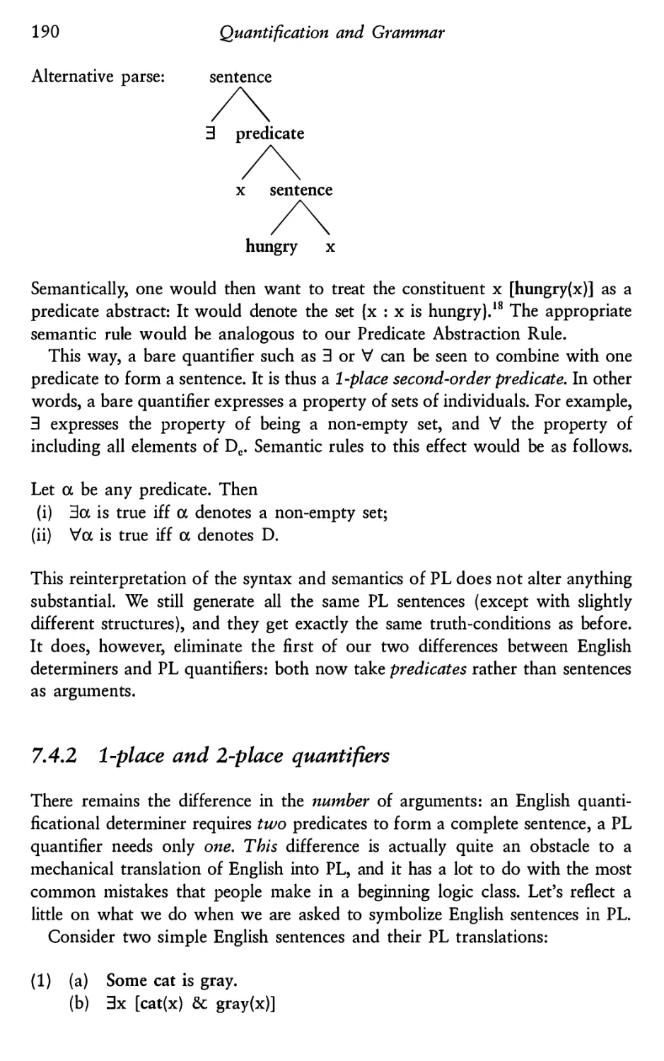
Text
Semantics in Generative Grammar
Blackwell Textbooks in Linguistics
1 Liliane Haegeman
2 Andrew Spencer
3 Helen Goodluck
4 Ronald Wardhaugh
5 Martin Atkinson
6 Diane Blakemore
7 Michael Kenstowicz
8 Deborah Schiffrin
9 John Clark and
Colin Yallop
10 Natsuko Tsujimura
11 Robert D. Borsley
12 Nigel Fabb
13 Irene Heim and
Angelika Kratzer
Introduction to Government and Binding Theory
(Second Edition)
Morphological Theory
Language Acquisition
Introduction to Sociolinguistics (Third Edition)
Children’s Syntax
Understanding Utterances
Phonology in Generative Grammar
Approaches to Discourse
An Introduction to Phonetics and Phonology
(Second Edition)
An Introduction to japanese Linguistics
Modern Phrase Structure Grammar
Linguistics and Literature
Semantics in Generative Grammar
Semantics in Generative Grammar
Irene Heim and Angelika Kratzer
Massachusetts Institute of Technology and
University of Massachusetts at Amherst
Copyright © Irene Heim and Angelika Kratzer 1998
The right of Irene Heim and Angelika Kratzer to be identified as authors
of this work has been asserted in accordance with the Copyright, Designs
and Patents Act 1988.
First published 1998
Reprinted 1998, 2000
Blackwell Publishers Inc
350 Main Street
Malden, Massachusetts 02148, USA
Blackwell Publishers Ltd
108 Cowley Road
Oxford OX4 IJF, UK
All rights reserved. Except for the quotation of short passages for the purposes
of criticism and review, no part of this publication may be reproduced, stored
in a retrieval system, or transmitted, in any form or by any means, electronic,
mechanical, photocopying, recording or otherwise, without the prior permission
of the publisher.
Except in the United States of America, this book is sold subject to the condition
that it shall not, by way of trade or otherwise, be lent, re-sold, hired out, or
otherwise circulated without the publisher’s prior consent in any form of binding
or cover other than that in which it is published and without a similar condition
including this condition being imposed on the subsequent purchaser.
Library of Congress Cataloging in Publication Data
Heim, Irene
Semantics in generative grammar / Irene Heim and Angelika Kratzer
p. cm. — (Blackwell textbooks in linguistics; 13)
Includes index.
ISBN 0—631—19712—5 — ISBN 0—631—19713—3 (pbk)
l. Semantics. 2. Generative grammar. I. Kratzer, Angelika.
11. Title. III. Series.
P325.5 .G45H45 1998
97—11089
401’.43—dc21
CIP
British Library Cataloguing in Publication Data
A CIP catalogue record for this book is available from the British Library
Typeset in 10 on 13pt Sabon
by Graphicraft Typesetters Limited, Hong Kong
Printed and bound in Great Britain
by MPG Books Ltd, Bodmin, Cornwall
This book is printed on acid-free paper
Contents
Preface
1 Truth-conditional Semantics and the Fregean Program
1.1
1.2
1.3
Truth~conditional semantics
Frege on compositionality
Tutorial on sets and functions
1.3.1 Sets
1.3.2 Questions and answers about the abstraction
notation for sets
1.3.3 Functions
2 Executing the Fregean Program
2.1
2.2
2.3
2.4
2.5
First example of a Fregean interpretation
2.1.1 Applying the semantics to an example
2.1.2 Deriving truth-conditions in an extensional semantics
2.1.3 Object language and metalanguage
Sets and their characteristic functions
Adding transitive verbs: semantic types and
denotation domains
Schonfinkelization
Defining functions in the K-notation
3 Semantics and Syntax
3.1
3.2
3.3
3.4
3.5
Type-driven interpretation
The structure of the input to semantic interpretation
Well-formedness and interpretability
The @-Criterion
Argument structure and linking
4 More of English: Nonverbal Predicates, Modifiers,
Definite Descriptions
4.1
4.2
Semantically vacuous words
Nonverbal predicates
ix
A
t
—
x
r
—
x
10
13
13
16
2O
22
24
26
29
34
43
43
45
47
49
53
61
61
62
vi
4.3
4.4
4.5
Contents
Predicates as restrictive modifiers
4.3.1 A new composition rule
4.3.2 Modification as functional application
4.3.3 Evidence from nonintersective adjectives?
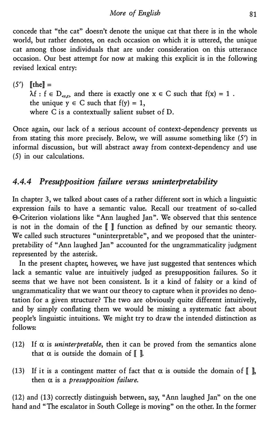
The definite article
4.4.1 A lexical entry inspired by Frege
4.4.2 Partial denotations and the distinction between
presupposition and assertion
4.4.3 Uniqueness and utterance context
4.4.4 Presupposition failure versus uninterpretability
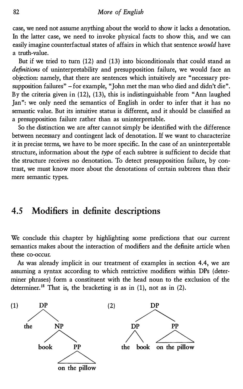
Modifiers in definite descriptions
Relative Clauses, Variables, Variable Binding
5.1
5.2
5.3
5.4
5.5
Relative clauses as predicates
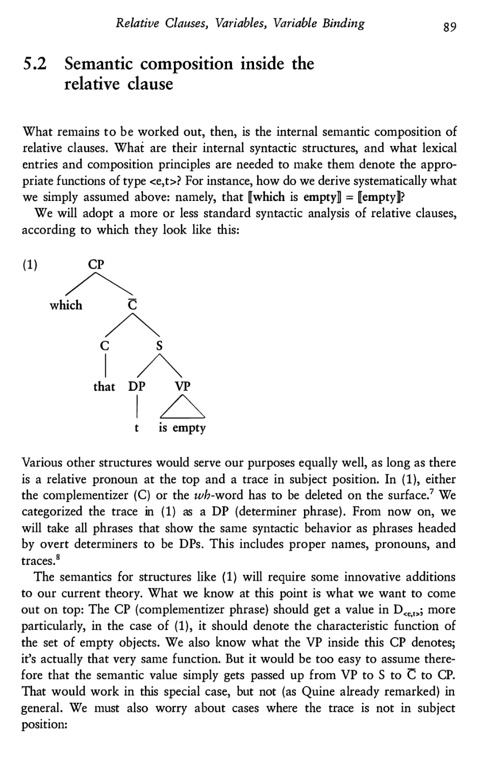
Semantic composition inside the relative clause
5.2.1 Does the trace pick up a referent?
5.2.2 Variables
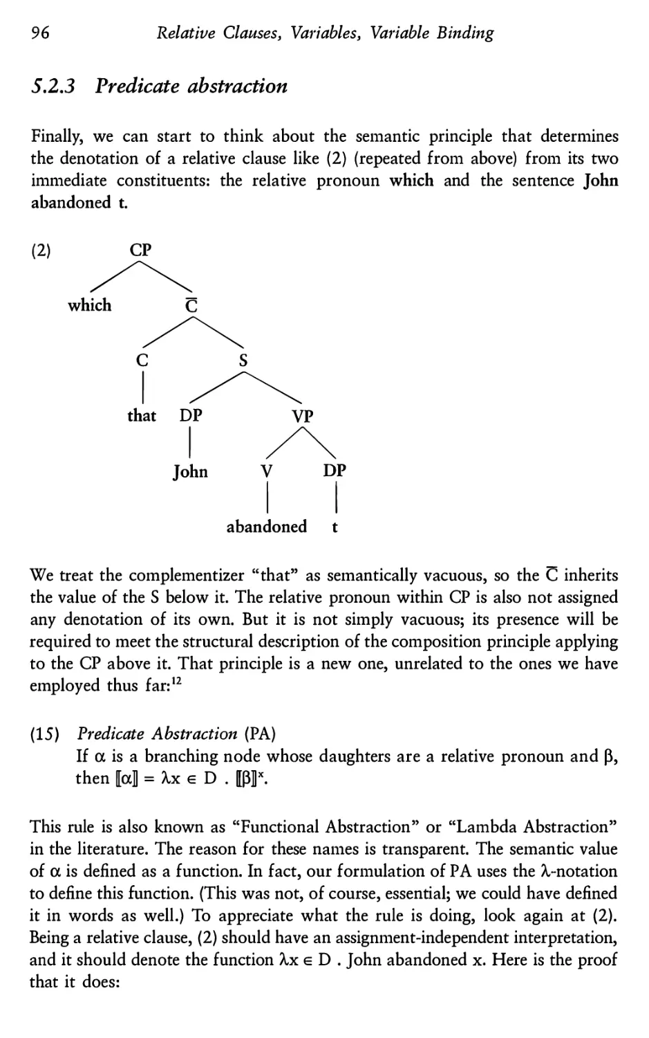
5.2.3 Predicate abstraction
5.2.4 A note on proof strategy: bottom up or top down?
Multiple variables
5.3.1 Adding “such that” relatives
5.3.2 A problem with nested relatives
5.3.3 Amending the syntax: co-indexing
5.3.4 Amending the semantics
What is variable binding?
5.4.1 Some semantic definitions
5.4.2 Some theorems
5.4.3 Methodological remarks
Interpretability and syntactic constraints on indexing
Quantifiers: Their Semantic Type
6.1
6.2
6.3
6.4
6.5
Problems with individuals as DP-denotations
6.1.1 Predictions about truth-conditions and
entailment patterns
6.1.2 Predictions about ambiguity and the effects of
syntactic reorganization
Problems with having DPs denote sets of individuals
The solution: generalized quantifiers
6.3.1
“Something”, “nothing”, “everything”
6.3.2 Problems avoided
Quantifying determiners
Quantifier meanings and relations between sets
63
65
66
68
73
73
75
80
81
82
86
86
89
90
92
96
99
106
106
108
109
110
115
116
120
121
123
131
131
132
135
138
140
140
142
145
147
6.6
Contents
6.5.1 A little history
6.5.2 Relational and Schonfinkeled denotations
for determiners
Formal properties of relational determiner meanings
6.7 Presuppositional quantifier phrases
6.8
6.7.1 “Both” and “neither”
6.7.2 Presuppositionality and the relational theory
6.7.3 Other examples of presupposing DPs
Presuppositional quantifier phrases: controversial cases
6.8.1 Strawson’s reconstruction of Aristotelian logic
6.8.2 Are all determiners presuppositional?
6.8.3 Nonextensional interpretation
6.8.4 Nonpresuppositional behavior in weak determiners
Quantification and Grammar
7.1
7.2
7.3
7.4
7.5
The problem of quantifiers in object position
Repairing the type mismatch in situ
7.2.1 An example of a “flexible types” approach
7.2.2 Excursion: flexible types for connectives
Repairing the type mismatch by movement
Excursion: quantifiers in natural language and
predicate logic
7.4.1 Separating quantifiers from variable binding
7.4.2 1-place and 2~place quantifiers
Choosing between quantifier movement and in situ
interpretation: three standard arguments
7.5.1 Scope ambiguity and “inverse” scope
7.5.2 Antecedent-contained deletion
7.5.3 Quantifiers that bind pronouns
Syntactic and Semantic Constraints on Quantifier Movement
8.1
8.2
8.3
8.4
8.5
Which DPs may move, and which ones must?
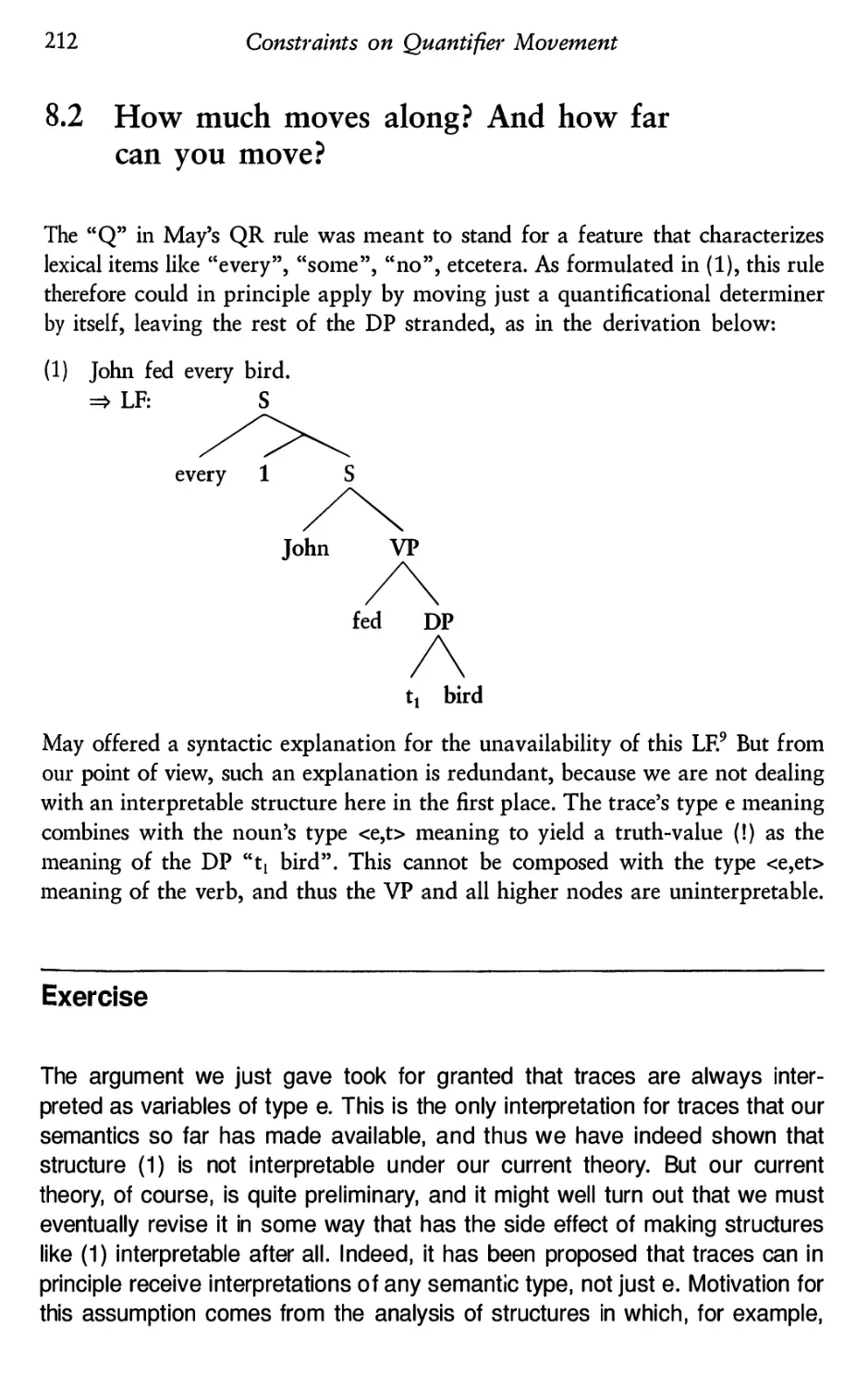
How much moves along? And how far can you move?
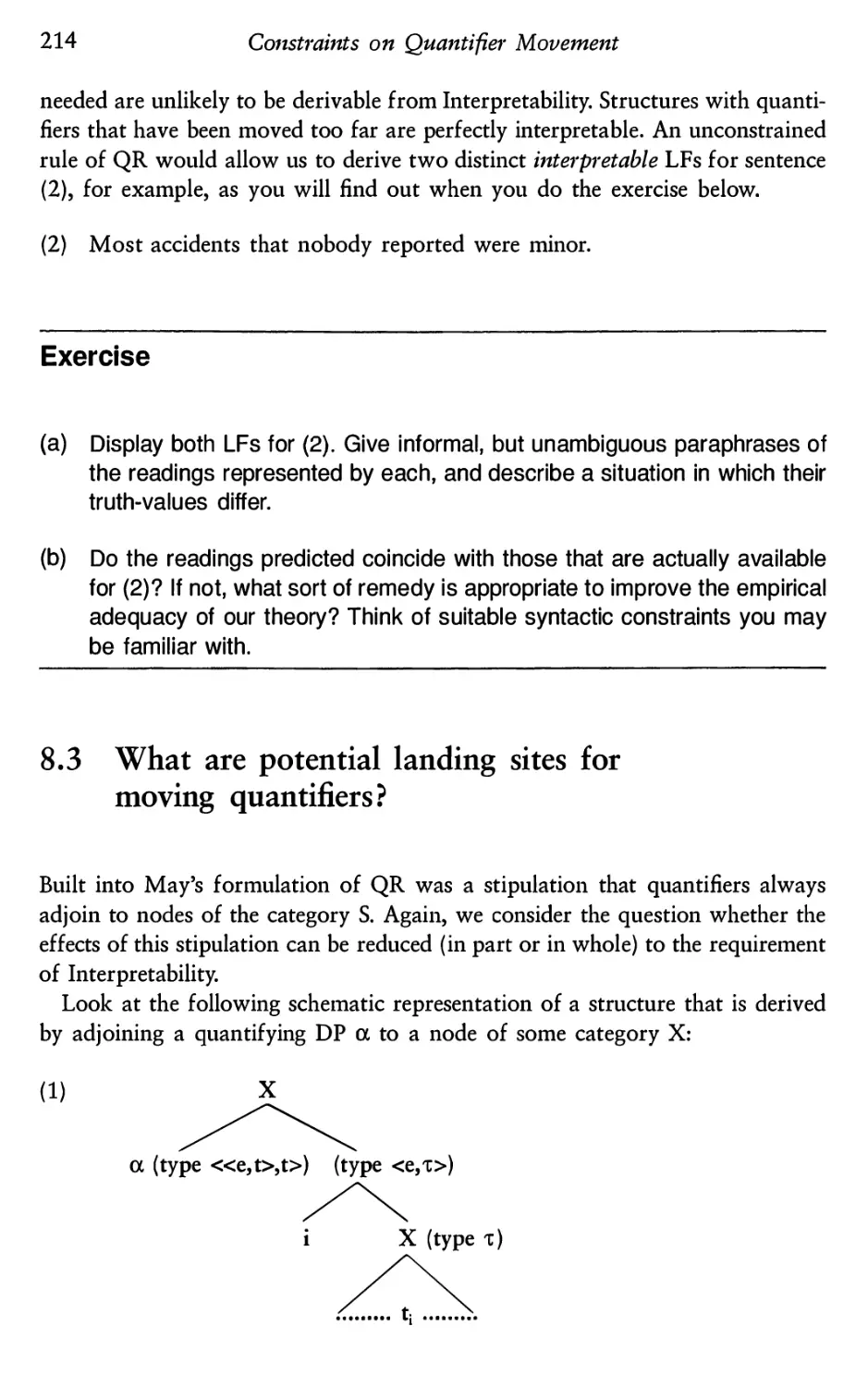
What are potential landing sites for moving quantifiers?
Quantifying into VP
8.4.1 Quantifiers taking narrow scope with respect to
auxiliary negation
8.4.2 Quantifying into VP, VP-internal subjects, and
flexible types
Quantifying into PP, AP, and NP
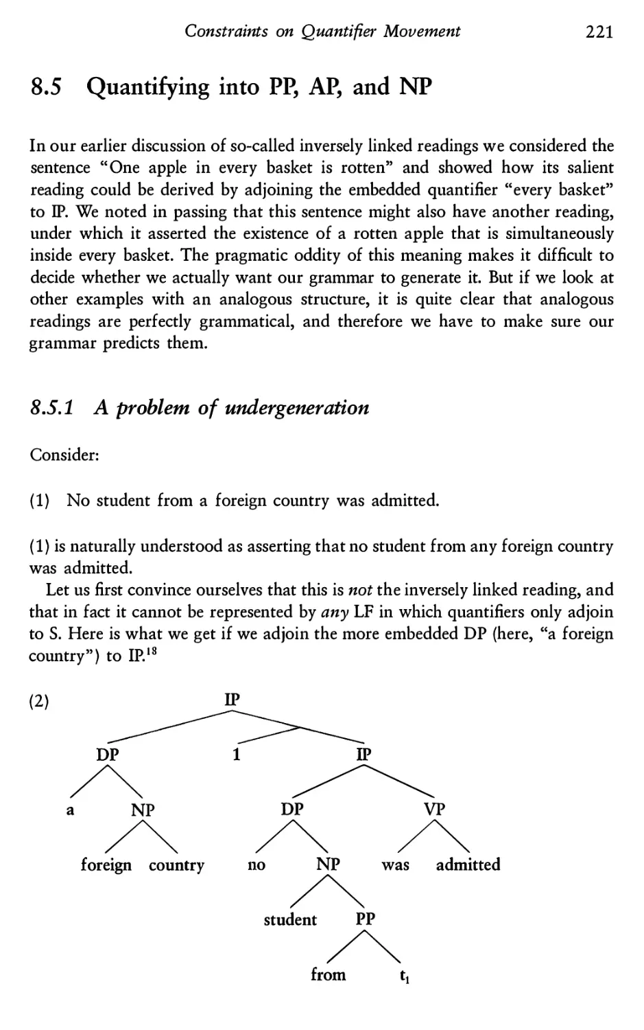
8.5.1 A problem of undergeneration
8.5.2 PP-internal subjects
8.5.3 Subjects in all lexically headed XPs?
vii
147
149
151
153
154
154
157
159
159
162
165
170
178
178
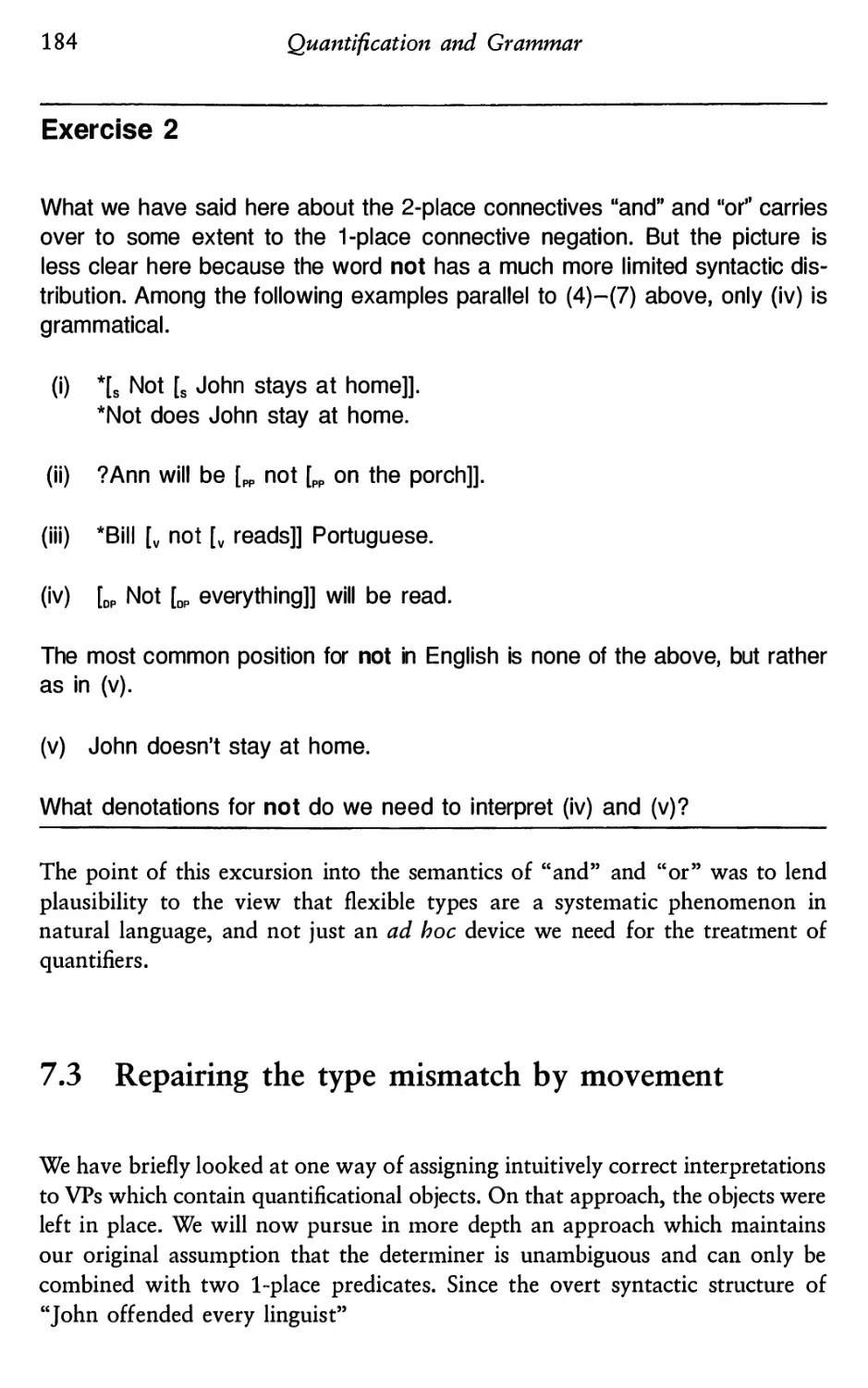
179
180
182
184
189
189
190
193
194
198
200
209
210
212
214
215
215
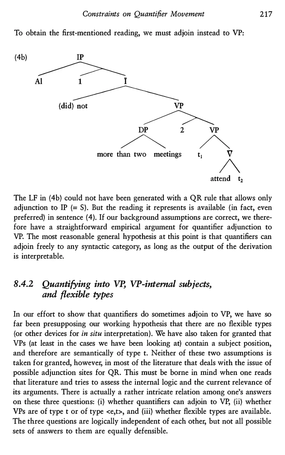
217
221
221
225
228
viii
Contents
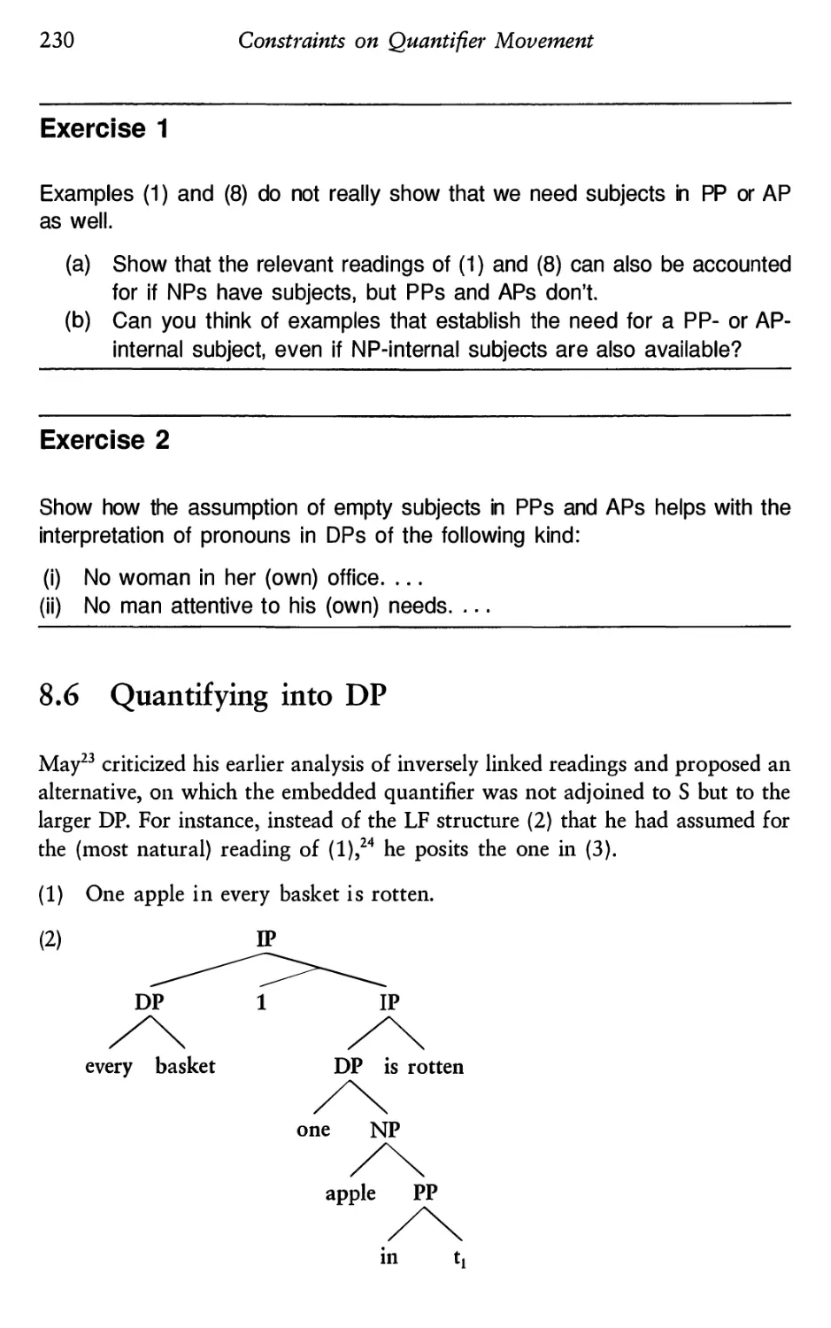
8.6 Quantifying into DP
8.6.1 Readings that can only be represented by
DP adjunction?
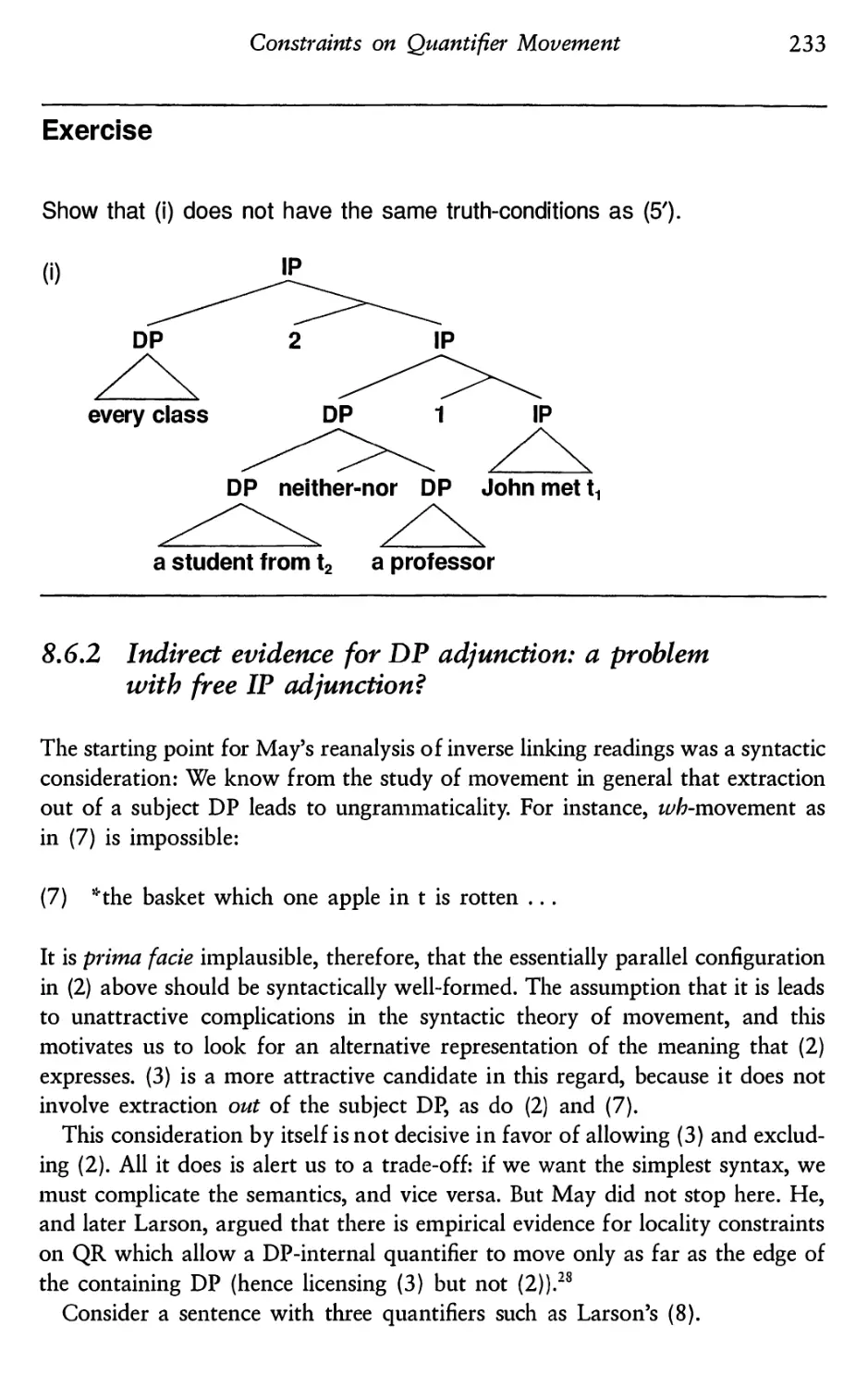
8.6.2 Indirect evidence for DP adjunction: a problem with
free IP adjunction?
8.6.3 Summary
9 Bound and Referential Pronouns and Ellipsis
9.1 Referential pronouns as free variables
9.2
9.3
9.1.1 Deictic versus anaphoric, referential versus
bound-variable pronouns
9.1.2 Utterance contexts and variable assignments
Co-reference or binding?
Pronouns in the theory of ellipsis
9.3.1 Background: the LF Identity Condition on ellipsis
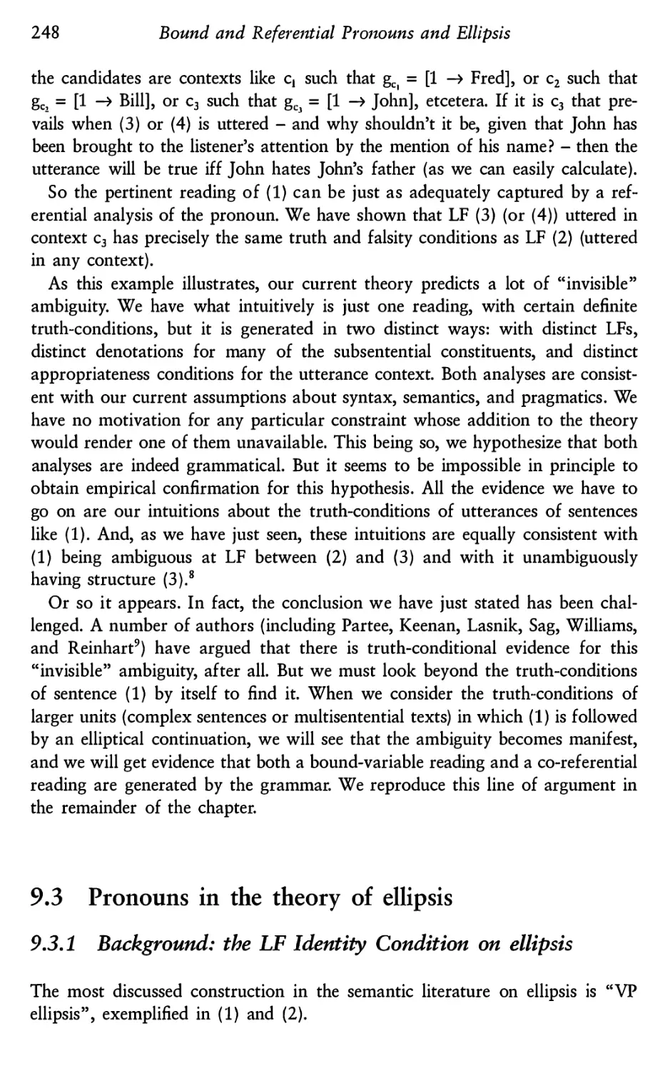
9.3.2 Referential pronouns and ellipsis
9.3.3 The “sloppy identity” puzzle and its solution
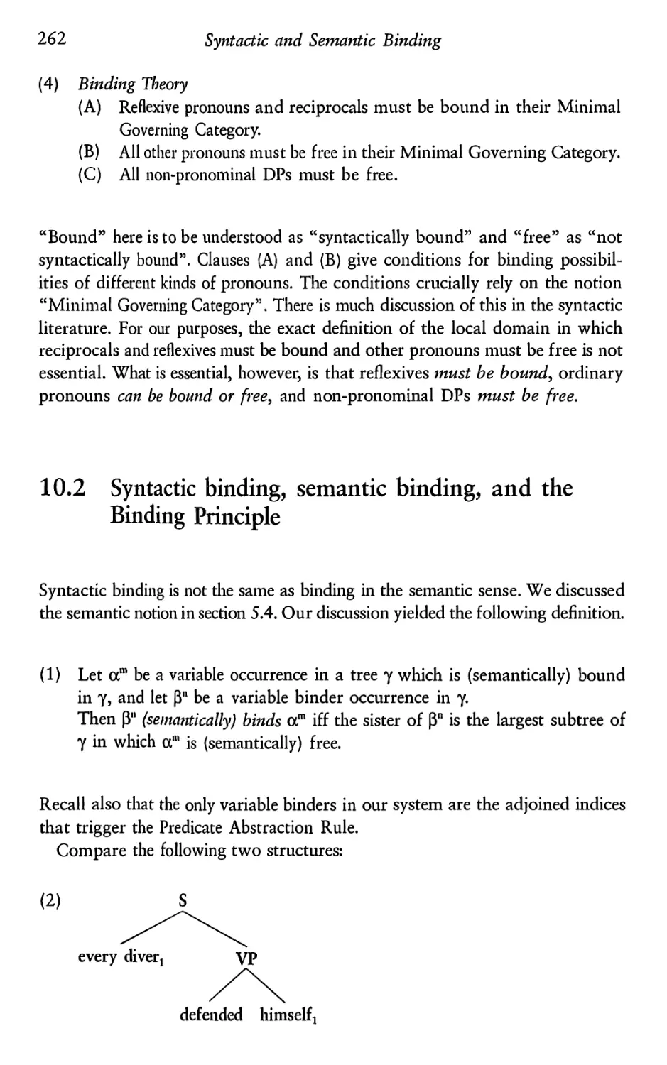
10 Syntactic and Semantic Binding
10.1
10.2
10.3
10.4
10.5
10.6
Indexing and Surface Structure binding
Syntactic binding, semantic binding, and the Binding
Principle
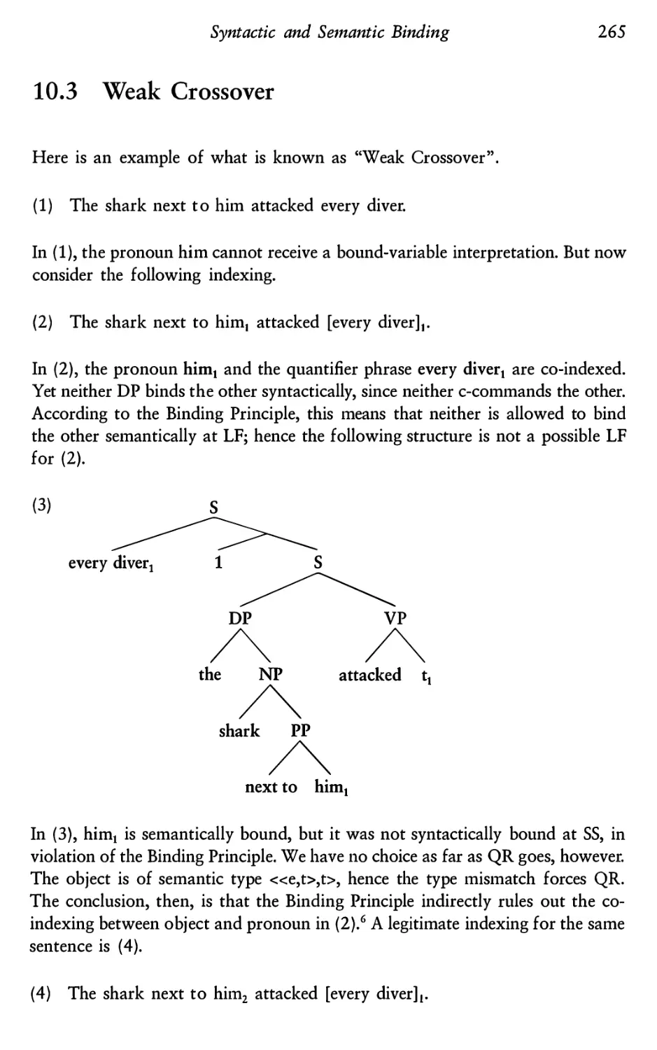
Weak Crossover
The Binding Principle and strict and sloppy identity
Syntactic constraints on co-reference?
Summary
11 E~Type Anaphora
11.1
11.2
11.3
11.4
11.5
11.6
Review of some predictions
Referential pronouns with quantifier antecedents
Pronouns that are neither bound variables nor referential
Paraphrases with definite descriptions
Cooper’s analysis of E~Type pronouns
Some applications
12 First Steps Towards an Intensional Semantics
12.1
12.2
12.3
Where the extensional semantics breaks down
What to do: intensions
An intensional semantics
12.4 Limitations and prospects
Index
230
232
233
234
239
239
239
242
245
248
248
252
254
260
260
262
265
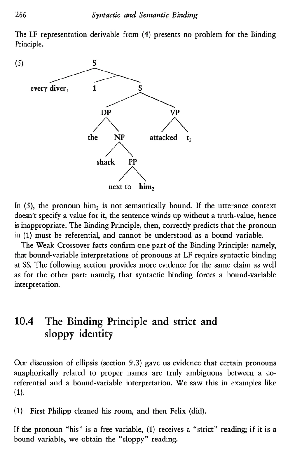
266
269
274
277
277
280
286
288
290
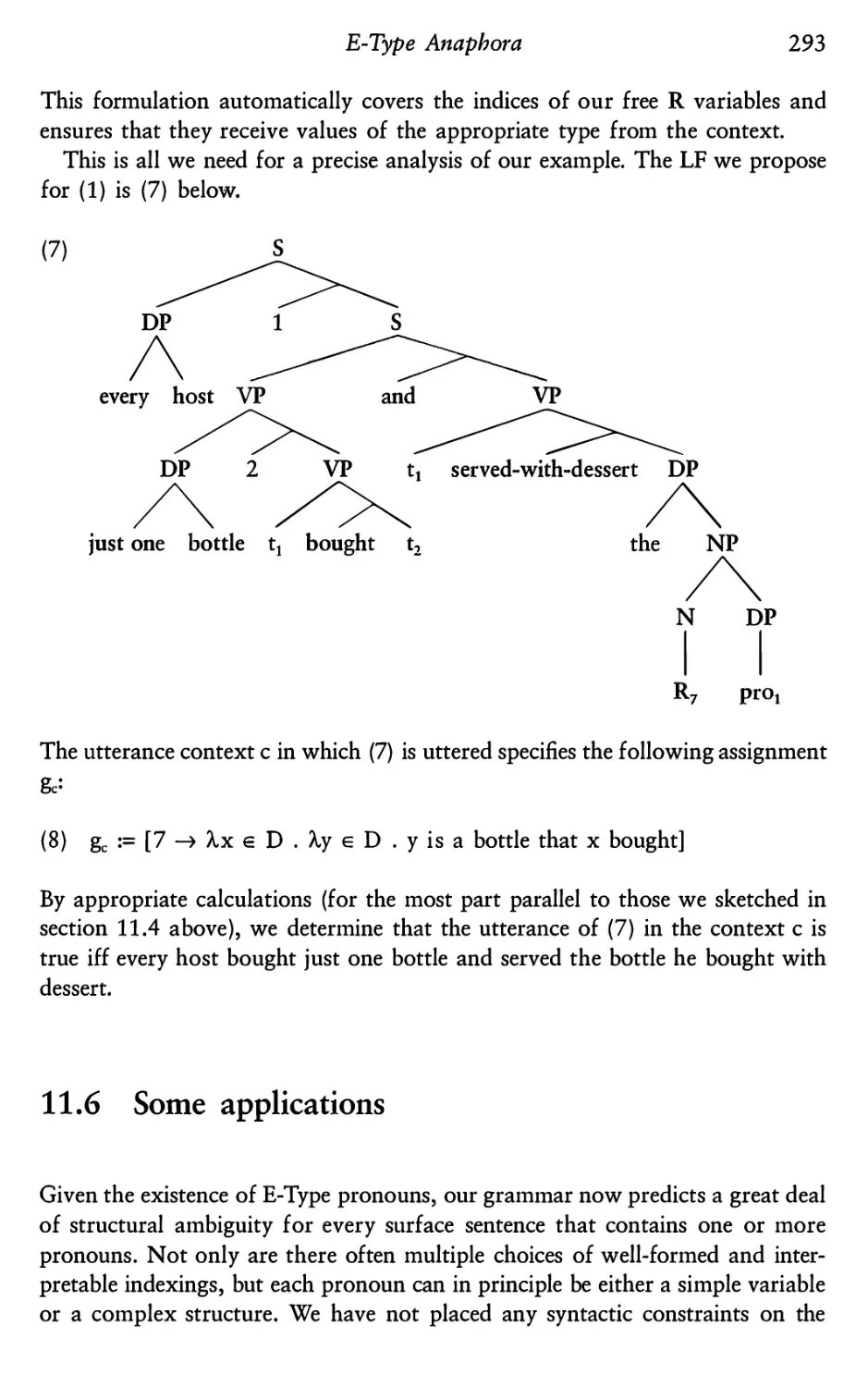
293
299
299
301
303
310
313
Preface
This book is an introduction to the craft of doing formal semantics for linguists.
It is not an overview of the field and its current developments. The many recent
handbooks provide just that. We want to help students develop the ability for
semantic analysis, and, in view of this goal, we think that exploring a few topics
in detail is more effective than offering a bird’s-eye view of everything. We also
believe that foundational and philosophical matters can be better discussed once
students have been initiated into the practice of semantic argumentation. This
is why our first chapter is so short. We dive right in.
The students for whom we created the lectures on which this book is based
were graduate or advanced undergraduate students of linguistics who had
already had a basic introduction to some formal theory of syntax and had a first
understanding of the division of labor between semantics and pragmatics. Not
all of them had had an introduction to logic or set theory. If necessary, we filled
in gaps in formal background with the help of other books.
We learned our craft from our teachers, students, and colleagues. While working
on this book, we were nurtured by our families and friends. Paul Hirschbiihler,
Molly Diesing, Kai von Fintel, Jim Higginbotham, the students in our classes,
and reviewers whose names we don’t know gave us generous comments we
could use. The staff of Blackwell Publishers helped us to turn lecture notes we
passed back and forth between the two of us into a book. We thank them all.
Irene Heim and Angelika Kratzer
Cambridge, Mass., and Amherst, April 1997
1 Truth-conditional Semantics and
the Fregean Program
1.1 Truth-conditional
semantics
To know the meaning of a sentence is to know its truth-conditions. If I say
to you
(1) There is a bag of potatoes in my pantry
you may not know whether what I said is true. What you do know, however,
is what the world would have to be like for it to be true. There has to be a bag
of potatoes in my pantry. The truth of (1) can come about in ever so many ways.
The bag may be paper or plastic, big or small. It may be sitting on the floor or
hiding behind a basket of onions on the shelf. The potatoes may come from
Idaho or northern Maine. There may even be more than a single bag. Change
the situation as you please. As long as there is a bag of potatoes in my pantry,
sentence (1) is true.
A theory of meaning, then, pairs sentences with their truth-conditions. The
results are statements of the following form:
Truth-conditions
The sentence “There is a bag of potatoes in my pantry” is true if and only if
there is a bag of potatoes in my pantry.
The apparent banality of such statements has puzzled generations of students
since they first appeared in Alfred Tarski’s 1935 paper “The Concept of Truth
in Formalized Languages.”l Pairing English sentences with their truth-conditions
seems to be an easy task that can be accomplished with the help of a single
schema:
Schema for truth-conditions
The sentence “
” istrueifandonlyif
2
Truth-conditional Semantics
A theory that produces such schemata would indeed be trivial if there wasn’t
another property of natural language that it has to capture: namely, that we
understand sentences we have never heard before. We are able to compute the
meaning of sentences from the meanings of their parts. Every meaningful part
of a sentence contributes to its truth-conditions in a systematic way. As Donald
Davidson put it:
The theory reveals nothing new about the conditions under which an
individual sentence is true; it does not make those conditions any clearer
than the sentence itself does. The work of the theory is in relating the
known truth conditions of each sentence to those aspects (“words”) of the
sentence that recur in other sentences, and can be assigned identical roles
in other sentences. Empirical power in such a theory depends on success
in recovering the structure of a very complicated ability — the ability to
speak and understand a language.2
In the chapters that follow, we will develop a theory of meaning composition.
We will look at sentences and break them down into their parts. And we will
think about the contribution of each part to the truth-conditions of the whole.
1.2 Frege on compositionality
The semantic insights we rely on in this book are essentially those of Gottlob
Frege, whose work in the late nineteenth century marked the beginning of both
symbolic logic and the formal semantics of natural language. The first worked-
out versions of a Fregean semantics for fragments of English were by Lewis,
Montague, and Cresswell.3
It is astonishing what language accomplishes. With a few syllables it ex-
presses a countless number of thoughts, and even for a thought grasped for
the first time by a human it provides a clothing in which it can be recog-
nized by another to whom it is entirely new. This would not be possible
if we could not distinguish parts in the thought that correspond to parts
of the sentence, so that the construction of the sentence can be taken to
mirror the construction of the thought. . .. If we thus view thoughts as
composed of simple parts and take these, in turn, to correspond to simple
sentence-parts, we can understand how a few sentence-parts can go to
make up a great multitude of sentences to which, in turn, there correspond
a great multitude of thoughts. The question now arises how the construc-
tion of the thought proceeds, and by what means the parts are put together
Truth-conditional Semantics
3
so that the whole is something more than the isolated parts. In my essay
“Negation,” I considered the case of a thought that appears to be com-
posed of one part which is in need of completion or, as one might say,
unsaturated, and whose linguistic correlate is the negative particle, and
another part which is a thought. We cannot negate without negating some-
thing, and this something is a thought. Because this thought saturates the
unsaturated part or, as one might say, completes what is in need of com-
pletion, the whole hangs together. And it is a natural conjecture that
logical combination of parts into a whole is always a matter of saturating
something unsaturated."
Frege, like Aristotle and his successors before him, was interested in the semantic
composition of sentences. In the above passage, he conjectured that semantic
composition may always consist in the saturation of an unsaturated meaning
component. But what are saturated and unsaturated meanings, and what is
saturation? Here is what Frege had to say in another one of his papers.
Statements in general, just like equations or inequalities or expressions in
Analysis, can be imagined to be split up into two parts; one complete in
itself, and the other in need of supplementation, or “unsaturated.” Thus,
e.g., we split up the sentence
“Caesar conquered Gaul”
into “Caesar” and “conquered Gaul.” The second part is “unsaturated”
—
it contains an empty place; only when this place is filled up with a proper
name, or with an expression that replaces a proper name, does a complete
sense appear. Here too I give the name “function” to what this “unsatur-
ated” part stands for. In this case the argument is Caesar.5
Frege construed unsaturated meanings as functions. Unsaturated meanings, then,
take arguments, and saturation consists in the application of a function to its
arguments. Technically, functions are sets of a certain kind. We will therefore
conclude this chapter with a very informal introduction to set theory. The same
material can be found in the textbook by Partee et al.‘5 and countless other
sources. If you are already familiar with it, you can skip this section and go
straight to the next chapter.
1.3 Tutorial on sets and functions
If Frege is right, functions play a crucial role in a theory of semantic composition.
“Function” is a mathematical term, and formal semanticists noWadays use it in
4
Truth-conditional Semantics
exactly the way in which it is understood in modern mathematics.7 Since functions
are sets, we will begin with the most important definitions and notational
conventions of set theory.
1.3 .1 Sets
A set is a collection of objects which are called the “members” or “elements”
of that set. The symbol for the element relation is “e ”. “x e A” reads “x is an
element of A”. Sets may have any number of elements, finite or infinite. A
special case is the empty set (symbol “Q”), which is the (unique) set with zero
elements.
Two sets are equal iff8 they have exactly the same members. Sets that are not
equal may have some overlap in their membership, or they may be disjoint (have
no members in common). If all the members of one set are also members of
another, the former is a subset of the latter. The subset relation is symbolized
by“g ”. “A g B”reads“AisasubsetofB”.
There are a few standard operations by which new sets may be constructed
from given ones. Let A and B be two arbitrary sets. Then the intersection of A
and B (in symbols: A n B) is that set which has as elements exactly the members
that A and B share with each other. The union of A and B (in symbols: A U B)
is the set which contains all the members of A and all the members of B and
nothing else. The complement of A in B (in symbols: B - A) is the set which
contains precisely those members of B which are not in A.
Specific sets may be defined in various ways. A simple possibility is to define
a set by listing its members, as in (1).
(1) Let A be that set whose elements are a, b, and c, and nothing else.
A more concise rendition of (1) is (1’).9
(1’) A:={a,b,c}.
Another option is to define a set by abstraction. This means that one specifies
a condition which is to be satisfied by all and only the elements of the set to
be defined.
(2) Let A be the set of all cats.
(2’) Let A be that set which contains exactly those x such that x is a cat.
Truth-conditional Semantics
5
(2’), of course, defines the same set as (2); it just uses a more convoluted
formulation. There is also a symbolic rendition:
(2”)A:={x:-xisacat}.
Read“{x:xisa cat}” as “thesetofallxsuchthatxisa cat”. Theletter “x”
here isn’t meant to stand for some particular object. Rather, it functions as a
kind of place-holder or variable. To determine the membership of the set A
defined in (2”), one has to plug in the names of different objects for the “x”
in the condition “x is a cat”. For instance, if you want to know whether
Kaline e A, you must consider the statement “Kaline is a cat”. If this statement
is true, then Kaline e A; if it is false, then Kaline G. A (“x e A” means that x
is not an element of A).
1.3.2 Questions and answers about the abstraction
notation for sets
Q1: If the “x” in “{x : x is a positive integer less than 7}” is just a place-holder,
whydowe needitatall?Whydon’t we justput a blank asin “{_:
_ is a positive
integer less than 7}”?
A1: That may work in simple cases like this one, but it would lead to a lot
of confusion and ambiguity in more complicated cases. For example, which
setwouldbemeantby“{_:{_:
_
likes _} = @j”? Would it be, for instance,
the set of objects which don’t like anything, or the set of objects which noth-
ing likes? We certainly need to distinguish these two possibilities (and also
to distinguish them from a number of additional ones). If we mean the first
set, we write “[x : {y : x likes y} = Q)”. If we mean the second set, we write
“{x:{y:ylikesx}=Q)”.
Q2: Whydidyou just write “{x:[y:ylikes x}=Q}” rather than “[y:[x: x
likes y} = @j”?
AZ: No reason. The second formulation would be just as good as the first, and
they Specify exactly the same set. It doesn’t matter which letters you choose; it
only matters in which places you use the same letter, and in which places you
use different ones.
Q3: Why do I have to write something to the left of the colon? Isn’t the
condition on the right side all we need to specify the set? For example, instead
of “{x : x is a positive integer less than 7}”, wouldn’t it be good enough to write
simply “{x is a positive integer less than 7}”?
6
Truth-conditional Semantics
A3: You might be able to get away with it in the simplest cases, but not in more
complicated ones. For example, what we said in A1 and A2 implies that the
following tWo are different sets:
{x:{y:xlikesy}=O}
{y:{x:xlikesy}=Q}
Therefore, if we just wrote “{{x likes y}= Q)”, it would be ambiguous. A mere
statement enclosed in set braces doesn’t mean anything at all, and we will never
use the notation in this way.
Q4: What does it mean if I write “{California : California is a western state}”?
A4: Nothing, it doesn’t make any sense. If you want to give a list specification
of the set whose only element is California, write “{California}”. If you want to
give a specification by abstraction of the set that contains all the western states
and nothing else but those, the way to write it is “{x : x is a western state)”.
The problem with what you wrote is that you were using the name of a particular
individual in a place where only place-holders make sense. The position to the
left of the colon in a set-specification must always be occupied by a place-holder,
never by a name.
Q5: How do I know whether something is a name or a place-holder? I am
familiar with “California” as a name, and you have told me that “x” and “y”
are place-holders. But how can I tell the difference in other cases? For example,
ifIseetheletter “a”or“d”or“s”, howdoIknowifit’sa nameoraplace-
holder?
A5: There is no general answer to this question. You have to determine from
case to case how a letter or other expression is used. Sometimes you will be told
in so many words that the letters “b”, “c”, “t”, and “u” are made-up names
for certain individuals. Other times, you have to guess from the context. One
very reliable clue is whether the letter shows up to the left of the colon in a set-
specification. If it does, it had better be meant as a place-holder rather than a
name; otherwise it doesn’t make any sense. Even though there is no general way
of telling names apart from place-holders, we will try to minimize sources of
confusion and stick to certain notational conventions (at least most of the time).
We will normally use letters from the end of the alphabet as place-holders, and
letters from the beginning of the alphabet as names. Also we will never employ
words that are actually used as names in English (like “California” or “John”)
as place-holders. (Of course, we could so use them if we wanted to, and then
Truth -conditional Semantics
7
we could also write things like “{California : California is a western state)”,
and it would be just another way of describing the set {x : x is a western state}.
We could, but we won’t.)
Q6: In all the examples we have had so far, the place-holder to the left of the
colon had at least one occurrence in the condition on the right. Is this necessary
for the notation to be used properly? Can I describe a set by means of a
condition in which the letter to the left of the colon doesn’t show up at all?
What about “{x : California is a western statej”?
A6: This is a strange way to describe a set, but it does pick one out. Which one?
Well, let’s see whether, for instance, Massachusetts qualifies for membership in
it. To determine this, we take the condition “California is a western state” and
plug in “Massachusetts” for all the “x”s in it. But there are no “x”s, so the
result of this “plug-in” operation is simply “California is a western state” again.
Now this happens to be true, so Massachusetts has passed the test of membership.
That was trivial, of course, and it is evident now that any other object will
qualify as a member just as easily. So {x : California is a western state} is the
set containing everything there is. (Of course, if that’s the set we mean to refer
to, there is no imaginable good reason why we’d choose this of all descriptions.)
If you think about it, there are only two sets that can be described at all by
means of conditions that don’t contain the letter to the left of the colon. One,
as we just saw, is the set of everything; the other is the empty set. The reason
for this is that when a condition doesn’t contain any “x” in it, then it will either
be true regardless of what value we assign to “x”, or it will be false regardless
of what value we assign to “x”.
Q7: When a set is given with a complicated specification, I am not always sure
how to figure out which individuals are in it and which ones aren’t. I know how
to do it in simpler cases. For example, when the set is specified as “{x : x + 2
= x2}”, and I want to know whether, say, the number 29 is in it, I know whatI
have to do: I have to replace all occurrences of “x” in the condition that follows
the colon by occurrences of “29”, and then decide whether the resulting statement
about 29 is true or false. In this case, I get the statement “29 + 2 = 292”; and
since this is false, 29 is not in the set. But there are cases where it’s not so
easy. For example, suppose a set is specified as “[x : x e [x : x :t O}}”, and
I want to figure out whether 29 is in this one. So I try replacing “x” with
“29” on the rightside of thecolon. What I getis “29 e{29: 297t0}”. ButI
don’t understand this. We just learned that names can’t occur to the left of the
colon; only place-holders make sense there. This looks just like the example
“{California : California is a western state}” that I brought up in Q5. 80 I am
stuck. Where did I go wrong?
8
Truth-conditional Semantics
A7: You went wrong when you replaced all the “x” by “29” and thereby went
from “{x: x e{x: x :t 0))”to “29e{29:297t0)”. Theformer makes sense,
the latter doesn’t (as you just noted yourself); so this cannot have been an
equivalent reformulation.
Q8: Wait a minute, how was I actually supposed to know that “{x : x e {x :
x :t 0))” made sense? For all I knew, this could have been an incoherent definition
in the first place, and my reformulation just made it more transparent what was
wrong with it.
A8: Here is one way to see that the original description was coherent, and
this will also show you how to answer your original question: namely, whether
29 e {x : x e {x : x at 0)). First, look only at the most embedded set descrip-
tion, namely “{x : x at O)”. This transparently describes the set of all objects
distinct from 0. We can refer to this set in various other ways: for instance, in
the way I just did (as “the set of all objects distinct from O”), or by a new name
thatweespeciallydefineforit,sayas “S:={x: x :tO)”, orby“{y:y:t0)”.
Given that the set {x : x at O) can be referred to in all these different ways, we
can also express the condition “x e {x : x :t O)” in many different, but equivalent,
forms — for example, these three:
“x e the set of all objects distinct from O”
“x e S (where S is as defined above)”
“xe{y:y:t0}”
Each of these is fulfilled by exactly the same values for “x” as the original
condition “x e {x : x at O)”. This, in turn, means that each can be substituted
for“xe{x:xatO)”in“{x:x e {x: x:t0})”, withoutchangingthesetthat
is thereby defined. So we have:
{x:xe{x:x¢0))
=
{x : x e the set of all objects distinct from O)
: x e S} (where S is as defined above)
:xe{y:y¢0)).
I
I
n
3
?
?
?
Now if wewanttodetermine whether 29isa member of{x : x e {x: x :t 0)),
we can do this by using any of the alternative descriptions of this set. Suppose
we take the third one above. So we ask whether 29 e {x : x e S). We know that
itisiff29eS.BythedefinitionofS,thelatterholdsiff29e{x: x :t0).And
this in turn is the case iff 29 qt 0. Now we have arrived at an obviously true
statement, and we can work our way back and conclude, first, that 29 e S,
second,that29e{x:xeS},andthird,that29e{x:xe {x:xat0)).
Truth-conditional Semantics
9
Q9: I see for this particular case now that it was a mistake to replace all
occurrences of “x” in the condition “x e [x : x ¢ 0}” by “29”. But I am still
not confident that I wouldn’t make a similar mistake in another case. Is there
a general rule or fool-proof strategy that I can follow so that I’ll be sure to avoid
such illegal substitutions?
A9: A very good policy is to write (or rewrite) your conditions in such a
way that there is no temptation for illegal substitutions in the first place. This
means that you should never reuse the same letter unless this is strictly neces-
sary in order to express what you want to say. Otherwise, use new letters
wherever possible. If you follow this strategy, you won’t ever write something
like “{x: x e {x: x at0})” to beginwith,andifyou happen to readit,you will
quickly rewrite it before doing anything else with it. What you would write
instead would be something like “{x : x e {y : y at 0})”. This (as we already noted)
describes exactly the same set, but uses distinct letters “x” and “y” instead of
only “x”s. It still uses each letter twice, but this, of course, is crucial to what
it is meant to express. If we insisted on replacing the second “x” by a “z”, for
instance, we would wind up with one of those strange descriptions in which the
“x” doesn’t occur to the right of thecolon at all,thatis, “{x: z e {y:yat0))”.
As we saw earlier, sets described in this way contain either everything or nothing.
Besides, what is “z” supposed to stand for? It doesn’t seem to be a place-holder,
because it’s not introduced anywhere to the left of a colon. So it ought to be a
name. But whatever it is a name of, that thing was not referred to anywhere in
cc 3:
cc 3:
the condition that we had before changing x to z , so we have clearly
altered its meaning.
Exercise
The same set can be described in many different ways, often quite different
superficially. Here you are supposed to figure out which of the following
equalities hold and which ones don’t. Sometimes the right answer is not just
plain “yes” or “no”, but something like “yes, but only if . . For example, the
two sets in (i) are equal only in the special case where a = b. In case of doubt,
the best way to check whether two sets are equal is to consider an arbitrary
individual, say John, and to ask if John could be in one of the sets without
being in the other as well.
(i) {a}={'3}
(ii){x:x=a}={a}
10
Truth-conditional
Semantics
(iii) {x:xisgreen}={y:yisgreen}
(iv) {x:xlikesa}={y:ylikesb}
(v){x:xeA}=A
(vi) {xzxe{y:yeB}}=B
(vii) {x:{y:ylikesx}=Q}={x:{x:xlikesx}=Q}
1.3.3 Functions
If we have two objects x and y (not necessarily distinct), we can construct
from them the ordered pair <x, y>. <x, y> must not be confused with {x, y}.
Since sets with the same members are identical, we always have {x, y) = {y, x).
But in an ordered pair, the order matters: except in the special case of x = y,
<x, y> 7t <y, x>.10
A (2-place) relation is a set of ordered pairs. Functions are a special kind
of relation. Roughly speaking, in a function (as opposed to a non-functional
relation), the second member of each pair is uniquely determined by the first.
Here is the definition:
(3) A relation f is a function iff it satisfies the following condition:
Foranyx:ifthereareyand2suchthat<x, y>efand<x,z>ef,then
y=2.
Each function has a domain and a range, which are the sets defined as follows:
(4) Let f be a function.
Then thedomain of f is (x: thereis a y suchthat <x, y> e f), and therange
offis(x:thereisaysuchthat <y,x>ef}.
WhenAisthedomain andBtherangeoff, wealsosaythatfisfrom A
and onto B. If C is a superset“ of PS range, we say that f is into (or to) C.
For “f is from A (in)to B”, we write “f : A —>B”.
The uniqueness condition built into the definition of functionhood ensures
that whenever f is a function and x an element of its domain, the following
definition makes sense:
(5) f(x) := the unique y such that <x, y> e f.
For “f(x)”, read “f applied to x” or “f of x”. f(x) is also called the “value of
f for the argument x”, and we say that 7‘maps x to y. “f(x) = y” (provided that
it is well-defined at all) means the same thing as “<x, y> e f” and is normally
the preferred notation.
Truth-conditional Semantics
11
Functions, like sets, can be defined in various ways, and the most straight-
forward one is again to simply list the function’s elements. Since functions are
sets of ordered pairs, this can be done with the notational devices we have
already introduced, as in (6), or else in the form of a table like the one in (7),
or in words such as (8).
(6) F={<a,b>,<c,b>,<d,e>)
a——>b
(7) F = c——>b
d——>e
(8) Let F be that function f with domain [a, c, d} such that f(a) = f(c) = b and
f(d) = e.
Each of these definitions determines the same function F. The convention for
reading tables like the one in (7) is transparent: the left column lists the domain
and the right column the range, and an arrow points from each argument to the
value it is mapped to.
Functions with large or infinite domains are often defined by specifying a
condition that is to be met by each argument—value pair. Here is an example.
(9) Let FH be that function f such that
f:IN——>IN,andforeveryxe IN,f(x)=x+1.
(IN is the set of all natural numbers.)
The following is a slightly more concise format for this sort of definition:
(10) I:+1:= f: IN —> IN
ForeveryxeIN,f(x)=x+1.
Read (10) as: “ H is to be that function f from IN into IN such that, for every
x e IN, f(x) = x + 1.” An even more concise notation (using the K-operator) will
be introduced at the end of the next chapter.
Notes
1 A. Tarski, “Der Wahrheitsbegriff in den formalisierten Sprachen” (1935), English
translation in A. Tarski, Logic, Semantics, Metamatbematics (Oxford, Oxford
University Press, 1956), pp. 152—278.
12
10
11
Truth-conditional Semantics
D. Davidson, Inquiries into Truth and Interpretation (Oxford, Clarendon Press,
1984), p. 24.
D. Lewis, “General Semantics,” in D. Davidson and G. Harman (eds), Semantics
of Natural Languages (Dordrecht, Reidel, 1972), 169—218; R. Montague, Formal
Philosophy (New Haven, Yale University Press, 1974); M. J . Cresswell, Logics and
Languages (London, Methuen, 1973).
G. Frege, “Logische Untersuchungen. Dritter Teil: Gedankengefiige,” Beitra'ge zur
Philosophie des deutschen Idealismus, 3 (1923-6), pp. 36 -51.
Frege, “Function and Concept” (1891), trans. in M. Black and P. Geach, Translations
from the Philosophical Writings of Gottloh Frege (Oxford, Basil Blackwell, 1960),
pp. 21 —41, at p. 31.
B. H . Partee, A. ter Meulen, and R. E . Wall, Mathematical Methods in Linguistics
(Dordrecht, Kluwer, 1990).
This was not true of Frege. He distinguished between the function itself and its
extension (German: Wertuerlauf). The latter, however, is precisely what mathemat-
icians today call a “function”, and they have no use for another concept that would
correspond to Frege’s notion of a function. Some of Frege’s commentators have
actually questioned whether that notion was coherent. To him, though, the distinc-
tion was very important, and he maintained that while a function is unsaturated, its
extension is something saturated. So we are clearly going against his stated inten—
tions here.
“Iff” is the customary abbreviation for “if and only if”.
We use the colon in front of the equality sign to indicate that an equality holds by
definition. More specifically, we use it when we are defining the term to the left of
“:=” in terms of the one to the right. In such cases, we should always have a
previously unused symbol on the left, and only familiar and previously defined
material on the right. In practice, of course, we will reuse the same letters over and
over, but whenever a letter appears to the left of “:=”, we thereby cancel any
meaning that we may have assigned it before.
It is possible to define ordered pairs in terms of sets, for instance as follows: <x, y>
:= ((x), (x, y}). For most applications of the concept (the ones in this book included),
however, you don’t need to know this definition.
The superset relation is the inverse of the subset relation: A is a superset of B iff
Bc A.
2 Executing the Fregean Program
In the pages to follow, we will execute the Fregean program for a fragment of
English. Although we will stay very close to Frege’s proposals at the beginning,
we are not interested in an exegesis of Frege, but in the systematic development
of a semantic theory for natural language. Once we get beyond the most basic
cases, there will be many small and some not—so -small departures from the
semantic analyses that Frege actually defended. But his treatment of semantic
composition as functional application (Frege’s Conjecture), will remain a leading
idea throughout.
Modern syntactic theory has taught us how to think about sentences and their
parts. Sentences are represented as phrase structure trees. The parts of a sen-
tence are subtrees of phrase structure trees. In this chapter, we begin to explore
ways of interpreting phrase structure trees of the kind familiar in linguistics.
We will proceed slowly. Our first fragment of English will be limited to simple
intransitive and transitive sentences (with only proper names as subjects and
objects), and extremely naive assumptions will be made about their structures.
Our main concern will be with the process of meaning composition. We will see
how a precise characterization of this process depends on, and in turn con-
strains, what we say about the interpretation of individual words.
This chapter, too, has sections which are not devoted to semantics proper,
but to the mathematical tools on which this discipline relies. Depending on the
reader’s prior mathematical experience, these may be supplemented by exercises
from other sources or skimmed for a quick review.
2.1 First example of a Fregean interpretation
We begin by limiting our attention to sentences that consist of a proper name
plus an intransitive verb. Let us assume that the syntax of English associates
these with phrase structures like that in (1).
14
Executing the Fregean Program
(1)
S
/\7P
VP
Nl
l|
Ann
smokes
We want to formulate a set of semantic rules which will provide denotations
for all trees and subtrees in this kind of structure. How shall we go about
this? What sorts of entities shall we employ as denotations? Let us be guided
by Frege.
Frege took the denotations of sentences to be truth-values, and we will fol-
low him in this respect. But wait. Can this be right? The previous chapter began
with the statement “To know the meaning of a sentence is to know its truth-
conditions”. We emphasized that the meaning of a sentence is not its actual
truth-value, and concluded that a theory of meaning for natural language should
pair sentences with their truth-conditions and explain how this can be done in a
compositional way. Why, then, are we proposing truth-values as the denotations
for sentences? Bear with us. Once we spell out the complete proposal, you’ll see
that we will end up with truth-conditions after all.
The Fregean denotations that we are in the midst of introducing are also
called “extensions”, a term of art which is often safer to use because it has no
potentially interfering non-technical usage. The extension of a sentence, then,
is its actual truth-value. What are truth-values? Let us identify them with the
numbers 1 (True) and 0 (False). Since the extensions of sentences are not func-
tions, they are saturated in Frege’s sense. The extensions of proper names like
“Ann” and “Jan” don’t seem to be functions either. “Ann” denotes Ann, and
“Jan” denotes Jan.
We are now ready to think about suitable extensions for intransitive verbs like
“smokes”. Look at the above tree. We saw that the extension for the lexical item
“Ann” is the individual Ann. The node dominating “Ann” is a non-branching
N-node. This means that it should inherit the denotation of its daughter node.1
The N—node is again dominated by a non-branching node. This NP-node, then,
will inherit its denotation from the N-node. So the denotation of the NP-node
in the above tree is the individual Ann. The NP-node is dominated by a branching
S—node. The denotation of the S-node, then, is calculated from the denotation
of the NP-node and the denotation of the VP-node. We know that the denotation
of the NP-node is Ann, hence saturated. Recall now that Frege conjectured that
all semantic composition amounts to functional application. If that is so, we
Executing the Pregean Program
15
must conclude that the denotation of the VP-node must be unsaturated, hence
a function. What kind of function? Well, we know what kinds of things its
arguments and its values are. Its arguments are individuals like Ann, and its
values are truth-values. The extension of an intransitive verb like “smokes”, then,
should be a function from individuals to truth-values.
Let’s put this all together in an explicit formulation. Our semantics for the
fragment of English under consideration consists of three components. First,
we define our inventory of denotations. Second, we provide a lexicon which
specifies the denotation of each item that may occupy a terminal node. Third,
we give a semantic rule for each possible type of non-terminal node. When we
want to talk about the denotation of a lexical item or tree, we enclose it in
double brackets. For any expression on, then, IIOLII is the denotation of on. We can
think of II II as a function (the interpretation function) that assigns appropriate
denotations to linguistic expressions. In this and most of the following chapters,
the denotations of expressions are extensions. The resulting semantic system
is an extensional semantics. Towards the end of this book, we will encounter
phenomena that cannot be handled within an extensional semantics. We will
then revise our system of denotations and introduce intensions.
A. Inventory of denotations
Let D be the set of all individuals that exist in the real world. Possible denotations
are:
Elements of D, the set of actual individuals.
Elements of {0, 1}, the set of truth-values.
Functions from D to {0, 1}.
B. Lexicon
IIAnn]!= Ann
IIJanll = Jan
etc. for other proper names.
IIworksll = f : D —>{0, 1}
Forallx e D,f(x)=1iffxworks.
IIsmokesll = f : D —>{0, 1}
Forallxe D,f(x)=1iffxsmokes.
etc. for other intransitive verbs.
C. Rules for non—terminal nodes
In what follows, Greek letters are used as variables for trees and subtrees.
16
Executing the Pregean Program
8
(81) If 06 has the form /\, then [led]= [[7]](IIBII).
B7
NP
(82) If on has the form I , then [led]= [[5]].
B
VP
(83) If on has the form | , then [led]= m.
B
N
(84) If 0c has the form I , then IIOLII= IIBII.
B
v
(85) If on has the form I , then IIOLII= [[3]].
[3
2.1.1 Applying the semantics to an example
Does this set of semantic rules predict the correct truth-conditions for “Ann
smokes”? That is, is “Ann smokes” predicted to be true if and only if Ann
smokes? “Of course”, you will say, “that’s obvious”. It’s pretty obvious indeed,
but we are still going to take the trouble to give an explicit proof of it. As
matters get more complex in the chapters to come, it will be less and less
obvious whether a given set of proposed rules predict the judgments it is supposed
to predict. But you can always find out for sure if you draw your trees and work
through them node by node, applying one rule at a time. It is best to get used
to this while the calculations are still simple. If you have some experience with
computations of this kind, you may skip this subsection.
We begin with a precise statement of the claim we want to prove:
Claim:
r'
S
I
/\NP
VP
l
I
= 1 iff Ann smokes.
N
V
L Ann
smokes _
Executing the Fregean Program
17
We want to deduce this claim from our lexical entries and semantic rules
(SD—(85). Each of these rules refers to trees of a certain form. The tree
S
NP
VP
N
V
Ann
smokes
is of the form specified by rule (81), repeated here, so let’s see what (81) says
aboutiL
S
(81) If 0!. has the form /\ , then [[06]]= II'yII([[B]]).
B7
When we apply a general rule to a concrete tree, we must first match up the
variables in the rule with the particular constituents that correspond to them in
the application. In this instance, on is
S
NP
VP
N
V
Ann
smokes
so [3must be NP
and7mustbe VP
N
V
Ann
smokes
18
The rule says that [106]]= II'y]I(IIB]]), so this means in the present application that
'l
(2)
S
_ Ann
Executing the Pregean Program
smokes __
VP
V
_ smokes_
Now we apply rule (S3) to the tree
(This time, we skip the detailed justification of why and how this rule fits this
1
VP
V
smokes
tree.) What we obtain from this is
VP
V
(3)
"l
From (2) and (3), by substituting equals for equals, we infer (4).
l
(4)
.
Ann
Now we apply rule (85) to the appropriate subtree and use the resulting equation
_ smokes ..
smokes _
V
smokes
for another substitution in (4):
[NP'
lN
|j_ Ann _ll
Executing the Fregean Program
19
(5) l'
S
1
/\
"NP1‘
NP VP
)
I
l
=
[[smokes]] N
Nv
1
l
)
Lll A11111 J
.
Ann
smokes .
Now we use rule (82) and then (S4), and after substituting the results thereof
in (5), we have (6).
<6)‘ S
/\NP
VP
|
I
=
IIsmokesll(IIAnIllll
N
V
Il
_ Ann
smokes _l
At this point, we look up the lexical entries for Ann and smokes. If we just use
these to substitute equals for equals in (6), we get (7).
(7) ll
3
NP
VP
fD{O1)
: —>,
l
l
[ For all x e D,f(x) = 1 iffx smokes](Ann)
N
V,
_ Ann
smokes __
Let’s take a close look at the right-hand side of this equation. It has the gross
form “function (argument)’, so it denotes the value that a certain function yields
for a certain argument. The argument is Ann, and the function is the one which
maps those who smoke to 1 and all others to 0. If we apply this function to
Ann, we will get 1 if Ann smokes and 0 if she doesn’t. To summarize what we
have just determined:
20
Executing the Fregean Program
(8) s
_) {0’
1}
.
(Ann) = 1 iff Ann smokes.
For allx e D,f(x)=1iffxsmokes
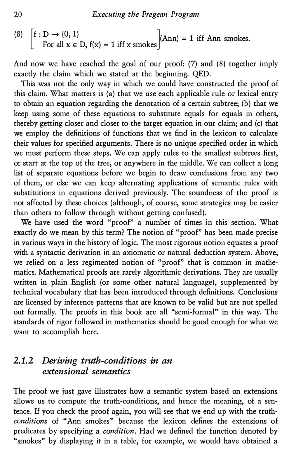
And now we have reached the goal of our proof: (7) and (8) together imply
exactly the claim which we stated at the beginning. QED.
This was not the only way in which we could have constructed the proof of
this claim. What matters is (a) that we use each applicable rule or lexical entry
to obtain an equation regarding the denotation of a certain subtree; (b) that we
keep using some of these equations to substitute equals for equals in others,
thereby getting closer and closer to the target equation in our claim; and (c) that
we employ the definitions of functions that we find in the lexicon to calculate
their values for specified arguments. There is no unique specified order in which
we must perform these steps. We can apply rules to the smallest subtrees first,
or start at the top of the tree, or anywhere in the middle. We can collect a long
list of separate equations before we begin to draw conclusions from any two
of them, or else we can keep alternating applications of semantic rules with
substitutions in equations derived previously. The soundness of the proof is
not affected by these choices (although, of course, some strategies may be easier
than others to follow through without getting confused).
We have used the word “proof” a number of times in this section. What
exactly do we mean by this term? The notion of “proof” has been made precise
in various ways in the history of logic. The most rigorous notion equates a proof
with a syntactic derivation in an axiomatic or natural deduction system. Above,
we relied on a less regimented notion of “proof” that is common in mathe-
matics. Mathematical proofs are rarely algorithmic derivations. They are usually
written in plain English (or some other natural language), supplemented by
technical vocabulary that has been introduced through definitions. Conclusions
are licensed by inference patterns that are known to be valid but are not spelled
out formally. The proofs in this book are all “semi-formal” in this way. The
standards of rigor followed in mathematics should be good enough for what we
want to accomplish here.
2.1.2 Deriving truth—conditions in an
extensional semantics
The proof we just gave illustrates how a semantic system based on extensions
allows us to compute the truth-conditions, and hence the meaning, of a sen-
tence. If you check the proof again, you will see that we end up with the truth-
conditions of “Ann smokes” because the lexicon defines the extensions of
predicates by specifying a condition. Had we defined the function denoted by
“smokes” by displaying it in a table, for example, we would have obtained a
Executing the Fregean Program
21
mere truth-value. We didn’t really have a choice, though, because displaying the
function in a table would have required more world knowledge than we happen
to have. We do not know of every existing individual whether or not (s)he
smokes. And that’s certainly not what we have to know in order to know the
meaning of “smoke”. We could look at a fictitious example, though.
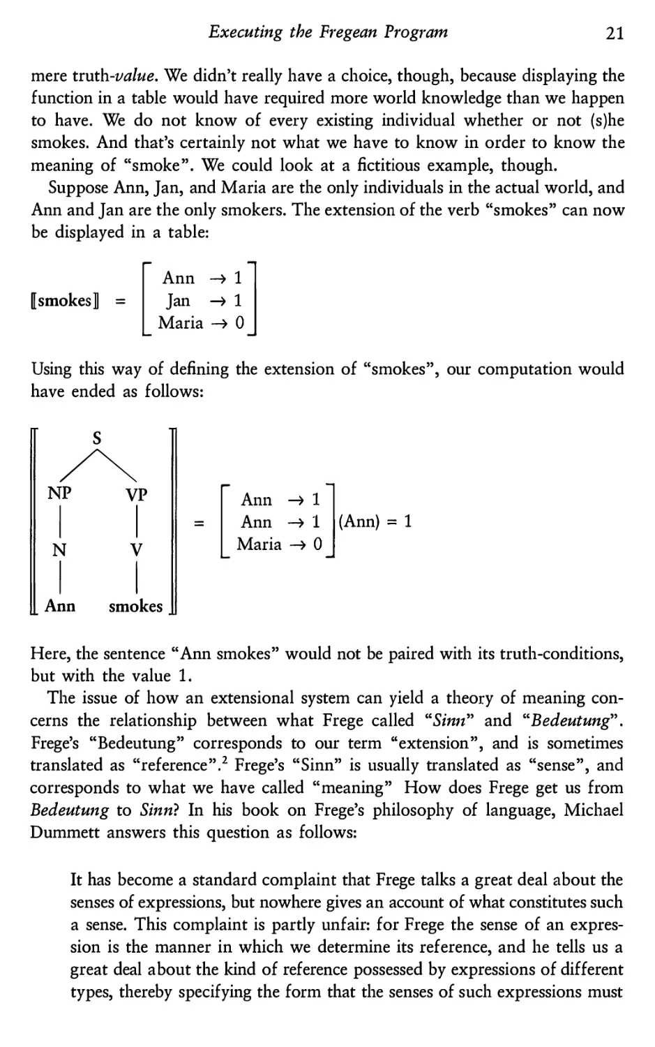
Suppose Ann, Jan, and Maria are the only individuals in the actual world, and
Ann and Jan are the only smokers. The extension of the verb “smokes” can now
be displayed in a table:
Ann ——> 1
IIsmokesfl =
Jan —>1
Maria ——> 0
Using this way of defining the extension of “smokes”, our computation would
have ended as follows:
S
NP
VP
Ann —)1
l
I
=
Ann ——>1 (Ann) = 1
N
V
Maria ——> O
__
Ann
smokes _l
Here, the sentence “Ann smokes” would not be paired with its truth-conditions,
but with the value 1.
The issue of how an extensional system can yield a theory of meaning con-
cerns the relationship between what Frege called “Simz” and “Bedeutung”.
Frege’s “Bedeutung” corresponds to our term “extension”, and is sometimes
translated as “reference”.2 Frege’s “Sinn” is usually translated as “sense”, and
corresponds to what we have called “meaning” How does Frege get us from
Bedeutung to Sinn? In his book on Frege’s philosophy of language, Michael
Dummett answers this question as follows:
It has become a standard complaint that Frege talks a great deal about the
senses of expressions, but nowhere gives an account of what constitutes such
a sense. This complaint is partly unfair: for Frege the sense of an expres-
sion is the manner in which we determine its reference, and he tells us a
great deal about the kind of reference possessed by expressions of different
types, thereby specifying the form that the senses of such expressions must
22
Executing the Fregean Program
take. .. . The sense of an expression is the mode of presentation of the
referent: in saying what the referent is, we have to choose a particular way
of saying this, a particular means of determining something as a referent.3
What Dummett says in this passage is that when specifying the extension
(reference, Bedeatang) of an expression, we have to choose a particular way of
presenting it, and it is this manner of presentation that might be considered the
meaning (sense, Sinn) of the expression. The function that is the extension of a
predicate can be presented by providing a condition or by displaying it in a
table, for example. Only if we provide a condition do we choose a mode of
presentation that “shows”4 the meaning of the predicates and the sentences they
occur in. Different ways of defining the same extensions, then, can make a
theoretical difference. Not all choices yield a theory that pairs sentences with
their truth-conditions. Hence not all choices lead to a theory of meaning.
2.1.3 Object language and metalanguage
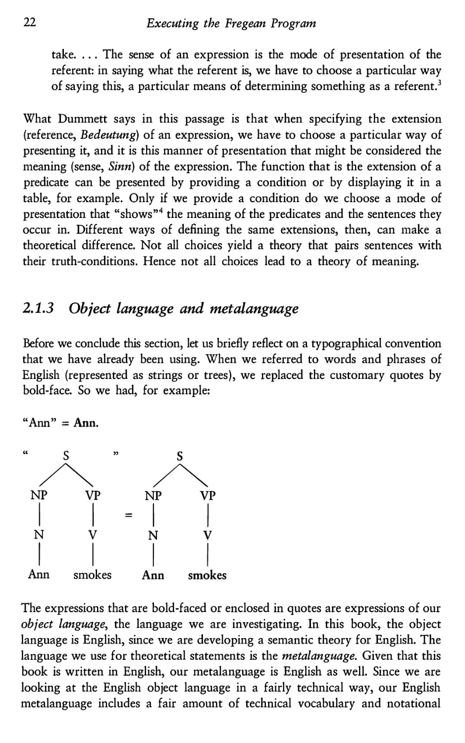
Before we conclude this section, let us briefly reflect on a typographical convention
that we have already been using. When we referred to words and phrases of
English (represented as strings or trees), we replaced the customary quotes by
bold-face. So we had, for example:
“Ann” = Ann.
“
S
”
S
/\
/\
NP
VP
NP
VP
ll=ll
N
V
N
V
I|ll
Ann
smokes
Ann
smokes
The expressions that are bold-faced or enclosed in quotes are expressions of our
object language, the language we are investigating. In this book, the object
language is English, since we are developing a semantic theory for English. The
language we use for theoretical statements is the metalanguage. Given that this
book is written in English, our metalanguage is English as well. Since we are
looking at the English object language in a fairly technical way, our English
metalanguage includes a fair amount of technical vocabulary and notational
Executing the Pregean Program
23
conventions. The abstraction notation for sets that we introduced earlier is an
example. Quotes or typographical distinctions help us marlc the distinction be-
tween object language and metalanguage. Above, we always used the bold-faced
forms when we placed object language expressions between denotation brackets.
For example, instead of writing the lexical entry for the name “Ann”:
[[“Ann”]] = Ann
we wrote:
IIAnnII = Ann.
This lexical entry determines that the denotation of the English name “Ann” is
the person Ann. The distinction between expressions and their denotations is
important, so we will usually use some notational device to indicate the difference.
We will never write things like “IIAnn]]”. This would have to be read as “the
denotation of (the person) Ann”, and thus is nonsense. And we will also avoid
using bold-face for purposes other than to replace quotes (such as emphasis, for
which we use italics).
Exercise on sentence
connectives
Suppose we extend our fragment to include phrase structures of the forms
below (where the embedded S-constituents may either belong to the initial
fragment or have one of these three forms themselves):
3
S
S
/\/l\/K
it-is-not-the—case —that S
SandS
SorS
A
A
A
A
A
How do we have to revise and extend the semantic component in order to
provide all the phrase structures in this expanded fragment with interpreta-
tions? Your task in this exercise is to define an appropriate semantic value for
each new lexical item (treat “it-is-not-the—case -that" as a single lexical item
here) and to write appropriate semantic rules for the new types of non—terminal
nodes. To do this, you will also have to expand the inventory of possible
semantic values. Make sure that you stick to our working hypothesis that all
semantic composition is functional application (Frege’s Conjecture).
24
Executing the Fregean Program
2.2 Sets and their characteristic functions5
We have construed the denotations of intransitive verbs as functions from
individuals to truth-values. Alternatively, they are often regarded as sets of
individuals. This is the standard choice for the extensions of 1-place predicates
in logic. The intuition here is that each verb denotes the set of those things that
it is true of. For example: IIsleeps]]= {x e D : x sleeps).6 This type of denotation
would require a different semantic rule for composing subject and predicate, one
that isn’t simply functional application.
Exercise
Write the rule it would require.
Here we have chosen to talce Frege’s Conjecture quite literally, and have avoided
sets of individuals as denotations for intransitive verbs. But for some purposes,
sets are easier to manipulate intuitively, and it is therefore useful to be able
to pretend in informal tallc that intransitive verbs denote sets. Fortunately, this
make-believe is harmless, because there exists a one-to-one correspondence
between sets and certain functions.
(1) Let A be a set. Then charA, the characteristic function of A, is that func-
tionfsuchthat,foranyx e A,f(x)=1,andforanyxG.A,f(x)=O.
(2) Let f be a function with range {0, 1). Then charf, the set characterized by f,
is{xe D:f(x)=1}.
Exploiting the correspondence between sets and their characteristic functions,
we will often switch baclc and forth between function tallc and set tallc in the
discussion below, sometimes saying things that are literally false, but become
true when the references to sets are replaced by references to their characteristic
functions (or vice versa).
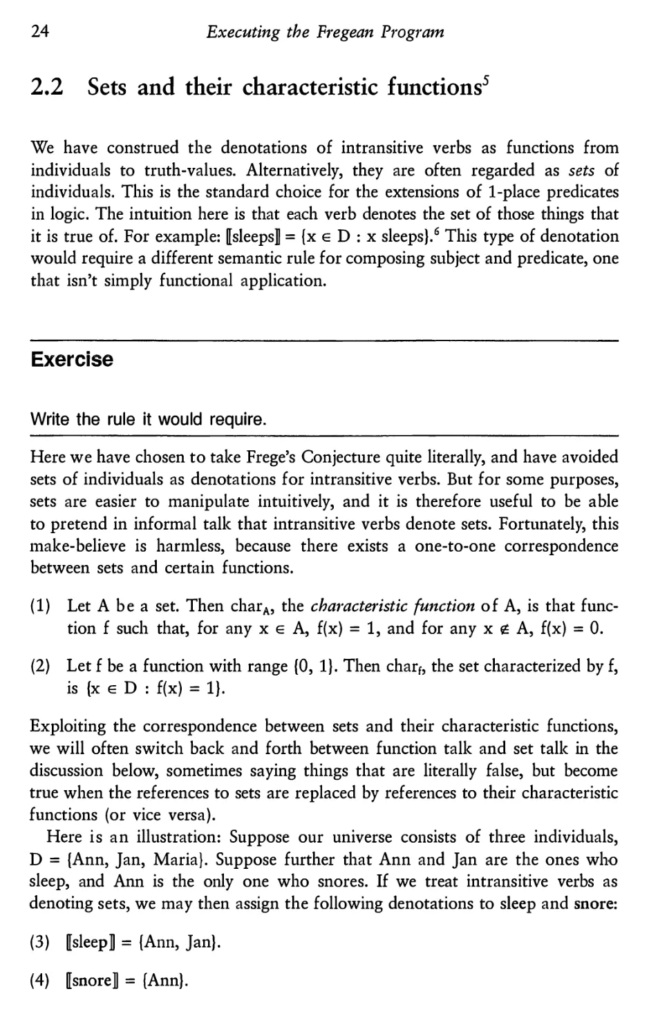
Here is an illustration: Suppose our universe consists of three individuals,
D = {Ann, Jan, Maria}. Suppose further that Ann and Jan are the ones who
sleep, and Ann is the only one who snores. If we treat intransitive verbs as
denoting sets, we may then assign the following denotations to sleep and snore:
(3) IIsleepll= {Ann, Jan).
(4) IIsnore]]= {Ann}.
Executing the Fregean Program
25
We can now write things like the following:
(5) Ann 6 IIsleepll.
(6) IIsnoreII ; IIsleep]].
(7) |IIsnore]] n IIsleep]]|= 1.
IAI (the cardinality of A) is the number of elements in the set A.
(5) means that Ann is among the sleepers, (6) means that the snorers are a
subset of the sleepers, and (7) means that the intersection of the snorers and
the sleepers has exactly one element. All these are true, given (3) and (4). Now
suppose we want to switch to a treatment under which intransitive verbs denote
characteristic functions instead of the corresponding sets.
Ann —>1
Jan —>1
Maria —> O
(3’) [8166131]
Ann —>1
(4’) IIsnore]] =
Jan —>0
Maria —> 0
If we want to make statements with the same import as (5)-(7) above, we can
no longer use the same formulations. For instance, the statement
Ann 6 IIsleepII
if we read it literally, is now false. According to (3’), IIsleepII is a function.
Functions are sets of ordered pairs, in particular,
IIsleepII= {<Ann, 1>, <Jan, 1>, <Maria, O>).
Ann, who is not an ordered pair, is clearly not among the elements of this set.
Likewise,
IIsnoreII ; IIsleepII
is now false, because there is one element of flsnorell, namely the pair <Jan, O>,
which is not an element of IIsleep]]. And
26
Executing the Pregean Program
IIIsnoreII n [Isleep]]|= 1
is false as well, because the intersection of the two functions described in (3’)
and (4’) contains not just one element, but two, namely <Ann, 1> and <Maria, O>.
The upshot of all this is that, once we adopt (3’) and (4’) instead of (3) and
(4), we have to express ourselves differently if we want to make statements that
preserve the intuitive meaning of our original (5)—(7). Here is what we have to
write instead:
(5’) IIsleepll(Ann) = 1
(6’) For all x e D : if [[snore]|(x) = 1, then [[sleepll(x) = 1
Or, equivalently:
{x : IIsnore]|(x) = 1} g {x : IIsleep]I(x)= 1}
(7’) |{x : IIsnorell(x) = 1} n {x : [Isleepll(x) = 1}| = 1
As you can see from this, using characteristic functions instead of sets makes
certain things a little more cumbersome.
2.3 Adding transitive verbs: semantic types and
denotation domains
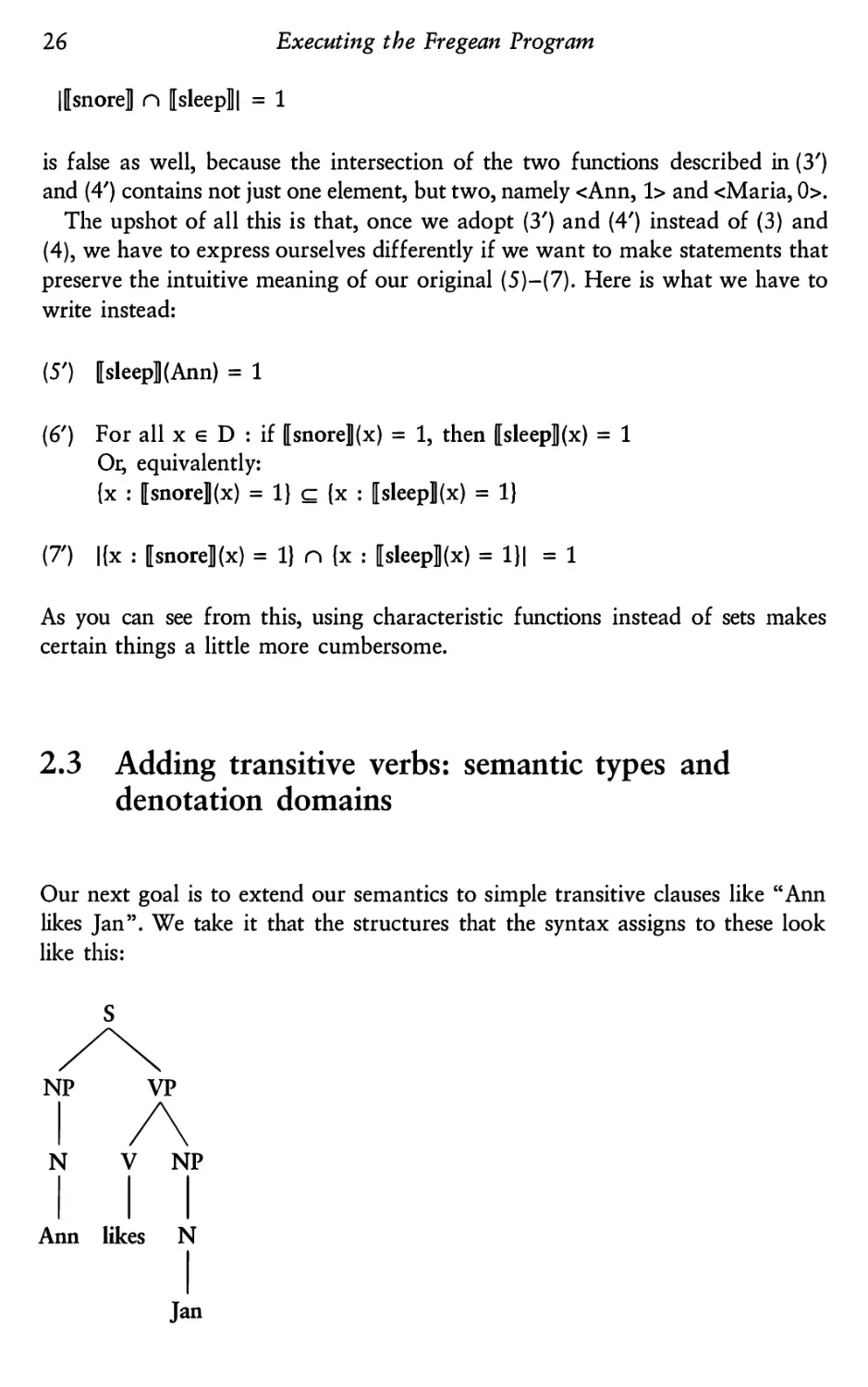
Our next goal is to extend our semantics to simple transitive clauses like “Ann
likes Jan”. We take it that the structures that the syntax assigns to these look
like this:
S
/\NP
VP
I/\
TlNIP
Ann likes N
Jan
Executing the Fregean Program
27
The transitive verb combines with its direct object to form a VP, and the VP
combines with the subject to form a sentence. Given structures of this kind,
what is a suitable denotation for transitive verbs? Look at the above tree. The
lexical item “likes” is dominated by a non-branching V—node. The denotation
of “likes”, then, is passed up to this node. The next node up is a branching
VP-node. Assuming that semantic interpretation is local, the denotation of this
VP—node must be composed from the denotations of its two daughter nodes.
If Frege’s Conjecture is right, this composition process amounts to functional
application. We have seen before that the denotations of NP-nodes dominating
proper names are individuals. And that the denotation of VP-nodes are functions
from individuals to truth-values. This means that the denotation of a transitive
verb like “likes” is a function from individuals to functions from individuals to
truth-values.7
When we define such a function-valued function in full explicitness, we have
to nest one definition of a function inside another. Here is the proposed meaning
of “likes”.
{Ilikell=f:D —>{g:gisafunctionfromD to{0,1}}
Forallxe D,f(x)=gx:D —>{0,1}
ForallyeD,gx(y)=1iffylikesx.
This reads: {Ilikell is that function f from D into the set of functions from D to
{0, 1} such that, for all x e D, f(x) is that function gx from D into {0, 1} such
that, for all y e D, gx(y) = 1 iff y likes x. Fortunately, this definition can be
compressed a bit. There is no information lost in the following reformulation:8
{Ilikell=f:D —>{g:gisafunctionfromD to{0,1]}
Forallx,yeD,f(x)(y)=1iffylikesx.
{Ilikell is a 1-place function, that is, a function with just one argument. The
arguments of {Ilikell are interpreted as the individuals which are liked; that is,
they correspond to the grammatical object of the verb “like”. This is so because
we have assumed that transitive verbs form a VP with their direct object. The
direct object, then, is the argument that is closest to a transitive verb, and is
therefore semantically processed before the subject.
What is left to spell out are the interpretations for the new kinds of non-
terminal nodes:
VP
(86) If on has the form /\, then [led]= mum).
BY
28
Executing the Fregean Program
What we just proposed implies an addition to our inventory of possible,
denotations: aside from individuals, truth-values, and functions from individuals
to truth-values, we now also employ functions from individuals to functions
from individuals to truth-values. It is convenient at this point to introduce a way
of systematizing and labeling the types of denotations in this growing inventory.
Following a common practice in the tradition of Montague, we employ the
labels “e” and “t” for the two basic types.9
(1) e is the type of individuals.
De:=D.
(2) t is the type of truth-values.
Dt := {0, 1}.
Generally, DI is the set of possible denotations of type 1:. Besides the basic types
e and t, which correspond to Frege’s saturated denotations, there are derived
types for various sorts of functions, Frege’s unsaturated denotations. These are
labeled by ordered pairs of simpler types: <0','c> is defined as the type of functions
whose arguments are of type 0' and whose values are of type ’C. The particular
derived types of denotations that we have employed so far are <e,t> and <e,<e,t>>:
(3) Dq.’t> := {f : fis a function from DC to D,}
(4) m»
:= {f : f is a function from Dc to D<c’,,}
Further additions to our type inventory will soon become necessary. Here is a
general definition:
(5) Semantic types
(a) e and t are semantic types.
(b) If 0' and “c are semantic types, then <O',T> is a semantic type.
(c) Nothing else is a semantic type.
Semantic denotation domains
(a) De := D (the set of individuals).
(b) Dt := {0, 1} (the set of truth-values).
(c) For any semantic types 0' and 1:,
D<o¢>
is the set of all functions from
Do to D,.
(5) presents a recursive definition of an infinite set of semantic types and a
parallel definition of a typed system of denotation domains. Which semantic
Executing the Fregean Program
29
types are actually used by natural languages is still a matter of debate. The issue
of “type economy” will pop up at various places throughout this book, most
notably in connection with adjectives in chapter 4 and quantifier phrases in
chapter 7. So far, we have encountered denotations of types e, <e,t>, and <e,<e,t>>
as possible denotations for lexical items: Dc contains the denotations of proper
names, D<e’t> the denotations of intransitive verbs, and D<L.’<c,t>> the denotations of
transitive verbs. Among the denotations of non-terminal constituents, we have
seen examples of four types: Dt contains the denotations of all Ss, Dc (= D) the
denotations of all Ns and NPs, D“,t> the denotations of all VPs and certain Vs,
and D
the denotations of the remaining Vs.
<c,<c,t.>
2.4 Schonfinkelization
Once more we interrupt the construction of our semantic component in order
to clarify some of the underlying mathematics. Our current framework implies
that the denotations of transitive verbs are 1-place functions. This follows from
three assumptions about the syntax—semantics interface that we have been making:
Binary Branching
In the syntax, transitive verbs combine with the direct object to form a VP, and
VPs combine with the subject to form a sentence.
Locality
Semantic interpretation rules are local: the denotation of any non-terminal node
is computed from the denotations of its daughter nodes.
Frege’s Conjecture
Semantic composition is functional application.
If transitive verbs denote 1-place function-valued functions, then our semantics
contrasts with the standard semantics for 2-place predicates in logic, and it is
instructive to reflect somewhat systematically on how the two approaches relate
to each other.
In logic texts, the extension of a 2-place predicate is usually a set of ordered
pairs: that is, a relation in the mathematical sense. Suppose our domain D
contains just the three goats Sebastian, Dimitri, and Leopold, and among these,
Sebastian is the biggest and Leopold the smallest. The relation “is-bigger—than”
is then the following set of ordered pairs:
3O
Executing the Fregean Program
Rugs“ = {<Sebastian, Dimitri>, <Sebastian, Leopold>, <Dimitri, Leopold>}.
We have seen above that there is a one-to-one correspondence between sets and
their characteristic functions. The “functional version” of Rbigge, is the following
function from D x D to {0, 1}.10
— <L,S>
—aol
<L,D> —>O
<L,L> —>0
<8, L> -—>1
fbiggcr
=
<S, D> —>1
<8,S> —>O
<D, L> —>1
<D, S> —)O
_<D, D> —) OJ
fuss“ is a 2—place function.11 In his paper “Uber die Bausteine der mathematischen
Logik,”12 Moses Schonfinkel showed how n-place functions can quite generally
be reduced to 1-place functions. Let us apply his method to the 2-place function
above. That is, let us Schonfinkell3 the function fbigger. There are two possibilities.
f’biggc, is the left-to-right Schonfinkelization of fbiggfl. f”biggc, is the right-to—left
Schonfinkelization of fbiggcr.
pL
-—>0‘
L—>S —>O
D —>0‘
—L+fl
Fags“:
S -—>S —>O
_D
—>lj
—L
— >1“
D ——>S —>O
L
-D
——>OJ
f’biggc, is a function that applies to the first argument of the “bigger” relation to
yield a function that applies to the second argument. When applied to Leopold,
it yields a function that maps any goat into 1 if it is smaller than Leopold. There
is no such goat. Hence we get a constant function that assigns O to all the goats.
When applied to Sebastian, f’biggc, yields a function that maps any goat into 1
if it is smaller than Sebastian. There are two such goats, Leopold and Dimitri.
And when applied to Dimitri, f’biggc, yields a function that maps any goat into
1 if it is smaller than Dimitri. There is only one such goat, Leopold.
Executing the Fregean Program
31
l lL—w"
L—> S—>1
LID—)1:
L—>O
f”biggcr=
S “‘9
S '—)O
D-— >OJ
"Lao"
D—> S—>1
D——>OJ
f”b,ggc, is a function that applies to the second argument of the “bigger” relation
to yield a function that applies to the first argument. When applied to Leopold,
it yields a function that maps any goat into 1 if it is bigger than Leopold. These
are all the goats except Leopold. When applied to Sebastian,
f”biggct
yields a
function that maps any goat into 1 if it is bigger than Sebastian. There is no
such goat. And when applied to Dimitri, Whigs” maps any goat into 1 if it is
bigger than Dimitri. There is only one such goat, Sebastian.
On both methods, we end up with nothing but 1-place functions, and this is
as desired. This procedure can be generalized to any n-place function. You will
get a taste for this by doing the exercises below.
Now we can say how the denotations of 2-place predicates construed as
relations are related to the Fregean denotations introduced above. The Fregean
denotation of a 2-place predicate is the right-to-left Schonfinkeled version of
the characteristic function of the corresponding relation. Why the right-to-left
Schonfinkelization? Because the corresponding relations are customarily speci-
fied in such a way that the grammatical object argument of a predicate corre-
sponds to the right component of each pair in the relation, and the subject to
the left one. (For instance, by the “love”-relation one ordinarily means the set
of lover—loved pairs, in this order, and not the set of loved—lover pairs.) That’s
an arbitrary convention, in a way, though suggested by the linear order in which
English realizes subjects and objects. As for the Fregean denotations of 2-place
predicates, remember that it is not arbitrary that their (unique) argument cor-
responds to the grammatical object of the predicate. Since the object is closest
to the predicate in hierarchical terms, it must provide the argument for the
function denoted by the predicate.
Exercise 1
Suppose that our universe D contains just two elements, Jacob and Maria.
Consider now the following binary and ternary relations:
32
Executing the Fregean Program
Radores = {<Jacob, Maria>, <Maria, Maria>}
Rassignsto = {<Jacob, Jacob,Maria>, <Maria, Jacob, Maria>}
In standard predicate logic, these would be suitable extensions for the 2-place
and 3-place predicate letters “F2” and "G3" as used in the following scheme of
abbreviation:
“F2": “a adores b"
“G3": “a assigns b to c"
Find the characteristic functions for both of these relations, and then Schonfinkel
them from right to left. Could the two Schonfinkeled functions be suitable
denotations for the English verbs “adore" and “assign (to)" respectively? If yes,
why? If not, why not?
Exercise 2
In the exercise on sentence connectives in section 2.1, we stipulated ternary
branching structures for sentences with “and” and “or". Now assume that all
English phrase structures are at most binary branching, and assign accord-
ingly revised syntactic analyses to these sentences. (Whether you choose
right—branching or left-branching structures does not matter here, but stick to
one option.) Then revise the semantics accordingly. As always, be sure to
provide every subtree with a semantic value, as well as to adhere to our
current assumptions about the semantic interpretation component (Locality
and Frege’s Conjecture).
Using the labeling system introduced at the end of section 2.3, specify the
type of denotation for each node in your binary branching structure for the
sentence "Jan works, and it is not the case that Jan smokes”.
Exercise 3
(a) Extend the fragment in such a way that phrase structure trees of the
following kind are included.
Executing the Fregecm Program
33
S
/\
NlP
VP
/\
N
V
PP
Ann
\ll
NlP T
NIP
introduces
T
to
T
Maria
Jacob
Add the necessary semantic rules and lexical entries, sticking to Locality and
Frege’s Conjecture. Assume that the preposition “to" is a semantically vacuous
element; that is, assume the ad hoc rule below:
PP
/\
If on has the form P B, then |Ioc]]= [[13]].
l
to
(b) Suppose now that the actual world contains just three individuals, Ann,
Maria, and Jacob. And suppose further that Ann introduces Maria to Jacob,
and Maria introduces Jacob to Ann, and no further introductions take place.
Which particular function is [[introducell in this case? Display it in a table.
(0) Using the table specification of IIintroducell from (b) and the lexical
entries for the names, calculate the denotations of each non-terminal node in
the tree under (a).
(d) Under standard assumptions, a predicate logic formalization of the
English sentence “Ann introduces Maria to Jacob” might look like this:
|3(A M J)
Scheme of abbreviation:
“A”:
“Ann”
“M":
“Maria"
“J":
“Jacob"
“la":
“a introduces b to c"
34
Executing the Pregean Program
The extension of “la” under this scheme of abbreviation is the following set X
of ordered triples:
X:={<x,y,z>eDxDxD:xintroducesyto2}.
How is this extension related to the extension — let’s call it t — for introduce
that you defined in (a)? Give your answer by completing the following statement:
Foranyx,y,zeD,f(x)(y)(z)=1iff eX.
2.5 Defining functions in the A-notation
The final section of this chapter is devoted to yet another technical matter. You
have already had a taste of the ubiquity of functions among the denotations that
our Fregean semantics assigns to the words and phrases of natural languages.
We will now introduce another notation for describing functions, which will
save us some ink in future chapters.
The format in which we have defined most of our functions so far was
introduced in section 1.3 with the following example:
(1) F+1=f:IN—>IN
ForeveryxeIN,f(x)=x+1.
The same definition may henceforth be expressed as follows:
(2) F+1:=[7\,x:xe lN.x+1]
The K-term, “Xx : x e IN . x + 1”, is to be read as “the (smallest) function which
mapseveryx suchthat xisinIN tox+1”.
Generally, K-terms are constructed according to the following schema:
(3) [Mutt]
We say that 0!.is the argument variable, 4) the domain condition, and 'y the value
description. The domain condition is introduced by- a colon, and the value
description by a period.14 0!. will always be a letter standing for an arbitrary
argument of the function we are trying to define. In (2), this is the letter “x”,
which we generally use to stand for arbitrary individuals. The domain condition
4) defines the domain of our function, and it does this by placing a condition on
Executing the Fregean Program
35
possible values for 06. In our example, 4) corresponds to “x e IN”, which encodes
the information that the domain of F+1contains all and only the natural numbers.
The value description 7, finally, specifies the value that our function assigns to
the arbitrary argument represented by on. In (2), this reads “x + 1”, which tells
us that the value that F+1assigns to each argument is that argument’s successor.
The general convention for reading K-terms in (semi-mathematical) English is
such that (3) reads as (3’):
(3’) the smallest function which maps every 06 such that q) to 'y
We will typically omit “smallest”, but it is always understood, and it is
strictly speaking necessary to pick out the intended function uniquely. Notice,
for instance, that besides F“, there are lots of other functions which also map
every natural number to its successor: namely, all those functions which are
supersets of F“, but have larger domains than IN. By adding “smallest”, we
make explicit that the domain condition (1) delimits the domain exactly; that is,
that in (2), for instance, “x e IN” is not only a sufficient, but also a necessary,
condition for “x e dom(F+1)”.15
Like other function terms, K-terms can be followed by argument terms. So we
have:
(4) [sxe|N.x+1](5)=5+1=6.
The K-notation as we have just introduced it is not as versatile as the format in
(1). It cannot be used to abbreviate descriptions of functions which involve a
distinction between two or more cases. To illustrate this limitation, let’s look at
the function G defined in (5).
(5) G=f:|N—>|N
For every x e IN, f(x) = 2, if x is even, and f(x) = 1 otherwise.
The problem we encounter if we attempt to press this into the shape “[M :
q). 'y]” is that there is no suitable value description 7. Obviously, neither “1” nor
“2” is the right choice. [Rx : x E IN . 1] would be that function which maps
every natural number to 1, clearly a different function from the one described
in (5). And similarly, of course, “ [1.x : x E IN . 2]” would be inappropriate.16
This implies that, as it stands, the new notation is unsuitable for precisely
the kinds of functions that figure most prominently in our semantics. Take the
extension of an intransitive verb.
(6) IIsmokeII= f : D —>[0, 1}
ForeveryxeD,f(x)=1iffx smokes.
36
Executing the Pregean Program
(6) stipulates that f(x) is to be 1 if x smokes and 0 otherwise.17 So we face the
same difficulty as with (5) above when it comes to deciding on the value
description in a suitable K-term.
We will get rid of this difficulty by defining an extended use of the K-notation.
So far, you have been instructed to read “MOI.: q) . 7]” as “the function which
maps every 06 such that (b to 'y”. This paraphrase makes sense only when the
value description 7 is a noun phrase. If 7 had the form of a sentence, for
instance, we would get little more than word salad. Try reading out a K-term
like “[Kx : x e IN . x is even]”. What comes out is: “the function which maps
every x in IN to x is even”. This is neither colloquial English nor any kind of
technical jargon; it just doesn’t make any sense.
We could, of course, change the instructions and stipulate a different way to
read the notation. Suppose we decided that “[Aoc: (b . 7]” was to be read as
follows: “the function which maps every 06 such that (I) to 1 if 'y and to 0
otherwise”. Then, of course, “[Kx : x e IN . x is even]”, would make perfect
sense: “the function which maps every x in IN to 1, if x is even, and to 0
otherwise”. With this new convention in force, we could also use the K-notation
to abbreviate our lexical entry for “smoke”.
(7) [Ismokell:= [Rx : x e D . x smokes]
If this reads: “let [[smoke] be the function which maps every x in D to 1, if
x smokes, and to 0 otherwise”, it is easily seen as an equivalent reformulation
of (6). If we add an argument term, we have:
(8) [Ismokell(Ann) = [Rx : x e D . x smokes](Ann) = 1 if Ann smokes
= 0 otherwise.
Instead of (8), we’ll write:
(8’) [IsmokeII(Ann) = [Rx : x e D . x smokes](Ann) = 1 iff Ann smokes.
The down side of substituting this new convention for reading K-terms for the
previous one would be that it makes garbage of those cases which we considered
at first. For instance, we could no longer write things like “[Kx : x e IN . x + 1]”
if this had to be read: “the function which maps every x in IN to 1, if x + 1
[sic], and to 0 otherwise”.
We will have our cake and eat it too, by stipulating that K-terms may be read
in either one of the two ways which we have considered, whichever happens to
make sense in the case at hand.
Executing the Fregecm Program
37
(9) Read “Ma : <1) . 7]” as either (i) or (ii), whichever makes sense.
(i) “the function which maps every on such that (b to 7”
(ii) “the function which maps every 0!. such that (b to 1, if 'y, and to 0
otherwise”
Luckily, this convention doesn’t create any ambiguity, because only one clause
will apply in each given case. If 'y is a sentence, that’s clause (ii), otherwise (i).18
You may wonder why the same notation has come to be used in two distinct
senses. Wouldn’t it have been wiser to have two different notations? This is a
legitimate criticism. There does exist a precise and uniform interpretation of
the K-notation, where K-terms can be shown to have the same meaning in the
two cases, after all, despite the superficial disparity of the English paraphrases.
This would require a formalization of our current informal metalanguage,
however. We would map phrase structure trees into expressions of a K-calculus,
which would in turn be submitted to semantic interpretation.19 Here, we use
K-operators and variables informally in the metalanguage, and rely on a purely
intuitive grasp of the technical locutions and notations involving them (as is the
practice, by the way, in most mathematical and scientific texts). Our use of the
K-notation in the metalanguage, then, has the same status as our informal use
of other technical notation, the abstraction notation for sets, for example.
The relative conciseness of the K-notation makes it especially handy for the
description of function-valued functions. Here is how we can express the lexical
entry of a transitive verb.
(10)[[love]]:=[Ax:xeD .[Ky:yeD .ylovesx]]
In (10), we have a big X-term, whose value description is a smaller K-term.
Which clause of the reading convention in (9) applies to each of these? In the
smaller one (“[Ky : y e D . y loves x]”), the value description is evidently
sentential, so we must use clause (ii) and read this as “the function which maps
every y in D to 1, if y loves x, and to 0 otherwise”. And since this phrase is a
noun phrase, clause (i) must apply for the bigger K-term, and thus that one
reads: “the function which maps every x in D to the function which maps every
yinDto1,ifylovesx,andto0otherwise”.
Functions can have functions as arguments. Here, too, the K—notation is handy.
Take:
(11) [M:f e D<c,t>. thereis somex EDesuchthatf(x)=1]
The function in (11) maps functions from Dw,t> into truth-values. Its arguments,
then, are functions from individuals to truth-values. The function in (12) is a
possible argument:
38
Executing the Fregean Program
(12) [70’ 3Y E De
.
y stinks]
If we apply the function in (11) to the function in (12), we get the value 1 if
there is some x 6 DC such that [Ky : y e De . y stinks](x) = 1. Otherwise, the
value is 0. That is, we have:
(13) [M:feD“,t>. thereissomex e Dcsuchthatf(x)=1]([7»y:yEDe.
y stinks]) = 1
iffthereissome x 6DCsuchthat[Ky:yEDe.ystinks](x)=1
iff there is some x 6 DC such that x stinks.
Let us introduce a couple of abbreviatory conventions which will allow us to
describe the most common types of functions we will be using in this book even
more concisely. First, we will sometimes omit the outermost brackets around a
Nterm which is not embedded in a larger formal expression. Second, we will
contract the domain condition when it happens to be of the form “06 e [3”.
Instead of “7x06 : 06 e B . y”, we will then write “7»06 e B . 7”. (This corresponds
to shortening the paraphrase “every 06 such that 06 is in B” to “every 0!. in B”.)
And sometimes we will leave out the domain condition altogether, notably when
it happens to be “x e D”. So the lexical entry for “love” may appear, for
example, in either of the following shorter versions:
(14) IIlove]]:=fix6D.[KyeD.ylovesx]
IIloveII := Rx . [Ky . y loves x]
You have to be careful when K-terms are followed by argument terms. Without
further conventions, 15 (a) is not legitimate, since it is ambiguous between 15 (b)
and 15 (c), which are not equivalent:
(15)(a) fix6D.[KyeD.ylovesx](Sue)
(b) [7»xeD.[KyeD.ylovesx](Sue)]=fix6D.Suelovesx
(c) [7»xe D.[KyeD.ylovesx]](Sue)=KyeD.ylovesSue
In cases of this kind, use either the formulation in (b) or the one in (c), whichever
corresponds to the intended meaning.
There is a close connection between the abstraction notation for sets and the
K-notation for functions. The characteristic function of the set-{x e IN : x 9t 0}
is [fix 6 IN . x :t O], for example. Much of what you have learned about the
abstraction notation for sets in chapter 1 can now be carried over to the 7»-
notation for functions. Set talk can be easily translated into function talk. Here
are the correspondences for some of the cases we looked at earlier:
Executing the Fregean Program
39
Settalk
29E {xe|N:x¢O}iff29¢O
Massachusetts 6 {x e D : California
is a western state} iff California is a
western state.
{x e D : California is a western
state} = D if California is a
western state.
{x e D : California is a western
state} = E if California is not a
western state.
{xelN:x¢O}={yelN:y¢O}
{xelN:xe{xelN:x¢O}}=
{xelN:x¢O}
{xelN:xe{yelN:y¢O}}=
{xelN:x¢O}
Function talk
[Me |N.x¢0](29)=
1 iff29¢0
[RX 6 D . California is a western
state](Massachusetts) = 1 iff
California is a western state.
[RX 6 D . California is a western
state](x)=1forallxe Dif
California is a western state.
[RX 6 D . California is a western
state](x) = Ofor all x e D if
California is not a western state.
[lxelN:x¢O]=[7»yelN:y¢O]
[AxelN.[7txelN.x¢O](x)]=
[AxelN.x¢O]
[Kxe |N.[7»ye lN.y¢O](x)]=
[Axe|N.x¢O]
If you are still unclear about some of the statements in the left column, go back
to chapter 1 and consult the questions and answers about the abstraction notation
for sets. Once you understand the set talk in the left column, the transition to
the function talk in the right column should be straightforward.
Exercise 1
Describe the following functions in words:
(a) AXE|N.X>3andx<7
(b) Ax:xisaperson. x'sfather
(0) XX6Pow(D).{yeD:yaX}?0
(d) AX:X;D.[>.y'eD.yex1
Exercise 2
In this exercise, simple functions are described in a rather complicated way.
Simplify the descriptions as much as possible.
Executing the Fregean Program
[Axe D .[AyeD .[A26 D. 2 introduced xtoy]]](Ann)(Sue)
[Axe D .[AyeD .[A26D.2introduced xtoy](Ann)](Sue)]
[Axe D .[Aye D .[A26 D. 2 introduced xto y](Ann)]](Sue)
[Axe D.[AyeD .[A26 D.2introduced xtoy]](Ann)](Sue)
[Afeu> .[AxeDe.f(x)=1and xisgray]]([AyeDe.yisacat])
[Af 6 Dad,»
. [AxeDe.f(x)(Ann)=1]]([AyeD, . [A26D, . 2sawy]])
[AXE |N.[Aye |N.y>3andy<7](x)]
[A26|N.[Aye|N.[AxeW.x>3andx<7](y)](2)]
Exercise 3
Suppose “and" and “or" have Schonfinkeled denotations, that is [and] and [mi]
are both members of Dd'dy». They are functions that map truth-values into
functions from truth-values to truth-values. Specify the two functions using the
A-notation.
Exercise 4
Replace the “?" in each of the following statements (you may want to review
definition (5) of section 2.3 before tackling this exercise):
(a)
(b)
(c)
[AfeDd,t>.[AxeD, . f(x)=1andxisgray]]eD?
[Af e Dwe,»
. [AxeDe. f(x)(Ann)=1]]eD,
[AyeDe.[AfeD<,,I.>.[AxeDe.f(x)=1andxisiny]]]eD?
(d) [AfeDd,t>.thereissomex e D, suchthat f(x)=1]e D?
(e)[AfeD“,t> .Mary]eD?
(f) [At6D“,t>.[Ag6D4,.t>.thereisnoxeD(,suchthatf(x)=1and
900 =
1]]5D?
Notes
1 Here and below, when we speak of the clenotation of a node in a tree, we really
mean the clenotation of the subtree dominated by that node.
2 M. Black andP.Geach, Translations from the Philosophical Writings of Gottloh Frege
(Oxford, Basil Blackwell, 1960), use “reference” to translate Frege’s “Bedeutung”.
0
1
-
h
10
11
12
13
14
15
16
Executing the Fregean Program
41
Some translations, for instance, in A. P . Martinich (ed.), The Philosophy of Language,
2nd edn (New York and Oxford, Oxford University Press, 1990), and J. L . Garfield
and M. Kiteley (eds), The Essential Readings in Modern Semantics (New York,
Paragon House, 1991), use “nominatum”. This is the translation Rudolf Carnap
introduced in Meaning and Necessity. A Study in Semantics and Modal Logic
(Chicago, University of Chicago Press, 1947).
M. Dummett, Frege. Philosophy of Language, 2nd edn (Cambridge, Mass., Harvard
University Press, 1981), p. 227 .
The use of Wittgenstein’s term “show” in this connection is due to Dummett, ibid.
This is another mathematical-background section, which the mathematically sophis-
ticated need only skim.
The notation “(x e D : x sleeps}” is a standard abbreviation for “(x : x e D and
x sleeps)”. (Recall that when we first introduced the set-abstraction notation, we
allowed only a variable to the left of the colon.)
This conclusion, even though we are motivating it by using his general proposal
about semantic composition, Frege himself would not have endorsed. As discussed
by Dummett (Frege, pp. 40ff.), he did not allow for function-valued functions.
Notice that the implicit bracketing in “f(x)(y)” is “[f(x)](y)”, not “f[(x)(y)]”. The
latter wouldn’t make any sense. (What could we possibly mean by “(x)(y)”?) So it
is not necessary to make the correct parse explicit in the notation.
R. Montague, Formal Philosophy (New Haven, Yale University Press, 1974); “e” is
for “entity”, “t” for “truth~value”.
D x D is the Cartesian product of D with D, which is defined as the set of ordered
pairs of elements of D.
A 2-place function on a domain A is a function with domain A x A, which is defined
as(<x,y>:xeAandyeA].
Mathematische Annalen, 92 (1924), pp. 305—16.
This procedure is also called “Currying” after the logician H. B. Curry, who built
on Schonfinkel’s work. Molly Diesing informs us that by Stephen Jay Gould’s
“Brontosaurus principle”, one could argue that we should use “Currying”: gener-
ality of use takes priority over temporal precedence. We are not sure how general
the use of “Currying” is at this time, however, hence we don’t know whether the
Brontosaurus Principle applies to this case. We’ll stick to temporal priority, then.
W. Kneale and M. Kneale, The Development of Logic (Oxford, Clarendon Press,
1962), pp. 522f., credit Schonfinkel for Schonfinkelization.
Most versions of the A-notation in the literature look a little different. What we are
calling the “domain condition” is typically absent, and the intended domain is
indicated instead by using argument variables that are assigned to fixed semantic
types. The value description is frequently enclosed in brackets rather than intro-
duced by a period. The terms “argument variable”, “domain condition”, and “value
description” are also our own invention.
The attentive reader may have noticed that another piece of information seems to
get lost in the reformulation from (1) to (2): viz. information about which set F“
is into. Nothing in (2) corresponds to the part “—> IN” in (1). Is this a problem? No.
If you go back to our initial definition of “function” in section 1.3, you can see that
the information supplied in (2) is entirely sufficient to define a unique function. It
already follows from (2) that all values of F” are in IN. In other words, the format
employed in (1) is actually redundant in this respect.
The best we can do, if we insist on using the A-notation to define G, is to describe
G as the union of two separate functions with smaller domains:
42
17
18
19
2.0
Executing the Pregean Program
G:=7Lx:xelN&cxiseven.2U7Lx:xe|N8Cxisodd.1
But this is not much of an abbreviation of (5). Remember, we were planning to save
ink.
Incidentally, the indication that f is into {0, 1} is not redundant in (6).Without this
information, we could not conclude that f(x) = 0 when x doesn’t smoke. From the
condition “f(x) = 1 iff x smokes” by itself, we can infer only that f(x) ¢ 1 in this
case. If we want to render “—) (O, 1}” as redundant here as “- — ) IN” was in (1) and
(5), we have to replace “f(x) = 1 iff x smokes” by something like the formulation
in the text below: “f(x) = 1 if x smokes and 0 otherwise’.
Even with this disjunctive convention, by the way, the il-notation remains unsuitable
for abbreviating definitions like the one for G in (5). But we can live with this,
because functions like G are not common in semantic applications.
A. Church, “A Formulation of a Simple Theory of Types,” journal of Symbolic
Logic, 5 (1940), pp. 5 6—68. See also L. T . F . Gamut, Logic, Language and Meaning,
vol. 2: Intensional Logic and Logical Grammar (Chicago, University of Chicago
Press, 1991).
“Pow(D)” reads “the power set of D”. The power set of a set is the set of all its
subsets. (More formally: for any set X, Pow(X) := (Y : Y c_: X}.)
3 Semantics and Syntax
In defining the semantic component for the small fragment of English we
considered in the previous chapter, we followed the traditional method of writing
a special semantic rule for each syntactic configuration that we encountered in
our trees. There was a rule for Ss dominating an NP and a VP, a rule for VPs
dominating a V and an NP, a rule for VPs dominating just a V, and so on.1 But
if Frege’s Conjecture is right, and all non-trivial semantic composition is functional
application, then we shouldn’t need all these construction-specific interpretation
rules. It should be sufficient to specify the denotations of the lexical items, and
the rest should follow automatically.
We begin the present chapter by implementing this attractive suggestion.
Then we proceed to some reflections about the place of the semantic compon-
ent within the grammar, especially its relation to the syntactic component. Our
Fregean approach gives us an interesting perspective on the relation between a
verb and its arguments, which has been discussed from more syntactic points of
view throughout the history of generative grammar.
3.1 Type-driven interpretation
The term “type-driven interpretation” was coined by Ewan Klein and Ivan Sag,
whose paper “Type-Driven Translation” criticized the construction-specific
interpretation method of classical Montague Grammar and proposed essentially
the same revision that we present in this section.2
We continue to assume that the input for the semantic component is a set of
phrase structure trees. But we no longer allow semantic rules for specific types
of subtrees like the ones we wrote in chapter 2. Instead, we posit three very
general principles:
(1) Terminal Nodes (TN)
If on is a terminal node, IIOLII is specified in the lexicon.
44
Semantics and Syntax
(2) Non-Branching Nodes (NN)
If on is a non-branching node, and B is its daughter node, then [[06]]= [[B]].
(3) Functional Application (FA)
If 06 is a branching node, (B, 7] is the set of oc’s daughters, and [[B]]is a
function whose domain contains [[7]], then [[06]]= [[B]]([[7]]).
Notice that (3) does not specify the linear order of B and 7. Nevertheless, it
applies in a unique way to each given binary branching tree. If 06 is of the form
[5 NP VP], we have to apply it in such a way that the right-hand daughter
corresponds to B and the left-hand daughter to 7. How do we know? Because
this is the only way to satisfy the condition that [IB]] must be a function whose
domain contains [[7]]. If 0!.is of the form [W V NP], it’s the other way round: B
must be the left node, and y the right one. Here you can see, by the way, what
is behind the name “type-driven interpretation”: it’s the semantic types of the
daughter nodes that determine the procedure for calculating the meaning of the
mother node. The semantic interpretation component, then, can ignore certain
features that syntactic phrase structure trees are usually assumed to have. All it
has to see are the lexical items and the hierarchical structure in which they are
arranged. Syntactic category labels and linear order are irrelevant.
During the course of the book, we will add one or two additional principles
to the above list, but we will strive to keep it as parsimonious as possible. When
we look at a new construction for which we don’t yet have a semantic analysis,
we always try first to accommodate it by adding only to the lexicon.
Our current set of lexical entries is just the beginning of a long list that we
will extend as we go:
(4) Sample of lexical entries:
(i) [[Annl]= Ann
(ii) [Ismokesfl = Ax e De . x smokes
(iii) [Iloves]]= Ax6 DC. [Ky6 DC. yloves x]
1 __)1 ——>1
0 ——>O
O_) 1 ——>O
0——>0
or, using the K-notation:
[Iand]]=7\.peD,.[7\.q,.p=q=1]3
(iv) [Iandl]=
CtC.
Given the lexicon, the three interpretive principles TN, NN, and FA should
suffice to derive all the predictions that were made by our old semantic component
Semantics and Syntax
45
from chapter 2. For the most part, it is transparent how this works out. The
semantic rules (SZ)—(S5) in chapter 2 are evidently special cases of NN, and (SI)
and (S6) are special cases of FA. What is not covered by the new theory is the
interpretation of ternary trees, like those we initially assumed for sentences with
“and” and “or”. The semantic rules from the exercise on connectives in section 2.1
cannot be seen as special cases of any current principle. (Our formulation of FA
above stipulates that on has no more than two daughters.) But rather than worry
about this limitation, we will henceforth assume (mainly for pedagogical reasons)
that phrase structures in natural language are at most binary branching.4 If
necessary, it would not be too difficult to adjust our system of composition rules
so that it could interpret a more realistic range of input structures.
3.2 The structure of the input to semantic
interpretation
We have been assuming that the entities which are assigned denotations by the
semantic component are phrase structure trees, and that these are somehow
generated by the syntactic component of the grammar. We have not committed
ourselves to any concrete assumptions about the kind of syntax that does this.
Indeed, a variety of views on this matter are compatible with our approach to
semantics and have been entertained. According to the so-called “Standard
Theory” of early generative grammar, the input to semantic interpretation con-
sisted of the Deep Structures generated by the base component of the syntax,
essentially a context-free grammar.5 In Generative Semantics, Deep Structures
were representations that resembled formulas of the Predicate Calculus, and
could involve decomposition of predicates. From a more modern Chomskyan
perspective, the inputs to semantic interpretation are Logical Forms, which are
the output of transformational derivations. Many other syntactic theories can be,
and have been, combined with the same kind of semantic theory — for instance,
categorial grammars and monostratal phrase structure grammars.6 The only
requirement for the syntax is that it provides us with phrase structure trees.
When we say “(phrase structure) trees”, what exactly do we mean? According
to standard definitions, a phrase structure tree consists of a (finite) set of labeled
nodes which are ordered by a dominance relation and a linear precedence rela-
tion.7 Many structural concepts can be defined in terms of dominance and pre-
cedence, among them the ones that happen to be referred to by our interpretation
principles TN, NN, and FA: namely, “(non-) terminal node”, “(non—) branching”,
and “daughter”. This being so, phrase structure trees in the standard sense are
suitable structures for our semantic rules to apply to them.
46
Semantics and Syntax
We mentioned already that certain somewhat more impoverished structures
would be suitable as well. Nothing in our semantic component — in particular,
none of our principles TN, NN, and FA — makes any direct or indirect mention of
non-terminal node labels or linear precedence. “(Non—) terminal node”, “(non-)
branching”, and “daughter” are all definable in terms of the dominance relation
alone, and these are the only syntactic notions that have been mentioned. We
therefore conclude that our semantics can also be combined with a syntax that
provides unlinearized structures without syntactic category labels instead of
standard phrase structure trees.3 If the syntactic theory you are working with is
of that kind, you may tacitly ignore the syntactic category labeling and linear-
ization information encoded by the tree diagrams which we will be drawing in
this book. It won’t make any difference.
Even though our semantics does not rely on syntactic category labels, we will
normally employ at least some commonly used labels when we present phrase
structure trees. Using syntactic category labels makes it easier for us to talk
about particular nodes or types of nodes in a tree. We want to emphasize,
however, that our choice of labels does not have any theoretical significance; the
semantic component doesn’t have to see them. Here is an overview of the lexical
category labels that we will be using most often:
syntactic category
label
verb
noun
adjective
preposition
determiner
inflectional elements
(“do”, tense, modal auxiliaries, etc.)
complementizer
C
H
U
w
>
Z
<
Labels for phrasal categories are coined in the usual way. A maximal verbal
projection is a VP (verb phrase), for example. An intermediate verbal projection
is a V (V-bar). We will be using “S” or “IP” (inflection phrase) as labels for
sentences. Other labels may be introduced as we go along.
The kind of semantic theory we are developing here is compatible with a wide
range of approaches to syntax. It may be worth pointing out, however, that it
is nevertheless fundamentally incompatible not only with many conceivable
proposals regarding the structure of the input to semantic interpretation, but even
with some that have actually been made. For instance, Jackendoff9 and other
representatives of the Extended Standard Theory argued that meaning depended
on both Deep Structure and Surface Structure. Roughly, Deep Structure was to
Semantics and Syntax
47
determine predicate-argument relations, and Surface Structure scope and binding
relations. In our terms, this would mean that the domain of the interpretation
function [[ ]]should consist of (or include) something like pairs of phrase struc-
ture trees. What this would amount to in concrete detail is far from clear, and
our current conception of semantic composition would have to be substantially
altered and/or enriched to make it work.10
3.3 Well-formedness and interpretability
Montague’s view of the role of syntax was that the syntactic component served
to generate exactly the trees to which the semantic component assigned
denotations. In such a framework, there is no such thing as a tree generated by
the syntax but not in the domain of the interpretation function II ]], or a tree in
the domain of [[ ]] but not generated by the syntax. Syntactic well-formedness
and semantic interpretability coincide completely. This was just the situation
that philosophical logicians were used to from their work on formal languages.
But linguists have questioned this set-up for a long time. Even before the word
“modularity” became common, it was widely agreed that the grammars acquired
by human beings do not just divide the set of all possible expressions into the
well-formed, meaningful ones versus all the rest. Sentences or near-sentences may
be judged deviant for a variety of independent reasons. It is easy to find examples
that speakers reject as ungrammatical despite perfectly clear and definite intuitions
about what they mean. Considering how general and universal our principles of
interpretation are, of course, it is only to be expected that they will apply not
only to those structures that happen to represent grammatical English sentences,
but to many others besides.
The existence of the reverse case — that is, of uninterpretable but otherwise
completely well-formed examples — is harder to establish without already pre-
supposing a certain amount of theory, but there is certainly no reason to rule
it out a priori either. The following examples might be cases in point.
(1) ’*Ann laughed Jan.
(2) "‘It is not the case that greeted Ann.
Suppose the syntax of English provides derivations for these which are not ruled
out by any syntactic (or phonological) principle and which assign them the
following phrase structures.
48
Semantics and Syntax
(1')
Ann
laughed Jan
(2')
it is not the case that
greeted Ann
What happens if we try to calculate denotations for these trees by means of our
current composition rules and lexicon?
In (1') we obtain a truth-value for the constituent “laughed Jan” (by applying
the function IIlaughedfl, of type <e,t>, to Jan, of type e). But at the next higher node,
we can’t apply any of our rules. FA demands that either IIAnnII or [Ilaughed Janll
be a function. Since one is a person and the other a truth-value, it cannot apply.
In (2’), we obtain a function of type <e,t> for the node dominating greeted Ann
(by applying [[greetedll, of type <e,<e,t>>, to Ann, of type e). There again we are
stuck at the next node up: [fit is not the case that]] is a function of type <t,t>
and IIgreeted Annll a function of type <e,t>. Neither has the other in its domain,
so FA cannot apply.
Thus, in both cases we are looking at trees that don’t receive any denotation
by our semantic component. That is, they are not in the domain of the [I ]]
function as defined by our current lexicon and composition rules. It is reason-
able to hypothesize that this — and this alone — is what accounts for the deviance
judgments that we represented by the asterisks in (1) and (2). We have not
shown, of course, that there isn’t something else wrong with these structures in
addition to their failure to receive denotations. But let’s suppose for the sake of
the argument here that there isn’t.
Structures which, like (1’) and (2’), fail to receive denotations will be called
uninterpretable. We take it that uninterpretability is one among other sources
of ungrammaticality. Uninterpretable structures are those filtered out by the
semantic component of the grammar. Here is a more precise formulation of our
set of semantic rules, which explicitly takes into account the possible existence
of uninterpretable (sub)trees. We define the interpretation function II I] as the
smallest function that fulfills the following conditions:
(3) Terminal Nodes (TN)
If on is a terminal node, then 0!. is in the domain of [I I]if [[06]]is specified in
the lexicon.
Semantics and Syntax
49
(4) Non-Branching Nodes (NN)
If on is a non-branching node, and B is its daughter node, then on is in the
domain of II I] if B is. In this case, IIOLII = IIB]].
(5) Functional Application (FA)
If 0c is a branching node and {B, 7} is the set of oc’s daughters, then 06 is in
the domain of II I] if both B and 'y are and IIBII is a function whose domain
contains [[7]]. In this case, IIOLII= IIB]](II7]I).
Notice that each of (3)—-(5) gives sufficient (but not necessary) conditions for 0!.
being in the domain of the interpretation function II I]. But by defining II I] as the
smallest function that meets all these conditions, we say, in effect, that a tree is
not in the domain of II I] unless one of (3)—(5) implies that it is. We could have
achieved the same result, of course, by using “if ” rather than “if” in (3)—(5).
Finally, let us make explicit the filtering function of the semantic component:
(6) Principle of I nterpretability
All nodes in a phrase structure tree must be in the domain of the inter-
pretation function II I].
In sum, we are adopting a view of the grammar as a whole on which syntax and
semantics are independent modules. Each imposes its own constraints on the
grammatical structures of the language, and we expect there to be structures
that are interpretable though syntactically illegitimate, as well as structures that
are syntactically correct but uninterpretable.
3.4 The 8-Criterion
In the syntactic literature, the ungrammaticality of examples like (1) and (2) has
sometimes been attributed to the so-called @-Criterion (Theta-Criterion).
(1) ”'Ann laughed Jan.
(2) ”'It is not the case that greeted Ann.
Chomsky gives the following formulation.“
(3) 9-Criterion
Each argument bears one and only one @-role, and each @-role is assigned
to one and only one argument.
50
Semantics and Syntax
What are 9~roles? The term “9-role" (“theta-role”) is an abbreviation for the
more commonly used term “thematic role”. If an event of greeting takes place
somewhere, then there is a greeter and someone who is greeted. Greeter and
greetee are two specific 6-roles. If a kicking takes place, then there is a kicker
and someone who is kicked. Kicker and kickee are again two specific B-roles.
A verb like “greet” requires one argument that is Interpreted as the greeter,
and another argument that is interpreted as the one that is greeted. We may say,
then, that it assigns these two specific O-roles to its arguments. A verb like
“kick” requires one argument that is interpreted as the kicker, and another
argument that is interpreted as the one that is kicked. Again, we may say that
it assigns those two specific Groles. Kicking and greeting are both actions,
kickers and greeters are both agents, and whatever is greeted or kicked is
a patient or theme according to a common terminology. Usually, when you
hear about e-roles, it's general 6-roles like “agent”, “theme", “patient”, or
“experiencer' that are being talked about." General e-roles are potentially
interesting, since there are generalizations linking them to syntactic positions in
a systematic way. As far as the eocriterion is concerned. however, only specific
G-roles are relevant. Now, what does the eocriterion do?
One part of the 6-Criterion says that whenever a lexical element requires an
argument with a certain 6-role, then there must be such an argument some-
where in the syntactic representation. And there can be only one. There couldn't
be two NPs, for example, that are both interpreted as the greeter argument {or
the verb “greet”. The other part of the 8-Criterion says that whenever there is
a “candidate” for an argument, like an NP or what have you, then this element
must be in fact an argument of a lexical element that assigns it a G-role. That
it can't be assigned more than one e-role means that it can't fill more than one
argument position at once.
The 6-Criterion is meant to exclude the followuig kinds of cases:
(4) 'Ann laughed Jan. l= (1) above)
(5) 'Greeted Ann.
(4) is ruled out by it since one of the NPs cannot be assigned a 6-role. “Laugh”
has only one 6—mle to assign, and since this one B-role cannot be assigned to
two NPs, (4) cannot possibly mean that Ann and Jan both laughed. (S) is ruled
out by the 6-Criterion since ‘greeted" assigns two 9-mles. but there is only one
NP present. Since no NP can receive two Groies. (5) cannot mean that Ann
greeted herself.
We saw above how similar examples are treated by our current semantic
theory: (4) came out as simply uninterpretable; that is, it receives no denoration.
Semarmcs and Syntax
51
In other words. it is predicted to have no truth-conditions at all, neither those
of “Ann and jan both laughed” nor any others. As far as (4) is concerned, then.
the predictions of our semantics coincide fully with those of the 9-Criterion.
May we conclude that the 9-Criterion is - apart from differences in terminology
-
|ust a corollary of our current theory? In other words, does every 6-Criterion
violation reduce to a case of uninterpretability in the sense we specified above?
Or is there merely a certain overlap in predictions? Let's take a closer look at
this question.
What about (St? The Principle of lnterpretability succeeds (gust like the 6-
Criterion) in ruling our examples like (2) above. in which (5) appears as an
embedded constituent. But (5) all by itself isn't actually uninterpretable accord-
ing to our semantics. It gets, in effect. the denotation of the VP “greeted Ann"
(which is the function Ax e D, . x greeted Ann). We therefore predict correctly
that “greeted Ann" cannot be used to make a statement - that is, is nor capable
of truth or falsity.
Summarizing the discussion so far, we still haven't seen any predictions of the
GCriterion that were not covered by the Principle of lnterpretability in our
current theory. But it would be premature to stop looking. ln fan, the following
abstract consideration shows that the 6-Criterion is a genuinely stronger con-
straint than lnterpretability.
Suppose we have a predicate a With one 6-role to assign. In our terms,
suppose that [al is of type <e,t>. According to the 9-Criterion, a must appear
in the Vicmity of something which receives its 6-mle. That means a has to have
a sister node with a meaning of type e. According to our lnterpretability prin-
ciple. on the other hand. a sister node of type e is not strictly required. It would
proVide one suitable enVironment for a, but not the only kind. Imagine instead
that a has a sister node whose meaning is a function with domain Du”. (For
instance, it might be of type <<e.t>,e>.) In that case, the next higher node could
be interpreted by applying this sister‘s meaning to [a]. So we could have an
interpretable structure which does not contain an argument for a! a would
not be assigning its B-role to any phrase. in violation of the 6-Cnterion. Yet
lnterpretability would be fulfilled. in virtue of a being a suitable argument for
its sister node.
The question now is: Can we find concrete instances of this sort of situation?
And if yes. are they in fact grammatical (as predicted by lnterpretability) or
ungrammatical (as predicted by the stronger 6-(Zriterion)?
In the following chapter. we will propose that common nouns like “barn” are
l-place predicates (type <e,t>). In other words, they have a Borole to assign. and
thus the B-Criterion requires the presence of an argument. in certain examples
(predicariye uses), this is unproblematic:
(6) This is a barn.
52
Semantics and Syntax
The required argument here is the subject NP “this”. (6) is true if and only if
the object referred to by “this” has the property of being a barn. But consider
the following sentence:
(7) The barn burned down.
(7) contains no phrase that receives the ®~role of “barn”. It thus seems to
violate the 9-Criterion. Yet it is perfectly fine, and we will see below how it can
be interpreted by assigning “the” a meaning of type <<e,t>,e>, suitable to take
[[barnfl as an argument. So this is the sort of case we have been looking for. The
Interpretability Principle and the @-Criterion make different predictions here,
and if the analysis we will give for (7) is on the right track, then the empirical
facts favor the former.13
Another case which prima facie points in the same direction arises with
coordinated predicates. So far, all our examples involving “and” and “or” had
these connectives combining with sentences, as in propositional logic. But English
apparently also allows these connectives to conjoin subsentential constituents,
such as two VPs, as in (8).14
(8)
S
Ann VP and
VP
sings
dances
To interpret this, we need a new lexical entry for the homonym of “and” that
we encounter here. (The familiar meaning of type <t,<t,t,>> evidently doesn’t
work here.)
(9) [landll= ME D...» - [Kg6 DW,
- [RXEDe
-
f(X)
= g(X)=
1]]
You can verify that, given (9), the tree in (8) is interpretable by our general
principles and receives intuitively correct truth-conditions. What interests us
here is that this is another interpretable structure which seems to violate the
@-Criterion, in that there are not enough arguments to go around for all the @-
roles that need to be assigned in (8). “Sing” and “dance” each have a @-role to
assign, but only one potential argument (the NP “Ann”) is present. Once more,
we tentatively conclude that the weaker requirements imposed by our Inter-
pretability Principle make the better empirical predictions.
Semantics and Syntax
53
These two arguments against the @-Criterion are not beyond question, of
course. They are only as good as the syntactic and semantic analyses we have
sketched. It might very well turn 0t upon closer inspection that there is more
than meets the eye to the structures of examples (7) and (8). Specifically, we
might find evidence for non-overt constituents which provide just the super-
ficially missing arguments that are demanded by the (9-Criterion. In that event,
these examples might not only cease to be counterexamples, but might ulti-
mately turn out even to support the @-Criterion. We will set this possibility
aside for now, but in principle it remains open.
3.5 Argument structure and linking
Some syntactic theories posit a syntactic representation of a verb’s argument
structure that is distinct from the representation of the verb’s denotation.
Argument structure representations are meant to encode “the syntactically relevant
argument-taking properties of a verb”15 (and any lexical item that takes argu-
ments). Argument structure representations play a role in theories of linking —
that is, theories about how a verb’s arguments are linked to syntactic positions
in a tree. In this section, we will look at some proposals that have actually been
made for argument structure representations and linking. We will see that some
of the information that has been attributed to argument structure representations
and linking principles turns out to be redundant, given the semantic theory we
have been developing.
Minimally, the argument structure representations found in the syntactic lit-
erature list the arguments a verb takes. This information has been thought to
be relevant to the syntax, because of the deviance of sentences like (1) or (2):
(1) ”‘Ann laughed Jan.
(2) "“Greeted Ann.
In the previous section, we discussed the possibility that the deviance of (1) and
(2) might actually be accounted for in the semantics. (1) fails Interpretability,
and (2) receives a VP-denotation, hence cannot be used to make a statement
capable of truth or falsity. If this view of the syntax—semantics interface should
turn out to be correct, there is no need for separate syntactic representations of
argument structure, unless they provide more information than a mere list of the
verb’s arguments.
54
Semantics and Syntax
In her book Argument Structure,“ Jane Grimshaw explores the hypothesis
that argument structure representations also reflect prominence relations among
arguments. The verb “introduce” would be given the following argument struc-
ture representation, for example:17
(3) introduce (agent (goal (theme)))
(3) says that “introduce” has three arguments that are hierarchically ordered:
the agent argument is the highest, the goal argument comes next, and the theme
argument is at the bottom. Grimshaw emphasizes that the general thematic role
labels
“agent”, “goal”, or “theme” have no theoretical status; they merely serve
to identify the verb’s arguments. She could have used labels for specific thematic
roles instead. A prominence relation among arguments is part and parcel of our
Fregean verb denotations. The Fregean denotation of “introduce” is
(4)fix6Dc.[Ay6De.[MEDe.2introducesxtoy]]
Like (3), (4) encodes the information that the agent argument of “introduce” is
most prominent, the goal argument is next, and the theme argument fills the
lowest position. If we apply the function in (4) to an individual, Sue, for example,
we get (5).
(5) KyEDe, [7,2EDe. 2introduces Sue to y]
The first argument to be processed, then, is given the role of the person who is
introduced (the theme). Next, if we apply the function in (5) to Ann, the result
is (6): Ann is assigned the role of the person who Sue is introduced to (the goal):
(6) AZ 6 De . 2 introduces Sue to Ann
If we finally apply the function in (6) to, say, Pat, we end up with a truth-value:
“True” if Pat introduces Sue to Ann, and “False” otherwise. That is, the last
argument to be processed is understood as the agent of the introduction event.
We can conclude, then, that we do not need separate argument structure repre-
sentations to display prominence relations among arguments. This information
is already provided by the representation of the verb’s denotation.
Our system of type-driven interpretation principles implies a rather strong
claim about the linking of a verb’s arguments to syntactic positions. The lexi-
cally determined prominence relations must be preserved in the syntax. '3 This
means that there couldn’t be a natural language that has structures like (7) as
well as structures like (8), with the truth-conditions (7') and (8') respectively.
Semantics and Syntax
55
(7)
S
(7’) Tmth-conditions
/\
[[7]]= 1 iff Ann loves Jan.
NP
VPactivc
IT
V IT?
Ann loves N
Jan
(8’) Tmth-conditions
S
/\
[[8]|= 1 iff Jan loves Ann.
(8)
NP VPpmvc
IL
VNP
II|
Ann loves N
Jan
Since the V—denotation must combine with the denotation of its direct object by
Functional Application, the lexical meaning of “loves” determines that “Jan” is
interpreted as the one who is loved in both (7) and (8).Consequently, (7) and
(8) cannot have different truth-conditions. If we allowed construction-specific
interpretation rules, we could in principle have rules like (9) and (10):
VP active
(9) If on has the form /\,
then [06]]= [IB]]([['y]]).
B7
VPpassivc
(10) If on has the form /\,
then IIOL]]= [RX 6 De IIB]](x)(I]7]])].
B7
Keeping our earlier rules for the interpretation of lexical, non-branching, and
S~nodes, both (7) and (8) would now be assigned the intended truth-conditions.
56
Semantics and Syntax
Active structure (7)
[[VP‘mmcfl=[KyEDe. [MEDe. z loves y]](Jan)=[Me D, . z lovesJan].
[{7}]= [M 6 DC . z loves Jan](Ann) = 1 iff Ann loves Jan.
Passive structure (8)
IIVPpmswcfl = [fix 6 Dc . [Ky 6 DC. [K2 E De . z loves y]](x)(]an)]
= [7»x 6 DC. Jan loves x].
[[8]]= [7»x 6 DC . Jan loves x] (Ann) = 1 iff Jan loves Ann.
Many syntactic theories consider it necessary to stipulate principles that prevent
a language from having both structures like (7) and structures like (8). Take
Mark Baker’s Uniformity of Theta Assignment Hypothesis (UTAH):19
(11) The Uniformity of Theta Assignment Hypothesis (UTAH)
Identical thematic relationships between items are represented by identical
structural relationships.
The UTAH can be given a weaker or stronger interpretation. On the weaker
interpretation, the UTAH says that NPs that bear the same specific thematic role
bear the same syntactic relationship to their verb. The stronger interpretation
requires that all NPs that bear the same general thematic role (given some
inventory of general thematic roles) bear the same syntactic relationship to their
verb. The weaker version of the UTAH requires that all arguments that bear the
lover role must be syntactically realized in a uniform way, and the same is true
of all arguments that bear the role of the one who is loved. The stronger version
of the UTAH might require, for example, that all arguments that bear the
experiencer (of an emotion) role appear in the same syntactic position, and
likewise all arguments bearing the theme, patient, or agent role. Both versions
exclude the hypothetical situation described above. If (7') states the correct
truth-conditions for (7), then the truth-conditions (8’) are ruled out for (8), and
if (8’) states the correct truth-conditions for (8), then the truth-conditions (7’)
are ruled out for (7).
We have just seen that some of the work done by principles like the UTAH
is automatically taken care of by our semantic component. In fact, the weak
version of the UTAH is at least close to becoming superfluous. What about the
more interesting strong version? What about general thematic roles in our frame-
work? It is fairly obvious that the prominence relations among a verb’s argu-
ments do not have to be learned separately for each verb. There are generalizations
involving general thematic roles. Agent arguments are generally higher than
theme or patient arguments, for example. The exact nature of such generaliza-
tions is still a matter of debate. The most worked-out proposal is that of Dowty,"‘0
Semantics and Syntax
57
whose argument selection principles are stated on the basis of thematic proto-
roles. Dowty assumes that thematic roles like agent or patient are cluster con-
cepts like the prototypes of Rosch and Mervis.Zl According to him, the argument
with the greatest number of proto-agent properties is selected as the lexically
most prominent argument, for example. With ditransitive verbs, the argument
with the greatest number of proto-patient properties would be the lowest argu-
ment. The middle argument would have fewer proto—patient properties than the
lowest argument and fewer proto-agent properties than the highest argument.
Be this as it may, whatever the correct generalizations about lexical prominence
relations are, our semantic interpretation system automatically imposes them on
the hierarchical line-up of arguments in the syntax. The syntactic component,
then, does not have to worry about thematic roles, be they specific or general.
What appear to be generalizations about the syntactic realization of arguments
might in fact be rooted in uniformities of prominence relations across lexical
items.
Does this mean that we can dispense with syntactic linking principles alto-
gether? Not quite yet. There is an important syntactically relevant distinction
between a verb’s arguments that does not yet fall out from our semantics.
Syntactic work that was most vigorously pursued within Relational Grammar
has established that not all arguments that are lexically most prominent show
the same syntactic behavior.”
(12) Unaccusative verb: IIdieII = XX 6 De . x dies
Unergative verb: IIworkII= fix 6 Dc . x works
(13) Transitive agentive verb:
IIgreetII= fix E De . [Ky6 DC. y greets x]
Transitive experiencer verb: IIworryII = fix 6 Dc . [Ky e De . y worries x]
As far as lexical prominence relations are concerned, there is no difference
between “die” and “work”, and the same is true for “greet” and “worry”. Yet
syntactically, unaccusative verbs behave differently from unergative verbs, and
agentive verbs do not pattern with (object) experiencer verbs in important respects.
Using the terminology of Williams,23 the most prominent argument of unergative
and agentive transitive verbs is an external argument. The most prominent argu-
ment of unaccusative and (object) experiencer verbs is an internal argument.
According to Williams, the external argument is located external to the maximal
projection of the verb, whereas internal arguments appear within the maximal
projection of the verb (at some level of representation). In one way or other, the
difference between external and internal arguments has been held responsible
for the fact that subjects of unaccusative and (object) experiencer verbs show
certain properties of objects, unlike the subjects of unergative and agentive
transitive verbs.
58
Semantics and Syntax
The syntactic impact of the distinction between external and internal argu-
ments cannot be directly derived from our semantics as is. To be sure, there are
plenty of proposals which try to correlate the distinction with some semantic
property. But that’s not enough. This all by itself will not spare us the stipula-
tion of a special linking principle. Our semantic composition rules only impose
hierarchical relationships on the syntactic representation of arguments. There is
no way for them to influence whether a most prominent argument is realized
within or outside a VP, for example. One possible conclusion, then, is that the
distinction between external and internal arguments might be the only piece of
information about a verb’s argument structure that has to be taken care of in the
syntax. This is not a necessary conclusion, however. Marantz24 has argued that
external arguments are not arguments of their verbs at all. Within our current
semantic framework, it is hard to see how to even make sense of such an idea.
It is possible, however, to implement it within a theory that construes verb
denotations along the lines of Donald Davidson.” Kratzer shows how this move
eliminates the need for a syntactic representation of the distinction between
external and internal arguments.26 All information about a verb’s argument
structure, then, would be directly derivable from its denotation. There would be
no syntactic theory of argument structure or linking. While this line of research
might have promise, it goes way beyond what we can and should pursue in an
introductory text.
Notes
1 This is similar to the method of “rule-by-rule interpretation” (so dubbed by Emmon
Bach) which you find in Montague’s papers, for example. Suppose we described the
set of phrase structures that are interpretable by our current semantics by means of a
context-free grammar. Then each of our semantic rules would correspond to exactly
one of the phrase structure rules — hence the name “rule-by-rule”. See E. Bach,
“An Extension of Classical Transformational Grammar,” in Problems of Linguistic
Metatheory, Proceedings of the 1976 Conference at Michigan State University, 1976,
pp.183—224.
2 E. Klein and I. Sag, “Type-Driven Translation,” Linguistics and Philosophy, 8 (1985),
pp. 163—201. For a recent approach along similar lines, see M. Bittner, “Cross-
Linguistic Semantics,” Linguistics and Philosophy, 17 (1994), pp. 53—108. Bittner
uses an intensional semantics and covers a much greater range of constructions than
we do here.
3 Note that we can’t write “AP 6 Dt . [lq e Dt . p and q]”. “p” and “q” are variables
for truth-values, so the “and” in “p and q” would have the same status as the “and”
in “1 and O”, for example. Without further conventions, it is not clear what this
would mean.
4 This has been argued for, e.g ., by R. Kayne, Connectedness and Binary Branching
(Dordrecht, Foris, 1984).
10
11
12
13
14
15
16
17
18
Semantics and Syntax
59
See B. H . Partee, A. ter Meulen, and R. E . Wall, Mathematical Methods in Linguistics
(Dordrecht, Kluwer, 1990), chs 16—22, for definitions of this and other types of formal
grammars.
The question whether and, if yes, what kind of phrase structure trees are actually
constructed during sentence processing has been at the center of debates in psycho-
linguistics. See L. Frazier, “Sentence Processing: A Tutorial Review,” in M. Coltheart
(ed.), Attention and Performance, vol. 12 (Hillsdale, NJ, Lawrence Erlbaum Associates,
1987), pp. 559—86. Also J. D . Fodor, “Comprehending Sentence Structure,” and
M. Steedman, “Computational Aspects of the Theory of Grammar,” in L. R . Gleitman
and M. Liberman (eds), Language, vol. 1 of D. N. Osherson (ed.), An Invitation to
Cognitive Science, 2nd edn (Cambridge, Mass., MIT Press, 1995), pp. 209—46 and
247—81 respectively.
For a precise definition, see e.g., Partee et al., Mathematical Methods, pp. 443—4.
The phrase markers contemplated by Chomsky in recent work, for instance, don’t
have linear order. They do have syntactic category labels, though. See N. Chomsky,
“A Minimalist Program for Linguistic Theory,” in K. Hale and S. J . Keyser (eds),
The View from Building 20 (Cambridge, Mass., MIT Press, 1993), pp. 1—52.
R. Jackendoff, Semantic Interpretation in Generative Grammar (Cambridge, Mass.,
MIT Press, 1972).
Similar comments apply to N. Hornstein, Logic as Grammar (Cambridge, Mass.,
MIT Press, 1984).
N. Chomsky, Lectures on Government and Binding (Dordrecht, Foris, 1981), p. 36.
An important modern reference is J. S. Gruber, “Studies in Lexical Relations” (Ph.D.
dissertation, MIT, 1965). See also J. S. Gruber, Lexical Structures in Syntax and
Semantics (Amsterdam, North-Holland, 1976).
We might stress that this objection is directed at the specific formulation of the @-
Criterion that we have quoted. It does not apply to all versions of the @-Criterion
that you find in the literature. James Higginbotham, in particular, has proposed
to replace the second part of the @—Criterion by the more flexible requirement
that every thematic role must somehow be discharged. See J. Higginbotham,
“On Semantics,” Linguistic Inquiry, 16 (1985), pp. 547—93; idem, “Elucidations of
Meaning,” Linguistics and Philosophy, 12 (1989), pp. 465—517 . In the latter he spells
out a list of different discharge mechanisms (pp. 475f.).
Recall our pedagogical decision to avoid ternary branching - hence the somewhat
arbitrary right-branching structure.
B. Levin and M. Rappaport Hovav, Unaccusativity. At the Syntax—Lexical Semantics
Interface (Cambridge, Mass., MIT Press, 1995), p. 21 .
J. Grimshaw, Argument Structure (Cambridge, Mass., MIT Press, 1990).
Ibid., p. 4, with “announce” instead of “introduce”.
This is actually not quite true. Our semantics doesn’t force us to assume that there
is no way to change the argument structure of a verb. It does imply, however, that
if there are such changes at all, they have to be brought about by specific mor-
phemes. We could have a morpheme of the following kind, for example:
[[passivefl= M e q»
.
[Xxe Dc.thereissomeaEDesuchthatf(x)(a)=1]
|[passive]] operates on transitive V— or V—denotations, and eliminates the highest
argument. An analysis of this kind for the participle affix “-en” was proposed by
D. Dowty, “Governed Transformations as Lexical Rules in a Montague Grammar,”
Linguistic Inquiry, 9 (1978), pp. 393 —426. We will not take a stand here as to
6O
19
2O
21
22
23
24
25
26
Semantics and Syntax
whether natural languages have items like passive. All we are interested in right now
is to point out that our framework requires any change in argument structure to be
brought about by some morpheme.
M. C. Baker, Incorporation. A Theory of Grammatical Function Changing (Chicago,
University of Chicago Press, 1988), p. 46. Baker’s condition includes the require-
ment that UTAH is a principle for Deep Structure representations. At the present
stage of our investigation, we are not presupposing a multistratal syntax, so we left
out the level-specification in Baker’s original formulation of the UTAH. Baker’s
UTAH is a stronger version of Perlmutter and Postal’s Universal Alignment Hypothesis
(UAH), which states that “there exist principles of universal grammar which predict
the initial relation borne by each nominal in a given clause from the meaning of the
clause” (D. M . Perlmutter and P. M . Postal, “The 1-Advancement Exclusiveness
Law,” in D. M . Perlmutter and C. G. Rosen (eds), Studies in Relational Grammar,
vol. 2 (Chicago, University of Chicago Press, 1984), pp. 81—125). Principles like UAH
or UTAH arc defended in a very 50pl1isticated way in D. Pesetsky, Zero Syntax,
Experiencers and Cascades (Cambridge, Mass., MIT Press, 1995), but have been
argued to be untenable by Carol Rosen, “The Interface between Semantic Roles and
Initial Grammatical Relations,” in Perlmutter and Rosen (eds), Relational Grammar,
pp. 38—77.
D. Dowty, “Thematic Proto-Roles and Argument Selection,” Language, 67/3 (1991),
pp.547 —619.
E. Rosch and C. B. Mervis, “Family Resemblances: Studies in the Internal Structure
of Categories,” Cognitive Psychology, 8 (1975), pp. 382—439.
A good collection of relevant work is found in the three volumes of Studies in
Relational Grammar published by the University of Chicago Press: vol. 1, ed. D. M .
Perlmutter (1983); vol. 2, ed. D. M . Perlmutter and C. G . Rosen (1984); vol. 3, ed.
P. M . Postal and B. D . Joseph (1990). For unaccusativity, consult also Levin and
Rappaport Hovav, Unaccusativity. For experiencer verbs, an important recent ref-
erence is A. Belletti and L. Rizzi, “Psych-verbs and @—theory,” Natural Language
and Linguistic Theory, 6 (1988), pp. 291—352.See also the discussions in Grimshaw,
Argument Structure, and Pesetsky, Zero Syntax.
E. Williams, “Argument Structure and Morphology,” Linguistic Review, 1 (1981),
pp. 81—114.
A. Marantz, On the Nature of Grammatical Relations (Cambridge, Mass., MIT
Press, 1984).
D. Davidson, “The Logical Form of Action Sentences,” in N. Rescher (ecl.),
The Logic of Decision and Action (Pittsburgh, University of Pittsburgh Press, 1967),
pp. 81—95. See also the neo—Davidsonian verb meanings of T. Parsons, Events in
the Semantics of English. A Study in Subatomic Semantics (Cambridge, Mass.,
MIT Press, 1990).
A. Kratzer, “Severing the External Argument from its Verb,” in J. Rooryck and
L. Zaring (eds), Phrase Structure and the Lexicon (Dordrecht, Kluwer Academic
Publishers, 1996), pp. 109—37.
4 More of English: Nonverbal
Predicates, Modifiers, Definite
Descriptions
We ultimately want to determine appropriate types of meanings for lexical items
of all syntactic categories and to predict how these meanings are composed in
all sorts of syntactic constructions. In this chapter, we take some further small
steps towards this goal. We continue with the Fregean working hypothesis that
there are two types of basic, or saturated, meanings — namely, individuals and
truth-values — and that all other meanings are functions that are somehow
constructed out of these.
We will run into important general issues like vagueness, context-dependency,
and presupposition, but will not stop to consider them seriously and systematic-
ally. We will also make quite a few concrete decisions without defending them
against alternatives. The primary purpose of this chapter is to build a reasonably
broad base of simple constructions for which we have at least a preliminary
treatment, so that we are not too constrained in our choice of examples in the
subsequent chapters. A secondary purpose is to give an overview of some of the
basic issues regarding modification and presupposition.
4.1 Semantically vacuous words
Some lexical items are widely held to make no semantic contribution to the
structures in which they occur. The standard example is of certain occurrences
of prepositions, such as “of” in “proud of John” or “father of John”. Another
plausible candidate is the copula “be” in predicative sentences like “John is
rich”. We will also assume, at least for the time being, that the indefinite article
cc :9
a is vacuous when it occurs in predicate nominals such as “a cat” in “Kaline
is a cat”.1 We would want the following equalities, for example:
62
More of English
(1) [[of Johnll = [Johnfl
[[be richll = [Irichfl
[[a cat]]= [Icat]]
There are various ways of making this come out. One way is to list semantically
vacuous items in the lexicon as denoting the identity function of the appropriate
type, for instance:
(2) [[ofll=fix6 De. x
(3) IIbeII= M e D“,t> . f
(4) [[3]]=MeDW>.f
In words: [OH]is that function which maps every individual in DC to itself, and
[[be]](= IIaII) is that function which maps every function in D<c1t> to itself.
An even easier possibility is to assume that the semantic component simply
“doesn’t see” such items. In other words, a structure that is really binary-
branching may be treated as non-branching in the semantics: a branch occupied
only by a vacuous item doesn’t count. The principle for nonbranching nodes
then applies and passes up the meaning unchanged. Either way, we ensure the
equalities in (1).
4.2 Nonverbal predicates
What we have assumed for verbs can be extended straightforwardly to adjectives,
nouns, and prepositions. Just as intransitive verbs denote functions from indi-
viduals to truth-values, so do many nouns and adjectives, for instance:
(1)[Icatll=fix6De.xisacat
(2) [[grayll= fix 6 Dc . x is gray
Among prepositions, intransitive (1-place, monadic) ones are the exception rather
than the rule, but there are some candidates:
(3) [[outll=fixEDe. xisnotinx’shome
More of English
63
Each of these categories also has transitive (2-place, dyadic) members, whose
extensions are just like those of transitive verbs — for example, “part” in “part
of Europe” and “proud” in “proud of John” (note the vacuity of “of”), and all
run-of-the-mill prepositions:
(4)[[partll=fix6Dc.[Ky6DC.yispartofx]
(5) IIfondII=fix6De. [KyeD, . yisfondofx]
(6) IIinII=7txeDe.[KyeDc.yisinx]
These lexical entries allow us to calculate appropriate denotations for the phrases
“part of Europe”, “fond of Joe”, “in Texas”, by means of our composition
principle Functional Application (PA), for instance:
By FA: [[in Texas]] = [[in]|(|[Texas]])
By lexical entry for Texas: IITexasll = Texas
Hence: [[in Texas]] = [[inIKTexas)
By lexical entry for in: IIinIKTexas)
= [7»xe De.[KyEDe.yisinx]](Texas)=KyeDc.yisinTexas.
Hence: [[in Texas]] = Ky E De . y is in Texas.
We will disregard the case of ditransitive (3-place, triadic) predicates, though
there are presumably some analogs to verbs like “give” and “introduce” in
other syntactic categories.
Exercise
Calculate the truth-conditions for at least one of the sentences “Joe is in
Texas”, “Joe is fond of Kaline”, and “Kaline is a cat".
4.3 Predicates as restrictive modifiers
It has often been observed that prepositional phrases (PPs) may appear inside
NPs in three distinct semantic roles: as arguments, as restrictive modifiers, or as
nonrestrictive modifiers.2 Typical examples of each type are the following:
64
More of English
(1) a part of Europe
(argument)
(2) a city in Texas
(restrictive modifier)
(3) Susan, from Nebraska,
(nonrestrictive modifier)
We have already dealt with the first case: PPs that are arguments are headed
by vacuous prepositions, thus they have the same denotations as the NPs they
contain (individuals), and they are arguments of Z-place (relational) nouns such
as “part”.
About the third case, we have next to nothing to say, and we mentioned it
only to guard against confusing nonrestrictive modifiers with restrictive ones.
The basic intuition that most authors have expressed about the semantics of
nonrestrictive modification3 is that nonrestrictive modifiers are not semantically
composed at all with the phrases they modify. Rather, they have the status of
separate sentences which serve to make side-remarks of some kind. For example,
the meaning of (4) is not unlike that of (5).
(4) It is surprising that Susan, from Nebraska, finds it cold in here.
(5) It is surprising that Susan finds it cold in here. Note that she is from
Nebraska.
This makes it reasonable to assume that at the level at which our semantic rules
apply, the nonrestrictive modifier isn’t part of the structure at all, so the question
of how its denotation should be composed with that of its modifier doesn’t arise
in the first place. This said, we will concentrate on restrictive modifiers, which
are our primary topic in this section.
While the distinction between arguments and restrictive modifiers is notori-
ously difficult to make in practice, the basic semantic intuition behind it is
simple: Arguments reduce the adicity of the noun they combine with; modifiers
leave it unchanged.
What it means to reduce the adicity of the noun is illustrated by the example
we have treated: “part” is a 2-place predicate, while the result of combining it
with “of Europe” to form “part of Europe” is a 1-place predicate. Restrictive
modifiers, by contrast, are characterized by the fact that they leave the semantic
type, including the adicity, of the modifier completely unchanged. Intuitively,
“city in Texas” has the same kind of extension as “city”: namely, the charac--
teristic function of a set. More specifically, if [city in Texasll is the characteristic
function of a set A and IIcityII is the characteristic function of a set B, then A is
a subset of B: namely, that subset which results by intersecting B with the set
of things in Texas. Consider the truth-conditions of “Lockhart is a city in Texas”
to confirm this intuition.
More of English
65
Now we have already proposed an analysis of “in” above (motivated at the
time by occurrences of this preposition in simple copula + PP phrases), under
which “in Texas” has a denotation of type <e,t>. Given this decision and our
current inventory of composition rules, we predict “city in Texas” to be
uninterpretable. As a branching structure with daughters “city” and “in Texas”,
we should be interpreting it by applying either IIcityII to [[in Texas]] or vice versa.
But neither is possible, as both are functions of type <e,t>.
What shall we do about this problem? There are two directions we could take:
either revise out lexical semantics for (some of) the ingredients, or else stipulate
a new composition rule. We will entertain both options, beginning with the second.
4.3.1 A new composition rule
Here is a composition principle which is tailored to the situation at hand.
(6) Predicate Modification (PM)4
If 06 is a branching node, {[3, 7} is the set of 065 daughters, and [[13]] and [[7]]
are both in DW» then
[[061]= M 6 D.
. llBIKX)= IIYIKX)=
1-5
Applied to “city in Texas”, (6) gives the desired result:
(7) IIcity in Texas]]
= Ax 6 DC . IIcityII(x)= IIin Texas]](x) = 1
= fix6De.xisacityandxisinTexas.
(In the last step, we used the lexical entries and the result of a previous calculation
from section 4.2 above.)
PM is general enough to cover not just PPs modifying nouns, but likewise
adjective phrases (APs), whether to the right or the left of a noun, and also
stacked modifiers in unlimited numbers. For instance, we can now predict cor-
rectly the truth-conditions of (8).
(8) Kaline is a gray cat in Texas fond of Joe.
To treat this example, we must, of course, impose some binary-branching hier-
archy among the three modifiers “gray”, “in Texas”, and “fond of Joe”. Given
the nature of the semantic operation performed by PM, it so happens that all
our different choices in this regard yield logically equivalent results. This is as
it should be. The syntax of English (to the best of our knowledge) does not
determine a unique parse for this sentence, but it is nevertheless perceived as
truth-conditionally unambiguous.
66
More of English
Exercise
Calculate the truth-conditions for (8), given one possible syntactic parse.
The operation performed by PM has also been called “intersective modification”,
because if we look at the sets instead of at their characteristic functions, it
amounts to set-theoretic intersection. “Conjunctive composition” would be an-
other natural name, highlighting the connection with the semantics of “and”.6
(Notice that “city in Texas” receives exactly the meaning we derive for “city and
in Texas”, using the predicate-coordinating “and” we defined in section 3.4.)
Predicate modification is a genuinely new semantic composition principle on
our list. It is obviously not functional application. If it is really needed, there is
more to semantic composition than Frege’s Conjecture. Are we forced to this
conclusion?
4.3.2 Modification as functional application
As we have already mentioned, the alternative to PM is to explore revisedlexical
entries for the words that may head modifiers. Suppose we insist that IIcity]] and
IIin Texasll combine by Functional Application after all. If we keep [Icityll as
before, with type <e,t>, then IIin Texasll will have to be of type <<e,t>,<e,t>>.
This in turn requires a new semantics for at least one of “in” and “Texas”. If
we keep the assumption that [[Texas]] = Texas E De, we must reinterpret “in”.
It must now denote a function of type <e,<<e,t>,<e,t>>>. Which such function?
Well, we know that we want to be able to derive equations like these:
(9) [[in]](Texas)(?»x e De . x is a city)
= AxeDe.xisacityandxisinTexas.
IIinII(Building 20)(?»x E De . x is a room)
= AxEDe. xisaroomandxisinBuilding20.
The generalization appears to be that, for any individual y e D,: and any function
f e D<c,,,,IIinII(y)(f) = Ax e Dc . f(x) = 1 and x is in y. This determines directly
the desired definition for the function [[inll:
(10)[[in]]=KyED, . [MeD“,t>.[AxeDe.f(x)=1andxisiny]]
By similar reasoning, we can determine an entry for the adjective “gray” that
permits phrases like “gray cat” to be interpreted by Functional Application:
(11) [[grayll= M e Dfi,‘t>. [Ax 6 De . f(x) = 1 and x is gray]
More of English
67
Exercise
Calculate the truth-conditions for (8), given one possible syntactic parse. This
time, use FA instead of PM.
By systematically revising the entries of all adjectives and prepositions, we are
able to interpret all phrases containing a noun with one or more modifiers in
themby means of Functional Application alone, and so we can eliminatePredicate
Modification from the theory.
But there is a trade-off. What happens now when an AP or PP stands as a
(maximal) predicate by itself, as in “Julius is gray” or “Julius is in Amherst”?
If APs and PPs denote functions of type <<e,t>,<e,t>>, these sentences are prima
facie uninterpretable. We could try to solve the problem by assigning a suitable
denotation to the copula “be”.
Exercise
Define such a denotation. There are two distinct solutions.
But then this same “be” would not be interpretable in sentences with a nominal
predicate, for example, “Julius is a cat”, since NPs like “a cat” are still of type
<e,t>. So the copula would have to be ambiguous between vacuous and
nonvacuous occurrences.
Another solution is to assume a systematic lexical ambiguity in all adjectives
and prepositions. Each has both the initially assumed type <e,t> (or <e,<e,t>>)
meaning and the new type <<e,t>,<et>> (or <e,<<e,t>,<et>>>) denotation. The
syntax may freely generate both homonyms in all the same places, but the
Principle of Interpretability will allow only one in any given environment.
Exercise
It would not be adequate to list the two readings of each preposition or adjec-
tive separately in the lexicon, as if they had to be learned individually. Evi-
dently, there is a systematic relation between the two readings, which makes
one predicable, given the other. So we would want to list only one in the
68
More of English
lexicon, and derive the other by means of a general “lexical rule". Spell out two
versions of this proposal. For the first version, assume that the homonyms with
the simpler types (<e,t> or <e,<e,t>>) are basic and listed in the lexicon. For
the second version, assume that the more complicated types <<e,t>,<et>> or
<e,<<e,t>,<et>>> are the ones of the basic, individually listed items. Your task
is to formulate the appropriate lexical rules for either version. That is, you have
to specify general recipes that map arbitrary denotations of the basic type to
secondary denotations of the appropriate nonbasic type. Rules of this kind are
called “type-shifting rules".7
Yet another solution is to posit a certain amount of non-overt structure in VPs
of the surface form “be” + AP or “be” + PP. Perhaps these VPs contain an
invisible predicate that the AP or PP modifies, something like a zero equivalent
of a bland noun like “thing” or “individual”.
We will not explore or try to evaluate these options further. All we wanted
to show here is that the elimination of the Predicate Modification rule is not
without its price. As matters stand, it does not look entirely unreasonable if we
decide to adopt PM after all.
4.3.3 Evidence from nonintersectz've adjectives?
Both analyses of adjectives that we have entertained so far predict that the
following pair of sentences are logically equivalent:
(12) (a) Julius is a gray cat.
(b) Julius is gray and Julius is a cat.
In the analysis that uses PM, the equivalence follows directly from the content
of the rule. We can prove it without using any specific information about the
meanings of the lexical items, except the information about their semantic type.
In the analysis that relies on Functional Application alone, the equivalence fol-
lows from the lexical meaning of the adjective “gray”. On this alternative, mere
inspection of the types of the words and the applicable composition principles
does not suffice to prove it.
Since the equivalence in (12) is indeed intuitively valid, both analyses make
the correct prediction, albeit in different ways. But it has often been noted8 that
analogous equivalences do not obtain for many other adjectives, and it seems that
this fact might have some bearing on the choice we have been contemplating.
Consider adjectives like “large” and “small”. One might truthfully assert that
a small elephant is still a very large animal. So it is intuitively possible for (13)
to be true while (14) is false.
More of English
69
(13) Jumbo is a small elephant.
(14) Jumbo is a small animal.
This shows that (13) does not intuitively entail (14). But “Jumbo is an elephant”
does entail “Jumbo is an animal”, and given the meaning of “and”, this implies
that (15) entails (16).
(15) Jumbo is small and Jumbo is an elephant.
(16) Jumbo is small and Jumbo is an animal.
So (13) and (14) cannot be equivalent to (15 ) and (16) respectively. At least one,
perhaps both, of these equivalences must be denied, or else we falsely predict
that (13) entails (14).
Now we have seen that if adjectives are of type <e,t> and combine with their
modifiees by PM, the equivalences in question follow regardless of specific lexical
meaning. We have to conclude, therefore, that it is not possible to define an
adequate type <e,t> meaning for “small”.
But if the meaning of “small” is of type <<e,t>,<e,t>>, it seems that we have
a chance of defining it appropriately, so that the inference from (13) to (14) does
not go through. We do not want a lexical entry analogous to (11) above, of
course (that is, we don’t want to define IIsmallll as M e D“;t> . [7»x . f(x) = 1 and
x is small]), but fortunately there are other functions of type <<e,t>,<e,t>> to
consider. Here is a proposal that seems to reflect the relevant intuition about
why small elephants are not small animals.
(17) [[small]]=
M e Dq.‘t>. [RXE De . f(x) = 1 and the size of x is below the average size
of the elements of {y : f(y) = 1)]
One might quibble with some of the details, but (17) is definitely on the right
track towards an explanation of why (13) fails to imply (14). According to (17),
(13) asserts that Jumbo is an elephant and Jumbo’s size is below the average
elephant size. The set of all animals contains mostly individuals that are smaller
than any elephants, so the average animal size is much lower than the average
elephant size, and it is easy for Jumbo’s size to fall between the two. This is how
(14) can be false when (13) is true.
So it seems that we should allow at least some adjectives to denote functions
of type <<e,t>,<e,t>>. “Small”, we have seen, cannot possibly be interpreted
with the lower type <e,t>, and this is just one of many examples for which
the same kind of argument can be made. These adjectives are often called
70
More of English
nonintersective. In the adjective inventories of natural languages, they are appar-
ently in the majority. “Intersective” adjectives - that is, those which validate
equivalences like (12), like our initial example “gray” — represent the exception
rather than the rule.
Are there any implications of this discussion for the analysis of the intersective
adjectives? Not as far as we have seen up to now. Adding type <<e,t>,<e,t>>
adjectives like “small” to the lexicon does not seem to cost us anything extra,
whether we add them to a grammar that also has type <e,t> adjectives and a
rule of PM, or to one where all adjectives have type <<e,t>,<e,t>> and PM is
absent. Notice that our theory does not place any premium per $6 on having a
uniform semantic type for all members of a given syntactic category. So the fact
that on the PM option, some adjectives have type <e,t> and others type
<<e,t>,<e,t>> is not in itself a reason to disprefer it.
The picture changes if we recall some of the trade-offs we thought to be tied
to the elimination of PM. For instance, we observed that type <<e,t>,<e,t>>
meanings are less straightforwardly interpretable than type <e,t> meanings in
predicative occurrences of APs, as in “Julius is gray”. But it turns out that
adjectives like “small”, which we have seen cannot have lexical entries of type
<e,t>, also occur as seemingly complete predicates:
(18) Jumbo is small.
What do we make of this? We seem to need one of the mechanisms that we
considered in section 4.3.2 as a replacement for PM after all, whether we have
PM or not. For instance, we may posit a zero modifiee in the syntax of (18),
or assume a lexical rule that routinely produces secondary type <e,t> meanings
from type <<e,t>,<e,t>> inputs. (See exercise above.) But this tips the balance,
and a theory without PM begins to look more parsimonious over all.
Or does it? Let’s consider the whole case based on “small” a bit more care-
fully before we jump to conclusions. Is a type <<e,t>,<e,t>> analysis as in the
entry (17) really forced on us by the data we have considered?
An elementary observation about adjectives like “small” that we have so far
left aside is that they are vague and heavily context-dependent. In suitable
specific discourse settings, people may have truth—value judgments about utter-
ances containing “small” which are firm and uniform across speakers. But if we
try to generalize over all felicitous uses of a given “small” sentence, we find that
objects of practically any size can count as “small” and also as “not small”. It
is important to note that this vagueness and context-dependency are not limited
to predicative occurrences like the one in (18). It remains even when there is a
noun that “small” modifies. Consider Jumbo again. When you first read sen-
tence (13), which described him as “a small elephant”, in the context in which
we presented it above, you spontaneously interpreted it in the manner we have
More of English
71
described: namely, as true only if Jumbo is smaller than the average elephant.
But imagine we had first introduced a scenario populated with an army of
monsters like King Kong. We might then have said something like: “Jumbo
doesn’t have a chance; he’s only a small elephant”, and this could have been true
even if Jumbo were as large as or even larger than most other elephants.
So the meaning for “small” we codified in (17) represents at best a sort of
default that applies when phrases of the form “small N” are interpreted more
or less out of context. The contribution of the modified noun’s meaning to the
meaning of the whole phrase is not in general this mechanical. Perhaps the basic
generalization about “small” is that it means “of a size less than the contextu-
ally salient standard”. How the contextually salient standard is established for
each given utterance of the word “small” is a complex affair. Previous discourse
and the nonlinguistic circumstances of the utterance play a role. The mention of
the word “elephant” in the immediate vicinity of the adjective draws attention
to the elephant stereotype, including the stereotypical elephant size. Perhaps this
is the whole reason why the average size of elephants happens to be the most
salient standard in most situations where somebody utters the phrase “small
elephant”. In other words, the contribution of the modified noun may be rather
indirect and mediated by the context.
If this picture is correct, a type <e,t> interpretation for “small” may be viable
after all. The lexical entry might say essentially the following:
(19) IIsmall]]= Xx e Dc . x’s size is below c, where c is the size standard made
salient by the utterance context.
“Small elephant”, as it occurs in (13), could then be interpreted by PM after all.
It would receive the truth-conditions in (17) just in case the context of utterance
does not supply a more salient size standard than the average size of elephants.
To explain the intuition that (13) does not entail (14), we would assume that
utterance contexts change quickly. We must acknowledge that it is possible, in
fact highly natural, for an utterance of (14) which follows right after (13) to
change the prevailing size standard from average elephant size to average animal
size. We do predict that (13) entails (14) if the context for both is the same. But
this prediction may be compatible with the evidence, if we can tell a plausible
story about why the context will automatically change whenever an utterance
of (14) follows one of (13).
We have evidently scratched only the surface of a complex of important
issues here. Vagueness and context-dependency have been studied quite carefully
by philosophers and linguists within the general framework of natural language
semantics that we are presenting here. But the results of their work, both sub—
stantive and technical, are largely beyond the scope of this text.9 Our present
conclusion must therefore remain open for reconsideration. But for the purposes
72
More of English
of this book, we assume that type <e,t> entries for vague adjectives like “small”
are viable, and we continue to work with the Predicate Modification rule.
We should briefly mention that there are a few other types of apparently
nonintersective adjectives, with a behavior rather different from “small”. One
group is represented by “former” and “alleged”. Clearly, if John is a former
teacher, it does not follow that John is former and John is a teacher. The second
conjunct is clearly false in this case, and the first is not even grammatical. The
latter fact suggests that “former” does not have a meaning of type <e,t>, and
moreover that it is not, after all, advisable to make a zero modifiee available in
the syntax of all VPs of the form “be” + AP. At least, these are the obvious
conclusions to draw if we want to predict that “John is former” is plainly
uninterpretable. In this respect, “former”, unlike “small”, shows just the distribu-
tion that we would expect of an adjective of type <<e,t>,<e,t>>. But unfortu-
nately its meaning can be shown not to be of this type. The reasoning goes as
follows: if IIformer]] were a function of type <<e,t>,<e,t>>, then for any two
nouns 0!. and [3, the following would hold:
(20) If '10i = IIj3]], then IIformer 0L]]= [[former [3]].
The reason for (20) is that “former or” (and likewise “former [3”) could only be
interpreted by Functional Application: that is, [[former 0i = [[formerjlflIOLII).Since
IIoc]] is by assumption the same as [[[31], we must have [[formerjjfljocjl)= [[formerIKIIBJI).
But (20) implies counterintuitive predictions. Suppose Bill’s lovers happen to be
exactly the tenants of 13 Green Street. So for any x e D, [[lover of Bill’sjl(x) = 1
iff [[tenant of 13 Green St]](x) = 1. By the mathematical definition of a function,
this means that [[lover of Bill’sjl= [Itenant of 13 Green St]]. With (20), it then
follows that, if “John is a former lover of Bill’s” is true, then so is “John is a
former tenant of 13 Green Street”. But intuitively, the situation described is
entirely compatible with the first of these being true and the second false. So we
conclude that [[formerjl is not of type <<e,t>,<e,t>>.
Apart from these negative conclusions, our present framework doesn’t enable
us to say anything precise. Very roughly, a successful analysis of “former” pre—
supposes a general account of the time parameter in predicates. We must first
adapt our semantics to the elementary fact that, for example, “John is a teacher”
may be true in 1970 and false in 1980. Our current entries for predicates only
make sense if we either disregard any change over time, or tacitly agree that we
are considering a certain fixed point in time. The proper treatment of implicit
time reference and temporal quantification requires an intensional semantics. An
intensional semantics will be introduced in chapter 12, but even there, we will
neglect temporal dependencies. Accordingly, we cannot fully answer the ques-
tion of what the existence of adjectives like “former” implies for the treatment
of adjectives and modification in general.
More of English
73
Many other loose ends have been left in this brief introduction to modifiers.
The astute reader may have noticed, for instance, that we have said nothing
about PPs modifying verbs rather than nouns. A few cautiously chosen examples
of this type happen‘ to mean what we predict them to mean: for example, “Julius
is sleeping on the couch” does seem to be true just in case Julius is sleeping and
is on the couch. (Exercise: Show that this is what we predict.) Many other
examples that readily come to mind, however, do not have the predicted mean-
ings at all. Consider “John wrote on the blackboard”, “Mary put the book on
the table”, or “Max tossed the salad in the bowl”, to name just a few. There
are plenty of good grounds here to suspect that our present account of modifiers
is very far from how modification really works in natural language. On the
other hand, it might turn out that the problems lie elsewhere — for instance, in
our simplistic assumptions about verb meaning and VP structure. Indeed, cur-
rent research overwhelmingly points to the latter conclusion, and many prima
facie counterexamples emerge as cases of intersective modification after all. '0
4.4 The definite article
We have proposed that common nouns like “cat” denote the characteristic
functions of sets of individuals. What does this imply for the semantic analysis
of determiners? We will defer the general version of this question to chapter 6.
Right here, we will look at only one determiner: namely, the definite article.11
4.4.1 A lexical entry inspired by Frege
The basic intuition about phrases of the form “the NP” is that they denote
individuals, just like proper names. Had it not been for Bertrand Russell’s famous
claim to the contrary, few people would think otherwise. Frege, for one, thought
it obvious: “let us start, e.g., with the expression ‘the capital of the German
Empire.’ This obviously takes the place of a proper name, and has as its reference
an object. ”12 Hence his practice of referring to definite descriptions as “compound
proper names”.
If you read on in that particular passage, Frege imposes a rather odd syntactic
analysis on his example. Instead of dividing it into the constituents “the” and
“capital of the German Empire”, he splits it up into “the capital of” and “the
German Empire”. He then proceeds to analyze “the capital of” as denoting a
function from objects to objects (our type <e,e>). Elsewhere, however, he treats
a similar example as follows:
74
More of English
“the negative square root of 4”. We have here a case in which out of a
concept-expression a compound proper name is formed with the help of
the definite article in the singular, which is at any rate permissible when
one and only one object falls under the concept.13
We follow Frege in this second syntactic and semantic analysis. Notice that by
“concept-expression”, he means an expression whose meaning is of type <e,t>.
In his example, that’s the NP “negative square root of 4”, which indeed receives
a meaning of that type if we analyze it along the lines of the previous sections
of this chapter. (“Square root”, it seems, is a transitive noun like “part”, with
a meaning of type <e,<e,t>>. “Of” is vacuous, [[square root]] applies to 4 by
tctional Application, and the result of that composes with [[negativell under
Predicate Modification.)
The determiner “the”, then, denotes a function with arguments in
D<c,t>
and
values in Dc. For instance, IItheII applied to the function [negative square root
of 4]] yields the number —2. IIthe]] applied to IIpresident of the USA]] yields Clinton
at the time of writing. [[thell applied to [[opera by Beethovenll yields Fidelio. The
generalization that emerges is (1).
(1) For any f e D4,,t> such that there is exactly one x for which f(x) = 1,
IItheIKf)= the unique x for which f(x) = 1.
What about functions f which do not map exactly one individual to 1? What
is [Ithell(f) for one of those?
Let’s examine our intuitions on this matter. What are the objects denoted by
the following definites?
(2) the escalator in South College
(3) the stairway in South College
You should know that South College has no escalator and more than one
stairway. Once we are aware of this, we are hard pressed to say which objects
(2) and (3) denote. The only natural answer is that neither of these phrases
denotes any object at all. Let’s go ahead and implement precisely this simple—
minded intuition in our lexical entry for “the”.
What we are aiming to predict is that (2) and (3) have no semantic value. In
other words, there is no such thing as IIthe escalator in South College]] or [Ithe
stairway in South College]]. The reason has to be that the functions IIescalator in
South College]] and IIstairway in South College]] are not in the domain of IItheII. If
they are not in the domain of IIthe]], then IItheII can’t apply to them, and this means
that we cannot apply FA to calculate a semantic value for the DP-nodes in (2)
or (3). The generalization that emerges regarding the domain of [Ithell is this:
More of English
75
(4) The domain of IItheII contains just those functions f e Dq,’t> which satisfy the
condition that there is exactly one x for which f(x) = 1.
Putting (1) and (4) together, we can now formulate our lexical entry for “the”:
(5) IIthell =
M:feD“,t>andthereisexactlyonexsuchthatf(x)=1 .
the unique y such that f(y) = 1.
This is a bit of an unwieldy 7\.-term,14 but if you apply it to the examples above,
you can see that it describes the function we were trying to define.
Before we end this subsection, let’s dispose of a technical matter. What is the
semantic type of IItheIIP In the strict sense of our definitions so far, it actually has
none. To say that its type is <<e,t>,e> would mean that it is a function from
D“,t> to De. But “from DW,” means “with domain DWQ’, and we have just seen
that the domain of IItheII is not D“,t> but only a subset thereof. At this point, we
find ourselves with an inconvenient terminology, and we will simply change it.
We henceforth define Dw,t> (for any types (5,1:) as the set of all partial functions
from
Do
to Dr. “Partial function from” is defined as follows:
(6) A partial function from A to B is a function from a subset of A to B.
(When we emphatically mean “function from” rather than “partial function
from”, we will sometimes say “total function from”.) With these new definitions,
we can now say that IItheII is in DMPD, or that its type is <<e,t>,e>.
4.4.2 Partial denotations and the distinction
between
presupposition
and assertion
When a tree contains a lexical item that denotes a partial function, this may
cause the tree to wind up without a semantic value. We have already seen this
happen in (2) and (3) above. In larger structures, there are repercussions all the
way up the tree. For instance, the following sentences are predicted not to have
any semantic values, neither 1 nor 0 nor anything else.
(7) The stairway in South College is dirty.
(8) John is on the escalator in South College.
This is a direct consequence of our set of composition principles. The only
principle that could potentially provide a semantic value for the branching node
76
More of English
above the definite description (that is, the S-node in (7) and the PP-node in (8))
is Functional Application, repeated here from chapter 3.
(9) Functional Application (FA)
If 0!. is a branching node and {[3, y) is the set of OL’s daughters, then or is in
the domain of [I ]]if both [3 and 'y are and [[7]]is in the domain of [[13]]. In
this case, [[06]] = [[Bflfllrlli-
But, as this formulation makes plain, you can’t apply the denotation of one
daughter to that of the other unless both daughters have denotations. So FA
can’t apply (and no other composition principle even came close). By the same
reasoning, no semantic values can be obtained for any higher nodes that indirectly
dominate a denotationless definite description like (2) or (3).
Exercise
Consider an example with one definite description embedded in another:
(i) The killer of the black cat escaped.
(a) Draw an interpretable syntactic structure for (i).
(b) Describe three possible states of affairs:
one where (i) is false;
another one where (i) lacks a truth-value because “the black cat" has no
extension;
a third one where (i) is also without a truth-value, butthis time because “the
killer of the black cat" lacks a denotation. (Assume for this third scenario
that “the black cat" does have a denotation.)
Are the empirical predictions that are implied by our current semantic component
correct? Consider what we predict about (8): If you know English, and if you
furthermore know that there is no escalator in South College, then you know
that:
(a) the sentence “John is on the escalator in South College” is not true,
and
(b) the sentence “John is on the escalator in South College” is not false.
More of English
77
Part (a) of this prediction is unobjectionable. But in apparent disagreement with
(b), many informants will spontaneously classify the assertion “John is on the
escalator in South College” as false.
Does this mean that our Fregean semantics for the definite article has proved
empirically inadequate and must be abandoned? Many philosophers and lin-
guists have drawn this conclusion.” It is a reasonable conclusion, but it is not
inescapable. An alternative response is to reconsider the straightforward identi-
fication which we have assumed so far between the semantic values 1 and O and
the pre-theoretical notions of truth and falsity. Might we perhaps reconcile the
present semantic analysis with the empirical evidence if we posit a somewhat
more indirect correspondence between the truth-values of our semantic theory
and the intuitions that people report in truth-value judgment tasks?
As a first step in this direction, let us propose that the colloquial term “false”
covers both truth-value-less sentences and those that are false in the technical
sense of denoting O. In other words, the technical terms of our theory translate
into pre-theoretical terms as follows:
MI]= 1
(1) is true
[121111215 (1)10 semantic value} 4) is false
This stipulation makes the predictions of our semantics consistent with the data
we reported above: for example, with the fact that informants who are told that
South College contains no escalator and are asked to decide whether (8) is true
or false will choose “false”.
Mere compatibility with the data is not all we are aiming for, of course. To
justify our choice over competing theories, in particular those that make only a
2—way distinction between true and false, we have to show that the additional
distinction between two sources of intuitive falsity does some useful work. For
instance, we might argue that it helps us to explain certain other manifestations
of semantic competence, which can be observed when we move beyond simple
truth-value judgment tasks and elicit subtler intuitions.
Indeed, this kind of argument has been offered.16 Specifically, it has been
argued that the technical distinction between lacking a value and denoting O
can be systematically related to an intuitive distinction: namely, the distinction
between what is asserted and what is presupposed. For an illustration, consider
the following three sentences.
(10) (a) John is absent again today.
(b) Today is not the first time that John is absent.
(c) John is absent today, and that has happened before.
78
More of English
All three of these sentences somehow express the speaker’s belief that John is
absent today and has been absent at least once before. But they are not simply
interchangeable. If you are talking to somebody with whom you already share
the information that John has been absent in the past, but who doesn’t yet know
about today, (10a) is a natural choice, but (10b) is not. If you are talking to
somebody who already knows that John is absent today, but knows nothing
about his past history, then (10b) is natural, whereas (10a) is not. And if your
audience knows nothing at all about John’s past or present attendance, the most
natural choice is (10c). We accordingly say that (10a) presupposes that John was
absent before and asserts that he is absent today. With (10b), it’s the other way
round: this sentence presupposes that John is absent today and asserts that he
was absent before. Finally, (10c) asserts that John both is absent today and was
absent before, without presupposing anything.
The ability to discriminate between (10a), (10b), and (10c) and decide which
is most appropriate for an audience with a given state of information is clearly
part of understanding English. We would therefore like to capture it somehow
in our semantics. The hypothesis presently under consideration is that a semantic
theory equipped to distinguish two kinds of non-true sentences is better suited
to accomplish this than one that isn’t. The concrete proposal is that 4) having
no value represents the case that (1) has a false presupposition, and MI]= 0 means
that (1) does not presuppose anything false but makes a false assertion. (The third
case, [M]= 1, thus has to mean that both what 4) presupposes and what it asserts
are true.)
Let’s return to the definite article. The analysis we presented above (following
Frege) may be called a “presuppositional” analysis of “the”. In light of what we
have said in the present subsection, it predicts that a sentence like (8) (“John is
on the escalator in South College”) would be used most naturally by a speaker
Who assumes that her audience knows that there is a unique escalator in South
College, but doesn’t know about John’s whereabouts. This seems basically right.
Minimal pairs like (11a, b) below point in the same direction.
(11) (a) There will be one mid-term, which will be on November lt.
(b) The mid-term will be on November lt.
If the topic of mid—term exams for this course hasn’t come up yet at all, (11a)
is the natural choice; (11b) is fully appropriate only when the audience is already
aware that there will be one mid-term. Neither sentence can be true unless there
will be a unique mid-term, but in (11a) this is part of the assertion, while in
(1 lb) it is presupposed. Our semantic analysis predicts this: If there isn’t a unique
mid—term, then (11b) has no truth-value at all. (In contrast with (11a), which
should denote O in this case. We say “should”, because we have yet to develop
an analysis of the words and constructions in (11a) that actually predicts this.)
More of English
79
We have made an attempt here to provide some initial evidence in favor of
our presuppositional analysis. This is not meant to be a compelling justification
of this analysis, however. There are many well-known objections which we have
not even mentioned, much less addressed. For the time being (especially for the
next chapter), it is convenient to be able to assume some concrete analysis of
the definite article, even if it turns out to be only a crude approximation. This
will allow us to get our analysis of other parts of English off the ground.
Exercise 1
Assume that sentence (i) has the structure (i’) at the level at which it is
interpreted.
(i) John doesn’t use the escalator in South College.
mfl/\S
on/V\D
/DP\
the
NP
//\
escalator in South College
n (i’), the determiner “the” is assumed to be a D (determiner, not to be
confused with the domain of individuals D, also referred to as “D,") heading
a DP (determiner phrase).17 The structure (i’) differs from the surface structure
of (i) with respect to the position of the subject “John". We might assume that
(i’) is the Deep Structure of (i), where the subject appears below the negation
before movement to a higher position. Or else we could assume that (i’) is a
Logical Form representation that results from reconstruction of the raised subject
into its original position.
What does our current theory predict about this sentence? Are the predic-
tions empirically correct? Construct suitable examples and scenarios that help
80
More of English
sharpenintuitions and promote discussion. It might also be useful to go through
Bertrand Russell's “On Denoting" (see n. 15) and see which of his examples
would argue against the analysis of the definite article proposed in this chapter.
Exercise 2
Look at the following scenario:
(<— LEFT) C3 8’ C3 Ii
6’ C3 (RIGHT —>)
b1b2b3b4b5b6
and consider the following three definite descriptions:
(i) the leftmost apple in the row
(ii) the leftmost dark apple in the row
(iii) the apple that is both leftmost in the row and dark
(a) In your intuitive judgment, which individual, if any, does each of these
definite descriptions refer to in this situation?
(b) What predictions concerning the denotations of the definite descriptions
(i), (ii), and (iii) would follow from an analysis that treats adjectives like
“leftmost" as 1-place predicates?
(C) Specify a more adequate denotation for attributive uses of “leftmost”.
(d) In a compositional fashion, compute the denotation of the definite de-
scription “the leftmost dark apple in the row", given the above scenario.
For the purpose of this computation, take “apple in the row" as an
unanalyzed predicate. That is, you don't have to worry about the PP
“in the row".
4.4.3 Uniqueness and utterance context
Frege’s uniqueness presupposition has often been objected to as an idealization
that does not really fit the definite singular article in English. We frequently say
things like “the door is locked” or “the cat wants to be fed”, yet we don’t
believe that there is just one door and just one cat in the world, and nobody
that hears us speak this way will attribute such beliefs to us either.
There are a number of different responses to this objection, but this is not
the occasion to give them serious consideration. Somehow or other, we have to
More of English
81
concede that “the cat” doesn’t denote the unique cat that there is in the whole
world, but rather denotes, on each occasion on which it is uttered, the unique
cat among those individuals that are under consideration on this utterance
occasion. Our best attempt for now at making this explicit is in the following
revised lexical entry:
(5’) lithell =
M:feDq.’t>andthereisexactlyonexECsuchthatf(x)=1 .
theuniqueye C suchthatf(y)=1,
where C is a contextually salient subset of D.
Once again, our lack of a serious account of context-dependency prevents us
from stating this more precisely. Below, we will assume something like (5’) in
informal discussion, but will abstract away from context-dependency and use
(5) in our calculations.
4.4.4 Presuppositiou
failure versus uninterpretability
In chapter 3, we talked about cases of a rather different sort in which a linguistic
expression fails to have a semantic value. Recall our treatment of so-called
@~Criterion violations like “Ann laughed Jan”. We observed that this sentence
is not in the domain of the II ]] function as defined by our semantic theory.
We called such structures “uninterpretable”, and we proposed that the uninter-
pretability of “Ann laughed Jan” accounted for the ungrammaticality judgment
represented by the asterisk.
In the present chapter, however, we have just suggested that sentences which
lack a semantic value are intuitively judged as presupposition failures. So it
seems that we have not been consistent. Is it a kind of falsity or a kind of
ungrammaticality that we want our theory to capture when it provides no deno-
tation for a given structure? The two are obviously quite different intuitively,
and by simply conflating them we would be missing a systematic fact about
people’s linguistic intuitions. We might try to draw the intended distinction as
follows:
(12) If on is uninterpretable, then it can be proved from the semantics alone
that on is outside the domain of [[ j].
(13) If it is a contingent matter of fact that on is outside the domain of [I I],
then on is a presupposition failure.
(12) and (13) correctly distinguish between, say, “Ann laughed Jan” on the one
hand and “The escalator in South College is moving” on the other. In the former
82
More of English
case, we need not assume anything about the world to show it lacks a denotation.
In the latter case, we need to invoke physical facts to show this, and we can
easily imagine counterfactual states of affairs in which that sentence would have
a truth-value.
But if we tried to turn (12) and (13) into biconditionals that could stand as
definitions of uninterpretability and presupposition failure, we would face an
objection: namely, that there are sentences which intuitively are “necessary pre-
supposition failures” — for example, “John met the man who died and didn’t die”.
By the criteria given in (12), (13), this is indistinguishable from “Ann laughed
Jan”: we only need the semantics of English in order to infer that it has no
semantic value. But its intuitive status is different, and it should be classified as
a presupposition failure rather than as uninterpretable.
So the distinction we are after cannot simply be identified with the difference
between necessary and contingent lack of denotation. If we want to characterize
it in precise terms, we have to be more specific. In the case of an uninterpretable
structure, information about the type of each subtree is sufficient to decide that
the structure receives no denotation. To detect presupposition failure, by con-
trast, we must know more about the denotations of certain subtrees than their
mere semantic types.
4.5 Modifiers in definite descriptions
We conclude this chapter by highlighting some predictions that our current
semantics makes about the interaction of modifiers and the definite article when
these co—occur.
As was already implicit in our treatment of examples in section 4.4, we are
assuming a syntax according to which restrictive modifiers within DPs (deter-
miner phrases) form a constituent with the head noun to the exclusion of the
determiner.18 That is, the bracketing is as in (1), not as in (2).
(1)
DP
(2)
DP
/\
/\
the
NP
DP
PP
/\
/\ /\
book
PP
the book on the pillow
/\on the pillow
More of English
83
Accordingly, our semantics composes the values of the noun and the modifier
before composing the result of this with the value of the determiner.
Syntacticians have frequently entertained the opposite hierarchical organiza-
tion (2). Suppose this were the structure of the object in the sentence “Ann
dislikes the book on the pillow”. What would happen if we attempted to inter-
pret this sentence by our principles of semantic composition?
The first answer to this question is that the alternative structure in (2) leads
to uninterpretability within our framework — not within (2) itself, but in what-
ever larger structure (2) is part of. What happens is that the lower DP, “the
book”, denotes the unique (contextually relevant) book (if any), and the higher
DP then denotes a truth-value: namely, 1 if the unique book is on the pillow,
and 0 if it is not. So any attempt to interpret the next higher node (say, the 8-
node if (2) is a subject, or the VP-node if it is the object of a transitive verb)
will fail due to type-mismatch.l9
In a historic debate, Barbara Partee20 took the uninterpretability of structures
like (2) (given certain plausible assumptions) to be an argument against syntactic
analyses that imply the bracketing [[determiner noun]modifier] and in favor of
those that assume [determiner [noun modifier]]. Noam Chomsky?‘1pointed out
in response that there is undeniable evidence for such alleged “uninterpretable”
surface bracketings in at least some constructions in some languages. (Directly
relevant here, for instance, are Scandinavian languages, where the definite article
is realized as a suffix on the noun and intervenes in the linear surface order
between it and the PP.) The proper conclusion to draw seems to be that surface
structure need not always be the appropriate input to semantic interpretation.
Rather, the level that is interpreted is a more abstract one. Our hypothesis then
must be that even languages that exhibit the bracketing [[determiner noun]
modifier] on the surface have [determiner [noun modifier]] at some other level
of representation.
Notes
For a more systematic treatment of the indefinite article, see ch. 6.
See especially R. Jackendoff, X’ Syntax (Cambridge, Mass., MIT Press, 1977).
Ibid., chs 4 and 7.
A more explicit formulation along the lines of section 3.3 would be (4’).
A
m
N
i
—
t
(4’) If on is a branching node and {[3, 'y) is the set of oc’s daughters, then on is in the
domain of II [I if both [3 and 'y are, and [H31] and [[7]] are both in D<c’,,.
In this case, [all = Ax e Dc . [[BIKX) = [[‘yII(x) = 1.
5 Remember that we couldn’t have written “[[OLII = XX 6 DL.. [[BIKX) and [[‘yII(x)” in
the last line of (6). [[3]](x) and [[7]](x) are truth-values. A value description of the
84
10
11
12
13
14
More of English
form “|I(3]](x) and (I'yII(x)”, then, is as ill-formed as a value description of the form
“1 and 0”.
Higginbotham calls this operation “theta identification”: J. Higginbotham, “On
Semantics,” Linguistic Inquiry, 16 (1985), pp. 547—93, at p. 564.
Two influential papers concerning type shifting and flexible types are B. Partee
and M. Rooth, “Generalized Conjunction and Type Ambiguity,” in R. Béiuerle,
C. Schwarze, and A. von Stechow (eds), Meaning, Use and Interpretation of Language
(Berlin, de Gruyter, 1983), pp. 361—83, and B. H . Partee, “Noun Phrase Interpreta-
tion and Type-Shifting Principles,” in J. Groenendijk, D. de Jongh, and M. Stokhof
(eds), Studies in Discourse Representation Theory and the Theory of Generalized
Quantifiers (Dordrecht, Foris, 1987), pp. 115—43.
For an informative overview and many references, consult C. Hamann, “Adjectival
Semantics,” in A. von Stechow and D. Wunderlich (eds), Se;nantik/Semantics. An Inter-
national Handhook of Contemporary Research (Berlin and New York, de Gruyter,
1991), pp. 657-73. Another useful overview article (mainly discussing the semantics
of adjectives) is B. H. Partee, “Lexical Semantics and Compositionality,” in L. R .
Gleitman and M. Liberman (eds), Language. An Invitation to Cognitive Science,
2nd edn, vol. 1 (Cambridge, Mass., MIT Press, 1995), pp. 311—60 .
The best overview article on context dependency (unfortunately in German) is T. E.
Zimmermann, “Kontexttheorie,” in von Stechow and Wunderlich (eds), Semantile/
Semantics, pp. 156-229. The references given in Zimmermann’s article are a good
starting point even for readers who cannot read the article itself. A classic reference
is D. Kaplan, “Demonstratives: An Essay on the Semantics, Logic, Metaphysics, and
Epistemology of Demonstratives and other Indexicals,” in J. Almog, J. Perry, and
H. K . Wettstein (eds), Themes from Kaplan (New York, Oxford University Press,
1989), pp. 481—563. As for formal accounts of vagueness, we recommend M. Pinkal,
Logic and Lexicon: The Semantics of the Indefinite (Dordrecht, Kluwer Academic
Publishers, 1995). The classic reference for an account of the vagueness of adjectives
is H. Kamp, “Two Theories about Adjectives,” in E. Keenan (ed.), Formal Semantics
of Natural Language (Cambridge, Cambridge University Press, 1975), pp. 123—55.
See also E. Klein, “A Semantics for Positive and Comparative Adjectives,” Linguistics
and Philosophy, 4 (1981), pp. 1—45.
The classic reference is D. Davidson, “The Logical Form of Action Sentences,”
in N. Rescher (ed.), The Logic of Decision and Action (Pittsburgh, University of
Pittsburgh Press, 1967), pp. 81—95.See also T. Parsons, Events in the Semantics of
English. A Study in Subatomic Semantics (Cambridge, Mass., MIT Press, 1990).
And we won’t even consider the full range of occurrences of this. Since all the
common nouns we use in the book are singular count nouns, we say nothing about
definite mass and plural terms. We confine our attention to what philosophers call
“definite descriptions”: viz. singular terms in which “the” combines with an NP
headed by a count noun.
Frege, “Function and Concept” (1891), trans. in M. Black and P. Geach, Translations
from the Philosophical Writings of Gottloh Frege (Oxford, Basil Blackwell, 1960),
pp. 5 6—78.
Quote from Frege, “Uber Sinn und Bedeutung,” trans. as “On Sense and Nomina-
tion,” in A. P . Martinich (ed.), The Philosophy of Language, 2nd edn (New York
and Oxford, Oxford University Press, 1990), pp. 190—202, at pp. 197—8 .
If we help ourselves to a little bit of mathematical and logical notation, we can make
it shorter:
15
16
17
18
19
20
21
More of English
85
M : f e D“, 85El!x[f(x)= 1] . Ly[f(y)= 1].
The abbreviatory conventions used here are the following:
“El!x[¢]” abbreviates “there is exactly one x such that ¢”.
“tx[¢]” abbreviates “the unique x such that d)”.
(The first symbol in the last line is the Greek letter iota.)
Most notably B. Russell, in “On Denoting,” Mind, 14 (1905), pp. 479—93, who
proposed an alternative analysis which predicts that IIJohn is on the escalator in
South College]] = 0 (given that there is no escalator in South College).
The classical reference here is once again Frege. See “Uber Sinn und Bedeutung,”
pp.196—7.
See 8. Abney, “The English Noun Phrase in its Sentential Aspect” (Ph.D. dissertation,
MIT, 1987).
The issue did not really arise before section 4.4, since in section 4.3 we only used
the determiner “a”. Since that was taken to be vacuous, nothing depended on its
exact place in the phrase structure hierarchy.
We predict, thus, that if structures like (2) are generated by the syntax of English
at all, they can only be used unembedded to make statements, or embedded in
positions where truth-values are selected (e.g., as complements to truth-functional
connectives). This possibility seems not to be realized, a fact for which we must seek
some syntactic explanation.
B. H. Partee, “Some Transformational Extensions of Montague Grammar,” in
B. Partee (ed.), Montague Grammar (New York, Academic Press, 1976), pp. 51 —76,
esp. pp. 53ff. Actually, Partee makes her point about restrictive relative clauses
rather than restrictive PP modifiers. But the internal semantics of relative clauses (see
next chapter) is not relevant to it, and it carries over to any kind of postnominal
restrictive modifier.
N. Chomsky, “Questions of Form and Interpretation,” Linguistic Analysis, 1/1 (1975),
pp. 75 —109, esp. pp. 96ff .
5 Relative Clauses, Variables,
Variable Binding
In this chapter, we consider the internal semantics of another kind of NP-
modifier, the relative clause. This will give us occasion to introduce variables
and variable binding. The standard interpretation techniques for structures
with variables work with variable assignments. Since the notion of a “variable
assignment” is not an easy one, we will introduce it in a stepwise fashion. We
will start out with a simplified notion of a variable assignment that allows us
to interpret structures with (possibly multiple occurrences) of just one variable.
Once the essential methods of variable interpretation and variable binding are
in place, we will introduce the general notion of a variable assignment and look
at structures with multiple variables. The final two sections of the chapter are
devoted to general issues of variable binding in syntax and semantics.
5.1 Relative clauses as predicates
Our analysis of relative clauses goes back at least to Quine:1
The use of the word “relative” in “relative clause” has little to do with its
use in “relative term” .2 A relative clause is usually an absolute term. It has
the form of a sentence except that a relative pronoun stands in it where
a singular term3 would be needed to make a sentence, and often the word
order is switched; thus “which I bought”. A general term of this sort is
true of just those things which, if named in the place of the relative
pronoun, would yield a true sentence; thus “which I bought” is true ofjust
those things x such that x I bought, or, better, such that I bought x.
From this last broad rule we see in particular that a relative pronoun is
in a way redundant when it occurs as subject. For example, “who loves
Mabel” is true of just the persons of whom “loves Mabel” is true, and
“which is bigger than Roxbury” is true of just the things of which “bigger
than Roxbury” is true. But the redundant pronoun can serve a grammatical
Relative Clauses, Variables, Variable Binding
87
purpose: we switch from “loves Mabel” to “who loves Mabel” for attri-
butive use as in “brother who loves Mabel”, just because relative clauses
are adjectival4 and hence suited, unlike the verbal form “loves Mabel”, to
attributive position. There is less purpose in “which is bigger than Roxbury”,
since “bigger than Roxbury” is adjectival already. The main use of a form
like “which is bigger than Roxbury” is after a comma as an unrestrictive
clause; and we may pass over unrestrictive clauses, for they are only
stylistic variants of coordinate sentences.
At any rate the peculiar genius of the relative clause is that it creates
fromasentence“... x
. . . ” a complex adjective summing up what that
sentence says about x. Sometimes the same effect could be got by dropping
“x is”, as in the last example, or by other expedients; thus, in the case of
“I bought x”, “bought by me” (formed by conversion and applications)
would serve as well as the relative clause “which I bought”. But often, as
in the case of “the bell tolls for x”, the relative clause is the most concise
adjective available for the purpose.
.
..
A fruitful basis for singular descriptions is the general term of the
form of a relative clause; thence “the car [which] I bought from you”. Let
us build this example from its elements. We have a triadic relative term
“bought from”, which, applied predicatively to the singular terms “I”, “x”
(say), and “you”, gives a sentence form “I bought x from you”. Putting
the relative pronoun for the “x” here and permuting, we get the relative
clause “which I bought from you”. This clause is a general term, adjectival
in status. Combining it attributively with the general term “car”, we get
the general term “car which I bought from you”; and then “the” yields the
singular term.
As Quine makes clear, if we abstract away from their internal syntactic and
semantic composition, relative clauses are just like other modifiers in NP — for
example, the FPS and APs we considered earlier. They have the same type of
denotation (namely, characteristic functions of sets), and they contribute in the
same way to the denotation of the surrounding structure. The latter actually
follows from the former in our framework. Since we don’t allow construction-
specific semantic rules but only general principles of composition, we are
committed to the prediction that phrases in the same environment and with the
same type of denotation must make the same contribution. Let’s consider an
example:
(1) The house which is empty is available.
Omitting the internal structure of the relative clause, the determiner phrase (DP)
in (1) has a structure of the following kind:
88
Relative Clauses, Variables, Variable Binding
(1’)
S
DP//\
VP
l /N\
the NP
CP
l/\
house which is empty
3,,
‘C
“House
empty”, and “available” have the obvious lexical entries; for example,
IIemptyfl= fix E De . x is empty. We also have a denotation for the determiner
“the”. So once we decide on an interpretation for the complementizer phrase
(CP) “which is empty”, we can calculate the truth-conditions of (1’).
Following Quine, we hypothesize that “which is empty” has exactly the same
denotation as “empty”. This is suggested by the fact that substituting “empty”
for “which is empty” leads to a sentence with equivalent truth-conditions: “The
empty house is available”. (Never mind the change in order, which is for some
reason required by the syntax of English.) The rest now follows: IIhouse]] and
IIwhich is empty]] combine by Predicate Modification (PM), with the result that
the NP “house which is empty” denotes the function fix 6 Dc . x is a house and
x is empty. When we apply Functional Application (FA) to compute the denota-
tion of the DP above, this function becomes the argument of [[thell. According
to the entry for “the”, then, the DP “the house which is empty” has a denota~
tion iff there is exactly one empty house, and in that case it denotes the unique
empty house. Finally, the whole S (again by FA) has a truth-value iff there is
a unique empty house, and it has the value 1 iff the unique empty house is
available. This prediction conforms to intuitive judgment.
Notice that this analysis correctly distinguishes restrictive relatives from their
nonrestrictive counterparts: for example, ( 1) from (2).
(2) The house, which is empty, is available.
If we assume (as we did above and as does Quine) that nonrestrictive modifiers
are like separate sentences, then [Ithe]] in (2) applies to the extension of “house”
by itself (and not to the extension of any constituent including “which is empty”).
This implies that (2) presupposes there to be exactly one house — unlike (1),
which is entirely compatible with there being two or more houses, as long as
only one of them is empty.“ In what follows, we will disregard nonrestrictives
and talk exclusively about restrictive relatives.
To sum up, restrictive relatives are just another kind of intersective modifier.
Relative Clauses, Variables, Variable Binding
89
5.2 Semantic composition inside the
relative clause
What remains to be worked out, then, is the internal semantic composition of
relative clauses. What are their internal syntactic structures, and what lexical
entries and composition principles are needed to make them denote the appro—
priate functions of type <e,t>? For instance, how do we derive systematically what
we simply assumed above: namely, that [which is emptyll = IIemptyII?
We will adopt a more or less standard syntactic analysis of relative clauses,
according to which they look like this:
(1)
or
/\_
which
C
(A
that DP
VP
)A:
t is empty
Various other structures would serve our purposes equally well, as long as there
is a relative pronoun at the top and a trace in subject position. In ( 1), either
the complementizer (C) or the wla-word has to be deleted on the surface.7 We
categorized the trace in (1) as a DP (determiner phrase). From now on, we
will take all phrases that show the same syntactic behavior as phrases headed
by overt determiners to be DPs. This includes proper names, pronouns, and
traces.8
The semantics for structures like ( 1) will require some innovative additions
to our current theory. What we know at this point is what we want to come
out on top: The CP (complementizer phrase) should get a value in D<m>g more
particularly, in the case of (1), it should denote the characteristic function of
the set of empty objects. We also know what the VP inside this CP denotes;
it’s actually that very same function. But it would be too easy to assume there-
fore that the semantic value simply gets passed up from VP to S to C to GP.
That would work in this special case, but not (as Quine already remarked) in
general. We must also worry about cases where the trace is not in subject
position:
90
Relative Clauses, Variables, Variable Binding
(2)
CP
/\
which
O
/\
(’3
S
/\
that DP
VP
l/\
John
V
DP
abandoned
t
(2) should denote the function fix 6 D . John abandoned x. In this case, this is
not the value of any of its subtrees.
The basic question we face at this point is: What are the semantic values of
traces? For instance, what is the extension of the object DP in (2)?
We face a dilemma here. On the one hand, we would like traces to have the
same type of extension as other DPs, because then we could use the same
composition principles as before to interpret the structures they appear in. For
instance, we would like “t” in (2) to denote an individual, because that would
make a suitable argument for the extension of the verb “abandon”. If we treated
the trace as semantically vacuous, for instance, we would be in trouble: the S-
node would denote the characteristic function of the set of all individuals who
abandoned John — with John being the one abandoned instead of the abandoner!
On the other hand, does it make sense to assign a referent to the trace? Let’s
investigate this possibility.
5.2.1 Does the trace pick up a referent?
It is sometimes suggested that the relative pronoun is anaphorically related to
and inherits the reference of the relative clause’s head.9 For instance, in “the
movie (which) Mary saw t”, the trace is said to get its denotation from “which”,
which in turn gets it from the head. One immediate objection to this idea is that
it would not apply to relatives in quantifier phrases like “no movie that Mary
saw”, since such phrases do not denote individuals (as we will argue in more
detail below). But even if we stick to definite DPs, it is an idea that raises
puzzling questions.
First, what do we mean by the “head” of the relative clause? In the syntactic
structure we are assuming, this could only be the whole containing DP:
Relative Clauses, Variables, Variable Binding
91
(3)
h
/
D
P
\
N
e
/\CP
NP
l
/CP\_
movie which
/C\S
C
.L.(\VA
Mary V DP
I:
There just is no smaller DP in this structure. In fact, there is no smaller constituent
of any kind that denotes an individual and from which a referent of the desired
type e could thus be picked up by the trace. The whole DP does denote an
individual. But if we said that the trace inherits its denotation from that, we
would get into a vicious circle: The denotation of the whole is supposed to be
built up from the denotations of its parts, and this construction can’t get off the
ground if we need the denotation of the whole before we can interpret some of
the parts.
Should we reconsider the structure, then, and adopt the following bracketing
after all?
saw
(4)
DP
the movie
which...
No, that just gets us into different problems.10 Now IIthe]] applies to IImoviefl,
giving rise to a presupposition that there is just one (relevant) movie. Besides,
it is mysterious what the CP would have to denote. It couldn’t be a function of
type <e,t>, because then the whole DP would denote (if anything) a truth-value
instead of an individual.
92
Relative Clauses, Variables, Variable Binding
Let us abandon this line of approach. Here, then, is the dilemma: We would
like the trace to denote an individual so that we can interpret the nodes above
it, but we can’t seem to find a suitable individual. There is no easy way out
within the confines of our current theoretical apparatus. It is time to explore the
utility of a genuinely new theoretical construct, the variable.
5.2.2 Variables
Variables were invented precisely to be like ordinary referring phrases in the
respects we want them to be, but sufficiently unlike them to avoid the puzzles
we just ran up against. A variable denotes an individual, but only relative to a
choice of an assignment of a value. What is a value assignment for a variable?
The simplest definition for our present purposes is this:
(5) Preliminary definition: An assignment is an individual (that is, an element
of D (= Dc)).
A trace under a given assignment denotes the individual that constitutes that
assignment; for example:
(6) The denotation of “t” under the assignment Texas is Texas.
An appropriate notation to abbreviate such statements needs to be a little more
elaborate than the simple II .. . ]] brackets we have used up to now. We will
indicate the assignment as a superscript on the brackets; for instance, (7) will
abbreviate (6 ):
(7) [It
Tm“
= Texas.
The general convention for reading this notation is as follows: Read “|[0c]]“” as
“the denotation of on under a” (where on is a tree and a is an assignment).
(7) exemplifies a special case of a general rule for the interpretation of traces,
which we can formulate as follows:
(8) If on is a trace, then, for any assignment a, IIOLIIa = a.
The decision to relativize the denotations of traces to assignments has reper-
cussions throughout our system of rules. We must allow the denotations of larger
phrases that contain traces to be assignment-relative as well. For instance, a VP
whose object is a trace will not denote a fixed function in Dmb, but may denote
different functions under different assignment functions; for instance:
Relative Clauses, Variables, Variable Binding
93
VP
/\V
DP
_ abandoned t
VP
/\V
DP
'John
_ abandoned t J
T
VP
/\V
DP
_ abandoned t .J
' Mary
" Fred
= XX E De. x abandoned Mary
= XX6 Dc. x abandonedJohn
= XX E De.xabandonedFred
A sentence like John abandoned t, then, does not have truth-conditions per se,
but only with respect to an assignment. We have, for example:
J
S
/\
John
V
DP
VP
l/\
abandoned
abandoned
DP
tl
t.
' Mary
= 1 iff John abandoned Mary
lJohn
= 1 iff John abandoned John
94
Relative Clauses, Variables, Variable Binding
l
S
' Fred
l
/\
= 1 iff John abandoned Fred
abandoned t ll
Now that we have admitted traces into our syntactic representations, we find
ourselves in a rather odd situation. We have sentences like “John abandoned
Mary” that have truth—conditions (and hence a meaning) per se, and our theory
should acknowledge this fact, as it has always done. But we also have to deal
with sentences like “John abandoned t” that may appear as parts of relative
clauses, and need to have assignment-dependent denotations. How can we do
justice to both types of sentences without complicating our composition principles?
Take the Functional Application principle, for instance. It should be written in
such a way that the top node gets an assignment-dependent value whenever
either of the daughters does. Now it would be rather inelegant to have to
distinguish three different cases here, according to whether the function-denoting
daughter, or the argument-daughter, or neither of them happens to contain a
trace and therefore to have an assignment-relative value. It is simpler, if a bit
artificial, to formulate all our composition principles for assignment—dependent
denotations and introduce assignment-independent denotations through a
definition, as follows:
(9) For any tree 0c, 06 is in the domain of II ]] iff for all assignments a and b,
lIoclla = llaflb.
If on is in the domain of II I],then for all assignments a, [[oc]] = IIOLII“.
As for lexical rules, if we have an item like laugh, we can still assign it the
assignment-independent denotation [[laughfl. But with definition (9), we auto-
matically also have a semantic value for this item under any arbitrary assignment.
From (9) and the lexical entry for laugh, it follows that
(10) For any assignment a, [IlaughIIa = IIlaugh]]= Xx 6 DC . x laughs.
Now we can write the new versions of our composition principles almost as
simply as the old ones, except that we need to distinguish two cases in the
interpretation of terminal nodes. Our previous Terminal Nodes rule now divides
into (8) above and (11).11
(11)
(12)
(13)
(14)
Relative Clauses, Variables, Variable Binding
95
Lexical Terminals
If on is a terminal node occupied by a lexical item, then [[0L]] is specified in
the lexicon.
N on-Branclaing Nodes (NN)
If on is a non-branching node and [3 its daughter, then, for any assignment
21,
(loclla = (1311“-
Functional Application (FA)
If on is a branching node and [[3,'y] the set of its daughters, then, for any
assignment a, if [[BIIa is a function whose domain contains IMP, then IIoc]]“
= lBll“(|IYll“)-
Predicate Modification (PM)
If on is a branching node and {[3, y} the set of its daughters, then, for
any assignment a, if IIBH“ and [7])“ are both functions of type <e,t>, then
([all“ = XX 6 D - llBll“(X)= ([Yll“(X)=
1-
Exercise
Consider a state of affairs with the following properties:
D(=0,) ={b,j,m,s}.
s invites b and m; b invites b, j, and m; no other invitations take place.
IIBob]] = b.
(a)
(i)
(b)
(C)
Show that |[(i)]]"‘ = 1.
/\
DP
VP
l/\
Bob
V
DP
invited
t
Which assignments make (i) true? (List all.)
Show that |[(i)]] is undefined: that is, that the tree under (i) is not in the
domain of [[ 1].
96
Relative Clauses, Variables, Variable Binding
5.2.3 Predicate abstraction
Finally, we can start to think about the semantic principle that determines
the denotation of a relative clause like (2) (repeated from above) from its two
immediate constituents: the relative pronoun which and the sentence John
abandoned t.
CP
/\_
which
C
/\
(’3
S
/\
that DP
VP
I/\
John
V
DP
abandoned
t
(2)
We treat the complementizer “that” as semantically vacuous, so the C inherits
the value of the 8 below it. The relative pronoun within CP is also not assigned
any denotation of its own. But it is not simply vacuous; its presence will be
required to meet the structural description of the composition principle applying
to the CP above it. That principle is a new one, unrelated to the ones we have
employed thus far:12
(15) Predicate Abstraction (PA)
If on is a branching node whose daughters are a relative pronoun and B,
then IIOLII = XX 6 D . IIBH".
This rule is also known as “Functional Abstraction” or “Lambda Abstraction”
in the literature. The reason for these names is transparent. The semantic value
of 0c is defined as a function. In fact, our formulation of PA uses the k—notation
to define this function. (This was not, of course, essential; we could have defined
it in words as well.) To appreciate what the rule is doing, look again at (2).
Being a relative clause, (2) should have an assignment-independent interpretation,
and it should denote the function XX 6 D . John abandoned x. Here is the proof
that it does:
Relative Clauses, Variables, Variable Binding
97
‘
CP
7
c
s
= (by PA)
abandoned t )
ll (3'
'X
C
S
XX6D.
/\
= (by vacuity of C)
John
VP
/\
abandoned t ))
/‘°’\
XX6D. John
VP
= (by FA)
/\
abandoned t)
('
VPX
XX6D.
/\
(flJohnIl‘) = (by definition (9))
_ abandoned t
('
VPX
XX6D.
/\
(|[John]])= (by lexical entry of John)
_ abandoned t
'X
VP
X
XX6D.
/\
(John) = (by FA)
abandoned t
XX 6 D. IIabandonedfl""‘(|[t]l) John): (by Traces Rule)
XX 6 D . IIabandoned]]*'(x)(John)= (by definition (9))
98
Relative Clauses, Variables, Variable Binding
Xx e D . IIabandoned]](x)(John) = (by lexical entry of abandoned)
XxeD .[fly6D.[MeD .zabandonedy]](x)(John)
= (by definition of k-notation)
Xx e D . John abandoned x. QED.
The Predicate Abstraction Rule gives the moved relative pronoun what is called
a syncategorematic treatment. Syncategorematic items don’t have semantic values
of their own, but their presence affects the calculation of the semantic value for
the next higher constituent. A syncategorematic treatment of relative pronouns
goes against the concept of type—driven interpretation that we argued for earlier,
and we will eventually want to abolish rules of this kind. At the moment, we
will not worry about this blemish of our theory, however, and will keep the
current version of the Predicate Abstraction Rule (at least for a little while),
since it is easier to handle for beginning semanticists than the theoretically more
adequate alternatives.
When you work with assignments, do not confuse denotations under assign-
ments with denotations applied to assignments. There is a big difference be-
tween IIa]]" and IIa]](x). For example,
IIwhom John abandoned t Chad“ at IIwhom John abandoned t]](Charles)
IIsleeps]]A““ at IIsleeps]](Ann)
What you see on the left side is a function of type <e,t>, but what you have on
the right is the result of applying such a function to an individual — in other
words, a truth-value. In many other instances, one of the two notations isn’t
even well-defined in the first place. For example,
“IIJohn abandoned t "”
makes sense: it stands for a truth-value; that is,it equals either 1 or 0, depending
on what individual “x” stands for.
“IIJohn abandoned t]](x)”
on the other hand is nonsense, for two reasons. First, it falsely presumes that
“John abandoned t” is in the domain of II II; that is, that it has a semantic value
independently of a specified assignment. This is not the case. Second, even if
“John abandoned t” did happen to have an assignment-independent denotation,
its denotation (like that of any other 8) would be a truth-value, not a function.
80 it would be as though we had written “1(x)” or “0(x)”.
Relative Clauses, Variables, Variable Binding
99
5.2.4 A note on proof strategy: bottom up or top down?
When you are asked to calculate the semantic value of a given tree, you have
a choice between two strategies: to work from the bottom up or from the t0p
down. To take a very simple example, you are told that, as a matter of actual
fact, Ann doesn’t like Al, and you are asked to show that
S
/\Ann
VP
=O
likes Al _
One way to present your proof is as follows:
Bottom-up proof
By lexicon: [[AnnII = Ann (=: (i))
Bylexicon:fllikesfl=AxeD .KyeD .ylikesx(=:(ii))
By lexicon: [[A1]]= Al (=: (iii))
VP
By FA: /\
= fllikesflflIAlfl)
likes Al
Therefore, using (ii) and (iii) from above:
VP
/\
= [XxeD .fly6D.ylikesx](Al)=fly6D.ylikesAl(=:(iv))
likes Al
8
VP
map
=
A
(IIAnnll)
A
likes Al
likes
AlJ
100
Relative Clauses, Variables, Variable Binding
Therefore, using (i) and (iv) from above:
8
/\Ann
VP
likes
This means:
:L
A
F
l
=[kyeD
A1l
S
/\
Ann
VP
A
.
y likes Al](Ann)
= 1 iff Ann likes Al.
likes Al _L
And given the description of the facts, Ann doesn’t like Al, therefore
P
S
/\
Ann
VP
likes
QED.
AAl__
This was the bottom-up strategy, because we calculated values for the lowest
nodes first and got to the top node last. Alternatively, you could have presented
your reasoning as follows:
Top-down proof
lS
/\
Ann
VP
likes
iff (by FA)
VP
A AIJ
/\ (IIAnnll)=1
likes Al
Relative Clauses, Variables, Variable Binding
101
iff (by FA)
lllikeSlKllAllllfllAnnll)= 1
iff (by lexical entries)
[XX6D.KyeD.ylikesx](Al)(Ann)=1
iff (by definition of k-notation)
Ann likes Al.
8
/\
Since she doesn’t, therefore, Ann
VP
=O.
(_
likes All
QED.
This second strategy was the top-down strategy. Both strategies are equally sound,
and there is no major difference in efficiency. Most people are naturally inclined
towards the bottom-up strategy at first, but there is really no reason to prefer it.
As we turn to calculations involving Predicate Abstraction, however, the top—
down method begins to have an advantage. Suppose your assignment is to show
that the following equation holds:
CP
' Ann
/\
= XX6D.xsleeps.
sleeps J.
Let’s first prove this by the top-down method.
102
Relative Clauses, Variables, Variable Binding
Top—down proof
T
CP
' Ann
>
= (by PA and definition (9))
>
m
>
0
1
t sleeps __
lC
XX6D. C
S
= (by vacuity of C)
/\t sleeps (
S
X
rxeD. /\
=(byFA)
t sleeps
XX 6 D . [IIsleepIIx(|[t]]")] = (by Traces Rule)
XX 6 D . [IIsleep]]"(x)]= (by lexical entry of sleep and definition (9))
XX 6 D . [[ky e D . y sleeps](x)] = (by definition of lt-notation)
XX6 D . x sleeps.
QED.
This was straightforward. Now suppose we had tried to do it bottom up. Here
is the right way to do that:
Bottom-up proof
Let x e D (= D.) be an arbitrarily chosen assignment.
By the rule for traces: M" = x (=: (i))
|[sleeps]|x = Ky e D . y sleeps. [=: (ii)]
S
X
By FA: /\
= [[sleeptr)
t sleeps
Relative Clauses, Variables, Variable Binding
103
herefore, using (i) and (ii) from above:
8
At sleeps
y vacuity of C:
x
= [KyeD-y
sleeps}(X).
C
l"
C/\S
= [fly6D.ysleeps](x)
ince x was arbitrary, we can now summarize:
oranyxeD:C
e
"X
/\/S\
= [KY 6 D . y sleeps](x) [==(iiill
t sleeps _.
y PA and definition (9):
CF
A:
A
who
C
S
/\
T
Ann
l “C"
'X
=
XX6D. C
S
t sleeps jl
t sleeps __
y (iii) above, this means:
CP
'l Ann
= XX6D.[[KyeD .ysleeps](x)]
104
Relative Clauses, Variables, Variable Binding
By the definition of k—notation, this is equivalent to:
lCP
f Ann
/\_
who
C
/\
= XX6D.xsleeps.
C
S
At sleeps ll
QHL
This is just as good a proof as the previous one. However, it required a certain
amount of foresight to write up.We had to anticipate right at the beginning that
we would need to work out the semantic values of the subtrees up to C for an
arbitrary assignment. Had we just plunged in without thinking ahead, we would
have been tempted to calculate something which subsequently turns out to be
irrelevant: namely, the extension of C with respect to the particular assignment
Ann. In that case, we would have wasted the first few steps of the proof to
determine that
lC
T Ann
AAt sleeps j
= [fly 6 D . y sleeps](Ann). [=: (i)]
This is perfectly correct, but it is not helpful for the continuation of the proof,
because for the next node up, we derive:
l
(31)
7 Ann
PC
“A
/\
/A\
=xxeD. C
s
/\
CS
/\
_
t sleeps j
t sleeps __
Now the fact established in (i) gives us only a tiny piece of partial information
about which function it is that we have at the right-hand side of this equation:
Relative Clauses, Variables, Variable Binding
105
(i) merely tells us that it is some function or other which to Ann assigns 1 iff she
sleeps. It doesn’t tell us how it behaves with arguments other than Ann. So that’s
not enough information to finish the proof. We are supposed to prove the equality
of two functions, and for this it does not suffice to make sure that they assign the
same value to Ann. Rather, we must show that they agree on all their arguments.
The moral of this is the following: If you already see clearly where you are
headed, the bottom-up strategy can be as efficient and elegant as the top-down
strategy. But if you are still gr0ping in the dark or don’t want to take any chances,
t0p-down is the way to go. The advantage is that by the time you get to the
lower nodes, you will already know which assignments it is relevant to consider.
Exercise
Some interesting issues arise when we bring together our new analysis of
relative clauses and the previous chapter’s Fregean treatment of definite
descriptions. Suppose we embed a nondenoting definite in a relative clause:
(i) John is a man who attended the 1993 Olympics.
The intuitive status of (i) is the same as that of (ii).
(ii) John attended the 1993 Olympics.
Both are perceived as presupposition failures, since there were no Olympic
Games in 1993. Our semantics from chapter 4 predicts that (ii) receives no
truth-value. The same should come out for (i). Check whether it does by using
the “pedantic” versions of the PA rule and the other composition principles,
repeated here for convenience:
(12’) Non-Branching Nodes (NN)
If on is a non-branching node and [3 its daughter, then, for any assignment
a, on is in the domain of [[ ]]a if [3 is. In this case, [[oc]]a = [[[3]]"*.
(13’) Functional Application (FA)
|f or is a branching node and {[3, y} the set of its daughters, then, for any
assignment a, on is in the domain of II ]]a if both [3 and y are, and [[B]]a
is a function whose domain contains Ma. In this case, [[ocfla = [Bfla([[y]]a).
(14’) Predicate Modification (PM)
If or is a branching node and {[3, y} the set of its daughters, then, for
any assignment a, or is in the domain of [[ 11“ if both [3 and y are, and
106
Relative Clauses, Variables, Variable Binding
[Ma and [[y]]"“ are both of type <e,t>. In this case, |Ioc]]a = Ax : x e D and
x is in the domain of |IB]]a and Ma. |IB]]a(x)= flyfla(x) = 1.
(15’) Predicate Abstraction (PA)
|f or is a branching node whose daughters are a relative pronoun and
[3,then [col]= Xx : x e D and B is in the domain of [[1]x. [[Bfl".
Consider next a case where the definite in the relative clause contains the
variable. An example is (iii).
(iii) John is a man whose wife is famous.
This involves so-called “pied-piping", the fronting of a larger constituent than
the mere relative pronoun. Following many previous authors, we assume that
pied-piping is essentially a surface phenomenon, and that the input structure
for semantic interpretation is as if only the relative pronoun had moved:13
(iv) John is a man who [t’s wife is famous].
We also assume that possessive constructions like “John’s wife”, “his wife”, and
in this case, “t’s wife”, are definites, headed by a non-overt equivalent of “the”.
Glossing over the details, we assume that the syntactic representation of “John’s
wife” (at the relevant level) is essentially “[the [wife (of) John]]”. This can be
straightforwardly interpreted by our semantic rules (assuming that “wife” has
a meaning of type <e,<e,t>>). The prediction — adequate, it seems — is that
“John’s wife” denotes John's unique wife if he has a unique wife, and nothing
otherwise. So a sentence like “John’s wife is famous” is truth-value-less (a
presupposition failure) if John is not married to any woman, or to several.
Back now to (iv). The analysis of “t's wife” is just like that of “John’s wife”,
except, of course, that this time the denotation depends on the assignment.
Assuming the “pedantic” versions of the composition principles, compute the
denotations of the essential constituents of (iv). What happens if John is not
married? What if nobody (in the salient universe of discourse) is married? At
what point does the computation crash in each case?
5.3 Multiple variables
5.3.1 Adding “suck that” relatives
Quine’s discussion of relative clauses also includes a remark on the “such that”
construction:
Relative Clauses, Variables, Variable Binding
107
The reason for permuting word order in forming relative clauses is to
bring the relative pronoun out to the beginning or near it. The task can
be exacting in complex cases, and is sometimes avoided by recourse to
an alternative construction, the unlyrical “such that”. This construction
demands none of the tricks of word order demanded by “which”, because
it divides the two responsibilities of “which”: the responsibility of standing
in a singular-term position within the clause is delegated to “it”, and the
responsibility of signaling the beginning of the clause is discharged by
“such that”. Thus “which I bought” becomes “such that I bought it”; “for
whom the bell tolls” becomes “such that the bell tolls for him”.
The “such that” construction is thus more flexible than the “which”
construction.‘4
So the “such that” construction has a different syntax, but essentially the same
semantics as ordinary relatives. It should be a routine matter, therefore, to
extend our analysis to cover it. We just need to generalize our Traces Rule to
pronouns, and to rewrite PA so that it treats a “such” like a relative pronoun.
(The “that” is presumably the semantically vacuous complementizer again.)
(1) Pronoun Rule (new addition)
If on is a pronoun, then for any assignment a e D (= D,), IIoc]]“ = a.
(2) Predicate Abstraction (revised)
If on is a branching node and B and 7 its daughters, where B is a relative
pronoun or B = “such”, then IIOLII = Xx e D . [[yfl".
It is now easy to calculate a semantic value for a tree like (3),
(3)
AP
such/\CP
that/\S
Joe
VP
bou;t\it
and to prove that this “such that” phrase has exactly the same denotation as
its tub-counterpart in (4).
108
Relative Clauses, Variables, Variable Binding
(4)
CP
which
8
/\Joe
VP
/\
bought t
5.3.2 A problem with nested relatives
Our reason for introducing “such that” relatives is that it allows us to look at
certain examples where one relative clause is nested inside another.”
Let’s see
what interpretation we obtain for the following NP:
(5) man such that Mary reviewed the book he wrote
This phrase has the structure in (5’) and receives a meaning of type <e,t>.
/N\A
NP
l
/AP\CP
man
such
/CP\S
that
/S\VP
Mary
/VP\DP
reviewed
th/DP\NP
he
/NP\CP
NP
l/\
book
wh
S
MAW
/\wrote
I:
(5’)
Relative Clauses, Variables, Variable Binding
109
We encounter no problems of interpretability here, but the interpretation we
derive under our current assumptions is very wrong.
Exercise
Prove that the following predictions are made by our current semantics:
(i) If there isn’t a unique book that wrote itself, then (5) has no denotation
under any assignment.
(ii) If Mary reviewed the unique book that wrote itself, then [(5)]] = flmanfl.
(iii) If Mary didn’t review the unique book that wrote itself, then |I(5)]] =
XX6D.0.16
The meaning predicted, then, is not the meaning that (5) actually has in English.
If we can express this strange predicted meaning in English at all, we have to
use quite a different phrase, namely (6).
(6) man such that Mary reviewed the book which wrote itself
In order to rectify this inadequacy, we will have to reconsider the syntax as well
as the semantics of variables.
5.3.3 Amending the syntax: co-indexing
The fact that our example (5) wrongly received the meaning of (6) points us
to something that seems to be wrong with our present analysis: namely, that,
informally speaking, the semantics pays no attention to which trace/ pronoun
is related to which wh-word/“such”. Specifically, it apparently treated the
“he” in (5) as if it was a trace of the “iv/7” right below “book”. This suggests
that part of the solution might be to employ syntactic representations which
explicitly encode which trace or pronoun belongs with which relative pronoun
or “such”.
The standard notational device for this purpose is co—indexing by means of
numerical subscripts. We will henceforth assume that the syntactic structure for
(5) which constitutes the input to the semantic component is a bit richer than
(5’) above. It looks rather like (5”) below.
110
Relative Clauses, Variables, Variable Binding
(5”)
NP
/\
NP
l
/AP\CP
man such;
/CP\S
that
/S\VP
Mary
/VP\DP
reviewed
he/DP\NP
/NP\CP
NP
l /CP\S
book wh1
h/S\
e
VP
wrote t1
Of course, there are infinitely many other possible indexings for the same surface
phrase. We will return to this point below. For the moment, our goal is to make
sure that if (5) is represented as in (5”), then it receives the intuitively correct
interpretation. Merely adding co-indexing in the syntax is not, of course, sufficient
by itself to attain this goal. As long as our semantic rules fail to “see” the
indices, co-indexing will do nothing to determine the appropriate denotation.
5.3.4 Amending the semantics
In order to write an appropriately index-sensitive set of semantic rules, we must
first redefine what we mean by an “assignment”. So far, an assignment was just
an element of D (= Dc).This worked fine as long as we only considered examples
in which each variable was contained in at most one relative clause. In our
present, more complicated example (5), we have traces and pronouns that are
Relative Clauses, Variables, Variable Binding
111
contained in both a smaller and a bigger relative clause. This situation requires
a richer notion of assignment. Our new definition is (7):
(7) A (variable) assignment is a partial function from IN (the set of natural
numbers) into D.
For example, the following functions are assignments in this new sense:
(8) ’1
-— ) John-
1 -—) John
2 —> Mary_ [2. —) John [1 —) John]
P2
—> John”
5 —> Mary
_7
—>Ann
Given definition (7), Q (the empty set) comes out as an assignment too. Q is the
(only) function with Q as its domain. Any function from Q into D, for example,
would have to be a subset of Q x D, the Cartesian product of Q and D.17 Since
QxD=Q,theonlysubsetofQxDisQ,henceQistheonlyfunctionfrom
Q into D. Since Q g IN, Q qualifies as a partial function from IN into D, hence
as an assignment.
Since assignments are now functions, it makes sense to speak of their
“domain”. We write “dom(a)” to abbreviate “the domain of the assignment a”.
Assignments in the new sense assign potentially different individuals to different
numerical indices. This allows us to replace our old rules for (unindexed) traces
and pronouns by a new rule that is sensitive to the index.18
(9) Traces and Pronouns Rule
If on is a pronoun or a trace, a is a variable assignment, and i e dom(a),
then IIociIIa = a(i).
(9) makes the following kinds of predictions:
(10> [[hezllli-jlggl = I:3 333(2)=Joe
flt 13335] = [33135:](1) = Sue
(9) also implies that a given trace or pronoun will not have a well-defined
semantic value under just any assignment. For instance, hez is not in the domain
of II III—”ml, II III3"-l°°], or II IIQ’. As regards I II”, no pronoun or trace is in its
domain. Are any expressions at all? Yes, but only those which are in the domain
of II IIa for every a. This is the case, for example, for the lexical items. Recall our
earlier convention, which we carry over into the new system:19When an expression
112
Relative Clauses, Variables, Variable Binding
is in the domain of II II, it is also in the domain of II II“ for all a. In fact, we will
now think of “II II” as simply an abbreviation for “I Hg”.
(11) For any tree on, IIocII := IIocIIQ’
To have a semantic value simpliciter means nothing more and nothing less than
to have a semantic value under the empty assignment.
As before, assignment dependency is systematically passed up the tree when
we construct phrases from lexical items and one or more traces and pronouns.
The composition rules NN, FA, and PM can stay just as we formulated them
before (though, of course, wherever they refer to “assignments”, this now means
something different than it used to). With their help, we can now calculate
semantic values under given assignments for many larger phrases composed of
lexical items and variables. For instance, we can prove the following:
(1 2)
l--)"Barr|ers"]
2—) Ice
1162
wrote t1
= '1 iff Joe wrote “Barriers”
Exercise
Prove (12).
The Predicate Abstraction rule will have to be revised. Before we can do this,
we have to define one further technical concept, that of a so-called modified
(variable) assignment:
(13) Let a be an assignment, i e IN, and x e D. Then ax” (read: “a modified
so as to assign x to i”) is the unique assignment which fulfills the following
conditions:
(i) dom(ax") = dom(a) U {i},
(ii) ax’i(i)= x, and
(iii) for every j e dom(ax") such that j ¢ i: ax’i( j) = a( j).
(13) defines a possibly new assignment a"’i on the basis of a given assignment
a. Clause (i) of (13) states that the domain of the new assignment contains the
number i. If dom(a) contains i already, then, dom(a) = dom(ax"). Otherwise, the
Relative Clauses, Variables, Variable Binding
113
index i has to be added. Clause (ii) states that the new assignment a"" is a
function that maps the number i to the individual x. If dom(a) contains i
already, then ax" might differ from a with respect to the individual assigned to
i. Suppose a(5) .= Mary, for example. Then aA"“’5(5)= Ann, hence a(5) #5 aAn"’5(5).
Clause (iii) makes sure that the new assignment ax" is indeed like the original
assignment a, except for a possible difference regarding i.
Exercise
Determine a"""*"l”‘2 for various concrete choices of a (for example, the assign-
ments mentioned in (8) above).
Sample answers:
(14) 1 —> John Mary’z _ 1
—> John
2 —> Mary
_
2 —> Mary
1—>JohnMary’z _ 1
—> John
2 —> John
_
2 —> Mary
1 —> John
Mary/2 =
[1 —> John]
[2 _) Mary]
As you can see from these examples:
The domain of a"""*"l”‘2 always includes the number 2;
The domain of a"""*"""2 is either the same as the domain of a or larger by one
element, depending upon whether a already happened to have 2 in its
domain;
aMaW’2 is either identical to a or differs from it in one argument, depending upon
whether a already happened to map 2 to Mary.
Modified assignments can be modified further, so the notation can be iterated,
and we get things like this:
Sue/1
(15) [[1 __) John]lvlary/2]Sncll
___
[1 '—) 101111]
=
[1 __) 81.16 :|
2 —> Mary
2 —> Mary
The bracketing here was added for clarity. In practice, we will write
[1 __) John] Mary/2, Sue/l
114
Relative Clauses, Variables, Variable Binding
but it must be understood that this refers to the result of first modifying [1 —>
John] so as to assign Mary to 2, and then modifying the result of that so as to
assign Sue to 1.
Reference to modified assignments allows us to manipulate the values of
certain designated variables (that is, traces or pronouns) while leaving the values
of all other variables intact. The usefulness of this device will be seen when we
apply our new rule of Predicate Abstraction. This is given in (16).20
(16) Predicate Abstraction Rule (PA)
If on is a branching node whose daughters are Bi and 'y, where [3 is a
relative pronoun or “”such ,and i e IN, then for any variable assignment
,llocll =xx e D M“.
Every application of the Predicate Abstraction Rule targets one variable (identified
by its index) in an expression 7, and defines a function of type <e,t> by manip-
ulating the value assigned to that particular variable. Let’s see how this works
by computing the denotation of our problematic “such that” clause in (5”)
(repeated from above).
(5”)
NP
NP
AP
/\
mzlm suchz
CP
/\
that
S
/\VP
Mary
/VP\DP
reviewed
A
N/\CP
book whl
S
Relative Clauses, Variables, Variable Binding
115
What we want to show is that the constituent “such that Mary reviewed the
book whl he2 wrote t1” denotes a certain function in D<e,t,: namely, the one that
maps to 1 exactly those individuals x such that Mary reviewed the book written
by x. More precisely, we want to show that this constituent denotes this function
independently of any assignment. So let’s calculate:21
[such that Mary reviewed the book whl hez wrote
t1ll
= (by convention (11))
[such that Mary reviewed the book whl hez wrote ting
= (by PA)
Xx e D . IIthat Mary reviewed the book whl hez wrote tllle’mz
= (by definition (13) (assignment modification))
Xx e D . [that Mary reviewed the book whl hez wrote tllllz‘ml
= (by vacuity of that and three applications of FA)
Xx e D . IIreviewedfllZ—m(IItheIl‘Z‘ix'flIbook wh1 he2 wrote t1]][2*x]))(I[Mary]|[2”xl)
= (by convention (9) of section 5.2 and lexical entries for review, the, Mary)
Xx e D . Mary reviewed the unique y such that
[book whl he2 wrote t1]][24“(y)= 1
= (by PM and lexical entry for book)
Xx e D . Mary reviewed the unique y such that
y is a book and [[t hez wrote tlfllquy) = 1
Exercise
Continue the computation started above.
5.4 What is variable binding?
In this section, we introduce definitions and theorems for some important notions
related to variable binding. The whole section is necessarily more technical and
more abstract than the previous parts of this book, and can be postponed22 if
you are satisfied with a merely informal understanding of the notion “variable
binding” at this point.
116
Relative Clauses, Variables, Variable Binding
5.4.1 Some semantic definitions
We have informally referred to traces and pronouns as “variables”. What do we
mean by this? The term “variable”, though it clearly began its history as an
(informal) semantic concept, is nowadays sometimes used in a purely syntactic
sense, with explicit disclaimers that variables have any particular semantic
interpretation in common. This practice may be unobjectionable in certain
contexts, but not when matters of semantic interpretation and the syntax—
semantics interface are at the very center of attention, as they are here in this
book. We will therefore use the term “variable” (and various related terms) in
a purely semantic sense. By this we don’t mean that variables are not syntactic
objects. They are. They are linguistic expressions. But what defines them as
“variables” is not their shape or syntactic behavior, but the fact that they are
interpreted in a certain way.
A variable in our sense is by definition something whose denotation varies
with the assignment. More precisely:
(1) A terminal symbol on is a variable iff there are assignments a and a’ such
that [[oc]]“ i |[oc]]“'.
Consider in the light of this definition our Traces and Pronouns Rule from
above:
(2) Traces and Pronouns Rule
If on is a pronoun or a trace, a is a variable assignment, and i e dom(a),
then IIociII“ = a(i).
It follows directly from that rule (and plausible assumptions about D) that
traces and pronouns are variables in the sense of (1). Terminal symbols that are
not variables are called “constants”:
(3) A terminal symbol on is a constant iff for any two assignments a and a’,
[[04]‘1 = Hall‘-
Let’s consider some further concepts that have to do with variables: in particu-
lar, the notions of “bound” versus “free” variables and of a “variable binder”.
These terms as well have been adapted to purely syntactic uses, but we are
interested here in their semantic senses.
Roughly, what is meant by “variable binding” is any semantic operation
which removes (or reduces) assignment dependency. By combining an expression
whose denotation varies across assignments with one or more variable binders,
we can create a larger expression whose denotation is assignment-invariant. This
Relative Clauses, Variables, Variable Binding
117
is what happens when we build a relative clause. The embedded S-constituent
(for example, “Joe likes t1”) has different semantic values under different
assignments, but the complete relative clause (here “whol [Joe likes t,]”) has a
fixed semantic value, which stays the same under all assignments. In our current
semantics for English, Predicate Abstraction is in fact the only rule that accom-
plishes variable binding in this sense. Accordingly, the only items which qualify
as variable binders are the ones which trigger the application of this rule: namely,
indexed relative pronouns and “such”. Here is a precise characterization of
which expressions of a language L qualify as variable binders.23
(4) An expression on is a variable binder (in a language L) iff there are trees I3
(in L) and assignments a such that
(i) B is not in the domain of II II“, but
(ii) some tree (of L) whose immediate constituents are on and I3is in the
domain of II II“.
To appreciate how this definition works, it is useful to be aware of the following
general fact:24Whenever any expression is in the domain I II“ for any assignment
a, it is also in the domain of II II“ for any larger assignment a’ Q a. So if an
expression is not in the domain of II II“ for a given a, this can only be because
the domain of a is too small, never because it is too large. Hence the kind of
assignment which satisfies conditions (i) and (ii) of (4) has to be an assignment
whose domain is too small to interpret [3, yet big enough to interpret the next
higher node.
Consider an example: How does, say, “who;” qualify as variable binder of
English under (4)? Well, pick the expression “t2 left” and the assignment Q, for
example. They meet the conditions (4)(i) and (4)(ii) on B and a respectively,
since (i) “t2 left” is not in the domain of II I]“’, and (ii) the tree “[who2 t2 left]”
is in the domain of II II“. (We can show (i) and (ii) by applying the relevant
lexical entries and composition rules.) For a negative example, why is, say, “the”
not a variable binder of English? Because we can prove from its lexical entry
and the FA rule that whenever an NP [3 is not in the domain of II I“, then a DP
consisting of the determiner “the” and the NP [3 isn’t either.
The related notions of “bound” and “free” occurrences of variables can be
defined along similar lines. These terms (unlike the ones defined so far) apply to
particular occurrences of expressions in a tree, not to the expressions (considered
as types) themselves. We will see that the same variable may have bound and
free occurrences in a given tree. The basic intuition behind the “free” versus’
“bound” distinction is this: A variable is “free” in a tree if that tree can only be
interpreted under a specified assignment to this variable. For instance, the object
trace t1 is free in the trees [W likes t1], [5 Mary likes t1], [5 it is not the case that
he2 likes t1], and [NP man who2 t2 likes t1], since all these trees have well-defined
118
Relative Clauses, Variables, Variable Binding
denotations only under assignments whose domains include 1 and thus specify
a value for “t1”. By contrast, the object trace “t1” is bound (2 not free) in the
trees [cp who] Mary likes t1], and [NP man who, hez likes t1], since these trees do
have denotations under assignments that exclude 1. An example with bound and
free occurrences of the same variable in different places in the tree would be
[5 t1 likes the man who, t1 left], in which the first occurrence of “ti” is free and
the second bound.
To formulate a precise definition, we need a way of referring to occurrences
of expressions. Let’s assume that the occurrences of each given expression on in
a tree can be numbered oc‘, ocz, etc. (say, from left to right).25
(5) Let on" be an occurrence of a variable on in a tree [3.
(a) Then on“ is free in B if no subtree26 y of B meets the following two
conditions:
(i) 7 contains 0c", and
(ii) there are assignments a such that on is not in the domain of II II“,
but 7 is.
(b) on“is bound in [3iff 0t“is not free in B.
Exercise
Apply these definitions to the examples given in the text right above.
It is a consequence of definition (5) that on" can be bound in B only if B contains
a variable binder in the sense of definition (4). In fact, something more specific
follows: namely, that [3 must contain an occurrence of a variable binder in B
which c-commands27 on“. Let us examine why this is so.
Suppose 0c" is bound in [3. Then definition (5) implies that there is some
subtree of B which fulfills the conditions (i) and (ii). Let 'y be the smallest such
subtree of B. Let 6 be that daughter of 'y which contains 0t“, and 8 that daughter
of 'y which doesn’t contain on". Let a be an assignment such that 7, but not on,
is in the domain of II II“. By assumption, 7 is the smallest subtree of B which
meets (i) and (ii), so 6 (which is smaller) doesn’t. In particular, 6 must fail (ii),
since it does meet (i) by assumption. Hence it cannot be the case that 8 is in the
domain of II I“. But this implies that 8 meets the definition of “variable binder”
in (3). QED.
We have shown that for every bound variable there is a variable binder which
is responsible for its being bound. This being so, it makes sense to define a 2—
place relation “binds”, which obtains between an occurrence of a variable binder
and an occurrence of a variable:
Relative Clauses, Variables, Variable Binding
119
(6) Let [3“ be a variable binder occurrence in a tree 7, and let 06“ be a variable
occurrence in the same tree 7 which is bound in 7.
Then [3“ binds oc'“ iff the sister of B" is the largest subtree of 'y in which 00“
is free.
It follows directly from (4), (5), and (6) that (i) every bound variable is bound
by a unique binder, and that (ii) no free variable is bound by anything. (By (ii),
we mean more precisely: if a variable is free in 'y, then nothing in 'y binds it.)
Exercise
What binds what in the following structure:
NP
/\
NP
AP
l/\
man such2
CP
that
S
/\VP
Mary
/VP\DP
reviewed
h/DP\NP
e
/NP\CP
NP
l
/CP\S
book wh1
/S\
he2
VP
/\
wrote t1
Show how the present definition applies to each binder—bindee pair.
120
Relative Clauses, Variables, Variable Binding
5.4.2 Some theorems
The concepts we have introduced in this section provide a convenient and
widely used terminology in which we can state a number of generalizations
which turn out to be predicted by our current semantics for English phrase
structures. For example, we can give a precise characterization of the syntactic
configurations in which variables get bound. First, we can prove that there is no
binding without co-indexing:
(7) If B binds on, then B and 0c are co-indexed.
Exercise
Prove (7).
Using (7) and our earlier definition of “variable binding”, we can state necessary
and sufficient conditions on the syntactic configurations in which variables get
bound:
(8) B binds on if and only if
(i) on is an occurrence of a variable,
(ii) B is an occurrence of a variable binder,
(iii) B c-commands 06,
(iv) B is co-indexed with on, and
(v) B does not c-command any other variable binder occurrence which
also c-commands and is co—indexed with on.
Exercise
Prove (8).
We can also state a precise theorem about how the extent to which the denotation
of a tree depends on the choice of assignment correlates with the presence of
free variables in that tree. The general version of this theorem is (9), and a
special case is (10).
Relative Clauses, Variables, Variable Binding
121
(9) If a tree 7 contains no free occurrences of variables indexed i, then for all
assignments a and all x e D:
.
.
.
.
.
. xli
either 'y 18 in the domain of neither [[ ]]a nor [[ ]]“ ,
xlt
or it is in the domain of both, and [[y]]" = [M]a .
(10) If a tree 7 contains no free variables, then it either has no semantic value
under any assignment, or else it has the same one under all of them.
Here is a proof-sketch for (9). We begin by observing that (9) holds trivially
when 7 is a terminal node. Then we show that, if 'y is a non-terminal node, and
if we can take for granted that all of 7’s daughters conform to (9), it follows that
’y itself Will too. To do this, we consider five cases. The first case (trivial) is that
none of our composition principles is applicable to 'y. The second case (also
trivial) is that NN applies to 'y. The remaining three cases correspond to the
composition principles FA, PM, and PA. We first show that if FA applies to 'y,
then 7 must conform to (9) whenever both its daughters do. Then we do the
same for PM, and finally for PA. When we are done with all these subproofs,
we have shown that, however 7 is constructed, it must conform to (9).
Why is it useful to be aware of laws like (7)—(9)? It can often save us lengthy
calculations when we want to assess whether a given syntactic representation
does or does not represent a given denotation. For instance, by relying on (7)
and (9) we can tell very quickly that the predicate such, that Mary reviewed the
book whz he2 wrote t; denotes a constant function (and thus cannot possibly
single out a non-empty proper subset of the men). Using (8), we determine that
the 8 beginning with Mary contains no free variable, and given (9), this implies
that this S is either true under all assignments or false under all assignments. We
need not derive predictions like this by doing all our semantic calculations from
scratch with each new example. Once the appropriate general theorems have
been proved, many questions about the interpretation of a given syntactic struc-
ture can be answered simply by taking a glance at it. Experienced semanticists
use such shortcuts all the time, and we will increasingly do so in the later
chapters of this book. Still, we must never lose sight of the fact that all pre-
dictions about which structure means what must be deducible from the lexical
entries and composition principles, and from those alone. If they are not, they
are not predictions at all.
5.4.3 Methodological remarks
We have stressed that we are interested in the semantic senses of the concepts
“variable”, “bound”, “free”, etcetera. We acknowledged in passing that other
122
Relative Clauses, Variables, Variable Binding
authors use these terms in purely syntactic senses, but have made it sound as if
this was a relatively recent development in the syntactic literature, and that
tradition was on our side. “What traditionP,” you may be wondering, especially
if you have some background in formal logic. Logic books invariably give purely
syntactic definitions of these terms. For instance, a typical presentation of the
syntax of Predicate Logic (PL) may begin with the definition of a vocabulary,
including a clause like: “the variables of PL are x, y, 2, x1, y], 21, x2, y2, zz, . . .”.
So the term “variable” is defined simply by a list, or by a specification of the
shapes of variables. Typical definitions of “bound” and “free” for variables in
PL formulas read like this: “An occurrence of a variable on in a formula (1) is free
in (1) iff this occurrence of 0c does not fall within any subformula of (I) that has
the form Von]! or How.” If this is not a purely syntactic definition, then what is?
Apart from superficial differences in terminology (for example, logicians don’t
say “c-command”), the standard logic-book definition of “variable binding”
amounts to exactly the biconditional that we presented as a “theorem” in (8)
above — except that the term “variable binder” is typically replaced by a list of
the relevant symbols: namely, “VOL” and “Eloc” in the case of PL.
So it looks as if we don’t really have tradition on our side when we insist that
“variable” and “binding” be defined in terms of their semantic import, or when
we say that (8) describes the empirical predictions of a particular semantic
theory and is not true by mere definition.
However, the picture changes somewhat if we attend not just to the official
definitions, but also to the informal terminological practices in the logic litera-
ture.While the explicit definitions for “variable,” “bound”, etcetera are syntactic
definitions, there is also an informal, but very firmly established, consensus
among logicians that it would be inappropriate to employ these terms for
expressions that do not share essentially the same semantics. This emerges more
clearly if you don’t just look at presentations of standard systems like PL, but
observe the terminological choices that a logician will make when contemplating
innovations or comparing different systems. No logician will call a “variable”
something that is interpreted as a constant (in the sense captured by a semantic
definition like our (3)). And no logician would alter the definition of “bound”/
“free” (perhaps with the aim of making it simpler) without proposing exactly
concomitant changes in the semantics. (The definition is clearly not simple or
natural from a syntactic point of view; this in itself is an indication of the fact
that the concept it aims to formalize is not a syntactic, but a semantic, one.) We
are not claiming that all commonly accepted uses of the relevant terminology
are compatible with the exact definitions we have formulated here. In fact,
perhaps none of them are, since these particular definitions make sense only in
the context of a particular formalization of the semantics of variables. Even
relatively superficial technical changes would require revisions in the definitions.
Still, we think that the concepts we have defined can be recognized as formal
Relative Clauses, Variables, Variable Binding
123
counterparts of the informal concepts which have guided the terminological
practice (if not the explicit definitions) of logicians and formal semanticists.
So, as far as the question “What tradition?” is concerned, we note that there
is more to a logician’s concept of variable-hood and binding than what is
revealed in the letter of the standard definitions. We have tried to elucidate some
of this. To what end? Why do we, as linguists, feel the need to keep syntactic
and semantic terminology neatly apart where logicians have been quite content
to conflate them? This has to do with a fundamental difference between formal
and natural languages, or between logic and linguistic semantics. The formal
languages defined by logicians are specifically designed to receive a certain
semantic interpretation. Their vocabulary and syntax are deliberately set up in
such a way that vocabulary items that are interpreted alike are also alike in
shape and distribution. It would be pointless for the inventor of a logical lan—
guage to introduce syntactically distinct vocabulary items (say, “pronouns” and
“traces”, or “nouns” and “verbs”) only to give them identical interpretations.
Therefore, the syntactic categories of these artificial languages correspond straight—
forwardly to classes of expressions with shared semantic properties. It is not a
discovery or a matter of possible controversy that this should be so. It is there-
fore harmless, and even convenient, to use the very terms that informally char-
acterize a certain semantic behavior as labels for the artificial syntactic categories.
But what’s harmless and convenient for logicians may be confusing and coun-
terproductive for linguists. When it comes to theorizing about natural language,
we don’t know ahead of the endeavor what general properties we will find.
Perhaps natural languages will turn out to have some of the design features of
logical languages, such as a more or less simple correspondence (or even a one-
to-one match) between syntactic and semantic categories. This could be an inter-
esting finding, and it looks like an interesting working hypothesis to explore.
But it is hardly obvious, and it is definitely controversial. Whether we want to
argue for it or against it, we are better off with a terminology that allows us to
state the issue than with one that equivocates.
5.5 Interpretability and syntactic constraints
on indexing
In this section, we will reflect on the proper assignment of indices to pronouns
and traces. Look at the analysis of our example from the previous section, for
example.
(1) man such that Mary reviewed the book wh he wrote t
124
Relative Clauses, Variables, Variable Binding
We succeeded in predicting that this NP can have the reading it intuitively has.
That is, we found a structure for (1) which, by our revised semantic rules,
demonstrably expresses the intended meaning:
(2) man such that Mary reviewed the book whz he, wrote t2
But we have yet to show that our grammar correctly predicts the meaning of (2)
to be the only reading of (1). In other words, we have yet to make sure that we
don’t generate any additional, intuitively unavailable, meanings for (1).
The prima facie problem here is that the indices, which we saw play a crucial
role in determining denotation, are not overt on the surface. So in principle, the
surface structure of (1) could be associated with as many different structures as
there are different possible indexings. Many of the infinitely many options that
arise here are semantically equivalent. Still, there are quite a few non-equivalent
choices for assigning indices to the four items “such”, “wh”, “he”, and “t” in
(1). What about (3), for example?
(3) man such that Mary reviewed the book whz he; wrote t1
(3) has a meaning that is easy to express in English: namely, the meaning of
“man such that Mary reviewed the book that wrote him”. Why can (1) not be
read in this way? Because, we assume, the structure in (3) is syntactically ill-
formed. It is simply not made available by the syntactic component of the
grammar. If it were well-formed, we claim, then (1) could be understood in the
sense indicated. This is what our semantics commits us to, at any rate, and as
far as we can see, it is consistent with the evidence.
From a syntactician’s point of view, the assumption that (3) is syntactically ill-
formed is unobjectionable. In fact, it exhibits simultaneous violations of several
commonly pr0posed syntactic constraints. One problem is that “such” in (3)
binds a trace instead of a pronoun. That this in itself leads to ungrammaticality
can be seen in simpler examples like (4).
(4) the man such that he1/”t1left
Another problem is that the relative pronoun in (3) binds a pronoun rather than
a trace. This can also be seen to be a sufficient reason for ungrammaticality, at
least when the pronoun is so close to its binder:
(5) the man whol ”heI/tl left
Over longer distances, English sometimes tolerates such “resumptive pronouns”
fairly well (for example, i “the man who1 Mary wonders where he1 went”), and
other languages allow them freely, even in local configurations like (5). This sort
Relative Clauses, Variables, Variable Binding
125
of cross-linguistic and language-internal variation makes it all the more plausible
that our semantics is on the right track in giving pronouns and traces the same
interpretation. It is not inconceivable a priori that the different distribution of
pronouns and traces in English ultimately derives from some nonobvious inter-
pretive difference between the two, or that there could be differences between
the vocabularies of individual languages in this regard. But at the current state
of linguistic research, there is less evidence for this than for the hypothesis that
the distributional regularities have syntactic explanations compatible with an
indiscriminate semantics.
Yet another thing that seems to be wrong with (3) has to do with the distri-
bution of gender features: the masculine feature of “he” somehow clashes with
the neuter feature of “book”. Again, simpler examples than (3) illustrate the
phenomenon more clearly:
(6) the book such1 that Mary reviewed “him1/it1
It is less clear than in the cases of (4) and (5) that what we are looking at here
is a matter of syntactic well-formedness. We could treat it as that, by laying
down an appropriate set of syntactic agreement principles. But lay opinion
points towards a different approach. The naive answer to what is wrong with
“the book such that Mary reviewed him” is that “him” can’t refer to an inanimate
thing like a book, which sounds like a semantic explanation. Could this be
spelled out in our theory? Taken literally, we cannot accept the naive story.
Bound variables don’t refer to individuals in the first place. As we have argued
at the beginning of the chapter, the “it” in the good variant of (6) does not refer
to a book either. But there seems to be a way of rephrasing the basic intuition
in the light of this objection: suppose “him,” cannot denote an inanimate (or
non~male) individual under any assignment. More precisely, for any assignment
a such that a(1) is not male, “him,” is not in the domain of II 1]“. What would
this predict for (6)?
The immediate prediction is that “Mary reviewed himl’ will have a truth-
value only under those assignments which map 1 to a male. For assignments a
which don’t meet this condition, IIMary reviewed himd]a is undefined. “Mary
reviewed it1”, by contrast, gets a truth-value only under those assignments which
map 1 to a nonhuman. What happens, then, when we apply the predicate abstrac-
tion rule to compute the denotation of ([such1 that Mary reviewed “himl/itlll?
Here we need the pedantic version, which produces partial functions:
3
(7) Predicate Abstraction (pedantic version)
If on is a branching node whose daughters are (3, and 'y, where B is a rela-
tive pronoun or “such”, and i e IN, then for any variable assignment a,
IIOLII“ = Xx : x e D and ’y is in the domain of II (lam.[[7]]“m.
126
Relative Clauses, Variables, Variable Binding
Given (7), we obtain:
(8) (a) [such that Mary reviewed himlfl =
Xx:xe D andxismale.Maryreviewed x.
(b) [such that Mary reviewed itlll =
Xx : x e D and x is nonhuman. Mary reviewed x.
If we combine [[book]] with the partial function in (8a), we need the pedantic
version of the Predicate Modification rule:
(9) Predicate Modification (pedantic version)
If on is a branching node and (B, 'y} the set of its daughters, then, for any
assignment a, on is in the domain of II ]]n if both [3 and 'y are, and [[Bfl“ and
II'YII“ are both of type <e,t>. In this case, [[06]?= Xx : x e D and x is in the
domain of IIBIJ“ and M“- flBII“(x)= llYll“(X)=
1-
Given (9), the denotation of book such, that Mary reviewed himl is a function
that does not map anything to 1, regardless of what the facts are: only male
individuals are in its domain, and of those, none are books. Therefore, the
definite DP the book such1 that Mary reviewed him1 can never get a denotation.
Combining IIbook]] with the function in (8b), on the other hand, yields a function
which maps all books that Mary reviewed to 1, and all nonhuman things which
are either not books or are not reviewed by Mary to 0 (and is undefined for
humans). Under the appropriate circumstances (that is, if there happens to be
a unique book reviewed by Mary), the book such, that Mary reviewed it, thus
denotes.
This is only a sketch of a semantic account of gender agreement, but it looks
as if it could be made to work. For the purposes of this book, we may leave it
open whether feature mismatches as in (3) and (6) are ruled out by the syntax
or by the semantics.
Besides (2) and (3), there are many other conceivable indexings of (1). But
(equivalent variants aside), these two were the only possibilities in which each
of the two binders binds a variable. What about indexings which don’t have this
property, say (10)?
(10) man such1 that Mary reviewed the book whl he, wrote t1
Here the such1 binds no variable. (This is so despite the fact that it c-commands
and is co-indexed with two variables. Those variables are already bound by the
lower whl.) It is a so-called vacuous binder. Syntacticians have proposed that
vacuous binding configurations are generally ill-formed:
(11) Each variable binder must bind at least one variable.
Relative Clauses, Variables, Variable Binding
127
Again, simpler examples than (10) are more appropriate to motivate (11), since
(10) violates other conditions as well (see below). Consider (12).
(12) (a) *the man such that Mary is famous
(b) *the man who Mary is famous
Here there simply are no variables present at all, so the binders in (12a) and
(12b) will be vacuous under any possible indexing. Plausibly, this is the reason
why these examples are ungrammatical.
Notice that (12a) and (12b) are not uninterpretable. Our semantics predicts,
in fact, that if Mary happens to be famous and there happens to be just one man
in D, then (12a) and (12b) denote this unique man. Otherwise they denote
nothing. So we predict that (12a) and (12b) are tantamount to the simple DP
the man, except that they convey an additional presupposition: namely that
Mary is famous. Similarly, we do derive a well—defined meaning for (10) — in
fact, the same meaning that we derived for (1) before we introduced the refine-
ments of section 5.3 - see above. It is not prima facie inconceivable that natural
language might have expressed such meanings, and might have expressed them
in these forms. But (12a) and (12b) cannot be used with this (or any) meaning.
So we need a syntactic constraint like (11) to exclude them.
(11) takes care of ruling out (10) and all other indexings of (1) in which one
or both binders wind up vacuous. As we already noted, we have thus considered
all possible indexings of (1), since there are only as many variables as binders
in this example. Other examples, however, offer additional options, and allow
us to illustrate further syntactic constraints on indexing.
For instance, neither of the two indexings we give in (13) below violates any
of the syntactic constraints we have mentioned so far. Yet only one represents
a meaning that is available for the corresponding surface string.
(13) the man who, t1 talked to the boy whoz t2 visited himmz
On the starred indexing, our semantics interprets (13) as denoting the man who
talked to the boy who visited himself. This is a typical violation of a well-known
binding constraint that says that a non-reflexive pronoun cannot be co-indexed
with a c-commanding position in the same minimal clause. The precise
formulation of the relevant constraint has been a topic of much syntactic research.
Our aim here is not to contribute to this, but just to point out where bind-
ing constraints fit into our overall picture: The structures that violate such bind-
ing constraints are no less interpretable than those that conform to it. Binding
constraints belong to syntax: they talk about purely formal aspects of syntactic
representations, specifically about indices, c-command, and morphological
properties of indexed DPs. Any semantic predictions they imply - that is,
128
Relative Clauses, Variables, Variable Binding
predictions about possible and impossible meanings for a given sentence — come
about indirectly, and depend crucially on the semantics that interprets indexed
structures.
In sum, we argued that our semantics for variables and variable binders
makes correct predictions about the meanings of a wide range of relative clause
constructions, provided it is combined with suitable syntactic constraints which
cut down on the number of possible indexings. The constraints which we found
it necessary to appeal to all appeared to be well-established in syntactic theory.
Notes
1 Quoted from W. V . O . Quine, Word and Object (Cambridge, Mass., MIT Press,
1960), pp. 110—11; emphasis and footnotes added.
2 Quine distinguishes between absolute general terms and relative general terms.
By an “absolute (general) term” he means a 1-place predicate, i.e ., an expression
that is true or false of an object. In our terms, this would be an expression with a
meaning of type <e,t>, e.g., an intransitive verb or common noun. By a “relative
(general) term” he means a 2- (or more) place predicate. His examples are “part of”,
“ bigger than”, “ exceeds”.
3 A singular term is any expression with a denotation in Dc (e.g., a proper name).
4 An “adjective” in Quine’s sense seems to be anything that can modify a noun. It
needn’t have a head of the syntactic category A.
5 Conversion is the operation that switches the two arguments of a 2-place predicate;
e.g., it maps “taller” to “shorter”, and “buy” to “be-bought-by”. Application is the
combination of a 2-place predicate with an argument to yield a 1-place predicate;
e.g ., it forms “likes John” from “likes” and “John”.
6 These judgments about (1) and (2) must be understood with the usual qualification:
viz., that we pretend that the domain D contains only those individuals which are
considered relevant in the context in which these sentences are uttered. (2) does not
really presuppose that there is exactly one house in the world. But it does presup-
pose that only one house is under consideration, and this presupposition makes it
appreciably odd in some utterance contexts where (1) would be entirely natural.
7 We will not always write both the wb-word and “that” in the trees below.
8 Richard Montague treated pronouns, proper names, and quantifier phrases as “term
phrases”. Our current NPs would correspond to Montague’s “common noun phrases”.
See R. Montague, “On The Proper Treatment of Quantification in Ordinary Eng-
lish,” in R. H . Thomason (ed.), Formal Pbilosopby. Selected Papers by Richard
Montague (New Haven, Yale University Press, 1974), pp. 247 —70. The term “DP”
is due to S. Abney, “The English Noun Phrase in its Sentential Aspect” (Ph.D .
dissertation, MIT, 1987).
9 Remember that we are here concerned with restrictive relatives. The criticism that
follows would not apply to nonrestrictives.
10 See section 4.5, where we discussed the analogous bracketing with a PP-modifier.
11 The fully explicit versions of (12)-(14), which take possible undefinedness into
account, are as follows:
12
13
14
15
16
17
18
19
2O
21
22
23
Relative Clauses, Variables, Variable Binding
129
(12’) If 0L is a non-branching node and B its daughter, then, for any assignment a,
or is in the domain of [[ ]]a if B is. In this case, [[oc]]a = (IB]]“.
(13’) If on is a branching node and (B, 'y} the set of its daughters, then, for any
assignment a, or is in the domain of [[ ]]a if both B and 'y are, and [[B]]“ is a
function whose domain contains MB“. In this case, [[OLH" = [[B]]"([['y](‘).
(14’) If 0L is a branching node and (B, 'y} the set of its daughters, then, for any
assignment a, 0L is in the domain of [[ B“ if both B and 'y are, and [[B]]‘1 and [MP
are bothof type <e,t>. In this case, [[Otfl“= Xx : x e D and x is in the domain
of [1131]“ and llYll“- llBII“(X) = llYll"(X)=
1-
Pedantic version:
(15’) If on is a branching node whose daughters are a relative pronoun and B, then
[[OLI]= Xx : x e D and B is in the domain of [[ ]]"'. [[B]]"‘.
There are interesting issues about the syntax and semantics of movement here which
we don’t want to take up at this point. The issue we are pursuing in this exercise
does not really depend on one’s analysis of pied-piping. This just happens to be the
most straightforward kind of example that we can treat at this stage.
Quine, Word and Object, p. 112 .
Trying to paraphrase the “such that” relative by an ordinary wb-relative in such
cases typically leads to ungrammaticality, at least in English: e.g ., (5) would come
out as *‘“man who Mary reviewed the book wrote”. This can be improved a bit by
inserting a resumptive pronoun for the wb-trace: ?“man who Mary reviewed the
book he wrote”. We will return to examples of this sort and the general issues which
they raise about the division of labor between syntax and semantics at the end of
this chapter.
Xx . O is the function that maps every individual to the truth-value O. In other words,
it is the characteristic function of the empty set.
For any sets A and B, the Cartesian product of A and B, written as “A x B”, is
definedas(<x,y>:xe AandyeB}.
Pedantic version:
(8’) If 0L is a pronoun or a trace, a is a variable assignment, and i e dom(a), then
on,is in the domain of [[ fl“, and [[oc,]]a = a(i).
Pedantic version: 0L is in the domain of [[ ]] only if 0L has a semantic value under all
assignments, and the same one under all assignments.
Pedantic version: If 0L is a branching node whose daughters are Bi and 'y, where
B is a relative pronoun or “such”, and i e lN, then for any variable assignment a,
[[ocfl" = 2.x : x e D and 'y is in the domain of [[ ]]“‘/' . [[7]]“d'.
In the presentation of this calculation, we are writing mere strings between the
double brackets. Strictly speaking, what should appear there, of course, are the
corresponding pbrase structure trees. This is merely a shorthand. We mean each
string to stand for the subtree that dominates it in (5") above. So please look at that
diagram (5”) in order to follow the calculation.
The semantic notion of “variable binding” will be needed in chapter 10.
(4) presupposes that all trees are at most binary-branching. This is just to simplify
matters. (4) is a special case of a more general definition, according to which or is
a variable binder iff there are trees Bl, . . . , B" (for some n 2 1) and assignments a
such that (i) none of the BI are in the domain of[[ H", but (ii) a tree whose immediate
constituents are 0L and BI, . . . , B” is in the domain of [[ ]]“.
130
24
25
26
27
Relative Clauses, Variables, Variable Binding
We do not give a proof of this law here, but take a minute to think about why it
holds true. For lexical items, it follows from convention (9) in section 5.2. For traces
and pronouns, it follows directly from the Traces and Pronouns Rule. This takes
care of all possible terminal nodes. Now if we take any one of our composition
rules, we can show that, as long as the law is true of all the daughter nodes, the
application of the rule will ensure that it is true of the mother node as well.
We use superscripts here to avoid any confusion with the subscript indices, which
are parts of the variables (qua expressions) themselves.
“Subtree” is understood in such a way that [3 counts as a subtree of itself.
“C-command” in the sense of the definition: x c-commands y iff x is sister to a node
which dominates y.
6 Quantifiers: Their Semantic Type
The only DPs treated so far (not counting predicate nominals) have been proper
names, definite descriptions, pronouns, and traces.1 We assumed that their
denotations were individuals — that is, elements of De. There are many other
kinds of DPs — for example, DPs made up with a variety of determiners (“this”,
“that”, “a(n)”, “every”, “no”, “many”, “few”, “most”, and so forth) and yet
other types, such as “only John”. What denotations should we assign to all
these DPs and to the determiners they contain? What types of denotations will
be suitable in each case?
Before we address these questions directly, we will establish a couple of im-
portant negative points. First, we show that at least some DPs do not denote
individuals. Second, we are going to see that sets of individuals (or their char-
acteristic functionsz) are not a suitable type of denotation either. We will con-
sider more arguments than are strictly speaking needed to make these points.
It may seem like overkill, but it serves the additional purpose of drawing up a
checklist against which to test positive proposals, in particular the one adopted
below.
6.1 Problems with individuals as DP-denotations
There are various types of DPs for which denotations of type c seem to work
well. We had some success treating proper names in this way, and also definite
descriptions. Pronouns (“he”, “I”, . . . ), and demonstratives (“this book”, “that
cat”) might also be accommodated if we allowed that their extensions are not
fixed by the semantics once and for all, but vary from one occasion of utterance
to the next. “I”, for instance, seems to denote on each occasion when it is
uttered the individual who utters it. This individual then enters the calcula-
tion of the truth-value of the uttered sentence in the usual way. For instance,
when Irene Heim utters “I am sleepy”, this is true just in case Irene Heim is
in the extension of “sleepy”, and false otherwise. We will give more detailed
132
Qaantifiers
consideration to the proper treatment of such context dependency later on. Even
if denotations may be fixed in part by the utterance occasion, however, individuals
don’t seem to be the right kind of denotation for many DPs. Let us see why not.
6.1.1 Predictions
about truth—conditions and
entailment patterns
Naive intuition is not a reliable guide as to which DPs denote individuals. If
asked whom or what “no man” denotes, a lay person might say that it doesn’t
denote anything, but with “only John”, they might say it refers to John.
As it turns out, the latter suggestion is immediately falsified by its predictions.
If [only John]]= John, then IIonly John leftII= 1 iff John left. But if John and Sam
both left, this sentence is intuitively false, not true as just predicted. Of course,
this argument relies on a number of assumptions: in particular, assumptions
about the constituent structure of the example and about the principles of
semantic composition. It is thus not an indefeasible argument, but it is sound.
By comparison, the mere fact that it offends common sense to assign a ref-
erent to “no man”, is at best a weak reason not to do so in our theory.3 More
decisive, in this instance as well, will be considerations pertaining to predicted
semantic judgments about sentences. Such considerations can be used to refute
a particular assignment of denotation for a given DP, as in the case above, where
we showed that [only John]] cannot be John. And sometimes they can even be
used to show that no denotation of a certain type will do. Let us give a few
illustrations of this type of reasoning.
DPs that fail to validate snbset~to~snperset inferences
The following inference is intuitively valid:
(1)
John came yesterday morning.
John came yesterday.
Not only is it intuitively valid, but it is predicted to be valid by any semantics
that implies these three assumptions:
0) llJOhnll E De
(ii) IIcame yesterday morningII ; IIcame yesterday]]4
(iii) A sentence whose subject denotes an individual is true iff that indi-
vidual is a member of the set denoted by the VP.
Quantifiers
133
Proof: Suppose the premise is true. Then, by (iii), [Johnfl e IIcame yesterday
morningII. Hence, by (ii) and set theory, [Johnfl 6 [came yesterdayII. And, again
by (iii), the conclusion is true. QED. Notice that no concrete assumption about
which element of De John denotes was needed for this proof.
Now consider the parallel inference in (2).
(2)
At most one letter came yesterday morning.
At most one letter came yesterday.
This one is intuitively invalid: It is easy to imagine a state of affairs where the
premise is true and the conclusion is false. For example, only one letter comes
in the morning but two more in the afternoon. If we want to maintain (ii) and
(iii), it therefore follows that [at most one letter]| e Dc, or else we could prove
the validity of (2) exactly as we proved that of (1). Should we give up (ii) or
(iii) to avoid this conclusion? (ii) seems well-motivated by other data: for example,
the tautological status of “If John came yesterday morning, he came yesterday”.
And giving up (iii) would set our whole enterprise back to square one, with no
plausible substitute in sight. These would be costly moves at best.
We can test other DPs in this inference schema:
(3)
00 came yesterday morning.
0: came yesterday.
Among the substitutions for on that systematically fail to make this valid are DPs
with the determiners “no” and “few”, and with all determiners of the form “less
than n”, “at most 11”, “exactly 11” (for some numeral “11”). For all such DPs,
we thus have a strong reason to assume that their denotations are not of type e.
(The reverse does not hold: there are many DPs that do validate (3) but still can-
not have type e denotations, for other reasons, such as those considered next.)
DPs that fail the Law of Contradiction5
If you choose two VPs with disjoint extensions and combine first one, then the
other, with a given proper name, you get two sentences that contradict each
other. For example, (4) is contradictory.
(4) Mount Rainier is on this side of the border, and Mount Rainier is on the
other side of the border.
Again, this is a judgment predicted by any semantics committed to a few plausible
assumptions. The following four suffice:
134
Quantifiers
(i) ([Mount Rainier]] E De
(ii) IIbe on this side of the borderII n ([be on the other side of the borderII
=Q
(iii) (composition rule for subject + VP, same as above)
(iv) standard analysis of and.
We leave the proof to the reader.
The important point is again that this proof does not rely on a more specific
assumption about Mount Rainier than what type of denotation it has. It will
therefore generalize to analogous sentences with any other DP that denotes an
individual. But many such sentences are not in fact contradictory, for example:
(5) More than two mountains are on this side of the border, and more than
two mountains are on the other side of the border.
80, unless we want to mess with (ii), (iii), or (iv), we have to conclude that more
than two mountains does not denote anything in De.
Further DPs to which this argument extends are “a mountain”, “n moun-
tains” (for any numeral “11” , “no mountain”, and lots of others.
DPs that fail the Law of Excluded Middle6
Again we form minimal pairs of sentences whose subjects are identical and
whose VPs differ. This time we choose two VPs the union of whose extensions
exhausts everything there is, and we coordinate the two sentences by “or”. For
example:
(6) I am over 30 years old, or I am under 40 years old.
(6) is a tautology, which we can prove if our semantics implies this much:
(i) lllll E De
(ii) [[be over 30 years oldII U [[be under 40 years oldII = D
(iii) (as above)
(iv) standard analysis of or.
Our reasoning must be foreseeable at this point: Any other individual-denoting
DP in place of “I” in (6) would likewise be predicted to yield a tautology.
So if there are counterexamples, the DPs in them cannot denote individuals.
Here is one:
(7) Every woman in this room is over 30 years old, or every woman in this
room is under 40 years old.
Quantifiers
135
There are other such systematic differences in the entailments, tautologies, and
contradictions that we get for proper names on the one hand and for the lot of
nondefinite DPs on the other. They all yield potential arguments for a distinction
in semantic type. But you have the idea, and we can turn to an argument of a
somewhat different kind.
6.1.2 Predictions about ambiguity and the effects of
syntactic reorganization
English syntax often allows us to construct different sentences out of more
or less the same lexical items. Often we will get different meanings as a result.
For instance, “John saw Mary” has different truth~conditions from “Mary saw
John”, and this is easily accounted for in our current theory. Other times, we
get pairs of sentences whose truth-conditions coincide. This occurs with active-
passive pairs, with pairs of a topicalized sentence and its plain counterpart, or
with certain more stilted circumlocutions like the “such that” construction:
(8a) I answered question #7.
(8b) Question #7, I answered.
(9a) John saw Mary.
(9b) Mary is such that John saw her.
(9c) John is such that Mary saw him.
Whatever the subtler meaning differences in each of these groups, we cannot
imagine states of affairs in which one member of the pair or triple is true and
the other(s) false. Our semantics (given suitable syntactic assumptions) predicts
these equivalences. Let us briefly sketch how before we resume our main line of
argument.
First, take the unlyrical (9b) and (9c). If you treat the pronouns “her” and
“him” as variables and “such that” as signaling predicate abstraction, then
[[such that John saw herJI = (the characteristic function of) the set [x : John
saw x}. This is also the value of the whole VP, and (9b) is thus predicted to be
true iff Mary is in this set — which means nothing more and nothing less than
that John saw her. So we have proved (9b) equivalent to (9a). The same goes
for (9c).
Second, consider the topicalization construction in (8b). This may be
much like the “such that” construction. In the analysis of Chomsky’s
“On
Wb-Movement,”7 the topicalized phrase in (8b) would be linked to a moved
tub-phrase, and we might assume a structure of the following kind:
136
Quantifiers
TopicP
/\
DP
CF
I/\
question #7 wh1
S
/\
DP
VP
|/\
I
V
DP
answered t,
The CP here looks like just another predicate abstract, and indeed interpreting
it this way predicts the right meaning and the equivalence with (8a).
Why did we bring up these equivalences? Because we now want you to look
at analogous cases in which the names and first person pronouns of (8) and (9)
have been replaced by some other kinds of DPs:
(10a) Almost everybody answered at least one question.
(10b) At least one question, almost everybody answered.
(11a) Nobody saw more than one policeman.
(11b) More than one policeman is such that nobody saw him.
(11c) Nobody is such that he or she saw more than one policeman.
Suddenly the “transformations” affect truth-conditional meaning. (1021) can be
true when no two people answered any of the same questions, whereas (10b)
requires there to be some one question that was answered by almost all. For
instance, imagine there were ten students and ten questions; student #1 answered
just question #1, student #2 just question #2, and so on, except for student #10,
who didn’t answer any. (10a) is clearly a true description of this state of affairs,
but (10b) is false of it. (Some speakers might decide upon reflection that they
actually get two distinct readings for (10a), one of which is equivalent to (10b).
But even so, the fact remains that (10b) cannot express the salient reading of
(10a))
Similar comments apply to (11a), (11b), and (11c). (11c) does not require for
its truth that any policeman went completely unnoticed, whereas (11b) claims
that two or more did. Conversely, (11b) is true and (11c) false when everybody
saw several policemen and there were some additional unseen policemen hiding
Quantifiers
137
in the shadows. (11a) seems to be equivalent to (11c), and hence distinct from
(11b). Even if some speakers find (11a) ambiguous, (11b) clearly differs from
(11c) on any reading of either, and this is enough for us to make our point.
The point is this: The truth—conditional effects that we have just seen to be
associated with certain structural rearrangements are completely unexpected if
the DPs in (10) and (11) are treated like those in (8) and (9).The basic semantic
properties of the “such that” and topicalization constructions directly imply that
shuffling around DPs with meanings of type e in these constructions cannot
possibly change truth-values.8 So when we do observe such changes, as between
(11b) and (11c), they are one more piece of evidence that certain DPs don’t
denote individuals.
A final problem with trying to assimilate the semantics of all DPs to that
of proper names (closely related, as it turns out, to the preceding puzzle) is
that such an approach does not anticipate certain judgments of ambiguity.
For example, (13) is ambiguous in a way that (12) is not.
(12) It didn’t snow on Christmas Day.
(13) It didn’t snow on more than two of these days.
Suppose ten days are under consideration, and it snowed on exactly three of
them. Is (13) true or false then? This depends on how you understand it. I could
argue: “(13) is true. There was no snow on as many as seven days, and seven
is more than two, so surely it didn’t snow on more than two days.” You might
argue: “No, (13) is false. It snowed on three days, and three is more than two,
so it did snow on more than two.” We are not going to settle our argument,
because each of us is reading the sentence in a different way, and both are
apparently readings allowed by English grammar. (There may be differences in
the ways the two readings are most naturally pronounced, and if so, these might
be traceable to some subtle difference in syntactic structure. Should this turn out
to be the case, we should really group this example with the ones in the previous
section; that is, it would then be another instance of how changes in structure
affect truth-conditions. For our purposes here, this wouldn’t make an important
difference, since one way or the other, the example highlights a fundamental
semantic difference between “more than two of these days” and a proper name
like “Christmas Day”.)
There is no ambiguity of this kind in (12), and there can’t really be, given that
“Christmas Day” denotes a day.9 The three ingredients of this sentence — the name
Christmas Day, the predicate it snows on, and the negation — can only be put
together to produce a truth-value in one way, so there is simply no room for any
possible ambiguity. If DPs like more than two days likewise denoted individuals,
there ought to be no more room for ambiguity in (13). (The argument as stated
138
Quantifiers
is a bit simple-minded, we admit: one can think of more than one way to
semantically compose the verb snow, the temporal preposition on, a time-name,
and a negation. But since all plausible alternatives come to the same thing in
the case of (12) — they had better, or else we would predict an ambiguity that
doesn’t in fact exist! — it’s hard to see how they could wind up with different
truth-values for (13).)
6.2. Problems with having DPS denote sets of
individuals
The view that all DPs denote individuals may have been a dead horse as soon
as anyone gave it conscious thought. But another similarly problematic idea still
comes up every now and then. P. T. Geach introduces and warns against it as
follows:
Another bad habit often picked up from the same training is the way of
thinking that Frege called mechanical or quantificatious thinking: me-
chanische Oder quantifizierende Auffassung. I have used a rude made-up
word “quantificatious” because Frege was being rude; “quantificational”
and “quantifying” are innocent descriptive terms of modern logic, but they
are innocent only because they are mere labels and have no longer any
suggestion of quantity. But people who think quantificatiously do take
seriously the idea that words like “all”, “some”, “most”, “none”, tell us
how much, how large a part, of a class is being considered. “All men”
would refer to the whole of the class men; “most men”, to the greater part
of the class; “some men” to some part of the class men (better not ask
which part!); “no man”, finally, to a null or empty class which contains
no men. One can indeed legitimately get to the concept of a null class -
but not this way.
I have not time to bring out in detail how destructive of logical insight
this quantificatious way of thinking is.10
Exercise
Consider the following “quantificatious” fragment of English. Assume our cus-
tomary composition principles. As before, the basic domains are D (= D,) and
{0, 1}, but the denotations of lexical items are now different.
Quantifiers
139
[[AnnII= {Ann}
IIJacobll = {Jacob}
[[everything} = D
[[nothingll = Q
flvanishedl] = XX 5 Pow(D). X g {Y e D : y vanished}.11
[[reappeared1]= XX 6 Pow(D) . X
_c_ {y e D : y reappeared}.
(a) Discuss the adequacy of this proposal withrespect to the following types
of structures:
8
S
S
/\
/\
/\
”f “l”
”l’
“l’
”I" “f
N
V
everything
V
nothing
V
Ann vanished
vanished
vanished
Are the correct truth-conditions predicted in each of the three cases?
Can the proposal be extended to other quantifier phrases?
(b) Which of the following inferences are predicted to be valid, given a
“quantificatious” semantics of the sort presented above? Which predictions are
correct?
(i) Ann vanished fast.
Ergo: Ann vanished.
(ii) Everything vanished fast.
Ergo: Everything vanished.
(iii) Nothing vanished fast.
Ergo: Nothing vanished.
For this exercise, add an unanalyzed predicate vanished fast to our fragment,
and assume the following relationship:
{xeD:xvanishedfast};{xeD:xvanished}.
Given this assumption, determine whether you are able to prove that the
premise logically implies the conclusion in each of the above examples. Note
that, strictly speaking, the premises and conclusions are phrase structure trees,
not just strings of words.
140
Quantifiers
(c) Consider now the following passage from Geach:
In a reputable textbook of modern logic I once came across a shocking
specimen of quantificatious thinking. Before presenting it to you, I must
supply some background. In ordinary affairs we quite often need to talk
about kinds of things that do not exist or about which we do not yet know
whether they exist or not; and this applies to ordinary scientific discourse
as well —I once saw a lengthy chemical treatise with the title “Nonexistent
Compounds.” Accordingly, logicians need to lay down rules for proposi-
tions with empty subject-terms. The convention generally adopted is that
when the subject-term is empty, ostensibly contrary categorical proposi-
tions are taken to be both true; for example, if there are no dragons,
“All dragons are blue" and “No dragons are blue” are both true. This
convention may surprise you, but there is nothing really against it; there
are other equally consistent conventions for construing such proposi-
tions, but no consistent convention can avoid some surprising and even
startling results.
Now my author was trying to show the soundness of this convention,
and to secure that, came out with the following argument.
“If there
are no dragons, the phrases ‘all dragons’ and ‘no dragons’ both refer to
one and the same class - a null or empty class. Therefore ‘All dragons
are b|ue’ and ‘No dragons are blue’ say the same thing about the same
class; so if one is true, the other is true. But if there are no dragons to
be blue, ‘No dragons are b|ue’ is true; therefore, ‘All dragons are blue’
is also true.” I know the argument sounds like bosh; but don’t you be
fooled — it is bosh.12
Question: What is wrong with the logician’s argument?
6.3 The solution: generalized quantifiers
6.3.1
“Something”,
“nothing”,
“everything”
We have seen that quantificational DPs like “something”,
“everything”,
and
“nothing” are not proper names. Within our current framework, this means
that their denotations are not in De. That is, quantificational DPs are not of
semantic type e. We have also seen that the denotations of quantificational
DPs like “something”,
“everything”,
and “nothing” are not sets of individuals.
Hence they cannot be of semantic type <e,t>. What, then, is the semantic type of
quantificational DPS? The Fregean reasoning that we have been following so far
Quantifiers
141
gives a clear answer, given (a) the usual kind of phrase structure, as in (1) below,
(b) our previous assumptions about the denotations for WS and sentences, and
(c) our goal to reduce semantic composition to functional application whenever
possible.
(1)
S
S
s
/\
/\
/\
DP
vlp
DIP
VF
or
l
11
\l/
N
j]
N
v
nothing vanished
everything vanished
something vanished
Our rules of semantic composition determine that the denotations of the VP-
nodes in the above structures coincide with the denotation of vanish, hence are
elements of Dm, Since the denotations of the sentences must be members of D,,
we now conclude that the semantic type of quantificational DPs must be <<e,t>,t>,
provided that the mode of composition is indeed functional application, and
given that type e is excluded.
Here is a more intuitive way of thinking about the semantic contribution
of “nothing”, “everything”, and “something” in subject position. Rather than
denoting an individual or a set of individuals, “nothing” in “nothing vanished”
says something about the denotation of the predicate “vanished”. It states that
there is no individual of which the predicate is true; that is, there is no indi-
vidual that vanished. If we replace “nothing” with “everything”, the claim is
that the predicate is true of all individuals. Finally, sticking “something” in the
subject position of a predicate leads to the statement that there is at least one
individual of which the predicate is true. Quantificational DPs, then, denote
functions whose arguments are characteristic functions of sets, and whose values
are truth-values. Such functions are sometimes called “second-order properties”,
first-order properties being functions of type <e,t>. The second-order property
IInothingfl, for example, applies to the first-order property IIvanishedfl, and yields
truth just in case IIvanishedfl does not apply truly to any individual. More recently,
second—order properties are commonly referred to as “generalized quantifiers”.l3
The reasoning we just went through leads to the following lexical entries for
“nothing”, “everything”, and “something”:
IInothingfl= M e D“,t> . there is no x 6 DCsuch that f(x) = 1.
IIeverythingfl= M 6 13¢,»
.
forallxEDe,f(x)=1.
IIsomethingfl= M e D
.
there is some x 6 DCsuch that f(x) = 1.
<e,t>
142
Quantifiers
Our semantic composition rules guarantee the right modes of combination for
subject DPs with their VPs without any further machinery. If the DP is a proper
name, the denotation of the VP applies to the denotation of the DP. If the DP
is a quantifier phrase, the denotation of the DP applies to the denotation of the
VP. The difference between the two modes of semantic composition can be
illustrated by trees with semantic type annotations as in (2):
(2)
S,t
S,t
/\
/\
DP, <<e,t>,t> VP, <e,t> DP, e
VP, <e,t>
N
V
N
V
nothing
vanished Mary vanished
In both structures, the rule for Non-Branching Nodes (NN) determines that the
denotation of the lexical item occupying the subject position is passed up to the
DP-node. The difference between the denotations of the lexical items “nothing”
and “John”, then, brings about a difference in the way the respective DP-nodes
are semantically combined with their VPs.
Exercise
Calculate the truth-conditions for the trees in (1) above.
6.3.2 Problems
avoided
Before we adopt the new higher type for quantificational DPs, we want to be
sure that it will indeed avoid the problems we noted for the simpler types e and
<e,t>. Let us return to the inference patterns we looked at in section 6.1.1.
Subset to superset
When [all is of type e, and B necessarily denotes a subset of 'y, then on [3 entails
on 7. But At most one letter came yesterday morning does not entail At most one
letter came yesterday. So we concluded that [at most one letterII cannot be in Dc.
Quantifiers
143
Now we must show that Dmp,t> contains a denotation that will predict the
invalidity of this inference. That is, we must show that there exists a function
fe
D<<c,t>,t>
such that it is possible that f(|[came yesterday morning]]) = 1, but
f(|[came yesterday]]) = 0. This is quite evident. We only need to point out that
it is possible for the actual facts to be such that [came yesterday morning]] ¢
IIcame yesterday]]. There are as many different functions in
D<<c,:>,.>
as there are
ways of mapping the elements of D“,t> to {0, 1}. So for each given pair of dis-
tinct elements of D<c,,,, there are lots of functions in D
that map the first
to 1 and the second to O.
<<e,t>,t>
Law of Contradiction
When IIoc]] is of type e, and B and 7 denote necessarily disjoint sets, then “on [3
and on 'y” is a contradiction. But More than two cats are indoors and more than
two cats are outdoors is not a contradiction. So [more than two catsll cannot
be in De.
Now we must show that DMD,t> contains a denotation that will predict the
possible truth of this conjunction. That is, we must show that there exists a func-
tion f e Dmp,t> such that it is possible that f(|[indoors]])= 1 and f(|[outdoors]l) = 1.
Obviously, there exist plenty such functions.
Law of Excluded Middle
When IIOLII is of type e, and B and 7 denote sets whose union is necessarily all
of D, then “on B or on 'y” is a tautology. But Everybody here is over 30 or
everybody here is under 40 is not a tautology. So IIeverybody]] here cannot be
in De. The proof that a suitable denotation exists in BMW,t> is similarly trivial.
In sum, once we allow DPs to have meanings of type <<e,t>,t>, the problem-
atic predictions of a theory that would only allow type e (or types e and <e,t>)
are no longer derived. This in itself is not a tremendously impressive accom-
plishment, of course. There are always many boring theories that avoid making
bad predictions about logical relations by avoiding making any at all.
flatly-conditional
effects of syntactic reorganization
It is more challenging to reflect on our second argument against the uniform
type e analysis of DPs. We observed that certain syntactic operations which
systematically preserve truth-conditions when they affect names (for example,
topicalization, passive) sometimes alter them when they affect quantifiers. Does
the type <<e,t>,t> analysis help us predict this fact, and if so, why?
144
Quantifiers
For reasons that we will attend to in the next chapter, the English examples
we used to illustrate this issue in section 6.1.2 involve complications that we
cannot yet handle. For instance, we are not ready to treat both sentences in pairs
like (3a) and (3b).
(3) (a) Everybody answered many questions correctly.
(b) Many questions, everybody answered correctly.
But we can construct a hypothetical case that shows how it is possible in
principle to alter truth-conditions by the topicalization of a phrase whose meaning
is of type <<e,t>,t>.
Suppose we topicalized the embedded subject 06 in a structure of the form
(4a), yielding (4b).
(4) (a) It is not the case that a is asleep.
(b) a, it is not the case that t is asleep.
Never mind that structures like (4b) are syntactically ill-formed. We only
want to show here that (4a) and (4b) can differ in truth-conditions when
IIOLII e D<<cit,,,,, which they couldn’t when IIOLII E De.
Here are two possible structures (see section 6 .1.2).
(4a’)
8
/\
it is not the case that
S
Q;
on is asleep
(4b’)
TopicP
/\
on
CP
/\
wh1
S
/\
it is not the case that
S
t, is asleep
Quantifiers
145
If [[06]] E DC, the two structures are provably equivalent. (Exercise: Give the
proof.)But what happens if Hod] e D<<cppP We will show that in this case their
truth-conditions may differ. Suppose, for instance, that on = everything, with the
lexical entry given above. Then we calculate as follows:
(5) [(4201] = 1
iff
[everything is asleepll = 0
iff
IIeverythingflflIasleepll)= 0
iff
[[asleeplkx) = 0 for some x e D.
(6) [WW]= 1
iff
IIeverythingflflIwhl it is not the case that t1 is asleepll) = 1
iff
[[t itisnot thecasethatt,is asleepll(x)=1for all x e D
iff
[[it is not the case that tI is asleepflll’ml = 1 for all x e D
iff
[It1is asleep]]“"“'l = 0 for all x e D
iff
[[asleeplkx) = 0 for all x e D.
The last lines of (5)and (6) express clearly distinct conditions. It is easy to
imagine that the actual facts might verify the former but falsify the latter: this
happens whenever some, but not all, individuals sleep.
So we have shown that topicalization of a phrase with a type <<e,t>,t> meaning
can affect truth-conditions. The example was a hypothetical one, but we will
soon be able to analyze real-life examples of the same kind.
6.4 Quantifying determiners
Having decided on the denotations for quantifying DPs like “nothing”,
“everything”, or “something”, we are now ready to find denotations for the
3, CC
3, CC
quantifying determiners “no , every , some”, and what have you. Consider
the following structure:
146
Quantifiers
‘1’
/\
DP
VP
/\
l
D
NP
V
no
painting vanished
every
some
We reason as before. Assume that
(a) The phrase structures for phrases containing quantifying determiners are
as given above.
(b) The semantic type of common nouns is <e,t>.
(c) The semantic type of quantificational DPs is <<e,t>,t>.
(d) Determiners and NPs semantically combine via functional application.
It now follows that the semantic type of quantifying determiners is
<<e,t>,<<e,t>,t>>. The annotated tree (2) illustrates the composition process. (2)
has two binary-branching nodes, and in each case, the mode of composition is
Functional Application.
(7-)
S,t
/\
DP, <<e,t>,t>
VP, <e,t>
D, <<e,t>,<<e,t>,t>> NP, <e,t>
V
no
painting vanished
every
some
As for the lexical entries, we have the following:
IIevery]]= M e
D<c,t>
.
[kg6D
|Ino]] = M 6 13¢,»
.
[kg6D
.
forallxEDesuchthatf(x)=1,g(x)=1]
.
thereisnoxEDesuchthatf(x)=1and
g(X)
=
1]
.
there is some x 6 DCsuch that f(x) = 1 and
g(X)
=
1]
<c,t>
<c,t>
IIsomeII = M e D<C,t> . [kg 6 D <c,t>
Quantifiers
147
Exercise
Calculate the truth-conditions for (1) step by step.
Our analysis of quantifying determiners with denotations of type <<e,t>,<<e,t>,t>>,
is essentially the one first proposed by David Lewis in “General Semantics.”l4
A similar proposal for the treatment of quantification in natural languages was
independently made by Richard Montague, and was taken up in subsequent
work by Cresswell, Barwise and Cooper, and Keenan and Stavi.”
6.5 Quantifier meanings and relations
between sets
6.5.1 A little history
The semantics for quantifying determiners that we arrived at in the last section
is a variant of the oldest known view of quantification, the so-called relational
view, which can be traced back to Aristotle. About Aristotelian logic (syllogistics),
the dominant paradigm up to the nineteenth century, Dag Westerstz‘ihl says the
following:
The syllogistics is basically a theory of inference patterns among quantified
sentences.Here a quantified sentence has the form
(1) QXY
where X, Y are universal terms (roughly 1-place predicates) and Q is one
of the quantifiers all, some, no, not all. In practice, Aristotle treated these
quantifiers as relations between terms. Aristotle chose to study a particular
type of inference pattern with sentences of the form (1), the syllogisms. A
syllogism has two premisses, one conclusion, and three universal terms
(variables). Every sentence has two different terms, all three terms occur
in the premisses, and one term, the “middle” one, occurs in both premisses
but not in the conclusion. It follows that the syllogisms can be grouped
into four different “figures”,
according to the possible configurations of
variables:
QIZY
QIYZ
Q1ZY
QIYZ
sz
Q2XZ
sX
sX
Q3XY
Q3XY
Q3XY
Q3XY
148
Quantifiers
Here the Q, can be chosen among the above quantifiers, so there are
44 = 256 syllogisms.
Now the question Aristotle posed — and, in essence, completely answered
— can be formulated as follows:
For what choices of quantifiers are the above figures valid?
Forexample,if weinthefirst figure letQ, = Q; =Q3= all, a valid
syllogism results (“Barbara” in the medieval mnemonic); likewise if Ql =
Q3 = no and Q2 = all (“Celarent”). Note that Aristotle’s notion of validity
is essentially the modern one: a syllogism is valid if every instantiation of
X, Y, Z verifying the premisses also verifies the conclusion.16
In their history of logic, William and Martha Kneale describe a contribution by
Leibniz as popularized by the eighteenth-century mathematician L. Euler:l7
Leonhard Euler’s “Lettres a une Princesse d’Allemagne” (which were writ-
ten in 1761 and published in St. Petersburg in 1768) must be mentioned
among works of the eighteenth century that contributed something to
mathematical logic. Those letters which deal with logic contain no attempt
to work out a calculus, though Euler was a great mathematician; but they
popularized Leibniz’s device of illustrating logical relations by geometrical
analogies, and this had some influence on thinkers in the next century.
In particular it directed attention to the extensional or class interpretation
of general statements; for Euler represented (or rather illustrated) the four
Aristotelian forms of statements by three relations of closed figures accord-
ing to the following scheme . . .
Everyaisb
b@
Noaisb
@
®
Someaisb
And Frege (though he may be more famous for his invention of predicate logic,
with its 1-place quantifiers) also endorsed the relational view of quantifiers in
various places: “the words all, every, no, some combine with concept words
[our NPs or VPs]. In universal and particular affirmative and negative statements
we express relations between concepts and indicate the specific nature of these
relations by means of those words. ”‘8
Quantifiers
149
6.5.2 Relational and Scho'nfinkeled denotations
for determiners
On the relational theory of quantification, quantifiers denote relations between
sets. For instance, “every” denotes the subset relation, and “some” denotes the
relation of non-disjointness. A sentence like “Every goat is a mutt” is understood
as stating that the set of goats is a subset of the set of mutts. And a sentence
like “Some goat is a mutt” is understood as stating that the set of all goats is
not disjoint from the set of all mutts.
If we take “relation” in its exact mathematical sense (a set of ordered pairs),
then our semantics for quantifying determiners from the previous section is not
literally an instance of the relational theory. But there is a very straightforward
connection between our determiner denotations and relations between sets.
Here is a sample of the relations that common quantifying determiners would
express on a relational theory in the strictest sense of the word:
(1)ForanyAgDandanyBgD:
(a) <A,B>e RmryiffAgB
(b) <A,B>e RsomciffAn BatQ
(c) <A,B>e RnoiffAnB=Q
(d) <A, B> e Ratlcastmo iff IA 0 Bl 2 2‘9
(e) <A,B> e Rmostiff IA0 Bl> IA—B|
It is clear why we are not assuming in this book that [[every]]= Revcry,[Isomejl=
Rsomc, etcetera. This would not be consistent with our goal of minimizing the
number of principles of semantic composition. (If, for example, IIevery]]literally
were Remy, we could not interpret Every painting vanished by functional applica-
tion, but would need special new rules.) Nevertheless, just as it is sometimes con-
venient to pretend that VPs denote sets (though they really denote functions), it
can be convenient to talk as if determiners denoted relations between sets. We
just have to understand clearly how such talk translates back into our official
theory.
To see the connection between the relations defined in (1) above and our
determiner meanings of type <<e,t>,<<e,t>,t>>, it is helpful to appreciate an
important analogy between quantificational determiners and transitive verbs:
Both can be viewed as expressing 2-place relations, the only difference being
that the latter are first-order relations (they relate individuals), while the former
are second-order relations (they relate sets of individuals or characteristic func-
tions thereof). In the section on Schonfinkelization, we saw how to construct
functions in m»
out of first-order 2-place relations. By analogous opera-
tions, we can get from second-order 2~place relations to functions in D<<c',>,«c',>',».
150
Quantifiers
To consider a concrete case, how do we get from Remy to [[everyfl? Our
starting point is (1a) (repeated from above).
(Ian) R... = [<A. B> e Pow(D) ><
Pow(D)
=A;BF"
The set R has a characteristic function, which we’ll call “Kym”:
every
(2')
ccry =
k<A3
B>
EPOW(D)XPOW(D).AgB}!
Fcvcry is a 2-place function that maps pairs of sets of individuals into truth-values.
It can now be Schonfinkeled in two ways. We Schonfinkel it from left to right
and call the result “fevm”:
(3) fevery= AA6 Pow(D) . [AB6 Pow(D) . A g B].
We are almost there now: fevery just about could serve as the meaning of every
if it weren’t for the fact that NPs and VPs denote functions, not sets. To correct
this, we must replace the sets A and B by functions f and g, and accordingly
rewrite the subset condition to the right of “if ”.
(4) IIevery]]= M e D
.[nD
.{xeD:f(x)=1};{xeD:g(x)=1}].
<c,t>
<c,t>
This is the lexical entry for every as we determined it in section 6.4 in a slightly
different, but equivalent, formulation. In definition (4), we just used a bit more
set-theoretic notation for the formulation of the value description of the A-term.
Exercise
Every one of Rm”, Fevew, fevew, and our fleveryl] is in principle a candidate for
the denotation of the English determiner every provided that one assumes
suitable composition principles to fit one’s choice. And these four are not the
only possibilities. Due to the systematic relations between sets and their char-
acteristic functions, and between 2-place functions and their various
Schonfinkelizations, there are lots of additional variants. Most of them are of
no particular interest and don’t occur in the literature; others happen to be
common. In the influential paper by Barwise and Cooper (see n. 13), deter-
miners were treated as denoting functions from Pow(D) into Pow(Pow(D)).
Your task in this exercise is to spell out this option.
Quantifiers
151
(a) Give examples of Barwise and Cooper-style lexical entries for a couple
of run-of-the-mill determiners.
(b) Specify the composition rules that are needed in conjunction with these
lexical entries.
(c) Show that there is a one-to-one correspondence between functions
from Pow(D), into Pow(Pow(D)) and relations between subsets of D.
_—.——
6.6 Formal properties of relational
determiner meanings
If quantifiers correspond to binary relations, we may investigate whether they
do or do not have standardproperties of binary relations like symmetry,reflexivity,
and so on. Aristotle was already interestedin questions of this kind. A substantial
part of the Prior Analytics is dedicated to investigating whether the two terms
A and B in a statement of the form QAB are “convertible”; that is, whether the
quantifier involved expresses a symmetric relation. By way of illustration, let Q
be the determiner “some”, and A and B the predicates “US citizen” and “native
speaker of Spanish” respectively.Since “Some US citizens are native speakers of
Spanish” and “Some native speakers of Spanish are US citizens” are logically
equivalent (that is, they have the same truth-conditions), we have grounds to
believe that “some” is convertible. It all depends, of course, on whether the
logical equivalence is unaffected by the particular choice of predicates.
Here is a list of some potentially interesting mathematical properties of rela-
tional determiner denotations. In every definition, 5 stands for a determiner, and
A, B, C range over subsets of the domainD.22
Definiendum
Definiens
5 is reflexive
forallA:<A,A>eR5
5 is irreflexive23
forallA: <A,A>6.R5
5 is symmetric
forallA,B:if<A,B>eR5,then<B,A>eR5
5 is antisymmetric
for all A,B:if<A,B>eR5and<B,A>e
R5,thenA= B
5 is transitive
forall A,B,C:if<A,B>eR5and<B,C>
e R5,then<A,C> e R5
5 is conservative
for allA,B:<A,B>eR5iff<A,AnB>eR5
5 is left upward monotone24
for allA,B,C:ifAgBand<A,C>eR5,
then<B,C>eR5
5 is left downward monotone
for all A,B,C:ifAgBand<B,C>eR5,
then<A,C>eR5
152
Quantifiers
8 is right upward monotone
forallA,B,C :ifAgBand<C,A>e R5,
then<C,B>eR8
8 is right downward monotone
forallA,B,C :ifAgBand<C,B>e R5,
then<C,A>e R5
Exercise
For every property defined above, try to find determiners whose denotations
have it, as well as determiners whose denotations don’t.
Why have linguists been interested in classifying determiner meanings according
to such mathematical properties? Is this just a formal game, or does it throw
some light on the workings of natural language? Modern research within the gen-
eralized quantifier tradition” has shown that some of those mathematical proper—
ties may help formulate constraints for possible determiner meanings. Keenan
and Stavi, for example, have proposed that all natural language determiners are
conservative.26 In order to see what a non-conservative determiner would look
like, imagine that English “only” was a determiner rather than an adverb. The
non-equivalence of “only children cry” and “only children are children that cry”
would now establish that “only” is a determiner that is not conservative. Conser-
vativity, then, is a non-trivial potential semantic universal.
Other mathematical properties have been argued to pick out linguistically
significant classes of DPs. The following two exercises will give you some taste
of this influential line of research. When you work on those exercises, be warned
that you may not be able to come up with completely satisfactory answers. Try
your best, and note any open problems. If you want to delve deeper into those
areas, consult the pioneering work of Milsark, Fauconnier, and Ladusaw,27 and
the handbook articles mentioned in note 25 at the end of the chapter for further
directions.
Exercise on “there”-insertion
It has often been observed that not all kinds of NPs are allowed in “there"-
insertion constructions. Here are two examples:
(i) There are some apples in my pocket.
(ii) *There is every apple in my pocket.
Quantifiers
153
Test a number of quantifiers as to their behavior in “there”-insertion construc-
tions, and try to characterize the class of quantifiers that are permitted in this
environment with the help of some formal property of determiner denotations.
Consider the mathematical properties defined above.
——
aercise
on negative polarity
The adverb “ever” is an example of a so-called negative polarity item (NPI),
so called because it seems to require a negative environment:
(i) I haven’t ever visited the Big Bend National Park.
(ii) *I have ever visited the Big Bend National Park.
However, there needn’t always be a “not” to license “ever”. For instance, the
following examples are also grammatical.
(iii) Very few people ever made it across the Cisnos range.
(iv) Every friend of mine who ever visited Big Bend loved it.
Try out other sentences like (iii) and like (iv) with different determiners in place
of “very few” and “every”. Which property of these determiners seems to cor-
relate with the distribution of “ever"? Again, consider the properties defined
above.
6.7 Presuppositional quantifier phrases
Determiners denote functions of type <<e,t>,<<e,t>,t>>. Total or partial functions?
So far we have tacitly assumed the former. The lexical entries we have given
for every, some, no, more than two, etcetera, all define total functions. They
thus guarantee that every 0L, some 0L, no 0L, . . . always have a semantic value,
regardless of the facts (provided that 0L itself has a semantic value”). In other
words, quantifying determiners, as we have treated them so far, never give rise
to presuppositions.
But we have no good reason to assume that this is generally correct for all
quantifying determiners of natural languages.Indeed, there are some persuasive
examples of determiners which seem to denote partial functions.
154
Quantifiers
6.7.1
“Both” and “neither”
Consider the determiners both and neither, as in both cats, neither cat.29 What
are the intuitive truth~conditions of a sentence like (1), for instance?
(1) Neither cat has stripes.
If there are exactly two cats and neither has stripes, (1) is clearly true. If there
are exactly two cats and one or both of them have stripes, (1) is clearly false.
But what if there aren’t exactly two cats? For example, suppose there is just one
cat and it doesn’t have stripes. Or suppose there are three cats (all equally
relevant and salient) and none of them has stripes. In such circumstances, we are
reluctant to judge (1) either true or false; rather, it seems inappropriate in much
the same way as an utterance of the cat when there isn’t a unique (relevant and
salient) cat. This suggests the following lexical entry:30
(2) imam,= AA:Ae Pow(D)8c|A|=2 . [x13 6 Pow(D). An B=o]
Together with the definition of “presupposition” in chapter 4, (2) predicts that
(1) presupposes there to be exactly two cats.
Similar judgments apply to sentences like Both cats have stripes, suggesting an
analogous lexical entry for both:
(3) fbmh=M :AePow(D)8C|A|=2 .[KB6Pow(D).AgB].
Exercise
Give a precise characterization of the relation between [[neitherfl and [[no]] and
the relation between [[both]] and [[every]].
6.7.2 Presuppositionality and the relational theory
The existence of presuppositional determiners like neither and both is actually
incompatible with a strictly relational theory of quantifiers. A relation, as you
recall, is a set of ordered pairs. A given ordered pair is either an element of a
given relation, or else it is not. There is no third possibility. Suppose, for instance,
that R is some relation between sets of individuals; that is, R is some subset
of Pow(D) x Pow(D). Then for any arbitrary pair of sets <A, B> e Pow(D) ><
Pow(D), we either have <A, B> e R or <A, B> G. R. The characteristic function of
R is a total function with domain Pow(D) x Pow(D), and any Schonfinkelizations
of it are total functions with domain Pow(D).
Quantifiw's
155
This means that the procedure for constructing determiner meanings from
relations which we gave in section 6.5.2 always produces total functions, hence
non-presuppositional meanings. In practice, this means that we cannot obtain
the entries for both and neither by this construction. Put differently, we cannot
fully describe the meanings of these determiners by sets of ordered pairs of sets.
If we try, for example, for both, the best we can come up with is (4).
(4) Rboth
='> [<A,
13>
EP0W(D) XPow(D):Ag B& |A|=2}
(4) correctly characterizes the conditions under which a sentence of the form
both on B is true, but it fails to distinguish the conditions under which it is false
from those where it has no truth—value. If we based our lexical entry for both
on (4), we would therefore predict, for example, that (5) is true (l) in a situation
in which there is only one cat and I saw it.
(5) I didn’t see both cats.
This is undesirable. Speakers’ actual judgments about (5) in this situation fit much
better with the predictions of the presuppositional analysis we adopted earlier.
While a strictly relational theory cannot describe the meanings of both and
neither, an almost relational theory, on which determiner meanings are poten-
tially partial functions from Pow(D) X Pow(D) to (O, 1}, would work fine. On
such a theory, both and no, for instance, would denote the functions defined in
(6).
(6) (a) Fbod,=?t<A,B>:AQD8CBQD8C|A|=2.A;B.
(b) Fno=K<A,B>:AgD&BgD.AflB=Q.
In the case of a nonpresuppositional determiner 8, F5 happens to be the
characteristic function of some relation on Pow(D), but not when 8 is pre—
suppositional. In practice, the label “relational theory” is also applied to such
an almost relational theory.
The fact that presuppositional determiners do not correspond to relations in
the strictest sense gives rise to some indeterminacy as to how standard properties
of relations apply to them. Consider, for example, the notion of irreflexivity. As
a property of relations between subsets of D, it may be defined as in (7a) or (7b).
(7) R is irreflexive
(a) ...iffforallAgD,<A,A>ER.
(b) ...ifffor noA;D,<A,A>eR.
(7a) is the definition we employed above; (7b) would have been a fully equivalent
choice, and no less natural. Suppose we now ask ourselves whether neither is
an irreflexive determiner. The initial answer that we come up with is that this
156
Quantifiers
is not a well-defined question. The only definition that we have for “irreflexivity”
as a property of determiners is the one in section 6.6. But this cannot be applied
to neither, since there is no such thing as
Rneithcr'
We just learned that it is not
possible to define such a relation.
We might stop right here and agree henceforth that the concept of irreflexivity
is applicable only to nonpresuppositional quantifiers. But this may not be desir-
able if this concept plays some role in our semantic theory. For example, Barwise
and Cooper (see note 13) have claimed that it plays a central role in the analysis
of the English “there”-construction. If we are interested in this sort of claim, we
have an incentive to look for a natural extension of the definition of irreflexivity
that will allow it to apply to both total and partial determiner meanings.
So let’s replace the “R” in (7) by an “P”, which stands for a possibly partial
function from Pow(D) x Pow(D) into {0, 1}. How should we rewrite the rest?
There are, in principle, two possibilities:
(8) F is irreflexive
(a) ...iffforallAg D,F(A,A)
(b) ...ifffor no Ag D,F(A,A)=
O.
1
When F happens to be total — that is, when P is the characteristic function of
some relation — then (8a) and (8b) are equivalent, and they amount to exactly
the same thing as (7). More precisely, if R is irreflexive in the sense of (7), then
charR31is irreflexive in the sense of both (8a) and (8b): and if charR is irreflexive
in the sense of either (8a) or (8b), then R is irreflexive in the sense of (7). (Exercise:
Prove this.) This being so, both (8a) and (8b) qualify as natural extensions of
the basic concept of irreflexivity. However, the two are not equivalent! They do
coincide for total functions F, but they diverge for partial ones. To see this,
consider the function Fneither:
(9) Fucitllcr=k<A3
B>.A;D
8CBQD
8CIAI=2
HA0B=Q
If we adopt (8b), Fneither qualifies as irreflexive, but if we adopt (8a), it doesn’t.
(Exercise: Prove this.)
So we have to make a choice between (8a) and (8b). From a purely formal
point of view, the choice is entirely arbitrary. The standard choice in the linguistic
literature is (8b), for reasons that have to do with the intended empirical applica-
tions (see exercise below). (8b) is the more liberal definition of the two, in the
sense that it makes it easier to qualify as irreflexive: Any F that is irreflexive
according to (8a) is also irreflexive under (8b), but not vice versa. This fact
becomes more transparent if we reformulate (8b) as follows:
(10) F is irreflexive
iffforallAgDsuchthat<A,A>e dom(F):F(A,A)=O.
Quantifiers
157
—__ .
Exercise
Prove that (10) is equivalent to (8b).
—__
Similar choices arise when other mathematical properties are extended from
relations between sets to potentially partial determiner meanings.In many such
cases, one of the prima facie reasonable definitions has been chosen as the
standard definition in the linguistic literature. For instance, here are the official
extended versions for selected concepts from our list in section 6.6. As before,
“A”, “B”, and “C” range over subsets of D, and 8 stands for a determiner.
Definiendum
Definiens
8 is reflexive
for all A such that <A, A> e dom(F5) :
F5(A,A)=1
8 is irreflexive
for all A such that <A, A> e dom(F5) :
F5(A,A)=0
8 is symmetric
for all A, B : <A, B> e dom(F5)iff <B, A>
e dom(F5),and F5(A,B) = 1 iff F5(B,A) = 1
8 is conservative
for all A,B:<A,B>edom(F5)iff<A,An B>
e dom(F5),and F5(A,B) = 1 iff F5(A, A n B)
=1
8 is left upward monotone32
forall A,B,C :ifAgB,F5(A,C)=1,and
<B, C> e dom(F5), then F5(B, C) = 1
8 is left downward monotone
for allA,B,C :ifAgB,F5(B,C)=1,and
<A, C> e dom(F5), then F5(A, C) = 1
8 is right upward monotone
for allA,B,C:ifAgB,F5(C,A)=1,and
<C, B> e dom(F5), then F5(C, B) = 1.
8 is right downward monotone
for all A,B,C :ifAg B,F5(C,B)=1, and
<C, A> e dom(F3), then F5(C, A) = 1.
Exercise
Go back to the exercises on “there"-sentences and negative polarity in section
6.6, and reconsider your answers in the light of the present discussion of pre-
suppositional determiners.
6.7.3 Other examples of presupposing DPS
Our observations about the presupposition of both cats generalize to DPs of
the form the two cats, the three cats, the four cats, etcetera. A sentence like
158
Quantifiers
The twenty-five cats are in the kitchen is felt to presuppose that there are twenty-
five (relevant) cats, and to assert that all (relevant) cats are in the kitchen. Our
semantics should thus predict that, for any numeral 11 and any NP CL:
(11) the n on has a semantic value only if IIIOLIII= n.
Where defined, [[the n all = RA . [all g A.
How do we ensure this prediction by appropriate lexical entries in conjunction
with the usual composition principles?
The answer to this question depends on what we take to be the syntactic
structure of DPs of this form. If we could assume that their constituent structure
is [DP [D the 11] NP], and could treat the n as a lexical unit, it would be straight-
forward. We would only have to write lexical entries like those in (12), then.
(12')
Fthctlircc
=
AKA:
13>
3[AI=3
.
AgB
R... to... =
RA,
B>:|A|=4 .AgB
etc.
This analyis is quite clearly not right. The definite article and the numeral are
evidently lexical items in their own right, and we would like to explain how
their separate meanings contribute to the meaning of the DP as a whole. More-
over, the constituent structure of such DPs seems to be [the [11 NP]] rather than
[[the n] NP]. Unfortunately, we cannot attend to these facts, since we will not
be able to go into the semantics for plural NPs in this book.33 Well aware of its
limitations, then, we will assume the ad hoc analysis in (12).
Exercise
Suppose we treated the cat and the cats as elliptical surface variants of the
one cat and the at least two cats respectively. How does this treatment
compare to the semantics for singular definites that we gave in chapter 4?
Another type of DP that gives rise to presuppositions is the so-called partitive
construction, exemplified by two of the five cats, none of the (at least two) dogs,
etcetera. Assuming again a very ad hoc syntactic analysis, we could capture their
presuppositions by lexical entries for the complex determiners along the lines of
(13).
(13) Fnonc
of the (at least two) =
A'<1A‘3
B>:[AI22'
'
AnB=Q
Quantifiers
159
——7
Exercise
Return to the exercises on there-sentences and NPls in section 6.6. What
predictions do the solutions you proposed imply for DPs of the forms con-
sidered in this section, e.g ., the seven cats, none of the cats?
6.8 Presuppositional quantifier phrases:
controversial cases
In the previous section, we considered some types of DPs which carry pre-
suppositions about the cardinality of their restrictors. For most of them, we did
not provide a serious compositional analysis to pinpoint the exact lexical sources
of these presuppositions. But whatever their sources may turn out to be, the fact
that the DPs as a whole carry the presuppositions in question is rather apparent
and uncontroversial.
With these observations in the background, we now turn to a family of much
more controversial claims about the presuppositions of quantified structures in
natural languages.
6.8.1 Strawson’s reconstruction of Aristotelian logic
The meanings we have been assuming throughout this chapter for sentences
with every, some (a), and no are the ones that were promoted by the founders
of modern logic. We repeat once more the definitions of the relevant second-
order relations:
(1) (a) R...cry= [<A,B> : A g B}
(b) Rsome= [<A,B>:An BiQ}
(c) Rno={<A,B>:AnB=Q}
As has beennoted by many commentators on the history of logic,34 the definitions
in (1) are not consistent with certain assumptions about the semantics for every,
some,no that were part of (at least some versions of) Aristotelian logic. In many
works in this tradition, generalizations such as the ones in (2) were considered
valid.
16O
Quantifiers
(2) For any predicates 0c, B:
(i) every a B and no a B is a contradiction.
(ii) some a B or some a not B is a tautology.
(iii) every a B entails some a B.
(iv) no a B entails some a not B.
We give a concrete English instance for every of the sentence schemata is (2(i))—
(2(iv)):
(3) (a) Every first-year student in this class did well and no first-year student
in this class did well.
(b) Some cousin of mine smokes, or some cousin of mine doesn’t smoke.
(c) Every professor at the meeting was against the proposal.
Some professor at the meeting was against the proposal.
(d) No student presentation today was longer than an hour.
Some student presentation today wasn’t longer than an hour.
According to the Aristotelian laws in (2), (3a) is contradictory, (3b) is a tautology,
and (3c) and (3d) are valid inferences. The predictions of the modern (“classical”35)
analysis in (1), are otherwise: (a) is contingent; specifically, it is true when there
are no first-year students in this class. (b) is likewise contingent; it is false when
the speaker has no cousins. The premise in (c) doesn’t entail the conclusion: the
former is true but the latter false when there were no professors at the meeting.
Likewise for (d): its premise is true, but its conclusion false if there were no
student presentations today.
Which of the two sets of predictions is correct for English? As we will see,
the empirical evidence bearing on this question is surprisingly difficult to assess.
Before we take a closer look at it, let’s present a concrete semantic analysis of
the determiners every and some that predicts the validity of the Aristotelian laws
in (2). Such an analysis is suggested in the following passage from Strawsonz36
Suppose someone says “All John’s children are asleep”. Obviously he will
not normally, or properly, say this, unless he believes that John has chil-
dren (who are asleep). But suppose he is mistaken. Suppose John has no
children. Then is it true or false that all John’s children are asleep? Either
answer would seem to be misleading. But we are not compelled to give
either answer. We can, and normally should, say that, since John has no
children, the question does not arise. . ..
...
The more realistic view seems to be that the existence of children of
John’s is a necessary precondition not merely of the truth of what is said,
but of its being either true or false. . . .
Quantifiers
161
...
What I am proposing, then, is this. There are many ordinary sen-
tences beginning with such phrases as “All . . .”, “All the . . .”, “No . . .”,
“Noneofthe...”, “Some...”, “Someofthe...”,“Atleastone...”,“At
least one of the . . .” which exhibit, in their standard employment, parallel
characteristics to those I have just described in the case of a representative
“All . . .” sentence. That is to say, the existence of members of the subject-
class37 is to be regarded as presupposed (in the special sense described) by
statements made by the use of these sentences; to be regarded as a neces-
sary condition, not of the truth simply, but of the truth or falsity, of such
statements. I am proposing that the four Aristotelian forms [i.e., “all on B”,
“no on B”, “some on B”, “some on not B”, as they are interpreted in Aristo-
telian logic] should be interpreted as forms of statements of this kind.
Will the adoption of this proposal protect the system from the charge of
being inconsistent when interpreted? Obviously it will. For every case of
invalidity, of breakdown in the laws [of Aristotelian logic], arose from the
non-existence of members of some subject-class being incompatible with
either the truth or the falsity of some statement of one of the four forms.
So our proposal, which makes the non—existence of members of the subject-
class incompatible with either the truth or the falsity of any statement of
these forms, will cure all these troubles at one stroke. We are to imagine
that every logical rule in the system, when expressed in terms of truth and
falsity, is preceded by the phrase “Assuming that the statements concerned
are either true or false, then . . .” Thus . . . the rule that [all a B] entails
[some a B] states that, if corresponding statements of these forms have
truth-values, then if the statement of the [form all a B] is true, the state-
ment of the [form some a B] must be true; and so on.
At the beginning of this quote, it is not immediately apparent which set of English
determiners Strawson means to make claims about. His primary example all John’s
children is probably among those less controversial candidates for a presupposi-
tional analysis which we already surveyed in the previous section. Possessive DPs
like John’s children are standardly analyzed as covert definite descriptions (with
structures essentially of the form the children (of) John), and all + definite is taken
to be a partitive. (So all John’s children is a surface variant of all of John’s chil-
dren, the optionality of of being an idiosyncratic property of all.) As far as this
particular example goes, then, Strawson’s claims may not go beyond what is com-
monplace in contemporary formal semantics, and the same goes for none of the,
some of the, and at least one of the, which he lists a few paragraphs down. But
in this same list he also includes plain all, no, some, and at least one. So it is clear
that he means his proposal to extend beyond the partitives, and we concentrate
here on its application to the simple determiners he mentions, plus every (which
we assume Strawson would not distinguish from all in any respect relevant here).
162
Quantifiers
According to Strawson then, at least some occurrences of English every, some,
etcetera behave as if their lexical entries were not as in (1) above, but rather as
below:
(4) (a) Fem).=?t<A,B> : A¢Q . AgB.
(b) F,,o=?t<A,B>:A¢Q.AnB=®.
(c) Fsomc=x<A,B>:A¢®.AnB¢@.
These entries validate the Aristotelian generalizations in (2), provided, as Strawson
notes, that there are suitable definitions of the basic semantic properties. Here
is a proposal:
Basic semantic properties
45 is a tautology iff the semantic rules alone establish that, if q) is in the domain
of II ]], then |I¢]]= 1.
(b is a contradiction iff the semantic rules alone establish that, if (I) is in the
domain of III],then M = 0.
¢ entails ‘l’ iff the semantic rules alone establish that, if q) and l]!are both in the
domain of II I] and |Iq>]]= 1, then |[\|I]]= 1.
So it is reasonable to hypothesize that, to the extent that native speakers’
judgments about examples like (3) conform to the predictions in (2), this is due
to their using the entries in (4) rather than those in (1).
6.8.2 Are all determiners presuppositional?
Strawson was not directly engaged in natural language semantics, and it is
impossible to attribute to him any very specific claim in that domain. He did
say that at least some uses of simple English determiners carried existence pre-
suppositions, but this certainly doesn’t imply that (4a), (4b), and (4c) are the
lexical entries for English every, no, some. At best it implies that some English
utterances are correctly translated into a symbolic language whose determiners
have the semantics of (4). As regards English itself, this leaves many possibil-
ities open. Perhaps (4) represents certain readings, among others, of lexically
ambiguous items of English. Or perhaps it’s not the lexical denotations of the
determiners at all that are responsible for the relevant presuppositions, but other
ingredients of the structures in which they occur. Linguists inspired by Strawson’s
discussion have explored various concrete options in this regard. We will begin
here with a hypothesis that is simpler and more radical than most of the other
proposals that are out there. By considering some standard objections to it, we
will develop an appreciation for a variety of hypotheses that are currently under
debate.
Quantifiers
163
Following up on Strawson’s remarks, let us look at the following Presupposi—
tionality Hypothesis, versions of which have been argued for by James McCawley,
and more recently by Molly Diesing.38
(5) Presuppositionality Hypothesis
In natural languages, all lexical items with denotations of type
<<e,t>,<<e,t>,t>> are presuppositional, in the sense of the following
mathematical definition (where 5 is a lexical item of the appropriate semantic
type, such as a determiner):
5ispresuppositionaliffforallAg D,Bg D:ifA=Q,then<A,B>E
dom(F5).
According to this hypothesis, determiner denotations like those defined in (1)
are not possible in natural languages at all, and a fortiori cannot be the denota-
tions of English every, all, some, at least one, a, no on any of their readings.
The closest allowable denotations are the minimally different presuppositional
ones defined in (4). Similarly, the denotations of most other determiners that we
have considered in this chapter must be slightly different from what we have
assumed. The following would be some revised lexical entries that conform to
the Presuppositionality Hypothesis:
(6) (a) cw = K<A,B>: AatQ.IAn BIissmall.
(b) Fm,t =k<A,B>: AatQ.IA0 Bl>i-IAI.
(c) Fat mm“,
= X<A,B>:A¢Q.IA0Bl23.
(d) momhrcc= K<A,B>:A¢Q.IA(‘1BlS3.
How does this hypothesis fare with respect to the linguistic facts?
There are some observations that appear to support it, as even its harshest
critics concede. Lappin and Reinhart,39 for instance, report that their informants
judge 7(a) below to be a presupposition failure rather than a true statement.
(The informants were all aware, of course, that America has never had kings,
and made their judgment on the basis of this piece of factual knowledge.)
McCawley40 already reported similar intuitions about 7(b):
(7) (a) All/every American king(s) lived in New York.
(b) All unicorns have accounts at the Chase Manhattan Bank.
These judgments are predicted by the lexical entry for every in (4) (and a
parallel entry for all), whereas the one in (1) would predict judgments of “true”.
So we have observations here which, ceterz's paribus, favor (4) over (1), and thus
support the Presuppositionality Hypothesis. But for other examples, the
predictions seem not to be borne out. Here are some more data from Reinhart:41
164
Quantifiers
(8) (a) No American king lived in New York.
(b) Two American kings lived in New York.
Regarding (8a) and (8b), only about half of Reinhart’s informants judged them
presupposition failures on a par with (7). The other half judged (8a) true and
(8b) false. So this looks as if some people employed the presuppositional entries
in (4) and (6), whereas others employed the standard ones from (1) and previous
sections. Reinhart also contrasts (7) with (9).
(9) (a) Every unicorn has exactly one horn.
(b) Every unicorn is a unicorn.
Her informants judged (9a) and (9b) true without hesitation, as if in this case,
unlike with (7), they employed the standard nonpresuppositional entry of every.
So the evidence seems to be mixed. Can we detect some systematic pattern?
Lappin and Reinhart (following earlier authors, especially Barwise and Cooper
and de Jong and Verkuyl‘”) endorse two descriptive generalizations. The rel-
evant difference between (7) and (9), they maintain, is that (9) need not be taken
as a description of the actual world, whereas (7) cannot naturally be taken any
other way. They formulate this first generalization roughly as follows:
.
,.
.
.
"
a
(10) In non contingent contexts speakers judgments
about presupposrtion
failure and truth-value conform to the standard (nonpresuppositional)
analyses of determiners.
The notion of a “non-contingent context”, of course, cries out for further
clarification, and we will return to this shortly.
If (10) succeeds in distinguishing (7) from (9), the difference between (7) and
(8) must lie elsewhere, both presumably being understood as “contingent” state-
ments in the relevant sense. Apparently, what is decisive here is the choice of
determiner. (7) and (8) are completely alike up to their determiners, and by
testing a larger sample of additional determiners in the same kind of context,
it emerges that the dividing line is the same as that which determines the gram-
maticality of there be sentences. Determiners disallowed in the there construc-
tion (every, almost, every, not every, most, and, unsurprisingly, uncontroversially
presuppositional ones like both and neither) give rise to presupposition failure
judgments in examples like (7). The ones that are alright in there sentences (no,
numerals, few, many), when placed in the same sentence frame, evoke the mixed
reactions found with (8). If (following Milsark) we define a “strong” determiner
as one that is barred from there sentences, and a “weak” determiner as one that’s
allowed there, we can state Lappin and Reinhart’s second descriptive general-
ization as follows:
Quantifiers
165
(11) In contingent contexts, strong determiners evoke judgments that conform
to the presuppositional analysis, whereas weak determiners give rise to
mixed judgments that conform sometimes to the presuppositional and
sometimes to the standard analysis.
We will assume that both of these empirical generalizations are at least roughly
on the right track. Either one of them seems to threaten the Presuppositionality
Hypothesis by outlining a set of prima facie counterexamples. Suppose we never~
theless wanted to defend this hypothesis. Let us take a closer look, first at (10)
and then at (11), to see whether such a defense is possible and what it would
commit us to.
6.8.3 Nonextensional
interpretation
The fact that (9a) and (9b) are spontaneously judged true is unexpected if every
carries a Strawsonian existence presupposition. Similar facts were acknowledged
by previous proponents of a presuppositional semantics for every: in particular,
Diesing, de Jong and Verkuyl, and Strawson himself. Let’s look at some of their
examples and how they responded to the challenge. We quote from de Jong and
Verkuyl:43
...
we claim that the standard interpretation of universal quantification is
not based upon the most regular use of all in natural language, but rather
upon the marked use of this expression: its conditional use. Due to its
conditional structure,
(12) Vx (Px —) Qx)
expresses a specific relation between P and Q. Such an interpretation of
(13) All ravens are black
is favored by the fact that the set of all ravens is a subset of the set
of black entities, which is not based on observation, but on induction or
hypothesis. Blackness is taken as a property inherent to ravens, as long as
no counterexample shows up. Examples such as (13) must be treated as
marked cases in comparison with contingent sentences such as (14) and
(15).
(14) All seats are taken.
(15) All men are ill.
We use the term “marked” here in the linguistic sense. Sentence (13) is a
clear example of a statement having the status of a law — or a hypothesis,
166
Quantifiers
an opinion or a belief — that is firmly settled in science, in biological theory
and also in our everyday naive physics. . . . In general, sentences like (14)
and (15) are fully nonsensical if there are no men or seats in the context
of use. This seems to be due to the fact that there is no inherent relation
between seats and the property “to be taken”, or between men and the
property “being ill”. As a consequence (12) cannot serve as a basis for this
interpretation of (14) and (15). However, suppose that (ultrafeminist) sci-
ence discovers that (15) is a law of nature. In that case, the interpretation
of (15) is on a par with (13). So it depends on whether a certain sentence
functions as a lawlike statement in a theory (or a more or less consistent
set of everyday assumptions), when the conditional use gets the upper
hand. . . . We regard the lawlike use of sentences as marked because we
do not think it is a property of natural language that there are theories,
whether scientific or embedded in our everyday opinions. Summarizing,
all can be used in lawlike sentences as well as in contingent statements.
Both contexts impose different interpretations on all. Only in hypothetical
contexts can all be interpreted without presuppositions on the size of
IIN]]. In contingent statements the use of all requires a non-empty noun
denotation.
De Jong and Verkuyl and Lappin and Reinhart, though they come down on
opposite sides about the two competing lexical entries for all (every), agree
essentially on the terms of the debate. Not only do they give similar descriptions
of the relevant intuitions, they also assume that, first, the judgments about (9a),
(9b), and (13) are incompatible with a (unambiguously) presuppositional analysis
of every/all, and that, second, they support the standard nonpresuppositional
analysis. But are these two assumptions so evidently correct? Strawson, it turns
out, argued long ago that the second was quite mistaken:44
...
There are, in fact, many differences among general sentences. Some of
these differences have been exploited in support of the claim that there are
at least some general sentences to which the negatively existential analysis
(“(x)(fx D gx)”) is applicable.“ For example, it may be said that every one
of the following sentences viz.,
(16) All twenty-side rectilinear plane figures have the sum of their angles
equal to 2 X 18 right angles
(17) All trespassers on this land will be prosecuted
(18) All moving bodies not acted upon by external forces continue in a
state of uniform motion in a straight line
Quantifiers
167
might be truthfully uttered; but in no case is it a necessary condition
of their truthful utterance that their subject-class should have members.
Nor can it be said that the question of whether or not they are truthfully
uttered is one that arises only if their subject-class has members. . . . These
facts, however, are very inadequate to support the proposed analysis. If
the proposed analysis were correct, it would be a sufficient condition of
the truthful utterance of these sentences that their subject-classes had no
members; for “~(Elx)(fx)” entails “(x)(fx :3 gx)”. But this is very far from
being the case for these, or for any other, general sentences.
Let us consider this important point more carefully. If Strawson is right, it was
no more than a coincidence that the “true”-judgments which Reinhart found
with (9a) and (9b) conformed to the standard analysis of every. If we vary the
predicate, we will find just as many “false”-judgments:
(9) (c) Every unicorn has exactly two horns.
(d) Every unicorn fails to be a unicorn.46
Similarly, if we make suitable alterations in the predicates of Strawson’s examples,
their intuitive truth-values go from true to false:
(18’) All moving bodies not acted upon by external forces decelerate at a rate
of 2.5 m/secZ.
The same knowledge of physics that makes us assent to (18), regardless of whether
we believe that there actually exist any bodies not acted upon by external forces,
will make us dissent from (18’).
The same point can be made by minimally varying the quantifier, say from all/
every to no:
(9) (e) No unicorn has exactly one horn.
(18”)
No moving body not acted upon by external forces continues in a
state of uniform motion in a straight line.
If the “true”~judgments on (9a) and (18) are claimed as evidence for the standard
analysis of every/all, shouldn’t the “false”-judgments on (9e) and (18”) be counted
as evidence against the standard analysis of no?
Summarizing Strawson’s point, the judgments that speakers have about truth
and falsity of lawlike quantificational statements do not support the standard
analysis of quantifiers any more than the presuppositional one. Both analyses
168
Quantifiers
seem to make systematically wrong predictions in this domain, albeit differ-
ent ones. The presuppositional analysis errs by predicting that emptiness of the
restrictor’s extension suffices to render all such statements truth-value-less. The
standard analysis errs by predicting that emptiness of the restrictor’s extension
suffices to verify all of them. It looks like both analyses miss the point of what
really determines the intuitive truth-values of these statements.
We might leave it at this and simply set the semantics of lawlike quantifica-
tional sentences aside. What data we have looked at concerning their truth-
conditions turned out to be simply irrelevant to the question we set out to answer:
namely, whether natural language exhibits a universal constraint against non-
presuppositional determiners. But this is not entirely satisfactory. If none of the
semantic treatments of quantifiers that we are currently entertaining is applicable
to lawlike statements, then shouldn’t we abandon them all, instead of wasting
our time comparing them to each other.>47
Fortunately, we can do better. Diesing maintains her version of the Pre-
suppositionality Hypothesis in spite of the apparently conflicting data in connec-
tion with lawlike statements that she is well aware of. Here is a possible story
that is in the spirit of Diesing’s reaction to the challenge.43
So far, we have only seen negative characterizations of what people do when
they decide that, say, (9a) is true and (9c) is false. They don’t, we saw, treat the
fact that there are no actual unicorns as evidence one way or the other. What
do they treat as evidence, then? It’s not really so hard to give at least the rough
outlines of a positive answer. There is a certain body of mythology that we have
acquired together with the word unicorn. This mythology specifies a set of
possible worlds in which there exist unicorns and in which these unicorns have
certain properties and not others. All unicorns in the worlds that instantiate the
myth have one horn, for instance, and none of them in any of these worlds have
two horns. This, it seems, is the intuitive reason why (9a) is true and (9c) is
false. If we consider not the set of actual unicorns (which is empty), but rather
the set of mythologically possible unicorns (which consists of all the unicorns in
the possible worlds which are truly described by the relevant myth), then it turns
out that this set is (i) nonempty, (ii) a subset of the set of possible individuals
with exactly one horn, and (iii) disjoint from the set of possible individuals
with two horns.
This account suggests that the interpretation of (9a) and (9c) does, after all,
involve a run-of—the-mill interpretation of every: namely, the one in (1) or (4).
Either makes the correct prediction that (9a) is true and (9c) false, once we
assume that the quantifier does not quantify over actual unicorns, but rather over
mythologically possible unicorns. We do not have to commit ourselves to a par-
ticular technical realization of this idea here. Diesing assumes that lawlike state-
ments are implicitly modalized. Quantificational DPs in lawlike statements, then,
would be under the scope of a modal operator, and this is why quantification
Quantifiers
169
is over possible individuals. Suppose some such analysis is on the right track.
It appears, then, that what’s special about the class of statements that Lappin
and Reinhart call “non-contingent” and de Jong and Verkuyl “lawlike” is not
a special interpretation of the quantifier at all. Rather, it is a special property
of the environment the quantifier finds itself in.
Analogous stories can be told about de Jong and Verkuyl’s biological law (13)
or Strawson’s sentences (16)—(18). The point about (18), we might say, is that
it quantifies over all physically possible bodies not acted on by external forces,
not just the actual ones. And (17) quantifies over all possible trespassers in
the worlds that conform to the intentions of the land-owner at least as well as
any world with trespassers in it can conform to them. In every one of these
examples, we make our truth-value judgments by considering such sets of
(wholly or partially) non-actual individuals.
At this point, it looks as if the truth-conditions of lawlike statements such
as (9a)—(9e),(13), (16)-— (18), and (18’), (18”) are, after all, consistent with both
the presuppositional or the standard analysis of every/all and no. The existence
presuppositions of the former are automatically fulfilled once the restrictor is
interpreted in a suitably large domain of possible individuals, and then both
analyses make the same, correct, predictions. It seems, then, that the data about
lawlike quantificational statements that we have considered so far have no
bearing one way or the other on the decision between presuppositional and
standard lexical entries for the quantifiers. But this time around, the conclusion
does not come packaged with reasons to suspect that both are wrong. Rather,
both remain in the running, and we are ready to continue our search for decisive
evidence.
Diesing reports an argument due to Kratzer49 that intends to show that the
presuppositional analysis is not just compatible with, but even necessary for, an
adequate treatment of quantifying determiners in lawlike and other modalized
statements. The bottom line of the argument is that unless we adopt a pre-
suppositional analysis, quantifying determiners within the sc0pe of modal Oper-
ators might give rise to the Samaritan Paradox, a paradox that is well known
to scholars of modal logic and conditionals.5O Although we cannot go into the
technical details of the argument here, we think an informal sketch may be useful,
even in the absence of the necessary background from modal logic.51
The Samaritan Paradox comes up with sentences like (19a)—(19c):
(19) (a) The town regulations require that there be no trespassing.
(b) The town regulations require that all trespassers be fined.
(c) The town regulations require that no trespassers be fined.
Suppose we live in a world in which (19a) and (19b) are true, but (19c) is
false. Intuitively, there is nothing wrong with such an assumption. Yet any theory
170
Quantifiers
that combines the standard modal analysis for verbs like “require” with the
nonpresuppositional analysis of “all trespassers” and “no trespassers” would
predict otherwise. (19a) says that there is no trespassing in any possible worlds
that are compatible with the actual town regulations (these are the possible
worlds in which no actual town regulation is violated). If “all trespassers”
and “no trespassers” are nonpresuppositional, (19b) and (19c) would both
be true. (19b) is true just in case all trespassers are fined in all possible worlds
that conform to the actual town regulations. Since there is no trespassing in
any of those worlds, there are no trespassers, and (19b) comes out true. And so
does (19c). Consequently, we can’t draw the desired distinction between (19b)
and (19c).
The way we seem to understand (19b) and (19c) is that we temporarily
suspend the regulation that there be no trespassing. But how come we suspend
this regulation? Because we are temporarily assuming that there are trespassers.
Where does this assumption come from? If “all trespassers” and “no trespassers”
are presuppositional, we have an answer. The presupposition that there are tres-
passers could play a systematic role in picking out the set of possible worlds we
are considering. For this to be an acceptable answer, however, we have to give
a good account of the difference between the nonpresuppositional “no tres-
passing” in (19a) and the presuppositional “no trespassers” in (19c). The next
section will look into this issue.
6.8.4 Nonpresuppositional behavior in weak determiners
We now turn to the challenge that the Presuppositionality Hypothesis faces from
the behavior of weak determiners. Recall Reinhart and Lappin’s generalization
(11):
(11) In contingent contexts, strong determiners evoke judgments that conform
to the presuppositional analysis, whereas weak determiners give rise to
mixed judgments that conform sometimes to the presuppositional and
sometimes to the standard analysis.
The salience of the standard (nonpresuppositional) interpretation is known to be
affected by pragmatic and grammatical factors, and in some examples it is entirely
natural.” Consider these:
(20) (a) No phonologists with psychology degrees applied for our job.
(b) Two UFOs landed in my backyard yesterday.
(c) At most, twenty local calls from this number were recorded.
Quantifiers
171
These sentences might very well be used in conversations where speaker and
hearer are fully conscious of the possibility that there may be nothing that satis-
fies the restrictor. For instance, ifI believe that there just aren’t any phonologists
with psychology degrees and am trying to convince you of this, I might use
(20a) to cite circumstantial evidence for my conviction. If it later turns out that
indeed there are no phonologists with psychology degrees, I will not feel any
pressure to rephrase my statement. Quite to the contrary, I may then reiterate:
“That’s what I thought: there aren’t any phonologists with psychology degrees.
No wonder that none applied.”
The situation with (20b) is a bit different. Unlike the previous sentence, this
one cannot be used by a sincere speaker who believes that the restrictor is
empty. After all, if there are no UFOs, then (20b) cannot be true. But it seems
quite clear intuitively that it can be false in this case. Imagine that you and I
have an ongoing disagreement about the existence of UFOs: I believe they exist,
you do not. (20b) could be uttered in the course of one of our arguments about
this matter: I might use it as evidence for my position. If you want to defend
yours then, you will argue that (20b) is false. So in this case as well, the non-
emptiness of the restrictor seems not to be a presupposition of (20b).
The case of (20c) is more similar to that of (20a), in that the non-existence
of any local calls from this number would make it true (rather than false).
Imagine I just got the phone bill and there is no extra charge for local calls.
According to my contract with the phone company, the first twenty calls every
month are covered by the basic rate. If I utter (20c) in this situation, I will not
be taken as prejudging the question of whether there were any local calls from
this number at all.
In every one of these cases, the standard, nonpresuppositional entries for
the determiners seems to fit our intuitions much better than their presupposi-
tional alternatives, and the Presuppositionality Hypothesis might accordingly
look undesirable. This conclusion is further reinforced when we broaden the
sc0pe of our examples to include quantifiers in positions other than subject
position.’3 An especially natural environment for nonpresuppositional interpreta-
tions is the post-c0pular position of there sentences. Reinhart,’4 for instance,
reports that even those informants who perceived (8a) and (8b) as presupposi-
tion failures had no hesitation in judging (21a) and (21b) as respectively true
and false.
(8) (a) No American king lived in New York.
(b) Two American kings lived in New York.
(21) (a) There were no American kings in New York.
(b) There were two American kings in New York.
172
'Quantifiers
In this particular construction, strong determiners are not grammatical in the
first place. But in non-subject positions where both weak and strong determiners
can occur, we see quite clearly that there is indeed a minimal contrast between
weak and strong determiners. Strong determiners receive presuppositional readings
regardless of position, whereas weak ones need not. Zucchi cites the following
paradigm from Lumsdenzss
(22) If you find every mistake(s), I’ll give you a fine reward.
most
many
a
no
three
The examples with the strong determiners (every, most) convey that the speaker
assumes there to be mistakes, whereas the ones with weak determiners (many,
a, no, less than 2) sound neutral in this regard.
What do we conclude from this (cursory) survey of data? An obvious pos-
sibility is to maintain the Presuppositionality Hypothesis in its radical form and
explore the possibility that weak determiners might be affected by a type ambi-
guity, as considered by Partee.“ In chapter 4, we looked at predicative uses of
indefinites like a cat in Julius is a cat, and concluded that when so used, indefinites
are of semantic type <e,t>. Maybe all nonpresuppositional uses of weak DPs can
be assimilated to the predicative use. This is the line taken by Diesing,57 who
builds on insights from Discourse Representation Theory.58 Weak DPs may or
may not be interpreted as generalized quantifiers. Only if they are, are they
presuppositional. If weak DPs are ambiguous, we now need to say something
about the observed distribution of possible readings. Diesing invokes a special
principle, her Mapping Hypothesis, to this effect.
Much current research explores ways of doing away with principles like the
Mapping Principle. De H00p59 follows Diesing in assuming a type ambiguity
for weak DPs, but links the different semantic types to different cases (in the
syntactic sense). She then pr0poses to derive the distribution of the two types
of weak DPs from syntactic principles governing the two types of cases, plus
independent principles governing the interpretation of t0pic and focus. Other
recent attempts in the literature reject the idea that weak DPs are ambiguous as
to their semantic type, and argue that t0picality and focus all by themselves are
able to account for the presuppositionality facts.60 As things stand, there is no
consensus yet.
Quantifiers
173
Notes
1
m
m
10
11
12
13
14
15
Remember that we are assuming (following Abney) that phrases like “the mouse”
are DPs (determiner phrases) headed by a determiner whose sister node is an NP.
Since proper names, pronouns, and traces behave syntactically like phrases headed
by an overt determiner, they are classified as DPs as well. Our DPs correspond to
Montague’s “term phrases”. Our NPs correspond to Montague’s “common noun
phrases”.
In this chapter, we will indulge in a lot of set talk that you should understand as a
sloppy substitute for the function talk that we would need to use to be fully accurate.
Russell wouldn’t disagree here, we presume, even as he criticizes Meinong for his
“failure of that feeling for reality which ought to be preserved even in the most
abstract studies,” and continues: “Logic, I should maintain, must no more admit a
unicorn than zoology can” “Descriptions,” in A. P . Martinich (ed.), The Philosophy
of Language, 2nd edn (New York and Oxford, Oxford University Press, 1990),
pp. 212—18, at p. 213). Such pronouncements can sound dogmatic out of context,
but they don’t, of course, carry the burden of Russell’s argument.
Once again, we pretend that VPs denote sets when they really denote the corre-
sponding characteristic functions.
The Law of Contradiction states the validity of “not (p and not p)”.
The Law of Excluded Middle states the validity of “p or not p”.
Noam Chomsky, “On Wh-Movement,” in P. Culicover (ed.), Formal Syntax (New
York, Academic Press, 1977), pp. 71 —132.
This statement would have to be qualified if we considered DPs that contain vari—
ables that are free in them. In that case, movement may affect variable binding
relations, and thus affect truth-conditions, even if the moving phrase is of type e.
We may safely disregard this qualification here, since it seems obvious that the DPs
under consideration (“at least one question”, “more than one policeman”, etc.) have
no free variables in them.
Days are, of course, included among the elements of D. They are more abstract
entities than chairs and policemen, but objects nonetheless.
P. T. Geach, Logic Matters (Berkeley and Los Angeles, University of California Press,
1972), pp. 56ff.
Recall that Pow(D), the power set of D, is defined as {X : X g D].
Geach, Logic Matters, pp. 58f.
The modern notion of a generalized quantifier was introduced by A. Mostowski,
“On a Generalization of Quantifiers,” Fundamenta Mathematica, 44 (1957), pp. 12 —
36. The standard reference for linguists is J. Barwise and R. Cooper, “Generalized
Quantifiers and Natural Language,” Linguistics and Philosophy, 4 (1981), pp. 15 9—
219.
D. Lewis, “General Semantics,” in D. Davidson and G. Harman (eds), Semantics of
Natural Languages (Dordrecht, Reidel, 1972), pp. 169—218. Lewis has intensional
denotations instead of our extensional ones, but this has little impact on the treat-
ment of quantifier phrases. Lewis’s paper was first presented at the third La Jolla
Conference on Linguistic Theory in 1969.
R. Montague, Formal Philosophy, ed. R . M . Thomason (New Haven, Yale Uni-
versity Press, 1974); M. J. Cresswell, Logics and Languages (London, Methuen,
1973); Barwise and Cooper, “Generalized Quantifiers”; E. L. Keenan and J. Stavi,
174
16
17
18
19
2O
21
22
23
24
25
26
27
28
29
Quantifiers
“A Semantic Characterization of Natural Language Determiners,” Linguistics and
Philosophy, 9 (1986), pp. 253—326.
D. Westerste‘ihl, “Quantifiers in Formal and Natural Languages,” in D. Gabbay and
F. Guenthner (eds), Handbook of Philosophical Logic, vol. 4: Topics in the Philo-
sophy of Language (Dordrecht, Reidel, 1989), pp. 6f ., our emphasis.
W. Kneale and M. Kneale, The Development of Logic (Oxford, Clarendon Press,
1962), p. 349, our emphasis.
This quote is from G. Frege, “Uber Begriff und Gegenstand” [“On concept and
object”], Vierteljahresschrift fu'r wissenschaftliche Philosophie, 16 (1892); our
emphasis. See also Grundgesetze der Arithmetik.
For any set A, |A| is the cardinality of A, i.e ., the number of members of A.
For any set A, Pow(A) (the power set of A) is the set of all subsets of A.
For any sets A and B, A x B (the Cartesian Product of A and B) is defined as
(<x,y>:xeAandyeB].
These definitions don’t directly mention the quantifier denotation [[8]], but only the
corresponding relation R5. Given the previous section, however, it is a routine exer-
cise to translate every definiens into equivalent conditions on F5, f5, and [[5]].
Note that “irreflexive” doesn’t mean “nonreflexive”.
For this and the following three monotonicity properties, a number of other terms
are also in common use. “Upward monotone” is also called “upward-entailing” or
“monotone increasing”, and “downward monotone” is called “downward-entailing”
or “monotone decreasing”. “Left upward monotone” is called “persistent”, and “left-
downward monotone”, “anti-persistent”. Authors who use these terms “persistent”
and “anti-persistent” tend to use “monotone increasing” or “upward monotone”
in the narrower sense of “right upward monotone’ (and similarly for “monotone
decreasing” and “downward monotone”).
Useful overview articles are Westerstahl, “Quantifiers”; J. van Eijck, “Quantifica-
tion,” in A. von Stechow and D. Wunderlich (eds), Semantik/Semantics. An Inter-
national Handbook of Contemporary Research (Berlin and New York, de Gruyter,
1991), pp. 459—87; E. L. Keenan, “The Semantics of Determiners,” in S. Lappin
(ed.), The Handbook of Contemporary Semantic Theory (Oxford, Basil Blackwell,
1996), pp. 41—63. E. L. Keenan and D. Westerste‘ihl, “Generalized Quantifiers in
Linguistics and Logic,” in J. van Benthem and A. ter Meulen (eds), Handbook of
Language and Logic (Amsterdam, Elsevier, forthcoming).
Keenan and Stavi, “Semantic Characterization.” Conservativity is Barwise and
Cooper’s live-on property. Barwise and Cooper, “Generalized Quantifiers” conjecture
that every natural language has conservative determiners.
G. Milsark, “Existential Sentences in English” (Ph.D. dissertation, MIT, 1974);
G. Fauconnier, “Polarity and the Scale Principle,” in R. E. Grossman, L. J. San, and
T. J. Vance (eds), Proceedings of the 11th Meeting of the Chicago Linguistic Society
(University of Chicago, 1975), pp. 188—99; W. A. Ladusaw, “Polarity Sensitivity and
Inherent Scope Relations” (Ph.D. dissertation, University of Texas, 1979).
If the restrictor happens to lack a semantic value, as in every woman on the esca-
lator in South College, then of course the whole DP doesn’t get one either. This is
evidently not due to any lexical property of the determiner (here every).
We are not talking here about “both” and “neither” when they occur as part of the
discontinuous coordinators “both . . . and . . .”, “neither . . . nor . . .” (as in “Both
John and Bill left”, “Neither John nor Bill left”). These are not determiners and do
not interest us here.
3O
31
32
33
34
35
36
37
38
Quantifiers
175
Strictly speaking, the lexical entry has to define IIneitherH, of course. But you know
how to get IIneitherIl from fmher.
Recall that charR is the characteristic function of R.
Regarding the four monotonicity concepts, there is less of a consensus about how
to extend them to partial determiners. For instance, an alternative to the present
definition of “left upward monotone” would be the following:
5 left upward monotone
forallA,B,C:ifAgBandF5(A,C)=1,then
<B, C> e dom(F5) and F5(B, C) = 1
Analogous alternative definitions may be entertained for the other three monotonicity
properties. As you may discover in the exercise below, it is not completely evident
which choice is preferable.
The classical reference for linguists is G. Link, “The Logical Analysis of Plurals and
Mass Terms: A Lattice-theoretic Approach,” in R. Béiuerle et al. (eds), Meaning, Use,
and Interpretation (Berlin, Walter de Gruyter, 1983), pp. 302—23. Useful handbook
articles are G. Link, “Plural,” in von Stechow and Wunderlich (eds), Semantik,
pp. 418—40, and F. Landman, “Plurality,” in S. Lappin (ed.), Handbook, pp. 425 —
57. See also R. Schwarzschild, Pluralities (Dordrecht, Kluwer Academic Publishers,
1996), and P. Lasersohn, Plurality, Conjunction and Events (Dordrecht, Kluwer
Academic Publishers, 1995).
Our primary source here is P. F . Strawson, Introduction to Logical Theory (London,
Methuen, 1952), who in turn refers to Miller, The Structure of Aristotelian Logic.
According to Horn, however, Aristotle’s own writings are not explicit enough to
endorse all the “laws of the traditional system” as listed by Strawson (Introduction,
pp. 15 6—63), and Aristotle’s commentators have fleshed out the system in partially
disagreeing directions. See L. Horn, A Natural History of Negation (Chicago, Uni-
versity of Chicago Press, 1989), esp. ch. 1, sect. 1.1 .3: “Existential Import and the
Square of Opposition,” pp. 23—30. We do not want to get into questions of exegesis
and history here. Strawson’s proposal is interesting to us in its own right, even if
(as Horn argues) it contradicts explicit statements by Aristotle and the majority of
his medieval followers.
Don’t be confused by the fact that “the classical analysis” refers to the modern one,
not to any of those that date from antiquity. This is the customary terminology in
the contemporary literature. The same perspective is reflected in the labels “standard”
or “orthodox”, which also mean the modern analysis.
Strawson, Introduction, pp. 173—7 .
By “subject-class”, Strawson means the set denoted by the restrictor (i.e., 0c in the
schemata in (2)).
J. D . McCawley, “A Program for Logic,” in Davidson and Harman (eds), Semantics,
pp. 498—544; M. Diesing, “The Syntactic Roots of Semantic Partition” (Ph.D.
dissertation, University of Massachusetts, Amherst, 1990); idem, Indefinites (Cam-
bridge, Mass., MIT Press, 1992). McCawley associates all quantifying determiners
other than “any” with existential presuppositions. Diesing (“Syntactic Roots” and
Indefinites) connects the presuppositionality of quantifying DPs to the presence of
a syntactically represented restrictive clause and the ability to undergo the syntactic
operation of Quantifier Raising (see our chapters 7 and 8 for a discussion of quan-
tifier raising). In M. Diesing and E. Jelinek, “Distributing Arguments,” Natural
Language Semantics, 3/2 (1996), pp. 123—76, the connection with type theory and
generalized quantifiers is made explicit. Combining the two works by Diesing with
176
39
4O
41
42
43
44
45
46
47
48
49
50
51
Quantifiers
that by Diesing and Jelinek, we conclude, then, that we are justified in ascribing to
Diesing the view that all DPS that express generalized quantifiers are presuppositional
in the sense under discussion here. Be this as it may, the arguments for or against
the presuppositionality hypothesis that we are about to discuss apply directly to
Diesing’s proposals concerning the presuppositionality of quantifying DPs, even under
the syntactic characterization of Diesing 1990 and 1992.
S. Lappin and T. Reinhart, “Presuppositional Effects of Strong Determiners: A Process-
ing Account,” Linguistics, 26 (1988), pp. 1022—37; T. Reinhart, Interface Strategies,
OTS Working Paper TL-95-002 (Utrecht University, 1995), ch. 4: “Topics and the
Conceptual Interface.”
McCawley, “Program for Logic.”
Reinhart, Interface Strategies.
Barwise and Cooper, “Generalized Quantifiers”; F. de Jong and H. Verkuyl, “Gen-
eralized Quantifiers: The Properness of their Strength,” in J. van Benthem and A. ter
Meulen, Generalized Quantifiers in Natural Language (Dordrecht, Foris, 1985),
pp. 21 —43.
De Jong and Verkuyl, “Generalized Quantifiers,” pp. 29f., emphasis added and
examples renumbered.
Strawson, Introduction, pp. 195ff. (emphasis in original, examples renumbered).
Reinhart, Interface Strategies, cites the examples from this passage.
Strawson’s label “negatively existential” for the standard analysis of every derives
from the fact that “Vx (fx —> gx)” is equivalent to “—Elx (fx 8C —. gx)”. Notice also
that Strawson uses the so-called Principia Mathematica notation for predicate logic,
where “(x)” is the symbol for “Vx”, and “:2” for “—>”.
Lappin and Reinhart, “Presuppositional Effects,” and Reinhart, Interface Strategies,
actually cite (i):
(i) Every unicorn is not a unicorn.
They report that their informants judge (i) false and imply that this judgment con-
forms to the predictions of the standard analysis. But this sentence is predicted false
by the standard analysis only if the negation takes scope over the subject quantifier.
On the other scope-order, it is predicted true. In (i), the latter scope-order may be
excluded or dispreferred for independent reasons (see A. S . Kroch, “The Semantics
of Scope in English” (Ph.D . dissertation, MIT, 1974). Our (9d) is constructed so as
to avoid the potential scope ambiguity.
We might avoid this conclusion if we agreed with de Jong and Verkuyl that the
lawlike use of quantified sentences is somehow “marked”, i.e ., beyond the proper
domain of linguistic theory. But this does not seem right to us (and here we agree
with Lappin and Reinhart). It is true that it is not “a property of natural language
that there are theories,” but — more to the point — it does appear to be a property
of natural language that theories can be expressed in it.
Diesing, Indefinites, pp. 95ff.
The argument was developed by Kratzer in class lectures. See Diesing, Indefinites,
p. 96.
For an overview and further references consult L. Aqvist, “Deontic Logic,” in Gabbay
and Guenthner, Handbook, pp. 605—714. See also A. Kratzer, “Modality,” in von
Stechow and Wunderlich, Sernantik, pp. 639 —50.
See also our chapter 12, where an intensional semantics is introduced, and the
semantics of attitude verbs is discussed.
52
53
54
55
56
57
58
59
6O
Quantifiers
177
The observations we are sketching here are found in a large number of works,
many of which build on the work of Milsark. See Milsark, “Existential Sentences in
English”; and idem, “Toward an Explanation of Certain Peculiarities of the Existen-
tial Construction in English,” Linguistic Analysis, 3/1 (1977), pp. 1—29. (Linguistic
Analysis misspells his name as “Milwark.”)
The following discussion includes examples with quantifying DPs in object position
that we cannot yet interpret in a compositional way. Quantifying DPs in object
position are the topic of the next chapter. We are confident, however, that the point
of the examples can still be appreciated.
Reinhart, Interface Strategies.
A. Zucchi, “The Ingredients of Definiteness and the Definiteness Effect,” in Natural
Language Semantics, 3/1 (1994), pp. 33—78. M . Lumsden, Existential Sentences
(London, Croom Helm, 1988).
B. Partee, “Noun Phrase Interpretation and Type Shifting Principles,” in J.
Groenendijk, D. de Jongh, and M. Stokhof (eds), Studies in Discourse Representa-
tion ‘Theory and the Theory of Generalized Quantifiers (Dordrecht, Foris, 1987),
pp.115—43.
Diesing, “Syntactic Roots”; idem, Indefinites.
J. W . A. Kamp, “A Theory of Truth and Semantic Representation,” in J. Groenendijk,
T. Janssen, and M. Stokhof (eds), Formal Methods in the Study of Language (Am-
sterdam, Mathematical Centre, 1981), pp. 277—321; I. Heim, “The Semantics of
Definite and Indefinite Noun Phrases” (Ph.D. dissertation, University of Massa-
chusetts, Amherst, 1982).
H. de H00p, “Case Configuration and Noun Phrase Interpretation” (Ph.D. disserta-
tion, Rijksuniversiteit Groningen, 1992).
For attempts along those lines, see Reinhart, Interface Strategies, and D. Biiring, “A
Weak Theory of Strong Readings,” in T. Galloway and J. Spence (eds), Proceedings
from SALT (Semantics and Linguistic Theory) VI (Cornell University, Ithaca, NY,
1996), pp. 17 —34.
7 Quantification and Grammar
7.1 The problem of quantifiers in object position
Almost all instances of quantifying DPs that we have looked at so far were in
subject position. And there was a good reason for it. Compare (121) to (1b):
(1) (a) [0,. every linguist] [W offended John].
(b) John [W offended [0,, every linguist]].
(1a) is true just in case the set of linguists is included in the set of those who
offended John. We have seen how to arrive at the correct truth-conditions in
a compositional way. The determiner denotation relates two sets. The first set
(the restrictor set) is provided by the common noun “linguist”, the second by
the VP “offended John”. But what if “every linguist” occurs in object position
as in (1b)? Shouldn’t we assume that “every” still denotes a relation between
sets? But then, which two sets? The restrictor set is the set of linguists, and it
is provided by the common noun as before. The second set should be the set of
all those who were offended by John. But this set is not denoted by any constituent
in (1b). This is, in a nutshell, the problem of quantifiers in object position.
The dilemma becomes more dramatic if we consider sentences with multiple
quantifier phrases:
(2) Some publisher offended every linguist.
(2) has two readings. On one reading, the claim is that there is at least one
publisher who offended every linguist. The other reading is compatible with
a situation where every linguist was offended by a possibly different publisher.
Set theory lets us express the two readings:
(2’) (a) {x:xisapublisher}0[x:[y:yisalinguist};{z:xoffended2}}
atE
(b) [x : x is a linguist} _C_
{x:[y:yisapublisher}0{z:zoffendedx}¢Q}.
Quantification and Grammar
179
But how can we compute such statements in a compositional way from plausible
syntactic structures?
From the perspective of our type-theoretic framework, the problem of quan-
tifiers in object position presents itself as a type mismatch. What happens if we
try to interpret (1b), for example? Recall that [[every]]is of type <<e,t>,<<e,t>,t>>,
and IIlinguistII of type <e,t>. These combine by Functional Application (FA) to
yield a denotation of type <<e,t>,t> for the quantifier phrase. IIoffend]]is of type
<e,<e,t>>. Unfortunately, denotations of this type do not combine with those of
<<e,t>,t>, either as function and argument or as argument and function. 80 FA
yields no value for the VP, nor does any other principle apply. We are stuck.
We mentioned in the last chapter that the relational theory of quantification
that we have ad0pted here is the oldest known theory of quantification, dating
back at least to Aristotle. The problem of quantifiers in object position is almost
as old. Medieval scholars tried to solve it, but failed, and so did many logicians
and mathematicians in more modern times. A solution was eventually found by
Frege. Frege discovered the notation of quantifiers and variables, and thereby
“resolved, for the first time in the whole history of logic, the problem which had
foiled the most penetrating minds that had given their attention to the subject.”1
Modern linguistic theories fall into different camps, depending on their
approach to the problem of quantifiers in object position.2 There are those who
assume in the spirit of Frege that sentences are constructed in stages, and that
at some stage, the argument positions of predicates might be occupied by traces
or pronouns that are related to quantifier phrases via a syntactic relationship.
The relationship is movement (Quantifier Lowering or Quantifier Raising) in
Generative Semantics and in Chomsky’s Extended Standard Theory and its
offspring, and the Operation of “Quantifying in” in Montague Grammar. Other
semanticists avoid displacement of quantifier phrases, and try to interpret all
arguments of predicates in situ. The displacement of quantifier phrases may be
simulated in the semantics by storing their denotation in a so-called C00per
Store,3 or the flexibility of type theory may be used to overcome type mis-
matches. Variable-free versions of predicate logic (Combinatory Logic“) led to
variable-free versions of natural language semantics, as in the work of Szabolcsi,
Steedman, Cresswell, and Jacobson.5 In what follows, we have picked an example
of an in situ approach and a particular instantiation of a movement approach
for further discussion and comparison.
7.2 Repairing the type mismatch in situ
We will now consider a way of overcoming the problem of quantifier phrases
in object position by leaving the quantifier phrase in place.
180
Quantification and Grammar
7.2.1 An example of a “flexible types” approach
011 the “flexible types” approach,6 we try to solve the problem of quantifier
phrases in object position by Optionally changing the semantic type of the
quantifier phrase or of the verb.We will illustrate the first possibility here. You
are invited to try out the second on your own.7
Let quantifier phrases be multiply ambiguous. For 1-place and 2—place predi-
cates as arguments we have the following two entries8 (extending this approach
to any n-place predicate is straightforward — see exercise below):
[everybodylll = M 6 13¢,»
.
forall personsx e D, f(x)= 1.
[everybodyzll = M e
D<c,<c,t>>
.
[XxeD .forallpersons yeD,f(y)(x)=1].
[somebodyfll = M e Dq.’t> . there is some person x e D such that f(x) = 1.
IIsomebodyzll = M e D<c,<c,t» . [Xx e D . there is some person x e D such that
f(y)(X)
=
1]-
For an example, consider the phrase structure tree (1):
(1)
S
/\
IT)
/VP\
N
V
NP
everybody offended
N
somebody
The truth-conditions of (1) can be calculated as follows:
|[[S everybody] [W offended somebody2]]]]= 1
iff
IIeverybody1]|(|[[VP offended somebody2]]])= 1
iff
for all persons x, [[[W offended somebody2]]l(x) = 1
iff
Quantification and Grammar
181
for all persons x, [somebodyZIKIIoffendedfl)(x) = 1
iff
for all persons x, there is some person y, such that IIoffendedfl(y)(x) = 1
iff
for all persons x, there is some person y, such that x offended y.
This pr0posal implies that all English quantifier phrases are multiply ambiguous.
They all have multiple syntactic representations. Since the ambiguity is systematic,
it’s a benign case of ambiguity. On this pr0posal, the syntax of English doesn’t
have to specify that, say, everybodyl can only occur in subject position, and
everybody2 can only occur in object position. As far as the syntax goes, any
quantifier phrase with any subscript can occur in any position. If a quantifier
phrase appears in the wrong position, its mother node is not interpretable, and
the structure is automatically ruled out.
Exercise 1
Specify the semantic rule for nobodyz. and calculate the truth-conditions for
the phrase structure tree corresponding to somebody1 greets nobodyz.
Exercise 2
Design a new entry for “everybody” (everybody,) that makes it possible to
interpret phrase structure trees of the following kind:
3
/\
Ann
VP
/\
A PAP
introduced everybody to Maria
Up to now in this section, we have limited ourselves to quantifying DPs that
33 CC
consist of one word, like “everybody , something”. But of course we must deal
182
Quantification and Grammar
with the full range of quantifying DPs of the form [Det NP]. These are not listed
in the lexicon, so if they are ambiguous, their ambiguity must be traceable to
a lexical ambiguity in one of their constituents. The natural place to locate this
ambiguity is in the determiner.
For instance, the DP “a linguist” ought to have an alternate meaning of type
<<e,et>,et>9 so that we can use it in object position in place of “somebody” in
(2). If we keep the familiar meaning for linguist of type <e,t>, this means that
the determiner must be of type <et,<<e,et>,et>> in this case. Specifically, we need
the following entry:
(2') llaZl] =
A'f
E D<e,t>
'
[kg 6 D<c,<c,t>>
'
[Xxe D.forsome yeD,f(y)=1andg(y)(x)=1]]
Similarly for other determiners.
If every English determiner is multiply ambiguous in this way, then we would
obviously be missing a generalization if we simply listed each reading for each
determiner in the lexicon. Speakers of English presumably need not learn each
reading separately: once they know what a determiner means in a subject DP,
they can infer its meaning in object position without further evidence. So they
must know some general rule by which the alternate readings of an arbitrary
determiner are predictable from its basic type <et,<et,t>> meaning. In other
words, there has to be a lexical rule like the following:
(3) For every lexical item 81 with a meaning of type <et,<et,t>>, there is a
(homophonous and syntactically identical) item 52 with the following
meaning of type <et,<<e,et>,<e,t>>:
[52]]= M E D...» - [Kg6 Em...»
- [XX 6 D - l5ill(f)(?~z E D - g(Z)(X))]]-
(3) automatically provides an alternate meaning for any arbitrary determiner.
The only determiner entries we need to list individually are those of the simplest
type <et,<et,t>>.lo
7.2.2 Excursion: flexible types for connectives
Flexible types were first proposed not for quantifiers but for connectives like
“and” and “or”.“ These seem to be able to coordinate phrases of a variety of
different syntactic categories, with meanings of a corresponding variety of semantic
types. For example:
(4) [_ . ,[5 John stays at home] and [S Mary works]].
(5) Ann will be [,,,.[,,,. in the garden] or [,,,, on the porch]].
Quantification and Grammar
183
(6) Bill [\,[\, writes] and [v reads]] Portuguese.
(7) [0..[Dp A few books] or [up a lot of articles]] will be read.
Suppose the structure of the coordinate phrase in each example is as follows:12
(8)
X
whereX=S,PP,V,orDP
X
AandX
or
A
Suppose further that and and or have their familiar meanings from propositional
logic or, more accurately, appropriate Schonfinkelizations thereof:
(9)
1_) 1—>1
1_)1—>1
O——>O
O—>1
[[and]] =
[[01]]:
1—>0
1—>1
0—)
0—)
0—)0
0—)0
Sentence (4), where X = S, is then straightforwardly interpretable. But (5)
and (6) are not, because the denotations of PP and V in these examples are
of type <e,t> and <e,<e,t>> respectively, therefore unsuitable to combine with
[[and]]or IIorI].
A natural response is to posit a systematic ambiguity: There is not just
one word “and”, but a family of related words and,, andz, and3, etcetera (and
likewise for “or”). The most basic members of each family, and1 and orl,
are of type <t,<t,t>> and have the meanings defined in (9). The next ones are
of type <et,<et,et>>; for instance, or2 is interpreted as follows.
(10) [[orzll = M e D...» - [Kg 6 D...» - [XX 6 D - flor1l(f(X))(g(X))]]-
This is the homonym of “or” that we must employ in (5) to make the sentence
interpretable. Try it out to verify that it predicts the appropriate truth-conditions!
Homonyms of yet more complicated types are needed for (6) and (7).
Exercise 1
Define appropriate meanings for and3 and or4 to be used in (6) and (7).
184
Quantification and Grammar
Exercise 2
What we have said here about the 2-place connectives “and” and "or” carries
over to some extent to the 1-place connective negation. But the picture is
less clear here because the word not has a much more limited syntactic dis-
tribution. Among the following examples parallel to (4)—(7) above, only (iv) is
grammatical.
(i) *[SNot [S John stays at home]].
*Not does John stay at home.
(ii) ?Ann will be [PP not [PP on the porch]].
(iii) *Bill [v not [V reads]] Portuguese.
(iv) [DPNot [0,. everything]] will be read.
The most common position for not in English is none of the above, but rather
as in (v).
(v) John doesn’t stay at home.
What denotations for not do we need to interpret (iv) and (v)?
The point of this excursion into the semantics of “and” and “or” was to lend
plausibility to the view that flexible types are a systematic phenomenon in
natural language, and not just an ad hoc device we need for the treatment of
quantifiers.
7.3 Repairing the type mismatch by movement
We have briefly looked at one way of assigningintuitively correct interpretations
to VPs which contain quantificational objects. On that approach, the objects were
left in place. We will now pursue in more depth an approach which maintains
our original assumption that the determiner is unambiguous and can only be
combined with two 1—place predicates. Since the overt syntactic structure of
“John offended every linguist”
Quantification and Grammar
185
(1)
5
John
VP
offended
DP
/\
every linguist
does not contain two such predicates, it follows that this structure cannot be
the input to the semantic component. Rather, this sentence must have another
structural description under which “every” combines with two constituents each
having a denotation of type <e,t>. Such a structure can be created by moving
the DP “every linguist”.
To have a concrete pr0posal to work with, suppose here (and in the chapters
to come) that we have a model of grammar like the inverted Y model of the
Revised Extended Standard Theory and Government Binding Theory:l3
DS
SS
LF
PF
semantic
phonetic
interpretation interpretation
According to this model, semantic interpretation applies to representations on
a level of Logical Form (LF), which is transformationally derived from S(urface)
Structure (88). The DP “every linguist” in (1) will move out of its VP and adjoin
to S in the derivation from 88 to LP. This movement Operation, then, might feed
semantic interpretation, but not necessarily phonetic realization, and might there-
fore be invisible. Like all movement operations, it leaves a trace. So the structure
created by this movement has at least the following ingredients:
(2)
S
DP
S
/\
/\
every linguist
John VP
/\
offended 1
186
Quantification and Grammar
What we see in (2) is not quite enough yet to make an interpretable structure.
Traces, on our assumptions from chapter 5, must bear an index to be interpretable.
And since in a complete sentence every variable must be bound, the index on
the trace has to be matched by an index on a variable binder somewhere. We
pr0pose that (3) below is a more complete and accurate representation of the
structure created by moving “every linguist”.
(3)
S
/>\
DP
1
S
every linguist
John VP
/\
offended t,
The indexed trace here is straightforwardly interpreted by our Traces and Pro-
nouns Rule as a variable. The adjoined index right below the moved phrase is
supposed to be the variable binder. This requires a slight generalization of
our Predicate Abstraction Rule, which currently only covers variable binders of
the form “such,” “whi”, “who,” etcetera. The fact that the rule had to mention
particular lexical items was undesirable to begin with, since it went against the
spirit of type—driven interpretation that does not permit composition principles
that mention lexical items. When you look at the Predicate Abstraction Rule a
bit more closely, however, you will notice that all it needs to see is the index on
the relative pronouns, not their particular shapes. Let’s therefore ad0pt the fol-
lowing revision of the Predicate Abstraction Rule, with the understanding that
“such” and the relative pronouns are to count as semantically vacuous items.
(4) Predicate Abstraction Rule (PA)
Let 0L be a branching node with daughters B and 'y, where B dominates
only a numerical index i. Then, for any variable assignment a, [[06]]‘1=
xx6D.ma“.
The interpretation of structure (3) is now straightforward. Inside the VP, the
transitive V of type <e,<e,t>> composes by PA with the trace of type e, yielding
a VP meaning of type <e,t>. This composes (again by PA) with the subject’s
meaning, here of type e, to yield a type t meaning for the lower 8. Concretely,
the interpretation obtained for this lower S-node is this:
For any a: [John offended fill“ = 1 iff John offended a(1).
Quantification and Grammar
187
At the next higher node, PA applies, and yields the following meaning of type
<e,t>.
/\
= Xxe D.Johnoffendedx.
offended t1 _
This is a suitable argument for the quantifying DP’s meaning of type <<e,t>,t>,
so FA can apply to the t0p S-node, and we obtain:
[[(3)]]= 1 iff for every x such that x is a linguist, John offended x.
We have obtained the correct result, and we have been able to derive it here
without resorting to a type-shifted homonym of “every”. We used exactly the
denotation for “every linguist” that this DP has in subject position. There was
no type mismatch at any point in the tree, thanks to the movement Operation
that applied to the object. This Operation effected two crucial changes: it provided
the transitive verb with an argument of type e, and the moved quantifier phrase
with an argument of type <e,t>.
So far, so good. But the structure in (3) is not exactly what syntacticians
imagine to be the output of movement.14 When we introduced the idea of
moving the object in (2), you probably expected a representation like (5) rather
than (3).
(5)
S
/\
/\
every linguist
John VP
A
offended t1
The difference between (3) and (5) is that in (5) the higher index forms a
constituent with the moved phrase, whereas in (3) it forms a constituent with
188
Quantification and Grammar
the moved phrase’s sc0pe (= sister). Is this a substantive difference or just an
insignificant variation of notation?
From the point of view of semantics, the difference is clearly substantive (or
else we wouldn’t have bothered to depart from familiar custom): the constituency
in (5) would not have been interpretable by means of our existing inventory of
composition principles (or minor revisions thereof).‘5 How about from the point
of view of syntax? There it is less obvious that it makes a real difference whether
we assume (3) or (5). Certain principles that refer to co-indexing will have to
be trivially reformulated, but otherwise, how could we possibly tell the difference?
One apparent difference in predictions concerns the question of what happens
when a moved phrase moves further (as in successive cyclic movement). (5)
leads us to expect that the whole unit including the index moves, as in (6),
whereas (3) would seem to imply that a new binder—trace relationship is created
(possibly marked by a new index j i i), as in (7).
(6) /Y\
=>
Y
/\
oci/\Y
a.
x
./x\.
ti
X
(7) /Y\
=> /Y>\
..... X.....
/>\
oni Y
.....
t,.
tii
X
These surely look different, but it is harder than one might think to come up
with empirical evidence that would bear on the choice. To our knowledge,
the issue has not been investigated, and there are no obvious reasons why (3)
(and (7)) wouldn’t be just as suitable for the purposes of syntactic theory as (5)
(and (6)). So we will assume henceforth that whenever we find representations
like (5) in the syntactic literature, we can simply treat them as abbreviations for
representations like (3).
Quantification and Grammar
189
7.4 Excursion: quantifiers in natural language and
predicate logic
The movement analysis that we just looked at makes it possible for us to
maintain that a quantifier word such as every or some always combines with
two 1-place predicates to make a sentence. For instance, the sentence every cat
is hungry is interpreted by combining the denotations of every, cat, and is
hungry. And the denotation of the sentence Ann fed every cat is computed by
combining the denotations of every, cat, and a predicate abstract of the form
[i [Ann fed ti]]. In this respect, English quantifiers are quite unlike the quantifiers
‘v’ and El of standard predicate logic16 (henceforth PL). The latter seem to have
the syntax of sentence Operators. For instance, a sentence like Elx [hungry(x)] is
built by prefixing Elx to a sentence hungry(x).l7
Thus we see two salient differences between English determiners and PL
quantifiers. One difference concerns the types of arguments they combine with:
English determiners combine with (1-place) predicates, PL quantifiers with sen-
tences. The other difference has to do with the number of arguments each needs
in order to make a complete sentence: English determiners need two arguments,
PL quantifiers only one.
As we will see in this section, the first of these differences is relatively super-
ficial, and can easily be removed by a minor departure from the standard syn-
tactic and semantic treatment of PL. But the second difference is more substantive,
and points to an important property of natural languages that is not shared
by PL.
7.4.1 Separating quantifiers from variable binding
As we have mentioned, the syntax of PL is customarily set up in such a way that
a quantified expression like Elx [hungry(x)] is built up from a sentence hungry(x)
by adding a prefix Elx. But this is not the only possible way of doing it. One
could equally well think of 3x [hungry(x)] as built up from the bare quantifier
3 and an expression x [hungry(x)].
Customary
parse:
sentence
3x
sentence
Ahungry x
190
Quantification and Grammar
Alternative parse:
sentence
El predicate
x
sentence
hungry
x
Semantically, one would then want to treat the constituent x [hungry(x)] as a
predicate abstract: It would denote the set {x : x is hungry).18 The appropriate
semantic rule would be analogous to our Predicate Abstraction Rule.
This way, a bare quantifier such as El or V can be seen to combine with one
predicate to form a sentence. It is thus a 1-place second-order predicate. In other
words, a bare quantifier expresses a pr0perty of sets of individuals. For example,
El expresses the property of being a non-empty set, and V the property of
including all elements of De. Semantic rules to this effect would be as follows.
Let on be any predicate. Then
(i) 30L is true iff 0c denotes a non-empty set;
(ii) VOL is true iff 0c denotes D.
This reinterpretation of the syntax and semantics of PL does not alter anything
substantial. We still generate all the same PL sentences (except with slightly
different structures), and they get exactly the same truth-conditions as before.
It does, however, eliminate the first of our two differences between English
determiners and PL quantifiers: both now take predicates rather than sentences
as arguments.
7.4.2 1-place and 2-place quantifiers
There remains the difference in the number of arguments: an English quanti-
ficational determiner requires two predicates to form a complete sentence, a PL
quantifier needs only one. This difference is actually quite an obstacle to a
mechanical translation of English into PL, and it has a lot to do with the most
common mistakes that pe0ple make in a beginning logic class. Let’s reflect a
little on what we do when we are asked to symbolize English sentences in PL.
Consider two simple English sentences and their PL translations:
(1) (a) Some cat is gray.
(b) Elx [cat(x) 8c gray(x)]
Quantification and Grammar
191
(2) (a) Every cat is gray.
(b) Vx [cat(x) —) gray(x)].
The transition from (a) to (b) involves an evident distortion of syntactic structure,
and even the insertion of new lexical items (the connectives SC and —>). Why are
such changes necessary?
One way of putting the point is as follows. The PL quantifiers El and V don’t
really symbolize the English determiners some and every; rather, they corre-
spond to certain complete DPS of English: namely, the DPs some individual and
every individual.19 So when we translate English sentences into PL, we must first
paraphrase them in such a way that all instances of some and every combine
only with the noun individual. Combinations of the form D + noun for any
other noun must be paraphrased away. For instance, we can get rid of some cat
in (1a) by paraphrasing (1a) as (1c), and we can eliminate every cat from (2a)
by paraphrasing it as (2c) or (equivalently (26)”).
(1) (c) Some individual is [both a cat and gray].
(2) (c) Every individual is [gray if a cat].
(c') Every individual is [either not a cat or gray].
If it weren’t for the existence of paraphrases of this kind, we wouldn’t be able
to express the meanings of (1a) and (2a) in PL at all.
In a way it is a lucky coincidence that such paraphrases exist. It depends on
the particular lexical meanings of some and every. The meaning of English
some, for instance, ensures that, for two arbitrary predicates 0L and B, some 0L
B is equivalent to some individual [a and B] (and not, for example, to some
individual [[not on] or B], except for certain specific choices of CC and B). Like-
wise, it is a fact about the particular meaning of English every that every 0L B
is always equivalent to every individual [[not on] or B] (but normally has very
different truth-conditions from every individual [on and B]).
A question that suggests itself at this point is the following: Do all English
determiners support systematic equivalences of this kind? More precisely, if 5
is an arbitrary determiner of English, is there going to be some way of forming
out of two predicates 0L and B some complex predicate F(0L, B) by means of and
and not,“ in such a way that (for arbitrary 0L and B) [5 0L] B is equivalent to
[5 individual(s)] F(OL, B)?
It turns out that the answer to this question is “no”. The standard
counterexample is the determiner most. It has been proved that there is no way
to construct a predicate F(oc, B) out of CC and B by conjunction and negation so
that most 0t B is always equivalent to most individuals F(OL, B). We will not
attempt to prove this general claim here — you will have to take our word for
192
Quantification and Grammar
it.22 But the following exercise should at least give you some intuitive appreci-
ation of it.
Exercise
Suppose we add a quantifier M to PL and give it the following interpretation:
M on is true iff 0c is true of more individuals than it is false of.
(We presuppose here the alternative parse introduced in 7.4.1.) An appropri-
ate English gloss for Mx [F(x)] would be “most individuals are F”.
Now consider the following two proposed PL symbolizations for the English
sentence Most cats are gray.
(i) Mx [cat(x) & gray(x)]
(ii) Mx [cat(x) —> gray(x)]
Neither of them is right. Explain why not. For each symbolization, describe a
possible state of affairs where its truth-value deviates from the intuitive truth-
value of the English sentence.
What exactly is the significance of the fact that natural languages have determiners
like most? One thing that it implies is that English most sentences cannot be
translated into PL. This in itself, however, would not be so interesting if it could
be traced to a mere limitation in the lexicon of PL. As it turns out, there are
other English quantifiers that cannot be translated into PL: for instance, finitely
many. As logicians have proved, an English statement of the form
(3) [finitely many 0L][3
cannot be symbolized in PL. But in this case, the problem is not that the English
determiner finitely many takes two arguments rather than just one. (3) is equi-
valent to (4).
(4) finitely many individuals [or and [3]
(For instance, Finitely many natural numbers are smaller than 100 has exactly
the same truth-conditions as Finitely many individuals are natural numbers and
smaller than 100.) In this case, the problem is simply that PL has so few
Quantification and Grammar
193
quantifiers: namely, just El and V. This is, so to speak, a mere limitation in the
lexicon of PL, and it could be relieved, without any change to the syntax and
compositional semantics of PL, by adding further quantifier symbols. For example,
we might add to El and V such symbols as ~EI, 3!, 3°“, and ~EI°°, and define their
semantics as follows:
(5) Let 0L be a ’l-place predicate. Then:
(i) ~3 CC is true iff 0c denotes the empty set;
(ii) Ella is true iff 0L denotes a singleton set;
(iii) El” 0c is true iff 0L denotes an infinite set;
(iv) ~EI°° CC is true iff 0L denotes a finite set.
By enriching the lexicon of PL in this way, we could make expressible such
English statements as (3). But we still couldn’t express most. The problem
with most runs deeper. It is an irreducibly 2-place quantifier, and adding more
1-place quantifiers to PL will therefore not help.
7.5 Choosing between quantifier movement and
in situ interpretation: three standard
arguments
We began this chapter by observing a problem with quantifiers in object position.
Given the semantic type for quantificational DPs that we had come up with in
chapter 6, we predicted that they were interpretable only when they were sisters
to a phrase of type <e,t>. This prediction was falsified by the distribution of
quantificational DPs in English — or at least, it was falsified by their surface
distribution. We presented two different responses to this problem. One response
took for granted that the surface distribution of quantifiers essentially reflected
their distribution at the level at which semantic interpretation takes place, and
it consisted of positing a systematic type ambiguity in the lexical meanings of
determiners. The other response was to stick by the prediction and draw appro-
priate conclusions about the syntactic behavior of quantifiers. For the time being,
the choice between them seems to be open. There is a trade-off between positing
lexical type-shifting rules and positing movement. Pending independent motivation
for either one or the other, the choice seems to be just a matter of taste.
But maybe if we broaden our scope of linguistic phenomena, we will find
that there is some independent evidence for one choice over the other? Indeed,
this has been claimed to be the case. Specifically, it has been argued that the
194
Quantification and Grammar
movement approach has a decided advantage in dealing with three phenomena:
scope ambiguity, antecedent-contained deletion, and bound-variable anaphora.
We will present some versions of these standard arguments in this section. But
we should note at the outset that their ultimate force is very difficult to assess.
For one thing, proponents of the in situ approach have developed ever more
sophisticated answers to these arguments, and the most recent theories that they
have developed differ from the movement-based theories in so many respects at
once that comparison becomes a very global and difficult matter. And an even
more important difficulty is that the issue is not really an all-or—nothing choice.
It is entirely conceivable that there exist both quantifier movement and mechan-
isms for in situ interpretation (of nonsubject quantifiers), and that the grammars
of natural languages employ one option in some constructions and the other in
others. In fact, the majority of scholars who have done influential work in this
domain have (explicitly or implicitly) taken such mixed positions of one sort or
another.23
So we could not possibly purport here to give decisive evidence in favor of
a pure movement approach. The best we can hope for is to give you some
preliminary idea of what sorts of considerations are pertinent, and what price
you have to pay for a particular decision.
7.5.1 Scope ambiguity and “inverse” scope
If all quantifiers are interpreted in their surface positions, then a given surface
structure with two or more quantifiers in it can receive only one reading, unless
we admit ever more complicated types, going far beyond the flexible types
options we have considered so far.24 Take sentence (1):
(1) Somebody offended everybody.
(1) has two readings, not just one. It can mean that there is somebody who
offended everybody. Or else it can mean that for everybody there is somebody
that s/he offended. On either of the proposals for in situ interpretation that
we discussed above, we predict only the reading where there is somebody who
offended everybody.
Once we move quantifiers, however, it is trivial to derive several distinct and
truth-conditionally non-equivalent LFs from a given 88. For instance, we can
derive at least the LFs (3) and (4) from the 88 of sentence (2).
(2) The company sent one representative to every meeting.
Quantification and Grammar
195
<3> /\
D
NP
2
S
every meeting
.
D
NP
1
S
one representative
NP
lAA
the company V DP P
t
sent t1
0t2
(4)
s
/\
DP
.
/\
/\
D
NP’
1
S
/\
one representative
DP
.
A/\
D
NP
2
S
DP/\VP
D/D\
_/\
NP
lAA
the company V DP
every meeting
sent t1 to t2
196
Quantification and Grammar
If we apply our semantic rules to these two structures, they assign them distinct
truth-conditions. We can prove this, for example, by considering the following
state of affairs:
(5) There is exactly one company, c
There are exactly two representatives, r1 and r2.
There are exactly three meetings, ml, m2, and 1m.
c sent r1 to 111,, r2 to both m2 and m3, and nobody else to anything else.
We can show that one of the LFs above is true in this scenario and the other
one is false. More specifically:
(6) Claim 1: Given the facts in 5()(,II(3)]]—-
1.
Claim 2: Given the facts 1n 5()(,II(4)I|-
—
Here is a proof of claim 2:
(i) Work out the extension of the larger predicate abstract in (4):25
Let’s abbreviate that predicate abstract by “CL”
CL := 1[every meeting 2[the company sent t1 to t2]]
Now let x e D be an arbitrary individual. Then:
llall(X)= 1
iff
n
[1[every meeting 2[the company sent t1 to t2]]]]@x = 1
iff
IIevery meeting]](II2[the company sent t, to t2]]]“‘"‘])= 1
iff
for every y 6 (ml, m2, m3}: [[2[the company sent t, to t2]]][1""'](y) = 1
iff
for every y 6 (ml, m2, m3} : IIthe company sent t, to t2]]“‘"“'y’2 = 1
iff
l—>x
for every y 6 (m1, m2, m3}: IIthe company sent t, to t2]] 2‘”
=1
iff
l—)x
for every y 6 (ml, m2, m3} : IIsent t, to t2]][?-— ’y (c) = 1
iff
l—>x
l—>x
for every y e (mi,
mz, m3}
= lIsentIKIItdl[2*Yl)(lltzlllz"yl)(c) = 1
lff
[lax]
[lax]
for every y e (m1, m2, m3} : c sent (IIt,]]
2‘”
) to (IIt2]] 2‘”
)
iff
foreveryye(m,,m2,m3}:csentxtoy
iff
c sent x to m1, m2, and 1113.
Quantification and Grammar
197
According to (5), no individual x satisfies this condition, so we have
determined:
FornoxeD :[[oc]](x)=1.
(ii) It follows that there is no x e D such that flrepresentativemx) = 1 and
[locll(X)=
1-
According to the lexical entry of IIoneIIZG, this implies that
IIone]l(flrepresentativefl)(l[0t]])= 0.
But IIone]|(I[representative]I)(IIOL]]) = II(4)]|, so we have proved our claim 2.
Exercise
Prove claim 1 of (6).Annotate each step in your proof with references to all
the rules and definitions that you are applying.
May27 argued that the case for quantifier movement is even stronger when we
consider not just examples like (2), but also examples like (7).
(7) One apple in every basket is rotten.
May’s point about example (7) is that its most natural reading (perhaps even its
only reading) cannot be generated by an in situ approach, but is straightforwardly
predicted by quantifier movement.
Consider what we get on the in situ analysis with flexible types: “in” has the
same type of meaning as a transitive verb, <e,et>. So “every” must have its type
<et,<<e,et>,et>> meaning here. Thus we get:
[[in every basketII = Rx . for every basket y, x is in y
We proceed to the next node up by Predicate Modification and get:
flapple in every basketI] = Xx . x is an apple and for every basket y, x is in y
Finally we apply the meanings of “one” and “rotten” and derive the following
truth-condition for (7):
[[(7)I| = 1 iff
thereisatleastonexe Dsuchthatxisanappleandxisineverybasketand
x is rotten.
198
Quantification and Grammar
This is definitely not the salient meaning of (7).28 What (7) rather seems to mean
is that every basket contains one rotten apple.” By moving the quantifier phrase
“every basket”, we can easily generate this meaning:
(7’)
S
/>\
DP
1
S
/\
ever~{b\asket
DP
is rotten
Exercise
Calculate the truth-conditions of (7’).
7.5.2 Antecedent-contained deletion
Another phenomenon that is a potential problem for an in situ interpretation of
quantifier phrases is so-called Antecedent-Contained VP Deletion, illustrated by
the following example.
(8) I read every novel that you did.
Antecedent-Contained VP Deletion is an instance of VP deletion.30 Here are
some more examples of VP deletion.
(9) I read War and Peace before you did.
(10) I went to Tanglewood even though I wasn’t supposed to.
Quantification and Grammar
199
(11) You may very well put this experience behind you, but you shouldn’t
think that you really have to.
Suppose that in the construction of those sentences, a VP is deleted in the
derivation from SS to PF. This VP, then, is not pronounced, but is available for
semantic interpretation. The deletion is licensed by a preceding VP that has the
same shape. With sentences (9)—(11), it is easy to see what the licensing VP
would be. In (9), it’s “read Wm and Peace”. In (10), it’s “go to Tanglewood”,
and 1n (11), it’s “put this experience behind you”. But now go back to(8).What
has to be deleted in (8) is a VP consisting of the verb read and a trace that is
bound by the (index introduced by) the relative pronoun. The surface structure
of (8) does not seem to provide an antecedent VP that looks the same. If the
object quantifier phrase in (8) is allowed to move out, however, we obtain the
right antecedent VP. The LP for (8) will now look at follows:31
(8’)
IP
/\I
/N\C
/\_
NP
I
novel wh /C\
PAST
that
IP
read t1
/\_
you
I
A
Clld
VP
read t1
So in examples involving Antecedent-Contained VP Deletion, we seem to need
movement of object DPs anyway. So there are reasons to assume such movement
is in principle available, and we might as well use it to resolve the type mismatch
in simple sentences with quantified objects as well. An additional mechanism of
type-shifting is, at best, redundant.32
200
Quantification and Grammar
7.5.3 Quantifiers that bind pronouns
Consider the following sentences:
(12) Mary blamed herself.
(13) No woman blamed herself.
(14) Every woman blamed herself.
Sentences (12)—(14) contain instances of reflexive pronouns. Reflexive pronouns
are necessarily anaphoric. If a pronoun is used anaphorically, its value is deter-
mined by its antecedent. If the antecedent is a proper name, then a pronoun that
is anaphorically related to it might simply inherit the proper name’s referent as
its semantic value. But what if the antecedent is a quantifier phrase? (13) is not
synonymous with (13'), and (14) is not synonymous with (14’). Hence we don’t
seem to be able to claim that reflexives always inherit the denotation of their
antecedent.
(13’) No woman blamed no woman.
(14’) Every woman blamed every woman.
Reflexives are not the only pronouns that can be anaphorically related to quantifier
phrases. Pronouns like he, she, it have such uses as well. This is shown by the
following examples:
(15) No man noticed the snake next to him.
(16) We showed every woman a newspaper article with a picture of her.
Again, it would not do to say that these pronouns simply inherit the denotations
of their antecedents. (15) does not mean the same as “No man noticed the snake
next to no man”.
So how should we interpret these reflexives and pronouns? It seems that they
behave as bound variables. We have successfully treated some other cases of
bound-variable pronouns in the chapter on relative clauses. Can’t we just com-
bine our treatment of pronouns from that chapter with the present treatment of
quantifier phrases? Let’s try.
On the quantifier movement approach, the matter is straightforward. Although
subject quantifiers are not forced to move in order to avoid a type mismatch,
there is no reason why they shouldn’t be allowed to move. Suppose we exercise
Quantification and Grammar
201
this option, and also choose to co-index the pronoun with the trace left by the
moved quantifier. This leads to the following representations.
(17)
S
/\
DP
.
every woman 1
8
DP
VP
t1
V
DP
blamed herselfI
(18)
s
/\
DP
.
/\
/\
no
man
1
S
/\DP
VP
l/\
t1V
DP
/\
noticed D
NP
lA
the NP
PP
|/\
snake P
DP
next to him1
The rules for interpreting these structures are already all in place. Look up, in
particular, our Traces and Pronouns Rule. Although we did not have reflexive
202
Quantification and Grammar
pronouns in mind when we first wrote that rule, our formulation just mentions
a “pronoun”; so it will apply equally to “herself,” in (17) and “him I” in (18)
— provided only that the lexicon classifies both as pronouns.
Exercise
Calculate the predicted truth-conditions for one of the structures (17), (18).
On a pure in situ approach to quantifiers, it is less obvious how to derive the
appropriate meanings. Suppose the pronoun is co-indexed with its antecedent,
but that antecedent is an unmoved DP:
(19)
s
/\
DP,
VP
/\no
woman blamed herself1
Does (19) express the correct truth-conditions?
The interpretation of the VP-node in (19) is straightforward. Given that
we are interpreting “herself,” as a variable, by the Traces and Pronouns Rule,
it receives the following assignment-dependent meaning:
For any a: IIblamed herselfl ‘1= Xx . x blamed a(1).
But how do we continue up to the S-node? If we simply compose the VP
meaning with the meaning of the DP “no woman”, ignoring the index on the
latter, we wind up with this:
For any a: [[(19)]]“ = 1 iff no woman blamed a(1).
This cannot be what we want, since it does not give us an assignment-independent
truth-value for (19).
Somehow, we must interpret (19) in such a way that the variable 1 gets
bound. Where is the variable binder that does this? The only candidate is the
index on the DP “no woman”. In light of our earlier discussion, let’s try to think
of (19) as an abbreviation for (19').
Quantification and Grammar
203
DP
1
VP
/\no woman blamed herself1
Is this an interpretable structure? We get without problems to the (unlabeled)
node above VP. According to our current formulation of PA, this denotes the
following function:
-
/\
w
1
VP
= xx . [[blamed herselffll'HX}
/\
(_ blamed herself, l)
This turns out to be a function of type <e,<e,t>>. (Exercise: Calculate this
function, and find an English word or phrase that actually denotes it.) So it is
not a suitable argument for the basic type <et,t> meaning of “no woman”, but
forces us to employ the alternate type <<e,et>,et>. But then the whole sentence
in (19’) receives a meaning of type <e,t> instead of a truth-value! (Exercise:
Calculate the predicted meaning of (19'), and find an English word or phrase
that actually denotes it.)
80 reading (19) as short for (19’) did not work in this case. What other
options do we have? Well, one thing we can certainly do is take (19) at face
value and introduce a new composition rule specifically for structures of this
form. Here is a proposal that yields the correct predictions for our example:
(20) If 0c has the daughters [3, and 'y, where IIBH“ e Dm,t> for all a, then, for any
assignment a: IIoc]]a = IIB]]“(?»X . fl'yflnx'(x))
Applying this to (19’), we obtain:
[[19]]:1
iff (by (20))
IIno woman]|(?\.x . IIblamed herselflllam(x)) = 1
iff (by meaning of “no woman”)
there is no woman y such that [Xx . flblamed he1'self1fl“\h(x)](y) = 'l
204
Quantification and Grammar
iff (by definition of k-notation)
there is no woman y such that [[blamed herself 1]]"m(y) = 1
iff (by meaning of VP, as calculated earlier)
there is no woman y such that y blamed a""(1)
iff (by definition of assignment modification)
there is no woman y such that y blamed y.
This works, but the addition of a new composition rule is costly, and, ceteris
paribus, we would prefer an alternative that avoids it. Moving the quantified
subject seems to be just such an alternative. By doing that, we were able to
interpret the examples with bound-variable pronouns with no more, semantic
rules than we had already motivated before.
Exercise
It might be suspected that the problem we have just outlined for the in situ
approach is really an artifact of an inadequate view of pronouns. Wouldn’t
things be easier if we didn’t think of “herself” as a variable in the first place?
Then we wouldn’t need to worry about getting it bound. In this exercise, you
get to explore a non-variable semantics of reflexives which at first sight is quite
attractive.33
Maybe a reflexive is a special sort of second-order predicate, as in the
following lexical entry:
[[herself]] = M e Dad”>> . XX 6 D . f(x)(x)
This meaning is of type <<e,et>,et> so as to be able to take the <e,<et>> type
meaning of a transitive verb like blame as its argument and yield an <et> type
VP meaning as the value.
(a) Show how sentence (13) above is interpreted on this proposal.
(b) What does the proposal predict for the following example?
No woman bought a book about herself.
Draw a tree for this example; then work through it under the flexible types the-
ory that was presented above, using suitable readings for the type-ambiguous
determiners “no” and “a”.
Quantification and Grammar
205
Notes
1 M. Dummett, Frege. Philosophy of Language, 2nd edn (Cambridge, Mass., Harvard
University Press, 1981), p. 8. Frege’s Begriffsschrift was published in 1879.
2 Useful handbook articles are A. von Stechow, “Syntax and Semantics,” in A. von
Stechow and D. Wunderlich (eds), Semantik/Semantics. An International Handbook
of Contemporary Research (Berlin and New York, de Gruyter, 1991), pp. 90 —148;
J. van Eijck: “Quantification,” in ibid., pp. 459—87; P. Jacobson, “The Syntax/
Semantics Interface in Categorial Grammar,” in S. Lappin (ed.), The Handbook of
Contemporary Semantic Theory (Oxford, Basil Blackwell, 1996), pp. 89 —116.
3 R. Cooper, “Montague’s Semantic Theory and Transformational Syntax” (Ph.D.
dissertation, University of Massachusetts, Amherst, 1975), idem, Quantification and
Syntactic Theory (Dordrecht, Reidel, 1983).
4 M. Schonfinkel, “Uber die Bausteine der mathematischen Logik,” Mathematische
Annalen, 92 (1954), pp. 305—16; H. Curry and R. Feys, Combinatory Logic (Amster-
dam, North-Holland, 1958).
5 A. Szabolcsi, “Bound Variables in Syntax (Are There Any?),” in Proceedings of the
Sixth Amsterdam Colloquium (University of Amsterdam, Institute for Language,
Logic and Information, 1987), pp. 331—51; M. Steedman, “Combinators and Gram-
mars,” in R. T . Oehrle, E. \V. Bach, and D. Wheeler (eds), Categorial Grammars and
Natural Language Structures (Dordrecht, Reidel, 1988), pp. 417 —42; M. J. Cresswell,
Entities and Indices (Dordrecht, Kluwer, 1990); P. Jacobson, “Antecedent-Contained
Deletion without Logical Form,” in C. Barker and D. Dowty (eds), Proceedings of
the Second Conference on Semantics and Linguistic Theory, Columbus, Ohio State
University, 1992, Ohio State University Working Papers in Linguistics, 40, pp. 193—
214; P. Jacobson, “Bach—Peters Sentences in a Variable-Free Semantics,” in P. Dekker
and M. Stokhof (eds), Proceedings of the Eighth Amsterdam Colloquium (University
of Amsterdam, Institute for Logic, Language, and Computation, 1992), pp. 283—
302; idem, “Flexible Categorial Grammar: Questions and Prospects,” in R. Levine
(ed.), Formal Grammar: Theory and Implementation (Oxford, Oxford University
Press, 1992), pp. 168—242 .
6 Some references: H. Hendriks, “Type Change in Semantics: The Scope of Quanti-
fication and Coordination,” in E. Klein and J. van Benthem (eds), Categories,
Polymorphism and Unification (Edinburgh, Centre for Cognitive Science, and
Amsterdam, ITLI, University of Amsterdam, 1987), pp. 96-119; idem, Studied Flex-
ibility, ILLC Dissertation Series (Amsterdam, ILLC, 1993); B. H . Partee and M.
Rooth, “Generalized Conjunction and Type Ambiguity,” in R. Béiuerle, C. Schwarze,
and A. von Stechow (eds), Meaning, Use and Interpretation of Language (Berlin, de
Gruyter, 1983), pp. 361—83 .
7 That is the one which Richard Montague used in his paper “On the Proper Treat-
ment of Quantification in Ordinary English” (“PTQ”), in R. H. Thomason (ed.),
Formal Philosophy. Selected Papers by Richard Montague (New Haven, Yale Uni-
versity Press, 1974), pp. 247—70. Abstracting away from matters irrelevant to the
present issue, Montague’s lexical entries for transitive verbs specify denotations of
type <<<e,t>,t>,<e,t>>. Exercise: Define a meaning of this type for the verb “offend”,
and show that your proposal correctly predicts the truth-conditions of sentence (1).
8 The subscripts on the quantifier phrases help distinguish between homonyms of
different semantic types. They shouldn’t be confused with the indices we use for the
interpretation of pronouns and traces.
206
9
10
11
12
13
14
15
16
Quantification and Grammar
Here and below, we sometimes leave out the innermost angled brackets and
commas in complicated type expressions. For instance, “<<e,et>,et>” abbreviates
“<<e:<eat>>,<e,t>>”. This notational practice improves readability without intro-
ducing any ambiguity.
Actually, this is not quite right: (3) as formulated generates only variants of type
<et,<<e,et>,<e,t>>, not those of even more complex types which we would need,
e.g., in the innermost object position of a 3-place verb like “introduce”. It is pos-
sible, however, to formulate a more general version of (3) which recursively defines
meanings for a whole infinite supply of alternate determiners of all the types that
could possibly be required. If you are interested, you can consult, for instance, Mats
Rooth’s 1985 UMass Ph.D . thesis, “Association with Focus.”
For an extensive discussion, see E. L . Keenan and L. Faltz, Boolean Semantics
(Dordrecht, Reidel, 1983).
We assume binary branching because our system of composition rules is not equipped
to deal with ternary branching nodes. If instead we extended the system so that it
could deal with ternary branching, this should not substantially affect the point
about type flexibility that we are interested in at the moment.
N. Chomsky, “Conditions on Rules of Grammar,” Linguistic Analysis, 2 (1976),
pp. 303 —51; idem, Lectures on Government and Binding (Dordrecht, Foris, 1981).
Most of what we have to say about quantifier movement applies to more recent
instantiations of the movement theory as well. Consult C.- T. J. Huang, “Logical
Form,” in G. Webelhuth (ed.), Government and Binding Theory and the Minimalist
Program (Oxford, Basil Blackwell, 1995), pp. 125 -75 . See also N. Hornstein, Logical
Form. From GB to Minimalism (Oxford, Basil Blackwell, 1995).
At least not in most of the syntactic literature. We are aware of one exception:
Edwin Williams and Henk van Riemsdijk, for reasons of their own, have actually
proposed syntactic structures more like (3) than like (5), not only for QR but also
for tub-movement. See, e.g ., Edwin Williams, “A Reassignment of the Functions of
LF,” Linguistic Inquiry, 17/2 (1986), pp. 265—99, for an argument why “Who left?”
should have structure (i) instead of (ii).
(i) /3’\
(ii)
5’
who S1
whol 8
t1 left
t1 left
The best we could do if forced to interpret (5) is to add a new composition principle
which wraps up predicate abstraction and functional application of quantifier to
argument all in one operation. Exercise: Formulate that principle.
See L. T . E Gamut, Logic, Language and Meaning, vol. 1: Introduction to Logic
(Chicago, University of Chicago Press, 1991), ch. 3, or any other logic text.
17 We are using “sentence” here in the sense of what logicians call a “formula”.
“Sentences” in the narrower sense of logic are only those formulas that don’t con-
tain any variables free. Our non-standard terminology may not be optimal for
the purposes of logicians, but it is more natural from a linguist’s point of view, and
it facilitates the comparison between natural language and logic that interests us
here.
18
19
20
21
22
23
24
25
26
27
28
29
3O
31
32
Quantification and Grammar
207
Or, more accurately, the characteristic function of this set. As usual, we will indulge
in set talk.
Where the predicate individual is to be understood in its most general sense, in
which it is true of every element of D.
The equivalence of (2c) and (2c’) is a consequence of the semantics of if. As you
recall from propositional logic, if (I), \|! is equivalent to [not 4)] or V.
We could also say here: “by means of and, not, or, if, and iff”. But this wouldn’t
make any difference, because it is known that or, if, and iff are definable in terms
of and and not. (See Gamut, Logic, vol. 1, ch. 2, or any other introduction to
propositional logic.)
There are proofs in the literature, see, e.g., J. Barwise and R. Cooper, “Generalized
Quantifiers and Natural Language,” Linguistics and Philosophy, 4 (1981), pp. 15 9—
219.
This includes R. Montague, in Thomason (ed.), Formal Philosophy; R. Fiengo
and J. Higginbotham, “Opacity in NP,” Linguistic Analysis, 7 (1981), pp. 395—421;
C.- T. J. Huang, “Logical Relations in Chinese and the Theory of Grammar” (Ph.D.
dissertation, MIT, 1982); R. May, Logical Form: Its Structure and Derivation (Cam-
bridge, Mass., MIT Press, 1985); T. Reinhart, Interface Strategies, OTS Working
Paper TL-95-002 (Utrecht University, 1995).
See Hendriks, “Type Change.” Cooper stores are another option; see Cooper,
Quantification.
In some of the steps of this derivation, we have collapsed more than one rule
application. If necessary, fill in the intermediate steps.
In the first step of our calculation, we presuppose that IIOLII = flan”. To make sense
of this, remember that the empty set E is a special case of a partial function from
IN to D, hence qualifies as an assignment in the technical sense of our definition
from chapter 5. Q is the (extremely partial) assignment which has no variable at all
in its domain. It is generally the case that a tree will have a well-defined semantic
value under the assignment Q just in case it has the same semantic value under all
assignments. So “[[¢]]” can always be replaced by “[[¢]]Q”.
We assume here that one has the following entry: [[one]]= M e D“,t> . [Kg 6 D<,,’t> .
thereisatleastonexe Dsuchthatf(x)=g(x)=1].
R. May, “The Grammar of Quantification” (Ph.D . dissertation, MIT, 1977).
We can leave open for the moment whether it is a grammatical (though implausible)
reading, or not even that. See ch. 8.
May dubbed this the “inversely linked” reading, because the scope relations here are
in some sense the “inverse” of the surface hierarchy: the superficially more embedded
quantifier has the widest scope.
VP deletion will be discussed in chapter 9.
The account of Antecedent-Contained Deletion we just sketched presupposes that
information about the presence of a suitable antecedent VP at LP is available during
the derivation from SS to PF. Apparent “communication” between LF and PF is a
currently much debated issue that comes up independently in the area of focus
interpretation and pronunciation. As for Antecedent-Contained Deletion, some
authors assume that DPs are not truly in their VP-internal positions at PF any more.
They have already moved up the tree, and occupy a position within a functional
projection. See Hornstein, Logical Form, for example.
This argument is originally due to Ivan Sag, Deletion and Logical Form, MIT
(Ph.D. dissertation, MIT, 1976; published by Garland, New York, 1980), and
208
33
Quantification and Grammar
repeated in May, Logical Form. But see Jacobson, “Antecedent-Contained Deletion,”
for an analysis of VP deletion that does maintain the in situ interpretation of
quantifiers.
More sophisticated versions of this analysis have been extended to all pronouns (not
just reflexives). Some of them are serious competitors for the quantifier movement
solution we adopt in this book, and thus potentially invalidate the objection to
in situ approaches we have raised here. See especially the works of Pauline Jacobson,
cited in n. 5.
8 Syntactic and Semantic Constraints
on Quantifier Movement
That quantifying DPs are (sometimes or always) interpreted in positions that
are different from their argument positions and related to them by movement
is an idea that has a long tradition in generative syntax. Cardenl (working in
a framework where surface structure was transformationally derived from the
input to semantic interpretation) proposed a rule of Quantifier Lowering, and
an analogous raising rule was assumed by Chomsky2 to affect quantifiers in the
derivation from Surface Structure to Logical Form. At each step in the evolution
of syntactic theory, syntacticians have sought to describe quantifier movement
within a general theory of movement and to deduce as many of its properties
as possible from basic principles of syntax. An up-to-date overview and assessment
of this enterprise would be way beyond the scope of this book. Our purpose
here is merely to clarify some of the respects in which certain questions that
have been asked about the syntax of quantifiers depend on assumptions about
their semantics.
From the perspective which we are taking in this book, we expect quantifier
movement to be constrained from two independent directions: by interpretabil-
ity and by the laws of syntax. Ideally, we expect to find that every observation
about where quantifiers move can be fully explained by the assumptions that
(i) every derivation must terminate in an interpretable structureand (ii) quanti-
fier movement is subject to exactly the same syntactic laws as every other kind
of movement. Which structures are interpretable depends, of course, on our
semantic analysis. Specifically, it depends on our inventory of composition rules
and lexical type-shifting rules. We will adopt as a working hypothesis the
most restrictive theory in this regard. Our composition rules are only Functional
Application, Predicate Modification, and Predicate Abstraction, and there are
no type-shifting rules at all. This means that fewer potential structures will be
interpretable than on alternative assumptions.
Let us consider in this light some of the questions that appear in the syntactic
literature on quantifier movement. Many of these were discussed by May,3 in the
first extensive study of quantifiers within a framework similar to contemporary
transformational syntax. While May’s particular answers in that work have mostly
been revised or replaced by now, the questions themselves are still pertinent.
210
Constraints on Quantifier Movement
8.1 Which DPs may move, and which ones must?
May posited a special rule of Quantifier Raising (QR), formulated as follows:4
(1) Adjoin Q (to S).
“Q” stands for “quantifier”, so this rule explicitly targeted quantificational DPs,
and the question of it applying to, say, a proper name or a pronoun did not even
arise. Soon after May’s writing, however, syntacticians questioned the existence
of specific rules like (1) and began to explore a theory of grammar in which
there is only a completely general rule “Move 0L”. From this perspective, all DPs
should be equally movable, and if adjunction to S is an option for any of them,
it should in principle be as available for those which do not contain a quanti-
ficational determiner as for those that do. So if the syntax generates a structure
like (2), why wouldn’t it also generate (3)?
(2’
ADP
1
S
/\
/\
every linguist
John VP
/\
offended t1
(3)
/:>\S
DP
| /\V
Mary
John
/VP\
offended t1
There is no problem with interpretability. As you can easily verify, (3) has well-
defined truth-conditions, equivalent to those of “John offended Mary” with
“Mary” left in situ. Given this equivalence, it is difficult to see how we could
have direct empirical evidence for or against the hypothesis that DPs of type 6
can undergo all the same movements as those of type <<e,t>,t>. The simplest
assumption, then, is that they can, and this is what we will assume henceforth”
As regards quantificational DPs, May assumed that his rule (1) was, like
all transformational rules, in principle optional, but that constraints on the
Constraints on Quantifier Movement
211
output of LF derivations made its application effectively obligatory. One of the
constraints he posited was essentially the version of the @-Criterion that we
discussed in section 3.4.6 As we noted there, this @~Criterion requires every
function-denoting node to be sister to something that can be interpreted as its
argument. Specifically, it requires every phrase of a type <e,t> to have a sister
of type e. In this regard, it is stronger than our Interpretability Principle, which
allows phrases of type <e,t> to take sisters of type e, type <e,t>,7 or type <et,t>.
In cases like (2), the @-Criterion and Interpretability both force movement,
because two nodes with types <e,et> and <et,t> respectively cannot be sisters
under either constraint. But the same does not hold for all quantifiers in argu-
ment positions. We have seen that quantifying DPs in subject position are inter-
pretable in situ, and this holds more generally for whatever position realizes the
highest (outermost) argument of a predicate. For instance, if unaccusative verbs
like “arrive” take their only argument as an object, then there are structures in
which quantifying DPs are straightforwardly interpretable in situ in object posi-
tion. The stronger 9-Criterion adopted by May, by contrast, forces all quanti-
fiers to vacate their base positions by LP, even those that are sisters to nodes of
type <e,t> to begin with.
It would be interesting to obtain some empirical evidence that distinguishes
between these two predictions, but this may be difficult, perhaps even impos-
sible. Leaving a quantifier in situ never gives rise to truth-conditions which could
not also be obtained by subjecting it to (short) movement. So the two theories
are indistinguishable in their immediate semantic predictions. If they can be
teased apart at all, it will require some imaginative use of indirect evidence. We
are not aware that any arguments have been presented one way or the other,
and we will leave the matter open.8
Exercise
Let 0c and [3 be constituents with denotations of type <et,t> and type <e,t>
respectively, and let i E IN be such that [3 contains no free occurrences of
variables indexed i. Then the following two trees have the same denotation
under every assignment.
A5»
(XBOL'
ltlB
Prove this.
212
Constraints on Quantifier Movement
8.2 How much moves along? And how far
can you move?
The “Q” in May’s QR rule was meant to stand for a feature that characterizes
lexical items like “every”, “some”, “no”, etcetera. As formulated in (1), this rule
therefore could in principle apply by moving just a quantificational determiner
by itself, leaving the rest of the DP stranded, as in the derivation below:
(1) John fed every bird.
=> LF:
8
/>\
every 1
S
John/\VP
tI/Erd
May offered a syntactic explanation for the unavailability of this LF.9 But from
our point of view, such an explanation is redundant, because we are not dealing
with an interpretable structure here in the first place. The trace’s type e meaning
combines with the noun’s type <e,t> meaning to yield a truth-value (l) as the
meaning of the DP “t1 bird”. This cannot be composed with the type <e,et>
meaning of the verb, and thus the VP and all higher nodes are uninterpretable.
Exercise
The argument we just gave took for granted that traces are always inter-
preted as variables of type 9. This is the only interpretation for traces that our
semantics so far has made available, and thus we have indeed shown that
structure (1) is not interpretable under our current theory. But our current
theory, of course, is quite preliminary, and it might well turn out that we must
eventually revise it in some way that has the side effect of making structures
like (1) interpretable after all. Indeed, it has been proposed that traces can in
principle receive interpretations of any semantic type, not just 9. Motivation for
this assumption comes from the analysis of structures in which, for example,
Constraints on Quantifier Movement
213
APs, predicative PPs, VPs, or Vs have been moved.10 Consider the following
topicalization structures:
(i) [0,. Brahms],_, I adore [0,. t1].
(ii) [PP on the porch],, she isn’t [PP t1].
(iii) [APhard-working],, he is [,P t,].
(iv) . .. and [VP buy the couch]1I did [VP t1].
How can we interpret these structures? One answer might be: not at all — they
are uninterpretable, and therefore the moved phrases must be lowered back
into their base positions before the semantic component applies. But another
response would be to generalize our rules for traces and abstraction so that
they can handle these structures as they stand. Here is how we might go
about this. Let’s assume that an index is not just a number, but a pair of a
number and a semantic type. We correspondingly need a revised definition of
“assignment".
(v) A variable assignment is a partial function a from the set of indices to the
set of all denotations, such that, for every <i,’t> e dom(a), a(i,t) e D,.
The semantic rules stay essentially the same, except that the formulations of
Pronouns and Traces and of Predicate Abstraction need trivial adjustments to
fit the more complicated notion of an index:
(vi) lf or is a trace or pronoun, and i and ’t are a number and a type
respectively, then, for any assignment a, [loam]? = a(i,t).
(vii) lf or is a branching node with daughters [3 and y, where [3 (apart from
vacuous material) dominates only an index <i,’t>, then, for any assignment
xl<i.r>
a: IIoc]]a= xx 6 D1. II'y]]a .
(a) Show how this proposal applies to examples (i)—(iv).(Choose one of (ii)—
(iv) to illustrate.) Also show briefly that it subsumes our previous treatment
of relative clauses and quantifier movement structures.
(b) What does this proposalpredict regarding the potential structure (1) that
we considered above?
If there is a movement operation like QR, we expect it to be subject to the very
same locality constraints that are obeyedby other, better-known movement
operations.Many authors have noted a close parallel between constraints on
rub-movement and constraints on quantifier scope, for example.“ The constraints
214
Constraints on Quantifier Movement
needed are unlikely to be derivable from Interpretability. Structures with quanti-
fiers that have been moved too far are perfectly interpretable. An unconstrained
rule of QR would allow us to derive two distinct interpretable LFs for sentence
(2), for example, as you will find out when you do the exercise below.
(2) Most accidents that nobody reported were minor.
Exercise
(a) Display both LFs for (2). Give informal, but unambiguous paraphrases of
the readings represented by each, and describe a situation in which their
truth-values differ.
(b) Do the readings predicted coincide with those that are actually available
for (2)? If not, what sort of remedy is appropriate to improve the empirical
adequacy of our theory? Think of suitable syntactic constraints you may
be familiar with.
8.3 What are potential landing sites for
moving quantifiers?
Built into May’s formulation of QR was a stipulation that quantifiers always
adjoin to nodes of the category 8. Again, we consider the question whether the
effects of this stipulation can be reduced (in part or in whole) to the requirement
of Interpretability.
Look at the following schematic representation of a structure that is derived
by adjoining a quantifying DP Ct to a node of some category X:
(1)
X
on (type <<e,t>,t>) (type <e,t>)
i
X (type T)
Constraints on Qaantifier Movement
215
“’E” stands for the type of X here, whatever it may be. The node dominating
X and the adjoined index is subject to the Predicate Abstraction Rule, which
assigns it a meaning of type <e,T>.12 Up to this point, the structure is interpretable
regardless of what type 1: is. (Notice that our formulation of PA places no
condition on the type of 7.) However, at the next node up (the higher X—node),
we obtain a value only if t = t. Any other choice for 1: would make it impossible
to apply on (type <<e,t>,t>) to its sister (type <e,’t>) (and any other ways to
compose these two nodes by our rules are unavailable to begin with). It follows
thus that quantifier movement can only target adjunction sites whose semantic
type is t.13
How does this prediction relate to May’s assumption that QR can only adjoin
to the category 8? The two are clearly not equivalent. They might coincide in
practice, however, if independent factors conspire to make 8 (= IP) the only
syntactic category with denotations of type t. In the majority of examples we
have analyzed so far, this happened to be the case.14 But we have no good reason
to be sure it will hold up when we consider more refined syntactic analyses and/
or a wider range of constructions. There may well be non-S categories with
meanings of type t (for instance, small clauses, or VPs with internal subjects),
and if there are, we expect quantifier movement to be able to adjoin to them.
The assumption that QR always adjoins to S was never uncontroversial.
Montague had already proposed (the equivalent of) quantifier adjunction to VP
and NP,”
and the syntactic literature soon converged on a consensus that at
least these two additional options were indeed needed, and probably adjunction
to DP as well.16 Let us review some of the evidence that was presented in this
literature and assess it from our current perspective.
8.4 Quantifying into VP17
8.4.1 Quantifiers taking narrow scope with respect to
auxiliary negation
One fairly straightforward argument for quantifier adjunction to VP can be
constructed if we combine our current general assumptions with certain particular
ones about the syntax and semantics of negation. Concretely, let’s assume that
auxiliary negation in English occupies an I(nflectional)-node, at LF as well as on
the surface. And let’s furthermore assume that it has the familiar denotation of
type <t,t>:
1—)0]
(1) llnotl] = [0&1
216
Constraints on Quantifier Movement
Such a syntax and semantics of negation imply that the VP in the LP of a
sentence like “John didn’t leave” must have a denotation of type t. A natural
way to ensure this is to generate the subject “John” inside the VP and let it leave
a trace there when it moves to its surface subject position:
(2)
/IP>\
John
1
/\
(did) not VP
t1 leave
The interpretation of (2) is straightforward (“do”, we take it, is vacuous).
Consider now (3) and (4).
(3) Joe didn’t invite a professor.
(4) Al didn’t attend more than two meetings.
These examples are judged to be ambiguous. (3) can either mean that Joe didn’t
invite any professor. Or else it can mean that there was some professor that he
failed to invite. Similarly, (4) can mean that Al attended no more than two
meetings; or else that there were more than two meetings from which he was
absent. The second reading in each case is the one that we generate if we adjoin
the object DP to IP:
(421)
IP
/>\
/DP\
2
IP
more than two meetings
Al
1
T
(did) not
VP
/\_
t1
V
/\
attend t2
Constraints on Quantifier Movement
217
To obtain the first-mentioned reading, we must adjoin instead to VP:
(4b)
IP
/>\
A1
1
T
/\
(did) not
VP
DP/>\
2
more than two meetings
attend t2
The LP in (4b) could not have been generated with a QR rule that allows only
adjunction to IP (= 8). But the reading it represents is available (in fact, even
preferred) in sentence (4). If our background assumptions are correct, we there-
fore have a straightforward empirical argument for quantifier adjunction to
VP. The most reasonable general hypothesis at this point is that quantifiers can
adjoin freely to any syntactic category, as long as the output of the derivation
is interpretable.
8.4.2 Quantifying into VP, VP-intemal subjects,
and flexible types
In our effort to show that quantifiers do sometimes adjoin to VP, we have so
far been presupposing our working hypothesis that there are no flexible types
(or other devices for in situ interpretation). We have also taken for granted that
VPs (at least in the cases we have been looking at) contain a subject position,
and therefore are semantically of type t. Neither of these two assumptions is
taken for granted, however, in most of the literature that deals with the issue of
possible adjunction sites for QR. This must be borne in mind when one reads
that literature and tries to assess the internal logic and the current relevance of
its arguments. There is actually a rather intricate relation among one’s answers
on these three questions: (i) whether quantifiers can adjoin to VP, (ii) whether
VPs are of type t or of type <e,t>, and (iii) whether flexible types are available.
The three questions are logically independent of each other, but not all possible
sets of answers to them are equally defensible.
218
Constraints on Quantifier Movement
In much of the early 19803 literature on the syntax of quantifier movement,
the idea of VP-internal subjects was not even entertained, and it was implicitly
taken for granted that VP meanings were of type <e,t>. On that assumption, how
compelling is the putative evidence for VP adjunction that we have reviewed in
this section? Let’s look again at the case of quantifier scope below auxiliary
negation, as in (4).
(4) Al didn’t attend more than two meetings.
Assuming (as before) that the scope of negation is fixed in some I(nflectional)
position, what does the ambiguity of (4) tell us about possible adjunction sites
for QR?
To get any interpretable LF out of (4) at all, we must now assume that “not”
has a type-shifted meaning of type <et,et>. Then, if “more than two meetings”
adjoins to IP, we derive the reading on which there are more than two meetings
from which Al was absent. How about the other reading? Can we still argue
that we need adjunction to VP to generate that reading? Let us see what adjunction
to VP would give us here:
(4c)
IP
/\
Al
T
//\
(did) not
VP
/>\
DP
1
VP
/\
A
more than two meetings
attend t1
Is this even interpretable? Yes, but only if we employ flexible types for quantifiers,
in this case, a meaning of type <<e,et>,et> for “more than two meetings”! If we
do that, we can calculate as follows:
[[more-than-twoz meetings 1[attend t1]]]
=
flmore-than-twozfl(flmeetingsfl)(III[attend t1]]l)
=[” fix 6 D . IImore-than-twodl(flmeetingsfl)(Ky e D . IIl[attend t,]]](y)(x))
=
fix 6 D . there are more than two y e D such that flmeetingfl(y) = 1 and
Illlattend
t1]]I(y)(x)
=1
=
%.x e D . there are more than two meetings y such that IIl[attend t1]]](y)(x)
=1
Constraints on Quantifier Movement
219
=[21 fix 6 D . there are more than two meetings y such that flattend t1]]“"”](x)
=1
=
fix 6 D . there are more than two meetings y such that flattendII(IItII|“""l)(x)
=1
=
?\x e D . there are more than two meetings y such that x attended y
=
%.x e D . x attended more than two meetings
In checking this calculation, pay attention especially to the steps marked
by superscripts on the “=”. Step [1] eliminates more-than-twoz (of type
<<et>,<<e,et>,et>>) in favor of its basic homonym more-than-twol (of type
<<et>,<<et>,t>>, whose lexical entry is then used in the following step). Step [2]
is licensed by the Predicate Abstraction Rule, which tells us that IIl[attend t1]1|®(y)
= flattend “not".
(It also exploits the fact that IIocl] = llocljg and that Q’” = [1 —) y].)
Given the denotation we have just calculated for the higher VP in (4e), it can
be further shown that (4c) as a whole does indeed represent the desired reading
of (4) (that is, that it is equivalent to (4b).) But it would be premature to con-
clude from this that quantifiers must be able to adjoin to VP. Since we needed
flexible types for the interpretation of (4c) anyway, we might as well have left
the quantifier in situ:
(4d)
IP
Al
1
/\
(did) not
VP
/\
attend
DP
/\
more than two meetings
(4d) is just as interpretable as (4c), and receives exactly the same truth conditions!
(Exercise: Show this.)
So it looks at this point as if we cannot make a case for quantifying into VP
unless we take a stand against flexible types, which in turn commits us to VP-
internal subjects. If we want to show that VP adjunction is needed even if we
allow flexible types, we must come up with more complicated examples. One
way to do this is to bring in bound-variable pronouns. Consider the following
variant of (4):
(5) Al didn’t return every clock to its owner.
220
Constraints on Quantifier Movement
(5) has a reading where the direct object every clock has narrower scope than
the negation, but at the same time is the antecedent of the bound-variable
pronoun it. What is the LF for this reading? As we saw earlier, if the pronoun
is to be bound, it must be inside a PA configuration and co-indexed with a trace.
So every clock cannot have stayed in situ in this LF; rather, it must have adjoined
to a node which is high enough to dominate both its own trace and the pronoun.
The only such nodes in (5) are VP, l, and IP. But since the scope of every clock
also is narrower than that of the negation in the intended reading, it cannot
have raised as high as T or IP. This leaves adjunction to VP as the only possibility.
In other words, (5) has a reading that is expressed by the LP in (5), but not by
any LF derivable without adjoining to VP.
(5’)
3
did
n0t2
/I)P\
1 /‘IP\
every2 clock /V\
/PP\
return
t1 to
DP
Ait1’s owner
Exercise
Another way to show that flexible types are not sufficient to do away with
quantifying into VP is to construct examples with two quantifiers in the VP.
Spell out this argument.
In sum, then, the need for quantifier adjunction to VP can be established even
if we remain neutral on the availability of flexible types (or other methods of
in situ interpretation) — provided, of course, that we accept the background
assumptions that we have made here about negation, as well as the background
assumptions that we needed earlier to argue for quantifier movement in the first
place.
Constraints on Quantifier Movement
221
8.5 Quantifying into PP, AP, and NP
In our earlier discussion of so-called inversely linked readings we considered the
sentence “One apple in every basket is rotten” and showed how its salient
reading could be derived by adjoining the embedded quantifier “every basket”
to IP. We noted in passing that this sentence might also have another reading,
under which it asserted the existence of a rotten apple that is simultaneously
inside every basket. The pragmatic oddity of this meaning makes it difficult to
decide whether we actually want our grammar to generate it. But if we look at
other examples with an analogous structure, it is quite clear that analogous
readings are perfectly grammatical, and therefore we have to make sure our
grammar predicts them.
8.5.1 A problem of undergeneratz'on
Consider:
(1) No student from a foreign country was admitted.
(1) is naturally understood as asserting that no student from any foreign country
was admitted.
Let us first convince ourselves that this is not the inversely linked reading, and
that in fact it cannot be represented by any LP in which quantifiers only adjoin
to 8. Here is what we get if we adjoin the more embedded DP (here, “a foreign
country”) to IP.18
DP
1
DP/IP\
VP
/\
was
admitted
a /NP\
nO/DP\P
foreign country
/NP\PP
student
/\
from
222
Constraints on Quantifier Movement
(2) is an interpretable LF, but it does not represent the meaning of (1) that we
are interested in. For (2) to be true, there needs to be only one foreign country
from which no students were admitted. So (2) might be true even when there
are many students from foreign countries who were admitted. The reading of (1)
that we described above, by contrast, is false as soon as there is even one student
who is from a foreign country and is admitted.19
Is there a better candidate than (2) for the LP of this intended reading? If only
type t nodes are available adjunction sites for quantifier movement, there is little
else we can do. Raising the “no” DP above the “a” DP, as in (3), won’t help.
(3)
IP
DP//>\
2
IP
O/DP\NP
DP/1>\IP
n
/\
/D\
/\
student
NP
/\
/\
/\
from
t, foreign country
was
admitted
(3) violates both the prohibition against vacuous binding (the variable binder
“1” binds nothing!) and the prohibition against unbound traces (“t,” is free!).20
The types all fit together fine, but the truth-conditions of (3) turn out to be
dependent on the assignment. Calculate them, and you will see that they don’t
even bear a remote resemblance to the ones we are after.
Exercise 1
Prove the following two claims about (3):
(i) For any assignment a, (3) is not in the domain of [[ 1|a unless the domain
of a includes 1.
(ii) For any assignment a such that (3) is in the domain of [[ ]]a, [[(3)]]a = 1 iff
there are either no foreign countries, or no student from a(1) was admitted
(or both).
Constraints on Quantifier Movement
223
Exercise 2
It may seem that the problems with the unbound trace and vacuous binder in
(3) could have been avoided if we had allowed a different constituent struc-
ture for the subject DP of (3): namely, [DP [up no student] [PP from a foreign
country]] instead of [DP no [NP student [PP from a foreign country]]]. Then
we could have QR’d the no DP above the a DP without creating unbound
traces or vacuous binders:
IP
//>\
DP
2
IP
no
student DP
1
IP
/\
/\
a
NP
DP
VP
/\
/\
/\
foreign country t2
PP
was
admitted
from
t1
Show that this is not a solution to our problem.
We have seen that, once we have QR’d “a foreign country” out of the containing
DP “no student from t”, we cannot QR the latter any higher than the former.
We can then at best QR it to adjoin to its immediately dominating IP-node, but
that, of course, gives us no meaning distinct from leaving it in situ.
So if we want to find an interpretable LF for (1) that’s truth-conditionally
distinct from (2) yet interpretable, it seems that we will have to avoid QR’ing
“a foreign country” out of its containing DP. But where could we adjoin it
within that DP? The PP- and NP-nodes have meanings of type <e,t>, and the
containing DP itself has a meaning of type <et,t>. So these are all excluded as
adjunction sites by the Interpretability principle. We have thus exhausted all the
possible LF derivations, and have not found any one suited for the natural
reading of (1) that we described at the beginning of this section.
This conclusion, of course, depends on our tacit assumption that we don’t
have the option of flexible types. If we do allow those, the picture changes
completely. Then, all we need to do to obtain the desired interpretation is to
leave everything in situ:
224
Constraints on Quantifier Movement
DP
VP
no
NP
was
admitted
/\
student
PP
/\
from
D
/\
P
a
NP
/\
foreign country
Exercise 1
Identify the type-shifted meaning for “a” that we need to interpret (4), and show
that the predicted meaning is the one we want.
Exercise 2
Huang, following Fiengo and Higginbotham (see n. 16), proposed that the
intended reading of (1) could be generated by adjoining the smaller DP to the
NP containing it:
DP
VP
no
NP
was admitted
/\
/\
foreign country
student
PP
Constraints on Quantifier Movement
225
(a) Show that (i) is equivalent to (4), provided that we use a type-shifted
meaning for “a".
(b) Show that adjunction of “a foreign country” to PP would yield yet an-
other LF with the same meaning as (4) and (i).
(c) Can you think of examples that show that QR must be allowed to
adjoin to PP or NP, even if flexible types (and hence in situ interpreta-
tion) are also available? (Hint: Recall what we have said about the
analogous question regarding adjunction to VP.)
8.5.2 PP-intemal subjects
May was aware that examples like (1) were a problem for his hypothesis that
QR always adjoined to S, and he proposed a solution. He hypothesized that in
the derivation from 8 structure to the input of the semantic component, PP
modifiers were sometimes allowed to rewrite as clausal structures.If this operation
were applied to the PP “from a foreign country” in (1), it would turn it into
something essentially isomorphic to the relative clause “who is from a foreign
country”.
Now this relative clause, of course,contains an S-node,and hence an
adjunction site for QR.
Exercise
Show that sentence (i) has a straightforwardly interpretable LF which repre—
sents exactly the reading that we are trying to generate for (1).
(i) No student who is from a foreign country was admitted.
(By “straightforwardly interpretable”, we mean, of course, interpretable without
the use of flexible types.)
May’s idea, then, was to account for the reading that ('1) shares with (i) by
adding enough internal structure within the DP “no student from a foreign
country” so that it, too, would contain an internal IP-node for QR to adjoin to.
The attractiveness of this idea does not depend on any commitment to a syntactic
characterization of the possible landing sites for QR. We can equally appreciate
it from our present perspective, where the decisive factor is semantic interpret-
ability, and quantifiers must therefore adjoin to nodes with meanings of type t.
From this perspective, we don’t need an S-node between the embedded and the
containing DP; but we do need something with type t, hence something more,
it seems, than the superficially present PP and NP, whose types are <e,t>.
226
Constraints on Quantifier Movement
We are reminded at this point of the assumption of VP-internal subjects that
made it possible to have an additional site for quantifier scope without any
syntactic structure building. It is natural to ask, then, whether it would serve our
present purposes to posit subject positions in other categories, such as PP or NP,
as well. Indeed, there are arguments for such covert subject positions in the
syntactic literature.21 So let’s explore this possibility.
Suppose, for instance, there is a subject position within the PP headed by
“from” in example (1):
W /DP\
student
PP
from
DP
a foreign country
What occupies this subject position? On the surface, it is evidently an empty
category. Could it be a trace? Then something would have had to move from
there, but it’s hard to see what that would be. Let’s assume, rather, that it is a
base-generated empty category: that is, an empty pronoun usually referred to as
“PRO
33:
‘5" /DP\
no
NP
student
PP
from
DP
a foreign country
Constraints on Quantifier Movement
227
How are we going to interpret the empty pronoun? An empty pronoun pre-
sumably gets the same semantic interpretation as an overt one; in particular, it
can be a variable. This, at any rate, would seem to be the most promising
hypothesis for us here; it would imply that the PP has a subject of semantic type
e, hence that the PPS type is t, which makes it a good adjunction site for the
quantifier “a foreign country”.
So far, so good; but there remains a big hole in this analysis: If the PRO is
a variable, it needs a binder. The meaning of sentence (1) as a whole is clearly
independent of a variable assignment, so its LF cannot contain any free vari-
ables. What could possibly be binding this PRO, though? It is not contained
within a predicate abstraction configuration, and there is no obvious way to
create one around it by performing some suitable movement.
Here is a possible solution. Suppose that PRO is not, after all, a variable (like
overt pronouns), but rather is semantically vacuous. Now this assumption looks
at first like a step in the wrong direction. If PRO is vacuous, it doesn’t provide
an argument for IIfrom]], and hence the PP won’t get a meaning of type t. We
might as well have left it out altogether then, it seems. — But that’s not quite
right. There is a difference between generating no subject position at all and
generating one that is semantically vacuous. Such an item is still visible to the
syntax, hence can be subjected to movement. Look what happens then:
/\
student
/\a foreign country
(6) is derived from (5’) by short movement of the PRO: PRO has adjoined to
its immediately dominating PP, leaving an indexed trace in its previous site and
giving rise to the insertion of a co-indexed variable binder at the adjunction site.
(This is just how movement always operates, on our assumptions.) As a result
of this movement, the lower PP now has a nonvacuous subject, the indexed
228
Constraints on Quantifier Movement
trace. It also has a binder for this subject. There are no unbound variables in
(6): the trace has a binder, and the PRO, being semantically vacuous, is not a
variable in need of a binder in the first place.
Now all that we have left to do to make this structure interpretable is QR
“a foreign country”. The lower PP provides a suitable adjunction site, and the
LF we thus obtain for the whole sentence (1) is (7):
(7)
IP
DP//\
VP
/DP\P
no
was admittcd
/P\PP
student
/PP>\
PRO
1
PP
ADP
2
PP
lA
a foreign country t1 P
from t2
We leave it to the reader to calculate the interpretation of (7), and thereby verify
that it captures the intended reading of (1) — without committing us to flexible
types.
In sum, we saw how positing an underlying subject position in PP may help
us account for the NP-internal scope readings of DPs embedded within other
DPs, while still maintaining the smallest possible inventory of composition prin-
ciples and lexical meanings for quantifiers. This analysis did not have to stipu-
late anything apart from lexical properties of PRO: PRO was taken to be a DP
that is visible to the syntax, but not to the semantics. Interpretability did the
rest. Being a DP, PRO could undergo QR, just like any other DP. In order for
the whole structure to be interpretable, PRO bad to undergo QR.
8.5.3 Subjects in all lexically headed XPs?
Once we entertain a subject position not only in VP but also in PP, it is natural
to do the same for the remaining categories that were traditionally analyzed as
Constraints on Quantifier Movement
229
1-place predicates: namely, APs and NPs. Regarding APs, it is easy to construct
examples analogous to our (1), except with an AP modifier instead of the PP
modifier:
(8) No student [,u. interested in more than one topic] showed up.
(8) has a natural reading paraphrasable as “no student who was interested in
more than one topic showed up”. We can generate this reading by giving the AP
a PRO subject and then adjoining both this PRO and the quantifier “more than
one topic” to the AP. This analysis is exactly parallel to the one we just applied
to (1), so we need not elaborate further.
Are there examples which require a subject in NP.>22 (9) looks like a case in
pornt.
(9) No owner of an espresso machine drinks tea.
This example differs from (1) in that the PP here is presumably an argument of
the noun, not a modifier. In other words, the “of” in (9) (unlike the “from” in
(1)) is semantically vacuous, and the meaning of “owner” is of type <e,et>.
Positing a subject in PP here would not be helpful: due to the vacuity of “of,”
there is no chance of getting a type t meaning for the PP anyway. How, then,
do we generate the meaning of (9) (paraphrasable as “no one who owns an
espresso machine drinks tea”)? A PRO subject in the NP seems the obvious
solution. The LP then looks as in (9’), and you are invited to show that this
means what it should.
(9’)
IP
/\
DP
VP
/\
no
NP
drinks tea
/>\
PRO
1
NP
/>\
DP
2
NP
an espresso machine
tl /N\
owner
PP
(0f)
t2
230
Constraints on Quantifier Movement
Exercise 1
Examples (1) and (8) do not really show that we need subjects in PP or AP
as well.
(a) Show that the relevant readings of (1) and (8) can also be accounted
for if NPs have subjects, but PPs and APs don’t.
(b) Can you think of examples that establish the need for a PP- or AP-
internal subject, even if NP-internal subjects are also available?
Exercise 2
Show how the assumption of empty subjects in PPs and APs helps with the
interpretation of pronouns in BPS of the following kind:
(i) No woman in her (own) office.
(ii) No man attentive to his (own) needs.
8.6 Quantifying into DP
May23 criticized his earlier analysis of inversely linked readings and proposed an
alternative, 011which the embedded quantifier was not adjoined to S but to the
larger DP. For instance, instead of the LF structure (2) that he had assumed for
the (most natural) reading of (1),24 he posits the one in (3).
(1) One apple in every basket is rotten.
(2)
IP
/>\
DP
1
IP
every/b\asket
Batten
01{\NP
appl/e\PP
in
t1
Constraints on Quantifier Movement
231
(3)
IP
/\
DP
is rotten
/>\
DP
1
DP
/\
/\
every basket
one
NP
/\
apple PP
in
t1
Before we turn to the reasons why May (and others) thought that (3) might be
preferable to (2), let us first see whether (3) is interpretable at all and expresses
(as May assumes) the same truth-conditions as (2).
It is evident that (3) is not interpretable on the most restrictive assumptions
that we have been trying to maintain up to now: The DP one apple in t1 has
a meaning of type <et,t>. The node above it that includes the variable binder 1,
then, gets a meaning of type <e,<et,t>>. (This follows as usual from the semantics
of Predicate Abstraction.) This cannot combine with the standard type <et,t>
meaning of every basket. 80 we need flexible types. Specifically, we need here a
meaning for every basket that is of type <<e,<et,t>>, <et,t>>. Let’s define such
a meaning which not only has the desired type but also gives rise to the intended
truth-conditions for (3):“
(4) [[every basket]] = M e
D<c,<ct,t>>
. [Kg 6 D<,_ . ,t> . for every basket x, f(x)(g) = 1]
Exercise
Apply (4) in the interpretation of (3) and thereby convince yourself that (3) is
equivalent to (2).
Having shown that (3) is in principle viable as an alternative to (2), we turn to
the question of whether there is any evidence for such LFs.
232
Constraints on Quantifier Movement
8.6.1 Readings that can only be represented by
DP adjunction?
When we argued for quantifier adjunction to VP, PP, etcetera, we based our
arguments on the existence of readings which could not be generated without
these adjunction options. Can we come up with analogous positive evidence
for adjunction to DP? This is not easy. The fact that (3) represents an attested
reading of (1), for instance, shows nothing, because (3) has an equivalent
counterpart involving only 8 adjunction (namely (2)). Is it possible in principle
to construct DP adjunction LFs that do not have such equivalent IP adjunction
alternatives?
The following example provides a possible candidate:26
(5) John met neither a student from every class nor a professor.
We take it that (5 ) can mean that neither (i) nor (ii) are true (that is, that both
are false):
(i) For every class x, John met a student from x.
(ii) John met a professor.
The connective neither . . . nor here conjoins two quantificational DPs, so it
seems to have a meaning of type <<et,t>,<<et,t>,<et,t>>>,as follows:27
(6) IIneither. . . norII= M e Dm,t>. Kg6 Dam, . 9th6 Dq,’t>. f(g)=f(h)=0.
Indeed, with (6) and (an analog of) (4) at our disposal, we can show that the
following LF has precisely the meaning we just described for (5 ):
(5’)
IP
/>\
DP
1
[P
/>\
A
DP
neither-nor
DP
John met t1
DP
2/DP\
a professor
every class a student from t2
(Exercise: Prove this.) But — and this is the point of the example — there is no
equivalent alternative in which every class adjoins to an IP-node instead.
Constraints on Quantifier Movement
233
Exercise
Show that (i) does not have the same truth-conditions as (5’).
: DP:
2
/IP>\
every class
DP
1
IP
/>\A
DP neither-nor
DP John met t1
AA
a student from t2 a professor
8.6.2 Indirect evidence for DP adjunction: a problem
with free IP adjunction?
The starting point for May’s reanalysis ofinverse linking readings was a syntactic
consideration: We know from the study of movement in general that extraction
out of a subject DP leads to ungrammaticality. For instance, tub-movement as
in (7) is impossible:
(7) ,*the
basket which one apple in t is rotten . . .
It is prima facie implausible, therefore, that the essentially parallel configuration
in (2) above should be syntactically well-formed. The assumption that it is leads
to unattractive complications in the syntactic theory of movement, and this
motivates us to look for an alternative representation of the meaning that (2)
expresses.(3) is a more attractive candidate in this regard, because it does not
involve extraction out of the subject DP, as do (2) and (7).
This consideration by itself is not decisive in favor of allowing (3) and exclud-
ing (2). All it does is alert us to a trade-off: if we want the simplest syntax, we
must complicate the semantics, and vice versa.But May did not stop here. He,
and later Larson, argued that there is empirical evidence for locality constraints
on QR which allow a DP-internal quantifier to move only as far as the edge of
the containing DP (hence licensing (3) but not (2)).28
Consider a sentence with three quantifiers such as Larson’s (8).
234
Constraints on Quantifier Movement
(8) Two politicians spy on someone from every city.
(8) has a number of possible readings, but Larson reports that it cannot mean
“for every city x, there are two politicians who spy on someone from x”.
Larson’s generalization is that sentences of this form do not allow readings
where a third, separate DP takes scope in between the two nested DPs. Here is
a summary of possible and impossible scope orders that Larson observes:29
(a)
O"every
cityx [[someone from x]y [two politicians, [z spies on y]]]
(b) OKtwo
politicians, [every cityx [8011160116 from l [[2 spies on Yll]
(c)
=“every
cityx [two politicians2 [[someone from x]y [z spies on y]]]
To get an intuitive grasp of what the missing reading (c) amounts to, imagine
a situation in which it would be true, but (a) and (b) false. Let there be two
cities, LA and NY. Each has two natives, l, and 12 for LA, n1 and n2 for NY.
There are four politicians p1, . . . , p4, each of whom spies on exactly one person:
pl on 11, p2 on 12, p3 on 11,, and p4 on n2. (c) is true here. (a) is false, because
not every city (in fact, neither) has a native on whom two politicians spy. (b)
is false, because there aren’t two politicians (in fact, not even one) who spy on
natives of every city.
The point about the example now is this: If a quantifier embedded inside
another DP were allowed to move out of the containing DP and adjoin to the
IP above it, then all three of (a)—(c) could be generated. If, on the other hand,
such a quantifier can move at most as far as the edge of its containing DP, then
(a) and (b) can be generated, but (c) cannot be. (Draw the relevant structures
and calculate their meanings to convince yourself of this claim.)
So the unavailablity of reading (c) for (8) yields an indirect argument for
the existence of quantifier adjunction to DP. Once we make adjunction to IP
unavailable for DP-contained quantifiers — which is a good move if we want to
exclude (c) -— then adjunction to DP seems to be the only way to represent those
inverse-linking readings that are grammatical.
8.6.3 Summary
The argument we have just presented is sound and important, but the conclusion
to which it has led May and Larson is nevertheless rather unattractive. Not only
does it force us to admit type flexibility after all; it also raises — as May and
Larson were well aware — a serious problem with bound pronouns. Consider an
example from May’s book:30
(9) Someone from every city despises it.
Constraints on Quantifier Movement
235
(9) shows that the embedded quantifier in an inverse-linking sentence can be the
antecedent of a bound-variable pronoun which is outside the containing DP. The
intended reading of (9) is straightforwardly predicted if every city is allowed to
adjoin to S:
(9’)
IF
DP
1
IP
every city
DP
VP
All.
someone from tI despises itl
But in a DP adjunction structure like (9”) the pronoun is free:
(9”)
IP
/\
DP
VP
/>\
A
DP
1
DP
despises it1
A
/\
every city
someone from t1
In the response to this problem, May and Larson propose far-reaching revisions
of the theory of pronominal anaphora. We are not prepared to discuss these at
this point, and therefore we must withhold judgment as to whether their overall
proposals can ultimately justify the price we have to pay for them.31
Notes
1 G. Carden, “English Quantifiers” (MA thesis, Harvard, 1968); also idem, English
Quantifiers: Logical Structure and Linguistic Variation (New York, Academic Press,
1973). Related work in the tradition of generative semantics includes E. Bach, “Nouns
and Noun Phrases,” in E. Bach and R. T . Harms, Universals in Linguistic Theory
(New York, Holt, Rinehart BC Winston, 1968), pp. 90 —122; G. Lakoff, “On Genera-
tive Semantics,” in D. D . Steinberg and L. A. Jakobovits (eds), Semantics (Cambridge,
Cambridge University Press, 1971), pp. 232—96; J. D . McCawley, “Where Do Noun
Phrases Come From?,” in A. R . Jacobs and P. S . Rosenbaum (eds), Readings in Eng-
lish 'I'i‘ansformational Grammar (Waltham, Mass, Ginn 86 Co., 1970), pp. 166—83.
236
4
:
0
.
)
C
h
10
11
12
13
14
15
16
Constraints on Quantifier Movement
N. Chomsky, “Conditions on Rules of Grammar,” Linguistic Analysis, 2 (1976),
pp. 303—51.
R. May, “The Grammar of Quantification” (Ph.D . dissertation, MIT, 1977).
Ibid., p. 18.
In her analysis of ellipsis constructions and sloppy identity, Tanya Reinhart gives an
independent argument for it. See T. Reinhart, Anaphora and Semantic Interpretation
(London, Croom Helm, 1983). See chapters 9 and 10 below.
May called it the “Predication Condition” (“Grammar of Quantification,” p. 22).
The type <e,t> option is due to the existence of Predicate Modification and not
directly relevant to the present discussion. Both e and <<et>,t> are possible because
we have Functional Application.
It may well be that there are syntactic reasons (e.g ., Case Theory) that force the
outermost argument of each predicate to move anyway, independently of the @-
Criterion or Interpretability.See N. Hornstein, Logical Form. From GB to Minimalism
(Oxford, Basil Blackwell, 1995).
May’s explanation relied on his “Condition on Analyzability”, which said that
a transformation whose structural description mentions a specifier must affect the
minimal DP containing that specifier which isn’t immediately dominated by another
DP. Independent motivation for this condition came from facts about pied-piping in
wh—movement. See May, “Grammar of Quantification,” for details.
A. von Stechow, “Syntax und Semantik,” in A. von Stechow and D. Wunderlich
(eds), Semantik/Semarztics. An International Handbook of Contemporary Research
(Berlin and New York, Walter de Gruyter, 1991), pp. 90 —148; M. Bittner, “Cross-
linguistic Semantics,” Linguistics and Philosophy, 17 (1994), pp. 53-108; H.
Rullmann, “Maximality in the Semantics of Wh-Constructions” (Ph.D. dissertation,
University of Massachusetts, Amherst, 1995); D. Cresti, “Extraction and Recon-
struction,” Natural Language Semantics, 3/1 (1995), pp. 79—122.
P. Postal, “On Certain Ambiguities,” Linguistic Inquiry, 5 (1974), pp. 367—424;
G. Fauconnier,“Pragmatic Scales and Logical Structure,” Linguistic Inquiry, 6 (1975),
pp.353—76; R. Rodman,“Scope Phenomena, Movement Transformations,and Rela-
tive Clauses,” in B. H . Partee (ed.), Montague Grammar (New York, Academic Press,
1976), pp. 165—76; May, “Grammar of Quantification”.
We are not adopting the revision that was tentatively entertained in the exercise in
section 8.2 .
More accurately, this restriction holds for the final landing site of a moved quanti-
fier. Intermediate landing sites are not so constrained, for the same reason for which
movement of DPs of type e is not. Exercise: Show that Interpretability considera-
tions place no constraints at all on the type of the adjunction site for a moved name
or an intermediate trace of a moved quantifier.
One exception (but perhaps not an interesting one) results from our decision to treat
the complementizers (in relative clauses) as semantically vacuous. This implies that
C constituents have meanings of type t as well.
See R. Montague, “The Proper Treatment of Quantification in Ordinary English”
(1971), in R. Thomason (ed.), Formal Philosophy (New York, Academic Press, 1974),
pp. 247-70. We say“the equivalent of”, because Montague worked in a framework
of syntax which did not have transformational rules in a literal sense. His syntactic
category labels were also different: our VP corresponds to his IV (“intransitive
verb”), and our NP to his CN (“common noun” .
That QR needs to be able to adjoin to VP was argued by (among others) E.
Williams, “Discourse and Logical Form,” Linguistic Inquiry, 8 (1997), pp. 101-39;
17
18
19
2O
21
22
23
24
25
26
27
28
Constraints on Quantifier Movement
237
H. Koopman and D. Sportiche, “Variables and the Bijection Principle,” Linguistic
Review, 2 (1982/3), pp. 139—60; and R. May, Logical Form (Cambridge, Mass.,
MIT Press, 1985). For arguments in favor of adjunction to NP (then called N-bar),
see R. Fiengo and J. Higginbotham, “Opacity in NP,” Linguistic Analysis, 7 (1981),
pp. 395—421, and C.-T. J. Huang, “Logical Relations in Chinese and the Theory of
Grammar” (Ph.D. dissertation, MIT, 1982).
Adjunction to DP was defended by R. May, Logical Form: Its Structure and
Derivation (Cambridge, Mass., MIT Press, 1985), as well as by M. Rooth, “Associ-
ation with Focus” (Ph.D . dissertation, University of Massachusetts, Amherst, 1985);
and R. Larson, “Quantifying into NP” (unpubl. MS, 1987). (For these authors,
“NP” corresponds to our “DP”.)
The locution “quantifying into” comes from the philosophical literature, and came
into linguistics through Montague’s papers. Montague employed something more
like a Quantifier Lowering rule in his syntactic derivations. But we use his terminol-
ogy here in an extended sense. For us, “quantifying into category X” means adjoin-
ing a quantifier to X.
In (2) and below, we disregard the VP-internal subject position and the movement of
the subject from there. This simplification does not affect any points in this section.
Whether sentence (1) also has the reading represented by (2) is not relevant to our
discussion here. If that reading is altogether absent (and not just less prominent),
that is problematic for our overall theory. But let us set this potential problem aside
here. What we are concerned with in this section is how to predict the other reading
we have described, which is no doubt available.
See chapter 5, where we introduced these conditions.
See, e.g., T. Stowell, “Subjects across categories,” Linguistic Review, 2 (1983),
pp. 285—312.
See P. Jacobson’s “i-within-i Effects in a Variable-Free Semantics and a Categorial
Syntax,” in P. Dekker and M. Stokhof (eds), Proceedings of the Ninth Amsterdam
Colloquium (Amsterdam, University of Amsterdam Institute for Logic, Language,
and Computation, 1994), pp. 349—68, for an interesting study of pronoun binding
within DP. Jacobson’s evidence actually supports the view that NPs (in contrast to
APs and PPs) do not have subjects, and therefore there might be a problem with our
analysis of (9).
May, Logical Form, p. 69.
May, “Grammar of Quantification,” p. 63.
Once we have (4), it is a routine exercise (which we leave to the reader) to define
an appropriate meaning for the determiner every itself which combines with the
standard meaning of basket to yield (4).
This argument does not appear in the literature, as far as we know. Only Rooth,
“Association with Focus,” and Larson, “Quantifying into NP,” have tried to show
that there are possible readings of English sentences which can only be generated by
quantifying into DP, and their examples involve DPs in the object position of inten-
sional verbs like need, want, and look for. Their argument relies on Montague’s
analysis for these verbs, which is beyond the scope of this book.
We are distorting the syntax of neither . . . nor here, by treating it as a unit which
appears between the two phrases it coordinates (see LF (5’)). A better analysis would
probably treat it as negation affixed to either . . . or. These refinements shouldn’t
affect our present point.
See Huang, “Logical Relations in Chinese”; May, Logical Form; J. Hobbs and
S. Shieber, “An Algorithm for Generating Quantifier Scopings,” Computational
238
Constraints on Quantifier Movement
Linguistics, 13 (1987), pp. 47—63; and Larson, “Quantifying into NP.” We present
Larson’s examples here.
29 We are disregarding any readings on which every city takes scope internal to the NP
person from every city. We are also disregarding any readings on which from every
city is an argument or modifier of the verb spy rather than a part of the some DP
(as in I spied on him from the window).
30 May, “Logical Form,” p. 68.
31 Huang, “Logical Relations in Chinese,” pp. 228—35, drew from examples similar
to (8) a very different conclusion. He hypothesized that relative scope always had
to be disambiguated at S structure. More precisely, he claimed that if one DP
c-commanded another at SS, it also had to c-command it at LF. At first sight, this
principle appears to be violated by the existence of wide-scope object readings in
sentences like (i).
(i) Two politicians spy on every citizen.
(i) can mean that for every citizen there are two politicians who spy on him/her.
In the LP of this reading, every citizen is not c-commanded by two politcians, but
at SS, it apparently is. Huang explained away this apparent counterexample to his
principle by maintaining that (i) had (at least) two different SSs, including one in
which the DP every citizen was extraposed, i.e., right-adjoined to S. He proposed
that this SS was the one that went with to the wide-scope object reading.
We cannot discuss the merits of this general proposal here, but Huang’s applica-
tion to examples like (8) is interesting. If nothing extraposes at SS in (8), Huang
predicts the reading in (a). (Note that the some DP and the every DP do not stand
in a c-command relation one way or the other, so their relative scopes with respect
to each other are unaffected by Huang’s principle.) If the object of spy on extraposes
(as in (i)), we get an SS in which the some DP c-commands the subject, so this forces
reading (b). For (c) to be generated, we would have to extrapose the DP every city
outside the c-command domain of the subject, without at the same time extraposing
the containing some DP so high that it c-commands the subject.
9 Bound and Referential Pronouns
and Ellipsis
We have had a semantics for bound-variable pronouns since chapter 5, but up
to now we have ignored the referring uses of pronouns. In this chapter, we
introduce a treatment of referring pronouns and attend to some consequences
of the fact that every occurrence of a pronoun gives rise to a potential bound—
free ambiguity. In particular, we will look at the interpretation of ellipsis
constructions and show that the so-called strict—sloppy ambiguity in an elided
phrase reduces to the ambiguity of pronouns in its antecedent. To set the stage
for this argument, we will have to include a rudimentary sketch of a theory of
ellipsis.
9.1 Referential pronouns as free variables
9.1.1 Deictic versus anaphoric,
referential versus
bound-variable pronouns
Traditional grammar distinguishes between “deictic” and “anaphoric” uses of
personal pronouns.1 The terms are typically explained as follows: A pronoun is
used deictically when it receives its reference from the extralinguistic utterance
context, and it is used anaplaorically when it “picks up its reference” from
another phrase in the surrounding text. Paradigm cases of deictic uses are the
demonstrative uses: that is, those accompanied by a pointing gesture which
bears the main burden of fixing the reference. But the term also applies to cases
where the intended referent is sufficiently salient in the utterance context even
without the help of pointing. For instance, (1) might be uttered immediately
after a certain man has left the room.2
(1) I am glad he is gone.
240
Bound and Referential Pronouns and Ellipsis
Under the right circumstances, this utterance is felicitous, and be unambiguously
refers to the man who just left. No previous reference to the same person need
have been made; nor need the referent be physically present and available to be
pointed at. This too is classified as a “deictic” use.
It is not clear, however, whether the traditional division into deictic and
anaphoric uses has any role to play in linguistic theory. In the more recent
tradition of formal linguistics, both generative syntacticians and philosophers of
language have frequently advocated the view that a certain subset of the anaphoric
uses does not differ in any theoretically relevant way from the deictic uses.3 The
idea is that anaphora may often be viewed as reference to a contextually salient
individual as well. It seems to differ from deixis only insofar as the cause of
the referent’s salience is concerned. For instance, when the he in an utterance of
(2) refers to Smith, this may be attributed to the fact that Smith has just been
referred to in the previous sentence and that this has made him salient to the
audience.
(2) I don’t think anybody here is interested in Smith’s work. He should not be
invited.
The mechanism by which this anaphoric pronoun acquires its reference is not
really different from the mechanism by which a typical deictic pronoun (as in
(1)) does. Anaphoric and deictic uses seem to be special cases of the same
phenomenon: the pronoun refers to an individual which, for whatever reason,
is highly salient at the moment when the pronoun is processed. There are many
possible reasons why a particular individual might have become salient. Sometimes
it is due to an act of pointing by the speaker; at other times it is because the
individual in question has just been mentioned (by name or description) by the
(current or a previous) speaker; and yet other times its salience is caused by
circumstances which were not created by the speaker’s linguistic or non-linguistic
behavior at all.
Let us assume, then, that all deictic pronouns and also many anaphoric ones
are interpreted by the same general strategy. In disambiguating the pronoun’s
reference, listeners assign it to the most salient individual that allows them to
make sense of the utterance. This may not be the most salient individual in
absolute terms, if that would lead to a reading for the utterance which conflicts
with basic common sense and with the speaker’s manifest beliefs and intentions.
In such a case, the most salient individual will be passed over in favor of the
next most salient one until a plausible overall reading is found. How this works
exactly, and how salience interacts with various other factors, is not easy to say,
and there is much room here for psycholinguistic research. As semanticists, we
abstract away from the strategies of reference resolution and the conditions they
require to succeed. We take for granted that where they do apply successfully,
Bound and Referential Pronouns and Ellipsis
241
the pronoun denotes a unique individual. In this respect, there is no difference
between anaphora and deixis.
Can all examples of anaphoric pronouns be subsumed under this character-
ization? No. We already know that this is not feasible, for the simple reason that
some pronouns don’t refer to an individual at all (hence, a fortiori, not to the
most salient individual that contributes to a sensible overall reading). We have
already seen many instances of such nonreferring pronouns: for instance, in such
that clauses (chapter 5) and with quantifying DPs as antecedents (chapter 7). An
example of the latter sort is (3)," on the reading that this sentence receives most
readily when uttered in isolation.
(3) Every man put a screen in front of him.
The pronoun him here doesn’t refer to an individual any more than its antecedent
every man does. Rather, it is best treated as a bound variable. In the theory we
have developed in the last few chapters, this means that it is co-indexed with the
QR trace of its antecedent and interpreted by the following rule (repeated from
chapter 5).
(4) Pronouns and Traces Rule
If on is a pronoun or trace, i is an index, and g is a variable assignment
whose domain includes i, then flaiflg = g(i).
Cases like (3) conclusively show that not all anaphoric pronouns can be treated
as referential. At least some of them are bound variables.
Would it be possible, on the other hand, to attempt a unification in the
opposite direction and treat all anaphoric pronouns as bound variables? Should
we, for example, reconsider our analysis of (2) above and attempt, instead, to
analyze the he in (2) as a bound variable as well? That would require us to posit
an LP for (2) in which the DP Smith has been raised high enough to c-command
the entire two-sentence text. We assume that such LF representations cannot be
generated, due to general constraints on movement."
If so, then cases of inter-
sentential anaphora must always involve co—reference rather than variable binding.
A similar argument can be made about certain cases of intrasentential anaphora
as well: namely, those where the antecedent is very deeply embedded. Take (5),
on the reading where her is anaphoric to Mary.
(5) Most accidents that Mary reported were caused by her cat.
In order to apply a bound variable analysis to this pronoun, we would have to
raise Mary all the way from inside the relative clause to the edge of the matrix
clause. Assuming that such movement is blocked by island constraints, we have
242
Bound and Referential Pronouns and Ellipsis
here another example in which the relevant anaphoric relation must be co~
reference rather than variable binding. We conclude, therefore, that at least
some “anaphoric” pronouns are best analyzed as referring pronouns, just like
the “deictic” pronouns.
We have used the term “co-reference” in opposition to “variable binding”
here, and we want to draw your attention to our terminological policy in this
regard. Much of the syntactic literature uses “co-reference” in an informal sense
that covers bound-variable anaphora along with other semantic relations. “Co-
reference” there is used much like the traditional term “anaphora”. A broad
descriptive term like this can be useful in order to have short labels for the
different readings of a given sample sentence and to indicate quickly which one
of them we are talking about. We will use “anaphora” (and also “antecedent”)
in this way below. But when we say “co-reference”, we always mean it in a
narrow literal sense: two expressions (or occurrences of expressions) co-refer iff
they refer to the same individual. It follows that if two expressions co-refer, then
each of them refers to something. A bound-variable pronoun therefore cannot
possibly co-refer with any expression. Co-reference implies reference. We cannot
legislate this terminology to the general linguistic community, but for the pur-
poses of working with this textbook, it is important that you adopt it too and
maintain it consistently. Many points we will be making may otherwise be lost
on you.
In summary, the descriptive category of “anaphoric” uses of pronouns appears
to fall into two semantically rather different groups: bound-variable uses and
(co-)referring uses. The traditional taxonomy “anaphoric” versus “deictic” dis-
regards this important semantic distinction. Instead, it focuses on a subdivision
within the class of referring uses, which seems to be more relevant to the theory
of language use (processing) than to the theory of grammar (semantics and
syntax).
9.1.2 Utterance contexts and variable assignments
We have yet to say how referring pronouns are represented in our LFs and
treated by our semantic rules. The simplest assumption we can make at this
point is that all pronouns have the same internal syntax and semantics. They
must all bear an index (numerical subscript) at LP to be interpretable, and they
are all interpreted by the same rule, Traces and Pronouns. The only thing that
distinguishes referring pronouns from bound-variable pronouns is that they hap-
pen to be free variables. In other words, the difference between referential and
bound-variable pronouns resides in the larger surrounding LF structure, not in
the pronouns themselves.
Bound and Referential Pronouns and Ellipsis
243
Treating referring pronouns as free variables implies a new way of looking at
the role of variable assignments. Until now we have assumed that an LP whose
truth-value varied from one assignment to the next could ipso facto not repres-
ent a felicitous, complete utterance. We will no longer make this assumption.
Instead, let us think of assignments as representing the contribution of the utter-
ance situation. The physical and psychological circumstances that prevail when
an LP is processed will (if the utterance is felicitous) determine an assignment
to all the free variables occurring in this LF. Let’s implement this formally.
If you utter a sentence like
(6) She is taller than she
then your utterance is felicitous only if the utterance situation provides values
for the two occurrences of the pronoun “she”. Given that referring pronouns
bear indices at LF, (6) has some representation such as (7),
(7) She, is taller than shez
and we can think of an utterance situation as fixing a certain partial function
from indices to individuals. An appropriate utterance situation for LP (7) is one
that fixes values for the indices 1 and 2. That is, it is appropriate for (7) only
if the variable assignment it determines includes 1 and 2 in its domain.
Let “c” stand for an utterance situation or “(utterance) context” (we use these
terms interchangeably), and let “gc” stand for the variable assignment deter-
mined by c (if any). We can thus formulate the following appropriateness and
truth-conditions for LFs with free pronouns.
(8) Appropriateness Condition
A context c is appropriate for an LF 4; only if c determines a variable
assignment gc whose domain includes every index which has a free
occurrence6 in q).
(9) Truth and Falsity Conditions for Utterances
If 4; is uttered in c and c is appropriate for (I), then the utterance of 4; in
c is true if [(4)115= 1 and false if [[(bllg‘= O.
For instance, suppose that (6) with LF (7) is uttered in a situation cl which
furnishes the assignment gcl:
=
1 ——) Kim
gc'
2 ——) Sandy
244
Bound and Referential Pronouns and Ellipsis
c, is appropriate for (7), and thus this is a true utterance if Kim is taller than
Sandy, and a false utterance if she isn’t.
What about the role which gender, person, and number features of referential
pronouns play in their interpretation? For instance, if Kim or Sandy is male,
then the context cl that we just defined is not intuitively appropriate for the
use of LF (7). Since both pronouns in (7) are third person feminine singular,
they both must refer to female individuals distinct from the speaker and the
addressee. Can we capture this intuition as well?
As it turns out, we already make the correct predictions, at least as regards
the gender features. In section 5.5, when we briefly addressed the role of fea-
tures in constraining the possible indexings for bound pronouns, we proposed
in passing a presuppositional account of gender features. Here is a more expli-
cit version. Suppose that features are nodes of their own, adjoined to the DP
(at least, that the semantic composition principles treat them this way). For
instance, we may have structures like:
/I)P\
[third person]
DP
[feminine]
DP
[singular] DP
she,
The lowest DP-node is interpreted by the Pronouns and Traces rule, the higher
ones by Functional Application. Each feature has a suitable lexical entry, for
example:
(10) [feminine] = Xx : x is female . x
So a feature denotes a partial identity function. If the DP-node above such a
feature gets a denotation at all, it will be the same as the one of the next lower
DP. But if the lower DP’s denotation fails to have the appropriate property (for
example, femaleness), the one above gets no value.
Consider now what happens if, for example, the LF (7) is uttered in a con-
text C; which maps the index 1 to a man. (That is, gc2(1) is male.) Although
this context may qualify as “appropriate” for (7) in the technical sense of our
Appropriateness Condition (8) (provided that gC2 also has index 2 in its domain),
Bound and Referential Pronouns and Ellipsis
245
it will not provide a referent for the complete DP that corresponds to the pro-
noun “shel”. Instead, this DP will fail to be in the domain of [[ ]]3°*, due to (10).
Therefore, the whole sentence (7) will also not be in the domain of|[ Hg”, and
the utterance of (7) in c2 is neither true nor false. In short, the result is presup-
position failure.
On this account of gender features, it is not strictly speaking impossible to use
a feminine pronoun to refer to a man. But if one does so, one thereby expresses
the presupposition that this man is female. This is intuitively right. If the dis-
course participants mistakenly believe a male referent to be female, or if they are
willing to pretend that they do, then indeed an occurrence of she can refer to
a man, without any violation of principles of grammar.
Person and number features might be treated in an analogous fashion. You
may add appropriate lexical entries analogous to (10).
9.2 Co-reference or binding?
We have seen some clear cases of referring pronouns and also some cases that
compellingly called for a bound-variable analysis. Whenever an anaphoric pro-
noun has a quantifier as its antecedent, for instance, it cannot be referential,
at least not on the reading which we intend when we say the pronoun is
“anaphoric”. Anaphoric pronouns with quantifier antecedents are the paradigm
cases of bound-variable pronouns, but they are by no means the only instances
of bound-variable pronouns that we find in natural language. Bound-variable
readings for pronouns are not confined to sentences involving quantifiers. It is
easy to see that our theory predicts them to have a much wider distribution.
And we will argue that this prediction is welcome and supported by empirical
evidence.
Exercise
The following sentence contains a pronoun (his), but no quantifier. (Assume
our Fregean analysis of the, on which definite DPs have type 9.)
(i) The dog that greeted his master was fed.
(a) Give a precise paraphrase of the presupposition and assertion that
(i) expresses on its most salient reading. (Imagine an out-of-the-blue
246
Bound and Referential Pronouns and Ellipsis
utterance, with no contextually salient candidate for the reference of
his.)
(b) Show that this reading can be correctly predicted by means of a bound
variable construal of his.
(c) Argue that no referential analysis of his can adequately capture this
same reading.
As we noted in section 9.1.1, many anaphoric pronouns with referring antecedents
such as proper names are best analyzed as referring pronouns that co-refer with
their antecedents. When the antecedent was in a separate sentence, or deeply
embeddedin an island, this co-reference analysis was virtually forced on us. But
that still leaves many cases where anaphora to a referring antecedent can be
analyzed as variable binding. Consider (1).
('1) John hates his father.7
Disregard any reading where his refers to someone other than John and
concentrate on the reading which is true iff John hates his own (John’s) father.
There is nothing that prevents us from generating the following LF for (1).
(2)
S
/>\
DP
1
S
l/\
John
DP
VP
lt1 V/\DP
hates the
NP
/\DP N
he1 father
John has been QR’d here, and he, carries the same index as the trace of John.
(Why not?) So heI is a bound variable. Applying our semantic rules, we find that
(2) is true iff John is in the set [x e D : x hates x’s father}; that is, iff John hates
John’s father. Or, more pedantically, we observe that our Appropriateness Con-
dition is trivially satisfied for (2) by an arbitrary context (since (2) contains no
Bound and Referential Pronouns and Ellipsis
247
free indices), and then we apply the semantic rules and the Truth and Falsity
Conditions for utterances to derive that any utterance of (2) is true if John hates
John’s father and false if he doesn’t.
So the relevant (“anaphoric”) reading of ('1) is adequately captured by a
bound-variable analysis of the pronoun his.
It is just as easy, of course, to generate LFs in which the pronoun is free, either
by not QR’ing John at all (see (3)), or by giving its trace an index different from
the pronoun’s (see (4)).
(3)
S
/\
DP
VP
|/\
hates the
NP
ADP N
hie1 father
(4)
S
/>\
DP
2
S
John
DP
VP
/\
t2
V
DP
l/\
hates the
NP
DPN
he1 father
In (3) and (4), he1 is free. By the Appropriateness Condition, these LFs thus
require an utterance context which assigns a referent to the index 1. Among
248
Bound and Referential Pronouns and Ellipsis
the candidates are contexts like c, such that gcl = [1 —) Fred], or c2 such that
gcl = [1 —) Bill], or c3 such that gcJ = [1 —) John], etcetera. If it is c3 that pre-
vails when (3) or (4) is uttered — and why shouldn’t it be, given that John has
been brought to the listener’s attention by the mention of his name? — then the
utterance will be true iff John hates John’s father (as we can easily calculate).
So the pertinent reading of (1) can be just as adequately captured by a ref-
erential analysis of the pronoun. We have shown that LF (3) (or (4)) uttered in
context c3 has precisely the same truth and falsity conditions as LF (2) (uttered
in any context).
As this example illustrates, our current theory predicts a lot of “invisible”
ambiguity. We have what intuitively is just one reading, with certain definite
truth-conditions, but it is generated in two distinct ways: with distinct LFs,
distinct denotations for many of the subsentential constituents, and distinct
appropriateness conditions for the utterance context. Both analyses are consist-
ent with our current assumptions about syntax, semantics, and pragmatics. We
have no motivation for any particular constraint whose addition to the theory
would render one of them unavailable. This being so, we hypothesize that both
analyses are indeed grammatical. But it seems to be impossible in principle to
obtain empirical confirmation for this hypothesis. All the evidence we have to
go on are our intuitions about the truth-conditions of utterances of sentences
like (1). And, as we have just seen, these intuitions are equally consistent with
(1) being ambiguous at LF between (2) and (3) and with it unambiguously
having structure (3).8
Or so it appears. In fact, the conclusion we have just stated has been chal-
lenged. A number of authors (including Partee, Keenan, Lasnik, Sag, Williams,
and Reinhart9) have argued that there is truth-conditional evidence for this
“invisible” ambiguity, after all. But we must look beyond the truth-conditions
of sentence (1) by itself to find it. When we consider the truth~conditions of
larger units (complex sentences or multisentential texts) in which ('1) is followed
by an elliptical continuation, we will see that the ambiguity becomes manifest,
and we will get evidence that both a bound-variable reading and a co-referential
reading are generated by the grammar. We reproduce this line of argument in
the remainder of the chapter.
9.3 Pronouns in the theory of ellipsis
9.3.1 Background: the LF Identity Condition on ellipsis
The most discussed construction in the semantic literature on ellipsis is “VP
ellipsis”, exemplified in ('1) and (2).
Bound and Referential Pronouns and Ellipsis
249
(1) He smokes. He shouldn’t.
(2) Laura took a nap, and Lena did too.
The second sentence in each text is missing a VP on the surface, but it is
understood just as if there was one present ([W smoke] in (1), [W take a nap]
in (2)). Here we will talk about VP ellipsis as well as a somewhat different
construction known as “stripping” or “bare argument ellipsis”. The latter is
illustrated by (3)—(5).
(3) Some people smoke, but not many.
(4) Laura left Texas, and Lena as well.
(5) Laura drank the milk last night, or perhaps the juice.
The main difference between the two constructions is that in bare argument
ellipsis the auxiliary is absent as well. Apart from negation and adverbs like “as
well”, merely a bare noun phrase remains. Note also that (unlike in VP ellipsis)
the remnant phrase need not be the subject, as seen in (5 ).
We assume that in the derivation of all these sentences, some constituent is
deleted on the way from 88 to PF. In VP ellipsis, it’s a VP, and in bare argument
ellipsis, an S. If bare argument ellipsis always deletes an S constituent, we must
assume that the “remnant” argument always has been topicalized (adjoined to
8) before the deletion. These assumptions, of course, would need to be justified
if we were to attempt a serious syntactic analysis of the construction.‘0
Elliptical sentences are thus incomplete as sentences on the surface, but they
nevertheless have the semantic interpretation of complete sentences. How can
this be? A straightforward answer is that they are complete sentences at the level
of LP. The deletion on the PF branch does not take place in the derivation from
88 to LP. This way, the LFs can be interpreted by the familiar semantic rules and
will wind up with run-of-the-mill sentence meanings. For instance, if Lena as
well has essentially the same LF as the complete sentence Lena left Texas as
well, then we don’t have to say anything further about how it receives its
interpretation.
The deletion operation that yields elliptical sentences is evidently not allowed
to delete arbitrary material in arbitrary environments. If it were, then the text
in (4) would be predicted to have many readings in addition to the one we
observe. For instance, it should be able to mean that Laura left Texas and Lena
also moved. This reading could result from deleting moved instead of left Texas.1|
But (4) cannot be understood in this way. We clearly judge (4) false, for in-
stance, if Lena moved only from San Antonio to Dallas. Apparently, the material
250
Bound and Referential Pronouns and Ellipsis
that is deleted in the derivation of an elliptical sentence must be identical to
material that is present overtly in the antecedent discourse. Roughly, the explana-
tion for why the covert portion of the LP of Lena as well in (4) can be left
Texas, but cannot be moved, has to be that the former expression, but not the
latter, matches the overt material in the antecedent sentence Laura left Texas.
How exactly should this identity condition be stated, and at what level does
it apply? A main insight of work on ellipsis in the 1970s was that the relevant
level had to be one which was fully disambiguated with respect to interpreta-
tion.12 In our framework, this is LF. Mere identity of representations at some
pre-LF stage of the derivation is not sufficient to license ellipsis. To appreciate
this point, we must look at examples in which non-trivial changes occur in the
derivation towards LP. (The ones above are too simple.) Take a sentence in
which LF movement has an essential disambiguating role to play, such as (6).
(6) Laura showed a drawing to every teacher.
(6) displays a scope ambiguity and can mean either that there was a drawing
that Laura showed to every teacher, or else that for every teacher there was a
drawing that Laura showed her. The two readings have distinct LFs, but the
same structure at SS. Now examine your intuitions about possible meanings for
the text in (7), in which (6) is followed by an elliptical sentence.
(7) Laura showed a drawing to every teacher, but Lena didn’t.
The elliptical conjunct “Lena didn’t” here can be understood to say that there
wasn’t any drawing that Lena showed to every teacher — but only if the preceding
sentence is understood analogously: namely, as saying that there was a drawing
that Laura showed to every teacher. Alternatively, “Lena didn’t” can mean that
not for every teacher was there a drawing that Lena showed her — but only
when the preceding sentence means that for every teacher there was a drawing
that Laura showed her. It is not possible to read the first conjunct with one
scope order, and the elliptical sentence with the reverse one. This is readily
explained if the elided material has to have the same LF as its antecedent, but
it would not automatically follow if they merely needed to look alike at some
pre-LF stage in the derivation, say 88.
We thus adopt the following general condition on ellipsis:
(8) LP Identity Condition on Ellipsis
A constituent may be deleted at PF only if it is a copy of another constituent
at LF.
Before we return to the topic of pronouns, here are a few sample derivations.
The first one involves VP ellipsis, the second one bare argument ellipsis with an
Bound and Referential Pronouns and Ellipsis
251
object remnant. The constituent to be deleted at PF is always the one that is
boxed.
(9) SS:
S
/>\
S
but
S
/\
/\
Laura
I
Lena
I
/\
/\
PAST
VP
didn’t
VP
/\
/\
leave Texas
leave Texas
In the derivation to LP, everything can stay the same in this case. The VP in the
first conjunct is a copy of the deleted VP in the second conjunct, and thus it
serves to fulfill the LF Identity Condition.
The case of bare argument ellipsis is slightly more complicated. In the SS, the
remnant has already been fronted.
(10) SS for (5): /S>\
S
or perhaps /S>\
Laura drank the milk
the juice
1
S
/>\
Laura drank t1
In deriving the LF, we may now QR the milk, leaving a trace also indexed 1.
(11)
s
/>\
S
or perhaps
S
/>\
the milk 1
S
the juice
1
S
/>\
Laura
drank
t1
Laura drank t1
Now we have an LF-identical antecedent for the deleted S-node.
252
Bound and Referential Pronouns and Ellipsis
9.3.2 Referential pronouns and ellipsis
What happens when the antecedents of elided phrases contain pronouns? Let us
begin with examples of pronouns which are clearly referential. For instance,
(12) has a natural reading on which it means that Philipp went to Roman’s
office.
(12) (On Roman’s birthday), Philipp went to his office.
Imagine that an utterance of (12), with the reading just described, is continued
as follows.
(13) (On Roman’s birthday), Philipp went to his office. Marcel didn’t.
What can the continuation mean? The fact is that, given that we have understood
the first sentence to mean that Philipp went to Roman’s office, we must understand
the second one to mean that Marcel didn’t go to Roman’s office. It cannot then
mean that Marcel didn’t go to Philipp’s office, or didn’t go to Felix’s office, or
didn’t go to Marcel’s office. However salient one of these other individuals may
be, the only choice for the referent of the elided copy of his is Roman, the
referent of the overt copy of his.
We would like our theory of ellipsis to make this prediction. Let us see what
it predicts as it stands. On the reading we have specified for the first half of (13)
(= (12)), its LF must contain a free pronoun. Let’s say it looks as in (14), and
the utterance context c is such that gc(1) = Roman.
(14)
S
Philipp
T
I
VP
PAST go to his1 office
Given this first half, what options do we have for the LP of the whole text? The
LP Identity Condition requires that the deleted VP in the second part be a copy
of the antecedent VP. So this has to be go to his, office as well, and not, for
instance, go to hisz office. We predict that (15) is a grammatical LF for (13), but
(16) an ungrammatical one.
Bound and Referential Pronouns and Ellipsis
253
(15)
S
S
/\
/\
Philipp
I
Marcel
I
/\
I
VP
I
VP
l/\
l
PAST go to his 1 office
didn’t go to hisl office
(16)”
S
S
Phlllpp
I
Marcel
I
/\
I/\
I
VP
|/\
l/VP\
PAST go to his1 office
didn’t go to hisz office
In the grammatical LP (15), the two occurrences of hisI cannot fail to co-refer.
Given our context c, the second S in (15) is true iff Marcel didn’t go to Roman’s
office. The ungrammatical LP (16), on the other hand, could express one of the
undesirable readings we seek to exclude. For example, if c happened to be such
that gc(2) = Felix, then the second S in (16) as uttered in c would be true iff
Marcel didn’t go to Felix’s office. It is a good thing, then, that the LF Identity
Condition excludes (16).
Unfortunately, however, there is another possible LF which we do not yet
exclude and which also expresses one of the unavailable readings. Suppose we
had chosen to QR Marcel and to give its trace the index 1, as in (17).
(17)
S
S
/\
/>\
Philipp
I
Marcel 1
S
/\
I
VP
tl/\I
l
/\
PAST go to his1 office
I
r /V"’\
didn’t go to his1 office
254
Bound and Referential Pronouns and Ellipsis
No principle that we know of excludes this LF, and in particular, it does not
violate our LF Identity Condition. But look at its interpretation. Given our
context c, the first part still says that Philipp went to Roman’s office, but the
second part says that Marcel didn’t go to Marcel’s office. If this LP is generated
for our text in (13), we are in trouble.
To close this “loophole,” we need to tighten up the theory somehow. How
exactly this should be done has been a matter of considerable debate in the
literature on ellipsis.l3 For our purposes in this book, a very preliminary remedy
will have to do. What appears to be causing the trouble in (17) is that we have
a free pronoun in the first sentence but a bound-variable pronoun in the anal-
ogous place in the second sentence. Perhaps we should rewrite the LF Identity
Condition in such a way that it is sensitive to this difference, even though it is
not a difference that can be detected by merely looking inside the LF repre-
sentations of the deleted phrase and its putative antecedent. Another option is
to leave the LF Identity Condition as it stands, but add a general prohibition
against LFs in which a given index has both bound and free occurrences. We
might as well choose the second option here.
(18) No LF representation (for a sentence or multisentential text) must contain
both bound occurrences and free occurrences of the same index.
Given (18), LFs like (17) are simply not generated, whether the derivation
involves PF deletion or not.‘ (Note that the adoption of (18) makes no difference
to anything other than our predictions about ellipsis. The reason for this is that
every LF prohibited by (18) has “notational variants”14 that are semantically
equivalent with it, as well as indistinguishable from it in all respects relevant to
syntactic principles other than the identity condition on ellipsis.)
With (17) as a source of unwanted readings out of the way, our LF Identity
Condition predicts just what we were aiming for. Whenever the first sentence in
an utterance of (13) means that Philipp went to Roman’s office, the elliptical
second sentence can only mean that Marcel didn’t go to Roman’s office. More
generally, we predict that whenever a pronoun in the antecedent phrase refers
to an individual x, then that pronoun’s counterpart in the deleted phrase must
refer to x as well. Referential pronouns keep their reference under ellipsis. This
law follows from our current theory.
9.3.3 The “sloppy identity” puzzle and its solution
Against the background of the law we just deduced, the phenomenon of so-
called sloppy identity readings can look very puzzling. Consider (13) once more.
Bound and Referential Pronouns and Ellipsis
255
('13) (On Roman’s birthday), Philipp went to his office. Marcel didn’t.
In the previous section, you were instructed to read the first sentence as “Philipp
went to Roman’s office”, and we did not consider other interpretations. But, of
course, it is also possible to read this first sentence as claiming that Philipp went
to his own (Philipp’s) office, for instance. In this case, what are the possible
readings for the continuation “Marcel didn’t”? Clearly, it is possible then to
understand “Marcel didn’t” as claiming that Marcel didn’t go to his own
(Marcel’s) office. (This is even the most salient reading.) The text (13) as a
whole can mean that Philipp went to Philipp’s office and Marcel didn’t go to
Marcel’s office (the so-called sloppy reading). Doesn’t this constitute a blatant
counterexample to the law we have just seen? If the antecedent VP means “go
to Plyilipp’s office”, how can the deleted VP mean “go to Marcel’s office” and
yet have an identical LF? When the antecedent VP meant “go to Roman’s
office”, the deleted VP bad to mean “go to Roman’s office”. No “sloppy”
alternative was available then. But when the antecedent VP means “go to Pbilipp’s
office”, the deleted VP doesn’t necessarily mean “go to Pbilipp’s office”! Why
this difference between Roman and Philipp?”
The puzzle persists only as long as we take it for granted that the overt
pronoun has to be referential.16 It is certainly tempting to think that whenever
Philipp went to his office has the truth-conditions of “Philipp went to Philipp’s
office”, it must be because his refers to Philipp. But we ought to know better.
As we saw earlier in this chapter, the truth-conditions of “Philipp went to
Philipp’s office” can also come about in an entirely different way: namely, by
interpreting his as a bound-variable pronoun. Let us examine this alternative
possibility and how it affects the predictions of the LF Identity Condition.
Here is an LP for the text (13) in which the overt as well as the deleted
occurrence of the pronoun have been construed as bound variables. In both
sentences, the subjects were QR’d, and the same indices were chosen for their
traces.
(19) S
/S>\
Philipp 1 S
Marcel 1 S
/\t
T
t/\T
ll/\vp
All)
l/\
l/\
PAST go to his1 office
didn’t go to his1 office
256
Bound and Referential Pronouns and Ellipsis
The LP in (19) expresses precisely the so-called sloppy reading of the text in
(13). As we can easily calculate by our semantic rules, both trees in (19) are true
iff Philipp went to Philipp’s office and Marcel didn’t go to Marcel’s office. (19)
also meets the LF Identity Condition on ellipsis, since the two VPs are identical.
And it is not in violation of stipulation (18), since all occurrences of index 1 are
bound in the overall representation. (19), then, shows that the “sloppy” identity
reading is not, after all, a counterexample to our theory. It only seemed to be
a counterexample when we reasoned on the basis of the prejudice that the
pronouns here were all referring.
We have solved the sloppy identity puzzle and vindicated our assumptions
about ellipsis. In doing so, we have found an indirect, yet compelling, argument
for the coexistence of bound-variable readings and referential readings in ana-
phoric pronouns with referring antecedents. This is the argument which we
announced at the end of section 9.2, where it had seemed at first as if the
bound-variable reading could not possibly be told apart from a co-referential
reading.
There is more to be done in order to establish these conclusions firmly. Ideally,
we would like to see that our assumptions about pronouns and our assumptions
about ellipsis conspire to yield exactly the right predictions about the distribu-
tion of strict and sloppy readings in all sorts of examples. As a first small step
in this direction, let’s make sure that our simple text (13) receives all and only
the readings that it intuitively allows. We have just seen how the “sloppy”
reading is accounted for, and we already saw in section 9.3 .2 how to generate
a “strict” reading. By a “strict” reading, we mean any reading with truth-
conditions of the form “Philipp went to x’s office, and Marcel didn’t go to x’s
office”, for some given person x. x may be Philipp, or Marcel, or a third person
such as Roman. The LP in (15) above can represent any one of these readings,
given an appropriate utterance context which maps the free index shared by
both pronouns to the relevant person x. This is as it should be, since all such
strict readings are available. The harder job is to show that we generate no
unwanted sloppy readings: that is, no truth-conditions of the form “Philipp
went to x’s office and Marcel didn’t go to y’s office”, where x at y, except in the
one case where x = Philipp and y = Marcel.
We reason as follows. Assume there are x at y such that a given utterance of
(13) has the truth-conditions of “Philipp went to x’s office and Marcel didn’t go
to y’s office”. Now suppose, first, that x at Philipp. Then the meaning “Philipp
went to x’s office” for the first conjunct cannot have come about through a
bound-variable construal of his, but must be due to a referential construal.
Hence the overt pronoun in the antecedent must be a free variable, and, by (8)
and (18), its counterpart in the deleted predicate must be another free variable
with the same index. Then, both pronouns refer to x, and the second conjunct
means that Marcel didn’t go to x’s office. Given that x at y, this contradicts our
Bound and Referential Pronouns and Ellipsis
257
initial assumption. Second, suppose that y at Marcel. By analogous reasoning, it
follows that the elided pronoun must be a free variable, and therefore that its
overt counterpart must be equally free and co-indexed. Hence the first conjunct
must mean that Philipp went to y’s office — again contrary to assumption. In
sum, if either x at Philipp or y at Marcel, we derive a contradiction with our
initial assumption that the text has “sloppy” truth conditions (that is, x at y).
This proves that the case where x = Philipp and y = Marcel constitutes the only
option for a grammatical “sloppy” reading.
In this section, we have analyzed a simple example of pronoun interpretation
in an ellipsis construction. Our main aim has been to argue that the distinction
between bound-variable anaphora and co-reference, which was forced upon us
by our general analysis of pronouns, has an important role to play in explaining
the emergence of “strict” and “sloppy” readings under ellipsis. If the approach
we have outlined is correct, it also follows that ellipsis data can give us valuable
indirect evidence about the constraints that syntax places on the LF configura-
tions in which pronouns are bound.We will return to this point in the following
chapter.
Exercise
Disregarding any readings where the italicized pronoun refers to a person not
mentioned in the sentence, each of the following sentences is ambiguous.
(a) Only Bill can get his car started.
(b) Only Mary knows why she is crying.
(0) Only Ed understood the objections to his theory.
(d) Only he was asked a question that he understood.
Your first task is to describe what the ambiguity consists in and how the two
readings differ in truth-conditions. Then choose one example and explain in
detail how the two readings are accounted for under our current theory. This
will involve specifying the relevant properties of the LFs for each of the read-
ings and showing how our semantic rules apply to these LFs.
To do all this, you will have to assume a semantic value for the word only.
Assume that this word combines with DPs of type e (at least in the present
examples), but that the DPs of the form [0,,only DP] that it forms with them are
of type <<e,t>,t>. Assume the following lexical entry:
lIonly]]=XX6 De. M e Dd,“l>. forallye Desuchthat y7’:x, f(y)=0.
258
Bound and Referential Pronouns and Ellipsis
You are permitted - in fact, encouraged — to abstract away from irrelevant
complexity by taking the semantic values of certain complex LF chunks for
granted instead of deriving them compositionally. For example, you may make
assumptions like the following without argument:
[[[S ti knows why shel is crying]]]9 = 1 iff g(i) knows why g(j) is crying.
Notes
E
l
l
-
b
10
11
See, e.g ., J. Lyons, Semantics (Cambridge, Cambridge University Press, 1977),
vol. 2, ch. 15.
H. Lasnik, “Remarks on Co-reference,” Linguistic Analysis, 2 (1976), pp. 1—22,has
an example like this.
Representative authors expressing this view are Lasnik (n. 2); B. H . Partee, “Bound
Variables and Other Anaphora,” in D. Waltz (ed.),Proceedings of TINLAP-Z (1978);
D. Lewis, “Score-Keepingin a Language Game,” in R. Béiuerle,U. Egli, and A. von
Stechow (eds), Semantics from Different Points of View (Berlin, Springer, 1979),
pp. 172—87.
From Partee, “Bound Variables.”
The assumptions we are making in this paragraph about the limitations on LP
movement will be scrutinized more thoroughly in chapters 10 and 11 below. But,
to anticipate the results, they will hold up well enough.
Recall the definition of “free occurrence” of an index in a tree from chapter 5.
As before when we have needed an ad laoc account of possessive constructions, we
assume that the structure of the DP is something like [DP the [Np he father]], with a
covert definite article. Father is a transitive noun (type <e,<e,t>>), and he saturates
its internal argument.
The possibility that only (2) and not (3) is grammatical is excluded by the fact that
his can refer to someone other than John. Such a reading clearly requires structure
(3).
See B. Partee, “Opacity, Coreference, and Pronouns,” Syntlaese, 21 (1970), pp. 359—
85; E. Keenan, “Names, Quantifiers, and a Solution to the Sloppy Identity Prob-
lem,” Papers in Linguistics, 4/2 (1971); Lasnik, “Remarks”; I. Sag,Deletion and
Logical Form (Ph.D. dissertation, MIT, 1976, distributed by Indiana Linguistics
Club, and published in 1980 by Garland, New York); E. Williams, “Discourse and
Logical Form,”
Linguistic Inqiiry, 8 (1977), pp. 101—39; T. Reinhart, Anaplaora
and Semantic Interpretation (London, Croom Helm, 1983); and idem, “Coreference
and Bound Anaphora: A Restatement of the Anaphora Questions,” Linguistics and
Philosophy, 6 (1983), pp. 47—88.
See Reinhart, Anaplyora; idem, “Coreference”; idem, “Bare Argument Ellipsis”
(unpubl. MS, 1985); Sag,Deletion; Williams, “Discourse”; D. Pesetsky, “Paths and
Categories” (Ph.D. dissertation, MIT, 1982); and others.
Even further unavailable readings would be generated if we disregarded the “as
well”, which places some constraints of its own on the missing material. Very
roughly, as well (and its synonyms also and too) give rise to a presupposition which
is only fulfilled if the predicate they co-occur with denotes a superset of some salient
predicate in the previous discourse.For instance, Laura left Texas, and Lena moved
12
13
14
15
16
Bound and Referential Pronouns and Ellipsis
259
too is okay, because (x : x moved} is a superset of (x : x left Texas}; whereas Laura
left Texas, and Lena drank milk too is weird, because (x : x drank milk} cannot be
taken for granted to be a superset of (x : x left Texas}. We will not undertake a
serious analysis of these particles here. We would like to stress, however, that not
all examples of ellipsis include such a particle. See, e.g., (1), (3), (5). Therefore, the
problem of overgeneration from an unconstrained deletion operation is actually
even worse than it looks for (4). For instance, why shouldn’t the elliptical disjunct
in (5) be able to mean “. . . or perhaps Lena spilled the juice”?
An excellent summary of the arguments for this conclusion is found in Sag, Deletion,
ch. 2. Sag also provides a useful overview of the literature up to 1976.
See Williams, “Discourse,” and especially Sag, Deletion, for a broader survey of
problem cases of this kind and for more general versions of our stipulation and
alternatives to it. Sag, in fact, argued at length for a version of the LF Identity
Condition which was much more restrictive than the combination of our (8) and
(18). It was so restrictive, in fact, that it ruled out many of the derivations we
present in this chapter, including (11) and (19). This, in turn, led Sag to adopt a
different LF syntax for VPs. A serious introduction to the theory of ellipsis would
have to include a thorough discussion of Sag’s proposal and the complex collection
of data that has been brought to bear on it. This would go far beyond the scope
of an introductory semantics text. See R. Fiengo and R. May, Indices and Identity
(Cambridge, Mass., MIT Press, 1994), for a useful recent overview.
For instance, (17) has variants like (i).
(i)
s
s
I
VP
tz/\I
PAST gomoffice
I/\VP
didn’t go to his2 office
(17) violates (18), (i) abides by it. There is no difference in interpretation, and no
difference with respect to the syntactic mechanisms which generate and license LFs —
except, of course, for the LF Identity Condition, which doesn’t license deletion in (i).
Presumably, it was this way of looking at the phenomenon that originally gave rise
to the label “sloppy” (due to Ross — see J. R . Ross, “Constraints on Variables in
Syntax” (Ph.D . dissertation, MIT, 1967), distributed by Indiana Linguistics Club).
If the LF Identity Condition were strictly applied, it seems, such readings would be
ruled out. But, as we will see right away, there is a different and more insightful way
of looking at the phenomenon, which reveals that the “sloppy” reading does not
really deserve to be called “sloppy” at all. It actually obeys the LF Identity Condi—
tion just as strictly as the “strict” reading. Nevertheless, the descriptive labels “sloppy”
and “strict” have stuck, despite the overwhelming success of the theory that contra-
dicted them, and so we are using them too.
Among the first authors to see this clearly were Partee (“Opacity”) and Keenan
(“Names, Quantifiers”).
10 Syntactic and Semantic Binding
In the sections to come, we will first look at syntactic co-indexing procedures
and conditions on binding. This will be short, since the details belong in a
syntax text. We will then distinguish syntactic and semantic notions of “binding”
and state a principle connecting the two. The outcome will be essentially Reinhart’s
theory of pronoun interpretation,‘ and we will review its predictions about
“sloppy identity” readings and the so-called Weak Crossover effect, as well as
its implications for the syntax of co-reference.
10.1 Indexing and Surface Structure binding
We have argued that the input for the semantic interpretation component
should be LF representations. LF representations are transformationally derived
from 88 representations by Quantifier Raising (QR). We have adopted a very
unconstrained view of QR: it is optional; it can apply to any kind of DP; and
it can adjoin to any node. Its application is indirectly constrained by syntactic
principles on the one hand and by interpretability on the other.
QR, like all movement, leaves a co~indexed trace. Where do the indices come
from? One possibility is that they are added in the application of movement
itself, so that even an initially index-less phrase would be co-indexed with its
trace after movement. Another possibility is that the phrase to be moved had an
index to begin with, which then gets duplicated in the movement. What we have
done so far in this book was compatible with either option, but in this chapter,
we take the second view: all indices are already present by 88.
Suppose that indices are optionally inserted with any DP at DS and may be
chosen freely at this point. When a DP 0L, moves in the course of the derivation,
a trace t, is left in its original site, and the index of the moved DP is also
adjoined to its sister node at the landing site (to form a predicate abstract). So
the configuration after movement looks like this:2
Syntactic and Semantic Binding
261
(1)
Though indices are assigned freely, certain choices will later be filtered out. One
obvious constraint is that every pronoun must be generated with an index, or
else it will not be interpretable.3 For non-pronominal DPs, indices are in principle
optional, but will, in effect, be required if the DP is going to move. Otherwise,
there will be no index on its trace, and the trace will be uninterpretable. Another
way in which the semantics indirectly constrains indexing possibilities has to do
which features like gender, person, and number. Recall from chapters 5 and 9
that these induce certain presuppositions, which will systematically fail if we try
to co-index DPs with conflicting features.
Among syntactic constraints on indexing possibilities, we have mentioned
(in chapter 5) the Prohibition against Vacuous Binding and, briefly, the so-called
Binding Theory. It is the latter’s effects which we want to look at more closely
now.
To formulate the Binding Theory, we need a definition of syntactic binding,
which in turn presupposes a definition of c-command. Here are two more or less
standard definitions.4
(2) C—command
A node 0L c-commands a node [3 iff
(i) neither node dominates the other, and
(ii) the first branching node dominating oc dominates B.
(3) Syntactic binding
A node 0L syntactically binds a node [3 iff
(i) 0L and [3 are co-indexed,
(ii) 0L c-commands [3,
(iii) 0c is in an A-position, and
(iv) oc does not c-command any other node which also is co-indexed with
B, c-commands B, and is in an A-position.
“A-positions” are the positions of subjects and objects: “non-A (A~bar) positions”
are adjoined and complementizer positions. The Binding Theory only applies to
binders in A-positions. The following version is from Chomsky.5
262
Syntactic and Semantic Binding
(4) Binding Theory
(A) Reflexive pronouns and reciprocals must be bound in their Minimal
Governing Category.
(B) All other pronouns must be free in their Minimal Governing Category.
(C) All non-pronominal DPs must be free.
“Bound” here is to be understood as “syntactically bound” and “free” as “not
syntactically bound”. Clauses (A) and (B) give conditions for binding possibil-
ities of different kinds of pronouns. The conditions crucially rely on the notion
“Minimal Governing Category”. There is much discussion of this in the syntactic
literature. For our purposes, the exact definition of the local domain in which
reciprocals and reflexives must be bound and other pronouns must be free is not
essential. What is essential, however, is that reflexives must be bound, ordinary
pronouns can be bound or free, and non-pronominal DPs must be free.
10.2 Syntactic binding, semantic binding, and the
Binding Principle
Syntactic binding is not the same as binding in the semantic sense. We discussed
the semantic notion in section 5.4. Our discussion yielded the following definition.
(1) Let 06“ be a variable occurrence in a tree 7 which is (semantically) bound
in 'y, and let B“ be a variable binder occurrence in 7.
Then [3" (semantically) binds oc‘“ iff the sister of B" is the largest subtree of
'y in which on” is (semantically) free.
Recall also that the only variable binders in our system are the adjoined indices
that trigger the Predicate Abstraction Rule.
Compare the following two structures:
(2)
S
/\
every diver1
VP
defended himself1
Syntactic and Semantic Binding
263
(3)
3
every diver, 1
S
defended himself,
The pronoun “himself,” is syntactically bound in both (2) and (3), but
semantically bound only in (3).Accordingly, our semantic rules give very differ—
ent results when applied to these two structures. In (2), “himself,” is interpreted
like a free variable; it receives its value from the variable assignment supplied by
the utterance context (if any). The index on “every diver” receives no interpreta-
tion at all. It is not seen by any of our semantic rules, and we assume it is just
skipped over. (2) can only mean that every diver defended a certain contextually
salient individual. In (3), on the other hand, the pronoun “himself,” is interpreted
like a bound variable. It is bound in the interpretation of the predicate abstract,
and the predicted meaning for (3) is that every diver defended himself.
(3) correctly captures the truth-conditions of the English sentence “Every
diver defended himself”; (2) does not. We have to find out, then, what excludes
(2) as a possible LF for this sentence. In other words, we have to give an
explanation for why QR is obligatory in structures like this, even though it is
an optional rule and there is no type mismatch forcing us to move the quantifier
phrase.
We propose that what is at play here is a principle which enforces a tight
connection between syntactic binding at SS and semantic binding at LF. Roughly
speaking, every syntactic binding relation must correspond to a semantic binding
relation, and vice versa. To give a precise statement, we must first introduce a
derivative notion of “semantic binding”, which relates two DPs. (On the literal
notion, only variable binders in the semantic sense can bind anything.)
(4) A DP 0L semantically binds a DP [3 (in the derivative sense) iff [3 and the
trace of DC are (semantically) bound by the same variable binder.
In this derivative sense, we can say that “every diver,” in (3) “semantically
binds” “himselfl”, even though the real binder is the adjoined index right
below it.
We can now state our principle.
264
Syntactic and Semantic Binding
(5) Binding Principle
Let 0c and [3 be DPs, where [3 is not phonetically empty. Then 0L binds B
syntactically at SS iff 0c binds [3 semantically at LP.
(The qualification “not empty” serves to exempt traces.)
The Binding Principle in interaction with the Binding Theory excludes (2) as
a possible LF, even though it is a possible 88, of course. The Binding Theory
requires syntactic binding between quantifier phrase and reflexive at 88. Because
of the Binding Principle, this must be matched by semantic binding at LF. This
means that QR must apply in this case, hence the correct interpretation of the
sentence “Every diver defended himself” is guaranteed.
Let us look at another example.
(6) Shel said that she1 saw a shark next to herl.
In (6), we have two syntactic binding relations: the first pronoun binds the
second, and the second binds the third. The Binding Principle requires that each
of these syntactic binding relations corresponds to a semantic binding relation.
This means that all but the lowest pronoun must QR, and the LF looks as
follows:
(6’)
S
she1 1
8
t1
said
that
S
A
Shel
1
S
A
t1 saw a shark next to herl
The Binding Principle imposes a direct correspondence between syntactic binding
at Surface Structure and variable binding at Logical Form. Whenever you find
syntactic binding of a pronoun at 88, you have a bound-variable interpretation
at LF. And whenever you have a bound variable interpretation at LF, you have
syntactic binding at 88. The second subclaim is a version of the so-called Weak
Crossover condition. The first subclaim is surprising and controversial. Is the
bound-variable interpretation really the only way to interpret syntactic binding
of pronouns? We will see that there are reasons for a positive answer. They are
laid out in detail in Reinhart’s book, and we will review them below.
Syntactic and Semantic Binding
265
10.3 Weak Crossover
Here is an example of what is known as “Weak Crossover”.
(1) The shark next to him attacked every diver.
In (1), the pronoun him cannot receive a bound-variable interpretation. But now
consider the following indexing.
(2) The shark next to himI attacked [every diver],.
In (2), the pronoun him, and the quantifier phrase every diver, are co-indexed.
Yet neither DP binds the other syntactically, since neither c-commands the other.
According to the Binding Principle, this means that neither is allowed to bind
the other semantically at LF; hence the following structure is not a possible LF
for (2).
every diver1
1 /S\
DP
VP
the /NP\
attacked t1
shark
PP
/\
next to him1
In (3), him1 is semantically bound, but it was not syntactically bound at SS, in
violation of the Binding Principle. We have no choice as far as QR goes, however.
The object is of semantic type <<e,t>,t>, hence the type mismatch forces QR.
The conclusion, then, is that the Binding Principle indirectly rules out the co-
indexing between object and pronoun in (2).6 A legitimate indexing for the same
sentence is (4).
(4) The shark next to him2 attacked [every diverh.
266
Syntactic and Semantic Binding
The LP representation derivable from (4) presents no problem for the Binding
Principle.
(5)
S
/>\
every diver1
1
S
/\
DP
VP
/\
/\
the
NP
attacked tl
shai<\PP
/\
next to him2
In (5), the pronoun himz is not semantically bound. If the utterance context
doesn’t specify a value for it, the sentence winds up without a truth-value, hence
is inappropriate. The Binding Principle, then, correctly predicts that the pronoun
in (1) must be referential, and cannot be understood as a bound variable.
The Weak Crossover facts confirm one part of the Binding Principle: namely,
that bound-variable interpretations of pronouns at LF require syntactic binding
at 88. The following section provides more evidence for the same claim as well
as for the other part: namely, that syntactic binding forces a bound-variable
interpretation.
10.4 The Binding Principle and strict and
sloppy identity
Our discussion of ellipsis (section 9.3) gave us evidence that certain pronouns
anaphorically related to proper names are truly ambiguous between a co-
referential and a bound-variable interpretation. We saw this in examples like
(1).
(1) First Philipp cleaned his room, and then Felix (did).
If the pronoun “his” is a free variable, (1) receives a “strict” reading; if it is a
bound variable, we obtain the “sloppy” reading.
Syntactic and Semantic Binding
267
The Binding Principle which we have posited in this chapter now states
that the bound-variable interpretation is grammatical in exactly those cases
where we also have syntactic binding at Surface Structure. Given the connection
between bound-variable interpretation and sloppy identity, this implies further
predictions about the distribution of strict and sloppy readings. In the configura-
tion of example (1), the syntactic Binding Theory permits, but does not force,
co—indexing between “Philipp” and “his” at SS. The emergence of both sloppy
and strict readings is thus precisely what we expect in this case. Let us look at
the predictions for some other cases.7
Since syntactic binding always requires c-command, a pronoun which is ana-
phorically related to a name-commanding antecedent can only be an instance of
co-reference anaphora, but never of bound-variable anaphora. We have already
seen that therefore the antecedent can never be a quantifier (see section 10.3).
It also follows that when the antecedent is a proper name and there is an
elliptical continuation, a sloppy reading is systematically unavailable.
(2) His father spoils Roman, but not Felix.
(2) cannot mean that Roman’s father spoils Roman, but Felix’s father doesn’t
spoil Felix.
Further test cases for this prediction are the following examples:8
(3) (a) Zelda bought Siegfried a present on his birthday, and Felix too (that
is,
...
and she bought Felix . . . too”).
(b) Zelda thought about Siegfried on his birthday, and about Felix too.
(4) (a) You can keep Rosa in her room for the whole afternoon, but not
Zelda.
(b) Felix is kissing Rosa in her favorite picture but not Zelda (that is, “he
is not kissing Zelda”).
(c) Rosa is wearing a pink dress in her favorite picture, but not Zelda.
Lack of c-command is one possible obstacle to syntactic binding, but not the
only one. The Binding Theory (clause (B)) also implies that a non-reflexive pro-
noun may not be bound when it is “too close” to a potential antecedent, as in
““‘Bill, likes him,”. In this case, too, our theory predicts that only co-reference
anaphora may obtain, never bound-variable anaphora. For reasons we will
turn to in the last section, even co-reference at first seems impossible here. But
there are special discourse conditions under which it is not entirely excluded,
and these provide us with another kind of test case for the Binding Principle.9
Consider (5).Io
268
Syntactic and Semantic Binding
(5) I know what Bill and Mary have in common. Mary likes Bill and Bill likes
him too.
(5) illustrates that there is a possible context in which “Bill likes him” has the
truth~conditions of “Bill likes Bill”. Assuming that the Binding Theory is correct,
this configuration precludes co-indexing, and if the Binding Principle is right, the
observed truth-conditions can therefore not be the result of construing “him” as
a bound variable. This can only be a case of co-reference. It follows, then, that
elliptical continuations will unambiguously have a strict reading. The prediction
is borne out:
(6) Ann: “Nobody likes Bill.”
Mary: “No, that’s not quite right. Bill likes him, of course, just like you
do
n
Mary’s utterance in (6) cannot have a sloppy reading. It can’t mean that Bill
likes Bill, just like you like you.
Thus far, we have looked at implications from one direction of the Binding
Principle. If there is a bound-variable interpretation, there has to be syntactic
binding at Surface Structure. The other part of the biconditional says that when-
ever there is syntactic binding at 88, there must be semantic binding at LF. This
part, too, implies predictions about the distribution of strict and sloppy readings.
Let’s look at cases where the syntax doesn’t just allow, but requires, binding.
Reflexive pronouns must be syntactically bound according to clause (A) of the
Binding Theory. The Binding Principle therefore predicts them to be bound vari-
ables in all cases. Co-reference is never an option, and we expect the absence
of a “strict” reading in examples like (7).ll
(7) Ann hurt herself, and Mary (did) too.
Let us finally note (again with Reinhart) that parallel examples with only can
be constructed for all of the ellipsis examples in this section.12 In these examples,
capitalization represents focal stress.
(8) Only Philipp cleaned his room.
(9) I only claimed that his father spoils ROMAN.
(10) (a) Zelda only bought SIEGFRIED a present on his birthday.
(b) Zelda only though about SIEGFRIED on his birthday.
Syntactic and Semantic Binding
269
(11) (a) You can only keep ROSA in her room for the whole afternoon.
(b) Felix is only kissing ROSA in her favorite picture.
(c) Only Rosa is wearing a pink dress in her favorite picture.
(12) Despite the big fuss about Felix’s candidacy, when we counted the votes,
we found out that in fact only Felix himself voted for him.
(13) Only Ann hurt herself.l3
We leave it to the reader to deduce (and examine) the relevant predictions about
possible readings.
10.5 Syntactic constraints on co-reference?
The Binding Principle stipulates a tight correspondence between syntactic binding
at SS and bound-variable interpretation at LF, and we have seen ample support
for this. Our theory also implies that syntactic binding or the absence thereof
has nothing to do with allowing or prohibiting co-reference. If a DP is not
syntactically bound, it is not interpreted as a bound variable. But how else it is
interpreted in that case depends solely on its lexical content (if it is a non-
pronominal DP) or on the assignment contributed by the utterance situation (if
it is a pronoun). There is nothing in the theory which predicts that any of the
following examples should be ungrammatical or require disjoint reference between
the italicized DPs.
a) My father voted for my father.
b) I hurt me.
c) Bill Clinton overestimates him.
d) She sold Ann’s car.
(1)
A
A
A
A
Bound-variable interpretations are precluded, but co-reference is allowed by the
theory (provided suitable utterance contexts), and in some cases even necessitated
by the DPs’ inherent meanings (including feature-related presuppositions).
For some examples (though admittedly not the ones that come to mind at
first), this permissiveness is welcome. For instance, we don’t have to worry
about sentences like (2).
(2) She is the boss.
270
Syntactic and Semantic Binding
Presumably, clause (C) of the Binding Theory prohibits co-indexation of she and
the boss in (2). But there is clearly no obstacle to co-reference between the two
DPs. On our current approach, (2) receives a truth-value only in contexts that
fix a reference for she. The referent of she must have been mentioned earlier, or
else must be picked out with a gesture, or be salient otherwise. If the context
does indeed specify a referent for she in (2), then (2) is true just in case this
referent is the boss. And this account seems right.
The point is not limited to identity sentences like (2). For another classic
example,14 imagine yourself at a Halloween party, trying to guess which of your
friends is hiding behind which costume. One of the guests just left the party, and
somebody utters (3).
(3) He put on John’s coat.
The pronoun “he” refers to the one who just left, and the utterance is just as
grammatical and felicitous if this is John as it is if it’s somebody else. Moreover,
there is the type of example which we already saw in the section on sloppy
identity:
(4) I know what Bill and Mary have in common. Mary likes Bill and Bill likes
him too.
In sum, there is some evidence which indicates that it would actually be misguided
to search for a theory on which Binding Theory directly constrains reference.
Our present approach makes some good predictions.
Still, there are problems. Notwithstanding the existence of examples like (2),
(3), and (4), most examples with c-commanded names and locally c-commanded
pronouns are clearly judged to disallow co-reference. Except for the identity
sentence in (2), we had to set up rather special discourse contexts to bring out
the judgment that co~reference was possible. The problem is highlighted by pairs
like (5) and (6).
(5) She liked the flowers that we bought for Zelda.
(6) The flowers that we bought for her pleased Zelda.
(6), in which the pronoun precedes but does not c-command the name, is readily
accepted with a co-referential reading. (5) clearly has a different intuitive status.
Once the pronoun c-commands the name, only a much narrower set of con-
ceivable utterance contexts will make co-reference acceptable.
Reinhart offers an explanation for this difference. She proposes a further
principle, which establishes a preference ranking between different LFs that
Syntactic and Semantic Binding
271
convey the same meaning. In a nutshell, Reinhart’s principle says that if a given
message can be conveyed by two minimally different LFs of which one involves
variable binding where the other has co-reference, then the variable binding
structure is always the preferred one.” A precise formulation of the principle is
not trivial,16 and we will content ourselves here with a few elementary and
informal illustrations.
Suppose a speaker wants to convey the information that Felix voted for
himself. That is, she wants to produce an utterance which is true if Felix voted
for Felix and false if he didn’t. There are various different possible utterances
which have these truth-conditions. The following pairs of LFs and reference
assignments (where needed) represent a few of these choices:
(7) Felix voted for Felix
(8) Felix voted for him1
gc = [1 —) Felix]
(9) Felix 1 [t1 voted for himself,]
(10) He1 voted for Felix
gc = [1 —) Felix]
In (7), (8), and (10), the object co-refers with the subject, but in (9), it is a
bound variable. Reinhart’s principle thus dictates that the speaker choose (9)
over (7), (8), or (10). It thus accounts for the fact that speakers will not use the
surface sentences corresponding to (7), (8), or (10) if they mean to express these
particular truth-conditions.
We have presented the example from the speaker’s perspective, but we can
equally well look at it from the hearer’s. Whereas the speaker needed to make
a choice between different ways of encoding a given truth-condition, the hearer’s
task is to disambiguate a given surface string. Suppose the hearer hears “Felix
voted for him” and needs to guess the LF structure and reference assignment
that the speaker intends him to recover. Among the candidates might be the
following pairs.
(8) Felix voted for him] gc = [1 —> Felix]
(11) Felix voted for him, gC = [1 - —> Max]
(12) Felix voted for himl gc = [1 —) Oscar]
Now the bearer is taking into account that the speaker is guided by Reinhart’s
principle, and thus he must reason as follows: “If she intended (8), she would
272
Syntactic and Semantic Binding
be expressing the information that Felix voted for Felix. But in order to convey
this message, she could also have chosen a different utterance, the one in (9).
And by Reinhart’s principle, she would have preferred that choice. I therefore
conclude that she must not have intended (8), but perhaps (11) or (12).” So
Reinhart’s principle also explains why a hearer will not assign a co-referential
reading to the surface form “Felix voted for him”.
Similar reasoning applies to other examples. For instance, (5) (repeated from
above) must not be used with “she” referring to Zelda,
(5) She liked the flowers that we bought for Zelda
because the meaning thereby expressed would be the same as that of a competing
LF which involves variable binding: namely, (13).
(13) Zelda 1[tl liked the flowers that we bought for herl]
Reinhart’s principle therefore predicts that the binding structure in (13) must be
chosen over a co-reference use of (5). It also correctly predicts that (6) is different.
(6) The flowers that we bought for her pleased Zelda.
(6) on the reading where “she” refers to Zelda does not have any “competitor”
that expresses the same meaning through variable binding.l7 If (14) or (15) were
grammatical, they would qualify, but these LFs cannot be generated without
violating the Binding Principle. (See section 10.3.)
(14) Zelda 1[the flowers that we bought for t1 pleased her1]
(15) Zelda 1[the flowers that we bought for herl pleased t1]
Reinhart’s approach to the connection between syntactic Binding Theory and
the interpretation of referential DPs seems roundabout and complicated at first,
and it uses concepts and procedures that need to be made precise for it to yield
correct predictions. As it has turned out, however, this is not a weakness, but
relates directly to its greatest strengths. In particular, the approach leads naturally
to an interesting and plausible hypothesis about the so-called “exceptional” cases
like (2), (3), and (4) above, in which co-reference is allowed.18 Let us illustrate
with example (2).
What we want to explain is why co—reference is okay in (2); that is, why the
speaker is permitted to choose the following LF plus reference assignment.
(16) She1 is the boss gc := [1 —> the boss]
Syntactic and Semantic Binding
273
Why isn’t she required to forgo this choice in favor of the following alternative,
which involves variable binding instead of co-reference?
(17) The boss 1[tl is herselfl]
Reinhart’s answer is that (17) would not convey the same information as (16).
This is what distinguishes example (2) from the ones above (for example, “Felix
voted for him”). The information that the speaker intended to convey in our
story about “Felix voted for him” was adequately expressed by the bound-
variable structure “Felix, voted for himself,”. But the information that the
speaker wants to convey when she says “She is the boss” is not preserved in the
reformulation “The boss is herself”. The latter is completely trivial, and only
attributes to the boss the necessary property of self-identity. The original utterance,
by contrast, can clearly serve to tell the hearer something new (and possibly
false). Reinhart’s principle regulates only choices between possible utterances
which convey a given intended message. It thus implies that (17) is not in
competition with (16), and therefore leads to the correct prediction that the co-
reference in (16) is acceptable.
Incidentally, the account just sketched raises an interesting question about the
relevant concept of “same information” or “intended message”. The difference
between “She is the boss” (with co-reference) and “the boss is (identical to)
herself” is intuitively real enough, but it turns out that it cannot be pinned down
as a difference between the truth-conditions of utterances in the technical sense
of our theory.19 As a simple calculation reveals, if the LF she1 is the boss is
uttered in a context c such that gc(1) = the boss, then this utterance has precisely
the same truth-conditions as an utterance of the LP the boss 1[t1 is herselfl]
(uttered in any context). Both utterances are true non~contingently, since the
boss = the boss, of course. It appears that there is something wrong here with
our conception of “truth-condition of an utterance,” or at least that this is not
the appropriate theoretical construct to explicate the semantic (or pragmatic)
notions that are relevant to the operation of Reinhart’s principle. Unfortunately,
we cannot offer a better explication here, since it would require a serious theory
of context dependency.20
Reinhart’s account of examples (1) and (3) follows the same general strategy.
In each of these cases, there is a clear intuition that the speaker would not be
conveying exactly her intended message if she replaced the utterance involving
co-reference by one involving variable binding. This being so, the preference
principle licenses the structure with co-reference. As in the case of (2), it is
beyond our current means to analyze precisely what it is that would get lost in
the replacement. But for the purposes of the present argument (and Reinhart’s),
this doesn’t matter. We have shown that Reinhart’s theory explains not only why
Binding Theory appears to constrain co-reference is most cases, but also why it
274
Syntactic and Semantic Binding
sometimes doesn’t. This vindicates the view that co-reference, as opposed to
variable binding, is not directly represented in linguistic representations, and
thus cannot be directly affected by syntactic rules.
10.6 Summary
We started out with a problem and ended up with Reinhart’s theory of anaphora.
The problem arose when we wondered what it is that forces anaphoric inter-
pretation in cases like (1).
(1) Annl defended herselfl
Our semantic rules for proper names and pronouns just don’t allow us to
establish a connection between the two noun phrases in (1). The interpretation
of nouns doesn’t depend on the index on the noun at all. And the interpretation
of pronouns is strictly local. It depends on the index of the pronoun, but it can’t
see whether this pronoun is co-indexed with another node or not. We saw that
we could guarantee an anaphoric interpretation for (1) only if we had reasons
to require that the noun phrase Ann1 must undergo QR. This led to one half
of the Binding Principle: namely, that whenever there is syntactic binding, there
must be semantic binding. The preceding sections gave support for this gen-
eralization, as well as for the other half of the Binding Principle: namely, that
whenever there is semantic binding, there must be syntactic binding (a version
of the “Weak Crossover Condition”). We also defended the view that neither the
Binding Theory nor the Binding Principle make any mention of co-reference.
Notes
1 T. Reinhart, Anapbora and Semantic Interpretation (London, Croom Helm, 1983),
and idem, “Coreference and Bound Anaphora,” Linguistics and Philosophy, 6 (1983),
pp. 47—88.
2 This looks a little different from the structures we have been drawing so far (see
section 7.3). We previously did not include an index in the moved phrase itself.
Most of the time, the index in on, will in fact be semantically vacuous, and thus we
might as well leave it out. The exceptions are cases in which the moved phrase is
itself a variable (e.g ., a pronoun).
3 We are not assuming here that the index is part of the pronoun as a lexical item.
If pronouns are listed in the lexicon at all, they are listed there without an index and
as semantically vacuous items. No semantic rule sees the pronoun itself, and the
10
11
12
13
14
15
Syntactic and Semantic Binding
275
lowest node that is interpreted is the indexed DP dominating it. This implies that
our definition of “variable” in section 5.4 needs a small correction. As it is written,
only terminal nodes can be variables. Instead of “terminal node”, we should have
said “node that dominates at most one non-vacuous item”. This allows the indexed
DP dominating a pronoun to count as a variable, but still excludes truly complex
constituents containing meaningful material in addition to a (single) variable.
See N. Chomsky, Lectures on Government and Binding (Dordrecht, Foris, 1981).
What we are defining under (3) is actually called “local A-binding” there. But since
this is the only syntactic notion of binding we will be talking about, we can afford
to omit “local” and “A” from its name.
Ibid.
This is not quite correct if there are nodes of type t below the subject, which can
serve as alternative landing sites for QR (see ch. 8). On that assumption, the SS in
(2) will not be ruled out. But note that QR’ing the object to a site below the subject
would not result in binding the pronoun himl. It would remain a free variable,
whose interpretation is unrelated to that of the object’s trace (despite co-indexing),
and which can only get a referent from the context. So the empirical prediction
remains the same: (1) cannot mean that every diver x was attacked by the shark next
to X.
This will be a superficial and incomplete survey. See Reinhart’s work for a detailed
defense of the predicted generalizations, and much recent work for critical discussion.
Taken more or less from Reinhart, Anapbora, p. 153.
See ibid., p. 169 for the argument to follow.
See G. Evans, “Pronouns,” Linguistic Inquiry, 11/2 (1980), pp. 337—62, at
p. 349. Evans’s paper contains several other classic examples illustrating the same
phenomenon.
A wider range of examples with reflexives reveals that the data are more complex.
For recent discussion and controversy, see A. Hestvik, “Reflexives and Ellipsis,”
Natural Language Semantics, 3/2 (1995), pp. 211-37, and Fiengo and May, Indices
and Identity, among others.
In many of these examples, only is a VP operator that associates with a focused
element in the VP. See M. Rooth, “Association with Focus” (Ph.D. dissertation,
University of Massachusetts, Amherst, 1985, distributed by GLSA) for ways of
interpreting such constructions.
See Geach’s discussion of the example “Only Satan pities himself” (P. Geach, Refer-
ence and Generality (Ithaca, NY, Cornell University Press, 1962).
This one is due to Higginbotham (J. Higginbotham, “Anaphora and GB: Some
Preliminary Remarks,” Calaiers Linguistiques d’Ottawa, 9 (1980), pp. 223—36). See
also Evans, “Pronouns.”
Reinhart’s principle is sometimes called a “pragmatic” principle and has been re-
lated to general maxims of conversation like “Avoid ambiguity”. (See S. Levinson,
Pragmatics (Cambridge, Cambridge University Press, 1983).) It is tempting, indeed,
to speculate that the preference for bound-variable anaphora (“Felix voted for him-
self”) over co-reference (“Felix voted for him”) is due simply to the fact that the
reflexive disambiguates the utterance, whereas a plain pronoun creates referential
ambiguity. We do not want to endorse a reduction to pragmatics of this simple-
minded sort. For one thing, many applications of the principle as stated by Reinhart
involve rankings among structures which all contain plain non-reflexive pronouns
and thus have equally ambiguous surface forms. Also, the appeal to a general
strategy of ambiguity avoidance opens the door to many objections. For example,
276
16
17
18
19
20
Syntactic and Semantic Binding
why do we allow co-reference in the coordinate sentence “Felix is smart and he is
nice” when there is the less ambiguous alternative “Felix is smart and nice”? (Keenan,
personal communication). Given that referential ambiguity is easily tolerated in this
case, doesn’t this undermine the whole idea behind Reinhart’s proposal?
We do not mean to discourage attempts to reduce Reinhart’s principle to some-
thing more general. Clearly, it should not simply be accepted as an isolated stipula-
tion, and perhaps it really does turn out to follow from “pragmatics” in some sense
of the word. But in our experience, billing the principle as a “pragmatic” one some-
times misleads people about what it actually says, and leads them to dismiss it
without appreciating the considerable empirical support for it.
See Reinhart, Anaphora; Y. Grodzinsky and T. Reinhart, “The Innateness of Binding
and Coreference,” Linguistic Inquiry, 24 (1993), pp. 69 —102; and I. Heim,“Anaphora
and Semantic Interpretation: A Reinterpretation of Reinhart’s Approach,” SfS-
Report-O7-93 (University of Tubingen, 1993), for discussion and concrete proposals.
This example shows that the set of potential “competitors” must be limited to LFs
with essentially the same overall structure, in a sense to be made precise. We do not
want (6) to have to compete with (i), for example:
(i) Zelda 1[t. was pleased by the flowers that we bought for her.]
(i) is truth-conditionally equivalent with the co-referential reading of (6), and it is
a grammatical structure involving variable binding. Nevertheless, its existence does
not preempt the co-referential use of (6). The success of Reinhart’s principle thus
depends on an appropriate characterization of the set of structures that are being
compared in its application. (See references in n. 16.)
Another strong argument for the approach has emerged from the study of language
acquisition. Young children typically go through a stage in which they allow co-
reference in linguistic structures in which adults do not. An insightful explanation
of the children’s performance has been based on the hypothesis that they have adult-
like competence in the Binding Theory but an immature ability to apply Reinhart’s
preference principle. See Y.- C . Chien and K. Wexler, “Children’s Knowledge of
Locality Conditions in Binding as Evidence for the Modularity of Syntax and Prag-
matics,” Language Acquisition, 1 (1991), pp. 225-95; J. Grimshaw and S.T . Rosen,
“Knowledge and Obedience: The Developmental Status of the Binding Theory,”
Linguistic Inquiry, 21 (1990), pp. 187—222; and Grodzinsky and Reinhart, “Innate-
ness,” for details and discussion.
Refer to the definition in section 9.1 .2 .
The problem here is actually a version of what is widely known as “Frege’s prob-
lem” in the philosophical literature. See R. Stalnalcer, “Assertion,” in P. Cole (ed.),
Syntax and Semantics, vol. 9: Pragmatics (New York, Academic Press, 1979),
pp. 315—32, and the references on context dependency in chapter 4 above.
11 E—Type Anaphora
We have distinguished referential from bound-variable pronouns and have
discussed the relevance of the distinction for the semantics of ellipsis and the
interpretation of syntactic Binding Theory. We have argued, in particular, that
“anaphoric” relations in the descriptive sense of the term are a mixed bag, and
that some cases involve variable binding whereas others involve co-reference. In
this chapter, we will show that there are even further kinds of anaphoric relations
to be distinguished, and additional interpretations for pronouns as well.
We will begin with a review of predictions from the current theory, specific-
ally its predictions about the distribution of pronouns which are anaphorically
related to quantificational antecedents. We will find that the syntactic assump-
tions that gave rise to these predictions hold up well under scrutiny. Yet, they
seem at first to exclude a whole bunch of perfectly grammatical examples. This
problem will lead us to reexamine some assumptions: Is it possible, after all, to
assign a referential interpretation to a pronoun whose antecedent is a quantifier?
What does “antecedent” mean in this case? In the end, we will find conclusive
evidence that some pronouns are neither referential nor bound variables. They
have a third kind of interpretation, as so-called E—Type pronouns. We will spell
out one concrete analysis of E~Type pronouns, on which they are definite descrip-
tions with complex silent predicates, and will briefly mention applications to
some famous examples.
11.1 Review of some predictions
QR is subject to some locality constraints. For instance, it is not grammatical
to QR the “no” DP in the relative clause of (1) all the way to the matrix S.
(1) Every problem that no man could solve was contributed by Mary.
Such constraints on QR entail constraints on the distribution of bound-variable
pronouns. If the predicate abstract created in the movement of no man cannot
extend beyond the relative clause, then the binder index that heads this abstract
278
E-Type Anapbora
cannot bind pronouns outside the relative clause. In this particular example,
there aren’t any pronouns around in the first place. But look at (2) and (3).
(2) Every problem that no man showed to his mother was easy.
(3) Every problem that no man could solve kept him busy all day.
For the his in (2), an anaphoric reading where its antecedent is no man is
entirely natural. This is predicted, since we can generate an LP in which the
relative clause looks as follows:
(4)
CP
/\
whl
S
/>\
DP
2
S
no/\man
t2/\VP
showed t1 to his2 mother
(3), on the other hand, is strange — unless, of course, we imagine a context in
which the reference for him is somehow fixed independently of the information
contributed by this sentence. This, too, is predicted. If we QR no man within
the relative clause, the pronoun remains free (even if it happens to bear the
same index):
(5)
s
/>\
DP
3
S
problc/m\CP
kept my
...
{\s
ADP
2
S
no man
t2 could VP
Asolve t1
E-Type Anapbora
279
This LF requires a context that assigns a referent to the index 2. If we wanted
to get the pronoun bound, we would have to QR no man to the matrix S:
(6)’*
S
/>\
DP
2
S
A
/>\
no
man
DP
3
S
/\
/\
every
NP
t3
VP
/\
problem
CP
kepthim2 busy...
wh1
S
/>\
t2
could
VP
/\solve
t1
(6) would mean that there is no man who was kept busy all day by every
problem he could solve. No such reading is available for (3), and the prohibition
against QR out of relative clauses correctly predicts this.
The binding of the pronoun in (6) would probably be ruled out even if the
long-distance application of QR to no man were legitimate. The reason is that
the trace of no man fails to c-command him, so the co-indexing in (6) also
violates (at least some versions of) the Weak Crossover prohibition (for instance,
our Binding Principle from chapter 10). LFs like (6) are thus ruled out redundantly.
Still, we have independent evidence — namely, from judgments about the truth-
conditions of sentences like (1) (where pronoun binding does not play a role at
all!) — that one of the reasons why (6) is ruled out is a constraint on QR. (6)
would be impossible even if Weak Crossover did not apply here.
Let us look at a couple more structures in which the scope of a quantifier
phrase cannot be wide enough to allow the binding of a certain pronoun. (These
cases, too, are redundantly excluded by Weak Crossover.)
The simplest case of this kind arises when the pronoun isn’t even in the same
sentence as the quantifier. The highest adjunction site that we could possibly
choose when we QR a DP is the root node for the whole sentence. It follows
from this that bound-variable anaphora is a sentence-internal relation. Indeed,
it is impossible to construe no boy as the antecedent of he in the text in (7).
280
E-Type Anapbora
(7) No boy was invited. He complained.
A similar situation arises in coordinate structures. There is some evidence that
QR obeys the Coordinate Structure Constraint,l so that a quantifying DP in one
conjunct of and, for instance, cannot take scope over the whole conjunction.
This implies that it is also impossible for no boy to bind the he in the following
variant of (7).
(8) No boy was invited and he complained.
Compare (7) with (9).
(9) John was invited. He complained.
(7) doesn’t have an anaphoric reading where no boy is the antecedent of he, but
(9) is easily read with he anaphoric to John. This contrast is not mysterious
from our present point of view. Due to the sentence-internal nature of QR,
neither example permits a bound-variable construal for he. Hence both examples
can only be read with he as a referring pronoun. In (9), he may refer to the same
individual as John, in which case the two DPs co—refer. In (7), he cannot co—refer
with no boy for the simple reason that no boy doesn’t refer.
So far, so good. But as we look at a wider range of examples, this simple
picture will come to look insufficient.
11.2 Referential pronouns with quantifier
antecedents
Consider a variant of an example from Evans:2
(1) Only one congressman admires Kennedy. He is very junior.
Only one congressman is not a referring DP. If we wanted to treat it as referring
to an individual, we would run into many of the familiar paradoxes afflicting
such treatments (see chapter 6). Therefore, only one congressman and he could
not possibly co~refer. Nor should it be possible for he to be a bound variable
co-indexed with the QR trace of only one congressman. Since the two are in
separate sentences, there is no possible landing site for the quantifier phrase that
would be high enough to c-commancl the pronoun. Yet our intuitions tell us that
he can be read as anaphorically related to the antecedent only one congressman.
How can this be, if neither co-reference nor variable binding are possible?
E-Type Anapbom
281
The first response to this dilemma that comes to mind is that QR is perhaps
less constrained than we have thought, after all. Perhaps the constraints that we
reviewed above for DPs with the determiner no do not pertain to DPs in general.
Could it be that some DPs, among them only one congressman, are able to take
scope over whole multisentential texts?
We could implement this possibility by introducing a constituent T (for “text”)
that dominates all the Ss in a text. A suitable semantic rule for such T constitu-
ents is easy to state:
(2) If (1)1, ... , (1)“ are Ss, and ‘l’ is [l (1)1, ... , ¢"],
then [[\|I]]= 1 iff for all i such that 1 S i S n, [[49]]= 1.
In other words, a text is interpreted as the conjunction of all its sentences. In
(1), we could now apply QR in such a way that it adjoins only one congressman
to T. And if Weak Crossover for some reason didn’t apply here either, we could
also co~index this DP with the pronoun he. The result would be an LP with the
pronoun bound:
(3)
T
Dp/>\T
DAN
s/\s
l
l
/\
/\
only one congressman
t1
VP
he1
VP
admires Kennedy
is very junior
(3) is interpretable and receives the following truth-conditions: II(3)]]= 1 iff there
is only one element of D that is a congressman and admires Kennedy and is very
junior.
Does this solve our problem of accounting for the anaphoric reading in (1)?
No. As Evans pointed out, the truth-conditions of (3) are not the intuitive truth-
conditions of the English text (1). To see why not, imagine a situation in which
two congressmen admire Kennedy, one of them very junior and the other one
senior. The structure (3) is true in this state of affairs, since there is only one
individual who is a congressman, admires Kennedy, and is very junior. Intu-
itively, however, someone who utters (1) under these circumstances has made a
false assertion. (1) contains the assertion that only one congressman admires
Kennedy; and this assertion is falsified by our scenario.
282
E-Type Anapbora
We conclude from this, with Evans, that our attempt to account for (1) by
liberalizing syntactic constraints on QR and pronoun binding was misguided.
Upon closer inspection, (1) actually supports these constraints. The fact that (1)
cannot have the meaning of (3) confirms that DPs with the determiner only one
are subject to these constraints as well, no less than DPs with no.
It’s back, then, to our initial assumption that the scope of only one congress-
man is confined to the first sentence. We might as well forget again about T-
nodes and the rule for their interpretation, and assume that the text in (4) is
represented at LF as a sequence of Sea.
(4)
s
s
/>\
/\
DP
1
S
he2
VP
/\
/\
/\
D
N
t1
VP
is very junior
|I
/\
only one congressman
admires Kennedy
In (4), hez is a free variable. (And it would be just as free if we had insisted on
writing hel instead.) So it must be a referential pronoun. Can we argue that this
prediction is correct?
To do so, we have to answer three questions: (i) What does the pronoun refer
to (on the intended reading)? (ii) Does this assignment of reference lead to
intuitively correct truth-conditions for each sentence in the text? (iii) How does
the referent in question become salient enough to be available when the pro-
noun is processed? Regarding the third question, a somewhat vague and sketchy
answer will have to do for us here. But concrete and precise answers to the first
two are definitely our responsibility as semanticists.
Here is a quick answer to question (i). The pronoun hez in (4) refers to the
congressman who admires Kennedy.
Here is a quick answer to question (ii). The first sentence in (4) is true iff only
one congressman admires Kennedy. Given that hez denotes the congressman
who admires Kennedy, the second 8 in (4) is true iff the congressman who
admires Kennedy is very junior. So for both sentences of (4) to be uttered truly,
it must be the case that only one congressman admires Kennedy and that the
congressman who admires Kennedy is very junior. This prediction accords with
intuition.
And here is a quick answer to question (iii). The congressman who admires
Kennedy is a salient referent for the pronoun hez, because a bearer who has just
processed the first sentence of text (4) will naturally be thinking about this guy.
E-Type Anapbora
283
These are basically the answers we will stick by, although there are some details
to be made more precise. We said that the pronoun refers to the congressman
who admires Kennedy. But what if there isn’t one? Or if there are two or more?
Taking these possibilities into account, we give the following more precise answer
to question (i): When the text (4) is uttered on the “anaphoric” reading that is
under consideration here, then the pronoun hez refers to the congressman who
admires Kennedy, if there is exactly one; otherwise it has no referent. In the
latter case, the utterance context is not appropriate for (4) (in the technical sense
of our Appropriateness Condition from chapter 9), and the second sentence in
(4) gets no truth—value. A speaker might, of course, be using (4) in the false
belief that there is exactly one congressman who admires Kennedy. But in that
case, we are claiming, he acts just like a speaker who uses a pronoun demon-
stratively and points in a direction where he believes there is something to point
at, when in fact there isn’t.
So what we are saying about truth-conditions is, more precisely, the follow-
ing. A speaker who uses (4) makes two consecutive utterances. The first one is
true if only one congressman admires Kennedy, and false otherwise. The second
one is neither true nor false if the first one was false. But if the first one was
true, then the second one is true if the congressman who admires Kennedy is
very junior, and false if he is not.
Let’s also take a second look at question (iii). What causes the referent of hez
(when it has one, and when this is the congressman who admires Kennedy) to
be suitably salient? Clearly, the utterance of the sentence that precedes the
pronoun (namely, Only one congressman admires Kennedy) plays a crucial role
in this. We said that processing that sentence will make the listener think of this
man. Why? Because the sentence Only one congressman admires Kennedy is in
some sense “about” him. The appropriate notion of “aboutness” here cannot be
defined very precisely. Crucially, we don’t want to say that an utterance is only
“about” an entity if that entity is the referent of one of its parts. There is no
constituent in Only one congressman admires Kennedy which denotes the con-
gressman who admires Kennedy. The “aboutness” relation is more indirect. The
sentence, in effect, makes a claim about the cardinality of a certain set (namely,
the intersection of congressmen and admirers of Kennedy). When the claim is
true, the set is a singleton and uniquely determines its sole member. Whatever
the psychological details, it seems reasonable to assume that a listener who has
just interpreted this sentence and imagined it to be true is therefore in a state
of mind in which he readily guesses that the intended referent of the subsequent
hez may be the congressman who admires Kennedy.
In a certain sense, then, quantifiers can serve as “antecedents” for referential
pronouns. It is no longer mysterious now that there are perfectly grammatical
and interpretable anaphoric pronouns whose quantificational antecedents do
not c-command them at 88 or at LF. In fact, we may have to wonder at this
284
E-Type Anapbora
point why we were able to find any confirmation at all for our earlier expecta-
tion that quantifiers could only antecede pronouns they c-command. Why, for
example, did the examples we saw in section 11.1 give us that impression?
(5) Every problem that no man could solve kept him busy all day.
(6) No boy was invited and he complained.
In (5‘) and (6), there is just no anaphoric reading at all. How come? How do
these differ from example (1)?
There seems to be a significant difference between no and only one. We can
see this in minimal pairs like (6) versus (7), or (1) versus (8).
(7) Only one boy was invited and he complained.
(8) No congressman admires Kennedy. He is very junior.
When we choose no, anaphoric readings become impossible. The reason for this
is actually quite transparent, given the story we have told about (1). If (8) had
a reading analogous to the one in (1), the pronoun he in (8) should also refer
to the congressman who admires Kennedy. But in this case, it is not compatible
with the truth of the first sentence that there is any such congressman. Whenever
the first sentence of (8) is uttered truthfully, there is no congressman admiring
Kennedy which the pronoun could possibly refer to. Nor is there any other
person who is systematically brought to the attention of a listener who processes
this negative claim (except, of course, Kennedy, who indeed is the only possible
referent for “he”, when (8) is presented out of context).
If this approach is right, it is not the presence of no per se that prevents an
anaphoric construal, but the meaning of the antecedent discourse as a whole. If
the speaker denies the existence of the relevant potential referent in any other
way than by using a sentence with no, the effect should be the same. If, on the
other hand, a no DP is embedded in an utterance that doesn’t amount to a
denial of existence, anaphoric pronouns should become okay again. There is
some evidence that these predictions are on the right track:
(9) I seriously doubt that there is a congressman who admires Kennedy. He
is very junior.
(10) I can’t believe that I received no mail at all today. You stole it!
“He” in (9) cannot be taken to refer to the congressman who admires Kennedy,
whereas “it” in (10) can refer to the mail I received today.
E—Type Amp/70m
285
Let us look at a couple of other quantifiers besides “no” and “only one”.
(11) Every woman was invited. She was pleased.
(12) A woman was invited. She was pleased.
(11) does not allow any anaphoric reading. Without a context that independently
furnishes a referent, it simply sounds incoherent. Can we explain why? Apparently
an utterance of “Every woman was invited” strongly conveys the message that
there were several women invited. The semantic analysis of “every” that we
have assumed in this book does not predict this as part of the truth-conditions,
and so we currently don’t have an explanation for this intuition.3 But the intuition
is clearly there, and this is all we need to know for the present purpose. Given
that the first sentence in (11) evokes a scenario with multiple invited women, it
is not suited to highlighting any individual woman as the intended referent.
From the perspective of our approach to the previous examples, the use of “she”
in (11) is infelicitous for essentially the same reason as when you utter “she”
while pointing at a crowd. Indeed, this analogy is reinforced by the observation
that (11) becomes a lot better when “She was pleased” is changed to “They
were pleased”.
Example (12) raises more delicate questions, which have been debated exten-
sively.4 The basic judgment is that an anaphoric reading in (12) is naturally
available. Can we analyze this reading in the same way as we analyzed the
anaphoric reading in (1) (with “only one”)? That is, can we say that the pro-
noun either refers to the unique woman who was invited (provided there is one)
or else gets no value? Many concrete uses of such sentences clearly fit this
analysis. For example, suppose the topic of conversation is this year’s party
convention. Who will be the keynote speaker? In this context, if I utter (12),
(12) A woman was invited. She was pleased.
you will understand me as claiming, first, that a woman was invited (to give the
keynote address), and second, that the woman who was invited was pleased. If
you suspect that my first claim is false (perhaps because they invited a man, or
perhaps because no invitation has been issued yet), then you will accordingly
assume (just as the analysis predicts) that my use of “she” may not refer to
anyone. The possibility that two or more women might have been invited probably
doesn’t even cross your mind, given the scenario we have specified. But it is not
strictly inconceivable, of course, and we can examine our intuitions about this
case as well.
If two women were invited, then my use of “she” did not refer to an indi-
vidual who was the unique woman invited — that much is clear as a matter of
286
E-Type Anapbora
logic. But might it still have referred to somebody, perhaps to one of the two
invited women? Under appropriate circumstances, this seems to be possible.
Imagine, for instance, that you happen to find out not only that two women
were invited, but also that one of the invitations occurred in my (the speaker of
(12)’s) presence, whereas the other one was issued secretly behind my back. In
that case, you will conclude that my use of “she” referred to the woman whose
invitation I witnessed. (And accordingly, your judgment about the truth of my
second utterance will depend on whether this woman was pleased.)
This kind of observation suggests that we should not commit ourselves to any
simple-minded recipe for fixing the reference of pronouns which are, in some
pre—theoretical sense, “anaphorically related” to quantificational antecedents. A
large number of cases of this sort conform to a common pattern: the antecedent
sentence is of the form “Det A B”, and the pronoun refers to the unique A that
is B, if there is one, or else denotes nothing and causes presupposition failure.
But it doesn’t always have to work in this way. Reference resolution is a com-
plex cognitive task, and we have been aware all along that we could not provide
rules for it, even when we were thinking only about run-of-the-mill deictic uses
and cases of co-reference anaphora.
What we have learned in this section is that there are anaphoric relations
which are neither variable binding nor co-reference. If the approach we have
indicated here is right, then the ways in which previous discourse can furnish
a referent for a pronoun have to be varied and sometimes rather indirect. The
pronoun does not always simply co-refer with its so-called antecedent. Often,
the antecedent contributes to the fact that a referent is made available in a much
more roundabout way, in concert with the message conveyed by the surrounding
sentence, and with miscellaneous information about the speaker’s grounds for
her assertions.
11.3 Pronouns that are neither bound variables
nor referential
We have concluded that there are referential pronouns which have quantifiers
as “antecedents”, in a certain sense. Although we had not thought of this
possibility when we first discussed the distinction between referential and bound-
variable pronouns, its existence does not really challenge our theory. The Evans
example ((1) in section 11.2) seemed at first to create a problem, but we were
eventually able to argue that it could be accommodated without revising any of
our syntactic or semantic assumptions. The examples we will look at next are
E-Type Anapbora
287
more recalcitrant. They contain pronouns which, for rather obvious reasons,
cannot be considered referential and cannot be treated as bound variables.5
There is, in fact, a general recipe for constructing this problematic type of
example. Take a sentence that exhibits the kind of anaphoric dependency we
saw in Evans’s congressman sentence:
(1) Only one congressman admires Kennedy, and he is very junior.
Introduce another pronoun into it. For instance, substitute a pronoun for the
name “Kennedy”:
(2) Only one congressman admires him and he is very junior.
Finally, embed the whole thing in a construction in which this new pronoun is
bound. For example:
(3) Every president thought that only one congressman admired him and he
was very junior.
We might have hoped that the analysis we developed for the “he” in the simpler
original example would carry over to (3). But there is an obstacle. The “he” in
(1), we argued, was a referential pronoun. Can the “he” in (3) be referential as
well? What would be its referent? The congressman who admired Kennedy? The
congressman who admired Johnson? The congressman who admired Reagan? No.
None of these guys is the right choice. Whichever of them we take “he” to denote,
the truth-conditions we then predict for (3) as a whole turn out different from
the ones we intuitively understand. It seems that the denotation of “he” must
be allowed to vary with the assignment somehow. But can “he” be a bound-
variable pronoun? Then what would it be bound by? The quantifier “only one
congressman”? But we have argued at length that such an analysis makes wrong
predictions in sentence (1), and the argumentation carries over entirely to (3).
Here is another pair of examples which illustrates the problem. Take (4) first.
(4) John bought just one bottle of wine and served it with the dessert.
(4) is similar to (1) above and can be accounted for along the same lines: it
refers to the bottle of wine John bought. This correctly accounts for the intuition
that (4) implies that John served the unique bottle of wine he bought with the
dessert, and is not equivalent to “there is just one bottle of wine which John
bought and served with the dessert”. The latter could be true if John bought,
say, five bottles, four of which he served before the dessert and one of which he
served with it. But (4) is judged false in this case.
But now look at (5).
288
E-Type Anaphom
(5) Every host bought just one bottle of wine and served it with the dessert.
Here the same account no longer works. The argument against a bound-variable
analysis of it carries over from (4) to (5). (5) does not have the truth-conditions
of “for every host, there is just one bottle that he bought and served with
dessert”. Otherwise it could be true if some of the hosts bought two or more
bottles. The English sentence (5) is falsified by such circumstances. So (5) no
more involves a bound-variable reading of the pronoun than does (4). But it in
(5) cannot be referential either. What could its referent possibly be? The bottle
of wine that host John bought? If that were its reference, (5) should mean that
every host bought just one bottle of wine and then served the one that [aim
bought for dessert. The actual truth-conditions of (5 ) are not of the form “every
host bought just one bottle of wine and served x for dessert”, for any x e D.
So there are some pronouns that are neither free variables nor bound vari-
ables. Let’s call them “E-Type pronouns”.6 Our current theory interprets all
pronouns as (bound or free) variables, so it plainly denies their existence. We
will have to make some substantive revision. So far, we only have a label and
a negative characterization. What are E~Type pronouns? What is their syntactic
representation and their semantic interpretation?
11.4 Paraphrases With definite descriptions
We begin with an observation: E-Type pronouns can always be paraphrased by
certain definite descriptions. For instance, (5) in section 11.3 on the relevant
reading is truth-conditionally equivalent to (1).
(1) Every host bought just one bottle of wine and served the bottle of wine be
had bought with the dessert.
Of course, a paraphrase is not yet a semantic analysis. But it may help us find
one. Let us first consider in detail how the paraphrase in (1) is interpreted, and
return to the original sentence with the pronoun in the following section.
What is the LP of (1)? Evidently, every host has scope over everything else in
the sentence and binds the pronoun be. We have also seen that just one bottle
of wine does not take scope over the conjunction and. Since and here conjoins
two VPs, and the scope of just one bottle of wine is confined to the left conjunct,
there has to be an adjunction site for QR at or below the VP level. As discussed
in chapter 8, we can solve this problem by assuming VP-internal subjects.7 The
SS of (1) is then something like (2) (making obvious abbreviations).
E~Type Anapbom
289
every host
VP
and
VP
A
tI
bought DP tl served-with-dessert DP
just one bottle
the
NP
In deriving an interpretable LF from this, we need not move every host fur-
ther (its index already binds the pronoun), but we must QR just one bottle.
80 the LP is (3) (omitting the internal stucture of the definite DP, which stays
as in (2)).
(3)
S
/>\
DP
1
S
/>\
eveflost
VP
and
VP
/>\
DP
2
VP t1 served-with-dessert DP
A
iustfittle
t1 bought t2
the/\NP
boé\CP
290
E-Type Anaphora
We sketch the most important steps in the semantic interpretation of this structure:
1(3)” = 1
iff
for every host x, I[[\,,.[V, ..... ] and [v1...... ]]]]“"x' = 1
iff
for every host x,
IIjust one bottle 2[t1 bought t2]]]“""1= 1
and [It1served . . . the bottle he1 bought]]“""']= 1
iff
for every host x,
there is just one bottle y such that [It1 bought t2]][1‘”"
2"”
=1
andxserved.. .
[[the bottle he1 bought]]“"”‘]
iff
for every host x,
there is just one bottle y such that x bought y
and x served .. .
the bottle x bought.
11.5 Cooper’s analysis of E-Type pronouns
We have considered the analysis of the definite description paraphrase and have
seen an LP that correctly expresses its truth-conditions. Let us now return to our
original example with the pronoun, (1).
(1) Every host bought just one bottle of wine and served it with the dessert.
(1), we have noted, has the same truth-conditions we have just calculated. Can
we devise an analysis for the E—Type pronoun which will yield this prediction?
One thing is clear. If the pronoun it in (1) is to have the same interpretation
as the DP the bottle he1 bought, then the LF representation of it has to contain
an occurrence of the variable 1. Otherwise, the semantic value of the E-Type
pronoun could not possibly vary with the value of that variable. It would not
be able to denote different bottles of wine for different choices of host. It is also
clear that the variable 1 cannot be the only meaningful constituent in the LP of
it. The semantic values of it as a whole are not hosts, but bottles.
Here is an analysis due to Robin Cooper.8 Cooper proposes, in effect, that the
LF representation of an E—Type pronoun consists of a definite article and a pre-
dicate that is made up of two variables. The first variable is of type <e,<e,t>>
and remains free in the sentence as a whole. The second variable is of type e,
and typically gets bound in the sentence (in our example, that is the variable 1).
We may think of these variables as unpronounced pro-forms. We will use the
E~Type Anapbora
291
notation R, for the type <e,<e,t>> variable and pro, for the type e variable
(where i in each case is an index). The syntactic representation of an E—Type
pronoun then looks like this:
(2)
DP
/\the
NP
ANDP
R7 P1'01
We have little to say about the syntactic or morphological side of the analysis.
Let us simply assume that DPs which consist of a definite article followed by
nothing but unpronounced items will always be spelled out as pronouns. For
instance, (2) may become it.9
How are such structures interpreted? The basic idea is that the R variable
receives a denotation from the context of utterance. In this respect, it is like a
referential pronoun — except that it has a different semantic type, and therefore
it requires that the context specify not a salient individual, but a salient 2—place
relation. In the example at hand (sentence (1) under the intended reading), the
R variable denotes the relation which holds between people and bottles they
have bought. (More accurately, it denotes the function [Xx e D . Ky e D . y is
a bottle that x bought].‘°) This relation (function) will have been made salient
to the bearer as a result of his or her processing the first conjunct of the VP in
(1), the predicate bought just one bottle. It will therefore be a natural candidate
for the value of the free R variable in the second conjunct. Given this choice of
value for the node R7, the rest of the interpretation of structure (2) will be
straightforward. By Functional Application and the entry for the, the denotation
of (2) under an assignment g turns out to be the (unique) bottle bought by g(1).
We will spell all this out more precisely right below.
To summarize Cooper’s proposal, an E-Type pronoun is a definite description
with an unpronounced predicate. The predicate is complex, and crucially con-
tains a bound variable as well as a free variable. The free variable is essentially
a relational noun (like “father”), except that its semantic value is not fixed
lexically, but depends entirely on the utterance context. (It also is not restricted
to semantic values which happen to be expressible by lexical items or constitu-
ents of the language. For instance, in our example the R variable is interpreted
as “bottle-bought—by”, but this is presumably not a well-formed constituent in
English.) The bound variable serves as the free variable’s argument, and it will
typically be co-indexed with other bound variables in the larger structure. As a
292
E-Type Anap/rora
result, the E-Type pronoun’s value co-varies systematically with the values of
other variables in the sentence. (In our example, the bottle assigned to it varies
with the person assigned to the QR trace of every host.) The proposal explains
why an E—Type pronoun can be paraphrased by an explicit definite description.
The explicit description and the E-Type pronoun are interpreted alike, except
that the E—Type pronoun relies on context where the explicit description relies
on lexical meaning.
To implement this analysis in our semantic theory, we don’t need to make any
real changes. We just have to make sure that our formulation of certain rules
and principles covers higher-type variables as well as those of type e. First, let’s
assume that an index is not merely a number, but a pair of a number and a
semantic type.ll So the tree we gave in (2) is really an abbreviation of (3) below.
(3)
DP
R<7,<c,<¢:,t>>>
pr0<1,c>
(Of course, we will get away with the abbreviated versions for all practical
purposes, since the types in interpretable structures are always predictable from
the environment.) A variable assignment is then defined as follows:
(4) A partial function g from indices to denotations (of any type) is a (variable)
assignment iff it fulfills the following condition:
For any number n and type 1: such that <n,1:> e dom(g), g(n,t) e D,.
Now our so-called Pronouns and Traces Rule should really be called “Pro-forms
and Traces Rule”, and be formulated as follows:
(5) Pro-forms and Traces
If on is pro-form or trace, i is an index, and g is an assignment whose
domain includes i, then [[Otiflg= g(i).
The Appropriateness Condition for utterances can stay as it is (cf. section 9.1.2):
(6) Appropriateness Condition
A context c is appropriate for an LF «1; only if c determines a variable
assignment gc whose domain includes every index which has a free occurrence
in «1;.
E-Type Anapbora
293
This formulation automatically covers the indices of our free R variables and
ensures that they receive values of the appropriate type from the context.
This is all we need for a precise analysis of our example. The LP we propose
for (1) is (7) below.
(7)
S
/>\
DP
1
S
A />\
every host VP
and
VP
/>\
/>\
DP
2
VP
t1 served-with-dessert DP
/\
/\
just one bottle t1 bought t2
the NP
N
DP
ll
R7 pro]
The utterance context c in which (7) is uttered specifies the following assignment
gc:
(8) gc:=[7—>Xxe D .KyeD .yisabottlethatxbought]
By appropriate calculations (for the most part parallel to those we sketched in
section 11.4 above), we determine that the utterance of (7) in the context c is
true iff every host bought just one bottle and served the bottle he bought with
dessert.
11.6 Some applications
Given the existence of E-Type pronouns, our grammar now predicts a great deal
of structural ambiguity for every surface sentence that contains one or more
pronouns. Not only are there often multiple choices of well-formed and inter-
pretable indexings, but each pronoun can in principle be either a simple variable
or a complex structure. We have not placed any syntactic constraints on the
294
E-Type Anaphora
generation of E-Type pronouns, and thus there should be E-Type readings for
pronouns all over the place. Is this a problem?
A little reflection shows that an E—Type interpretation of a given pronoun will
generally be indistinguishable from a referential interpretation, unless the pro-
noun is in the scope of a quantifier. Consider an example which illustrates this
point. Before we were persuaded that we needed E-Type pronouns, we looked
at examples like (1).
(1) Only one congressman admires Kennedy. He is very junior.
The he in (1), we argued, could be represented as a simple free variable, to
which the utterance context assigned the congressman who admires Kennedy.
But nothing stops us now from generating another LP in which he is an E-Type
pronoun with the structure the [R proi]. We even have good reason to believe
that such an LP would be easy to interpret, since a context in which (1) as a
whole is uttered will naturally furnish a salient referent for proi (namely, Kennedy)
and a salient referent for R, (namely, the relation between people and the
congressmen that admire them). Given these choices of values, the structure the
[Ri proi] will denote the congressman who admires Kennedy. So the overall
interpretation is the same as on our original analysis. In general, when all the
variables contained in an E—Type pronoun happen to be free variables, the
pronoun as a whole receives a fixed referent (if it is interpretable at all). In that
case, we can always give an alternative analysis on which this referent is directly
assigned to a simple free variable pronoun. It is not surprising, therefore, that
we needed to turn to examples containing a higher quantifier in order to get
evidence for the existence of E—Type pronouns in the first place.
We assume that the coexistence of multiple analyses for examples like (1) is
harmless. Presumably, when listeners process utterances, they will first consider
simpler parses and entertain more complex ones only when forced to. So if there
is a highly salient suitable referent for a simple individual variable (as in para-
digm examples of deictic uses or of co~reference anaphora), the listener will have
no motivation to try out the E-Type analysis. With an example like (1), it is less
evident that the single variable analysis is simpler than the E—Type analysis from
a processing point of view. We leave this as an empirical question. Our main
point here is that the free generation of E—Type pronouns in all sorts of environ-
ments does not appear to give rise to unattested readings.
There is even some direct empirical evidence that pronouns which are not in
the scope of quantifiers can have E—Type analyses. Consider our earlier example
with an elliptical continuation.
(2) John bought just one bottle of wine and served it with the dessert. Bill did
too.
E-Type Anapbora
295
(2) allows (in fact, strongly favors) a sort of “sloppy” reading, on which the
second sentence means that Bill bought just one bottle and served the bottle
that he, Bill, bought with the dessert. Given our assumptions about ellipsis in
chapter 9, this reading calls for an E—Type analysis of it. We leave it to the reader
to spell out the argument, as well as to explore more systematically what the
existence of E-Type pronouns implies for the emergence of strict and s10ppy
readings under ellipsis.12
Cooper’s analysis of E-Type pronouns has been successfully applied to a variety
of examples of great notoriety. We will conclude the chapter with a few brief
illustrations.
The so-called donkey sentences were brought to the attention of modern
linguists through the discussion of Geach.13 The typical donkey sentence has an
indefinite DP in an “if” clause or relative clause, and a pronoun anaphoric to
it in the main clause. Geach’s original examples are (3) and (4).
(3) If a man owns a donkey, he beats it.
(4) Every man who owns a donkey beats it.
(5) Nobody who owns just one computer keeps it at home.
Much of our discussion from the previous sections obviously carries over to
these examples. It is easy to see, for instance, that the it in (5) cannot be a
referential pronoun (there is no contextually given computer it refers to), and
that it can also not be a bound-variable pronoun (the sentence does not have
the truth-conditions that would result from giving just one computer wide enough
sc0pe to bind the pronoun). A definite description paraphrase (“it” = “the
computer that he or she owns”) captures the intended reading, and it makes
transparent that the pronoun’s value must vary with the value of the QR trace
of the “no” DP. Cooper’s analysis exploits the plausible assumption that the
phrase “nobody who owns just one computer” is suited to make salient the
relation between people and their computers. We leave it to the reader to spell
out the LF and interpretation of (5) in more detail.
Another staple of the literature on pronouns are the “paycheck” sentences.
Here is Jacobson’s edition of Karttunen’s classic example.14
(6) A woman who puts her paycheck in a federally insured bank is wiser than
one who puts it in the Brown Employees’ Credit Union.
The it cannot be referential, since it denotes no particular, contextually salient
paycheck. It can also not be a bound variable, since there is no possible binder
high enough in the structure. QR’ing the “antecedent” her paycheck all the way
296
E-Type Anapbora
out of its relative clause to a position c-commanding it is definitely not an option,
since that would leave the her unbound. Cooper’s E-Type analysis applies natur-
ally. Let it be represented as the [R proi], where j is co-indexed with the relative
pronoun (in the second relative clause), and i is mapped to the relation between
people and their paychecks, which has plausibly been brought to salience with
the earlier mention of paychecks.”
An interesting extension of Cooper’s analysis of paycheck sentences was de-
veloped in Jacobson’s study of the so-called Bach—Peters paradox.16 An example
is (7).
(7) Every boy who deserved it got the prize he wanted.
Bach and Peters had observed that there was no possible LF for this sentence
in which both pronouns could be bound. Either every boy who deserved it
c-commands he, or the prize he wanted c-commands it, but not both. Even if
we disregard all syntactic constraints on movement and indexing, it is strictly
impossible to derive from (7) an interpretable LF with no free variables. Jacobson
argues that in every example of this kind, one of the pronouns is not a bound—
variable pronoun, but an E-Type pronoun. In (7), for example, the he is bound
by the every DP, but the it can be represented as the [R, proi], where the pro
is co-indexed with the trace of who, and the R variable refers to the relation
“prize-wanted-by” (the relation between boys and the prizes they want). As
Jacobson shows, this analysis makes sense of the distribution of possible deter-
miners in these “paradoxical” sentences, as well as of syntactic constraints on
the relations between pronouns and antecedents.
Cooper’s E-Type analysis also throws light on many examples with pronouns
whose antecedents are in the scope of modal verbs and adverbs and of pro-
positional attitude verbs. These including the “fish” sentences discussed since
the late 1960s17 and the cases of so-called modal subordination.‘8
(8) John wants to catch a fish and eat it for dinner.
(9) A wolf might come in. It would eat you first.
Like the pronouns we have discussed in this chapter, the occurrences of “it” in
(8) and (9) are not in suitable configurations to be bound by their “antecedents”;
nor would such an analysis (even if permitted by syntax) represent their intuitive
truth-conditions. And they also cannot be simply referential, for which fish or
which wolf would be the referent? There may not even be any fish or wolves
at all, yet (8) and (9) can be true. The solution, in a nutshell, exploits the fact
that want, might, and would are quantifiers (namely, quantifiers over possible
worlds). Once this is made explicit, the examples reveal a structure similar to
E-Type Anaphora
297
the ones we have analyzed here. For example, (8) means that every possible
world w in which John gets what he wants is such that he catches a fish in w
and eats the fish he catches in w for dinner in w. This is just a vague hint at
an analysis, but we cannot do much more in the absence of a real analysis of
sentence-embedding verbs and modals. Largely, that is beyond the scope of this
book, though you will get a first taste in the next chapter.
Notes
1 For recent discussion of the applicability of the Coordinate Structure Constraint to
QR, see E. Ruys, The Scope of Indefinites (Ph.D. dissertation, University of Utrecht,
1992; OTS Dissertation Series).
'
2 Evans’s original example contains “few” and “they” instead of “only one” and
“he”. We have changed the example (and others below) in order to avoid compli-
cations related to plurality, a topic beyond the scope of this book. See G. Evans.
“Pronouns,” Linguistic Inquiry, 11/2 (1980), pp. 337-62. For a fuller elaboration
of the most important points in that paper, see idem, “Quantifiers and Relative
Clauses I,” Canadian journal of Philosophy, 7 (1977), pp. 467—536, repr. in G.
Evans, Collected Papers (Oxford, Oxford University Press, 1985), pp. 76-152 .
3 This holds regardless of whether we favor the “classical” analysis or the “presupposi-
tional” analysis, at least if we stick to the official version of the latter, as it was pre-
sented in section 6.8 . On that version, “Every woman was invited” presupposes that
there is at least one woman, but not that there is more than one. Perhaps we should
adopt a stronger version, on which every 0!.[3 always presupposes that [[0L]] has at
least two elements. This looks like a reasonable proposal, but we cannot take the
space here to examine it seriously.
4 See Evans, “Quantifiers”; idem, “Pronouns”; N. Kadmon, “On Unique and Non-
unique Reference and Asymmetric Quantification” (Ph.D. dissertation, University of
Massachusetts, Amherst, 1987; distributed by GLSA); idem, “Uniqueness,” Linguistics
and Philosophy, 13/3 (1990), pp. 273-324; S. Neale, Descriptions (Cambridge, Mass.,
MIT Press, 1990); and others.
5 The existence of such examples has been known for a long time. Besides Evans,
“Quantifiers”; idem, “Pronouns”, see R. Cooper, “The Interpretation of Pronouns,”
in F. Heny and H. Schnelle (eds), Syntax and Semantics, vol. 10: Selections from
the Third Groningen Round Table (New York, Academic Press, 1979), pp. 61—92.
Many examples go back to earlier literature; an especially good source is B. Partee,
“Opacity, Coreference, and Pronouns,” Synthese, 21 (1970), pp. 359—85.
6 The term was coined by Evans, but its usage in the linguistic literature has broadened,
and it is often now applied to pronouns which Evans explicitly distinguished from
“E-Type” pronouns. We, too, are applying it indiscriminately to all pronouns which
are not covered by the theory we had up to now. See Evans, “Quantifiers”, and
Neale, Descriptions, for discussion.
7 A flexible types approach would also be feasible at this point.
8 See Cooper, “Interpretation of Pronouns.” For recent versions and some discus-
sion of alternatives, see also I. Heim, “E-Type Pronouns and Donkey Anaphora,”
298
10
11
12
13
14
15
16
17
18
E-Type Anaphora
Linguistics and Philosophy, 13/2 (1990), pp. 137—78;G. Chierchia, “Anaphora and
Dynamic Binding,” Linguistics and Philosophy, 15/2 (1992), pp. 111 -83; and Neale,
Descriptions.
One detail that we gloss over here is how the pronoun receives the correct gender,
number, and person features. Our presuppositional treatment of features from sec-
tion 9.1 .2 can be applied to E-Type pronouns as well. Suppose that the structure
in (2) has features adjoined to it, which determine the shape of the spelled-out
pronoun. Then the presuppositions generated by these features will, in effect, put
constraints on the denotation of R7. You are invited to elaborate this remark and
apply it to an example.
This is the Schonfinkelization of the 2-place relation just described.
See exercise in section 8.2 .
See Fiengo and May, Indices and Identity, and S. Tomioka, “A Sloppy Identity
Puzzle,” Natural Language Semantics, 6 (forthcoming).
P. Geach, Reference and Generality (Ithaca, NY, Cornell University Press, 1962).
L. Karttunen, “Pronouns and Variables,” in Papers from the Fifth Regional Meeting
of the Chicago Linguistics Society (University of Chicago, 1969), pp. 108—15 .
Evans calls the pronoun in the paycheck sentence a “pronoun of laziness”, which
he specifically distinguishes from an “E-Type pronoun”. Following Geach’s terminol-
ogy, a pronoun of laziness is equivalent to an (exact) repetition of its antecedent.
The paycheck pronoun fits this description, since (6) is indeed accurately para-
phrased by substituting “her paycheck” for “it”. Notice that our previous examples
of E-Type pronouns do not have this property. Example (1) of section 11.5, for
example, does not mean the same thing as “Every host bought just one bottle of
wine and served just one bottle of wine with the dessert”. As we have noted before,
we do not adhere to Evans’s terminology, but use “E-Type pronoun” in a broader
sense. If the analysis we have adopted from Cooper is right, then the indiscriminate
terminology is indeed theoretically justified. Be that as it may, it is common. The
term “pronoun of laziness” is rarely used these days, but has also been employed
in a very broad sense (e.g ., in Partee, “Opacity”).
E. Bach, “Problominalization,” Linguistic Inquiry, 1 (1970), pp. 121—2; P. Jacobson,
The Syntax of Crossing Coreference Sentences (Bloomington, Indiana Linguistics
Club, 1979).
See, e.g ., J. Dean, “Nonspecific Noun Phrases in English,” Harvard Computational
Laboratory Report no. NSF-2O (Cambridge, Mass., 1968); Partee, “Opacity”;
R. Montague, “The Proper Treatment of Quantification in Ordinary English,” in
J. Hintikka, J. Moravcsik, and P. Suppes (eds), Approaches to Natural Language
(Dordrecht, Reidel, 1972), pp. 221-42.
C. Roberts, “Modal Subordination and Pronominal Anaphora in Discourse,”
Linguistics and Philosophy, 12/6 (1989), pp. 683-721.
12 First Steps Towards an
Intensional Semantics
In chapter 2, we made a move that cost us some effort to sell to our readers.
We identified the clenotations of sentences with their actual truth-values. We put
potential protests to rest by demonstrating that the resulting extensional theory
as a whole was still able to pair sentences with their truth-conditions. While
sticking to an extensional semantics, we managed to develop a theory of meaning.1
In this chapter, we will have to face the limitations of the extensional framework
we have been working in up to now. We will see that it breaks down in certain
contexts, a fact that Frege was well aware of.2 Fortunately, a minor change in
the semantic system will repair the problem (at least to a certain extent), and
most of what we have learned will stay intact.
12.1 Where the extensional semantics
breaks down
One of the basic assumptions underlying our semantics has been that the extension
of a complex expression can be computed from the extensions of its parts in a
stepwise fashion, using no more than a handful of composition principles. While
this assumption was correct for the examples we have discussed so far, it is plain
wrong for examples of the following kind.
(1) Mary believes Jan is loyal.
(2) Mary believes Dick is deceitful.
300
First Steps Towards an I ntensional Semantics
(1')
S
(2')
S
/\
/\
DP
VP
DP
VP
IA
I/\
Mary
V
Mary
V
S
/\V
I/\
believes DP
believes DP VP
A
|/\
JanVAP
Dick V AP
II
II
isA
isA
I
I
loyal
deceitful
Here is the problem. Our type-driven interpretation system implies that in the
two trees above, the denotations of the higher VP-nodes are computed from the
denotations of the matrix V-nodes and the denotations of the embedded S-nodes
by the same mode of composition. The two V-nodes dominate the same lexical
item, hence are assigned the same denotation. The two S-nodes both denote a
truth-value. Suppose now that in the actual world, Jan is indeed loyal, and Dick
deceitful; that is, [[Jan is loyal]]= [[Dick is deceitful] = 1. Consequently, the two
embedded S-nodes have the same denotation, and we predict that [[[Wbelieves
[SJan is loyal]]]] = [[[Wbelieves [,Dick is deceitful]]]l, and [[Mary [Wbelieves [sJan
is loyal]]]]= [[Mary [Wbelieves [,Dick is deceitful]]]l. This isn’t a welcome prediction,
though, since Mary may believe that Jan is loyal without believing that Dick is
deceitful (and vice versa).
We want to say that sentences embedded under believe are nonextensional
contexts. Nonextensional contexts are also called‘‘oblique”, “opaque”, or “in-
direct”. Other words that create nonextensional contexts include the verbs hope,
fear, look (as in look smart), seem, seek, the adjectives alleged or fake, the prep-
osition about, the connective because, and modal words of various categories
like must, may, probably, obviously, provable, and permissible.
Exercise
Show that alleged, seem, might, about, and because create nonextensional
contexts. Demonstrate this by constructing compositionality arguments of the
First Steps Towards an I ntensional Semantics
301
sort we have just given for believe. Note that nonextensional contexts do not
have to be sentential. The nonextensional context created by alleged is the
modified noun phrase: for example, son of a sphinx in alleged son of a
sphinx.
12.2 What to do: intensions
Frege proposed that in opaque contexts, expressions denote their Simz (sense).
But what is a Fregean Simz? Recall the quote from Dummett in chapter 2 that
addresses a frequently voiced complaint about Frege being rather vague as to
what the senses of expressions are:
It has become a standard complaint that Frege talks a great deal about the
senses of expressions, but nowhere gives an account of what constitutes such
a sense. This complaint is partly unfair: for Frege the sense of an expres-
sion is the manner in which we determine its reference, and he tells us a
great deal about the kind of reference possessed by expressions of different
types, thereby specifying the form that the senses of such expressions must
take. . . . The sense of an expression is the mode of presentation of the
referent: in saying what the referent is, we have to choose a particular way
of saying this, a particular means of determining something as a referent.3
The Fregean sense of an expression, then, is the mode of presentation of
its extension (reference, Bedeutung). It’s a particular means of determining
the extension. But what kind of formal object is a “means of determining an
extension”? It could just be a linguistic expression — an expression of set theory,
for example. Or it could be an algorithm computing the values of a function for
arbitrary arguments. Different expressions might specify the same set, and different
algorithms might compute the same function. Expressions of set theory and
algorithms, then, are means of determining extensions. But there are other, more
abstract possibilities. One was proposed by Rudolf Carnap, a student of Frege’s.4
Here is the idea.
The truth of a sentence depends on the circumstances. It’s now true that you
are in Amsterdam, but in a little while, that’s not going to be the case any more.
And if circumstances had been different, you might never have left your native
Buffalo at all.
The extension of a predicate depends on the circumstances as well. You are
a member of the garden club, but you haven’t always been, and you might never
have joined. Quite generally, then, the extension of an expression depends on
302
First Steps Towards an I ntensional Semantics
possible circumstances. An intension in Carnap’s sense is something that deter-
mines bow extensions depend on possible circumstances. David Lewis tells us
where to go from there:
What sort of things determine how something depends on something else?
Functions, of course; functions in the most general set-theoretic sense, in
which the domain of arguments and the range of values may consist of
entities of any sort whatsoever, and in which it is not required that the
function be specifiable by any simple rule. We have now found something
to do at least part of what a meaning for a sentence, name, or common
noun does: a function which yields as output an appropriate extension
when given as input a package of the various factors on which the exten-
sion may depend. We will call such an input package of relevant factors
an index; and we will call any function from indices to appropriate exten-
sions for a sentence, name, or common noun an intensions
A (Carnapian) intension,6 then, is a function from indices to appr0priate
extensions. To simplify matters in this introductory text, let us neglect all index
dependence except for dependence on possible worlds. That is, we will neglect
temporal dependence, speaker dependence, and what have you. For our limited
purposes here, then, (Carnapian) intensions are functions from possible worlds
to appr0priate extensions. The intension of a sentence is a function from possible
worlds to truth-values. The intension of a 1-place predicate is a function that
maps possible worlds into characteristic functions of sets of individuals, etcetera.
If you wonder about possible worlds, here is what David Lewis says about them:
The world we live in is a very inclusive thing. Every stick and every stone
you have ever seen is part of it. And so are you and I. And so are the
planet Earth, the solar system, the entire Milky Way, the remote galaxies
we see through telesc0pes, and (if there are such things) all the bits of
empty space between the stars and galaxies. There is nothing so far away
from us as not to be part of our world. Anything at any distance at all
is to be included. Likewise the world is inclusive in time. No long-gone
ancient Romans, no long-gone pterodactyls, no long-gone primordial clouds
of plasma are too far in the past, nor are the dead dark stars too far in
the future, to be part of the same world. . ..
The way things are, at its most inclusive, means the way this entire
world is. But things might have been different, in ever so many ways. This
book of mine might have been finished on schedule. Or, had I not been
such a commonsensical chap, I might be defending not only a plurality of
possible worlds, but also a plurality of impossible worlds, whereof you
speak truly by contradicting yourself. Or I might not have existed at all
First Steps Towards cm Intensional Semantics
303
«- neither myself, nor any counterpart of me. Or there might never have
been any people. Or the physical constants might have had somewhat
different values, incompatible With the emergence of life. Or there might
have been altogether different laws of nature; and instead of electrons and
quarks, there might have been alien particles, without charge or mass or
spin but with alien physical properties that nothing in this world shares.
There are ever so many ways that a world might be: and one of these
many ways is the way that this world is.7
12.3 An intensional semantics
In this section, we will develop a semantic system that allows denotations to be
(Carnapian) intensions, and we will show that such a system solves the problem
we ran into at the beginning of this chapter.
There are various intensional frameworks in the possible worlds tradition that
you find in the literature.8 The framework we chose here for illustration is a
conservative extension of the extensional semantics we have been working with
all along. We start out with a recursive definition of an intensional system of
semantic types (Montague’s), which will be followed by a parallel definition of
a typed system of semantic domains.
(1) Recursive definition of semantic types
(a) eisatype.
(b) tisatype.
(c) If a and b are types, then <a,b> is a type.
(d) If a is a type, then <s,a> is a type.
(e) Nothing else is a type.
(2.) Semantic domains
Let W be the set of all possible worlds. Associated with each possible
world w is the domain of all individuals existing in w. Let D be the union
of the domains of all possible worlds. That is, D contains all individuals
existing in the actual world, but also all individuals existing in any of the
merely possible worlds. It is the set of all possible individuals. The set of
intensional domains is now defined as follows:
(a) Dc2D
(M Di
m [0,
1}
(c) If a and b are semantic types, then Dang, is the set of all functions
from Da to Db.
(d) If a is a type, then Deg,” is the set of all functions from W to D,.
304
First Steps Towards an I ntensional Semantics
In addition to our familiar extensions, we now have intensions. The domain
D‘s't> contains all functions from W to {0, 1}, for example: that is, all characteristic
functions of subsets of W. Possible world semanticists take such functions to be
the formal construals of propositions. Construing propositions as characteristic
functions of sets of possible worlds is natural, as emphasized in the following
statement by Robert Stalnaker:
The explication of proposition given in formal semantics is based on a very
homely intuition: when a statement is made, two things go into determining
whether it is true or false. First, what did the statement say: what prop-
osition was asserted? Second, what is the world like: does what was
'said
correspond to it? What, we may ask, must a proposition be in order that
this simple account be correct? It must be a rule, or a function, taking us
from the way the world is into a truth value. But since our ideas about
how the world is change, and since we may wish to consider the statement
relative to hypothetical and imaginary situations, we want a function tak~
ing not just the actual state of the world, but various possible states of the
world into truth values. Since there are two truth values, a proposition will
be a way — any way — of dividing a set of possible states of the world into
two parts: the ones that are ruled out by the truth of the proposition, and
the ones that are not.9
Let us look at some examples of lexical entries. Following Montague, we will
relativize the interpretation function to a possible world and an assignment
function. As before, we can drop reference to an assignment when the choice of
assignment doesn’t matter, since we define for any possible world w, and any
expression 0t:
(3) llOtllw == llall‘v’g-
We now have:
(4) Names
For any possible world w:
[[JanIIw = Jan.
lIAnn]I“’ = Ann.
etc.
Following Saul Kripke, we treat proper names as rigid alesigmutors.10 Their
reference is picked out in the actual world, and they denote the same individual
that was so picked out in every possible world.11Proper names, then, differ from
definite descriptions like the coldest winter, which may denote different winters
in different possible worlds.
First Steps Towards an I ntensional Semantics
305
The extensions of predicates may vary depending on the circumstances as
well:
(5) Easy predicates
For any possible world w:
[[smoke]]“’= Ax e D . x smokes in w
[[love]]w=XxeD.[KyeD.ylovesxinw]
[[cat]]“’=?»xeD.xisacatinw
etc.
Nothing exciting happens with quantifiers. Their extension does not depend on
the circumstances, but for reasons of generality, we carry the world parameter
along, as we did with proper names:
(6) Determiners
For any possible world w:
[[every]]w = M e D<c,t>.[Kg 6 Dwig. for all x such that f(x) = 1, g(x) = 1]
CtC.
The fragment we have been building does not yet require any new composition
rules. The ones we already have in place will do, except that the interpretation
function depends now not just on an assignment, but also on a possible world.
Both parameters have to be schlepped along as the interpretation machinery
works its way through a given tree. Assignments, too, are what they used to be:
partial functions from the set of natural numbers to D (but D has changed, of
course).
Consider now the attitude verbs believe, know, hope, and so on. As a starting
point, we will pursue an approach (in the spirit of Hintikka”) that has it that
the content of an attitude can be characterized by a set of possible worlds:
namely, those that are compatible with the attitude. Here is how David Lewis
illustrates this rather simple idea:
The content of someone’s knowledge of the world is given by his class of
epistemically accessible worlds. These are the worlds that might, for all he
knows, be his world; world W is one of them iff he knows nothing, either
explicitly or implicitly, to rule out the hypothesis that W is the world
where he lives. Likewise the content of someone’s system of belief about
the world (encompassing both belief that qualifies as knowledge and belief
that fails to qualify) is given by his class of doxastically accessible worlds.
World W is one of those iff he believes nothing, either explicitly or impli-
citly, to rule out the hypothesis that W is the world he lives.
Whatever is true at some epistemically or doxastically accessible world
is epistemically or doxastically possible for him. It might be true, for all
306
First Steps Towards an I ntensional Semantics
he knows or for all he believes. He does not know or believe it to be false.
Whatever is true throughout the epistemically or doxastically accessible
worlds is epistemically or doxastically necessary; which is to say that he
knows or believes it, perhaps explicitly or perhaps only implicitly.
Since only truths can be known, the knower’s own world always must
be among his epistemically accessible worlds. Not so for doxastic access-
ibility. If he is mistaken about anything, that is enough to prevent his own
world from conforming perfectly to his system of belief.13
Lexical entries for attitude verbs will accordingly look as follows:
(7) Attitude verbs
For any possible world w:
[[believe]l“'= hp 6 D6,». [Xx e D . p(w’) = 1, for all w’ e W that are
compatible with what x believes in w]
[[know]]“’= hp6D“,t>.[XxeD.p(w’)=1,forallw’eWthatare
compatible with what x knows in w]
[[hope]lW=hp6D<s,,>.[Xxe D .p(w’) =1,forallw’e Wthatare
compatible with what x hopes in w]
What a person believes, knows, or hopes can vary from one possible world to
another. The world parameter in the lexical entries for attitude verbs matters,
then, as it does for most other predicates. For example, we can’t simply write
“w is a world where Mary’s hopes come true” unless we mean: “w is a world
where those hopes come true that Mary has in the actual world”. Otherwise,
we must make explicit which world we are talking about; that is, we must write
things of the form: “w’ is a world where Mary’s hopes in w come true”.
For Mary to believe that p it is not sufficient that p be true in some world
that is compatible with what she believes. If her belief worlds include worlds
where p is true as well as worlds where p is false, then she is agnostic as to
whether or not p. Likewise for the other attitude verbs.
We can say that a possible world having such and such properties is com-
patible or incompatible with what Mary believes, or that w is a world where
Mary’s hopes come true. But never say things like “Mary hopes to be in w”,
“Mary believes that she is in w”, “Mary knows that she is in w”. Taken literally,
these make sense only if Mary is so choosy that there is only one possible world
that satisfies her desires, or so opinionated that just one possible world con-
forms to her beliefs, or omniscient. The same objection applies to locutions like
“the world according to Mary”, “the world of her dreams”, “the world she
thinks she lives in”, etcetera. We talk this way when we are not semanticists,
but it doesn’t make literal sense within the present theoretical framework. If
we don’t want to commit ourselves to such unrealistic assumptions, we have
First Steps Towards an I ntensional Semantics
307
to express ourselves in a way that makes it clear that actual desires, beliefs,
etcetera, pick out sets of worlds. For instance, we might write: “w is a world
where Mary’s hopes come true”, “w is a world that conforms to everything
Mary believes”, “what Mary knows is true in w”.
Attitude verbs denote functions that apply to propositions. But so far, our
interpretation procedure doesn’t yet deliver any propositions, nor intensions of
any other kind. Look at what happens when we try to interpret sentence (8):
(8) Mary believes Jan is loyal.
(8’)
5
DP
VP
Mary
V
S
believes DP
VP
A
Jan V
AP
isA
loyal
We have for any possible world w:
(a) ([Mary [Wbelieves [sJan is loyal]]]|“’
= (FA)
(b) [[believes [SJan is loyal]]|“’ ([[Mary]l“’) = (lexical entry Mary)
(c) [[believes [SJan is loyal]]l“' (Mary)
We are stuck. The denotation of the verb believes applies to a proposition: that
is, an intension of type <s,t>. The interpretation system, however, provides only
[[Jan is loyal]l“', which is a denotation of type t, hence a mere truth-value: 1 if
Jan is loyal in w, and 0 otherwise. Here is the proof:
[Dan is loyal]|“'
= (PA)
[[is loyal]l“’([[Jan]|“’)
= (lexical entry Jan and emptiness of is)
[[loyal]l“’(Jan)
= (lexical entry loyal)
[Ax eD .x isloyalinw](Jan).
308
First Steps Towards an I ntensional Semantics
By the definition of the l—notation, [Xx e D . x is loyal in w] (Jan) = 1 iff Jan
is loyal in w.
To make sure that the lexical requirements of the verb believes can be met,
we introduce an additional composition principle: Intensional Functional Applica-
tion (IFA):14
(9) Intensional Functional Application (IFA)
If on is a branching node and {[3, 'y}the set of its daughters, then, for any
possible world w and any assignment a, if ([[3]|“”a is a function whose domain
contains Kw’ . M“,
then [[0c]|“"a = [[[3]|“"“(?tw’ . [[7]]‘V"").
We can now continue our computation at the point where we got stuck:
(c) [[believes [,Jan is loyal]]]“’(Mary)
= (by IFA)
(d) [[believesll“' (Kw’ . [[Jan is loyal]]“") (Mary) = (by previous computation)
(e) [[believes]l“’(Kw’ . Jan is loyal in w’)
(Mary)
= (by lexical entry believe)
(f) [AP 6 D<s,t>
' [xx6D'p(W’)=
13
for all w’ e W that are compatible
with what x believes in w]] (Kw’ .
Jan is loyal in w’) (Mary)
= (by definition of l—notation)
(g)[fix6D.[Kw’. Janisloyalinw’]
(w’)=1,forallw’eWthatare
compatible with what x believes in w]
(Mary)
= (by definition of l—notation)
(h)[Xxe D.Janisloyalinw’, forall
w’ e W that are compatible with
what x believes in w] (Mary).
Finally (again by definition of the l—notation) we have:
[Xxe D.Jan isloyalinw’, forallw’e Wthatarecompatiblewithwhatx
believes in w] (Mary) = 1 iff Jan is loyal in w’, for all w’ e W that are compatible
with what Mary believes in w.
We have arrived at the correct truth-conditions for sentence (8). (8) is true in
the actual world iff Mary’s actual beliefs exclude all possible worlds in which
Jan is not loyal. In an analogous way, we obtain the right truth-conditions for
(10):
(10) Mary believes Dick is deceitful.
First Steps Towards an I ntensional Semantics
309
(10) comes out true in the actual world iff there is no world that is compatible
with Mary’s actual beliefs in which Dick is not deceitful. Given an intensional
semantics, we do not run into any difficulties any more when we assume that
all of the sentences 11(a)—(d) might actually be true together:
(11) (a) Jan is loyal.
(b) Dick is deceitful.
(c) Mary believes that Jan is loyal.
(d) Mary does not believe that Dick is deceitful.
The problem we started out with in this chapter is now gone. The solution is
very much in the spirit of Frege. The usual denotations are extensions. But for
nonextensional contexts, Intensional Functional Application allows a switch to
intensions. The switch is triggered by particular lexical items — those that create
nonextensional contexts. Whether a lexical item does or does not create a non-
extensional context, then, is part of the information conveyed by its denotation,
like any other information about selectional restrictions.
Exercise 1
Look at sentence (i):
(i) Mary hopes that a plumber is available.
(i) may mean that there is a particular plumber, say Mr French, whom Mary
hopes will be available (de re interpretation of a plumber). Or else it may
mean that she hopes that some plumber or other is available (de dicto
interpretation of a plumber). It is customary to treat the ambiguity as a
scope ambiguity. On the de re interpretation, a plumber is moved into the
matrix clause. On the de dicto interpretation, a plumber can be interpreted
in situ.
(a) Draw appropriate LFs for the two readings of (i).
(b) Add lexical entries to our fragment as needed. Treat that and is as
semantically empty, but treat a as a quantifying determiner.
(0) Compute the truth-conditions for both LFs.
310
First Steps Towards an I ntensional Semantics
Exercise 2
Look at sentence (ii):
(ii) Lee is an alleged drug dealer from Springfield.
Draw an appropriate LF for (ii) and compute its truth-conditions. Add lexical
entries to our fragment as needed. Treat is and an as semantically empty, and
drug dealer as an unanalyzed common noun. The truth-conditions you want
to end up with should imply that (ii) is true in the actual world just in case Lee
is a drug dealer from Springfield in all those possible worlds that are compat-
ible with the allegations in the actual world. Let’s not fuss about the fact that
allegations may vary from time to time and place to place, even in a single
world. We chose to ignore that kind of dependence here to make things easier
for all of us.
12.4 Limitations and prospects
Carnap” insists that sentences embedded under attitude verbs are neither
extensional nor intensional contexts. And he is right. Take two sentences that
are true in the same possible worlds but do not have to be believed together.
Here is an example due to John Bigelow:16
(1) (a) Robin will win.
(b) Everyone who does not compete, or loses, will have done something
Robin will not have done.
(2) (a) Marian believes that Robin will win.
(b) Marian believes that everyone who does not compete, or loses, will
have done something Robin will not have done.
It may take some time to figure this out, but (1a) and (1b) are true in exactly
the same possible worlds. They express the same proposition, then. But if what
we believe are propositions (as our analysis of attitude verbs assumes), anybody
who believes (1a) should also believe (1b). This is not right. (2a) and (2b) can
have different truth—values. We are in trouble again. Propositions are still not
good enough as objects of beliefs and other attitudes.
First Steps Towards an I ntensional Semantics
311
Carnap proposed the concept of “intensional isomorphism” or “intensional
structure” as a remedy.17 David Lewis follows up on this idea and identifies
“meanings” with “semantically interpreted phrase markers minus their terminal
nodes: finite ordered trees having at each node a category and an appropriate
intension.”18 A slightly simpler construct, “structured propositions”, is proposed
by Cresswell and von Stechow.l9 There is no agreement on the issue yet. The
good news is, however, that the uncertainty in the area of propositional attitudes
does not seem to have a lot of repercussions on the way linguists do semantics
every day. A slight change led us from an extensional system to an intensional
one. The switch to a hyperintensional system should not be much more eventful.
What we have learned about particular extensional or intensional phenomena
should be adaptable to a new foundation without too much ado. Barbara Partee
observes:
Many of the most fundamental foundational issues in formal semantics
(and in semantics as a whole) remain open questions, and there may be
even less work going on on them now than there was in the seventies; per—
haps this is because there is more work by linguists and less by philosophers,
so the empirical linguistic questions get most of the attention now.20
The empirical linguistic questions have certainly been our main concern in this
book.
Notes
1 At least of those ingredients of meaning that have to do with truth-conditions. There
are other components of meaning that are not usually dealt with in semantics, but
in pragmatics.
2 G. Frege, “Uber Sinn und Bedeutung,” trans. as “On Sense and Nomination,’ in
A. P . Martinich (ed.), The Philosophy of Language, 2nd edn (New York and Oxford,
Oxford University Press, 1990), pp. 190-202.
3 M. Dummett, Frege. Philosophy of Language, 2nd edn (Cambridge, Mass., Harvard
University Press, 1981), p. 227.
4 R. Carnap, Meaning and Necessity. A Study in Semantics and Modal Logic (Chicago,
University of Chicago Press, 1947, 1956). See also]. Hintikka, Knowledge and Belief
(Ithaca, NY, Cornell University Press, 1962).
5 D. Lewis, “General Semantics,” in D. Davidson and G. Harman (eds), Semantics of
Natural Language (Dordrecht, Reidel, 1972), p. 174 .
6 The term “Carnapian intension” is used by Lewis (ibid.) .
7 D. Lewis, On the Plurality of Worlds (Oxford, Basil Blackwell, 1986), pp. 1f. If you
are interested in the foundations of possible world semantics, consult M. J. Loux
(ed.), The Possible and the Actual. Readings in the Metaphysics of Modality (Ithaca,
NY, Cornell University Press, 1979).
312
11
12
13
14
15
16
17
18
19
20
First Steps Towards an I ntensional Semantics
Apart from the original works of D. Lewis, Montague, and Cresswell mentioned
earlier, we recommend L. T . F . Gamut, Logic, Language and Meaning, vol. 2:
Intensional Logic and Logical Grammar (Chicago, University of Chicago Press,
1991)
R. C. Stalnaker, “Pragmatics,” in Davidson and Harman (eds), Semantics, p. 381.
S. A. Kripke, Naming and Necessity (Oxford, Basil Blackwell, 1980); J. - Y. Lerner
and T. E. Zimmermann, “Eigennamen” (Proper Names), in A. von Stechow and
D. Wunderlich (eds), Semantik/Semantics. An International Handbook of Contem-
porary Research (Berlin and New York, Walter de Gruyter, 1991), pp. 349-70.
Scholars differ with respect to their views on trans-world identity of individuals.
David Lewis has argued, for example, that individuals should not be assumed to
exist in more than one possible world. Individuals may be related to very similar
individuals in other possible worlds via a counterpart relationship. See D. K . Lewis,
“Counterpart Theory and Quantified Modal Logic,” journal of Philosophy, 65
(1968), pp. 113—26; idem, Plurality of Worlds.
Hintikka, Knowledge and Belief.
Lewis, Plurality of Worlds, p. 27 .
Maria Bittner has proposed an analogous type adjustment rule (M. Bittner, “Cross-
linguistic Semantics,” Linguistics and Philosophy, 17/1 (1994), pp. 53—108).
Carnap, Meaning and Necessity.
Reported in M. J. Cresswell, Structured Meanings (Cambridge, Mass., MIT Press,
1985), p. 4 .
Carnap, Meaning and Necessity.
Lewis, “General Semantics,” p. 182.
M. J. Cresswell and A. von Stechow, “De re Belief Generalized,” Linguistics and
Philosophy, 5 (1982), pp. 503-35. See also Cresswell, Structured Meanings.
B. H. Partee, “The Development of Formal Semantics in Linguistic Theory,” in
S. Lappin (ed.), The Handbook of Contemporary Semantic Theory (Oxford, Basil
Blackwell, 1996), p. 36.
Index
Abstraction notation for sets 4-9
and lambda-notation for functions
38-9
see also Predicate Abstraction,
functional abstraction, lambda
abstraction
Adicity 62—3
and modification 64
Adjective phrases (APs)
predicate modification 65, 67-8
quantifying into 229—30
syntactic category label 46
Adjectives 62
functional application 66, 67
nonextensional contexts 300—1
nonintersective 68-73
predicate modification 65, 66, 67-73
syntactic category label 46
see also Adjective phrases
Agent arguments 54, 56-7
Ambiguity
ellipsis 250
indexing 123-8
lambda notation 38
pronouns: E-Type 294; “invisible”
ambiguity 248; referential or bound-
variable pronoun 245-8, 257—8;
strict and sloppy identity 254-7
quantifiers 137-8, 194-7, 216—9
scope ambiguity 137—8, 194—7,
216-9
type 180—4
see also Flexible types, Inverse-linking
readings, Quantifier Raising, Scope
relations
Anaphora 239—42
co-reference or bound-variable 245-8,
255-7, 266-8
E-Type 286-90: applications 293-7;
Cooper’s analysis 290-3, 295, 296
quantifier raising constraints 277-80
referential pronouns with quantifier
antecedents 280-6
relative pronouns and relative clauses
90-1
Antecedent-contained verb phrase
deletion 198-9
Antecedents of pronouns 139-42,
280-6, 286-90
Appropriateness Condition, Logical
Forms 243, 244-5, 246-8
E—Type pronouns 292—3
APs see Adjective Phrases (APs)
Argument structure, and linking 5 3-8
Argument variable in lambda notation
34-5
Arguments
external 5 7-8
of functions 10, 34-5
internal 57—8
and modifiers distinguished 64
see also Argument structure, and
linking; Verbs; Schonfinkelization
Aristotelian logic (syllogistics) 147—8
Strawson’s reconstruction 15 9—62
Assertion, presupposition distinguished
77-9
Assignment see Variable assignment
Attitude verbs, intensional semantics
305-9, 310
Auxiliary negation, quantifying into verb
phrases 215 -17
Bach-Peters paradox 296
Baker, M. C., Uniformity of Theta
Assignment Hypothesis 56
314
Bare argument (stripping) ellipsis 249-51
Barwise, J., determiners 150—1, 156,
164, 173, 207
Bedeutn (extension, reference) 21-2,
301
Belief systems, possible world semantics
302—3, 305—9, 310
Bigelow, J., intensional semantics 310
Binding
Binding Principle 263-4: reflexive
pronouns 262-4; strict and sloppy
identity 266-9; Weak Crossover
264, 265-6
Binding Theory 127—8, 261-2: and
constraints on co—reference 269—74;
and minimal governing category 262
semantic binding see variable binding
syntactic and semantic senses of
“binding” 121—3, 262-3
syntactic binding 261—4
variable binding 115-23, 262-4: and
c—command 120; and co-indexing
120; definition 119; separating
quantifiers from 189—90; theorems
120—1; vacuous binding 126-8, 261
see also Indexing; Predicate
Abstraction; Pronouns; Variables
“Both” determiner 154-5
presuppositionality 164
Bound see Variable, bound
Car'den, G., quantifier lowering 209
Carnap, R., intensions 301-2, 303, 310,
311
C—command 118
definition 261
E-type pronouns 296
referential pronouns with quantifier
antecedents 280, 284
and syntactic binding 261, 267, 270
Chierchia, G., E—Type pronouns 298
Chomsky, N.
Binding Theory 261—2
inputs to semantic interpretation 45
quantifiers in object position 185,
194-7, 199, 209
Theta-Criterion 49-50
uninterpretable surface bracketings 83
Co-indexing see Indexing
Index
Combinatory logic, quantifiers in object
position 179
Complementizer Phrases (CPs) 46
relative clauses 88—90
Compositionality, Frege on 2-3
see also Frege’s Conjecture
Compound proper names 73, 74
Concept-expressions 74
Conjunctive composition 66
Connectives
flexible types 182-4
Frege’s Conjecture 23
nonextensional contexts 300-1
and theta-criterion 52-3
Conservativity of determiners 152
Constants 116
Context dependency 84
adjectives 71—2
E-type pronouns 291-3, 294
individuals as determiner phrase-
denotations 131—2
referential pronouns 242-5
referential pronouns with quantifier
antecedents 283
syntactic constraints on co-reference
270—3
and uniqueness 80—1
Contingent contexts, quantifiers 164-70
Contradiction, law of 133—4, 143
C00per, R.
determiners 150-1, 156, 164, 173, 207
E-type pronouns 290-3, 295, 296
C00per store, quantifiers in object
position 179
Coordinate structure constraint,
quantifier raising 280
Coordinated predicates, and Theta-
Criterion 52—3
Co-reference
anaphora 241—2: and bound-variable
readings 245-8, 256-7, 266—8
syntactic constraints 269-74
and referential pronouns with
quantifier antecedents 280-6
use of term 242
CPs see Complementizer phrases
Cresswell, M. J.
quantifiers in object position 179
structured propositions 311
Index
Currying 41
see also Schonfinkelization
Davidson, D.
argument structure 58
truth-conditions 2
Deep structures 45, 46-7
Definite article 73—83
assertion and presupposition
distinguished 77—9
E-Type pronouns 288—93
interaction with modifiers 82—3
partial denotations 75 —9
and relative clauses 105—6
uniqueness and utterance context 80-1
De Hoop, H., weak determiners 172
Deictic uses of pronouns 239—42
de Jong, E, presuppositionality 164,
165—6, 169
Denotations 14—5
domains (inventory) of 15, 28—9:
intensional 303—4
partial 73-9, 125—7
under assignments 92
Determiner Phrases (DPs) 73—4, 131
denoting sets of "iiidividuals 138—40
denoting generalized quantifiers 140—5,
172
denoting individuals 131—8
modifiers in definite descriptions 82—3,
91—2
quantificational see Quantifiers
quantifying into 230—5, 279—80
see also Binding, Co—reference,
Indexing
Determiners
definite article 73-83
indefinite article 61—2
intensional semantics 305
quantifying determiners 145—7: formal
properties of relational meanings
151—2; presuppositional determiners
153—70; relational and Schonfinkeled
denotations 149—51
strong determiners 164—5
syntactic category label 46
weak determiners 164-5, 170—2
see also Determiner Phrases;
Quantifiers
315
Diesing, M.,
Mapping Principle 172
presuppositionality 163, 165, 168—9
Direct objects 26—9
Discourse representation theory, and
weak determiners 172
Disjoint sets, definition 4
Domain condition (in lambda notation)
34—5
Domains
of functions (in general): definition 10;
notational conventions 11, 34—5, 38
of interpretation functions 48—9,
111—2
semantic (domains of denotations) 15,
28—9: intensional 303—4
of variable assignments 111
Donkey sentences, E—Type analysis 295
Dowty, D., argument selection principles
56—7
Doxastically accessible worlds 305—6
DPs see Determiner Phrases
Dummett, M., senses of expressions
21—2, 301
Dyadic prepositions 63
“e” (type label) 28—9
Elements (members) of sets 4
Ellipsis
bare argument (stripping) 249—51
and bound-variable pronouns in 253—4
and E-Type pronouns 295
Logical Form Identity Condition
248—51, 252—4
and referential pronouns in 252—4,
255—7
“sloppy” identity 254—8, 266, 267,
268, 295
“strict” identity 256, 268
Verb Phrase ellipsis 198—9, 248—9,
250—1
Empty pronouns (PRO)
prepositional phrase-internal subjects
226—8
quantifying into adjective phrases 229
quantifying into noun phrases 229
Empty set, definition and symbol 4
as an assignment 111
Epistemically accessible worlds 305—6
316
E-Type pronouns 286-90
applications 293-7
Cooper’s analysis 290-3, 295, 296
paraphrases with definite descriptions
288-90
Euler, L., on Leibniz 148
Evans, G., pronouns 275, 280, 297—8
“Everything”, generalized quantifier
140-2
Excluded middle, law of 134, 143
Extended Standard Theory 46-7
quantifiers in object position 179, 185
Extensional semantics 15
deriving truth-conditions in 20-2
limitations 299-301
Extensions 14
Bedeutung 21-2, 301
and intensional semantics 301-2
see also Denotations
External arguments, verbs 57-8
FA see Functional Application
Falsity
and presupposition failure 77
of utterances 243
Fauconnier, G., negative polarity 152,
174
Fish sentences, E-Type analysis 296-7
Flexible types
connectives 182-4
quantifiers in object position 180—2,
193, 194, 197
quantifying into determiner phrases
233—5
quantifying into NP and PP 223-5
quantifying into verb phrases 217-20
“Former”, behavior of 72
Free see Variable, free
Frege, G.
Bedeutung—Simz relationship 21-2, 301
truth-conditions in an extensional
semantics 20-2
compositionality 2-3
the definite article 73-4
limitations of extensional semantics 299
relational quantifiers 148, 179
Frege’s Conjecture 2-3, 13
connectives 23
intransitive verbs 13-6
Index
quantifiers 140-1
Schonfinkelization 29—34
sets and their characteristic functions
24-6
transitive verbs 26-9
Functional Abstraction see Predicate
(Functional, lambda) Abstraction
Functional Application (FA) 44, 49, 95,
105
intensional 308, 309
modification as 66-7
partial denotations 76
with assignment-dependent denotations
94-5
type-driven interpretation 44-5
well-formedness and interpretability
48, 49
see also Frege’s Conjecture
Functions
characteristic 24-6, 141
definitions and notational conventions
3—4, 10-11: argument-value pairs
10, 11; domains 10, 11; lambda-
notation 34-9; ordered pairs 10, 11;
ranges 10, 11; relations 10; tables
11; uniqueness 10
Schonfinkelization 29—34
unsaturated meanings as 3, 14-15, 28
Geach, P. T .
donkey sentences 295
quantificatious thinking 138, 140
Gender features
indexing and interpretability 125 -7, 261
referential pronouns 244—5
Generalized quantifiers 140-5
Generative semantics, quantifiers in
object position 179
Goal (patient) arguments 54, 56-7
Government Binding theory 185
Grimshaw, J., argument structure 54
Huang, C.-T . J.
quantifying into NP and PP 224
quantifying into DP 237-8
Hyperintensional semantics 311
Identity Condition of Logical Form, and
ellipsis 248-51, 252-4, 255-7
Index
In situ interpretation
quantifiers in object position 179-84,
193-204
quantifying into NP and PP 223-5
quantifying into verb phrases 217—20
Index dependence, intensional semantics
302
Indexing 109-10
and binding: syntactic binding 261;
variable binding 120
with movement 185-8, 260-1
in relative clauses 109-10
and LF Identity condition 254
of pronouns 109-10, 200-1, 260-1;
referring pronouns 242—3; E—Type
pronouns 290-2
syntactic constraints on indexing
123-8, 261—2
variable assignments as functions from
indices 110—12
see also Binding; Variables
Indirect (nonextensional) contexts 300-1,
305-9
Inflectional Phrases (IPs) 46
and landing sites for quantifiers
214-15
and VP-internal subjects 217—20
Intensional Functional Application (IFA)
308,309
Intensional isomorphism 311
Intensional semantics 299-312
attitude verbs 305-9, 310
Carnapian intensions 301—2, 303, 310,
311
determiners 305
doxastically accessible worlds 305-6
easy predicates 305
epistemically accessible worlds 305-6
and extensional semantics limitations
299-301
Intensional Functional Application
308
limitations 310-11
propositions 304, 307, 310, 311
prospects 310-11
rigid designators 304
Intensional structure 311
Intensions 302
Internal arguments, verbs 57-8
317
Interpretability
constraints on quantifier movement
209-15
modifiers in definite descriptions 83
and presupposition failure 81-2
Principle of 49
quantifiers in object position 185—6
Theta-Criterion 5 0-3, 21 1
and well-formedness 47-9, 125
Interpretation
rule-by-rule 58
type—driven 43-5
Interpretation function 15
intensional semantics 305
Intersection of sets, definition and
symbol 4
Intersective modification 66
see also Predicate (intersective)
Modification
Intransitive prepositions 62—3
Intransitive verbs
denotations 29
Fregean interpretation 13-23
lambda-notation 35-6
as denoting sets of individuals 24—6
Inverse-linking readings 197-8
quantifying into determiner phrases
233—5
quantifying into prepositional phrases
221
IPs see Inflectional Phrases (IPs)
Irreflexivity 151
presuppositional quantifiers 15 5 -7
Jackendoff, R., Extended Standard
Theory 46—7
Jacobson, P.
Bach-Peters sentences 296
noun phrase internal subjects 237
paycheck sentences 295-6
quantifiers in object position 179
Karttunen, L., paycheck sentences 295 —6
Keenan, E., conservativity 152
Klein, E., type-driven interpretation 43
Kneale, W. and M., on Leibniz 148
Kratzer, A.,
agent argument 58
presuppositionality 169
318
Ladusaw, W. A., negative polarity 152,
174
Lambda abstraction see Predicate
(functional, lambda) abstraction
Lambda-notation
defining functions in 34—9
Lappin, 8., presuppositionality 163,
164—5, 169, 170
Larson, R., quantifying into determiner
phrases 233—5
Lawlike statements, quantifiers 165—70
Leibniz, G. W . von, quantifiers 148
Lewis, D.
intensional semantics 302—3, 305—6
quantifying determiners 147
Lexical category labels 46
Lexical Terminals, rule 95
Lexicon
Fregean program 15, 19—20
type-driven interpretation 44—5
LF see Logical Form (LF)
Linking, and argument structure 5 3-8
Listing of set members, notation 4
Logic
Aristotelian 147—8: Strawson’s
reconstruction 159—62
history of quantifying determiners
147-8
Predicate Logic (PL): quantifiers
189—93; variable binding 122—3
Logical Form (LP) 45, 185
ellipsis 248—57
see also Quantifier Raising
Lumsden, M., weak determiners 172
Mapping Principle, and weak determi‘ners
172
Marantz, A., argument structure 58
May, R.
quantifier raising rule 209, 210—11,
212, 214—15, 225
quantifiers in object position 197
quantifying into determiner phrases
230—1, 233—5
McCawley, J. D ., presuppositionality 163
Members of sets 4
Metalanguage 22—3
Milsark, (3., determiners 152, 164, 174,
177
Index
Minimal governing category, and Binding
Theory 262
Modal operators, in lawlike statements
168—70
Modal subordination 296-7
Modified assignment see Variable
assignment
Modifiers
in definite descriptions 82-3
non-restrictive 63—4
relative clauses 87
restrictive 63—73
see also Predicate (intersective)
Modification
Monadic prepositions 62-3
Monotonicity, relational determiner
denotations 151—2, 157
Montague Grammar
quantifiers in object position 179
type-driven interpretation 43
Montague, R.
quantifier movement 215
role of syntax 47
semantic types 28, 303
Movement see Quantifier Raising,
Relative clauses
Names 14
intensional semantics 304
see also Determiner Phrases
Negation 23-4
flexible types 184
partial denotations 79-80
quantifying into verb phrases 215—17
scope relations 137—8, 144—5, 215—19,
232
Negative polarity items (NPIs) 153
“Neither” determiner 154-7
presuppositionality 164
Nested relatives 108—9
Non-Branching Nodes (NN) rule 44, 49,
95, 105
Non-contingent contexts, quantifiers 164,
165—9
Nonextensional contexts 300-1, 305—9
Nonextensional interpretation of
quantifiers 165-70
Nonintersective adjectives 68-73
Nonrestrictive modifiers 63-4
Index
Non-terminal nodes 45 -6
Nonverbal predicates 62-3
Notational conventions
functions 10-11
lambda 34-9
metalanguage and object language
22—3
sets 3—5
“Nothing”, generalized quantifier 140-2
Noun Phrases (NPs)
and modifiers 63-6
quantifying into 221-30
see also Determiner Phrases
Nouns 62
adicity and modification 64
syntactic category label 46
see also Noun phrases (NPs)
NP see Noun Phrases (NPs)
NPIs (negative polarity items) 153
Number features see Gender features
Objects see Direct objects
Object language 22-3
Object position, quantifiers in 178-9
in situ analysis 179-84
movement analysis 184-9
movement and in situ analysis
compared 193-204
Oblique contexts 300-1, 305—9
1-place function-valued functions, and
Schonfinkelization 29-31
1-place predicates
intensional semantics 302-3
second-order 190
and theta-criterion 51—2, 53
1—place prepositions 62—3
1—place quantifiers 190—3
Opaque contexts 300-1, 305-9
Ordered pairs 10, 11
Partee, B.
empirical linguistics 311
pronouns 258, 297
type shifting 84
uninterpretable surface bracketings 83
weak determiners 172
Partial denotations 75 -9
referential pronouns 244
Partitive construction, presuppositions 158
319
Patient (goal) arguments 54, 56-7
Paycheck sentences 295-6
Person features see Gender features
Phrase structure trees 45
proof strategies 99-105
syntactic category labels 46
type-driven interpretation 43-5
well-formedness and interpretability
47-9
Pied-piping 106
Place-holder see Variable, informal use
Possible worlds, intensional semantics
302-11
PPs see Prepositional Phrases
Predicate (Functional, lambda)
Abstraction 96—8, 106, 107, 114,
125, 186
proof strategy 101—5
quantifiers in object position 186-7
quantifying into verb phrases 219
“such that” construction 107
variable binding 117
Predicate—argument relations, Standard
Theory 46-7
Predicate Logic (PL)
quantifiers 189-93
variable binding 122—3
Predicate (intersective) Modification
65-8, 95, 105-6
nonintersective adjectives 68—72
and relative clauses 88, 95, 126
verbs 73
Predicates
intensional semantics 301—3, 305
as nonrestrictive modifiers 63-4
nonverbal 62-3
relative clauses as 86-8
as restrictive modifiers 63—73:
functional application 66—7;
nonintersective adjectives 6 8—73;
Predicate (intersective) Modification
65-73
Schonfinkelization 29-32
and theta-criterion 51—2, 53
weak determiner phrases 172
Prepositional Phrases (PPs)
as arguments 62-3
internal subjects 225—8
as nonrestrictive modifiers 63, 64
320
quantifying into 221—30
see also Predicates, as restrictive
modifiers
Prepositions 62-3
semantically vacuous 61—2
syntactic category label 46
see also Prepositional Phrases (PPs)
Presupposition
assertion distinguished 77—9
and interpretability 81—2
Presuppositional quantifier phrases 15 3 —72
“both” 154—5, 164
“neither” 154—7, 164
Presuppositionality Hypothesis 163—5:
nonextensional interpretation
165—70; Samaritan paradox 169—70;
weak determiners 164—5, 170—2
relational theory 154-7
Strawson’s reconstruction of
Aristotelian logic 159—62
PRO (empty pronouns)
prepositional phrase-internal subjects
226—8
quantifying into adjective phrases 229
quantifying into noun phrases 229
Pro—forms, E-Type pronouns 290-1, 292
Prominence relations, argument structure
54—8
Pronouns
Bach-Peters paradox 296
Binding Theory 261—2
bound-variable 123—8, 200-4, 241—2:
and co-reference 242, 245-8,
255-7, 266—8, 269—74; and E-Type
286—8; quantifiers binding 200—4 .
Quantifier raising locality constraints
277-80; quantifying into determiner
phrases 234-5; quantifying into verb
phrases 219-20. Or referential
241-2
deictic and anaphoric uses 239—42
donkey sentences 295
and ellipsis 248-58, 253-4, 255—7:
“sloppy” and “strict” readings
254—8, 266, 267, 268, 295
empty (PRO): prepositional phrase-
internal subjects 226—8; quantifying
into adjective phrases 229;
quantifying into noun phrases 229
Index
E-Type 286—90: applications 293-7;
Cooper’s analysis 290-3, 295, 296
gender features 125-7, 244-5, 261
reflexive pronouns: Binding Theory
262; quantifiers binding 200-4;
syntactic and semantic binding
262—4
paycheck sentences 295—6
relative pronouns and relative clauses
90—1
referential 239—45: or bound-variable
241—2; and E-Type 286—8; as free
variables 242—5, 253—7, 266; with
quantifier antecedents 280-6
rule 107; see also Traces and Pronouns
rule
in “such that” construction 107
Weak Crossover 264, 265—6
see also Binding; Co-reference
Proof
bottom up or top down 99—105
notion of 20
Proper names see Names
Propositions, intensional semantics 304,
307, 310, 311
QR see Quantifier Raising (QR)
Quantificatious thinking 138-40
Quantifiers 140—7
generalized 140—5, 172
interpretability 178—9, 209, 210-11,
212—15
negative polarity items 153
in object position 178-9: in situ analysis
179-84; movement analysis 184—9
in predicate logic 189—93
presuppositional 153—72: “both”
154-5; “neither” 154—7;
nonextensional interpretation
165 —70; partitive construction 158;
Presuppositionality Hypothesis
163—5; relational theory 154—7;
Strawson’s reconstruction of
Aristotelian logic 159—62; weak
determiners 164-5, 170—2
relational denotations 149—51: formal
properties 151-3, 157; history of
relational view 147-9; Schonfinkeled
denotations 149—51
Index
syllogistics 147-8
“there”-insertion 15 2-3
Quantifier phrases see Quantifiers
Quantifier Raising (QR) 184—8, 210-11,
212,260-1
constraints on movement 209-38
coordinate structure constraint 280
indexing 187-8, 260—1
interpretability 212—14
landing sites 214—35
locality constraints 277-80
movement and in situ analysis
compared 193—204
obligatoriness: type mismatch 210—1;
Binding Principle 263—4
pronoun binding 200—1
quantifying into determiner phrases
233—5, 279-80
quantifying into verb phrases 217, 218
quantifying into PP, AP, and NP
223—30
rule stated 210-11
Weak Crossover 265-6, 279
Quine, W. V. 0 .,
relative clauses 86-7,
106-7
Ranges, definition and notation 10, 11
Reference (Bedeutung, extension) 21-2,
301
Referential pronouns 239—45
or bound-variable 241-2
and ellipsis 252—4, 255-7
and E-Type 286—8
as free variables 242—5
with quantifier antecedents 280—6
see also Co—reference
Reflexive pronouns
Binding Theory 262
quantifiers binding 200—4
syntactic and semantic binding 262-4
Reflexivity 151
presuppositional quantifiers 157
Reinhart, T.
anaphora and semantic interpretation
260, 264, 270—4
presuppositionality of quantifiers
163—5, 169, 170, 171
Relation variable see E-Type pronouns,
Cooper’s analysis
321
Relational grammar, argument structure
57
Relational theory of quantification
denotations for determiners 149-51
formal properties 151-3, 157
history 147-8
and presuppositionality 154-7
Relations, definition and notation 10
Relative clauses 86-115
and definite descriptions 105—6
multiple variables 109—12
nested 108—9
pied-piping 106
as predicates 86—8
restrictive 87—8
semantic composition in 89-106
“such that” relatives 106-9, 114-15,
123-7
see also Predicate Abstraction;
Variables; Variable assignments;
Variable binding
Restrictive modifiers 63-73
in definite descriptions 82—3
Revised Extended Standard Theory,
quantifiers in object position 179,
185
Rigid designators, intensional semantics
304
Roberts, modal subordination 296-7
Rooth
“only” 275
type shifting 84
Rule-by-rule interpretation 58
Sag, I.,
ellipsis 198—9, 248-54
type-driven interpretation 43
Samaritan paradox 169—70
Saturated meanings 3, 14-15, 28
Schonfinkelization 29-34
quantifiers 149—51
Scope relations
and bound variable pronouns 277-80
between negation and quantifier
137—8, 144-5, 215-9, 232
among quantifiers 136, 194-8, 214,
221—5, 230-4
Second-order properties 141
see also Generalized quantifiers
322
Semantic binding see Variable binding
Semantic domains (domains of
denotation) 15, 28-9
intensional 303—4
Semantic types 28—9,303
Semantic values see Denotations
Semantically vacuous items 61-2
PRO 227—8
relative pronouns 186
Sense (Simz) 21—2, 301
Sets
and characteristic functions 24—6
definitions and notation 3-11:
abstraction 4—9; complement 4;
disjoint 4; empty set 4; intersection
4; listing members 4; members
(elements) 4; subsets 4; union 4
Simz (sense) 21-2, 301
“Sloppy” identity 254—8
and Binding Principle 266—9
and E-Type pronouns 295
“Something”, generalized quantifier
140—2
SS see Surface structure
Stalnaker, R. C ., propositions 304
Standard theory 45, 46-7
Stavi, J., conservativity 152
Steedman, M., quantifiers in object
position 179
Strawson, P. E, presuppositions 15 9—62,
165, 166—8
“Strict” identity 256
and binding principle 266—9
Stripping (bare argument) ellipsis 249—51
Structured propositions 311
Subsets 4
“Such that” construction 106—9,114—15
ambiguity and syntactic reorganization
135, 137
Surface structure (SS) 46—7
binding and indexing 260—2,263—4:
Weak Crossover 264, 265—6
see also in. situ interpretation
Syllogistics 147-8
Symmetry, relational determiner
denotations 151—2,157
Syncategorematic treatment, relative
pronouns 98
Index
Syntactic binding 261-4
Binding Principle 263-4: reflexive
pronouns 262—4; strict and sloppy
identity 266—9; Weak Crossover
264, 265—6
Binding Theory 127-8, 261—2
and semantic binding distinguished
121—3, 262—3
see also Indexing
Syntax
argument structure and linking.53—8
category labels 46
constraints on quantifier movement
209, 213—4,277—80
indexing 109—10,123-8, 261—2
of Predicate Logic 189—93
structure of input to semantic
interpretation 45 —7
Theta—Criterion 49—53
Szabolcsi, A., quantifiers in object
position 179
“t” (type label) 28—9
Table notation for functions 11
Tarski, A., truth-conditions 1
Terminal nodes
Lexical Terminals rule 95
Terminal Nodes rule (TN) 43, 48
Thematic (theta) roles 50, 54, 56—7
Theme arguments 54, 56—7
“There”-insertion constructions 152—3
presuppositionality 164
Theta-Criterion 49—50
and Interpretability Principle 50—3
and Quantifier Raising 211
Theta-roles 50
argument structure and linking 54,
56—7
Time parameter, adjectives 72
see also Intensional semantics
TN see Terminal nodes
Topicalization construction 135—6,
143—5, 213
Traces
indexing 109—11,123—8, 260-1
and Pro-forms rule 292
and Pronouns rule 111, 129
and referents 90—1
Index
rule 92
types other than e 212-13
as variables 92, 116
see also Quantifier Raising; Relative
clauses; Variables
Transitive prepositions 63
Transitive verbs 26—9
analogy with quantifiers 149—50
argument structure 57-8
denotations 28-9
and Schonfinkelization 29-31, 149—50
Truth-conditions 1—2,14
in an extensional semantics 20—2
intensional semantics 308—9
for utterances 243
Truth-values 14—15
intensional semantics 299-303
and presupposition 77
2-place predicates
Fregean denotation 31
quantifiers as 147-50, 190—3
Schonfinkelization 29-32, 149—50
see also Transitive verbs; Relational
theory of quantification
2-place prepositions 63
Types see Semantic types
Type-driven interpretation 43—5
argument structure and linking 54—7
and syncategorematic treatments 98
Type shifting
connectives 182—4
quantifier phrases in object position
179—82,193, 194, 197, 199
quantifying into determiner phrases
233—5
quantifying into NP and PP 223-5
quantifying into verb phrases 217—20
rules 68
weak determiners 172
Typographical conventions see Notational
conventions
Unergative verbs, argument structure
57
Uniformity of Theta Assignment
Hypothesis (UTAH) 56
Uninterpretability see Interpretability
Union of sets, definition and symbol 4
323
Uniqueness
definite article 74-5: and utterance
context 80—1
functions 10
Unsaturated meanings 3, 14—15, 28
Utterance contexts
adjectives 70—1
E-Type pronouns 291—3, 294
individuals as determiner phrase-
denotations 131-2
referential pronouns 242—5
referential pronouns with quantifier
antecedents 283
syntactic constraints on co—reference
270-3
and uniqueness 80-1
Vacuous binding 126—8, 222
Vacuous words see Semantically vacuous
items
Vagueness, adjectives 71—2
Value, function 10
Value description, lambda notation 34—5
Variable 92, 110—11,116
bound 117-8
definition 116
free 117-18
informal use 5 —9, 34—9
pronouns as 107, 200-1, 241:
referential pronouns as 239-45
syntactic and semantic senses of term
116, 121-3
traces as 92, 116
types other than e 212—13, 292
see also Variable assignment; Variable
binding
Variable assignment 92—5,110-15
definition 111: alternative definition
213; preliminary definition 92
denotations under 92, 95, 111:
assignment—(in)dependency of
denotations 94, 98, 111—2,
116—7
modified assignment 112—14
proof strategy 99—105
utterance context determining 243
see also Variable binding
Variable binder 117, 122
324
Variable binding 115-23, 262—4
and c—command 120
and co-indexing 120
definition 119: syntactic definitions 122
separating quantifiers from 189-90
theorems 120-1
vacuous binding 126-8, 261
see also Binding; Indexing; Predicate
Abstraction; Pronouns
Verb phrases (VPs)
argument structure 53, 55—6
deletion (ellipsis) 198—9, 248-9,
250—1: antecedent—contained 198—9
ellipsis see VP deletion above
internal subjects 218—20, 226
limitations of extensional semantics
300
modifiers in 73
with quantificational objects 178—9,
184—8
quantifying into 215-20
Verbs
argument structure 5 3-8
intensional semantics 305-9, 310
intransitive: denotations 29 (as sets of
individuals 24—6); Fregean
Index
interpretation 13—23; lambda-
notation 35-6
nonextensional contexts 300-1, 305—9
with modifiers 73
syntactic category label 46
transitive 26-9: analogy with
quantifiers 149—50; argument
structure 57—8; denotations 28—9;
and Schonfinkelization 29—31,
149—50
see also Verb phrases
'
Verkuyl, H., presuppositionality 164,
165—6, 169
von Stechow, A., structured propositions
311
VPs see Verb phrases
Weak Crossover 264, 265-6
Quantifier Raising constraints 279
Weak determiners 164—5, 170-2
Well-formedness, and interpretability
47—9, 125
Westerstahl, D., on syllogistics 147—8
Williams, E., argument structure 57
Zucchi, A., weak determiners 172