>
Π)
3
о
О
О
Ρ
л
СТО
it)
э
65
ел
3?
50
о.
о
hart ·
α
ел
3
D-
П
О
3
ГО
о"
ft
о
40

The book is mainly concerned with the mathematical foundations of
Bayesian image analysis and its algorithms. This amounts to the
study of Markov random fields and dynamic Monte Carlo algorithms
like sampling, simulated annealing and stochastic gradient algorithms.
The approach is introductory and elementary: given basic concepts
from linear algebra and real analysis it is self-contained. No previous
knowledge from image analysis is required. Knowledge of elementary
probability theory and statistics is certainly beneficial but not absolutely
necessary. The necessary background from imaging is sketched and
illustrated by a number of concrete applications like restoration,
texture segmentation and motion analysis.

Stochastic Mechanics
Random Media
Signal Processing
and Image Synthesis
Mathematical Economics
Stochastic Optimization
Stochastic Control
Applications of
Mathematics
Stochastic Modelling
and Applied Probability
27
Edited by
I. Karatzas
M.Yor
Advisory Board
P. Bremaud
E. Carlen
R. Dobrushin
W. Fleming
D. Geman
G. Grimmett
G. Papanicolaou
J. Scheinkman

Applications of Mathematics
1 Fleming/Rishel, Deterministic and Stochastic Optimal Control (1975)
2 Marchuk, Methods of Numerical Mathematics, Second Edition (1982)
3 Balakrishnan. Applied Functional Analysis, Second Edition (1981)
4 Borovkov. Stochastic Processes in Queueing Theory (1976)
5 Liptser/Shiryayev, Statistics of Random Processes I: General Theory
(1977)
6 Liptser/Shiryayev, Statistics of Random Processes II: Applications (1978)
7 Vorob'ev, Game Theory: Lectures for Economists and Systems Scientists
(1977)
8 Shiryayev, Optimal Stopping Rules (1978*
9 Ibragi mov/Rozanov, Gaussian Random Processes (1978)
10 Wonham. Liqear Multivariable Control: A Geometric Approach,
Third Edition (1985)
11 Hida. Brownian Motion (1980)
12 Hestenes. Conjugate Direction Methods in Optimization (1980)
13 Kallianpur. Stochastic Filtering Theory (1980)
14 Krylov, Controlled Diffusion Processes (1980)
15 Prabhu. Stochastic Storage Processes: Queues, Insurance Risk, and Dams
(1980)
16 Ibragimov/Has'minskii, Statistical Estimation: Asymptotic Theory (1981)
17 Cesari. Optimization: Theory and Applications (1982)
18 Elliott, Stochastic Calculus and Applications (1982)
19 Marchuk/Shaidourov, Difference Methods and Their Extrapolations
(1983)
20 Hijab, Stabilization of Control Systems (1986)
21 Protter, Stochastic Integration and Differential Equations (1990)
22 Benveniste/Metivier/Priouret, Adaptive Algorithms and Stochastic
Approximations (1990)
23 Kloeden/Platen, Numerical Solution of Stochastic Differential Equations
(1992)
24 Kushner/Dupuis, Numerical Methods for Stochastic Control Problems
in Continuous Time (1992)
25 Fleming/Soner, Controlled Markov Processes and Viscosity Solutions
(1993)
26 Baccelli/Bremaud, Elements of Queueing Theory (1994)
27 Winkler, Image Analysis, Random Fields and Dynamic
Monte Carlo Methods (1995)

Gerhard Winkler
Image Analysis,
Random Fields
and Dynamic
Monte Carlo Methods
A Mathematical Introduction
With 59 Figures
Springer

Gerhard Winkler
Mathematical Institute, Ludwig-Maximilians Universitat,
TheresienstraBe 39, D-80333 Miinchen, Germany
Managing Editors
I. Karatzas
Department of Statistics, Columbia University
New York, NY 10027, USA
M.Yor
CNRS, Laboratoire de Probabilites, Universite Pierre et Marie Curie,
4 Place Jussieu, Tour 56, 75252 Paris Cedex 05, France
Mathematics Subject Classification (1991):
68U10,68U20,65С05,/ЗЕхх, 65K10,65Y05,60J20,62M40
\/
ISBN 3-540-57069-1 Springer-Verlag Berlin Heidelberg New York
ISBN 0-387-57069-1 Springer-Verlag New York Berlin Heidelberg
Library of Congress Cataloging-in-Publicadon Data.
Winkler. Gerhard. 1946-
Image analysis, random fields and dynamic Monte Carlo methods: a mathematical introduction
Gerhard Winkler, p. cm. (Applications of mathematics; 27)
Includes bibliographical references and index.
ISBN 3-540-57069-1 (Berlin: acid-free paper). - ISBN 0-387-57069-1 (New York: acid-free paper)
I. Image analysis-Statistical methods. 2. Markov random fields. 3. Monte Carlo method.
I.T«le.ILSeries.TAI637.W56 1995 62l.36T0l5l92-dc20 94-24251 CIP
This work is subject to copyright. All rights are reserved, whether the whole or part of the material
is concerned, specifically the rights of translation, reprinting, reuse of illustrations, recitation,
broadcasting, reproduction on microfilm or in any other way, and storage in data banks. Duplication
of this publication or parts thereof is permitted only under the provisions of the German Copyright
Law of September 9,1965, in its current version, and permission for use must always be obtained from
Springer-Verlag. Violations are liable for prosecution under the German Copyright Law.
€> Springer-Verlag Berlin Heidelberg 1995
Printed in Germany
Typesetting: Data conversion by Springer-Verlag
SPIN: 10078306 41/3140 - 5 4*2 I 0 - Primed on acid-free paper

To my parents, Daniel and Micki

Preface
This text is concerned with a probabilistic approach to image analysis as
initiated by U. GRENANDER, D. and S. Geman, B.R. Hunt and many
others, and developed and popularized by D. and S. Geman in a paper from
1984. It formally adopts the Bayeeian paradigm and therefore is referred to
as 'Bayeeian Image Analysis'.
There has been considerable and still growing interest in prior models
and, in particular, in discrete Markov random field methods. Whereas image
analysis is replete with ad hoc techniques, Bayeeian image analysis provides
a general framework encompassing various problems from imaging. Among
those are such 'classical' applications like restoration, edge detection, texture
discrimination, motion analysis and tomographic reconstruction. The subject
is rapidly developing and in the near future is likely to deal with high-level
applications like object recognition. Fascinating experiments by Y. Chow,
U. GRENANDER and D.M. Keenan (1987), (1990) strongly support this
belief.
Optimal estimators for solutions to such problems cannot in general be
computed analytically, since the space of possible configurations is discrete
and very large. Therefore, dynamic Monte Carlo methods currently receive
much attention and stochastic relaxation algorithms, like simulated annealing
and various dynamic samplers, have to be studied. This makes up a major
section of this text. A cautionary remark is in order here: There is scepticism
about annealing in the optimization community. We shall not advocate
annealing as it stands as a universal remedy, but discuss its weak points and
merits. Relaxation algorithms will serve as a flexible tool for inference and
a useful substitute for exact or more reliable algorithms where such are not
available.
Incorporating information gained by statistical inference on the data or
'training* the models is a further important aspect. Conventional methods
must be modified to become computationally feasible or new methods must be
invented. This is a field of current research inspired for instance by the work of
A. Benveniste, M. METiviERand P. PRIOURBT (1990), L. Younes (1989)
and R. Azencott (1990)-(1992). There is a close connection to learning
algorithms for Neural Networks which again underlines the importance of
such studies.

VIII Preface
The text is intended to serve as an introduction to the mathematical
aspects rather than as a survey. The organization and choice of the topics
are made from the author's personal (didactic) point of view rather than in
a systematic way. Most of the study is restricted to finite spaces. Besides
a series of simple examples, some more involved applications are discussed,
mainly to restoration, texture segmentation and classification. Nevertheless,
the emphasis is on general principles and theory rather than on the details of
concrete applications. We roughly follow the classical mathematical scheme:
motivation, definition, lemma, theorem, proof, example. The proofs are
thorough and almost all are given in full detail. Some of the background from
imaging is given, and the examples hopefully give the necessary intuition.
But technical details of image processing definitely are not our concern here.
Given basic concepts from linear algebra and real analysis, the text is self-
contained. No previous knowledge of image analysis is required. Knowledge
of elementary probability theory and statistics is certainly beneficial, but not
absolutely necessary. The text should be suitable for students and scientists
from various fields including mathematics, physics, statistics and computer
science. Readers are encouraged to carry out their own experiments and some
of the examples can be run on a simple home computer. The appendix reviews
the techniques necessary for the computer simulations. The text can also serve
as a source of examples and exercises for more abstract lectures or seminars
since the single parts are reasonably selfcontained.
The general model is introduced in Chapter 1. To give a realistic idea
of the subject a specific model for restauration of noisy images is developed
step by step in Chapter 2. Basic facts about Markov chains and their
multidimensional analogue - the random fields - are collected in Chapters 3 and 4.
A simple version of stochastic relaxation and simulated annealing, a generally
applicable optimization algorithm based on the Gibbs sampler, is developed
in Chapters 4 through 6. This is sufficient for readers to do their own
experiments, perhaps following the guide line in the appendix. Chapter 7 deals with
the law of large numbers and generalizations. Metropolis type algorithms are
discussed in Chapter 8. It also indicates the connection with combinatorial
optimization. So far the theory of dynamic Monte Carlo methods is based
on Dobrushin's contraction technique. Chapter 9 introduces to the method
of 'second largest eigenvalues' and points to recent literature. Some remarks
on parallel implementation can be found in Chapter 10. It is followed by
a few examples of segmentation and classification of textures in Chapters
11 and 12. They mainly serve as a motivation for parameter estimation by
the pseudo-likelihood method addressed in Chapters 13 and 14. Chapter 15
applies random field methods to simple neural networks. In particular, a
popular learning rule is presented in the framework of maximum likelihood
estimation. The final Chapter 16 contains a selected collection of other typical
applications, hopefully opening prospects to higher level problems.

Preface IX
The text emerged from the notes of a series of lectures and seminars the
author gave at the universities of Kaiserslautern, Munchen, Heidelberg,
Augsburg and Jena. In the late summer of 1990, D. Geman kindly gave us a copy
of his survey article (1990): plainly, there is some overlap in the selection of
topics. On the other hand, the introductory character of these notes is quite
different.
The book was written while the author was lecturing at the universities
named above and Erlangen-Numberg. He is indebted to H.G. Kellerer, H.
Rost and K.H. Fichtner for giving him the opportunity to hold this series of
lectures on image analysis. Finally, he would like to thank G.P. Douglas for
proof-reading parts of the manuscript and, last but not least, D. Geman for
his helpful comments on Part I.
Gerhard Winkler

Table of Contents
Introduction 1
Part I. Bayesian Image Analysis: Introduction
1. The Bayesian Paradigm 13
1.1 The Space of Images 13
1.2 The Space of Observations 15
1.3 Prior and Posterior Distribution 16
1.4 Bayesian Decision Rules 19
2. Cleaning Dirty Pictures 23.
2.1 Distortion of Images 23
2.1.1 Physical Digital Imaging Systems 23
2.1.2 Posterior Distributions 26
2.2 Smoothing 29
2.3 Piecewise Smoothing 35
2.4 Boundary Extraction 43
3. Random Fields 47
3.1 Markov Random Fields 47
3.2 Gibbs Fields and Potentials 51
3.3 More on Potentials 57
Part II. The Gibbs Sampler and Simulated Annealing
4. Markov Chains: Limit Theorems 65
4.1 Preliminaries 65
4.2 The Contraction Coefficient 69
4.3 Homogeneous Markov Chains 73
4.4 Inhomogeneous Markov Chains 76

XII Table of Contents
5. Sampling and Annealing 81
5.1 Sampling 81
5.2 Simulated Annealing 88
5.3 Discussion 94
6. Cooling Schedules 99
6.1 The ICM Algorithm 99
6.2 Exact MAPE Versus Fast Cooling 102
6.3 Finite Time Annealing Ill
7. Sampling and Annealing Revisited 113
7.1 A Law of Large Numbers for Inhomogeneous Markov Chains .113
7.1.1 The Law of Large Numbers 113
7.1.2 A Counterexample 118
7.2 A General Theorem 121
7.3 Sampling and Annealing under Constraints 125
7.3.1 Simulated Annealing 126
7.3.2 Simulated Annealing under Constraints 127
7.3.3 Sampling with and without Constraints 129
Part III. More on Sampling and Annealing
8. Metropolis Algorithms 133
8.1 The Metropolis Sampler 133
8.2 Convergence Theorems 134
8.3 Best Constants 139
8.4 About Visiting Schemes 141
8.4.1 Systematic Sweep Strategies 141
8.4.2 The Influence of Proposal Matrices 143
8.5 The Metropolis Algorithm in Combinatorial Optimization ... 148
8.6 Generalizations and Modifications 151
8.6.1 Metropolis-Hastings Algorithms 151
8.6.2 Threshold Random Search 153
9. Alternative Approaches 155
9.1 Second Largest Eigenvalues 155
9.1.1 Convergence Reproved 155
9.1.2 Sampling and Second Largest Eigenvalues 159
9.1.3 Continuous Time and Space 163
10. Parallel Algorithms 167
10.1 Partially Parallel Algorithms 168
10.1.1 Synchronous Updating on Independent Sets 168
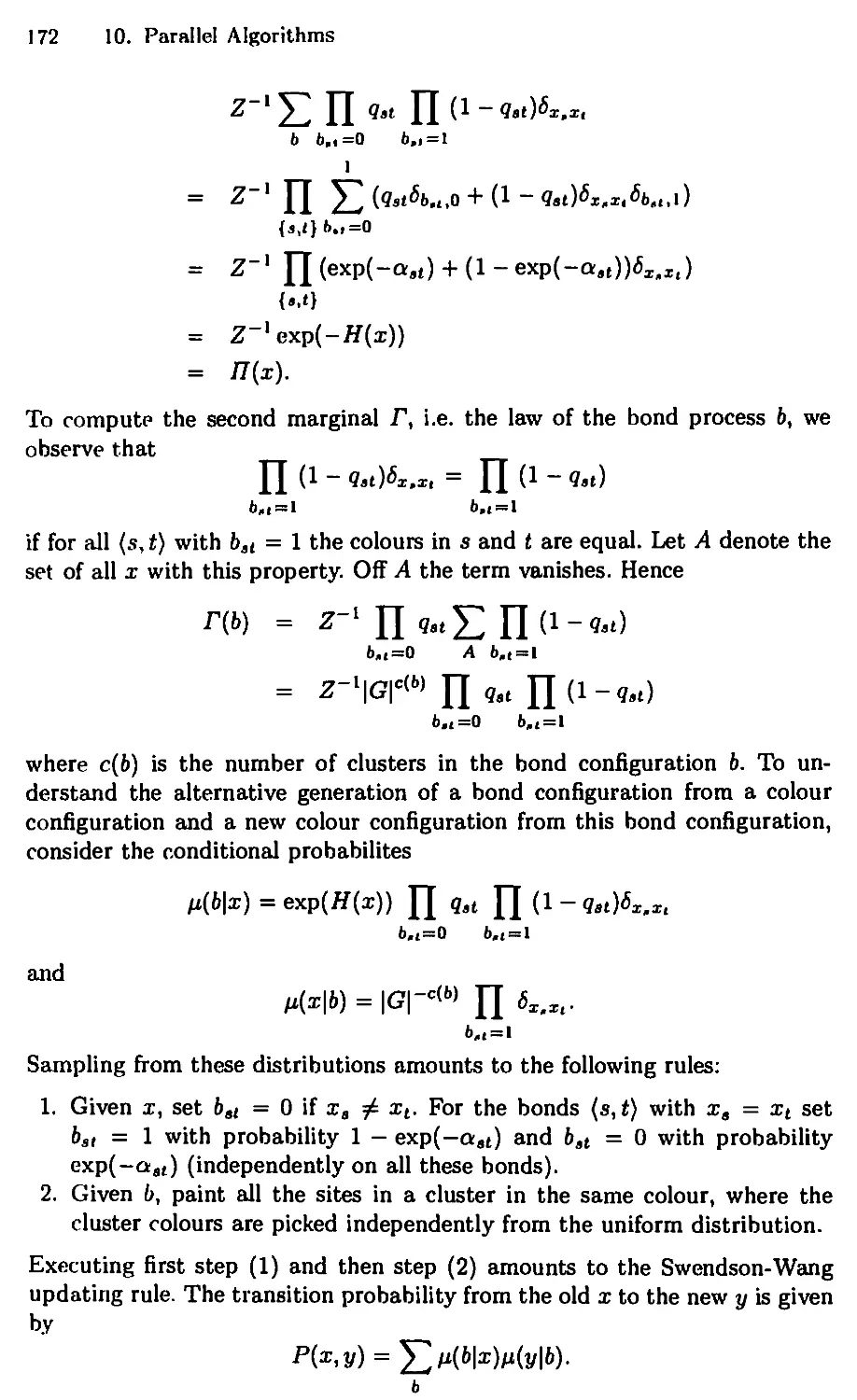
10.1.2 The Swendson-Wang Algorithm 171

Table of Contents XIII
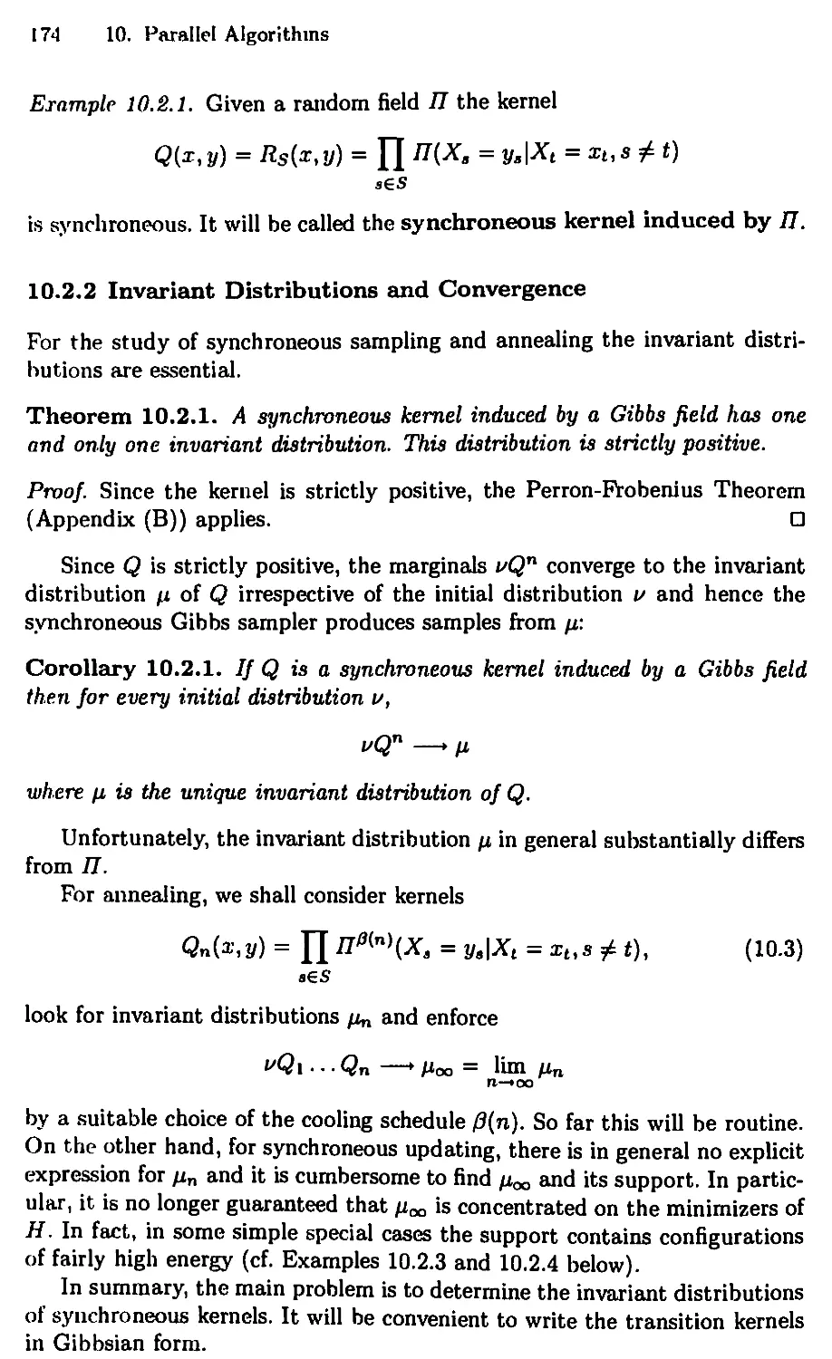
10.2 Synchroneous Algorithms 173
10.2.1 Introduction 173
10.2.2 Invariant Distributions and Convergence 174
10.2.3 Support of the Limit Distribution 178
10.3 Synchroneous Algorithms and Reversibility 182
10.3.1 Preliminaries 183
10.3.2 Invariance and Reversibility 185
10.3.3 Final Remarks 189
Part IV. Texture Analysis
11. Partitioning 195
11.1 Introduction 195
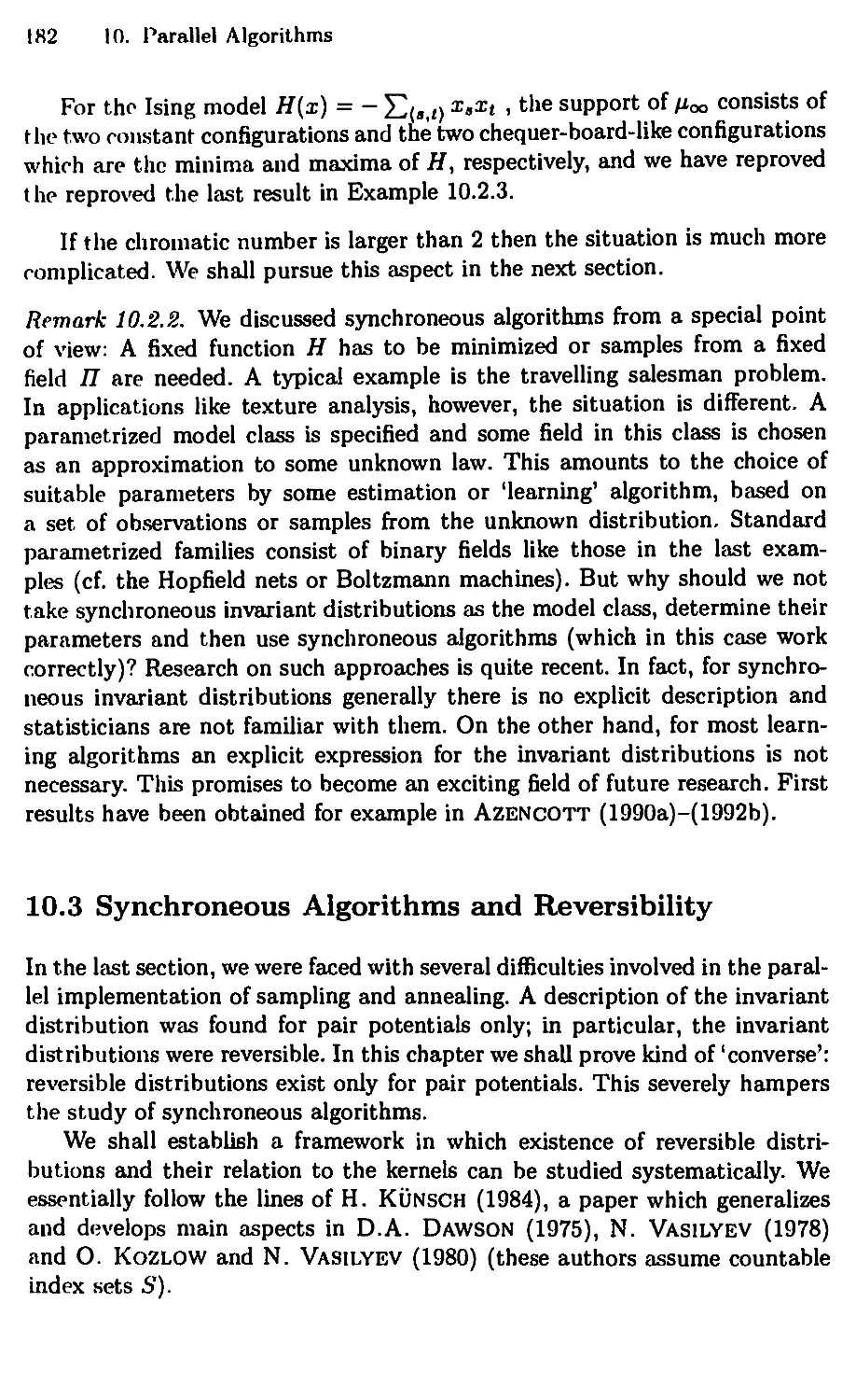
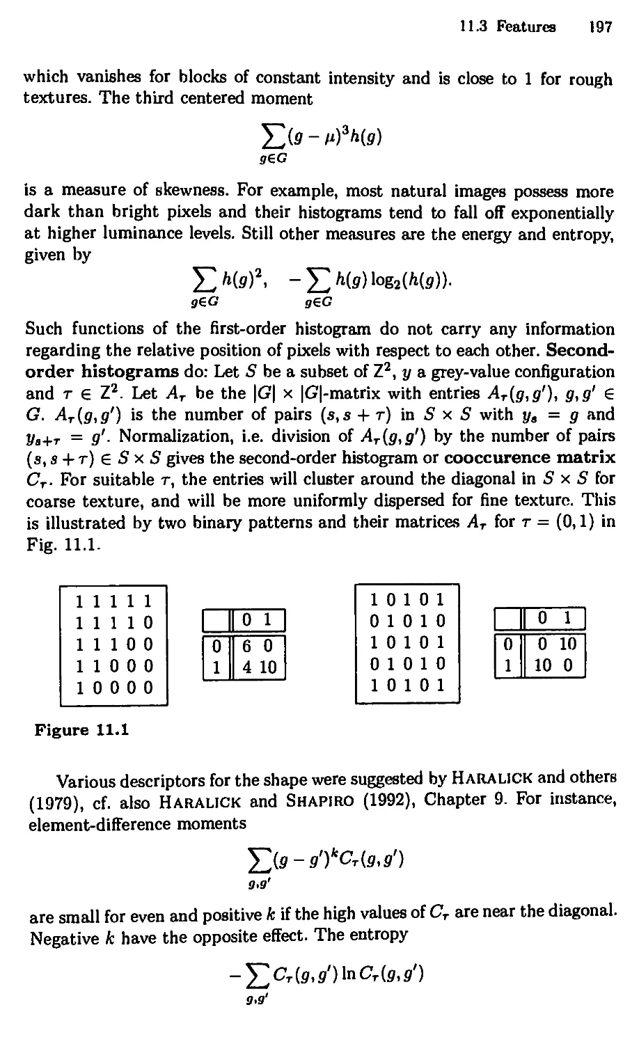
11.2 How to Tell Textures Apart 195
11.3 Features 196
11.4 Bayesian Texture Segmentation 198
11.4.1 The Features 198
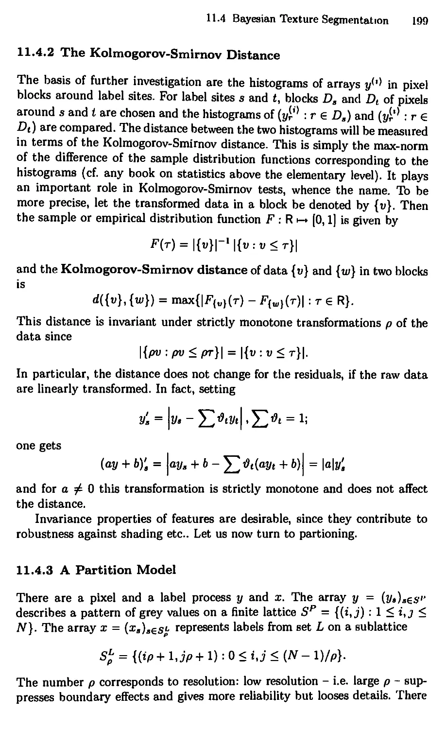
11.4.2 The Kolmogorov-Smirnov Distance 199
11.4.3 A Partition Model 199
11.4.4 Optimization 201
11.4.5 A Boundary Model 203
11.5 Julesz's Conjecture 205
11.5.1 Introduction 205
11.5.2 Point Processes 205
12. Texture Models and Classification 209
12.1 Introduction 209
12.2 Texture Models 210
12.2.1 The Φ-Model 210
12.2.2 The Autobinomial Model 211
12.2.3 Automodels 213
12.3 Texture Synthesis 214
12.4 Texture Classification 216
12.4.1 General Remarks 216
12.4.2 Contextual Classification 218
12.4.3 MPM Methods 219
Part V. Parameter Estimation
13. Maximum Likelihood Estimators 225
13.1 Introduction 225
13.2 The Likelihood Function 225

XIV Table of Contents
13.3 Objective Functions 230
13.4 Asymptotic Consistency 233
14. Special ML Estimation 237
14.1 Introduction 237
14.2 Increasing Observation Windows 237
14.3 The Pseudolikelihood Method 239
14.4 The Maximum Likelihood Method 246
14.5 Computation of ML Estimators 247
14.6 Partially Observed Data 253
Part VI. Supplement
15. A Glance at Neural Networks 257
15.1 Introduction 257
15.2 Boltzmann Machines 257
15.3 A Learning Rule 262
16. Mixed Applications 269
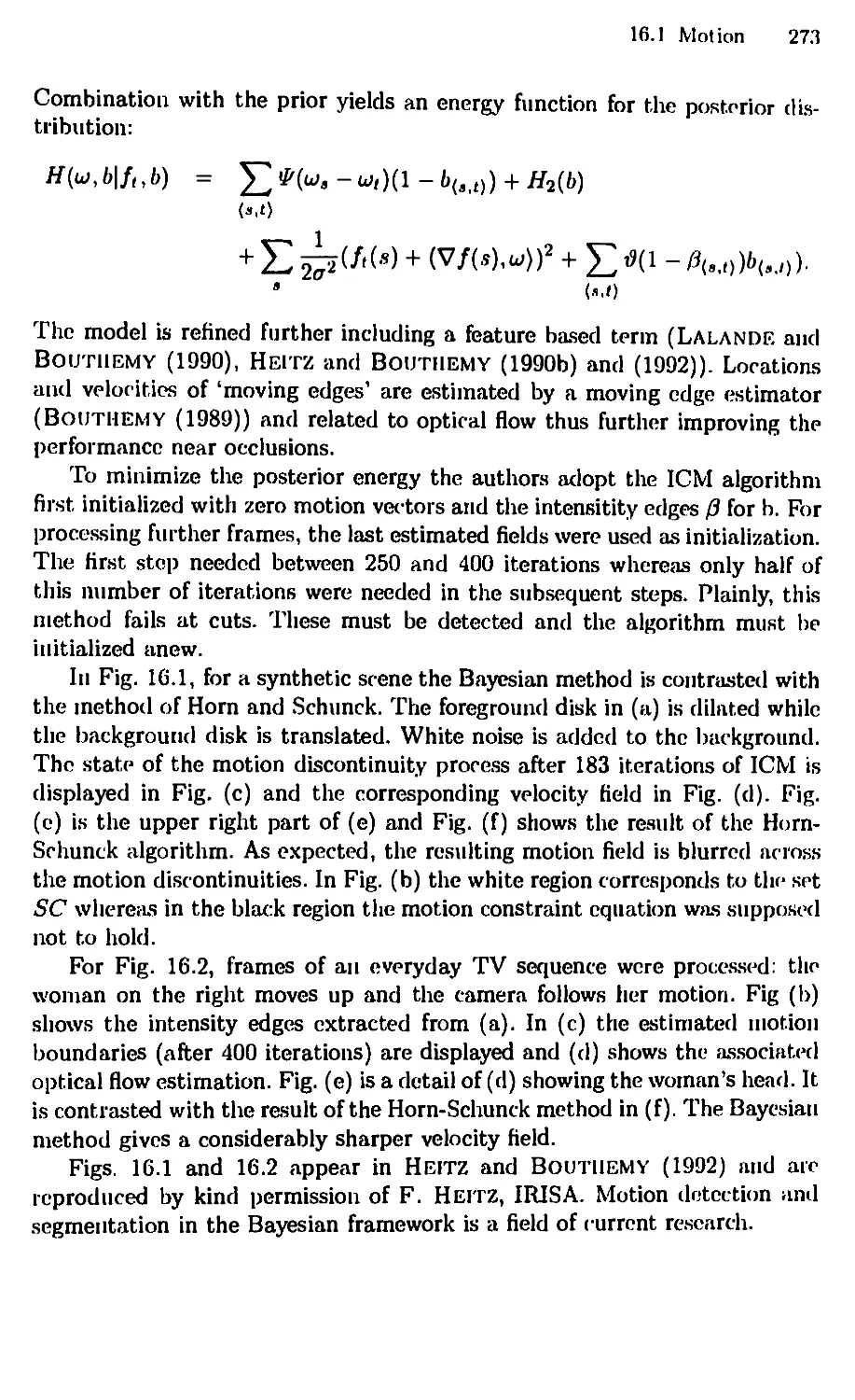
16.1 Motion 269
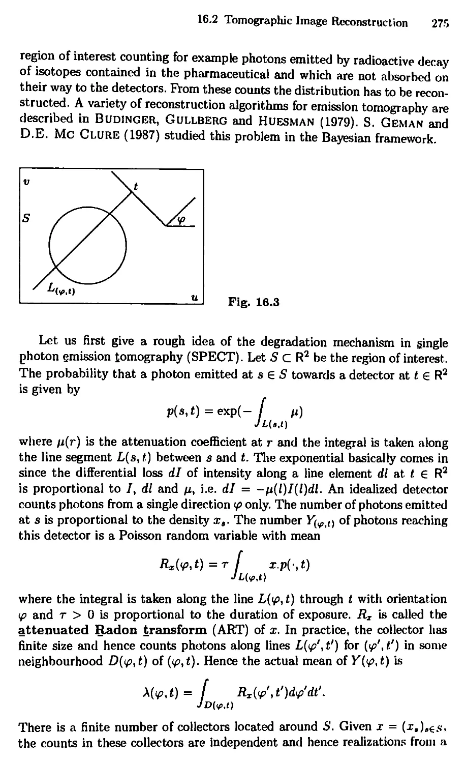
16.2 Tomographic Image Reconstruction 274
16.3 Biological Shape 276
Part VII. Appendix
A. Simulation of Random Variables 283
A.l Pseudo-random Numbers 283
A.2 Discrete Random Variables 286
A.3 Local Gibbs Samplers 289
A.4 Further Distributions 290
A.4.1 Binomial Variables 290
A.4.2 Poisson Variables 292
A.4.3 Gaussian Variables 293
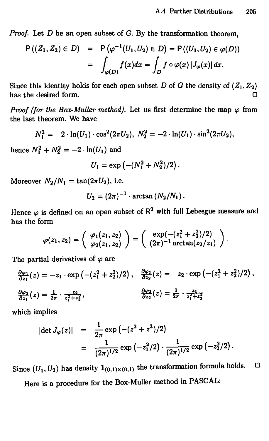
A.4.4 The Rejection Method 296
A.4.5 The Polar Method 297
B. The Perron-Probenius Theorem 299
C. Concave Functions 301
D. A Global Convergence Theorem for Descent Algorithms .. 305
References 307
Index 32i

Introduction
In this first chapter, basic ideas behind the Bayesian approach to image
analysis are introduced in an informal way. We freely use some notions from
elementary probability theory and other fields with which the reader is perhaps
not perfectly familiar. She or he should not worry about that - all concepts
will be made thoroughly precise where they are needed.
This text is concerned with digital image analysis. It focuses on the
extraction of information implicit in recorded digital imago data by automatic
devices aiming at an interpretation of the data, i.e. an explicit (partial)
description of the real world. It may be considered as a special discipline in
image processing. The latter encompasses fields like image digitization,
enhancement and restoration, encoding, segmentation, representation and
description (we refer the reader to standard texts like ANDREWS and HUNT
(1977), Pratt (1978), Horn (1986), Gonzalez and Wintz (1987) or Har-
alick and Shapiro (1992)).
Image analysis is sometimes referred to as 'inverse optics'. Inverse
problems generally are underdetermined. Similarly, various interpretations may
be more or less compatible with the data and the art of image analysis is to
select those of interest. Image synthesis, i.e. the 'direct problem' of mapping
a real scene to a digital image will not be dicussed in this text.
Here is a selection of typical problems :
- Image restoration: Recover a 'true' two-dimensional scene from noisy data.
- Boundary detection: Locate boundaries corresponding to sudden changes
of physical properties of the true three-dimensional scene such as surface,
shape, depth or texture.
- Tomographic reconstruction: Showers of atomic particles pass through the
body in various directions (transmission tomography). Reconstruct the
distribution of tissue in an internal organ from the 'shadows' cast by the
particles onto an array of sensors. Similar problems arise in emission
tomography.
- Shape from shading: Reconstruct a three-dimensional scene from the
observed two-dimensional image.
- Motion analysis: Estimate the velocity of objects from a sequence of images.
- Analysis of biological shape: Recognize biological shapes or detect
anomalies.

2 Introduction
We shall comment on such applications in Chapter 2 and in Parts IV
and VI. Concise introductions are Geman and GlDAS (1991), D. Geman
(1990). For shape from shading and the related problem of shape from texture
see Gidas and Torreao (1989). A collection of such (and many other)
applications can be found in Chellapa and Jain (1993). Similar problems
arise in fields apparently not related to image analysis:
- Reconstruct the locations of archeological sites from measurements of the
phosphate concentration over a study region (the phosphate content of soil
is the result of decomposition of organic matter).
- Map the risk for a particular disease based on observed incidence rates.
Study of such problems in the Bayesian framework is quite recent, cf. Besag,
York and Mollie (1991).
The techniques mentioned will hopefully be helpful in high-level vision
like object recognition and navigation in realistic environments.
Whereas image analysis is replete with ad hoc techniques one may believe
that there is a need for theory as well. Analysis should be based on precisely
formulated mathematical models which allow one to study the performance of
algorithms analytically or even to design optimal methods. The probabilistic
approach introduced in this text is a promising attempt to give such a basis.
One characterization is to say it is Bayesian. As always in Bayesian inference,
there are two types of information: prior knowledge and empirical data. Or,
conversely, there are two sources of uncertainty or randomness since empirical
data are distorted ideal data and prior knowledge usually is incomplete.
In the next paragraphs, these two concepts will be illustrated in the
context of restoration, i.e. 'reconstruction' of a real scene from degraded
observations. Given an observed image, one looks for a 'restored image' hopefully
being a better represention of the true scene than was provided by the
original records. The problem can be stated with a minimum of notation and
therefore is chosen as the introductory example.
In general, one does not observe the ideal image but rather a distorted
version. There may be a loss of information caused by some deterministic
noninvertible transformation like blur or a masking deformation where only
a portion of the image is recorded and the rest is hidden to the observer.
Observations may also be subject to measurement errors or unpredictable
influences arising from physical sources like sensor noise, film grain irregularities
and atmospheric light fluctuations. Formally, the mechanism of distortion is
a deterministic or random transformation у = f(x) of the true scene χ to
the observed image y. 'Undoing' the degradations or 'restoring' the image
ideally amounts to the inversion of /. This raises severe problems associated
with invertibility and stability. Already in the simple linear model у = Bx,
where the true and observed images are represented by vectors χ and y,
respectively, and the matrix В represents some linear 'blur operator', В is in
general highly noninvertible and solutions χ of the equation can be far apart.
Other difficulties come in since у is determined by physical sampling and

Introduction 3
the elements of В are specified independently by system modeling. Thus the
system of equations may be inconsistent in practice and have no solution at
all. Therefore an error term enters the model, for example in the additive
form у = Bx + e(x).
Restoration is the object of many conventional methods. Among those
one finds ad hoc methods like 'noise cleaning' via smoothing by weighted
moving averages or - more generally - application of various linear filters to
the image. Surprising results can be obtained by such methods and linear
filtering is a highly developed discipline in engineering. On the other hand,
linear filters only transform an image (possibly under loss of information),
hopefully, to a better representation, but there is no possibility of analysis.
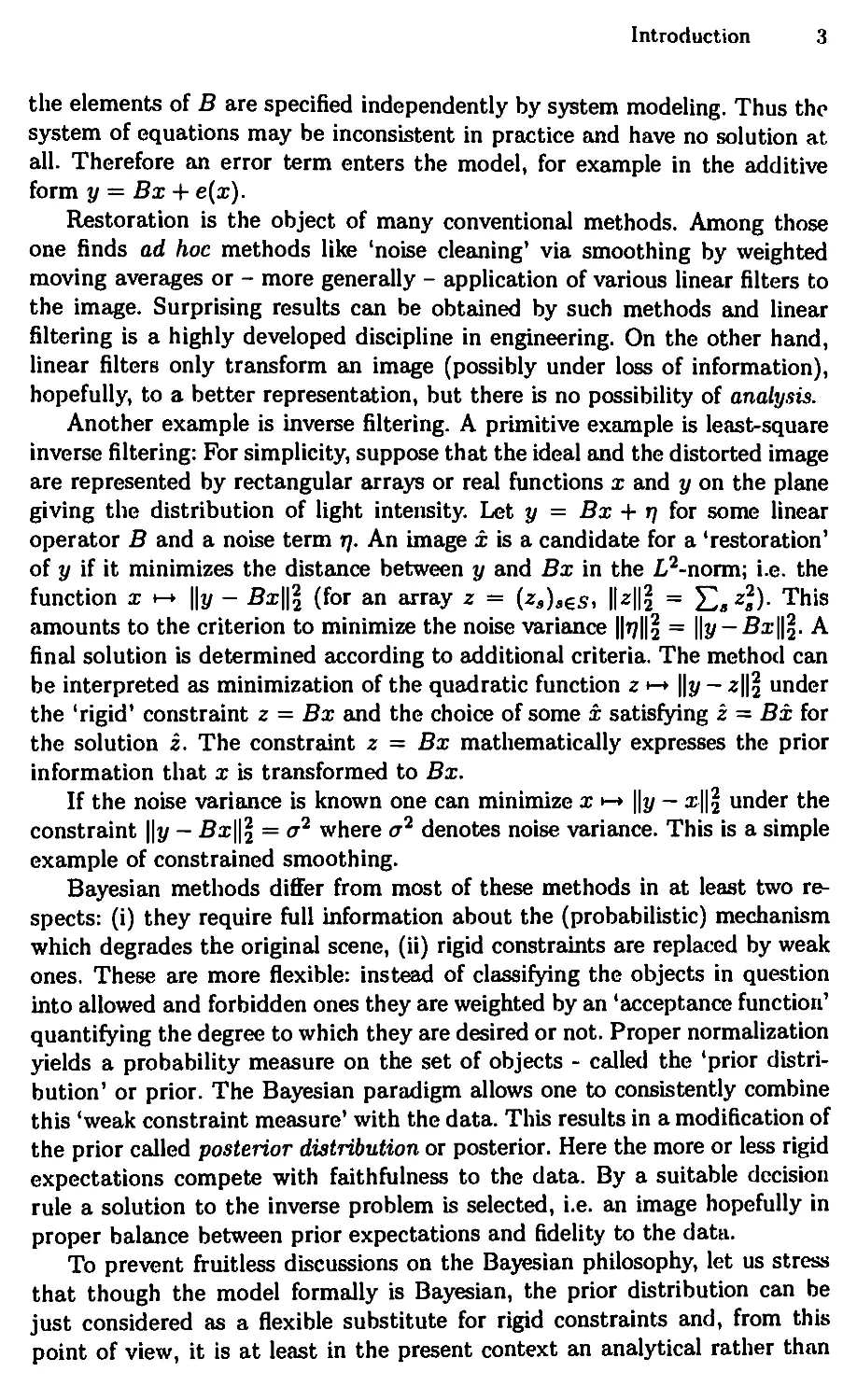
Another example is inverse filtering. A primitive example is least-square
inverse filtering: For simplicity, suppose that the ideal and the distorted image
are represented by rectangular arrays or real functions χ and у on the plane
giving the distribution of light intensity. Let у = Bx + η for some linear
operator В and a noise term η. An image χ is a candidate for a 'restoration'
of у if it minimizes the distance between у and Bx in the L2-norm; i.e. the
function χ h-+ \\y ~ Bx\\\ (for an array ζ = (za)seS, \\Α\\ = Ί2βζΐ)· Tnis
amounts to the criterion to minimize the noise variance \\η\\% = \\y-Bx\\%. A
final solution is determined according to additional criteria. The method can
be interpreted as minimization of the quadratic function ζ »-+ ||y - z\\l under
the 'rigid' constraint ζ = Bx and the choice of some χ satisfying ζ = Bx for
the solution z. The constraint ζ = Bx mathematically expresses the prior
information that χ is transformed to Bx.
If the noise variance is known one can minimize χ *-* \\y - x\\\ under the
constraint ||y — Bx]]2, = σ2 where σ2 denotes noise variance. This is a simple
example of constrained smoothing.
Bayesian methods differ from most of these methods in at least two
respects: (i) they require full information about the (probabilistic) mechanism
which degrades the original scene, (ii) rigid constraints are replaced by weak
ones. These are more flexible: instead of classifying the objects in question
into allowed and forbidden ones they are weighted by an 'acceptance function'
quantifying the degree to which they are desired or not. Proper normalization
yields a probability measure on the set of objects - called the 'prior
distribution' or prior. The Bayesian paradigm allows one to consistently combine
this 'weak constraint measure' with the data. This results in a modification of
the prior called posterior distribution or posterior. Here the more or less rigid
expectations compete with faithfulness to the data. By a suitable decision
rule a solution to the inverse problem is selected, i.e. an image hopefully in
proper balance between prior expectations and fidelity to the data.
To prevent fruitless discussions on the Bayesian philosophy, let us stress
that though the model formally is Bayesian, the prior distribution can be
just considered as a flexible substitute for rigid constraints and, from this
point of view, it is at least in the present context an analytical rather than

J Introduction
a probabilistic concept. Nevertheless, the name 'Bayesian image analysis' is
common for this approach. Besides its formal merits the Bayesian
framework has several substantial advantages. Methods from this mature field of
statistics can be adopted or at least serve as a guideline for the development
of more specific methods. In particular, this is helpful for the estimation of
optimal solutions. Or, in texture classification, where the prior can only be
specified up to a set of parameters, statistical inference can be adopted to
adjust the parameters to a special texture.
All of this is a bit general. Though of no practical importance, the
following simple example may give you a flavour of what is to come.
Fig. 0.1. A degraded image
Consider black and white pictures as displayed on a computer screen.
They will be represented by arrays (ял)в€$; S is a finite rectangular grid of
pixels' .s, xs = 1 corresponds to a black spot in pixel s and xs = 0 means
that s is white. Somebody (nature ?) displays some image у (Fig. 1).
We are given two pieces of information about the generating algorithm:
(i) it started from an image χ composed of large connected patches of black
and white, (ii) the colours in the pixels were independently flipped with
probability ρ each. We accept a bet to construct a machine which roughly
recovers the original image. There are 2σ possible combinations of black and
white spots, where σ is the number of pixels. In the figures we chose σ =
80 χ 80 and hence 2σ ~ 10192; in the more realistic case σ = 256 χ 256 one
has Τ ~ ΙΟ19 ββ0. We want to restrict our search to a small subset using the
information in (i). It is not obvious how to state (i) in precise mathematical
terms. We may start selecting only the two extreme images which are either
totally white or totally black (Fig. 2). Formally, this amounts to the choice
of a feasible subset of the space X = {0, l}5 consisting of two elements. This
is a poor formulation of (i) since it does not express the degrees to which for
instance Fig. 3(a) and (b) are in accordance with the requirement: both are
forbidden. Thus let us introduce the local constraints
- xH - xt for all pixels s and t adjacent in the horizontal, vertical or diagonal
directions.

Introduction 5
In the example, we have η = 80 rows and columns, respectively, and hence
2n(n - 1) = 12,640 adjacent pairs s, t in the horizontal or vertical directions,
and the same number of diagonally adjacent pairs. The feasible set is the
same as before but weighting configurations χ by the number A(x) of valid
constraints gives a measure of smoothness. Fig. 3(a) differs from the black
Fig. 0.2. Two very smooth images
image only by a single white dot and thus violates only 8 of the 25, 280 local
constraints whereas (b) violates one half of the local constraints. By the rigid
constraints both are forbidden whereas A differentiates between them. This
way the rigid constraints are relaxed to 'weak constraints'. Hopefully, the
reader will agree that the latter is a more adequate formulation of piecewise
smoothness in (i) than the rigid ones.
ι ^^шшшшшш тшшшвштшшвШЪ
Fig. 0.3. (a) Violates few, (b) violates many local constraints
More generally, one may define local acceptor functions by
if
if
ι φζι
(a for 'attractive' and г for 'repulsive'). The numbers a„t and rBt control the
degree to which the rigid local constraints are fulfilled. For the present, they
are not completely specified. But if we agree that Aet(xa,x<) > /l,<(t's,i;'t)

Ь Introduction
moans that (.r.,,.-rt) is more favourable than (x'a,x{) we must require that
a,f > rsf since smooth images are desired. Forming the product over all
horizontal, vertical and diagonal nearest neighbour pairs gives the global
acceptor
Mx) = П^я'(Хл'Хе)·
Since in (i) no direction is preferred, we let aat = α and ral = г, а > г, in the
experiment. Little is lost, if the acceptor is normalized such that A > 0 and
Σχ A(x) = 1. Then A formally is a probability distribution on X which we
call the prior distribution.
From (ii) we conclude: Given χ the observation у is obtained with
probability
(the function 1A equals 1 on Л and vanishes off A). Given a fixed observation
y, the acceptor A should be modified by the weights P(x,y) to
A(x) = A(x)P(x,y) = J] (ПЛ^Х-Х')) p^'-^-Kl-p)'1—β-1
(this rule for modification is borrowed from the Bayesian model). Л is a new
acceptor function and proper normalization gives a probability distribution
called the posterior distribution. Now two terms compete: A formerly
desirable configuration with large A{x) may be weighted down if not compatible
with the data, i.e. if P{x, y) is small, and conversely, an α priori less favourable
configuration with small A(x) may become acceptable if P(x, y) is large.
Finally, we need a rule how to decide which image we shall present to
our contestant. Let us agree that we take one with highest value of A. Now
r*—r^v—ι
Fig. 0.4. (a) A poor reconstruction of (b)?
we are faced with a new problem: how should we maximize A? This is in
fact another story and thus let us suppose for the present that we have an
optimization method and apply it to A. It generates an image like Fig. 4(a).
Now the original image 4(b) is revealed.

Introduction 7
At the first glance, this is a bit disappointing, isn't it ? On the other
hand, there is a large black spot which even resembles the square and thus
(i) is met. Moreover, we did not include any information about shape into the
model and thus we should be suspicious about much better reconstructions
with this prior. Information about shape can and will be exploited and this
will result in almost perfect reconstructions (you may have a look at the
figures in Chapter 2).
Just for fun, let us see what happens with a 'wrong' acceptance function
A. We tell our reconstruction machine that in the original image there are
vertical stripes. To be more precise, we set aat equal to a large number and
rst equal to a low number for vertical pixel pairs and, conversely, aat to a
low and rat to a large numbers for pairs not in the same coloumn. Then the
output is Fig. 5.
Fig. 0.5. A reconstruction with an impropriate
acceptance function
Like the broom of the wizard's apprentice, the machine steadfastly does
what it is told to do, or, in other words, it sees what it is prepared to see. This
teaches us that we must form a clear idea which kind of information we want
to extract from the data and precisely formulate this in the mathematical
terms of the acceptor function before we set the restoration machine to work.
Any model is practically useless unless the solution of the reconstruction
problem cannot be computed. In the example, the function χ »-» A(x) has to
be maximized. Since the space of images is discrete and because of its size this
may turn out to be a tough job and, in fact, a great deal of effort is spent on
the construction of suitable algorithms in the image analysis community. One
may search through the tool box of exact optimization algorithms. Nontrivial
considerations show that, for example, the above problem can be transformed
into one which can be solved by the well-known Ford-Fulkerson algorithm.
But as soon as there are more than two colours or one plays around with the
acceptor function it will no longer apply. Similarly, most exact algorithms are
tailored for rather restricted applications or they become computationally
unfeasible in the imaging context. Hence one is looking for a flexible albeit
fast optimization method.
There are several general strategies: one is 'divide and conquer'. The
problem is divided into small tractable subproblems which are solved indepen-

8 Introduction
dent.ly. The solutions to the subproblems then have to be patched together
consistently. Another design principle for many common heuristics is
'successive augmentation1. In this approach an initially empty structure is
successively augmented until it becomes a solution. We shall not pursue these
aspects. 'Iterative improvement1 is a dynamical approach. Pixels are
subsequently selected following some systematic or random strategy and at each
step the configuration (i.e. image) is changed at the current pixel. 'Greedy'
algorithms, for example, select the colour which improves the objective
function A the most. They permanently move uphill and thus get stuck in local
maxima which are global maxima only in very special cases. Therefore it
is customary to repeat the process several times starting from different, for
instance randomly chosen configurations, and to save the best result. Since
the objective functions in image analysis will have a very large number of
local maxima and the set of initial configurations necessarily is rather thin in
the very large space of all configurations this trick will help in special cases
only. The dynamic Monte Carlo approach - which will be adopted here -
replaces the chain of systematic updates by a temporal stochastic process:
at. each pixel a dye is tossed and thus a new colour picked at random. The
probabilities depend on the value of λ for the respective colours and a control
parameter β. Colours giving high values are selected with higher
probability than those giving low values. Thus there is a tendency uphill but there
is also a chance for descent. In principle, routes through the configuration
space designed by such a procedure will find a way out of local maxima.
The parameter β controls the actual probabilites of the colours: let p(A>)
be the uniform distribution on all colours and let ρ(βοο) be the degenerate
distribution concentrated on the locally optimal colours. Selection of a colour
w.r.t. ρ(βοο) amounts to the choice of a colour maximizing the local acceptor
function, i.e. to a locally maximal ascent. If updating is started with ρ(βο)
then the process will randomly stagger around in the space of images. While
β varies from βο to &» the uniform distribution is continuously transformed
into ρ(βοο)'- Favourable colours become more and more probable and the
updating rule changes from a completely random search to maximal ascent.
The trick is to vary β in such a fashion that, on the one hand, ascent is fast
enough to run into maxima, and, on the other hand, to keep the procedure
random enough to escape from local maxima before it has reached a global
one.
Plainly, one cannot expect a universal remedy by such methods. One has
to put up with a tradeoff between accuracy, precision, speed and flexibility.
We shall study these aspects in some detail.
Our primitive reconstruction machine still is not complete. It does not
know how to choose the parameters aat = α and rat = r. The requirement
a>r corresponds to smoothness but it does not say anything about the
degree of smoothness. The latter may for example depend on the approximate
number of patches and their shape. We could play around with a and г until a

Introduction 9
satisfactory result is obtained but this may be tiring already in simple cases
and turns out to be impracticable for more complicated patterns. A more
substantial problem is that we do not know what 'satisfactory' does mean.
Therefore we must gain further information by statistical inference.
Conventional estimation techniques frequently require a large number of independent
samples. Unfortunately, we have only a single observation where the colours
of pixels depend on each other. Hence methods to estimate parameters (or, in
more fashionable terms 'learning algorithms') based on dependent
observations must be developed. Besides modeling and optimization, this is the third
focal point of activity in image analysis. In summary, we raised the following
clusters of problems:
- Design of prior models.
- Statistical inference to specify free parameters.
- Specification of the posterior, in particular the law of the data given the
true image.
- Estimation of the true image based on the posterior distribution (presently
by maximization).
Specification of the transition probabilites in the third item is more or less
a problem of engineering or physics and will not be discussed in detail here.
The other three items roughly lay out a program for this text.

Parti
Bayesian Image Analysis: Introduction

1. The Bayesian Paradigm
In this chapter the general model used in Bayesian image analysis is
introduced.
1.1 The Space of Images
A monochrome digital picture can be represented by a finite set of numbers
corresponding to the intensity of light. But an image is much more. An array
of numbers may be visualized by a transformation to a pattern of grey levels
on a computer screen. As soon as one realizes that there is a cat shown on
the screen this pattern achieves a new quality. There has been some sort of
high-level image processing in our eyes and brain producing the association
'cat'. We shall not philosophize on this but notice that information hidden in
the data is extracted. Such informations should be included in the description
of the image.
Which kind of information has to be taken into account depends on the
special task one is faced with. Most examples in this text deal with problems
like restoration of degraded images, edge detection or texture discrimination.
Hence besides intensities, attributes like boundary elements or labels marking
certain types of texture will be relevant. The former are observable up to
degradation while the latter are not and correspond to some interpretation
of the data.
In summary, an image will be described by an array
x = (xp,rrL,xB,...)
where the single components correspond to the various attributes of
interest. Usually they are multi-dimensional themselves. Let us give some first
examples of such attributes and their meaning.
Let Sp denote a finite square lattice - say with 256 χ 256-lattice points -
each point representing a pixel on a screen. Let G be the set of grey values,
typically \G\ = 256 (the symbol \G\ denotes the number of elements of G) and
for s 6 Sp let xp denote the grey value in pixel s. The vector xp = (xp)s&s·'
represents a pattern or configuration of grey values. In this example there are
2562562 ~ io157·826 possible patterns and these large numbers cause many of
the problems in image processing.

14 1. The Bayesian Paradigm
Remark 1.1.1. Grey values may be replaced by any kind of observable
quantities. Let us mention a few:
- intensities of any sort of radiant energy;
- the numbers of photons hitting the cells of a CCD-camera (cf. Chapter 2);
- tristimulus: in additive colour matching the contributions of primary
colours - say red, green and blue light - to the colour of a pixel, usually
normalized by their contribution to a reference colour like 'white' (Pratt
(1978), Chapter 3));
- depth, i.e. at each point the distance from the viewer; such depth maps may
be produced by stereopsis or processing of optical flow (cf. Marr (1982));
- transforms of the original intensity pattern like discrete Fourier- or Hough-
transforms.
In texture classification blocks of pixels are labeled as belonging to one of
several given textures like 'meadow', 'wood' or 'damadged wood'. A pattern
of such labels is represented by an array xL = (x^)„^s^ where SL is a set of
pixel blocks and xf" = I 6 L is the label of block s, for instance 'damadged
wood'. The blocks may overlap or not. Frequently, blocks center around pixels
on some subgrid of Sp and then SL usually is identified with this subgrid.
The labeling is not an observable but rather an interpretation of the intensity
pattern. We must find rules how to pick a reasonable labeling from the set
Ls' of possible ones.
Image boundaries or edges are useful primitive features indicating
sudden changes of image attributes. They may separate regions of dark or bright
pixels, regions of different texture or creases in a depth map. They can be
represented by strings of small edge elements, for example microedges between
adjacent pixels:
* pixel
— : microedge
Let SE be the set of microedges in Sp. For s e SE set xE = 1 if the microedge
represents a piece of a boundary (it is 'on') and xE = 0 otherwise (it is 'off').
|| : microedge is 'on'
| : microedge is 'off'
Again, the configuration xE is not observable. An edge element can be
switched on for example if the contrast of grey levels nearby exceeds a certain
* I * I *
* I * I *
* I * I *
^_ I * I *
* II * I *
* ι 7 ι Τ

1.2 The Space of Observations 15
threshold or if the adjacent textures are different. But local criteria alone are
not sufficient to characterize boundaries. Usually they are smooth or
connected and this should be taken into account.
These simple examples of image attributes should suffice to motivate the
concepts to be introduced now.
1.2 The Space of Observations
Statistical inference will be based on Observations' or 'data' y. They are
assumed to be some deterministic or random function Υ of the 'true' image x.
To determine this function in concrete applications is a problem of
engineering and statistics. Here we introduce some notation and give a few simple
examples.
The space of data will be denoted by Υ and the space of images by X.
Given χ e X, the law of Υ will be denoted by P(x, ■).
If Υ is finite we shall write P(x, y) for the probability of observing Υ =
у if χ is the correct image. Thus for each χ 6 X, P(x, ■) is a probability
distribution on Y, i.e. P{x,y) > 0 and Y^yP(x,y) = 1. Such transition
probabilities (or Markov kernels) can be represented by a matrix where
P(x, y) is the element in the x-th row and the y-th column.
Frequently, it is more natural to assume observations in a continuous
space Y, for example in an Euclidean space Rrf and then the distributions
P(x, ■) will be given by probability densities fx(y). More precisely, for each
measurable subset В of Rrf,
P(x,S) = J fx(y)dy
where fx is a nonnegative function on Υ such that / fx(y)dy = 1.
Example 1.2.1. Here are some simple examples of discrete and continuous
transition probabilities.
(a) Suppose we are interested in labeling a grey value picture. An image is
then represented by an array χ = (xp,xL) as introduced above. If undegraded
grey values are observed then у = xp and 'degradation' simply means that the
information about the second component xL of χ is missing. The transition
probability then is degenerate:
P(xv)=l1 « y = xP
nx*V) \ 0 otherwise
For edge detection based on perfectly observed grey values where χ =
(xp,xE), the transition kernel Ρ has the same form.
(b) The grey values may be degraded by noise in many ways. A
particularly simple case is additive noise. Given χ = xp one observes a realization
of the random variable

16 1. The Bayesian Paradigm
Υ =χ + η
whore r/ = (i?s ),€$/> is a family of real-valued random noise variables. If
the random variables r/s are independent and identically distributed with a
Gaussian law of mean 0 and variance σ2 then η is called white Gaussian
noise. The law P(x, ■) of Υ has density
where d = |5P|. Thermal noise, for example, is Gaussian. While quantum
noise obeys a (signal dependent) Poisson law, at high intensities a Gaussian
approximation is feasible. We shall discuss this in Chapter 2. In a strict sense,
the Gaussian assumption is unrealistic since negative grey values appear with
positive probability. But for positive grey values sufficiently larger than the
variance of noise the positivity restriction on light intensity is violated
infrequently.
(c) Let us finally give an example for multiplicative noise. Suppose that
the pattern x, xa 6 {—1,1}, is transmitted through a channel which
independently flips the values with probability p. Then Ys = xs · η„ with independent
Bernoulli variables η3 which take the value —1 with probability ρ and the
value 1 with probability 1 - p. The transition probability is
P(x,y) = ρΚ-еЛь—*->l(1 _р)И*€Ль-*.}|.
This kind of degradation will be referred to as channel noise .
More background information and more realistic examples will be given
in the next chapter.
1.3 Prior and Posterior Distribution
As indicated in the introduction, prior expectations may first be formulated
as rigid constraints on the ideal image. These may be relaxed in various
ways. The degree to which an image fulfills the rigid regularity conditions
and constraints finally is expressed by a function П(х) on the space X of
images. By convention, П{х) > П{х') means that x' is less favourable than
x. For convenience, we assume that Π is nonnegative and normalized, i.e.
Я is a probability distribution. Since Π does not depend on the data it
can be designed before data are recorded and hence it is called the prior
distribution.
We shall not require foreknowledge from measure theory and therefore
most of the analysis will be carried out for finite spaces X. In some
applications it is more reasonable to allow ranges like R+ or Rd. Most concepts
introduced here easily carry over to the continuous case.

1.3 Prior and Posterior Distribution 17
The choice of the prior is problem dependent and one of the main problems
in Bayesian image analysis. There is not too much to say about it in the
present general context. Chapter 2 will be devoted exclusively to the design
of a prior in a special situation. Later on, more prior distributions will be
discussed. For the present, we simply assume that some prior is fixed.
The second ingredient is the distributions P(x, ■) of the data у given x.
Assume for the moment that Υ is finite. The prior Π and the transition
probabilities Ρ determine the joint distribution of data and images on the
product space Χ χ Υ by
P(x,y) = Я(х)Р(х,у), χ e X, у 6 Υ.
This number is interpreted as the probability that χ is the correct image and
that у is observed.
The distribution Ρ is the law of a pair (X, Y) of random variables with
values in Χ χ Υ where X has the law Π and Υ has a law Γ given by
Γ(Υ = у) = Σχ P(x,y). We shall use symbols like Ρ and Γ for the law of
random variables as well as for the underlying probabilities and hence write
P(x, y) or Ρ(Λ" = χ, Υ = у) if convenient. There is no danger of confusion
since we can define suitable random variables by X(x, y) = χ and K(x, у) = у.
Recall that the conditional probability of an event (i.e. a subset) Ε in
Χ χ Υ given an event F is defined by ?{E\F) = P(EnF)/P(F) (provided the
denominator does not vanish). Setting Ε = у and F = χ shows immediately
that P(y\x) = P(x,y).
Assume now that data у are observed. Then the conditional probability
of χ 6 X is given by
1"" P({(*,S): * 6 X}) Е,Л(г)Р(*,»)·
(we have tacitly assumed that the denominators do not vanish). Since P(|y)
can be interpreted as an adjustment of Π to the data (after the observation)
it is called the posterior distribution of χ given y.
For continuous data, the discrete distributions P(x, ·) are replaced by
densities fx and in this case, the joint distribution is given by
P({x} χ В) = Щх) J fx(y)dy
for χ 6 X and a measurable subset Б of Υ (e.g. a cube).
The prior distribution Π will always have the Gibbsian form
Щх) = Z-lexp(-H(x)),Z = ]Гехр(-Я(г)) (1.1)
г€Х
with some real-valued function
Η : X —♦ R, χ h— Щх).

18 1. The Bayesian Paradigm
In accordance with statistical physics, Я is called the energy function of
Π. Thus is not too a severe restriction since every strictly positive probability
distribution on X has such a representation: For
Я(х) = -1пЯ(х)
one has
Я(х) = ехр(-Я(х))
and
Ζ = Σβχρ(-Η(ζ)) = ΣΠ(ζ) = 1
ζ ζ
and hence (1.1).
Plainly, the quality of χ can be measured by Я as well as by Я. Large
values of Я correspond to small values of Я.
In most cases the posterior distribution given у is concentrated on some
subspace X of X and the posterior is again of Gibbsian form, i.e. there is a
function Я(-|у) on X such that
P(x|y) = Z(y)-1 ехр(-Я(х|у), χ 6 X.
Remark 1.3.1. The energy function is connected to the (log-) likelihood
function, an important concept in statistics. The posterior energy function can
be written in the form
H{x\y) = c(y)ln(P(x,y)) - 1п(Я(х)) = c(y) - ln(P(x,y)) + H(x).
The second term in the last expression is interpreted as 'infidelity'; in fact it
becomes large if у has low probability P(x, y). The last summand corresponds
to 'roughness': If Я is designed to favour 'smooth' configurations then it
becomes large for more 'rough' ones.
Example 1.3.1. Recall that the posterior distribution P(x|y) is obtained from
the joint distribution P(x, y) by a normalization in the x-variable. Hence the
energy function of the posterior distribution can be read off from the energy
function of the joint distribution.
(a) The simplest but nevertheless very important case is that of unde-
graded observations of one or more components of x.
Suppose that X = Υ χ U with elements χ = (y,u). For instance, if
χ = (xp,xL) or χ = (xp,x£) the data are у = xp and и = xL or
и = xE, respectively. According to Example 1.2.1 (a) P((y,u),y) = 1 and
P({y, u),y') = 0 if у ф у'. Suppose further that an energy function Я is given
and the prior distribution has the Gibbsian form (1.1). Given у the posterior
distribution is then concentrated on the space of those χ with first component
y. The posterior distribution becomes
Р(уМу)= ехр(-я^'ц»
W' W) Егехр(Я(у,г))·

1.4 Bayesian Decision Rules 19
The conditional distribution P(u\y) = P(y,u\y) can be considered as a
distribution on U and written in the Gibbsian form (1.1) with energy function
H(u\y) = H(y,u).
(b) Let now the patterns χ = xp of grey values be corrupted by additive
Gaussian noise like in Example 1.2.1 (b). Let again the prior be given by an
energy function Η and assume that the variables X and η are independent.
Then the joint distribution Ρ of X and Υ is given by
where Б is a measurable set and d = \S\. The joint density of X and Υ is
f(x,y) = canst · exp (- (н(х) + ^β&Χ\;
(||x||2 denotes the Euclidean norm of χ i.e. \\x\\\ = Σ5χ,). Hence the energy
function of the posterior is
2<72
(c) For the binary channel in Example 1.2.1 (c) the posterior energy is
proportional to
χ —» H{x) -\{seS:y„ = -x„}\ lnp - \{s 6 S : y„ = xa}\ ln(l - p).
Since 1^Уя=х^ = ^тр- + ^ this function is up to an additive constant equal
to
х^Н(х)-\\п(^^х'У-
For further examples and more details see Section 2.1.2.
1.4 Bayesian Decision Rules
A 'good' image has to be selected from the variety of all images compatible
with the observed data. For instance, noise or blur have to be removed from
a photograph or textures have to be classified. Given data у the problem of
determining a configuration χ is typically underdetermined. If, for example,
in texture discrimination we are given undegraded grey values xp = у then
there are N = \SL\, configurations (y,xL) compatible with the data. Hence
we must watch out for rules how to decide on x. These rules will be based on
precise mathematical models. Their general form will be introduced now.
On the one hand, the image should fit the data, on the other hand, it
should fulfill quality criteria which depend on the concrete problem to be
accomplished. The Bayesian approach allows one to take into account both

20 I. The Bayesian Paradigm
requirements simultaneously. There are many ways to pick some χ from X
which hopefully is a good representation of the true image, i.e. which is in
proper balance between prior expectation and fidelity to the data.
One possible rule is to choose an χ for which the pair (x,y) is most
favourable w.r.t. P, i.e. to maximize the function χ ·-* Р((я,2/)). One can as
well maximize the posterior distribution. Since maximizers of distributions
are called modes we define
- A mode χ of the posterior distribution P(|y) is called a maximum a
posteriori estimate of χ given y, or, in short-hand notation a MAP
estimate.
Note that the images χ are estimated as a whole. In particular, contextual
requirements incorporated in the prior (like connectedness of boundaries or
homogeneity of regions) are inherited by the posterior distribution and thus
influence x. Let us illustrate this by way of example. Suppose we are given
a digitized aerial photograph of ice flow in the polar sea. We want to label
the pixels as belonging to ice or water. We may wish a naturally looking
estimate xL composed of large patches of water or ice. For a suitable prior
the estimate will respect these requirements. On the other hand, it may erase
existing small or thin ice patches or smooth fuzzy boundaries. This way, some
pixels may be misclassified for the sake of regularity.
If one is not interested in regular structures but only in a small error rate
then there will be no contextual requirements and it is reasonable to estimate
the labels site by site independently of each other. In such a situation the
following estimator is frequently adopted: A maximizer xs of the function
xa ·— P(x3\y) is called a marginal posterior mode and one defines:
- A configuration χ is called a marginal posterior mode estimate
(MPME) if each x„ is a marginal posterior mode (given y).
In applications like tomographic reconstruction the mean value or
expectation of the posterior distribution is a convenient estimator:
- The configuration χ = Σ яР(я|2/) is called the minimum mean squares
estimator (MMSE).
The name will be explained in the following remark. Note that this
estimator makes sense only if X is a subset of a Euclidean space. Even then the
MMSE in general is not an element of the discrete and finite space X and
hence one has to choose the element next to the theoretical MMSE. In this
context it is natural to work on continuous spaces. Fortunately, much of the
later theory generalizes to continuous spaces.
For continuous data the discrete transition probabilities are replaced by
densities. For example, the MAP estimator maximizes
х—+П{х)Ш
and the MMSE is

1.4 Bayesian Decision Rules 21
TO-».
ЕгЩг)Л(у)
Remark 1.4.1. In estimation theory, estimators are studied in terms of loss
functions. Let
X : Υ — X, у — X(y)
be any estimator, i.e. a map on the sample space for which χ = X(y) hopefully
is close to the unknown x. The loss of estimating a true χ by χ or the 'distance'
between χ and χ is measured by a loss function L(x,x) > 0 with the
convention L(x, x) = 0. The choice of L is problem specific.
The Bayes risk of the function X is the mean loss
ft = £ L(x, X(y))P(x, y)=J2 £(*, *(</)) Л(х)Р(х, у).
X,l/ *,t/
An estimator minimizing this risk is called a Bayes estimator. The quality
of an algorithm depends on both, the prior model and the estimator or loss
function. The estimators introduced previously can be identified as Bayes
estimators for certain loss functions. One of the reasons why the above estimators
were introduced is that they can be computed (or at least approximated).
Consider the simple loss function
r, »v ίθ if χ = χ ,, η.
«»·»>-( 1 if χφχ ■ <12>
This is in fact a rather rough measure since an estimate which differs from
the true configuration χ everywhere has the same distance from χ as one
which fails in one site only. The Bayes risk
υ *
is minimal if and only if each terra of the first sum is minimal; more precisely,
if for each y,
Σ Их, *(y))P(x, у) = £ P(x, у) - P(*(y), у)
I I
is minimal. Hence MAP estimators are the Bayes estimators for the 0-1 loss
function (1.2).
There are arguments against MAP estimators and it is far from clear in
which situations they are intrinsically desirable (cf. Marroquin, Mitter
and Poggio (1987)). Firstly, the computational problem is enormous, and
in fact, quite a bit of space in this text will be taken by this problem. On
the other hand, hardware develops faster than mathematical theories and
one should not be too worried about that. Some found MAP estimators too
'global', leading to mislabelings or oversraoothing in restoration (cf. Fig. 2.1).
In our opinion such phenomena do not necessarily occur for carefully designed

22 1. The Bayesian Paradigm
priors #, and criticism frequently stems from the fact that in the past prior
models often were chosen for sake of computational simplicity only.
The next loss function is frequently used in classification (labeling)
problems:
L(x,x) = \S\-l\{seS:x,txa}\ (1.3)
is the error rate of the estimate. The number
d(x,x) = \{seS:xa фха}\
is railed the Hamming distance between χ and x. A computation similar
to the last one shows: the corresponding Bayes estimator is given by an X{y)
for which in each site s € S the component X(y)a maximizes the marginal
posterior distribution P(xa\y) in xa. Hence MPM estimators are the Bayes
estimators for the mean error rate (1.3). There are models especially designed
for MPM estimation like the Markov mesh models (cf. Besag (1986), 2.4 and
also Ripley (1988) and the papers by Hjort et al.).
The MMS estimators are easily seen to be the Bayes estimators for the
loss function
L(x,x)="£\xa-xa\2.
They minimize a mean of squares which explains their name.
The general model now is introduced completely and we are going to
discuss a concrete example.

2. Cleaning Dirty Pictures
The aim of the present chapter is the illustration and discussion of the
previously introduced concepts. We continue with the discussion of noise reduction
or image restoration started in the introduction. This specific example is
chosen since it can easily be described and there is no need for further theory.
The very core of the chapter are the Examples 2.3.1 and 2.4.1. They are
concerned with Bayesian image restoration and boundary extraction and due
to S. and D. Gem AN. A slightly more special version of the first one was
independently developed by A. Blake and A. ZlSSERMAN. Simple
introductory considerations and examples of smoothing hopefully will awaken the
reader's interest. We also give some more examples how images get dirty.
The chapter is not necessary for the logical development of the book. For
a rapid idea what the chapter is about, the reader should look over Section
2.2 and then work through Example 2.3.1.
2.1 Distortion of Images
We briefly comment on sources of geometric distortion and noise in a physical
imaging system and then compute posterior distributions for distortions by
blur, noise and nonlinear degradation.
2.1.1 Physical Digital Imaging Systems
Here is a rough sketch of an optoelectronical imaging system. There are
many simplifications and the reader is referred to Pratt (1978) (e.g. pp.
365), Gonzalez and Wintz (1987) and to the more specific monographs
BlBERMAN and NUDELMAN (1971) for photoelectronic imaging devices and
Mees (1954) for the theory of photographic processes.
The driving force is a continuous light distribution /(u, v) on some
subset of the Euclidean plane R2. If there is kind of memory in the system,
time-dependence must also be taken into account. The image is recorded and
processed by a physical imaging system giving an output Io(u,v). This
observed image is digitized to produce an array у followed by the restoration
system generating the digital estimation ι of the 'true image'. The function

24 2. Cleaning Dirty Pictures
of digital image restoration is to compensate for degradations of the physical
imaging system and the digitizer. This is the step we are actually interested
in. The output sample of the restoration system may then be interpolated by
an image display system to produce a visible continuous image.
Basically, the physical imaging system is composed of an optical system
followed by a photodetector and an associated electrical filter. The optical
system, consisting of lenses, mirrors and prisms, provides a deterministic
transformation of the input light distribution. The output intensity is not
exactly a geometric projection of the input. Potential degradations include
geometric distortion, defocusing, scattering or blur by motion of objects
during the exposure time. The concept can be extended to encompass the spatial
propagation of light through free space or some medium causing atmospheric
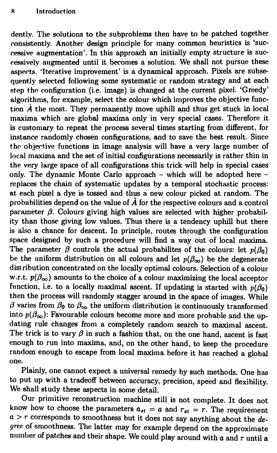
turbulence effects. The simplest model assumes that all intensity
contributions in a point add up, i.e. the output at point (u, v) is
В1(щ υ) = Π J(u\ i/)tf((u, v), (и', υ')) du'dv'
where K((u,v),(υ,',υ1)) is the response at (u,i>) to a unit signal at {υ!,υ').
The output ВI of the optical system still is a light distribution. A
photodetector converts incident photons to electrons, or, optical intensity to a
detector current. One example is a CCD detector (charge-coupled device)
which in modern astronomy replace photographic plates. CCD chips also
replace tubes in every modern home video camera. These are semiconductor
sensors counting indirectly the number of photons hitting the cells of a grid
(e.g. of size 512 χ 512). In scientific use they are frequently cooled to low
temperatures. CCD detectors are far more photosensitive than film or
photographic plates. Tubes are more conventional devices. Note that there is a
system inherent discretization causing a kind of noise: in CCD chips the plane
is divided into cells and in tubes the image is scanned line by line. This results
in Moire and aliasing effects (see below). Scanning or subsequently reading
out the cells of a CCD chip results in a signal current ip varying in time
instead of space. The current passes through an electrical filter and creates
a voltage across a resistor. In general, the measured current is not a linear
function but a power iP = const ■ BI(u, i>)7 of intensity. The exponent 7 is
system specific; frequently, 7 ~ 0.4. For many scientific applications a linear
dependence is assumed and hence 7 = 1 is chosen. For film the dependence is
logarithmic. The most common noise is thermal noise caused by irregular
electron fluctuations in resistive elements. Thermal noise is reasonably
modelled by a Gaussian distribution and for additive noise the resultant current
is
Уг = ip + ifr
where ητ is a zero mean Gaussian variable with variance σ2 = NT/R, NT
the thermal noise power at the system output and R resistance. In the simple
case in which the filter is a capacitor placed in parallel with the detector and

2.1 Distortion of Images 25
load resistor, NT = kT/RC, where к is the Boltzmann factor, Τ temperature
and С the capacity of the filter.
There is also measurement uncertainty 77Q resulting from quantum
mechanical effects due to the discrete nature of photons. It is governed by a
Poisson law with parameter depending on the observation time period r, the
average number us of electrons emitted from the detector as a result of the
incident illumination and the average number uh of electron emissions caused
by dark current and background radiation:
Prob{qQ = kq/τ) = -£j-e-a;
here q is the charge of an electron and a = us +ujj. The resulting
fluctuation of the detector current is called shot noise. In presence of sufficient
internal amplification, for example a photomutiplier tube, the shot noise will
dominate subsequent thermal noise. Shot noise is of particular importance in
applications like emission computer tomography. For large average electron
emission, background radiation is negligible and the Poisson distribution can
be approximated by a Gaussian distribution with mean qusr and variance
q2us/r2. Generally, thermal noise dominates and shot noise can be neglected.
Finally, this image is converted to a discrete one by a digitizer. There
will be no further discussion of the various distortions by digitization. Let us
mention only the three main sources of digitization errors.
(i) For a suitable class of images the Wittacker-Shannon sampling
theorem implies:
Suppose that the image is band-limited, i.e. its Fourier transform
vanishes outside a square [-r,r]2. Then the continuous image can completely be
reconstructed from the array of its values on a grid of coarseness at most r~l.
For this version, the Fourier transform / of /is induced by
ΐ(φ,ψ) = f(u,v)exp(-2m(ipu + il)v))dudv.
If the hypothesis of this theorem holds - one says that the Nyquist
criterion is fulfilled - then no information is lost by discrete sampling. A major
potential source of error is undersampling, i.e. taking values on a coarser
grid. This leads to so-called aliasing errors. Moreover, intensity distributions
frequently are not band-limited. A look at the Fourier representation shows
that band-limited images cannot have fine structure or sharp contrast.
(ii) Replacing 'sharp' values in sampling by weighted averages over a
neighbourhood causes blur.
(iii) There is quantization noise since continuous intensity values are
replaced by a finite number of values. Restoration methods designed to
compensate for such quantization errors can be found in Pratt (1978).
These few remarks should suffice to illustrate the intricate nature of the
various kinds of distortion.

26 2. Cleaning Dirty Pictures
2.1.2 Posterior Distributions
Let .r and у be grey value patterns on a finite rectangular grid 5. The previous
considerations suggest models for the distortion of images of the general form
Υ = Φ(ΒΧ)Θη
where Θ is any composition of two arguments (like '+' or '·'). We shall
consider only the special case in which degradation takes place site by site, i.e.
Y„ = Ф((ВХ)а) Θ η„ for every s 6 5. (2.1)
Let us explain this formula.
(i) β is a linear blur operator. Usually it has the form
t
with a point spread function K. K(t,s) is the response at s to a unit
signal at t. In the space invariant case, К only depends on the differences
s —t and Bx ig a convolution
(Bx)a = YtxtK{s-t).
t
The definition does not make sense on finite lattices. Frequently, finite
(rectangular) images are periodically extended to all of Z2 (or 'wrapped around a
torus'). The main reason is that convolution corresponds to multiplication of
the Fourier transforms which is helpful for analysis and computation. In the
present context, К is assumed to have finite support small compared to the
image size and the formula is modified near the boundary. It holds strictly
on the interior, i.e. for those s for which all t with K(s -1) > 0 are members
of the image domain.
Example 2.1.1. The simplest example is convolution with a 'blurring mask'
like
B(kl)-i W if fc'/ = 0
D^l>- \ 1/16 if |fc|,|/|<l,(fc,/)^(0,0)
where (г, j) denotes a lattice point. The blurred image has components
(HjJ-E^'^W+i) (2·2)
off the boundary. If one insists on the common definition of convolution with
a minus sign one has to modify the indices in B.
(i) The blurred image is pixel by pixel transformed by a possibly nonlinear
system specific function Φ (e.g. a power with exponent 7).
(ii) In addition, there is noise 77, and finally, one arrives at the above
formula where 0 stands for addition or say multiplication according to the
nature of the noise.

2.1 Distortion of Images 27
For the computation of posterior distributions the conditional distribution of
the data given the true image, i.e. the transition probabilities P, are needed.
To avoid some (minor) technical difficulties we shall assume that all variables
take values in finite discrete spaces (the reader familiar with densities can
easily fill in the additional details). Let X = Xp χ Ζ where χ 6 Xp is
an intensity configuration and Ζ is a space of further image attributes. Let
Υ = φ(Χ,η). Let Ρ and Q denote the joint distribution of (X, Z) and Υ and
of (X, Z) and 77, respectively. The distribution of (A-, Z) is the prior Π. The
law of η will be denoted by Γ.
Lemma 2.1.1. Let {X,Z) and η be independent, i.e.
Q((X, Z) = (χ, ζ), η = n) = Я(х, ζ)Γ{η = π).
Then
P(K = y\{X,Z) = (x,z)) = Γ(φ(χ,η) = у).
Proof. The relation follows from the simple computations
P(K = y\(X,Z) = (х,г)) = 0(φ(Χ,η) = y\X=x,Z = z)
QHx,r?) = y,X = x,Z = 2)/Я(х,г)
Γ{φ{χ,η) = ν).
Independence of (X, Z) and η was used for last but one equation. For the
others the definitions were plugged in. □
Example 1.3.1 covered posterior distributions for the simple case у = χ +
η with white noise and y„ = χ8ηβ for channel noise. Let us give further
examples.
Example 2.1.2. The variables {X,Z) and η will be assumed to be
independent.
(a) For additive noise, Ya = Φ(Β{Χ)„)+ηΒ. For additive white noise, the
lemma yields for the density fx of Ρ(·|χ,ζ) that
fM = (27r<7V/2exp (-(2<72Γ1Σ> -Ф(В(х)а)А
where σ2 is the common variance of the η„. In the case of centered but
correlated Gaussian noise variables the density is
/,(y) = (2πdetC)-d/2exp(-(l/2)(y-Φ(βχ))C-|(y-Φ(βχ))*
where С is the covariance matrix with elements
C(s,i) = cov(^,T7t) = E(7?57?t),
detC is the determinant of С and a vector и is written as a row vector with
transpose u*.

28 2. Cleaning Dirty Pictures
Under mild restrictions the law of the data can be computed also in the
general case. Suppose that a Gibbsian prior distribution with energy Η on
X = Xя χ Ζ is given.
Theorem 2.1.1. (S. and D. Geman (1984), D. Geman (1990)).
Let
Υ8=Φ((ΒΧ)β)Θη,
with white noise η of constant mean μ and variance σ2, and independent of
(X, Z). Assume that for each a > 0 the map ^^v = aQ')hasa smooth
inverse Ξ(α,ν) strictly increasing in v. Then the posterior distribution of
(X, Z) given Υ is of Gibbsian form with energy function
H(x,z\y) = H{x,z)
+ (2σ2)-153(Ξ(Φ((βχ)β),2/β)-μ)2
β
- Σ|η ^-(*«**>■>· »->·
(The result is stated correctly in the second reference.) The previous
expressions are simple special cases.
Proof. By the last lemma it is sufficient to compute the density hx of the
vector-valued random variable (Ф((Вх)„) 0^)л€5р. Letting hXfS denote the
density of the component with index s, by independence of the noise variables,
My) = Π **-(»-)■
By assumption, the density transformation formula (Appendix (A.4)) applies
and yields
Ь*ЛУш)=9°2{*{{Вх).),у.)\-^Е{Ф[[Вх)а),уа)\
where g denotes the density of a μ - σ2 real Gaussian variable. This implies
the result. D
(b) Shot noise usually obeys a Poisson law, i.e.
Γ(η, = к) = е- · ^
for each nonnegative integer к and a parameter a > 0. Expectation and
variance equal a. Usually the intensity α depends on the signal. Nevertheless,
let us compute the posterior for the simple model ya = χ„ + η„. If all variables
η8, s 6 5P, and {X,Z) are independent the lemma yields

2.2 Smoothing 29
POr-HWD-h.,,-.-·!!^
= exp ( - ( ad + ]Г((хя - у.) In α - 1п(уя - χ,)!)
if Ул > Хз and 0 otherwise, where d = \SP\. The joint distribution is obtained
multiplying by Я(х, ζ) and the posterior by subsequent normalization in the
(x, z)-variable. The posterior is not strictly positive on all of X and hence
not Gibbsian. On the other hand, the space Π»{{χ»} x z : a» < У в) where
it is strictly positive has a product structure and on this space the posterior
is Gibbsian. Its energy function is given by
Я(х, z\y) = Я(х, z) + ad + ]Г((хя - y„) In a - ln(ye - хя)!).
2.2 Smoothing
In general, noise results in patterns rough at small scale. Since real scenes
frequently are composed of comparably smooth pieces many restoration
techniques smooth the data in one or another way and thus reduce the noise
contribution. Global smoothing has the unpleasant property to blur
contrast boundaries in the real scene. How to avoid this by boundary preserving
methods is dicussed in the next section. The present section is intended to
introduce the problem by way of some simple examples.
Consider intensity configurations (xe)eesp on a finite lattice Sp. A first
measure of smoothness is given by
Я(1)=^(1,-1()2, /?>0, (2.3)
(-.0
where the summation extends over pairs of adjacent pixels, say in the south-
north and east-west direction. In fact, Η is minimal for constant
configurations and maximal for configurations with maximal grey value differences
between neighbours.
In presence of white noise the posterior energy function is
н{х\у) ^Σ^-^ + έ D*- - y>?- (2·4>
(5.0
Two terms compete: the first one is low for smooth - ideally constant -
configurations, and the second one is low for configurations close to - ideally
equal to - the presumably rough data. Because of the first term, MAP
estimation, i.e. minimization of #(|y), will result in 'restorations' with blurred
grey value steps and smoothed creases. This effect will be reinforced by high
β.

30 2. Cleaning Dirty Pictures
Results of a simple experiment are displayed in Figure 2.1 (it will be
continued in the next section). The one-dimensional 'image' in Fig. (a) is
corrupted by white noise (Fig. (b)) with standard deviation about 6% of the
total height. Fig. (c) shows the result of repeated application of a binomial
Fig. 2.1. Smoothing: (a)
Original, (b) degraded image,
(c) binomial filter, (d) MAP
estimate for (2.3)
filter of length 3, i.e. convolution with the mask (1/4)(1,2,1) (cf. (2.2)). Fig.
(d) is an approximate MAP estimate. Both smooth the step in the middle.
Note that (d) is much smoother than (c) (e.g. at the top of the mountain).
In binary images there is no blurring of edges and hence they can be used
to illustrate the influence of the prior on the organization into patches of
similar (here equal) intensity.
Sp is a finite square lattice and x„ = ±1. Hence the squares in (2.3)
can have the two values 0 and 4 only. A suitable choice of β (1/4 of that in
(2.3))and addition of a suitable constant (which has no effect on the induced
Gibbs field) yields the energy function
#(*) = -/? £ ЗД
(-.0
which for /3 > 0 again favours globally smooth images. In fact, the minima of
Η are the two constant configurations. In the experiment, summation extends
over pairs {s,t} of pixels adjacent in the vertical, horizontal or diagonal

2.2 Smoothing .Η
directions (hence for fixed s there are 8 pixels t in relation (s,t); the relation
is modified near the boundary of Sp).
The data are created corrupting the 80 χ 80 binary configuration in Fig.
2.2 (a) by channel noise like in Example 1.2.1 (c): the pixels change colour
with probability ρ = 0.2 independently of each other. The posterior energy
function is
НШ = -Pj^xsxt -l\n^—lTxays.
<7o 2 p ш
Fig. 2.2. Smoothing of a
binary image, (a)
Original, (b) degraded image,
(c) MAP estimate, (d)
d median filter
The approximate minimum of H(x\y) for β = 1 in (c) is contrasted with
the 'restoration' obtained by the common 'median filter' in Fig. (d). The
misclassification rate is not an appropriate quality measure for restoration
since it contains no information about the dependence of colours in different
pixels. Nevertheless, it is reduced from about 20% in (b) to 1.25% in Fig. (c).
The median filter was applied until nothing changed any more, it replaces
the colour in each site s by the colour of the majority of sites in a 3 χ 3-block
around s. The misclassification rate in (d) is 3.25% (the misclassifications
along the border can be avoided if the image is mirrored across the border
lines and the median filter is applied to the enlarged image. But one can
easily construct images where this trick does not work.)
The next picture (Fig. 2.3(a)) has some fine structure which is lost by
MAP estimation for this crude model. For β = 1 the misclassification rate is

32 2 Cleaning Dirty Pictures
about 4% (Fig. (c)). The smaller smoothing parameter β = 0.3 in (d) gives
more fidelity to the data and the misclassification rate of 3.95% is slightly
better.
Anyway, Fig. (a) is much nicer than (c) or (d) and playing around with
the parameters does not help. Obviously, the prior (2.3) is not appropriate
for the restoration of images like 2.3(a). Median filtering resulted in (e) (with
lO^ error rate).
ι 1 i. Brooothin|
with tli·
Original (b) degraded
ι
m< dial) hid ι
Remark 2.2. L Already these primitive examples show that MAP estimation
strongly depends on the prior and that the same prior may be appropriate
for some scenes but inadequate for others. As Sigeru Mase (1991) puts it,
we must take into account of underlying spatial structure and
relevant knowledges carefully and can not choose a prior because of its
mere simplicity and tractability.
In some applications it can at least be checked whether the prior is
appropriate or not since there is
the ability synthetically to degrade images, thus having the
'original' for comparison; or simply having actual digits or road maps for
checking algorithms for optical character recognition or automated
cartography.

2.2 Smoothing 33
(GEMAN and Geman (1991)). In the absence of 'ground truth' (as in
archeology, cf. Besag (1991)), on the other hand, it is not obvious how to
demonstrate that a given prior is feasible.
Before we turn to a better method, let us comment on some conventional
smoothing techniques.
Example 2.2.1. (a) There are a lot of ad hoc techniques for restoration of
dirty images which do not take into account any information about the
organization of the ideal image or the nature of degradation, The most simple
ones convolve the observed image with 'noise cleaning masks' and this way
smooth or blur the noisy image. Due to their simplicity they are frequently
used in applied engineering (a classical reference book is Pratt (1978), see
also Jahne (1991b), in German (1991a)). Perhaps the simplest smoothing
technique is running moving averages. The image χ is convolved with a
noise cleaning mask like
β,^(ϋί)· *-*(!;;)
(convolution is defined in (2.2)). A variety of such masks (and combinations)
can be found in the tool-box of image processing. They should not be applied
too optimistically. The first mask, for example, does not only oversmooth,
it does not even remove roughness of certain 'wave lengths' (apply it to
vertical or horizontal stripes of different width). The 'Binomial mask' B2
performs much better but there is still oversmoothing. Hence filters have to
be carefully designed for specific applications (for example by inspection of
Fourier transforms).
Sharp edges are to some extent preserved by the nonlinear median filter
(cf. Fig. 2.5). The grey values inside an Ν χ ЛГ-Ыоск around s of odd size
are arranged in a vector (fid,... ,9nn) in increasing order. The middle one
(with index (N2 - l)/2 + 1) is the new grey value in s (cf. Fig. 2.3). The
performance of the median filter is difficult to analyze, cf. Tyan (1981).
(b) Noise enters a model even if it is deterministic at the first glance.
Assume that there is blur only and у = Bx for some linear operator B.
Theoretically, restoration boils down to solving a system of linear equations. If
В is invertible then χ = B~ly is the unique solution to the restoration
problem. If the system is underdetermined then the solutions form a possibly high
dimensional affine space. It is common to restrict the space of solutions
imposing further constraints, ideally allowing a single solution only. The method
of pseudo inverses provides rules how to do so (cf. Pratt (1978), chapters 8
and 14 for examples, and STRANG (1976) for details). But this is only part of
the story. Since у is determined by physical sampling and the elements of В
are specified independently by system modeling, the system of equations may
be inconsistent in practice and there is no solution at all. Plainly, у = Bs

34 2. Cleaning Dirly Pictures
then is the wrong model and one tries у = Bx + e(x) with a hypothetical
error term e(x) (which may be called noise).
(c) If there are no prior expectations concerning the true image and little is
known about noise, then a Bayesian formulation cannot contribute anything.
If, for example, the observed image is у = Bx + ή with noise η then one
frequently minimizes the function
x~\\y-Bx\\l
This is the method of unconstrained least-squares restoration or least-
squares inverse filtering. For identically distributed noise variables of
mean 0, the law of large numbers tells us that Ц77Ц2 ~ \Sp\a2, where σ2
is the common variance of the η„. Hence minimization of the above quadratic
form amounts to the minimization of noise variance.
(d) Let us continue with the additive model у = Bx + η and assume that
the covariance matrix С of η is known. The method of regression image
restoration minimizes the quadratic form
x~{y-Bx)C-\y-Bxy.
Differentiation gives the conditions B*C~lBx = B*y. If B*C~lB is not
invertible the minimum is not unique and pseudo inverses can be used.
Since no prior knowledge about the true image was assumed, the Bayesian
paradigm is useless. Formally, this is the case where JI(x) = |X|-1 and where
noise is Gaussian with covariance matrix C. The posterior distribution is
proportional to
exp (- In |X| - (y - Bx)C~l(y - Bx)*).
(e) The method of constrained smoothing or constrained mean-
squares filters exploits prior knowledge and thus can be put into the
Bayesian framework. The map
χ ·—► f(x) = xQx*
is minimized under the constraint
9(x) = (У- Bx)M(y - Bx)" = с
Frequently, Μ is the the inverse C~l of the noise covariance matrix and Q
is some smoothing matrix, for example xQx* = £(яя - xt)2, summation
extending over selected pairs of sites. Here the smoothest image compatible
with prescribed fidelity to the data (expressed by the number c) is chosen.
The dual problem is to minimize
χ ·—* g(x) = (y- Bx)M(y - Bx)*
under the constraint
f{x) = xQx* = d.

2.3 Piecewise Smoothing 35
For a solution χ of these problems it is necessary, that the level sets of / and
g are tangential to each other (draw a sketch !) and - since the tangential
hyperplanes are perpendicular to the respective gradients - that the gradients
V/(x) and Vp(x) are colinear:
V/(:e) = -XVg(x).
Solving this equation for each λ and then considering those χ which
satisfy the constraints provides a necessary condition for the solutions of the
above problems (this is the method of Lagrangian multipliers); requiring the
gradients to be colinear amounts to the search for a stationary point of
χ *—* xQx* + X{((y - Bx)M(y - BxY - c)) (2.5)
for the first formulation or
х*—+(у- Bx)M(y - Bx)* + -y(xQx* - d) (2.6)
where 7 = λ-1 for the second one. For 7 = 0 and Μ = C~\ minimization of
(2.6) boiles down to regression restoration. Substitution of 7 = 1, Μ = С-1
and the image covariance Q results in equivalence to the well-known Wiener
estimator.
If χ satisfies the gradient equation for some Xq then an χ solving the
equation for Xq + ε satisfies the rigid constraints approximately and thus
solutions for various λ-values may be said to fulfill a 'relaxed* constraint. For
Gaussian noise with covariance С the solutions of (2.5) correspond to MAP
estimates for the prior
П(х) ocexp(-xQx')
and
P(x,y) = (πλ"1)-'5"!/2 · exp(A(i/ - Βχ)0~ι(ν - Bx)*).
Thus there is a close connection between this conventional and the Baycsian
method. For a thorough discussion cf. HUNT (1973).
It should be mentioned that the Bayesian approach with additive
Gaussian noise and nonlinear Φ in (2.1) and a Gaussian prior was successfully
adopted by B.R. HUNT already in 1977.
2.3 Piecewise Smoothing
For images with high contrast a method based on (2.3) will not give anything
which deserves the name restoration. The noise will possibly be removed
but also all grey value steps will be be blurred. This is caused by the high
penalties for large intensity steps. On the other hand, for high signal to noise
ratio, large intensity steps are likely to mark sudden changes in the visible
surface. For instance, where a surface ends and another begins there usually

36 2. Cleaning Dirty Pictures
is a sudden change of intensity called an Occluding boundary'. To avoid
blur, such boundaries must, be located and smoothing has to be switched off
there. Locating well-organized boundaries combined with smoothing inside
the surrounded regions is beyond the abilities of most conventional restoration
methods. Here the Bayesian method really can give a new impetus.
In a first step let us replace the sum of squares by a function which
smoothes at small scale and preserves high intensity jumps. We consider
]T>(z5-xt)
(-.0
with some function Ψ of the type in Fig. 2.4, for example
Fig. 2.4. A cup function
*M=xTWl °r *(U) = T7W (2·7)
For such functions Ψ, one large step is cheaper than many small ones. The
scaling parameter δ controls the height of jumps to be respected and its choice
should depend on the variance of the data. If the latter is unknown then δ
should be estimated.
If you do not feel happy with this statement cut off the branches ofui-»u2
and set
φΜ = T^fl-Kirt») + 1{|«1>*)(«)· (2-8)
Set the parameters /?, 2σ2 and δ to 1 and compare the posterior energy
functions (2.4) and
H(x\y) = ]Γ Ψ(χ, - xt) + Σ(χ, - ys)\
(S,t)
To be definite, let S = {0,1,2,3} с Ζ with neighbour pairs {0,1}, {1,2} and
{2,3}. To avoid calculations, choose date y0 = -1/2 = y2} y\ = 1/2 = y3 and
x, = 0 for every i. Then H{x\y) = 1 = H(x\y). This is a low value illustrating
the smoothing effect of both functions. On the other hand, set yQ = 0 = t/,
and y-i = 3 = t/3 with a jump between s = 1 and s = 2. For χ = у you get
H(r\y) = 9 whereas H(x\y) = 1! Hence a restoration preserving the intensity
step is favourable for Η whereas it is penalized by H.

2.3 Piecewise Smoothing 37
In the following rnini-experient two 'edge preserving' methods are applied
to the data in Fig. 2.1(b) (= Fig. 2.5(b)). The median filter of length 5
produced Fig. 2.5.(c). It is too short to smooth all the edges caused by noise
but at least it respects the jump in the middle. Fig. (d) is a MAP estimate:
the squares in Η were replaced by the simple 'cup'-function Ψ in (2.8).
1 Γ
' A
J
**./*·*-·
1 1 1
Fig. 2.5. (a) Original, (b)
degraded image, (c) median
filter, (d) MAP with cup
function
Piecewise smoothing is closely related to edge detection: accompanied
by a simple threshold operation it simultaneously marks locations of sharp
contrast. In dimensions higher than one the above method will not work well,
since there is no possibility to organize the boundaries. This will be discussed
now. The model was proposed in S. Geman and D. Geman (1984); we follow
the survey by D. Geman (1990).
Example 2.3.1. Suppose we are given a photograph of a car parked in front
of a wall (like those in Figs. 2.10 and 2.11). We observe : (i) In most parts the
picture is smooth, i.e. most pixels have a grey value similar to those of their
neighbours, (ii) There are thin regions of sharp contrast for example around
the wind-screen or the bumper. We shall call them edges, (iii) These edges are
organized: they tend to form connected lines and there are only few local edge
configurations like double edges, endings or small isolated fragments. How can
we allow for these observations in restoring an image degraded by noise, blur
and perhaps nonlinear system transformations? Because of (ii) smoothing
should be switched off near real (contrast) boundaries. The 'switches' are

38 2. Cleaning Dirty Pictures
represented by an edge process which is coupled to the pixel process. This
way (iii) can also be taken into account.
Besides the pixel process χ an edge or boundary process 6 is introduced.
Let χ = (xa)s>' with a finite lattice Sp represent an intensity pattern and
let the symbol (s, t) indicate a pair of vertical or horizontal neighbours in
Sp. Further let SB be the set of micro edges defined in Section 1.1. The
micro edge between adjacent pixels s and t will also be denoted by (s,£) and
SB = {(s,t) : s,te Sp adjacent} is the set of edge sites. The edge variables
b(s.t) will take the values 1 if there is an edge element at (s, t) and 0 if there
is none. The array b = (b(a,t))(e,0€SB is a pattern of edge elements. The prior
energy function will be composed of two terms:
H(x,b)=Hl(x1b) + H2(b).
The first term is responsible for piecewise smoothing and the second one for
boundary organization.
For the beginning, let us set
Я,(х,Ь) = 1?Х;^(|хв-Х1|)(1-Ь(я10)
with ϋ > 0 and
Ψ(0) = -1 and Ψ(Δ) = 1 otherwise.
The terms in the sum take values -1, 0 or 1 according to table 2.1:
Table 2.1
«contrast
no | yes
If there is high contrast across a micro edge then it is more likely caused
by a real edge than by noise (at least if the signal to noise ratio is not too
low). Hence the combination 'high contrast' - 'no edge' is unfavourable and
its contribution to the energy function is high. Note that Ψ does not play any
role if 6(5i<) = 1, i.e. seeding of edges is encouraged where there is contrast.
This disparity functions treats the image like a black-and-white picture
and hence is appropriate for small dynamic range - say up to 15 grey values
- only. The authors suggest smoothing functions like in Fig. 2.4, for example
*(4) = 1-TT(2w (2J)
for larger dynamic range with a scaling constant δ > 0, Φ(δ) = 0.

2.3 Piecewise Smoothing 39
The term H2{b) = -aW(b), a > 0, serves as an organization term for
the edges. The function W counts selected local edge configurations weighted
with a large factor if desired and with a small one if not. Boundaries should
not be set inside smooth surfaces and therefore local configurations of the
type
get large weights w0. Smooth boundaries around smooth patches are welcome
and configurations
are weighted by w\ < w0; sharp turns and T-junctions
get weights w^ <W2 < W\ and blind endings and crossings
are penalized by weights w^ < W3. Here organization is reduced to weighting
down undesired local configurations. One may add an 'index of
connectedness' and further organization terms but this will increase the computational
burden. We shall illustrate this aspect once more in the next example.
The prior energy function Η = H\ + Hi is specified now. Given a model
for degradation and an observation у of degraded grey values the posterior
can be computed (Example 2.1.2) and maximization yields a MAP estimate.
Let us finally mention that the MAP estimate depends on the parameters and
finding them by trial and error in concrete examples may be cumbersome.
A. Blake and A. Zisserman tackle the problem of restoration from a
deterministic point of view (cf. their monograph from 1987). They discuss
the analogy of smoothing and fitting an elastic plate to the data such that its
elastic energy becomes minimal. To preserve real edges the plate is allowed
to break but each break is penalized. By physical reasoning they arrive at an
energy function of the form
tf(x,6) =
(-.0
- xt)2 (1 - b{s<t)) + α ]T b{eJ) + ]T(x.
(-.0
-v,f

40 2 ('leaning Dirty Pictures
where о is a penalty levied for each break and λ is a measure of elasticity.
Obviously, this is a special case of the previous model: the first two terms
correspond to Ψ(Δ) = Δ'2 - a and the third one to degradation by white noise.
Note that there is a term proportional to the total contour length which
favours smooth boundaries. For special energy functions an exact
minimization algorithm called the graduated non-convexity (GNC) algorithm exists.
It does not apply to the more general versions developed above and no blur
or nonlinear system function can be incorporated. We shall comment on the
GNC algorithm in Chapter 6.
Fig. 2.6. Piecewise smoothing (ϋ = 10, δ = 0.75, η = 3000). (a) Original, (b)
degraded image, (c) MAP of grey values, (d) MAP of edges
Figs. 2.6-2.9 show some results of a series of simple experiments carried
out by Y. Edel in the exercises to my lectures at Heidelberg. Perhaps you
may wish to repeat them (after we learn a bit more about algorithms) and
therefore reasonable parameters will be listed. For 16 grey values and the
disparity function Ψ from (2.9), the following parameters are reasonable:
ϋ = α and w0 = 1.3,wx = 0A,w2 = w3 = -0.5 and w4 = -1.4. The other
parameters are noted in the captures. The MAP estimates were approximated
by simulated annealing (cf. Chapter 5), for completeness we note the number
η of sweeps in the caption. All original configurations (displayed respectively
in Figs. 2.6(a)-2.9(a)) were degraded by additive white noise of variance σ2 =
9 (Figs. (b). For instance the grey values in Fig. 2.6 were perfectly restored
after 3000 sweeps of annealing (Fig. 2.6(c)), the edges are nearly perfect, up
to a small artefact in the right half (Fig. 2.6(d)). Fig. 2.7 is similar; annealing
three times for 5000 sweeps gave two times the perfect reconstructions (c) and

2.3 Piecewise Smoothing 41
1
D
_d
Fig. 2.7. Piecewise
smoothing (ϋ = 10, 6 =
0.1, η = 5000). (a)
Original, (b) degraded
image, (c), (d), (e), (f)
approximate MAP
estimates of grey-values and
edges
(d) and once (e) and (f) (simulated annealing is a stochastic algorithm and
therefore the outcomes may vary). Fig. 2.8 illustrates the dependence on the
scaling parameter <5. Finally, Fig. 2.9 shows an undesired effect. The energy
function is not isotropic and, for example, treats horizontal and diagonal
'straight' lines in a different way. Since discrete diagonals resemble a staircase
they are destroyed by w^.
This first serious example illustrates a crucial aspect of contextual models.
Smoothing, boundary finding and organization are simultaneous and
cooperative processes. This distinguishes contextual models as compared to classical
ones.
There is a general principle behind the above method. A homogeneous
local operation is switched off where there is evidence that it does not make
sense. Simultaneously, the set where the operation is switched off is organized

42 2 Cleaning Dirty Pictures
'" '· ·■ '■'■■'■■' ·'■'· '''-
Φ
1 :'i" '· ν :|
t' ·-' ·:Ι
b
[c
Э
llv ..I \l \Г Г.. ОГЫПН liOII I.. ■ Up
1.5,(1 b)i I
I
agotudft (a) < I
■ I
MAPI

2.4 Boundary Extraction 13
according to regularity requirements. We shall meet this principle in various
other models for example in texture segmentation (part IV) and estimation
of motion (Chapter 16).
2.4 Boundary Extraction
Besides restoration, edge detection or boundary finding is a typical task of
image analysis. Edges correspond to sudden changes of an image attribute
such as luminance or texture and indicate discontinuities in the actual scene.
They are important primitive features; for instance they provide an indication
of the extent of objects and hence together with other features may be helpful
for higher level processing. We focus now on intensity discontinuities (finding
boundaries between regions of different texture will be addressed later). The
example is presented here since it is very similar to Example 2.3.1.
Again, there is a variety of filtering techniques for edge detection. Most are
based on discrete derivatives, frequently combined with smoothing at small
scale to reduce the noise contribution. There are also many ways to do some
cosmetics on the extracted raw boundaries, for example erasing loose ends
or filling small gaps. More refined methods like fitting step shaped templates
locally to the data have been developed but that is beyond the scope of
this text (cf. the concise introduction Niemann (1990) and also the above
mentioned approach by Blake and Zisserman (1987)).
While the edge process in Example 2.3.1 mainly serves as an auxiliary
tool, it is considered in its own right now. The following example is reported
in D. Geman (1987) and S. Geman, D. Geman and Cur. Graffigne
(1987).
Example 2.4.1. The configurations are (x,b) = (xp,xB) where Sp is a finite
square-lattice of pixels. The possible locations s € SB of boundary elements
are shown in a sketch:
о pixel
— microedge
* position of a boundary element
Given perfectly observed grey values x„ and the prior energy function H,
the posterior distribution has the form
P(b\x) = Z;1 exp(-H(x,b)).
Η is the sum of two terms:
О | О | О |
ο Ι ο Ι ο I
— * — * — *
о | о | о |

ΦΙ λ. Cleaning Dirty Pictures
Я(х,/>) = Я,(а-,6) + Я2(6)
whore #i is responsible for seeding boundaries and Я2 for the organization.
Seeding is based on contrast and continuation:
я,(.г./>) = ϋ, ]Γ *(A,.f)(i - 6A) +1?2 Σ (6s " ^x))2
<a./> aes»
with positive parameters tf,. In the first term summation extends over pairs
of adjacent boundary positions:
о | о
о | о
— * —
о J о
Between two adjacent boundary positions s and t there is a micro edge (s, t)
separating two pixels. A„t(x) is the contrast across this micro edge, i.e. the
distance of grey values. Ψ is an increasing function of contrast, for example
Δ4
The second term depends on an index ζ(χ) of connectedness. It is defined as
follows: Given thresholds cx < c2 a micro edge is called active if either (i)
the contrast across the micro edge exceeds c2 or (ii) the contrast exceeds c\
and the contrast across one of the neighbouring micro edges exceeds c\. The
index ζ„{τ) equals 1 if s is inside a string of say four active micro edges and
0 otherwise.
The second term depends on b only and organizes the boundary:
H2(b) = tf3 ]Γ Π b» ~ **ЩЬ).
c<=c, вес
The parameters tf3 and ϋΛ are again positive. The first term penalizes double
boundaries counting the local boundary configurations depicted below (and
their rotations by 90 degrees):
('*' means that there is a boundary element and '■' that there is none).
The members С of Ci are the corresponding sets of boundary sites. Like in
Example 2.3.1, the second term penalizes a number of local configurations.
The processes of seeding and organization are entirely cooperative. Low
contrast segments may survive if sufficiently well organized and, conversely,
о | о |
о | о |

2.4 Boundary Extract
DM ι. r dependence

46 2. Cleaning Dirty Pictures
.11 .. t.
Ь FiK. 2.12. Wnk
unstructured boundary segments are removed by the organization terms. Fig.
2.10 shows approximate minima of Η for several combinations of the
parameters ϋ\ and $2 (the term Hi is switched off). This shows that the results
may depend sensitively on the parameters and that a careful choice is
crucial for the performance of the algorithms (more on that later). Fig. 2.11 is
similar with higher resolution. In Fig. 2.12 the seeding is too weak which
results in a small catastrophy O. Wendlandt, Munchen, wrote the programs
and produced the illustrations 2.10-2.12.

3. Random Fields
This chapter will be theoretical and - besides the examples - possibly a
bit dry. No doubt, some basic ideas can be imparted without this material.
But a deeper understanding, in particular of topics like texture, parameter
estimation or parallel algorithms, requires some abstract background and
therefore one has to learn random fields. In this chapter, we present some
basic notions and elementary results.
3.1 Markov Random Fields
Discrete images were represented by elements of finite product spaces and
special probability distributions on the set of such images were discussed. An
appropriate abstract setting will now be introduced.
Let 5 be a finite index set - the set of sites; for every site s € S let X„
be a finite space of states xs. The product X = PLes ^e *s fc'ie sPace °f
(finite) configurations χ = (xa)eGs· ^c consider probability measures
or distributions Π on X, i.e. vectors Π = (Π(χ))χζΧ such that Π{χ) > 0
and ΣΧζχΠ(χ) = *· Subsets Ε C.X are called events; the probability of
an event Ε is given by Π(Ε) = Σι<ξ/2#(:γ). A strictly positive probability
measure Π on X, i.e. Π(χ) > 0 for every χ G X, is called a stochastic or
random field.
For А С S let Xa = Плел ^« denote the space of configurations хл =
(x3)s<ea on A; the map
Хл ■ X —» Хл , х = (z»)e€s '—► (x*)a(iA
is the projection of X onto Xa- We shall use the short-hand notation Xa
for X{.,} and {XA = xa) for {x e X : Xa(x) = xa}· Commonly one writes
{Xa = xa . Хв = хв) for intersections {Xa = xa)^{Xb = хв}· For a
random field Π the random vector X = (X3)aGS on the probability space (Χ. Π)
is also frequently called a random field.
For events Ε and F the conditional probability of F given Ε is defined
by n(F\E) = IJ(FnE)/II(E). Conditional probabilities of the form
Π (Χα = xa \Xs\a = xs\a ) > А С S, xa € Xa , xs\a € Xs\,\ .

48 3. FtAndom Fields
are called local characteristics. They are always defined since random fields
are assumed to be strictly positive. They express the probability that the
configuration is xA on A and xS\a on the rest of the world. Later on, we
shall use the short-hand notation Π (хл \xs\a)-
We compute now local characteristics for a simple random field.
Example 8.1.1. Let Хя = {-1,1} for all s 6 S. Then
П(х) = - exp Г xsxt
z Wo /
where Ζ is the normalization constant. The index set 5 is a finite square
lattice and (s, i) means that t is the site next to s on the right or left or the
next upper or lower site (or more generally, 5 is a finite undirected graph
with bonds {s,t)). Then
π/γ * Ι γ -r *ut\ П(Хя=хв for all s)
n(Xt=xt\Xr = Xr,rtt)= n(Xs=Xa fora„ аф%)
exp [ £ x„xt I exp ( £ xrx„ I
\(,,t) / \(r,,),r#t,,^t /
£ exp ( £ х[хя I exp I J] xrxB )
x't€X, \(s,t) J \(г,,),г&,зф1 J
exp ( xt Σ xs I
V μ J
Σ exP
x't€X,
{*&*)
Hence the conditional probabilities have a particularly simple form; for
example,
Π {Xt = -\\ Xr = xr, r φ t) = - 1
1 +exp
(2£л)
This shows: The probability for the state Xt in t given the configuration on
the rest of S depends on the states on the (four) neighbours of t only. It is
not affected by a change of colours in sites which are no neighbours of t .
The local characteristics of the other distributions in the last chapter also
depend only on a small number of neighbouring sites. If so, conditional
distributions can be computed in reasonable time whereas the computing time
would not be feasible for dependence say on all states if the underlaying space
is large. Later on, we shall develop algorithms for the approximate
computation of MAP estimates. They will depend on the iterative computation

3.1 Markov Random Fields Ί9
of local characteristics and there local dependence will be crucial. We shall
discuss local dependence in more detail now.
Those sites which possibly influence the local characteristic at a site s will
be called the neighbours of s. The relation 's and t are neighbours' should
fulfill some axioms.
Definition 3.1.1. A collection д = {d(s) : s 6 5} of subsets of S is called
a neighbourhood system, if (i) s $ d(s) and (ii) s e d(t) if and only if
t e d(s). The sites s 6 d(t) are called neighbours oft. A subset С of S is
called a clique if two different elements of С are always neighbours. The set
of cliques will be denoted by С'. We shall frequently write (s, t) if s and t are
neighbours of each other.
Remark 3.1.1. The neighbourhood relation induces an undirected graph with
vertices s 6 S and a bond between .s and t if and only if s and t are
neighbours. Conversely, an undirected graph induces a neighbourhood system. The
'complete' sets in the graph correspond to the cliques.
Example 3.1.2. (a) A degenerate neighbourhood system is given by d(s) = 0
for all s 6 S. There are no nonempty cliques and the sites act independently
of each other.
(b) The other extreme is d(s) = S\{s} for all s e S. All subsets of S are
cliques and all sites influence each other.
(c) Some of the neighbourhood systems used in the last chapter are of the
following type: The index set is a finite lattice
S = {(*> J) 6 Ζ χ Ζ : -m < ij < rri)
and
d((iJ)) = {(k,l):0<(k-i)2 + (l-j)2<C}.
Up to modifications near the boundary, a site * has for С = 1 the upper,
lower, left and right site as neighbours; in this case the cliques are
0, *, *—* and |
For С = 2 and sites (г, j), i,j $ {-m,m}, the neighbours о of * are:
ο ο ο Ι
о * о .
о о о Ι
The corresponding cliques are:

50 3. Random Fields
and rotations,
i*i
For sites near the boundary the cliques are smaller which may cause some
trouble in programming the algorithms.
(d) If there is a pixel and an edge process there may be interaction between
pixels, between edges and between pixels and edges. If Sp is a lattice of pixels
and SE the set of microedges then the index set for (xp,x£) is S = Sp U
SE. There may be a neighbourhood system on Sp as in (c) and microedges
can be neighbours of pixels and vice versa. For example, pixel * can have
neighbouring edges | or — like | * | .
Now we can formalize local dependence as indicated in Example 3.1.1.
Definition 3.1.2. The random field Π is a Markov field w.r.t. the
neighbourhood system д if for all χ e X,
П{ХЯ =х3\Хг=хг,гф s) = П(Х„ = хя \Xr = хг , г е d(s)).
This definition takes only single site local characteristics into account.
The others inherit this property by 3.3.2(b).
Remark 3.1.2. For finite product spaces X the above conditions are in
principle no restriction since every random field is a Markov field for the
neighbourhood system 3.1.2 where all different sites are neighbours. But we are
looking for random fields which are Markov for small neighbourhoods. For
instance, the Markov property for the neighbourhood system d(s) = 0 boiles
down to
П(Ха = хя\Хт = хг,гф s) = П{Ха= хв).
Since for events Ei,...,Ek with nonempty intersection,
П(Е1п...пЕк) = П(Е1)'П(Е2\Е1).....ЩЕк\Е1п...пЕк-1)
this implies that the random variables X„ are independent. Large
neighbourhoods correspond to long-range dependence.

3.2 Gibbs Fields and Potentials 51
3.2 Gibbs Fields and Potentials
Now we turn to the representation of random, fields in the Gibbsian form
(1.1). It is particularly useful for the calculation of (conditional) probabilities.
The idea and hence most of the terminology is borrowed from statistical
mechanics where Gibbs fields are used as models for the equilibrium states
of large physical systems (cf. Example 3.2.1).
Probability measures of the form
ехр(-Я(х))
П(х) =
Σ exp(-H(z))
ί<ΞΧ
are always strictly positive and hence random fields. Π is called the Gibbs
field (or measure) induced by the energy function Η and the numerator
is called the partition function. Every random field Π can be written in
this form. In fact, setting H(x) = - In IJ(x) - In Z, one gets exp (-H(x)) =
Π{χ)Ζ and Ζ necessarily is the partition function of H. Moreover, the energy
function for Π is unique up to an additive constant; if Η and H' are energy
functions for Π then
H(x)-H'(x) =\nZ' -\nZ
for every χ 6 X. It is common to enforce uniqueness choosing some reference
or 'vacuum' configuration о е X and requiring Ζ = Π(ο)~ι, or, equivalently,
H(o) = 0.
Hence we restrict attention to Gibbs fields. It is convenient to decompose
the energy into the contributions of the configurations on subsets of 5. Let 0
denote the empty set.
Definition 3.2.1. A potential is a family {UA : А С S} of functions on X
such that
(i) C/0=O,
(it) UA(x) = UA(y) ifXA(x) = XA(y).
The energy of the potential U is given by
HV=Y,UA.
ACS
Given a neighbourhood system д a potential U is called a neighbour
potential w.r.t. difUA=0 whenever A is not a clique. IfUA =0 for \A\ > 2
then U is a pair potential.
Potentials define energy functions and thus random fields.
Definition 3.2.2. A random field Π is a Gibbs field or Gibbs measure
for the potential U, if it is of the form (3.2) and Η is the energy Hy of
a potential U. If U is a neighbour potential then Π is called a neighbour
Gibbs field.

.72 Я. Random Fields
Wo give some examples.
Example .12.1. (a) The Ising model is particularly simple. But it shows
phenomena which are also typical for more complex models. Hence it is
frequently the starting point for the study of deep questions about Markov
holds. It will lie used as an example throughout this text.
S is a finite square lattice and the neighbours of s 6 S are the sites with
Euclidean distance one (which is the case С = 1 in Example 3.1.2(c)). The
possible states are -1 and 1 for every site. In the simplest case the energy
function is given by
H{x) = -pYjxsxt
(s,t)
where (s. t) indicates that s and t are neighbours. Hence Η is the energy
function of a neighbour potential (in fact, of a pair potential). The
configurations of minimal energy are the constant configurations with states -1 and
1. respectively.
Physicists study a slightly more general model: index set, neighbourhood
system and state space are the same but the energy function is given by
.7 У2 x3xt — mB Yj x3 .
(*Л) » J
The German physicist E. IsiNG (1925; the / pronounced like in eagle and
not like in ice) tried to explain theoretically certain empirical facts about
ferromagnets by means of this model; it was proposed by Ising's doctoral
supervisor W. Lenz in 1920. The lattice is thought of as a crystal lattice,
j\s = ±1 means, that there is a small dipole or spin at the lattice point s
which is directed either upwards or downwards. Ising considered only one-
dimensional (but infinite) lattices and argued by analogy for higher dimension
(unfortunately these conclusions were wrong).
The first term represents the interaction energy of the spins. Only
neighbouring spins interact and hence the model is not suited for long-range
interactions. J is a matter constant. If J > 0 then spins with the same direction
contribute low energy and hence high probability. Thus the spins tend to
have the same direction and we have a ferromagnet. For J < 0 one has an
antifeiTomagnet. The constant Τ > 0 represents absolute temperature and к
is the Boltzmann factor'. At low temperature (or for large J) there is strong
interaction and there are collective phenomena; at high temperature there
is weak coupling and the spins act almost independently. The second sum
represents a constant external field with intensity B. The constant m > 0
depends again on the material. This term becomes minimal if all spins are
parallel to the external field. Besides in physics, similar models were also
adopted in various fields like biology, economics or sociology. We used it for
smoothing.
H^ = -w

3.2 Gibbs Fields and Potentials Γ.3
The increasing strength of coupling with increasing parameter β can be
illustrated by sampling from the Ising field at various values of β. The samples
in Fig. 3.1 were taken (from left to right) for values β = 0.1, 0.45. 0.47 and
4.0 on a 56 χ 56 lattice; there is no external field. They range from almost
random to 'nearly constant*.
Fig. 3.1. Typical
configurations of an Ising
field at various
temperatures
The natural generalization to more than two states is
Я(х) = -^1{,=1(}.
It is called the Potts model.
(b) More generally, each term in the sum may be weighted individually,
i.e.
H{x) = ^2 astx3xt + У^ аахя
<·.ι>
where хя = ±1. If aat = 1 then xs = xt is favourable and, conversely, aat = -I
encourages хя = -xt. For the following pictures, we set all a„ to 0 and almost
all ast to +1 like in the Ising model but some to -1 (the reader may guess
which !). The samples from the associated Gibbs field were taken at the same
parameter values as in Fig. 3.1. With increasing β the samples contain larger
and larger portions of the image in Fig. 2.3(a) or of its inverse much like the

3. Random Fields
Fig. 3.2. a,b,c,d
samples in 3.1 contain larger and larger patches of black and white. Fig. 3.2
may look nicer than 3.1 but it does not tell us more about Gibbs fields.
(c) Nearest neighbour binary models are lattice models with the same
neighbourhood structure as before but with values in {0,1} :
H(x) = Σ Ь'*х°х* + Σ6»*" ^ 6 {°>!} ·
(s,t) *
In the 'autologistic model', bat = bh for horizontal and bat = bv for vertical
bonds; sometimes the general form is also called autologistic. In the isotropic
case bst = α and bs = b; it looks like an Ising model and in fact, the
models in (b) and the nearest neighbour binary models are equivalent by the
transformation {0,1} —► {-1,1}, x3 \—► 2x3 - 1.
Plainly, models of the form (b) or (c) can be defined on any finite
undirected graph with a set S of nodes and (s, t) if and only if there is a bond
between s and t in the graph. Such models play a particularly important
role in neural networks (cf. Kamp and HASLER (1990)). In imaging, these
and related models are used for description, synthesis and classification of
binary textures (cf. Chapter 15). Generalizations (cf. the Potts model) apply
to textures with more than two colours.
(d) Spin glass models do not fit into this framework but they are natural
generalizations. The coefficients aat and ae are themselves random variables.
In the physical context they model the 'random environment' in which the

3.2 Gibbs Fields and Potentials 5Γ>
particles with states x3 live. Spin glasses become more and more popular in
the Neural Network community, cf. the work of VAN Hemmen and others.
If a Markov field is given by a potential then the local characteristics may
easily be calculated. For us this is the main reason to introduce potentials.
Proposition 3.2.1. Let the random field Π be given by some neighbour
potential U for the neighbourhood system d, i.e.
exp
П(х)
Σβχρ
f- Σ uc(x))
(- Σ uc(y))
\ cec )
where Cdenotes the set of cliques of д. Then the local characteristics are
given by
П(ХЯ = x3,seA\Xa=x3, ssS\A) =
expf- Σ Uc(x))
_ \ C€C,Cn/i/0 /
Σ exP I - Σ Uc (va*s\a) 1
1м€Х/» \ C€C,Cn/i/0 /
(For α general potential, replace Con the nght-hand side by the power set of
S.) Moreover,
П{Ха =x„, se A\X3 =xs, seS\A) =
= IJ(X3=x3,s€A\Xe=x3}s€ d(A))
for every subset A of S. In particular, Π is a Markov field w.r.t д.
Proof By assumption,
П(Хл=хл\Хлл=хЛл) = „(XSV,=*SV1)
Π (Χ = xaXs\a)
[Xs\A = XS\a)
exp ( - Σ uc {xaXs\a) )
\ cec /
Σ expf- £ Uc(vaXs\a))
ϊλ€Χλ \ cec /
Divide now the set of cliques into two classes:
С = С,иС2 = {СбС:СпЛ/Й}и{СбС:СпЛ = 0}.

5fi 3. Random Fields
Letting R = S\{AUdA) where dA = UseAd(s)\A and introducing a reference
element о 6 X,
Uc {zazb.azr) = Uc {oAZdAZR) if С 6 C2,
and similarly,
Uc {zazqazr) = Uc {zazqaOr) if С 6 Cx.
Rewrite the sum as
Σ--Σ-+Σ-.
cec ceCi cec2
and use the multiplicativity of exponentials to check that in the above fraction
the terms for cliques in Ci cancel out. Let xqa denote the restriction of xs\a
to dA. Then
exP I - Σ Uc {xa^baOr) j
Π (XA = xa \Xs\a = xs\a ) = η r
Σ expl- Σ UcivAXdAOR) J
улех-л \ ceci )
which is the desired form since Uc does not depend on the configurations on
R.
The last expression equals
exP I - Σ Uc (хлХдАОп) I ■ Σ exP I - Σ Uc (oaXoaVr) J
\ C€C, J yn \ CeCi /_
ΣβχΡ I - Σ Uc (yAXdA<>R) J ■ ΣβχΡ I - Σ Uc (ол^элЫ J
va \ сесл J vn \ cec2 )
Σ βχΡ Ι - Σ Uc (xaXbaVr) J · exp ( - Σ Uc {xA^dAVR) 1
_ УЧ \ C€Ci J \ CeCi J
Σ Eexp I - Σ Uc (VAXaAVR) J · exp ( - Σ uc (2/л*<м2/л) 1
im vn \ ceci ) \ cec2 )
= Π (ΧΛ = χα \Хал = ^ал) ·
Specializing to sets of the form A = {s} shows that Я is a Markov field
for д. This completes the proof. О

3.3 More on Potentials 57
3.3 More on Potentials
The following results are not needed for the next chapters. They will be used
in later chapters and may be skipped in a first reading. On the other hand,
they are recommended as valuable exercises on random fields.
For technical reasons, we fix in each component Xt a reference element
ot and set о = (ot)tes- For a configuration χ and a subset Л of 5 we denote
by Ax the configuration which coincides with a; on Л and with о off A.
Theorem 3.3.1. Every random field Π is a Gibbs field for some potential.
We may choose the potential V with Vq> = 0 and which for Α φ 0 is given by
VA(x) = -Σ (-1)И-*1 in (Щвх)). (3.1)
вел
For all Ac S and every a € A,
Va(x) = - Σ (-1)И-В1 In (Я (Xa = Bxa \XS = Bxs, s^a)). (3.2)
вел
For the potential V one has Va(x) = 0 whenever xa = oa for some a € A.
Remark 3.3.1. If a potential V fulfills Va(x) = 0 whenever xa = oa for
some о 6 A then it is called normalized. We shall prove that V from
the theorem is the only normalized potential for Π (cf. Theorem 3.3.3
below). The proof below will show that the vacuum о has probability #(o) =
(£2exp(-#y(z)))_I = Z~y which is equivalent to Hv(o) = 0. This
explains why a normalized potential is also called a vacuum potential and the
reference configuration о is called the vacuum (in physics, the 'real vacuum'
is the natural choice for o). If Π is given in the Gibbsian form by any
potential then it is related to the normalized potential by the formula in Theorem
3.3.3.
Example 3.3.1. Let xa 6 {0,1}, V{s](x) = b„xa, У{вЛ)(х) = bBtxBxt and
Ι^ξΟ whenever |Л| > 3. Then V is a normalized potential. Such potentials
are of interest in texture modelling and neural networks.
For the proof of Theorem 3.3.1 we need the Moebius inversion formula,
which is of independent interest.
Lemma 3.3.1. Let S be α finite set and Φ and Ψ real-valued functions on
the power set of S. Then
φ(Α) = Σ (-1)1л-в^(Б) for every AcS
вел
if and only if
ψ(Α) = J]) Φ(Β) for every А С S.
вел

58 3. Random Fields
Proof (of the lemma). For the above theorem we need that the first condition
implies the second one. We rewrite the right-hand side of the second formula
•AS
Σ φ(β) = Σ E(-1>|e_D|*<I>>
ВСЛ ВСА DCB
Σ (-1)|С|^Ф)
DCA,CCA\D
= Σ*^) ς (-i)|C| = *w
DCA CCA\D
Let us comment on the last equation. We note first that the inner sum equals
1 if A\D = 0. If A\D φ 0, then we have setting η = \A\D\,
Σ ί"1)101 = £|{СсЛ\Я:|С| = А;}|(-1)к
CCA\D k=0
= Σ (Й<-1>* -α-ч"-*
fc=0 ^ '
Thus the equation is clear.
For the converse implication assume that the second condition holds. Then
the same arguments show
£(-1)|Л"в|*(Я) = Σ (-1)"*"β|*Φ)
ВСА DCBCA
= Σφ(^) Σ (-i)|c| = *M)
DCA CCA\D
which proves the lemma. D
Now we can prove the theorem. We shall write В + a for В U {o}.
Proof (of Theorem 3.3J). We use the Mobius inversion for
Ф(В) = -VB(x), Ф(В) = In
Suppose Α φ 0. Then Ев0»(-1)И_В| = 0 (<*· the last proof) and hence
*M) = -VA(x)
= Σ (-1)И_в| In (Я (вх)) - In (Я(о)) Σ (-1)|Λ-Β>
вел ВсА
= Σ(-1)|Λ-β|*(Β).
ВС/»
^ Я(о) i ·

3.3 More on Potentials 59
-88)"
Furthermore,
Φ(0) = -Vi(x) = 0 = In (^^\ = tf(0).
Hence the assumptions of the lemma are fulfilled. We conlude
= *(S) = £ Φ(Β) = -Σ VB(x) = -Hv{x)
and thus
Π(χ) = Π(ο)βχρ(-Ην(χ)).
Since Я is a probability distribution, #(o)-1 = Ζ where Ζ is the
normalization constant in (3.2). This proves the first part of the theorem.
For a € A the formula (refformula for V) becomes:
VA(x) = - Σ (-1)И-В|рп(^(^))-1п(Я(в+вх))] (3.3)
ВСА-а
and this shows that Va{x) = 0 if xa = oa.
Now the local characteristics enter the game; for В С .<4\{α} we have
П(Ха = вха\Ха = вхгпзфа) _ П(вх)
Π(Χα = в+*ха \Xt = B+«xs, s^a) Π(Β+αχ)' 1 '
In fact, the denominators of both conditional probabilities on the left-hand
side coincide since only x„ for χ φ a appear. Plugging this relation into (3.3)
yields (3.3.1). This completes the proof. D
By (3.3.1),
Corollary 3.3.1. A random field is uniquely determined by the local
characteristics for singletons.
A random field can now be represented as a Gibbs field for a suitable
potential. A Markov field is even a neighbour Gibbs field for the original
neighbourhood system. Given А С S the set dA of neighbours is the set
Theorem 3.3.2. Let a neighbourhood system д on S be given. Then the
following holds:
(a) A random field is a Markov field for д if and only if it is a neighbour
Gibbs field for д.
(b) For a Markov random field Π with neighbourhood system d,
Π(X„ = xs, seA\X„ = x„ s€S\A) =
= Π(X„ = x„ s б А\ХЯ = x„, s 6 d(A))
for every subset A of S .

60 Я. Random Fields
In western literature, this theorem is frequently referred to as the
Hiiinmersley-Clifford theorem or the equivalence theorem. One early version
is Hammersley and Clifford (1968), but there are several independent
papers in the early 70's on this topic; cf. the literature in Grimmett (1975),
Averintsev (1978) and Georgii (1988). The proof using Moebius inversion
is due to G.R. GRIMMETT (1975).
Pwof (of the tteorem). A neighbour Gibbs field for д is a Markov field for
д by proposition 3.2.1. This is one implication of (a). The same proposition
covers assertion (b) for neighbour Gibbs fields.
To complete the proof of the theorem we must check the remaining
implication of (a). Let Π be Markovian w.r.t д and let V be a potential for
Я in the form (3.3.1). We must show that Va vanishes whenever A is not a
clique. To this end, suppose that A is not a clique. Then there is о б Л and
b e A\d(a). Using (3.3), we rewrite the sum in (3.3.1) in the form
Va(x) = ~ Σ (-V]A-B]
BCA\{a,b)
\Хя = вх„8фа)
, ( π(χ°-
<1п\Щх7=
■■ B+bxa\Xe = B+bxln s^a)
n{Xa = B+a+bXg\Xe = B+a+bX
Π (Xa = в+аха \Х„ = в+ах
х^зфа) )'
Consider the first fraction in the last line: Since ο φ b we have {Xa = Bxa] =
{Xa = B+bxa}', moreover, since b $ d(a), the numerator and the denominator
coincide by the very definition of a Markov random field. The same argument
applies to the second fraction and hence the argument of the logarithm is 1
and the sum vanishes. This completes the proof of the remaining implication
of (a) and thus the proof of the theorem. D
We add some more information about potentials.
Theorem 3.3.3. The potential V given by (3.3.1) is the unique normalized
potential for the Gibbs field Π. A potential U for Π is related to V by
Va(x)= Σ (-1)μ-Β|ΜΒ*)·
BCACDCS
This shows for instance that normalization of pair potentials gives pair
potentials.
Proof. Let U and W be normalized potentials for П. Since two energy
functions for Π differ by a constant only and since Hrj(o) = 0 = Hw(o) the two
energy functions coincide. Let now any χ· 6 X be given. For every s 6 5, we
have

3.3 More on Potentials 6J
^ {.)(*) = U{a)(sx) = Hu(sx) = Hw('x) = W{s}(sx) = W{a)(x).
Furthermore, for each pair s,t€S,s^t,
UM(x) = UM ((··'>*) = Ни [Μx) - U{s} [Μχ) - U{1) (Μχ) .
The same holds for W. Since Hv (i'^x) = Hw ({■·*>a;) and U{s} (<в''>х) =
U{s} (ί"·'>χ) we conclude that UA = WA whenever \A\ = 2. Preceding by
induction over |Л| shows that U = W.
Let now U be any potential for IJ. Then for В с 5 and о б 5,
V ' DCS
Choose now А С S and а € A. Then
νΛ{χ) = Σ {-ir-°HnJLg±
ВСА-а П I X>
= Σ Σ (-ΐ)μ-β|Μβ*)-Μβ+β*)
DCS ВСА-а
= Σ Σί-^'Μ"*)
DCS BCA
= Σ Σ (-ΐ)|Λ-βΊ^(Β'χ) ς (-i)'M-D)-s"'.
DCS В'СОПЛ В''СЛ-D
The first equality is (3.3.1), then the above equality is plugged in. Observing
Ud {bx) = Ud (BnDx) gives the next identity. The last term vanishes except
for A\D = 0, i.e. Ac D. This proves the desired identity. D
Corollary 3.3.2. Two potentials U and U' determine the same Gibbs field
if and only if
Σ (-ir-B\(uD(Bx)-u>D(Bx))=o
BCACDCS
for every Αφ§.
Proof By uniqueness of normalized potentials, two potentials determine the
same Gibbs field if and only if they have the same normalized potential.
By the explicit representation in the theorem this is equivalent to the above
identities. □
The short survey by D. Griffeath (1976) essentially covers the previous
material. Random fields for countable index sets S are introduced as well.
S.D. KlNDERMANN and J.L. Snell (1980) informally introduce to the
physical ideas behind. French readers may consult Prum (1986); there is also an
English version Prum and Fort (1991). Presently, the most comprehensive
treatment is Georgh (1988).

Part II
The Gibbs Sampler and Simulated Annealing
For the previously introduced models estimates of the true scene were defined
as means or modes of posterior distributions, i.e. Gibbs fields on extremely
large discrete spaces. They usually are analytically intractablfi.
A host of algorithms for 'hard' and 'very hard' optimization problems
are provided by combinatorial optimization and one might wonder if they
cannot be applied or adapted at least to MAP estimation. In fact, there
are many examples. Ford-Pulkerson algorithms were applied to the
restoration of binary images (Greig, PORTEOUS and Seheult (1986); the exact
GNC algorithm was developed for piecewise smoothing (Blake and Zisser-
man (1987), cf. Example 2.3.1); for a Gaussian prior and Gaussian noise,
Hunt (1977) successfully applied coordinatewise steepest descent to
restoration (though severe computational problems had to be overcome); etc. On the
other hand, their range of applications usually is rather limited. For example,
multicolour problems cannot be dealt with by the Ford-Fulkerson algorithm
and any attempt to incorporate edge sites will in general render the network
method inapplicable. Similarly, the GNC algorithm applies to a very special
restoration model and white Gaussian noise only. Also, most algorithms from
'classical' optimization are especially tailored for various versions of standard
problems like the travelling salesman problem, the graph colouring problem
etc.. Hopefully, specialists from combinatorial optimization will contribute
to imaging in the future; but in the past there was not too much interplay
between the fields.
Given the present state of the art, one wants to play around with various
models and hence needs flexible algorithms to investigate the Gibbs fields
in question. Dynamic Monte Carlo methods recently received considerable
interest in various fields like Discrete Optimization and Neural Networks and
they became a useful and popular method in modern image analysis too. In
the next chapters, a special version, called the Gibbs sampler is introduced
and studied in some detail. We start with the Gibbs sampler and not with
the more common Metropolis type algorithms since it is formally easier to
analyze. Analysis of the Metropolis algorithms follows the same lines and is
postponed to the next part of the text.

4. Markov Chains: Limit Theorems
All algorithms to be developed have three properties in common: (i) A given
configuration is updated in subsequent steps, (ii) Updating in the nth step is
performed according to some probabilistic rule. (Hi) This rule depends only
on the number of the step and on the current configuration. The state of
such a system evolves according to some random dynamics which have no
memory. Markov chains are appropriate models for such random dynamics
(in discrete time).
In this chapter, some abstract limit theorems are derived which later can
easily be specialized to prove convergence of various dynamic Monte Carlo
methods.
4.1 Preliminaries
The following definitions and remarks address those readers who are not
familiar with the basic elements of stochastic processes (with finite state
spaces and discrete time). Probabilists will not like this section and those
who have met Markov chains should skip it. On the other hand, the author
learned in many lectures that students from other fields than mathematics
often are grateful for some 'stupid' remarks like those to follow.
We are already acquainted with random transitions, since the observations
were random functions of the images. The following definition generalizes this
concept.
Definition 4.1.1. Let X be a finite set called state space. A family
(Ж*,-))«€Х
of probability distributions is called a transition probabability or a
Markov kernel.
A Markov kernel Ρ can be represented by a matrix - which will be denoted
by Ρ as well - where P(xty) is the element in the x-th row and the y-th
coloumn, i.e. a |X| x |X| square matrix with probability vectors in the rows.
If ν is a probability distribution on X then u(x)P(x, y) is the probability
to pick χ at random from ν and then to pick у at random from P(x, ·). The
probability of starting anywhere and arriving at у is

66 4. Markov Chains: Limit Theorems
Since summation over all у gives 1, vP is a new probability distribution
on X. For instance, eTP{y) = P(x, y) for the Dirac distribution ex in χ (i.e.
£-(.r) = 1). If we start at x, apply Ρ and then another Markov kernel Q we
get у with probability
PQ{x,y) = Y,P{x,z)Q{z,y).
ζ
The composition PQ of Ρ and Q is again a Markov kernel as summation over
у shows. Note that и Ρ and PQ correspond to multiplication of matrices (if
ι/ is represented by a 1 χ |X| matrix or a row vector). Given и and kernels P<
one defines recursively uPx...Pn = (uPx... Pn_i)Pn. All the rules of matrix
multiplication apply to the composition of kernels. In particular, composition
of kernels is associative.
Definition 4.1.2. An (inhomogeneous) Markov chain on the finite
space X is given by an initial distribution и and Markov kernels Pi, P<i,...
on X. If Рг = Ρ for all г then the chain is called homogeneous.
Given a Markov chain, the probability that at times 0,..., η the states are
xo,xi,...,xn is u(xo)Pi(xo,xi)...Pn(xn_i,xn). This defines a probability
distribution Pin) on the space χί°·· ··"} of such sequences of length η + 1.
These distributions are consistent, i.e. p(n+I> induces P(n> by
P<">((xo,...,x„))= X;P(n+l>((xo,...,Xn,Xn+i))·
An infinite sequence (xq, ·. · xn, ■ · ·) of states is called a path (of the Markov
chain). The set of all paths is XNo. Because of consistency, one can define the
probability of those sets of paths, which depend on a finite number of time
indices only: Let Л С XN° be a (finite cylinder) set A = Β χ χίη+Ι····} with
В С Х{0 n>. Then Р(А) = P<n>(B) is called the probability of A (w.r.t. the
given chain).
Remark 4.1.1. The concept of probability was extended from the subsets of
a finite set to a class of subsets of an infinite space. It does not contain sets of
paths which depend on an infinite number of times, for example defined by a
property like 'the path visits state 1 infinitely often'. For applications using
such sets the above concept is too narrow. The extension to a probability
distribution on a sufficiently large class of sets involves some measure theory.
It can be found in almost any introduction to probability theory above the
elementary level (e.g. Billincsley (1979)). For the development of the
algorithms in the next chapters this extension is not necessary. It will be needed
only for some more advanced considerations in later chapters.

4.1 Preliminaries 67
Markov chains can also be introduced via sequences of random variables
& fulfilling the Markov property
Ρ(ξη = *„|ξο = *o, ■ ■ ■ ,ξη-ι = x„-i) = Ρ(ξ„ = χη|ξη_! = ι„_ι)
for all π > 1 and ζ0,··,Ζη € X. To obtain Markov chains in the above
sense let u(x) = Ρ(ξ0 = χ) be the initial distribution and let the transition
probabilities be given by the conditional probablities
Ρη(χ,ν) = Ρ(ξη = ΐλξη-ι=χ).
Conversely, given the initial distribution and the transition probabilities the
random variables ξ, can be denned as the projections of XNo onto the
coordinates, i.e. the maps
e„:X<°'~>—X,(*itee·—*».
Example ^ΛΛ. Let us compute the probabilities of some special events for
the chain (£*) of projections. In the following computations all denominators
are assumed to be strictly positive.
(a) The distribution of the chain in the n-th step is
M*) = P(£n=*)= Σ P((zo,-..,Xn-i,x))
χο,...,χη-ι
Σ ν(χο)Ρι(χο,Χι)·.·Ρη(Χη-ι,χ) = νΡι--Ρη(χ)·
X0,...,X„-1
νη is called (the n-th) one-dimensional marginal distribution of the
process.
(b) For m < n, the two-dimensional marginals are given by
VTnn(x,y) = P(tm=X>tn=V)
= J3 53 P((30i--..:Tm-1.3.3m+li-"i3n-liV))
x0,...,arm_i xm+i,...s„-i
= uPi .. . Pm(x)Pm+l · · ■ Pn(x, У)·
(c) Defining a Markov process via transition probabilities and via the
projections & is consistent:
Ρ(ξη-ι=Χ,ξη=υ) "n-i,n(g,y)
Ptfn=!/Kn-,=*) = Ρ{ξη_ι=χ) ~ *,_,(,)
уРх...Рп-Х{х)Рп{х,у) _ л
It is now easy to check the Markov property of the projections:

68 4. Markov Chains: Limit Theorems
P(£n = ν\ξο = *0, · · · ,£n-i =x)
= Ρ(ξο = χο,..-,ξη-ι =χ,ξη = у)
~ΣζΡ(*0=Χ0,·~,ξη-1=Χ,ξη=ζ)
_ u(xq)Pi(xq,xi) ... Рп-|(Дп-|,ж)Рп(а;,у)
~ Σζ"(χο)ΡΛχο,χι)--·Ρη-ι(χη-ι,χ)Ρη(χ,ζ)
= Ρη(χ,ν) = Ρ(ξη = ν\ξη-ι=χ)-
Expressions like those in (a) and (b) can be derived also for the higher
dimensional marginal distributions P(£„, = x\,..., £nfc = x/t). We shall
sometimes call Ρ the law of the Markov chain (ξη)η>ο· Given Ρ the expectation
E(/) is denned in the usual way for those functions / on XNo which depend
on a finite number of time indices only. More precisely, if there is к > 0 such
that, for all (xn)n>o, f((xn)n>o) = f(xu· ··,**) then
E(/)= Σ /fo. ·■·.**)?((*>. ■·■·**))·
*o Xk
Example 4.1.2. Let χ 6 X be fixed. Then Л((а:<)*>о) = ΣΓ=ο 1{ξ,=χ] is the
number of visits of the path (xt) in χ up to time n. The expected number of
visits is
η
ВД= £ МУо,...,Уп)Р((уо,...,Уп)) = £,/,·(*).
Wo I/n »=0
We will be interested in the limiting behaviour of Markov chains. Two
concepts of convergence will be used: Let ξ and £o> f ι> · · · be random variables.
We shall say that (£,) converges to ξ
(a) in probability if for every ε > 0,
P(I6-€!>*) — 0, i-oo;
(b) in L2, if
E((6-0a)—0, »-»oo.
For every nonnegative random variable 77, Markov's inequality states that
Р<„>е)<Ж£>.
By this inequality,
Pdb-ti >„*!«§-«£)
and hence L2 -convergence implies convergence in probability. For bounded
functions the two concepts are equivalent.
Let us finally note that a Markov chain with strictly positive initial
distribution and transition probabilities induces a (finite) Markov field in a natural

4.2 The Contraction Coefficient 69
way: on each time interval / = {0,..., n} define a neighbourhood system by
d(k) = {k - 1, к + 1} Π J. Then for к e /\{0}.
f/(xo)Pi(xo,xi)...Pfc_l(xfc_2,xfc_1)Pfc(xfc_l,xfc)
£2l/(x0)Pl(X0,Zl)..Pfc-l(Xfc-2,Sfc-l)^(Zfc-l,z)
Pfc+1(Xfc,Xfc+1)...Pn(Xn-l,Xn)
P/t+i(z,Xfc+i)... Pn(xn_i,xn)
f/fc-i(xfc-l)Pfc(xfc-i,Xfc)Pfc.n(xfc,Xfc+l)
X;2i/fc_i(xfc_i)Pfc(xfc_,,z)Pfc+i(z,xfc+i)
P(£fc-i = Sfc-i»£fc = Xfc,£fc+i = xfc+i)
P(£fc-1 = Xfc-l,£fc+l =Xfc+l)
= P(£fc = Xfc|&_i = Xfc_i,ifc+i = Xfc+i)
and similarly,
P(&> = χο\ξί =x»l<i<n) = Ρ(ξ0 = ζ0|£ι = xi)·
This is the spatial Markov property we met in Chapter 3.
Markov chains are introduced at an elementary level in Kemeney and
Snell (1960). Those who prefer a more formal (matrix-theoretic) treatment
may consult Seneta (1981).
4.2 The Contraction Coefficient
To prove the basic limit theorems for homogeneous and inhomogeneous
Markov chains, the classical contraction method is adopted, a remarkably
simple and transparent argument. The proofs are given explicitely for finite
state spaces. Adopting the proper definition of total variation and replacing
some of the 'max' by 'l.u.b.' essentially yields the corresponding results for
more general spaces.
The special structure of the configuration space X presently is not needed.
Hence X is merely assumed to be a finite set.
For distributions μ and и on X, the norm of total variation of the
difference μ - ν is given by
\\μ-ν\\ = Σ\μ{χ)-ν{χ)\.
X
Note that this simply is the L^norm of the difference. The following
equivalent descriptions are useful.

70 4. Markov Chains: Limit Theorems
Lemma 4.2.1. Let μ and и be probability distributions on X. Then
||/i-HI = 2j>(x)-!/(*))+
= 2(1-£μ(*) Λ !/(*))
^Α(ι)(μ(ι)-φ))
: \h\ < 1
}■
For a vector ρ = (p(x))xex the positive part p+ equals p(x) if p(x) > 0 and
vanishes otherwise. The negative part p~ is (-p)+. The symbol aAb denotes
the minimum of real numbers a and b.
If X is not finite a definition of total variation is obtained replacing the
sum in the last expression by the integral J h ά(μ — и) and the maximum by
the least upper bound.
Remark 4.2.1. For probability distributions μ and ν the triangle inequality
yields ||μ - f|| < 2. From the second identity in the lemma one reads off that
equality holds if and only if μ and ν have disjoint support (the support of
a distribution и is the set where it is strictly positive; two distributions with
disjoint support are called orthogonal).
Proof (of Lemma 4.2.1). Plainly,
ΙΙμ-"ΙΙ = Σ(μ(χ)-^(χ))+ + Σ(μ(χ)-^(χ))-
χ χ
*··μ(χ)>ι>(ζ) χ:μ(χ)<ι/(χ)
The difference of the sums vanishes since μ and и are probability distributions
and hence the sums are equal. This yields
11д-И1/2 = £>(х)-ф:))+
X
and hence the first identity. Furthermore,
11М-И1/2 = Σ μ(*)- £ u(x)
χ:μ(χ)>ι/(ι) χ:μ(χ)>ι/(χ)
= 5>(*)- Σ ^(χ)- Σ "(*)
χ χ:μ(χ)<ι/(χ) χ:μ(χ)>ι/(χ)
= ι-Σμ(*)Λφ;)
which proves the second identity. Finally, the inequality

4.2 The Contraction Coefficient 71
Ι|μ-"ΙΙ = Σΐ^)-Φ)Ι
Σ>(*)(μ(*)-"(*))
|Λ| < ι
is obvious. To check equality plug in h(x) = sgn^(x) - u(x)). a
The contraction coefficient of a Markov kernel Ρ is defined by
c(P) = (1/2) max ||P(x,.)-P(y,-)ll·
The notion of a contraction coefficient can be considerably generalized, cf.
Seneta (1981), 4.3.
Remark 4.2.2. By the last remark, c(P) < 1 and equality holds if and only if
at least two of the distributions P(x, ·) have disjoint support. Plainly, c(P) =
0 if and only if all P(x, ·) are equal. Hence the contraction coefficient is a
rough measure for orthogonality of the distributions P(x, ■).
The name 'contraction coefficient' is justified by the next inequality. This
and the following one are nearly all what is needed to prove the ergodic
theorems below.
Lemma 4.2.2. Let μ and ν be probability distributions and Ρ and Q be
Markov kernels on X. Then
\\μΡ-*Ρ\\ < ο(Ρ)\\μ-ι
c(PQ) < c(P)c(Q).
In particular,
\\μΡ-νΡ\\ < ||μ-ι/||,
\\μΡ-*Ρ\\ < 2c(P).
Proof. Let us start with the first inequality. For a real function / on X let
d = (max/(x) + min/(x))/2.
Then
max |/(x) - d\ = (1/2) max |/(x) - /(y)|.
Writing μ{}) for £χ /(χ)μ(χ), we conclude
|μ(/)-"(/)Ι = |μ(/-*)-Κ/-«ΟΙ<πωχ|/ω-ΦΙΙμ-ΗΙ
= (1/2)тах|/(х)-/(у)Н^-И1· (4-1)
For a function h on X, the function Ph is defined by

72 4. Markov Chains: Limit Theorems
P/i(x) = 5>(y)P(x,y).
У
Plugging in Ph for / yields
\\μΡ-νΡ\\ = max{\UiP)h-(vP)h\:\h\<l]
= max{MPh)-v{Ph)\:\h\<l}
< max j(l/2)max|P/i(x) - Ph(y)\ : \h\ < l| \\μ - u\\
= (1/2) maxmax{\Ph(x) - Ph(y)\ : \h\ < 1}||μ-ΗΙ
= с(Р)||м - ι/Ц
and hence the first inequality. The second one follows from
c(PQ) = (l/2)max||PQ(x..)-PQ(t/,-)ll
= (l/2)max||P(x,-)Q-P(y,-)QII
< c(P)c(Q).
The other inequalities follow from the first two since c(P) < 1 and ||μ-ί^|| < 2.
This completes the proof. □
Remark 4.2.3. An immediate consequence is asymptotic loss of memory
or weak ergodicity of Markov chains:
Let Pn, η > 1, be Markov kernels and μ and и two initial distributions.
Then c(Pi... P„) -► 0 implies
||дРг...Рп-1/Р,...Рп||—»0.
Markov chains will converge quickly if the contraction coefficient is small.
Therefore the following estimate is useful.
Lemma 4.2.3. For every Markov kernel Q on a finite space X,
c(Q) < 1 - |X| min{Q(x, у) : х, у 6 X} < 1 - min{Q(x, у) : х, у 6 X}.
In particular, ifQis strictly positive then c(Q) < 1.
Proof. By Lemma 4.2.1,
||д-И1/2 = 1-5>(х)Л</(х)
I
for probability distributions μ and v. Hence
c(Q) = 1 - min I 53Q(x,z) AQ(y,2) : x,y 6 X i
which implies the first two inequalities. The rest is an immediate consequence.
D

4.3 Homogeneous Markov Chains 73
4.3 Homogeneous Markov Chains
A Markov chain is called homogeneous if all its transition probabilities are
equal. We prove convergence of marginals and a law of large numbers for
homogeneous Markov chains.
Lemma 4.3.1. For each Markov kernel Ρ on a finite state space the sequence
(c(Pn))n>0 decreases. If Ρ has a strictly positive power PT then the sequence
decreases to 0.
Markov kernels with a strictly positive power are called primitive. A
homogeneous chain with primitive Markov kernel eventually reaches each
state with positive probability from any state. This property is called ir-
reducibility (a characterization of primitive Markov kernels more common
in probability theory is to say that they are irreducible and aperiodic, cf.
Seneta (1981)).
Proof (of Lemma 4.3.1). By Lemma 4.2.2,
c(Pn+l)<c(P)c(Pn)<c(Pn).
If Q = PT then
c(Pn) < (QkPn-Tk) < c{Q)k
for η > r and the greatest number к with rk < n. If Q is strictly positive
then c(Q) < 1 by Lemma 4.2.3 and c(Pn) tends to zero as η tends to infinity.
This proves the assertion. D
Let μ be a probability distribution on X. If /ιΡ = μ then μΡη = μ
for every η > 0 and hence such distributions are natural candidates for
limit distributions of homogeneous Markov chains. A distribution μ satisfying
μΡ = μ is called invariant or stationary for P. The limit theorem reads:
Theorem 4.3.1. A primitive Markov kernel Ρ on a finite space has a unique
invariant distribution μ and
uPn —► μ as η —» oo
uniformly in all distributions v.
Proof. Existence and uniqueness of the invariant distribution is part of the
Perron-Frobenius theorem (Appendix B). By Lemma 4.3.1, the sequence
(c(Pn)) decreases to zero and the theorem follows from
\\uPn - μ\\ = \\uPn - μΡη\\ < \\u - μ\\ο(Ρη) < 2 · c(Pn). (4.2)
D

74 4. Markov Chains: Limit Theorems
Homogeneous Markov chains with primitive kernel even obey the law
of large numbers. For an initial distribution ν and a Markov kernel Ρ let
(£»)i>o be a corresponding sequence of random variables (cf. Section 4.1).
The expectation Σχ 1(хЖх) of a function / on X w.r.t. a distribution μ
will be denoted by Εμ(/).
Theorem 4.3.2 (Law of Large Numbers). Let X be a finite space and
let Ρ be a primitive Markov kernel on X with invariant distribution μ. Then
for every initial distribution и and every function f on X,
in L2(Pu). Moreover, for every ε > 0,
ρ(μΣ/(ω-Μ/)
where \\f\\ = Zx\fMl
For identically distributed independent random variables & the Markov
kernel (P(x,y)) does not depend on x, hence the rows of the matrix coincide
and c(P) = 0. In this case the theorem boils down to the usual weak law of
large numbers.
Proof Choose χ 6 X and let / = l^y By elementary calculations,
= Ε((^Σ>=*>-*Χ))2)
= ^Σ (Μ*.*) - Κ*)2) - ΜχΜχ) - μ(χ)2)
-(ФЫх) - φ)2)).
There are three means to be estimated. The first one is most difficult. Since
μΡ = μ, for i,k > 0 and x,y e X the following rough estimates hold:
•Ы
13Ц/112
c(P))ne2

4.3 Homogeneous Markov Chains 75
\^Ρ\χ)εχΡ1ι(υ)-μ(χ)μ(ν)\
< \иР1(х)ехРк(у) - μΡί(χ)εχΡΙί(ν)\
+ \μ(χ)εχΡΙ((ν)-μ(χ)μΡ'<(ν)\
< \\^-μ)Ρί\\ + \\(εχ-μ)Ρ,ί\\
< 2-(с(РУ + с(Р)к).
Using the explicit expression
V- t 1-е" η
> α* = α- , 0<o<l,
for the finite geometric series, one computes
г n-i η
^ΕΣ м*. у) - №Μν)\
4 1
- l-c(P)n'
The same estimate holds for the mean over pairs (г, j) of indices with
j < i. For convenience of notation set иц(х,х) = uPl(x) and иц(х,у) = 0 if
χ Фу. The sum over the corresponding terms is bounded by η and hence
By (4.2) the second and third mean can be estimated:
~2 Σ Σ ΜΦΛν) - μ(Φ(ν)\
Jl-c(P)ny± ^Ji^l-c(P)n
Hence the above expectation is bounded by (13/n)(l - c(P))~l. For general
/, the triangle inequality gives a bound (c/n)(l - c(P))~l with с = 13Ц/Ц2,
11/11 = Ί2Χ \f(x)\- This proves the first part of the theorem. The second one
follows form Markov's inequality. D
Remark 4-3.1. [continuous state space] With a little extra work the above
program (and also the extension to inhomogeneous chains in the next section)
can be carried out on abstract measurable spaces. Madson and Isaakson
(1973) give proofs for the special case
P(x,dy) = My)Mx)

76 4. Markov Chains: Limit Theorems
with densities fx w.r.t. a σ-finite measure v. In particular, they cover the
important, case of densities w.r.t. Lebesgue measure on X= Rd. They also
indicate the extension to the case where densities do not exist. This type of
extension is carried out in M. IosiFESCU (1972). Some remarks on the limits
of the contraction technique can be found in Remark 5.1.2.
4.4 Inhomogeneous Markov Chains
Let us now turn to inhomogeneous Markov chains. We first note a simple
observation.
Lemma 4.4.1. If μη, η > 1, are probability distributions on X such that
Ση ll/Wi - //n|| < oo then there is a probability distribution μ<» such that
βη —* Moo βη II ' II) as η —♦ со.
Since X is finite, pointwise convergence and convergence in the I^-norm
Ц -1| coincide.
Proof. For m < n,
||μ»-μπ.||< Σΐ|μ*+ι-μ*||
k>m
which tends to zero as m tends to infinity. Thus (μη) is a Cauchy sequence
in the compact space {μ 6 Rx : μ > 0, Σχμ(χ) = Ц an<^ hence has a limit
/x<x, in this set. D
The limit theorem for inhomogeneous Markov chains reads:
Theorem 4.4.1. Let Pn,n> 1, be Markov kernels and assume that each Pn
has an invariant probability distribution μη- Assume further that the following
conditions are satisfied
53lK-^+1||<co, (4.3)
jim c(Pi... Pn) = 0 for every г > 1. (4.4)
Then μ<χ, = Ηηΐη-,οο μη exisL· and uniformly in all initial distributions u,
uPi...Pn —► μοο for η -» со.
Proof The existence of the limit /^ was proved in the preceding lemma. Let
now г > 1 and к > 1. Use μηΡη = μη for

4.4 Inhomogeneous Markov Chains 77
μοοΡι ■ · - Pi+k - μοο
= (μοο - н)Р{... Pi+k + μίΡί+ι ... Pi+k - μοο
к
= (μοο - μ<)Α ■ ■ · Pi+k + 5Z(/*i-i+i - H+3)Pi+j · · ■ Pi+k
3 = \
+ Pi+k -μοο-
For г > N this implies
Ι|μ«χ,Α...·Ρ<+*-μοο||<2.8υρ||μ0ο-μη||+ ]Γ ||μη - μ„+ι||. (4.5)
η-Ν η>Ν
We used Lemma 4.2.2 and that the contraction coefficient is bounded by 1.
By condition (4.3) and since μ,» exists, for large N the expression on the
right hand becomes small. Fix now a large N. For 2 < N < г < η we may
continue with
II^....Pn-μοοΙΙ
= \\(ι>Ρι...Ρι-ι-μ00)Ρί...Ρη+μοοΡν...Ρη-μβο\\ (4-6)
< 2·ο(Ρι...Ρη) + \\μ00Ρί...Ρη-μ00\\
For large n, the first term becomes small by (4.4). This proves the result. D
The proof shows that convergence of inhomogeneous chains basically is
asymptotic loss of memory plus convergence of the invariant distributions.
The theorem frequently is referred to as Dobrushin's theorem (Do-
brushin (1956). There are various closely related approaches and it can even
be traced back to Markov (cf. Seneta (1973) and (1981), pp. 144-145). The
contraction technique is exploited systematically in Isaacson and Madson
(1976).
There are some simple but useful criteria for the conditions in the theorem.
Lemma 4.4.2. For probability distributions μη, η > 1, condition (4-3) is
fulfilled if each of the sequences (μη(ζ))η>ι ^e" or increases eventually.
Proof By Lemma 4.2.1,
0 <Σ\\μη+ι-μη\\ = 2]T;X>n+1(:r) -μ„(*))+.
η χ η
By monotony, there is no such that either (μη+ι(χ) - μη(ι))+ = 0 for all
η > n0 and thus Ση>ηο(μη+ι(χ) ~ Vn{x))+ = 0 or (μη+ι(χ) - М*))+ =
μη+ι(χ) - μη(χ), and thus
Ν
Σ (μη+ι(*) -μη(χ))+ = μΝ+ι(χ) -μ,,οί*) < ι
η=ηο
for all large N. This implies that the double sum is finite and hence condition
(4.3) holds. Π

78 4. Markov Chains: Limit Theorems
Lemma 4.4.3. Condition (44) is implied by
J] c(Pk) = 0 for every г > 1. (4.7)
or by
c(Pn) > 0 for every η and fj c(Pk) = 0. (4.8)
fc>l
Proof. Condition (4.7) implies (4.4) by the second rule in Lemma 4.2.2 and
obviously (4.8) implies (4.7). Ε
This can be used to check convergence of a given inhomogeneous Markov
chain in the following way: The time axis is subdivided into 'epochs' (r(k -
1),т(к)] over which the transitions
Qk = -P-rOfc-o+i · ■■ -FV(fc)
are strictly positive (and hence also the minimum in the above estimate).
Given a time i and a large η there are some epochs inbetween and
c(Pt...Pn)
< c(Pi... PT(P-i))c(Qp.. ■ Qr)c(PT(r)+, · ■ ■ Pn)
< c{Qp)...c{QT)
< n(l-|X|minQfc(x,y)).
In order to ensure convergence, the factors (which are strictly smaller
than 1) have to be small enough to let the product converge to zero, i.e. the
numbers minItV Qfc(x,y) should not decrease too fast.
The following comments concern condition (4.4).
Example 4.4.1. It is easy to see that condition (4.4) cannot be dropped: for
each η let Pn = I where / is the unit matrix. Then c(Pn) = 1, every
probability disribution ρ is invariant w.r.t. Pn and (4.3) holds for μ« = p. On the
other hand vP\... Pn -* ν for every v. One can modify this example such
that the μη are the unique invariant distributions for the Pn. Let
ρ =( 1 - a»» on \
n V a" 1 - On /
with small positive numbers an. For these Markov kernels the uniform
distribution μ = (1/2,1/2) is the unique invariant distribution. The contraction
coefficients are c(Pn) = |1 - 2an\. There are an such that
Пс(^) = П(1-2ап)>!·
η>1 η>\ 4

4.4 Inhomogeneous Markov Chains 79
(or which amounts to the same Ση1η(1 - 2θη) > ln(3/4)). Let now ν =
(1,0) be the initial distribution. Then the one-dimensional marginals un =
K(l), "n(2)) = vP\... P„ of the chain fulfill
"n(l)> (1-αι)(1-β2)...(1-ο„)>(3/4) for each η
and hence do not converge to μ.
Similarly, conditions (4.4), (4.7) or (4.8) cannot be replaced by
c(A...Pn)-»0
or
Цс(Рк) = 0,
к
respectively. In the example, v\ = (1 - αι,Οι)· If Pi is replaced by
/l-o, о, \
Px~\\-ax α, J'
then vP\ = (1 - αι,αι) for every initial distribution v. Convergence of this
chain is the same as before but П*с(^) = 0 since c(^i) = 0·
The Remarks 4.3.1 on continuous state spaces hold for inhomogeneous
chains as well.

5. Sampling and Annealing
In this chapter, the Gibbs sampler is established and a basic version of the
annealing algorithm is derived. This is sufficient for many applications in
imaging like the computation of MMS or MPM estimators. The reader may
(and is encouraged to) perform own computer experiments with these
algorithms. He or she may get some ideas from the appendix which provides the
necessary tools.
In the following, the underlying space X is a finite product of finite state
spaces Χθ, s 6 S, with a finite set S of sites.
5.1 Sampling
Sampling from a Gibbs field
Π(χ) = Ζ-1 ехр(-Я(х))
is the basis of MMS estimation. Direct sampling from such a discrete
distribution (cf. Appendix A) is impossible since the underlying space X is too
large (its cardinality typically being of order Ю100000); in particular, the
partition function is computationally intractable. Therefore, static Monte Carlo
methods are replaced by dynamic ones, i.e. by the simulation of
computationally feasible Markov chains with limit distribution П. Theorem 4.3.1 tells
us that we should look for a strictly positive Markov kernel Ρ for which Π
is invariant. One natural construction is based on the local characteristics of
Π. For every / С S a Markov kernel on X is defined by
Я/(Х) ) = ( V eM-H(Vi*s\!)) if »s\/ = *s\/ (5Л)
'v 'yy \ 0 otherwise v
Zi = ^exp(-H(zIxS\i)).
These Markov kernels will again be called the local characteristics of П.
They are merely artificial extensions of the local characteristics introduced
in Chapter 3 to all of X. Sampling from Я/(х,·) changes χ at most on /.
Note that the local characteristics can be evaluated in reasonable time if

82 5. Sampling and Annealing
they depend on a relatively small number of neighbours (cf. the examples in
Chapter 3).
The Gibbs field Я is stationary (or invariant) for Я/. The following result
is stronger but easier to prove.
Lemma 5.1.1. The Gibbs field Π and its local characteristics Πι fulfill the
detailed balance equation, i.e. for all x,y 6 X and I C S,
Я(х)Я7(х,у) = Я(г/)Я7(у,х).
This concept can be formulated for arbitrary distributions μ and
transition probabilities P; they are said to fulfill the detailed balance equation
if
μ(χ)Ρ(χ,ν) = μ(ν)Ρ(ν,χ)
for all χ and y. Basically, this means that the homogeneous Markov chain
with initial distribution μ and transition kernel Ρ is reversible in time (this
concept will be discussed in an own chapter). Therefore Ρ is called reversible
w.r.t. μ.
Remark 5.1.1. Reversibility holds if and only if Ρ induces a selfadjoint
operator on the space of real functions on X endowed with the inner product
</.0)μ = Σ,/(*)*(*)/*(*) by Ρf{x) = Συί(ν)Ρ(χ,ν)' In fact,
(ρ/,9)μ = ς(Σρ(*·»)Μ))*(*μ*)
= Σ я») ί Σ ρ<»· *)»(*)) ^ = u*ps)r
For the converse, plug in suitable / and g.
Proof (of Lemma 5.1.1). Both sides of the identity vanish unless ys\i =
xS\i- Since χ = xiyS\i and у = yixs\i one has the identity
rT( H(x)) ехр(-Я(У/х5Х/))
P( ())Ег/ехр(-Я(г,х5Х/))
= ехр(-Я(у))^еХр(-Я(х/^\^)
Ш;Ег/ехр(-Я(г/У5Х/))
which implies detailed balance. D
Stationarity follows easily.
Theorem 5.1.1. //// and Ρ fulfill the detailed balance equation then μ is
invariant for P. In particular, Gibbs fields are invariant for their local
characteristics.

5.1 SamplinR 83
Proof. Summation of both sides of the detailed balance equation over τ yields
the result. □
An enumeration S = {si,...,sa} of S will be called a visiting scheme.
Given a visiting scheme, we shall write S = {1,... ,σ} to simplify notation.
A Markov kernel is defined by
Ρ(χ,υ) = Π{ι)...Π{σ)(χ,ν). (5.2)
Note that (5.2) is the composition of matrices and not a multiplication
of real numbers. The homogeneous Markov chain with transition
probability Ρ induces the following algorithm: an initial configuration χ is chosen
or picked at random according to some initial distribution u. In the first
step, χ is updated at site 1 by sampling from the single-site characteristic
#{i)(a:, xs^i}). This yields a new configuration у = y\Xs\{i] which in turn
is updated at site 2. This way all the sites in S are sequentially updated.
This will be called a sweep. The first sweep results in a sample from vP.
Running the chain for many sweeps produces a sample from uP. ..P. Since
Gibbs fields are invariant w.r.t. local characteristics and hence for the
composition Ρ of local characteristics too, one can hope that after a large number
of sweeps one ends up in a sample from a distribution close to Π. This is
made precise by the following result.
Theorem 5.1.2. For every χ 6 X,
\\mouPn(x) = Π(χ)
uniformly in all initial distributions u.
Whereas the marginal probability distributions converge the sequence of
configurations generated by subsequent updating will in general never settle
down. This finds an explanation in the law of large numbers below.
Convergence was first studied analytically in D. Geman and S. Gem an
(1984). These authors called the algorithm the Gibbs sampler since it
samples from the local characteristics of a Gibbs field. Frequently, it is referred to
as stochastic relaxation, although this term is also used for other (stochastic)
algorithms which update site by site.
Proof (of Theorem 5.1.2). The Gibbs field μ = Π is invariant for its local
characteristics by Theorem 5.1.1 and hence also for P. Moreover, P(x,y)
is strictly positive since in each s 6 S the probability to pick y„ is strictly
positive. Thus the theorem is a special case of Theorem 4.3.1. D
There were no restrictions on the visiting scheme, except that it proposed
sites in a strictly prescribed order. The sites may as well be chosen at random:
Let G be some probability distribution on S. Replace the local
characteristics (5.1) in (5.2) by kernels

S4 Γ>. Sampling and Annealing
/7(.,,»={0адя<-'(·-"»:
f Us\\s} = xs\{s) f°r some s e S
otherwise
(5.3)
and let Ρ - Πσ. G is called the proposal or exploration distribution.
Frequently G is the uniform distribution on S.
Theorem 5.1.3. Suppose that G w strictly positive. Then
liin i/P"(.r) = π(χ)
for- every J· € X.
Ii reducibility of G is also sufficient. Since we want to keep the introductory
discussion simple, this concept will be introduced later.
Proof. Since G is strictly positive, detailed balance holds for Π and Ρ and
hence Π is invariant for P. Again, Ρ is strictly positive and convergence
follows from Theorem 4.3.1. Π
Fig. 5.1. Sampling at high temperature
San.pl.iig from a Gibbs field yields 'typical' configurations. If, for instance,
M«· regularity conditions for some sort of texture are formulated by means of
«m „.orgy function then such textures can be synthesised by sampling from

5.1 Sampling 85
the associated Gibbs field. Such samples can then be used to test the quality
of the model (cf. Chapter 12). Simple examples are shown in Chapter 3. Figs.
5-1 and 5.2 show states of the algorithm after various numbers of steps and
for different parameters in the energy function. We chose the simple Ising
model H0(x) = PT,(s,t)x'xt on a 80 χ 80-square lattice. In Fig. 5.1, we
sampled from the Ising field at inverse temperature β = 0.43. Fig. (a) shows
the pepper and salt initial configuration and (b)-(f) show the result after
400, 800, 1200, 1600 and 2000 sweeps. A raster scanning-visiting scheme was
adopted, i.e. the sites were updated line by line from left to right (there arc
better visiting schemes). Similarly, Fig. 5.2 illustrates sampling at inverse
temperature β = 4.5. Note that for high β the samples are considerably
smoother than for low β. This observation is fundamental for the optimization
method developed in the next section.
Fig. 5.2. Sampling at low temperature
Now we turn to the computation of MMS estimates, i.e. the expectations
of posterior distributions. In a more abstract formulation, expectations of
Gibbs distributions have to be computed or at least approximated. Recall
that in general analytic approaches will fail even if the Gibbs distribution
is known. In statistics, the standard approximation method exploits some
law of large numbers. A typical version reads: Given independent random
variables ζι with common law μ, the expectation Εμ(/) of a function / on X

86 Γ). Sampling and Annealing
w.r.t. /< can be approximated by the means in time (1/η)Σ"Γ0 /(ξ,) with
high probability. Sampling independently for many times from Π by the
Gibbs sampler is computationally too expensive and hence such a law of
large numbers is not useful. Fortunately, the Gibbs sampler itself obeys the
law of large numbers. The following notation will be adopted:
bs = sup{|#(:r) - H(y)\ : xS\{s) = Vs\{.)}
is the oscillation of Я at site s and
Δ = max{6„ : s 6 5}
is the maximal local oscillation of H. Finally, (ξ,) denotes a sequence of
random variables the law of which is induced by the Markov chain in question.
Theorem 5.1.4. Let the law of (ξ,) be induced by (5.2) or (5.3). Then for
every function f onX,
-ЕЖ·)—'МЛ
in L2 and in probability. For every ε > 0,
ρφ'Σ/(ί.)-Ε„(/)|>ε)<^£-
when с = 13Ц/Ц2 for (5.2) and с = 13Ц/Ц2 min5 G(s)-ff for (5.3).
Proof. The Markov kernel Ρ in (5.2) is strictly positive and hence Theorem
4.3.2 applies and yields L2 convergence. For the law of large numbers, the
contraction coefficient is estimated:
Given ieX, let z8 be a local minim izer in s, i.e.
H(z„xS\{s}) = ms = mm{H(vexS\{s]) : v„ 6 Xs}.
Then
Συ,€Χ. exP (- №»*s\{,}) - m,))
and thus
σ
mmP(x,y) > [J (|Хя|е-й<) < \X\-le~^.
5=1
By the general estimate in Lemma 4.2.3,
c(P) < 1 - |X| ■ min P(x, y) < 1 - е"Лог. (5.4)
This yields the law of large numbers for (5.2).
The proof for (5.3) requires some minor modifications which are left to
the reader. n

5.1 Sampling 87
Convergence holds even almost surely.
By the law of large numbers the expected value E(/) can be approximated
by means of the values /(xi), /(x2), ■ · ·, /(xn) where xk is the configuration
of the Gibbs sampler after the k-th sweep. If the states are real numbers or
vectors the means in time approximate the expected state. In particular, if
Π is the posterior given data у then the expectation is the minimum mean
squares estimate (cf. Chapter 1). The law of large numbers hence allows to
compute approximations of MMSEs.
Sampling from Π amounts to the synthesis of typical configurations or
'patterns'. Thus analysis and inference is based on pattern synthesis or, in
the words of U. Grenander, the above method realizes the maxim 'pattern
analysis = pattern synthesis' (Grenander (1983), p. 61 and 71). We did not
yet prove that this maxim holds for MAP estimators but we shall shortly see
that it is true.
The law of large numbers implies that the algorithm cannot terminate
with positive probability. In fact, in each state it spends a fraction of time
proportional the probability of the state. To be more precise, let for each
xeX,
i=0
be the relative frequency of visits in χ in the first n—1 steps. Since En(l{T)) =
Я(х), the theorem implies
Proposition 5.1.1. Under the assumptions of Theorem 5.1.4, AXiTl —►
#(x) in probability.
In particular, the Gibbs sampler visits each state infinitely often.
A final remark concerns the applicability of the contraction technique to
continuous state spaces.
Remark 5.1.2. We mentioned in Remark 4.3.1 that the results extend to
continuous state spaces. The problem is to verify the assumptions.
Sometimes it is easy: Assume, for example, that all Хя are compact subsets of
Rrf with positive Lebesgue measure and let the Markov kernel be given by
P(x, dy) = fx(y) dy with densities fx. If the function (x, y) *-* fx(y) is
continuous and strictly positive then it is bounded away from 0 by some real number
a > 0 and by the continuous analogues of the Lemmata 4.2.1 through 4.2.3,
c(P) < 1 - α ί dx<\.
By compactness, Ρ has an invariant distribution which by the argument ixi
Theorem 5.1.2 for every initial distribution и is the limit of uPn in the norm
of total variation.
For unbounded state space the theorems hold as well, but the estimate
4.2.3 usually is useless. If, for example, X is a subset of Rd with infinite

88 5. Sampling and Annealing
Lebesgne measure then infv f(y) = 0 for every Lebesgue density /. Hence
the contraction technique cannot be used e.g. in the important case of
(compound) Gaussian fields. The following example shows this more clearly.
Let for simplicity \S\ = 1 and X = R. A homogeneous Markov chain is
defined by the Gaussian kernels
0 < p< 1. This is the transition probability for the autoregressive sequence
ξη = Ρξη-\ + Vn
with a (Gaussian) white noise sequence (τ/η) of mean 0 and variance 1 - p2
(similar processes play a role in texture synthesis which will be discussed
later). It is not difficult to see that
vPn(dy)-^ -Le-^dy,
for every initial distribution u, i.e. the marginals converge to the standard
normal distribution. On the other hand, c(Pn) = 1 for every n. In fact, a
straightforward induction shows that
^■τ^-ρ^)
1
ν^πίΐ-ρ2")'
and
<P") = 1-5 /sup
^ J x,x'
\/2π(1-ρ2")
Hence Theorem 4.3.1 does not apply in this case. A solution can be obtained
for example using Ljapunov functions (LasOTA and Mackey (1985)).
5.2 Simulated Annealing
The computation of MAP estimators for Gibbs fields amounts to the
minimization of energy functions. Surprisingly, a simple modification of the Gibbs
sampler yields an algorithm which - at least theoretically - finds minima on
the image spaces.
Let a function Я on X be given. The function βΗ will for large 0 have
the same minima as Η but the minima are much deeper. Let us investigate
what this means for the associated Gibbs fields.

5.2 Simulated Annealing 89
Given an energy function Я and a real number /?, the Gibbs field for
inverse temperature β is defined by
Π"{χ) = (Ζ")"1 exp(-0H(x)),Z* = ]Гехр(-/?Я(г)).
ζ
Let Μ denote the set of (global) minimizers of Я.
Proposition 5.2.1. Let Π be a Gibbs field with energy Junction H. Then
lim Πβ(χ) = ί Μ if
0-oo > \ 0 Oti
xe Μ
otherwise
For χ e M, the function β -* Π0(χ) increases, and for χ & Μ, it decreases
eventually.
This is the first key observation: The Gibbs fields for inverse temperature
β converge to the uniform distribution on global minimizers of Я as β tends
to infinity. Sampling from this distribution yields minima of Я and sampling
from Π13 at high β approximately yields minima.
Proof. Let m denote the minimal value of H. Then
exp(-0H(x))
nf){x) =
Е2ехр(-ДЯ(г))
ехр(-/9(Я(д)-то))
Σ,:*(,)-„, ехр(-0(Я(г) -т)) + ЕкНМ>т вкр(-0(Н(г) - т))'
If χ or z is a minimum then the respective exponent vanishes whatever β may
be and the exponential equals 1. The other exponents are strictly negative and
their exponentials decrease to 0 as β tends to infinity. Hence the expression
increases monotonically to |M|-1 if χ is a minimum and tends to 0 otherwise.
Let now χ & Μ and set a(y) = H{y) - H(x). Rewrite IJ0(x) in the form
1\{у.Н(у) = Щх)}\+ Σ exp(-/to(y))) + £ exp(-/k(y))) .
\ а{у)<0 α(„)>0 /
It is sufficient to show that the denominator eventually increases.
Differentiation w.r.t β results in
Σ (-a(y))exp(-0a(y))+ ]T (-afo)cxp(-/to(y)).
l/:a(y)<0 1/:оЫ>0
The second term tends to zero and the first term to infinity as β / oo. Hence
the derivative eventually becomes positive which shows that β »-» Πβ(χ)
decreases eventually. Π

90 5. Sampling and Annealing
Remark 5.2. J. If 0 -» 0 the Gibbs fields Πβ converge to the uniform
distribution on all of X. In fact, in the sum
Я'(*) = }Гехр(-0(Я(у)-Я(*)))
ν
each exponential converges to 1. Hence IJ^(x) = Zfl(x)~l converges to |X|-1.
We conclude that for low β the states in different sites are almost independent.
Let now Η be fixed. In the last section we learned that the Gibbs sampler
for each Πβ converges. The limits in turn converge to the uniform distribution
on the minima of H. Sampling from the latter yields minima. Hence it is
natural to ask if increasing β in each step of the Gibbs sampler gives an
algorithm which minimizes H. Basically, the answer is 'yes'. On the other
hand, an arbitrary diagonal sequence from a sequence of convergent sequences
with convergent limits in general does not converge to the limit of limits.
Hence we must be careful.
Again, we choose a visiting scheme and write 5" = {1,... ,σ}. A cooling
schedule is an increasing sequence of positive numbers β(η). For every η > 1
a Markov kernel is defined by
Рп(х,У) = Я{^>...Я^>(х,у)
where Я^." is the single-site local characteristic of #^(n> in fc. Given an
initial distribution these kernels define an inhomogeneous Markov chain. The
associated algorithm randomly picks an initial configuration and performs
one sweep with the Gibbs sampler at temperature β(1). For the next sweep
inverse temperature is increased to /9(2) and so on.
Theorem 5.2.1. Let (β(η))η>ι be a cooling schedule increasing to infinity
such that eventually,
P(n) < —г Inn
σΔ
where Δ = max{<5a : s € S}. Then
Ит„Л...Р„(*) = {1М,Г *,ГМ
n—oo ^ 0 otherwise
uniformly in all initial distributions v.
The theorem is due to S. and D. Geman (1984). The proof below is based
on Dobrushin's contraction argument.
The following simple observation will be used.
Lemma 5.2.1. Let 0 < an < bn < 1 for real sequences (an) and (bn). Then
£,, a„ = oo implies Цп(1 - bn) = 0.

5.2 Simulated Annealing 91
Proof. The inequality
In χ < χ - 1 for χ > 0
implies
1η(1-6η)<1η(1-αη)<-αη.
By divergence of the sum, we have
]Tln(l-bn) = -oo,
η
which is equivalent to
Π(ΐ-Μ=θ· α
η
Proof (of the theorem). If there are β{η) such that the assumptions of
Theorem 4.4.1 hold for Pn and μη = ##(") then the result follows from this
theorem and Proposition 5.2.1
The Gibbs fields μη are invariant for the kernels Pn by Theorem 5.1.1.
Since (β{η)) increases the sequences (μη(ζ)), χ e X, de- or increase
eventually by Proposition 5.2.1 and hence (4.3) holds by Lemma 4.4.2. By (5.4),
α(Ρη)<1-β-0{η)Δσ.
This allows to derive a sufficient condition for (4.7), i.e. ГЦ>|с(^е) = 0 f°r
all i. By Lemma 5.2.1, this holds if β\ρ(-β(η)Δσ) > an for~an € [0,1) with
divergent infinite sum. A natural choice is on = n-1 and hence
β(η) < -^rlnn
ο~Δ
for eventually all η is sufficient. This completes the proof. D
Note that the logarithmic cooling schedule is somewhat arbitrary, since
the crucial condition is
]Texp(-/?(n)A7) =oo.
For instance, inverse temperature may be kept constant for a while, then
increased a bit and so on. Such piecewise constant schedules are frequently
adopted in practice.
The result holds as well for the random visiting schemes in (5.3). Here
Pn = (77^η))σ and
α(Ρη)<1-Ίβ-βΜΔσ
with 7 = min5 G(s)a. If G is strictly positive, then 7 > 0 and

42 5. Sampling and Annealing
Ίβχρ(-β(η)Δσ) >-yn '.
Since (-)7j~')n has divergent infinite sum, the theorem is proved.
Note, that in contrast to many descent algorithms simulated annealing
yields global minima and does not get trapped in local minima. In the present
context, it is natural to call χ € X a local minimum if H(y) > H(x) for
every у which differs from X in precisely one site.
Remark 5.2.2. The algorithms were inspired by statistical physics. Large
physical systems tend to states of minimal energy - called ground states -
if cooled down carefully. These ground states usually are highly ordered like
ice crystals or ferrornagnets. The emphasis is on 'carefully'. For example if
melted silicate is cooled too quickly one gets a metastable material called
glass and not crystals which are the ground states.
Similarly, minima of the energy are found by the above algorithm only
if β increases at most logarithmically. Otherwise it will be trapped in 'local
minima'. This explains why the term 'annealing' is used instead of 'freezing'.
The former means controlled cooling.
The parameter β was called inverse temperature, since it corresponds to
the factor (fcT)-1 in physics where Τ is absolute temperature (cf. Chapter
3).
J. Bretagnolle constructed an example which shows that the constant
(At)-1 cannot be increased arbitrarily (cf. Prum (1986), p. 181). On the
other hand, better constants can be obtained exploiting knowledge about the
energy landscape. Best constants for the closely related Metropolis annealing
are given in Section 8.3.
A more general version will be developed in the next chapters. In
particular, we shall see that it is not necessary to keep the temperature constant
over the sweeps.
Remark 5.2.3. For continuous state spaces cf. Remark 5.1.2. A proof for the
Gaussian case using Ljapunov functions can be found in Jeng and Woods
(1990). Haario and Saksman (1991) study (Metropolis) annealing in the
general setting where the finite set X (equipped with the uniform
distribution) is replaced by an arbitrary probability space (X, T,m) and Я is a
bounded .F-measurable function. In particular, they show that one has to be
careful generalizing Proposition 5.2.1: \\Πβ - m\M\\ -> 0 as β / со if and
only if m(M) > 0 (m\M denotes the restriction of m to M). A weak result
holds if m{M) = 0.
Under the above cooling schedule, the Markov chain spends more and
more time in minima of H. For the set Μ of minimizers of Η let

5.2 Simulated Annealing 93
be the fraction of time which the algorithm spends in the minima up to time
n-1.
Corollary 5.2.1. Under the assumptions of the theorem, An converges to 1
in probability.
Proof. Plainly,
i=0 i=0
as η -* со. Since An < 1, P(An > 1 - ε) -* 1 for every ε > 0. D
Hence the chain visits minima again and again.
Remark 5.2.4- We shall prove later that (for a slightly slower annealing
schedule) the chain visits each single minimum again and again. In particular, it
eventually leaves each minimum after a visit (at least if there are several
global minima). Even if the energy levels are recorded at each step one
cannot decide if the algorithm left a local or a global minimizer. Hence the
algorithm visits global minima but does not detect them and thus there is no
obvious criterion when to stop the algorithm. By the same reason, almost
sure convergence cannot be expected in general.
Similarly, the probability to be in a minimum increases to 1.
Corollary 5.2.2. Under the assumptions of the theorem,
Ρ(Η(ξη) = minH(x)) —> 1 as η -»οο.
Proof. Assume that Η is not constant. Let m = minx H(x). By the theorem,
Е(Я(£П) - m) = Σ(Η(χ) - m)un(x) — 0,
X
where un denotes the law of ξη. Since H(x) - m > 0, for every ε > 0,
Ρ(Η(ξη) -m>e) —►() as п-юо.
Let ml be the value of Η strictly greater than but next to m. Choosing
ε = (m' - m)/2 yields the result. □

91 5. Sampling and Annealing
5.3 Discussion
Keeping trade of the constants in the proofs yields rough estimates for the
speed of convergence.
For the homogeneous case the estimate (4.2) yields:
\\νΡη-Π\\<2ρη
where ρ = 1 -οχρ(-Δσ) (> c(P)). If Η is not constant then ρ < 1 and the
Gibbs sampler converges with geometric rate.
For the inhomogeneous algorithm (4.5) and (4.6) imply the inequality
Ц/νΡ,...Ρη-μοοΙΙ (5.5)
η η
< 2 [J c(Pk) + 2max \\μαο - μ„|| + ]Γ ||/ifc+, - #*fc||-
fc=l П- A. = l
All three terms have to be estimated. Let us assume
«ц = ^ tot.
Then e(Pfc) < 1 - *"' and hence
f[c(Pk) < Π(1 -*"') <exp [-Σ*"') * 'η'
k=i /t=i V fc=t J
The second inequality holds because of (1 - a) < exp(-a) and the last one
since
ln(m-') < ln(n + 1) - In г = ]Γ(1η(Α; + 1) - In Jb)
fc=t
= £ΐη(1+ *-')<£*-'■
k=i к=г
For the rest we may and shall assume that the minimal value of Η is 0. Let
in denote the value of Η next to the best. Since convergence eventually is
monotone the maximum in (5.5) eventually becomes ϋμ^ - μ,||. If χ is not
minimal then
ехр(-/3(г)Я(х)) < ехрНАт)"1 ln(tm) = ГА'(4<Г>
and
ехр(-/?(г)Я(х)) ^ 1 £_ΜίΔσ)
|μ»(*) -μ<χ,(χ)| =
\Μ\ + Σ.*Βκρ(-β{ί)Η(ζ)) - \Μ\1
(as before, \M\ is the number of global minima and £* extends over the non-
lniuimal configurations z). For minimal x, the distance fulfills the inequality

5.3 Discussion 95
mm -
Fig. 5.3. Sampling from the Ising model
Mx) ~ /A» (*) I =
||М| + Е*ехр(Д(г)Я(г)) \М\\
- \м\*-\ imp ;*
Writing /(n) = 0(g(n)) if |/(n)| < φ(η)|, the last two inequalities read
||μ,-μοο||=θ(ι--/^).
Finally, for large г the sum
η
either vanishes - if χ is not minimal - or it is dominated by
\μ„+ΐ(χ) - μι(χ)\ < ||μη+ι -/ίοο|| + ||μ.-/looll
< 2\\μί-μ00\\ = θ(ί-*"Δ')).
Hence a bound for the expressions in (5.5) is given by

9fi 5. Sampling and Annealing
This becomes optimal for
i = (a ■ wist)1^n7^
and since -^ = ,-η™Δσ we conclude
\WPl ■ ■ ■ Pn - μ»|| = Ο („-*/<*+*θ) .
Figure 5.3 illustrates the performance for the Ising model H{x) =
- J2u t) xsxi on an 80 x 80 square lattice. Annealing was started with the
random configuration (a). The configurations after 5, 15, 25, 100 and 550 sweeps
of raster scanning arc shown in Figs, (b)-(f). An optimum was reached after
about 600 sweeps.
The Ising model is ill-famed for very slow convergence (cf. Kindermann
and Snell (1980)). This is caused by vast plateaus in the energy landscape
and a lot of shallow local minima (a local minimum is a configuration the
energy of which cannot be decreased changing the state in a single site).
Although global minima seem to be quite different from local minima for the
human observer, their energy is not much lower. Consider for instance the
local minimum of size η χ η in Fig. 5.4(a).
^^^^^^^^И Fig. 5.4. Local minima
"""" """ of the Ising energy func-
Ь С | tion
Its energy is h = -2n(n - 1) + 2n. Let us follow the course of energy if
wf peel off the rightmost black coloumn. Flipping the uppermost pixel, two
terms in the energy function of value 1 are replaced by two terms of value -1
and a -1 is replaced by a 1. This results in a gross increase of energy by 2.
Flipping successively the next pixels does not change the energy until flipping
the lowest, pixel lowers the energy by 2 and we have again the energy h. The
same happens if we peel off the next coloumns until we arrive at the left
coloumn. Flipping the upper pixel does not change the energy (since -1 and
1 are replaced by 1 and -1). Flipping the next pixel lowers the energy by 2
each time and the last pixel contributes a decrease by 4 (the final energy is
/ι - (it - 2)2 - 4 = -2n(n - 1) + 2n - 2n + 4 - 4 = -2n(n - 1)
С

5.3 Discussion 07
v \/ ν ν \ zz S+2
\ h-2(n-2)
\ -2n(n-1)
Fig. 5.5. Energy plateaus and local minima
which in fact is the energy of the white picture). The course of the energy
is displayed in Fig. 5.5. The length of the plateaus is η - 2 and increases
linearly with the size of the picture. Simulated annealing has to travel across
a flat country-side before it reaches a global minimum. Other local minima
are shown in Fig. 5.4(b) and (c). Although this is an extreme example, similar
effects can appear in nearly all applications. For Metropolis annealing, which
is very similar to the algorithm developed here, the evolution of the n-step
probabilities for a function with many minima (but in low dimension) is
illustrated in the Figures 8.4-9.
Various steps are taken to arrive at faster algorithms. Let us mentioti
some.
- Fast cooling. The logarithmic increase of inverse temperature and the small
multiplicative constant may cause very slow convergence (on a small
computer this may range from annoying to agonizing). So faster cooling
schedules are adopted like β{η) = η or β(η) = an for example with a = 1.01
or α = 1.05 (sometimes without mentioning, like in RtPLEY (1988)). Even
β{η) = со is a popular choice. This may give suboptimal results sufficient
for practical purposes. Convergence to an optimum, on the other hand,
is no longer guaranteed. We shall comment on fast cooling in the next
chapter.
- Fast visiting schemes. The way one runs through S affects the finite time
behaviour of annealing. For instance, if 5 is a finite square lattice then
a 'chequer board* enumeration usually is preferable to raster scanning.
Various random visiting schemes are adopted as well. There are only few
papers in which visiting schemes are studied systematically (cf. Amit and
GRENANDER (1989)). For the Metropolis algorithm some remarks can be
found in Chapter 8.
- Updating sets of sites. The number of steps is reduced updating sets of
sites simultaneously i.e. using the local characteristics for sets instead of
singletons. On the other hand, computation time increases for each single
step. Nevertheless, this may pay off in special cases. This method is studied
in Chapter 7.
- Special algorithms. In general, the Gibbs sampler is not recornmendable
if the number of states is large. A popular alternative is the Metropolis
sampler which will be discussed in Chapter 8. Sometimes approximations,
for example Gaussian, or variants of basic algorithms provide faster
convergence. For instance for the Ising model, Swendson and Wang (1987)

98 5. Sampling and Annealing
proposed an algorithm which changes whole clusters of sites simultaneously
and thus improves speed considerably (cf. Section 10.1.2).
- Partially synchroneous updating. An obvious way of speeding up is
partially parallel implementation. Suppose that Η is given by a neighbour
potential. Suppose further that S is partitioned into disjoint totally
disconnected set* Si,...tSr , i-e. the S} do not contain any neighbours. Then
the sites in each S} are conditionally independent and updating the sites
in S simultaneously docs not affect convergence of the algorithm. For
instance in the Ising model, S can be divided into two totally disconnected
sets and partially parallel implementation theoretically reduces the
computation time of sequential implementation by a factor 2/|S|. In the near
future, parallel computers will be available at low cost (as compared to
bigger sequential machines) and partially parallel algorithms will become
more and more relevant.
- Synclironeous updating. Simultaneous application of the single-site local
characteristics (instead of the sequential one), technically is one of the
most appealing methods. In general, such algorithms neither sample from
the desired distribution nor give minima of the objective function in
question. Presently there is a lot of research on such problems, cf. Azencott
(1992a). Synchroneous algorithms will be studied in some detail in Chapter
10.
- Adapting models. Models frequently are chosen to keep computation time
within reasonable limits. Such a procedure must carefully be commented
in order to prevent misinterpretations.

6. Cooling Schedules
Annealing with the theoretical cooling schedule may work very slowly.
Therefore, in practice faster cooling schedules are adopted. We shall compare the
results of such algorithms with exact MAP estimations.
6.1 The ICM Algorithm
To get a feeling what happens for fast cooling, consider the extreme case
of infinite inverse temperature. Fix a configuration χ 6 X and an index set
I С S. The local characteristic for П0 on / has the form
Πβ(χ v) = i ^"' exP(-W*//xs\/)) if Vs\i = *s\i,
/v %UI \ 0 otherwise,
Ζί = 5%χρ(-0Η(ζ,*βχ/)).
Zl
Denote by Nf(x) the set of /-neighbours of x, i.e. those configurations which
coincide with χ off /. Let M/(x) be the set of /-neighbours which minimize
Η when χ runs through Nj(x). Like in Lemma 5.2.1,
In the visiting schemes considered previously, the sets / were singletons {«}.
Sampling from П?·, at β = oo can be described as follows: Given χ € X,
pick ya 6 Хя uniformly at random from the set
{y„ : H(ysxS\{s}) = min{H(zaxS\{a}) :г,еХ,)}}
and choose yaXs\{a\ as the new configuration.
Sampling from the limit distribution hence gives a s-neighbour of
minimal energy and sequential updating boils down to a coordinatewiso 'greedy'
algorithm. Call у 6 U„Na(x) a neighbour of x. The greedy algorithm gets
trapped in basins of configurations which do not have neighbours of lower
energy, i.e. in local minima.

ΙΟΙ) 6 Г'ооИпд Schedules
The greedy algorithm usually terminates in a local minimum next to
the mirial configuration after few sweeps. The result sensitively depends on
ι lie initial configuration and on the visiting scheme. Despite of its obvious
drawbacks, 'zero temperature sampling* is a popular method since it is fast
and easy to implement.
Though coordinatewise maximal descent is common in combinatorial
optimization, in the statistical community, it is frequently ascribed to J. Be-
S\g (1983) (it was independently described in J. KlTTLER und J. FOGLEIN
(1984)) who called it 'the method of iterated conditional modes' or, shorter,
the ICM-method. In fact, updating in .s results in a maximum of the single-
site conditional probability, i.e. in a conditional mode. BESAG's motivation
came from estimation rather than optimization. He and others do not mainly
view zero temperature sampling as an extreme case of annealing but as an
estimator in its own right (besides MAP, MPM and other estimators). We
feel that this estimator is difficult to analyse in a general context, since it
strongly depends on the special form of the Gibbs field in question, the
initial configuration and the visiting scheme.
In Fig. 6.2, convergence to local minima of the ICM algorithm is
illustrated and contrasted with the performance of annealing in Fig. 6.1. We use
the simple Ising model like in the last chapter. Both algorithms are started
with a configuration originally black on the left third and white on the rest
and degraded by independently flipping the colours (Figs. 6.1(a) and 6.2(a)).
Figs, (b)-(f) show the configurations of annealing and steepest descent,
respectively, after m=5, 15, 25, 100 and 400 sweeps. Note the large number of
steps between the similar configurations in Figs. 6.2(e) and (f). The
arguments in Section 5.3 suggest that the greedy algorithm is rather inefficient
near plateaus in the energy landscape and there we are.
Remark 6.1.1. It is our concern here, to compare algorithms, more precisely,
their ability to minimize a function (in the examples H(x) = -a]C<s f) xsx,,
α > 0). We are not discussing 'restoration' of an image from the data in the
Figs, (a) (as a cursory glance at Fig. 6.2 might suggest).
Better results are obtained with better initial configurations. To find them
one can run annealing for a while or use some classical method. For instance,
for data у and configurations χ living on the same lattice S (like in restora-
tion), Besag (1986), 2.5, suggests to choose the initial configuration x(0) for
the ICM algorithm according to a conventional maximum likelihood method,
which at each site s chooses a maximizer x^ of P(xs\ys) (many commercial
systems use the configuration found this way as the final output; cf. Section
12.4.3).
Rrmark ϋ.1.2. A correctly implemented annealing algorithm can degenerate
to я gieedy algorithm at high inverse temperature because of the following
effect:

6.1 The ICM Algorithm 101
«
d e
Fig. 6.2. Various steps oflCM

102 6. Cooling Schedules
Let χ Ε X, s 6 S and β be given and set p0(g) = #f5}(0*s\{»})·
Assume that a random number generator (cf. Appendix A) picks a number
rnd uniformly at random from R = {1,... .maxrand} С N. The interval
(0. maxrand] С R is partitioned into subintervals Ig - one for each grey value
of length pe{g) ■ maxrand, respectively, and h with rnd 6 h is taken as
the new grey value in s. Let Ms be the set of all grey values maximizing jfi.
Since pe(g) decreases to 0 for each g $ Мя, for large /?,
У^ p?{g) · maxrand < 1.
If the Ig are ordered according to their length then
[ (J /5)ПЛ = 0
and one always gets a g 6 M„.
6.2 Exact Μ APE Versus Fast Cooling
Annealing with the theoretic cooling schedule and the coordinatewise greedy
algorithm are extreme cases in the variety of intermediate schedules. A
popular choice, for example, are exponential cooling schedules β(η) = Apn,
A > 0 and ρ > 1 but close to 1. Too little is known about their performance
(for some recent results due to O. Catoni cf. Azencott (1992), Chapter
3). They are difficult to analyze for several reasons. The outcomes depend on
the initial configuration, on the visiting scheme and on the number of sweeps.
Moreover, in general the exact estimate (say the MAP estimate) is not known
and it is hard to say what the estimator and the outcome of an algorithm
have in common. Experiments by Greig, Porteous and Seheult (1986)
and (1989) shed some light on these questions.
The authors adopt the prior model IJ(x) = Z~l exp(a · v(x)) with x„ 6
{0,1} where v(x) is the number of neighbour pairs with like colours (for the
neighbourhood system comprising the eight adjacencies of each pixel except
for the boundary modifications). They compare exact MAP estimates with
the outcome of annealing under various cooling schedules. The algorithms are
applied to the posterior for Gaussian and channel noise and then the error
rates and other relevant quantities are contrasted.
To compute exact MAP estimates the Ford-Pulkerson algorithm is adopted.
Example 6.2.1 (Ford-Fulkerson Algonthm). To binary scenes and Ising type
priors the classical Ford-Pulkerson algorithm from linear optimization applies.
Though limited in application, this method is extremely useful for testing

6.2 Exact MAPE Versus Fast Cooling 103
other - for example stochastic - algorithms which in general are suboptimal
only.
Consider binary images χ 6 {-1, l}5 on a finite lattice with prior
Я(х) = ~ Σ Μχ»χΊ·
(-.0
Notation is simplified by transformation into the function
H(x) = ~ Σ b«t (x»x* + ί1 " s-N1 - *')) ·
(-.0
where x„ e {0,1}. In fact, in both expressions the terms in square brackets
have value 1 if x„ = xt and values -1 and 0, respectively, if xa φ xt, and
hence they are equivalent. For channel noise, the observation у is governed
by the law
and the posterior distribution is proportional to
exp Σλ»Χβ + Σ bat \х'х^г ~ x«)(l ~ a'i)l
where Ая = 1п(р(1,г/я)/р(0,г/я)). The MAP estimate is computed by
minimization of the posterior energy function
Щх\у) = " ΣΛβΧ- ~ Σ Μχ»χ' + (1 - *.)(! - xt)]·
This optimization problem can be transformed into the problem of finding
minimal cuts in networks:
The network is a graph with \S\ + 2 nodes - one node for each pixel and
two additional nodes ρ and σ called source and sink. An arrow is drawn from
the source ρ to each pixel s for which Ая > 0. One may think of such an
arrow as a pipe-line through which a liquid can flow from ρ to s; its capacity,
i.e. the maximal possible flow from ρ to s is cpe = Ая. Similarly, there arc
arrows from pixels s with Ля < 0 to the sink σ with capacity cBO = -λΛ.
To complete the graph, one draws arrows between pairs a,t of neighbouring
pixels with capacity c8t = bBt (into each direction). Given a binary image x,
the colours define a partition of the nodes into the two sets
{p}U{seS:xa = l} = {p}UB(x),
{s 6 S : хя = 0} U {σ} = W(x) U {σ}.
Conversely, from such a partition the image can be reconstructed: black pixels
are on the source-side, i.e. in Б(х), and white pixels are on the sink-side, i.e.
in W(x). The maximal possible flow from {p} U В to W U {σ} is

104 6. Cooling Schedules
5 — t
where summation extends over s € {p} U В and t € W U {<r} for which there
is an arrow from s to t. Evaluation of the function С gives
си = 53 cpt+ 53 ceff+ χ; cei
fe\v,A,>o ees,A.<o .»ев,<еи'
= £(1 - *.)(А. V 0)+ £*·("Α· ν0) +Σ ^Л1-"*')*
β€5 s€5 (5.0
where a V 6 denotes the maximum of the real numbers a and 6. Since о V 0 -
(-α) V0 = a and χ^ = xs,
c(x) = -Σ>χ-+Σ>
β s
+ (Σ6-^x-+x? -2x-Xt) - Σb«)+ Σ6"
\(..t> (-.0 / <-.»>
= ΣλβΧ» ~ Σ 6»t(x»x'+ ί1 ~ ^ίί1 ■x*))+c
(5,0
= Я(х|у) + с
where the constant с does not depend on x. Hence we are done if we find
minimizers of C, i.e. minimizing partitions pL)B(i), W{x) U {σ}. There are
efficient algorithms for the exact computation of such 'cuts' with minimal
value C(x). The basic version is due to Ford and Fulkerson (1962) (cf.
also most introductions to operations research). The DMKM-algorithm is
a considerable improvement (Dinic (1970), Malhorta, Kumar and Мл-
heshwari (1978); a detailed analysis can be found in Mehlhorn (1984)).
Although extremely useful for theoretical reasons, this approach is rather
limited in application. Any attempt to incorporate edge sites like in Chapter
2 will in general render the network method inapplicable. Similarly, the
multicolour problem cannot be dealt with by this method. For large images, the
computational load is remarkable.
Greig, Porteous and Seheult (1986), (1989) contrast the outcomes of
the following algorithms:
- the (exact) Ford Fulkerson algorithm,
- annealing with logarithmic schedules of the form 0(k) = C-ln(l + k) where
к ranges from 1 to К, for several values of С and K,
- geometric schedules of the form P(k)~l = Apk~l with A = 2(ln2)_I and
К chosen such that the final inverse temperature is greater than 100,
- the ICM method for 8 iterations.

6.2 Exact MAPE Versus Fast Cooling 105
Fig. 6.3. True two-colour scene: 88 χ 100; from
Besag (1986), by courtesy of A.H. Seheult,
Durham, and The Royal Statistical Society,
London
Two synthetic binary scenes are used. The first ono shews some white
islands in a black sea on a 88 χ 100 lattice. It is displayed in Fig. 6.3.
Records are created by adding independent Gaussian noise of mean zero
and with variance 0.9105 leading to a 30% expected misclassification rate for
the maximum likelihood classifier. The misclassification rates are summarized
in Table 6.1.
Table 6.1
α
0.3
0.5
0.7
0.9
1.1
Map
5.5
6.7
9.5
16.8
27.1
annealing
lo
C'=
0.5
K=
5000
6.1
6.0
7.7
9.7
12.2
garithmic
C=
0.5
1<=
750
6.3
5.8
7.3
9.5
11.7
C=
0.25
K=
5000
8.1
7.0
8.5
11.4
14.2
ί
P=
0.95
K=
112
-5.7 "
5.6
6.6
8.0
9.5
reometric
P~
0.99
K=
565
■5.6"
5.6
7.1
9.7
10.8
P=
0.995
K=
1131
—S.4
5.8
7.7
9.2
12.1
iCM
1 7.6
6.4
7.0
7.7
| 8.3
The first coloumn confirms our intuition that smoothing by an Ising prior
does not restore a degraded image, and once more illustrates the sensitive
dependence of MAP estimates on the smoothing parameter a. The error
rate generally is a U-shaped function of a for all estimators. For logarithmic
schedules, the misclassification rates for slower cooling are closer to the rates
of the exact estimates. For weak coupling the rates are comparable while
for large a they are far apart: this corresponds to the fact that equilibriums
are reached faster at high than at low temperature. Increasing the number
of sweeps improves the results (and gives worse 'restorations'). Nevertheless,
the rates are far from the exact ones and 5000 sweeps are not enough, at least
for strong coupling. In this case, geometric schedules are much too fast and,
plainly, ICM then is not a good method to compute MAP estimates (and
thus - following Besag - should be considered as an own estimator).
Further examples are displayed in Fig. 6.4(a)-(f). Exact MAP estimates
in the left coloumn are contrasted with the 750*'' iteration of annealing for

106 6. Cooling Schedules
Fig. 6.4. (a) MAP estimate: α = 1/3, 5% error rate; (b) simulated annealing:
α = 1/3, 5.5% error rate; (c) MAP estimate: α = 1/2, 6.4% error rate; (d) simulated
annealing: α = 1/2, 5.8% error rate; (e) MAP estimate: a = 2/3, 10.2% error rate;
(f) simulated annealing: α = 2/3, 7.6% error rate. From Besag (1986), by courtesy
of A.H. Seheult, Durham, and The Royal Statistical Society, London

6.2 Exact MAPE Versus Past Cooling 107
inverse temperature schedule β(η) = (ln(l + n))/2 in the right colournn. The
different values of a are given in the caption. For further comments cf. Greig,
Porteous and Seheult (1986), pp. 282-284.
The second scene is a bold letter Ά* on a 64x64-lattice and the records are
created by applying a binary channel with 25% error rate (i.e. flip probability
1/4). The results in Table 6.2 support the above conclusions. Some of the
corresponding image estimates are displayed in Fig. 6.5.
Table 6.2
α
Газ"
0.7
1.1
MAP
5.2
9.6
22.8
annealing
logarithmic
0.5
K=
750
7.9
10.4
P=
0.95
K=
112
5.3
7.2
9.1
geometric
P=
0.99
K =
565
5.3
7.2
10.6
P=
0.995
K=
1131
-5X
7.2
11.1
iCM
1 6.9
6.4
[ 6.3
Fig. 6.3 is taken from Besag (1986), p. 277, Fig. 6.4 from p. 283 in the
same reference, and Fig. 6.5 from Greig, Porteous and SEHEULT (1989),
p. 274. The author is indebted to A.H. SEHEULT, University of Durham, and
to the Royal Statistical Society, London, for kind permission to reprint
these Figures.
In the last example, a standard algorithm was applied to a problem in
imaging. Conversely, the following algorithm is specially tailored for a
problem in image restoration. The idea of gradient descent is pushed through for
special functions with many local minima. We give a rough sketch of this
method.
Example 6.2.2 (The GNC Algonthm). A model for edge preserving
restoration of noisy pictures was discussed in Chapter 2. We shall continue with
notation from Example 2.3.1. For quadratic disparity function Ψ, fixed penalty
a for each break and additive white Gaussian noise the posterior energy is
Н(х,Ь) = Нг(х,Ь) + H2(b) + D(x)
= A2 £ (χ. - xt)2(l - b(et)) + a £ Ь{яЛ) + ]Г> - χβ)2.
<5,t) <M) «
The GNC-algorithm (graduated non-convexity) approximates global minima
of this special Η by local minima of suitable approximating functions (Blake
(1983), Blake and Zisserman (1987)).
The variables x„ take real values and hence the GNC algorithm does not
lend itself to discrete-valued problems. In a preliminary step, the binary line
process is eliminated. Since D does not depend on b one has

I OS β Cooling Schedules
□пи
I || I '·

6.2 Exact МАРЕ Versus Fast Cooling I Of)
Fig. β.β.
rnin Η(χ, b) = imn I D(x) + min ]T li(x„ - xu 6(s t)) J
\ Ь <*.0 J
where
(ι(Δ,1) = Χ2Δ2(1-1) + α-1.
Hence for each χ one may first minimize the terms in the sum separately in
fya.O t0 Ket the minimum over b and then minimize in x. For the first step
let
g(A)= min Ιι(Δ,Ι).
/€{0,1}
Since Ιι(ΔΛ) = α and Л(Д0) = Л2Л2, <у(Л) equals λΜ2 if λΜ2 < α, i.o.
if \Δ\ < ν/αΛ-1, and the constant α otherwise. This way, the problem is
reduced to the minimization of
G(i) = !>(*) +£ rti.-n).
КО
The function g is approximated from below by the following functions:
AM2 if \Δ\ < (ρ)
a - (c(p)/2) (\Δ\ - r(p))2 if q{p) < \Δ\ < r(p)
a if \Δ\ > r(p)
Figure β.5 (a) TYue 64 χ 64 binary scene; (b) true scene corrupted by a binary
channel with 25% error rate; (c) exact MAP estimate (a = 0.3); (d) simulated
annealing estimate with geometric schedule Apk~' {k = Ι,.,.,Κ), with A = 2/ In 2,
ρ = 0.99 and К = 565 (α = 0.3); (e) ICM estimate (a = 0.3); (f) exact MAP
estimate (a = 0.7); (g) simulated annealing estimate with geometric schedule Apk~l
{k = 1,..., A'), with A = 2/ In 2, ρ = 0.99 and К = 565 (α = 0.7); (h) ICM estimate
(a = 0.7); (i) exact MAP estimate (a = 1.1); (j) simulated annealing estimate with
geometric schedule Apk~l (k = 1 K), with A = 2/ bi 2; ρ = 0.99 and К = 565
(α = 1.1); (к) ICM estimate (α = 1.1). From Greig, Porteous and Seheult
(1989), by courtesy of A.H. SEHEULT, Durham, and The Royal Statistical Society.
London

110 6. Cooling Schedules
where
r(p)=cp-\ τ·(ρ)2 = α(2φ)-'+λ2), q(p) = qA-V(p)-1
and r is some constant (cf. Fig. 6.6).
Plainly, the sequence (g^) increases pointwise to g as ρ decreases to 0.
Hence tho sequence of functions
GM(x) = D(x) + YtgM(x,-xt)
<a,0
increases to G. There is a constant с such that G(1> is strictly convex and
hence has a unique minimum я*1*. Starting from this minimum, local
minima т{р) of the G(p) are tracked continuously as ρ varies from 1 to 0. Under
reasonable hypothesis, the net (x(p>) converges to a global minimum of G. In
practice, a discrete sequence (p(n))n is used and each G(p(n>) is minimized
by some descent algorithm using the local minimum a-(p(n)> of G(p(n-1>> as
the starting point. For a discussion, proofs and applications we refer to the
detailed treatment by A. Blake and A. Zisserman (1987). For those
interested in restoration or optimization, this book is a must.
There are also several studies comparing simulated annealing and the
GNC algorithm for restoration. The latter applies to real-valued problems
only. Kashko (1987) shows that GNC requires about the same
computational effort to solve a real-valued reconstruction problem in two dimensions
(cf. Example 2.3.1) as annealing does to perform a similar Boolean-valued
reconstruction. For a special one-dimensional reconstruction, Blake (1989)
compares GNC to several types of annealing like the Gibbsian version and two
Metropolis algorithms. Plainly, the specially tailored GNC algorithm wins.
This underlines the demand to construct fast exact algorithms as soon as a
(Bayesian) method is developed to a degree where it applies in practice to a
well-defined class of problems.
Fig. 6.7 symbolically displays what can be expected from the various
algorithms.
Fig. β.7.

6.3 Finite Time Annealing 111
Here 'sa' means simulated annealing for realistic constants and
cooling schedules. MAP is reached for the theoretical schedules only. In fact,
a celebrated result by Hajek (1988) provides a necessary condition for
Ρ(ξη minimal) -» 1 (cf. Theorem 8.3.1). It is violated by exponential schedules
as soon as Η has a proper local minimum.
6.3 Finite Time Annealing
This introduction is no manual for the intended or practical annealer.
Nevertheless let us shortly comment on the notion of 'finite time annealing'. This
is important, since resources are limited and there is a bounded amount of
available CPU time.
It is not obvious that the theoretical (logarithmic) cooling schedule is
optimal w.r.t. natural performance criteria if computation time is limited
to a number N of sweeps. In most papers, the temperature parameters are
carefully tuned to obtain good results. On the other hand, there are only
few general results. Most research is done for Metropolis type algorithms
(Chapter 8)) which are closely related to the Gibbs sampler. Heuristics on
the actual choice of schedules can be found in Laarhoven and Aarts (1987)
and Siarry and Dreyfus (1989).
For example, HOFFMANN and Salaman (1990) find a schedule for a
function on three points where one peak has to be overpassed. The schedule with
optimal mean final energy coincides in the limit N -* oo with the optimal
theoretic schedule found by Hajek (1988). For the set Μ of global minimiz-
ers, Catoni (in Azencott (1992a)) shows that the rate
Ρ(ξΝ iM)~ (c/n)* (6.1)
computed in Section 5.3 (with the best possible a) can be obtained by
exponential schedules Ap% with A independent of N and ps = (c\nN)~l/N.
Azencott (p. 5 of the reference) concludes that 'suitably adjusted
exponential cooling schedules are to be preferred to logarithmic cooling schedules'.
All the mentioned schedules increase. Hajek and Sasaki (1989) construct
a family of problems for which any monotone schedule is not optimal. In
summary, finite time annealing is an intricate matter and this explains why
this section is so short. Let us quote literally from Hajek and Sasaki (1989)
[] '... it is unclear how to efficiently find an optimal temperature
sequence ... for a problem instance. It may be that computing such
a sequence may be far more difficult than to solve the problem
instance. '
Notwithstanding these misgivings, something can be said. For example, one
can ask how to spend the available N sweeps wisely. Azencott (1992b) asks
if it is better to anneal for N sweeps or to run annealing L times independently
with К < N/2 sweeps. Plainly К and L must fulfill

112 6. Cooling Schedules
Each of the L independent versions is carried through with the same
cooling schedule. At the end there are L independent terminal configurations
{чА',ь · · · iOv\/,}· A. configuration Ξ with the least energy finally is selected.
The computing time does not exceed N but the error probability is
Ρ(Ξ<?Μ) = [J P(fr,*M).
l<p</<-
Running annealing for N sweeps follows the rate (c/N)Q in (6.1) while
distributed annealing has the rate (c/K)aL ~ ((cL)/N)aL which is a great
improvement of the exponent (at the cost of an increased constant).
For more details cf. Azencott (1992b).
There is also the possibility to adopt adaptive schedules which exploit
their past experience with the energy landscape. Such random cooling
schedules have been proposed by many authors but they are still in the state of
heuristics and speculation.

7. Sampling and Annealing Revisited
The results from Chapter 5 will be generalized in several respects:
(i) Single-site visiting schemes are replaced by schemes selecting subsets of
sites,
(ii) The functions tfTl = 0(n)H or #fl = H are replaced by more general
functions.
The latter include functions of the type tf„ = β(η)(Η + A(n)V) or Hn =
Η + X(n)V with functions V > 0. Lotting X(n) tend to infinity, higher and
higher energy barriers are set up on the set {V > 0} and the algorithms finally
spend most of their time on {V = 0}. This amounts to the minimization of
Я or sampling from IJH on the set {V = 0}, respectively. Via the function
V, constraints can be introduced in addition to the weak ones formulated
in terms of H. This is useful and appropriate if expectations about certain
constraints are precise and rigid.
Moreover, a law of large numbers for simulated annealing is proved which
allows deeper insight into the behaviour of the algorithm.
7.1 A Law of Large Numbers for Inhomogeneous
Markov Chains
In this chapter a law of large numbers for inhomogeneous Markov chains is
derived. It generalizes the corresponding result 4.3.2 for homogeneous chains.
7.1.1 The Law of Large Numbers
We continue with the notation from Chapter 4. Let P„ be the probability
distribution on XN" generated by the initial distribution ν and the transition
kernels Pn arid let ξ = (ξη )η>ο be a sequence of random variables with law P„.
By utj we denote the joint distribution of ξι and £jf i.e. utj(x,y) - Ρ„(ζ, =
ζ. ξ3 = !/); we set uit(x,x) = щ(х) and иц(х,у) =0\ϊχ £y where ut is the
distribution of £f.
The proof is based on a slight generalization of the central Theorem 4.4.1.

114 7. Sampling and Annealing Revisited
Theorem 7.1.1. Let Pnt η > 1, be Markov kernels and assume that each Pn
ha* an invariant probability distribution μη. Assume further that the following
conditions are satisfied
ΣΐΙ*ι„-μη+ιΙΙ<00· (7Л)
η
lim с (Pn ... Pn+fc(n)) = 0 for some sequence k(n) > 0. (7.2)
Then fioc = lim^n exists and uniformly in all initial distributions u,
vP\...Pn —►μ,» as η -» oo, (a)
uPi...Pn —► μ.» as г -»oo, η > г + k(i). (b)
Remark 7.1.1. More precisely, in (b) we mean that for every ε > 0 there is
i(, such that \\uPt... Pn - μοο II < e for every г > i0 and η > г + к(г).
Proof (of Theorem 7.1.1). The proof is the same as for Theorem 4.4.1. To be
pedantic we replace the last lines by: For 2 < N < г < г· + к(г) < η we may
continue with
1№...Яп-Лоо||
= \\(ν-μ00)Ρι...Ρη + μο0Ρϊ..·Ρη-μ00\\
< 2c (Pi... Pi+k(t)) + ||μοοΉ · · ■ Pn - Moo II
For large i, the first term becomes small by (7.2). This proves the second
statement. The first one follows similarly. D
Remark 7.1.2. Theorem 7.1.1 implies Theorem 4.4.1: Assume that (4.4)
holds, i.e. for each i,c(Pt... Pn) —► 0 as η -* со. Then there are k(i) such
that с (Pt... Pl+k(i)+j) <c(Pt... Pi+k(i)) < 2~* for all j > 0. Hence (7.2)
holds for this sequence (k(i)) and thus part (a) of 7.1.1 .
Lemma 7.1.1. If the conditions (7.1) and (7.2) in Theorem 7.1.1 are
fulfilled then
ur}(x,y) —► Доо(ж) · Доо(у) for χ,у 6 Χ 05 г -юо, j > г + к(г).
Proof. For j > г, the two-dimensional marginals have the form
"y (*, У) = № · ■ ■ Pt) (x) ■ (exPt+i ...Pj) (y)
where ετ denotes the point or Dirac measure in x. By 7.1.1(a) there is N
such that ut(x) is close to μ^χ) for every г > N. Choose now г according to
7.1.1(b). D
For the law of large numbers, Cesaro convergence is essential. As a
preparation we prove the following elementary result:

7.1 A Law of Large Numbers for Inhomogeneous Markov Chains 115
Lemma 7.1.2. Let (dij)j>i be a bounded family of real numbers. Assume
that
atj —► 0 as г -» oo, j > i + k(i), where -^ -» 0.
Then
Γ2 Σ Σ аУ —* ° ω η "» °°·
1=1 j = i+l
Рпю/. Choose ε > 0. By assumption, there is m such that
|atj|<e for every г >m,j >i +k(i).
We need an estimate of the number of those indices for which this fails.
Plainly,
{(ij):l<i<j<n, Ы>е}
С {(г J) : 1 < г < j < η, i < m or (j - i < k(i))}.
The cardinality χ of the lower set can be estimated from above by
η
χ <пт + ^к(г).
ι=1
Let с = max |ο^|. Then
^Σ Σ ή,
1 J=t+1
m 1 ν-*, ,.ν ^ τη 1гл feu)
<e+ —+c--s> A(t)<e+ —+c--> -V^
η η2 ^-f η η *-f г
The last inequality holds for every ε > 0 and the Cesaro mean of a sequence
converging to 0 converges to 0 as well. This proves the result. D
Lemma 7.1.3. Assume that 7.1.1(a) and (b) hold and, moreover, ^ψ- -* 0.
Then
1 У ^(x.y)—» ДооОФооМ for all x,t/6X as n-»oo.
t,J=l
Proof. In the last lemma plug in ац = Ujj(x,y) -μ» (a:) ·μοο(ΐ/) if j > i- By
Lemma 7.1.1,
— Σ Σ (M*>2/) _ μοοΟΟμοοίί/)) —► 0 for all x,y € X as η - oo.
n .=u=.+i
The mean over the lower triangle and the diagonal converge to 0 as well. This
proves the lemma. Π
These preparations are sufficient to prove the law of large numbers.

116 7. Sampling and Annealing Revisited
Theorem 7.1.2. [Law of Large Numbers] Let X be a finite space and let
Pn- η > 1) be Markov kernels on X. Assume that each Pn has an invariant
distribution μ,, and the conditions
-μ„+,||<οο, (7.5)
Σ и*.
k(i)
lim c(Pt... Pi+кЦ)) = 0 for k(i) > О, -Ц -» 0. (7.6)
Then μοο = lim μ„ exists and for every initial distribution ν and every
function f on X,
In particular, the means in time converge to the mean in space in Pu-
probabUity.
The proof below follows Winkler (1990).
Proof. Existence of μ,» was verified in Theorem 7.1.1. Let Ε denote
expectation w.r.t. P„. By linearity, it is sufficient to prove the theorem for functions
f{x) = 1{χ}ι χ 6 X. Elementary calculations give
£έ/κ<>-Ε*.(/)
E Ι "Σί1^^) -μ°ο(χ))
^ Σ Ε((1(ξ.=χ} -μ00(χ))(1{ξί=χ} -μοο(χ)))
1 χ
^2 Σ (^Λχ*χ)-ί^(χ>Λχ)-βο0(Φχ(χ) + μοο(χ)μο0(χ))-
By convergence of the one-dimensional marginals and by Lemma 7.1.3 each
of the four means converges to μ00(χ)μ00(χ) and hence the Cesaro mean
vanishes in the limit. This proves the law of large numbers. D
The following observation simplifies the application of the theorem in the
next chapter.
Remark 7.1.3. Let (7t)f>1 be an increasing sequence in the interval (0,1).
Then
(а) г · (1 - 7,) -» oo as i -* со,

7.1 A Law of Large Numbers for Inhomogeneoiis Markov Chains 117
implies
(b) there is a sequence (&(*)),>, of natural numbers such that
·+*(·> k(i)
ГТ 7t -»0 and —■ -»0 as i-»oo.
If a sequence (7i),>i satisfies (a) and с(Р{) < ηχ then
i+fc(i) i+k(i)
c(p,...pi+fc(0)< Π c(p^ Π^°·
In particular, if there is such a sequence (7<)t>i then condition (7.6) is
fulfilled.
Proof. Suppose that (a) holds. The sequence p{i) = inffc>, к ■ (1 - 7fc)
increases to oo. Let fc(i) be the least integer greater than г · p{i)~y/'2; then
*-p(0",/a <*(«)<*'-p(0",/a + i
and
Moreover,
(*(«) + l)(l-7i+*(.)) > -^Щ ^JTW)
ip(i)W _ piiY'*
This implies
Σ (1 - 7*) > (*(0 + 1) (1 - 7i+*(i>) - oo
and hence 7» ·... · 7t+fc(0 -* 0· □
Since Theorem 7.1.2 deals with convergence in probability it is a 'weak'
law of large numbers. 'Strong' laws provide almost sure convergence. The
strong version below can be found in Gantert (1990). It is based on theorem
1.2.23 in Iosifescu and Theodorescu (1969).

118 7. Sampling and Annealing Revisited
Theorem 7.1.3. Given the setting of Theorem 7.1.2, assume that each Pn
has an invariant distribution μη, that (7.5) holds and
Cn = max {c(Pt) : 1 < i < n} < 1.
Moreover, assume
g|2.(i-*»)<eo·
Then μαο = lim μ„ exists and for every i7iitial distribution и and every
function f on X,
- Y^ /(£,) —» Εμοο(Η P„ - almost everywhere.
Note that the set where the means converge does not depend on a finite
set of ζ, only and hence the primitive notion of probability from Chapter 4
is not sufficient. Some measure theory is required and we do not prove the
theorem here.
7.1.2 A Counterexample
For the law of large numbers stronger assumptions are required than for
convergence of the one-dimensional marginal distributions. This is refleced by
lower cooling schedules in annealing. We shall show that these assumptions
cannot be dropped in general. It is easy to construct some counterexample.
For instance, take a Markov chain which fulfills the assumptions of the general
convergence Theorem 4.4.1. One may queeze in between the transition kernels
sufficiently many identity matrices such that the law of large numbers fails. In
annealing, the transition probabilies are strictly positive and the contraction
coefficients increase strictly. The following counterexample takes this into
account.
Example 7.1.1. The conditions
53ΐ|μη-μη+ι|| <οο,
J] c(Pk) = 0 for every N > 1,
k>N
imply convergence of the one- and two-dimensional marginal distributions ux
and u,j to μ,» and μ,» Φμ,», respectively. The following elementary example
shows that they are not sufficient for the (L2-version of the) law of large
numbers. The reason is that in
"υ(*. У) = № --Pi) (x) {e*Pi+\ -..P,)(x)

7.1 A Law of Large Numbers for Inhomogeneous Markov Chains 119
for i, j —» oo the convergence of the second term may be very slow and destroy
Cesaro convergence in the Lemmata 7.1.2 and 7.1.3. The condition k{i)/i -» 0
controls the speed of convergence and thus enforces the law of large numbers.
For χ 6 X and f = 1{X} the theorem implies that
1 n
^2 Σ ("м(х>х) _ βοο(Φ3{χ) - μοο(χ)^(χ) + μ00(χ)μ00(χ)) — 0, η — oo.
By convergence of the one-dimensional marginals and since the Cesaro mean
of the diagonal vanishes in the limit this is equivalent to
iE Σ"«Μ4Σ Σ ^)^(х,х)-1/2лоо(а:)а
1 = 1 j=t+l t=l j = i+l
where PitJ = Pj+i ...Pj. Since i/t(x) -* μ,» this fails as soon as
n-l η
ЧЙ£Г ϊ? Σ Σ ЯЛ*·*) > *»(*)/2. (7.7)
i=l j=t+l
Let now X = {0,1} and let the transition kernels be given by
Г 1 - 1/n 1/n 1
^n " [ 1/n 1 - 1/n J *
Then c(Pn) = 1 - 2/n, μ», = (1/2,1/2) and thus μ.» = (1/2,1/2). In
particular, the Markov kernels are strictly positive and the contraction coefficients
increase strictly. The sum in (4.3) vanishes and hence is finite; by £ 1/n = oo
one has £ ln(l-2/n) = -oo which implies Y[c(Pn) = ПО-2/n) = 0. Hence
(4.8) holds and consequently (7.6) is fulfilled.
Elementary calculations will show that for χ = 1 condition (7.7) holds as
well and hence we have a counterexample. More precisely, we shall see that
the mean in (7.7) is greater than 1/4:
- ά"Σ(Η,-„.(Ν).,.-ο)·^-ΐ4-;4
The second and third identity will be verified below.
The same counter example is given in Gantert (1990). The reasoning
there follows H.-R. Kunsch. Our elementary calculations are replaced by an
abstract argument based on a 0 - 1-law for tail-cr-fields.

120 7. Sampling and Annealing Revisited
In particular, the example shows that the L2-theorem 1.3 in Gidas (1985)
and the conclusions fail. In part (Hi) of this theorem the conditions (1.25)
and (1.27) follow from (7.5) and (7.6). Moreover, Ρ = Итп_чоо Рп is the unit
matrix and hence all requirements in this paper are fulfilled. Part (i) and (ii)
in theorem 1.3 of Gidas (1985) do not hold for similar reasons.
Here are the missing computations: For the second identity, we show
'■« «GH&i-iH
For j = г + 1 the left-hand side is the upper left element of the matrix Ρί+ι,
i.e. 1 - 7^]· = t^y . The right-hand side is
' У t + l' J ' г + 1 г + 1
For the induction step j -* j + 1 observe that products of matrices of the
form (2 α ) are °f the same form:
fa b \ fa' b' \ = f aa' + bb' ab' + a'b \ _ f с d \
\ b a J' \ b' a! } \ a'b + ab' aa' + W ) ~ \ d с )
Specializing to
'· '·=(,.-, νμ-Γ** ,4)
yields
c = fl+1...PJPJ+1(l,l) = o^l-^j+(l-a).TL.
By hypothesis,
■-Ш-Э4
Hence
с = ί 1- -—-J ·α+ -—-
- (-A)iA(-i)*i(-7b)'lil
■ ί&(-»Η

7.2 A General Theorem 121
which we had to prove. For the second identity, we show again by induction
that
£JlL(-8-'--(i-i)·
Plainly, the identity holds for г = η - 1. For the step г + 1 -» i we compute
,5.10-1) ■ (-А)(»,Ш-Э)
■ (-AH Ό4τ-3)
■ -«-'(!-;)■
This completes the discussion of the example.
7.2 A General Theorem
In this chapter, a general result from Geman and Geman (1987), cf. also
Geman (1990) combined with an extension from Winkler (1990) is proved.
It will be exploited in the next section to derive several versions of Gibbs
samplers.
Let S be a set of σ < со sites, X„ s 6 S, finite spaces and X their
Cartesian product. The Gibbs field for the energy function Я on X is given
by
Пн(х) = —ехр(-Щх)), ZH = ]Гехр(-Я(х)), у е X,
1/€X
and for I C S the local characteristic is
П?(х,у) = { ^
Z? = ^exp{-H(zIxS\I))
-±π exp (-H(yixS\i)) if yS\i = *s\i
0 otherwise,
where summation extends over all г/ б ГЬе/ ^«' *n tne estimates °f local
characteristics the oscillation of Η on I will be used. It is defined by
δ? = sup {\H(x) - H(y)\ : x5\/ = Vs\i} ■
Once more, Markov chains constructed from local characteristics will be
considered. The sites will be visited according to some generalized visiting
scheme, i.e. a sequence (5n)n>i of nonempty subsets of S. In every step
a new energy function Hn will be used. We shall write μη for ΠΗη, Ρη for

122 7. Sampling and Annealing Revisited
#"n. Zf, for Z"^ and δη for δ£\ For instance, the version of annealing from
Chapter 5 wilfbe the case Sn = {sn} and Hn = β(η)Η.
The following conditions enforce (4.3) or (7.1):
For every χ 6 X the sequence (#n (*))„> ι increases eventually, (7.8)
there is χ 6 X such that the sequence(Я„(х))п>, is bounded from above.
(7.9)
The Lemmata 7.2.1 and 7.2.2 are borrowed from Geman and Geman (1987).
Lemma 7.2.1. The conditions (7.8) and (7.9) imply condition (7.1).
Proof. Condition (7.9) implies a = inf Zn > 0. By (7.8), 6 = supZn exists.
For * € X let hn = exp(-#n(x)). Then
\μη+ι(χ) - μη(χ)\
I hn+l hn I 1
- \hn+iZn -hnZn+i\
Zn+i Zn\ ZnZn+i
1 (Λη+ι |^+i-2^1 +^+i |Λη+ι-Λη|)
- znzr
< \(\Zn+l-Zn\+\hn+l-hn\).
or
Since the sequences (/in)n>i and (Zn)n>l both are strictly positive and
decrease eventually by (7.8), the series
53 iiMn+i - μη\\ = Σ Σ ΐ/*η+ι(*) - м*)ι
η in
converges and (7.5) holds. Π
The visiting scheme has to cover S again and again and therefore we
require
T(fc)
5= (J Sj for every к > 1 (7.10)
j=T(fc-l)+l
for some increasing sequence т(к), к > 1, of times; finally, we set r(0) =
0. We estimate the contraction coefficients of the transitions over epochs
]т{к - 1), ?■(*)), i.e. c(Qk) for the kernels
Qk =-PT(fc-l )+!·.. PT(fc).
The maximal oscillation of Η over the Jb-th epoch is
Лк = max {δj : r(k -l)<j< r(k)} .

7.2 A General Theorem 123
Lemma 7.2.2. // the visiting scheme fulfills condition (8.10) then there is a
positive constant c, such that
c(Qk) <l-ce-"Ak for every k>l. (7.11)
Proof. By Lemma 4.2.3,
c{Qk) < 1 - |X| -mmQkfay). (7.12)
To estimate c(Qk) we estimate first the numbers Qk(x,y)· Let j е]т(к -
1), т(к)). For every configuration χ € X choose zsj such that
hj (zSjXs\Sj) =rrij = mm{Hj(y) : ys\Sj = xs\Sj} ■
Then
РЛ**У8,х«8,) - £ехр(-Я>^)+т,)
exp(-gj) exp(-^fc)
" Ι Π Xjl " ixi '
ies,
Now we enumerate the sites according to the last visit of the visiting scheme
during the к-th epoch. Let L\ = ST(jfc). l\ = т(к) and define recursively
i,+ 1 = max \j 6 (τ(* - 1), Ц) : 5Д (J Lm # 0 I , L<+1 = S,,+1\ (J Lm.
By (8.10) this defines a partition of S into at most σ nonempty sets
L\,..., Lp\ a site is an element of Li, if it was visited at U for the last time.
Finally, set Lp+i = 0. If и is an initial distribution for the Markov process
generated by the Pn (we continue with notation from Chapter 4), we may
procede with
Qk(x,V) = P, fc(r(*)) = У |«т(* - 1)) = x) (7.13)
= Σ p(№ " J) = г|«т(*-1))=«)РШ. = V.,* 6 L,,
г€Х
1<«<р|«/р-1)) = г)
= ΣΡ« Π P(^i)-=i5/e.«eL,|^m)e = i/i,s6Lm,i<m</>,
*€Χ 1<»<Ρ
ξ(Ιρ-1)= ze,s = Ln,l <η<ϊ)
= ΣΡ" Π P(^i)-=2/-.seL<№-l)- = I/-.^Lm,i<m</9,
г€Х 1<*<Р
a/i-l) = 2e,s = Ln,l <n<i)
г^Х .<4I',,,'€X «IX
= ΙΧΓ^βχρί-σ-ΑΟ.

124 7. Sampling and Annealing Revisited
By (7.12) the inequality (7.11) holds for с = |X| ff+1. This completes the
proof. Π
The previous abstract results can now be applied to prove the desired
limit theorem. As before, Pv denotes the law of a Markov process (£»)t>o
with transition kernels P„ and initial distribution v.
Theorem 7.2.1. Let {Sn)n>\ be a visiting scheme on S satisfying condition
8.10 and let (Hn)n>i be a sequence of functions on X fulfilling (7.8) and
(7.9). Then:
(a) If
]Гехр(-<7Дк)=оо, (7.14)
k>\
then /ioo = limn-,,» μ^ exists and
uP\ ...Pn —► μ» as η —* со
uniformly in all initial distributions v.
(b) Let the epochs be bounded, i.e. s\ipk>i(r(k) — т(к — 1)) < со, and let
к ■ exp ί -σ ■ max Λ,- J -♦ со. (7.15)
Then μ,» = lim μη exists. For every initial distribution и and every function
f on X,
£Σ/(&)-Εμββ(/) w L2(P») as η -co.
In particular, the means in time converge to the means in space in probability.
Proof. The assumptions of Theorem 7.1.1 and 7.1.2, respectively, have to be
verified. Invariance μη = μηΡη was proved in Theorem 5.1.1; condition (7.1)
is met by Lemma 7.2.1. Furthermore, for 1 < г < т(р - l)lr(r) < η the
contraction coefficients fulfill:
c(Pl...P„)<c(Pt...PT(p_1)c(Qp...Qr)c(PT(r)+1...Pn)<[]c(Qfc).
fc=p
(7.16)
(a) Because of this relation and by (7.11) condition (4.7) is implied by
Π <*Qk) < Π ί1 " c «Ф(-*4к)) = О
k>p k>p
(hence (7.2) holds according to Remark 7.1.1). The equality may be rewritten
as
]P In (1 - с · ехр(-аЛк)) = -со.
k>p

7.3 Sampling and Annealing under Constraints 125
Since ln(l - x) < -x for χ < 1 the equality
]Гехр(-<тД0 = оо
implies (4.7) and hence (7.2).
(b) Since the epochs are bounded and by (7.16) there is a sequence k(i)
in (7.6) for the kernels Pn if there is such a sequence for the kernels Qk. We
use criterion 7.1.3. The sequence
7fc = 1 - с · exp
(—σ max Δ-,)
increases and fulfills c(Qk) < 7fc· Hence the condition (7.15) means that
к · (1 - 7fe) -♦ oo. This proves (b) and the proof of the theorem is complete.
D
Remark 7.2.1. (a) Part (a) is - up to a minor generalization - the main result
in Geman and Geman (1987) (cf. Geman (1990)), part (b) is contained in
Winkler (1990).
(b) If the epochs are shorter than σ or if S is covered in few steps at the
end of the epoch then σ can be replaced by the smaller number ρ determined
by (7.3).
(c) There is an almost sure version of the law of large numbers. It requires
more careful cooling. For the special case in Chapter 5, N. Gantert (1990)
derived from Theorem 7.1.3 sufficient conditions (which mutatis mutandis
apply also in the general case):
Let Я be a function on X and let Μ denote the set of global minima of
H. Let (ξι) be a Markov chain for the initial distribution ν and the kernels
Pn = Π?№ ... n№ (where 1,... σ is an enumeration of S). Then for every
function / on X the condition
0(n)<l/2~.lnn
implies
- Σ /&) "iiTiE tw almost surely·
7.3 Sampling and Annealing under Constraints
Specializing from Theorem 7.2.1, the central convergence Theorem 5.2.1 will
be reproved and some useful generalizations will be obtained.

126 7. Sampling and Annealing Revisited
7.3.1 Simulated Annealing
Let Η be the energy function to be minimized and choose a cooling schedule
β{η) increasing to infinity. Set 7 = min{#(z) : ζ 6 X} and
Ηη(χ) = β(η)·(Η(χ)-Ί).
For every τ 6 X, the value H(x) - 7 is nonnegative, and hence Hn increases
in n. On minimizers of Η the functions Hn vanish. Hence the sequence (#n)n
fulfills the conditions (7.8) and (7.9). Since #„ determines the same Gibbs
field /in as β(η) ■ Η the limit distribution μ<» is the uniform distribution
on the minimizers of Η (Proposition 5.2.1). Let now (Sfc)/t>i be a visiting
scheme and
Δ = max {<5g : j > θ}
(or as a rough estimate the diameter of the range of H). Then the maximal
oscillation of Η during the fc-th epoch fulfills Ak < Р(т(к))-Л. If the condition
Р(т(к))<-^д\пк + с (7.17)
is fulfilled for all к greater than some k0 and some с е R then
]Гехр(-аД0 > 53 с' -ехр(-а0(т(к))Л) > с' ■ ]Γ - = оо
/t>i к>к„ к>к„
where d > 0, and thus condition (7.14) holds.
Remark 7.3.1. In the common case т{к) = ka or, more generally, if the
epochs are uniformly bounded then we may replace т{к) by k.
In summary,
Convergence of Simulated Annealing. Assume that the visiting scheme
{Sk)k>\ fulfills condition (8.10) and that (β(τή) is a cooling schedule
increasing to infinity and satisfying condition (7.17). Let Μ be the set of minimizers
of H. Then:
^-^.••■адч ι«ι ;; Щ
\ 0 if
Specializing to singletons Sk+nff = {sk}> η > 0, where si,. ..,sff is an
enumeration of S yields Theorem 5.2.1. In fact, the transition probabilities Pn
there describe transitions over a whole sweep with systematic sweep strategy
and hence correspond to the previous Qn for epochs given by τ(η) = ησ.
By the above remark the τ(π) may be replaced by η and Theorem 5.2.1 is
reproved.
In experiments, updating whole sets of pixels simultaneously may be
favourable to pixel by pixel updating. E.g. Gem an, Gem an, Grappigne

7.3 Sampling and Annealing under Constraints 127
and Ping Dong (1990) use crosses Sk of five pixels. Therefore general
visiting schemes are allowed in the theorem.
For the law of large numbers it is sufficient to require
P(r(k))<^A.\nk + c for k>k0 (7.18)
for some ε > 0, с 6 R and k0 > 1. Then
к ■ exp Ι -σ ■ maxΔ3λ > к · d · ехр(-<т · 0(т(к)) ■ Δ) > ке
for d > 0 and the right-hand side converges to oo as к -► oo. Hence (7.18)
implies (7.15).
Law of Large Numbers for Simulated Annealing. Assume the
hypothesis of the convergence theorem and let the cooling schedule fulfill condition
(7.18. Let ξϊ denote the random state of the annealing algorithm at time i.
Then
for every initial distribution и and every function / on X in L2(PV) and in
probability.
Specializing / = 1{xj for minima χ 6 Μ yields
Corollary 7.3.1. Assume the hypothesis of the law of large numbers. Then
for a fixed minimum of Η the mean number of visits up to time η converges
to тщ in L2(Pi/) and in probability as η -* oo.
This is a sharper version of Corollary 5.2.1. It follows by the standard
argument that there is an almost surely convergent subsequence and hence
with probability one the annealing algorithm visits each minimum infinitely
often. This sounds pleasant but reveals a drawback of the algorithm. Assume
that Η has at least two minima. Then the common criterion to stop it if it
stays in the same state, is useless - in summary, the algorithm visits minima
but does not detect them.
7.3.2 Simulated Annealing under Constraints
Theorem 7.2.1 covers a considerable extension of simulated annealing.
Sometimes a part of the expectations about the constraints are quite
precise and rigid; for instance, there may be forbidden local configurations
of labels or boundary elements. This suggests to introduce the feasible set
Xf of those configurations with no forbidden local ones and minimize Я он
this set only. Optimization by annealing under constraints was developed in
Geman and Geman (1987).

128 7. Sampling and Annealing Revisited
Given X and Η specify a feasible subset Xf. Choose then a function V
on X such that
V(r) = 0 if χ 6 Xf, V(x) > 0 if χ i Xf.
Besides the cooling schedule 0{n) choose another sequence \{n) increasing
to infinity. Set
Hn=p(n)((H-K) + X(n)V),
where к = min {Я(у) : у 6 Xf}. Similarly as in Proposition 5.2.1, the Gibbs
fields μ.,, = Пп for the energy functions Hn converge to the uniform
distribution μοο on the minimizers of Η |Xf as 0(n) —> со and λ(η) —► со. On such
minima Hn vanishes which implies (7.9). The term in large brackets
eventually becomes positive and hence (Hn) increases eventually and satisfies (7.8).
For a visiting scheme (Sk)k>l let
r = max{^:j>0}.
Then
Лк<0(т(к))-(Л + \(т(к))Г)
and condition (7.14) in Theorem 7.2.1 holds if
]Texp(-<7 · β(τ(η)) [Δ + Х(т(п))Г\) = со.
η
This is implied by
0 (r(k)) ■ (Δ + A(r(fc)) · Γ) < - In к + с. (7.19)
о
Since P(k) < P(k)X(k) for large к a sufficient condition is
Р(т(к)) · \{т(к)) < a ■ In к + const
for large к and a = (σ · (Δ + Γ))~ . In summary, the convergence theorem
holds in presence of one of these conditions for visiting schemes fulfilling
(8.10) and in the limit the marginals of the algorithm converge to the uniform
distribution on the minima of Η relative to Xf.
Similarly, for the law of large numbers the condition
0(т(к)) -(Δ + Χ (т[к)) · Γ) < —- \nk + c
о
is sufficient. All conclusions in Section 7.3.1 keep valid under this condition
if 'minimum of Я on X' is replaced by 'minimum of Η |Xf'.
This algorithm sets up higher and higher potential barriers on the
forbidden area. If these regions would completely be blocked off then they might
separate parts of the feasible set and the algorithm would not reach a
minimum in one part if started in the other.
The same considerations apply to sampling.

7.3 Sampling and Annealing under Constraints 129
7.3.3 Sampling with and without Constraints
If there are no constraints then sampling is the case Hn = H. The bounds Δ3
do not depend on j and all assumptions of Theorem 7.2.1(a) (besides (8.10))
are automatically fulfilled. The algorithm samples from Пи = βη = μ<χ>·
Similarly, part (b) of the theorem holds true under (8.10) alone and allows
to approximate means w.r.t. Gibbs fields by means in time.
To sample from IJH restricted to the feasible set Xf choose V > 0 with
V |X/ =0 and set
Hn = H + λ(π) · V
Again, conditions (7.8) and (7.9) are met. Condition (7.14) holds if eventually
X(k)< -^-lnfc + c
for some с and similarly (7.15) is implied by
X(T(k))<Q^Jl-\nk + c
eventually for some ε > 0.

Part III
More on Sampling and Annealing

8. Metropolis Algorithms
This chapter introduces Metropolis type algorithms which are popular
alternatives to the Gibbsian versions considered previously. For low temperature
and many states these methods usually are preferable. Metropolis methods
are not restricted to product spaces and therefore lend themselves to many
applications outside imaging, for example in combinatorial optimization.
Related and more general samplers will be described as well.
We started our discussion with Gibbsian algorithms since their theory
formally is more pleasant. It will serve us now as a guide line to the theory
of other samplers.
8.1 The Metropolis Sampler
A popular alternative to the Gibbs sampler is the Metropolis algorithm
(Metropolis, Rosenbluth, Teller and Teller (1953)). Let Η denote
the energy function of interest (possibly replaced by a parametrized energy
βΗ) and let χ be the configuration currently to be modified. Updating is
then performed in two steps:
1. The proposal step.
A new configuration у is proposed by sampling from a probability
distribution G(x, ·) on X.
2. The acceptance step.
a) If H(y) < H(x) then у is accepted as the new configuration.
b) If H(y) > H(x) then у is accepted with probability
exp(H(x)-H(y)).
c) If у is not accepted then χ is kept.
The matrix G is called the proposal or exploration matrix .
A new configuration у which is less favourable than χ is not rejected
automatically but accepted with a probability decreasing with the increment
of energy H(y) - H(x). This will - like annealing with the Gibbs sampler
and unlike steepest descent - allow the annealing algorithm to climb hills
in the energy landscape and thus to escape from local minima. Moreover,

134 8. Metropolis Algorithms
this allows the sampling algorithms to visit the states in a number of steps
approximately proportional to their probability under the Gibbs field for Η
and thus to sample from this field.
Example 8.1.1. In image analysis a natural proposal procedure is to pick a
site at random (i.e. sample fom the uniform distribution on the sites) and
then to choose a new state at this site uniformly at random. More precisely,
G(x y) = / ^ if Хш Ф У" f0f PredSely °neS€S (8.1)
y лУ) \ 0 otherwise '
where σ is the number of sites and N is the number of states in each site
(we assume |ХЯ| = N for all s). Algorithms with such a proposal matrix are
called single flip algorithms.
Note that the updating procedure introduced above is not restricted to
product spaces X; it may be adopted on arbitrary finite sets. Hence for the
present it is sufficient to assume that X is a finite set and Я is a real function
on X.
A further remark is in order here. Suppose that the number N of states
in the last example is large. To update χ one simply picks а у at random and
then one either is done or has to toss a coin with probability exp(H(x)—H(y))
of - say - head. If the energy only changes locally (which is the case in most
of the examples) then this updating procedure may need less computing time
than the evaluation of all exponentials in the partition function for the Gibbs
sampler. In such cases the Metropolis sampler is preferable.
Before we are going to establish convergence of Metropolis algorithms let
us note an explicit expression for the transition matrix π of the updating
step:
^у) = (^)ехр(-(ЯЫ-Я(х))+) Ихфу
If the energy function is of the form βΗ the transition matrix will be denoted
by π0.
8.2 Convergence Theorems
The basic limit theorems will be derived now. We follow the lines developed
for the Gibbs sampler. In particular, the proofs will be based on Dobrushin's
argument.
Let us first check invariance of the Gibbs fields.
Theorem 8.2.1. Suppose that the proposal matrix G is symmetric and the
energy Junction is of the form βΗ. Then Πβ and ττβ fulfill the detailed balance
equation
n0(x)ir0(x,y)=n0(y)ir0(y,x)

8.2 Convergence Theorems 135
for allx,y 6 X. In particular, the Gibbs field Π0 is invariant w.r.t. the kernel
Proof. It is sufficient to consider χ φ у. Since G is symmetric one only has
to check the identity
ехр(-/?Я(х))ехр(-/?(Я(у) - Я(х))+)
= ехр(-/?Я(у))ехр(-/?(Я(х) - H(y))+).
If H(y) > Я(х) then the left-hand side equals
ехр(-/?Я(х))ехр(-/?(Я(у) - Я(х)))
= ехр(-рЩу))
= ехр(-/?Я(т/))ехр(-/?(Я(х) - Я(у))+).
Interchanging χ and у gives the detailed balance equation and thus invariance.
D
Recall that it was important in Chapter 4 that every configuration у
could be reached from each χ after one sweep. The following condition yields
a sufficient substitute for this requirement:
Definition 8.2.1. A Markov kernel G on X is called irreducible if for
all x,y e X there is a chain χ = ио,щ,... ,ησ^χ<υ) = у in X such that
G(Uj-ltUj) > 0, 1 < j < <7(x,y) < oo.
The corresponding homogeneous Markov chain is called irreducible as
well.
Extending the neighbourhood relation from Chapter 6 we shall call у 6 X
a neighbour of χ 6 X if G(x, y) > 0. In fact, if G is symmetric then
N(x) = {y€X:xjiy, G(x, y) > 0} (8.3)
defines a neighbourhood system in the sense of definition 3.1.1 (where
symmetric neighbourhood relations were required). In terms of neighbourhoods
the definition of irreducibility reads: There is a sequence χ = uo, u\,..., и^х<у)
= у such that Xj+i 6 N(Xj) for all j = 0,... ,a(x,y) - 1. In this case, we
shall say that χ and у communicate. This relation inherits symmetry from
the neighbourhood relation.
Plainly, a primitive Markov kernel generates an irreducible Markov chain.
We shall find that Metropolis algorithms with irreducible proposal are
irreducible themselves (the samplers are even primitive and annealing has a
similar property).
Example 8.2.1. Single-flip samplers are irreducible, i.e. for all χ and у in
X there is a chain χ = щ,и\,... ,ησ(χ<υ) = у such that ^(uj-i.u,) > 0
for all j = l,...,a(x,y) (this will be proved before long). On a product
space X = Πβ x»> cnains witn an exchange proposal are not irreducible in

136 8. Metropolis Algorithms
general: A pair of sites is picked at random and their colours are exchanged.
This way, proportions of colours are preserved and thus the Markov chain
cannot be irreducible. On classes of images with the same proportions of
colours the exchange proposal is irreducible. Such a class is not of product
form and hence there is no Gibbsian counterpart to the exchange algorithm.
Conservation of proportions is one way to control the (colour) histograms.
The exchange algorithm was used in CROSS and JAIN (1983) for texture
synthesis (cf. Chapter 12). Fig. 8.1 shows samples from a Gibbs field on
{0.1} with a 64 χ 64 square lattice. The energy is given by a pair potential
with cliques (s, f)/, and (s,<)w where s and t are nearest neighbours in the
horizontal and vertical direction, respectively:
#(.r) = -5.09]Tzs + 2.16 ]T x5xt+2.25 ]T xaxt.
(s,t)n <·.*)..
The first, term favours black (i.e. 'colour Γ) pixels and the other terms are
inhibitory, i.e. weight down neighbours which are both black. Irrespective
of the initial configuration, the Gibbs sampler produces a typical
configuration from {0,1}S (Fig. 8.1(b)). There are more white than black pixels since
'white-white* is not weighted down. The exchange algorithm started with a
pepper and salt picture with about 50% black and white pixels ends up in a
texture like Fig. (c) which has the same proportions of colours.
Fig. 8.1. Sampling, (a) initial configuration, (b) Metropolis sample, (c) sample
from exchange algorithm
The crucial point in proving convergence of the algorithms was the
estimation of the contraction coefficients and this will be crucial also for Metropolis
methods. The role of maximal local oscillation will be played by maximal
local increase
Δ = тах{Я(у) - H(x) : .τ 6 Χ, у 6 Ν (χ)}. (8.4)
Two further constants will be used: Denote for x,y e X the length of the
shortest path along which χ and у communicate by σ(χ, у) and set

8.2 Convergence Theorems I.47
r = max{cr(x,i/) : x,t/ e X}.
Finally, let
ϋ = min{G(x, y) ■. x, у e X, G(x, j/) > 0}.
Lemma 8.2.1. Suppose that Η is not constant and that G is irreducible. Let
(β(η))η be a sequence of positive numbers and set
Qk = nP((k-\)r+l) n0(kr)
Ι/β(η) = β > 0 for all η then Qk is primitive. Ι/(β(η))η increases to infinity
then
c(Qk) <l-tfTexp(-р(кт)тЛ)
eventually.
Proof. For every χ and у 6 N(x),
π^(η)(χ,!/) > ϋοχρ(-β(η)Δ). (8.5)
Since Η is not constant and since G is irreducible, there is χ e X such
that H(x) is minimal and χ has a neighbour ζ of higher energy. Let δ =
H{z) - H{x) > 0. Then
]T G(x, y) exp (-p(n)(H(y) - H(x))+)
veN(x)
< G(x,z)exp(-p(n)6)+ Σ G(x,y)
yeN(x),y9iz
= G(i,z)exp(-P(n)6) + 1 - (G(x,x) + G(x,z))
= 1-С(х,г)(1-ехр(-/3(п)6))
< 1-δ(1-βχρ(-β(η)δ)). (8.6)
The minimizer χ communicates with every χ along some path of length
σ(χ,χ) < r and by (8.5) χ can be reached from χ with positive
probability in σ(χ,χ) steps. The inequality (8.6) implies ^(n)(x,x) > 0 and hence
the algorithm can rest in χ for r - σ(χ, χ) steps with positive probability.
In summary, every χ can be reached from χ in precisely r steps with
positive probability. This implies that the stochastic matrix Qk has a (strictly)
positive row and hence is primitive.
Let now β{η) increase to infinity. Then (8.6) implies
π^χ,χ) > ϋ{\ -οχρ(-β(η)δ) > ϋοχρ(-0(η)Δ)
for sufficiently large η. Together with (8.5) this yields
c(Qk) < 1-min^Qfc(x,2)AQfc(y,z) <l-rninQfc(x,i)
< 1 -1?техр (-Р(кт)тЛ).
which completes the proof. О

138 8. Metropolis Algorithms
The limit theorems follow from the lemma in a straightforward way. We
consider first the homogeneous case and prove convergence of one-dimensional
marginals and the law of large numbers.
Theorem 8.2.2. Let X be a finite set, Η a nonconstant function on X and
Π the Gibbs field for H. Assume further that the proposal matrix is symmetric
and irreducible. Then:
(a) For every ieX and every initial distribution ν on X,
νπη(χ) ι—► Π(χ) as η -+ oo.
(b) For every initial distribution ν and every function f on X,
££/(*.)—>Ея(/) as n-oo
in L2 and in probability.
Proof. Let Q denote the transition kernel for r updates, i.e. Q = Qk in
Lemma 8.2.1 for β(η) = 1. By this lemma, Q is primitive. Moreover, Π
is invariant w.r.t. π by Theorem 8.2.1. Hence the result follows from the
theorems 4.3.1 and 4.3.2. D
A simple version of the limit theorem for simulated annealing reads:
Theorem 8.2.3. Let X be a finite set and Η a nonconstant function on X.
Let a symmetric irreducible proposal matrix G be given and assume that β(ή)
is a cooling schedule increasing to infinity not faster than
1 .
—7 Inn.
τΔ
Then for every initial distribution и опХ the distributions
converge to the uniform distribution on the set of minimizers of H.
Remark 8.2.1. We shall not care too much about good constants in the
annealing schedules since Hajek (1988) gives best constants (cf. Theorem
8.3.1).
Proof. We proceed like in the proof of Theorem 5.2.1 and reduce the theorem
to Theorem 4.4.1. The distributions Я/3(п> are invariant w.r.t. the kernels
vtHn) \)y Theorem 8.2.1 and thus condition (4.3) in 4.4.1 holds by Lemma
4.4.2. Now we turn to the contraction coefficients.
Divide the time axis into epochs ((fc - \)т,кт\ of length r and fix t > 1.
For large n, the contraction coefficients of the transition probability Qk over
the A:-th epoch (defined in Lemma 8.2.1) fulfill

8.3 Best Constants 139
< с (И'>... *«<ρ-»>τ)) c(Qp... Q9)C ^tor+i) π/3(η) J
fc=p
By the estimate in Lemma 8.2.1 and the argument from Theorem 5.2.1 this
tends to zero as q tends to infinity if
]Гехр(-/3(*т)тД) = оо.
к
Hence Р(кт) < (τΔ)~ι \п(кт) is sufficient. This proves the theorem. D
Remark 8.2.2. Requiring that Η is not constant excludes such pathological
(and not interesting) cases like the following one:
Let X = {0,1}, Η be constant and G(0,1) = G(1,0) = 1. Then
irrespective of the values β and β',
,-(!ί)·Λ'-(ί!)·
If the sampling or annealing algorithm is started at 0 then the one-dimensional
marginals at even steps are (1,0) and those at odd steps are (0,1) and the
respective limit theorem does not hold.
8.3 Best Constants
We did not care too much about good constants in the cooling schedule for
two reasons: (i) we wanted to keep the theory as simple as possible, (ii)
there are results even characterizing best constants. Two such theorems are
reported now. The proofs are omitted since they are rather involved.
Before the theorems can be stated, some new notions and notations have
to be introduced (the reader should not be discouraged by the long list - all
notions are rather conspicuous). Let an irreducible and symmetric proposal
matrix G be given. G induces a neighbourhood system or equivalently a
graph structure on X. A path linking two elements χ and у in X is a chain
χ = x0,..., Xk = у such that G(xj-\ ,x3) > 0 for every j = 1,..., k. If there
is a path linking χ and у these two elements are said to communicate; they
communicate at level h if either χ = у and H{x) <h or if there is a path
along which the energy never exceeds h, i.e. H(xi) < h. A proper local
minimum χ does not communicate with any element у of lower energy at
level Я(х), i.e. if H(y) < H(x) then every path linking χ and у visits an
element ζ such that H(z) > H{x). The elements χ and у are equivalent if
they are linked by a path of constant energy. This defines an equivalence

140 8. Metropolis Algorithms
a b с
Fig. 8.2. Easy and hard problems
relation on the set of proper local minima-, an equivalence class is called a
bottom.
Lot further Xmtn denote the set of minimizers of Η and X/oc the set of
proper local minima. A proper local minimum χ is at the bottom of a 'cup*
with a possibly irregular rim; if it is filled with water it will run over after the
water has reached the lowest gap: the depth dx of a proper local minimum
χ is the smallest number d > 0 such that χ communicates with а у at height
H(x) + d and H(y) < H(x) (if ζ is a global minimum then dx = oo).
Theorem 8.3.1 (Hajek (1988)). For every initial distribution u,
P(e„€Xmm) = i/^.../(n)(Xmin)-l as η-oo (8.7)
if and only if
oo
£exp(-/?(n)C) = oo (8.8)
where
С = SUp {dx : Χ 6 Xioc\Xmm} ·
Usually we adopted logarithmic annealing schedules β(η) = D~l Inn. For
them the sum becomes ^Z n~clO and Hajek's result tells us that (8.7) holds
if and only if D > C. In particular, if all proper local minima are global
then С = 0 and we may cool as rapidly as we wish. On the other hand, we
conclude that for С > 0 exponential cooling schedules β(η) = Apn, A > 0,
ρ > 1, cannot guarantee (8.7) since for them the sum in (8.8) is finite. Note
that this result does not really cover the case of the Gibbs sampler; but
the Gibbs sampler 'nearly* is a special case of the Metropolis algorithm and
corresponding results should hold also there. Related results were obtained
by Gelfand and Mitter (1985) and Tsitsiklis (1989).
Fig. 8.2 symbolically displays hard and easy problems ( Jennison (1990)).
Note that we met a situation similar to (c) in the Ising model.
The theorem states that the sets of minimizers of Η have probability close
to 1 as η gets large. The probability of some minimizers, however, might
vanish in the limit. This effect does not occur for the annealing schedules

8.4 About Visiting Schemes M!
fulfilling condition (7.18) (cf. Corollary 7.3.1). The following result, gives the
best constants for annealing schedules for which in the limit each minimum is
visited with positive probability. Let for two elements i,j/eX the minimal
height at which they communicate be denoted by /i(x, y).
Theorem 8.3.2 (Chiang and Chow (1988)). The conditions
\\moun0^...nl3^(x) = 0 if x£Xmm,
\imoVVi*lK..iri*n\x) > 0 if ieXmin
hold if and only if
]Гехр(-/?(п)Я) = оо
n=l
where R = CR! with R' = sup{h(x,y) : x,y e Χ„ΜΒ,ι φ у}.
8.4 About Visiting Schemes
In this section we comment on visiting schemes in an unsystematic, way.
First we ask if Metropolis algorithms can be run with deterministic visiting
schemes and then we illustrate the influence of the proposal matrix on the
performance of samplers.
8.4.1 Systematic Sweep Strategies
The Gibbs sampler is an irreducible Markov chain both for deterministic
and random visiting schemes (with a symmetric and irreducible proposal
matrix), i.e. each configuration can be reached from any other with positive
probability. In the latter case (and for nonconstant energy) the Metropolis
sampler is irreducible as well. On the other hand, Η being nonconstant is not
sufficient for irreducibility of the Metropolis sampler with systematic sweep
strategy.
Consider the following modification of the one-dimensional Ising model:
Let the σ sites be arranged on a circle and enumerated clockwise. Let in
addition to the nearest neighbour pairs {г,г + 1}, 1 < г < σ, the pixels s = 1
and t = σ be neighbours of each other. This defines the one-dimensional
Ising model on the torus. Given a configuration x, pick in the just visited
site s a colour different from xe uniformly at random (which amounts for the
Ising model to propose a flip in s) and apply Metropolis* acceptance rule.
If, for instance, σ = 3 and the sites are visited in order Ι,.,.,σ then the
configuration χ = (1,-1,1) is turned to (-1,1,-1) (and vice versa) after
one sweep. In fact, starting with the first pixel, there is a neighbour with
state 1 (site 3) and a neighbour with state -1 (site 2). Hence the energies
for x„ = 1 and x„ = -1 are equal and the proposed flip is accepted. This

I 12 N Metropolis Algorithms
Fig. 8.3. High temperature sampling, (a)-(c) chequer board scheme, (d)-(f)
random scheme
results in the configuration (-1,-1,1). The situation for the second pixel is
the same and consequently it is flipped as well. The third pixel is flipped for
the same reason and the final configuration is -x. Hence χ and (1,1,1) do
not communicate. The same construction works for every odd σ > 3. For
<>ven σ = 2τ one can distinguish between the cases (i) r even and (ii)r odd.
Concerning (i) visit first the odd sites in increasing order and then the even
ones. Starting with χ = (1,1,-1,-1,... ,1,1,-1,-1) all flips are accepted
and one never reaches (1,1,..., 1,1). For odd r visit 1 and then r + 1, then
2 and r -f 2, and so on. Then the configurations
(1,1 1,-1,-1 -1), (1,1,...,1)
т times τ times It times
do not communicate (GlDAS (1991), 2.2.1).
You may construct the obvious generalizations to more dimensions
(Hwang and Sheu (1991b)).
A similar phenomenon occurs also on finite lattices. For Figure 8.3, we
adopted a chequer board scheme and a random proposal to the Ising model
without external field. Figs, (b) and (c) show the outputs of the chequer board
algorithm after the first and second sweep for inverse temperature 0.001 and
initial configuration (a) (in the upper part one sees the beginning of the next

8.4 About Visiting Schemes U3
Fig. 8.4. The egg-box function with 25 minima. By courtesy of Ch. Jennison, Bath
half-sweep). For comparison, the outcomes for a random proposal at the same
inverse temperature are displayed in the Figs, (e) and (f).
8.4.2 The Influence of Proposal Matrices
The performance of annealing considerably depends on the visiting scheme.
For the Gibbs sampler the (systematic) chequer-board scheme is faster than
(systematic) raster scanning. Similarly, for proposals with long range,
annealing is more active than for short range proposals. This effect is illustrated by
Си. Jennison on a small-sample space. Let X = {1,..., 100}2 and
/2ttu,\ f2nu2\
H^ = cos{-w)cos{-w)·
The energy landscape of this function is plotted in Fig. 8.4. It resembles an
egg box. There are 25 global minima of value -1. Annealing should converge
to probability 1/25 at each of these minima. The cooling schedule
0(n) = ±ln(l + n)
has a constant 3. A result by B. Hajek shows that the best constant ensuring
convergence is 1 for the above energy function (next chapter) and hence the
limit theorem holds for this cooling schedule. Starting from the front corner,
i.e. ν = £(1,1), the laws un of annealing after η steps can be computed
analytically. They are plotted below for two proposals and various step numbers
n. The proposal G\ suggests one of the four next neighbours of the current
configuration χ with probability 1/4 each. The evolution of the marginals vn
is plotted in Figs. 8.5(a)-(d) (n = 100,1000,5000,10000). The proposal Gi.2u
adds the four points with coordinates ui ±20, the probability being proposed
1/8 for each of the eight near and far 'neighbours'. There is a considerable
gain (Fig. 8.6). Marginals for the function

144 8. Metropolis Algorithms
Fig. 8.5. (a) Gi, η = 100. (b) Gun= 1000. (c) Gltn= 5000. (d) G,, η = 10000
By courtesy of Ch. Jennison, Bath

8.4 About Visiting Schemes M5
ι · Ь 1000. Bye,
It.nl.
\*~/
Pig. M.7. \ iiiil. iiiiiiimhiiii \U ι.щи. Ml, lenilJ и H.ilh
H(x) = H(x) + ^ ((u, - 60)2 + (tta - 50)2)
(Fig. 8.7) which has a unique global minimum at χ = (60,50) are displayed
in the Figs. 8.8 and 8.9. Parameters are given in the captions. I thank Ch.
Jennison for proofs.

146 Я. Metropolis Algorithms
Fig. 8.8. (a) Gi, η = 100. By courtesy of Ch. Jennison, Bath; (b) Gu
By courtesy of Ch. Jennison, Bath

8.4 About Visiting Schemes 147
Fig. 8.9. (a) Gi,20, η = 100. (b) G,,2o, η =
of Ch. Jennison, Bath
200. (c) G|,2o, η = 1000. By courtesy

148 8. Metropolis Algorithms
8.5 The Metropolis Algorithm in Combinatorial
Optimization
Annealing as an approach to combinatorial optimization was proposed in
Kirkpatrick, Gellatt and Vecchi (1982), Bonomi and Lutton (1984)
and Cerny (1985). In combinatorial optimization, the sample space typically
is not of the product form like in image analysis. The classical example,
perhaps because it is so easy to state, is the travelling salesman problem. It
is one of the best known NP-hard problems. It will serve as an illustration how
dynamic Monte Carlo methods can be applied in combinatorial optimization.
Example 8.5.1 (Travelling salesman problem). A salesman has to visit each
of TV cities precisely once. He has to find a shortest route. Here is another
formulation: A tiny 'soldering iron1 has to solder a fixed number of joints on
a microchip. The waste rate increases with the length of the path the iron
runs through and thus the path should be as short as possible. Problems of
this flavour arise in all areas of scheduling or design.
To state the problem in mathematical terms let the N cities be denoted
by the numbers 1,..., N and hence the set of cities is С = {1,..., Ν}. The
distance between city г and j is d(i,j) > 0. A 'tour* is map (/):СмС such
that <pk(i) φ г for all к = 1,... ,/V - 1 and φΝ(ι) = г for all i, i.e. a cyclic
permutation of C. The set X of all tours has (N - 1)! elements. The cost of
a tour is given by its total length
Η(φ) = γ/^Φ)).
We shall assume that d(i,j) = d(j,i). This special case is known as the
symmetric travelling salesman problem. For a reasonably small number
of towns exact solutions have been computed but for large N exact solutions
are known only in special cases (for a library cf. Reinelt (1990), (1991)). To
apply the Metropolis algorithm an initial tour and a proposal matrix have
to be specified. An initial tour is easily constructed picking subsequently
new cities until all are met. If the cooling schedule is close to the theoretical
one it does not make sense to look for a good initial tour since it will be
destroyed after few steps of annealing. For classical methods (and likewise
for fast cooling), on the other hand, the initial tour should be as good as
possible, since it will be improved iteratively. The simplest proposal exchanges
two cities. The number θ of neighbours will be the same for all tours and
one will sample from the uniform distribution on the neighbours. A tour ψ is
called a neighbour of the tour φ if it is obtained from φ in the following way:
Think of φ as a directed graph like in Figure 8.10(a). Remove two nonadjacent
arrows starting at ρ and φ~' (q), respectively, replace them by the arrows from
ρ to φ~ι(ς) and from φ(ρ) to q and finally reverse the arrows between ψ{ρ)
and φ~ι(ς). This gives the graph in Fig. 8.10(b). A formal description of the
procedure reads as follows:

8.5 The Metropolis Algorithm in Combinatorial Optimization 149
p_l(q)
a
Fig. 8.10. A two-change
Let q = ч>к(р) where by assumption 3 < к < N. Set
Φ(ψ(ρ)) = q,
Ψ(ψη(ρ)) = φη~1{ρ) for n = 2,...,fc-l1
ф(г) = ψ(τ) otherwise.
One says that ψ is obtained from φ by a 2-change. We compute the number
of neighbours of a given tour φ. The reader may verify by drawing some
sketches the following arguments: Let N > 4. Given p, the above construction
does not work if q is the next city. If q is the next but one, then nothing
changes (hence we required к > 3). There remain ЛГ-3 possibilities to choose
q. The city ρ may be choosen in N ways. Finally, choosing p = q reverses the
order of the arrows and thus gives the same tour for every p. In summary, we
get N(N - 3) + 1(= (N - 1){N - 2) - 1) neighbours of φ (recall that φ is not
its own neighbour). The just constructed proposal procedure is irreducible.
In fact, any tour ф can be reached from a given tour φ by N - 2 2-changes;
if 7n, η = 0,..., N - 3 is a member of this chain (except the last one) then
for the next 2-change one can choose ρ = ψη(1) and q = 7n(l/'n+l(1))·
In the symmetric travelling salesman problem the energy difference Η(ψ)-
Η(φ) is easily computed since only two terms in the sum are changed. For the
asymmetric problem also the terms corresponding to reversed arrows must
be taken into account. This takes time but still is computationally feasible.
More generally, one can use fc-changes (LlN, Kernighan (1973)).
Let us mention only some of the many authors who study annealing in
special travelling salesman problems. In an early paper, OERNY (1985) applies
annealing to problems with known solution like N cities arranged uniformly
on a circle and with Euclidean distance (an optimal tour goes round the
circle; it was found by annealing). The choice of the annealing schedule in
this paper is somewhat arbitrary. RossiER, Troyon and LlEBLING (1986)
systematically compare the performance of annealing and the Lin-Kernighan
(LK) algorithm. The latter proposes 2- (or k-) changes in a systematic way
and accepts the change whenever it yields a shorter tour. Like many greedy
algorithms, it terminates in a local minimum.
In the next examples, a quantity called normalized length will appear.
For a tour φ it is defined by

150 8. Metropolis Algorithms
1(φ) = H(<p)/y/M
for a measure -4 of an appropriate region containing the N cities.
- In the grid problem with Ν = η2, η even, points (cities) on a square grid
{1 ,n}2 С Ζ2 and Euclidean distance the optimal solutions have tour
length N. The cities are embedded into a (n + 1) χ (η 4- l)-square, hence
the optimal normalized tour length is n/{n + 1). For N = 100, the optimal
normalized tour length is slightly larger than 0.909. All runs of
annealing (with several cooling schedules) provided an optimal tour whereas the
best normalized solution of 30 runs with different initial tours of the L-K
algorithm was about 3.3% longer.
- For "Grotschel's problem* with 442 cities nonuniformly distributed on a
square and Euclidean distance, annealing found a tour better than that
claimed to be the best known at that time. The best solution of L-K in
43 runs was about 8% larger and the average tour length was about 10%
larger. (Grotschel's problem issued from a real world drilling problem of
integrated circuit boards.)
- Finally, N points were independently and uniformly distributed over a
square with area A. A theorem by Beardwood, Halton and Hammer-
sley (1959) states that the shortest normalized tour length tends to some
constant 7 almost surely as N -♦ oo. It is known that 0.625 < 7 < 0.92
and approximations suggest 7 ~ 0.749. Annealing gave a tour of
normalized length 0.7541 which is likely to be less than 1% from the optimum.
Detailed comparisons of annealing and established algorithms for the
travelling salesman problem are also carried out in JOHNSON, Aragon, Mc-
Geoch and Schevon (1989).
Another famous problem from combinatorial optimization, the graph
colouring problem is of some interest for the limited or partially parallel
implementation of relaxation techniques (cf. Section 10.1). The vertices of a
graph have to be painted in such a fashion that no connected vertices get the
same colour and this has to be done with a minimal number of colours.
We strongly recommend the thorough and detailed study by D.S.
JOHNSON, C.R. Aragon, L.A. McGeoch and C. Schevon (1989)-(1991)
examining the competetiveness of simulated annealing in well-studied domains
of combinatorial optimization: graph colouring, number partitioning and the
travelling salesman problem. A similar study on matching problems is
Weber and Liebling (1986).
For applications in molecular biology cf. Goldstein and Waterman
(1987) (mapping DNA) and Dress and Kruger (1987).

8.6 Generalizations and Modifications 151
8.6 Generalizations and Modifications
There is a whole zoo of Metropolis and Gibbs type samplers. They can be
generalized in various ways. We shortly comment on the Metropolis-Hastings
and the threshold acceptance method.
8.6.1 Metropolis-Hastings Algorithms
Frequently, the updating procedure is not formulated in terms of an energy
function Η but by means of the field Я from which one wants to sample.
Given the proposal matrix G and a strictly positive probability distribution
Я on X the Metropolis sampler can be defined by
[ <?(*,y)gg} if Щу)<П(х)
т(х,у) = < G(x,y) if Щу) > Щх) and χ φ у
[ 1-Σζ*χη(χιζ) if х = у
If Я is a Gibbs field for an energy function Η then this is equivalent to (8.2).
A more general and hence more flexible form of the Metropolis algorithm
was proposed by HASTINGS (1970). For an arbitrary transition kernel G set
V >*» | l-ΣζϊχΦ'Ζ) >f
хфу
X = y
where
А^ = ттШт (8·9)
and 5 is a symmetric matrix such that 0 < A(x, y) < 1 for all χ and y. This
makes sense if G(x, y) and G(y, x) are either both positive or both zero (since
in the latter case 7r(x,y) = 0 = 7r(y,x) regardless of the choice of A(x,y)).
The detailed balance equation is readily verified and hence Я is stationary
for π. Irreducibility must be checked in each specific application.
A special choice of 5 is
at, л /1 + «Й « §»^ (810)
The updating rule is similar as before: Given χ draw у from the transition
function C?(x,·); accept у with probability
Л(х,у)=т.п|1,я(х)(?(Х)у)|, (8.11)
else reject у and stay at x. For symmetric G this boils down to the Metropolis
sampler.

152 8. Metropolis Algorithms
The Gibbs sampler fits into this framework too: X is a finite product
space and the proposal matrix is defined as follows: a site s is chosen from S
uniformly at random, and the proposed new colour is drawn from the local
characteristic at s:
G(x,y) = j^£# Ых5\{в})1{УгЛ{»}=**\(.)}·
For χ Φ у at most one term is positive. Hence for χ φ у, the proposal G(x, y)
is positive if and only if χ and у differ in precisely one site and then G(y, x)
is positive too. In this case
G(x,y) _ П(у)
G(y,x) П(х)
and thus the acceptance probability A(x, y) is identically 1 (and S(x,y) is
identically 2). From this point of view, the Gibbs sampler is an extreme
form of the Hastings-Metropolis method where the proposed state is always
accepted. The price is (i) a model-dependent choice of the proposal, (ii)
normalization is required in Π {-\xs\{s}) which is expensive unless there are only
few colours or the model is particularly adapted to the Gibbs sampler. There
are other Metropolis methods giving zero rejection probability (cf. Barone
and FRIGESSI (1989)).
For S(x, y) = 1 and symmetric G one gets
which for random site visitation and binary systems again coincides with
the Gibbs sampler. Hastings refers this to as Barker's method (Barker
(1965)). Like the Gibbs sampler, this is one of the 'heat-bath methods' (cf.
Binder (1978)); they are called 'heat-bath' methods since in statistial physics
a Gibbs field corresponds to a 'canonical ensemble' which is a model for a
system exchanging energy with a 'heat bath'.
Numerous modifications of Gibbs and Metropolis samplers were adopted
(cf. Green (1991)). For instance P. Green (1986) suggests to modify the
prior and use
= Л(х)ехр(-7Д(х))
1 ' Ея(ехр(-7Я(х))
where D(x) measures the extent to which χ departs from some desired
property. This shrinks the old prior Π towards the ideal property and may be
regarded as kind of rejection method, since a sample χ from Π is accepted
with probability aexp(-7.D(x)). Formally, this simply amounts to a method
to construct suitable priors. Barone and Frigessi (1989) propose a
modification which in the Gaussian case can give faster convergence. Following the
lines sketched on the last pages, Green and Η AN (1991) propose Gaussian

8.6 Generalizations and Modifications 153
approximations to the Gibbs sampler in the continuous case (they also give
an outline of the arguments in Barone and Frigessi (1990)) et cetera, et
cetera.
The number of steps needed for a good approximation of the limit may be
reduced by updating whole sets of sites simultaneously. The limit theorems
hold if the single-site updating rules are replaced by such for subsets. For
the Gibbs sampler and Gibbsian annealing this was proved in Chapter 7 and
the reader may easily adapt the arguments to the Metropolis case. For large
subsets the single steps become computationally expensive or even unfeasible.
Applying the single-site rules on subsets simultaneously is cheap on parallel
computers but there are theoretical limitations (which will be discussed later).
More literature about Metropolis algorithms can be found in the next
chapter.
Let us finally compare the (standard version of the) Metropolis sampler
with the Gibbs sampler by way of a simple example. On product spaces,
both, the Gibbs and the Metropolis sampler can be adopted. Which one is
preferable depends for example on the form of the energy function and on
the computational load. For many colours, the Metropolis sampler usually
is preferably in this respect. Performance of the algorithms also depends on
the temperature. Roughly spoken, the Gibbs sampler is better at high
temperature while for low temperature the Metropolis sampler is better. There
are some recent results making this thumb rule precise. We shall shortly
discuss this in the next chapter. Let us for the present just display the results
of a simple experiment: For the Ising model without external field and
inverse temperature β = 9 the Gibbs sampler (Figs. 8.11(a)-(c)) is opposed to
the Metropolis sampler (Figs. 8.11(d)-(f)). A closer look at the illustrations
shows that at this high inverse temperature the Metropolis sampler produces
better configurations than the Gibbs sampler.
8.6.2 Threshold Random Search
Threshold search is a relaxation of the greedy (maximal descent) algorithm.
Given a state x, a new state у is proposed by some deterministic or random
strategy. The new state is not only accepted if it is better than x, i.e. H(y) -
H(x) < 0, but also if H(y) - H(x) < t for some positive threshold t. Such
algorithms are not necessarily trapped in poor local minima.
In threshold random search algorithms a random sequence (£fc) of
states (given an initial state ξο) are generated according to the following
prescription:
Given (ζο· - · - · &) generate ηίι+\ by
Pfafc+i = 2/Ko = *o,...,& = Xk) = G(xkty) (8.12)
with a proposal matrix G. Then generate a random variable Uk+\ uniformly
distributed over [0,1] and set

154 8. Metropolis Algorithms
d e
Fig. 8.11. Sampling at low temperature: the Gibbs samples (a)-(c) opposed to the
Metropolis sampler (d)-(f)
ifc+1 :
Vk+i
if fffafc+i)
otherwise.
- Я (&) < ifcl
(8.13)
If the thresholds tk are real constants then this defines a 'deterministic-
threshold, threshold random search'. More generally, the thresholds are
random variables.
The proposal step in (Metropolis) simulated annealing is the same as
(8.12). The acceptance step can be reformulated as follows:
if Uk < exp(-0(k + l)(H(Vk+l) - ff(fc)))
otherwise.
(8.14)
Letting tk = -P(k + l)~l lnC/fc, we see that (8.14) and (8.13) are equivalent
and Metropolis annealing is a special case of threshold random search.
The latter concept is a convenient framework to study generalizations
of the Metropolis algorithm, for example with random, adaptive, cooling
schedules. Such algorithms are not yet well understood. The paper Hajek
and Sasaki (1989) sheds some light on problems like this. These authors
discuss also cooling and threshold schedules for finite time annealing. The
reader may also consult LASSERRE, VARAIJA and WALRAND (1987).

9. Alternative Approaches
There are various approaches to stochastic relaxation methods. We started
with the conceptually and technically simplest one adopting Dobrushin's
contraction technique on finite spaces. Replacing the contraction coefficients by
principal eigenvalues gives better estimates for convergence. This technique
is adopted in most of the cited papers. Relaxation may also be introduced
in continuous space and continuous time and then sampling and annealing
is part of the theory of continuous-time Markov and diffusion processes. It
would take quite a bit of space and time to present these and other
important concepts in closed form. Therefore, we just sketch some ideas in the air.
Neither of the topics is treated in detail. The chapter is intended as an
incitement for further reading and work and we give a sample of recent papers
at the end.
9.1 Second Largest Eigenvalues
We shall first reprove the convergence theorem for homogeneous Markov
chains in terms of principal eigenvalues and then report some interesting
recent results which were proved by this and similar methods.
9.1.1 Convergence Reproved
Let us first consider homogeneous algorithms. Let Ρ be a Markov kernel on
the finite space X with invariant distribution μ (for a while we shall not
exploit the product structure). The general estimate
ΐμρη-μ||<2£<ρ)η
in (4.2) gives geometric convergence to equilibrium as soon as c(P) < 1. By
inspection of P, in special cases upper bounds of the rate of convergence can
be obtained (cf. Section 5.3). These estimates can be improved considerably.
One way is to estimate the rate of convergence by means of the eigenvalues
of P. We shall illustrate this technique reproving the convergence theorem
for homogeneous Markov chains.

156 9. Alternative Approaches
For the correct interpretation of the main Theorem 9.1.1 some facts about
eigenvalues are useful. We shall also need some results concerning linear
operators on the finite-dimensional Euclidean vector spaces Ε = Rx endowed
with the inner product (/,#),, = Ex /faM^M^)· Η*0*11 that p is reversible
w.r.t. μ if and only if μ(χ)Ρ(χ,ν) = μ(ν)Ρ(ν,χ) for all i,y 6 X and selfad-
joiut if and only if (Ρ/,9)μ = {ί,Ρα)μ for all f,g 6 E. For basic facts from
linear algebra we refer to standard texts like HORN (1985). Recall also that
Ρ is primitive if it has a strictly positive power.
Lemma 9.1.1. Let Ρ be a Markov kernel on X. Then:
(a) If Ρ is primitive then
1*1 < c(P) < 1
for every eigenvalue λ Φ 1 of Ρ ('Ρ primitive' can be dropped).
(b) Ρ is reversible w.r.t. μ if and only if Ρ is a selfadjoint operator on
(Rx, <·,·>,)■
(c) If Ρ is reversible then all eigenvalues are real and hence in [-1,1]·
Proof. For the proof of (a) recall the elementary inequality (4.1), i.e.
Ш) ~ »U)\ < (1/2) max\f(x) - f(y)\\\p - u\\
for distributions ρ and и and real functions / on X. Plugging in pairs of rows
of Ρ for и and ρ yields
max \Pf(x) - Pf(y)\ < c(P) max \f(x) - f(y)\.
For every (possibly complex) eigenvalue λ with real right eigenvector / this
implies
|A| max |/(i) - /Ml < c(P) mn|/(x) - f(y)\.
Every eigenvalue λ φ 1 of Ρ has a real nonconstant eigenvector (by the
Perron-Frobenius theorem only λ = 1 has real constant eigenvectors and
the real and imaginary parts of an eigenvector are eigenvectors for the same
eigenvalue) and this implies |A| < c(P). For a proof for general Markov kernels
cf. Seneta (1981), thm. 2.10.
For equivalence of reversibility and selfadjointness cf. Remark 5.1.1. Given
(b), assertion (c) is a well-known property of selfadjoint operators. D
We state now the main theorem for homogeneous Markov chains. As usual,
Εμ(/) will denote the expectation Σχ f(x)μ(x) and var^/) the variance
Εμ((/ - Ед(/))2) of a function / w.r.t. a distribution μ. For a reversible
Markov kernel Ρ let As and As/ denote the smallest and the second largest
eigenvalue, respectively, and set
A. = |A.|VA.,.
By the Perron-Frobenius theorem (Appendix B), A» < 1 if Ρ is primitive.

9.1 Second Largest Eigenvalues 157
Theorem 9.1.1. Let Ρ be a primitive Markov kernel reversible w.r.t. its
invariant distribution μ. Then
\\»Ρη-μ\\<οΚ
for every initial distribution и and each π > 1 where с = var,t(po)1/2 for
po(x) = ν(χ)/μ(χ). In particular,
for every ieX.
Remark 9.1.1. Physicists prefer another measure of convergence. Let the
relaxation time r be defined by
A. = exp (-- J .
Then
||1/Р"-д||<Сехр(~).
This shows that r is a (arbitrarily chosen but generally accepted) time-unit
for rates of convergence.
The theorem is propositon 3 in DiACONis and Stroock (1991). A proof
can be based on the spectral radius formula A, = \\P - Q\\op where Q is the
matrix with identical rows μ and || ■ \\op is the operator norm for (·, ·)μ (cf.
GiDAS (1991)). The more probabilistic proof below follows the lines in Fill
(1991) (where it is extended to the nonreversible case). It uses the following
characterization of eigenvalues.
Lemma 9.1.2. Let L be a selfadjoint linear operator on (E, (·, ·)μ) for a
strictly positive distribution μ. Then the smallest eigenvalue of L is given by
—«■»·}■
If, moreover, the eigenvectors o/7s are the constant functions then the second
smallest eigenvalue is given by
Ъа = min | ^ *'yJ* ι f not constant) .
The minima are attained by the corresponding eigenvectors.

158 9. Alternative Approaches
Proof. The first statement is an easy consequence of the minimax
characterization of the eigenvalues of symmetric matrices (Rayleigh-Ritz theorem,
Horn (1985), theorem 4.4.4) which states: The smallest eigenvalue of a
symmetric matrix S is .
where (/,.9) is the usual inner product YdXf{x)g{x). The vectors μ(χ)~ι/2εχ
form an orthonormal base in (Ε,(·,·)μ) and w.r.t. this base L is represented
by a symmetric matrix S and S has the same eigenvalues as L. Since μ is
strictly positive,
"{«••"•}-"№Ь-™'·}
where D is the diagonal matrix with entries μ(χ)ι/2. Since (p, g) = (Df, Df) =
(Λ/),* and similarly, (Sg,g) = (P/,/%, the first equality is proved. Under
the additional hypothesis, the orthocoraplement of the eigenspace of ja
consists of the functions / - Εμ(/), / 6 Ε, the restriction LL of L to this space is
selfadjoint and does not have eigenvalue 7S and hence the smallest eigenvalue
of L1 is the second smallest of L. Since
™„(/) = </-ЕЛ/),/-Е„(/))„
the second equality follows from the first one.
If / is an eigenvector of 7S then (£/,/% = 7β(/,/)μ and hence the first
minimum is attained by η„. The same holds for jas. This completes the proof.
D
Another simple identity will be useful (in Fill (1991) it is referred to as
Mihail's identity, Mihail (1989)). Let / denote the identity operator.
Lemma 9.1.3. If the Markov kernel Ρ is reversible w.r.t. the distribution μ
then
<U - P2)/, /)„ = var„(/) - var„(P/).
Proof. Observe that (/ - P2) is selfadjoint and use
<(' " Ρ)/, ί)μ = <(/ - P)(/ - E„(/)), / - Ε„(/))μ
and
(P2(/ - E„(/)),/ - Ε„(/))μ = (Ρ/ - E„(P/),P/ - Ε„(Ρ/))μ. D

9.1 Second Largest Eigenvalues 159
Proof (of Theorem 9.1.1). By the Perron-Frobenius theorem (Appendix B),
Ρ has a unique invariant distribution μ and μ is strictly positive. Let и be
any initial distribution and vn = vP" the n-th marginal distribution of the
chain. Set pn(x) = ί>η(χ)/μη(χ). Then
к -mii2 = feMyx)U«))'
τ\νη(χ)-μ{χ)\2
~ ^ μ(χ)2 μ{Χ)
= ™μ(ρη).
The inequality follows from convexity of the square-function a *-* a2 (cf.
Appendix C). From reversibility follows
For / = pn, Lemma 9.1.3 reads
ν3^(ρη+1) = var„(pn) - ((/ - Ρ2)ρη,ρη)μ.
Since Ρ is reversible it is selfadjoint (Lemma 9.1.1) and so is L = I - P2.
The eigenvalues 7 of L and λ of Ρ are related by 7 = 1 - Λ2. In particular,
the smallest eigenvalue of L is 0 with the constant functions as eigenvectors.
Hence Lemma 9.1.2 yields
(Lpn,pn)tl >7ssvar^(p)
and thus
var^pn+i) < var„(pn)(l -7„).
By induction,
var^pn) <varA1(p0)(l-7es)n
and the result follows from the relation between the eigenvalues 7 = 1 - A2
of L and λ of P. The rest is a straightforward calculation. D
Remark 9.1.2. The function pn = νη/μ is called the likelihood ratio and
2 v^ ("n(z) -P(x))2 1 \
is called the chi-square distance of и and μ.
9.1.2 Sampling and Second Largest Eigenvalues
Let us now specialize to Gibbs fields. We indicate how second largest
eigenvalues can be estimated and the applicaton of such estimates to the comparison
of algorithms. Then we shortly comment on variance reduction.

160 9. Alternative Approaches
Estimation of Second Largest Eigenvalues. To exploit the theorem,
good estimates of Λ. have to be found for the various samplers. In general,
this is a rather technical affair.
In the following statements about the Gibbs sampler we assume that X
is a finite product space; some statements about the Metropolis sampler hold
also for general X. To simplify notation we assume without loss of generality
that
the minimal value of Η is 0.
In addition to the notation introduced in Section 8.3 we need some more:
The minimal elevation h at which χ and у communicate will be denoted by
/jj.y; plainly, hx,y = hVlX and hXiV < ΗχιΖ Λ hZtV for all z,y, ζ 6 X. Finally,
we set
η = vaax{h(x,y) — H(x) — H(y) : x,y 6 X}.
Note that η > 0 and h(xv,yv) - Η(χη) - H(yT)) = η implies that either χη
or t/η is a global minimum. It is not difficult to show that
- η = 0 if and only if Я has only one bottom (Ingrassia (1991), Proposition
3.1 or (1990), proposizione 2.2.1).
For the next results, let X be of product form and for simplicity assume the
same number of colours at every site. The Metropolis sampler in the single
flip version, given x, will pick a neighbour of χ (differing from χ at precisely
one site) uniformly at random and then choose or reject this neighbour by
the Metropolis acceptance rule; the Gibbs sampler chooses a site uniformly
at random and then picks a new (or the old) state there sampling from the
one-site local characteristics. For the (general) Metropolis sampler at inverse
temperature β (in continuous time) Holley and Stroock (1988) obtain
estimates for Λ, = A,(M,6)) of the form
(1 - Οβχρ(-βη)) < Χ.(Μ,β) < (1 - οβχρ(-βη)
where 0 < с < С > со. Following ideas in Holley and STROOCK (1988) and
Diaconis and Stroock (1991), S. Ingrassia (1990) and (1991) computes
'geometric' estimates of this form giving better constants. Similar bounds can
be obtained adopting ideas by Freidlin and Wentzell (1984); they are
sketched in Azencott (1988). For the Gibbs sampler with random visiting
scheme Ingrassia shows that for low temperature
Л.(<?,/?)<(1-сехр(-/?(77 + Л))
where Δ is the maximal local oscillation of H. By the left inequality in the
first expression, λ.(Μ,β) tends to 1 as β increases to infinity if η > 0. It can
be shown that

9.1 Second Largest Eigenvalues 161
- If Η has at least two bottoms then \.(β) converges to 1 as β tends to oo
both for the Metropolis and the Gibbs sampler. This does not hold if Я
has only one bottom (Frigessi, Hwang, Sheu and di Stefano (1993),
Theorem 5).
This indicates that the algorithms converge rather slow at high inverse
temperature which is in accordance with the experiments. Moreover, at high
inverse temperature the Metropolis sampler should converge faster than the
Gibbs sampler since the Gibbs sampler is the local equilibrium distribution
and the Metropolis sampler favours flips. At low inverse temperature the
Gibbs sampler should be preferable: if, for instance, the Metropolis sampler
for the Ising model is started with a completely white configuration it will
practically always accept a flip since βχρ(βΔΗ) is close to 1 for all ΔΗ.
Such phenomena (for single site updating dynamics) are studied in detail by
Frigessi, Hwang, Sheu and di Stefano (1993) (and Hwang and Sheu
(1991a)). They call a sampler better than another if the A, of the first one is
smaller than that of the other. They find
- The Gibbs sampler is always better than the following version of the
Metropolis sampler: after the proposal step the updating rule is applied
twice,
- for the Ising model at low temperature the Metropolis sampler is better
than the Gibbs sampler,
- for the Ising model at high temperature the Metropolis sampler is worse
than the Gibbs sampler.
In the Ising case the authors compare a whole class of single site updating
dynamics of which the Gibbs sampler is a member. It would be interesting
to know more about the last items in the general case. An introduction to
the circle of these ideas is contained in Gidas (1991), 2.2.3.
Variance Reduction. Besides sampling from the invariant distribution,
estimation of expectations is a main application of dynamic Monte Carlo
methods. By the law of large numbers
-£/&) —E„(/), „-oo,
and hence the empirical mean is a candidate for an estimator of the
expectation. A distinction between accuracy, i.e. speed of convergence, and precision
of the estimate has to be drawn. The latter can be measured by the variance
of the estimator, i.e. the empirical mean. By the Inversion of the law of large
numbers,
var ( - ]Γ/(ξ,) J —► 0 as η -» oo,
independently of the initial distribution. Under the additional hypothesis of
reversibility one can show (Keilson (1979)) that even

162 9. Alternative Approaches
""(s §л«)
converges to some limit ι>(/, Ρ,μ). For good samplers this limit should be
small for high precision. The asymptotic variance is linked to the eigenvalues
and eigenvectors of Ρ by the identities
,.(/,* μ) = Jm ηvar(± £/(&))
((/-Р)-'(/-Р)(/-Е/1(/),/-Е/Д/))/1
= Σγ
fc=2 ' Лк
where 1 = λι>λ2>.··>λ/ν are the N = |X| eigenvalues of Ρ and the
ek are normalized eigenvectors (Frigessi, Hwang and Younes (1992); for
a survey of related results cf. Sokal (1989), Gidas (1991)). This quantity is
small if all eigenvalues are negative and small (except the largest one which
equals 1) and explains the thumb rule 'negative eigenvalues help'. In contrast,
rapid convergence of the marginals is supported by eigenvalues small in
absolute value. Thus speeding up convergence of the marginals and reduction
of the asymptotic variance are different goals: a chain with fast convergence
may have large asymptotic variance and vice versa.
Pescun (1973) compares Metropolis-Hastings algorithms (like (8.9). For
a given proposal G, he proves that (8.11) gives best asymptotic variance
(Peskun (1973), thm. 2.2.1). Hence for symmetric G, the usual Metropolis
sampler has least asymptotic variance. Peskun also shows that Barker's
method, a heat bath method closely related to the Gibbs sampler, performs
worse. It is not difficult to show that the asymptotic variance v(f, Ρ, μ) is
always equal or greater than 1 -2min{^(a;) : χ 6 X}. Frigessi et al. (1992)
describe a sampler which attains this lower bound (see also Green and Han
(1991)).
Importance sampling is a trick to reduce the asymptotic variance. It
is based on the simple observation that for any strictly positive distribution
M/) = X>>ggp(z).
Hence estimation of the mean of (/(χ)μ(χ)/ρ(χ) w.r.t. ρ is equivalent to the
estimation of the mean of / w.r.t. μ. The variance of the fraction is minimized
P() Vl/WMi»)·

9.1 Second Largest Eigenvalues 163
There remains the problem to find computationally feasible approximations
to p.
These ideas can be used to study annealing algorithms too. We shall not
pursue this aspect.
9.1.3 Continuous Time and Space
Relaxation techniques can also be studied in continuous space and/or time.
Most authors mentioned below base their proofs on the study of eigenvalues.
For a deeper understanding of their results, foreknowledge about
continuous Markov and diffusion processes is required. The reader may wish to have
a look at the subsequent remarks although he or she is perhaps not familiar
with these concepts.
Besides discrete time and finite state space, there are the following
combinations:
Discrete Time, Continuous State Space. The continuous state
Metropolis chain, where usually X = Rd and Я is a real function on Rrf, formally is
similar to the discrete-space version. The Gibbs fields are given by densities
Zpl exp(—/?Я(я)) w.r.t. some σ-finite measure on X, in particular Lebesgue
measure λ on Rrf. The proposal g{x,y) is a (conditional) density in the
variable y. The densities for acceptance or rejection are formally given by the
same expression as for finite state space (plainly, sums are replaced by
integrals). Under suitable hypothesis one can procede along the same lines as
in the finite case since Dobrushin's theorem holds for general spaces (even
with the same proof). On the other hand, it does not lend itself to densities
with unbounded support (in measure), in particular to the important
Gaussian case (cf. Remark 5.1.2). A systematic study of Metropolis annealing for
bounded measurable functions Η on general probability spaces is started in
Haarfo and Saksman (1991).
Continuous Time, Discrete State Space. The discrete time-index set No
is replaced by R+ and the paths are functions x(-) : R+ -♦ X, t *-* x(t) 6 X
instead of sequences (a;(0),i(l),...). The Gibbs fields and the proposals are
given like in the last chapter. If the process is at state χ then it waits an
exponential time with mean 1 and then updates χ according to Metropolis'
rule. To define the time-evolution precisely, introduce for inverse temperature
β operators on Rx by
WW = E(/(!l)-/W)4!/)·
υ
Given a cooling schedule P(t) the transition probabilities Pti between times
s < t are then determined by the forward or Fokker-Planck equation, i.e.
for all /,

164 9. Alternative Approaches
JtP>tf(x) = (PstL0Wf)(x),s<t,
Psafay) = l{*=l/}>
(where Ρf{x) = £ Р(Х,У)1Ш- For sampling, keep 0(t) constant. These
Markov kernels fulfill the Chapman-Kolmogorov equations
Pst(x,y) = Р.гРн(х,У) = ΣΡ*ν{χ,ζ)ΡΗ(ζ,ν), 0 < s < r < t,
which correspond to the continuous-time Markov property. They also satisfy
the backward equation
§~sP,tf(x) = -L0(s)P.tf(x).
This constitutes a classical framework in which sampling (P(t) = β) and
annealing can be studied. To be more specific, define
*(/, /) = (1/2) V ]T(/(</) - /(z))2 exp(-0H(x) V H(y))G(x, y).
χ,υ
Then
-UMfin* = -Σ№{№-Κχ))*β{.χ,ν)πβ{χ) = ε{!,!).
χ,υ
By Lemma 9.1.2, the second smallest eigenvalue of -Lp is given by
7.. = min < ' : / not constant > > 0
I var/j/j J
and 7. = 7SS is the gap between 0 and the set of other eigenvalues of -Lp.
This indicates that -Lp plays the role of / - Ρ in the time-discrete case
and that the analysis can be carried out along similar lines (Holley and
Stroock (1988)).
Continuous Time, Continuous State Space. These ideas apply to
continuous spaces as well. The difference operators Lp are replaced by
differential operators and S is given by a (continuous) Dirichlet form. This way,
relaxation processes are embedded into the theory of diffusion processes.
Examination of the transition semi-groups via forward and backward equations
is only one (Kolmogorov's analytical) approach to diffusion processes. It
yields the easiest connection between diffusion theory and the theory of
operator semigroups. Ito's approach via stochastic differential equations gives
a better (probabilistic) understanding of the underlying processes and helps
to avoid heavy calculations.
Let us start from continuous-time gradient descent in Rrf , i.e. from the
differential equation

9.1 Second Largest Eigenvalues 165
dx(t) = -VH(x(t)) dt, x(0) = x0.
To avoid getting trapped in local minima, a noise term is added and one
arrives at the stochastic differential equation (SDE)
dx(t,u>) = -Vff(i(i,w)) dt + a(t)dB(t,u>), χ(Ο,ω) = χ0{ω),
where (Β(ί, ))t>o is some standard Revalued Brownian motion. This
equation does not make sense path by path (i.e. for every ω) in the framework
of classical analysis since the functions t ►-» B(t, ω) are highly irregular.
Formally rewriting these equations as integral equations results in
x(t) = x(0) - [ VH(x(a)) ds+ f c(t) dB(t).
Jo Jo
The last integral does not make sense as a Lebesgue-Stieltjes integral since
the generic path of Brownian motion is not of finite variation on compact
intervals. It does make sense as a Wiener or Ito integral (see every
introduction to stochastic analysis like v.Weizsacker and Winkler (1990)). Under
suitable hypothesis, a solution x(-) exists and the distributions ut of the
variables x(t) concentrate on the set of global minima of Η if σ(ί) -♦ 0 as t -* oo
for a suitable constant D (Gidas (1985b), Aluffi-Pentini, Parisi and Zir-
illi (1985), Geman and Hwang (1986), Baldi (1986), Chiang, Hwang and
Sheu (1987) - improved in Royer (1989), Goldstein (1988)).
In this framework connections between the various samplers (or versions
of annealing) can be established (Gelfand and Mitter (1991)). Besides the
comparisons sketched in the last section, this is another and most interesting
way to compare the algorithms.
Let (ξη)η>ο be a Markov chain for the Metropolis sampler in Rrf (the
variables ξη live on some space Ω, for example on (Rrf)N°). For each ε > 0
define a right-continuous process xe(·) by
xe(t,u>) = ξη(ω) if en < t < ε(η + 1).
If Η is continuously differentiable and VH is bounded and Lipschitz
continuous then there is a standard Rrf-Brownian motion В and a process xM{·)
(adapted to the natural filtration of B) such that xe -> xM as ε -> 0 weakly
in the space of Rd-valued right-continuous functions on R+ endowed with the
Skorohod topology (cf. Kushner (1974)) and
dxM(t) = -^VH(xM(t))dt + dB(t),t>0,
xM (0) = xq in distribution.

166 9. Alternative Approaches
The authors do not compare the Metropolis sampler with the Gibbs sampler
but with Barker's method (last chapter). The SDE for Barker's method reads
dxB{t) = -?-VH{xB(t)) dt+^= dB(t), t > 0.
We conclude that the interpolated Metropolis and Barker chains converge to
diffusions running at different time scales:
If the diffusion z(·) solves the SDE
dz(t) = -VH(z(t)) dt + J£ dB(t), t > 0,
with 2(0) = .to in distribution, then for the time-change r(t) = (Pt)/2 the
process г(т(·)) has the same distribution as xM whereas for r(t) = (0t)/4
the process г(г(·)) has the same distribution as xB. Thus the limit diffusion
for the Metropolis chain runs at twice the speed as the limit diffusion for
Barker's chain.
Letting β depend on t gives analoguous results for annealing. The
authors promise related results in the forthcoming monograph on simulated
annealing-type algorithms for multivariate optimization (1992).
Further References. Research on sampling and annealing is still growing
and we can only refer to a small fraction of recent papers on the subject.
Besides the papers cited above let us mention the work of Taiwanese
scientists, for instance Chiang and Chow (1988), (1989), (1990) and Chow and
Hsieh (1990) and also Hwang and Sheu (1987)-(1988c). A lot of research
is presently done by a group around R. AZENCOTT, see for example Catoni
(1991a,b) and (1992). Some of these authors use ideas from Freidlin and
Wentzell (1984), a monograph on random perturbations of dynamical
systems (in continuous time; for a discrete time version of their theory cf. Kifer
(1990)). In fact, augmentation of the differential equation dx(t) = -VH(x(t))
by the noise term a(t)dB(t) reveals relaxation as a disturbed version of a
classical dynamical system. Azencott (1988) is a concise exposition of the circle
of such ideas. More about the state of the art can be learned from Azencott
(1992). A survey of large time asymptotics is also Tsitsiklis (1988). See also
D. Geman (1990), Aarts and Korst (1989) and Laarhoven and Aarts
(1987) for more information and references. Gibbs samplers are embedded
into the framework of adaptive algorithms in Benveniste, Metivier and
Priouret (1990).

10. Parallel Algorithms
In the previously considered relaxation algorithms, current configurations
were updated sequentially: The Gibbs sampler (possibly) changed a given
configuration χ in a systematically or randomly chosen site s, replacing the
old value x„ by a sample y„ from the local characteristic II(xs\xS\{s}). The
next step started from the new configuration у = ysxs\{a)· More generally,
on a (random) set Л С 5 the subconfiguration xa could be replaced by a
sample from П(уА\хд\А) and the next step started from у = yAxS\A- The
latter reduces the number of steps needed for a good estimate but in general
does not result in a substantial gain of computing time. The computational
load in each step increases as the subsets get larger; for large A (A = S) the
algorithms even become computationally infeasible.
It is tempting to let a large number of simple processing elements work
simultaneously thus reducing computing time drastically. In the extreme case
of synchroneous or 'massively parallel' algorithms, a processor is assigned to
each site s. It has access to the data on d(a) and serves as a random state
generator on Xs with law П(-\хя\{я)). All these units work independently of
each other and simultaneously pick new states y„ at random thus simulating
a whole 'sweep' in a single step. This can be implemented on parallel
computers, which are presently developed for a broad market (a well known
parallel computer is the Connection Machine invented by W.D. Hillis (1985)).
Unfortunately, a naive application of this technique can produce absolutely
misleading results. Therefore, a careful analysis of the performance of parallel
algorithms and of the envisaged applications is needed.
A large number of parallel or partially parallel algorithms have been
proposed and experimentally simulated, but there are only few rigorous results.
We give two examples for which convergence to the desired distributions can
be proved and study massively parallel implementation in some detail.
Before, let us mention some basic parallelization techniques which will
not be covered by this text.
- Simultaneous independent searches. Run annealing independently on ρ
identical processors for N steps and select the best terminal state.
- Simultaneous periodically interacting search. Again, let ρ processors
px,..., pp anneal independently, but let periodically each pi restart from
the best state produced by p\,....pv (Laarhoven and Aarts (1987)).

168 10. Parallel Algorithms
- Multiple trials. Let ρ processors execute one trial of annealing and pick
an outcome different from the previous state (if such an outcome was
produced).
At high inverse temperature this improves the rate of convergence
considerably. Note that it can be implemented sequentially as well: repeat the same
trial until something changed. This algorithm can be studied rigorously, cf.
Catoni and TROUVE, Chapter 9 of the last reference.
Note that these algorithms lend themselves to arbitrary finite spaces. The
next algorithm works on finite spaces X = Y[s£S ^:
- r-synchroneous search. There is a processing unit for each site s e S, which
in each step with probability r independently of the others decides to be
active. With probability 1 - r it is inactive. Afterwards the active units
independently pick new states.
For r = 1 the algorithm works synchroneous, r = 0 corresponds to sequential
annealing. The former will be studied below. In Chapter 10 of the last
reference, Trouve shows that for 0 < r < 1 and r = 1 the asymptotic behaviour
of the algorithms differs substantially.
For (partial) rigorous results and simulations with these and other
techniques cf. Azencott (1992a).
To keep the formalism simple, we now return to the setting of Chapter 5.
In particular, the underlying space X will be a finite product of finite spaces
Xs, and the algorithms will be based on the Gibbs sampler.
10.1 Partially Parallel Algorithms
We give two examples where several (but not all) sites are updated
simultaneously and for which limit theorems in the spirit of previous chapters can
be proved. The examples are chosen to illustrate opposite approaches: The
first one is a simple all-purpose technique while the second one is specially
tailored for a special class of models.
10.1.1 Synchroneous Updating on Independent Sets
Systematic sequential sweep strategies visit sites one by one. There are no
restrictions on the order in which the sites are visited. On a finite square
lattice, for example, raster scanning can be adopted, but one can as well visit
first the sites s = (ij) with even i + j ('black' fields on a chequer board) and
then those with odd г + j (the 'white' fields). For a 4-neighbourhood with
northern, eastern, southern and western neighbours, an update at a 'black'
site needs no information about the states in other 'black' sites. Hence, given a
configuration χ, all 'black' processing units may do their job simultaneously
and produce a new configuration y' on the basis of χ and then the white

10.1 Partially Parallel Algorithms 169
processors may update y' in the same way and end up with a configuration
y. Thus a sweep is finished after two time steps and the transition probability
is the same as for sequential updating over a sweep in \S\ time steps.
Let us make this idea more precise. We continue with the previously
introduced notations. In particular, S denotes the finite set of sites and X
the product of σ = \S\ finite spaces Xs. There is a function Я on X inducing
a Gibbs field Я. Either Я is to be minimized or a sample from Я is desired.
Let now Γ be a set of sites (e.g. the set of black sites in the above example)
and let χ be a given configuration. Then the parallel updating step on Τ is
governed by the transition probability
Ых,У) = 1[Пв(х,у)
where IJa = П(ау More explicitely,
RT(x y) = ί Пв6Г Я(Хв = Ув|Х' = Xu l ф S) if ys^T = X^T (10 1)
\ 0 otherwise · \ · /
Let now Τ = {Τι,..., Ύκ} be a partition of S into sets Tt. Then the
composition
Q(x,y) = Rrl...RTK(x,v)
gives the probability to get у from χ in a single sweep. Such algorithms
are called limited or partially synchroneous (some authors call them
partially or limited parallel) (r-synchroneous algorithms deserve this
name as well).
Let now a neighbourhood system д = {d(s) : s 6 S} on S be given and call
a subset Г of 5 independent if it contains no pair of neighbours; independent
sets are also called stable. If the Gibbs field Π enjoys the Markov property
w.r.t. д then
П(Х3 = ya\Xt =xt,stt) = П(Хв = ys\Xt =xt,t€ 0(a)).
For an independent set Г, the conditional probabilities in s 6 Τ depend only
on the values off Τ and
П3(х,у) = П(х',у) for s 6 Τ whenever x5\r = x's\t·
Hence
Лг(*,У) = Яв1...Яв|Т|(х,у) (10.2)
for every enumeration sb... ,S|T| of T. We conclude that Q coincides with
the transition probability for one sequential sweep.
The limit theorem for sampling reads:
Theorem 10.1.1. If Τ is α partition of S into independent sets then for
every initial distribution u, the marginals uQn converge to the Gibbs field Π
as η tends to infinity. The law of large numbers holds as well. Partitions can
be replaced by coverings Τ of S with independent sets.

170 10. Parallel Algorithms
Proof. In view of the above arguments, the result is a reformulation of the
sequential version in 5.1 if Τ is a partition. If it is a covering, specialize from
7.3.3. □
For annealing, let a cooling schedule (β(η)) be given and denote by Rr,n
the Markov kernel for parallel updating on Τ and the Gibbs field #0(ri> with
energy β{η)Η. Given the partition Τ of 5 into independent sets, the n-th
sweep has transition kernel
<Э„ = Яг,.п...Лт„,п.
Let us formulate the corresponding limit theorem. Recall that Δ is the
maximal local oscillation of H.
Theorem 10.1.2. Assume that Τ is a partition of S into independent sets.
If ((3(n)) is a cooling schedule increasing to infinity and satisfying
β{η) < —г Inn
σΔ
then for each initial distribution ν the marginals vQ\... Qn converge to the
uniform distribution on the minimizers of Η as η tends to infinity.
More generally, partitions Τ of S can be replaced by coverings by
independent sets.
Proof. The result is a reformulation of Theorem 5.2.1 and of 7.3.1,
respectively. D
For many applications, partitioning the sites into independent sets is
straightforward (like for the Ising model). For other models, it can be hard
to find such a partition.
The smallest cardinality of a partition of S into independent sets is called
the chromatic number of the neighbourhood system. In fact, it is the
smallest number of colours needed to paint the sites in such a fashion that
neighbours never have the same colour. The chromatic number of the Ising model
is two; if the states in the sites are independent, then there are no
neighbouring pairs at all and the chromatic number is 1; in contrast, if all sites interact
then the chromatic number is \S\ and partially synchroneous algorithms are
purely sequential. Loosely spoken, if the neighbourhoods become large then
the chromatic number becomes large. In the general case, partitioning the
sites into few independent sets can be extremely difficult. In combinatorial
optimization this problem is known as the graph colouring problem. It is NP-
hard and its (approximate) solution may consume more time than the original
optimization problem. Especially in such cases, it would be desirable to have
a massively parallel implementation, i.e. to update all sites simultaneously
and independently of each other.

10.1 Partially Parallel Algorithms 171
10.1.2 The Swendson-Wang Algorithm
Besides general purpose algorithms there are techniques taylored for special
problem classes. As an example, let us shortly discuss the Swendson-Wang
algorithm (1987). For the Ising model - and more generally for the Potts
model - these authors adopt ideas from percolation theory to improve the
rate of convergence.
Consider a generalized Potts model: Let S be a finite set of sites and G a
finite set of colours. Each χ e X = Gs has energy
Я(*) = -£>я<(1{х.=Х|}-1)
with individual coupling constants att = ata > 0 (the '-Г is inserted for
convenience only). This model originates from physics but it is of interest
in texture synthesis as well. Note that 'long-range' interactions are allowed.
To describe the algorithm for sampling from the Potts field Π proposed by
Swendson and Wang, some preparations are needed.
Define a neighbourhood system by s e d(t) if and only if ast > 0. This
induces a graph structure with bonds (s, t) where ast > 0. Let SB denote the
set of bonds. Like in Chapter 2, introduce bond variables bsl = 6(st) taking
values 0 or 1. If b„t = 1 we shall say that the bond is active or on and else
it is off or inactive. The set of active bonds defines a new - more sparse -
graph structure on 5. Let us call С С S a cluster if for all s, t 6 С there is
a chain s = uq, ..., Uk = t in С with active bonds between subsequent sites.
A configuration χ is updated according to the following rule:
- Between neighbours s and t with the same colour, i.e. formally t 6 d(s)
and xa = xt, activate independently bonds with probability pst = (1 -
exp(-a5t)). Afterwards, no active bonds are present between sites of
different colour. Now assign a random colour to each of the clusters and erase
the bonds.
What is left is a new configuration which can differ substantially from the
old one.
We present an explanation of the idea behind following the lines in Gidas
(1991). First, we introduce the bond process b coupled to the colour process
x. To this end, we specify the joint distribution μ of χ and b on Χ χ {0,1}S .
To simplify notation we shall use the Kronecker symbol 6 (6tJ = 1 if i = j
and 6tJ = 0 otherwise), and write qai = exp(-ast). Let
μ(χ,6) = Ζ-' Π <!<* Ц(1-Ь№*.**·
6.,=0 b.t = \
То verify that μ is a probability distribution with first marginal Π we compute
the sum over the bond configurations:

172 10. Parallel Algorithms
ζ~ιΣ Π«««Ш1-**)*---
b Ь„=0 Ь„ = 1
1
= ζ~' Π Σ (9si<5b.t.o + (1 - 9βί)<5χ„χΛ„,ι)
{Л,*}Ь.,=0
= Ζ"1 fj (βχρ(-αθί) + (1 - exp(-aet))6x,Xl)
= £-'ехр(-Я(х))
= Я(х).
То compute the second marginal Г, i.e. the law of the bond process 6, we
observe that
Π i1 " «-»)*«.«. = Π ί1 " ««»>
Ь„ = 1 Ь„ = 1
if for all (s, i) with bat = 1 the colours in s and t are equal. Let A denote the
set of all χ with this property. Off A the term vanishes. Hence
Г(Ь) = Ζ-1 Π ««Σ Ш1"^)
ь,,=о а ь„«=1
= Z~l\G\^ Π i.e Πί1"^)
b.t=0 b,t = l
where c(b) is the number of clusters in the bond configuration b. To
understand the alternative generation of a bond configuration from a colour
configuration and a new colour configuration from this bond configuration,
consider the conditional probabilites
μ(6|χ) = ехр(Я(х)) Ц q.t Ц (1 - qtt)6XmXt
b,t=0 b,t = l
and
μ(χ|6) = |Gr<6> [J <W
6,t = l
Sampling from these distributions amounts to the following rules:
1. Given x, set bsi = 0 if xs φ xt. For the bonds (s,i) with xs = xt set
ba, = 1 with probability 1 - exp(-ast) and bat = 0 with probability
exp(-ast) (independently on all these bonds).
2. Given b, paint all the sites in a cluster in the same colour, where the
cluster colours are picked independently from the uniform distribution.
Executing first step (1) and then step (2) amounts to the Swendson-Wang
updating rule. The transition probability from the old χ to the new у is given
by
Ρ{**ν) = Σ,№\*Μν\ν>.
ь

10.2 Synchroneous Algorithms 173
Plainly, each configuration can be reached from any other in a single step with
positive probability; in particular, Ρ is primitive. A straightforward
computation shows that Π is invariant for Ρ and hence the sampling convergence
theorem holds.
The Swendson-Wang algorithm is nonlocal and superior to local methods
concerning speed. The study of bond processes is a matter of percolation
theory (cf. Swendson and Wang (1987), Kasteleyn and Fortuin (1969),
1972)). For generalizations and a detailed analysis of the algorithm, in
particular quantitative results on speed of convergence, cf. Goodman and Sokal
(1989), Edwards and Sokal (1988), (1989), Sokal (1989), Li and Sokal
(1989), Martinelli, Olivieri and Scoppola (1990).
10.2 Synchroneous Algorithms
Notwithstanding the advantages of partially parallel algorithms, their range
of applications is limited, sometimes they are difficult to implement and in
some cases they even are useless. Therefore (and not alone therefore) it is
natural to ask why not to update all sites simultaneously and independently
of each other.
Before we go into some detail let us as usual look at the Ising model on α
finite square grid with 4-neighbourhood and energy H(x) = -/3£(s,oXsXt'
β > 0. The local transition probability to state xt at site t is proportional
to exp(/?£<s,oXs)" ^ог а chequerboard-like configuration all neighbours of
a given site have the same colour and hence the pixel tends to attain this
colour if β is large. Consequently, parallel updating can result in some kind
of oscillation, the black sites tending to become white and the white ones to
become black. Once the algorithm has produced a chequer-board-like
configuration it possibly does not end up in a minimum of Я but gets trapped
in a cycle of period two at high energy level. Hence it is natural to suppose
that massively parallel implementation of the Gibbs sampler might produce
substantially different results than a sequential implementation and a more
detailed study is necessary.
10.2.1 Introduction
Let us first fix the setting. Given a finite index set S and the finite product
space X = Y[aes x<" a transition kernel Q on X will be called synchroneous
if β _
Q(x,v) = \l<ta{x,v)
a€S
where qs{x, ·) is a probability distribution on X.
The synchroneous kernels we have in mind are induced by Gibbs fields.

174 10. Parallel Algorithms
Example 10.2.1. Given a random field Π the kernel
Q(x,y) = Rs{x,v) = Π n(<x> = y>\Xt = Xt's ф ь)
is synchroneous. It will be called the synchroneous kernel induced by П.
10.2.2 Invariant Distributions and Convergence
For the study of synchroneous sampling and annealing the invariant
distributions are essential.
Theorem 10.2.1. A synchroneous kernel induced by a Gibbs field has one
and only one invariant distribution. This distribution is strictly positive.
Proof. Since the kernel is strictly positive, the Perron-Frobenius Theorem
(Appendix (B)) applies. D
Since Q is strictly positive, the marginals uQn converge to the invariant
distribution μ of Q irrespective of the initial distribution ν and hence the
synchroneous Gibbs sampler produces samples from μ:
Corollary 10.2.1. If Q is a synchroneous kernel induced by a Gibbs field
then for every initial distribution u,
uQn —>μ
where μ is the unique invariant distribution of Q.
Unfortunately, the invariant distribution μ in general substantially differs
from Π.
For annealing, we shall consider kernels
Qn(*,y) = Π П^п\Ха = ys\Xt =xt,sjL i), (10.3)
s€5
look for invariant distributions μη and enforce
vQi...Qn —► μ.» = \\m μ„,
n-»oo
by a suitable choice of the cooling schedule β(η). So far this will be routine.
On the other hand, for synchroneous updating, there is in general no explicit
expression for μη and it is cumbersome to find μ,» and its support. In
particular, it is no longer guaranteed that μ,» is concentrated on the minimizers of
H. In fact, in some simple special cases the support contains configurations
of fairly high energy (cf. Examples 10.2.3 and 10.2.4 below).
In summary, the main problem is to determine the invariant distributions
of synchroneous kernels. It will be convenient to write the transition kernels
in Gibbsian form.

10.2 Synchroneous Algorithms 175
Proposition 10.2.1. Suppose that the synchroneous kernel Q is induced by
a Gibbs field Π. Then there is a function £/:XxX-»R such that
Q(x,y) = Zq(x)~1 exp(-C/(x,y)).
IfV = (VA)AcS is a potential for Π then an energy function U forQ is given
by
s€S/19s
We shall say that Q is of Gibbsian form or a Gibbsian kernel with
energy function U.
Proof. Let V be a potential for Π. By definition and by the form of local
characteristics in Proposition 3.2.1 the synchroneous kernel Q induced by Π
can be computed:
Q^y) = u^p{~(zrviTX{s}))^
V Евехр(-ЕлЭв^(г^5\{в}))
= ехр{-ЕаЕлэауА(У'хз\{а)))
Σζ exp (- Σ, Еаэ* Va(z.xs\{s)))
Hence an energy function U for Q is given by
U{x,y) = J2J2VA(yaXs\{»)}· °
a ABs
For symmetric C/, the detailed balance equation yields the invariant
distribution.
Lemma 10.2.1. Suppose that the kernel Q is Gibbsian with symmetric
energy, i.e. U(x,y) = U(y,x) for ail x,y 6 X. Then Q has a reversible
distribution μ given by
,, £2ехр(-С/(*,*))
μ( } ~ ΣυΣζ*Μ-υ(ν,ζ)Υ
Proof. The detailed balance equation reads:
p{x)ZQ{x)-x exp(-U(x,y)) = p{y)ZQ(y)-1 exp(-U(y,x)).
By symmetry, this boils down to
p(x)ZQ(x)-1 = p(y)ZQ(y)-1
and hence p{x) = ccmst-ZQ{x) is a solution. Since the invariant distribution μ
of Q is unique we conclude that μ is obtained from ρ by proper normalization
and hence has the desired form. D
If Я is given by a pair potential then a symmetric energy function for Q
exists.

176 10. Parallel Algorithms
Example 10.2.2 (Pair Potentials). Let the Gibbs field Π be given by a pair
potential V and let U denote the energy function of the induced synchioneous
kernel Q from Proposition 10.2.1. Then there is a syrnrnetrization 0 of U:
U(r,y) = U{xty) + ^iV{a){x)=YiV{a,t){yaxt)) + YiV{e}{x)
= D'Wfo·*1» + Σ vw(»·) + Σ vwM
sjtt
= Σ^'.'Π*·»*»+ Σ νι*)ΐν·)+Σ *<«)(*■>
a*t s a
= Щу,х).
Since the difference U(x,y) - U(x,y) does not depend on y, U is an energy
function for Q. By Lernina 10.2.1 the reversible distribution μ of Q has energy
Η(χ) = -\η(^βχρ(-ϋ(χ,ζ))Υ
There is a representation of Η by means of a potential V. Extracting the
sum in U which does not depend on ζ yields
μ(χ) = Ζ;ιβχρ(-Σν8(χ,)\ -c(x) (10.4)
where c(x) equals
ΣΠβχρ (-Σ ν<«.*> (*.**) - Умы J
= ΠΣ«ρ(-Σ^*.*ο-ν(β}(ζΑ
Hence a potential for μ is given by
V{b)(x) = V{a}{xe),seS, (Ю.5)
seS,
Via}um.)(x) = -lnj^Texpi- £ νΜ(ζΛ)-ν(.}(*.)| Ι
and V"/» = 0 otherwise.
Λί-marA: J 0.2. J. This crucially reUes on reversibility. It will be shown before
long that it worb only if Π is given by α pair potential. In absence of
reversibility, little can be said.

10.2 Synchroneous Algorithms 177
The following lemma will be used to prove a first convergence theorem
for annealing.
Lemma 10.2.2. Let the energy function Η be given by the pair potential V
and let (β(η)) increase. Let Qn be given by (10.3). Then every kernel Qn has
a unique invariant distribution μ,,. The sequences (μη(χ))η>ι, χ € X, are
eventually monotone. In particular, condition (4.3) holds.
Proof. By Example 10.2.2 and Lemma 10.2.1 the invariant distributions μη
exist and have the form
μη(χ) = μ«">(*) = Σ««φ(-/?(η)17(*,ζ))
with U specified in Example 10.2.2. The derivative w.r.t. β has the form
—μβ{χ) = const(p)-1 Σ gkexp(phk)
where const(P) is the square of the denominator and hence strictly positive
for all β, and where K, gk and hk do not depend on β. We may assume that
all coefficients in the sum do not vanish and that all exponents are different.
For large β, the term with the largest exponent (in modulus) will dominate.
This proves that μη(χ) eventually is monotone in n. Condition (4.3) follows
from Lemma 4.4.2. D
The special form of U derived in Example 10.2.2 can be exploited to
get a more explicit expression for μ,». We prefer to compute the limit in
some examples and give a conspicuous description for a large class of pair
potentials.
In the limit theorem for synchroneous annealing the maximal
oscillation
Δ = max{|C/(x,y) - U{x,z)\ : x,y,z & X}
of U will be used. The theorem reads: ^
Theorem 10.2.2. Let the function Η on X be given by a pair potential.
Let Π be the Gibbs field with energy Η and Qn the synchroneous kernel
induced by β(η)Η. Let, moreover, the cooling schedule {β{η)) increase to
infinity not faster than A~l Inn. Then for any initial distribution ν the sequence
(uQi.. .Qn) converges to some distribution μ,» as η —♦ oo.
Proof. The assumptions of Theorem 4.4.1 have to be verified. Condition (4.3)
holds by the preceding lemma. By Lemma 4.2.3, the contraction coefficients
fulfill the inequality
c(Qn) < 1 - βχρ(-β(η)Δ)
and the theorem follows like Theorem 5.2.1.
D

178 10. Parallel Algorithms
10.2.3 Support of the Limit Distribution
For annealing the support
supp/ioo = {x 6 X : μ<»(χ) > 0}
of the limit distribution is of particular interest. It is crucial whether it
contains minimizers of Η only or also high-energy states. It is instructive to
compute invariant distributions and their limit in some concrete examples.
Example 10.2.S. (a) Let us consider a binary model with states 0 or 1, i.e.
H(x) = ~ Σ w*x»x^ x» 6 {°«l)
where S is any finite set of sites. Such functions are of interest in the
description of textures. They also govern the behaviour of simple neural networks
like Hopfield nets and Boltzmann machines (cf. Chapter 15). Let a neighbour
potential be given by
V{a,t}(zext) = watzaxt,V{a](xa) = waaxa.
For updating at inverse temperature β the terms V^ are replaced by βνΑ.
Spezializing from (10.4) and (10.5), the corresponding energy function Η
becomes
Y^0waaxa - In l ]Texp I -P^wstzaxt - waaza
[ ζ. \ tita
With the short-hand notation
νΛχ) = ^WstXt ~ w" (10,6)
we can continue with
= ]T Pwaaxa - ln(l + exp(-/?t/.(x)))
= Y^0waaxa + pva(x)/2 - \n(exp(pva(x)/2) + exp(-pva{x)/2))
в
= βΥ,{~β~Χ ln(cosh(0t/e(*)/2) + (2waaxa + va(x))/2 - In2}.
Hence the invariant distribution μ0 is given by
μβ{χ) = ZeUxpl-J2-Hcosh{pv9(x)/2) + p{2waaxa + va(x))/2)
= V YlcoMPMx)/2)exp(-p(2waaxa + va(x))/2)
■

10.2 Synchroneous Algorithms 179
with a suitable normalization constant Ζβ. Let now β tend to infinity. Since
lncosh(a) ~ \a\ for large |a|,
the first identity shows that μβ, β -» oo, tends to the uniform distribution
on the set of minimizers of the function
χ ι—» ^2wMxB + vs{x) - \vs(x)\.
(b) For the generalized Ising model (or the Boltzmann machine with states
± 1), one has
Ы)
The arguments down to (10.6) apply mutatis mutandis and H0 becomes
^0и>яяха - \η(βχρ(βυ„(χ)) + βχρ(-βυ„(χ)))
л
= ]Γ{/?ω„χ5 - ln(cosh(/3v5(x))) - In 2}.
Again, cancelling out In 2 gives
//(*) = ^1exp|53-/9tu„xi + lncosh(/9t;5(x))i
= Ζβ1 Yl cosh{five(x))exp(-fiw„exa).
The energy function
yi{/fttfssSs - lncosh(/3ue(x))}
in the second expression is called the Little Hamiltonian (Peretto
(1984)).
Similarly as above, μβ tends to the uniform distribution on the set of
minimizers of the function
χ —>Σν
^2wstxt-wa
In particular, for the simple Ising model on a lattice with
H{x) = - Σ xsxt,
(5,0
annealing minimizes the function

180 10. Parallel Algorithms
* Ι Μ) |
This function becomes minimal if and only if for each s all the neighbours have
the same colour. This can only happen for the two constant configurations and
the two chequer-board configurations. The former are the minima whereas
the latter are the maxima of H. Hence synchronous annealing produces
minima and maxima with probability 1/2 each.
By arguments of A. TrOUVE (1988) the last example can be generalized
considerably.
Let S be endowed with a a neighbour hood system д. Denote the set of
cliques by С and let a neighbour potential V = (Vc)ceC be given. Assume
that, there is a partition Τ = {Τ} of S into independent sets and choose
Τ e Т. Since a clique meets Τ in at most one site and since Vc(x) does not
depend on the values xt for t £ C,
Σ Σ vc(y*xs\{*}) = Σ vc(vtXs\t)·
s€Ts€C€C С6С.С7П7У0
Hence
Rt{XiV)
eXP (~ Ед€Г Σ,€<?€0 Vc(y.XS\ja) ))
Σζχ βΧΡ (- Σβ€Τ E»€C€C Vc(zaXS\{.}))
exp(- Vc(yTXs\T))
ЕггеХР(- Vc(ztxS\t))
exp (- Есес.сптув vc(vtXs\t) - Ec€C,cnr=0 vc(yTXs\T))
Σζτ eXP (~ ЕС7€С,СПТУ0 Vc{zTXS\t) - Ес€С,С7ПГ=0 Vc(zTXs\t))
exp(-H(yTxS\T)
ЕгтехР(-Я(г7,Х5\т)"
Since
Q(x,v) = Rs(x,v) = ЦЯт(х,у)
we find that
U{x,V)= Y,H{yTxT) (10.7)
тет
defines an energy function for Q = Rs.

10.2 Synchroneous Algorithms 181
Example 10.2.4 ΓΓιιουνέ (jgss)). Let the chromatic number be 2.
Note that this implies that Η is given by a neighbour potential. The
converse does not hold: For S = {1,2,3} the Ising model H{x) = χλχ2 +
Х2Я3 + x^x\ is given by a neighbour potential for the neighbourhood system
with neighbour pairs {1,2}, {2,3}, {3,1} . The set 5 is a clique and hence the
chromatic number is 3.
For chromatic number 2, S is the disjoint union of two nonempty
independent subsets R and T. Specializing from (10.7) yields
U(x, y) = H(xRyT) + H(yRxT). (10.8)
The invariant distribution μη of Q is given by
μη(χ) = г-1^ехр{-0(п)и{х,г))
ζ
where
Zn=£exp(-0(n)tf(yfz))
I/.z
is the normalization constant. To find the limit μ,» as 0(n) tends to infinity,
set
m = min{C/(x,y): x,y 6 X}
and rewrite μη in the form
(x) £гехр(-/?(п)(С/(х,г)-т)
^ ^ Ev„exp(-0(n)(tf(y,*)-m)·
The denominator tends to
<7 = |{(у,г):С/(у,г)=т}|
and the numerator to
<7(х) = |{г:С/(х,г)=т}|.
Hence , .
In particular, μ<»(χ) > 0 if and only if there is а г such that U(x,z) is
minimal. Since U is given in terms of Η by (10.8), the latter holds if and
only if both, H(xrzt) and H(zRxT), are minimal. In summary, μ<»(χ) > 0
if and only if χ equals a minimizer of Η on R and a (possibly different)
minimizer on T. Hence the support of μ,» is
supp^oo = {хяут '· x and у minimize H}.
Plainly, the minimizers of Η are contained in this set, but it can also contain
configurations with high energy. In fact, supp/ioo is strictly larger than the
set of minimizers of Η if and only if Η has at least two (different) minimizers.

182 10. Parallel Algorithms
For the Ising model H(x) = - T,(a,t) x»xt 'tlie support of μ.» consists of
the two constant configurations and the two chequer-board-like configurations
which are the minima and maxima of Я, respectively, and we have reproved
the reproved the last result in Example 10.2.3.
If the chromatic number is larger than 2 then the situation is much more
complicated. We shall pursue this aspect in the next section.
Remark 10.2.2. We discussed synchronous algorithms from a special point
of view: A fixed function Η has to be minimized or samples from a fixed
field Π are needed. A typical example is the travelling salesman problem.
In applications like texture analysis, however, the situation is different. A
parametrized model class is specified and some field in this class is chosen
as an approximation to some unknown law. This amounts to the choice of
suitable parameters by some estimation or 'learning' algorithm, based on
a set of observations or samples from the unknown distribution. Standard
parametrized families consist of binary fields like those in the last
examples (cf. the Hopfield nets or Boltzmann machines). But why should we not
take synchroneous invariant distributions as the model class, determine their
parameters and then use synchroneous algorithms (which in this case work
correctly)? Research on such approaches is quite recent. In fact, for
synchroneous invariant distributions generally there is no explicit description and
statisticians are not familiar with them. On the other hand, for most
learning algorithms an explicit expression for the invariant distributions is not
necessary. This promises to become an exciting field of future research. First
results have been obtained for example in Azencott (1990a)-(1992b).
10.3 Synchroneous Algorithms and Reversibility
In the last section, we were faced with several difficulties involved in the
parallel implementation of sampling and annealing. A description of the invariant
distribution was found for pair potentials only; in particular, the invariant
distributions were reversible. In this chapter we shall prove kind of 'converse':
reversible distributions exist only for pair potentials. This severely hampers
the study of synchroneous algorithms.
We shall establish a framework in which existence of reversible
distributions and their relation to the kernels can be studied systematically. We
essentially follow the lines of H. Kunsch (1984), a paper which generalizes
and develops main aspects in D.A. Dawson (1975), N. Vasilyev (1978)
and O. Kozlow and N. Vasilyev (1980) (these authors assume countable
index sets S).

10.3 Synchroneous Algorithms and Reversibility 183
10.3.1 Preliminaries
For the computations it will be convenient to have (Gibbsian) representations
for kernels in terms of potentials. Let S denote the collection of nonempty
subsets of S and SQ the collection of all subsets of S.
A collection Φ = {ΦΑΒ : A 6 S0,B 6 5} of functions
Флв ·· X * X —» R
is called a potential (for a transition kernel) if Флв(х,у) depends on χ a
and у в only. Given a reference element о 6 X the potential is normalized
if Флв(х, у) = 0 whenever χβ = o„ for some s 6 A or y„ = o„ for some s e B.
A kernel Q on X is called Gibbsian with potential Φ if it has the form
Q(x,y) = ZQ(x)-lexpl- Σ ΣφΑΒ(χ*νη·
\ Aes0 Bes /
Remark 10.3.1. Random fields - i.e. strictly positive probability measures
on X - are Gibbs fields (and conversely). Similarly, transition kernels are
Gibbsian if and only if they are strictly positive. For Gibbsian kernels there
also is a unique normalized potential. This can be proved along the lines of
Section 3.3. We shall not carry out the details and take this on trust.
Example 10.3.1. If
ΦΑΒ =0 if |B| > 1 (Ю.9)
then Q is synchroneous with
4a(x,Vs) = Z-lexp I - 53 фА{в)(^У)) ·
\ Aes0 /
Conversely, if Q is synchroneous then (10.9) must hold for normalized Ф.
The synchroneous kernel Q induced by a Gibbs field Π with potential V
(cf. Example 10.2.1) is of the form
Q(x,y) = ZQ(x)-1exp(-53 Χ) V*u{.>(v.*s\{.}))
(Proposition 10.2.1). Hence Q is Gibbsian with potential
Фл{,)(х,У) = V/iu{»}0/»xs\{»})
if s φ A and ФАв = 0 otherwise. Note that Φ is normalized if V is normalized.

184 10. Parallel Algorithms
We are mainly interested in synchroneous kernels Q. But we shall deal
with 'reversed' kernels Q of Q and these will in general not be synchroneous
(ef. Example refex synchroneous two examples). Hence we had to introduce
the more general Gibbsian kernels.
Recall that a Markov kernel Q is reversible w.r.t. a distribution μ if it
fulfills the detailed balance equation
/i(z)Q(x,y) = μ(ν)(2(υ,χ), x,y e X.
Under reversibility the distribution
Д((х, у)) = μ β Q((x, у)) = /z(x)Q(x, у)
on X χ X is symmetric i.e. Д(х,у) = Д(у,х) and vice versa (we skipped
several brackets). If χ is interpreted as the state of a homogeneous Markov
chain (ξη)η>ο with transition probability Q and initial distribution μ at time
0 (or n) and у as the state at time 1 (or η + 1) then the two-dimensional
marginal distribution μ is invariant under the exchange of the time indices
0 and 1 ( or η and η + 1) and hence 'reversible'.For a general homogeneous
Markov chain (ξη) the time-reversed kernel Q is given by
Q(x, y) = Ρ(ξο = y|& = x) = Д(М x X|X x {*}).
Reversibility implies Q = Q which again supports the above
interpretation. Moreover, it implies invariance of μ w.r.t. Q and therefore the one-
dimensional marginals of μ are equal to μ.
Why did we introduce this concept? We want to discuss the relation of
transition kernels and their invariant distributions. The reader may check
that all invariant distributions we dealt with up to now fulfilled the detailed
balance equation. This indicates that reversibility is an important special
case of invariance. We shall derive conditions under which distributions are
reversible for synchroneous kernels and thus gain some insight into
synchroneous dynamics. The general problem of invariance is much more obscure.
Example 10.3.2. (a) Let X = {0,1}2 and ge((*o,*i),t/») = p, 0 < ρ < 1, for
y8 = xB. Let Q denote the associated synchroneous kernel and q = 1 — p.
Then Q can be represented by the matrix
p2 рч pq q2 \
pq p2 q2 pq
pq q2 p2 pq
q2 pq pq p2 J
where the rows from top to bottom and the coloumns from left to right
belong to (0,0),(0,1), (1,0), (1,1), respectively. Q has invariant distribution
μ = (1/4,1/4,1/4,1/4) and by the symmetry of the matrix μ is reversible.
The reversed kernel Q equals Q and hence Q is synchroneous.

10.3 Synchroneous Algorithms and Reversibility 185
(b) Let now gs((xo,si),t/s) = ρ for ya = xQ. Then the synchroneous kernel
has the matrix representation
and the invariant distribution is
M=((p2 + 92)/2,pg,pg,(p2 + 92)/2).
We read off from the first coloumn in the tableau that for instance
Q((o,o)) = const · ((p2 + g2)p2/2,P2pg,92pg,(p2 + <?V/2).
This is a product measure if and only if ρ = 1/2 and else μ is not reversible
for Q and the reversed kernel is not synchroneous.
10.3.2 Invariance and Reversibility
We are going now to establish the relation between an initial distribution μ,
the transition kernel Q and the reversed kernel Q and also the relation
between the respective potentials. In advance, we fix a reference element о е X,
and a site α 6 5; like in Chapter 3 the symbol °x denotes the configuration
which coincides with χ off α and with °xa = oa. We shall need some
elementary computations. The following identity holds for every initial distribution
μ and every transition kernel Q:
μ(χ) = Q(°x,y) Q(y,x)
μ{°χ) Q(x,y) Q{y*x)'
(10.10)
Proof.
μ(χ)
M(x)Q(x,t/)Q(</,ex)
Д(х,у) fi(°x,y)
Д(^.У) A(s.y)
- μ{<1χ) μ(·τ) МЫ
= μ^Μ^νΜν,χ).
In particular, both sides of the identity are defined simultaneously or neither
of them is defined. D

186 10. Parallel Algorithms
Assume now that Φ is a normalized potential for the kernel Q. Then
Q(*x,y) = £цд(амО<ЭС*,ц)
Q(x,y) 9(х,У)
where g(x,y) = exp f - ]Г £ Фав(х,у) ) , (10.11)
]T>(.T,u)Q(*r,u) = |jk
We wrote Zx for ZQ(x).
Prvo/. The first equality is verified by straightforward calculations:
QCfc.y)
Q(*,y)
Zx exp{-ZAes0ZBes*AB(°x,y))
Z«* exp{-ZAes0ZBes*AB(x,y))
1 Ег eXP (~ Σ,ΑΖβα Σβ€5 ΦΛb(x, ζ))
Ζ·* ехр{-^аеА^везфлв(^у))
1 / Лехр(Е,^ЕвеД^а(»^))
= -?—γΣθχρ -2^2^Флв(х'гМ— τ
Е,у(*.г)<ЭСь.*)
$(*.У)
The rest follows immediately from the last equation. D
Putting (10.10) and (10.11) together yields:
μ(*) =Zz9(*,z)Q(°x,z) Q(y,x)
μ{°χ) g(x,y) Q(y°x)'
Let us draw a first conclusion.
(10.12)
Theorem 10.3.1. Suppose that the transition kernel Q has the normalized
potential Φ. Then the invariant distribution μ of Q and the reversed kernel
Q are Gibbsian. The normalized potential Φ of Q fulfills
Флв(х,У) = Фвл(у,х) for A,B eS.
The normalized potential V of μ and the functions Φ$Α determine each other
by

10.3 Synchroneous Algorithms and Reversibility 187
Proof. Q is Gibbsian and hence strictly positive. The invariant distribution
of a strictly positive kernel is uniquely determined and itself strictly positive
by the Perron-Probenius Theorem (Appendix B). Hence the last fraction in
(10.12) is (finite and) strictly positive and thus Q is Gibbsian since 'Gibbsian'
is equivalent to strict positivity.
Assume now that μ and Q are Gibbsian with normalized potentials V
and Φ. Then the left-hand side of (10.12) is
μ(*Γ) '
>(-5>(*>У
\ аел I
Setting
the right-hand side becomes
E.gfouWte.tt) Щх)
9(x,V) Q(y,ax)
= 7 · exp
Hence
\ AeS0aeB aZABeS /
exp (- Σ#<μ(*) - Σ ΣΦΒΛ{χ,ν) -#лв{х,у) I ·
\ аел I
= 7 exp (- ΣΦολ(χ) ~ Σ ΣΡΒΛίυ,χ) - *ab{x*v)) J ·
\ аел аел Bes I
For every x, the double sum on the right does not depend on у and vanishes
for у = о. Thus it vanishes identically. This yields the representation of
μ. By the uniqueness of normalized potentials even the single terms of the
double sum must vanish and hence ФЛв(х, У) = Фвл(У, x) for Л, В 6 5. This
completes the proof. D

J 88 10. Parallel Algorithms
The formulae show that the joint dependence of Q on χ and у - expressed
by the functions ФАВ - is determined by Q while the dependence on χ alone
- expressed by the functions Ф<ьл{х) ~ is influenced by μ. If μ is invariant for
Q then because of the identity μ = μ(}α& potential depends on both, Q and
Q. If we are looking for a kernel leaving a given μ invariant we must take the
reversed kernel into account which makes the examination cumbersome. For
reversible (invariant) distributions we can say more.
Theorem 10.3.2. Let Q be a Gibbsian kernel witli unique invariant
distribution μ. Let Φ denote a normalized potential for Q. Then μ is reversible if
and only if
Флв(х,у) = Фва(у,χ) for all A,BeS.
The normalized potentials V of μ and Φ of Q determine each other by
\ аел /и \ пел
= -^βχρ(-Υ"φ0/ι(χ) ].
Za* \ t?A J
Proof By the last theorem, μ and Q are Gibbsian. If μ is reversible then the
reversed kernel coincides with Q and again by the last theorem
Флв(х, У) = ФвА(у,χ) = Фвл(у,х) for Α,Β eS.
In addition, Фвв(х) = Ф<ьв{х) and thus the representation of the potential
V follows from the last theorem. That the symmetry condition implies
reversibility will be proved in the next proposition. D
Proposition 10.3.1. Let Q be a Gibbsian kernel tuith potential Φ satisfying
the symmetry condition
Флв(х, у) = Фва(у, χ) for all x, у б X and А, В е 5.
Then the invariant distribution of Q is reversible. It can be constructed in
the follomng way: Consider the doubled index set 5 χ {0,1} and define a
potential
Ψ(λ> {o))u(Bx{i))(x,y) = Флв(х,у) for A e So,В б 5,
Флх{о){х,у) = Ф<ьл(х) for AeS.
(χ denotes the coordinates zs<0> seS, and у the coordinates z„ ι of an element
ζ of
Π χ..«. χ-,-χ,).
s€S,i€{0,l}
Then the projection μ of the Gibbs field for Φ onto the 0-th time coordinate
is invariant o,nd reversible for Q.

10.3 Synchroneous Algorithms and Reversibility 189
Proof. We are going to check the detailed balance equation. We denote the
normalization constants of μ and Q(x, ■) by Ζμ and ZQ(x), respectively, and
write Фм for ΨΑχ{α}· Then
Ζμμ(χ) = ]Гехр - Σ Φλβ(χ,ζ) I = exp ( - ]Γ ΦΜ(χ)) ■ ZQ(x).
г \ A.BeSo ) \ AeS J
Hence
Ζμμ(χ)<2(χ, у)
>(-ΣΦλ*>(χ))
\ Aes )
exp - 53 фч>в(у) + Σ ф4в(х, у) ·
\ B<=S A,BeS J
By symmetry, this equals Z^(y)Q(y, x) and detailed balance holds. D
Let us now spezialize to synchroneous kernels Q. The symmetry condition
for the potential is rather restrictive.
Proposition 10.3.2. A synchroneous Gibbsian kernel with normalized
potential Π has a reversible distribution only if all terms of the potential vanish
except those of the form
Флв(х,у) = <Pst(xa,yt), Фтв(у) = ФаШ-
The kernel is induced by a Gibbs field with a pair potential given by
V{a}(x) = Фа(ха), seS,
V{s,t}(x) = 2Ф{в,4}(зд), s,teS,s?t,
VA(x) = 0, \A\ > 2.
Proof. Let Q denote the synchroneous kernel. Then ФАВ = 0 if \B\ > 1, and
by symmetry, ФАв = 0 if |B| > 1 or |Л| > 1. This proves the first assertion.
That a Gibbs field with potential V induces Q was verified in Example 10.2.2.
D
10.3.3 Final Remarks
Let us conclude our study of synchroneous algorithms with some remarks
and examples.
Example 10.3.3. Let the synchroneous kernel Q be induced by a random field
with potential V like in Example 10.2.1 and Proposition 10.2.1:
Фа{.)(х,у) = VAU{a}{yexs\{,))· (10·13)

100 10. Parallel Algorithms
By the last result, V is a pair potential, i.e. only VA of the form V{s>t) or V{a]
do not vanish. This shows that the invariant distribution of Q satisfies the
detailed balance equation if and only if Я is a Gibbs field for a pair potential.
By Proposition 10.3.2 and Example 10.2.2 (or by Proposition 10.3.1) the
reversible distribution of a Gibbsian synchroneous kernel has a potential V
given by
\>M(.r) = Фя(яя), seS,
1W<.)(*) = -1п|]Г>р(- Σ *.*(*..**)-*.(*.) Η , se5>
VA(x) = 0 otherwise. (10.14)
We conclude:
If the Gibbsian synchroneous kernel Q has a reversible distribution, then
there is a neighbourhood system d, such that
Яа(х,Уа) =9»(Я{»}иЭ(а).Ув)·
Define now a second order neighbourhood system by
d(s) = d(d(s)).
Then the singletons and the sets {s}u9(s) are cliques of д and μ is a 'second
order' Markov field, i.e. a Markov field for д.
Let us summarize:
1. Each Markov field Я induces a synchroneous kernel Q. If Я is Gibbsian
with potential V then Q is Gibbsian with the potential Φ given by (10.13).
Q has an invariant Gibbsian distribution μ. In general, μ is different from
Я and there is no explicit description of μ.
2. Only a Gibbs fields Я for a pair potential induces a reversible
synchroneous kernel Q. If so, then the invariant distribution μ is Gibbsian with
the potential in (10.14). This μ is Markov for a neighbourhood system
with larger neighbourhoods than those of Я. Conversely, each
synchroneous kernel is induced by a Gibbs field with pair potential.
3. Let, Я(п> be the Gibbs field for pair potential /3(n)V, let Q<n> be the
induced synchroneous kernel β(η) / oo. These kernels have reversible
(invariant) distributions μη. In general, lim,,-.» Я(п> φ lim,,-,» = μ«,.
In particular, the support of μ,» can be considerably larger than the set
of minima of the energy function Η = ΣΑ ^л-
Note that the potentials for generalized Ising models or Boltzmann machines
are pair potentials and μ,» can be computed. The models for imaging we
advocate rarely are based on pair potentials. On the other hand, for them
limited parallelism is easy to implement. If there is long range dependence or

10.3 Synchroneous Algorithms and Reversibility 191
if random interactions are introduced (like in partitioning) this can be hard.
But even if synchroneous reversible dynamics exist one must be aware of (3).
Let us finally mention another naive idea. Given a function Η to be
minimized, one might look for a potential V which gives the desired minima and
try to find corresponding synchroneous dynamics. Plainly, the detailed
balance equation would help to compute the kernel. An example by Dawson
(1975) shows that even in simple cases no natural synchroneous dynamics
exist.
Example 10.3.4- Dawson's result applies to infinite volume Gibbs fields. It
implies:
For the Ising field Π on Z2 there is no reversible synchroneous Markov
kernel Q for which Π is invariant and for which the local kernels qa are
symmetric and translation invariant.
The result extends to homogeneous Markov fields (for the Ising
neighbourhood system) the interactions of which are not essentially one-dimensional.
The proof relies on explicit calculations of the local probabilites for all
possible local configurations. For details we refer to the original paper.

Part IV
Texture Analysis
Having introduced the Bayesian framework and discussed algorithms for the
computation of estimators we report now some concrete applications to the
segmentation and classification of textures. The first approach once more
illustrates the range of applicability of dynamic Monte Carlo methods. The
second one gives us the opportunity to introduce a class of random field
models, generalizing the Ising type and binary models. They will serve as
examples for parameter estimation to be discussed in the next part of the
text.
Parts of natural scenes often exhibit a repetitive structure similar to the
texture of cloth, lawn, sand or wood, viewed from a certain distance. We
shall freely use the word 'texture' for such phenomena. A commonly accepted
definition of the term 'texture' does not exist and most methods in texture
discrimination are ad hoc techniques. (For recent attempts to study textures
systematically see Grenander (1976), (1978) and 1981)).
Notwithstanding these misgivings, something can be done. Even without a
precise notion of textures, one may tell textures apart just comparing several
features. Or, very restricted texture models can be formulated and parameters
in these models fitted to samples of real textures. This way, one can mimic
nature to a degree, which is sufficient or at least helpful for applications like
quality control of textile or registration of damages done to forests (and many
others).
Let us stress that the next two chapters are definitely not intended to
serve as an introduction to texture segmentation. This is a field of its own.
Even a survey of recent Markov field models is beyond the scope of this text.
We confine ourselves to illustrate such methods by way of some representative
examples.

11. Partitioning
11.1 Introduction
In the present chapter, we focus on partitioning or segmenting images into
regions of similar texture. We shall not 'define' textures. We just want to tell
different textures apart (in contrast to the classification methods in the next
chapter).
A segmentor subdivides the image; a classifier recognizes or classifies
individual segments as belonging to a given texture. Direct approaches to
classification will be addressed in the next chapter. However, partitioning can
also be useful in classification. A 'region classifier' which decides to which
texture a region belongs can be put to work after partitioning. This is helpful
in situations where there are no a priori well-defined classes; perhaps, these
can be defined after partitioning.
Basically, there are two ways to partition an area into regions of different
textures: either different textures are painted in different colours or
boundaries are drawn between regions of different textures. We shall give examples
for both approaches. They are constructed along the lines developed in
Chapter 2 for the segmentation of images into smooth regions.
Irrespective of the approach, we need criteria for similarity or disparity
of textures.
11.2 How to Tell Textures Apart
To tell a white from a black horse it is sufficient to note the different colours.
To discriminate between horses of the same colour, another feature like their
height or weight is needed. Anyway, a relatively small amount of data should
suffice for discrimination and a full biological characterization is not
necessary. In the present context, one has to decide whether the textures in
two blocks of pixels are similar or not. The decision is made on the basis of
texture features, for example primitive characteristics of grey-value
configurations, hopefully distinguishing between the textures. The more textures
one has and the more similar they are, the more features are necessary for
reliable partitioning. Once a set of features is chosen, a deterministic decision

196 11. Partitioning
rule ran be formulated: Decide that the textures in two blocks are different
if they differ noticeable in at least one feature and otherwise treat them as
equal. Let us make this precise. Let {ys)„<=s'· be a grey value configuration
on a finite square lattice Sp and let В and D denote two blocks of pixels.
The blocks will get the same label if they contain similar textures and for
different textures there will be different labels. For simplicity, labeling will
be based on the grey-value configurations ув and yo on the blocks. Let L
be a supply of labels or symbols large enough to discriminate between all
possible pairs of textures. Next, a set (0(i>) of features is chosen. For the
present, features may be defined as mappings у в *-* Ф^Чув) € Φ(ι> to a
suitable space Φ(,), typically a Euclidean space Rd. Each space Φ^ is equipped
with some measure d^ of distance. A rigid condition for equality of textures
(and assigning equal labels to В and D) is <^(0(<>(ув),0(,>(2/о)) < c(i> for
all i and thresholds c(,>. If one of these constraint is violated the labels will
be different. This way a family (1в)ваЫоск of labels - called a labeling - is
defined. The set of constraints may then be augmented by requirements on
organization of label configurations. Then the Bayesian machinery is set to
work: the rigid constraints are relaxed to a prior distribution, and, given the
observation, the posterior serves as a basis for Bayes estimators.
11.3 Features
Statistics provides a whole tool-kit of features, usually corresponding to
estimators of relevant statistical entities. The most primitive features are based
on first-order grey value histograms. If G e R is the set of grey-values the
histogram of a configuration on a pixel block В is defined by
^='{ДеВ|вГ=!,}'· 9eG-
The shape of histograms provides many clues as to characterizes textures.
There are the empirical mean
geG
or the (empirical) variance or second centered moment
</€G
The latter can be used to establish descriptors of relative smoothness like
1 l+<72

11.3 Features 197
which vanishes for blocks of constant intensity and is close to 1 for rough
textures. The third centered moment
Σ(»-
</€C
μ)3^9)
is a measure of skewness. For example, most natural images possess more
dark than bright pixels and their histograms tend to fall off exponentially
at higher luminance levels. Still other measures are the energy and entropy,
given by
Σ ад2, -Х>ы1об2(од).
gea gec
Such functions of the first-order histogram do not carry any information
regarding the relative position of pixels with respect to each other. Second-
order histograms do: Let 5 be a subset of Z2, у a grey-value configuration
and r e Z2. Let AT be the \G\ χ |G|-matrix with entries AT(g,g'), g,g' e
G. AT(g,g') is the number of pairs (s,s + r) in S χ S with ys = g and
Уа+т = 91- Normalization, i.e. division of AT(g,g') by the number of pairs
(s, s + r) e 5 χ S gives the second-order histogram or cooccurence matrix
CT. For suitable r, the entries will cluster around the diagonal in 5 χ 5 for
coarse texture, and will be more uniformly dispersed for fine texture. This
is illustrated by two binary patterns and their matrices AT for τ = (0,1) in
Fig. 11.1.
11111
11110
1110 0
110 0 0
10 0 0 0
6 0
4 10
10 10 1
0 10 10
10 10 1
0 10 10
10 10 1
ZD
0 10
10 0
Figure 11.1
Various descriptors for the shape were suggested by Haralick and others
(1979), cf. also Haralick and Shapiro (1992), Chapter 9. For instance,
element-difference moments
5>-0')*Cr(*0')
g.g'
are small for even and positive к if the high values of CT are near the diagonal.
Negative к have the opposite effect. The entropy
-£ст(0,0')1пСг(0,<Л
g.g'

198 11. Partitioning
is maximal for the uniform and small for less 'random' distributions. A variety
of other descriptors may be derived from such basic ones (cf. Pratt (1978),
17 8) or Haralick and Shapiro (1992).
The use of such descriptors is supported by a conjecture by B. Julesz et
al. (1973) (see also Julesz (1975)), who argue that, in general, it is hard for
viewers to tell a texture from another with the same first- and second-order
statistics. This will be discussed in Section 11.5.
11.4 Bayesian Texture Segmentation
We are going now to describe a Bayesian approach to texture segmentation.
We sketch the circle of ideas behind the comprehensive paper by D. and
S. Geman, Chr. Graffigne and Ping Dong (1990), cf. also D. Geman
(1990).
11.4.1 The Features
These authors use statistics of higher order, derived from a set of
transformations of the raw data. Thus the features are now grey-value histograms.
The simplest transformation is the identity
y{1) = y
where у is the configuration of grey values. Let now s be a label site (labeling
is usually performed on a subset of pixel sites) and let Ba be a block of pixel
sites centering around s. Then
„W
= max{j/t ·. t 6 Bs} - min{j/t : * 6 Ba},
is the intensity range in Bs. If dBs denotes the perimeter of B„ then the
'residual' is given by
Г ~ Ш7\ Σ Щ
\дВв\
tedB.
Similarly,
νϊ4) = |i/--(i/e+(i,o,+J/e-(i,o))/2|,
У? = |i/S-(i/-+(o,i)+J/e-(o.i))/2|,
are the directional residuals (we have tacitly assumed that the pixels are
arranged on a finite lattice; there are modifications near its boundary). The
residuals gauge the distance of the actual value in s to the linear prediction
based on values nearby. One may try other transformations like mean or
variance, but not all add sufficient information. The block size may vary
from transformation to transformation and from pixel to pixel.

11.4 Bayesian Texture Segmentation 199
11.4.2 The Kolmogorov-Smirnov Distance
The basis of further investigation are the histograms of arrays y(,> in pixel
blocks around label sites. For label sites s and t, blocks D„ and Dt of pixels
around s and i are chosen and the histograms of (yi'* : r € D„) and (yil) : г 6
Dt) are compared. The distance between the two histograms will be measured
in terms of the Kolmogorov-Smirnov distance. This is simply the max-norm
of the difference of the sample distribution functions corresponding to the
histograms (cf. any book on statistics above the elementary level). It plays
an important role in Kolmogorov-Smirnov tests, whence the name. To be
more precise, let the transformed data in a block be denoted by {υ}. Then
the sample or empirical distribution function F : R »-» [0,1] is given by
ητ) = \{υ}\-ι\{ν:υ<τ}\
and the Kolmogorov-Smirnov distance of data {υ} and {w} in two blocks
is
«£({»}, {w}) = max{|F{u}(r) - F{w](t)\ : г б R}.
This distance is invariant under strictly monotone transformations ρ of the
data since
\{pv : pv < pr}\ = \{v : υ < τ}|.
In particular, the distance does not change for the residuals, if the raw data
are linearly transformed. In fact, setting
one gets
(ay + b)'e = \aye + b - J^MWt + Ь)\ = \а\у'в
and for α Φ 0 this transformation is strictly monotone and does not affect
the distance.
Invariance properties of features are desirable, since they contribute to
robustness against shading etc.. Let us now turn to partioning.
11.4.3 A Partition Model
There are a pixel and a label process у and x. The array у = (y»)sesi'
describes a pattern of grey values on a finite lattice Sp = {(i,j) : 1 < t.j <
N}. The array χ = (xs)a^sL represents labels from set L on a sublattice
Si = {(ip+ljp+l) ■ 0 < г J < {N-l)/p}.
The number ρ corresponds to resolution: low resolution - i.e. large ρ -
suppresses boundary effects and gives more reliability but looses details. There

200 П. Partitioning
is some neighbourhood system on Sf; and - as usual - the symbol (s, t) will
indicate that .s,i 6 S% are neighbours. The pixel-label interaction is given by
Κ(ν,χ)=Σ*.Λν)*:ΐ(*)
(s.t)
where usually #s,t(x) = l{x.=Xt)· # measures disparity of the textures around
s and t - hence Φ must be small for similar textures and large for dissimilar
ones. Later on, a term will be added to K, weighting down undesired label
configurations.
Basically, the textures around label sites s,t 6 S% are counted as different,
if for some г the Kolmogorov-Smirnov distance of the transformed data yj^
in a block Ds around s and t/p in a block Dt around t exceeds a certain
threshold c(,). This leads to the choice
*att(y) = max J2 · !{„(,(;) ,yw)>e(o}(») - * : *} ·
In fact, ФзАу) = +1 or -1 depending on whether $■*) > c(,> for some index
?' or <i(,) < c(,) for all i. Thus iP^.td/) = 1 corresponds to dissimilar blocks
and is coupled with distinct labels; similarly, identical labels are coupled with
*..t(v) = -i.
Note the similarity to the prior in Example 2.3.1. The function Ψ there
was a disparity measure for grey values.
Remark 11.4-1- Let us stress that the disparity measure might be based on
any combination of features and suitable distances. One advantage of the
features used here is the invariance property. On the other hand, their
computation requires more CPU-time.
In their experiments, Geman, Geman et al. (1990) use one (i.e. the raw
grey values) to five transformations. In the first case, the model seems to
be relatively robust to the choice of the threshold parameter с and it was
simply guessed. For more transformations, parameters were adjusted to limit
the percentage of false alarms: Samples from homogeneous regions of the
textures were chosen; then the histograms for the Kolmogorov-Smirnov
distance for pairs of blocks inside these homogeneous regions were computed
and tliresholds were set such that no more than three or four percent of the
intra region distances were above the thresholds. 'Learning the parameters'
c(t) is 'supervised' since texture samples are used.
To complete the model, undesired label configurations are penalized, in
particular small and narrow regions. A region is 'small' at label site s if less
than 9 labels in a 5 χ 5-block E„ in S% around s agree with x„ . 'Thin'
regions are only one label-site wide (at resolution p) in the horizontal or
vertical direction. Hence the number of penalties for small regions is

11.4 Bayesian Texture Segmentation 201
and the number of thin regions is
2^ 1{*.-(1.о)^.,х.^.+П.о)} + 1{x.-(0.i)/x..x./i.+,o.i)}·
The total number V{x) of penalties is the sum of these two terms. In
summary, the complete energy function takes the form
H(y,x) = K(y,x) + V(x).
11.4.4 Optimization
Some final remarks concern optimization of H. The authors experiment with
sampling and annealing methods or with combinations of these. They adopt
sequential visiting schedules as well as setwise updating.
Recall that у is fixed. Given a site s, either the label in site s is updated
or a small set of labels around s is updated simultaneously. The latter is
feasible by the results in Chapter 7. The authors frequently use a cross of
5 sites in S^ with center s. Following the lines of early chapters, one would
minimize the overall energy function K(x) + V{x) by annealing or sample
from β(Κ(χ) + V(x)) at sufficiently high temperature. The authors argue,
that the expectations about certain types of labels are quite precise and
rigid. Hence they introduce hard constraints for the forbidden configurations
counted by V. The set of feasible solutions is {V(x) = 0} and Η is minimized
on this set only. By the theory in Chapter 7 this can be done introducing
β(Κ(χ) + AV(x)) and then run annealing with β,Χ / oo. In practice, the
authors fix some high inverse temperature β0 and let λ tend to infinity in
order to gradually introduce the hard constraints.
Pig. 11.2.
There are two main drawbacks in these algorithms. The energy landscape
of Η contains wide local minima like the Ising model. Thus convergence is

202 11. Partitioning
extremely slow. Secondly, regions of the same texture but with nonoverlap-
ping boundaries like the striped ones in Fig. 11.2 may get different labels
and such of different texture like the smaller patches in the Figure may be
labeled identically. This undesired effect is illustrated by a simple example
below. As a remedy, the authors introduce random neighbourhoods. From time
to time, given a label site s, they randomly choose 'neighbours' t which
possibly are far away. The labels are then updated as usual using these random
neighbours. Introduction of such long range interactions suppresses spurious
labelings. There is some evidence that the problem of wide local minima is
also overcome. On the other hand, there is little theoretical support for such
a conjecture.
Let us conclude this section with the announced example.
Example 11.4-1- Consider the following problem: Given a grey-value pattern
find a labeling such that patches of the same grey values are uniformly labeled.
Let у denote a pattern of ρ grey values and χ a pattern of g > ρ labels.
(Plainly, у itself is a labeling and thus the example is not of practical interest.)
In view of the Ising or Potts model, an energy function appropriate for the
above task is given by
tf(y,*) = £i{,.«i}flWv)
(»,t)
where &s,t(y) weights the disparity of ys and y3. A reasonable choice is
\&s t(y) = -1 if y„ = yt and &s,t(y) = * otherwise. If undegraded data are
observed the posterior distribution is
Я(х|у) = ^(уГ1ехр(-Я(у,х)).
Let now S be a 3 χ 3-lattice, d(s) the usual 4-neighbourhood and ρ = 2.
Consider two observations y:
1
1
0
1
0
0
0
0
0
For the left observation all labelings assigning one label to regions of grey-
value 1 and another to regions of grey-value 0 is an MAP estimate. For q = 3
such labelings may look like
1
1
0
1
0
0
0
0
0
2
2
1
2
1
1
1
1
1
The right observation has MAP estimates like

11.4 Bayesian Texture Segmentation 203
0
1
1
1
1
1
1
1
0
2
1
1
1
1
1
1
1
0
Regions of the same grey value can break into regions of different labels if their
neighbourhoods do not intersect. The model solves the problem of assigning
the same label to connected patches of the same grey value but it does not
necessarily label disconnected regions of the same grey value uniformly. To
solve the latter problem long range interactions have to be introduced as
indicated above.
11.4.5 A Boundary Model
Various types of boundaries correspond to sudden changes of image attributes
in two-dimensional scenes. There may be sudden changes in shape (surface
creases), depth (occluding boundaries) or surface composition. We focus on
the latter now. Whereas in the models of Chapter 2 a boundary element was
encouraged by disparity of intensity, disparity of textures will be the criterion
now. The pixel lattice Sp is the same as above and the boundary lattice SB
is the (N -1) χ (Ν - l)-lattice interspersed among the pixels like in Example
2.4.1. SB is the sublattice of SB for resolution p. The boundary process is
b = (Ья)я€5» with b„ e {0,1} and neighbourhoods consisting of the northern,
southern, eastern and western nearest neighbours in SB. Thus (s,t) in SB
corresponds to a horizontal or vertical string of p +1 sites in Sp including s, t
and the sites inbetween. In Fig. 11.3, the pixel locations are indicated by o,
the bars are the micro edges and the stars are the vertices of SB (i.e. SB for
ρ = 1). Vertices of Sf of boundary elements for resolution ρ = 3 are marked
by a diamond.
о | о | о | о | о |
— о — * — * — о — *
о I о I о I о I о I
— * — * — * — * — *
о I о I о I о I о I
— * — * — • — * — *
о I о I о I о I о I
— о — * — * — о — *
Figure 11.3
Only boundary sites in SB interact with the pixels. The interaction has
the general form

204 11. Partitioning
*(У,6)=£*(4.,1(У))(1-6Л).
(M>
■^s.f(y) W'H gauge the 'disparity flux' across the string (s,t). To make this
precise, let B(s, t) and D(s, i) be adjacent blocks of pixels separated by (s, t)
as displayed in Fig. 11.4.
о о о о о и и о о о о о
о
о о о о о II | II о о о о о
*
о о о о о II | II о о о о о
*
о о о о о || | || о о о о о
о
о о о о о II II о о о о о
Figure 11.4
Let у(,) be the data under the i-th transformation, Уд(Я)4) and Ущя^ the
transformed data in the blocks and set
ДзЛу) = max
{(«^r'^SU.iSUM
Similar to the partition model, the thresholds c^ are chosen to limit false
alarms. Plainly, a boundary string (s, t) = [o - * - • - o] should be switched
on, i.e (1 - b„bt) = 1, if the adjacent textures are dissimilar. The function Ψ
should be low for similar textures i.e. around the minimum of Δ which is 0.
Furthermore, Ψ should be increasing with Ψ(0) < 0 (if Ψ were never negative
then 6=1 would minimize the interaction energy). The authors employ
Ψ(Δ)
= (^)\*>ъ *(Л) = -(^)\о<л<7.
Finally, forbidden configurations are penalized. There are selected undesidered
local configurations in Sf, for instance
0
0 1 0
1
1 0 1
1
1 1 1
1
1 1
1 1
Figure 11.5
correspond to an isolated or abandoned segment, sharp turn, quadrupel

11.5 J ulesz's Conjecture 205
junction and small structure, respectively. V(b) denotes the number of these
local configurations and defines the forbidden set. Then Η is minimized under
the constraint V = 0 like in partitioning.
For more information the reader is referred to the original paper and to D.
Geman (1990). The authors perform a series of experiments with partioning
and boundary maps and comment on details of modelling and computation.
11.5 Julesz's Conjecture
11.5.1 Introduction
In Section 11.3, a conjecture of Julesz and others was mentioned, concerning
the ability of the human visual system to discriminate textures. We shall
comment on its mathematical background and give a 'counterexample'. This
gives the opportunity for an excursion to the theory of point processes.
The objective of the last pages was the design of systems which
automatically discriminate different textures. Basically, one should be able to tell
them apart by statistical means like suitable features. In practice, features
often are chosen or discarded interactively, i.e. by visual inspection of the
corresponding labelings. This brings up the question about human ability
to discriminate textures. B. JULESZ (1975) and others (1973) systematically
searched for a 'mathematical' or quantitative conjecture about the limits
of human texture perception and carried out a series of experiments. They
conclude that
[] texture discrimination ceases rather abruptly when the order of
complexity exceeds a surprisingly low value. Whereas textures that differ
in the first- and second-order statistics can be discriminated from
each other, those that differ in their third or higher order statistics
usually cannot.
(Julesz (1975), p. 35).
Fig. 11.6 shows a simple example (for more complicated ones cf. the cited
literature). Two textures are displayed. There is a large square with white
ns on black background and a smaller one in which the ns are rotated.
Rotation by 90° results in a texture with different second-order statistics and
the difference is readily visible. If the ns are turned around (right figure) the
second-order statistics do not change and discrimination requires deliberate
effort.
11.5.2 Point Processes
Point processes are models for sparse random point patterns on the Euclidean
plane (or, more generally, on Rrf). One might be reminded of cities distributed
over the country or stars scattered over the sky. Such a point pattern is a

206 П. Partitioning
Pig. 11.6. Patterns with (a) different, (b) identical second-order statistics
countable subset ω С R2 and the point process is a probability distribution Ρ
on the space Ω of all point clouds ω. Here we leave discrete probability, but
the arguments should be plausible. The space β is a continuous analogue of
the discrete space X and Ρ corresponds to the former Π. One is particularly
interested in the number of points falling into test sets; for every (measurable
and) bounded subset A of the plane this number is a random variable given
by
Ν(Α):Ω—>Νο,ω>—* Ν(Α)(ω) = \ΑΠω\.
The homogeneous Poisson process is characterized by two properties
(i) For each measurable bounded nonempty subset A of the plane the
number N(A) of counts in A has a Poisson distribution with parameter λ ·
агеа(Л).
(ii) The counts N(A) and N(B) for disjoint subsets A and В of R2 are
independent.
The constant λ > 0 is called intensity. A homogeneous Poisson process
is automatically isotropic. To realize a pattern ω, say on a unit square, draw
a number N from a Poisson distribution of mean A, and distribute N points
uniformly and independently of each other over the square. Hence Poisson
processes may be regarded as continuous parameter analogues of independent
observations.
Second-order methods are concerned with the covariances of a process.
In the independent case, only the variances of the single variables have to be
known and this property is shared by the Poisson process. In fact, let A and
В be bounded, set A' = A\B, B' = B\A and С = А П B. Then by (ii),
cov (N (A), N(B))
= cov(N(A') + N(C),N(B') + N(C))
= var(N(C)) = var(N(AnB)).
A.J. Baddeley and B. W. Silverman (1984) construct a point process
with the same second-order properties as the Poisson process which easily can
be discriminated by an observer. The design principle is as follows: Divide
the plane into unit squares, by randomly throwing down a square grid. For

11.5 Julesz's Conjecture 207
each cell C, choose a random occupation number N(C) independently of the
others, and with distribution
P(N(C) = 0) = ±,P(N(C) = 1) = ^P(N(C) = 10) = ±.
Then distribute N(C) points uniformly over the cell С The key feature of
this distribution is
Е(ЩС)) = var(N(C))(= 1). (Ц.1)
This is used to show
Proposition 11.5.1. For boih, the cell process and the Poisson process with
intensity 1,
E(N(A)) = var(N(A)) = агеа(Л)
for every Borel set A mR2.
Proof. For the Poisson process, N(A) is Poissonian with mean - and therefore
variance - о = агеа(Л). Let Eg and varc denote expectation and variance
conditional on the position and orientation of the grid. Let C, denote the cells
and a, the area of А П С, (recall area (С,) = 1). Conditional on the grid and
on the chosen number of points in C„ N(AnCt) has a binomial distribution
with parameters N(Ct) and o,. By (11.1),
EG(N(AnCt)) = Εο(Ε(Ν(Αηα)\Ν(0)) = E(aiN(Ct)) = α,.
Similarly,
var(N(AnCt))
= EG(wG(N(A П Ct)\N(Ci))) + wG(E(N(A η Ct)\N(Ct)))
= EG(N(Ct)at(l -at))+ var g(atN(Ct)))
= a,(l - at) + a2 = a,.
Plainly,
EG(N(A)) = J2^G(N(AnCt))=a.
Conditional on the grid, the random variables N(A П Cx) are independent
and hence
varG(N(A)) = ]Г\агс(ЛГ(ЛПС,)) = α.
We conclude
E(N(A)) = E(EG(N(A))) = a
and
var(N(A)) = varG(N(A)) + var(EG(N(A))) = а + 0 = α.
This completes the proof. D

208 11. Partitioning
Thp relation between the two processes, revealed by this result, is much
closer than might be expected. B. Ripley (1976) shows that for a
homogeneous and isotropic processes the noncentered covariances can be
reduced to a nonnegative increasing function К on (0, oo). By homogeneity,
E(N(A)) = λ · агеа(Л). К is given by (don't worry about details)
E(N(A)N{B)) = X(A П Β) + λ2 / vt{A χ B)dK{t)
Jo
where
ut(A xB)= at({v - u\v 6 B, \\v - u\\
Ja
-- t})du
and at is the uniform distribution on the surface of the sphere of radius t
centered at the origin. For a Poisson process, K{t) is the volume of a ball
of radius t (hence K(t) = nt in the plane). Two special cases give intuitive
interpretations (Ripley (1977)):
(i) X2K(t) is the expected number of (ordered) pairs of distinct points
not more than distance t apart and with the first point in a set of unit area.
(ii) XK(t) is the expected number of further points within radius t of an
arbitrary point of the process.
By the above proposition,
Corollary 11.5.1. The cell and the Poisson process have the same K-
function.
Fig. 11.7. (a) A
sample from the cell
process, (b) a sample
from the Poisson pro-
Hence these processes share a lot of geometric properties based on
distances of pairs of points. Nevertheless, realizations from these processes can
easily be discriminated by the human visual system as Fig. 11.7 shows.

12. Texture Models and Classification
12.1 Introduction
In contrast to the last chapter, regions of pixels will now be classified as
belonging to particular types or classes of texture. There are numerous
deterministic or probabilistic approaches to classification, and in particular, to
texture classification. We restrict our attention to some model-based
methods.
For a type or class of textures there is a Markov random field on the full
space X of grey value configurations and a concrete instance of this type is
interpreted as a sample from this field. This way, texture classes correspond
to random fields. Given a random field, Gibbs- or Metropolis samplers may
be adopted to produce samples and thus to synthesize textures. By the way,
well-known autoregressive techniques for synthesis will turn out to be special
Gibbs samplers.
The inverse - and more difficult - problem is to fit Gibbs fields to given
data. In other words, Gibbs fields have to be determined, samples of which
are likely to resemble an initially given portion of pure texture. This is an
own and difficult topic and will be addressed in the next part of the text.
Given the random fields corresponding to several texture classes, a new
texture can be classified as belonging to that random field from which it is
most likely to be a sample.
Pictures of natural scenes are composed of several types of texture,
usually represented by certain labels. The picture is covered with blocks of pixels,
and the configuration in each block is classified. This results in a pattern of
labels - one for each texture class - and hence a segmentation of the picture.
In contrast to the methods in the last chapter, those to be introduced
provide information about the texture type in each segment. Such information is
necessary for many applications. The labelling is a pattern itself, possibly
supposed to be structured and organized. Such requirements can be integrated
into a suitable prior distribution.
Remark 12.1.1. Intuitively, one would guess that such random field models
are more appropriate for pieces of lawn than for pictures of a brick wall. In
fact, for regular 'textures' it is reasonable to assume, for example, that they
are composed of texture elements or primitives - such as circles, hexagons

210 12. Texture Models and Classification
or dot patterns - which are distributed over the picture by some
(deterministic) placement rule. Natural microtextures are not appropriately described
by such a model since possible primitives are very random in shape. Cross
and .Iain (1983) (see below) carried out experiments with random field
models of maximum fourth-order dependence i.e. about 20 neighbours mostly on
64 χ 64 lattices (for higher order one needs larger portions of texture to
estimate the parameters). The authors find that synthetic microtextures closely
resemble their real counterparts while regular and inhomogeneous textures
(like the brick wall) do not. Other models used to generate and represent
textures include (Cross and Jain (1987)): (1) time series models, (2)
fractals, (3) random mosaic methods, (4) mathematical morphology, (5) syntactic
methods, (6) linear models.
12.2 Texture Models
We are going now to describe some representative Markov random field
models for pure texture. The pixels are arranged on a finite subset S of Z2, say a
large rectangle (generalization to higher dimension is straightforward). There
is a common finite supply G of grey values. A pure texture is assumed to be
a sample from a Gibbs field Π on the grey value configurations у 6 X = Gs.
All these Gibbs fields have the following invariance property: The
neighbourhoods are of the form (d(0) + s)nS for a fixed 'neighbourhood' d(0) of 0 e Z2,
and, whenever (d{0) + s),(d(0) + t) С S then
Π (Xs = ха\Хд(в) = x9(s)) = n(Xt = (et-ax)t\Xd(t) = (9t-,x)d(t))
where (fiux)i = xt-u. The energy functions depend on multidimensional
parameters i? corresponding to various types of texture.
12.2.1 The Φ-Model
We start with this model because it is constructed like those previously
discussed. It is due to Chr. Graffigne (1987) (cf. also D. Geman and Chr.
Graffigne (1987)). The energy function is of the form
β
t=i (..0.
The symbol (s, t)t indicates that s and t form one of six types of pair cliques
like in Fig. 12.1.
The disparity function Ψ is for example

12.2 Texture Models 211
о jo о о
о о о о
о о Ъ о Fig. 12.1. Six types of pair cliques
with a positive scaling parameter <5. Any other disparity function increasing in
\Δ\ may be plugged in. On the other hand, functions like the square penalize
large grey value differences too hard and the above form of Ψ worked
reasonably. Derin and Elliott (1987) adopt the degenerate version Ψ(Δ) = -η
if Δ = 0, i.e. y„ = yt, and Ψ(Δ) = η otherwise, for some 7 > 0. The latter
amounts to a generalized Potts model. Note that for positive 1?,, similar grey
values of г-neighbours are favourable while dissimilar ones are favourable for
negative i9j. Small values |i?i| correspond to weak and large values |i?»|
correspond to strong coupling. By a suitable choice of the parameters clustering
effects (cf. the Ising model at different temperatures), anisotropic effects,
more or less ordered patterns and attraction-repulsion effects can be
incorporated into the model.
Graffigne calls the model Φ-model since she denotes the disparity
function by Φ.
12.2.2 The Autobinomial Model
The energy function in the autobinomial model for a pure texture is given by
r
к{у) = -Σΰ* Σ »-w -*oj> -Σ1η
where the grey levels are denoted by 0,..., N and Щ are the binomial
coefficients. This model was used for instance in Cross and Jain (1983) for
texture synthesis and modeling of real textures. Like in the Φ-inodel, the
symbol (s, t)i indicates that я and t belong to a certain type of pair cliques.
The single-site local characteristics are
О(вхр(^0 + ЕГ-1^Е<„еЬц))У'
Σ,, ffl (exp (*o + ΣΓ=ι* Σ(..ο. ю)Г"
Setting
a = exp(i?o + ]T> £ yi ) , (12.1)
the binomial formula gives (1 + a)N for the denominator and the fraction
becomes
e

212 12. Texture Models and Classification
С)-'--"-С)(ш)"(-тт-.Г'·
Thus the grey level in each pixel has a binomial distribution with parameter
o/(l + a) controlled by its neighbours. In the binary case N = 1, where
</s e {0,1}, the expression boils down to
«ρ^ο + ςΓ-^ς^.*)^ (122)
1+6χρ(ι?ο + ΣΓ=1^Σ<β,οί^) '
Cross and Jain use different kinds of neighbours. Given a pixel s 6 5,
the neighbours of first order are those next to s in the eastern, western,
northern and southern direction, i.e. those with Euclidean distance 1 from s.
Neighbours of order two are those with distance л/2, i.e. the next pixels on
the diagonals. Similarly, order three neighbours have distance 2 from s and
order 4 neighbours have distance y/b. The symbols for the various neighbours
of a pixel s can be read off from Table 12.1.
Table 12.1
ol
I
qi'
ol
υ
t
z'
92'
m
и
s
u'
m'
ql
ζ
t'
v'
o2'
I'
ol'
Because of translation invariance the parameters say for the pair (s, t) and
(s,t') must coincide. They are denoted by 0(1,1). Similarly, the parameter
for (s,u) and (s,u') is 0(1,2). These are the parameters for the first-order
neighbours. The parameters for the third-order neighbours m, ml and /, /' are
0(3,1) and 0(3,2), respectively. Hence for a fourth-order model the exponent
(In a) takes the values
0(0) + 0(1, l)(i + t') + 0(1,2)(u + u')
+ ϋ(2Λ)(υ + ν')+ΰ(2,2)(ζ + ζ')
+ 0(3,l)(m + m') + 0(3,2)(/ + O
+ 0(4, l)(ol + ol' + o2 + o2') + 0(4,2){ql + ql' +q2+ q2').
(we wrote t for yt,...). For lower order, just cancel the lines with higher
indices к in 0(fc,·).
Samples from Graffigne's model tend to be smoother than those from
the binomial model.

12.2 Texture Models 213
12.2.3 Automodels
Gibbs fields with energy function
H(x) = - Σ °(У')У' ~ ο Σ °"ΜΜ
Ы)
are called automodels. They are classified according to the special form of
the single-site local characteristics. We already met the autobinomial model,
where the conditional probabilities are binomial, and the autologistic model.
If grey values are countable and the projections X„ conditioned on the
neighbours obey a Poisson law with mean μ„ = ехр(ая + ^2astyt) then the field
is autopoisson. For real-valued colours autoexponential and autogamma
models may be introduced - corresponding to the exponential and gamma-
distribution, respectively. Of main interest are autonormal models. The
grey values arc real with conditional densities
fs(x„\rest) = (2πσ2)~ι exp -^ I x„ - Ι μ„ + £ a«dxt ~ tit) J J
where asl = atB. The corresponding Gibbs field has density proportional to
eXp> (~2σ*(Χ ~~ μ)*Β(χ ~~ μ4 '
where μ = fas)S£S and В is the \S\ χ |5|-matrix with diagonal elements 1
and off-diagonal elements -a„t (if s and t are not neighbours then ast =
0). Hence the field is multivariate Gaussian with covariance matrix σ2Β~λ
(В is required to be positive definite). These fields are determined by the
requirement to be Gaussian and by
E(X„\rest) = μ„ + ^ a„t(Xt - μι),
var(Xs\rest) = σ2.
Therefore they are called conditional autoregressive processes (CAR). They
should not be mixed up with simultaneous autoregressive processes (SAR)
where typically
γ» = /*· + Σ α'№ ~μ^+η"
with white noise η of variance σ2. The SAR field has densitiy proportional
βχρ(-^(χ-μ)'Β'Β(χ-μή

211 l'J. Texture Models and Classification
where В is defined as before. Hence the covariance matrix of the SAR process
is σ2(Β*Β)~ι. Note that here the symmetry requirement ast = ata is not
needed since В* В is symmetric and the coefficients in the general form of
the antomodel are symmetric too. Among their various applications, CAR
and SAR models are used to describe and synthesize textures and therefore
are useful for classification. We refer to Besag's papers, in particular (1974),
and Ripley's monograph (1988).
12.3 Texture Synthesis
It is obvious how to use random field texture models for the synthesis of
textures. One simply has to sample from the field running the Gibbs or some
Metropolis sampler. These algorithms are easily implemented and it is fun to
watch the textures evolve. A reasonable choice of the parameters i?t requires
some care and therefore some sets of parameters are recommended below.
Some examples for binary textures appeared in Chapter 8, where both,
the Gibbs sampler and the exchange algorithm were applied to binary models
of the form (12.2). Examples for the general binomial model can be found in
Cross and Jain (1983). The Gibbs sampler for these models is particularly
easy to realize: In each step compute a realization from a binomial
distribution of size N and with parameter a/(l + a) from (12.1). This amounts to
tossing a coin with probability a/(l + a) for 'head' N times independently
and counting the number of 'heads' (cf. Appendix A).
To control proportions of grey values, the authors adopt the exchange
algorithm which ends up in a configuration with the proportions given by the
initial configuration. This amounts to sampling from the Gibbs field
conditioned on fixed proportions of grey values. One updating step roughly reads:
given a configuration χ DO
BEGIN
pick sites s φ t uniformly at random;
for all и e S\{s, t} set yu := xu; ya := xt; yt := xa\
r := П(у)/П(х);
IFr>=l THEN x:=y ELSE
BEGIN
и := uniform random number in (0,1);
IFr>u THEN x:=y ELSE retain χ
END
END;
Fig. 12.2 shows some binary textures synthesized with different sets of ΰ-
values, (a)-(d) on 64 χ 64-lattices and (e) on a 128 χ 128-lattice. The exchange
algorithm was adopted and started from a configuration with about 50%
white pixels.

12.3 Texture Synthesis 21 Γ»
Figs, (a) and (b) arc examples of anisotropic textures, (c) is an ordered
pattern, for the random labyrinths in (d) diagonals are prohibited and (e)
penalizes clusters of large width. The specific parameters are:
(a) 0(0) = -0.26,i9(l,l) = -2, 0(1,2) =2.1, #(2,1) = 0.13,0(2,2) =0.015;
(b) 0(0) = -1.9, 0(1,1) = -0.1, 0(2,1) = 1.9, 0(2,2) = 0.075;
(c) 0(0) = 5.09, 0(1,1) = -2.10, 0(1,2) = -2.16;
(d) 0(0) = 0.10, 0(1,1) = 2.00, 0(1,2) = 2.05, 0(2,1) = -2.03,
0(2,2) = -2.10;
(e) 0(0) = -4.6, 0(1, ■) = 2.G2, 0(2, ■) = 2.17, 0(3, ·) = -0.78,
0(4,·) = -0.85.
Instead of the exchange algorithm, the Gibbs sampler can be used,. In-
order to keep control of the histograms the prior may be shrunk townrdu the
desired proportions of grey values using the modified prior energy K{.v) +
a\S\ \\p(x) - μ\\1 where p{x) = (p/k(x)), the pk(x) are the proportions uf grey
values in the image, and the components /zfc of μ are desired proportions (this
is P. Green's suggestion mentioned in Chapter 8). Experiments with this
prior can be found in Acuna (1988) (cf. D. Geman (1990), 2.3.2). This
modification is not restricted to the binomial model.
Similarly, for the other models, grey values in the sites are sampled from
the normal, Poisson or other distribution, according to the form of the single-
site local characteristics (for tricks to sample from these distributions cf.
Appendix A).

216 12. Texture Models and Classification
Remark 12.3.1. Some more detailed comments on the (Gaussian) CAR-
model are in order here. To run the Gibbs sampler, subsequently for each
pixel s a standard Gaussian variable η„ is simulated independently of the
others and
χ* = μ» + 2-, a*(Xt ~ μ^ + ση' ί12·3)
is accepted as the new grey value in pixel s. In fact, the local characteristic in
s is the law of this random variable. To avoid difficulties near the boundary,
the image usually is wrapped around a torus.
There is a popular simulation technique derived from the well-known au-
toregression models. The latter are closely related to the (one-dimensional)
time-series models which are studied for example in the standard text by J.E.
Box and G.M. Jenkins (1970). Apparently they were initially explored for
image texture analysis by Mc CORMICK and Jayaramamurthy (1974); cf.
also the references in Haralick and Shapiro (1992), chap. 9.11, 9.12. The
corresponding algorithm is of the form (12.3). Thus the theory of Gibbs
samplers reveals a close relationship between the apparently different approaches
based on autoregression and random fields. The discrimination between these
methods in some standard texts therefore seems to be somewhat artificial.
Frequently, the standard raster scan visiting scheme is adopted for these
techniques and only previously updated neighbours of the current pixel are
taken into account (i.e. those in the previous row and those on the left).
The other coefficients ast are temporarily set to zero. This way techniques
developed for the classical one-dimensional models are carried over to the
more-dimensional case. 'Such directional models are not generally regarded
adequate for spatial phenomena' (Ripley (1988)).
12.4 Texture Classification
12.4.1 General Remarks
Regions of pixels will now be classified as belonging to particular texture
classes. The problem may be stated as follows:
Suppose that data у = (ys)ses are recorded - say by far remote sensing.
Suppose further that a reference list of texture classes is given. Each texture
class is represented by some label from a finite set L. The observation window
S is covered by blocks of pixels which may overlap or not. To each of these
blocks B, a label xB e L has to be assigned expressing the belief that the grey
value pattern on В represents a portion of texture type xB. Other possible
decisions or labels may be added to L like 'doubt' for 'don't know' and Out'
for 'not any of these textures'. The decision on χ = (хв)в given у follows
some fixed rule.
Many conventional classifiers are based on primitive features like those
mentioned in Section 11.3. For each of the reference textures the features

12.4 Texture Classification 217
arc computed separately and represented by points PiJeL, in a Euclidean
space Rrf. The space is divided into regions Rt centering around the fl; for
example, for minimum distance classifiers, Rt contains those feature vectors
υ for which d(u,Pj) < d(v,Pk), к φ I, where d is some metric or suitable
notion of distance. Now the features for a block В e S are represented by a
point Ρ and В is classified as belonging to texture class I if Ρ <= Щ.
Frequently, the texture types are associated to certain densities // and
Ri is chosen as {/, > fk for every к φ 1} (with ambiguity at {/, = fk}). If
there is prior information about the relative frequency p(l) of texture classes
then Ri = {p(l)fi > p(k)fk for every к φ /}. There is a large variety of such
Bayesian or non-Bayesian approaches and an almost infinite series of papers
concerned with applications. The reader may consult Niemann (1990),
Niemann (1983) (in German) or Haralick and Shapiro (1992).
The methods sketched below are based on texture models. Basically, one
may distinguish between contextual and noncontextual methods. For the
former, weak constraints on the shape of texture patches are expressed by a
suitable prior distribution. Hence there are label-label interactions and
reasonable estimates of the true scene are provided by MAP or MMS estimators.
Labeling by noncontextual methods is based on the data only and MPM
estimators guarantee an optimal misclassification rate.
The classification model below is constructed from texture models like
those previously discussed. Once a model is chosen - we shall take the Φ-
model - different parameters correspond to different texture classes. Hence
for each label / € L there is a parameter vector ϋ^. We shall write K^
for the corresponding energy functions. These energy functions are combined
and possibly augmented by organization terms for the labels in a prior energy
function Я(у,х;1?(,),/ € L). Note that for this approach, the labels have to
be specified in advance and hence the number of texture classes one is looking
for, as well.
Classification usually is carried out in three phases:
1. The learning phase. For each label / € L, a training set must be
available, i.e. a sufficiently large portion of the corresponding texture. Usually
blocks of homogeneous texture are cut out of the picture to be classified.
From these samples the parameters ΰ[1) are estimated and thus the Gibb-
sian fields for the reference textures are specified. This way the textures
are 'learned'. Since training sets are used, learning is supervised.
2. The training phase. Given the texture models and a parametric model for
the label process, further parameters have to be estimated which depend
on the whole image to be classified. This step is dropped if noncontextual
methods are used.
3. The operational phase. A decision on the labeling is made which in our
situation amounts to the computation of the MAP estimate (for
contextual methods) or of the MPM estimate (for noncontextual models).

218 V2. Texture Models and Classification
12.4.2 Contextual Classification
Wc are going now to construct the prior energy function for the pixel-label
interaction. To be specific, we carry out the construction for the Φ-model.
Let a set L of textures or labels be given. Assume that for each label / e L
there is a Gibbs field for the associated texture class, or which amounts to the
same, that the parameters ϋ[ι\... ,ϋ%] are given. Labels correspond to grey
value configurations in blocks В of pixels. Usually the blocks center around
pixels s from a subset SL of Sp (like in the last chapter). We shall write
J8 for xB. if B„ is the block around pixel s. Thus label configurations are
denoted by χ = (xs)5l and grey value configurations by у = (ys)si>-
The energy is composed of local terms
β
#(</,/,*) = Σΰ[1)(Ψ(υ, - ye+Ti) + HVs - ys-n))
t=l
where r, is the translation in Sp associated with the i-th pair clique. One
might set
Hl(y,x) = Y^K(y,xlns).
Graffigne replaces the summands by means
K(yJ,s)=a:1 £/<:(<,,/,*)
teN,
over blocks Ns of sites around s and chooses a such that the sum of all
block-based contributions reduces to K^:
Κ«\ν) = ΣΚ(ν,1}8).
Thus each pair-clique appears exactly once. If, for example, each N„ is a
5 χ 5-block then aa = 50. The modified energy is
Я,(у,*) = ][;Л-(у,х,5).
3
Due to the normalization, the model is consistent with Я(/) if x„ = I for
all sites. Given undegraded observations у there is no label-label interaction
so far and Hx can be minimized by minimizing each local term separately
which requires only one sweep. If we interpret K{y, /, s) as a measure for
the disparity of the actual texture around s and texture type I then this
reminds us of the minimum distance methods. Other disparity measures,
which are for example based on the Kolrnogorov-Smirnov distance, may be
more appropriate in some applications.
To organize the labels into regular patches, Graffigne adds an Ising
type term

12.4 Texture Classification 219
H2(x) =-ηΣΐχ.=Χι
<·.0
(and another correction term we shall not comment on). For data у
consisting of large texture patches with smooth boundaries the Ising term organizes
well (cf. the illustrations in Graffigne (1987)). On the other hand, it prefers
patches of rectangular shape (cf. the discussion in Chapter 5) and destroys
thin regions (cf. Besag (1986), 2.5). This is not appropriate for real scenes
like aerial photographs of 'fuzzy' landscapes. Weighting down selected
configurations like in the last chapter may be more pertinent in such cases.
As soon as there are label-label interactions, computation of MAP
estimation becomes time consuming. One may minimize Η = Ну + Яг by
annealing or sampling at low temperature, or, one may interpret V = #2
as weak straints and adopt the methods from Chapter 7 Hansen and
Elliott (1982) (for the binary case) and Derin and Elliott (1987) develop
dynamic programming approaches giving suboptimal solutions. This requires
simplifying assumptions in the model.
12.4.3 MPM Methods
So far we were concerned with MAP estimation corresponding to the 0 — 1
loss function. A natural measure for the quality of classification is the mis-
classification rate, at least if there are no requirements on shape or
organization. The Bayes estimators for this loss function are the MPM estimators
(cf. Chapter 1). Separately for each s e 5L, they maximize the marginal
posterior distribution μ(χ„\\/). Such decisions in isolation may be reasonable
for tasks in land inspection but not if some underlying structure is present.
Then contextual methods like those discussed above are preferable (provided
sufficient computer power).
The marginal posterior distribution is given by
μ(χ.\ν) = Z(y)-1 £ n(xszS\{,},y). (12.4)
All data enter the model and the full prior is still present. The conditional
distributions are computationally unwieldy and there are many suggestions
for simplification (cf. Besag (1986), 2.4 and Ripley (1988)).
In the rest of this section, we shall indicate the relation of some
conventional classification methods to (12.4).
As a common simplification, one does not care about the full prior
distribution Π. Only prior knowledge about the probabilities or relative frequencies
π (I) of the texture classes is exploited. To put this into the framework above
forget label-label interactions and assume that the prior does not depend ou
the intensities and is a product Π(χ) = Uses'- π(χ»)· Let ^TtheT transition
probabilities Ря(/, у) for data у given label / in s be given (they are interpreted

220 12. Texture Models and Classification
as conditional distributions Prob(y\texture / in site s) for some underlying
hut unknown law Prob). Then (12.4) boiles down to
μ(χ»\ν) = Ζ(νΓ1π{χ.)Ρ.{χ„ν)·
and for the MPM estimate each n(L)Pa(l,y) can be maximized separately.
The estimation rule defines decision regions
Ai = {y: n(l)P3(l,y) exceeds others}
and / wins on Αι.
The transition probabilities P(l,y) are frequently assumed to be
multidimensional Gaussian, i.e.
P(/,y) = 1 exp ί-hy - μι)·ΣΓι{χ - μι)
vW|i7,| V
with expectation vectors μι and covariance matrices Σι. Then the
expectations and the covariances have to be estimated. If the labels are distributed
uniformly (i.e. π(/) = |L|_I) and Σι = Σ for all / then the Bayes rule amounts
to choosing the label minimizing the Mahalanobis distance
Δ(1) = (α-μιΥΣ-\χ-μι)
If there are only two labels / and к then the two decision regions are separated
by a hyperplane perpendicular to the line joining μι and μ/t.
The assumption of unimodality is inadequate if a texture is made up of
several subtypes. Then semiparametric and nonparametric approaches are
adopted (to get a rough idea you may consult Ripley and Taylor (1987);
an introduction is given in Silverman (1986)). Near the boundary of the
decision regions where
*Ц)Рз&у)~*(к)Рш{к,у),1*к,
the densities P3(l, ·) and Ps(k, ·) usually both are small and one may be in
doubt about correct labeling. Hence a 'doubt' label d is reserved in order
to reduce the misclassification rate. A pixel s will then get the label /, if /
maximizes n(l)P„(l,y) and this maximum exceeds a threshold 1 - ε, ε > 0;
if n(l)Ps(l,y) < 1 - ε for all I then one is in doubt.
An additional label is useful also in other respects. In aerial photographs
there use to be many textures like wood, damadged wood, roads, villages,...
. If one is interested only in wood and damadged wood then this idea may
bo adopted to introduce an 'out'-label. Without such a label classification is
impossible since in general the total number of actual textures is unknown
and/or it is impossible to sample from each texture.
The maximization of each тг(/)Ря(/,у) may still consume too much CPU-
time and many methods maximize тг(/)Ря(/, yBt) for data in a set B„ around s.

12.4 Texture Classification 221
Let us finally note that many commercial systems for remotely sensed data
simply maximize n(l)P(l,ys), i.e. they only take into account the intensity at
the current pixel. This method is feasible (only) if texture separation is good
enough.
We stress that there is no effort to construct a closed model i.e. a
probability space on which the processes of data and labels live. This is a major
difference to our models. Hjort and Mohn (1987) argue (we adopt our
notation):
It is not really necessary for us to derive Ps(l,y) from fully given,
simultaneous probability distributions, however; we may if we wish
forget the full scene and come up with realistic local models for the
у в. alone, i.e. model Ря(1,ув,) above directly. Even if some proposed
local ... model should turn out to be inconsistent with a full model
for the classes, say, we are allowed to view it merely as a
convenient approximation to the complex schemes nature employs when
she distributes the classes over the land.
Albeit useful and important in practice, we do not study noncontextual
methods in detail. The reader is referred to the papers by Hjort, Mohn and
coauthors listed in the references and to Ripley and Taylor (1987), Ripley
(1987). Let us finally mention a few of the numerous papers on Markov field
models for classification: ABEND, Harley and Kanal (1965), Hassner and
Slansky (1980), Cohen and Cooper (1983), Derin and Elliott (1984),
Derin and Cole (1986), Lakshmanan and Derin (1989), Khotanzad
and Chen (1989), Klein and Press (1989), Hsiao and Sawchuk (1989),
Wright (1989), Karssemeijer (1990).

Part V
Parameter Estimation
We discussed several models for Bayesian image analysis and, in particular,
the choice of the corresponding energy functions. Whereas we may agree
on general forms there are free parameters depending on the data to be
processed. Sensitivity to such parameters was illustrated by way of several
examples, like the scaling parameter in piecewise smoothing (Fig. 2.8) or the
seeding parameter in edge detection (Fig. 2.10). It is even more striking in
the texture models where different parameter sets characterize textures of
obviously different flavour and thus critically determine the ability of the
algorithms to segment and label. All these parameters should systematically
be estimated from the data.
This is a hazardous problem. There are numerous problem-specific
methods and few more or less general approaches. For a short discussion and
references cf. Geman (1990), Section 6.1. We focus on the standard approach
of maximum likelihood estimation or rather on modifications of this method.
Recently, they received considerable interest not only in image analysis but
also in the theory of neural networks and other fields of large-systems
statistics.

13. Maximum Likelihood Estimators
13.1 Introduction
In this chapter, basic properties of maximum likelihood estimators are derived
and a useful generalization is obtained. Only results for genoral finite spaces
X are presented. Parameter estimation for Gibbs fields is discussed In the
next, chapter.
For the present, we do not need the special structure of the sample space
X and hence we let X denote any finite set. On Χ α family
Π={Π(\ΰ):ϋζθ}
of distributions is considered whore θ С Rd is α set of parameters. The
'true' or 'best' parameter ϋ» e θ is not known and needs to be determined
or at least approximated. The only available Information is hidden In the
observation x. Hence we need a rule how to choose some ΰ as α substitute for
#♦ if .τ is picked at random from Я(-;т?#). Such a map χ ι—► ΰ(χ) is called
an estimator . There are two basic requirements on estimators:
(i) The estimator ϋ(χ) should tend to ϋ» as the sample χ contains more
and more information.
(ii) The computation of the estimator must be feasible.
The property (i) is called asymptotic consistency. There is a highly
developed theory providing other quality criteria and various classes of
reasonable estimators. We shall focus on the popular maximum likelihood methods
and their asymptotic consistency.
A maximum likelihood estimator ϋ for tf. is defined as follows: given
a sample x£X, ΰ(χ) maximizes the function ϋ ι—> Π(χ·,ΰ), or in formulae,
χ ι—* argmax Π{χ\ ·).
Plainly, there is ambiguity if the maximum is not unique.
13.2 The Likelihood Function
It is convenient to maximize the (log-) likelihood function

226 13. Maximum Likelihood Estimators
L(x,):0—> R, ΰ>—*\ηΠ(χ]ΰ)
instead of Я(х; ·) .
Example 13.2.1. (a) (independent sampling). Let us consider maximum
likelihood estimation based on independent samples. There is a finite space Ζ
and a family {Π(·;ΰ) : ΰ 6 θ} of distributions on Z. Sampling η times
from some Π(\ΰ) results in a sequence x(1>,...,x(n> in Ζ or in an element
(x(,\...,x(n>) of the η-fold product X(n> of η copies of Z. If independence
of the single samples is assumed, then the total sample is governed by the
product law
Л<"> ((x(1> x(n>) ;i?) = Я (χ^-,ϋ) ·.... Я (x(n>;i?) .
Letting Я(п> = (Я(п>(-;#): ΰ 6 θ), the likelihood function is given by
η
0 _-»In Я(п> ((x(1\..., x(n>); i?) = 53 In Я (x(i>; ΰ) .
(b) The MAP estimators introduced in Chapter 1 were defined as maxima
χ of posterior distributions, i.e. of functions χ ►-» IJpost(x | y) where у was
the observed image. Note that the role of the parameters ΰ is played by the
'true' images χ and the role of χ here is played by the observed image y.
We shall consider distributions of Gibbsian form
Π(χ;ΰ) = Ζ(ΰ)-ιβχρ(-Η(χ;ϋ))
where Я(·; ΰ) : Χ ι—» R is some energy function. We assume that Я(·; ΰ)
depends linearly on the parameter i?, i.e. there is a vector Η = (#lt..., Hd) such
that Η(·\ϋ) = -(ΰ,Η) ((ι?,Я) = Σ,χ^ίΗί и the usual inner product on Rd;
the minus sign is introduced for convenience of notation). The distributions
have the form
Π(·;ΰ) = Z(u)-lexp({u,H)) ,i? 6 Θ.
A family Я of such distributions is an exponential family.
Let us derive some useful formulae and discuss basic properties of
likelihood functions.
Proposition 13.2.1. Let θ be an open subset ofRd. The likelihood function
ϋ ι—► L(x; i?) ы twice continuously differentiable for every x. The gradient is
given by
±.Цх^) = Н{(х)-Е(Н^)
and the Hessean matrix is given by
In particular, the likelihood function is concave.

13.2 The Likelihood Function 227
Proof. Differentiation of
L(x; i?) = (ΰ, Я(х)) - In ]T exp ((i?, H{z)))
-^-Llx'u) - H(x) £«*■■(*) exp «J, Я(г)))
W|L(«,*) - Я,(х) Σ|βχρ((α(ι)))
= Я,(х)-^Я,(г)Я(ч*)
ζ
and thus the partial derivative has the above form. The second partial
derivative becomes
Σζ Щг)Н,{г) exp «J, Η (г))) Σ2 exp «J, Я(г)))
(Егехр((1?,Я(г))))2
£гЯ»(г)ехр((т9,Я(г)))ЕгЯЛг)ехр((т9,Я(г)))
(Егехр«т?,Я(г)»)2
= -Е(Я(Я/,1?) + Е(Я{;1?)Е(Я^1?)
= -cov (Н{, Ηj-,ϋ).
By Lemma C.4 in Appendix C, covariance matrices are positive semi-definite
and by Lemma C.3 the likelihood is concave. □
One can infer the parameters from the observation only if different
distributions have different parameters: a parameter ΰ, 6 θ is called identifiable
if Я(·; ι?) φ Я(·; ϋ.) for each ΰ 6 θ, ϋ Φ ϋ,. The following equivalent
formulations will be used repeatedly.
Lemma 13.2.1. Let θ be an open subset ofRd. The following are equivalent:
(a) П{-,$)фП{-\$.)!огеиегу$фд*.
(b) For every афО, the function (a,H(·)) is not constant.
(c) var^ ((a,H)) > 0 for every stnctly positive distribution μ onX and every
афО.
Proof. Since
<т?,Я> - (1?.,Я) = In (jl^fi) + OnSW -InЖ*.))
we conclude that (ΰ - ι?·, Я) is constant in χ if and only if Π{·\ ϋ) = const ■
Π (·; ι?·). Since the Я'в are normalized the constant equals 1. Hence part (a)
is equivalent to (ΰ -ΰ.,Η) not being constant for every ϋ φ ϋ.. Plainly, it
is sufficient to consider parameters ΰ in some ball Β(ΰ„ε) С θ and we may
replace the symbol ϋ - i?« by a. Hence (a) is equivalent to (b). Equivalence
of (b) and (c) is obvious. D

228 13. Maximum Likelihood Estimators
Let us draw a simple conclusion.
Corollary 13.2.1. Let θ be an open subset ofRd and tf, 6 Θ. The map
i?—>E(L(-;i?);iM
has gradient
VE(L(-;i?);i?.) = Е(Я;0.) - Е(Я;0)
and Hessean matrix
V2E(L(.;i?);i?·) = -cm(H;u).
Л is concave with a maximum at ϋ,. If ϋ* is identifiable then it is strictly
concave and the maximum is unique.
Proof. Plainly,
AE(L(-;t9);t9.) = E(^L(.;i9);t9.)
and hence by Proposition 13.2.1 gradient and Hessean have the above form.
Since the Hessean is the negative of a covariance matrix the map is concave
by C.4. Hence there is a maximum where the gradient vanishes, in particular
at 1?.. By Lemma C.4,
<>V2E (L(·; ϋ); ΰ.) a* = var ((а, Я); ϋ).
If tf. is identifiable this quantity is strictly negative for each α Φ 0 by the
above lemma. Hence the Hessean is negative definite and the function is
strictly concave by Lemma C.3. This completes the proof. D
The last result can be extended to the case where the true distribution is
not necessarily a member of the family Π = (Я(·; ϋ) : ϋ е θ) (cf. the remark
below).
Corollary 13.2.2. Let θ = Rd and Γ be a probability distribution on X.
Then the function
ι? —Ε(ί,(·;ι9);.Γ)
is concave with gradient and Hessean matrix
VE(L(.;t9);r) = Е(Я;Г) - Е(Я;0),
ν2Ε(ί,(·;ι?);Γ) = -соу(Я;0).
// some ϋ' 6 θ is identifiable then it is strictly concave. If, moreover, Γ is
strictly positive then it has a unique maximum ϋΦ. In particular, Е(Я;т9») =
Е(Я;Г)-
Note that for θ = Rd, Proposition 13.2.1 is the special case Γ = εχ.

13.2 The Likelihood Function 229
Remark 13.2.1. The corollary deals with the map
ΰ .— E(L(·; tf); Γ) = ]Γ Γ(χ) In tf(z; 0).
Subtraction of the constant
Ε(1ηΓ(.);Γ) = ΣΓ(ζ)1ηΓ(ζ)
and multiplication by —1 gives
This quantity is called divergence, information gain or Kullback-Leibler
information of Π(·; ϋ) w.r.t. Г. Note that it is minimal for ϋ. from Corollary
13.2.2. For general strictly positive distributions μ and и on X it is defined
by
' (μ Μ = Υ, Φ) In ^Щ = Ε(1η ι/; и) - E(ln μ; ι/)
χ №Χ>
(letting OlnO = 0 this makes sense for general и).
It is a suitable measure for the amount of information an observer gains
while realizing that the law of a random variable changes from μ to v. The
map / is no metric since it is not symmetric in μ and v. On the othor hand,
it vanishes for и = μ and is strictly positive whenever μ φ и; the inequality
follows from In α > 1 —α-1 for a > 0. Because equality holds for a = 1 only,
the sum in the left is strictly greater than the sum on the right whenever
u(x) Φ μ(χ). Hence Ι(μ \ и) = 0 implies μ = v. The converse is clear.
Formally, / becomes infinite if u(x) > 0 but μ{χ) = 0 for some x, i.e.
when 4a new event is created'. This observation is the basis of the proof for
Corollary 13.2.2.
Now we can understand what is behind the last result. For example,
consider parameter estimation for the binomial texture model. We should
not insist that the data, i.e. a portion of a natural texture, are a sample from
some binomial model. What we can do is to determine that binomial model
which is closest to the unknown distribution from which 'nature' drew the
data.

230 13. Maximum Likelihood Estimators
Proof (of Corollary 13.2.2). Gradient and Hessean matrix are computed like
in the last proof. Hence strict concavity follows like there. It is not yet clear
whether the gradient vanishes somewhere or not and hence existence of a
maximum has to be proved.
Let \¥(ϋ) = Ε(Ι(·;ι?);Γ). We shall show that there is some ball, such
that W is strictly smaller on the boundary than in the center. This yields a
local maximum and the result will be proved.
(1) By Proposition 5.2.1, Π(χ;βα) ■—► 0 as β — oo, for each χ not
maximizing #(·;<*)· Such an element χ exists as soon as #(·;<*) is not the
uniform distribution. On the other hand, #(-;0) is the uniform distribution
and by identifiability and Lemma 13.2.1, Я(-;а) is not uniform if α φ 0.
Since Γ is assumed to be strictly positive, we conclude that \Υ(βα) —» -со
as β —» со, for every α φ 0.
(2) We want to prove the existence of some ball B(0,e), ε > 0, such
that И'(0) > W{d) for all ϋ on the boundary 8Β(0,ε). By way of
contradiction, assume that for each к > 0 there is a(fc), || c*(fc) ||= Jfc, such
that W (a(k)) > W(0). By concavity, W(a) > W(0) on the line-segments
{Aa(fc) : 0 < λ < 1}. By compactness, the sequence (7(fc)). 7(fc) = &_1<*()к).
in dB(0,1) has a convergent subsequence. We may and shall assume that
the sequence is convergent itself and denote the limit by 7. Choose now
7i > 0. Then n7(fc) —» ηη as Jfc —» 00 and W (пущ) > W(0) for к >n. Hence
W(n-y) > W(0) and W is bounded from below by W(0) on {Xn-y : 0 < λ < 1}.
Since this holds for every η > 0, W is bounded from below on the ray
{λ7 : λ > 0}. This contradicts (1) and completes the proof. D
13.3 Objective Functions
After these preparations we return to the basic requirements on estimators:
computational feasibility and asymptotic consistency. Let us begin with the
former.
By Proposition 13.2.1, a maximum likelihood estimate ϋ(χ) is a root of
the equation
VL(x;tf) = H(x) -Е(Я;0) = 0.
Brute force evaluation of the expectations involves summation over all χ 6 X.
Hence for the large discrete spaces X in imaging the expectation is intractable
this way and analytical solution or iterative approximation by gradient ascent
are practically impossible. Basically, there are two ways out of this mysery:
(i) The expectation is replaced by computationally feasible
approximations, for example, adopting the Gibbs- or Metropolis sampler. On the other
hand, this leads to gradient algorithms with random perturbations. Such
stochastic processes are not easy to analyze. They will be addressed later.
(ii) The classical maximum likelihood estimator is replaced by a
computationally feasible one.

13.3 Objective Functions 231
Example 13.3.1. In this example X is a finite product space Z9. J. Besag
suggests to maximize the product of conditional probabilites
ti—>X[n{xa\xSKa-d)
for a subset Τ of the index set S instead oft? ι—> Я(х; ϋ). The corresponding
pseudolikelihood function is given by
РЦх-,ΰ) = \n(l[n(xs\xSXa;u)\
-6Γ \ ζ, J
Application of Proposition 13.2.1 to the conditional disributions yields
VPL(x;tf) = ]Г(Я(х) -Е(Я | xS\,;tf))
where Ε (Я | xs\5;tf) denotes the expectation of the function
za "—» Я (zaxS\s) on Хя w.r.t. Π (хя I х$\я;0). If Я is a Markov field with
small neighbourhoods, the conditional expectations can be computed directly
and hence computation of the gradient is feasible.
In the rest of this chapter we focus on asymptotic consistency. In
standard estimation methods, information about the true law is accumulated by
picking more and more independent samples and, for exponential models,
asymptotic consistency is easily established. We shall do this as an example
before long. In imaging, we are faced with several important new aspects.
Firstly, estimators like the pseudolikelihood are not of exponential form. The
second aspect is more fundamental: typical samples in imaging are not
independent. Let us explain this by way of example. In (supervised) texture
classification inference is based on a single portion of a pure texture. The
samples, i.e. the grey values in the single sites, are realizations of random
variables which in contextual models are correlated. This urges the question
whether inference can be based on dependent observations (we shall discuss
this problem in the next chapter).
In summary, various ML estimators have to be examinated. They differ in
the form of the likelihood function or use independent or dependent samples.
In the next sections, an abstract framework for the study of various ML
estimators is introduced. Whereas it is presented in an elementary form, the
underlying ideas apply in more abstract situations too (cf. Section 14.4).
Let i?» be some distinguished parameter in θ С Rd. Let for each η > 1 a
finite sample space X(n>, a parametrized family
Π{η) = {π(η)(-,ΰ):ϋ£θ}

232 13. Maximum Likelihood Estimators
and a strictly positive distribution Γ<η> on X(n> be given. Suppose further
that there are functions g{n) : X(n> x θ —»R which have a common unique
maximum at ΰ, and fulfill
pH(x; ϋ) < -71И - Ml + 9in)(v #*) (i3.i)
on a ball B(u.,r) in θ for some constant 7 > 0 (independent of χ and n).
We call a sequence (G(n)) of functions G<n> : X(n> χ θ —> R an objective
function with reference function (ρ(η>) if each G(n>(x; ·) is concave and for
all ε > 0 and δ > 0,
Γ(η) (|G(n)(tf) -0(n>(tf)| < δ for every ΰ 6 Β(ϋ.,ε)} —> 1
as η -> oo. (13.2)
Finally, let us for every η > 1 and each χ 6 X(n> denote the set of those
1? e Θ which maximize d 1—> G<n>(x;d) by θ(χ).
The p(n>(x; ·) are 'ideal' functions with maximum at the true or best
possible parameter. In practice, they are not known and will be approximated
by known functions G(n>(x; ·) of the samples. Basically, the Gn will be given
by likelihood functions and the p(n> by some kind of expectation. Let us
illustrate the concept by a simple example.
Example 13.3.2 (independent samples.). Let Ζ be a finite space and X(n> the
product of η copies of Z. For each sample size η a family
#(n> = {#(n>(-;tf):tfe0}
is defined as follows: Given ΰ 6 θ and η, under the assumption of
independence, the samples are governed by the law
Я(">((х(1>,...,х(">);1?)=я(х(1>;^).....я(х(">;^).
Let
G(n)((i(1) ι(η»);ΰ) = ±1пЛ<»>((*М,...,*(,|>);*)
= ±£> Л (*«;*).
Set further
0(n>(x; ΰ) = Ε (<?<">(.; ϋ)· Π^(ϋ.ή = Ε (InЯ(.;tf); ϋ.).
In this example (gW) neither depends on χ nor on n. By the previous
calculations, each gM(x· ·) = g(x) has a unique maximum at ϋ. if and only if
ΰ, is identifiable and by lemma C.3,
9(4)<-Ί\\ΰ-ΰ.\\1 + 9(ϋ.)
for some 7 > 0 on a ball Β(ϋ.;Γ) in θ. The convergence property will be
verified below.

13.4 Asymptotic Consistency 233
For a general theory of objective functions the reader may consult
Dacunha-Castelle and Duflo (1982), Sections 3.2 and 3.3.
13.4 Asymptotic Consistency
To justify the general concept, we show that the estimator
i?i—>argmaxG(n>(x;i?)
is asymptotically consistent.
Lemma 13.4.1. Let θ С Rd be open and let G be an objective function with
reference function g. Then for every ε > 0,
Γ(η>(θ<η><ΐβ(ι?.,£)) —*1 as η-co.
Proof Choose ε > 0 such that Β(ΰ,,ε) С θ. Let
Λ(η)(ε,<5) = {χ e Χ(η> : |c<n)(x;t?) -<7(η>(χ;ι?)| < 6 on S(i?.,e)} .
We shall write g and G for #(n>(x;·) and G(n>(x;-), respectively, if χ 6
Α^(ε,δ). By assumption,
for all i? on the boundary 3Β(ΰ*,ε) of the ball Β{ϋ.,ε). We conclude that
for sufficiently small <5,
G(tf)<G(tf.) for every ΰεδΒ(ϋ.,ε).
By concavity,
G(i?)<G(tf.) for every ΰεθ\Β(ΰ.,ε).
This is easily seen drawing a sketch. For a pedantic proof, choose ϋ™1 e
θ\Β(ϋ*,ε). The line segment [i?„,i?out] meets the boundary of Β(ΰ»,ε) in a
point ub = ad, - (1 - α)0°"' where 0 < a < 1. Since G is concave,
aG(ub) + (1 - a)G(tfb) = G(i?b) > aG(tf.) + (1 - a)G(dout).
Rearranging the terms gives
(1 - a) (G(tf6) - G(O) > л (<?(*·) - G(ub)) (> 0).
Therefore
G(tf·) > G(i?b) > Gii?0"').
Hence θ<η)(ζ) С Β(ι?.,ε) for every χ 6 Л(п>(е,<5). By assumption,
Г<п)(л(п)(е,<5)) —»l,n-»oo.
Plainly, the assertion holds for arbitrary ε > 0 and thus the proof is complete.
D

234 13. Maximum Likelihood Estimators
For the verification of (13.2), the following compactness argument is
useful.
Lemma 13.4.2. Let θ be an open subset of Rd. Suppose that all functions
G(n)(.r; ·) and g{n)(x\ ■), x € X(n\ η > 1, are Lipschitz continuous in ΰ with
a common Lipschitz constant. Suppose further that for every δ > 0 and every
ύ(Ξθ'
Γ(">(|(7(η>(·;ι9)-ρ(η>(·;ύ)|<<5)—>1
as η -> oo. Then for every δ > 0 and every ε>0,
Γ(η)(|(7(η>(·;ι9)-0(η>(·;0)| < δ for every ΰ e Β(ϋ.,ε)ηθ>) —> 1.
Proof. Let for a finite collection θ С θ of parameters
= {χ 6 X(n> : IG(n>(χ; ϋ) - g{n)(χ; ϋ)\<6 for every ΰ e θ} .
By assumption, Г(п> (а{п) f^.*5)) —► 1 as η -+ oo. Choose now ε > 0.
By the required Lipschitz continuity, independently of η and x, there is a
finite covering of Β(ΰ„ε) by balls Β(ϋ,ε), ϋ e θ, such that the oscillation
of G(n>(x;·) and p(n>(x;·) on Β(ΰ,ε)Π θ is bounded say by <5\3. Each ϋ e
Β(ϋΦ,ε) Π θ is contained in some ball Β(ΰ,ε) and hence
|G(n>(x;tf)-</n>(x;t?)|
< |G<n>(x;tf) -G<n>(x;tf)| + |i7(n>(x;t9) -<?(η>(χ;0)|
+ |p(n>(x;^)-p(n>(x;i?)| < <5
for every χ 6 By the introductory observation, the probability
of these events converges to 1. This completes the proof. D
As an illustration how the above machinery can be set to work, we give
a consistency proof for independent samples.
Theorem 13.4.1. LetX be any finite space and θ an open subset ofRd. Let
further Π = {Π(ϋ) : ϋ 6 θ} be a family of distributions on X which have the
form
Π{χ·ϋ) = ЗД^ехр^Жх))).
Suppose that ϋ. is identifiable. Furthermore, let (Χ<η>,#(η>(·;0)) be the n-
fold product of the probability space (Χ, Π(·\ύ)). Then all functions
η
ϋ>—>Σ\ηπ(χΜγ (χ(·> *<»>) 6χ<»>,

13.4 Asymptotic Consistency 235
and the ρ(η> admit a common Lipschitz constant. By the weak law of large
numbers,
are strictly concave with a unique maximum ϋ(χ) and for every ε > 0,
Я(п> (t?<n> 6 B(0.,e);0.) —>1.
Proo/. The functions <?("> and 0<n> are defined in Example 13.3.2. <?<"> is
Lipschitz continuous and all functions ϋ ι—> In Л(х; ·) are Lipschitz continuous
as well. Since X is finite and by Lemma C.l, all functions
С<">(х;.) = ^Х>я(х«>;·)
common Lipschitz constant. By
Л(п) ( U ]Tln Л (x(t>;i?) - E(ln Л(-;0);0.) < δ\ΰ. J —♦ Ι,η - οο,
for each ΰ 6 θ. The other hypothesis of the Lemmata 13.4.1 and 13.4.2 were
checked in Example 13.3.2. Hence the assertion follows from these lemmata.
D
If the true distribution Γ is not assumed to be in Π, the estimates tend
to that parameter ϋ, which minimizes the Kullback-Leibler distance between
Tand Л(0,)·
Theorem 13.4.2. Let θ = Rd and let Γ be a strictly positive distribution on
X. Assume tiie hypothesis of Theorem 13.4-1- Denote the unique maximum
of ϋ ρ—* Ε (L(·; ι?); Γ) by ϋ,. Then for every ε > 0 and η -► oo,
Γ(η>(ι?(η>(χ)6Β(0.,ε)) — 1.
Proof. The maximum exists and is unique by Corollary 13.2.2. The rest of
the proof is a slight modification of the last one. □
In the next chapter, the general concept will be applied to likelihood
estimators for dependent samples.

14. Spacial ML Estimation
14.1 Introduction
We focus now on maximum likelihood estimators for Markov random field
models. This amounts to the study of exponential families on finite spaces
X like in the last chapter, with the difference that the product structure of
these spaces plays a crucial role.
Though independent sampling is of interest in fields like Neural Networks,
it is practically useless for the estimation of texture parameters since one
picture is available only. Hence methods based on correlated samples are
of particular importance. We shall study families of Gibbs fields on bounded
'windows' S С Ζ2. The configurations χ are elements of a finite product space
X = Z5. Having drawn a sample χ from the unknown distribution #(tf°),
we ask whether an estimator is close to ϋ°. Reasonable estimates should be
better for large windows than for small ones. Hence we must show that ΰ(χ)
tends to ΰ° as S tends to Z2, i.e. asymptotic consistency.
The indicated concepts will be made precise now. Then we shall give an
elementary consistency proof for the pseudolikelihood method adopting the
concept of objective functions. Finally, we shall indicate extensions to other,
in particular maximum likelihood, estimators.
14.2 Increasing Observation Windows
Let the index set 5(oo) be a multi-dimensional square lattice Z9. Usually, it
is two-dimensional but there are applications like motion analysis requiring
higher dimension. Let further X(oo> = Zs(°°> be the space of configurations.
A neighbourhood system on 5(oo) is a collection д = {d(s) : s € 5(oo)}
of subsets of 5(oo) fulfilling the axioms in definition 3.1.1. Cliques are also
defined like in the finite case. The Gibbs fields on the observation windows
will be induced by a neighbour potential
U = {UC:C a clique for 0}
with real functions Uc depending on the configurations on С only (mutate
mutandis, the definitions are the same as for the finite case). We shall write

238 14. Spacial ML Estimation
Uc(xc) for Uc{x) if convenient. We want to apply our knowledge about
finite-volume Gibbs fields and hence impose the finite range condition
\d(s)\ < с < oo for every s 6 S(oo).
This condition is automatically fulfilled in the finite case.
Fix now observation windows S(n) in 5(oo). To be definite, let the S(n)
be cubes S(n) = [-n,ri\'} in Zq. This is not essential; circular windows would
work as well. For each cube, choose an arbitrary distribution μ(η> on the
boundary configurations, i.e. on Xasin)- Let clS(n) = S{n)Ud{S(n)) be the
closure of S{n) w.r.t. д. On XclS(n) a Gibbs field Я(п) is defined by
Я(п> (χ5(„>ζ95(„>) = Я<п> (xs(„>|zas(n>) Vn> Ы(п)) (14.1)
where the transition probability is given by
П(п) {xs(n)\zas(n)) = Ζ (zdS(n)) ' exp - 53 Uc (xS(n)Zas(n))
The slight abuse of notation for the transition probability is justified since
it is the conditional distribution of #(n> given zas(n) on the boundary. The
consistency results will depend on these local characteristics only and not on
the 'boundary conditions' μ(η> .
The observation windows S(n) will increase to S(oo), i.e.
S(m) С S{n) if m<n, S(oo) = (J S(n).
Let
I{n) = {se S(n) : d(s) С S{n)}
be the interior of S(n) w.r.t. д.
Conditional distributions on I(n) will replace the Gibbs fields on finite
spaces.
Lemma 14.2.1. Let А С 1{п). Then for every p>n,
Σ2Λ exp [- Еспа^й uc (ζαΧθα))
Proof. Rewrite Proposition 3.2.1. Π
By the finite range condition, the interiors I(n) increase to S{oo) as the
observation windows increase to 5(oo). Hence a finite subset A of 5(oo) will
eventually be contained in all I(n). The lemma shows: For all η such that
clA с S(n) the conditional probabilities w.r.t. Я(п> depend on xclA only and
not on n. In particular, they do not depend on the boundary conditions μ(η>.
Therefore, we shall drop the superscript '(n)' where convenient and denote
them by #(z,i|xdS(n)\/0·

14.3 The Pseudolikelihood Method '239
Remark Ц.2.1. The limit theorems will not depend on the boundary
distributions μ(η). Canonical choices are Dirac measures μ(α) = eUHS(n) where ω
is a fixed configuration on 5(oo) or μ(η> = εΖθί!(η) for varying configurations
zas(n)·
This corresponds to a basic fact from statistical physics: There may be a
whole family of 'infinite volume Gibbs fields' on 5(oo) induced by the
potential, i.e. Gibbs fields with the conditional probabilities in (14.2.1) on finite sets
of sites. This phenomenon is known as 'phase transition' and occurs already
for the Ising model in two dimensions. In contrast to the finite volume
conditional distributions, the finite dimensional marginals of these distributions do
not agree. In fact, for every sequence (μ(ηί) of boundary distributions there
is an infinite volume Gibbs fields with marginals (14.1). For infinite volume
Gibbs fields our elementary approach from Chapters 3 and 4 does not support
enough theoretical background. The reader is referred to Georgh (1988).
14.3 The Pseudolikelihood Method
We argued in the last chapter that replacing the likelihood function by the
sum of likelihood functions for single-site local characteristics yields a
computationally feasible estimator. We shall study this estimator in more detail
now.
Let the setting of the last section be given. We consider families Я(п) =
{ tf(n>(-;i?) : ϋ 6 θ] of distributions on X(n) = Z5(n> where θ С Rd is some
parameter set. The distributions Я(п)(т?) are induced by potentials like in the
last section. Fix now some finite subset Τ of S(oo). Recall that conditional
distributions on Τ eventually do not depend on n. The maximum
pseudolikelihood estimate of ΰ given the data is on 5 D clT is the set &r(xs) of
those parameters ΰ which maximize the function
ϋ *— ΐΙπ(χ*\χϋ\»\ΰ) = 1[Π(χβ\χβ.;ΰ).
If - and hopefully it is - 9T(xs) is a singleton {i?r(zs)} then we call uT(xs)
the MPLE. The estimation does not depend on the data outside cl(T). Thus
it is not necessary to specify the surrounding observation window.
Given some neighbour potential, the corresponding Gibbs fields were
constructed in the last section. We specialize now to potentials of the form
US= -V,Vc)
where V = (Vi,..., Vd) is a vector of neighbour potentials for д (V will be
refered to as a d-dimensional neighbour potential). To simplify notation set
for each site s,
V'{xcHs)) = Y,Vc{x)·
СЭ»

240 14. Spacial ML Estimation
The definition is justified since all cliques С containing s are subsets of
{s} и d(.s). With these conventions and by Lemma 14.2.1 the conditional
distributions have the form
Π (xa\x9(sy 0) = Ζ(χ9(β))~ι exp «0, Vs(xaxd{s))))
and the pseudo- (log-) likelihood function (for T) is given by
PLT(x-u) = Σ ((ΰ,ν3(χβχ9(β))) -1п53ехр((1?,Кв(гвха(в))))
β€Γ \ ζ»
We must require spacial homogeneity of the potential. To define this notion
let
0U : X(°°) — X(oo),x h— (xa-u)a£Sioo)
be the shift by u. The potential is shift or translation invariant if
t 6 d(s) if and only if t + и 6 d(s + u)
for all e.t.u 6 5(oo), (14.2)
Vc+u(^u(a:)) = Vc(x) for all cliques С and u 6 5(oo).
Translation invariant potentials V are determined by the functions Vc for
cliques С containing 0 6 S(oo) and the finite range condition boils down to
|d(0)| < oo. The functions Vs may be rewritten in the form
V{x) = Y^Vco9a{x).
СЭ0
The next condition ensures that different parameters can be told apart
by the single-site local characteristics.
Definition 14.3.1. A parameter ΰ° 6 θ is called (conditionally,)
identifiable if for each ΰ 6 θ, ΰ φ ϋ°, there is a configuration хсц0) such that
Π {χ0\χ9{0);ϋ) φ Π (χ0\χ9{0)·ΰ°). (14.3)
A maximum pseudolikelihood estimator (MPLE) for the observation
window S(n) maximizes PLI{n)(x; ■). The next theorem shows that MPLE
is asymptotically consistent.
Theorem 14.3.1. Let θ be an open subset ofRd and V a shift invanant Rd
valued neighbour potential of finite range. Suppose that ΰ e θ is identifiable.
Then for every ε > 0
Я(п) [PLI(n) is strictly concave with maximumu e S(i?°,e);i?°) —► 1
as η -» oo. The gradient of the pseudolikelihood function has the form
VPLHn)(x;*)= Σ [У(*)-*Ря(Х.ха1ш))Ы.у,*)].
β6/(η)

14.3 The Pseudolikelihood Method 241
The symbols
Е(/(А-я)|хг9(я);1?),Уаг(/(Хл)|ха(в);1?),соу(/(Хя),р(Хя)|ха(л);19),
denote expectation, variance and covariance w.r.t. to the (conditional)
distribution il{xa\xd{sy,u) on Хя. Since s 6 I(n) these quantities do not depend
on large n.
A simple experiment should give some feeling how the pseudo-likelihood
works in practice. A sample was drawn from an Ising field on a 80 χ 80 lattice
S at inverse temperature β° = 0.3. The sample was simulated by stochastic
relaxation and the result χ is displayed in Fig. 14.1(a). The pseudolikelihood
function on the parameter interval [0,1] is plotted in Fig. (b) with suitable
scaling in the vertical direction. It is (practically) strictly concave and its
maximum is a pretty good approximation of the true parameter /?°. Fig.
14.2(a) shows a 20 χ 20 sample - in fact, the upper left part of Fig. 14.1(a).
With the same scaling as in 14.1(b) the pseudolikelihood function looks like
Fig. 14.1(b) and estimation is less pleasant.
/|\
Fig. 14.1. (a) 80 χ 80 sample
from the Ising model; (b) pseu-
H~I 1Ь dolikelihood function
Fig. 14.2. (a) 20 χ 20 sample from the Ising
I 1 1Ь model; (b) pseudolikelihood function
Ch.-Ch. Chen and R.C. Dubes (1989) apply the pseudolikelihood
method to binary single-texture images modeled by discrete Markov random
fields (namely to the Derin-Elliott model and to the autobinomial model)
and compare them to several other techniques. Pseudolikelihood needs most
CPU-time but the authors conclude that it is at least as good for the
autobinomial model and significantly better for the Derin-Elliott model than the
other methods.
We are going now to give an elementary proof of Theorem 14.3.1. It follows
the lines sketched in Section 13.3. It is strongly recommended to have a look
at the proof of Theorem 13.4.1 before working through the technically more

242 14. Spacial NIL Estimation
involved proof below. Some of the lemmata are just slight modifications of
the corresponding results in the last chapter.
The following basic property of conditional expectations will be used
without further reference.
Lemma 14.3.1, Let Τ С S С 5(oo), S finite, Π a random field and f a
function on Хя. Then
E(/(*s)) = Е(Е(1(ХтХз\т)\Хз\т))·
Proof. This follows from the elementary identity
Y^f(xs)n{xs)= 53 \^f(xT^s\T)n(xT\xs\T)j n(xS\T).
Independence will be replaced by conditional independence. D
Lemma 14.3.2. Let Π be a random field w.r.L to д on Xs, \S\ < oo. Let Τ
be a finite family of subsets of S such that clTnT' = 0 for different elements
Τ and V ofT. Then the family {Χτ : Τ 6 Τ} is independent given xq on
D = S\UT.
Proof. Let
Τ = (T,)ti.^i = №. = xt,},F = {XdTi =хат<Л<г<к}.
Then by the Markov property and a well-known factorization formula,
Я(XTt -XTt,l<i< k\XD = xd)
= Π (Ει П ... П Ek\F)
= n(El\F)n(E2\ElnF)...II{Ek\Ein...Ek-lnF).
Again by the Markov property,
II(EJ\Ein...nEj-lnF)
= Π (XTj = хта \Хдт, = хэт,) = Я (ХТ] = хт, №d = xd)
which completes the proof. D
The pseudolikelihood for a set of sites is the sum of terms corresponding
to single sites. We recall the basic properties of the latter. Let PLa = PL{„)
be the pseudolikelihood for a singleton {s} in S(n).
Lemma 14.3.3. The function ϋ ι—* PLa(x-tu) is twice continuously differ-
entiable for every χ with gradient
VPLe(:r;t?) = V{xdM) - Ε (V(Xcl{s)\xd{sy,0))
and Hessean matrix

14.3 The Pseudolikelihood Method 243
V2PLe(x;i?) = -cov(Va(Xsxd{a))\xd{e)-u) ■
In particular, PL„(x\) is concave. For any finite subset Τ o/S(oo), a e RH
and ύ<Εθ,
aV2PLr(x;u)a* = - J2^r((a,Va(Xaxa{a)))\xd{e)-u). (14.4)
Proof. This is a reformulation of Proposition 13.2.1 for conditional
distributions where in addition Lernrna C.4 is used for (14.4). D
The version of Lernrna 13.2.1 for conditional identifiability (14.3) reads:
Lemma 14.3.4. For s 6 I(n) the folloudng are equivalent:
(i) ϋ° is conditionally identifiable.
(ti) For even/ α φ 0 there is za(o) such that x0 ι—► (α, V"(x0xa(Q))) is not
constant.
(Иг) For every α φ 0 there is хв(о) such that for every ΰ,
var {(a,Va(X0xa{Q)))\xd{0)-u) > 0 (14.5)
Proof. Adjust Lernrna 13.2.1 to conditional indentifiability. D
Since the interactions are of bounded range, in every observation window
there is a sparse subset of sites which act independently of each other
conditioned on the rest of the observation. This is a key observation. Let us make
precise what 'sparse' means in this context:
A subset Τ of 5(oo) enjoys the independence property if
dd(s) П d(t) = 0 for different sites s and t in Γ. (14.6)
Remark Ц.З.1. The weaker property d(s) Π d(t) = 0 will not be sufficient
since independence of variable Xd(a) and not °f variables Xs is needed (cf.
Lemma 14.3.2).
The next result shows that pseudolikelihood eventually becomes strictly
concave
Lemma 14.3.5. There is α constant к 6 [0,1) and и sequence m(n) -» oo
such that for large n,
jjM j0 ,—t РЬцП)(хз(п)\0) W strictly concave;^) > 1 - nm^n).
Proof. (1) Suppose that S С I(n) satisfies the independence property (14.6).
Note that the sets d(s), s 6 S are pairwise disjoint. Let z9S be a fixed
configuration on dS. Then there is ρ 6 (0,1] such that
Π^{Χθ3 = Ζ83\ΰ°)>ρ^. (14.7)
In fact: Since Хаэ(о) is finite> for everv s 6 5>

24<1 \4. Sparial ML Estimation
ρ = miu in(n){Xa{s) = zaia)\ea(xdd(Q))\u0) · жаа(о) е Хэа(о)} > 0.
By translation invariance, the minimum is the same for all s 6 S. By the
indepence property and Lemma 14.3.2, the variables Хэ(3), s e S, are
independent conditioned on some zS(n)\dS· Hence (14.7) holds conditioned on
zs(u)\ds Since the absolute probabilities are convex combinations of the
conditional ones, inequality (14 7) holds.
(2) By the finite range condition, there is an infinite sublattice Τ of 5(oo)
enjoying the independence property. Let T(n) = TDI(n). Note that \T(n)\ -»
ос· as η —» oo.
Suppose that T(n) contains a subset S with |Xa(o)l elements. Let φ : S -»
Xfl(o) be one-to-one and onto. Then xas = №a(4>(s))ses contains a translate
of every .та(о) 6 Xa(o) as a subconfiguration. For every configuration χ on
S(n) with Xas(x) = xas, the Hessean matrix of PL/(n)(x;·) is negative
definite by (14.4) and Lemma 14.3.4(iii).
By part (1),
Я(п) (Xds ф xas) < 1 - Ρ151 = κ < 1.
Similarly, if T(n) contains m(n) pairwise disjoint translates of S then the
probability not to find translates of all za(o) on S(n) is less than кт(-пК Hence
the probability of the Hessian being negative definite is at least 1 - кш^п)
which tends to 1 as η tends to infinity. This completes the proof. D
It still has to be shown that the MPLE is close to the true parameter i?°
in the limit. To this end, the general framework established in Section 13.3
is exploited The next result suggests candidates for the reference functions.
Lemma 14.3.6. For every s 6 I(n) and χ 6 Xs(n) the conditional
expectation
^^E(PLs(Xcl{s)-u)\xS(n)Vlia);u°)
is hm.ee continuously differentiable with gradient
VE(PLa(Xcl{a);u)\xs(n)vl{s)^0)
= t(V (*«,)) \xs{n)\ciieyj°)
~ E (EiYM (*Aw) \Xei.)\*) l*s(n)\ci(e>;i?0)
and Hessean matrix given by
aV2a-E(PL, (Xc/(e);i?) |*e(fl,VdW;0°) (14.8)
= " Σ Уаг«а^Я№гаЫ))|а:а(^)Я(га(я)|а:5(пЛс/ы;19«).
In particular, it is concave with maximum at ϋ°. Ι/ϋ° is conditionally
identifiable then it is strictly concave.

14.3 The Pseudolikelihood Method 245
Proof. The identities follow from those in Lemma 14.3.3 and Lemma C.4.
Concavity holds by Lemma C3. The gradient vanishes at i?° by Lemma 14.3.1.
Strict concavity is implied by conditional identifiability because of 14.3.4 and
because the summation in (14.8) extends over all of Хэ(а). This completes
the proof. □
Let us now put things together.
Proof (of Theorem Ц.3.1). Strict concavity was treated in Lemma 14.3.5.
We still have to define an objective function, the corresponding reference
function and to verify the required properties.
Let
and
9in){x'u)=\iL· Σ E(PM%;tf)lw^).
1 V Л 5б/(п)
By the finite range condition and translation invariance the number of
different functions of i? in the sums is finite. Hence all summands admit a common
Lipschitz constant and by Lemma C.l all G{n)(x\ ·) and g^n)(x;) admit a
common Lipschitz constant. Similarly, there is 7 > 0 such that
9^(χ;ΰ)< -7||*-*°H5
on a ball B(u°\r) С θ uniformly in χ and n. Choose now 1? e θ and 6 >
0. By the finite range condition there is a finite partition Τ of ό'(οο) into
infinite lattices Τ each fulfilling the independence property. For every Τ 6 Τ
let T(n) = Τ Π Ι(η). By the independence property and by Lemma 14.3.2,
the random variables PLa(Xcns)\u), s 6 T(n), are independent w.r.t. the
conditional distributions n(-\xS(n)\ciT(n)'^0) on Xcir(n) and by translation
invariance they are identically distributed. Hence for every Τ 6 Τ, the weak
law of large numbers yields for
/i(nW(n);d)
= FFTli Σ [^e(xci(e);i?)-E(PLe(Xci(e)^)l^(n)\d(e);t?0)]
1Г(П)| siF(n)
that χ
Л(п) (|/i(nW(n);d)| > Ь | se(n)W(.,;d°) < j^p·
The constant const > 0 may be chosen uniformly in Τ 6 Т. The same
estimate holds for the absolute probabilities, since they are convex combinations
of the conditional ones, which yields

246 14. Spacial ML Estimation
0 1 n\ COTlst
>n"W(n>;rf)|>M0)<ij^p
Finally, the estimate
b(nW) - 91η){χ\ΰ)\
£ЙГ^«
Σ h^(xcll
yields
я(п) (|(j(n>(.;tf) - ρ(π)(·;^)| < Μ°) —* 1 as η ->οο.
Hence G(n) is an objective function, the hypothesis of Lemma 13.4.1 and
13.4.2 are fulfilled, and the theorem is proved. D
Consistency of the pseudolikelihood is studied in Graffigne (1987)
and Geman and Graffigne (1987), Guyon (1986), (1987), Jensen and
Moller (1989), (not all proofs are correct in detail).
A modern and more elegant proof by F. Comets (1992) is based on
'large deviations'. He also proves asymptotic consistency of spatial MLEs.
These results will be sketched in the next section.
The pseudolikelohood method was introduced by J. Besag (1974) (see
also (1977)). He also introduced the coding estimator which maximizes
some РЬт(п) instead of PLj(n). The set T(n) is - say a maximal - subset
of I{n) such that the variables XS)s6 T(n), are conditionally independent
given xs(n)\T(n)· The coding estimator is computed like the MPLE.
14.4 The Maximum Likelihood Method
In the setting of Section 14.2, the spacial analogue of maximum likelihood
estimators can be introduced as well. For each observation window S(n) it
is defined as the set θ/(η)(χ) of those ΰ 6 θ which maximize the likelihood
function
* >— I/<„)terf) = 1пЯ<п)(х/(п) | χ3{η)\ηη)\ΰ).
The model is identifiable if
Л(п)(· Ι Χ8Μ\ηη)\ΰ) φ Л<»>(- I *β(η,ν(η);*°)
for some η and xs(n)\i(n)·
For shift invariant potentials of finite range the maximum likelihood
estimator is asymptotically consistent under identifiability. In principle, an
elementary proof can be given along the lines of Section 14.3. In this proof,
all steps but the last one would mutatis mutandis be like there (and even

14.5 Computation of ML Estimators 247
notationally simpler). We shall not carry out such a proof because of the
last step. The main argument there was a law of large numbers for i.i.d.
random variables. For maximum likelihood, it has to be replaced by a law of
large numbers for shift invariant random fields. An elementary version - for
a sequence of finite-volume random fields instead of an infinite volume Gibbs
field - would have a rather unnatural form obscuring the underlying idea.
We prefer to report some recent results.
F. Comets (1992) proves asymptotic consistency for a general class of
objective functions. The specializations to maximum likelihood and pseudo-
likelihood estimators in our setting read:
Theorem 14.4.1. Assumme tliat the model is identifiable. Then for every
ε > 0 there are c> 0 and η > 0 such that
Π(η) (θΗη) 2S(i?V);i?°) <cexp(-|/(n)|7)
and
Π(η) (θ/(η) Ϊ S(i?V);i?°) <cexp(-|/(n)|7)
For the proof we refer to the transparent original paper.
Remark Ц4-1· The setting in Comets (1992) is more general than ours.
The configuration space X may be a product Ζη of Ζ = Rn or any Polish
space Z. Moreover, finite range of potentials is not required and replaced by
a summability condition. The proof is based on a large deviation principle
and on the variational principle for Gibbs fields (on the infinite lattice).
Whereas pseudolikelihood estimators can be computed by classical
methods, computation of maximum likelihood estimators requires new ideas. One
approach will be discussed in the next section.
Remark 14-4.2. The coding estimator is a version of MLE which does not
make full use of the data in the observation window.
Asymptotics of ML and MPL estimators in a general framework are
also studied in Gidas (1987), (1988), (1991a), Comets and Gidas (1991),
Almeida and Gidas (1992). The Gaussian case is treated in Kunsch (1981)
and GuYON (1982). An estimation framework for binary fields is developed
in POSSOLO (1986). See also the pioneer work of PlCKARD (cf. (1987) and
the references there).
14.5 Computation of ML Estimators
Besag's pseudolikelihood method became a popular alternative to maximum
likelihood estimation in particular since the latter was not computable in the

2ΊΧ Η. Sparinl ML Ustimntion
general яег-up (it, could bo evaluated for special fields, cf. the гошагкв
concluding this section). Only recently, suitable, optimization techniques were
proposed and studied. Those we have in mind are randomly perturbed
gradient ascent methods. Proofs for the refined methods, for oxamplo In YoiJNRS
(1ПНЙ), require delicate estimates, and therefore, they are fairly technical. We
shall not repeat, the heavy formulae here, but present, a 'naive' and Riinplc
algorithm. It is based on the approximation of expectations via the law of large
numbers. Hopefully, this will smooth the way to the more involved original
papers.
Let us first discuss deterministic gradient ascent for the likelihood
function. We wish to maximize α likelihood function of the typo ΰ »-> \ιιΠ(χ,ΰ)
for a fixed observation .r. Generalizing slightly, wo shall discuss the function
W:G—>R,tfi—> Ε(ί,(·;ι?);Γ) (14.9)
where
- θ = R'\
~ Γ is an arbitrary probability distribution on X.
The usual likelihood function is the case Γ = εχ. We shall assume that
- οον(Η,ϋ) is positive definite for each ΰ 6 θ,
- the function W attains its (unique) maximum at $♦ e Θ.
Remark Ц.5.1. By Corollary 13.2.2, the last two assumptions are fulfilled,
if some ϋ' is identifiable and Γ is strictly positive. Given the set-up in the
last section, for likelihood functions they are fulfilled for large η with high
probability.
The following rule is adopted: Choose an initial parameter vector tf(0) and
a step-size λ > 0. Define recursively
tf(fc+i) = 0(fc) + AVW(0(fc)) (14.10)
for every к > 0. Note that λ is kept constant over all steps.
For sufficiently small step-size λ the sequence ti(k) in (14.10) converges to
Theorem 14.5.1. Let X e (0,2/(ri · D)), where
D = maxfvar^tf,) :l <i<d, μα probability distribution on X}.
Then for each initial vector i?(0), the sequence in (Ц.10) converges to t?..
Remark Ц.5.2. A basic gradient ascent algorithm (which can bo traced back
to a paper by Cauchy from 1847) procedes as follows: Let W : R'1 -> R be
smooth. Initialize with some tf(0). I„ the A:-th step - given D{k) - let 0(fc+„
be the maximizer of W on the ray {u(k) + *yVW(tf(k)) ; 7 > 0}. Since we
need и simple expression for %+l) in terms of u(k) and expectations of #,
we adopt the formally simpler algorithm (14.10).

M.5 Computation of ML Кн1.1гпи1огн 219
Gradient ascent in ill-famed for slow convergence near the optimum. It
Ih also numerically problematic, since it is sensitive to scaling of variables.
Moreover, tho step size λ above is impracticably small, and in practice, thn
hypothesis of the theorem will be violated.
Proof (of Theorem 14.5.1). The theorem follows from the general
convergence theorem of nonlinear optimization in Appendix D. Λ proper
specialization lends:
Lemma 14.5.1. Let the objective function W : R'1 -» R be continuous.
Consider a continuous map a : R'1 -* R'1 and given tf(0) let the sequence
OV)) be recursively defined by ti(k\\) = фУ(к))> k > 0. Suppose that W has
a unique maximum at ΰ. and
(i) the, sequence (fl(k))k>o м contained in a compact set;
(it) W{a{0)) > W(d) ifti e R'1 м no maximum of W;
(iii)W{a{d.)) = W[6.),
Then the sequence (ifyt)) converges to ϋ» (ef. Appendix D.(c)).
The leiuina will be applied to the previously dolined function W and to
a(0) = ϋ + WWW).
These maps are continuous and, by assumption, W line a unique maximum
ϋ.. The requirements (i) through (iil) will be verlfiod now.
(iii) the gradient of W vanishes in maxima and hence (iil) holds.
(ii) Let now ϋ φ ϋ,, λ > 0 and ψ - ΰ + XVW(u). The step-size A has
to be chosen such that \Υ{φ) > 1У(т9). The latter holds If and only if the
function
h : R+ — R,7,—* |У(0 + 7VIW))
fulfills
h(X) - h(0) > 0.
Let; VW bo represented by a row vector with transpose VW". By Corollary
13.2.1, a computation in C.3 and the Cauchy-Schwnrz inequality, for every
7 6 [0,A] the following estimates hold
/t"(7) = ν\ν(ΰ)ν*\ν(ϋ-\-\ν\ν(ίή)(ν\ν(ϋ))·
= -var((Viy(tf),tf»
> Ι|νΗΌ?)|βΕ(Σ(#, - Е(Я,))а)
= - WVWmiJ^yariHi)
> -\\VW(u)\\l-d-D.
Variance and expectations are taken w.r.t. tf(·;ϋ + -yVW(iJ)), the factor D
is a common bound for the variances of tho functions //,. Hence

250 14. Spatial ML Estimation
h'(y) > h'(0) + [ h'b'W
Jo
> (VW(U),VW(U)) - l\\VW(u)\\l d-D
= (l-Td-D)\\VWml
and .
h(X)-h(0) = [ Ιι'(η)άΊ>Χ(1-Χ-ά-0/2)\\ν\ν(ΰ)\\1
Jo
which is strictly positive if λ < 2/(d · D). This proves W(ip) > W{d) and
hence (ii).
(i) Since the sequence (W(uw)) never decreases, every u(k)\s contained in
L = {ϋ : W(u) > W(u(o))}. By assumption and Lemma C.3, W is majorized
by a quadratic function
ΰ^ -7||tf-tf.||3 + W(tf.),7>0.
Hence L is contained in a compact ball and (i) is fulfilled.
In summary, the lemma applies and the theorem is proved. D
The gradients
VW4*(fc,) = E(tf;r)-E(tf;rf(fc))
in (14.10) cannot be computed and hence will be replaced by proper
estimates. Let us make this precise:
- Let ϋ e θ and η > 0 be fixed.
- Let ξι,... ,ξη be the random variables corresponding to the first η steps
of the Gibbs sampler for Π(;ϋ) and set
/?<»> = igtfte).
i=0
- Let 771,..., ηη be independent random variables with law Γ and set
*w-;; £"<*>·
t=0
Note that for likelihood functions W, i.e. if Γ = εχ for some χ 6 X,
#(n) = H{x) for every n.
The 'naive' stochastic gradient algorithm is given by the rule: Choose
φ{0) € θ. Given v?(fc), let
¥><fc+i) = ¥><*) + λ (#(nfc) - Я<п*>) (14.11)
where for each k, nk is a sufficiently large sample size.
The following results shows that for sufficiently precise estimates the
randomly perturbated gradient ascent algorithm still converges.

14.5 Computation of ML Estimators 2Г>1
Proposition 14.5.1. Let φ{0) e θ\{ΰ.} and ε > 0 be given. Set λ =
(d · D)~l. Then there are sample sizes nk such that the algorithm (Ц.11)
converges to tf* with probability greater than 1-е.
Sketch of a proof. We shall argue that the global convergence theorem
(Appendix D) applies with high probability. The arguments of the last proof will
be used without further reference.
Let us first introduce the deterministic setting. Consider ϋ φ ϋ.. Wc
found that
W(ti + AVW(t9)) > W(u)
and VW(u + AVW(tf)) φ 0. Hence there is a closed ball
Α(ϋ) = B(u + \VW(u),r(u))
such that W(tf') > W(u) and VW(t9') φ 0 for every ΰ' 6 Α(ΰ). In particular,
i?. £ Α(ΰ). The radii r(u) can be chosen continuously in ϋ. To complete the
definition of A let
Α(ϋ.) = {ΰ.}.
The set-valued map A is closed in the sense of Appendix D and, by
construction of A, W is an ascent function.
Let us now turn to the probabilistic part. Let С be a compact subset of
θ\{ϋ.} and r(C) = min{r(tf) : ϋ 6 С}. The maximal local oscillation Δ(ϋ)
of the energy — (ϋ, Η) depends continuously on ΰ and
/111 n_I II \ 1
p " Yb ~ ВД;0) > M < -W const βχγ>(σΔ(ϋ))
Vlri=Q II 7 ηδ
(Theorem 5.1.4). By these observations, for every δ > 0 and 7 6 (0,1) there
is a sample size n(C, 7) such that uniformly in all ϋ 6 С,
Ρ (||ι9 + А(ЯП(С,7) - Ηη{€;Ί)) 6 Α(ΰ)\\ < 6; ϋ) > 1 - 7·
After these preparations, the algorithm can be established. Let v?(0) 6 θ\{ϋ.}
be given and set n0 = n({y?(0)},e/2). Then ψ(Χ) is in the compact set C0 =
Λ(γ?(ο)) with probability greater than 1 - ε/2. For the fc-th step, assume
that ip(k) 6 Ck for some compact subset Ck of θ\{ϋ.}. Let ilk = n(Cfc,e ·
2-(fc+i))> Then v?(fc+i) € А{ч>(к)) with probability greater than 1 -e-2-(fc+,).
In particular, such <P(k+\) ^ contained in the compact set Ck = \J{A{u) ■'
ϋ e C(k-i)} which does not contain 1?.. This induction shows that with
probability greater than 1-е every φ&+\), к > 0, is contained in Α{φ{^)
and the sequence (<?(*)) stays in a compact set. Hence the algorithm (14.11)
converges to ϋ, with probability greater than 1-е. This completes the proof.
In (14.11), gradient ascent and the Gibbs sampler alternate. It is natural
to ask if both algorithms can be coupled. L. YOUNES (1988) answers thus

252 14. Special ML Estimation
question in the positive. Recall that for likelihood functions W the gradient
at ϋ is H{x) - Е(Я; ϋ). Younes studies the algorithm
*<*+.> = *(*) + (SbTih{H{X) ~ mk+l)) (14Л2)
Р(^+1=г|^ = у) = Лк(у,г;<?)
where 7 is a large positive number and Pk{y, ζ; ΰ) is the transition probability
of a sweep of the Gibbs sampler for #(·; #(*))· F°r
7 > 2Δ · |5| тах{||Я(у) - Я(х)||2 : у 6 Χ}
this algorithm converges even almost surely to the maximum ϋΦ. Again, it is
a randomly perturbed gradient ascent. In fact, the difference in brackets is
of the form
Η(χ)-Η(ξ) = (Я(*)-Е(Я;0)) + (Е(Я;*)-Я(0)
= νΨ(ΰ) + {Ε(Η;ύ)-Η(ξ)).
Let us finally turn to annealing. The goal is to mmlmize the true energy
function
x~ -(*.,Я(*)).
In the standard method, one would first determine or at least approximate
the true parameter ϋ„ by one of the previously discussed methods and then
run annealing. Younes carries out estimation and annealing simultaneously.
Let us state his result more precisely.
Let (тцп)) be a sequence in Rd converging to t9. which fulfills the following
requirements:
- there are constants С > 0, ε > 0, A > ||t?.|| such that
N«+D-»?(n)l| < C/(n + l),
\\V(n)-M < Cn-.
Assume further the stability condition
- For ΰ close to ϋΦ the functions χ *-* - (ι?, Я(х)) have the same minimizers.
Then the following holds:
Under the above hypothesis, the marginals of the annealing algorithm
with schedule
0(n) = Vin)(AA\S\)-l\nn
converge to the uniform distribution on the minimizers of - (0.,Я(·)).
Younes' ideas are related to those in Metivier and Priouret (1987)
who proved convergence of 'adaptive' stochastic algorithms naturally
arising in engineering. These authors, in turn, were inspired by Freidlin and
Wentzell (1984). The circle of such ideas is surveyed and extended in the
recent monograph Benveniste, Metivier and Priouret (1990).

14.6 Partially Observed Data 253
14.6 Partially Observed Data
In the previous sections, statistical inference was based on completely
observed data x. In many applications one does not observe realizations of the
Markov field X (or Π) of interest but of a random function Υ of X. This was
allowed for in the general setting of Chapter 1. Typical exam pes are:
- data corrupted by noise,
- partially observed data.
We met both cases (and combinations): for example, Υ = X + η or an
observable process Υ = Xp where X = (Xp, XL) with a hidden label or edge
process XL.
Inference has to be based on the data only and hence on the 'partial
observations' y. The analysis is substantially more difficult than for completely
observed data and therefore is beyond the scope of this text. We confine
ourselves to some laconic remarks and references. At least, we wish to point out
some major differences to the case of fully observed data.
Again, a family
Π={Π(;ϋ):ϋ£θ}
of distributions on X is given. There is a space Υ of data and P{x,y) is the
probability to observe у € Υ if χ € X is the true scene (for simplicity, we
assume that Υ is finite). The (log)likelihood function is now
t?»-— L(y;d) = In S(y;t?)
where Ξ(·,ϋ) is the distribution of the data given parameter ΰ. Plainly,
S(y;t?) = £tf(x;t?)P(x,y). (14.13)
Let μ{·; ϋ) denote the joint law of χ and y, i.e.
Д(х,у;1?) = Я(х;0)Я(х,у).
The law of X given Υ = у is
Щх;д)Р(х,у)
In the sequel, expectations, covariance and so on will be taken w.r.t. β: for
example, the symbol E(-|y;t?) will denote the expectation w.r.t. μ(χ\ν\ϋ). To
compute the gradient of L{y; ·), we differentiate:
д T( „ Σ.χ&Π{χ;ϋ)Ρ{χ,ν)
—Цу-,ϋ) - ΣχΠ{χ.ϋ)ρ{χ,ν)
Σ,χ-&-\ηΠ(χ;ϋ)μ(χΜϋ)
Ξ(ν)
= Ε
(£ΐη*(.;*)Μ).

254 14. Special ML Estimation
Plugging in the expressions from Proposition 13.2.1 gives
VL(y; ϋ) = Е(Я|у; ΰ) - Е(Я; ΰ). (14.14)
Differentiating once more yields
V2L(y; i?) = cov(tf; ΰ) - cov(tf|y; ϋ). (14.15)
The Hessean matrix is the difference of two covariance matrices and the
likelihood in general is not concave. Taking expections does not help and
therefore the natural reference functions are not concave as well. This causes
considerable difficulties in two respects: (i) Consistency proofs do not follow
the previous lines and require more subtle and new arguments, (ii) Even
if the likelihood function has maxima, it can have numerous local maxima
and stochastic gradient ascent algorithms converge to a maximum only if the
initial parameter is very close to a maximizer.
If the parameter space θ is compact, the likelihood function at least
has a maximum. Recently, Comets and Gidas (1992) proved asymptotic
consistency (under identifiability and for shift invariant potentials) in a fairly
general framework and gave large deviations estimates of the type in Theorem
14.4.1.
If θ is not compact, the nonconcavity of the likelihood function creates
subtle difficulties in showing that the maximizer exists for large observation
windows, and eventually stays in a compact subset of θ (last reference, p.
145). The consistency proof in the noncompact case requires an additional
condition on the behaviour of the Π^η)(ϋ) for large ||t?||. The authors claim
that without such an extra condition asymptotic consistency cannot hold in
complete generality. We feel, that such problems are ignored in some applied
fields (like applied Neural Networks). A weaker consistency result, under
stronger assumptions, and by different methods, was independently obtained
by Younes (1988a), (1989). Comets and Gidas remark, 'that consistency
for noncompact θ (and incomplete data) does not seem to have been treated
in the literature even for i.i.d. random variables' (p. 145).
The behaviour of stochastic gradient ascent is studied in Younes (1989).
Besides the already mentioned papers, parameter estimation for
imperfectly observed fields is addressed in Chalmond (1988a), (1988b), (for a
special model and the pseudolikelihood method), Lakshmanan and Derin
(1989), Frigessi and PlCClONl (1990) (for the two-dimensional Ising model
corrupted by noise), Arminger and Sobel (1990) (also for the
pseudolikelihood), Almeida and Gidas (1992).

Part VI
Supplement
We inserted the examples and applications where they give reasons for the
mathematical concepts to be introduced. Therefore, many important
applications have not yet be touched. In the last part of the text, we collect a few
in order to indicate how Markov field models can be adopted in various fields
of imaging.

15. A Glance at Neural Networks
15.1 Introduction
Neural networks are becoming more and more popular. Let us comment on
the particularly simple Hopfield model and its stochastic counterpart, the
Boltzmann machine.
The main reason for this excursion is the close relationship between neural
networks and the models considered in this text. Some neural networks even
are special cases of these models. This relationship is often obscured by the
specific terminology which frequently hinders the study of texts about neural
networks. We show by way of example that part of the theory can be described
in the language of random fields and hope thereby to smooth the way to
the relevant literature. In particular, the limit theorems for sampling and
annealing apply, and the consistency and convergence results for maximum
likelihood estimators do as well.
While we borrow terminology from statistical physics and hence use words
like energy function and Gibbs field, neural networks have their roots in
biological sciences. They provide strongly idealized and simplified models for
biological nervous systems. That is the reason why sites are called neurons,
potentials are given by synaptic weights and so on. But what's in a name!
On the other hand, recent urge of interest is to a large extent based on their
possible applications to data processing tasks similar or equal to those
addressed here ('neural computing') and there is no need for any reference to the
biological systems which originally inspired the models (Kamp und Hasler
(1990)). Moreover, ideas from statistical physics are more and more
penetrating the theory. We shall not go into details and refer to texts like Kamp and
Hasler (1990), Hecht-Nielsen (1990), Muller and Reinhardt (1990)
or Aarts and Korst (1987). We simply illustrate the connection to dynamic
Monte Carlo methods and maximum likelihood estimation.
- All results in this chapter are special cases of results in Chapters 5 and 14.
15.2 Boltzmann Machines
The neural networks we shall describe are special random fields. Hence
everything we had to say is said already. The only problem is to see that this

258 15. A Glance at Neural Networks
is really true, i.e. to translate statements about probabilistic neural networks
into the language of random fields. Hence this section is kind of a small
dictionary.
As before, there is a finite index set S. The sites s 6 S are now called
units or neurons. Every unit may be in one of two states, usually 0 or 1 (there
arc good reasons to prefer ±1). If a unit is in state 0 then it is 'off' or 'not
active' if its state is 1 then it is said to be 'on', 'active' or 'it fires'. There
is a neighbourhood system д on S and for every pair {s,t} of neighbours a
weight ΰ3ί. It is called synaptic weight or connection strength. One requires
the symmetry condition ust = t?ts. In addition, there are weights t?s for some
of the neurons. To simplify notation, let us introduce weights uat = 0 and
ΰ8 = 0 for those neighbour pairs and neurons, which are not yet endowed
with weights.
Remark 15.2.1. The synaptic weights t?st induce pair potentials U by
U\a,t}(x) = uatxaXt (see below) and therefore symmetry is required.
Networks with asymmetric connection strengths are much more difficult to
analyze. From the biological point of view, symmetry definitely is not justified
as experiments have shown (Kamp and Hasler (1990), p. 2).
Let us first discuss the dynamics of neural networks and then turn to
learning algorithms. In the (deterministic) Hopfield model, for each neuron
s there is a threshold pa. In the sequential version, the neurons are updated
one by one according to some deterministic or random visiting strategy. Given
a configuration χ = (xt)tes and a current neuron s the new state ya in s is
determined by the rule
ί l \ v-. f >'"
V' = \x'\ if Υ,ΰ,ιΧι+ΰ. < =Ps · (15.1)
I ° J i€9(») { <Ps
The interpretation is as follows: Suppose unit t is on. If uat > 0 then its
contribution to the sum is positive and it pushes unit s to fire. One says that
the connection between s and t is 'excitory'. Similarly, if uat < 0 then it is
'inhibitory'. The sum T,ted(s) ΰ*&ι + t?s is called the postsynaptic potential
at neuron s. Updating the units in a given order by this rule amounts to
coordinatewise maximal descent for the energy function
H(x) = " ( Σ 0,tX,Xt + Σ ΰ,Χ, - Σ PtXt] ■
\(-.0 » « /
In fact, if s is the unit to be updated then the energy difference between the
old configuration χ and the new configuration yaxs\ia) is
Я(yax5\{.}) " Щх) = ЛН(ха,уя) = (ιβ -ya)lua+ Σ uatxt - Ps )

15.2 Boltzmann Machines 259
since the terms with indices и and υ such that s $ {u,v} do not chanRe.
Assume that χ is fixed and the last factor is positive. Then ΔΗ{χ„, ■) becomes
minimal for y„ = 1. Similarly, for a negative factor, one has to set y„ = 0.
This shows that minimization of the difference amounts to the application of
(15.1) (up to the ambiguity in the case ... = p„).
After a finite number of steps this dynamical system will terminate in
sets of local minima. Note that the above energy function has the form of the
binary model in Example 3.2.1,(c).
Optimization is one of the conceivable applications of neural networks
(Hopfield and Tank (1985)). Sampling from the Gibbs field for Η also
plays an important role. In either case, for a specific task there are two
problems:
1. Transformation to a binary problem. The original variables must be
mapped to configurations of the net and an energy function Η on the net
has to be designed the minima of which correspond to the minima of the
original objective function. This amounts to the choice of the parameters
uat, ϋ„ and ps.
2. Finding the minima of Я or sampling from the associated Gibbs field.
For (1) we refer to MULLEa and REINHARDT (1990) and part II of Aarts
and Korst (1989). Let us just mention that the transformation may lead
to rather inadequate representations of the problem which result in poor
performance. Concerning minimization, we already argued that functions of
the above type may have lots of local minima and greedy algorithms are out of
the question. Therefore, random dynamics have been suggested (Hinton and
Sejnawski (1983), Hinton, Sejnawski and Ackley (1984)). For sampling,
there is no alternative to Monte Carlo methods anyway.
The following sampler is popular in the neural networks community. A
unit s supposed to flip its state is proposed according to a probability
distribution G on 5. If the current configuration is χ 6 {0, l}5 then a flip results
in у = (1 - xa)xS\[a}. The probability to accept the flip is a sigmoid function
of the gain or loss of energy. More precisely,
п(х,{1-хя)х3\{в]) = G(s)-(l+exp(AH(xa,(l-xe)rl,
π(ι,ι) = 1-]TV(:E,(1-St)ss\{t}) (15·2)
t
n(x,y) = 0 otherwise
Usually, G is the uniform distribution over all units. Systematic sweep
strategies, given by an enumeration of the units, are used as well. In this case, the
state at the current unit s is flipped with probability
l+exp(AH(xa,(l-x,))-1 (15-3)
The sigmoid shape of the acceptance function reflects the typical response
of neurons in a biological network to the stimulus of their environment. The
random dynamics given by (15.2) or (15.3) define Boltzmann machines .

260 15. Λ Glance at Neural Networks
The fraction in (15.2) or (15.3) may be rewritten in the form
1 = ехр(-Я(у))
1+схр{ЛН{ха,у3)) " ехр(-Я(у))+ехр(-Я((1-уа)ж5\{,}))
= Па{у\х)
where Па is the single-site local characteristic of the Gibbs field Π associated
with H. Hence Boltzmann dynamics are special cases of Gibbs samplers.
Plainly, one may adopt Metropolis type samplers as well.
Remark 15.2.2. If one insists on states .τ 6 {-1,1}, a flip in s results in
У - (-хя)т$\{а)· I" this case the local Gibbs sampler is frequently written
in the form
tfe(</|x) = -(l-tanh(xA(x)))
with
h3(x) = Σ tist + Dss-Ps.
ted(s)
The corresponding Markov process is called Glauber dynamics.
For convenience, let us repeat the essentials. The results are formulated
for the random sweep strategy in (15.2) only. Analoguous results hold for
systematic sweep strategies.
Proposition 15.2.1. The Gibbs field for Η is invariant under the kernel in
(15.2).
For a cooling schedule β(η) let π(η> be the sampler in (15.2) for the energy
function β{η)Η, let σ = \S\ and Δ the maximal local oscillation of H.
Theorem 15.2.1. // the proposal matrix G is strictly positive and if the
cooling schedule β(η) increases to infinity not faster than (σΔ)~ι Inn then
for every initial distribution и the distributions ι/π(1>... π(η> converge to the
uniform distribution on the minimizers of H.
Remark 15.2.3. Note that the theorem covers sequential dynamics only. The
limit distribution for synchronous updating was computed in Chapter 10.
Example 15.2.1. Boltzmann machines have been applied to various problems
in combinatorial optimization and imaging. Aarts and Korst (1989),
Chapter 9.7.2, carried out simulations for the 10 and 30 cities travelling salesman
problems (cf. Chapter 8) on Boltzmann machines and by Metropolis
annealing. We give a sketch of the method but the reader should not get lost in
details.
The underlying space is X = {0,1}"\ where N is the number of cities,
the cities have numbers 0,..., N - 1 and the configurations are (jc<p) where
:/,,, = 1 if and only if the tour visits city i at the p-th position. In fact, a

15.2 Boltzmann Machines 261
configuration χ represents a tour if and only if for each i one has τ,ρ = 1 for
precisely one ρ and for each ρ one has xip = 1 for precisely one i. Note that
most configurations do not correspond to feasible tours. Hence constraints
are imposed in order to drive the output of the machine towards a feasible
solution. This is similar to constraint optimization in Chapter 7.
One tries to
ЛГ-1
minimize G{x) = £ atjpqxipxjq,
where
<iijpq=d(ij) if q = (p + l)moda,
dtjpq = 0 otherwise,
under the constraints
J^z.p = 1, p = 0,...,N-l
t
Y^xip = 1, i = 0...,N-l.
ρ
The Boltzmann machine has units (ip) and the following weights:
ϋιρ,3<ι = ~d{hj) if г ф j,q = (p+l)modN,
utPtip > max{d(i, k) + d{i, l): к ф /},
ΰιρ,Μ < ~ min{i9ip,tp, u3q,jq}y if (г = j and ρ φ q) or (г* φ j and ρ = 7).
Wereas the concrete form of the energy presently is not of too much interest,
note that the constraints are introduced as weak constraints getting stricter
and stricter as temperature decreases (similar to Chapter 7). The authors
found that 'the Boltzmann machine cannot obtain results that are comparable
to the results obtained by simulated annealing'. Whereas for these small
problems the Metropolis method found near optimal solutions in few seconds,
the Boltzmann machine needed computation times ranging from few minutes
for the 10 cities problem up to hours for the 30 cities problem to compute
the final output. Moreover, the results were not too reliable. Frequently, the
machine produced non-tours and the mean final tour length considerably
exceeded the smallest known value of the tour length. For details cf. the above
reference. MOller and Reinhardt (1990), 10.3.1., draw similar conclusions.
Because of the poor performance of Boltzmann machines in this and other
applications, modifications are envisaged. It is natural to allow larger state
spaces and more general interactions. This amounts to a reinterpretation of
the Markov field approach in terms of Boltzmann machines. This coalescence
will not surprise the reader of a text like this. In fact, the reason for the

262 15. A Glance at Neural Networks
past discrimination between the two concepts has historical and not intrinsic
reasons (cf. AzENCOTT (1990)-(1992)).
For sampling, note that π|51 is strictly positive and hence Theorems 5.1.2,
5.1.3 and 5.1.4 and Proposition 15.2.1 imply
Theorem 15.2.2. If the proposal matrix G is strictly positive then νπη
converges to the Gibbs field Π with energy function H. Similarly,
£Е/(е.) — Е(/;Л)
in probability.
15.3 A Learning Rule
A most challenging application of neural networks is to use them as (auto-)
associative memories. To illustrate this concept let us consider classification
of patterns as belonging to certain classes. Basically, one proceeds along the
lines sketched in Chapter 12. Let us start with a simple example.
Example 15.3.1. The Boltzmann machine is supposed to classify incoming
patterns as representing one of the 26 characters a,...,z. Let the
characters be enumerated by the numbers 1,..., 26. These numbers (or labels) are
represented by binary patterns 10... 0,..., 0... 01 of length 26, i.e.
configurations in the space {0, l}5""' where Smt = {1,..., 26}. Let Sin be a - say
- 64 χ 64-square lattice and {0, l}5'" the space of binary patterns on Sin.
Some of these patterns resemble a character a, others resemble a character ρ
and most configurations do not resemble any character at all (perhaps cats
or dogs or noise). If for instance a noisy version xin = xs,n of the character a
is 'clamped' to the units in 5m the Boltzmann machine should show the code
2-Oui = zs-f of a, i.e. the configuration 10...0, on the 'display' Sotlt. More
precisely: A Gibbs field Π on {0, l}5, where S is the disjoint union of 5m and
Sout has to be constructed such that the conditional distribution IJ(x0Ut \xin)
is maximal for the code Xout of the noisy character xin. Given such a Gibbs
field, the label can be found maximizing IJ(-\xin). In other words, xout is the
MAP estimate given xin. The actual value Я(х<ше|х^) is a measure for the
credibility of the classification. Hence π(10...0|χ№) should be close to 1 if
im really is a (perhaps noisy) version of the character a and very small if xin
is some pepper and salt pattern.
Since the binary configurations in {0,1}5"" are 'inputs' for the 'machine'
the elements of Sin are called input neurons . The patterns in {0, l}5""'
are the possible outputs and hence an s e Sout is called an output neuron.

15.3 A Learning Rule 263
An algorithm for the construction of a Boltzmann machine for a specific
task is called a learning algorithm. 'Learning' is synonymous for estimation
of parameters. The parameters to be estimated are the connection strcnghts
Consider the following set-up: An outer source produces binary patterns
on 5 as samples from some random field Γ on {0,1 }s. Learning from Γ
means that the Boltzmann machine adjusts its parameters ΰ in such a way
that its outputs resemble the outputs of the outer source Γ. The machine
learns from a series of samples from Γ and hence learning amounts to
estimation in the statistical sense. In the neural network literature samples
are called examples. Here again the question of computability arises and
leads to additional requirements on the estimators. In neural networks, the
neighbourhood systems typically are large. All neurons of a subsystem may
interact. For instance, the output neurons in the above example typically
should display configurations with precisely one figure 1 and 25 figures 0.
Hence it is reasonable to connect all output neurons with inhibitory, i.e.
negative, weights. Since each output neuron should interact with additional units
it has more than 26 neighbours. In more involved applications the
neighbourhood systems are even larger. Hence even pseudolikelihood estimation may
become computationally too expensive. This leads to the requirement, that
estimation should be local. This means that a weight u„t has to be
estimated from the values x„ and xt of the examples only. A local estimation
algorithm requires one additional processor for each neighbour pair only and
these processors work independently. We shall find that the stochastic
gradient algorithms in Sections 14.5 and 14.6 fulfill the locality requirement. We
are going now to specialize this method to Boltzmann machines.
To fix the setting, let a finite set S of units and a neighbourhood system
д on S be given. Moreover, let S' С S be a set of distinguished sites. The
energy function of a Boltzmann machine has the form
H(x) = ~ Ι Σ ^зд + Σ ΰ*χ' I ·
\(..0 ·€5' /
To simplify notation, let i?ss = ϋ8 and
J = {{s,t} eSxS:ted{s) or s = teS'}.
Since x2a = xa the energy function can be rewritten in the form
H(x) = ~ Σ u»'x»xf
{a,t)eJ
The law of a Boltzmann machine then becomes
Π(χ;ΰ) = Z~x exp ( Σ ΰ«χ·χ* Ι ·

264 15. A Glance at Neural Networks
Only probability distributions on X = {0,1}5 of this type can be learned
perfectly. We shall call them Boltzmann fields on X.
Recall that we wish to construct a 'Boltzmann approximation' Π(;ϋ*)
to a given random field Γ on X = {0,1}5- In principle, this is the problem
discussed in the last two chapters since a Boltzmann field is of the exponential
form considered there: Let Θ = RJ, Hat(x) = XaXt(x) and Η = (Hst){ett)eJ.
Then
Π(-;ΰ) = Ζ(ϋ)-ιβχρ((ΰ,Η)).
The weights uat play the role of the former parameters ϋχ and the variables
XsXt play the role of the functions Я,.
The family of these Boltzmann fields is identifiable.
Proposition 15.3.1. Two Boltzmann fields on X coincide if and only if they
have tlie same connection strengtfis.
Proof Two Boltzmann fields with equal weights coincide. Let us show the
converse.
The weights u3t define a potential V by
Vat(x)=u„xaxt if {s,i} 6 J,
Vat(x)=0 if {s,i} i J,
VA(x)=0 if |A| > 3.
which is normalized for the 'vacuum' о = 0. By Theorem 3.3.3, the Va are
uniquely determined by the Boltzmann field and if one insists to write them
in the above form, the ust are uniquely determined as well.
For a direct proof, one can spezialize from Chapter 3: Let Π(·;ΰ) =
Π(·\ΰ). Then
]T#etxext-]Ti95tz5zt =\ηΖ(ϋ)-\ηΖ(ϋ) = C
and the difference does not depend on x. Plugging in χ = 0 shows С = 0 and
hence the sums are equal. For sets {s, i} of one or two sites plug in χ with
i, = 1 = xt and xr = 0 for all г $ {s, i}, which yields
*.t = Σ UuvXuXv = Σ UatXuXv =uat. Ώ
The quality of the Boltzmann approximation usually is gauged by the
Kullback-Leibler distance. Recall that the Kullback-Leibler information is
the negative of the properly normalized expectation of the likelihood defined
in Corollary 13.2.1. Gradient and Hessean matrix have conspicuous
interpretations as the following specialization of Proposition 13.2.1 shows.
Lemma 15.3.1. Let Γ be α random field on X and let ύ 6 Θ. Then
ΘΙ(Π(ΰ)\Γ)
duat = Е(ад;*)-Е(ад;г),
02Ι(Π(ΰ)\Γ)

15.3 A Learning Rule 26Γ,
The random variables XaXt equal 1 if x„ = 1 = xt and vanish otherwise.
Hence they indicate whether the connection between a and t is active or
not. The expectations E(XaXt\u) = П{Ха = 1 = Xt;u) or E(XaXt-,r) =
Г(Ха = 1 = Xt) are the probabilities that s and t both are on. Hence they
are called the activation probabilities for the connections (я,£).
Remark 15.3.1. For s 6 6" the activation probability is П(ХЯ = 1). Since
П(Ха = 0) = 1 - П(Хв = 1) the activation probabilities determine the
one-dimensional marginal distributions of Π for s e S'. Similarly, the two-
dimensional marginals can easily be computed from the one-dimensional
marginals and the activation probabilities. In summary, random fields on X
have the same one- and two-dimensional marginals (for s 6 S' and neighbour
pairs, respectively) if and only if they have the same activation probabilities.
Proof (of Lemma 15.3.1). The lemma is a reformulation of the first part of
Corollary 13.2.2. D
The second part of Corollary 13.2.2 reads:
Theorem 15.3.1. Γ be a random field on X. Then the map
θ —- R,i? i—*Ι(Π(-;ΰ)\Γ)
is strictly convex and has a unique global minimum ϋ,. Π(·;ϋ.) ώ the only
Boltzmann field with the same activation probabilities on .7 as Γ.
Gradient descent with fixed step-size A > 0 (like (14.10)) amounts to the
rule: Choose initial weights i?(o) ancl define recursively
*(*+i> =*(fc>-AVJ(tf(tf(fc))|r) (15.4)
for every к > 0. Hence the individual weights are changed according to
0(fc+i)..t (15·5)
= *(*)..! " λ {ЩХа = 1 = Xt\ulk)) - Г(Ха = 1 = Xt)).
This algorithm respects the locality requirement which unfortunately outrules
better algorithms. The convergence Theorem 14.5.1 for this algorithm reads:
Theorem 15.3.2. Let Г be a random field on X. Choose a ι-eal number A €
(0,8-|J|-1). Then for each vector i?(0) of initial weights, the sequence (ϋ{Ιί))
in (15.4) converges to the unique minimizer of the function ϋ »-> Ι(Π(·\ϋ)\Γ).
Proof The theorem is a special case of Theorem 14.5.1. The upper bound for
A there was 2/(d ■ D) where d was the dimension of the parameter spare and
D an upper bound for the variances of the #,. Presently, d = \J\ and, since
each X„Xt is a Bernouilli variable, one can choose D = 1/4. This proves the
result. D

266 15. A Glance at Neural Networks
In summary: if Γ = Π{-,ϋ) is a Boltzmann field then
νν(ΰ)=Ι(Π(·;ϋ)\Π{·\ΰ.))
has a unique minimum at tf. which theoretically, but not in practice, can
be approximated by gradient descent (15.4). If Γ is no Boltzmann field then
gradient descent results in the Boltzmann field with the same activation prob-
abilitcs as Γ.
The learning rule for Boltzmann machines usually is stated as follows
(cf. Aarts and KoRST (1987)): Let φ(0) be a vector of initial weights and
λ a small positive number. Determine recursively new parameters φ^+ι)
according to the rule:
(i) Observe independent samples »ji,..., ifo* fr°m Γ an<^ compute the
empirical means
1 n*
(ii) Run the Gibbs sampler for #(■; <P(k)), observe samples ξι,..., ξmk and
compute relative frequencies
, ГПк
(iii) Let
V(k+i),st = <Р(к)м ~ А(ЯШл - МПк). (15.6)
Basically, this is stochastic gradient descent discussed in Section 14.5. To
be in accordance with the neural networks literature, we must learn some
technical jargon.
Part (i) is called the clamped phase since the samples from Г are
lclamped' to the neurons. Part (ii) is the free phase since the Boltzmann
machine freely adjusts its states according to its own dynamics.
Convergence for sufficiently large sample sizes nk and mk follows easily
from Proposition 14,5.1.
Proposition 15.3.2. Let φ{0) 6 R|J|\{t9.} and ε > 0 be given. Set λ =
4■ |J\~'. Then there are sample sizes nk = mk such that the algorithm (15.6)
converges to i9. with probability greater than 1 - ε.
For suitable constants the algorithm
4>{k+i) = ¥>(*) - ((* + 1)7)"' (Cfc+i - щ+ι) (15.7)
converges almost surely. The proof is a straightforward modification of
Younes (1988). For further comments cf. Section 14.5.
The following generalization of the above concept receives considerable
interest. One observes that adding neurons to a network gives more flexibility.
Hence the enlarged set Τ = S U R of neurons, R η S = 0, is considered. As

15.3 Λ Learning Rule 267
before, there is a random field Γ on {0,1}S and one asks for a Boltzmann
field Π{·\ϋ) on {0,l}r with marginal distribution IIs(;ϋ) on {0,1}S close
to Γ in the Kullback-Leibler distance. Like in (14.13) the marginal is given
by
Π3(χ8;ϋ)=Σπ(χΛχ3^)-
χ it
Remark 15.3.2. A neuron s 6 S is called visible since in most application it
is either an input or an output neuron. The neurons s 6 R are neither
observed nor clamped and hence they are called hidden neurons. The
Boltzmann field on Τ has now to be determined from the observations on S only.
Like in Section 14.6 inference is based on partially observed data and
hence is unpleasant. Let us note the explicit expressions for the gradient and
the Hessean matrix. To this end we introduce the distribution
Π(χ;ϋ) = Γ(χ8)Π(χη\χ3;ΰ)
and denote expectations and covariance matrices w.r.t. #(·; ΰ) by Ε(·; ϋ) and
cov(-,0).
Lemma 15.3.2. The map ϋ »-» /(Я6"(;1?)|Г) has first partial derivatives
-f-/(tfs(stf)|r) = Ε(Χ.Χ,;*)-Ε(ΧΛ;*)
ovBt
and second partial derivatives
—^—-Ι(Π3(']ϋ)\Γ) = cov(XaXt,XuXw;tf) -6Sv(XeXt,XuXv^)·
dustduuv
Proof. Integrate in (14.14) and (14.15) w.r.t. Г. О
Hence the Kullback-Leibler distance in general is not convex and
(stochastic) gradient descent (15.6) converges to a (possibly poor) local minimum,
except it is started close to an optimum.
There is a lot of research on such and related problems (cf. van И km μ en
and Kuhn (1991) and the references therein) but they are not yet
sufficiently well understood. For some promising attempts cf. the papers by R.
Azencott (1990)-(1992). He addresses in particular learning rules for нуп-
chroneous Boltzmann machines.

16. Mixed Applications
We conclude this text with a sample of further typical applications. They once
more illustrate the flexibility of the Bayesian framework. The first example
concerns the analysis of motion. It shows how the ideas developed in the
context of piecewise smoothing can be transfered to a problem of appearently
different flavour. In single photon emission tomography - the second example
- a similar approach is adopted. In contrast to former applications, shot noise
is predominant here. The third example is different from the others. The basic
elements are no longer pixel based like grey levels, labels or edge elements.
They have an own structure and thereby a higher level of interpretation may
be achieved. This is a hint along which lines middle or even high level image
analysis might evolve. Part of the applications recently studied by leading
researchers is presented in Chellapa and Jain (1993).
16.1 Motion
The analysis of image sequences has received considerable interest, in
particular the recovery of visual motion. We shall shortly comment on two-
dimensional motion. We shall neither discuss the reconstruction of motion
in real three-dimensional scenes (Tsai and Huang (1984), Weng, Huang
and Ahuja (1987), Nagel (1981)) nor the background of motion analysis
(Jaiine (1991), Musmann, Pirsch and Gallert (1985), Nagel (1985),
Aggarwal and Nandhakumar (1988)).
Motion in an image sequence may be indicated by displacement vectors
connecting corresponding picture elements in subsequent images. These
vectors constitute the displacement vector field. The associated field of
velocity vectors is called optical flow. There are several classes of methods to
determine optical flow; most popular are feature based and gradient based
methods. The former are related to texture segmentation: Around a pixel
an observation window is selected and compared to windows in the next
image. One decides that the pixel has moved to that place where the 'texture'
in the window resembles the texture in the original window most.
Gradient based methods infer optical flow from the change of grey values. These
two approaches are compared in Aggarwal (1988) and Nagel and Enkel-
mann (1986). A third approach are image transform methods using spa-

270 16. Mixed Applications
tiotemporal frequency filters (Heeger (1988)). We shall shortly comment on
a gradient based approach primarily proposed by B.K.P. HORN and B.G.
Schunck (1981) (cf. also ScHUNCK (1986)) and its Bayesian version,
examined and applied by Heitz and Bouthemy (1990a), (1992) (cf. also Heitz
and Bouthemy (1990b)). Let us note in advance that the transformation of
the classical method into a Bayesian one follows essentially the lines sketched
in Chapter 2 in the context of smoothing and piecewise smoothing.
For simplicity, we start with continuous images described by an intensity
function f(u,v,t) where (u,v) € D С R2 are the spacial coordinates and
t e R+ is the time parameter. We assume that the changes of / in ί are
caused by two-dimensional motion alone. Let us follow a picture element
travelling across the plane during a time interval Τ = (t0 - Δτ,τ + Δτ0). It
runs along a path (u(t),v(t))TeT. By assumption, the function
r "—» g{r) = /(u(t), w(t), r)
is constant and hence its derivative w.r.t r vanishes:
Q = ^9(r) = |:/o(u(.),t,(.))(r)
_ c9/(u(r),u(r),r) du(r) д/(и(т),ь(т),т)ау(т)
ди dr dv dr
c9/(u(r),u(r),r)dr
dt dr'
or, in short-hand notation,
dj_du 0/ffo__d/
dudv dv dt ~ dt'
Denoting the velocity vector (^, ^) by ω, the spacial gradient (§£, §£)
by V/ and the partial derivatives by fz the equation reads
(V/,ω) = -ft.
It is called the image flow or motion constraint equation. It does not
determine uniquely the optical flow ω and one looks for further constraints.
Consider now the vector field ω for fixed time r. Then ω depends on и and
υ only. Since in most points of the scene motion will not change abruply, a
first requirement is smoothness of optical flow i.e. spatial differentiability of
ω and, moreover, that ||Vcj|| should be small on the spatial average. Image
flow constraints and smoothness requirements for optical flow are combined
in the requirement that optical flow minimizes the functional
ω " /,α2((ν/,ω) + ft)2 + WVujWldudv

16.1 Motion 271
for some constant a. Given smooth functions, this is the standard problem
in calculus of variations usually solved by means of the Euler-Lagrange
equations. There are several obvious shortcomings. Plainly, the motion constraint
equation does not hold in occlusion areas or on discontinuities of motion. On
the other hand, these locations are of particular interest. Moreover, velocity
fields in real word images tend to be piecewise continuous rather than globally
continuous. The Bayesian method to be described takes this into account.
Let us first describe the prior distribution. It is similar to that used for
piecewise smoothing in Example 2.3.1. The energy function has the form
H(u,b) = Σηω„ -ut)(l - b{Stt)) + H2(b)
where b is an edge field coupled to the velocity field ω. Ηειτζ and Bouthemy
use the disparity function
Г 7-а(И1а-7)2 if 1ИЬ>7
П*)-\ _7-2(|№_7)2 if |№<7 ·
There is a smoothing effect whenever \\ω„ -ut\\2 < 7- A motion discontinuity,
i.e. a boundary element, is favoured for large \\ua - ut\\2 presumably
corresponding to a real motion discontinuity. The term Hi is used to organize the
boundaries, for example, to weight down unpleasant local edge configurations
like isolated edges, blind endings, double edges and others, or to reduce the
total contour length.
Next, the observations must be given as a random functioti of {ω, b). One
observes the (discrete) partial derivatives /u, fv and /t. The motion constraint
equation is statistically interpreted and the following model is specified:
-ft(s) = (Vf(s),u)+Vs
with noise η accounting for the deviations from the theoretical model. The
authors choose white noise and hence arrive at the transition density
Ηω. = Zf' exp ("2^2(/*(-) + (Wis),"»2) ·
Plainly, this makes sense only at those sites where the motion constraint
equation holds. The set SC of such sites is determined in the following way:
The intensity function is written in the form
f(utt) = (at,u)+ct.
A necessary condition for the image flow constraint to hold is that at ~ α,+Δι
for small At. A statistical test for this hypothesis is set to work and the site a
is included in SC if the hypothesis is not rejected. The law of /, given (ω, b)
becomes __
Λ(ΛΜ)= Π ^.Ш*))·
sesc

272 Hi. Mixpd Applications
| Fig. 16.1. (a)-(f).
Moving balls. By
L courtesy of F. Heitz,
IRISA
This model may be refined taking into account that motion discontinuities
are likely to contribute to intensity discontinuities. Hence motion
discontinuities should have low probability if there is no corresponding intensity edge.
The latter are 'observed' setting an edge detector to work (the authors use
Canny's criterion, cf. Deriche (1987)). It gives edge configurations (P(s,t))
and the corresponding transition probability is
0ь<..о(0<-.о) = Z2-!exp(-tf(l - Р(аЛ))Ь{аЛ))
where ύ is a large positive parameter. In summary, the law of the observations
(/,, fi) given {ω, b) is
Λ«.6(/ι,0)= Π 'v(A(*))Ibb<..o(/W·
«esc (ЗЛ)

16.1 Motion 273
Combination with the prior yields an energy function for the posterior
distribution:
H{u,b\ft,b) = ΣΨ(ωΒ-ω,)(1-ΰ{βΛ)) + Η2(ΰ)
+Σ £1Шв>+ (ν/(*)'ω»2 + Σ *о - /ww-
(-.0
The model is refined further including a feature based term (Lalande and
Bouthemy (1990), Heitz and ΒουτίΐΕΜΥ (1990b) and (1992)). Locations
and velocities of 'moving edges' are estimated by a moving edge estimator
(Bouthemy (1989)) and related to optical flow thus further improving the
performance near occlusions.
To minimize the posterior energy the authors adopt the ICM algorithm
first initialized with zero motion vectors and the intensitity edges β for b. For
processing further frames, the last estimated fields were used as initialization.
The first step needed between 250 and 400 iterations whereas only half of
this number of iterations were needed in the subsequent steps. Plainly, this
method fails at cuts. These must be detected and the algorithm must be
initialized anew.
In Fig. 16.1, for a synthetic scene the Bayesian method is contrasted with
the method of Horn and Schunck. The foreground disk in (a) is dilated while
the background disk is translated. White noise is added to the background.
The state of the motion discontinuity process after 183 iterations of ICM is
displayed in Fig. (c) and the corresponding velocity field in Fig. (d). Fig.
(c) is the upper right part of (e) and Fig. (f) shows the result of the Horn-
Schunck algorithm. As expected, the resulting motion field is blurred across
the motion discontinuities. In Fig. (b) the white region corresponds to the set
SC whereas in the black region the motion constraint equation was supposed
not to hold.
For Fig. 16.2, frames of an everyday TV sequence were processed: the
woman on the right moves up and the camera follows her motion. Fig (I))
shows the intensity edges extracted from (a). In (c) the estimated motion
boundaries (after 400 iterations) are displayed and (d) shows the associated
optical flow estimation. Fig. (e) is a detail of (d) showing the woman's head. It
is contrasted with the result of the Horn-Schunck method in (f). The Bayesian
method gives a considerably sharper velocity field.
Figs. 16.1 and 16.2 appear in Heitz and Bouthemy (1992) and are
reproduced by kind permission of F. Heitz, IRIS A. Motion detection and
segmentation in the Bayesian framework is a field of current research.

274 16. Mixed Applications
Fig. 16.2. (a)-(f). Rising woman. By courtesy of F. Heitz, IRISA
16.2 Tomographic Image Reconstruction
Computer tomography is a radio-diagnostic method for the representation of
a cross section of a part of the body or objects of industrial inspection. The
3-dimensional structure can be reconstructed from a pile of cross sections.
In transmission tomography, the object is bombarded with atomic
particles part of which is absorbed. The inner structure is reconstructed
from counts of those particles which pass through the object. In
emission tomography the objective is to determine the distribution of a
radiopharmaceutical in a part of the body. The concentration is an indicator for
say existence of cancer or metabolic activity Detectors are placed around the

16.2 Tomographic Image Reconstruction 27Γ,
region of interest counting for example photons emitted by radioactive decay
of isotopes contained in the pharmaceutical and which are not absorbed on
their way to the detectors. FVom these counts the distribution has to be
reconstructed. A variety of reconstruction algorithms for emission tomography are
described in Budinger, Gullberg and Huesman (1979). S. Geman and
D.E. Mc Clure (1987) studied this problem in the Bayesian framework.
Fig. 16.3
Let us first give a rough idea of the degradation mechanism in single
photon emission tomography (SPECT). Let S С R2 be the region of interest.
The probability that a photon emitted at s 6 S towards a detector at t e R2
is given by
p(s,t) = exp(- / μ)
JL(B,t)
where ц(г) is the attenuation coefficient at r and the integral is taken along
the line segment L(s, t) between s and t. The exponential basically comes in
since the differential loss dl of intensity along a line element dl at t e R2
is proportional to /, dl and μ, i.e. dl = -μ(1)Ι(1)άΙ. An idealized detector
counts photons from a single direction φ only. The number of photons emitted
at s is proportional to the density xs. The number Υ(φ,ΐ) of photons reaching
this detector is a Poisson random variable with mean
R*(<P,t)=r
f x.jK-,0
JH4>,t)
where the integral is taken along the line L(y?,f) through t with orientation
φ and r > 0 is proportional to the duration of exposure. Rx is called the
attenuated Radon transform (ART) of x. In practice, the collector has
finite size and hence counts photons along lines I(<p',i') for (</,*') in some
neighbourhood Ό(φ,ί) of (<p,t). Hence the actual mean of Υ{φΛ) is
A(v-
JDl
^{φ',ί^άφ'άί'.
There is a finite number of collectors located around 5. Given χ = (х.),е£.
the counts in these collectors are independent and hence realizations from a

276 16. Mixed Applications
finite family Υ = (У(„,о)(„.оег of independent Poisson variables Y(lfi<t) with
mean Χ{φΛ) are observed. Given the density of x, the probability of the
family у of counts is
™-π ·—*Й?
<„.0€T У^ '
Remark 16.2J. Only the predominant shot noise has been included so far.
The model is adaptable to other effects like photon scattering, background
radiation or sensor effects (cf. Chapter 2).
Theoretically, the MLE can be computed from P(-,y). In fact, the
mathematical foundations for this approach are laid in Shepp and Vardi (1982).
These authors adopt an EM algorithm for the implementation of ML
reconstructions (cf. also Vardi, Shepp and Kaufman (1985)). ML reconstructions
in general are too rough and therefore it is natural to adopt piecewise
smoothing techniques like those in Chapter 2. This amounts to the choice of a prior
energy function. The set S will be assumed to be digitized and the sites are
arranged on part of a square grid. S. Geman and D. Mc Clure used a prior
of the simple form
н(х) = ρΣφ(χ>-**> + -4 Σ *(*■ -**>
(-.Op V <·.0-
with the disparity function Ψ in_(2.4) and a coupling constant β > 0. The
symbol (s, t)p indicates that s and t are nearest neighbours in the vertical or
horizontal direction and, similarly, (s, t)d corresponds to nearest neighbours
on the diagonals (which explains the factor y/2). One might couple an edge
process to the density process χ like in Example 2.3.1.
In summary, the posterior distribution is Gibbsian with energy function
H(x\y) = Σ \(φ, t) + lnfofo t)\)- y{ip, t) ln(Afo>, t)).
MAP and MMS estimates may now be approximated by annealing or
sampling and the law of large numbers. The reconstructions based on the MAP
estimator turned out to be more satisfactory than those based on the ML
estimator. For illustrations see S. Geman and McClure (1987) and D.
Geman and Gidas (1991).
16.3 Biological Shape
The concepts presented in this text may be modified and developed in order
to tackle problems more complex than those in the previous examples. In the
following few lines we try to impart a rough idea of the pattern theoretical

16.3 Biological Shape 277
study 'Hands' by U. Grenander, Y. Chow and D.M. Κεενλν (1991)
and Grenander (1989). These authors develop a global shape model and
apply it to the analysis of real pictures of hands. They focus on restoration of
the shape in two dimensions from noisy observations. It is assumed that the
relevant information about shape is contained in the boundary The general
ideas apply to other types of (biological) shape as well.
Let us first consider two extreme 'classical' approaches to the restoration
of boundaries from noisy digital pictures: general purpose methods and tailor
made methods. We illustrate these techniques by way of simple examples
(taken from 'Hands'):
1. General techniques from the tool box of image processing may be
combined for instance in the following way (cf. Haralick and Shapiro
(1992)):
a) Remove part of the noise by filtering the picture by some moving
average or median filter.
b) Reduce noise further filling small holes and removing small isolated
regions.
c) Threshold the picture.
d) Extract the boundary.
e) Smooth the boundary closing small gaps or removing blind ends.
f) Detect the connected components and keep the largest as an estimate
of the hand contour.
2. Templates may be fitted to the data: Construct a template - for example
by averaging the boundaries of several hands - and fit it to the data by
least squares or other criteria. Three parameters have to be estimated,
two for location and one for orientation. If a scale change is included
there is another parameter for scale.
The first method has some technical disadvantages like sensitivity to
non uniform lighting etc.. More important in the present context is the
following: the technique applies to any kind of picture. The algorithm does not
have any knowledge about the characteristic features of a human hand
(similar to the edge detector in Example 2.4.1). Therefore it does not care if, for
example, the restoration lost a finger. The second algorithm knows exactly
how an ideal hand looks like but does not take into account variability of
smaller features like the proportions of individual hands or relative positions
of fingers. The Bayesian approach developed in 'Hands' is based on the
second method but relaxing the rigid constraints (that the restoration is a linear
transform of the template) incorporates both, ideal shape and variability.
'Ideal boundaries' are assumed to be closed, nonintersecting and
continuous. Hence the space X should be a subset of the space of closed Jordan
curves in the plane. This subset - or rather an isomorphic space - is
constructed in the following way: The boundaries of interest are supposed to be
the union of a fixed number σ of arcs. Hence S = {1,..., σ} is the set of 'sites'
and for each s 6 S there is a space Za of smooth arcs in R2. To be definite,

278 16. Mixed Applications
let each Z9 be the set of all straight line segments. The symbol Ζ denotes the
set of all σ-tuples of line segments forming (closed nonintersecting) polygons.
By such polygons, the shapes of hands may be well approximated but also
the shapes of houses or other objects. Most polygons in Ζ will not correspond
to the shape of any object. Hence the space of reasonable boundaries is
reduced further: A template t = (έι,...,έ<τ) representing the typical features
of interest is constructed. For biological shapes it is reasonable to chose an
approximation from Ζ to an average of several objects (hands). The space
X of possible restorations is a set of deformed Vs. It should be rich enough
to contain (approximations of the) contours of most individual hands. The
authors introduce a group G of similarity transformations on Zs and let X
be the set of those elements in Ζ composed of σ arcs gt(ti), 1 < г < σ, i.e. the
nonintersecting closed polygons Uy<t<t,gx{ti) where the endpoint of «?,(*,) is
the initial point of gx+y(tt+y) (σ +1 is identified with 1). The transformations
in G are induced by linear transformations g on the plane via
9(t) = {£K v) : (u, v) 6 r}, r 6 Zs.
The planar transformations g are members of low-dimensional Lie groups,
for example:
- The group US(2) of uniform scale changes g:
g(u,v) = (cu,cv),c > 0.
- The general linear group GL(2), where each g e G is a linear
transformation
with a 2 χ 2-matrix G of full rank.
- The product of US(2) and the orthogonal group 0(2).
Note that (fifi(*i),... ,ga{ta)) in general cannot be uniquely reconstructed
from the associated polygon.
The prior distribution on X is constructed from a Gibbs field on Gn (here
our construction of Gibbs fields on discrete spaces is not sufficient any more).
First a measure m on G and a Gibbsian density
/(9^-^а) = г-1ехр\^-^Н111+1(дидг+1)-^Нг(дг)]
are selected (again σ +1 is identified with 1). The Gibbs field on G is given
by the formula
r(B)= / f(gi,...,ga)dm®m
Jb
for Borel sets В in Gn. To obtain a prior distribution on X the image
distribution of Г under the map

16.3 Biological Shape 279
(01 Or)—»Ы*1),...,&,(«,))
is conditioned on X. Since all spaces in question are continuous, conditioning
requires some subtle limit arguments. In the 'Hands' study various priors of
this kind are examinated.
Finally, the space of observations and the degradation mechanism must
be specified. Suppose we are given a noisy monochrome picture of a hand in
front of a light background. The picture is thresholded and thus divided into
two regions - one correponding to the hand and one to the background. We
want to restore the boundary from the former set and thus the observations
are the random subsets of the observation window. A 'real' boundary χ e X
is degraded in a deterministic and a random way. Any boundary χ defines a
set I(x), its 'interiour'. It is found giving an orientation to the Jordan curve
χ - say clockwise - and letting I(x) the set on the right hand of the curve.
This set is then deformed into the random set у = /^(я) by some kind
of noise. The specific form of the transition density fx(y) depends upon the
technology used to acquire the digital picture.
Given all ingredients, the Bayesian machinery can be set to work. One may
either approximate the MAP estimate by Metropolis annealing or the least
squares estimate, i.e. the mean of the posterior, via the law of large numbers
and a sampling algorithm. Due to the continuous state spaces and the form of
the degradation mechanism and the prior, the formerly introduced methods
have to be modified and refined which amounts to considerable technical
problems. We refer to the authoritative treatment by Grenander, Chow
and KEENAN (1991).
U. Grenander developed a fairly general framework in which such
problems can be studied. In Grenander (1989) he presents applications from
various fields like the theory of shape or the theory of formal languages.
Several algorithms for simulation and basic results from linear algebra
and analysis are collected. Nothing is new and most results can be found
in standard texts. For simulation, a standard reference is Knuth (1969);
Ripley (1987a) perhaps is more adapted to our needs. On the other hand,
some of the remarks we found illuminating are scattered over the literature.
For the Perron-Frobenius theorem, we refer to the excellent treatment by
Seneta (1981) and, similarly, for convex analysis to Rockafellar (1970).
But there is not much of the theory really needed here and sometimes short
proves can be given for these special cases. Moreover, it often requires
considerable effort to get along with specific notation. For convenience of the reader,
we therefore collect the results we need and present them in the language the
reader hopefully is familiar with now.

Part VII
Appendix

I

A. Simulation of Random Variables
This appendix provides some background for the simulation of random
variables and illustrates their practical use for stochastic algorithms. Basic
versions of some standard procedures are given explicitely (they are written in
PASCAL but should easily be translated to other languages like MODULA
or FORTRAN). There is no fine-tuning. For more involved techniques we
refer to Knuth (1981) and Ripley (1987).
Most algorithms in this text are based on the outcomes of random
mechanisms and hence we need a source of randomness. Hopefully, there is no
random component in our computer. Importing randomness from external
physical sources is expensive and gives data which are not easy to control.
Therefore, deterministic sequences of numbers which behave like random ones
are generated. More precisely, they share important statistical properties of
ideal random numbers, or, they pass statistical tests applied to finite parts
which aim to detect relevant departures from randomness.
Independent uniformly distributed variables are a useful source of
randomness and can be turned into almost everything else. Thus simulation is
performed in two steps:
(i) simulation of i.i.d. random variables uniformly distributed on [0,1),
(ii) transformation into variables with desired distribution.
A.l Pseudo-random Numbers
We shortly comment on the generation of pseudo-random numbers.
Among others, the following requirements are essential:
(1) a good approximation to a uniform distribution on [0,1),
(2) close to independency,
(3) easy, fast and exact to generate.
Complex algorithms for the generation are by no means necessarily 'more
random' than simple ones and there are good arguments that it is better
to choose a simple and well-understood class of algorithms and to use a
generator from this class good enough for the prespecified purposes.

284 A. Simulation of Random Variables
Remark A. 1.1. We cautionarily abstain from an own judgement and quote
from Ripley (1988), §5:
The whole history of pseudo-random numbers is riddled with myths
and extrapolations from inadequate examples. A healthy scepticism
is needed in reading the literature.
and from §1 in the same reference:
Park and Miller (1988) comment that examples of good
generators are hard to find .... Their search was, however, in the
computer science literature, and mainly in texts at that; random number
generation seems to be one of the most misunderstood subjects in
computer science!
Therefore, we restrict attention to the familiar linear congruential method.
To meet (3), we consider sequences (ufc)fc>0 in [0,1) which are defined
recursively, a member of the sequence depending only on its predecessor:
щ = seed, uk+i = f(uk)
for some initial value seed e [0,1) and a function / : [0,1) —» [0,1). One may
choose a fixed seed and then the sequence can be repeated. One may also
bring pure chance into the game and, for instance, couple the seed to the
internal clock of the computer. We shall consider functions / given by
f(u) = (au + b) mod 1 (A.l)
for natural numbers a and b (v mod 1 is the difference of υ and its integer
part). Hence the graph of / consists of a straight lines with gradient a. The
choice of the number a is somewhat tricky, which stems from the finite-
precision arithmetic in which f(u) is computed in practice.
We give now some informal arguments that (1) and (2) are met. We claim:
Let intervals / and J in [0,1) be given with length X(I) and X(J) considerably
greater than a-1. Assume that uk is uniformly distributed on [0,1). Then
Prob (ufc+i 6 J | uk 6 I) ~ Prob (uk+l e J) ~ Λ( J).
This means that ufc+i is approximately uniformly distributed over [0,1) and
that this distribution is not affected by the location of uk. The function / is
linear on the a elementary intervals [fc/α, (fc + l)/a), 0 < fc < a. An interval
J is scattered by /_I over the elementary intervals and
*(rln/e) = ^A(J) = A(/e)A(/-V))
if Ic is the union of η elementary intervals. If / is any interval in [0,1) let Ie
be the maximal union of η elementary intervals. Then

A.l Pseudo-random Numbers 285
Fig. A.l. f(u) = au + b mod 1
If Uk is uniformly distributed over [0,1) then
-^-A(J) < Prob(Ufc+1K 6 /) < —A(J).
П -ή- Ζ ΤΙ
Hence the above assertion holds for large n (which implies that a has to be
large). Such considerations are closely related to the concept of 'mixing* in
ergodic theory (cf. Bilungsley (1965), in particular Examples 1.1 and 1.6
and the section on mixing in Chapter 1.1).
In practice, we manipulate integer values and not real numbers. The
linear congruential generator is given by
vq = seed, Vk+\ = (avk + b) mod с
for a multiplier a, a shift b and a modulus c, all natural numbers, and seed 6
{0,1,..., c— 1} (n mod с is the difference of n and the largest integer multiple
of с less or equal to n). This generates a sequence in {0,1,... ,c - 1} which
is transformed into a sequence of pseudo-random numbers in [0,1) by
uk = —.
с
Plainly, (uk) and (г/*) are periodic with period at most с The full period
can always be achieved, for example with a = b = 1 (which does not make
sense). It is necessary to choose a, b and с properly, according to some
principles which are supported by detailed theoretical and practical investigations
(Knuth (1981), ch. 3): (i) The computation of (av + b) mod с must be done
exact, with no round off errors, (ii) The modulus should be large - about 232
or more - to allow large (not necessarily maximal) period and the function
mod should be easy to evaluate. If integers are represented in binary form
then for powers с = 2P one gets n mod с by simply keeping the ρ lowest
bits of n. (iii) The shift is of minor importance: basically, 6^0 prevents 0
automatically to be mapped to 0. If с is a power of 2 then b should be an odd
number; 6=1 seems to be a reasonable choice. Hence the search for good
generators reduces to the choice of the multiplier, (iv) If с is a power of 2 then
the multiplier a should be picked such that a mod 8 = 5. A weak form of the

286 A. Simulation of Random Variables
requirements (1) and (2) is that the fc-tuples (ui(. ..,u1+fc-i), г > 0, evenly
fill a fine lattice in [0, l)k at least for fc-values up to 8; the latter is by no
means self-evident as the examples below illustrate. For this one needs many
different values in the sequence and hence large period. B. Ripley tested a
series of generators on various machines (Ripley (1987a), (1989b)). Among
other choices, he and others advocate
α = 69069, 6 = 1, с = 232
from Marsaglia (1972) (e.g. used for the VAX compilers). This generator
has period 232 and 69069 mod 8 = 5. Good generators are available through
internet. Ask an expert!
Examples. In Fig. A.2, pairs (ujt,ujt+i) for several generators are plotted.
The examples are somewhat artificial but, unfortunately, similar
phenomena occur with some generators integrated into widely used commercial
systems; a well-known example is IBM's notoriously bad and once very
popular generator RANDU, where vk+l = (216 + S)vk mod 231; successive triples
(vfc,Vfc+ii Vfc+2) lie on 15 hyperplanes, cf. Ripley (1987a), p. 23, Marsaglia
(1968) or Huber (1985)). The modulus is 2048 in all examples. In (a) we used
a = 65 and 6 = 1 for 2048 pairs, (b) is a plot of the first 512 pairs of the same
generator; in (c) we had a = 1229 and 6=1 and in (d) α = 3 and 6 = 0,
both for 2048 pairs. The individual form of the plots depends on the seed.
For more examples and a thorough discussion see Ripley (1987a).
Particularly easy to implement in hardware are the shift register
generators. They generate 0-1-sequences (6») according to the rule
b = (aibi-i + ... + adbi-d) mod 2,
with aj e {0,1}. If ah = ... = aih = 1 and a,j = 0 otherwise then
6, = bi-j.EOR bi4iEOR... EOR bi4h
where EOR is the exclusive or function which has the same truth table as
addition mod 2 (cf. Ripley (1987), 2.3 ff).
For theoretical background - mostly based on number theoretic arguments
- wc refer to Ripley's monograph, 2.2 and 2.7.
A.2 Discrete Random Variables
Besides the various kinds of noise, we need realizations of random variables
X with a finite number of states x,,..., xN. We assume that there is function
RND which - if called repeatedly - generates independent samples from a
uniform distribution on {1,... ,maxrand}; for example;

A.2 Discrete Random Variables 287
Fig. A.2. (a)-(d)
CONST maxrand=$ffffff;
FUNCTION RND: LONG-INTEGER;
{returns a random variable RND uniformly distributed on the
numbers 0,..., maxraad}
($fffFffisl6e-l = 22*-l).
With the function
FUNCTION UCRV: REAL;
{returns a Uniform (Continuous) Random Variable UCRV on [Ο,Ν]}
BEGIN UCRV:=RND/maxrand*NEND; {UCRV}
one samples uniformly from {0, l/maxrand,..., N} or approximately
uniformly from [Ο,Ν]. In particular,
FUNCTION U: REAL;
BEGIN U:=rnd/maxrand END; {(/}
samples from [0,1]. To sample uniformly from {fc,..., m} set
FUNCTION UDRV (k,m:INTEGER): INTEGER;
{returns a Uniform Discrete Random Variable UDRV on k,...,m,
uses FUNCTION V)
BEGIN UDRV:=TRUNC(U*(m - к)) + к END; {UDRV}
where TRUNC computes the integer part. Random visiting schedules for
Metropolis algorithms onJVxJV grids need two such lines, one for each

288 A. Simulation of Random Variables
coordinate. For a Bernoulli variable В with P(B = 1) = ρ = 1 - P(B = 0),
lot В = 1 if U < ρ and zero otherwise:
FUNCTION BERNOULLI (p.REAL) .INTEGER:
{returns a Bernoulli variable with values 0 and 1 and prob(l) = p,
uses FUNCTION V)
BEGIN IF (U<=p) THEN BERNOULLI:=l ELSE BERNOULLI:=0
END; {BERNOULLI}
This way one generates channel noise or samples locally from an Ising field.
Let, more generally, X take values 1,..., N with probabilities pi,... ,рлл А
straightforward method to simulate X is to partition the unit interval into
subintervals /, = (с*_1,с,],0 = c0 < cx < ... < Cn of length pt. Then one
generates U, looks for the index i with u 6 /,· and sets X = i. In fact,
P(X - i) = P(C/ 6 /»)= Pi.
This may be rephrased as follows: compute the cumulative distribution
function F(i) = £3fc<i Pk and find i such that
F(i -1)<U< F(i).
The following procedure does this:
TYPE lut.type {vectors (рь-.-.рлг) usually representing look-up
tables}
: ARRAY[1 ...N]OFREAL;
FUNCTION DRV(p {vector of probabilities} .lut.type) : INTEGER;
{returns a Discrete Random Variable with prob(i)=p[i], uses
FUNCTION U}
VAR i : INTEGER; cdv {values of the cumulative distribution
function} :REAL;
BEGIN
i:=l; cdf:=0;
WHILE (cdf<U) DO BEGINi:=SUCC(i); cdf:=cdf+p(il) END;
DRV:=i
END; {DRV}
(where SUCC(i) = i+1). If U is in It then it is found after г steps and hence
thp expected number of steps is £ ipx = E(X). We do not loose anything by
rearranging the states. Then the expected number of steps becomes minimal
if they are arranged in order of decreasing p». On the other hand, there is
a tradeoff between computing time for search and ordering and the latter
only pays off if X is needed for several times with the same p{. Sometimes
the problem itself suggests a natural order of search. If (p<) is unimodal (i.e.
increasing on [1,..., m] and decreasing on [m + 1,..., N]) one should search
left or right from the mode m. Similarly, in restoration started with the
degraded image, one may search left and right of the current grey value.

A.3 Local Gibbs Samplers 280
For larger N a binary search becomes more efficient: One checks if U is
in the first or second half of the I{ and repeats until fc with U e Ik is found.
For small N it does not pay off since all values of the cumulative distribution
function are needed in advance.
VAR
ρ {a probability vector} Aut.type;
cdf {a cumulative distribution function} Aut.type;
PROCEDURE addup (p:lut.type;NINTEGER;
VAR cdf {cdf[i]=p[l]+ ... +p/j/ is the c.d.f} Aut.type);
{returns the complete c.d.f. cdf=(cdf\l],.. ,,cdf[N])}
VAR i-.INTEGER;
BEGIN cdf[lj:=p[l}; FOR i:=2 TO N DO cd^ij:=cdf(i-l)+p[i) END;
{addup}
FUNCTION DRV(p.lut-type; N:INTEGER;cdfAut.type) .INTEGER;
{returns a Discrete Random Variable DRV, uses FUNCTION U}
VAR i : INTEGER;
BEGIN
1:=0; r:=N;
REPEAT
i:=TRUNC((l+r)/2);
IF (U>=r) THEN l:=i ELSE r:=i;
UNTIL (I>=r);
DRV:=i
END; {DRV}
BEGIN READ(p,N); addup(p,N,cdf); X:=DRV(p,N,cdf) END; {DRV}
More involved methods exploit the internal representation of numbers, cf.
Marsaglia's method (Knuth (1981)).
A.3 Local Gibbs Samplers
Frequently it is cheaper to compute multiples cpk or cF(fc) of the probabilities
or the c.d.f. than to compute the quantities p* or F(k), respectively. Let, for
instance, a local Gibbs sampler be given in the form
pg = Z-lexp(-ph(g))
for g G G = {0,... ,fif.max}. Then we recursively compute G = Ζ ■ F by
G(-l) = 0,G(<? + 1) = G(g) + exp(-ph(g + 1)),
realize V = G(g.max) * U (uniform in (0,G(g.max)) = (0,Z)) and choose g
such that G(g-l) <V < G(g). This amounts to a minor modification in
the last two procedures. As long as the energy does not change the values of
G or exp (-/?/*(·)) should be computed in advance and stored in a look-up

290 A. Simulation of Random Variables
table. In sampling, this can be done once and forever, whereas in annealing
a new look-up table has to be computed for every sweep.
Computation time increases with increasing number of states. Time can
be saved by sampling only from a subset of states with high probability.
One has to be careful in doing so since in general the resulting algorithm is
no longer in accordance with the theoretical findings. For local samplers an
argument of the following type helps to find the 'negligible' subset.
Lemma A.3.1. Let ε > 0 and set
h'0 = hmin + (\nr-\ne)/p,
where hm\n = min {h(g) : g 6 G}. Then the set
G0 = {geG:h(g)>h'0}
has probability less or equal to ε.
Proof. Setting r = p. max,
G0 = {geG:h(g)>hp} = {geG:li(g)-hmm>p-l\n(re-1)}
= {geG:exp(-p(h(g)-hmln))<e-r-1}
= {geG.exp (-β · h(g)) < exp (-β ■ hmin) ■ ε · r"1} .
Gp has at most г elements and thus
μ{ββ) < r · ε ■ r"1 · Ζ'1 · exp (-β · hmin) < ε
which proves the result. D
A simpler alternative is the Metropolis sampler.
A.4 Further Distributions
We can generate approximations to all kinds of random variables by the above
general method. On the other hand, various constructions from probability
theory may be exploited to design decent algorithms.
A.4.1 Binomial Variables
They are finite sums of i.i.d. Bernoulli variables. To be specific, let X =
X\ +... + XN for independent variables with Ρ(Χ{ = 1) = ρ = 1 - P(X{ = 0).
X is realized generating U for N times and counting the number X of Ut less
(or equal to) p.

A.4 Further Distributions 291
FUNCTION BINOMIAL (N:INTEGER;p:REAL):INTEGER;
{uses FUNCTION U}
VAR i-.INTEGER;
BEGIN
BINOMIAL:=0;
FOR i:=l TON DO IF (U< =p) THEN BINOMIAL:=SUCC(BINOMIAL
END; {BINOMIAL}
If you insist on the general method you may compute the probabilities
pk = P(X = k)=(Nky{1_p)N-k
recursively by
Λ . (N+l)p-k\
Pfc=Pfc-41+-fca^rJ·
A useful general principle is the inversion method.
Theorem A.4.1. Let Υ be a real-valued random variable with c.d.f. F(t) =
P(K < t). Set
F~(u) = min {t:F(t) >u}.
Then X = F~(U) has c.d.f. F.
Corollary A.4.1. Let X be a real-valued random variable with invertible
c.d.f. F. Then X = F~l(U) has c.d.f. F.
Example A.4.1. (a) The general method (p. 288) is a special case. In fact, if
X takes values xi,... ,xn with probabilities pi,... ,pw, respectively, then
N
F = £pfcl(*((,o0)·
For и 6 (0,1), we have F"(u) = xk if and only if F{xk-i) <u< F{xk).
(b) An exponential distribution has density ae"at, a > 0 on R+ (and
0 on the negative axis). We have:
The random variable X = -J In U is exponentially distributed for
parameter a.
Proof. The exponential c.d.f. is F(t) = 1 - e~at with inverse F~l(u) =
_I m(i _ u). By the corollary, Υ = -£ln(l - U) has an exponential
distribution and - since 1 - U has the same distribution as U - the result is
proved. D
Hence we may use
FUNCTION Ε (alpha:REAL):REAL;
{returns an exponentially distributed variable; the parameter alpha
must be strictly positive; uses FUNCTION U)
BEGIN E:=-ln(U)/alpha END; {E}

292 A. Simulation of Random Variables
Proof (of the tlieorem). By right-continuity of F the minima in F exist.
First we observe that the supergraph of F" and the subgraph of F coincide:
{(u,f): F"(«) <t} = {(u,t) : и < F(t)}.
In fact, for an element (u,t) from the left set, F"(u) < t, hence
F(t) > F (F-(u)) = F(min{* : F(t) > и}) > и
and (u,i) is contained in the right set. Conversely, let и < F(t). Since F~
incrcases,
F~(u) < F-(F(t)) = min{r : F(r) > F(t)} = t
again by right-continuity. We conclude
P(X<t) = P(F~(U)<t)
= P(U<F(t)) = F(t).
This completes the proof. □
A.4.2 Poisson Variables
They have countable state space {0,1,...} and law
P(X = k) = ^e"°, a > 0.
One gets approximate Poisson variables either by
(i) truncating to get a finite approximation and using the general method,
or by
(ii) binomial approximation: for Ν · ρχ -♦ a one has
(ϊ)*(ΐ-*0"--£-
and hence for large N and ρ = aN~l the binomial distribution is close to
the Poisson distribution.
A direct method is derived from the Poisson process: Let E\,..., E„, · ■ ·
be i.i.d. exponentially distributed for parameter 1. By induction, Sn = Ex +
... + En has an Erlang distribution (which is a special Γ-distribution) with
c.d.f.
G«W = |>-'£.'>0,
andGn(i) =0 fort <0. Set
N(a) = max{k:Sk<a}.

Α.4 Further Distributions 293
It can be shown that this makes sense with probability 1 and on this set
N(a) > η if and only if Sri < a (for details cf. Billingsley (1979)). This
event has probability
P(N(a)=n) = P(N(a)>n)-P(N(a)>n + l)
= Gn(a)-Gn+l(a) = ^e-n
as desired. To get a suitable form for simulation, recall that Ε = -InС/ is
exponential with parameter 1. For such 2?it Srl < a < Sn+, if and only if
C/i-...-C/n>e"a>C/i-...-C/n+i·
Hence one generates C/'s until their product is less than e"° for the first time
and lets X be the last index. This method is fast for small a. For large α
many C/'s have to be realized and other methods are faster.
FUNCTION POISSON(alpha:REAL):INTEGER;
{returns a Poisson variable; the parameter alpha must be strictly
positive; uses function U)
VAR i.INTEGER; y,c:REAL;
BEGIN
c:=exp(-alpha);
i:=0; y:=l;
WHILE (y>=c) DO BEGIN y:=y*U; i:=SUCC(i) END;
POISSON:=i
END; {POISSON}
A.4.3 Gaussian Variables
The importance of the normal distribution is mirrored by the variety of
sampling methods.
Plainly, it is sufficient to generate standard Gaussian (normal) variables
N, since variables
Υ = σΝ + μ
are Gaussian with mean μ and variance σ2.
The inversion method does not apply directly since the c.d.f. is not
available in closed form; hence the method has to be applied to approximations.
Frequently, one finds the somewhat cryptic formula
12
It is based on the central limit theorem which states: Given a sequence
of real i.i.d. random variables V, with finite variance σ2 (and hence finite
expectation μ), the c.d.f. of the normalized partial sums

294 A. Simulation of Random Variables
tend to the c.d.f. of a standard Gaussian variable (i.e. with expectation 0 and
variance 1) uniformly. Since E(C/) = 1/2 and var(C/) = 1/12 the variable X
above is such a normalized sum for Yt = Ut and η = 12.
These are approximative methods.
There is an appealing 'exact method' given by Box and Muller (1958)
which we report now. It is very easy to write a program if the subroutines
for the squareroot, the logarithm, sinus and cosinus are available. It is slow
but has essentially perfect accuracy. The generation of N is based on the
following elementary result:
Theorem A.4.2 (The Box-Muller Method). LetUi andU2 be i.i.d.
uniformly distributed random variables on (0,1). Then the random variables
Ni = (-2-lnC/,)1/2.cos(27rC/2),
N2 = (-2.1nC/,)1/2-sin(27rC/2),
are independent standard Gaussian.
To give a complete and selfcontained proof recall from analysis:
Theorem A.4.3 (Integral Transformation Theorem). Let Dy and D2
be open subsets ofR2, φ : D\ ►-» D2 a one-to-one continuously differentiable
map with continuously differentiable inverse φ~ι and f : D2 ►-» R some
real function. Then f is (Lebesgue-) integrable on D2 if and only if f ο φ is
mtegrable on D\ and then
I f(x)dx= ( foip\detMx)\dx,
where det J<p{x) is the determinant of the Jakobian J<p{x) of φ at x.
A simple corollary is the
Theorem A.4.4 (Transformation Theorem for Densities). LetZ\, Z2,
U\ and U2 be random variables. Assume that the random vector {U\,U2) takes
values in the open subset G' of R2 and has density f on G\ Assume further
that [Zi,Z2) takes values in the open subset GofR2. Let φ : G —► G' be a
continuously differentiable bijection with continuously differentiable inverse
φ'1 : G' = φ{β) -» G. Given
the random vector {Z\,Z2) on g has density
9{z) = foV(z)\Jv(z)\.

A.4 Further Distributions 295
Proof. Let D be an open subset of G. By the transformation theorem,
P((ZuZ2)eD) = P(v?-1(C/,,C/2)6D) = P((C/,,C/2)6V?(D))
= / f(x)dx= [ /οφ(χ)μφ(χ)\άχ.
J>p(D) JD
Since this identity holds for each open subset D of G the density of (Zi, Z2)
has the desired form. D
Proof (for the Box-Muller method). Let us first determine the map φ from
the last theorem. We have
Nf = -2 · ln(C/,) · cos2(27rC/2), N22 = -2 ■ ln(C/,) ■ s\n2(2nU2),
hence N,2 + Щ = -2 ■ ln(C/,) and
C/, =exp(-(N,2 + yV22)/2).
Moreover N2/Ny = tan(27rC/2), i.e.
C/2 = (27Г)-1 · arctan (ЛЪ/ЛМ.
Hence φ is defined on an open subset of R2 with full Lebesgue measure and
has the form
nl7 ^.ί ΨΛ^Ζ2)\_( ехр(-(*2 + г2)/2) \
φ{Ζΐ'Ζ2) ~ V Ы*1,*г) )-\ ^Tr^arctan^/z,) J '
The partial derivatives of φ are
§£(г) = -г, ■ exp (-(г? + 4)β), &(г) = -г, ■ exp (-(г? + г|)/2),
which implies
|detJ„(*)| = iexp(-(Z2 + Z2)/2)
" (2^ШеХр(-г?/2'(2^еХр(-г?/2)-
Since (C/i, t/2) has density l(0,i)x(o.i) the transformation formula holds. D
Here is a procedure for the Box-Muller method in PASCAL:

296 A. Simulation of Random Variables
PROCEDURE BOXMULLER (VAR N1,N2:REAL);
{returns a pair N1, N2 of independent standard Gaussian variables}
{uses FUNCTION U}
CONST pi=3.1415927
VAR Ul, U2:REAL;
BEGIN
U1:=U; U2:=U;
N1: =SQRT(-2*ln(Ul)) *cos(2*pi*U2);
N2:=SQRT(-2*ln(Ul))*sin(2*pi*U2)
END; {BOXMULLER}
A single standard Gaussian deviate is obtained similarly. For the
generation of degraded images this method is quick enough since it is needed only
once for each pixel. On the other hand, we cannot resist to describe another
algorithm which avoids the time-consuming computation of the
trigonometric functions sin and/or cos. It is based on a general principle, perhaps even
more flexible than the inversion method.
A.4.4 The Rejection Method
Sampling from a density / is equivalent to sampling from its subgraph: Given
[X, Y) uniformly distributed on Τ = {(s,u) : /(s) < u}, the X-coordinate
has density /:
rr tl /·/(«) ft
P{X<t)= duds = / duds = I f(s)ds.
J J J-oo JO J-oo
Τ
Uniform samples from Τ may be obtained from uniform samples from a
larger area Q conditional on ?\ sample (V, W) uniformly from Q, reject until
(V, W) e Τ and then let X = V. In most applications, the larger set Q is the
subgraph of Μ · g for another density g. Note that the arguments hold also
for multi-dimensional X.
For the general rejection method let / and g be probability densities
such that f/g < Μ < со. To sample from /, generate V from g and,
independently, W = MU uniformly from [0,M]. Repeat this until W < f(V)/g(V)
and then let X = V.
The formal justification is easy:
Ρ {V < t, V is accepted) = Ρ (V < t, U < f(V)/(g(V) · M))
ft rf(s)/(g(,)M) , -t
'Li ^Mds=-j_J(s)ds.
Hence V is accepted with probability M~l and
Ρ (V < t | V is accepted) = / f(s)ds
•/-oo
as desired.

Α.4 Further Distributions 297
A.4.5 The Polar Method
This is a variant of the Box-Muller method to generate standard normal
deviates. It is due to G. Marsaglia. It is easy to write a program if the
square-root and logarithm subroutines are available. It is substantially faster
than the Box-Muller method since it avoids the calculation of the
trigonometric functions (but still slower than some other methods, cf. Knuth (1981),
3.4.1) and it has essentially perfect accuracy.
The Box-Muller theorem may be rephrased as follows: given (W, Θ)
uniformly distributed on [0,1] χ [0,2π), the variables TV, = (-2\nW)l/2s\nO
and N2 = (-2 In W)l/2cosG are independent standard Gaussian. The
rejection method allows to sample directly from (W,cos&) and (W,sinO) thus
avoiding to calculate the sinus and cosinus:
Given (Z\,Z2) uniformly distributed on the unit disc and the polar
coordinates R, Θ, i.e. Z\ = Я cos θ and Z2 = Я sin©, W = Я2 and θ have joint
density ^ on [0,1] χ [0,2π) and hence are uniform and independent. Plainly,
W = Z2 + Z\, cos© = W-^Zx and sin© = W~l'2Z2 and we may set
To sample from the unit disk, we adopt the rejection method: sample (Vb V2)
uniformly from the square [-1, l]2 until V,2 + V22 < 1 and then set (Zu Z2) =
(Vi,V2).
PROCEDURE POLAR (VAR N1,N2:REAL);
{returns a pair N1, N2 of standard Gaussian deviates}
{uses FUNCTION U]
VAR VI, V2, W, D : REAL;
BEGIN
REPEAT
BEGIN V1:=2*U; V2:=2*U; W:=SQR(V1)+SQR(V2) END
UNTIL (0<W<=1);
D:=SQRT(-2*ln(W)/W);
N1:=D*V1; N2:=D*V2
END; {POLAR}
Remark A.4.L The outcomes of the random number generator are
transformed by these algorithms in a nonlinear way. Fig. A.3 shows plots of
subsequent pairs from the Box-Muller algorithm (a) and the polar algorithm (b)
applied to the generator from Fig. A.2 (a) and from the polar method applied
to the (unspecified) generator from ST PASCAL plus version 2.00.

298 A. Simulation of Random Variables
Fig. A.3. (a-c)

В. The Реггоп-Frobenius Theorem
Let X denote a finite set. A Markov kernel or transition matrix Ρ =
(р(х1У))х,Уех is primitive if some power PT is strictly positive, i.e.
PT(x,y) > 0 for all x, у e X.
Theorem B.0.5. Let Ρ be a primitive Markov kernel. Then η = \ is an
eigenvalue of P. The corresponding right eigenvectors are constant and the
left eigenspace is spanned by a distribution μ. This distribution μ is the unique
invariant distribution of Ρ and strictly positive. Moreover, 7 > |A| for any
eigenvalue Χ Φ η.
The eigenvalue 7 = 1 is the Реггоп-Frobenius eigenvalue of P. X
Proof We assume first that Ρ is strictly positive. Let С be the cone R+\{0}.
Define the continuous function Л on С by
Plainly, h{C) coincides with the image under h of the set of probability
vectors. Hence h(C) is compact and has a greatest element 7. Let μ 6 С be a
maximizer. By way of contradiction we show that μ is a left eigenvector for 7.
By the choice of 7, μΡ(χ) > 7μ(χ)· If μΡ φ 7μ then this inequality is strict
for at least one χ and since Ρ is strictly positive this implies that (μΡ - 7μ) Ρ
is strictly positive. But then Λ(μΡ) > η which contradicts the choice of 7.
Hence μΡ = ημ. Note that for each χ the component μ(χ) = 7~Ιμ/3(ζ) is
strictly positive. We may assume that μ is normalized, i.e. ^2χμ(χ) = 1.
Then
]Γμ(χ)Ρ(χ,ί/) = μΡ(υ) = 7/х(у).
χ
Since the sum over the rows of Ρ is 1, summation over у yields 7 = 1. Hence
μΡ = μ and μ is an invariant distribution for P.
To see that 7 is a simple eigenvalue choose any real left eigenvector ν for 7
(if и were complex we could consider the real and imaginary parts separately).
с = mm< —7—7 :i6X>.
\μ(χ) J

.300 В. The Perron-Probenius Theorem
Then we haw always v(z) > c- μ(ζ). If this inequality were strict for a single
z. then it were strict for every τ G X since
u{x) - ομ(χ) = - ]Г И*) - αμ(ζ)) P(ztx) > 0.
' 2
This contradicts the choice of с Hence ν = с · μ which shows that the left
eigenspace of 7 has dimension 1.
Consider any eigenvalue λ of P. Let и be a left eigenvector for λ and
* = min {P(x,x) : χ 6 X} > 0. Since
u(P-tl) =u(X-t)
we have for every у G X
J>(*)l (P(x,y)-tl(xty)) > |A -*|Иу)|
and hence
^Kx)|P(x,3/)>(|A-t| + i)Ky)|.
Recalling the definitions of h and 7, we conclude
7 = max/i(C) > (|A - t\ + t).
This shows that either λ = 7 or |A| < 7.
These arguments can be repeated for right eigenvalues (except the proof
of 7 = 1). The 7 produced is the same since |A| < 1 for λ φ η is a statement
about eigenvalues only.
Assume now that Ρ is nonnegative and the power PT is strictly positive.
Observe: (i) For every eigenvalue λ of Ρ the power AT is an eigenvalue of
PT and the eigenvectors of Ρ for A are eigenvectors of PT for AT. (ii) For a
stochastic matrix the number 7 = 1 is always an eigenvalue. Hence Ρ inherits
the stated properties from Ρτ. Ο

С. Concave Functions
A subset С of η linear space Ε is called convex if for all x, у б С tho
line-segment
[ζ,!/] = {λχ + (1-λ)?/:0<λ<1}
is contained in C. For χΙι\.. .,x<n> e Ε and A<l\...,A(n) > 0, £,A(0 = 1,
the element χ = Σι A(,)x(<) is called a convex combination of the olements
x(,). For χ = (xb...,xrf), у = (xi,...,yrf) € Rrf, the symbol (x,y) denotes
the Euclidean scalar product J^ xtyt and || · || denote Euclidean norm. A
real-valued function g on a subset θ of Rrf is called Lipschitz continuous
if there is A > 0 such that
\9{x) - 9(y)\ < Цх - У\\ for all x,y€0.
If g : θ -* R is differentiable the gradient of g at χ is given by
v«(.>-(£.<»> a^W)
where -^-g{x) is the partial derivative w.r.t. x< of fif at x.
Lemma C.0.1. Let θ be an open subset ofRd.
(a) Every continuously differentiable function on θ is Lipschitz
continuous on every compact subset ο/θ.
(b) A convex combination of junctions on θ with common Lipschitz
constant is Lipschitz continuous admitting the same constant.
Proof, (a) Let g be continuously differentiable on Θ. The map χ *-* \\Vg{x)\\ \н
continuous and hence bounded on a compact subset Cof θ by some constant
7 > 0. By the mean value theorem, for x,y€C there is some ζ on [x, j/J such
that
0(y)-fl(s) = (V<7(*),y-3;>.
Hence
\g(v)-g(x)\<i\\v-xl
(b) Let »7(1\...,<7(n) be Lipschitz continuous with constant 7 and
A*1* λ<Λ)>0, Σίλ(<) = 1· Then

302 С. Concave Functions
Σλ(,ν°ω-Σλ(,ν°Μ
<Σ,χl^)\^(*)lv)-^i^)^xЦί^to-χ}^■
о
A real-valued function g on a convex subset θ of Rrf is called concave if
g(Xx + (l-X)y) > Xg(x) + (1 - b)g(y) for all x,y 6 θ and 0 < λ < 1.
If the inequality is strict then g is called strictly concave. The function g
is (strictly) convex if -g is (strictly) concave.
Lemma C.0.2. Let g be a twice continuously differentiable function on an
open interval on the real line. If the second derivative g" is (strictly) negative
then g is (strictly) concave.
The converse holds also true.
Proof. Denote the end points of the interval by a and 6 and let a < χ < у < b,
0 < λ < 1 and ζ = Xx + (1 - X)y. If the second derivative g" is negative then
the first derivative g' decreases and
g(z)-g(x) = / g'(u)du>g'(z)(z-x),
9(y)-9(z) = / g'(u)du <g'(z)(y-z).
Using ζ — χ = (1 — λ)(у — χ) and у — ζ = Х(у — χ) this may be rewritten as
g(z) > g(x) + (l-X)g'(y-x),
g(z) > g(y)-*g'(z)(y-x).
Hence
g(z) > Xg(x) + (1 - X)g(y)
which proves concavity of g. If the second derivative of g is strictly negative
then the inequalities are strict and g is strictly concave. D
We shall write
v2'MaisWL
for the Hessean matrix. Adx d-matrix A is called negative semi-definite
if aAa' < 0 for every a 6 Rrf\{0} (where χ is a row vector and x* its
transpose). It is negative definite if these inequalities are strict. Plainly,
it is sufficient to require the conditions for a 6 U\{0}, where U contains a
ball around 0 6 Rrf. A is called positive (semi-) definite if -A is negative
(semi-) definite. Recall further, that the directional derivative of a function
g on Rd at χ in direction ζ 6 Rrf is (z, Vg(x)).

С. Concave Functions 303
Lemma C.0.3. Let g be a twice continuously differentiable real-valued
function on a convex open subset θ o/Rd. Then
(a) If the Hessean of g is negative semi-definite then g is concave on
θ (and conversely). If it is negative definite then g is strictly concave (and
conversely).
(b) Let g(x{0)) = 0 be a maximum of g and B(x{0\r) a closed ball in Θ.
If V2g is negative definite on θ then there is 7 > 0 such that
g{x) < -y\\x-xl0)\\ for every χ 6 B(x(0),r).
Proof, (a) The function g is concave on θ if and only if for every x(0> in
θ and ζ with norm 1 it is concave on the line segment {χ(0) + Xz : X 6 L}
where
L={xeR-.xW+Xzee}.
Set
h:L-*R,X~g(xW+\z).
Then
»-(A)-|;(..V,(«m + A,))
= zV2g(x{0) + Xz)z* < 0. (C.l)
Hence h is concave by Lemma C.2 and so is g. Similarly, g is strictly concave
if the Hessean is negative definite.
(b) We continue with just introduced notation. Let
|x(0) + Xz : -a < X < a}
be the intersection of a line through x(0) with B(x(0),r). By assumption, the
last inequality in the proof of (b) is strict. By continuity and compactness,
—h" < -7' for some 7' > 0 which is independent of λ and z. Integrating
twice yields the assertion. □
The Hessean matrices in this text have the form of covariance
matrices and thus share some useful properties. Let ξ and η be real-valued
random variables on a (finite) probability space. The covariance of χ and η is
defined as οον(ξ,η) = Ε((ξ - Ε{ξ))(η - Ε(η))). Α straightforward
computation shows cov(£,t?) = Ε(ξη) - Ε(ξ)Ε(η). The variance var(£) is cov(£,£).
If ξ = (ξΐι···ι£τ) takes values m R" then COV(0 = (cov(&'&))..; te the
covariance matrix of ξ.

304 С. Concave Functions
Lemma C.0.4. Let ξ = (ξι,...,ξη) be a Rn-valued random vector on a
(finite) probability space. Then for every a 6 Rn
αεον(ξ)α* = var((a,£)).
In particular, covariance matrices are positive semi-definite.
Proof. This follows from
5>^Е((6-Е(Ш&-Е(0)) = Е
Σα*κ·-Ε(*·))

D. A Global Convergence Theorem
for Descent Algorithms
Let Л be a mapping defined on Rrf assigning to every point ϋ e Rd a subset
Α(ϋ) С Rrf. It is called closed at ϋ if %> -» ϋ and y?(fc) € Л (%)), <?(*) -»</?,
imply φ 6 Λ(ι9). Given some solution set Л с Rrf, the mapping A is said to
be closed if it is closed at every ΰ 6 R. A continuous real-valued function W
is called a descent function for R and A if it satisfies
(i) if i? i R and ψ 6 Л(0) then W(y?) < W(i?)
(ii) if i? 6 R and φ 6 Λ(ι?) then W(p) < W(tf).
Theorem D.0.6 (Global Convergence Theorem). Let R be a solution
set, A be closed and W a descent function for R and A. Suppose that given
i?(0) the sequence (#(*)) fc>0 is generated satisfying tf(fc+i) 6 A(u(k)) and
being contained in a compact subset of Rd. Then the limit of any convergent
subsequence of (u(k))k>Q is an element of R.
The simple proof can be found in Luenberger (1989), p. 187.
In our applications, the solution set is given by the global minima of W.
The following special cases are needed:
(a) A is given by a continuous point-to-point map α : Rd —» Rrf via Α(ΰ) =
{α(ΰ)}. Plainly, A is closed.
(b) There are a continuous map a : Rd —♦ Rrf and a continuous function
г : Rd -* R+. Л is defined by Α(ΰ) = Β(α(ΰ),Γ(ΰ)) where Β(ΰ, r) is the closed
ball with radius г centering around ΰ. Again, A is closed: Let ΰ^) -* <? and
V(fc) -* <P- Then
||a (*(*))-^*)||-N*)-HI-
(|| ■ || is any norm on Rrf). If ip(k) 6 A (i?(fc)) then the left side is bounded from
above by г (tf(fc)) and thus the limit is less or equal to lrnifc—oo r(uk) = r(u).
Hence φ 6 Β(α(ΰ),τ(ΰ)) = Α(ϋ) which proves the assertion.
(c) If there is a unique minimum i?. then u(k) -* t?.. In fact, by
compactness there is a convergent subsequence (with limit ϋ,) and every subsequence
converges. Otherwise - again by compactness - there would be a clusterpoint
i?c Φ iV

References
[1] Aarts Ε. and Korst J. (1987): Simulated Annealing and Boltzmann Ma-
chines. Wiley & Sons, Chichester New York Brisbane Toronto Singapore
[2] Abend K., Harley T. and Kanal L.N. (1965): Classification of binary
patterns. IEEE Trans. Inform. Theory IT-11, 538-544
[3] ACUNA С (1988): Parameter estimation for stochastic texture models. Ph.D.
thesis, Dept. of Mathematics and Statistics, University of Massachusetts
[4] Aggarwal J.K. and Nandhakumar N. (1988): On the computation of
motion from sequences of images. A review. Proc. IEEE 76, 917-935
[5] Almeida P.M. and GiDAS B. (1992): A variational method for estimating
the parameters of MRF from complete or noncompete data. To appear in:
Ann. Applied Prob., 46 pp
[6] Aluffi-Pentini F., Parisi V. and Zirilli F. (1985): Global optimization
and stochastic differential equations. J. Optim. Theory Appl. 47, 1-16
[7] Amit Y. and Grenander U. (1989): Compare sweeping strategies for
stochastic relaxation. Div. Appl. Math., Brown University
[8] Arminger G. and Sobel M.E. (1990): Pseudo-maximum likelihood
estimation of mean and covariance structures with missing data. J. Amer. Statist.
Assoc. 85, 195-103
[9] Averintsbv M.B. (1978): On some classes of Gibbsian random fields. In: Do-
brushin, R.L., Kryukov, V.I., Toom, A.L. (eds.) Locally Interacting Systems
and their Applications in Biology. Proceedings held in Pushchino, Moscow
region. Lecture Notes in Mathematics, vol.653. Springer, Berlin Heidelberg
New York, pp. 91-98
[10] AzENCOTT R. (1988): Simulated Annealing. Seminaire Bourbaki, no. 697
[11] AzENCOTT R. (1990a): Synchroneous Boltzmann machines and Gibbs fields:
Learning algorithms. In: Foglman Soulie, F. and Herault, J. (eds.) Neurocom-
puting, NATO ASI Series, vol.F68. Springer, Berlin Heidelberg New York,
pp. 51-62
[12] AzENCOTT R. (1990b): Synchroneous Boltzmann machines and artificial
learning. In: Les Entretiens de Lyon, Neural Networks Biological
Computers or Electronic Brains. Springer, Berlin Heidelberg New York, pp. 135-143
[13] AzENCOTT R. (1991): Extraction of smooth contour lines in images by
synchroneous Boltzmann machine. Procedings Int. J. Cong. Neural Nets,
Singapore
[14] AzENCOTT R. (1992a): Simulated Annealing: Parallelization techniques.
Edited by R. Azencott. Wiley & Sons
[15] Azencott R. (1992b): Boltzmann machines: high-order interactions and
synchroneous learning. In: Barone P., Frigessi Α., Piccioni M. (eds) Stochastic
models, statistical methods, and algorithms in image analysis. Lecture Notes
in Statistics, vol. 74. Springer, Berlin Heidelberg New York, pp. 17-45

Bapdeley A.J. and Silverman B.W (1984): A cautionary example on the
use of second order methods for analyzing point patterns. Biometrics 40,
1089-1093
Baldi P. (1986): Limit set of homogeneous Ornstein-Uhlenbeck processes,
destabilization and annealing. Stochastic Process. Appl. 23, 153-167
Barker A.A. (1965): Monte Carlo calculations of the radial distribution
functions for a proton-electron plasma. Aust. J. Phys. 18, 119-133
Barone P. and Frigessi A. (1989): Improving stochastic relaxation for
Gaussian random fields. Probability in the Engineering and Informational
Sciences 4, 369-389
Beardwood J., Halton J.H. and Hammersley J.M. (1959): The shortest
path through many points. Proc. Cambridge Phil. Soc. 55, 299-327
Benveniste Α., Metivier M. and Priouret P. (1990): Adaptive algorithms
and stochastic approximations. Springer, Berlin Heidelberg New York London
Paris Tokyo HongKong Barcelona
Besag J. (1974): Spatial interaction and the statistical analysis of lattice
systems (with discussion). J. of the Royal Statist. Soc, series Β, 3β, 192-236
Besag J. (1977): Efficiency of pseudolikelihood for simple Gaussian field.
Biometrika 64, 616-619
Besag J. (1986): On the statistical analysis of dirty pictures (with discussion).
J. of the Royal Statist. Soc, series B, 48, 259-302
Besag J. (1989): Towards Bayesian image analysis. J. Appl. Stat. 16, 395-407
Besag J. and Moran P. A.P. (1975): On the estimation and testing of spatial
interaction in Gaussian lattice processes. Biometrika 62, 555-562
Besag J., York J. and Mollie A. (1991): Bayesian image restoration with
two applications in spatial statistics. Aim. Inst. Statist. Math. 43, 1-59
Biberman L.M. and Nudelman S. (1971): Photoelectronic imaging devices,
vol. 1, 2. Plenum, New York
Billingsley P. (1965): Ergodic theory and information. Wiley & Sons, New
York London Sidney
Billingsley P. (1979): Probability and measure. Wiley & Sons, New York
Chichester Brisbane Toronto
Binder K. (1978): Monte Carlo methods in Statistical Physics. Springer,
Berlin Heidelberg New York
Blake A. (1983): The least disturbance principle and weak constraints.
Pattern Recognition Lett. 1, 393-399
Blake A. (1989): Comparison of the efficiency of deterministic and stochastic
algorithms for visual reconstruction. IEEE Trans. PAMI 11(1), 2-12
Blake A. and Zisserman A. (1987): Visual reconstruction. MIT Press,
Cambridge (Massachusetts) London (England)
Bonomi E. and Lutton J.-L. (1984): The N-city travelling salesman
problem: Statistical mechanics and the Metropolis algorithm. SIAM Rev. 26, 551-
568
Box G.E.P. and Muller M.E. (1958): A note on the generation of random
normal deviates. Ann. Math. Statist. 29, 610-611
Box J.E. and Jenkins G.M. (1970): Time series analysis. Holden-Day, San
Francisco
Budincer Т., Gullberg G. and Huesman R. (1979): Emission computed
tomography. In: Herman G. (ed.) Image Reconstruction from Projections:
Implementation and Application. Springer, Berlin Heidelberg New York
[39] C'atoni O. (1991a): Applications of sharp large deviations estimates to
optimal cooling schedules. Ann. Inst. H. Poincare 27, 463-518

References .409
Catoni О. (1991b): Sharp large deviations estimates for simulated annealing
algorithms. Ann. Inst. H. Poincare 27, 291-383
Catoni O. (1992): Rough large deviations estimates for simulated annealing.
Application to exponential schedules. Ann. Probab. 20, 109-146
Cerny V. (1985): Thermodynamical approach to the travelling salesman
problem: an efficient simulation algorithm. JOTA 45, 41-51
Chalmond B. (1988a): Image restoration using an estimated Markov model.
Prepublications Universite* de Paris-Sud, Departement de Mathematique. Bat.
425, 91405 Orsay, France
Chalmond B. (1988b): Image restoration using an estimated Markov model.
Signal Processing 15, 115-129
Chellapa R. and Jain A. ((eds.) (1993): Markov random fields: theory and
application. Academic Press, Boston San Diego
Chen C.-C. and Dubes R.C. (1989): Experiments in fitting discrete Markov
random fields to textures. IEEE Computer Vision and Pattern Recognition,
pp.298-303
Chiang T.-S. and Chow Y. (1988): On the convergence rate of the annealing
algorithm. SIAM J. Control and Optimization 26, 1455-1470
Chiang T.-S. and Chow Y. (1989): Л limit theorem for a class оГ inhomo-
geneous Markov processes. Ann. Probab. 17, 1483-1502
Chiang T.-S. and Chow Y. (1990): The asymptotic behaviour of
simulated annealing processes with absorption. Report Institute of Mathematics,
Academia Sinica, Taipei, Taiwan
Chiang T.-S, Hwang Hh.-R. and Sheu Sh.-.). (1987): Diffusions for global
optimization in R". SIAM J. Control Optim. 25, 737-753
Chow Y, Grenander U. and Keenan D.M (1987): Hands. A pattern
theoretic study of biological shapes. Division of Applied Mathematics, Brown
University, Providence, Rhode Island 02912, USA
Chow Y. and IisiEH J. (1990): On occupation times of annealing processes.
Institute of Mathematics, Academia Sinica, Taipei, Taiwan
Cohen F.S. and Cooper D.B. (1983): Real time textured Image
segmentation based on noncausal Markovian random field methods. In: Proc. SPIE
Conf. Intell. Robots, Cambridge, MA
Comets F. (1992): On consistency of a class of estimators for exponential
families of Markov random fields on the lattice. Ann. Statist. 20, 455-480
Comets F. and Gidas B. (1991): Asymptotics of maximum likelihood
estimators for the Curie-Weiss model. Ann. Statist. 19, 557-578
Comets F. and Gidas B. (1992): Parameter estimation for Gibbs
distributions from partially observed data. Ann. Appl. Probab. 2, 142-170
Cross G.R. and Jain A.K. (1983): Markov random field texture models.
IEEE Trans. PAMI 5, 25-39
Dacunha-Castelle D. and Duflo M. (1982): Probabilitc et Statistique 2.
Masson, Paris
Dawson D.A. (1975): Synchronous and asynchronous reversible Markov
systems. Canad. Math Bull. 17, 633-649
Dennis J.E. and Schnabel R.B. (1983): Numerical methods for
unconstrained optimization and nonlinear equations. Prentice Hall, Inc., Englewood
Cliffs, New Jersey
DERICHE R. (1987): Using Canny's criteria to derive a recursively
implemented optimal edge detector. Int. J. Computer Vision, pp. 1167-187
Derin II. (1985): The use of Gibbs distributions in image processing. In:
Blake I. and Poor V. (eds.) Communications and Networks: A Survey of
Recent Advances. Springer, New York

Derin Η. and Cole W.S. (1986): Segmentation of textured images using
Gibbs random fields. Comput. Vision, Graphics, Image Processing 35, 72-98
Derin H. and Elliott H. (1987): Modeling and segmentation of noisy and
textured images using random fields. IEEE TYans. PAMI 9, 39-55
Derin H., Elliott H., Christi R. and Geman D. (1984): Bayes smoothing
algorithms for segmentation of binary images modeled by Markov random
fields. IEEE Trans. PAMI β, no. 6, 707-720
Devijver P.A. and Dekesel M.M. (1987): Learning the parameters of a
hidden Markov random field image model: a simple example. In: Devijver P.A.
and Kittler J. (eds.) Pattern Recognition Theory and Applications, NATO
ASI Series, voI.F30. Springer, Berlin Heidelberg New York, pp. 141-163
Diaconis P. and Stroock D. (1991): Geometric bounds for eigenvalues of
Markov chains. Ann. Appl. Probab. 1, 36-61
Dinic E.A. (1970): Algorithm for solution of a problem of maximal flow in a
network with power estimation. Soviet. Math. Dokl. 11, 1277-1280
Dobrushin R.L. (1956): Central Limit Theorem for Non-Stationary Markov
Chains I, II. Theo. Prob. Appl. 1, pp. 65-80; Theo. Prob. Appl. 1, 329-383
Dress A. and Kruger M. (1987): Parsimonious phylogenic trees in metric
spaces and simulated annealing. Adv. Appl. Math. 8, 8-37
Edwards R.G. and Sokal A.D. (1988): Generalization of the Fortuin-
Kasteleyn-Swendson-Wang representation and Monte-Carlo algorithm. Phys.
Rev. D 38, 2009-2012
Edwards R.G. and Sokal A.D. (1989): Dynamic critical behavior of Wolff's
collective-mode Monte Carlo algorithm for the two-dimensional O(n)
nonlinear σ-model. Phys. Rev. D 40, 1374-1377
Fill J.A. (1991) Eigenvalue bounds on convergence to stationarity for
nonreversible Markov chains, with an application to the exclusion process. Ann.
Appl. Probab. 1, 62-87
FOLLMER H. (1988): Random fields and diffusion processes. In: Hennequin
R.L. (ed.), Ecole d'Ete de Probabilites de Saint Flour XV-XVII, 1985-87.
Lecture Notes in Mathematicss, vol. 1362. Springer, Berlin Heidelberg New
York
Ford L.R. and Fulkerson D.R. (1962): Flows in networks. Princeton
University Press, Princeton
Fortuin CM. and Kasteleyn P.W. (1972): On the random cluster model.
Physica (Utrecht) 57
Freidlin M.I. and Wentzell A.D. (1984): Random perturbations of
dynamical systems. Springer, Berlin Heidelberg New York
Frigessi Α., Hwang Ch.-R., Sheu Sh.-J. and di Stefano P. (1993):
Convergence rates of the Gibbs sampler, the Metropolis algorithm and other single
site updating dynamics. J. of the Royal Statist. Soc, Series В 55, 205-219
Frigessi Α., Hwang Ch.-R. and Younes L. (1992): Optimal spectral
structure of reversible stochastic matrices, Monte Carlo methods and the
simulation of Markov random fields. Ann. Appl. Probab. 2, 610-628
Fhigessi A. and Piccioni M. (1990): Parameter estimation for two-
dimensional Ising fields corrupted by noise. Stochastic Process. Appl. 34,
297-311
Gantert N. (1989): Laws of Large Numbers for the Annealing Algorithm.
Stochastic Process. Appl 35, 309-313
Gelfand S.B. and Mitter S.K. (1985): Analysis of simulated annealing for
optimization. Proc. of the Conference on Decision and Control, Ft.
Lauderdale, FL., pp. 779-786

References 311
(83] Gelfand S.B. and Mitter S.K. (1991): Weak convergence of Markov chain
sampling methods and annealing algorithms to diffusions. J. Optimization
Theory Appl. 68, 483-498
(84] Gelfand S.B. and Mitter S.K. (1992): Simulated annealing-type
algorithms for multivariate optimization. Algorithmica (in press)
[85] Geman D. (1987): Stochastic model for boundary detection. Image and
Vision Computing 5, 61-65
[86] Geman D. (1990): Random fields and and inverse problems in imaging. In:
Hennequin P.L. (ed.) Ecole d'Ete de Probabilite de Saint-Flour XVTI-1988.
Lecture Notes in Mathematics, vol. 1427. Springer, Berlin Heidelberg New
York London Paris Tokyo Hong Kong Barcelona, pp. 113-193
[87] Geman D. and Geman S. (1987): Relaxation and annealing with constraints.
Complex Systems Technical Report no. 35, Div. of Applied Mathematics,
Brown University
[88] Geman D. and Geman S. (1991): Discussion on the paper by Besag J., York
J. and Mollie Α.: Bayesian image restauration with two applications in spatial
statistics. Ann. Inst. Statist. Math., vol.43
[89] Geman S. and Geman D. (1984): Stochastic relaxation, Gibbs distributions,
and the Bayesian restoration of images. IEEE Trans. PAMI β, 721-741
[90] Geman D., Geman S. and Graffigne Chr. (1987): Locaung texture and
object boundaries. In: Devijer P.A. and Kittler J. (eds.) Proceedings of the
NATO Advanced Study Institute on Pattern Recognition Theory and
Applications, NASA ASI Series. Springer, Berlin Heidelberg New York
[91] Geman D., Geman S., Graffigne Chr. and Ping Dong (1990): Boundary
detection by constrained optimization. IEEE Trans. PAMI 12, 609-628
[92] Geman D. and Gidas B. (1991): Image analysis and computer vision. NRC
Report. Spatial Statistics and Image Processing, 43 pp
[93] Geman S. and Graffigne Chr. (1987): Markov random field models and
their applications to computer vision. In: Gleason M. (ed.) Proceedings of the
International Congress of Mathematicians (1986). Amer. Math. Soc.
Providence, pp.1496-1517
[94] Geman S. and Hwang Ch.-R. (1986): Diffusions for global optimization.
SIAM J. Control Optim. 24, 1031-1043
[95] Geman S. and McClure D.E. (1987): Statistical methods for tomographic
image reconstruction. In: Proceedings of the 46th Session of the ISI, Bulletin
of the ISI, vol. 52
[96] Geman S., McClure D., Manbeck K. and Mertus J. (1990):
Comprehensive statistical model for single photon emission computed tomography.
Brown University
[97] Georgii H.-O. (1988): Gibbs measures and phase transition. In: De Gruyter
Studies in Mathematics, vol. 9. de Gruyter, Berlin New York
[98] Gidas B. (1985a): Nonstationary Markov chains and convergence of the
annealing algorithm. J. Stat. Phys. 39, 73-131
(99] Gidas B. (1985b): Global optimization via the Langevin equation.
Proceedings of the 24th Conference on Decision and Control, Ft. Lauderdale, FL,
Dec. 1985, pp. 774-786
100] Gidas B. (1987): Consistency of maximum likelihood and pscudolikelihood
estimators for Gibbs distributions. Proceedings of the Wokshop on Stochastic
Differential Systems with Applications. In: Electronical/Computer
Engineering, Control Theory and Operations Research, IMS, University of Minnesota.
Springer, Berlin Heidelberg New York

312 References
(101) Gidas В. (1988): Consistency of maximum likelihood and pseudolikeli-
hood estimators for Gibbs distributions. In: Fleming W., Lions P.L. (eds.)
Stochastic Differential Systems, Stochastic Control Theory and Applications,
Springer, New York, pp. 129-145
[102] Gidas B. (1989): A renormalization group approach to image processing
problems. IEEE Trans. PAMI 11, 164-180
[103] Gidas B. (1991a): Parameter estimation for Gibbs distributions I: fully
observed data. In: Chellapa R., Jain R. (eds.) Markov Random Fields: Theory
and Applications. Academic Press, New York
[104] Gidas B. (1991b): Metropolis-type Monte Carlo simulation algorithms and
simulated annealing. Trends in Contemporary Probability, 88 pp
[105] Gidas B. and Hudson. H.M. (1991): A non-linear multi-grid EM algorithm
for emission tomography. Preprint, 45 pp
[106] Gidas B. and Torreao J. (1989): A Bayesian/geometric framework for
reconstructing 3-D shapes in robot vision. SPIE vol. 1058, High Speed
Computing II, 86-93
[107] Goldstein L. (1988): Mean square rates of convergence in the continuous
time simulated annealing algorithm on Rd. Adv. Appl. Math. 9, 35-39
[108] Goldstein L. and Waterman M.S. (1987): Mapping DNA by stochastic
relaxation. Adv. Appl. Math. 8, 194-207
[109] Gonzalez R.C. and Wintz P. (1987); Digital image processing, second
edition. Addison and Wesley, Reading, Massachusetts
[110] Goodman J. and Sokal A.D. (1989): Multigrid Monte Carlo method.
Conceptual foundations. Phys. Rev. D 40, 2035-2071
[111] GRaffigne Chr. (1987): Experiments in texture analysis and segmentation.
Thesis, Brown University
[112] Green P.J. (1986): Discussion on the paper by J. Besag: On the statistical
analysis of dirty pictures. J. R. Statist. Soc. В 48, 284-285
[113] GREEN P.J. (1991): Discussion on the paper by Besag J., York J. and Mollie
Α.: Bayesian image restoration with two applications in spatial statistics.
Ann. Inst. Statist. Math, vol.43
[114] Green P.J. and Han Xiao-liang (1992) Metropolis methods, Gaussian
proposals and antithetic variables. In: Barone P., Frigessi Α., Piccioni M.
(eds) Stochastic models, statistical methods, and algorithms in image
analysis. Lecture Notes in Statistics, vol. 74. Springer, Berlin Heidelberg New York,
pp.142-164
[115] Greig D.M., Porteous B.T. and Seheult A.H. (1986): Discussion on the
paper by J. Besag: On the statistical analysis of dirty pictures. J. R. Statist.
Soc. В 48, 282-284
(116) Greig D.M., Porteous B.T. and Sehbult A.H. (1989): Exact maximum
a posteriori estimation for binary images. J. R. Statist. Soc. В 51, 271-279
[117] GRENANDER U. (1976, 1978, 1981): Lectures on pattern theory (3 vols.).
Springer, Berlin Heidelberg New York
[118] Grenander U. (1983): Tutorial in pattern theory. Technical Report, Division
of Applied Mathematics, Brown University, Providence, Rhode Island 02912,
USA
[119] Grenander U. (1989): Advances in pattern theory. Ann. Statist. 17, 1-30
(120) Grenander U., Chow Y. and Keenan D. (1991): A pattern theoretic study
of biological shapes (Research Notes in Neural Computing, vol.2). Springer,
Berlin Heidelberg New York
[121] Griffbath D. (1976): Introduction to random fields, chapter 12. In: Kemeney
J.G., Snell J.L. and Knapp A.W.: Denumerable Markov Chains. Graduate
Texts in Mathematics, vol. 40. Springer, New York Heidelberg Berlin

References 313
122] Grjmmett G.R. (1973): A theorem about random fields. Bull. London Math.
Soc. 5, 81-84
123] Guyon X. (1982): Parameter estimation for a stationary process on a rl-
dimensional lattice. Biometrika 69, 95-105
124] Guyon X. (1986): Estimation d'un champ de Gibbs. Preprint Univ. Paris-I
125] Guyon X. (1987): Estimation d'un champ par pseudo-vraisemblance conrli-
tionelle: Etude asymptotique et application au cas markovien. In: Droesbeke
P. (ed.) Spatial processes and Spatial time Series Analysis. Publ. Fac. Univ.
St Louis, Bruxelles, pp. 15-62
126] Нлл Rio H. and Saksman E. (1991) Simulated annealing process in general
slate space. Adv. Appl. Prob. 23, 866-893
Г27] HajeK B. (1985): A tutorial survey of theory and applications of simulated
annealing. Proc of the 24th Conference on Decision and Control, Ft.
Lauderdale, FL, Dec. 1985, pp. 755-760
128] Hajek B. (1988): Cooling schedules for optimal annealing. Math. Oper. Res.
13, pp. 311-329
129] Hajek B. and Sasaki G. (1989): Simulated annealing - to cool or not.
Systems and Control Letters 12, 443-447
130] Hammersley J.M. and Clifford P. (1968): Markov fields on finite graphs
and lattices. Preprint Univ. of CAL, Berkeley
131] Hansen F.R. and Elliott H. (1982): Image segmentation using simple
random field models. Computer Graphics and Image Processing 20, 101-132
132] Haralick R.M. (1979): Statistical and structural approaches to texture.
Proc. 4th Int. Joint Conf. Pattern Recog., pp. 45-60
133] Haralick R.M., Shanmugan R. and Dinstein I. (1973): Textural features
for image classification. IEEE TYans. Syst. Man Cyb., vol. SMC-3, no. 6,
610-621
134] Haralick R.M. and Shapiro L.G. (1992): Computer and robot vision,
volume 1. Addison-Wesley, Reading, Massachusetts
135] Hassner M. and Slansky J. (1980): The use of Markov random fields as
models of textures. Comput. Graphics Image Processing 12, 357-370
136] Hastings W.K. (1970): Monte Carlo sampling methods using Markov chains
and their applications. Biometrika 57, 97-109
137] Hecht-Nielsen R. (1990): Neurocomputing. Addison-Wesley, Reading,
Massachusetts
138] Heeger D.J. (1988): Optical flow using spatiotemporal filters. Int. Сотр.
Vis. 1, 279-302
139] Heitz F. and Bouthemy (1990a): Motion estimation and segmentation using
a global Bayesian approach. IEEE Int. Conf. ASSP, Albuquerque
140] Heitz F. and Bouthemy (1990b): Multimodal motion estimation and
segmentation using Markov random fields. Int. Conf. Pattern Recognition,
Atlanta City, pp. 378-383
141] Heitz F. and Bouthemy (1992): Multimodal estimation of discontinuous
optical flow using Markov random fields. Submitted to: IEEE Trans. PAMI
142] van Hemmen J.L. and KUHN R. (1991): Collective phenomena in neural
networks. In: Domany E., van Hemmen J.L. and Schulten K. (eds.) Physics
of Neural Networks. Springer, Berlin Heidelberg New York, pp. 1-105
143] HlLLis W.D. (1988): The connection machine. The MIT Press,
Cambridge/Massachusetts London/England
144] Hinton G.E. and Sejnowski T. (1983): Optimal perceptual inference. Proc.
IEEE Conference on Computer Vision and Pattern Recognition, pp. 448-453

.414 References
Hinton G.E., Sejnowski T. and Ackley D.H.F (1984): Boltzmann
machines: constraint satisfaction networks that learn. Technical Report, CMU-
CS-84-119, Carnegie Mellon University
Hjort N.L. (1985): Neighbourhood based classification of remotely sensed
date based on geometric probability models. Tech. Report no. 10/NSF, Dept.
of Statistics, Stanford University
Hjort N.L. and Mohn E. (1985): On the contextual classification of data
from high resolution satellites. Proceedings of the 18th International
Symposium on remote Sensing of the Environment, Paris, pp. 1693-1702
Hjort N.L. and Mohn E. (1987): Topics in the statistical analysis of re-
motel ν sensed data. Invited paper 21.2, 46th ISI Meeting, Tokyo, September
1987 '
Hjort N.L., Mohn E. and Storvik G.O. (1987): A simulation study of
some contextual classification methods for remotely sensed data. IEEE
Transactions on Geoscience and Remote Sensing, vol. GE 25, no. 6, 796-804
Hjort N.L. and Тлхт Т. (1987): Automatic training in statistical pattern
recognition. Proc. Int. Conf. Pattern Recognition, Palermo, October 1987
Hjort N.L. and Тлхт. Т (1987): Automatic training in statistical symbol
recognition. Research Report no. 809, Norwegian Computing Centre, Oslo
Hoffmann K.H. and Salaman P. (1990): The optimal annealing schedule
for a simple model. J. Phys. A: Math. Gen. 23, 3511-3523
Holley R.A. and Stroock D. (1988): Simulated annealing via Sobolev
inequalities. Comm. Math. Phys. 115, 553-569
Holley R.A., Kasuoka S. and Stroock D. (1989): Asymptotics of the
spectral gap with applications to the theory of simulated annealing. J. Funct.
Anal. 83, 333-147
Hopfield J. and Tank D. (1985): Neural computation of decisions in
optimization problems. Biological Cybernetics 52, 141-152
Horn R.A. (1985): Matrix analysis. Cambridge University Press, Cambridge
New York New Rochelle Melbourne Sidney
Horn B.K.P. (1987): Robot vision. The MIT Press, Cambridge (Massach-
setts), London (England); McGraw-Hill Book Company, New York St. Louis
San Francisco Montreal Toronto
Horn B.K.P. and Schunck B.G. (1981): Determining optical flow. Artificial
Intelligence 17, 185-204
Hsiao J.Y. and Sawchuk A.A. (1989): Supervised textured image
segmentation using feature smoothing and probabilistic relaxation techniques. IEEE
Trans. PAMI, vol. 11, no. 12, 1279-1292
HUBER P. (1985): Projection pursuit. Ann. Statist. 13, 435-475
Hunt B.R (1973): The application of constrained least squares estimation
to image restoration by digital computers. IEEE Transactions on Computers,
vol.C-22, no. 9, 805-812
Hunt B.R. (1977): Bayesian methods in nonlinear digital image restoration.
IEEE Transactions on Computers, vol. C-26, no. 3, 219-229
Hwang C.-R. and Sheu S.-J. (1987): Large time behaviours of perturbed
diffusion Markov processes with applications, I, II and III. Technical Report,
Inst, of Math., Academia Sinica, Taipei, Taiwan
Hwang C.-R. and Sheu S.-J. (1989): On the weak reversibility condition in
simulated annealing. Soochow J. of Math. 15, 159-170
Hwang Ch.-R. and Sheu Sh.-J. (1990): Large-time behaviour of perturbed
diffusion Markov processes with applications to the second eigenvalue
problem for Fokker-Planck operators and simulated annealing. Acta Applicandae
Mathematicae 19, 253-295

References 315
166] Hwang C.-R. and Sheu S.-J. (1991): Remarks on Gibbs sampler and
Metropolis sampler. Technical Report, Inst, of Math., Academia Sinica,
Taipei, Taiwan, R.O.C
167] Hwang C.-R. and Sheu S.-J. (1992): A remark on the ergodicity of
systematic sweep is stochastic relaxation. In: Barone P., Frigessi Α., Piccioni M.
(eds) Stochastic models, statistical methods, and algorithms in image
analysis. Lecture Notes in Statistics, vol. 74. Springer, Berlin Heidelberg New York,
pp.199-202
168] Hwang C.-R. and Sheu S.-J. (1991c): Singular perturbed Markov chains
and the exact behaviors of simulated annealing processes. Technical Report,
Inst, of Math., Academia Sinica, Taipai, Taiwan, to appear in: J. Theoretical
Probability
169] Hwang C.-R. and Sheu S.-J. (1991d): On the behaviour of a stochastic
algorithm with annealing. Technical report, Institute of Mathematics, Academia
Sinica, Nangkang, Taipai, Taiwan 11529, R.O.C.
170] Ingrassia S. (1990): Spettri di catene di Markov e algoritmi di ottimiz-
zazione. Thesis, Universita degli studi di Napoli
171] Ingrassia S. (1991): A geometric bound on the rate of convergence of a
Metropolis algorithm. Preprint, Dipartimento di Matematica, Universita di
Catania, Viale Andrea Doria, 6 - 95125 Catania (Italy)
172) Iosifescu D.L. and Theodorescu R. (1969): Random processes and
learning. Grundlehren der math. Wissenschaften, Bd. 150. Springer, New York
173] Iosifescu M. (1972): On two recent papers on ergodicity in nonhomogeneous
Markov chains. Ann. Math. Statist. 43, 1732-1736
174] Isaacson D.L. and Madson R.W. (1976): Markov chains theory and
applications. Wiley & Sons, New York London Sydney Toronto
175] Jaiine B. (1991a): Digitale Bildverarbeitung (in German), 2nd edition.
Springer, Berlin Heidelberg New York London Paris Tokyo
176] Jaime B. (1991b) Digital image processing. Concepts, algorithms and
scientific applications. Springer, Berlin Heidelberg New York
177] Jeng F.-C. and Woods J.W. (1990): Simulated annealing in compound
Gaussian random fields. IEEE Trans. Inform. Theory 3β, 94-107
178] Jennison Ch. (1990): Aggregation in simulated annealing. Lecture held at
"Stochastic Image Models and Algorithms", Mathematisches Forschungsin-
stitut Oberwolfach, Germany, 15.7-21.7.1990
179] Jensen J.L. and M0LLER J. (1989): Pseudolikelihood for exponential family
models of spatial processes. Research reports no. 203, Department of Theo-
retial Statistics, Institute of Mathematics, University of Aarhus
180] Jensen J.L. and Moller J. (1992): Pseudolikelihood for exponential family
models of spatial processes. Ann. Appl. Prob. 1, 445-461
181] Johnson D.S., Aragon C.R., McGeoch L.A and Schevon С (1989):
Optimization by simulated annealing: an experimental evaluation, Part I (graph
partition). Operations Research 37, 865-892
182] Johnson D.S., Aragon C.R., McGeoch L.A and Schevon С (1989):
Optimization by simulated annealing: an experimental evaluation, Part II (graph
colouring and number partitioning). To appear in: Operations Research
183] Johnson D.S., Aragon C.R., McGeoch L.A and Schevon С (1989):
Optimization by simulated annealing: an experimental evaluation, Part III
(the travelling salesman problem). In preparation
184] Julesz B. (1975): Experiments in the visual perception of texture. Scientific
American 232, no. 4, 34-43
185] Julesz B. et al. (1973): Inability of humans to discriminate beetween visual
textures that agree in second-order statistics. Perception 2, 391-405

316 References
[186] Kamp Υ. and Hasler M. (1990): Recursive neural networks for associative
memory. Wiley & Sons, Chichester New York Brisbane Toronto Singapore
[187] KaRSSEMEIJER N. (1990): A relaxation method for image segmentation using
a spatially dependent stochastic model. Pattern Recognition Letters 11, 13-
23
[188] KaSHKO A. (1987): A parallel approach to graduated nonconvexity on a
SIMD machine. Dep. Comput. Sci., Queen Mary Colledge, London, England
[189] Kasteleyn P.W. and Fortuin CM. (1969): Phase transitions in lattice
systems with random local properties. J. Phys. Soc. Jpn. [Suppl. 11]
[190] Keilson J. (1979): Markov chain models - rarity and exponentiality.
Springer, Berlin Heidelberg New York
[191] Kemeney J.G. and Snell J.L. (I960): Finite Markov chains, van Nostrand
Company, Princeton/New Jersey Toronto London New York
[192] Khotanzad A. and Chen J.-Y. (1989): Unsupervised segmentation of
textured images by edge detection in multidimensional features. IEEE Trans.
ΡΛΜΙ, vol. 11, no.4, 414-421
[193] KlFER Y. (1990): A discrete-time version of the Wentzell-Freidlin theory.
Ann. Probab. 18, 1676-1692
[194] Kindermann R. and Snell J.L. (1980): Markov random fields and their
applications. Contemporary Mathematics, vol. 1. American Mathematical
Society, Providence, Rhode Island
[195] Kirkpatrick S., Gelatt CD. Jr. and Vecchi M.P. (1982):
Optimization by simulated annealing. IBM T.J. Watson Research Center, Yorktown
Heights, NY
[196] Kirkpatrick S., Gelatt CD. Jr. and Vecchi M.P. (1983): Optimization
by simulated annealing. Science 220, 671-680
[197] KlTTLER J. and FOGLEIN J. (1984): Contextual classification of multispectral
pixel data. Image and Vision Computing 2, 13-29
[198] Kittler J. and Illingworth J. (1985): Relaxation labelling algorithms - a
review. Image and Vision Computing 3, 206-216
[199] Klein R. and Press S.J. (1989): Contextual Bayesian classification of
remotely sensed data. Comm. Statist. - Theory Methods 18, 3177-3202
[200] Knuth D.E. (1969): The art of computer programming. Volume 2/Seminu-
merical Algorithms. Reading, Massachusetts; Melo Park, California; London;
Don Mills, Ontario
[201] Kozlow O. and Vasilyev N. (1980): Reversible Markov chains with local
interaction. In: Dobrushin R.L., Sinai, Ya.G. (eds.) Multicomponent Random
Systems. Academy of Sciences Moscow, USSR; Marcel Dekker Inc., New York
and Basel
[202] KUnsch H. (1981): Thermodynamics and the statistical analysis of Gaussian
random fields. Z. Wahrscheinlichkeitstheorie und Verw. Gebiete 58, 407-421
[203] Kunsch H. (1984): Time reversal and stationary Gibbs measures. Stochastic
Process. Appl. 17, 159-166
[204] Kushner H.J. (1974): Approximation and weak convergence of interpolated
Markov chains to a diffusion. Ann. Probab. 2, 40-50
[205] van Laarhoven P.J.M. and Aarts E.H.L. (1987): Simulated annealing:
theory and applications. Kluwer Academic Publishers, Dordrecht, Holland
[206] Lakshmanan S. and Derin H. (1989): Simultaneous parameter estimation
and segmentation of Gibbs random fields using simulated annealing. IEEE
Trans. ΡΛΜΙ, vol. 11, no. 8, 799-813
[207] Lalande P. and Bouthemy P. (1990): A statistical approach to the
detection and tracking of moving objects in an image squence. 5th European Signal
Processing Conference EUSIPCO 90, Barcelona

References 317
Lasota A. and MacKEY M.C. (1995): Probabilistic properties on dynamic
systems. Cambridge Univ. Press, New York
Lasserre Y.B., Varaija P.P. and Walrand J. (1987): Simulated
annealing, random search, multistart or SAD. Systems Controll Letters 8, 297-301
Li X.-J. and Sokal A.D. (1989): Rigorous lower bound on tlie dynamic
critical exponent of the Swendson-Wang algorithms. Phys. Rev. Letters 63,
827-830
Lin S. and Kernighan B.W. (1973): An effective algorithm for the travelling
salesman problem. Oper. Res. 21, 498-516
Luenberger D.G. (1989): Introduction to linear and nonlinear
programming. Addison-Wesley, Reading MA
Madson R.W. and Isaacson D.L. (1973): Strongly ergodic behaviour for
non-stationary Markov processes. Ann. Probab. 1, 329-335
Malhorta V.M., Kumar Pramodh M. and Maheshwari N. (1978): An
0([V[3) algorithm for finding the maximum flows in networks. Inform.
Process. Lett. 7, 228-278
Marr D. (1982): Vision. W.H. FVeeman and Company, New York
Marroquin J., Mitter S. and Poggio T. (1987): Probabilistic solution of
ill-posed problems in computational vision. J. Amer. Statist. Assoc. 82, 76-89
MarSaglia G. (1968): Random numbers fall mainly in the planes. Proc. Nat.
Acad. Sci. 60, 25-28
Marsaglia G. (1972): The structure of linear congruential sequences. In:
Zaremba S.K. (ed.) Applications of Number Theory to Numerical Analysis.
Academic Press, London, pp. 249-285
Martinelli F., Olivieri E. and Scoppola E. (1990): On the Swendson-
Wang dynamics I, II. Preprint
Mase Sigeru (1991): Discussion on the paper by Besag J., York J. and Mollie
A. : Bayesian image restauration with two applications in spatial statistics.
Ann. Inst. Statist. Math. 43
McCormick B.H. and Jayaramamurthy S.N. (1974): Time series models
for texture synthesis. International J. of Computer and Information Sciences
3, 329-343
Mees C.E.K. (1954): The theory of the photographic processes. Macmillan,
New York
Mehlhorn K. (1984): Data structures and algorithms 2: graph algorithms
and NP-completeness. EATC Monographs on Theoretical Computer Science.
Springer, Berlin Heidelberg New York
Metivier M. and Priouret P. (1987): Theoremes de convergence presque
sure pour une classe d'algorithmes stochastique a pas decroissant. Probab.
Th. Rel. Fields 74, 403-428
Metropolis N., Rosenbluth A.W., Rosenbluth M.N., Teller A.H. and
Teller E. (1953): Equations of state calculations by fast computing
machines. J. Chem. Phys. 21, 1087-1092
Mitra D., Romeo F. and Sangiovanni-Vincentelli A. (1985):
Convergence and finite-time behavior of simulated annealing. Proc of the 24th
Conference on Decision and Control, Ft. Lauderdale, FL, Dec. 1985, pp. 761-767
Mitra D., Romeo F. and Sangiovanni-Vincentelli A. (1986):
Convergence and finite-time behavior of simulated annealing. Adv. Appl. Probab.
18, 747-771
Mitter S.K. (1986): Estimation Theory and Statistical Physics. In: Hida,
Ito (eds.) Stochastic Processes and their Applications, Proceedings of the
International Conference held in Nagoya, July 2-6, 1985. Lecture Notes in
Mathematics, vol. 1203. Springer, Berlin Heidelberg New York, 157-176

Muller B. and Reinhardt .1. (1990): Neural networks. An introduction.
Springer, Berlin Heidelberg New York London Paris Tokyo Hong Kong
Barcelona
Murray D.W., Kashko A. and Buxton H. (1986): A parallel approach to
t he picture restoration algorithm of Geman and Geman on an SIMD machine.
Image and Vision Computing 4, 133-142
Musmann H.G., PlRSCH P. and Gallert H.-J. (1985): Advances in picture
coding. Proc. IEEE 73, 523
Nagel H.-H. (1981): Representation of moving objects based on visual
observations. IEEE Computer, 29-39
Nagel H.-H. (1985): Analyse und Interpretation von Bildfolgen. Informatik
Spektrum 8, 178, 312
Nagel H.-H. and Enkelmann (1986): An investigation of smoothness
constraints for the estimation of displacement vector fields from image sequences.
IEEE Trans. PAMI-8, 565
Neumann K. (1977): Operations Research Verfahren. Band II: Dynamische
Programmierung, Lagerhaltung, Simulation, Warteschlangen. Carl Hanser
Verlag, Miinchen Wien
Niemann H. (1983): Klassifikation von Mustern. Informatiklehrbuchreiho.
Springer, Berlin Heidelberg New York Tokyo
Niemann H. (1990): Pattern analysis and understanding. Springer Series in
Information Sciences, vol. 4. Springer, Berlin Heidelberg New York
Ogawa H. and Oja E. (1986): Projection Filter, Wiener Filter, and
Karhunen-Loeve Subspaces in Digital Image Restoration. J. Math. Anal.
Appl. 114, 37-51
Park S.K. and Miller K.W. (1988): Random number generators: good ones
are hard to find. Comm. Assoc. Comput. Mach. 31, 1192-1201
Peretto P. (1984): Collective properties of neural networks, a statistical
physics approach. Biological Cybernetics 50, 51-62
Peskun P.H. (1973): Optimum Monte Carlo sampling using Markov chains.
Biometrika 60, 607-612
PlCKARD D. (1976): Asymptotic inference for an Ising lattice. J. Appl.
Probab. 13, 486-497
Pickard D. (1977): Asymptotic inference for an Ising lattice II. Adv. in
Appl. Probab. 9, 479-501
Pickard D. (1987): Inference for discrete Markov field: The simplest non-
trivial case. J. Amer. Statist. Assoc. 82, 90-96
Pickard D. (1979): Asymptotic inference for an Ising lattice III. J. Appl.
Probab. 1β, 12-24
Possolo A. (1986): Estimation of binary Markov random fields. Department
of Statistics, University of Washington, Technical Report
Pratt W.R. (1978): Digital image processing. Wiley & Sons, New York
Cliichester Brisbane Toronto
Prum B. (1984): Processus sur un reseau et mesures de Gibbs. Applications.
Masson, Paris New York Barcelona Milan Mexico Sao Paulo
Prum B. and Fortet J.V.C. (1991): Stochastic processes on a lattice and
Gibbs measures. Kluwer Academic Publishers, Dordrecht Boston London
Reinelt G. (1990): TSPLIB - A Traveling Salesman Problem library, Report
No 250, Augsburg. To appear in: ORSA Journal on Computing
Reinelt G. (1991): TSPLIB - Version 1.2. Report No 330, Augsburg
Ripley B.D. (1976): The second-order analysis of stationary point processes.
J. Appl. Probab. 13, 255-266

References 319
Ripley B.D. (1977): Modelling spatial patterns. J. R. Statist. Soc, Series В
39, 172-212
Ripley B.D. (1981): Spatial statistics. Wiley & Sons, New York Chichester
Brisbane Toronto Singapore
Ripley B.D. (1986): Statistics, images, and pattern recognition. Can ad. J.
Statist. 14, 883-1111
Ripley B.D. (1987a): Stochastic Simulation. Wiley, New York
Ripley B.D. (1987b): An introduction to statistical pattern recognition. In:
Phelps R. (ed.) Interactions in Artificial Intelligence and Statistical Methods.
Gower Technical Press, Aldershot, pp. 176-189
Ripley B.D. (1988): Statistical inference for spatial processes. Cambridge
University Press, Cambridge New York New Rochelle Melbourne Sidney
Ripley B.D. (1989a): The use of spatial models as image priors. In: Possolo
A. (ed.) Spatial Statistics & Imaging. IMS Lecture Notes, 29 pp
Ripley B.D. (1989b): Thoughts on pseudorandom number generators. In:
Lehn J. and Neunzert H. (eds.) Random numbers and simulation, 29 pp
Ripley B.D. and Taylor C.C. (1987): Pattern recognition. Sci. Prog. Oxf.
71, 413-428
Rockafellar K.T. (1970): Convex analysis. Princeton University Press,
Princeton, New Jersey
Rossier Y., Troyon M. and Liebling Th.M. (1986): Probabilistic exchange
algorithms and Euclidean Traveling Salesman problems. OR-Spektmm 8,
151-164
Royer G. (1989): A remark on simulated annealing for diffusion processes:
SIAM J. Control. Optim. 27, 1403-1408
SCHUNCK B.G. (1986): The image flow constraint equation. CVGIP 35, 20-46
Seneta E. (1973): On the historical development of the theory of finite in-
homogeneous Markov chains. Proc. Cambridge Phil. Soc. 74, 507-513
Seneta E. (1981): Non-negative matrices and Markov chains, 2nd edition.
Springer, New York Heidelberg Berlin
Shepp L.A. and Vardi Y. (1982): Maximum likelihood reconstruction in
positron emission tomography. IEEE Trans, on Medical Imaging 18, 1225-
1228
Siarry J. and Dreyfus G. (1989): La methode du recuit simule. Paris:
IDSET
Silverman B.W. (1986). Density estimation for statistics and data analysis.
Chapman and Hall
SOKAL A.D. (1989): Monte Carlo methods in Statistical Mechanics:
Foundations and new algorithms. Lecture Notes, Lausanne
Sontag E.D. and Sussmann H.J. (1985): Image restoration and
segmentation using the annealing algorithm. Proceedings of the 24th Conference on
Decision and Control, Dec. 1985, Ft. Lauderdale, FL, pp. 768-773
Strang G. (1976) Linear algebra and its applications. Academic Press, New
York
Swendsen R.H. and Wang J.-S. (1987): Nonuniversal critical dynamics in
Monte Carlo simulations. Physical Review Letters 58, 86-88
Trouve A. (1988): Problemes de convergence et d'ergodicite pour les algo-
rithmes de recuit parallelises. C.R. Acad. Sci. Paris 307, Serie I, 16Ы64
Tsai R.Y., Huang T.S. (1984): Uniqueness and estimation of 3-D motion
parameters of rigid bodies with curved surface. IEEE Trans. PAMI-6, 13
Tsitsiklis J.N. (1988): A survey of large time asymptotics of simulated
annealing algorithms. In: Fleming W., Lions P.L. (eds.) Stochastic Differential
Systems, Stochastic Control Theory and Applications. New York, pp. 583 599

Tsitsiklis J.N. (1989): Markov chains with rare transitions and simulated
annealing. Math. Op. Res. 14, 70-90
Tuckey Y.W. (1971): Exploratory data analysis. Addison-Wesley, Reading,
Massachusets
Tuckweli. H.C. (1988): Elementary applications of probability theory.
Chapman and Hall, London
TVan S.G. (1981): Median filtering: Deterministic properties. In: Huang (ed.)
Two-dimensional Digital Signal Processing II. Springer, Berlin Heidelberg
New York
Vardi Y., Shepp L.A. and Kaufman L. (1985): A statistical model for
positron emission tomography. JASA 80, 8-20 and 34-37
Vasilyev N. (1978): Bernoulli and Markov stationary measure in discrete
local interactions. In: Dobrushin R.L., Kryukov V.I. and Toom A.L. (eds.)
Locally interacting systems and their application in biology. Springer Lecture
Notes in Mathematics, vol. 653. Springer, Berlin Heidelberg New York
Weber M. and Liebling Th.M. (1986): Euclidean matching problems and
the Metropolis algorithm. ZOR 30, A 85. A 110
v. Weizsacker H. and Winkler G. (1990): Stochastic integrals. An
introduction. Vieweg & Sohn, Braunschweig Wiesbaden
Weng J., Huang T.S. and Ahuja N. (1987): 3-D motion estimation,
understanding, and prediction from noisy images. IEEE Trans. PAMI-9, 370
Winkler G. (1990): An Ergodic L-theorem for simulated annealing in
Bayesian image reconstruction. J. Appl. Probab. 28, 779-791
Wright W.A. (1989): A Markov random field approach to data fusion and
colour segmentation. Image and Vision Computing 7, No 2, 144-150
Younes L. (1986): Couplage de l'estimation et du recuit pour des champs de
Gibbs. C. R. Acad. S. Paris, t. 303, serie I, n° 13
Younes L. (1988a): Estimation pour champs de Gibbs et application au
traitement d'images. Universite Paris Sud Thesis
Younes L. (1988b): Estimation and annealing for Gibbsian fields. Ann. Inst.
Henri Poincare 24, no. 2, 269-294
Younes L. (1989): Parametric inference for imperfectly observed Gibbsian
fields. Prob. Th. Rel. Fields 82, 625-645
Zhou Y.T., Venkateswar V. and Chellappa R. (1989): Edge detection
and linear feature extraction using a 2-d random field model. IEEE Trans.
PAMI 11, 84-95

Index
antiferromagnet 52
asymptotic consistency 225,233
asymptotic loss of memory 72
attenuated Radon transform 275
auto binomial model 211
automodels 213
autopoisson 213
autoregression models 216
autoregressive process 213
backward equation 164
Barker's method 152
В ayes estimator 21
Bayes risk 21
Bayesian image analysis 11
Bayesian paradigm 13
bayesian texture segmentation 198
Binomial distribution 291
Boltzmann machine 259
bottom 140
boundary condition 238
boundary extraction 43
boundary model 203
Box-Muller method 294
CAR 213
CCD detector 24
central limit theorem 293
channel noise 16
Chapman-Kolmogorov equation 164
chi-square distance 159
chromatic number 170
clamped phase 266
clique 49,237
closure 238
cluster 171
coccurence matrix 197
coding estimator 246
communicate 135,139
concave 302
conditional autoregressive process 213
conditional identifiability 240
conditional mode 100
conditional probability 17,47
configuration 47
congruential generator 285
connection strength 258
constrained mean-squares 34
constrained mean-squares filter 34
constrained smoothing 34
contraction coefficient 71
convergence in L2 68
convergence in probability 68
convex 301
convex combination 301
cooling schedule 90
covariance 303
density transformation theorem 294
Derin-EUiott model 211
detailed balance equation 82
Dirac distribution 66
discrete distribution 286
distribution 47
divergence 229
emission tomographgy 274
energy 51
energy function 18, 51
equivalent states 139
error rate 22
estimator 225
event 47
example 263
exchange proposal 135
expectation 68,74
exploration distribution 84
exploration matrix 133
exponential distribution 291
exponential family 226
exponential schedule 102

322 Index
feasible set 127
feature 196
features 196
ferromagnet 52
finite range condition 238
Fokker-Planck equation 163
forward equation 163
free phase 266
Gaussian distribution 293
Gaussian noise 16
Gibbs field 51
Gibbs sampler 83
Gibbsian form 17
Gibbsian kernel 175
Glauber dynamics 260
GNC algorithm 40
GNC-algorithm 107
gradient 301
graph colouring problem 150
greedy algorithm 99
ground state 92
Hamming distance 22
heat bath method 152
hidden neuron 267
histogram 196
homogeneous Markov chain 66,73
homogeneous Poisson process 206
Hopfield model 258
I-neighbour 99
ICM method 100
identifiability 240
identifiable 227
image flow equation 270
importance sampling 162
independence property 243
independent random variables 27
independent set 169
infinite volume gibbs fields 239
information gain 229
inhomogeneous Markov chain 66
input neuron 262
integral transformation theorem 294
intensity 206
interior 238
invariant distribution 73
inverse temperature 89
inversion method 291
irreducibility 135
irreducible Markov chain 73
Ising model 52
Ising model on the torus 141
iterated conditional modes 100
Julesz's conjecture 205
kernel 15
kernel, Gibbsian 175
kernel, synchroneous 173
Kolmogorov-Smirnov distance 199
Kullback-Leibler information 229
labeling 196
law 68
law of a random variable 15
law of large numbers 74
learning algorithm 263
least squares 34
least-squares inverse filtering 34
likelihood function 225,246
likelihood function, independent
samples 226
likelihood ratio 159
limited parallel 169
limited synchroneous 169
linear congruential generator 285
Little Hamiltonian 179
local characteristic 48,81
local minimum 92,96,99
local minimum- proper 139
local oszillation 86
loglikelihood function 225
loss function 21
Mahalanobis distance 220
MAP estimate 20
marginal distribution 67
marginal posterior mode 20
Markov chain 66
Markov field 50
Markov inequality 68
Markov kernel 15,65
Markov property 67
Markov property, continuous time 164
maximal local oscillation 86
maximal oscillation 177
maximum a posteriori estimate 20
maximum likelihood 225
maximum likelihood estimator 225
maximum pseudolikelihood estimator
239,240
Metropolis algorithms 133
Metropolis annealing 138
Metropolis sampler 138
Metropolis-Hastings sampler 151
minimum mean squares estimator 20

Index 323
mode 20
motion constraint equation 270
moving average 33
MPLE 239
MPM methods 219
MPME 20
multiplicative noise 16
negative definite 302
negative semi-definite 302
neighbour 49,99,135
neighbour (travelling salesman) 148
neighbour Gibbs field 51
neighbour potential 51, 237
neighbour, -I 99
neighbourhood system 49,237
neuron 258
normalized potential 57
normalized potential for kernels 183
normalized tour length 149
Nyquist criterion 25
objective function 232
objective functions 230
observation window 237
occluding boundary 36
orthogonal distributions 70
oscillation 86
output neuron 262
pair potential 51
parameter estimation 223
partial derivative 301
partially parallel 169
partially synchroneous 169
partition function 51
partition model 199
partitioning 195
path 66,139
Perron-FVobenius eigenvalue 299
Perron-Frobenius theorem 299
phi-model 210
point processes 205
point spread function 26
Poisson distribution 292
Poisson process 206
polar method 297
positive definite 302
positive semi-definite 302
posterior distribution 17
postsynaptic potential 258
potential 51
potential for transition kernel 183
potential of finite range 238
Potts model 53
primitive 299
primitive Markov kernel 73
prior distribution 16
probability distribution 15, 16
probability measure 47
proper local minimmum 139
proposal distribution 84
proposal matrix 133
pseudo-random numbers 283
pseudolikelihood estimator 239
pseudolikelihood function 231
random field 47
random numbers 283
raster scanning 85
reference function 232
regression image restoration 34
rejection method 296
relaxation time 157
reversibility 82
SAR 213
shift incariant potential 240
shift register generator 286
shot noise 25
simulated annealing 88
simultaneous autoregressive process
213
single flip algorithm 134
site 47
stable set 169
state 47
state space 65
stationary distribution 73
stochastic field 47
stochastic gradient descent 266
strictly concave 302
support 70
sweep 83
Swendson-Wang algorithm 171
symmetric travelling salesman problem
148
synaptic weight 258
synchroneous kernel 173
synchroneous kernel induced by a Gibbs
field 174
temperature 89
texture anlysis 193
texture classification 216
texture models 210
texture synthesis 214
thermal noise 24

324 Index
threshold random search 153
time-reversed kernel 184
total variation 69
transition probability 15,65
translation invariant potential 240
transmission tomography 274
travelling salesman problem 148
two-change 149
unconstrained least squares 34
uniform distribution 287
unit 258
vacuum 57
vacuum potential 57
variance 303
variance reduction 162
visible neuron 267
visiting scheme 83,121
weak ergodicity 72
white noise 16
Wiener estimator 35
Wittacker-Shannon sampling theorem
25

Springer-Verbg
and the Environment
We at SpringerVerlag firmly believe that an
international science publisher has a special
obligation to the environment, and our
corporate policies consistently reflect this conviction.
We also expect our
business partners - paper mills, printers,
packaging manufacturers, etc. -tocommit themselves
to using environmentally friendly materials and
production processes.
1 he paper in this book is made from
low- or no-chlorine pulp and is acid free, in
conformance with international standards for
paper permanency.