Invariant Subspaces of Matrices with Applications - Gohberg I., Lancaster P., Rodman L.

Part One Fundamental Properties of Invariant Subspaces and Applications
Chapter One Invariant Sub spaces: Definition, Examples, and First Properties
Chapter Two The Jordan Form and Invariant Subspaces
Chapter Three Coinvariant and Semiinvariant Subspaces
Chapter Four Jordan Forms for Extensions and Completions
Chapter Five Applications to Matrix Polynomials
Chapter Six Invariant Subspaces For Transformations Between Different Spaces
Part Two Algebraic Properties of Invariant Subspaces
Chapter Nine Commuting Matrices and Hyperinvariant Subspaces
Chapter Ten Description of Invariant Subspaces and Linear Transformations with the Same Invariant Subspaces
Chapter Eleven Algebras of Matrices and Invariant Subspaces
Chapter Twelve Real Linear Transformations
Part Three Topological Properties of Invariant Subspaces and Stability
Chapter Thirteen The Metric Space of Subspaces
Chapter Fourteen The Metric Spaces of Invariant Subspaces
Chapter Fifteen Continuity and Stability of Invariant Sub spaces
Chapter Sixteen Perturbations of Lattices of Invariant Subspaces with Restrictions on the Jordan Structure
Part Four Analytic Properties of Invariant Subspaces
Chapter Eighteen Analytic Families of Subspaces
Chapter Nineteen Jordan Form of Analytic Matrix Functions
Appendix Equivalence of Matrix Polynomials
Author: Gohberg I. Lancaster P. Rodman L.
Tags: mathematics matrix
ISBN: 0-89871-608-Х
Year: 2006
Similar
Applications of Algebraic Topology
Complex variables and applications
A History of Algebraic and Differential Topology 1900-1960
Theory and applications of infinite series
Text
                    Invariant Subspaces
of Matrices with
k itlications
&> : o2
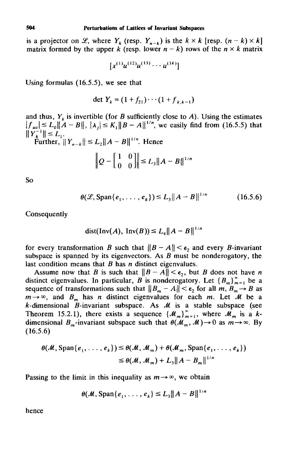
Israel Gohberg
Peter Lancaster
Leiba Rodman
C-L-A-S-S-I-C-S
In Applied Mathematics
sihjtl 51

Invariant Subspaces
of Matrices with
Applications

SlAM's Classics in Applied Mathematics series consists of books that were previously allowed to go
out of print. These books are republished by S1AM as a professional service because they continue
to be important resources tor mathematical scientists.
Editor-in-Chief
Robert E. O'Malley, Jr., University of Washington
Editorial Board
Richard A. Brualdi, University of Wisconsin-Madison
Leah Edelstein-Keshet, University of British Columbia
Nicholas J. Highani, University of Manchester
Herbert B. Keller, California Institute of Technology
Andrzej Z. Manitius, George Mason University
Hilary Ockendon, University of Oxford
Ingram Olkin, Stanford University
Peter Olver, University of Minnesota
Ferdinand Verhulst, Mathematiscfi Instituut, University of Utrecht
Classics in Applied Mathematics
C. C. Lin and L. A. Scgel, Mathematics Applied to Deterministic Problems in the Natural Sciences
Johan G. F. Belinfante and Bernard Kolman, A Survey of Lie Groups and Lie Algebras with
Applications and Computational Methods
James M. Ortega, Numerical Analysis: A Second Course
Anthony V. Fiacco and Garth P. McCorrnick, Nonlinear Programming: Sequential Unconstrained
Minimization Techniques
F. H. Clarke, Optimisation and Nonsmooth Analysis
George F. Carrier and Carl E. Pearson, Ordinary Differential Equations
Leo Breiman, Probability
R. Bellman and G. M. Wing, An Introduction to Invariant Imbedding
Abraham Berman and Robert J. Plemmons, Nonnegattve Matrices in the Mathematical Sciences
Olvi L. Mangasarian, Nonlinear Programming
*Carl Friedrich Gauss, Theory of the Combination of Observations Least Subject to Errors:
Part One, Part Two, Supplement. Translated by G. W. Stewart
Richard Bellman, Introduction to Matrix Analysis
U. M. Ascher, R. M. M. Mattheij, and R. D. Russell, Numerical Solution of Boundary Value
Problems for Ordinary Differential Equations
K. E. Brenan, S. L. Campbell, and L. R. Petzold, Numerical Solution of Initial-Value Problems
in Differential-Algebraic Equations
Charles L. Lawson and Richard J. Hanson, Solving Least Squares Problems
J. E. Dennis, Jr. and Robert B. Schnabel, Numerical Methods for Unconstrained Optimization
and Nonlinear Equations
Richard E. Barlow and Frank Proschan, Mathematical Theory of Reliability
Cornelius Lanczos, Linear Differential Operators
Richard Bellman, Introduction to Matrix Analysis, Second Edition
Beresford N. Parlett, The Symmetric Eigenvalue Problem
*First time in print.
ii

Classics in Applied Mathematics (continued)
Richard Haberman, Mathematical Models: Mechanical Vibrations, Population Dynamics,
and Traffic Flow
Peter W. M. John, Statistical Design and Analysis of Experiments
Tamer Basar and Geert Jan Olsder, Dynamic Noncooperative Game Theory, Second Edition
Emanuel Parzen, Stochastic Processes
Petar Kokotovic, Hassan K. Khalil, and John O'Reilly, Singular Perturbation Methods
in Control: Analysis and Design
Jean Dickinson Gibbons, Ingram Olkin, and Milton Sobel, Selecting and Ordering Populations:
A New Statistical Methodology
James A. Murdock, Perturbations: Theory and Methods
Ivar Ekeland and Roger Temam, Convex Analysis and Variational Problems
lvar Stakgold, Boundary Value Problems of Mathematical Physics, Volumes I and II
J. M. Ortega and W. C. Rheinboldt, Iterative Solution of Nonlinear Equations in Several Variables
David Kinderlehrer and Guido Stampacchia, An Introduction to Variational Inequalities and
Their Applications
E Natterer, The Mathematics of Computerized Tomography
AvinashC. Kak and Malcolm Slaney, Principles of Computerized Tomographic Imaging
R. Wong, Asymptotic Approximations of Integrals
O. Axelsson and V A. Barker, Finite Element Solution of Boundary Value Problems: Theory
and Computation
David R. Brillinger, Time Series: Data Analysis and Theory
Joel N. Franklin, Methods of Mathematical Economics: Linear and Nonlinear Programming,
Fixed-Point Theorems
Philip Hartman, Ordinary Differential Equations, Second Edition
Michael D. Intriligator, Mathematical Optimization and Economic Theory
Philippe G. Ciarlet, The Finite Element Method for Elliptic Problems
Jane K. Cullum and Ralph A. Willoughby, Lanczos Algorithms for Large Symmetric Eigenvalue
Computations, Vol. 1: Theory
M. Vidyasagar, Nonlinear Systems Analysis, Second Edition
Robert Mattheij and Jaap Molenaar, Ordinary Differential Equations in Theory and Practice
Shanti S. Gupta and S. Panchapakesan, Multiple Decision Procedures: Theory and Methodology
of Selecting and Ranting Populations
Eugene L. Allgower and Kurt Georg, Introduction to Numerical Continuation Methods
Leah Edelstein-Keshet, Mathematical Models in Biology
Heinz-Otto Krciss and Jens Lorcnz, Initial-Boundary Value Problems and the Navier-Stolces Equations
J. L. Hodges, Jr. and E. L. Lehmann, Basic Concepts of Probability and Statistics, Second Edition
George F. Carrier, Max Krook, and Carl E. Pearson, Functions of a Complex Variable: Theory
and Technique
Friedrich Pukelsheim, Optimal Design of Experiments
Israel Gohberg, Peter Lancaster, and Leiba Rodman, Invariant Subspaces of Matrices ivith
Applications
in

This page intentionally left blank

Invariant Subspaces
of Matrices with
Applications
Israel Gohberg
Tel-Aviv University
Ramat-Aviv, Israel
Peter Lancaster
University of Calgary
Calgary, Alberta, Canada
Leiba Rodman
College of William & Mary
Williamsburg, Virginia
siam.
Society for Industrial and Applied Mathematics
Philadelphia

Copyright © 2006 by die Society for Industrial and Applied Mathematics
This SIAM edition is an unabridged republication of the work first published by John
Wiley &. Sons, Inc., New York, 1986.
10 9 8 7 6 5 4 3 2 1
All rights reserved. Printed in the United States of America. No part of this book
may be reproduced, stored, or transmitted in any manner without the written
permission of the publisher. Fot information, write to the Society for Industrial and
Applied Mathematics, 3600 University City Science Center, Philadelphia, PA
19104-2688.
Library of Congress Cataloging in Publication Data
Gohberg, I. (Israel), 1928-
Invarient subspeces of matrices with applications / Israel Gohberg, Peter
Lancaster, Leiba Rodman.
p. cm. — (Classics in applied mathematics ; 51)
Originally published: New York : Wiley, cl986, in series: Canadian Mathematical
Society series of monographs and advanced texts.
Includes bibliographical references and indexes.
lSRN0-89871-608-X(pbk.)
1. Invariant subspaces. 2. Matrices. I. lancaster, Peter, 1929-. II. Rodman, L.
III. Title. IV. Series.
QA322.G649 2006
515'.73--dc22
2006042260
is a registered trademark.

To our wives
fcetfa, Diane, andlzffa
MM

This page intentionally left blank

Contents
Introduction I
Part One Fundamental Properties of
Invariant Subspaces and Applications 3
Chapter One Invariant Subspaces: Definition, Examples, and First
Properties 5
1.1 Definition and Examples 5
1.2 Eigenvalues and Eigenvectors 10
1.3 Jordan Chains 12
1.4 Invariant Subspaces and Basic Operations on Linear
Transformations 16
1.5 Invariant Subspaces and Projectors 20
1.6 Angular Transformations and Matrix Quadratic
Equations 25
1.7 Transformations in Factor Spaces 28
1.8 The Lattice of Invariant Subspaces 31
1.9 Triangular Matrices and Complete Chains of Invariant
Subspaces 37
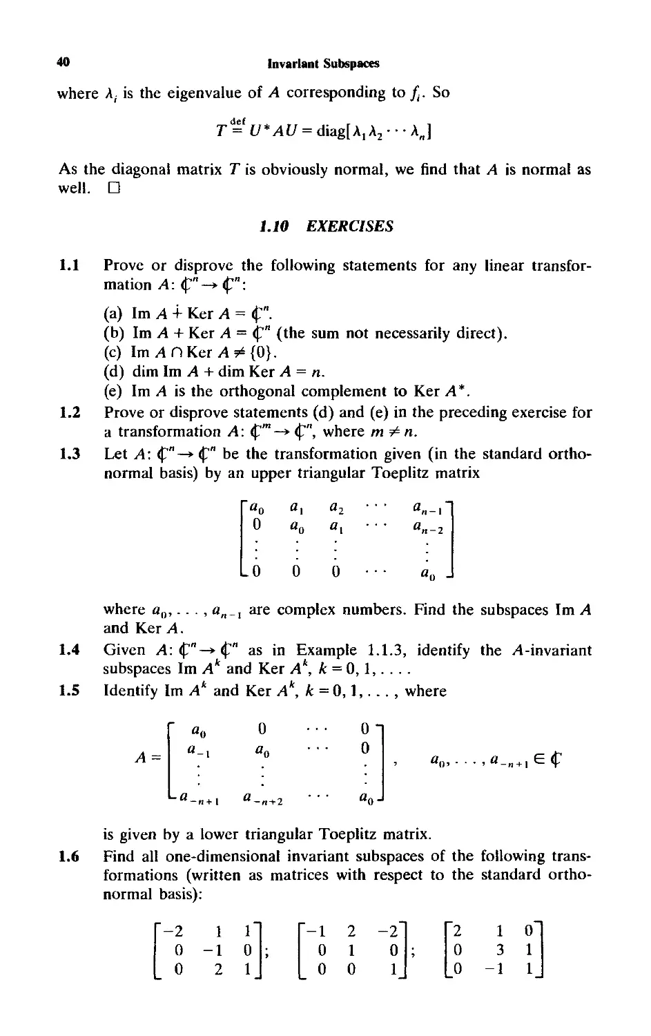
1.10 Exercises 40
Chapter Two Jordan Form and Invariant Subspaces 45
2.1 Root Subspaces 45
2.2 The Jordan Form and Partial Multiplicities 52
2.3 Proof of the Jordan Form 58
2.4 Spectral Subspaces 60
2.5 Irreducible Invariant Subspaces and Unicellular
Transformations 65
2.6 Generators of Invariant Subspaces 69
2.7 Maximal Invariant Subspace in a Given Subspace 72
2.8 Minimal Invariant Subspace over a Given Subspace 78
2.9 Marked Invariant Subspaces 83
ix

X
Contents
2.10 Functions of Transformations 85
2.11 Partial Multiplicities and Invariant Subspaces of
Functions of Transformations 92
2.12 Exercises 95
Chapter Three Coinvariant and Semiinvariant Subspaces 105
3.1 Coinvariant Subspaces 105
3.2 Reducing Subspaces 109
3.3 Semiinvariant Subspaces 112
3.4 Special Classes of Transformations 116
3.5 Exercises 119
Chapter Four Jordan Form for Extensions and Completions 121
4.1 Extensions from an Invariant Subspace 121
4.2 Completions from a Pair of Invariant and Coinvariant
Subspaces 128
4.3 The Sigal Inequalities 133
4.4 Special Case of Completions 136
4.5 Exercises 142
Chapter Five Applications to Matrix Polynomials 144
5.1 Linearizations, Standard Triples, and Representations of
Monic Matrix Polynomials 144
5.2 Multiplication of Monic Matrix Polynomials and Partial
Multiplicities of a Product 153
5.3 Divisibility of Monic Matrix Polynomials 156
5.4 Proof of Theorem 5.3.2 161
5.5 Example 167
5.6 Factorization into Several Factors and Chains of
Invariant Subspaces 171
5.7 Differential Equations 175
5.8 Difference Equations 180
5.9 Exercises 183
Chapter Six Invariant Subspaces for Transformations Between
Different Spaces 189
6.1 [A B]-Invariant Subspaces 189
6.2 Block Similarity 192
6.3 Analysis of the Brunovsky Canonical Form 197
6.4 Description of [A B]-Invariant Subspaces 200
6.5 The Spectral Assignment Problem 203
6.6 Some Dual Concepts 207
6.7 Exercises 209

Contents
xi
Chapter Seven Rational Matrix Functions 212
7.1 Realizations of Rational Matrix Functions 212
7.2 Partial Multiplicities and Multiplication 218
7.3 Minimal Factorization of Rational Matrix Functions 225
7.4 Example 230
7.5 Minimal Factorizations into Several Factors and Chains
of Invariant Subspaces 234
7.6 Linear Fractional Transformations 238
7.7 Linear Fractional Decompositions and Invariant
Subspaces of Nonsquare Matrices 244
7.8 Linear Fractional Decompositions:
Further Deductions 251
7.9 Exercises 255
Chapter Eight Linear Systems 262
8.1 Reductions, Dilations, and Transfer Functions 262
8.2 Minimal Linear Systems: Controllability and
Observability 265
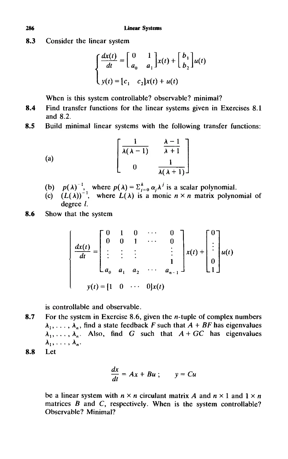
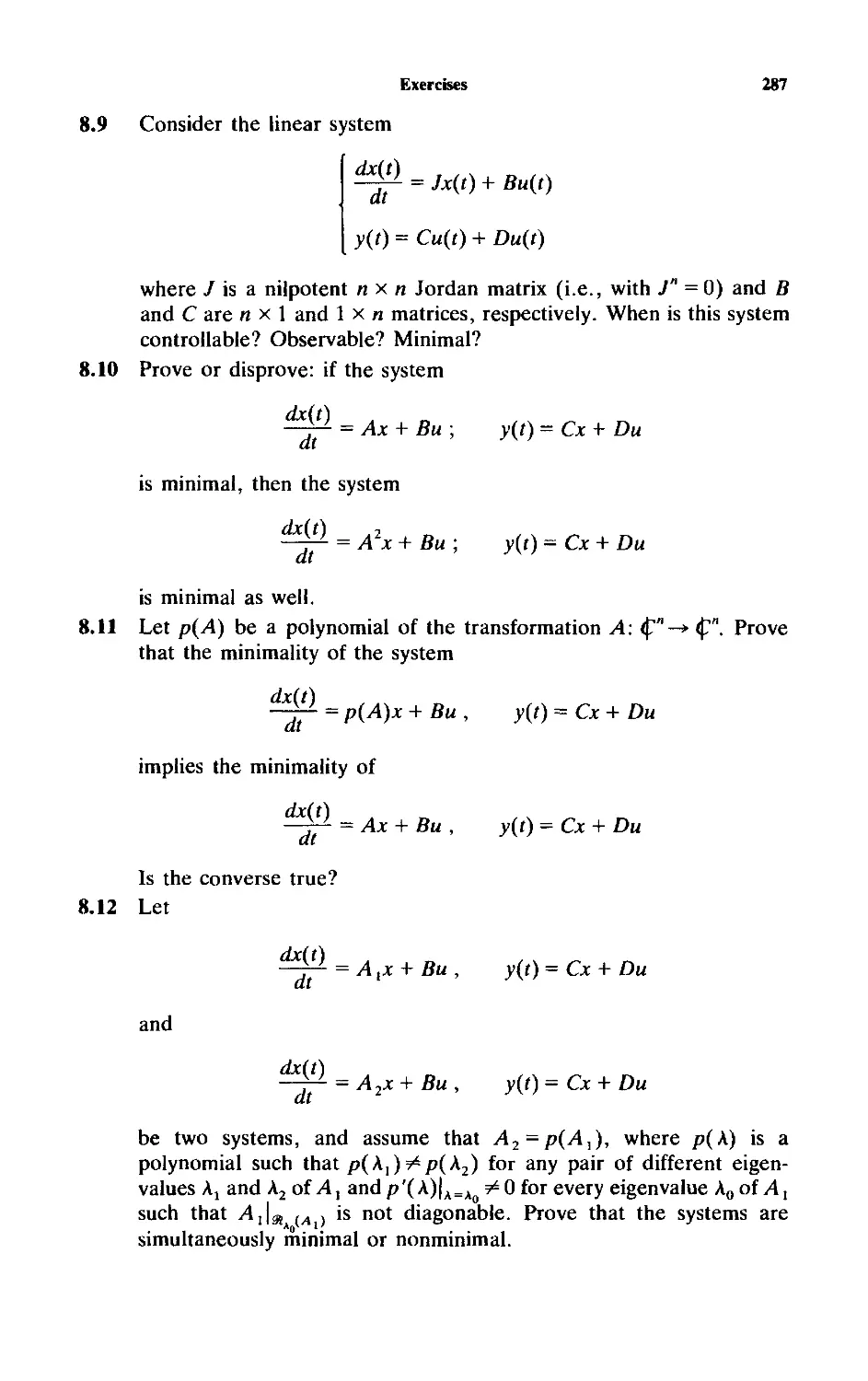
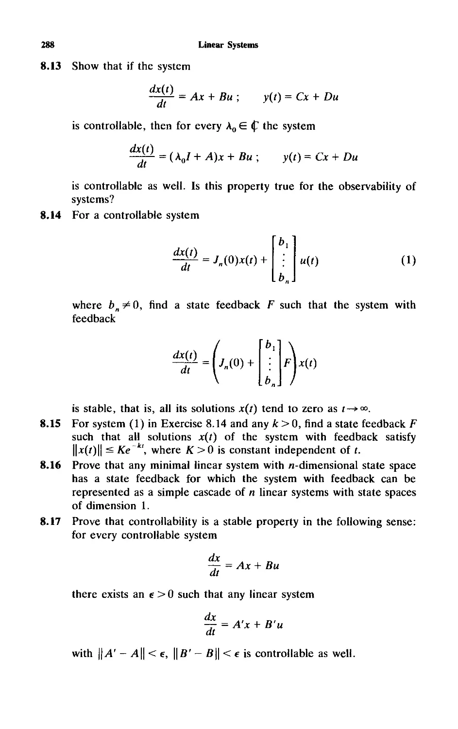
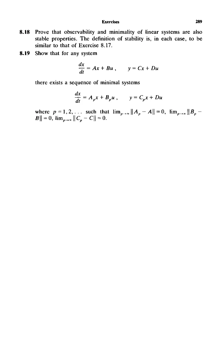
8.3 Cascade Connections of Linear Systems 270
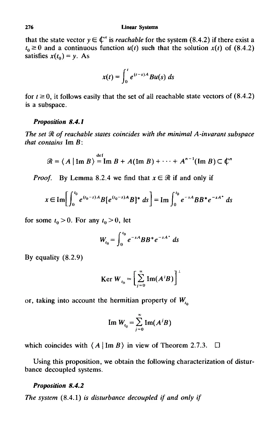
8.4 The Disturbance Decoupling Problem 274
8.5 The Output Stabilization Problem 279
8.6 Exercises 285
Notes to Part 1. 290
Part Two Algebraic Properties of Invariant Subspaces 293
Chapter Nine Commuting Matrices and Hyperinvariant Subspaces 295
9.1 Commuting Matrices 295
9.2 Common Invariant Subspaces for Commuting
Matrices 301
9.3 Common Invariant Subspaces for Matrices with Rank 1
Commutators 303
9.4 Hyperinvariant Subspaces 305
9.5 Proof of Theorem 9.4.2 307
9.6 Further Properties of Hyperinvariant Subspaces 311
9.7 Exercises 313
Chapter Ten Description of Invariant Subspaces and Linear
Transformations with the Same Invariant Subspaces 316
10.1 Description of Irreducible Subspaces 316
10.2 Transformations Having the Same Set of Invariant
Subspaces 323

Xll
Contents
10.3 Proof of Theorem 10.2.1 328
10.4 Exercises 338
Chapter Eleven Algebras of Matrices and Invariant Subspaces 339
11.1 Finite-Dimensional Algebras 339
11.2 Chains of Invariant Subspaces 340
11.3 Proof of Theorem 11.2.1 343
11.4 Reflexive Lattices 346
11.5 Reductive and Self-Adjoint Algebras 350
11.6 Exercises 355
Chapter Twelve Real Linear Transformations 359
12.1 Definition, Examples, and First Properties of Invariant
Subspaces 359
12.2 Root Subspaces and the Real Jordan Form 363
12.3 Complexification and Proof of the Real Jordan
Form 366
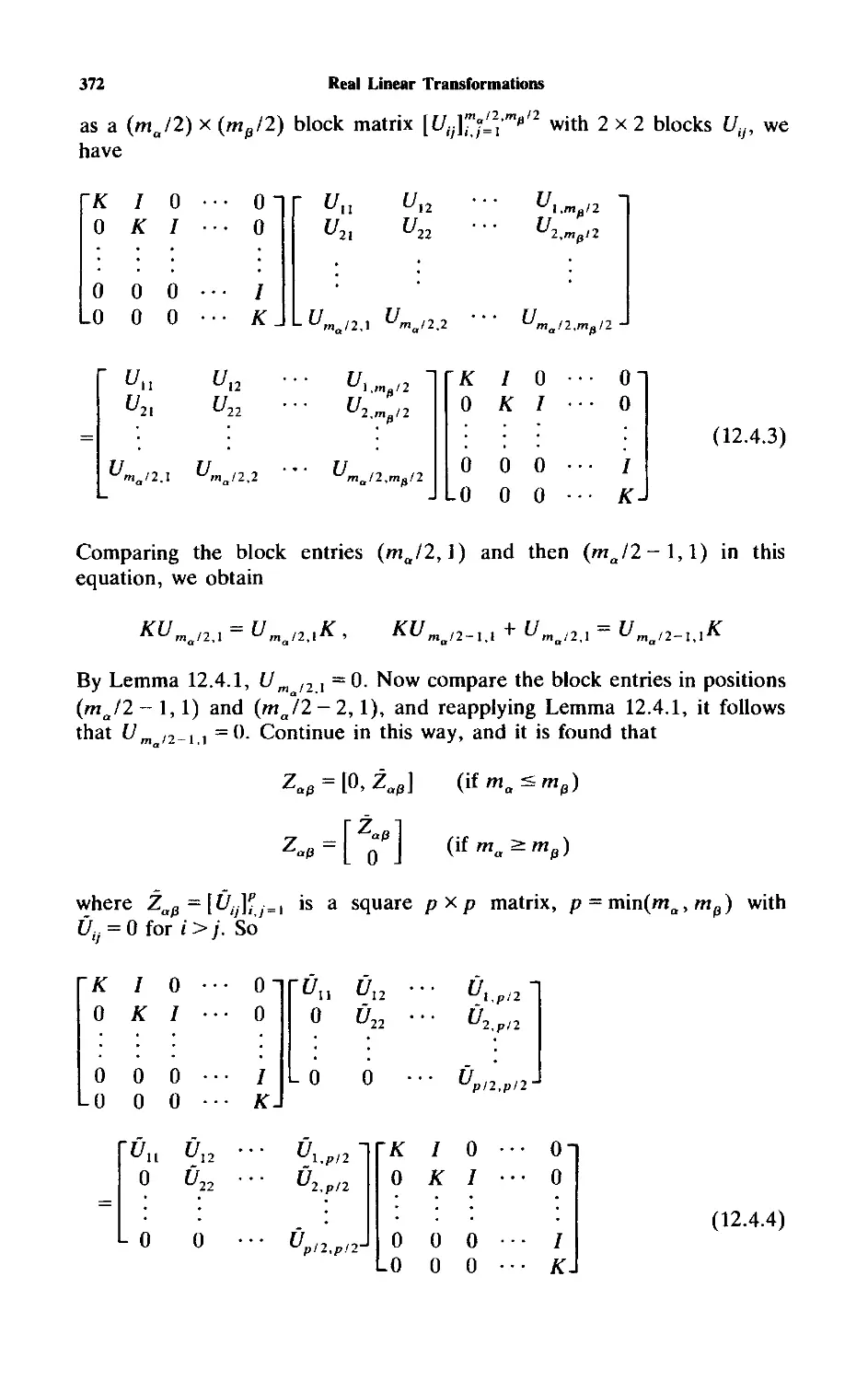
12.4 Commuting Matrices 371
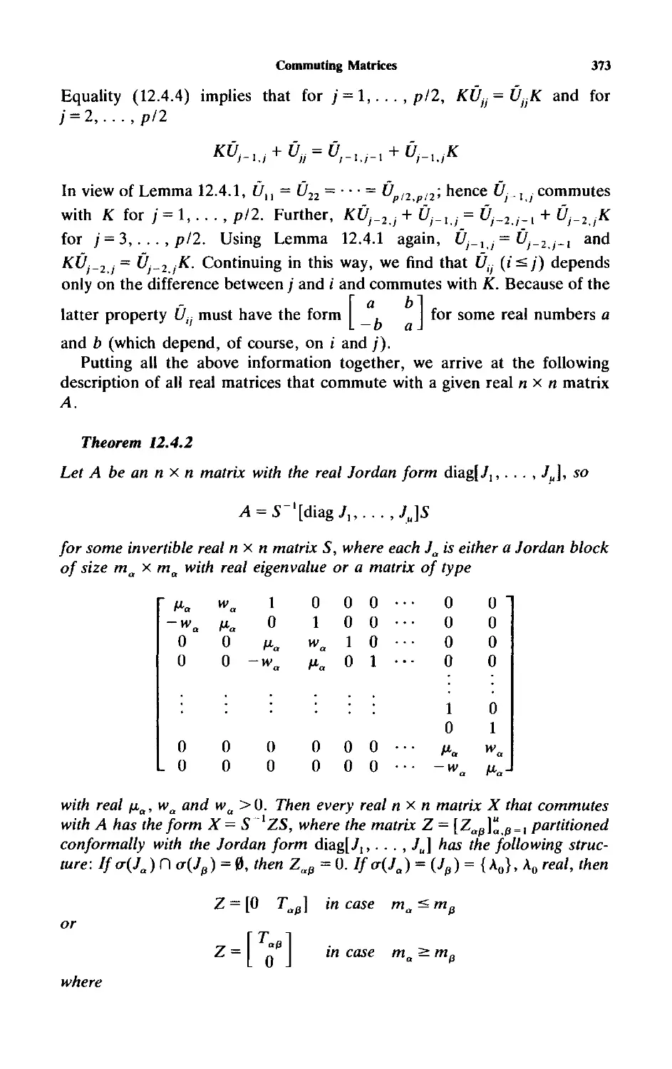
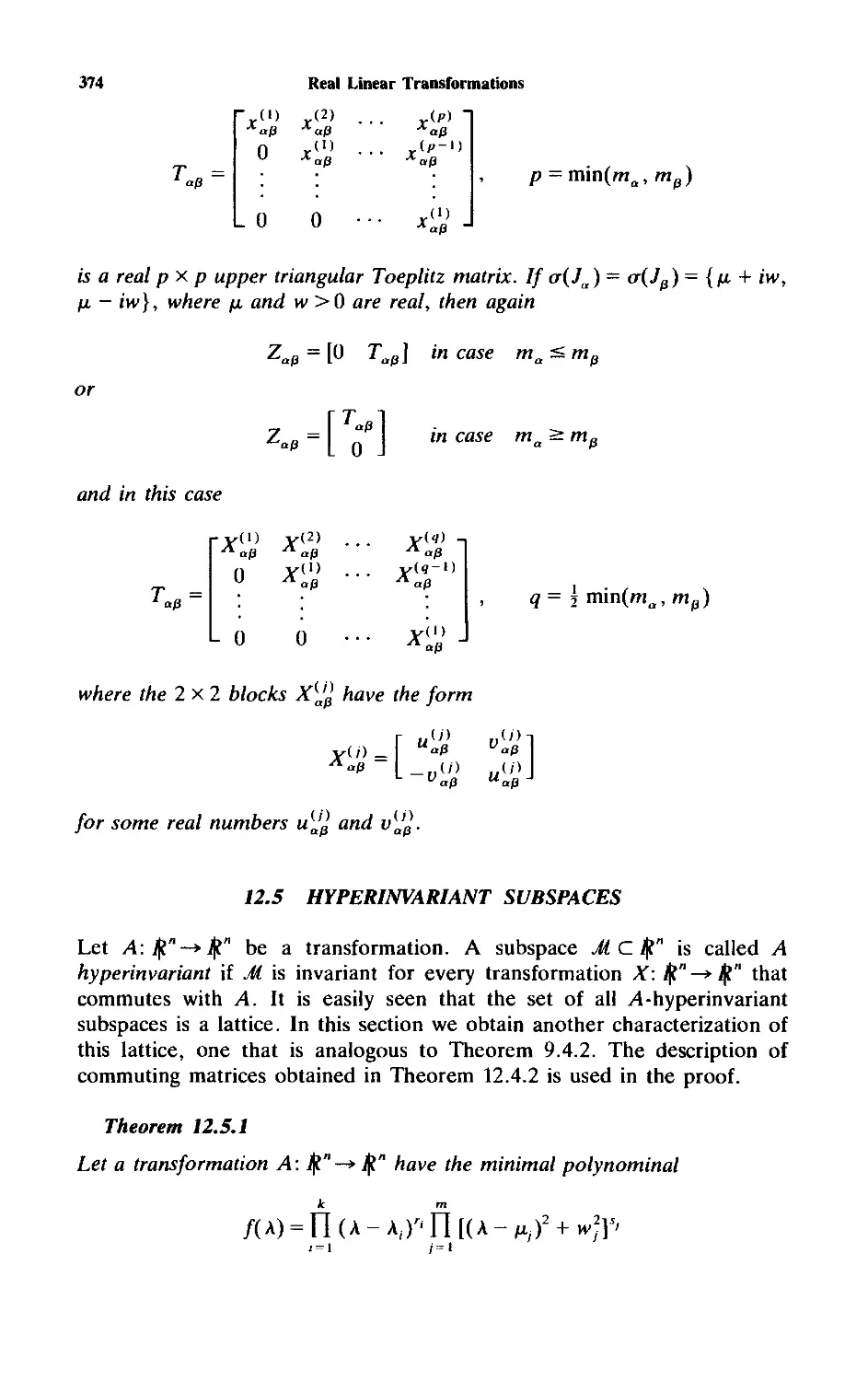
12.5 Hyperinvariant Subspaces 374
12.6 Real Transformations with the Same Invariant
Subspaces 378
12.7 Exercises 380
Notes to Part 2. 384
Part Three Topological Properties of
Invariant Subspaces and Stability 385
Chapter Thirteen The Metric Space of Subspaces 387
13.1 The Gap Between Subspaces 387
13.2 The Minimal Angle and the Spherical Gap 392
13.3 Minimal Opening and Angular Linear
Transformations 396
13.4 The Metric Space of Subspaces 400
13.5 Kernels and Images of Linear Transformations 406
13.6 Continuous Families of Subspaces 408
13.7 Applications to Generalized Inverses 411
13.8 Subspaces of Normed Spaces 415
13.9 Exercises 420

Contents
xiii
Chapter Fourteen The Metric Space of Invariant Subspaces 423
14.1 Connected Components: The Case of One
Eigenvalue 423
14.2 Connected Components: The General Case 426
14.3 Isolated Invariant Subspaces 428
14.4 Reducing Invariant Subspaces 432
14.5 Coinvariant and Semiinvariant Subspaces 437
14.6 The Real Case 439
14.7 Exercises 443
Chapter Fifteen Continuity and Stability of Invariant Subspaces 444
15.1 Sequences of Invariant Subspaces 444
15.2 Stable Invariant Subspaces: The Main Result 447
15.3 Proof of Theorem 15.2.1 in the General Case 451
15.4 Perturbed Stable Invariant Subspaces 455
15.5 Lipschitz Stable Invariant Subspaces 459
15.6 Stability of Lattices of Invariant Subspaces 463
15.7 Stability in Metric of the Lattice of Invariant
Subspaces 464
15.8 Stability of [A B]-Invariant Subspaces 468
15.9 Stable Invariant Subspaces for Real
Transformations 470
15.10 Partial Multiplicities of Close Linear
Transformations 475
15.11 Exercises 479
Chapter Sixteen Perturbations of Lattices of Invariant Subspaces with
Restrictions on the Jordan Structure 482
16.1 Preservation of Jordan Structure and Isomorphism of
Lattices 482
16.2 Properties of Linear Isomorphisms of Lattices:
The Case of Similar Transformations 486
16.3 Distance Between Invariant Subspaces for
Transformations with the Same Jordan Structure 492
16.4 Transformations with the Same Derogatory Jordan
Structure 497
16.5 Proofs of Theorems 16.4.1 and 16.4.4 500
16.6 Distance between Invariant Subspaces for
Transformations with Different Jordan Structures 507
16.7 Conjectures 510
16.8 Exercises 513

xiv
Contents
Chapter Seventeen Applications 514
17.1 Stable Factorizations of Matrix Polynomials:
Preliminaries 514
17.2 Stable Factorizations of Matrix Polynomials:
Main Results 520
17.3 Lipschitz Stable Factorizations of Monic Matrix
Polynomials 525
17.4 Stable Minimal Factorizations of Rational Matrix
Functions: The Main Result 528
17.5 Proof of the Auxiliary Lemmas 532
17.6 Stable Minimal Factorizations of Rational Matrix
Functions: Further Deductions 537
17.7 Stability of Linear Fractional Decompositions of
Rational Matrix Functions 540
17.8 Isolated Solutions of Matrix Quadratic Equations 545
17.9 Stability of Solutions of Matrix Quadratic
Equations 551
17.10 The Real Case 553
17.11 Exercises 557
Notes to Part 3. 561
Part Four Analytic Properties of Invariant Subspaces 563
Chapter Eighteen Analytic Families of Subspaces 565
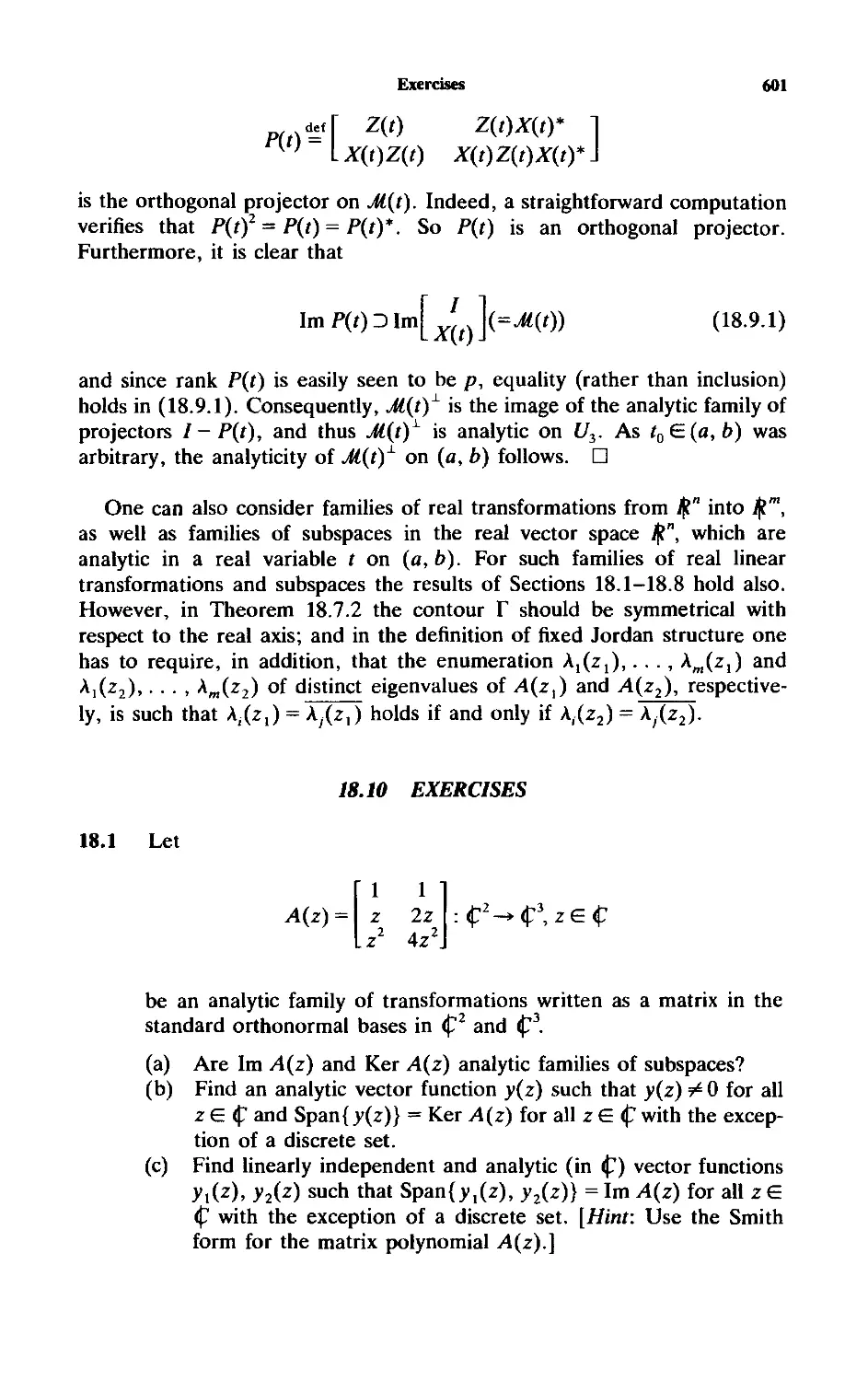
18.1 Definition and Examples 565
18.2 Kernel and Image of Analytic Families of
Transformations 569
18.3 Global Properties of Analytic Families of
Subspaces 575
18.4 Proof of Theorem 18.3.1 (Compact Sets) 578
18.5 Proof of Theorem 18.3.1 (General Case) 584
18.6 Direct Complements for Analytic Families of
Subspaces 590
18.7 Analytic Families of Invariant Subspaces 594
18.8 Analytic Dependence of the Set of Invariant Subspaces
and Fixed Jordan Structure 596
18.9 Analytic Dependence on a Real Variable 599
18.10 Exercises 601
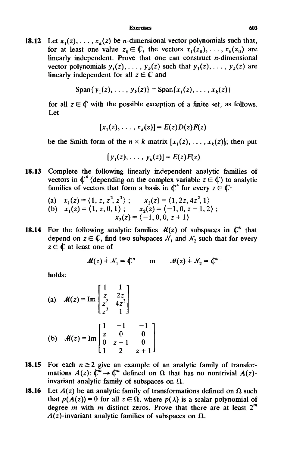
Chapter Nineteen Jordan Form of Analytic Matrix Functions 604
19.1 Local Behaviour of Eigenvalues and Eigenvectors 604
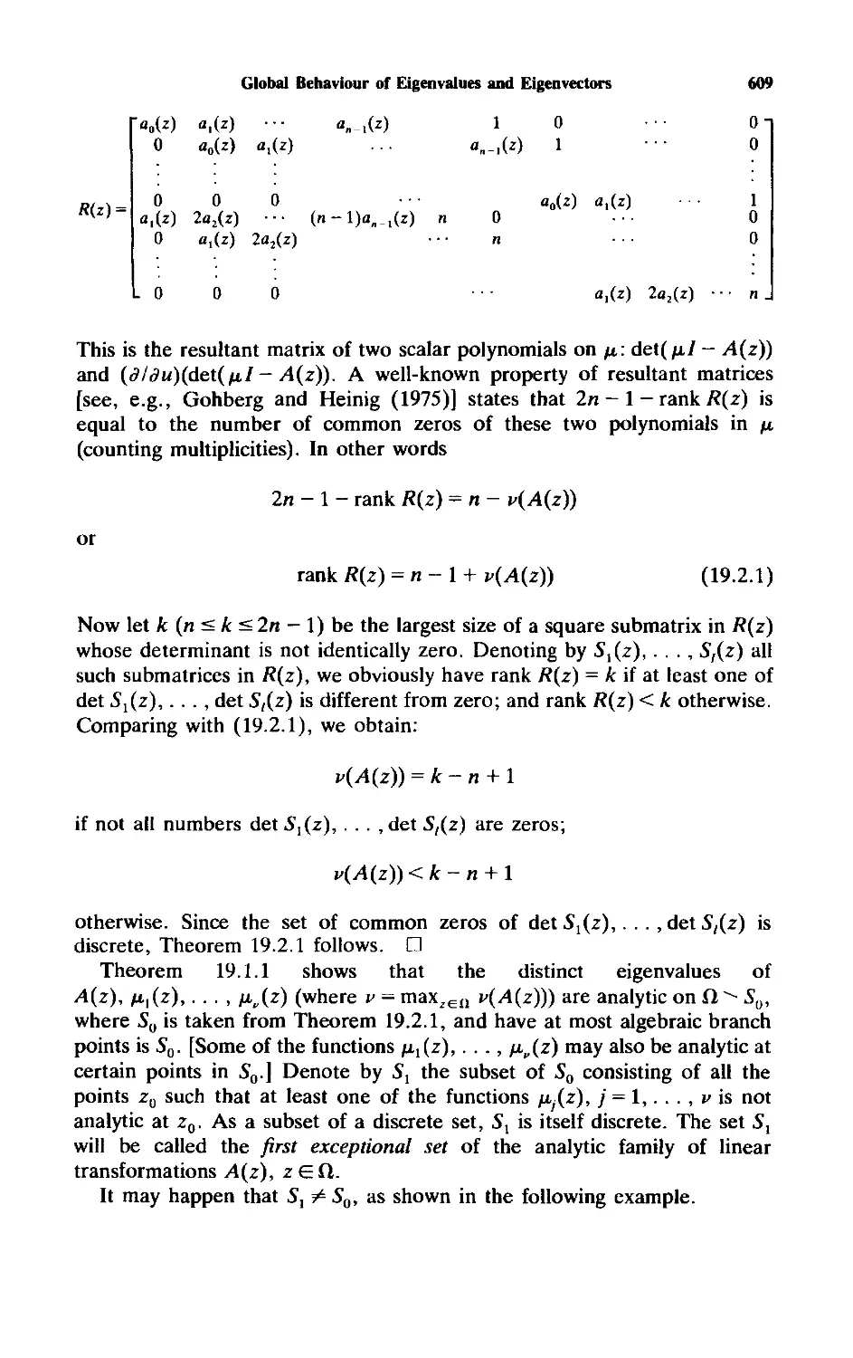
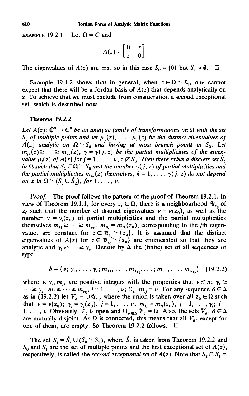
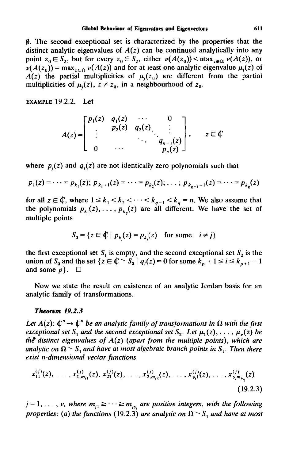
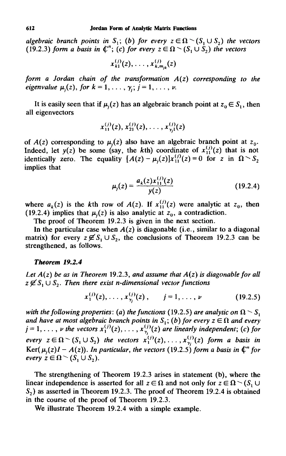
19.2 Global Behaviour of Eigenvalues and Eigenvectors 607

Contents
xv
19.3 Proof of Theorem 19.2.3 613
19.4 Analytic Extendability of Invariant Subspaces 616
19.5 Analytic Matrix Functions of a Real Variable 620
19.6 Exercises 622
Chapter Twenty Applications 624
20.1 Factorization of Monic Matrix Polynomials 624
20.2 Rational Matrix Functions Depending Analytically on a
Parameter 627
20.3 Minimal Factorizations of Rational Matrix
Functions 634
20.4 Matrix Quadratic Equations 639
20.5 Exercises 642
Notes to Part 4. 645
Appendix. Equivalence of Matrix Polynomials 646
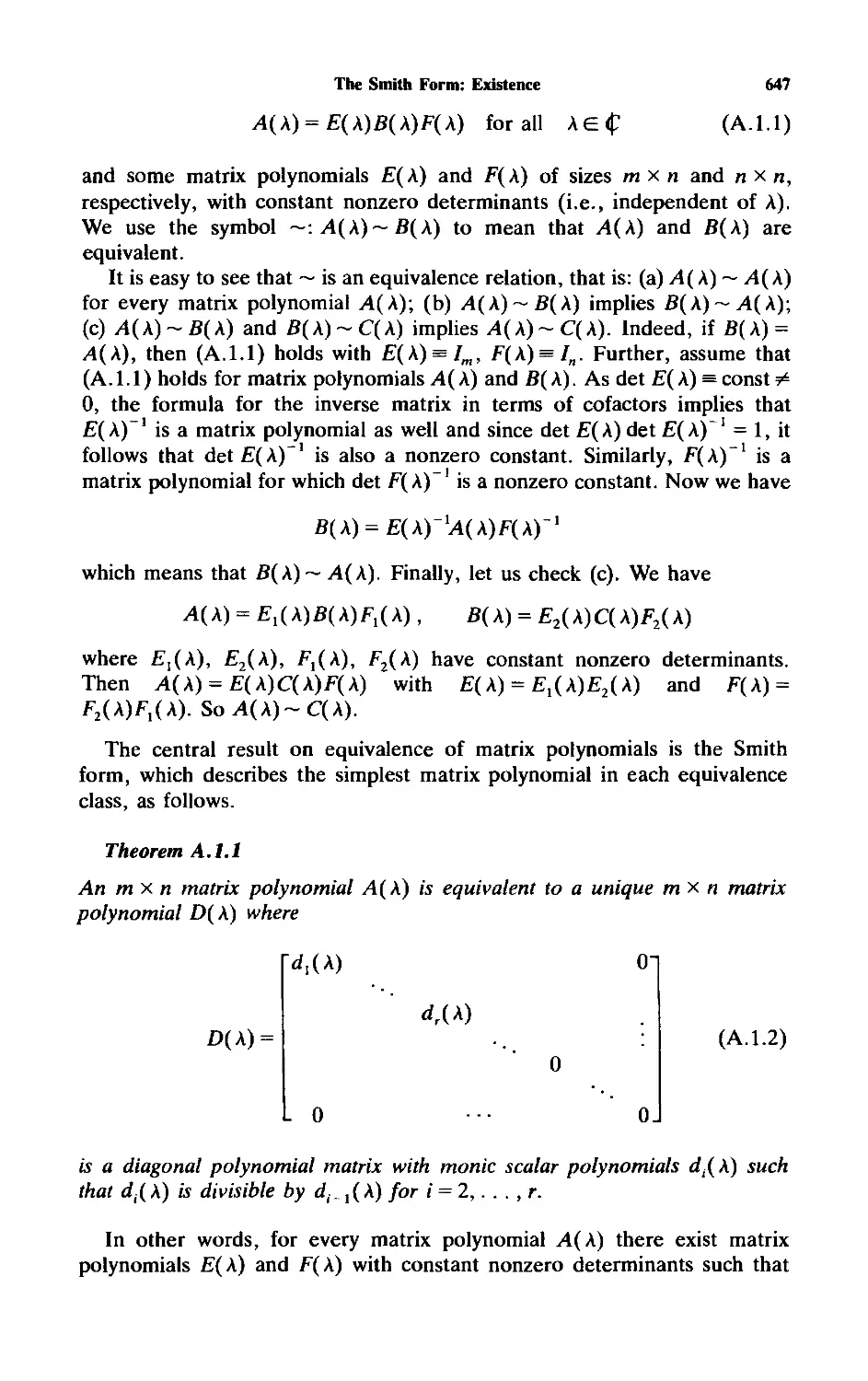
A.l The Smith Form: Existence 646
A.2 The Smith Form: Uniqueness 651
A.3 Invariant Polynomials, Elementary Divisors, and Partial
Multiplicities 654
A.4 Equivalence of Linear Matrix Polynomials 659
A.5 Strict Equivalence of Linear Matrix Polynomials:
Regular Case 662
A.6 The Reduction Theorem for Singular Polynomials 666
A.7 Minimal Indices and Strict Equivalence of Linear Matrix
Polynomials (General Case) 672
A.8 Notes to the Appendix 678
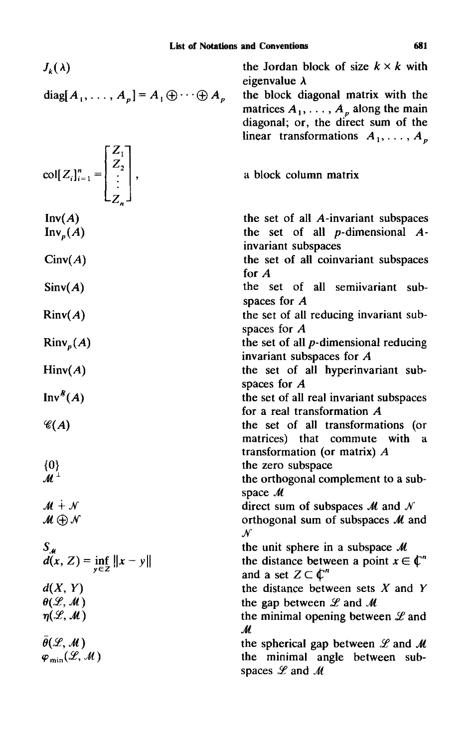
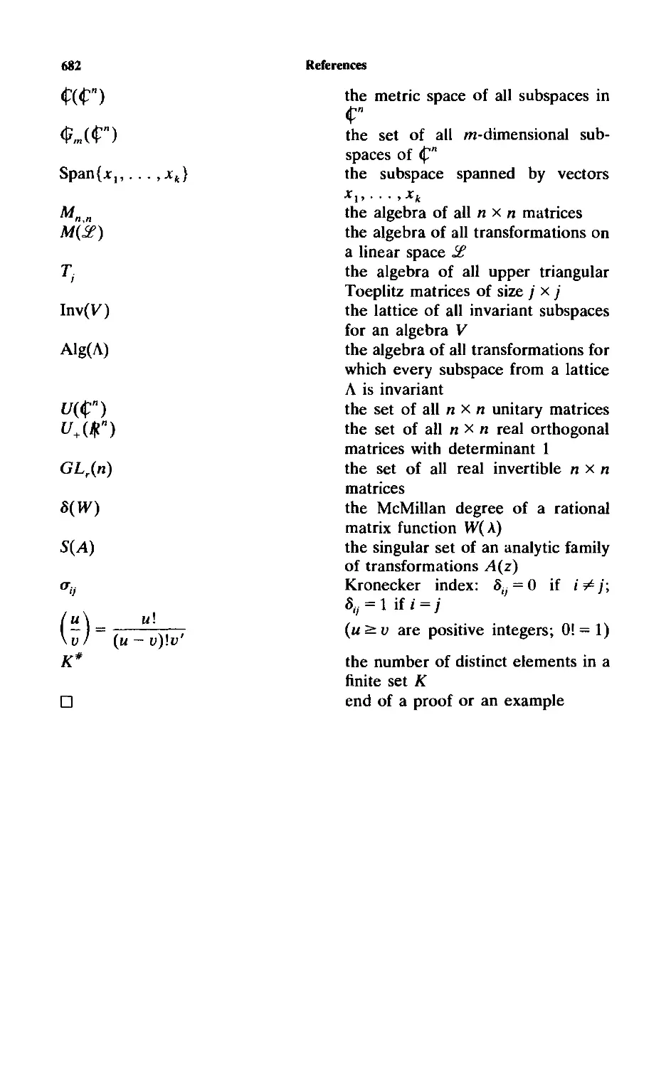
List of Notations and Conventions 679
References 683
Author Index 687
Subject Index
689

This page intentionally left blank

Preface to the SI AM Classics
Edition
In the past 50 or 60 years, developments in mathematics have led to
innovations in linear algebra and matrix theory. This progress was often initiated
by topics and problems from applied mathematics. A good example of this
is the development of mathematical systems theory. In particular, many new
and important results in linear algebra cannot even be formulated without the
notion of invariant subspaces of matrices or linear transformations. In view of
this, the authors set out to write a work on advanced linear algebra in which
invariant subspaces of matrices would be the central notion, the main
subject of research, and the main tool. In other words, matrix theory was to be
presented entirely on the basis of the theory of invariant subspaces, including
the algebraic, geometric, topological, and analytic aspects of the theory. We
believed that this would give a new point of view and a better understanding
of the entire subject. It would also allow us to follow up systematically the
central role of invariant subspaces in linear algebra and matrix analysis, as
well as their role in the study of differential and difference equations, systems
theory, matrix polynomials, rational matrix functions, and algebraic Riccati
equations.
The first edition of the present book was the result. To the authors'
knowledge it is the only book in existence with these aims. The first parts of the
book have the character of a textbook easily accessible for undergraduate
students. As the development progresses, the exposition changes to approach the
style and content of a graduate textbook and even a research monograph until,
in the last part, recent achievements are presented. The fundamental
character of the mathematics, its accessibility, and its importance in applications
makes this a widely useful book for experts and for students in mathematics,
sciences, and engineering.
The first edition sold out in early 2005, and we could not help colleagues
who found a need for it. We are grateful to Wiley-Interscience publications
for producing the first edition and for returning the copyright to us in order to
give the work a new life. We are especially thankful to SIAM for the decision
to include this work in their series Classics in Applied Mathematics.
We would like to mention some other literature with strong connections
to this book. First, there are two other relevant monographs by the present
authors: Matrix Polynomials, published by Academic Press in 1982, and
Matrices and Indefinite Scalar Products, published by Birkhauser Verlag in 1983.
Invariant subspaces play an important role in both of them. In fact, work on
these two books convinced us of the need for the present systematic
treatment. The monograph of I. Gohberg, M. A. Kaashoek, and F. van Schagen,
xvii

XV111
Preface to the Classics Edition
Partially Specified Matrices and Operators: Classification, Completion,
Applications, Birkhauser Verlag, 1995, is recommended as additional reading for
Chapter 4. A later, comprehensive account of the theory of algebraic Riccati
equations, discussed in Chapters 17 and 20, can be found in the monograph
Algebraic Riccati Equations by P. Lancaster and L. Rodman, published by
Oxford University Press in 1995.
By the end of 2005 Birkhauser Verlag will also publish the authors' In-
definite Linear Algebra. This can also be recommended as a book in which
invariant subspaces play an important role.
It is a pleasure to repeat the acknowledgments appearing in the first
edition. These include support from the Killam Foundation of Canada and the
Nathan and Lily Silver Chair on Mathematical Analysis and Operator
Theory of Tel Aviv University. Continuing support was also provided by staff
at the School of Mathematical Sciences of Tel Aviv University and at the
Department of Mathematics and Statistics of the University of Calgary. In
particular, Jacqueline Gorsky in Tel Aviv and Pat Dalgetty in Calgary
contributed with speedy and skillful development of the first typescript. Support
from national organizations is also acknowledged: the Basic Research Fund
of the Israel Academy of Science, the U.S. National Science Foundation, and
the Natural Sciences and Engineering Research Council of Canada.
COMMENTS ON THE DEVELOPMENTS OF TWENTY
YEARS
Twenty years have passed since the appearance of the first edition.
Naturally, in this time advances have been made on some the theory appearing
in the first edition, advances which have appeared in specialized journals and
books. Also, the status of some conjectures made in the first edition has
been clarified. Here, several developments of this kind are summarized for the
interested reader, together with a short bibliography.
1. Chapter 2. A characterization of matrices all of whose invariant sub-
spaces are marked is given in [1].
2. Chapter 4. The problem of describing the Jordan forms of completions
from an invariant and a coinvariant subspace, also known as the Carlson
problem, has been solved (in terms of Littlewood-Richardson sequences). As
it turns out, it is closely related to the problem of describing the range of the
eigenvalues of A + B in terms of the eigenvalues of Hermitian matrices A and
B, solved by Klyachko [5]. See the expository paper [2] and references there.
3. Chapter 9. Various results on the existence of complete chains of
invariant subspaces that extend Theorem 9.3.1 are presented in [8] (see also
references there). We quote Radjavi's theorem [7]: A collection S of n x n
complex matrices has a complete chain of common invariant subspaces if and
only if the trace is permutable: trace(A\ ■ ■ ■ Ap) = trace (A^^ ■ ■ ■ Aa^) for
every p-tuple A\,..., Ap, Aj G S, and every permutation a of {1,2,... ,p}.

Preface to the Classics Edition
xix
4. Chapter 11. A simple proof of Bumside's theorem (Theorem 11.2.1 in
the text) is given in [6].
Conjecture 11.2.3 was disproved in [3] (for all n > 1 except 7 and 11) and
in [10] (for n — 1 and n — 11). It is certainly of interest to describe all pairs
of complementary algebras V\ and Vi for which this conjecture is correct. In
[3] it was proved that the conjecture is valid if the complementary algebras
V\ and Vi are orthogonal.
5. Chapter 15. The past twenty years have seen the development of
a substantial literature concerning stability (in various senses) of invariant
subspaces of matrices, as well as of linear operators acting in an infinite-
dimensional Hilbert space. For much of this material and its applications in
the context of finite-dimensional spaces, we refer the reader to the expository
paper [9] and references there.
6. Chapter 16. Conjecture 16.7.1 is false in general. A counterexample
is given in [4]. The conjecture holds when A is nonderogatory (however, the
proof given on page 512 is erroneous, as pointed out in [4]) and when A is
diagonable. These results were established in [4] as well. An interesting open
question concerns the characterization of those Jordan structures for which
Conjecture 16.7.1 fails.
References
[1] R. Bru, L. Rodman, and H. Schneider, "Extensions of Jordan bases for
invariant subspaces of a matrix," Linear Algebra Appl. 150, 209-225
(1991).
[2] W. Fulton, "Eigenvalues, invariant factors, highest weights, and Schubert
calculus," Bull. Amer. Math. Soc. 37, 209-249 (2000).
[3] M. D. Choi, H. Radjavi and P. Rosenthal, "On complementary matrix
algebras," Integral Equations and Operator Theory 13, 165-174 (1990).
[4] J. Hartman, "On a conjecture of Gohberg and Rodman," Linear Algebra
Appl. 140, 267-278 (1990).
[5] A. A. Klyachko, "Stable bundles, representation theory and Hermitian
operators," Selecta Math. 4, 419-445 (1998).
[6] V. Lomonosov and P. Rosenthal, "The simplest proof of Burnside's
theorem on matrix algebras," Linear Algebra Appl. 383, 45-47 (2004).
[7] H. Radjavi, "A trace condition equivalent to simultaneous triangulariz-
ability," Canad. J. Math. 38, 376-386 (1986).
[8] H. Radjavi and P. Rosenthal, Simultaneous Triangularization, Springer
Verlag, New York, 2001.

XX
Preface to the Classics Edition
[9] A. C. M. Ran and L. Rodman, "A class of robustness problems in matrix
analysis," Operator Theory: Advances and Applications 134, 337-389
(2002).
[10] T. Yoshino, "Supplemental examples: 'On complementary matrix
algebras,'" Integral Equations and Operator Theory 14, 764-766 (1991).

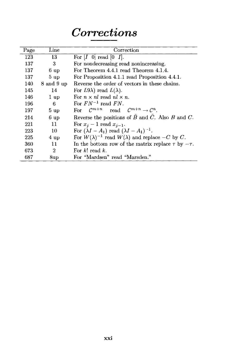
Corrections
Page Line Correction
~T23 13 For [I 0] read [0 I].
137 3 For nondecreasing read nonincreasing.
137 6 up For Theorem 4.4.1 read Theorem 4.1.4.
137 5 up For Proposition 4.1.1 read Proposition 4.4.1.
140 8 and 9 up Reverse the order of vectors in these chains.
145 14 For L9X) read L(X).
146 1 up For n x nl read nl x n.
196 6 For FN-1 read FN.
197 5 up For Cm+n read Cm+n -> Cn.
214 6 up Reverse the positions of B and C. Also B and C.
221 11 For Xj — 1 read Xj-\.
223 10 For (XI- Ax) read (XI- Ai)-1.
225 4 up For W(X)-1 read W(A) and replace -C by C.
360 11 In the bottom row of the matrix replace r by —t.
673 2 For fe! read fe.
687 8up For "Mardsen" read "Marsden."
xxi

This page intentionally left blank

Introduction
Invariant subspaces are a central notion of linear algebra. However, in
existing texts and expositions the notion is not easily or systematically
followed. Perhaps because the whole structure is very rich, the treatment
becomes fragmented as other related ideas and notions intervene. In
particular, the notion of an invariant subspace as an entity is often lost in the
discussion of eigenvalues, eigenvectors, generalized eigenvectors, and so on.
The importance of invariant subspaces becomes clearer in the context of
operator theory on spaces of infinite dimension. Here, it can be argued that
the structure is poorer and this is one of the few available tools for the study
of many classes of operators. Probably for this reason, the first books on
invariant subspaces appeared in the framework of infinite-dimensional
spaces. It seems to the authors that now there is a case for developing a
treatment of linear algebra in which the central role of invariant subspace is
systematically followed up.
The need for such a treatment has become more apparent in recent years
because of developments in different fields of application and especially in
linear systems theory, where concepts such as controllability, feedback,
factorization, and realization of matrix functions are commonplace. In the
treatment of such problems new concepts and theories have been developed
that form complete new chapters in the body of linear algebra. As examples
of new concepts of linear algebra developed to meet the needs of systems
theory, we should mention invariant subspaces for nonsquare matrices and
similarity of such matrices.
In this book the reader will find a treatment of certain aspects of linear
algebra that meets the two objectives: to develop systematically the central
role of invariant subspaces in the analysis of linear transformations and to
include relevant recent developments of linear algebra stimulated by linear
systems theory. The latter are not dealt with separately, but are integrated
into the text in a way that is natural in the development of the mathematical
structure.
1

2
Introduction
The first part of the book, taken alone or together with selections from
the other parts, can be used as a text for undergraduate courses in
mathematics, having only a first course in linear algebra as prerequisite. At
the same time, the book will be of interest to graduate students in science
and engineering. We trust that experts will also find the exposition and new
results interesting. The authors anticipate that the book will also serve as a
valuable reference work for mathematicians, scientists, and engineers. A set
of exercises is included in each chapter. In general, they are designed to
provide illustrations and training rather than extensions of the theory.
The first part of the book is devoted mainly to geometric properties of
invariant subspaces and their applications in three fields. The fields in
question are matrix polynomials, rational matrix functions, and linear
systems theory. They are each presented in self-contained form, and—rather
than being exhaustive—the focus is on those problems in which invariant
subspaces of square and nonsquare matrices play a central role. These
problems include factorization and linear fractional decompostions for
matrix functions; problems of realization for rational matrix functions; and the
problem of describing connections, or cascades, of linear systems, pole
assignment, output stabilization, and disturbance decoupling.
The second part is of a more algebraic character in which other properties
of invariant subspaces are analyzed. It contains an analysis of the extent to
which the invariant subspaces determine the parent matrix, invariant sub-
spaces common to commuting matrices, and lattices of subspaces for a single
matrix and for algebras of matrices. .,
The numerical computation of invariant subspaces is a difficult task as, in
general, it makes sense to compute only those invariant subspaces that
change very little after small changes in the transformation. Thus it is
important to have appropriate notions of "stable" invariant subspaces. Such
an analysis of the stability of invariant subspaces and their generalizations is
the main subject of Part 3. This analysis leads to applications in some of the
problem areas mentioned above.
The subject of Part 4 is analytic families of invariant subspaces and has
many useful applications. Here, the analysis is influenced by the theory of
complex vector bundles, although we do not make use of this theory. The
study of the connections between local and global problems is one of the
main problems studied in this part. Within reasonable bounds, Part 4 relies
only on the theory developed in this book. The material presented here
appears for the first time in a book on linear algebra and is thereby made
accessible to a wider audience.

Part One
Fundamental
Properties of
Invariant Subspaces
and Applications
Part 1 of this work comprises almost half of the entire book. It includes what
can be described as a self-contained course in linear algebra with emphasis
on invariant subspaces, together with substantial developments of
applications to the theory of polynomial and rational matrix-valued functions, and
to systems theory. These applications demand extensions of the standard
material in linear algebra that are included in our treatment in a natural
way. They also serve to breathe new life into an otherwise familiar body of
knowledge. Thus there is a considerable amount of material here (including
all of Chapters 3, 4, and 6) that cannot be found in other books on linear
algebra.
Almost all of the material in this part can be understood by readers who
have completed a beginning course in linear algebra, although there are
places where basic ideas of calculus and complex analysis are required.
3

This page intentionally left blank

Chapter One
Invariant Subspaces:
Definition, Examples,
and First Properties
This chapter is mainly introductory. It contains the simplest properties of
invariant subspaces of a linear transformation. Some basic tools (projectors,
factor spaces, angular transformations, triangular forms) for the study of
invariant subspaces are developed. We also study the behaviour of invariant
subspaces of a transformation when the operations of similarity and taking
adjoints are applied to the transformation. The lattice of invariant sub-
spaces of a linear transformation—a notion that will be important in the
sequel—is introduced. The presentation of the material here is elementary
and does not even require use of the Jordan form.
/./ DEFINITION AND EXAMPLES
Let A: <p"—»<p" be a linear transformation. A subspace M C <p" is called
invariant for the transformation A, or A invariant, if Ax £ M for every
vector x£l In other words, M is invariant for A means that the image of
M under A is contained in M; AM CM. Trivial examples of invariant
subspaces are {0} and <p". Less trivial examples are the subspaces
Ker A = {x £ <p" | Ax = 0}
and
lmA = {Ax\xe.$"}
Indeed, as Ax = 0 £ Ker A for every x £ Ker A, the subspace Ker A is A
invariant. Also, for every x £ <p", the vector Ax belongs to Im A; in
particular, A(lm >4)Clm A, and Im A is A invariant.
5

6 Invariant Subspaces
More generally, the subspaces
Ker Am = {x £ <£" | Amx = 0} , m = l,2,...
and
ImA"
{Amx\xe$*} , m = l,2,...
are A invariant. To verify this, let x £ Ker Am, so Amx = 0. Then Am(Ax) =
A(Amx) = 0, that is, Ax £ Ker Am. This means that Ker Am is /I invariant.
Further, let x£ Im /T, sox= j4"> for some >> £ <£". Then /Ix = A{Amy) =
Am(Ay), which implies that Ax £ Im /lm. So Im /4"1 is /I invariant as
well.
When convenient, we shall often assume implicitly that a linear
transformation from <pm into <p" is given by an n x m matrix with respect to
the standard orthonormal bases el = (1, 0,. . . ,0), e2 = (0,1, 0,. . . , 0),
e„ = <0,0,..., 0,1) inf ",<?„...,<?„, in <pm.
The following three examples of transformations and their invariant
subspaces are basic and are often used in the sequel.
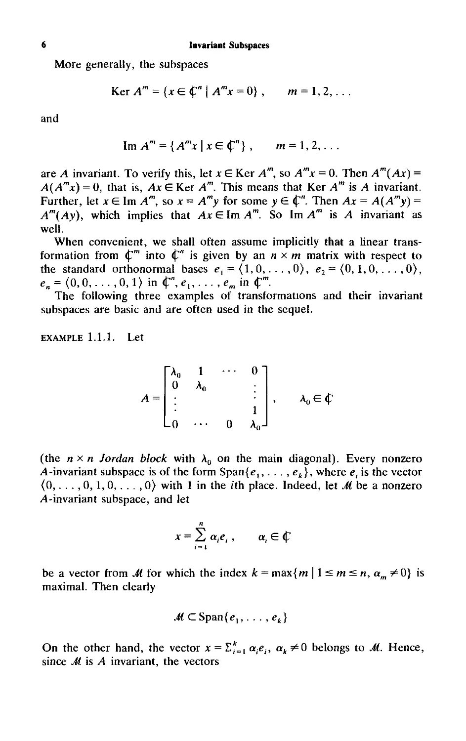
example 1.1.1. Let
L0
A0J
(the nx/i Jordan block with A0 on the main diagonal). Every nonzero
A -invariant subspace is of the form Span{ex,. . ., ek), where et is the vector
(0,. . . , 0,1, 0,. . . , 0} with 1 in the tth place. Indeed, let M be a nonzero
/1-invariant subspace, and let
n
x = Zj aiei , «, £ <p
be a vector from M for which the index k = maxjm | 1 < m < n, am ¥= 0} is
maximal. Then clearly
M C Span{e,, . . . , ek)
On the other hand, the vector x = E,=l a,e,, ak ¥=0 belongs to M. Hence,
since M is A invariant, the vectors

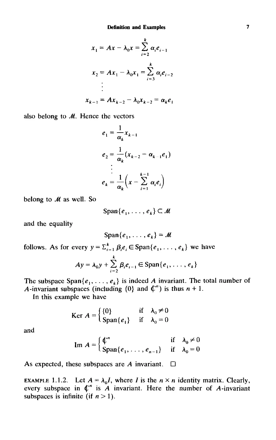
Definition and Examples
k
jc, = Ax - \0x = Zj otiei_l
1 = 2
k
x2 = Axl - A0x, = 2j <*,<?,_
z = 3
Xk_1 — Axk_2 "■oxk-2 akei
also belong to M. Hence the vectors
1
e, = —xL
e2= — (Xk-2~ak -i<?i)
belong to J< as well. So
Span{e,,. . . ,ek} CM
and the equality
Span{e,,. . . ,ek) ~ M
follows. As for every y — £*_, ^iei £ Span{e,,. . . , ek) we have
Ay = Ky + ^ A-e.-^Spanf*?,,. ..,«*}
i = 2
The subspace Span{e,,. . . , ek) is indeed A invariant. The total number of
/1-invariant subspaces (including (0} and <p") is thus n + 1.
In this example we have
KerA
({0} if An*0
lSpan{e,} if Ao = 0
and
f <t" if An * 0
lmA = \Z t x -t » n
I Span{<?,,. . .,<?„_,} if Ao = 0
As expected, these subspaces are /I invariant. □
example 1.1.2. Let A = A0/, where / is the n x n identity matrix. Clearly,
every subspace in <p" is A invariant. Here the number of /1-invariant
subspaces is infinite (if n > 1).

8
Invariant Subspaces
Note that the set ln\(A) of all yt-invariant subspaces is uncountably
infinite. Indeed, for linearly independent vectors x, y G <p" the one-
dimensional subspaces Span{x + ay}, a G i|J are all different and belong to
Inv(^4). So they form an uncountable set of /1-invariant subspaces.
Conversely, if every one-dimensional subspace of <p" is A invariant for a
linear transformation A, then A = A0/ for some A0. Indeed, for every x ¥=0
the subspace Span{x} is A invariant, so Ax = \(x)x, where X(x) is a
complex number that may, a priori, depend on x. Now if A(x,)# A(x2)
for linearly independent vectors xx and x2, then Span{x, + x2) is not A
invariant, because
A{xx + x2) = \(xl)xl + A(A:2)A:2^'Span{x:1 + x2}
Hence we must have A0 = A(x) is independent of x ¥= 0, so actually
A = A0/. D
Later (see Proposition 2.5.4) we shall see that the set of all ^4-invariant
subspaces of on n x n complex matrix A is never countably infinite; it is
either finite or uncountably infinite.
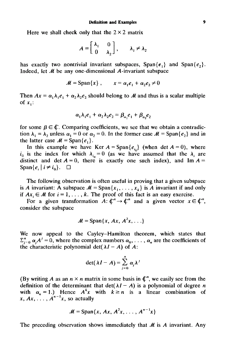
example 1.1.3. Let
A =
'A,
L0
0
A,
(«>2)
where the complex numbers A,, . . . , A„ are distinct. For any indices 1 ^
j, < • • • < ik s n the subspace Span{e, ,. . . , et } is A invariant. Indeed, for
we have
Ax = 2 a A e G Span{<?, ,. . . , <?, }
;=1 ' '
It turns out that these are all the invariant subspaces for A. The proof of this
fact for a general n is given later in a more general framework. So the total
number of /1-invariant subspaces is
.?.(;)-*■

Definition and Examples
9
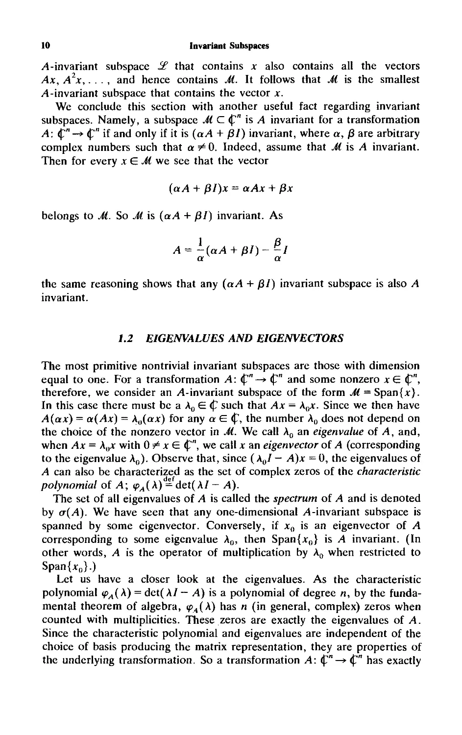
Here we shall check only that the 2x2 matrix
A,^A2
has exactly two nontrivial invariant subspaces, Span{e,} and Span{e2}.
Indeed, let M be any one-dimensional .^-invariant subspace
J£ = Span{;c}, x = atet + a2e2 ^0
Then Ax = alXlel + a2\2e2 should belong to M and thus is a scalar multiple
of *,:
alklel+ a2k2e2 = ^e^ /3ae2
for some /3 G <p. Comparing coefficients, we see that we obtain a
contradiction A, = A2 unless a, = 0 or a2 = 0. In the former case M = Span{e2} and in
the latter case M = Span{e,}.
In this example we have Ker A = Span{^ } (when det/l=0), where
L is the index for which A, = 0 (as we have assumed that the A; are
distinct and det A - 0, there is exactly one such index), and Im A =
Span{e, | i^i0}. □
The following observation is often useful in proving that a given subspace
is A invariant: A subspace M — Span{*,,. . . , xk} is A invariant if and only
if AXj €E M for i = 1,. . . , k. The proof of this fact is an easy exercise.
For a given transformation j4:<p"-^<p" and a given vector *G<p",
consider the subspace
M = Span{*, Ax, A2x,. . .}
We now appeal to the Cayley-Hamilton theorem, which states that
E"=0 afA' = 0, where the complex numbers a(),. . . , a„ are the coefficients of
the characteristic polynomial det(A/ - A) of A:
n
det(A/-,4) = X ajk'
(By writing A as an n x n matrix in some basis in <p", we easily see from the
definition of the determinant that det(A/- A) is a polynomial of degree n
with an = \.) Hence Akx with k^n is a linear combination of
x, Ax,. . . , A"~lx, so actually
M = Span{*, Ax, A2x,. . . , A"~lx}
The preceding observation shows immediately that M is A invariant. Any
-r
Lo
A,.

10
Invariant Subspaces
/1-invariant subspace !£ that contains x also contains all the vectors
Ax, A2x,. . . , and hence contains M. It follows that M is the smallest
/1-invariant subspace that contains the vector x.
We conclude this section with another useful fact regarding invariant
subspaces. Namely, a subspace M C <p" is A invariant for a transformation
A: <p"-» <p" if and only if it is (aA + /?/) invariant, where a, j8 are arbitrary
complex numbers such that a ¥= 0. Indeed, assume that M is A invariant.
Then for every x £ M we see that the vector
(a A + pi)x = aAx + fix
belongs to M. So M is (a/1 + /3/) invariant. As
,4= -(aA + pi)--I
a a
the same reasoning shows that any (aA + j8/) invariant subspace is also A
invariant.
1.2 EIGENVALUES AND EIGENVECTORS
The most primitive nontrivial invariant subspaces are those with dimension
equal to one. For a transformation v4: <p" —>■ <p" and some nonzero *£ <p",
therefore, we consider an .^-invariant subspace of the form M = Span{;c}.
In this case there must be a A0 £ <p such that Ax — A0;c. Since we then have
A(ax) = at(Ax) = \u(ax) for any a £ <p, the number A0 does not depend on
the choice of the nonzero vector in M. We call A0 an eigenvalue of A, and,
when Ax = A0* with 0 ¥= x £ <p", we call x an eigenvector of A (corresponding
to the eigenvalue A0). Observe that, since (A0/ - A)x = 0, the eigenvalues of
A can also be characterized as the set of comnlex zeros of the characteristic
def
polynomial of A; (pA( A) = det( A/ - A).
The set of all eigenvalues of A is called the spectrum of A and is denoted
by a(A). We have seen that any one-dimensional >4-invariant subspace is
spanned by some eigenvector. Conversely, if x0 is an eigenvector of A
corresponding to some eigenvalue A„, then Span{*0} is A invariant. (In
other words, A is the operator of multiplication by A0 when restricted to
Span{*0}.)
Let us have a closer look at the eigenvalues. As the characteristic
polynomial <pA( A) = det( A/ - A) is a polynomial of degree n, by the
fundamental theorem of algebra, <p4(A) has n (in general, complex) zeros when
counted with multiplicities. These zeros are exactly the eigenvalues of A.
Since the characteristic polynomial and eigenvalues are independent of the
choice of basis producing the matrix representation, they are properties of
the underlying transformation. So a transformation A: <p"—> <p" has exactly

Eigenvalues and Eigenvectors
11
n eigenvalues when counted with multiplicities, and, in any event, the
number of distinct eigenvalues of A does not exceed n. Note that this is a
property of transformations over the field of complex numbers (or, more
generally, over an algebraically closed field). As we shall see later, a
transformation from iff" into Jf?" does not always have (real) eigenvalues.
Since at least one eigenvector corresponds to any eigenvalue A0 of A it
follows that every linear transformation v4: <p" —>■ <p" has at least one one-
dimensional invariant subspace. Example 1.1.1 shows that in certain cases a
linear transformation has exactly one one-dimensional invariant subspace.
We pass now to the description of two-dimensional >4-invariant subspaces
in terms of eigenvalues and eigenvectors. So assume that M is a two-
dimensional >4-invariant subspace. Then, in a natural way, A determines a
transformation from M into M. We have seen above that for every
transformation in a (complex) finite-dimensional vector space (which can be
identified with <pm for some m) there is an eigenvalue and a corresponding
eigenvector. So there exists an x0 €E Jt\{0} and a complex number A0 such
that A*,, = A0a:0. Now let xx be a vector in M for which {x0, xx) is a linearly
independent set; in other words, M = Span{*0, *,}. Since M is A invariant it
follows that
Axx = nQx0 + nixl
for some complex numbers /j^ and /u.,. If fig — 0, then x x is an eigenvector of
A corresponding to the eigenvalue /i,l. If fi,0 ¥ 0 and /n, ^ A0, then the vector
y = ~fJiltx0 + (A0 - fJil)xl is an eigenvector of A corresponding to fj,l for
which {x0, y) is a linearly independent set. Indeed
Ay = -/V**„ + (A0 - /u.,)Ar, = -^qXo + (A0 - fi{)(Wo + f^ixi)
= (A0 - M,V,*i - nlfM0x0 = nty
Finally, if /t0^0 and /n, = A0, then x0 is the only eigenvector (up to
multiplication by a nonzero complex number) of A in M. To check this,
assume that a0xa + a,*,, ax ¥=0, is an eigenvector of A corresponding to an
eigenvalue v0. Then
A(aox0 + <*,*,)= v0a0x0 + v0aixi (1.2.1)
But the left-hand side of this equality is
a0Ax0 + alAxl = a0X0x0 + a{(fi.QxQ + XqX^
and comparing this with equality (2.1), we obtain
Kai = "o«I .
«0A0+«lMo= "o"o

12
Invariant Subspaces
which (with a, ^0) implies A0 = v0 and a1fio = 0, a contradiction with the
assumption /n0 # 0. However, note that the vectors z = (l//i,0)xl and x0 form
a linearly independent set and z has the property that Az - A0z = x0. Such a
vector z will be called a generalized eigenvector of A corresponding to the
eigenvector x0.
In conclusion, the two-dimensional invariant subspace M is spanned by
two eigenvectors if and only if either p^ - 0 or p^ ¥=Q and /a, # A0. If p0 # 0
and px = A(), then M is spanned by an eigenvector and a corresponding
generalized eigenvector.
A study of invariant subspaces of dimension greater than 2 along these
lines becomes tedious. Nevertheless, it can be done and leads to the
well-known Jordan normal form of a matrix (or transformation) (see
Chapter 2).
Using eigenvectors, one can generally produce numerous invariant sub-
spaces, as demonstrated by the following proposition.
Proposition 1.2.1
Let X{,. . . , Xk be eigenvalues of A (not necessarily distinct), and let x, be an
eigenvector of A corresponding to A,, i = 1,. . . , k. Then Span{jr,,. . . , xk}
is an A-invariant subspace.
Proof. For any * = £,„, aixi £ Span{x,, . . . , xk}, where a, G <p, we
have
k k
Ax = Zj atAxt — 2j at X,xi
so indeed Span!*!,. . . , xk} is A invariant. □
For some transformations all invariant subspaces are spanned by
eigenvectors as in Proposition 1.2.1, and for some transformations not all
invariant subspaces are of this form. Indeed, in Example 1.1.1 only one of
the n nonzero invariant subspaces is spanned by eigenvectors. On the other
hand, in Example 1.1.2 every nonzero vector is an eigenvector
corresponding to A0, so obviously every /1-invariant subspace is spanned by
eigenvectors.
1.3 JORDAN CHAINS
We have seen in the description of two-dimensional invariant subspaces that
eigenvectors alone are not always sufficient for description of all invariant
subspaces. This fact necessitates consideration of generalized eigenvectors as
well. Let us make a general definition that will include this notion. Let A0 be
an eigenvalue of a linear transformation A: <p" -* <p". A chain of vectors

Jordan Chains
13
Xi\ * X |
, xk is called a Jordan chain of A corresponding to A0 if x0 ¥= 0 and
the following relations hold:
AxQ a0x0
Ax^ \0x{ — x0
(1.3.1)
Axt
*0Xk Xk-\
The first equation (together with x0 ^ 0) means that x0 is an eigenvector of
A corresponding to A0. The vectors x{,...,xk are called generalized
eigenvectors of A corresponding to the eigenvalue A0 and the eigenvector xQ.
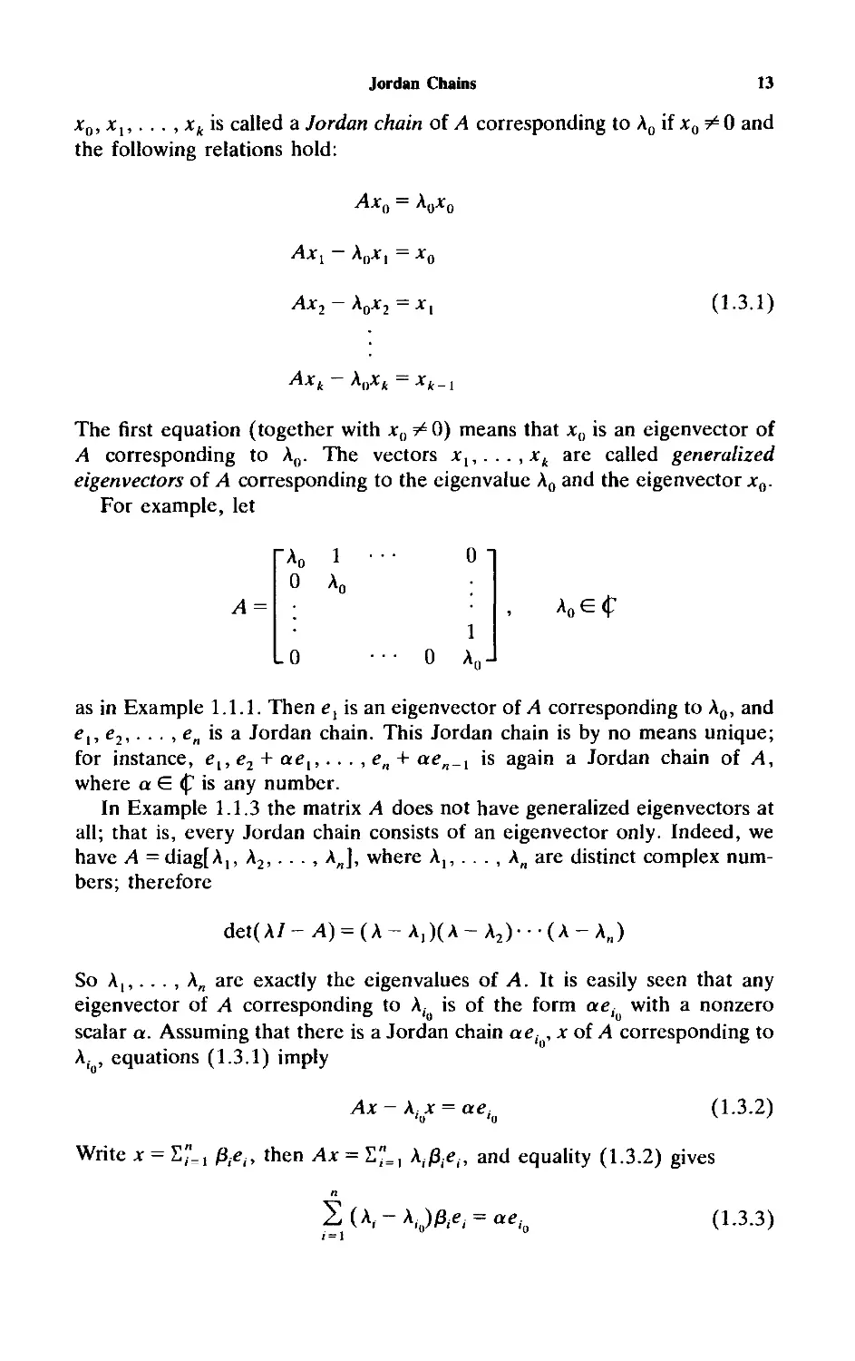
For example, let
A =
L0
0
0 A0J
A0e<p
as in Example 1.1.1. Then e, is an eigenvector of A corresponding to A0, and
ex, e2,. . . , en is a Jordan chain. This Jordan chain is by no means unique;
for instance, ev, e2 + ae{,. . . , en + aen_l is again a Jordan chain of A,
where a E <p is any number.
In Example 1.1.3 the matrix A does not have generalized eigenvectors at
all; that is, every Jordan chain consists of an eigenvector only. Indeed, we
have A = diag[A,, A2,. . . , Aj, where A,, . . . , An are distinct complex
numbers; therefore
det(A/-^) = (A-A,)(A-A2)--(A-A„)
So A,,. . . , A„ are exactly the eigenvalues of A. It is easily seen that any
eigenvector of A corresponding to A, is of the form ae{ with a nonzero
scalar a. Assuming that there is a Jordan chain aes , x of A corresponding to
A,., equations (1.3.1) imply
Ax — A; x = ae, (1.3.2)
Write x = E,"=1 0,.*?,., then Ax = E"=1 A,j8,<?., and equality (1.3.2) gives
n
SU-A.^A^a^ (1.3.3)

14
Invariant Snbspaces
As A, =£ Xt for i -^ i0, we find immediately that /3, = 0 for i -^ j0. But then the
left-hand side of equation (1.3.3) is zero, a contradiction with a^O. So
there are no generalized eigenvectors for the transformation A.
Jordan chains allow us to construct more invariant subspaces.
Proposition 1.3.1
Let x0,. . . , xk be a Jordan chain of a transformation A. Then the subspace
M — Span{*0, . . . , xk) is A invariant.
Proof. We have
AXq = ^o-^o ^ ^
where A0 is the eigenvalue of A to which x0,. . . ,xk corresponds; and for
t= 1 A:
Axi = A0a:( tXj^el
Hence the A in variance of M follows. D
The following proposition shows how the Jordan chains behave under a
linear change in the matrix A.
Proposition 1.3.2
Let a ¥= 0 and p be complex numbers. A chain of vectors xu, xt,. . . ,xk is a
Jordan chain of A corresponding to the eigenvalue A0 if and only if the vectors
xo> ~*i> • • • > *•** (1.3.4)
a a
form a Jordan chain of a A 4- pi corresponding to the eigenvalue aX0 + p of
aA + pi.
Proof. Assume that x0,. . . ,xk\s a Jordan chain of A corresponding to
A0, that is, equalities (1.3.1) hold. Then we have
(a A + pi)x0 = aAx0 + 0xo = aXQx0 + 0xo = (aX0 + p)xQ
(aA + pl)—xl - (aAit + j8)—*, = Axx - A,,*, = xQ
and in general for i = 1, . . . , k
1 11 1
{aA + pi)— x, - (oAo + P)— x, = -7=7 (Ar, - A^,) = -7=7*,.,
a a a a

Jordan Chains
IS
So by definition the vectors in equality (1.3.4) form a Jordan chain of
a.A + pi corresponding to aA0 + /3.
Conversely, assume that equality (1.3.4) is a Jordan chain of aA + j8/
corresponding to a\0 + $. As
A= -(/1 + /3/)--/
a a
the first part of the proof shows that the vectors
x0, «(-*,) = *„..., a"y~jxkj = xk
form a Jordan chain of A corresponding to the eigenvalue (l/a)(«A0 + /3) -
(0/a) = Ao. D
Two corollaries from Proposition 1.3.2 will be especially useful in the
sequel.
Corollary 1.3.3
(a) The vector x0 is an eigenvector of A corresponding to A0 if and only if x0
is an eigenvector of a A + j8/ (here a t^O, j8 are complex numbers)
corresponding to a\0 + j8; (b) the vectors x0,. . . ,xk form a Jordan chain of A
corresponding to A0 if and only if these vectors constitute a Jordan chain of
A + /3/ corresponding to A0 + /3 for any complex number j8.
In many instances Corollary 1.3.3 allows us to reduce the consideration of
eigenvalues and Jordan chains to cases when the eigenvalue is zero. Our first
example of this device appears in the proof of the following proposition.
Proposition 1.3.4
The vectors in a Jordan chain x(),. . . , xk of A are linearly independent.
Proof. Assume the contrary, and let xp be the first generalized
eigenvector in the Jordan chain that is a linear combination of the preceding
vectors:
p->
x„ = Z oLiXi; a, e. <p
We can assume that the eigenvalue A0 of A to which the Jordan chain
x0,. . . ,xk corresponds is zero. (Otherwise, in view of Corollary 1.3.36, we
consider A - A0/ in place of A.) So we have Axp = xp_x. On the other hand,
we have

16
Invariant Subspaces
Ax = 2 (XiAXt = 2, a,*,-.
Comparing both expressions, we see that xp_y is a linear combination of the
vectors x0,. . . , x 2. This contradicts the choice of xp as the first vector in
the Jordan chain that is a linear combination of the preceding vectors. □
1.4 INVARIANT SUBSPACES AND BASIC OPERATIONS
ON LINEAR TRANSFORMATIONS
In this section we first consider questions concerning invariant subspaces of
sums, compositions, and inverses of linear transformations. We shall also
develop the connection between invariant subspaces for a linear
transformation and those of similar and adjoint transformations.
The basic result for the first three algebraic operations is given in the
following proposition.
Proposition 1.4.1
Let A, B: <p"—> <p" be transformations, and let MC$" be a subspace which
is simultaneously A invariant and B invariant. Then M is also invariant for
a A + /3B (with any a, j3 £ (p) and for AB. Further, if A is invertible, then M
is also invariant for A~l.
Proof. For every x £ M we have
(aA + pB)x = a(Ax) + p(Bx) G M
and (AB)x~ A(Bx) G M because Bx &. M.
Assume now that A is invertible, and let x,,..., xp be a basis in M. Then
the vectors y, = Axx,. . . ,yp- Axp are linearly independent (because A is
invertible) and belong to M (because M is A invariant). So y,, . . . , y is also
a basis in M. Now
A'lM = A'1 Spanfy,,. . . , yp} = Span{x,,. . . ,xp} = M U
For any transformation A, we denote by Inv(^4) the set of all A -invariant
subspaces. Then Proposition 1.4.1 means, in short, that
Inv(,4)ninv(B)CInv(a<4 + /3B) (1.4.1)
Inv(/l)ninv(£)Clnv(,4£) (1.4.2)
Inv(^)Clnv(^"') (if A is invertible) (1.4.3)

Basic Operations on Linear Transformations
17
By applying equality (1.4.3) with A replaced by A~\ we get Inv(/4~')C
ln\(A), so actually equality holds in (1.4.3). It is very easy to produce
examples when the equality fails in (1.4.1) or (1.4.2). For instance:
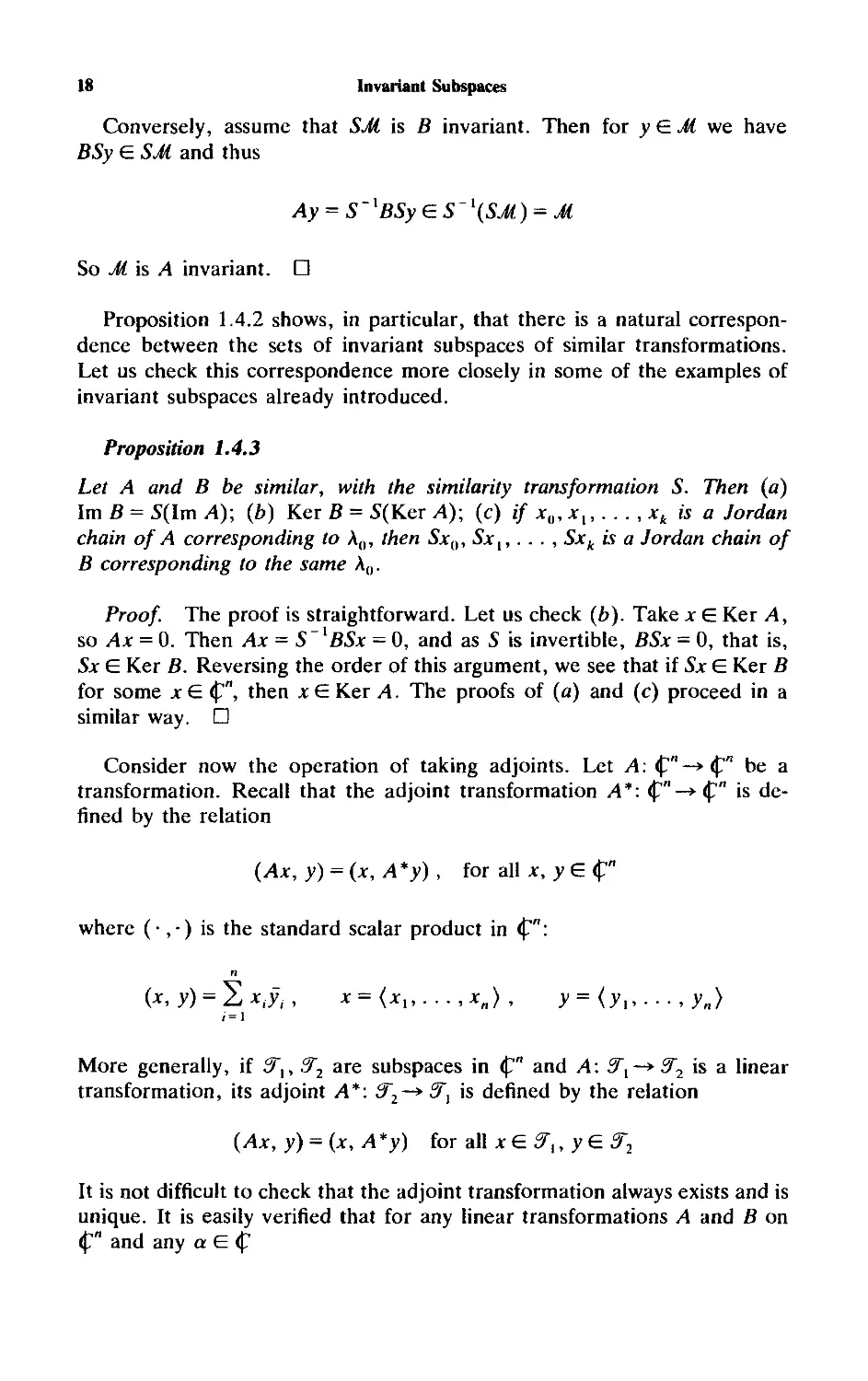
example 1.4.1. Let A: <p"—► <p" be a transformation that is not of the form
y/ for some y G <p (if n>2, such transformations obviously exist). By
Example 1.1.2, not all subspaces in <p" are A invariant. On the other hand,
take B = A and a + /3 =0 in (1.4.1). Then the right-hand side of (1.4.1) is
the zero transformation for which every subspace in <p" is invariant. □
To give an example where the inclusion in (1.4.2) is strict, put
TO 11
^Ho oJ
The following example of strict inclusion in (1.4.2) is also instructive.
example 1.4.2. Let
-ft ;i- -ft :]• ^
An easy analysis (using Example 1.1.1) shows that A and B have no
nontrivial common invariant subspaces. Thus Inv(^4)n Inv(B) = ({0}, <p2}.
On the other hand, ln\(AB) must have an eigenvector that spans a
nontrivial ,4£-invariant subspace. Again, the inclusion (1.4.2) is strict. □
Consider now the notion of similarity. Recall that two transformations A
and B on <p" are called similar if A - S~*BS for some invertible
transformation 5 (called a similarity transformation between A and B). Evidently,
similar transformations have the same characteristic polynomial and,
consequently, the same eigenvalues. The next proposition reveals the close
connection between invariant subspaces of similar transformations.
Proposition 1.4.2
Let transformations A and B be similar, with the similarity transformation
S: A = S~ BS. Then a subspace M C <p" is A invariant if and only if the
subspace
SM = {Sx\xeM}C$"
is B invariant.
Proof. Let M be A invariant, and let x €E SM, so that x = Sy for some
yGM. Then Bx = BSy = SAy, and since Ay G Jl, we find that Bx G SM. So
SM is B invariant.

18
Invariant Subspaces
Conversely, assume that SM is B invariant. Then for yE.M we have
BSy £ SM and thus
Ay = 5" lBSy £ S' l(SM ) = M
So M is A invariant. □
Proposition 1.4.2 shows, in particular, that there is a natural
correspondence between the sets of invariant subspaces of similar transformations.
Let us check this correspondence more closely in some of the examples of
invariant subspaces already introduced.
Proposition 1.4.3
Let A and B be similar, with the similarity transformation S. Then (a)
Im B = 5(Im A); (b) Ker B = S(Ker A); (c) if x0, x{,. . . , xk is a Jordan
chain of A corresponding to A0, then Sxu, 5a:,, ... , Sxk is a Jordan chain of
B corresponding to the same A„.
Proof. The proof is straightforward. Let us check (b). Take x £ Ker A,
so Ax = 0. Then Ax = S~ BSx = 0, and as S is invertible, BSx = 0, that is,
Sx £ Ker B. Reversing the order of this argument, we see that if Sx £ Ker B
for some x £ <p", then x £ Ker A. The proofs of (a) and (c) proceed in a
similar way. □
Consider now the operation of taking adjoints. Let A: <p"-*<p" be a
transformation. Recall that the adjoint transformation A*: <p"-*<p" is
defined by the relation
(Ax, y) = (x, A*y) , for all x, y £ <p"
where (•, •) is the standard scalar product in <p":
n
(x, y) = YjXiyl, x = {xx,...,xn), y=(yl,.--,y„)
More generally, if STX, 3~2 are subspaces in <p" and A: 9~x-* 9~2 is a linear
transformation, its adjoint ^4*: 9~z-* 5", is defined by the relation
(Ax,y) = (x,A*y) for all x £ ST{, y £ 9~2
It is not difficult to check that the adjoint transformation always exists and is
unique. It is easily verified that for any linear transformations A and B on
<p" and any a £ <p

Basic Operations on Linear Transformations 19
(A +B)*= A*+B* , (aA)* = aA*
(AB)*=B*A*, (A*)* = A
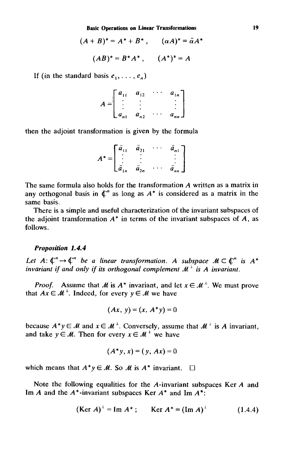
If (in the standard basis ex,...,en)
L«nl «n2
then the adjoint transformation is given by the formula
a,, a,
The same formula also holds for the transformation A written as a matrix in
any orthogonal basis in <p" as long as A* is considered as a matrix in the
same basis.
There is a simple and useful characterization of the invariant subspaces of
the adjoint transformation A* in terms of the invariant subspaces of A, as
follows.
Proposition 1.4.4
Let ^4:<p"-*<p" be a linear transformation. A subspace M C <p" is A*
invariant if and only if its orthogonal complement M1 is A invariant.
Proof. Assume that Mis A* invariant, and let x G M ±. We must prove
that Ax E. Jl1. Indeed, for every yEMwe have
(Ax,y) = (x, A*y) = 0
because A*yEM and xGi1. Conversely, assume that Mx is A invariant,
and take y £ M. Then for every x £ M L we have
(A*y,x) = (y,Ax) = 0
which means that A*y E.M. So M is A* invariant. □
Note the following equalities for the /1-invariant subspaces Ker A and
Im A and the A*-invariant subspaces Ker A* and Im A*:
(Ker A)1 = Im A* ; Ker A* = (Im A)A
(1.4.4)

20
Invariant Snbspaces
Indeed, let x=A*y and zGKer/1. Then (x, z) = {A*y, z) - {z, A*y) =
{Az, y) = 0; so x G (Ker A)^l Hence we have proved that
\mA*C{KcrA)1 (1.4.5)
On the other hand, let x be orthogonal to 1m A*. Then for every y G <p", we
have {Ax, y) = {x, A*y) = 0; so Ax J_ <p", and thus Ax = 0, or x G Ker ^4. So
(Im A*)1 CKer A. Taking orthogonal complements, we obtain Im/1*D
(Ker j4)\ Combining with (1.4.5), we obtain the first equality in (1.4.4).
The second equality follows from the first one applied to A* instead of A
[recall that (A*)* = A].
Later, we shall also need the following property:
lmA = lm{AA*)
Here, the inclusion D is clear. For the opposite inclusion, let x&lmA.
Then x = Ay for some y. If z is the projection of y onto Ker A, then
y-z6 (Ker A)1 and also x = A{y - z). Then (1.4.1) implies that y — z G
Im A* and so x G lm{AA*), as required.
A transformation ^4: <p" —» <p" is called self-adjoint ii A = A*. It is easily
seen that A is self-adjoint if and only if it is represented by a hermitian
matrix in some orthogonal basis (recall that a matrix [«,-*]"*_! is called
hermitian if ajk = dkj, j, k = 1, . . . , n). For this important class of
transformations we have the following corollary of Proposition 1.4.4.
Corollary 1.4.5
If A is self-adjoint, then Jt± is A invariant if and only if M is A invariant.
1.5 INVARIANT SUBSPACES AND PROJECTORS
A linear transformation defined by P: <p" -* <p" is called a projector if
P2 = P. The important feature of projectors is that there exists a one-to-one
correspondence between the set of all projectors and the set of all pairs of
complementary subspaces in <p". This correspondence is described in
Theorem 1.5.1.
Recall first that iiM,Z£ are subspaces of <p", then M+£={zE$"\z =
x + y, xEM,yEJ£}. This sum is said to be direct if M D Z£ = {0}, in which
case we write M 4- if for the sum. The subspaces M, if are complementary
{are direct complements of each other) if M D if = {0} and M + if = <p".
Nontrivial subspaces M, if are orthogonal if for each x G M and y G if we
have (x, y) = 0 and they are orthogonal complements if, in addition, they are
complementary. In this case, we write M = if1, if = M1.

Invariant Subspaces and Projectors
21
Theorem 1.5.1
Let P be a projector. Then (Im P, Ker P) is a pair of complementary
subspaces in <p". Conversely, for every pair (if, ,if2) °f complementary
subspaces in <p", there exists a unique projector P such that Im P = if,,
KerP = if2.
Proof. Let x G <p". Then x = (x - Px) + Px. Clearly, Px G Im P and
x - Px G Ker P (because P2 = P). So Im P + Ker P = <p". Further, if x G
Im P n Ker P, then a: = Py for some y G <£" and Px = 0. So
X = Py = P2y = P(Py) = Px = 0
and Im P n Ker P = {0}. Hence Im P and Ker P are indeed complementary
subspaces.
Conversely, let if, and if2 be a pair of complementary subspaces. Let P be
the unique linear transformation in <p" such that Px = x for x G if, and
Px = 0 for x G if2. Then clearly P2 = P, if , C Im P, and if, C Ker P. But we
already know from the first part of the proof that Im P + Ker P = <p". By
dimensional considerations we have, consequently, if, = Im P and if2 =
Ker P. So P is a projector with the desired properties. The uniqueness of P
follows from the property that Px = x for every xGImP (which, in turn, is a
consequence of the equality P2 = P). □
We say that P is the projector on if, along if, if Im P = if,, Ker P = if2.
A projector P is called orthogonal if KerP = (ImP)1. Thus the
corresponding complementary subspaces are mutually orthogonal. Orthogonal
projectors are particularly important and can be characterized as follows.
Proposition 1.5.2
A projector P is orthogonal if and only if P is self-adjoint, that is, P* = P.
Proof. Suppose that P* = P, and let x G Im P, y G Ker P. Then (x, y) =
(Px, y) = (x, Py) = (x, 0) = 0, that is, Ker P is orthogonal to Im P. Since by
Theorem 1.5.1 Ker P and Im P are complementary, it follows that in fact
Ker P = (Im P)\
Conversely, let Ker P = (Im P)1. To prove that P* = P, we have to check
the equality
(Px, y) = (x, Py) for all x, yG<p" (1.5.1)
Because of the sesquilinearity of the function (Px, y) in the arguments
x, y G <p", and in view of Theorem 1.5.1, it is sufficient to prove equation
(1.5.1) for the following four cases: (a) x, yGImP; (b) xGKerP, y G
Im P; (c) x G Im P, y G Ker P; (d) x, y G Ker P. In case (d), equality (1.5.1)

22
Invariant Subspaces
is trivial because both sides are 0. In case (a) we have
(Px, y) = {Px, Py) = (x, Py)
and (1.5.1) follows. In case (b), the left-hand side of equation (1.5.1) is
zero (since x £ Ker P) and the right-hand side is also zero in view of
the orthogonality Ker P = (Im P)\ In the same way, one checks (1.5.1) in
case (c).
So (1.5.1) holds, and P* = P. □
Note that if P is a projector, so is / - P. Indeed, (/ - P)2 =
/-2P+P2 = /-2P+P=/-P. Moreover, KerP=Im(/-P) and
Im P = Ker(/ - P). It is natural to call the projectors P and I - P
complementary projectors.
We now give useful representations of a projector with respect to a
decomposition of <p" into a sum of two complementary subspaces. Let
T: <p"-* <p" be a transformation and let if,, S£2 be a pair of complementary
subspaces in <p". Denote m, = dim if, (i = 1,2); then m, + m2 = n. The
transformation T may be written as a 2 x 2 block matrix with respect to the
decomposition if, 4- if2 = <p":
T=\i" I12} (1.5.2)
L1!l * 22 J
Here T/; (i, j — 1, 2) is an m, x my matrix that represents in some basis the
transformation P,T|^: S£f-* if,., where P, is the projector on if, along if3_,
(so P, + P2 = I). '
Suppose now that T= P is a projector on if, = Im P. Then representation
(1.5.2) takes the form
for some matrix A". In general, X ¥= 0. One can easily check that A" = 0 if and
only if if, = Ker P. Analogously, if if, = Ker P, then (1.5.2) takes the form
P=[o ]] (1.5-4)
and Y-0 if and only if if2 = Im P. By the way, the direct multiplication
P■ P, where P is given by (1.5.3) or (1.5.4), shows that P is indeed a
projector: P2 = P.
Consider now an invariant subspace M for a transformation A: <P"-» <P".
For any projector P with Im P = M we obtain
P/1P = AP
(1.5.5)

Invariant Subspaces and Projectors
23
Indeed, if x &. Ker P, we obviously have
PAPx = APx
If x e Im P = Jt, we see that Ax belongs to Jt as well and thus
PAPx = PAx = Ax = APx
once more. Since <p" = Ker P -(- Im P, (1.5.5) follows. Conversely, if P is a
projector for which (1.5.5) holds, then for every x E. Im P we have PAx =
Ax; in other words, Im P is A invariant. So a subspace Jt is A invariant if
and only if it is the image of a projector P for which (1.5.5) holds.
Let Jt be an /i-invariant subspace and let P be a projector on Jt [so that
(1.5.5) holds]. Denoting by Jt' the kernel of P, represent A as a 2 x 2 block
matrix
21 ^22"
with respect to the direct sum decomposition <p" = Jt + Jt'. Here A,,
is a transformation PAP\M: M-* Jt, AX2 is a linear transformation
P4(/-P)L.:.ir-»,^,
/121 = (/-P)/IP|^:^-*^'
A22 = (I-P)A(I-P)\M.:Jt'^Jt'
and all these transformations are written as matrices with respect to some
chosen bases in M and Jt'. As Jt is A invariant, equation (1.5.5) implies
that (/- P)AP = 0, that is, A2l =0. Hence
ft" a':) <'-5-6>
Using this representation of the matrix A, we can deduce some important
connections between the restriction A\M = Al{ and the matrix A itself.
Proposition 1.5.3
Let x0,. . . , xk be a Jordan chain of A\M corresponding to the eigenvalue A0
of A\M. Then x0,. . . , xk is also a Jordan chain of A corresponding to A0. In
particular, all eigenvalues of A\M are also eigenvalues of A.
Proof. We have x0 ¥= 0; x, £ Jt for i = 0,. . . , k, and
^M-r*. ~ Kxi = xi-\ > i = I,. . . , k

24
Invariant Snbspaces
As A\M = PAP\M = AP\M, these relations can be rewritten as
APx0 = A0x0 , APXj — A0jt(- = xj_l , i — \,...,k
But Px^Xj, i = 0,1,. . . , k, and we obtain the relations defining
xQ,. . . , xk as a Jordan chain of /I corresponding to A0. □
The last statement in Proposition 1.5.3 can also be proved in the
following way. Suppose that A0e a(An), that is, Ker(A07- Au) ^ {0}.
The representation (1.5.6) implies that any nonzero vector from
Ker(A0/-^H) belongs to Ker(A0/ - A). Thus Ker(A0/- A) * {0}, and
A0 £ <t(A).
In fact, a more general result holds.
Proposition 1.5.4
Let M be an A-invariant subspace with a direct complement M' in <p", and let
be the representation of A with respect to the decomposition <p" = M + M'.
Then
<r(A) = o-(An)Uo-(A22)
Proof. This follows immediately from the fact that det(A/-^4) =
det(A/- ,4,,) det(A7- A22). □
As an example in which projectors and the subspaces Im A and Ker A of
a transformation A all play important roles, let us describe here a
construction of generalized inverses for A.
Given a transformation A: <p"-» <pm, the transformation X: <pm-> <p" is
called a generalized inverse of A if the following holds: for any b £ Im A the
linear system Ax = b has a solution x = Xb, and for any bElm X the linear
system Xx - b has a solution x - Ab. So this is a natural generalization of
the notion of the inverse transformation.
Observe that A" is a generalized inverse of A if and only if AX A = A and
XAX = X. Indeed, let Ibea generalized inverse of A. Then AXb = b for
every b G Im A, that is, for every b of the form b = Ay. So AX Ay = Ay for
all y e <p", and AX A = A. Similarly, one checks that XAX = X. Conversely,
if AX A = A, then for every b of the form b = Ay the vector Xb = XAy is
obviously a solution of the linear equation Ax = b.
The descrition of all generalized inverses of A, which implies, in
particular, that a generalized inverse of A always exists, is given by the following
theorem.

Angular Transformations and Matrix Qnadratic Equations
25
Theorem 1.5.5
Let A: $"-* <£"" be a transformation, let <p" = Ker A + N, <pm = Im A + R
for some subspaces N and R, and let P be the projector on Im A along R, Q
the projector on N along Ker A. Then (a) the transformation A{ = A\„ is a
one-to-one transformation of N onto Im A; (b) the transformation A defined
on <pm by A y = A ~ (Py), for all y €E <pm, is a generalized inverse of A for which
A A = P and AA = Q; (c) all generalized inverses of A are determined as
N, R range over all complementary subspaces for Ker A, Im A, respectively.
The proof of Theorem 1.5.5 is straightforward.
It is easily seen that, in the hypothesis of the theorem, complementary
subspaces R, N are simply the range and null-space of the generalized
inverse that they determine.
Corollary 1.5.6
In the statement of Theorem 1.5.5, we have
Im A' = N and Ker A1 = R
Ker A + Im A1 = <p" and Im A + Ker A1 = <pm
1.6 ANGULAR TRANSFORMATIONS AND
MATRIX QUADRATIC EQUATIONS
In this section we study angular transformations and their connections with
matrix quadratic equations and invariant subspaces. The correspondence
between the invariant subspaces of similar transformations described in
Proposition 1.4.2 is useful here.
This discussion can be seen as the first step in the examination of
solutions of matrix quadratic equations. In this program, we first need the
notion of a subspace "angular with respect to a projector." In Chapter 13
we discuss the topological properties of such subspaces in preparation for
the applications to quadratic equations to be made in Chapters 17 and 20.
Let 7r be a projector defined on <p". Transformations acting on <p" in this
section are written in 2 x 2 block matrix form with respect to the
decomposition <p" = Ker 7r 4- Im it.
A subspace Jf of <p" is said to be angular with respect to it if Jf + Ker it =
<p". That is, if and only if ^V and Ker it are complementary subspaces of <p".
Thus Im it is angular with respect to it, but more generally, if R is any
transformation from Im -n into Ker it, then the subspace
•XR ='{x \x = Ry + y, y E Im n} (1.6.1)

26 Invariant Subspaces
is angular with respect to it. To see this, observe first that MR is indeed a
subspace; that is, if *,, x2 E JfR, then for some yl, y2 G Im tt
xl+x2 = (Ryl+yl) + (Ry2 + y2) = R(yi+ y2) + (y, 4- y2) G JfR
and if a G <p
ax, = a(Ryt + y,) = R(ay) + (ay) G JfR
Then <p" = NR + Ker it because, for any y G <p", if y, = iry, y2 = (/ - 7r)y,
then
y = yi+y2 = (Ryl + yi) + (y2-Ryi)
and /?y, + y, G jVr, y2 - Ryt G Ker ir.
Finally, if z G jVr D Ker 7r, then z = Ry + y, where y G Im tt and also
ttz - 0. Thus
0 = TrRy + iry = irRy + y
Since R is into Ker rr, nR — 0 and it follows that y = 0. Hence z = 0 and
<p" = jVk 4- Ker tt.
The angular subspaces generated in this way are, in fact, all possible
angular subspaces.
Proposition 1.6.1
Let N be a subspace of <p". Then N is angular with respect to it if and only if
J{-J{R for some transformation R: Im tt + Ker tt that is uniquely determined
by Jf.
Proof If ^V = NR, we have already checked that N is angular. To prove
the converse, assume that Jf is angular with respect to tt, and let Q be the
projector of <p" onto Jf along Ker tt. Put
Rx = (Q- tt)x , xGlnur (1.6.2)
Then Jf = JfR. Indeed
tt(Rx) = (irQ - ir)x = (it - tt)x = 0
that is, R: Im 7r-*Ker it, and we have to show that Jf- JfR.
If x G NR, then for some y = 7ry,
x = Ry + y = (Q - 7r)y + Try = Qy G Jf

Angular Transformations and Matrix Quadratic Equations
27
Thus NR C Jf. Conversely, if yEJf then
y = Qy = Qny = (R + ir)iry = R(^y) + (^y) e •#«
thus N = Nr, as required.
To prove the uniqueness of R, we show that any defining transformation
R in (1.6.1) must have the form (1.6.2). Thus let Nbe angular with respect
to 7r, and let R: Im 7r-*Ker -tt satisfy (1.6.1). Let yGlm7r and x =
Ry + y G jV. Then, since / - Q is onto Ker it along Jf
0 = (I-Q)x = (I-Q)Ry + (I-Q)iry
But QR = 0 and Qtt = 0 so that Ry = (Q - rr)y. □
The transformation /? appearing in the preceding proposition is called the
angular transformation for Jf. Note that R can be defined as the restriction
of a difference of projectors:
R = (Q-*)\tm*
Consider now a transformation T: <p"-»<p". As before, let v. <p"—* <p"
be a projector so that we have <p" = Im tt 4- Ker tt. Then T has a
representation with respect to this decomposition:
T=\ln ln] (1.6.3)
L,ll i 22 J
It is clear that Im it is invariant under T if and only if T21 = 0. Similarly,
Ker 7r is T invariant if and only if Tl2 — 0. More generally, what is the
condition that a subspace Jf that is angular with respect to it be T invariant?
Theorem 1.6.2
Let N be an angular subspace with respect to the projector it. Let T have the
representation (1.6.3) with respect to the decomposition <p" = Im it + Ker it.
Then N is T invariant if and only if the angular transformation R for Jtf
satisfies the matrix quadratic equation.
RTl2R + RTn-T22R-T2l = 0 (1.6.4)
Proof. If /,, I2 are the identity transformations on Im it and Ker ir,
respectively, then since R: Im 7r-*Ker it we can define the transformation

28 Invariant Subspaces
which is written as a 2x2 matrix with respect to the decomposition
<p" = Im 7r + Ker it. The transformation £ is obviously invertible and
Y-r lA
For every xGlmirwe have Ex = x + Rx £ Jf. So £ maps Im it onto Jf and
E~ maps Jf back onto Im it. By Proposition 1.4.2, Jf is T invariant if and
only if Im -tt is E~ TE invariant. Now observe that
£-'Tir_l *11 + ^12^ T\2
1TE = \
I -j
(1.6.5)
RTl2R-RTu + T22R+T2l T22- Tl2R
so Im 7r is £ TE invariant if and only if (1.6.4) holds. □
Another important observation follows from the similarity (1.6.5).
Corollary 1.6.3
If Jf is T invariant, then
<r(T)=<r(Tn+Tl2R)U<T(T22-Ti2R) (1.6.6)
and
<r(T\J,)=<r(Tu + Tl2R) (1.6.7)
Proof. We have
«r)-.<E-7*)-4r"7,»" T!il"TJ
Now use Proposition 1.5.4 to obtain (1.6.6). Further, a(T\^) =
0-(£1r£|lnij = cr(r11 + r12/?). □
1.7 TRANSFORMATIONS IN FACTOR SPACES
Let ^V C <p" be a subspace. We say that two vectors x, y £ <p" are
comparable modulo Jf if x - y £ Jf, and denote this by x = y (mod ^V). In
particular, x = 0 (mod Jf) if and only if xE.Jf. This relation is easily seen to be
reflexive, symmetrical, and transitive. That is
x = x(mod Jf) for all x £ <p"
x = y(mod Jf) 4> y = x(mod jV)
x = y(modJV) and y = z(modJf)^x = z(modJf)

Transformations in Factor Spaces
29
Thus we have an equivalence relation on <p". It follows that <p" is
decomposed into disjoint classes of vectors with the properties that in each class
the vectors are comparable modulo J{, and in different classes the vectors
are not comparable modulo M. We denote by [x] v the class of vectors that
are comparable modulo /to a given vector x G <p". The set of all such
classes of vectors defined by comparability modulo N is denoted <p"A/V.
Proposition 1.7.1
Let set <p"/jV be a vector space over <p with the following operations of
addition and multiplication by a complex number.
Proof. We have to check first that these definitions do not depend on
the choice of the representatives ^G^]^ and yGfy]^. If xl G [x\x and
y^lyL. then
(*i + yi) - (x + y) = (*, " x) + (y, - y) G Sf
that is, Jt, + y, G [x + y]^. So indeed the class [x + y]^ does not depend on
the choice of x and y. Similarly, one checks that [a*]^ does not depend on
the choice of x in the class [x]x (for fixed a).
It is a straightforward but tedious task to verify that <p7^V satisfies the
following defining properties of a vector space over <p: The sum is
commutative and associative: (a) x + y = y + x, (x + y) + z = x + (y + z) for every
x, y, z G <p7^V; (b) there is a zero element 0€E <p7^V", that is, an element 0
such that x + 0 = x for all x G <p7jV; (c) for every x G <p7jV there is an
additive inverse element y G $"IN, that is, such that x + y =■ 0; (d) for every
a, /3 G <p and j,y£ <p7^V the following equalities hold: a(x + y) = ax + ay,
(a + fj)x = ax + fix, (afi)x ~ a(fix), and Ix = x (here 1 is the complex
number). We leave the verification of all these properties to the reader. □
The vector space (p7^Vis isomorphic to any direct complement Jf' of Jfin
<p". Indeed, let a G <p7^V; then there exists a unique vector y G N' such that
a = [y]^ and in fact, y = Px, where P is the projector on Jf' along ^V and
x is any vector in the class a. This is easily checked. We have y — x =
-(/ — P)x &.N, so y G a. If there were two different vectors y, and y2 from
jV' such that [yx]x = [y2L- = «, then y, = y2 G jV' n jV and y, ^ y2, which
contradicts the choice of •//"' as a direct complement to ^Vin <p". So we have
constructed a map <p: <p"-*^V' defined by <p(a) = y. This map is easily seen
to be a homomorphism of vector spaces; that is
<p(a + b)= <p(a) + (p(b) ; <p(aa) = atp(a)

30
Invariant Subspaces
for every a, b E. <p7^V and every a E. <p. Moreover, if <p(a) = ip(b), then the
vector y = ip{a) = <p{b) belongs to both classes a and b of comparable
vectors modulo M, and thus a = b. So <p is one-to-one. Taking any y&.Jf',
we see that <p([y]v) = y, so <p is onto. Summing up, <p is an isomorphism
between the two vector spaces $"Uf and N'. In particular, dim <p"/^V =
n — dim Jf. Assume now that Jf is A invariant for some transformation
A: <p"^<p". Then the induced transformation A: $"/#-*■$"/# is defined
by i4[jr]jV = [Ar] v for any x E <p". This definition does not depend on the
choice of the vector x in its class [x)x. Indeed, if [xx\x = [x2\x, then
Axl — Ax2 = A(xl — x2) £ Jf
because x{ - x2 G N and Jf is A invariant.
We now present some basic properties of the induced linear
transformation A.
Proposition 1.7.2
If Jf is invariant for both transformations A: <p" -» <p" and B: <p" -» <p", then
(aA + BB) = aA + BB for any a, B G <p
(1.7.1)
(,4B) = ,4B
//, in addition, A is invertible, then
(A^) = (Ayl (1.7.2)
Proof By Proposition 1.4.1, N is invariant for aA + /3B, AB, and ^4 '
(if /I is invertible). For any xE. <p" we have
(a^A+^B)[x\, = [(a A + BB)x]x = a[Ax], + B[Bx]x
= aA[x]x + BB[*].s-
Further, by definition of the induced transformation we have
(AB)[x]x = [ABx]x
and
AB[x\x = A[Bx\, = [ABxls
for every x£.$". Finally, (1.7.2) is a particular case of (1.7.1) (with
B = A~l), taking into account the fact that / = /. □

The Lattice of Invariant Subspaces 31
It may happen that A is not invertible but A is invertible. For instance,
let A: <p" -* <p" be any transformation with the property that <p" = Ker A +
Im A. (There are many transformations with this property; those
represented by a diagonal matrix in some basis for <p", for example.) Put N = Ker A.
Then for every vector x G <p" that is not in Jf we have A [x]y = [At].* ¥= 0.
Thus Ker A = {0} and A is invertible. The following proposition clarifies the
situation.
Proposition 1.7.3
If k0 is an eigenvalue of A and Ker(A - X0I) is not contained in Jf, then A0 is
also an eigenvalue of A. Conversely, every eigenvalue A0 of A is an
eigenvalue of A and Ker(A — A0/) is not contained in M.
The proof is immediate: if Ax = X0x with x^Jf, then j4[*]v = A0[jc]v
with [x]x ¥" 0, and conversely.
/.* THE LATTICE OF INVARIANT SUBSPACES
We start with the notion of a lattice of subspaces in <p". A set 5 of subspaces
in <p" is called a lattice if {0} and <p" belong to 5 and 5 contains the
intersection and sum of any two subspaces belonging to 5. The following are
examples of lattices of subspaces: (a) 5= {{0}, M, M1, <p"}, where M is a
fixed subspace in <p"; (b) 5 = {{0}, Span{e,,. . ., ek) for k = 1, . . . , «}; (c)
5 is the set of all subspaces in <p". For us, the following example of a lattice
of subspaces will be the most important.
Proposition 1.8.1
The set ln\{A) of all invariant subspaces for a fixed transformation
A: £"-» <p" is a lattice.
Proof. Let Jt, NE.In\(A). If xGM HJf, then because of the A in-
variance of M and ^V we have Ax G M and Ax G M, so M D ^V is A invariant.
Now let x G M + M, so that x = xl+ x2, where x1E.M, x2E.N. Then
Ax = Axx + Ax2 G M, + Jf, and M + N is A invariant as well. Finally, both
{0} and <p" obviously belong to Inv(^4). □
Actually, examples (b) and (c) are particular cases of Proposition 1.8.1:
(b) is just the set of all .^-invariant subspaces for
0
0
0
1
0
0
1
0
1
0
and example (c) is the set of all invariant subspaces for the zero matrix.

32
Invariant Subspaces
In contrast, if n > 2, the lattice of example (a) is never the lattice of
invariant subspaces of a fixed transformation A. Indeed, assuming the
contrary, the restriction A\M has a one-dimensional invariant subspace (a
subspace spanned by an eigenvector; here we consider A\M as a
transformation from M into M). By Proposition 1.5.3, this subspace is also an
invariant subspace of A. Hence necessarily $\mM = \, and for the same
reason dim M1 = 1. Since <p" = M + M 1 we obtain a contradiction when
n>2.
In terms of the lattices of invariant subspaces, Propositions 1.4.2 and
1.4.4 can be restated as follows. We define [Inv(zl)]1 to be the set of
subspaces M ± for which M G Inv(^4).
Proposition 1.8.2
Given a transformation A: (p" —* <p" and an invertible transformation
S: <p"-*<p", we have
S[Inv(/l)] = Inv(SAS ')
and
lnv(A*) = [Inv(zl)]1
We know that if Mx and M2 are A invariant, then so are Mx + M2 and
l,ni2. It is of interest to find out how the spectra of the restrictions
a\mi+m2 and A\M[nM2 are related to the spectra of A\Mj and A\Mz.
Theorem 1.8.3
If Jtt and Jt2 are A-invariant subspaces, then
<t(A\m1+m2) = <r(A\M) U a{A\M) (1.8.1)
and
<r(AL,nM2) C <r(A\M) D *(A\M) (1.8.2)
Recall that <r(B) stands for the set of eigenvalues of a transformation B.
Proof. Proposition 1.5.3 shows that the inclusion D holds in (1.8.1). To
prove the opposite inclusion, write
Mt + M2 = M[ + (M1nM2) + M2 (1.8.3)
where M\ is a subspace in Mx such that M\ + (Mx n M2) = Jtl, and
M'2C M2 satisfies M2 4- (Jtl n M2) = M2. Write A\M +M as the 3x3 block
matrix with respect to decomposition (1.8.3):

The Lattice of Invariant Subspaces
33
A =
~*u
A2l
_j431
Al2
A 22
A 22
Al3~
A 22
A 22 _
M, ^ + M,2 —* Mx-\- J&2
Here, Ait = PtAPt, and P, (resp. P3) is the projector on M\ along
(Mx DM2) + M'2 [resp. on M'2 along (i,nj((2) + M[], and P2 = /- P, -
P3. As we have seen above, the A invariance of Ml implies Ait = A31 - 0,
and the A invariance of M2 implies A12 = A13 = 0. So
A =
'21
'22
0
423
433
(1.8.4)
We find that
det(A/-/lLi+^) = det(A/-/l11)det(A/-J422)det(A/-/l33)
and hence that \E.<t(A\m +m ) implies that \E.<t(A\m ) or \E.(t(A\Mi).
For the proof of (1.8.2) note that M1n Jt2C Mx, and hence by
Proposition 1.5.3, a(A\MjnMx)Ca(A\Mi). Similarly, <r(A\MinM2)C <t(A\m), and
(1.8.2) follows. D
The following example shows that the inclusion in (1.8.2) may be strict.
example 1.8.1. Let
A =
1
0
0
0
0
0
0
0
0
Mx = Span{e1? e2} , Jt2 = Span{el, e3}
Then Mx and M2 are A invariant and <r(A\M nM ) = {1}; a(A\M) =
<riA\M2) = {1,0}. □ '
A set 5 of subspaces in <p" is called a chain if {0} and <p" belong to S and
either M CJi or ^V C M (with proper inclusions) for every pair of different
subspaces M,NE.S. Obviously, a chain is also a lattice. Also, a chain of
subspaces is always finite (actually, it cannot contain more than n + 1
subspaces), in contrast to lattices that may be infinite, as in example (c)
above.
Let
{0}Ci,CJ2C'-'C Mk_x CMk = $"
(1.8.5)
be a chain of different subspaces. We choose a direct complement J2) to

34
Invariant Snbspaces
Mi_l in the subspace M1(i = 1,. . . , k). Then we obtain a decomposition of
<p" into a direct sum
if, 4-i?2 + ■ ■ ■ 4-i?t = £" (1.8.6)
This means that for every vector x £ <p" there exists unique vectors
jt,E^, i,6i?4 such that x = xx + x2 + • ■ ■ + xk. Now let P, be the
projector on if. along
if, + i?2 + • • • + <£t_, + i?,+ , + -■•+ <ek
The projectors P, are mutually disjoint; that is, Pf^ = P-P, = 0 for i ¥■ j, and
P, + • •• + Pk = I.
Now any transformation A: <p"-*<p" can be written as a k x k block
matrix with respect to the decomposition (1.8.6):
^11 ^12 * ' ' ^ It
x= ; ; •; (18-7)
-•"tl -^*:2 ' ' ' ™kk -
where each transformation Ai: = PAP\V: J£-* J£ is written as a matrix in
some fixed bases in ^ and S£k.
Choose a basis x,,. . . , xn in <p" in such a way that
Span (a:,, . . . , xp } - Mi,, i= 1,. . . , k
where 0 < p, < p2 < ■ ■ ■ < pk = n, and let
■£< = Span{jrft t,xPi | + 1(... ,xp)
Then one can characterize all matrices for which (1.8.5) is a chain of (not
necessarily all) invariant subspaces in terms of the k x k block
representation as follows.
Proposition 1.8.4
All subspaces from the chain (1.8.5) are invariant for a transformation A if
and only if A has the following form in the chosen basis xlt. . . , xn:
(1.8.8)
where A,y is a (pt..- p,■_,) x (p. - p._,) matrix, 1 </<;"< k {and we define
Po = 0).
A =
An An
L n
A.... .

The Lattice of Invariant Subspaces
35
Proof. Assume that A has the form (1.8.8), which means that in terms
of the projectors Px,...,Pk defined above the equalities PtAPt = 0 for i> j
hold. For a fixed j, it follows that
(Pj+} + --- + Pk)A(Pl + --- + Pi) = 0
def ,
As Q). = P, + • • • + P- is a projector on Mi and P;+, + • ■ • + Pk = I - Qjy we
obtain (/ — Qj)AQj = 0, which means that M • = Im Q; is A invariant.
Conversely, if Ml, M2, . . . , Mk are all A invariant, then the equality
(/ - Qj)AQj = 0 holds for j = 1, . . . , k. So PiAPj = 0 for i > /, and A has
the form (1.8.8). □
A chain of subspaces
{0}ciocj,ci<2C"-ci(t = (|:"
(1.8.9)
is called maximal (or complete) if it cannot be extended to a larger chain,
that is, any chain of subspaces
{0} C 20 C iP, C 22 C • • • C X, = <p"
with the property that every ^(. is equal to some i?y, coincides with the chain
(1.8.9). It is easily seen that a chain (1.8.9) is maximal if and only if
dim Mt: = i, i = 1,. . . , n.
Now if (1.8.9) is a maximal chain, we may choose a basis x{,. . . , x„ in
<p" in such a way that
Mj = Span{x,,. . . , *,} , i = 1,. . . , n
As a particular case of Proposition 1.8.4, we find that all the subspaces
Mx,. . . , Mn are A invariant for a transformation A if and only if A has
upper triangular form in the basis xl,. . . , xn:
A =
L 0
'12
0
We conclude this section with a useful result on chains of invariant
subspaces for a transformation having a basis of eigenvectors in <p". It turns
out that such chains can be chosen to be complementary to any chain of
subspaces given in advance.
Theorem 1.8.5
Let .4: <p" —»<p" be a transformation having a basis in <p" formed by
eigenvectors of A. Then for every chain of subspaces Jft C • • • C Xp in <p"

36
Invariant Subspaces
there exists a chain of A-invariant subspaces M, D • • • D Mp such that M - is a
direct complement to N-, j = 1,. . . , p.
Proof. Let *,, x2,. . . , xn be a basis in <p" consisting of eigenvectors of
A. We show first of all that there exists a set of indices Kx C {1,. . . , n) such
that the subspace Mx = {*, | i £ /£,} is a direct complement to ^V, in <p". Let
t, be the first index such that x, does not belong to Jf{. If i, < t2 < • • • < i's
(Sn) are already chosen, let is+l be the first index such that xt does not
belong to Span (a:, , . . . , x, } + ^V,. This process will stop after t steps (say)
when the equality Span{x, ,. . . , xt} + Jf{ = <p" is reached. Now one can put
K{ = {/,,... , i,} to ensure that Span!*, | i £ Kx) is a direct complement to
Jft.
dcf
By the same token, there is a set K2 C Kx such that M2 = Span{x, | i £
K2) is a direct complement to Mxr\Jf2 in Ml. As jV2 = (iini'2) + J'l,
clearly Jt2 is a direct complement to N2 in <p". Let M^ = Span{x, | i £ K3},
where ^3 C K2 and Jt3 is a direct complement to J<2 D ^V3 in M2, and so on.
Clearly, all the subspaces M ■ are A invariant. □
In connection with Theorem 1.8.5 we emphasize that not every
transformation has a basis of eigenvectors. Indeed, we have seen in Example 1.1.1 a
transformation with only one eigenvector (up to multiplication by a nonzero
complex number); obviously one cannot form a basis in <p" from the
eigenvectors of A. Furthermore, the transformation A of Example 1.1.1
does not satisfy the conclusion of Theorem 1.8.5. We leave it to the reader
to verify the following fact concerning this transformation A: for a chain
jVj C ■ • • C Jfp of subspaces in <p" there is a chain Mx D ■ • ■ D M p of A-
invariant subspaces such that Mi + ^V( = <p", / = 1,. . . , p if and only if each
jV) is spanned by the vectors of type en +/„, <?„_, +/„_,,. . . , <?„_,>+, +
/„_r+1, where rj = dim Mj and the vectors /„,/„_,,...,/„_,.+, belong to
Span{e[, e2,. . . , en_r}. (As usual, ek stands for the kth unit coordinate
vector in <p".)
The converse of Theorem 1.8.5 is also true: if for every chain of sub-
spaces jV, C • • • C Jfp in <p" there exists a chain of /1-invariant subspaces
MXD ■ ■ -D M such that Jtt is a direct complement to Njy j = 1,. . . , p,
then there exists a basis of eigenvectors of A. However, a stronger
statement holds.
Proposition 1.8.6
Let A: <p"-* <p" be a transformation. If each subspace M C <p" has a
complementary subspace that is A invariant, there is a basis in <p" consisting of
eigenvectors of A.
Proof. Let ^V0 be the subspace spanned by all the eigenvectors of A. We
have to prove that J{Q = <p". Assume the contrary: Jf0 ¥= <p". The hypothesis

Triangular Matrices 37
of the theorem implies that there is an >4-invariant subspace M0 that is a
direct complement to Jf0. Clearly, ^,,^{0}. Hence there exists an
eigenvector x0 of A in MQ: Ax0 = A0jt0, x„ ^0. Since xu^N0, we contradict the
definition of JfQ. □
1.9 TRIANGULAR MATRICES AND COMPLETE CHAINS OF
INVARIANT SVBSPACES
The main result of this section is the following theorem on unitary trian-
gularization of a transformation. It has important implications for the study
of invariant subspaces.
Recall that a transformation U: <p" —*• <p" is called unitary if it is invertible
and U~l = U* or, equivalently, if (Ux, Uv) = (x, y) for all x, ye. <p". Note
that the seemingly weaker condition \\Ux\\ — \\x\\ for all x G <p" is also
sufficient to ensure that U is unitary. Note also that the product of two
unitary transformations is unitary again, and so is the inverse of a unitary
transformation.
It will be convenient to write linear transformations from <p" into <p" as
n x n matrices with respect to the standard orthonormal basis ex, . . . , en in
<p". We shall use the fact that a matrix is unitary if and only if its columns
form an orthonormal basis in <p".
Theorem 1.9.1
For any n x n matrix A there exists a unitary matrix U such that
T=U*AU = [tll]:j=l (1.9.1)
is an upper triangular matrix, that is, f, = 0 for i > j, and the diagonal
elements tn,. . . , tnn are just the eigenvalues of A.
Proof. Let A, be an eigenvalue of A with an eigenvector xx and assume
that H*,|| = 1. Let x2,. . . , xn be vectors in <p" that, together with xx, form
an orthonormal basis for <p". Then the matrix
o. = [*.-••*„]
is unitary. Write Ux in a block matrix form Ux = [x,V], where V= [x2 ■ ■ ■ xn]
is an n x (n - 1) matrix. Then because of the orthonormality of x,,..., xn,
V*xx =0. Now, using the relation Axx = Aj*,, we obtain
V\AVX = [ X*\ \a\xxV\ = [ j£ ][A,*„ AV]
[a,!!*,!!2 xt/ivnrA, x*avi
~lkxV*xx V*Av\~lO V*AV\

38 Invariant Subspaces
Applying the same procedure to the (n - 1):
we find an (n - 1) x (« - 1) unitary matrix U2 such that
def
Applying the same procedure to the (n - 1) x (n - 1) matrix A2 = V*AV,
u*a>uAxo 1}
for some eigenvalue A2 of A2 and some (n - 2) x (« - 2) matrix /13. Apply
the same procedure to A3 using a suitable (/i - 2) x (« - 2) unitary matrix
t/3, and so on.
Then for the n x n unitary matrix
U=Ul
i oir/2 o] [■/„_, oi
o i/JLo i/J L o uJ
the product U*AU is upper triangular. Finally, as £/* = £/ ', we have
det(A/-X) = det(A/-7) = (A-r1I)---(A-ril(l)
so that /,,,. . . , („„ are the eigenvalues of A. D
Let T= U*AU be a triangular form of the matrix A as in Theorem 1.9.1.
Then it follows from Proposition 1.8.4 that there is a maximal chain
0CM1C---CM„_lCM„ = <p"
where all subspaces Mt are T invariant. Then Proposition 1.4.2 shows that
the maximal chain
0C U*MX C • • • C U*Mn_l CMn = $"
consists of /1-invariant subspaces. We have obtained the following fact.
Corollary 1.9.2
Any transformation {or n x n matrix) A: <p"-* <p" has a maximal chain of
A-invariant subspaces. In particular, for every i, 1 < i < n, there exists an
i-dimensional A-invariant subspace.
In general, a complete chain of /1-invariant subspaces is not unique. An
extreme case of this situation is provided by A = a I, a £ <p. For such an A,
every complete chain of subspaces is a complete chain of A -invariant
subspaces. Clearly, there are many complete chains of subspaces in <p"
(unless n = 1).
Let us characterize the matrices A for which there is a unique complete
chain of invariant subspaces.

Triangular Matrices 39
Theorem 1.9.3
An n x n matrix A has a unique complete chain of invariant subspaces if and
only if A has a unique eigenvector (up to multiplication by a scalar).
Proof. We have seen in the proof of Theorem 1.9.1 that for any
eigenvector x of A the subspace Span {a:} appears in some complete chain of
^-invariant subspaces. So if a complete chain of invariant subspaces is
unique, the matrix A has a unique eigenvector (up to multiplication by a
scalar).
The converse part of Theorem 1.9.3 will be proved later using the Jordan
normal form of a matrix (see Theorem 2.5.1). □
Theorem 1.9.1 has important consequences for normal transformations.
A transformation A: <p" —> <p" is called normal if AA* = A*A. Self-adjoint
and unitary transformations are normal, of course, but there are also normal
transformations that are neither self-adjoint nor unitary.
Theorem 1.9.4
A transformation A: <p" -* <p" is normal if and only if there is an orthonormal
basis in <p" consisting of eigenvectors for A.
Proof. Write A as an n x n matrix. Assuming that A is normal, the
matrix T from (1.9.1) is easily seen to be normal as well:
TT* = U*AUU*A*U = U*AA*U
= U*A*AU= U*A*UU*AU= T*T
But T is upper triangular:
'll 'l2 *13 ' l\n
0 '22 " h"
Hence the (1,1) entry in T*T is \t11\2, whereas this entry in TT* is
l'ii|2 + l'i2|2 + "- + l'iJ2- As T*T= TT*, it follows that /,2 = ■•• = *,„ =0.
Comparing the (2, 2) entries in T*T and TT*, we now find that t2i = ■ ■ ■ =
hn = 0' and so on- I* turns out that T is diagonal. Now Uex,. . . , Uen is an
orthonormal basis in <p" consisting of eigenvectors of A.
Conversely, assume that A has a set of eigenvectors/,, ...,/„ that form
an orthonormal basis in <p". Then the matrix U = [ff2 • • •/„] is unitary and
U*AUel = U*Af = \iU*fi = Xle,

40 Invariant Subspaces
where A, is the eigenvalue of A corresponding to ft. So
def
T= t/Mt/ = diag[A,A2---A„]
As the diagonal matrix T is obviously normal, we find that A is normal as
well. □
1.10 EXERCISES
1.1 Prove or disprove the following statements for any linear
transformation A: $"-*$":
(a) Im A + Ker A = <£".
(b) Im A + Ker A = <p" (the sum not necessarily direct).
(c) Im/inKer,4#{0}.
(d) dim Im A + dim Ker A = n.
(e) Im A is the orthogonal complement to Ker A*.
1.2 Prove or disprove statements (d) and (e) in the preceding exercise for
a transformation A: <pm-* <p", where m ¥" n.
1.3 Let A: <p" -» <p" be the transformation given (in the standard ortho-
normal basis) by an upper triangular Toeplitz matrix
L0
0 0
«n J
where a0,. . . , an_, are complex numbers. Find the subspaces Im A
and Ker A.
1.4 Given /4:<p"-*<p" as in Example 1.1.3, identify the /l-invariant
subspaces Im Ak and Ker Ak, k = 0,1,... .
1.5 Identify Im A and Ker A , k = 0,1,. . . , where
*-a.
OH
0
"O' ■ ' - ' "-BH
is given by a lower triangular Toeplitz matrix.
1.6 Find all one-dimensional invariant subspaces of the following
transformations (written as matrices with respect to the standard ortho-
normal basis):
-2
0
0
1
-1
2
1
0
1
>
"-1
0
0
2
1
0
-2
0
1
9
2
0
0
1
3
-1
0
1
1

Exercises
41
1.7 In the preceding exercise, which transformations have a Jordan chain
consisting of more than one vector? Find these Jordan chains.
1.8 Show that all invariant subspaces for the projector P on the subspace
,/V" are of the form Ml 4- ^V,, where Mx (resp. ^V,) is a subspace in M
(resp. J>f). Find the lattice Inv P*.
1.9 Given P as in Exercise 1.8, find all the invariant subspaces of
axP + a2(I - P), where a, and a2 are complex numbers.
1.10 Let A: <p"-» <p" be a transformation with A2 = I. Show that Im(/ 4-
A) and Im(/ - ^4) are the subspaces consisting of the zero vector and
all eigenvectors of A corresponding to the eigenvalues 1 and -1,
respectively.
1.11 Find all invariant subspaces of a transformation A: <p"-» <p" such that
A2 = I.
1.12 Let
(a) Show that A is similar to
[
0
-/
(b) Find all invariant subspaces of A.
1.13 Let
A =,
0 0
0 a2I ■ ■
akl
0
0
:<p"e---e<P"-<P"e---e<P"
La,/ 0
Show that A is similar to a matrix of type
A times
/3,/ 0
0 /32/
L 0
0
0 1
0
and find the lattice Inv(/1). What are the invariant subspaces of A*1
1.14 Let
Q
0
0
0
.1
1
0
0
0
0 •
1 •
0 •
0 •
• 0"
• 0
1
• 0.
<p"-»<p"

42
Invariant Subspaces
Prove that the eigenvalues of Q are cos(2irk/n) + i sin(2irk/n),
k = 0,1,. . . , n — 1. Find the corresponding eigenvectors.
1.15 Show that the transformation
a
1
a
1
0
1
a
1
1
a J
:f—f>e<f
has eigenvectors xp whose yth coordinate is sin{jpir/(n +1)},
p = 0,. . . , n - 1 (independently of a). What are the corresponding
eigenvalues?
1.16 Let
0 1
0 0
0 0
a«> a.
0
1
0
0
:$"-*("
where a0,. . . , a„_, are complex numbers. Show that A0 is an
eigenvalue of A if and only if A0 is a zero of the equation
a,A - au =0
1.17 Let
A =
0
0
1
0
0
1
0
0
L- -(") -(") - -(.:,)]
(a) Find all eigenvalues and eigenvectors of A.
(b) Find a longest Jordan chain.
(c) Show that A is similar to a matrix of the form
1
0
0
<p"-»<p"
L 0 0
1
A„
and find the similarity matrix.

Exercises
43
(d) Find the lattice lnv(A) of all invariant subspaces of A.
(e) Find all invariant subspaces of the transposed matrix A .
1.18 Let A: <p"-»<p" be a transformation represented as a matrix in the
standard orthonormal basis. Show that all invariant subspaces for the
transposed matrix AT are given by the formula Span {J,, . . . ,xk},
where *,,. . . , xk is a basis in the orthogonal complement to some
/1-invariant subspace, and for a vector y = (y,, . . . , yn) €E <p" we
denote y=(yt,. ..,yn).
1.19 Prove a generalization of Proposition 1.4.4: if i4:<p"-»<p" is a
transformation and M, N are subspaces in <p", then AM C M holds if
and only if A*Jf±CM\
1.20 Give an example of a transformation A: <p"-*<p" that is not self-
adjoint but nevertheless AM 1 C M 1 for every /1-invariant subspace
M.
1.21 Let
■*. = {[*]e<p2"|*e<p"}, ^ = {
X
L — Jt J
<P2"|a:G<P"}
Find the angular transformations of Mx and M2 with respect to the
projector on <p" © {0} along {0} © <p".
1.22 Find at least one solution of the quadratic equation
RTnR + RTn
T21R-T21=0
where
(a)
T« =
_ 0
0
1
0 0
0
0
A,e<p
1.23
are n x n matrices.
(b) T are n x n diagonal matrices.
(c) T^ are n* n circulant matrices.
Prove that xx 4- M,. . . , xk + M is a basis in $"IM (where
xt, . . . , xk £ <p) if and only if for some basis _y,,.. . , y in M the
vectors *,,. . . , xk, y,,
1.24 Let >4 = diag[a1
, yp form a basis in <p".
<p"^ (p", where the numbers a,,. . . , an
are distinct. Show that for any .^-invariant subspace M the induced
transformation A: 4(nIM —> 4(nIM can also be written in the form
diag[b[, . . . , bk] in some basis in $"/M.

44
Invariant Subspaces
1.25 Find all the induced transformations A: §"/M-* $"IM, where
A =
Ao
0
_0
1
Ao
0
0 •
1 •
• 0
• 0
1
A,
and M is any /1-invariant subspace.
1.26 Show that if P is a projector on <p" and P is the induced
transformation on $"/M, where M is a P-invariant subspace, then P is a
projector as well. Find Im P and Ker P.
1.27 Let
"1 0 3"
A= 0 1 4
0 0 2
be in a triangular form. Show that
0
1
0
1
0
0
0
0
1
A
0
1
0
-1
0
0
0
0
1
*A
is also in a triangular form. Hence the triangular form of a matrix is
not unique, in general.
1.28 Find complete chains of invariant subspaces for the transformations
given in Exercise 1.6. Check for uniqueness in each case.
1.29 Given a transformation in a matrix form
A =
0 0
0
v23
with respect to the basis ex, e2, e3, find a complete chain of A-
invariant subspaces. Find a basis in which A has the upper triangular
form.
1.30 Let A: <p2"—► <p2" be a transformation. Prove that there exists an
orthonormai basis in <p2" such that, with respect to this basis, A has
the representation
[An Anl
A21 A22]
where, for each i and /, Aif is an upper triangular matrix.

Chapter Two
The Jordan Form and
Invariant Subspaces
We have seen in Section 1.4 and Proposition 1.8.2 that there is a strong
relationship between lattices of invariant subspaces of similar
transformations, namely
5(Inv(/l)) = Inv(5/l5"1)
for any two tranformations A and S from <p" into <p" with 5 invertible. Thus,
for the study of invariant subspaces, it is desirable to use similarity
transformations to reduce a given transformation to the simplest form, in the hope
that the lattice of invariant subspaces for the simplest form would be more
transparent than that for the original transformation. The "simplest form"
here is the Jordan form. It is obtained in this chapter and used to study
some properties of invariant subspaces. Special insights are obtained into
the structure of invariant subspaces and are exploited throughout the book.
We examine irreducible invariant subspaces, generators of invariant sub-
spaces, maximal and minimal invariant subspaces, and invariant subspaces
of functions of transformations. An interesting class of subspaces is
introduced and studied in Section 2.9 that we call "marked." All the subject
matter here is well known, although this exposition may be unusual in
matters of emphasis and detail that will be useful subsequently.
2.1 ROOT SUBSPACES
In this section we introduce the root subspaces of a transformation. The
study of these subspaces is the first step towards an understanding of the
Jordan form. At the same time it will be seen that the root subspaces are
important examples of invariant subspaces that can be described in terms of
Jordan chains.
45

46 The Jordan Form and Invariant Subspaces
We consider now some ideas leading up to the definition of root
subspaces. Let A: (p" -» <p" be a transformation and let A„ be an eigenvalue
of A. Consider the subspaces Ker(A - A0/)', i = 1,2,.... For z = l the
subspace Ker(A - A,,/) ^ {0} is just the subspace spanned by the
eigenvectors of A corresponding to A„. As (A - A,,/)'* = 0 implies (A - A0/)' + 1a: = 0,
we have
Ker(A - A0/) C Ker(A - A()/)2 C • • • C Ker(A - A0/)'
CKer(,4-A0/), + ,C--- (2.1.1)
Consequently, Ker(A - A0/)' + 1 ¥= Ker(/1 - A0/)' if and only if dim Ker(^4 -
A0/)'+ > dim Ker(A - A0/)'. Since the dimensions of the subspaces
Ker(>4 - A0/)', /' = 1, 2, . . . are bounded above by n, there exists a minimal
integer p>l such that
Ker(A - A0/)' = Ker(,4 - A0/)p
for all integers i >p. The subspace Ker(/1 - A0/)p is called the rootsubspace
of A corresponding to A„ and is denoted 3£A (A).
In other words, §lK (A) consists of all vectors x E <p" such that (A—
h0I)qx = 0 for some integer q s 1. (This integer may depend on x.) Because
A{A - kjj = {A - XJJA , t = 1,2,...
all subspaces in (2.1.1) are A invariant. In particular, the root subspace
0tx (A) is A invariant.
By definition, S/lK (A) = Ker(/1 - A0/)'' is the biggest subspace in the
chain (2.1.1). We see later that, in fact, p is the minimal integer t > 1 for
which the equality Ker(>4 - A0/)' = Ker(/4 - A0/)' + 1 holds, and that p < n.
Hence we also have
»Ao(X)={Jf6<p-|M-A0/)"jf = 0}
The nesting of the kernels in (2.1.1) has a dual in the (descending) nesting
of images:
lm(A - A0/) D Im(A - A0/)2 D • • • D lm(A - A0/)' D •• •
But these sequences of inclusions are coupled by the fact that, for any
integer i > 0,
dim Ker(,4 - A0/)' + dim \m(A - A0/)' = n
Consequently, if p is the least integer for which Ker(A - \0I)p + l =
Ker(A - \J)P, it is also the least integer which\m{ A - A0/)''+1 =Im(a - k0l)p.

Root Subspaces
47
Proposition 2.1.1
The root subspace 3£A (A) contains the vectors from any Jordan chain of A
corresponding to A0.
Proof. Let x0,. . . , xk be a Jordan chain of A corresponding to A0. Then
(A - A(1/)* + '** = {A- A0/)* • (A - \J)xk = {A- A0/) V.
= {A - Kl)k~X*k-i =-=(A- \0I)x0 = 0
Hence all the vectors xi (i = 0, . . . , k) belong to l3tK (A). □
Let us look at the simplest examples. For
A =
A« 1
L0
01
A0J
as well as for A = A0/, the only eigenvalue is A0, and the corresponding root
subspace 'St k (A) is the whole of <p". If
y4 = diag[A,, A2,. . . , A„], A,¥= Xj for i¥^j
then the root subspace 3£A (A) is one-dimensional and is spanned by et for
i - 1, 2,. . . , n.
Later, we also use the following fact: if A, S: <p"-» <p" are
transformations with 5 invertible, then
Xo(SASyl=S[®,a(A)]
(2.1.2)
for every eigenvalue A0 of A. An analogous property holds also for every
member of the chain (2.1.1). The proof of equation (2.1.2) follows the same
lines as the proof of Proposition 1.4.3.
The following property of root subspaces is crucial.
Theorem 2.1.2
Let A,,.... A, be all the different eigenvalues of a transformation
A: <p"-* <p". Then <p" decomposes into the direct sum
<p" = aAi(x) + • • • + 9tkr{A)
We need some preparations to prove this theorem.

48 The Jordan Form and Invariant Subspaces
Lemma 2.1.3
For every eigenvalue A0 of A, the restriction A(gr (i4) has the sole eigenvalue
A0.
Proof. Let B = A^ iA). We shall show that for every A, # A0 the
transformation A,/- B on 3£A (,4) is invertible. Let q be an integer such
that
«Ao(>4) = Ker(A0/-^)'
Then clearly
(A, - A0)«/= (A, - A,)*/- (B - A0/)« (2.1.3)
Since this implies that
(A1-A0)*/=(A,/-fl)
x ((A, - A0)'"7+ (A, - A0)"-2(fi - A07) + • • • + (B - A0/)*-')
and since A, ^ A0, the invertibility of A,/- B follows. □
Lemma 2.1.4
Given a transformation A: <p"-* <p" with an eigenvalue A0, let q be a positive
integer for which
KQx{A-Klf=0iKn{A) (2.1.4)
Then the subspaces Ker(/1 - A0/)* and lm(A - X0I)q are direct complements
to each other in <p".
Proof. Since
dim Ker(>4 - A0/)« + dim lm(A - \QI)q = n
we have only to check that
Ker(yl - A0/)« n Im(,4 - A0/)« = {0} (2.1.5)
Arguing by contradiction, assume that there is an x ¥= 0 in the left-hand side
of equation (2.1.5). Then x = (A - A l)qy for some y. On the other hand,
for some integer r^l we have
(A - \0I)rx = 0 , and (A- \0I)r lx*0

Root Snbspaces 49
It follows that
(A-\QI)q+ry = 0, and (A - A0/),+r~1.y *0
Hence
Ker(A - \J)q+r # Ker(A - A0/),+r_1
a contradiction with (2.1.4) and the definition of a root subspace. □
Proof of Theorem 2.1.2 Let A[ be an eigenvalue of A. Lemma 2.1.4
shows that
Ker(/1 - kJY + lm(A - A,/)" = <p"
where q is some positive integer for which
Ker(A - XJ)* = ®^(A)
By Lemma 2.1.3, the restriction of A to Ker(^4 - \J)q has the sole
eigenvalue A,. On the other hand, A[ is not an eigenvalue of the restriction
of A to \m(A - A0/)«.
To see this, observe that we also have
Im(X-AI/)* + ,=Im(i4-A1/)'
Hence A - A,/ maps Im(/4 - A,/)* onto itself. It follows that A, is not an
eigenvalue of the restriction of A to the j4-invariant subspace Im(^4 — A,/)'.
So the restrictions of A to the subspaces Ker(A — A,/)* = 9lK (A) and
i£ = Im(>4 — A,/)* have no common eigenvalues. This property is easily
seen to imply that, for any eigenvalue A2 of A ^
aA2(x) = aA2(x„)
So we can repeat the previous argument with A replaced by A^ and with A[
replaced by an eigenvalue A2 of A^, to show that
«Ai(X) + 9lXi{A) + M = <p"
for some /1-invariant subspace M such that Aj and A2 are not eigenvalues of
A\M. Continuing this process, we eventually prove Theorem 2.1.2. □
Another approach to the proof of Theorem 2.1.2 is based on the fact that
if <7)(A),. . . , qr{*) are polynomials (with complex coefficients) with no
common zeros, there exist polynomails p,(A),. . . , pr(A) such that

50
The Jordan Form and Invariant Subspaces
Pl(X)ql(X)+-+pr(X)qr(X)^l (2.1.6)
(This is easily proved by induction on r, using the Euclidean algorithm for
the case r = 2.) Now let the characteristic polynomial <pA(X) = det(XI - A)
be factorized in the form
r
«P„(A) = n(A-A,)"'
1 = 1
where A,,. . ., Ar are different complex numbers (and are, of course, just
the eigenvalues of ^4) and v{,. . . , vr are positive integers. Define
r
^(A)=n(A-A,r
(=i
for y = l,...,r. Using the fact that (pA(A)-0 (the Cayley-Hamilton
theorem) one verifies that actually
StXi(A) = lmqj(A) (2.1.7)
for /=],..., r. Finally, take advantage of the existence of polynomials
p,(A), . . . , pr(A) such that equality (2.1.6) holds, and use equation (2.1.7),
to prove Theorem 2.1.2. This approach can be used to prove results
analogous to Theorem 2.1.2 for matrices over fields other than <p.
Now let M be an ^4-invaraint subspace. Consider the restriction A\M as a
linear transformation from M into Jt, and note that
®>o(A\M)={x<EM\(A\M-XoI)''x=0} for some q > 1}
= m n ®ko(A)
for every A0 that is an eigenvalue of ^4|^. If A0 is an eigenvalue of A but not
an eigenvalue of A\M, then ^(^1^) = {0}; but also M D ^(A) = {0}. So
the equality 9£A (A\M) = M D 9lk (A) holds for any A0 Ea(A). Applying
Theorem 2.1.2 for the linear transformation A\M and using the above
remark, we obtain the following result.
Theorem 2.1.5
Let A: <p"-* <p" be a transformation, and let M be an A-invariant subspace.
Then M decomposes into a direct sum
m = m n 0ik (A) + • • • -i- m n s?A (A)
where A,, . . . , Ar are all the different eigenvalues of A.

Root Subspaces
51
Note that Theorem 2.1.2 is actually the particular case of Theorem 2.1.5
with M = <p". We consider now some examples in which Theorem 2.1.5
allows us to find all invariant subspaces of a given linear transformation.
example 2.1.1. Let A = diag[A,, A2,. . . , Aj where A,,. . . , An are
different complex numbers (as in Example 1.1.3). Then <r(A) = {A,,. . . , A„}, and
S/lx(A) = Span{ei} , i = \,2,...,n
By Theorem 2.1.5, any .4-invariant subspace M is a direct sum
M = (M DSpan{<?,}) + • • • + (M nSpan{<?„})
As M nSpan{e,} is either {0} or Span{e,}, it follows that any /1-invariant
subspace is of the form
M - Span{^ } + ••• + Span{e, } = Span{e, ,. . . , et }
for some indices 1 < j, < i2 < ■ • • < t < n. This fact was stated without proof
in Example 1.1.3. □
example 2.1.2. Let
A =
A,
0
0
0
1
A,
0
0
0
0
A2
0
0"
0
0
A2J
:<P4-<P4
where A, and A2 are different complex numbers. The matrix A has the
eigenvalues A, and A2. Further,
v=
"0
0
0
-0
i
0
0
0
0
0
A2 - A,
0
0
0
0
A2 - A,
and thus
f Span{e.} , if /' = 1
lSpan{e,,e2} , if y > 1
So 9£A (A) = Span{e,, e2). For the eigenvalue A2 we have 9tKi{A) =
Span{e3, e4\.

52
The Jordan Form and Invariant Subspaces
We see (as Theorem 2.1.2 leads us to expect) that <p" is a direct (even
orthogonal) sum of Rx (A) and $/lK (A). Let M be any /1-invariant subspace.
By Theorem 2.1.5, we obtain
M = M n Span{e,, e2) 4- M D Span{e3, e4)
It is easily seen (cf. Example 1.1.1) that the only .^-invariant subspaces in
Spanj^!, e2) are {0}, Span{e,}, and Span{e,, e2). On the other hand, any
subspace in Span{e3, e4} is A invariant.
One can easily describe all subspaces in Span{e3,e,,} as follows: {0};
the one-dimensional subspaces Span{e3 + ae4}, where a G <p is fixed for
each particular subspace; the one-dimensional subspace Span{e4}; and
Span{e3,e4}. Finally, the following is a complete list of /1-invariant sub-
spaces:
{0}, Span{e,}, Span{e,,e2}
Span{e3 4- ae4} for a fixed a G <p
Span{e,, e3 + ae4} for a fixed a G <p
Span{e,, e2, e3 + aeA) for a fixed a G <p
Span{^}, Span{e,, e4}, Span{e,, e2, e4}
Span{e3,^}, Span{e,,e3,e4}, <p4. D
2.2 THE JORDAN FORM AND PARTIAL MULTIPLICITIES
Let A be an n x n matrix. In this section we state one of the most important
results in linear algebra—the canonical form of a matrix A under similarity
transformations A—>S~lAS, where 5 is an invertible n x n matrix.
We start with some notations,
eigenvalue A0 is the matrix
The Jordan block of size k x k with
Jk(K) =
1 0
A0 1
0 0
o_
Clearly, det( A/ - Jk( A0)) = (A - A0) , so A0 is the only eigenvalue of Jk( A0).
Further
A0/-
-J«(K) =
'0
0
-0
-1
0
0
0 ■■
-1 ••
0 ■■
0
0
-1
0

The Jordan Form and Partial Multiplicities
S3
so the only eigenvector of Jk( A0) (up to multiplication by a nonzero complex
number) is ex. The invariant subspaces of 7t(A0) were described in Example
1.1.1; they form a complete chain of subspaces in <p*:
Span{eJ CSpan{e,, e2} C • • • CSpan{e,, e2,. . . , ek_t} C <p*
It turns out that a similarity transformation can always be found
transforming a matrix into a direct sum of Jordan blocks.
Theorem 2.2.1
Let A be an nX n (complex) matrix. Then there exists an invertible matrix S
such that S lAS is a direct sum of Jordan blocks:
S-lAS = Jti(Xl)@---®Jkp(Xp) (2.2.1)
The Jordan blocks Jk(Xj) in the representation (2.2.1) are uniquely
determined by the matrix A (up to permutation) and do not depend on the choice
ofS.
Since the eigenvalues of a matrix are invariant under similarity, it is clear
that the numbers A,, . . . , A are the eigenvalues of A. Note that they are
not necessarily distinct.
We stress that this result holds only for complex matrices. For real
matrices there is also a canonical form under similarity with a real similarity
matrix. This canonical form is dealt with in Chapter 12.
The right-hand side of equality (2.2.1) is called a Jordan form of the
matrix (or the linear transformation) A. For a given eigenvalue A0 of A, let
/, (A:),..., J k (A, ) be all the Jordan blocks in the Jordan form of A for
which A; = A0, q = 1, . . . , m. The positive integer m is called the geometric
multiplicity of A„ as an eigenvalue of A, and the integers kt ,. . . , kt are
called the partial multiplicities of A0. So the number of partial multiplicities
of A0 as an eigenvalue of A coincides with the geometric multiplicity of A0. In
view of Theorem 2.2.1, the geometric multiplicity and the partial
multiplicities depend on A and A0 only and do not depend on the choice of the
invertible matrix 5 for which (2.2.1) holds. The sum kt + V k, of the
y ' 'I lm
partial multiplicities of A0 is called the algebraic multiplicity of A0 (as an
eigenvalue of A). Obviously, the algebraic multiplicity of A0 is not less than
its geometric multiplicity.
The following property of the partial multiplicities will be useful in the
sequel.
Corollary 2.2.2
If A, and A2 are /i, x /j, and n2 x n2 matrices with the partial multiplicities
k^A^,. . . , km (At) and kr(A2),. . . , km (A2) ofA{ and A2, respectively,

54
The Jordan Form and Invariant Subspaces
all corresponding to the common eigenvalue A0, then £,(,4,),. . . , km(At),
kt(A2),. . . , km^(A2) are the partial multiplicities of the matrix
A, 0 ]
. 0 A2l
corresponding to A0. In particular, the geometric (resp. algebraic) multiplicity
of
A, 0 1
. 0 A2\
at A0 is the sum of the algebraic (resp. geometric) multiplicities of Ax and A2
at A0.
The proof of this corollary is immediate if one observes that the Jordan
form of
L 0 A2\
can be obtained as a direct sum of the Jordan forms of Al and A2.
We also need the following property of partial multiplicities.
Corollary 2.2.3
The partial multiplicities of A at A0 coincide with the partial multiplicities of
the conjugate transpose matrix A* at A0.
Proof. Write A = SJS~\ where J is the Jordan form of A and 5 is a
nonsingular matrix. Then A* = S~l*J*S*. Now the conjugate transpose J*
of the matrix J is similar to the matrix J that is obtained from J by replacing
each entry by its complex conjugate. Indeed, if we define the permutation
("rotation") matrix R with elements r(; defined in terms of the Kronecicer
delta by rt = 5, „ + 1^, then it is easily verified that R~l = R and
RJk(\)*R = Jk(\)
Hence J is the Jordan form of A*, and Corollary 2.2.3 follows from the
definition of partial multiplicities. D
To describe the result of Theorem 2.2.1 in terms of linear
transformations, let us introduce the following definition. An /1-invariant subspace
M is called a Jordan subspace corresponding to the eigenvalue A0 of A if M
is spanned by the vectors of some Jordan chain of A corresponding to A0.

The Jordan Form and Partial Multiplicities
55
Theorem 2.2.4
Let A: <p"-» <p" be a linear transformation. Then there exists a direct sum
decomposition
§n = Mx + --- + Mp (2.2.2)
where M{ is a Jordan subspace of A corresponding to an eigenvalue A, (here
A,, . . . , A are not necessarily different).
If <p" = Jft + • ■ ■ + Nq is another direct sum decomposition with Jordan
subspaces Jft corresponding to eigenvalues /u.,,«' = 1,. . . , <jr, then q—p, and
(possibly after a permutation of Jf{,. . . , Jf ) dim Mi = dim M, and A, = fit
for /= 1,. . . , q.
Note that in general the decomposition (2.2.2) is not unique. For
example, if A = /, then one can take Mt = Span{x,}, where *,,. . . , xn is
any basis in <p".
Theorem 2.2.1 follows easily from Theorem 2.2.2 and vice versa. Indeed,
let 5 be as in Theorem 2.2.1. Then put
Ml = S(Span{ei,...,eki})
M2 = S(Spzn{eki+l,eki+2,..., eki+h})
Mp = S(Span{gti + ...+Vi + I) . . . , «»l+...+^})
to satisfy equality (2.2.2).
Conversely, if Mi are as in (2.2.2), choose a basis x\'\ . . . ,xk0 in Mi
whose vectors form a Jordan chain for A. Then put
5 = [*< V* • • • 4\}A2) ■ ■ ■ 4\] ■ ■ ■ *\p) ■ ■ ■ x\£\
The direct sum decomposition (2.2.2) ensures that 5 is an n x n nonsingular
matrix, and the definition of a Jordan chain ensures that S~lAS has the form
(2.2.1).
Theorem 2.2.1 (or Theorem 2.2A) is proved in the next section. Note
that because of Theorem 2.1.2 one has to prove Theorem 2.2.1 only for the
case when 3£A (A) = <p", that is, A has only one eigenvalue A0. In this sense
the property of root subspaces described in Theorem 2.1.2 is the first step
toward a proof of the Jordan form.
In view of Proposition 1.4.2, there are many cases in which the Jordan
form allows us to reduce the consideration of invariant subspaces of a
general linear transformation to the consideration of invariant subspaces of
a linear transformation that is given by the Jordan normal form in the
standard orthonormal basis. This reduction is used many times in the sequel.
As a first example of such a reduction we note the following simple fact.

56 The Jordan Form and Invariant Subspaces
Proposition 2.2.5
Let A: <p" -* <p" be a linear transformation. Then the geometric multiplicity of
any A0 G o-(A) coincides with dim Ker(A - A0/), and the algebraic
multiplicity of \Q coincides with the dimension of 3£A {A), the root subspace of A0 [i.e.,
with the dimension ofKer(A — A0/)"].
Proof. By (2.1.2) and Theorem 2.2.1 we can assume without loss of
generality that
Then for any A0 G <p we have
A-\0I= yt((A, - Ao)0- • -®Jkp(\p - A0)
From the definition of the Jordan block it is easily seen that
^^'-^-ISpanK}, if A0 = A,
Hence
p
dim Ker(/1 - A0/) = 2 dim Ker Jk (A - A0)
i=» '
is the number of indices / for which A0 = Ay, and, by definition, this number
coincides [in case A0 G o"(^4)] with the geometric multiplicity of A0.
Similarly
Kert/^-Ajr
{0}, if Ao*A,.
Span{<?,,... ,^} , if A0 = A, and q = 1,. . . , ki,- 1
.<£*', if A0 = A, and q > A:,
So for q = 1, 2,. . . and A0 G <p we have
p
dim[Ker(,4 - A0/)«] = 2 dim[Ker[7tj(A/ - A0)]"]
Z* min(^y, q) (2.2.3)
As 9£A (/I) is the maximal subspace of the type Ker(/1 - X0l)q, q = 1, 2,. . . ,
we obtain

The Jordan Form and Partial Multiplicities 57
dim[Ker »Jj4)] = 2 /c,
which, by definition, is just the algebraic multiplicity of A0. D
Proposition 2.2.5 is actually a particular case of the following general
proposition.
Proposition 2.2.6
Let A: <p"-» <p" be a transformation with partial multiplicities kl, . . . , km
corresponding to the eigenvalue A0 of A. Then
i
dim[Ker(A-k0I)q] = 'Z{j\l^j^m, k^i}*, q = l,2,...
i = I
where il* represents the number of different elements in a finite set il.
Proof. In view of formula (2.2.3) we have only to show that
2min{*,., $}=2{/|ls/<m, k^i}* , <? = 1,2,... (2.2.4)
i=i i=i
This equality is certainly true for q = 1 (for then both sides are equal to m).
Assume that the equality is true for q - 1. We have
mm m
2 min{A:,., q) - Y, min{A;,, q ~ 1} = 2 [min{/c,, q) - min^, q - 1}]
i=i i=i i=i
= {/|l</£m, k^q}*
Adding the relation
m q-\
2min{£,., ? - 1} = £ (y | 1 </< m , *.-s=*}#
i=i 1=1
(which is just the induction hypothesis) we verify (2.2.4). □
It follows from Proposition 2.2.6 that if
Kcx{A - A0/)' = Ker(A - A0/)*+1
for some positive integer q, then actually
Ker(,4 - A0/)" = Ker(A - A0/)p
for all p^q, that is
Ker(x - \Qiy = aAo(x)

58 The Jordan Form and Invariant Subspaces
2.3 PROOF OF THE JORDAN FORM
In this section we prove Theorem 2.2.4. In view of Theorem 2.1.5, it is
sufficient to consider A^ (A), where A0 £ <r(A) is fixed, in place of A. In
other words, we can assume that A has only one eigenvalue A0, possibly with
several partial multiplicities.
Let if) = Ker(>4 - A,,/)', j-\,2,. . . ,m, where m is chosen so that
^m = ^A()(<4) but ym-x*$tKu(A). Note that ^C^C-'C^. Let
x^,. . . , x^m) be a basis in ifm modulo ^m_,, that is, a linearly independent
set in ifm such that
Z'm-l + Span{xiJ,\...,xy} = ym (2.3.1)
(the sum here is direct). We claim that the mtm vectors
(A - A,,/)**^, ...,(A~ KI)k*{Lm) , * = 0,. . . , m - 1
are linearly independent. Indeed, assume
m— \ tm
1 1 alk(A - Xjfx^ = 0, alke( (2.3.2)
*=oi=i
Applying (a-A0/)m~' to the left-hand side and using the property that
(a - XJ)mx^ = 0 for i = 1,. . . , tm, we find that
(A-\oir~,{iaiOx^} = 0
Hence Ej™, ai0x(£ &. 5^m_, and because of (2.3.1), am = • • • = a, 0 = 0.
Applying (A - A0/)m~2 to the left-hand side of (2.3.2) we show similarly that
atl = • • • = a, [ = 0, and so on, We put
Mx = Span{(/1 - \0I)kx^ , A: = 0,. . . , m - 1}
M2 = Span{(,4 - A0/)*a^2) , k = 0,. . . , m - 1}
M,m = Span{(A - Xjfx^ , k = 0, . . . , m - 1}
As we have just seen, the sum Ml + M2 + ■ ■ ■ + Mt is direct.
Consider now the vectors
'ii-i^-Ao/)*^, i=l,...,tm
We claim that

Proof of the Jordan Form
^m_2nSpan{xLn1,^2l„...,4'"-,1} = {0}
Indeed, assume
1=1
Applying (A - A0/)m~ to the left-hand side, we get
•m
(/t-vr'S^^o
i=i
which implies a, = •• • = a, =0 in view of equality (2.3.1). So equation
(2.3.3) follows.
Assume first that 5^m_2 + Span{x'^)_i, . . . , x^J does not coincide with
^m_,. Then there exist vectors x{^xl),. . . , x{^Cx'm~i) in ifm_x such that the
set {•*„-!},'™"i'",~1 is linearly independent and
<fm_z + SpanUL0 „ . - . , ^-r-,)} = ^-. (2-3.4)
Applying the previous argument to (2.3.4) as with (2.3.1), we find that the
vectors
(A - V)**^i. • ••.(*- Ao/)**^'-0 . ^ = 0,. . • , fit -2
are linearly independent. Now put
M,m+1 = Span{(A - A,,/)*^-*" , A = 0,.... m - 2}
•*,_♦,„,_, = Span{04 - AaO^Ji-V-'' , * =0,. . . , m -2}
If it happens that
^m„2 + Span{^,_1, i = \,...,tm) = ym_x
then put formally tm_l =0.
At the next step put
*li)-2 = M-A0/)*i:)-,, «=i,..., <„ + <„_,
and show similarly that
ym_3nSpan{xJ;,_2 , « = 1,. . . , tm + *„_,} = {0}
Assuming that 5^,_3 + Span{^)_2, i= 1, . . . , /m + /„,_,} ^ 5^m_2, choose

60
The Jordan Form and Invariant Subspaces
*m-2. ' = 'm + 'm-1 + *. ■ • • . 'm + 'm-1 + (m-2 »° SUch 3 W3y that the VeCtOrS
xm-2» '•= 1> • ■ • . lm + 'm-i + ?m-2 are linearly independent and the linear
span of these vectors is a direct complement to 5^m_3 in 5^m_2. Then
put
M>m+-m^, = Span{(/1 - V)**«--V,-,+'') - * = 0,.... in - 3}
for / = 1, .. . , rm_2. We continue this process of construction of Mt, i =
1,. . . , p, where p = tm + tm_, + • • • + /,. The construction shows that each
Mt is a Jordan subspace of A and the sume Mi 4- • • • 4- J<p is a direct sum.
Also
Mi + --- + Mp = ®/lo(A)=$"
because of our assumption that <t(A) = {<t0}. Hence (2.2.2) holds.
Let us prove the uniqueness part of Theorem 2.2.4. Assume that (2.2.2)
holds, and let A,,. . . , At be all the different eigenvalues of A. Denoting
by Ej the set of all integers /", l</<p, such that A, = A;, we have for
/ = 0,1,2,...:
- , JO, if i0 E-
dim Ker(^|A - A,/) = { ^ ^ ^ .f . £ £_
Consequently
dim Ker(A - A/)' = 2 min(l, dim Mt) (2.3.5)
,e£;
In particular (taking / = 1), the number of elements in E coincides with
dim Ker(A - Ay/). This proves that for a direct sum decomposition <p" =
^V, 4- • ■ • -i- Jfq as in Theorem 2.2.4 we have q - p and for a fixed j the
number of /u-, values that are equal to Ay coincides with the numbers of A,
values that are equal to A-. Hence we can assume /n, = A,, i = 1,. . . , p.
Further, (2.3.5) implies that (for fixed A;) the number
dim Ker(,4 - A,/)' - dim Ker(A - Ay/)'_l
coincides with the number of indices i £ £y such that dim Mi >t(t =
1,2,...), and thus it also coincides with the number of indices i €E £; such
that dim jV) s /. This implies the uniqueness part of Theorem 2.2.4.
2.4 SPECTRAL SUBSPACES
Let A: <p"—» <p" be a transformation. A subspace M C <p" is called a spectral
subspace for A if M is a sum of root subspaces for A. The zero subspace is
also considered spectral. Since root subspaces are A invariant, a spectral

Spectral Subspaces 61
subspace for A is A invariant. It is easily seen that the total number of
spectral subspaces for A is 2r, where r is the number of distinct eigenvalues
of A.
By Theorem 2.1.5, for every A invariant subspace M, we have
M = [M D 9?A[(i4)] + • • • + [M n <3lk (A)] (2.4.1)
where A,, . . . , A are all the distinct eigenvalues of A. From this formula it
is clear that M is spectral if and only if for every Ay either MV\'3tK (A) = {0}
or the inclusion $/lK {A) C M holds. Another consequence of formula (2.4.1)
is that, for any nonzero spectral subspace M of A,
m = m^A) + ■■■ + n^A)
where fi{, . . . , fis are all the distinct eigenvalues of the restriction A\M.
A useful characterization of spectral subspaces is given by their
maximally property.
Proposition 2.4.1
An A-invariant subspace M ¥= {0} is spectral if and only if any A-invariant
subspace if with the property a{A\^) C <t{A\m) is contained in M.
Proof. Assume that M is not spectral so that, in particular, {0} ¥=
M nS4 (A) ¥= 9iK (A) for some A0 €E a(A). Define the /1-invariant subspace
if by the equalities
if n %o(A) = %a(A), if n stK(A) = Mn si^a)
for all eigenvalues A, of A different from A0. Obviously, o-(/i|^) = (t{A\m)
but if is not contained in M (actually, if contains M properly).
On the other hand, assume that M is spectral. If if is A invariant with
(t(A\^) (Z a(A\M), then the equality
if = [if (1 »Ai(/t)] + • ■ ■ + [iP D 9lA (A)] (2.4.2)
(where A,,..., A are the distinct eigenvalues of A) implies that if n
9lK (A) = 0 for every A„ G a{A) not belonging to the spectrum of A\M. It
follows then from (2.4.2) that
i?caMi(i4) + --- + aMf(X) (2.4.3)
where /n,,. . . , fis are the distinct eigenvalues of A\M. As the right-hand side
of (2.4.3) is equal to M, the inclusion if C M follows. □
Another characterization of spectral subspaces can be given in terms of
direct complements.

62
The Jordan Form and Invariant Subspaces
Theorem 2.4.2
The following statements are equivalent for an A-invariant subspace M: (a) M
is spectral for A; (b) there exists a direct complement JftoM such that Jf is A
invariant and
ff(XL)ntr(X|.v) = 0 (2.4.4)
(c) there exists a unique A-invariant direct complement Jf to M; (d) for any
A-invariant subspace i£ that contains M properly, o-(A^) contains a(A\M)
properly.
To accommodate the cases M = {0} and M = (p" in Theorem 2.4.2 we
adopt the convention that the spectrum of the restriction of A to the zero
subspace is empty.
Proof. The equivalence of (a) and (d) follows immediately from
Theorem 2.4.1. By Theorem 2.1.5 (considering each root subspace of A
separately) we can assume that 3£A (A) = <p", that is, A has the single
eigenvalue A0. Then the only spectral subspaces of A are {0} and <p".
Further, since o-(j4|^,) = {A,,} for every nonzero /1-invariant subspace if,
equation (2.4.4) implies that either a(A\M) or <r(/i|^) is empty; in other
words, either M = {0} or Jf={0}. But if the latter case holds, then
obviously M = <p". Thus M - {0} and M - <p" are the only subspaces
satisfying (b), and (a) and (b) are equivalent.
Obviously, (a) implies (c). So it remains to prove that (c) implies (a).
Let M be a nontrivial ^-invariant subspace (i.e., different from {0} and
<P") that has an >4-invariant direct complement Ji. Then ^V is nontrivial as
well. We now use the Jordan form (Theorem 2.2.4) for the restriction A\x:
M = Span{x(11),. . . , x^} + Span{*(12),. . . , *£»}
+ --- + Span{Ar(,,?,,...,A:<*)}
where x^\ . . . , x^' is a Jordan chain (necessarily with eigenvalue A0) of A,
i = 1,. . . , q. It is easily seen (cf. Proposition 1.3.4) that the vectors xj0 ,
j = 1,. . . , &,, i: = 1, . . . , q are linearly independent and hence form a basis
in Jf.
We now construct another direct complement for M that is A invariant.
Let y (^0) be an eigenvector of A in Jt, and put
Ji' = Span{x\,\...,x[\)_l,x[\) + y}+Span{x\2\...,xi12)}
+ ---+Span{;c(1,,,...,A:<*)}.
As Ay = k0y, one checks easily that Jf' is A invariant. Also, Jf' ¥= Jf,

Spectral Snbspaces
63
because otherwise v would belong to M, a contradiction with the direct sum
M + Jf= <p". We verify that Jf' is a direct complement to M. Indeed,
observe that the vectors x^\. . . ; x[i]_,; x[u + y, Xj'\ j = 1,. . . , kt, i =
2,. . . , q are linearly independent and hence dim Jf' = dim M. So we must
only check that M HJf' = {0}. Let
« *i * i - •
^SS <v)° + 2 «^/<,) + «u,(4;) + y)e^n jr (2.4.5)
where a,, are complex numbers. The condition J< (1 ^V = {0} implies
z-aUiy = 0 (2.4.6)
which in turn implies
q ki
and, because of the linear independence of xj'\ all the coefficients a^ are
zeros. In particular, alk = 0, and z — 0 in view of equation (2.4.6).
We have proved that (when <r(A) = {A0}) any nontrivial /1-invariant
subspace either does not have ^-invariant direct complements or has at least
two of them. This means that (c) implies (a). □
We deduce immediately from Theorem 2.4.2 that the unique ^-invariant
direct complement jV to a spectral subspace M is spectral as well: if
M = ®,H{A) + ■■■ + dl^A), then M = M^A) + •■• + to^A), where
filt. . . , fis, vx,. . . , v, is a complete list of all the distinct eigenvalues of A.
We say that the spectral subspace M for A corresponds to the part A of
the spectrum of A if a(A\M) = A. Obviously, there is a unique spectral
subspace corresponding to any given subset A of <t(A) [with the
understanding that o-(/i|{0,) = 0], This spectral subspace can easily be described in case
A is given by an n x n matrix in Jordan form as in equation (2.2.1). Indeed,
using the notation of that equation, if A C a(A), define the k, x k^ matrix Ki
by AT, = / if A, e A and Kt, = 0 if A, ^A. Then the subspace
is the spectral subspace for A corresponding to A. Its only ^-invariant direct
complement is
Im[(/-K,)0---0(/-A:p)]
We conclude this section with a description of spectral subspaces in terms
of contour integrals. (Actually, this description is a particular case of the

(A
The Jordan Form and Invariant Subspaces
properties of functions of transformations that are studied in more detail in
Section 2.10.) Let T be a simple, closed, rectifiable, and positively oriented
contour in the complex plane. In fact, for our purposes polygonal contours
will suffice. Given an n x n matrix B( A) = [fciy( A)J">=,, that depends
continuously on the variable A £ T (this means that each entry btj{ A) in B{ A) is
a continuous function of A on Y) the integral
/rfi(A)rfA = [c/y]->.I
is defined naturally as the n x n matrix whose entries are the integrals of the
entries of B(A):
c*/ = JrMA)rfA; i,j=l,--.,n
The same definition of a contour integral applies also for transformations
B(A): <p"—►£" that are continuous functions of A on T. We have only to
write B(A) as a matrix [^(A)]"y=1 in a fixed basis, and then interpret
Jr B{ A) d\ as a transformation represented by the matrix [Jr bif( A) dA]"y=1
in the same basis. One checks easily that this defintion is independent of the
chosen basis.
Proposition 2.4.3
Let A be a subset of <t(A) where A is a transformation on <p", and let T be a
closed contour having A in its interior and <r(A) ^ A outside T. Then the
transformation
^liXl-AVdK
is a projector (known as a Riesz projector) onto the spectral subspace associated
with A and along the spectral subspace associated with <t(A) "- A.
Proof. Using the relation 5(A/- A)~lS~l = (A/ - SAS'1)'1, equation
(2.1.2), and the Jordan form, we can assume that A is an n x n matrix given
by
A = Jki(Xl)®---@Jkp(\p)
where 7t(A,) is the kt x k, Jordan block with A, on the main diagonal. One
easily verifies that
(A-A,-)"1 (A-A,)"2 ••• (A-A,)-*n
0 (A-A,)"' :
: : (a-'a,-)-2
0 0 ••• (A-A()_1 J
[AZ-y^A,)]^

Irreducible Invariant Snbspaces and Unicellular Transformations
65
As a first consequenc of this formula we see immediately that, because
ff(i4)(1T = 0, (A/- A)~l is indeed continuous on I\ Further, the Cauchy
formula gives
f m _ f 2iri , if m = 1 and A, is inside V
J r ^ ''•' 10, otherwise
Thus
^ jr (A/ - A)'1 d\ = 5(/C, 0 • • • 0 Kp)S l (2.4.7)
where Kt: = I if A G A and /C, = 0 if A ^A. Thus the matrix (2.4.7) is indeed a
projector with image and kernel as prescribed by the theorem. □
2.5 IRREDUCIBLE INVARIANT SUBSPACES
AND UNICELLULAR TRANSFORMATIONS
In this section we use the Jordan form to study irreducible invariant
subspaces. An invariant subspace M of a transformation /l:<p"-*<p" is
called reducible if M can be represented as a direct sum of nonzero
/1-invariant subspaces Mx and Jt2; otherwise M is called irreducible.
Let us consider some examples.
example 2.5.1. Let i4bea Jordan block. Then, as Example 1.1.1 shows,
each nonzero /1-invariant subspace (including <p" itself) is irreducible.
example 2.5.2. Let A = A0/, A0 G <p. Then an ^-invariant subspace is
irreducible if and only if it is one-dimensional.
example 2.5.3. Let
0
0
0
1
0
0
0
0
0
According to Theorem 2.1.5, the ^-invariant subspaces are as follows: {0};
Spanja^! + f}e3} for fixed numbers a, p G <p with at least one of them
different from zero; Span{e,, e2); Span{e,, e3}; <p3. Among these subspaces
Span{e,, e3} and <p are reducible and the rest are irreducible. □
The following theorem gives various characterizations of irreducible
invariant subspaces.

66
The Jordan Form and Invariant Subspaces
Theorem 2.5.1
The following statements are equivalent for an A-invariant subspace M:(a)Mis
irreducible; (b) each A-invariant subspace ^contained in M is irreducible; (c) M
is Jordan, that is, has a basis consisting of vectors that form a Jordan chain of A;
(d)thereisa unique eigenvector (up to multiplication by a scalar) of A in M;(e) the
lattice of invariant subspaces of A\M is a chain—that is, for any A-invariant
subspaces J£u 2?2CM either if, C i?2 or 2£2 C S£x holds; (/) every nonzero A-
invariant subspace that is contained in M is Jordan; (g) the spectrum of A \ M is a
singleton {A()}, and
rank[(A\M - A,,/)'] = max{0, (dim M) - i) , i = 0,1,. . .
(h) the Jordan form of the linear transformation A\M consists of a single
Jordan block.
Proof. The definition of a Jordan block and the description of its
invariant subspaces (Example 1.1.1) show that (h) implies all the other
statements in Theorem 2.5.1.
The implications (f)-*(c) and (b)-*(a) are obvious. Let us show that
(c)-*(d). Let *,,. . . , xk be a basis in M such that Axx = A0jt,; Ax2 - X0x2 =
*,;...; Axk - \0xk - xk_{. The matrix of A\M in this basis is the k x k
Jordan block with A0 on the main diagonal, so the spectrum of A\M is the
singleton {A0}. If x = Y*i=laixi is an eigenvector of A (necessarily
corresponding to A0), then (A - \aI)x — 0, which implies T.i=2aixi_l=0. As
xt, . . . , xk are linearly independent, a2 — ■ ■ ■ = ak = 0, and x is a scalar
multiple of*,. So (d) holds.
If x and y arc two eigenvectors of A\M such that Span{*} ^Span{y},
then for the /1-invariant subspaces if, = Span{*} and if, = Span{y} we have
i?, JZ'if, and Se20^l. So (e) implies (d).
It remains, therefore, to show that (d)-^(h), (a)-*(h), and (g)—>(h). To
this end we can assume that A\M is in Jordan form (written as a matrix in a
suitable basis in A„):
If p > 1, then e, and ek +1 are two eigenvectors of A in M that are not scalar
multiples of each other; so (d)-*(h). Further, if p>\, then
M = Span{<?,,. . . , eki} + Span{t*ti + I,. . . , eki+k^...+kp)
is a direct sum of two nonzero ^-invariant subspaces. Hence (a)-»(h).
Finally, assume that (g) holds. Then we have A, = A2 = ■ • • = A = A0 in
equation (2.5.1), and this equation implies
p
r<mk(A\M - A07)' = 2 max{0, kt - i} , / = 0,1, 2,. . .

Irreducible Invariant Subspaces and Unicellular Transformations 67
On the other hand, the statement (g) implies that the left-hand side of this
equation is also equal to max{0, /c, 4- • ■ -4- kp - i}. In particular (for i - 1),
we have
p
2 (*,-i) = *, + ••• + *„-!
which implies p = 1. So (h) holds, and Theorem 2.5.1 is proved. □
Observe that with M = <p", Theorem 1.9.3 is just the equivalence
(d)<=>(e). Thus the proof of that theorem is now complete.
A transformation A: <p"—► <p" is called unicellular if the Jordan form of A
consists of a single Jordan block. Comparing statements (a) and (h) of
Theorem 2.5.1, we obtain another characterization of a unicellular
transformation.
Proposition 2.5.2
A transformation A: <p" —» <p" is unicellular if and only if the whole space <p"
is irreducible as an A-invariant subspace.
Indeed, rewriting Theorem 2.5.1 for the particular case M — <p", one
obtains various characterizations of unicellular transformations.
Another important property of a unicellular transformation is the "near"
uniqueness of an orthonormal basis in which this transformation has upper
triangular form (see Section 1.9).
Theorem 2.5.3
A transformation A: <p"—* <£" is unicellular if and only if for any two
orthonormal bases x,,..., xn and y{,. . . , yn in which A has an upper
triangular form we have
*y = 0yy,, j=\,...,n (2.5.2)
where 0,,e <p and |0,-| = 1.
Proof. Assume that A is not unicellular. By Theorem 2.5.1 there exist
two eigenvectors x{ and y, (which can be assumed to have norm 1) such that
Span{x,} ^Span(_y,}. The proof of Theorem 1.9.1 shows that there exists
an orthonormal basis whose first vector is x{ and in which A has a
triangular form. Similarly, there exists such a basis whose first vector is y,.
So equation (2.5.2) does not hold for /= 1.
Assume now that A is unicellular, and let z,,. . . , zn be a Jordan basis
for A in <£". So
Az{ = A0z, ; Az-t - A0z, = z,_, , i = 2,...,n

68
The Jordan Form and Invariant Subspaces
For / = 1,2,. . . , n define x{ to be a vector in Span{z,,. . . , z,} that is
orthogonal to Span{z,,. . . , zL_x) and has norm 1. (By definition, *, =
az,/1|z, || for some a € <p with |a| = 1.) Then
Spanf*,,. . . , xJ = Span{z,,. . . , z,} , «'=1,. . . , «
and these subspaces are A invariant. By Proposition 1.8.4, A has an upper
triangular form with respect to the orthonormal basis xlt . . . , xn.
If A also has an upper triangular form in an orthonormal basis
y,,...,y„, then
Span{y,} C Span{y,, y2) C • • • C Span{y,, • • • , y„} (2.5.3)
is a chain of /1-invariant subspaces. But the lattice of all .^-invariant
subspaces is a chain (Example 1.1.1); therefore, (2.5.3) is a unique
complete chain of ^-invariant subspaces. Hence the chain (2.5.3) coincides with
Span{z,}CSpan{z,,z2}C---CSpan{z,,z2,. . . , z„}
Hence Span{y,, . . . , yt} = Span{z,,. . . , z,} for i = 1, 2,. . . , n, and the
orthonormality of y,,. . . , yn implies that (2.5.2) holds. □
We conclude this section with a proposition that was promised in
Section 1.1.
Proposition 2.5.4
The set \nw(A) of all invariant subspaces of a fixed transformation
A: <p"-» <p" is either a continuum [i.e., there exists a bijection <p: ln\(A)-* $]
or a finite set.
Proof. In view of Theorem 2.1.5 we can assume that A has only one
eigenvalue A0, that is, ^^(A) = <p". If A is unicellular, then by Example
2.1.1 the set Inv(^4) is finite (namely, there are exactly n + 1 ^4-invariant
subspaces). If A is not unicellular, then by the equivalence (c)<=>(d) in
Theorem 2.5.1 there exist two linearly independent eigenvectors x and y of
A: Ax = k0x, and Ay = A0y. Then {Span{* + ay} \ a E. $} is a set of A-
invariant subspaces which is a continuum. On the other hand, let t/> be the
map from the set of all n-tuples (*,,. . . , xn) of n — dimensional vectors
xx,.. . , xn onto \n\{A) defined by t\f{xu . . . , xn) - Span!*,,. . . , xn) if the
subspace Span!*),. . . , xn) is A invariant and (/>(*,, . . . , xn) = {0}
otherwise. As the set of all n-tuples (*,,..., xn), x, e <p" is a continuum, by an
elementary result in set theory it follows that ln\(A) is a continuum as
well. □

Generators of Invariant Subspaces
69
2.6 GENERATORS OF INVARIANT SUBSPACES
Let Jt be an invariant subspace for the transformation A: <p" -»<p". The
vectors *,,. . . , xm £ <p" are called generators for Jt if
./fl = Span{.r,,. . . , xm, Axx, . . . , Axm, A2xx, . . . , A2xm, . . .}
For example, any basis for Jt forms a set of generators for Jt. In connection
with this definition note that for any vectors y,,... j Gf the subspace
Span{y,,. . . , yp, Ay,,. . . , Ayp, A2y{,... , A2yp,. . .} is A invariant. The
particular case when Jt has one generator is of special interest (see also
Section 1.1), that is, when Jt = Span{*, Ax, A2x,. . .} for some x E <p". In
this case we call Jt a cyclic invariant subspace (and is frequently referred to
as a "Krylov subspace" in the literature on numerical analysis).
The notion of generators behaves well with respect to similarity. That is,
if Jt is an ^4-invariant subspace with generators *,,. . . , xm, then SM is an
SAS~'-invariant subspace with generators Sxx,. . . ,Sxm (here 5 is any
invertible transformation). So the study of generators of /1-invariant sub-
spaces can be reduced to the study of generators of /-invariant subspaces,
where J is a Jordan form for A. Let us give some examples.
example 2.6.1. Let A = I (or, more generally, A = al, where a G <p).
Then a A>dimensionaI subspace Jt in <p" (which is obviously /1-invariant) has
not less than k generators. Any set of vectors that span Jt is a set of
generators.
example 2.6.2. Let A = Jn{ A) be the n x n Jordan block with eigenvalue A.
An /1-invariant subspace Jlk = Span{e,,. . . , ek} is cyclic with the generator
ek. □
The generators xx, . . . , xm of Jt are called minimal generators for Jt if m
is the smallest number of generators of Jt. Obviously, any set of minimal
generators is a minimal set of generators. (A set of generators xt,. . . , xp for
the /1-invariant subspace Jt is called minimal if any proper subset of
{*,,. . . , xp} does not constitute a set of generators for Jt.) However, not
every minimal set of generators is a set of minimal generators. Let us
demonstrate this in an example.
example 2.6.3. Let
-[J S]
and let Jt — <p be the ^-invariant subspace. The vector (1, 1) is obviously a
generator for Jt, so a set of minimal generators must consist of a single
vector.

70
The Jordan Form and Invariant Subspaces
On the other hand, the set of two vectors {ex, e2} is a set of generators of
<p that is minimal. Indeed, neither of the vectors ex and e2 is a generator of
<p2. □
The number of vectors in a set of minimal generators admits an intrinsic
characterization as follows.
Theorem 2.6.1
Let M be an A-invariant subspace. Then the number of vectors in a
set of minimal generators coincides with the maximal dimension m of
Ker(>4 - A0/)|^, where A0 is any eigenvalue of A\M.
Proof We can assume that
A\M = Jkl(K)®---@Jkp(^P) (2.6.1)
a matrix in Jordan form (with respect to a certain basis in M). Further, we
can assume that A, = • • • = Am where m<p (recall that m is the maximal
number of Jordan blocks corresponding to any eigenvalue). Let xlt. . . ,x
be generators of M. Let y, be the m-dimensional vector formed by the &,th,
(kx + k2)th,. . . , (kx + k2 + • • • + km)th coordinates of xi (i = 1, . . . , q).
Now
e^eSpanl*,,. . . , xq, Axx,. . . , Axq, A2xx,. . . , A2xq,. . .}
Examining the kxth,. . . , (&, + k2 + ■ ■ • + km)th coordinates of xt and using
the condition A, = • • • = Am, we see that ex G Span{_y,, . . . , yq). Similarly,
the condition
et1 + t2eSPan{j:1, ...,xq, Axx,. . . , Axq, A2xx,. . . , A2xq, . . .}
gives rise to the conclusion that e2 £ Span{y,,. . . , yq). Continuing in this
way, we eventually find that et G Span{y,,. . . , yq}, i = 1, 2,. . . , m. So
yt, ■ ■ ■ , yq span the whole space <pm, and thus q>m.
We now prove that there is a set of m generators for M. We proceed by
induction on m.
Suppose first that m = l, that is, the eigenvalues A,,..., A are all
different. Then the vector x — ek + ek +k + ■ ■ ■ + ek +...+k is a generator
for M. Indeed
(A ~ XJp ■■■{A- \pI)k-x = (A- \2I)k> ■■■{A- kpDk>eki ='/,
Because of the form (2.6.1) of A{M the matrix (A - A2/)*2- • • (A - Ap/)^
has the form T{ ©0/t| ® • • • ©0^. , where Tx is an upper triangular non-

Generators of Invariant Subspaces
71
singular matrix. Hence the &,th coordinate flk of /, is nonzero. Now
(A - XjYfi has (&; -/)th coordinate equal to/, k (and thus nonzero) and
all the coordinates of (A - A,/)'/, below the (kl — y")th coordinate are zeros
(j=\,. . . ,kl-l). Consequently, the vectors el,. . . , ek belong to the
span of fv, (A - A,/)/,,. . . , (A - A,/)*1 '/,. Similarly, one shows that the
span of vectors
f2,{A-\2l)f2,...,{A-k2lt--xf2
where
f2 = (A - \J)k'(A - k3Ip ■■■(A- \p)k'x
contains vectors ek +,,..., ek +k . Proceeding in this way we find
eventually that all the vectors e,, i = 1,. . . , kl + ■ ■ ■ + kp belong to
Span{*, Ax, Ax,...}.
Assume now that m>\. Suppose that for any transformation B and any
B-invariant subspace i£ such that
max dimKer(B - A/)|^> = m - 1
there exists a set of m — 1 generators in i£. Given the transformation
A: <p"-*<p", write
A\m = AL,® A\m2
where M{ and M2 are some A -invariant subspaces such that
max dimKer(>4|^ - A/) = m - 1
max dimKer(/4|^ - A/) = 1
KBa(.A\Mj) 2
(Such subspaces Mx and M2 are easily found by using the Jordan form of A.)
By the induction hypothesis we have a set of m - 1 generatorsxu . . . ,xm_t
for the .^-invariant subspace Mx. Also, we have proved that there is a
generator xm for the /1-invariant subspace M2. Then, obviously, xl,...,xm
is a set of generators for M. □
In particular, an ^-invariant subspace M is cyclic if and only if there is
only one eigenvector (up to multiplication by a nonzero number) in M
corresponding to any eigenvalue of the restricton A\M.
We conclude this section with an example.

72
The Jordan Form and Invariant Subspaces
example 2.6.4. Let A = diag[A,A2 • • • A„] where Al5. . . , A„ are different
complex numbers. Then <p" is a cyclic subspace for A. A vector x =
(xv,. . . , xn) £ <p" is cyclic, that is
<p" = Span{x, Ax, A2x, . . .}
if and only if all the coordinates x{ are different from zero. Indeed, if xt = 0
for some /, then et does not belong to Span{x, Ax, Ax,...}. On the other
hand, if xt■ ¥= 0 for i = 1,. . . , n, then
det[jt, Ax,
A"~
'*] = det
x\
x2
-Xn
— xxx2
A,Jf,
X2x2
An^„
A:„det
...
" 1
1
i
A,"
A"-
a;:
A,
A2
A„
i -i
xi
i
x2
i
XnJ
■ K~l '
' Ar'
• a;- .
The determinant on the right-hand side is known as the Vandermonde
determinant, and it is well known that it is equal to Ilj<;(A; - A,) ^0. So
det[*, Ax, . . . , A"~ lx] ¥^ 0. It follows that the vectors x, Ax,. . . , A"~ x are
linearly independent and thus span <p". □
2.7 MAXIMAL INVARIANT SUBSPACE IN A GIVEN SUBSPACE
Given a transformation A: <p"-» <p" and a subspace Ji C <p", we say that an
>4-invariant subspace M is maximal in M \i MCM and there is no A-
invariant subspace that is contained in ^V and contains M properly.
Proposition 2.7.1
A maximal A-invaraint subspace in N exists, is unique and is equal to the sum
of all A-invariant subspaces that are contained in M.
Note that, because the dimension of Ji is finite, M can actually be
expressed as the sum of a finite number of /1-invariant subspaces.
Proof. Clearly, M is /1-invariant and contained in Ji. Also, M is maximal in
Ji. This follows from the definition of M that implies that every /1-invariant
subspace in ^Vis contained in M.
For the uniqueness, assume that there are two different maximal /1-invariant
subspaces in ^V, say, Mx and M2. Then Ml + M2 is an A -in variant subspace in ^V
that contains Mi properly, a contradiction with the definition of a maximal
/1-invariant subspace in ^V. □

Maximal Invariant Subspace in a Given Subspace
73
Observe that if Jf is A invariant, the maximal /1-invariant subspace in Jf
coincides with ^V" itself. At the other extreme, assume that Jf does not
contain any eigenvector, it follows that Jf does not contain nonzero A-
invariant subspaces. Hence the maximal /1-invariant subspace in ^V" is the
zero subspace.
Let us consider some examples.
examples 2.7.1. Let A = diag[A,, A2,. . . , AJ, where A,, . . . , A„ are
different complex numbers. Then the maximal ,4-invariant subspace in ^V is
Span{ey-,. . . , ey }, where ef, p = l,...,k are all the vectors among
ex,. . . , en that are contained in Jf (by definition, Span{ey|,. . . , ejk) = {0}
if none of the vectors e,,. .. , en belongs to Jf).
example 2.7.2. Let A = Jn{ A0), the n x n Jordan block with eigenvalue A0.
Then the maximal ^-invariant subspace in Jf is Span{e„...,e ,},
where p is the minimal index such that ep^Jf (again, we put
Span{e,,. . . , e ,} = (0} if Jf does not contain e,). □
The following more explicit description of maximal ^-invariant subspaces
is sometimes useful.
Theorem 2.7.2
The maximal A-invariant subspace in Jf coincides with
M^'njf.
where Jfj = {x S <p" | A'x G Jf} (in particular, Jf0 = Jf).
Proof. We have M C Jf0 = Jf. Further, M is ^-invariant. For, if x €E M,
then A'x = yy for some y)E.Jf(j = 0,l,...) and
A'(Ax) = yi + l, 7 = 0,1,...
Hence Ax €E M. It remains to verify that M is maximal in ^V. Let i£ be an
.^-invariant subspace contained in Jf. Then for j — 0,1,. . . ,
{x e <p" | A'x e %} c {x e <p" | A'x g Jf)
and (because i£ is A invariant)
X c {x e <p" j A'x e %}
Combining these inclusions, we have

74 The Jordan Form and Invariant Subspaces
i? c n {x e <p" I a'x e ^} c n {* e <P" I ^'* e jV} = ^
and J< is indeed maximal in Jf. D
In connection with Theorem 2.7.2 observe that Jfi = A~'Jf with A is
invertible.
Given a transformation >4: <p"-» <p", it is well known that there are scalar
polynomials/(A) such that, if/(A) = £1=0a,A', then
1=0
Indeed, the characteristic polynomial of A has this property (the Cayley-
Hamilton theorem). A nonzero polynomial g( A) of least degree—say, p—for
which g(A) = 0 is called a minimal polynomial for A (it can be shown that p
is uniquely defined). Then it is clear that for any integer />p, we can
equate A' to a polynomial in A of degree less than p. Thus (in the notation
of Theorem 2.7.2)
n^ = nVy (2.7.i)
where p is the degree of a minimal polynomial of A. Indeed, the inclusion C
in equation (2.7.1) is obvious. To prove the opposite inclusion, let q(X) -
Kp + Z£r„' aj^' be a minimal polynomial of A, so
p-i
q{A) = A" + 2 a/1' = °
,=0
Let x e Dp,1 .A}, so /f* G AT for / = 0,. . . , p - 1. Then
Apx=-Y, ajA'x E M
y=o
and xE.Np. Assume inductively that we have already proved that xEJij,
j = 0,. . . , q - 1 for some q^p. Then
p-i
A'x^-'Z atAq-p+ixe.J{
and x&.Nq. So actually x&.C\^0Np and equation (2.7.1) is proved.
Observe that (2.7.1) implies
n ^ = n ^- (2.7.2)
;=0 / = 0
for every <y >p - 1. In particular, equation (2.7.2) holds with q - n - 1.

Maximal Invariant Subspace in a Given Subspace
75
The case when Jf-KerC and C: <£"-*<£' is a transformation is of
particular interest. In this case one can describe the maximal /1-invariant
subspaces in Ker C in terms of the kernels of transformations CA', j =
0,1,....
Theorem 2.7.3
Given linear transformations /4:<p"-*<p" and C:<p"—»<pr, the maximal
A-invariant subspace in Ker C is
X(C,A)d=r\Ker(CA>)
Moreover, the subspace jfc{C, A) coincides with njro' Ker(CA') for every
integer q greater than or equal to the degree of a minimal polynomial of A.
Proof. In view of Theorem 2.7.2 and equality (2.7.2), we have only to
show that
Ker(CA') = {x £ <p" | A'x £ Ker C) , j = 0,1,. . .
However, this equality is immediately verified using the defintions of Ker C
and Ker(C4')- □
We say that a pair of linear transformations (C, A) where A: <p"-*<p"
and C: <p" —» <pr is a null kernel pair if the maximal /1-invariant subspace in
Ker C is the zero subspace, or, equivalently, if
nKer(C4') = {0}
It is easily seen that, also, the pair (C, A) is a null kernel pair if and only if
rank
C
CA
-CA" \
example 2.7.3. Let C = [c{-- cn\: <p"-» <p, and
For/ = 0, 1,. .
A =
. , n - 1 we h
"0
0
_0
ave
1
0
0
0 •
1 •
0 •
• 0
• 0
1
• 0

76 The Jordan Form and Invariant Subspaces
C4" = [0-0<vc„ 1
and hence
C]Ker(CAJ) = Span{el, . . . ,ek_x}
where k is the smallest index such that ck ¥=Q. In particular, (C, A) is a null
kernel pair if and only if c, ^0. □
The notion of null kernel pairs plays important roles in realization theory
for rational matrix functions and in linear systems theory, as we see in
Chapters 7 and 8. Here we prove that every pair of transformations has a
naturally defined null kernel part.
Theorem 2.7.4
Let C: <p"-*<pr and A: <p"-*<p" be transformations, and let Mx be the
maximal A-invariant subspace in Ker C. Then for every direct complement
M2 to Mx in <p", C and A have the following block matrix form with respect to
the direct sum decomposition <p" = Mx + M2.
C-I0.C,], A-[A« A<
(2.7.3)
where the pair C2: M2-^> <p', A22: M2—* M2 is a null kernel pair. If <p" =
M[ + M'2 is another direct sum with respect to which C and A have the form
C = [0,Q], A = [Aq
Al2
A22
(2.7.4)
where the pair (C2, A22) is a null kernel pair, then M[ is the maximal
A-invariant subspace in Ker C and there exists an invertible linear
transformation S: M2^>M2 such that
C2 = C2S, A22 = S'lA^2S (2.7.5)
Proof AsJ, is ^4 invariant and Cx = 0 for every xE;Ml, the
transformations C and A indeed have the form of equality (2.7.3). Let us show that
the pair (C2, A22) is null kernel. Assume x E. n°°=0Ker(C2A'22). As
A'
L0 A'J- '-0-'-
where by * we denote a transformation of no immediate interest, we have

Maximal Invariant Subspace in a Given Subspace 77
and hence
x<=r\Ker(CA')EMl
i-o
On the other hand, x belongs to the domain of definition of A22, that is,
x&M2. Since l,ni2 = {0}, the vector x must be the zero vector.
Consequently, (C2, A22) is a null kernel pair.
Now consider a direct sum decomposition <p" = M\ 4- M'j, with respect to
which C and /I have the form of equality (2.7.4) with the null kernel pair
(C2, A22 )■ As
O4y = [0,C220422y], 7=0,1,...
we have
0 Ker(C4') = ^1 + ( PI Ker[C22(,422)']) = ^|
where the last equality follows from the null kernel property of (C2, A'22).
Hence M\ actually coincides with Mx. Further, write the identity
transformation /: <p"-* <p" as a 2 x 2 block matrix
/= \:MX + M2^MX + M2
Here S: M2-* Jt'2 is a linear transformation that must be invertible in view
of the invertibility of /. The inverse of / (which is / itself) written as a 2 x 2
block matrix with respect to the direct sum decompositions <p" = Mx + M2 =
Mx + M2 has the form
7=1 X\:MX + M2-*MX + M2
We obtain the equalities
\AXX A12]\I * ]\A'XX A'X2
L 0 A22\ l_0 5"'JL 0 A'22
[0 C2] = [0 C2][*Q *]
which imply equality (2.7.5). D
Observe that if (2.7.5) holds, one can identify both M2 and M'2 with <pm,
/
LO

78
The Jordan Form and Invariant Subspaces
for some integer m. Write C2 and A22 as r x m and mxm matrices,
respectively, with respect to a fixed basis in <p' and some basis in <pm. Then
C2 and A22 are transformations represented by the matrices C2 and A22,
respectively, with respect to the same basis in <pr and a possibly different
basis in <pm. So the pairs (C2, ^422) and (C2, A'22) are essentially the same.
We conclude this section with an example.
example 2.7.4. Let C and A be as in Example 2.7.3, and assume that
c, = • • • = ck_x = 0, ck ¥=0 (k> 1). Then (C, ^4) is not a null kernel pair. The
null kernel part (C2, A22) of (C, A) (as in Theorem 2.7.3) is given by
^-2 = lC/t' Cfc + 1> • • ■ ' Cn\ ' A22 = -J„-;t+i(0)
2.8 MINIMAL INVARIANT SUBSPACES OVER A GIVEN SUBSPACE
Here we present properties of invariant subspaces that contain a given
subspace and are minimal with respect to this property. It turns out that
such subspaces are in a certain sense dual to the maximal subspaces studied
in the preceding section. We also see a connection with generators of
invariant subspaces, as studied in Section 2.6.
Given a transformation A: <p"-» <p" and a subspace ^V C <p", we say that
an /1-invariant subspace M is minimal over Jf if JCD Jf and there is no
/1-invariant subspace that contains M and is contained properly in M. As an
analog of Proposition 2.7.1 we see that a minimal A-invariant subspace over
N exists, is unique, and is equal to the intersection of all A-invariant
subspaces that contain Jf. The proof of this statement is left to the reader.
If ^V is A invariant, then the minimal /1-invariant subspace over ^V
coincides with ^V itself. On the other hand, it can happen that <p" is the
minimal /1-invariant subspace over ^V, even when ^V is one-dimensional.
example 2.8.1. Let A = diag[A,, A2,. . . , An], with different complex
numbers A,,. . . , An. Let N = Span E"=1 aiei be a one-dimensional subspace.
Then the minimal .^-invariant subspace over Jf is Span{^ | a; ^0}. In
particular, if all atj are different from zero, then the minimal /1-invariant
subspace over M is <p". □
Our next result expresses the duality between minimal and maximal
invariant subspaces in a precise form. (Recall that by Proposition 1.4.4 the
subspace M is A invariant if and only if its orthogonal complement M x is A*
invariant.)
Proposition 2.8.1
An A-invariant subspace M is minimal over J{ if and only if the A*-invariant
subspace M1 is maximal in Nx.

Minimal Invariant Snbspaces Over a Given Subspace
79
Proof. Assume that the .4-invariant subspace M is minimal over M. In
particular, M D N, so Jix C ML. If there were an A*-invariant subspace Z£
such that M± C2£CM^ and ML^^£, the subspace if1 would be A
invariant and MD 3?^ D N, M^ !£L. This contradicts the definition of M as
a minimal /1-invariant subspace over M. Hence M1 is a maximal A*-
invariant subspace in Jf^. Reversing the argument, we find that, if the
>l*-invariant subspace ML is a maximal in ML, the /1-invariant subspace M
is minimal over J{. □
Proposition 2.8.1 allows us to obtain many properties of minimal
invariant subspaces from the corresponding properties of maximal invariant
subspaces proved in the preceding section. For example, let us prove an
analogue of Theorem 2.7.2 in this way.
Theorem 2.8.2
The minimal A-invariant subspace M over M coincides with DJL0 A'Jf.
Proof. By Proposition 2.8.1 and Theorem 2.7.2, we have
M1 = C\Jfi (2.8.1)
where Jfj; = {x G <p" | A*'x G Jf1}. It is not difficult to check that for
/ = 0,1,...
Jfj- = AJSf (2.8.2)
Indeed, let y G A'Ji, so that y = A'z for some z E.N. Then for every x G <p"
such that A*'x G Jf± we have
(y, x) = {A'z, x) = (z, A*'x) = 0
Hence yE.Jff. If the equality (2.8.2) were not true, there would exist a
nonzero y0 G Jf]~ such that v0 would be orthogonal to A'N. Hence for every
z G ^V we have
0 = (yo,A'z) = (A*'yo,z)
which implies v0 G Jfj, a contradiction with y0 G Nf.
Now (2.8.1) and (2.8.2) give
Note that the equality M - Ejl0 A'Ji can also be verified directly without

80 The Jordan Form and Invariant Snbspaces
def
difficulty. To this end, observe that the subspace Jt0 = E°°_0 A'Jf is A
invariant: if x= A'z for some zE.Jf, then Ax = A'+lz belongs to M0.
Obviously, M0 contains Jf. If M' is an /1-invariant subspace that contains Jf,
then
oc oc
n = 0 n = 0
So MQ is indeed the minimal ^4-invariant subspace over Jf.
As all subspaces under consideration are finite dimensional, the sum
T.J=0A'Jf is actually the sum of a finite number of subspaces A'Jf (/ =
0,1,.. .). In fact
2 A'Jf^'Z A'Jf (2.8.3)
/=o >=o
where q is any integer greater than or equal to the degree p of a minimal
polynomial for A. Indeed, it is sufficient to verify equation (2.8.3) for q = p.
Let r(A) = \p + T.p~^ a. A' be a minimal polynomial of A, so
X" + 2 <V4> = 0
1 = 0
Assuming by induction that we have already proved the inclusion
j-i p-i
i-o /=o
for some s>p, for a: = Asy, y&Jfwe have
p-i P-\
x=A'y = -'2i ajAs~p+iy E X A'Jf
1=0 i=0
So the inclusion AsJf C T.p~q A 'Jf follows, and by induction we have proved
the inclusion C in (2.8.3) (with q - p). As the opposite inclusion is obvious,
(2.8.3) is proved.
Going back to Theorem 2.8.2, observe that
^ = Span{i4'/1,...M'A|/' = 0,l,...}
where /,,..., fk is a basis in Jf. In other words, the .^-invariant subspace M
has a set of k generators, where k = dim Jf. Combining this observation with
Theorem 2.6.1, we obtain the following fact.

Minimal Invariant Subspaces Over a Given Subspace 81
Theorem 2.8.3
If M is the minimal A-invariant subspace over Jf, and k = dim Jf, then for any
eigenvalue A0 of A ^ we have
dim Ker(A - k0I\M < k (2.8.4)
In particular, the theorem implies that if Jf is one-dimensional, then M is
cyclic.
It is easy to produce examples when the inequality in (2.8.4) is strict. For
instance, in the extreme case when N = <p" and A has n distinct eigenvalues,
we have M = <p" and
max dim Ker(^4 - A0/) = 1
A0Sor(/l)
The case when Jf - Im B, and B: $s—> <p" is a transformation is of special
interest. Noting that A'(lm B) = lm(A'B), Theorem 2.8.2 together with
(2.8.3) gives the following.
Theorem 2.8.4
Let B: <p*—»<p" and i4: <p" —» <p" be transformations. Then the minimal
A-invariant subspace over Im B coincides with
def °° 9_1
f(A, B) = 2 lm(A'B) = 5 Im(i4,'B)
y-o >-o
/or every integer q greater than or equal to the degree of a minimal
polynomial for A. [In particular, J(A, B) = E"J0' Im^'fl).]
We say that a pair of transformations (A, B), where A: <p"-*<p" and
B: <pJ—»<p", is a full-range pair if the minimal ^-invariant subspace over
Im B coincides with <p", or, equivalently, if
B-l
2 Im(i4^) = 4:"
, = 0
It is easy to see that, also, (A, B) is a full-range pair if and only if
rank[B AB ■■■ A"~lB] = n
The duality generated by Proposition 2.8.1 now takes the form: the pair
(A, B) is a full-range pair if and only if the adjoint pair (B*, A*) is a null
kernel pair. This follows from the orthogonal decomposition

82
The Jordan Form and Invariant Subspaces
<p"=Im[B AB
y4"~'B]©Ker
B* '
A*B*
(A*)"~lB*
which is obtained directly from Proposition 1.4.4.
example 2.8.2. Let
A =
1
0
0
1
0 0 0
0"
0
i
o_
B =
b2
A-
<F-<P"
Then
^(i4,B) = Span{<rl,...,eB1}
where m is the index determined by the properties that fcm^0, bm+l =
■ ■ ■ = bn = 0. In particular, ${A, B) - {0} if and only if B = 0, and the pair
(A, B) is full range if and only if bn #0. □
As with null kernel pairs, full-range pairs will be important in realization
theory for rational matrix functions and in linear systems theory (see
Chapters 7 and 8).
We conclude this section with an analog of Theorem 2.7.4 concerning the
full-range part of a pair of transformations.
Theorem 2.8.5
Given transformations A: <p"—»<p", B: <pJ—»<p", let ^V, be the minimal A-
invariant subspace over Im B. Then for every direct complement N2 to Jfl in
<p", and with respect to the decomposition <p" = Jfi + X2, the transformations
A and B have the block matrix form
0 A„l' LOJ
(2.8.5)
where the pair A n: ^ -+ Jf, B,: (f^l, ij full-range. If <p" = Jf[ + M'2 is
another direct sum decomposition with respect to which A and B have the
form
A =
A'u
I"]. -If]
(2.8.6)
with full-range pair (A'n, B[), then Jf\ = Ml and A'n = Au, B[ = Bx.

Marked Invariant Subspaces 83
Proof. Equality (2.8.5) holds because Jlfl is A invariant and Nl D Im B.
Further, in view of (2.8.5) we have
2 IiruM^B,) = 2 Im(y4'J?) = Jft
so (Al{, fij) is indeed a full-range pair. If (2.8.6) holds for a direct sum
decomposition <p" = Jf[ + J*f'2, then
2lm(i4>B) = 2lm((i4;i),'B;)
>=o /=o
which is equal to ^VJ in view of the full-range property of (A'n, B,). Hence
J([ is the minimal ^-invariant subspace over Im B and thus .A",' = M1. Now
clearly A'u = A,, (which is the restriction of A to J(\ = JV,) and BJ = B,. D
2.9 MARKED INVARIANT SUBSPACES
Let A: <p" —* <p" be a transformation, and let
7ll> ■ ■ ■ ' 7 U,i /21' ■ • • ' J 2k2> ■ ■ ■ > 7pl> • ■ • ' 7p*p
be a basis in which A has the Jordan form
Obviously, any subspace of the form
Span{/n,... ,/,,„,,,/21,...,/2,m2,.. ■>/p.,---./pmp} (2.9.1)
for some choice of integers m,, 0< m^ < kt, is y4 invariant. [Here mi = 0 is
interpreted in the sense that the vectors /",,..., fik do not appear in
(2.9.1) at all.] Such y4-invariant subspaces are called marked (with respect to
the given basis /)■ in which A is in the Jordan form).
The following example shows that, in general, not every ^-invariant
subspace is marked (with respect to some Jordan basis for A).
example 2.9.1. Let
A =
0 110
0 0 0 0
0 0 0 1
L0 0 0 0J
:<P4-<T

84
The Jordan Form and Invariant Subspaces
We shall verify that the ^-invariant subspace M = Span{e,, e2} is not
marked in any Jordan basis for A. Indeed, it is easy to see (because A2 ^0
and rank A = 2) that the Jordan form of A is
-OlOO"
0 0 1 0
0 0 0 0
.0 0 0 0.
So any Jordan basis of A is of the form /,, f2, /3, g, where Af = Ag = 0,
A/2 =/i> A/3 = fi- ^ -^ were marked with respect to this basis, we would
have either .^ = Span{/,, g} or M = Span{/,, f2). The former case is
impossible because A\M ^0, and the latter case is impossible because it
implies M CIm A, which is not true (e2^Im A). D
The description of marked invariant subspaces can be reduced to the
description of invariant subspaces which are marked with respect to a fixed
Jordan basis. This reduction is achieved with the use of matrices commuting
with J.
Theorem 2.9.1
Let J be an n x n matrix in Jordan form. Then every marked J-invariant
subspace 2! can be represented in the form ££ = BM, where M is marked (with
respect to the standard basis, e,,. . . , en in <p") and B is an « x n matrix
commuting with J.
Proof. Assume Z£=BM, where M is marked (with respect to the
standard basis) and BJ = JB. Denoting by /,,..., fn the columns of B, we
find that iCis a marked /-invariant subspace in the basis/,, ...,/„. (In view
of the equality BJ = JB, the matrix J has the same Jordan form in the basis
/1, •■-./.•)
Conversely, if ££ is marked with respect to some Jordan basis /,,. . . , fn
of J, then, denoting B = [/,/2 • • •/„] and M = B~lZ£, we obtain L in the
required form £ = BM. O
Note that the characteristic property of a marked invariant subspace
depends only on the parts of this subspace corresponding to each
eigenvalue: an .^-invariant subspace M is marked if and only if for every
eigenvalue A0 of A the ^4^ ,^-invariant subspace M C\ *3lh (A) is marked.
This follows immediately from the definition of a marked subspace.
In view of Example 2.9.1 it is of interest to find transformations for which
every invariant subspace is marked. We have the following result.
Theorem 2.9.2
Let A: <p"-» <p" be a transformation such that, for every eigenvalue X0of A,
at least one of the following holds: (a) the geometric multiplicity of A0 is equal

Functions of Transformations 85
to its algebraic multiplicity; (b) dim Ker(A - A0/) = 1. Then every A-
invariant subspace is marked.
Proof. Considering MD01. (A) and A\m (A) in place of M and A,
respectively, we can assume that A has a single eigenvalue A0.
If dim Ker(j4 - A0/) = 1, then there is a unique maximal chain of A-
invariant subspaces:
{0},Span{/„ £,...,/,}, k = l,...,n
where /,, /2, . . . , /„ is any Jordan chain for A. So obviously every A-
invariant subspace is marked.
Assume now that the geometric multiplicity of the eigenvalue A0 of A is
equal to its algebraic multiplicity. Then A\^ (A) = A07, and since every
nonzero vector in 9lk {A) is an eigenvector for A, again every ^-invariant
subspace is marked. □
It is easy to produce examples of transforamtions for which the
hypotheses of Theorem 2.9.2 fail, but nevertheless every invariant subspace is
marked; for example
0 1 0"
0 0 0
.0 0 0.
2.10 FUNCTIONS OF TRANSFORMATIONS
We recall the definition of functions of matrices. Let /(A) = E-=0 A'/ be a
scalar polynomial of the complex variable A, and let ^4: <p" —> <p" be a
transformation written as a matrix in the standard basis. Then f(A) is
defined as f(A) = E'=0 f(A'. Letting Jk( A) be the Jordan block of size k with
eigenvalue A, define
J = S-iAS = Jk](\l)®---®Jkp(\p)
a Jordan form for A. Then
1-0 (=0 Li=0 J
= s[2 fl[Jkl(\l)'®'^■®Jk(Xp)']}s-,
A computation shows that

86
The Jordan Form and Invariant Subspaces
^(A)2 =
A' 2A 1 0
0
0
Lo
A2
0
2A
1
2A
\2
and in general the (s, q) entry of J A A)' is ( ) A' iq s) if a > s and zero
otherwise (here ^ _ j = i\/[(q - s)\(i - (q - s))\] if i>q-s and
( ' ) = 0 if i < ^ - 5). It follows that
2 /,[/*(A)j" =
/(A) Yj/'(A) i/"(A)
/(A) jj/'(A)
(A:-!)!
(*"2)!
f-'(A)
r--(A)
/(A)
/(/I) =5
2©
/(*,) Tf/'i^,) 2TAA,)
0 /(A,) -/'(A,)
1
(*>-2)
0 /(A,.)
l/^^A,)
5 '
(2.10.1)
Hence for fixed A the matrix f(A) depends only on the values of the
derivatives
/(M;),...,/(m'-1)(M>), j=\,...,r
where fil, . . . , fir are all the different eigenvalues of A and mj is the height
of fy, that is, the maximal size of Jordan blocks with eigenvalue /xy in a
Jordan form of A. Equivalently, the height of /a; is the minimal integer m
such that Ker(j4 - ixjI)m — R^A). This observation allows us to define f(A)
by equality (2.10.1) not only for polynomials /(A), but also for complex-
valued functions that are analytic in a neighbourhood of each eigenvalue of
A.
Note that for a fixed A the correspondence /(A) —* f(A) is an algebraic
homomorphism. This means that for any two functions/(A) and g(A) that
are analytic in a neighbourhood of each eigenvalue of A the following holds:

Functions of Transformations 87
(a/ + fig)(A) = af(A) + pg(A); a, p £ <p ; (fg)(A) = f{A)g(A)
On the left-hand side the function af + fig (which is analytic in a
neighbourhood of each eigenvalue of A) is naturally defined by
Also, we define
(a/+/3g)(A) = a/(A) + 0g(A)
(/g)(A) = /(A)g(A)
(2.10.2)
These properties can be verified by a straightforward computation using
(2.10.1). For example:
/(A0) Jj/XAo)
0 /(A0)
0 0
1
(*-!)!
f(*-l)
r-l'(A„)
i
(*-2)l
r"(K)
/(A0)
g(A0) ^g'(K)
0 g(A0)
KK) yj^'(Ao)
0 h(\u)
0
0
1
(A:-!)!
,(*-2)
1
g^'(K)
gik-2)(K)
(k-2)\
g(K)
(k-iyr (Ao)
(fc-2)!
^R"Z,(A0)
^(A„)
where /(A) and g(A) are analytic functions in a neighbourhood of A0 and
^(A) =/(A)g(A). In particular, the property (2.10.2) ensures that
f(A)g(A) = g(A)f(A) for any functions /(A) and g(A) that are analytic in a
neighbourhood of each eigenvalue of A.
In the sequel we need integral formulas for functions of matrices. Let A

88 The Jordan Form and Invariant Subspaces
be an n x n matrix, and let T be any simple rectifiable contour in the
complex plane with the property that all eigenvalues of A are inside T. For
instance, one can take T to be a circle with center 0 and radius greater than
||i4|| (here and elsewhere the norm ||i4|| of a transformation A: <p" —*■ <p" is
defined by
||i4|| = max||i4jc||
where ||x|| = (|jc,|)2 + • - • + (k|2)"2 for a vector jc = <*„ . . . , xj £ (pn).
Proposition 2.10.1
-^-.\rk'(Ik-AYldk = A', 7 = 0,1,... (2.10.3)
Proof. Suppose first that T is a Jordan block with eigenvalue A = 0:
Then
0 1
0 0 1
Lo o
A"1 A"2
0 A"'
0
0
1
0J
(2.10.4)
(A/-T)~l =
L 0 0
(recall that n is the size of 7*). So
"" A
— I \>(\t- T\~l j\ = _!_ f
2iri )r
(2.10.5)
~ \ \\\I-Tyl d\=-^ f
liri h ' 277/ Ji
i>~2
ii-1
0 0
7 + 1
i
1
>/-« + !
1>-1
dk
L0
1
0.
= r

Functions of Transformations 89
It is then easy to verify (2.10.3) for a Jordan block Twith eigenvalue A0 (not
necessarily 0). Indeed, T - A0/ has an eigenvalue 0, so by the case already
considered
£-. fro A'[tt ~{T- A0/)]- d\ = (7- A0/)' , 7 = 0,1,...
where ro = {A - A0 | A GT}. The change of variables /x = A + A0 on the
left-hand side leads to
2^/r(/*-Ao)/(//*-r)",^ = (r-A0/)'', / = 0,1,... (2.10.6)
Now
= 2(J)K-l(T-\0iy = r
so (2.10.3) holds for the block T.
Applying (2.10.3) separately for each Jordan block, we can carry the
result further for arbitrary Jordan matrices J. Finally, for a given matrix A
there exists a Jordan matrix J and an invertible matrix 5 such that T =
S~[JS. Since (2.10.3) is already proved for J, we have
7r—\ iii(IX-Ay1dX = S~l^-:\xi(lX-jy1d\-S = S~1J'S=Ai D
2iri Jr ' 2tti Jr '
As a consequence of Proposition 2.10.1 we see that for a scalar
polynomial /(A) the formula
j-\rf{\)(l\-Ayld\=f{A)
holds. Note that here Y can be replaced by a composite contour that consists
of a small circle around each eigenvalue of A. (Indeed, the matrix function
(/A - A)'1 is analytic outside the spectrum of .4.) Using this observation and
formula (2.10.1) we see that for any function that is analytic in a
neighbourhood of each eigenvalue of A, the formula
/(y4)=2^/r/(A)(/A->irldA
holds, where T consists of a sufficiently small circle around each eigenvalue
of A [so that /(A) is analytic inside and on T].

90
The Jordan Form and Invariant Subspaces
A transformation A: <p"—*■ <p" (or an n x n matrix A) is called
diagonable if there exist eigenvectors xx,. . . ,x„ of A that form a basis in <p".
Equivalently, an n x n matrix A is diagonable if for some nonsingular matrix
5 the matrix S~lAS has a diagonal form:
S~lAS = diagfc*! a2 ••• a„]
So a diagonable matrix has n Jordan blocks in its Jordan form with each
block of size 1. If one knows that A is diagonable, then f{A) can be given a
meaning [by the same formula (2.10.1)] for every function /(A) that is
defined on the set of all eigenvalues of A. So, given a diagonable A, there is
an 5 such that
S-VtS = diag[a, ••• a„]
For any function /(A) that is defined for A = a,,. . . , A = an, put
f(A) = S diagt/K) ■■• /("J]*"1
In particular, f(A) is defined for a hermitian A and any function/defined on
J|?. Also, for a unitary A and any function / defined on the unit circle, the
matrix f(A) is well defined in this way.
Consider now the application of these ideas to the exponential function.
This is subsequently used in connection with the solution of systems of
differential equations with constant coefficients. As/(A) = ek is analytic on
the whole complex plane, the linear transformation f(A) = eA is defined for
every linear transfomation A: <p"—* <p". In fact
A2 A7,
eA = I + A+— + — +■■■ (2.10.7)
is given by the same power series as ek. In order to verify (2.10.7), we can
assume that A is in the Jordan form:
Then, by definition
1!
0 eA-
0 0
(*,-
(*,
-1)!
1
-2)!
A,
e '
e '
e '
On the other hand

Functions of Transformations
91
CM a,))''
^(ik'(2k2 - U'-ik4"
° *< (ik - (*kk*i+2
LO 0
A'
j = 0, 1,. . . . So the (s, q) (q > 5) entry in the matrix
(■MA,))2
/ + A,-(A,.)+ '2, + •■
k<-(<?-
" = 2
k«-(«-i)
1
(9-s)!(f-(9-s))! '
(9-5)!
e ■
Hence formula (2.10.7) follows.
This argument shows that the series (2.10.7) converges for every
transformation A. Actually, it converges absolutely in the sense that the series
/ + IMII + JLfjlL +
2 11,41.3
3!
+
converges as well.
The exponential function appears naturally in the solution of systems of
differential equations of the type
dx2(t)
dxn{t)
3r-,?,•«*«
Here akj are fixed (i.e., independent of /) complex numbers, and
jc,(f), . . . , xn(t) are functions of the real variable t to be found. Denoting
A = [akj]"kj=, and x(t) = (x,(0> ■ • ■ >*„(0)> we rewrite this system in the
form
dx(t)
dt
Ax{t)
A general solution is given by the formula

92
The Jordan Form and Invariant Suhspaces
x(t) = e'Ax0, -oo</<oo (2.10.8)
where jc0 = jc(0) is the initial value of x(t).
In connection with this formula observe that e(,+s)A = e'AesA, as follows,
for instance, from (2.10.7). In fact, eA+B = eAeB provided A and B
commute. However, eA+B is not equal to eA • eB in general.
2.11 PARTIAL MULTIPLICITIES AND INVARIANT SUBSPACES
OF FUNCTIONS OF TRANSFORMATIONS
From the definition of a function of a transformation A: <p"—* <p" it follows
immediately that if A,,. . . , An are the eigenvalues of A (not necessarily
distinct), then /(A,), . . . , /(AB) are the eigenvalues of f(A). Moreover we
compute the partial multiplicities oif(A), as follows.
Theorem 2.11.1
Let A: <p"—* <p" be a transformation with distinct eigenvalues /i,,. . . , fir and
partial multiplicities mn,. . . , mik corresponding to ftt,i=l,. . . ,r. Let /(A)
be an analytic function in a neighbourhood of each /*., (if all mtj are 1, it is
sufficient to require that /(/*,.) be defined for i = 1,. . . , r). For each mtj
define a positive integer s^ as follows: sif = mtj if m^ = 1 or if f( '(/*.,) = 0 for
k=\,...,mij — \; otherwise /^(/a,) is the first nonvanishing derivative of
/(A) at /x,.. Then the partial multiplicities of f(A) corresponding to the
eigenvalue A are as follows:
I IT J rePeated 541~\ ~ ma + sa times ' j=l,...,ki
— + 1 repeated mtj - st\ — times , j = 1,. . . , kt
for all indices i such that /(/*,-) = A.
Proof. By Corollary 2.2.2, if suffices to consider the case when A =
Jm(fi) is a Jordan block. Using equations (2.10.1), we see that
dim Ker[/(,4) -/(/*)/] = s
where /(5)(/x) is the first nonvanishing derivative of /(A) at (jl. [If m = 1 or if
f{k\fi) = 0 for & = 1, . . . , m, we put s = m.] More generally
dimKer[f(A)-f(fi)I]' = min(m,js), ;' = 1,2,... (2.11.1)

Partial Multiplicities and Invariant Subspaces
93
Denoting the left-hand side of this relation by t-, note that the sizes of
Jordan blocks of f(A) are uniquely determined by the sequence ti,. . . ,tm.
Indeed, the number of Jordan blocks of f(A) with size not less than; is just
tj - f ■_,, where j = 1,. . . , m and t0 is zero by definition. This observation,
together with (2.11.1), leads to the conclusion of the theorem. □
Let us give an illustrative example for Theorem 2.11.1.
example 2.11.1. Let A be a 23 x 23 matrix with only two distinct
eigenvalues 0 and 1, and with partial multiplicities 1,4,9 corresponding to the
eigenvalue 0, and with partial multiplicities 2,7 corresponding to the
eigenvalue 1. Let /(A) = A2( A - l)4. Then f(A) has the unique eigenvalue 0, and
the different partial multiplicities of A have the following contribution to the
partial multiplicity (PM) of f{A), according to Theorem 2.7.1:
The PM 1 for A gives rise to the PM 1 of f(A).
The PM 4 of A gives rise to the PM values 2,2 of f(A).
The PM 9 of A gives rise to the PM values 4,5 of f(A).
The PM 2 of A gives rise to the PM values 1,1 of f(A).
The PM 7 of A gives rise to the PM values 1,2,2,2 of f(A).
Hence a Jordan form for the transformation A2(A - I)4 has four Jordan
blocks of size 1,5 Jordan blocks of size 2, one Jordan block of size 4 and one
Jordan block of size 5, all corresponding to the eigenvalue zero. □
Note that for a given transformation A: <p"—* <p" and a function/(A) such
that f(A) can be defined as above, there exists a polynomial p( A) such that
p(A) =f(A). Indeed, takep(A) such that
/>(*,)=/(/*,), ■ ■ ■ , p{mrl)(H,) = fimrl\Hi) , j = h...,r
where /*.,,. . . , fir are all the different eigenvalues of A and m • is the height
of /xr
Consider now the connections between invariant subspaces of A and the
invariant subspaces of a function of A.
Proposition 2.11.2
If M is an invariant subspace of a transformation A, then M is also invariant
for every transformation f(A), where /(A) is a function for which f{A) is
defined.
The proof is immediate:
m
f(A)=p(A) = '2pjAi

94
The Jordan Form and Invariant Subspaces
for some polynomial p( A) = £™,0 Pjk'; so for every xEMv/e have A'x £ M,
j — Q,...,m, and thus
(2 PjA^xEM
Note that in general the linear transformation f{A) may have more invariant
subspaces than A, as the following example shows.
example 2.11.2. Let
TO 11
Ho o.
The invariant subspaces of A are {0}, Spanje,}, <p2, but the invariant
subspaces of A2 = 0 are all the subspaces in <p2. □
We characterize the cases when f(A) has exactly the same invariant
subspaces as A.
Theorem 2.11.3
(a) Assume that /(A) is an analytic function in a neighbourhood of each
eigenvalue fil,. . . , fir of A (/*.,, . . . , fir are assumed to be distinct). Then
f(A) has exactly the same invariant subspaces as A if and only if the following
conditions hold: (i) /(/u.,) ^/(/u.y) // /*., ¥■ /u.;; (ii) /'(/*.,) ^0 for every
eigenvalue fit with height greater than 1. (b) If A is diagonable and /(A) is a
function defined at each eigenvalue of A, then f(A) has exactly the same
invariant subspaces as A if and only if condition (i) of part (a) holds.
Proof. We shall assume that A has the Jordan form
where each A, coincides with some ft-, 1 </< r.
Suppose that (i) does not hold, and suppose, for instance, that Aj ^ A2
but/(A,) = /(A2). Formula (2.10.1) shows that ex + efc+l is an eigenvector of
f(A) corresponding to the eigenvalue/(A,). Hence Span{e, + ek +1} is/(j4)
invariant; but this subspace is easily seen not to be A invariant.
Suppose that (ii) does not hold; say, kx > 1 and /'(A,) = 0. Formula
(2.6.1) implies that e{ + e2 is an eigenvector oif{A) corresponding to/(A,).
So Span{e, + e2) is an f(A)-invariant subspace that is not A invariant.
Assume now that (i) and (ii) hold. As f(A) = p(A) for some polynomial
p(A), we can assume that /(A) is itself a polynomial. Condition (i) imposed
on the polynomial / ensures that the root subspace of A corresponding to
some eigenvalue A0 is also a root subspace of f{A) corresponding to the

Exercises
95
eigenvalue/(A0). Since every ^-invariant [resp. /(i4)-invariant] subspace is
a direct sum of ^-invariant [resp. /(y4)-invariant] subspaces, each summand
belonging to a root subspace, we can assume that cr(A) consists of a single
point; say, cr(A) = {0}. Replacing, if necessary, /(A) by a/(A) + [}, where
a, [} £ <p are constants and a ¥^ 0—such a replacement does not alter the set
Inv(/(y4)) of all f(A)-invariant subspaces—we can assume that /(0) = 0,
/'(0) = 1. In this case
p
f(A) = A + 2 atA' , a, G <P
But then f(A)= AF, where F = I + EfJ,' ai + iA' is an invertible matrix.
Clearly, every ^-invariant subspace is also AF invariant. Note that F~l is a
polynomial in AF (this can be checked, for instance, by direct computation
in each Jordan block of A, using the fact that A is a Jordan matrix and
(t(A) = {0}); so every y4F-invariant subspace is also (AF- F'1) invariant,
that is, A invariant. Thus we have proved that ln\( f(A)) = Inv A. □
2.12 EXERCISES
2.1 Let
where Ax: <pm—»<pm and A2: <p"—* (p" are transformations.
(a) Prove or disprove the following statement: every ^-invariant
subspace is a direct sum of an y4,-invariant subspace and an
y42-invariant subspace.
(b) Prove or disprove the preceding statement under the additional
condition that the spectra of ^4, and A2 do not intersect.
(c) Prove or disprove the preceding statement under the additional
condition that A, and A2 are unicellular with the same eigenvalue.
2.2 Let A: <p"—* <p" be a transformation with A2 = /. Describe the root
subspaces of A.
2.3 Describe the root subspaces of a transformation A such that Ai = I.
How many spectral ^-invariant subspaces are there?
2.4 Find the root subspaces of the transformation
where B: <p"—* <p" is some transformation and A, ^ A2. Is it true that
9lk (A) = Ker(A,/ - A), f = 1,2?

96 The Jordan Form and Invariant Snbspaces
2.5 Find the Jordan form for the following matrices A:
2
1
0
-1
-1
2
-1"
0
1.
)
1
0
0
-2
1
0
3"
0
1.
»
2 1 -1
0 3 1
0-10
For each one of the matrices A and each eigenvalue A0 of A, check
whether dt^A) = Ker( A0/ - >t).
2.6 Find all possible Jordan forms of transformations A: <p"-» <p"
satisfying A1 = 0. Express the number of Jordan blocks of size 2 in terms of
A.
2.7 Find the Jordan form of the transformation
Q =
0 1 0
0 0 1
0 0 0
.10 0
0
0
1
0J
: <p"^<p"
2.8 What is the Jordan form of Q , k = 2, 3,. . . , where Q is given in
Exercise 2.7.]
2.9 Describe the Jordan form of a circulant matrix
A =
a2
a,
La, a3
•n~2 "n-\
a. .
where a,, . . . , a„ are complex numbers. Prove that there exists an
invertible matrix 5 independent of ax,. . . , an such that 5^45"' is
diagonal. [Hint: A is a polynomial in Q, where Q is denned in
Exercise 2.7].
2.10 What is the Jordan form of the transformation
fi2
"0
0
6
u
h
0
6
0
o ■
h ■
6 •
o •
• 0"
• 0
• h
■ 0 J
2n „ Jr,2n<
<P2"-(P

Exercises
97
2.11 Find the Jordan form of the transformation
G*
o
0 0
'* o
0 0 0
Uk 0 0
0J
:£"*^<p"
2.12 Let Au A2,. . . , An be transformations on <p2, and define
,4 =
VI, A
An Al A2
2 ^3
•"2 3 4
A J
:<F2"^<P2
(a) Show that A is similar to a block diagonal matrix with 2x2
blocks on the main diagonal. [Hint: On writing
A> = [bJ. Cf]'- bi'ei.di-f>et
*> fr
for ;' = 1,. . . , n, A is similar to
ID F\
where B is the circulant matrix
A
*.
ub2 b3
K J
and analogously for C, D, and F. Now use the existence of one
similarity transformation that takes B, C, D, and F to the Jordan
form (Exercise 2.9).]
(b) Prove that in the Jordan form of A only Jordan blocks of size 2
or 1 may appear.
(c) Show that if all Ajt j = 1,. . . , n are diagonal matrices, then A is
diagonable, that is, the Jordan form of A is a diagonal matrix. Give
an example of nondiagonal A t,. . . , A n for which A is diagonable
nevertheless.

98 The Jordan Form and Invariant Subspaces
2.13 Prove that the block circulant matrix
A
A,
■A2 A3
A„_
nk Jc"*
:<p"*^<p
where A{,. . . , An are k x k matrices, has Jordan blocks of sizes less
than or equal to k in its Jordan form.
2.14 Find the Jordan form for the transformation
A =
0
0
1
0
0
a,
0
1
0
0
where a0,. . . , a„_, £ <p and the polynomial A" - E"J0' ayA' has n
distinct zeros. Show that a similarity that takes A to its Jordan form is
given by the Vandermonde matrix of type
LA
1
A,
1
A„
2.15 Let
0
0
0
«o
1
0
0
«1
0 •
1 •
0 •
«2 •
0
0
1
•• «„-
(a) Prove that, for each eigenvalue, A has only one Jordan block in
its Jordan form. (Hint: Use the description of partial
multiplicities of A in terms of the matrix polynomial A/ - A; see the
appendix.)
(b) Find the Jordan form of A.

Exercises
99
2.16 Show that any matrix of the type
0
0
0
^0
h
0
0
A\
0 •
h •
0 •
A2 ■
0
0
• /*
•• A.-1
:47"*-»^*
where A/ are kx k matrices, has not more than k Jordan blocks
corresponding to each eigenvalue in its Jordan form.
2.17 What is the Jordan form of the upper triangular Toeplitz matrix
L0 0
An -J
where a0,. . . , an_l are complex numbers with a, 7^0?
2.18 Find the Jordan form of (/„(A0))\ k = 2, 3, Show that [/n(0)]*
has infinitely many invariant subspaces if k & 2.
2.19 Describe the Jordan form of the matrix in Exercise 2.17 without the
restriction a^O. When does this matrix have infinitely many
invariant subspaces? [Hint: Observe that the matrix is a polynomial in
J„(0) and use Theorem 2.11.1.]
2.20 Prove that an n x n matrix A is similar to its transpose A .
2.21 Let A: <p" -» <f" be a transformation such that p(A) = 0, where p( A) is
a polynomial of degree k with k distinct zeros A,,. . . , \k.
(a) Show that Ker(A/- A)* {0}, j = 1, . . . , k.
(b) Verify the direct sum decomposition
<p" = Ker( A,/ - i4) + • • ■ + Ker(\kI - A)
2.22
2.23
(c) Prove that A is diagonable.
Assume that the transformation A:$"—»<p" satisfies the equation
p(A) = 0, where p(\) is a polynomial. Let A0 be a zero of p(X), and
let k be its multiplicity. Show that the ^-invariant subspace Im ^(^4),
where g(A) = /?(A)(A - A0)~\ is spectral.
Prove that for any transformation A: <p"—* <p" the inequalities
dim Ker As+l + dim Ker ,4s ' < 2 dim Ker A5, s = l,2,
hold.

100
The Jordan Form and Invariant Subspaces
2.24 Prove that a transformation A: $"-+$" has the property that
AML <ZMX for every .^-invariant subspace M if and only if A is
normal.
2.25 Show that a transformation has only one-dimensional irreducible
subspaces if and only if A is diagonable.
2.26 Find the minimal number of generators in <p" of the following
transformations:
(a) The circulant
- a, a2 ■•■ an~
an al ■■■ fl„-i
_a2 a3 ''" a\ -
(b) The lower triangular Toeplitz matrix
" a0 0
«i «o
-«„-l a„-2
(c) The companion matrix
"0 1 0
0 0 1
La0 a, a2
2.27 Prove that if A: (pn—»<p" has one-dimensional image, the minimal
number of generators of any ^4-invariant subspace is less than or
equal to n — 1. Show that Ker A is the only nontrivial .4-invariant
subspace whose minimal number of generators is precisely n-\.
2.28 For a given transformation A, denote by g(M) the minimal number of
generators in an ^-invariant subspace M. Prove that
g(M) = maxg(Mn0lX(>(A)]
where the maximum is taken over all eigenvalues A0 of A [g({0}) is
interpreted as zero].
«,e<P
o
o
0
0

Exercises
101
2.29 Let
A =
A, 0 1
. o aA
where Al and A2 are transformations such that every invariant
subspace of each of them is cyclic. Prove or disprove the following
statements:
(a) Every /4-invariant subspace is cyclic.
(b) Every ^-invariant subspace has not more than two minimal
generators.
2.30 Show that the vector (0,0, . . . , 0,1) G <p" is a generator of <p" as an
invariant subspace of a companion matrix.
2.31 Find the minimal ^-invariant subspace over Im B for the following
pairs of transformations:
(a)
(b)
(c)
A =
A =
~ax
-
"a\
a2
-an
i-
-«ih
«2
0
0
a,
«„-i ••
0
a2lk
a
a, .
0"
0
«i-
B =
B =
aJk
0 -
"0
0
0
-1
'0 0
0 0
1 0
-0 1
, B =
■o
0
0
Here a,,. . . , an are complex numbers.
2.32 Find the maximal y4-invariant subspace in Ker C for the following
pairs of transformations:
(a) C = [1 0 ■ • • 0]; A is a companion matrix.
(b) C=[l 0 ••• 0]; A is an upper triangular Toeplitz matrix.
(c) C = [Ik 0
0]; A is an in Exercise 2.31, (c).

102
The Jordan Form and Invariant Subspaces
2.33 Prove or disprove the following statements:
(a) If Ml is the maximal ^-invariant subspace in Vx and M2 is the
maximal .4-invariant subspace in ¥2, then Jii + M2 is the
maximal ^-invariant subspace in Vl + T2.
(b) If Mf and T, (i = 1, 2) are as in (a), then Mx C\M2 is the maximal
/l-invariant subspace in T, H T2.
(c) The analog of (a) for the case of minimal ^-invariant subspaces Mi
over Vi,i = 1,2.
(d) The analog of (b) for the case of minimal ^-invariant subspaces
M, over Y„ i = l,2.
2.34 Find when the following pairs of matrices are full-range pairs:
(a)
U.(Ao),
b,
where bltb2,. . . ,bnE$
(b) (A, B), where A is an n x n matrix with A" = 0 and B is an
« x 1 matrix.
2.35 Find when the following pairs of matrices are null kernel pairs:
(a) ([c,,. . . ,c„], J„(h0)k), where k > 1 is a fixed integer and
c,,...,c„e<p.
(b) (C, j4), where Cis an 1 x n matrix and A is an n x n upper triangular
matrix with zeros on the main diagonal.
2.36 Given a full-range pair >1: <p"-»<p", B:<pm^<p", prove that if
A': <£"-». (p", B': <pm-» <p" are transformations sufficiently close to >t
and B, respectively, (i.e., \{A' - A\\ < e, ||73'- B|| < e, where e>0
depends on A and B only), then (A', B') is a full-range pair as well.
2.37 Prove that for every pair of transformations A: <p"-* <p", B: <pm-» <p"
there exists a sequence of full-range pairs (Ap, Bp), p = 1, 2,. . . such
that lim„_ \\Ap - .4|| =0 and lim„_ \\Bp - B\\ = 0.
2.38 State and prove the analogs of Exercises 2.36 and 2.37 for null kernel
pairs.
2.39 Let A and B be transformations on <p". Show that the biggest
^-invariant (or, equivalently, B-invariant) subspace M for which
A\M = B\M consists of all vectors jcG(p" such that A'x= B'x,
7 = 1,2,....
2.40 Let Ax, . . . , Ak be transformations on <p". Show that the biggest
At - invariant subspace M for which A^M = Ap\M for p = 1,. . . , k,
consists of all jc E <p" such that A\x = A'px for p = 1,. . . , k and
7 = 1,2,....

Exercises
103
2.41 Show that the transformation eA is nonsingular for every
transformation A: <p"—* <p". Find the eigenvalues and the partial multiplicities
of eA in terms of the eigenvalues and the partial multiplicities of A.
2.42 Give an example of a transformation A such that lm(A) is finite but
Inv^) is infinite.
2.43 Show that for a transformation A the series
f{A) = I-A+±A2-jA3 + ---
converges provided all eigenvalues of A are less than 1 in absolute
value. For such an A prove that A = eS(A) -1, so one can write
f(A) = ln(/ + A). Prove that A and ln(/ + A) have exactly the same
invariant subspaces.
2.44 Find all marked ^-invariant subspaces for the transformation A of
Example 2.9.1.
2.45 Show that for any transformation A, all ^-hyperinvariant subspaces
are marked.
2.46 For which of the following classes of n x n matrices are all invariant
subspaces marked?
(a) Companion matrices
(b) Block companion matrices
" 0 / 0 • • 0 "
0 0 / •■■ 0
-A0 A{ A2 •■• Ap_x-i
with 2x2 blocks Ai {p = nil)
(c) Upper triangular Toeplitz matrices
(d) Circulant matrices
(e) Block circulant matrices
j4, A2 ■ ■ • Ap
Ap ^4, ••■ Ap_x
with 2x2 blocks Ai
(f) Matrices A such that A2 = 0

104 The Jordan Form and Invariant Subspaces
2.47 Prove that every invariant subspace of a matrix of type
"a, 0 0 ••• 0 /3,-
0 a2 0 ••• & 0
0 /3„_, 0 ••• a„'_, 0
L/3„ 0 0 ••• 0 a J
is marked.
2.48 Prove that for any transformation A: <p3—»<p3 every invariant sub-
space is marked.
2.49 Find all Jordan forms of transformations A: <p4 —» <p4 for which there
exists a nonmarked invariant subspace.

Chapter Three
Coinvariant and
Semiinvariant
Subspaces
In this chapter we study two classes of subspaces closely related to invariant
ones; namely, coinvariant and semiinvariant subspaces. A subspace is called
coinvariant if it is a direct complement to an invariant subspace. A subspace
is called semiinvariant if it is a coinvariant part of an invariant subspace.
Also, we introduce here the related notion of a triinvariant decomposition
for a transformation. This requires a decomposition of the whole space into
a direct sum of three subspaces with respect to which the transformation has
a block upper triangular form. It follows that the first, second, and
third subspace are invariant, semiinvariant, and coinvariant, respectively.
The triinvariant decomposition will play an important role in subsequent
applications.
3.1 COINVARIANT SUBSPACES
A subspace M Cj[p" is called coinvariant for the transformation A: <p"-» <p"
(or, in short, A coinvariant) if there is an ^-invariant direct complement to
M in <p". Consider some simple examples.
example 3.1.1. Let A be an n x n Jordan block. Then for each i (1 < i < n)
Span{e,-, ei+l,. . . , en) is an ^-coinvariant subspace (although there are
many other .4-coinvariant subspaces). For this subspace there is a unique
^-invariant subspace that is its direct complement, namely,
Span{e,, e2,. . . , ej_i} ({0} if i = l). Note that, in this case, the only
subspaces that are simultaneously A invariant and A coinvariant are the
trivial ones {0} and <p". □
105

106 Coinvariant and Semiinvariant Subspaces
example 3.1.2. Let A = diag[A,,. . . , Aj, where all A, are different. As we
have seen in Example 1.1.3, the only ^-invariant subspaces are {0}, <p", and
Span{e, ,. . . , ei }, k = 1,. . . , n - 1, for any choice of i, < i2 < • • • < ik. In
contrast, every subspace in <p" is A coinvariant. Indeed, let M =
Span{jc,,. . . , xq}, where oc,,..., oc are linearly independent vectors in <p".
Then the columns of the n x q matrix X = [jc,jc2 ••• x ] are linearly
independent. So there exist q rows of X, say, the i,th,. . . , i^th rows, which are also
linearly independent. Put {;',,..., jn_q) = {1,..., «}\{i,,..., iq) and
^V = Span{ey ,. . . , ^ } so that M is an y4-invariant subspace. As, by
construction, the n x n matrix
f jc, x-, ■ ■ • je e, e, ■ ■ ■ e{ 1
is nonsingular, 1 is a direct complement to M in <p". Thus M is A
coinvariant. □
example 3.1.3. If A = a I, a G <p, then every subspace in <p" is obviously A
coinvariant. For every ^-coinvariant subspace M there is a continuum of
^-invariant subspaces that are direct complements to M in <p". □
For an ^-coinvariant subspace M and any projector P onto M such that
Ker P is A invariant, we have PAP = PA. This follows, for instance, when
equation (1.5.5) is applied to I — P, or else it can be proved directly.
Conversely, if PAP= PA for some projector P onto a subspace M C <p",
then M is A coinvariant and Ker P is an /4-invariant direct complement to M
in <p".
Given an ^-coinvariant subspace M and a projector P onto M such that
Ker P is A invariant, the linear transformation A has the following block
triangular form:
with respect to the decomposition <p" = Im P + Ker P. In particular, we find
that every eigenvalue of the compression PA\M: M^>M of A to its coin-
variant subspace M, is also an eigenvalue of A. Indeed, in the
representation (3.1.1) the compression PA\M coincides with A,,, and this immediately
implies that cr(PA\M)C cr(A).
We note that, essentially, the compression to a coinvariant subspace
depends on the invariant direct complement only. (Actually, we have
encountered this property already in Theorem 2.7.4 and its proof.)
Proposition 3.1.1
Let Jil and M2 be A-coinvariant subspaces with a common A-invariant
direct complement N. Then the compressions PXA\M : MX-*MX and

Coinvariant Suhspaces 107
P2A\M\ ■M2—>M2 (where Pf is the projector on Mj along Jf for j = 1,2) are
similar.
Proof.
Write
-ft
-ft
A 22 J
/122 J
with respect to the direct sum decompositions <p" = J<, 4- Jf and <f" =
M2 + Jf, respectively. Also, write the identity transformation /: <p"—* <p" in
the 2 x 2 block matrix form
/= " 12 : M, + Jf-*M2 + J<f
21 22
(so 5,,: M1—*M2, 512: N—*M2, S21: M,—> Jf, S22: Jf—* Jf). It is easily seen
that 5,2 = 0 and S22 = 7^, the identity transformation on JV. As / is invert-
ible, the transformation 5n must be invertible as well, and
--[
Snl 0
: Jt2 + Jf-»Jl1 +Jf
Now
Mi, o i r 5-' o jr/i;, o irs,, o
Ly421 >*22 -■ L — S21Sn IjrMA2l i422JL52, IjV
which gives, in particular, Au = SuiA'uSn. It remains to observe that
The following property of coinvariant subspaces is analogous to the
property of y4-invariant subspaces proved in Section 1.4.
Proposition 3.1.2
A subspace M is A coinvariant if and only if its orthogonal complement M 1 is
A* coinvariant.
Proof Assume that M is A coinvariant, and let M be an ^4-invariant
direct complement to M in <p". Then M±nJf1 =(M+ Jf)x = i^")1 = {0},
and since dim M + dirn Jf1 = (n - dim M) + (« - dim N) - n, we have
M L + XL = <p". As JfL is A* invariant (see Section 1.4) it follows that M L
is A* coinvariant. Conversely, if M1 is A* coinvariant, then by the part of
this proposition already proved, the subspace (M^Y = M is (A*)* coin-
variant, that is, M is A coinvariant. □

108
Coinvariant and Semiinvarianl Subspaces
A subspace M C <p" is called orthogonally coinvariant for the
transformation A: <p"—» <p" (in short, orthogonally A coinvariant) if the orthogonal
complement M L of M is A invariant.
Proposition 3.1.3
A subspace M is orthogonally A-coinvariant if and only if M is invariant for
the adjoint linear transformation A*.
Proof. Assume that M is orthogonally A coinvariant. So Ax EML.
Then we have
(Ax,y) = 0
(3.1.2)
for all yEM. But the left-hand side of (3.1.2) is just (x, A*y). Hence
A*yE(M1)1 = M for all yEM and M is A* invariant. Reversing this
argument we find that if M is A* invariant, then Ax EM1 for every xEM1,
that is, M is orthogonally A coinvariant. □
We observe that, in general, ^-coinvariant subspaces do not form a
lattice, that is, the sum and intersection of ^-coinvariant subspaces need not
be A coinvariant. This is illustrated in the following example.
example 3.1.4. Let
A =
"0
0
.0
1
0
0
(T
1
0.
:<P3-<P3
The only y4-invariant subspaces are {0}, Span{e,}, Span{e,, e2}, <p3.
Consequently, all ^-coinvariant subspaces are as follows:
{0}; <p3;
Span{<x, y, 1)} , x, y E <p
Span{<jc,l,0>, (y,0,l)}, x,yE(
Indeed, assume Span{«, v} is a two-dimensional subspace for which
Span{e,} is a direct complement. Writing « = («,, u2, h3), v = <u,, v2, v3)
u2 u2]
7^0. Hence replacing u and v with their linear
we see that det
combinations, if necessary, we see that
Span{«(i>} = Span«x, 1,0), (y,0,l»

Reducing Subspaces
109
for some jc, yG (p. Now Span{e2, e3} and Span{e2, (1,0,1)} are ^-coin-
variant subspaces but their intersection (which is equal to Span{e2}) is not.
Also, Span{e3} and Span{(1,0,1)} are ^-coinvariant subspaces but their
sum (which is equal to Span{e3, (1,0,1)}) is not. □
In contrast, it follows immediately from Proposition 3.1.3 that the set of
all orthogonally ^-coinvariant subspaces is a lattice. Note also the following
property of orthogonally coinvariant subspaces.
Proposition 3.1.4
Any transformation has a complete chain of orthogonally coinvariant sub-
spaces.
Proof. Let A: <p" —» <p" be a transformation. As we have seen in Section
1.9, there is an orthonormal basis *,,...,*„ for <p" in which A has the
upper triangular form:
A =
Clearly, the subspaces Span{jcfc,. . . , *„}, k - 1,. . . , n are orthogonally A
coinvariant and form a complete chain. □
3.2 REDUCING SUBSPACES
An invariant subspace if of a transformation A: <p" —> <p" is called reducing
for A if !£ 4- M = <p" for some other A -invariant subspace M. In other
words, a subspace if C <p" is reducing for A if it is simultaneously A
invariant and A coinvariant. In particular, {0} and <p" are trivially reducing.
A more important example follows from Theorem 2.1.2. This shows that the
root subspaces 9lk {A) are reducing for A. A unicellular linear
transformation is an example in which the only reducing subspaces are the trivial
ones {0} and <p". On the other hand, A = I is a linear transformation for
which every subspace in <p" is invariant and reducing.
As a transformation on <p" with only one Jordan block (i.e., a unicellular
transformation) has the smallest possible number of reducing subspaces, one
might expect that a transformation with the most Jordan blocks has the most
reducing subspaces. This is indeed so. Recall that a transformation is called
diagonable if its Jordan form is a diagonal matrix.

110 Coin variant and Semiinvariant Subspaces
Theorem 3.2.1
If A is diagonable, then each invariant subspace of A is reducing. Conversely,
if each invariant subspace of A is reducing, then A is diagonable.
Proof. Assume that A is diagonable. Using Proposition 1.4.2, it is easily
seen that each invariant subspace of A is reducing if and only if the same is
true for S~ AS, for any nonsingular matrix 5. So we can assume that
A = diag[a, • • ■ a„] for some a,,. . . , an G (p. Let A,,. . . , A be all the
different numbers among the a, values, and for notational convenience
assume that
where
1 < kt < k2 < ■ ■ ■ < kp_1 <kp = n
are integers. Obviously, the eigenvalues of A are A,,. . . , A , and the root
subspaces of A are
&*,(>0 = Span{eti_i + 1, <Vi+2, . . . , ek) , i = \,...,p
(by definition we put k0 = 0). By Theorem 2.1.5 any ^-invariant subspace M
has the form
M = Mi + ■ ■ ■ + Mp
where Mi C 9lk(A). Let Mt be any direct complement for Mi in 9lk(A). As
Ax = A;jc for every xE:9lk(A), the subspace Mt is obviously A invariant.
Hence the subspace J*f = ^/", + • • • 4- Np, which is a direct complement to M
in <p", is also A invariant. This means, by definition, that M is reducing.
Conversely, assume that A is not diagonable. Let M be the ^-invariant
subspace of A spanned by its eigenvectors. As A is not diagonable, M # <p".
If M is any other ^4-invariant subspace and x is an eigenvector of ^4^, then jc
is also an eigenvector of A, and thus xE.M. So J CiJ{^{0} for every
y4-invariant jf. Consequently, M is not reducing. □
An important class of diagonable transformations A: <pn—* <p" are those
that have n distinct eigenvalues A,,...,A„. Indeed, the corresponding
eigenvectors xl, . . . , xn are linearly independent (and, therefore, form a
basis in <p") because jc, G 3tK(A) and the subspaces % (^4),. . . ,9lk {A)
form a direct sum. We have the following.

Reducing Subspaces 111
Corollary 3.2.2
If a transformation A: <p"—»<p" has n distinct eigenvalues, then every A-
invariant subspace is reducing.
Consider now the situation in which an ^-invariant subspace is reducing
and is orthogonal to its y4-invariant comlementary subspace. An invariant
subspace M of a transformation A: <p"—* <p" is called orthogonally reducing
if its orthogonal complement M y is also A invariant.
Theorem 3.2.3
Every invariant subspace of A is orthogonally reducing if and only if A is
normal.
Proof. Recall first (Theorem 1.9.4) that A is normal if and only if there
is an orthonormal basis of eigenvectors oc,, . . . , xn of A.
Assume that A is normal, and let x,,..., xn be an orthonormal basis of
eigenvectors of A that is ordered in such a way that
xx, . . . ,xk correspond to the eigenvalue A,
xk +,,..., xk correspond to the eigenvalue A2
xk ,. . . , xk correspond to the eigenvalue Ap
Here A,,. . . , \p are all the different eigenvalues of A. Arguing as in the
proof of Theorem 3.2.1 we see that any /4-invariant subspace is of the form
M = Mi + ■■ ■ + Mp
where Mi(Z^z.n{xk , . . . , *,.}, / = 1,. . . , p (by definition k() = 0) and its
orthogonal complement
ML = M\ + ■■■ + Mp
in <p" is also A invariant. Here M\ is the orthogonal complement to Mt in
the space (p*^*1"1
Conversely, assume that every ^-invariant subspace is orthogonally
reducing. In particular, every .^-invariant subspace is reducing, and by
Theorem 3.2.1, A = diag[a],. . . , an] in a certain basis in <p".
Denoting by A,,. . . , A all the different eigenvalues of A, it follows that
3ik(A) is spanned by the eigenvectors of A corresponding to A,. Now for
each L, 1 < i0 <p, the subspace 3i. (^4) is the unique ^-invariant subspace
'0
that is a direct complement to E,Vj £%A (A) in <p". [This follows from the fact

112
Coinvariant and Semiinvariant Subspaces
that any ,4-invariant subspace At has the form M - Ef=1 Ai n 9lk (A).] The
orthogonal reducing property of 91. (A) implies that the subspaces
9ik (A),. . . , 9ik (A) are orthogonal to each other. Taking an orthonormal
basis in each 9tk{A) (which necessarily consists of eigenvectors of A
corresponding to A,), we obtain an orthonormal basis in <p" in which A has a
diagonal form. Hence A is normal. □
The proof of Theorem 3.2.3 shows that if every ^-invariant subspace is
reducing and every root subspace for A is orthogonally reducing, then every
y4-invariant subspace is orthogonally reducing.
Note also the important special cases of Theorem 3.2.3: every invariant
subspace of a hermitian or unitary transformation is orthogonally reducing.
3.3 SEMIINVARIANT SUBSPACES
A subspace Ai C <p" is called semiinvariant for a transformation A: <p"—» <p"
(or, in short, A semiinvariant) if there exists an ^-invariant subspace ^Vsuch
that 1 n J = {0} and the sum Ai + jV is again A invariant. By taking
Jf = {0} we see that any ^-invariant subspace is also A semiinvariant.
If Ai is an ^-coinvariant subspace, then there is an ^-invariant direct
complement Jf to At in <p" (so the conditions that M fll = {0} and that
Ai -i- M is A invariant are automatically satisfied). Thus we see that any
^-coinvariant subspace is also A semiinvariant. In general, a subspace
At C <p" is A semiinvariant if and only if At is A\L-coinvariant for some
^-invariant subspace if containing At.
example 3.3.1. Let A be an n x n Jordan block. Then it is easily seen that
the subspaces Span{ej, ei+l,. . . , e-}, where 1 </</<«, are A
semiinvariant (but there are many other A semiinvariant subspaces). This example
shows that in general there exist semiinvariant subspaces that are neither
invariant nor coinvariant. D
Consider now the ^-semiinvariant subspace M, and let Ji be an A-
invariant subspace such that Jf nJt = {0} and At + Jf is A invariant. Then
we have a direct sum decomposition
$n = Jf + Ai + £ (3.3.1)
where if is a direct complement to M. + Jfin <p". To emphasize the fact that
this is a decomposition of <p" into the sum of invariant, semiinvariant, and
coinvariant subspaces, respectively, we call equation (3.3.1) a triinvariant
decomposition associated with the ^-semiinvariant subspace M. Triinvariant
decompositions play an important role in the applications of Chapters 5
and 7.

Semiinvariant Snbspaces
113
Note that in general a triinvariant decomposition associated with a given
M is not unique. With respect to the triinvariant decomposition (3.3.1), the
transformation A has the following 3x3 block form:
A= 0 A22 A23 (3.3.2)
"^1.
0
- 0
An
A 22
0
*»
A 23
A3J-i
Here An: Jf-*Jf, A22--M-*M, A3J: <£-*<£, A12:M-+Jf, A23:£-*M,
A13: !£—*Jf. The presence of zeros in (3.3.2) follows from the A invariance
of Jf and M + Jf (see Section 1.5). The converse is also true: if A is a
transformation from <p" into <p", and A has the form (3.3.2) with respect to
some direct sum decomposition (3.3.1), then M is A semiinvariant, and the
^-invariant subspace N is such that M, + Jf is A invariant as well.
In particular, it follows from the formula (3.3.2) that the spectrum of the
compression PA\M (where P: N + M—* N + Mis the projector on M along
Jf) of A to its semiinvariant subspace M is contained in the spectrum of A.
We characterize i4-semiinvariant subspaces in terms of functions of A,
as follows.
Theorem 3.3.1
Let A: <p"—* <p" be a transformation. The following statements are equivalent
for a subspace M C <p": (a) M is semiinvariant for A; (b) for a suitable
projector P mapping <p" onto M, we have
PAm\M = {PA\M)m , m = 0,l,2,...
(c) for any function /(A) such that f(A) is defined we have
Pf(A)\M=f(PA\M) (3.3.3)
where P is a suitable projector with Im P — M.
In (b) PAm\M is understood as a transformation from M into M. Recall
that f(A) is certainly defined for a function /(A) that is analytic on the
spectrum of A and, if A is diagonable, for any function /(A) that is merely
defined on the spectrum of A. As the spectrum of PA\M is contained in the
spectrum of A (provided M is A semiinvariant), it follows that f(PA\M) is
well defined if /(A) is analytic on the spectrum of A. We shall see in Section
4.1 that if A is diagonable, so is PA\M (provided M is A semiinvariant), and
thus f(PA\M) is well defined in the case when A is diagonable and /(A) is
defined on the spectrum of A.
Proof. Assume that M is A semiinvariant, and write A as in (3.3.2),
with respect to the triinvariant decomposition (3.3.1). Let P be the projec-

114
Coinvariant and Semiinvariant Subspaces
tor on M along JC + Z£. Then PA\M
tion shows that
A22. Now a straightforward calcula-
0
0
l22
Am
m = 0,1,2,.
Now assume that (b) holds. Let if be the smallest ^-invariant subspace
containing M. (In other words, if is the intersection of all ^-invariant
subspaces that contain Jt.) Equivalently, if is the span of all vectors of type
A'x, where x £ M and ; = 0,1, .... In particular, if D M. Let Q be a
projector on if such that Ker Q CKer P (e.g., take any direct complement
Jf' to j? n Ker P in Ker P, so that Ker P = JT 4- (if n Ker P), and let 0 be
the projector on if along Jf'). Then Im(/- (2) CKer P or, equivalently,
**(/ - C) = 0, that is, PQ = P. As if D M, the equality QP= P obviously
holds. Now
(Q - P)(Q - P) = Q2 - PQ - QP + P2 = Q - P
so Q- P is a projector, and lm(Q - P) is a direct complement to M in if.
We shall prove that Im((2- P) is A invariant, which shows that Jt is
semiinvariant for A. Clearly, QAQ = AQ (because Im Q = if is A
invariant) and QAP = AP (because for every vector jc G Im P = M, the vector
Ax belongs to i£ and thus QAx = Ax). Let us show that
PAP = PAQ (3.3.4)
For every x6i and for any / = 0,1,2,... we have
PAPA'x = PA\MPA'\Mx = PA\M ■ (PA\M)'x
= {PA\M)i+ix = PA' + ix = PA- A'x
where we have used the property (b) twice. As the subspace if is spanned by
A'x, x G Jt, j = 0,1,. . . , we conclude that PAPy = PAy for every y G if,
which amounts to the equality PAPQ = PAQ, and (3.3.4) follows. Using the
equalities QAQ = AQ, QAP = AP, PAP = PAQ, we easily verify that
(Q - P)A(Q - P) = A(Q - P). This means that Im(Q - P) is A invariant.
Finally, let /(A) be a function such that f(A) is defined. Then f(A) =
p{A), where p(\) is a polynomial such that
Ji>(
_ Ai)
pw'(At)=f»(A4), ;=0,.
»u
1
«: = !,.
where At,. . . , A, are all the distinct eigenvalues of A, and m^ is the height

Semiinvariant Subspaces
115
of \k(k = l,. . . ,s). Such a polynomial p( A) always exists. For example, the
Lagrange-Sylvester interpolation polynomial, which is given by the formula
s
P(A) = 2 [akl + ak2(X - A,) + • • • + « (A - At)m*-']^(A)
* = i
where
k> (/-!)!
/(A)
i/^(A)Ja=a*
7 = 1 «*;
«: = !,.
and </^(A) = (A - \k) m" Wi=l (A - A,)m\ k = 1,. . . , s [see, e.g. Chapter V
of Gantmacher (1959)]. As the eigenvalues of PA\M are also eigenvalues of
A, and the height of A0G a(PA\M) does not exceed the height of A0 as an
eigenvalue of A (see Section 4.1), we obtain f{PA\M) = p(PA\M). Now
equality (3.3.3) follows from (b). Conversely, (c) obviously implies (b). □
Given an ^-semiinvariant subspace M with an associated triinvariant
decomposition <p" = M 4- M + if, the proof of Theorem 3.1 shows that (b)
holds with P being the projector on M along N + !£. And conversely, if a
projector P satisfies (b), then Ker P = M + if, where M and if are A-
invariant and .d-coinvariant subspaces, respectively, taken from some
triinvariant decomposition associated with M.
Extending the notion of orthogonally coinvariant subspaces, we introduce
the notion of orthogonally semiinvariant subspaces as follows. A subspace
M C <p" is called orthogonally semiinvariant for a transformation A: <p"—» <p"
if there exists an A -invariant subspace N such that M + N is again A
invariant and M is the orthogonal complement to M in M + Jf. Clearly, an
orthogonally semiinvariant subspace is semiinvariant. For an orthogonally
/1-semiinvariant subspace M there exists an orthogonal decomposition
§" = Jf®M®% (3.3.5)
where if = (M + jV)\ Decomposition (3.3.5) will be called an orthogonal
triinvariant decomposition associated with M. Again, for a given M there are
generally many associated orthogonal triinvariant decompositions. (The
extreme case of this situation appears for A — 0.)
Consider the orthogonal triinvariant decomposition (3.3.5), and choose
orthonormal bases in M, M, and if. Then we represent A as the 3x3 block
matrix
(3.3.6)
An
0
0
An
A 22
0
Al3
A23
A ii
in the orthonormal basis for <p" obtained by putting together the ortho-

116 Coin variant and Semiinvariant Subspaces
normal bases in Jf, M, and if. As the representation (3.3.6) is in an ortho-
normal basis, we have
A* =
[K o
A* A*
A* A*
LjH13 "^23
This leads to the following conclusion.
Proposition 3.3.2
0
0
a;
33-
An orthogonally A-semiinvariant subspace is also orthogonally A*
semiinvariant.
Indeed, if equation (3.3.5) holds, then Z£ is A* invariant, and M is the
orthogonal complement to if in the ^"-invariant subspace J{± = M ®J£.
An analog of Theorem 3.3.1 holds for orthogonally semiinvariant sub-
spaces.
Theorem 3.3.3
The following statements are equivalent for a transformation A: <f" —* £" and
a subspace M C <p": (a) M is orthogonally semiinvariant for A; (b) we have
PMAm\M = (PMA\M)m, m = 0,1,2,...
where PM is the orthogonal projector on M; (c) for any function /( A) such
that f(A) is defined we have
PmKA)\m=KPmA\m)
The proof is like the proof of Theorem 3.3.1, with the only difference
that an orthogonal triinvariant decomposition is used and the projector Q is
taken to be orthogonal.
3.4 SPECIAL CLASSES OF TRANSFORMATIONS
In this section we shall describe coinvariant and semiinvariant subspaces for
certain classes of transformations. We start with the relatively simple case of
unicellular transformations.
Proposition 3.4.1
Let A: <p" —* <p" be a unicellular transformation that is represented as a
Jordan block in some basis xl,...,x„. Then a k-dimensional subspace

Special Classes of Transformations
117
M C <fr" is A-coinvariant if and only if M is spanned by a set of vectors
yt,. . . , yk with the property that jc,,. . . , xn_k, yu . . . , yk is a basis in <p".
A k-dimensional subspace M is A semiinvariant if and only if M =
Spanfy,,. . . , yk) where the vectors y,,. . . , yk are such that, for some
index I with k ^ / < n, we have yi £ Span{jt],. . . , x,}, i = 1,. . . , k and
*!,... ,x,_k, yt, . . . , yk is a basis in Span!*,,. . . ,x,}.
The proof follows easily from the definitions of coinvariant and semi-
invariant subspaces and from the fact that the only ^-invariant subspaces
are {0} and Span{jcl5. . . , x,}, 1= \, . . . , n.
Consider now a diagonable transformation A:$"—»<p", so that A =
diag[A],. . . , A J in some basis in <p". As we have seen in Example 1.2, if all
A, are different, then every subspace in <p" is A coinvariant and hence also A
semiinvariant. In fact, this conclusion holds for any diagonable
transformation (not necessarily with all eigenvalues distinct). Indeed, consider the
transformation B given by the matrix diag[/*i,. . . , /*.„] with different /*.,
values in the same basis in which A is given by diag[A,,. . . , An]. As every
B-invariant subspace is also A invariant, it follows that every B-coinvariant
subspace is also A coinvariant. But we have already seen that every
subspace is B-coinvariant.
We consider now the orthogonally coinvariant and semiinvariant sub-
spaces. We say that a transformation A: <p"—* <p" is orthogonally unicellular
if there exists a Jordan chain jc ,,..., xn of A such that the vectors
xx,...,xn form an orthogonal basis in <p". Clearly, any orthogonally
unicellular transformation is unicellular.
Proposition 3.4.2
Let A: <f""—* £" be an orthogonally unicellular transformation, and let
xl,...,x„ be its orthogonal Jordan chain. Then the only orthogonally
A-coinvariant subspaces are Span{jc^, xk + i, . . . ,xn}; k — l,...,n; and {0}.
The only orthogonally A-semiinvariant subspaces are Span{jc^,. . . , jc,},
1 <&</<« and {0}.
Again, Proposition 3.4.2 follows from the description of all ^-invariant
subspaces.
Consider a normal transformation A: £" —* <p": AA* = A*A. By
Theorem 1.9.4, A has an orthonormal basis of eigenvectors (and conversely,
if a transformation has an orthonormal basis of eigenvectors, it is normal). It
turns out that normal transformations are exactly those for which the classes
of invariant subspaces and of orthogonally semiinvariant subspaces coincide.
Theorem 3.4.3
The following statements are equivalent for a transformation: (a) A is
normal; (b) every A-invariant subspace is orthogonally A coinvariant; (c)

118
Coinvariant and Semiinvariant Subspaces
every orthogonally A-coinvariant subspace is A invariant; (d) every
orthogonally A-semiinvariant subspace is A invariant.
Proof. Obviously, (d) implies (c). Assume that A is normal, and let
A,,. . . , \k be all the different eigenvalues of A. Then
<£" = ®,,A)®---®®k(A)
is an orthogonal sum, and A\R (A) = A./. Let M be an orthogonally A-
semiinvariant subspace, so that' Ji is the orthogonal complement to an
/4-invariant subspace M in another ^-invariant subspace J£ We have
Jf = Jfl@---@Jfk, 2=%®---^
where jVj-Ci^C £%A(.4), i = 1,. . . , k. Denoting by Mi the orthogonal
complement of Jft in ifj, the definition of M implies that
M = Mx®---@Mk.
It follows that M is A invariant. So (a) implies (d). One sees easily that (a)
implies (b) also.
It remains to show that (c)=>(a) and (b)=>(a). Assume (c) holds, that is
(cf. Proposition 3.1.2) every ^-invariant subspace is /4-invariant. Write A*
in an upper triangular form with respect to some orthonormai basis
Xl> ■ ■ ■ ' Xn'
0 a
22
L 0 0
(3.4.1)
As Spanjjc,, . . . , xk), k = 1, . . . , n are i4*-invariant subspaces, they are
also A invariant. Hence (Proposition 1.8.4) A also has an upper triangular
form in the same basis:
A =
0
bln
b
In
(3.4.2)
0 0
On the other hand, equality (3.4.1) implies

Exercises
119
0
0
>t =
(3.4.3)
Lfl,
Comparison of (3.4.2) and (3.4.3) reveals that b,v = 0 for i<j, and A is
normal.
Assume now that (b) holds, and write
A =
0 fo„
L 0 0
bln
(3.4.4)
in some orthonormal basis jc ,,..., xn in <p". The subspaces
Spanjjc,, . . . , xk}, k = 1,. . . , n are A invariant and, by (b), orthogonally A
coinvariant. Hence Span{xt+1,. . . , *„}, k = 1,...,«- 1 are ^-invariant
subspaces, which means that A has a lower triangular form
A =
0
01
0
LC„
(3.4.5)
Comparing equations (3.4.4) and (3.4.5), we find that A is normal. □
As a corollary of Theorem 3.4.3 we obtain the following characterization
of a normal transformation in terms of its invariant subspaces.
Corollary 3.4.4
A transformation A: <p" —* <p" is normal if and only if a subspace M is A
invariant exactly when its orthogonal complement is A invariant.
Indeed, it follows from the definition that the subspace M x is A invariant
if and only if M is orthogonally A coinvariant.
3.5 EXERCISES
3.1 Prove that, in Example 3.1.2, there is a unique ^-invariant direct
complement to the ^-coinvariant subspace M if and only if M itself is
A invariant.
3.2 Prove that a subspace M is A coinvariant (resp. A semiinvariant) if
and only if M is (aA + /3/) coinvariant [resp. (aA + fil)
semiinvariant]. Here a, (3 are complex numbers and a/0.

120
Coinvariant and Semiinvariant Subspaces
3.3 Show that a subspace M is A coinvariant (resp. A semiinvariant) if
and only if ZfM is SAS~l coinvariant (resp. SAS~l semiinvariant),
where 5 is an invertible transformation.
3.4 Let A:$n —»<p" (n^3) be a unicellular transformation. Give an
example of a subspace M C <p" that is not A semiinvariant. List
all such subspaces when n = 3.
3.5 Show that every subspace in <p" is A coinvariant if and only if A is
diagonable (i.e., it is similar to a diagonal matrix).
3.6 Prove that every subspace in <p" is coinvariant for any n x n circulant
matrix.
3.7 Give an example of a nondiagonable transformation A: <p"—* <p" such
that every subspace in <p" is A semiinvariant.
3.8 Find all the coinvariant subspaces for the matrices
J
"0
0
,i
1
0
3
0 "
1
-3i.
3.9 Find all coinvariant and semiinvariant subspaces for the matrix
■0 1 -r
0 0 1
.0 0 1.
3.10 Prove that every reducing ^-invariant subspace is reducing also for
f(A), where /(A) is any function such that f(A) is defined. Is the
converse true?
3.11 If J is a Jordan block, for which positive integers k does the matrix /*
have a nontrivial reducing invariant subspace? Is the reducing sub-
space unique?
3.12 Prove that an ^-invariant subspace M is reducing if and only if
M n 9tk (A) is reducing for every eigenvalue A0 of A.
3.13 Find all the triinvariant decompositions <p3 = ^V 4- M 4- if with
dim N = dim M = dim if = 1 for the following matrices:
"0 1 0"
0 0 1
.0 2 1.
>
"0
0
.— i
1
0
3
(T
1
3/.

Chapter Four
Jordan Forms
for Extensions
and Completions
Consider a transformation A: <p"—»<f" and an i4-coinvariant subspace M.
Thus there is an ^-invariant subspace jV such that <p" = M + JV and there is
a projector P onto M along JV. The main problems of this chapter are: given
Jordan normal forms for A\x and PA\M, what are the possible Jordan forms
for A itself? In general, this problem is open. Here, we present partial
results and important inequalities.
4.1 EXTENSIONS FROM AN INVARIANT SUBSPACE
Let M C <p" be a subspace, and consider a transformation A0: M—* M. A
linear transformation A: <p"—* <p" is called an extension of A0 if Ax = AqX
for every jc G J<. Then, in particular, M is A invariant. Also, A0 is called the
restriction of ^4 to M. We are interested in the Jordan form (or, equivalently,
the partial multiplicities) of A0 and its extensions.
We start with a relatively simple but important case in which A as well as
its extension are in the Jordan form and have special spectral properties.
These spectral properties ensure that the partial multiplicities corresponding
to a particular eigenvalue A0 are the same for A0 and its extension A.
Theorem 4.1.1
Let J1 and J2 be matrices in Jordan normal form with sizes p*~ p and q x q,
respectively. Let B be a p x q matrix and
J=\h B]
I 0 J2 J
121

122
Jordan Forms for Extensions and Completions
Denote by Jl0 and 720 the Jordan submatrices of Jx and J2, respectively,
formed by those Jordan blocks with the same eigenvalue A0.
Then the partial multiplicities of J corresponding to A0 coincide with the
partial multiplicities of the submatrix
of J, where B0 is the submatrix of J formed by the rows that belong to the
rows of Ji0 and by the columns that belong to the columns ofJ20 (so actually
B0 is a submatrix of B).
Theorem 4.1.1 is used later to reduce problems concerning the Jordan
form of an extension to the case when the transformations involved have
only one eigenvalue. The proof of Theorem 4.1.1 is based on two lemmas,
which are also independently important.
Lemma 4.1.2
Let A, B, C be given matrices of sizes n x n, m x m, and n x m, respectively.
Consider the equation
AX-lBJt=C (4.11)
where X is an nx m matrix to be found. Equation (4.1.1) has a unique
solution X for every C if and only if cr(A) Pi <r(B) = 0.
This lemma follows immediately from the fact that, for the linear
transformation L: <p"*m-* <p"*m defined by L(X) = AX - XB, a{L) =
{A - fi | A E a(A) and fi E or(B)}. [See Chapter 12 of Lancaster and Tis-
menetsky (1985), for example.] Here we give a direct proof based on the
Jordan decompositions of A and B.
Proof. Equation (4.1.1) may be regarded as a system of linear
equations in the rs variables jt(. {i = 1,. . . , r; j = 1,. . . , s) that form the entries
in the matrix X. Thus it is sufficient to prove that the homogeneous equation
AX-XB = 0 (4.1.2)
has only the trivial solution X = 0 if and only if a(A) n cr(B) = 0.
Let JA and JB be the Jordan forms of A and B, respectively; so
A — SAJASA , B = SgJgSg1 for some invertible matrices 5^ and SB. It
follows that A' is a solution of (4.1.2) if and only if Z = 5^'A'5B is a
solution of
JAZ - ZJB = 0
(4.1.3)

Extensions from an Invariant Subspace
123
Thus we can restrict ourselves to equation (4.1.3). Let us write down JA and
JB explicitly:
JA = diag[7,4 ,, . . . , JAJ ; JB = diag[7fl ,,. . . , JBJ
where JAi (resp. JBJ) is a Jordan block of size mA, (resp. mB ;) with
eigenvalue A^ , (resp. Afl •). The matrix Z from (4.1.3) is decomposed into
blocks accordingly:
where Z,y is of size mA, x mfi •.
Suppose first that a(A)C\ (t(B)t^0. Without loss of generality we can
assume that A^ x = AB x. Then we can construct a nonzero solution Z of
equation (4.1.3) as follows. In the representation equation (4.1.4) put
Ztj = 0, except for the case that i— j= 1; and let
Z„ = [q] or [/ 0]
(according as mA , 2 ms , or mA , < mB j). Direct examination shows that
such a matrix Z satisfies (4.1.3).
Suppose now that cr(/l) n cr(B) = 0. Let Z be given by (4.1.4) and
suppose that Z satisfies (4.1.3). We have to prove that Z = 0.
Equation (4.1.3) means that
Jajzh = znJB,j for i = 1,.. . , /x ; / = 1,. .. , v (4.1.5)
Write
JAi = kAJ + H; JBl = kBJ+G
where H and G are the nilpotent matrices [i.e., <r(H) = <r(G) = {0}] having
1 on the first superdiagonal and zeros elsewhere. Rewrite equation (4.1.5) in
the form
(A^-A^Z^Z.G-Z/Z,
Multiply the left-hand side by A^ . - \B /? and in each term on the right-hand
side replace (A^ , - kBtj)Ztj by Z^G - HZir We obtain
(V.- - V,)% = zog2 ~ 2HZ-iG + H%
Repeating this process, we obtain for every p — 1, 2,. . .

124
Jordan Forms for Extensions and Completions
(A„, - Afl„yZ,7 = 2 (-\)*(P)wZijG>"> (4.1.6)
9 = 0 V9'
Choose p large enough so that either Hq = 0 or C * = 0 for every
q — 0,...,p. Then the right-hand side of equation (4.1.6) is zero, and since
\Ai * \B /; we find that Zl7 = 0. Thus Z = 0. □
Lemma 4.1.3
If A and B are n x n and m x m matrices, respectively, with a(A) C\ cr(fi) =
0, then for every n x m matrix C the (m + n) x (m + n) matrices
to b] a"d [o «]
are similar.
Proof. By Lemma 4.1.2, for every n x m matrix C there is a unique
n x m matrix A' such that .dA" - XB = - C. With this A\ one verifies that
As
the lemma follows. □
Proof of Theorem 1.1. For notational simplicity assume that
7 =
710 Bn B0 Bu'
0
0
.0
Jn
0
0
B23
•'20
0
fi24
B34
•*21 -
where Ju (resp. 721) are the Jordan blocks from 7, (resp. J2) with
eigenvalues different from A0, and Bit are the corresponding submatrices in /.
Applying Lemma 4.1.3 twice, we see that J is similar to
•Ao #12 &o 0
0 Jn 0 B24
0 0 J20 "34
L0 0 0 721.
which after interchanging the second and third block rows and columns (this
is a similarity operation) becomes

Extensions from an Invariant Subspace
125
Ji0
0
0
0
Bo
•lys
0
0
Bn
0
Ju
0
0 "
B}4
B14
J2i J
It remains to apply Lemma 4.1.3 once more to prove that J is similar to
[': ZM's £] °
It is convenient to describe the partial multiplicities of a transformation
A: <p" —» <p" at an eigenvalue A0 as a nonincreasing sequence of nonnegative
integers at(A; A0) > a2(/4'> Ao) — a3(-^'» Ao) — ''' > where the nonzero
members of this sequence are exactly the partial multiplicities of A at A0. In
particular, not more than n of the numbers a^A; A0) are different from
zero. Also, if A0 is not an eigenvalue of A, we define at(A; A0) = 0 for
7 = 1,2,.... Thus the nonnegative integers at(A; A0) are defined for all
A0 £ <p, and we have
X X otj(A; A0) = «
The following result describes the connections between the partial
multiplicities of a transformation and those of its extension.
Theorem 4.1.4
Let M C <p" be a subspace and let A0: M—> M be a transformation. Then for
every extension A: <p" —* <p" of Au we have
"/04; A0)&a;(^o; Ao)>
/or every A0 G (p. Conversely, let B^ B2>
nonnegative integers such that
2 B^n
; = 1,2,... (4.1.7)
be a nonincreasing sequence of
(4.1.8)
and
|5/2^o^). y = 1,2
(4-1.9)
/or a fixed complex number A0. 77ien tfiere is an extension A of A0 such that
o>(i4;A0) = ^,7 = l,2,....
Proof We prove (4.1.7) for an extension >4 of j40. In view of Theorem
4.1.1, we may restrict ourselves to the case when a(A) = {\0). (Indeed,

126
Jordan Forms for Extensions and Completions
without loss of generality it can be assumed that A0 is in the Jordan form.
Furthermore, the transformation PA\j,-: -V-» jV, where Jfis a direct
complement to Jl and P is the projector on Jf along Jl, may also be assumed to
have Jordan normal form.) There exists a chain of ^-invariant subspaces
j = j0ci(1C'-cj„.m = (|:" (4.1.10)
where dim M-t = m + i, i = 0,1,. . . , n — m (so m = dim Jl). This can be
seen by considering the transformation A: §"IJl —* ("/Jl induced by A and
using the existence of a complete chain of ^-invariant subspaces.
In view of the chain (4.1.10) and using induction on the index i of Jl^ it
will suffice to prove inequalities (4.1.7) for the case dim Jl = n - 1. Writing
A0 in a basis for Jl in which A0 has a Jordan form, we can assume
_\J B
A-lo aJ
where J= /Ai(A0)©- ■ -®Jk (A0), kl > • •• > kp is the Jordan form of A0
and B is an (« - l)-dimensional vector.
Let j be the first index (1 <;' </?) for which the (A:, + Ac2 H + &.)th
coordinate of B is nonzero (if such a / exists). Let 5 be the (n - 1) x (n - 1)
matrix
"/* 0 ••• 0 0
0 ■.. /t/ 0
S~ 0 ••• v,G/+, V'
.0 •■• apQp 0
where Qm is the A:m x ki matrix of the form [0 Ik] and aj+,,..., ap are
complex numbers chosen so that the (kl + k2 + ■ ■ ■ + km)th coordinates of
SB are zeros for m = j + 1,. . . , p. If all coordinates kx, kt + k2, . . . ,
k1 + • • kp of B are zeros, put 5 = /B_,. It is easy to see that SJ = JS and 5 is
nonsingular. Moreover, the A:,th, (&, + fc2)th,. . . , (kt + k2 + ■ ■ ■ + kp)th
coordinates of SB are all zero except for at most one of them. Further, let X
be an (« - 1)-dimensional vector such that the nonzero coordinates of the
vector
Y = (\0I-J)X + SB
can appear only in the places A:,, kl + k2,. . . , k1 + k2 + • • • + kp (this is
possible because
0
0

Extensions from an Invariant Subspace 127
Im(A0/-/) = Span{^| ;V k, kx + k2,. . . , kx + k2 + ■ ■ ■ + kp})
Now a computation shows that
[S X~\U BITS ' -S~lXl\J Y]
LO 1 JLO aJL 0 1 J LO A0J
As is the inverse of , it follows that and
T7 Y] °
have the same partial multiplicities. Now the partial multiplicities
L U Aq j
IJ Y]
of are easy to discover: they are kx,. . . , kp,l if Y = 0, and
kx, . . . , kj_x, kj + 1, kj + x,. . . , kp if V^0 and the nonzero coordinate of K
(by construction of Y there is exactly one) appears in the place kt + • • • + kr
So the inequalities (4.1.7) are satisfied. If B = 0, then (4.1.7) is obviously
satisfied.
Now let /3, be a sequence with the properties described in the theorem.
Let *,,. . . , xk be a basis in M in which A0 has the Jordan form. We
assume also that the first p Jordan blocks in the Jordan form have
eigenvalues A0 and sizes ax(A0; A0),. . . , ap(A0; A„), respectively. (Here,
otx(Aa; A0),. . . , ap(A0; A0) are all the nonzero integers in the sequence
{ctj(A0; A0)}JL,). So in the basis oc,,. . . , xk we have
^o = -/a](A0)©---©/ap(A0)©7mi(A1)©---©Jmu(Au)
where A,,...,AU are different from A0, and a/. = ctj{A0\ A0). Now let
yx, ■ • - , y„-k be vectors in <p" such that jc,, . . . , xk, yx,. . . , yn_k is a basis
in <p". Put
2j — xx,... , 2U| = xaj, 2„i + 1 — yx,. . . , Zpt = y^i_„|
0,+ l ~~ *ax + l' ■ ■ " ' Z0,+a2 _ ',;«i+a2
Z0,+«2+l = yp,-a, + l> • • • > 20,+02~ y^.-a.+pj-^' • " ' ' Zs ~~ yr
where s = E?=1 /3,, r = Ef_, (ft - a,), and q is the number of positive ft
values. Further, setting f = Ef=] a,, put
2s+i — *t+i' ■ ■ ■ > zk+s_, — xk, zk+s_l+x — yr+i, • • • > zn — y„-k
Now let A: <p"-» (f"1 be a transformation that is given in the basis zx,. . . , z„
by the matrix

128
Jordan Forms for Extensions and Completions
where / is any (« - k - r) x (« - k - r) matrix in the Jordan form with the
property that A0 is not an eigenvalue of J. From the construction of A it is
clear that /3,,. . . , B are the partial multiplicities of A corresponding to A0
and that A is an extension of A0. □
In particular, the theorem shows that if A is diagonable, then so is the
restriction of A to any ^-invariant subspace.
For coinvariant subspaces the notions of coextension and corestriction
become natural. Let M C <p" be a subspace, and let A0: M—*M be a linear
transformation. A transformation A: <p"—* <p" is called a coextension of A0 if
there exists an .4-invariant direct complement JV to M in <p" such that
PA\M = A0, where P is the projector on M along M. Clearly, in this case M
is an j4-coinvariant subspace. There is a connection between the partial
multiplicities of a transformation and those of a coextension of the kind
described in Theorem 4.1.4.
Theorem 4.1.5
Let M C £" be a subspace and A0: M—>M be a transformation. Then for
every coextension A of A0 we have a^A; A0) 2 a-(i40; A0), j = 1, 2,. . . for
every A0 e (p. Conversely, let &i ^ B2 ^ • • • be a nonincreasing sequence of
nonnegative integers such that equations (4.1.8) and (4.1.9) hold. Then there
is a coextension A of A0 such that at(A; A0) = /3., / = 1,2,. . . .
The proof of Theorem 4.1.5 is similar to the proof of theorem 4.1.4.
Given a transformation A0: M—*M, where M C <p", we say that a
transformation A: <p" —* <p" is a dilation of y40 if there exists an y4-invariant
subspace ^V for which ^V D M = {0}, M -i- Jf is ^4 invariant as well, and
F^l^ = j40, where P is some projector on M with ^VCKerP. (The term
"semiextension" would be more logical in the context of our terminology;
however, "dilation" is widely used in the literature.) In this case M is an
/4-semiinvariant subspace and A0 is the reduction of A (again the term
"semirestriction" would be consistent with our terminology, but "reduction"
is already widely used.) Thus there is a subspace if of <p" for which the
decomposition (3.3.1) holds, and this decomposition determines a triangular
representation such as (3.3.2) for A in which j422 = i40. A result similar to
theorems 4.1.4 and 4.1.5 also holds for dilations, and it can be proved by
first applying one of these theorems and then applying the second. In
particular, if A is diagonable, so is any reduction of A.
4.2 COMPLETIONS FROM A PAIR OF INVARIANT AND
COVARIANT SUBSPACES
Let A: M—*Jt and BiN—^N be transformations, where M and M are
subspaces in <p" which are direct complements to each other. A
transformation C: <p"—* <p" is called a completion of A and B if M is C invariant and

Completions from a Pair of Invariant and Covariant Subspaces 129
C\M - A, PC\M = B, where P is the projector on J{along M. So with respect
to the direct sum decomposition <p" = M + Jf, C has the form
for some matrix D.
Let a, > a2 > • • ■ (resp. B, s B2 > • • ■) be a sequence of nonnegative
integers whose nonzero elements are exactly the partial multiplicities of A
(resp. B) corresponding to a fixed point A0E<p. Assuming that C is a
completion of A and B, let -y, > -y2 > ■ ■ • be a sequence of nonnegative
integers such that the nonzero yl values are the partial multiplicities of C at
A0. In this section we study the connections between ait /3,, and yr In view
of Theorem 4.1.1, these connections describe the Jordan form of C in terms
of the Jordan forms of A and B.
Some such connections are easily seen. We have
det(C - A/) = det(>t - A/) det(B - A/) (4.2.2)
for every A G <p. Now the algebraic multiplicity of an eigenvalue A0 of a
matrix X coincides with the multiplicity of A0 as a zero of the polynomial
det(A" - A/). (When A0 is not an eigenvalue of X this statement is also true if
we accept the convention that, in this case, the algebraic multiplicity of A0 is
zero.) It follows from equation (4.2.2) that the algebraic multiplicity* of C
at A0 is equal to the sum of the algebraic multiplicities of A and B at A0. In
other words
00 OC 00
2 y,■ = 2 *, + 2 A (4.2.3)
i=i /=i i=i
Further, as C is an extension of A and a coextension of B, Theorems 4.1.4
and 4.1.5 imply that
7/amax(ai,ft), i = l,2,... (4.2.4)
The following inequality between (a^lJL,, {fy}*^, and {yyJJL, is deeper.
Proposition 4.2.1
Let C be a completion of A and B, with the partial multiplicities of A, B, and
C at a fixed A0 G <p given by the nonincreasing sequences of nonnegative
integers {a,}"^, {p,}7-„ and {y,}%lt respectively. Then
*It is convenient here to talk about the "algebraic multiplicity of C at A0" rather than the
"algebraic multiplicity of A0" as an eigenvalue of C.

130
Jordan Forms for Extensions and Completions
2 {k\yk^j}* sE (k\ /3ta/}# + 2 {k\ak*>j}* , m = l,2,...
i=\ j-i ,=\
(4.2.5)
As usual in this book, the symbol ft* represents the number of different
elements in a finite set il.
Proof. First we prove the following inequalities:
dim Ker(C - A0/)' < dim Ker(,4 - A0/)' + dim Ker(B - A0/)' , i = 1, 2,. . .
(4.2.6)
Indeed, for every e^Owe have [using formula (4.2.1)]
I"/ 0 lM-V D IT/ 0] = M-A0/ eD 1
Lo e'/JL 0 B-A0/JLo e/J L 0 B - A0/J
and thus
dim Ker(C-A0/)' = dim Kerf ^ -A°/ *** ,
L U a ~~ A,.i
i = l,2,.. .
(4.2.7)
Fix some i, and let
m
= rank[y4_0V ° ]
So there exists an mx m nonsingular submatrix Q in (A — A0/)' ©
(B - A()/)'. Consider the m x m submatrix Q(e) of
[i4-A0/ eD 1
L 0 B-\j\
which is formed by the same rows and columns as Q itself. Now Q(e) is as
close as we wish to Q provided e is sufficiently close to 0. Take e so small
that the matrix (2(e) is also nonsingular. For such an e
rank
A-k{)I eD V
0 B-A„/J
m
Comparing with (4.2.7), we obtain the desired inequality (4.2.6). Now use
Proposition 2.2.6 to obtain the inequalities (4.2.5). □
In connection with inequalities (4.2.5), note that

Completions from a Pair of Invariant and Covariant Subspaces 131
2{k\yk^)}*^2{k\ak^j}* + Y, {k\pk^j}* (4.2.8)
>=1 ; = l >=1
Indeed, as {k \ yk s=;}# =0 for j>yx, and similarly for {ak)l=l and
{/3*}jt=i' a^ tne sums in equation (4.2.8) are finite, so (4.2.8) makes sense.
Further, for any nonincreasing sequence of nonnegative integers {5,},1i w'tn
finite sum E*=1 8, we have
2s, = 2{*|^0# (4.2.9)
i=l i-l
The easiest way to verify (4.2.9) is by representing each nonzero Sj as the
rectangle with height S, and width 1 and putting these rectangles one next to
another. The result is a ladderlike figure 4>. For instance, if St = 5, S2 = S3 =
4, S4 = 1, Sj: = 0 for / > 4, then 4> is the following figure:
Obviously, the area of <& is just the left-hand side of equation (4.2.9). On
the other hand, the right-hand side of (4.2.9) is also the area of 4> calculated
by the rows of 4> (indeed, {k | Sk s i}# is the area of the ith row in 4>
counting from the bottom); hence equality holds in (4.2.9). Now appeal to
(4.2.3) and (4.2.8) follows. We need a completely different line of argument
to prove the following proposition.
Proposition 4.2.2
With {a,}°°=i» (Air=i and (X}T= i as m Proposition 4.2.1, we have
m m m
2 7^2 a,+ 2 ft, m = l,2,... (4.2.10)
>=i /=i /=i
Proof. Assuming that C is given by (4.2.1), one easily obtains
*-"-['* .-°J[J TV °,}
Using Theorem A.4.3 of the appendix, pick a pXp submatrix C0(A) in
C - A/ such that A0 is a zero of det C0( A) of multiplicity y„ + • • • + y„_p+1

132
Jordan Forms for Extensions and Completions
(here n x n is the size of C). The integer p is assumed to be greater than
ma\(nA, nB) where nA x nA is the size of A and nB x nB is the size of B (so
n = nA + nB). By the Binet-Cauchy formula (Theorem A.2.1 of the
appendix) we have
detC0(A)= 2 detB,(A)det£>,det Ak(\) (4.2.11)
i.j.k
where B,(A), Dy, Ak(X) are p xp submatrices of [Q fi_A/J>[o 7 J>
and
T/l-A/ 0
L 0 /
respectively, and the summation is taken over certain
triples i, j, k. Note that det B,.( A) = 0 unless B,( A) is of the form Is © B,( A),
where Bt(k) is a (p - s) x (p - 5) submatrix of B - XI (here 5 is an integer
that may depend on i and for which 0<s^nA). Similarly, det Ak(\) = 0
unless i4t(A) is of the form /,@Ak(\), where Ak(\) is a (p - f) x (p - ?)
submatrix of ^4 - A/ (0< t^nB). Taking these observations into account,
rewrite equation (4.2.11) as follows:
det C0( A) = 2 det B,( A) • det D, ■ det Ak( A)
Now the size of Bj(A) is at least (p ~ nA)x(p - nA), so by the same
theorem, Theorem A.4.3, the multiplicity of A0 as a zero of det Bt(\) is at
least
(here we use nB + nA = n and /3, = 0 for i > nB). Similarly, the multiplicity
of A0 as a zero of det Ak(X) is at least otn + a„_, + • • • + a +1. We find
that the multiplicity £J=B_p+i 7,- of A0 as a zero of detC0(A) is at least
Z"-„-p+i («/ + Pf)- It follows from equation (4.2.3) that
n-p n—p n—p
2 yy^ 2 a,+ 2/3, (4.2.12)
l-i >=i /=i
If it happens that p<nA, then the inequality
n n n
V V1 V -
Z r^ Z «,+ Z /3,
j = n— p+Y j—n—p + 1 j = n—p + l
and hence also the relation (4.2.12), follows from (4.2.4) because in this
case Bj = 0 for / > n - p + 1. Similarly, (4.2.12) holds for p^nB. We have
proved (4.2.10) for m = 1,. . . , n. For m s n the inequality (4.2.10)
coincides with (4.2.3), so the proof of (4.2.10) is complete. O
We have proved various inequalities and equalities relating the sequences

The Sigal Inequalities
133
{«;}:=,. m:.i, and {r,}°"l, [relations (4.2.3), (4.2.5), (4.2.8), (4.2.10)].
These relations are by no means the only connections between these
sequences. More specifically, there exist nonincreasing sequences of non-
negative integers {a,}"!,, {/3,}°°=1 and {-y,},=1, only a finite number of them
nonzero, that satisfy equations (4.2.3), (4.2.5), (4.2.8), and (4.2.10), but for
which there is no completion C of A and B with the property that for some
A0£<p the sequences {aJJLj, {/3,.}°Li» and (yJJLi give the partial
multiplicities of A, B, and C, respectively, corresponding to A0. In the next
section we see more general inequalities, but even they do not completely
describe the connections between the partial multiplicities of extensions of A
and B and the partial multiplicities of A and B. The problem of describing
all such connections is open.
4.3 THE SIGAL INEQUALITIES
The main result in this section is the following generalization of Proposition
4.2.2.
Theorem 4.3.1
Let {«,•}"=,, {/3,-IJLij and {"y;}°°=i be as in Proposition 4.2.1. Then for every
sequence r, < r2 < • ■ • < rm of positive integers we have
m m m
2%,^S«,, + 2/3, (4.3.1)
i=l ,=1 1-1
and
m m m
2%.^2^ + Sft. (4.3.2)
i=l i=l 1=1
Proposition 4.2.2 is obtained from this theorem by putting r;. = /, / =
1,. . . , m. It will be convenient to prove a lemma (which is actually a
particular case of Theorem 4.3.1) before proving the theorem itself.
Lemma 4.3.2
Let
c[v 2]
where B is (n - k)x(n- k) with a(B) = {0}. // {^}r»i and {A}T=i are the
nonincreasing sequences of partial multiplicities of C and B, respectively, then
yt = Bt+ S,, i = 1, 2, . . . , where S, is zero or one, and E°°=] 8t = k.

134 Jordan Forms for Extensions and Completions
Proof. Let jc ,, . . . , xt (/ ^ 2) be a Jordan chain for C:
Ct, + 1 = Jt,, f = l,...,7 — 1; *,*0 (4.3.3)
Write xi = ' , where y, is a ^-dimensional vector and z, is (n - &)-
dimensional. Equalities (4.3.3) then imply y, = • • • = y,_, = 0 and Bzj + 1 = z,,
i = 1, . . . , /-2, z, #0. In other words, z,,. . . , z,_, is a Jordan chain for
fi. Moreover, if A/y, = 0, then z,,. . . , z, is also a Jordan chain for B.
Now let
•*!!>•• • > X\,yt> ■ ■ • ' •''^l' ■ • • ' Xq,yq (4.3.4)
be a basis in <p" consisting of Jordan chains for C (so 9 is the maximal
index such that y >0). Denoting by /? the maximal index such that
y s: 2, let Z be the subspace spanned by the Jordan chains
zn,...,z,,;...; z ,,...,z, for fi constructed as in the preceding
paragraph from the Jordan chains oc-,,. . . , xjy, j - 1,. . . , p of C. Here l} is
either y^ - 1 or yr The order of Jordan chains in equation (4.3.4) of the
same length can be adjusted so that /,>•••> lp. Since Z is B invariant,
Theorem 4.1.4 gives B,,2: /,, 1 = 1,. . . , p. On the other hand, by Theorem
4.1.5 yt > ft, i'=l,2 So we obtain y, - ft < S,, / = 1, 2,. . . , where
each S, is either zero or one. The equality EJL, S, = k follows from the fact
that the sum of the partial multiplicities of C (resp. of B) is n (resp.
n-k). □
Proof of Theorem 4.3.1. Let <p" = M + Jf and let A: M -+ M, B: Jf^> Jf
be transformations such that {a,}°°-i> {ft)r=i> anc* {YjlT-i are tne nonin-
creasing sequences of nonnegative integers representing the partial
multiplicities of A, B, and
c = \A D
Lo b\
respectively, corresponding to the eigenvalue A0 (here D is some
transformation from jV into M). Applying a similarity transformation, if necessary,
we can assume that Jf = M \
Without loss of generality (Theorem 4.1.1) we can assume also that
A0 = 0 and a{A) = o\B) = {0} (then also cr(C) = {0}). We can assume also
that A is in the Jordan form:
^ = diag[7Oi(0),...,71,/(0)], (a,=0 for />/)
We use induction on the size a, of the biggest Jordan block in A. If

The Sigal Inequalities 135
a, = 1, then A = 0 and by Lemma 4.3.2 (applied to B* and C* in place of B
and C, respectively) we have
mm m mm
2 %, = 2 (ft, + «,,) ^ 2 ft, + min(w, /) = 2 ft, + 2 a,
(=1 / = ! (=1 1=1 /=1
Assume that inequality (4.3.2) is proved for all A with the property that the
size of the biggest Jordan block is less than a,. Using a matrix similar to A
in place of A, we can assume that
0 A2\
where A2 is a Jordan matrix with partial multiplicities {a,'}*!, satisfying
o; = a,-l,...,a; = a,-l;a;=0 for />/ (4.3.5)
r*ii
With the corresponding partition D = , and using the induction
hypothesis the partial multiplicities {-y J} °L, of the matrix C = 2 2
satisfy the inequalities:
m m m
2y;^2«; + 2ft (4.3.6)
,=1 ' i=\ 1=1 '
But in view of Lemma 4.3.2 (applied with C* and C* in place of B and C,
respectively)
m m
2 yr^2 yj +min(m,/) (4.3.7)
i-i ' 1=1 '
Now combine relations (4.3.5), (4.3.6), and (4.3.7) to obtain the inequality
(4.3.2). The inequalities (4.3.1) are obtained from (4.3.2) applied to the
transformation C* written as the 2x2 block matrix with respect to the
direct sum decomposition <p" = Jf + M. □
Inequalities (4.3.1) and (4.3.2) admit the following geometric
interpretation. Let q be any index such that y,=0 for i>q (e.g., ^ = E°L1 at +
E*=1 ft). Denote by Ki C W the convex hull of the points
a\ + ftd)' a2 + ft(2)' ■•■>", + ft(,)
where w is any permutation of {1,2, ... , q}, that is
Also let

136 Jordan Forms for Extensions and Completions
K2 = JS *,(«»(., + ft, . . . , «,,„ + 0,) 11,^0 , 2 *w = l}
Then inequalities (4.3.1) and (4.3.2) imply
(ylt...,yq)eKlnK2 (4.3.8)
Actually, the inclusion (4.3.8) in turn implies (4.3.1) and (4.3.2). The proof
of these statements would take us too far afield; we only mention that it is
essentially the same as the proof of Theorem 10 of Lidskii (1966). It is
interesting that the geometric interpretation of inequalities (4.3.1) and
(4.3.2) is completely analogous to the geometric interpretation of the
inequalities for the eigenvalues of the sum of two hermitian matrices in
terms of the eigenvalues of each hermitian matrix [see Lidskii (1966)].
Inequalities (4.3.1) and (4.3.2) can be generalized. In fact, for any
sequence r, < r2 < ■ ■ ■ < rm of positive integers and any nonnegative integer
k<rl the following inequalities hold [see Thijsse (1984)]:
m m m m m m
2 yr*H,a k + 2 Bi+k ; Er^S al+k + 2 &,-* (4-3-9)
i=l ( = 1 1=1 i=l i-l ;=1
Theorem 4.3.1 is a particular case of (4.3.9) with k = 0.
We have seen that, given the sequences {ajT-i an(J {/3,}T= 1 °f partial
multiplicities of A and B, respectively, corresponding to A0, the sequence
(7(}i°-i °f partial multiplicities corresponding to A0 of any completion C of A
and B satisfies the properties of (4.2.3), (4.2.4), (4.2.5), (4.3.1), and
(4.3.2); moreover, (4.3.9) is satisfied as well. However, the following
example shows that, in general, these properties do not characterize the
partial multiplicities of completions.
example 4.3.1. Let a, = a2 = 3, a, = 0 for i > 2; B, = f}2 = 5; B3 = 4; Bt = 0
for i > 3; yx = 7, y2 = 6, y3 = 4, y4 = 3, yt = 0 for i > 4. One verifies that
relations (4.2.3), (4.2.4), (4.2.5), and (4.3.9) hold [the verification of
(4.3.9) is lengthy because of the many possibilities involved]. However,
Theorem 7 of Rodman and Schaps (1979) implies that there is no
completion C of A and B such that the partial multiplicities of A, B, and C
corresponding to some A0 are given by {a,}°°=], {/3,}°°=1, and {7;} °L,,
respectively.
4.4 SPECIAL CASE OF COMPLETIONS
In this section we describe all the possible sequences of partial multiplicities
corresponding to A0 for completions of A and B in case at least one of A and
B has only one partial multiplicity at A0. First, we establish some general

Special Case of Completions
137
observations on partial multiplicities of completions that are used in this
description.
It is convenient to introduce the set Q, of all nondecreasing sequences of
nonnegative integers such that, in each sequence, only a finite number of
integers is different from zero. For a = (alt a2,. . .), fi = (&, fi2,. . .) Eil
denote by T(a, fi) the set of all sequences y = (y,, y2,. . .)Eft with the
following properties: (a) there is a transformation C: <p" —*■ <p" (for some n)
and a C-invariant subspace M such that the restriction C\M has partial
multiplicities a,, a2,. . . corresponding to a certain eigenvalue A0; (b) the
compression of C to a coinvariant subspace that is a complement to M has
partial multiplicities /3,, /32,. . . corresponding to A0, and (c) C itself has partial
multiplicities y,, y2,. . . corresponding to the same A0.
Proposition 4.4.1
Let a = (a,, a2, . . .)Gft, fi = (/3j, /32,. . .)Gft, and put m = E"=1 a,, « =
E°°_, /3,-. 77ien a sequence y = (y,, y2,. . .) G ft belongs to T(a, /3) i/and o«/y
i/ f/iere is an m~x- n matrix A such that the partial multiplicities of the matrix
Ho 1} <"■*>
where 7, = 7Oi(0) 0 • ■ • 07^(0), 72 = 7^(0)©• • ■ ©7^(0) [n, (resp. «2)]
is tfie largest index such that an ^0 [res/;. /3n #0] are y1; y2, . . . .
Proof. As the part "if" follows from the definition of T(a, /3), we
have only to prove the "only if part. Assume y G T(a, fi). By definition,
there is a matrix C partitioned as follows:
C = L o" c22J
where for some eigenvalue A0 of C the partial multiplicities of C (resp. Cn,
C22) at A0 are given by y (resp. a, fi). Replacing C by C- A0/, we can
assume A0 = 0. Furthermore, we can assume that C,, and C22 are matrices in
the Jordan form. It remains to appeal to Theorem 4.4. l.i. □
It follows immediately from Proposition 4.4.1 that r(a, fi) = T(/3, a).
Indeed, in the notation of Proposition 4.4.1 we have
ro /p ^nro /] = |"72 o
L7 oJL 0 72JL/ OJ LA 7,.
so the matrices
[i ;j - [i :i

138
Jordan Forms for Extensions and Completions
have the same Jordan form. But then (in view of Corollary 2.2.3) this is also
true for the matrices
[•/, Al \J2 01* \J*2 A*]
Lo j2\ and [a jJ =Lo j*\
As 7* and 7* are similar to J2 and 7,, respectively, the conclusion T(a, /3) =
V(fi, a) follows.
In view of Proposition 4.4.1, in order to determine T(a, /3), we have to
find the partial multiplicities -y, > y2 > •• • (or, what is the same, the Jordan
form) of matrices 7 of type (4.4.1). As
{k | yk> i + 1}# = rank 7' - rank 7'" , i = 0,1,. . .
(by definition, 7° = /), we focus on a formula for computation of the ranks
of 7', i = 1,2,
Divide the matrix A into blocks Atj, i = 1, ...,«,;/= 1,. . . , n2
according to the sizes of Jordan blocks in 7, and 72 (so the size of Ait is aj x /8).
For fixed i and ;', write i4j; = E*'=1 E°'=, «m£m, where Epq is an a, x /3,
matrix with 1 in the intersection of the (a, - p + l)th row and gth column
and zero in all other places. Let
df = Uu + "2,-1 + ■ " + ",1
(we put upq = 0 if p > a, or ^ > fy). Define
Bf = 2 4P+""*)£P<? , * = 1,2,... (4.4.2)
where the sum is over all the pairs p,q such that p <min(&, a,), ^ <
min(A:, /3;), and p + q> k. For example, fi;;n has «n in the lower left corner
and zeros elsewhere, Z?l2> has '' 12 21 in the lower left corner and
' L 0 «., J
zero elsewhere, Btl has
<11
0
0
"12 + "21
«,,
0
"l3 + M22 + «31
"l2+«21
«,, J
in the lower left corner and zeros elsewhere (provided a,, /3 >3). Let B(k)
be the m x n matrix with blocks fi|/'(i = 1,...,«,; y = 1,... , «2).
Lemma 4.4.2
In the preceding notation we have
rank Jk = rank 7* + rank j\ + rank /3(A:) , k = 1, 2,. . .

Special Case of Completions
139
Proof. Let Aw be defined by Jk = ! k . An easy induct
argument on k shows that
ion
Aik) = H J\AJ\-'-', A: = 1,2,.
and hence
*-i
k-l
^^wr^s-^w
'p<tJV
= 2 2««~£
p,<? 5=0
P9 p + s,<7 + A:—s—1
A-l
F
-k+s + l'-'p'q' '
where Eab = 0 whenever at least one of the inequalities 1 ^ a < a,; 1 s fr < /^
is violated, and uab = 0 for a < 1 or />< 1.
It follows that
|(<0
B)j + (terms with Ep.q. such that p' > k or q' > k)
By column operations from /* and row operations from Jk, we can eliminate
all terms of A\k) except those in the block B\k). Permuting the rows and
columns of the resulting matrix, we obtain the following matrix that has the
same rank as Jk:
0
0
0
-0
l»k
0
0
0
0
B{k)
0
0
0
0
hk
0
where ak = rank 7, and bk = rank J2. Lemma 4.4.2 follows. □
It is an immediate consequence of the lemma that the sequence {yjjli
depends only on the diagonal sums d^, for t <min(a(, Bt). Thus we can
replace each A(j by a matrix in which only the first column can contain
nonzero entries. Alternatively, we can presume that only the bottom row of
Atj can contain nonzero entries.
For illustration of Lemma 4.4.2, consider the following example.
example 4.4.1. Let a = (a,,0,0,. . .), B = (/3,, 0,0,. . .), where a,, /3, >
0. We suppose for definiteness that a, > Bv If d0) ^0, it is easily seen that

140
Jordan Forms for Extensions and Completions
rank B^ = min(k, a,) + min(A;, ft) - k , A>1
In general, we have
{Jt) _ f min(A:, a,) + min(A:, ft) - fc - ?0 + 1 for k^t0
rank*,, -j Q ior k<t0
(4.4.3)
where f0 is the smallest t such that d^ # 0, or t0 = ft + 1 if all d*'/ are zeros.
It is now clear that y = (y,, y2, . . .) £ T(a, ft) is determined completely by
the value of t0. Further, using formula (4.4.3) and Lemma 4.4.2, we
compute
{k | yk > i + 1}# = rank f - rank J' + l
Computation shows that
r(o, ft) = {(a, + ft, 0), (a, + ft - 1,1),... , (a, + 1, ft - 1), (a„ ft)}
(In every y sequence we write only the first members; the others are zeros.)
The y sequence (a, + ft — p, p) corresponds to the value t0 = p + 1.
The possibility of y = (a^ + ft - p, p), p = 0, . . . , ft, is realized for the
matrix
i(p)
Lo jA
where Ap is an a, x ft matrix with all but the (a^ - p, l)th entry equal to
zero, and this exceptional entry is equal to 1 (for p = ft we put Ap = 0). It is
not difficult to construct two independent Jordan chains of A/ - /(p) of
lengths «] + ft - p and p. Namely, the Jordan chain of length al + ft - p is
««,+<>,. ««I+Pl-i. ••■.««, + !. %-p> ««,-p-i» ••■.«!■ The Jordan chain of
length p is e0[ - e„|+(1, <?„,_, - ett|+p_,, . . . , eai_p + 1 - <?„, + ,. □
Using Lemma 4.4.2, we shall now give a complete description of the set
r(a, ft) in the case that a = (0], a2,. . . , a„,0,. . .) and /3 = (ft,0,0,. . .)
where an and ft are positive.
Introduce the set ft0 of all n-tuples («,, w2,. . . , w„), where w, are
integers such that 1 < ^ < A, + 1 and A; = min(ay, ft). For a given sequence
(o = (<i>j, a>2, . . . , a>„) G ft0 and i = 1, 2,. . . , define integers c{"' as follows:
(i - min(wi - 1, i) for 1 < j =£ A,
Aj-min^.-l.A,) for A,.</<M>
A ■ + /x- - i - min(w, - 1, A. + /x. - i) for i > p,y

Special Case of Completions 141
where ^■ = max(a,, /3,). Now let y = (yt, y2,. . .) be the nonincreasing
sequence of nonnegative integers denned by the equalities
{; | y> a k + 1}# = {; | a,, s A: + 1}# + max(/3, - k, 0)
-max(/31-*-l,0)+/t-/t+1
for k = 0,1, 2,... , where /„ = 0 and
/t = max(4-),cE\...,ci:)) for A:>0 (4.4.4)
Thus for every w G il0 we have constructed a sequence -y. Let us denote this
sequence by F(w).
Theorem 4.4.3
For every (d£(1(i f/ie sequence F{w) belongs to Y{a, fi). Conversely, if
y G T(a, B), there exists <o G (l0 such that y = F(cd).
Proof Recall that
{; | yt a fc + 1}# = rank 7* - rank Jk + 1
In view of Lemma 4.4.2, we find that
rank Jk - rank Jk+1 = rank Jk — rank Jk+l + rank 7* _ rank 7*+l
+ rank B{k) - rank B(*+,)
= {;' | at > A; + 1}# + max(/3, - fc, 0)
- max(/3, - k - 1,0) + rank B(*> - rank B(*+1)
It remains to check, therefore, that for every <o Eft it is possible to pick
the complex numbers djj' (l</<n, f = l,2, ...) in such a way that
fk = rank B(A:) for k = 1, 2, ... , where /t is denned by equation (4.4.4) and
B(*> is denned as in Lemma 4.4.2; and conversely, for every choice of rfj'j' it
is possible to find an <o Eft0 such that fk = rank B{k).
Note that fi1*' depends on d^ with f ^ A., so we restrict ourselves only to
these values of ?.
Given &> = (w,,. . . , wn)GO0, choose dj',' in such a way that w; is the
smallest index t with the property that d{^ # 0 [if wy = A, + 1, put df? = 0 for
all t]. It is easy to see that ck"} is just the rank of the matrix fijj' [denned by
(4.4.2)]. Observe that after crossing out some zero columns and rows, if
necessary, BJJ* is an upper triangular Toeplitz matrix with min(A:, /3,)
columns. Thus the rank of

142
Jordan Forms for Extensions and Completions
Bik) =
B
(*)
is just the maximum of the ranks of B\\\ B\]',. . . , BJ,,\ that is, fk.
Conversely, if d^ are given, define w; as the minimal /(l <r< A;) such
that d^ # 0; and if d^ = 0 for every t, 1 < t < A;, put w, = A; + 1. D
4.5 EXERCISES
4.1 Supply a proof of Theorem 4.1.5.
4.2 State and prove a result for dilations analogous to Theorems 4.1.4 and
4.1.5.
4.3 Prove that the maximal dimension of an irreducible ^-invariant sub-
space coincides with the maximal dimension of a Jordan block in the
Jordan form of A.
4.4 Find all possibilities for the partial multiplicities of matrices of type
ro *i
Lo o J
where X is any n x m matrix.
4.5 What is the answer to the preceding exercise under the restriction that
rank X ^ k, where & is a fixed positive integer?
4.6 Find all possibilities for the partial multiplicities of matrices of the
following types:
(a)
(b)
J-(0)
0
0 J
where X is any n x m matrix
r-uo) x]
L o oJ
where X is any n x m matrix of rank 1. (Hint: Prove that there
exists an n x m matrix X0 with exactly one nonzero entry such
that
[.UO) X] |"7„(0) X0
I o oJ and L o o
are similar.)
(c) What happens if we allow matrices X of rank 2?

Exercises 143
4.7 Find all possibilities for partial multiplicities of matrices of type
U„(0)
L o j.
x
,(0)J
where X is any n x m matrix.
4.8 Let
C,=
«1 «2
.a, a,
and C2 =
P.
bn
-b2
b2 ■
b, ■
■ bn
■ bx
be circulant matrices. Find all possibilities for the partial multiplicities
of matrices of type
re, x^
L o cA
where X is an n x n matrix.

Chapter Five
Applications to
Matrix Polynomials
Let A0, A,,. . . , j4,_( be complex n x n matrices. We call the matrix-valued
function L(A) = IX + E^ AtX' a monic matrix polynomial of degree /. It
will be seen that there are In x In matrices C such that
L o / and A/_c
are equivalent. (See the appendix for the notion of equivalence.) In this case
C is said to be a linearization of L(A). The invariant, coinvariant, and
semiinvariant subspaces for C play a special role in the study of the matrix
polynomial L(X). For example, certain invariant subspaces of C are related
to factorizations of L(A). More precisely, certain invariant subspaces
determine monic right divisors of L(A), certain coinvariant subspaces determine
monic left divisors, and certain semiinvariant subspaces determine three
monic factors of L(A). In this chapter we explore these and similar
connections and study the behavior of solutions of differential and
difference equations with constant coefficients.
5.1 LINEARIZATIONS, STANDARD TRIPLES, AND
REPRESENTATIONS OF MONIC MATRIX POLYNOMIALS
In this section we introduce the main tools required for the study of monic
matrix polynomials. These tools are freely used in subsequent sections.
Let L(A) = /A' + L'jZl AjX' be a monic matrix polynomial of degree /,
where the A; are n x n matrices with complex entries. Note that det L(A) is
a polynomial of degree nl. A linear matrix polynomial IX - A of size
(« + p) x (n + p) is called a linearization of L( A) if
144

Monic Matrix Polynomials
/A- A = E(A)
L(A)
0
a
F(A)
145
(5.1.1)
where £( A) and F( A) are (« + p) x (n + p) matrix polynomials with
constant nonzero determinants. Admitting a small abuse of language, we also
call matrix A from equation (5.1.1) a linearization of L(A). Comparing
determinants on both sides of (5.1.1), we conclude that det(/A - A) is a
polynomial of degree nl, where / is the degree of L(\). So the size of a
linearization A of L( A) is necessarily nl.
As an illustration of the notion of linearization, consider the
linearizations of a scalar polynomial (n = 1). Let L(A) = fl*,, (A - A,)"' be a scalar
polynomial having different zeros A,,. . . , \k with multiplicities at,. . . ,ak,
respectively. To construct a linearization of L( A), let Ji(i = 1,. . . , k) be the
Jordan block of size at with eigenvalue A,, and consider the linear
polynomial A/ - / of size E*=1 ajy where J = diag[7;]j=1. Then J is a linearization of
L9A). Indeed, IX.- J and have the same elementary divisors;
so using Theorem A.3.1, we find that / is a linearization of L(A).
The following theorem describes a linearization of a monic matrix
polynomial directly in terms of the coefficients of the polynomial.
Theorem 5.1.1
For a monic matrix polynomial L(\) - /A + E;=0 Aj\' of size « x n, define
the nl x nl matrix
C,=
0
0
-Ao
I
0
-A,
0 •■
/ •■
0
0
/
Then Cxis a linearization of L( A).
Proof. Define nl x nl matrix polynomials E{k) and F(A) as follows:
F(A) =
' / 0 ••
-A/ / ••
0 0-
- 0 0 ••
• 0
• 0
/
• -A/
0
0
0
7

146
Applications to Matrix Polynomials
E(A) =
/-,(A) B,_2(A) •••
-/ 0
0 -/
Bo(A)
0
L 0
/
0
where B0(A) = / and Br+1(A) = ABr(A) + /!,_,._, for r = 0,1,...,/- 2. It is
immediately seen that det F( A) = 1 and det £(A) = ±1. Direct multiplication
on both sides shows that
EUXAZ-C,)^^ °JF(A)
(5.1.2)
and Theorem 5.1.1 follows. □
The matrix Ct from Theorem 5.1.1 will be called the (first) companion
matrix of L(A), and will play an important role in the sequel. From the
definition of C, it is clear that
det(/A-C1) = detL(A)
In particular, the eigenvalues of L( A), that is, zeros of the scalar polynomial
det L(A), and the eigenvalues of /A - C, are the same. In fact, we can say
more: since C, is a linearization of L(A), it follows that the elementary
divisors (and thus also the partial multiplicities of every eigenvalue) of
/A - C, and L(A) are the same.
Now we prove an important result connecting the rational matrix function
L(A)~' with the resolvent function for the linearization C,.
Proposition 5.1.2
For every AG (p that is not an eigenvalue of L(A), the following equality
holds:
[L(\)]-l = Pl(I\-Cl),Rl
(5.1.3)
where
F, = U 0
0]
is an n x nl matrix and
*.=
o
LI.
(5.1.4)
is an n x nl matrix.

Monic Matrix Polynomials
147
Proof. Consider the equality (5.1.2) used in the proof of Theorem
5.1.1. We have
['L(f 5] = F(A)(/A-C'rl^A)]"' (5L5)
It is easy to see that the first n columns of the matrix [E( A)]"' have the form
(5.1.4). Now, multiplying equation (5.1.5) on the left by P, and on the
right by PTX and using the relation
P,P(A) = [/ 0 ••■ 0] = P,
we obtain the desired formula (5.1.3). □
Formula (5.1.3) is referred to as a resolvent form of the monic matrix
polynomial L(A). The following result follows directly from the definition of
a linearization and Theorem A.4.1.
Proposition 5.1.3
Any two linearizations of a monic matrix polynomial L(\) are similar.
Conversely, if a matrix T is a linearization of L( A) and matrix S is similar to
T, then S is also a linearization of L{\).
This proposition and the resolvent form (5.1.3) suggest the following
important definition: a triple of matrices (X, T, Y), where T is nl x nl, X is
n x nl, and Y is nl x n, is called a standard triple of L(A) if
L(A) ' = ^(/A-T)My
For example, Proposition 5.1.2 shows that (P,, C,, Rt) is a standard triple
of L(A).
It is evident from the definition that, if (X, T, Y) is a standard triple for
L(A), then so is any other triple (X, f, Y) that is similar to (X, T, Y), that
is, such that
X=XS, T = S lfS, Y = S~lY
for some nonsingular matrix 5. As we see in Theorem 5.1.5, this is the only
freedom in the choice of standard triples.
We start with some useful properties of standard triples. Here and in the
sequel we adopt the notation col[Z,]f=0 for the column matrix
~za-
Zy

148 Applications to Matrix Polynomials
Proposition 5.1.4
If (X, T,Y) is a standard triple of a monic n x n matrix polynomial
/A' + EJIq Aj\', then the nl x nl matrices
col[AT'];;J and [Y, TY, . . . , T'~lY]
are nonsingular. Further, the equalities
A0X + A,XT + ■ ■ ■ + At^XT1'1 + XT' = 0 (5.1.6)
and
YAn + TYA, + ■■■ + T'~,YA,_l + TlY = 0 (5.1.7)
hold.
Proof. We have
L(\)~l = X(I\- T)~lY
and by Proposition 2.10.1,
^—. I ^Lixy1 dy = ~ I k*X{Ik-TYlYdk = XTjY , / = 0,1,...
2tti Jr v 2iti Jr
(5.1.8)
where T is a circle with centre 0 and sufficiently large radius so that cr(T)
and the eigenvalues of L(A) are inside V. On the other hand, since L( A) is a
monic polynomial of degree /, the matrix function L(A) = A~'L(A) is
analytic and invertible in a neighbourhood of infinity and takes the value / at
infinity. In fact, L(A) is analytic outside and on T. Hence
^-. [ X'L(\yld\=^-. I A'-'LUr'dA
2tti Jr ' 2iti Jr v '
and representing L(X)~ as a power series / + E£_, X~kLk, we see that
^[A-Lur'A-f0, !"' >-?••; ■'-2
2iti Jr ' I / for ; = /- 1
Combining this with (5.1.8), we have

J-f
Monic Matrix Polynomials
i '-1 -i
LA'
, /
, 2i-2
L(A)"1 d\ =
0 ••• 0 /"!
/
6 / *
149
X 1
XT
LxT
x[Y TY ■■■ T'~lY] (5.1.9)
As the right-hand side in equation (5.1.9) is nonsingular, the nl x nl matrices
oo\[XT']'rX and [Y TY ■■■ TllY] are both nonsingular.
Now use equation (5.1.8) again and we find that, for i = 0,1,...,/- 1,
0=^-. I A'L(A)L(A)~1dA=-^ | x'Li^XilA-Ty^dX
= {XT' + --- + AtXT+ A0X)T'Y
It follows that
(XT' + ■ ■ ■ + AlXT + A0X)[Y, YT,..., TllY] = 0
and since the second factor is nonsingular, formula (5.1.6) follows.
Similarly, starting with the equality
°=2^/rA'L(ArlL(A)dA
formula (5.1.7) can be verified. □
We are now ready to state and prove the basic result that the standard
triple for a monic matrix polynomial is essentially unique (up to similarity).
Theorem 5.1.5
Let (Xx, Tx, Yt) and (X2, T2, Y2) be two standard triples of the monic matrix
polynomial L( A) of degree I. Then there exists a unique nonsingular matrix S
such that
X,=X2S, r,=5_1r25, Y1 = S~,Y2 (5.1.10)
The matrix S is given by the formula
S = (col[X2T2]'i:lyl.Co\[XlTi1]'-l0
= [Y2, t2y2,..., T'fXliYi, r.r„• • •, r'r'y,]- (5.1.11)
where the invertibility of the matrices involved is ensured by Proposition

ISO
Applications to Matrix Polynomials
5.1.4. In particular, if (X, T,Y) is a standard triple of L(A), then T is a
linearization of L{k).
Proof. Assume we have already found a nonsingular 5 such that
(5.1.10) holds. Then
and
coi[*Ir1]I':0 = coi[*2r2]I':0s
[y„ r.y,,..., r'r'yj = s~1[y2, t2y2,..., t'2~xy2]
Thus formulas (5.1.11) hold and consequently S is unique.
Now we prove the existence of an 5 such that (5.1.10) holds. Without loss
of generality, and taking advantage of Proposition 5.1.2, we can assume that
X, = P,, r2 = C,, Y2 = R{. Using (5.1.6) [with (X,T,Y) replaced by
(X{, 7,, y,)], the equality
coi^.rjii^c, coi^r,],':,'
where C, is the companion matrix of L(A), is easily verified. Also, (5.1.9)
implies
coiiJf.r'jUy^cop,,/];.,
where S(/ is the Kronecker index (8,; = 0 if i # /; 51; = 1 if i = ;'). Obviously
*, = [/ o ■■■ o]coit^r,]!:,;
and equations (5.1.10) hold with 5 = col[Ar,ri]f:(1).
Finally, if {X, T, Y) is a standard triple of L(A), then, by the part of
Theorem 5.1.4 already proved, T is similar to the companion matrix C, of
L(A), and thus T is also a linearization of L(A). □
Proposition 5.1.2 gives an example of a standard triple based on the
companion matrix of L(A). Another useful example of a standard triple is
where
([0 ••■ 0 /l.Q.cop,,/]!.,)
0 ••• 0 -A0
1 ■■■ 0 -A,
(5.1.12)
-0 ••• / -^,_J
and is called the second companion matrix of L(A). Indeed, if we define

Monic Matrix Polynomials 151
mAx A2 ••■ i4,_, r
- / 0 ••■ 0 -
then we have
[0 ■•• 0 /] = [/ 0 ••• 0]B ', C2 = BC1B~l
col[8„/];=1 = Bcol[8„C
Thus the triple (5.1.10) is similar to the standard triple given in Proposition
5.1.2. The notion of a standard triple is the main tool in the following
representation theorem.
Theorem 5.1.6
Let L(\) = /A + L'Z0 v4;A' be a monic matrix polynomial of degree I with
standard triple (X, T, Y). Then L(X) admits the following representations:
(a) Right canonical form:
L(A)=/A'-AT'(V, +V2\ + --- + Vt\'-1) (5.1.13)
where Vt are nl x n matrices such that
[v, •■• v,] = {coi[*n;:jri
(b) Left canonical form:
L(A) = A'/- (W, + kW2 + ■ ■ ■ + k'-lW,)T'Y (5.1.14)
where W, are n x nl matrices such that
coi[w;.];.,=[y, 7Y,...,r'-Iy] '
Note that only X and T appear in the right canonical form of L(A),
whereas only T and Y appear in the left canonical form.
Proof. Observe that the forms (5.1.13) and (5.1.14) are independent of
the choice of the standard triple (X, 7, Y). Let us check this for (5.1.13),
for example. We have to prove that if (X, T, Y) and (A", 7", V) are
standard triples of L(A), then
XT'[V, ■■■ V,] = X'(T,)'[V[ ■■■ V]} (5.1.15)
where

152 Applications to Matrix Polynomials
[V, •■• Vl] = {col[XT']'r_l0}-1, [V\ ••• V'l]^{co\[X'T',]'i:l0}-i
But these standard triples are similar:
X' = xs, r' = s-1r5, y' = s~1y
Therefore
[v; •■• v;] = {coi[jfr'];:0}-, = {coi[jfr];:0s}-1
= S"1[V1 ••• V,]
and (5.1.15) follows.
Thus it suffices to check equation (5.1.13) only for the special standard
triple
x = [i o ••• o], r=c,, y = coi[8,,/L'-i
and for checking (5.1.14), we choose the standard triple defined by (5.1.12).
To prove (5.1.13), observe that
[/ 0 ••• 0)C\=[-A0 -A, ••■ -A,.,]
and
[Vx ••• K,] = {col[[/ 0 •■• 0]C\]'llrl = l
so
[/ 0 ■■■ 0]Ci[K, V2 ■■■ V,] = [-A0 -A, ■■■ -A,.,]
and (5.1.13) becomes evident. To prove (5.1.14), note that by direct
computation one easily checks that for the standard triple (5.1.12)
c^coi^ ,/]!=. = coi[s<i>+I/i;_1, y = o,...,/-1
and
Cicol^./Jl.^colI-^^i
So
[col^-j;., , C2 col[S(1/],'=,> ...,C'~l col[8n/]J-.] = /
Thus

Multiplication of Monic Matrix Polynomials 153
coi[wa'.,=/
and
W,C2 col^/lU^-^V,, i=l,...,/
So equations (5.1.14) follows. □
5.2 MULTIPLICATION OF MONIC MATRIX POLYNOMIALS
AND PARTIAL MULTIPLICITIES OF A PRODUCT
In this section we describe multiplication of monic matrix polynomials in
terms of their standard triples. First we compute the inverse L~ (A) of the
product L(A) = L2(A)L,(A) of two monic matrix polynomials L,(A) and
MA).
Theorem 5.2.1
Let L,( A) be a matrix polynomial with standard triple (Xt, T,, Yt)for i — 1, 2,
and let L(A) = L2(A)L,(A). Then
L-1(A) = [^10](/A-r)-1[yJ (5.2.1)
where
T2 ,
L o
Proof. It is easily verified that
(/A T) ~l o (/A-r2)-' J
The product on the right of equation (5.2.1) is then found to be
^(/A-r.r'y.^/A-^)-1^
But, using the definition of standard triples, this is just L1~'(A)LJ,(A), and
the theorem follows immediately. □
Corollary 5.2.2
If L,(A) are monic matrix polynomials with standard triples (Xt, Tn V,) for
i = l,2, then L(\) = L2(A)L,(A) has a standard triple (X, T, Y) with the
representations

154
Applications to Matrix Polynomials
™. '-ft r£]. y-[°r,}
Proof. Combine Theorem 5.1.5 with Theorem 5.2.1. □
Corollary 5.2.2 allows us to describe the partial multiplicities of a product
of monic matrix polynomials. We first give some necessary definitions. For a
monic matrix polynomial L(A) and its eigenvalue A0 [i.e., det L(A0) = 0], let
a, 2 a2 > • • • > ar be the degrees of the elementary divisors of L( A)
corresponding to A0. The integers a, are called the partial multiplicities of L(\)
corresponding to A0. It is convenient to augment the a, values by zeros and
call the sequence a = (a,, a2,. . . , ar, 0,. . .) the sequence of partial
multiplicities of L( A) at A0. Thus a £ 12 (see Section 4.4 for the definition of ft).
Also, we shall say formally that the partial multiplicities of L( A)
corresponding to a complex number that is not an eigenvalue of L(A) are all zeros.
Recall also the definition of the set r(a, /3) given in Section 4.4.
Theorem 5.2.3
Let Lj(A) and L2(X) be n x n monic matrix polynomials. Let a, (3 and y be
the sequences of partial multiplicities of L,(A), L2(A), and L2(A)Lj(A),
respectively, at A0. Then y £ r(a, /3). Conversely, if y £ r(a, /3), then for n
sufficiently large there exist nXn monic matrix polynomials Lt(\) and
L2( A), such that the sequence of their partial multiplicities at A0 are a and [},
respectively, and the sequence of partial multiplicities of L2(A)L,(A) is y.
Proof. Let (A',, 7,, Y,) be a standard triple for L,(A) and i = 1,2. By
the multiplication formula (Corollary 5.2.2), the matrix
rr, y.x2~\
Ho T2\
is a linearization of L2(A)L,(A). From the properties of a linearization it
follows that y is also the sequence of partial multiplicities of T at A0. Now
from the structure of T it is clear that y £ T(a, /3), and the first part of the
theorem follows.
To prove the second part of Theorem 5.2.3, we first prove the following
assertion: let A be an rx x r2 matrix. Then for n sufficiently large there exist
an /-] x n matrix Y and an n x r2 matrix X such that YX - A, the rows of Y
are linearly independent, and the columns of X are linearly independent.
Indeed, multiplying A by invertible matrices from the left and the right (if
necessary), we can suppose that

Multiplication of Monk Matrix Polynomials
155
where / is the unit rxr matrix (for some r < min^j, r2)). Then we can take
[.
0
"/
0
_0
0"
0
*.-
where Yi is an (r, - r)x r{ matrix with linearly independent rows and
Xy is an r2 x (r2 - r) matrix with linearly independent columns. Then n =
r+rx + r2, of course.
Now let y £ T(a, /3), so that y is the sequence of partial multiplicities of
0
for some Tx, T2, A, and the partial multiplicities of Tx (resp. T2)
corresponding to A0 are given by the sequence a (resp. /3). Applying a similarity
to T0, if necessary, we can assume that Tt and T2 are in Jordan form.
Further, in view of Theorem 4.1.1 we can assume that a(Tx) = a(T2) -
{A,,}-
According to the assertion proved in the preceding paragraph, for n
sufficiently large there exist matrices Xt) and V0 of sizes n x r2 and r, x n,
respectively (where r, = E*=, a;, r2 = E°L, /3y) such that VqA",, = A, the rows
of Y0 are linearly independent, and so are the columns of X0. Choose an
n x {n - r2) matrix A", such that the matrix [A'(IA'1] (of size n x n) is
invertible, and put
L2(A) = A/-[*-„*,]
T2 0
0 z/
W,^]
where z is some complex number different from A0. Similarly, choose an
ryoi
(n - r,) x n matrix Yt such that is nonsingular, and put
As T2@zl (resp. 7\ ©z/) is a linearization of L2(A) [resp. of L,(A)], it
follows that the partial multiplicities of L2(A) [resp. of L,(A)] corresponding
to A() are given by the sequence /3 (resp. a). Further
(WAV; i].M,ii - ([;;]-'.[j :,),m
are the standard triples for L2(A) and L,(A), respectively. By Corollary
5.2.2 the matrix

156
Applications to Matrix Polynomials
rr, o yox0 Y0xt-\ rr, o a ym
0 zl YtX0 YlXl 0 zl YlXli Y,X,
0 0 T2 0 0 0 T2 0
.00 0 z/JLoO 0 zl .
is a linearization of L2( A)L,( A). Now Theorem 4.1.1 ensures that the partial
multiplicities of T corresponding to A0 are exactly those for T0; that is, they
are given by the sequence y. □
The proof of the converse statement of Theorem 5.2.3 shows that for a
yEr(a, /3) there exist linear monic matrix polynomials L,(A) and L2(A)
with the desired properties and with the size not exceeding min(r,,r2) +
ri + r2> where r, (resp. r2) is the sum of all integers in a (resp. /3).
Our analysis of partial multiplicities of completions in sections 4.2-
4.4, combined with Theorem 5.2.3, allows us to deduce various
connections between the partial multiplicities of monic matrix polynomials and the
partial multiplicities of their product, as indicated, for instance, in the
following corollary.
Corollary 5.2.4
Let Lj(A) and L2(A) be n x n monic matrix polynomials. Let a =
(a,, a2,. . .), /3 = (/§,, /32,. . .), and y = (y,, y2,. . .) be sequences of partial
multiplicities o/L,(A), L2(A), and L2(A)Lj(A), respectively, at A0. Then
m / m mm m \
Syrs min( X a, +E ft, E «, + E ft)
/or any sequence r, < • • • < rm of positive integers.
The corollary follows from Theorems 4.3.1 and 5.2.3.
5.3 DIVISIBILITY OF MONIC MATRIX POLYNOMIALS
Let L( A) be an n x n monic matrix polynomial of degree /, and let
(X, T, Y) be a standard triple for L(A). Consider a r-semiinvariant sub-
space M. Thus there exists a triinvariant decomposition (see Section 3.3)
associated with M:
$"' = £ +M+Jf (5.3.1)
where the subspaces if and Z£ + M are T invariant. The triinvariant
decomposition (5.3.1) is called supporting [with respect to (X, T, Y)] if, for some
integers p and q, the transformations

Divisibility of Monic Matrix Polynomials
157
and
X
XT
LXTp~lJ
\X+M
^£ + M^^n
(5.3.2)
X 1
XT
I XT
q-\
2-+C"1
\x
(5.3.3)
are invertibie (in particular, this implies that dim(i? + M) = np,
dim i?= nq).
Cases in which i?= {0} are of particular interest; then M is T invariant
and condition (5.3.3) is vacuous. Also, if N — {0}, then M is T coinvariant
and the condition (5.3.2) is satisfied automatically with p = I. (Indeed,
we have seen in Proposition 5.1.4 that the matrix co\[XT']'i=o is non-
singular.)
The definition of a supporting triinvariant decomposition is given in terms
of (X, T) only. However, if Px is a projector with Ker Px = Jf, the
following lemma shows that the invertibiiity of (5.3.2) is equivalent to
the invertibiiity of the transformation from c"{l~p) into Im PM defined by
PAT'-p-lY, ...,TY, Y] = [PyTl-p-1PxY, ..., PMTP„Y, PXY]
Similarly, (5.3.3) is invertibie if and only if
P<e[T'-"-iY,. . . , TY, Y] = [P^T'"lP^Y, ..., P^TP^Y, P^Y]
is invertibie, where Px is a projector with Ker P^ - ££ (note that because of
the T invariance of £ and Jf we have P^T' = PXT'PX, P^V = P^T'P^,
; = 1,2,...).
Lemma 5.3.1
Let L(X) be a monic matrix polynomial of degree I with standard triple
(X, T, Y), and let P be a projector in <p"'. Then the transformation
col[XT-l]UlmP--I™P^Pk
(where k< I) is invertibie if and only if the transformation
(5.3.4)
(I-P)[T'" W,
n/-Jfc-2
Y,. . . , Y]: <p
*('-*)
KerP (5.3.5)
is invertibie.

158
Applications to Matrix Polynomials
Proof. Put A = col[*r ']{_, and B = [1J lY,. . . ,TY, Y]. With
respect to the decompositions $nl = Im P + Ker P and <p"' = <pB* © $"<'~k)
write
A Ya3 a4V b Yb3 bJ
Thus the At are transformations with the following domains and ranges:
Ax:\mP^$nk;
A2: Ker P->$"";
AylmP^$ni'-k);
A4: Ker P^ §n(,k);
and similarly for the Br
Observe that Ax and B4 coincide with the transformations (5.3.4) and
(5.3.5), respectively. By formula (5.1.9) the product AB has the form
\ D. 01
L * D2J
where Dx and D2 are nonsingular matrices. Recall that A and B are also
nonsingular by Proposition 5.1.4. But then At is invertible if and only if B4
is invertible. This may be seen as follows.
Suppose that B4 is invertible. Then
r / o i [*, b2]\ i o l
\--B4lB3 B4-'J lB3 Bt\l-B;lB3 B~4l J
_ [ B\ ~ fi2fi4 fi3 fi2B4 1
L o i \
is invertible in view of the invertibility of B, and then also Bx - B2B4lB3 is
invertible. The special form of AB implies AXB2 + A2B4 = 0. Hence D, =
AxBt + A2B3 = AXBX - AxB2B~iB3 = AX(BX - B2B41B3) and it follows
that Ax is invertible. A similar argument shows that invertibility of Ax
implies the invertibility of B4. This proves the lemma. □
The importance of supporting triinvariant decompositions stems from the
following result describing factorizations of a monic matrix polynomial L( A)
in terms of supporting triinvariant decompositions associated with a
linearization of L(A).

Divisibility of Monic Matrix Polynomials
159
Theorem 5.3.2
Let Z£{ A) be an n x n monic matrix polynomial with standard triple
(X, T, Y), and let <p" = !£ 4- M 4- J*f be a supporting triinvariant
decomposition associated with a T-semiinvariant subspace M. Then L(k) admits a
factorization
L(A)=L,(A)L2(A)L3(A)
(5.3.6)
where L^k), i= 1,2,3 are monic matrix polynomials with the following
property: (a) (X^, T^, Y) is a standard triple of L3(A), where
r x -\
XT
Y =
XT
9-1
\*>
01
0
0
(5.3.7)
(b) (X, PjfT\lmP , PXY) is a standard triple for L{(k), where Fv is a
projector with Ker Pv = i? 4- M and
* = [0 0
I)(PAY,TY,...,T'-plY])
(5.3.8)
(c) (Z|W, PMT\M, Y) is a standard triple for L2(A), where PM is the projector
on M along !£ 4- Im PN,
Z = [0 ••• 0 /]{(?„ +Pj,)[Y, TY,..., r'"'"1y]}"1:^ + ImPv-»4:"
(5.3.9)
and
z(^r)
r
p-«-i_
\ '
\M J
"0"
0
-/-
(5.3.10)
[//ere g< / and I -p<l are the unique nonnegative integers such that the
linear transformations col(XT')1~^: if—* <pn<? and /VfK,. . . , T ~p~ Y,
TlplY]: (p"('"",-»^> 4- M are invertible.]
Conversely, if equation (5.3.6) is a factorization of L(k) into a product of
three monic matrix polynomials L^k), L2(k), and L3(A), there exists a
supporting triinvariant decomposition
§"' = y + M+N
(5.3.11)

160
Applications to Matrix Polynomials
associated with a T-semiinvariant subspace M such that the standard triples
0/L,(A), L2(A),and L3(A) are (X, PxT[lmPj<, PXY), (Z\M, PMT[M, PMY),
and (X\<g, T\<g, Y), respectively, where Px is a projector with Ker Px =
Z£ + M, PMis the projector on M along !£ + Im P^, and X, Y, Z, Y are given
by (5.3.8), (5.3.7), (5.3.9) and (5.3.10), respectively.
Moreover, the T-invariant subspaces J£ and J£ + M in (5.3.11) are
uniquely determined by the factors Lj(A), L2(\), and L3(\).
It is assumed in Theorem 5.3.2 that PM: <p"'—»M, Px: <p" —* Jf, where
/ is the degree of L(A).
As a monic matrix polynomial M(A) and its inverse are uniquely
determined by any standard triple (see Theorem 5.1.6 and the definition of a
standard triple), Theorem 5.3.2 provides an explicit description of the
factors L,(A) in (5.3.6) in terms of supporting triinvariant decompositions.
For instance, if <p"' = if 4- M 4- M is a supporting triinvariant
decomposition (associated with a T-semiinvariant subspace M) and L( A) =
L,(A)L2(A)L3(A) is the corresponding factorization of L(A), then (in the
notation of Theorem 5.3.2) we have
LI(A)-, = *(A/-p^r|lB#v)-,JVi'
L2(\yl = zlM(M-PMTllmPMylY
L3(\y1 = x^(\i-Tl^y,Y
Similarly, using Theorem 5.3.2, one can produce the formulas for L,(A),
L2(A), and L3(A) themselves. The proof of Theorem 5.3.2 is quite lengthy
and is relegated to the next section.
The following particular case of Theorem 5.3.2 is especially important.
We assume that L(A) and (X, T, Y) are as in Theorem 5.3.2.
Corollary 5.3.3
Let <p" =Z£ + M+Nbea supporting triinvariant decomposition associated
with a T-semiinvariant subspace M such that Z£ 4- M = <p"' (so Jf = {0} and M
is actually T coinvariant). Then L(\) admits a factorization
L(A)=L2(A)L3(A) (5.3.12)
where L3(A) is a monic matrix polynomial of degree q with a standard triple
of the form (X^, T\x, Y), where
.XT"'1
\*t

Proof of Theorem 5.3.2
161
Also, L2{\) is a monic matrix polynomial of degree I- p with a standard
triple of the form (X\M, PM T[M, PM Y) where
X = [0 ■■■ 0 I)(PM[Y,TY,...,T'-p-lY)yl
and PM is the projector on M along !£.
Conversely, if equation (5.3.12) is a factorization of L(X) into a product
of two monic matrix polynomials L2{\) and L3{\), there exists a unique
T-invariant subspace Z£ such that the triinvariant decomposition <p"' = i? +
M 4- {0} {where M is a direct complement to Z£) is supporting and the
standard triples of L2{\) and L3{\) are as described above.
Note that under the conditions of Corollary 5.3.3 we have q = I-p (cf.
Lemma 5.3.1).
Again, as in Theorem 5.3.2, one can write down explicit formulas for the
factors in (5.3.12) and their inverses using the triinvariant decomposition
<p"' = if + M + Jf with Jf = {0}. For example
in the notation of Corollary 5.3.3.
5.4 PROOF OF THEOREM 5.3.2
We need the following fact.
Proposition 5.4.1
Let L(A) = E>=0 ^^A' be an n x n matrix polynomial {not necessarily monic)
and let L,(A) be an nx n monic matrix polynomial with standard triple
(A"], 7,, Yt). Then {a) L(A) = L2(A)L,(A) for some matrix polynomial
L2(A) if and only if the equality
i
I.A^T'^0 (5.4.1)
holds; (b) L{ A) = L, (A) L3( A) for some matrix polynomial L3( A) if and only
if the equality
i
2 t[yxa. = o
holds.
Proof. Let us prove (a). We have L^A)"'= Jr,(A7-7'1)~1K1.
Therefore

162 Applications to Matrix Polynomials
l(a)l1(a)-' = (S z^.a'Wa/- rj-'y,
and for |A| large enough (e.g., for |A|> ||r,||) we have
L(A)L,(A)-, = (2 A^xJJ: rA"' ')y, (5.4.2)
Now assume L(A)L,(A)~' is a polynomial. Then in formula (5.4.2) the
coefficients of negative powers of A are zeros. But the coefficient of
A~/_I(/ = 0, 1,...) in (5.4.2) is
A0XJ\YX + AXXXT\+,YX + ■■■ + AtXxT\+'Yx
which is zero. So
(tlAixlri)TliYl=o, y = o,i,...
\ = 0 '
As [ y,, 7",, y,,. . . , T * ~' y, ] is nonsingular [where A: is the degree of L, (A);
see Proposition 5.1.4], we obtain equality (5.4.1).
Conversely, if (5.4.1) holds, then
AnXlT\Yl + AlXJ\+lYl+ ■■■ +A,XlT{+,Yl=0, ; = 0,1,. . .
which means that all coefficients of negative powers of A in (5.4.2) are zeros,
that is, L(A)L,(A)~' is a polynomial.
Statement (b) of Proposition 5.4.1 follows from the (already proved)
def _
statement (a) when applied to the matrix polynomials L(A) = (L(A))* =
def
E/=0 A*\' and L,(A) = (L,(A))* in place of L(A) and L,(A), respectively.
{Note that {Y*, T*,X*) is a standard triple for L,(A), and that L(A) =
L,(A)L3(A) if andonly if L(A)=L3(A)^i(A), where L3(A) = [L3(A)]* is a
matrix polynomial together with L3(A).} □
Assume now that <p" = !£ 4- M + Jf is a supporting triinvariant
decomposition associated with r-semiinvariant subspace M, as in Theorem 5.3.2.
As [col[A'T']fro1]|^: if—* (p"* is an invertible transformation, we can define
the n x n monic matrix polynomial L3(A) by the formula
L3(A) = /A" - X^T^nV, + V2A + • • ■ + V^A'"1)
where

Proof of Theorem 5.3.2
163
(so V,: $"-+£, i = l,. .. ,q). It turns out that {X^, T^, Vq) is a standard
triple of L3(A). Indeed, we note that the following equalities hold:
[/ 0 •■• 0][col[XT>]«:X = Xw
c3[co\[xr]i:X = [coi[xr}'>:;][xTly
where C, is the companion matrix for L3(A), and
^\lSiqI]ll=[col[XT']l:XVll
(The second equality is obtained from
[Vt V2 ■■■ Vq\[co\[XT']?:X = VqX^ + V2XT^ + --- + VqXT^ = I
on premultiplication by ATj^,.) Hence (X^,T^,V ) is similar to the
standard triple (P,, C,, /?,) for the matrix polynomial L3(A) (in the notation
of Proposition 5.1.2), so (X^,, T^, Vq) is itself a standard triple for L3(A).
Because of the equality
A0X +AtXT + --- + Al_lXT,x + XT' = 0
where / is the degree of L(A) and A/ is the coefficient of A' in L(\) [see
formula (5.1.6)], Proposition 5.4.1 ensures that there exists a matrix
polynomial L4(A) such that L(A)= L4(A)L3(A). The matrix polynomial L4(A) is
necessarily monic and of degree / - q. Let us find its standard triple. First
note that the transformation Q = PM + Pv is a projector on M 4- Im Pv
along if. Indeed, for every jc £ if we have Qx = PMx + Pxx = 0 + 0 = 0, and
for every yEM (resp. yElmPv) we have Qy = PMy + Pyy = y + 0 = 0
(resp. Qy = Pxy = y). Then by Lemma 5.3.1, the transformation
Q[Y, TY,..., T'~",_1yj: (nV-")-*M + Im PN
is invertible.
Now we check that
LA{kYl = Z{Ik-QTQ)-lQY (5.4.3)
where
Z = [0 ■•• 0 I]{Q[Y, TY,..., T'~q'lY]yl:lmQ-*(n
and QTQ is considered as a transformation from Im Q into itself. In view of

164
Applications to Matrix Polynomials
the multiplication theorem (Theorem 5.2.1) it will suffice to check that the
triple (A, T, Y) is similar to the triple
(^ ».. V: aril P)
vqz
QTQ
For then we have L(A) ' = L3(A) '^(A) ', where L4(\) is the right-hand
side of (5.4.3) and thus L4(\) = L4(\). To this end define
P' = [col[Jf,T[~']?_,]~l col[XT-']«.,: £"'-* <p"'
where A', = Aji?, Tj = 7^. Then P' is a projector and Im P' = if. Indeed,
we obviously have P'y — y for every y£if. Further, formula (5.1.9) implies
that
KerP'Dlm[y, TY,. . . , r,~'"1K]
In fact, we have the equality:
Ker P' = Im[y, TY,..., T'~qiY} (5.4.4)
To check this, let y GKer P'. As [Y, TY,..., T,~"~lY] is invertible, we
have y = E,'lo T'Yxi for some *„,...,.*,_,£ <p". Now
o = coi[XT-']Uy
i_ii« .. —
AT
AT
»-i
[y, 7Y,...,r-1y]
LJCi_,
and formula (5.1.9) easily implies that X/_q = ■ ■ ■ = x,_1 = 0. Hence (5.4.4)
follows.
In view of Lemma 5.3.1 the transformation [Y, TY,. . . , T''qlY\ is
one-to-one; therefore
dim Im[y, TY,..., Tl~q~1Y] = (/ - q)n
Using (5.4.4) and the fact that P'^ = /, it follows that if and
Im[y, TY,. . . , T'~q~*Y\ are direct complements to each other in <p"'.
Thus P' is indeed a projector.
Define 5: <p"'-*Im P + Im Q by
5 =
ft
where P' and (2 are considered as transformations from <p"' into Im P' and

Proof of Theorem 5.3.2 165
Im Q, respectively. One verifies easily that 5 is invertibie. We show that
[*, o)s = x, 5r=[r0' %£\s, 5y = [e°y]
(5.4.5)
Take y£ (p"'. Then P'yE^and co\[XJ\'lP'y]ki=l = co\[XT'ly]ki=i. In
particular, XtP'y = Xy. This proves that [Xx 0]5 = X. The second equality
in (5.4.5) is equivalent to the relations
P'T= TiP' + VqZQ (5.4.6)
and QT= QTQ. The last follows immediately from the fact that Ker Q is an
invariant subspace for T. To prove (5.4.6), take y G <p"'. The case when
y e Ker Q = Im P' is trivial. Therefore, assume that y £ Ker P'. We then
have to demonstrate that P'Ty = VtZ2Qy. Since y £ Ker P', there exist
*o. ■ • • . */-,-i e <P" such that u = E!=? ^"'"'Kx,.,. Hence
with uGKerF' and, as a consequence, P'Ty = P'Tl'qYx0. But then it
follows from the definition of P' that
P'Ty = [T\"V,,. . . , T.V;, V,]col[0,. . . ,0, *0] = V„
On the other hand, putting x = col[jc, jjl*, we obtain
Qy = Q[T'~"~'Y, ...,TY, Y]x
= [(GrQj'-'-'Qy,. . . , (QTQ) ■ QY, QY]x
and so VqZQy is also equal to Vqxu. This completes the proof of equation
(5.4.6). Finally, the last equality in (5.4.5) is obvious because P'Y = 0.
We have now proved equality (5.4.3), from which it follows that
(Q, QTQ, QY) is a standard triple for L4(A).
Now define the monic matrix polynomial
MA) = a'""/ - (i/, + u2x + • • ■ + f/,_pA'-p-1)(P^r|Im Pv.)'-"p^y
where col[£/,],';? = A'1 and
-^ = [^Vy. P^T\lm Pjf • P*Y, • • • . CV^|im Pjf) Pjr*\
Then (A", P^T ilm Pji_, PXY) is a standard triple for Lt(\). Indeed, this
follows from the equalities

166 Applications to Matrix Polynomials
PJl.Y=Aco][8n\'rP,PJfTilaPyA = AC2, XA = [0- • 0 /] (5.4.7)
where C2 is the second companion matrix of Lj(A). The first and third
equations of (5.4.7) follow from the definitions; the second equality follows
from the structure of C2 using the fact that A col[£/,]Jl^ = /.
Now Proposition 5.4.1, (b) implies that L4(A) = L,(A)L2(A) for some
(necessarily monic) matrix polynomial L2(\). So in order to prove the direct
statement of Theorem 5.3.2 we have only to verify that (Z\M, PMT\M, Y) is
indeed a standard triple for L2(X). To this end, put
L2(A) = /A'" - Z^(P.ttTlM)p-'(Vl + V2\ + --- + Vp_q\"-"~l)
where
tt V2 •■■ K|,_,] = [col[Z|J(((P<,^|.lf)'■]f_-0'-,]-, (5-4.8)
Note that, in view of Lemma 5.3.1, the invertibility of the transformation on
the right-hand side of (5.4.8) follows from the invertibility of A. As shown
earlier in this section, (Z^, PMT^M, Y) is a standard triple for L2(X), and
L4(A) = L,(A)L2(A) for some monic matrix polynomial Lt(\) with standard
triple (X, PvT|lm/v PVY). Hence L,(A)= L,(A), and thus L2(\) = L2(A).
Consider now the proof of the converse statement of Theorem 5.3.2. This
statement amounts to the following: if L(A) = L4(A)L3(A) for some monic
matrix polynomials L4(\) and L3(\), then there is a unique T-invariant
subspace !£ such that (X^., T^,, Y), with
y=[col[JfT']»-o|^]"lcol[8I.,/]?_l,
is a standard triple for L3(A). Here q is the degree of L3(\). Let C be the
first companion matrix of L(A). Proposition 5.4.1 implies that
ccoi^.r.L'z^coi^r,];:^, (5.4.9)
where (X,, 7",, V,) is a standard triple for L3(A). Also
c coi[xr]':l0 = coi[XT']J;0r (5.4.10)
Eliminating C from (5.4.9) and (5.4.10), we obtain
r[coi[A-r];:;j-,[coi[jf1r1];:1,] = [coi[jfr,];;0]-l[coi[jf1T'I]j:0]r (5.4.11)
This readily implies that the subspace
2=lmacol[XT,fr_l0]-l[col[XlT'Jrl0])

Example
167
is T invariant. Moreover, it is easily seen that the columns of
[col[AT'],Zo]~'[col[A'17"1]1'~o] are linearly independent; equation (5.4.11)
implies that in the basis of informed by these columns, T^is represented by
the matrix Tt.
Further
jf[coi[jfr'];:i]-,[coi[jf1r,l];;i] = jf1
so X\x is represented in the same basis in Z£ by the matrix X. Now it is clear
that (A'j^,, T|^, Y) is similar to (A\, 7\, y,), and thus (X^, T^, Y) is also a
standard triple for L3(A).
It remains to prove the uniqueness of 5£. Assume that if' is also a
^-invariant subspace such that (X^., T^,, Y) is a standard triple for L3(A)
(for some admissible Y). As any two standard triples of L3(A) are similar,
there exists an invertible transformation 5: if'-
T,y, = 5 Ti^S. Then
•if such that X^, = X^S,
col[AT'];
-o \je'
col[XT
li=0 | if
,5
In particular
Im(col[*nU| *) = Im(col[*n;:J, ^)
But the matrix co\[XT']'i=l0 is invertible, so $' = if.
Theorem 5.3.2 is proved completely.
5.5 EXAMPLE
We illustrate Theorem 5.3.2 with an example. Let
A
L(A)
A(A-l)2
0
A2(A-2)J
Then
10 0 0 0 0]
0 1 0 0 0 oJ'
is the standard triple for L(A) of Proposition 5.1.2, where

168
Applications to Matrix Polynomials
"0
0
0
0
0
-0
0
0
0
0
0
0
1
0
0
0
-1
0
0
1
0
0
-1
0
0
0
1
0
2
0
0
0
0
1
0
2
c =
is the companion matrix for L(A). As we are concerned with semiinvariant
subspaces for C, it is more convenient to use a Jordan form for C in place of
C itself. The only eigenvalues of L(A) (and thus also of C) are 0,1, and 2. A
calculation shows that the vectors
x, = <-l, 1,0,0,0,0) , x2 = <0,0, -1,1,0,0)
form a Jordan chain of C corresponding to 0; the vector jt3 =
(1,0,0,0,0,0) is an eigenvector of C corresponding to 0; the vectors
jc4 = <1, 0,1, 0,1,0), x5 = (0,0,1,0, 2,0)
form a Jordan chain of C corresponding to 1; and the vector jc6 =
(-1,1, -2, 2, -4, 4) is an eigenvector of Ccorresponding to 2. The vectors
jc, , . . . , x6 are easily seen to be linearly independent. Denoting by 5 the
invertible 6x6 matrix with columns xu . . . , jc6, let
ri oooo o] r-i oiio -l]
Lo iooo oJ L ioooo lJ
7=5-C5 = [^ J]©[0]©[J j]©[2] (5.5.1)
(J is the Jordan form of C); and
Y = S~*
-o o-
0 0
0 0
0 0
1 0
-0 1-
- o
0
1
-1
1
- 0
4
1
2
1
-1
1
I
d
Clearly, (X, J, Y) is a standard triple for L(A).
We now find some factorizations
L(A)=L,(A)L2(A)L3(A) (5.5.2)
where L-( A), i — 1, 2, 3 are monic matrix polynomials of the first degree. As

Example
169
in Theorem 5.3.2, we express these factorizations in terms of the supporting
triinvariant decompositions
$6 = £ + M + J{ (5.5.3)
with respect to the standard triple (X, J, Y). So we are looking for
7-semiinvariant subspace M with if and Z£ + M J invariant, such that the
transformations
X\x: if —* <p
and
X
.XJi\x
are invertible. In particular, dim if = dim M = dim M = 2. As if and <£ + M
are / invariant, we have
if = (if n 9i0(j)) + (se n »,(/» + (if n $2(/))
and
if + ^ = ((j? + M) n $„(./)) + ((i? + j«) n »!(/)) + ((i? + j«) n $2(/))
where i%A (7) is the root subspace of J corresponding to the eigenvalue A0.
We consider only those supporting triinvariant decomposition (5.5.3) for
which
dim(i? n %{J)) = dim(if n &,(./)) = 1, dim(if n 912{J)) = 0 (5.5.4)
and
dim((if + M) n 38o(/)) = 2 ,
(5.5.5)
dim((if + i)n»,(/)) = dim((if + .if)n ^2(7)) = 1 .
In other words, we consider only those factorizations (5.5.1) for
which detL3(A) = A(A-l) and det(L2(A)L3(A)) = A2(A - 1)(A - 2), or,
equivalently
detL,(A) = A(A-l); det L2(A) = A(A - 2) ; det L3(A) = A(A - 1)
One could consider all other factorizations (5.5.2) of L(A) in a similar way.
First, we find all pairs of /-invariant subspaces (if, if 4- M) with the

170
Applications to Matrix Polynomials
properties (5.5.4) and (5.5.5). Using the Jordan form (5.5.1), it is not
difficult to see that all such pairs are given by the following formulas:
(a) !£ = Spanje, + ae3, e4}\ !£ 4- M - Span{e,, e3, e4, e6}, where a G <p is
arbitrary.
(b) i? = Span{e3, e4}; <£ + M =Span{e,, e3, e4, e6}.
(c) i? = Span{e,, e4}; Z£ 4- M = Span{e,, e2 + fie3, e4, e6}, where /3 e <f is
arbitrary.
Let us check which of these pairs (if, !£ 4- M) give rise to supporting
triinvariant decompositions, that is, for which pairs the transformations
are invertible. We have for if = Span{e1 + ae3,e4):
Ai* L i oJ
(in the basis et + ae3, e4 in if and the standard basis in <p2), and this matrix
is invertible for all a G (p. For i? = Span{e3, e4}
L|if
Lo oJ
which is not invertible. For ££ + M= Span{e,, e3, e4, e6}
"-1 1
LXj\\X+Jt
which is invertible. For if 4- M = Span{e,, ez + /3e3, e4, e6}
L XJ \\se+M
111 —1
10 0 1
0 0 1-2
L 0 0 0 2J
-1 /3 1
1 0 0
0 -1 1
L 0 10
-1
1
-2
2J
which is invertible if and only if /3 # 0. (In this calculation we have used the
formula
[£]-
"-1
1
0
. 0
0
0
-1
1
1
0
0
0
1
0
1
0
0
0
1
0
-1"
1
-2
2.

Factorization into Several Factors and Chains of Invariant Subspaces 171
Summarizing, one obtains all the supporting triinvariant decompositions
(5.5.3) with the properties (5.5.4) and (5.5.5) where either 3! = Span{e, +
ae3,e4} for some a £ <p, M is a direct complement to Span{ej, e3, e4, e6} in
<p6, or, for some nonzero /3 E <p we have i? = Span{ej, e4}, J< is a direct
complement to if in Span{e,, e2 + /3e3, e4, e6}, and ^V is a direct
complement to Span{e,, e2 + ^eiy e4, e6} in <p .
Using the formulas given in Theorem 5.3.2, one finds all the
factorizations (5.5.2) corresponding to the supporting triinvariant decomposition
with properties (5.5.4) and (5.5.5) (here a E <p and /3 E <p, /3 ¥■ 0 are as
above):
, , r A— 1 A-11TA -A + 21TA-1 A-ll
L^=[ 0 A JLo A-2JI 0 A J
A-l -1
0 A
5.6 FACTORIZATION INTO SEVERAL FACTORS AND
CHAINS OF INVARIANT SUBSPACES
In this section we study factorizations of the monic n x n matrix polynomial
L(A) of degree / into the product of several factors:
L(A)=L,(A)L2(A)-■■/,,(A) (5.6.1)
where L((A), . . . , Lk{k) are monic n x n matrix polynomials of positive
degrees /,,..., lk, respectively (of course, /, + ■■• + lk = I). We have
already encountered particular cases of factorizations (5.6.1) in Theorem
5.3.2 (with k = 3) and in Corollary 5.3.3 (with k = 2). In Theorem 5.3.2
factorizations (5.6.1) with k = 3 were described in terms of supporting
triinvariant decompositions associated with semiinvariant subspaces of a
linearization of L(A). In contrast, the description of (5.6.1) is to be given
in terms of chains of invariant subspaces for a linearization of L(A).
The following main result can be regarded as a generalization of
Corollary 5.3.3.
Theorem 5.6.1
Let (X, T, Y) be a standard triple for L(A). Then for every chain of
T-invariant subspaces
p+2 p+2
L(A)
P
P
2 2
P A+£J
2 2(0 + 1)
A+0 P
2
'P
A-
2(P + 1)
P .

172
Applications to Matrix Polynomials
{0} c£tci?t_, c • • • c^2c <p"'
(5.6.2)
satisfying the property that the transformations
X
XT
LOT™'"'J
:&r
j = 2,...,k
\*i
are invertible {for some positive integers mk < mk_l <■ ■ ■ <m2< I) there
exists a factorization (5.6.1) of L{\), with the factors L;(A) uniquely
determined by the chain (5.6.2), as follows. For j = 1, 2,. . . , k - 1, let Mj be
a direct complement to i^ + 1 in &■ {by definition, =Sf, = <J7") and let
PM\ yt^Mj be the projector on M t along £j+1. Then for j = 1,2,. . . , k —
Lj{\) = A'<I-(Wn + \Wf2 + ■ • • + I'^W^iPjT^PjY; (5.6.3)
where /■ = m; - mj+1 {by definition, ml = I) and
Y, = {aAlXT1]^)-' collfi,^/]"/, (5.6.4)
and tfie transformations Wyj: ^y—» (p" (i = 1,. . . , /.) are determined by
col[W„]L = [PMYr PMT{MPMY.t,..., {PMTlM/PM)'riPMYl}
Further
L,(A) = A"*/- A^(7Vtr*(KtI + V,2A + • • • + V^A""-1) (5.6.5)
w/iere
[v*. n2 ••• ^Bfj=(coi[jfr'r.*oiitr,:rM*-^
so V^ are transformations from <p" into i^ /or # = 1,. . . , mk. Conversely,
for every factorization (5.6.1) of L{\) there is a unique chain of T-invariant
subspaces (5.6.2) such that for j = 2,3,..., k the transformations
col[Xr)r>o^:^-rm'
where m; = lt + lj + i + • • • + lk (/, is the degree of Ly), are invertible and
formulas (5.6.3) and (5.6.5) hold.
Observe that in view of Proposition 3.1.1 formulas (5.6.3) do not depend
on the choice of M;.
Proof. Apply Corollary 5.3.3 several times to see that factorization

Factorization into Several Factors and Chains of Invariant Subspaces 173
(5.6.1) holds for the monic matrix polynomial Ly(A)L/+1(A)- ■ ■ Lk(\)
having the standard triple (A^, T^, Yj), where Yt is given by (5.6.4)
(j = 2,. . . , k). Now use Theorem 5.1.6 to produce the formulas
L/(A)L. + I(A)---Lt(A)
= W-X^T^)m'{Vii + ---+Vhm\mrl), j = 2,...,k
where
[ytl Vji ■■■ vj„) = [ccA[XTi]T^\tlrl--cm'^^
(so Vj are transformations from <p" into if; for q — 1, . . . , m;). In particular
(with j = k), formula (5.6.5) follows. Further, using the formulas for the
standard triple of the factor L2(A) in Corollary 5.3.3, one easily obtains the
desired formulas [equation (5.6.3)]. The converse statement also follows by
repeated application of the converse statement of Corollary 5.3.3. □
A "dual" version of Theorem 5.6.1 can be obtained if one uses the left
canonical form [equation (5.1.14) instead of the right canonical form
equation (5.1.13)] to produce formulas for L;(A)L/+1(A)■• ■ Lk(\). Then
one uses (5.1.13) [instead of (5.1.14)] to derive the formulas for
Lj(A),. . . , LA_j(A). We omit an explicit formulation of these results.
We are interested particularly in factorizations (5.6.1) with linear factors
Lj(\): L}(\) = A/+ A j for some n x n matrices Aj (;'= 1,. . . , k). Note
that in contrast to the scalar case, not every monic matrix polynomial admits
such a factorization:
example 5.6.1. Let
We claim that L(A) cannot be factorized into the product of (two) linear
factors. Indeed, assume the contrary:
TA2 -llU + a, bx ITA + fl, b2 ]
Lo A2 J I- c, A + rfJL c2 A + dJ (56'6)
for some complex numbers a,, bit c,, dt,i = \, 2. Multiplying the factors on
the right-hand side and comparing entries, we obtain
a1 + a2=0; b2 + bt = 0
c, + c2 = 0 ; dl + d2 = 0
Letting

174 Applications to Matrix Polynomials
-[:: si
we can rewrite equality (5.6.6) in the form
[AQ ~J]=(XI+A)(\I-A)
which implies A2 = . However, there is no 2 x 2 matrix A with this
property (indeed, such an A must have only the zero eigenvalue, but then
inevitably A2 = 0). □
As we shall see in the next theorem, a necessary (but not sufficient)
condition for a monic matrix polynomial L( A) not to be decomposable into a
product of monic linear factors is that the linearization of L(A) is not
diagonable. Indeed, in Example 5.6.1 the linearization of 2 has
only one Jordan block 74(0) in its Jordan form.
Theorem 5.6.2
Let L{ A) be an n x n monic matrix polynomial of degree I for which the
companion matrix is diagonable. Then there exist n x n matrices AV,...,A,
such that
L(\) = (\I + Al)(\I+ A2)--(\I+ A,)
Proof. Let (X, T, Y) be a standard triple for L(\), and let
Jfj = Ker
X
XT
7 = 1 / — 1
LaT"'.
Obviously, the Jfj are subspaces in <p"' and
^D^D-O/,.,
By Theorem 1.8.5 there exist ^-invariant subspaces Mx C M2 C - • - C M,_{
such that Mj is a direct complement to N} in <p"'. The transformations
col[^T'K:^;: M,^ <T , ; = 1,...,/- 1 (5.6.7)
are invertible. Indeed, by the choice of M{ we have Ker(col[AT']'Io|^ ) =
{0}. As the matrix col[AT']j:', is invertible, the matrix col[AT']j:,' has
linearly independent rows and thus \m{co\\XTl^\[M ) = Im(col[A7"']|:£) =
<P"', j = 1, ...,/- 1. Invertibility of (5.6.7) now follows. The proof is
completed by applying Theorem 5.6.1. □

Differential Equations
175
5.7 DIFFERENTIAL EQUATIONS
Consider the homogeneous system of differential equations with constant
coefficients:
d'xjt)
dt1
i-o
d'x(t)
dt'
o, /e[o,»)
(5.7.1)
where Au,. . . , At_l are n x n (complex) matrices, and x(t) is an n-
dimensional vector function of t to be found. The behaviour of solutions of
equation (5.7.1) as t—»°° is an important question in applications to physical
systems. We look for solutions with prescribed growth (or decay) at infinity.
It will turn out that such solutions depend on certain invariant subspaces of
a linearization of the monic matrix polynomial
i-\
L(A) = /A' + E At\'
connected with (5.7.1).
First we observe that a solution of (5.7.1) is uniquely defined by the
initial data xu\a) = xj, j = 0, ...,/- 1, with given initial vectors
xa,. . . ,x,_1. Indeed, denoting by y(t) the «/-dimensional vector
r *(') -i
x'(t)
,('-')
»J
equation (5.7.1) is equivalent to the following equation:
dy{t) _
dt
0
0
0
L-i4n
/
0
0
-A,
0
/
0
-A
0
0
-^,-,-1
y(t), re [a, oo)
(5.7.2)
As it is well known [cf. Section 2.10, especially formula (2.10.8)], a solution of
equation (5.7.2) is uniquely defined by the initial data y(a), which amounts
to the initial data xu\a), j - 0,...,/- 1 for equation (5.7.1). In particular,
the dimension of the set of all solutions of (5.7.1) (this set obviously is a
linear space) is nl, the number of (complex) parameters in the n-dimensional
vectors jt0, . . . , x,_x that determine the initial data of a solution and thus
the solution itself.
It will be convenient to describe the general solution of (5.7.1) in terms
of a standard triple (X, T, Y) of the monic matrix polynomial L(\).

176
Applications to Matrix Polynomials
Lemma 5.7.1
A function x{t) is a solution of (5.7.1) if and only if it has the form
x{t) = Xe'Tc, tE[a,n) (5.7.3)
for some vector c £ <p".
Proof. Differentiating (5.7.3), we obtain
n> (T-
xu\t) = XT'e"c, 7 = 0,1,
so
i-i
^P-+lA, ^ = XT'e'Tc + tAtxre'Tc = I XT1 + £ A.XT^u
dt' y = o ' dt' y = 0 ' ^ j = 0 ' '
which is equal to zero in view of Proposition 5.1.4. It remains to show that
every solution of (5.7.1) is of the type (5.7.3) for some c G <p"'. As the linear
space of all solutions of (5.7.1) has dimension nl it will suffice to show that
the solutions Xe'Tct,. . . , Xe' cnl that correspond to a basis c1,...,cnl'm
<p"' are linearly independent. In other words, we should prove that Xe'Tc = 0
for all t^a implies c — 0. Indeed, differentiating the relation Xe'Tc = 0
j times, we obtain XT'e'Tc = 0 for / = 0,1,2, . . . . In particular
X
XT
\-XT
i-\
e'Tc = 0
As the matrices e'T and col(AT')j=o are nonsingular (Proposition 5.1.4), it
follows that c = 0. □
Now let us introduce some T-invariant subspaces: 9t+{T) [resp. 3i_{T)\
is the sum of all root subspaces of T corresponding to its eigenvalues with
positive real part (resp. with negative real part); 310{T) is the sum of all root
subspaces of T corresponding to its pure imaginary eigenvalues (including
zero); and
Xo(T)= 2 Ker(r-A07)
A0Sa(T)
Obviously, 3fc0(T) is a T-invariant subspace contained in 3i0{T). If it
happens that T has no eigenvalues with positive real part, we set 3i+{T) =
{0}. A similar convention will apply for 9l_(T), 9l0(T), and 9CQ(T).

Differential Equations
177
Let 9Cy(T) be a fixed direct complement to JC0(T) in &t0{T) and note that
3ifi(r) is never T invariant [unless JC1(T) = {0}]. Otherwise ft^T) would
contain an eigenvector of T that, by definition, should belong to 3C0(T).
We now have the direct sum <p"' = 91 (T) + 9C0(T) + 3fCt(T) + 91JJ).
For a given vector c £ <p"', let
c = c_ + c0 + c, + c+ (5.7.4)
where ce».(r), c0E3if0(r), c,e3Sr,(r), ct6»+(r). We describe the
qualitative behaviour of solutions of (5.7.1) in terms of this decomposition
of the initial value of the solution x(t).
A solution x(t) of (5.7.1) is said to be exponentially increasing if for some
positive number p.
0<\mi\\e->ux(t)\\^™ (5.7.5)
but
lim||e"u+"'jc(0||=0 (5.7.6)
for every e >0. Obviously, such a positive number p is unique and is called
the exponent of the exponentially increasing solution x(t). A solution x(t) of
(5.7.1) is exponentially decreasing if (5.7.5) and (5.7.6) hold for some
negative number p [which is unique and is called again the exponent of x(t)].
We say that a solution x(t) is polynomially increasing if
0<iim||rmjc(0l|<a>
for some positive integer m. Finally, we say that a solution x(t) is oscillatory
if
0<iirn||jc(0l|<ao
These classes of solutions of (5.7.1) can be distinguished according to the
decomposition (5.7.4) of the vector c, as follows.
Theorem 5.7.2
Let x(t)-Xe'Tc be a solution of (5.7.1). Then (a) x(t) is exponentially
increasing if and only ifc+ # 0; (b) x{t) is polynomially increasing if and only
if c+ = 0, Cj ¥" 0; (c) x(i) is oscillatory if and only if c+= c, = 0, c0 # 0; (d)
x(t) is exponentially decreasing if and only if c+ = c, = c0 = 0, c_ ^0. In
cases (a) and (d), the exponent of x(t) is equal to the maximum of the real
parts of the eigenvalues A0 of T with the property that P^c # 0, where PA is
the projector on 3ikQ{T) along EAeo.(T)$A(r).

178
Applications to Matrix Polynomials
Proof. We have
x(t) = Xe'T c + Xe'To(c0 + c,) + Xe'T+c+
(5.7.7)
where T = T^ (r), T0 = TjS) (r), T+ = Tim <T). Without loss of generality
[passing to a similar triple (X, T, Y), if necessary] we can assume that T_,
T0, T+ are matrices in Jordan form.
Note that for the Jordan block Jk( A) we have (according to Section 2.10)
,"*(*)
1!
te
t
(*-l)!
1
1!
te
So every entry in Xe' +c+ is a function of the type
2 *>,(f)
i*< A,>0
(5.7.8)
for some polynomials /»,-(')■ Also, every entry in ^e'T°(c0 + c,) is of the
type
A,e<r(r)
38« A, = 0
(5.7.9)
whereas every entry in Xe'T°c0 is of the type (5.7.9) with all polynomials
Pj(t) constant. Finally, every entry in Xe'Tc_ is of the type
2 e'k'pt{t)
A,e<r(T)
38. A,<0
(5.7.10)
Further, note that
Xeu±c^=0 for all f>a
(5.7.11)
if and only if c± =0. Indeed, if equality (5.7.11) holds, then successive
differentiation gives XT'±e'Tlc± = 0, / = 0, 1,.... In particular
•T±~ =i
[coi[*n;:0]lflMT/'*c±=o
(5.7.12)
As co1[AT']'=q is a nonsingular matrix, the transformation

Differential Equations 179
[col[Ar]i:Xt(r>:SUn-»r'
has zero kernel, and equation (5.7.12) implies c± =0. Also, the equality
Xe,T°(co + ci) = 0, t>a
holds if and only if c0 + cl- 0. Also
Xe'T°c0 = 0 , t > a
if and only if c0 = 0. According to the observation made in this and the
preceding paragraphs, statements (a)-(d) follow easily from formula (5.7.7).
For instance, assume that x{t) is exponentially increasing. In view of
(5.7.8)-(5.7.10), this means that Xe'T'c+^0 (since \ez\ = e*" for any
complex number z), and this is equivalent to the inequality c+ ^ 0. □
A special case with X= [I 0 ■ ■ • 0] and T the companion matrix of
L(A) deserves special attention. In this case the matrix col[AT']|lo is just
the identity, and thus
*(0)
*'(0)
c -
,('-!)
L^'-"(0).
Exponentially decreasing solutions of (5.7.1) are of particular interest. We
present one result on existence and uniqueness of exponentially decreasing
solutions in which only partial initial data are prescribed.
Theorem 5.7.3
For every set of k vectors xQ,. . . , xk_l in <p" there exists a unique
exponentially decreasing solution x{t) of (5.7.1) such that
xt'\a) = xl, i = 0,...,*-l
if and only if the matrix polynomial L( A) admits a factorization L( A) =
L2(A)L,(A), where Lj(A) and L2(A) are monk matrix polynomials of
degrees k and I - k, respectively, such that Re A <0 for all A E o"(L,) and
3le A>0 for all AEcr(L2).
Proof. In the notation of Theorem 5.7.2 the solution x{t) is
exponentially decreasing if and only if
x{t) = Xe,Tc_ (5.7.13)
where c_ E 91_{T). When *(/) is given by (5.7.10) we have

180 Applications to Matrix Polynomials
x{i\a) = Xte'Tc_, i = 0,l,2,...
It follows that for every set jc0, . . . , jc^, G <p" there exists a unique
exponentially decreasing solution x(t) of (5.7.1) with jc<0(a) = *,, i = 0,...,
A: — 1 if and only if the transformation
is one-to-one and onto. This amounts to the invertibility of
col[X(T\m_(7-)),]*J0l> which in turn is equivalent (by Corollary 5.3.3) to the
existence of a factorization L(A) = L2(A)L,( A). Moreover, in this
factorization [X\m (r), T^ (r), Y] is a standard triple for L,(A) (for a suitable Y),
whereas (X, PT\lmP, PY) is a standard triple for L2(A) for a suitable X,
where P is the projector on 9l0(T) + 3l+(T) along 3i_{T). As r^_(r) and
PT\lmP are linearizations of L,(A) and L2(A), respectively (Theorem 5.1.5),
it follows that indeed 0ie A<0 for all AE<r(L,), and 3le A>0 for all
aeit(l2). a
5.S DIFFERENCE EQUATIONS
In this section we consider the system of difference equations
xj+t + At_xxj+l^ + --- + AoXj = Q, / = 0,1,... (5.8.1)
where AQ,. . . , A,_l are given « x n matrices, and {jCy}JL0 is a sequence of
n-dimensional vectors to be found. Clearly, given / initial vectors
jc0, . . . , */_,, the vectors xh jc,+], and so on are determined uniquely from
(5.8.1). Hence, a solution {*y}JL0 of equation (5.8.1) is determined by its
first / vectors.
Again, it will turn out that the asymptotic behaviour of solutions of
(5.8.1) can be described in terms of certain invariant subspaces of a
linearization of the associated monic matrix polynomial
i-\
L(A)=/A' + 2 A^'
Let (X, T, Y) be a standard triple for L( A). The general solution of (5.8.1) is
then
{XT'c):.0 (5.8.2)
where c E <p" is an arbitrary vector. Indeed, putting jcy = XT'c, j =
0, 1,..., we have

Difference Equations
181
xl+l + i4,_,je|.+/_1 + • • • + A0Xj = XTI+Jc + A^,XT'+l lc + ■ ■ ■ + A0XT'c
= {XT1 + A^XT1'1 + ■■■ + A0X)Vc
which is zero in view of Proposition 5.1.4. If the first / vectors in (5.8.2) are
zeros, that is
Xc = XTc=-=XT'~ic = 0
then by the nonsingularity of col[AT']|~o we obtain c = 0. This means that
the solutions (5.8.2) are indeed all the solution of (5.8.1).
The solutions of (5.8.1) are now to be classified according to the rate of
growth of the sequence {*;}JL0. We say that the solution {Xj}J=0 is of
geometric growth (resp. geometric decay) if there exists a number q > 1
(resp. a positive number q< 1) such that
0<TET||<r'"xJ|<oo
but
for every positive number e. The number q is called the multiplier of the
geometrically growing (or decaying) solution {jc;-}°°=0. The solution {jty}JL0 is
said to be of arithmetic growth if for some positive integer k the inequalities
0<TFrrr||m"*xJ|<oo
holds. Finally, {*;}7=0 is oscillatory if
0<TFrrri|x J|<°o
The classification of the solution *. = XT'c, / = 0, 1, . . . of (5.8.1) in
terms of c G <p"' is based on certain T-invariant subspaces. Let us introduce
these subspaces. Denote by 91+{T) [resp. £%(T)] the sum of all root
subspaces of T corresponding to the eigenvalues A0 of T with | A0| > 1 (resp.
with |A0| < 1), and let 5tf\T) be a direct complement to the subspace
%°(T)= 2 Ker(r-A0/)
U0l = i
Ane<r(r)
in the sum of ail root substances of T corresponding to the eigenvalues An
with |A0| = 1. Observe that 01+{T), 9l~(T), and 3C°(T) are 7invariant. We
have a direct sum decomposition

182
Applications to Matrix Polynomials
<f"' = 01 +{T) + X°{T) + X\T) + 01 ~(T)
according to which every vector c G <f"*' will be represented as
+ , o , i ,
c = c + c + c + c
Theorem 5.8.1
Let {Xj = XT'c}*=0 be a solution of (5.8.1). Then the solution is (a) of
geometric growth if and only ifc+ ^O; (b) of arithmetic growth if and only if
c+ =0, c1 t^O; (c) oscillatory if and only if c+ =0, c1 =0, c°^0; (d) of
geometric decay if and only if c+ = c1 = c° = 0, c~ # 0. In cases (a) and {d)
the multiplier of {jc,}^L0 is equal to the maximum of the absolute values of the
eigenvalues A0 of T with the property that Pk c ¥^ 0, where Px is the projector
on 01 (T) along EAe„(r) ®X(T).
A*A„
The proof of Theorem 5.8.1 is similar to the proof of Theorem 5.7.2 if we
first observe that the mth power of the Jordan block of size k x k with
eigenvalue A is
[■MA)]M =
a- (7)a- (»)*■
■'■ (7)'-
o
0
L 0
■ (*ffl2)'-'*!
(5.8.3)
(It is assumed here that ( . ) = 0 if y > m.) This formula can be easily
verified by induction on m.
The following result on existence of geometrically decaying solutions of
equation (5.8.1) can be established using a proof similar to that of Theorem
5.7.3.
Theorem 5.8.2
For every set of k vectors ya,. . . , yk_x in <p" there exists a unique
geometrically decaying solution {*,},,
0 with x0
y».
= yk
if and only if
L(A) admits a factorization L{X) = L2(A)L,(A), where L2(A) and L,(A) are
monic matrix polynomials of degrees I— k and k, respectively, such that
|A0| < 1 for every A() G <r(L,) and |A0| 2:1 for every A0G cr(L2).

Exercises
183
5.9 EXERCISES
For a monic n x n matrix polynomial L( A) of degree /, the pair of
matrices (X, T), where X and T have sizes n x nl and nl x «/,
respectively, is called a r/g/i/ standard pair for L(A) if (X, T, Y) is a
standard triple of L(A), for some n x n matrix Y.
(a) Prove that a pair of matrices (X, T) of sizes nx nl and n/ x n/,
respectively, is a right standard pair for a monic matrix
polynomial L(A) = /A' + Ej:j j4,Ay if and only if co\[xr]'-J0 is in-
vertible and
i40AT + • • • + A,_xXt~x + XT' = 0
[Hint: The necessity follows from Proposition 5.1.4. To prove
sufficiency, define
y=(coi[jfr];:i)-lcoi[51.l/];.l (i)
and verify that (X, T, Y) is similar to the triple (P,, C,, /?,)
from Proposition 5.1.2 with the similarity matrix col[AT']'lo.]
(b) Show that given a right standard pair (X, T) of L(A), there
exists a unique Y such that (X, T, Y) is a standard triple for
L( A), and in fact Y is given by formula (1). [Hint: Use formula
(5.1.11) for the similarity between the standard triple (X, T, Y)
and the standard triple (Ply C,, r?j) from Proposition 5.1.2.]
A pair of matrices (T, Y) of sizes nl x nl and nix n, respectively, is
called a left standard pair for the monic n x n matrix polynomial L( A)
if for some n x nl matrix X the triple (X, T, V) is a standard triple of
L(A).
(a) Prove that a pair of matrices (T, Y) of sizes n/ x nl and nix n,
respectively, is a left standard pair for L(A) = /A' + EJIq Aj\' if
and only if [Y, TY,. . . , r'"'y] is invertible and
YA0+ TYAl + ■■■+ T'~lYAl_l + T'Y^0
(b) Show that given a left standard pair (T, Y) of L(A), there exists
a unique X such that (X, T, Y) is a standard triple of L(A), and
in fact
*=[o ••• o j][y,ty,..., r'_ly]_I
(c) Prove that (T, Y) is a left standard pair for L(A) = /A' +
Ejlo /i^A' if and only if (K*, 71*) is a right standard pair for the
monic matrix polynomial Ik' + EJI^ A*X'.

Applications to Matrix Polynomials
Let L(A) = A' + EJZq a,A' be a scalar polynomial with / distinct zeros
A,,..., A,.
(a) Show that
(X,T) = ([l 1 ••• 1], diag[A,,...,A,])
is a right standard pair for L(A). Find Y such that (X, T, Y) is a
standard triple for L(A).
(b) Show that
(r,K)= diag[A,,...,A,],
1
1
U
is a left standard pair for L( A), and find X such that (X, T, Y) is
a standard triple for L(A).
Let L(A) = ( A - A0)' be a scalar polynomial. Show that ([1 0 ■ • ■ 0],
J,(K)) 's a right standard pair of L(A) and that (J,(A0), col[5,;]J=1) is
a left standard pair for L(A). Find X and Y such that ([1 0 • • • 0],
/,(A0), Y) and (X,J,(K)> co'[S,i]|=1) are standard triples for L(A).
Let L(A) = (A - A,)' • • - (A - \k) * be a scalar polynomial, where
A,, . . . , \k are distinct complex numbers. Show that
{[Xl,...,Xk],Jli{X1)@---®Jlt(Xk))
and
^(Aje-'-e/jAj,
L^J
are right and left standard pairs, respectively, of L(A), where X,
[1 0 • • • 0] is an 1 x /; matrix and
K.=
0
LU
is an L x 1 matrix.

Exercises
185
5.6 Let
5.7
5.8
5.9
5.10
5.11
5.12
L(A)
4Ll
(A)
0
0
L2(A)J
be a monic matrix polynomial, and let (A",, Ty, Yx) and (X2, T2, Y2)
be standard triples for the polynomials L,(A) and L2(\), respectively.
Find a standard triple for the polynomial L(A).
Given a standard triple for the polynomial L( A), find a standard triple
for the polynomial S~"'L(A + a)S, where S is an invertible matrix,
and a is a complex number.
Let (X, T, Y) be a standard triple for L(A). Show that
[*,0],
o n ro-ix
t or iy\)
is a standard triple for the matrix polynomial L(A2).
Given a standard triple for the matrix polynomial L(A), find a
standard triple for the polynomial L(/?(A)), where p(\) = \m +
T.J'Jq \'aj is a scalar polynomial.
Let
l(a) = /a' + S Aj\'
be a 3 x 3 matrix polynomial whose coefficients are circulants:
h bh c
Ak =
ubk
k = 0,1,...,/-!
(ak, bk, and ck are complex numbers). Describe right and left
standard pairs of L(X). [Hint: Find an invertible S such that
S~'L(A)S is diagonal and use the results of Exercises 5.5-5.7.]
Identify right and left standard pairs of a monic n x n matrix
polynomial with circulant coefficients.
Using the right standard pair of a scalar polynomial given in Exercise
5.5, describe:
(a) The solutions of differential equation
;-i
/ = 0
where a0, . . . , a,^, are complex numbers;
(b) The solutions of difference equations
f/+i + «,-,JfJ+,-, + "- + fl,Jf/+I +«„*,-=0, 7 = 0,1,.. .

186 Applications to Matrix Polynomials
5.13 Find the solution of the system of differential equations
x{'\t) + 2(aJxU)(t) + b/i\t)) = 0
j = 0
Ao + X(V(>)(0 + «>//)(0) = o
where a0,. . . , a,_, and b0,. . . , b,_l are complex numbers. When
are all solutions exponentially decreasing? When does there exist a
nonzero oscillatory solution?
5.14 Find the solutions of the system of difference equations
xj+l+ S (akxj+k + bkyj+k) = 0
k = 0
i-\
yi+l+ S (bkyj+k + akxj+k) = 0; j = 0,1,2,...
When do all nonzero solutions have geometric growth?
5.15 Find the supporting triinvariant decomposition i? 4- Jt 4- {0} = <p'
corresponding to the divisor (A - A,)"1 • • • (A - \k)"k of the scalar
polynomial (A - A,)"1 • • • (A - Xk)Pk (here a; < 0y, j = \,...,k, and
a; are nonnegative integers). Use the standard triple determined by
the right standard pair described in Exercise 5.5.
5.16 Let XI — Xx and XI — X2 be linear n x n matrix polynomials such
that the matrix Xx - X2 is invertible. Construct a monic n x n matrix
polynomial of second degree with right divisors XI - Xx and XI - X2.
[Hint: Look for a matrix polynomial with the standard pair ([/ /],
Xy@X2).]
5.17 Let Lj(A) and L2(A) be monic matrix polynomials with no partial
multiplicities greater than 1. Show that the product L,(A)L2(A) has
no partial multiplicities greater than 2.
5.18 State and prove a generalization of the preceding exercise for the
product of k monic matrix polynomials with no partial multiplicities
greater than 1.
5.19 Show that a monic n x n matrix polynomial has not more than n
partial multiplicities corresponding to any zero of its determinant.
(Hint: Use Exercise 2.16.)
5.20 Prove that a monic n x n matrix polynomial of degree / with
circulant coefficients has not more than / partial multiplicities
corresponding to any zero of its determinant.
5.21 Describe all supporting triinvariant decompositions for the scalar
polynomial (A - A0)".

Exercises
187
5.22 Given an n x n monic matrix polynomial L( A) of degree /, a
CL-invariant subspace i? is called supporting if the direct sum
decomposition Z£ 4- M 4- {0} = £"' is a supporting triinvariant
decomposition with respect to the standard triple
[/ 0-- 0], CL,
ro
o
Find all supporting subspaces for the scalar polynomial
(A-A,)*'(A-A2)*>
5.23 Find all supporting subspaces for the scalar polynomial
(A-A,)*'---(A-Ar)*'
5.24 Prove that for a scalar monic polynomial L(A), every CL-invariant
subspace is supporting.
5.25 Describe all supporting subspaces for a monic matrix polynomial
whose coefficients are circulant matrices, that is, matrices of type
«,e<P
5.26
5.27
Give an example of a monic matrix polynomial of second degree
with nondiagonable companion matrix that admits factorization into
linear factors.
Prove the following extension of Theorem 5.6.2 for polynomials of
second degree. Let L(A) be a monic n x n matrix polynomial of
second degree such that its companion matrix has at least 2n - 1
blocks in its Jordan form. Then L(A) admits a factorization into
linear factors (A/- /t,)(A/- A2). [Hint: Let (X, J) be a right
standard pair of L(A) with J in the Jordan form. Arguing by
contradiction, assume that every n columns of X formed by the
eigenvectors of L(A) are linearly dependent. Then the columns in
that correspond to the eigenvectors of L(A) are linearly
dependent, and this contradicts the invertibility of
XJ
]

188
Applications to Matrix Polynomials
5.28
5.29
5.30
A factorization L(A) = L2(A)L3(A) of a monic matrix polynomial
L(A) is called spectral if det L2(A) and det L3(A) have no common
zeros. Show that the factorization is spectral if and only if in the
corresponding triinvariant decomposition i? 4- M + {0} = <p"'
(Corollary 5.3.3) the /"-invariant subspace 2£ is spectral.
Prove or disprove the following statement: each monic matrix
polynomial ^(A) has a spectral factorization corresponding to every
triinvariant decomposition Z£ 4- M + {0} = <p" with spectral T-
invariant subspaces i? and M, where T is a linearization for L(A).
Let a,, a2, a3, a4 be distinct complex numbers, and let
L(A) = [
(A-fll)(A-a2)
0
A-a, 1
(A-fl3)(A-fl4)J
(a) Show that
(fl2-fl3) ' (a2-a4)'
1
1
, diag[fl1,fl2,a3,fl4]j
5.31
is a right standard pair for L(A).
(b) Find Y such that (X, T, Y) is a standard triple for L(A).
(c) Using the supporting triinvariant decomposition i? 4- M 4- {0} =
<p4 with spectral T-invariant subspace !£, find all spectral
factorizations of L(A).
Let M{ A) and N( A) be a monic matrix polynomials of sizes n x n
and mx m, respectively, and of the same degree /, and let
^>-[T
01
(X)i
/V(A)
5.32
5.33
5.34
be a direct sum of A/(A) and /V(A). Prove or disprove each of the
following statements: (a) the monic matrix polynomials L,(A) and
L2(A) in every factorization L(A) = L,(A)L2(A) are also direct sums;
(b) same as (a) with the extra assumption that M( A) and /V(A) do not
have common eigenvalues.
Verify formula (5.8.3).
Supply the details for the proof of Theorem 5.8.1.
Prove Theorem 5.8.2.

Chapter Six
Invariant Subspaces
For Transformations
Between Different
Spaces
We are now to generalize the notion of an invariant subspace for
transformations from <p" into <p" in such a way that it will apply to transformations
from <pm+" into <p", or from <£" into $m+". The definitions introduced will
have associated with them a natural generalization of similarity, called
"block similarity", that will apply to transformations between different
spaces. This will form an equivalence relation on the class of
transformations between two given (generally different) spaces. A canonical form is
developed for this similarity that is a generalization of the Jordan normal
form. These ideas and results are then applied to the resolution of two
spectral assignment problems. This really means analysis of the changes in
spectra brought about by block similarity transformations.
Although this material is based on the theory of feedback in time-
invariant linear systems, the presentation here is in the framework of linear
algebra.
6.1 [A B]-INVARIANT SUBSPACES
Consider a transformation from <pm+'' into <p". Our objective in this section
is to develop and investigate a generalization of the notion of an invariant
subspace that will apply to such transformations and that reduces to the
familiar concept when m = 0. Let P be the projector on $m+" that maps
each vector onto the corresponding vector with zeros in the last m positions.
We treat vectors of <pm+" in terms of their components in Im P and
189

190 Invariant Subspaces for Transformations Between Different Spaces
Im(/ - P), respectively, and, for x = {.*,,. . . , xm+n) E. §m+" we identify
Px = (xt, . . . , xn,0,. . . ,0) with {.*,, . . . , xn) e<p". Then we may
represent any x £ <pm+" as an ordered pair (Px, (/ - P)x) and, with respect to this
decomposition, a transformation from $m+" into <p" can be written in the
block form [A B] where A: $"-*$" and fl: <pm-> <p". We also write
[A B}:$" + <pm^<p".
A subspace J( of <p" will be said to be [A B] invariant if there is a
subspace Sf of £m+'' with M = P^and[A B]y C Py = M. Of course, when
m = 0, P = /, and this is interpreted as the familiar definition AM (ZM tor A
in variance.
We now characterize this concept in different ways and, for this purpose,
introduce another definition. Given a transformation [A B]: <p" 4-
£"■-»• <p", a transformation T: <pm+"^> $m+n is called an extension of
[/I B] if it has the form
T=\A B]
IC D
for some transformations C: $"—* <pm and D: <£""—> <pm.
Theorem 6.1.1
Let M be a subspace of <p" and [/I B] be a transformation from $m+n into
<p". Then the following are equivalent: (a) M is [A B] invariant; (b) there
exists a subspace y of <pm+" with M = Py and an extension of [A B] under
which y is invariant; (c) the subspace M satisfies
AMGM+lmB (6.1.1)
(d) there is a transformation F: <p"—> <fm such that
(A + BF)MCM (6.1.2)
Proof. The theorem will be proved by verifying the implications
(a)^>(d)^>(c)^>(b)^>(a).
(a)=>(d): Since M is [A B] invariant, there is a subspace Sf of <pm+" with
M = py and [A B\y C ^. Let at, ,. . . , xk be a basis for J(. Then there exist
z,, . . . , z* £ Sf such that Xj = Pzjf j= 1,2,..., k. Define y; = (/- P)z, G
<pm, j = 1,2,. . . , k and then, since ' \ey,[A B]ycM implies that, for
/ = 1,2,. . . , k, AXj + By j E. M. Now define a transformation F: <p" -> <pm by
setting f^ = _y; for / = 1,. . . , £ and letting F be arbitrary on some direct
complement to M in <p". Then for any m = E*=1 a^ £i we have
(.4 + BF)m = 2! "/(A^. + By,) e M
as required.

[A fi]-Invariant Subspaces
191
(d)=>(c): Given condition (6.1.2) we have, for any xEM
Ax = (A + BF)x - BFx e M + Im B
and (6.1.1) follows.
(c)=>(b): Let *,, . . . , xk be a basis for M and, using formula (6.1.1), let
yl,. . . , yk be vectors in <£"" for which Axi + Byi E M for / = 1, 2,. . . , k.
Define a transformation H: <p"—><pm by means of the relation Hxj = y/,
j = 1, 2,. . . , k and letting H be arbitrary on some direct complement to M
in <p". Then define the subspace V of $m+" by
S^ =
m 1 i
and note our construction ensures that (.4 + BH)m G M for any mE M.
Consider the extension of [/I B]. It is easily verified that 5^ is
L r/yH no j
invariant under this extension.
(b)=£>(a): This follows immediately from the definitions. □
We will find the next simple corollary useful.
Corollary 6.1.2
With the notation of Theorem 6.1.1, if M is [A B] invariant, then for any
transformation F: $"—* <pm, M is [A + BF B] invariant.
Proof. We use the equivalence of statements (a) and (d) of the theorem.
The fact that M is [,4 B] invariant implies the existence of an F0: <pm—» <pm
such that M is (A + BF0) invariant. Thus, for any F: <p"—* <pm, M is
invariant under A + BF + B(F0 - F). Consequently, M is [A + BF B]
invariant. □
Subspaces characterized by equation (6.1.1) are described in more
geometric terms by replacement of Im B by some subspace V of <p". In this
context it is useful to describe a subspace M as A invariant (mod T) if
AMdM+r
When T = {0} a subspace is A invariant (mod V) if and only if it is A
invariant. At the other extreme, when V = <p", every subspace is A invariant
(mod T).
For a given transformation A: <p" —> <p" and a subspace V of <p", consider
the class of all subspaces that are A invariant (mod V). It is easy to see that
this class is closed under addition of subspaces, but is not closed under
intersection. This is illustrated in the next example. We observe that

192 Invariant Subspaces for Transformations Between Different Spaces
(reverting to the language of transformations), although the set of all
/1-invariant subspaces form a lattice, the same is not generally true for the
set of all [A Z?]-invariant subspaces.
example 6.1.1. Let A: <p3—><p3 be defined by linearity and the equalities
Ael = e2, Ae2 = el, Ae3 — ey. Let V = Span{e2 + e3}. The subspaces
Span{e1; e2} and Span{e,,e3} are both A invariant (mod T). (The sub-
space Span{e,,e2} is actually A invariant.) However, their intersection
Span{e,} is not A invariant (mod T). Indeed, Aet = e20Span{el} +
Span{e2 + e3). □
Given A and V as above, it is natural to look for a "largest" subspace
among all of those that are A invariant (mod V). More generally (cf.
Section 2.7), given a subspace M of <p", a subspace °U of M that is A
invariant (mod V), is said to be maximal in M if % contains all other
subspaces of M that are A invariant (mod T).
Proposition 6.1.3
For every subspace M C <p" there is a unique subspace of <p" that is A
invariant (mod V) and maximal in M.
Proof. Let % be the sum of all subspaces that are A invariant (mod V)
and are contained in M. Because of the finite dimension of M, % is in fact
the sum of a finite number of such subspaces. Consequently, % is itself A
invariant (mod V) and thus maximal in M. The uniqueness is clear from the
definition. O
6.2 BLOCK SIMILARITY
In the preceding section the idea of [,4 B]-invariant subspaces has been
developed where [A B] is viewed as a transformation from (f"1 + <pm into
<p". We must also consider transformations of the other kind, namely, those
acting from <p" to <p" 4- <pm. Such transformations can be written in the form
where A: <p"—><p" and C: (pn—»(pm. For these transformations,
[ a~\ r a ~*
need a dual concept of -invariant subspaces where
A
we
is viewed as a
transformation from <p" into <p" 4- <pm. Thus, guided by Proposition 1.4.4, it
is natural to define a subspace M of <p" is r\ invariant if and only if M x is
[A* C*] invariant in the sense of Section 6.1. We develop this idea in
Section 6.6. The purpose of this section is to generalize the notion of
similarity to transformations [A B] and in a way that will be consistent
with the definitions of these generalized invariant subspaces.

Block Similarity 193
Let us begin with similarity for transformations from <(7" into
L C J [ A ~\
<£"■ 4- <pm. In this case it is natural to say that a transformation 'is
Ml . LCiJ
similar to if there is an invertible transformation S on <£"■ 4- <pm such
that
and the additional assumption that <p" is S invariant. Thus S\fn defines an
invertible transformation on <p"—the space on which acts. This
means that, with respect to the decomposition <f""+n = <p" 4- <pm, S has the
representation
S =
X Z
0 Y
where X, Y are invertible transformations on <£" and <pm, respectively. The
formal definition is thus as follows: transformations ' and 2 from
<p" into <p" 4- (pm are said to be block similar if there is an invertible
transformation
5 =
X Z
0 Y
j: £" + 4r"-*<p"-i-<p"
such that
[c;Mc,'k' <*»>
Going to the adjoint transformations, this leads us to the dual definition:
transformations [Al Bt] and [A2 B2] from (f"1 4- <pm into <p" are said to be
fe/oc/: similar if there is an invertible transformation
5 = [l ^]:(P" + (Pm^P+<Pm (6-2.3)
such that
[/l2 B2] = N"I[/l1 Bj[^ ^] (6.2.4)
Now let us describe block-similar pairs [Al B,] and [A2 B2] in two other
ways.

194 Invariant Subspaces for Transformations Between Different Spaces
Theorem 6.2.1
Let [Al B,] and [A2 B2] be transformations from <£" 4- <£"" into (p". Then
the following statements are equivalent: (a)[Ax B,] and [A2 B2] are block
similar; (b) there exist invertible transformations N and M on <p" and <pm,
respectively, and a transformation F: <p" —* <pm such that
A2 = N'\Ay + ByF)N and B2 = N'1BlM (6.2.5)
(c) for any extension Tl of [A, B,] there is an extension T2 of [A2 B2] and a
triangular invertible transformation S of the form (6.2.3) for which Tl =
ST2S~l.
Proof. Given statement (a) and, hence, equation (6.2.4), let F= LN'\
and it is found immediately that equation (6.2.4) implies the relations
(6.2.5). So (a)4>(b).
Given statement (b), define S as in (6.2.3), let L = FN, and let
be an extension of [Al BJ. Then it is easily verified that S~1TlS is an
extension of [A2 B2], and statement (c) follows.
Finally, statement (c) implies that for any extension Tl of [Ax B,] [as in
(6.2.6)] there is an extension T2 of [A2 B2] such that T2 = S~1TlS with S as
in (6.2.3). This immediately implies equation (6.2.4). Thus (c)=>(a). □
Corollary 6.2.2
Let [/4, B,] and [A2 B2] be block-similar transformations with
transforming matrix S given by [6.2.3]. Then Mis an [A, B^-invariant subspace if and
only if N~ M is an [A2 B2]-invariant subspace.
Proof. Assume that M is \AX BJ invariant. By Theorem 6.1.1 there is
an extension Tx of [At B,] and a subspace y such that M-Py and
T^CV. Since 7, = ST2S~\ r2(5"V)C (S1?). But also, using (6.2.3),
P(S'ly) = N~lPy=N~iM. Hence [A2 B2](S~l^)C N~lM and, by
definition, N~lM is [A2 B2] invariant.
If we are given that N~1M is [A2 B2] invariant, it follows from T2 =
S'1TlS that Mis [A2 BJ invariant. D
Corollary 6.2.3
If transformations [At B,] and [A2 B2] are block similar, they have the
same rank.
Proof. Let [At B,] and [A2 B2] be block similar. Then Theorem 6.2.1
implies that

Block Similarity 195
[A2 B2] = N~l[(Al + B1F)N BXM]
Writing G = FNM ', we see that
rank[,42 B2] = rank[ ,4, + B,G B,]
But it is easily verified that Im[A1 + BlG B^-lv^A^ B,], and so
rank[,42 B2] = rank[Al B,]. D
By use of the characterizations of block-similar transformations
developed in Theorem 6.2.1, it is easily verified that block similarity
determines an equivalence relation on the class of all transformations from
<p" 4- <pm into <p". This immediately raises the problem of finding a canonical
form for representations of the transformations in the equivalence classes
determined by this relation. The rest of this section is devoted to the
derivation of such a form. It will, of course, be a generalization of (and so
be more complicated than) the Jordan normal form, which is associated with
similarity of transformations in the usual sense, and which appears herein as
Theorem 2.2.1.
Our argument will make use of the Kronecker canonical form for linear
matrix polynomials under strict equivalence, as developed in the appendix.
The following proposition is an important step in the argument. Note that it
is convenient to work with matrices here. The previous analysis applies, of
course, when they are viewed as transformations in the natural way.
Proposition 6.2.4
Let A{ and A2 be n x n matrices and B, and B2 be n x m matrices. Then
[A, B,] and [A2 B2] are block similar if and only if the linear matrix
polynomials [I\ + Ay B,] and [/A + A2 B2] are strictly equivalent, that is,
there exist invertible matrices S and T such that
S[I\ + Al Bl]T=[IX + A2 B2] (6.2.7)
Proof. Assume that (6.2.7) holds and write
TJTn Tl2l
*- -*21 '22-*
where Tu is n x n. Then
5(/A + >li)7'11 + 5Bjr21 = /A + A2
Hence Tn = S~\ and
S(At + BJ2lS)S ' = A2 (6.2.8)
Equation (6.2.7) also implies that

196 Invariant Subspaces for Transformations Between Different Spaces
S(I\ + A,)Tl2 + SB1T22 = B2
It follows that Tl2 = 0 and then that SBtT22 = B2. Combining this relation
with (6.2.5), it follows from Theorem 6.2.1 that [Al B,] and [A2 B2] are
block-similar.
Conversely, suppose that the relations (6.2.5) hold for appropriate N, M
and F. Then (6.2.7) holds with 5= N~\ Tu = N, Tl2 = 0, T2l = FN'r, and
Tr. = M. D
Now we are ready to state and prove a result giving a canonical form for
block-similar transformations and known as the Brunovsky canonical form.
In the statement of the theorem Jk(\) will, as usual, denote the kxk
Jordan block with eigenvalue A.
Theorem 6.2.5
Given a transformation [A B]: <p" 4- <pm-» <p", there is a block-similar
transformation [A0 B0] that (in some bases for <p" and <pm) has the
representation
A0=Jkl(0)@---®JkJiO)®Jli(\l)®---®Jl<i(\q) (6.2.9)
for some integers i, s • • • > kp > 0 and all entries in B0 are zero except for
those in positions (£,, 1), (i, + k2, 2), ...,(&, + ••• + /c p), and these
exceptional entries are equal to one. Moreover, the matrices A0 and B0
defined in this way are uniquely determined by [A B], apart from a
permutation of the blocks J, (A,),...,/, (\q) in (6.2.9).
Thus the pair of matrices A0, B0 or the block matrix [A0 B0] may be
seen as making up the Brunovsky canonical form for the transformation
[A B]. It will be convenient to call the matrix Jk(0)@---@Jk (0) the
Kronecker part of A0 and the integers kl, . . . ,k the Kronecker indices of
[A B]. Similarly, we call /, (A,)0- ■ -®J, (\q) the Jordan part of A0 and
/,,..., / the Jordan indices of [A B],
Proof. We use the terminology and results of the appendix to this book.
We may consider A and B to be n x n and n x m matrices, respectively.
Consider the linear matrix polynomial
C(A) = [A/+ A,B]
of size n x (« + m). As the equation
x(X)TC(X) = 0T, AG<p
has no nontrivial polynomial solution *(A), the minimal row indices of C(A)

Analysis of the Brunovsky Canonical Form
197
are absent. Further, the polynomial AC(A~') = [/ + \A, ABJ obviously has
no elementary divisors at zero, so C(A) has no elementary divisors at
infinity. Let k1,...,k be the minimal column indices of C(A) and
(A + Ai)'\ . . . ,(A + \q)'i be the elementary divisors of C(A). Then
Theorem A.7.3 ensures that C(A) is strictly equivalent to the linear matrix
polynomial
[^©•••©^©(A/+/,1(A1))©-'©(A/+y/jA,)),0„XI] (6.2.10)
where Lk is the k x (k + 1) matrix
"A 1 0 ••• 0 0-
0 A 1 ••• 0 0
.0 0 0 ■•■ A 1.
and j = maxAglp (rank C(A)) - n [and we have used the elementary fact that
-/;(A0) and J,(~K) are similar]. After a permutation of columns the
polynomial (6.2.10) becomes [/A + A0 B0] with A0 and B0 as defined in the
statement of the theorem. The theorem itself now follows in view of
Proposition 6.2.4. □
6.3 ANALYSIS OF THE BRUNOVSKY CANONICAL FORM
We first draw attention to an important special case of Theorem 6.2.5. This
concerns transformations [A B]: <pm+"—»<£■" in which the pair (A, B) is a
full-range pair in the sense defined in Section 2.8. That is, when
2 Im(A'B) = 2 Im(A'B) = <p"
where p is the degree of a minimal polynomial for A.
The following lemma will be useful.
Lemma 6.3.1
Consider any transformations [A B]: <pm+" and F:<p"^<pm. For s =
0, 1,2,. . . we have
s s
X lm(A'B) = 2 lm(A + BF)'B (6.3.1)
/-o /-o
Proof. The proof is by induction on s. When 5=0, equation (6.3.1) is
trivially true. Using a binomial expansion it is found that

198 Invariant Subspaces for Transformations Between Different Spaces
Im A(A + BF)rlB = A lm((A + BF)' lB)
CAlm[B AB ••• ArlB]
Clm[AB A2B ■■■ A'B]
Hence
Im^A + BF)rB C Im A(A + BF)r~lB + Im BF(A + BF)r~lB
d\m[AB ■■■ ArB] + lmB
= Im[B AB ••• A'B]
Assuming that the relation (6.3.1) holds when s = r-1, this implies that the
right-hand side of (6.3.1) is contained in the left-hand side. But the opposite
inclusion follows from that already proved on replacing A by A - BF. □
We now formulate other characterizations of full-range pairs (A, B).
Theorem 6.3.2
For a transformation [A B]: <pm+"—»<p" the following statements are
equivalent: (a) the pair (A, B) is a full-range pair; (b) there is a full-range pair
(A^By) for which [Ax Bx) and [A B] are block-similar; (c) in the
Brunovsky form [A0 B0] for [A B], the matrix A0 has no Jordan part; (d)
the rank of the transformation [IX + A B] does not depend on the complex
parameter A.
Proof. Consider statement (b). If [At B,] and [A B] are block-similar,
then, by Theorem 6.2.1, there are invertible transformations N, M and a
transformation F such that
Al = N~\A + BF)Nt BX = N~'BM
Thus A\B1 = N'\A + BF)'M. From the definition of full-range pairs and
Lemma 6.3.1 it follows that (A, B) is a full-range pair. So (a) and (b) are
equivalent.
Now consider a canonical pair (A0, B0) as defined in Theorem 6.2.5. It is
easily verified that such a pair is a full-range pair if and only if the Jordan
part of A0 is absent. Since [A B] is block-similar to a canonical pair
[A0 B0] (by Theorem 6.2.5), the equivalence of (a) and (c) follows from the
equivalence of (a) and (b).
Consider condition (d). It follows from Corollary 6.2.3 that the rank of
[IX + A B] for any A G <p is just that of [IX + A0 B0] where [A0 B0] is a
Brunovsky form for [A B]. A moment's examination of A0 and B0 convin-

Analysis of the Brnnovsky Canonical Form
199
ces us that the rank of [/A + A0 B0] takes the same numerical value, except
at the points A = -A •, j = 1, . . . , q, where there is a reduction in rank. Thus
the rank of [/A + A B] is independent of A if and only if there is no Jordan
part in A0, and the equivalence of (c) and (d) is proved. □
So far, the discussion of this section has focussed on cases in which the
matrix A0 of a canonical pair (A0, B0) has no Jordan part. This can be
described as the case q — 0 in equation (6.2.9). It is also possible that A0 has
no Kronecker part; the case p = 0 in equation (6.2.9). In this case B0 = 0 as
well. We return to this case in Section 6.6.
We conclude this section by showing that the Kronecker indices of the
Brunovsky form can be determined directly from geometric properties of
the transformation [A B] without resort to the computation of the minimal
column indices of [IX + A B].
Proposition 6,3.3
Let [A B] be a transformation from $m+" into <p" and define the sequence
d^l,do,dl,...byd^l=0 and, for s = 0,1,. . .
s
ds = dim 2 lm(A'B) (6.3.2)
/ = 0
Then the Kronecker indices klt. . . , kp of [A B] are determined by the
relations
{*,| *,>*}* = </,-</, , (6.3.3)
Note that the sequence d_,, d0,. . . is ultimately constant and (if B ¥=0),
is initially strictly increasing (see Section 2.8).
Proof. Use Theorems 6.2.1 and 6.2.5 to write
/l'B = N"1(>l0 + B0F)/B0^
where M and /V are invertible and [A0 B0] is block similar to [A B). Now
Lemma 6.3.1 implies
t ha(A'B) = WS lm(A0 + B0F)jb\m = /V"'(S M,4'0B0))a#
/ = () \=0 ' X/ = 0 '
Consequently, the integers ds defined by formula (6.3.2) are invariant under
block similarity. Now formula (6.3.3) is easily verified for a canonical pair
04o,B0). □

200
Invariant Subspaces for Transformations Between Different Spaces
Note that the number of Kronecker indices p is given by equation (6.3.3)
in the case 5 = 0. Thus
d0 = p = dim(Im B) = rank B
6.4 DESCRIPTION OF [A B]-INVARIANT SUBSPACES
In some special cases Theorem 6.2.5 can be used to describe explicitly all
[A B]-invariant subspaces. We consider a primitive but important "full-
range" case in this section.
Theorem 6.4.1
Let [A B] be a transformation from <p" + 1 into <p" for which (A, B) is a
full-range pair. Then there exists a basis /,,••,/„ in <p" such that every
m-dimensional [A B]-invariant subspace M ¥= {0} admits the description:
M
= ^r\±X^fk,±(\l)x^fk,...
■•■.il*!1!)**"''/*; /•=!.■••.'} (6-4.1)
where r,,. . . , r, are positive integers with r, + • • • + r,- m and A,,. . . , A,
are distinct complex numbers (as usual, I } = m\l[p\(m — p)\ with the
(m\ yP'
understanding that 0! = 1 and that I I =0 for m< p). Conversely, every
subspace M(Z§" of the form (6.4.1) is [A B] invariant.
Proof. Taking advantage of the equivalence (a)<=>(b) in Theorem 6.3.2,
we can assume that
A =
"0 10-
0 0 1-
-0 0 0-
• o-
• 0
• 0-
B =
>
-o-
0
-1-
Let M ¥" {0} be an [A B]-invariant subspace. Then, by Theorem 6.1.1,
there exists a 1 x n matrix F = [a0, . . . , an^x] such that M is invariant for
the matrix
A + BF =
0 1 0
0 0 1
0 0 0
Lfl„ a, a,
0
0

Description of [A B]-Invariant Subspaces 201
Let r,,. . . , r, be all the partial multiplicities of (A + BF)\M (so r, + • • • +
r, = dim M), and let At, . . . , A, be the corresponding eigenvalues. For every
A0£ <p the matrix Au/- (A + BF) has a nonsingular (n - 1) x (n - 1) sub-
matrix (namely, that formed by the rows 1,2, ...,n-l and columns
2, 3,... , «). It follows that dim Ker(A0/ - (A + BF)) = 1 for every A0 e
<r(A). So there is exactly one Jordan block in the Jordan form of A + BF
corresponding to each A0 £ <r(A + BF). Hence the same property holds for
(A + BF)\M, and the eigenvalues A,, . . . , A, must be distinct. It follows that
in order to prove that M has the form (6.4.1), it will suffice to verify that for
any Jordan chain g,, . . . , gr of (A + BF)\M corresponding to A; we have
Span{g„ . . . , gr) = Spanf £ \^lek, . . . , £ (^W^J (6.4.2)
Observe first that
det(A/- (A + BF)) = A" - an .A""1 a,A - a0
and consequently A^ is a zero of the polynomial A" - fln_lAn_ -•■•-- a,A -
a0 of multiplicity at least r. Further, for t = 1, 2, . .. , r
[(A + BF) - A,/] £ (kt~_\)^'ek = £ (^2 )a;+J ^ (6-4-3)
(and the right-hand side is interpreted as zero for t = 1). Indeed, equality in
the 5th place (s = 1,. . . , n - 1) on both sides of (6.4.3) follows from the
easily verified combinatorial identity:
(,-,)-(;:;m;-1)
Equality in the nth place on both sides of (6.4.3) amounts to
1?1'.-.(*:1,)v-'-^(::1,K-'-C:2,K"'-
or
SS'-fciV'+C-ik'-'-o «■«>
but the left-hand side of this equation is just the (t— l)th derivative of the
polynomial A" - an_xX" ' a0 evaluated at A;; so equation (6.4.4),
and hence (6.4.3), is confirmed.
Ik - 1\
We have verified that the vectors £*_, kkrlek,... , E^, I _ )X*~rek
form a Jordan chain of A + BF corresponding to A.. As the restriction
(A + BF)\
mK (a+bf) 's unicellular, there exists a unique (A + BF)-

202 Invariant Subspaces for Transformations Between Different Spaces
invariant subspace in $t k(A + BF) of dimension r, and this subspace is
spanned by the vectors in any Jordan chain of (A + BF) of length r
corresponding to A;. So (6.4.2) follows.
Conversely, let M be given by (6.4.1) (with fk replaced by ek, k =
1,. . . , n). Let/(A) = A" - fln^,A"_1 - • • • - a0 be a polynomial such that A;
is a zero of /( A) of multiplicity of at least r•, / = 1,. . . , /. As we have seen
above, the vectors E* = 1 A*"'e*,. . . , E*=l ( _1)A*"r' form a Jordan
chain of A + BF corresponding to A^ for / = 1, . . . , / (here F =
[a0, a,, . . . , an_,]). So by Theorem 6.1.1, M is [A B] invariant. □
The case /= m in Theorem 6.4.1 deserves special attention.
Corollary 6.4.2
Let [A B] be as in Theorem 6.4.1. Then there exists a basis /,,. . . , fnin <p"
such that, for every m-tuple of distinct complex numbers Al5. . . , Am, the
m-dimensional subspace
Span! S A*-1/*; y=l,...,m)
is [A B] invariant.
This corollary shows that (at least in the case of a full-range pair
A: <p"-» <p" and B: <p—> <p") there are a lot of [A Z?]-invariant subspaces.
Indeed, Corollary 6.4.2 shows the existence of a family of [A B]-invariant
m-dimensional subspaces that depends on m complex parameters (namely,
A„...,AJ.
For the general case of a full-range pair we have the following partial
description of [,4 B]-invariant subspaces.
Theorem 6.4.3
Let (A, B) be a full-range pair with Kronecker indices &,>•••> kr. Then
there exists a basis fn,. . . , fik, i - 1,. . . , r in <p" such that for every r-tuple
ofnonnegative integers lt,. . . , lr satisfying l,si/,! = l,.,.,r, and for every
collection {Aa, . . . , A,,; / = 1,. . . , r} of complex numbers the subspace
SSpanfS A^.-%|y = l,...,/.}
is [A B] invariant.
The proof of Theorem 6.4.3 is obtained by combining Theorem 6.3.2 and
Corollary 6.4.2.

The Spectral Assignment Problem
203
6.5 THE SPECTRAL ASSIGNMENT PROBLEM
For a transformation A on <p" the eigenvalues are invariant under similarity
transformations. More generally, if A is defined by a transformation
[A B]: <p" + <pm^> <p", then, by Theorem 6.2.1, block similarity transforms
A into N~\A + BF)N for some invertible /V. Thus the eigenvalues of A are
no longer invariant, but are transformed to those of A + BF, where F
depends on the similarity. Now we ask, for given [A B], what are the
attainable eigenvalues of A + BF? We do not answer this question directly,
but we present solutions to two closely related problems.
First, suppose that we are given n complex numbers A,,. . . , An (possibly
with repetitions) that are candidates for the eigenvalues of A + BF. Under
what conditions on the transformation [A B] does a transformation
F: <p"—* £" exist such that the numbers A,,. . . , A„ are just the eigenvalues
of A + BF, counting algebraic multiplicities? This is known as the spectral
assignment problem. It is important in its own right and is also relevant to
our discussion of the stability of [A B]-invariant subspaces.
Clearly, when B = 0, the problem is not generally solvable. Another
extreme case arises if B = I when it is easily seen that a solution can always
be found by using diagonable matrices F. We show first that the problem is
always solvable as long as {A, B) is a full-range pair.
Theorem 6.5.1
Let A: $"—> <p", B: <£""—> <£" be a full-range pair of transformations. Then
for every n-tuple of complex numbers A,, . . . , An there exists a transformation
F: <p"—> <pm such that A + BF has eigenvalues A,, . . . , A„.
Proof. With the use of Theorem 6.2.1 it is easily seen that we can
assume, without loss of generality, that A and B are in Brunovsky canonical
form. Furthermore, by Theorem 6.3.2, it follows that the Jordan part of A is
absent [see equation (6.2.9)]. So the Kronecker indices kx,. . . ,kpoi[A B]
satisfy the condition kx + •• ■ + k = n. For j = 1,. . . , p let
«y(A) = A*'+2 c„A«
be the scalar polynomial with zeros A, +1,. . . , A,., where // = kt + • ■ • + kf
(and we define /0 = 0). Let
F=[FX F2 ■■■ Fp]
where F, is the m*- kt matrix whose ith row is [-c,0, —cn, . . . , -cik,_x\
and the other rows are zeros. Then

204 Invariant Subspaces for Transformations Between Different Spaces
A + BF = dmg[A1,A2,...,A„]
where
A,=
0
0
1
0
L-C;„ -C,
0
1
0
-c,
0
0
is a kt x kt matrix for / = 1,. . . , p [the companion matrix of «,-(•)]. It is well
known that the eigenvalues of At are exactly A, +,,. . . , A,.. This proves the
theorem. □
The argument used in proving Theorem 6.5.1 can also be utilized to
obtain a full description of the solvable cases of the spectral assignment
problem. We omit the details of the proof.
Theorem 6.5.2
Let A: <p"—> (f"1 and B: <pm—* <p" be a pair of transformations, and let the
I x / matrix J = J, (A,) ©•••©/, (A^) be the Jordan part of the Brunovsky
form for [A B]. Then, given an n-tuple of (not necessarily distinct) complex
numbers fil,. . . , /i.„, there exists a transformation F: <p"—> <pm such that
A + BF has eigenvalues /a, , . . . , fin if and only if at least I numbers among
fiy,. . . , ftn coincide with the eigenvalues of J (counting multiplicities).
We need another version of the spectral assignment problem, known as
the spectral shifting problem. Given a transformation [A B]: §m+n—> <p"
and a nonempty set H C <p, when does there exist a transformation
F: <p"-^ <pm such that u(A + BF) CO? When (A, B) is a full-range pair,
such an F always exists in view of Theorem 6.3.2. In general, the answer
depends on the relationship between the root subspaces of A and the
minimal ,4-invariant subspace over Im B:
def n-1
</l|lmB) = ImB + i4(ImB) + --- + >l""I(ImB)=2 Im(A'B)
1=0
[known as the "controllable subspace" of the pair (A, B) in the systems
theory literature; see also Proposition 8.4.1]. Observe first that the subspace
{A | Im B) is the minimal ,4-invariant subspace over Im B (see Theorem
2.8.4). In particular, (A | Im B) is A invariant. Also, equation (6.3.1) can
be expressed in the form
<i4|ImB) = <>l + BF|ImB)
(6.5.1)
for any transformation F: <p" -» <pm.

The Spectral Assignment Problem
205
Theorem 6.5.3
Given a nonempty set ft C <p and a transformation [A B]: $m+"—> <p", there
exists a transformation F: $"—> <pm such that cr(A + BF) CCl if and only if
®Ao(A)C(A\lmB) (6.5.2)
for every eigenvalue A0 of A that does not belong to ft.
Recall that S?A (.4) = Ker( A0/ - A)" is the root subspace of A
corresponding to the eigenvalue A0 and, by definition, £%A (A) = {0} if \o0<r(A).
In the proof we use the following basic fact about induced transformations
in factor spaces. (Recall the definition of the induced transformation given
in Section 1.7.)
Lemma 6.5.4
Let X: <p"—> <p" be a transformation with an invariant subspace Z£, and let
X: §"13!—* <p7iP be the induced transformation. Then for every A0G <p we
have
®Xg(X) = P®Xu(X) (6.5.3)
where P: <p"—> <p7i?is the canonical transformation: Px = x + Z£, x G <p". In
particular, every eigenvalue of X is also an eigenvalue of X.
Proof Let p( A) = ( A0 - A)". Then for every x e <p" with Px e 9tko(X)
we have
P(p(X)x) = p(X)(Px) = 0
So p(X)x<E<£. Let fl(A) = n;_1(A/-A)", where A,,..., A, are all the
eigenvalues of X different from A0. As p(A) and q(X) are polynomials with
no common zeros, there exist polynomials g(A) and /i(A) such that
g(A)p(A) + h(\)q(\) = 1. (This is well known and is easily deduced from
the Euclidean algorithm.) Hence
x = g(X)p(X)x + h(X)q(X)x (6.5.4)
Since p(X)x e i?, we also have g(X)p(X)x e !£. On the other hand, the
Cayley-Hamilton theorem ensures that p(X)h(X)g(X)x = 0, that is, the
vector u = h(X)g(X)x belongs to 9tx(X). Now equation (6.5.4) implies
Px=Pu<E PM^X)

206 Invariant Subspaces for Transformations Between Different Spaces
We have proved the inclusion C in equality (6.5.3). The opposite inclusion
follows from the relation
P{p(X)y) = p{X)(Py)
for every vector y E <p". □
Proof of Theorem 6.5.3. First consider a pair (A0, B0) in the Brunovsky
canonical form, as described in Theorem 6.2.5. Then
(A0 | Im B0> = Span{ey | / = 1, ...,*, + ■■• + *,}
The condition 3frx (A0) C { A0 | Im B0) for every A0 e (p -~ ft means that [in
the notation of equation (6.2.9)] A,,..., A Eft. It remains to apply
Theorem 6.5.2.
Now consider the general case, and let
Aa = N~l(A + BF0)N; B0 = N'lBM
where [A0 B0] is in Brunovsky canonical form. It is easily seen that there
exists a transformation F, such that cr(A0 + B0F,)cn if and only if there
exists an F2 with a(A + BF2) Cft (indeed, one can take F2 = F0 +
MFlN~l). Further, using equation (6.5.1), we have
(A | Im B) = (A + BF0 | Im B) = N(A0 | Im B0)
and obviously, for any A0 E <p
^o(A + BF0) = Jf^o(A0)
So it remains to show that (6.5.2) holds if and only if
^o(A + BF0)C(A\\mB) , A0E<p-.ft (6.5.5)
This is done by using Lemma 6.5.4. Denote by P: <p"-* §"l{A \ Im B) the
canonical transformation
Px = x+(A\lmB) , Are<p"
For a transformation X: <p"^ <p" with invariant subspace (A | Im B), let
X:$nl(A\\mB)^>$Hl{A\\mB)
be the induced transformation. Using (6.5.1), we see that A and A + BFare
well defined. Further, for every x E <p"

Some Dual Concepts 207
Ax = (A 4 BF0)x - BFx G(A + BF0)x 4 {A | Im B)
so A = A + BF0. Now, assuming that (6.5.5) holds, and in view of Lemma
6.5.4, we find that for every A0 £ <p -. ft:
m^A) = ®,u(A) = »,JLA + BF0) = PW^A 4 BF) C P( A | Im B) = {0}
Hence Sft k (A) C{A\lm B). A similar argument shows that (6.5.2) implies
(6.5.5). a
6.6 SOME DUAL CONCEPTS
The definitions and analysis of this chapter have primarily concerned
transformations [A B]: <p" + <pm—><p". Questions arise concerning analogs for
transformations : <p" -> (p" 4- (pm. In this section we quickly review
some notions and results in this direction. Recall first that a subspace M of
<£"■ will be called invariant if and only if M1 is [A* C*] invariant.
Thus, with the characterization (d) of Theorem 6.1.1 for [A* C*]-invariant
subspaces, there is a transformation G* such that
(A* + C*G*)M±CM1 (6.6.1)
if and only if M is invariant. Using Proposition 1.4.4, we see that this is
equivalent to
(A + GC)MCM
We include this discussion as part of the following statement.
Theorem 6.6.1
Let M be a subspace of <p" and \ be a transformation from <p" into
<p" 4- <pm. Then the following are equivalent: (a) M is \ \ invariant;
(b) A(M<lKeTC)CM (6.6.2)
(c) there is a transformation G: <pm—> <p" such that
(A + GC)MCM (6.6.3)
Proof. It remains only to establish the equivalence of (a) and (b). This
is done by using the equivalence of statements (a) and (c) in Theorem 6.1.1.
Thus M is invariant if and only if

208 Invariant Subspaces for Transformations Between Different Spaces
A*M±CMX +lm C* = ML + (Ker C)x (6.6.4)
Now it is easily verified that, for subspaces %, T, and a transformation A,
the relations ATCll and A*aUA~CY± are equivalent. Thus equation
(6.6.4) is equivalent to
A(ML +(KeTC)L)A CiM1)1
or
A(M n Ker C)CM
which is condition (6.6.2). □
It is useful to have a terminology involving an arbitrary subspace in the
place of Ker C in (6.6.2). Thus, if A is a transformation on <p" and T is a
subspace of <p", we say that a subspace M is A invariant intersect T, or A
invariant (int T), if A(M n7)Cl
Through extension of the terminology of Section 2.8 for any given
subspace M, a subspace % that is A invariant (int V) is said to be minimal
over M if °U D M and there is no other ,4-invariant (int T) subspace that
contains At and is contained in °U.
Now consider a generalization of similarity for transformations from <p"
to <p" 4- <pm. If is such a transformation, an extension of is a
transformation T on <p" + <pm of the form
A Bl
C Di
Then we say that transformations ' and 2 from <p" into <p" + <pm
are block similar if, given any extension Tl of ' , there is an extension
such that r, and T2 are similar. Comparing this with the
-[:
T2 of
A2
C2
corresponding definition of Section 6.2, we see that this is equivalent to the
block similarity of [A* C*] and [A* C*]. We may thus apply Theorem
6.2.1 to obtain the following theorem.
Theorem 6.6.2
The transformations ' and 2 from <p" to §m+" are block similar if
and only if there exist invertible transformations N on <p" and M on <pm, and a
transformation G: <pm —»• <p" such that
A2 = N(Al + GCl)N~l , C2 = MClN~l (6.6.5)

Exercises
209
Once again, it is found that block similarity determines an equivalence
relation on all transformations from <p" into <£" 4- <pm. Furthermore, the
canonical forms in the corresponding equivalence follow immediately from
the Brunovsky form of Theorem 6.2.5 by duality.
Theorem 6.6.3
Given a transformation _ : C —> <t" + <tm there is a block-similar trans-
\ A~\ LCJ „
formation ° that (in some bases for <£"" and (f"1) has the representation
L C0 J
^o = V°)©---©V°)@/'1(A>)©---©VA<) (6-66)
for some integers fc, > /c2 > • ■ • ^ /c and al entries in C0 are zero except for
those in positions (1,1), (2, kl + 1),. . . , (p, &, + •■• + kp_l + 1), and those
exceptional entries are equal to one. Moreover, the matrices A0 and C0
defined in this way are uniquely determined by A and C, apart from a
permutation of the blocks /, (A,),...,/, (A ) in equation (6.6.6).
The case of full-range pairs (.4, B), which was one of our concerns in
Section 6.3, is now replaced by the dual case in which (C, A) is a null kernel
pair (see the definition in Section 2.7 and Theorem 2.8.2). The dual of
Theorem 6.3.2 is now as follows.
Theorem 6.6.4
For a transformation : <p" —> (f"1 + <pm the following statements are
equivalent: (a) the pair (A, C) is a null kernel pair; (b) there is a null kernel pair
(/!,, CJ for which
and ' are block similar; (c) in the Brunovsky
, the matrix A0 has no Jordan part; (d) the rank of the
form [Ac°] for [* _
\I\ + A] J
transformation does not depend on the complex parameter A
6.7 EXERCISES
6.1 Let A: <p"—»<p" be a transformation. A chain
Ml(Z---dMk (1)
of subspaces in <p" will be called almost A invariant if AMj(ZMi + l,
i = 1,. . . , k - 1. Show that the chain (1) is almost A invariant if and
only if A has the block matrix form A = [Aij\ki*il with j4i7 = 0 for
i - / > 1, with respect to the direct sum decomposition C" = J£l +
•■• + iP*+i> where i?; is a direct complement to Mi_l in Mt (by
definition, M0 = {0} and Mk + l = <£").

210 Invariant Subspaces for Transformations Between Different Spaces
6.2 Prove that every transformation /l:<p"-><p" has an almost A-
invariant chain
{0}ci,c--ci(„.,c<|:"
consisting of n + 1 distinct subspaces, where Ml is any given one-
dimensional subspace. {Hint: For a given Mx — Span{x},
x^O, put M2 = Span{x, Ax), . . . , Mk = Span{*, Ax, . . . , A lx},
where k is the least positive integer such that the vectors
x, Ax,. . . , Akx are linearly dependent. Use the preceding exercise.)
6.3 A block matrix A = [Au]1y=1 is called tridiagonal if Arj = Q for
|i - j\ > 1. Show that a transformation A has tridiagonal block matrix
form with respect to a direct sum decomposition <p" = 5£x + • • • 4- j? if
and only if the chains
oZ- | V_ oZ-1 "T" aL"} >^ V— oZ-1 "T" I n7. _ .
and
^cifr]i^c-cl2 + - + ^
are almost ,4 invariant.
6.4 Let A: <p" —» <p" be a self-adjoint transformation. Prove that for any
vector .*, G <p" with norm 1 there exists an orthonormal basis
xx,. . . , xn in <p" such that the chains
Spanf*,} CSpan{jr,, x2} C • • ■ CSpanl^j, x2,. . . , xn_x)
and
SpanljcJCSpanfj:^,, *,,} C • ■ • C Span{*2,. . . ,xj
are almost A invariant (so A has a tridiagonal form with respect to the
basis xx,. . . , xn). [Hint: Apply Gram-Schmidt orthogonaliza-
tion to a basis xx, y2,. . . , yn in <p" such that the chain
Span{x,}CSpan{x1,)'2}C---CSpan{x1,)>2, . . . , yn_x)
is almost A invariant (Exercise 6.2) and use the self-adjointness
of A.]
6.5 Let A: $"->■ <p" and B: (pm-* <p" be transformations.
(a) Show that
dimIm[A/- A,B] = n (2)
for every A e <p with the possible exception of not more than
n - (dim Im B) points.
(b) Show that if equation (2) holds at k eigenvalues of A (counting
multiplicities) then for every i-tuple /a, ,. . . , fik there exists a
transformation F: £"->£'" such that /At, . . . , /aa E <t(A + BF).

Exercises
211
6.6 State and prove the analogs of Exercises 6.5 (a) and (b) for a pair
of transformations C: $'-*(", A: <p"^ <p".
6.7 Let (A, B) be a full-range pair of transformations. Show that for any
F the transformation A + BF has not more than dim Im B Jordan
blocks corresponding to each eigenvalue in its Jordan form.
6.8 Let
6.9
6.10
6.11
0 1 0"
0 0 1
1 0 2.
, B =
"-1
0
. 1
(a)
(b)
(c)
Show that (.4, B) is a full-range pair.
Find matrices N, M and F, where N and M are invertible, such
that the pair N~\A + BF)N, N~lBM is in the Brunovsky
canonical form.
Find G such that A + BG has the eigenvalues 0,2,-1.
Let A: <p" —> <p" be a transformation, and let x £ (p" be a cyclic vector
in <p" for A (i.e., <p" = Span{;t, Ax, A2x,. . .}). Show that for any
n-tuple of not necessarily distinct complex numbers A,, . . . , An there
exists a transformation B: <£""—» <p" with Im B CSpan{.*} such that
A + B has the eigenvalues A,,. . . , A„.
Let A: <p" -> <p" be a transformation, and let M C <p" be a subspace such
that <p" is the minimal /I-invariant subspace that contains M. Show
that for n-tuple A1; . . . , A„ of not necessarily distinct complex numbers
there exists a transformation B: <p"-» <p"withlm B C M such that A + B
has eigenvalues A,,. . . , A„.
Let
C = [l,-1,0]; A =
0 0 1
1 0 0
L0 1 -2.
(a) Show that (C, ,4) is a null kernel pair.
(b) Find matrices N, M and F, where /V and M are invertible such
that MCN~l, N(A + FC)N~l are in the canonical form as
described in Theorem 6.6.3.
(c) Find G such that A + GC has the eigenvalues 1,-1,0.
6.12 Let A: <p"—» <p" be a transformation, and let M C <p" be a subspace
such that {0} is the maximal ,4-invariant subspace in M. Prove that
for any n-tuple of not necessarily distinct complex numbers
A,, . . . , An there exists a transformation C: <p"—» <p" with Ker CC M
such that A + C has eigenvalues A,,. . . , A„.

Chapter Seven
Rational Matrix
Functions
In this chapter we study r x n matrices W(A) whose elements are rational
functions of a complex variable A. Thus we may write
where p,;(A) and qtj(X) are scalar polynomials and <^(A) are not identically
zero. Such functions W(A) are called rational matrix functions.
We focus on problems for rational matrix functions in which different
types of invariant subspaces and triinvariant decompositions play a decisive
role. All these problems are motivated mostly by linear systems theory, and
their solutions are used in Chapter 8. The problems we have in mind are the
following: (1) the realization problem, which concerns representations of a
rational matrix function in the form D + C(A/- A)~lB with constant
matrices A, B, C, D; (2) the problem of minimal factorization; and (3) the
problem of linear fractional decomposition.
7.1 REALIZATIONS OF RATIONAL MATRIX FUNCTIONS
Let W(A) be an r x n rational matrix function. We assume that W(A) is finite
at infinity; that is, in each entry /?,7(A)/^/y(A) of W(\) the degree of the
polynomial p,7(A) is less than or equal to the degree of <7/7(A).
A realization of the rational matrix function W( A) is a representation of
the form
W(A)=D + C(XIm-Ay1B, A0<t(A) (7.1.1)
where A, B, C, D are matrices of sizes /n x m, m x n, r x m, r x n,
212

Realizations of Rational Matrix Functions
213
respectively. Observe that limA_>03(A/- A)~l = 0. [To verify this, assume
that A is in the Jordan form and use formula (1.9.5).] So if there exists a
realization (7.1.1), then necessarily D = W(°°). We may thus identify such a
realization with the triple (A, B, C). The following lemma is useful in the
proof of existence of a realization.
Lemma 7.1.1
Let //(A) = Ejlo XiH) and L(A) = A 7 + EJI^ A'^, berXnand nxn matrix
polynomials, respectively. Put
B =
Then
0"
0
L/J
A =
0
0
0
-A,
0 "
/
C = [H0
H
;-iJ
H(X)L(\)'1 = C(U-A)'1B
Proof. We know already (see Section 5.1) that for \0<r(A)
L(\yl = Q(\I-AylB
(7.1.2)
where Q = [/ 0
by
0]. We may define C,( A),. . . , C,(A) for all \0<r(A)
col[C/(A)]/LI = (A/-/l)-,B
From equation (7.1.2) we see that C,(A)= L(A)~'. As
(A/-^)[col[C/(A)]|'=I] = B
the special form of A yields
C,(A) = A'-'C1(A),
1 < i < /
It follows that C(XI - A)~lB = EJZj //;C/ + 1(A) = //(A)L(A)-1, and the proof
is complete. □
Theorem 7.1.2
Every r x n rational matrix function that is finite at infinity has a realization.
Proof. Let W( A) be an r x n rational matrix function with finite value at
infinity. There exists a monic scalar polynomial /(A) such that /(A)W(A) is a

214
Rational Matrix Functions
(matrix) polynomial. For instance, take /(A) to be a least common multiple
of the denominators of entries in W(\). Put //(A) = /(A)(W(A) - W(°°)).
Then //(A) is an r x n matrix polynomial. Clearly, L(A) = /(A)/n is monic
and W(A) = VV(oo) + //(A)L(A)"1. Further
lim H(A)L(A)~' = lim [W(\) - W(°°)] = 0
A—*cc A—*=c
So the degree of //(A) is strictly less than the degree of L(A). We can apply
Lemma 7.1.1 to find A, B, C for which
W(\) = W(oo) + //(A)L(A)-1 = W(oo) + C(A/- A)~lB
This is a realization of W(A). D
A realization for W(A) is far from being unique. This can be seen from
our construction of a realization because there are many choices for /(A). In
general, if (A, B, C) is a realization of W(A), then so is (A, B, C), where
4u
0
0
An
A
0
An
A 23
^33J
, B =
[0.1
B
.0.
C = [0CC,]
(7.1.3)
for any matrices Aif, Bx, and C, with suitable sizes (in other words, the
matrices A, B, C are of size s x s, s x n, r x s, respectively, and partitioned
with respect to the orthogonal sum <p* = <pp 0 <pm © <p*, where m is the size
of A; for instance, Al3is a px q matrix). Indeed, for every \0<r(A) we
have
(A/-^)"' =
(XI-AU)
0
0
0
(A/
^33rlJ
and thus
B(A/- ^)"'C= B(A/- /l)"'C= W(A)- W(oo)
Among all the realizations of W(A) those with the properties that (C, A)
is a null kernel pair and (A, B) is a full-range pair will be of special interest.
That is, for which
D Ker C47
{0}
and
2 Im /I'B = <p"
(7.1.4)
The next result shows that any realization "contains" a realization with

Realizations of Rational Matrix Functions
215
those properties. To make this precise it is convenient to introduce another
definition. Let (.4, B, C) be a realization of W(A), and let m x m be the size
of A. Given a triinvariant decomposition <pm = i? 4- M 4- Jf associated with
an /l-semiinvariant subspace M (so that the subspaces i? and 2£ + M are A
invariant) with the property that C\^ — 0 and Im B C i? + Ji, a realization
(PjtAly, PMB, C\M), where PM:$m—*M is a projector on M with
Ker PM D !£, is called a reduction of (A, B, C). Note that
(PMA\jf, PMB, C\M) is again a realization for the same W(X). [See the
proof that (7.1.3) is a realization of W(A) if (A, B, C) is.] We shall also say
that (A, B, C) is a dilation of (PMA\M, PMB, C\M) (in a natural extension of
the terminology introduced at the end of Section 4.1).
Theorem 7.1.3
Any realization (A, B, C) of W(A) is the dilation of a realization (A0, B0,
C0) of W(A) with null kernel pair (C0, A0) and full-range pair (A0, B0).
Proof. Let X(C, A) = n~=0Ker(C4') and ${A, B) = E°l0 Im(A'B) be
the maximal ,4-invariant subspace in Ker C and the minimal ,4-invariant
subspace over Im B, respectively.
Put £ = %(C,A), let M be a direct complement of S£n#(A,B) in
#(A, B), and choose Jf so that
(pm = 2 + M 4- jV (7.1.5)
and we recall that m is the size of A. Let us verify that equality (7.1.5) is a
triivariant decomposition associated with an ^4-semiinvariant subspace M,
and that the realization
(PMA\M,PMB,C\M) (7.1.6)
where P: <pM—»J( is the projector on M along i? 4- jV, is a reduction of
(/I, B, C), and has the required properties. Indeed, i? and 1£ + M =
jfc(C, A) + $(A, B) are ,4-invariant subspaces, so (7.1.5) is indeed a tri-
invariant decomposition. Further, C\% = 0 and
lmBCf(A,B)C2 + M
so (7.1.6) is a reduction of (.4, B, C). It remains only to prove that the
realization (7.1.6) of W(A) has the null kernel and full-range properties.
Indeed
KerC|^(P^L)' = (KerC/lOni(, / = 0,1,...
So

216 Rational Matrix Functions
H Ker C\M(PMA\M)' = f) Ker CA' D M = if n M = {0}
j=0 ;=0
Also
Im(P^L)'/»^B = PJI(Im^/B)
Hence
2 lm(PMA\MyPJllB = pjj: Im ,4'fi) = PM($(A, B)) = J<
because by construction M C^(A, B). D
It turns out that a realization {A, B, C) for which conditions (7.1.4) are
satisfied is essentially unique. To state this result precisely and to prove it,
we need some observations concerning one-sided invertibility of matrices.
By Theorems 2.7.3 and 2.8.4 we have
Ker coliCA'^Io = {0} , Im[fl, AB,...,A" lB] = <pm
where p is any integer not smaller than the degree of the minimal
polynomial for A. Hence there exists a left inverse [co\[CA']?~q]~ . Thus
[co\[ca%^]1-co\[ca%^ i
Also, there exists a right inverse [B, AB,. . . , AP~XB\~R:
[B, AB,..., AplB][B, AB,..., A" [B]'R = I
Note that in general the left and right inverses involved are not unique.
Theorem 7.1.4
Let (Al,Bl,Cl) and (A2,B2,C2) be realizations for a rational matrix
function W(X) for which (C,, ,4,) and (C2, A2) are null kernel pairs and
(,4,,/?,), (A2, B2) are full-range pairs. Then the sizes of Ay and A2
coincide, and there exists a nonsingular matrix S such that
Al = S~lA2S, B, = S~'B2, Ct = C2S (7.1.7)
Moreover, the matrix S is unique and is given by
s = [coi[c2/i2];:01]-L[coi[c1/i'l]f:01]
= [B2, A2B2,..., Ap2-lB2][Bl,A1Bl,. . . , A^B^* (7.1.8)

Realizations of Rational Matrix Fnnctions 217
Here p is any integer greater than or equal to the maximum of the degrees of
minimal polynomials for Al and A2, and the superscript -L (resp. -R)
indicates left (resp. right) inverse.
Proof. We have
W(A) = D + C1(XI-AiylB1 = D + C2(A/- A2)~lB2
For |A|>max{||i4j||, ||i42||} the matrices XI-A^ and XI- A2 are non-
singular and for / = 1,2
(xi-Alyl = x~\i-x~lAlyl = JZ A"/-l/i{
,=o
Consequently, we have
Cj(2 X~'~1A\)bi = C2(S X~'~xA'2\b2
for any A with |A| >max{||>t1||, ||^2II}- Comparing coefficients, we see that
C1A\B1 = C2A'2B2, j = 0,1,. . . . This implies fl,A, = il2A2, where, for k =
1, 2 we write
ak = coi[c^i];;0', a, = \Bk, AkBk,..., Apk-lBk\
Premultiplying by a left inverse of il2 and postmultiplying by a right inverse
of A2, we find that the second equality in (7.1.8) holds. Now define S as in
(7.1.8). Let us check first that S is (two-sided) invertible. Indeed, we can
verify the relations
(ni"Ln2)S = /, S(A,A2-R)=7
Since ClA\Bl = C2A'2B2, for ; = 0,1, . . . , we have n2"Ln,A1A2TR =
ft2 Lft2A2A2 * = /. Similarly, one checks that iVLft2A2A~* = /. Because S is
invertible, the sizes of Al and A2 must coincide.
It remains to check equations (7.1.7). Write
Q2A2A2 =a,/l1A1 = a.A.A'^A, = O.AjA'M.A,
Premultiply by il2L and postmultiply by A^" to obtain A2S = SA^ Now
5B, = a2LalB1 = a2La2B2 = b2
and
C25-C2A2A7R = C,A1ArR = C1 D

218 Rational Matrix Functions
Theorems 7.1.3 and 7.1.4 allow us to deduce the following important
fact.
Theorem 7.1.5
In a realization {A, B, C) of W( A), (C, ,4) and (A, B) are null kernel pairs
and full-range pairs, respectively, if and only if the size of A is minimal
among all possible realizations of W( A).
Proof Assume that the size m of A is minimal. By Theorem 7.1.3,
there is a reduction (A', B', C") of (A, B, C) that is a realization for W(A)
and satisfies conditions (7.1.4). But because of the minimality of m the
realizations (A', B', C") and (A, B, C) must be similar, and this implies that
(A, B, C) also satisfies condition (7.1.4).
Conversely, assume that (A, B, C) satisfies conditions (7.1.4). Arguing
by contradiction, suppose that there is a realization (A', B', C") with A' of
smaller size than A. By Theorem 7.1.3, there is a reduction (A", B", C") of
(A', B\ C) that satisfies conditions (7.1.4). But then the size of A' is
smaller than that of A, which contradicts Theorem 7.1.4. D
Realizations of the kind described in this theorem are, naturally, called
minimal realizations of W(\). That is, they are those realizations for which
the dimension of the space on which A acts is as small as possible.
7.2 PARTIAL MULTIPLICITIES AND MULTIPLICATION
In this section we study multiplication and partial multiplicities of rational
matrix functions. To facilitate the presentation, it is assumed that the
functions take values in the square matrices and that the determinant
function is not identically zero.
Let W(A) by an n x n rational matrix function with det W(A)^0. In a
neighbourhood of each point A0 G <p the function W( A) admits the
representation, called the local Smith form of W(A), at A0:
W(A) = £,(A) diag[(A - A0)\ . . . , (A - A0)"»]£2(A) (7.2.1)
where £,(A) and E2(\) are rational matrix functions that are defined and
invertible at A0, and vx,. . . , vn are integers. Indeed, for matrix polynomials
equation (7.2.1) follows from Theorem A.3.4 in the appendix. In the
general case write W(A) =p(A)~1VV'(A), where W(\) and p(\) are matrix
and scalar polynomials, respectively. Since we have a representation (7.2.1)
for W(\), it immediately follows that a similar representation holds for
W(X).
The integers f,,. . . , vn in (7.2.1) are uniquely determined by W(A) and

Partial Multiplicities and Multiplication
219
A0 up to permutation and do not depend on the particular choice of the local
Smith form (7.2.1). To see this, assume that vx < • • ■ < vn, and define the
multiplicity of a scalar rational function g(A)^0 at A0 as the integer v such
that the function g(A)(A - A„)~" is analytic and nonzero at A0. Then, using
the Cauchy-Binet formula (Theorem A.2.1 in the appendix), we see that
f, + ••• + p, is the minimal multiplicity at A0 of the not identically zero
minors of size i x / of W(A), / = 1,. . . , n. Thus the numbers vx + ■ ■ • + vn
i - 1,. . . , n, and, consequently, vx, . . . ,vn are uniquely determined by
W(A).
The integers vx,. . . , vn from the local Smith form (7.2.1) of W(A) are
called the partial multiplicities of W(A) at A0.
Note that A0 G <p is a pole of W(A) [i.e., a pole of at least one entry in
W(A)] if and only if W(A) has a negative partial multiplicity at A0. Indeed,
the minimal partial multiplicity of W(A) at A0 coincides with the minimal
multiplicity at A0 of the not identically zero entries of W( A). Also, A0 G <p is
a zero of W(A) [by definition, this means that A„ is a pole of W(A)~'] if and
only if W(X) has a positive partial multiplicity. In particular, for every
A0 G <p, except for a finite number of points, all partial multiplicities are
zeros.
There is a close relationship between the partial multiplicities of W(\)
and the minimal realization of W(A). Namely, let W(A) be a rational n x «
matrix function with determinant not identically zero. Let
i
W(A)= 2 A'W, (7.2.2)
be the Laurent series of W(A) at infinity (here q is some nonnegative integer
and the coefficients W; are n x n matrices): write f/(A) = E*=0 \'Wj for the
polynomial part of W(A). Thus W(\) - U(\) takes the value 0 at infinity,
and we may write
W(\) = C(\J- A)~lB + U(\) (7.2.3)
where C(XI - A) lB is a minimal realization of the rational matrix function
W(A) - t/(A). We say that (7.2.3) is a minimal realization of W(A). We see
later (Theorem 7.2.3) that A0G <p is a pole of W(A) if and only if A0 is an
eigenvalue of A. Moreover, for a fixed pole of W( A) the number of negative
partial multiplicities of W(X) at A0 coincides with the number of Jordan
blocks with eigenvalue A„ in the Jordan normal form of A, and the absolute
values of these partial multiplicities coincide with the sizes of these Jordan
blocks. A similar statement holds for the zeros of W(A).
An analytic n-dimensional vector function
<KA) = 2(A-A0)Vy

220
Rational Matrix Functions
defined on a neighbourhood of A0 G <p is said to be a null function of a
rational matrix function W{\) at A0 if (/fo^O, W(A)</f(A) is analytic in a
neighbourhood of A0, and [W/(^)(/'(^)]a=* = 0- The multiplicity of A0 as a
zero of the vector function VV(A)</f(A) is the order of <HA), and i/>0 is the null
vector of <KA). From this definition it follows immediately that for n x n
matrix-valued functions U{ A) and V{ A) that are rational and invertible in a
neighbourhood of A0, </f(A) is a null function of V{\)W{\)U{\) at A0 of
order k if and only if U{ \)ip( A) is a null function of W{ A) at A0 of order k. A
set of null functions </f,(A),. . . , if/p{ A) of W(A) at A0 with orders kt,. . . , kp,
respectively, is said to be canonical if the null vectors ^(A,,),. . . , t^p(A0)
are linearly independent and the sum kt + k2 + ■ ■ ■ + kp is maximal among
all sets of null functions with linearly independent null vectors.
Proposition 7.2.1
Let W{\) be as defined above and t^,(A),. . . , i//p{\) be a canonical set of
null functions of W{\) {resp. W(A)~') at A0. Then the number p is the
number of positive {resp. negative) partial multiplicities of W{\) at A0, and
the corresponding orders klt. . . , k are the positive {resp. absolute values of
the negative) partial multiplicities of W{\) at A0.
Proof. Briefly, reduce W{\) to local Smith form as described above and
apply the observation made in the paragraph preceding Proposition
7.2.1. □
Now we fix an n x n rational matrix function W(A) with det W{X)^0.
Let
W{\) = C{XI- A) lB + U{\) (7.2.4)
be its minimal realization, and fix an eigenvalue A0 of A. Replacing (7.2.4),
if necessary, by a similar realization, we can assume that
where cr{Ap) — {A0} and Xo0cr{A'p). Note also that if A0 is a pole of W(A),
then equation (7.2.4) implies that A0 is an eigenvalue of A.
Proposition 7.2.2
Let W{ A), Ap, and Bp be defined as above. Let A0 be a pole of W{ A), let </f( A)
be a null function of W{ X)' at A0 of order k, and let <p be the coefficients of
def
?(A)=W(A)-V(A):

Partial Multiplicities and Multiplication 221
^(A) = E(A-A0)V/ (7.2.5)
Then
xr^(Ap-X0ir-ilBp^, / = 0, . . . , fe - 1 (7.2.6)
is a Jordan chain for A at A0. Conversely, if A0 is an eigenvalue of A and
x0,. . . ,xk^l is a Jordan chain of A at A0, there is a null function </f(A) of
W( A) ' at A0 with order not less than kfor which (7.2.6) holds [in particular,
A„ is a pole of W(A)].
Note that as o-(Ap) - {A0}, the series in (7.2.6) is actually finite.
Proof. By definition, vectors (7.2.6) form the Jordan chain for Ap at A0
if
(Ap - A0/)*u = 0 , x0*0
(Ap-X0J)xl = xj-l, / = 1,2,...,*-1
The last k - 1 statements follow immediately from (7.2.6). Also
(Ap - \0I)x0 =t(Ap- KI)"Bp<pv
Now the Laurent series for W(A) at A0, say, W(A) = EjL_„ (A - A0)'W,, has
the following coefficients of negative powers of (A — A0):
W_l = Cp(Ap-\0iy-1Bp, j=\,2,...,q
and it is easily seen that q is the least positive integer for which
(Ap - A0/)9 = 0. (One checks this by passing to the Jordan form of Ap.)
Now recall that </f(A) = W(A)<p(A) is analytic near A0; so equating
coefficients of negative powers of (A-A0) to zero and using the fact that
(Ap - A0/)* = 0, we obtain for / = 1,2, . . .
vk
0 = 2 W.r.itPv = X Cp(Ap - A0/)"+'-'B^„
= lcp(Ap-x0iy+>-lBp<Pl,
= C(Ap-\0iy-\Ap-\0I)x0

222
Rational Matrix Functions
Since n*=0Ker CA' = {0}, it follows that n*=0Ker CpA'p = {0} or, what is
the same, that col[C A' ]r,2o is left invertible for some integer r. As
C„{Ap ~ V)
_Cp(Ap-\l)I)r>} L(-A0)
(r;1W-
CnAr
cAr;
the matrix co\[Cp(Ap - A0/)'],rr,J is left invertible as well, and since (Ap -
XJf-0 for s>q, we obtain the left invertibility of co\[Cp(Ap -
A0/)/_1]J=1. It now follows that (A - A0/);tu = 0 as required. Finally, since
</f(A0) = x0, it is also true that xQ #0. Thus, as asserted, equations (7.2.6) do
associate a Jordan chain for Ap with the null function <HA).
Conversely, let x0, xx, . . . , xk_x be a Jordan chain of Ap at A0. From the
definition of a minimal realization it follows that the matrix
[BpMP-Ki)Bp,...MP-Ki)m~W
is right invertible for some integer m. Consequently, there exist vectors
ipk, <pk + l, ■ ■ ■ , with only finitely many nonzero, such that
*t-,=i(^-vfV/
(7.2.7)
The definition of a Jordan chain includes (Ap - h0I)Xj = xj_l for j -
1,2, . . . , k - 1, and so equations (7.2.6) follow immediately from (7.2.7). It
remains only to check that W(A)<p(A) is now a null function of W(\)~l at A0,
where <p( A) = Ejlt (A - Au)Vy
Observe first that *0 ^0 and that CpA'px0 = \'Cpx0 for/ = 0,1,2, As
the matrix col[Cp(Ap - A,,/)7]^1 is left invertible for some integer m, so is
col[CpAp]JL~0l, and it follows that Cpxo^0. But using (7.2.6), we obtain
0*Cpxo
2c,04,-A0/)>
'B a>
pre
lim W(A)<p(A) D
If the Jordan chain xn
, of Ap at A() cannot be prolonged, then
xk , f£\m{Ap - A0/), and it follows from (7.2.7) that ipk ^0. Thus a
maximal Jordan chain of length k determines, by means of (7.2.6), an associated
null function </f(A) of W(\)~l of order k.
Propositions 7.2.1 and 7.2.2 prove the following result. [The second part
of Theorem 7.2.3 concerning zeros of W( A) is obtained by applying the first
part to W(\)\]

Partial Multiplicities and Multiplication 223
Theorem 7.2.3
Let W(X) be a rational n x n matrix function with det W(A)f^0, and let its
minimal realization be given by equation (7.2.4). A complex number A0 is a
pole of W(\) if and only if A0 is an eigenvalue of A, and then the absolute
values of negative partial multiplicities of W( A) at A0 coincide with the sizes of
Jordan blocks with eigenvalue A„ in the Jordan form of A, that is, with the
partial multiplicities of A0 as an eigenvalue of A.
A complex number A0 is a zero of W(A) if and only if A0 is an eigenvalue
of Ax, where Ax is taken from a minimal realization for W(A)-1:
W(A)_I = C,(A/- AX)BX + K(A)
with matrix polynomial K(A). In this case the positive partial multiplicities of
W( A) at A„ coincide with the partial multiplicities of A0 as an eigenvalue of Ax.
Now we apply Theorem 7.2.3 to study the partial multiplicities of a
product of two rational matrix functions. Let W,(A) and W2(A) be rational
n x n matrix functions with realizations
W,(A) = D, + C,(A/-/l,r1B, (7.2.8)
for i = 1 and 2. [Of course, the existence of realizations (7.2.8) presumes
that W,(A) and W2(\) are finite at infinity.] Then the product W,(A)W2(A)
has a realization
W,(A)W2(A) = D1Z)2 + [C1,D1C2](a/-[^1 B£2]) [Bf2] (7.2.9)
Indeed, the following formula is easily verified by multiplication:
M, fljCj-h-'rU/-*,)-' (A/-^ir1BlC2(A/-^2)-'l
L o a2 \) V o (\i-A2yl J
so the right-hand side of (7.2.9) is equal to
DlD2 + Cl(M- Al)~lBlD2
+ [C,(A/- A,) 'B,C2(A/- A2)~l + D,C2(\I - A2) l)B2
= D1D2 + C,(A/-/11)"IBID2
+ Cx(M-AxylBxC2(M- A2)~lB2 + D,C2(A/- ^2)_1B2
= H^,(A)D2 + (W,(A) - DX)(W2(X) - D2) + D,(W2(A) - D2)
= W,(A)W2(A)

224
Rational Matrix Functions
So formula (7.2.9) produces a realization for the product W1W2 in terms
of the realizations for each factor. Easy examples show that (7.2.9) is not
necessarily minimal even if the realizations (7.2.8) are minimal. See the
following example, for instance.
example 2.1. Let
W"<A)=A^T' W2(A) = ^p
Minimal realizations for W,(A), * = 1,2 are not difficult to obtain:
W,(A)=1 + 1-(A-1)~'-1; Wj(A)=l-l-A~'-l
Formula (7.2.9) gives
/=W,(A)W2(A) = 1 + [1,-1][a/-[J "*]] [j]
which is a realization of the rational matrix function /, but not a minimal
one. More generally, if W2(A) = W,(A)~', then the realization (7.2.9) is not
minimal [unless W,(A) is a constant]. □
Let W( A) be an n x n rational matrix function with determinant not
identically zero. For A0 G <p, denote by ir(W; A0) = {tj}}"!, tne nonincreas-
ing sequence of absolute values of negative partial multiplicities of W( A) at
A0. This means that irx ^ tt2 s • • • are nonnegative integers with only a finite
number of them nonzero (say, ~nk> irk + x = 0), and — tt,, — tt2, . . . , —irk are
the negative partial multiplicities of W(A) at A0.
Consider nonincreasing sequences a = {«;}"=, and /3 = {0y}JLi °i non"
negative integers such that only finitely many of them are nonzero, and
recall the definition of the set T(a, /3) given in Section 4.4.
Theorem 7.2.4
Let W,( A) and W2( A) be n x n rational matrix functions with determinant not
identically zero and that take finite value at infinity. Then for every A0 G <p
and j - l, 2, . . . we take 7r; ^ 5;, where {tt;-}"=1 = ir(WlW2; A0) and {S-}"_, «
some sequence from V(ir(Wl; A0), 7r(W2; A0)). //, i/z addition, W,(A) and
W2(X) admit minimal realizations (7.2.8) for which the realization (7.2.9) of
Wl(\)W2(\) is minimal as well, then actually
ir(W,W2; A0)er(ir(W„ A0), tt(W2; A0))
Proof. Let W,(A) and W2(A) have minimal realizations as in equation
(7.2.8). Using Theorem 7.2.3 and the definition of r(7r(W,;A0),

Minimal Factorizations of Rational Matrix Functions 225
7r(W2; A0)), we see that the nonincreasing sequence 5 = {S-}JL, of partial
multiplicities of the matrix
\AX B,C2
^"U A2\
belongs to r^W,; A0), it(W2; A0)). Now (7.2.9) is a realization (not
necessarily minimal) of WI(A)W2(A). Theorem 7.1.2 shows that there is a
\B.S
restriction (A0, B0, C0) of (>t, , [C.C2]) to some ,4-semiivariant sub-
Li^ J
space such that the realization
W,(A)W2(A) = / + C„(A/ - Aoy'B0
is minimal. Then {tjj}*=1 is the sequence of partial multiplicities of A0 at A0.
But as A0 is a restriction of A to M, we have it- ^ 5/; for / = 1, 2,. . . (see
Section 4.1). □
The assumption that both W,(A) and W2(A) take finite values at infinity is
not essential in Theorem 7.2.4. However, we do not pursue this
generalization.
The condition that the realization (7.2.9) is minimal for some minimal
realizations (7.2.8) is important in the theory of rational matrix functions
and in the theory of linear systems. It leads to the notion of minimal
factorization and is studied in detail in the following sections.
7.3 MINIMAL FACTORIZATIONS OF RATIONAL MATRIX
FUNCTIONS
In this section we describe the minimal factorizations of a rational matrix
function in terms of certain invariant subspaces. To make the presentation
more transparent, we restrict ourselves to the case when the rational matrix
functions involved are n x n and have value / at infinity. (The same analysis
applies to the case when the matrix function has invertible value at infinity.)
We start with a definition. The McMillan degree of a rational n x n matrix
function W(\) [with W(°°) = /], denoted 5(W), is the size of the matrix A in
a minimal realization
W(A)-' = /-C(A/-,4r1fl (7.3.1)
It is easily verified that
W(xyl = I-C(XI- Ax)lB (7.3.2)
where A* - A- BC. Moreover, if realization (7.3.1) is minimal, so is

226
Rational Matrix Functions
equation (7.3.2). Indeed, equation (6.3.1) shows that the pair (A - BC, B)
is a full-range pair [because (A, B) is so]. Further, (C, A) is a null kernel
pair, or, equivalently, (A*, C*) is a full-range pair. By the same argument,
the pair (A* - C*B*, C*) is also a full-range pair. Hence (C, A - BC) is a
null kernel pair, and therefore realization (7.3.2) is minimal. In particular,
d(W~1) = 5(W).
Consider the factorization
W(X)=Wl(X)W2(X)-W(X)
(7.3.3)
where, for /' = 1, . . . , p, W;(A) are n x n rational matrix functions with
minimal realizations
Wj(X)^I+Cl(XI-AjylBj
Formula (7.2.9) applied several times yields a realization for W(A):
W(A) = / + [C, C2
c,l A/"
Ax B,C2
0 y4,
0
0
0 0
LV
(7.3.4)
This realization is not necessarily minimal, so we have (in view of Theorem
7.1.2)
S(W)^S(W1) + --+5(Wp)
We say that the factorization (7.3.3) is minimal if actually 8(W) = d(Wl) +
•■•-t-S(W), that is, realization (7.3.4) is minimal as well. In informal
terms, minimality of (7.3.3) means that zero-pole cancellation does not
occur between the factors W-(A). Because the McMillan degrees of a
rational matrix function (with value / at infinity) and of its inverse are the
same, (7.3.3) is minimal if and only if the corresponding factorization for
the inverse matrix function
MA)"1 = W^ArX^A)-'• • • W,(A)-'
is minimal.
Let us focus on minimal factorizations (7.3.3) with three factors (/? = 3).
A description of all such factorizations in terms of certain triinvariant
decompositions associated with /l-semiinvariant subspaces is given. Here A
is taken from a minimal realization W( A) = / + C(XI - A)~lB. Write Ax =
A - BC, and let A and A* be of size m.

Minimal Factorizations of Rational Matrix Functions
227
We say that a direct sum decomposition
$m=<e + M+Jf (7.3.5)
is a supporting triinvariant decomposition for W(A) if (7.3.5) is a triinvariant
decomposition associated with an ,4-semiinvariant subspace M (so i? and
i? 4- M are A invariant) and at the same time M is A* semiinvariant with
associated triinvariant decomposition <pm = Jf 4- M 4- i? (i.e., Jf and ^V 4- J(
are /4X invariant). Note that a supporting triinvariant decomposition for
W(A) depends on the choice of minimal realization. We assume, however,
that the minimal realization of W(A) is fixed and thereby suppresses the
dependence of supporting triinvariant decompositions on this choice. (In
view of Theorems 7.1.4 and 7.1.5, there is no loss of generality in making
this assumption.)
The role of supporting triinvariant decompositions in the minimal
factorization problem is revealed in the next theorem.
Theorem 7.3.1
Let (7.3.5) be a supporting triinvariant decomposition for W( A). Then W(\)
admits a minimal factorization
W(X) = [I + Ctt^XI- AylirxB][I + Ciru(\I- A)~lirMB]
x[/+Cirjr(A/-^)-V-B]
= [/ + C(A/- A)~lwxB][I + Or, (A/- A)~lirMB]
x[/+Ctj>(A/- A)~lB] (7.3.6)
where irx is the projector on !£ along M 4- Jf, and irM and ir_v are defined
similarly.
Conversely, for every minimal factorization W(\) = Wl(\)W2(\)W3(\)
where the factors are rational matrix functions with value I at infinity there
exists a unique supporting triinvariant decomposition <pm = i? 4- M 4- Jf such
that
W,(A) = / + Cirx(\I- A)-\XB
W2(A) = /+C^(A/-/l)-l^B (7.3.7)
W3(X) = 1+ Cw^XI - Ay^B
Note that the second equality in (7.3.6) follows from the relations
it^A7ra = Attx and ■nxATiJ( = tr^A, which express the A invariance of i?
and S£ + M, respectively (see Section 1.5).

228 Rational Matrix Functions
Proof. With respect to the direct sum decomposition (7.3.5), write
A =
4.i
0
0
Al2
^22
0
^,3
A23
An
A =
A* A*
J\2X A.22
A* A*
^31 ^32
0
0
l33
C = [Cl C2 C3], B =
B2
B3\
Note, in particular, that the triangular form of A* implies Au = BXC2,
Al3 = BXC3, and A23 = B2C3. Applying formula (7.2.9) twice, we now see
that the product on the right-hand side of (7.3.6) is indeed W(\). Further,
denoting Wx(\) = I + Cirx(\I- A)~\XB, for 3iT=iP, M, or M, we
obviously have S(WX) ^ dim %. Hence
S(W) 2£ 8( Wx) + 8{WM) + 5(H^) < dim if + dim M + dim Jf = m
Since, by definition, m = 8(W), it follows that
8(Wy) + 8(WM) + 8(Wy) = m = 5(W)
and the factorization (7.3.6) is minimal.
Next assume that IV = WXW2W^ is a minimal factorization of W, and for
i= 1,2,3 let
W,(A) = /+C,(A/-/1,) 'fl,
be a minimal realization of W^k). By the multiplication formula (7.2.9)
W(A) = /+C(A/- A) lB
(7.3.8)
where
c = [c,
Note that
C2
c3],
i =
0
.0
fl,C2
j4,
0
B,C3
B2C3
/13 J
fl =
B2
,4-flC =
i ~ B,C,
-B2C,
-B3C,
0
**- 2 ^2 2
"~ O3C2
0
0
/l3-i
As the factorization W = H^H^Wj is minimal, the realization (7.3.8) is

Miuimal Factorizations of Rational Matrix Functions 229
minimal. Hence, by Theorem 7.1.4, for some invertible matrix S we have
C=CS, i = 5"U5, B = S~lB
To satisfy (7.3.7), put if = S&, M = SM, and Jf=SJf, where
^ = Span{e,,. . .,ePi}, A = Span{ePi + 1,. . • ,ePl+P2}
jV- = Span{epi+P2+1,...,ePi+P2+P3}
and Aj has size p, for i = 1, 2, 3.
It remains to prove the uniqueness of if, J(, and jf. Assume that
$m = J£' + M' + Jf' is also a supporting triin variant decomposition such that
W,(A) = / + Ctt^,(A/- ^)_17r^,B
W2(\) = I+C7rM,(AI-A)~1irM.B (7.3.9)
W3(A) = /+C7T>.(A/-,4r17T>B
As the realizations (7.3.7) and (7.3.9) are minimal (see the first part of the
proof), there exist invertible transformations 7"^: if' —*!£, TM: M'—> M,
Tjf\ Jf' -^ Jf such that
Cirx, = CirxTx , irx,Airx. = (Tx) itxA'!txTx
itX'B = \TX) ^%B , 3if = j?, ^*l, jf
Therefore, the invertible transformation T: <pm—> <pm defined by T\x. = Tx
for 3ST = if, M, jf is a similarity between the minimal realization W(A) =
/+C(A/-^)"'Band itself:
C=CT; A=T~lAT; B=TlB
Because of the uniqueness of such a similarity (Theorem 7.1.4), we must
have T=I. So if'= if, M'= M, Jf'= Jf. D
Using formula (7.3.2), we can rewrite the minimal factorization (7.3.6) in
terms of the minimal factorization of the inverse matrix function:
W(A)-' = [/-CirJ,(A/->lx)-1irvBp-CirJI(A/-^,,r1irJIB]
x[/-Ctt^(A/- Ax)~lirxB]
= [/- C(A/- A*YXTr„B][I- CirM{XI- A*y\MB]
x[I-Cir^(\I-AxylB]

230
Rational Matrix Functions
where the second equality follows from ttxA t:k = A 7i> and it % A ir<£ —
■jrxAx, expressing the Ax invariance of Jf and M + Jf.
An important particular case of Theorem 7.3.1 appears when jV" = {0} in
the supporting triinvariant decomposition (7.3.5). This corresponds to the
minimal factorization of W(A) into the product of two factors, as follows.
Corollary 7.3.2
Let 3? and M be subspaces in <pm that are direct complements of each other.
Assume that Z£ is A invariant and M is A* invariant. Then W(A) admits a
minimal factorization
W(A) = [/ + C{\I- A)'\ieB\[I + C(/-77>)(A/-,4)~1B]
where irx is the projector on Z£ along M. Conversely, if W(A) = Wl(\)W2(\)
is a minimal factorization with W,(o°) = W2(°°) = /, then there exists a
unique direct sum decomposition <£"" = i? 4- M, where !£ is A invariant,
M is Ax invariant, and such that W,(A) = / + C(A/- A)~\^B, W2(\) =
/+C(/-7ra,)(A/- A)lB.
7.4 EXAMPLE
Let us illustrate the description of minimal factorizations obtained in
Theorem 7.3.1. The rational matrix function
W(A)
['
+ A"'(A-1)"1
l + A-'J
has a realization
where
W(\) = I + C(\I- A)~lB
(7.4.1)
A =
"1 0 0-
1 0 0
0 0 0.
, B =
i o-
0 1
.0 1.
ro l 01
Lo o lj
This realization is minimal. Indeed, the matrix
r0
0
1
Ll
1
0
0
0
°1
1
0
OJ
has rank 3 and hence zero kernel. The matrix

Example
231
[B,AB\
10 10
0 110
0 10 0
has rank 3, and hence its image is <p • Further
Ax = A- BC =
1 -1 0
1 0 -1
0 0-1
Let us find all invariant subspaces for A and A*. It is easy to see that
(1,1,0) is an eigenvector of A corresponding to the eigenvalue 1, whereas
the vectors (0,0,1), (0,1,0) are the eigenvectors of A corresponding to
the eigenvalue 0. Hence all one-dimensional ,4-invariant subspaces are of
the form Span{(l,1, 0)}; Span{(0,1,0)}; Span{<0, a, l)}, a e <p. All
two-dimensional ,4-invariant subspaces are of the form
Span{(l,0,0), (0,1,0)}; Span{(l, 1, 0), (0, a, 1)} , a G <p
Span{(0,1,0), (0,0,1)}
Passing to A*, we fin'd that A* has three eigenvalues — l,y=\(\ + iV3),
and y with corresponding eigenvectors (1,2,3), (l,y, 0), and (l,y, 0),
respectively. There are three one-dimensional A * -invariant subspaces
Span{(l,2,3)}, Span{(l, f,0)}, Span{(l, y,0)}, and three
two-dimensional A * -invariant subspaces Span {(1,2,3), (l,y,0)}, Span{(l, 2, 3),
(1, y,0)}, and Span{(l,0,0), (0,1,0)}.
Now we describe supporing triinvariant decompositions
<p3 = if 4- m + Jf
(7.4.2)
of W(A) with ^ = Span{(l,2,3)}, if = Span{(l, 1,0)}. If we let M =
Span{(*, y, z)}, we easily see that
<f3 = Span{(l, 1,0)} 4- M 4- Span{(l, 2, 3)}
if and only if z ¥= 3(y - x). Further, one of the following four cases appears:
(a) ^ = Span{(l,0,0),(0,l,0)}nSpan{(l,2,3),(l,y,0)}.
(b) ^ = Span{(l,l,0),(0,a,l)}nSpan{(l,2,3),(l,y,0)}, a G (p.
(c) ^ = Span{(l,0,0),(0,l,0)}nSpan({l,2,3),(l,r,0)}.
(d) ^=Span{(l,l,0),(0, a, l)}nSpan{(l,2,3),(l,y,0)}, a E (p.
In cases (a) and (c) we obtain M = Span{(l, y, 0)} and M =
Span{(l, y, 0)}, respectively. In case (b) we have

232
Rational Matrix Functions
X
y
7.
= />
1
1
0
+ q
0
a
1
= r
1
2
3
+ 5
1
y
o
(7.4.3)
for some complex numbers p, q, r, s. Consider the second equality in (7.4.3)
as an equation with unknowns p, q, r, s. Solving this equation and putting
r = 1 - y, we get q = 3- 3y, 5 = 1- 3a, p = 2 - 3a - y, and M is spanned by
(2 - 3a - y, 2-3 ay - y, 3 - 3y), where a # 5. [This condition reflects the
inequality z ^3(y - x).] Similarly, in case (d) we obtain J£ = Span{{2-
3a - y, 2- 3ay - y, 3 - 3y)}, where a # 5. To summarize, the subspaces
M for which
<p3 = Span{<l,l,0)} +J(+Span{(l,2,3)}
is a supporting triinvariant decomposition for W(A) are exactly the
following: Span{<l,y,0)}; Span{<l, y,0)}; Span{(2 - 3a - y, 2-3ay-y,
3-3y)}, a*\; and Span{(2- 3a - y, 2 - 3ay - y, 3 - 3y)}, a*\.
To compute the corresponding minimal factorizations according to
formula (7.3.6), write the matrices A, B, C (understood as transformations in
the standard orthonormal bases in <p2 and <p3) with respect to the basis
(1,1,0), (l,y,0), (1,2,3) in <p3 and the standard basis (1,0), (0,1) in
<P2:
A =
-1
0
-0
1
0
0
1-
0
0-
-[J
y
0
B =
-y(i-y)"1 -3(7 + 1X7-1)
(l-y)"
0
f(y-i)"'
So the minimal factorization corresponding to the supporting triinvariant
decomposition (7.4.3) with M = Span{(l, y,0)} is W(A) =
Wl(X)W2(X)W3(X), where
W,(A) = / +
ri-
(A-
l)-[-y(l
y) ',-|(y + l)(y-l)
-(y + 1)
■]
(l-y)(A-l) 3(y-l)(A-l)
0 1

w,(a) = / + [J]a-'[
W3(A) = /+[3]a-'[o,|] =
Example
(i-y) '^(y-i)1
233
1 +
2y
(l-y)A 3(y-l)A
0 1
_2_ '
3A
1 + A
A J
Replacing y by y in these expressions we obtain the minimal factorization
corresponding to (7.4.3) with M = Span{(l, y,0)}.
Now for a ¥= \ write A, B, and C in the basis (1,1, 0), (2 - 3a - y,
2-3ay-y,3-3y), (1,2,3):
A =
1 2-3a-y 1
0 0 0
0 0 0
[J
2 — 3ay — y 2
3-3y 3.
B
y(y-i)
-(y + l)(l-y)-
(3a-l)-(y-l)-' ?(3a-ir'(l-y)-'
(3a-l)"1 (a-l)(2a-l)-1
The corresponding minimal factorization is given by
y y + i
W,(A) =
i +
(y-l)(A-l) 3(l-y)(A-l)
0 1
W2(A) =
1 +
2 — 3ay — y
(3a-l)(y-l)A
3-3y
(3a-l)(y-l)A
1 +
2(2 — 3ay — y)
3(3a-l)(l-y)A
2(3-3y)
3(3a-l)(l-y)A.
W3(A)
1 +
2 2(a - 1)
(3a-l)A (3a-l)A
3(a - 1)
(3a-l)A
1 +
(3a-l)A J

234
Rational Matrix Functions
Taking y in the place of y in these expressions, we obtain the
minimal factorization corresponding to (7.4.3) with M - Span{{2 - 3a - y,
2-3ay-y, 3-3y».
Note that these four factorizations exhaust all minimal factorizations
1 + A~'(A-1)-1 A-1
0 1 + A
-i
= W,(A)W2(A)W3(A)
with not identically constant rational 2x2 matrix functions W,(A) with value
/ at infinity and for which W,( A) has a pole at A0 = 1 and W3(A) has a zero at
A0 = -1 [i.e., H^A)-1 has a pole at A0 = -1].
7.5 MINIMAL FACTORIZATIONS INTO SEVERAL FACTORS AND
CHAINS OF INVARIANT SUBSPACES
Let W(X) be an n x n rational matrix function with minimal realization
W(\) = I+C(\I- A) lB (7.5.1)
so that, in particular, W(pc) - /. We study minimal factorizations of W(A) by
means of the realization (7.5.1), and in terms of chains of invariant
subspaces for A and A* - A - BC. We state the main theorem of this
section.
Theorem 7.5.1
Let m be the size of A in equation (7.5.1), and let
<pm = i?, + • • • + £p (7.5.2)
where the chain
2lC2l+22C---C2l+22 + --- + 2p_l (7.5.3)
consists of A-invariant subspaces, whereas the chain
<£p C 2p + if,., C • • • C jfp + i?p_, + ••• + i?2 (7.5.4)
consists of Ax-invariant subspaces. Then W(A) admits the minimal
factorization
W(\) = [/ + C7r,(A/ - Ay\yB] •••[/+ Cirp(A/ - A)~lirpB] (7.5.5)
where 7ry is the projector on i?; along J^4- • • • 4- 5£j_l + J£j+i + ■ • ■ + J£p.
Conversely, for every minimal factorization

Factors and Chains of Invariant Snbspaces
235
W(A) = W,(A)---H;(A) (7.5.6)
where W;( A) are rational nx n matrix functions with W;(o°) = /, there exists a
unique direct sum decomposition (7.5.2) with the property that the chains
(7.5.3) and (7.5.4) consist of invariant subspaces for A and A*, respectively,
such that
W,(A) = I + Cir,(A/- A)'\B , j = \,...,p
The proof is obtained by p - 1 consecutive applications of Corollary
7.3.2.
As in the remark following the proof of Theorem 7.3.1, the factorization
(7.5.5) implies the minimal factorization for W^A)-1:
W(A)-, = [/-Cir,(A/->lT\,B]
x[/-Cirp_,(A/-^x)-,irp_1fl] [/- Cir,(A/- Axy\B)
We are interested in the case when p, the number of factors in the
minimal factorization (7.5.6), is maximal [of course, we exclude the case
when some of the W^A) values are identically equal to /]. Obviously, p
cannot exceed the McMillan degree of W(A), 8(W), for then each factor
Wj(\) must have McMillan degree 1. It is not difficult to find a general form
of rational n x n matrix functions K(A) with V(°°) = / and 8{V) - 1; namely
K(A) = /+(A-A0)_17? (7.5.7)
where A0 is a complex number and R is an n x n matrix of rank 1. Indeed, if
V( A) has the form (7.5.7), then by writing R = C0B0, where C0 is an n x 1
matrix and B0 is a 1 x n matrix, we obtain a realization / + C0( A - A0)-1B0
of K(A) that is obviously minimal. So S(V)-\. Conversely, if 5(K) = 1,
then we take a minimal realization / + C0(A - A0)~'i?0 of K(A) and put
7? = C0B0 to obtain (7.5.7).
Note that if V(A) has the form (7.5.7), then so does V(\)~l [because
8(K_1) = 8(V) = 1]. Indeed, by equation (7.3.2)
V(A) 1 = /-(A-(A0-tr7?))-1/?
where tr R is the trace of 7? (the sum of its diagonal entries).
We arrive at the following problem: study minimal
factorizations
W(A) = KI(A)-Km(A) (7.5.8)
of W(A), where each V^(A) has the form (7.5.7) for some A0 and R. First let

236 Rational Matrix Functions
us see an example showing that not every W( A) admits a minimal
factorization of this type.
example 5.1. Let
This realization (with
-[Sil- -[X?l- -[J SI'
is easily seen to be minimal. As BC = 0, we have
—IS J]
Obviously, there is no (nontrivial) direct sum decomposition <p2 = if, 4- i?2,
where if, and i?2 are /I invariant. So by Theorem 7.5.1 (or Corollary 7.3.2)
W(A) does not admit minimal factorizations, except for the trivial ones
W(\) = W(\)I=IW(\). □
We give a sufficient condition for the existence of a minimal factorization
(7.5.8). This condition is based on the following independently interesting
property of chains of invariant subspaces.
Lemma 7.5.2
Let A,, A 2: <p" —> <p" be transformations and assume that at least one of them
is diagonable. Then there exists a direct sum decomposition <p" = !£l + ■ • • 4-
£n with one-dimensional subspaces if., / = 1, . . . , n, such that the complete
chains
if, c if, + i?2 c • - • c if, + ■ • - + if„_,
and
if, c if 4- if . c • • • c if 4- if , 4- • • - + if,
consist of A ^invariant and A2-invariant subspaces, respectively.
Proof. It is sufficient to prove the existence of a direct sum
decomposition
$n = M + £ (7.5.9)
where dim M = n - 1, dim i? = 1, M is Al invariant, and i? is A2 invariant.

Factors and Chains of Invariant Subspaces
237
Indeed, we can then use induction on n and assume that Lemma 7.5.2 is
already proved for A^M and PMA2\M in place of Al and A2, respectively,
where PM is projector on M along ££. (Remember that if at least one of Al
and A2 is diagonable, the same is true for AX\M and PMA2\M; see Theorems
4.1.4 and 4.1.5.) Combining (7.5.9) with the result of Lemma 7.5.2 for A^M
and PMA2\M, we prove the lemma for A{ and A2.
To establish the existence of the decomposition (7.5.9), assume first that
At is diagonable, and let /,,...,/„ be a basis for <p" consisting of
eigenvectors of At. If g is an eigenvector of A2, (7.5.9) is satisfied with
iP = Span{/-,...,/,-_ }, where the indices /,,...,/„_, are such that
//,.-••, /,•„_,'. g form"a'basis in <£".
If A2 is diagonable but A, is not, then use the part of the theorem already
proved with A\ and A* in place of A^ and A2, respectively. We obtain an
(n - 1)-dimensional A*-invariant subspace M and a one-dimensional A\-
invariant subspace & that are direct complements of each other. Then put
M = (i?)1 and j?= (M)1 to satisfy (7.5.9). D
We can now state and prove the following sufficient condition for minimal
factorization of a rational matrix function W(A) into the product of 8(W)
nontrivial factors.
Theorem 7.5.3
Let W(\) be a rational n x n matrix function with a minimal realization
W(\) = I+C(\I- A)~lB (7.5.10)
and assume that at least one of the matrices A and A - BC is diagonable.
Then W( A) admits a minimal factorization of the form
W(A) = [/ + (A - A,)"1/?,] •••[/ + (A - AJ-'KJ (7.5.11)
where A,,. . . , Am are complex numbers and /?,, . . . , Rm are n x n matrices
of rank 1.
The proof of Theorem 7.5.3 is obtained by combining Theorem 7.5.1 and
Corollary 7.5.2. In Example 7.5.1 the hypothesis of Theorem 7.5.3 is
obviously violated. Indeed, the matrix is not diagonable. The
following form of Theorem 7.5.3 may be more easily applied in many cases.
Theorem 7.5.4
Let W( A) be a rational n x n matrix function with W(&) = I. Assume that
either in W(A), or in W(\)~\ all the poles (if any) of each entry are of the
first order. Then W(\) admits a factorization (7.5.11).

238
Rational Matrix Functions
Recall that the order of a pole A0 of a scalar rational matrix /(A) is defined
as the minimal positive integer r such that limA^ [(A - A0)'/(A)] is finite.
Proof. Assume that all the poles of each entry in W(A) are of the first
order. The local Smith form (7.2.1) implies that all the negative partial
multiplicities (if any) of W(A) at each point A0 are -Is. By Theorem 7.2.3,
all the partial multiplicities of the matrix A from the minimal realization
(7.5.10) are Is. Hence A is diagonable and Theorem 7.5.3 applies. If all
poles of W(\)~l are of the first order, apply the above reasoning to W(A)_1,
using its realization W(A)_1 = /- C(A/- (A - BC))~{B, which is minimal
if (7.5.10) is minimal. □
7.6 LINEAR FRACTIONAL TRANSFORMATIONS
In this and the next sections we study linear fractional transformations and
decompositions of general (nonsquare) rational matrix functions. We deviate
here from our custom and denote certain matrices by lower case Latin and
Greek letters.
Let W( A) be a rational matrix function of size rx.m written in a 2 x 2
block matrix form as follows:
Iff A)'
H» £(j$]= t-' + r-r + t"' <"■»
Here m, and r, (/ = 1,2) are positive integers such that m = ml + m2,
r=rl + r2. Let V(\) be a rational m2*-rl matrix function for which
det(/- W12(A)K(A))^'0, and define matrix function
U(\) = W21(A) + W2l(X)V(\)(I- Wl2(\)V(\)ylWn(\) (7.6.2)
So U(\) is a rational matrix function of size r2 x ml. It is called the linear
fractional transformation of K(A) by W(A) [with respect to the block matrix
form of (7.6.1)] and is denoted by !FW(V). It is easily seen that when
m, = /-[ and det Wu(X)^0, (7.6.2) can be rewritten in the form
U(X) = (K,(A) - /?2(A)K(A))(H,(A) - H4(A)V(A))-' (7.6.3)
where
K,(A) - W21(A)W11(A)-1 , R2(\) = W21(A)WH(A) 'W12(A) - W22(A)
R3(\)=Wn(\y1 , 7?4(A)=WH(A)-V12(A)
Conversely, if (7.6.3) holds, then we have (7.6.2) with

Linear Fractional Transformations
239
WH(A) = R3(X)~l , Wl2(X) = R3(xylR4(X),
W2I(A) = R^R^Xy1 , W22(A) = R^R^XyXiX) - R2(X)
The form (7.6.3) justifies the terminology "linear fractional
transformation", however, the form (7.6.2) will be more convenient for our analysis.
Observe that multiplication of rational matrix functions is a particular
case of the linear fractional transformation, which is obtained in case
W21(A) = 0, WI2(A) = 0, and either W22(A) = /or WU(A) = /.
Assume now that both W(A) and K(A) take finite values at infinity. Then
(see Section 7.1) there exist realizations
W(X) = D + C(XI- A)~lB (7.6.4)
where A, B, C, and D are matrices of sizes n x n, n x m, r x n, and r x m,
respectively, and
V(\) = d + c(XJ-a)1b (7.6.5)
with matrices a, b, c, d of size pXp, pxr,, m2 x p, and m2'Xrl,
respectively. At this point we do not require that the realizations (7.6.4) and
(7.6.5) be minimal. We are to find a realization of &W(V) in terms of the
realizations (7.6.4) and (7.6.5) of W(X) and K(A).
With respect to the direct sum decompositions <pm = <pm' + (p™2 and
<pr = <pr' 4- (f"2, we write B, C, and D as block matrices
As D = VV(°o), formula (7.6.2) shows that 9FW{V) is analytic at infinity (i.e.,
has no poles there) provided the matrix /- Dl2d is invertible; in this case
9w(V)(co) = D2i + D22d(I-Dl2d)'xDu
We restrict our attention to rational matrix functions that are analytic at
infinity, so it will be assumed that /- Dl2d is invertible. Then /- dDl2 is
invertible as well and
(I-dDn)'x = I + d(I- D12d)"'Dl2 (7.6.6)
Indeed, multiplication gives
(I-dDl2)[I + d(I-Dl2dylDl2]
= / - dDl2 + (d- dDl2d)(I - Dnd)~lDl2
= / + d[-I + (I- D12d)(I - Dl2d)l]D12 = J

240 Rational Matrix Functions
Define transformations:
\A + B2d(I- Dl2dylCy B2(/-dD12)"V 1
aL b(I-Dl2d)~lCl fl + fe(/-D12d)_1D12cJ'
$" + $"-*$" + $" (7.6.7)
7 = [y„ %] = [C2 + D22d(/- O^l-'C,, D22{I-dDl2ylc): <p" + 47'—47r»
(7.6.9)
5 = D21 + D22d(/ - Dl2dylDu: f"-^ <T2 (7-6.10)
Theorem 7.6.1
We have
9w(Y)(\) = 8 + y(\I-a) 'j8 (7.6.11)
Further, if this realization of &W(V) is minimal, then the realizations (7.6.4)
and (7.6.5) of W(A) and V(X), respectively, are minimal as well.
Proof. Write
= I" Du + C,(A/- /i)-1^, Dl2 + C1(\I-A)~1B2'\
~LD21 + C2(A/-^)"'B, D22 + C2(A/-^)"'B2J
So
l^7(A) = Z)1/ + C,(A/-/l)-1B;, i, / = 1,2
We use a step-by-step procedure to compute a realization for
&w(v) = w21(\) + w22(\)v(\)(i-wl2(\)v(\)ylwn(\)
using these realizations for W/;(A) and the realization (7.6.5) for K( A) by the
following rules: given two rational matrix functions A^A) and A"2(A) with
finite values at infinity and realizations
*,(A) = D, + C,(A/- AiylBi , /=1,2
realizations for A",(A) + A"2(A), A"1(A)Ar2(A), and A^A)-1 can be found as
follows [cf. formulas (7.2.9) and (7.3.2)]:

Linear Fractional Transformations
241
x1{x) + x2{\) = d1 + d2 + [c1c2](xi-[a01 j1]) [?']
x1(\)x2(\) = d1d2 + [c1,d1c2]{m-[A01 Bf2]) [Bf2]
x.(A)-1 = d~1 -d;1c1{xi-(A1 - bxd'xxcx)Y1bxd-x1
(it is assumed in the last formula that Dx is invertible). A computation shows
that
9w{V) = 8 + y(\I-a)-lp
(7.6.12)
where
8 = D2X + D22d(I- Dx2d) lDu
y = [C2, C2) D22c, D22d(l- Dl2d)~lCx, D22d(l - Dx2d)~lDX2c ,
D22d(I-Dx2d)lCx)
A 0 0
0 A B2c
0 0 0 ■
XC, XDl2c XCX
0 0 a yC, yD12c yCx
0 0 0 >i + XCX (B2 + XDn)c XCX
0 0 0 yCx a + yDx2c yCx
0 A .
L 0 0 0 0
and X=B2d{I- Dnd)~\ y = b(I- Dl2dyl;
J8
XDXX
yDu
XDXX
L fl, J
Let
S =
r7-
0
0
0
0
-0
0
0
K
0
0
0
0
/„
0
0
0
0
0
K
0
h
0
0
0
0
Ip
0
Ip
0
ln
-h
0
-h
0
/„

242 Rational Matrix Functions
where n x n and p x p are the sizes of A and a, respectively. Then
5~' =
nn o o o o -/„-|
o o ip o -ip o
o /. o -/„ o o
0 0 0 /„
0 0 0 0
0
>, °
.0 0 0 0 0 /„
and
yS = [c2, D22c, C2, C2 + D22d(I - Dl2dylClt D22(I - dDl2)~lc, 0]
5" aS =
S~lp =
[A 0 0
0 fl 0
0 B2c A\
0
0
0
fl[ + XDU
. fl,
Writing (7.6.12) in the form
9wiY) = $ + ys(\i - s~ldsyls'l0
we see that formula (7.6.11) follows.
Assume now that (7.6.11) is a minimal realization. Let xE. <p" be such
that
[£]
Akx = 0
(7.6.13)
for all nonnegative integers k. Using formula (7.6.7), one proves by
induction on k that
«tH"o*]. *-<>•■■■ <«■">
Indeed, (7.6.14) holds for k-0. Assuming that (7.6.14) is true for k - 1, we
have
where the last equality follows in view of (7.6.13). Now

Linear Fractional Transformations
243
ya
= (ci + D22d(I- D12d)_1C,)^ = 0 , k = 0,1,
and x = 0 because (y, a) is a null kernel pair. [This follows from the
minimality of (7.6.11)] So the pair (C, A) is also a null kernel pair.
To prove that (A, B) is a full-range pair, observe that a can be written
in the form
k-\
Ak + 2 A'B2Ylk 2 ^'B2Z,*
it = 0,1,.
(7.6.15)
where y|A and Z,A are certain matrices and the stars denote matrices of no
immediate interest. Formula (7.6.15) can be proved by induction on k by
means of formula (7.6.7). From the minimality of (7.6.11) it follows that for
every x G <p" there exist vectors v0,. . . ,vq G <pm' such that
But then, using (7.6.15) and (7.6.8), we have
* = 2 {U* + 2 A'B.Y.Ab, + B2d(I- Dl2d)lDu\vk
+ 2 A'B2Zlkb(I-DndylDnv\= 2 /l*[fl„fl2]M
;=o J *=<> L * J
and (,4, B) is a full-range pair. So the realization (7.6.4) is minimal.
Now consider the realization (7.6.5). Let xG <pp be such that cakx = 0,
A: = 0,1,... . One proves that a* = k , A: = 0,1,. . . using an
argument analogous to that used in obtaining (7.6.14). Hence
iYi> %]«*[ J =l*> %lf ! 1 = D22(I-dDl2y1ca"x = 0
In view of the minimality of (7.6.11) we obtain x = 0, and (c, a) is a null
kernel pair. Finally, write a* in the form
k-\
2 a'bzlk ak + 2 afy„
A = 0,1,... (7.6.16)
for some matrices zlk and ylk. [Again, equation (7.6.16) can be proved by
induction on k using (7.6.7).] For every x€l$p by the minimality of
(7.6.11) there exist vectors u0,. . . , uq G <£""' such that

244 Rational Matrix Functions
From (7.6.16), it follows that
i
x — 2j akbwk
* = 0
for some vectors w0,...,wq, and the full-range property of (a, b) is
proved. Hence the realization (7.6.5) is minimal as well. □
Observe that if £>12 = 0, D21 = 0, DU = I, C, = 0, B,=0, we have
W21(A) = 0, W12(A) = 0, Wn(\) = l, and so
9W(Y)(X) = W22(X)V(X)
On the other hand, formulas (7.6.7)-(7.6.10) take the form
d J . y = [C2,D22c] , 8 = D22d
which coincides with formula (7.2.9) for the realization of a product of
rational matrix functions. So (7.6.11) is a generalization of (7.2.9). On the
other hand, putting Dl2 = 0, D2l = 0, D22 = /, C2 = 0, B2 = 0, we have
^(V)(A) = HA)WM(A)
and formula (7.6.11) gives another version for the realization of the product
of two rational matrix functions:
7.7 LINEAR FRACTIONAL DECOMPOSITIONS AND INVARIANT
SVBSPACES FOR NONSQUARE MATRICES
Let U( A) be a rational matrix function of size q x s with finite value at
infinity. A linear fractional decomposition of t/(A) is a representation of
U(\) in the form
U{k) = 9w(\) (7.7.1)
for some rational matrix functions W(A) and V(X) that take finite values at
infinity. In this section we describe linear fractional decompositions of i/(A)
A
0
B2c
P =

Linear Fractional Decompositions and Invariant Subspaces
245
in terms of certain invariant subspaces for nonsquare matrices related to a
realization of t/(A).
Minimal linear fractional decompositions (7.7.1) are of particular
interest. First observe that the definition of the McMillan degree of a rational
matrix function with value / at infinity (given in Section 7.3) extends
verbatim to a (possibly rectangular) rational matrix function W(\) with
finite value at infinity: namely, 8(W) is the size of the matrix A taken from
any minimal realization
W(\) = D + C(XI-A)~lB
of W(A). In any linear fractional decomposition (7.7.1) of £/(A) for which
the rational functions W(A) and K(A) take finite values at infinity, we have
8(U)<8(W) + 8(V) (7.7.2)
Indeed, assuming that (7.6.4) and (7.6.5) are minimal realizations of W(A)
and K(A), respectively, then by Theorem 7.6.1 U(\) has a realization (not
necessarily minimal) 8 + y(A/- a)~'/3, where the size of a is t x t, with
t= 8(W) + 8(V). Hence (7.7.2) follows.
The linear fractional decomposition (7.7.1) is called minimal if equality
holds in (7.7.2), that is, 8(U) = 8(W) + 8(V). As in the preceding
paragraph, Theorem 7.6.1 implies that (7.7.1) is minimal if and only if for some
(and hence for any) minimal realizations (7.6.4) and (7.6.5) of W(A) and
t/(A), respectively, the realization (7.6.11) of £/(A) = &W(V) is again
minimal.
Let
t/(A) = 5 + y(A/-a)"'^ (7.7.3)
be a realization (not necessarily minimal) of t/(A), where a, J3, y, and 8 are
matrices of sizes / x /, / x s, q x /, and q x s, respectively. Recall from
Theorem 6.1.1 that a subspace M C <p' is [a /3] invariant if and only if there
exists an 5 x / matrix F such that M is invariant for a + pF. Also (see
Theorem 6.6.1), a subspace Jf C <p' is invariant if and only if there
exists an / x q matrix G such that (a + Gy)Jf C Jf. For the purpose of this
section we can accept these properties as definitions of [a /3]-invariant and
-invariant subspaces, respectively.
A pair of subspaces (M,, M2) of £' will be called reducing with respect to
realization (7.7.3) if Mx is [a /3] invariant, M2 is invariant, and Ml and
Ji2 are direct complements to each other in <p'.
The following theorem provides a geometrical characterization of
minimal linear fractional decompositions of U(X) in terms of its realization
(7.7.3).

246 Rational Matrix Functions
Theorem 7.7.1
Assume that (Ml,M2) is a reducing pair with respect to the realization
(7.7.3) of U( A). The following recipe may be used to construct realizations of
rational matrix functions W( A) and V( A) such that
U(\) = 9W(V) (7.7.4)
and
= \DU + Cl(\I-AylBl Dn + C,(A/- A)~1B21
~ID21 + C2(A/- A)~lBl D21 + C2(\I- A)~lB2i'
(7.7.5)
with a transformation A: Mx-*Mx, and
V(X) = d + c(XJ-a)'lb: 4?-»<p* (7.7.6)
with a transformation a: M2-^> M2: (a) choose any transformation
and any transformation d: <ps—»(p* such that the transformations Dn, D22
and J — Dl2d are invertible and
8 = D21 + D22d(I - Dl2d) 'D,, (7.7.7)
(b) choose any transformations F:<p'—»<p* and G:$q—>$ for which
(a + BF)Ml CM{ and (a + Gy)M2 C M2; (c) let
r oc oc i
/3 = [^]:<P^^,+^2; T = [7. %]:^,+^2-<F' (7.7.8)
F=[F, F2]:^, + i«2-»^; G = [ ']: £*-».*, + J<2
be block matrix representations with respect to the direct sum decomposition
<p = My + M2. Then, defining

Linear Fractional Decompositions and Invariant Subspaces
247
^ = «ii-G,(5-D21)F1
B,-A + G,(5-Z)2I)
B2 = -GlD22 (7.7.9)
C^-DnF,
C2 = Tl + (5-D2I)F,
and
a=a22- B2D~{llDX2{I- dDn)D22y2
fe = /32D-'(/-D12d) (7.7.10)
c = (/-dD12)D;2'r2
equation (7.7.4) /jo/tij. Moreover, if, in addition, the realization (7.7.3) is
minimal, the linear fractional decomposition (7.7.4) is minimal as well; and
conversely, any minimal linear fractional decomposition
(/(A) = W21(A) + W22(A)V(A)(/ - W21(A)V(A)r V,,(A) (7.7.11)
of f/(A) where the rational matrix functions
r^,(A) w12(A)i
W(A) LW21(A) W22(A)J
and V(\) take finite values at infinity and the matrices W, ,(<*>) and W22(o°) are
invertible, can be obtained by this recipe.
Proof. Let A, Bjt Cy, D:/ and a, b, c, d be defined as in the recipe.
Then, using the relationships (7.7.7), (7.7.9), and (7.7.10) and the
equalities a21 + /32F,=0 and al2 + Gly2=0 (which follow from the in-
variance of Mx and M2 under the transformations a + BF and a + Gy,
respectively), one checks that the equalities (7.6.7)-(7.6.10) hold. Now by
Theorem 7.6.1. we obtain the linear fractional
decomposition (7.7.4).
Assume now that (7.7.3) is a minimal realization of t/(A); hence 8(U) =
I. By Theorem 7.6.1 the realizations (7.7.5) and (7.7.6) are minimal, so
8(W) = dim M^ 8(V) = dimM2
As Mx and M2 are direct complements to each other in <p', we have
8(U) = 8(W) + 8(V), and the minimality of the linear fractional
decomposition (7.7.4) follows.

248
Rational Matrix Functions
Conversely, assume that (7.7.3) is a minimal realization of £/(A), and let
(7.7.10) be a minimal linear fractional decomposition of £/(A), where the
rational functions W(A) and K(A) are finite at infinity and Wn(<x>), W22(o°)
are invertible. Here
and K(A) is of size ^xj. [The sizes of W(A) and V(\) are dictated by
formula (7.7.11) and by the invertibility of W, ,(<*>) and W22(oo); in particular,
the matrix functions WH(A) and W22(A) must be square.] Let
W(A)=[^I D22] + [c2](A/_/irl[B' B>] (7713)
be a minimal realization of W(\) partitioned as in (7.7.12), where the
matrix A has size n x n, n = 8(W). Let
V(X) = d + c(\I-a)'ib (7.7.14)
be a minimal realization of V( A) in which a is p x p, p = 8{V). By Theorem
7.6.1, form a realization
l/(A) = 8' + y'(A/-a')-'0' (7.7.15)
where a', j3\ y', and 8' are given by formulas (7.6.7), (7.6.8), (7.6.9), and
(7.6.10), respectively, using the realizations (7.7.13) and (7.7.14). As
(7.7.11) is a minimal linear fractional decomposition, the realization
(7.7.15) is minimal. [The size of a' is (n + p) x (n +/?).] Comparing the
minimal realizations (7.7.3) and (7.7.15) we find, in view of Theorem 7.1.4,
that 8 = 8' and there exists an invertible transformation S: <p" + <pp-»<£'
such that
a = Sa'S~\ 0 = S0\ y = y'S~l
Putting Mx = 5(<p" + {0}), M2 = 5({0} + C),
'-i-i>r.'c1i-u..i, G.["S^™B'D-']
one verifies that (a + ^F)MlC Ml, (a + Gy)M2C M2, and the minimal
linear fractional decomposition (7.7.11) is given by our recipe. □
Observe that the linear fractional decomposition of £/( A) described in the
recipe of Theorem 7.7.1 depends on the reducing pair {Ml, M2), on the
choice of D and d such that condition (a) holds, and on the choice of F and

Linear Fractional Decompositions and Invariant Subspaces
249
G such that (a + pF)M1 C Mt, (a + Gy)M2CM2. [We assume that the
realization (7.7.3) of U(\) is fixed in advance.] We determine the parts of
this information that are uniquely defined by the linear fractional
decomposition. Let us introduce the following definition. Let (Mlt M2) be a reducing
pair [with respect to the realization (7.7.3)] and F: $'-> <pf, G: $"->■ <£' be
transformations such that (a + pF)Ml Ci„(« + Gy)M2 C Ji2, and write
F=lFltF2), G = [%]
with respect to the direct sum decomposition <p' = Mx + Ji2. The quadruple
(Mx, M2; F,, G,) will be called a supporting quadruple [with respect to the
realization (7.7.3)]. Given a supporting quadruple, for every choice of D
and d satisfying condition (a) of Theorem 7.7.1, the recipe produces a linear
fractional decomposition of £/(A). We now have the following important
addition to Theorem 7.7.1.
Theorem 7.7.2
Assume that the realization (7.7.3) is minimal, and let (7.7.11) be a minimal
linear fractional decomposition of f/(A) such that W1;(A) and K(A) take finite
values at infinity and the matrices W, ,(<*>) and W22(°°) are invertible. Then
there exists a unique supporting quadruple Q = (My, M2; Fl, G,) that
produces, together with some choice of D and d satisfying condition (a), the
decomposition (7.7.11) according to the recipe of Theorem 7.7.1.
Proof. The existence of Q is ensured by Theorem 7.7.1. To prove the
uniqueness of Q, assume that Q' = (M[, M2, F\, G[) is another supporting
quadruple that gives rise (with some choice of D and d) to the same
decomposition (7.7.11). As D = W(pc), d = V(°°), we see that actually the
matrices
Ld21 d22J
and d, which, together with Q\ give rise to the decomposition (7.7.11) are
the same matrices chosen to produce (7.7.11), together with Q. Further, let
(7.7.8) be the block matrix representations of a, p, and y with respect to the
direct sum decomposition <p' = Jil + Ji2, and let
«=[:■:!;] *-[£]. -^
be the corresponding representations with respect to the direct sum <p' =
M[ + M'2. We now have two realizations for W(A):

250
Rational Matrix Fnnctions
W(A)
ol D:V[cli"-«r'W B!l (7.7.16)
where A, Bt, and Ci are given by formulas (7.7.9) and A', B\, and C;' are
given by (7.7.9) with a,,, G,, F,, fl„ r, replaced by «;„ G',, F|, fl;, y;,
respectively. By Theorem 7.6.1, both realizations (7.7.16) are minimal, so in
view of Theorem 7.1.3 there exists an invertible transformation S: MX—*M[
such that
/l = 5-U'5,[^'] = [^]5,[B1 «2] = S-[B; fl2] (7.7.17)
Similarly, we have
V(A) = d + c(A/ - a)~lb = d + c\XI- a') V
(7.7.18)
where a, b, and c are given by (7.7.10) and a', b', and c' are given by
(7.7.10) with a22, B2, y2 replaced by a'22, B2, y'2, respectively. Since both
realizations (7.7.18) are minimal, we have
a= T~la'T ,
c'T, b=T~xb'
(7.7.19)
for some invertible transformation T: M2-
We now verify that
■ M.'2 ■
\s~l o ](■«;, «;2]rs o] [«„ «I2]
L 0 T~ll\-a'21 a'22\l0 Ti U2] a22J
[5o r0)][fi;] = [^]; [y[ y'Ao °] = [* *]
(7.7.20)
Indeed, formulas (7.7.9) together with (7.7.17) give
f, = f;s, gx = s~1g\, fl^s-'a;, y1 = y'1s
and
«„ - G,(5 - D2I)F, = S-'(a;, ~ G;(5 - £>2I)F,')5
= 5-'a'115-GI(5-D21)F1
so an = S-^,'^. From formulas (7.7.10) and (7.7.19) one obtains

Linear Fractional Decompositions: Further Deductions 251
ft=r"1^, y2 = y'2T
and
«22 = « - /32£>H'DI2(/ - dDl2)D22y2
= T~\a' - ^'2D'^Dn(I- dDn)D22y'2)T = T'la22T
Further, the definition of the supporting quadruples Q and Q' implies
«i2 = -Gi?2' «2i = -/32F,, a'12 = -G;y2, a21 = -$'2F\
so
5 a'12r= — S G[y'2T = — G,y2 = a12
and
7^1a2I5=-7-1^2F;5=-/32F1=a21
All the established relationships verify the equalities (7.7.20).
It remains to observe that the transformation V= is a similarity
of the minimal realization (7.7.3) with itself. Since such a similarity must be
unique (Theorem 7.1.4), it follows that V= /andhenceMl = M\,M2 — M'2,
Fx = F\, and G, = GJ. D
7.8. UNEAR FRACTIONAL DECOMPOSITIONS:
FURTHER DEDUCTIONS
We consider here some deductions, examples, and results on linear
fractional decompositions that follow from the main theorems, Theorems 7.7.1 and
7.7.2.
The particular case when 8 = /, D - I, and d = I in Theorems 7.7.1 and
7.7.2 is of special interest. In this case condition (a) of Theorem 7.7.1 is
satisfied automatically, and we have the following.
Theorem 7.8.1
Let
£/(A) = / + y( A/-«)"'£ (7.8.1)
be a minimal realization of the rational q * q matrix function U(X). Let
{Ml, Ji2) be a reducing pair for the realization (7.8.1), and write

252 Rational Matrix Functions
[a,, «121
r. Mt + M2 —* Mx + M2
Oty\ 22
Choose any transformations
F=[Fl F2\:MX+M2^^ , G = [ J ]: f«-» Mx + J<2
/« smc/i a way </ia< (a 4- f}F)Ml Ci,, (a + Gy)J(2 C M2. Then
W(\) = I+\ "/' l(A/-(a1I-G,F1))-,[,31 + G1,-G1] (7.8.2)
and
K(A) = /+r2(A/-a22)-'/32 (7.8.3)
produce a minimal linear fractional decomposition £/( A) = ^(K).
Conversely, every minimal linear fractional decomposition U(\) = 3PW(V) with
W(°o) = / and K(oo) = / can be obtained in this way, and the quadruple
(Mx, M2; Fx, G,) is determined uniquely by W(\) and V(A).
Let us give a simple example illustrating Theorem 7.8.1.
example 7.8.1. Let
^rr <,-;-]■ •-
A minimal realization for f/(A) is easy to find:
U(\) = 8+y(\I-a)~lp
with 8 = y = [} = I, «=n nWe ^nc^ a" nontrivial [i.e., such that
W(\)^I, K(A)^7] minimal linear fractional decompositions f/(A) =
&W(V) such that VV(oo) =/, V(<*>) = I. Every subspace in <p2 is [a /3]
invariant, as well as invariant. We consider the case when the one-
dimensional subspaces Ml and M2 and <p2 that are direct complements to each
other are of the form

M,= Span
Then one computes
Linear Fractional Decompositions: Fnrther Deductions
1
L Xi
253
M2 = Span ,
x i* y
exy
?y
y-x y-x
-ex2 -exy
Ly-x y-x.
p =
y
y-x
-x
y-x
-1 "
y-x
1
y-x.
y =
1
. X
1
y-
with respect to the direct sum decomposition <p = Ml + M2, where (l,x)
and (l, y) are chosen as bases in Mx and M2, respectively. Further,
F = \Fi Fi\is such that (<* + PF)-^i C.M{ if and only if the transformation
'■-[*]
satisfies
-xfi+fi = ex
(7.8.4)
The transformation G= ' is such that (a + Gy)M2 C M2 if and only if
for G, = [g, g2] we have
ffi + ygi =
ey
y-x
(7.8.5)
Now formulas (7.8.2) and (7.8.3) give
W(\) = I+(\-(y^-g1f1-g2f2)) '
-1
-u ■
u
Lx+f2
\ y-x/ lyily-x y — xl
(7.8.6)
(7.8.7)
We conclude that for every six-tuple of complex numbers (*, y, /,, f2, g,, g2)
such that *#>' and (7.8.4) and (7.8.5) hold, there is a minimal linear
fractional decomposition t/(A) = &W(V) where W(A) and V(\) are given by
equalities (7.8.6) and (7.8.7), respectively. □
As an application of Theorem 7.7.1, let us consider linear fractional
decompositions with several factors.

254
Rational Matrix Functions
Theorem 7.8.2
Let U(X) be a rational matrix function that has no pole at infinity, and let
m = S(U). Then U(\) admits a linear fractional decomposition
£/(A) = 9Wi{9Wi{ ■ ■ ■ (9WmJ WJ) ■ • •) (7.8.8)
where for j = 1,. . . , m H^(A) is a rational matrix function that is finite at
infinity with McMillan degree 1. Moreover, W;(A) can be chosen in such a
way that
&Wi(V) = Wj2(\) + V(\)Wn(A), j=\,...,m-\ (7.8.9)
for any rational matrix function K(A) of suitable size, where W;I(A) and
W/2(A) are rational matrix functions of appropriate sizes with Wj2dx>) = 0,
Observe that the decomposition (7.8.8) is minimal in the sense that
5(U) = 8(Wl) + ••• + d(Wm). So, in contrast with the factorization of
rational matrix functions (Example 7.5.1), nontrivial minimal linear
fractional decompositions always exist.
Proof. Choose a minimal realization
U(\) = 8 + y(\I-a) ~'0
By the pole assignment theorem (Theorem 6.5.1), there exists a
transformation F such that a(a + /3F) = {A,,. . . , A,} with distinct numbers
A,,. . . , A, (here / x / is the size of a). So there is a basis g,,. . . g, in <p' such
that (a + flF)gj = A;gy, / = 1,...,/. On the other hand, for any
transformation G: (p9—> <p' there is a basis /,,...,/, in <p' in which the matrix of
a + Gy has a lower triangular form (Theorem 1.9.1). Choose gj in such a
way that g/( /2, f3,. . . , /; are linearly independent and put Ml = Spanfg^},
M2 = Span{/2, /3, • • • , /,}• Then (Mlf M2) is a reducing pair and the recipe
of Theorem 7.7.1 (with D = I, d= 8) produces a minimal linear fractional
decomposition i/(A) = ^,(1/,), where 8(W) = 1 and W(o°) = /. Moreover,
taking G = 0 it follows that W( A) has the form
W(AHwi2(A) /J
Hence ^(V) has the form (7.8.9). Now apply the preceding argument to
i/,(A), and so on. Eventually we obtain the desired linear fractional
decomposition (7.8.8). □
Observe that, because 8(Wj) = l, each function W;(A) from Theorem
7.8.2 has only one pole /*., and the multiplicity of this pole is 1. The proof of

Exercises
255
Theorem 7.8.2, together with formula (7.7.8) for the transformation A,
shows that the functions W;(A) can be chosen with the additional property
that /u,,,. . . , fim are the eigenvalues (counted with multiplicities) of the
transformation a taken from a minimal realization (7.8.3) of U(X).
7.9 EXERCISES
7.1 Find realizations for the following rational matrix functions:
(a)
(b)
(c)
r i a- i
rn-(A-i)-' a- i
L 0 1 + (A +1)"1 J
Determine whether these realizations are minimal.
7.2 Find the McMillan degree and a minimal realization for the following
rational matrix functions:
(a)
(b)
A-+3A + 2
A2+2A + 1
A + 2
A2 + l
A2 + 3A + 4
A2 + 3A+2
1
(A-2)2 A
J_ A
.2
A + 2J
7.3 Reduce the following realizations to minimal realizations
or
o
(a)
(b)
(c)
1 + [0 1 0
0](A/-/„(Ao)r
l+Cp(A/-/„(A0))-C;
where Cp is the 1 x n matrix with 1 in the pth place and zeros
elsewhere;
1 + [1 0 0] [XI-
rl l ll
l l l
.1 l l.
V
/
roi
l
.0.

256
Rational Matrix Functions
7.4 Find minimal realizations for the following scalar rational functions:
A-A.
(a) y—^, A,*A2
(A - A )*
^ ( _ t*' A, t-4 A2 , where A: is a positive integer
(A — A2)
[Hinf: In the minimal realization I + C(\I- A)'lB the matrix
A is the Jordan block of size k with eigenvalue A2.]
(c) 2fly(A-A0)-'"
7.5 Find a minimal realization for the scalar rational function with finite
value at infinity, assuming that its representation as a sum of simple
fractions is known, that is, of the form E^=1 E*=0a;7(A - A,)-'. [Hint:
Use Exercise 7.4 (c) and Exercise 7.11.]
7.6 Show that if
W,(A) = /„ + C,(A/- Al)~xBl , W2(\) = Im + C2(\I-A2)~lB2
(1)
are realizations for n x n and my. m rational matrix functions W, (A)
and W2(X), then the (n + m) x (n + m) rational matrix function
W, (A) © W2( A) has realization
(2)
Show, furthermore, that (2) is minimal if and only if each realization
(1) is minimal.
7.7 Describe a minimal realization for the 2x2 circulant rational matrix
function
where a,(A) and a2(A) are scalar rational functions with finite value at
infinity.
7.8 Describe a minimal realization for the n x n circulant rational matrix
function

Exercises
257
w
«,(A) «2(A)
«-(A) «i(A)
.a2(A) fl3(A)
«,(A) "
«„-.(*)
«,(A) J
[As usual, assume that W(o°) is finite at infinity.]
7.9 Let W,(A) and W2(A) be rational matrix functions with realizations
W,( A) = D, + Cy( A/ - /!;)"'By, y = l,2
Show that the sum Wt(A) + W2(A) has the realization
(3)
Wl(A) + ^(A)-DI + Da + [C1 C2](A/-[^ £])"'[£]
(4)
7.10 Give an example of rational matrix functions W,(A) and W2(A) with
minimal realizations (3) for which the realization (4) is not minimal.
7.11 Assume that the realizations (3) are minimal and Al and A2 do not
have common eigenvalues. Prove that (4) is minimal as well. [Hint:
We have to show that l[C,, C2], ' ) is a null kernel pair
/\Al 0 1 [ B.~\\
and I I, Ms a full-range pair. Suppose that x and y
are
such that
ClAklx+ C2A2y = 0
for k = 0, 1,. . . . Because cr(>4,) n <r(A2) = 0, for jfe = 0,1,. . . there
exists a polynomial pt(A) such that pk(A{) = 0, pk(A2) = Ak. Then
0 = CxPk{Ax)x + C2p,(,42)y = C^Jy
Hence _y = 0. Similarly, one proves that x - 0.]
7.12 Let
W(A) = D + Sz/A-A/rl
/=i
be a rational n x n matrix function, where A,,. . . , Xk are distinct
complex numbers. Show that W(\) admits a realization

258 Rational Matrix Functions
W(\)=D + [I ••• /]diag[(A-A,)-7,...,(A-A,)-1/]
Z2
l2»j
When is this realization minimal?
7.13 Find a realization for a rational n x n matrix function of the form
W(A) = Z> + EZ;(A-A,)
/ = i
(where A,, . . . , Xk are distinct complex numbers). When is the
obtained realization minimal?
7.14 Given a realization W(A) = C(A - A)~lB, find a realization for the
rational matrix function
/ W(A)1
0 / J
Is it minimal if the realization W(A) = C(A - ,4) '/? is minimal?
7.15 Given a realization
W(\) = D + C(\I- A)'[B (5)
of a rational matrix function, find a realization for W(a\ + /3), where
a t^O and /3 are fixed complex numbers. Assuming that (5) is
minimal, determine whether the obtained realization is minimal as
well.
7.16 Given a realization (5), show that W(A2) has a realization
*(*■,-«>♦[. o,(>,-[° £])"[•]
If (5) is minimal, is this realization minimal as well?
7.17 Given a realization (5), find a realization for W(p(A)), where p(A) is
a scalar polynomial of third degree. Is the realization obtained
minimal if (5) is minimal?
7.18 Let
W(X)= l+C(XJ- A) {B (6)
be a minimal realization,
(a) Show that

W(A)2 = / +
Exercises
A/-
259
[C 0](
A BC
0 A
ra
A
0
0
BC
A
0
BC
BC
A
BC-
BC
BC
A .
v
\
/
~kB~
IB
- B -
is a realization of W(A)2.
(b) Is the realization of W( A)2 minimal?
(c) Is the realization minimal if, in addition, the zeros and poles of W( A)
are disjoints?
7.19 For the minimal realization (6), show that
W(A)* = / + [C0---0]|A/-
LO 0 0
is a realization of W(X) . Is it minimal? Is it minimal if the zeros and
poles of W(A) are disjoint?
7.20 Show that a realization W(\) = I + C(A/ - A)'lB is minimal if A and
A - BC do not have common eigenvalues. (Hint: Use Theorem
7.1.3.)
7.21 Let W( A) be an n x n rational matrix function with W(o°) = / and
assume that W(\) is hermitian for all real A that are not poles of W(A).
Prove that for every minimal realization
W(\) = l+C(\I- A)~lB
there exists a unique invertible matrix S such that
C=B*S, A = S~lA*S, B = 5"'C*
7.22 Show that the McMillan degree of
fl+iz/A-^.)-1
where A,, . . . , \k are distinct complex numbers, is equal to the sum
of ranks of Zx,. . . , Zk.
7.23 Show that for rational n x n matrix functions W{(\) and W2(A) with
finite values at infinity the inequalities
\S(Wy) - 5(W2)| < S( W, + W2) < S(W1) + S(W2)
|5(W1)-8(W2)|<5(W1W2)<8(W1) + 5(W2)
hold.

260 Rational Matrix Functions
7.24 Find the McMillan degree of the circulant rational matrix function
W(A)
■«,(A) «2(A)
«„(A) «i(A)
La2(A) a3(A)
«„(A)
«„-i(A)
«,(A) J
7.25 Find a minimal realization of W(A), and, with respect to this
realization, describe all the minimal factorizations W(\)= W,(A)W2(A) of
W(\) in terms of subspaces i? and M as in Corollary 7.3.2, for the
following scalar rational functions:
(a)
(b)
(c)
(A-A,)2
(A-A2)
2 '
A,^A2
(A-A,)*
(A-A2)*
A, # A2, where k > 3 is a fixed integer
k
2«,-(A-Aj -i
7.26 When is the realization /„ + /„( AIn - /I)~ B, where /I is upper
triangular with zeros on the main diagonal and B is diagonal with
distinct eigenvalues, minimal? Show that in this case W(\) admits a
minimal factorization with factors having McMillan degree 1.
7.27 Prove that a circulant rational matrix function (Exercise 7.24) with
value / at infinity admits a minimal factorization with factors having
McMillan degree 1.
7.28 Let
W(\) = J+C(XJ-A)'lB
be a minimal realization, and assume that BC = 0.
(a) Prove that W( A)"' + W( A) = 21.
(b) Prove that W(A) admits a nontrivial minimal factorization if and
only if A is not unicellular.
7.29 Let
t/(A) =
A-
I
- A J
A,^A2
be a scalar rational function. Use the recipe of Theorem 7.7.1 to
construct all minimal linear fractional decompositions t/(A) = &W{V),

Exercises
261
such that W(A) and K(A) take finite values at infinity and Wn(°°),
W22(o°) are invertible. Find all the corresponding reducing pairs of
subspaces with respect to a fixed minimal realization of U(\).
7.30 Show that all the following decompositions of a rational matrix
function i/(A) are particular cases of the linear fractional
decomposition:
(a) U(X) = W,(A) + W2(A)
(b) £/(A) = W,(A) + W2(A)W2(A)
(c) f/(A) = (WI(A)-' + W2(A)-1)-1
7.31 For the rational function t/(A) given in Example 7.8.1, find all
minimal linear fractional decompositions i/(A) = ^W(V), with
W(oo) = / and K(oo) = /.

Chapter Eight
Linear Systems
In this chapter we show how the concepts and results of previous chapters
are applied to the theory of time-invariant linear systems. In fact, this is a
short self-contained introduction to linear systems theory. It starts with the
analysis of controllability, observability, minimality, and state feedback and
continues with a selection of important problems with full solution. These
include cascade connections, disturbance decoupling, and output
stabilization.
8.1 REDUCTIONS, DILATIONS, AND TRANSFER FUNCTIONS
Consider the system of linear differential equations
f dx( t)
—if = Ax(t) + Bu(t); x(0) = *0, (20
(8.1.1)
Vy{t) = Cx(t) + Du(t)
where A: <pm^ <pm, B: ("-> <pm, C: <pm-^ <£', and D: $"-> <p' are constant
transformations (i.e., independent of t). Here u(t) is an n-dimensional
vector function on f > 0 that is at our disposal and is referred to as the input
(or control) of the linear system [equations (8.1.1)]. The r-dimensional
vector function y(t) is the output of (8.1.1), and the m-dimensional function
x(t) is the state of (8.1.1). Usually the state of the system (8.1.1) is unknown
to us and must be inferred from the input (which we know) and the output
(which we may be able to observe, at least partially).
Let x(t; x0, u) be the solution of the first equation in (8.1.1) [with the
initial value jc(0) = x0\. It follows from the basic theory of ordinary
differential equations [see Coddington and Levinson (1955), for example] that the
solution x(t; x0, u) is unique and is given by the formula
262

Reductions, Dilations, and Transfer Functions
263
x(t\x0,u) = e'Ax0 + jei'~')ABu(s)ds, <>0 (8.1.2)
Substituting into the second equation of (8.1.1), we have
y = y(t; x0, u) = Ce'Ax0 + J Ce('_I)/,Bu(s) ds + Du(t), t >0 (8.1.3)
Formula (8.1.3) expresses the output in terms of the input. In other words,
the input-output behaviour of the system is represented explicitly.
Now we introduce some important operations on linear systems of type
(8.1.1). It is convenient to describe (8.1.1) by the quadruple of
transformations (A, B, C, D). A linear system (A', B', C", D') with transformations
A'; (pm'^(p"!', B':^"'-»<p"', C: <pm'^ <£r', D'. <p"'-» £'' will be called
similar to (A, B, C, D) if there exists an invertible transformation
5: (pm'-> (pm such that
A' = S lAS, C' = CS, B' = S~'fl, D' = D
(In particular, this implies that m = m', n = n', r = r'.) We also encounter
system (8.1.1) with transformations A:M—*M, B: <p"—> M, C: M-* <pr,
and D: <p"—> <pr, where M is a subspace of <pm for some m. The definition of
similarity applies equally well to this case. [In particular, similarity with the
system {A', B', C, D') described above implies dim M = m'.\
A system (A', B', C, D') with A': <pm'-* <pm', B':<p"^(pm,
C": <fm'-» <fr, D': <p"-* (pr will be called a d/to/on of (^, B, C, D) if there
exists a direct sum decomposition
<pm' = se + m + jr
(8.1.4)
with the two following properties: (1) the transformations A', B', C have
the following block forms with respect to this decomposition
A'
'*
0
.0
*
A
0
*'
*
*
C' = [0 C *]
B' =
(8.1.5)
where the stars denote entries of no immediate concern (so A: M—>M,
C:M^>$r, B:$"^>M); (2) the system (A, B, C, D') is similar to
(A, B, C, D). In particular, if (A', B\ C", D') is a dilation of {A, B, C, D),
then D' = D. The form (8.1.5) for A' shows that the subspaces i? and
i? 4- M are A' invariant; in other words, (8.1.4) is a triinvariant
decomposition associated with the ,4-semiinvariant subspace M. Similarity is actually
a particular case of dilation, with M — <£"" and i? = Jf = {0}.
We say that (A, B, C, D) is a reduction of (/!', B\ C, D') if
{A', B\ C, D') is a dilation of (/I, B, C, D).

264
Linear Systems
The basic property of reductions and dilations is that they have essentially
the same input-output behaviour; as follows.
Proposition 8.1.1
Let (A', B',C',D') be a dilation of (A,B,C,D). Then, for x0 = 0, the
input-output behaviours of the systems (A', B', C, D') and (A, B, C, D)
are the same. In other words, if u(t) is any (say, continuous) n-dimensional
vector function, then the output y = y(t; 0, u) of the system (A', B', C, D')
and the output y - y(t; 0, u) of the system (A, B, C, D) coincide.
Proof. Formula (8.1.3) gives
y(t; 0, u) = J C'e(,~s)A'B'u(s) ds + D'u(t) , / > 0
y(f,0, «)=[ Cel'~')ABu{s) ds + Du(t) , t>0
As D' = D, and e^'~s)A (for a fixed / and s) admits a power series
representation (see Section 2.6), we have only to show that for q = 0,1,. . .
(8.1.6)
CA"B
Now (A, B, C, D') and (A, B, C, D) are similar, so there exists an invert-
ible transformation S such that A = 5"U5, C= CS, and B = 5-1B. Hence
CA"B= CS(S'lAS)"S'lB = CA"B
and (8.1.6) follows. □
In practice one is concerned about the dimension m of the state space of
a given system (8.1.1). It is desirable to make this dimension as small as
possible without changing the input-output behaviour. We say that the
system (8.1.1) is minimal if the dimension m of its state space is minimal
among all linear systems {A', B', C, D') that exhibit the same input-output
behaviour given the initial condition that that state vector is zero [i.e.,
*(0) = 0]. In view of Proposition 8.1.1, the following problem arises: given
the linear system (8.1.1), not necessarily minimal, produce a minimal system
by reduction of (8.1.1). We see later that this is always possible.
CA"B
= C'A,qB'
Using formula (8.1.5), we obtain
"* * *
C'A'qB' = [0 C *]
0 A9 *
0 0*
*
B
0

Minimal Linear Systems: Controllability and Observability
265
To study this and other problems in linear system theory, it is convenient
to introduce the transfer function. Consider the system (8.1.1) with x(0) = 0,
and apply the Laplace transform. Denote by the capital Roman letter the
Laplace transform of the function designated by the corresponding small
letter; thus
Z(A) = |o e-*sz(s)ds
[It is assumed here that for t > 0 z(/) is a continuous function such that
\z(t)\ ^ Ke^' for some positive constants K and fi. This ensures that Z(A) is
well defined for all complex A with Re A > /u,.] The system (8.1.1) then takes
the form
\X(\) = AX(\) + BU(\)
Y(\) = CX(\) + DU(\)
Solving the first equation for X(\) and substituting in the second equation,
we obtain the formula for the input-output behaviour in terms of the
Laplace transforms:
K(A) = [D + C(A/ - AY'B^iX)
So the function W(A) = D + C(A/- A) lB performs the input-outut map
of the system (8.1.1), following application of the Laplace transform. This
function is called the transfer function of the linear system (8.1.1). Observe
that the transfer function is a rational matrix function of size r x n that has
finite value (=D) at infinity. Observe also that the transfer functions of two
linear systems coincide if and only if the systems have the same input-
output behaviour. In particular, systems obtained from each other by
reductions and dilations have the same transfer functions.
8.2 MINIMAL LINEAR SYSTEMS:
CONTROLLABILITY AND OBSERVABILITY
Consider once more the linear system of the preceding section:
~^- = Ax(t) + Bu(t) ; f>0
(8.2.1)
(y(t) = Cx(t) + Du(t)
and recall that this system is called minimal if the dimension of the state
space is minimal. [We omit the initial condition x(0) = x0 from (8.2.1); so
(8.2.1) has in general many solutions *(/).]

266
Linear Systems
Applying the results of Section 7.1 to transfer functions, we obtain the
following information on minimality of the system (8.2.1).
Theorem 8.2.1
(a) Any linear system (8.2.1) is a dilation of a minimal linear system; (b) the
linear system (8.2.1) is minimal if and only if (A, B) is a full-range pair and
(C, A) is a null kernel pair:
Pi Ker CA' = {0} , 2 Im(fl'/1) = £m (8.2.2)
where m is the dimension of the state space. Moreover, in (8.2.2) one can
replace n"_0Ker CA1 by npj Ker CA' and EjL0Im(B;,4) by Ef,"0' \m(B'A),
where p is any integer not smaller than the degree of the minimal polynomial
of A.
Indeed, (a) is a restatement of Theorem 7.1.3, and (b) follows from
Theorem 7.1.5.
It turns out that the conditions (8.2.2) obtained in Chapter 7 from
mathematical considerations have important physical meanings, namely,
"controllability" and "observability" of the linear system (8.2.1). Let us
introduce these notions.
The system (8.2.1) is called observable if for every continuous input u(t)
and output y(t) there is at most one solution x(t). In other words, by
knowing the input and output one can determine the state (including the
initial value) in a unique way.
Theorem 8.2.2
The system (8.2.1) is observable if and only if (C, A) is a null kernel pair:
f) Ker CA' = {0} (8.2.3)
Proof. Assume that (8.2.1) is observable. With y(t) = 0 and u(t) = 0,
the definition implies that the only solution of the system
^ = /lx((), Ot(/) = 0 (8.2.4)
for t>0 is x(t) = 0. If equality (8.2.3) were not true, there would be a
nonzero x0 e DjL0 Ker CA' and the function x(t) - e'Ax0 would be a not
identically zero solution of equation (8.2.4). Indeed, for every (>0we have

Minimal Linear Systems: Controllability and Observability
267
" 1
Thus observability implies the condition stated in equality (8.2.3).
Now assume that (8.2.3) holds but (arguing by contradiction) the system
(8.2.1) is not observable. Then there exist continuous vector functions y(t)
and u(t) such that for / = 1, 2 and all t ^0, we obtain
dxit)
—^- = Ax ft) + Bu(t), y[t) = Cx,(t) + Du(t) (8.2.5)
for some xx{t) and x2(t) that do not coincide everywhere. Subtracting
(8.2.5) with/'= 2 from (8.2.5) with/= 1, and denotingx(0 = *,(?) - x2(t)^
0, we have
^P = Ac(0; Cx(r) = 0, rso
In particular, C[*(Ar)(0],=o = 0. Since x(?) = e'Ax0 it is found that
Ci4**0 = 0, Jt = 0,1, ...
Hence x0 = 0 by (8.2.3); but this contradicts x(t)^0. D
The system (8.2.1) is called controllable if by a suitable choice of input
the state can be driven from any position to any other position in a
prescribed period of time. Formally, this means that for every xx G <pm,
x2 G <pm, and <2 ><,>() there is a continuous function «(r) such that
x(ty) = jc,, x(t2) = x2 for some solution x(t) of
^^ = Ax{t) + Bu{t), t > 0 (8.2.6)
Note that in the definition of controllability the second equation y(t) =
Cx(t) + Du(t) of equation (8.2.1) is irrelevant. Further, by replacing x(t) by
x{t - ty) we can assume in the definition of controllability that tx is always 0.
Theorem 8.2.3
The system (8.2.1) is controllable if and only if (A, B) is a full-range pair:
2 lm(A'B) = <pm
/ = 0
We need the following lemma for the proof of Theorem 8.2.3.

268 Linear Systems
Lemma 8.2.4
Let G(t), /G [0, t0] be an m x n matrix depending continuously on t. Then
I G(t)u(t) dt | u(t) is continuousj = Im I G(t)G(t)* dt
(8.2.7)
Proof. Let W= J„0 G(t)[G(t)]* dt. Assume x e <pm is such that x = Wy
for some y e <p". Then putting u{t) = [G(t)]*y we find that x belongs to the
left-hand side of (8.2.7).
Conversely, if xl ^Im W, then there exists an x2 e <pm such that Wx2 = 0
and (at,, ;t2) #0. [Here we use the property that W= W* and thus Im W =
(Ker W)x.] Arguing by contradiction, assume that there exists a continuous
vector function u(t) such that
Jo°G(0«(0 = *i
f'°
I x*G(t)u(t)dt = (xlyx2)^0 (8.2.8)
Then
On the other hand
0 = x*2Wx2 = jo° x*2G(t)G(t)*x2 dt = Jo'° ||G(0**2||2 dt
and since the norm is nonnegative and G(f)* continuous, we obtain
G(t)*x2 = 0, orx*G(0 = 0foralUe[0, t2]. But this contradicts (8.2.8). D
Proof of Theorem 8.2.3. By formula (8.1.2) for every solution x(t) of
(8.2.6) with *(0) = *, we have
x(t) = e'Axx + jo e°-s)ABu(s) ds , t > 0
Hence
x{t2) = e'*Axx + j* e(,>~°)ABu(s) ds = ehAxx + e'*A P esABu(s) ds
From this equation it is clear that (8.2.1) is controllable if and only if for
every t2 > 0 the set of m-dimensional vectors

Minimal Linear Systems: Controllability and Observability 269
jl e sABu{s) ds | u{t) is continuous?
coincides with the whole space <£"". By Lemma 8.2.4, the controllability of
(8.2.1) is equivalent to the condition that Im W, = <pm for all t>0, where
W, = j'o esABB*esA' ds: <pm-» <pm
We prove Theorem 8.2.3 by showing that for all t> 0
Ker W, = 2 Im BA')
Ly=o J
If x e Ker VV„ then jc* W>: = 0, that is
(8.2.9)
j \\B*e-sA'x\\2ds^0 (8.2.10)
So B*e^/t*j: = 0, 0=£s;£f. [Otherwise, in view of the continuity of
||Z?*eJ/t*;t||2 as a function of s, we obtain a contradiction with (8.2.10).]
Repeated differentiation with respect to s and putting 5 = 0 gives
B*A*'~lx = 0, i = l,2,...,n
It follows that
x£flKer(BM,w)= f) [Im(/l' 'fl)]1
i = i ;=i
L,=i J L,=0 J
Assume now that x e [E;=i Im(,4'B)]\ Then B*A*'~lx = 0, / = 1, 2, .... It
follows that B*eA'x = 0 when * >0, and hence x*W,x = 0 for / > 0. But Wt
is nonnegative definite, so actually W,x - 0, that is, x G Ker Wr □
Combining Theorem 8.2.1 with Theorems 8.2.2 and 8.2.3, we obtain the
following important fact.
Corollary 8.2.5
The linear system (8.2.1) is minimal if and only if it is controllable and
observable.
This corollary, together with Theorem 7.1.5, shows that the concept of
minimality for systems and realizations of rational functions are consistent,

270
Linear Systems
in the sense that a system is minimal precisely when it determines a minimal
realization for its transfer function.
8.3 CASCADE CONNECTIONS OF LINEAR SYSTEMS
Consider two systems of type (8.1.1) (with initial value zero):
*,(<>) = 0
1^,(0 = c,*1(o + d,m1(0
dx.
-jj- = Alxl{t) + Blul{t);
(8.3.1)
and
dx2
~dl
= A2x2(t) + B2u2(t) ; x2(0) = 0
ly2(t) = C2x2(t) + D2u2(t)
(8.3.2)
Suppose also that ux(t) and y2{t) are from the same space. The two systems
are combined in a "cascade" form when the output y2 of the second system
becomes the input «, of the first system. We obtain
dxx
~dt
Axxx(t) + Bxy2(t) = A1xl(t) + BtC2x2(t) + BxD2u2(t)
and
yx(t) = Cxx,{t) + Dxy2{t) = C,*,(r) + DsC2x2(t) + D,D2m2(0
Writing x(t) = ' , we obtain a new system of the same type:
idx(t) _\A,
dt L 0
BXC2
x(t) +
BXD2
B,
"2(0
>,(0 = [C, D,C2]*(0 + D,D2«2(0
(8.3.3)
The system (8.3.3) is called a simple cascade composed of the first
component (8.3.1) and the second component (8.3.2). Note that the dimension of
the state space of the simple cascade is the sum of the state space
dimensions of its components, and the input of the simple cascade coincides
with the input of its second component, whereas the output of the simple
cascade coincides with the output of the first component.
Similarly, one can consider the simple cascade of more than two
components. Let (/I,, Bx, C,, Dx),. . . ,(Ap, Bp, Cp, Dp) be linear systems of

Cascade Connections of Linear Systems
271
type (8.1.1). A linear system that is obtained by identifying the output of
04,., fl„ C„ D,) with the input of (/!,_,, B,_p C,.lt £>,_,), i = 2,3,...,p
will be called the simple cascade of the systems (Al,Bl,Cl,Dl), . . . ,
(Ap, Bp, C , Dp). By applying formula (8.3.2) p-\ times, we see that such
a simple cascade has the form
dx[i)
dt
\4, B,C2 B,C3
0 A2 B2C3
: :
-0 0
yl(t) = [C1,DlC2,
B,Cp
B2Cp
*(<) +
BlDp
L B„ .
",(0
.D.C^WO + D.D^-'D^O
(8.3.4)
In the language of transfer functions the simple cascading connection has
a very simple interpretation: formula (7.2.9) shows that the transfer
function of the simple cascade of two systems is the product of the
transfer functions of its first and second components (in this order). More
generally, if (A, B, C, D) is the simple cascade of 04,, Bx, C,, D,), . . . ,
04,, Bp, Cp, Dp), then
D + C(A/- A)~lB = [D, + C,(A/- A.y'B,] ■ • ■ [D, + Cp(U-Ap)lBp\
The following problem is of considerable interest: describe the
representation of a given linear system (A, B,C, D) as a simple cascade of other
linear systems. We can assume that (A, B, C, D) is minimal (otherwise
replace it by a minimal system with the same input-output behaviour). In
order to relate this problem to the factorization problem for rational matrix
functions described in Sections 7.3 and 7.5, we shall assume that D = I and
that in each component (At, Bt, C,, D,) of the simple cascade (A, B, C, I)
we have D, = I. Equation (8.3.4) shows that if (j4, B, C, D) is a simple
cascade with components (/!,-, Bn C,, D,), / = 1,. . . , p, then the size of A
[or, what is the same, the McMillan degree 8{W) of the transfer function
W( A) of (A, B, C, I)] is equal to m, + • • ■ + mp, where mi is the size of Ar
Denoting by W,(A) the transfer function of (A,, Bt, C,, D(), we have
5( W,) < mr On the other hand, as we have seen in the preceding paragraph
W(A)=W,(A)---J*;(A)
(8.3.5)
which implies
8(W) < 5(W,) + • • • + 5(Wp) < m, + • • • + mp = 5(W) (8.3.6)
So equality holds throughout (8.3.6), which means that the factorization
(8.3.5) is minimal and that each system (A,, Bt, C,, D,), i = l,. . . , p is

272
Linear Systems
minimal. Now we can use the results of Sections 7.3 and 7.5 concerning
minimal factorizations of rational matrix functions to study simple cascading
decompositions of minimal linear systems. The following analog of Theorem
7.5.1 is an example.
Theorem 8.3.1
The components of every representation of a minimal system (A, B, C, J) as
a simple cascade (with the transfer functions of the components having value I
at infinity) are given by
(ir.^ir,, tt.B, Ctt,, /), . . . , (vpAnp, irpB, Cttp, I) (8.3.7)
where the projectors irl, . . . ,ir and associated subspaces if,,. . . , 5£ are
defined as in Theorem 7.5.1. The transformations irjAirl in (8.3.7) are
understood as acting in S£f, and the transformations Cirj and ir^B are
understood as acting from i?y into <p", and from <p" into ^, respectively,
where n is the number of rows in C (which is equal to the number of columns
in B).
We now describe a more general way to connect two linear systems.
Consider the linear system
dx
-r = Ax+ Bu, y = Cx + Du , x(0) = 0 (8.3.8)
and assume that the input vector u = u(t) and the output vector y = y(t) are
divided into two components:
Now let
^^ = aw(t) + bs(t), z(t) = cw(t) + ds(t), z(0) = 0 (8.3.10)
be another linear system with the input s(t), output z(t), and the state w(t).
(Here a, b, c, and d are constant matrices of appropriate sizes.) We obtain a
new system by feeding the first component of the output of (8.3.8) into the
input of (8.3.10) and at the same time feeding the output of (8.3.10) into the
second component of the input of (8.3.8). [It is assumed, of course, that the
vectors y^t) and s(t) are in the same space, as well as the vectors u2(t) and
z(t).\ This situation is represented diagrammatically by
". J 1 ?! J I 1
Z^ 1' Z^ Z^ s» (8.3.11)
y2 ' ' u2 z ' '

Cascade Connections of Linear Systems
273
Here 2, and %2 represent the linear systems described by equations (8.3.8)
and (8.3.10), respectively. The new system has «,(/) as an input and y2(t) as
an output and is called the cascade of (8.3.10) by (8.3.8). The "simple
cascade" described in the first part of this section is a particular case of a
cascade. Indeed, if the first component of the output yx(t) in the system
(8.3.8) depends on M,(f) only, and y2(t) = u2(t), then the cascade described
by (8.3.11) is actually a simple cascade.
We turn now to a description of the cascade in terms of transfer
functions. First, rewrite (8.3.8) in the form
B.
(:}
x(0) = 0
ly2\ lc2\X + LD2l D22JLm2J
where
B = [BX B2],
"[£]■ »
Du Dl2
D2l D22
are the block matrix representations of B, C, and D conforming with the
division [equations (8.3.9)] of y(t) and u(t). The transfer function of this
system is
W(x)~\-D21 dJ + [c2\(xi~a) [b' ^'[^(a) w22(\)\
where H^y( A) = £>.y + C,(A/ - A) lBf, i, j = 1, 2. So passing to the Laplace
transforms, we have
y,(A)i = rw11(A)
y2(A)J Lw21(a)
w12(A)]ri/,(A)i
W22(A)JLt/2(A)J
(8.3.12)
where, as usual, the capital Roman letters indicate Laplace transforms of
the functions designated by the corresponding lowercase letters. Let K(A) be
the transfer function of (8.3.10); then
Z(A) = K(A)5(A)
(8.3.13)
Now identify
5(A)=YI(A), Z(A)=f/2(A)
(8.3.14)
Using (8.3.12)-(8.3.14) we have (omitting the variable A)

274
Linear Systems
y, = wllul + wnu2 = wuut + w12vy1
and hence
Yx = (I-Wx2VylWuUx
Further
y2 = w2xux + w22u2 = w2xux + w22vyx = (w2l + w22v(i- wx2vylwn)ux
So the cascade of a linear system with the transfer function K( A) by a linear
system with the transfer function
^A) Lw21(A) W22(A)J
has the transfer function U(X) given by the formula
U(X) = W2X(X) + W22(X)V(X)(I- Wx2(X)V(X)ylWxl(X)
We recognize that t/(A) is just a linear fractional transformation, U(X) =
2FW(V), as discussed in Chapter 7. Consequently, the results of Sections 7.6,
7.7, and 7.8 can be interpreted in terms of minimal cascades of linear
systems. The cascade of (7.3.10) by (7.3.8) will be called minimal if the
corresponding linear fractional decomposition U = &W(V) is minimal. As an
example, let us restate Theorem 7.8.2 in these terms.
Theorem 8.3.2
Any minimal linear system with m-dimensional state space can be represented
as a minimal cascade of m linear systems each of which has one-dimensional
state space.
8.4 THE DISTURBANCE DECOUPLING PROBLEM
In this and the next section we consider two important problems from linear
system theory in which [A B]-invariant subspaces (as discussed in Chapter
6) appear naturally and play a crucial role.
Consider the linear system
^~ = Ax(t) + Bu(t) + Eq{t), t > 0
' (8.4.1)
I 2(0 = Dx(t)

The Disturbance Decoupling Problem
275
where A: <p"-+ <p", B: <pm^ <p", E: ("-> <p", and D: <p"-» <p' are constant
transformations, and *(<), «(<), q(t), anc* 2(0 are vector functions taking
values in <p", <pm, <p", and <pr, respectively.
As in Section 8.1, <p" is interpreted as the state space of the underlying
dynamical system, and u(t) is the input. The vector function z(t) is
interpreted as the output. The term 17(f) represents a disturbance that is supposed
to be unknown and unmeasurable. We assume that q(t) is a continuous
function of t for f > 0.
An important transformation of the system (8.4.1) involves "state
feedback." This is obtained when the state x(t) is fed through a certain constant
linear transformation F into the input, so the input of the new system is
actually the sum of the original input u(t) and the feedback. Diagrammati-
cally, we have
u
1
F
1
z
ta
*
Our problem is to determine (if possible) a state feedback F in such a way
that, in the new system, the output is independent of the disturbance q(t).
To express this problem in mathematical terms we introduce the
following definition. The system (8.4.1) is called disturbance decoupled if for every
x0 G <p" the output z(f) of the system (8.4.1) with x(0) = x0 is the same for
every continuous function q(t). We have (cf. Section 8.1)
x(t) = e'Ax(0) + J() e°'s)A[Bu(s) + Eq(s)] ds , t >0
and thus
z(0 = De'Ax(0) + D jo el'~')ABu(s) ds + D J el'~')AEq{s) ds , t >0
Hence the system (8.4.1) is disturbance decoupled if and only if
D\Qe1' S)A Eq(s) ds = 0 , f>0
for every continuous function q{t).
We need one more notion from linear system theory. Consider the linear
system
dx
dt
Ax(t) + Bu(t); f>0; x(0)=0
(8.4.2)
where A: <p"-><p" and B: <pm—>£" are constant transformations. We say

276 Linear Systems
that the state vector y E <p" is reachable for the system (8.4.2) if there exist a
r0^0 and a continuous function u(t) such that the solution x(t) of (8.4.2)
satisfies x(t0) = y. As
x(t)= \e{'-s)ABu(s)ds
for / > 0, it follows easily that the set of all reachable state vectors of (8.4.2)
is a subspace.
Proposition 8.4.1
The set $t of reachable states coincides with the minimal A-invarant subspace
that contains Im B:
<& = (A | Im B) = Im B + A(\m B) + ■ ■ ■ + ^""'(Im B) C <p"
Proof. By Lemma 8.2.4 we find that x E 01 if and only if
x E Im[ jj ei'.-'"1B[e''»-'MBj. dsj = Im |o° e-'ABB*e-'A' ds
for some /0>0. For any <0>0, let
W. = f ° e-sABB*e~sA' ds
'« Jo
By equality (8.2.9)
KerW,o = [ilm(/l'B)]
or, taking into account the hermitian property of W,
Im W, =2 Im(,4'fl)
0 /=o
which coincides with (A\lm B) in view of Theorem 2.7.3. □
Using this proposition, we obtain the following characterization of
disturbance decoupled systems.
Proposition 8.4.2
The system (8.4.1) is disturbance decoupled if and only if

The Disturbance Decoupling Problem
277
(,4|lm£)CKerD
Returning to the problem mentioned above, note that state feedback is
described by a transformation F: <p" -> <pm, and substituting u(t) + Fx{t) in
place of u(t) in the system (8.4.1), we obtain the system with state feedback:
^- =(A + BF)x{t) + Bu(t) + Eq(t) , f > 0
2(0 = Dx(t)
The new system has the same form as the original system (8.4.1), with A
replaced by A + BF. Our mathematical problem is: given transformations
A: <p"-> <p" and B: <pm^> <p", and given subspaces % C <p" (which plays the
role of Im E) and 3) C <p" (which plays the role of Ker D), find, if possible,
a transformation F: <p"—> (pm such that the subspace
def
(A + BF\%) = % +(A + BF)% + ••• + (/! + BF)"l%
[which is the minimal (A + BF)-invariant subspace containing %\ is
contained in 3).
The solution to this problem depends on the notion of [A Z?]-invariant
subspaces, as developed in Chapter 6.
Theorem 8.4.3
In the preceding notation, there exists a transformation F: <p"—> <pm such that
(A + BF\%)C2> (8.4.3)
if and only if the [A B]-invariant subspace °U that is maximal in 3) contains
%. In this case any transformation F: <p"^> <pm with (A + BF)°U C °U (which
exists by Theorem 6.1.1) has the property (8.4.3).
Proof. Assume that there is an F: <p"—> <pm with the property (8.4.3).
By Theorem 2.8.4 (applied with A + BF playing the role of A and any
transformation whose image is % playing the role of B) the subspace
(A + BF | %) is(A + BF) invariant, and thus (Theorem 6.1.1) it is [A B]
invariant. As (A + BF\ %) D %, and the maximal (in 3>) [A B]-invariant
subspace °U contains (A 4- BF \ %), we obtain ID?.
Conversely, assume I D %. By Theorem 6.1.1 there is a transformation
F: <p"^ <pm such that (A + BF)<H C <U. Now
(A + BF\%)C{A + BF\ati) = aUaQ>
and (8.4.3) follows. □

278
Linear Systems
When applied to the disturbance decoupling problem, Theorem 8.4.3 can
be restated in the following form.
Theorem 8.4.4
Given a system (8.4.1), there exists a state feedback F: <£" —»• <£"" such that the
system
dx(t)
dt
lz(t) = Dx(t)
= (A + BF)x{t) + Bu(t) + Eq(t),
0
(8.4.4)
is disturbance decoupled if and only if the [A B]-invariant subspace °U that
is maximal in Ker D, contains Im E. In this case the system (8.4.4) is
disturbance decoupled for every transformation F: <p" -*<pm with the property that
°U is (A + BF) invariant.
We illustrate Theorem 8.4.4 by a simple example.
example 8.4.1. Let
A =
0 1 0-
0 0 1
.0 0 0.
fl =
0"
0
.1.
E =
a2
axi
D = [6, b2 b3]
where a,, a2, and a3, as well s&bl,b2, and b3 are complex numbers not all
zero. Using Theorem 6.4.1 and its proof, we find that a one-dimensional
subspace M is [A B] invariant if and only if
M = Span{(\, A, A2)}
for some A £ <p, and a two-dimensional subspace M is [A B] invariant if and
only if either
it = Span{<l, A, A2), (1, n, fi2)} ; X^fi; A)/Ae<p
or
it = Span{<l,A, A2), (0,1,2A)}; A e <p
Consider first the case when Ker D is [A B] invariant. This happens if and
only if b3i*Q. Then obviously Ker D is the maximal [A B]-invariant

Tbe Output Stabilization Problem
279
subspace in Ker D, and Ker D D Im E if and only if a,6, + a2b2 + a3b3 = 0.
So, when b3^0, there exists a 1x3 matrix F= [/j, f2, f3] such that the
system (8.4.4) is disturbance decoupled if and only if axbx + a2b2 + a3b3 = 0,
and in this case one can take f- in such a way that the polynomial
fej + b2x + b3x divides -/, - f2x - f3x2 + x3. Assume now that Ker D is not
[A B] invariant, that is, b3 = 0. If b2 ¥= 0, then the maximal [A B]-invariant
subspace in Ker D is Span{(l, A0, A0)}, where A0 = -bl/b2. In this case we
have Span{(l, A0, Ag)} D Im E if and only if
a, t^O, albl + a2b2 = 0, a3b2 = atbl (8.4.5)
So, if b3 = 0 and b2^0, there exists an F= [/,/2/3] as in Theorem 8.4.4 if
and only if (8.4.5) holds, in which case one can take^ in such a way that the
polynomial bt+b2x divides -/, - f2x - f3x2 + x3. Finally, assume b2 -
b3 - 0. Then the maximal [A B]-invariant subspace in Ker D is the
zero subspace, and there is no F for which the system (8.4.4) is
disturbance decoupled. D
8.5 THE OUTPUT STABILIZATION PROBLEM
Consider the system
^-= Ax(t) + Bu(t), />0
z(t) = Dx(t)
(8.5.1)
where the transformations /i: <p"-» <p", B: <pm^> <p", and D: (p"-* <f" are
constant. The problem we deal with in this section is that of stabilizing the
output z{t) by means of a state feedback while still maintaining the freedom
to apply a control function u{t). More exactly, the problem is to find a
transformation F: <p" —» <pm (which represents the state feedback) such that the
solution of the new system
^- = (A + BF)x(t) + Bu(t), *(0) = x0
I £(t) = Dx(t)
with identically zero input u(t) satisfies lim,_^ z(t) = 0 for every initial value
z(t) = De,(A + BF)x0
x0. As

280 Linear Systems
this condition amounts to
\imDe,(A+BF) = 0 (8.5.2)
To study the property (8.5.2), we need the following lemma. This is, in
fact, a special case of Theorem 5.7.2, but it is convenient to have some of
the conclusions recast in the present form.
Lemma 8.5.1
Let A: <p"—> <£" be a transformation, and let M_, M0, M+ be the sum of root
subspaces of A corresponding to the eigenvalues with negative, zero, and
positive real parts, respectively. Thus
(«) }HI(eM)L ll = o
(b) liminf||(eM)LJ|>0
and for some x0 G M0 we have lim,^ sup||e' *0|| < °°;
(c) lim||eM*|| = °° for all x£lt<{0}
Note that M_, M(), and M+ are ,4-invariant subspaces, and therefore
these subspaces are also invariant for the transformations e'A, < > 0.
Given A, B, D as in (8.5.1) and any transformation F: <p"—»<pm, let
JfF= HKerlDiA + BF)"1]
be the maximal (.4 4- Z?F)-invariant subspace in Ker D. The condition
(8.5.2) can be expressed in terms of the root subspaces of A + BF as
follows.
Lemma 8.5.2
We have
limDe'{A+BF)=0
t—K»
if and only if $tx(A + BF) C JfF for every eigenvalue \0of A + BF such that
ReAo>0.
Proof. By Theorem 2.7.4 we have
D-[D DJ, rf + BF-ft" A»]

The Output Stabilization Problem
281
with respect to the direct sum decomposition <p" = JfF + M, where M is a
direct complement to JfF in (f"1. Also, (D,, A22) is a null kernel pair. Hence
De'(A + BF) = Die,A^, />0
Now clearly m^A + BF) = Ker(A + BF- A0/)n C JfFfor every A0G <r(A +
BF) with 0te A0 sO if and only if ,422 has all its eigenvalues in the open
left-half plane. So we have to prove that
limD.eM22 = 0 (8.5.3)
if and only if all the eigenvalues of A22 are in the open left-half plane.
Let x{) be an eigenvector of A 22 corresponding to the eigenvalue A0 with
0te An > 0. Then
DIeM»x0=D1e'*%
and by Lemma 8.5.1 (applied to A = j422|Span{Xo,)
KminfllD.e'Sd^O (8.5.4)
unless x0 G Ker D,. But if x0 G Ker £>,, then
Span{*0} + JfFcf] Ker[D(A + BF)'~l]
which contradicts the definition of JfF. Hence in equality (8.5.4) holds,
and thus (8.5.3) does not.
Conversely, if cr(Az2) lies in the open left-half plane, then (8.5.3) holds
by Lemma 8.5.1 (where A22 plays the role of A). □
Now we can reformulate the problem of stabilizing the output by state
feedback as follows: given transformations A: <p"—> <p", B: <pm—► <p", and a
subspace % C <p" (which plays the role of Ker D), find an F: <p"^ (pm such
that every root subspace of A + BF corresponding to an eigenvalue A„ with
nonnegative real part is contained in %.
In this formulation there is nothing special about the set of eigenvalues
with nonnegative real parts. In general, we can consider any proper subset
Hb of <p (the "bad" domain) in place of the closed right-half plane.
Now we can prove a general result on solvability of this problem in terms
of [A B]-invariant subspaces.
Theorem 8.5.3
Given transformations /i: <p"-> <p", B: <pm^(p" and a subspace % C <p",
there exists a transformation F. <p" -> <pm such that Sfl^A + BF) C % for

282 Linear Systems
every eigenvalue A0 £ flb of A + BF if and only if, for every eigenvalue A0 of
A in ftb, we have
®Xo(A)C(A\lmB) + °U
where (A | Im B) is the minimal A-invariant subspace containing Im B and
% is the maximal [A B]-invariant subspace in %.
Proof. For a given transformation F: <p"—» 4-"" 'et NF be the maximal
(A + Z?F)-invariant subspace in %. As JfF is also [A B] invariant, we have
JfFCU.
Assume now that F is such that
9tKo{A + BF)C%
for every eigenvalue A0 of A + BF that belongs to ilb. Then, by Lemma
8.5.2, for every A0 £ o-(A + BF) D ilb we have
®Xo(A + BF)CJfF
and hence
aAo(/l + BF) C <U
Denote by P the canonical linear transformation <p" —» <p7 (.4 | Im 6)
(so Px = * 4- (/I | Im B) for every *£<p"), and for a transformation
X: <p"—> <p" for which (.4 | Im B) is an invariant subspace, let X be the
transformation induced by X on <p7 {^4 | Im B). One easily checks that
A = A + BF. Now use Lemma 6.5.4 to obtain
mXg(A) = 9t,a(A) = ®Aa(ATBF) = PSlJiA + BF)
G{{A\lmB) + <U)/(A\lmB) (8.5.5)
for every A0 £ cr(A + BF) O ilb. Similarly
P®Xo(A)C((A\lmB) + °U)/(A\lmB)
for every A0 £ ilb that is not an eigenvalue of A + BF. Consequently
9lXo(A)C(A\lmB) + <U (8.5.6)
for every A0 £ cr(A) n ilb.
Conversely, assume that (8.5.6) holds for every A0£flfc. We have
to prove that there exists an F such that 5ft. x (A + BF) C % for every

Tbe Output Stabilization Problem
283
eigenvalue of A + BF that belongs to ilb. Let F0: <p"-» <pm be a
transformation such that (A + BFA^l C aU. It is easily seen that the subspace
def _
M = (A\lm B) + °U\s A invariant. We have A + BF0 = A, where the upper
bar denotes the induced transformation on <p"M. Denoting by Q the
canonical transformation <£""—»• §"IM, we see that Lemma 6.5.4 and equality
(8.5.6) give for every A0Eftfc:
Qto^A + BF0) = St^A + BF0) = ®^(A) = Q^A) C QM = {0}
Hence
«Ao(>l + BF0) C J< (8.5.7)
Further, the inclusion (A + BF0)^l C % implies that °U = JiFg. Indeed, we
have seen the inclusion JfF C % at the beginning of this proof. To prove the
opposite inclusion, take x £ °U. Then Dx - 0. For i = 2, 3,. . . , n - 1 we
have (A + BF0)'x e <%; hence D(A + BF0)'x = 0, and the inclusion °ll C JfFg
follows. Let P : <p"—><p7% be the canonical transformation. Denoting by
A": <p"/%-» <p"/% the transformation induced by X: <p"^> <p" (it is assumed
that % is A' invariant), we have in view of Lemma 6.5.4 and inclusion
(8.5.7), for every A0£ftt:
0t,o{{A + BF0)') = P'0tKa{A + BF0) C P'((A | Im B) + <K)
= P'(M | Im B>) = P'((A + BF0 | Im B))
= ((A + BF0)' | Im(P'fl))
Now Theorem 6.5.3 implies the existence of a transformation F,: <p7
<%-► <pm such that the spectrum of (/I + BF0)' + P'flF, lies in the
complement of S\b. Let F, = F,P': <p"^> <pm We have
[(/I + BF0)' + P'BF^P' = P'[,4 + B(F0 + F,)]
which means that
(/I + BF0)' + P'BFt =(A + B(F0 + F,))'
By Lemma 6.5.4 again, for every A0ei\
P'^o(A + B(F0 + F,)) = 0tKa{A + B(F0 + F,))' = {0}
so
^AaM + B(F0+F,))C%C^
and F - Fa + F^ is the desired transformation. □

284
Linear Systems
The proof of Theorem 8.5.3 shows that, assuming 0tK (A) C
(A | Im B) + °U for every A0 e flb, the transformation F: <p" -> <pm such that
SkK (A + BF) C % for every A0 G i\ can be constructed as follows: F =
F0 + FXP, where F0: <p"-* <pm is such that (,4 + BF0)°U C <%; P: <p7% is the
canonical transformation; and Fl: <p7% —»• <pm has the property that the
spectrum of the transformation on <p7% induced by the transformation
/4 + B(F0 + ^P) on <p" lies outside ilb.
Applying Theorem 8.5.3 to the output stabilization problem, we obtain
the following result.
Theorem 8.5.4
Given the linear system
^- = Ax(t) + Bu(t)
^ z(0 = Dx(t)
t>0
(8.5.8)
with constant transformations A: ("-*$", B:$m-* <£", and D: <p"-» <£',
there exists a transformation (state feedback) F: <p"—* <pm such that, for every
initial value x(0), the solution of (8.5.8) with u(t) = Fx(t) satisfies
lim,^ z(t) = 0 if and only if
®jJtA)C{A\lmB) + aU
for every eigenvalue A0 of A lying in the closed right half plane, and where ^l
is the maximal [A B]-invariant subspace in Ker D.
We conclude this section with an example illustrating Theorem 8.5.4.
example 8.5.1. Let
A =
0 10"
0 0 0
0 0 A0.
; b =
"0"
l
.0.
A0e<p; KerD = Span{(fl,,fl2,fl3)}
where a,, a2, a3 are complex numbers not all zeros. Here {A\lm B) =
Span{epe2}. If $eAo<0, then there is always an F=[flf2f3] with
properties as in Theorem 8.5.4 (one can take f3 = 0 and choose /, and f2 so
that the equation A -/2A -/, = 0 has its zeros in the open left-half plane).
So assume S/le A0 > 0. Then there exists an F as in Theorem 8.5.4 if and only
if
Span{e,,e2} + % = <p3
(8.5.9)

Exercises
285
If a3 = 0, then (8.5.9) is always false. If a3 ¥^ 0, then (8.5.9) happens if and
only if the subspace Ker D is [A B] invariant, or, equivalently, if Ker D is
(A + BG) invariant for some G = \gig2gi\- An easy verification shows that
this is the case if and only if a2 = A0a,. So there exists an F = [fifjfi] as in
Theorem 8.5.4 if and only if fl3^0 and a2 = A0a,. In this case f3 =
Aofli ~ fia\ ~ Kfia\ and /i and f2 f°r which the zeros of A2 - /2A - /, = 0 are
in the left half plane will do. □
8.6 EXERCISES
8-1 For every input u(t) find the output y(t) for the following linear
systems:
(a)
dt
m
o
L-2
(b)
dx(t)
dt
= /J,(0)*(r) +
u(t), x(0) = 0
LiJ
y(t) = [l ■■■ !]*(*) +«(0
8.2 For every input u(t) find the output y(t) for the following linear
systems:
(a)
f dx(t)
-jf = [hx( Ao) 0 Jk2( K)U(t) + Bu(t) ; *(0) = *0
ly(t) = Cx(t)
where B is the (A:, + k2) x 2 matrix whose first column is et and
second column is ek +k , and C is the 2 x (&, + k2) matrix whose first
row is e[ and second row is e^+1.
(b)
'^p-=Ax(t)+CTu(0; x(0) = xo
_y(t) = Cx(t)
where A is an n x n lower triangular matrix and C =
[0 • • • 0 1 0 • • • 0] with 1 in the A:th place.

286
Linear Systems
8.3 Consider the linear system
dx(t)
dt
yit) = [c, c2\x{t) + (i(r)
When is this system controllable? observable? minimal?
8.4 Find transfer functions for the linear systems given in Exercises 8.1
and 8.2.
8.5 Build minimal linear systems with the following transfer functions:
(a)
1
1
A(A-l)
0
A +1
1
A(A+ 1)J
(b) p(k) \ wherep(A) = E* =0a-Ay is a scalar polynomial.
(c) (L(A))1, where L(A) is a monic n x n matrix polynomial of
degree /.
8.6 Show that the system
dx(t)
dt
y(t)
"0 1 0 ••■ 0 "
0 0 1 ••• 0
1
Lfl0 a, a2 ••• flB_,^
= [i o ••• omo
*(0 +
"0
0
Li
u(t)
is controllable and observable.
8.7 For the system in Exercise 8.6, given the «-tuple of complex numbers
A,,. . . , A„, find a state feedback F such that A + BF has eigenvalues
A,,...,A„. Also, find G such that A + GC has eigenvalues
A,,. . . , A„.
8.8 Let
dx
— = Ax + Bu ; y = Cu
dt y
be a linear system with n x n circulant matrix A and nxl and 1 x n
matrices B and C, respectively. When is the system controllable?
Observable? Minimal?

Exercises
287
8.9 Consider the linear system
dx(t)
Jx(t) + Bu(t)
dt
y{t) = Cu(t) + Du{t)
where / is a nilpotent n x n Jordan matrix (i.e., with J" =0) and B
and C are n x 1 and 1 x n matrices, respectively. When is this system
controllable? Observable? Minimal?
8.10 Prove or disprove: if the system
—jl = Ax + Bu , y(t) = Cx + Du
is minimal, then the system
—P- = A2x + Bu ; y(t) = Cx + Du
dt > /w
is minimal as well.
8.11 Let p(A) be a polynomial of the transformation A: <p"—* (p". Prove
that the minimality of the system
-^ = p(A)x + Bu , y(t) = Cc + Du
implies the minimality of
dx(t) _
= Ax + Bu , y{i) =Cx + Du
Is the converse true?
8.12 Let
dx{t)
dt
= Atx + Bu , y(t) = Cx + Du
and
—P = A2x + Bu , y(t)=Cx + Du
be two systems, and assume that A2-p(Ax), where p(A) is a
polynomial such that p(\x)^p(\2) for any pair of different
eigenvalues Aj and A2 of A} and/?'(A)|A=A ^0 for every eigenvalue A0of At
such that .4,|gj (A ) is not diagonable. Prove that the systems are
simultaneously minimal or nonminimal.

288 Linear Systems
8.13 Show that if the system
dx(t)
dt
= Ax + Bu; y(t) = Cx + Du
is controllable, then for every A0 E <p the system
dx(t)
dt
= (\0I+ A)x + Bu; y(t)=Cx + Du
is controllable as well. Is this property true for the observability of
systems?
8.14 For a controllable system
dx{t)
dt
= J„{0)x(t) +
bi
\-K
«(0
(1)
where bn ¥= 0, find a state feedback F such that the system with
feedback
dx(t)
dt
7,(0) +
bi
F\x(t)
is stable, that is, all its solutions x(t) tend to zero as t—►«>.
8.15 For system (1) in Exercise 8.14 and any A: > 0, find a state feedback F
such that all solutions x(t) of the system with feedback satisfy
||;c(r)|| s Ke'k', where K>0 is constant independent of t.
8.16 Prove that any minimal linear system with n-dimensional state space
has a state feedback for which the system with feedback can be
represented as a simple cascade of n linear systems with state spaces
of dimension 1.
8.17 Prove that controllability is a stable property in the following sense:
for every controllable system
dx
Tt
= Ax + Bu
there exists an e > 0 such that any linear system
^■ = A'x + B'u
dt
with \\A' - A\\ < e, ||fi' - fi|| < e is controllable as well.

Exercises
289
18 Prove that observability and minimality of linear systems are also
stable properties. The definition of stability is, in each case, to be
similar to that of Exercise 8.17.
19 Show that for any system
dx „ „
— = Ax + Bu , y = Cx + Du
dt J
there exists a sequence of minimal systems
dx
-jt = Apx + Bpu , y = Cpx + Du
where p = 1,2,. . . such that limp_ \\Ap - A\\ = 0, limp__ \\Bp -
B||=0,lim„_||C -C|| = 0.

Notes to
Part 1
Chapter 1. The material here is quite elementary and well known,
although not everything is readily available in the literature. Part of Section
1.5 is based on the exposition in Chapter S4 of the authors' book (1982).
More about angular transformations and matrix quadratic equations can be
found in Bart, Gohberg, and Kaashoek (1979). Angular subspaces and
operators for the infinite dimensional case were introduced and studied in
Krein (1970).
Chapter 2. The proof of the Jordan form presented here is standard and
can be found in many books in linear algebra; for example, see Gantmacher
(1959) or Lancaster and Tismenetsky (1985). A proof of the Jordan form
can be obtained also by analyzing the properties of the set of all invariant
subspaces as a lattice. This was done in Soltan (1973a). In this approach, the
invariance of the Jordan form follows from the well-known Schmidt-Ore
theorem in lattice theory [see, e.g., Kurosh (1965)].
"The ^-invariant subspace maximal in JV" and "the ^-invariant subspace
minimal over Jf" are phrases that are introduced here probably for the first
time, although the notions themselves had been developed and are now well
known in the context of linear systems theory. In general, the whole
material of Sections 2.7 and 2.8 is influenced by linear system theory.
However, our presentation here is independent of that theory and leads us
to abandon its well-established terminology. In particular, in linear systems
theory, "full-range" and "null kernel" pairs are known as "controllable"
and "observable" pairs, respectively. Marked invariant subspaces are
probably introduced for the first time. The existence of nonmarked invariant
subspaces is often overlooked. The description of partial multiplicities and
invariant subspaces of functions will hold no surprises for the specialist, but,
again, these are results that are not easily found in the standard literature on
linear algebra.
290

Notes to Part 1
291
Chapter 3. The material of this chapter (except for Theorem 3.3.1) is
well known. Theorem 3.3.1 in the infinite dimensional case was proved by
Sarason (1965). Here we follow his proof.
Chapter 4. The problem of analysis of partial multiplicities of extensions
from an invariant and a coinvariant subspace was stated in Gohberg and
Kaashoek (1979). This problem was connected there with the description of
partial multiplicities of products of matrix polynomials in terms of partial
multiplicities of each factor and reappears in this context in Section 5.2. The
first results concerning this description were proved in Sigal (1973). In
particular, Theorem 3.3.1 was proved in that paper. Example 4.3.1 and the
material in Section 4.4 (except for Proposion 4.4.1) is taken from Rodman
and Schaps (1979). For further information and more inequalities
concerning the partial multiplicities, see Thijsse (1980, 1984) and Rodman and
Schaps (1979).
When this book was finalized, the authors learned about another
important line of development concerning the problem of partial multiplicities of
products of matrix polynomials. This has been intensively studied (even in a
more general setting) by several authors. The reader is referred to recent
work of Thompson (1983 and 1985) for details and further references.
Chapter 5. The theory presented in this chapter can be viewed as a
generalization of the familiar spectral theory of a matrix A but, in this
context, identified with the linear matrix polynomial A/- A. This theory of
matrix polynomials was developed by the authors and summarized in the
book by Gohberg, Lancaster, and Rodman (1982). The material and
presentation in this chapter is based on the first four chapters of that book.
It also contains further results on matrix polynomials including least
common multiples, greatest common divisors, matrix polynomials with her-
mitian coefficients, nonmonic matrix polynomials, and connections with
differential and difference equations. Lists of relevant references and
historical comments on this subject are found in the above-mentioned
monograph by the authors (1982). In this presentation we focus more
closely on decompositions into three or more factors. Theorem 5.2.3 is close to
the original theorem of Sigal (1973) concerning matrix-valued functions. See
also Thompson (1983 and 1985).
Chapter 6. The main results of this chapter were first obtained in a
different form in the theory of linear systems [see, e.g., monographs by
Wonham (1974) and Kailath (1980)]. In this chapter the presentation is
independent of linear systems theory and is given in a pure linear algebraic
form. This approach led us to change the terminology, which is well
established in the theory of linear systems, and to make it more suitable for
linear algebra.
The ideas of block similarity in Sections 6.2 and 6.6, as well as of
[A fi]-invariant and -invariant subspaces, are taken from Gohberg,

292
Notes to Part 1
Kaashoek, and van Schagen (1980). That paper contains a more general
theory of invariant subspaces, similarity, canonical forms, and invariants of
blocks of matrices in terms of these blocks only. Some applications of these
results may be found in Gohberg, Kaashoek, and van Schagen (1981,1982).
Theorem 6.2.5 was proved (by a direct approach, without using the Kronec-
ker canonical form) in Brunovsky (1970). The connection between the
Kronecker form for linear polynomials and the state feedback problems is
given in Kalman (1971) and Rosenbrock (1970). In Theorem 6.3.2 the
equivalence of (a) and (d) is due to Hautus (1969).
The spectral assignment problem is classical, by now, and can be found in
many books [see, e.g., Kailath (1980) and Wonham (1974)]. There is a more
difficult version of this problem in which the eigenvalues and their partial
multiplicities are preassigned. This problem is not generally solvable. For
further analysis, see Rosenbrock and Hayton (1978) and Djaferis and Mitter
(1983).
Chapter 7. The concept of minimal realization is a well-known and
important tool in linear system theory [see, e.g., Wonham (1979) and
Kalman (1963)]. See also Bart, Gohberg, and Kaashoek (1979), where the
exposition matches the purposes of this chapter. Section 7.1 contains the
standard material on realization theory, and Lemma 7.1.1 is a particular
case of Theorem 2.2 in Bart, Gohberg, and Kaashoek (1979).
Section 7.2 follows the authors' paper (1983a). Sections 7.3-7.5 are based
on Chapters 1 and 4 in Bart, Gohberg, and Kaashoek (1979). Here, we
concentrate more on decompositions into three or more factors.
Linear fractional decompositions of rational matrix functions play an
important role in network theory; see Helton and Ball (1982). Theorem
7.7.1 is proved in that paper. The exposition in Sections 7.6-7.8 follows that
given in Gohberg and Rubinstein (1985).
Chapter 8. In the last 20 years linear system theory has developed into a
major field of research with very important applications. The literature in
this field is rich and includes monographs, textbooks, and specialized
journals. We mention only the following books where the reader can find
further references and historical remarks: Kalman, Falb, and Arbib (1969),
Wonham (1974), Kailath (1980), Rosenbrock (1970), and Brockett (1970).
This chapter can be viewed as an introduction to some basic concepts of
linear systems theory.
The first three sections contain standard material (except for Theorem
8.3.2). In the last two sections we follow the exposition of Wonham (1979).

Part Two
Algebraic
Properties of
Invariant Subspaces
In Chapters 9-12 we develop material that supplements the theory of Part 1.
In particular, we go more deeply into the algebraic structure of invariant
subspaces. We include a description of the set of all invariant subspaces for a
given transformation and examine to what extent a transformation is denned
by its lattice of invariant subspaces. Special attention is paid to invariant
subspaces of commuting transformations and of algebras of
transformations . In the final chapter the theory of the first two parts (developed for complex
linear transformations) is reviewed in the context of real linear transformations.
293

This page intentionally left blank

Chapter Nine
Commuting Matrices
and Hyperinvariant
Subspaces
In this chapter we study lattices of invariant subspaces that are common to
different commuting transformations. The description of all transformations
that commute with a given transformation is a necessary part of the
investigation of this problem. This description is used later in the chapter to
study the hyperinvariant subspaces for a transformation A, that is, those
subspaces that are invariant for any transformation commuting with A.
9.1 COMMUTING MATRICES
Matrices A and B (both of the same size n x n) are said to commute if
AB = BA. In this section we describe the set of all matrices which commute
with a given matrix A. In other words, we wish to find all the solutions of
the equation
AX = XA (9.1.1)
where X is an n x n matrix to be found.
We can restrict ourselves to the case that A is in the Jordan form. Indeed,
let J = S~ AS be a Jordan matrix for some nonsingular matrix S. Then A' is a
solution of equation (9.1.1) if and only if Z = S~*XS is a solution of
JZ = ZJ (9.1.2)
So we shall assume that A = J is in the Jordan form. Write
295

296
Commutiug Matrices and Hypcrinvariant Subspaces
7 = diag[7,,.. . , JJ
where Ja(a = 1,. . . , u) is a Jordan block of size max ma, Ja = \aIa + Ha,
where Ia is the unit matrix of size ma x ma, and Ha is the ma x ma nilpotent
Jordan block:
H =
0 1
0
0'
L0 0 (
Let Z be a matrix that satisfies (9.1.2) and write
Z ~ [Zap\a p
where Za/3 is a m„ x rn^ matrix. Rewrite equality (9.1.2) in the form
(K-^)Zap-ZapHp-HaZap , l<a,|3<u (9.1.3)
Two cases can occur:
(a) Aa ^ Ap. We show that in this case Za/3 = 0. Indeed, multiply the
left-hand side of equality (9.1.3) by Aa - Ap and in each term in
the right-hand side replace (Aa - Ap)Za/3 by ZapHp - HaZaP. We
obtain
(Aa ~ Ap) Za(3 = ZaPHp ~ 2HaZaPHp + HaZap
Repeating this process, we obtain for every p = 1, 2,. . . :
(K ~ A,)"Za, = £ (-1)*(^ Wa,//£-* (9.1.4)
Choose /? large enough that either //* = 0 or //^* = 0 for every
q = 0, . . . , p. Then the right-hand side of equation (9.1.4) is zero,
and since Aa ¥^ A^, we find that Za/3 = 0.
(b) A„ = Ap.Then
Zap*ip **aZap
(9.1.5)
From the structure of Ha and Hp it follows that the product Ha Za/3
is obtained from Za/3 by shifting all the rows one place upward and
filling the last row with zeros; similarly, ZapHp is obtained from Za/3

Commuting Matrices
297
by shifting all the columns one place to the right and filling the first
column with zeros. So equation (9.1.5) gives (where £,ik is the
(/, A:)th entry in Za/3, which depends, of course, on a and /?):
»i+!,* »(./
i = l.
,™a
k = 1, . . . , m0
where by definition £/0 = Cma + i,k ~ 0- These equalities mean that the
matrix ZaB has one of the following structures:
For m=ma:
For
For
Z =
'a/3
0
0
c(2)
c(1)
La/3
0
,.("■„-'>
'a(3
c(1)
=TJ^e<P) (9-1.6)
ta<mlt:ZaP^[0 T ]
(9.1.7)
ma>me: Zaj3 =
0
m„ -mfi ,m
0
>0 -"'fl
(9.1.8)
where 0 stands for the zero p* q matrix. Matrices of types
(9.1.6)-(9.1.8) are referred to as upper triangular Toeplitz matrices.
So we have proved the following result.
Theorem 9.1.1
Let i = diag[i,,. . . , Ju] be an n x n Jordan matrix with Jordan blocks
7,,. . . , Ju and eigenvalues A,, . . . , Au, respectively. Then an n x n matrix Z
commutes with J if and only if ZaB = 0 for Aa ¥^ \B and ZaB is an upper
triangular Toeplitz matrix for Aa = A^, where Z = [ZaB]ua B = l is the partition
of Z consistent with the partition of J into Jordan blocks.
We repeat that Theorem 9.1.1 gives, after applying a suitable similarity
transformation, a description of all matrices commuting with a fixed matrix
A. This theorem has a number of important corollaries.
Corollary 9.1.2
Let A be an n x n matrix partitioned as follows:
\Al °1
L o aA
(9.1.9)

298
Commutiug Matrices and Hyperinvariant Subspaces
where the spectra of the matrices A, and A2 do not intersect. Then any n x n
matrix X that commutes with A has the form
X =
X, 0
0 X2
with the same partition as in equality (9.1.9).
Proof. Let 7, (resp. J2) be the Jordan form of Ax (resp. A2), so
/, = S^AfS; for some nonsingular matrices 5, and S2. Then
Lo JJ
is the Jordan form of A. By Theorem 9.1.1, and since cr(/,) H cr{J2) = 0, any
matrix Y that commutes with J has the form Y = V, © Y2 with the same
partition as in (9.1.9). Now Y commutes with J if and only if X= SYS1
commutes with A, where S = Sl@S2. So
s.y.s,-1 o
rs.y.sp o i
L o s.y.s:1!
S2Y2$2
has the desired structure. D
This corollary, reformulated in terms of transformations, runs as follows:
let >1: <p"—► <p" be a transformation, and let Ml and M2 be ^-invariant
subspaces that are complementary to each other and for which the
restrictions A\M and A\M have no common eigenvalues. Then Ml and M2 are
invariant subspaces for every transformation that commutes with A. To
prove this, write A in the 2x2 block matrix form with respect to the direct
sum decomposition <p" = Mx + M2 and use Corollary 9.1.2. The next result
is a special case.
Corollary 9.1.3
Every root subspace for a transformation A: <p"—* <p" is a reducing invariant
subspace for any transformation that commutes with A.
The proof of Theorem 9.1.1 allows us to study the set ^(A) of all
matrices (or transformations) that commute with the matrix (or linear
transformation) A. First, observe that ^(A) is a linear vector space. Indeed,
if AX, = XtA for i = 1 and 2, then also A(aX^ + $X2) = (aX{ + (iX2)A for
any complex numbers a and )3.
To compute the dimension of ^(A), consider the elementary divisors of
A. Thus, for every Jordan block or size k x k and eigenvalue A0 in the
Jordan normal form of A we have an elementary divisor (A0- A0)* of A

Commuting Matrices
299
(which is a polynomial in A). The greatest common divisor of two
elementary divisors (A-A,)*1 and (A-A2)*2 of A is (A-A,)min(*1,*2) if A, = A2
and is 1 if A, # A2. Taking this observation into account, Theorem 9.1.1
shows that the dimension of ^(A) is T.ps l=l asl, where asl is the degree of
the greatest common divisor of (A-Aj*1 and (A-A,)*', and
(A - A,)*1,. . . , (A - \p)kp are all the elementary divisors of A. In particular
dim <€(A) a S a„ = 2 k, = n
(9.1.10)
where n is the size of A.
We have seen that, quite obviously, any polynomial in A commutes with
A, and we now ask about conditions on A such that, conversely, each matrix
commuting with A is a polynomial in A.
To this end we need the following notion. An n x n matrix (or
transformation A: <p" —► <p") is called nonderogatory if there is only one Jordan block
in the Jordan form of A associated with each eigenvalue. It turns out that A
is nonderogatory if and only if any one of the following four equivalent
statements holds: (a) dim Ker( A/ - A) < 1 for every A £ <p; (b) A is similar
to a matrix
0 1 0
0 0 1
0 0
Lfln
(9.1.11)
for some complex numbers a„,. . . , a„_,; (c) the minimal polynomial of A
coincides with the characteristic polynomial of A; and (d) A is cyclic, that is,
there exists an x E <p" such that
<p" = Span{;c, Ax, A2x,. . .}
(9.1.12)
Indeed, by assuming that A is in the Jordan form, condition (a) is clearly
equivalent to A having only one Jordan block for each eigenvalue. By
Theorem 2.6.1, (d) is equivalent to A being nonderogatory. Further, the
minimal polynomial for A is easily seen to be (A — A,)"1, •-(A — A )"',
where A,, . . . , Ap are all the distinct eigenvalues of A and «y is the maximal
size of the Jordan blocks of A corresponding to A. From this description it is
clear that (c) is equivalent to (a). We have proved, therefore, that (a), (c),
and (d) are equivalent to each other and to the condition that A is
nonderogatory.
Let A be the matrix (9.1.11). We want to prove that (a) holds. Let

300
Commuting Matrices and Hyperinvariant Subspaces
x= (xx, . . . ,xn) andy = {y,,..., y„) be eigenvectors of A corresponding
to the eigenvalue A0. Thus Ax = A0;c, Ay = \0y, and x^O, y#0. The
structure of A implies that *, = \'0~1x1, y, = Aj,-1)', for / = 1, . . . , n. But
then necessarily x, 5^0, yt t^O, and x = {yjx-^y, that is, x andy are linearly
dependent. Hence (a) holds.
Finally, we show that (d) implies (b). First observe that if (9.1.12) holds,
then the vectors x, Ax, . . . , A"'lx are linearly independent (otherwise <p"
would be spanned by less than n vectors, which is impossible). In the basis
x, Ax,. . . , A"~lx the matrix A has the form (9.1.11).
Theorem 9.1.4
Every matrix commuting with A is a polynomial in A if and only if A is
nonderogatory.
Proof First recall that in view of the Cayley-Hamilton theorem the
number of linearly independent powers of A does not exceed n. Thus, if
AX = XA implies that X is a polynomial of A, then X can be rewritten as
X = p(A), where / = deg p{ A) < n and all powers /, A, A2,. . . , A'~l are
linearly independent. So in this case dim <€(A) = I < n. Inequality (9.1.10)
then implies that dim ^(A) = n. This means [again in view of (9.1.10)] that
asl = 0 for s ¥=■ t. So in the Jordan form of A there is only one Jordan block
associated with each eigenvalue of A.
Conversely, assume that the Jordan form of A is
/=^,(A,)e---e/ms(AI)
where A,,. . . , A5 are different complex numbers. As we have seen, the
solution X of AX = XA is then similar to a direct sum of upper tnangular
Toeplitz matrices
y.=
~c]l)
0
_0
c,<2)
c]l)
0
c?}
c,(,)J
for i = 1,2,. . . , s
More exactly, Yt © • • • © Ys = S lXS, where 5 is a nonsingular matrix such
that J = S~lAS. Now a polynomial p(\) satisfying the conditions
p(Ai) = cJ1',...,
1
K-l)!
pim'-l\\i) = c\m,)
for / = 1,. . . , s gives the desired result:

Common Invariant Subspaces for Commuting Matrices
301
^=5(yle■••en)5",=5diag[/7(7ml(AI)),...)p(7mI(Ai))]5-,
= SpW1 = Pisjsy1 =p{A)
Note that p(\) can be chosen with degree not exceeding n - 1. D
We now confine our attention to matrices commuting with a diagonable
matrix. Recall that an n x n matrix A is diagonable if and only if there is a
basis in <p" of eigenvectors of A. The following corollary is obtained from
Theorem 9.1.1.
Corollary 9.1.5
// A,, . .. , A, are the distinct eigenvalues of a diagonable matrix A, then
s
dim«(,4) = E jSf
i=i
where
)3, = dim Ker(,4 - A,/), i=l,...,s
For future reference let us also indicate the following fact.
Proposition 9.1.6
An n x n matrix B commutes with every n x n matrix A if and only if B is a
scalar multiple of I: B = A/ for some A E (p.
Proof. The part "if" is obvious. So assume that B commutes with every
n x n matrix A—in particular, taking A to be diagonal with n different
eigenvalues with respect to a basis xt,. . . , xn in <p", Corollary 9.1.2 implies
that B is also diagonal in this basis. Therefore, Bxl ESpanl*,}. As any
nonzero vector x, appears in some basis in <p", we find that Bx = \x for
every x E <p" -^ {0}, where the number can depend on x: A = A(z).
However, if Bx = \(x)x, By = \(y)y with \(x)^\(y), then B(x + y)0
Span{;c + y}, a contradiction. Hence A is independent of x and the
proposition is proved. D
9.2 COMMON INVARIANT SUBSPACES FOR COMMUTING MATRICES
In this section we establish a fundamental property of a set of commuting
transformations, namely, that there is always a complete chain of subspaces
that are invariant for every transformation of the set.

302
Commuting Matrices aud Hyperinvariant Subspaces
Theorem 9.2.1
Let ft be a set of commuting transformations from <p" into <p" (so AB — BA
for any A, BE.il). Then there exists a complete chain of subspaces 0 = M0 C
Mi ■ ■ ■ C Mn — <p", dim M . =j, such that M0, Mx, . . . , Mn are invariant for
every transformation from ft.
Proof. For every nonzero vector x E <p" write
£(x) = Span{x, AtA2-Akx\ A l7. ..,AkE.Sl, k = 1,2,. . .}
Clearly !£(x) is a nonzero subspace that is invariant for any A E ft (in short,
ft invariant).
Now let *[ E <p" be an eigenvector of some transformation /I, Eft
corresponding to an eigenvalue A,; so Axxt — A,*,. Hence for every
B,,. . . , Bk E ft we have
,4,5, • • • Bkx, = BXAXB2 • • Bkx{ = ■ ■ ■ = BtB2 ■■■ BkAlXl
= A,fi,fi2- Bkxl
So
Let XjEif^,) be an eigenvector of some A2 Eft: A2x2 = \2x2. Then
A2lXix } = A2/, and 3?(x2) C i?(x,). We continue the construction of nonzero
subspaces
i(x,)D%)D-0%)
where At^(x) = A;7, i = 1, . . . , k for some At,. . . , Ak Eft and complex
numbers A,,. . . , \k, until we encounter the situation where ££{y) = 3?(xk)
for every eigenvector y E Z£{xk) corresponding to any eigenvalue A of any
transformation B E ft. In this case every B E ft has an eigenvalue \B with
the property that fi^,, } = AB7. Let yx be any nonzero vector from 2£{xk).
Then the subspace Mx =Span{)'I} is ft invariant.
Let X{ be a direct complement to Mx in (p". With respect to the
decomposition M, 4- jV, = (p", we have
The condition >lfi= ZM implies that A2B2 = B2A2. Repeating the above
procedure, we find a common eigenvector y2€EJfl of all linear
transformations from ft. Put M2 =Span{>'I, y2}, and so on. Eventually we obtain a
complete chain of common ft-invariant subspaces. □
In terms of bases, Theorem 9.2.1 can be stated as follows.

Commou Invariant Subspaces for Matrices with Rank 1 Commutators 303
Theorem 9.2.2
Let ii be a set of commuting transformations from <p" into <p". Then there
exists an orthonormal basis xt,. . . , xn in (p" such that the representation of
any A £ £1 in this basis is an upper triangular matrix.
Proof. Let {0} = JtQ C M, C • • • C Mn = £" be a complete chain of
subspaces as in Theorem 9.2.1. Now construct an orthonormal basis
xv,. .. , xn in such a way that Spanf*,,. . . , xf} = Mi for /= 1, . . . , n. □
If every transformation from the set (1 is normal, the upper triangular
matrices of Theorem 9.2.2 are actually diagonal (cf. the proof of Theorem
1.9.4). As a result we obtain the "only if" part of the following result.
Theorem 9.2.3
Let ft be a set of normal transformations <p"—* <p". Then AB = BA for any
transformations A, B £ (1 if and only if there is an orthonormal basis
consisting of eigenvectors that are common to all transformations in £1.
The part "if" of this theorem is clear: if x,,..., xn is an orthonormal
basis in <p" formed by common eigenvectors of A and B, where A, BE.il,
then in this basis we have
/4=diag[A,, A2,. . . , A J , B = diag[/i,, fi2, . . . , fi„]
9.3 COMMON INVARIANT SUBSPACES FOR MATRICES WITH
RANK 1 COMMUTATORS
For n x n matrices A and B, the commutator of A and B is, by definition,
the matrix AB — BA. So the commutator measures the extent to which A
and B fail to commute. We have seen in the preceding section that if A and
B commute, that is, if their commutator is zero, then there exists a complete
chain of common invariant subspaces of A and B. It turns out that this result
is still true if the commutator is small in the sense of rank.
Theorem 9.3.1
Let A and B be n x n matrices with rank(AB - BA) s 1. Then there exists a
complete chain of subspaces:
such that each M - is both A invariant and B invariant.

304
Commuting Matrices and Hypcrinvariaut Subspaces
Proof. We shall assume that rank(,4fi - BA) = 1. (If AB~BA = Q,
Theorem 9.3.1 is contained in Theorem 9.2.1.) We can also assume that A is
singular. (If necessary, replace A by A - A0/ for a suitable A0, and note that
the commutators of A and B and of A - A0/ and B are the same.) We claim
that either Ker A or Im A is B invariant. Indeed, if Ker A is not B
invariant, then there exists a nonzero vector x E <p" such that Ax — 0 and
ABx^O. Thus
(AB - BA)x = ABx
span the one-dimensional range of AB - BA. Hence for every y E <p" there
exists a constant /j,(y) such that
(AB- BA)y = n(y)ABx
It follows that
BAy = AB(y-n(y)x)
and hence
Im(fi,4) C Im(,4fi) C Im ,4
so Im A is fi invariant. We have shown that there is a nontrivial subspace JV
that is invariant for both A and B.
Write A and fi as 2 x 2 block matrices with respect to the decomposition
Jf + Jf' - <p", where Jf' is some direct complement to Jf:
Then rank(/4,B, - S,j4,) =£ 1 and rank(/42B2 - B2A2) s 1. So we can apply
the preceding argument to find a nontrivial common invariant subspace for
At and fi, (if dim^V>l). Similarly, there exists a nontrivial common
invariant subspace for A2 and B2 (if dim Jf' > 1). Continuing in this way, we
ultimately obtain the result of the theorem. □
Theorem 9.3.1 can also be restated in terms of simultaneous trianguliza-
tions of A and B, just as Theorem 9.2.1 was recast in the form of Theorem
9.2.2. In contrast with Theorem 9.2.1, the result of Theorem 9.3.1 does not
generally hold for sets of more than two matrices.
example 9.3.1. Let
^• = [-1 J' ^2 = L0 1
Mi
It is easily checked that

Hyperinvariaut Subspaces 305
rank(AlA2 - A.2At) = rank(y4,J43 - A^A^) = rank(A2A3 - A3A2) = 1
Nevertheless, there is no one-dimensional common invariant subspace for
Alt A2, and A3. Indeed, A3 has exactly two one-dimensional invariant
subspaces, Span{e,} and Span{e2}, and neither of them is invariant for both
/4, and A2. □
9.4 HYPERINVARIANT SUBSPACES
Let A: <p" —► <p" be a transformation. A subspace M C <p" is called hyperin-
variant for .4 (or j4 hyperinvariant) if J< is invariant for any transformation
that commutes with A. In particular, an /l-hyperinvariant subspace is A
invariant. Let us study two simple examples.
example 9.4.1. Let A = A/, A E (p. Obviously, any transformation from <p"
to <p" commutes with A, so the only subspaces which are invariant for every
linear transformation that commutes with A are the trivial ones: {0} and <p".
Hence A has only two hyperinvariant subspaces: {0} and <p". □
example 9.4.2. Assume that A: <p" —* <p" has n distinct eigenvalues
A,,. . . , \n with corresponding eigenvectors xt,.. ., xn. Then A has exactly
2" invariant subspaces Span{;c, | i E K}, where K is any subset in {1,... , n)
(see Example 1.1.3). By Theorem 9.1.4, the only transformations that
commute with A are the polynomials in A. Since every ^-invariant subspace
is invariant also for any polynomial of A, we find that every ^-invariant
subspace is A hyperinvariant. □
More generally, let A be a nonderogatory transformation. Then Theorem
9.1.4 shows that every ^-invariant subspace is also A hyperinvariant. This
property is characteristic for nonderogatory transformations.
Theorem 9.4.1
For a transformation A: §"-* <p" every A-invariant subspace is A
hyperinvariant if and only if A is nonderogatory.
Proof. We have seen already that the part "if" is true. To prove the
"only if" part, assume that A is not nonderogatory. We prove that there
exists an ^-invariant subspace that is not A hyperinvariant. By assumption,
dim Ker(A - \0I) > 2 for some eigenvalue A0 of A. Without loss of
generality we can assume that A is a Jordan matrix
where m > 2 and the first m Jordan blocks correspond to the eigenvalue A0,

306
Commuting Matrices and Hyperinvariaut Subspaces
they are arranged so that kl < k2 and Am+I,. . . , kp are different from A0.
Obviously, Span{e,} is an .^-invariant subspace. It turns out that this
subspace is not A hyperinvariant. Indeed, by Theorem 9.1.1 the matrix S
with 1 in the entries (/c, + 1,1),..., (2/t,, &,) and zero elsewhere,
commutes with A. On the other hand, Sei — ek+l, so Span{e,} is not 5
invariant. □
It is easily seen that all the /l-hyperinvariant subspaces form a lattice,
that is, the intersection and sum of A-hyperinvariant subspaces are again A
hyperinvariant. Denote this lattice by Hinv(j4). Now we can state the main
result concerning the structure of Hinv(j4).
Theorem 9.4.2
The lattice of all A-hyperinvariant subspaces coincides with the smallest lattice
$fA of subspaces in <p" that contains
Im(^-A/)* and Ker(,4 - A/)* , A £ <p , A: = 1,2,...
Actually, SfA coincides with the smallest lattice of subspaces in <p" that
contains
Ker(A - A ./)* , \m{A - A ./)*, /=l,...,w; k = 1,. . . , r> - 1
(9.4.1)
where (A - A,)r'• •• (A - Am)'m is the minimal polynomial of A. Indeed,
Ker(A - A/)* = {0} for X0{\,,. . . , \J and Ker(A - A/)* = R^A) for
A = A and k ^ rr
The proof of Theorem 9.4.2 is given in the next section.
The following example shows that, in general, not every y4-hyperinvariant
subspace is the image or the kernel of a polynomial in A.
example 9.4.3. Let A be the 6x6 matrix
oioooo-
0 0 10 0 0
0 0 0 10 0
0 0 0 0 0 0
0 0 0 0 0 1
.000000.
According to Theorem 9.4.2, the subspace i? = Span{e,, e2, e5} = Ker A +
Im A2 is A hyperinvariant. On the other hand, there is no polynomial p(\)
such that 3! = Ker p(A) or J£ = Im p(A). Indeed, for any polynomial p(\)
the matrix p(A) has the form (see Section 9.2.10):
A =

Proof of Theorem 9.4.2
307
Pi
0
0
0
0
0
Pi
Px
0
0
0
0
Pi
Pi
Px
0
0
0
Pa
Pi
Pi
Px
0
0
0
0
0
0
Px
0
0
0
0
0
Pi
Px
P(A)
for some complex numbers p,, p2, p3, p4. So Ker p(A) can be only one of
the following subspaces: {0} (if p,^0); Span{e,,e5} (if p,=0, p2^0);
Span{e,,e2,es,e6} (ifp, =p2 = 0, p3 ^0); Span{e,, e2, e3, es, e6} (if p, =
p2 = p3 = 0, p3 * 0); <p (if p, = 0, i = 1, 2, 3,4). The subspace Im p(A) can
be one of the following: <p6; Span{e,, e2, e3, e,}; Span{e,,e2}; Span{e,};
{0}. None of these subspaces coincides with 5£. □
9.5 PROOF OF THEOREM 9.4.2
The proof of Theorem 9.4.2 requires some preparation. We first prove
several auxiliary results that are useful in their own right.
Proposition 9.5.1
For any A E <p the subspaces
Ker(,4 - A/)* , \m{A-kl)k , it = 1,2,...
are A hyperinvariant.
Proof. Fix A e <p and a positive integer k, and let jc be any vector from
Ker(/lc- A/)*. If fi commutes with A, we have
(.4 - KI)kBx = B(A - kl)kx = 0
So Bx £Ker(j4 - A/)*, and the subspace Ker(.<4 - A/)* is A hyperinvariant.
Similarly, let y £ Im(,4 - A/)* and BA = ,4fi. Then for any z £ <p" such that
(A - A/) z = _y, we obtain
(A - A/)*Bz = B(A - \I)kz = By
So By E lm(A - A/)*; therefore, lm(A - A/)* is .4 hyperinvariant. □
We proceed now with the identification of Hinv(j4), assuming that A
has only one eigenvalue. Given positive integers p,>-->pm, let
A(p,,. . . , pm) be the set of all w-tuples of integers (qt,. . . , qm) such that
Qx a • • • s Im - ° and Pi " ?i -P2 " ?z & • ■ • sPm -?.20. For every two

308 Commuting Matrices and Hyperinvariant Subspaces
sequences q' = {q[,..., q'J and q" = (q", . . . , q'J from A(Pl,. . . , pj
put
max(q', q") = (max(q\, q'[),. . . , max(?;, q'J)
It is easily seen that max(q\ q")E.A{pt,. . . , pj. Similarly, let
minU', q'[) = (mm(q'lt q'[),..., min(^, q'J)
then min(^', q") belong to A(p,,. . . , pm).
Let fi: <p"—> <p" be a transformation with a single eigenvalue A0, and let
71 '■■•■> J P, ' J i > • • • ' J p2 ' • • ■ ' J i '■■•>/(,„ (,?.:>.r;
be a Jordan basis in (p" for fi, where p, >p2 s • • • >pm. So in this basis fi
has the form
JPi(K)®---®JPm(K)
Let
^Spanf/''>,...,/<"}, i=l,...,m; / = 1,. . . , p, (9.5.2)
Lemma 9.5.2
For every (q^ . . . , qj e A(p,,. . . , pm) the subspace
is B hyperinvariant. Conversely, every B-hyperinvariant subspace !£ has the
form <p(qx, . . . , qj for some (qlt. . . , qj£ A(p,, . . . , pj. Moreover
4>(max(q', q')) = 4>{q') + <P(q") (9.5.4)
4>{min(q',q"))=4>(q')n<K<n (9-5.5)
for every q\ ?"£ A(p,,. . . , pj.
Proof. Let if be a nonzero B-hyperinvariant subspace, and let x E if be
an arbitrary nonzero vector. Write x as a linear combination of the basis
vectors:
Pl Pm
1=1 l=L
Assume that for some /' the vector

Proof of Theorem 9.4.2 309
y = 2 i\nf\n
is nonzero, and let q be the maximal index i (1 :s ;' =£77,) such that £^y) t^O.
We show that the subspace "X'q is in if.
Let Pj be the projector on %'p denned by Py/a') = 0 for i#; and
PlfiJ)=flt) (a = l,..., p,). Obviously, PjB=BPj. Therefore, the sub-
space if is Pj invariant. Hence y = P-x £ if. For every k = 1, 2,. . . the linear
transformation (fi - A0/) commutes with B and hence
Then the vectors
/<'!>, = (fi - A0/)/<'\. . . , /<» = (B - A0/)/<»
also belong to if. Thus %'q C if.
Furthermore, we show that if I'^Ci? (;>2), then also %'~X<Z%.
Indeed, let A"": <p"-* <p" be the linear transformation given in the basis
(9.5.1) by the matrix
where X^ is a pv x p^ matrix, and ZM v = 0 for all fi, v except for A^., y,
which is given as follows:
*/-.., = [ 0 J
Theorem 9.1.1 shows that X commutes with B. Consequently, if is X
invariant and the vectors
/('-'> = */}» (i = l,...,q)
belong to if.
We have proved that if has the form (9.5.3) with qt>-- •>qm. Let us
verify that px - q^- • ■ ^ pm- qm. Fix i0</0 and let C:<p"-»<p" be
defined in the block matrix from C = [Cl7]™y=, with respect to the basis
(9.5.1) where C,y is the zero pi x py matrix if i¥=j0 or ;V «0 and CyoJo is the
p. xp. matrix [0 /]. By Theorem 9.1.1, C commutes with A, so if is C
invariant. If ^,o = 0 or pio~ qio^pio, then obviously pig- qig>pk- qh.
Otherwise
which implies pyo - p,o + qif> s ^, that is, ph - qig > ph - qlo again.

310
Commuting Matrices and Hyperinvariant Subspaces
It remains to show that every subspace
2=X\ + --- + X"
with (qlt. . . , qm)E A(p,,. . . , pm) is B hyperinvariant. Let Ce <€(B).
We must prove that if is C invariant. With respect to the basis (9.5.1), write
C as the block matrix C - [C;y]™/==1, where C,7 is a p, x pf matrix of one of
the following types (see Theorem 9.1.1):
TPi if i = j; [0 Tp} if i>j; [ *] if i<j
[in the notation of (9.1.6)—(9.1.8)]. From the structure of C it is easily seen
that J? is C invariant if and only if the ^th column in every C/y has all entries
zero in the places q, + l,. . . , pt. In case i > j the first nonzero entry in
the <yyth column of C1; can be in the [/?,. — (pt — gy)]th place; but pt —
(Pi ~ <?/) s <li because (?,,. . . , qm)£ A(p,,. . . , pm). In case i<j the first
nonzero entry in the q^h column of Ctj can be in the ^th place; but qt^qt,
so we are done in this case also. Finally, in case i = j obviously the qjth
column of C/y has zeros in places qt: + 1, .. . , pr We have verified that if is
indeed C invariant.
Finally, equalities (9.5.4) and (9.5.5) are clear from the definitions of
mm{q', q") and max(g', q"). □
Now we begin the proof of Theorem 9.4.2 itself. In view of Proposition
9.5.1, every element in the lattice SfA, the smallest lattice containing the
subspaces (9.4.1), is A hyperinvariant. Now let ££ be an ^-hyperinvariant
subspace. Then if is, in particular, A invariant; therefore
SB = SB D 9iAi(A) + ■ ■ ■ 4- 2 D 9lAm(A) (9.5.6)
where A,,. . . , Am are all the distinct eigenvalues of A. Now if D S/l^A) =
3i fl Ker(/1 - A,/)'1 is also an /4-hyperinvariant subspace. [Recall that the
integers r- are defined by the minimal polynomial (A - A, )r' ■ •• (A - Am )r"' of
A.] Thus, to show that ^6^,, we can assume that A has only one
eigenvalue A0. Letting p, > • • • >p, be the partial multiplicities of A, in view
of Lemma 9.5.2 it will suffice to verify that
where (qt, . . . , ^()EA(/?,, . . . , p,) and X1- are defined as in equation
(9.5.2) [with respect to a Jordan basis/'0 of A]. Actually
Xlqi + --- + X'qi = (Ker N"1 D Im N"1'"1) + ■ ■ ■ + (Ker N* D Im N"''q')
(9.5.7)

Further Properties of Hyperinvariant Subspaces
311
where N=A- A0/. Indeed, as Tq CKer W'Tl Im NPrq', i = 1,...,/, the
inclusion C in (9.5.7) is obvious. For the opposite inclusion, let
reKerW'THmW'"''' so x = NPr9iy for some y with N"'y = 0.
Write >> = >>, +y2 + ••• + y„ where yy eSpan{/(/\ . . . , f^}. Then x =
E;'=I JV^'^and
Wy^O for j=l,...,l (9.5.8)
We want to show that Np'~'l,yJE 3C' or, equivalently
N9'+p-9'yj = 0, j = \,...,l (9.5.9)
But since (<?,,. . . , ?,)6A(p„ . . . , p,), we have qt+ pt - q{ >min(p,, p;),
l</</, and (9.5.9) follows from (9.5.8). Theorem 9.4.2 is proved.
9.6 FURTHER PROPERTIES OF HYPERINVARIANT SUBSPACES
We present here some properties of the lattice Hinv(j4) of all /4-hyperin-
variant subspaces.
Theorem 9.6.1
For any transformation A: <p"—> <p" the lattice Hinv(/4) is distributive and
self-dual and contains exactly
k r">,~\ -,
n n^-pjv.+iX^+i) (9.6.i)
elements, where p(,° > • • • > p^' are f/ie partial multiplicities of A
corresponding to the ith eigenvalue, i—\,...,k, and k is the number of different
eigenvalues of A (in particular, Hinv(j4) is finite).
Let us explain the terms that appear in this theorem. By definition, a
lattice A of subspaces in <p" is called distributive if
m n (,v, + jv2) = {M n xx) + (m n ,v2)
for every Jt, J*ft, Jf2E.A. The lattice A is said to be self-dual if there exists a
bijective map i/r: A-* A such that \p(M + ,V) = ifi(M)n i(i(Jf), ^(M C\Jf) =
ip(Jl) + iff(Jf) for every J,i"EA. [In other words, A is isomorphic (as a
lattice) to the dual lattice of A.]
Proof. Note that every /l-hyperinvariant subspace if admits the
representation

312 Commuting Matrices and Hyperinvariant Subspaces
<£ = $ n 9tAi(A) + ■ ■ ■ + £ n mKk(A)
where A,,. . . , \k are all the distinct eigenvalues of A. As
k
&i n i?2 = 2 (^, n aAi(i4» n (i?2 n aAi(i4»
i = 1
and
#, + i?2 = E [(#, n aAj(^)) + (i?2 n aAi(,4))]
for any /l-hyperinvariant subspaces if, and 2£2, we assume (without loss of
generality) that A has only a single eigenvalue A0 [i.e., 9tK (A) = <p"].
To show that the lattice of /l-hyperinvariant subspaces is distributive, first
observe the following equality for any real numbers r, s, t:
min(max(r, s), t) = max(min(r, t), min(s, t)) (9.6.2)
This equality can be easily verified by assuming (without loss of generality)
that r<s, and then by considering three cases separately: (1) t<r<s; (2)
rs;<j; (3) r<s < t. Now let Mx, M2, Jt3 be /l-hyperinvariant subspaces.
According to Lemma 9.5.2, write
M, = 3K\n + --- + 3fm{l), i = 1,2,3
in the notation of Lemma 9.5.2, where q{,) = (q\'\. . . , <7^)£
A(p,, . . . , pm), i = 1,2, 3, andp, s: • • • >pm are the partial multiplicities of
A. Using (9.5.4) and (9.5.5), we have
Mx n (M2 + M3) = <p(min[max(?<2), q0)), q(l)]) (9.6.3)
and
(Jt1 flijj + fi.n M3) = <p(max[min(?(1), qi2)), mm(q{1\ ?(3))]) (9.6.4)
Using (9.6.2), we obtain equality between (9.6.3) and (9.6.4).
To prove the self-duality of Hinv(.<4), observe that, in view of Lemma
9.5.2, the map i/»: Hinv(J4)-*Hinv(J4) denned by
where (<?,,. . . , qm) e A(p,,. . . , pm) satisfies the definition of a self-dual
lattice. For instance:

Exercises
313
(m m \ / m \
i=\ i=\ ' xi=\ f
m m
- 2j -npi-maxiqlq",) ~ 2j ■# min( Pl ~q\,Pl~q ■
i=l j = 1
= (2n->(Z*U)
It remains to verify the H'mv(A) has exactly
[U(pj-pl+t + i)]{pm + i)
(9.6.5)
elements. Instead of Hinv(A), we count elements in A(p,,. . . , pm). Using
induction on m [formula (9.6.5) obviously holds for m - 1], assume that
HP2, ■ ■ ■ , Pm) has exactly [ny™2' {Pj-pi+l + 1)] (pm + 1) elements. Now
observe that (q2 + s, q2,. . . , qm) belongs to A(p,,. . . , pm) if and only if
Uz> • • • » <lm) belongs to A(p2, . . . , pm) and 0<s<p, -p2. This
completes the induction step. □
We conclude this section by observing that the number of /l-hyperin-
variant subspaces for A: <p"-»(p" lies between 2 and 2", and both bounds
can be attained. Indeed, the transformation / has only trivial hyperinvariant
subspaces, whereas a diagonable transformation with n distinct eigenvalues
has 2" hyperinvariant subspaces (see Examples 9.4.1 and 9.4.2). That the
number of A -hyperinvariant subspaces cannot exceed 2" follows from a
general result in lattice theory [see, e.g., Theorem 148 in Donnellan (1968)]
using the fact that Hinv(>l) is distributive and each chain in Hinv(/1)
contains not more than n + 1 different subspaces.
9.7 EXERCISES
9.1 Consider the transformation
2 1 0
-10 0
1 1 2.
:<P3-<P3
written as a matrix with respect to the standard basis e,, e2, e3.
(a) Find all transformations that commute with A.
(b) Find all j4-hyperinvariant subspaces.

314
Commuting Matrices and Hyperiuvariant Subspaces
9.2
9.3
9.4
9.5
Show that if a transformation A: <p"—><p" has n distinct eigenvalues,
then every transformation commuting with A is diagonable.
Conversely, if every transformation commuting with A is diagonable, then
A has n distinct eigenvalues.
Supply a proof for Corollary 9.1.5.
Show that if AJn(\it) = Jn(\u)A, then A is diagonable if and only if A
is a scalar multiple of the identity.
Prove or disprove each of the following statements for any commuting
transformations A: $"-> <p" and B: $"-> <£":
(a) There exists an orthonormal basis in which A and B have the
lower triangular form.
(b) There exists a basis in which both A and B have Jordan form.
(c) Both A and B have the same eigenvectors (possibly
corresponding to different eigenvalues).
(d) Both A and B have the same invariant subspaces.
9.6 Show that any matrix commuting with
"0
0
0
L.1
1
0
0
0
0 •
1 •
0 •
0 •
• 0"
• 0
• 1
• 0-
is a circulant.
9.7 Show that any matrix commuting with
0
0
0
flo
1
0
0
«1
0 •
1 •
0 •
a2 •
0
• 0
1
• an_
where a0, a,,
of A.
9.8 Describe all matrices commuting with
, an_t are given complex numbers, is a polynomial
"0 0
0 0
Q =
0 i-
1 0
Ll 0
0 0J

Exercises
315
Are all of these polynomials of Ql Find all Q-hyperinvariant sub-
spaces.
9.9 Describe all transformations commuting with a transformation
A: <£■"—> <p" of rank 1. Find all /4-hyperinvariant subspaces.
9.10 Let A: <p"—> <p" be a transformation. Prove that every /l-hyperin-
variant subspace is the image of some transformation which
commutes with A. {Hint: Use Lemma 9.5.2.)
9.11 Show that every /1-hyperinvariant subspace is the kernel of some
transformation which commutes with A.
9.12 Prove that for the matrix A from Exercise 9.7 we have Hinv(j4) =
Inv(,4).
9.13 Is Hinv(>l) = Inv(j4) true for any block companion matrix
" 0 I 0 ••• 0 "
0 0 I ••• 0
- ^0 ^l -™2 ' " ' -™n-l "
where Af are 2x2 matrices?
9.14 Show that for circulant matrices A in general Hinv(>l) ^ lnv(A). Find
necessary and sufficient conditions on the circulant matrix A in order
that Hinv(,4) = lnv(A).
9.15 Give an example of a transformation A and of an /l-hyperinvariant
subspace M that does not belong to the smallest lattice of subspaces
containing the images of all polynomials in A.
9.16 Give an example analogous to Exercise 9.15 with "images" replaced
by "kernels."
9.17 Give an example of a transformation A such that lm(A) is not
distributive.

Chapter Ten
Description of
Invariant Subspaces and
Linear Transformations
with the Same
Invariant Subspaces
In this chapter we consider two related problems: (a) description of all
invariant subspaces of a given transformation and (b) to what extent a
transformation is determined by its lattice of all invariant subspaces.
We have seen in Chapter 2 that every invariant subspace of a linear
transformation A: <£""—* <p" is a direct sum of irreducible ^-invariant sub-
spaces, that is, such that the restriction of A to each one of these subspaces
has only one Jordan block in its Jordan form. Thus, to solve the first
problem mentioned above it will be sufficient to describe all irreducible
^-invariant subspaces. This is done in Section 10.1.
The second objective of this chapter is a characterization of
transformations having exactly the same set of invariant subspaces. It turns out that,
in general, not all such transformations are polynomials of each other. Our
characterization (given in Section 10.2) will depend on the description of
irreducible invariant subspaces given in Section 10.1.
10.1 DESCRIPTION OF IRREDUCIBLE SUBSPACES
In the description of invariant subspaces upper triangular Toeplitz matrices,
and matrices that resemble upper triangular Toeplitz matrices, play an
important role, as we see later. We recall first some simple facts about
Toeplitz matrices.
316

Description or Irreducible Subspaces
317
A matrix A of size / x / is called Toeplitz if its entries have the following
structure
an a_
uV,
-y+i
-y + i
a0 J
= k-*ll,
(10.1.1)
where a, £ <p, i = -/' + 1, -;' + 2,. . . , / - 1. Denote by Ty the class of all
upper triangular Toeplitz matrices of size ;' x /', that is, such that a, = • • • =
aj_x =0 in equation (10.1.1).
Proposition 10.1.1
The class T- is an algebra, that is, it is closed under the operations of addition,
multiplication by scalars, and matrix multiplication. Moreover, if AE Tj and
det^^O, then A'1 £ Tr
Proof. All but the last assertions of Proposition 10.1.1 are immediate
consequence of the definition of T-. To prove the last assertion, suppose that
0 fln
0 0
-y+i
fl„ J
*.yi
U;1 .- bu.
= 1
One deduces easily that blk = 0 for i > k. Further
ft« = flo'; floft,--i.( + fl-i^« = o
and in general
2 "-*+„&,-,.,-= 0, ■ * = 0 /-I; i = l, / (10.1.2)
p = 0
(It is assumed that bkt = 0 whenever A: <0.) Equations (10.1.2) define Z>,_t,
recursively:
'<-*./
2 «-*+/,-„,, (10.1.3)
p=0 J
Using (10.1.3), we can prove by induction on A: (starting with A: = 0) that
bi_k t does not depend on i*. But this means exactly that the matrix \bik\t k=l
is Toeplitz. □

318 Description of luvariant Subspaces and Linear Transformations
Let A: <p"—» <p" be a transformation. It is clear that each .4-invariant
subspace M can be represented as a direct sum of nonzero /l-invariant
subspaces Ml,. . . , Mk, each of which is irreducible, that is, not represent-
able as a direct sum of smaller invariant subspaces (indeed, let / be the
maximal number of factors in a decomposition
M = M1 + --- + M, (10.1.4)
into a direct sum of nonzero ^-invariant subspaces M{; then from the choice
of / it follows that each Mt in equality (10.1.4) is irreducible). To describe
the /l-invariant subspaces, therefore, it is sufficient to describe all the
irreducible subspaces.
It follows from Theorem 2.5.1 that an /l-invariant subspace if is
irreducible if and only if the Jordan form of A ^ consists of one Jordan block
only. In other words, if is irreducible if and only if there exists a basis
x,,.., xp in if and a complex number A such that
{A-XI)Xl=0, (A-\I)xl+l=Xj (/ = 1, ...,/>-1) (10.1.5)
that is, the system {xt}p=l is a Jordan basis in if. Consequently, every
irreducible subspace is contained in some root subspace. (One can see this
also from Theorem 2.1.5.) Thus it is sufficient to describe all the irreducible
subspaces contained in a fixed root subspace corresponding to the
eigenvalue A. Without loss of generality, we assume that A = 0. (Otherwise,
replace A by B = A- \I and observe that both transformations A and B
have the same invariant subspaces.)
The root subspace @l0(A) is decomposed into a direct sum of Jordan
subspaces:
9t0(A) = 2l + --+2m (10.1.6)
The description of the Jordan subspaces contained in 9t0{A) is given
according to the number m of irreducible subspaces in the decomposition
(10.1.6).
If $10{A) is an irreducible subspace [i.e., m = 1 in (10.1.6)] and the
vectors {xi}pi=l form a Jordan basis in 9l0(A), then Span{*,, . . . , xy},
;' = 1,. . . , p are all the /l-invariant subspaces in 9ta{A), and all of them are
irreducible subspaces.
Consider now the case when m = 2 in (10.1.6). We use the following
notation: if {z,}f=I is a system of vectors z, E <p", denote by z(y) the column
formed by vectors, as follows:
If /'</>, then zU) =
L z, .

Description or Irreducible Subspaces
319
If ; > p, then z
(»_
" ZP
ZP-
*1
0
_ 0
Let g,, . . . , gp £ «SP, and f%,. . . , fqE.2£2 be Jordan bases in if, and iP2,
respectively. Without loss of generality, suppose that p>q.\t is known that
in any irreducible subspace ^(¥=0) of A there exists only one eigenvector
(up to multiplication by a nonzero scalar). We describe first all the
irreducible subspaces that contain the eigenvector g, [and thus are contained in
In the following proposition /' is a fixed integer, 1 </'</?.
Proposition 10.1.2
Let T{v), where v = min(/, q), be an upper triangular matrix of size j x /',
whose diagonal elements are zeros and the block formed by the first v rows
and first v columns is a Toeplitz matrix:
y(") _
0
0
0
0
0
».
0
0
0
0
»2 '
a,
0 •
0 •
0 •
• "--i
• "u-2
• "u-3
0
0
ft.„+l •
ft.„+l •
ft.B+l •
Pu.v + l
0
• ft,
■■ ft,
•■ ft,
• ft/
• 0
(10.1.7)
Then the components of the column
r<» .
g
(/)
_)_ y(")r<y
(10.1.8)
/orm a Jordan basis of some j-dimensional A-invariant irreducible subspace
that contains g,. Conversely, every irreducible subspace of dimension j of A
that contains g, has a Jordan basis given by the components of (10.1.8),
where T is some matrix of type (10.1.7).
The multiplication in T(v)f(i) is performed componentwise: for complex
numbers xrs and n-dimensional vectors z,,..., z- we define
L*,.
«•*/-!
zn
'/-j
rxuzl+xnzj_1 + ---+xljz1
21/ 22 i — I * 2/ I
t-XklZj "*" ■KJk2Z/-l + ' ' ' + -**/Z|

320 Description or Iuvariant Subspaces and Linear Transformations
Note also that the dimension of every irreducible subspace of A contained
in 0lo(A) does not exceed p [recall that m = 2 in (10.1.6) and that dim iP, =
p s: dim iP2 > 1]; so Proposition 10.1.2 does indeed give the description of all
irreducible subspaces that contain g,.
Proof. First observe that if iP is an irreducible subspace and g, E iP,
then
iPniP2 = {0} (10.1.9)
Indeed, if y E iP D iP2 -- {0}, then for some i (0si<p-l) and some
complex number y # 0 the equality A'y = y/, holds. So /, E iP n iP2 C if,
and since also g, E iP, the irreducible subspace if contains two linearly
independent eigenvectors/, and g,, which is impossible. From (10.1.9) and
the inclusion iP + iP2 C $0(;4) = iP, + iP2 it follows that dim iP < dim iP, =
p. Now let iP be an irreducible subspace containing g, with a Jordan basis
yu . . . , yt\ so yx = «0g, and Ayj + 1 = yfc = 1,...,/'- 1). We look for the
vectors _y2,. . . , yy in the form of linear combinations of gt,. . ■ , g ,
/,,..., / . Two possibilities can occur: (l)/':£ #; (2) </ + 1 </'<p. Consider
first the case when /< ^. Condition Ay2 = _y, implies that
yi = "oft + "i£i + Pi/i
Condition j4y3 = y2 implies that _y3 = a0g3 + alg2 + a2gx + /3, /2 + j82/,.
Continuing these arguments, we obtain
y, = <*„g, + <*,«,-, + <*2g,-2 + ■■■ + ",-282 + «, ,s, + ft/,-, + ft/,- 2 + • ■ ■ + ft-2/2 + ft-,/,
y,-, = «„«,., + «,g,-2 + a2g,-, + • • • + o;_2g, + /},/,., + ft,/;_3 + • • ■ + ft_2/,
y, =a(lg, +a,g2 +a2g, +0,/, +■ 02/f
y2 = a„g2 +a,g, +0,/, (10.1.10)
J" i = a»8,
where a,, . . . , ay_,, j8,,. . . , j3y_, are some numbers. In case <j> + 1 </</?
one finds analogously
y, =«o£, +«iS,-, + a2g;.2 + --- + a,-2& + a,-,g, + ft/, + ft/,-, + • ■ ■ + ft-,/2 + ft/,
>V I = °0S,-l + ",8,-2 + "2^,-3 + ■ • ■ + «,-2g, + ft/,-, + ft/,-2 + • • ' + ft-,/,
?/-,+ , = aoS,-,*i + «i£/-, + »28,„-i + --- +ft/i (10.1.11)
>'i = "o& + ",82 +a28,
^2 = "oft +a,8i
y, =«,,«,
where a,,. . . , a; ,, j3,,. . . , )3 are some complex numbers.

Description or Irreducible Subspaces
321
Formulas (10.1.10) and (10.1.11) can be written in the form
where C and 5(t,) are ;' xj matrices, and C is an upper triangular invertible
Toeplitz matrix (invertible because its diagonal element is «0^0). By
Proposition 10.1.1, C_1 is also an upper triangular Toeplitz matrix. It is easy
to see that the matrix C~'S(l,) has the form T(v) [see (10.1.7)]: T(u) =
C~'S(V). Put zU) = C'lyU) = gU) + Tiv)fU). It is easy to see that
Spanly,}', =Span{zJ', and the vectors zl,...,z- satisfy (10.1.5). So
the components of zU) form a Jordan basis in if. □
Now let Jt[ (¥ag{) be an arbitrary eigenvector of A contained in
9l0(A) = if, 4- SS2. Evidently, *, = £g, + tj/, (£ #0). Consider the system of
vectors xi = £g{ + rjf, i = 1,. . . , q. Clearly, the vectors xlt...,xq satisfy
the condition (10.1.5); therefore, they form a Jordan basis of some
irreducible subspace <£C3/lQ(A). It can easily be verified that ^ + £-
9t0{A). Hence t\\m3! = q. By Proposition 10.1.2, for every irreducible
subspace if containing the vector xl (the dimension ;' of ££ is necessarily not
larger than q) there exists a matrix TU) of the form (10.1.7) such that the
components of the column v(i) = xll) + r(y)g(,) form a Jordan basis in if.
Conversely, for every matrix TU) of size / x / the components of the column
J(y) form a Jordan basis in some irreducible subspace of A. Thus a complete
description of the irreducible subspaces contained in the root subspaces
%{A) = £et+£e2,is obtained.
This description for the case when m = 2 in the decomposition (10.1.6)
can be generalized for an arbitrary m. This is the content of the following
theorem.
Theorem 10.1.3
Let
m^A) = <£x 4- • ■ • + <£m
be a decomposition of the root subspace 9lx (A) of the transformation
A: <p"—»<p" into a direct sum of irreducible subspaces if,,... , ifm. Let
g1,...,gPiei?1;... ;/„..., 4e^r;...;/i,,...,/iPmei?m be Jordan
bases in <£t,. . . , ifr,. . . , ifm, respectively (/?,>••• >pm). Let j be an
integer such that 1 s/<pr = dim if,. For every i=\,...,m let vt =
min(;', p,). Then for every set of matrices T\"l\. . . , 7,Jn"m) of the form
(10.1.7) and of size j x /' the components of the column
£<'"> = r<*i>g-(» + ... + Tir"rl')aii) +j*n + Tiryi')vU) + ■■■ + T^]hU)
(10.1.12)

322 Description of Invariant Subspaces and Linear Transformations
form a Jordan basis in some irreducible subspace of A that contains the vector
/, (here «,,..., u E iP,_, and u,,.. . , v G <3Pr + , are Jordan bases in
i?,_, and iPr+,, respectively). Conversely, for every irreducible subspace ££of
dimension j such thatf G iP there exist matrices J1"1',. . . , T("m' such that the
components of the column (10.1.12) form a Jordan basis in !£.
Proof. Use induction on the number m of subspaces in the
decomposition (10.1.6). For m-2 this theorem coincides with Proposition 10.1.2.
Suppose that the theorem holds for m < k - 1, and assume that 0tx (A) =
iP, 4- • • • 4- !£k. If iP is an irreducible subspace such that /, G if, then
2C\&r = {Q) (10.1.13)
where &r = <#, 4- • • • + £r_x 4- £r+l 4- 2k. Indeed, for every y6^^{0}
there exist a nonnegative integer i and a complex number y#0 such that
j4')' = yf. If, in addition, y G J^, then y/, = A'y G JX",, which contradicts the
direct decomposition 3?A (A) = S£x + • • • + 3!k. From (10.1.13) and from the
inclusion iP C %o(;4) = if, + • • • + $k we deduce that dim i? < dim ££r.
Assume that r < k. (The case r = k can be considered in a similar way.) If
iP C if, 4- • • • 4- Z£k _,, then by the induction hypothesis the components of a
column of the form (10.1.12) form a Jordan basis in iP. If if^iP, 4- • • • 4-
i^_,, consider the subspace .2" = (iP 4- &k) n (if, 4- • • • 4- &k_t). Since iP D
iPA = {0}, the equality dim %' = dim(<2 4- £k) + dim(<2, 4- • • • 4- <£k ,) -
dim(^P, 4- • •• 4- 5£k) = dim 5£ holds. Evidently, ££' is ,4 invariant. Let us
show that iP' is an irreducible subspace. Suppose the contrary; then there
exists an eigenvector gG.2" of A that is not a scalar multiple of/,. Since
JX" C iP, 4- i?t, the vector g is a linear combination of the eigenvectors/, and
A,, where A, G iPt. But then A, G if' C iP, 4- • • • 4- <£k_x, which means that
the sum (i?, 4- • • • 4- i?t_,) + .2^ is not direct, and this is a contradiction with
our assumptions. So ££' is an irreducible subspace. Since ££' C j£, 4- • • • 4-
■^t-i> by tne assumption of induction the components of the column f(y)
form a Jordan basis in iP' for some T\"'\ . . . , r*"*,"1'. The property that
if C i? 4-j^ implies the inclusion iP C iP'4-iPt. As it has been proved
above, there exists a matrix Tk"k) such that the components of the column
yd) = f(/> + rK>£</> = r(-.)^(y) + ...+/(» + ... + r^A(/) form a Jordan
basis in iP. □
Theorem 10.1.3 also gives a description of all irreducible subspaces of A
that contain an arbitrarily given eigenvector of A from the root subspace
Indeed, let xx G 3?A (j4) be an eigenvector, and let r be the minimal
integer such that *, G iP, 4- • • • 4- <£r. Then *, = a,g, + • • • + arf, where
a,, . . . , ar G <p and ar ^ 0. Consider the system of vectors xl = algj + • ■• +
arf, i = 1,. . . , pr. Evidently, xt,...,x satisfy the condition (10.1.5).

Transformations Having the Same Set of Invariant Subspaces 323
Therefore, their linear span Z£r — Spanf*,,. . . , x } is an irreducible sub-
space. It is easily seen that
£, n (#, + ■•• + #,_, + #r+1 + ••■ + sek) = {0}
So in the representation (10.1.6) one can replace !£r by 3?r. Then in view of
Theorem 10.1.3 the components of the columns of form (10.1.12) describe
all the irreducible subspaces of A, which contain the vector xx [in (10.1.12)
write x' in place of/(/)].
Observe that every irreducible subspace contains an eigenvector of A. So
the description in the preceding paragraph gives all the irreducible subspaces
of A (if the vector xl is varied).
10.2 TRANSFORMATIONS HAVING THE SAME SET
OF INVARIANT SUBSPACES
Consider a transformation A: <p" —► (p". In this section we describe the class
of all transformations fi: <p"—»■ <p" such that lnv(A) = Inv(fi). A relative
simple case of this situation has already been pointed out in Theorem 2.11.3
(when one transformation is a polynomial in the other). Surprisingly
enough, it turns out that the set of transformations B such that Inv(B) =
lnv(A) does not generally consist only of the transformations f(A), where
/(A) is a polynomial with the properties indicated in Theorem 2.11.3. It can
even happen that noncommuting transformations have the same set of
invariant subspaces.
Before we embark on the statement and proof of the main theorem
describing the transformations with the same set of invariant subspaces
(which is quite complicated), let us study some examples.
example 10.2.1. Let A be the n x n Jordan block 7„(A(I). The invariant
subspaces of A are Z£- = Span{e,, . . . , ey}, / = 0,. . . , n (by definition £0 =
{0}). Let us find all transformations B: <p" -* <p" for which Inv(/1) = Inv(fl).
It turns out that Inv(>l) = Inv(B) if and only if (in the basis e,,. . . , e„) B
has the form
an
0
0
0
«12
fl22
0
0
fl13 •
fl23 •
fl33 -
0 •
• «.„"
•• a2n
■ °3n
■ <*nn-
where
fln = ••-=■«„„ and a,2«23---«„-..„ *0 (10.2.2)

324 Description of Invariant Subspaces and Linear Trausformations
Indeed, suppose Inv(B) = lnv(A). Then clearly the matrix representing B
has the triangular form (10.2.1). Moreover, it is easy to see that au = • • • =
ann. Indeed, the numbers au,. . . , ann are the eigenvalues of B; if they are
not all equal, then there exists a pair of nonzero complemented invariant
subspaces of B, namely, the root subspaces corresponding to a pair of
complemented nonempty subsets in cr(B). But the existence of a pair of
nonzero complemented subspaces contradicts the assumption that Inv(fi) =
Inv(,4).
Let us show that a12 a23 ■ • • an _l n ^0. Consider the transformation C =
B — anI, which has the same invariant subspaces as B. If for some ;'
(1<;'<«-1) we have ajJ+i - , then C^+l C S6j_l. Hence
dimKerCs2 (10.2.3)
Since any nonzero vector in Ker C spans a one-dimensional C-invariant
subspace, inequality (10.2.3) contradicts the assumption Inv(B) = \x\\{A)
again.
Conversely, suppose that B satisfies (10.2.1) and (10.2.2). Put C =
B-auI. We show that Ker C = %v Let x = E"=, £ye, e Ker C and x * 0.
Let p be such that £p +, = • • ■ = £„ = 0 and £jp ¥= 0. Then p = 1. Indeed, if p
were greater than 1, then Cx = ap p + lep + l + • ■ ■ #0. So x = £,e,, that is,
KerC = i?I. This means that any two eigenvectors of B are collinear.
Appeal to Theorem 2.5.1 [(d) <£>(e)] and deduce that for any two B-
invariant subspaces Ml and M2, either MlCM2 or Jt2CJtl. Since
S£0, !£x,. . . ,!£n are B invariant and dim 5£^; = / (/ = 0,. . . , «), it follows
that any B-invariant subspace coincides with one of i?.. D
Example 10.2.1 provides a situation when Inv(j4) = Inv(B) but A and B
do not commute [take A = J„(\()), n^3, and B as in (10.2.1) with distinct
nonzero numbers a- -+1, y = 1,. . . , « — 1].
If A has more than one Jordan block, the situation may be completely
different from Example 10.2.1.
example 10.2.2. Let
i4 = y3(0)e^2(0)
It turns out that Inv(fi) = Inv(.<4) if and only if B is a polynomial in A,
B = p(A), such that /?'(A) =^0. In other words, B has the form
©[« »] (.0.2.4,
for some a, b, c E <p where b ¥^ 0.
As by Theorem 2.11.3 Inv(fi) = Inv(/4) for every B in the form (10.2.4)
B =
a o c
0 a b
L0 0 a

Transformations Having the Same Set of Invariant Subspaces 325
with b t^O, we must verify only that every B: <f5—* <ps such that Inv(fi) =
Inv(/1) has the form (10.2.4) with b ^0 (in the basis et, e2, e3, e4, e5).
So assume Inv(fi) = Inv(j4). Then clearly B has upper triangular form,
and (see the argument in Example 10.2.1) the elements on the main
diagonal of B are all equal. Without loss of generality, we can assume that
the main diagonal in B is zero:
B =
0 a,
0
0
0
0
0
0
0
0
fl23
0
0
0
fl24
«34
0
0
"35
«45
0 J
As Span{e4, es} is A invariant and hence belongs to Inv(fi), we have
fli4 = fli5 = fl24 = fl25 = fl34 = fl3s ~ 0- ^ one °f tne numbers ai2> a23, or a4S
were zero, then B would have three one-dimensional invariant subspaces
whose sum is direct. This contradicts the assumption Inv(B) = lm(A) (A
cannot have more than two one-dimensional invariant subspaces whose sum
is direct). Hence al2, a23, and a45 are different from zero. It remains to show
that al2 = a2J = a4S. To this end observe that Span{e, + e4, e2 + e5} is A
invariant and hence B invariant. So
B{e2 + e5) = a12e, + a45e4 e Span{e, + e4, e2 + e5}
which implies aI2 = a45. A similar analysis of the fi-invariant subspace
Span{e,, e2 + e4, e3 + es} leads to the conclusion that a23 = a45. D
Now we state the main theorem, which describes all transformations
B: <£""-* <p" with Inv(B) = Inv(,4), where the transformation A: <p"^» (p" is
given. This description will contain the results of Examples 10.2.1 and 10.2.2
as very special cases. Note that without loss of generality we can assume
(and we do) that A is an n x n matrix in the Jordan form
A = d\ng[Al,A2,. . . , Ak]
where cr(Aj) = {Ay}, A,,...,At are all the different eigenvalues of A,
and
i4|=diag[JPi(A>),...,J#>iit(Ay)]
where pt > • • • ^pm. Of course, the number m, as well as p, pm,
depend on /; we suppress this dependence in the notation for the sake of
clarity. The notation for upper triangular Toeplitz matrices will be
abbreviated to the form

326 Description of Invariant Subspaces and Linear Transformations
r,(fl0.---.fl,-i):
Finally, we use the notation
£/,K>--- >ap-i*F) =
3-/-3
',-2
0 0 0
L0 0 0
"o
0
0
0
0
ai
ao
0
0
0
«z •
«r
<V
0
0
• v,
•fl„-2
•flP-3
/..-
Vl
flP-2
/l2 •
/zz •
Vl ■
f\,q-p-\
Jl.q-p-l
Jl.q-p-l
°p-l
fl„-2
/..,
h.
h.q
Jq-p.
°P-
~P
~P
~P
q-p
1
Lo 0
0
0
An -I
where F is the (q - p) * (q - p) upper triangular matrix whose (/, /) entry
is ftj (i=s/). It is assumed, of course, that p^q. In other words,
U {aQ,. . . , a x; F) is & q x q matrix whose first p superdiagonals (starting
from the main diagonal) have the structure of a Toeplitz matrix, whereas
the next q — p superdiagonals contain the upper triangular part of the
matrix F, which is not necessarily Toeplitz. If p = q, F is empty and
Up(.a0,..., flp_,; F) = Tp(a0, . .., ap_x).
Theorem 10.2.1
If Inv(fi) = Inv(/4) for a transformation B: <p"—» <p", then
fi = diag[fi1,...,B,]
(10.2.5)
(in a chosen Jordan basis for A), where each block Bj = B\m (>l)(/ =
1,. . . , k) has the form
Bj = Upi(njt b2,..., bp-, F)®TP2(^ b2,..., bp2)®-- ■
®TPm(nrb2,...,bpJ (10.2.6)
for some complex numbers ju,,. . . , p.k, b2,. . . , b with ju, ¥^ ^ (i?4/),
b2 ¥" 0 and an upper triangular matrix F of size (p, - p2) x (pt - p2); the
numbers b2,. . . , b , as well as the matrix F, depend on j. Conversely, if B
has the form (10.2.5), (10.2.6) and jii,, bf and F have the above properties,
then Inv(B) = Inv(v4).

Transformations Having the Same Set of Invariant Subspaces
327
We relegate the lengthy proof of this theorem to the next section. The
proof will be based on the description of irreducible subspaces obtained in
Section 10.1.
We conclude this section with two corollaries of Theorem 10.2.1.
Corollary 10.2.2
Suppose that AB = BA. Then \m{A) = Inv(fi) if and only if B = f(A),
where /(A) is a polynomial such that /(A,) ^ /(A^) for eigenvalues A, ^ A> o/
A, f'(K)^° whenever A0 £ a(A) and Ker(A - A0/) ^ 9lXo{A).
In other words, the conditions of Theorem 2.11.3 are not only sufficient,
but also necessary, provided A and B commute.
Proof. In view of Theorem 2.11.3 it is necessary to prove merely the
"only if" statement. So assume Inv(j4) = Inv(fi). Let A,,...,At be the
different eigenvalues of A, and let
be the decomposition of 3?A (A) into a direct sum of Jordan subspaces
<2,,,. . . , i£ „, such that dim jk. > • • • > dim 5£: „ . The restrictions A\ „ and
B\ig commute; so in view of Theorem 9.1.1 (observing that A\^ has only
one Jordan block) there exists a polynomialpy(A) such that B\^ - pj(A\<£ ).
It follows now from Theorem 10.2.1 that B\m ~ Pj(A\m). Since the minimal
polynomials of A\m, /' = 1,. . . , k are relatively prime, there exists a
polynomial p{ A) such that B - p(A). Indeed, let p(\) be an interpolating
polynomial such that />(A,) = />y(A;); />'(A;) =/>;.(Ay);...;/>(*'_,)(Ay) =
//*'""( A;), /= 1,. . . , k, where kj = dim&.l and <7lQ)(Ap) denotes the ath
derivative of the polynomial q(\) evaluated at A0. (See tiantmacher (1959),
Lancaster and Tismenetsky (1985), for example, for information on
interpolating polynomials (see also Section 2.10).)
From the definition of a function of the matrix A (see Section 2.10), it
follows that B|yj = p(A\m) for j = 1,. . . , k and, consequently, B = p(A).
Using Theorem 10.2.1 once more, we deduce that p(A(.) ^p(A;) for i^j
andp'(A,)#0for i = l,.. .,*. □
Corollary 10.2.3
Let A: $"—>$" be a transformation. Then every transformation B with
Inv(fi) = Inv(j4) commutes with A if and only if the following condition
holds: for every eigenvalue A0 of A with Ker(.<4 - A0/) ¥^ 9tk (A) and
dim Ker(j4 - A0/) > 1 we have
dim 9lXo(A) - dim Ker(,4 - A0/)p > 2

328 Description of Invariant Subspaces and Liuear Transformations
where p = p(\0) is the maximal integer such that Ker(A - A0/)p # 0tK (A).
Further, the set of all transformations B with Inv(B) = ln\(A) coincides with
the set of all transformations commuting with A if and only if dim Ker(A —
A0/) = 1 for every eigenvalue A0 of A, that is, A is nonderogatory.
The proof is obtained by combining Theorem 10.2.1 with the description
of all matrices commuting with A (Theorem 9.1.1).
10.3 PROOF OF THEOREM 10.2.1
We start with three lemmas to be used in the proof of Theorem 10.2.1.
Let A: <p"—»• (p" be a unicellular transformation. (Recall that A is called
unicellular if <p" is its irreducible subspace.) Let g,,. . . , gn be a Jordan basis
of A. Let B be a transformation such that its matrix in the basis g,,. . . , gn
has the form
B=Un(bl,...,bk;F) (10.3.1)
for some Z>, € <p and an (n - k) x (n - k) upper triangular matrix F.
Lemma 10.3.1
If B has the form (10.3.1) with 62^0, then in any Jordan basis for B the
transformation A has the form
A = UK(alt...,ak;G) (10.3.2)
for some a, G <p with a2 ^0, and some upper triangular matrix G.
Proof. Without loss of generality we can assume that cr(A) = {0} and
the Jordan basis g,,.,g„ coincides with the standard basis: & = e,,
/ = 1,. . . , n. Let B = B, + C, where
B^Tn{bx,...,bn), C=Un(0,...,0;F') (10.3.3)
for some bk + l,. . . , bn £ <p and upper triangular matrix F' of size (n - k) x
(n - k). Since b2^0, it follows from Example 10.2.1 that the
transformations A, B, and fi, have the same invariant subspaces. Hence (recalling
the equivalence (a)o(e) in Theorem 2.5.1) the transformations B and B,
are also unicellular.
As ABt = BXA and B, is unicellular, it follows from Theorem 9.1.1 that
A = p(Bt) for some polynomial p(A).
Let /,,...,/„ be a Jordan basis for B. We claim that the matrix of C in
the basis ft,.--,f„ has the form (10.3.3) again, possibly with another
matrix F'. Indeed, the only nonzero B-invariant subspaces are

Proof of Theorem 10.2.1
329
Span{e,, e2,. . . , e,}, i = 1,. . . , n (because they are ^-invariant sub-
spaces). On the other hand, Example 10.2.1 ensures that the only nonzero
fi-invariant subspaces are Span{/,, f2, ...,/},/ = 1,. . . , n. It follows that
f E Span{e,, e2,. . . , et}, i = 1,. . . , n. Now it is easily seen that the matrix
of C in the basis /,,...,/„ has the form (10.3.3).
Consider the following relations
m m
A = p{Bx) = p(B-C) = ^ a,(fi-C)y = E aB' + H (10.3.4)
;=0 ;=0
where every summand in H contains C as a factor. Consequently, the matrix
of H in the basis /,,...,/„ is upper triangular and the first k diagonals
(counting from the main diagonal) are zeros. Now (10.3.2) follows from
(10.3.4) and, by Example 10.2.1, a2^0. □
Let vectors dx,. . . , dp, /,,..., / , be linearly independent in <p". In the
sequel we shall encounter systems of vectors of the form
gp =dp +«/„_, + Bfp_2+--- + yf2 + 8f1
g„-. = 4,-i + «/p-2 + 0/#,-3 + "- + y/i
g3 =d3 +af2 + Bf (10.3.5)
g2 =d2 + ag{
Ei = di
where a, B,. . . ,y,S are some numbers, and
hP =dP +ap.p-JP-\ +ap.P-ifp-2 +--- + ap2f2 +aplfy,
hp-l= dp\ + "p-l.p-lfp-l + "p-l.p-lfp-l +■■■+ Ap-l.l/l ,
*3 = <*3 +ai2f2 +a3,/i. (10-3.6)
h2 =d2 +a21/,,
hi =di
where atj are certain numbers.
Lemma 10.3.2
If for every m = l,...,p the subspaces Span{g,,. . . , gm) and
Span{A,, ...,hm) coincide, then gj = h, (/; = 1, . . . , p).
Proof. Use induction on p. For p = 1 the lemma is evident. Assume
the lemma holds true for p = k, and Span{g1; . .. , gk + l} =

330 Descriptiou of Invariant Subspaces aud Linear Transformations
Span{ft,, . . . , hk + l}. By the induction hypothesis, g, - hx, . . . , gk- hk.
For every vector x = E**,1 £ygy ESpan{g,,. . . , gk+l} we have x =
E*^,1 T}jh/. Rewrite the equation
k+l k + l
S gjgj = 2 Vjh,
in the form
k
2 U/-17y)gy + &+igjt + i -^Jk + l^i + l =0 -
/-I
If £;t + 17^%+1 or ^t + i -%+i and gi + 1 ^hk + i, this will contradict the linear
independence of dt,. . . , dk + l, fx,. . . , fk. So we must have gJk + ,=
Let ^ be the set of all irreducible subspaces of a transformation
.4: <p"-* <p". Clearly, $A C Inv(j4). Since every invariant subspace for a
transformation can be represented as a direct sum of irreducible subspaces,
the equality Inv(j4) = Inv(fi) holds if and only if $A = $B. Now consider a
special case of this equality.
Lemma 10.3.3
Let A: <p"-> <p" be such that
where if, (i' = l,2) are irreducible subspaces of A corresponding to the
same eigenvalue. Let dim if, = q s p = dim i?2, and to dx,. . . , dq E «SP,;
/,,..., / E i?2 £>e Jordan bases in these subspaces. Then for B: <p"—»• <p" we
/lave /^ = ^B i/ and ort/y if f/ie matrix of B in the basis dx,...,d,
/,,. . . , fp has the form
B = [/,(*>„ ...,bp; F)©Tp(i„. . . , 6„) (10.3.7)
where bi,...,b are complex numbers with b2¥:0 and F is an upper
triangular matrix of size (q - p) x(q - p).
Proof. First we prove the necessity, that is, if $A = $B, then B has the
form (10.3.7). Consider first the case p = q and prove the necessity by
induction on p. For p = 1 everything is evident. Suppose that the lemma is
true for p = k, and let if,, i?2 be irreducible subspaces of dimension k + l.
Let <£\ = Span{d,, ...,dk); 22 = Span{/,,.. . , fk). Evidently, 2[ and <£'2
are irreducible subspaces of A corresponding to the same eigenvalue. Since

Proof of Theorem 10.2.1
331
$A-$B by assumption, the subspaces ,SP,, iPJ, iP2) iP2 are irreducible
subspaces for B. By Example 10.2.1 and the induction hypothesis, the
matrix representation of B in the basis dt,. . . , dk+l, /,, . . . , fk + l has the
form
•i,* + i
J2.* + >
*3,*+l
R =
whei
P.
0
0
0
.0
e b2
b2
ft,
0
0
0
.c*
^3
&2
0
0 •
*+l>fl*
■• bk
■■ bk_t
■■ bk_2
■■ bt
0
*+,*o.
cl.*+l
C2,k + l
CJ,k+l
Ck,k + l
ft, J
e
p.
0
0
0
_0
ft2
ft,
0
0
0
ft3
ft2
ft,
0
0
■**,* + ,
ft, J
We assume bl t^O; otherwise, consider the linear transformation fi + A0/,
where A0#-6,, in place of fi and use the property that Inv(fi) =
Inv(B + A0/). This condition means that B is invertible.
Let J5P be an irreducible subspace of A such that dim iP = k + 1 and
d, E if. By Theorem 10.1.3, there exist numbers a , ak such that the
vectors
Xk+l=dk + l+alfk +»2/*-I +
Xk =dk + «l/*-l + «2/fc-2 + ■
x3 = d3 +a,/2 + or2/,
+ "t-l/2 + "t/l
l2 =^2 + «,/,
^1
M
form a Jordan basis in JiP. Since 6,^0, it follows that
Span{*,, . . . ,xk,xk + l} = Span{*,,. . . , xk, Bxki_l}
It follows from the form of B that
Bxk + l = btdk + 1 + X cjk + ldj + «J 2 ft* + i->/y + • • • + «*ft,/,
/=, Ly=, J
k
+ 2 «yft*+,-;J/,
uy=i
and

332 Description or luvariaut Subspaces and Linear Transformations
k
Bxk + 1 - 2 Cj.k + lXj = M* + l + "A/* + K(fc2 - Ct>t + l) + «2i»lJ/*~l +
/=1
Put
y = tr^^t + i - 2 cM + IJ:y) = dk + 1 + a,/t + • ■ •
Evidently, Spanf*,, . . . , j:*, j:t+,} =Span{jc,,. . . , xk, y}. Then by Lemma
10.3.2 we have
aibV(b2-ck.k+i) + <*2 = «2;-• •;2 ay&r1(6*+i-/-c>+i.*+i)+ «* = "*
These equalities hold for every a,,. . . , ak (by choosing all possible if; see
Theorem 10.1.3). Therefore
"2 ~ cJk,* + l» ^3 = c*-l.* + l> • • • ' "k-\ ~ c3,* + l> "* — C2,t + 1
Similarly, considering Jordan bases of the form
A+l + M* + Mt-l + • • • + «*-1^2 + Ml
/* +«!<**-! +M*-2 + •••+«*-l<*1
k + ».rfi
/,
we obtain 62 = flt_4 + 1, 63 = ak_l%k + 1, ...,bk_{= a3k + 1, bk = a2k+1. Let us
show that, in fact, cuk+l = ax k+l. To this end consider a Jordan basis of A
of the form
where £ and ij are arbitrary numbers. We have
* + i
Bzk + 1 = *Z bk + 1_jzj + Zclk + ld1+r)alk + lf1
7 = 2
t + 1
y=2
As above, we obtain

Proof of Theorem 10.2.1
333
Span{z,,.. .,zk,zk+1} = Span{zl,.. . ,xk,Bzk+l}
Further,
k
Bzk + l - X bk + l_jZj - C1-Jk + I2, = ft,2t + I + T)(flIJt + I - Clk + l)fl
Puty = zt+I+TjZ)r1(flI.lt+1-cIJt+I)/I. Evidently,
Span{z,, . . . ,zk, zk+i} = Span{z,, . . . ,zt, y}
By Lemma 10.3.2, Tjftj" (a, t+, - c1Jk+I) = 0. Since ijcan be arbitrary, a, t + 1 =
c, t + 1. Thus the necessity part of Lemma 10.3.3 is proved for the case/7 = q.
Now consider the case q>p. Put h = q - p and proceed by induction on
h. Assume that the necessity part of Lemma 10.3.3 holds for h^k, and let
i?,, i?2 be irreducible subspaces for A with dim if, = p + k + 1 and
dim i?2 = p. By Example 10.2.1 and the assumption of induction, the matrix
representation of B in the basis dx,. . . , dp+k^1, ft, ■ ■ ■ , fp has the form
B
bl b2 b3
0 bx b2
0 0 b,
0 0 0
0 0 0
L0 0 0
>"2
.P + i
>"'
■l,p + k
"j,p + k
"i,p+k
■l,p + k + l
"l,p + k + \
~3,p + k+l
P
^k.p + k+i
p-1 ''k + l.p+k+l
0 0 0 bx c.
0
^p + k,p + k+l
ft. .
e
Z>, b2 b3
0 bt ft2
0 0 b,
LO 0 0
ft. J
where b7 ^ 0. Let
■*,,+*-M =^P + t + l + "./p +»2/p-l +•■• + «,,-l/2 +«/./!
*-p + k
*p + k
+ aifp-l + <*lfp-2
+
+ "p-l/l
Xk + 2 "*+Z "*" al/l
= <*.

334 Description of Invariant Subspaces and Linear Transformations
be a Jordan basis (for A) of an arbitrary irreducible subspace if of
dimension p + k + 1 and such that dl G if. As above, we obtain
Span{*,, x2,..., xp+k, xp+k + l} = Span{*,, ...,xp + k, Bxp+k+1}
Now
p + k
PT« r V "I
+ k + i = t>ldp+k + l+ 2 c,.ptHi^ + «iul bp + l_jfj\ + --- + apbjl
/=1 L;=l
p + lfc
p 1
Hence
p + k
"Xp + k+l 2Ll Cj,p+k+lXj "\"-p + k+l """ a\"\Jp
1=1
+ K(*>2 - cp+*.P+*+.) + «2M/„-i + • • •
+ S <*j(bp + l-i - Cp+k + i-j,p+k + t) + otpbi /,
Put
p + Jt
y = fe. ' &* +k + l - S Cj k + lXi \=dp + k + l + ajp + ---
Since Span{*,,. . . , xp+k, xp+k + l} = Span{*,,. . . , xp+k, y} for every
a,,. . . , ap, Lemma 10.3.2 implies that
"2 ~ Cp+k,p + k + l' "3 ~ Cp + k-\.p + k+li • " • ' "p ~ Ck+l.p + k + l
The necessity part of Lemma 10.3.3 is proved.
Let us prove the sufficiency of the conditions of Lemma 10.3.3. Assume
that B has the form (10.3.7) in a Jordan basis for A. Let iPbe an irreducible
subspace for A with dim if = k (1<H/)) and *, E if be an eigenvector.
Then xl = £di+ r)fl for some numbers £ and i). Put xt■ = fdt + r\fj (/ =
2, . . . , p). Suppose that tjt^O. In view of Proposition 10.1.2 (see also the
remark after its proof), there are some number a,,. . . , ak_{ for which the
vectors

Proof of Theorem 10.2.1 335
vk =xk + aldk_i+--- + ak_2d2 + ak_ldi
vk~i = **-i + aidk-i + ■■■ + otk-2di (10.3.8)
v2 = x2 + a,t/,
form a Jordan basis of A in if. [If 17 = 0, replace d{,. . . , dk_l by
/i> • ■ • . fk\ respectively in (10.3.8).] A straightforward computation reveals
that if is B invariant, and in the basis vx,. .. , vk we have:
B\z = Tk(bub2,...,bk) (10.3.9)
As in Example 10.2.1, b2¥^Q implies that if is an irreducible subspace for B.
Now let if be an irreducible subspace for A such that dim if = m
(p + 1 < m < #). It is easily seen that dl G if and (by Proposition 10.1.2)
there exist numbers «,,...,« such that the vectors
«» =dm +0(i/P +--- + <Vi/2 + "P/i
«»-i =^m-i +»i/„-i+ ••' + «„-./i
Um-p + l ~ "m-p+1
form a Jordan basis of j4 in if. Again, a straightforward calculation shows
that ££ is B invariant and in the basis w,,. . . , um
B\* = Um(b1,...,bp;F0) (10.3.10)
where the (i, j) entry of F0 is cM ('^/)- Since b29i0, it follows from
Example 10.2.1 that the subspace if is an irreducible subspace of B. So we
have proved that $AC$B.
Let us prove the opposite inclusion $BC$A. Let g,,. . . , g be a Jordan
basis of B in the subspace J£2. Write gt = E*=1 i-kift (k = 1,. . . , p); put
hk = E*=, f^dj (k = l,. . . , p). Evidently, the vectors hx,. .. ,hp form a
Jordan basis for B in if' = Span{d,,. . . , dp}.
We show that the sequence hl, . . . ,hp can be augmented by vectors
hp+l,. . ., hq so that /i,,.. . , hq is a Jordan basis of B in if,. (Observe that
by Example 10.2.1, if, is an irreducible subspace for B.) Assume that the
vectors ht = E^=1 ^,-dj, / = p + l,...,r-l are already constructed. Then
for /ir = £,r=1 £,,d, the following equation must be satisfied in order that
{B-btl)hr = hr_x:

336 Description of Invariant Subspaces and Linear Transformations
Arr.
=
where Z, is the (r-l)x(r-l) submatrix of B — bj formed by the first
r - 1 rows and the columns 2, 3,. . . , r - 1, r. From (10.3.7) and b2 t^O it
follows that Zr is invertible, so (10.3.11) always has a (unique) solution
£r2> • ■ •» £rr< a°d A, is constructed. By Lemma 10.3.1, A has the following
form in the basis hu . . . , hq, g,,. . . , gp:
A=U<l(a„...,ap;F)®Tp(al,...,ap)
for some F, where a2 ¥^ 0. The first p diagonals in both blocks are the same
in view of the choice of h,,..., hp.
Now we can repeat the proof of the inclusion $A C $B given above, with
A and B interchanged. So j?B C $A follows and, therefore, also $B = gA and
Inv(fi) = ln\(A). a
Now we are prepared to prove Theorem 10.2.1 itself.
Proof of Theorem 10.2.1. As every ^-invariant subspace is the sum of
its intersections with the root subspaces of A, we may restrict ourselves to
the case when <p" is a root subspace for A. Let
<p" = <£x + ■ ■ • + i£m (10.3.12)
be the decomposition of <p" into a direct sum of irreducible subspaces
#„...,.£„ of A. Let di1),...,4,i>ei?1;...;d(r),...,4^eiPni be
Jordan bases in i^,. . . , !£m, respectively. Assume (without loss of
generality) that Pl >••• >/>m.
Now let B: <p" —► <p" be a transformation, and suppose that the invariant
subspaces of B and those of A are the same. Applying Lemma 10.3.3 to the
restrictions A\x +2>, i = 2,. . . , m, we find that B has the form described in
Theorem 10.2.1.
Conversely, assume that B has the form
B = Upi(fi, b2,..., bp2; F)®TP2(», b2,..., bpz)®-- ■
®TPm(n,b2,...,bpJ (10.3.13)
with b2¥"0. We now prove that Inv(fi) = Inv(j4). Suppose for definiteness
that cr(A) = {0}. Let us show that every irreducible subspace for A is also
an irreducible subspace of B. Let if be an irreducible subspace for A
with d\m£-j, and let *, e i? be an eigenvector of A. Then *, e
Span«\ . . . , d<m)} = Ker ,4. Write x = Uld\l) + ■■■ + ard^ with ar*0,
for some r (1 < r < m). Put *, = a,*/,-0 + • • • + ard\r), i = 1,. . . , pr. It is

Proof of Theorem 10.2.1
337
easily seen that / = dim if :Spr. Then the vectors z,,..., zy given by
(10.1.12) (replacing/,,..., /y by *,,... , *•) form a Jordan basis for A, for
some numbers at,a2,.... Two possibilities occur for the number /
(=dimif): / ^p2 or p2 + 1 </'<p,. Consider first the case /^p2- Taking
into account the form of B, it is easy to check that if is B invariant and the
matrix of B\x in the basis z,,. . . , z; is of the form
B\<e = ry(M»62. •••>*>;)
with Z)2t^0. Then by Example 10.2.1 if is an irreducible subspace for fi.
Now suppose that p2 + 1 </' <p,. Since /' <p„ clearly r = 1. This means
that the eigenvector *, E if is collinear with d, G if,. Taking into account
the form of B [given by (10.3.13)] we conclude that i?is B invariant and the
matrix of B\x in the basis z,,. . . , z- is given by (10.3.10) with Z>, = p. and
b2¥"0. By Example 10.2.1, if is an irreducible subspace for B.
We show that every irreducible subspace for B is also an irreducible
subspace for A. As we have already proved, the subspaces if,,. . . , ifm
[which appear in (10.3.12)] are also irreducible subspaces for B. Let
hi,. . . , hp be a Jordan basis of B in ifm; then
** = 2&A (k = i,...,pm)
where h,,..., h is the Jordan basis of A in ifm. Let <pt,.. . , <pPm_l be a
Jordan basis of A in ifm _,. Construct the vectors <p,,. . . , q>Pm as follows
(recall that pm<pm_,):
<Pk = S &;<*>,
i=l
Since the vectors h,,..., A„ form a Jordan basis in if , the vectors
<p,, . . . , <pPm satisfy the equalities (B - ju7)«p, = 0; (B - pl)<pj + i = q>- for / =
2,. . . , pm. Because ifm_, is an irreducible subspace for B, there exists
vectors <pp +,,..., <pp _ such that the system <p,,. . . , q>p forms a Jordan
basis for B in ifm_,. (See the last paragraph in the proof of Lemma 10.3.3.)
Express q>p +,,..., <pp by means of the Jordan basis for A in ifm_,:
k
<Pk = S &;<*>, , * = Pm + 1. • • • , Pm-i
Continuing these constructions, we obtain Jordan bases for B in each of the
subspaces ifm, 5£m_,,..., if,. From the choice of these bases and Lemma
10.3.1 it follows that the matrix of A in the union of these bases has the
form
A = Upi{\, a2,. . . , ap2, F')® Tp2(\, a2,. . . , api)® ■ ■ ■
®TPm(\,a2,...,aPm)

338 Description or Invariant Subspaces and Linear Transformations
where A is the eigenvalue of A and a2^0. As it was proved above, every
irreducible subspace for B is also irreducible for A. Thus the equality
Inv(,4) = Inv(B) holds. □
10.4 EXERCISES
10.1 Let
A = J2(P)@J3(0)
(a) Describe all irreducible ^-invariant subspaces that contain e,.
(b) Describe all irreducible /1-invariant subspaces that contain e3.
10.2 Let A = (Jn(0))2. Describe all irreducible /l-invariant subspaces that
contain e,.
10.3 Prove or disprove the following statement: if A, B: <p"--» <p" are
transformations with a(A) — a(B) - {A0}, A0 G <p and with ln\(A) =
lnv(B), then A and B are similar.
10.4 Show that if A, B: <£"—> <p" have the same set of hyperinvariant
subspaces and if cr(A) = cr(B) = {A0}, A0E(p, then A and B are
similar.
10.5 Show that two lower triangular Toeplitz matrices have the same
invariant subspaces if and only if each matrix is a polynomial in the
other.
10.6 Show that two circulants have the same invariant subspaces if and
only if each circulant is a polynomial in the other.
10.7 Is the property expressed in Exercise 10.6 true for two block
circulants of type
A i A2 • • • An
A„ A { ■ • ■ An_l
where A- are 2x2 matrices? What happens if A! are 3x3 matrices?
10.8 Show that two companion matrices have the same invariant subspaces
if and only if each is a polynomial in the other. Is this property true
for block companion matrices
" 0 / 0 ••• 0 "
0 0 / ••• 0
6 6 6 ■■• /
_j40 j4, A2 ■ ■ • An_l-
with 2x2 blocks Af! For block companion matrices with 3x3 blocks

Chapter Eleven
Algebras of Matrices
and Invariant Subspaces
In this chapter we consider subspaces that are invariant for every
transformation from a given algebra of transformations. In fact, this framework
includes general finite-dimensional algebras over (p. The key result, that
every algebra of n x n matrices that is not the algebra of all nx n matrices
has a nontrivial invariant subspace, is developed with a complete proof.
Some results concerning characterization of lattices of subspaces that are
invariant for every transformation from an algebra are presented. Finally, in
the last section we study algebras of transformations for which the
orthogonal complement of an invariant subspace is again invariant.
11.1 FINITE-DIMENSIONAL ALGEBRAS
A linear space V (over the field of complex numbers <p) is called an algebra
if an operation (usually called multiplication) is defined in V, which
associates an element in V (denoted xy or x ■ y) with every (ordered) pair of
elements x, y from V with the following properties: (a) a(xy) — (ax)y =
x(ay) for every a E <p and every x, y E V; (b) (xy)z = x(yz) for every
x,y,zE.V (associativity of multiplication); (c) (x + y)z - xz + yz, x(y +
z) = xy + xz for every x, y, z E V (distributivity of multiplication with
respect to addition).
Note that generally speaking xy ^ yx in the algebra V. The algebra V may
or may not have an identity, that is, an element e E V such that ae - ea = a
for every a E V.
We consider only finite-dimensional algebras, that is, those that are
finite-dimensional linear spaces. The basic example of an algebra is Mn n, the
algebra of all n x n matrices with complex entries, with the usual
multiplication operation. Another important example is the algebra of upper
triangular n x n (complex) matrices.
The following theorem shows that actually every (finite-dimensional)
339

340
Algebras of Matrices aud Invariant Subspaces
algebra is an algebra of (not necessarily all) matrices. This is the basic
simple result concerning representations of finite-dimensional algebras.
Theorem 11.1.1
Let V be an algebra of dimension n (as a linear space). If V has identity, then
V can be identified with an algebra of n x n matrices. If V does not have
identity, it can be identified with an algebra of {n + 1) x (n + 1) matrices.
Proof. Assume first that V has the identity e. Let Jt, Jt»bea basis
in V. For every a G V the mapping a: V—> V denned by d(x) = ax, x E V is a
linear transformation. Denote by M(a) the n x n matrix that represents the
linear transformation a in the fixed basis x,,..., xn. It is easy to check that
the mapping M: V—>Mnn defined above is an algebraic homomorphism:
M(a + b) = M(a) + M(b)
M(ab) = M(a)M(b)
M(aa) = aM(a)
for any elements a,bEV and any a E <p. Further, the only element a E V
for which M(a) - 0 is a = 0. Indeed, if M(a) = 0, then ax = 0 for every xEV.
Taking x = e, we obtain a = 0. Hence we can identify V with the algebra
{M(a) | a E V}, which is simply an algebra of n x n matrices.
Assume now that V does not have identity. Define a new algebra V as all
ordered pairs (x, a) with x&V, aE.$ and with the following operations:
(x,a) + (y,p) = (x + y,a + p)
(x, a)-(y,p) = (xy + ay + /3x, a)3)
y(x, a) = (yx, ya)
for any x, y&V and any a, j3, y E <f\ Obviously, the algebra V has the
identity (0,1) and dimension n + 1. According to the part of Theorem
11.1.1 already proved, we can identify V with an algebra of (n + 1) x (n + 1)
matrices (clearly, dim V= n + 1). As V can be identified in turn with the
subalgebra {(x, 0)\xEV} of V, the conclusion of Theorem 11.1.1
follows. □
In view of Theorem 11.1.1 we consider only algebras of matrices in the
sequel.
11.2 CHAINS OF INVARIANT SUBSPACES
Let V be an algebra of (not necessarily all) n x n matrices. A subspace
Jt C <p" is called V invariant if Jt is invariant for any matrix from V. The

Chaius of Invariant Suhspaces
341
following basic fact (known as Burnside's theorem) establishes the existence
of nontrivial invariant subspaces for algebras of matrices.
Theorem 11.2.1
Let V be an algebra of n x n (complex) matrices with V ¥" Mn n and n >2.
Then there exists a nontrivial V-invariant subspace.
We exclude the case n = 1, when every subspace in <p" is trivial (in this
case the theorem fails for V= {0}). The proof of Theorem 11.2.1 is lengthy
and based on a series of auxiliary results; it is given in the next section.
Taking a maximal chain of V-invariant subspaces and using Burnside's
theorem we arrive at the following conclusion.
Theorem 11.2.2
For any algebra Vofn*n matrices, there is a chain of V-invariant subspaces
such that, with respect to a direct sum decomposition
(11.2.1)
V = jrl + --- + jrk
(11.2.2)
where jfp is a direct complement to M in M +1 (p = 1,. . . , k), every
transformation AE.V has a block triangular form
A-[APq\p,q = l
with
*« = o
for p>q
and the set {App \ A E V), coincides with the algebra of all transformations
from Mp into Jfp, for p = 1,. . . , k. The chain (11.2.1) is maximal, and every
maximal chain of V-invariant subspaces has the property stated above.
The case when V is the algebra of all block upper triangular matrices with
respect to the decomposition (11.2.2) is of special interest. Then Mn n is a
direct sum of two subspaces: V and W, where W is the algebra of all lower
block triangular matrices with zeros on the main block diagonal:
W-
x e M„ „ I x =
0
l21
L31
■-**,
0
0
X32
L*3
0'
0
0
oj
, Xtl: Jfr
•Jf,
The subspaces

342
Algebras of Matrices aud Invariant Subspaces
^, = {0}, %2 = Jfk,..., %k = Jf2 + --- + Jfk, 2k+l = f"
are all the invariant subspaces for W. In particular, we have the following
direct sum decompositions:
<p" = Mx + £k = M2 + <£k_x = --- = Mk + 2l
This motivates the following conjecture.
Conjecture 11.2.3
Let V, and V2 be nonzero subalgebras in M„ n such that VlC\V2 = {0},
Vt + V2 = Mn n. Then there exist nonzero invariant subspaces M1 and M2 for
Vl and V2, respectively, which are direct complements of each other in <p".
We are able to prove a partial result in the direction of this conjecture.
Namely, if Vx and V2 are subalgebras in Jtn n such that Vj + V2 = Mn n, then
for every V,-invariant subspace Mx and every K2-invariant subspace M2
either Mx C\M2 = {0} or Mx + M2 = <p" (or both) holds. Indeed, assuming
the contrary, let M\ be a direct complement to Mx D M2 in Mk, i = 1,2, and
let M be a direct complement to M, + M 2 in (p". Then we have a direct sum
decomposition
<p" = m ; 4- (m1 n j<2) + M'2 4- .y
With respect to this decomposition, every A'eV, has a block matrix
representation of type
* * * *
0 0 * *
.0 0 * *.
[the zeros appear because of the V, invariance of M{ = M[ + (Mt fl M2)],
whereas every V G V2 has a block matrix representation of type
"* 0 0 *"
* * * *
_* 0 0 *.
[the zeros appear because of the V2 invariance of M2 = {Jit n M2) 4- M'2\.
So every matrix in V, + V2 has a zero in the (4,2) block entry, which
contradicts the assumption that V{ + V2 = Mn „.

Proof of Theorem 11.2.1
343
11.3 PROOF OF THEOREM 11.2.1
We start with auxiliary results. A subset Q of an algebra U of n x n matrices
is called an ideal if Q is a subalgebra; that is, A,, A2 E Q implies A{ + A2G
Q, AXA2 G Q, and «j4, E £? for every complex number a; and, in addition,
AB and BA belong to Q as long as A E £/ and B & Q. Trivial examples of
ideals are Q = {0} and Q = M„ „.
Lemma 11.3.1
The algebra Mn n has no nontrivial ideals.
Proof. Let Q be a nonzero ideal in Mn n, and let A E <2, A ¥0. It is
easily seen that for every pair of indices (i, j) (1<i,/<«) there are
matrices G,y, //,y such that GHAHtj has a one in the (i, /) entry and zeros
elsewhere. Now any n x n matrix B - [btj]" x can be written
n
B=2 b^AH,
and thus belongs to Q. Hence Q = Mnn. □
Now let U be an algebra of n x n matrices (« s 2) that has no nontrivial
invariant subspaces. We prove that U = Mnn, thereby proving Theorem
11.2.1. The first observation is that without loss of generality we can assume
/ E U. Indeed, consider the algebra 0 = {A + al\ AGU, aE(p}.
Obviously, U has no nontrivial invariant subspaces as well. Also, U is an ideal in U.
Hence, if we know already that 0 = Mn n, then Lemma 11.3.1 implies that
either U - Mn „ or U - {0}. But the latter case is excluded by the definition
of U and the condition n a 2. So it is assumed that / E U. U.
Lemma 11.3.2 For every nonzero vector x in <p" and every y E <p" there
exists a matrix AG U such that Ax = y.
Proof. The set M - {Ax \ A E U} is an invariant subspace for U. This
subspace is nonzero because x = I ■ x is a nonzero vector in M (recall that
IGU). By our assumption on U the subspace M coincides with (p". Hence
for every y G <p" there exists an A G U such that y = Ax. □
Lemma 11.3.3
The only matrices that commute with every matrix in U are the scalar
multiples of I.
Proof. Let S G Mn „ be such that SA = AS for every A Gil. Let A0 be
an eigenvalue of S with corresponding eigenvector x0. Then for every AG U
we have

344
Algebras of Matrices and Invariant Subspaces
SAx0 = ASx0 = \0Ax0 (11.3.1)
By Lemma 11.3.2, for every y £ (p" there is an A in U with Ax0 = y. So
equations (11.3.1) mean that S = \0I. D
Lemma 11.3,4
If x, and x2 are linearly independent vectors in (p", then for every pair of
vectors y,,y2E(p" there exists a matrix A from U such that Axl=yl,
and Ax2 = y2.
Proof. It is sufficient to show that there exist A,, A 2 £ U such that
Alxl¥!0, Alx2=0 and A2xl = 0, A2x2¥"0. Indeed, we may then use
Lemma 11.3.2 to find Bl,B2GU with BlA1xl= yt, B2A2x2 = y2. Hence
(BlAl + B2A2)xi = yi, i = l,2
We now prove the existence of Ax. (The existence of A2 is proved
similarly.) Arguing by contradiction, assume that Ax2 = 0 implies Axx =0
for every A&U. Then one can define a transformation T: <p"—» <p" by the
requirement that TAx2 = Ax, for all A £ U. Indeed, if Ax2 = Bx2 for some
A and B in U, then (j4-S)j:2 = 0 and thus also (A- B)x1=0, which
means Ac, = Bxx. So 71 is correctly defined. Further, {Ax2 \ A £ U} = <p"
by Lemma 11.3.2; hence T is defined on the whole of <p". Now for any A
and J5 in U we have
7Vtft*:2 = ABxx = .47^2
and since {Bx21 fi £ [/} = <p", we find that 7V1 = ,47 for all A £ t/. By
Lemma 11.3.3, T= «/ for some a £ (p. Therefore, A(xl - ax2) = 0 for all
AG U. But this contradicts Lemma 11.3.2. □
We say that an algebra V of n x n matrices is & transitive if for every set
of & linearly independent vectors x,,..., j^ in <p" and every set of & vectors
y1,...,yt in <p" there exists a matrix A £ V such that Ax^y^ i =
1, . . . , &. Evidently, every ^-transitive algebra is /? transitive for p<k.
Lemma 11.3.4 says that the algebra U is 2 transitive.
Proof of Theorem 11.2.1 In view of Lemma 11.3.4 it is sufficient to
prove that every 2-transitive algebra V of n x n matrices is n transitive.
Assume by induction that V is k transitive, and we will prove that V is
(k + 1) transitive (here 2<&<«-l).
So let x,,..., xk+1 be linearly independent vectors in <p". It will suffice to
verify that for every i(l</<Hl) there exists a matrix Ai £ V such that
AjXj ^ 0, Aixj = 0, /' ¥■ i (indeed, for given y,,. . . , yk+1 £ <p" the 1 transitiv-

Proof of Theorem 11.2.1 345
ity of V implies the existence of Bt;E V such that BjAjX^y,; then for
A = S*.*1 B,A we have Ac,- = yt, i = 1,. . . , k + 1).
We will prove the existence of A k +, (for A t, 1 < i < A: one has simply to
permute the indices). Suppose that no such Ak + 1 exists; that is, Ac, = ■ ■ =
Axk — 0, A E V implies that Axk + i = 0. Consider the algebra
of 2n x 2n matrices. It turns out (because of the 2 transitivity of V) that any
K<2)-invariant subspace is one of the subspaces {0}, <p2", {0} © <p",
| he E <p" [ for some A E (p. Indeed, the V(2)-invariant subspace M
(which we can assume to be nonzero) is a sum of cyclic K(2)-invariant
subspaces: M = Ef=1 Mt, where
Fix an index i. For any nxn matrix B, assuming xn,xi2 are linearly
independent, and by the assumption of 2 transitivity of V, we have Bxn =
Axn, Bxj2 = Axi2 for some AEV; hence Mt is Myn invariant, where
-?>{[? £][;:;]|«-4
Now because of the obvious 2 transitivity of Mn/1, we find that Ml,=
<P" © <P"- Assume now that xn and *,2 are linearly dependent. Then 1
transitivity of V implies again that Mt is M^\ invariant. If xn =0, we get
•M-i = {0} © <P"> and if xi2 = \xn for some A E <p, we get
•«<-{[£] I 'ef"l
Consequently, J< = Sf=, J<, is equal to <p2" except for the two cases: (1)
xiX = 0 for all i = 1,... , /?; (2) *,2 = Ax,.,, i* = 1,. . . , p for the same AE (p.
In the first case M = {0} © <p", and in the second case M = j he E
}L L Ax J I
Now we return to the proof of the existence of Ak + l. By the induction
hypothesis, for each / (l</sfc) there is some C^V with C-x. #0 and
Cjxi = 0 for i ¥=j, lsi'< &. The subspace
mA[ao' Ic)Lxk'J\A*v> /--1--.*}
is V(2) invariant; therefore (according to the fact proved in the preceding

346
Algebras or Matrices and Invariant Subspaces
paragraph), there exists a complex number a such that ACtxk + l = a.jACixj
for all A E V. The induction hypothesis implies that
k limes
A 0
A
.0 AS
\A<EV
k shows
and the assumption that Axk + l = 0 whenever Axi = 0 for/ = 1,
that a mapping T: <p" —> <p" is unambiguously defined by
UAxl®--'®Axk) = Axk + l, AEV
Obviously, T is linear. Further, for A E V and /' = 1, . . . , k we have (where
the term ACjXj appears in the /th place)
T(0® ■ ■ • © AClxi ©0© ■ ■ ■ ©0) = T
01
-0 U-ILO
C,J
Since Cpc^Q, the subspace {AC^Xj | .4 E V} coincides with <p" by the 1
transitivity of V. So the linearity of T gives
*
/=!
Then, for ,4 E K
^(**+i - E vj = Axk+i - T(Axi © • • • © Axk) = Axk+i ~ Axk+i = o
Hence {x \ Ax = 0 for all A E V} is a nontrivial K-invariant subspace. This
contradicts the 1 transitivity of V. D
JJ.4 REFLEXIVE LATTICES
Let A be a lattice of subspaces in <p". The set of all n x n matrices ,4 such
that A!£d!£ for every i?EA, denoted Alg(A), is an algebra. Indeed, if
A, fiEAIg(A), then
{A + B)% CA£ + B2!C2!
(AB)% = >l(fii?) C AS? C i?
(a>l).Sf = a(i4.£) C aiP C if , (a E <p)

Reflexive Lattices
347
for every subspace if E A. On the other hand, for an algebra V of n x n
matrices the set Inv(K) of all V-invariant subspaces in <p" is easily seen to be
a lattice of subspaces [i.e., J£, M E Inv(K) implies i? + M E Inv(K) and
5£ D M E Inv(V)]. The following properties of Alg(A) and Inv(K) are
immediate consequences of the definitions.
Proposition 11.4.1
(a) If A, and A2 are two lattices of subspaces in <p", and A,CA2, then
Alg(A,)D Alg(A2). (b) If V{ and V2 are algebras of n x n matrices and
V,DV2, then Inv(V,)Clnv(V2); (c) Inv(Alg(A)) D A; (d) Alg(Inv(V))DK
Let us check property (c), for example. Assume S'EA; then Aid C if for
every /4GAlg(A). Hence if is Alg(A) invariant; that is, 5£ G Inv(Alg(A)).
example 11.4.1. Let A be the chain
OC Span{e,} CSpan{e,, e2} C • • • CSpan{e,,. . . , en_,} C (p"
Then Alg(A) is the algebra of all upper triangular matrices. □
example 11.4.2. Let A be the set of subspaces Span{e; | i'G K}, where K
runs over all subsets of {1, . . . ,«}. Clearly A is a lattice. The algebra
Alg(A) is easily seen to be the algebra of all diagonal matrices. □
example 11.4.3. For a fixed subspace M C <p", let A be the lattice of all
subspaces that are contained in M. Then Alg(A) is the algebra of all
transformations A having the form
[ al * ~\ .
with respect to the direct sum decomposition <p" = M + Jf (for a fixed direct
complement Jf to Jt). □
example 11.4.4. Let V be the algebra of polynomials Ej=0 a^A', a^E. <p,
where A: $"—> <p" is a fixed linear transformation. Then Inv(K) is the lattice
of all ^-invariant subspaces. □
example 11.4.5. Let A: <J7" -» <p" be a fixed transformation, and let V be
the algebra of all transformations that commute with A. Then lnv(K) is the
lattice of all /l-hyperinvariant subspaces. □
Note that
Alg(Inv(Alg(A))) = Alg(A)
(11.4.1)

348
Algebras of Matrices aud Invariant Subspaces
for every lattice A of the subspaces in <p". Indeed, the inclusion C in
equation (11.4.1) follows from (c) and (a). To prove the opposite inclusion,
let A E Alg(A). Then any subspace M belonging to Inv(Alg(A)) is invariant
for every transformation in Alg(A); in particular, M is A invariant. This
shows that A E Alg(Inv(Alg(A))). Similarly, one proves that
Inv(Alg(Inv(l/))) = Inv(K) (11.4.2)
for every algebra V of transformations <p" —► <p".
A lattice A of subspaces in <p" is called reflexive if Inv(Alg(A)) = A.
Equality (11.4.2) shows, for example, that any lattice of the form Inv(V) for
some algebra V is reflexive. Let us give an example of a nonreflexive lattice.
example 11.4.6. Let A be the following lattice of subspaces in <p2: {0},
J£ = Span{e2}, M = Span{e,}, Jf = Span{e, + e2}, <p2. Let us find the alge-
\ a b~\
bra Alg(A). The 2x2 matrix A = \ has invariant subspaces Z£ and M
if and only if b = c = 0. Further, X is A invariant if and only if a + b = c + d.
So
Alg(A) = {[o °]|«G<f} = W|ae<p}
and Lat(Alg(A)) consists of all subspaces in <p2. □
Many results are known about sufficient conditions for reflexivity of a
lattice of subspaces. Often the key ingredient in such conditions is distribu-
tivity. Recall the definition of a distributive lattice of subspaces given in
Section 9.6.
Theorem 11.4.2
A distributive lattice of subspaces in <p" is reflexive. Conversely, every finite
reflexive lattice of subspaces is distributive.
The proof of Theorem 11.4.2 is beyond the scope of this book, and we
refer the reader to the original papers by Johnson (1964) and Harrison
(1974) for the full story. Here, we shall only prove two particular cases in
the form of Theorems 11.4.3 and 11.4.4.
Theorem 11.4.3
A complete chain of subspaces
{0} C J,C Jt2C- • ■ C Mn_x dp", dim M^ i; i*= 1,. .. ,«-l
is reflexive.

Reflexive Lattices
349
Proof. Let/,, ...,/„ be a basis in <p" such that Span{/,, ...,/} = Mt,
i = 1,. . . , n - 1, and write linear transformations as matrices with respect to
this basis. Example 11.4.1 shows that Alg(A) consists of all upper triangular
matrices. As the linear transformation
0 10-
0 0 1-
0 0
• 0
• 0
1
• 0
K
obviously belongs to AlgA, and its only invariant subspaces are {0}, M,,
i = 1,...,«- 1, and (p", we have Inv(Alg(A)) C A. Since the reverse
inclusion is clear, the conclusion of Theorem 11.4.3 follows. D
The next theorem deals with lattices that are as unlike chains as possible.
A lattice A of subspaces in <p" is called a Boolean algebra if it is
distributive and for every M E.A there is a unique complement M' (i.e.,
M + M' = <p", ini' = {0}) that belongs to A. We say that a nonzero
subspace % E A is an atom if there are no subspaces for the lattice A strictly
between JC and {0}. The Boolean algebra A is called atomic if any M E A is
a sum of all atoms J{ contained in M. A typical example of an atomic
Boolean algebra of subspaces is A= {Span{*, | ;'E £}, where E is any
subset in {1,2,..., n}}, and *,,. . . , xn is a fixed basis in (p".
Theorem 11.4.4
Every atomic Boolean algebra A of subspaces of <p" is reflexive.
Proof. Let K be the set of all atoms in A, and for every 3C C K let Px be
the projector on 3C along the complement 3C' of 9if in the lattice A. We shall
show that A = Inv(V), where V is the algebra generated by the
transformations of type PXAPX, where A: <p"-» <p" and 3if E K. In other words, V
consists of all linear combinations of transformations of type
Pycfi i Pjcfx^ 2 J°ar2' " * PycJ^ m PXm
where Ak\ <p"-*■ <p", and 9if,,. . . , 9ifm are atoms in A.
Let if be an atom in A. For any atom %, we have either if = % or
$<Z3C. (This follows from the distributivity of A:
if - se n (3? u 3r) = (if n w) u (i? n 3Z"');
as if is an atom, either iffl^ = iforifn^' = if holds.) In the former
case Im PXAPX C if for every transformation A: <p"-> <£"", and in the latter

350
Algebras of Matrices and Invariant Subspaces
case if CKer PXAPX. In either case if is PXAPX invariant. Hence i?£
lnv(V). Now every Jt £ A is a sum of the (finitely many) atoms contained in
Jt. Hence Jt Elnv(K). In other words, ACInv(V).
To prove the reverse inclusion, it is convenient to use the following fact:
if X is an atom in A and Jt &lnv(V), then either X C M or JtCX'.
Indeed, suppose that Jt is not contained in X', so there exists a vector
/ £ <p" such that/ £ Jt~-X'. Since Pxf^0, it follows that every vector x in
X has the form APxf for some transformation A: <p"—»<p". Then also
x = PxAPxf. As /€ Jt and Jt £ Inv(V), we have x £ Jt, that is, X C Jt.
Return to the proof of the inclusion Inv(V) C A. Let Jt £ Inv(V), and let
Jt0 £ A be the sum of all the atoms in A that are contained in Jt. Also, let
Jt, £ A be the intersection of all the complements of atoms in A such that
these complements contain Jt. Obviously
Jt<)CJtCJtl (11.4.3)
Since A is atomic, the complement Jt'Q of Jt0 is the sum of all atoms that are
not contained in M. (Indeed, if an atom 9Hs contained in Jt'Q, then 3Sf is not
contained in Ma and thus by the definition of Jt0, % is not contained in Jt.
Conversely, if an atom % is not contained in Jt, then obviously % is not
contained in M0, and since "3Cis an atom, it must be contained in Jt'0.) The
fact proved in the preceding paragraph shows that Jt'0 is the sum of all the
atoms JC with the property that %' D Jt. For any finite set Sif,,. . . , 9if of
atoms with <3i'i D Jt, i = 1,. . . , p, we have (using the distributivity of A):
(af1 + --- + af#,) + (af;n---nar;)
= (ar, + • • • + xp + x\) n • • • n (ar, + • • • + xp + ar;> = <p"
and
(ar, + • • • + xp) n (X [ n • • • n X'p)
= (ar, n ar; n • • • n ar;) + • • • + (ar,, n ar; + • • ■ + ar;> = {0}
so actually
ar, + • • • + ar, = (ar; n • • • n ar;)'
This shows that Jt'Q = Jt[; hence Jt0 = Jtx. Combining this with (11.4.3), we
see that Jt = Jt0 = Jtl and thus Jt £ A. □
11.5 REDUCTIVE AND SELF-ADJOINT ALGEBRAS
We have seen in Corollary 3.4.4 that the set lnv(A) of invariant subspaces of
a transformation A: §"-*§" has the property that M £ lm(A) exactly
when ML £ \xm{A) if and only if A is normal. This property makes it

Reductive and Self-Adjoint Algebras
351
natural to introduce the following definition: an algebra V of n x n matrices
is called reductive if it contains / and for every subspace belonging to Inv(V)
its orthogonal complement belongs to Inv(V) as well. Thus the algebra P(A)
of all polynomials E™,0 a,/!', where A is a normal transformation, is
reductive. This algebra P(A) has the property that X E. P(A) implies X* E P(A).
Indeed, we have only to show that, for the normal transformation A, the
adjoint A* is a polynomial in A. Passing, if necessary, to the orthonormal
basis of eigenvectors of A, we can assume that A is diagonal: A =
diag[A,, A2,. .. , Aj. Now let /(A) be a scalar polynomial satisfying the
conditions /(AJ = A,, i = 1, . . . , n. Then clearly A* =f(A).
The next theorem shows that this property of the reductive algebra P(A)
is a particular case of a much more general fact.
Theorem 11.5.1
An algebra V of nx n matrices with I E.V is reductive if and only if V is
self-adjoint, that is, X E V implies X* E V.
As a subspace M is A invariant if and only if Jt1 is A* invariant, it
follows immediately that every self-adjoint algebra with identity is reductive.
To prove the converse, we need the following basic property of invariant
subspaces of reductive algebras.
Lemma 11.5.2
Let V be a reductive algebra of n x n matrices, and let M{,... , Mm be a set
of mutually orthogonal V-invariant subspaces such that
C = Ml@---®Mm
and for every i the set of restrictions {A\M \ A E V) coincides with the algebra
M(Mt) of all transformations from Mt into Mr Then V is self-adjoint.
Proof. We proceed by induction on m. For m = \, that is,Ml = <p" and
V= M(<£■"), the lemma is obvious. So assume that the lemma is proved
already for m — 1 subspaces, and we prove the lemma for m subspaces.
It is convenient to distinguish two cases. In case 1, there exist distinct
integers / and k between 1 and m and an algebraic isomorphism
<p: M(JtJ)—*M(Mk) such that A\M = (p(A\M ) for every Ae.V. This means
that ip is a one-to-one and onto map with the following properties:
(a) <p(aA\Mi + 0B\M) = aA\Mk + 0A\Mk for every A, B E V and a, p E <p
(b) 9{A\Mi • B\M) = A\Mk ■ B\Mk for every A,BEV
(c) 9V\m) = AMk

352 Algebras of Matrices and Invariant Subspaces
As dim M(Jtj) = (dim Jtj)2 is equal to dim M(Mk) = (dim Jtk)2, we have
dim Jtt = dim Mk.
We show first that there exists an invertible transformation S: Mj-*Mk
such that (p{X) = SXS~l for every XEM(Mj). Note that <p takes
rank 1 projectors into rank 1 projectors. Indeed, if P =PGM(Mj) and
rankP = l, then (<p(P))2 = <p(P), so <p(P) is a projector. Moreover, the
one-dimensional subspace
{PXP \XElM(Mj)} C M(^;)
is mapped by <p into the subspace
{<p(P)Y9(P)\YeM(Mk)}CM(Mk)
so the subspace {<p(P)Y<p(P) \ YE M(Jtk)} is also one-dimensional; hence
rank <p(P) = 1. Now fix any nonzero vector/£ M;, and let j40: M ■-*Mi be
the orthogonal projector on Span{/}. As (p(A0): Jlk—>Jlk is also a one-
dimensional projector, there exists an invertible transformation
S0: Jtj—>Mk such that <p(A0) = 5qJ405„'. (This follows from the fact that
the Jordan form of any one-dimensional projector in (p" is the same:
diag[l, 0,. . . , 0].) Define S: Jij->Jik by
S(Af) = <p(A)S0f, A<EM{Mt)
Let us show that this definition is correct. Indeed, if Atf=A2f, then
(j4, - A2)A0 = 0. Consequently, (<p(j4,) - <p(A2))<p(A0) = 0, and since
<p(A0) is a projector onto Span{50/}, we obtain (<p(/4,)- (p(A2))S0f = 0.
In other words, Atf = A2f happens only if <p(j4,)S0/= (p(A2)S0. Hence 5
is correctly defined. Clearly, S is linear and onto. If (p(A)Sof = 0y then
<p(A)<p(A0) = 0, which implies /4/40 = 0 and /4/=0. This shows that
KerS={0}. Hence S is invertible. Finally, for every A,BEzM(Mj) we
have
S(AB)f= <p(A)<p(B)S0f = <p(A)SBf ,
and thus SAg - <p(A)Sg for every gEJtr Thus <p(j4) = 5y4S_1 for all
A<EM{Mt).
Next, we show that S can be taken to be unitary, that is, S ' = S*. Let M
be a subspace in <p" consisting of all vectors of the form xl + • • • + xm, where
i|Gi„...,j:m£ Mm and xk = S^. As
for every A E V, it follows that J< is V invariant. Since V is reductive, M 1 is
V invariant as well. A computation shows that

Reductive and Self-Adjoint Algebras 353
Jt1 = {xj + xk I xjEJtj,xk E.Mk, Xj = -S***}
The fact that AM1 CM1 for all A G V implies that if Xj = -S*xk for
Xj E Mj and j^ G Mk, then
Acy = -S*Axk = -5M|^t = -5*5/lL S-lxk = S*SA\MS-lS*-ixj
As {.<4|^ |j4GK} coincides with M{M ^ and in the preceding equality xt
can be an arbitrary vector from Jtj, we obtain B = S*SBS~iS*~i for all
BE M{Mj). By Proposition 9.1.6, 5*5 = A/ for some number A that must
be positive because 5*5 is positive definite. Letting U = A" 5, we obtain a
unitary transformation U such that <p(fi) = UBU'1 for all fi G M(Jtt).
We next show that V\ ± is reductive. Indeed, \ttMCMk=Ml + --- +
Mk„. + Mk+l + • • • + Mm be V| ^invariant. Then clearly X is V invariant,
and by the reductive property of V, so is Jf1, and hence also Jf1 C\ Mk. It
remains to notice that JfL D Jtk coincides with the orthogonal complement
to JfL in Mk.
By the induction hypothesis, V\M is self-adjoint. Therefore, for every
matrix
A = Al®-'-®Ak_l@Ak®---®AmeV
the transformation
A*l®---®A*k_i®A*k + l®---®A*m.MkL^JlkL
belongs to V\M x. As for every fi = Bl ® ■■ ■ ® Bk ® ■ ■ ■ ® Bm G V we have
Bk = UBtU~\ it follows that
A*®---®A*k_l®UA*U~1®A*k+l®---®A*meV (11.5.1)
But Ak = UAjU~i and t/ is unitary. So the transformation (11.5.1) is just
A*. We have proved that V is self-adjoint (in case 1).
Consider now case 2. For any pair of distinct integers ; and k between 1
and m, there is no algebraic isomorphism <p as in case 1. If for fixed j¥= k,
A\M =0 implies A\M =0 for any AE.V and vice versa, then we can
correctly define an algebraic isomorphism q>: M(Jtj)—> M(Jtk) by putting
<p(A\M ) = A\Mk for all A G V (recall that V\M = M{Mj)). Thus our
assumption in case 2 implies the following. For each pair /, k of distinct integers
between 1 and m there exists a matrix A G V such that exactly one of the
transformations A\M and A\M is zero.
We now prove that there exists a matrix AEV such that A\M is different
from zero for exactly one index /. Choose AEV different from zero so that
the number p of indices /' (1 s/< m) with A\M 9^0 is minimal. Permuting

354
Algebras of Matrices and Invariant Subspaces
Jtu . . . , Jtm if necessary, we can assume that A\M 7^0,... , A\M 5^0,
A\M =0 for j> p. We must show that p - 1. Assume the contrary, that is,
p > 1. Interchanging J<, and Jt p if necessary, we can assume that C|^ 5^0,
^- \m = 0 for some matrix C &V. Let ^, denote the set of all transformations
B:Jtx-+Jtx such that B=B\Mi for some B6V with B|^ =0. The fact
that V\M = A/(y^,) implies that /, is an ideal in A/(^,). Since Ce^, and
C#0, Lemma 11.3.1 shows that actually ^, = M{Jtl). Similarly, the set /2
of all transformations B: Jtx—> Jty such that B = B\M for some B EV with
#L =0»--->^L =0, 's a nonzero ideal in M{Jtl) and thus ^2 =
M(Jt,). Now the identity transformation I: Jtl—*-Jtl belongs to both$x and
$2. Therefore, there exist transformations Bj:Jtl-^Jtl (/Vl, /#p) and
C-\ Jij—^Jlj (j = 2,3,... , p) such that
B=lI®B2®---®Bp_l®0®Bp + 1®---@Bm
and
C™I®C2®---®Cp_l®Cp®0®---®0
belongs to V. Then also BC belongs to V, and (BC)\M = 0 for ;>/?.
However, this contradicts the choice of p. So, indeed, p = 1.
As the ideal ^2 constructed above coincides with M(Jtx), it follows that
every matrix B from V is a sum of two transformations B\Mi and B| ,.
Since VL = M(/^,) we find that V is self-adjoint provided V\ , is. But the
I M |
algebra V\ ± is easily seen to be reductive because V is. Now the self-
adjointness of V\M follows from the induction hypothesis. Lemma 11.5.2 is
proved completely. □
Now we are ready to prove the converse statement of Theorem 11.5.1. If
V has no nontrivial invariant subspaces, then by Theorem 11.2.1 V= Mn n,
and obviously V is self-adjoint. If V has nontrivial invariant subspaces, then
it has a minimal one, say, Jtl. As V is reductive, Jt I is also V invariant, and
the restriction V\ml is reductive. If V\M± is not the algebra of all
transformations Jtx —*Jt\, then there exist a minimal nontrivial V-invariant sub-
space Jt2CJti. Proceeding in this manner, we obtain a sequence of
mutually orthogonal K-invariant subspaces Jtx,. . . , Mm such that
$" = Jtl+--- + Mm
and for each ;' there are no nontrivial V-invariant subspaces in Jt y. By
Theorem 11.2.1 the restriction V\M (/' = 1,. . . , m) coincides with the
algebra of all transformations M •-» Jt.. It remains to apply Lemma 11.5.2.

Exercises
11.6 EXERCISES
355
11.1 Prove or disprove that the following sets of n x n matrices are
algebras:
(a) Upper triangular Toeplitz matrices:
' a\
0
-0
itrice
ai
ai
0
s:
fli
«3
a2
0
a2
a„ -
a„ i
a, -
»
an-n
flye<p
(1)
L-dL
a_
(c) Circulant matrices:
a, a2
a„ a,
(d) Companion matrices:
0 1 0
0 0 1
0 0 0
Lfl0 Ai «z
fl,e<p (2)
fl„ -|
fl>e«p
(3)
fl;e<p
(4)
(e) Upper triangular matrices [fll7]"y=, where fl/y = 0 if i >/.
11.2 Prove or disprove that the following sets of nk x nk matrices are
algebras:
(a) Block upper triangular Toeplitz matrices (1), where ay are k x k
matrices, / = 1, . . . , n.
(b) Block Toeplitz matrices (2), where ay are k x k matrices,
/'=—« + l,...,n — 1.
(c) Block circulant matrices (3), where a- are k x k matrices,

356 Algebras of Matrices and Invariaut Subspaces
(d) Block upper triangular matrices [a,,]"i=l, where aly are k x k
matrices and atj = 0 if / > /.
(e) Matrices of type
r o
0
0 0
Lfl„
0
0 1
0
a„„ J
where atj are k x k matrices.
11.3 Show that the set of all n x n matrices of type
r, 0 0 ••• 0 b„
0 a2 0
0 0 a.
0 b2 0
\-bl 0 0
0
0 a.J
is an algebra. Find all invariant subspaces of this algebra.
11.4 Let A be an n x n matrix,
(a) Show that the set
is not necessarily an algebra.
(b) Prove that the closure of Q, that is, the set of all n x nmatricesXfor
which there exists a sequence {Xm}2=] with Xm E Q for m =
1,2,... and limm^0O Xm = X, is an algebra with identity.
(c) Describe all invariant subspaces of the closure of Q.
11.5 Show that the algebra of all n x n upper triangular Toeplitz matrices
and the algebra of all n x n upper triangular matrices have exactly
the same lattice of invariant subspaces.
11.6 Show that the algebra of all upper triangular n x n matrices contains
any algebra A for which
lnv(yl) = {{0}( Span{e,},. .. ,Span{e,,.. ..e,,.,}, <p"}
11.7 Show that there is no algebra A with identity strictly contained in the
algebra UT(n) of upper triangular Toeplitz matrices for which
Inv(yl) = {{0}, Spanfe,},. . . , Span{e,, . . . , e^,}, <p"}

Exercises
357
11.8 Prove that the algebra U(n) of n x n upper triangular matrices is the
unique reflexive algebra for which the lattice of all invariant sub-
spaces is the chain
{0} CSpan{e,} CSpan{e,, e2} C • • • CSpan{e,,. . . , e„_,} C <p"
(5)
11.9 Show that there exist n different algebras V,,. . . , V„ whose set of
invariant subspaces coincides with (5) and for which
UT(n) = V1CV2C---CV„ = U(n)
11.10 Find all invariant subspaces of the algebra of all In x 2« matrices of
type
A fil
C D\
where A, B, C, and D are upper triangular matrices.
11.11 As Exercise 11.10 but now, in addition, B and C have zeros along
the main diagonal.
11.12 Find all invariant subspaces of the algebra of all In x 2« matrices
A B ]
, where A, B, C, and D are n x n circulant matrices.
11.13 Let A be an n x n matrix that is not a scalar multiple of the identity.
Find a nontrivial invariant subspace for the algebra of all matrices
that commute with A. Does there exist such a subspace of dimension
1?
11.14 Let A be an n x n matrix and
2 Ct/L1
; = 0
«n
e<p
be the algebra of polynomials in A. Give necessary and sufficient
conditions for reflexivity of V in terms of the structure of the Jordan
form of A.
11.15 Indicate which of the following algebras are reflexive:
(a) n x n upper triangular Toeplitz matrices.
(b) n x n upper triangular matrices.
(c) n x n circulant matrices.
(d) nk x nk block circulant matrices (with k x k blocks).
(e) nk x nk block upper triangular matrices (with k x k blocks).
(f) nk x nk block upper triangular Toeplitz matrices (with k x k
blocks).
(g) the algebra from Exercise 11.3.

358
Algebras of Matrices and Invariant Subspaces
11.16 Let Q be as in Exercise 11.4. When is the closure of Q a reflexive
algebra?
11.17 Given a chain of subspaces
{0}ci1C'--cij,C((;" (6)
construct reflexive and nonreflexive algebras whose set of invariant
subspaces coincides with (6).
11.18 Let i„..,,i,bea basis in <p", and let A be the minimal lattice of
subspaces that contains Span{j:1},. . . ,Span{j:n}. Prove that there
exists a unique algebra V for which A = Inv(V). Is V reflexive?
11.19 Let V be an algebra of n x n matrices without identity and such that
A" = 0 for every AEV. Prove that A XA2- ■ -An= 0 for every «-tuple
of matrices Ax,. . . , A from V. (Hint: Use Theorem 11.2.2.)

Chapter Twelve
Real Linear
Transformations
In this chapter we review the basic facts concerning invariant subspaces for
transformations A: $"—*$", focusing mainly on those results that are
different (or their proofs are different) in the real case, or cannot be
obtained as immediate corollaries, from the corresponding results for
transformations from <p" into <p".
We note here that the applications presented in Chapters 5, 7, and 8 also
hold in the real case. That is, applications to matrix polynomials E;'=0 A;j4;
with real n x n matrices Aj and to rational matrix functions W(\) whose
values are real n x n matrices for the real values of A that are not poles of
W(\). In fact, the description of multiplication and divisibility of matrix
polynomials and rational matrix functions in terms of invariant subspaces (as
developed in Chapters 5 and 7) holds for matrices over any field. This
remark applies for the linear fractional decompositions of rational matrix
functions as well. In contrast, the Brunovsky canonical form (Section 6.2) is
not available in the framework of real matrices, so all the results of Chapter
6 that are based on the Brunovsky canonical form fail, in general, in this
context. Also, the results of Chapter 11 do not generally hold in the
context of finite-dimensional algebras over the field of real numbers.
12.1 DEFINITION, EXAMPLES, AND FIRST PROPERTIES
OF INVARIANT SUBSPACES
Let A: Jf?"—> $" be a linear transformation. As in the case of linear
transformations on a complex space, we say that a subspace Jt C J|f" is
invariant for A (or A invariant) if Ax G Jt for every xE.Jt. The whole of $"
and the zero subspace are trivially A invariant, and the same applies to
Im A and Ker A. As in the complex case, one checks that all the nonzero
359

360
Real Linear Transformations
invariant subspaces of the n x n Jordan block with real eigenvalue
(considered as a transformation from $" into $" written as a matrix in the
standard orthonormal basis e,,. . . , e„) are Span{e,,. . . , e^}, k = 1, . . . , n.
Also, for the diagonal matrix A = diag[A,,. . . , A„], where A,,. . . , A„ are
distinct real numbers, all the invariant subspaces are of the form
Span{e, | i E K) with KC{1 «} (Span{<?, | i E 0} is interpreted as the
zero subspace).
In addition to these examples, the following example is basic and
specially significant for real transformations.
example 12.1.1. Let
" a
— T
0
0
0
L0
T
a
0
0
0
0
1
0
a
— j
0
0
0 ••
1 ••
T • ■
a • •
0 ••
0 •■
• 0
• 0
• 0
• 0
1
0
a
T
where a and r are real numbers and r ¥^ 0. The size n of the matrix A is
obviously an even number. It is easily seen that Span{e,, .. . , e2k}, k =
1,. . . ,«/2 are ^-invariant subspaces. It turns out that A has no other
nontrivial invariant subspaces. Indeed, replacing A by A - a I, we can
assume without loss of generality that a = 0. We prove that if M is an
^-invariant subspace and x = T.j=l ap^M with at least one of the real
numbers a 2k_l and a2k different from zero, then M D Span{e,,. . . ,e2k}, and
proceed by induction on k.
In the case k - 1 we have a,e, + a2e2 E M and A(alel + a2e2) = ra2el -
ra,e2 E M. The conditions t # 0 and a\ + a\ ¥* 0 ensure that both vectors e,
and e2 are linear combinations of a,e, + a2e2 and Ta2et — ra1e2, and the
assertion is proved for k = 1. Assuming that the assertion is proved for
k - 1, let x = E;2*, ayey E M with «2*-i + alk ^ 0. A computation shows that
the vector y = (A2 + j2)x belongs to Span{e,,. . . , e2k_2} and in the linear
combination y = Ey2*j~2 P;ej at least one of the numbers j82Jk_3, j82t_2 is
different from zero. Obviously, yE.M, so the induction assumption implies
M DSpan{e,,. . . , e2k_2}. Hence a2k_le2k_l + a2ke2kE. M; as the
difference Ax - (ra2ke2k_l - ra2k_le2k) belongs to Span{e,,. . . , e2k_2}, also
ra2ke2k~i ~ Ta2k-ie2k e •&. Consequently, the vectors e2k_1 and e2k belong
to M, and M D Span{e,,. . . , e2k). In particular, A has no odd-dimensional
invariant subspaces. □

Defiuition, Examples, and First Properties of Invariant Subspaces 361
We say that a complex number A0 is an eigenvalue of A if det( A0/ - A) =
0. Note that we admit nonreal numbers as eigenvalues of the real
transformation A. As before, the set of all eigenvalues of A will be called the
spectrum of A and denoted by a(A). Since the polynomial det(A/- A) has
real coefficients (as one can see by writing A in matrix form in some basis in
ft"), it follows that the spectrum of A is symmetrical with respect to the real
axis: if A0 is an eigenvalue of A, so is A0, and the multiplicity of A0 as a zero
of det( A/ - A) is equal to that of A0.
Not every transformation A: ft"-^ ft" has real eigenvalues. For instance,
in Example 12.1.1 the eigenvalues of A are a + ir and a - ir. However, if n
is odd, then A must have at least one real eigenvalue. Indeed, det(A/ - A)
is a monic polynomial of degree n with real coefficients; hence for n odd det
(A/- A) has real zeros. This implies the following fact (which has already
been observed in the case of Example 12.1.1).
Proposition 12.1.1
If the transformation A: ft"-* ft" has no real eigenvalues, then A has no
odd-dimensional invariant subspaces.
Proof. If M C ft" were an odd-dimensional /4-invariant subspace, the
restriction A\M would have a real eigenvalue, which contradicts the fact that
A has no real eigenvalues. (As in the complex case, the eigenvalues of any
restriction A\^ to an /1-invariant subspace are necessarily eigenvalues of
A.) □
The Jordan chains for real transformations are defined in the same way as
for complex transformations: vectors x0,. . . , xk E ft" form a Jordan chain
of the transformation A: #"—» ft" corresponding to the eigenvalue A0 of A if
x0 t^O and Ax0 = A0;c0; Axf - A0;Cy = xj_i, j = 1,. . . , k. The vector x0 is
called an eigenvector. The eigenvalue A0 for which a Jordan chain exists must
obviously be real. Since not every real transformation has real eigenvalues,
it follows that there exist transformations A: ft"-* ft" without Jordan chains
(and in particular without eigenvectors). On the other hand, for every real
eigenvalue A0 of A: ft"-* ft" there exists an eigenvector (which is any
nonzero vector from Ker( A0/ - A) C ft"). In particular, A has eigenvectors
provided n is odd.
As we have seen (e.g., in Example 12.1.1), not every real transformation
has one-dimensional invariant subspaces. In contrast, two-dimensional
invariant subspaces always exist, as shown in the following proposition.
Proposition 12.1.2
Any transformation A: ft"—* ft" with n >2 has at least one two-dimensional
invariant subspace.

362
Real Linear Transformations
Proof. Assume first that A has a pair of nonreal eigenvalues a + h,
a - h (or, t are real, t ¥^ 0). Then
0 = det((cr + it)/ - A) det((cr - h)I -A) = det((cr2 + t2)/ - 2aA + A2)
Let * £ ft" - {0} be such that
[(a2 + r2)I-2aA + A2]x = 0 (12.1.1)
Then clearly the subspace Jt = Span{x, Ax) is .4-invariant. Further, M
cannot be one-dimensional because otherwise Ax = fix for some p G ft,
which in view of equality (12.1.1) would imply /j,2 - 2/jlct + (a2 + t2) = 0, or
(fj. — a)2 + t2 = 0, which is impossible since t ^ 0.
If A has no nonreal eigenvalues, then (leaving aside the trivial case when
A is a scalar multiple of /) the subspace Span{;c, y), where x and y are
eigenvectors of A corresponding to different eigenvalues, is two-dimensional
and A invariant. □
It is clear now that Theorem 1.9.1 is generally false for real
transformations. The next result is the real analog of that theorem.
Theorem 12.1.3
Let A: ft" —> ft" be a transformation and assume that det( A/ - A) has exactly
s real zeros (counting multiplicities). Then there exists an orthonormal basis
*,,. . . , xn in ft" such that, with respect to this basis, the transformation A
has the form [a ]"_i = l where all the entries atj with i > j are zeros except for
fls + 2.j+l' fljM,i+3' • • • ' an,n-l-
So, the matrix [a,;]"/=1 is "almost" upper triangular.
Proof. Apply induction on n. If A has a real eigenvalue, then use the
proof of Theorem 1.9.1. If A has no real eigenvalues, then pick a two-
dimensional /1-invariant subspace (which exists by Proposition 12.1.2) with
an orthonormal basis x, y. Write A as the 2 x 2 block matrix with respect to
the orthogonal decomposition <p" = M 4- M ±:
-ft" %}
and apply the induction hypothesis to the transformation A22: Mx —*M1.
a
It follows from Theorem 12.1.3 that a transformation A: ft"-* ft" with
det( A/ - A) having s real zeros has a chain of p + 1 = \(n + s) + 1 invariant
subspaces:

Root Subspaces and the Real Jordan Form
363
{0} = MoCMlC---CMp = $n
(Observe that n - s is the number of nonreal zeros of det( A/ - A). So n - s
and n + s are even numbers.) We leave it to the reader to verify that
\(n + s) + 1 is the maximal number of elements in a chain of ^-invariant
subspaces.
We say that a transformation A: ft"—> tjt" is self-adjoint if (Ax, y) —
(x, Ay) for every x, y e J({", [As usual, (-, •) stands for the standard scalar
product in $"•] In other words, A is self-adjoint if A = A*. Also, a
transformation A is called unitary if A* = /4-1 and normal if /4j4* = A* A.
Note that in an orthonormal basis a self-adjoint transformation is
represented by a symmetric matrix, and a unitary transformation is represented by
an orthogonal matrix. (Recall that a real matrix U is called orthogonal if
UUT=UTU = I.)
For normal transformations the "almost" triangular form of Theorem
12.1.3 is actually "almost" diagonal:
Theorem 12.1.4
Let A be as in Theorem 12.1.3 and assume, in addition, that A is normal.
Then there exists an orthonormal basis in ft" with respect to which A has
the matrix form [fll7]"y=,, where fl,y = 0 for i^j except for as + 2_s+l,
fl»+l.j + 2' • • • ' an.n-l> an-l.n-
Proof. Use an orthonormal basis in ft" with the properties described in
Theorem 12.1.3, and observe that the equality A*A = AA* implies that
actually atj = 0 for i>j except as+iJ+2, ...,d,.,,. □
12.2 ROOT SUBSPACES AND THE REAL JORDAN FORM
Let A: $"—* ft" be a transformation. The root subspace 9tk (A)
corresponding to the real eigenvalue A0 of A is denned to be Ker( A0/ - A)", as in the
complex case. Then 9tK (A) is spanned by the members of all Jordan chains
of A corresponding to A0. For a pair of nonreal eigenvalues a + ir, a - k of
A (here a, t are real and t#0) the root subspace is denned by
3la±iM) = Ker[(cr2 + t2)/ - 2aA + A2]"
where p is a positive integer such that
Ker[(cr2 + t2)/ - 2aA + A2]k C Ker[(cr2 + t2)I - 2aA + A2]"
for every positive integer k.
Note that, if A,,. . . , Ar are the distinct real eigenvalues of A (if any) and

364
Real Liuear Transformations
or, + j't as + irs are the district eigenvalues of A in the open upper half
of the complex plane (if any), then
r s
det( A/ - A) = II (A - A,)"' 11 [{<t\ + r\) ~2ak\+ A2]**
>=i * = i
for some positive integers a,,. . . , a,, j8,, . . . , (is. Using this observation, it
can be proved that there is a direct sum decomposition
r = gt^A) + ■■■ + 9tK{A) + ®a^(A) + ■■■ + Stas±iTs(A)
(see the remark following the proof of Theorem 2.1.2). Moreover, we have:
Theorem 12.2.1
For every A-invariant subspace M the direct sum decomposition
M = (Mn stXi(A)) 4- • • • + (M n »Ar(i4» + (M n «„i±iTi(i4)) + ■ • •
+ {MnaaM±lTt(A))
holds.
For the deeper study of properties of invariant subspaces, the real Jordan
form of a real transformation, to be described in the following theorem, is
most useful. As usual, Jk{\) denotes the k x k Jordan block with eigenvalue
A. Also, we introduce the 2/ x 2/ matrix
Ji(^ w) =
K
0
0
0
h
K
0
0
0 •
h ■
0 •
0 •
• 0"
• 0
• h
■ K-
[u, wl
and it, w are real numbers with w # 0 and L
-W jU. J
represents the 2x2 identity matrix.
Theorem 12.2.2
For every transformation A: 4?"-* ft" there exists a basis in tjL" in which A has
the following matrix form:
A = -rkl(*i)®---®Jkp(iP)®Jll(vi,Wi)®---®Jl<L*,>w,) C12'2-1)
where A,,. . . , Ap; /u,,. . ., \iq; w,,. . . , wq are real numbers (not necessarily

Root Subspaces and the Real Jordan Form
365
distinct) and wt,. . . ,w are positive. In the representation (12.2.1) the
blocks 7^ (A,) and 7,(jt*y, wf) are uniquely determined by A up to
permutation.
The proof of Theorem 12.2.2 will be relegated to the next section.
The right-hand side of equality (12.2.1) is called a real Jordan form of A.
Clearly, A,,. . . , A are the real eigenvalues of A, and fil ± nv,,. .. , p.q ±
iwq are the nonreal eigenvalues of A. Given A0 E cr(A), A0 real, the partial
multiplicities and the algebraic and geometric multiplicity of A
corresponding to A0 are denned as in the complex case. For a nonreal eigenvalue /x + iw
of A, the partial multiplicities of A corresponding to p. + iw are, by
definition, the half-sizes /. of the blocks 7,.( p,jt Wj) with p.t = p. and w; = ± w.
The number of partial multiplicities of A corresponding to p + iw is the
geometric multiplicity of p + iw, and the sum of partial multiplicities is the
algebraic multiplicity of p. + iw.
By use of the real Jordan form, it is not difficult to prove the following
fact, which we need later.
Proposition 12.2.3
If n is odd, then every transformation A: If —* If has an invariant subspace
of any dimension k with Ost< n.
Proof. Without loss of generality we can assume that A is given by an
n x n matrix in the real Jordan form. As n is odd, A has a real eigenvalue,
so that blocks Jk (A,) in the real Jordan form (12.2.1) of A are present.
Since the subspaces Span{e,,. . . , ey}, / = 1,. . . , kt are 7t(A;) invariant,
and the subspaces Span{e,, .. . , e2j}, j = 1,. . . , /, are 7,(/*y, wy) invariant,
we obtain the existence of /l-invariant subspaces of any dimension k,
0<k<n. D
Analogs of the results on spectral and irreducible invariant subspaces
proved in Chapter 2 can be stated and proved for transformations from $"
to $". (As in the complex case we say that an ^-invariant subspace M is
irreducible if M cannot be represented as a direct sum of two A -invariant
subspaces.) For example, see Theorem 12.2.4.
Theorem 12.2.4 Let A: $" —* If" be a transformation. The following
statements are equivalent for an A-invariant subspace M:
(a) M is irreducible.
(b) Each A-invariant subspace contained in M is irreducible.
(c) The Jordan form of the restriction A\M is either 7„(A), AE If, or (in
case n is even) Jn/2(p,, w), /u., w E If, w ¥= 0.

366
Real Linear Transformatious
(d) There is either a unique eigenvector (up to multiplication by a nonzero real
number) of A in M or (in case A\M has no eigenvectors) a unique
two-dimensional A-invariant subspace in M.
(e) The lattice of A-invariant subspaces is a chain.
(/) The spectrum of A\M is either a singleton {A0}, A„GJ|?, or a pair of
nonreal eigenvalues {p, + iw, p. - iw}, and
nvk[(A\M - A0/)'] = max{0, dim M - i) , i = 0,1,. . .
in the former case and
rank[[(ju.2 + w2)I - IpA + A2]\M]' = max{0, dim M - 2i} , i = 0,1,. . .
in the latter case.
The real Jordan form can be used instead of the (complex) Jordan form
to produce results for real transformations analogous to those presented in
Chapters 3 and 4 (with the exception of Proposition 3.1.4). For this purpose
we say that a transformation A: ft" —> §." is diagonable if its real Jordan form
has only 1 x 1 blocks 7,(Ay), A,, . . . , kp e # or 2x2 blocks 7,(/*y, wy),
/ = 1,. . . , q. Also, we use the fact that the Jordan form of the
transformation A: ^"-»4?" with the real Jordan form (12.2.1) is
®Jlq(p.q + iw<l)@Jlq(p<l-iwij)
12.3 COMPLEXIFICATION AND PROOF OF THE
REAL JORDAN FORM
We describe here a standard method for constructing a transformation
<p"—> <p" from a given transformation J)?"—>$" with similar spectral
properties. In many cases this method allows us to obtain results on real
transformations from the corresponding results on complex transformations. In
particular, it is used in the proof of Theorem 12.2.2.
Let A: ft"—> $" be a transformation. Define the complexification
Ac: <p"-+ <p" of A as follows: Ac(x + iy) = Ax + iAy, where x, ye tf".
Obviously, Ac is a linear transformation. If A is given by an n x n matrix in some
basis in $", then this same basis may be considered as a basis in <p" and Ac is
given by the same matrix. It is clear from this observation that the
eigenvalues and the corresponding partial multiplicities of A and of Ac are
the same.
Let M be a subspace in $". Then M + iM = {x + iy \ x, y E M} is a

Complexification and Proof of the Real Jordan Form
367
subspace in <p". Moreover, if M is A invariant, then M + iM is easily seen to
be Ac invariant.
We need the following basic connection between the invariant subspaces
of a real transformation and the invariant subspaces of its complexification.
Theorem 12.3.1
Assume that the transformation A: $"—> ft" does not have real eigenvalues.
Let 0l+ C <p" be the spectral subspace of Ac corresponding to the eigenvalues
in the open upper half plane. Then for every A-invariant subspace i?(C JfO
the subspace (if + i2£) C\ 9t+ is Ac invariant and contained in 9t+.
Conversely, for every A1-invariant subspace MG9t+ there exists a unique A-invariant
subspace Z£ such that (5£ + iif) n 52+ = M.
Proof. The direct statement of Theorem 12.3.1 has already been
observed. To prove the converse statement, let M G9t+ be an ^'-invariant
subspace. Fix a basis z,,. . . , zk in M, and write zi = x, + iyr j = 1,. . . , k,
where xjt y, e ft". Put J£ = Span!*,,. . . , xk, yx,. . . , yk} C ft". Let us
check that S£ is A invariant. Indeed, for each /', Aczj is a linear combination
(with complex coefficients) of z,,..., zk, say
*fz,= 2a<'\ (12.3.1)
Letting ap'} - f}^ + iyp'\ where fi^ and y(l) are real, use the definition of
Ac to rewrite (12.3.1) in the form
Ax, + iAy, = E (Up" + iyPn)(xp + iyp), / = 1,. . . , *
After separation of real and imaginary parts, these equations clearly imply
that if is A invariant. Further, it is easily seen that
JP + i£ = Span{z,, . . . , zk, £,, . - . , zk) C <p"
where zj = xf - iyjt j = 1,. . . , k. Equality (12.3.1) implies that the subspace
M = Span{z1, . . . , z~k) is Ac invariant and
a(A%)=a(A%)
This statement is easily verified; by letting z,, . . . , zk be a Jordan basis for
AC\M, for example. As M C 0t+, we have M C 0t_, where 9i_ is the spectral
subspace of Ac corresponding to the eigenvalues in the open lower half
plane. Now

368 Real Linear Trausformations
£B + iSB = [(SB + iSB) fl 9t+\ + [(SB + iSB) fl <M_)
DSpan{z,, . . . , zk) + Span{z,,. . . , zk} = SB + iSB
Hence
(SB + iS£) fl ®+ = Span{z,, . . . , zt} = M
It remains to prove the uniqueness of SB. Let SB' be another .4-invariant
subspace such that
(SB'+ iSP')n»+ = M (12.3.2)
For a given subspace Jf C (p", define its complex conjugate:
^={<z-I,...,z-„)|{z1,...,zn)e^z/e(p}
Obviously, Jfis also a subspace in <p". We have if' + iSB' = SB' + iSB'. Also,
it is easy to check (e.j»., by taking complex conjugates of a Jordan basis in
0t+ for Ac\m ) that 3?+ = £%_. Taking complex conjugates in (12.3.2), we
have
(2' + &')r\9l_=M
and
if' + iSB' = [(,2" + is?') n 3?+] + [(,2" + is?') n »_]
= J< + J = [(iP + tSP) D 98+] + [(iP + tSP) fl &_] = SB + iSP
As iP + OB = {a: + iy \ x, y G SB}, and similarly for iP' + iSt', the equality of
SB' and iP follows. D
The proof shows that Theorem 12.3.1 remains valid if the subspace 0l+ is
replaced by the spectral subspace of Ac corresponding to any set S of
eigenvalues of Ac such that A0ES implies \O0S and S is maximal with
respect to this property.
We pass now to the proof of Theorem 12.2.2. First, let us observe that in
terms of matrices Theorem 12.2.2 can be restated as follows.
Theorem 12.3.2
Given an n x n matrix A whose entries are real numbers, there exists an
invertible n x n matrix with real entries S such that
sas l = 7,,(A,)e-• -e^(A^e/,,(/*„*i)0-• -e■//,(**«• •%>
(12.3.3)

Complexiflcation and Proof of the Real Jordan Form
369
where A., a, and w^ are as in Theorem 12.2.2. The right-hand side of
(12.3.3) is uniquely determined by A up to permutations of blocks Jk(\t) and
'/,.(/*/. wj)-
We now prove the result in the latter form. The Jordan form for
transformations from <p" into (p" is used in the proof.
Proof. Let Ac be the complexiflcation of A. Let 91^{AL)C <p" be the
root subspace of Ac corresponding to a real eigenvalue A0. As the matrices
(Ac - A0/)', i = 0,l,2,... have real entries, there exists a basis in each
subspace Ker(Ac - A0/)' C C that consists of n-dimensional vectors with
real coordinates. (Here, we use the fact that vectors j:, jtt6i(i"
are linearly independent over $ if and only if they are linearly
independent over (p.) Further, if m is such that Ker(A* - \0I)m = 9tXo{Ac) but
Ker(>lc - A0/)m"' ¥■ 9tk (Ac), then, by using the same fact, we see that there
is a basis in 9tK (Ac) modulo Ker(Ac - Aq/)"1-1 consisting of real vectors. We
can now repeat the arguments from the proof of the Jordan form (Section
12.2.3) to show that there exists a basis in 9tK (Ac) consisting of Jordan
chains of Ac (in short, a Jordan basis) with real coordinates.
Further, let xn,. . . ,xim;, i-\,...,p be a Jordan basis in *3lk (Ac)
where A0 is a nonreal eigenvalue of Ac (so for each i the vectors
xii> ■ ■ • ' xi.m f°rm a Jordan chain of Ac corresponding to A0). By taking
complex conjugates in the equalities
Mt_VKj = Vi' j=l,...,mi; i=\,...,p
(by definition, xi0 - 0) and using the fact that Ac is given by a real matrix in
the standard basis, we see that
*.-i.--•>*,.„.,. i = h---,P (12-3.4)
are the Jordan chains of Ac corresponding to A0. The vectors (12.3.4)
inherit linear independence from the vectors x,r Further, dim 3?A (Ac) =
dim 3?A- (Ac) (because the algebraic multiplicities of Ac at A0 and at A0 are
the same); hence the vectors (12.3.4) form a basis in 3l^o(Ac).
Putting together Jordan bases for each 9lK (Ac), where A0 E i|f n a(Ac),
which consist of vectors with real coordinates, and Jordan bases for each
pair of subspaces ihk (Ac) and <3l-k (Ac) (where A0 is a nonreal eigenvalue of
Ac) that are obtained from each other by complex conjugation, we obtain
the following equality:
AR = R{Jmi(\l)®---®Jmp(\p)®[Jli(\p + i)®Jh(\p+l)\®--.
0[^Ap+,)©i/((Apt,)]} (12.3.5)

370
Real Linear Trausformations
Here A,,. . . , A are real numbers, A +1,. . . , \p+q are nonreal numbers
(which can be assumed to have positive imaginary parts), and R is an
invertible n x n matrix that, when partitioned according to the sizes of
Jordan blocks in the right-hand side of (12.3.5), say
/? = [/?,-•• RpRp+lRp+2- " " Rp+2q-\Rp + 2q\
has the property that /?, (i=l,...,p) are real and Rp+2j-t = R
j=l,...,q.
Fix /' (l</< q), and consider the 11- x 2/y matrix
p+2j'
u.
V2
1 -i 0 0
0 0 l-i
0 0 0 0
1/00
0 0 1 i
0 0
0 0
1 -i
0 0
0 0
Lo o o o ••• i
One checks easily that U- is unitary, that is, UjU* = I, and that
and /a; and w- are the real and imaginary parts of Ap+y, repectively (see the
paragraph preceding Theorem 12.2.2 for the definition of /((/u.y, wy)). Also,
it is easily seen that the matrix
[RP+2l-i, RP+2jW = [RP+2r^ Rp+v-W
has real entries. Multiplying (12.3.5) from the right by
£/='diag[/mi /^ t/fi £//fl]
and denoting the real invertible matrix RU by Q, we have
AQ = RUU*{Jmi(\1)@---®Jmf(\p)®[Jli(\p+l)®Jli(\p+l)]
©[•/,,(W©VA~'+«)1}1/
= G{/Ml(A1)©---e^p(A#,)©y,1(^,wl)©---©y,(/t,,w,)}
and formula (12.3.3) follows.
The uniqueness of the right-hand side of (12.3.3) follows from the

Commuting Matrices
371
uniqueness of the Jordan form of Ac. [Indeed, the right-hand side of (12.3.3)
is uniquely determined by the eigenvalues and partial multiplicities of Ac.\
□
12.4 COMMUTING MATRICES
Let A be an n x n matrix with real entries. In this section we study the
general form of real matrices that commute with A. This result is applied in
the next section to characterize the lattice of hyperinvariant subspaces of a
real transformation.
In view of Theorem 12.2.2, we can assume that
^ = diag[y„...,yj (12.4.1)
where each Ja is either a Jordan block of size ma x ma with real eigenvalue
Aa, or J = Jm /2(jHQ, wa) (in the notation introduced before Theorem
12.2.2). Let Z be a real matrix such that AZ = ZA. Partition Z according to
(12.4.1): Z = [Zafj]"a p = l, where Za/3 is an ma x mp real matrix. Then we
have
JaZaP = ZapJ„ ; a, fi = 1, . . . , u (12.4.2)
If a(Ja) fl a(Jp) = 0, then equation (12.4.2) has only the trivial solution
Za/3 =0 (Corollary 9.1.2). Assume cr{Ja) = a(Jp) = {A()}, where A„ is real.
Then, as in the proof of Theorem 9.1.1, ZQ/3 is an upper triangular Toeplitz
matrix.
To study the case cr(Ja) = cr{Jp) = {/j.f) + iwu, /x() - iwf)}, it is convenient
to first verify the following lemma.
Lemma 12.4.1
Let K =
* W]bea
— w n J
2x2 matrix with real n, w such that w ¥" 0. Then
the system of equations
KA + C=AK; KC = CK
for unknown 2x2 matrices A and C implies C = 0.
The lemma is verified by a direct computation after writing out the
entries in A and C explicitly.
Now return to the case a(Ja) = o-(Jp) = { ju.0 + iw0, /*„ - i'wu}, ^, w0 e
4?, w„>0 in equations (12.4.2). Letting K= _ " ° and writing Zafj

372
Real Linear Transformations
as a (m„/2) x (m„t2) block matrix [Ulj]"]L\mit'2 with 2x2 blocks £/„, we
have
K / 0 •
o a: / ■
0
0
0 0 0 ••■ /
.0 0 0 ••• K
r f,i u,i
u
u,
22
u2l
-UmJ2.\ Umal2.2
ma/2,maf2
u.
I.mp/2
2,m„/2
UmJ2.l ^m„l2
vm.
m„/2,mBl2
K I 0
OK/
0
0
0 0 0 ••■ /
LO 0 0 ■•• K
(12.4.3)
Comparing the block entries (mJ2,1) and then (ma/2-l,l) in this
equation, we obtain
By Lemma 12.4.1, t/m /2, =0. Now compare the block entries in positions
(mJ2- 1, 1) and (mJ2-2,1), and reapplying Lemma 12.4.1, it follows
that Um ,2-1,, =0. Continue in this way, and it is found that
Zap = [0,Zap] (if ma< nip)
z»" = [Zofl] (ifm-amfl)
where Za/3 = [t//y-]fy=1 is a square pxp matrix, /? = min(ma, m^) with
U0 = 0 for i>/. So
'K
0
/
K
0 0
-0 0
'0n
0
- 0
0 •••
0 •••
0 ■■•
u12
u22
0
0"
0
/
K.
0 0
12
!2
- 0 0 •
KPn -
^2,p/2
Upl2,pl2-
-K
0
0
.0
••
/
K
0
0
^2,„,2
Upl2,pl2-i
0 •••
/ •••
0 ■••
0 •••
o-
0
/
(12.4.4)

Commuting Matrices
373
Equality (12.4.4) implies that for / = 1,. . . , p/2, KUjj=UijK and for
j = 2,...,p/2
KVl-U + Vu-
",-,.,-,+ 1/,-,.,*
In view of Lemma 12.4.1, 0U = U22 = - • • = {/ ; hence t/y-_, y commutes
with K for /' = 1,. . . , p/2. Further, Kt/y_2>y + £/;_,,; = f//-2.y-1 + ^-2.;^
for /' = 3,. . . , p/2. Using Lemma 12.4.1 again, t/y_, t= t/y_2 ■_, and
KUi_2 j = Uj_2 jK- Continuing in this way, we find that £/,y (i^j) depends
only on the difference between /' and i and commutes with K. Because of the
1
a J
for some real numbers a
latter property Utj must have the form
and b (which depend, of course, on i and /).
Putting all the above information together, we arrive at the following
description of all real matrices that commute with a given real n x n matrix
A.
Theorem 12.4.2
Let A be an « x n matrix with the real Jordan form diag[7,,. . . , Ju], so
/I = S-'[diag/„..., 7JS
for some invertible real n x n matrix S, where each Ja is either a Jordan block
of size ma x ma with real eigenvalue or a matrix of type
Ma
~W*
0
0
0
0
wa
Ma
0
0
0
0
1
0
M„
-wa
0
0
0
1
wa
M„
0
0
0
0
1
0
0
0
0 ••
0 ••
0 ••
1 ••
0 ••
0 ••
0
0
0
0
1
0
• Ma
• ~wa
0
0
0
0
0
1
w«
V-a
with real fia, wa and wa > 0. Then every real n x n matrix X that commutes
with A has the form X— SlZS, where the matrix Z = [Za/3]" p = 1 partitioned
conformally with the Jordan form diag[7,, ■■ . , Ju] has the following
structure: Ifcr(Ja)r\ a(Jp) = 0, then Zap = 0. Ifcr(Ja) = (Jp)= {A0}, A0 real, then
or
where
Z = [0 Tap] in case ma s m^
in case mn^m
P

374
af)
• (I) ,.(2)
■*a(3 AaP
Real Linear Transformations
Xafi
-af)
L o o
'-Q/3
(■)
Ca/3
p = min(ma,mp)
is a real p x p upper triangular Toeplitz matrix. If cr(Ja) = cr(Jp) = {fi + iw,
ft — iw}, where ft and w>0 are real, then again
or
and in this case
T =
1 a/3
ry(l)
Aa0
0
- 0
z.* =
*.* =
v<2>
y(')
0
[o r0
ra
p] w case
w case
Aa/3
Aa0
y(l)
»
ma<mli
ma>mp
q= \ m
w/iere the 2x2 blocks A*„y /iave f/ie /owi
r u(>) o(>)i
'a(3
/or some rea/ numbers u(Jl and v(Jl.
12.5 HYPERINVARIANT SUBSPACES
Let A: ft"—* $" be a transformation. A subspace Jtclf" is called j4
hyperinvariant if J< is invariant for every transformation X: If" —> tf" that
commutes with A. It is easily seen that the set of all /l-hyperinvariant
subspaces is a lattice. In this section we obtain another characterization of
this lattice, one that is analogous to Theorem 9.4.2. The description of
commuting matrices obtained in Theorem 12.4.2 is used in the proof.
Theorem 12.5.1
Let a transformation A: $"—>$" have the minimal polynominal
k m
/(A)=n(A-A/)"ii[(A-^)2 + W/2r'

Hyperinvariant Subspaces 375
where A,, /j,t, and w; are real and wj >0, A,,. . . , Kk are distinct, and so are
jti, + MV,, . . . , jtij + i(»s. Then the lattice of ail A hyperinvariant subspaces
coincides with the smallest lattice SfA of subspaces in <p" that contains
KerM - A,/)*, lm(A - A/)* for k = 1,. . . , ry; /' = 1,. . . , k, and Ker[(,4 -
/*,/)* + w)l\\ \m[(A - My/)2 + w)l)k for k = 1,. . . , Sj\ j = 1,. .. , m.
We consider first a particular case of Theorem 12.5.1 when the
spectrum of A consists only of one pair of nonreal eigenvalues ft + iw, n - iw
(H, w&$, w¥^0). Let
fd) f(2). /■(2) f{2). . fim) r(m) ,, - , ,-.
)\ >••■■> J 2Pl' J I >■■•■> J lPl> ■■■■>) \ ' • • • > J 2pm (14.3.1)
be a Jordan basis in $", where p, > • • • >pm so that, in this basis, A is
represented by the matrix
Let
ar; = sPan{/(1'>,...,/<;)}, y = i,...,/>,; i = i,...,m
The following lemma is an analog of Lemma 9.5.2.
Lemma 12.5.2
Every A-hyperinvariant subspace is of the form
3fi + --- + X" (12.5.2)
where qx,. . . , qmis a non-decreasing sequence of nonnegative integers such
thatp1-ql^--^pm-qm^O.
If q, = 0 for some i, then, of course, 3Clq is interpreted as the zero
subspace. We see later that conversely, every subspace of the form (12.5.2)
is A hyperinvariant.
Proof. Let if be a nonzero /l-hyperinvariant subspace, and let x G !£.
Write * as a linear combination of the vectors (12.5.1):
x=2^f],)+---+Z{r)f]m)
1=1 i=i
We claim that each vector yr = t]i\ £,W/.W belongs to if. Indeed, let Pr be
the projector on 9^ denned by Prf\s) = 0 for s^r and Prf\r) = f(p for
i = 1,. . . , 1pr. It follows from Theorem 12.4.2 that Pr commutes with A.
Hence 5£ is Pr invariant, and yr = Prx E Z£.

376
Real Linear Transformations
Fix an integer r between 1 and m and denote by a the maximal index i* of
a nonzero coefficient £,-r) (i = 1,. . . , 2pr). Without loss of generality, we
can assume that a = 2/8 is even (otherwise consider Ax in place of x). Let us
show that all the vectors /f\ . .. , f^} belong to if. Indeed, the vectors
Zt-KA-vlf + w'n'-'y^tfljV + tff?
and z2 = Azx belong to if and also to Span{/(/'),/2'')}. Now zx and z2 are not
collinear; otherwise, A would have a real eigenvalue, and this is impossible.
It follows that Span{z,, z2} = Span{/(,r), /f >}, and hence fi\ f?e2. If
we already know that f\r\ . . . , f2r,)-2 £ ^ for some i > 2, then by a similar
argument using the vectors
z2l^-[(A-nI)2 + w2I]eiyrG^
and z2, = Az2i_, £ #, we find that /^,,/^GX For i = /3 we have
/<",...,/I" ei?.
As the vector x & £ was arbitrary, it follows that if = dCl + ■ • ■ + 3if™
for some integers #, such that Os^.sp,., i = l,...,/M. To prove that
<?, > • •• > qr, we must show that l^Ci? implies 9^_1 C if. Consider the
transformation B: tf"—> $" that, in the basis (12.5.1), has the block matrix
form B = [Xjj]"j=l where Xtj is the 2p, x 2pt zero matrix (i, /' = 1,. . . , m),
except for
*'-■•'= L 'o J
Theorem 12.4.2 ensures that B commutes with A. Hence 3! is B invariant,
and f[_,) = B/,(r) e iP, i = 1,. . . , 2a. In other words, 3C C if.
Further, consider the transformation C: $" —»$" that, in the basis
(12.5.1), has the block matrix form C = [y,;]™/=1, where y/; is the 2pt x 2py
zero matrix except for
n+1, = [o i2PrJ
Then by Theorem 12.4.2, C commutes with A, and assuming 2qr >
2(pr-pr+1), we have
/"f(0 _ /•(<■ +1) ^ a>
This implies 2qr-2(pr-pr + l)<2qr+l, or pr - ?f >/>, + I - 9r+1. If qr <
Pr~ Pr+i> tnen tne inequality pr ~ qr^ pr+l~ qr+l is obvious. □
We are now in a position to prove Theorem 12.5.1 for the case cr(A) =
{ft. + iw, p - iw}. As in the proof of Theorem 9.4.2, one shows that every

Hyperinvariant Subspaces 377
subspace of the form Ker[(,4 - filf + w2I]k, or Im[(,4 - /xl)2 + w2I]k is A
hyperinvariant. So we have only to show that every j4-hyperinvariant
subspace if belongs to the lattice SfA. By Lemma 12.5.2
.SP=afi +--- + X" (12.5.3)
for some sequence of integers qx,. . . , qm such that qx > • • • > qm >0 and
Pi ~~ <7i — Pi ~ Q2 — ''' — Pm ~ <im — 0- We prove that &E.yA by induction
on ^,. Assume first qx = 1. Then .3?= af| 4- • •• 4- af', for some ism. As
P,>P,-n> we nave
if = Ker[(,4 - ju/)2 + w2/] D Im[(i4 - fil)2 + w2I]"''1 e 5^
Now assume that the inclusion if E 5^, is proved for ty, = v - 1, and let iPbe
a subspace of the form (12.5.3) with qx = v. Let r, a be the maximal integers
for which qx = • • • = qr and pa - pr + v >0. Consider the subspace
j< = ar: + • • • + ar: + ar;;^, + • • ■ + af;o_Pr+„
It is easily seen that
M = Ker[(A - nl)2 + w2I]" n Im[(i4 - ^/)2 + w2/]p'+*e ^
The inequalities /?, - ^ srpf+, - qi+i imply that Jl C J£. Further, the sub-
space
Jf = % fl Ker[(,4 - /a/)2 + w2I)v
is j4 hyperinvariant, and since
m = ari_, + • • • + ar^_, + ar;^ + ■ • • + ar™M
the induction hypothesis ensures that le^,. Finally, if = J< + JV belongs
to S^ as well.
We have proved Theorem 12.5.1 for the case when the spectrum of A
consists of exactly one pair of nonreal eigenvalues. As the proof shows, the
converse statement of Lemma 12.5.2 is also true: every subspace of the form
(12.5.2) is A hyperinvariant.
Proof of Theorem 5.1 {the general case). Again, it is easily seen that
each subspace Ker(i4 - A,./)*, Im(i4 - A/)*, Ker[(,4 - A/)2 + w2I]k,
Im[(j4 - Ay/) + w2I] is A hyperinvariant. So we must show that each
^-hyperinvariant subspace belongs to ifA. Let M be an /l-hyperinvariant
subspace. By Theorem 12.2.1 we have

378 Real Linear Trausformations
m = (M n®Ai(A)) + ■ ■ ■ + {M nmKh{A)) + (Jtn9t ^^(A)) + ■■■
+ (Mn®^iWt(A))
Write A in the real Jordan form (as in Theorem 12.2.2) and use Theorem
12.4.2 to deduce that each intersection M D 0tj(A) is A\.j) {A) hyperinvariant
and M n &t „ ^m, is A\M hyperinvariant (p = I,. . .', s). With the use
of Theorem 9.4.2, it follows that MC\9lx (A) belongs to the smallest lattice
that contains the subspaces
KerMl^, - A/)* = Kcr(A - A,./)* , k = 1,. . . , r,
and
ImML^, " A/)* = Im(yl - Ay/)* n Ker(i4 - A/)'' , k = 1,. . . , ry
Similarly, by the part of the theorem already proved, we find that M D
3?M ±,v M) belongs to the smallest lattice that contains the subspaces
Ker[(/lL _ U) - »plf + w\l\k = Ker[M - »plf + w2pI]k
for k = 1,2,. . . ,s and
Im[(i4|iB)j^i^(A) - fyl)2 + w*/]*
' = lm[(A - mp/)2 + w2pl]k n Ker[(i4 - m„/)z + *#]''
It follows that M e. ¥A, and Theorem 12.5.1 is proved completely. □
1.2.6 flEAL TRANSFORMATIONS WITH THE SAME
INVARIANT SUBSPACES
In this section we describe transformations B:lf"—>lf", which have the
same invariant subspaces as a given transformation A: If"-* If". This
description is a real analog of Theorem 10.2.1.
By Theorem 12.2.2, we can assume that, in a certain basis in If", A has
the matrix form
i4 = diag[y1,...,y#>, *„...,*,] (12.6.1)
where
/, = diagfi, n( A,),. . ., Jkm (A,)], i = l,...,p
with different real numbers A,,. . . , A ; and

Real Transformations with the Same Invariant Subspaces 379
Kt = diag^n( fi., w,),. . . , J,.r((ii, w,)] , i=l,...,q
with different complex numbers /j,l + iw,,..., fiq + iwq in the open upper
half plane. We use the notation introduced in Section 12.2, and also assume
that kn
k I
/.>•
Now introduce the following notation (partly used in Section 10.2): given
real numbers a0,...,as _,, denote by Ts(a0,. . . , as_{) the sxj upper
triangular Toeplitz matrix
0 a0 ■
L0 0 ■
Further, for positive integers s s ( let
5-2
an J
(12.6.2)
£/,(«„, . . . ,fls_,,F)
a0 a, a2
0 a0 a,
0 0
0 0
L0 0
/i1 /l2
fl,-l fl
22
••• f2.,-2
as-\ Jl-s.l-s
°s-2 flS-I
0 fl„
where Z7 is a real (f — s) x (f — s) upper triangular matrix
/li 7l2
0 /?2
Lo o
J 2.1-s
Jl-s.i-s
Similarly, if aj =
-c, b,
(12.6.3)
(12.6.4)
, j = 1, . .. , s - 1 are 2x2 real matrices, we
define the 2* x 2s upper triangular Toeplitz matrix T2.*2 (a0, . . . , as_,) by
the same formula (12.6.2). If, in addition, the real 2x2 matrices fjk
(l</'<i<l-j) are given, denote by U2*2 (a0, . . . ,as_t;F) the It x It
matrix given by (12.6.3) with F given by (12.6.4). By definition, for s = t we
have
U,{aa,...,a,_l\F)=T,{aa,...,a,_l)
and

380 Real Linear Transformatious
U]x2(aa,. . . ,as_,;F)= r2x2(a0,.. .,«,_,)
We can now give a description of all transformations B: /f?" —*- /f?" with the
same invariant subspaces as A.
Theorem 12.6.1
Let the transformation A: $"—>$" be given by (12.6.1), in some basis in tjt".
Then a transformation B: $"—*$" has the same invariant subspaces as A if
and only if B has the following matrix form (in the same basis):
B = dmg[Bl,...,Bp, C,,...,C,]
where
B, = Ukii(b«\ . . . , b%; F,',)©^<l^(fe,l',,. . . , b%)®-- ■
®Tk (b^,...,b\° )
for some real numbers b\'\ .... b^ with b[l) t^O and some (kn - k-7) x
(kn - ki2) matrix F(,);
q = C^ ^;G<")©ff) <)©-
i', J',
for some 2x2 real blocks
Ah fii)
r du> fU)~\
s L -fU) dU)i ' ' ' ' ' '
;2
with f\n r^O and det c£y> #0 and some 2(/;1 - lj2) x 2(/yl - lj2) real matrix
Gu\ Moreover, the real numbers b^,. . . , b\p are different and the
complex numbers d\l) + i\f\n\, ..., d\q) + i\f\q)\ are different as well.
For the proof of Theorem 12.6.1, we refer the reader to Soltan (1974).
12.7 EXERCISES
12.1 Prove that the transformation of rotation through an angle <p:
Uostp sin«H
L sin <p cos <p J '
has no nontrivial invariant subspaces except when <p is an integer
multiple of it.

Exercises
381
12.2 Given an example of a transformation A: ft2" —> ft2" such that A has
no eigenvectors but A2 has a basis of eigenvectors in ft2".
12.3 Show that if A: ft" —> ft" is such that A has an eigenvector
corresponding to a nonnegative eigenvalue A0, then A has an eigenvector
as well.
12.4 Show that if A: ft2" -» ft2" is a transformation with det A< 0, then A
has at least two distinct real eigenvalues.
12.5 Find the real Jordan form of the n x n matrix
0 1 0 ••• 0
0 0 1 ••• 0
0 0 0 ■•• 1
Ll 0 0 ••■ 0.
Find all the invariant subspaces in ft" of this matrix.
12.6 Describe the real Jordan form and all invariant subspaces in ft of the
3x3 real circulant matrix
a b c
cab
b c a J
a, b, cG ft
12.7 Find the real Jordan form of an n x n real circulant matrix
fl„ 1
Lfl,
12.8 Find the real Jordan form and all invariant subspaces in ft" of the
real companion matrix
ro i
o o
o
i
o
o
0
a,
0 1
0
fl„-r
a,A - a0 has n
assuming that the polynomial A" - fln_,A"
distinct complex zeros.
12.9 What is the real Jordan form of real n x n companion matrix?

382
Real Linear Transformations
12.10 Find the real Jordan form and all invariant subspaces in ft" of the
matrix
0
0
0
a„
0
0
"„-l •
0 •
• 0
•• a2
■■ 0
•■ 0
"l
0
0
0
where a,,. . . , an E ft.
12.11 Two linear matrix polynomials Aj4, + fi, and \A2 + B2 with real
matrices At, B,, A2, and B2 are called strictly equivalent (over ft) if
there exist invertible real matrices P and Q such that P(\Ai +
BX)Q - A/42 + B2. Prove the following result on the canonical form
for the strict equivalence (over ft) (the real analog of Theorem
A.7.3). A real linear matrix polynomial \A + B is strictly equivalent
(over ft) to a real linear polynomial of the type
0pq®Lki®---®Lk®Mli®---®Ml®(Imi + \Jmi(0))®---
® (L, + A/m,(0)) 0 (A/,, + ■/„,( A,)) 0 • • • 0 (Klnu + Jnu( \u))
®(\Ihi + Jhi(plt a>l))®---®(\IK+JK(n„, »„)) (1)
where 0 is the p * q zero matrix; L€ is the e x (e + 1) matrix
A 1 0
0 A 1
on
0
0 0 0 ••• Al J
M6 is the transpose of Lt; A,,. . . , \u are real numbers;
J,(l*, <o) =
[K I2 0
0 K L
L0 0 0
o-
0
K.
; and u,, w, are real numbers with <t>>0 for
— u> fii > ' '
} — \,...,v. Moreover, the form (1) is uniquely determined by
\A + B up to permutations of blocks. (Hint: In the proof of
Theorem A.7.3 use the real Jordan form in place of the complex
Jordan form.)

Exercises
383
12.12 Prove the following analog of the Brunovsky canonical form for real
transformations. Two transformations [Al fij: ft" + 4?'"—>$" and
[ A 2 B2\: ft" © ft™ —» ft" are called block similar if there exist invert-
ible transformations M: ftm—>ftm and N: ft"—>ft" and a
transformation F: ft"-*ftm such that
Prove that every transformation [A B]: ft" + ftm-> ft" is block
similar to a transformation [An B0] of the following form (written as
matrices with respect to certain bases in ftm and ft"):
A0 = Jki(0)®---®Jk(0)®J
where J is a matrix in the real Jordan form; Bu has all zero entries
except for the entries (kt, 1), (kl + k2, 2), . . . , (kl + ■ • • + kr, r),
and these exceptional entries are equal to 1. {Hint: Use Exercise
12.11 in the proof of the Brunovsky canonical form.)
12.13 Let A: ft"-* ft" and B:ftm-*ft" be a full-range pair of
transformations. Prove that given a sequence S = {A,,...,An} of n (not
necessarily distinct) complex numbers such that A0 E S implies A() E S
and A0 appears in S exactly as many times as A0, there exists a
transformation F: ft"—> ftm such that A,, . . . , A„ are the eigenvalues
of A + BF (counted with multiplicities). (Hint: Use Exercise 12.12.)

Notes to Part 2
Chapter 9. The first two sections contain standard material in linear
algebra [see, e.g., Gantmacher (1959)]. Theorem 9.3.1 is due to Laffey
(1978) and Guralnick (1979). The proof presented here follows Choi,
Laurie, and Radjavi (1981). Theorem 9.4.2 appears in Soltan (1976) and
Fillmore, Herrero, and Longstaff (1977). Our expositions of Theorem 9.4.2
and Section 9.6 follow the latter paper.
Chapter 10. The results and proofs of this chapter are from Soltan
(1973b).
Chapter 11. Theorem 11.2.1 is a well-known result (Burnside's
theorem). It may be found in books on general algebra [see, e.g., Jacobson
(1953)] but generally not in books on linear algebra. In the proof of
Theorem 11.2.1 we follow the exposition from Chapter 8 in Radjavi and
Rosenthal (1973). Other proofs are also available [see Jacobson (1953);
Halperin and Rosenthal (1980); E. Rosenthal (1984)]. Example 11.4.6 and
Theorem 11.4.4 are from Halmos (1971). In the proof of Theorem 5.1 we
are following Radjavi and Rosenthal (1973).
Chapter 12. The real Jordan form is a standard result, although not so
frequently included in books on linear algebra as the (complex) Jordan
form. The real Jordan form can be found in Lancaster and Tismenetsky
(1985), for instance. The proof of Theorem 5.1 is taken from Soltan (1981).
384

Part Three
Topological
Properties of
Invariant Subspaces
and Stability
There are a number of practical problems in which it is necessary to obtain
an invariant subspace of a transformation or a matrix by numerical methods.
In practice, numerical computation can be performed with only a finite
degree of precision and, in addition, the data for a problem will generally be
imprecise. In this situation, the best that we can hope to do is to obtain an
invariant subspace of a transformation that is close to the one we really have
in mind. However, simple examples show that although two transformations
may be close (in any reasonable sense), their invariant subspaces can be
completely different. This leads us to the problem of identifying all invariant
subspaces of a given transformation that are "stable" under small
perturbations of the transformation—that is, to identify those invariant subspaces
for which the perturbed transformation will have a "close" or
"neighbouring" invariant subspace, in an appropriate sense.
To develop these ideas, we must introduce a measure of distance between
subspaces and to analyze further the structure of the invariant subspaces of a
given transformation. This is done in Part 3, together with descriptions of
stable invariant subspaces, using different notions of stability.
This machinery is then applied to the study of stability of divisors of
polynomial and rational matrix functions and other problems. The reader
whose interest is confined to the applications of Chapter 17 needs only to
study the material presented in Chapter 13, Section 14.3, and Chapter 15.
385

This page intentionally left blank

Chapter Thirteen
The Metric Space
of Subspaces
This chapter is of an auxiliary character. We set forth the basic facts about
the topological properties of the set of subspaces in £". Observe that all the
results and proofs of this chapter hold for the set of subspaces in i|f" as well.
13.1 THE GAP BETWEEN SUBSPACES
We consider <p" endowed with the standard scalar product. If x =
{xl,...,xn),y = {y1,...,yn)<=$", then (x, y) = Y,"=l x,y„ and the
corresponding norm is
\\x\\ = (i\x,\2)1
The norm of an n x n matrix A (or a transformation y4: <p" —* <p") is defined
accordingly:
|M||= max M*||/|M|
Now we introduce a concept that serves as a measure of distance between
subspaces. The gap between subspaces if and M (in <p") is defined as
6{^M)=\\PM-P:f\\ (13.1.1)
where Px and PM are the orthogonal projectors on if and M, respectively. It
is clear from the definition that 0(if, M) is a metric in the set of all
subspaces in <p"; that is, 6($,M) enjoys the following properties: (a)
8(<e,M)>0 if 2¥>Jt, d(<e,£) = 0; (b) d(<£,M) = 8(jU,<e); (c)
e(<£,M)< 0(ie, Jf) + 9(Jf,M) (the triangle inequality).
387

388
The Metric Space of Subspaces
Note also that 0{2£, M)<\. [This property follows immediately from the
characterization given in condition (13.1.3).] It follows from (13.1.1) that
8(£,M) = 8(£\M±) (13.1.2)
where if1 and M x denote orthogonal complements. Indeed, F^i = / - Px,
*>||^-P*|| = ||P«i-'Vl|.
In the following paragraphs denote by S^, the unit sphere in a subspace
if C £", that is, 5^ = {x G if | ||*|| = 1}. We also need the concept of the
distance of d(x, Z) from x G <p" to a set Z C <£"". This is defined by
d(*,Z) = infieZ||*-f||.
Theorem 13.1.1
Let M, i£ be subspaces in <f"\ Then
0(if, M) = max{sup d{x,£), sup d(x, M)} (13.1.3)
xSSM x£Sy
If exactly one of the subspaces if and M is the zero subspace, then the
right-hand side of (13.1.3) is interpreted as 1; if if = M = {0}, then the
right-hand side o/(13.1.3) is interpreted as 0. ///>, and P2 are projectors with
Im P2 = if and \m P2 = M, not necessarily orthogonal, then
6(<e,M)^\\Pl-P2\\ (13.1.4)
Proof. For every jr6 5ywe have
||jc-P2x|| = ||(P1-P2)*||s||P1-P2||
Therefore
sup d(x,M)^\\Pi-P2\\
x£Sx
Similarly, supxeSj( d(x, if) <\\Pt- P2\\; so
max^.^l^HF.-^ll (13.1.5)
where fix = supxg^ d{x, M),/tM= sup,eSj( d(*, if).
Observe that >* = supxgJJ|(/-Pa)*||, ^ =supxgSj( ||(/-F^)*||.
Consequently, for every * G <p" we have
\W-Px)PMx\\*fiM\\PMx\\, \\V~ PM)P*x\i* fiAP**\\ (13-1-6)
Now

The Gap Between Subspaces 389
11^^- P*)*\\2 = ((/- P*)PmV- P*)x, V-P*)x)
^\\(i-p*)pAI-pM\-Ui-Px)x\\
Hence by (13.1.6)
II^(/ - ^)*H2 ^ ^ II^C - P*)x\\ • IK'" PM\
(13.1.7)
\\PAI-PM\^/>A(I-Px)x\\
On the other hand, using the relation
Pm-Ps = Pm(I-P*)-V-Pm)P*
and the orthogonality of PM, we obtain
\\{PM - Pa)x\\2 = \\PM(I- PM\2 + ll(/- ^)^H2
Taking advantage of (13.1.6) and (13.1.7) we obtain
||(^-^)*||2=£>i||(/-P^||2+/k^||^||2^max{^,^}||jt||2
So
ll^-^NmaxOW^}
Using (13.1.5) (with P, = Px, P2 = PM), we obtain (13.1.3). The inequality
(13.1.4) follows now from (13.1.5). □
It is an important property of the metric 6(J£, M) that, in a
neighbourhood of every subspace i? G <f"", all the subspaces have the same dimension
(equal to dim if). This is a consequence of the following theorem.
Theorem 13.1.2
If 0(if, M)<\, then dim if = dim M.
Proof. The condition 0(if, M)<\ implies that if n Mx = {0} and
if x fl M - {0}. Indeed, suppose the contrary, and assume, for instance, that
ifn^^O}. Let x<=S<er\M±. Then d{x, M) = 1, and by (13.1.3)
0(if, M)>1, a contradiction. Now <£C\JI± = {0} implies that dim if <
dim M, and ifx ni = {0} implies that dim if >dim M. D
It also follows directly from this proof that the hypothesis 0(if, M ) < 1
implies §" = Z£ + Mx = Z£± + M. In addition, we have
PM(<e) = M, P^M) = ^£

390
The Metric Space of Subspaces
For example, to see the first of these observe that for any xE M there is the
unique decomposition x = y + z, y £ if, z £ M±. Hence x = PMx = PMy so
that M C PM(J£). But the reverse inclusion is obvious, and so we must have
equality.
The following result makes precise the idea that direct sum
decompositions of <p" are stable under small perturbations of the subspaces, as
measured in the gap metric.
Theorem 13.1.3
Let M, Mxd <p" be subspaces such that
M+Mx = $n
If Jf is a subspace in <p" such that B(M, Jf) is sufficiently small, then
Jf + M^V (13.1.8)
and
6(M, Jf) ^\\PM- PJ\ ^ Cd(M, Jf) (13.1.9)
where PM(Pj,-) projects <f"1 onto M (onto Jf) along Ml and C is a constant
depending on M and M, but not on Jf. In fact
C = 2\\PM\\ max {d{x,M)1}
xGM,. \\x\\ = l
Proof. Let us prove first that the sum Jf + Jtl is indeed direct. The
condition that M + Ml = <p" is a direct sum implies that ||* - _y|| s 8 > 0 for
every x £ SM and every y £ M. Here 8 is a fixed positive constant. Take Jf
so close to M that 8(M,Jf)<8/2. Then ||z-y||<5/2 for every zE.Sv,
where y = y(z) is the orthogonal projection of z on M. Thus for x £ SM and
z £ S v we have
||*-z||*||*-;H|-|l*-J'll*i
so JfnM, = {0}. By Theorem 13.1.2 dim Jf = dim M if 6(M,Jf)<\, so
dimensional considerations tell us that Jf + M, = <p" for Q(M, Jf)<\, and
equation (13.1.8) follows.
To establish the right-hand inequality in (13.1.9) two preliminary remarks
are needed. First note that for any xE.M, and yE.Ml we have x —
PM{x + y) so that
h + y\\^\\PMV\\x\\ (B.i.io)
It is claimed that, for 0(M, Jf) small enough

The Gap Between Snbspaces 391
llz + ylls^llA.iriMI (13.1.11)
for all z € Jf and yE.Ml.
Without loss of generality, assume ||z|| = l. Suppose that 0(M, Jf)< 8
and let xE.M. Then, using (13.1.10), we obtain
Wz + yW^Wx + yW-Wz-xMrj-'WxW-a
But then x = (x - z) + z implies )|jc|| s= 1 — S, and so
\\z + y\\^\\PM\\-\l-8)-8
and, for 8 small enough, (13.1.11) is established.
The second remark is that, for any x G <p"
\\x-PMx\\sC0d(x,M) (13.1.12)
for some constant C0. To establish (13.1.12), it is sufficient to consider the
case that x G Mx and \\x\\ - 1. But then, obviously, we can take
Co= ma,x„ {d(x,M)~1}
Now for any xE. 5V, by use of (13.1.12) and (13.1.3), we obtain
\\(PM - Px)x\\ = \\x - PMx\\ < C0d(jt, M) < C06(M, Jf)
Then, if w G <p", \\w\\ = 1, and w = y + z, y G Jf, z G M{, it follows that
\\(PM - Pv>|| = \\(PM - /V)y|| < \\y\\C08(M, Jf)^2C0\\PM\\6(Jt, Jf)
and the last inequality follows from (13.1.11). This completes the proof of
the theorem. □
We remark that the definition and analysis of the gap between subspaces
presented in this section extends verbatim to a finite-dimensional vector
space V over <p (or over J|?) on which a scalar product is defined. Namely,
there exists a complex-valued (or real-valued) function defined on all the
ordered pairs, x, y, where x, y G V, denoted by (x, y), which satisfies the
following properties: (a) (ax + py, z) - a(x, z) + f}(y, z) for every
x,y,zEV and every a, p G <p (or a, p G f); (b) (x, y) = (y, x), x,y<=V;
(c) (jt, x) > 0 for all i6V; and (*, x) = 0 if and only if * = 0.

392
The Metric Space of Suhspaces
13.2 THE MINIMAL ANGLE AND THE SPHERICAL GAP
There are notions of the "minimal angle" and the "spherical gap" between
two subspaces that are closely related to the gap between the subspaces. The
basic facts about these notions are exposed in this and the next sections. It
should be noted, however, that these notions and their properties are used
(apart from Sections 13.2 and 13.3) only in Section 13.8 and in the proof of
Theorem 15.2.1.
Given two subspaces iE,Md (£"", the minimal angle tpmm{^£, i) (0<
<pmin(.£, M.)^ it 12) between it and M is determined by
sinVBin(iPf^) = inf{||jt + y|||jtE^,^e^,max{|M|,|^||} = l}
(13.2.1)
The minimal angle can also be denned by the equality
cos<pmin(J2>,^) = sup |i>,y)| (13.2.2)
Indeed, writing
bx = inf \\ax + py\\
for any x, y G £", we have
fc2, = min{inf ||x + /Jy||2, inf ||a* + >-||2}
Now for ||jt|| = ||y|| = l
||jc + py\\2 = (jc, jc) + p(x, y) + /§(y, *) + \p\\y, y)
= l + 0(*,y) + /3(y,*) + |0|2
and writing (i = u + iv, where u and v are real, we see easily that the
function f(u, v) = l + /3(jc, y) + /3(_y, jc) + |0|2 of two real variables u and v
has its minimum for u = -|((jt, y) + (y, x)) and v = j(i(y, x) - i(x, y)),
that is, when p = -(y, x). Thus
inf ||jt + ^||2 = l-|(Jt,y)|2 (13.2.3)
Similarly, if ||x|| = ||y|| = 1
inf \\aX + y\\2 = l-\(x,y)\2
a SI

The Minimal Angle and the Spherical Gap 393
Denote by a and b the right-hand sides of equations (13.2.2) and (13.2.1),
respectively. Then
1 * " = Jnf.s (1" l(*' ^l2); bl = Jnls b'y
In view of (13.2.3) the equality 1 - a2 = b2 follows, and this means that,
indeed, formulas (13.2.1) and (13.2.2) define the same angle (pmjn(if, M)
with0<^pmin(if,^)<7r/2.
Proposition 13.2.1
For two nontrivial subspaces if and M of <f"", if D M = (0) if and only if
sin^pmin(if,^)>0
Proof. Obviously, if x G if D M is a vector of norm 1, then
sin ?BjB( <£.*)< ||*+ (-*)ll=0
so (pmin(if, M) = 0. Conversely, assume <pmin(if, M) = 0. As the set
<&='{(*, y)E. <p" x <p" | max{||*||, ||y\\) = 1} is closed and bounded, the
continuous function ||* + _y|| has a minimum in the set <f>, which in our case
is zero. In other words, ||*() + y0|| = 0 for some x0 G if, y0 G M, where at
least one of ||*0|| and ||_y0|| is equal to 1. But then, clearly, *0 G if n M "-
{0}. n
We also need the notion of the "spherical gap" between subspaces. For
nonzero subspaces if, M in (p" the spherical gap 0(if, M) is defined by
0(if, M) = max{sup d(x, SX), sup d(x, SM)}
We also put 0({O}, if) = 0(if, {0}) = 1 for every nonzero subspace if in £"
and 0({O}, {0}) = 0. The spherical gap is also a metric in the set of all
subspaces in <f"". Indeed, the only nontrivial statement that we have to verify
for this purpose is the triangle inequality:
6(<e, Jt) + 0(M, Jf)>&(<£, Jf) (13.2.4)
for all subspaces if, M, and Jf in <p". If at least one of if, M, and Jf is the
zero subspace, (13.2.4) is evident (observe that 6(£,M.)<2 for all sub-
spaces if, M C <p"). So we can assume that if, M and JV are nonzero. Given
x G 5^, let zx G SM be such that ||* - zx\\ = d(x, SM). Then for every y E. S^,
we have

394 The Metric Space of Subspaces
II* - J'll s II* - z,ll + Ik - y\\ = d(x, Su) + \\zx -y\\
and taking the infinum with respect to y, it follows that
d(x, Sy) s d(x, SM) + d{zx, Sx) < 6(Jf, M) + 6(M, SB)
It remains to take the supremum over x G Sx and repeat the argument with
the roles of Jf and i? interchanged, in order to verify (13.2.4).
In fact, the spherical gap 0 is not far away from the gap 0 in the following
sense:
8(<e,M)<0(<e,M)<V28(£,M) (13.2.5)
The left inequality here follows from (13.1.3). To prove the right inequality
in (13.2.5) it is sufficient to check that for every x G <p" with ||jc|| = 1 we
have
d(x,Sy)^y/2d(x,Se) (13.2.6)
where !£ C <p" is a subspace. Let y - Pxx, where Px is the orthogonal
projector on i£. If y — 0, then x 1 if, and for every z G S^, we have
||x-z||2 = ||^||2 + ||z||2 = 2 = 2[^,^)]2
So (13.2.6) follows. If y¥=0, then, in the two-dimensional real subspace
spanned by x and y, there is an acute angle between the vectors x and y.
Consider the isosceles triangle with sides x, y/\\y\\ and enclosing this acute
angle. In this triangle the angle between the sides >"/||y|| and x - y/||.y|| is
greater than it/4. Consequently
\x-^\<V2\\x-y\\=V2d(x,X)
and (13.2.6) follows again.
Proposition 13.2.2
For any three subspaces 5£, M, Jf C <p",
sin <pmin(if, #) s sin <pmin(i?, M) - 6(M, Jf) (13.2.7)
Proof. Let _y, G i? and y3 G Jf be arbitrary vectors satisfying
max{||>'1||, ||y3||} = 1. Letting e be any fixed positive number, choose
y2 G M such that f| jv2 j I== M JV3.11 and
11* " y2ll =£ 0(M, Jf) + e)\\y3\\ =s 0(M, Jf) + e

The Minimal Angle and the Spherical Gap 395
Indeed, if y3 = 0, choose y2 = 0; if y3 ¥=0, then the definition of 0(M, Jf)
allows us to choose a suitable y2. Now
As e >0 was arbitrary, the inequality (13.2.7) follows. □
The angle between subspaces allows us to give a qualitative description of
the result of Theorem 13.1.3.
Theorem 13.2.3
Let M,Jf be subspaces in <p" such that M D Jf = {0}. Then for every pair of
subspaces Jp^Cf" such that
0(41,41,) + 0(Jf, JV,)< sin <pmin(Jl, Jf) (13.2.8)
we have M.lC\Jfl = {0}. If, in addition, M + Jf = <p", then every pair
of subspaces M^Jf, satisfying (13.2.8) has the additional property that
Ml+jfl = i;''.
Proof. In view of Proposition 13.2.2 we have
sin ?„,,.„(,«„ JV.) > sin vmia(MltJf) ~ 6(Jf, Jft)
and
sin <pmin(Mlt Jf)>s\n <pmin(Jf,M)- B(M,Mt)
Adding these inequalities, and using (13.2.8) and Proposition 13.2.1, we
find that Mx n JV, = {0}.
Assume now that, in addition, M + Jf - §". Suppose first that M = Mx.
Let e > 0 be so small that
e^Ji^ + e s <t
If M + Jfx ¥ <p", then there exists a vector x G <p" with ||*|| = 1 and
||^->-||>S for all y&M+Jfx [e.g., one can take xE.(M + JV,)1]. We
can represent the vector jc as x = y + z, yE.M, ze.Jf. It follows from
the definition of sin tpmin(M, Jf) that
\\z\\*(sin9min(M,Jf))-1
Indeed, denoting u = max{||y||, ||z||}, we have

396 The Metric Space of Subspaces
sin <pmin(£, M) = inf{||*, + x2|| |jc, E J?, *2 E M, max{\\Xl||, ||jc2||} = 1}
y-+Z-
i J_
«~llz|
By the definition of 0{2£, M) we can find a vector z, from jV, with
lkll = NI. ||z-z1||<[^,^) + 6]||z||<s
The last inequality contradicts the choice of x, because z - z, = x - t, where
t = y + zlEM + Jfx, and ||jt-f||<S.
Now consider the general case. Inequality (13.2.8) implies d{Jf, Jfl)<
sin <pmin(M, JV) and, in view of Proposition 13.2.2, d(M,Ml)<
sin <pmin(Jt, Jft). Applying the part of Theorem 13.2.3 already proved, we
obtain M + Mx = <p" and then Ml + Jft = <p". □
/J.J MINIMAL OPENING AND ANGULAR
LINEAR TRANSFORMATION
In this section we study the properties of angular transformations in terms of
the minimal angle between subspaces.
Let MX,M2 be subspaces in <p". The number
■qiM^MJ = inf{||* + y\\\xGMl,yeM2, max(||*||, \\y\\) = 1}
is called the minimal opening between Mi and M2. So
■q[Mx, M2) = sin (pmiJ,MltM2)
where ^>mjn(^j, M2) is the minimal angle between Mx and J<2. By
convention, t/({0}, {0}) = oo. if n is any projector defined on <p", then
max{||n||, ||/ - n||} < (7,(Im n, Ker II)) ' (13.3.1)
To see this, note that for each z G <p"
||z|| = ||nz + (/-n)z||>r,(Imn,Kern)-max(||nz||,||(/-n)z||)
We would like to mention also the following properties of the minimal
opening. If Qx and Q2 are nontrivial (i.e., different from 0 and I)
orthogonal projectors of <p" onto the subspaces Mx and M2, respectively, then
and

Minimal Opening and Angular Linear Transformation
1 - r\yMx, M2) = sup 2 = sup
0^xGM{ ||*|| 0*yeM2 \\ y\\
Indeed, these formulas follow from the equality
in{{\\x+y\\\yEM2) = \\x-Q2x\
for every iGl,, and from
397
(13.3.2)
inf
I*-(Mill2. -. lWl2-ll(Mli2
11*11
] - i
inf
, ,,^'2-n 1 \(x, y)\
1 - sup 2 = 1 - sup sup . 2
OjiiEJI, ||Jt|| x<EMiy£M2 \\X\\ \\y\\
x*0 y¥-0
\\Q*\
= 1 - sup sup '2 2 = 1 -
\\QM\2
yBM.x^M, \\X\\-\\y\\- 0*yGM2 ||>-||2
= inf
0*y£M2
\y-QM\V
\\y\\ J
As a consequence of (13.3.2) we obtain the following connection between
the minimal opening and the distance from one subspace to another. For
two subspaces Mx and M2 in <p", put
p{Mx,M2) = sup d(x,M2)
[if Ml = {0}, then define p(Ml, J<2) = 0]. Then we have
p(M2, Mt) = (l- viM^M,)2)112 = cos <pnin(MltM2) (13.3.3)
whenever Ml # {0}. To see this, note that for J<2 # {0}
p{M2,Mx)- sup jy-ji — = sup I, I,
o*yeM2 \\y\\ o*y^M2 \\y\\
where Qx is the orthogonal projector onto Mx. But then we can use (13.3.2)
to obtain formula (13.3.3). If M2 = {0}, then (13.3.3) holds trivially.
We use the notion of the minimal opening between two subspaces to
describe the behaviour of angular transformations when the corresponding
projectors are allowed to change.

398 The Metric Space or Subspaces
Lemma 13.3.1
Let Il0 be a projector defined on <p", and let Yl be another projector on <p"
such that Ker Il0 = Ker n. Then, provided
p(Im IT, Im n0) < T/(Ker n„, Im n„)
we have the following estimate for the norm of the angular transformation R
of Im n with respect to Yl0:
|| A|| s p(Im n, Im n0)(Tj(Ker no, Im II0) - p(Im n, Im IT,,))"1 (13.3.4)
Proof. Put p0 = p(Im II, Im Il0) and t/0 = T/(Ker no, Im no). Recall that
« = (n-n0)|lmI(n (13.3.5)
For xGlmll and z £ Im no we have
||(n - n0)jt|| = ||(/ - n„)jt|| = ||(/ - n0)(* - z)|| * \\i - nj ||* - z||
Taking the infimum over all z G Imll0 and using inequality (3.1), one sees
that
IKn-iioHI^PoTjo'lHl, *eimn (13.3.6)
Now recall that Ry + y G Im 11 for each yGlmIlu. As /?yGKerIl0 =
Kerll, we see from (13.3.5) that
(n-ll0)(Ry + y)=Ry
So, using (13.3.6), we obtain
\\Ry\\^pov~ol\\Ry + yL yeimn0 (13.3.7)
It follows from (13.3.7) that (1 - p0-qQ ')||/?y|| ^put?« 'IMI for each y G
Imll0, which proves the inequality (13.3.4). D
The following lemma will be useful.
Lemma 13.3.2
Let P and P* be projectors defined on <p" such that <p" = Im P + Im P*. Then
for any pair of projectors Q and Qx defined on <p" with \\P - Q\\ + \\P* -
Q*\\ sufficiently small, we have <p" = Im Q + Im Qx, and there exists an
invertible transformation S: <f""—* <p" which maps Im Q on Im P, ImQ" on
Im Px, and

Minimal Opening and Angular Linear Transformation 399
max{||5 - /||, US"1 - /||} < fi(\\P- Q\\ + \\PX - Qx\\) (13.3.8)
where the positive constant /3 depends on P and Px only.
Proof. Let a = ^(Im P, Im PX)(||PX|| + l)_l, and assume that the
projectors Q and Qx satisfy
H^-eiMl^-ei-^ (13.3.9)
As 0(lm P, Im Q) < || P - Q\\ and 0(lm Px, Im Q x) < || Px - Q X ||,
condition (13.3.9) implies that
V20(Im P, Im Q) + V20(Im Px,Im Q x) < Tj(Im P,Im/>x)
But then we may apply Theorem 13.2.3 combined with (13.2.5) to show that
<f:" = Im0 + Im0x.
Note that (13.3.9) implies that \\P- Q\\<\. Hence S, = / + P- Q is
invertible, and we can write S^l = I + V with ||V|| ^ 5 ||P - Q\\ < }. As
/ — P + Q is invertible also, we have
ImP = P(I- P + Q) = PQ = (I + P- Q)Q = 5,(Im Q) (13.3.10)
Further
s1Qxs];l - px = (/ + p- Q)Qx(i + v) - px
= QX +{P-Q)QX + QXV + (P-Q)QXV-PX
= Qx - Px + (P-Q)(QX - PX) + {P-Q)PX
+ (QX -PX)V + PXV + (P-Q)(QX -PX)V
+ (P-Q)PXV
So ||S,0xSr' - PX|| ^3||ex - Px\\ + 3||P- OH • ||PX||. But then
p(lmSlQ*S;l,lmP*)^SlQxS;1 - Px\\
<3(||P-0|| + ||Px-0x||)(||Pl + l)
<^(ImP,ImPx)
Let n0(Il) be the projector of <p" along Im P (Im Q) onto Im Px
(Im(2) and put n=5in5~1. Then II is again a projector, and by
(13.3.10) we haveKerfi = Kern0. Further, Imft = Im SlQxS;1, and so we
have
p(Im ft, Im n0) < |r/(Ker n<„ Im no)
Hence, if R denotes the angular transformation of Im ft with respect to no,
then because of equation (13.3.4) of Lemma 13.3.1, we obtain

400 The Metric Space of Subspaces
||fl|| <2p(Im II, Im n„)[i,(Ker II0, Im no)]"'
As p(Imii,Imn0)<3(||/>-e|| + ||/jX-e,<||)(||/jX|| + l), this implies
that
II*ii^(I|j,-gii + iij,x-g1) (13.3.H)
Next, put S2 — I- RU0, and take 5 = 52S,. Clearly, S2 is invertible; in
fact, SJ1 = / + RU{). It follows that S is invertible also. From the properties
of the angular transformation one easily sees that S(Im Q) = Im P,
S(Im0x) = ImPx.
To prove (13.3.8), we simplify our notation. Put d= \\P- Q\\ + \\PX -
0*||, and let v = 7j(Im P, Im P*). From S = (/- RIl0)(I + P- Q) and the
fact that \\P - 0|| < i, one deduces that ||S - /|| < ||P - Q\\ + f \\R\\ • ||n0||.
For \\R\\ an upper bound is given by (13.3.11), and from (13.3.1) we know
that ||n0||<T/-1. It follows that
WS-lW^d+Uiar,)'1 (13.3.12)
Finally, we consider S~l. Recall that S~l = I + V with ||V||<
I\\P-Q\\<1 Hence
||5-,-/||=s||K|| + ||V||-||n0||.||i?|| + ||i?||-||n0||
*i\\p-Q\\ + m\\-\\n0\\*id + u(<*vrl
and (13.3.8) follows in view of (13.3.12). □
13.4 THE METRIC SPACE OF SUBSPACES
We have already seen in Section 13.1 that the set <£(<p") of all subspaces in
<p" is a metric space with respect to the gap 0(i?, M). In this section we
investigate some topological properties of <£(£"), that is, those properties
that depend on convergence (or divergence) in the sense of the gap metric.
Theorem 13.4.1
The metric space 4?(<p") is compact, and, therefore, complete (as a metric
space).
Recall that compactness of <£(£") means that for every sequence
i?,,i?2,... of subspaces in <£(<p") there exists a converging subsequence
•2J., Z£h,.. ., that is, such that
Iim0(«2;v «%) = ()

The Metric Space of Subspaces
401
for some i?0G ^((p"). Completeness of <$(§") means that every sequence
of subspaces i£(, i = 1, 2, . . . , for which lim,, -_„ 0(i^, &j) = 0 is convergent.
Proof. In view of Theorem 13.1.2, the metric space <$(§") is
decomposed into components 4?m, m = 0,. . . , n, where 4?m is a closed and open
set in C|?(<P") consisting of all m-dimensional subspaces in <£"".
Obviously, it is sufficient to prove the compactness of each <$m. To this
end consider the set $m of all orthonormal systems u = {«*}*=, consisting of
m vectors u,,. . . , um in £".
For u = {uk)mk={ E$m,v = {«,}?_, G £m define
m -| ;
2 ll"*-i>J2
1/2
S(u, v) =
It is easily seen that 8(u, v) is a metric in £m, thus turning $m into a metric
space. For each u = {«t}™=1 G £m define ;4mu = Span{ut,. . . , um) G <J?m.
In this way we obtain a map A m: $m —> <J?m of metric spaces $m and (pm.
We prove that the map Am is continuous. Indeed, let i?G (J?m and let
vl,...,vm be an orthonormal basis in 3?. Pick some u = {uk}k"=l G ^m
(which is supposed to be in a neighbourhood of v = {vk}k"=l G £m). For u,,
/ = 1,. . . , m, we have (where M = /tmu and Px stands for the orthogonal
projector on the subspace JV):
lltf* " ^Kll = II *V, " "il ^ II^K " ",)ll + II", - "ill
^ II^J Ik - «,IMk - t\N2S(«, i;)
and thus for jc = Efl, c^u, G 5^
ll(^-^)*N2 2k|s(«,i')
/=i
Now, since ||jt|| = E™=1 |a,|2 = 1, we find that \a\ < 1 and E™ , |a,| <m, and
so
ll(^-^)LN2mfi(ii,i>) (13.4.1)
Fix some y G Sy±. We wish to evaluate PMy. For every x G i?, write
(x, P„y) = (P„x, y) = ((P* - P*)jc, y) + (x, y) = ((PM - Px)x, y)
and
\(x,PMy)\^2m\\x\\8(u,v) (13.4.2)
by (13.4.1). On the other hand, write

402 The Metric Space of Subspaces
m
then for every zE.iE1
(z, p.«y) = (z,2 «,(", - «>,■)) + (z,2 «,",) = (z,2 «,(«, - y,)),
v 1=1 ' v /=i ' v ;=i '
and
|(z,P^)|=£||z||E «,(",-«,)
<||z||m max |or,.| Hii,. - u,|
X^i-^m
But ||>-|| = 1 implies that E,m=1 |«J2 < 1, so max{|a,|, . . . , |aj}<l. Hence
\(z,PMy)\^\\z\\m8(u,v) (13.4.3)
Combining (13.4.2) and (13.4.3), we find that \(t, PMy)\ <3mS(u, v) for
every t E <p" with \\t\\ = 1. Thus
\\PMy\\^3m8(u,v) (13.4.4)
Now we can easily prove the continuity of Am. Pick an *£<£" with
||*|| = 1. Thus, using (13.4.1) and (13.4.4) we have
\\{PM - Pr)x\\ ^ \\{PM - Px)P*x\\ + \\PM(x - P^x)\\ <5m • 8(u, v)
so
6(M,<e) = \\Ptt - Py\\^5m8(u,v)
which obviously implies the continuity of A m.
It is easily seen that $m is compact. Indeed, this follows from the
compactness of the unit sphere {x £ (f" | ||*|| = 1} in §". Since
Am'- $m —* fym 's a continuous map onto (f?m, the metric space <$m is compact
as well.
Finally, let us prove the completeness of 4?m. Let i?,, i?2,. . . be a
Cauchy sequence in (f?m, that is, 0(i^, i^-)—»0 as /, y-»oo. By compactness,
there exists a subsequence i^ such that \imk^0{Z£ik, Z£)=0 for some
i?e (J7m. But then it is easily seen that in fact if = lim,_„ J^. D
Next we develop a useful characterization of limits in 4?(<P")-
Theorem 13.4.2
Let Mx, M2,. . . be a sequence of m-dimensional subspaces in 4?(<pn), such
that 6(Mp,M)-^>0 as p-^<x> for some subspace M C <p". Then M consists of
exactly those vectors x £ <p" /or which there exists a sequence of vectors
x £ <p", p — 1, 2,. . . suc/i f/iaf jr E ./# , /j = 1,2,. . . and x = lim « jt .

The Metric Space of Subspaces 403
Proof. Denoting by Py the orthogonal projector on the subspace Jf C
<p", for every xEM. we have:
ll*V -*ll - IIC*,- ^)*ll ^ \\Pmp-Pm\\ ■ 11*11
<6{Mp,M)\\x\\->Qzs p-»«
So xp = Pu x has the properties that xp £ Mp and limp^ xp = x.
Conversely, let xp £ Mp, p = 1, 2, . . . be such that lim^.. xp = x. Then
IIP.** ' x\\ s ||/V - P^*|| + IIP^* - PMxp\\ + \\xp - *||
^d(M,Mp)\\x\\ + \\PMp\\-\\x-xp\\ + \\xp-x\\
*0{M,Mp)\\x\\+2\\x-xp\\->0as p-^°°
(in the last inequality we have used the fact that the norm of an orthogonal
projector is 1); so PMx = x, and xE M. □
Using Theorems 13.4.2 and 13.1.3, one obtains the following fact.
Theorem 13.4.3
Let ^Band M be direct complements to each other in <p", and let {iCm}* = 1,
{■^mJm-i be sequences of subspaces such that
£m8(2m,2)=]ime(Mm,M) = 0
Then, denoting by P (resp. Pm) the projector on i? along M {resp. on Z£m
along Mm) we have
rim\\Pm-P\\-0
m—*^
Moreover, there exists a constant K>0 depending on 5£and M only such that
\\Pm - P\\ < K{6{Zm, 2) + 6(Mm,M)} (13.4.5)
for all sufficiently large m.
Observe that, in view of Theorem 13.1.3, the subspaces !£m and Mm are
direct complements to each other for sufficiently large m.
Proof. Let Pmie be the projector on Mm along it and PM m be the
projector on M along Z£m (for sufficiently large m). By Theorem 13.1.3 we
have

404
The Metric Space of Subspaces
WPm.x-PW^CMM^M) (13.4.6)
\\PM.m-P\\^C2e^m,X)
where
C^2\\P\\ max {d(x, M)'1}, C2 = 2||P|| max {d(x,2y1}
x£2e,\\x\\ = l xEM,\\x\\-l
As usual, d(x, N) = inf{||* - y|| | y G Jf} is the distance between x G <p" and
a subset .A" C <p". In particular, for m large enough we find that
H^ll = 1111 + 1
When Theorem 13.1.3 is applied again, it follows that
ll^-/V*ll^2||/>m,y|| max {d(x,<eyl)e{<emt<e)
x^Mm,\\x\\ = ]
Now use (13.4.6) and deduce (for sufficiently large m):
\\pm-p\\*\\pm-pmA + \\p«x-p\\
S2(||P|| + 1) max {d(x, 2)~l}8(Sem, SB) + Cl6(Mm, M)
x<=Mm,\\x\\=\
We finish the proof by showing that
max {d(x,Se)~l}^2 max {d(xy&y1} (13.4.7)
*£.*„„ ||x ||=1 jre^,||*||=1
for m sufficiently large.
Arguing by contradiction, assume that (13.4.7) does not hold. Then there
exists a subsequence {Mm }^=1 and vectors xm G Mm with norm 1 such that
d(xm,Xyl>2 max {<*(*, «£)"'} (13.4.8)
* j:G^(,||j:|| = 1
As the sequence {xm }£_, of ^-dimensional vectors is bounded, it has a
converging subsequence. So we can assume that xm —»*0 as &—»°°. Clearly,
||jt0|| = l, and by Theorem 13.4.2, x0E.M. In view of (13.4.8) for each
k = l,2,. . . , there is a vector yk e if such that
\\xk-yk\\<(2 max {d{x,Z£yl)yl (13.4.9)
In particular, the sequence {yk}k^i is bounded, and we can assume that
yk—>y0 as k —>°°, for some y0Gif. Passing to the limit in (13.4.9) when k
tends to infinity, we obtain the inequality

The Metric Space of Subspaces 405
2 max {d(x,Serl}*\\x0-y0\\-1* max {d(x,^)~1}
which is contradictory. □
The proof of Theorem 13.4.3 shows that actually equation (13.4.5) holds
with
tf = 4(||P|| + l) max {d(x,Xy1}
xeM,\\x\\ = i
We conclude this section with the following simple observation.
Proposition 13.4.4
The set <$m($") of all m-dimensional subspaces in <p" is connected.
That is, for every M, Jf G <$m(§") there exists a continuous function
f: [0, l]-» $m($) such that /(0) = M, /(l) = Jf (and the continuity of f is
understood in the gap metric).
Proof. Using the proof of Theorem 13.4.1 and the notation introduced
there, we must show that the set $m is connected. As any orthonormal
system «,,..., wm in <fV can be completed to an orthonormal basis in <p",
the connectedness of $m would follow from the connectedness of the group
£/(£") of all n x n unitary matrices. To show that £/(£") is connected,
observe that any X G U(§") has the form
*=Sdiag[e"\.. .,ei6"]S'1 ,
where S is unitary and 0,,. . . , 0„ are real numbers (see Section 1.9). So
f(t) = Sd\ag[ei,e\...,ei,6"}S-1, f£ [0,1]
is a continuous U(§")-valued function that connects / and X. □
Similarly, one can prove that the set §m(x%") of all m-dimensional
subspaces in i%" is connected. To this end use the facts that any orthonormal
systems u,,..., um in $" (m < n) can be completed to an orthonormal basis
«,,. . . , un with det[U[, u2,. . . , un] - 1 and that the set U+($") of all
orthogonal n x n matrices with determinant 1 is connected. Recall that a
real n x n matrix U is called orthogonal if UTU = UU T = I.
For completeness, let us prove the connectedness of U+($"). It follows
from Theorem 12.1.4 that any * E U+($") admits the representation
*=S",diag[Kl,K2,...,K|,]S
where S is orthogonal and each Kj is either the scalar ±1 or the 2x2 matrix

406 The Metric Space of Subspaces
*» = - c-n 0 os 0 Mor some "> 0 — ^ — 2tt, which depends on j. As det
X= 1, also det[K,, K2,. .. , KB] = 1, which means that the number of
f-1 01
indices j such that Kj = -1 is even. Since _ = Wv, we can assume
that each /Cy is either 1 or *fl, 0 = 0(y). Putting
X(t) = S"1 diag[ *,(*), K2(t),..., Kp(t)]S , 0< f <1
where /^(f) = K, if Ky = 1 and Ks(t) = Vm if Kf = *„, we obtain a £/+(#")-
valued continuous function that connects / and X.
13.5 KERNELS AND IMAGES OF LINEAR TRANSFORMATIONS
Important examples of subspaces in <p" are images of transformations into
<p" and kernels of transformations from <p". We study here the behaviour of
these subspaces when the transformation is allowed to change. The main
result in this direction is the following theorem.
Theorem 13.5.1
Let X: <f""-* <f"" be a transformation, and let Px be a projector on Ker X.
Then there exists a constant K>0, depending only on X and Px, with the
following property: for every transformation Y: (£""—» <pm with dim Ker Y =
dim Ker X there exists a projector PY on Ker Y such that
\\PY-PX\\^K\\X-Y\\. (13.5.1)
In particular
0(Ker*,Kery)<A:||*-y||. (13.5.2)
Proof. It will suffice to prove (13.5.1) for all those Y with dim Ker Y =
dim Ker X that are sufficiently close to X, that is, ||X - Y\\ < €, where e > 0
depends on X and Px only. Indeed, for Y with dim Ker Y = dim Ker X and
||.Y-Y||>e, use the orthogonal projector PY on Y and the fact that
IJP,, - Px\\ < ||PJ + HPJ = 1 + ||Pj to obtain (13.5.1) (maybe with a
bigger constant K).
Consider first the case when X is right invertible. There exists a right
inverse X' of X such that Im X' = Im(/ - Px) (cf. Theorem 1.5.5), and then
X'X = I - Px (indeed, both sides are projectors with the same kernel and
the same image). It is easy to verify that any transformation Y: <f""—>• <f""
with the property
.\\Y-X\\*l\\X'\\-1 (13-5.3)

Kernels and Images of Linear Transformations 407
is also right invertible and one of the right inverses Y1 is given by the
formula Y1 — ZX1 where
Z=2 (-l)"(X'(Y- X))"
n = 0
Indeed, we have
y = x + ( y - x) = x(i + x'(Y - x))
and hence
YZX' = lim X(I + X'(Y - X))t2 (~\)"(X'(Y- X))")x'
= lim *(/ + (-1 )*(*'( y - A-))*)*' = XX' = I
where the penultimate equality follows from (13.5.3), because
\\(X\Y-X))k\\*2-
-k
A similar argument shows that Z is invertible and ||Z||^2, ||/-Z||<
2\\X'\\ \\X- Y\\. Now put PY = /- y'y. We have
Up, - /Ml = ||*'*- y'y|| = H*'*- *'zy||
^||*'||-||*-zyN||*'||-{||/-z||-||*|| + ||z||-||^-v||}
<||*l||{2||*'||-||A'-y||-||*|| + 2||*-y||}
So (13.5.1) holds for every Y satisfying ||y-*|| < |||*'|r', with
/C = 2||*'||2||A'||+2||Z'||.
Now consider the case when X is not right invertible, and let r be the
dimension of a complementary subspace N to Im X in (pm. Consider the
transformation
defined by X(x + y) = Xx + Ly; xE <p\ y E $r, where L: <f:r-» Jf is some
invertible transformation. As the image of A" is the whole space <pm the
transformation X is right invertible. Also Ker X = Ker X. Let P^ be a
projector on Ker * defined by Pk{x + y) = Pxx; x E £", y£ <pr. Applying
the part of Theorem 13.5.1 already proved to X, we find positive
constants e and K such that, for every transformation Y: <p" © <f"-» <pm with
||* - y|| < e, there exists a projector Pf on Ker Y such that

408 The Metric Space of Subspaces
\\Pi-PA*K\\X-Y\\ (13-5.4)
Note that the equality dim Ker Y = dim Ker X holds automatically for e
small enough because then such Y will also be right invertible (see the first
part of this proof). Apply (13.5.4) for Y of the form Y(x + y) = Yx + Ly;
x e <p", y G £r, where Y: <p"-» <pm is a transformation such that \\X- Y\\ =£
e and dim Ker Y = dim Ker X. Let us check that Ker Y C <p". Indeed
dim Ker Y = dim Ker X = dim Ker X = dim Ker Y
and since Ker Y C Ker Y, we have in fact Ker Y = Ker Y and thus Ker Y C
(p". Now put Px = Px\ , Py = F^i n to satisfy (13.5.1), for transformations
Y: <" -* (pm such that ||X - Y\\ < e.
Finally, observe that (13.5.2) follows from (13.5.1) in view of Theorem
13.1.3. □
The condition dim Ker Y = dim Ker X is clearly necessary for the
inequality (13.5.1), since otherwise we obtain a contradiction with Theorem 13.1.2
on taking a Y: <p"-+ £" such that \\X - Y\\ < K~\
A result analogous to Theorem 13.5.1 also holds for the images of linear
transformations. The statement of this result is obtained from Theorem
13.5.1 by replacing KerX and Ker Y by Im X and Im Y, respectively, and
its proof is reduced to Theorem 13.5.1 by observing that Im A = (Ker A*)1
for a linear transformation A and that 6(M, Jf) = 6(Mx, jVx) for any
subspaces M, N C <p".
13.6 CONTINUOUS FAMILIES OF SUBSPACES
As before, we denote by ^((p") the set of all subspaces in <p" seen as a
metric space in the gap metric.
In this section we consider subspace-valued families Z£(t) defined on some
fixed compact set K C $m, that is, for each t G K, i?(f) is a subspace in <p".
The family Z£{t) will be called continuous (on K) if for every t0E K and
every e >0 there is S >0 such that ||f-fj<5, tEK implies 6(<£(t),
if(f0)) < e (the norm \\t - t0\\ is understood as the Euclidean norm, that is,
generated by the standard scalar product (x, y) = E™,, xiyi for x =
(xl,...,xm),y={yl,...,ym) E^m). In other words, the continuity is
understood in the sense of the gap metric.
Examples of continuous families of subspaces are provided by the
following proposition.
Proposition 13.6.1
Let B(t) be a continuous m x n complex matrix function on K such that
rank B{t) = p is independent of t on K. Then Ker B(t) and Im B(t) are
continuous families of subspaces on K.

Continuous Families of Subspaces
409
Proof. Take t0 £ K. There exists a nonzero minor of size p x p of B(/0).
For simplicity of notation assume that this minor is in the upper left corner
of B(t0). By continuity the p x p minor in the upper left corner of B(t) is
also nonzero as long as t belongs to some neighbourhood U0 of t0. So [here
we use the assumption that rank B(t) is independent of t] for t £ UQ
lmB(t) = Span{bt(t),...,bp(t)} (13.6.1)
where fc,(f) is the ith column of B(t). Let btj(t) be the (i, y')th entry in B(f);
and let D(t) = [6^(0]!:^=,; C(0 = [MOlf.,--,- Then the matrix
is a continuous projector with Im P(t) = Im B(t). Hence P(t) is uniformly
continuous on Ul, where Ul is a neighbourhood of t0 in ^ such that Ul C t/0.
By Theorem 13.1.1 [inequality (13.1.4)] the orthogonal projector on Im B(t)
is also uniformly continuous on I/,.
The statement concerning Ker B(t) can be reduced to that already
considered because Ker B(t) is the orthogonal complement to lm(B(t))*
(note that B(t)* is continuous in t if B(t) is). □
In particular, we obtain an important case.
Corollary 13.6.2
Let P(t) be a continuous projector-valued function on K. Then Im P(t) and
Ker P(t) are continuous families of subspaces on K.
We have to show that rank P(t) is constant if the projector function P(t)
is continuous. But this follows from inequality (13.1.4) and the fact that the
set of subspaces of fixed dimension is open in the set of all subspaces in <p"
(Theorem 13.1.2).
The following characterization of continuous families of subspaces is very
useful.
Theorem 13.6.3
Let i£{t) be a family of subspaces {of <p") on a connected compact subset K
of $m. Then the following properties are equivalent: (a) Z£(t) is continuous;
(b) for each tE.K there exists an invertible transformation S(t): £"—»<(?"
which depends continuously on t for tE. K, and there exists a subspace
M C <p" such that Z£(t) = S{t)M for all t £ K; (c) for each r0 £ K there exist a
neighbourhood Ut of t0 in K, an invertible transformation S,(t): <pB—»<p"
that depends continuously on t in U, , and a subspace Mt C <p" such that
m = sla(t)Mla,teuh.

410 The Metric Space of Subspaces
We prove Theorem 13.6.3 only for the case K = [0,1] (of course, the case
when K C $ is easily reduced to this one). The proof when K is a connected
compact set of $m requires mathematical tools that are beyond the scope of
this book [see Gohberg and Leiterer (1972) for the complete proof].
Proof. Assume that J£(t) is continuous on K = [0, 1]. Let 0 = t0 < t, <
t2 < ■ • ■ < tp _, < t = 1 be points with the property that
ll^o,)-^(,)ll<l for f,<7,<f, + 1, i = 0,...,p-l
Here Px is the orthogonal projector on the subspace Jf C <p". For each
i: - 0,. . . , p - 1, the transformation S,.(tj), tt < t\ < ti + l, defined by S.(t/) =
/ - (P M{, ( - Pmm) maps •/#(',-) on M(tj), is invertible and S,(f,) = I. Now
put
S(0=S,(f)-"S1(f2)So(f1) for ti<t<tl+l; M = M(0)
to satisfy (b).
Obviously, (b) implies (c). Finally, let us prove that (c) implies (a). Given
S, and Mt as in (c), let P0 be the orthogonal projector on Mt . Then
5, (t)P0(St (0) ' is a projector on Z£(t); therefore, for tE.il, we have
e(2(t), ^(<o)) = nvonvo" - wWor'ii
< ll^onv)"1 - WW)"1!!
+ II V»)p»5J0 "l - Vo)poVo)_,ll
^IIVO-VOII-ll^oll-IIW'll
+ IIVo)l|-|lfol|-||\(0",--SfDOo)",H-
As 5, (0 is continuous and invertible in U, , its inverse is continuous as well,
and the continuity of !£(i) follows from the preceding inequality. □
Corollary 13.6.4
Let Z£(t) be a continuous family of subspaces (of §") on K, where KG $m is
a connected compact set. Then there exists a continuous basis *,(f), . . . , x (t)
in Z£(t), where p = dim Z£(t). (Note that because of the connectedness of K the
dimension of i£(t) is independent of t on K.)
Indeed, use Theorem 13.6.3, (b) and put Xj(t) = S(t)xjf j; = 1,. . . , p,
where jt,,. . . , xp is a basis in M.
Corollary 13.6.5
Let B(t) be a continuous mx n matrix function on a connected compact set
KG If, such that rank B(t) = p is independent of t. Then there exists a

Applications to Generalized Inverses 411
continuous basis *,(?)>. . . , x„_p(t) in Ker B{t) and a continuous basis
yi{t),...,yp(t)inlmB{t).
This corollary follows from Corollary 13.6.4, taking into account
Proposition 13.6.1.
13.7 APPLICATIONS TO GENERALIZED INVERSES
In this section we apply results of the preceding sections to study the
behaviour of a generalized inverse of a transformation when this
transformation is allowed to change. Recall that a transformation B: <pm—»<p is
called a generalized inverse of a transformation A: <p" —» <f"" if the equalities
BAB = B, ABA = A hold (see Section 1.5).
As an application of Theorem 13.5.1, we have the following result
concerning close generalized inverses for close linear transformations.
Theorem 13.7.1
Let X: <p" -h> <pm be a transformation with a generalized inverse X1: <pm —* <f.
Then there exist constants K>0 and e > 0 with the property that every
transformation Y: £" -»<pm with \\Y- X\\<e and dim Ker Y = dim Ker X
has a generalized inverse Y satisfying
\\Y'-X'\\<K\\Y~X\\ (13.7.1)
Proof. By Theorem 1.5.5, the generalized inverse X is determined by a
direct complement Jf to Ker X in <p" and by a direct complement M to Im X
in <f"", as follows:
x'y = x;\pxy), >-e<r
where Px is the projector on Im X along M, and Jf,: .A^Im Jf is the
invertible transformation defined by Xtx = Xx, XE.M. Denote by 3Sf(Z) the
set of all transformations Y:§"-^>§m such that dim Ker Y = dim Ker X.
Using Theorem 13.1.3 and inequality (13.5.2), choose e,>0 in such a
way that Jf is a direct complement to Ker Y for every Y G X(X) with
HA'- y||<e,. Using the analog of Theorem 13.5.1 for images of linear
transformations, we find a projector PY on Im Y such that
IIP*-PJ =£*,!!*-Y|| (13.7.2)
for every Y G 51T(Ar). Here the constant Ki depends on X and Px only.
Our next observation is that, by Lemma 13.3.2 and (13.7.2), there exists

412
The Metric Space of Subspaces
a positive number e2 =s e, such that for any Y G 3£(X) with || X - Y\\ < €2 we
can find an invertible transformation SY: (p",-^<p"' with SY(lm Y) = Im X
and
max(||Sy-/||,||S,;1-/||)</yX-Y||
where the positive constant K2 depends on X and Px only. Let Y - SYY,
and note that for every generalized inverse Y1 of Y the transformation Y'SY
is a generalized inverse for Y. Now for YE.3C(X) with H*- Y\\ < e2 we
have
lly's.-^ll^lly'-^'ll + lly^-y'Hlly'-^ll + lly'll^ll^-yll
so it is sufficient to prove Theorem 13.7.1 for Y in place of Y. In other
words, we can (and will) assume that the transformation Y from Theorem
13.7.1 satisfies the additional property that Im Y = lmX.
Now we verify (13.7.1) for the generalized inverse Y' = Y\lPY, where
y,: jV-h> Im y = Im X is defined by Ytx =Yx,x& JV. Indeed
\\Y;lpY-xVrx\\^\\YV\\-\\P¥-PA + \\YV-xV\\-\\Px\\
and
\\y;1-x;1\\ = \\y~\x, - y,)^,'||<lly;1!! II*, - r.ll PT'll
^llyr'llll^-ylMl^r'll
But the norms ||y^'|| are bounded provided the transformation YE.J((X)
with lmY = lmX is such that \\X - Y\\ < 111^'II- Theorem 13.7.1 is
proved. □
Observe that the complete analog of Theorem 13.5.1 does not hold for
the case of generalized inverses. Namely, given X and X as in Theorem
13.7.1, in general there is no positive constant K such that any
transformation Y: <p"—»<pm witn dim Ker Y = dim Ker X has a generalized inverse
Y1 satisfying (13.7.1). To produce an example of such a situation, take
n = m and let X: <£""—» <p" be invertible. Then there is only one generalized
inverse of X, namely, its inverse X~\ Further, let Y = aX, where a¥=Q. If
(13.7.1) were true, we would have for some K>0 and all a:
la-'-iHljr-'ll^lk-ilHI*"'!!
which is contradictory for a close to zero.
Now we consider continuous families of transformations and their
generalized inverses. It is convenient to use the language of matrices with
the usual understanding that n x m matrices represent transformations from
<pm into <p" in fixed bases in <pm and <p".

Applications to Generalized Inverses 413
Theorem 13.7.2
Let Bit) be a continuous mx n matrix function on a connected compact set
KC$q such that rank B(t) - p is independent of t. Then there exists a
continuous n x m matrix function X(t) on K such that, for every tE. K, X(t)
is a generalized inverse of B(t).
Proof. In view of Corollary 13.6.5 there exists a continuous basis
*,(?),. . . , xn_p(t) in Ker B(t), as well as a continuous basis _y,(f),. . . , yp(t)
in Im B(t). By the same corollary there exist a continuous basis
xn-P + i(0, • • - , *„(') in Im B(0* and a continuous basis yp+l(t),. . . , ym(t)
in KerB(f)*. As Im B{t)* = (Ker B(t))1, it follows that x^t),. . . ,x„(t)
is a basis in <pm for all re K. Also, yt(t), . . . , ym(t) is a basis in <pm for all
tEK. Define a transformation X(t): <pm^> £" as follows: X(t)yj(t)=0,
j = p + 1, . . . , m; and for / = 1,. . . , p X(t)yj(t) is the unique vector in
lm B(t)* such that B(t)X(t)yi(t) = y.(t). Theorem 1.5.5 shows that X(t) is
indeed a generalized inverse of B(t) for all t G K. It remains to show that
X(t) is continuous.
For a fixed vector z G <pm and any t G /£, write z = E^l, Z;(0>\(0> f°r
some complex numbers z,(f) that depend on f. These numbers z,(0 turn out
to be continuous, because
Further, the transformation
B|lmB(f).:ImB(0*^ImB(0
is invertible, so
n
/ ^ /i - p+1
for some complex numbers a7,(0 that also depend on t. Again, a-,(f) are
continuous on /£. Indeed, a;,(0 is the unique solution of the linear system of
equations
n
y,(t)= 2 ajl(t)B(t)xXt), j = \,...,p (13.7.3)
i—n—p+1
= [yl(t)---ym(t)V1z
Writing yfo), j = 1, ■ ■ ■ , p in terms of linear combinations of the standard
basis vectors e,,. . . , em, and writing *,(<), i = n - p + 1, . . . , n in terms of

414
The Metric Space of Subspaces
linear combinations of e,,. . . , en we can represent the system (13.7.3) in
the form
A(t)a(t) = C(t), t<=K (13.7.4)
where a(t) is the /?2-dimensional vector formed by a;/(0> /= 1> • • • » P>
i = n- p + 1,. . . , n, and A(t) and C(t) are suitable matrix and vector
functions, respectively, which are continuous in t. As the solution of (13.7.4)
exists and is unique for every t G K, it follows that the columns of A(t) are
linearly independent for every t G K. Now fix t() G K, and assume for
simplicity of notation that the upper p2 rows of A(t0) are linearly
independent. Partition
«»-[%$■• <*>-&
where A0(t) and C„(f) are the top p2 rows of A(t) and C(t), respectively.
Then At)(tQ) is nonsingular; as A(t) is continuous in t, the matrix A0(t) is
nonsingular for every t from some neighbourhood £/, of tQ in /£. It follows
that
a(0 = Mo(0)_,C„(0
is continuous in f for f G [/, . As f0 G ^ was arbitrary, the functions av(0 are
continuous on K.
Returning to our generalized inverse X(t), we have for every
m
the following equalities:
x(t)z = s 2,(0^(0^(0 = 2 z,.(o*(o '>-,(o
i=i i=i
= 2 Z,-(0 2 a,,(0*;(0
; = n-p+l
and so X(t) is continuous on /£. □
A particular case of Theorem 13.7.2 deserves to be mentioned explicitly.
Corollary 13.7.3.
Let B(t) be a continuous mx. n matrix function on a connected compact set
Kd$q such that, for every t G K, the matrix B(t) is left invertible (resp. right
invertible). Then there exists a left inverse (resp. a right inverse) X(t) of B(t)
such that X(t) is a continuous function of t on K.

Subspaces of Normed Spaces
415
13.8 SUBSPACES OF NORMED SPACES
Until now we have studied the notions of gaps, minimal angle, minimal
opening, and so on for subspaces of <p" where the norm of a vector
x = {*,,. . . , xn) is Euclidean: ||*|| = (E"=1 |*.|2)"2. Here we show how
these notions can be extended to the framework of a finite-dimensional
linear space with a norm that is not necessarily generated by a scalar
product.
Let V be a finite-dimensional linear space over <p or over ft. A real-
valued function defined for all elements * G K, denoted by ||jt||, is called a
norm if the following properties are satisfied: (a) ||*||s:0 for all xE.V;
||*|| =0 if and only if x = 0; (b) ||Ajc|| = |a| ||jt|| for every xEV and every
scalar A (so A G <p or A G ft according as V is over <p or over ft); (c)
||* + y|| < ||*|| + ||y||, for all x, yE.V (the triangle inequality).
example 13.8.1. Let/,, ..,/„ be a basis in V, and fix a number/? 3:1. For
every * = E"=1 aJ^V, put
11*11, = (Ski")
Also, define H*^ = max(|a,|,. . . , |a„|). We leave it to the reader to verify
that ||'||,(p —1) and ||-||„ are norms (one should use the Minkowski
inequality for this purpose): for any complex numbers xly. . . ,xn,
yt,. . . , yn and any p>lwe have
/ " \Up/n \ Up I " \\lp
(2|x/ + ^r) *\L\x,\') +(2W) a
example 13.8.2. For V= <p" (or V= ft") let
/ " \ 1/2
NI = (2W2)
/—i
where x = (*,, ...,*„) belongs to <p" (or to ft"). We have used this norm
throughout the book. Actually, this is a particular case of Example 13.8.1
(with the basis /. = e,, i = 1, . . . , n in £" (or ft") and p = 2). □
Any norm on V is continuous, as proved in the following proposition.
Proposition 13.8.1
Let /,,. . . , fn be a basis in V, and let \\ ■ || be a norm in V. Then, given e > 0
there exists a 8 > 0 such that the inequality

416
The Metric Space of Snbspaces
IIW|-|MII<e
holds provided \xj — yj\<8 for j — l,...,n, where x = Z"=lxjfj and
Proof. Letting M = max,£;.sn ||^||, choose 8 = eM~ln~l. Then for
every x = E"=1 Xjfj, y = E"=1 >^. with |x;. - >»;.| < S, y = 1, . . . , n, we have
n n
\\x-y\\^\xj-yj\\\fj\\^MjJ\xryj\<Mn8 = e
;'=i
;=i
It remains to use the inequality
IIMI + IHII*II*-:HI
which follows easily from the axioms of a norm. D
It is important to recognize that different norms on a given finite-
dimensional vector space are equivalent in the following sense.
Theorem 13.8.2
Let || • ||' and || • ||" be two norms in V. Then there exists a constant K^l
such that
K-'WxW^WxW-^KWxW
(13.8.1)
for every x £ V.
We stress the fact that K depends on || • ||', || • ||" only (and of course on
the underlying linear space V).
Proof. Let /,,. . . , /„ be a basis in V. It is sufficient to prove the
theorem for the case when
, / " , 1/2
2 a,/, =(Sk|2
i = i i'=i
Consider the real-valued continuous function g defined on <f"" by
g(a,, . . . ,aj =
Z a,./. , at G <p for j=l,...,n
As the set {(a,, . . . , a„)£ <p"| £"=i la/l = 1) 's closed and bounded, the

Subspaces of Normed Spaces 417
function g attains its maximum and minimum on this bounded set. So there
exist *,, x2 G V such that ||jt,||' = Ikll' ~ 1 ar,d
IklMMMkll"
for every v G V with ||i>||' = l. Now for x G K, x^Owe have ||jt/||jt||'||'= 1
and hence
Thus inequality (13.8.1) holds with /C = max(||^2||", 1/||jc,||"). □
In the rest of this section we assume that an arbitrary norm || • || is given
in the finite-dimensional linear space V.
For any subspace iCK, let
S(M) = {x<=M\ ||jc|| = 1}
be the unit sphere of M. Now the gap 0(if, M) between the subspaces if and
M in V is defined by formula (13.1.3):
0(<e,M) = max{ sup d(x,S£), sup d(x, M))
xSS(M) .(Ells')
where d(x, Z) = inf,eZ ||* - t\\ for a set Z C V.
The gap has two properties of a metric: (a) 0(if, M) = 6(M, if) for all
subspaces i,lCl/;(b) 0(if, J<) > 0 if if ^ M; 0(if, if) = 0. However, the
triangle inequality
0(£,M)<d(£,J{) + 0(J{,M) (13.8.2)
for all subspaces if, M, JV in V fails in general, although it is true when the
norm is defined by means of a scalar product (jc, y), as Theorem 13.1.1
shows. The following example illustrates this fact.
example 13.8.3. Let ft2 be the normed space with the norm
ll<k>*2>lli = kl + kl > (x^x^eft2
Consider a family of one-dimensional subspaces
if(a) = Span{e, + ote2} , a G ft
We compute 0(if(a), if(0)). Take x G S(if(0)), so that x = (y, yp), where
M = O + l0lr'- Now

418 The Metric Space of Subspaces
inf ||jt-y||,= inf If 7J - f M II = inf {|y- /Lt| + |-y/3-/x«|>
As the function f(n) — \y - fi\ + \yp - fia\ is piecewise linear, we have
inf {\y - fi\ + \y^ - fia\) = mini |-y/3 - -yorl, y- —
_ |/3-a
l + l/3|
So
min(l,|a| ')
= |/3 - a| max{(l + |/3|)-' min(l, |a|-'), (1 + |a|)-' min(l, l/T')}
Let a < (i < y be positive numbers such that /3 < 1 < y and /3-y < 1. We
compute
0(2(a), 2(0)) +0(2(0), £{y)) = £^ + 7~^
1 + a y + /ty
and
However, clearly
so the inequality
0(2(a),2(y)) = ^~^-
y + ay
&~a + y~& < y~a
1 + a J + fly y + ay
holds for sufficiently small positive a, and the triangle inequality for the gap
fails in this particular case. □
In contrast, the spherical gap
6(<e,M) = max{ sup d(x,S(2)), sup d(x,S(M))}
.r£S(.«) x£S(2)
is a metric. (The verification of this fact is exactly the same as that given in
Section 13.2.) Instead of inequality (13.2.5), we have in the case of a general
normed space the weaker inequality

Subspaces of Normed Spaces
419
0(Z£,M)<d{£,M)<2d{%,M) (13.8.3)
for any subspaces it, M C V. Indeed, the left-hand inequality of (13.8.3) is
evident from the definitions of 0(2£, M) and B(Z£, M). To prove the
right-hand inequality in (13.8.3), it is sufficient to verify that for every
vector v E.V with \\v\\ = 1 and every subspace iCKwe have
d(u,S(Jf))<2d(u,Jf) (13.8.4)
For a given e > 0 there exists a v G Jf such that
||n-i;||<d(K,JV) + e (13.8.5)
and we can assume that v ^ 0. [Otherwise, replace v by a nonzero vector
sufficiently close to zero so that (13.8.5) still holds.] Then i>0 = u/|i>||E
S(Jf) and hence
d(u,S(Jf))*\\u-v0\\*\\u-v\\ + \\v-v0\\
But
lk-"ollHH-i| = IIMI-HI^II<>-"ll
and we have
d(u, S(Jf)) <2||v - u\\ < 2d(u, Jf) + 2e
As e>0 is arbitrary, the desired inequality (13.8.4) follows.
The minimal angle between two subspaces is defined in a normed space
by the formula (13.2.1). With this definition, Proposition 13.2.2 and
Theorem 13.2.3 are valid in this case. Without going into details, we remark
that Lemmas 13.3.1 and 13.3.2 also can be extended to the normed space
context.
Concerning the metric space properties of the set of all subspaces in the
spherical gap metric (such as compactness, completeness), it follows from
inequality (13.8.3) and the following result that these do not depend on the
particular choice of the norm.
Theorem 13.8.3
Let || • ||' and || • ||" be two norms in V, with the corresponding gaps 6'{M, Jf)
and d"(M, Jf) between subspaces M and Jf in V. Then there exists a constant
L > 1 such that
L~l6'(M, Jf) < d'\M, Jf) < L6'(Jl, Jf) (13.8.6)
for all subspaces M and Jf.

420 The Metric Space of Subspaces
Again, the constant L depends on the norm || • ||' and || • ||" only.
Proof. By Theorem 13.8.2 we have for any xEV
/r,lUI|'<lUII''</clUI|'',
where the constant K > 1 is independent of x. Hence
sup inf ||.r-f||'= sup inf||*-?||
xEM '£& x£M IE^
*K sup mi\\x-t\\"=K2 sup inf ||jt-,||"
x<EM 'e-^ x<=M ,G&
= K' sup inf ||*-f II"
xEM '^y
IMI"=1
In view of the definition of 6(3!, M) we obtain the left-hand inequality in
,2
(13.8.6) with L = K\ The right-hand inequality in (13.8.6) follows
similarly. □
13.9 EXERCISES
13.1 Compute the gap 0{M, Jf), where
M
= Span[*], ^ = SpanP]c<p2
and x and y are complex numbers such that |*| = |_y|.
13.2 Compute the gap 0(M, Jf), spherical gap 0(M, Jf), minimal opening
7](M, Jf) and minimal angle (pmm(M, Jf), where
J< = Spanl I, JV = Span left
y-
and x and y are real numbers such that |*| = \y\.
13.3 Compute &(M,Jf), i)(M,Jf), and (pmin(M,Jf) for any two one-
dimensional subspaces M and Jf in fj[".
13.4 Let U: <p" —* <p" be a unitary transformation. Prove that
0(Jl,Jf)=0(UM,UJf); 0(M,Jf) = 0(UM,UJf)
v(M,Jf) = r)(UJl,UJf)
for any pair of subspaces M, Jf C <p".

Exercises 421
5 Prove that for subspaces if, M in £"
6 Show that the equality 0(i?, M) = 1 holds if and only if either
&1 n M * {0} or <£ n M L ¥> {0} (or both).
7 Let Ml,Jfl be subspaces in <p" and M2,M2 be subspaces in <pm.
Prove that
0(^, ©i<2, JV, © JV2) = max{0(^,, JV,), 0(^<2, Jf2)}
where M^M^ ^, © ^2 C <p" © <f:m
8 Find the gaps 0(Ker v4, Ker B) and 0(lm v4, Im B) for the following
pairs of transformations A, B: <fB—» (pB:
(a) A and B are diagonal in the same orthonormal basis.
(b) A and B are commuting normal transformations.
(c) A and B are circulant matrices in the same orthonormal basis.
{Hint: A and B can be simultaneously diagonalized by a unitary
matrix.)
(d) A
0
0
"l
«2
0 •
•• 0 a 1
0 :
0
0.
B =
"0
0
L0.
&
0
0
0 Bn-
0
0 -
in the same orthonormal basis, where a. and Bj are complex
numbers.
9 For each of cases (a)-(d) in Exercise 13.8, find
0(KerA,KerB), 6{\mA,\mB), Tj(Ker A, Ker B),
r,(Im/l,ImB), <pmin(Ker,4,KerB), and ^(Im/l.ImB)
10 Let A: $"-*$" be a transformation. Then 6(M,N) = \ for any
distinct ,4-invariant subspaces M and jV if and only if A is normal
with n distinct eigenvalues.
11 Show that if A(t), t G [0,1] is a continuous family of n x n circulant
matrices and dim Ker A(t) is constant (i.e., independent of t), then
the subspaces Ker A(t) and Im A(t) are constant.
12 Prove or disprove the following:
(a) If A(t) is a continuous family of upper triangular Toeplitz n x n
matrices for t G [0,1], then dim Ker A(t) is constant if and only
if Ker A(t) and Im A(t) are constant.

422
The Metric Space of Subspaces
(b) Same as (a) for
n-l
A(t) = 2 <*i{t)A'
,=0
where a-(f) are continuous scalar functions of t G [0, 1] and A is
a fixed n x n matrix.
13.13 Show that a circulant matrix has a generalized inverse that is also a
circulant.
13.14 Let A{t) be a continuous family of circulant matrices with
dim Ker A(t) constant for f£[0,1]. Show that there exists a
continuous family B(t) of generalized inverses of A(t) on [0,1] that
also consists of circulant matrices.
13.15 Solve Exercises 13.13 and 13.14 with "circulant" replaced by "upper
triangular Toeplitz."
13.16 Assume the hypotheses of Lemma 13.3.1 and, in addition, assume
that the projector no is orthogonal. Prove that \\R\[ = cotan <pmin,
where <pmin is the minimal angle between Ker no and Im n.
13.17 Find the minimal angle between any two one-dimensional subspaces
in the normed space $ with the following norms:
(a) ll<*,y>ll, = W + M-
(b) ||<*,>->|L = max(|*|,|>i).

Chapter Fourteen
The Metric Spaces
of Invariant Subspaces
We study the structure of the set lnv(A) of all invariant subspaces of a
transformation A: <p"—» <p" in the context of the metric space (p^") of all
subspaces in <p". Throughout this chapter <p" is considered with the standard
scalar product and the gap metric determined by this scalar product on
^((p"1), as studied in the preceding chapter. With the exception of Section
14.3, the results of this chapter are not used subsequently in this book.
14.1 CONNECTED COMPONENTS: THE CASE OF ONE EIGENVALUE
Let si C % be two sets of subspaces of (f"\ We say that si is connected in 38
if for any subspaces i?, MC. si there is a continuous function /: [0,1]—* 38
such that /(0) = if, /(l) = M. [The continuity of / is understood in the gap
metric. Thus, for every ta 6 [0, 1] and every e > 0 there is a 8 > 0 such that
\t - tQ\ < 8 and t £ [0,1] imply 8(f(t), f(tit)) < e.] The set si is called
connected if si is connected in si.
We start the study of connectedness of the set lnv(A) with the case when
A = J, a Jordan matrix with <t(7) = {0}. Let r be the geometric multiplicity
of the eigenvalue 0 of J, and let kl>--->kr be the sizes of the Jordan
blocks in J. Also, denote the set of all /^-dimensional ./-invariant subspaces
by Invp.
Let / = (/,,..., /r) be an ordered r-tuple of integers such that 0< /, < kt,
E;=,/, = /?, and let 4>p be the set of all such r-tuples. We associate every
/ = (/,,...,/,) E<t>p with the subspace ^(/)6lnvp, spanned by vectors mJ°;
j = 0,. . . , /; - 1; i = 1, . . . , r, where uj° are unit coordinate vectors in <p"
and the sole nonzero coordinate of m'0 is equal to one and is in the place
k{ + • • • + kt:_, + ;' + 1 (we assume k0 = 0) for j = 0,. . . , kt - 1 and / =
1,. . . , r. There is a one-to-one correspondence between elements of <P and
423

424 The Metric Spaces of Invariant Subspaces
subspaces from Inv,, spanned by unit coordinate vectors. So we can assume
that *p CInv/;.
Lemma 14.1.1
<t>p is connected in Invp.
Proof. Let / = (/,,..., lr) and / = (/,,..., ir) be r-tuples from <t>p, and
suppose, for example, that /, > /, and /,</2- Let ^(e)Glnvp be the
subspace spanned by vectors wj'2, + euj,2>, u(\l),. . . , u\l)_2, w*0 for ;'=
0, ...,/,- 1 and i = 2,. . . , r, where e is a complex number. Then ^(0) =
$(/) (the subspace corresponding to the r-tuple /) and
^(») = »(/,-l,/2 + l,/.„...,/,)
So / = (/,,..., lr) and (/, - 1, l2 + 1, /,, . . . , lr) are connected in Invp.
Applying this procedure several times, we obtain a connection between /
and /. □
Lemma 14.1.2
Let 2Fl G Invp. Then S>x is connected in Invp with some !f2E.<t>p.
Proof. For i' = 0, 1, 2,. . . , let
38, = {x e (p" | fx = 0}
Then 0 = 9t0 C 38, C • • • C 38, = <p" for some integer 5 (5 is the minimal
integer such that Js =0). We construct the basic set of vectors in 5FX in the
following way (see the proof of the Jordan form in Section 2.3). Let i'„ be the
greatest index that satisfies (58, "^ 58,_,) n &x ¥=0. Take a basis
v, ,,..., v,■ „ in 9. fl 58, modulo 58, ,. Then the vectors J'v, ,,..., J'v, „
are linearly independent in ^nSf _, modulo 38, _,_,; / = 1,. . . , /0 - 1.
We complete the set Jvt x,. . . ,Jvt by additional vectors
V: _,,,... , V: _, „ to form a basis in iflt , modulo 58, _,. Then the
vectors
J V: ,,,..., J V,_.„ , J V,: |, . . . , J V. „
'o-1'1 '0 l'9i0-i 'o' 'oil,,
are linearly independent in 9X fl 58; _. modulo 38, _,_, for / = 2,. . . , i0 - 1.
Complete the set
Jv, _,,,... ,Jv. ^. „ ; J V: ,,.. . ,J2v, „
by additional vectors v, _7 ,,. . . , v., _, u to a basic set of vectors in

Connected Components: The Case of Oue Eigenvalue 425
$\ OS. , modulo 0t, _-,, and so on. So we obtain the basic set of vectors in
{J'vn,. . . ,J'viq.; j = l,...,/0; / = 0,...,/-1}
To connect &x with some subspace 3>2 G <t> , we use the following procedure.
Take a set of a, coordinate unit vectors y,,,...,y,„ in 0t, that are
independent modulo 01, _,. For j = 1,2,. . . , qt , put
B,i>(A)=Au,, + (l-A)nj
where A is a complex parameter. Then the i>, ,(A) are linearly independent
modulo 0ti _, for every A G <p except possibly for a finite set S{. Indeed, let
jt,,. . . , xk be a basis in 5?, _,, and put
fl(A) = K1(A),...,u1(1,i.u(A),*l,...,*t]
Then i>,(l/(A), y = 1,. . . , qt are linearly independent modulo 9?,- , if and
only if the columns of B{ A) are linearly independent. Let fc( A) be a minor of
B(A) of order i0 + A: such that 5(0)^0 (such a minor exists because yi(/,
;'= 1,. . . , g, are linearly independent modulo 01, _,). So 6(A) is a
polynomial that is not identically zero. Clearly, for every A that does not belong
to the finite set 5, of zeros of b(\), the vectors u, y(A), ;'= 1,. . . , qi
are linearly independent modulo 0ii _,. Observe that Sx does not contain 0
and 1.
Further, take a set of q, , coordinate unit vectors y,; _, ,,. . . , y,■ _, „
in 82, . such that the vectors
are independent modulo 011 _2. Putting
^-../(A^AiVu + O-AbVu
for ;' = 1,. . . , ql_,, we see similarly that the vectors
«Vi.i(A). y=1.---.?*0-i; -^(A), 7 = 1,...,?,-,
are independent modulo 0t t _2 for A G <p "- 52, where S2 D S, is a finite set of
complex numbers (not including 0 and 1). We continue this procedure and
obtain vectors
MA); /=1,...,<7,; i = i0,i0-l,...,l
such that

426 The Metric Spaces of Invariant Subspaces
{•/'*>/+,,/(A); ; = 1,. ..,<7,; r = 0, l,...,/0-i,
i = i0,i0-1,...,1} (14.1.1)
are linearly independent for A G <p" ~- 5, where S is finite set of complex
numbers not including 0 and 1 and i>/y(l) are coordinate unit vectors. From
this procedure it follows also that u.y(A)G 3ij for AG £"- S. Therefore, the
subspace ^(A) in <p" spanned by vectors (14.1.1) for AG<p~~-S is a
/-invariant subspace with dimension not depending on A. Since S is finite we
can connect between 0 and 1 by a continuous curve T such that T D 5 = 0.
Then 9{k), AGT carries out the connection between 3>x = 3F(0) and
&2 = (1), where &2 G <frp. □
We say that a set si C <$(§") has connected components s&x,. . . , sim if
each s&-t, « = l,...,m is a nonempty connected set, but there is no
continuous function /: [0, l]-> $($") such that /(0)£i„ /(1)G jtfy, and
i^j. (In other words, each sii is a maximal connected set in M.)
Lemmas 14.1.1 and 14.1.2 allow us to settle the question of connected
components of the set Inv(/1) when the transformation A has only one
eigenvalue.
Theorem 14.1.3
Assume that the transformation A: <pH—» <P" has only one eigenvalue A((. Then
lnv(A) has exactly n + 1 connected components, and each connected
component consists of all A-invariant subspaces of fixed dimension.
Proof. Without loss of generality we can assume A0 = 0. Let J be the
Jordan form of A, and A = S~*JS for some invertible transformation S.
Obviously, Inv(v4) = 5"'(Inv(7)) and ln\p(A) = S l(lnvp(J)), where
lnvp(A) is the set of all /t-invariant subspaces of dimension p. Lemmas
14.1.1 and 14.1.2 show that Invp(7) and, therefore, lnvp(A) are connected.
On the other hand, if if! G Invp(A) and M G Invq{A) with p ¥= q, then there
is no continuous function /: [0, l]-» (jj(£") with /(0) = i? and /(l) = M.
Indeed, if there were such a function /, then dim f(t) would not be constant
in a neighbourhood of some point r„ G [0,1]. This contradicts the continuity
of/in view of Theorem 13.1.2. □
14.2 CONNECTED COMPONENTS: THE GENERAL CASE
The description of connected components in ln\(A) for a general
transformation A: <p"—»<f"' is given in the following theorem.
Theorem 14.2.1
Let A,,. . . , A(. be all the different eigenvalues of A, and let tl>l,. . . , iffc be
their respective algebraic multiplicities. Then for every integer p, Os^<n,

Connected Components: The General Case
427
and for every ordered c-tuple of integers (\i> • • • » Xc) sucn tnat Q — X, — 1!',,
j= 1,. . . , candT,ci=1 Xi = P
{!£ £ Inv A | dim if = p and the algebraic multiplicity of
A\<f corresponding to A, is #, for / = 1,. . . , c) (14.2.1)
is a connected component of \m(A), and each connected component of
Inv(/1) has the form (14.2.1) for a suitable p and suitable c-tuple
\ X\ ' • • • ' Xc )■
Proof. In the proof we use the following well-known properties of the
trace of a transformation A: <f""—* <p", denoted by tr(A) {e.g., see Section
3.5 in Hoffman and Kunze (1967)]. We may define tr(A) to be the sum of
eigenvalues of A. If A is written as an n x n matrix in any basis in <f"", then
tt(A) is also the sum of diagonal elements of A. We have tr(AB) = tr(BA)
for any transformations A, B: <£""—» §"; in particular, tr(S~US) = tr(A) for
any invertible S. The trace (considered as a map from the set of all
transformations <f""—* <p" onto <p) is a continuous function.
Returning to the proof of Theorem 14.2.1, let T, be a small circle around
A, with no other eigenvalue of A inside or on r,.. Let Jf be an ,4-invariant
subspace, and let xA-N) be the geometric multiplicity of A, for the
transformation A\ v. Using the Jordan form of A\x, for instance, it is easily seen that
xx*) = «(^ijiAM-A\Arid\)
Let a,,..., ap be an orthonormal basis in Jf. Then in some neighbourhood
V(Jf) of Jf, Px.al, . . . , Pxap will be a basis in the subspace Jf' e V(Jf),
where Pv. is the orthogonal projector on Jf'. We have
6(Jf, Jf') = \\PX - Px.\\ - \\P,.ai - a,\\ (14.2.2)
Write A\A- as a matrix in the basis a,,. . . ,ap, and for every /1-invariant
subspace Jf' that belongs to V(Jf), write A\x, as a matrix in the basis
Pxat,. . . , Pxap. Using formula (14.2.2) and the continuity of the trace,
we see that there exists a 8 >0 such that, if 0(Jf, Jf')<8 and Jf' is A
invariant, then
\x,W - *,(•*")! < i
Since Xi(N') assumes only integer values, it follows that #,(-^') is constant
in some neighbourhood of Jf in ln\(A) and, therefore, constant in the
connected component of Inv(/1) that contains Jf.
We show now that if Jf and Jf' are p-dimensional ,4-invariant subspaces

428
The Metric Spaces of Invariant Subspaces
such that Xi(N) = xX-^') for / = 1,. . . , c, then Jf and Jf' are connected in
1ti\(A). Indeed, applying Theorem 14.1.3 to each restriction A\m (A) for
j = 1, . . . , c, we find that Jf D 8?A.(/1) is connected with Jf' D S?A (A) in the
set of all ,4-invariant subspaces of dimension xX-^) in 5?A(/1). Since
jf = (jf n &Xi(A)) + (Jfn m^(A)) + • • • + (jf n »AcC4))
and similarly for Jf', it follows that .A" and Jf' are connected in lnv(A).
It remains to show that, given integers Xi»• - • , Af< sucn that 0 < ^(. < ^,
and E^=1 *,=/?, there exists a subspace .A" G ln\(A) with #,C^") = #,> f°r
/ = 1, . . . , c. But assuming that A is in Jordan form, we can always choose
an Jf spanned by appropriate coordinate unit vectors. □
Corollary 14.2.2
The set lnv(A) has exactly n)_,(^, + l) connected components, where
tpl,. . . , if/c are the algebraic multiplicities of the different eigenvalues
A,,. . . , A( of A, respectively.
The proof of Theorems 14.1.3 and 14.2.1 shows in more detail how the
subspaces in Inv A belonging to the same connected component are
connected. We say that a vector function x(t) defined for t G [0,1] and with
values in <p" is piecewise linear continuous if there exist m points 0 < t, <
•••<fm<l and vectors y,,. . . , ym + l and z,,...,zm + 1 such that, for
/ = 1,. . . , m + 1
*(/) = .y, + fz,-, ti.^t^t,
(by definition, ta = 0, tm + l = 1), and for i = 1,. . . , m, we obtain
Corollary 14.2.3
Let M and Jf be p-dimensional A-invariant subspaces that belong to the same
connected component in Inv A. Then there exist piecewise linear continuous
vector functions i>,(0> • • ■ . vp(t) such that, for all t £ [0,1], the subspace
Span{y,(f),. . . , vp(t)} is p-dimensional, A invariant, and
M = SpanfMO),. . . , vp(0)} , Jf = Span^O),. . . , vp(l)}
14.3 ISOLATED INVARIANT SUBSPACES
Let A: §"—> (p" be a transformation. An /1-invariant subspace M is called
isolated if there is an e>0 such that the only ^-invariant subspace Jf
satisfying 0(M, Jf) < e is M itself.

Isolated Invariant Subspaces 429
Theorem 14.3.1
An A-invariant subspace M is isolated if and only if, for every eigenvalue A0
of A with dim Ker(A - A0/) > 2, either M D St^A) or M n 9tXf)(A) = {0}.
To prove Theorem 14.3.1, we use a lemma that allows us to reduce the
problem to the case when A has only one eigenvalue.
Lemma 14.3.2
An A-invariant subspace M is isolated if and only if for every eigenvalue A0 of
A the subspace M niA (A) is isolated as an A\M (Ayinvariant subspace.
Proof We have
M = Mn $lX{{A) + M Pi 9?A2(v4) + --- + MH ®K(A)
where A,, . . . , Af are all the different eigenvalues of A.
Assume that M is isolated. If for some A, the subspace M niA (.A)
is not isolated [as an /lja (/l)-invariant subspace], then there exists a
sequence of ,4-invariant subspaces Mm C &lx(A), m - 1, 2,. . . , such that
Mm¥=M fl 38Ai(y4) and Q{Mm,M n 3?Ai(v4))-»'(). For m = 1, 2,. . . , let
jfm = m n »AiC4) + • • • + m n mx. t(A) + Mm + Mr\ »A.tl(>0 + • ■ •
+ ^ n 9?Ar(v4)
Obviously, >Vm is A invariant. Let ify be a direct complement to J< D S?A (/I)
in 9?A.(/t) for y = 1, . . . , r, and put if = if, + if, + • • • + ifr. Then if is a
direct complement to M in <p". Theorem 13.1.3 shows that for m sufficiently
large, if,, is a direct complement to Mm in 5?A (,4), and therefore if is a direct
complement to Mm in <f"\ Letting Q (resp. Qm) be the projector on M
(resp. ^rm) along if, we have (cf. (13.1.4))
^^j^lle-ej^iie-eji-il^ll (14.3.1)
where P, is the projector on S?A (/I) along
&ki(A) + ■■■ + 9tAi_t(A) + aAi+IM) + • • • + aAr(>i)
and Q: 9?Ai(v4)-»9?A((v4) [resp. Qm: 9?A.(v4)-» 3?A(/1)] is the projector on
J< (~1 S?A(/t) (resp. on Mm) along if,. Theorem 13.1.3 shows that for large m
WQ-Qj^ceiJt^Jtnm^A))
where the constant O 0 is independent of m. Comparing with (14.3.1), we

430
The Metric Spaces of Invariant Subspaces
obtain d(M,Jfm)-^0 as m-^oo, a contradiction with the fact that M is
isolated.
Assume now that, for / = 1, . . . , r, M C\ $lx(A) is isolated as an A\x iA)-
invariant subspace. So there exists an e, >0 such that the only ,4-invariant
subspace JV) C 5?A (A) satisfying
e(M n9?A.(/t), jv;)<e,
is M D &i„(A) itself.
We show now that, for every e > 0, there exists a 8 > 0 such that, for any
/t-invariant subspace Jf with d(M, Jf)<8, the inequalities 6(M nSA(/l),
Jf fl £%A (/!)) < e hold for i = 1,. . . , r. Indeed, arguing by contradiction,
assume that for some e >0 and some / there exists a sequence {Jfm)Z=i of
,4-invariant subspaces such that d(M,Jfm)-^>0 as m—»°° but
6(M D ®X(A), Jfm n m^A)) > e (14.3.2)
Let y 6 M n S?A (/I). Then, in particular, >- G J< and by Theorem 13.4.2
there exists a sequence {Jtm}^ = 1 such that xm E.Jfm for m = 1,2,. . . and
y = i,im^ (14.3.3)
Write *m = *ml + • • • + xmr, where xmj G JVm n 98a.(j4), / = 1, . . . , r. Apply
the projector on $lk (A) along the sum of all other root subspaces of A to
both sides of (14.3.3). We see that y = lim^^^ xmi. Conversely, if y =
\imm^xxmi for some xmiE.JfmC\3^/t(A), then obviously yE.&lx(A), and,
by Theorem 13.4.2, we also have y G M. Now by the same Theorem
13.4.2 any limit point of the sequence Jfm n 8?A {A), m = 1, 2,. . . coincides
with M C\0ix(A). Since Theorem 13.4.1 ensures that the limit points of
{Jfm fl 5?A (/4)}* = 1 exist, we obtain a contradiction with (14.3.2).
Now take e = min(e,,. . . , er). Then for S >0 with the property
described in the preceding paragraph, we find that for every ,4-invariant
subspace Jf with d(M, Jf)<8 the equalities Jf n S?A (A) = M D S?A (/I) hold
for; = 1,. . . , r. But these equalities imply Jf ~ M, that is, M is isolated. □
Proof of Theorem 14.3.1 In view of Lemma 14.3.2, we can assume that
a(A) = {\0}. If dim Ker(A - \0I) = 1, then /I is unicellular and has a
unique complete chain of invariant subspaces. Obviously, every ,4-invariant
subspace is isolated. Now assume that dim Ket(A - A0/) > 2. In view of
Theorem 14.1.3, the set lmp(A) of all ,4-invariant subspaces of fixed
dimension p is connected. So to prove that the only isolated /t-invariant
subspaces are {0} and <p", we must show that ln\p(A) has at least two
members for 0 ^ p ¥= n. However, for every p with 0 < p < n, and in a fixed
Jordan basis for A, the transformation A has at least two invariant subspaces
of the same dimension p spanned by some vectors from this basis. □

Isolated Invariant Subspaces
431
An A -invariant subspace M is called inaccessible if the only continuous
mapping of the interval [0, 1] into the lattice Inv(/1) of A -invariant subspaces
with ^>(0) = M is the constant map <p(t) = M. Clearly, every isolated
invariant subspace is inaccessible. The converse is also true, as follows.
Proposition 14.3.3
Every inaccessible A-invariant subspace is isolated.
Indeed, if A has only one eigenvalue Au and dim Ket(A - A0/) = 1, then
any /t-invariant subspace is obviously inaccessible and isolated. It can be
proved by using the arcwise connectedness of Inv (A) for 0<p < n that, if
(r(/t) = {A0} and dim Ker(^4 - A0Z) > 1, then any nontrivial /t-invariant
subspace is not inaccessible (Corollary 14.2.3). The reduction of the general
case to this special case is achieved with the following lemma.
Lemma 14.3.4
An A-invariant subspace M is inaccessible if and only if, for every eigenvalue
A0 of A, the subspace MC\0lk (A) is inaccessible as an A\X {A)-invariant
subspace.
The proof of Lemma 14.3.4 is left to the reader. (It can be obtained along
the same lines as the proof of Lemma 14.3.2.)
Theorem 14.3.5
Every inaccessible (equivalently, isolated) A-invariant subspace is A hyper-
invariant.
Proof. Let A,, . . . , As be the distinct eigenvalues of A (if any) with
dim Ker(A - \J) = 1 for / = 1,. . . , s, and let AJ+1, AJ+2,. . . , Ar be other
distinct eigenvalues of A (if any). For a given isolated /t-invariant subspace
M we have, by Theorem 14.3.1
J n «A(yl) = {0} , for i = s + l,s + 2,...,t
MZ>9tx, for i = t + l,...,r
and some t with s + 1 < t ^ r. Letting a, be the dimension of M n S?A, we
have M = KeTP(A), where />(A) = n;=1 (A - A,)"' -n;,/+1 (A - A,)"-.' As
every transformation that commutes with A also commutes with p(A), the
subspace M is A hyperinvariant. □
The converse of Theorem 14.3.5 does not hold in general, as the next
example shows.

432
The Metric Spaces of Invariant Subspaces
EXAMPLE 14.3.1. Let
"o
0
Lo
0
0
0
0]
1
OJ
T =
The subspace M = Span{e,, e2} is the kernel of T and is thus T
hyperinvariant. For any complex number a, the subspace M(a) =
Span{e, + ae3, e2} is easily seen to be T invariant. We have
[1
0
lo
0
1
0
0
0
oJ
•«(")
1
o
o
Vl + |«|
0
.Vi + I«l2 Vi + I«l2
so
B{M(fi), M(a)) = ||P.
«(0) ",«(a)l
and as the norm of a hermitian matrix is equal to the maximal absolute
value of its eigenvalues, a computation shows that
6{M((i), M{a)) = £max{|p + q + \'(p - qf + 4r|,
where
\p + q~ \l{p-q?+*r\)
1 I0|2
0
<? =
VTTW VTTR
r =
a
V^W VTTR
So the subspace valued function F defined on <p by F{a) = M(a) is
continuous and nonconstant and takes T-invariant values. As F(0) = M, the T-
invariant subspace M is not inaccessible. □
14.4 REDUCING INVARIANT SUBSPACES
Recall that an invariant subspace M of a transformation A: <p" —* <p" is called
reducing if there exists an ,4-invariant subspace J{ that is a direct
complement to M in <p".

Reducing Invariant Subspaces
433
The question of existence and openness of the set of reducing A-invariant
subspaces of fixed dimension p is settled by the following theorem.
Theorem 14.4.1
Let A: §" —* <p" be a transformation with partial multiplicities m,,..., mk
(so m, + • • • + mk = n). Then there exists a reducing A-invariant subspace of
dimension p¥=0 if and only if p is admissible, that is, is the sum of some
partial multiplicities mt,,. . . , m{, . In this case the set of all reducing A-
invariant subspaces of dimension p is open in the set of all A-invariant
subspaces.
Proof. If p is admissible, then obviously a reducing ,4-invariant sub-
space of dimension p exists. Conversely, assume that M is a reducing
,4-invariant subspace of dimension p with an ,4-invariant complement Jf.
Write
A L 0 A2.
with respect to the direct sum decomposition M + Jf = <p". Taking Jordan
forms of Ai and A2, we see that p is admissible.
For an admissible p, let Rinvp(/1) be the set of all /^-dimensional reducing
/1-invariant subspaces. For a subspace M G Rinvp(/1), let Jf be a direct
complement to M that is A invariant. Theorem 13.1.3 shows that there exists
an e < 0 such that Jf is a direct complement for any ,4-invariant subspace M,
with &(M,Mx)<e. Hence R\mp(A) is open in the set \mp(A) of all
p-dimensional A -invariant subspaces. □
Now consider the question of whether (for admissible p) the set Rinvp(/1)
of all p-dimensional reducing subspaces for A is dense in the set Invp(A) of
all p-dimensional .A-invariant subspaces. We see later that the answer is, in
general, no. So a problem arises as to how one can describe the situations
when RinVp(/l) is dense in \n\p(A) in terms of the Jordan structure of A.
We need some preparation to state the results. Let A: <p"—»• <p" be a
transformation with single eigenvalue A0 and partial multiplicities m, a
• • •> mr. It follows from Section 4.1 that the partial multiplicities p, > • • - >
p, of the restriction A |M to an ,4-invariant subspace M satisfy the inequalities
/<r, Pj^mj, y = l,...,/ (14.4.1)
Given an integer p with 1 < p =£ n, let p, 3: • • • 3: p, be a sequence of positive
integers such that (14.4.1) holds and p{ + -- + p, = P', a sequence with
these properties is called p admissible. For a p admissible sequence p, >
•••Srp, denote by \n\p(A; p , p,) the (nonempty) set of all A-
invariant subspaces M such that the restriction A\M has the partial multi-

434
The Metric Spaces of Invariant Subspaces
plicities p,,. . . , p,, Clearly, dim M - p for every M Glnvp(/i; p{, . . . , p,).
Moreover
Invp(i4)= U lmp(A; plt. . . , Pl)
where the union is taken over the finite set of all p-admissible sequences
p, > • • • > p,. For each p-admissible sequence p, > • ■ ■ > p, let
pi
E(A;pl,...,p,) = ,ZqXcl-qi) (14.4.2)
1 = 1
where c- = {j\ l<;<r, m^i}*, g,. = {;" | 1 <y</, p^i}*, and K#
indicates the number of elements in the finite set K. In connection with the
definition of E(v4; />,,..., p,), observe that cy s <jn for /' = 1, 2,. . . (so each
summand on the right-hand side of (14.4.2) is a nonnegative integer), and/?,
is the maximal index with q„ >0.
We now give a necessary and sufficient condition for the denseness of
Rinvp(/1) in ln\p(A), for a transformation A: £"—»<p" with single
eigenvalue and partial multiplicities m, s • • • s mr.
Theorem 14.4.2
For a fixed admissible integer p, the set Rinvp(A) is dense in ln\p(A) if and
only if the following condition holds: any p-admissible sequence Pi — '-^Pi
for which the number a(A; p,,. . . , p,) attains its maximal value among all
p-admissible sequences has the form p, = m, ,. . . , p, = mt for some indices
1 < /, < i2 <■••</, < r. In particular, Rimp(A) is dense in ln\p(A)
provided there is only one p-admissible sequence p{> • • •> pt for which
B(A; p,, . . . , p,) is maximal.
In the proof of Theorem 14.4.2 we apply a result proved in Shayman
(1982) concerning a representation of ln\p(A) as a union of complex
(analytic) manifolds. In this proof (and only in this proof) we assume some
familiarity with the definition and simple properties of complex manifolds
that can be found, for instance, in Wells (1980).
Theorem 14.4.3
For every p-admissible sequence p, s • • • a p{ the set Invp(A; p,,. . . , p,) is,
in the topology induced by the gap metric, a connected complex manifold
whose (complex) dimension is equal to H(v4; p,, . . . , p,).
For the proof of Theorem 14.4.3 we refer the reader to Shayman (1982).
Proof of Theorem 14.4.2. Assume that the condition fails, that is, there
exists a p-admissible sequence p, > • • • >p, with maximal a(A; p,,. . . , p,)

Reducing Invariant Subspaces
435
that is not of the form p, = m,■,..., p, = ml■., 1 < i, < i2 <•••</, < r. By
Theorem 14.4.3 the complex manifold Invp(/1; p,,. . . , p,) has maximal
dimension among all the complex manifolds whose union is Inv (A). On the
other hand, it is easily seen that \mp(A; plt. . . , p,) does not contain any
reducing subspace for A (cf. the proof of Theorem 14.4.1). So Rinvp(/1) is
not dense in lmp(A).
Assume now that the condition holds. Then every complex manifold
lnvp(A; p,,. . . , p,) with maximal H(v4; pl7 . . . , p,) will contain a reducing
subspace M{pl,. . . , p,) for A. Fix such a p-admissible sequence p, > • • • >
p,, and let JVbe an ,4-invariant direct complement to M(pl, . . . , pt) in <p".
It follows from Theorem 7 in Shayman (1982) that the complex manifold
Invp(/1; Pi, ■ ■ ■ , Pi) can be covered by a finite number of analytic charts
and that each chart is of the form <p: §q—*lnv(A; p{, . . . , pt)
(q = E(A; p,,. . . ,p,)) with <p(z) = Span{*,(z), . . . , xp(z)}, where
jc,(z), . . . , xp(z) are analytic vector functions in (p*. Now it is easily seen
that the set of all subspaces M GInvp(/t; p,, . . . , p,) that are not direct
complements to Jf is an analytic set (i.e., the union of the sets of zeros
of a finite number of analytic functions that are not identically zero) in
each of the charts mentioned above. Denoting by K the union of all
Invp(/1; p,, . . . , pi) for which a(A; p,,. . . , p,) is maximal, it follows that
Rinvp(/1) D K is dense in K. As \mp(A) is connected (Theorem 14.1.3), it
follows from Theorem 14.4.3 that the closure of K coincides with lnvp(A);
hence Rinvp(/1) is dense in Invp(^4).
Finally, suppose that there exists only one p-admissible sequence p\ 3:
• • • SrpJ,, for which H(/l; pj,. . . , p'r) is maximal. As the set ln\p(A) is
connected, and Theorem 14.4.3 implies that \n\p(A) is the closure of
Invp(/4; p[,. . . , p'r). Since p is admissible, there exists a p-dimensional
/4-invariant subspace MQ such that M0 + JV0 = <p" for some /t-invariant
subspace jV„. So there exists a subspace M in Invp(^4; p|,. . . , p'r)
(sufficiently close to M„) for which ^T0 is a direct complement. Now we can
repeat the arguments in the preceding paragraph to show that Rin\p(A) is
dense in lnvp(A). □
Let us give an example showing that, for an admissible p, Rinvp(/1) is not
generally dense in ln\p(A).
example 14.4.1. Let
/1 = 75(0)©73(0)©J1(0)
where /m(0) is the Jordan block of size m with eigenvalue 0. Clearly, p = 5 is
admissible. However, Rinv5(/1) is not dense in Inv5(/1). According to
Theorem 14.4.3, the connected set Inv5(/i) is the disjoint union of five
analytic manifolds 5,, S2, 53, 54, Ss described as follows: let yl = {5};
y2 = (4,l}; "ft = (3, 2); y, = {3,l,l}; y5 = (2,2,l}. Thenfory = l,...,5,

436
The Metric Spaces of Invariant Subspaces
0
0
.0
1 0'
0 0
0 0.
S; consists of all five dimensional A -invariant subspaces M such that the
restriction A\M has partial multiplicities given by yr Further, the (complex)
dimensions of 5,, S2, S3, S4, S5 are 4, 4, 3, 2, 0, respectively. It is easily seen
that there is no reducing subspace for A in S2. Indeed, the sum of a
subspace from S2 and any four-dimensional /1-invariant subspace fails to
contain the vector e5 £ <p9. Since the dimension of S2 is maximal among the
dimensions of Sj, ; = 1,...,5, it follows that Rinvs(A) is not dense in
lnvs(A). □
In the next example Rinvp(/1) is dense in ln\p(A), for all admissible p.
example 14.4.2. Let
A =
Obviously, all p-0, 1, 2, 3 are admissible. Among the one-dimensional
/t-invariant subspaces Span{ae, + (1 - a)e3) (where a G <p), all are
reducing with the exception of Span{e,} (i.e., when a = 1). Indeed
Span{e,, e2} + Span{ae, + (1 - a)e3} = <p3
for a # 1. So Rinv,(/1) is dense in Inv,(/t). Further, in the set
Span{e,, e3} U I U Span{e,, e2 + ae3})
Va£<t' '
of two-dimensional ^-invariant subspaces the reducing ones are
Span{e,, e2 + ae3}, a £ <f", that is, again a dense set. □
We note the following corollary from Theorem 14.4.2.
Corollary 14.4.4
If the transformation A:$n—> §" has only one eigenvalue A0 and
dim Ker( A0/ - A) = 2, then Rinvp(/1) is dense in lmp(A) for every p such
that Rinvp(A) is not empty.
Proof. Indeed, let m, ^m2 be the partial multiplicities of A. A simple
calculation shows that for every p-admissible sequence p^p2 we have
3(v4; /»,, p2) = m2 - p2, and for the p-admissible sequence consisting of one
integer p, only, we have H(^4; p,) = m2. Hence there exists only one
p-admissible sequence p, > • • • >/>, for which 3(v4; p,,. . . , p,) is maximal,
and the second part of Theorem 14.4.2 applies. □

Covariant and Semiinvariaut Subspaces
437
14.5 COVARIANT AND SEMIINVARIANT SUBSPACES
In this section we study topological properties of the sets of coinvariant and
semiinvariant subspaces for a transformation A: <pH—»<p". As usual, the
topology on these sets is the metric topology induced by the gap metric.
For the coinvariant subspaces we have the following basic result.
Theorem 14.5.1
The set Co\m(A) of all coinvariant subspaces for a transformation
A: <f""—»<p" is open and dense in the set (|?(<p") of all subspaces in <p".
Furthermore, the set Coin\p(A) of all A-coinvariant subspaces of a fixed
dimension p is connected.
Proof. Let M be A coinvariant, so there is an ,4-invariant subspace Jf
that is a direct complement to M in <p". By Theoreml3.1.3 there exists an
e >0 such that Jf is a direct complement to any subspace i?£ §(§") w'tn
0{M, Z£) < e. Hence Com\{A) is open.
We now prove that Coinv(^4) is dense. Let M = Span{u,,. . . , vp) be a
/^-dimensional subspace in <f"\ There exists an («- /?)-dimensional A-
invariant subspace Jf. Let «,,... ,un_p be a basis for Jf. Denoting by
m>,, . . . , iv a basis for some direct complement to Jf, put
Mv) = Span{i>,+ tjiv,,.. . ,vp + T)\vp}
where tj ¥0 is a complex number. As vlt. . . ,v are linearly independent,
for t] close enough to zero the vectors u, + tjiv,, . . . , i>, + i)wp are linearly
independent as well. Hence dim J£(t/) =/? for t; close enough to zero.
Further, the determinant of the n x n matrix [u, • • • u„ iv, • • • ivp] is
nonzero. If £ G <p the determinant of [u, • • • un_p, ^y, + iv,, . . . , ijvp + wp] is a
polynomial in £ that is not identically zero, and it follows that
det[u,,...,u„_p, fu. + iv,,. ..,{vp + wp}¥0
for all £ such that |f | is large enough. For such £, the subspace Span{^y, +
iv,, . . . , £vp + wp} is a direct complement to Jf. As M(Tq) =
Span{(l/T7)y, + w,,. . . , (1/T;)yp + wp) it follows that for 17#0 and close
enough to zero M{r\) + Jf = <p". To show that M belongs to the closure of
the set of all A -coinvariant subspaces, it remains to prove that
X\m{M,M(?i)) = § (14.5.1)
To prove this, assume for simplicity of notation that the upper p rows in
[i>, • • • vp] are linearly independent. Then the same will be true for the upper
p rows of [u, + tjiv,, . . . ,vp + Tjwp] (for t; close enough to zero). Write

438
The Metric Spaces of Invariant Subspaces
where B(t/) is a nonsingular p *■ p matrix and C(t/) is an (n - p) x p matrix.
Then the matrix
KV) IX(V)L(V) X(V)L(V)X(V)* \
where X(v) = C(V)B(V)1 and L(v) = (/ + X(t,)*X(t,)) ' is the orthogonal
projector on M.(tj). As the entries of P(tj) are continuous functions of t\,
equality (14.5.1) follows.
Finally, let us verify the connectedness of Coinvp{A). Let Mt, M2E.
Coinvp(;4). So Ml 4- if, = M2 4- i?2 = <p" for some (« -/?)-dimensional A-
invariant subspaces if, and i?2. Let i>,,. . . , vp and «,,..., u be bases in
Mx and J<2, respectively, and consider the subspaces M(rf) = Span{u, +
tju ,,..., i; +t/«p} where 17 £ (p. As in the preceding proof of the dense-
ness of Coinv(A), one verifies that for all 17 with the possible exception of a
finite set <t> (= the set of zeros of a certain polynomial), M(tj) is a direct
complement to the least one of the subspaces if, and if2. Pick a continuous
curve T(f) in <p U {°°} where t £ [0,1] and that does not intersect <t> and such
that r(0) = 0, T(l) = 00. Then M(r(t)) for t £ [0,1] is the desired connection
between Mx and M2 in the set Coinvp(/t). □
Now we consider the semiinvariant subspaces. As any /1-coinvariant
subspace is also A semiinvariant, Theorem 14.5.1 implies that the set
Sinv(/1) of all A -semiinvariant subspaces is dense in <$($"). However,
Sinv(/1) is not necessarily open, as the following example shows.
example 14.5.1. Let y4 = y4(0): <p4—»■ <p4. The two-dimensional subspace
Span{e2, e3} is obviously A semiinvariant, and
lim0(Span{e2, e3}, Span{e2, e3 + 17^4}) = 0
7J-.0
(see the proof of Theorem 14.5.1). But the subspace Span{e2, e3 +17^4} is
not A semiinvariant for 17 # 0. Indeed, suppose that
Span{e2,e3+T7<?4} + jV= M (14.5.2)
where .A" and M are A invariant. As the only nonzero /t-invariant subspaces
are Span{e, | 1 < i </} for / = 1, 2, 3, 4, and (14.5.2) implies e3 + 7je4 EM,
it follows that M = <p4. Then dim Jf = 2. Hence Jf must be Span{e,, e2),
which contradicts (14.5.2). □

The Real Case
439
Theorem 14.5.2
For any transformation A: £"—» <p" the set Sinvp(/1) of all A-semiinvariant
subspaces of a fixed dimension p is connected.
Proof. Given an ,4-invariant subspace N with dimension not less than p,
denote by Sp{Jf) the set of all ,4-semiinvariant subspaces if of dimension p
such that if + M = ./Vfor some /1-invariant subspace M (in other words, if is
A\v coinvariant). It will suffice to show that for any .A" and any if, G Sp(Jf),
if, G Sp(<p") there exists a continuous function /: [0,1]—» Sinvp(A) such that
/(0) = if,, /(l) = if,. Let if2 + M2 = <p", where M2 is A invariant, and let
/,,..., f and g,,. . . , gp be bases in if2 and if,, respectively. Denote by S
the finite set of all T?G<p for which Span{/, + r/g,,. . . ,
fp + ygp) is not a direct complement to M2 in <p". Then put f(t) =
Span{f1 + T(t)gl,...,fp + T(t)gp} for 0<f<l and /(l) = if,, where
T: [0, l]-^(<pU {°o})^5 is any continuous function with r(0)=0,
r(i) = °o. a
14.6 THE REAL CASE
Consider now a transformation A: J(f"-^ $". We study here the connected
components and isolated subspaces in the set lnv*(A) of all ,4-invariant
subspaces in J|f".
Theorem 14.6.1
If A has only one eigenvalue, and this eigenvalue is real, then the set \n\p(A)
of all A-invariant subspaces of fixed dimension p is connected.
The proof of Theorem 14.6.1 will be modeled after the proof of Theorem
14.3.1, taking into account the fact that in some basis in $" the
transformation A has the real Jordan form (see Section 12.2). We apply the
following fact.
Lemma 14.6.2
The set GLr(n) of all real invertible nx n matrices has two connected
components; one contains the matrices with positive determinant, the other
contains those with negative determinant.
Proof. Let T be a real matrix with det T > 0 and let J be a real Jordan
form for T. We first show that J can be connected in GLr(n) to a diagonal
matrix K with diagonal entries ±1. Indeed, / may have blocks Jp of two
types: first

440
The Metric Spaces of Invariant Subspaces
',=
in this case we
"A,
0
-0
define
1
K
0
0 ••
1 ••
• 0'
• 0
1
• v
ApG#, A„*0
/„(') =
Ap(0 1-f
0 A„(0
L 0
0 1
\-t
Ap(0-
for any tE. [0,1], where A (0 is a continuous path of nonzero real numbers
such that Ap(0) = Ap, and Ap(l) = 1 or -1 according as Ap >0 or Ap <0.
Second, a Jordan block / may have the form
0 K„
LO
0
I
0
0
M
where / = , ^p = I for real a and t with r # 0. Then 7p(f) is
defined to have the same zero blocks as Jp, whereas the diagonal and
superdiagonal blocks are replaced by
\(l-t)a + t (1-0t ] \l~t 0 ]
L ~{\-t)r (l-t)a+t\' L 0 1-fJ
respectively, for t G [0,1]. Then Jp(t) determines a continuous path of real
invertible matrices such that 7p(0) = Jp and ip(l) is an identity matrix.
Applying the above procedures to every diagonal block in J, we see that J
is connected to K by a path in GLr(n). Now observe that the path in GLr(2)
defined for t G [0, 2] by
-(1-0
-t
Y-Cl-i
(2-0
(1-0
f-lJ
]
when f£ [0,1]
when fG[l,2]
connects to . Consequently AT, and hence J, is connect-

The Real Case
441
ed in GLr{n) with either / or diag[-l, 1,1,. . . , 1]. But det T>0 implies
det/>0, and so the latter case is excluded. Since T=S~1JS for some
invertibie real S, we can hold S fixed and observe that the path in GLr(n)
connecting J and / will also connect T and /.
Now assume TeGLr(«) and det7"<0. Then det7">0, where 7" =
T diag[-l, 1,. . . , 1]. Using the argument above, we find that 7" is
connected with / in GLr(n). Hence 7" is connected with diag[-l, 1,. . . , 1] in
GLr(n). a
Proof of Theorem 14.6.1. Without loss of generality we can assume that
A = 7„(0). Let kl > • • • > kr be the sizes of Jordan blocks in A. Let <t>p the
set of all ordered r-tuples of nonnegative integers /,,..., lr such that
0</,<A:,, E^=1/, = />. As in Section 14.1, each (/,,..., lr) e<J>p is
identified with a certain /^-dimensional ,4-invariant subspace; so <£>p can be
supposed to be contained in Inv*(.A). The proof of Lemma 14.1.1 shows
that <&p is connected in Inv*(/t). Further, we apply the proof of Lemma
14.1.2 to show that any 3'1 e Inv*(/1) is connected in Inv*(/1) with some
3F2 G <t>p. Take vectors vi} £ %", j = 1,. . . , qt; i = i0, i0 - 1, . . . , 1 as in the
proof of Lemma 14.1.2. Let /?, = dim 9?(. - dim £%,_, for i = i0, iQ — 1,. . . , 1.
As the vectors y,- ,,. . . , v, q. are linearly independent modulo 9?,- _(, the
Pi x ^.( matrix £),„ formed by the rows /„,&, + /„,...,£, + ••• + &, + «„
of the n x <jr. matrix [f,c,,. • • , vi ] has linearly independent columns. For
simplicity of notation assume that the top qt x q. submatrix Qt of Qt is
nonsingular. Now Lemma 14.6.2 allows us to connect the vectors
y<o" • • •' v'o«,0 with ±e'C e*i+-o' • • • ' e*l + -+*„j_1+ib. respectively ^ (the
sign + or - coincides with the sign of the nonzero real number det Qt ) in
the set of all qt -tuples of vectors in 9?, that are linearly independent modulo
»(„-i- Put ytJ= ±ei0> yiQJ = e*l + ... + *|°_1+,0 for y = 2,. . . , 9iu in the proof of
Lemma 14.1.2. Using an analogous rule for the choice of y/y at each step of
the procedure described in the proof of Lemma 14.1.2, we finish the proof
of Theorem 14.6.1. □
Theorem 14.6.3
If the transformation A: J)?"—> J|J" has the only eigenvalues a ± ifi, where a
and (3 are real and p # 0, then again the set Inv*(/1) of all A-invariant
subspaces of fixed dimension p is connected.
Note that under the condition of Theorem 14.6.3, A does not have
odd-dimensional invariant subspaces (in particular, n is even), so we can
assume that p is even (see Proposition 12.1.1).
Proof. Consider A as the n x n real matrix that represents the
transformation A in the basis e,,..., en in tf.", and let Ac be the complexification

442
The Metric Spaces of Invariant Subspaces
of A; so Ac: <f" —* £". By Theorem 12.3.1, there exists a one-to-one
correspondence between the v4''-invariant (/?/2)-dimensional subspaces M in
8fta+ip(A') and the ,4-invariant /^-dimensional subspaces 5£, which is given
by the formula
At = (2 + i£) D 98a+1-p(y*f) ='*>(■#) (14.6.1)
It is easily seen from the proof of Theorem 12.3.1 that this correspondence
is actually a homeomorphism <p: lnvf(A)-^ lnvp/2(Ac\^ (/,f)).
Now the connectedness of Inv*(/1) follows from the connectedness of
i^fiii^L.^A')) (see Theorem 14.1.3). □
Recall that as shown in Chapter 12, any ,4-invariant subspace 2 admits
the decomposition
2 = (sen &Xi(A)) + • • • + (if n aAi(A)) + (<en® ai±ifii(A)) + ■■■
+ (^na„,±ift(/i))1
where A,, . . . , A^ are all the distinct real eigenvalues of A (if any) and
a, + j/3[, . . . , a, + j/3, are all the distinct eigenvalues of A in the open upper
half plane. Using this observation, the proof of Theorem 14.2.1 yields the
following description of the connected components in the metric space
Inv*(/1) of all ,4-invariant subspaces in ft" for the general transformation
A:%"^%".
Theorem 14.6.4
Let A,, . . . , As be all the different real eigenvalues of A, let their algebraic
multiplicities be i//,,. . . , \ps, respectively, and let or, + i/3,, . . . , or, + /j8, be all
the distinct eigenvalues of A in the open upper half plane with the algebraic
multiplicities «pt,. . . , <pn respectively. Then for every (s + t)-tuple of integers
X = (Xi,- ■ •, Xs+I) such that 0< AT, <'/',, i = l,...,s; 0< *J+I.< <p,., / =
1, . . . , t the set {££ G Inv*(/i) | dim 2 = p; x< is the algebraic multiplicity of
A\^ corresponding to kjor i = 1,. . . , s; Xs+j is that corresponding to a; + /j3;.
for] = 1,. . . , t}, where p = Xl + ■ ■ ■ + xs + 2(*, + i + • • • + *s+,) is a
connected component of Inv*(/1) and every connected component of Inv*(/1) has
this form. In particular, Inv*(/t) has exactly n*=1 (^ + 1)- l\'j=1 (<p. + 1)
connected components.
Finally, consider the isolated subspaces in Inv*(/1).
Theorem 14.6.5
Let A: Jj?"—»^f" be a transformation. Then an A-invariant subspace M is
isolated in Inv*(/1) if and only if either M n 9?A (v4) = {0} or M^> 9?A (/t)

Exercises
443
for every real eigenvalue A0 of A with dim Ker(A0/- A) 3:2, and either
M D 01 a±lli(A) - {0} or M D 01 a±ip(A) for any nonreal eigenvalue a + if} of
A with geometric multiplicity greater than 1.
Proof. Using the real analog of Lemma 14.3.2 (its proof is similar to
that of Lemma 14.3.2), we can assume that one of two cases holds: (a)
a(A) = {\0}, A0G#; (b) a(A)={a + ip, a-if}}, a,j36»J#0. In the
first case Theorem 14.6.5 is proved in the same way as Theorem 14.3.1. In
the second case use Theorem 14.3.1 and the homeomorphism between
\mf(A) and Invp/2(,4f|
»,„.(#)) 8iven by formula (14.6.1). □
14.7 EXERCISES
14.1
14.2
14.3
Supply the details for the proof of Lemma 14.3.4.
Prove that for a transformation A the sets of A -hyperinvariant
subspaces and isolated /t-invariant subspaces coincide if and only if A
is diagonable. In this case an /1-invariant subspace is isolated if and
only if it is a root subspace.
What is the number of isolated invariant subspaces of the companion
matrix
0 1 0
0 0 1
0 0 0
Lfl,,
0
0
a>e<F?
14.4 Let A = diag[72(0), 72(0), 72(0)]: <p6-> (p6 Is the set of all reducing
,4-invariant subspaces dense in Inv(/1)?
14.5 Show that there exists a converging sequence of semiinvariant sub-
spaces for the matrix 7,(0) whose limit is not 7,(0)-semiinvariant.

Chapter Fifteen
Continuity and
Stability of
Invariant Subspaces
It has already been mentioned that computational problems for invariant
subspaces naturally lead to the problem of describing a class of invariant
subspaces that are stable after small perturbations. Only such subspaces can
be amenable to numerical computations. The analysis of stability of
invariant subspaces is the main topic of this chapter. We also include related
material on stability of other classes of subspaces (notably, [A B]-invariant
subspaces), and on stability of lattices of invariant subspaces. Different types
of stability are analyzed.
15.1 SEQUENCES OF INVARIANT SUBSPACES
In this section we consider the continuity of invariant subspaces for
transformations from <p" into <p". We start with the following simple fact.
Theorem 15.1.1
Let {Am)1l=x be a sequence of transformations from <p" into <p" that
converges to a linear transformation A: §"-^> $". If Mm is an Am-invariant
subspace for m = 1,2,. . . such that Mm—*M for some subspace M C (£"",
then M is A invariant.
Proof Let xE. M. Then, by Theorem 13.4.2, there exists a sequence
{*m}m = J SUCfl that Xm G ^m for each m ar>d nmm-^ ll*m ~ *ll = °- NOW
\\A* ~ Amxm\\ *\\Ax- Amx\\ + \\Amx - Amxm\\
*\\A- Am\\-\\x\\ + \\Am\\-\\x-xm\\
444

Sequences of Invariant Subspaces
As Am-+A, the norms \\Am\\ are bounded; \\Am\\
constant K independent of m. So as m—»°°,
445
K for some positive
\Ax-AmXm\
< ||,4-,4J|-1|*||+ tf-||*-*J|-*0
As Mm is A„ invariant, we have AmxmE.Mm for each m, and Theorem
mm * m m m »
13.4.2 can be applied to conclude that Ax E.M. □
The continuity property of invariant subspaces expressed in Theorem
15.1.1 does not hold for the classes of coinvariant and semiinvariant
subspaces.
example 15.1.1. For m = 1, 2,. . . , let
A =
0
0
r
i
m.
IS
The subspace Span{et} is Am coinvariant for every m. (Indeed, Span
a direct complement to Span{e,}, which is Am invariant.) However,
m
1
0 11
o oJ
is the limit of Am. The
□
Span{e,} is not A coinvariant, where A =
same subspace Span{e,} is also Am reducing, but not A reducing.
example 15.1.2. For m = 1, 2,. . . , let
0
0
0
1
1
m
0
0
1
1
m
The eigenvectors of Am are (up to multiplication by a scalar) el,mel + me2,
me2 + 2e3. Consequently, the subspace Span{e,,e3} is Am semi-
2
m e.
invariant for all m (because Spanfme, + e2) is a direct complement to
Span{el5 e3}, which is an /lm-invariant subspace). However, Span{e,, e3} is
not A semiinvariant, where
A =
0
0
.0
1
0
0
cv
1
0.
is the limit of Am if m—»°°. □

446
Continuity and Stability of Invariaut Subspaces
Corollary 15.1.2
The set of A-invariant subspaces is closed; that is, if {MmYm^l is a sequence
of A-invariant subspaces with limit M = limm_=e M, then M is also A
invariant.
Simple examples show that the ,4-invariant subspaces Ker A and Im A
are not generally continuous in the sense of Theorem 15.1.1. Thus it may
happen that {Ker/tm}*=1 does not converge to Ker A and {Im/lm}*=1
does not converge to Im A as Am—* A. The following result shows that the
only obstruction to convergence of Ker Am and lmAm is the dimension.
Theorem 15.1.3
Let {Am}~m = x be a sequence of transformations on <p" that converges to a
transformation A on <p". Then Ker A contains the limit of every convergent
subsequence of the sequence {Ker Am}2, = l- In particular, if dim Ker Am =
dim Ker A for every m = 1, 2,. . . then Ker Am and Im Am converge, and
Ker A = lim Ker Am , Im A = lim Im Am
Proof. For k = 1, 2,... , let Ker Am converge to some M C <p". Then
for every xE. M there exists a sequence xm G Ker Am , such that xm —» x.
As A„ xm = 0, we have also Ax — 0, that is, x G Ker A.
mk mk
Now let \xaAm be a sequence converging to some Jf C (p". Then [see
formula (13.1.1)] *
Since j4*-» v4*, by the part of the theorem already proved, Jfx C Ker /I* =
(Im A)1 and so .A" D Im v4.
Assume in addition that dim Ker Am= dim Ker A for all m = 1, 2, .... If
i£ is a limit of a converging subsequence from the sequence {Ker v4m}^,,
then (see Theorem 13.1.2) dim if = dim Ker A. From the first part of the
theorem we know that i? C Ker A. So actually !£ = Ker A. Hence Ker A is
a limit of every converging subsequence of {Ker Am)'m = l. It follows [using
the compactness of (frf^")] that Ker Am converges to Ker A. Further, we
also have dim Im Am = dim Im A for each m. A similar argument shows that
Im Am converges to Im A. □
Let M be an .4-invariant subspace and 11 be an open set in <f. We
conclude this section by showing that the inclusion a(A\M) Cll is preserved
under small perturbations. Recall that 0 denotes the "gap" metric
introduced in Chapter 13.

Stable Invariant Subspaces: The Main Result
447
Theorem 15.1.4
Let M be an invariant subspace for the transformation A: <p"—* <f"", and let
ilC <p be an open set such that all eigenvalues of A\M are inside il. Then for
transformations B on <p" and B-invariant subspaces JV, (t(B\ v) C il as long as
||B - A || + d(M, Jf) is sufficiently small.
Proof Arguing by contradiction, suppose that there exists a sequence
of transformations {Bm}* = ] on <p" and a sequence of subspaces {Jfm)Z-i
such that Jfm is Bm invariant,
\\Bm-A\\ + d(Jt,Jfm)<^, m = l,2,...
and cr(Bm\ v JjZ'O. For each m, let Am be an eigenvalue of Bm\s outside il:
Bmxm = \mxm, ||*J| = 1, *meJVm (15.1.1)
Since ||B„, -/4||—»0 as m-»°°, the norms {||Bm||}^ = i are bounded;
hence the sequence {Am}* = 1 is bounded as well. Passing to subsequences in
formula (15.1.1), if necessary, we can assume that Am—»• A0 and xm—> x0 (as
m-^oo), for some A0£<p and jt„ G £". By Theorem 13.4.2, x0Gi, and
clearly x0^0. As Ant,, = A0jr0, A0 is an eigenvalue of v4|-<f, which, by
hypothesis, belongs to il. But this contradicts Am 0il for m = 1,2,... . O
15.2 STABLE INVARIANT SUBSPACES: THE MAIN RESULT
Let A: £" —* <p" be a transformation. An ,4-invariant subspace .A" is called
stable if, given e>0, there exists a 6>0 such that ||B-.A||<6 for a
transformation B: <p"^> <p" implies that B has an invariant subspace M with
0(M, Jf) < e. The same definition applies for matrices.
This concept is particularly important from the point of view of numerical
computation. It is generally true that the process of finding a matrix
representation for a linear transformation and then finding invariant sub-
spaces can be performed only approximately. Consequently, the stable
invariant subspaces will generally be the only ones amenable to numerical
computation.
Suppose that JV is a direct sum of root subspaces of A. The JV is a stable
invariant subspace for A. This follows from the fact that JV appears as the
image of a Riesz projector
^ = 2^/i.(/A-^)-,dA (15.2.1)
where T is a suitable closed rectifiable contour in <p such that the eigenvalue

448
Continuity and Stability of Invariant Subspaces
A0 of A is inside T if 9?Ao(v4) C Jf and outside T if ®Xg(A) C\Jf = {0} (see
Proposition 2.4.3). Further, the function F(A) = (/A- A)"1 is a continuous
function of A on T. This follows from the formula
(/A - A)~l = [det(/A - /4)]"'Adj(/A - ,4)
where Adj(/A - A) is the matrix of algebraic adjoints of /A - A, and from
the continuity of det(/A - A) and Adj(/A - A) as functions of A. Since T is
compact, the number KA = maxAer ||(/A - A)~l\\ is well defined. Now any
transformation B: §"-+§" with ||B — v4|| </T^1 has the property that
/A - B is invertible for all A G T. [Indeed, for A £ T we have
I\-B = (I\- A) + (A- B) = (/A - A){I + (/A - A)'\A - B)]
and since ||(/A - A)~\A - B)\\ < 1, the invertibility of Ik-B follows.]
Moreover
||(/A - AT1 - (/A - B)-'|| ^ KAKB\\A - £||
which implies that H^/j-^H is arbitrarily small if ||.A-B|| is small
enough.
Theorem 13.1.1 shows that
8{Jf,M)<\\RB-RA\\ (15.2.2)
so 0(Jf, M) is small together with \\RB - RA\\.
However, it will turn out that not every stable invariant subspace is
spectral. On the other hand, if dim Ker(Ay/- A) > 1 and Jf is a one-
dimensional subspace of Ker(A7— A), it is intuitively clear that a small
perturbation of A can result in a large change in the gap between invariant
subspaces. The following simple example provides such a situation. Let A be
the 2x2 zero matrix, and let ■A" = Spanj r C <p2 Clearly, Jf is A
invariant, but JV is unstable. Indeed, let B = diag[0, e], where e#0 is close
enough to zero. The only one-dimensional B-invariant subspaces are M, =
Span n \ and M2 - Spam \\, and both are far from Jf: computation
101
shows that
6(Jf, M) = lh/2, 1 = 1,2
The following theorem gives the description of all stable invariant
subspaces.
Theorem 15.2.1
Let A,,..., A, be the different eigenvalues of the transformation A. A
subspace Jf of <p" is A invariant and stable if and only if Jf — jV, + • • • 4- Jfr,

Stable Invariant Snbspaces: The Main Result
449
where for each j the space JV} is an arbitrary A-invariant subspace of 9?A (A)
if dim Ker(Ay/ - A) = 1; if dim Ker( Ay/ - A) # 1 then either JV; = {0} or
Jfr®^A).
Comparing this theorem with Theorem 14.3.1, we obtain the following
important fact: an A-invariant subspace Jf is stable if and only if Jf is isolated
in the metric space \n\{A) of all A-invariant subspaces.
An interesting corollary is easily detained from Theorem 15.2.1.
Corollary 15.2.2
All invariant subspaces of a transformation A: <p"—»<p" are stable if and only
if A is nonderogatory [i.e., dim Ker(/t - Au/) = 1 for every eigenvalue A0
of A).
The proof of Theorem 15.2.1 will be based on a series of lemmas and an
auxiliary theorem that is of some interest in itself. We will also take
advantage of an observation that follows immediately from the definition of
a stable subspace: the ,4-invariant subspace Jf is stable if and only if the
SAS~'-invariant subspace SJf is stable. Here S: <p"-H»<p" is an arbitrary
invertible transformation.
First we present results leading to the proof of Theorem 15.2.1 for the
case when A has only one eigenvalue. To state the next theorem we need
the following notion: a chain Mx C M2 C • • • C Mn_l of /t-invariant sub-
spaces is said to be complete if dim M ■ = j for j = 1,. . . , n — 1.
Theorem 15.2.3
Given e > 0, there exists a 8 > 0 such that the following holds true: if B is a
transformation with \\B — A\\ < 8 and {M .} is a complete chain of B-
invariant subspaces, then there exists a complete chain {Jf^ of A-invariant
subspaces such that 0(Jft, Mj)<e for j=\, . . . ,n — \.
In general, the chain {M .} for A will depend on the choice of B. To see
this, consider
TO 01
Mo oJ« B^
where v G (p. Observe that for v ^ 0 the only one-dimensional invariant
subspace of Bu is Span{e2}, and for B'v, v^O, the only one-dimensional
invariant subspace is Span{e,}.
Proof. Assume that the conclusion of the theorem is not correct. Then
there exists an e > 0 with the property that for every positive integer m there
exists a transformation Bm satisfying \\Bm - A\\ < 1 Im and a complete chain
{Mmj} of Bm-invariant subspaces such that for every complete chain {^}
of /t-invariant subspaces
0 °1 R'J° V]
v or ° _o ol

450
Coutinuity and Stability of Invariant Snbspaces
max 0(Jf„Mmi)>e m = l,2,... (15.2.3)
Denote by Pmj the orthogonal projector on Mmj.
Since ||Pm;-|| = l, there exists a subsequence {m,} of the sequence of
positive integers and transformations P,,. . . , P„ _, on <f"\ such that
lim/V/=^. j=\,...,n-\ (15.2.4)
(—•30 ''' '
Observe that P,,. . . , P„_, are orthogonal projectors. Indeed, passing to the
limit in the equalities Pm y = (Pm>/)2, we find that Pj = P;2. Further,
equation (15.2.4) combined with P£' y = Pm } implies that P* = Pf, so P. is
an orthogonal projector (see Section 1.5).
Further, the subspace Jff = Im P. has dimension /", j' = 1, . . . , n - 1. This
is a consequence of Theorem 13.1.2.
By passing to the limits it follows from BmPmj = PmJBmPmj that APj =
PjAPj. Hence ^T is A invariant. Since Pmj = PmJ+iPmj we have P;. = Pj+iPj,
and thus J;C^+1. It follows that .A", is a complete chain of /4-invariant
subspaces. Finally, 0(.^, ./#.)= ||P. - PmJ|-»0. But this contradicts
(15.2.3), and the proof is complete. □
Corollary 15.2.4
If A has only one eigenvalue, A0, say, and if dim Ker( A0/ - A) = 1, tfie« each
invariant subspace of A is stable.
Proof. The conditions on A are equivalent to the requirement that for
each 1 < / < n - 1 the operator A has only one y'-dimensional invariant
subspace and the nontrivial invariant subspaces form a complete chain (see
Section 2.5). So we may apply the previous theorem to obtain the desired
results. □
Lemma 15.2.5
If A has only one eigenvalue, A0 say, and if dim Ker(A0/- A) >2, then the
only stable A-invariant subspaces are {0} and <p".
Proof. Let J = diagf/,. (A0), . . . , Jk (A0)] be the Jordan form for A. As
dim Ker( A0/ - A) > 2, we have s > 2. By similarity, it suffices to prove that J
has no nontrivial stable invariant subspace.
For e G <p, define the transformation Tc on <p" by setting
Te =("'-' >f' = *! + ••■+ *> + !. / = 1 * - 1
' ' lo otherwise
and put B€ - J + T€. Then ||B£ - i|| tends to 0 as e—»0. For e #0 the linear
transformation Bf has exactly one y'-dimensional invariant subspace, namely,

Proof of Theorem 15.2.1 in the General Case
451
Jfj = Span{e,, . . . , et). Here 1 </ < fc - 1. It follows that JfJ is the only
candidate for a stable /-invariant subspace of dimension ;'.
Now consider 7 = diag[7t (A0),. . . , 7^(A0), /^(A,,)]. Repeating the
argument of the previous paragraph for / instead of /, we see that Jft is the
only candidate for a stable /-invariant subspace of dimension /'. But / =
SJS \ where S is the similarity transformation that reverses the order of the
blocks in /. It follows that SJfj is the only candidate for a stable /-invariant
subspace of dimension j. As s 3:2, however, we have SJf. ^ Jf- for 1 ^ j; s
k - 1, and the proof is complete. □
Corollary 15.2.4 and Lemma 15.2.5 together prove Theorem 15.2.1 for
the case when A has one eigenvalue only.
15.3 PROOF OF THEOREM 15.2.1 IN THE GENERAL CASE
The proof of Theorem 15.2.1 in the general case is reduced to the case of
one eigenvalue considered in the preceding section. Recall the notion of the
minimal opening
rj(Jt,Jf) = inf{\\x + y\\\x<=Jl,y<=Jf, max(||x||, |M|) = 1}
between subspaces M and ^"(Section 13.3). Always 0<tj(JI, Jf) < 1, except
when both M and Jf are the zero subspace, in which case r\{M, Jf) = °°.
Note that t](M, Jf) >0 if and only if M fl Jf = {0} (Proposition 13.2.1). We
need to apply the following fact.
Proposition 15.3.1
Let {■Mm}^ri = 1 be a sequence of subspaces in <£"". If limm^x 0(-Mm, &) =0for
some subspace !£, then
v(Mm,Jf)-^v(<e,Jf) (15.3.1)
for every subspace Jf.
Indeed, if both if and Jf are nonzero, then also Mm are nonzero (at least
for m large enough; see Theorem 13.1.2). Then (15.3.1) follows from
formula (13.3.2). If at least one of 3? and Jf is the zero subspace, then
(15.3.1) is trivial.
Let us introduce some terminology and notation that will be used in the
next two lemmas and their proofs. We use the shorthand Am—*A for
limm^ot ||.4m - A\\ = 0, where Am, m = 1,2,. . . , and A are transformations
on (p". Note that A m —» A if and only if the entries of the matrix
representations of Am (in some fixed basis) converge to the corresponding entries of

452
Continuity and Stability of Invariant Subspaces
A (represented as a matrix in the same basis). We say that a simple
rectifiable contour T splits the spectrum of a transformation T if <r(T) n<$> =
0. In that case we can associate with T and T the Riesz projector
nT;r)=j^.jr(i\-Tyld\
The following observation is used subsequently. If T is a transformation
for which T splits the spectrum, then T splits the spectrum for every
transformation S that is sufficiently close to T (i.e., ||5 - 7"|| is close enough
to zero). Indeed, this follows from the continuity of eigenvalues of a linear
transformation as functions of this transformation.
Lemma 15.3.2
Let r be a simple rectifiable contour that splits the spectrum of T, let T0 be the
restriction of T to Im P(T; V), and let Jfbe a subspace of Im P(T; T). Then Jf
is a stable invariant subspace for T if and only if jV is a stable invariant
subspace for 7"0.
Proof. Suppose that Jf is a stable invariant subspace for T0, but not for
T. Then one can find an e > 0 such that for every positive integer m there
exists a transformation Sm such that
\\Sm-T\\<^ (15.3.2)
and
V,l)>e, M<Elnv(Sm) (15.3.3)
From (15.3.2) it is clear that Sm—» T. By assumption, T splits the spectrum
of T. Thus, for m sufficiently large, the contour T will split the spectrum of
Sm. Moreover, P(Sm; r)-+ P(T; T), and hence lmP(Sm-,r) tends to
Im P(T\ T) in the gap topology. But then, for m sufficiently large,
KetP(T;r) + lmP(Sm;r) = p
(cf. Theorem 13.1.3).
Let Rm be the angular transformation of Im P(Sm; T) with respect to
P(T; T). Here, as in what follows, m is supposed to be sufficiently large. As
P(Sm;T)->P(T;r), we have /?„,-»0. Put
-[J Rr\
where the matrix representation corresponds to the decomposition

Proof of Theorem 15.2.1 iu the Geueral Case
453
<:'! = Ker/J(r;r)-i-Im/J(r;r) (15.3.4)
Then £L is invertible with inverse
[J ""I
Also, Em Im P(T; T) = Im P(Sm; T), and Em -* /.
Put Tm = E~mlSmEm. Then 7"m Im P(T; T) C Im P(T; T) and Tm-^ 7". Let
Tmg be the restriction of Tm to Im P(T; T). Then TmQ-^ T0. As JVis a stable
invariant subspace for T0, there exists a sequence {^m} of subspaces of
Im P(T; T) such that Jfm is Tm<j invariant and d(Jfm, Jf)-^0. Note that Jfm is
also Tm invariant.
Now put Mm = EmJfm. Then J<m is an invariant subspace for Sm. From
Em-*I one can easily deduce that 0(^m, .A"m)-^0. Together with
8(Mm, Jf)-+0, this gives 6(Mm, Jf)-^0, which contradicts (15.3.3).
Next assume that Jf C Im P(T; T) is a stable invariant subspace for T, but
not for T0. Then one can find an e >0 such that, for every positive integer
m, there exists a transformation Sm on Im P(T; T) satisfying
\\Sm ~ T0\\<- (15.3.5)
and
0(^, M) > e , JV e Inv(Smn) (15.3.6)
Let T, be the restriction of T to Ker /*(r; T) and write
T,
S =
i
L 0
°1
S„ J
where the matrix representation corresponds to the decomposition (15.3.4).
From (15.3.5) it is clear that Sm—* T. Hence, as Jf is a stable invariant
subspace for T, there exists a sequence {Jfm} of subspaces of <p" such that
Jfm is 5m invariant and 8(Jfm, M)-^0. Put Mm = P(T; F)Jfm. Since P(T; T)
commutes with 5m, then Mm is an invariant subspace for Sm . We now prove
that 0{Mm, 1A")-»0, thus obtaining a contradiction with (15.3.6).
Take yE.Mm with ||_y|| < 1, and let x G Jfm be such that y = P(T; Y)x.
Then
||y|| = ||P(r;r^||>inf{||x-M|||MeKerP(r;r)}
a^JV,,,, Ker P(r;r))-11*11 (15.3.7)
By Proposition 15.3.1, 0(Jfm, JV)-»0 implies that Tj(JVm, Ker P(T; V))-^^,

454 Continuity and Stability of Invariant Subspaces
where t)0 = T)(Jf, Ker P{T; T)). So, for m sufficiently large,
■t)(Jfm, Ker P(T; T)) > |tj„. Together with (15.3.7), this gives
IMIainblMI
for m sufficiently large. Using this inequality, we obtain
z||< sup inf ||P(r;r>-z||
= sup inf\\P(T;r)x-P(T;Dz\\
ze.vB *e-v
lkll = 2'l«
-||p(r;r)||(|-)0(^m,^)
y||<sup inf \\P(T;r)z - P(T;r)x\\
26.V '£-^
Ik 11 = 1
=s||p(r;r)||e(jvm,jv)
So
for m sufficiently large. We conclude that d(Mtn, .^)-+0, and the proof is
complete. □
Lemma 15.3.3
Let Jf be an invariant subspace for T, and assume that the contour F splits the
spectrum of T. If Jf is stable for T, then P(T; r)Jf is a stable invariant
subspace for the restriction T0 of T to Im P(T; T).
Proof It is clear that M - P{T; T)Jf is T0 invariant.
Assume that M is not stable for T0. Then M is not stable for T, either, by
Lemma 15.3.2. Hence there exist e>0 and a sequence {Sm} such that
Sm —* T and
6(<e,M)>e, i?eInv(Sm), m = l,2, ... (15.3.8)
As Jf is stable for T, one can find a sequence of subspaces {Jfm} such
that SmJfm CJfm and d(Jfm, Jf)-^0. Further, since T splits the spectrum of
T and Sm —* T, the contour T will split the spectrum of Sm for m suf-
and
sup inf II y
lkll-i
sup inf
2SJV y^Mm
Ik 11 = 1
\z —

Perturbed Stable Invariant Subspaces
455
ficiently large. But then, without loss of generality, we may assume that T
splits the spectrum of each Sm. Again using Sm-+T, it follows that
p(sm,r)-^p(T;r).
Let 2E be a direct complement of Jf in £". As 0(Jfm, Jf)-+0, we have
<p" = 3f + Jfm for m sufficiently large (Theorem 13.1.3). So, without loss of
generality, we may assume that <p" = 2£ + Jfm for each m. Let Rm be the
angular transformation of Jfm with respect to the projector of <p" along 3E
onto Jf, and put
-I"7 Rm\
E"' ~ 10 /J
where the matrix corresponds to the decomposition <p" = 2t + Jf. Note that
T„ = EmlSmEm leaves Jf invariant. Because Rm-*0, we have Em-*/, and
sorm-^r.
Clearly, T splits the spectrum of 7"| v. As rm-» T and Jf is invariant for
Tm, the contour T will split the spectrum of Tm\^ too, provided m is
sufficiently large. But then we may assume that this happens for all m. Also,
we have
iimP(rm|,.;r)-^p(r|.v;r)
Hence J<m = Im P^J^; T)^Im P(T| v-; T) = M in the gap topology.
Now consider Z£m = EmMm. Then ifm is an 5m-invariant subspace. From
Em-*I it follows that 0(i?m, MJ-^0. This, together with 0(./0m, ■/«)-»0,
gives 6{Z£m, M)-^0. So we arrive at a contradiction to (15.3.8) and the
proof is complete. □
After this long preparation we are now able to give a short proof of
Theorem 15.2.1.
Proof of Theorem 15.2.1. Suppose that JVis a stable invariant subspace
for A. Put Jf^Jfn 3?A (v4). Then Jf = Jfl + • • • + Jfr. By Lemma 15.3.3,
the space Jfj is a stable invariant subspace for the restriction Ai of A to
S?A (A). But, by Lemma 2.1.3, Aj has one eigenvalue only, namely, Ar So
we may apply Lemma 15.2.5 to prove that Jfi has the desired form.
Conversely, assume that each Jfj has the desired form, and let us prove
that Jf — JV, + • • • 4- Jfr is a stable invariant subspace for A. By Corollary
15.2.4, the space Jfj is a stable invariant subspace for the restriction v4 . of A
to 0l^(A). Hence we may apply Lemma 15.3.2 to show that each Jfj is a
stable invariant subspace for A. But then the same is true for the direct sum
Jf = Jfl + --- + Jfr. □
15.4 PERTURBED STABLE INVARIANT SUBSPACES
In this section we show that the stability of an A -invariant subspace M is
preserved under small perturbations of M and A. This is true also when we
restrict our attention to the intersection of M and a fixed spectral subspace

456 Continuity and Stability of Invariant Suhspaces
of A. To state this result precisely, denote by dla(A) the spectral subspace
of A (the sum of root subspaces for A) corresponding to those eigenvalues
of A that lie in an open set ft.
Theorem 15.4.1
Let A: <p"—* <p" be a transformation, and let (1C <p be an open set whose
boundary does not intersect o-(A). Assume that M is an A-invariant subspace
for which the intersection M fl 9?n(v4) is stable (with respect to A). Then any
B-invariant subspace Jf has the property that Jf fl 8fta(B) is stable (with
respect to B) provided ||B — v4|| and 0(M, Jf) are small enough.
The particular case of Theorem 15.4.1 when fl=(p is especially
important.
Corollary 15.4.2
Let M be a stable A-invariant subspace. Then there exists an e >0 such that
any B-invariant subspace Jf is stable provided
\\B- A\\ + 0(M,Jf)<e
We need the following lemma for the proof of Theorem 15.4.1.
Lemma 15.4.3
Let A and fl be as in Theorem 15.4.1, and let M be an A-invariant subspace.
Then for every e > 0 there exists a 8 > 0 such that every B-invariant sub-
space Jf with ||B - A|| + 6(M, Jf)<8 satisfies the inequality 6(M D $ln(A),
Jf D 9ia(B)) < e.
Proof. Arguing by contradiction, assume that there is a sequence of
transformations {Bm}* = i and a sequence of subspaces {Jfm)Z~i sucn that
limm_ ||Bm - A\\ =0, Hmm_ 6(M, Jfm) = 0, Jfm is Bm invariant for each
m, but
e(M n ma(A), jfm n ma(Bm))> e >o (15.4.1)
where e does not depend on m.
Denote by Pn(Bm) [resp. Pa(A)] the Riesz projector onto 3in(Bm) [resp.
onto 9?n(v4)]. By Lemma 13.3.2, for m large enough there exists an
invertible transformation Sm: <p" —» <p" such that
Sm(®a(A)) = ®a(Bm) , Sm(Ker Pn(A)) = Ker Pa(Bm)
and, moreover,
max{||Sm-/||,||s;1-/||}<C1||,4-Bj|

Perturbed Stable Invariant Subspaces 457
Here C,, C2,. . . are positive constants that depend on A only. Actually,
one can take Sm defined as follows:
Smx = (/ - Pa{Bm) + Pa(A))x , x G Ker Pa(A)
Smx = (/ + Pa(Bm) - Pn(A))x , x G mn(A)
Put Bm = S~mlBmSm and Xm = S^X (so that ^ is Bm invariant). Let PM
(resp. Px ) be the orthogonal projector onto M (resp. jVm). As SmlPx Sm is
a projector onto Jfm (not necessarily orthogonal), we have
8(M, Jfjs ||5m'P,m5m - Pj| < C20(^, Jfm) (15.4.2)
where the first inequality follows from (13.1.4). Hence
0(M,Jfm)->0 as m-H>°° (15.4.3)
It is easily seen that 3?la(Bm) = 3in{A) and Ker Pn(Bm) = Ker Pn(A) (for m
large enough). Consequently
K = (*m n »nM)) + (^m D Ker Pa(^))
Since also
M = (M n 98„(j4)) + (^ D Ker Pn(/4))
Theorem 13.4.2, together with (15.4.2), implies that
0(J#n3?n(v4),.yVmn3?fi(v4))-»O as m-^oo (15.4.4)
(cf. the proof of Lemma 14.3.2). Now, as in (15.4.2), we have
e(M n ®a(A), Jfm n ®a(Bm)) < c,e{M n an(>4), ^m n aa(A))
which contradicts (15.4.1) in view of (15.4.4). D
Proof of Theorem 15.4.1. Consider first the case fl = <p (i.e., S?n(/4) =
<p", where n is the size of A). Arguing by contradiction, assume that the
statement of the theorem is not true (for Cl = <p). Then there exist an e > 0
and a sequence {Bm } * =, of transformations on <p" converging to A such that
6(M, Ji) > e for every stable fim-invariant subspace ^T, m = 1, 2,. . . Since
M is stable and Bm—* A, there exists a sequence {Mm}^ = l of subspaces in
<p" with BmMmdMm for each m and &{Mm, M)-+Q. For m sufficiently
large we have &(Mm, M)< e, and hence the Bm-invariant subspace Mm is
not stable.

458
Continuity and Stability of Invariant Subspaces
Let 3? be a direct complement of M in §". We may assume that 3? is also a
direct complement to each Mm (Theorem 13.1.3). Let Rm be the angular
transformation of Mm with respect to the projector onto M along St. Then
fl-»0. Write
m Lo /J
where the matrix representation is taken with respect to the decomposition
§" = 2£ + M. Then Em is invertible, EmM = Mm, and £m-^/. Put v4m =
E'mlBmEm. Obviously, Am—* A and AmM CM. Note that J< is not stable
for Am.
With respect to the decomposition <p" = M + 3?, we write
■^m m I
o wj
Then Um-+U and Wm-* W Since J< is not stable for Am, Theorem 15.2.1
ensures the existence of a common eigenvalue Am of Um and Wm such that
dimKer(Am/-v4m)>2, m = l,2,... (15.4.5)
Now |A,J < \\Um\\ and {Um} converges to U. Hence the sequence {Am}
is bounded. Passing, if necessary, to a subsequence, we may assume
that Am-»A0 for some A(( G <f. But then \mI - Um—> \0I - U and
Am/ - Wm -^ A,,/ - W. It follows that A(( is a common eigenvalue of U and W.
Again applying Theorem 15.2.1, we see that A() is an eigenvalue of
geometric multiplicity one: dim Ker(A0/ - A) = 1. So there exists a nonzero
(« — 1) x (n — 1) minor in A()/— A. Then, for m large enough, the
corresponding minor in Am/- Am is also nonzero, a contradiction with (15.4.5).
Now consider the general case of Theorem 15.4.1. It is seen from the
proof of Lemma 15.4.3 that we can assume that B satisfies 8ftn(B) = 3in{A).
But then we can apply the part of Theorem 15.4.1 already proved with <p",
A and B replaced by ffln(A), A\# (A) and B\^ (B), respectively. □
Now let us focus attention on the spectral A -invariant subspaces, that is,
sums of root subspaces for A (the zero subspace will also be called spectral).
Theorem 15.2.1 shows that each spectral invariant subspace is stable. The
converse is not true in general: every invariant subspace of a unicellular
transformation is stable, but the only spectral subspaces in this case are the
trivial ones.
For the spectral subspaces, an analog of Theorem 15.4.1 holds.
Theorem 15.4.4
Let A and Q, be as in Theorem 15.4.1. Assume that M is an A-invariant
subspace for which M D &tn(A) is a spectral invariant subspace for A. Then
A =
U
0
V
w
A„ =

Lipschitz Stable Invariant Subspaces
459
any B-invariant subspace Jf has the property that 1 n SS!(B) is spectral (as a
B-invariant subspace) provided \\B - A\\ + 6(M, Jf) is small enough.
Proof. As in the proof of Theorem 15.4.1, the general case can be
reduced to the case fl = <f\ So assume il- <f\
Since every invariant subspace is the sum of its intersections with the root
subspaces, it follows that an /t-invariant subspace if is spectral if and only if
there is an ,4-invariant direct complement if' to i? such that a(/l|^)n
cr(y41^.) = 0. Let A be an open set containing a(A\ u), and let A' be an open
set disjoint with A that contains all other eigenvalues of A (if any). Then
(t(A\u.) C A' for an /1-invariant direct complement M' to M (actually, M' is
the spectral /t-invariant subspace corresponding to the eigenvalues in A').
By Theorem 15.1.4, any B-invariant subspace Jf satisfies ct(B|v)CA
provided ||B - A\ + B(M, Jf) is small enough. On the other hand, by
Theorems 15.2.1 and 15.1.4 there exists a B-invariant subspace Jf' such that
ct(B|v.)CA' and 6(M',Jf') is as small as we wish provided ||B-/t|| is
small enough. As Jf' is a direct complement to Jf (Theorem 13.1.3) and
a-(B|w.)n o-(B|-V..) = 0, it follows that jV is spectral. □
The proof of Theorem 15.4.4 shows that if M is a spectral /t-invariant
subspace with o-(A\M) Cfl, where flC(f is an open set, then for any
B-invariant subspace Jf such that ||B — A\\ + d(M, Jf) is small enough, we
also have a(B|v)Cfl.
15.5 LIPSCHITZ STABLE INVARIANT SUBSPACES
In this section we study a stronger version of stability for invariant sub-
spaces. A subspace M C <p" that is invariant for a transformation
A: <p" —» <p" is said to be Lipschitz stable (with respect to A) if there exist
positive constants K and e such that every transformation B: <f""—* <)7" with
||B-/l||<e has an invariant subspace Jf with 6(M, JV)< K\\B - v4||.
Clearly, every Lipschitz stable subspace is stable; the converse is not true in
general.
The following theorem decribes Lipschitz stability.
Theorem 15.5.1
For a transformation A and an A-invariant subspace M the following
statements are equivalent: (a) M is Lipschitz stable; (b) M - {0} or else
M = S?A (A) 4- • • • + 3?A (A) for some different eigenvalues A,,. . . , Ar of A;
in other words, M is a spectral A-invariant subspace; (c) for every
sufficiently small e > 0 there exists a 8 > 0 such that any transformation B with
|| A - B || < S has a unique invariant subspace Jf for which 6(M, Jf) < e.

460
Continuity and Stability of Invariant Subspaces
The emphasis in (c) is on the uniqueness of Jf; if the word "unique" is
omitted in (c), we obtain the definition of stability of M.
Proof. First, arguing as in the proof of Lemma 15.3.2, one shows
that M is a Lipschitz stable A-invariant subspace if and only if each
intersection M C\0l ^(A) is Lipschitz stable (with respect to the restriction
Mm (A)) f°r )'' = 1> • • • > s> where /x,,. . . , ns are all the distinct eigenvalues
of A.
Assume that (c) holds but (b) does not. Then M is a stable subspace, and
Theorem 15.2.1 ensures that for some eigenvalue A(( of A with
dim Ker( A0/ - A) = 1 we have {0} ¥= M n 3?A (A) ¥= 3?A (A). Let
l3*A„M)
in a Jordan basis for A in
where 0 < a < 1, as follows:
A0 1
0 A,
0
1
1
A„J
L0 0
(A), and define the transformation B(a),
.(A)
0
La
1
0
0
1
0An
(15.5.1)
B(a) = A on all root subspaces of A other than 8?A (A). Then B(a)—> A as
a-»0. Let /? = dimS?A (A); q = dim Ker M D 3tko(A); so 0<q<p. For
brevity, denote the right-hand side of (15.5.1) by K(a). To obtain a
contradiction, it is sufficient to show that for a small enough the number of
^-dimensional ^(a)-invariant subspaces JV such that 0(M C\ S?A (A), Jf) s
C, ailp is exactly ( J > 1 (we denote by C,, C2,. . . positive constants that
depend on p and q only).
Let us prove this assertion. The matrix K(a) has p different eigenvalues
e,,. . . , e„, which are the p different roots of the equation xp = a. The
corresponding eigenvectors are y, = (l,e,,.
'), i = l,...,p. The
only ^-dimensional ^(a)-invariant subspaces are those spanned by any q
vectors among yt, . . . , yp
notational convenience that Jf - Span{y,,
Jf along the subspace spanned by e +1,. .
Take such a subspace Jf and suppose for
• > yq)- The projector (2.^ onto
e is given by the formula
My y-' oJ
Y Y
p-i i

Lipschitz Stable Invariant Subspaces
461
where Yq (resp. Yp-q) is the q x q [resp. (p - q) x q] matrix formed by the
first q (resp. last p - q) rows of the matrix [y, y2 ■ • • yq\. As Yq is a
Vandermonde matrix, det Yq = nis,<>S(? (e^-e^^O (cf. Example 2.6.4).
Let Z^ = Adj J^ be the matrix of algebraic adjoints to the elements of Yq,
so that Y"1 = l/(det Yq)Zq. From the form of Yq it is easily seen that
\\Zq\\^C2ar!p, where r=l+2+■• •+ (q-2)= \(q-\)(q-2). Further,
|det Yq\ = C-ias,p, where s= ^q(q - 1) is the number of all pairs of integers
(i,y) such that \<i<j<q. As \\Yp^q\\< C4a'"p, it follows that
||yp_,y;'|| =£ C5a{r+s+q>'p = C,allp. Consequently,
\\Q-QA\^Cb-ailp (15.5.2)
', o-
0 0.
(resp. onto Jf) we have
where Q
As Q (resp. Q„) is a projector onto JDSA (/I)
0(^n^,M),jv)<ne-e.vll
[see (13.1.4)]. Combining this inequality with (15.5.2), we find that
6(M D 8?A (A), Jf) < C6 • a"p for a >0 small enough. Since the number
of ^-dimensional ^(a)-invariant subspaces iV is exactly I J, the required
assertion is proved.
Conversely, assume that (b) holds but (c) does not. Since M is a stable
subspace (by Theorem 15.2.1), this implies the existence of a sequence
{BmYm = \ a"d the existence of two different Bm-invariant subspaces Jflm and
Klm such that ||Bm - /i|| < (1 /m) and
0(-M,^im)<^ (15-5.3)
for i = 1 and 2. Let T (resp. A) be a closed simple rectifiable contour such
that cr(A) D T = 0 [resp. a(A) D A = 0] and A,, . . . , Ar are the only
eigenvalues of A inside T (resp. outside A). Letting 9?,.(C) be the image of the
Riesz projector (2iri)~ J, (A/— C)~ dX, where the matrix C has no
eigenvalues on T, we have M = 9ix{A). Since 0(», (B,„), &tr(A))-*0 as
m-^oo, we find in view of (15.5.3) that
6{%{Bm),Jfim)-^0 asm-**, i = l,2 (15.5.4)
Now ^.^(^n^BJJ + l^n^flJ); combining this with
(15.5.4), it is easily seen that Jfim DS?A(Bm) = {0}, at least for large m.
(Indeed, argue by contradiction and use the properties that the set of all
subspaces in <p" is compact and that the limit of a converging sequence of
nonzero subspaces is again nonzero.) So Jfim C &lv(Bm). But (15.5.3) implies
that (for large m) dim Jfim = dim M = dim % (Bm). Hence Jfl)n = 3?lr(Bm),

462
Coutiuuity and Stability of Invariant Subspaces
i = 1,2 (for large m), contradicting the assumption that Jflm and Jf2m are
different.
Now we prove the equivalence of (a) and (b). In view of Theorem 15.2.1,
we have to check that the only Lipschitz stable invariant subspaces of the
Jordan block
0 1 0
0 0 1
01
1
0J
<p"^<f:"
M) 0 0 •
are the trivial spaces {0} and <f"'. For a > 0, let
/_ =
"0 10-
0 0 1
-a 0 0 •
• 0"
1
• 0.
For k = 1, ...,«- 1, the only ^-dimensional /-invariant subspace Jfk is
spanned by the first k unit coordinate vectors. Denote by Pk the orthogonal
projector onto Jfk, and let Pka denote the orthogonal projector onto a
^-dimensional 7a-invariant subspace Jfk a (l<i<n-l). We have
y=(h
e" ) G Jfk a, where e = a
So
*(•*■*>•*■*..)= II f*
P*-J"IM
\Pky-pk.ay\
-v=*
ki
>I21
i\2
112
s;^iei
Now use |e| = Va. One finds that for a sufficiently small
«(■""*.■*■*.„) M«*'"
On the other hand, ||/ - Ja \\ = a. But then it is clear that for 1 < k < n - 1
the space Jfk is not a Lipschitz stable invariant subspace of J, and thus J has
no nontrivial Lipschitz stable invariant subspace. □
The property of being a Lipschitz stable subspace is stable in the
following sense: let M be an /t-invariant Lipschitz stable subspace. Then any
B-invariant subspace Jf is Lipschitz stable (with respect to B) provided
\\B - A\\ and 0(M, Jf) are small enough. In view of Theorem 15.5.1, this is
simply a reformulation of Theorem 15.4.4.
It follows from Theorem 15.5.1 that a transformation A: <p"—»<p" has

Stability of Lattices of Invariant Subspaces 463
exactly 2r different Lipschitz stable invariant subspaces, where r is the
number of distinct eigenvalues of A.
15.6 STABILITY OF LATTICES OF INVARIANT SUBSPACES
In this section we extend the notion of stable invariant subspaces to the
lattices of invariant subspaces.
Recall that a set A of subspaces in <p" is called a lattice if 1,^£A
implies i+lGA and M DJf E.A. Two lattices A and A' of subspaces in
<p" are isomorphic if there exists a bijective map S: A—* A' such that
S(Jt n JV) = SM D SJf and S{M + Jf) = SM + SJf for any two members M
and Jf of A. In this case 5 is called an isomorphism of A onto A'.
Let A be a lattice of (not necessarily all) invariant subspaces of a
transformation v4: <p"-» <p". The lattice A is called stable if for every e >0
there exists a 5>0 such that, for any transformation B:(p"-^(p" with
||/1-B||<S, there exists a lattice A' of (not necessarily all) B-invariant
subspaces that is isomorphic to A and satisfies sup^eA 0(i?, 5(if)) < e for
some isomorphism S: A—* A'. If A consists of just one subspace, we obtain
the definition of a stable invariant subspace.
Theorem 15.6.1
A lattice A of A-invariant subspaces is stable if and only if it consists of stable
A-invariant subspaces.
Proof. Without loss of generality we can assume that {0} and <p" belong
to A.
Suppose first that A contains an A-invariant subspace M that is not stable.
Then there exist an e>0 and a sequence of transformations {Bm)* = 1
tending to A such that d(M, Jf) > e0 for any Bm-invariant subspace Jf and
any m. Obviously, A cannot be stable.
Assume now that every member of A is a stable A -invariant subspace. As
the number of stable /t-invariant subspaces is finite (by Theorem 15.2.1),
the lattice A is finite. Let M,,..., Mp be all the elements in A. Denote by
A,,. . . , Ar the different eigenvalues of A ordered so that
dim Ker(/t - \J) = 1 for i = 1, . .. , s
dim Ker(A - A,/) > 1 for / = s + 1,. . . , r
Then
M, = Jfn+Jf,2 + --- + Jfir, i=l,...,p
where Jfif = Mi n S?A (A), and Jftj is equal either to {0} or to ^(A) for

464
Continuity and Stability of Invariant Subspaces
;' = 5 + 1, . . . , r. Let T; (/ = 1,. . . , r) be a small circle around Ay such that
A; is the only eigenvalue of A inside or on 1^. There exists a 8Q > 0 such that
all transformations B: <f"'—* <p" with \\B - A\\ < 8f) have all their eigenvalues
inside the circles Ty; for such a B denote by 5?,(B) the sum of root subspaces
of B corresponding to the eigenvalues inside r.. Now put
M'i = Jf'n + --- + Jf'ir, i = l p
where for / = s + 1, . . . , r, M'h = {0} if Jftf = {0} and #'„ = ^(B) if Jf,. =
mk (A); for j = 1,. . . , 5 we take Jf'u as follows. Let {0} = i?0 C if, C • • • C
3?m = tfljiB) be a complete chain of B-invariant subspaces in £%;(B); then
Jf'ji is equal to that subspace i£k whose dimension coincides with the
dimension of Jfir Clearly, M\ is B invariant. Further, it is clear from the
construction that M\CMk if and only if Mi CMk. Using Theorem 15.2.3,
it is not difficult to see that, given e < 0, there exists a positive 8 < 80
such that max1SlS/,0(J<(, M'i)< e for any transformation B: <p"-» <p" with
||B - A\\ < 8. Putting A' = {M\,. . . , M'p), we find that A is stable. □
The case when the lattice A is a chain is of special interest for us.
We say that a chain i?, C • • • C 3?r of ^-invariant subspaces is stable if for
every e >0 there exists a 8 >0 such that any transformation B: <p"—* <p"
with ||B - A\\ < 8 has a chain i£\ C • • • C <£'r of invariant subspaces such that
0(i?;, &,) < e for / = 1,. . . , r. It follows from Theorem 15.6.1 that a chain
of ,4-invariant subspaces is stable if and only if each member of this chain is
a stable ,4-invariant subspace.
The notion of Lipschitz stability of a lattice of invariant subspaces is
introduced naturally: a lattice A of (not necessarily all) ,4-invariant sub-
spaces is called Lipschitz stable if there exist positive constants e and K such
that every transformation B with ||B - .A|| < e has a lattice A' of invariant
subspaces that is isomorphic to A and satisfies
inf sup 0{£, S(%)) *kK\\B-A\\
where S runs through the set of all isomorphisms of A onto A'. Obviously,
every Lipschitz stable lattice of invariant subspaces is stable. We leave the
proof of the following result to the readers.
Theorem 15.6.2
A lattice A of A-invariant subspaces is Lipschitz stable if and only if A
consists only of a spectral subspaces for A.
15.7 STABILITY IN METRIC OF THE LATTICES
OF INVARIANT SUBSPACES
If the lattice A consists of all ,4-invariant subspaces, then a different notion
of stability (based on the distance between sets) is also of interest. To
introduce this notion, we start with some terminology.

Stability in Metric of the Lattices of Invariant Subspaces 465
Given two sets X and Y of subspaces in <p", the distance between X and Y
is introduced naturally:
dist(*, Y) = max{sup inf 8(M,Jf), sup inf 0(M, Jf)}
Borrowing notation from set theory, denote by 2Z the set of all subsets in a
set Z. Then distfA', Y) is a metric in 2<>i<:") [as before, (p(<p") represents the
set of all subspaces in £"]. Indeed, the only nontrivial property that we have
to check is the triangle inequality:
dist(*, Y) < dist(*, Z) + dist(Z, Y)
for any subsets X, Y, Z in <$(("). For M e X, Jf G Y, <£ E Z we have
0(M,Jf)<0(M,£) + d(<£,Jf) (15.7.1)
Fix J< and e>0 and take i£ in such a way that 0(M,Z£)<
inf#ez0(J<, ^) + e. Taking the infimum in (15.7.1) with respect to Jf, we
obtain
inf 6(M, Jf) < inf 6»(^, 3?) + inf BiJ£, Jf) + e
<dist(*, Z) + dist(Z, Y) + e
Now take the supremum with respect to J<, and, from the resulting
inequality with the roles of M and Jf interchanged, it follows that
dist(A', Y) s dist(A", Z) + dist(Z, Y) + e
As e >0 was arbitrary, the triangle inequality follows.
Note also that dist(Z, Y) < 1 for any X, yeZW)
The lattice lm(A) of all invariant subspaces of a transformation
>1: <p"—»• <p" is called stable in metric if for every e > 0 there exists a 8 > 0
such that the lattice Inv(fi) of any transformation B:<p"—»<p" with
||B-/1||<S satisfies dist(Inv(B), Inv(/l))<e. The following theorem
describes all transformations with stable lattices of invariant subspaces.
Theorem 15.7.1
lnv(A) is stable in metric if and only if A is nonderogatory, that is,
dim Ker(/t - A0/) = 1 for every eigenvalue A„ of A.
Proof. Assume that A is derogatory. Then obviously lm(A) is an
infinite set. Without loss of generality we can assume that A is a matrix in
the Jordan form:

466
Coutinuity and Stability of Invariant Subspaces
Here A,,. . . , Ar are (not necessarily distinct) eigenvalues of A. For i —
1,. . . , r let {e;(m)}* = 1 be a sequence of numbers such that lim,n^„ e,(m) =
0 and
kl + el(m)*\i + el{m)
for any i¥=j and any positive integer m. (Such sequences can obviously be
arranged.) Letting
Am = /t|( A, + e,(m)) © • • • ®JkJ[ A, + e,(m))
we obtain || /I m - A \\ —* 0 as m —» °°. Moreover, the number of /I m-invariant
subspaces is exactly (ki + 1)- •• (kr + 1), and the lattice of/lm-invariant
subspaces is independent of m. As Inv(/1) is infinite, clearly, dist(Inv(/l),
Inv(/lm))s e >0, where e does not depend on m. Hence ln\(A) is not
stable.
Assume now that A is nonderogatory. Then the lattice lnv(A) is finite.
Let Ml,...,M be all the ,4-invariant subspaces. Theorem 15.2.1 shows
that every Mt is stable. That is, given e >0, there exists a S,>0 such that
any transformation B: <p"-» <p" witn II^ ~~ ^11 < fy has an invariant subspace
JV, such that 0(^,, Jf,) < e. Taking S' = min(81( . . . , 8p), we have
max inf 6(M, Jf) < e
for every transformation with ||fi - v4|| < 8'. We prove now that given e >0
there exists a S">0 such that
sup inf 6(M,Jf)<e
.Ae;inv(B) *elnv(/l)
for every transformation B with \\B - A\\ < 8". Suppose not. Then there is a
sequence of transformations on <p", {Bm}^, = l, such that Bm—> A as m—»°°
and for every m there exists a Bm-invariant subspace Jfm with
inf 8(l,/J>Eo>0 (15.7.2)
M elnv(.4)
where e0 is independent of m. Using the compactness of the set of all
subspaces in <p", we can assume that limm^„ 0(Jfm, Jf) = 0 for certain
subspace Jf in <p". Then (15.7.2) gives
inf 6(M>Jf)>e0 (15.7.3)
^Glnv(i4)
However, by Theorem 15.1.1, Jf Blm(A), which contradicts (15.7.3).

Stability in Metric of the Lattices of Invariaut Subspaces
467
Now given e >0, let 8 = min(S', 8") to see that dist(Inv(B), lm(A)) < e
for every transformation B with ||B - A\\ < 8. □
It follows from Theorems 15.6.1 and 15.7.1 that lm(A) is stable if and
only if it is stable in metric.
Also, let us introduce the notion of Lipschitz stability in metric. We say
that the lattice Inv(/1) of all invariant subspaces of a transformation
A: <p" —* <p" is Lipschitz stable in metric if there exist positive constants K
and e such that for any transformation B: §n-^> <F" w'tn II# ~ ^11 < e tne
inequality dist(Inv(B), Inv(/t))< K\\B- A\\ holds.
Theorem 15.7.2
The lattice \n\(A) for a transformation A: <p" —* <p" is Lipschitz stable in
metric if and only if A has n distinct eigenvalues.
Proof. Assume that A has n distinct eigenvalues. Then every A-
invariant subspace is spectral and by Theorem 15.5.1 every /t-invariant
subspace is Lipschitz stable, let M{,. . . ,Jl be all ,4-invariant sub-
spaces (their number is finite). So there exist positive constants Kt, ei
such that any transformation B with || B - A || < e, has a invariant subspace
Jf, with d{Mi,M'i)^Kl\\B- A\\. Letting K = max(Kl,. . . , Kp), e =
min(e,,. . . , e ), we find that
sup inf B(M,Jf)<K\\B-A\\ (15.7.4)
-«elnv(/l)>elnv(fl)
provided ||B - v4|| < e. Now consider the invariant subspaces of B. As A has
n distinct eigenvalues, the same is true for any transformation B sufficiently
close to A. So every B-invariant subspace N is spectral:
JV = Im
1 ■ fv(\i- By1 dx]
2tt-/ Jr
for a suitable contour T. We can assume that T D o-(A) = 0. Then, letting
M = Im
we find that
bX^i-^A
sK,\\B-A
— I (\I-Ay1 dk-~ \ (\I-B)
for every transformation B sufficiently close to A (cf. the verification of

468 Continuity and Stability of Invariant Subspaces
stability of a direct sum of root subspaces in the beginning of Section 15.2).
Hence
sup inf d(M,Jf)^Kl\\B-A\\ (15.7.5)
„«elnv(fl)V61nv<'4)
for all such B. In view of (15.7.4) and (15.7.5), Inv(/t) is Lipschitz stable in
metric.
Conversely, if A has less than n distinct eigenvalues, then by Theorem
15.5.1 there exists an ,4-invariant subspace that is not Lipschitz stable. Then
clearly \n\{A) cannot be Lipschitz stable in metric. □
15.8 STABILITY OF [A B]-INVARIANT SUBSPACES
In this section we treat the stability of [A B]-invariant subspaces. In view of
the important part they play in our applications (see Section 17.7), the
reader can anticipate subsequent applications of this material.
Let >1: <p" —»• <p" and B: <p"—»<p" be linear transformations. Recall from
Chapter 6 that a subspace M C (p" is called [A B] invariant if there exists a
transformation F: (f" -»$m such that (A + BF)M C M (actually, this is a
property that is equivalent to the definition of an [A B]-invariant subspace,
as proved in Theorem 6.1.1). We restrict our attention to the case most
important in applications, when the pair (A, B) is a full-range pair; thus
■x
'Zlm(A>B)= (p"
It turns out that, in contrast with the case of invariant subspaces for a
transformation, every [A B]-invariant subspace is stable and, moreover, the
stability is understood in the Lipschitz sense. More exactly, we have the
following theorem.
Theorem 15.8.1
Let v4: £"—» <f"' and B: <pm —* <p" be a full-range pair of transformations.
Then for every [A B]-invariant subspace M there exist positive constants e
and K such that, for every pair of transformations A': (p"-»<prf ond
B':<f:m-^(p", with
|M-^|| + ||B-fl'||<e
there exists an [A' B']-invariant subspace M' satisfying
6(M',M)< K(\\A - A'\\ + ||£ - B'||) (15.8.1)
Proof. Let F: <p"-^ <pm be such that (A + BF)M C M. Write A + BF

Stability of {A B]-Invariant Subspaces 469
and B as block matrices with respect to the decomposition <p" - M + Jf,
where Jf is some direct complement to M:
»-"-K- :;;]• -[«;]
We claim that (A22, B2) is a full-range pair. Indeed, since (A,B) is a
full-range pair, so is (A + BF, B) (Lemma 6.3.1). Now for every x =
xM + xx G <p" with xM G M, Xjf G M we have
(/I + BF)'Bjt G A'21B2xx + J<
Hence in view of the full-range property of (A + BF, B) we find that
Span {/122 #2*^ | jtjy EJf ; i = 0,1,. . .} = Jf
This implies the full-range property of (A22, B2).
We appeal to the spectral assignment theorem (Theorem 6.5.1).
According to this theorem, there exists a transformation G: Jf^> <pm such that
a(A22 +B2G)na(Au) = & (15.8.2)
Put F0 = F+G, where the transformation G: $"-^ $m is defined by the
properties that Gx = 0 for all x G M and Gx = Gx for all x E.Jf. Clearly
A + BF0
An A
0 A22
12 + S.Cl
-,-, + B-yG J
Condition (15.8.2) ensures that J< is a spectral invariant subspace for A +
BF0. By Theorem 15.5.1, M is Lipschitz stable [as an (A + B/^-invariant
subspace]. So there exist constants e', K' >0 such that every transformation
H: §"-^> <p" with ||A + BF0 - H\\ < e' has an invariant subspace M' such
that
8(M,M')<K'\\A + BFQ- H\\
It remains to choose e in such a way that
\\A-A'\\ + \\B-B'\\<e implies \\(A + BF0) - (A'+ B'F0)\\ < e'
and put K= AT'max(l, ||F0||) to ensure (15.8.1). □
We emphasize that the full-range property of (A, B) is crucial in
Theorem 15.8.1. Indeed, in the extreme case when B-0 the [A B]-
invariant subspaces coincide with ,4-invariant subspaces and, in general, not
every ^-invariant subspace is Lipschitz stable.

470
Continuity and Stability of Invariant Subspaces
The proof of Theorem 15.8.1 reveals some additional information about
the stability of [A B]-invariant subspaces:
Corollary 15.8.2
Let A: (p"-* <P" and B: <pm—»<p" be a full-range pair of transformations, and
let M be an [A B]-invariant subspace. Then for every transformation
F: <pB—* <pm such that (A + BF)M C M and every direct complement Jf to M
in <p" there exists positive constants K and e with the property that to any pair
of transformations A': <p"-» (p", B': <pm-^ <p" with \\A - A'\\ + \\B- B'\\ <
e there corresponds a transformation F': <p"-» <pm with Ker F' D M, and a
subspace M' C C", such that {A' + B'{F + F'))M' C M' and
8(M, M')< K(\\A - A'\\ + \\B - B'\\)
A dual version of Theorem 15.8.1 also holds. Namely, given a null kernel
pair of transformations G: <p"-> £"" and A: $"-+ <£", every -invariant
subspace is Lipschitz stable in the above sense. The proof can be obtained
by using Theorem 15.8.1 and the fact that a subspace M is I 1 invariant if
and only if its orthogonal complement is [A* G*] invariant. We leave it to
the reader to state and prove this dual version of Corollary 15.8.2.
15.9 STABLE INVARIANT SUBSPACES FOR
REAL TRANSFORMATIONS
Let A: 4?"—»■ $" be a transformation. The definition of stable invariant
subspaces of A is analogous to that for transformations from <p" to <p".
Namely, an /t-invariant subspace M C ft" is called stable if for every e >0
there exists a 8 >0 such that any transformation B: ft"-^ft" with \\B -
A\\ < 8 has an invariant subspace .A" with 0(M, N)<e. However, it turns out
that, in contrast with the complex case, the classes of stable and of isolated
invariant subspaces no longer coincide. More exactly, every stable invariant
subspace is isolated, but, in general, not every isolated invariant subspace is
stable.
To describe the stable invariant subspaces of real transformations, we
start with several basic particular cases.
Lemma 15.9.1
Let A: ft"'—* ft" be a transformation such that a(A) consists of either exactly
one real eigenvalue or exactly one pair of nonreal eigenvalues. Let the
geometric multiplicity {multiplicities) be greater than one in either case. Then
there js no nontrivial stable A-invariant subspaces.
The proof of this lemma is similar to the proof of Lemma 15.2.5.

Stable Invariant Subspaces for Real Transformations
471
Lemma 15.9.2
Assume that n is odd and the transformation A: tjL"-^>$" has exactly one
eigenvalue (which is real) and the geometric multiplicity of this eigenvalue is
one. Then each A-invariant subspace is stable.
Proof. As n is odd, every transformation X: i£"-^ ft" has an invariant
subspace of every dimension A: for 1 < A: < n - 1 (this follows from the real
Jordan form for X, because X must have a real eigenvalue). Arguing as in
the proof of Theorem 15.2.3, one proves that for every e >0 there exists a
8>0 such that, if B is a transformation with ||B-/l||<S and M is a
A:-dimensional B-invariant subspace, there exists a A:-dimensional A-
invariant subspace Jf with 6(M, Jf) < e. Since A is unicellular, this subspace
Jf is unique, and its stability follows. □
Lemma 15.9.3
Let n be even, and A: $"—»ft" have exactly one real eigenvalue. Let its
geometric multiplicity be one. Then the even dimensional A-invariant sub-
spaces are stable and the odd dimensional A-invariant subspaces are not
stable.
Proof. If k is even, then the stability of the ^-dimensional ,4-invariant
subspace (which is unique) is proved in the same way as Lemma 15.9.2,
using the existence of a ^-dimensional invariant subspace for every
transformation X: $"-*$".
Now let J be a ^-dimensional /1-invariant subspace where k is odd.
Without loss of generality we can assume A = J„(0). For every positive e,
the transformation A(e) = S(e) + A, where 5(e) has e in the entries (2, 1),
(4, 3), ...,(« — 2, n — 3), («, n - 1), and zeros in all other entries, has no
real eigenvalues. Hence A(e) has no /c-dimensional invariant subspaces, so
6(M, N) 3:1 for every /l(e)-invariant subspace Jf (Theorem 13.1.2).
Therefore, M is not stable. □
Lemma 15.9.4
Assume that A: $"-+ ft" has exactly one pair of nonreal eigenvalues a ± iB,
and their geometric multiplicity is one. Then every A-invariant subspace is
stable.
Proof. Using the real Jordan form of A, we can assume that
A =
K
0
0
0
/ 0 ••
K I ■
0 0--
0 0--
• 0
• 0
• K
■ 0
0"
0
/
K-
K =
a 01
-B a\

472
Continuity and Stability of Invariant Subspaces
(In particular, n is even.) Theorem 12.2.4 shows that the lattice of A-
invariant subspaces is a chain; so for every even integer k with 0< fe<«,
there exists exactly one ,4-invariant subspaces of dimension k. Also, there
exists an e > 0 such that any transformation B with || B - A || < e has no real
eigenvalues. [Indeed, for a suitable e all the eigenvalues of B will be in the
union of two discs (A G £ 11A - (a ± iB)\ < {812)} that do not intersect the
real axis.] Now one can use the proof of Lemma 15.9.2. □
Now we are prepared to handle the general case of a transformation
A: $"—> ft". Let A,,. . . , Ar be all the distinct real eigenvalues of A, and let
a, + //?,,. . . , as + iBs be all the distinct eigenvalues of A in the open upper
half plane (so at are real and 8, are positive). We have
ft" = »AlM) + ■ • ■ + mK(A) + mai^(A) + ■■■ + ^as±iPs(A)
For every ,4-invariant subspace ^we also have
jf = (jfn m^A)) + • • • + (Jf n mK(A)) + (jfnm ai±i,t(A)) + ■■■
+ (^n98aj±lft(^))
(see Theorem 12.2.1). In this notation we have the following general result
that describes all stable ,4-invariant subspaces.
Theorem 15.9.5
Let A be a transformation on ft". The A-invariant subspace Jf is stable if and
only if all the following properties hold: (a) Jf C\ 8/lx (A) is an arbitrary even
dimensional A-invariant subspace of 8ftA(A) whenever the algebraic
multiplicity of Ay is even and the geometric multiplicity of kf is 1; (b) Jf n 5RK (A) is
an arbitrary A-invariant subspace of '31^ (A) whenever the algebraic
multiplicity of kj is odd and the geometric multiplicity of kj is 1; (c) JfZ) 0tx (A), or
Jf nS?A (A) = {0} whenever Ay has geometric multiplicity at least' 2; (d)
Jfr\8fta±ifi(A) is an arbitrary A-invariant subspace of &laiip(A)
whenever the geometric multiplicity of otj + iBj is 1; (e) Jf D @la.±ip(A) or
«V H 3? a ±p (/4) = {0} whenever at + iBt has geometric multiplicity of at least 2.
Proof. As in Lemma 15.3.2 one proves that Jf is stable if and only if
each intersection Jf D 8ft A (A) is stable as an A\x ^-invariant subspace, and
each intersection Jf D 5? +in(A) is stable as an v4L -invariant sub-
space. Now apply Lemmas 15.9.1-15.9.4. □
Comparing Theorem 15.9.5 with Theorem 14.6.5, we obtain the
following corollary.

Stable Invariant Subspaces for Real Transformations
473
Corollary 15.9.6
For a transformation A: $"—»ft", every stable A-invariant subspace is
isolated. Conversely, every isolated A-invariant subspace is stable if and only if
A has no real eigenvalues with even algebraic multiplicity and geometric
multiplicity 1.
We pass now to Lipschitz stable invariant subspaces for real
transformations. The definition of Lipschitz stability is the same as for
transformations on <(7". Clearly, every Lipschitz stable invariant subspace is stable.
Also, for a transformation A: ft"—>ft" every root subspace 3ix(A)
corresponding to a real eigenvalue A of A, as well as every root subspace
@l a±ip(A) corresponding to a pair a ± ifi of nonreal eigenvalues of A, is a
Lipschitz stable ,4-invariant subspace. Moreover, every spectral subspace for
A (i.e., a sum of root subspaces) is also a Lipschitz stable /t-invariant
subspace. As in the complex case, these are all Lipschitz stable subspaces:
Theorem 15.9.7
For a transformation A: ft"-^ ft" and an A-invariant subspace N C ft",
the following statements are equivalent: {a) M is Lipschitz stable;
(b) M = ®Xi(A) + --- + ®K(A) + ®ai±il3i(A) + --- + mas±il3s(A) for some
distinct real eigenvalues A,,. . . , A, of A and some distinct eigenvalues
a, + j/3,,. . . , as + i(3s in the open upper half plane (here terms $lK (A) or
terms 8%a±ip(A), or even both (in which case M is interpreted as the zero
subspace) may be absent); (c) for every e >0 small enough there exists a
8 >0 such that every transformation B: ft" —* ft" for which \\B - A\\ < 8 has
a unique invariant subspace Jf for which 0(M, Jf) < e.
Proof. As in Lemma 15.3.2, one proves that M is Lipschitz stable if and
only if for every real eigenvalue A of A the intersection Mr\<3lk(A) is
Lipschitz stable as an /^^-invariant subspace and for every nonreal
eigenvalue a + if3 of A M A &ia±,p(A) is Lipschitz stable as an A\# (A)-
invariant subspace.
Let us prove the equivalence (a)o(b). In view of the above remark, we
can assume that A has either exactly one real eigenvalue or exactly one pair
of nonreal eigenvalues. By Theorem 15.9.6 we have only to prove that the
transformations represented by the matrices
AG^
1
"A 1 0 •
0 A 1 •
.0 0
• 0
• 0
1
• A
and

474
Continuity and Stability of Invariant Subspaces
2
~K I2 0 •
0 K I2 ■
-0 0
• o-
•• 0
• k.
K =
•= [ a Tl
. —t crJ'
8, t 6 ^ , t ^ 0
have no nontrivial Lipschitz stable invariant subspaces. For Al one shows
this as in the proof of Theorem 15.5.1. Consider now A2. By a direct
computation one shows that
A2 = S[Jn/2(cr - h)®Jnf2(a+ir)]S-1
where n is the size of A2 and
5 =
- 1
— i
0
0
0
. 0
0
0
1
-/
0
0
0
0
0
0
1
— i
1
i
0
0
0
0
0 •
0 •
1 •
i
0 •
0 •
• 0
• 0
• 0
• 0
• 1
i
(For convenience, note that
5~' =
i
0
0
i
0
-1 0
0 i
0 0
1 0
0 i
0 •
-1 •
0
0 •
1 •
• 0
• 0
i
■ 0
• 0
0
0
-1
0
0
L0 0 0
0
1
Moreover, denoting by T the n x n matrix that has 1 in the entries {nil, 1)
and («, nil + 1) and zeros elsewhere, we have (for a G J|?)
A2(a)
K I 0
OKI
0 0 0
al 0 0
0
0
/
KJ
S~l[V»,2(<r ~ 'T)®Jm,2(" + ir)) + aT]S
(15.9.1)

Partial Multiplicities of Close Linear Transformations
475
Now the proof of Theorem 15.5.1 shows that the only candidates for
nontrivial Lipschitz invariant subspaces for A2 are S~'(Span{e,,. . . , enl2))
and S~'(Span{e„/2+1,. . . , e„}). But since these subspaces are not real (i.e.,
cannot be obtained from subspaces in ft" by complexification), A2 has no
nontrivial Lipschitz invariant subspaces.
The implication (b) => (c) is proved as in the proof of Theorem 15.5.1. To
prove the converse implication, observe that, as we have seen in the proof
of Theorem 15.5.1, it is sufficient to show that for any /l2-invariant subspace
M(C ft") of dimension q (0 < q < n) the number of ^-dimensional invariant
subspaces JV of A2(a) such that
8(M,Jf)<Ca2'" (15.9.2)
is at least ( ) (Here a is positive and sufficiently close to zero, and C is a
positive constant depending on q and n only.) Observe that q, as well as n,
must be even. Using formula (15.9.1) and arguing as in the proof of
Theorem 15.5.1, we find that for any choice of different complex numbers
e,,..., eg/2 with e"'2 = 1, i'• = 1,. . . , q/2, the subspace Jf spanned by the
columns of the real matrix
V • • - V 1
v v V Vi = (i,ei,...,el ), i = \,...,qll
satisfies (15.9.2). □
15.10 PARTIAL MULTIPLICITIES OF CLOSE
LINEAR TRANSFORMATIONS
In this chapter we have studied up to now the behaviour of invariant
subspaces under perturbations of the given linear transformation. We have
found that certain information about the transformation (e.g., its spectral
invariant subspaces) remains stable under small changes in the
transformation. Here we study the corresponding problem of stability of the partial
multiplicities of transformations.
Given a transformation A: £"-> <p", denote by &,(A, A),. . . , kp(\, A)
the partial multiplicities of A corresponding to its eigenvalue A, arid put
kr( A, A) = 0 for r > p (here p is the geometric multiplicity of the eigenvalue
A). For a closed contour T in the complex plane that does not intersect the
spectrum of A, let
kj(r,A)=tkl(\k,A), ; = 1,2,

476
Continuity and Stability of Invariant Subspaces
where A,,. . . , Ar are all the distinct eigenvalues of A inside I\ If there are
no eigenvalues of A inside T, put formally kj(T, A) = 0 for j'• = 1, 2,. . . .
Theorem 15.10.1
Given a transformation A: (p"-* <P" an& a closed contour V with T n (t(A) =
0, there exists an e >0 such that any transformation B: §" —»<p" with
\\B — A\\<e has no eigenvalues on V and satisfies the inequalities
JZkj(r,B)^2ki(r,A); s = 2,3,... (15.10.1)
and f«e equality
f,kXr,B) = flkj(r,A) (15.10.2)
Proof Let n(r, /) be the number of zeros (counting multiplicities) of a
scalar polynomial/inside I\ (It is assumed that/does not have zeros on T.)
For 5 = 1, 2,...,«, we have the relations
s
I,kn + l_i(T;A) = n(T;fs) (15.10.3)
>=■
where /(A) is the greatest common divisor of all determinants of sxj
submatrices in A/— A. (Here and in the sequel all transformations on <p"
are regarded as n x n matrices in a fixed basis in <p".) Indeed, (15.10.3)
follows from Theorem A.4.3 (in the appendix).
Consider the Smith form of A/- A (see the appendix):
kI-A = F(A) diag[fll(A), a2(A),. . . , fl„(A)]G(A)
where F( A) and G( A) are n x n matrix polynomials with constant nonzero
determinant, and fl,(A), . . . , a„(A) are scalar polynomials such that fl,(A) is
divisible by fl,_,(A) for i = 2,. . . , n. By the Binet-Cauchy formula
(Theorem A.2.1) /j(A) coincides with the greatest common divisor of all
determinants of jxj submatrices in diag[at(A),. . . , a„(A)], and this is
equal to the product a,(A)-• • a5(A) in view of the properties of
a,(A),. . . ,an(\). So for s= 1,2,. . . , n
2 *,-(r; A) = 2 *„+,-,(r; a) = «(r; /,) = «(r; fll(A)- • • «,(a))
j-n + 1—5 i= I
(15.10.4)
Now let e >0 be so small that if \\B - A\\ < e, the determinant of the top
sxs submatrix in F(A)"'(A/-B)G(A)"1 has exactly «(f; a,(A) • • • fls(A))

Partial Multiplicities of Close Linear Transformations
477
zeros in I\ [Such an e exists by Rouche's theorem in the theory of functions
of a complex variable; e.g., see Marsden (1973).] Denote by hs(\) the
greatest common divisor of determinants of all s x s submatrices of F(A)_1
(A/ - B)G(A)-1. Then hs(A) coincides (again by the Binet-Cauchy formula)
with the greatest common divisor of determinants of all s x s submatrices in
XI-B. When ||B-/t||<e we obviously have n(r; a,(A)- • • a,(A)) >
«(r; hs). Combining this inequality with (15.10.4) and using (15.10.3) with
A replaced by B, we find that, for s = 1, . . . , n
2 *>(rM)s= 2 *>(r;B)
; = n + 1 — A* ) = n + 1 — .y
As the inequalities (15.10.1) with s>n are trivial, (15.10.1) is proved.
Further, EJL, £;-(T; /I) coincides with the number of zeros of det(A/- A)
inside T, counting multiplicities. This number does not change after
sufficiently small perturbations of A, again by the Rouche theorem. □
The following question arises in connection with Theorem 15.10.1: Are
the restrictions (15.10.1) and (15.10.2) imposed on the transformation B
sufficient for existence of such a B arbitrarily close to Al Before we answer
this question (it turns out that the answer is yes), let us introduce a
convenient notation for the partial multiplicities of a transformation.
Given a transformation v4: <p"-+ <p\ let
{s; r,, r2, . . . , rs; mu, . . . , mlr|; m21,. . . , mlr\,. . . ; msl, . . . , msr)
(15.10.5)
be an ordered sequence, where s is the number of distinct eigenvalues of A,
and the ith eigenvalue has geometric multiplicity r, and partial multiplicities
m,,,. .. , mi . So E,v=] E^, mH = n. The order in (15.10.5) is determined by
the following properties: (a) r, > r2- ■ ■ > rs; (b) if r, = ri+l, then
', r,
Sm0a2»i, + 1/ (15.10.6)
(c) if r, = r( + 1 and equality holds in (15.10.6), then
k k
Im,y>Sm,tl/, k = l,2,...,ri-l
We say that (15.10.5) is the Jordan structure sequence of A. Denote by $ the
finite set of all ordered sequences of positive integers (15.10.5) such that
properties (a)-(c) hold and E*=1 EJ'_, m,v = n (here n is fixed).
Given the sequence flE<l> as in (15.10.5), for every nonempty subset
AC {1,... ,s} define

478 Continuity and Stability of Invariant Subspaces
*,(fl;A)=2mw-, / = 1,2,...
(mpj is interpreted as zero for j> rp). Now we have the following.
Theorem 15.10.2
Let A: <p"—» <f"" be a transformation with s distinct eigenvalues and Jordan
structure sequence SI. Then, given a sequence
SI'= {s'; r[,. . . ,r'5.;m'n,...,m'lr[;.. . ;«;.,,.. . ,«;.,..}£*
there exists a sequence of transformations on <p", say, {BmYm = l that converges
to A and has a common Jordan structure sequence SI' if and only if there is a
partition {1,2, ... ,s'} into s disjoint nonempty sets A,,.. . , As such that the
following inqualities hold:
S M": <W) s 2 *,-(«'; A„); t=l,2,...; p = l,...,s
;=l ;=1
(15.10.7)
2*,(il;{p}) = 2*y(n';A|,); p = l,...,s (15.10.8)
Informally, if A,,. . . , A^ are the distinct eigenvalues of A ordered as in
SI, and if Alm,. . . , Asm are the distinct eigenvalues of Bm ordered as in SI',
then the eigenvalues {A-m}yEJ cluster around \p, for /? = 1, . . . , s.
Proof of Theorem 15.10.2. The necessity of conditions (15.10.7) and
(15.10.8) follows from Theorem 15.10.1.
To prove sufficiency, we can restrict our attention to the case 5 = 1. Let A0
be the eigenvalue of A, and write mi = T,p=l m'pj (recall that r[ =
max{rj,. . . , r\) and that m'pj is zero by definition if j > r'p). We then have
the inequalities
Sw,7<Swy, t = l,2,...
>=i j=\
and the equality
■x ix.
Now we construct a sequence {B9}*=1 converging to A such that A0 is the
only eigenvalue of Bq and, for each q, the Jordan structure sequence of Bq is
SI = {1; /•[; m,,..., wfl). Using induction on the number E^i (Sj=1 m; -

Exercises
479
E'_, m,y), it is sufficient to consider only the case when, for some indices
l<q,we have m, = mu + 1, mq = mlq - 1, whereas mi = mXj lox\¥^ I, j' ¥> q.
Write
as a matrix in some Jordan basis for A. Let
B =A+-Q
where the matrix Q has all zero entries except for the entry in position
(mu + ■■ ■ + mu, mn H + mlq) that is equal to 1. One verifies without
difficulty that the partial multiplicities of Bq are ml = mll + q,mq = mlq-l,
and rhj = mXi for j ¥^ I, q.
Given a sequence {Bq}q_] converging to A such that a(Bq) = {A0} and
the Jordan structure sequence of Bq is SI (for each q). For a fixed q, let
■*11 > • • • i ■* l.m, > -^21 ' • ■ ' > ■*2.m2' ' ' " ' > *ri.l > ' ' ' ' *r\,mri \^~>■ IV.y)
be a Jordan basis for Bq; in other words, *yi, . . . , xjA is a Jordan chain for
Bq for ; = 1,. . . , rj. Let /x,,. . . , [is, be distinct complex numbers; define
the transformation B (filt. . . , fis.) by the requirement that in the basis
(15.10.9) it has the matrix form
Bq + diag[tiJm.i,fi2Im.i,... ,fis.I
tnri* * * * *
JV'm;.2> • • • , Ml^miri. A^m^, • • • ' ^7m;.,j] (15.10.10)
where /, is the i x / unit matrix, and /*,■/„,. does not appear in (15.10.10) if
k> r\. Clearly, Bq{\Lx,. . . , fis.) has the Jordan structure sequence SI', and
by suitable choice of ja, values one can ensure that
||^(Ml,...,Ms.)-Sj|<^
With this choice of ja, values (which depend on q), put Bm =
^m(Mi» • - - > Ms■) to satisfy the requirements of Theorem 15.10.2. □
15.11 EXERCISES
15.1 When are all invariant subspaces of the following transformations
A: <p"—»<p" (written as matrices in the standard orthonormal basis)
stable?

480
Continuity and Stability of Invariant Subspaces
(a) A is an upper triangular Toeplitz matrix.
(b) A is a circulant matrix.
(c) A is a companion matrix.
15.2 Describe all stable invariant subspaces for the classes (a), (b), and (c)
in Exercise 15.1.
15.3 Describe all stable invariant subspaces of a block circulant matrix
with blocks of size 2x2.
15.4 Show that any transformation A: <p"—»<p" with rank A < n - 2 has a
nonstable invariant subspace and identify it.
15.5 Prove that for every transformation A there exists a transformation
B such that every invariant subspace of A + eB is stable. Show that
one can always ensure, in addition, that rank B = n - 1.
15.6 Give an example of a transformation A: <f""—* <f"' such that there is
no transformation B: £"—»£" with rank fi<n-2 such that, for
some e £ <p, all invariant subspaces of A + eB are stable.
15.7 Given transformations A: <p"—»■ <P" and B: <p"—»<p", an ^-invariant
subspace i£ will be called B stable if for every e0 > 0 there exists
S0>0 such that each transformation A + SB, with |S|<S0 has an
invariant subspace M such that 0(i?, M)< e0. Clearly, every stable
A -invariant subspace is B stable for every B. Give an example of a
B-stable ,4-invariant subspace that is not stable.
15.8 Show that if A and B commute, then there is a complete chain of
B-stable ,4-invariant subspaces.
15.9 Give an example of transformations A and B with the property that
an /4-invariant subspace is stable if and only if it is B stable.
15.10 Show that an ,4-invariant subspace is stable if and only if it is B
stable for every B.
15.11 Show that the set of all stable invariant subspace of a transformation
A: <p" -» <p" is a lattice. When is this lattice trivial, that is, when does
it consist of {0} and <p" only? When does this lattice coincide with
Inv(/4)?
15.12 Show that every stable invariant subspace is hyperinvariant. Is the
converse true?
15.13 Prove that the transformation A: <p" —» §" has the following property
if and only if A is nonderogatory: for every orthonormal basis
jt,,. . . , xn in which A has an upper triangular form and any e >0
there exists a S>0 such that any transformation B: <p"—»<p" with
||B-/1||<S has an upper triangular form in some orthonormal
basis yl, . . . , yn that satisfies
ib,-*,l|<e
i=i

Exercises
481
15.14 Let A: if?" —*■ i(?^ and B: $m—> %" be a full-range pair of real
transformations. Show that every [A B]-invariant subspace is stable (in
the class of real transformations and real subspaces). [Hint: Use the
spectral assignment theorem for real transformations (Exercise
12.13).]
15.15 Let A be an upper triangular Toeplitz matrix. Find all possible
partial multiplicities for upper triangular Toeplitz matrices that are
arbitrarily close to A.
15.16 Let A and B be circulant matrices. Compute dist(Inv(/t), Inv(B)).

Chapter Sixteen
Perturbations of
Lattices of
Invariant Subspaces
with Restrictions
on the Jordan Structure
In this chapter we study the behaviour of the lattice Inv(A') of all invariant
subspaces of a matrix X, when X is perturbed within the class of matrices
with fixed Jordan structure (i.e., with isomorphic lattices of invariant
subspaces). A larger class of matrices with fixed Jordan structure
corresponding to the eigenvalues of geometric multiplicity greater than 1 is also
studied. For transformations A and B on <p", our main concern is the
relationship of the distance between the lattices of invariant subspaces for A
and B to ||v4 - B||.
16.1 PRESERVATION OF JORDAN STRUCTURE AND
ISOMORPHISM OF LATTICES
We start with a definition. Transformations A, B: <p" -+ <p" are said to
have the same Jordan structure if they have the same number of distinct
eigenvalues [so that we may write a(A) = {A,,. . . , \s) and a(B) —
{fi{,. . . , ns}], and the eigenvalues can be ordered in such a way that the
partial multiplicities of A; as an eigenvalue of A coincide with the partial
multiplicities of ja, as an eigenvalue of B, i = 1,. . . , s.
Given a transformation A, denote by J{A) the set of all transformations
with the same Jordan structure as A. This structure is determined by the
sequence of positive integers (which was also a useful tool in Section 15.10):
482

Preservation of Jordan Structure and Isomorphism of Lattices 483
{s;r,,r2,.. . ,rs;mu,. . . , mlri; m21,. . . , m^,. . . ;msl,. . . ,msr)
(16.1.1)
where s is the number of distinct eigenvalues of A, and the /th eigenvalue
has geometric multiplicity r, and partial multiplicities mn,. . . , mir. Thus
E,r=1 EyL, nijj = n. The parameters of this sequence are ordered in such a
way that rl>r2-"'-rj. ant' if r, = ri+i> then
Xm^E«i+M (16.1.2)
and, furthermore, if r, = r, + , and equality holds in inequality (16.1.2), the
integers m/; and mi + uj are ordered in such a way that
Sw,^E»i/ti;, £ = 1,2, . . . , r, - 1
Clearly, the property of having the same Jordan structure induces an
equivalence relation on the set of all transformations on £". The number of
equivalence classes under the relation is finite and is equal to the number of
all different sequences of type (16.1.1) with the order properties described.
It is shown in the first theorem that transformations have the same Jordan
structure if and only if they have isomorphic (or linearly isomorphic) lattices
of invariant subspaces.
Let us define the notion of isomorphism of lattices. First, let Sfl and Sf2 be
two lattices of subspaces in <p". A map ip: if',—» if2 is called a lattice
homomorphism if y({0}) = {0}, <p($n) = <f"\ and <p(M + JV) = tp(M) +
tp(N), ip(Jt n jV) = tp(Jt) n ip(N) for every two subspaces J,jV£yr
Then a lattice homomorphism tp is called a lattice isomorphism if <p is
one-to-one and onto; in this case the lattices ifl and if2 are sa^ to be
isomorphic. An example of a lattice isomorphism is provided by the
following proposition.
Proposition 16.1.1
IfS: <pH—» <p" 's an invertible transformation and ifis a lattice of subspaces in
<p", then Sif = {SM \ M G if} is also a lattice of subspaces and the
correspondence cp(M) = SM is a lattice isomorphism of if onto Sif.
Proof. The definition of <p ensures that ip is onto, and invertibility of S
ensures that tp is one-to-one. Furthermore,
S(M n jv) = sm n sjt (16.1.3)
for any subspaces M and Jf in <f"\ Indeed, the inclusion C in equation

484
Perturbations of Lattices of Invariant Subspaces
(16.1.3) is evident. To prove the opposite inclusion, take x £ SM n SJf, so
x = Sm = Sn for some mE.M, nE.Jf. As S is invertible, actually m = n
and * £ S{M D JV). Finally, the equality S{M + Jf) = SM + SJf is
evident. D
The lattice isomorphisms described in Proposition 16.1.1 are called linear.
So the lattices Sfl and if2 are called linearly isomorphic if there exists a
transformation S: <£""—» <p" (necessarily invertible) such that if E 5^, if and
only if S£<=y2.
It is easy to provide examples of lattices of subspaces that are isomorphic
but not linearly isomorphic. For instance, two chains of subspaces
{0} = M0CMlCM2C---CMk_lCJlk = £"
and
{0} = ^ c sex c &2 c • • • c j?,_, cse, = C
are lattice isomorphic if and only if k = I (it is assumed that Mi ¥^ M . for
j ^ / and i^ # i^ for / 5^ /). However, there exists an invertible matrix S such
that SMj = iEi for / = 1,. . . , k if and only if dim M. = dim ^ for each *'.
The following theorem shows, in particular, that for the lattices of all
invariant subspaces isomorphism and linear isomorphism are the same.
Theorem 16.1.2
Let a transformation A: §"—>§" be given. The following statements are
equivalent for a transformation B: <pH—»<p": (a) B has the same Jordan
structure as A; (b) the lattices Inv(B) and lnv(A) are isomorphic; (c) the
lattices Inv(B) and Inv(,4) are linearly isomorphic.
Proof. Assume B G J(A). Let A,, . . . , A and ja,,. . . , fip be all the
distinct eigenvalues of A and B, respectively, and let them be numbered so
that the partial multiplicities of A and Ay coincide with the partial
multiplicities of B at yu.; for / = 1,. . . , p. For a fixed /, let
■*11 ' - • • ' Xlk,' X2\ ) • • • > X2k2> • • • ' Xq\ > • ■ • » Xqkq
be a Jordan basis in dik (A), and let
j'n. • • •. yi.*,; ^21. • • •. yik^ • • ■; y,i. • • •, y,,t,
be a Jordan basis in S?M(B) (so kl, k2,. . . , kq are the partial multiplicities
of A at A; and of B at nt). Given an ,4-invariant subspace M C S?A(A)
spanned by the vectors

Preservation of Jordan Structure and Isomorphism of Lattices 485
1 kr q *,
[here a'^' are complex numbers], put
*l>i(M) = Span {/a,,. . . , /x,}
where
"rlSa^, f=l,...,/
Clearly, tyiM) is a B-invariant subspace that belongs to 8? (B). Now for
any ,4-invariant subspace M put
*(M) = ^(M n mXi(A)) + ■■■ + 4,p{m n<%Ap(,4))
It is easily seen that ^ is a desired isomorphism between Inv(/1) and Inv(B);
moreover, t(i(Jl) = 5J<, where 5 is the invertible transformation defined by
Sxrs=y„; s = l,...,kr; r=l,...,q.
Conversely, suppose that tp: lnv(A)—> Inv(B) is an isomorphism of
lattices. Let A,, . . . , \p be all the distinct eigenvalues of A, and let Jft =
«K5?A{A)), i = 1, . . . , p. Then <p" is a direct sum of the B-invariant sub-
spaces jfl,. . . , JV . We claim that o-(B| v) n er(B| ^) = 0 for i¥=j. Indeed,
assume the contrary, that is, fi0 G a(B| v) D ct(B|v) for some .A^- and Jf} with
/t^;'. Let Ji = Span{_y, + y2}, where yt (resp. _y,) is some eigenvector of B\x
(resp. of B\x) corresponding to the eigenvalue fi^. Then Jf is B invariant.
Let J< be the A -invariant subspace such that if/(Jl) = Jf. Since M must
contain a one-dimensional /I-invariant subspace, and since ip is a lattice
isomorphism, the subspace J< is one-dimensional. Therefore, JC9tA (/I)
for some k. This implies ^V= tf>(M) C i/»(3?A (/I)) = Jfk, a contradiction with
the choice of Jf.
Further, the spectrum of each restriction B\y is a singleton. To verify
this, assume the contrary. Then for some i the subspace Jft is a sum of at
least two root subspaces for B:
jf1 = mli(B) + --- + m^(B), k>2
Letting At f be the yt-invariant subspace such that ifi(At,) = 91 ^ (B), /' =
1,. . . , k, we have
If xl and x2 are eigenvectors of A\Mf and of v4|^ , respectively, then

486
Perturbations of Lattices of Invariant Subspaces
Span{*, + *2} is ,4-invariant and does not belong to any subspace M ■.
Hence ^(Span{*, + jc2}) is B invariant, belongs to Mt but does not belong to
any subspace 01 M(B). This is impossible because ^(Span{*, + x2)) is
one-dimensional.
We have proved, therefore, that JV, = 8^(B), i=l,. . . , p, where
Hi,. . . , p, are all the distinct eigenvalues of B.
For a fixed i, the number of partial multiplicities of A corresponding to A.
that are greater than or equal to a fixed integer q, coincides with the
maximal number of summands in a direct sum if, + • • • + S£s, where, for
;' = 1, . . . , s, SB)C Wi x (A) are irreducible subspaces with dimension not less
than q. As \p induces an isomorphism between Inv(/l|^ (A)) and
ln\(B\m (B)), it follows that the number of partial multiplicities of A
corresponding to A, that are greater than or equal to q coincides with the
number of partial multiplicities of B corresponding to ja, that are not less
than q. Hence A and B have the same Jordan structure. □
Corollary 16.1.3
Assume that A and B are transformations on <p" with one and only one
eigenvalue A0: a(A) = a(B) = {A,,}. Then the lattices ln\(A) and Inv(B) are
isomorphic if and only if A and B are similar.
16.2 PROPERTIES OF LINEAR ISOMORPHISMS OF LATTICES:
THE CASE OF SIMILAR TRANSFORMATIONS
In view of Theorem 16.1.2, for transformations A and B with the same
Jordan structure, the set y(A, B) of all invertible transformations S such
that i?£lnv(/l) if and only if SSB elnv(B), is not empty. Denote
il(A, B) = inf{||/- S|| \SSSr\A, B)}
Note that the set 5^(/l, B) contains transformations arbitrarily close to zero
[Indeed, take a fixed SG^(/4,B) and consider aS with a-^0, a^O.]
Hence Cl(A, B) < 1 for any A and B with the same Jordan structure. This
observation will be used frequently in the sequel.
The following example shows that the equality Cl(A, B) = 1 is possible.
example 16.2.1. Let
Hi or- Ho oJ
Then

and
Properties of Linear Isomorphisms of Lattices 487
<KA,B)= inf If1"8 -Ml
«,i..ceil!L -c 1 Jll
However, it is easily seen that the norm of is at least 1, for
any choice of a, b, and c, and can be arbitrarily close to 1. Hence
Cl(A,B)=l. D
The number Q.(A, B) is closely related to the distance between Inv(/1)
and Inv(B), as we shall see in the next theorem. Recall that
dist(Inv(/l),Inv(B)) = max{ sup inf 6(A, B) ,
sup inf 6(A,B)}
^elnv(fl) AtElnv(B)
Theorem 16.2.1
If A and B have the same Jordan structure and £1{A, B) < 1, then
dist(Inv(>4), lm(B))<2il(A, B)(l - Q(A, B))~l
Proof. For positive e < 1 - fl(v4, B) let S e S?(v4, B) be such that
\\I-S\\^q~,a(A,B) + e
For every nonzero x £ <p", denoting y = S'lx, we have
1MI .\\y-Sy\\ + \\Sy\\^q\\y\\
11*11 " 11*11 ~ 11*11
Hence
UzJU_i_
11*11 1-9
so ||5-|| < (1 - 9)- and ||/- S'H < |{S '|| ||/- S|| <<?(! - <?)-. Now for
any subspace M C <p" the transformation 5/*^ 5 ' is a projector on 5J< (we
denote by PM the orthogonal projector on M). So

488 Pertnrbations of Lattices of Invariant Subspaces
6(M, SM)*\\PM- SPMS~l\\ < \\PM - SPj\ + \\SPM - SPMS l\\
^l|/-5||-||^|| + ||5||-||^||.||/-5-'||
^||/-5|| + ||/-5-1|| + ||/-5||-||/-5-1||<29(l-9)-1
Consequently
dist(Inv(/t), Inv(B)) <2^(1 - q)~l
and since e <0 was arbitrary, Theorem 16.2.1 follows. □
Now consider the case when A and B are similar. Then, evidently, A and
B have the same Jordan structure. Clearly, in this case $f(A, B) contains all
the similarity transformations between A and B:
Sf(A,B)^>{S: $"-^$"\S is invertible and A = S~lBS}
We remark that this inclusion can be proper. Indeed, in Example 16.2.1
above, the similarity transformations between A and B have the form
which is a proper subset of {f(A, B).
Theorem 16.2.2
For every transformation A: <p" —*■ <p" we have
il(B,A) . dist(Inv(B),Inv(/l)) ,„„,,
^py/Mr*3 and gnp—iig-^ii <o° (i62i)
where the suprema are taken over all transformations B that are similar to A.
In other words, the first inequality in (16.2.1) means that there exists a
positive constant ^>0 (depending on A) such that for every B that is
similar to A we have
||/-r||<K||B-,4||
for some invertible transformation T satisfying A = TBT~\
In the next section the result of Theorem 16.2.2 is generalized to include
all the transformations B with the same Jordan structure as A.
Proof of Theorem 16.2.2. As 0(M,J()-^\ for any subspaces M,J{
in <p" [this follows, for instance, from formula (13.1.3)], we have
dist(Inv(A-),Inv(y))<l (16.2.2)

Properties of Linear Isomorphisms of Lattices
489
for any transformations X, Y: (f"1—* <p". So, by Theorem 16.2.1, the second
inequality in (16.2.1) follows from the first one.
To prove the first inequality in (16.2.1), consider the linear space L($")
of all transformations A: $"->$", with the scalar product (X, Y) = tr(XY*)
for X,YEL($") (where Y* denotes the adjoint of Y defined by the
standard scalar product on <£"") and the corresponding norm ||Jf||,=
ViXTX) for all A"6L(f). For every B6L(f) consider the linear
transformation
WB(X) = AX - XB, X £ L(<p)
so that, in particular, WA(X) = AX- XA. If B is similar to A, then
dim Ker WB = dim Ker WA (indeed, Ker WB = {XS \ X e Ker WA}, where S
is a fixed invertible transformation such that B = S~US). Let PA be a fixed
projector on Ker W^. [Thus PA: L(f)-» L(<p").] By Theorem 13.5.1
there exists a positive constant K^ such that, if B is similar to A, then
\\pa ~ pb\\, - kiWwa ~ wb\\, for some projector PB on Ker WB. Here
\\PA-PB\\,= max ||(/*>, - -P»)Jf|L
is the norm induced by || • ||/( and similarly for \\WA - WB\\r
Observe that the norm || • ||, is multiplicative: ||XY\\, < 11*11, ■ || Y\\, for all
transformations X, Y: <p" —»■ (p". Indeed, if || • || is the norm induced on
transformations by the standard norm on <p", then it is easily verified
that ||y||2/-yy* is positive semidefinite and hence that ||y||2A'A'*-
XYY*X* is positive semidefinite. Thus
||*y||,2 = tr(A-yy*A-*) < tr(|| y||2***) = || y||2 ■ ||*||2 (16.2.3)
Further, denoting by A, > ■ • • > A„ (s:0) the eigenvalues of the positive
semidefinite transformation Y*Y, we have every /£ (p" with ||/|| = 1:
|| y/||2 = (Yf, Yf) = (Y* Yf, f) < A, < A, + ■ • • + A„
= tr(y*y) = tr(yy*) = ||y||2
so ||y||2^||y||2. Substitution in (16.2.3) yields the desired inequality
||*y||^||*||,||y||,.
Note that (WA - WB)(X) = X(B - A); so the multiplicative property of
II • II, implies
WWa-WsI^WB-AW,
Now \\PA - PB||, </C,||fl - A\\t for every transformation B similar to A.
The identity transformation / belongs to Ker WA; so PA(I) = I and

490 Perturbations of Lattices of Invariant Subspaces
||/- PB(I)\\, *Kt\\B- Al\\l\\, = VnK.WB - A\\,
If, in addition, ||B- A\\t< (VnKiy\ then PB(I) is an invertible
transformation. In this case PB(I) £ 5^(B, A); hence
il(B, A)<K2\\B-A\\ (16.2.4)
for every fl£L((p") that is similar to A and such that ||fl-.4||,<
{VnK^)~x, where the constant K2 >0 depends on A only.
Taking into account the fact that Q(B, A)< 1 for all B similar to A, we
find that (16.2.1) follows from (16.2.4). □
Results analogous to Theorem 16.2.2 hold also for other classes of
subspaces connected with a linear transformation. For example, the lattice
of all invariant subspaces in Theorem 16.2.2 can be replaced by any one of
the following sets: coinvariant subspaces, semiinvariant subspaces, hyper-
invariant subspaces, reducing invariant subspaces, and root subspaces. The
proof remains the same in all these cases.
Theorem 16.2.2 fails in general if we drop the requirement that B is
similar to A. The next example illustrates this fact.
example 16.2.2. Let
A-[l l\^f: B(S)-[l 0S].Sef
Let us compute dist(Inv(/l), Inv(fl(S)) for S ^0. We have for a complex
number a
a(span{ei},SPan{[;]}) = |[J J] - (N> + !>-[ f ?]|
= (|a| + l)(|«|2 + ir'
d({0}, Span{[ "]}) = fl((p2, Span{["]}) = 1
So
f 0, if M = {0}, M = Span{e,}, M = <p2
inf 6(M,£)=\ r ,
[ min(l, (|a| + l)(|a|2 + l)"1), if M = Span[ " J
Jfelnv B(«)
Hence

Properties of Linear Isomorphisms of Lattices 491
sup inf d(M,Z£) = \
.«elnv(/*)^elnvB(S)
As any subspace in <p is A invariant, we obviously have
inf 6(%,M) = 0
for every ^GlnvB(S). Thus dist(Inv(,4), Inv(fl(5))) = 1. In the limit as
5—»0, we see that the conclusion of Theorem 16.2.2 fails for this particular
A if we drop the condition that B be similar to A. □
We conclude this section with a simple example in which il(B, A) and
dist(Inv(B), Inv(j4)) can be calculated explicitly.
example 16.2.3. Let
TO 01 „ [0 x"l
Ho J- Ho iFe*>
Then
^•»)"{[o 1]
and
il(A,B)2 = mm{ inf max {|(1 - a)u - xdv\2 + |(1 - d)v\2}
|«|2 + IH2=i
inf max {|(1 - xd)u - av\2 + \-du + v\2}}
|«|2 + |«|2=l
Taking a = 1, it follows that
il(A,B)2< inf {\xd\2 + |1 - d\2}
On the other hand, taking u = 0, we have
il(A,B)2>min{ inf max {\xdv\2 + |(1 - d)v\2}}
inf max {|au|2 + |u|2} = min{inf {|xd|2 + |1 - d\2}, 1}
So
Jl(,4,fl)2 = inf {\xd\2 + \1 - d\2}
de<f
a,d^0
u [- ;] ..^o

492 Perturbations of Lattices of Invariant Subspaces
An elementary calculation (using the stationary points of \xd\2 + |l - d\2
considered as a function of two real variables %e d and 3m d) yields
il(A,B) = \x\(\x\2 + iyu2
To calculate the distance between lnv(A) and Inv(fl), note that the
unique different invariant subspaces of A and B (if jc^O) are Span and
Span , respectively, with corresponding orthogonal projectors
,,-[l J] and ,,-dxl-..,-[«' ;]
Observe that
ii/w2u = W(M2 + ir,/2
and, letting P3 = I - P,, we find that
\\Pt-p3\\ = u \\pi-p2\\-(\x\2 + iyU2
These inequalities, together with the fact that 6(M, Jf) = l if dim M ¥^
dim M (see Theorem 13.1.2), allow us to verify that
dis(Inv(,4), Inv(fl)) = \x\(\x\2 + 1)~"2
It is curious that il(A, B) = dist(Inv(/l), Inv(fl)) in this example. □
16.3 DISTANCE BETWEEN INVARIANT SUBSPACES FOR
TRANSFORMATIONS WITH THE SAME JORDAN STRUCTURE
We state the main result of this chapter.
Theorem 16.3.1
Given a transformation A on <£"", we have
il(A,B)
SUPP^|
and
<oo (16.3.1)
dist(InvM), Inv(B)) ,„ „ „,
SUP l|fl-^|l <C° (1632)
where the suprema are taken over the set J(A) of all transformations
B: (p"—* <p" which have the same Jordan structure as A.

Transformations with the Same Jordan Structure 493
Before we proceed with the proof of Theorem 16.4.1 (which is quite
long), let us mention the following result on Lipschitz continuity of
dist(Inv(j4), Inv(B)), whose proof is facilitated by the use of Theorem
16.3.1.
Theorem 16.3.2
Let J be a class of all linear transformations having the same Jordan structure.
Then the real function defined on J by
<p(A, B) = dist(Inv(.4), Inv(fl))
for all A, B G J is Lipschitz continuous at every pair Aa, fl0 G J, that is
\<p(A, B) - <p(A0, B0)\ ^ K(\\A - A0\\ + \\B - BQ\\)
for every A, BE. J, where the constant K>0 depends on A0 and B0 only.
Proof. We need the following observation (proved in Section 15.6):
dist(Inv(,4), Inv(B))<dist(Inv(^), Inv(C))+ dist(Inv(C), Inv(fl))
(16.3.3)
for any transformations A, B, C: <p"-» <p". Using (16.3.3) and (16.3.2), we
obtain for a fixed A0, B0 G J:
\<p(A, B) - <p(A{i, B0)\ < \<p(A, B) - <p(A0, B)\ + \<p(A0, B) - <p(A0, B0)\
- <p(A, A0) + 9(B, B0)<zK(\\A - A0\\ + \\B- B0\\) D
Proof of Theorem 16.3.1. Since Theorem 16.2.1, together with (16.3.1),
implies (16.3.2), we have only to prove (16.3.1). The main idea of the proof
is to reduce it to Theorem 16.2.2. For the reader's convenience the proof is
divided into three parts.
(a) Let A,,. . . , Ap be all the distinct eigenvalues of A, and let T; be a
circle around A,, i = 1,. . . , p chosen so small that T, PI r; = 0 for
i ¥" j and A. is the unique eigenvalue of A inside T.. For every T, and
every transformation B: <p"—»(p" that has no eigenvalues on T,,
define
i
kl(ri,B) = 2kj(nl,B), / = 1,2
where /i,,. . . , /i are all the eigenvalues of B inside T, and

494
Perturbations of Lattices of Invariant Subspaces
kx(fim, B) s: k2(ij.m, B) s: • • • are the partial multiplicities of B at /j.m
(we put kr(nm, B) = 0 for r greater than the geometric multiplicity
of \xm as an eigenvalue of B). By Theorem 13.5.1 there exists an
e, >0 such that any transformation B with \\B - A\\ < e, has all its
eigenvalues in the union of the interiors of r,,...,!^; and,
moreover, the sum of algebraic multiplicities of the eigenvalues of B
inside a fixed circle T, is equal to the algebraic multiplicity of the
eigenvalue A,of A, for i = 1,. . . , p; further
■x x
SW,B)-^Mr^)- ; = 1,2,...; i = 1 p
j=s j=s
(16.3.4)
provided ||fl- j4||<e,.
(b) Assume now that \\B - A\\ < e, and B £ J(A). As the numbers of
different eigenvalues of B and of A coincide, there is exactly one
eigenvalue of B, denoted (tjt inside each circle T,. We claim that for
every i = 1,. . . , p the eigenvalue A, of A and the eigenvalue /a, of B
have the same partial multiplicities. Indeed, assuming the contrary,
it follows from (16.3.4) that
i*,(r(|,,B)<i k,(rio,A) (16.3.5)
for some «0 (1 < i„ < p) and some sQ (note that the equality
2 *,cX'B) = i *>(r„ /i)
/=i >=i
holds for j = 1,. . . , p). For notational simplicity assume that j0 = 1,
and that A,, A2,. . . , A are exactly those eigenvalues of A whose
algebraic multiplicities are equal to the algebraic multiplicity of A,.
As B £ J(A), there is a permutation tr of {1,2, . . . , p0) such that
ki(ri,A) = kf(rwU),B), i=l,...,p0; j = l,2
Consequently,
Po * Pa *
2 2*,(r,,B) = 2 2 k,(T„A)
However, (16.3.4) and (16.3.5) imply
2 2 *,-(r„ b)<2 2 k^A)
which is a contradiction.

Transformations with the Same Jordan Structnre 495
(c) Observe that a transformation F: (p"-* (p" with \\F- A\\ < e,/2 has
no eigenvalue on T, U T2 U • • - U Tp. So the number
M= max max ||(A/- F) 'I
\\F-A\\*t,l2
is well defined. For the transformation B E J(A) with ||fi—j4||<
e,/2 we have [using (13.1.4)]
6(®^A), %,(B))
-It^ L (A/-^)"'rfA--^ f (A/-B)-'dAl
II27TZ Jr.- 27TZ Jr, v ' ||
- 2^ Ir, HCA/- ^)"' " (A/- S) 'II MA|
^ /,. IK A/- /I)"'!! • ||/l - B|| • ||(A/ - B)-'|| ■ |dA|
2i
MU-BI
M2A
2tt
where A, is the length of T,. Let
5' = ' ~ 2^r7 /r,l( A/ ~~ A)"' ~ (A/ " B)"] dA '
1 = 1, . . . , p
Then ||/-5,|| < (M2A,/2tt)||j4 - B|| and (provided, in addition,
(M2A;/2tt)|M - fi|| < 1) S,(%(A)) = m^B), i = 1, . . . ,p.
Put
e, irM'A,]-1 lTM2Ap
and for fixed i(l</<p) let 5. be the transformation constructed above for
the transformation BE J(A) with ||B - A\\ < e2. Define the transformation
Bi:aAj(^)-aAjM)by
Bi = 5; fi|^(B)5-
where 5, = S^m . Obviously, /a, is the only eigenvalue of fl,. Further, for
the transformation At = A\m (A) we have (here xE 9?A(/1)):

496 Perturbations of Lattices of Invariant Subspaces
Ik^-B^IMI/U-sr'flVH
< \\Ax - S~lBx\\ + \\S;lB(I-S,)x\\
*\\Ax- Bx\\ + ||(/- S;l)Bx\\ + \\S7lB(I- S,)x\\ (16.3.6)
Now
(16.3.7)
||fl||<IM|| + IM-fl||<|M|| + i
and WS-'W^il-q,)1, \\I ~ S;l\\ < q,(l - fl,)"' where 9, = ||/-5|.|| (cf.
the proof of Theorem 16.2.1). Since (1 - q,) ' <2, (16.3.6) gives
\\A,-Bi\\<K\\A-B\
(16.3.8)
where Kt = \ + (AM%lw)(\\A\\ + 1) + 4(||,4|| + l)(M2A,/"n-)- Now we have
we
det(A/ - A,) = (A - A,)*', det(A/ - B,) = (A - j*,.)*',
tri, = A;,A, , tr B,■ = &,A, (16.3.9)
On the other hand, for any orthonormal basis fn . . . , fk in 3?A (/I) the
inequality (16.3.8) gives
M,-trB,| =
St/i,/,,/;)"^/^)
/-I
^ 2 IM,),, /,) - (B,fr f,)\ * kt\\A, - B,\\ < *,K,||,4 - B||
Taking into account (16.3.9), we obtain
k-Ajrsfcfjy^-Bll (16.3.10)
Now define the transformation B': <p"—»(p" by
fi'jt = (fi-/tt,./ + Ai/)*, *e%.(fl)
Then B' is clearly similar to A. As every invariant subspace of a
transformation is the direct sum of its intersections with all the root subspaces of this
transformation, it follows that Inv(B) = Inv(B'). Moreover, inequality
(16.3.10) shows that for all x, £ %(B),
||(B' - A)x,\\ ^ ||(B - A)xt\\ + ||(m, - A.KH < (1 + k*K,)\\A - B|| • \\x,\\
(16.3.11)

Transformations with the Same Derogatory Jordan Structure 497
For every x£<p" write x = x, + • • •+ xp, where Xj~Pj(B)x, and P^B)
is the projector on %(fl) along E^S^fl). As P;(B) = (1/2-n-i)
J, (A/- B)~x d\, we have
M2 A
WPfiB)- P^W^-^WA- B\\
where /^(.d) is the projector on 0ix (A) along T,l?tj0i/i(A). Denoting
/M2A- \
G, = max I —-^|M - fi|| + ||P,(/1)||) (16.3.12)
we see that ||Py(B)|| ^ 0,, / = 1,. . . , p. Now using (16.3.11) with these
inequalities we obtain
||(B' - A)x\\^ ||(fi' - A)Xj\\ ^ (2 (1 + k^Wx^WA - fi||
*{£(i + *,2^G,}|M-b|NMI
'/=i
and thus
|fi'-^||<G2|M-B|
where Q2 = <2, E?=1 (1 + k)^). By Theorem 16.2.2 there exists Qi >0 such
that for any transformation X that is similar to A there exists an invertible S
with A = S lXS and ||/- 5|| < Q3\\X- A\\. Applying this result for X= B'
and bearing in mind that Inv(fi') = Inv(fi), we obtain
il(A,B)^Q2Q3\\B-A\\ (16.3.13)
for any B £ J(A) with || B - A \\ < e3.
As L\A, B) < 1 for any B £ J{A), (16.3.1) follows from (16.3.13). D
16.4 TRANSFORMATIONS WITH THE SAME DEROGATORY
JORDAN STRUCTURE
The result on continuity of lnv(A) that is contained in Theorem 16.4.1 can
be extended to admit pairs of transformations that are close to one another
and have different Jordan structures, provided the variations in this structure
are confined to those eigenvalues with geometric multiplicity 1. To make
this idea precise, we introduce the following definition. We say that
transformations A: (f"1-* <p" and fl: <p"—» (pn have the same derogatory Jordan
structure if A\^iA) and B\%(B) have the same Jordan structure, where ^(A) is

498
Perturbations of Lattices of Invariant Subspaces
the sum of the root subspaces of A corresponding to eigenvalues A0 with
dim Ker( A0/ - A) > 1. By definition, <%(A) = 0 if dim Ker( A0/ - A) = 1 for
every eigenvalue A0 of A.
Denote by DJ(A) the set of all transformations that have the same
derogatory Jordan structure as A.
We need one more definition to state the next theorem. For a
transformation A, the height of A is the maximal partial multiplicity of A
corresponding to the eigenvalues A0 with dim Ker( A(l/ - A) = 1. If A has no such
eigenvalues, its height is defined to be 1.
Theorem 16.4.1
Let A: <p"—»<pn be a transformation with height a. Then
dist(Inv(/i), Inv(B))
sup-
<co
iiB-^ir
where the supremum is taken over all B 6 DJ(A).
The inequality in Theorem 16.4.1 is exact in the sense that in general a
cannot be replaced by a smaller number. Namely, given a transformation A
with height a, there exists a sequence {flm}* = i of transformations
converging to A with Bm e DJ(A) such that
. x dist(Inv(/l), Inv(g„,)) ^ n
hm int T-r— > U
\B„-A \Ua
(16.4.1)
Indeed, it is sufficient to consider the case when A = 7„(0) is a Jordan block.
Then the sequence
B„
0 1 0
0 0 1
m
0 0
satisfies (16.4.1). This is not difficult to verify using the fact that Bm has n
distinct eigenvalues em""" with corresponding eigenvectors
Span(l, em ,. . . , e m )
where e is an «th root of unity. Indeed, writing £ = em l/", we see that the
orthogonal projector on Span(l, f,. . . , £"~l) is

Transformations with the Same Derogatory Jordan Structure
499
(i + ki2 + --- + ki2<"",>r'
i
ki2
yn — 1
cTl
c2Tl
/|2("-1>
so
^SpanCpSpa^l, f,...,r_l»sC|fI =Cm-1"'
where the positive constant C is independent of m. Hence for m large
enough (such that C|£| < 1) we have
dist(Inv(i4),Inv(Bm)) a Cm"""
and (16.4.1) follows.
The proof of Theorem 16.4.1 is given in the next section. For the time
being, note the following important special case.
Corollary 16.4.2
Let A: <p" —* <p" be a nonderogatory transformation with height a. Then there
exists a neighbourhood °U of A in the set of all transformations on <p" such
that
supdist(Inv(^),Inv(fl))<oo
se*
\B-A\V
Recall that a transformation A is called nonderogatory if dimKer(A/ —
A) = 1 for every eigenvalue A of A, and note that the set of all
nonderogatory transformations is open. Indeed, if A: <p"—»<p" is nonderogatory, then
rank(/l - A()/) = n — \ for every eigenvalue A0 of A. Write A as an n x n
matrix in some basis in <p", and let A 0 be an (n — 1) x (n — 1) nonsingular
submatrix of A - A0/. Then, for B sufficiently close to A and A sufficiently
close to A0, the corresponding (n-l)x(n-l) submatrix BQ of B - A/ will
also be nonsingular. Consequently
rank(B - A/) > n ~ 1
(16.4.2)
for all such B and A. Now the eigenvalues of a transformation depend
continuously on that transformation. So the set of A values for which
(16.4.2) holds will contain all eigenvalues of B (if B is close enough to A),
which means that B is nonderogatory.
Using the openness of the set of all nonderogatory linear transformations,
we see that Corollary 16.4.2 follows immediately from Theorem 16.4.1.

500
Perturbations of Lattices of Invariant Subspaces
The following result on continuity of dist(Inv(j4), Inv(fl)) can be
obtained from Theorem 16.4.1 in the same way that Theorem 16.3.2 was
obtained from Theorem 16.3.1.
Theorem 16.4.3
Let DJ be a class of all transformations having the same derogatory Jordan
structure. Then the real function defined on DJ by
<p(A, B) = dist(Inv(.4), Inv(fl))
for every A, BE DJ is continuous. Moreover, for every pair A0, B0E J there
exists a constant K>0 such that
\<p{A, B) - <p(A0, B0)\ < K(\\A- A0\\l,a + \\B- B0\\Ufi)
for every A, BE DJ that is sufficiently close to A0, B0, and where a, 6 are
the heights of Aa and fl„, respectively.
Now we consider stable invariant subspaces. Recall from Section 15.2
that an ^-invariant subspace M is called stable if for every e > 0 there exists
8 >0 such that any transformation B with ||fl- j4||<S has an invariant
subspace ^V with the property that d(M, Jf)< e. Using Theorem 16.4.1 and
its proof, we can prove a stronger property of stable invariant subspaces:
Theorem 16.4.4
Let A: <p"—»<p" be a transformation with height a, and let M be a stable
A-invariant subspace. Then
inf 0(M,Jf)
-V£Inv(S)
SUP U.--4I"- *"
where the supremum is taken over all transformations B: <pn—* <p".
It will be convenient to prove Theorem 16.4.4 in the next section,
following the proof of Theorem 16.4.1.
16.5 PROOFS OF THEOREMS 16.4.1 AND 16.4.4
We start with a preliminary result.
Lemma 16.5.1
Let A: ("-*(" be a transformation with cr(A) = {0} and dim Ker A = l.
Then, given a constant M>0, there exists a K>0 such that
\X0\^K\\B-A\\l/" (16.5.1)
for every eigenvalue A0 of every transformation B:(p"—»(p" satisfying
\\B- A\\<M.

Proofs of Theorems 16.4.1 and 16.4.4 501
Proof. Let B: <p" -»• (f" be such that ||B - A|| < M. We have .4" - 0 and
thus
||B"|I = IIB" - ^"11 = \\B"~\B - A) + B"\B - A)A + ---
+ B(B - A)A"~2 + (B- i4)i4"_l||
^\\B-A\\2\\B\\"l->\\A\\>
; = 0
^\\B-A\\2(M+\\A\\rl->\\A\\>
i-o
On the other hand, if A0 is an eigenvalue of B, then A„ is an eigenvalue of B"
(as one can easily see by passing to the Jordan form of B). Hence
|A,,!" = |AjJ| < ||fl"||. If this inequality is combined with the preceding one
and nth roots of both sides are taken, the lemma follows. □
Now we prove Theorem 16.4.1 for the case when A: (pn —» <p" is non-
derogatory and has only one eigenvalue.
Lemma 16.5.2
Let o-(J4) = {A0} and dim Ker( A()/ - A) = 1. Then there exists a constant
K>0 such that the inequality
dist(Inv(.4), lm(B))<K\\B- A\\lln (16.5.2)
holds for every transformation B: <p"—» (p".
Proof. It will suffice to prove (16.5.2) for all B belonging to some
neighbourhood of A. We can assume A0 = 0. By Lemma 16.5.1 there exist
K{ >0 and e, >0 such that any eigenvalue A0 of a B with \\B - A\\ < e,
satisfies |A0| < KX\\B - AW1'". As the set of nonderogatory
transformations is open, we can assume also that every B with ||fl - A\\ < e, is non-
derogatory. Now for such a B and its eigenvalue A0 let x0 be the
corresponding eigenvector: (B — A0/)x0 = 0, x0^0. Then dim Ker(B - A0/) =
dim Ker A = 1, and using Theorem 13.5.1, we find that
6)(Ker A, Ker(B - A0/)) < K2\\A - B\\Un (16.5.3)
for any eigenvalue A0 of any B satisfying ||fl - A\\ < e2, where the positive
constants K2 and e2 < e, depend on A only.
It is convenient to assume that A is the Jordan block with respect to the
standard orthonormal basis in (p": A = •/„(()). For any B sufficiently close to
A write B - A = [bii]"J=l. Inequality (16.5.3) shows that there is an eigen-

502
Perturbations of Lattices of Invariant Subspaces
vector x of B corresponding to an eigenvalue A0 of the form x =
(l,x2,x3, . . . ,xn), where x2,. . . , xn G <p. The equation (B - \QI)x = 0
has the form
fc,,-A0 l + bi2 bl3
b2l b22 - A0 1 + b23
b3l b32 b33 - A0
bn-i,i bn_l2 b„_l3
b„, b^ b.
'In
bn-\.n-\ K 1 + b„-i n
n2 "n"i u n,n~\
Rewrite the first n - 1 equations in the form
b„,„- V
-1-
x2
x3
~*n-
=
1
0
0
-0.
'l + fc,2 bl3
b22 - A0 1 + b23
L bn-l,2 fe«-1.3
'2n
1 + 6^,,,-IL^
'-(*,i-A0)"
-*2,
Using |A0|^ AT,||fi-i4||l/B and Cramer's rule, we see that for
/ = 2, 3,. . . , n, xf has the following structure:
xj = A0"l(l +fi,i-l(bpq)) + K'2fi.,-2(bpq) + • ■ ■ + A0/;,(fcM) +fj0(bpq)
(16.5.4)
where fjk(bpq) are scalar functions of n2 variables {bpq}"p q=l such that
I/;*(V)I^MM-b||
where B satisfies ||fl - A\\ < e2. Here and in the sequel L0, L,,. . . , denote
positive constants that depend on A only.
Now let x°\ . . . , x(k) be k eigenvectors of B corresponding to k different
eigenvalues A,,. . . , \k. Construct new vectors using divided differences:
,(12)
C("-x(2>
A, - A2
,"
(23) _
x(2)-x(3)
A2 - A3
Ak-Uk) _
x«-l)-xik)
K-\ A*
u(13) =
»(12)-»(23)
A,-A,
,"
(21) _
(23) _ ,,(34)
tr ' - u
A2 - A4
(*-2,*-l)_ (*-
(*-2.t) _ " "
1.*)
A*-2 ~~ At
<1.A-1) _ „<2,*>
(1,*) _ U M
A, A^
Let

Proofs of Theorems 16.4.1 and 16.4.4
503
0,2:0
a, H +af = k
be the homogeneous polynomial of degree /c in variables yl, . . . , y,. A
simple induction argument [using (16.5.4)] shows that u(/*} has the following
form (where s = k - / and the first s coordinates in uuk) are zeros):
0
0
P|(Ay, A;+1,
/>2(Ay, A/ + 1,
.</*)_
•-.A*)(l+/, + 2.I+l)+/1+2.,
■•.Aj(l+/J+3j+2) + pl(A/,
"*)/i + 3,s+ 1 ' / s + 3.
P«-i-,(A>. A/+i> ■ ■ • • AJ(1 +/„,„_,) + p,,-,^^, . . . , \k)fn „_2
+ -" + P,(Ay,...,Aj/J1<J+l,+/llt
(16.5.5)
Here fuw— fuw{b ). The induction argument is based on the following
equality (where we put formally p0 = 1):
P«(A;, ■ ■-, A,f)-p„(A/M,.. . , A^,)
(A;-A, + 1)
= [^l=o AjVu-tt-CAy+i, . . . , A^) - £",=0 A^+1pu_,v(A/+i, . . . , A^)]
A/~ A„ + i
U
= X Pk.^(A;, A9 + 1)^_vv(A; + 1,. . . , A9) = pu^,(A;, . . . , A„ + 1)
»V= 1
Now consider the subspace
^=Span{*(,>, u(,2), u(,3),...,u<")}.
Obviously
^ = Span{x(,U(2),...^,*)}
On the other hand, the matrix
Q
Ly .y:1 OJ
y y~

504
Perturbations of Lattices of Invariant Subspaces
is a projector on 5£, where Yk (resp. Yn_k) is the k x k [resp. (n - k) x k]
matrix formed by the upper k (resp. lower n - k) rows of the n x k matrix
^(l)„(12)u(13)
,("*>
[;tl'V
Using formulas (16.5.5), we see that
detyt = (l+/2I)---(l+/M_,)
and thus, Yk is invertible (for B sufficiently close to A). Using the estimates
\fm\^L0\\A-B\\, |A,|==KI||B-i4||",\ we easily find from (16.5.5) that
' * II ^= ^i-
Further, II Y„
B
L2\\A
\Q-[o o
Hence
<L3||,4
B\
So
Consequently
e(Se,Span{elt...,ek}):
L3\\A
B
(16.5.6)
dist(Inv(J4), Inv(fl))< L4||,4 - fl||'
for every transformation B such that ||fl-/4||<e2 and every B-invariant
subspace is spanned by its eigenvectors. As B must be nonderogatory, the
last condition means that B has n distinct eigenvalues.
Assume now that B is such that \\B - A\\ < e2, but B does not have n
distinct eigenvalues. In particular, B is nonderogatory. Let {#„,}„ = , be a
sequence of transformations such that \\Bm - A\\ < e2 for all m, Bm-* B as
m—>«>, and Bm has n distinct eigenvalues for each m. Let M be a
^-dimensional B-invariant subspace. As J is a stable subspace (see
Theorem 15.2.1), there exists a sequence {-^„,}™ = i, where Mm is a k-
dimensional BTO-invariant subspace such that 0(Mm, M)—*0 as m—»». By
(16.5.6)
0(J<, Span{ei, . . . , ek}) < fl(it, J<J + fl(^M, Span{e„
Passing to the limit in this inequality as m—*«>, we obtain
8(M,Svan{el,...>ek}<Li\\A-B\V"'
ek))
hence

Proofs of Theorems 16.4.1 and 16.4.4 505
dist(Inv(i4), Inv(B))<Lj.4-B||""
for all B with ||B-.4||<e2. D
Proof of Theorem 16.4.1. We now start to prove Theorem 16.4.1 in full
generality. Let T, and T2 be two closed contours in the complex plane such
that T, D T2 = 0 and the eigenvalues A(l of A lying inside T, (resp. T2) are
exactly those for which dim Ker(A0/ - A) = 1 (resp. dim Ker( A„/ - A) > 1).
Let 5, >0 be chosen so that any transformation B:(pn—»(p" with
||B - A\\ < 8, has no eigenvalues on T, U T2. For such a B, let
S' = I~^i Jr> [(A/" Ay' ~(A/" By l]dx' i = hl
and define the transformation S: <p"-»<p" by Sx-SjX for jt£9?.(y4), the
spectral subspace associated with the eigenvalues of A inside rr Denote by
P, the projector on 0tx(A) along 9t2(A); then for any xE <p" with ||jt|| = 1
we have
||(/ - S)x\\ = ||(P, - S,P,)* + ((/ - P.) - S2(/ - P,))4
s||/-SI||-||PI|| + ||/-52||.||/-P1||
=s^M-B||-||PI|| + ^||X-B||-||/-P1||
where A is the length of r. and
M= max max ||(A/-F)_1||
f. ([■"-.((•" Aer,ur2
||F-/t||-S,
(cf. the proof of Theorem 16.3.1). Letting N =(2ir)'lM2^l\\Pl\\ +
A2||/-P,||), we have ||/ - S\\ < N\\A - B\\. Hence for ||.4-B||<
min(5,,(2A0~l) the transformation S is invertible and SSt^A) = 3?,(B),
/=1,2. Now put B = S~'B.S. Then (cf. the proof of Theorem 16.2.1)
dist(Inv(B), \m(B))-&2N\\A- B||(l - 2W||,4 - fl||)~'
As
dist(Inv(/l), Inv(B))<dist(Inv(/4), Inv(B)) + dist(Inv(B), Inv(B))
(16.5.7)
it is sufficient to prove Theorem 16.4.1 only for those B: (f"1—* <p" that are
close enough to A and satisfy 9?,(B) = 01^ A), j = 1, 2.

506
Perturbations of Lattices of Invariant Subspaces
Note that for any transformation B sufficiently close to A with 3?;(B) =
0lj(A), every B-invariant subspace Jf is of the form Jf = Jfl + Jf2, where
Jfj = Jff\ @lj{A). Let M be an /t-invariant subspace, and let M = Mx + M2,
where Mj = M D ^(A). Then, denoting by Py (resp. Qy) the orthogonal
projector on the subspace if, (resp. i?2) in ®X(A) [resp. 3?2(/l)], we have
fl(J£, Jf) ^ \\(PMi + Q.M) ~ (Px> + QXi)||
Hence
dist(Inv(/l), Inv(B)) < dist^nv^^,), \m(B\^A)))
+ dist^nv^^,), Inv(BUj(yl))) (16.5.8)
Further, we remark that if B is sufficiently close to A, and 9?y(B) = ^(A)
for; = 1,2, then B^ (/M is nonderogatory, that is, dim Ker( A0/ - B\# (A)) = 1
for every eigenvalue A0 of B\A (A). Indeed, this follows from the choice of
9?,(/l), which ensures that j4|gj^) is nonderogatory and from the openness
of the set of nonderogatory transformations. If, in addition, BE DJ(A), it
now follows that A\.^ (/1) and B\A (A) have the same Jordan structure. Hence
in view of (16.5.8) and Theorem 16.3.1, we only need to prove the
inequality
distanv^l^,), Inv(flUi(/,;)) *K\\B- A\\lla
In other words, we can assume that A is nonderogatory. Moreover, using
the arguments similar to those employed above, we can assume in addition
that A has only one eigenvalue, and this case is covered already in Lemma
16.5.2.
Theorem 16.4.1 is proved completely. □
Proof of Theorem 16.4.4. It is sufficient to prove that there exist
positive constants e and K such that the inequality
inf 6(M,Jf)^K\\B- A\\1,a (16.5.9)
holds for every transformation B satisfying ||fl - A\\ < e.
Observe that for any transformations B, B: £"—» (p" the inequality
inf 6(M,Jf)< inf 6(M, Jf) + dist(Inv(B), Inv(fl)) (16.5.10)
.velnv(B) .veinv(B)
holds. Indeed, for every ^VGlnv(B) and JfEln\(B) we have

Transformations with Different Jordan Structures 507
9{M, Jf) < 0(M, Jf) + 6(Jf, Jf)
Taking the infimum over all ^VGlnv(B) it follows that
inf e(M,Jf)<6(M,JT) + inf 6(Jf, Jf)
Xelnv(B) „VeInv(B)
< 8{M, Jf) + dist(Inv(B), Inv(B))
It remains to take the infimum over all ^V"£lnv(B) to obtain (16.5.10).
Using the arguments from the proof of Theorem 16.4.1 [when (16.5.10) is
used instead of (16.5.7)], we reduce the proof of (16.5.9) to the case when B
has the property that every root subspace 9?A (A) of A is a spectral subspace
for B and, moreover, the spectra of B\M ^A) and B\A {A) do not intersect if
A, ^ A2. Let A,, . . . , Ar be all the distinct eigenvalues of A; then
M = {Mf\ S8A|(i4)) + • ■ • + (M D ®Kr{A))
Also, for every B-invariant subspace ^V we have
^ = (jf n MXi{A)) + --- + (jfnm K(A))
Arguing as in the proof of Theorem 16.4.1, we obtain
r
6(M, Jf) < 2 e(M fl 0lK {A), JfC\0l, (A))
i=\ ' '
So in order to prove (16.5.9), we can assume without loss of generality that
A has only one eigenvalue, say A,. If dim Ker(A,/- A) > 1, then by
Theorem 15.2.1 (here we use the assumption that M is stable) M - {0} or
M = $", in which case (16.5.9) is trivial. If dimKer(A,/ - A) = 1, then
(16.5.9) follows from Theorem 16.4.1. [Note that in this case B £ DJ(A) for
all B sufficiently close to A.] O
16.6 DISTANCE BETWEEN INVARIANT SUBSPACES FOR
TRANSFORMATIONS WITH DIFFERENT JORDAN STRUCTURES
In this section we investigate the behaviour of dist(Inv(/l), Inv(fl)) when A
and B have different Jordan structures or different derogatory Jordan
structures. The basic result in this direction is as follows.
Theorem 16.6.1
We have
infdist(Inv(/l),Inv(B))>0 (16.6.1)

508
Perturbations of Lattices of Invariant Subspaces
where the infimum is taken over all pairs of transformations A, B: <pB—» <p"
such that A is derogatory and B is nonderogatory. [The infimum in (16.6.1)
depends on n.\
Proof. Recall that B is nonderogatory if and only if the set of its invariant
subspaces is finite.
By assumption, dim Ker( A0/ - A) > 1 from some eigenvalue A0 of A. Let
x and y be orthonormal vectors belonging to Ker(A0/- A), and put
M(t) = Span{x + ty) , 0<f<l
Clearly, the subspaces M(t) are A invariant.
On the other hand, for every nonderogatory B: <p"—* (pn it is easily seen
that the number of B-invariant subspaces does not exceed
s
max 11 (/>, + !) = 2"
where the maximum is taken over all sequences /?,,..., ps of positive
integers with p{ + ■ ■ ■ + ps = n.
Now for any set of 2" subspaces if,, . . . , if2„ in (pn put
F(Seit. . . , .&.) = max min d(M{t), if)
Osisl ]<j<2»
As 6{M{t), if) is a continuous function of t on [0,1], so is
min]sjs2« 6(M(t), if,), hence F(££x, . . . , if2*) 's we" defined. Let us show
thatf^if,,. . . , if 2„) is a continuous function of <2\,. . . , S£ 2». For some S >0,
let Ml., i = 1,. . . , 2" be subspaces in <(7" such that 0(./V,, if,) < 5 for each i. Then
for i = 1, . . . , 2" and / G [0,1], we obtain
6)(J<(0,^;)^6)(J<(0,if,) + S
First take the minimum with respect to / on the left-hand side and then on
the right-hand side. We obtain
minn 6(M(t), Jft) < minn 6(M(t), if,) + 8
for all f £[0,1]. Taking the maximum with respect to t on the right-hand
side first, and then on the left-hand side, we obtain
FpV,,. . . , Jf2.)<F(Seit. . . , if2„) + S
With the roles of if, and Niy switched it also follows that

Transformations with Different Jordan Structures
509
that is
F(^, ...,<e2.)s F(Jf{, ...,Jf2„) + 8
\F(Jft,. . . , Jf2„) - F(Seit ..., %r)\ < 8
which proves the continuity of F(i£v
, !£2n). Obviously,
F(iP,, . . . , S£s„) > 0 for all <er As the set of all 2"-tuples of subspaces in <p" is
compact, there exists an e>0 such that F(^,,. . . , Z£2„) > e for all $£-,,
i = 1,. . . , 2". From the definition of F(J£X, . . . , 2£2-) is it easily seen that e
does not depend on the choice of x and y (because any pair of orthonormal
vectors in <p" can be mapped to any other pair of such vectors by a unitary
transformation). Hence the theorem follows. D
When the transformations A and B are both derogatory, or both non-
derogatory, with different Jordan structures, the situation is more
complicated. The following question arises naturally: if {Bm}* = 1 is a sequence of
transformations converging to A and such that each Bm has Jordan structure
different from that of A, does it follow that
dist(Inv(^),Inv(flm))
l,m =00?
™->* ||B - A\\
(16.6.2)
The next example shows that the answer is, in general, negative.
example 16.6.1. For m = 1, 2, . . . , let
A =
[0 1
0 0
Lo o
01
0
oJ
:<P3-<F3;
B_ =
-m~l
0
0
1
0
0
0
0
oJ
:<P3-<P3
Clearly, for all m, Bm and A have different derogatory Jordan structure (in
particular, different Jordan structure).
One-dimensional /1-invariant subspaces are Span{e, + Be3}, B £ <p and
Span{e3}. The orthogonal projector on Span{e, + Be3} is
^ = (l + l)8|2)"
1 0 B
0 0 0
P 0 |0|2
One-dimensional Bm-invariant subspaces are Span{e,}, Span{e3}, and
Span{e, + m~1e2 + 3e3} where B £ (p. The orthogonal projector on
Span{e, + m~1e2 + Be3} is

510
Perturbations of Lattices of Invariant Subspaces
0B,-=(l + «"2 + liB|2)-
0
/3m"'
P jBm"1 |)8|2
1 m"
-1 -2
Now there exists a constant L, >0 (independent of B and m) such that
G.
m.p I
Lxm
(16.6.3)
Two-dimensional /1-invariant subspaces are Span{e,, e2 + j8e3} where
)8 E (p and Span{e,,e3}. Two-dimensional Bm-invariant subspaces are
Span{e, + m~ e2, e3\, Span{e,, e3}, and Span{e,, e2 + Be3], where )8 E (p.
The orthogonal projector on Span{e, + m~'e2, e3} is
Rm = (l + m'Y
m
m m
0
0
1
n
0 0 1 + wt'J
There exists a constant L2 >0 (independent of m) such that
rt«-
[1 0 0]
0 0 0
L0 0 lj
L-,m
(16.6.4)
Now the inequalities (16.6.3) and (16.6.4) ensure that for m = l,2,
dist(Inv(Bm),Inv(/i))<m~l max(L,, L2). D
In the last example both A and Bm are derogatory. Taking
A = [°o o] fl« = ["o ' J]
we obtain an example contradicting (16.6.2) with both A and Bm non-
derogatory.
16.7 CONJECTURES
In view of Example 16.6.1 the following question arises: Given a
transformation A: (pn—» <p" with a certain Jordan structure, it is true that for any
other Jordan structure there exists a sequence of linear transformations
{#,„}* = , that have this other Jordan structure, for which fl„,—> A, and for
which
dist(Inv(,4), Inv(BJ)
lim ~ -71 =00?
B„
A\\
(16.7.1)

Conjectures
511
A similar question arises for the case of derogatory Jordan structure, when
(16.7.1) is replaced by
,. dist(Inv(,4), Inv(fi))
— \\Bm-A\\Va
and a is the height of A. Of course, certain conditions should be imposed on
the Jordan structure (or on the derogatory Jordan structure) of {Bm}^=1 to
ensure the existence of a sequence {flm}* = 1 converging to A. A complete
set of such conditions is given in Theorem 15.10.2.
Let us describe the Jordan structure of transformations on (p" in terms of
sequences as in (16.1.1), and let <I> be the set of all such sequences. As in
Section 15.10, for
11 =
{s; r,, r2,. . . , rs; mn,..., mlri; m21,. . . , mlr;,. . . ; mtl,.... msr) e*
(16.7.2)
and for every nonempty set A C {1, . . . , s} define
kj(il;A)=2mpi, /=1,2,....
Further, for ft given by (16.7.2) denote by P(il) the set of all sequences
ft' =
{s';r[,r^,...,r'1;m[l,. . . , m[r.; m'2l,. . . , m2r,;. . . ;m;.„.. ■ , m's.r)
£<!>
for which there is a partition of {1,. . . , s'} into s disjoint nonempty sets
A,,. . . , As such that the following relations hold:
2 *,(!!;{?})<=£*,(**';*,,); f=l,2,...; p = l,...,s
2^(0; {/>}) = 2 *,(!!'; A„); p = l,...,5
Note that fleP(fl) always (one takes Ap = {p}, p = 1,. . . , s). The set
J°(ft) consists of Q if and only if Q represents the Jordan structure
corresponding to n distinct eigenvalues, that is, s = n.
Note that by Theorem 15.10.2, P(il) represents exactly those Jordan
structures for which there is a sequence of transformations converging to a
given transformation with the Jordan structure Q.
We propose the following conjecture.

512
Perturbations of Lattices of Invariant Subspaces
Conjecture 16.7.1
Let A: <£""—* <p" be a transformation with the Jordan structure ftE<I>. Then
for any sequence ft' that belongs to P(ft) and is different from ft, there exists
a sequence of transformations {Bm} ^ _, that converges to A, for which each
Bm has the Jordan structure ft', and for which
v dist(InvM),Inv(BM))
J'JH. p-r^y
It is not difficult to verify this conjecture when A is nonderogatory.
Indeed, without loss of generality we can assume that A is the n x n Jordan
block with eigenvalue zero. In view of Theorem 15.10.2, any sequence ft'
belonging to P(ft) (here ft is the Jordan structure of A) has the form
il' = {s;\,\,. . . ,l;m,; . . . ;ms}
where s> 1 and mt are positive integers with E'=1 /n, = n. Given such ft',
consider the following n x n matrix (we denote by 0m and lm the m x m zero
and identity matrices, respectively):
B=/l + diag[0J,V«I-..---.'»A,-il + /l«' e>0
where tj, ,. . . , % are the s\h roots of e, and the n x n matrix A f has e in the
(s, 1) entry and zeros elsewhere. It is easy to see [by considering, e.g.,
det( A/ - B()] that, at least for e close enough to zero, the matrix B( has the
Jordan structure ft'. Clearly, tj,, . . . ,17, are the eigenvalues of Be, and
(1, T);,. . . , tj*-', 0, . . . , 0) is the only eigenvector of B (up to
multiplication by a nonzero scalar) corresponding to tj, for / = 1,. . . , s. It follows (cf.
the remark following Theorem 16.5.1) that
dist(Inv(/l), Inv(fl))
and Conjecture 16.7.1 is verified for the matrix A.
To formulate the corresponding conjecture for derogatory Jordan
structure, we introduce one more notion. Let
ft={s;r,,. . . ,rs;mu,. . . , mlf|;. .. ,;/n,,,. . . ,msr)
and
il' = {t;r[,. . . ,r',;m'u,. .. ,m\r[\. .. ;m'n,. . . , m'„.}
be two sequences from <I>. We say that ft and ft' have the same derogatory
part if the number (say, u) of indices j, 1 < /' < s such that r. > 2 coincides
with the number of indices ;', l</<f such that r'^2, and, moreover,
ri = r'j, ) = 1, • • • . «; miq = m'Jq, q = 1,. . . , r,; )' = 1, . . . , u. If it does not
happen that ft and ft' have the same derogatory part, we say that ft and ft'
have different derogatory parts.

Exercises
513
Conjecture 16.7.2
Let the transformation A: <pn—» <p" have the Jordan structure (1G$. Then
for every sequence il' that belongs to P(il) and such that il' and il have
different derogatory parts there exists a sequence of transformations {Bm}^ = l
that converges to A, for which each Bm has the Jordan structure il', and for
which
dist(Inv(/l), Inv(flJ) m
— \\Bm-A\r =co
where a is the height of A.
16.8 EXERCISES
16.1 Given an n x n upper triangular Toeplitz matrix A, find all possible
Jordan structures of upper triangular Toeplitz n x n matrices that are
arbitrarily close to A. Are there additional Jordan structures if the
perturbed matrix is not necessarily upper triangular Toeplitz?
16.2 Solve Exercise 16.1 for the class of n x n companion matrices.
16.3 Solve Exercise 16.1 for the class of n x n circulant matrices.
16.4 Solve Exercise 16.1 for the class ofnxn matrices A such that A2 = 0.
16.5 Prove or disprove each one of the following statements (a), (b), and
(c): for every transformation A: <£""—»(p" there exists an c >0 such
that any transformation B: ("—* <p" with ||fl - A\\ < e has the
property that (a) the height of B is equal to the height of A; (b) the height
of B is not greater than the height of A; (c) the height of B is not
smaller than the height of A.
16.6 Prove Conjecture 16.7.1 for the case when A = 73(0).
16.7 Given a transformation A:("—»(p" and a number a>0, an A-
invariant subspace M is called a stable if there exist positive constants
K and e such that every transformation B: <p"—* <p" with ||fl - A\\ < e
has an invariant subspace Jf satisfying
0{M,N)rEkK\\B- A\\lla
Show that all invariant subspaces of the Jordan block J„{K) are a
stable if aSn. (Hint: Use Lemma 16.5.2.)
16.8 (a) For every a>l, give an example of an a-stable ^-invariant
subspace that is not Lipschitz stable, (b) For every a si, give an
example of a stable /1-invariant subspace that is not a stable.
16.9 Are there a-stable invariant subspaces with 0< a < 1?

Chapter Seventeen
Applications
Chapters 13-16 provide us with tools for the study of stability of divisors for
monic matrix polynomials and rational matrix functions. In this chapter we
develop a complete description of stable divisors in terms of their
corresponding invariant subspaces and supporting projectors. Special attention is
paid to Lipschitz stable and isolated divisors. We consider also the stability
and isolatedness properties of solutions of matrix quadratic equations as well
as stability of linear fractional decompositions of rational matrix functions.
17.1 STABLE FACTORIZATIONS OF MATRIX POLYNOMIALS:
PRELIMINARIES
Let L(X) be an n x n monic matrix polynomial, and let
L(A)=L,(A)L2(A)-L,(A) (17.1.1)
be a factorization of L(A) into a product of n x n monic polynomials
L,(A),. . . , Lr(\). We say that the factorization (17.1.1) is stable if, after
sufficiently small changes in the coefficients of L(A), the new matrix
polynomial again admits a factorization of type (17.1.1) with only small
changes in the factors L-(A). In the next section we study stability of the
factorization of type (17.1.1) in terms of invariant subspaces for the
linearization of the matrix polynomial L(A). In this section we establish the
framework for this study and prove results on continuity of the
correspondence between factorizations and invariant subspaces to be used in the next
section.
Let CL be the companion matrix for L(A):
514

Matrix Polynomials: Preliminaries
515
cL =
' 0
0
0
--A*
I
0
0
-A,
0
/
0
-A2 ■•
0
0
/
■ ~A,-
-
1 -
where L(A) = /a' + T.'jJ0 j4;A;. As we have seen in Chapter 5, the triple
(X0, CL,YQ), where
X0 = [I 0
0],
Y0 =
01
0
0
./J
is a standard triple for L(A). Further, there is a one-to-one correspondence
between the factorizations (17.1.1) of L(A) and chains of CL-invariant
subspaces
{0}CJ,C--'Ci2Cf'
(17.1.2)
with the property that the transformations
-X0Cl
\M
;.*,-*$•"*,
2,. . . ,r
(17.1.3)
are invertible (see Section 5.6). Here, lr<: ■ • <l2<l are some positive
integers. The correspondence between factorizations (17.1.1) and chains of
CL-invariant subspaces is given by the formulas from Theorem 5.6.1.
Namely, let Jf. be a direct complement to Mi+X in Mj(;' = 1,. . . , r - 1) (by
definition, Jtl = (p"'), and let Px: Mj—*Nj be the projector on Jff along
Mj+i. For j=l,. . . ,r—l, let pt be the difference /•+1-// where, by
definition, /, = /. Here / is the degree of L(A). Then for/= 1,. . . , r- 1 we
have
L.( A) = A"'/ - (Wn + \WJ2 + ■■■ + k^Wi^(PJCCLy'PyYj
where
Yj = (colf^CJ^,^)- col[5/m /]-',
and the transformations W^: ^.—> (p", / = 1,. . . , /n, are determined by

516 Applications
col[W;1]?L, = [Psfi, PxCLUPxYn ..., (P^C^/rip^]
(As usual, Suu denotes the Kronecker symbol: duv = 1 if u = v and Suv =0 if
u ¥" v.) For the last factor L,(A) we have
Lr( A) = A''/ - ^ok(C,u)''(Krl + Vr2A + • • • + Vr>, A''"1)
where
IK, Vr2 • ■ • Vr,J = (colMfoC'jJ'-oU,)"1: (p"''-^.
Also, it is convenient to use the formulas for the products
L1(A)L2(A)-L,_1(A) and L;(A)L,.+](A)-• • Lr(A) (cf. the proof of
Theorem 5.6.1). We have for / = 2,. . . , r:
L,(A)- • • L,(A) = /A'- - X0(CL[Mi)\Vn + K2A + • • • + V,,^"')
(17.1.4)
where
Wn ^•■•^Ml^otCzW'"1]-'-,]
/-'I', 1-1
(Observe that when / = r formula (17.1.4) coincides with the preceding
formula for Lr.) Also, for i = 2,. . . , r.
- (z„ + z,2a + • • • + z^a'"''") • (^cL|j(fi)'-''y0
(17.1.5)
where J£j is a direct complement to Mt in ("', P, is the projector on M\
along J<,., and
Zn 1
LZ.
= [p,y0, pc^^y,, ..., (PiC^.y-'^p^y1
..(-(,-■
Our next step is to show that this correspondence between factorizations
of monic matrix polynomials L(A) and chains of certain CL-invariant
subspaces is continuous. To this end define a metric <rk on the set 8Pk of all
n x n monic matrix polynomials of degree k:
Jia" + £ b,x1, /a* + E b;a'") = 2 ||b, - b;||

Matrix Polynomials: Preliminaries
517
Now fix a positive integer /. Consider the set Wr of all r-tuples
(Mr, Mr_t,. . . , M2, L(X)), where L(A) is a monic matrix polynomial of
degree /, and Mr CiM C • • • C M2 is a chain of CL-invariant subspaces.
The set Wr is a metric space with the metric
6r((Mr, ...,M2, L(A)), (M'„ ...,M^ L'(A)))
r
i-2
For every increasing sequence £ = {lT < /r_, < • • • < l2) of positive integers /,
with l2 < I, define the subset Wr ^ of Wr consisting of the elements
(Mr,. . . , M2, L(k)) from Wr with the additional property that the
transformations (17.1.3) are invertible.
Theorem 17.1.1
For each £ the set Wr ( is open in Wr.
Proof. Define the subspace cSl_p
<*!,...,*,)£ ^,_p if and only if xx = •
of (p"' by the condition x =
■ = xp = 0 (here x,e(p"). As
XqCl
= [/„, o]
for p = 1, . . . , /, it follows that the transformation (17.1.3) is invertible if
and only if Mt is a direct complement to %_, in (p"'. From Theorem 13.1.3 it
follows that, if Mt + <§,_,. = (p"', then for e > 0 sufficiently small we also have
M\\- <8,_t = <£"" for every subspace M\ in <p"' with e(Mt, M'i)< e. Hence
W,wt is open in Vr. D
Now define a map
*i:*V
' '2 '2 '3 'r-l 'r 'r
where £ = {/,.,. . . , /2} is an increasing sequence of positive integers
lr, /,_,,. . . , l2 with /2</, as follows. Given (Mr, Mr_x, . . . ,M2, L(\))E.
Wr (, the image of this element is (L,(A),. . . , Lr(\)), where the monic
matrix polynomials L,(A) are taken from the factorization
L(A)=L,(A)L2(A)---Lr(A)
which corresponds to the chain MT C • • • C J<2 of CL-invariant subspaces. It

518
Applications
is evident that Ft is one-to-one and surjective, so that the map F ^ exists.
Make the set 3>i = g>,_,2 x 0> x • • • x 0>, _t x ^ into a metric space
by defining
p(t^,...,LX(L\,...,K)) = <rl_h{Li,L\)
+ <rh_li(L2,L'2) + --- + (rlr(Lr,L'r)
If A',, X2 are topological spaces with metrics p,, p2, defined on A', and X2,
respectively, the map G: X^ —*■ X2 is said to be locally Lipschitz continuous
if, for every i£Z„ there is a deleted neighbourhood Ux of x for which
SUp I r— I < oo
Obviously, a locally Lipschitz continuous map is continuous. It is easy to see
that the composition of two locally Lipschitz continuous maps is again locally
Lipschitz continuous.
Theorem 17.1.2
The maps F( and FJ1 are locally Lipschitz continuous.
Proof. Given (Mr,. . . , M2, L(\)) G WrV write M,(A) =
L,(A)- • • L,_,(A), jV,(A) = L,(A)- • • Lr(A), where the products L, • • • L,_,
and L, • • • Lr are given by (17.1.5) and (17.1.4), respectively. Then
L( A) = M2( A)A^2( A) = • • • = Mr( A)N,( A)
We show first that the coefficients of M,(A), jV,( A), i = 1,. . . , r- 1 are
locally Lipschitz continuous. Observe that in the representations (17.1.4)
and (17.1.5) the coefficients of Mk and N, are uniformly bounded in some
neighbourhood of (Mr,. . . , M2, L(A)). It is then easily seen that in order
to establish the local Lipschitz continuity of the coefficients of M, and Ni it is
sufficient to verify the following assertion: for a fixed
(Mr,. . . , M2, L( A)) GWr( there exist positive constants S and C such that,
for a set of subspaces i?r_,, . . . , i£, satisfying 0(j^, Mt) < S for / = 2,. . . , r,
it follows that
•e;.+ »,_,,= <;"'
Here «,_, = {(0,. . . ,0, «„ . . . , «„„_,_,> G $"' | «, G (p) and \\PX<-
PM || ^ C6(^, Mj), where P^ (resp. PM) is the projector on J2j (resp. J*,)
along ^,_(. But this conclusion follows from Theorem 13.1.3. Hence the
coefficients of A/,(A) and N,(A) are locally Lipschitz continuous functions of
an element in Wr e. In particular, L, = M2 and Lr = Nr are locally Lipschitz
continuous.

Matrix Polynomials: Preliminaries
519
To prove this property for L2,. . . , Lr_,, note that
M/(A)L/(A) = Mj+1(A), i = 2,...,r-l (17.1.6)
Regard the equalities (17.1.6) as a system of linear equations
Ax = b (17.1.7)
where A and b are formed by the entries of coefficients of M,(A) and
M( + 1(A) for i = 2,. . . , r - 1, and the unknown vector x is formed by the
entries of the coefficients of L2,. . . , Lr_v The system (17.1.7) has a unique
solution x; hence the matrix A is left invertible. Sox = A'b, where A is a
left inverse of A. Observe that every matrix B with ||B - A\\ < ^Wa'W'1 is
also left invertible with a left inverse B1 satisfying
{B'-A'W^lWA'i
IB
(cf. the proof of Theorem 13.5.1). This inequality shows that x is a locally
Lipschitz continuous function of (dtr,. . . , Jt2, L(A))G Wr (, because A
and b have this property.
To establish the local Lipschitz continuity of F^1, we consider a fixed
element (L,,. . . , Lr)e 9>i. It is apparent that the polynomial L =
LlL2-Lr will be a Lipschitz continuous function of L,,...,Lr in a
neighbourhood of this fixed element. Further, let MrC-- -CM2 be the
chain of CL-invariant subspaces corresponding to the factorization L =
L,L2 • •• Lr. Let TV, = LiLl+l ■ ■ ■ Lr for / = 2,. . . , r, and let
»/-
{<0,...,0,a„...,a.(/_m/)>E<p-'kE<p}
where / is the degree of L and mi is the degree of TV,. The projector PM on
Mt along cSl_m is given by the formula
p J* °
'■*■ Lf. o
F.=
x0(cNy-
McJ
(17.1.8)
where .Y0 = [/ 0 ■ ■ • 0] and CN is the companion matrix of Nr Indeed,
obviously, PM is a projector and Ker PM = <S,_m. Let us check that
Im PM = J<(. Recall (see the proof of the converse statement of Theorem
5.3.2) that Mk is given by the formula
M, = Im{[col[*0Ci-'];=1] ' col[X0(C„Y-%,}
As
and
coi[^0ci'];=1 = /

520 Applications
coi^c^r']^/
we find that ^, = Im = Im P^,. Formula (17.1.8) implies the local
Lipschitz continuity of PM '(as a function of (L,, . . . , Lr)) and, therefore, also
of Mi (cf. Theorem 13.1.1). □
17.2 STABLE FACTORIZATIONS OF MATRIX POLYNOMIALS:
MAIN RESULTS
We say that a factorization
L(A)=L1(A)L2(A)---Lr(A) (17.2.1)
of a monic matrix polynomial L(\), where L,(A) are monic matrix
polynomials as well, is stable if for any e >0 there exists a 8 >0 such that any
monic matrix polynomial L(A) with o-,(L, L)<8 admits a factorization
£(A) = Lj(A)-• • £r(A), where £,(A) are monic matrix polynomials
satisfying
max(a-,_,2(£1, L,), o-,^h(L2, L2),. . . , <r, ,_, (Lr_,, L,_,), a-,(Lr, Lr))< e
Here / is the degree of L and L, whereas for / = 2,. . . , r, /, is the degree of
the products Li+i ■ ■ ■ Lr and Ll+1 • • • Lr.
Recall the definition of a stable chain of invariant subspaces given in
Section 15.6.
Theorem 17.2.1
Let equality (17.2.1) be a factorization of the monic matrix polynomial L(A).
Let (Mr, . . . , M2, L(A)) = F^ (L,,. . . , Lr) be the corresponding chain of
CL-invariant subspaces. Then the factorization (17.2.1) is stable if and only if
the chain
MrC---CM2 (17.2.2)
is stable.
Proof. If the chain (17.2.2) is stable, then by Theorem 17.1.2 the
factorization (17.2.1) is stable.
Now conversely, suppose that the factorization (17.2.1) is stable but the
chain (17.2.2) is not. Then there exists an e >0 and a sequence of matrices
{Cm)Z = \, such that limm_,„ Cm = CL and for any chain

Matrix Polynomials: Main Results 521
%im) C • • • C #<m)
of Cm -invariant subspaces the inequality
holds. Put Q = col[S(.,/]j=1 and
Sm = col[QC'-l]'l.l, m = l,2,...
Then 5m converges to col[J2C"~']{=1, which is equal to the unit nl x nl
matrix. So without loss of generality we may assume that Sm is nonsingular
for all m. Let Smx = [Uml, Um2,..., Uml], and note that
£C-col[5;7/];=1, i = l,...,/ (17.2.3)
A straightforward calculation shows that SmCmS~J is the companion matrix
associated with the monic matrix polynomial
i-\
Mm(K) = \'l-^KiQC'mUm_i + l
1=0
From (17.2.3) and the fact that Cm-*CL it follows that a,{Mm, L)-»0. But
then we may assume that for all m the polynomial Mm admits a factorization
Mm(A) = Llm(A)--Lr,„,(A) (17.2.4)
where crp(Lim(\), L,(A))-»0 for i = 1,. . . , r (here pt is the degree of Lt,
which is also equal to the degree of Lim for m = 1,2,. . .).
Let Mr m C- ■ • C M2m be the chain of CM -invariant subspaces
corresponding to the factorization (17.2.4), that is
Ft(Mr>m,..., M2m, Mm(A)) = (Llm(A),. . . , L, m(A))
By Theorem 17.1.2 we have
^n(ie(M^,M,)) = 0
Put Yim = S~J MIJK for / = 2,. . . , r and m = 1, 2,. . . . Then Yim is an
invariant subspace for Cm for each m. Moreover, it follows from Sm—>I
that, for i = 2,...,r, d(Yim, M,m)-*0 as m-»<». (Indeed, by Theorem
13.1.1

522 Applications
where Pim is the orthogonal projector on Mim. Now
\\S-JPimSm - Pim\\ ^ ||(5m' - I)PimSj + \\Pim(I - Sm)\\
<max||5m||-||5;,-/|| + ||/-5j|
which tends to zero as m tends to infinity.) But then 6(Ttm, J*,)—»0 as
m —* °o, for / = 2,. . . , r. This contradicts the choice of Cm, and the proof of
Theorem 17.2.1 is complete. □
Comparing Theorem 17.2.1 with Corollary 14.6.2 and Theorem 14.2.1,
we obtain the next result.
Corollary 17.2.2
A factorization
L(A)=L,(A)L2(A),...,Lr(A)
with monk matrix polynomials L(\), Lt(\),. . . , Lr(A) is stable if and only
if the corresponding chain
Mrd--dM2
of CL-invariant subspaces satisfies the condition that for every eigenvalue A0
of CL with dim Ker(CL - A0/) > 1 and for every i (2 < i s r) either M{ D
S?Ao(CJor J<,n2?Ao(CJ={0}.
One can formulate a criterion for stability of factorizations of this kind in
terms of eigenvalues of the polynomials L,(A) rather than the companion
matrix (as we have done in Corollary 17.2.2), as follows.
Theorem 17.2.3
A factorization (17.2.1) is stable if and only if, for any common eigenvalue A0
of a pair Lt(k), L;(A) (i¥^j) we have dimKer L(A0) = 1.
The proof of Theorem 17.2.3 is based on the following lemma.
Lemma 17.2.4
Let

Matrix Polynomials: Main Results
523
be a transformation from <fm into <pm, written in matrix form with respect to
the decomposition <f"" = <£""' ® <f""2 (m, + /n2 = /n). Then $m is a stable
invariant subspace for A if and only if for each common eigenvalue A0 of A,
and A 2 the condition dim Ker( A0/ - A) = 1 is satisfied.
Proof. It is clear that (p""1 is an invariant subspace for A. We know from
Theorem 15.2.1 that <£""' is stable if and only if for each Riesz projector P of
A corresponding to an eigenvalue A0 with dim Ker( A0/ - A) > 2, we have
P(pm' = 0 or P(pm' = Im P.
Let P be a Riesz projector of j4 corresponding to an arbitrary eigenvalue
A0. Also for / = 1, 2, let Py be the Riesz projector associated with Ai and A0:
Pi = ^~- I (lX-Ai)~ldX
' Itri J|a-a0|=€ v >'
for j = 1,2, where e > 0 is sufficiently small. Then
0
P,
d\
Observe that for i — 1, 2, the Laurent expansion of (/A - At) ' at A0 has the
form
(/A - A,)"' = 2 (A - XoYP&jP, + ■■■ +
(17.2.5)
where £>/y are some transformations of Im P,. into itself and the ellipsis on
the right-hand side of (17.2.5) represents a series in nonnegative powers of
(A - A0). From (17.2.5) one sees that P has the form
L o
^e. + ^/y
where Qt and Q2 are certain transformations acting from (p™2 into (pm*. It
follows that {0} # P(pm' ^ Im P if and only if A0 Eor(y4,)n or(y42). Now
appeal to Theorem 15.2.1 (see first paragraph of the proof) to finish the
proof. □
Proof of Theorem 17.2.3. Let (M„ . . . , M2, L( A)) = /^'(L,,. . . , Lr)
be the chain of CL-invariant subspaces corresponding to the factorization
(17.2.1). From Theorem 17.2.1 (taking into account Corollary 17.2.2) we
know that this factorization is stable if and only if M2, . . . , Mr are stable
CL-invariant subspaces. Let / be the degree of L, let r, be the degree of
LXL2 ■ • • L,, and let

524 Applications
», = {<*„....:OE<p"'l*, = --- = */-,, = 0}
Then <p"' = Mt + fy. With respect to this decomposition, write
L L o c2/J
As we know (see Corollary 5.3.3), cr(Li+l • ■ • Lr) = cr(Cu) and
o-(L, • • • Lj) = a-(Cu). Also o-(CL) = o-(L); the desired result is now
obtained by applying Lemma 17.2.4. □
Another characterization of stable factorizations of monic matrix
polynomials can be given in terms of isolatedness. Consider a factorization
L(A)=L,(A)L2(A)---Lr(A) (17.2.6)
of a monic matrix polynomial L( A) into the product of monic polynomials
L,(A),. . . , L,(A), and let p. be the degree of Lt for / = 1,. . . , r. This
factorization is called isolated if there exists an e > 0 such that any
factorization
L(A)=M,(A)M2(A)--Mr(A)
of L(X) with monic polynomials M,(A) satisfying o- (L^A), M,(A))< e (it is
assumed that the degree of M, is pt) coincides with (17.2.6), that is,
M,(A)=L,.(A)fori = l,...,r.
Theorem 17.2.5
A factorization (17.2.6) is stable if and only if it is isolated.
Proof. Let (Mr,. . . , M2, L(A)) = F^ '(L,, L2,. . . , Lr) be the
corresponding chain of CL-invariant subspaces. By Theorems 17.1.2 and 17.2.1,
the factorization (17.2.6) is isolated if and only if each Mt satisfies the
condition that either Mt D 3?A (CL) or Mt n 9?A (CL) = {0} for every
eigenvalue A0 of CL with dimKer(CL - A0/)>1. Now it remains to appeal to
Corollary 17.2.2. □
We conclude this section with a statement concerning stability of the
property that a given factorization of a monic matrix polynomial is stable.
Theorem 17.2.6
Assume that
L(A)=L,(A)L2(A)---Lr(A)

Monic Matrix Polynomials 525
is a stable factorization with monic matrix polynomials L,(A),
L2(A),. . . , Lr(A). Then there exists an e >0 such that every factorization
M(A) = M1(A)M2(A)---Mr(A)
with monic matrix polynomials M,(A), . . . , Mr(A) is stable provided
"i-iSM^ L>> + <WM2> Li) + ■ ■ ■ + <V,-,,(M,-,. t,-i) + °i,(^,. *v)< «
where for i = 2,... , r, /, is the degree of the products L, •• • Lr and M, • ■ • Mr.
The proof of Theorem 17.2.6 is obtained by combining Theorem 17.2.1
and Corollary 15.4.2.
17.3 LIPSCHITZ STABLE FACTORIZATIONS OF MONIC
MATRIX POLYNOMIALS
A factorization
L(A)=L,(A)L2(A)---Lr(A) (17.3.1)
of the monic matrix polynomial L(A), where L,(A),. . . , Lr(\) are monic
matrix polynomials as well, is called Lipschitz stable if there exist positive
constants e and K such that any monic matrix polynomial £(A) with
at(L, L)<e admits a factorization £(A) = £,(A)■ • • Lr(A) with monic
matrix polynomials L,(A) satisfying
max{oi_fi(L„ L,), <r,t_h{L2, L2),..., a,(Lr, Lr)} == /Cor,(£, L)
Obviously, every Lipschitz stable factorization is stable. The converse is not
true in general, as one can see from the results of this section.
We start with the correspondence between the factorization (17.3.1) and
chains of CL-invariant subspaces, where CL is the companion matrix for
L(A), described in Section 17.1.
Theorem 17.3.1
The factorization (17.3.1) is Lipschitz stable if and only if the corresponding
chain of CL-invariant subspaces
MrCMr_lC---CM2 (17.3.2)
is Lipschitz stable.

526
Applications
The Lipschitz stability of (17.3.2) is understood in the sense of Lipschitz
stability of lattices of invariant subspaces (Section 15.6). In the particular
case of chains, the chain (17.3.2) is, by definition, Lipschitz stable if there
exist positive constants e and K [that depend on CL and the chain (17.3.2)]
with the property that every nl x nl matrix A with \[A - CL\\ < e has a chain
5£r C • • • C %2
of invariant subspaces such that
max(8(Mr, %r), ..., 6(M2, .%))< K\\A - CL\\
Proof. If the chain (17.3.2) is Lipschitz stable, then by Theorem 17.1.2
the factorization (17.3.1) is Lipschitz stable. Conversely, assume that the
factorization (17.3.1) is Lipschitz stable but the chain (17.3.2) is not. Then
there exists a sequence {Cm}^_, of nl x nl matrices such that \\Cm - CL\\ <
(1/m) and for every chain 3?rC---C%2 of Cm-invariant subspaces the
inequality
max(0(Mr, <£r),..., 6(M2, i?2)) > m\\Cm - CL\\ (17.3.3)
holds. We continue now with an argument analogous to that used in the
proof of Theorem 17.2.1. Putting Sm=co\[QCim,]'i=i, where Q = col[5n]j=1,
we verify that Sm is nonsingular (at least for large m) and that 5mCm5^' is
the companion matrix associated with the matrix polynomial
i-\
Mm(\) = \lI-2\,QC'mUmJ+l
i = 0
where [Uml, Um2, . . . , Uml] = 5m'. We assume that Sm is nonsingular for
m = 1, 2,. . . . Observe that col[QC"L-1][=, is the unit matrix /; so it is not
difficult to check that for m = 1, 2,. . .
<r,{Mm,L)*K,\\Cm-CL\\ (17.3.4)
Here and in the sequel we denote certain positive constants independent of
m by K-y, K2,.... As the factorization (17.3.1) is Lipschitz stable, for m
sufficiently large the polynomial Mm(k) admits a factorization
AUA) = Mlm(A)---Mrm(A) (17.3.5)
with monic matrix polynomials Mlm(\),. . . , Mrm(A) such that
max(cr (Mlm, L,),. . . , crPr(Mrm, Lr)) < K2<r,(Mm, L) (17.3.6)

Monic Matrix Polynomials 527
Let Mr m C • ■ • C M2 m be the chain of CM -invariant subspaces
corresponding to the factorization (17.3.5). By Theorem 17.1.2 we have
2 6(Mjm, <2>) + <rt{Mm, L) < K\t crJMjm, L;)l (17.3.7)
From (17.3.4), (17.3.6), and (17.3.7) one obtains
t e(Mjm, ^)< rKxK2K3\\Cm - CL\\ (17.3.8)
Put Tim = Sm'Mim for / - 2,. . . , r and m = 1, 2,. . . . Then Tim is Cm
invariant for each m. Further, the formula for Sm shows that
||/-Sj|</g|Cm-Cj| (17.3.9)
Indeed
I~Sm=co\[Q(Ci-'-Ci-')]'i=]
= col[Q(CL-2(CL -Cm)+ CL-3(CL - Cm)Cm
+ ■■■ + CL(CL - CJC'-3 + (Q - Cm)C-2%-_x
and (17.3.9) follows. Now (cf. the proof of Theorem 17.2.1)
fl(^,m,^,J^rnax||5m||-||C-/|| + l|/-5m||
<(max||5m||max||5;1|| + l)||/-5j|<A:5||Cm-Cj|
Using this inequality and (17.3.8), we obtain
r r
2 6(Yhm, %) < 2 [6^, M^m) + 6(Mim, #,)] < Kb\\Cm - CL\\
f-2 i-2
a contradiction with (17.3.3). □
Combining Theorem 17.3.1 with Theorems 15.6.2 and 15.5.1, we obtain
the following corollary.
Corollary 17.3.2
For the factorization (17.3.1) and the corresponding chain of CL-invariant
subspaces (17.3.2), the following statements are equivalent: (a) the
factorization (17.3.1) is Lipschitz stable; (b) all the CL-invariant subspaces

528
Applications
M2, . . . , Mr are spectral; (c) for every e > 0 sufficiently small there exists a
8 >0 with the property every nl x nl matrix B with \\B - CL\\ < 8 has a
unique chain of invariant subspaces Jfr C JVr_j C • • • C N2 such that
max(0(Mr, Jfr),. . . , 6(M2, Jf2)) < e.
Now we are ready to state and prove the main result of this section,
namely, the description of Lipschitz stable factorizations. (Recall the
definition of the metric ak on matrix polynomials given in Section 17.1.)
Theorem 17.3.3
The following statements are equivalent for a factorization
L(A)=L,(A)---Lr(A) (17.3.10)
of the monk n x n matrix polynomial L( A) of degree I, where
L,(A),. . . , Lf(A) are also monic matrix polynomials of degrees px,. . . , pr,
respectively: (a) the factorization (17.3.10) is Lipschitz stable; (b) a(Lj)C)
cr(Lk) = 0 for j ^ k; (c) for every e > 0 sufficiently small there exists a 8 >0
such that any monic matrix polynomial L(A) with a;(L, L)<8 has a
unique factorization L(A) = L,(A)-• ■ L,(A) with the property that
max(crpi(Lx, L,),. . . , crp(Lr, Lr))<e.
Proof. Observe that for ;' = 2,. . . , r,
°{CL\M)=u{Lr--Lr)
where JrC---CJ2 is the chain of CL-invariant subspaces corresponding
to the factorization (17.3.10) (see formula (17.1.4)). Also, denoting by M) a
direct complement to Mj in MJ_l for j = 2,... , r, defining My = <p"', and
letting Pf. Mj_i-*M'j be the projector on Jf'f along Mf, we have
<r(PICL\M.)=a{Li ,)
So, the subspaces M;- are spectral if and only if a{L^) (1 a(Lk) = 0 for / ^ k.
Hence the equivalence (a)o(b) in Theorem 17.3.3 follows from the
equivalence (a)o(b) in Corollary 17.3.2. Similarly, the equivalence
(a)O(c) in Theorem 17.3.3 follows from the corresponding equivalence in
Corollary 17.3.2, taking account of Theorem 17.1.2. □
17.4 STABLE MINIMAL FACTORIZATIONS OF RATIONAL MATRIX
FUNCTIONS: THE MAIN RESULT
Throughout this section W0(\), W01(A), W02(\),. . . , Wok(\) are rational
nx n matrix functions that take the value / at infinity. We assume that

Rational Matrix Functions: The Main Result
529
W0(A) = W01(A)W02(A)- • • W0k( A) and that this factorization is minimal. The
following notion of stability of this factorization is natural. Let
W0(\) = In + CQ(\Is-Aoy,B0 (17.4.1)
Wo,(A) = /„ + C0,(A/6-J40,.)-,B0,) « = 1,...,* (17.4.2)
be the minimal realizations for W0 and W01, W02,. . . , W0k (so 8 is the
McMillan degree of WQ, and 8, is the McMillan degree of Wt for / =
1,. . . , k). The minimal factorization W0 = W01 ■ ■ ■ WQk is called stable if for
each e>0 there exists a w>0 such that \\A - AQ\\ + ||fl - B0|| + \\C —
C0\\ < a) implies that the realization
W(\) = In + C(Us-Ay1B
is minimal and W admits a minimal factorization W= W1W2,. . . ,Wk, where
for / = 1,. . . , k, the rational matrix function W|(A) has a minimal
realization
Wi(\) = I„ + Ci(\IsrAiy1Bi
with the extra property that ||y4, - A0i\\ + \\Bj - BQi\\ + \\C,,- Cm\\ < e.
Since all minimal realizations of a given rational matrix function are
mutually similar (Theorems 7.1.4 and 7.1.5), this definition does not depend
on the choice of the minimal realizations (17.4.1) and (17.4.2).
The next theorem characterizes stability of minimal factorizations in
terms of spectral data.
Theorem 17.4.1
The minimal factorization W0( A) = W01( A)W02( A) ■ ■ • W0k( A) is stable if and
only if each common pole (zero) of W0i and W0p (j^p) is a pole (zero) of
W0 of geometric multiplicity 1.
The geometric multiplicity of a pole (zero) A0 of a rational matrix function
W( A) is the number of negative (positive) partial multiplicities of W( A) at A0
(see Section 7.2).
We need some preliminary discussion before starting the proof of
Theorem 17.4.1. As we have seen in Theorem 7.5.1, the minimal
factorizations
W0(A) = W01(A)- --^(A) (17.4.3)
of W0(A) are in one-to-one correspondence with those direct sum
decompositions
(p6 = jJP, + • ■ • + 2k (17.4.4)

530
Applications
for which the subspaces if, + • ■ • + Z£p (p = 1,. . . , k) are A0-invariant and
the subspaces £k +£k + l + • •• + £p (p = k,. . . , 1) are Aq invariant,
where A^ = A0 - BnC0. Moreover, the minimal factorization (17.4.3)
corresponding to the direct sum decomposition (17.4.4) is given by
W0/(A) = /+C0ir;.(A/-i40rV,fl0, j = l,...,k (17.4.5)
where iry is the projector on i?y along if, + • • • -i- £j_l + S£j+l + ■ ■ • + Z£k;
note that the realizations (17.4.5) are necessarily minimal. In the formula
(17.4.5) the transformations C07ry: i?-» (pn, 7ry/407jy. <2y-*i^, and
iT/Bq: <p"—* !£f are understood as matrices of sizes n x l.t I. x ljt and /; x n,
respectively, where /; = dim <£jf with respect to some basis in S£r
Let (A, B, C) be a triple of matrices of sizes 5x8, 8 x n, n x 8,
respectively. Consider the ordered /c-tuple II = (tt,, . . . , irt) of projectors in
<|7 . We say that II is a supporting k-tuple of projectors with respect to the
triple of matrices (A, B, C) if irjTTi = ■uiTtj = 0 for / ^ j, trl + ■ ■ • + irk = /, the
subspaces Im(7T, + ■ • • + 7rp) for p = 1, 2, . . . , k are /I invariant, and the
subspaces Im(ir + ir +1 + • • • + trk), p = 1,. . . , k, are A" invariant, where
Ax — A - BC. Clearly, II is a supporting /c-tuple of projectors with respect to
(A0, BQ, Cn)ifandonlyifthesubspacesi^ = Im 7r/(/ = 1,. . . , k) form a direct
sum decomposition of <p6 as in (17.4.4).
A supporting fc-tuple of projectors 11 = (it,, . . . , irft) with respect to
(A, B, C) will be called stable if for every e > 0 there exists an <o > 0 such
that, for any triple of matrices (A', B', C) of sizes 8x5, 8 x n, n x 5,
respectively, with \\A - A'\\ + \\B - B'\\ 4- \\C - C'\\ < u>, there exists a
supporting /c-tuple of projectors IT = (ir\,. . . , Tr'k) with respect to (A', B', C)
such that
k
2 Ik;- mil < 6
The first step in the proof of Theorem 17.4.1 is the following lemma.
Lemma 17.4.2
Let (17.4.1) be a minimal realization for W0( A), and let II = (7T,,. . . , irk) be
a supporting k-tuple of projectors with respect to (AQ, B0, CQ), with the
corresponding minimal factorization
WW A) = W01(A)Wra(A)- • • WQk(\) (17.4.6)
(so that, for j - 1,. . . , k, ^.(A) = / + C07Ty(A/ - An)~1irjB0 with respect to
some basis x^\ . . . , x\j) in Im ir.). Then II is stable if and only if the
factorization (17.4.6) is stable.

Rational Matrix Functions: The Main Result
531
The proof of Lemma 17.4.2 is rather long and technical and is given in
the next section.
Next, we make the connection with stable invariant subspaces.
Lemma 17.4.3
Let 11 = (7r1; . . . , irk) be a supporting k-tuple of projectors with respect to
(A0, BQ, C0). Then n is stable if and only if the A0-invariant subspaces
Im(7r, + • • • + 77;), ; = 1, . . . , k are stable and the Aq -invariant subspaces
Im^ + 7T/+1 + • ■ • + irk), j = 1,. . . , k are stable as well (as before, A^ =
■■4(1 — B0CU).
Again, it will be convenient to relegate the proof of Lemma 17.4.3 to the
next section.
Proof of Theorem 17.4.1. Let 11 = (ttx, . . . , Trk) be the supporting
/c-tuple of projectors with respect to (A0, BQy C0) that corresponds to the
minimal factorization
W0(A) = W01(A)W02(A)---W0A(A)
(17.4.7)
By Lemmas 17.4.2 and 17.4.3 the factorization (17.4.7) is stable if and only
if the A0-invariant subspaces ^ = Im^ + ■ • • + 7^),;' = 1, . . . , k are stable
and the Aq -invariant subspacesM, = Im(7r; + irj+i H + irk),j= 1, . . . , k
are stable as well.
With respect to the decomposition <p6 = Im 7r, + Im ir2 + ■ ■ ■ + Im trk,
write
An A12
L 0
22
0
AuL.
K =
A x A x
0
0
1kk
In view of Lemma 17.2.4, !£■ is stable if and only if, for every common
eigenvalue A0 of
In
0
0
Al2 '
A22 •
0 •
•• Aul
" A.2>
■ An-
and
'A>
+ i,
0
0
; + i
•^/ + i,y+2
Aj + 2,i + 2
0
/ + ],*
i + 2,k
lkk
we have dim Ker( A0/ - A) = 1. So all the subspaces if,,. . . , iPt are stable if
and only if every common eigenvalue of Afi and A (j^p) is an eigenvalue
of A0 of geometric multiplicity 1. Similarly, all the subspaces Mx,. . . , Mk

532
Applications
are stable if and only if every common eigenvalue of A* and A* with j ^ p
is an eigenvalue of Aq of geometric multiplicity 1. It follows that the
factorization (17.4.7) is stable if and only if every common eigenvalue of A-
and App (resp. of A*} and A*p) with / ¥^p is an eigenvalue of A0 (resp. of
Aq) of geometric multiplicity 1. To finish the proof, observe that the
realizations (17.4.5) are minimal and hence, by Theorem 7.2.3, the poles
(resp. zeros) of WQj(\) coincide with the eigenvalues of ttjAqttj = An (resp.
eigenvalues of ttjA^tti - A*). Also, the partial multiplicities of a pole (resp.
zero) A0 of Woj are equal to the partial multiplicities of A0 as an eigenvalue of
Ajj (resp. Ajj). Analogous statements hold for the poles and zeros of W0(A)
and eigenvalues of A0 and A%. □
17.5 PROOF OF THE AUXILIARY LEMMAS
We start with the proof of Lemma 17.4.2.
Assume that II is stable. Given e >0, let e' be a positive number that we
fix later. By Lemma 13.3.2 there exists an w, >0 with the property that, for
any projector Tr'f such that || -rrj'. — 77^ || < &>,, there exists an invert-
ible transformation Sf. (pa->- (pa with 5y(Im irj = Im tr\ and ||/ - 5y|| < e'.
We also assume that Wj ^ min(e\ 1). Further, let a>2 be the number
corresponding to to, as defined by the stability of II.
As the realization (17.4.1) is minimal, in view of Theorem 7.1.5 the
matrix col[C0^;0]p0' is left invertible, where p is the degree of the minimal
polynomial for A0, and the matrix [B0, A0B0,. . . , Ap0 lBa] is right
invertible. Since the left (right) invertibility of a matrix X is stable under small
perturbations [indeed, if \\Y- X\\ < ||A''||~1, then Y is also left (right)
invertible), there exists a t >0 such that the realization
W(X)=I„ + C(\Is-AylN (17.5.1)
is minimal provided \\A - A0\\ + \\B - B0|| + \\C - CQ\\ < r.
Now put a) = min(w,, <o2, 7, e') and let (A, B, C) be such that
||/l - ^0|| +||fl - B0|| + ||C-C0|| <«
Then the realization (17.5.1) is minimal. By the stability of II, there exists a
supporting /c-tuple of projectors IT = (tt\, . . . , ir'k) with respect to
(.4, B, C) such that
2lk;-«ill<«,
/ = i
For ; = 1,..., let 5;: (p6—»(p6 be invertible transformations with
Sy(Im tt,-) = Im it) and ||/ - 5;|| < e'. Now put

Proof of the Auxiliary Lemmas 533
Wj(k) = /„ + Cir,Sy( A/ - S;,ir'iATT'jSjylS:,TT'iB (17.5.2)
for each j, where the transformation 5y is understood as 5y: Im it;—»Im 7rJ.
Also, we regard the rational functions (17.5.2) as matrix functions with
respect to the basis introduced for Im 7r;. We have the minimal factorization
W(A)=W1(A)W2(A)---W'il(A)
Moreover, writingp = max(||A0||, ||flj, ||C0||, ||7r,||,. . . , ||7rJ|), we obtain
< ||C07ry(/- S,.)|| + ||C0(ir; - ir;.)5;|| + ||(C- C0)«-;5,||
+ ysrV^oCfl) - 7r;)5;|| + ||5rV;(^0 - >t>«-;sy|| +1|(/- s;VyBj
+ ||5r,(7r;-7r;.)B0|| + ||5r17r;(B0-B)||
< pV + pw,(l + e') + o>(w, + p)(l + e')
+ ||(/- s:')||P3 + ||5-'||p36' + ||sr'|kp2(l + e')
+ II^'IIK + pWi +*') + 1157'IIK + p)2»(i +O + P- 5;MIp2
+ ||5:,||a,1p + ||5:1||(Wl+p)W
Use the inequalities w, < e', <o s e' and the inequalities HSr'H < (1 - e')~",
||7— 5rl|| < e'(l - e')_1 (assuming e'< 1; cf. the proof of Theorem 16.2.1)
to get
||C0ir, - Cir'jSjW + WirjA^ - SJ^AvftW + ||ir,B0 - Sy"V;B||
< p2e' + pe'(l + e') + e'(e' + p)(l + e')+2e'(l - e')"'p3
+ (1 - 6')" VP2(1 + 6') + (1 - *')" V + p)p€'(l + 6')
+ (1 - e')~ V + P)2^'(l + «') + «'(1 - e')"'p2 + (1 - «')" Vp
+ (l-6T,(e' + P)6'
It remains to choose e' < 1 in such a way that this expression is less than e,
and the stability of factorization (17.4.6) is proved.
Conversely, let the factorization (17.4.6) be stable and assume that II is
not stable. Then there exist an e>0 and sequences {Am}°^=l, {Bm}°°m^l,
{Cm)Z = i such that
Km{\\Am - A0\\ + \\Bm - B0|| + ||Cm - C0||} =0 (17.5.3)
and

534
Applications
i-l
where II = (ir[, . . . , ir'k) is any supporting /c-tuple of projectors with respect
to at least one of the triples (Am, Bm, Cm), m = 1, 2, . . . . Since (17.5.1) is a
minimal realization, we can assume (using Theorem 7.1.5 and the fact that
the full-range and null kernel properties of a pair of transformations are
preserved under sufficiently small perturbation of this pair) that
WJ\)d=In + Cm(\Is-Am)-lBm
is minimal for all m. In view of the stability of (17.4.6), we can also assume
that each Wm(\) admits a minimal factorization
*UA) = Wml(K)Wm2{k)-- ■ Wmk{K) (17.5.4)
where for /' = 1, 2,. . . k, we obtain
Wmi(\) = I+Cmi(U-Amjy1Bm/ (17.5.5)
and
cm{-Im "/-* <p" , Amr Im fl)-*Im irt, Bmj: (p"^Im ■ni
are transformations written as matrices with respect to the basis introduced
for Im iTj with the property that
Urn (He,,. - C07ry|| + \\Amj - Vt07r;.|| + \\Bmi - ^B0\\} = 0
(17.5.6)
For fixed m, consider the minimal realization
Wm(\) = I+Cm(\I-Am) lB„
where
*-m l^ml' ^m2' ■ • • > ^mk\
A_ =
Am\ BmlCm2
"ml^mk
BmlCmk
B_ =
Bml
ml
Bm-,
Bmk-

Proof of the Auxiliary Lemmas
535
obtained from the minimal factorization (17.5.3) [cf. formula (7.3.4)]. As
any two minimal realizations of Wm(\) are similar, there exists an invertible
transformation Sm: Im ttx 4- • • ■ 4- Im irk—*- <p such that
L-.A-, — C_ , om Amj_ — j4_ , im om — o„
Actually, such an Sm is unique, and from the explicit formula for Sm
(Theorem 7.1.3) we find, using (17.5.3) and (17.5.6), that Sm —*■ I as m —> ».
Now let n(m) = (tr\m),. . . , trkm)) be the supporting /c-tuple of projectors
with respect to (Am,Bm,Cm), which corresponds to the minimal
factorization (17.5.4). Thus, for / = 1,. . . , k we have
Wmj(X) = I+ Cm7r<m)(A/- ^Am^y^Bm (17.5.7)
and hence 7r;(m) = SmTrjSm1. We find that £*=1 ||77;(m) - «ry||-*0 as /n^oo, a
contradiction with the choice of (Am, Bm, Cm). Lemma 17.4.2 is proved.
We pass on to the proof of Lemma 17.4.3. Assume that the subspaces
Im(7r, + • • • + 7T;), j = 1,. . . , k are stable ^-invariant subspaces and that
Im(7j-:+ 77/+1 H + TTk) are stable Aq -invariant subspaces. Arguing by
contradiction, assume that II is not stable. Then there exist an e>0 and
sequences {AJl = l,{Bm}l=l, and {CJ^., such that
Hm {\\Am - A0\\ + \\Bm - B0\\ + \\Cm- C0\\) =0
and
2 Ik;- ir{\\ >e (17.5.8)
for every supporting /c-tuple of projectors (ir[,. . . , ir'k) with respect to
(Am,Bm,C), m = l,2, .... Then clearly Am^AQ and A* = Am -
BmCm-* Aq as m—*«>. By assumption, and using Theorem 15.6.1, for each
positive integer m there exists a sequence of chains of subspaces {0} C
£\m) C---C £km_\ C %\m) = <p6, such that &?\ ..., %[m) are Am invariant
and
Km 0(#y<M),Im(ir1 +■■• + !>))) = {) for ; = 1, ...,* (17.5.9)
Similarly, there exists a sequence of chains of subspaces
^s = M(r)DM^)D---DM[m)D{0}, rn = l,2,...
such that M^m), j= I,. . . ,k are A^ invariant and
Mm d{M<"\ ImCfly + 7r; + I + - • • + ttJ) = 0, / = 1, . . . , /c
(17.5.10)

536 Applications
As Im(7r, + ■ • • + 7r;) + Im(7r/+1 + ■ • • + irk) = $s, for / = 1,. . . , k - 1 and
sufficiently large m, we find, using Lemma 13.3.2, that
Now let
jv<»> = ^<»)n^{"), 7 = 1,..., k
It is easy to see that
^<m)ni?;(m> = {0}, j = 2,...,k (17.5.11)
Furthermore
^(,m) + • • ■ + jV<m> = jjp<m) , / = 1 it (17.5.12)
Indeed, (17.5.12) obviously holds for ;'=1. Assuming that (17.5.12) is
proved for / = p - 1, we have
jf™ + ..- + j{W = #£>, + (#<,"■> n J< <m))
where is clearly contained in ifj,m). Take xE££^\ and write jc = y + z,
where y e i^m', and z6i,w. Then z = x-y E-S?*"0, and x E <e<?_\ +
(g^nM^). So (17.5.12) is proved. Combining (17.5.11) and (17.5.12),
we find that
Jf\m) + ■■■ + Jf™ = <fa
Developing an analog of the proof of (17.5.12), one proves that
Jf)m) + JV£> + • ■ • + JVf' = M<;m), j = 1,... , k
For sufficiently large m, let 7rjm) be the projector on ^V;(m) along JV"(,m) 4-
• • • 4-^V)mJ 4-^V]^ +--- + Jf^"\ Then the fc-tuple of projectors
(iriM>, 7r<m),. . . , 7r(r') is supporting for (,4m, Bm, Cm). Denoting by T<m)
the projector on %f> along .*<"{ (/= 1, ...,*-1), we have T;(m) =
7r(,m) + • - • + 7r]m). On the other hand, (17.5.9) and (17.5.10) imply, in view
of Theorem 13.4.3, that for /' = 1,. . . , k - 1.
lim||r<m,-(7r1+-- + 7ry)||=0
and so limm_0O ||7r/(m) - 7ry|| =0, a contradiction with (17.5.8).
Conversely, assume that n is stable, but one of the j40-invariant sub-
spaces Im 7r,,. . . , 1111(77-, + ■ ■ ■ + irk), say, Im(7r, + • • ■ + Try), is not stable.

Rational Matrix Fnnctions: Further Deductions 537
Then there exist an e>0 and a sequence {Am}*°m=x such that ||/lm-
.<40||-»0 as m-*°° and
6)(J<,Im(7r1+-- + 7r/))>6 (17.5.13)
for every j4m-invariant subspace M (m = 1, 2,. . .). As II is stable, there
exists a sequence of k-tuples of projectors II<m) = (7r(,m>,. . . , 7r^m)), m =
1,2,... such that II<m) is supporting for (Am, BQ, C0) and
\immJi\\^-^\\]=0
Hence for the v4m-invariant subspace Im(ir(1m) + • • • + 7rjm') we have
Jim fl(Im(fl-(1",) + • ■ • + 7r;(m)), Im(7r, + • ■ • + ny)) = 0
a contradiction with (17.5.13). In a similar way, one arrives at a
contradiction if n is stable but one of the Aq -invariant subspaces Im(?7v + ir-+, +
• - - + 7rA), j - 1,. . . , /c, is not stable.
Lemma 17.4.3 is proved completely.
17.6 STABLE MINIMAL FACTORIZATIONS OF RATIONAL MATRIX
FUNCTIONS: FURTHER DEDUCTIONS
In this section we use Theorem 17.4.1 and its proof to derive some useful
information on stable minimal factorizations of rational matrix functions.
First, let us make Theorem 17.4.1 more precise in the sense that if the
minimal factorization
Wo(A) = W01(A)---W0i(A) (17.6.1)
is stable, then so is every minimal factorization sufficiently close to (17.6.1).
Theorem 17.6.1
Assume that (17.6.1) is a stable minimal factorization, and let
W0{\) = /„ + C0(A/S - AoylB0 (17.6.2)
and
W0>(A) = /„ + C0/(A/(. - AQjy'B0j, / = !,...,* (17.6.3)

538 Applications
be minimal realizations of W0(A) and W0;(A). Then every minimal
factorization
W(\)=Wi(\)-Wk(\)
with minimal realizations
W(\) = I„ + C(XIS-A)-1B
and
Wt(\) = /„ + C,(A/(/- A/)'lBj, j = 1,. . . , k
is stable provided
||/l->l0|| + ||fl-fl0|| + ||C-CJ
+ J. {\\Ar A0j\\ + \\Br B0i\\ + \\Cr C0j\\)
is small enough.
The proof of this result is obtained by combining Corollary 15.4.2 with
Lemmas 17.4.2 and 17.4.3.
Let us clarify the connection between isolatedness and stability for
minimal factorizations. The minimal factorization (17.6.1) is called isolated
if the following holds: given minimal realizations
W = /. + WrM"\
for j: = 1,. . . , k, there exists e > 0 such that, if
is a minimal factorization with rational matrix functions VVo,(A)- • • WQk(X)
that admit minimal realizations
WQi(\) = /„ + C0;(A/,;- AQj)-lBQj (17.6.4)
such that
2 {\\A0i - Ay\ + \\B0j - BJ + \\C0j - CQj\\} < e
then necessarily W0j(\) = W0j(\) for each j. It is easily seen that this
definition does not depend on the choice of the minimal realization (17.6.4).

Rational Matrix Functions: Further Deductions
539
From the proof of Theorem 17.4.1 and the fact that the stable invariant
subspaces coincide with the isolated ones (Section 14.3), it is found that this
property also holds for stable minimal factorizations:
Theorem 17.6.2
The minimal factorization (17.6.1) is stable if and only if it is isolated.
Consider again the minimal factorization (17.6.1) with given minimal
realizations (17.6.2) and (17.6.3) for W0(\) and W01(A),. . . , W0k(\). We
say that (17.6.1) is Lipschitz stable if there exist positive constants e and K
with the following property: for every triple of matrices (A, B, C) with
appropriate sizes and with \\A - j40|| + ||fl - B0|| + \\C - C0\\ < e, the
realization
W(\) = I„ + C(\IS-A)~,B
is minimal and W(X) admits a minimal factorization W= W,W2 • • • Wk such
that, for /' = 1, . . . , k, W^( A) has a minimal realization
Wj(\) = In + Cj(Ulj-Aj)1Bj
where, for each /
U^A^W + WB.-Bj + Wq-Cj
*K{\\A-A0\\ + \\B-B0\\ + \\C-C0\\}
Again, the proof of Theorem 17.4.1, together with the description of
Lipschitz stable invariant subspaces (Theorem 15.5.1), yields a
characterization of Lipschitz stable minimal factorizations, as follows.
Theorem 17.6.3
For the minimal factorization (17.6.1), the following statements are
equivalent: (a) equation (17.6.1) is Lipschitz stable; (b) for every pair of indices
j¥"p, the rational functions W0/(A) and WQp(\) have no common zeros and
no common poles; (c) given minimal realizations (17.6.2) and (17.6.3) of
W0( A) and W01(A),. . . , W0k(\), for every sufficiently small e>0 there exists
an <o>0 such that for any triple (A, B, C) with \\A - AQ\\ + \\B - B0\\ +
\\C - C0\\ < (o the realization
W(X) = In + C(XI8-Ay,B
is minimal and W( A) admits a unique minimal factorization W( A) =
Wl(X)W2(X) ■ ■ • Wk(X) with the property that for j = 1,. . . , k each W^k) has
a minimal realization

540 Applications
wi(\) = in + cj(\i,i-Aiy1Bi
satisfying
K~ ^11 + 11^-^11 + IICf-C0J\\<e
17.7 STABILITY OF LINEAR FRACTIONAL DECOMPOSITIONS OF
RATIONAL MATRIX FUNCTIONS
Let £/(A) be a rational ^xj matrix function with finite value at infinity. In
this section we study stability of minimal linear fractional decompositions
U(\) = &W(V) (17.7.1)
where W(\) and V(A) are rational matrix functions of suitable sizes that
take finite values at infinity. (See Sections 7.6-7.8 for the definition and
basic facts on linear fractional decompositions.)
In informal terms, the stability of (17.7.1) means that any rational matrix
function t/(A) sufficiently close to U(X) admits a minimal linear fractional
decomposition U(X) = &W(V), where the rational matrix functions W(X)
and V(X) are as close as we wish to W(X) and V(X), respectively. To make
this notion precise, we resort to minimal realizations for the matrix functions
involved. Thus let
U(X) = 8 +y(\I-a)',B (17.7.2)
be a minimal realization of U( A), where a, B, y, and 8 are matrices of sizes
/ x /, / x s, q x /, and q X s, respectively. Also, let
and
W(X) = D + C(XI-A)~lB
V(X) = d + c(XI-aylb
be minimal realizations of W(\) and V(X). We say that the minimal linear
fractional decomposition (17.7.1) is Lipschitz stable if there exist positive
constants e and K such that any q x s rational matrix function U( A) that
admits a realization
U(A) = 8 + y(Xl-aylp (17.7.3)
with

Decompositions of Rational Matrix Functions 541
max{||S-S||,||y-y||, ||/3-/3||,||«-a||) <€ (17.7.4)
has a minimal linear fractional decomposition
where the rational matrix functions W(\) and V(\) admit realizations
W(\) = D + C(\I- AylB , Vi^^d + ciXI-dy'b
with the property that
max{||D - D||, \\C-C\\, \\B- B\\, \\A - A\\, \\d-d\\, \\c - c\\,
||6-ftl|,||a-fl||}sJfmax{|lS-S||,||f-y||,
H/3-jB||, Hd-a||} (17.7.5)
It is assumed, of course, that the sizes of two matrices coincide each time
their difference appears in the preceding inequalities.
Since any two minimal realizations of the same rational matrix function
are similar (Theorems 7.1.4 and 7.1.5), it is easily seen that the definition of
Lipschitz stability does not depend on the particular choice of minimal
realizations for £/(A), W(\), and V(A).
It is remarkable that a large class of minimal linear fractional
decompositions is Lipschitz stable, as opposed to the factorization of monic matrix
polynomials and the minimal factorization of rational matrix functions,
where Lipschitz stability is exceptional in a certain sense (Sections 17.3 and
17.6).
Theorem 17.7.1
Let
U(\)=&w(V) = W2l(\) + W22(\)V(\)(I-Wn(\)V(\))-'Wu(\)
(17.7.6)
be a minimal linear fractional decomposition, where
W»A)-[^> "^
MA) W22(\)l
is a suitable partition of W(X). Assume that the rational matrix functions
W(X) and U(\) take finite values at infinity, and assume, in addition, that the
matrices Wu(°°) and W22(^>) are invertible. Then (17.7.6) is Lipschitz stable.

542
Applications
Proof. We make use of Theorem 7.7.1, which describes minimal linear
fractional decompositions in terms of reducing pairs of subspaces with
respect to the minimal realization (17.7.2). Thus there exists an [a /3]-
invariant subspace Mx C (p' and an -invariant subspace M2 C <p', which
are direct complements to each other and such that for some
transformations F:<p'-><p* and G: <£*-» <p' with (a + pF)MlCMl and (a+
Gy)M2CM2 the formulas (7.7.5)-(7.7.10) hold.
Moreover, one can choose F and G in such a way that M, is a spectral
invariant subspaces (i.e., a sum of root subspaces) for a + /3F and J<2 is
a spectral invariant subspace for a + Gy. Indeed, Theorem 7.7.2 shows
that the linear fractional decomposition (17.7.6) depends on
(Mj, M2; F\M[, Qm G) only, where QM is the projector on Mx along M2.
[Of course, it is assumed that the minimal realization (17.7.2) of £/(A) is
fixed.] But the proof of Theorem 15.8.1 shows that there exists a
transformation F': $'-*$s such that F'x = 0 for all xEMl and the (a + 0(F +
F'))-invariant subspace Mx is spectral. So we can replace F by F + F'.
Similarly, one proves that G can be chosen with spectral (a + Gy)-invariant
subspace M2. In the rest of the proof we assume that F and G satisfy this
additional property.
Now let £/( A) be another rational q x s matrix function with finite value
at infinity that admits a realization (17.7.3) with the property (17.7.4). Here
the positive number e > 0 is sufficiently small and is chosen later.
First, observe that for e >0 small enough the realization (17.7.3) is also
minimal. Indeed, by Theorem 7.6.1 we have
2lm(a'jB) = 4:\ H Ker(y«')={0}
which means the right invertibility of [/}, a/},. . . , a'-1/}] and the left
invertibility of
J
ya
.ya
Since one-sided invertibility of a matrix is a property that is preserved under
small perturbations of that matrix, our conclusion concerning minimality of
(17.7.3) follows.
Recall (Theorem 15.8.1) that the spectral invariant subspaces Ml and M2
for (a + /3F) and for (a + Gy), respectively, are Lipschitz stable. It follows
that there exists a constant AT,>0 such that d + /3F and a + Gy have
invariant subspaces Mx and M2, respectively, with the property that

Decompositions of Rational Matrix Functions 543
0(Ml,M1) + 6(M2, M2)^K, max{||d - «||, ||j§ - fi\\, \\y - y\\, \\S - S\\)
provided e is small enough. By Lemma 13.3.2, by choosing sufficiently small
e we ensure that Ji, and Ji2 are again direct complements to each other. In
other words, (MX,M2) is a reducing pair with respect to the realization
(17.7.3). Let d = d, Du = £>„, £>22 = D22, Dl2 = Dn, and
D2l = 8 - D22d(I-D12d)~lDu
Also, put F=F, G = G. By Theorem 7.7.1 we obtain a minimal linear
fractional decomposition £/(A) = ^^,(V), where the functions W(\) and
V(\) are given by formulas (7.7.5)-(7.7.10) except that each letter (with the
exception of <pV<P*> <P') nas a tilde. These formulas show that for e>0
small enough there is a positive constant K satisfying (17.7.5) provided F
and G satisfy the following property: given a basis /,,..., fk in Mt, there
exists a positive constant K2 (which depends on this basis only) such that
||F, - F,|| + ||G, - G,|| < K2{e(MuMx) + 6(M2, M2)} (17.7.7)
Here F, = F\M : M^ —*■ (p1 and G, = QM G: $q—*■ M^, where QM stands for
the projector on Mx along M2, are transformations written as matrices with
respect to the basis /,,. . . , fk (and the standard orthonormal bases in (p*
and (p*), and /", = F\Mt: Mx-^> (p1, G, = QUG: <p*—»^, are similarly
defined matrices with respect to some basis gx,. . . , gk'm Mx, where QM is
the projector on Ml along M2.
To prove the existence of a constant ^2>0 with the property (17.7.7),
we appeal to Lemma 13.3.2. In view of this lemma, in case Jtl and M2 are
sufficiently close to Mx and M2, respectively, there exists a constant K3>0
(depending on Mx and M2 only) such that
max(||/- 5||, ||/- 5"'||)< K3{e{Mx, Mx) + 6(M2, M2)}
for some invertible transformation S:(p'—»<p' such that SM, = Mx and
SM2 — Jt2. It remains to choose g, = S/j,.. . , gk = Sfk. O
It is instructive to compare Theorem 17.7.1 with Theorems 17.4.1 and
17.6.3. Thus any minimal factorization f/(A) = f/,(A)f/2(A), where £/,(A)
and t/2(A) are nx n rational matrix functions with value / at infinity, is
Lipschitz stable in the class of minimal linear fractional decompositions. In
contrast, this minimal factorization need not be Lipschitz stable (or even
stable) in the class of minimal factorizations. The following example
illustrates this point:

544
EXAMPLE 17.7.1.
Applications
Let
«™-[,+.A"' ,
0 1
It is easily seen that U(X) admits a minimal factorization
«™-['r x 1+v.]
(17.7.8)
This minimal factorization is not stable because the perturbed rational
matrix function
does not have nontrivial minimal factorizations at all. On the other hand,
(17.7.8) can be represented as a minimal linear fractional decomposition
U(k) = 9w(V) with
W(A) = diag[l,l,l + A-,,l]; V(A)=[J 1+°a_,]
Observe that W(\) has a minimal realization
W(A) = / +
0
0
1
OJ
(A-0)"'[0 0 1 0]
Now f/e(A) also admits a minimal linear fractional decomposition U€(\) =
&W(V), where
W.(A) =
0 0 0
Moreover, W€(A) has a minimal realization
1
0
0
0
1
-6A"1
0
0
1 + A"1
0
0
6A"1
W.(A) = / +
ro-
0
1
Lo.
(A-ori[o,-6,i,6}
Hence, as predicted by Theorem 17.7.1, the minimal factorization (17.7.8)
is Lipschitz stable when understood as a minimal linear fractional
decomposition. □

Isolated Solutions of Matrix Quadratic Equations 545
17.8 ISOLATED SOLUTIONS OF MATRIX QUADRATIC EQUATIONS
Consider the matrix quadratic equation
XBX+ XA- DX-C = 0
(17.8.1)
where A, B, C, D are known matrices of sizes n x n, n x m, m x n, mx m,
respectively, and A' is a matrix of size m x n to be found.
For any mx n matrix X, let
Gw={[^]|xGr}cr©r
be the graph of X. The following proposition connects the solutions of
(17.8.1) with invariant subspaces of the (m + n) x (m + n) matrix
= [Ac l\
Proposition 17.8.1
For an m x n matrix X, the subspace G(X) is T invariant if and only if X
satisfies (17.8.1).
Proof. Assume that G(X) is T invariant. So for every x G (p" there
exists a y G (p" such that
iXx\ LXv\
Xy.
The correspondence x—* y is clearly linear; so y — Zx for some n x n matrix
Z, and we have
■[*]■[
Zx
XZx
for all x G <£•", or
[Ac XH
z
xz\
(17.8.2)
This implies Z = A + BX and
C + DX=XZ = X(A + BX)
. def
which means that (17.8.1) holds.
Conversely, if (17.8.1) holds and Z"=A + BX, then (17.8.2) holds. This
implies the T invariance of G(X). O

546 Applications
To take advantage of Proposition 17.8.1 in describing isolated solutions
of (17.8.1), we need a preliminary result.
Lemma 17.8.2
Define a function G from the set Mmxn of all m x n matrices to the set of all
subspaces in <(7" © (pm by G(X) = G(X). Then G is a homeomorphism (i.e.,
a bijective map that is continuous together with its inverse) between MmXn and
the set of all subspaces M C <p" © §m with the property that 6(M, &)<1,
where ^=£"©{0}.
Here d(M, Jf) is the gap between M and jV (see Chapter 13).
Proof. The continuity of G and G ~' follows from the easily verified fact
that the orthogonal projector P on G(X) is given by
IXI
LX*
XL XLX*
(17.8.3)
where L = (I + X*X) \ Let us check that d(G(X), %)< 1. By Theorem
13.1.1
fl(G(*), #) = max{ sup ||(/-P)*||, sup ||(7-P*)*||}
11*11 = 1 ||x|| = l
(17.8.4)
where Px is the orthogonal projector on 2if. The second supremum is
sup|(7-P*)[^J|"=sup|LYy||
where ||[^y]| = l, that is, ||^||2 = 1 - ||>>||2 As ||A>|| /||y|| ^ \\X\\ is
uniformly bounded, it follows that ||>>|| is bounded away from zero. Hence
the second supremum in (17.8.4) is less than 1.
To show that the first supremum in (17.8.4) is also less than 1, assume
(arguing by contradiction) that
sup|(7-P)f*l| = l
||.r|| = ill LUJII
Asll(/-/,)[oI +IHo]|| =!ol =i'itfoi,°wsthat
ii r*in
inf P =0
11*11 = 111 LOJII
and by formula (17.8.3)

Isolated Solutions of Matrix Quadratic Equations 547
Lx
inf
XLxi
= 0 (17.8.5)
But L is invertible, so
||*|| HIL-Lrll^-'IHM
and (17.8.5) is impossible. Thus 6(G(X), ^)<1 as claimed.
Now we must show that every subspace M C (p" © Cm with 0(M, %!) =
a<\ is a graph subspace, that is, M = G(X) for some X. First, Theorem
13.1.2 shows that dim M = dim "M — n. Further, assume that Pxx = 0 for
some *£J<. Denoting by P the orthogonal projector on M, we have
11*11 = %?m - px)x\\> which, in view of the condition 6)(J<, Slf) = ||P<, -
Pa,||<l, implies x = 0. Hence Q- PX\M: M—*'3t is an invertible linear
transformation. Now M - G((/- Px)Q~l). Indeed, if xEM, then
x= Qx + (/- Px)Q~l ■ Qx E G((/- P^)^"1)
On the other hand, if for some uE 3€
y==l(I-Px)Q~lu\
then the vector v = Q'1u has the property that v EM, Pxy = u = Pxv and
(/- Px)y = (/- P^Q-1!* = (/- P^)y. So)/ = i); therefore, y belongs to
M. D
A solution X of (17.8.1) is called isolated if there exists a neighbourhood
of X in the linear space Mmxn of all m x n matrices that does not contain
other solutions of (17.6.1). A solution X is called inaccessible if the only
continuous function <p: [0,1]—* Mmxn such that (p(Q) = X and (p(f) is a
solution of (17.8.1) for every f£[0,1], is the constant function (p(t) = X.
Clearly, every isolated solution is inaccessible.
We now have a characterization of isolated and inaccessible solutions of
(17.8.1).
Theorem 17.8.3
The following statements are equivalent: (a) X0 is an isolated solution of
(17.8.1); (b) X0 is an inaccessible solution of (17.8.1); (c) for every
eigenvalue A0 of the matrix
A
A + BX0 B
D-XQB.
with dim Ker(T'0 - A0/) > 1, either

548 Applications
^o(r0)n[^] = {0}
or
(d) every common eigenvalue of A + BX0 and D — X0B has geometric
multiplicity one as an eigenvalue of TQ.
Proof. Making a change of variable Y = X - XQ, we see that X satisfies
(17.8.1) if and only if Y satisfies the equation
YBY+ Y(A + BX0) -(D-X0B)Y = 0 (17.8.6)
Hence XQ is an isolated (or inaccessible) solution of (17.8.1) if and only if 0
is an isolated (or inaccessible) solution of (17.8.6). By Proposition 17.8.1
and Lemma 17.8.2, the correspondence
is a homeomorphism between the set of all solutions Y of (17.8.5) and the set
r<ri
of ro-invariant subspaces M such that d(M,%C)<\, where 2i?= T> ■
Hence 0 is an isolated (resp. inaccessible) solution of (17.8.6) if and only if
2if is an isolated (resp. inaccessible) ro-invariant subspace. An application of
Theorem 14.3.1 and Proposition 14.3.3 shows that (a), (b), and (c) are
equivalent.
Further, the characteristic polynomial of T0 is the product of the
characteristic polynomials of A + BX0 and D - X0B. As the multiplicity of A0 as a
zero of the characteristic polynomial of a matrix S is equal to the dimension
of 9?A (5), it follows that A0 is a common eigenvalue of A + BX0 and
D - XQB if and only if
{o}*seAo(r0)n^seAo(r0)
So (c) and (d) are equivalent. □
An interesting particular case appears when B = 0. Then we have the
equation
XA-DX=C (17.8.7)
which is a system of linear equations in the entries of X. It is well known

Isolated Solntions of Matrix Quadratic Equations
549
from the theory of linear equations that equation (17.8.7) either has no
solutions, has a unique solution, or has infinitely many solutions. [In this
case the homogeneous equation
YA~DY = 0 (17.8.8)
has nontrivial solutions, and the general form of solutions of (17.8.7) is
X0 + Y, where X0 is a particular solutions of (17.8.7) and Y is the general
solution of the homogeneous equation.] Clearly, a solution X of (17.8.7) is
isolated if and only if (17.8.8) has only the trivial solution. Using the
criterion of Theorem 17.8.3, we obtain the following well-known result.
Corollary 17.8.4
The equation YA - DY = 0 has only the trivial solution Y = 0 if and only if
a(A)n<r(D)=0.
Reconsidering the general case of equation (17.8.1), let us give some
sufficient conditions for isolatedness of the solutions.
Corollary 17.8.5
If the matrix
r-[Ac 1}
is nonderogatory [i.e., dimKer(r- A0/) = 1 for every eigenvalue A0 of T],
then the number of solutions of (17.8.1) (// they exist) is finite and,
consequently, every solution is isolated.
Proof. The matrix T has a finite number of invariant subspaces; namely,
there are exactly nj_, (dim 3?A(T) + 1) of them, where A,,. . . , Ar are all
the distinct eigenvalues of T. It remains to appeal to Proposition 17.8.1. □
example 17.8.1. Consider the equation
[;]»WHS :i;h <-,,
WehaveZ? = [l l],A = l, D = [J °], C = [°]. So
i i r
o l o
.0 0 0-
The only one-dimensional T-invariant subspaces are J^ = Span{e,} and
M2 = Spanje, - e3}. Defining Slf = Span^,}, we have
Yc d\

550
fl(^„ ^) = 0; 6(M2,%) =
Applications
f i 0
0 0
L-i o
2
0
1
2.
-
1 0 01
0 0 0
-0 0 OJ
V2
<1
so by Proposition 17.8.1 and Lemma 17.8.2 there exist only two solutions
[y]]and[^]givenby
Hence
Ml =<
Ly,'
te$
M2 =•
Ly2'
f£<p
YMll [;:]-[-?]
y2-
As expected from Corollary 17.8.5, the number of solutions of (17.8.9) is
finite. □
Another particular case of (17.8.1) is of interest. Consider the equation
Xz+ A,X+ AQ = 0
(17.8.10)
where Ax and A0 are given n x n matrices, and X is an n x n matrix to be
found. Equation (17.8.10) is a particular case of (17.8.1) with B = I,
C = —A0, D = -At, and A = 0 and is sometimes described as "unilateral."
The matrix T turns out to be just the companion matrix of the matrix
polynomial L(A) = A2/ + Aj4, + AQ:
T=\ ° l 1
l-A0 -Aj
Proposition 17.8.1 gives a one-to-one correspondence between the set of
solutions X of (17.8.10) and the set of ^invariant subspaces of the form
{[;JI-d
We remark that a f-invariant subspace M has this form if and only if the
transformation [/ 0]|^: Jt-+$" is invertible. In this way we recover the
description of right divisors of L(\) given in Section 5.3. Similarly, the
equation
X2 + XAl + Aa = 0

Stability of Solutions of Matrix Quadratic Equations 551
considered as a particular case of (17.8.1) gives rise (by using Proposition
17.8.1) to a description of left divisors of the matrix polynomial A2/ +
Aj4, + A0.
17.9 STABILITY OF SOLUTIONS OF MATRIX QUADRATIC
EQUATIONS
Consider the equation
XBX + XA - DX - C = 0 (17.9.1)
with the same assumptions on the matrices A, B, C, D as in the preceding
section. We say that a solution X of (17.9.1) is stable if for any e > 0 there is
8 > 0 such that whenever A', B', C", £>' are matrices of appropriate size with
max{||i4 - A'\\, \\B - B% \\C-C% \\D - D'||} < 8
the equation
YB'Y+ YA'~D'Y-C' = 0
has a solution Y for which \\Y- X\\ < e. It turns out that the situation with
regard to stability and isolatedness is analogous to that for invariant
subspaces.
Theorem 17.9.1
A solution X of equation (17.9.1) is stable if and only if X is isolated.
Proof. It is sufficient to prove the theorem for the case when C = 0 and
the solution X is the zero matrix (see the proof of Theorem 17.8.3). In this
case G(X) = <p" © {0}; so the homeomorphism described in Lemma 17.8.2
implies that ^ = 0 is a stable (resp. isolated) solution of
XBX + XA- DX=0
A
"1-
n , invariant
if and only if <(7" © {0} is a stable (resp. isolated)
subspace. Now use the fact that the isolated invariant subspaces for a linear
transformation coincide with the stable ones (Theorems 15.2.1 and
14.3.1). □
In view of Theorem 7.9.1, statements (c) and (d) in Theorem 17.8.3
describe the stable solutions of equation (17.9.1). In the particular case
when B = 0 we find that the solution X of XA - DX = C is stable if and only
if o-O4)ntr(D) = 0.

SS2
Applications
As a solution X of (17.9.1) is stable if and only if the subspace Im is
stable as a T-invariant subspace, where
r-[Ac I)
we can deduce some properties of stable solutions of (17.9.1) from the
corresponding properties of stable T-invariant subspaces. For instance, the
set of stable solutions of (17.9.1) is always finite (it may also be empty), and
the number of stable solutions of (17.9.1) does not exceed the number y(T)
of ^-dimensional stable T-invariant subspaces, which can be calculated .as
follows. Let A,,. . . , A be all the distinct eigenvalues of T with algebraic
multiplicities m,,..., mp, respectively; then y(T) is the number of
sequences of type (qx, . . . , qp), where qt are nonnegative integers with the
properties that q^ < /n;, either qi = 0 or qf = mj for every ;' such that
dimKer(A;/- T)>1, and qx + ■■ • + qp = n.
Using Corollary 15.4.2, we obtain the following property of stable
solutions of (17.9.1).
Theorem 17.9.2
Let X be a stable solution of (17.9.1). Then every solution Y of equation
YB'Y+YA' -D'X- C'=0
where A', B', C", and D' are matrices of appropriate sizes, is stable provided
\\Y-X\\ + \\A-A'\\ + \\B-B'\\ + \\C-C'\\ + \\D-D-\\
is small enough.
The notion of Lipschitz stability of solutions of (17.7.1) is introduced
naturally: a solution X of (17.7.1) is called Lipschitz stable if there exist
positive constants e and K such that, for any matrices A', B', C, D' of
appropriate sizes with
max{\\A - A'\\, \\B - B%\\C - C'\\, \\D - D'\\} < e
the equation
YB'Y+ YA' - D'Y- C' = 0
has a solution Y satisfying
||A--y||sJC(||i4-^|| + ||fl-B'|| + ||C-C'|| + ||D-D'||)

The Real Case
553
Theorem 17.9.3
A solution of (17.9.1) is Lipschitz stable if and only if <r(A + BX) (1
<r(D-XB) = 0.
Proof. Again, we can assume without loss of generality that C = 0 and
^ = 0. Formula (17.8.3) shows that the function G introduced in Lemma
17.8.2 is locally Lipschitz continuous; that is, for every m x n matrix Y there
exists a neighbourhood °U of Y and a positive constant K such that
6(G(Z),G(Y))<K\\Z-Y\\
for every ZE.°U. The inverse function G is locally Lipschitz continuous as
well. So the zero matrix is a Lipschitz stable solution of (17.9.1) (where
C = 0) if and only if the subspace %C = (p" © {0} is Lipschitz stable as an
invariant subspace for the matrix
Lo d
By Theorem 15.5.1, ffl is Lipschitz stable if and only if it is a spectral
invariant subspace for T. This means that <r(A) (1 a-(D) = 0. Indeed, if
cr(A) H o-(D) t^0, then there exists a T-invariant subspace Z£ strictly bigger
than 2fand such that a-(T\x) = {T\x) [e.g., i£= W + Span{x0}, where x0 is
an eigenvector of D corresponding to an eigenvalue A0 G cr(A) (1 <r(D)]. So
2if is not spectral. Conversely, if cr(A) n a-(D) = 0, then with the use of
Lemma 4.1.3, it follows that !% is spectral. □
Similarly, one can obtain the following fact from Theorem 15.5.1: the
solution X in (17.9.1) is Lipschitz stable if and only if for every sufficiently
small e > 0 there exists a S > 0 such that
\\A - A>\\ + \\B - fl'U + ||C - C'|| + ||D - D'|| < S
implies that the equation
YB'Y+ YA'-D'Y-C' = 0
has a unique solution Y satisfying \\Y- X\\ < e.
17.10 THE REAL CASE
In this section we quickly review some real analogs of the results obtained in
this chapter.

554
Applications
Let L{ A) be a monic matrix polynomial whose coefficients are real n x n
matrices, and consider a factorization
L(A)=L,(A)L2(A)---Lr(A) (17.10.1)
where L^(A) are monic matrix polynomials with real coefficients. Using the
results of Section 15.9 and the approach developed in the proof of Theorem
17.3.1, one obtains necessary and sufficient conditions for stability of the
factorization (17.10.1) (the analog of Corollary 17.2.2). The definition of a
stable factorization of real monic matrix polynomials is the same as in the
complex case, except that now only real matrix polynomials are allowed as
perturbations of L(X) and as factors in a factorization of the perturbed
polynomial.
Theorem 17.10.1
Let CL be the companion matrix of L(A), and let
MrCMr_lC---CM2
be the chain of CL-invariant subspaces in $" [where I is the degree of L(A)]
corresponding to the factorization (17.10.1). Then (17.10.1) is stable if and
only if the following conditions are satisfied: (a) for every eigenvalue A0 of CL
with geometric multiplicity greater than 1 and for every i (2^i^r), either
Mt D 9?Ao(CL) or M, (1 9?Ao(CL) = {0}; (b) for every real eigenvalue A0 of CL
with geometric multiplicity of 1 and even algebraic multiplicity, the algebraic
multiplicity of A0 as an eigenvalue of each restriction CL\M. (if A0 is an
eigenvalue of CL\M at all) is also even.
In contrast with the complex case (Theorem 17.2.5), not every isolated
real factorization (17.10.1) is stable. Using the description of isolated
invariant subspaces for real transformations (Section 15.9), one finds that
(17.10.1) is isolated if and only if the condition (a) in Theorem 17.10.1
holds.
Now we pass to the stability of minimal factorizations
W0(A) = W0.(A)W01(A) • • • W0k( A) (17.10.2)
of a rational matrix function W0(A) such that the entries of W0(A) are real
for real A. (In short, such rational matrix functions are called real.) The
functions W0/(A) are also assumed to be real, and, in addition, we require
that all rational matrix functions involved are n x n and take value / at
infinity. Again, the stability of (17.10.2) is defined as in the complex case
with only real rational matrix functions allowed. The main result on stability
of (17.10.2) is the following analog of Theorem 17.4.1.

The Real Case
555
Theorem 17.10.2
The minimal factorization (17.10.2) of the real rational matrix function
W0(\) with W0(<*>) = I, where for j=l,2,...,k, W0j(\) is also a real
rational matrix function with W0/(<») = I, is stable if and only if the following
conditions hold: (a) each common pole (zero) of W0] and WQp (j¥=p) is a
pole (zero) ofW0 of geometric multiplicity 1; (b) each even order real pole A0
of WQ (resp. of Wq1) is also a pole of each W0j (resp. of each W^1) of even
order (if X0 is a pole of W0j or of W^ at all).
Recall that the geometric multiplicity of a pole (zero) A0 of a rational
matrix function W(\) is the number of negative (positive) partial
multiplicities of W(X) at A„. In connection with condition (b), observe that the
order of a pole A0 of W0(A) is the least positive integer p such that
(A- A0)PW0(A) is analytic in a neighbourhood of A0. It coincides with the
greatest absolute value of a negative partial multiplicity of W0(A) at A0, as
one can easily see using the local Smith form for WQ(\) at A0.
We omit the proof of Theorem 17.10.2. It can be obtained in a similar
way to the proof of Theorem 17.4.1 by using the description of stable
invariant subspaces for real transformations presented in Section 15.9.
As in the case of matrix polynomials, not every isolated minimal
factorization of a real rational matrix function with real factors is stable (in the
class of real factorizations). It is found that (17.10.2) is isolated if and only if
condition (a) of Theorem 17.10.2 holds. Let us give an example of an
isolated but not stable minimal factorization of real rational matrix
functions.
example 17.10.1. Let
W0(A) =
WQ2(\) =
1
.0
"1
.0
A-'+A"2]
1 + A"1 J;
° 1
1 + A-J
Wo,(A) =
1 A"1'
0 1 .
One verifies easily that W0(A) = WQl(\)WQ2(\) and this factorization is
minimal (indeed, the McMillan degree of W0(\) is 2, whereas the McMillan
degree of W01(A) and W02(\) is 1). Furthermore
Wo,(A)~
-[; r]. ««»--[; • .]
so W01(A) and W02(A) do not have common zeros. It is easily seen that
A0 = 0 is a common pole of W0(\), W01(A), and W02(A) and that the only
negative partial multiplicities of W0(A), W01(A), and W^A) at A0are -2, -1,
and —1, respectively. Hence condition (a) of Theorem 17.10.2 is satisfied,

556
Applications
but condition (b) is not. It follows that the factorization VV0(A) =
W0](A)W02(A) is isolated but not stable in the class of minimal factorizations
of real rational matrix functions. □
Finally, consider the matrix quadratic equation
XBX + XA - DX - C = 0 (17.10.3)
where A, B, C, D are known real matrices of sizes nx n, nxm, m x n,
mx m, respectively, and X is a real matrix of size m x n to be found. The
solution of X of (17.10.3) is called isolated if there exists e > 0 such that the
set of all real matrices Y satisfying ||^- Y\\ < e does not contain solutions
of (17.10.3) other than X. The solution of (17.10.3) is called stable if for any
e >0 there is S >0 such that whenever A', B', C, D' are real matrices of
appropriate sizes with
max{|M-/l'||, ||B-B'||, ||C-C'||,||D-D'||}<S,
the equation
YB'Y+YA'-D'Y-C'=0
has a real solution Y for which ||y-A'||<e. The isolated and stable
solutions can be characterized as follows.
Theorem 17.10.3
The solution X0 of (17.10.3) is isolated if and only if every common
eigenvalue of A + BX0 and D — X0B has geometric multiplicity 1 as an
eigenvalue of the matrix
T =
A
IC
Di
The solution X0 is stable if and only if it is isolated and, in addition, for every
real eigenvalue A0 of T with even algebraic multiplicity the algebraic
multiplicity of A0 as an eigenvalue of A + BX0 (or of D - X0B) is even (if A0 is an
eigenvalue of A + BX0, or of D - XQB at all).
In connection with the second statement in this theorem, observe that
and thus the algebraic multiplicity m(T; A0) for the eigenvalue A0 of T is
equal to the sum of the algebraic multiplicities m(A + BX0; A0) and m(D -
X0B; A0). Consequently, if m(T; A0) is even, then the evenness of one of

Exercises
557
the numbers m(A + BXQ; A0) and m(D - X0B; A0) implies the evenness of
the other.
Again, we omit the proof of Theorem 17.10.3. It can be obtained by
using an argument similar to the proofs of Theorems 17.8.3 and 17.9.1,
using the description of stable and isolated invariant subspaces for real
transformations (Section 15.9) and taking into account equation (17.10.4).
17.11 EXERCISES
17.1 Find all stable factorizations (whose factors are linear matrix
polynomials) of the monic matrix polynomial
,, , Taz-a -a + 11
Does L(A) have a nonstable factorization?
17.2 Solve Exercise 17.1 for the matrix polynomial
L(A) =
A2-2A -A+l
0 A2-2A
17.3 Let L( A) be a monic n x n matrix polynomial of degree / such that
CL has nl distinct eigenvalues. Show that any factorization of L(X)
(whose factors are monic matrix polynomials as well) is stable.
17.4 Is any factorization of monic matrix polynomial L(A) stable if CL is
diagonable?
17.5 Show that the factorization L = LlL1LJ of a monic matrix
polynomial L(\) is stable if and only if each of the factorizations
L = L2M, M = L2L3 is stable, where M = L^xL.
17.6 Is the property expressed in Exercise 17.5 true for Lipschitz
stability?
17.7 Show that a factorization of 2 x 2 monic matrix polynomials L =
LtL2 is stable if and only if one of L,(A0) and L2(X0) is invertible for
every A0 G <p such that L( A0) = 0.
17.8 Let L(\) = IX.' + 1.'^ AjX' be an n x n matrix polynomial whose
coefficients Aj are circulant matrices. Show that any factorization
L(A)=L,(A)L2(A)-Lr(A)
where for ;' = 1,. . . , r, L.( A) is a monic matrix polynomial with
circulant coefficients, is stable in the algebra of circulant matrices,
in the following sense: for every e >0 there exists a S >0 such that
every monic matrix polynomial L(A) of degree / with circulant
coefficients that satisfies cr,(L, L)<8 admits a factorization

558 Applications
L(A)=L,(A)L2(A)--£r(A)
where L,(A),. . . , Lr(A) are monic matrix polynomials with cir-
culant coefficients and such that
<rpi(Ll,Ll)+-- + apr(Lr,Lr)<e
(Here p- is the degree of L; and of Lr for /' = 1,. . . , r.)
17.9 Give an example of a nonstable factorization of an n x n matrix
polynomial with circulant coefficients.
17.10 Let L(A) = diag[M,(A), M2( A)], where M,(A) and Af2(A) are monic
matrix polynomials of sizes nx x nt and n2 x n2, respectively, and let
L(A) = diag[MH(A), M21(A)] • • -diag[Af „(A), Af2r(A)] (1)
be a factorization of L(A), where for / = l,...,r, A/,-(A) and
M2/(A) have sizes n, x «, and n2x n2, respectively.
(a) Prove that if (1) is stable, then each factorization
M,(A) = M„(A)- ■ • M„(A); M2(A) = M21(A)- • • M2,(A)
(2)
is stable as well.
(b) Show that the converse of statement (a) is generally false.
(c) Show that the factorization (1) is stable in the algebra of all
matrices of type
[Ao 1,]
where ,4, (resp. A2) is any ni x «, (resp. n2 x n2) matrix if and
only if each factorization (2) is stable. (Stability in the algebra
of all matrices of type (3) is understood in the same way as
stability in the algebra of circulant matrices, as explained in
Exercise 17.8.)
17.11 Let V be the algebra of all n x n matrices of type
"a, 0 ••• 0 0,"
0 a2 ••• /32 0
; • ; ; I
0 /3„_, ••• a„_, 0
lfin 0 ••• 0 aj
where a; and 0. are complex numbers, and let L(A) be a monic
matrix polynomial with coefficients from the algebra V. Describe
factorizations of L(A) that are stable in the algebra V. (Hint: Use
Exercise 17.7.)

Exercises
559
12 Find all stable minimal factorizations of the rational matrix function
1 + A"1 (A-l)~' + A~21
(A-l)2 1 J
Is there a nonstable factorization of this function?
13 Prove that every minimal factorization of a scalar rational function
with value / at infinity is stable. (It is assumed that the factors are
scalar rational functions with value / at infinity as well.)
14 Let W(\) be a rational matrix function with value / at infinity.
Assume that W(X) has S distinct zeros and 8 distinct poles, where 8
is the McMillan degree of W(X). Show that every minimal
factorization of W(X) is stable.
15 Let W( A) be an n x n rational matrix function with value / at infinity
that is a circulant, that is, of type
-h-,(A) w2(X) ••• h>„(A) "
wn(\) Wl(\) ••• wn_,(A)
-w2(A) w3(A) ••• Wl(X) .
where ^(A), w2(A), . . . , w„(A) are scalar rational functions. Show
that every minimal factorization of W(A) is stable in the class of
circulant rational matrix functions.
16 Give an example of nonstable minimal factorization of a circulant
rational matrix function with value / at infinity whose factors are also
from this class.
17 Let W( A) be a rational matrix function with W(<») = /, and let
W(A) = W1(A)---W^(A) (4)
be a factorization of W(\), where W;(A) are also rational matrix
functions with value / at infinity. Show that if
W(\2) = W,(\2)--Wr(\2)
is a minimal factorization, then (4) is also minimal. Is the converse
true?
18 (a) Find all solutions of the matrix quadratic equation
(b) Find all stable solutions of this equation.
(c) Find all Lipschitz stable solutions of this equation.

560
Applications
17.19 (a) Describe all circulant solutions of the equation
XBX + XA-DX-C = 0 (5)
with circulant matrices A, B, C, and D.
(b) Can one obtain all circulant solutions of (5), in the event that B
is invertible, by the formula \(D - A)B~X + (\(D - A)2B~2 +
4BC)"2?
17.20 Solve the quadratic equation

Notes to Part 3
Chapter 13. This chapter contains mainly well-known results. The main
ideas and results concerning the metric space of subspaces appeared first in
the infinite dimensional framework [see Krein, Krasnoselskii and Milman
(1948); Gohberg and Markus (1959); and also Gohbergand Krein (1957)], and
they are adapted here for the finite-dimensional case. The contents of Sections
13.1 and 13.4 are standard. The exposition presented here is based on that of
Chapter S.4 in the authors' book (1982) [see also Kato (1976)]. Theorem 13.2.3
is from Gohberg and Markus (1959). The exposition in Section 13.3 follows
Section 7.2 in Bart, Gohberg, and Kaashoek (1979). Theorem 13.6.3, along with
other related results, was obtained in Gohberg and Leiterer (1972) as a
consequence of general properties of cocycles in certain algebras of continuous
matrix functions. Theorem 13.5.1 appears in the infinite dimensional framework
in Gohberg and Krupnik (1979); here we follow the authors' book (1983b).The
material on normed spaces presented in Section 13.8 is standard knowledge. For
the first part of this section we made use of the exposition in Lancaster and
Tismenetsky (1985).
Chapter 14. The description of connected components in the set of
invariant subspaces (Sections 14.1 and 14.2) is found in Douglas and Pearcy
(1968) [see also Shayman (1982)]. An identification of isolated invariant
subspaces is given in Douglas and Pearcy (1968). Note that in the infinite-
dimensional framework (Hilbert space and bounded linear operators) there
exist inaccessible invariant subspaces that are not isolated [see Douglas and
Pearcy (1968)]. Theorem 14.3.5 was originally proved in the infinite-
dimensional case [Douglas and Pearcy (1968)]. The results on coinvariant
and semiinvariant subspaces in Section 14.5 appear here for the first time.
Chapter 15. Theorem 15.2.1 appeared in Bart, Gohberg and Kaashoek
(1978) and Campbell and Daughtry (1979). The proof presented here
follows the exposition in Bart, Gohberg and Kaashoek (1979). Parts
(a)>»(b) of Theorem 15.5.1 was first proved in Kaashoek, van der Mee and
Rodman (1982). The statement of Theorem 15.5.1 and the remaining proof
is taken from Ran and Rodman (1983). Theorem 15.7.1 was proved in
Conway and Halmos (1980). Theorem 15.8.1, although not stated in this
way, was proved in Gohberg and Rubinstein (1985). The material of Section
15.9 is based on Bart, Gohberg and Kaashoek (1979). Theorem 15.10.1 was
561

562
Notes to Part 3
proved in den Boer and Thijsse (1980) and Markus and Parilis (1980).
Theorem 15.10.2 is suggested by Theorem 2.4 in den Boer and Thijsse
(1980).
The results of this chapter play an important role in explicit numerical
computation of invariant subspaces. However, we do not touch the topic of
numerical computation in this book, and refer the reader to the following
sources: Bart, Gohberg, Kaashoek and van Dooren (1980); Golub and
Wilkinson (1976); Ruhe (1970,1970b); van Dooren (1981, 1983); and
Golub and van Loan (1983).
Chapter 16. Most of the results and expositions of the material in this
chapter is taken from Gohberg and Rodman (1986). Corollary 16.1.3
appeared in Brickman and Fillmore (1967). Lemma 16.5.1 is a particular
case of a result due to Ostrowski [see pages 334-335 in Ostrowski (1973)].
Chapter 17. The main results of Section 17.2 (where the case of
factorization into the product of two factors L(A) = L,(A)L2(A) was
considered) are from Bart, Gohberg and Kaashoek (1978). The exposition of
Sections 17.1 and 17.2 follows Gohberg, Lancaster, and Rodman (1982),
where only the case of two factors was considered [see also the authors'
paper (1979)]. The results of Section 17.3 are presented here probably for
the first time. The main part of the contents of Section 17.4, as well as
Theorems 17.6.1 and 17.6.2, is taken from Bart, Gohberg and Kaashoek
(1979). Lemma 17.8.2 is taken from Campbell and Daughtry (1979). The
main results of Section 17.7 are from Gohberg and Rubinstein (1985).
Example 17.10.1 is taken from Chapter 9 in Bart, Gohberg and Kaashoek
(1979).

Part Four
Analytic Properties
of Invariant
Subspaces
This part is devoted to the study of transformations that depend analytically
on a parameter, and to the dependence of their invariant subspaces on the
parameter. We begin with the simplest invariant subspaces, the kernel and
image of the transformation, and this already requires the development of a
theory of analytic families of invariant subspaces. Also, the solution of some
basic problems is required, such as the existence of analytic bases and
analytic complements for analytic families of subspaces. This material is all
presented in Chapter 18 and is probably presented in a book on linear
algebra for the first time. More generally, these results appeared first in the
theory of analytic fibre bundles.
The study of more sophisticated objects and their dependence on the
complex parameter z is the subject of Chapter 19. These include irreducible
subspaces, the Jordan form, and Jordan bases. These results can be viewed
as extensions of perturbation theory for analytic families of transformations.
The final chapter of Part 4 (and of the book) contains applications of the
two preceding chapters to problems that have already appeared in earlier
chapters, but now in the context of analytic dependence on a parameter.
These applications include the factorization of matrix polynomials and
rational matrix functions and the solution of quadratic matrix equations.
563

This page intentionally left blank

Chapter Eighteen
Analytic Families
of Subspaces
In this chapter we study analytic families of transformations and analytic
families of their invariant subspaces. For this purpose, the basic notion of an
analytic family of subspaces is introduced and studied. This notion is of a
local character, and the analysis of its global properties is one of the main
problems of this chapter. In the proofs of Lemmas 18.4.2 and 18.5.2 (only)
we use some basic methods from the theory of infinite-dimensional spaces,
and this leads us beyond the prerequisites in linear algebra required up to
this point. It is shown that the kernel and image of an analytic family of
transformations form two analytic families of subspaces (possibly after
correction at a discrete set of points). Other classes of invariant subspaces
whose behaviour is analytic (at least locally) are also studied. In Section 18.8
we analyze the case when the whole lattice of invariant subspaces behaves
analytically. This occurs for analytic families of transformations with a fixed
Jordan structure.
18.1 DEFINITION AND EXAMPLES
Let ft be a domain (i.e., a connected open set) in the complex plane <(7, and
assume that for every 2 Eft a transformation A(z): <pB—><f"" is given. We
say that A(z) is an analytic family on ft if in a neighbourhood Uz of each
point z0 Eft the transformation valued function A(z) admits representation
as a power series
A(z) = iAJ(z-zoy, zEU2o
where Aa, Ax,. . . , are transformations from (p" into <pm. Equivalently,
A(z) is said to depend analytically on 2 in ft if the entries in the matrix
565

566 Analytic Families of Snbspaces
representing A(z) in fixed bases in <p" and <pm are analytic functions of z on
the domain Qr Obviously, this definition does not depend on the choice of
these bases.
Now let {■M{z)}z^a be a family of subspaces in (p". So for every z in ft,
M(z) is a subspace in <f"\ We say that the family {M(z)}z(=n is analytic on ft
if for every 20E(1 there exists a neighbourhood Uz Cil of z0, a subspace
M C (p", and an invertible transformation /l(z): <p"—»<p" that depends
analytically on z in i/z and
M(z) = A(z)M, z£(/Jo (18.1.1)
It is easily seen that for an analytic family of subspaces {•M(z)}zfE{1 the
dimension of M(z) is independent of z. Indeed, (18.1.1) shows that
dim M(z) is fixed for z belonging to the neighbourhood Uz of z0. Since il is
connected, for any two points z',z"Eil there is a sequence z0 =
z', z,,. . . , zk = z" of points in il such that the intersections Uz (1 Uz ,
i = 1,. . . , k are not empty. Then obviously dim M(zi) = dim M(zi_l), i =
1, . . . ,k, and hence dim M(z') = dim J<(z").
Let us give some examples of analytic families of subspaces.
Proposition 18.1.1
Let xt(z), . . . , x (z) be analytic functions of z on the domain H whose values
are n-dimensional vectors. If for every z0 G il the vectors x,(z0),. . . , xp(z0)
are linearly independent, then
Span{x,(z),. . . , xp{z)} , zEil
is an analytic family of subspaces.
Proof Take zQEil, and let yp+l, ■ . . , y„ be vectors in (p" such that
xx(zQ),... , xp(zQ), yp+1,. . . , y„ form a basis in <p". Then
det[x,(z0)• • ■ xp(z0)yp+l ■ ■ ■ yn] *0
As the determinant is a continuous function of its entries and Xj(z),
j= 1,. . . , p are analytic (and hence continuous) functions of z on ft, it
follows that
det[xl(z)--xp(z)yp+r--yn]*0
for all z belonging to some neighbourhood U of z0. Hence
Span{x,(z), . . . , xp(z)} = [x,(z) ■ • ■ xp{z)yp+x • ■ ■ yn\M , z <= U

Definition and Examples
567
where M is spanned by the first p coordinate unit vectors in <p", and
Span{x,(z),. . . , xp(z)} is, by definition, analytic on ft. O
We see later that the property described in Proposition 18.1.1 is
characteristic in the sense that for every analytic family of subspaces, there exists a
basis that consists of analytic vector functions.
Proposition 18.1.2
Let A(z): <p"—»<£"" be an analytic family of transformations on ft, and
assume that dim Ker A(z) is constant (i.e., independent of z for z in ft).
Then Ker A(z) is an analytic family of subspaces (of <p") on ft, whereas
Im A(z) is an analytic family of subspaces (of <£"") on ft.
Note that dim Ker A(z) is constant on ft if and only if the rank of A(z) is
constant, or, equivalently, the dimension of Im A(z) is constant.
Proof. Write A(z) as an m x n matrix with respect to fixed bases in (pm
and (p". Take z0 G ft. There exists a nonzero minor of size p x p of A(z0),
where by assumption, p = rank A(z) is independent of z. For simplicity of
notation assume that this minor is in the upper left corner of A(zQ). As the
entries of A(z) depend analytically on z, this p x p minor is also nonzero for
all z in a sufficiently small neighbourhood U0 of z0. So for any z E. U0 [here
we use the assumption that rank A(z) is independent of z], we obtain
Im ,4(2) = Span{a,(z), . . . , ap(z)}
where a^z) is the /th column of A(z). Let bp+l,. . . , bm be /n-dimensional
vectors such that a,(z0),. . . , ap(z0), bp+x,. . . , bm form a basis in <f"", that
is
det[a,(z0),. . . , ap(z0), bp+l, ...,bm]*0
Again, by the analyticity of a,(z),. . . , ap(z), there exists a neighbourhood
V0 C U0 such that
det[ai{z),...,ap{z),bp+l,...,bm]*0
for all z £ V0. Now for z G V0 we have
Im A(z) = [at(z),..., ap(z), bp+l,..., bm]M
where M = Span{<?,, . . . , ep) C (pm. So, by definition, Im A(z) is an analytic
family of subspaces.
Now consider Ker A(z) and fix a z0 in ft. There exists a nonzero minor of

568
Analytic Families of Subspaccs
size p x p of A(z0), which will be supposed to lie in the left upper corner of
A(z0). Partition A(z) accordingly:
r*(z) c(z)i
A{Z) lD(z) E(z)\
D(z) E(z).
where B(z), C{z), D(z), and E(z) are matrix functions of sizes p x p,
p x(n- p), (m- p)x m, (m- p)x (n- p), respectively, and are analytic
on il. For some neighbourhood U of z0 we have det B(z) ¥^ 0 for z G U. If
the vector
x
, xG $p, y G £" p belongs to Ker A(z) and z£l/, then
f B(z)x+C(z)y=0
I D(z)x + E(z)y = 0
or
x = -B(zyiC(z)y
[-D(z)B(zy1C(z) + E(z)]y = Q
It follows that dim Ker A(z) = dim Ker[-D(z)B(z)"'C(z) + £(z)]. But dim
Ker j4(z) is independent of z and equal to n-p; consequently,
D(z)B(z)~lC(z) + £(z) = 0 for all zEU. Now, obviously
«-*.>-[j -B(2);'C(z)k. '6 1/
where ■^r = | ye<P"_P[- Hence Ker /l(z) is an analytic family on
n. □ y
We see later that the examples of analytic families of subspaces given in
Proposition 18.1.2 are basic. In fact, any analytic family of subspaces is the
image (or the kernel) of an analytic transformation whose values are
projectors.
More generally, without the extra assumption that the dimension of
Ker A(z) is independent of z, the families of subspaces Ker A(z) and
Im A(z), where A(z): <pB—» (pm is an analytic family on il, are not analytic
on il. Let us give a simple example illustrating this fact.
example 18.1.1. Let
2"
z
3
z
^(z) = [22 \\ *e<P
Obviously, A(z): <p2—»■ <t2 is an analytic family on <p (written as a matrix in
the standard basis in <p ). We have

Analytic Families of Transformations
Span[ J, z#0
{0},
569
Im A(z) ■■
Ker A(z) =
Span[ XZ],
<P\
2=0
2 = 0
As dim Im A(z) is not constant, the family of subspaces Im A(z) is not
analytic on (p. Similarly, Ker A(z) is not analytic on (p. Note, however, that
by changing Im A(z) at the single point 2 = 0 (replacing {0} by Span ,
TH L0J
we obtain a family of one-dimensional subspaces Span that is analytic on
<p) (indeed,
Span
m
Span{<?,})
Similarly, by changing Ker A(z) at the single point z = 0 we obtain an
analytic family of subspaces Span , z G (p. □
18.2 KERNEL AND IMAGE OF ANALYTIC FAMILIES
OF TRANSFORMATIONS
We have observed in the preceding section that, if A(z): <p"—» (pm is an
analytic family of transformations, then, in general, Ker A(z) and Im A(z)
are not analytic families of subspaces. However, Example 18.1.1 suggests
that after a change at certain points Ker A(z) and Im A(z) become analytic
families. It turns out that this is true in general. To make this statement
more precise, it is convenient to introduce some terminology. Let
A(z): <£" —* (pm be an analytic family of transformations on il. The singular
set S(A) of A(z) is the set of all z0E(l for which
rank A(zn) < max rank A(z)
Note that the singular set is discrete; that is, for every z0 G S(A) there is a
neighbourhood U C il of zQ such that U D S(A) — {z0}.
Theorem 18.2.1
Let A(z): ("—*■ (pm be an analytic family of transformations on il, and let
r = max2en rank A(z). Then there exist m-dimensional vector-valued func-

570
Analytic Families of Subspaces
tions y}(z), . . . , yr(z) and n-dimensional vector-valued functions
Xj(z),. . . , x„_r(z) that are all analytic on il and have the following
properties: (a) y^z), . . . , yr(z) are linearly independent for every zEil; (b)
x,(z),. . . , xn_r(z) are linearly independent for every z G il; (c) for every z
not belonging to the singular set of A(z)
Span{y,(z),. . . , y,(z)} = Im A(z) (18.2.1)
and
Span{x,(2), . . . , x„ r(z)} = Ker A(z) (18.2.2)
For any z belonging to the singular set of A(z) the inclusions
Span{y,(z), . . . , yr(z)} D Im A(z) (18.2.3)
and
Span{jc,(z),. . . , *„_r(z)} C Ker A(z)
hold.
In particular (Proposition 18.1.1), Span{y,(z),. . . , yr(z)} >s an analytic
family of subspaces that coincides with Im A(z) outside the singular set of
A(z). Similarly, Span{jt,(z),.. . , xn_r(z)} is an analytic family of subspaces
that coincides with Ker A(z) outside S(A).
The proof of Theorem 18.2.1 is based on the following lemma.
Lemma 18.2.2
Let xx(z), ■ ■ ■ , xr(z) be n-dimensional vector-valued functions that are
analytic on a domain il in the complex plane. Assume that for some z0 G il, the
vectors *,(z0),. . . , jc,(z0) are linearly independent. Then there exist n-
dimensional vector functions y,(z), . . . , yr(z) with the following properties:
(a) _y,(z),. . . , yr(z) are analytic on il; (b) y,(z),. . . , yr(z) are linearly
independent for every zEil; (c) Span{y,(z),. . . , yr(z)} =
Span{x,(z), . . . , xr(z)} (C(p") for every zGfixfl0, where fl0 = {zG
il | x,(z),. . . , xr(z) are linearly dependent). If, in addition, for some s (sr)
the vector functions x,(z),. . . , xs(z) are linearly independent for all z Gil,
then y,(2)' ' = 1, • • ■ ,»" can be chosen in such a way that (a)-(c) hold, and
moreover, y,(z) = *,(z), • • • , ys(z) = xs(z) for all zE.il.
In the proof of Lemma 18.2.2 we use two classical results (see Chapter 3
of Markushevich (1965), Vol. 3, for example) in the theory of analytic and
meromorphic functions that are stated here for the reader's convenience.

Analytic Families of Transformations
571
Recall that a set S Cil is called discrete if for every z E S there is a
neighbourhood V of z such that V (1 5 = {z}. (In particular, the empty set
and the finite sets are discrete.) Note also that a discrete set is at most
countable.
Lemma 18.2.3
(Weierstrass's theorem). Let S Cil be a discrete set, and for every z0 E S let a
positive integer s(z0) be given. Then there exists a (scalar) function f(z) that is
analytic on il and for which the set of zeros of f(z) coincides with S, and for
every z„ E 5 the multiplicity of z0 as a zero of f(z) is exactly s(z0).
Lemma 18.2.4
(Mittag-Leffler theorem). Let S Cil be a discrete set, and for every zQ E S let
a rational function of type
k
qZu(z) = 2 «j(z - zoy (18.2.4)
be given, where k is a positive integer (depending on z0) and a; are complex
numbers (also depending on z0). Then there exists a function f(z) that is
meromorphic on il, for which the set of poles of f(z) coincides with S, and
for every z0E S, the singular part of f(z) at zQ coincides with qz (z); that is,
f(z) - <7z„(z) « analytic at z0.
Proof of Lemma 18.2.2. We proceed by induction on r. Consider
first the case r = 1. Let g(z) be an analytic scalar function on il with the
property that every zero of g(z) is also a zero of x,(z) having the same
multiplicity, and vice versa. The existence of such a g(z) is ensured by the
Weierstrass theorem given above. Put yl(z) = (g(z))~lxl(z) to prove
Lemma 18.2.2 in the case r — \.
Now we can pass on to the general case. Using the induction assumption,
we can suppose that xt(z),. . . , xr_t(z) are linearly independent for every
z E il. Let X0(z) be an r x r submatrix of the n x r matrix [jc,(z), . . . , xr(z)]
such that det X0(z0) t^O. It is well known in the theory of analytic functions
that the set of zeros of the not identically zero analytic function det X0(z) is
discrete. Since det X0(z0) ^0 implies that the vectors x,(z0),. . . , xr(z0) are
linearly independent, it follows that the set
il0 = {x E il | Xj(z),. . . , xr(z) are linearly dependent}
is also discrete. Disregarding the trivial case when ilQ is empty, we can write
f^o = (£i> £>> • • ■}» where C, E il, i = 1, 2,. . . , is a finite or countable
sequence with no limit points inside il.
Let us show that for every ; = 1, 2,. . . , there exist a positive integer Sj

572
Analytic Families of Subspaces
and scalar functions au(z),. . . , ar_x j(z) that are analytic in a
neighbourhood of Cj such that the system of n-dimensional analytic vector functions on
x,(z),. . . , *r_,(z), (z - £.y> x,(z) + E «/y(z)AC,(z)] (18.2.5)
has the following properties: for each z ¥^ £; it is linearly equivalent to the
system x,(z),. . . , xT(z) (i.e., both systems span the same subspace in <p");
for z = Cj 't is linearly independent. Indeed, consider the n x r matrix B(z)
whose columns are formed by x,(z),. . . , xr(z). By the induction
hypothesis, there exists an (r - 1) x (r - 1) submatrix B0(z) in the first r — 1
columns of B(z) such that det B0( ^) ^ 0. For simplicity of notation suppose
that B0(z) is formed by the first r - 1 columns and rows in B(z); so
p0(z) fl,(z)l
*W Lfl2(z) fl3(z)J
where B,(z), B2(z)> and B3(z) are of sizes (r - 1) x 1, (n - r + 1) x (r - 1),
and (« - r + 1) x 1, respectively. Since B0(z) 's invertible in a
neighbourhood of (j, we can write
R( , = r / 0][B0(z) 0 lp Bo-^zJB.Cz)]
w Lb,(2)b:V2) /JL o Mz)JLo / J
(18.2.6)
where W(z) = fl3(z) - B2(z)B0",(z)B,(z) is an (n — r + 1) x 1 matrix. Let s
be the multiplicity of £; as a zero of the vector function W(z). Consider the
matrix function
B(z)
=L
(z)B-\z)
T\
0
(z-£,)"''W(z).
Clearly, the columns bt(z),. . . , br(z) of B(z) are analytic and linearly
independent vector functions in a neighbourhood V(£y) of £;. From formula
(18.2.6) it is clear that Span{jt,(z),. . . , xr(z)} = Span{6,(z),. . . , br(z)}
for z £ V(£y.) "- f;. Further, from (18.2.6) we obtain
rfl0(z) 0
"W l_fl2(z) (z-f.)"'>W(z)
and
(z-(,)->W(z)
]-<z-t,n*w[-»-",<;>'"w]

Analytic Families of Transformations
573
So the columns b,(z),. . . , br(z) °f ^(z) have the form (18.2.5), where
atj(z) are analytic scalar functions in a neighbourhood of £;.
Now choose yt(z),. . . , yr(z) in the form
r
y,(z) = *,(z),. . . , yr_,(z) = xr_,(z), yr(» = 2 g,(^i(z)
where the scalar functions gt(z) are constructed as follows: (a) gr(z) is
analytic and different from zero in ft except for the set of poles £,, £2, . . . ,
with corresponding multiplicities slts2,...; (b) the functions gt(z) (for
i = l,...,r — 1) are analytic in ft except for the poles £,, £2,. . . , and the
singular part of &(z) at £y (for / = 1, 2,. . .) is equal to the singular part of
an(z)gr(z) at Cr
Let us check the existence of such functions g^z). Let gr(z) be the inverse
of an analytic function with zeros at £,, £2,. . . , with corresponding
multiplicities sl,s2,... (such an analytic function exists by Lemma 18.2.3). The
functions g,(z),. . . , gr_,(z) are constructed by using the Mittag-Leffler
theorem (Lemma 18.2.4).
Property (a) ensures that y,(z), . . . , y,(z) are linearly independent for
every z £ ft"- { £,, £2,. . .}. In a neighbourhood of each £y we have
yr(z) = S (&(z) - a,7(z)gr(z))*,(*) + *r(z)U,(2) + 2 a^jx.-lz)
i=l x i=l '
= (z-f>)-,>L(z)+Sflff(z)^)l
L 1-1 J
+ {linear combination of *,(£■),. . . , *r_i (£,-)} + • • • +
(18.2.7)
where the final ellipsis denotes a vector function that is analytic in a
neighbourhood of £ and assumes the value zero at f;. Formula (18.2.7) and
the linear independence of vectors (18.2.5) for z = £; ensures that
y,(£;), . . . , yr(£j) are linearly independent. Finally, the last statement of
Lemma 18.2.2 follows from the proof of the first part of this lemma. □
Proof of Theorem 18.2.1. Let A0(z) be an r x r submatrix of A(z) that
is nonsingular for some zE.il, that is, det AQ(z) ¥> 0. So the set fl0 of zeros
of the analytic function detAQ(z) is either empty or consists of isolated
points. In what follows we assume for simplicity that A0(z) is located in the
top left corner of A(z) of size r x r.
Let JCj(z),. . . , xr(z) be the first r columns of A(z), and let
y,(z), . . . , y,(z) be the vector functions constructed in Lemma 18.2.2. Then
for each z G Q ~^ Q0 we have

574
Analytic Families of Subspaces
Span{y,(z),. . . , yr(z)} = Span{x,(z),. . . , xr(z)} = Im A(z)
(18.2.8)
[The last equality follows from the linear independence of jc,(z), . . . , xr(z)
for z G fi ^ fl0.] We now prove that
Span{y1(z),. . . , y,(z)} Dim i4(z), zen (18.2.9)
Equality (18.2.8) means that for every zGfl~-fl0 there exists an rxr
matrix B(z) such that
Y(z)B(z) = A(z), zGfl~-fl0 (18.2.10)
where Y(z) = [yx{z),. . . , yr(z)]. Note that B(z) is necessarily unique.
[Indeed, if B'(z) also satisfies (18.2.10), we have Y(z)(B(z) - fl'(z)) = 0,
and, in view of the linear independence of the columns of Y(z), B(z) =
fl'(z).] Further, B(z) is analytic in fl~-fl0. To check this, pick an arbitrary
z'£flvQ0, and let Y0(z) be an rxr submatrix of Y(z) such that
det(Y0(z')) 7^0. [For simplicity of notation assume that YQ(z) occupies the
top r rows of Y(z).] Then det(y0(z))^0 in some neighbourhood V of z',
and (y0(2)r' is analytic on z G V. Now Y(z)~ L d= [(Y0(z))~\0] is a left
inverse of Y(z); premultiplying (18.2.10) by Y(z)~L, we obtain
B(z)=Y(zyLA(z), zeV (18.2.11)
So B(z) is analytic on z G V; since z' G fi ~- fi0 was arbitrary, B(z) is analytic
on fi ~"fl0.
Moreover, B(z) admits analytic continuation to the whole of fi, as
follows. Let z0 G fi0, and let Y(z)'L be a left inverse of Y(z), which is
analytic in a neighbourhood Va of z0. [The existence of such Y(z) is proved
as above.] Define B(z) as Y(z) LA(z) for z G VQ. Clearly, B(z) is analytic on
V0, and for z G V0 "^ {z0}, this definition coincides with (18.2.11) in view of
the uniqueness of B(z). So B(z) is analytic on fi.
Now it is clear that (18.2.10) holds also for zG fi0, which proves
(18.2.9). Consideration of dimensions shows that in fact we have an equality
in (18.2.9), unless rank,4(z)<r. Thus (18.2.1) and (18.2.3) are proved.
We pass now to the proof of existence of yr+l(z),. . . , y„(z) such that
(b), (18.2.2), and (18.2.4) hold. Let at(z),.... ar\z) be the first r rows of
A(z). By assumption a,(z), . . . ,ar(z) are linearly independent for some
f Gfl. Apply Lemma 18.2.2 to construct ^-dimensional analytic row
functions b{(z),. .. , br(z) such that for all z Gfl the rows 6,(z),. . . , br(z) are
linearly independent, and for z G fi"- fi0,
Span{Z>,(z)r, . . . , br(z)T} = Span{a,(z)r,. . . , ar{z)T} (18.2.12)

Global Properties of Analytic Families of Subspaces
575
Fix zQ E il, and let br+l,. . . , br be ^-dimensional rows such that the vectors
bl(z0)T,. . . , br(z0)T, bj+,,..., bl form a basis in (p". Applying Lemma
18.2.2 again [for x,(z) = bx(z)T,. . . , xr(z) = br(zf, xr+1(z) =
bJ+],. . . , xn(z) = bTn\, we construct n-dimensional analytic row functions
br+i(z),. . . , bn(z) such that the n x n matrix
B(z)
bx{z)
b2(z)
is nonsingular for all zE.il. Then the inverse B(z)~l is analytic on il. Let
yr+1(z), . . . , yn(z) be the last (n - r) columns of B(z)~l. We claim that (b),
(18.2.2), and (18.2.4) are satisfied with this choice.
Indeed, (b) is evident. Take zEil"~il0; from (18.2.12) and the
construction of yr+l{z),.. . , yn(z) it follows that
Ker
a,(z)
a2(z)
Lar(*)J
DSpan{yf+1(z),.. . , y„(z)}
But since z^il0, every row of A(z) is a linear combination of the first r
rows. So in fact
Ker A(z)^Span{yr+i(z),..., yn(r)}
Now (18.2.13) implies that for zEil~-il0
>l(2)[y,+ ,(2),---,yB(2)] = 0
(18.2.13)
(18.2.14)
Passing to the limit when z approaches a point from il0, we find that
(18.2.14), as well as the inclusion (18.2.13), holds for every zEil.
Consideration of dimensions shows that the equality holds in (18.2.13) if and
only if rank A(z) = r. □
18.3 GLOBAL PROPERTIES OF ANALYTIC FAMILIES OF SUBSPACES
In the definition of an analytic family of subspaces the transformation A(z)
and the subspace M depend on z0, so the definition of an analytic family of
subspaces has a local character. However, it turns out that for a given
analytic family of subspaces M(z) there exists an analytic family A(z) and a
subspace M independent of zQ for which the equality M(z) = A(z)M holds.

576
Analytic Families of Subspaces
Theorem 18.3.1
Let {■M{z)}2^n be an analytic family of subspaces (of $") on il. Then there
exist invertible transformations A(z): <J7"—* <p" that are analytic on il, and a
subspace M C <p" such that M(z) = A(z)M, for all z E il.
The lengthy proof of Theorem 18.3.1 is relegated to the next two
sections. First, we wish to emphasize that this is a particularly important
result concerning analytic families of subspaces and has many consequences,
some of which we describe now.
Theorem 18.3.2
For an analytic family of subspaces M(z) (of <p") on il the following
properties hold: (a) there exist n-dimensional vector functions
xt(z), . . . , xp(z) that are analytic on il and such that, for each zE.il, the
vectors x,(z),. . . , xp(z) are linearly independent and
M(z) = Span{x,(z),. . . , xp(z)}
(b) there is an analytic family of projectors P(z) defined on il such that
M(z) = Im P(z) for all zEil; (c) for every zEil there exists a direct
complement Jf(z) to M(z) in <p" such that the family of subspaces N(z) is
analytic.
Proof. Let A(z) and M be as in Theorem 18.3.1, and let *,,. . . , xp be a
basis in M. Then xt(z) = A(z)xi, i = 1,. . . , p satisfy (a). To satisfy (b), put
P(z) = A(z)PA(z)~\ where P is a projector on M. Finally, the family of
subspaces N(z) = A(z)Jf, where Jf is a direct complement in M in <p",
satisfies (c). D
Note that property (b) [as well as property (a)] is characteristic for
analytic families of subspaces. So, if P(z) is an analytic family of projectors
on il, then Im P(z) is an analytic family of subspaces. We leave the
verification of this statement to the reader.
In connection with Theorem 18.3.2 (c), note that the orthogonal
complement M(z)x is usually not an analytic family, as the next example shows.
example 18.3.1. For any z E <p let
J<(2) = Span[1JC(p2
Then
M(z)L =Span

Global Properties of Analytic Families of Subspaces 577
which is not analytic. Indeed, if M(z)L were analytic, then for 2 in a
neighbourhood U of each point z0 £ (f we would have
*7l-
Span] I = A(z)M
where A(z) is a 2 x 2 analytic family of invertible matrices and M is a fixed
one-dimensional subspace that, without loss of generality, may be assumed
equal to Span{e,}. So
Span[7] = Spanh((zi]
z(*)-
I ic thp first rnliimn nf At:
.2(z).
on U, where , . is the first column of A(z). Hence aJz) ^0 and for all
La,(z)J
z(=U
z-=-ai(z)a2(zyl (18.3.1)
However, the function 2 is not analytic in U, so (18.3.1) cannot happen. □
In the next section we will need the following generalization of Theorem
18.3.2.
Theorem 18.3.3
Let M(z) and Jf(z) be analytic families of subspaces (of (p") on ft such that
M(z) C Jf(z) for all z G ft. Then there exist n-dimensional vector functions
xt(z), . . . , xp(z) [where p = dim Jf(z) - dim M(z)] that are analytic on il
and such that, for each z E il, the vectors xx(z), . . . , xp(z) form a basis in
^V(z) modulo M(z).
Proof. By Theorem 18.3.2 there are bases y^(z),. . . , ys(z) in M(z) and
11,(2),. . . , v,(z) in Jf(z) that are analytic on ft. By Lemma 18.2.2 there
exist analytic vector functions ys+l(z),. . . , y,(z) such that y,(2),. . . , v,(z)
are linearly independent for each 2 G ft and
Span{y,(2),. . . , y,(z)} = Span{y,(2),. . . , v,(z)} = Jf(z)
Obviously, ys+l(z),. . . , y,(z) is the desired analytic basis in N(z) modulo
M(z). D
We note one more consequence of Theorem 18.3.1.
Corollary 18.3.4
Let Mx(z),. . . , Mk(z) be analytic families of subspaces (of <p") on ft, and
assume that for each 2 G ft, (p" is a direct sum of Mx(z),. . . , Mk(z). Then,

578
Analytic Families of Subspaces
given z0 G il, there exists a family of invertible transformations S(z): <p" —» <p"
that is analytic on il and for which 5(z)J<,(zo) = ^i(z) on ^> and S(z0) = /.
Proof. It follows from Theorem 18.3.1 that there exist analytic families
of invertible transformations S,(z): <p"—»<p", *' = 1, ...,/c, such that
S;(z0) = / and ^(z^/z,,) = .^(z) f°r a" zG(p. Now the transformation
S(z): ("-* <p" denned by the property that S(z)x = S,(2)* for a1' * e ^;(zo)
satisfies the requirements of Corollary 18.3.4. □
JS.4 PK00F OF THEOREM 18.3.1 (COMPACT SETS)
As a first step towards the proof of Theorem 18.3.1, a result is proved in this
section that can be considered as a weaker version of that theorem. We
say that a function /(z) (whose values may be vectors, or transformations) is
analytic on a compact set KCil if f(z) is analytic on some open set
containing K.
Theorem 18.4.1
Let KCil be a compact set, and let M(z) C (p" be an analytic family of
subspaces on il. Then there exist vector functions /,(z),. . . , fr(z) G <p" that
are analytic on K and such that f(z),. . . , f(z) is a basis in M(z) for every
zCK.
In turn, we need some preliminaries for the proof of Theorem 18.4.1.
First, we introduce the notion of an incomplete factorization. Let A(z) be an
n x n matrix function that is analytic on a neighbourhood of the unit circle
and is nonsingular on the unit circle. An incomplete factorization of A(z) is a
representation of the form
A{z) = ~A(z)+A(z) (18.4.1)
that holds whenever |z| = 1 and the family +A(z) is nonsingular and analytic
on the disc \z\ < 1, and the family ~A{z) is nonsingular and analytic on the
annulus 1 < \z\ <».
Lemma 18.4.2
Every n x n matrix function A(z) that is analytic and nonsingular on a
neighbourhood of the unit circle admits an incomplete factorization.
Proof. Consider first the case when A(z) is analytic on the disc \z\ ^ 1.
Let z0 be a zero of det A(z) with |z0| < 1. Then for some invertible matrix
TQ the first row of T0A(z) is zero at the point z0. Put

Proof of Theorem 18.3.1 (Compact Sets) 579
Vt,(z) = diag[(z - zQy\ 1,. . . , 1] Vt(z)
-/l1(z)=r0-|[diag(z-z0),l,...,l]
Then A(z) = ~Ax(z) +^4,(z); moreover, ^,(z) is analytic and invertible for
1< Iz^00, +Aj(z) is analytic and invertible for |z|s 1, and the number of
zeros of det *A ,(z) inside the unit circle is strictly less than that of det A{z).
If det +/l,(z)#0 for \z\ < 1, then A(z) = ~At(z) +At(z) is an incomplete
factorization of A(z). Otherwise, we apply the construction above to +Ax(z),
and after a finite number of steps an incomplete factorization of A(z) is
obtained.
Now it is easy to prove Lemma 18.4.2 for the case that A(z) is
meromorphic in the disc \z\ < 1 (more exactly, admits a meromorphic
continuation into the disc). Indeed, let z,,..., zk be all the poles of A(z) inside
the unit disc with orders a{, . . . , ak, respectively. Then the function
B(z) = n*=] (z - zi)"iA(z) is analytic for \z\ < 1 and thus (according to the
assertion proved in the preceding paragraph) admits an incomplete
factorization: B(z) = ~B(z) +fl(z). So (18.4.1) with ~A(z) = {n*„,(z -
z,)-"'} B(z); +A(z) = +B(z) is an incomplete factorization of A(z).
Now consider the general case. Let e > 0 be such that A(z) is analytic and
invertible in the closed annulus <J> = {ze<p|l-e<|z|<l + e}. In the
sequel we use some basic and elementary facts about the structure of the set
CM of all n x n matrix functions X(z) that are continuous in the closed
annulus <t> and analytic in the open annulus 4> = {z£(p|l-e<|z|<l + e}.
The set CM is an algebra with pointwise addition and multiplication of
matrices and multiplication by scalars, that is, for z G <£ and X(z), Y(z) G Cm
we define
(XY)(z) = X(z) Y(z), (X + Y)(z) = X(z) + Y(z), (aX)(z) = aX(z)
Introduce the following norm in Cu:
||A-||C- = max||*(2)||
where X(z)E CM. It is easily seen that this is indeed a norm; that is, the
axioms (a)-(c) of Section 13.8 are satisfied. Moreover
H*y||c„*ll*llcJMk
for X, YGC^. In fact, the normed algebra CM is a Banach algebra, which
means that each Cauchy sequence converges in the norm || ■ ||c to some
function in Ca. This follows from the fact that the uniform limit of
continuous functions on O is itself a continuous function on 4>, and the limit
of analytic function on $ which is uniform on each compact set in 4> is itself
analytic on 4>.

580
Analytic Families of Subspaces
Let M + be the set of all matrix functions from Ca that admit an analytic
continuation to the set {z E (p | \z\ < 1 - e} and let M_ be the set of all
matrix functions from Ca that admit an analytic continuation to the set
{z£ <p||z|>l + e}U{°°} and assume the zero value at infinity. It is easily
seen (as for Cw) that Jt+ and M_ are closed subspaces in the norm || • ||c .
Clearly, M + Q M _ = {0} (here 0 stands for the identically zero n x n matrix
function on 4>). Furthermore, M+ + M_ = Ca. Indeed, recall that every
function X{z) G Ca can be developed into the Laurent series
X(z)= S ziXl (l-e<|z|<l + e)
where the functions
X+(z) = iz% and X_(z)=' 2 z%
belong to Jt+ and M_, respectively. Denoting P+(X(z)) = X+(z), we obtain
a projector P+: Ca-+ Ca with Im P+= M+ and Ker P+ = M_. It turns out
that P+ is bounded, that is
d*»f
ll^ll = «ip{\\P+(X)\\cm\X(z)BCM, \\X\\Cu= 1} <»
[See page 225 in Gohberg and Goldberg (1981), for example; the proof is
based on Banach's theorem that every bounded linear operator that maps a
Banach space onto itself, and is one-to-one, has a bounded inverse.]
Return to our original matrix function A(z). Clearly A(z)'1 G Ca, and
the Laurent series A(z)~l = £*!_„ z'Aj converges uniformly in the annulus
l-e<|z|^l + e. Therefore, for some N the matrix function AN{z)~
£ji_;v z'Aj has the following properties: det AN(z) t^O for l-e^|z|<l + e
and
A(z)-^AN(z)(I-M{z))
where M(z) G Ca and
l|M||c„<(4||P+||)" (18.4.2)
Let
+N=P+M + P+((P+M)M)---ECU,
Because of (18.4.2), ||+N||C <\, and hence I++N is invertible in the
algebra Ca. (Here / represents the constant n x n identity matrix.) Denote
+G = (/ + +7V)~'. Then +G and (+G)_1 belong to the image of P+. In

Proof of Theorem 18.3.1 (Compact Sets) 581
particular, +G and (+G)_I are analytic in the disc \z\ < 1. Furthermore, one
checks easily that
P[(I++N)(I- M)] = /
so the function ~G = (I ++N)(I - M) is analytic for 1 < |z| <: oo and at
infinity. As
\\'G - l\\c^\\+N\\Cu+ \\M\\Ca+ \\+NM\\c^< \ + \ + | <1
G is invertible in C^. Since both ~G and / belong to the (closed)
subalgebra C~ = {al + Ker P+ \ a G <£} of CM) also ("G)"'6C,". Now
write
A(z) l = AN{z)+G(z)-G(z), or /l(2) = CG(z)y\+G(z)y\AN{z)yi
and use the fact (proved in the preceding paragraph) that the function
(+G(z)y\AN(z))~\ which is meromorphic on the unit disc, admits an
incomplete factorization. □
Lemma 18.4.3
Let /,,...,/, G <|7" and g,,. . . , g, G <p" be two systems of analytic and
linearly independent vectors on il such that
Span{/j(z),. . . , fr(z)} =Span{g1(2),. . ., gr(z)} (18.4.3)
for zCil0, where ft0Cfl is a set with at least one limit point inside il. Then
Span{/,(2),. . . , fr(z)} = Spanlg.W,. . . , gr(z)}
for every z G il and
[/.(*) • • -/,W] = [?,(«) • • • 8r(*)] ■ A(z) (18.4.4)
where A(z) is an r x r matrix function that is invertible and analytic on il.
Proof Consider the system n= {/,,...,/r, g,,..., gr} of '2r n-
dimensional vectors. Then rank Il(z) = r for z G il0. On the other hand, the
set {z0GQ | rankll(z0)< maxzetl rank n(z)} is discrete. Thus r —
max*en rankil(z), and (18.4.3) holds for every zE.il because both systems
fi(z),. . . , fr(z) and g^z),. . . , gr(z) are linearly independent.
Consequently, there exists a unique matrix function A(z) such that (18.4.4) holds. It
remains to prove that A(z) is analytic on il. Let z0 G il, and suppose, for
example, that the square matrix X(z) formed by the upper r rows of

582
Analytic Families of Subspaces
[g,(z),. . . , gr{z)] is invertible for z = z0. Computing A(z) in a
neighbourhood of z0 by Cramer's formulas, we see that A(z) is analytic in a
neighbourhood of zQ. Thus A(z) is analytic on ft. □
Proof of Theorem 18.4.1. Without loss of generality, we can suppose
that K is a connected set (otherwise consider a larger compact set). Fix
z0 £ K, and let Jf0 be some direct complement for M(zQ) in (p". Then
(pn = M(z) + JfQ (18.4.5)
is a direct sum decomposition for every z £ K except maybe for a finite set
of points z,,. . . , zk. Indeed, by the definition of an analytic family of
subspaces, for every t\EK there exists a neighbourhood Uv of tj and an
analytic and invertible matrix function Bv(z) defined on Uv such that
Br)(z)M = M(z) on Uv, where M is a fixed subspace in (p". We can assume
[by changing fl,,(z) if necessary) that the subspace M is independent of 17.
[Here we use the fact that dim M(z) is constant because of the
connectedness of ft.] Actually, we assume M = M(z0). Let x,,. . . , xr be some basis in
M(z0), and let xr+i, . . . , xn be a basis in N{). Then for z E U^ the subspaces
J<(z) and Jf0 are direct complements to each other if and only if
D„(z) = det[B,(2)jr„ . . . , fi„(zK, xr+l,. . . , xn}*0
Two cases can occur: (a) Dv(z) = Q for zE Uv; (b) D^(z)#0, and then we
can suppose (taking U^ smaller if necessary) that D^(z) 7^0 only at a finite
number of points of Uv. Let us call the points 17 for which (a) holds points of
the first kind, and the points tj for which (b) holds points of the second kind.
Since K is connected, all tj E K are of the same kind, and since z0 is of the
second kind, all 17 £ K are of the second kind. Further, let Uv ,. . . , Uv be a
finite covering of the compact K. Since Dv (z) ^ 0 only at a finite number of
points z in Un , j = 1,. . . , /, we find that (18.4.5) holds for every z E K
except possibly for a finite number of points z,,. . . , zk E K.
By the definition of an analytic family of subspaces, there exist
neighbourhoods U(z,),..., U(zk) of z,,.--, zk, respectively, and functions
B(l)(z),. . . , B(k\z) that are invertible and analytic on £/(z,),. . . , U(zk),
respectively, such that
Bu\z) M(Zj) = M(z), z£f/(zy), j=l,...,k
Let x['\ . . . , jc';) be some basis of the subspace M{z^), and let g^iz) =
Bu\z)x\'\ (i = l,...,r; zEUiz,); j=l,...,k). Then for p >0 small
enough we have
Span{gS/)(z),...,g^(z)} = .^(z)

Proof of Theorem 18.3.1 (Compact Sets) 583
as long as \z - z-| ^ p for / = 1, . . . , k. Let
S;. = {zE<f:||z-z;|<p}; S=\JSj
For every zE K~- S let P(z) be the projector on M(z) along ,/V0. Then we
claim that P(z) is an analytic function on K ~- 5.
Indeed, we have to prove this assertion in a neighbourhood of every
p,0 E K ^ 5. Let U0 be a neighbourhood of p,0 in the set K ~- S such that,
when zEU0, M(z) = B(z)M(iia) for some analytic and invertible matrix
function B(z) on U0. The matrix function B(z) defined on U0 by the
properties that B(z)x = B(z)x for all x E ^<(mo) and B(z)y = y for all yEJf0
is analytic and invertible. As P(z) = B(z)P0(b(z))~\ where P0 is the
projector on M(ij.0) along Jf0, the analyticity of P(z) on U0 follows.
Let us now prove that there exist vector functions f\0)(z),. . . , /'0>(z)
that are analytic on K ^ S and for which
Span{/(,0)(z),. . . , /J0)(z)} = Im P(z) = M(z)
where z E K~^ S. Indeed, let z0E K~- 5 be a fixed point. Then dim
Im P(z0) = r; let g[0)(z),..., g[°\z) be columns of P(0\z) that are
linearly independent for z = z0. In view of Lemma 18.2.2, there exist
analytic and linearly independent vector functions /j0)(z), . . . , /*0)(z)
defined on K ~- S such that
Span{/<°>(z),. . . , /<0)(z)} = Span{gr(2), • • ■ - 8^)}
for every zG/k^S, except maybe for a finite set of points. (The set of
exceptional points is at most finite because of the compactness of K ~- 5.)
But from the choice of g\0),. . . , g<0) it follows that
Span{g(,0)(z), . . . , g<0)(z)} = Im P(z) = M{z)
for every zE K~-S, except perhaps for a finite set of points [viz., those
points z for which the vectors g(,0)(z),. . . , gi°^(z) are not linearly
independent]. Thus
Span{/(10,(2),. . . , /<0,(z)} = M(z) (18.4.6)
for every z E K ""- 5 except maybe for a finite number of points. As both
sides of (18.4.6) are analytic families of subspaces on K~-S (Proposition
18.1.1), it is easily seen that, in fact, (18.4.6) holds for every zEK~-S.
Consider now the systems {f\0)(z),...,f<r°\z)} and
{S^i2)*- ■ • > s\l)(z)}- These systems form two bases for M(z) that are
analytic in a neighbourhood of the circle \z - z,| = p. Therefore, by Lemma

584
Analytic Families of Subspaces
18.4.3 there exists an r x r matrix function A(z) analytic and invertible on a
neighbourhood U of the set {z£ <p | (z - z,| = p} and such that, for all
[g\l\z), ..., g?\z)] = [/<°>(2),. . . , f(r°\z)]A(z) (18.4.7)
By Lemma 18.4.2, the function A(z) admits an incomplete factorization
relative to the circle {z | \z - z,| = p}: A(z) - ~A(z)- +A(z) (\z - z,| = p).
In view of (18.4.7), we find that, when \z - z,| = p
[/(.,)(^)■••/il)(^)]-,[«(,,)(^)••■^,)W](^(^))-,
= [/(0)(2).../(o»(2)rA(2)
Clearly, the functions f\l\z),..., f\l\z) can be continued analytically
to the set K ~- (52 U ■ • • U Sk). Moreover, since +A(z) [resp. ~j4(z)] is
invertible for |z-z,|<p (resp. Iz-zjap), the set /'"'(z),... ,/<])(z) is
linearly independent for every z £ K ~-(S2 U ■ ■ • U Sk). Furthermore, for
any z £ K""- (S2 U • • ■ U Sk), we obtain
Span{ f\*\z),...,flrl\z)} = M(z)
Now take the point z2 and apply similar arguments, and so on. After k steps
one obtains the conclusion of Theorem 18.4.1. □
18.5 PROOF OF THEOREM 18.3.1 (GENERAL CASE)
In this section we finish the proof of Theorem 18.3.1. The main idea is to
pass from the case of compact sets (Theorem 18.4.1) to the case of a general
domain Q. To this end we need some approximation theorems.
A set M C <p is called finitely connected if M is connected and (p ~- M
consists of a finite number of connected components. A set N C M is called
simply connected relative to M if for every connected component Y of (p "- N
the set y (1 ((p "- M) is not empty. The first of the necessary approximation
theorems is the following.
Lemma 18.5.1
Let K C H be a finitely connected compact set that is also simply connected
relative to il. Let Y{, . . . ,YS be all the bounded components of (p "- K, and,
for j = 1,. . . , s let ZjEiYj^il be fixed points. Let A{z) be an mx n matrix
function that is analytic on K. Then for every e > 0 there exists a rational
matrix function B(z) of size m x n such that B(z) is analytic on <p ~^
{z,,. . . , zs} and, for any zE. K,
||B(z)-J4(z)||<6
(18.5.1)

Proof of Theorem 18.3.1 (General Case)
585
Proof. Without loss of generality we will suppose that m = n = 1, that
is, the functions A(z) and B(z) are scalars. We prove that it is possible to
choose a rational function of the form
*o s *;
R(z) = 2 z\. + H(z- zty'xj¥ (18.5.2)
r=0 / = 1 l/=l
where the xjvE$ and such that \A(z) - R(z)\ < e for any zEK. Let
£/C(p^{z1,...,zi}bea neighbourhood of K whose boundary <?£/
consists of s + 1 closed simple rectifiable contours. Then for z E K, we obtain
2 m )i>v r\
<4M-^l...r!?>*i
Since this integral can be uniformly approximated by Riemann sums, we
have to prove only that the function (tj-z)'1 can be uniformly
approximated by functions of the form S*=0 (z - zi)~"xv, xv E (p, where rjEdU n
y^ (/= 1,. . . , s), and (rj-z)'1 can be approximated uniformly by the
polynomials S*=0/^, (jc„ E <p) where tjE <?£/n(<p^(/CU y, U • • • U
y^)). But this assertion follows from Runge's theorem [Chapter 4 of
Markushevich (1965), Vol. 1], which states that, given a simply connected
domain T in (pU {°°} and a point £ in the interior of (<(7U {°°})~-I\ any
analytic function /(z) on T is the limit of a sequence of rational functions
with their only pole at £, and the convergence of this sequence to /(z) is
uniform on every compact subset of T. Indeed, for /= 1,. . . , s the set
bounded by the contour dU C\ V- is simply connected, as well as the set
(<pU{«>})-(KuyiU---y,). □
Lemma 18.5.2
Let K and z,, . . . , zs be as in Lemma 18.5.1. If A(z) is an n x n matrix
function that is analytic on K and invertible for every z E K, then for every
e > 0 there exists an analytic and invertible matrix function B(z) defined on
<p ~- {z,,. . . , zj such that (18.5.1) holds for any zEK.
Proof Denote by G the group of all n x n matrix functions M(z) that
are analytic on K and invertible for every z E K, together with the topology
induced by the norm ||M||G = maxzSK ||M(z)||. Let G, be the connected
component of the topological space G that contains /, the constant n x n
identity matrix. In fact
G,=
X E G | there exist an integer v > 0 and Mx,. . . , MVEG, \\ M; || G < 1
j=l,...,v such that X = f\ (I - MM (18.5.3)

586
Analytic Families of Subspaces
Indeed, denoting the right-hand side of (18.5.3) by G0, let us prove first
that G0 is both a closed and an open set in G. Let FE.G0 and HEGbe
such that \\H - F\\G < ||F~'||G'. Then H = (/- M)F, where M = I-HF'\
We have
||M||G = ||/-//F-1||G = ||(//-F)F,||G<||//-F||G||F-1||G<1
that is, H G G0. So GQ is open. Suppose now that Ff G G0, j = 1,2, . . . and
||Fy — F|| -»0 for some F G G. Let ;0 be large enough such that ||F; - F|| <
||Fr'||-'. Then F = (/-M)F/o where ||M||C = ||/-FFr,||c<l,°that is,
FE. G0. So GQ is a closed set.
Now let us prove that G0 is connected. Let
V
X = U{I-Mi)SG0, \\Mj\\G<l
then
V
^(0 = I1(/-/M.), ?G[0,1]
;=i
is a continuous function that connects X and /in G0. So G0 is connected and
thus is the connected component of G that contains /. So (18.5.3) is proved.
As a side observation, note that G0 is also a subgroup of G. Indeed, let
X, YE.G0. Then the set X-G^1 is connected and contains /; therefore,
X- G0 ' C G0. In particular, XY~l G G0, which means that G0 is a subgroup
of G.
Now let j4(z) be as in Lemma 18.5.2, and suppose first that A G G,. Then
A = (I-Ml)---(I-Mv)
for some M,, . . . , MvElG with ||Af^jlc < 1 for ;' = 1,. . . , v. Rewrite this
representation in the form
A = exp(ln(/ - M,)) • • ■ exp(ln(/ - MJ)
where
ln(/-A#y)=Z -M)
k = \ K
By Lemma 18.5.1, for each /' = 1,. . . , v there exists a rational n x n matrix
function D- whose poles are contained in {z,,. . . , zs,»}, with the property
that DJ approximates the analytic function ln(/ - M;(z)) well enough to
ensure that the analytic matrix function B(z) = exp(D,(z))- ■ • exp(D„(z))

Proof of Theorem 18.3.1 (General Case)
587
satisfies (18.5.1) for every zEK. Clearly, B(z) is invertible for every
2 £ <p^ {z{,. . . , zk), so the lemma is proved in the case A(z) E G,.
We now pass to the general case. Let GA be the connected component of
G which contains A(z). It suffices to show that there exists an n x n matrix
function D(z) that is analytic and invertible in fv{z: :,} and such
that D(z)EGA. Indeed, then A(z)D(z)~1 E Gn and as we have seen
already, there exists an analytic and invertible matrix function B(z) in
<p~-{z,,. . . ,zs} with the property that ||fi-j4D"'||g < e||D||c\ The
matrix function B(z) = B(z)D(z) is the desired one.
Thus let us prove the existence of D(z). According to Lemma 18.5.1, for
every S > 0 there exists a rational matrix function DQ(z) that is analytic on
<p"^ {z,,. . . ,zs) and such that ||£>0(z) - -<4(z)|| < 8 when zE K. Choose
8 > 0 small enough to ensure that D0(z) is invertible for zEK and
D0EGA. Since D0(z) is a rational function, det D0(z) ¥= 0 for every z E (p ^
{2,,. . . , zs) except perhaps for a finite set of points tj,, . . . , r\m E <p "-
{zx,...,zs}, which do not belong to K.
Denote by Y{r\x) the connected component of <p>/C that contains tj,,
and let 2(17,) be the point from {», 2,,. . . , zs) that belongs to y(Tj,). Let
p>0 be such that the disc {2 e <p | \z - tj,| < p} is contained in ^(tj,)^
{2(17,), tj2, . . . , Tjm}. By Lemma 18.4.2 there exists an incomplete
factorization of D0(z) with respect to the circle \z - tj,| = p:
D0(z)=-DQ(z)-+DQ(z) (|2-tj,| = p) (18.5.4)
where +D0(z) is analytic and invertible in the disc {z£<p||2-Tj,|<p} and
~D0(z) is analytic and invertible for p < \z - tj,| <». The equality ~D0 =
D0(+D0)~l shows that ~D0 admits analytic continuation to the whole of (p
and ~D0(z) is invertible for all z # tj, . Also, +DQ is analytic and invertible on
<F-{2I,...,2s,T,2,...,TJm}DA:.
Let Y(t), 0< t < 1 be a continuous function with values in y(Tj,) such that
y(Q) = tj,, y(l) = 2(17,). Then the formula
F,(z) = -DQ(z + tj, - y(t)), zEK, 0<,<1
defines a continuous map F: [0,1]—*G with FQ = ~DQ. Hence
D, = F, +D0_e GA. As +D0 is invertible on <p - {z,,. . . , zs, tj2, . . . , tjJ
and Fx{z) = DQ(z + tj, - z(tj,)) is invertible on <p^ {z(tj,)}, it follows that
D^z) is analytic and invertible on $ ~- {2,,. . . , zs, tj2, . . . , Tjm}. Repeating
this argument m - 1 times with respect to the points tj2, . . . , Tjm, we obtain
the desired function D(z). O
The following lemma is the main approximation result that will be used in
the transition from compact sets in Q to the domain ft itself.

588
Analytic Families of Subspaces
Lemma 18.5.3
Let KC ft be a finitely connected compact set that is also simply connected
relative to ft. Let M C (p" be a fixed subspace and A(z) be an n X n matrix
function that is analytic and invertible on K and such that A(z)M = M for
2 E K. Then for every e > 0 there exists a matrix function B(z) that is analytic
and invertible on ft and such that
\\B(z)-A{z)\\<e
for all z G K and B(z)M = M for all zEil.
Proof. Without loss of generality, we can assume that M =
Span{<?,,. . . , er), for some r. Then in the 2x2 block matrix formed by
representation with respect to the direct sum decomposition M + M ± = (p"
we have
Because A{z) is invertible when z G K, so are A^(z) and A2(z). Use Lemma
18.5.2 to find matrix functions fl,(z) and B2(z) that are analytic and
invertible on Q and such that \\B,(z) - ^,(z)|| < e/3 for z G K; i = 1, 2. By
Lemma 18.5.1 there exists an analytic matrix function Bl2(z) on ft such that
HBi2(2)-^i2(2)II <e/3 for zG K. Then
fl,(z) Bl2(z)
0 B2(z)
B(z)
satisfies the requirements of Lemma 18.5.3. □
The following result allows us to pass from the compact sets in ft to ft
itself.
Lemma 18.5.4
Let K,C K2C- ■ ■ Cft be a sequence of finitely connected compact sets K-,
which are also simply connected relative to ft. For m = 1,2,..., let Gm(z) be
an n x n matrix function that is analytic and invertible on Km and satisfies
Gm{z)M = Ji for z G Km and for some fixed subspace M C (pn. Then for
m = 1, 2,. . . , there exists an n x n matrix function Dm{z) that is analytic and
invertible on Km and such that, whenever zE.Km
DJz)M=M and Gm(z) = Dm(z)Dml+l(z)
Proof. We need the following simple assertion. Let Xl, X2,... , be a
sequence of n x n matrices such that

Proof of Theorem 18.3.1 (General Case)
589
«=f2 PUI<» (18-5-5)
def
Then the infinite product V = II^=, (/ + Jfm) converges and ||/ - Y\\ < aea.
Indeed, for the matrices Ym - njl, (/ + Xt) we have the estimates:
||ym||^exp(i||*;||W (m = l,2,...)
\\Ym ~ V„+1II = IIV™ - YJI + Xm+1)\\ = \\YmXm + l\\ < \\YJ ■ \\Xm+1\\
Thus, in view of (18.5.5) the infinite product Y = Il^=1 (/ + Xm) converges.
Moreover
HZ-yll^HZ-yJI+i lly.-y^.ll^llAr.H+i \\Xm+l\\e° < ae°
m = \ m— 1
We now prove Lemma 18.5.4 itself. Applying Lemma 18.5.3 repeatedly,
we find for m = \,2,... a matrix function Hm(z) that is analytic and
invertible on Km, for which //,(z) = /, and for z £ Km, Hm(z)M = M and
||/C(z)Gm(z)//m + 1(2)||<2-(m+1)
The assertion proved in the preceding paragraph ensures that for every
m = 1, 2,. . . , the infinite product
Em = 11 (Hml+iGm+iHm + l+J)
converges uniformly on Km, and ||/-£m(z)|| <2~m exp(2 m)< 1 for z£
Km. Consequently, Em(z) is invertible for every zE.Km. Further,
Em(z)M = M(z £ Km; m = 1,2,. . .). Indeed, since Em{z) is invertible, it is
sufficient to prove that Em{z)M CM. But this follows from the equalities
Hm(z)M = M, Gm(z)M = M and the definition of Em. Now we can put
Dmi.z) = Hm{z)Em{z), because Em = Hm1GmHm + lEm+l and consequently
Gm = (HmEm)(Hm + lEm+iyl. D
We are now prepared to prove Theorem 18.3.1.
Proof of Theorem 18.3.1. Let us show first that there exists a sequence
of compact sets KlC K2C • • ■ that are finitely connected, simply connected
relative to il, and for which U°°=1 Kf = il. To this end choose a sequence of
closed discs Sm C il, m = 1, 2,. . . , such that U^=1 Sm = il. It is sufficient to
construct Km in such a way that KmDSm, m = 1,2,... . Put AT, = 5,,

590
Analytic Families of Subspaces
suppose that Ki,. . . , Km are already constructed, and Ki D Sj for ;' =
1,. . . , m. Let M be a connected compact set such that M D Km U 5m+1, and
let Vx, . . . , Vk Cil be a finite set of closed discs from {5m}^=1 such that
N = U*=1 Vj D M. Clearly, A' is a finitely connected compact set. If N is also
simply connected relative to il, then put Km+y = N. Otherwise, put Km+} =
NUF,U---UFS, where V,,. . . , Ys are all the bounded connected
components of the set <£""- N, which are entirely in il.
Given the sequence Kx C K2 C • ■ • constructed in the preceding
paragraph. Choose z0 G K{ and put M0 = M(zQ) [here M(z) is the analytic family
of subspaces (of <p") on Q given in Theorem 18.3.1]. Without loss of
generality we can assume that MQ = Span{e,,. . . , er}. By Theorem 18.4.1,
there exist analytic vector functions /, \z),. . . , /*m)(z) in Km that form a
basis in M(z) for every z G Km. Using Lemma 18.2.2, we find analytic vector
functions f%\(z),. . . , f„(z) defined on Km such that the vectors
/(,m)(z),. . . , /im)(z) form a basis in <f" for every zEKm (indeed, apply
Lemma 18.2.2 with *,(*) = /(1m)(z),. . . , x,{z) = /<m)(z), *,+1(z) =
g,,. . . ,xn{z) = gn_r, where g,,. . . , gn_r is a basis in a fixed direct
complement to M0). Then the matrix function Am(z) =
t/im)(z)> /2m)(z). ■ ■ • . /im)(^)] ^ analytic and invertible on Km and satisfies
i(z) = /lm(z)ia (18.5.6)
where z<EKm. Put Gm(z) = i4^l(z)i4m+1(z) for zEKm. Then (18.5.6)
ensures that Gm(z)Ma = M0 (z E Km,m = 1,2,. . .). By Lemma 18.5.4 (for
m = 1,2,. . .) there exists an analytic and invertible matrix function Dm(z)
on Km such that Gm = DmD~m\x and, for z G Km
Dm(z)M0 = M0 (18.5.7)
Since ,4m+1(z)Dm+1(z) = Am(z)Dm(z) (zEKm; m = 1, 2,. . .) the relation
j4(z) = j4m(z)Dm(z), which holds for all zEKm, defines an analytic and
invertible matrix function ^4(z) on il. Now the relation A(z)M0 = M(z) for
z G11 follows from (18.5.6) and (18.5.7). □
18.6 DIRECT COMPLEMENTS FOR ANALYTIC FAMILIES
OF SUBSPACES
Let M(z) be an analytic family of subspaces of <(7" defined on a domain il. If
Jf is a direct complement to M{za) and z0 G il, then the results of Chapter
13 (Theorem 13.1.3) imply that N is also a direct complement to M(z) as
long as z is sufficiently close to z0. This local property of direct complements
raises the corresponding global question: does there exist a subspace Jf of
(p" that is a direct complement to M(z) for all zEil? The simple example
below shows that the answer is generally no.

Direct Complements for Analytic Families of Snbspaces 591
EXAMPLE 18.6.1. Let
^(z) = im[z 7z + 1]c<|:2, ze<:
As the polynomials z2 - z + 1 and z + z do not have common zeros, it
follows that M(z) is an analytic family of subspaces. Indeed, if z0 is such
that z\ + z0 ¥=0, then in a neighbourhood of z0 we have
_2
*„-[; 2;;r](span[»])
and if z0 is such that z0 - z0 + 1 ¥= 0, then there is a neighbourhood of z0 in
which
«*>-[! 2!;;i']W'])
However, there is no one-dimensional subspace Span (with at least one
of the complex numbers a, b nonzero) such that
Span["J + ^(z)=<:2 (18.6.1)
for all z e <p. Indeed, (18.6.1) means
detU Z ~2Z + 1] = (a-b)z2 + (<i + l>)z-b*0
for all z&$, which is impossible. □
It turns out that although one common direct complement for an analytic
family of subspaces may not exist, only two subspaces are needed to serve as
"alternate" direct complements for each member of the analytic family.
Theorem 18.6.1
For an analytic family of subspaces {M(z)}zen of $" there exist two
subspaces MX,M2C $" such that for each z E Q, either M(z) + J(x = <p" or
M(z) 4- jV2 = <:" holds.
Proof. To prove this we first need the following observation: for any
^-dimensional subspace 5£ C <p, the set DC{5£) of all direct complements to
X in <p" is open and dense in the set of all (n - /c)-dimensional subspaces.
Indeed, the openness of DC{5£) follows immediately from Theorem 13.1.3.
To prove denseness, let Jf be an (n - k)-dimensional subspace in $" with

592
Analytic Families of Snbspaces
basis /,,-■,/„_*, and let Jf0 be a direct complement to 5£ with basis
8i>- ■ • > 8n-k- F°r a complex number e put Jf(e) = Span{/, +
eSi> • •• . L-k + *£„-*}• Clearly, the vectors /, + eg,., i = 1,. . . , n - k are
linearly independent for e close enough to 0, so dim Jf(e) = n — k.
Moreover, Theorem 13.4.2 shows that
lim0(^(e),jV) = O
It remains to show that Jf(e) belongs to DC(Z£). To this end pick a basis
hx,...,hk'm3!, and consider the n x n matrix
G(«) = [/i + eg,,. . . , /„„* + eg„_t, hx,. . . , AJ
As
det[g1,...,gn_t,A1,... , AJ^O
(recall that jV0 + if = <pn); also
det[i/1+g„...,i/n_, + g„-„A1)...,^]^0
for |e| sufficiently large. Hence detG(e)#0 for |e| large enough. We find
that detG(e)^0, and since det G(e) is a polynomial in e it follows that
detG(e)7£0 for e^O and sufficiently close to zero. Obviously, ^V(e)G
DC(i?) for such e.
Now we start to prove Theorem 18.6.1 itself. Fix z0 G ft, and let JV\ be a
direct complement to M(z0) in <p". By Theorem 18.3.2 it is possible to pick
vector functions xx(z),. . . , xp(z) G <p" that are analytic on ft and such that,
for every z Gft, the vectors xx(z),. . . , xp(z) form a basis in M(z). Letting
/i» • • • > /« p De a basis in ^V,, consider the n x n matrix function
G(2) = [/,,..., f„-p,x,(z),...,xp(z)}
which is analytic on ft. As det G(.z0)#0, the determinant of G(z) is not
identically zero, and thus the number of distinct zeros of det G(z) is at most
countable. Let zx, z2, . . .Eil be all of these zeros. Then Jfx is a direct
complement to M(z) for z0{z{, z2,. . .}. On the other hand, we have seen
that, for i = l,2,..., the sets DC{M{zt)) are open and dense in the set of
all (n —/?)-dimensional subspaces in <p". As the latter set is a complete
metric space in the gap topology (Section 13.4), it follows that the
intersection n°°=1 DC(M(zt)) is again dense [the Baire category theorem;
e.g., see Kelley (1955)]. In particular, this intersection is not empty, so
there exists a subspace jV2 C $" that is simultaneously a direct complement
to all of M(zx), M(z2), □

Direct Complements for Analytic Families of Subspaces 593
The following result shows that for analytic families of subspaces that
appear as the kernel or the image of a linear matrix function there exists a
common direct complement. As Example 18.6.1 shows, the result is not
necessarily valid for nonlinear matrix functions.
Theorem 18.6.2
Let T, and T2 be m x « matrices such that the dimension ofKer(Tl + zT2) is
constant, that is, it is independent of z on (p [and the same is automatically
true for dim Im(r, + zT2)]. Then there exist subspaces Jfx C <p", Jf2 C <f""
such that
vV, + Ker(7\ + zT2) = (" , X2 + Im(r, + zT2) = <pm
for all z e <p.
Note that in view of Proposition 18.1.1 and Theorem 18.2.1 the families
of subspaces Ker(7\ + zT2) and lm(Ti + zT2) are analytic on (p.
Proof. For the proof of Theorem 18.6.2 we use the Kronecker canonical
form for linear matrix polynomials under strict equivalence (which is
developed in the appendix to this book).
As dim Ker^ + zT2) is independent of z £ <p, the canonical form of
Tl + zT2 does not have the term zl + J. So, in the notation of Theorem
A.7.3, there exist invertible matrices Qx and Q2 such that
0^ + zT2)Q2 = 0UXv®Lpi@- ■ -® Lpk® LTqi®- ■ -® LTqi
® (7ri + A/ri(0)) 0 • • • 0 (/,, + A/,/0)) (18.6.2)
It is easily seen that
Ker LTqi = {0} , Kcr(Ir + A/r/0)) = {0}
for all z £ <p, and that
Ker Lp = Span{e, - ze2 + z2e3 - • • • ± z"'~1ep} , z G <p
So there exists a direct complement Mx to Kerfg^T, + zT2)Q2\ for all
z G <p given as follows:
■*i = Span(cu+2,. . ., e„+Pl> Gv+pt+2' ■ - • ' et>+p,+p2> • • • >
e„+Pl+ ..+P/t_,+2> • • ■ . e„+„I + -+^. ej with 7> "+/>,+•■• + p4}
As

594 Analytic Families of Subspaces
Ker(r, + zT2) = Q^K^Q^T, + zT2)Q2))
it follows that
Q2MX + Ker(r, +zT2)= <p" , z E <p
The part of Theorem 18.6.2 concerning Im(r, + zT2) is proved similarly,
taking into account the facts that
ImLp,= <p"-\ Im(/r> + A/,,(0)) = <p"
and for each z£ <p, Im L^ has a direct complement Span{e,}. □
18.7 ANALYTIC FAMILIES OF INVARIANT SUBSPACES
Let A(z): <p"—» <p" be an analytic family of transformations on ft. Our next
topic concerns the analytic properties (as functions on z) of certain invariant
subspaces of A(z).
We have already seen some first results in this direction in Section 18.1.
Namely, if the rank of A(z) is independent of z, then Im A(z) and Ker A(z)
are analytic families of subspaces. In the general case, Im A(z) and
Ker A (z) become analytic families of subspaces if corrected on the singular
set of A(z). The next theorem is mainly a reformulation of this statement.
For convenience, let us introduce another definition: an analytic family of
subspaces {M(z)}2eC1 is called A(z) invariant on ft if the subspace M(z) is
A(z) invariant for every z G ft.
Theorem 18.7.1
There exist A(z)-invariant analytic families {M(z))zetl and {JV(.z)}z6n such
that M(z) = Im A(z) and N(z) = Ker A(z) for every z not belonging to the
singular set of A(z).
Proof. In view of Theorem 18.2.1 we have only to prove that M(z0) and
./V(z0) are A(z0) invariant for every z0GS(A). But this follows from
Theorem 15.1.1 because limz^z A(z) = A(z0) and
lim 0(M(z), M(z0)) = lim 0(Jf(z), Jf(z0)) = 0 D
Another class of A(z)-invariant subspaces whole behaviour is analytic (at
least locally) includes spectral subspaces, as follows.
Theorem 18.7.2
Let T be a contour in the complex plane such that T H a(A{z0)) = 0 for a
fixed z0 E ft. Then the sum MT(z) of the root subspaces of A(z) correspond-

Analytic Families of Invariant Subspaces
595
ing to the eigenvalues inside T, is an A(z)-invariant analytic family of
subspaces in a neighbourhood U of z0.
Proof. As A(z) is a continuous function of z on ft, the eigenvalues of
A(z) also depend continuously on z. Hence there is a neighbourhood U of
z0 such that A(z) has no eigenvalues on T for any z in the closure of U. Now
for z e U we have
Mr(z) = lm[^-.jr(XI-A(2))-ldx\ (18.7.1)
We have seen in Section 2.4 that
P(2)= 2^7 Jr(A/- ^C*))"' dA (18-7-2)
is a projector for every z£U. So, to prove that Mr(z) is an analytic family
in U, it is sufficient to check that P(z) is an analytic function on U. Indeed,
|det( A/ - A(z))\ > S >0 for every A £ T and z£t/, where 8 is independent
of A and z. Hence ||(A/- j4(z))~'|| is bounded for AGT and z G If, and
consequently the Riemann sums
5-7 2 (V.-A^KA,./-^))-1
^■"' /=o
where A,,,. . . , Am are consecutive points in the positive direction on T with
Am = A0, converge to the integral (18.7.2) uniformly on every compact set in
U. As each Riemann sum is obviously analytic on U, so is the integral
(18.7.2). D
In view of Theorems 18.7.1 and 18.7.2, the following question arises
naturally: does there exist an /l(.z)-invariant analytic family that is nontrivial
(i.e., different from {0} and <p")? Without restrictions on A(z) the answer is
no, as the following example shows.
example 18.7.1. Define an analytic family on <p by
Here the A(z)-invariant subspaces (for a fixed 2) are easy to find: the only
nontrivial invariant subspace of A(0) is Span{e,}, and, when z ¥■ 0, the only
nontrivial invariant subspaces of A(z) are
Span[M and Span[M
where ul and u2 are the square roots of z. It is easily seen that there is no
nontrivial, A(z)-invariant, analytic family of subspaces on (p. □

596
Analytic Families of Subspaces
In the next section we study A(z)-invariant analytic families of subspaces
under the extra condition that A (z) have the same Jordan structure for all
z G ft. We see that, in this case, nontrivial A{z)-invariant analytic families of
subspaces always exist. On the other hand, we have seen in Example 18.7.1
that there exists a nontrivial /i(z)-invariant family of subspaces that is
analytic in <p except for the branch point at zero. Such phenomena occur
more generally and are studied in detail in Chapter 19.
18.8 ANALYTIC DEPENDENCE OF THE SET OF INVARIANT
SUBSPACES AND FIXED JORDAN STRUCTURE
Given a family of transformations A(z): <p" —» <p" that depends analytically
on the parameter z in a domain ft G <p, we say that the lattice Inv(/i(z))
depends analytically on z G ft if there exists an invertible transformation
5(z): (p"-*^" that is analytic on ft and such that Inv(A(z)) =
S(z)(In\(A(z0))) for all z Gft and some fixed point z0Eft. This definition
does not depend on the choice of z0. Indeed, if
Inv(A(z)) = 5(z)(Inv(A(z0)))
then for every z'0 £ ft we have
Inv(/l(z)) = S(z)(S(z'0))\lm(A(z'0)))
Also, replacing S(z) by S(z)S(z0)~\ we can require in the definition of
analytic dependence of lnv(A(z)) that 5(z0) = /.
Since ln\(A), Inv(B) are linearly isomorphic if and only if A and B have
the same Jordan structure (Theorem 16.1.2), a necessary condition for
analytic dependence of lm(A(z)) on z is that A(z) have fixed Jordan
structure, that is, the number m of different eigenvalues of A{z) is
independent of z on ft, and for every pair z,,z2Gft the different eigenvalues
A,(zt), . . . , km{zx) and A,(z2), . . . , Am(z2) of A(zx) and A(z2),
respectively, can be enumerated so that the partial multiplicities of Ay(z,) [as an
eigenvalue of /t(z,)] coincide with the partial multiplicities of A^(z2) [as an
eigenvalue of A(z2)], for j - 1,. . . , m.
Using Theorem 16.1.2, we find that the family A(z) has fixed Jordan
structure if and only if, for every z,,z2Gft the lattices Inv(v4(z,)) and
Inv(/l(z2)) are isomorphic. Clearly, this property is necessary for the lattice
Inv(/l(z)) to depend analytically on z G ft. The following result shows that
this property is also sufficient as long as ft is simply connected.
Theorem 18.8.1
Let ii be a simply connected domain in <p, and let A{z): <p"-» <p" be an
analytic family of transformations on ft. Then Inv(A(z)) depends analytically
on z E ft if and only if A(z) have fixed Jordan structure.

Invariant Subspaces and Fixed Jordan Structure
597
In particular, the condition of a fixed Jordan structure ensures existence
of at least as many A(z)-invariant analytic families of subspaces as there are
j4(z0)-invariant subspaces.
Proof. We assume that A(z) is represented as a matrix-valued function
with respect to some basis in <p" that is independent of z on ft. Fix a z0 in ft.
Let A,, .... A be all the distinct eigenvalues of A(z0), and let T, be a circle
around A, chosen so small that T, n T. = 0 for i # j. As the proof of Theorem
16.3.1 shows, there exists an e > 0 with the property that if B: <p" —» <p" is a
transformation with the same Jordan structure as A(z0), and if ||iS-
-A(z„)|| < e, then there is a unique eigenvalue m,(#) °f B in each circle T,
(1 <i'</j), and, moreover, the partial multiplicities of /x,.(fi) (as an
eigenvalue of B) coincide with the partial multiplicities of A, (as an eigenvalue of
A(z0)). Hence, for every z from some neighbourhood U, of z0, there is a
unique eigenvalue [denoted by /x(-(z)] of A(z) in the circle T, (1 < / < p), and
the partial multiplicities of fi^z) coincide with those of A,. Obviously,
M,-(*o) = A/-
Let us prove that /i,(z) is analytic on Ux. Indeed, denoting by m, the
algebraic multiplicity of A, [as an eigenvalue of j4(z0)], we have
which is an analytic function of z on Ul.
We have proved that in a neighbourhood of each point z0 E ft the distinct
eigenvalues of A(z) are analytic functions of z. It follows that the
eigenvalues of A(z) admit analytic continuation along any curve in ft. By the
monodromy theorem [see, e.g. Rudin (1974); this is where the simple
connectedness of ft is used] the distinct eigenvalues /a,(z), .. . , u (z) of
A(z) are analytic functions on ft.
Now fix z0Eil and define the family of transformations B(z): <p"—»<f"\
z G ft by the requirement that B(z)x = [m,(zo) ~ My(z)]* f°r anv x belonging
to the root subspace of A(z) corresponding to the eigenvalue /i,(z). It is
easily seen that B(z) is analytic on ft. Indeed, for every z,Gft let
TJ,. . . , r'p be circles around /i,(z,),. . . , /x (z^, respectively, so small that
^(z,) is the only eigenvalue of A(z,) inside or on the circle Ty for
/= 1,. . . , p. There is a neighbourhood V of z, such that any A(z) with
z£ V has the unique eigenvalue fjLt(z) inside the circle T], /= 1,. . . , p.
Then
B(z) = 2 =M, [Hj(z0) - n,{z)](\I - A(z)yl dX, z G V
which is analytic on V in view of the analyticity of A(z) and /^(z) for
/ = 1,. . . , p. Put A(z) = A(z) + B{z). Obviously, the set of /l(z)-invariant

598 Analytic Families of Subspaces
subspaces coincides with the set of A(z)-invariant subspaces for all z E ft, so
it is sufficient to prove Theorem 18.8.1 for A(z) instead of A(z). From the
definition of A(z) it is clear that the eigenvalues of A(z) are
ju.,(z0), . . . , fip(z0), that is, they do not depend on z, and, moreover, the
partial multiplicities of Hj(z0) as eigenvalues of A(z) do not depend on z,
either. In other words, in Theorem 18.8.1 we may assume that A(z) is
similar to A(z0) for all zECl.
For /' = 1,. . . , p, let nij be the maximal partial multiplicity of fjLj(z0) as an
eigenvalue of A(z0) [and hence as an eigenvalue of A(z) for all z in ft].
Note that since A(z) is similar to A(z0) for all z Eft, by Proposition 18.1.2
there is an analytic basis in Kei(A(z) - ju.y(z0)/)m for m = 0,1,2,. . . (i.e.,
for each fixed /' and m). By Theorem 18.3.3 there exists a basis
x[[\z),..., x{p) in Ker(/l(z) - fifa)!)"1' modulo Ker(/l(z) - ai^o)"'""1
that is analytic on ft. It is easily seen that the vectors
(A(z) - h(z0)I)xH\z), r = \,...,qj
are linearly independent for all zEQ, and belong to Ker(/l(z) -
pLj(z0)I)m>~ . Hence by Theorem 18.3.3 again there is a basis
x^{z),..., x^(z) in Ker(/l(z) - M>(z0)/)m'~' modulo
Span{(A(z) - h(z0)I)xH\z), r = 1,. . . , qt}
which is analytic on ft. Next we find an analytic basis
x\i\z),...,x^{z)
in Ker(/l(z) - ^(z0)/)m'"2 modulo
Span{(/l(z) - iL,(z0)lfx\»{z) , r = 1, . . . , q,;
(A(z) - M/(z0)/)^>(z), * = 1,.... r,}
and so on. Now define the n x n matrix T(z) formed by the columns
(A(z) - Pfizjir^xtfiz),..., (A(z) - h(z0)I)x\{\z), x\[\z),
(A(z) - n^ir^x^iz),.. . , *<(>(z),. . . ,
(A(z) - Aiy(20)/)m'-,*«>(2),. . . ,*<;>(z), (A(z) - h{z0)I)mr2
x *<>>(*),..., x\»(z),. . . ,{A(z) - h(z0)irr>x(»iz)>. . . , xl»{z)>. . .
(18.8.1)
where / = 1,. . . , p. As the proof of the Jordan form of a matrix shows (see
Section 2.3), the columns of T(z) form a Jordan basis of A(z). In particular,

Analytic Dependence on a Real Variable
599
T(z) is invertible for all zEil. Clearly, T(z) is analytic on ft. As
T(z)~lA(z)T(z) is a constant matrix (i.e., independent of z) and is in the
Jordan form, the assertion of Theorem 18.8.1 follows. □
In the course of the proof of Theorem 18.8.1 we have also proved the
following result on analytic families of similar transformations.
Corollary 18.8.2
Let A(z): <p" —»<p" be an analytic family of transformations on ft, where ft is
a simply connected domain. Assume that, for a fixed point z0 G ft, A(z) is
similar to A(z0) for all z £ ft. Then there exists an invertible transformation
T(z): <p" -»<p", which is analytic on ft and such that T(z0) = / and
T(z)-lA(z)T(z) = A(z0) for all z e ft.
The assumption that ft is simply connected in Theorem 18.8.1 is
necessary, as the next example shows.
example 18.8.1. Let ft= <f"- {0}, and let
Clearly, A(z) has fixed Jordan structure on ft (the eigenvalues being the two
square roots of z). The nontrivial A (z) -invariant subspaces are
Span and Span
Clearly, there is no (single-valued) invertible 2x2 matrix function S(z) that
is analytic on £^{0} and satisfies the conditions of Theorem 18.8.1. □
Note that in the proof of Theorem 18.8.1 the existence of an analytic
Jordan basis [Formula (18.8.1)] of A{z) also follows from a general result on
analytic perturbations of matrices (see Section 19.2).
18.9 ANALYTIC DEPENDENCE ON A REAL VARIABLE
The results presented in Sections 18.1-18.8 include the case when the
families of transformations <p" —» <pm and subspaces of <p" are analytic in a
real variable on an open interval {a, b) of the real axis. The definition of
analyticity is analogous to that in the complex case: representation as a
power series (this time with real coefficients) in a real neighbourhood of each
point f0G(a, b). As the radius of convergence of this power series is
positive, it converges also in some complex neighbourhood of t0. Con-

600
Analytic Families of Subspaces
sequently, a family of transformations from <p" into <f"" (or of subspaces of
<jT") that is analytic on (a, b) can be extended to a family of linear
transformations (or subspaces) that is analytic in some complex
neighbourhood ft of (a, b), and the results presented in Sections 18.1-18.8 do apply.
It is noteworthy that, in contrast to the complex variable case, the
orthogonal complement preserves analyticity, as follows.
Theorem 18.9.1
Let M(t) be a family of subspaces (of$a) that is analytic in the real variable t
on (a, b). Then the orthogonal complement M(t)± is an analytic family of
subspaces on (a, b) as well.
Proof. Let t0 E (a, b). Then in some real neighbourhood U{ of t0 there
exists an analytic family of invertible transformations A(t): <p"—»<p" such
that M(t) = A(t)M, (£(/, for a fixed subspace M C <f"\ Assume (without
loss of generality) that M — Span{e,,. . . , ep} for some p, and write A(t) as
the n x n matrix with entries that are analytic on (a, b) with respect to the
standard basis in <p". Then M(t) = Im B{t) for (£(/,, where B(t) is formed
by the first p columns of A(t). As A{t) is invertible, the columns of B(t) are
linearly independent. For notational simplicity, assume that the top p rows
of B(t0) are linearly independent and hence form a nonsingular pxp
matrix. Then there is a real neighbourhood U2 C Ul of t0 such that the top
rows of B(t) form a nonsingular pxp matrix C(t) as well. So for te(/2,we
obtain
M(t) = Imf 2^1 = Im[ I v ,1
w lD(t)\ LD(0C(0 J
where D{i) is the (n - p)x p matrix formed by the bottom n — p rows of
B(t). Denoting X(t) = D(t)C(t)~\ consider the p x p matrix function 5(0 =
(/ + X(t)*X(t))~i for t e U2. Note that / + X(t)*X(t) is positive definite and
thus invertible. Clearly, 5(f) is positive definite and analytic on U2. Let T be
a contour that lies in the open right half plane, is symmetrical with respect
to the real axis, and contains all the eigenvalues of 5(f0) in its interior. Then
all eigenvalues of 5(f), where f is taken from some neighbourhood U3 C U2
of f0, will also be in the interior of I\ For such a t the integral
Z(0=2^/rA1/2(A/-5(f))-'dA
where A1'2 is the analytic branch of the square root that takes positive values
for A positive, is well defined and Z(t)2 = 5(f) (see Section 2.10). Moreover,
because of the symmetry of T, the matrix Z{t) is positive definite for all
t G U3. Also, Z(t) is an analytic family of matrices on U3. Now one sees
easily that, for f E U3

Exercises
601
-.if z(t) z(t)x(ty ]
u Ix(t)zu) x(t)z(t)xu)* J
x(t)Z(t) x(t)Z(t)x(ty
is the orthogonal projector on M(t). Indeed, a straightforward computation
verifies that P(tf = P(t) = P{t)*. So P(t) is an orthogonal projector.
Furthermore, it is clear that
ImP(0DIm[^0](=^(0) (18.9.1)
and since rank P(t) is easily seen to be p, equality (rather than inclusion)
holds in (18.9.1). Consequently, M{tY is the image of the analytic family of
projectors l-P{t), and thus M(t)L is analytic on U3. As t0E(a, b) was
arbitrary, the analyticity of M(t)L on (a, b) follows. □
One can also consider families of real transformations from ft" into %m,
as well as families of subspaces in the real vector space ft", which are
analytic in a real variable t on (a,b). For such families of real linear
transformations and subspaces the results of Sections 18.1-18.8 hold also.
However, in Theorem 18.7.2 the contour T should be symmetrical with
respect to the real axis; and in the definition of fixed Jordan structure one
has to require, in addition, that the enumeration A,(2 J,. . . , Am(z,) and
A,(z2),. . . , Am(z2) of distinct eigenvalues of A(zx) and A(z2),
respectively, is such that A,(z,) = A;(2,) holds if and only if A,(z2) = A;(z2).
18.10 EXERCISES
18.1 Let
r 1
z
U2
1 l
2z
4z2\
A(z)= z 2z :<p2-><p3, 2£<p
be an analytic family of transformations written as a matrix in the
standard orthonormal bases in <p2 and <p3.
(a) Are Im A(z) and Ker A(z) analytic families of subspaces?
(b) Find an analytic vector function y(z) such that y(z) ^ 0 for all
z e <p and Span{y(z)} = Ker A(z) for all z E <p with the
exception of a discrete set.
(c) Find linearly independent and analytic (in <p) vector functions
yi(z)» yi(z)sucn that sPan(.yi(z)> y2(2)}= Im Mz) f°r a11 * ^
<p with the exception of a discrete set. [Hint: Use the Smith
form for the matrix polynomial v4(z).]

602 Analytic Families of Subspaces
18.2 Solve Exercise 18.1 for
A{z) =
z + 1 z
Z 2-1
1 Z
18.3 Let P(z) be an analytic family of projectors. Show that Im P(z) is an
analytic family of subspaces.
18.4 Let
A(z) = diag[A,(z), A2(z),..., Ak(z)]
where for/ = 1,. . . , k, A^z) is an analytic family of transformations
on a domain ft. Prove that the following statements are equivalent:
(a) Im A{z) and Ker A(z) are analytic families of subspaces.
(b) Im Aj(z) is an analytic family of subspaces, for j = 1,. . . , k.
(c) Ker Aj(z) is an analytic family of subspaces, for j = 1,. . . , k.
18.5 Let A(z): <p"—»<p" be an analytic family of transformations on ft
such that A(z)2 = I for all z £ ft. Prove that the families of subspaces
Im(/i(z) - /) and Im(A(z) + /) are analytic on ft.
18.6 Let A(z) be an analytic family of transformations on ft such that
p(A(z)) = 0 for all z£ft, where p(A) is a scalar polynomial of
degree m with distinct zeros A,,. . . , Am. Prove that the families of
subspaces Ker( A;/ - A(z)), j = l,...,m are analytic on ft.
18.7 Does the result of Exercise 18.6 hold if p( A) has less than m distinct
zeros?
18.8 Given matrices A and B of sizes n x n and nx m, respectively, show
that Ker[A/ + A, B] is an analytic family of subspaces if and only if
(A, B) is a full-range pair.
18.9 Given matrices C and A of sizes p x n and nx n, respectively, show
that Im is an analytic family of subspaces if
and only if (C, A) is a null kernel pair.
18.10 Given an analytic n x n matrix function A(z) on ft that is upper
triangular for all zEil, when is Ker A(z) analytic on ft?
18.11 For the following analytic vector functions *,(z), x2(z), where z E £,
find analytic vector functions y,(z), y2(z) of z £ <p such that y,(z)
and y2(z) are linearly independent for every z £ <p and
Span{x,(z), x2(z)} = Spanfy^z), y2(z)}
for every z £ <p except for a discrete set:
(a) ^(z) = <z2,l-z,0), *2(z) = <z3,l-z2,z2-2>
(b) X,f»=<l,-2,2>, *2(Z) = <1,Z2,Z2 + Z>
[Hint: Use the Smith form for the matrix polynomial [*,(z), *2(2)]-]

Exercises
603
12 Let jc,(2), . . . , xk(z) be n-dimensional vector polynomials such that,
for at least one value z0£ (p, the vectors xx(z0),. . ., xk(zQ) are
linearly independent. Prove that one can construct n-dimensional
vector polynomials y,(2),.. . , yk(z) such that yx(z),. . ., yk(z) are
linearly independent for all 2 E <p and
Spanfy^z),. . . , yk(z)} = Span{x,(2),. . . , xk(z)}
for all 2 £ <p with the possible exception of a finite set, as follows.
Let
[Xl(z),...,xk(z)] = E(z)D(z)F(z)
be the Smith form of the n x k matrix [^,(2),. . . , xk(z)\; then put
[y,(z), . . . , yk(z)] = E(z)F(z)
13 Complete the following linearly independent analytic families of
vectors in <p (depending on the complex variable 2 E <p) to analytic
families of vectors that form a basis in <p4 for every 2 E <p:
(a) xl(z) = (l,z,z\z3); x2(2)=(l,22,422,l>
(b) x,(2) = <l,z,0,l>; *2(2) =(-1,0,2-1,2);
x3(z) = (-1,0,0, 2 + 1)
14 For the following analytic families M(z) of subspaces in <p" that
depend on 2 E <p, find two subspaces ^T, and Jf2 such that for every
2 E <p at least one of
M(z) + JV, = £" or ^(2) + ^V2 = <f"
holds:
(a) ^(2) = Im
1
2
22
L23
1 "
22
422
1 .
(b) M(z) = Im
1
2
0
1
-1
0
2-1
2
-1 ■
0
0
2 + 1-
15 For each n > 2 give an example of an analytic family of
transformations A(z): (p"-*^" defined on ft that has no nontrivial A(z)-
invariant analytic family of subspaces on ft.
16 Let A(z) be an analytic family of transformations defined on ft such
that p(A(z)) = 0 for all zEil, where p( A) is a scalar polynomial of
degree m with m distinct zeros. Prove that there are at least 2m
j4(2)-invariant analytic families of subspaces on ft.

Chapter Nineteen
Jordan Form of
Analytic Matrix Functions
In this chapter we study the behaviour of eigenvalues and eigenvectors of a
transformation that depends analytically on a parameter in both the local
and global frameworks. It turns out that this behaviour is analytic except for
isolated singularities that are described in detail. The results obtained allow
us to solve (at least partially) the problem of analytic extendability of an
invariant subspace. In turn, the solution of this problem is used in Chapter
20 for the solution of various problems concerning divisors of monic matrix
polynomials, minimal factorization of rational matrix functions, and
solutions of matrix quadratic equations, all of which involve analytic dependence
on a parameter. Clearly, the material of this chapter relies on more
advanced complex analysis than does that of the preceding chapters.
However, this is not a prerequisite for understanding the main results.
19.1 LOCAL BEHAVIOUR OF EIGENVALUES AND EIGENVECTORS
Let A(z): §"-* <p" be a family of transformations that is analytic on a
domain ft. In this section we study the behaviour of eigenvalues and
eigenvectors as functions of z in a neighbourhood of a fixed point z0 G ft.
First let us state the main result in this direction.
Theorem 19.1.1
Let p.x,. . . , fik be all the distinct eigenvalues of A(z0), that is, the distinct
zeros of the equation det( fil- A(z0)) -0, where k < n, and let r,(/ =
l,...,k) be the multiplicity of ^ as a zero of det(/i/- A(z0)) = 0 (so
r, + • • • + rk = n). Then there is a neighbourhood °U of z0 in ft with the
following properties: (a) there exist positive integers mn,. . . , mu ;
604

Local Behaviour of Eigenvalues and Eigenvectors 605
m2l,. . . , m2 s ;. . . ; mkl,. .. , mks such that the n eigenvalues (not
necessarily distinct) of A(z) for zE.°U> {z0}, are given by the fractional power
series:
do
/v(z) = ^ + S aaiJ[(z - Mi)!"""]"; °- = i, • • • > "v i = i. • • •. *,-
a = 1
i = l,...,fc (19.1.1)
where aaij G <p and for a = 1,. . . , mtj
(b) the dimension y- of Ker(.4(A) - /^(z)/), as well as the partial
multiplicities m\^ > • • • > m)j'j) (>0) of the eigenvalue fiija(z) of A(\), do not
depend on z (for z6l/^ {z0}) and do not depend on a; (c) for each
i — 1,. . . , k and j = 1,. . . , st there exist vector-valued fractional power series
converging for zEi°U:
x(£)(z)=ix^Kz-n,)::m"]l 5 = l,...,mj;»
r = 1 Ti/; <r=l,...,mt, (19.1.2)
where xlJ^ G <p", such that for each y and each zG^^fz,} the vectors
x]Jal)(z),. . . , x(Jam'' \z) form a Jordan chain of A(z) corresponding to
(A(z) - ^(z)I)x^\z) = x%>-l\z), p = 1,. . . , m}/>;
y = \,...,ytj, cr = l,...,m,7 (19.1.3)
where by definition x\]°\z) = 0, and x<;jj)(z)¥"0. Moreover, for every
zE.M "- {z0} the vectors
x\g>(z); fi = l,...,m</>; y = 1, . .. , y„ ; a = 1,. . . , m(>
/ = l,...,s,; i = !,...,*
form a basis in <p" .
The full proof of Theorem 19.1.1 is too long to be presented here. We
refer the reader to the book of Baumgartel (1985), and especially Section
IX.3 there, for a complete proof.
Let us make some remarks concerning this important theorem. First, in
the expansion (19.1.3), if m,7>l, then the greatest common divisor of all

606
Jordan Form of Analytic Matrix Functions
positive integers a such that aaii^0 is 1 (so iiijir{z), a = 1, ... , mtj have a
branch point at fit of branch multiplicity m,7 and not less). If mtj = 1, then
fiija(z) are analytic on a neighbourhood of ju.,; it may even happen that
fiija(z) is the constant function /x, (see Example 19.1.2). Second, the
theorem does not say anything explicit about the partial multiplicities
pM > • • • > pit of the eigenvalue fit of A(z0) (we know only that E;(i=1 ptj = r,
for i = 1,. . . , k). However, there is a connection between the partial
multiplicities m\p > • •• > mjV of the eigenvalues ii.ija(.z) of A(z) (zel^
{z0}) and the partial multiplicities of the eigenvalue /i, of A(z0). This
connection is given by the following formula (see Theorem 15.10.2):
Ep^ESmX'1, /=1,2,...,
where /j1? is interpreted as zero for k>tt, and similarly for m\^ when
q> yir As the total sum of partial multiplicities of eigenvalues near \it does
not change after small perturbation of the transformation, we also have the
equality
Let us illustrate Theorem 19.1.1 with an example.
example 19.1.1. Let 20 = 0 and
A(z) =
0 110
z 0 0 1
0 0 0 1
L0 0 z 0
The only eigenvalue of A(Q) is zero, with partial multiplicities 3 and 1. [The
easiest way to find the partial multiplicities of A(0) is to observe that
rank A(0) = 2 and A(0)2 ¥=0.] To find the eigenvalues of A(z), we have to
solve the equation det(fil— A(z)) = 0, which gives (in the notation of
Theorem 19.1.1)
p.ih,{z) = z"\ /=1; i=l; <r = l,2
(so we have k = 1, s, = 1, mM =2). It is not difficult to see that the only
partial multiplicity of i*.,i<r(z) is mj?' = 2. The Jordan chain of A(z)
corresponding to nijcr(z) is
*£>(z) = <l,2,,2,0,0>; 4l2)(*) = <0,0,l,z"2> D

Global Behaviour of Eigenvalues and Eigenvectors
607
An important particular case of Theorem 19.1.1 appears when the
eigenvalues of A(z) are analytic in a neighbourhood of z0, that is, all
integers mtj are equal to 1, as follows.
Corollary 19.1.2
Assume that all the eigenvalues ofA{z) are analytic in a neighbourhood ofz0.
Then the distinct eigenvalues fi^z),. . . , fik(z) of A(z), z¥^z0 can be
enumerated so that /x,-(.z) is an analytic function in a neighbourhood °UX ofz0.
Further, assuming that the enumeration of the distinct eigenvalues ofA(z) for
z¥= z0 is as above, there exist analytic n-dimensional vector functions
ylj\z); 1 = 1,...,*; j=l,...,s, ; y = l,...,^
(19.1.4)
in a neighbourhood °U2 C aUl ofz0 with the following properties: (a) for every
z£*!/2x{z0}, and for i = l,...,k; j = \,...,si the vectors
y\p(z),. . . , y\j''\z) form a Jordan chain of A(z) corresponding to the
eigenvalue fij(z); (b) for every zEl0U2~^ {z0} the vectors (19.1.4) form a
basis in <p".
The following example illustrates this corollary.
example 19.1.2. Let
A(z) = [°0 z0], ze<p
Obviously, the eigenvalues of A(z) are analytic (even constant). It is easy to
find analytic vector functions y\j (z) as in Corollary 19.1.2: we have k = 1,
si = !> Tn =2' and
/,1V) = [j], /,?>(*) = [J]
Note that y[\\z), y\\\z) do not form a basis in <p2 for z = 0; also, yjJ^O),
y(,f(0) do not form a Jordan chain of A(0). This shows that in (a) and (b) in
Corollary 19.1.2 one cannot, in general, replace %*"- {z0} by aU2. D
19.2 GLOBAL BEHAVIOUR OF EIGENVALUES AND EIGENVECTORS
The result of Theorem 19.1.1 allows us to derive some global properties of
eigenvalues and eigenvectors of an analytic family of transformations
A(z): <p"—>§" defined on ft. As before, ft is a domain in the complex
plane.

608
Jordan Form of Analytic Matrix Functions
For a transformation X: <p" —» <p" we denote by v{X) the number of
distinct eigenvalues of X. Obviously, 1 ^ v(X) < n.
Theorem 19.2.1
Let A(z): <p"—* <p" be an analytic family of transformations on ft. Then for
all zE.il except a discrete set S0 we have
v(A(z)) = max v(A(z))
for z0 G S0 we have
i>(A(z0))<maxv(A(z))
zefl
Proof. Theorem 19.1.1 shows that for every z0E(l there is a
neighbourhood SUZ of z0 such that v(A(z)) is constant (equal to v0, say) for
zE°U2 ~^ {z0} and v(A(z0)) ^ v0. A priori, it appears that v0 may depend on
z0. Let us show that actually v0 is independent of z0. For v = 1,. . . , n, let
Vv = U°UZ , where the union is taken over all z0EQ such that v(A(z)) = vin
a deleted neighbourhood °U "^ {z0} of z0. Obviously, T,,. . . , Tn are open
sets whose union is il, and it is easily seen that they are mutually disjoint.
This can happen only if all T; are empty except for Yv; therefore, V = Q.
It is clear also that
Now if v(A(z'))< vQ for some z'Eil, then by Theorem 19.1.1 we have
v(A(z)) — v0 in a deleted neighbourhood of z'. This shows that the set S0 of
all z e ft for which v(A(z)) < v0 is indeed discrete. □
The points from S0 will be called the multiple points of the analytic family
of transformations A(z), because at these points the eigenvalues of A(z)
attain higher multiplicity than "usual."
Another way to prove Theorem 19.2.1 is by examining a suitable
resultant matrix. Let
n-l
det( fil- A(z)) = fi" + 2 fl/U)/*'
/=o
for some scalar functions a;(z) that are analytic on ft, and consider the
(2/j - 1) x (2/j - 1) matrix whose entries are analytic functions on ft:

Global Behaviour of Eigenvalues and Eigenvectors
609
r«0(z) a,(z) ■■■ «„_,(*) 1 0 ••• 0-1
0 a0(z) «,(*) ... fl„_,(z) 1 ■• 0
0 0 ■•• aa(z) «,(z) ■■• 1
2a2(z) ■■• (fi-lK.,(z) 0 ... 0
«,(z) 2fl2(z) ■•■it ••• 0
.000 •• • a,(z) 2a2(z) • ■ • n .
This is the resultant matrix of two scalar polynomials on /j.: det( fil - A{z))
and (d/du)(det(ij,I - A(z)). A well-known property of resultant matrices
[see, e.g., Gohberg and Heinig (1975)] states that 2n - 1 - rank R(z) is
equal to the number of common zeros of these two polynomials in n
(counting multiplicities). In other words
In - 1 - rank R(z) = n- v{A(z))
or
rank R(z) = n - 1 + v{A(z)) (19.2.1)
Now let k (n < k < 2n - 1) be the largest size of a square submatrix in R(z)
whose determinant is not identically zero. Denoting by S^z), . . . , S,(z) all
such submatrices in R(z), we obviously have rank R(z) = k if at least one of
det S^z),. . . , det 5,(z) is different from zero; and rank R(z) < k otherwise.
Comparing with (19.2.1), we obtain:
v(A(z)) = k-n + \
if not all numbers det 5,(z), . . . , det S,(z) are zeros;
v{A(z)) <k-n + \
otherwise. Since the set of common zeros of det Sx(z),. . . ,detS,(.z) is
discrete, Theorem 19.2.1 follows. D
Theorem 19.1.1 shows that the distinct eigenvalues of
A(z), nx{z),. . . , fi„(z) (where v = max^en v(A(z))) are analytic on ft"-- S0,
where S0 is taken from Theorem 19.2.1, and have at most algebraic branch
points is 50. [Some of the functions fix(z), . . . , a«.„(z) may also be analytic at
certain points in 50.] Denote by Sx the subset of S0 consisting of all the
points z0 such that at least one of the functions fij(z), j - 1,. . . , v is not
analytic at z0. As a subset of a discrete set, 5, is itself discrete. The set 5,
will be called the first exceptional set of the analytic family of linear
transformations A(z), z Eft.
It may happen that 5, ¥=■ 50, as shown in the following example.
Riz) =
0
«■(*)
0

610
Jordan Form of Analytic Matrix Functions
example 19.2.1. Let ft = <p and
«->-[' o]
The eigenvalues of A(z) are ±z, so in this case S0 = {0} but 5, = 0. D
Example 19.1.2 shows that in general, when 2Eft^5,, one cannot
expect that there will be a Jordan basis of A(z) that depends analytically on
z. To achieve that we must exclude from consideration a second exceptional
set, which is described now.
Theorem 19.2.2
Let A(z): <£■"—» <p" be an analytic family of transformations on ft with the set
S0 of multiple points and let fi^z),. . . , p.„(z) be the distinct eivenvalues of
A(z) analytic on ft"~-S0 and having at most branch points in S0. Let
mn(z) > • • • > mh(z), y — y(j, z) be the partial multiplicities of the
eigenvalue fij(z) ofA(z) for j = 1,. . . , v; z 0SO. Then there exists a discrete set S2
in ft such that S2 C ft""- S0 and the number y( j, z) of partial multiplicities and
the partial multiplicities mjk(z) themselves, k - 1,. . . , y(j, z) do not depend
on z in ft""- (50 U S2), for 1,. . . , v.
Proof. The proof follows the pattern of the proof of Theorem 19.2.1. In
view of Theorem 19.1.1, for every z0 G ft, there is a neighbourhood %lz of
z0 such that the number of distinct eigenvalues v = v(z0), as well as the
number yt = y^z^ of partial multiplicities and the partial multiplicities
themselves mjl 2= • • • > mjy , mjk = mjk{z0), corresponding to the /'th
eigenvalue, are constant for zGl, ^{z0}. It is assumed that the distinct
eigenvalues of A(z) for zE^^^- {z0} are enumerated so that they are
analytic and yt s= • • • a yv. Denote by A the (finite) set of all sequences of
type
8 = {v\ ?,,..., %,; mu,..., mly]; ...;m„„..., mvy} (19.2.2)
where v,yj,mjk are positive integers with the properties that v<n; yl s
• • • > yv; mt > • • • > miy, i = 1, . . . , v; S,; m/; = n. For any sequence SEA
as in (19.2.2) let Ts=\JaUz , where the union is taken over all z0 eft such
that v = v(z0); y, = y^), j = 1,. . . , v; mtj = mtj{z0), j = l,...,yi; i =
1,. . . , v. Obviously, Vs is open and USea Vs = ft. Also, the sets Vs, S G A
are mutually disjoint. As ft is connected, this means that all Vs, except for
one of them, are empty. So Theorem 19.2.2 follows. □
The set S2 = S2 U (50""- 5,), where S2 is taken from Theorem 19.2.2 and
50 and 5, are the set of multiple points and the first exceptional set of A(z),
respectively, is called the second exceptional set of A(z). Note that 52 n 5, =

Global Behaviour of Eigenvalues and Eigenvectors
611
0. The second exceptional set is characterized by the properties that the
distinct analytic eigenvalues of A(z) can be continued analytically into any
point z0ES2, but for every z0E52, either y(/i(z0))<maxzen v(A(z)), or
v(A(z0)) = maxzen v(A(z)) and for at least one analytic eigenvalue fij(z) of
A(z) the partial multiplicities of ai,(z0) are different from the partial
multiplicities of /x;(z), z¥= z0, in a neighbourhood of z0.
example 19.2.2. Let
A(z) =
/j,(z) <?,(z) •••
p2(z) q2{z)
0
ze<p
where pt(z) and q^z) are not identically zero polynomials such that
/j,(z) = • • • = p. (z); pk+1(z) = • • • = p4 (z);. . . ; p* , + 1(z) = • • • = p (z)
"«-«■
for all z G <p, where 1 < &, < A:2 < • •• < Ar?_, <kq = n. We also assume that
the polynomials pk(z), ■ ■ . , pk (z) are all different. We have the set of
multiple points
S0 = {z E <j7 | /^ (z) = p* (z) for some i */}
the first exceptional set S, is empty, and the second exceptional set S2 is the
union of S0 and the set {z E <p ^ S0 | qt(z) = 0 for some kp + 1 < / < kp + l - 1
and some p). □
Now we state the result on existence of an analytic Jordan basis for an
analytic family of transformations.
Theorem 19.2.3
Let A(z): <p"-> <p" be an analytic family of transformations in ft with the first
exceptional set 5, and the second exceptional set S2. Let fi^z),. . . , ai„(z) be
tht distinct eigenvalues of A(z) (apart from the multiple points), which are
analytic onil^ Sj and have at most algebraic branch points in 5P Then there
exist n-dimensional vector functions
*ym, ■ ■ -. *!:;, co. *vm, ■. ■, x^co, ■.., *#(*), ■■■> <V2)
(19.2.3)
j = 1, . . . , v, where mjl > • • • > mjy are positive integers, with the following
properties: (a) the functions (19.2.3) are analytic on ft""- 5, and have at most

612 Jordan Form of Analytic Matrix Functions
algebraic branch points in S,; (b) for every z£(i^(S,US2) the vectors
(19.2.3) form a basis in <p"; (c) for every z E ft ^ (5, U S2) the vectors
x[[\z),...,x[%ik(z)
form a Jordan chain of the transformation A(z) corresponding to the
eigenvalue fi^z), for k = 1,. . . , yt; j = 1, . . . , v.
It is easily seen that if /x;-(z) has an algebraic branch point at z0 £ 5U then
all eigenvectors
X\[\z),X2[\z),...,X^{z)
of A(z) corresponding to ^(z) also have an algebraic branch point at z0.
Indeed, let y(z) be some (say, the /cth) coordinate of x\[\z) that is not
identically zero. The equality [A(z) - fij(z)]x[[)(z) = 0 for z in ft^S2
implies that
, , ak{z)x\\\z)
M>(2)= ky{^K (19.2.4)
where ak(z) is the fcth row of A(z). If x\'?(z) were analytic at z0, then
(19.2.4) implies that fij(z) is also analytic at z0, a contradiction.
The proof of Theorem 19.2.3 is given in the next section.
In the particular case when A(z) is diagonable (i.e., similar to a diagonal
matrix) for every z0Sl U52, the conclusions of Theorem 19.2.3 can be
strengthened, as follows.
Theorem 19.2.4
Let A(z) be as in Theorem 19.2.3, and assume that A(z) is diagonable for all
z0Sj U S2. Then there exist n-dimensional vector functions
x['\z),...,x[;.\z), /=1,...,„ (19.2.5)
with the following properties: (a) the functions (19.2.5) are analytic on ft"-- 5,
and have at most algebraic branch points in 5,; (b) for every z E ft and every
j = 1,. .. , v the vectors x\n(z),. . . , x^,;)(z) are linearly independent; (c) for
every zeft"-(5,U52) the vectors x\'}(z),. . . ,x^z) form a basis in
Keiifi^z)! - A(z)). In particular, the vectors (19.2.5) form a basis in <p" for
every z eft -- (5, U S2).
The strengthening of Theorem 19.2.3 arises in statement (b), where the
linear independence is asserted for all z E ft and not only for z E ft"-- (Sl U
S2) as asserted in Theorem 19.2.3. The proof of Theorem 19.2.4 is obtained
in the course of the proof of Theorem 19.2.3.
We illustrate Theorem 19.2.4 with a simple example.

Proof of Theorem 19.2.3
613
example 19.2.3. Let
Here S, = 0; Sz = {0}. The eigenvectors x,(z)= and x2(z) = 11
corresponding to the eigenvalues 0 and z2 of A(z), respectively, are analytic
and nonzero for all zE$ (including the point z = 0), as ensured by
Theorem 19.2.4. However, *,(z) and x2(z) are not linearly independent for
2 = 0. □
19.3 PROOF OF THEOREM 19.2.3
We need some preparation for the proof of Theorem 19.2.3.
A family of transformations B(z): <£""—» (p" is called branch analytic on ft
if B(z) is analytic on ft except for a discrete set of algebraic (as opposed to
logarithmic) branch points. The same definition applies to n-dimensional
vector functions as well. The singular set of a family of transformations
B(z): if"1—* <p", which is branch analytic on ft, is, by definition, the set of all
z0E.Q such that
dim Im B(zn) < max dim Im B(z)
It is easily seen that the singular set is discrete and coincides with the set of
all z0 £ ft with
dim Ker B(z0) > min dim Ker B(z)
zed
We use the notation S(B) to designate the singular set of B(z).
Lemma 19.3.1
Let B(z): <p"—»<pm be a branch analytic family of transformations on ft.
Then there exist m-dimensional branch analytic vector-valued functions
y,(z),. . . , yr{z) on ft. and n-dimensional branch analytic vector-valued
functions x^z), . . . ,xn_r(z) on ft with the following properties: (a) each
branch point for any function yt(z), j'•- 1,. . . , r or xk(z), k = 1,. . . , n - r is
also a branch point of B(z); {b) yx(z), . . . , yr(z) are linearly independent for
every z E ft; (c) xt(z),. . . , xn_r(z) are linearly independent for every z G ft;
(d) Span{y1(2),...,y,(2)} = ImB(z) and Span{*,(z),. . . , xn_r{z)} =
Ker B(z) for every z not belonging to S(B).
The proof of this lemma can be obtained by repeating the proofs of
Lemma 18.2.2 and Theorem 18.2.1 with the following modification: in place

614
Jordan Form of Analytic Matrix Functions
of the Weierstrass and Mittag-Leffler theorems (Lemmas 18.2.3 and
18.2.4), one must use the branch analytic and branch meromorphic versions
of these theorems. [In the context of Riemann surfaces, these versions can
be found in Kra (1972).]
Lemma 19.3.2
Let fi,(z): $"^>$m and B2(z): ^"-*^m be branch analytic families of
transformations on ft, such that
Ker B,(z)D Ker fi2(z)
for every z G ft that does not belong to the union of the singular sets of Bx(z)
and B2(z). Then there exist branch analytic n-dimensional vector functions
xx(z),. . . , xs(z), z G ft with the following properties: (a) every branch point
of any xf(z), j= I,. . . ,s is also a branch point of at least one of fi,(z) and
B2(z); (b) *,(z)> • •■ > xs(z) are linearly independent for every z Gft; (c) for
every zGft that does not belong to S{Bl)\JS{B2) the vectors
x{(z),. . . , xs(z) form a basis in Ker B,(z) modulo Ker B2{z).
An analogous result also holds in case Im B,(z) D Im B2(z), for all z G ft
with the possible exception of singular points of B{(z) and B2(z).
Proof. We regard fi,(z) and B2(z) as m x n matrix functions, with
respect to fixed bases in <p" and <pm. By Lemma 19.3.1, find linearly
independent branch analytic vector-valued functions ;y,(z), . . . , yu(z) on ft
such that
Span^Cz),. • • , yv(z)) = Ker B2(z) (19.3.1)
for all zGft not belonging to the singular set of B2{z). Fix z0Gft, and
choose xv+l,. . . , x„ in such a way that y,(z0),. . . , yv(z0), xu+l,... ,x„
form a basis in <p". Using the branch analytic version of Lemma 18.2.2 (cf.
the paragraph following Lemma 19.3.1), find branch analytic vector
functions y„+1(z),. . . , yn(z), zGil such that yx{z),..., yv(z),
^u + iC2)' • • • > yn(z) f°rm a basis in <p" for every z Gft. If necessary, replace
Bt{z) by Bt(z)s\z), i = 1,2, where S(z) = [yx{z)■ • • yn(z)] is an invertible
n x n matrix function, and we can assume that
Bi(z) = [OmxvBi(z)], i = l,2
where Bt(z) are branch analytic m x (n - v) matrix functions, and
Ker B2(z) = 0 for all z G ft with the possible exception of a discrete set of
points. By Lemma 19.3.1 again, find branch analytic linearly independent

Proof of Theorem 19.2.3
615
£" "-valued functions i,(z),. . • , xs(z), z&Q, such that x,(z),. . . , xs(z) is
a basis in Kerfl,(z) for all zEft except for the singular points of J3,(z).
Then the vector functions
satisfy the requirements of Lemma 19.3.2. □
Lemma 19.3.3
Let fl,(z) and B2(z) be as in Lemma 19.3.2, and let xx(z),. . . , x,(z) be
branch analytic n-dimensional vector functions with the following properties:
(a) every branch point of any x^z), j = 1,. . . , t is also a branch point of at
least one of Bx{z) and B2(z); (b) there exists a discrete set T D S(Bl) U S(B2)
such that *,(z), . . . , x,(z) belong to Ker B,(z) and are linearly independent
modulo Ker B2(z) for every zEft^T. Then there exist branch analytic
n-dimensional vector functions xl+l(z),. . . , xs(z) such that every point of
any jc;(z), /' = t + 1,. . . , s is a branch point of at least one ofBt(z) and B2(z)
and for every z E ft ^ T the set xx(z),. . . , x,(z), xt+l(z), . . . , xs(z) forms a
basis in Ker B,(z) modulo Ker B2(z).
The case t - 0 [when the set xx(z),. . . , xt(z) does not appear] is not
excluded in Lemma 19.3.3.
Proof. Arguing as in the proof of Lemma 19.3.2, we can assume that
Kerfi2(z) = 0 for every Z0S(B2). Replacing T by TUS(B2), we can
assume that S(B2) =0.
Further, by the branch analytic version of Lemma 18.2.2, there exist
branch analytic and linearly independent vector functions y^z),. . . , y,(z)
with
Spanfx^z), . . . , *,(*)} = Span{y,(.z),. . . , y,(z)} , z e Q - T
There exist branch analytic vector functions y,+1(z),. . . , y„(z) such that
yi(z),...,yn(z) form a basis in <f"" for every z E ft (cf. the proof of Lemma
19.3.2). By replacing B,(z) by B,(z)[y,(z)- • • y„(z)], we can assume that
fi1(z) = [Onx,fi,(z)]
and the proof is reduced to the case t = 0. But then Lemma 19.3.1 is
applicable. □
We are ready now to prove Theorem 19.2.3. The main idea is to mimic
the proof of the Jordan form for a transformation (Section 2.3) using
Lemma 19.3.2 when necessary.

616 Jordan Form of Analytic Matrix Functions
Proof of Theorem 19.2.3. For a fixed /' (/' = 1,. . . , v) let mjx be the
maximal positive integer p such that
Ker(M,(2)/ - A(z)Y * Ker(M/(z)/ - A(z))"-1
for all z0Sl U 52. By Theorem 19.2.1 and the definition of S2 the number
mjx is well defined. By Lemma 19.3.2, there exist branch analytic vector
functions x\'^m. (z),. . . , x['l, (z) on ft that are linearly independent for
every z G ft, can have branch points only in 5,, and such that
X\,ml-l\Z)i ■ • ■ i Xkl,mi,\Z)
form a basis in Ker(/*y(z)/- A(z))m» modulo Ker(^(z)/- A(z))m"'\ for
every zGft that does not belong to 5((^(z)/- A(z))m'')U 5((^;(z)/-
;4(z))",»"1). As we have seen in the proof of the Jordan form, the vectors
*$.„-!(*)=' (-^(*)/ + ^W)*i!i,;lW - 9 = 1,-..,*,
are linearly independent modulo Ker(^(z)/ - A(z))m,i~2 for every z0Sl U
52 (we assume here that m;1>2). By Lemma 19.3.3, there exist branch
analytic vector functions on ft:
with branch points only in 5, and such that for every z 0SxU S2 the vectors
xl,mll-l\Z)' X2,mji-l\Z)> ■ ■ • ■> xkl,mjl-l\Z)> **, +l,myI - iC2)' • • • > Xk2,mji-\\Z)
form a basis in Ker(^(z)/- A(z))m''1 modulo Ke^/i^z)/-y4(z))m"~2
Continuing this process as in the proof of the Jordan form, we obtain the
vector function (19.2.3) with the desired properties. □
19.4 ANALYTIC EXTENDAB1UTY OF INVARIANT SUBSPACES
In this section we study the following problem: given an analytic family of
transformations A(z) on ft and an invariant subspace M0 of A(z0), when is
there a family of subspaces M(z) that is analytic in some domain ft' C ft
with z0Eil', and such that M(z0) = M0 and Jt(z) is A(z) invariant for all
z E ft'? (As before, ft is a domain in <p.) If this happens, we say that M0 is
extendable to an analytic A(z) -invariant family of subspaces on ft'. The main
result in this direction is given in the following theorem.

Analytic Extendability of Invariant Subspaces
617
Theorem 19.4.1
Let A(z): <p" —»• <p" be an analytic family of transformations on ft with the
first and second exceptional sets 5, and S2, respectively. Then, provided
20e(l"-(52U5,), every A(70)-invariant subspace M0 is extendable to an
analytic A(z)-invariant family of subspaces on ft ~~* Sx.
Proof For j = 1,. . . , v, let
x\[\z),. . . , xiH^z), x[[\z),..., x[%i2(z),..., 4>(2),. . . , x^mjy(z)
(19.4.1)
be n-dimensional vector functions as in Theorem 19.2.3. We consider A(z)
and vectors (19.4.1) as an n x n matrix function and n-dimensional vector
functions, respectively, written in the standard orthonormal basis in <f"\
Let zQ G ft""- (52 U SJ, and let J0 be the Jordan form of A(z0):
/ = diag[/,,. . . ,/„]
where
Jf = diag^^zj),. . . , Jmh(iij{z0))]
and Jk( /j.) is the k x k Jordan block with eigenvalue p.. For z G ft "- Sl let
T(z) be the n x n matrix whose columns are the vectors (19.4.1) (in this
order). Observe that T(z) is analytic on ft "^ 5! with algebraic branch points
in 5, and T(z) is invertible for zEil^ (52 U 5,) [the function T(z) is
analytic but not necessarily invertible at points in S2]. Then we have
A(z0)T(z0) = T(z0)J. Given an .A(z0)-invariant subspace M0, and any
zGft^(S,US2), define
M(z)^T(z)T(zoyiM0
Clearly, M{z) is analytic and A(z) invariant for z Gft"-- (5, U S2), and also
M(z()) = M0. We show that M(z) admits analytic and A(z)-invariant
continuation into the set 52. Let /,,..., fk be a basis in M0; then the vectors
gl(z)= T(z)T(z0) '/„ . . . , gk(z)=T(z)nzoylfk
form a basis in M(z) for every z G ft*"- (5, U S2). Note that g,(z), . . . , gk(z)
are analytic in ft^Sr By Lemma 18.2.2 there exist n-dimensional vector
functions h^z), . . . , hk(z) that are analytic on ft^ S,, linearly independent
for every z G ft"-- 5,, and for which

618
Jordan Form of Analytic Matrix Functions
Span{A,(z),. . . , hk(z)} = Span{gl(z),. . . , gk(z)}
whenever z0St U S2. Putting M(z) = Span{fc,(z),. . . , hk{z)} for z G S2,
we clearly obtain an analytic extension of the analytic family
{M(z)}jgn-(s us,) to tne points in S2. As for a fixed z0E S2 we have
lim A(z) = A{z0) , lim 6(M(z), M(zQ)) = 0
it follows in view of Theorem 13.4.2 that Jt(z0) is A(z0) invariant. □
The proof of Theorem 19.4.1 shows that the analytic A(2)-invariant
family of subspaces M(z) on ft ~- 5, with M(z0) - M0, has at most algebraic
branch points in 5,, in the following sense. For every z' G S,, either M(z)
can be analytically continued into z' (i.e., there exists a subspace M', which
is necessarily A(z') invariant, and for which the family of subspaces
Jf(z), z£(ft--SI)U{z'} defined by ^V(z) = ./fl(z) on ft--S,, Jf(z') = M' is
analytic on (ft^ 5,)U {z'}), or M(z) = S(z)M0 in a neighbourhood of z',
where 5(2) is an invertible family of transformations that is analytic on a
deleted neighbourhood of z' and has an algebraic branch point at 2'.
Looking ahead to the applications of the next chapter, we introduce the
notion of analytic extendability of chains of invariant subspaces. Let
j4(z): <p"—»• <p" be an analytic family of transformations on ft, and let
A0 = {M0l C M02 C • • • C M0r)
be a chain of A(z0)-invariant subspaces. We say that A0 is extendable to an
analytic chain of A(z)-invariant subspaces on a set il'Cft containing z0 if
there exist analytic families of subspaces M0l(z),. . . , M0r(z) on ft' such
that M0j(z0) = M0j for /' = 1,. . . , r, MQj(z) C Mok(z) for j <k and 2 G ft',
and M0i(z) is A(z) invariant for all z G ft'. Clearly, this is a generalization of
the notion of extendability of a single invariant subspace dealt with in
Theorem 19.4.1. The arguments used in the proof of Theorem 19.4.1 also
prove the following result on analytic extendability of chains of invariant
subspaces.
Theorem 19.4.2
Let A(z), 5, and S2 be as in Theorem 19.4.1. Then every chain of A(z0)-
invariant subspaces, where z0Gft^(52 U 5,), is extendable to an analytic
chain of A(z)-invariant subspaces on ft "^ 5,. Moreover, the analytic families
of subspaces that form this analytic chain have at most algebraic branch
points at St {in the sense explained after the proof of Theorem 19.4.1).
Chains consisting of spectral subspaces are important examples of chains
of subspaces that are always analytically extendable. Recall that an A-
invariant subspace M is called spectral if M is a sum of root subspaces of A.

Analytic Extendability of Invariant Subspaces
619
Theorem 19.4.3
Let A(z) and 5, be as in Theorem 19.4.1. Then every chain A0 = {M0l C
• • C M0r) of spectral subspaces of A(z0), where z0Eil, is extendable to an
analytic chain of A(z)-invariant subspaces on ft""-(S, ^ {z0}) that has at
most algebraic branch points at S, ""> {z(l}.
Proof. For j = 1,. . . ,r write M0j = Im Pt (z0), where
plpo)=^-il(^'A(z0))-ld\
is the Riesz projector of A(z0) corresponding to a suitable simple rectifiable
contour T;. We can assume that 1^ lies in the interior of Tk, for / >k. Let
<U C ft be a neighbourhood of z0 that is so small that A(z) has no
eigenvalues on T, U • • • U Tr for z E %. Clearly, for z E °U, we find that
A(z) = {^,(z)C---C^r(z)}
where Mf(z) = Im Pr(z) form an analytic chain of /i(z)-invariant subspaces
in aU. Fix z E °U ^ (5, U S2), and let J?y(z) be the analytic /l(z)-invariant
family of subspaces (cf. the proof of Theorem 19.4.1) to which M^z) is
extendable. It is easily seen that My(z) = Mj(z) for z E %l "*■ (5, U S2), so A0
admits the desired extension. □
To analyze the extendability of ,4(z0)-invariant subspaces when zES2,
we need the following notion. An invariant subspace M0 of A(z0), z0 E ft is
called sequentially isolated (in ft) if there is no sequence zmit z0, m =
1,2, . . . of points in ft tending to z0 such that, for some A(zm)-invariant
subspace Mm (m = 1,2, . . .), we have limm^o0 6{Mm, M0) = 0. Theorem
19.4.1 shows, in particular, that every /l(z0)-invariant subspace with zQE
ft ~~- (S[ U 52) is sequentially nonisolated. However, certain ,4(z0)-invariant
subspaces with z0 E Sz may be sequentially isolated, as follows.
example 19.4.1. Let
^ = [o o]« 2e<p
Here 5, is empty, S2 = {0}. Any A(0)-invariant subspace of the form
Span , where y is a complex number, is sequentially isolated. On the
m
other hand, the A(0)-invariant subspace Span is sequentially
nonisolated. □

620 Jordan Form of Analytic Matrix Functions
Clearly, a sequentially isolated A(z0)-invariant subspace is not
extendable to an analytic A (z) -invariant family of subspaces on a neighbourhood
of z0.
We conjecture that these are the only nonextendable invariant subspaces.
Conjecture 19.4.4
Let A(z), Sl, and S2 be as in Theorem 19.4.1. Then every sequentially
nonisolated A(z0)-invariant subspace M0, where z0E S2, is extendable to an
analytic A(z)-invariant family of subspaces on il ~^ Sl that has at most
algebraic branch points in 5, (in the same sense as the remark following the
proof of Theorem 19.4.1).
Theorem 19.4.3 verifies this conjecture in case M0 is a spectral subspace.
19.5 ANALYTIC MATRIX FUNCTIONS OF A REAL VARIABLE
The results of Sections 19.1-19.4 hold also for n x n matrix functions A(t)
that are analytic in the real variable t on an open interval ft on the real line.
Of particular interest is the case when all eigenvalues of A(t) are real, as
follows.
Theorem 19.5.1
Let A(t) be an n x n matrix function that is analytic in the real variable t on
ft. Assume that, for all rEft, all eigenvalues of A(t) are real. Then the
eigenvalues of A(t) are also analytic functions of t on il.
Proof. Let t0 Eft. By Theorem 19.1.1, all eigenvalues of A(t), for t in a
neighbourhood of t0, are given by fractional power series of the form
oo
where cy are complex numbers. Let /', be the first index such that c; ^ 0. [If
all Cj are zeros, then A(f) = A0 is obviously analytic at t0.] Then
'A-StiF^ (19'51)
Take t > t0 and (t - t0)lla positive. Since \(t) and A0 are real, we find that ct
must be real. In (19.5.1) we now take t < 10 and (t - t0)"° = \t -
t0\ila • (cos(27r/7a) + i sin(27r//a)). We obtain a contradiction with the fact

Analytic Matrix Functions of a Real Variable 621
that Cj is real unless/', is a multiple of a. Uj2 >/', is the minimal integer with
c/2#o' then
. x(t)-x0-ch(t-t0Y',a
c<> SS [(f-r.)1'*]*
and the preceding argument shows that c; is real and j2 is a multiple of a.
Continue in this way to conclude that A(f) is analytic in a neighbourhood of
t0. As t0 was arbitrary in ft, the analyticity of \(t) on ft follows. □
Combining this result with Theorems 19.2.3 and 19.4.1, we have the
following corollary.
Corollary 19.5.2
Let A(t) be an analytic nx n matrix function of a real variable t on ft, and
assume that all eigenvalues of A(t) are real when t E ft. Let S2 be the discrete
set of points in ft defined by the property that either
v(tn)<max v(t), t0£S7
where v(t) is the number of distinct eigenvalues of A{t), or
KO = max v{t), (0£S2
but at least for one analytic eigenvalue fi.(t) ofA(t) the partial multiplicities of
fij(t0) are different from the partial multiplicities of fij(t), t ¥^ t0 in a real
neighbourhood of t0. Then there exist analytic n-dimensional vector functions
*..('), • • • , *,m,(0; • • • ; *„(0. - ■ • > *,mr(0 (19.5.2)
on ft such that for every f Eft""- 52 the vectors (19.5.2) form a basis in <p"
and, for j= 1,. . . , r, xjX{t),... , xjm(t) is a Jordan chain of the
transformation A(t). Moreover, when t0 E ft "^ S2, every A(t0)-invariant subspace M0
is extendable to an analytic A(t)-invariant family of subspaces on ft.
In particular, the conclusions of Corollary 19.5.2 hold for an analytic
n x n matrix function A{t) of the real variable t E ft that is diagonable and
all eigenvalues of which are real for every t E ft. These properties are
satisfied, for example, if A{t) is an analytic matrix function on ft that is
hermitian for all t E ft.

622 Jordan Form of Analytic Matrix Functions
19.6 EXERCISES
19.1 Find the first and second exceptional sets for the following analytic
families of transformations:
-[;;]
0
0
z4-3z2
1 0
0 1
3z z-z2
(a) A(z)
(b) A(z) =
19.2 In Exercise 19.1 (a) find a basis in <p2 that is analytic on <p (with the
possible exception of branch points) and consists of eigenvectors of
A(z) (with the possible exception of a discrete set of values of z).
19.3 Describe the first and second exceptional sets for the following types
of analytic families of transformations A(z): <p"—* <p" on ft:
(a) A(z) = diag[a,(z),. . . , an(z)] is a diagonal matrix.
(b) A(z) is a circulant matrix (with respect to a fixed basis in <p")
for every z E ft.
(c) A(z) is an upper triangular Toeplitz matrix for every z Eft.
(d) For every 2 Eft, all the entries in A(z), with the possible
exception of the entries (/, /') with i = j or with i + j = n + I,
are zeros.
19.4 Show that the analytic matrix function of type a(z)I + j3(z)/i, where
a(z) and )8(z) are scalar analytic functions and A is a fixed n x n
matrix, has all eigenvalues analytic.
19.5 Show that if A(z) = a(z)I + P(z)A is the function of Exercise 19.4
and f3(z) is a polynomial of degree /, then the second exceptional set
of A(z) contains not more than / points.
19.6 Prove that the number of exceptional points of a polynomial family
of transformations S*=0 z'A}, z E <f\ is always finite. [Hint: Use the
approach based on the resultant matrix (Section 19.2).]
19.7 Let A(z) be an analytic n x n matrix function defined on ft whose
values are circulant matrices. When is every A(z0)-invariant sub-
space analytically extendable for every z0 E ft?
19.8 Describe the analytically extendable /l(.z0)-invariant subspaces,
where A (z) is an analytic n x n matrix function on ft with upper
traingular Toeplitz values, and z0 E ft.
19.9 Let A(z): <p"—* <p" be an analytic family of transformations defined
on ft, and assume that A(z0) is nonderogatory for some 20Eft.
Prove that every A(z0)-invariant subspace is sequentially
nonisolated. (Hint: Use Theorem 15.2.3.)

Exercises
623
19.10 Let A(z) be an analytic n X n matrix function of the real variable
z G ft, where ft is an open interval on the real line, such that A(z) is
hermitian for every z G ft. Prove that there exist analytic families
*,(z),. . . , x„(z) of n-dimensional vectors on ft such that for every
z0 G ft the vectors x,(z0),..., xn(z0) form an orthonormal basis of
eigenvectors of A(z0). [Hint: Let A0(z) be an eigenvalue of A(z) that
is analytic on ft (one exists by Theorem 19.5.1). Choose an analytic
vector function *,(z)GKer(.A(z) - A0(z)/) on ft with ||*(z)|| = 1.
Repeat this argument for the restriction of A(z) to Spanfjt^z)}^—
recall that Span{jc,(z)}x is an analytic family of subspaces on
ft—and so on.]
19.11 Let A and B be hermitian n x n matrices, and assume that A has n
distinct eigenvalues A,, A2, . . . , A„. Show that in the power series
oo
and
representing the eigenvalue At(z) of A + zB and the corresponding
eigenvector fk(z) of A + zB, for z sufficiently close to zero, we have
where ak are pure imaginary numbers. It is assumed that ||/k(z)|| = 1
for real z sufficiently close to zero. [Hint: By Exercise 19.10, the
eigenvalue A*(z) and the corresponding eigenvector fk(z) are
analytic functions of z. Show that the equality
Afil) + Bfk = Xkfku + kkl)fk (1)
holds. Find A^1' by taking the scalar product of (1) with fk. By taking
the scalar product of (1) with /. (i ¥= k) it is found that
Ak A,
The condition \\fk(z)\\ = 1 gives (/<>>, /,) + (fk, f[") = 0.]

Chapter Twenty
Applications
This chapter contains applications of the results of the previous two
chapters. These applications are concerned with problems of factorizations of
monic matrix polynomials and rational matrix functions depending
analytically on a parameter. The main problem is the analysis of analytic properties
of divisors. Solutions of a matrix quadratic equation with coefficients
depending analytically on a parameter are also analyzed.
20.1 FACTORIZATION OF MONIC MATRIX POLYNOMIALS
Consider a monic matrix polynomial
L(\) = I\' + T.'-J0AI\>,
where
A0,. . . , Al_l are n x n matrices that depend analytically on the parameter
2 for 2 E ft, and ft is a domain in the complex plane. We write Af = At{z)
and L( A) = L( A, z). In this section we study the behaviour of factorizations
L(A, z) = L^A, £)■ ■ - Lr(A, z) of L(A, z) as functions of z. Our attention is
focused on the problem of analytic extension of factorizations from a given
20eft.
Let
C(z) =
0
0
/
0
0
/
-A0(z) -Ax{z) -A2(z)
0
0
-^/-.(z)-l
be the companion matrix of L(A, z). Obviously, C(z) is an analytic n x n
matrix function on ft. The first (resp. second) exceptional set of C(z) is
called the first (resp. second) exceptional set of L( A, z). In other words (see
Chapter 19), z0 E ft belongs to the first exceptional set S, of L( A, z) if and
only if not all solutions of det L( A, z) = 0 (as functions of z) are analytic at
20. The point z0 belongs to the second exceptional set S2 of L(A, z) if and
624

Factorization of Monic Matrix Polynomials
625
only if all solutions of det L(A, z) = 0 are analytic in a neighbourhood of z0
and, denoting by A^z), . . . , Ar(z) all the different analytic functions in a
neighbourhood of z0 satisfying det L( Ay(z), z) = 0, /' = 1,. . . , r, we have
either (a) A;(z0) = kk(z0) for some /V k or (b) all the numbers
A,(.z0),. . . , Ar(z0) are different, but for at least one A;(z) the partial
multiplicities of L(A, z) at A .(z) are not the same when z = z0 and when
z 9^ z() (and z is sufficiently close to z0).
Now we state the main result on analytic extendability of factorizations of
L(A,z).
Theorem 20.1.1
Let z0eQ^(5,US2) and
L(A,z0) = L1(A)-Lr(A) (20.1.1)
where L;(\), j = 1, . . . , r are monic matrix polynomials and 5, {resp. S2) is
the first (resp. second) exceptional set of L(X, z). Then there exist monic
matrix polynomials L,(A, z),. . . , Lr(A, z) whose coefficients are analytic
functions on fl^(5, US) (where S is some discrete subset of Q^{zu}),
having at most poles in S, and at most algebraic branch points in 5,, and such
that
L(A,z) = L,(A,z) •••Lr(A,z)
for z6ftxS, and Lj( A, z0) = L-( A) for j = 1,. . . , r.
Note that the case when Sl n 5 ¥=0 is not excluded. This means that the
coefficients Ajk(z) of L,(A, z) may have an algebraic branch point and a
pole at the same point z' simultaneously, that is, there is a power series
representation of type
A)k(z)= 2 Bfr-z')'*
in a deleted neighbourhood of z', where p and q are positive integers.
Proof. We use the description of factorizations of monic matrix
polynomials in terms of invariant subspaces developed in Chapter 5. Let
o-
X=[I 0 ••• 0], C(z), Y= Q (20.1.2)
L/.
be a standard triple for L(\), and let

626
Applications
i,C
CM,
(20.1.3)
be the chain of C(z0 )-invariant subspaces corresponding to the factorization
(20.1.1) [with respect to the triple (20.1.2)]. In particular, for / =
1,. . . , r - 1, the transformations
X\MC{z'0)\M.
m.^F
are invertible, where pi is the sum of degrees of the matrix polynomials
Lr_i+1(\),. . . , Lr(A). By Theorem 19.4.2 the chain (20.1.3) is extendable
to a chain Mx(z) C • • • C Mr_^z) of C(z)-invariant subspaces that is analytic
in ft "^ 5j and has at most algebraic branch points in 5,. Let 5 = 5(1> U • • • U
5(r_1), where SU) is the discrete set of all z G ft for which the transformation
X\mjU)
^L;(z)c(z)L;(I)
■*/(*)-<F
"Pi
^Mii4(C(z))\Mi(2)Yr\
is not invertible. For z E ft "- 5, let
L(A,2) = L1(A,2)---Lr(A,2)
be the factorization of L( A, z) that corresponds to the chain Mx{z) C • • • C
■^r-ii2) °f C(z)-invariant subspaces [with respect to the triple (20.1.2)].
Formulas (5.6.3) and (5.6.5) show that the coefficients of L;(A, z) have all
the desired properties. D
In the same way (using Theorem 19.4.3 in place of Theorem 19.4.2) one
proves the analytic extendability of spectral factorization, as follows.
Theorem 20.1.2
Let zn G ft and
L(A,z0)=L1(A)-L,(A)
where <r(Ly) n (r(Lk) - 0 for j ¥^ k. Then there exist monk matrix
polynomials L,(A, z),. . . , Lr( A, z) with the same properties as in Theorem 20.1.1,
and whose coefficients are, in addition, analytic at z0.

Rational Matrix Functions
627
We say that a factorization
L(A,z0) = L,(A)--Lr(A), z0Eft (20.1.4)
of monic matrix polynomials Ly(A) = IX.'1 + £^=0 Ajk\k, j = I, . . . , r is
sequentially nonisolated if there is a sequence of points {zm)Z,-\ m ft "" (2o)
such that limm_oc zm = z0 and a sequence of factorizations
L(A,zm) = L(r)(A)---L^>(A), m = l,2,...
where
L<m>( A) = /A'' + 2 ^A* , / = 1,. . . , r
* = o
with limm^o0 A]f = Ajk for A: = 0,...,/- 1 and / = 1,. . . , r. Theorem
20.1.1 shows, in particular, that every factorization (20.1.4) with zo0Sl U
S2 is sequentially nonisolated. Simple examples show that sequentially
isolated factorizations do exist, for instance:
example 20.1.1. Let C(z) be any matrix depending analytically on z in a
domain ft with the property that for z = z0Eil, C(z0) has a square root and
for z ¥= z0, z in a neighbourhood of z0, C(z) has no square root. The prime
example here is
Zo=<>, «z)=[°z I]
Then define L(A, z) = /A2 - C(z). It is easily seen that if L( A, z) has a right
divisor /A - A(z), then L(A, z) = /A2 - /42(z) and hence that L(A, z) has a
monic right divisor if and only if C(z) has a square root. Thus, under the
hypotheses stated, L(A, z) has an isolated divisor at z0. D
It is an open question whether every sequentially nonisolated
factorization L(A, z0) = L[(A) • • • Lr{ A) of monic matrix polynomials with z0
belonging to the second exceptional set 52 of L(\, z) is analytically extendable in
the sense of Theorem 20.1.1. (It is clear that the sequential nonisolatedness
is a necessary condition for the analytic extendability.) A proof of
Conjecture 19.4.4 will answer this question in the affirmative.
20.2 RATIONAL MATRIX FUNCTIONS DEPENDING
ANALYTICALLY ON A PARAMETER
In this section we study the realizations and exceptional points of rational
matrix functions that depend analytically on a parameter. This will serve as

628
Applications
a background for the study of analytic extendability of mimimal
factorizations of such functions to be dealt with in the next section.
Let W(A, z) = [w,v(A, z)]"-=1 be a rational n x n matrix function that
depends analytically on the parameter z for z G ft, where ft is a domain in
<f\ That is, each entry w(>(A, z) is a function of type pij(\,z)lqij(\,z),
where pti(k, z) and qtj(\, z) are (scalar) polynomials in A whose coefficients
are analytic functions of z on ft. We assume that:
(a) For each i and /' and for all z ECl, the polynomial qif{ A, z) in A is not
identically zero, so the rational matrix function W(A,z) is well
defined for every z ED,.
(b) It is convenient to make the further assumption, namely, that for
each pair of indices i, / (1 < i, j < n) there exists a z0 E ft such that
the leading coefficient of ^,;(A,z) is nonzero at z = z0 and the
polynomials p^(A, z0) and qti(k, z0) are coprime, that is, have no
common zeros. In particular, this assumption rules out the case
when p(.( A, z) and qtj( A, z) have a nontrivial common divisor whose
coefficients depend analytically on z for z G ft.
(c) Finally, we assume that for every z G ft the rational matrix function
W(A, z) (as a function of A) is analytic at infinity and W(°°, z) = /.
Assumptions (a), (b), and (c) are maintained throughout this section.
It can happen that W( A, z) has zeros and poles tending to infinity when z
tends to a certain point zn G ft. This is illustrated in the next example.
example 20.2.1. Let
Obviously, W(A,z) satisfies conditions (a), (b), and (c). Specifically,
W(A, z) depends analytically on z for z G <p, W(°o, z) = 1 for all z G <p, and
the polynomials 1 + Az and z 4-1 + Az have no common zeros for z = 1.
However, W(A, z) has a zero at A = -z_1 and a pole at A = -(z + l)z_1,
and both tend to infinity as z—»0. □
A convenient criterion for boundedness of zeros and poles in a
neighbourhood of each point in ft can be given in terms of the entries of W( A, z),
as follows.
Proposition 20.2.1
The poles and zeros of W(\, z) are bounded in a neighbourhood of each
point in ft if and only if, for each entry pti(k, z)/^;/(A, z) of W(A, z), the
leading coefficient of the polynomial q,j(X, z) has no zeros in ft (ay an
analytic function of z on ft).

Rational Matrix Functions 629
Proof. Assume that the leading coefficient of each <jrf.( A, 2) has no zeros
in ft. Fix 20 E ft. Write qtj( A, z) = E^=0 qijk(z)kk, and, in general, s depends
on i and /. As qijs(zo) ^ 0> tne zeros of qtj( A, z) are bounded in a
neighbourhood of z0. Indeed, writing rk(z) = qjjk(z)/qijs(z) for A: = 0,. . . , s - 1, the
zeros of the polynomial
s-l
A* + S rk(z)\k , zE:°U
k=0
are all in the disc | A( < 1 + maxz60i( (|r0(z)|, . . . , ^.^(z)!), where °U is a
suitably chosen neighbourhood of z0. As the poles of W(A, z) must also be
zeros of at least one of the polynomials qtj( A, z), i, j = 1, . . . , n, it follows
that there exists an M>0 such that the poles of W(\,z) are all in the
disc|A|<M for every z E aU. Arguing by contradiction, assume that the
zeros of W( A, z) are not bounded in any neighbourhood of z0. So there exist
sequences {zm}™ = 1 and {A,X=I such that
Am-», |Aj> A# and Am is a zero of W(zm). Then W(Am, zm)xm = 0 for
some vector *m E <p" of norm 1. [Here we use the fact that Am is not a pole
of W(A, zm).] Passing to a subsequence, if necessary, we can assume that
*m—»x0 for some x0E. <p", ||*0|| = 1. Using also the fact that W(«>, z) = /
for all z£l/, it follows that VV(A,z) is continuous on the set (A,z)E
({AE <p I |A| > M} U {»}) x aiL. A quick way to verify this is by using a
general result that says that if a function /(z,,. . . , zm) of complex variables
z,, . . . , zm defined on V, x - • • x Vm where each Vj is a domain in <p, is
analytic in each variable separately (when all other variables are fixed), then
/(z,,. . . , zm) is analytic (in particular, continuous) on K, x • • • x Vm. For
the proof of this result, see, for example, Bochner and Martin (1948). Now
the continuity of W(A, z) implies W(«>, z0)x0 = 0, a contradiction with the
fact that W(oo, z0) = /.
Conversely, let z0 € ft be a zero of the leading coefficient of some
<7,,(A, z). Then there is a zero A0 = A0(z) of the polynomial <7,;(A, z) such
that A0(z) tends to infinity as z tends to z0. As A0(z) is a pole of W(A, z)
provided />,- (A0(z), z)#0, we have only to show that A0(z) is not a zero of
Pij( A, z) for z ¥= z0 sufficiently close to z0.
To this end, use the existence of a point zxEl(1 such that qijs(z\) ^0 an^
the polynomials /?,7(A, Z[) and <?,7(A, zj are coprime. The coprimeness of
p(/( A, z) = Ej.o p^zjA' and gY/(A, z) is equivalent to the invertibility of the
(s + /) x (i + t) resultant matrix
<7,yo(2) Villi2) ■■ •?«,(*) ° ° •■ ° I
0 <7/,o(2) ■■• ?*-.W */,(*) ° •■' 0
0 0 ■• q.l0(z) qin(z) ■■• ?,,,(*)
P,to(z) P,/i(2> •• />«.(*) ° 0 ••• 0
0 P;/o(z) ••• />,„-,(*) J>;„(2) ° •■■ 9
0 0 ••• M2) PaM ••• M*)-
*„(*) =

630
Applications
as long as qijs(z)¥>0 [e.g., see Uspensky (1978)]. So detR{zx)¥^Q, and
since det R(z) is an analytic function of z on ft, it follows that det R(z) ¥= 0
for all z¥=zn sufficiently close to z0. Hence indeed, p,7(A0(2), z)¥=0 for
z ¥= z0 in some neighbourhood of z0. D
It turns out that the boundedness of the poles and zeros of W(A, z) is
precisely the condition needed for existence of an analytic minimal
realization in the following sense.
Theorem 20.2.2
Let W(A, 2) be a rational nx n matrix function that depends analytically on
the parameter z Eft and satisfies assumptions (a), (ft), and (c). Let the zeros
and poles of W(\, z) be bounded in a neighbourhood of every point in ft.
Then there exist analytic matrix functions on ft, A(z), B(z), and C(z) of sizes
m x m, m x n, and n x m, respectively, such that
W(\,z) = I + C(z)(\I-A(z))lB(z), 2 eft (20.2.1)
and for every z Eil, with the possible exception of a discrete set S, the
realization (20.2.1) is minimal.
Conversely, if (20.2.1) holds for some matrix functions A(z), B(z), and
C(z) of appropriate sizes that are analytic on ft, then the zeros and poles of
W(A, 2) are bounded in a neighbourhood of every point in ft.
Proof. By Theorem 7.1.2, for every zE.il there exists a realization
W(A, 2) = / + C0(2)(A/ - A0(z)YlB0(z)
for some matrices C0(z), A0(z), and B0(z). Further, by Proposition 20.2.1,
the leading coefficients of the denominators of the entries in W(A, 2) have
no zeros in ft. According to this fact, the proof of Theorem 7.1.2 shows that
A0(z), Bu(z), and CH(z) can be chosen to be analytic matrix functions of 2
on ft. Let p x p be the size of AQ(z). By Theorem 18.2.1 we can find
families of subspaces of <pp, 3C{z), and £{z), which are analytic on ft and are
such that, for every z Eil with the possible exception of a discrete set 5,, we
have
X(z) = H Ker(C0(2)(A0(2))') = Ker
i = 0
C0(z)
C0(z)A0(z)
.C0(z)(A0(z))
P-\
and

Rational Matrix Functions 631
p-i
#{z) = 2 Im((i40(z))''B0(z))
1 = 0
= Im[B0(z), i40(z)B0(z), . . . , (^(z))"-^^)]
For 2 E 5, we have
5f(z)cn1Ker(C0(2)(A0(2))')
i = 0
and
p-i
jf(2)DSlm((/l0(2))'B0(2))
i = 0
By Theorem 18.3.2, when 2 E ft we may write
X(z) = Im P(z) = Ker(/ - />(z))
jf(2) = Ker(/-e(2))
where P(z): <pp—» <pp and (?(z): <PP—* <PP are analytic families of projectors
on ft. Using the same Theorem 18.2.1, we find an analytic family of
subspaces i?(z) on ft such that
J2>(z) = X(z) n ${£) = Kerf l~_ ^ ]
for every 2 E ft except possibly for a discrete set S2 C ft. For each z E S2 we
have
%{z) C 3Sf(z) n ${z)
In view of Theorem 18.3.2 there exists an analytic family of subspaces
M{z) on ft such that
£" = ${z) 4- Jf(z)
for all zE.0.. Also, Lemma 19.3.2, with
ensures the existence of an analytic family of subspaces M(z) on ft such that
${z) = 2{z) + M{z)
for all z&Sl. Let

632
Applications
A(z)= PMU)A0\M2): M(z)^M(z)
B(z) = PMMB0(z):("-+M(z)
C{z) = C0(z)\M{z):M{z)^$"
where PMU) is the projector on M(z) along 5£(z) + Jf(z). We regard A(z),
B(z), and C(z) as matrices with respect to a fixed basis *,(z), . . . , xm(z) in
M(z) such that Xj(z) are analytic functions on ft (such a basis exists in view
of Theorem 18.3.2). It is easily seen that A(z), B(z), and C(z) are analytic
on ft. The proof of Theorem 6.1.3, together with Theorem 6.1.5, shows that
VV( A, z) = / + C(z)( A/ - A(z))~lB{z) (20.2.2)
for every zGft^(5, U S2), and that (20.2.2) is a minimal realization for
W(A, z) when z£S,US2. By continuity, equation (20.2.2) holds also for
2£S,U S2, and the first part of Theorem 20.2.2 is proved.
Assume now that (20.2.1) holds for some analytic matrix functions A(z),
B(z), and C(z). It follows from Theorem 7.2.3 that every pole of W(A, z) is
an eigenvalue of A(z) and every zero of W(A, z) is an eigenvalue of
A(z)- B(z)C(z) (although the converse need not be true). As the
eigenvalues of A(z) and of A(z) - B(z)C(z) depend continuously on z, they are
bounded in a neighbourhood of each point in ft, and the converse statement
of Theorem 20.2.2 follows. □
As the proof of Theorem 20.2.2 shows, the converse statement of this
theorem remains true if the matrix functions A(z), B(z), and C(z) satisfying
(20.2.1) are merely assumed to be continuous on ft.
The discrete set 5 from Theorem 20.2.2 consists of exactly those points
where the McMillan degree of W(A, z) is less than m. This follows from
Theorems 7.1.3 and 7.1.5. Note also that the McMillan degree of W(A) is
equal to m for every z G ft ^ 5.
From now on it will be assumed (in addition to the assumptions made in
the beginning of this section) that the zeros and poles of W(A, z) are
bounded in a neighbourhood of each point in ft. Let
VV( A, z) = / + C(z)(A/ - A(z))~lB(z) (20.2.3)
be a minimal realization of W(A, z) for zGfl^-S, as in Theorem 20.2.2.
Here 5 is the set of all z E ft such that the realization (20.2.3) is not
minimal. Denote by 5, and 52 the first and second exceptional sets,
respectively, of the analytic matrix function A(z), as defined in Section 19.2.
Similarly, let Sf and 52x be the first and second exceptional sets,
respectively, of /l(z)x =f A{z) - B(z)C{z), z eft. The set 5, U 5^ will be
called the first exceptional set 7\ of W(A, z). As the poles (resp. zeros) of
W(X,z), when zEONS, are exactly the eigenvalues of A(z) [resp. of

Rational Matrix Functions
633
/t(z)x] (see Section 7.2), it follows that the point 2(l Eft belongs to the first
exceptional set of W(\, z) if and only if there is a pole or a zero A0(z) of
W(A, z), where 2£l(s{z0}, where <U is a neighbourhood of 20, such that
z0 is an algebraic branch point of A0(z). Note that it can happen that
(20.2.3) is not a minimal realization for some z belonging to the first
exceptional set of W(A) (see Example 20.2.2). The set
(52>5r)U(52x-S,)U(5-(5rU5,))
will be called the second exceptional set T2 of W( A, z). Denoting by S(z) the
McMillan degree of W(A,z), we obtain the following description of the
points in the second exceptional set: z E T2 if and only if all poles and zeros
of W(A, z) can be continued analytically (as functions of z) to zn, and either
5(z„)<max S(z) or S(z„) = max S(z)
" zen v " zen '
and for at least one zero (or pole) A0(2) that is analytic in a neighbourhood
% of z(), the zero (or pole) multiplicities of W(A, z) corresponding to A0(2)
(z E °U "^ {z(l}) are different from the zero (or pole) multiplicities of
W(\, 20) at Al)(20). Again, it can happen that T2 intersects with the set of
points where the realization (20.2.3) is not minimal. Clearly, both Tl and T2
are discrete sets. Note also that the set T, U T2 contains all the points z0 for
which S(z(l)<max2en 8(z).
example 20.2.2. Let
W(A, z) = l + [0, 2,0, z] |A/-
0 1
z 0
0 0
0 0
0
0
0
-z + 2
01
0
1
oJ
V
|
}
/
rn
0
i
LoJ
1 +
*(z - 2)
z A - z(z - 2)
be a scalar rational function depending analytically on z for z E <p. Clearly,
W(s°, z) = 1 and the zeros and poles of W(A, z) are bounded in a
neighbourhood of each point z E <p (cf. Proposition 20.2.2). In the notation introduced
above we have 5, = {0, 2}; S2 = {1}; 5 = {0}. Further
A(zY
0
z
0
0
1-z
0
-z
0
0
0
0
-z+2
-z "
0
1-z
0 .
and a calculation shows that

634 Applications
det( A/ - A{z)x) = A4 + 2A2(z - 1) + 2(2 - 2)(2z - 1)
So the eigenvalues of A{z)x are given by the formula
A = (-(2 - 1) ± V-223 + 622-42 + l)"2
It is easily seen that 5J* = {0, 2, |, z„ z2, z3}, where z„ z2, z3 are the zeros
of the polynomial -22 +62 - 4z + 1, and S2 is empty. The first
exceptional set of W(A, 2) is {0, 2,5,2,, z2, z3}, whereas the second exceptional set
of W(A, z) consists of one point {!}. D
20.3 MINIMAL FACTORIZATIONS OF RATIONAL
MATRIX FUNCTIONS
Let W(A, z) be a rational n x n matrix function depending analytically on
the parameter z for z E ft, as in the preceding section. Let
W(A,z0) = W10(A)--Wr0(A) (20.3.1)
be a minimal factorization of W(A,z0), for some z0Eil. Here
W10(A),. . . , Wr0(A) are n x n rational matrix functions with value / at
infinity. We study the problem of continuation of (20.3.1) to an analytic
family of minimal factorizations. In case z0 does not belong to the
exceptional sets of W{\, z), such a continuation is always possible, as the following
theorem shows.
Theorem 20.3.1
Let W{ A, z) be a rational n x n matrix function that depends analytically on z
for z c. ft and such that W(=°, z) = I for z G ft. Assume that the denominator
and numerator of each entry in VV( A, z) are coprime for some z0Eil that is
not a zero of the leading coefficient of the denominator. Assume, in addition,
that the zeros and poles of W{ A, z) are bounded in a neighbourhood of each
point in ft. Let
5 = {z0eft|S(z0)<maxS(z)}
where 8{z) is the McMillan degree of W(A, z), and let Tl and T2 be the first
and second exceptional sets of W{\, z), respectively. Consider a minimal
factorization (20.3.1) with z0Eft ^(T, U T2). Then there exist rational
matrix functions W[(A, z),. . . , Wr{ A, z), the entries of which depend
analytically on z in ft {with the possible exception of algebraic branch points in Tl
and of a discrete set D C ft of poles), and having the following properties: {a)
W^.(°°, z) = / for j = 1,. . . , r and every z£flvD; {b) the point z0 does not

Minimal Factorizations of Rational Matrix Functions
635
belong to D and W,(A, z0) = W>0(A) for ;'=l,...,r; (c) W(A, z) =
W^ A, z)• • • Wr( A, 2) /or every z E fl ^ £>. Moreover, this factorization is
minimal for every z£fls(DUi),
The set D of poles of Wt(\, 2) in Theorem 20.3.1 generally depends on
the factorization (20.3.1), and not only on the original function W(A, 2).
This is in contrast with the sets Tl and T2 that depend on W(A, 2) only.
Proof. Let A{z), B(z), and C(z) be as in Theorem 20.2.2, so the
realization (20.2.1) is minimal for all zEil~- S. Using Theorem 7.5.1, let
H- — -*io >"■■■' =^>o
be the direct sum decomposition corresponding to the minimal factorization
(20.3.1), with respect to the minimal realization
W(A,20) = /+C(20)(A/->l(20))-1fi(20)
Thus, for j = 1, . . . , r - 1 the subspaces
•"*■ /o = =*io "*" ' ' ' "*" -*yo
are /l(z0) invariant, whereas the subspaces
^' =oc i...f* \r — V 4- ¥ hT = V
•"20 °t20 T -'-rO' • • • ' *" r-1.0 "^ r-1.0 T -^ rO' *'' rO °z' rl)
are v4(z0)x invariant. [Here, as usual, A(z)x = ^4(z) — Z?(z)C(z).] Now by
Theorem 19.4.2, there exist families of subspaces Mj(z) for; = 1,. . . , r - 1,
and Jfj(z) tor j = 2,... , r, which are analytic on ft, except possibly for
algebraic branch points in Tl, and have the following properties: (a)
^,(z)C---C^r_,(z) for all z£ft; (b) N2(z) D • ■ • D JVr(z) for all zGft;
(c) Mj(z) are /l(z) invariant, and .A^z) are A(z)x invariant; (d) Mj(z0) =
Mj0,j=l,.. , r-1; Jfi{z0) = Jfj0,j = 2,. . . , r.
Let m, be the dimension of J^0, / = 1,.. ., r (so m, + • • ■ + m, = m). It
follows from the proof of Theorem 19.4.2 that
^>(z) = Span{x(/>(z),...,^;)(z)}, zEft, / = l,...,r-l
(20.3.2)
jrl{z) = Sp*n{y\i\z),...,yl»{z)}, z£ft, / = 2,. . . , r (20.3.3)
where for each /', the vector functions x\'\z),. . . , x^'\z), as well as
y['\z), . . . , yl'}(z), are linearly independent for every zEil and analytic
on ft except possibly for algebraic branch points in T1. Here pj = ml +

636
Applications
• • • + ntj is the dimension of M^z) and qf = m/ + m-+l + ■ • • + mr is the
dimension of Jft(z).
Our next observation is that
Mf(z) + Jf/+l(z) = i:m, zBil^D,, >=1 r-1 (20.3.4)
where D- is a discrete set in ft. [Note that the sum in (20.3.4) is direct.]
Indeed, by (20.3.2) and (20.3.3) we have
dim(Mj(z) + jV)(z)) = rank Ffe), z e ft
where
F{z) = [x\'\z)■ ■ ■ *<;>(z) y\' + l\z)-- - ^;;,1)(2)] (20.3.5)
is a matrix function of size mx (pf -f qj+i) = m x m. It remains to observe
that det F-(z) is not identically zero [because detFy(20)#0] and (20.3.4)
holds with D- being the set of zeros of det Fj(z).
Let D = D1U---UD,_I. In particular, we have
j«y(z) + ^)(z) = <:", zeft--£>, ; = 2,...,r-l
(20.3.6)
Note also that z„ does not belong to D.
Consider the subspaces i?j(z) = Mf{z) D JVj-(z) for /' = 2,. . . , r — 1. First,
it is clear that
^.(z0) = ^.0f ;=2,..., r-1
Second
^,(2) + --- + if^) = C 2£ft-D (20.3.7)
where we put 5£x{z)~ M^J) and Z£r(z) = Nr(z). Indeed, it is sufficient to
verify that
Ml_l(z) + 2l(z) = M,(z), 2£ft-0, y = 2,...,r
(20.3.8)
[By definition, Mr(z) = <Fm] The inclusion C in (20.3.8) is evident from the
definition of i?y(z). Further, for z£ftK D, we have
^^,(2) n j^.(z) c ^;_,(z) n A}(z) n ^;(z) = {0}
in view of (20.3.4). Now, using (20.3.6), we have for z eft ^ D

Minimal Factorizations of Rational Matrix Functions 637
dim £j(z) = dim M^z) + dim Jfj(z) - m = m}
so
dim Mj_l(z) + dim i?y(z) = Pj_x + mi = pt - dim M^z)
and (20.3.8) follows.
By Theorem 7.5.1, for zGft^(DUS), there exists a minimal
factorization
iy(A,z) = W,(A,z)---Wr(A,z) (20.3.9)
which corresponds to the direct sum decomposition (20.3.7), with respect to
the minimal realization
VV( A, z) = / + C(z)( A/ - A(z)) 'fi(z)
If we show that each projector ■nj{z) on ify(z) along 5£x(z) 4- • • • 4- J^._,(z) +
i?/+I(z) + • ■ • + !£r(z) is analytic in ft, except possibly for algebraic branch
points in Tx and poles in D, then formula (7.5.5) shows that W,(A, z) have
all the properties required in Theorem 20.3.1. [Note that, by continuity,
factorization (20.3.9) holds also for z G S ^ D, but it is not minimal at these
points.]
To verify these properties of 7ry(z), introduce for z £ ft ^ D the projector
Qi(z) on Jtj(z) along jV/+1(z) for/ = 1,. . . , r - 1. Define also Q0{z) - 0 and
Qr(z) = /. One checks easily that for j = 1,. . . , r
Q,{z)Qi l(z)=Q^i(z)Q)(z), zetl^D (20.3.10)
[Indeed, both sides of (20.3.10) take the value 0 on vectors from ^V/+1(z)
and from i^(z), and take the value x on each vector x from M,._x{z).\
Therefore, (/- Qj-i(z))Qj(z) is a projector that coincides with 7r;(z)
for/=l,. . . ,r. But
e/(z) = F/(z)[^' ^(fyz))-1, /=!,.
..,r-l
where Ff(z) is given by (20.3.5); so 2,(z) is analytic on ft except possibly
for algebraic branch points in T, and poles in D. Hence 7r;(z) also enjoys
these properties. □
Consider now an important case of analytic continuation of minimal
factorizations that can also be achieved when z„ G 7\ U T2.
Theorem 20.3.2
Let W(A, z) be as in Theorem 20.3.1, and let

638
Applications
W(A,20)=W10(A)---Wr0(A)
be a minimal factorization of W(A, z0) where z0 E Q. [As usual, W>0( A) are
rational matrix functions with value I at infinity.] Assume that VV^A) and
Wk0( A) have no common zeros and no common poles when j ¥= k. Then there
exist rational matrix functions Wj(\,z), j = I,. . . ,r with the properties
described in Theorem 20.3.1 and that, in addition, are analytic on a
neighbourhood of z0.
The proof is obtained in the same way as the proof of Theorem 20.3.1, by
using Theorem 19.4.3 in place of Theorem 19.4.2.
To conclude this section we discuss minimal factorizations (20.3.1) that
cannot be continued analytically (as in Theorem 20.3.1). We say that the
minimal factorization (20.3.1) is sequentially nonisolated, if there is a
sequence of points {zm}^ =, in ft""- { z0} such that zm —» z0, and sequences of
rational matrix functions {W>m(A)}^=1, /'= 1,. . . , r with value / at infinity
such that
W(A,zJ = Wlm(A)---W;m(A)
is a minimal factorization of W( A, zm), m - 1, 2,. . . , and for /' = 1, . . . , r
hm W/m(A) = W/0(A) (20.3.11)
Equation (20.3.11) is understood in the sense that for each pair of indices
k,l{\<k,l<n) the (k, I) entry of Wjm(A) has the form
£p=0 apm^
where apm and )8pm are complex numbers (depending, of course, on j, k, and
/) such that Hmm^ <*pm = ar limm^„ )8,m = ft, (p = 1,. . . , u\ q =
1, . . . , v), and the {k, /)-entry in W/0(A) is
Clearly, if an analytic continuation (as in Theorem 20.3.1) of the minimal
factorization (20.3.1) exists, then this factorization is sequentially
nonisolated. In particular, Theorem 20.3.1 shows that every minimal factorization
(20.3.1) with z0Eil^~ (Tl U T2) is sequentially nonisolated. Also, Theorem
20.3.2 shows that a minimal factorization (20.3.1) is sequentially nonisolated
provided W/0(A) and Wk0(\) have no common zeros and no common poles
when j ¥= k.
It turns out that not every minimal factorization of W(A, z0)(z0Eil) can

Matrix Quadratic Equations
639
be continued analytically; indeed, we exhibit next a sequentially isolated
minimal factorization.
example 20.3.1. Let
and consider the minimal factorization of W(A,0):
.,„ , Tl + A ' 0 I fl A-1 lri + A"1 -A"1]
W(A'°H 0 l + A-'Ho i + A-«J[ 0 1 J
(20.3.12)
We verify that this factorization is sequentially isolated. To this end we find
all minimal factorizations of W(A, z), where z ¥=0. A minimal realization of
W(A, z) is easily found:
W(A, z) = / + /(a/-
z 0""-1
/
L0 0
In the notation of Theorem 20.2.1, we have
A(z) = [ZQ I], B(z) = C(z) = I, A(zY = [Z~Ql _°J
Theorem 7.5.1 shows that all nontrivial minimal factorizations of
W(A, z)(z ¥0) are given by the formulas
__,,. , ri + (A-z)-' oiri o i
W(A'2H 0 iJLo i + a-'J
W(A'Z> = Lo i + A-UL 0 iJ
So the minimal factorization (20.3.12) is indeed sequentially isolated. □
20.4 MATRIX QUADRATIC EQUATIONS
Consider the matrix quadratic equation
XBX + XA - DX - C = 0
where A, B, C, D are known matrices of sizes n x n, n x m, m x n, m x m,
respectively, and X is an m x n matrix to be found. We assume that

640
Applications
A = A(z), B = B(z), C = C(z), and D = D(z) are analytic functions of z on
ft, where ft is a domain in the complex plane. The analytic properties of the
solutions X as functions of z are studied.
Let
T(z)
A{z) B(z)
LC(z) D(z)1 26il
]■
be the (m + n) x (m + n) analytic matrix function, and let 5, and Sz be the
first and second exceptional sets of T(z) as defined in Section 20.2. We have
the following main result.
Theorem 20.4.1
For every z0 E ft "- (5, U S2) and every solution X0 of
XB{z0)X + XA(z0) - D(z0)X - C(z0) = 0 (20.4.1)
there exists an m x n matrix function X(z) that is analytic on ft, except
possibly for algebraic branch points in 5, and a discrete set of poles in ft, and
such that X(z0) = X0 and
X(z)B(z)X(z) + X(z) A{z) - D(z)X(z) - C(z) = 0 (20.4.2)
for every z E ft that is not a pole of X(z). [The case when a point z0E Sl is
also a pole of X(z) is not excluded.]
Proof. By Proposition 17.8.1, the subspace
^0 = Im[^Jc<p"+m
is T(z0) invariant. By Theorem 19.4.1, there is a family of subspaces M(z)
that is analytic on ft except possibly for algebraic branch points in 5,, for
which M(z0) = M0, and for which M(z) is T(z) invariant for all z&Q,. By
Theorem 18.3.2 there exists an (m + n) x n analytic matrix function S(z) on
ft with linearly independent columns such that, for all z E ft, M(z) =
Im 5(z).
Write
™-w
(*)
where 5,(z) is of size n x n and S2(z) is of size m x n, and observe that
det5j(2)f^0 [because 5,(20) = /]. Now by the same Proposition 17.8.1

Matrix Quadratic Equations
641
X(z) = S2(z)S1(zy1
is the desired solution of (20.4.2). □
Consider an example.
example 20.4.1. Let C(z) be an n x n analytic matrix function on ft with
det C(z)^0, and assume that the eigenvalues of C(z) are analytic functions.
[This will be the case if, for instance, C(z) has an upper triangular form.]
Assume in addition that C(z) has n distinct eigenvalues for every z E ft.
Consider the equation
X2 = C(z) (20.4.3)
Here
and it is easily seen that det(A/- T(z)) = det(A2/- C(z)). So A0 is an
eigenvalue of T(z0) if and only if A^ is an eigenvalue of C(z0). It follows that
the first exceptional set of T(z0) is contained in the set 5={zE
ft|det C(z) = 0}. As for every zEil~^S the matrix T(z) has In distinct
eigenvalues, it follows that the second exceptional set of T{z) is also
contained in 5. By Theorem 20.4.1 every solution X0 of (20.4.3) with
z = z0 E ft "^ 5 can be extended to a family of solutions X(z) of (20.4.3) that
is meromorphic on ft except possibly for algebraic branch points in 5. D
In addition, let us indicate a case when an analytic extension of a solution
of (20.4.1) is always possible.
Theorem 20.4.2
Let X0 be a solution of (20.4.1) and z0Eil. Furthermore, assume that the
T(z0)-invariant subspace Im is spectral. Then there exists an m x n
matrix function X(z) with the properties described in Theorem 20.4.1 and, in
addition, X(z) is analytic in a neighbourhood of z0.
The proof of Theorem 20.4.2 is obtained in the same way as the proof of
Theorem 20.4.1, but using Theorem 19.4.3 in place of Theorem 19.4.1.
In connection with Theorem 20.4.2, note the following fact. Assume that
m = n. If Xx and X2 are solutions of (20.4.1) such that
(t(A(z0) + B{z0)X,) D cr(A(z0) + B(zo)X2)=0
then both 7"(20)-invariant subspaces

642 Applications
^, = Im[^J, / = 1,2
are spectral. Indeed
T{zA x\ = [ x]{AiZo) + B^X>^ i = l>2
so (r(T(zo)\Mi)(~\(r(T(zo)\M2) = 0. In particular, Ml(~\M2 = {0}. As
dim Ml = dim M2 — n, it follows that Ml + M2 = <p2". (Here we use the
assumption that m = n.) Hence both Mx and M2 are spectral.
The following example shows that not every solution of the equation
XB(z0)X + XA(z0) - D(z0)X- C(z0) = 0, z0 E ft
can be continued analytically as in Theorem 20.4.1. (Of course, it is then
necessary that z0 E Sl U 52.)
example 20.4.2. Consider the scalar equation
zx2 = 0 (20.4.4)
The solution x = \ of (20.4.4) with z0 = 0 cannot be continued
analytically. □
20.5 EXERCISES
20.1 Let
i2
-kz A'-l
L(A,z) = [_A'_ l2
Find the analytic continuation (as in Theorem 20.1.1) of the
factorization
«*.,)-(«-[! j])(«-[X i])
What are the poles of this analytic continuation?
20.2 Let L(A, z) be a monic n x « matrix polynomial of degree / whose
coefficients are analytic on ft, and assume that for every z E ft
det L(A, z) has n/ distinct zeros. Prove that for every factorization
L(A, 20) = L,(A)-• • Lr(A), where 20Eft and Ly(A) are monic
matrix polynomials, there exist monic matrix polynomials
L[(A, z), . . . , Lr{ A, z) whose coefficients are analytic on ft and such
that L,( A, z0) = L;.( A) for / = 1, . . . , r.

Exercises
643
20.3 Show that if by Theorem 20.1.1 the polynomial L(A, z) is scalar,
then the analytic continuations of Ly( A) do not have poles in ft (i.e.,
5 = 0 in the notation of Theorem 20.1.1).
20.4 Let L(A,z) be a monic matrix polynomial whose coefficients are
circulant matrices analytic on ft. Prove that the analytic continuation
of every factorization L( A, z0) = L,(A) • • • Lr( A) where z0 E ft (as in
Theorem 20.1.1) has no poles in ft.
20.5 Prove that every factorization of a monic scalar polynomial L(A, z)
with coefficients depending analytically on z E ft is sequentially
nonisolated. (Hint: Use Exercise 19.9.)
20.6 Find the first and second exceptional sets for the following rational
matrix functions depending analytically on a parameter z E <p:
(a)
W(A,z) = l + f^ + f^
(b)
W(A,2) =
1 +
A2-z2
A + l
1 +
A2 + 22.
20.7 Let W(A, z) be as in Exercise 20.6 (a). Find the analytic
continuations (as in Theorem 20.3.1) of all minimal factorizations of the
rational matrix function W(A, z).
20.8 Let W(A, z) be a rational matrix function that satisfies the
hypotheses of Theorem 20.3.1. Assume that for some z0 E ft, W( A, z0) has
5 distinct zeros and 8 distinct poles, where S is the maximum of the
McMillan degrees of W(A, z) for 2 Eft. Prove that every minimal
factorization
W(A,20) = W1(A)--Wr(A)
admits an analytic continuation into a neighbourhood of z0, that is,
there exist rational matrix functions W^A, 2),. . . , Wr(A, 2) that are
analytic in 2 on a neighbourhood °U of z0 such that
W(A,2) = W,(A,2)---Wr(A,2)
is a minimal factorization for every zE°U, and W,( A, z0) = W,( A) for
j=\,. . . ,r.
20.9 Let
XB(z)X + XA(z) - D(z)X - C{z) = 0
(1)

Applications
be a matrix equation, where A(z), B(z), C(z), and D(z) are analytic
matrix functions (of appropriate sizes) on a domain ft C <p. Assume
that all eigenvalues of the matrix
A(z) B(z) ]
C(z) D(z)\
are distinct, for every 2 eft. Prove that given a solution X0 of (1)
with 2 = 20 E ft, there exists an analytic matrix function X(z) on ft
such that X{z) is a solution of (1) for every zEil and X(z0) = X0.
10 We say that a solution X0 of (1) with 2 = z0Eft is sequentially
nonisolated if there exist a sequence (2m}^=1 such that zm-^z0 as
m—* =0 and zm ¥^ z0 for m —1,2,... , and a sequence {Xm}^=l such
that
XmB(zm)Xm - XmA{zm) - D(Zm)Xm - C(zm) = 0
for m = 1,2,. . . , which satisfies
lim Xm = X0
Prove that if the matrix
M*o) B{z0) 1
C(20) D(20)J
is nonderogatory, then every solution of (1) with 2 = z0 is
sequentially nonisolated.
11 Give an example of a solution of (1) that is sequentially isolated.

Notes to
Part 4
Chapter 18. This chapter is an introduction to the basic facts on analytic
families of subspaces. The main result is Theorem 18.3.1, which connects
the local and global properties of an analytic family of subspaces. This result
(in a more general framework) appeared first in the theory of analytic fibre
bundles [Grauert (1958), Allan (1967), Shubin (1979)]. Here, we follow
Gohberg and Leiterer (1972,1973) in the proof of this theorem.
The result of Theorem 18.2.1 goes back to Shmuljan (1957) [see also
Gohberg and Rodman (1981)]. The proof of Theorem 18.2.1 presented here
is from the authors' book (1982). The results of Section 18.6 seem to be
new. In case of a function A/- A, where A is a bounded linear operator
acting in infinite dimensional Banach space, the result of Theorem 18.6.2
was proved in Saphar (1965).
Chapter 19. The starting point for the material in this chapter (Theorem
19.1.1) is taken from the book by Baumgartel (1985). Theorem 19.5.1 was
proved in Porsching (1968). The analytic extendability problem for invariant
subspaces is probably treated here for the first time.
Chapter 20. We consider in this chapter some of the applications dealt
with in Chapters 5, 7, and 17, but in the new circumstances when the
matrices involved depend analytically on a complex parameter. All the
results (except those in Section 20.1) seem to be new. In Section 20.1 we
adapt and generalize the results developed in Chapter 5 of Gohberg,
Lancaster, and Rodman (1982). Example 20.1.1 is Example 20.5.4 of the
authors' book (1982).
645

Appendix
Equivalence of
Matrix Polynomials
To make this work more self-contained, we present in this appendix the
basic facts about equivalence of matrix polynomials that are used in the
main body of the book. Two concepts of equivalence are discussed. For the
first of these, two matrix polynomials A(\) and B(A) are said to be
equivalent if one is obtained from the other by premultiplication and
postmultiplication with square matrix polynomials having constant nonzero
determinant. Elementary divisors (or, alternatively, invariant polynomials)
form the full set of invariants for this concept of equivalence, and the Smith
form (which is diagonal) is the canonical form. This equivalence is studied in
detail in Sections A.1-A.4.
The second concept of equivalence is the strict equivalence of linear
matrix polynomials A + \B and Al + AS,. This means that P(A + \B)Q =
Al + \Bl for some invertible matrices P and Q. For strict equivalence the
full set of invariants comprises minimal column indices, minimal row
indices, elementary divisors, and elementary divisors at infinity. The
Kronecker form (which is block diagonal) is the canonical form. A thorough
treatment of strict equivalence is presented in Sections A.5-A.7. The
canonical form for equivalence of matrix polynomials is a natural
prerequisite for this presentation.
AA THE SMITH FORM: EXISTENCE
In this and subsequent sections we consider matrix polynomials A(X) =
T.sj=0 AjX', where Aj are mx n matrices whose entries are complex numbers
(so that we admit the case of rectangular matrices Af). Of course, the sizes
of all Aj must be the same. Two m x n matrix polynomials /1(A) and Z?(A)
are said to be equivalent if
646

The Smith Form: Existence
647
y4(A) = £(A)B(A)F(A) for all Ae(f
(A.l.l)
and some matrix polynomials £(A) and F(A) of sizes mx n and n x n,
respectively, with constant nonzero determinants (i.e., independent of A).
We use the symbol ~:A(A)~B(A) to mean that A(\) and Z?(A) are
equivalent.
It is easy to see that ~ is an equivalence relation, that is: (a) A( A) ~ A( A)
for every matrix polynomial A(\); (b) A(X)~ B(A) implies B(\)~ A(\);
(c)/l(A)~iS(A) and B(A)~C(A) implies A(\)~ C( A). Indeed, if B(A) =
/1(A), then (A.l.l) holds with £(A) = /m, F(A) = /„. Further, assume that
(A.l.l) holds for matrix polynomials A( A) and B( A). As det £( A) = const ¥=
0, the formula for the inverse matrix in terms of cofactors implies that
£(A)~' is a matrix polynomial as well and since det £(A) det £( A)~' = 1, it
follows that det £(A)~' is also a nonzero constant. Similarly, F(A)~ is a
matrix polynomial for which det F(A)~' is a nonzero constant. Now we have
fl(A) = £(A) U(A)F(A)_1
which means that B(\)~ A(\). Finally, let us check (c). We have
i4(A) = £1(A)B(A)F1(A), B(A) = £2(A)C(A)F2(A)
where £,(A), £2(A), F,(A), F2(A) have constant nonzero determinants.
Then A(\) = E( A)C(A)F(A) with E( A) = £,(A)£2(A) and F(A) =
F2(A)F,(A). So A(A)~C(A).
The central result on equivalence of matrix polynomials is the Smith
form, which describes the simplest matrix polynomial in each equivalence
class, as follows.
Theorem A.l.l
An mx n matrix polynomial A(\) is equivalent to a unique m x n matrix
polynomial D( A) where
D(A) =
rf.(A)
0
o-
rfr(A)
0J
(A. 1.2)
is a diagonal polynomial matrix with monic scalar polynomials dt{ A) such
that dt( A) is divisible by d,_,(A) for i = 2,...,r.
In other words, for every matrix polynomial A(\) there exist matrix
polynomials £(A) and F(A) with constant nonzero determinants such that

648
Appendix
£(A)/1(A)F(A) = D(A)
(A.1.3)
has the form (A.1.2), and this form is uniquely determined by A(\). The
matrix polynomial D(A) of (A. 1.2) is called the Smith form of /1(A) and
plays an important role in the analysis of matrix polynomials. Note that
£(A) and F(A) from (A.1.3) are not unique in general. Note also that the
zeros on the main diagonal in D(A) are absent in case A(\0) has full rank
for some A0 €E (p- [In particular, this happens if ./4(A) is an n x n matrix
polynomial with leading coefficient /.]
Proof of Theorem A. 1.1 (First Part). Here we prove the existence of a
D(A) of the form (A.1.2) that is equivalent to a given A(\). We use the
following elementary transformations of a matrix polynomial A(\) of size
m x n: (a) interchange two rows, (b) add to some row another row
multiplied by a scalar polynomial, and (c) multiply a row by a nonzero
complex number, together with the three corresponding operations on
columns.
Note that each of these transformations is equivalent to the multiplication
of .A(A) by an invertible matrix as follows. Interchange of rows (columns) i
and / in /4(A) is equivalent to multiplication on the left (right) by
1
0
0
1
(A.1.4)
Adding to the ith row of A( A) the /th row multiplied by the polynomial /(A)
is equivalent to multiplication on the left by
n
i
i
/(A)
1J
(A.1.5)

The Smith Form: Existence
649
the same operation for columns is equivalent to multiplication on the right
by the matrix
1
/(A)
" 1
1
(A. 1.6)
Finally, multiplication of the ith row (column) in /1(A) by a number a ¥=0 is
equivalent to the multiplication on the left (right) by
1
1J
(A.1.7)
[Empty spaces in (A.1.4)-(A.1.7) are assumed to be zeros.] Matrices of the
form (A.1.4)-(A.1.7) are be called elementary. It is apparent that the
determinant of any elementary matrix is a nonzero constant. Consequently,
it is sufficient to prove that, by applying a sequence of elementary
transformations, every matrix polynomial /1(A) can be reduced to a diagonal
form: diag[d,(A), . . . , dr(A), 0,. . . ,0], where d,(A),. . . , dr(A) are scalar
polynomials such that the quotients d,(A)/d,_,( A), i = 1, 2,. . . , r - 1, are
also scalar polynomials. We prove this statement by induction on m and n.
For m-n — 1 it is evident.
Consider now the case m = 1, n > 1; that is
A(A) = K(AK(A)-«„(A)]
If all a;(A) are zeros, there is nothing to prove. Suppose that not all the
z,( A) are zeros, and let af (A) be a polynomial of minimal degree among the
nonzero entries of /1(A). We can suppose that /'0 = 1. [Otherwise,
interchange columns in /1(A).] By elementary transformations it is possible to

650
Appendix
replace all the other entries in .4(A) by zero. Indeed, let ay(A)^0. Divide
a-( A) by fl,(A): af( A) = &.( A)a,( A) + ry(A), where r;(A) is the remainder and
its degree is less than the degree of a,(A), or r-(A) = 0. Add to the /th
column the first column multiplied by -6;(A). Then r;(A) will appear in the
/'th position of the new matrix. If ry(A)?t0, then put ry(A) in the first
position, and if there is still a nonzero entry [different from r-( A)], apply the
same argument again. Namely, divide this (say, the kth) entry by r.( A) and
add to the Arth column the first multiplied by minus the quotient of the
division, and so on. Since the degrees of the remainders decrease, after a
finite number of steps [not more than the degree of a,(A)] we find that all
the entries in our matrix, except the first, are zeros. This proves Theorem
A.1.1 in the case m = 1, n > 1. The case m > 1, n = 1 is treated in a similar
way.
Assume now that m,n>\, and assume that the theorem is proved for
matrices with m - 1 rows and n - 1 columns. We can suppose that the (1,1)
entry of .4(A) is nonzero and has the minimal degree among the nonzero
entries of /4(A). [Indeed, if A(\)^0, we can reach this condition by
interchanging rows and/or columns in /1(A). If -4(A) = 0, Theorem A.1.1 is
trivial.] With the help of the procedure described in the previous paragraph
[applied for the first row and the first column of/1(A)], by a finite number of
elementary transformations we reduce /1(A) to the form
>»,(A) =
ali'(A) 0
0 «£>(A)
L 0 «i|>(A)
0
a^U)
Suppose that for some i, j>\, a(J\\)^0 and is not divisible by aJJ'CA)
(without remainder). Then add to the first row the /th row and apply the
above arguments again. We obtain a matrix polynomial of the form
^2(A) =
r«W(A) 0
0 «g>(A)
L 0
<C2'(A)
0
«£'(A)
<OA)J
where the degree of a\]\\) is less than the degree of a[\\\). If there still
exists some entry aJ;2)(A) that is not divisible by a(,^(A), repeat the same
procedure once more, and so on. After a finite number of steps we obtain
the matrix
-aiftA) 0
A3(\) =
i(3)
'22
(A)
o ■
,(3)
(A)
,(3>
(A).

The Smith Form: Uniqueness 651
where every a]p( A) is divisible by a\]\ A). Multiply the first row (or column)
by a nonzero constant to make the leading coefficient of the polynomial
a(,^(A) equal to 1. Now define the (m - 1) x (n — 1) matrix polynomial
-^■•(A) ~ (3)
«;r(A)
a^(A) •■• «£>(A)
<'(A) ••■ «i,3>(A)
and apply the induction hypothesis for /14(A) to complete the proof of
existence of a Smith form D(A). Q
A.2 THE SMITH FORM: UNIQUENESS
We need some preparations to prove the uniqueness of the Smith form D( A)
in Theorem A. 1.1. Let A = [a^]™,'" l be an m x n matrix with complex
entries. Choose k rows, 1 < i, < • • • < ik < m, and A: columns, 1 </[<••• <
jk^n, in A, and consider the determinant det[a,:J ]*,=1 of the fc x A:
submatrix of A formed by these rows and columns. This determinant is
called a minor of /I. Loosely speaking, we can say that this minor is of order
k and is composed of the rows i,,. . . , ik and columns jlt. . . , jk of A. It is
denoted by A
(• ::: ■*)
. We establish the important Binet-Cauchy
formula, which expresses the minors of a product of two matrices in terms of
the minors of each factor, as follows.
Theorem A.2.1
Let A = BC, where B is a mx p matrix, and C is a p x n matrix. Then for
every k, 1 < A: < min(m, ri) and every minor Ay 1 k J of order k we
have
4-1 "• m=eb('' ''2 '" ik)ch °2 ••• a*)
Vi •■• h> v"i «2 '•• <V v/! h •■■ Ik'
(A.2.1)
where the sum is taken over all sequences {a,}* = 1 of integers satisfying
1 ^ a, < a2 < • ■ ■ < ak < p. In particular, if k> p, then the sum on the
right-hand side of (A.2.1) is empty and the equation is interpreted as
Vi ••• h'

652
Appendix
Note that for k = 1 formula (A.2.1) is just the rule of multiplication of
two matrices. On the other hand, if m=p = n and k = n, then (A.2.1)
gives the familiar multiplication formula for determinants: det(BC) =
det B • det C.
Proof. As the rank of A does not exceed p. we have A\ } .* = 0
V/i ••• jj
as long as k>p. So we can assume k<p. For simplicity of notation
assume also iq=jq = q,q = l,...,k. Letting A = [fl,7]™;"=1, B = [b^f^,
C= [c/;]f'"_,, we may write AI ) in the form
det
2 blacail E blaca22
otj = 1 a-, = 1
P P
2j &2ttiCa]1 ^ ^2a2Ca22
a, = 1 a7= I
2 b*nic0]1 E bkac,
a22
2 fclatcat
P
p
2 &*„C„.j
and using the linearity of the determinant as a function of each column, this
expression is easily seen to be equal to
2 det
b\a,Cat\ "\afa22 ' ' " "\a,pakk
blafa^X b2a2Ca22 ■ ■ ■ b1<XiCa^k
~"kafa,\ "ka2Ca2l
bt„.c
kak ati.k '
where the sum is taken over all k-tuples of integers (a,,. . . , ak) such that
l^at<p. (Here we use the notation B\ to denote
\ai a2 ■■■ aj
det[6/a ]/,,=! even when the the sequence {aq}q=i is not increasing, or when
it contains repetitions of numbers.) If not all a,, a2,. . . , ak are different,
then clearly B\ I = 0. Ignoring these summands in
\Ul a2 ■■■ akJ
(A.2.2), split the remaining terms into groups of A:! terms each in such a way
that the summands in the same group differ only in the order of
indices or,, a2,. . . , ak. We obtain:

The Smith Form: Uniqueness 653
(1 2 •■■ k\
A(l 2 .- k)
y yb( 1 2 "' k )
(A.2.3)
where the internal summation is over all permutations tt of {1,2, . . . , k}.
Denoting by e(7r) the sign of ir (c(tt) is 1 if n is even and -1 if ir is odd), we
find that the right-hand side of (A.2.3) is
isa,< <«tSp Va, «2 ••• <V *">
' c<v<*)*
lSOl<-<ajt£p V"l <*2 ••• <V V1 ••• k/
and the theorem is proved. D
Returning to matrix polynomials observe that the minors of a matrix
polynomial A(X) are (scalar) polynomials, so we can speak about their
greatest common divisors.
Theorem A.2.2
Let A(\) be an m x n matrix polynomial. Let pk(X) be the greatest common
divisor (with leading coefficient 1) of the minors ofA(\) of order k, if not all
of them are zeros, and let pk( A) = 0 if all the minors of order k of A( A) are
zeros. Let p0(A) = l and D(A) = diag[d,(A),. . . , dr(A),0,. . . ,0] be a
Smith form of A(X) (which exists by the part of Theorem AAA already
proved). Then r is the maximal integer such that pr( A)^0, and
d,(A) = -^r, i = l,...,r (A.2.4)
Proof. Let us show that if A^k) and A2(k) are equivalent matrix
polynomials, then the greatest common divisors pk ,(A) and pk 2(A) of the
minors of order k of j4,(A) and A2(X), respectively, are equal. Indeed, we
have
A,(A) = £(A)A2(A)F(A)
for some matrix polynomials E( A) and F( A) with constant nonzero
determinants. Apply Theorem A.2.1 twice to express a minor of Al(A) of order k as

654
Appendix
a linear combination of minors of A2(\) of the same order. Therefore, it
follows that pk 2(A) is a divisor of pk ,(A). But the equation
/12(A)=£-1(A)A(A)F'(A)
implies that pk[(A) is a divisor oipk2{\). So pk ,(A) = pk2(k). In the same
way one shows that the maximal integer rl such that pr l (A) ^0 coincides
with the maximal integer r2 such that pr 2(A)^0.
Now apply this observation for the matrix polynomials /1(A) and D( A). It
follows that we have to prove Theorem A.2.2 only in the case that /1(A)
itself is in the diagonal form /1(A) = D(A). From the structure of D( A) it is
clear that
d,(A)d2(A)--d5(A), s = l,...,r
is the greatest common divisor of the minors of D(A) of order s. So
p,(A) = d,(A)---d,(A), * = l,...,r, and (A.2.4) follows. □
Theorem A.2.2 immediately implies the uniqueness of the Smith form
(A.1.2). Indeed, Theorem A.2.2 shows that the number r of not
identically zero entries in the Smith form of /1(A), as well as the entries
rfj(A),. . . , dr(A) themselves, can be expressed explicitly in terms of A(\),
that is, r and d,(A),. . . , dr(h) are uniquely determined by A(\).
A.3 INVARIANT POLYNOMIALS, ELEMENTARY DIVISORS, AND
PARTIAL MULTIPLICITIES
In this section we study various invariants appearing in the Smith form for
the matrix polynomials. Let /1(A) be an m x n matrix polynomial with the
Smith form D( A). The diagonal elements d,( A),. . , dr( A) in D( A) are called
the invariant polynomials of /1(A). The number r of invariant polynomials
can be defined as
r = max{rank /1(A)} (A.3.1)
Indeed, since £(A) and F(A) from (A. 1.3) are invertible matrices for every
A, we have rank /1(A) = rank D(A) for every A E <p. On the other hand, it is
clear that rank D( A) = r if A is not a zero of one of the invariant
polynomials, and rank D( A) < r otherwise. So (A.3.1) follows.
The set of invariant polynomials forms a complete invariant for
equivalence of matrix polynomials of the same size.
Theorem A.3.1
Matrix polynomials /1(A) and B( A) of the same size are equivalent if and only
if the invariant polynomials of /1(A) and B(A) are the same.

Invariant Polynomials, Elementary Divisors, and Partial Multiplicities 655
Proof. Suppose the invariant polynomials of /4(A) and B(k) are the
same. Then their Smith forms are equal:
A(k) = EMD(k)Fx(k), B(k) = £2(A)D(A)F2(A)
where det £,( A) = const ¥= 0, det F,( A) = const #0, i = 1, 2. Consequently
(^(AjrWAXF.U))-1 = (£2(A))-'fi(A)(F2(A))-1(=D(A))
and
j4(A) = £(A)B(A)F(A)
where £(A) = £1(A)(£2(A))"1, F(A) = F,(A)(F2(A))_1. Since £2(A) and
F2(A) are matrix polynomials with constant nonzero determinants, the same
is true for £~'(A) and F~'(A), and, consequently, for £(A) and F(A). So
A(k)~B(k).
Conversely, suppose A(k) - £(A)B(A)F(A), where det £(A) = const¥= 0,
det F(A) = const^0. Let D(A) be the Smith form for B(k):
B(A) = £1(A)D(A)F1(A)
Then D(A) is also the Smith form for /4(A):
/4(A) = £(A)£,(A)D(A)F1(A)F(A)
By the uniqueness of the Smith form for A(k) [more exactly, by the
uniqueness of the invariant polynomials of /1(A)], it follows that the
invariant polynomials of A( A) are the same as those of B(k). □
We now take advantage of the fact that the polynomial entries of /1(A)
and its Smith form D( A) are over <p to represent each invariant polynomial
d;(A) as a product of linear factors:
d/(A) = (A-AI.1)-»-.-(A-Al,t()"'*', i=l r
where An,. . . , A, k, are different complex numbers and an,. . . , aik are
positive integers. The factors (A - A;•)"'', /'= 1,. . . , kt, i = 1,. . . , r are
called the elementary divisors of/1(A).
Some different elementary divisors may contain the same polynomial
(A - A0)a (this happens, for example, in case d,(A) = di+l(k) for some i);
the total number of elementary divisors of /1(A) is thus E^=1 kr
The degrees a^ of the elementary divisors form an important
characteristic of the matrix polynomial /1(A). Here we mention only the following
simple property of the elementary divisors, whose verification is left to the
reader.

656
Appendix
Proposition A.3.2
Let A(\) be an n x n matrix polynomial such that det/l(A)#0. Then the
sum E^=1 £*![ atj of degrees of its elementary divisors (A - A,--)"'' coincides
with the degree o/det A (A).
Note that the knowledge of the elementary divisors of A{\) and the
number r of its invariant polynomials d,(A),. . , d,(A) is sufficient to
construct ^(A), . . . , dr(\). In this construction we use the fact that d,(A) is
divisible by d^^X). Let A,,. . . , A be all the different complex numbers
that appear in the elementary divisors, and let (A - A,-)"", . . . , (A - A,) ''*'
(i'= 1, . . . ,p) be the elementary divisors containing the number A,, and
ordered in the descending order of the degrees an s • • • > a, t > 0. Clearly,
the number r of invariant polynomials must be greater than or equal to
max{Ar,,. . . , kp). Under this condition, the invariant polynomials
^(A),. . . , dr(X) are given by the formulas
p
d,(A) = n(A-A,)a"+'-', / = 1 r
where we put (A - A,-)"'' = 1 for /' > kt.
The following property of the elementary divisors is used subsequently.
Proposition A.3.3
Let A(X) and B( A) be matrix polynomials, and let C( A) = diag[.4( A), B( A)],
a block-diagonal matrix polynomial. Then the set of elementary divisors of
C(A) is the union of the elementary divisors ofA(\) and B(\).
Proof Let D,(A) and D2(A) be the Smith forms of /1(A) and B(A),
respectively. Then clearly
C(A)=£(A)
D,(A) 0
0 D2(A)
F(A)
for some matrix polynomials £(A) and F(A) with constant nonzero
determinant. Let (A - A,,)"1, . . . , (A - A0)a", and (A - A,,)"1, . . . , (A - A0)^« be
the elementary divisors of D,(A) and D2(A), respectively, corresponding to
the same complex number A0. Arrange the set of exponents
a1,. . . , ap, By,. . . , Bq, in a nonincreasing order:
{a„ . . . , ap, j8,,. . . , ft,} = {ylt. . . , yp+q)
where 0 < -y, s • • • < Jp+q- Using Theorem A.2.2 it is clear that in the Smith
form D = diag[rf,(A),. . .,dr(A),0,.. . ,0] of diag[D,(A), D2(A)], the
invariant polynomial dr(A) is divisible by (A-A,,)^*' but not by (A-

Invariant Polynomials, Elementary Divisors, and Partial Multiplicities 657
A0)y"+, + 1, rf,-i(A) is divisible by (A - An)y"+' ' but not by (A - A0)y"+"l + 1,
and so on. It follows that the elementary divisors of
Pi(A) 0 1
L 0 D,(A)J
D2(A).
[and thus also those of C(A)] corresponding to A0, are just (A-
An)yi,. . . , (A - \0)yp*\ and Proposition A.3.3 is proved. Q
In the rest of this section we assume that (as in Proposition A.3.2) the
matrix polynomial /1(A) is square and that the determinant of /1(A) is not
identically zero. In this case, complex numbers A0 such that det /t(A0) = 0
are called the eigenvalues of/1(A). Clearly, the set of eigenvalues is finite [it
contains not more than degree (det /1(A)) points], and A0 is an eigenvalue of
/1(A) if and only if there is an elementary divisor of/1(A) of type (A - A0)a.
Let A0 be an eigenvalue of A(A), and let (A - A0)a', . . . , (A - A0)"'' be all
the elementary divisors of /1(A) that are divisible by A - A0. The exponents
Op . .. , a are called the partial multiplicities of /1(A) corresponding to A0.
Recall that some of the numbers ax, . . . , ap may be equal; the number ay
appears in the list of partial multiplicities as many times as there are
elementary divisors (A-A0)"' of /1(A). The partial multiplicities play an
important role in the following representation of matrix polynomials.
Theorem A.3.4
Let /1(A) be an nx n matrix polynomial with det A(\)^0. Then for every
A0E <p, /1(A) admits the representation
A(k) = EAX)
(A-Aor 0
0 (A-Ao)"-
F.(A) (A3.2)
where ZsA (A) and FA (A) are matrix polynomials invertible at A0, and
Kj < • • • < Kn are nonnegative integers, which coincide {after striking off
zeros) with the partial multiplicities of A(k) corresponding to A0.
Proof. The existence of representation (A.3.2) follows easily from the
Smith form. Namely, let £>(A) = diag[d,(A),. . . , d„(A)] be the Smith form
of/1(A), and let
/1(A) = £(A)D(A)F(A) (A.3.3)
where det £( A) = const ^ 0, det F(A) = const ¥=0. Represent each d^X.) in
the form

658 Appendix
d,(A) = (A-A0)X(A), i=\,...,n
where d,(A0)?tO and k(>0. Since dt(k) is divisible by dt_x(k), we have
k,s Ki_l. Now (A.3.2) follows from (A.3.3), where
£Ao( A) = £( A) diagK(A),. . . , d„(A)], FJ A) = F( A)
It remains to show that the k, coincide (after striking off zeros) with the
degrees of elementary divisors of/1(A) corresponding to A0. To this end we
show that any factorization of A(\) of type (A.3.2) with *,<-••<*„
implies that k; is the multiplicity of A0 as a zero of d;(A),/' = 1,. . . , n, where
£>( A) = diag[d,( A),. . . , dn( A)] is the Smith form of /1(A). Indeed, let
A(A) = £(A)D(A)F(A)
where £( A) and F( A) are matrix polynomials with constant nonzero
determinants. Comparing with (A.3.2), write
diagK(A),. . . , d„(\)] = £Ao(A) diag[(A - A0)"',. . . , (A - A0)"»]FAo(A)
(A.3.4)
where EA (A) = (£(A))~'£A (A), FA (A)(F(A))~' are matrix polynomials in-
vertible at A0. Applying Theorem A.2.1, we obtain
dx(X)d2{ A) • • • d, (A) = 2 m, £( A) • m, ,D (A) • m,f( A), i = 1,2,. . . , n
(A.3.5)
where mi£(k) [resp. m-_D (A), rnkp(\)] is a minor of order i0 of £(A)
[resp. diag[(A-A0)K|,. . . ,(A-A0)""], F(A)], and the sum in (A.3.5) is
taken over a certain set of triples (i, /', fc). It follows from (A.3.5) and the
condition *,<•••<*„, that A0 is a zero of the product dx (A)d2( A) • • • di (A)
of multiplicity at least k, + k2 + ■ • • + k, . Rewrite (A.3.4) in the form
(£Ao(A))-' diagK(A),. . . , dn(A)](FAo(A))-'
= diag[(A-A0)-',...,(A-Aor-]
and apply Theorem A.2.1 again. Using the fact that (EA(A))~' and
(FA (A))-1 are rational matrix functions that are defined and invertible at
A = A0, and that dt(\) is a divisor of d, + 1(A), we deduce that
(A - Ao)",+ +% = rf,( A)rf2(A)- • rfio(A)*lo(A)
where 4>,n( A) is a rational function defined at A = A0 (i.e., A0 is not a pole of

Equivalence of Linear Matrix Polynomials 659
<!>, (A)). It follows that A0 is a zero of d1(k)d2(k)- ■ • di (A) of multiplicity
exactly k, + k2 + • • • 4- k,. , i = 1,. . . , n. Hence Kt is exactly the multiplicity
of A0 as a zero of d,(A) for i = 1,. . . , n; that is, the nonzero numbers (if
any) among *,,...,*„ are the partial multiplicities of A{ A) corresponding
to A0. □
As a consequence of Theorem A.3.4, note that there are nonzero k. in
the representation (A.3.2) if and only if A0 is an eigenvalue of A(k).
A.4 EQUIVALENCE OF LINEAR MATRIX POLYNOMIALS
We study here equivalence and the Smith form for matrix polynomials of
type Ik — A, where A is an n x n matrix. It turns out that for such matrix
polynomials the notion of equivalence is closely related to similarity.
Theorem AAA
Ik — A ~ Ik- B if and only if A and B are similar.
To prove this theorem, we have to introduce division of matrix
polynomials.
We restrict ourselves to the case when the dividend is a general matrix
polynomial A(k) = £J„0 A^k', and the divisor is a matrix polynomial of type
Ik + X, where A' is a constant n x n matrix. In this case the following
representation holds:
A(k) = Qr{k)(Ik + X) + Rr (AAA)
where £?r(A) is a matrix polynomial, which is called the right quotient, and
Rr is a constant matrix, which is called the right remainder, on division of
A(k) by I\ + X. Also
A(k)^(Ik + X)Q,(k) + Rl (A.4.2)
where Q,(k) is the left quotient, and the constant matrix R, is the left
remainder.
Let us check the existence of representation (A.4.1); (A.4.2) can be
checked in a similar way. If / = 0 [i.e., A(k) is constant], put Qr(k) = 0 and
Rr = /1(A). So we can suppose /> 1. Write gr(A) = EJ:J Qfk'. Comparing
the coefficients of powers of A on the right- and left-hand sides of (A.4.1),
we can rewrite this relation as follows:
At = Q^, , A,., = Q?l2 + fiW.AT, ...,A, = Q^ + Q[r)X ,
A0 = Q?X+Rr

660 Appendix
Clearly, these relations define (?;-i>. . . , Q[r), Q^, and Rr, sequentially.
It follows from this argument that the left and right quotient and
remainder are uniquely defined.
Proof of Theorem A.4.1. In one direction this result is immediate: if
A = SBS ~ for some nonsingular 5, then the equality /A - A = 5(/A -
B)S proves the equivalence of /A - A and /A - B. Conversely, suppose
Ik- A — IX- B. Then for some matrix polynomials £(A) and F(k) with
constant nonzero determinant we have
£(A)(/A- A)F(k) = Ik- B
Suppose that division of (£(A)) ' on the left by /A - A and of F(k) on the
right by Ik - B yield
(E(k))~l=(Ik-A)S(k) + E0
(A.4.3)
F(k)=T(k)(Ik-B) + F0
Substituting in the equation
(E(k))'1(Ik-B) = (Ik-A)F(k)
we obtain
{(/A - A)S( A) + £0}(/A - B) = (Ik -A){T( A)(/A - B) + F0}
whence
(/A - A)(S( A) - T(k))(Ik - B) = (Ik - A)F0 - E0(Ik - B)
Since the degree of the matrix polynomial on the right-hand side here is 1, it
follows that 5(A) = T( A); otherwise, the degree of the matrix polynomial on
the left is at least 2. Hence
(Ik-A)F0 = E0(kI-B)
so that
F0 = E0, AF0 = E0B , AE0 = E0B0
It remains only to prove that E0 is nonsingular. To this end divide E( A)
on the left by Ik - B:
E(k) = (I\-B)U(k) + R0 (AAA)
Then, using (A.4.3) and (A.4.4), we have

Equivalence of Linear Matrix Polynomials 661
/ = (£(A))-'£(A) = {(/A - A)S(k) + £0}{(/A - B)U(k) + R0}
= (/A - A){S(k)(Ik - B)U(X)} + (/A - A)F0U(k)
+ (Ik-A)S(k)R0+E0R0
= (/A - A)[S{k)(Ik - B)U(k) + F0U(k) + S(k)R0] + E0R0
Hence the matrix polynomial in the square brackets is zero, and E0R0 = I. It
follows that E0 is nonsingular. D
The definitions of eigenvalues and partial multiplicities made in the
preceding section can be applied to an n x n matrix polynomial of the form
IX- A. On the other hand, as an n x n matrix (or as a transformation
represented by this matrix in the standard basis e,,. . . , en), A has
eigenvalues and partial multiplicities as denned in Sections 1.2 and 2.2. It is an
important fact that these notions for Ik- A and for A coincide.
Theorem A.4.2
A complex number A0 is an eigenvalue of Ik- A if and only if it is an
eigenvalue of A. Moreover, the partial multiplicities of Ik- A corresponding
to its eigenvalue A0 coincide with the partial multiplicities of A corresponding
to k0.
Proof. The first statement follows from the definitions: A0 is an
eigenvalue of Ik - A if and only if det(/A - A) - 0, which is exactly the definition
of an eigenvalue of A. For the proof of the second statement, we can
assume that A is in the Jordan form. Further, using Proposition A.3.3, we
reduce the proof to the case when A is a single Jordan block of size n x n:
A0 1 0
0 An 1
L0 0
0
0
An J
The partial multiplicity of A is clearly n, corresponding to the eigenvalue A0.
To find the partial multiplicities of Ik - A, observe that
Ik- A =
A-An
L 0
-1
0
0
0
-1
A-A,
o-1
has a nonzero minor of order n - 1 that is independent of A (namely, the

662
Appendix
minor formed by crossing out the first column and the last row in IX- A).
As det(/A - A) = (A - A0)", Theorem A.2.2 implies that the Smith form of
IX- A is diag[l, 1,. . . , 1, (A - A0)"]. So the only partial multiplicity of
IX - A is n, which corresponds to A0. □
We also need the following connection between the partial multiplicities
of a matrix A and submatrices of IX — A.
Theorem A.4.3
Let A be an nx n matrix. Let a, > • • • > am fte the partial multiplicities of an
eigenvalue X0 of A, and put at=0 for i = m + 1,. . . , n. Then an + ari_l +
••• + «„+, is the minimal multiplicity of A0 as a zero of the determinant
{considered as a polynomial in A) of any p x p submatrix in IX — A.
Proof. By Theorems A.4.2 and A.3.4 we have the following
representation:
IX - A = £Ao(A) diag[( A - A0)<\ (A - A0)"»-,. . . , (A - A0P]FAo(A)
(A.4.5)
where EK (A) and FA (A) are matrix polynomials invertible for A = A0. Now
the Binet-Cauchy formula (Theorem A.2.1) implies that the multiplicity of
A0 as a zero of the determinant of any pxp submatrix in IX — A is at least
a„ + a„_! + • - • 4- an_p + l. Rewriting (A.4.5) in the form
£Ao(A) '(/A - A)F)io(xyl = diag[(A - A0)°-, (A - A0)a-',. . . , (A - Aon
and using the Binet-Cauchy formula again, we find that
(A-Aor"+a-'+ +°" "+' = S 9,(A)det(Aj(A)) (A.4.6)
where /I,(A),. . . , AS(X) are certain p *• p submatrices in IX-A, and
<Pi(X), i = 1,. . . , s are rational functions defined at A0 [so A0 is not a pole of
any <p£X)]. It follows from equation (A.4.6) that at least one of the minors
det(y4,(A)) has a zero at A0 with multiplicity exactly equal to an + a„_, +
A.5 STRICT EQUIVALENCE OF LINEAR MATRIX POLYNOMIALS:
REGULAR CASE
Let A + XB and Al + XBl be two linear matrix polynomials of the same size
m x n. We say that A + XB and A x + XBl are strictly equivalent if there exist

Strict Equivalence of Linear Matrix Polynomials
663
invertible matrices P and Q of sizes m x m and n x n, respectively,
independent of A, such that, for all A E <p, we obtain
P(A + AB)Q = Al + ABl
s
We denote strict equivalence by A + \B~Al + AB^ It is easily seen that
strict equivalence is indeed an equivalence relation, that is, that the three
following properties hold: A + AB ~ A + AB for every polynomial A + AB.
If A + AB~A, + AB,, then also A, + AB^A + AB. If A + AB~Al + ABl
and A,, + ABl~A2 + AB2, then A + AB~A2 + AB2.
Obviously, strict equivalence of linear matrix polynomials implies their
equivalence. The converse is not true in general, as we see later in this
section.
In this and subsequent sections we find the invariants of strict
equivalence, as well as the simplest representative (the canonical form) in each
class of strictly equivalent linear matrix polynomials. This section is devoted
to the regular case. That is, when A and B are square matrices and
det(/l + AB) does not vanish identically. In particular, the polynomials
A + AB with squares matrices A and B and detB^O are regular. This
hypothesis is used in our first result.
Proposition A.S.I
Two regular polynomials A + AB and Ax + AS, with det B #0, det Bx ¥=0
are strictly equivalent if and only if they have the same invariant polynomials
(or, equivalently, the same elementary divisors).
The proof is easily obtained by combining Theorems A.3.1 and A.4.1.
However, the result of Proposition A.5.1 is false, in general, if we omit the
conditions det B ¥= 0, det Bl ¥= 0 and require only that the polynomials are
regular.
example A.5.1. Let
A = Al = I2, B = [°Q J], B,=0
The polynomials
A + AB = [o i]' and A'+Afi> = [J i]
are obviously regular, and both have the Smith form , that is, the
same invariant polynomials. However, they cannot be strictly equivalent
because B and Bt have different ranks. (If A + AB and Ax + AS, were

664
Appendix
strictly equivalent, we would have B = PBXQ for some invertible P and Q,
and this would imply the equality of the ranks of B and Bx.) D
To extend the result of Proposition A.5.1 to the class of all regular
polynomials A + XB, we must introduce the elementary divisors at infinity.
We say that Ap is an elementary divisor at infinity of a regular polynomial
A + XB if Xp is an elementary divisor of XA + B. Clearly, there exist
elementary divisors at infinity of A + XB if and only if det B = 0.
Theorem A.5.2
Two regular polynomials A + XB and A, + \Bl are strictly equivalent if and
only if the elementary divisors of A + XB and Ax + XB{ are the same and
their elementary divisors at infinity are the same.
Proof Assume that A + XB and Ax + AJ5, are strictly equivalent. Then
obviously A + XB and Ax + XBt are equivalent, so by Theorem A.3.1 they
have the same elementary divisors. Moreover, XA + B and XAX + Bx are
equivalent as well, so, by the same Theorem A.3.1, A + XB and Ax + AS,
have the same elementary divisors at infinity.
To prove the second part of the theorem, we introduce homogeneous
linear matrix polynomials. Thus we consider the polynomial p.A + XB where
p., A£ <p. Note that every minor m(X, p.) of order r of p.A + XB is a
polynomial of two complex variables p. and A that is homogeneous of order r
in the sense that
m(aX, ap.) = arm(X, p.)
for every a, A, p. E <p. For a fixed r, 1 ^ r ^ n, let pr{ X, p.) be the greatest
common divisor in the set of homogeneous polynomials of all the nonzero
minors m,(A, p.),. . . , ms(X, p.) of order r of p.A + XB. In other words,
/?r(A, p.) is a homogeneous polynomial that divides each m,(A, p,), and if
<?(A, p.) is another homogeneous polynomial with this property, then
<7(A, p.) divides /?r(A, p.). Clearly, /?,_i(^> P-) divides p,(^, m)- The
polynomials p,(A, p.), . . . , p„(A, p.) are called the invariant polynomials of
p.A + XB. As each minor m(A, p.) of p-A + XB is a homogeneous
polynomial in A and p., it admits factorizations of the form
9 l'
m(X, p.) = p? 11 (A + a>M)T'= A"' 11 (m + <*'A)y;
>=i >=i
for some complex numbers a; and a'r (In fact, the nonzero a J values are the
reciprocals of the nonzero a; values.) Using factorizations of this kind, it is
easily seen that p,(A,l),...,p„(A,l) are the invariant polynomials of
A + XB, whereas p,(l, p.),. . ., p„(l, p.) are the invariant polynomials
of p,A + B.

Strict Equivalence of Linear Matrix Polynomials
665
Returning to the proof of Theorem A.5.2, assume that the elementary
divisors of A + XB and Al + A/?,, including those at infinity, are the same.
This means that the invariant polynomials of A + XB and Ax + XBX are the
same, and so are the invariant polynomials of fiA + B and \x.Ax + Bx. Since
a homogeneous polynomial p(X, fi) of A and /j, is uniquely defined by
p(X, 1) and p{\, /J,), it follows from the discussion in the preceding
paragraph that the invariant polynomials of p. A + AS and of \x.Ax + XBX are the
same. Now we make a change of variables: A = xx A + x2/i, p. = yxX + y2/i,
where xxy2 — x2yx ^0. Then the invariant polynomials of p.A + KB and of
/JLAX + XBX are again the same, where A = y2A + x2B, B = yxA + xxB,
Ax = y2Ax + x2Bx, Bx = yxAx+ xxBx. As the polynomials A + \B and Ax +
\BX are regular, we can choose xx and yx in such a way that det 6^0 and
det Bx ¥=0. Apply Proposition A.5.1 to deduce that A + XB and Ax + \BX
are strictly equivalent: PAQ = Ax, PBQ = Bx for some invertible matrices P
and Q. Since
A=-{xxA-x2B), B=-(-yxA+y2B)
where A = xxy2 - x2yx, and similarly for Ax and Bx, we obtain PAQ - Ax,
PBQ = Bx, and the strict equivalence of A + \B and A x + \BX follows. D
Theorem A.5.2 allows us to obtain the canonical form for strict
equivalence of regular linear matrix polynomials, as follows.
Theorem A.5.3
Every regular, linear, matrix polynomial A + AS is strictly equivalent to a
linear polynomial of the form
(/tl+A/ti(O))©---©(/^+Aytp(O))©(A/,i+/,i(A1))©-"0(A//s+y/?(A€))
(A.5.1)
where /t(A) is the k* k Jordan block with eigenvalue A. The linear
polynomial (/1.5.1) is uniquely determined by A + \B. In fact, A ',..., A p are
the elementary divisors at infinity of A + XB, whereas (A + A;)', i = 1,. . . , q
are the elementary divisors of A + XB.
Proof. Let AX + XBX be the polynomial (A.5.1). Using Proposition
A.3.3, we see immediately that (A + A,)', i = 1,. . . , q are the elementary
divisors of Ax + XBX and A*', i = 1,. . . , p are its elementary divisors at
infinity. If the strict equivalence claimed by the theorem holds, it follows
from Theorem A.5.2 that (A.5.1) is uniquely determined by A + XB, and
that A + XB must have the specified elementary divisors.

666
Appendix
It remains to prove that there is a strict equivalence of the required form.
Let c e <p be such that det(A + cB) ¥=0. Write A + XB = {A + cB) + (A -
c)B, multiply on the left by (A + cB)_I, and apply a similarity
transformation reducing (A + cB)~lB to the Jordan form. We obtain
A + AS ~ (/ + (A - c)J0)©(/ + (A - c)/,) (A.5.2)
where J0 is a nilpotent Jordan matrix (i.e., Jl0 = 0 for some /) and /, is an
invertible Jordan matrix.
Multiply the first diagonal block on the right-hand side of (A.5.2) by
(/ - cJ0)~ . It is easily verified that
{/ + (A - c)/0}(/- cJoyl = / + A/0(/- c/J-1
and since J0(I - cJ0)~l is also nilpotent, /+ A/0(/-c/0)~l is similar to a
matrix of the form
(/4l + A/4i(O))0---0(/^0A/^(O))
Multiply the second diagonal block on the right-hand side of (A.5.2) by
/J"1 and reduce /j"1 to its Jordan form by similarity. We find that
/ + (A-c)/1~(A//i + //i(AI))0---0(A/^+^(A,))
for some complex numbers A,,. . . , A and some positive integers
A.6 THE REDUCTION THEOREM FOR SINGULAR POLYNOMIALS
Consider now the singular polynomial A + \B, where A and B are m x n
matrices. Singularity means that either m#norm = n but det(A + \B) is
identically zero. Let r be the rank of A + \B, that is, the size of the largest
minors in A + AS that do not vanish identically. Then either r < m or r < n
holds (or both).
Assume r<n. Then the columns of the matrix polynomial A + \B are
linearly dependent, that is, the equation
(A + \B)x = 0, Ae(f (A.6.1)
where x is an unknown vector, has a nonzero solution.
Let us check first that there is a vector polynomial x = x( A) ^0 for which
(A.6.1) is satisfied. For this purpose we can use the Smith form D(A) of
A + \B in place of A + XB itself (see Theorem A.1.1). But because of the

The Reduction Theorem for Singular Polynomials
667
assumption r<n, the last column of D(A) is zero. Hence D(A)* = 0 is
satisfied with x = (0,. . . , 0,1).
The following example is important in the sequel.
example A.6.1. Let
MA)
A 1 0
0 A 1
0 0 0
o o-
0 0
A lJ
be an e x (e + 1) linear matrix polynomial (e = 1, 2,. . .). We claim that the
minimal degree of a nonzero vector polynomial solution *(A) of the
equation
L£(A)*(A) = 0
is e. Indeed, rewrite this equation in the form AjCj(A) + *2(A) =0, A*2(A) +
jc3(A) = 0, . . . , A*,,(A) + *£ + 1(A) = 0, where xy(A) is the /'th coordinate of
jc(A). So
xk(\) = (-ly-Vx^A) , k = 1,2,. . . , e + 1
and the minimal degree for x( A) (which is equal to e) is obtained by taking
jc,(A) to be a nonzero constant. D
Among all not identically zero polynomial solutions x(\) of (A.6.1), we
choose one of least degree e and write
jc(A) = jc0- Ax, +\2x2 +(-l)£AX, xt¥=0 (A.6.2)
The following reduction theorem holds.
Theorem A.6.1
Ifeis the minimal degree of a nonzero polynomial solution of (A.6.1), and if
e>0, then A + \B is strictly equivalent to a linear matrix polynomial of the
form
L 0 4+abJ
(A.6.3)
where

668
Appendix
L =
X 1 0
0 A 1
0 01
0 0
A 1J
(A.6.4)
LO 0
is an e x (e 4-1) matrix, and the equation
(A + XB)x = 0
has no nonzero polynomial solutions of degree less than e.
(A.6.5)
It is convenient to state and prove a lemma to be used in the proof of
Theorem A.6.1. For an m x n matrix polynomial U + XV, let
u
V
0
0
0 •
u ■
V
0 -
• 0"
• 0
u
■ V.
M{U + XV]
be a matrix of size m{i 4- 2) x n(i + 1) for i = 0,1,2,. . . .
Lemma A.6.2
Assume that the rank of U + XV is less than n. Then e is the minimal degree
of nonzero polynomial solutions y( A) of
(Lf + AK)y(A) = 0, A £ <p
(A.6.6)
if and only if
and
rank Af,[C/ + XV] = (i + l)n ; i = 0,. . . , e - 1
rank Mt[U + XV] <(e + l)n
(A.6.7)
Proof. Let y(X) = EJ=0 X'yf be a nonzero polynomial solution of (A.6.6)
of the least degree. Then
tfy0 = 0; Vyo + Uy,=0,...,Vyf_^Uy€ = Q; Vyt=0
or, equivalently

The Reduction Theorem for Singular Polynomials
669
Mf[U + \V]
7o'
= o
Not all the vectors y are zero, and so (A.6.7) follows. Conversely, if (A.6.7)
holds, we may reverse the argument and obtain a nonzero polynomial
solution of (A.6.6) of degree e. D
Proof of Theorem A.6.1. The proof is given in three steps. In the first
step we show that
A + \B-
\Lt D + AFl
L0 i+AfiJ
for suitable matrices A, B, D, and F, then we show that A + \B satisfies the
conclusions of Theorem A.6.1, and finally we prove that
[Lt D + AF~\ztLe 0
L 0 A + XBi L 0 A + i
AB
(a) Let (A.6.2) be a vector polynomial satisfying (A.6.1):
(A + \B)(x0 - Ax, + \2x2 + (-l)'AX) = 0 , A £ <p
where x€ ^ 0. This is equivalent to
Ax0 = 0, AXi = Bx0,. . . , Axt = Bxt_u Bxf = 0 (A.6.8)
We claim that the vectors
/\ X. , J\X.y.y i . . j /\X f
(A.6.9)
are linearly independent. Assume the contrary, and let Axh (h =g 1) be the
first vector in (A.6.9) that is linearly dependent on the preceding ones:
Axh = axAxh_x + a2Axh_2 + ■•■ + ah_xAxx
By (A.6.8) this equation can be rewritten as follows:
Bxh_l = axBxh„2 + a2Bxh 3 + ■ • • + ah_xBx0
that is, Bxl_x =0, where

670
Appendix
aiXh-2 a2Xh-l '■' ah-\X0
Furthermore, again by (A.6.8), we have
ArJ_! = B(xh_2 - alXh_3 «*-2*o) = Bxt-z
where
Xh -2 = Xh-2 ~ aiXh-3 — • ■ • — 0th_2X0
Continuing the process and introducing the vectors
Xh-i ~ Xh-i ~ aiXh-4 ~ ' ' ' _ ah-3X0* ■ ■ ■ t X 1 — X\ ~ ^l^O' X0~ X0
we obtain the equations
&:;_,= 0, Ax*h^ = Bx*h„2, ..., Ax* = Bx*, Ax*o = 0 (A.6.10)
From (A.6.10) it follows that
x*(\) = x*0-\x* + --- + {~l)h-1x*h_l
is a nonzero solution of (A.6.1) with degree not exceeding h — 1< e, which
is impossible. [The fact that this solution is not identically zero follows
because Xq-x0¥=0; for if x0 were zero, then A_I*(A) would be a
polynomial solution of (A.6.1) of degree less than e.] Thus the vectors (A.6.9)
are linearly independent.
But then the vectors x0,. . . , xt are linearly independent as well. Indeed,
if E'=0a,*, = 0, then E'=1 a,.Ajc, = 0, and by the linear independence of
(A.6.9) a, = ■ • • = ae =0. So a0*0 = 0 and since ^o^O we find that also
«o = 0-
Now write A+\B in a basis in <p" whose first e + 1 vectors are
x0, xl,. . . , x€ and in a basis in $m whose first e vectors are Axx,. . . , Axf.
In view of equations (A.6.8), the polynomial A + \B in the new bases has
the form
["L, D + AFl
1-0 A+\Bl
for some D, F, A, and B.
In the second step we show that the equation (A + \B)x = Q has no
nonzero polynomial solutions of degree less than e. Note that
MjL< D + AF] (A.6.11)
is obtained from

The Reduction Theorem for Singular Polynomials
W._,[LJ Mfl[D + \F)
M£_,[i + A
0
"'I
671
(A.6.12)
by a suitable permutation of rows and columns. By Lemma A.6.2 the rank
of (A.6.11) is equal to en; that is, the columns of (A.6.11) are linearly
independent. By the same lemma, taking into account Example A.6.1,
rank Afe_,[LJ = e(e + 1); that is, the square e(e + 1) x e(e + 1) matrix
M(_X[L(\ is invertible. As the columns of (A.6.12) are linearly independent
as well, we find that the columns of Mf_x[A + AJ3] are linearly independent,
that is, rank M€_i[A + \B] = e(n - (e + 1)). Using Lemma A.6.2 again, we
find that (A + \B)x = 0 has no solutions of degree less than e.
In the third step, replacing
\Lt D + AF]
L 0 A+ABJ
by
I"/ YVLf D + AFir/ -X~\\Lt D + \F+Y(A+\B)-LtX-\
Lo III 0 i+AfiJI-0 / J L0 A + \B J
for suitable matrices X and Y, we see that Theorem A.6.1 will be
completely proved if we can show that the matrices X and Y can be chosen so that
the matrix equation
LeX=D + \F+Y(A +AJ3)
(A.6.13)
holds.
We introduce a notation for the elements of D, F, X and also for the rows
of Y and the columns of A and B:
D = [dik]';"k:r1, f =[/*]**":
«-i
X ~ [*/*]/,*=
€ + l,n-«-l
= 1
y =
Ly£J
i4 = [a1,a2,..., «„_._,], B = [bx,b2,.. . ,ft„_€_,]
Then the matrix equation (A.6.13) can be replaced by a system of scalar
equations that expresses the equality of the elements of the Arth column —
the right- and left-hand sides of (A.6.13). For k = 1, 2, . . . , n - e - 1,
obtain
on
we

672 Appendix
x2k + a*u = d>*+ A/u + y\ak + Ay a
xu + Ax2t = d2Jt + A/2* + y2ak + \y2bk
x*k + Ax3* = rf3t + A/3t + y3at + Ay3ft4 (A.6.14)
*. + i.* + A*<* = dmk + kf,k + ycak + Xytbk
The left-hand sides of these equations are linear polynomials in A. The free
term of each of the first e - 1 of these polynomials is equal to the coefficient
of A in the next polynomial. But then the right-hand sides must also satisfy
this condition. Therefore, for k = 1, 2,. . . , n — e - 1, we obtain
yiak-y2bk=f2k-dlk
y2ak-y3bk=f3k-d2k
(A.6.15)
If (A.6.15) holds, then the required elements of X can obviously be
determined from (A.6.14).
It now remains to show that the system of equations (A.6.15) for the
elements of Y always has a solution for arbitrary dik and fjk (i = 1, 2,. . . , e;
k = 1,2,. . . , n - e - 1). Rewrite (A.6.15) in the form
Lv„ -y2, y3, ■ ■ ■. (-lYyAK 2U + as] = [//,-•• //._,]
where
Hj = [fj+i,i - djlt. . . , //+1-n-«_i - d/.B-.-J , / = 1,. . . , e - 1
and use the left invertibility of MC_2[A + AJ3] (ensured by Lemma A.6.2) to
verify that (A.6.15) has a solution [>>,, —y2,. . . , (-l)€>"e] =
[H^- He_l]{Me_2[A + \B]}'L, where the subscript "L" denotes a left
inverse. Theorem A.6.1 is now proved completely. □
A.7 MINIMAL INDICES AND STRICT EQUIVALENCE OF LINEAR
MATRIX POLYNOMIALS (GENERAL CASE)
We introduce the important notion of minimal indices for linear matrix
polynomials. Let A + KB be an arbitrary linear matrix polynomial of size
m x n. Then the k polynomial columns xx(\),xz(\),. . . ,xk(\) that are
solutions of the equation
(A + \B)x = 0
(A.7.1)

Minimal Indices and Strict Equivalence of Linear Matrix Polynomials 673
are called linearly dependent if the rank of the polynomial matrix formed
from these columns X(X) = [^(A), x2(A), . . . , xk(\)] is less than A:! In that
case there exist k polynomials pt(\), p2(A),. . . , pk(A), not all identically
zero, such that
p1(A)x1(A)+p2(A)x2(A)+--+p*(A)x,(A) = 0 (A.7.2)
Indeed, let
A-(A) = £(A)D(A)F(A)
be the Smith form of X(\), where £(A) [resp. F(A)] is an n x n (resp.
A: x A:) matrix polynomial with constant nonzero determinant, and
^k rdiagK(A),...,dr(A)] 0]
with nonzero polynomials d^A),. . . , dr(^)- As the rank r of X(\) is less
than A;, the last column of D(A) is zero. One verifies that (A.7.2) is satisfied
with (p,(A), . ..,pt(A)) = F(A)"'(0,0, . . . , 0, 1). If polynomials p,(A)
(not all zero) with the property (A.7.2) do not exist, then the rank of X is A;
and we say that the solutions x,(A),. . . , xk(\) are linearly independent.
Among all the polynomial solutions of (A.7.1) we choose a nonzero
solution *[( A) of least degree e,. Among all polynomial solutions x( A) of the
same equation for which x,( A) and x( A) are linearly independent, we take a
solution x2(A) of least degree e2. Obviously, e{<e2. We continue the
process, choosing from the polynomial solutions x(A) for which x^A),
x2( A), and x(A) are linearly independent a solution x3(A) of minimal degree
e3, and so on. Since the number of linearly independent solutions of (A.7.1)
is always at most n, the process must come to an end. We obtain a
fundamental series of solutions of (A.7.1)
x,(A),x2(A),...,xp(A) (A.7.3)
having the degrees
e, < e2 s • ■ - < €p (A.7.4)
Note that it may happen that some degrees el,. . . , e- are zeros. [This is the
case when (A.7.1) admits constant nonzero solutions.] In general, a
fundamental series of solutions is not uniquely determined (to within scalar
factors) by the pencil A + A B. However, note the following.

674
Appendix
Proposition A.7.1
Two distinct fundamental series of solutions always have the same series of
degrees e,, . . . , ep.
Proof. In addition to (A.7.3), consider another fundamental series of
solutions xl(\),xz(\), . . . with the degrees e,, e2 Suppose that in
(A.7.4)
and similarly, in the series e,, e2,. . .
Obviously, €l-il. For every vector i,-(A) (i = 1, . . . , mx) there exists a
polynomial ^,(A)^0 such that
"i
6( A)i,(A) = 2 p,,( A)x,(A), i = 1,.... m, (A.7.5)
for some polynomials p0( A). (Otherwise, i,., j^, . . . , jc„ would be linearly
independent and one could replace xn +1 by x,, which is of smaller degree,
contrary to the definition of xn +1.) Rewrite (A.7.5) in the form
[i,(A) • • • xmi(k)\Q(k) = [x,( A) • • • xnj( A)]P(A) (A.7.6)
where G(A) = diag[g,( A),. . . , ?mi(A)] and P\k) = [^(A)]-'/^ is an n, x
m, matrix polynomial. Asf ,(A),. . . , xm (A) are linearly independent, there
is a nonzero minor/(A) of order mt of \xx{ A) • • • xm (A)]. So for every A E (p
that is not a zero of one of the polynomials /(A), qx(k), . . . , qm (A) the
rank of the matrix on the left-hand side of (A.7.6) is mx. Hence (A.7.6)
implies m,^n,. Interchanging the roles of i,-(A) and x^k), we find the
opposite inequality mx s nr As m, = n,, we have e„ +1 = em +1, and we can
repeat the above argument with n2 and m2 in place of n, and m„
respectively, and so on. □
The degrees e, < • • • < e of polynomials in any fundamental series of
polynomial solutions of (A.7.1) are called the minimal column indices of
A + kB. As Proposition A.7.1 shows, the number p of the minimal column
indices and the indices themselves do not depend on the choice of the
fundamental series. If there are no nonzero solutions of (A.7.1) (i.e., the
rank of A + kB is equal to n), we say that the number of minimal column
indices is zero, in this case no such indices are defined.
We define the minimal row indices of A + kB as the minimal column
indices of A* + kB*.

Minimal Indices and Strict Equivalence of Linear Matrix Polynomials 675
example A.7.1. Let L€ be as in Example A.6.1. The polynomial Lt has the
single minimal column index e, whereas the minimal row indices are absent.
Indeed, as in Example A.6.1, observe that every nonzero polynomial
solution x(\) = (^(A), . . . , *4 + i(A)) of
L£x(A) = 0 (A.7.7)
has the form
xk(\) = (-l)k'1\k'lxl(\), k=l,...,e + l (A.7.8)
and a solution i(A) of minimal degree e is obtained by taking j:,(A) = 1.
Hence the first minimal column index of Le is e. As (A.7.8) shows, every
other solution x(A) of (A.7.7) has the form x(\) = jc,(A)i(A), where x^A)
is the first coordinate of *(A). So *(A) and *,(A) are linearly dependent,
which means that there are no more minimal column indices.
As the rows of Lt are linearly independent for every A, the minimal row
indices are absent.
Similarly, we conclude that the transposed polynomial L J has the single
minimal row index e and no minimal column indices. D
The importance of minimal indices stems from their invariance under
strict equivalence, as follows.
Proposition A.7.2
IfA + \B~Al + \Bl, then the minimal column indices of the polynomials
A + AB and Al + AB, are the same, and the minimal row indices of these
polynomials are also the same.
The proof is immediate: if P(A + XB)Q = Al + \Bl for invertible
matrices P and Q, then the solutions of {A + XB)x{ A) = 0 are obtained from the
solutions of (At + \B1)y(\) = 0 by multiplication by Q: x(X)= Qy(\),
which preserves linear dependence and independence and also implies that
x(X) and v(A) have the same degree.
We are now in a position to state and prove the main result concerning
strict equivalence of linear matrix polynomials in general. We denote by Lt
the e x (e + 1) linear polynomial
A 1 0 ••• 0 0
0 A 1 ••• 0 0
LO 0 ••• \ 1
(A.7.9)
and L J is its transpose [which is an (e + 1) x e linear polynomial). Then 0„x„

676
Appendix
will denote the zero u x v matrix. As before, /t(A0) represents the k x k
Jordan block with eigenvalue A0.
Theorem A.7.3
Every m x n linear matrix polynomial A + \B is strictly equivalent to a
unique linear matrix polynomial of type
OuXu@L,i®---®Lfp®Lli®---®Lli®(Iki + XJki{0))®---
® (ikr + A/tp(o)) e ( a/,, + /,,( a, » e • • • e (\ils+/,/ a,»
(A.7.10)
Here £,<•••<« and tj, < • • • < 7^ are positive integers; kl,. . . , kr and
/,,..., ls are positive integers; A,,. . . , \s are complex numbers.
The uniqueness of the linear matrix polynomial of type (A.7.10) to which
A + AB is strictly equivalent means that the parameters u, v, p, q, r, s,
{*,}£.i, fa/l^n {£,}>=], and {Ay}^, are uniquely determined by the
polynomial A + \B. It may happen that some of the numbers u, v, p, q, r,
and s are zeros. This means that the corresponding part is missing from
formula (A.7.10).
Proof of Theorem A.7.3. Let x,,...,x„6(f" be a basis in the linear
space of all constant solutions of the equation
(A+\B)x = 0, A6(f (A.7.11)
that is, all solutions that are independent of A. Note that (A.7.11) is
equivalent to the simultaneous equations
Ax = 0 , Bx = 0
Likewise, let yx,. . . , yu £ $m be a basis in the linear space of all constant
solutions of
(A* + \B*)y=0, AGlf
or, what is the same, the simultaneous equations
A*y = Q, B*y = Q
Write A + KB (understood for each A E <p as a transformation written in the
standard orthonormal bases in <p" and <pm) as a matrix with respect to the
basis in <p" whose first v vectors are x,,..., xu and the basis in <f"" whose

Minimal Iudices and Strict Equivalence of Linear Matrix Polynomials 677
first u vectors are y,,..., y„ and the others are orthogonal to
Span{y1,. . . , yu). Because Im A = (Ker A*)x C(Span{y,,. . . , yu})L and
also Im B C(Span{y,,. . . , yu})L, it follows that, with respect to the
indicated bases, A + XB has the form 0UXU ®(Al + XBX). Here >!, + AJ5, has
the property that neither (Ax + XBl)x = 0 nor (A* + XB*)y = 0 has
constant nonzero solutions.
If the rank of /i, + AS, is less than the number of columns in Ax + XBX,
apply the reduction theorem (Theorem A.6.1) several times to show that
Al + XB, ~ L€] © • • • © LCp® {A2 + XB2)
where A2 + XB2 is such that the equation (A2 + XB2)x = 0 has no nonzero
polynomial solutions x = x(X). From the property of A + KB in Theorem
A.6.1 it is clear that Cj < • • • < e It is also clear that the process of
consecutive applications of Theorem A.6.1 must terminate for the simple
reason that the size of Al + XBl is finite. The Smith form of A2 + XB2
(Theorem A. 1.1) shows that the number of columns of the polynomial
A2 4- XB2 coincides with its rank.
If it happens that the rank of A2 + XB2 is less than the number of its
rows, apply the above procedure to A*2 + Afi*. After taking adjoints, we
find that
A2 + XB2 ~LTVi ©••■©/.;©(A3 + XB3)
where 0 < rjl ^ • • • ^ r\q and the rank of A3 + AB3 coincides with the number
of columns and the number of rows of (A3 + AB3). In other words,
/43 + \B3 is regular. It remains to apply Theorem A.5.3 in order to show
that the original polynomial A + XB is strictly equivalent to a polynomial of
type (A.7.10).
It remains to show that such a polynomial (A.7.10) is unique. Proposition
A.7.2 and Example A.7.1 show that the minimal column indices of A + \B
are 0,. . . , 0, e,,. . . , ep (where 0 appears u times) and the minimal row
indices of A + XB are 0,. . . , 0, tj,, . . . , tj (where 0 appears v times).
Hence the parameters u, v, p, q, {ejf=1, and {t);}?=, are uniquely
determined by A + AB. Further, observe that Lf and L J have no elementary
divisors; that is, their Smith forms are [It 0] and " , respectively. (This
follows from Theorem A.2.2 since both Le and L\ have an e x e minor that
is equal to 1.) Using Proposition A.3.3, we see that the elementary divisors
of (A.7.10) are (A + Aj'1,. . . , (A + Aj'', which must coincide with the
elementary divisors of A + \B because of the strict equivalence of A + XB
and (A.7.10) (Theorem A.3.1). Hence the parameters s, {/(-}*=1, and
{A,.}'„, are also uniquely determined by A + XB. Applying this argument for
XA +B in place of A + XB, we see that r and {ArJJL, are uniquely
determined by A + XB as well. D

678
Appendix
The matrix polynomial (A.7.10) is called the Kronecker canonical form of
A + AB. Here 0, . . . , 0, e,,. . . , e (m times 0) are the minimal column
indices of A + AS; 0,. . . , 0, tj,, . . . , tj (v times 0) are the minimal row
indices of A + XB; A*1, . . . , A*' are the elementary divisors of A + AS at
infinity; and (A 4- A,)'1,. . . , (A + As)'s are the (finite) elementary divisors of
A + AB. We obtain the following corollary from Theorem A.7.3.
Corollary A.7.4
We have A + \B ~ Al + AB, if and only if the polynomials A + \B and
Ax + Afl, have the same minimal column indices, minimal row indices,
elementary divisors, and elementary divisors at infinity.
Thus Corollary A.7.4 describes the full set of invariants for strict
equivalence of linear matrix polynomials.
A.8 NOTES TO THE APPENDIX
This appendix contains well-known results on matrix polynomials.
Essentially the entire material can be found in Chapters 6 and 12 of Gantmacher
(1959), for example. In our exposition of Sections A.5-A.7 we follow this
book. In the exposition of Sections A.1-A.4 we follow Gohberg, Lancaster,
and Rodman (1982).

List of Notations
and Conventions
XCY
r
C
die X= z(x + x)
$tnx = — (x — x)
{ax,...,a„)
(•••)
Ml = (*>*)'
=(ikll)J
inclusion between sets X and V
(equality not excluded)
the held of real numbers
the space of all ^-dimensional real
column vectors
the field of complex numbers
the space of all n- dimensional
complex column vectors
complex conjugate of complex
number x
the real part of x
the imaginary part of x
the n-dimensional column vector
La„
c
the standard scalar product in <p":
««,,.■■,«„>,<&,,... ,b„))
= 2«A
the norm of a vector
x=(x1,...,xH)fE(H
679

680
List of Notations and Conventions
e, = (0,...,0,l,0,...,0>
"Linear transformation"
[„ -\m,n
fll/Ji./-i
/
AT
A*
A
A~L
A-R
A1
UA
,. .. \\Ax\\
\\A = max ",, ,,"
lmA={Ay\yE$m}
KerA = {y\ Ay = 0}
a(A) = {A e £ | Ker(/1 - A/) * {0}}
(with 1 in the <th place) the <th unit
coordinate vector in <p"; its size
n will be clear from the context
often abbreviated to
"transformation"—when convenient, a linear
transformation from <pm into <p" is
assumed to be given by an n x m
matrix with respect to the bases
e,,. . . ,e„ in <p" and e,,. . . ,em in
<f"", consequently, when convenient,
an n x m matrix will be considered
as a linear transformation written in
the standard bases ex,. . . , en and
e\i ■ ■ ■ ' em
m x n matrix whose entry in the
(i, j) place is atj
unit matrix; identity linear
transformation (the size of / is
understood from the context)
the k x k unit matrix
the transpose of a matrix A
the adjoint of a transformation A;
the conjugate transpose of a matrix
A
complex conjugate in every entry of
a matrix A
left inverse of a matrix (or
transformation) A
right inverse of a matrix (or
transformation) A
one-sided inverse (left or right) of
A; generalized inverse of A
the trace of a matrix (or
transformation) A
the norm of a transformation A
the restriction of a transformation A
to its invariant subspace M
the image of a transformation
A:$m^$"
the kernel of a transformation A
the spectrum of a matrix (or
transformation) A
the root subspace of A
corresponding to its eigenvalue A

List of Notations and Conventions
681
A(A)
diag[Al,...,Ap] = Al®---®Ap
LZ.J
coi[z,];=1
Inv(A)
Invp(/1)
Cim(A)
Sinv(A)
Rinv(/1)
Rinvp(A)
Him(A)
Inv*(A)
<€{A)
{0}
M@Jf
d(x,Z)=ini\\x-y\
ylEZ
d(X, Y)
0(£,M)
<Pmin(if,J0
the Jordan block of size k x k with
eigenvalue A
the block diagonal matrix with the
matrices A,,. . . , Ap along the main
diagonal; or, the direct sum of the
linear transformations Aly. . . , A
a block column matrix
the set of all A-invariant subspaces
the set of all /^-dimensional A-
invariant subspaces
the set of all coinvariant subspaces
for A
the set of all semiivariant sub-
spaces for A
the set of all reducing invariant sub-
spaces for A
the set of all p-dimensional reducing
invariant subspaces for A
the set of all hyperinvariant sub-
spaces for A
the set of all real invariant subspaces
for a real transformation A
the set of all transformations (or
matrices) that commute with a
transformation (or matrix) A
the zero subspace
the orthogonal complement to a sub-
space M
direct sum of subspaces M and Jf
orthogonal sum of subspaces M and
Jf
the unit sphere in a subspace M
the distance between a point x E <p"
and a set Z C <p"
the distance between sets X and Y
the gap between Z£ and M
the minimal opening between J? and
M
the spherical gap between if and M
the minimal angle between sub-
spaces if and M

682
<P(0
Span{x,,. . . ,xk)
Inv(K)
Alg(A)
GLr(n)
S(W)
S{A)
References
the metric space of all subspaces in
the set of all m-dimensional sub-
spaces of <p"
the subspace spanned by vectors
xl> • • • > xk
the algebra of all n x n matrices
the algebra of all transformations on
a linear space if
the algebra of all upper triangular
Toeplitz matrices of size / x j
the lattice of all invariant subspaces
for an algebra V
the algebra of all transformations for
which every subspace from a lattice
A is invariant
the set of all n x n unitary matrices
the set of all n x n real orthogonal
matrices with determinant 1
the set of all real invertible n x n
matrices
the McMillan degree of a rational
matrix function W(A)
the singular set of an analytic family
of transformations A(z)
Kronecker index: Stj = 0 if ii^j;
fi„ = lifi=/
(u > v are positive integers; 0! = 1)
the number of distinct elements in a
finite set K
end of a proof or an example

References
Alien, G, R., "Hoiomorphic vector-valued functions on a domain of holomorphy," J. London
Math. Soc. 42, 509-513 (1967),
Bart, H., I. Gohberg, and M. A, Kaashoek, "Stable factorization of monk matrix polynomials
and stable invariant subspaces," Integral Equations and Operator Theory 1, 496-517
0978).
Bart, H., I. Gohberg, and M. A. Kaashoek, Minimal Factorization of Matrix and Operator
Functions (Operator Theory: Advances and Applications, Vol, 1) Birkhauser, Base!, 1979,
Bart, H., I. Gohberg, M. A, Kaashoek, and P, Van Dooren, "Factorizations of transfer
functions," SI AM J. Control Optim. 18(6), 675-696 (1980).
Bauntgartei, H. Analytic Perturbation Theory for Matrices and Operators (Operator Theory:
Advances and Applications, Vol. 15) Birkhauser, Basel-Boston-Stuttgart, 1985.
den Boer, H., aad G. Ph. A. Thijsse, "Semistability of sums of partial multiplicities under
additive perturbations," Integral Equations and Operator Theory 3, 23-42 (1980).
Bochner, S., and W, T. Martin, Several Complex Variables, Princeton University Press,
Princeton, NJ, 1948.
Brickman, L., and P. A. Fillmore, "The invariant subspace lattice of a linear transformaton,"
Canad. J. Math, 19, 810-822 (1967).
Brockett, R., Finite Dimensional Linear Systems, John Wiley & Sons, New York, 1970.
Brunovsky, P., "A classification of linear controllable systems," Kybernetika (Praha) 3,
173-187 (1970).
Campbell, S., and J. Daughtry, "The stable solutions of quadratic matrix equations," Proc.
AMS 74, 19-23 (1979).
Choi, M.-D., C. Laurie, and H. Radjavi, "On comnttttators and invariant subspaces," Linear
and Multilinear Algebra 9, 329-340 (1981).
Coddington, E, A., and N. Levinson, Theory of Ordinary Differential Equations, McGraw-
Hill, New York, 1955.
Conway, J. B., and P. R, Halntos, "Finite-dimensional points of continuity of Lat," Linear
Algebra Appt. 31, 93-102 (1980).
Djaferis, T. E., and S. K. Miner, "Some generic invariant factor assignment results using
dynamic output feedback," Linear Algebra Appl. 5t, 103-131 (1983).
Donnellan, T., Lattice Theory, Pergatnon Press, Oxford, 1968.
Douglas, R. G., and C. Pearcy, "On a topology for invariant subspaces," J. Functional Anaty.
2, 323-341 (1968).
Fillmore, P. A., D. A. Herrero, and W. E. Longstaff, "The hyperinvariant subspaces lattice of
a linear transformation," Linear Algebra Appl. 17, 125-132 (1977).
Ganttnacher, F. R., The Theory of Matrices, Vols. I and II, Chelsea, New York, 1959.
Gochberg, L Z., and J. Leiterer, "Uber Algebren stetiger Operatorfuncttonen," Studia
Mathematica, Vol. LVI1, 1-26, 1976.
Gohberg, L, and S. Goldberg, Basic Operator Theory, Birkhauser, Basel, 1981.
683

684
References
Gohberg, 1., and G. Heinig, "The resultant matrix and its generalizations, I. The resultant
operator for matrix polynomials," Acta Sci. Math. (Szeged) 37, 41-61 (Russian) (1975).
Gohberg, I., and M. A. Kaashoek, "Unsolved problems in matrix and operator theory, II.
Partial multiplicities of a product," Integral Equations and Operator Theory 2, 116-120
(1979).
Gohberg, I., M. A. Kaashoek, and F. van Schagen, "Similarity of operator blocks and
canonical forms. I. General results, feedback equivalence and Kronecker indices," Integral
Equations and Operator Theory 3, 350-396 (1980).
Gohberg, I., M. A. Kaashoek, and F. van Schagen, "Similarity of operator blocks and
canonical forms. II. Infinite dimensional case and Wiener-Hopf factorization," in Topics
in Modern Operator Theory. Operator Theory: Advances and Applications, Vol. 2,
Birkhauser-Verlag, 1981, pp. 121-170.
Gohberg, I., M. A. Kaashoek, and F. van Schagen, "Rational matrix and operator functions
with prescribed singularities," Integral Equations and Operator Theory 5, 673-717 (1982).
Gohberg, I. C, and M. G. Krein, "The basic propositions on defect numbers, root numbers
and indices of linear operators," Uspehi Mat. Nauk 12, 43-118 (1957); translation, Russian
Math. Surveys 13, 185-264 (1960).
Gohberg, I., and N. Krupnik, Einfuhrung in die Theorie der eindimensionalen singuldren
Integraloperatoren, Birkhauser, Basel, 1979.
Gohberg, I., P. Lancaster, and L. Rodman, "Perturbation theory for divisors of operator
polynomials," SIAM J Math. Anal. 10, 1161-1183 (1979).
Gohberg, I., P. Lancaster, and L. Rodman, Matrix Polynomials, Academic Press, New York,
1982.
Gohberg, I., P. Lancaster, and L. Rodman, "A sign characteristic for self-adjoint meromorphic
matrix functions," Applicable Analysis 16, 165-185 (1983a).
Gohberg, I., P. Lancaster, and L. Rodman, Matrices and Indefinite Scalar Products (Operator
Theory: Advances and Applications, Vol. 8) Birkhauser-Verlag, Basel, 1983b.
Gohberg, I., and Ju. Leiterer, "On holomorphic vector-functions of one variable, I. Functions
on a compact set," Matem. Issled. 7, 60-84 (Russian) (1972).
Gohberg, I., and Ju. Leiterer, "On holomorphic vector-functions of one variable, II. Functions
on domains," Matem. Issled. 8, 37-58 (Russian) (1973).
Gohberg, I. C. and A. S. Markus, "Two theorems on the gap between subspaces of a Banach
space," Uspehi Mat. Nauk 14, 135-140 (Russian) (1959).
Gohberg, I., and L. Rodman, "Analytic matrix functions with prescribed local data," /.
d'Analyse Math. 40, 90-128 (1981).
Gohberg, I., and L. Rodman, "On distance between lattices of invariant subspaces of
matrices," Linear Algebra Appl. 76, 85-120 (1986).
Gohberg, I., and S. Rubinstein, "Stability of minimal fractional decompositions of rational
matrix functions," in Operator Theory: Advances and Applications, Vol. 18, Birkhauser,
Basel, 1986, pp. 249-270.
Golub, G. H., and C. F. van Loan, Matrix Computations, The Johns Hopkins University Press,
Baltimore, 1983.
Golub, G. H., and J. H. Wilkinson, "Ill-conditioned eigensystems and the computation of the
Jordan canonical form," SIAM Review 18, 578-619 (1976).
Grauert, H., "Analytische Faserungen fiber holomorph vollstandigen Raumen," Math. Ann.
135, 263-273 (1958).
Guralnick, R. M., "A note on pairs of matrices with rank one commutator," Linear and
Multilinear Algebra 8, 97-99 (1979).
Halmos, P. R., "Reflexive lattices of subspaces," /. London Math. Soc. 4, 257-263 (1971).
Halperin, I., and P. Rosenthal, "Burnside's theorem on algebras of matrices," Am. Math.
Monthly 87, 810 (1980).
Harrison, K. J., "Certain distributive lattices of subspaces are reflexive," J. London Math. Soc.
8, 51-56 (1974).
Hautus, M. L. J., "Controllability and observability conditions of linear autonomous systems,"
Ned. Akad. Wet. Proc, Ser. A, 12, 443-448 (1969).

References
685
Helton, J. W., and J. A. Ball, "The cascade decompositions of a given system vs the linear
fractional decompositions of its transfer function," Integral Equations and Operator Theory
5, 341-385 (1982).
Hoffman, K., and R. Kunze, Linear Algebra, Prentice-Hall of India, New Delhi, 1967.
Jacobson, N., Lectures in Abstract Algebra II: Linear Algebra, Van Nostrand, Princeton, NJ,
1953.
Johnson, R. E., "Distinguished rings of linear transformations," Trans. Am. Math. Soc. Ill,
400-412 (1964).
Kaashoek, M. A., C. V. M. van der Mee, and L. Rodman, "Analytic operator functions with
compact spectrum, II. Spectral pairs and factorization," Integral Equations and Operator
Theory 5, 791-82? (1982).
Kailath, T., Linear Systems, Prentice-Hall, Englewood Cliffs, NJ, 1980.
Kalman, R. E., "Mathematical description of linear dynamical systems," SIAM J. Control 1,
152-192 (1963).
Kalman, R. E., "Kronecker invariants and feedback," Proceedings of Conference on Ordinary
Differential Equations, Math. Research Center, Naval Research Laboratory, Washington,
DC, 1971.
Kalman, R. E., P. L. Falb, and M. A. Arbib, Topics in Mathematical System Theory,
McGraw-Hill, New York, 1969.
Kato, T., Perturbation Theory for Linear Operators, 2nd ed., Springer-Verlag, Berlin, 1976.
Kelley, J. L., General Topology, van Nostrand, New York, 1955.
Kra, I., Automorphic Forms and Kleinian Groups, Benjamin, Reading, MA, 1972.
Krein, M. G., "Introduction to the geometry of indefinite ./-spaces and to the theory of
operators in these spaces," Am. Math. Soc. Translations (2) 93, 103-176 (1970).
Krein, M. G., M. A. Krasnoselskii, and D. P. Milman, "On the defect numbers of linear
operators in Banach space and on some geometric problems," Sbornik Trud. Inst. Mat.
Akad. Nauk Ukr. SSR 11, 97-112 (Russian) (1948).
Kurosh, A. G., Lectures in General Algebra, Pergamon Press, Oxford, 1965.
Laffey, T. J., "Simultaneous triangularization of matrices—low rank cases and the non-
derogatory case," Linear and Multilinear Algebra 6, 269-305 (1978).
Lancaster, P., Theory of Matrices, Academic Press, New York, 1969.
Lancaster, P., and M. Tismenetsky, The Theory of Matrices with Applications, Academic Press,
New York, 1985.
Lidskii, V. B., "Inequalities for eigenvalues and singular values," appendix in F. R. Gantmach-
er, The Theory of Matrices, Moscow, Nauka, 1966, pp. 535-559 (Russian).
Markus, A. S., and E. E. Parilis, "Change in the Jordan structure of a matrix under small
perturbations," Matem. Issled. 54, 98-109 (Russian) (1980).
Markushevich, A. I., Theory of Analytic Functions, Vols. I-III, Prentice-Hall, Englewood
Cliffs, NJ, 1965.
Marsden, J. E., Basic Complex Analysis, Freeman, San Francisco, 1973.
Ostrowski, A. M., Solution of Equations in Euclidean and Banach Space, Academic Press, New
York, 1973.
Porsching, T. A., "Analytic eigenvalues and eigenvectors," Duke Math. J. 35, 363-367 (1968).
Radjavi, H., and P. Rosenthal, Invariant Subspaces, Springer-Verlag, Berlin, 1973.
Ran, A. C. M., and L. Rodman, "Stability of neutral invariant subspaces in indefinite inner
products and stable symmetric factorizations," Integral Equations and Operator Theory 6,
536-571 (1983).
Rodman, [.., and M. Schaps, "On the partial multiplicities of a product of two matrix
polynomials," Integral Equations and Operator Theory 2, 565-599 (1979).
Rosenbrock, H. H., State Space and Multivariate Theory, Nelson, London, 1970.
Rosenbrock, H. H., and C. E. Hayton, "The general problem of pole assignment," Intern. J.
Control 27, 837-852 (1978).
Rosenthal, E., "A remark on Burnside's theorem on matrix algebras," Linear Algebra Appl.
63, 175-17? (1984).
Rudin, W., Real and Complex Analysis, 2nd ed., Tata McGraw-Hill, New Delhi.

686
References
Ruhe, A., "Perturbation bounds for means of eigenvalues and invariant subspaces," Nordisk
Tidskriftfur Informations Behandlung (BIT) 10, 343-354 (1970a).
Ruhe, A., "An algorithm for numerical determination of the structure of a general matrix,"
Nordisk Tidskriftfur Informations Behandlung (BIT) 10, 196-216 (1970b).
Saphar, P., "Sur les applications lineaires dans un espace de Banach. II," Ann. Sci. Ecole
Norm. Sup. 82, 205-240 (1965).
Sarason, D., "On spectral sets having connected complement," Acta Sci. Math. (Szeged) 26,
289-299 (1965).
Shayman, M. A., "On the variety of invariant subspaces of a finite-dimensional linear
operator," Trans. AMS 274, 721-747 (1982).
Shmuljan, Yu. L , "Finite dimensional operators depending analytically on a parameter,"
Ukrainian Math. J. 9(2), 195-204 (Russian) (1957).
Shubin, M. A., "On holomorphic families of subspaces of a Banach space," Integral Equations
and Operator Theory 2, 407-420 (translation from Russian) (1979).
Sigal, E. 1., "Partial multiplicities of a product of operator functions," Matem. Issled. 8(3),
65-79 (Russian) (1973).
Soltan, V. P., "The Jordan form of matrices and its connection with lattice theory," Matem.
Issled. 8(27), 152-170 (Russian) (1973a).
Soltan, V. P., "On finite dimensional linear operators with the same invariant subspaces,"
Matem. Issled. 8(30), 80-100 (Russian) (1973b).
Soltan, V. P., "On finite dimensional linear operators in real space with the same invariant
subspaces," Matem. Issled. 9, 153-189 (Russian) (1974).
Soltan, V. P., "The structure of hyperinvariant subspaces of a finite dimensional operator," in
Nonselfadjoint Operators, Kishinev, Stiinca, 1976, pp. 192-203 (Russian).
Soltan, V. P., "The lattice of hyperinvariant subspaces for a real finite dimensional operator,"
Matem. Issled. 61, 148-154, Stiinca, Kishinev (Russian) (1981).
Thijsse, G. Ph. A., "Rules for the partial multiplicities of the product of holomorphic matrix
functions," Integral Equations and Operator Theory 3, 515-528 (1980).
Thijsse, G. Ph. A., Partial Multiplicities of Products of Holomorphic Matrix Functions,
Habilitationschrift, Dortmund, 1984.
Thompson, R. C, "Author vs. referee: A case history for middle level mathematicians," Am.
Math. Monthly, 90(10), 661-668 (1983).
Thompson, R. C, "Some invariants of a product of integral matrices," in Proceedings of the
1984 Joint Summer Research Conference on Linear Algebra and its Role in Systems Theory,
1985.
Uspensky, J. V., Theory of Equations, McGraw-Hill, New York, 1978.
Van Dooren, P., "The generalized eigenstructure problem in linear system theory," IEEE
Trans. Am. Contr. AC-26, 111-129 (1981).
Van Dooren, P., "Reducing subspaces: Definitions, properties and algorithms," in A. Ruhe and
B. Kagstrom, Eds., Matrix Pencils, Lecture Notes in Mathematics, Vol. 973, Springer, New
York, 1983, pp. 58-73.
Wells, R. O., Differential Analysis on Complex Manifolds, Springer-Verlag, New York, 1980.
Wonham, W. M., Linear Multivariable Control: A Geometric Approach, Springer-Verlag,
Berlin, 1979.

Author Index
Allan, G.R., 645
Arbib, M.A., 292
Helton, J.W., 292
Herrero, D.A., 384
Hoffman, K., 427
Ball, J. V, 292
Bart, H., 290, 292, 561, 562
Baumgartel, H., 605, 645
Bochner, S., 629
den Boer, H., 562
Brickman, L., 562
Brockett, R., 292
Brunovsky, P., 292
Campbell, S., 561, 562
Choi, M.D., 384
Coddington, E.A., 262
Conway, J.B., 561
Daughtry, J., 561, 562
Djaferis, T.E., 292
Donnellan, T., 313
Douglas, R.G., 561
Falb, P.L., 292
Fillmore, P.A., 384, 562
Gantmacher, F.G., 115, 290, 384, 678
Gohberg, I., 290, 291, 292, 410, 561, 562,
580, 609, 645, 678
Goldberg, S., 580
Golub, G., 562
Grauert, H., 645
Guralnick, R.M., 384
Halmos, P., 384, 561
Halperin, I., 384
Harrison, K.J., 348
Hautus, M.L.J., 292
Hayton, C.E., 292
Heinig, G., 609
Jacobson, N., 384
Johnson, R.E., 348
Kaashoek, M.A., 290, 291, 292, 561, 562
Kailath.T.,291, 292
Kalman, R.E.,292
Kato, T., 561
Kelley, J.L., 592
Kra, I., 614
Krasnoselskii, M.A., 561
Krein, M.G., 290, 561
Krupnick, N., 561
Kunze, R., 427
Kurosh, A.G., 290
Laffey, T.J., 384
Lancaster, P., 122, 290, 291, 327, 384, 561,
562, 645, 678
Laurie, C, 384
Leiterer, Ju., 410, 561, 645
Levinson, N., 262
Lidskii, V.B., 136
Longstaff, W.E., 384
Markus, A.S.,561, 562
Markushevich, A.I., 570, 585
Mardsen, J.E., 477
Martin, W.T., 629
Milman, D.P., 561
Miner, S.K., 292
Ostrowski, A.M., 562
Parilis, E.E., 562
Pearcy, C, 561
Porsching, T.A., 645
687

688
Author Index
Radjavi, H, 384
Ran, A.C.M., 561
Rodman, L., 136, 291, 561, 562, 645,
Rosenbrock, H., 292
Rosenthal, E., 384
Rosenthal, P., 384
Rubinstein, S., 292, 561, 562
Rudin, W., 597
Rune, A., 562
Saphar, P., 645
Sarason, D., 291
Schaps, M., 136, 291
Shayman, M.A.,434, 561
Shmuljan, Yu.L., 645
Shubin, M.A., 645
Sigal, E.I., 291
Soltan, V.P., 290, 380, 384
Thijsse, G.Ph.A., 136, 562
Thompson, R.C., 291
Tismenetsky, M., 122, 290, 327, 384,
561
Uspensky, J.V., 630
vanderMee, C.V.M., 561
van Dooren, P., 562
van Loan, C.F., 562
van Schagen, F., 292
Wells, R.O., 434
Wilkinson, J.H., 562
Wonham, W.M., 291, 292

Subject Index
Algebra, 339
k-transitive, 344
reductive, 351
self-adjoint, 351
see also Boolean algebra
Analytic family:
of subspaces, 566
A(z)-invariant, 594
direct complement for, 590
real, 600
of transformations, 565, 599, 604
analytic Jordan basis for, 611
diagonable, 612
eigenvalues of, 604, 609
eigenvectors of, 605
first exceptional set, 609, 624, 632
image of, 569
incomplete factorization of, 578
kernel of, 569
multiple points of, 608
real, 600
second exceptional set of, 610, 624, 633
singular set of, 569
Angular subspace, 25
Angular transformation, 27, 398
Atom, 349
Baire category theorem, 592
Binet-Cauchy formula, 651
Block similarity, 193, 208, 383
Boolean algebra, 349
atomic, 349
Branch analytic family, 613
singular set of, 613
Brunovsky canonical form, 196, 359, 383
Bumside's theorem, 341
Cascade (of linear systems), 273
minimal, 274
simple, 270
Chain (of subspaces), 33
almost invariant, 209
analytic extendability of, 618
complete, 35, 348, 449
Lipschitz stable, 526
maximal, 35
stable, 464
Characteristic polynomial, iO
Circulant matrix, 43, 96, 256, 260
Coextension, 128
Coinvariant subspace, 105, 437, 490
orthogonally, 108
Col, 147
Column indices, minimal, 674
Commutator, 303
Commuting matrices, 295, 371
Companion matrix, 146, 515
second, 150
Completion, 128
Complexification, 366
Compression, 106
Connected components, 426, 442
Connected set, 423
finitely, 584
simply, 584
Connected subspaces, 405, 423, 437
Continuous families:
of subspaces, 408, 445
of transformations, 412
Controllable pair, 290
Controllable system, 267
Diagonable transformation, 109, 366
Difference equation, 180
Differential equation, 175
Dilation, 128
of linear system, 263
Direct sum of subspaces, 20
Distance:
between sets of subspaces, 465
689

690
Subject Index
Distance (Com.)
between subspaces, 397
from point to set, 388
Disturbance decoupling, 275
Eigenvalue, 10, 146, 361, 604, 609, 657, 661
Eigenvector, 10, 361, 605
generalized, 12, 13
Elementary divisors, 298, 655, 665
at infinity, 664, 665
Elementary matrices, 694
Equivalent matrix polynomials, 646
strictly, 195, 382, 662, 665
Extension, 121
Factorization:
of matrix polynomials, 159, 160, 171, 554,
624
analytic extendability, 625, 626
isolated, 524, 554
Lipschitz stable, 525
sequentially nonisolated, 627
stable, 520, 524, 554
of rational matrix functions, 226, 554
analytic continuation, 634
isolated, 538, 539, 555
Lipschitz stable, 539
minimal, 226, 529, 634
sequentially nonisolated, 638
stable, 529, 537, 539, 554
Factor space, 29
Feedback, 275, 277, 279
Fractional power series, 605
Full range pair, 81, 197, 290, 468
Gap, 387, 417
spherical, 393, 418
Generalized inverse, 24
continuity of, 411, 413
Generators, 69, 100
minimal, 69
Graph (of matrix), 545
Height:
of eigenvalue, 86
of transformation, 498, 513
Hyperinvariant subspace, 305-313, 374, 431,
490
Ideal, in algebra, 343
Image, 5, 406
Incomplete factorization, 578
Input (of linear system), 262
Invariant polynomials, 654, 664
Invariant subspace, 5, 359
of algebra, 340
u stable, 513
analytic extendability of, 616
B-stable, 480
common to different matrices, 301, 378
cyclic, 69
inaccessible, 431
intersect v, 208
irreducible, 65, 365
isolated, 428, 442, 473
Jordan, 54
Lipschitz stable, 459, 473
marked, 83
maximal, 72
minimal, 78
mod v, 191
orthogonal reducing, 111
real, 359
reducible, 65
reducing, 109, 298, 432, 490
sequentially isolated, 619
spectral, 60, 365, 458, 618
stable, 447
supporting, 187
Jordan block, 6, 52
Jordan chain, 13, 361
Jordan form, 53
real, 365
Jordan indices, 196
Jordan part (of Brunovsky form), 196
Jordan structure, 482
derogatory, 497
fixed, 596
Jordan structure sequence, 477, 483
derogatory part, 512
Jordan subspace, 54
Kernel, 5, 406
Kronecker canonical form, 678
Kronecker indices, 196, 199
Kronecker part (of Brunovsky form), 196
Laplace transform, 265
Lattice, 31
analytic dependence, 596
distributive, 311, 348
linear isomorphism, 484
reflexive, 348
self-dual, 311
Lattice homomorphism, 483
Lattice of invariant subspaces, 463, 470
analytic dependence, 596

Subject Index
691
Lipschitz stable, 464
in metric, 467
stable, 464
in metric, 465
Lattice isomorphism, 463, 483, 596
Left inverse, 216
continuity of, 414
Left quotient, 659
Left remainder, 659
Linear equation (in matrices), 548, 551
Linear fractional decomposition, 244. 274
Lipschitz stable, 540
minimal, 245, 274
Linear fractional transformation, 238
Linear isomorphism (of lattices),
484
Linearization, 144
Linear system, 262
controllable, 267
disturbance decoupled, 275
minimal, 264
observable, 266
similar, 263
Linear transformation:
diagonable, 109, 366
normal, 39, 363
self-adjoint, 363
unitary, 363
Lipschitz continuous map, locally, 518
Lipschitz stability, 467
Lyapunov equation, see Linear equation
McMillan degree, 225, 245, 632
Matrix:
block:
circulant, 98
tridiagonal, 210
circulant, 96, 97, 314
companion, 98, 100, 299, 314
cyclic, 299
diagonable, 90
hermitian, 20
nonderogatory, 299, 449, 465, 499
normal, 100, 111, 117, 303
orthogonal, 363, 405
Toeplitz, 317
Matrix polynomial, 646
monic, 144
see also Factorization, of matrix polynomials
Metric, 387
Metric space:
compact, 400
complete, 401
connected, 405
Minimal angle, 392, 419
Minimal opening, 396, 451
Minimal polynomial, 74
Minimal realization, 218, 219
Minimal system, 264
Minor, 651
Mittag-Leffler theorem, 571, 614
Monodromy theorem, 597
Multiplicity:
algebraic, 53, 365
geometric, 53, 365
partial. 53, 365
Norm, 88, 415
Normed space, 415
Null function, 220
associated, 222
canonical, 220
order of, 220
Null kernel pair, 75, 81, 209, 290
Null vector, 220
Observable pair, 290
Observable system, 266
Output (of linear system), 262
Output stabilization, 279
Partial multiplicities, 154, 219, 657, 661
stability of, 475
Pole (of rational function), 219, 223
geometric multiplicity of, 529
Projector, 20
complementary, 22
orthogonal, 21
Quadratic equation (in matrices), 27, 545, 637
inaccessible solution of, 547
isolated solution of, 547, 551, 556
Lipschitz stable solution of, 552
stable solution of, 551, 552, 556
unilateral, 550
Rational matrix function, 212
analytic dependence, 628
analytic minimal realization of, 630
exceptional sets of, 632, 633
minimal realization of, 218
partial multiplicities of, 219
pole of, 219
realization of, 212
zero of, 219
see also Factorization, of rational matrix
functions
Reachable vector, 276

692
Realization, see Rational matrix function
Reducing subspaces, 245, 251
Reduction:
of linear system, 263
of realization, 215
Regular linear matrix polynomial, 663
Resolvent form, 147
Restriction of transformation, 121
Riccati equation, see Quadratic equation
Riesz projector, 64, 447, 452
Right inverse, 216
continuity of, 414
Right quotient, 659
Right remainder, 659
Root subspace, 46, 363, 490
Rotation matrix, 54
Row indices, minimal, 674
Scalar product, 391
Schmidt-Ore theorem, 290
Self-adjoint transformation, 20
Semiinvariant subspace, 112, 438, 490
orthogonally, 115
Sigal inequalities, 133
Similarity, 17
of standard triple, 147
of systems, 263
Simply connected set, 584
Smith canonical form, 647
local, 218
uniqueness of, 651
Spectral assignment, 203, 383
Spectral factorization, 187
Spectral shifting, 204
Spectral subspace, 60
Spectrum, 10
Standard pair, 183
Standard triple, 147
similarity of, 147
State vector, 262
Subspace:
[A B]-invariant, 190, 481
-invariant, 192
angular, 25
coinvariant, 105, 437, 490
complementary, 20
Subject Index
controllable, 204
irreducible, 65
Jordan, 54
orthogonally coinvariant, 108
orthogonally semiinvariant, 115
reducible, 65
root, 46, 363, 490
semiinvariant, 112, 438, 490
spectral, 60
see also Invariant subspace
Supporting k-tuple, 530
stable, 530
Supporting quadruple, 249
Toeplitz matrix, 40, 317
upper triangular, 297, 317
Trace, 427
Transfer function, 265
Transformation:
adjoint, 18
angular, 27, 398
coextension of, 128
diagonable, 90, 100
dilation of, 128
extension of, 121, 190, 208
function of, 85
induced, 30
nonderogatory, 299, 449, 465, 499
normal, 39, 303
orthogonally unicellular, 117
reduction of, 128
self-adjoint, 20
unicellular, 67
Triinvariant decomposition, 112, 253
orthogonal, 115
supporting, 156, 277
Unitary matrix, 37
Vandermonde, 72, 98
Weierstrass' theorem, 571, 614
Zero:
geometric multiplicity of, 529
of rational function, 219, 223